Characterization and Testing of a Tool for Photovoltaic Panel Modeling

IEEE TRANSACTIONS ON INSTRUMENTATION AND MEASUREMENT, VOL. 60, NO. 5, MAY 2011 1613

Characterization and Testing of a Tool forPhotovoltaic Panel Modeling

Francesco Adamo, Filippo Attivissimo, Attilio Di Nisio, and Maurizio Spadavecchia

Abstract—This paper presents the evaluation of the perfor-mance, in terms of uncertainty, of a tool designed to estimate themain parameters of a model of a photovoltaic panel (PVP) underreal and/or simulated working conditions. The presented tool per-mits the characterization of the panel, and it is useful to predict itsbehavior in whatever working condition; in this way, it is possibleto compare the actual and expected performance to prevent anydecrease in the output power, so permitting the replacement of themonitored module before it goes out of order or its efficiency fallsunder a given threshold. The well-known two-diode model is usedto estimate the parameters of the electrical equivalent circuit of thePVP and to simulate the I–V and P –V characteristic curves inany given environmental condition of irradiance and/or temper-ature. The model and the estimation algorithm are implementedwith MATLAB functions, whereas data acquisition and resultpresentation are managed by a LabVIEW graphics user interface.The presented tool has been validated against an experimentallycharacterized PVP. The environmental parameters of the modelsuch as irradiance and temperature have been set (with theirrespective uncertainties) during simulations or directly measuredduring the outdoor tests, whereas the others parameters have beenevaluated using a best-fit algorithm on the measured data. Theestimation is based on the minimization of a new objective functionand on a modified expression of the model resistances, which differfrom those mentioned in the available literature. After a reviewof the state of the art, this paper provides the description of theestimation technique and its validation by means of simulationsand experiments. Some results are also provided to illustrate theperformance of the proposed test method.

Index Terms—Characterization, mathematical model, Newton’smethod, optimization algorithm, photovoltaic panel (PVP), simu-lation, validation.

I. INTRODUCTION

R ENEWABLE-ENERGY markets robustly grew in the lastyears. In particular, electricity production by solar energy

sources is actually promoted in many countries worldwide andis considered a strategic objective for the next years. Grid-connected solar photovoltaic (PV) plants continued to be thefastest growing power generation technology, with a 70% in-crease in existing capacity to 13 GW in 2008. Annual instal-lations of grid-connected solar PV plants reached an estimated

Manuscript received June 24, 2010; revised August 20, 2010; acceptedSeptember 28, 2010. Date of publication February 7, 2011; date of currentversion April 6, 2011. The Associate Editor coordinating the review processfor this paper was Prof. Alessandro Ferrero.

The authors are with the Electrical and Electronic Measurements Labo-ratory, Department of Electrical and Electronic Engineering, Polytechnic ofBari, 70125 Bari, Italy (e-mail: [email protected]; [email protected]; [email protected]; [email protected]).

Color versions of one or more of the figures in this paper are available onlineat http://ieeexplore.ieee.org.

Digital Object Identifier 10.1109/TIM.2011.2105051

5.4 GW in 2008 [1]. In particular, the European Union playsan important role; in fact, in 2009, 62% of all new installedpower was in renewable energy, clearly led by wind, PV, andbiomasses. In both 2008 and 2009, renewable-energy powersources have been the investors’ first choice [2].

As a specific case, PV energy is strongly affected by environ-mental conditions such as irradiance and ambient temperature,which determine the available output power and, then, theperformance of the whole PV plant [3] [4]. The knowledge ofthe I–V characteristic is very important in order to optimize thedesign and dimensioning of the PV power station and maximizethe power availability. This is a key issue particularly in consid-eration of the more and more growing interest in the field ofdistributed electric power generation from renewable sources,with all the related problems of their optimal exploitation, theenvironmental impact, and the grid stability.

There are two kinds of philosophies that attempt to give ananswer to these issues, i.e., the hardware emulation and thesoftware simulation of a PV panel (PVP). In most cases, theemulation of a PVP is obtained by a hardware implementationwith a power circuit, which emulates the maximum power thatcan be generated. A broad variety of realizations (commercialor prototypes) are presented in the technical literature; forexample, the implementations based on dc/dc power convertershave the advantage of having high efficiency [5]–[8]. It has beenwidely recognized that the laboratory analysis of a PV system,which is made of solar arrays and power electronic conversioncircuits, is a very difficult challenge [9]. This is mainly dueto the need of reproducing the environmental conditions sincethe electrical characteristics of the PV cells vary with solarirradiance and temperature.

This paper proceeds on the second philosophy and proposesa method to identify the mathematical model of a PVP on thebasis of the model of its constituent cells, taking into accounttheir electrical connections (series or parallel). This goal canbe achieved by using a computer simulation of an actual PVsystem. A simulation approach validated with actual data over-comes most challenges, simplifying the balancing of the systemcomponents and permitting the evaluation of the behavior of theentire system in various scenarios and the developing of high-performance power supplies.

The possibility of simulating a PV cell, in which voltage andcurrent behave like a real source, represents a very importantgoal. Indeed, such a facility would allow carrying out measure-ments and tests more cheaply and without the constraints ofthe environmental conditions, avoiding the use of an actual PVarray. Thus, for example, the optimal choice and design of thepower converter interfacing the PV array to the utility or load

0018-9456/$26.00 © 2011 IEEE

1614 IEEE TRANSACTIONS ON INSTRUMENTATION AND MEASUREMENT, VOL. 60, NO. 5, MAY 2011

and the study of all the problems related to the power electroniccontrol would be more rapidly and effectively performed. Thedeveloped tool goes in this way and will also give the advantageof simulating different PV array sizes and the possibility tovirtually arrange the PV cells into panels and the panels intoarrays to analyze the behavior and performance of a plant inmany possible configurations.

The main concern in modeling a PV cell or panel is theparametric estimation; after the model’s parameters have beenestimated in the given experimental conditions, they can beused to predict the behavior of an entire PV system underdifferent working conditions (i.e., modified surface temperatureof the PVP and different irradiance).

Many works are dedicated to these issues. Basically, there aretwo approaches: 1) the simulation of the I–V characteristics ofa PVP or array, which is obtained by modeling the PV cellsthrough equivalent circuits, and 2) the collection of a numberof I–V characteristics in different environmental conditionsarranged in a database [10], [11].

In [12], the evaluation of the equivalent circuit parameters ofa PV cell is presented, whereas, in [13]–[15], equivalent circuitsbased on either the single-diode or the double-diode represen-tations are used in order to perform computer simulations.

The contribution of this paper consists of focusing the mainissues of PVP modeling with respect to a well-characterizedPVP software simulation. Shortly speaking, the proposed toolsimulates an actual experimental setup in which all environ-mental sensors, as well as the electronic load and the PVP, aresimulated with their own uncertainties or specifications. Theproposed technique extends that proposed in [14], because, inaddition to the uncertainties on current, voltage, and temper-ature, it also takes into account the uncertainty on irradiancemeasurements in order to better characterize the robustness ofthe estimation procedure and to give a more accurate evaluationof its uncertainty.

This approach leads to a fully characterized method in termsof probability distribution and root-mean-square error (RMSE)of the estimated parameters, particularly of the series and shuntresistances.

This paper is organized as follows: In Section II, the funda-mental properties of a PV cell and its mathematical model arepresented. In Section III, a method for the estimation of twoparameters of the model of the PV cell, i.e., the series and shuntresistance, is discussed and validated by means of simulations.Section IV presents the test setup used to measure the I–Vcharacteristic of PV panels and to process the data. Finally, inSection V, the experimental results obtained by characterizinga PV panel are presented; in this section, the model of thePV panel, together with some parameters extracted from thedata sheets and the values of the series and shunt resistancesestimated from the measurement data, are used to predict theI–V characteristic of the panel.

II. EQUIVALENT CIRCUIT AND MATHEMATICAL

MODEL OF A PV CELL

This paper is mainly focused on crystalline silicon solarpanels; other technologies such as thin-film, dye-sensitized,

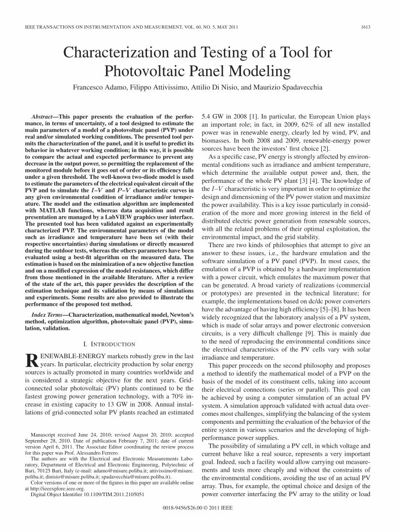
Fig. 1. Two-diode equivalent circuit of a PV cell.

or organic cells are not considered, although, in principle, alldiscussions here presented are general and also remain validfor them.

A. Circuital Model

A crystalline solar cell can be viewed as a large-area silicondiode. In the dark state, the I–V characteristic curve of thisdiode corresponds to that of a normal p-n junction diode, sothe cell does not generate any electric power [12]. Illuminationof the PV cell generates free-charge carriers, which allow thelight-generated current IL (proportional to irradiance [12]) toflow through a connected load.

The mathematical model used in this paper is the well-knowntwo-diode model [13], [14], as reported in Fig. 1; it consists ofa current source whose intensity is proportional to the incidentirradiance G, in parallel with two diodes D1 and D2. Diode D1simulates the diffusion process of the minority carriers into thedepletion layer, whereas D2 corresponds to the recombinationin the space charge region of the junction. The shunt resistanceRsh models the leakage current, whereas the series resistanceRs represents the internal losses due to the current flow and tothe connection wires and contributes to the modeling of the cellefficiency [12].

This model brings to a double-exponential equation, whichis particularly suited for polycrystalline cells [13].

The I–V characteristic is described by

I = IL − I0D1

(e

q(V +Rs·I)n1·k·T − 1

)

−I0D2

(e

q(V +Rs·I)n2·k·T − 1

)− V + Rs · I

Rsh(1)

which shows the net current I of the cell as a function of theexternal voltage V . In detail, n1 and n2 are the well-knownideality factors of the junctions, and their values range between1 and 2; k is the Boltzmann’s constant, q is the electron charge,and T is the ambient temperature.

Equation (1) does not permit to obtain V as a function ofI in analytical form, so numerical methods must be used tosolve it; in this work, the Newton–Raphson’s iterative method isused for this purpose, because it converges remarkably quickly,particularly if the iteration begins with a guess sufficiently nearthe desired root.

B. Basic equations

Equation (1) in itself does not let drawing the I–V curve;some other dependencies have to be included in the model.For example, the following show that photocurrent IL is also

ADAMO et al.: CHARACTERIZATION AND TESTING OF A TOOL FOR PVP MODELING 1615

affected by environmental conditions, i.e., temperature andirradiance [12], [14]:

IL(T ) = IL(Tref) + α(T − Tref) (2)

IL(Tref) = ISC(Tref)G

Gref. (3)

Knowledge of the open-circuit voltage VOC and of the sat-uration currents I0D1 and I0D2 is mandatory to complete themodel [13]

I0Di(Tref) =12ISC(Tref)

·(

eq·VOC(Tref )

n1·k·Tref − 1)−1

, i = 1, 2 (4)

I0Di(T ) = I0Di(Tref) ·(

Tcell

Tref

)3/ni

· eq·Eg(T )

ni·k·(

1T

− 1Tref

), i = 1, 2 (5)

VOC(T ) = VOC(Tref) + β(T − Tref). (6)

In the previous equations, G is the irradiance, α is thetemperature coefficient of the current, and β is the temperaturecoefficient of the voltage. The subscript “ref” identifies the stan-dard test conditions (STCs) (Tref = 298 K, Gref = 1000 W/m2,and air mass of 1.5) defined in the IEC 61215 internationalstandard [3]. Usually, manufacturers give the characteristicparameters, such as the short-circuit current ISC and the open-circuit voltage VOC in STC. The coefficients α and β allowpredicting the values of ISC and VOC at different temperatures.

A PV panel, which is composed by many PV cells, hasa model that is analogous to (1), but its parameters mustbe scaled. In particular, considering an array of NP parallelbranches each made of NS cells in series, the panel voltage,current, series, and shunt resistances can be calculated asfollows, under the conditions of uniform solar irradiance andtemperature: ⎧⎪⎪⎨

⎪⎪⎩

Ipanel = Np · IVpanel = Ns · VRspanel = Ns

NpRs

Rshpanel = Ns

NpRsh

. (7)

A similar rescaling also applies to IL, ISC, and VOC.Equations analogous to (7) can also be used to simulate an

array or a large PV plant made by Nparallel strings arranged inparallel, where each string is composed by a series of Nseries

PVPs, i.e., ⎧⎪⎪⎨⎪⎪⎩

Iplant = Nparallel · Ipanel

Vplant = Nseries · Vpanel

Rsplant = NseriesNparallel

Rspanel

Rshplant = NseriesNparallel

Rshpanel

. (8)

However, when dealing with larger plants, the hypothesis ofuniform irradiance and temperature conditions across the entireplant can became unrealistic. A more flexible method consistsof the simulation of each PVP as a single unit; in this case,we have to consider that PVPs in a string are constrained toconduct the same current because of the Kirchoff’s law, so that

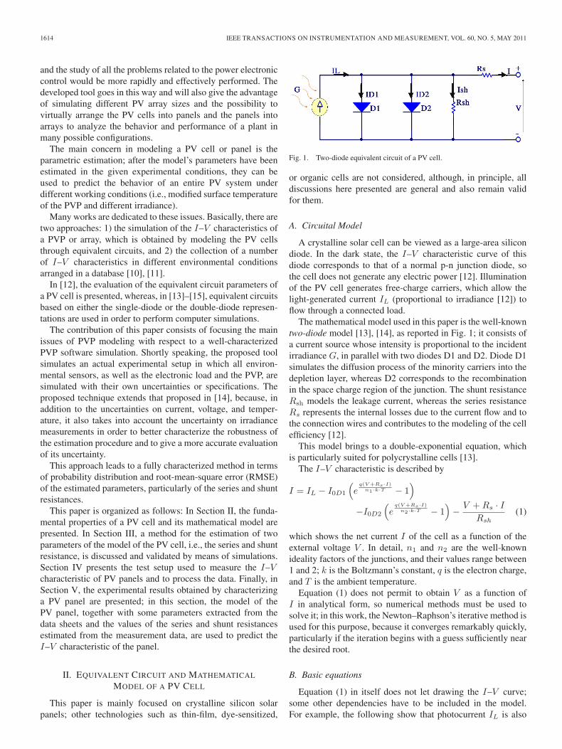
TABLE IIP10P SPECIFICATIONS IN STC

the less efficient module imposes the string current and theoverall efficiency of the array is reduced to the efficiency ofthis module. In such a way, it is possible, e.g., to simulate thepassing of clouds or other sources of shading, which change theirradiance level on a couple of contiguous PV modules. It maybe noted from (8) that Rsplant , Rshplant , and, consequently, thepower losses increase with the size of the plant.

C. Series and Shunt Resistances

To complete the model, we should determine the values ofRs and Rsh. Generally speaking, Rs has a marked effect onthe I–V characteristic near the open-circuit condition, whereasRsh acts on the slope of the characteristic near the short-circuitcondition. Rs and Rsh can be estimated from the measurementdata by using an iterative method. The initial estimation of theseparameters, which are denoted as Rs0 and Rsh0, respectively, isa critical task, because bad starting values can compromise theconvergence of the Newton–Raphson’s method used to estimatethe final values for Rs and Rsh. The estimation of Rs and Rsh

is discussed in the next section.

III. ESTIMATION OF SERIES AND SHUNT RESISTANCES

There are various methods to estimate Rs and Rsh usingmeasurements done in either dark or illuminated condition [13],[16]. In a previous work [17], the first estimate of Rs and Rsh

were obtained using equations proposed by Gow and Manning[13]. However, that approach requires the knowledge of thederivative of the voltage with respect to the current near theopen-circuit conditions to estimate Rs0; this kind of data ishardly available in common specifications. In [17], anotherapproach is also considered, in which the value of Rsh0 isderived from Rs0 and some other specifications by means of

Rsh0 =VMP + Rs0 · IMP

IMP − IL + I0

(e

q·(VMP+Rs0·IMP)n·k·T − 1

) (9)

where VMP and IMP are the maximum power voltage andcurrent of the PVP, respectively. VMP and IMP for an actualPV panel are reported in Table I.

Similarly, in [18], Rs0 is estimated from the slope of the por-tion of the curve near the open-circuit point in actual workingconditions. In more detail, Rs0 is obtained by means of a


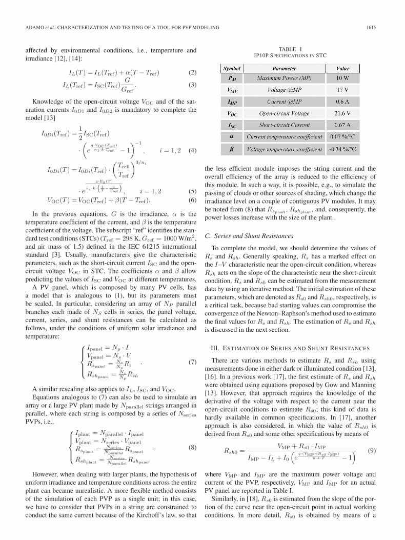
Fig. 2. Estimation errors without noise. (a) Rs estimation. (b) Rsh estimation.

least-squares fitting on the last part of the I–V characteristic,where V is greater, whereas Rsh0 is obtained by evaluatingthe first part of the I–V curve, where V is smaller. Thisapproach requires the acquisition of the first and last parts ofI–V characteristic and brings some errors in the estimation.

In this paper, a new approach is proposed, which requiresonly the knowledge of the specifications, and this makes it moreeffective for simulations, as well as for parameter estimation.The basic assumption is that the value of Rs0 for a PV cellis very low (typically a few tenths of an ohm); thus, for a firstapproximation, it can be supposed to be zero. Rsh0 is calculatedfrom (9), after modifying it for a two-diode model, i.e.,

Rsh0 =VMP

IMP − IL+I0D1

(e

q·VMPn1·k·T − 1

)+I0D2

(e

q·VMPn2·k·T − 1

) .

(10)

After having obtained the starting estimates of the resis-tances, these can be refined by using iterative methods. For thispurpose, the PVP model has been implemented as a MATLABfunction. After having expressed the measured I–V characteris-tics as a vector of currents I = [In]n=1,...,N and a vector of volt-ages V = [Vn]n=1,...,N , where N is the number of measuredpoints, the Rs and Rsh estimates are determined by means of abest-fit, which minimizes the objective function ‖K‖, where

K = [Kn]n=1,...,N

Kn = In −[IL − I0D1

(e

q(Vn+|Rs|·In)n1·k·T − 1

)

− I0D2

(e

q(Vn+|Rs|·In)n2·k·T − 1

)− Vn + |Rs| · In

Rsh

].

(11)

The optimization process is based on the Levenberg–Marquardt Algorithm (LMA), which is a robust algorithm that,in many cases, finds a solution, even if the starting point isfar from the true minimum, but is also a bit slower than otheralgorithms [19]. More simply, the designed MATLAB functionstarts with Rs0 and Rsh0 as initial values and, after the best-fit procedure, dramatically reduces potential estimation errorsdue to initial approximation. Obviously, with Rs being a valuenear zero, there is the risk to obtain negative values from the

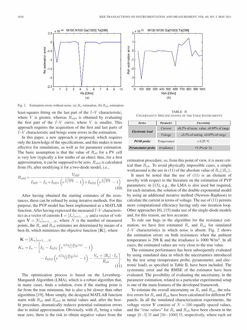
TABLE IIUNCERTAINTY SPECIFICATIONS OF THE USED INSTRUMENTS

estimation procedure, so, from this point of view, it is more crit-ical than Rsh. To avoid physically impossible cases, a simpleworkaround is the use in (11) of the absolute value of Rs(|Rs|).

It must be noted that the use of (11) is an element ofnovelty with respect to the literature on the estimation of PVPparameters; in [13], e.g., the LMA is also used but required,for each iteration, the solution of the double-exponential modelby using an additional iterative method (Newton–Raphson) tocalculate the current in terms of voltage. The use of (11) permitsmore computational efficiency having only one iteration loop.Other approaches [6], [15] make use of the single-diode modelsand, for this reason, are less accurate.

To rule out bugs in the algorithm for the resistance esti-mation, we have first estimated Rs and Rsh for simulatedI–V characteristics in which noise is absent. Fig. 2 showsthe estimation errors on both resistances when the ambienttemperature is 298 K and the irradiance is 1000 W/m2. In allcases, the estimated values are very close to the true value.

The estimator performance has been subsequently evaluatedby using simulated data in which the uncertainties introducedby the test setup (temperature probe, pyranometer, and elec-tronic load), as specified in Table II, have been included. Thesystematic error and the RMSE of the estimator have beenevaluated. The possibility of evaluating the uncertainty, in theparameter estimation, related to a particular experimental setupis one of the main features of the developed framework.

To estimate the overall uncertainty on Rs and Rsh, the rela-tive errors for Rs and Rsh have been calculated for different PVpanels. In all the simulated characterization experiments, thevoltage vector V consists of N = 100 equally spaced values,and the “true values” for Rs and Rsh have been chosen in therange [0−5] Ω and [50−1000] Ω, respectively, where each set


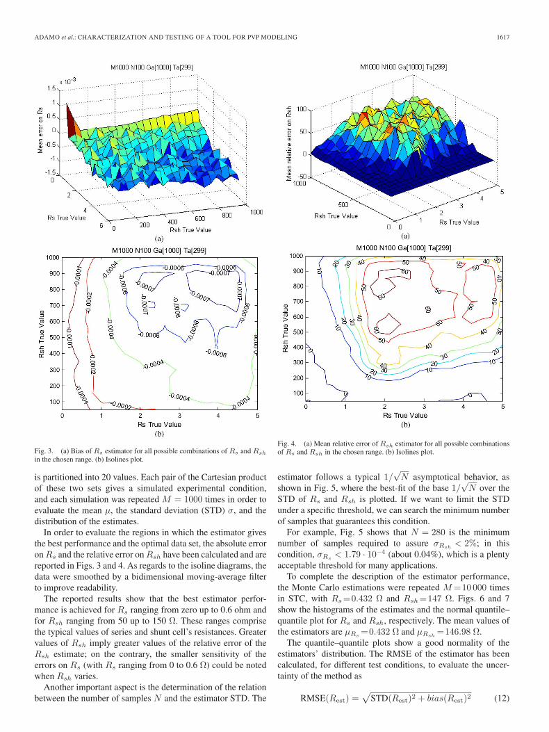
Fig. 3. (a) Bias of Rs estimator for all possible combinations of Rs and Rsh

in the chosen range. (b) Isolines plot.

is partitioned into 20 values. Each pair of the Cartesian productof these two sets gives a simulated experimental condition,and each simulation was repeated M = 1000 times in order toevaluate the mean μ, the standard deviation (STD) σ, and thedistribution of the estimates.

In order to evaluate the regions in which the estimator givesthe best performance and the optimal data set, the absolute erroron Rs and the relative error on Rsh have been calculated and arereported in Figs. 3 and 4. As regards to the isoline diagrams, thedata were smoothed by a bidimensional moving-average filterto improve readability.

The reported results show that the best estimator perfor-mance is achieved for Rs ranging from zero up to 0.6 ohm andfor Rsh ranging from 50 up to 150 Ω. These ranges comprisethe typical values of series and shunt cell’s resistances. Greatervalues of Rsh imply greater values of the relative error of theRsh estimate; on the contrary, the smaller sensitivity of theerrors on Rs (with Rs ranging from 0 to 0.6 Ω) could be notedwhen Rsh varies.

Another important aspect is the determination of the relationbetween the number of samples N and the estimator STD. The

Fig. 4. (a) Mean relative error of Rsh estimator for all possible combinationsof Rs and Rsh in the chosen range. (b) Isolines plot.

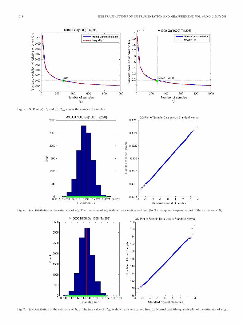
estimator follows a typical 1/√

N asymptotical behavior, asshown in Fig. 5, where the best-fit of the base 1/

√N over the

STD of Rs and Rsh is plotted. If we want to limit the STDunder a specific threshold, we can search the minimum numberof samples that guarantees this condition.

For example, Fig. 5 shows that N = 280 is the minimumnumber of samples required to assure σRsh

< 2%; in thiscondition, σRs

< 1.79 · 10−4 (about 0.04%), which is a plentyacceptable threshold for many applications.

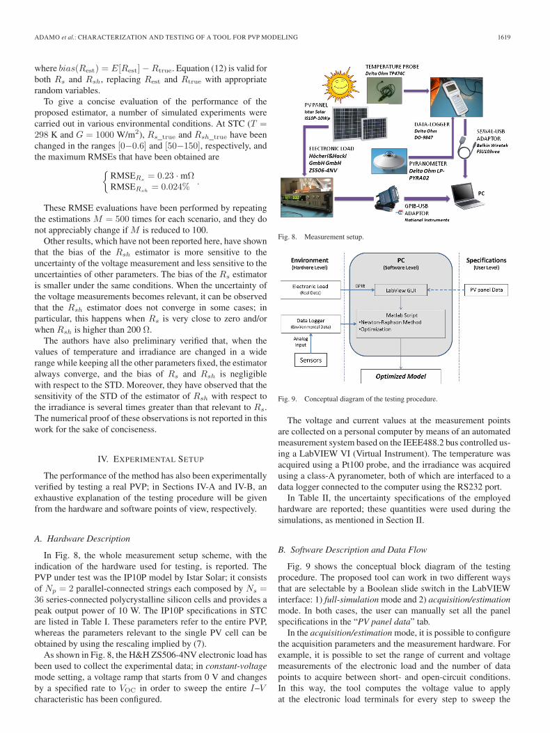
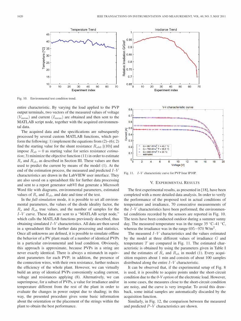
To complete the description of the estimator performance,the Monte Carlo estimations were repeated M =10 000 timesin STC, with Rs =0.432 Ω and Rsh =147 Ω. Figs. 6 and 7show the histograms of the estimates and the normal quantile–quantile plot for Rs and Rsh, respectively. The mean values ofthe estimators are μRs

=0.432 Ω and μRsh=146.98 Ω.

The quantile–quantile plots show a good normality of theestimators’ distribution. The RMSE of the estimator has beencalculated, for different test conditions, to evaluate the uncer-tainty of the method as

RMSE(Rest) =√

STD(Rest)2 + bias(Rest)2 (12)


Fig. 5. STD of (a) Rs and (b) Rsh versus the number of samples.

Fig. 6. (a) Distribution of the estimator of Rs. The true value of Rs is shown as a vertical red line. (b) Normal quantile–quantile plot of the estimator of Rs.

Fig. 7. (a) Distribution of the estimator of Rsh. The true value of Rsh is shown as a vertical red line. (b) Normal quantile–quantile plot of the estimator of Rsh.


where bias(Rest) = E[Rest] − Rtrue. Equation (12) is valid forboth Rs and Rsh, replacing Rest and Rtrue with appropriaterandom variables.

To give a concise evaluation of the performance of theproposed estimator, a number of simulated experiments werecarried out in various environmental conditions. At STC (T =298 K and G = 1000 W/m2), Rs_true and Rsh_true have beenchanged in the ranges [0−0.6] and [50−150], respectively, andthe maximum RMSEs that have been obtained are

{RMSERs

= 0.23 · mΩRMSERsh

= 0.024% .

These RMSE evaluations have been performed by repeatingthe estimations M = 500 times for each scenario, and they donot appreciably change if M is reduced to 100.

Other results, which have not been reported here, have shownthat the bias of the Rsh estimator is more sensitive to theuncertainty of the voltage measurement and less sensitive to theuncertainties of other parameters. The bias of the Rs estimatoris smaller under the same conditions. When the uncertainty ofthe voltage measurements becomes relevant, it can be observedthat the Rsh estimator does not converge in some cases; inparticular, this happens when Rs is very close to zero and/orwhen Rsh is higher than 200 Ω.

The authors have also preliminary verified that, when thevalues of temperature and irradiance are changed in a widerange while keeping all the other parameters fixed, the estimatoralways converge, and the bias of Rs and Rsh is negligiblewith respect to the STD. Moreover, they have observed that thesensitivity of the STD of the estimator of Rsh with respect tothe irradiance is several times greater than that relevant to Rs.The numerical proof of these observations is not reported in thiswork for the sake of conciseness.

IV. EXPERIMENTAL SETUP

The performance of the method has also been experimentallyverified by testing a real PVP; in Sections IV-A and IV-B, anexhaustive explanation of the testing procedure will be givenfrom the hardware and software points of view, respectively.

A. Hardware Description

In Fig. 8, the whole measurement setup scheme, with theindication of the hardware used for testing, is reported. ThePVP under test was the IP10P model by Istar Solar; it consistsof Np = 2 parallel-connected strings each composed by Ns =36 series-connected polycrystalline silicon cells and provides apeak output power of 10 W. The IP10P specifications in STCare listed in Table I. These parameters refer to the entire PVP,whereas the parameters relevant to the single PV cell can beobtained by using the rescaling implied by (7).

As shown in Fig. 8, the H&H ZS506-4NV electronic load hasbeen used to collect the experimental data; in constant-voltagemode setting, a voltage ramp that starts from 0 V and changesby a specified rate to VOC in order to sweep the entire I–Vcharacteristic has been configured.

Fig. 8. Measurement setup.

Fig. 9. Conceptual diagram of the testing procedure.

The voltage and current values at the measurement pointsare collected on a personal computer by means of an automatedmeasurement system based on the IEEE488.2 bus controlled us-ing a LabVIEW VI (Virtual Instrument). The temperature wasacquired using a Pt100 probe, and the irradiance was acquiredusing a class-A pyranometer, both of which are interfaced to adata logger connected to the computer using the RS232 port.

In Table II, the uncertainty specifications of the employedhardware are reported; these quantities were used during thesimulations, as mentioned in Section II.

B. Software Description and Data Flow

Fig. 9 shows the conceptual block diagram of the testingprocedure. The proposed tool can work in two different waysthat are selectable by a Boolean slide switch in the LabVIEWinterface: 1) full-simulation mode and 2) acquisition/estimationmode. In both cases, the user can manually set all the panelspecifications in the “PV panel data” tab.

In the acquisition/estimation mode, it is possible to configurethe acquisition parameters and the measurement hardware. Forexample, it is possible to set the range of current and voltagemeasurements of the electronic load and the number of datapoints to acquire between short- and open-circuit conditions.In this way, the tool computes the voltage value to applyat the electronic load terminals for every step to sweep the


Fig. 10. Environmental test condition trend.

entire characteristic. By varying the load applied to the PVPoutput terminals, two vectors of the measured values of voltage(Vmeas) and current (Imeas) are obtained and then sent to theMATLAB script node, together with the acquired environmen-tal data.

The acquired data and the specifications are subsequentlyprocessed by several custom MATLAB functions, which per-form the following: 1) implement the equations from (2)–(6); 2)find the starting value for the shunt resistance Rsh0 [(10)] andimpose Rs0 = 0 as starting value for series resistance estima-tion; 3) minimize the objective function (11) in order to estimateRs and Rsh, as described in Section III. These values are thenused to predict the current by means of the model (1). At theend of the estimation process, the measured and predicted I–Vcharacteristics are drawn in the LabVIEW user interface. Theyare also saved on a spreadsheet file for further data processingand sent to a report generator subVI that generate a MicrosoftWord file with diagrams, environmental parameters, estimatedvalues of Rs and Rsh, and date and time of the test.

In the full-simulation mode, it is possible to set all environ-mental parameters, the values of the diode ideality factor, theRs and Rsh true values, and the number of samples for theI–V curve. These data are sent to a “MATLAB script node,”which calls the MATLAB functions previously described, thusobtaining simulated I–V characteristics. All data are then savedin a spreadsheet file for further data processing and statistics.Once all unknowns are defined, it is possible to simulate offlinethe behavior of a PV plant made of a number of identical PVPsin a particular environmental and load condition. Obviously,this approach is approximate, because PVPs in a string arenever exactly identical. There is always a mismatch in equiv-alent parameters for each PVP; in addition, the presence ofthe connection wires, with their own resistance, further reducesthe efficiency of the whole plant. However, we can virtuallybuild an array of identical PVPs conveniently scaling current,voltage and resistances applying (8). Alternatively, we cansuperimpose, for a subset of PVPs, a value for irradiance and/ortemperature different from the rest of the plant in order toevaluate the changes in power output due to shading; in thisway, the presented procedure gives some basic informationabout the orientation or the placement of the strings within theplant to obtain the best performance.

Fig. 11. I–V characteristic curve for PVP Istar IP10P.

V. EXPERIMENTAL RESULTS

The first experimental results, as presented in [18], have beencompleted with a more detailed data analysis. In order to verifythe performance of the proposed tool in actual conditions oftemperature and irradiance, 70 consecutive measurements ofthe I–V characteristics have been performed; the environmen-tal conditions recorded by the sensors are reported in Fig. 10.The tests have been conducted outdoor during a summer sunnyday. The measured temperature was in the range 35 ◦C–41 ◦C,whereas the irradiance was in the range 695−970 W/m2.

The measured I–V characteristics and the values estimatedby the model at three different values of irradiance G andtemperature T are compared in Fig. 11. The estimated char-acteristic is obtained by using the parameters given in Table Iand the estimates of Rs and Rsh in model (1). Every acqui-sition requires about 1 min and consists of about 100 samplesdistributed along the entire I–V characteristic.

It can be observed that, if the experimental setup of Fig. 8is used, it is possible to acquire points under the short-circuitcondition due to the 0-V option of the electronic load. However,in some cases, the measures close to the short-circuit conditionare noisy, and the curve is very irregular. To avoid this draw-back, some initial samples are automatically discarded by theacquisition function.

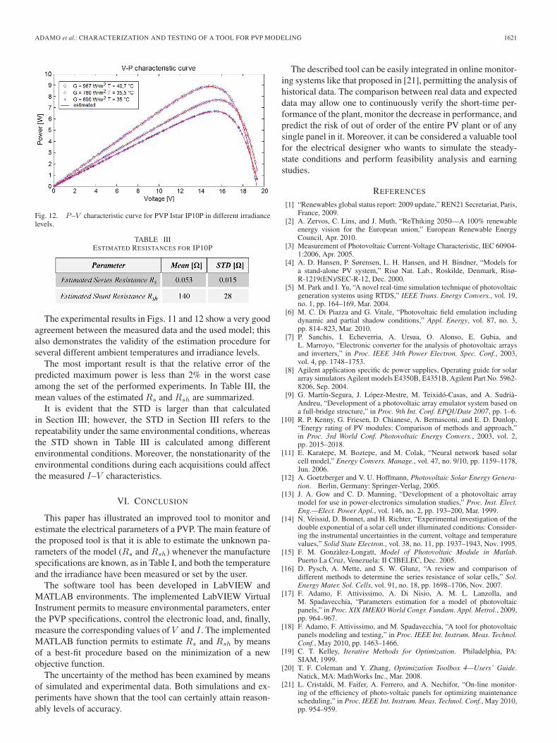
Similarly, in Fig. 12, the comparison between the measuredand predicted P–V characteristics are shown.


Fig. 12. P –V characteristic curve for PVP Istar IP10P in different irradiancelevels.

TABLE IIIESTIMATED RESISTANCES FOR IP10P

The experimental results in Figs. 11 and 12 show a very goodagreement between the measured data and the used model; thisalso demonstrates the validity of the estimation procedure forseveral different ambient temperatures and irradiance levels.

The most important result is that the relative error of thepredicted maximum power is less than 2% in the worst caseamong the set of the performed experiments. In Table III, themean values of the estimated Rs and Rsh are summarized.

It is evident that the STD is larger than that calculatedin Section III; however, the STD in Section III refers to therepeatability under the same environmental conditions, whereasthe STD shown in Table III is calculated among differentenvironmental conditions. Moreover, the nonstationarity of theenvironmental conditions during each acquisitions could affectthe measured I–V characteristics.

VI. CONCLUSION

This paper has illustrated an improved tool to monitor andestimate the electrical parameters of a PVP. The main feature ofthe proposed tool is that it is able to estimate the unknown pa-rameters of the model (Rs and Rsh) whenever the manufacturespecifications are known, as in Table I, and both the temperatureand the irradiance have been measured or set by the user.

The software tool has been developed in LabVIEW andMATLAB environments. The implemented LabVIEW VirtualInstrument permits to measure environmental parameters, enterthe PVP specifications, control the electronic load, and, finally,measure the corresponding values of V and I . The implementedMATLAB function permits to estimate Rs and Rsh by meansof a best-fit procedure based on the minimization of a newobjective function.

The uncertainty of the method has been examined by meansof simulated and experimental data. Both simulations and ex-periments have shown that the tool can certainly attain reason-ably levels of accuracy.

The described tool can be easily integrated in online monitor-ing systems like that proposed in [21], permitting the analysis ofhistorical data. The comparison between real data and expecteddata may allow one to continuously verify the short-time per-formance of the plant, monitor the decrease in performance, andpredict the risk of out of order of the entire PV plant or of anysingle panel in it. Moreover, it can be considered a valuable toolfor the electrical designer who wants to simulate the steady-state conditions and perform feasibility analysis and earningstudies.

REFERENCES

[1] “Renewables global status report: 2009 update,” REN21 Secretariat, Paris,France, 2009.

[2] A. Zervos, C. Lins, and J. Muth, “ReThiking 2050—A 100% renewableenergy vision for the European union,” European Renewable EnergyCouncil, Apr. 2010.

[3] Measurement of Photovoltaic Current-Voltage Characteristic, IEC 60904-1:2006, Apr. 2005.

[4] A. D. Hansen, P. Sørensen, L. H. Hansen, and H. Bindner, “Models fora stand-alone PV system,” Risø Nat. Lab., Roskilde, Denmark, Risø-R-1219(EN)/SEC-R-12, Dec. 2000.

[5] M. Park and I. Yu, “A novel real-time simulation technique of photovoltaicgeneration systems using RTDS,” IEEE Trans. Energy Convers., vol. 19,no. 1, pp. 164–169, Mar. 2004.

[6] M. C. Di Piazza and G. Vitale, “Photovoltaic field emulation includingdynamic and partial shadow conditions,” Appl. Energy, vol. 87, no. 3,pp. 814–823, Mar. 2010.

[7] P. Sanchis, I. Echeverria, A. Ursua, O. Alonso, E. Gubia, andL. Marroyo, “Electronic converter for the analysis of photovoltaic arraysand inverters,” in Proc. IEEE 34th Power Electron. Spec. Conf., 2003,vol. 4, pp. 1748–1753.

[8] Agilent application specific dc power supplies, Operating guide for solararray simulators Agilent models E4350B, E4351B, Agilent Part No. 5962-8206, Sep. 2004.

[9] G. Martín-Segura, J. López-Mestre, M. Teixidó-Casas, and A. Sudrià-Andreu, “Development of a photovoltaic array emulator system based ona full-bridge structure,” in Proc. 9th Int. Conf. EPQUDate 2007, pp. 1–6.

[10] R. P. Kenny, G. Friesen, D. Chianese, A. Bernasconi, and E. D. Dunlop,“Energy rating of PV modules: Comparison of methods and approach,”in Proc. 3rd World Conf. Photovoltaic Energy Convers., 2003, vol. 2,pp. 2015–2018.

[11] E. Karatepe, M. Boztepe, and M. Colak, “Neural network based solarcell model,” Energy Convers. Manage., vol. 47, no. 9/10, pp. 1159–1178,Jun. 2006.

[12] A. Goetzberger and V. U. Hoffmann, Photovoltaic Solar Energy Genera-tion. Berlin, Germany: Springer-Verlag, 2005.

[13] J. A. Gow and C. D. Manning, “Development of a photovoltaic arraymodel for use in power-electronics simulation studies,” Proc. Inst. Elect.Eng.—Elect. Power Appl., vol. 146, no. 2, pp. 193–200, Mar. 1999.

[14] N. Veissid, D. Bonnet, and H. Richter, “Experimental investigation of thedouble exponential of a solar cell under illuminated conditions: Consider-ing the instrumental uncertainties in the current, voltage and temperaturevalues,” Solid State Electron., vol. 38, no. 11, pp. 1937–1943, Nov. 1995.

[15] F. M. Gonzàlez-Longatt, Model of Photovoltaic Module in Matlab.Puerto La Cruz, Venezuela: II CIBELEC, Dec. 2005.

[16] D. Pysch, A. Mette, and S. W. Glunz, “A review and comparison ofdifferent methods to determine the series resistance of solar cells,” Sol.Energy Mater. Sol. Cells, vol. 91, no. 18, pp. 1698–1706, Nov. 2007.

[17] F. Adamo, F. Attivissimo, A. Di Nisio, A. M. L. Lanzolla, andM. Spadavecchia, “Parameters estimation for a model of photovoltaicpanels,” in Proc. XIX IMEKO World Congr. Fundam. Appl. Metrol., 2009,pp. 964–967.

[18] F. Adamo, F. Attivissimo, and M. Spadavecchia, “A tool for photovoltaicpanels modeling and testing,” in Proc. IEEE Int. Instrum. Meas. Technol.Conf., May 2010, pp. 1463–1466.

[19] C. T. Kelley, Iterative Methods for Optimization. Philadelphia, PA:SIAM, 1999.

[20] T. F. Coleman and Y. Zhang, Optimization Toolbox 4—Users’ Guide.Natick, MA: MathWorks Inc., Mar. 2008.

[21] L. Cristaldi, M. Faifer, A. Ferrero, and A. Nechifor, “On-line monitor-ing of the efficiency of photo-voltaic panels for optimizing maintenancescheduling,” in Proc. IEEE Int. Instrum. Meas. Technol. Conf., May 2010,pp. 954–959.


Francesco Adamo received the M.S. degree andthe Ph.D. degree in electronic engineering from thePolytechnic of Bari, Bari, Italy, in 2000 and 2004,respectively.

He is currently an Assistant Professor in mea-surement science with the Electrical and ElectronicMeasurements Laboratory, Department of Electricaland Electronic Engineering, Polytechnic of Bari. Hisresearch interests are industrial sensors and actuatorsand electronic measurement on devices and systems,with special regards to digital signal processing for

measurements, analog-to-digital converter modeling, characterization and opti-mization, and computer-based measurement systems.

Dr. Adamo is a member of the Italian Association “Electrical and ElectronicMeasurements Group” (GMEE).

Filippo Attivissimo received the M.S. and Ph.D. de-grees in electronic engineering from the Polytechnicof Bari, Bari, Italy, in 1993 and 1997, respectively.

Since 1993, he has worked on research projectsin the field of digital signal processing for mea-surements with the Polytechnic of Bari, where heis currently an Associate Professor of electric andelectronic measurements with the Electrical andElectronic Measurements Laboratory, Department ofElectrical and Electronic Engineering. His researchinterests include electric and electronic measurement

on devices and systems, estimation theory, uncertainty evaluation, design ofsensors, medicine and transportation, digital measurements on power electronicsystems, computer vision, and analog-to-digital converter modeling, character-ization, and optimization.

Dr. Attivissimo is a member of the Italian Association “Electrical andElectronic Measurements Group” (GMEE).

Attilio Di Nisio was born in Bari, Italy, in 1980. Hereceived the M.S. degree with honors and the Ph.D.degree in electronic engineering from the Polytech-nic of Bari, Bari, in 2005 and 2009, respectively.

Since 2005, he has been with the Electrical andElectronic Measurements Laboratory, Department ofElectrical and Electronic Engineering, Politecnicodi Bari, where he worked on research rojects inthe fields of analog-to-digital (A/D) and digital-to-analog (D/A) converters testing and automatic vi-sion inspection. His current research interests include

A/D and D/A converter modeling and testing, estimation theory, software forautomatic test equipment, image processing for quality control of surfaces,document image analysis for medical test results, digital-signal-processing-based systems for power quality analysis, and photovoltaic-panel modeling andtesting.

Dr. Di Nisio is a member of the Italian Association “Electrical and ElectronicMeasurements Group” (GMEE).

Maurizio Spadavecchia was born in Molfetta, Italy,in 1974. He received the M.S. degree (with honors)in electrical engineering from the Polytechnic ofBari, Bari, Italy, in 2006. He is currently workingtoward the Ph.D. degree in electrical engineeringwith the Electrical and Electronic MeasurementsLaboratory, Department of Electrical and ElectronicEngineering, Polytechnic of Bari.

In 2008, he was a Contract Researcher with thePolytechnic of Bari. Since 2006, he has been work-ing on research projects in the field of environmental

monitoring. His current research interests include electrics and electronicsmeasurement on instruments and devices, characterization of renewable-energydevices, software for automatic test equipment, and photovoltaic-panel model-ing and testing.

Mr. Spadavecchia is a member of the Italian Association “Electrical andElectronic Measurements Group” (GMEE).

Characterization and Testing of a Tool for Photovoltaic Panel Modeling

Documents

Transcript of Characterization and Testing of a Tool for Photovoltaic Panel Modeling