Variable mesh optimization for continuous optimization problems
Upload
khangminh22Category
view
1download
0
Characterization and optimization ofsingle-use bioreactors and
biopharmaceutical production processesusing Computational Fluid Dynamics
vorgelegt vonMaster of Science (M.Sc.)Stephan Christian Kaiser
geb. in Borna, Deutschland
von der Fakultat III - Prozesswissenschaftender Technischen Universitat Berlin
zur Erlangung des akademischen GradesDoktor der Ingenieurwissenschaften
-Dr.-Ing.-
genehmigte Dissertation
Promotionsausschuss:
Vorsitzender: Prof. Dr.-Ing. habil. Rudibert KingGutachter: Prof. Dr.-Ing. Matthias KraumeGutachter: Prof. Dr.-Ing. Dieter EiblGutachter: Prof. Dr.-Ing. Ralf Portner
Tag der wissenschaftlichen Aussprache: 08.12.2014
Berlin 2014


Contents
Acknowledgements III
Abstract V
Zusammenfassung VII
Abbreviations and Symbols XIAbbreviations . . . . . . . . . . . . . . . . . . . . . . . . . . . . . . . . . . XISymbols . . . . . . . . . . . . . . . . . . . . . . . . . . . . . . . . . . . . . XII
List of Figures XVII
List of Tables XX
1. Introduction 11.1. Single-use equipment in biomanufacturing . . . . . . . . . . . . . . . 11.2. Scope and outline of this thesis . . . . . . . . . . . . . . . . . . . . . 2
2. Theoretical background and fundamentals 52.1. Application of single-use bioreactors for human and animal cells . . . 52.2. Engineering characterization of SU bioreactors and scale-up . . . . . 7
2.2.1. Characteristics of dynamic SU bioreactors . . . . . . . . . . . 82.2.2. Scale-up considerations . . . . . . . . . . . . . . . . . . . . . . 14
2.3. Modeling and optimization of bioreactors by means of CFD . . . . . . 192.3.1. Applied model approaches . . . . . . . . . . . . . . . . . . . . 192.3.2. Overview on applications of CFD for bioreactor characteriza-
tion and scale-up . . . . . . . . . . . . . . . . . . . . . . . . . 272.4. Conclusions and objectives of this thesis . . . . . . . . . . . . . . . . 29
3. Material and methods 313.1. Investigated bioreactor systems . . . . . . . . . . . . . . . . . . . . . 313.2. Experimental investigations . . . . . . . . . . . . . . . . . . . . . . . 34
3.2.1. Mixing time . . . . . . . . . . . . . . . . . . . . . . . . . . . . 343.2.2. Oxygen mass transfer coefficient . . . . . . . . . . . . . . . . . 353.2.3. Power input . . . . . . . . . . . . . . . . . . . . . . . . . . . . 353.2.4. Suspension criteria . . . . . . . . . . . . . . . . . . . . . . . . 363.2.5. Liquid distribution in the traveling wave bioreactor . . . . . . 373.2.6. Particle image velocimetry . . . . . . . . . . . . . . . . . . . . 383.2.7. Bubble size determination . . . . . . . . . . . . . . . . . . . . 393.2.8. CHO cultivation . . . . . . . . . . . . . . . . . . . . . . . . . 39
3.3. Numerical investigations . . . . . . . . . . . . . . . . . . . . . . . . . 41
I

II Contents
4. Characterization and optimization of bioreactors and bioprocesses usingCFD: case studies 434.1. Engineering characterization of the Mobius R©CellReady 3L bioreactor 43
4.1.1. Introduction . . . . . . . . . . . . . . . . . . . . . . . . . . . . 434.1.2. Results from single-phase modeling . . . . . . . . . . . . . . . 454.1.3. Results from two-phase modeling . . . . . . . . . . . . . . . . 64
4.2. Development and optimization of microcarrier-based human mesenchy-mal stem cell expansion at small and benchtop scales . . . . . . . . . 774.2.1. Introduction . . . . . . . . . . . . . . . . . . . . . . . . . . . . 774.2.2. Preliminary studies in small scale spinner flasks . . . . . . . . 784.2.3. Design modifications of the UniVessel R©SU bioreactor . . . . . 85
4.3. Development of the traveling wave bioreactor . . . . . . . . . . . . . . 974.3.1. Introduction . . . . . . . . . . . . . . . . . . . . . . . . . . . . 974.3.2. Description of bioreactor motion . . . . . . . . . . . . . . . . . 984.3.3. Results of fluid flow prediction . . . . . . . . . . . . . . . . . . 1004.3.4. Model validation . . . . . . . . . . . . . . . . . . . . . . . . . 1034.3.5. Turbulence prediction . . . . . . . . . . . . . . . . . . . . . . 1044.3.6. Determination of engineering parameters . . . . . . . . . . . . 1074.3.7. Design modifications . . . . . . . . . . . . . . . . . . . . . . . 115
4.3.7.1. Influence of the annulus diameter ratio . . . . . . . . 1164.3.7.2. Influence of protuberances . . . . . . . . . . . . . . . 1194.3.7.3. Shear stress from a single droplet impact . . . . . . . 126
4.3.8. Proof-of-concept cultivation . . . . . . . . . . . . . . . . . . . 128
5. Concluding remarks and outlook 133
Bibliography 139
A. Appendix 169A.1. Complete list of publications and presentations . . . . . . . . . . . . . 169A.2. Additional figures and tables . . . . . . . . . . . . . . . . . . . . . . . 172A.3. Details of applied numerical models . . . . . . . . . . . . . . . . . . . 181
A.3.1. Turbulence models . . . . . . . . . . . . . . . . . . . . . . . . 181A.3.2. Bubble breakup and coalescence models . . . . . . . . . . . . 188
A.4. Publication reprints . . . . . . . . . . . . . . . . . . . . . . . . . . . . 192

Acknowledgements
This work was carried out during my employment as a research assistant at the In-stitute of Biotechnology (IBT) of the Zurich University of Applied Sciences (ZHAW)in Wadenswil. I would like to take this opportunity to express my deepest gratitudeto the persons who have made this work possible.First of all, I would like to thank Prof. Dr.-Ing. Matthias Kraume, head of the Chairof Chemical & Process Engineering, for his supervision of this thesis. I appreciatedour fruitful discussions, which gave me helpful guidance and served to improve thequality of this work.My special thanks belong to Prof. Dr.-Ing. Dieter Eibl and Prof. Dr.-Ing. RegineEibl, heads of the centres for Biochemical Engineering and Cell Cultivation Tech-nique at the IBT, for their outstanding engagement and their unbelievable passionfor research, which inspired this thesis. I would like to thank them for their trustand the freedom they gave me to develop my own ideas. Furthermore, I am verygrateful for their willingness to discuss ideas, which provided me with guidance andprevented me from getting lost in an overwhelming broad field of research. Not least,I would like to thank them for the the numerous opportunities to attend interna-tional conferences, symposiums and workshops.I would also like to thank Barbara Paldus and Mark Selker, CEOs of Finesse So-lutions, Inc. for their valuable input, their strong personal commitment, and theirfinancial support, which permitted me to do this thesis. Further research partners,in particular Lonza Cologne GmbH, Sartorius Stedim Biotech and the LevitronixGmbH, supported my research during the last five years in various ways.Thanks also go to the “CFD group” - Valentin Jossen, Christian Loffelholz andSoren Werner - for their great support, their invaluable, constructive input and thepleasant working atmosphere. Their helpful, honest advice and feedback made a bigcontribution to my work and without the friendship it would not have been thesame. I will miss the brain storming and great discussions, not only on scientifictopics.I owe innumerable thanks to my colleagues, Katharina Blaschczok, Ina Dittler,Nicole Imseng, Nicolai Lehmann, Lidija Lisica, Nadezda Perepelitsa, Iris Poggendorf,Carmen Schirmaier and Nina Steiger. Without their support some of the results ofthis thesis would not have been achievable. I will always have good memories of mytime with you.I thank the technicians at the IBT, Daniel Gubeli and Senad Lisica, and DanielHans for their valuable assistance during my research work.Furthermore, I would like to thank the students under my supervision, FranziskaFietz, Sarah Vogel and Saleem Halteh, who contributed to this thesis with theirworks and the generated data.Last but not least, I thank with my whole heart my parents and family, who alwayssupported me with their love and trust. Throughout my life, they gave valuabledirections and left enough space for me to make my own decisions.
III

IV

Abstract
Due to the spatially and time resolved modeling of fluid flows, Computational FluidDynamics (CFD) offer the potential for detailed analyses of hydrodynamics in biore-actors. However, only few studies on CFD in combination with single-use bioreac-tors, which can significantly differ from their conventional counterparts made of glassand/or stainless steel in the type of mixing and power input, have been publishedso far. The present thesis shall establish and evaluate suitable CFD models for thecharacterization and optimization of single-use bioreactors and production processesusing animal and human cell cultures. Based on a comprehensive literature review,special aspects of the CFD models are illustrated and discussed in three case studies.In the first case study, the fluid flow patterns for non-aerated and aerated conditionsand engineering parameters of the Mobius R©CellReady bioreactor were predicted us-ing single and multiphase models. The marine impeller induced a complex fluidflow pattern, which was qualitatively and quantitatively validated by experimentaldata obtained from Particle Image Velocimetry (PIV) measurements. Based on thesteady-state flow patterns, mixing times and power inputs were determined undercell culture typical operating conditions. Good quantitative agreement was foundwith experimental observations. The multiphase models underlined the importanceto consider the bubble size distribution for the calculation of (local) interfacial areasand oxygen mass transfer rates. A comparison of different bubble breakup and co-alescence models revealed significant differences, both quantitative and qualitative,which emphasized the need for model validation.In the second case study, the geometry of the stirred benchtop scale UniVessel R©SUbioreactor, which is used for the microcarrier (MC) based expansion of mesenchy-mal stem cells (MSC), was optimized. Based on CFD models for small scale spinnerflasks, which were validated by PIV measurements, nine bioreactor geometries wereinvestigated with respect to their suspension characteristics and occurring shearstresses. It was shown that, by modifying the blade angle from 30 to 45 and simul-taneously reducing the off-bottom clearance, the impeller speeds and power inputsrequired for MC suspension can be reduced by a factor of 2 and 3 respectively. Dueto the lowered shear stress, significantly shorter doubling times (18.6 h) and tenfoldhigher cell yields (7.2 · 105 cells mL−1) of therapeutically relevant, adipose-derivedMSCs were obtained, compared to the standard UniVessel R©SU bioreactor.The third case study shows the potential of CFD for the development of novel biore-actor types, while effectively reducing the number of prototypes. Based on a designstudy with 15 geometries, two bioreactor models of the traveling wave bioreactorwere constructed, characterized in terms of mixing and mass transfer and testedfor the cultivation of a CHO suspension cell line. Using chemically defined minimalmedia, the obtained growth rates (0.84 - 1.15 d−1) were similar to commercially avail-able single-use bioreactors at laboratory and pilot scale. This confirms the successfuluse of CFD models for the bioreactor development.
V

VI
Zusammenfassung
Durch die ortliche und zeitliche Modellierung der auftretenden Stromungen bietet dienumerische Fluiddynamik (engl. Computational Fluid Dynamics, CFD) das Poten-zial detaillierte Untersuchungen der Hydrodynamik in Bioreaktoren durchzufuhren.Allerdings sind bisher nur wenige Studien in Verbindung mit Einwegbioreaktoren,die sich durch konstruktiven Besonderheiten von ihren klassischen Gegenspielernaus Glas und/oder Edelstahl unterscheiden, publiziert. Die vorliegende Arbeit solldaher geeignete Modellansatze zur Charakterisierung und Optimierung von Einweg-bioreaktoren und Produktionsprozessen erarbeiten und diskutieren. Aufbauend aufeiner umfangreichen Literaturrecherche wurden in drei Fallstudien diverse Aspekteder CFD-Modellierung verdeutlicht und diskutiert.Zunachst wurden Ein- und Mehrphasenmodelle zur Berechnung des Stromungsfeldesund verfahrenstechnischer Parameter des Mobius R©CellReady Bioreaktors entwick-elt. Der eingesetzte Marine-Impeller induzierte ein komplexes Stromungsfeld, in demdie berechneten Stromungsgeschwindigkeiten qualitativ und quantitativ gut mit Ex-perimentaldaten ubereinstimmten, welche mittels Particle Image Velocimetry (PIV)gemessen wurden. Mit Hilfe der stationaren Stromungsfelder wurden Mischzeitenund Leistungseintrage fur Zellkultur typische Betriebsbedingungen berechnet, diewiederum durch experimentelle Untersuchungen mit guter Ubereinstimmung ver-ifiziert wurden. Anhand der Mehrphasensimulationen wurde die Bedeutung vonBlasengroßenverteilungen fur die (lokalen) Phasengrenzflachen und Sauerstofftrans-ferraten herausgearbeitet. Ein Vergleich unterschiedlicher Modelle zur Berechnungder Blasenzerfalls- und Blasenkoaleszenzraten offenbarte signifikante Unterschiede,sowohl quantitativ als auch qualitativ, die die Notwendigkeit einer detailliertenModellvalidierung unterstreichen.In der zweiten Fallstudie wurde die Geometrie des geruhrten LaboreinwegbioreaktorsUniVessel R©SU optimiert, welcher fur die Kultivierung mesenchymaler Stammzellenmittels Microcarriern (MC) eingesetzt wird. Basierend auf mittels PIV validiertenCFD-Modellen eines kleinskaligen Spinner Flask Bioreaktors wurden neun Biore-aktorgeometrien hinsichtlich der MC Suspendierung und des auftretenden Scher-stresses untersucht. Es wurde gezeigt, dass durch die Anderung des Anstellwinkelsder Ruhrerblatter von 30 auf 45 und einen reduzierten Bodenabstand die notwendi-gen Drehzahlen und Leistungseintrage zum Suspendieren der MC um den Faktor 2bzw. 3 reduziert wurden. Infolge des verringerten Scherstresses wurden im Vergleichzur Standardgeometrie deutlich kurzere Verdopplungszeiten (18.6 h) und zehnfachhohere Zellausbeuten (7.2 · 105 Zellen mL−1) therapeutisch relevanter Fettgewebe-Stammzellen erhalten.Die dritte Fallstudie zeigt das Potenzial der CFD zur Entwicklung neuartiger Biore-aktoren, wobei die Anzahl notwendiger Prototypen des traveling wave Bioreaktorseffektiv reduziert wurde. Basierend auf Studien mit 15 Geometrien wurden zweiBioreaktormodelle konstruiert, verfahrenstechnisch charakterisiert und fur die Kul-tivierung einer CHO-Suspensionszelllinie getestet. Die ermittelten Wachstumsraten(0.84 - 1.15 d−1) in chemisch definiertem Minimalmedium waren vergleichbar zu kom-merziellen Einwegbioreaktoren im Labor- und Pilotmaßstab, was den erfolgreichenEinsatz der CFD-Modelle fur die Bioreaktorentwicklung untermauert.
VII

VIII
IX
List of the author’s publications used for the cumulative thesis
The following publications, which are ordered chronologically, form the basis of thisthesis and are reprinted in section A.4 on page 192ff. A complete list of publicationscan be found in section A.1 on page 169ff.
S.C. Kaiser, R. Eibl, D. Eibl (2011) Engineering Characteristics of a Single-UseStirred Bioreactor at Benchtop Scale: The Mobius CellReady 3 L Bioreactor as aCase Study, Engineering in Life Sciences 4, 359-368. DOI: 10.1002/elsc.201000171.
S.C. Kaiser, C. Loffelholz, S. Werner, D. Eibl (2011) CFD for Characterizing Stan-dard and Single-Use Stirred Cell Culture Bioreactors, In: Computational Fluid Dy-namics, Igor Minin (ed.), InTech - Open Access Publisher (ISBN 978-953-307-169-5).DOI: 10.5772/23496.
S.C. Kaiser, M. Kraume, D. Eibl (2012) Development of the Travelling Wave Biore-actor - A Concept Study, Chemie Ingenieur Technik 85 (1-2), 136-143.DOI: 10.1002/cite.201200127
S.C. Kaiser, V. Jossen, C. Schirmaier, D. Eibl, S. Brill, C. van den Bos, R. Eibl(2012) Fluid Flow and Cell Proliferation of Mesenchymal Adipose-Derived StemCells in Small-Scale, Stirred, Single-Use Bioreactors, Chemie Ingenieur Technik 85(1-2), 95-102. DOI: 10.1002/cite.201200180
S.C. Kaiser, R. Eibl, M. Kraume, D. Eibl (2014) Single-use Bioreactors for Ani-mal and Human Cells, In: Animal Cell Culture, Vol. 9: Cell Engineering, Springer(ISBN 978-3-319-10319-8), 445-500.

X
Abbreviations and Symbols
Abbreviations
Abbreviation Description
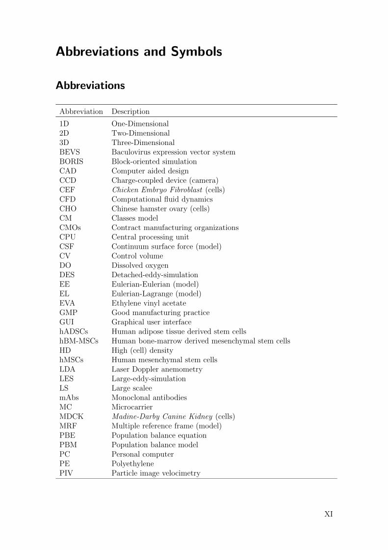
1D One-Dimensional2D Two-Dimensional3D Three-DimensionalBEVS Baculovirus expression vector systemBORIS Block-oriented simulationCAD Computer aided designCCD Charge-coupled device (camera)CEF Chicken Embryo Fibroblast (cells)CFD Computational fluid dynamicsCHO Chinese hamster ovary (cells)CM Classes modelCMOs Contract manufacturing organizationsCPU Central processing unitCSF Continuum surface force (model)CV Control volumeDO Dissolved oxygenDES Detached-eddy-simulationEE Eulerian-Eulerian (model)EL Eulerian-Lagrange (model)EVA Ethylene vinyl acetateGMP Good manufacturing practiceGUI Graphical user interfacehADSCs Human adipose tissue derived stem cellshBM-MSCs Human bone-marrow derived mesenchymal stem cellsHD High (cell) densityhMSCs Human mesenchymal stem cellsLDA Laser Doppler anemometryLES Large-eddy-simulationLS Large scaleemAbs Monoclonal antibodiesMC MicrocarrierMDCK Madine-Darby Canine Kidney (cells)MRF Multiple reference frame (model)PBE Population balance equationPBM Population balance modelPC Personal computerPE PolyethylenePIV Particle image velocimetry
XI
XII Abbreviations and Symbols
Abbreviation Description
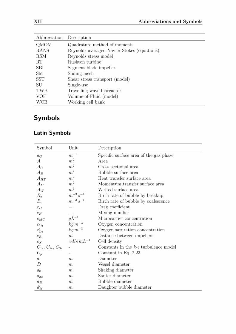
QMOM Quadrature method of momentsRANS Reynolds-averaged Navier-Stokes (equations)RSM Reynolds stress modelRT Rushton turbineSBI Segment blade impellerSM Sliding meshSST Shear stress transport (model)SU Single-useTWB Travelling wave bioreactorVOF Volume-of-Fluid (model)WCB Working cell bank
Symbols
Latin Symbols
Symbol Unit Description
aG m−1 Specific surface area of the gas phaseA m2 AreaAC m2 Cross sectional areaAB m2 Bubble surface areaAHT m2 Heat transfer surface areaAM m2 Momentum transfer surface areaAW m2 Wetted surface areaBb m−3 s−1 Birth rate of bubble by breakupBc m−3 s−1 Birth rate of bubble by coalescencecD − Drag coefficientcH − Mixing numbercMC gL−1 Microcarrier concentrationcO2 kg m−3 Oxygen concentrationc∗O2
kg m−3 Oxygen saturation concentrationcR m Distance between impellerscX cellsmL−1 Cell densityC1ε, C2ε, C3ε - Constants in the k-ε turbulence modelCµ - Constant in Eq. 2.23d m DiameterD m Vessel diameterd0 m Shaking diameterd32 m Sauter diameterdB m Bubble diameterd′B m Daughter bubble diameter

XIII
Symbol Unit Description
Db m−3 s−1 Death rate of bubble by breakupDc m−3 s−1 Death rate of bubble by coalescencedD m Droplet diameterdH m Hydraulic diameterDO2 ms−1 Oxygen diffusivitydP m Particle diameterdR m Impeller diameterdS m Sparger diameterDS m Diameter of a shaken flaskDT m2 s−1 Eddy diffusivityDm m2 s−1 Laminar (molecular) diffusivityEz,p − Impeller efficiencyfB m−3 Bubble number densityfBV − Bubble size ratio at bubble breakup~F N Force (vector)FG m−3 s−1 Gas flow rateFlz, p − Primary axial recirculation numberFr − Froude numberg ms−2 Gravitational accelerationGk kg m−1 s−3 Generation of turbulent kinetic energy from mean
velocity gradientsGb kg m−1 s−3 Generation of turbulent kinetic energy from
buoyancyGω kg m−3 s−2 Generation of specific turbulent dissipation rateh(di, dj) m3 s−1 Coalescence rate of two bubbles with diameters di
and djhR m Off-bottom clearanceH m Vessel heightHL m Liquid height~JΦ s−1 Molar flux of transport variable Φ (vector)k m2 s−1 Turbulent kinetic energykR s−1 Rocking ratekL ms−1 Liquid oxygen mass transfer coefficientkLa s−1 Specific overall mass transfer coefficientlR m Length of the impeller bladeLc m Characteristic lengthmL kg Liquid massMG molm−3 Molar mass of the gas phaseMW molm−3 Momentum at the wallsn - Viscosity index / number of replicatesn mol s−1 Molar fluxNC,OP s−1 Critical shaking rate for out-of-phase conditionsNR s−1 Impeller speed/rotational speed

XIV Abbreviations and Symbols
Symbol Unit Description
NS s−1 Shaking rateNS1 s−1 Impeller speed at suspension criterion (no
particles on vessel bottom observable)NS1u s−1 Impeller speed at suspension criterion (no
particles on vessel bottom at rest)NS90 s−1 Impeller speed at suspension criterion (particles
are lifted up to 90 % of liquid height)NS,c s−1 Critical shaking rate (Eq. 2.8)Ne − Newton number (power number)OTR molm−3 s−1 Oxygen transfer rateOUR molm−3 s−1 Oxygen uptake ratep Pa Pressure / probabilitypS Pa Solid pressureP W Power inputPC - Coalescene efficiencyPG W Power input under gassed conditionspR m Pitch of the stirrer bladePeL − Peclet numberPh − Phase number of shaken flasks/bottlesQG vvm Volume-related aeration rateqO2 mol s−1 cell−1 Specific oxygen consumption rater m Radial coordinate / radius of the annulus piperB m Baffle radiusR m Radius of the annulusRmax m Maximum rotation amplitude~r m Position vectorRe − Reynolds number (for stirrers)ReP − Reynolds number for a particleReS − Reynolds number for shaken flasks/bottlesReW − Reynolds number for wave-mixed bioreactorsRecrit − Critical Reynolds numberSΦ s−1 (Volume) source of transport variable ΦScT − Turbulent Schmidt numbert s TimeT K TemperaturetC s Characteristic time for (oxygen) mass transfertm s Mixing timetstart s Start time (required for maximum shaking rate)TS s−1 Strain rate magnitudeU m Wetted circumferenceu′ ms−1 Velocity fluctuationu m s−1 Time-averaged velocity~u ms−1 Velocity (vector)

XV
Symbol Unit Description
uD ms−1 Terminal droplet velocityuGS ms−1 Superficial gas velocityuS ms−1 Settling velocity of particlesutip ms−1 Tip speedV m3 VolumevB ms−1 Bubble volumeVL m3 Liquid volumeVS m3 Impeller swept volumew∗ ms−1 Mean fluid velocity through the annulusWB m Width of the culture bagWR m Width of the stirrer bladeWe − Weber numberYi − Mass fraction (of a tracer)Yk kg m−3 s−2 Dissipation of turbulent kinetic energyYω kg m−3 s−2 Dissipation of specific turbulent dissipation ratex, y, z m Coordinates of the Cartesian coordinate systemxi - Empirical constants (with i = 1− 10)z′ - Dimensionless distance between tracer injection
and mixing plane

XVI Abbreviations and Symbols
Greek Symbols
Symbol Unit Description
α - Phase volume fractionαG - Gas volume fractionαL - Liquid volume fractionβ m−3 Daughter bubble size distributionβB − Impeller blade angle
˙γnn s−1 Normal velocity gradient˙γnt s−1 Shear velocity gradientγΘS
kg K m−3 s−1 Collisional dissipation of energyδij - Kronecker symbolε m2 s−3 Turbulent dissipation rateεmax m2 s−3 Maximum turbulent dissipation rateλ m Eddy sizeλmin m Eddy sizes of the inertial subrangeλT m Kolmogoroff microscale of turbulenceµ Pa s Dynamic (molecular) viscosityµT Pa s Turbulent viscosityνL m2 s−1 Kinematic viscosity of the liquidπ − Mathematical constant (≈ 3.1415926535)Φ − Transport variableΦV kg m−1 s−3 Viscous dissipation rateφls kg K m−3 s−1 Energy exchange rate between liquid and solid phaseρG kg m−3 Density of the gas phaseρP kg m−3 Density of the particle phaseρL kg m−3 Density of the liquid phaseθ - Dimensionless timeΘS K Granular temperatureτ s−1 Stress (tensor)τnn Pa Normal stressτnt Pa Shear stressξ - Size ratio between bubbles and arriving eddiesσL N m−1 Liquid surface tensionσ - Rotation angleω s−1 Specific turbulence dissipation rateωB s−1 Collision frequency of bubbles and eddiesωC m3 s−1 (Specific) coalescence collision frequencyωmax s−1 Maximum angular velocityωR s−1 Angular velocityΩB s−1 Total bubble breakage rate
List of Figures
1.1. Potential fields of applications for Computational Fluid Dynamicsrelated to biomanufacturing processes. . . . . . . . . . . . . . . . . . 3
2.1. Power input-based categorization of dynamic SU bioreactors for ani-mal and human cells, taken from [1]. . . . . . . . . . . . . . . . . . . 7
2.2. Pictures of commercially available SU bioreactors. . . . . . . . . . . . 132.3. Influence of scale on different process parameters at constant P/V. . . 162.4. Principle of piece-wise linear reconstruction of the interface shape
applied in the geo-reconstruction scheme. . . . . . . . . . . . . . . . . 222.5. Bubble coalescence and breakup influence bubble size distribution. . . 26
3.1. The Mobius R©CellReady 3L bioreactor. . . . . . . . . . . . . . . . . . 313.2. SU spinner flask for small scale experiments. . . . . . . . . . . . . . . 323.3. The UniVessel R©SU bioreactor. . . . . . . . . . . . . . . . . . . . . . . 333.4. The traveling wave bioreactor. . . . . . . . . . . . . . . . . . . . . . . 343.5. Schematic of the power input measurement setup. . . . . . . . . . . . 363.6. Principle of measuring the liquid distribution in the traveling wave
bioreactor prototype. . . . . . . . . . . . . . . . . . . . . . . . . . . . 373.7. Schematic of the PIV experimental setup. . . . . . . . . . . . . . . . 383.8. Schematic of the experimental setup of the CHO cultivations in the
TWB prototypes. . . . . . . . . . . . . . . . . . . . . . . . . . . . . . 403.9. Parallelization of the CFD fluid domain . . . . . . . . . . . . . . . . . 42
4.1. Computational meshes used for modeling of the Mobius R©CellReadybioreactor . . . . . . . . . . . . . . . . . . . . . . . . . . . . . . . . . 44
4.2. Normalized fluid velocities in the stirred SU Mobius R©CellReady 3Lbioreactor . . . . . . . . . . . . . . . . . . . . . . . . . . . . . . . . . 46
4.3. Comparison of fluid flow patterns predicted using the Moving Refer-ence Frame and the Sliding mesh techniques. . . . . . . . . . . . . . . 48
4.4. Results of the grid sensitivity study for the Mobius R©CellReady biore-actor . . . . . . . . . . . . . . . . . . . . . . . . . . . . . . . . . . . . 49
4.5. Influence of turbulence models on CFD results in the Mobius R©CellReady3L bioreactor. . . . . . . . . . . . . . . . . . . . . . . . . . . . . . . . 51
4.6. Power number prediction for the Mobius R©CellReady 3L bioreactorwith 2 L working volume. . . . . . . . . . . . . . . . . . . . . . . . . . 52
4.7. CFD predictions for mixing in the Mobius R©CellReady 3L bioreactor. 554.8. Turbulence related hydrodynamic stress in the Mobius R©CellReady. . 584.9. CFD-predicted local stresses at 200 rpm in the Mobius R©CellReady
with 2 L working volume. . . . . . . . . . . . . . . . . . . . . . . . . . 614.10. Correlations of parameters related to hydrodynamic stress for the
Mobius R©CellReady. . . . . . . . . . . . . . . . . . . . . . . . . . . . . 624.11. Normalized fluid velocities in the stirred SU Mobius R©CellReady 3L
bioreactor under aerated conditions. . . . . . . . . . . . . . . . . . . . 64
XVII

XVIII List of Figures
4.12. Gas distribution in the Mobius R©CellReady bioreactor assuming con-stant and variable bubble sizes. . . . . . . . . . . . . . . . . . . . . . 66
4.13. CFD-predicted local bubble diameters in the Mobius R©CellReady biore-actor. . . . . . . . . . . . . . . . . . . . . . . . . . . . . . . . . . . . . 68
4.14. Comparison of bubble breakup models. . . . . . . . . . . . . . . . . . 71
4.15. Comparison of bubble coalescence models for different turbulent dis-sipation rates. . . . . . . . . . . . . . . . . . . . . . . . . . . . . . . . 72
4.16. CFD-predicted local oxygen mass transfer in the Mobius R©CellReady3L bioreactor. . . . . . . . . . . . . . . . . . . . . . . . . . . . . . . . 75
4.17. Objective of the CFD study for microcarrier-based cell expansion ofmesenchymal stem cells. . . . . . . . . . . . . . . . . . . . . . . . . . 78
4.18. CFD-predicted flow pattern for a spinner flask with 100 mL workingvolume. . . . . . . . . . . . . . . . . . . . . . . . . . . . . . . . . . . 80
4.19. Comparison of normalized tangential fluid velocities predicted by themulti-phase Euler-Euler model and a single-phase RANS model. . . . 81
4.20. Predicted solid particle distributions in the spinner flask with 100 mLworking volume meeting suspension criteria. . . . . . . . . . . . . . . 82
4.21. Expansion factors achieved at different stirrer speeds using MC typeI and II. . . . . . . . . . . . . . . . . . . . . . . . . . . . . . . . . . . 84
4.22. Fluid flow patterns in the modified UniVessel R©SU bioreactors. . . . . 87
4.23. Validation of the CFD models in the standard and modified UniVessel R©SUbioreactors by PIV measurements. . . . . . . . . . . . . . . . . . . . . 90
4.24. Experimentally determined impeller speeds based on suspension cri-teria NS1 and NS1u in the standard and modified UniVessel R©SU biore-actors. . . . . . . . . . . . . . . . . . . . . . . . . . . . . . . . . . . . 91
4.25. CFD-predicted MC distribution in the standard and modified geome-tries of the UniVessel R©SU bioreactor. . . . . . . . . . . . . . . . . . . 92
4.26. Power inputs for NS1 conditions in different single-use bioreactors. . . 92
4.27. Growth courses obtained for hMSC in the modified UniVessel R©SUbioreactor compared to its standard counterpart. . . . . . . . . . . . . 95
4.28. Schematic of the desired working principle of the traveling wave biore-actor. . . . . . . . . . . . . . . . . . . . . . . . . . . . . . . . . . . . . 97
4.29. Schematic of the time-dependent bioreactor motion. . . . . . . . . . . 98
4.30. CFD predicted air-liquid distribution for the unbaffled traveling wavebioreactor at different points in time. . . . . . . . . . . . . . . . . . . 101
4.31. Fluid flow in the traveling wave at a rotational speed of 40 rpm andamplitude of 25 mm after 15 seconds. . . . . . . . . . . . . . . . . . . 102
4.32. Model verification of the TWB for various operating conditions. . . . 103
4.33. CFD predicted Reynolds numbers for the TWB for various opera-tional conditions. . . . . . . . . . . . . . . . . . . . . . . . . . . . . . 105
4.34. CFD predicted specific power inputs for the TWB for various oper-ating conditions. . . . . . . . . . . . . . . . . . . . . . . . . . . . . . 108
4.35. Local energy dissipation rate in the liquid phase of the TWB. . . . . 109
4.36. Time series of the tracer volume fraction using an unsteady flow pattern.111

List of Figures XIX
4.37. CFD-predicted tracer concentrations using a transient approach withinthe VOF framework. . . . . . . . . . . . . . . . . . . . . . . . . . . . 112
4.38. CFD-prediction of mass transfer in the TWB. . . . . . . . . . . . . . 1144.39. Two geometries used in the TWB design studies. . . . . . . . . . . . 1154.40. Influence of the diameter ratio of the TWB on fluid flow. . . . . . . . 1184.41. Time series of the air-liquid distribution in two baffled TWB geometries.1194.42. Experimentally determined engineering data in two TWB prototypes. 1204.43. CFD predicted fluid velocities in the baffled modifications #6 and #10.1224.44. Profiles of the specific power input in the baffled torus geometries as
a function of time. . . . . . . . . . . . . . . . . . . . . . . . . . . . . 1234.45. CFD predictions for different baffled torus designs. . . . . . . . . . . 1244.46. CFD predicted fluid flow data for the baffled geometry modification
#10 under various operating conditions. . . . . . . . . . . . . . . . . 1254.47. CFD predicted shear stress distribution in the baffled annulus com-
pared to the unbaffled geometry. . . . . . . . . . . . . . . . . . . . . . 1264.48. Results of the local shear stress analysis for single droplet impact on
gas-liquid surface. . . . . . . . . . . . . . . . . . . . . . . . . . . . . . 1274.49. Results from a proof-of-concept cultivation in the TWB. . . . . . . . 132
A.1. Determination of the overall oxygen mass transfer coefficient. . . . . . 172A.2. Block scheme of the BORIS program used for data acquisition and
temperature control during the proof-of-concept cultivation in thetravelling wave bioreactor prototype. . . . . . . . . . . . . . . . . . . 172
A.3. Computational meshes used for the grid sensitivity study of the bench-top Mobius R©CellReady bioreactor . . . . . . . . . . . . . . . . . . . . 173
A.4. Volume-weighted frequency distribution of shear and normal stressesin the Mobius R©CellReady for different working volumes. . . . . . . . 174
A.5. Results for the drag coefficient obtained with different models avail-able in the literature. . . . . . . . . . . . . . . . . . . . . . . . . . . . 174
A.6. Measured bubble size distributions in the benchtop Mobius R©CellReadybioreactor. . . . . . . . . . . . . . . . . . . . . . . . . . . . . . . . . . 175
A.7. Distributions of different bubble sizes in the Mobius R©CellReady biore-actor at 200 rpm and 0.1 slpm (0.05 vvm). . . . . . . . . . . . . . . . . 175
A.8. Sensitivity of CFD results on the time step size. . . . . . . . . . . . . 176A.9. Definition of the Reynolds number for the travelling wave bioreactor. 176A.10.Predicted Reynolds numbers at two cross sections as a function of time.176A.11.Time series of the liquid surface shape in the unbaffled TWB geometry
under out-of-phase conditions. . . . . . . . . . . . . . . . . . . . . . . 177A.12.Correlation of the critical shaking frequency above which out-of-phase
conditions occur in the travelling wave bioreactor. . . . . . . . . . . . 177A.13.Time series of the tracer volume fraction assuming steady-state flow
(”frozen” flow approach). . . . . . . . . . . . . . . . . . . . . . . . . . 178A.14.Schematic of the work flow for the mixing time prediction in the TWB.178A.15.Meshes of the TWB modifications. . . . . . . . . . . . . . . . . . . . 179A.16.Mesh used for the single droplet impact study. . . . . . . . . . . . . . 179

List of Tables
2.1. Specific oxygen uptake rates of various cell lines. . . . . . . . . . . . . 18
3.1. Summary of the physical properties of MC types used, as given bythe manufacturers. . . . . . . . . . . . . . . . . . . . . . . . . . . . . 37
4.1. Mesh details of the Mobius R©CellReady bioreactor models. . . . . . . 444.2. Summary of CFD predicted power numbers in the Mobius R©CellReady
bioreactor obtained using the torque and energy dissipation approachfor different grid densities and turbulence models. . . . . . . . . . . . 54
4.3. Results from numerically predicted mixing times for the benchtopMobius R©CellReady bioreactor. . . . . . . . . . . . . . . . . . . . . . . 56
4.4. CFD-predicted parameters related to hydrodynamic stress in the bench-top Mobius R©CellReady bioreactor. . . . . . . . . . . . . . . . . . . . 60
4.5. Summary of correlations for mean and maximum shear stresses instirred tanks. . . . . . . . . . . . . . . . . . . . . . . . . . . . . . . . 63
4.6. CFD-predicted power inputs and power numbers for the Mobius R©CellReadybioreactor under aerated conditions. . . . . . . . . . . . . . . . . . . . 66
4.7. Results for the oxygen mass transfer predicted by the two-phasemodel with PBE. . . . . . . . . . . . . . . . . . . . . . . . . . . . . . 76
4.8. Experimentally determined suspension criteria for both MC types inspinner flasks with 100 mL working volume. . . . . . . . . . . . . . . 82
4.9. Summary of estimated shear stress levels, turbulent dissipation rateand Kolmogorov microscale of turbulence for different impeller speeds 84
4.10. Geometric parameters for the modifications of the UniVessel R©SUbioreactor compared with the standard vessel (Std.). . . . . . . . . . 85
4.11. Summary of flow and engineering parameters obtained for the nineimpeller modifications and the standard model. . . . . . . . . . . . . 88
4.12. Predicted shear stress levels at impeller speeds for the NS1u suspen-sion criterion in the original and modified UniVessel R©SU and theMobius R©CellReady 3L bioreactors. . . . . . . . . . . . . . . . . . . . 94
4.13. Details of the investigated torus geometries. . . . . . . . . . . . . . . 1164.14. Summary of reported cultivation results with the CHO XM111-10 cell
line using chemically defined medium in different single-use bioreactors.131
A.1. Summary of selected computational meshes used in studies based onthe RANS approach reported in literature . . . . . . . . . . . . . . . 180
A.2. Constants in the standard k-ε turbulence model . . . . . . . . . . . . 181A.3. Constants in the RNG k-ε turbulence model . . . . . . . . . . . . . . 182A.4. Constants in the standard k-ω turbulence model . . . . . . . . . . . . 186
XX

1. Introduction
1.1. Single-use equipment in biomanufacturing
During the last decades, cell cultures from plant, animal and human origins havebecome enormously important as expression systems for the production of mod-ern biopharmaceuticals, including hormones, cytokines, antibodies and vaccines [2],and in cell therapies, where the cells themselves are the desired product. The worldmarket for recombinant protein therapeutics has crossed the landmark threshold of100 billionsUSdollarperyear and the high annual growth rate in biopharmaceuticalmarkets of ≥ 15 % is expected to continue [3].However, the manufacturing of biopharmaceuticals is often difficult because the pro-duction organisms are sensitive to environmental changes as well as chemical andphysical stresses. Furthermore, product safety relies on assuring aseptic conditionsand the absence of cross-contamination of batches. Traditionally, this is performedby sophisticated sterilization and cleaning strategies, including the validation of theeffectiveness of these cleaning procedures in the case of GMP processes.Alternatively, single-use (SU) equipment1 can be used. After one use, the materialsthat are in contact with the cells and products are decontaminated and discarded,which makes sterilization, cleaning and validation procedures obsolete [4]. This alsoresults in reduced need for aggressive and corrosive cleaning agents and water forinjections (WFI). Consequently, the bioreactors’ periphery and the facility foot-prints can often be minimized. In contrast to conventional bioreactors made of glassor stainless steel, the cultivation containers of SU bioreactors consist of flexible orrigid plastic materials. Rigid systems, which are most often fabricated from poly-carbonate plastics, dominate in micro-, milliliter- and small liter scales. Flexibletwo-dimensional (2D) or three-dimensional (3D) bags, whose contact layers are forthe most part made of polyethylene (PE) or ethylene vinyl acetate (EVA) films, areused in larger systems and require a supporting container to fix and shape the bags.The cultivation container is pre-assembled and typically beta- or gamma-irradiatedfor sterilization before being delivered ready-to-use by the vendor [4].Even though there are some drawbacks, such as limited scalability, higher mate-rial costs, lower degree of instrumentation and automation, and the issue of leach-ables/extractables2, SU bioreactors have become well-accepted for screening studies,cell expansion, and for product expressions. They are used for the production of pre-clinical and clinical samples of therapeutic antibodies and preventive and therapeuticvaccines [1]. Furthermore, recent publications indicate the suitability of SU biore-actors for the production of cell therapeutics based on human mesenchymal stemcells (hMSCs) [7–10]. The use of SU bioreactors is particularly meaningful for the
1Single-use systems are also referred to as “disposable” systems when used in biopharmaceuticalproduction processes.
2Leachables are potentially toxic or inhibitory substances that are released from the disposablematerial during the biomanufacturing process [5]. Extractables are chemical entities (organicand inorganic) that can be extracted from disposables in controlled environments [6]
1

2 Chapter 1. Introduction
production of high-value products at small and medium scales. Due to their highflexibility and short setup times, SU bioreactors have advantages in processes wherefast and safe production is required.Nevertheless, there is still a lack of engineering characterization of SU bioreactors,which hampers comparison with different types of SU bioreactors and their con-ventional counterparts, and creates issues for scaling-up. Several studies have beenpublished that provide engineering parameters related to mixing time, oxygen masstransfer and power input of various SU bioreactor types, including stirred, wave-mixed and orbitally shaken systems (see section 2.2.1). However, considering theheterogeneous distribution of hydrodynamics within typical bioreactors, it seemsworthwhile to undertake detailed analyses of the fluid flow patterns. Even thoughthese data can be experimentally determined by comprehensive measurement tech-niques, such as Laser Doppler anemometry (LDA) or Particle Image Velocimetry(PIV), these methods are often too time-consuming for the complete characteriza-tion of flows in typical bioreactors. An alternative is provided by numerical methods,such as Computational Fluid Dynamics (CFD), which has become a widely acceptednumerical technique for studying local characteristics (e.g. liquid velocities, shearstresses, gas holdups, temperature profiles etc.) within bioreactors from mL to m3
scale [11–13].
1.2. Scope and outline of this thesis
The aim of this thesis is to evaluate possibilities, requirements and limitations ofcommonly applied CFD models with respect to their accuracy and predictabilityfor the characterization, optimization and development of SU bioreactors and pro-duction processes for biopharmaceuticals. Three potential fields of application forCFD are discussed (see Fig. 1.1) and are examined in three case studies (see chap-ter 4): (1) advanced engineering characterization, (2) bioreactor development andoptimization and (3) process optimization. All three fields are related to biologicalentities and their reaction to physical, chemical, thermal and hydrodynamic stresses,which have to be considered in order to guarantee high cell numbers and desiredproduct quantity and quality. Some demands however conflict with each other. Forexample, often a compromise has to be found between the power input necessary togenerate sufficient mixing and the risk of excessive power input generating criticalshear stress levels [14].The latter may be calculated from spatial-resolved flow data obtained from CFDanalyses. The suitability of CFD for advanced engineering characterizations of typ-ical bioreactors has been demonstrated for benchtop and pilot scale bioreactors (seesection 2.3.2). Provided that the models are validated, parameters can be obtained,that are hard or even impossible to measure [15]. Examples are the distributions ofshear stresses and turbulence parameters, which are related to cell stress/damage[16]. This is further discussed in the case study on the advanced engineering char-acterization of the Mobius R©CellReady 3L bioreactor (see section 4.1).Additionally, CFD can be used to optimize cultivation conditions, which is as an

1.2. Scope and outline of this thesis 3
example presented using the cultivation of human mesenchymal stem cells (see sec-tion 4.2). Human mesenchymal stem cells are of great interest in modern therapiesfor the treatment of cancer as well as orthopedic, immunological, cardiological andophthalmic diseases. In contrast to previously mentioned vaccines and antibodies,where cells are used as expression systems, the cells themselves represent the prod-uct. Since the two-dimensional (2D) monolayers that are typically used are limitedin scale and do not offer adequately controllable culture conditions, efficient, cost-effective and scalable processes are required to produce sufficient cell amounts. Theuse of microcarrier based cell expansion is considered to be a promising alternative.In this work, CFD has been used to predict critical shear stresses within stirredSU bioreactors from 100mL to 50L scale. An optimized bioreactor geometry hasalso been proposed which is based on a number of design studies and has led to asignificant reduction in the impeller speeds required in order to achieve microcarriersuspension.Since CFD is based on fundamental balance equations for mass, momentum andenergy (see section 2.3.1), the flow inside novel types of bioreactors can be investi-gated without the need for a physical model. Thus, the number of prototypes canbe reduced, resulting in time and cost savings. This is described in detail using thetravelling wave bioreactor, a novel bioreactor concept, that is based on an orbitallyshaken, toroidal shaped vessel (see section 4.3) as an example. In the partially filledvessel, a quasi-periodically travelling wave is induced, which is intended to drivemixing and (oxygen) mass transfer. The wave motion is described in detail and de-sign studies on the bioreactor geometry by means of CFD were used to optimize thebioreactor in terms of mixing and mass transfer.
Advanced engineering characterization
- Mixing - Mass transfer- Power input- Shear stress
- Residence time- Reaction rate
- Identification of process-relevant parameters- Parameter variation
Process optimization- Identification of equipment-relevant parameters (design studies)- Geometry variation
(Bio)reactor development/optimization
Biological entities- Physical stresses (pH, pO2, pCO2, osmolarity etc.)
- Chemical stresses (substrates, metabolites, etc.)- Hydrodynamic stresses
- Thermal stresses
Fig. 1.1.: Potential fields of applications for Computational Fluid Dynamics related tobiomanufacturing processes.

4

2. Theoretical background and fundamentals
2.1. Application of single-use bioreactors for humanand animal cells
Even though several applications for SU bioreactors for the cultivation of plant cells[17, 18], microalgae [19, 20] and microorganisms [21–25] have been described, SUbioreactors have mainly been used in production processes based on animal (i.e.mammalian and insect) and human cells over the last three decades. SU bioreactorshave established themselves for the production of pre-clinical and clinical samplesof therapeutic antibodies and preventative vaccines in screening studies, cell expan-sion, and product expressions [1]. Furthermore, their potential for the productionof cell therapeutics using stem cells, in particular human mesenchymal stem cells(hMSCs), has recently been demonstrated [7–10].The main application field of SU bioreactors is seed train production of animal andhuman continuous suspension cells, where mainly wave-mixed bioreactors are used.Typically, the pre-cultures are expanded in shake flasks, which are inoculated us-ing thawed cells from a vial-based working cell bank (WCB), detailed descriptioncan be found elsewhere [5]. As an alternative, large scale WCBs (LS-WCB) consist-ing of cryogenic bags of larger volumes [26, 27] or high density WCBs (HD-WCB)of ≈ 1 · 108 cellsmL−1 in traditional vials [28, 29] have been developed. For thispurpose, special wave-mixed bioreactors with an integrated fixed or floating microfiltration membrane that are operated in perfusion mode are available. Using thesesystems, very high cell densities can be achieved. For example, peak viable cell den-sities of up to 2.1 · 107 cellsmL−1 have been reported for mAb producing hybridomacells in the WAVE bioreactor (GE Healthcare) [30] and even higher densities of15 · 107 cellsmL−1 have been achieved for PER.C6 cells in the BIOSTAT R©CultiBagRM [31]. Using LS-WCBs or HD-WCBs, the time required for seed production canbe significantly reduced. For example, it has become possible to inoculate 50 L ofmedium to a cell density of 1.1 · 106 cellsmL−1 of Trichioplusia ni (Hi-5 ) cells within5 days rather than the usual 10 days.Furthermore, SU bioreactors have become well accepted for the production of ther-apeutic monoclonal antibodies (mAbs), which explains the fact that many contractmanufacturing organizations (CMOs) use them at scales up to 2 m3 [1]. In severalstudies, comparable living cell densities, viability and expression profiles, and prod-uct quality similar to standard stainless steel vessels have been demonstrated [32–34].Typical antibody productions are performed in fed-batch mode (i.e the cells are sup-plemented with a concentrated nutrient solution) and final product concentrations,which are harvested batch-wise, are in the range of 2 g L−1 to 5 g L−1 [35]. Continu-ous processes in SU bioreactors were developed in order to increase the space-timeyield of antibody production processes. Using XD R©technology, which is based on across flow filtration system, antibody concentrations of between 10 g L−1 to 27 g L−1
at cell densities of 1 · 108 cellsmL−1 have become realistic [36].
5

6 Chapter 2. Theoretical background and fundamentals
Due to their one time use, the biosafety of virus-based production processes is en-hanced by using SU bioreactors. In addition, production scales (10 L to 2500 L) aresmaller compared to those of mAbs, because clinical doses of viral vaccines are typi-cally smaller [37]. Often adherently cultivated production cell lines, including Africangreen monkey kidney-derived Vero cells, Madin-Darby Canine Kidney (MDCK) cellsor Chick Embryo Fibroblast (CEF), are used for virus production [38, 39]. Hence, thecells must be cultivated in SU bioreactors which allow 2D cell growth, such as rollerbottles and multitray systems, or systems that operate either with hollow fibers [40]or microcarriers [41]. The suitability of wave-mixed and stirred bioreactors for virusproduction with MDCK and Vero cells grown on microcarriers has been demon-strated in numerous studies [42–47]. As an alternative to microcarrier-based sys-tems, different SU fixed bed bioreactors, including the iCELLis
TMbioreactor (ATMI
Life Sciences) [41, 48], the 5 L BioBLU SU packed-bed bioreactor (Eppendorf) [49]and the Current Perfusion bioreactor (AmProtein) [50], are suitable.In recent years, product expressions with the baculovirus expression vector system(BEVS) have become increasingly important [51, 52]. These have mainly been pro-duced using cell lines of the Fall army worm (Spodoptera frugiperda; Sf-9 ) or the cab-bage looper (Hi-5 ) and its derivatives. They are routinely cultivated in wave-mixedand stirred SU bioreactors for the production of seasonal and pandemic vaccine can-didates (e.g. virus like particles of Influenza A/H1N1/Puerto Rico8/34). Currently,upstream concepts, that are entirely based on SU devices, are also being developed[1].A very modern field of application for SU bioreactors is the production of humanprimary cells, which are manufactured in small scale batch production processes.Different studies have demonstrated that clinically relevant doses of natural killercells and activated T-cells, which are mostly used for autologous transplantations1
can be cultivated in wave-mixed SU bioreactors [53–55]. In contrast, only a few solu-tions are available for the proliferation of human mesenchymal stem cells (hMSCs),which are from interest in both autologous and allogeneic2 therapies, that yieldclinically relevant cell amounts of 3 · 107 to 5 · 108 cells for a single patient [56].SU hollow fiber bioreactors (Quantum cell-expansion system, [57]) or SU fixed bedbioreactors (iCELLIs
TM, [58]) provide controllable and efficient hMSC expansion,
but their scalability is limited. In addition to cultivation in spheroids and encapsula-tion, microcarrier-based hMSC expansions have shown promising results in differentstudies. Details are given in the case study in section 4.2.
1In autologous transplantations, the donors receive their own cells after biopsy, manipulation (e.g.cell activation, genetic manipulation) and cell expansion.
2In allogeneic transplantations, the donor and the receiver of the cells are different.

2.2. Engineering characterization of SU bioreactors and scale-up 7
2.2. Engineering characterization of SU bioreactorsand scale-up
During the development of SU bioreactors, a multitude of different types have beenintroduced to the market, which differ in the design of the cultivation container, typeof power input, instrumentation, and scale. Currently, SU bioreactors with workingvolumes of up to 2m3 are commercially available [59], which can be categorized,based on the power input, into static and dynamic systems [60]. Due to the lim-ited mass transfer that leads to lower cell densities and product titers compared todynamic systems, static systems, such as t-flasks and multilayer flasks, are exclu-sively used at small and medium scales. The dynamic SU bioreactors are furthersub-divided into mechanically, pneumatically and hydraulically driven systems, andso-called hybrids (see Fig. 2.1). Today, the mechanically driven SU bioreactors, whichare either stirred, oscillating or orbitally shaken, form the largest group. This chap-ter summarizes important engineering parameters for SU bioreactors, with a mainfocus on stirred, wave-mixed and orbitally shaken systems. Furthermore, scaling-upstrategies that take into consideration the specific requirements of cell cultures areaddressed. CFD models and their applications for the characterization and optimiza-tion of bioreactors, which form the basis of the case studies, are then reviewed.
Dynamic SU bioreactors
Mechanically driven Pneumatically driven Hydraulically driven
Hollow fiber bioreactors
Fixed bed bioreactors
Hybrid systems
Air wheel mechanism
Stirred systemsCombination of air-lift & stirring
Orbitally shaken systems
Oscillating systems
Wave-mixed Vibrating discs Rotarory
1D motion
2D motion
3D motion
Rotating stirrers
Tumbling stirrers
Air-lift bioreactors
Fig. 2.1.: Power input-based categorization of dynamic SU bioreactors for animal and hu-man cells, taken from [1].

8 Chapter 2. Theoretical background and fundamentals
2.2.1. Characteristics of dynamic SU bioreactors
In 2006, the Thermo Scientific Single Use Bioreactor (S.U.B.) was the first SU stirredbag bioreactor until Xcellerex launched its XDR SU stirred-tank bioreactor. Bothsystems use angular, off-centered, axial flow impellers for agitation, which eliminatesthe formation of a fluid vortex that is often observed in unbaffled vessels. While onlylimited engineering data have been documented for the Xcellerex’s product family,more comprehensive characterizations of the S.U.B. Hyclone bioreactors (50 L and250 L scale) are available [59, 61, 62]. Reported mixing times (9 - 155 s) and oxygentransfer coefficients kLa (2 - 25 h−1) for typical cell culture conditions are compara-ble to conventional and other SU stirred bioreactors at pilot scale. In the 50-L and200-L Mobius R©CellReady bioreactors, average mixing times in the range of 25 s and38 s have been reported at maximum filling levels [63]. Here, kLa values in the rangeof 4 h−1 and 49 h−1 have been determined for aeration rates of between 0.0025 vvmand 0.05 vvm and power inputs of up to 10 Wm−3, whereas the maximum powerinputs were 120 W m−3 (50 L) and 33 Wm−3 (200 L) [63].In contrast to the aforementioned stirred SU bag bioreactors, the bioreactors ofthe BIOSTAT R©CultiBag STR family (Sartorius Stedim Biotech) are agitated bytwo impellers mounted on the centered shaft [64]. Two impeller configurations areavailable: two three-bladed segment impellers (SBI-SBI) and a combination with alower-mounted six-blade Rushton turbine (disk impeller, SBI-RT). CFD simulationshave shown that the latter produces a radial flow pattern [59], which is known toimprove gas dispersion [65, 66]. In terms of vessel geometry, agitation and aeration,the cultivation bags, which offer working volumes up to 2 m3, have a design that isvery close to conventional stainless steel bioreactors [67], with typical geometric ra-tios (e.g. dR/D=0.38, HL/D=1.8, hR/D=0.24) and a convex shaped bottom. Eithertraditional ring spargers or microspargers with 0.8 mm and 0.15 mm holes are usedfor aeration. Using typical aeration rates for cell culture applications, only minoreffects (< 15 %) on the power input were determined both experimentally and byCFD investigations [59]. This is in agreement with expectations and findings forthe “elephant ear impeller”, which has a similar geometry to the SBI [68]. Thus,the specific power inputs in the BIOSTAT R©CultiBag STR 50 at a tip speed (utip)of 1.8 ms−1 were about 86 and 240 Wm−3 for the SBI-SBI and the SBI-RT config-urations respectively. Since power input influences shear forces, mean local sheargradients were predicted in order to estimate potential cell damage by agitation.The correlation given in Eq. 2.13 is valid for BIOSTAT R©CultiBag STR bioreactorswith working volumes of up to 1000 L, and also describes shear rates in the Hy-clone S.U.B. relatively well. This is interesting, because the impeller geometry ofthe Hylcone S.U.B. differs significantly from that of the BIOSTAT R©CultiBag STRbioreactors.
γNT = 0.05
(P
V
)1/3(dRD
)−2.7
VL−0.16 (2.1)
3In Eq. 2.1, all parameters have to be inserted in SI units, as given in the list of symbols, in orderto obtain the shear rate γNT in s−1.

2.2. Engineering characterization of SU bioreactors and scale-up 9
Depending on the scale and applied power input, shear gradients between 0.1 s−1
and 30 s−1 were predicted in the BIOSTAT R©CultiBag STR bags. Assuming water-like culture media (i.e. viscosity of ≈ 1 mPas), this corresponds to shear stressesof 10−4 Pa and 0.03 Pa, which is significantly below critical values (in the order of1 · 105 s−1 to 3 · 105 s−1) that cause substantial cell damage [69]. Thus, it is not en-tirely surprising that cell densities of 6 · 106 cellsmL−1 to 7.5 · 106 cellsmL−1 withviabilities above 96 % were achieved using chemically defined minimal medium [59].Mixing analysis using conductivity methods and CFD models revealed, that, depend-ing on the power input (0.86 - 86 Wm−3), mixing times in the BIOSTAT R©CultiBagSTR 50L at the maximum filling level were between 10 s and 60 s [59]. This suggeststhat the level of mixing is comparable to conventional stirrers and sufficient for cellculture applications [70]. Similar results have been reported for oxygen mass trans-fer, with kLa values of up to 35 h−1 measured at an aeration rate of 0.1 vvm [71].This suggests sufficient oxygen supply for cultures with a low to medium oxygen-demand.Comparable oxygen transfer rates were measured in the UniVessel R©bioreactor (Sar-torius Stedim Biotech), a benchtop scale bioreactor with a rigid cultivation vesselthat is agitated by a geometrically similar two-stage SBI. Depending on the specificpower input (0.4 Wm−3 < P/VL < 150 Wm−3), kLa values in the range of 10 h−1 to40 h−1 for 0.01 vvm (uGS = 2.8 · 10−4 ms−1) and 20 h−1 to 65 h−1 for 0.02 vvm (uGS= 5.6 · 10−4 ms−1) were obtained [59]. These kLa values (in h−1) could be correlatedto the specific power input P/VL (in W m−3) and the superficial gas velocity uGS(in ms−1), as given by Eq. 2.2, indicating the strong influence of the aeration. Thiscan be explained by the low gas dispersion of the slow rotating, axially pumpingimpellers most often used for cell culture applications [72].
kLa = 7.97 103 (P/VL)0.25 uGS0.87 (2.2)
Besides stirred SU bioreactors, those with wave-induced motion have become thestandard for inoculum production and in cases where very shear-sensitive cell cul-tures are used [73]. Thus, wave-mixed bioreactors are regarded as low-shear systemswith more homogeneous energy dissipation than stirred bioreactors.In general, wave-mixed bioreactors can be categorized according to their type ofmotion. The first models, which entered the laboratories at the end of the 1990s,had rocker platforms with a periodic, 1D oscillatory motion [74]. The fluid motioninside the partially filled, pillow shaped bag is influenced by the bag geometry, fillingvolume, rocking rate and angle, and the liquid properties [73, 75]. It can be char-acterized by a modified Reynolds4 number (ReW ), that is defined by the workingvolume (VL), the width of the culture bag (WB), the liquid level (HL), the rock-ing rate (kR), the kinematic viscosity of the liquid (νL), and an empirical constant(C) that depends on the bag type (see Eq. 2.3). The authors proposed turbulentconditions to be expected above a critical Re (Recrit) of 1000 [73].
ReW =VL kR C
νL (2HL +WB)(2.3)
4The British physicist Osborne Reynolds (1842 - 1912) did pioneering work that contributed tothe understanding of fluid dynamics.

10 Chapter 2. Theoretical background and fundamentals
The wave motion promotes bulk mixing, off-bottom suspension of cells and parti-cles, bubble-free surface aeration and reduces foaming and flotation in comparisonto stirred cell culture bioreactors [73]. Even though detailed comparisons of differentcultivation bags are difficult because of a lack of comparability of operational con-ditions and measurement techniques, reported kLa values are in the range of 0.5 h−1
and 24 h−1. This makes them suitable for cultures with low and medium oxygendemands [75]. However, it should be noted, that very high cell densities have beenreported for wave-mixed systems operated in perfusion mode5 (see section 2.1).In general, oxygen mass transfer in a given culture medium and bag geometry isinfluenced by the rocking rate, rocking angle and the filling level. Contrary datahave been reported with respect to the aeration rate. While Eibl et al. (2010a) [73]stated that raising the aeration rate at a given working volume has a smaller effecton the kLa than changes in the rocking rate and/or rocking angle, relatively highdependency was found in 2 L and 20 L wave-mixed bags [76, 77]. Nevertheless, itshould be emphasized that, according to the traditional definition of the kLa value(provided, for example, by [66]), the overall mass transfer for a given specific sur-face area (a) is limited by resistance at the liquid side of the gas-liquid interface(expressed by kL). As long as no significant surface turbulence is induced by the airflow, it is unlikely that this resistance is influenced by the aeration in the cultivationbags.Mixing times in 1D wave-mixed systems, which have been determined by injectinga fluorescent dye and videotaping the dispersion of the dye [76] or by the decoloriza-tion method (as described in section 3.2.1) [73, 78], range from 5 s to 60 s, dependingon the scale (2 L to 20 L) and rocking parameters. Nevertheless, a wider range of upto 1400 s has been reported for scales of up to 100 L with filling levels of between40 % and 50 % [73].The specific power inputs in Wave bioreactor bags (2 L and 20 L) have been deter-mined experimentally by calculating the momentum based on the center of gravityand the surface area of the fluid [73] and numerically using CFD simulations [62].Specific power inputs of up to ≈560 Wm−3 (0.2 L, 30 rpm, 30) were determined,reducing to ≈70 Wm−3 at the maximum filling level (2 L). Nevertheless, it shouldbe noted that operational parameters must be evaluated together. For example, aspecific power input of ≈150 Wm−3 in BIOSTAT R©CultiBag RM 200 L bags at 50 %can be achieved by either setting a rocking rate of 30 rpm and rocking angle of 6.5
or a rocking rate of 20 rpm and a rocking angle of 9 [62].Significantly higher specific power inputs have been measured in a wave-mixedCELL-tainer R©SU bioreactor, which has a 2D movement. The oscillating rockingmotion is superimposed by a horizontal translation, which leads to specific powerinputs of up 3 kWm−3 (15 L working volume, 16, 10 cm displacement) [79]. Thisis comparable to standard stirred bioreactors that are used for microbial cultures,and facilitates much higher oxygen transfer rates than 1D motion wave systems [79].Even though there are some doubts about the reliability of the reported data, kLavalues of up to 600 h−1 have been measured in the 15 L system, which makes the
5For this purpose special cultivation bags are available from Sartorius Stedim Biotech and GEHealthCare, which incorporate perfusion membranes

2.2. Engineering characterization of SU bioreactors and scale-up 11
bioreactor suitable for cultures with high oxygen demands. However, it should beemphasized that such high oxygen transfer rates are not required for animal andhuman cell cultures. Furthermore the shear forces may even harm such cells.Besides stirred and wave-mixed bioreactors, orbitally shaken systems, such as mi-crowell plates, shake flasks, and the TubeSpin R©bioreactor (Techno Plastic materi-als), are among the most often used bioreactors. These bioreactors are primarily usedin the early stages of inoculum production and for screening experiments, where thepossibility of miniaturization is advantageous for the processing of a large numberof different cultivation experiments [80]. During the last decade, engineering param-eters for various small scale systems, including mixing time, oxygen mass transferand power input, have been widely reported [81–88]. Furthermore, advanced param-eters for shear stress and turbulent energy have been predicted by means of CFD forsingle wells of microtiter plates [89], TubeSpin R©bioreactors [86], shake flasks [90],and shaken bottles [91].Eq. 2.4 was established to calculate the power input in unbaffled shake flasks [82],where ReS is the shake flask Reynolds number. This is defined by Eq. 2.5, where NS
is the shaking frequency and DS is the maximum inner diameter of the flask.
P = 1.94VL1/3ρLNS
3DS4ReS
−0.2 (2.4)
with
ReS =ρNS DS
2
µL(2.5)
Depending on the flask geometry, filling level and shaking parameters, specific powerinputs of up to 6 kWm−3 were determined for total flask volumes of 2 L, which issignificantly higher than typical power inputs in cell culture applications. For thecalculation of kLa, Eq. 2.66 can be used for a wide range of operational conditions,where DO2 and d0 denote the oxygen diffusivity and the shaking diameter respec-tively [92].
kLa = 0.5DS2.03NS V
−0.89L νL
−0.24DO2
0.5 g−0.13 d00.25 (2.6)
For differently sized cylindrical, orbitally shaken bioreactors, a slightly different cor-relation (see Eq. 2.76) was proposed, which can be explained by the different liquidmotion compared to shake flasks [92].
kLa = 3.82DS4.3NS
2.12 VL−1.2 νL
−0.21DO2
0.12 g−0.51 (2.7)
This correlation is valid (with an accuracy of ±30 %) for operating conditions abovecritical circulation frequencies NS,c, guaranteeing rotation of the liquid, and can becalculated by Eq. 2.8.
NS,c =1
DS2
√0.28VL g (2.8)
6All parameters have to be inserted with units given in the list of symbols to obtain kLa in h−1.

12 Chapter 2. Theoretical background and fundamentals
Interestingly, the oxygen supply in single-use flasks made of polycarbonate was foundto be ≈30 % lower than in conventional glass flasks, which may be explained by thedifferences in surface wetting that influence the specific surface area.Both the specific power input and the oxygen mass transfer in orbitally shakenbioreactors were found to be affected by the ‘out-of-phase’ phenomenon. This ischaracterized by liquid not moving in-phase with the rotation of the shaker table[81, 93]. To describe this effect quantitatively, the dimensionless phase number (Ph)was introduced (see Eq. 2.9), which represents the operating conditions at whichthe Ph > 1.26 and the Froude number Fr = NS d
g> 0.4 are ‘in-phase’. In general,
the phase number depends on the vessel geometry (DS), the shaking diameter (d0)and the liquid properties (i.e. density and viscosity), however, in shaking flasks ofvolumes smaller than 1 L ‘out-of-phase’ conditions are only observed at elevatedliquid viscosities.
Ph =d0
DS
1 + 3 log10
ρL π NSDS2
2µL
1−
√√√√1− 4
π
(VL
1/3
DS
)2
2 (2.9)
Since the maximum working volume of shake flasks is only 20 - 30 % of the total vol-ume, scaling-up is limited to approximately 1 L total volume. In contrast, cylindrical-or cube-shaped culture containers with larger volumes of up to 1000 L have been de-veloped [94–96]. In addition, special constructions, such as helical tracks on theinner vessel wall, have been tested in order to improve mixing and mass transfer.By driving the liquid onto these helical tracks, the gas-liquid interface is signifi-cantly increased, resulting in 5 to 10-fold higher kLa values (up to 55 h−1) comparedto non-modified vessels. Furthermore, cell growth was comparable to small scaleTubeSpin R©and 30 L stirred bioreactors [97].Although none of these systems became commercially available, they finally led tothe development of the OrbShake
TMbioreactor in 2009 [98], a SU 200 L orbitally
shaken bioreactor (distributed by Sartorius Stedim Biotech and Kuhner AG). Sinceno internal mixing and sparging devices are present, the bags are considered to bean economical alternative to stirred SU bioreactors and a solution to typical issues,such as foam formation and sealing of the impeller shaft. At the maximum fillinglevel kLa values in the order of 8 h−1 are achievable with agitation rates of 75 rpmand a shaking diameter of 10 cm [99]. However, significantly higher values of upto 25 h−1 have been reported for 100 L working volumes [100]. Depending on theshaking frequency (50 - 70 rpm), reported mixing times are between 25 s and 70 s.
2.2. Engineering characterization of SU bioreactors and scale-up 13
1
6
7
2 3
54
8
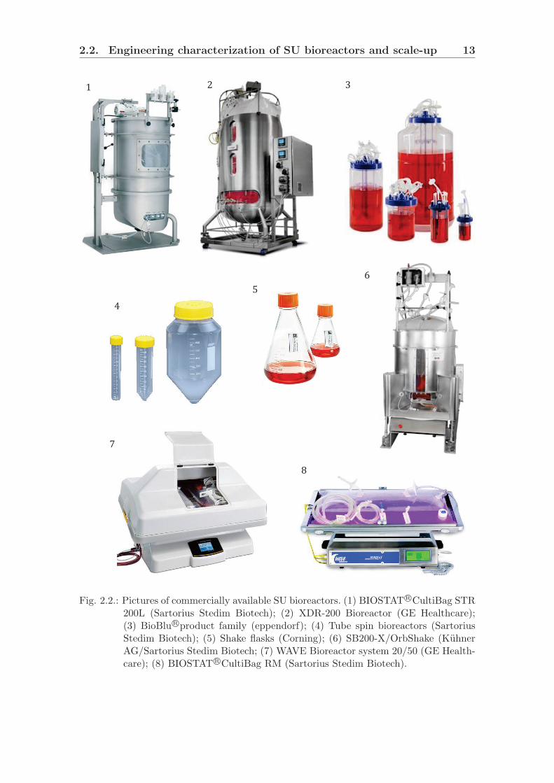
Fig. 2.2.: Pictures of commercially available SU bioreactors. (1) BIOSTAT R©CultiBag STR200L (Sartorius Stedim Biotech); (2) XDR-200 Bioreactor (GE Healthcare);(3) BioBlu R©product family (eppendorf); (4) Tube spin bioreactors (SartoriusStedim Biotech); (5) Shake flasks (Corning); (6) SB200-X/OrbShake (KuhnerAG/Sartorius Stedim Biotech; (7) WAVE Bioreactor system 20/50 (GE Health-care); (8) BIOSTAT R©CultiBag RM (Sartorius Stedim Biotech).

14 Chapter 2. Theoretical background and fundamentals
2.2.2. Scale-up considerations
Even though the working volumes of SU bioreactors have steadily risen to their cur-rent maximum in the 2000 L range, two factors may limit the further enlargement ofcultivation bags: (a) the manufacturability of the bags, associated issues relating tosupporting the massive weights and the costs of very large bags; (b) engineering lim-itations (i.e. mixing, oxygen mass transfer and heat transfer). While mixing and oxy-gen mass transfer can be enhanced by increasing agitation and (submerged, oxygen-supplemented) aeration, temperature is still controlled by heat transfer through thevessel walls, which does not increase to the same extent as the volume for increasingvessel diameters (AHT ∝ D2 but VL ∝ D3).Even if two geometrically similar vessels are used, it is not possible to simultane-ously maintain identical operational characteristics, such as power input, tip speed,mixing time and kLa value over the different scales (see Fig. 2.3) [101]. Other pro-cess variables, such as the bubble size (distribution), nutrient supply and processcontrol capabilities may also contribute to varying performance results across scales.Furthermore, local flow structures that depend on the geometry and operating condi-tions of the bioreactors can neither be preserved in the scaling-up of cell cultivationsnor adequately described by global scale-up parameters [102]. Therefore, spatiallyresolved data obtained by experimental [103] and numerical techniques [104–107]have increasingly been introduced in scale-up studies.The main focus of this section is stirred bioreactors, since scale-up principles forthese bioreactors have generally been better characterized than for other bioreac-tor types, such as wave-mixed and orbitally shaken bioreactors [108]. An often usedscale-up criterion in biopharmaceutical applications is impeller tip speed (defined byEq. 2.10) [109–111], which is determined by the impeller diameter dR and rotationalspeed NR. Furthermore, it correlates well with the maximum fluid velocities andconsequently the maximum shear rates within many SU bioreactors (only valid forunaerated conditions, see discussion in section 4.1.2) [59, 70].
utip = π dRNR (2.10)
Even though there are some doubts from the fluid dynamic perspective, maximumtolerable tip speeds, which depend on the cell line, and the culture media and sup-plements, such as serum albumin or shear protective agents (e.g Pluronic F68) aredescribed in the literature [16, 112, 113]. For example, it was found that hybridomacells were not damaged at tip speeds of up to ≈ 0.7 ms−1 in culture media supple-mented with 15 vol% horse serum. Using a lower serum concentration of 7.5 vol%, cellgrowth was already affected at ≈ 0.5 ms−1 and the specific death rate increased withincreasing impeller tip speeds [114]. In contrast, 13 000 L scales have been reportedthat use tip speeds of up to 6 ms−1 without any adverse effects on a hybridoma cellline [113]. Furthermore, by using the tip speed for scaling-up, the actual shape of theimpellers and volume changes within the process (e.g. from feeding steps) are notconsidered. In addition, the specific power input decreases when scaling-up to largerbioreactors using a constant tip speed (see Eq. 2.11), a relationship which was alsoproven for the UniVessel R©SU and the BIOSTAT R©CultiBag STR bioreactors [115].

2.2. Engineering characterization of SU bioreactors and scale-up 15
P/V ∝ utip3
D(2.11)
Keeping a constant specific power input P/V is the most often applied approachto scaling-up (e.g. in [63, 110, 116, 117]), since mechanical stress, mixing intensity,oxygen mass transfer and carbon dioxide removal in aerobic cultivations depend onthe specific power input. The specific power input can be predicted by Eq. 2.12provided the power number (also called Newton7 number, Ne) is known.
P/V =NeρLNR
3 dR5
VL(2.12)
However, Ne is a function of the impeller type, the Reyolds number, the diameterratio d/D, the bottom clearance hR, the number of baffles NB etc. [65]. Differentcorrelations have been proposed, for example the correlation given by Eq. 2.13 thatconsiders the impeller diameter dR as the reference length [118], where pR, lR andwR represent the blade pitch8, the blade length and the blade width of the impellerrespectively.
Ne ∝ Rex1 Frx2(D
dR
)x3 (HL
dR
)x4 (hRdR
)x5 (pRdR
)x6 ( lRdR
)x7 (wRdR
)x8(2.13)
If vortex formation is avoided, Ne is independent of Re above a critical value(Recrit ≈ 1 · 104 to 5 · 104) that indicates fully turbulent conditions. Reported Nenumbers for stirred SU bioreactors range from 0.3 (Mobius R©CellReady 3L, see sec-tion 4.1.2) to 4.2 (Mobius R©CellReady 50/250 L). For the UniVessel R©SU, a powernumber of Ne = 1.1 was reported [59], while according to the manufacturer theBioBLU 14c/50c bioreactors (Eppendorf) have power numbers of 1.5. Using a con-stant (ungassed) specific power input as the primary scale-up criteria at three scalesof the Mobius R©CellReady bioreactor family (3 L, 50 L, 250 L), comparable cellgrowth (with µ ≈ 0.0398 h−1 to ≈ 0.0428 h−1), viability, and nutrient metabolism ofthe CHO cell line were obtained at each scale [63]. Similarly, comparable maximumgrowth rates (0.04 - 0.046 h−1) were found for VPM8 hybridoma cells cultivatedin microwell plates and shake flasks operated at matched power consumptions (≈40 Wm−3) [83]. Nevertheless, it should be mentioned that comparable peak cell den-sities and growth rates were even found in a 3.5 L stirred bioreactor in the samestudy, although the specific power input (3.64 Wm−3) was lower by a factor of 10[83].
7Named after Isaac Newton (1642 - 1726), who laid the foundation for classical mechanics withhis laws of universal gravitation and motion.
8The blade pitch is considered as the height difference (in m) over the blade width.

16 Chapter 2. Theoretical background and fundamentals
Scale-up factor
1 10 100 1000
Rel
ativ
e ch
ange
of
the
pro
cess
par
amet
er
at c
on
stan
t sp
ecif
ic p
ow
er in
pu
t
0.1
1
10
100
Eddy length scale Tip speed utip
Froude number FrMixing time tm
Reynolds number ReImpeller speed NR
Rel
ativ
e ch
ange
of
the
pro
cess
p
aram
eter
Фla
rge/Ф
smal
l (-)
Eddy length scale λT
Tip speed utip
Froude number FrMixing time tM
Reynolds number ReImpeller speed NR
Scale-up factor Vlarge/Vsmall (-)Scale-up factor
1 10 100 1000
Rel
ativ
e ch
ange
of
the
pro
cess
par
amet
er
at c
on
stan
t sp
ecif
ic p
ow
er in
pu
t
0.1
1
10
100
Eddy length scale Tip speed utip
Froude number FrMixing time tm
Reynolds number ReImpeller speed NR
Scale-up factor
1 10 100 1000
Rel
ativ
e ch
ange
of
the
pro
cess
par
amet
er
at c
on
stan
t sp
ecif
ic p
ow
er in
pu
t
0.1
1
10
100
Eddy length scale Tip speed utip
Froude number FrMixing time tm
Reynolds number ReImpeller speed NR
100
10
0.1
1
1001 10 1000
Fig. 2.3.: Influence of scale on different process parameters at constant P/V.
Interestingly, in comparison studies with different, non-geometrically similar biore-actors it was found that similar specific growth rates (µ) of the AGE1.HN humanproduction cell line can be obtained if a common mixing time is maintained in therange of 10 s to 12.5 s [117]. An optimum of µ was determined for these mixing times.In contrast, three completely different results were obtained if the specific power in-put was kept constant. Although the cells were capable of growing at specific powerinputs of up to ≈ 1000 Wm−3 in a bioreactor agitated by Rushton turbines, a sig-nificant reduction in µ was observed at < 75 Wm−3 in a bioreactor agitated bya 3-blade marine impeller (which is in fact often considered to be a “low shear”impeller [119]). Successful mixing time based process transfer from the 1D rocker-type BIOSTAT R©CultiBag RM to the 2D moving CELL-tainer R©was also describedfor Vero cell based polio virus production [47]. For stirred systems, it has beensuggested that, based on turbulence theory, mixing times are independent of theimpeller type and inversely proportional to turbulent diffusion, as defined by Eq.2.14, where ε and Lc represent the local energy dissipation rate and the integralscale of turbulence respectively.
tm ∝(
ε
Lc2
)−1/3
(2.14)
A correlation for mixing time as a function of the specific power input and geomet-rical parameters, given by Eq. 2.15, was established by assuming that the integrallength scale and the local energy dissipation are proportional to the vessel diameterand the stirrer power respectively [120]. The term (H/dR)2.43 was originally devel-oped for multiple impellers but also takes the influence of the fill height in singleimpeller systems into account.
tm ∝(P
V
)−1/3 (dRD
)−1/3 (HL
dR
)2.43
D2/3 (2.15)
No general guidelines on required mixing times in cell culture bioreactors were foundin the literature, but often mixing times in the minute range are not accepted in

2.2. Engineering characterization of SU bioreactors and scale-up 17
biopharmaceutical industry, in particular when working in the liter range. However,it should be emphasized that keeping mixing time constant when scaling-up results ina significant increase in the specific power input at larger scales [121, 122], which mayresult in unfavourable impeller speeds. Nevertheless, particularly in larger scales,inhomogeneous mixing contributes to the formation of pH and nutrient gradients asa result of local hydrodynamics [123] and may result in a reduction in cell growth andprotein expression [119, 124, 125]. In a comparison study of geometrically dissimilar200 L scale SU bioreactors (including cylindrical and cube-shaped vessels with oneor two impellers), mixing times between approximately 44 s and 86 s for a constanttip speed of 0.5 m s−1 were found [38]. These decreased to between 16 s and 58 sfor tip speeds of 1 m s−1, the BIOSTAT R©CultiBag STR and the XCellerex XDRhaving the shortest and longest mixing times respectively. Nevertheless, there is stilla lack of systematic comparisons of mixing in SU bioreactors that consider geometricparameters.For the scaling-up of microcarrier (MC) based processes with animal [47, 126] andhuman [127, 128] cells, the use of the mixing time and the minimum impeller speedfor suspension have been proposed. If the available growth surface area is to beeffectively used, the microcarriers need to be kept in suspension, which is describedby the suspension criteria NS90, NS1 and NS1u. The first value describes the impellerspeed that is required to lift the particles up to 90 % of the filling height. It should benoted that for microcarrier-based processes, it has been shown that this criterion isachieved at very low impeller speeds. Only a few particles are lifted up while the mainbody of the particles is located at the bottom of the vessel [128], a major constraintfor mixing and mass transfer. In contrast, NS1 is the impeller speed required tocompletely suspend all MCs, even though it does not require homogeneous MCconcentrations throughout the whole volume. NS1u is the lower limit of NS1, meaningthat some particles still remain at the vessel bottom, but none of them are at rest[65]. More detailed analysis of suspension investigations in MC based cultivatonprocesses are provided in the chapter 4.2.Another typically applied scale-up criteria that is related to oxygen mass transfer isthe specific liquid mass transfer coefficient, kLa. Even though kLa is not expectedto have an influence on cell growth as long as dissolved oxygen is at non-limitinglevels, it is often used as a secondary scale-up criterion in order to identify suitableaeration rates for larger scales (e.g. by [63, 129]). Furthermore, it has been shownthat a constant kLa is sufficient to keep the pH level constant during scale-up [91],which may be ascribed to the similar levels of dissolved carbon dioxide (i.e. CO2
removal) rather than the oxygen supply.In general, kLa determines the oxygen mass transfer rate (OTR) proportional to theconcentration difference between the gas-liquid interface and the bulk fluid (cO2
∗−cO2
represents the driving force of the mass transfer). The OTR must be equal to orlarger than the oxygen uptake rate OUR in order to meet the oxygen demand ofcells under steady-state conditions (see Eq. 2.16):
qO2cX(t)︸ ︷︷ ︸OUR ≡ oxygen utilization rate
= kLa (cO2
∗ − cO2(t))︸ ︷︷ ︸OTR ≡ oxygen transfer rate
(2.16)

18 Chapter 2. Theoretical background and fundamentals
The terms qO2 , x, cO2 and cO2∗ represent the (culture) specific oxygen uptake rate,
the cell concentration, the oxygen concentration and the oxygen saturation concen-tration respectively. For animal cell cultures, typical specific oxygen demands arein the range of approximately 1 · 10−9 - 1 · 10−8 mmol cell−1 day−1. A comprehen-sive overview about oxygen utilization rates of cell cultures is given by ref. [130].In order to guarantee sufficient oxygen supply for medium cell densities of around5 · 106 cells mL−1, kLa values from ≈ 1 h−1 to 37 h−1 are required, assuming an oxy-gen saturation concentration9 of 5 mg L−1 and a DO set-point of 30 % (see also Tab.2.1). For a given bioreactor geometry and culture medium (i.e. viscosity, density,surface tension), the kLa in stirred bioreactors is mainly influenced by the specificpower input and the aeration rate, which can be described by the superficial gasvelocity vG, as given by Eq. 2.17 [132].
kLa ∝ (P/V )x9 vGx10 (2.17)
Thus, the kLa can be improved by increasing the specific power input and/or aera-tion rate. However, it should be emphasized that the shear stress caused by aerationmay exceed agitation-induced shear stresses by several orders of magnitude [133].This may be the reason for a dramatic reduction in cell numbers in hybridoma cellcultures, even at low sparging rates, compared to non-sparged conditions [134, 135].The most pronounced effect was assigned to bubbles rupturing at the liquid surface,in particular small bubbles. Thus, the bursting of a 1 - 2 mm bubble may lead tolocal energy densities in the order of 0.1 - 1 · 105 kWm−3, which is sufficient to de-stroy suspended animal cells [136]. The effect can be explained by the fact that thereceding film at the top of the bubble is estimated experimentally and numericallyto retreat at ≈ 8 ms−1 [137, 138]. This is particularly important, since microspargersare often used in SU bioreactors that produce very small bubble in order to increaselarge specific surface areas for oxygen mass transfer.
Tab. 2.1.: Specific oxygen uptake rates of various cell lines. The required oxygen masstransfer coefficients were calculated for defined cell densities of 5 · 106 cellsmL−1
and an oxygen saturation concentrations of 5 mg L−1 and a DO set-point of 30 %(see Eq. 2.16.) Modified from [115].
Cell line qO2 (10−13 mol cell−1 h−1) kLareq (h−1)
Baby hamster kidney (BHK) 3.0 13.7Chinese Hamster Ovary (CHO) 2.6 to 8 12.2 to 36.8Chinese Hamster Ovary (CHO DG44) 2.0 9.1Human diploid cells (FS-4) 0.5 2.3Hybridoma (AB-2-143.2) 1.9 to 4.0 8.7 to 18.3Hybridoma (167.4G5.3) 0.23 to 0.87 1.1 to 4.0Murine myeloma (NS0) 2.19 to 4.06 10.0 to 18.6Spodoptera frugiperda ovary (Sf -9) 2.7 to 3.89 12.3 to 17.4Trichoplusia ni ovary (Hi -5) 3.8 17.3
9The oxygen saturation concentration depends on the liquid temperature, pressure and ionicstrength. Comprehensive investigations of various salt solutions have been reported by [131].

2.3. Modeling and optimization of bioreactors by means of CFD 19
2.3. Modeling and optimization of bioreactors bymeans of CFD
In the following section, modeling approaches for the characterization and optimiza-tion of bioreactors by means of CFD are briefly described. More detailed descriptionsof the theory of CFD and the solution algorithms can be found in several excellenttext books [15, 139, 140].
2.3.1. Applied model approaches
Conservation equations and turbulence modeling
The prediction of the fluid flows is based on solving conservation equations for mass,momentum and energy. These represent balances of accumulation, net inflow byconvection and diffusion and volumetric production within a defined volume. Theycan be written by Eq. 2.18, where ~uΦ and ~JΦ represent convective and molecularfluxes of Φ respectively. The term SΦ represents net sources of Φ from (chemical)reactions and volumetric and/or surface forces.
∂Φ
∂t= −∇ · (~uΦ)−∇ ~JΦ + SΦ (2.18)
Since most bioprocesses take place under isothermal condition (e.g. T ≈ const.), theenergy balance is often neglected. The mass and momentum equations for incom-pressible Newtonian media, which are also referred to as Navier-Stokes-equations(NSE), can be written for Cartesian coordinates as:
∂ρ
∂t+∇ · (ρ ~u) = 0 (2.19)
∂ (ρ ~u)
∂t+∇ · (ρ ~u~u) +∇p−∇τ − ρ~g + S = 0 (2.20)
In the case of modeling flows in moving reference frames (MRF), which is requiredto consider impeller rotation, additional terms appear in the momentum equation inorder to take the acceleration of the fluid into consideration. Taking the Coriolis andthe centrifugal forces into account, the term ~Fi is applied to the rotating referenceframe for relative velocities ~ur:
~Fi = ρ (2 ~ωR × ~ur + ~ωR × ~ωR × ~r) (2.21)
However, the local instantaneous velocities that are necessary to solve the trans-port equations fluctuate significantly as a result of the turbulence that occurs undertypical bioreactor operating conditions (see section 2.2.1). The Direct NumericalSimulation (DNS) of such fluctuations would require huge processing capacity and,
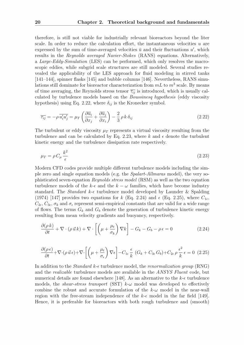
20 Chapter 2. Theoretical background and fundamentals
therefore, is still not viable for industrially relevant bioreactors beyond the literscale. In order to reduce the calculation effort, the instantaneous velocities u areexpressed by the sum of time-averaged velocities u and their fluctuations u′, whichresults in the Reynolds averaged Navier-Stokes (RANS) equations. Alternatively,a Large-Eddy-Simulation (LES) can be performed, which only resolves the macro-scopic eddies, while subgrid scale structures are still modeled. Several studies re-vealed the applicability of the LES approach for fluid modeling in stirred tanks[141–144], spinner flasks [145] and bubble columns [146]. Nevertheless, RANS simu-lations still dominate for bioreactor characterization from mL to m3 scale. By meansof time averaging, the Reynolds stress tensor τij is introduced, which is usually cal-culated by turbulence models based on the Boussinesq hypothesis (eddy viscosityhypothesis) using Eq. 2.22, where δij is the Kronecker symbol.
τij = −ρ u′iu′j = µT
(∂ui∂xj
+∂uj∂xi
)− 2
3ρ k δij (2.22)
The turbulent or eddy viscosity µT represents a virtual viscosity resulting from theturbulence and can be calculated by Eq. 2.23, where k and ε denote the turbulentkinetic energy and the turbulence dissipation rate respectively.
µT = ρCµk2
ε(2.23)
Modern CFD codes provide multiple different turbulence models including the sim-ple zero and single equation models (e.g. the Spalart-Allmaras model), the very so-phisticated seven-equation Reynolds stress model (RSM) as well as the two equationturbulence models of the k-ε and the k − ω families, which have become industrystandard. The Standard k-ε turbulence model developed by Launder & Spalding(1974) [147] provides two equations for k (Eq. 2.24) and ε (Eq. 2.25), where C1ε,C2ε, C3ε, σk and σε represent semi-empirical constants that are valid for a wide rangeof flows. The terms Gk and Gb denote the generation of turbulence kinetic energyresulting from mean velocity gradients and buoyancy, respectively.
∂(ρ k)
∂t+∇ · (ρ ~u k) +∇ ·
[(µ+
µtσk
)∇k]−Gk −Gb − ρ ε = 0 (2.24)
∂(ρ ε)
∂t+∇·(ρ ~u ε)+∇·
[(µ+
µtσε
)∇ε]−C1ε
ε
k(Gk + C3εGb)+C2ε ρ
ε2
kε = 0 (2.25)
In addition to the Standard k-ε turbulence model, the renormalization group (RNG)and the realizable turbulence models are available in the ANSYS Fluent code, butnumerical details are found elsewhere [148]. As an alternative to the k-ε turbulencemodels, the shear-stress transport (SST) k-ω model was developed to effectivelycombine the robust and accurate formulation of the k-ω model in the near-wallregion with the free-stream independence of the k-ε model in the far field [149].Hence, it is preferable for bioreactors with both rough turbulence and (smooth)

2.3. Modeling and optimization of bioreactors by means of CFD 21
shear flow, such as wave-mixed bioreactors [62]. For this reason, it was used for fluidflow prediction of the traveling wave bioreactor (see section 4.3). The model consistsof two transport equations for the turbulent kinetic energy k (Eq. 2.26) and thespecific turbulence dissipation rate ω (Eq. 2.27), which is the ratio of k and ε:
∂(ρ k)
∂t+∇ · (ρ ~u k)−∇ ·
[(µ+
µtσk
)∇k]−Gk + Yk = 0 (2.26)
∂(ρω)
∂t+∇ · (ρ ~uω)−∇ ·
[(µ+
µtσω
)∇ω]−Gω + Yω = 0 (2.27)
In these equations, Gk and Gk represent the generation of turbulence kinetic energydue to mean velocity gradients and the production of ω respectively, while Yk andYω denote the dissipation of k and ω. These terms are calculated using various sub-models, which are explained in detail by [148]. While the aforementioned models areonly applicable for single-phase flows or in cases where the influence of the secondaryphase is negligible, multiphase models are often required to characterize bioreactors.Thus, the dispersion of sparged gas, typically used for the oxygenation of the aer-obic growing production organisms, or solid suspensions, as found in carrier-basedprocesses (e.g., micro-carriers, fluidized beds etc.), can be considered. Important en-gineering parameters, such as gas hold-up, specific surface area and/or oxygen masstransfer rates, can thus be predicted.
The Volume-Of-Fluid (VOF) model
The Volume-of-Fluid (VOF) model, which is the multiphase model with the leastcomputational effort, was developed for modeling two or more immiscible fluids.Assuming that the phases share the same velocity and pressure field, a single set ofmass and momentum equations is solved and topology changes to the interface in-duced by the relative motion between the dispersed and continuous phase is trackedin time. For this purpose, a balance equation for the fractional volume or “color”function α(x, t) is used. If the mass transfer between the phases is neglected, thiscan be written for the qth phase by Eq. 2.28.
∂ (α ρ~u)
∂t+∇ · (α ρ~u) = 0 (2.28)
The volume fraction of the primary phase is not solved by a transport equation, butis computed based on the following constraint:
N∑q=1
αq = 1 (2.29)
Besides the continuum equation, a single momentum equation is also solved through-out the domain. Hence, the accuracy of the velocities computed near the interface

22 Chapter 2. Theoretical background and fundamentals
can be adversely affected if large velocity differences exist between the phases, alimitation of the shared-fields approximation.
∂
∂t(ρ ~u) +∇ · (ρ ~u~u) = −∇p+∇ ·
[µ ·(∇~u+ ~uT
)]+ ρ~g + ~F (2.30)
The density ρ and the viscosity µ are the weighted mean values defined as follows:
ρ =∑
αq ρq (2.31)
µ =∑
αq µq (2.32)
In Eq. 2.30, ~F represents all volumetric forces except gravity. The most importantinterphase force in the VOF model is the surface tension, which is modelled accordingto the continuum surface force (CSF) model [150]. The free surface is often modelledby the geometric reconstruction scheme, which approximates the interface betweenfluids using a piecewise-linear approach (see Fig. 2.4). In Fluent, this scheme is themost accurate and, based on the work of [151], is applicable for general unstructuredmeshes. It assumes that the interface between two fluids has a linear slope for eachcell, and uses this linear shape to calculate the advection of the fluid through thecell faces.
Actual interface shapeInterface shape represented by the geometric reconstruction
(piecewise-linear) scheme
Fig. 2.4.: Principle of piece-wise linear reconstruction of the interface shape applied in thegeo-reconstruction scheme.

2.3. Modeling and optimization of bioreactors by means of CFD 23
The Euler-Euler model
The Euler-Euler approach (EE; also referred to as the dense phase approach) de-scribes the mass and momentum of each phase separately. Therefore, modeling ofmultiple separate, yet interacting phases is possible, while it is assumed that a sin-gle pressure is shared by all phases. In contrast to the Euler-Lagrange models, EEconsiders all phases as interacting continua. The conservation equations for the qth
phase, which can be derived either by averaging the local instantaneous balancefor each of the phases [152] or by using the mixture theory approach [153], can bewritten as follows:
∂ (αq ρq)
∂t+∇ · (αq ρq ~uq) = 0 (2.33)
∂ (αq ρq ~uq)
∂t+∇ · (αq ρq ~uq ~uq) + α∇p−∇τq − αq ρq ~g + ~Fq (2.34)
The term ~uq is the velocity of phase q, while τq and ~Fq represent the qth phase stress-strain tensor and the interfacial momentum transport respectively. The phase stresstensor is obtained by Eq. 2.35, where µq and λq are the shear and bulk viscositiesof phase q.
τq = αq µq(∇~uq + ~uTq
)+ αq
(λq −
2
3µq
)∇ · ~uq δij (2.35)
Even though there is no consensus in the literature as to whether all forces should beconsidered in every case, the most important phase interaction forces include dragforce ~FD, lift force ~FL and virtual mass force ~FVM . In this work, only drag force,which describes the forces acting on the disperse phase due to relative velocitybetween the phases, was considered. The drag force can be calculated by Eq. 2.36,where cD is the drag coefficient, the index q is for the continuous phase and p is theparticular phase.
~FD =3
4ρq αq αp
cDdp
(~up − ~uq) |~up − ~uq| (2.36)
The standard correlation for the drag coefficient was proposed by [154]:
CD =
ReP ≤ 1000 : 24
ReP·(1 + 0.15 ·ReP 0.687
)ReP > 1000 : 0.44
(2.37)
Special multiphase turbulence models were developed in order to estimate the Reynoldsstress tensor in EE models. If the secondary phase is dilute and the primary phaseis clearly continuous, the dispersed k-ε turbulence model, which was also used inthis work, can be applied (see sections 4.1.3). In this case, interparticle collisions arenegligible and the dominant process in the random motion of the secondary phases
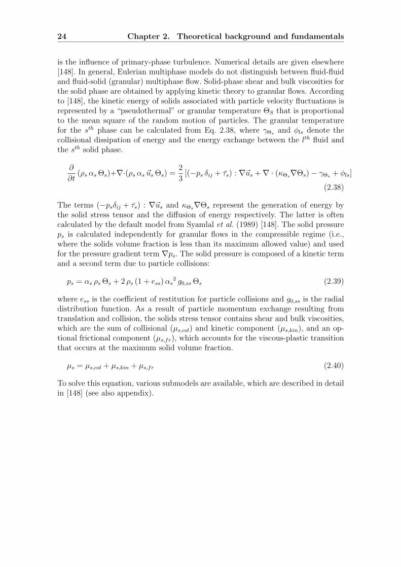
24 Chapter 2. Theoretical background and fundamentals
is the influence of primary-phase turbulence. Numerical details are given elsewhere[148]. In general, Eulerian multiphase models do not distinguish between fluid-fluidand fluid-solid (granular) multiphase flow. Solid-phase shear and bulk viscosities forthe solid phase are obtained by applying kinetic theory to granular flows. Accordingto [148], the kinetic energy of solids associated with particle velocity fluctuations isrepresented by a “pseudothermal” or granular temperature ΘS that is proportionalto the mean square of the random motion of particles. The granular temperaturefor the sth phase can be calculated from Eq. 2.38, where γΘs and φls denote thecollisional dissipation of energy and the energy exchange between the lth fluid andthe sth solid phase.
∂
∂t(ρs αs Θs)+∇·(ρs αs ~us Θs) =
2
3[(−ps δij + τs) : ∇~us +∇ · (κΘs∇Θs)− γΘs + φls]
(2.38)
The terms (−psδij + τs) : ∇~us and κΘs∇Θs represent the generation of energy bythe solid stress tensor and the diffusion of energy respectively. The latter is oftencalculated by the default model from Syamlal et al. (1989) [148]. The solid pressureps is calculated independently for granular flows in the compressible regime (i.e.,where the solids volume fraction is less than its maximum allowed value) and usedfor the pressure gradient term ∇ps. The solid pressure is composed of a kinetic termand a second term due to particle collisions:
ps = αs ρs Θs + 2 ρs (1 + ess)αs2 g0,ss Θs (2.39)
where ess is the coefficient of restitution for particle collisions and g0,ss is the radialdistribution function. As a result of particle momentum exchange resulting fromtranslation and collision, the solids stress tensor contains shear and bulk viscosities,which are the sum of collisional (µs,col) and kinetic component (µs,kin), and an op-tional frictional component (µs,fr), which accounts for the viscous-plastic transitionthat occurs at the maximum solid volume fraction.
µs = µs,col + µs,kin + µs,fr (2.40)
To solve this equation, various submodels are available, which are described in detailin [148] (see also appendix).

2.3. Modeling and optimization of bioreactors by means of CFD 25
The Euler-Lagrange model
In contrast to the Euler-Euler model, the Euler-Lagrange (EL) model combines thedescription of the continuous (liquid) phase with a segregated description of thedispersed (solid/gas) phase. Here, the trajectory of the particles of the Lagrangianphase is predicted by Eq. 2.41, which inherently requires a time-resolved treatment[15].
d~x
dt= ~u (2.41)
In order to consider random particle movement in turbulent flow as a result of theturbulent dispersion superimposed on the convective flow, a random jump ∆xi,t inspatial direction (x, y, or z) can be introduced (see Eq. 2.42). Here, χ denotes arandom number with a variance of 1, and DT represents the local eddy diffusivitycalculated from the continuous phase.
∆xi,t = χ√
2DT ∆t (2.42)
The velocities of the discrete phase are obtained by integrating the force balance onthe particles, which can be written in a Lagrangian reference frame as follows:
d ~updt
= ~FD ( ~uL − ~uP ) +gx (ρp − ρL)
ρp+ ~Fx (2.43)
where ~Fx is an additional acceleration (force/unit particle mass). Similarly to the
EE approach, the phases are coupled via momentum exchange terms ( ~FD) andadditional forces, such as “virtual mass” forces, the Saffman10 lift force, the Magnus11
force and the Basset12 history force, can be considered by using special sub-models.However, the computing effort is much higher because of the separate treatmentof each computational particle, which usually still represents a large collective ofreal particles. Hence, the EL models are still limited to low volume fractions ofthe dispersed phase (usually < 10 %), even though high mass loadings (mparticles ≥mliquid) are acceptable.
10The British mathematician Philip Geoffrey Saffman (1931 - 2008) worked on dynamics of vor-tices, flows of viscous fluids and interactions of fluid waves.
11The German physicist and chemist Heinrich Gustav Magnus (1802 - 1870) was the first to explainthe commonly observed effect in which a spinning particle curves away from its principal flightpath.
12The British mathematician Alfred Barnard Basset (1854 - 1930) worked on algebraic geometry,electrodynamics and hydrodynamics and was elected a fellow of the Royal Society.

26 Chapter 2. Theoretical background and fundamentals
Population balance models
Population balance equations (PBEs) can be applied if the disperse phase shows awide distribution of one or more physical properties, such as size, density or shape.In bioreactor CFD models, PBEs are most often introduced to describe the sizedistribution of bubbles that occur during aeration, where the number density ofthe bubbles fB is introduced as the characteristic parameter. This is defined by thenumber of bubbles ΔNB,i within the bubble size range ΔvB,i per volume V :
fB =ΔNB,i
V ΔvB,i
(2.44)
The number density within a control volume can change as a result of convection,bubble coalescence and breakup, gas expansion and mass transfer (see Eq. 2.45).The terms n, AB and MG denote the molar flux, the bubble surface area and themolar mass of the gas respectively.
∂fB∂t
= ∇ [ufB]︸ ︷︷ ︸Convection
+1
ρg
DρGDt
∂(vB fB)
∂vB︸ ︷︷ ︸Gas expansion
− ∂
∂vB
(n AB
MG
ρGfB
)︸ ︷︷ ︸
Mass transfer
− Bc +Dc − Bb +Db︸ ︷︷ ︸Break−up and coalescence
(2.45)
The Boltzmann-type PBE includes four source terms that describe the “birth” (Bc
and Bb) and “death” (Dc and Db) of bubbles, since both bubble coalescence andbreak-up lead to a simultaneous increase and decrease in bubble sizes (i.e., two smallbubbles merge to one bigger bubble or one big bubble breaks into multiple smallerones; see Fig. 2.5). The calculation of these source terms requires special submodels,which are mostly derived from turbulence theory. More detailed descriptions canbe found in the section 4.1.3, the appendix (on page 188ff) and in the references[155–159].
Initial bubbles Bubble deformation Film drainage
Coalescence
No coalescence
bMother bubble Bubble deformation Daughter bubbles
a
Fig. 2.5.: Bubble coalescence and breakup influence bubble size distribution. (a) Bubblecoalescence occurs if the drainage time is shorter than the contact time of twobubbles; (b) Bubble breakup results from bubble deformation as a result of ed-dies arriving at the bubble surface. Breakup with multiple and two daughterbubbles (binary, equally or non-equally sized) has been described in the litera-ture.

2.3. Modeling and optimization of bioreactors by means of CFD 27
2.3.2. Overview on applications of CFD for bioreactorcharacterization and scale-up
As mentioned above, stirred bioreactors are the most commonly used systems inbiopharmaceutical applications. CFD modeling has been performed for the milliliter[160] to cubic meter [107] scale. While the fluid flow patterns of standard industrialprocess stirrers, such as Rushton turbines or pitched blade impellers, were char-acterized during early attempts in the 1990’s, more specialized impellers found inbiotechnological applications have subsequently been investigated [161–163]. Due tothe lower computational effort required in comparison to the sliding mesh approach,the MRF method with position-fixed grids13 has mostly been used for both single-phase [164, 165] and multiphase models [159, 166–169].In investigations into the mixing performance of four Ekato Intermig R©impellers ina laminar flow regime, rigorous compartmentalization, which was caused by weakaxial transport and may lead to concentration gradients during fermentation pro-cesses, was demonstrated [161]. By decreasing the distance between the impellersand positioning them on a single shaft at 45 angles to each other (instead of 90
as recommended by manufacturers), the suppression of compartment build-up anda wider range of operating conditions were achieved [161, 162]. Although inhomo-geneities are more likely to occur at large scales, mixing can also be challengingfor stirrers in mL scale bioreactors, where fully established turbulence is hard toachieve. For a 30 mL stirred minibioreactor it was found that, when using eccentricstirrers, mixing was driven by chaotic flow fields, rather than by turbulence [164].Furthermore, it was demonstrated, that segregated or low-rate mixing regions wereprevented by the use of round shaped bottoms, while the shear stress distributionwas narrower in comparison to conventional Rushton turbines [164].Besides classical bioreactors made of glass or stainless steel, fluid flows in small [170],benchtop [59, 115] and pilot scale [62, 171] single-use stirred bioreactors have alsobeen investigated. In comparison studies with wavy-walled spinner flasks and theircylindrical counterparts used for tissue engineering applications, it was shown thatthe wavy walls reduced the tangential velocity and the maximum shear stress by halfat identical impeller speeds [170]. This is expected to influence the specific powerinput and the mechanical properties of cultured tissues.As mentioned in the section 2.2.1, the impellers of several SU stirred bioreactors, suchas the S.U.B. (also known as HyClone) from ThermoFisher or the Mobius R©CellReady250 from Merck Millipore, significantly differ from standard configurations. Hence,complex fluid flow patterns are likely to occur, making detailed flow analysis impor-tant. In the case of the HyClone bioreactor, a downward pumping axial flow patternfrom the pitched blade impeller was predicted, where the fluid recirculated upwardsalong the outer walls. Furthermore, the CFD simulations, which were validated byPIV measurements, revealed two differently sized flow loops, which can be ascribedto the off-center position of the impeller [59, 62]. While well-mixed conditions were
13The Multiple Reference Frame (MRF) method is also referred to as the “frozen-rotor” method,where flow characteristics of the inner region are used as boundary conditions for the outerregion and vice versa.

28 Chapter 2. Theoretical background and fundamentals
found near the vessel bottom, weak flow was found near the liquid surface, whenworking at maximum filling height, potentially leading to inhomogeneities withinthe vessel contents, especially if media are added at the liquid surface. Based on thesteady fluid flow pattern, a constant power number of Ne = 1.9 was predicted abovea critical Reynolds number of 4 · 104, based on Eq. 2.46 [62].
Re =NR dR
2 ρLµL
(2.46)
Another special SU agitator, which was investigated by means of CFD, is the cube-shaped Integrity
TMPadReactor
TMfrom ATMI Life Sciences. Even though the tum-
bling motion of the patented PadDriveTM
was greatly simplified by an MRF approach,a complex flow pattern was predicted, where the cubical vessel acts as baffles andconsequently prevents vortex formation [172].In recent years, great attention has been given to (oxygen) gas-liquid mass transferresulting in a multitude of publications that discuss CFD modeling of aerated stirredbioreactors [159, 166–169, 173, 174]. While previous studies used single bubble sizesto study gas dispersion, more recent models consider the effects of bubble breakupand coalescence [99, 159, 175]. By applying a Multiple Size Group (MUSIG) modelfor the polydispersed gas phase, different flow regimes that prevail in stirred reactorswere well modeled, compared to experimental observations [167]. This enabled theprediction of important flow characteristics, such as gas hold-up, mixing time, and(aerated) power input, over a wide range of operating conditions. In an optimizationstudy of a multi-stage agitator in a mammalian cell culture vessel, a combination ofthree pitched blades and three rotating microspargers was proposed and gas disper-sion and resulting kLa values were predicted using an Euler-Euler framework [176].While the CFD-predicted power input was halved, the oxygen mass transfer was in-creased 34-fold due to the smaller gas bubbles and more homogenous gas dispersion.However, no experimental verification of the CFD results has been reported.Besides stirred systems, there are an increasing number of publications describingCFD models for orbitally shaken systems at small [90, 177, 178] and pilot scales[91]. These models exclusively include the VOF model for the description of the freesurface, but limited data for model validation have often been reported, which canbe explained by the difficulty of measuring local fluid velocities in these systems.Although there have been some attempts, for example using laser-based flow fieldvisualization [179], engineering parameters, such as oxygen mass transfer rates orspecific power input, are often used to validate models. For example, oxygen masstransfer and energy dissipation in unbaffled 250 mL shake flasks have been investi-gated for typical operating parameters (100 - 300 rpm, 20 - 60 mm amplitude, 25- 100 mL filling volume). Although the specific surface is three-fold larger than incomparable stirred bioreactors, the kLa was smaller by a factor of 10, which can beexplained by much lower energy dissipation and resulting lower turbulence intensityat the phase boundary [90]. However, approximately 20 % lower shear strain hasbeen predicted in a newly developed frusto-conical shaking bioreactor than in flatbottom shaking bioreactors under the same conditions [180].

2.4. Conclusions and objectives of this thesis 29
2.4. Conclusions and objectives of this thesis
Even though a multitude of single-use bioreactors, which are mostly used for thecultivation of animal and human cell cultures, has been introduced to the marketover the last decades, there is still often a lack of engineering data. This hampers acomparison of different single-use bioreactor types among each other and with theirconventional counterparts made of stainless steel as well a fast scaling-up. Further-more, the hydrodynamics in most bioreactors are known to be very complex andthey can influence the growth and production expression of cell cultures. Consid-ering the heterogeneous distribution of shear stress and turbulence within typicalbioreactors, the need for spatially resolved flow data becomes obvious. These can beprovided by CFD models, but only a few studies on the use of CFD to characterizebioreactors have been published so far, in particular considering single-use systems.Using the Mobius R©CellReady benchtop bioreactor as a case study, the applica-bility of CFD for the engineering characterization of a benchtop scalebioreactor is demonstrated. Suitable models are discussed and the results arecompared with experimental and literature data. Considering the single-phase flow,special attention is given to grid resolution and turbulence modeling.Furthermore, the applicability of an Euler-Euler multiphase model in con-junction with population balances is evaluated.While CFD is comprehensively used in automobile, aviation and chemical industryfor development and optimization of apparatuses, only few examples using CFDto optimize bioreactors and/or bioprocesses are available. However, since the CFDmodels are based on general conservation equations, the need for costly and time-consuming prototyping may be reduced. In order to improve the cell yield of aMC-based stem cell expansion process, CFD models for the optimization ofa commercially available single-use bioreactor are developed and tested.Furthermore, two-phase models for the development of the traveling biore-actor, a novel concept for cell culture applications, are established, whichmay also reduce the need for prototypes. The proposed bioreactor is evaluated bycultivation experiments with a CHO suspension cell line and the advantages andlimitations of used CFD models are discussed.

30

3. Material and methods
This chapter describes materials and methods used for the experimental determina-tion of mixing time, oxygen mass transfer, power input, and local fluid velocities bymeans of PIV in the investigated bioreactors. Furthermore, the determination of sus-pension criteria for MC-based processes and the prediction of the liquid distributionin the orbitally shaken bioreactors are also described.
3.1. Investigated bioreactor systems
The Mobius R©CellReady 3L SU bioreactor
The Mobius R©CellReady 3L bioreactor (Merck Millipore, USA) has a working volumeof between 1.0 L and 2.4 L, whereas the total volume of the cultivation vessel is 3 L.The diameter and height of the unbaffled vessel were 0.137 m and 0.25 m respectively,providing a typical H/D ratio of 1.82 (see Fig. 3.1). Mixing was driven by a marineimpeller with a diameter equal to 1/2 the tank diameter (0.076 m) and an off-bottomclearance of 0.028 m. An open pipe and a microsparger made of sintered polyethylene(15 - 30µm pore size) were installed below the impeller for aeration, whereas onlythe latter was used in the present work. Classical, autoclavable probes were used forDO and pH measurements, and were also considered in the CFD models. Controland data acquisition were performed using either an ez-control tower (ApplikonBiotechnology, Netherlands) or a PC-based RDPDmini controller in conjunctionwith µTruBio PC software (Finesse Solutions, Inc.).
137.0
76.2
28.0
HL
250
a b
Fig. 3.1.: The Mobius R©CellReady 3L bioreactor. (a) Schematic with main geometric fea-turess. The dimensions are given in millimeter. The liquid height HL was ad-justed according to the filling volume. (b) Picture of the bioreactor.
31

32 Chapter 3. Material and methods
Spinner flasks
Pre-sterilized SU spinner flasks (Corning, USA) with 70-mm top caps and two angledside ports were used. The total volumes and vessel diameters were 0.125 L and ≈0.063 m respectively. For all investigations, the working volume was 0.1 L, giving aHL/D ratio of ≈0.71. An impeller consisting of a blade and a bar with a maximumdiameter of 0.0415 m (dR/D ≈ 0.66) was mounted to the vessel top and magneticallydriven via the drive of the stirring platform (Variomag Biosystem direct, ThermoScientific). The bioreactor was non-instrumented (see Fig. 3.2).
b
58
41.5
8.0
142
63
41
a
Fig. 3.2.: SU spinner flask for small scale experiments (a) Schematic with main geometricfeatures. The dimensions are given in millimeter. (b) Picture of the bioreactor.
The UniVessel R©SU
The rigid UniVessel R©SU bioreactor (Sartorius Stedim Biotech, Germany) was thefirst commercially available rigid SU cell culture bioreactor agitated by two-stagesegment blade impellers (SBI). These had a diameter of 0.055 m and the three bladeswere pitched at 30 (see Fig. 3.3). The off-bottom clearance of the lower impellerwas 0.047 m (hR/D ≈ 0.39) and the distance between the impellers was 0.07 m(cR/dR ≈ 1.3). The vessel, with a total volume of 2.6 L, provided working volumesof between 0.6 L and 2.0 L. Due to the manufacturing process, the diameter of thecylindrical vessel (D) increased towards the top (from 0.12 m to 0.15 m), however themean vessel diameter gave a common dR/D ratio of 0.43. For aeration, a submergedL-shaped macro-sparger with small holes (0.5 mm, 14 holes) was installed. The biore-actor was controlled using a BIOSTAT R©Bplus control unit and BioPAT R©MFCS/winsoftware (Sartorius Stedim Biotech).

3.1. Investigated bioreactor systems 33
a b
245
180
70
48.5
55
118
126
Fig. 3.3.: The UniVessel R©SU bioreactor. (a) Schematic with main geometric features. Thedimensions are given in millimeter. (b) Picture of the bioreactor.
Traveling wave bioreactor prototypes
Based on the results of CFD simulations (see section 4.3), two vessel prototypeswere fabricated from acrylic glass (HL Kunststofftechnik, Germany). The diametersof the tori and the annuluses in both versions were 0.374 m and 0.198 m respec-tively, which gave an r/R ratio of ≈ 0.36 (see Fig. 3.4). While the torus of onemodel was not modified, protuberances were installed in the second model, in aneffort to increase the mixing and mass transfer. Six concentric, semicircular rings(radius 0.011 m) were mounted on the inner walls, evenly distributed around thecircumference. At the vessel bottom, a SmartPuck sensor assembly from FinesseSolutions, Inc. (USA) was mounted in order to measure DO, pH and temperature.The sensor data were read using a SmartBag Reader
TM(Finesse Solutions, Inc.) and
collected by TruFluorTM
pH and DO transmitters respectively.The bioreactor prototypes were placed on a vessel holder, which was mounted ontoa LS-X shaker platform, provided by Kuhner AG (Switzerland). The minimum ro-tational speed was 20 rpm, while maximum values of up to 60 rpm were achieved,depending on the filling level (7.5 L to 35 L). The shaking diameter (d0) was fixedat 50 mm for all investigations. The gas supply was regulated using individual massflow controllers (vogtlin Instruments AG, Switzerland) for air, with ≤ 5 L min−1, andfor oxygen, carbon dioxide and nitrogen, with ≤ 0.5 L min−1 maximum flow rates .For the CHO cultivations, a SU pressure sensor (PendoTech, USA), which was pro-vided by ReseaChem GmbH (Switzerland), was installed in the off-gas line beforethe exhaust air filter. The pressure sensor, together with the gas supply line, was

34 Chapter 3. Material and methods
connected to a pressure switch (ReseaChem GmbH) that was configured to stop airsupply in case of any overpressure in excess of 40 mbar1. The analog outputs (4 -20 mA or 0 - 10 V) of the pressure monitor, the TruFluor
TMpH and DO transmitters
and the shaker drive were sent to a PC via a U12 LabJack signal converter2 (LabJackCorporation). Data acquisition was performed by BORIS software (block orientedinteractive simulation, Kahlert Ingenierburo, Germany). The temperature signal ofthe TruFluor
TMpH transmitter was used as an input signal of the PID controller in-
tegrated in the BORIS program. The output signal for the heating blankets, whichwere provided by Prang+Partner AG (Switzerland) and used for temperature con-trol, was generated by a pulse width modulation block. A schematic of the completeexperimental setup is given in Fig. 3.8. The BORIS block scheme is shown in Fig.A.2 on page 172 of the appendix.
R
r
a b
Fig. 3.4.: The traveling wave bioreactor. (a) Schematic with main geometric features. (b)Picture of the bioreactor prototype without baffles.
3.2. Experimental investigations
3.2.1. Mixing time
The mixing time, which was defined as the time required to achieve 95 % homogene-ity following the addition of a tracer substance, was determined by the well-acceptedde-colorization method [181]. The bioreactor content was colorized by the addition of0.1 mL L−1 iodine solution (250 g L−1 iodate-free potassium iodide and 128 g L−1 io-dine) and 4 mL L−1 starch solution (10 g L−1 soluble starch and 2 g L−1 benzoic acid).The tracer was 1.05 M sodium thiosulfate solution (166 g L−1) and was pipetted im-mediately (0.1 mL L−1). The time was then taken until the blue color disappearedcompletely. Each measurement was taken at least three times and the experimentswere performed by a single person in order to minimize inter-observer differences.
1Interrupting the air supply in case of overpressure, for example as a result of clogging of theexhaust air filter, was intended to prevent the prototype from bursting.
2The U12 LabJack converter required an anolog signal of 0 - 10 V. If current signals were providedby the connected devices, a current transformer (3RS17 05-1FD00, Siemens) was used.

3.2. Experimental investigations 35
3.2.2. Oxygen mass transfer coefficient
The oxygen mass transfer, quantified by the oxygen mass transfer coefficient kLa,was determined by the well-known dynamic gassing-out method, as described by[59]. The dissolved oxygen concentration was measured as a function of time fromthe point when aeration was turned on, following complete removal using nitrogen.Assuming that the gas phase is well-mixed and the dissolved oxygen concentrationis uniform inside the liquid, the rate of oxygen transfer can be described by Eq. 3.1,where cO2
∗ is the saturation concentration given by Henry‘s law.
OTR =dcO2(t)
dt= kLa · (cO2
∗ − cO2(t)) (3.1)
By integrating Eq. 3.1 with cO2(t = 0) = cO2,0 the following equation can be ob-tained:
ln
(cO2∗ − cO2,0
cO2∗ − cO2(t)
)= kLa · t (3.2)
Plotting the left hand-side of Eq. 3.2 against time, the kLa was determined as theslope of the linear regression curve (see. Fig. A.1). The measurements were takenin distilled water and in a 0.5 mol L−1 Na2SO4 aqueous solution at 20 C, repre-senting non-viscous coalescent and non-coalescent media respectively. The oxygensaturation concentrations of the sodium sulfate solution were calculated in accor-dance with [131]. The actual oxygen concentration in the Mobius R©CellReady wasmeasured using a Clark electrode (TruDO, Finesse Solutions, Inc. or comparable),while a TruFluor SmartPuck in conjunction with a SmartReader provided by FinesseSolutions, Inc. was used in the traveling wave bioreactor prototype. Both sensor sys-tems were connected to a PC via a LabJack U12 converter and data acquisition wasperformed using BORIS software (Kahlert Ingenieurburo).
3.2.3. Power input
The power input from the impellers of the benchtop bioreactors (Mobius R©CellReady3L and UniVessel R©SU) was determined by means of the stirrer torque (see Fig. 3.5).This was measured by a T20WN torque meter3 (Hottinger Baldwin Messtechnik AG,Switzerland) with a measurement range of up to 0.2 Nm. The impellers were installedin a 3 L glass vessel with a diameter of 0.13 m, provided by Finesse Solutions, Inc..For the impeller shaft bearing, a low-friction air bearing (IBS precision engineering,Netherlands) was used. Agitation was controlled by a PC-based TruViu RDPDminicontroller in conjunction with µTruBio PC software (Finesse Solutions, Inc.). Theintegrated recipe manager was used for automated measurements. By varying theimpeller speed and liquid viscosity4, different Reynolds numbers in the range of
3The measurement of the dynamic torque uses strain gauges.4The liquid viscosity and density were elevated by addition of sucrose solution up to a final
concentration of ≈ 60 wt%.
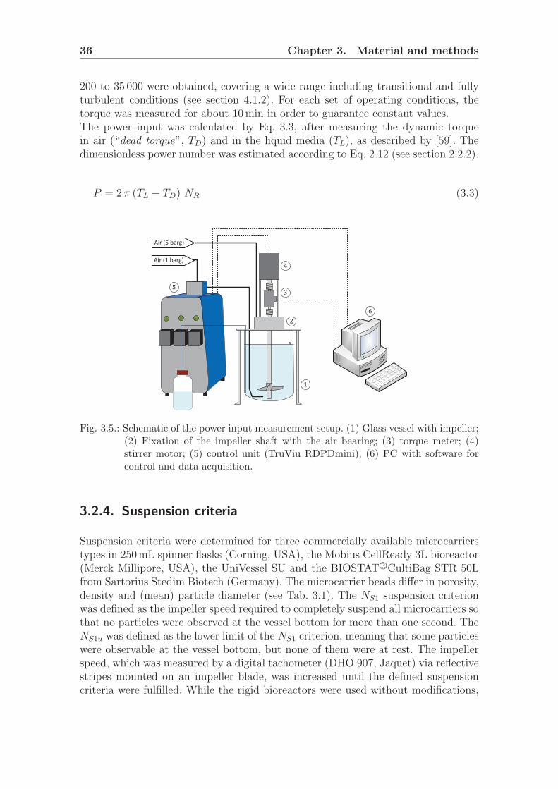
36 Chapter 3. Material and methods
200 to 35 000 were obtained, covering a wide range including transitional and fullyturbulent conditions (see section 4.1.2). For each set of operating conditions, thetorque was measured for about 10min in order to guarantee constant values.The power input was calculated by Eq. 3.3, after measuring the dynamic torquein air (“dead torque”, TD) and in the liquid media (TL), as described by [59]. Thedimensionless power number was estimated according to Eq. 2.12 (see section 2.2.2).
P = 2 π (TL − TD) NR (3.3)
Air (5 barg)
Air (1 barg)
1
234
56
Fig. 3.5.: Schematic of the power input measurement setup. (1) Glass vessel with impeller;(2) Fixation of the impeller shaft with the air bearing; (3) torque meter; (4)stirrer motor; (5) control unit (TruViu RDPDmini); (6) PC with software forcontrol and data acquisition.
3.2.4. Suspension criteria
Suspension criteria were determined for three commercially available microcarrierstypes in 250mL spinner flasks (Corning, USA), the Mobius CellReady 3L bioreactor(Merck Millipore, USA), the UniVessel SU and the BIOSTATR©CultiBag STR 50Lfrom Sartorius Stedim Biotech (Germany). The microcarrier beads differ in porosity,density and (mean) particle diameter (see Tab. 3.1). The NS1 suspension criterionwas defined as the impeller speed required to completely suspend all microcarriers sothat no particles were observed at the vessel bottom for more than one second. TheNS1u was defined as the lower limit of the NS1 criterion, meaning that some particleswere observable at the vessel bottom, but none of them were at rest. The impellerspeed, which was measured by a digital tachometer (DHO 907, Jaquet) via reflectivestripes mounted on an impeller blade, was increased until the defined suspensioncriteria were fulfilled. While the rigid bioreactors were used without modifications,

3.2. Experimental investigations 37
a rigid plastic model of the flexible cultivation bag from the BIOSTAT R©CultiBagSTR 50L was constructed. It was assumed that the bag completely filled the stainlesssteel container. Defined portions of the microcarriers were weighed (0.25 g mL−1),equilibrated in pure water and transferred into the bioreactors to meet the desiredconcentrations. A mirror was placed below the vessel for improved observability.
Tab. 3.1.: Summary of the physical properties of MC types used, as given by the manu-facturers.
MC type PorosityDensity Particle size
ρP (kgm−3) dP (µm)
MC type I microporous 1120± 30 180± 20
MC type II microporous 1026± 4 169± 43
MC type III macroporous (10 - 20 µm) ≈ 1030 130 - 380
3.2.5. Liquid distribution in the traveling wave bioreactor
The liquid distributions in the moving traveling wave bioreactor prototypes weredetermined at the lateral surface wall (see Fig. 3.6). A digital camera (RICOHCX6) was placed on the holder, at the far edge of the shaker platform and videosequences of at least three complete rotations were taken. Afterwards, the videoswere converted to images with a resolution 1920 x 1080 pixels and a frame rateof 30 fps by means of the Linux FFmpeg software package5. The liquid height inevery frame was analysed semi-automatically using an own Matlab R©code. In orderto calculate the liquid height in mm from the images, a scale was fixed to the lateralsurface of the prototype torus.
1
2 3
4
Fig. 3.6.: Principle of measuring the liquid distribution in the traveling wave bioreactorprototype. The torus vessel (1) was shaken on a platform (2) with a holder (3)for the camera (4). On the right side, two example pictures are shown.
5An example code for the video conversion is: ffmpeg -an -ss 0:1:40 -t 0:0:10 -i Unbaf-fled 35L 20rpm.avi -r 30 -s 1920 x 1080 Unbaffled 35L 20rpm%06d.jpg

38 Chapter 3. Material and methods
3.2.6. Particle image velocimetry
For contactless measurements of local fluid velocities, the particle image velocime-try FlowMaster PIV system (LaVision, Germany) was used. The light sheet with athickness of approximately 1mm was generated by a double-pulsed Nd:YAG laser(litron nano piv) with a wavelength of 532 nm. If not stated otherwise, the lasersheet was vertically oriented through the impeller shaft (mid-bioreactor plane, seeFig. 3.7). Hence, the laser orientation allowed axial and radial components of fluidvelocities to be determined. Even though the tangential component of velocity wasexpected to be significant, its determination was hampered by the lack of optical ac-cessibility through the round-shaped vessel bottoms. In order to minimize errors dueto refraction/diffraction of the laser on the cylindrical vessel surfaces, the cultivationcontainers of the small scale spinner flasks and the benchtop scale UniVessel R©SUand Mobius R©bioreactors were placed into a rectangular, water-filled box. Dependingon the bioreactor system, images were captured for up to four and eight positionsin horizontal and vertical direction, respectively. For this purpose, a traverse systemwas used.The double-frames with a time delay of 1ms were recorded by a CCD camera (ImagerPro X 4M) with a resolution of 2048× 2048 pixels. DaVis 7.2 software (LaVision)was used for image acquisition and flow field prediction, which was performed usingcross correlation based on an interrogation window of 32× 32 pixels with an overlapof 50%. Even though up to 2500 double frames have been recommended in order tominimize statistical deviation [182], based on previous investigations of single-usebioreactors [59, 181], sets of up to 1000 double frames were taken in the presentstudies. Rhodamine coated fluorescence particles with a density of 1.19 kgm−3 anddiameter of 20 - 50 m (LaVision) were used. By means of a corresponding opticalfilter mounted at the CCD camera, optical distortions by light reflection were min-imized. The camera and laser were synchronised to the impeller speed by means ofa laser-based trigger signal (Sick AG) in order to carry out phase-resolved measure-ments.
Δt
Δxy
zx
Image #1Image #2
1 23
4
5
6
7
Fig. 3.7.: Schematic of the PIV experimental setup. A laser (1) and sheet optics (2) pro-duced the laser sheet (3) to illuminate fluorescence particles (4), which wererecorded by a CCD camera (5). By using cross correlation in the DaVis software(6), the instantaneous vector field (7) was calculated.

3.2. Experimental investigations 39
3.2.7. Bubble size determination
Local bubble sizes in the Mobius R©CellReady bioreactor were measured manuallyfrom photographs. Two impeller speeds of 100 rpm and 200 rpm and aeration ratesof 0.025 vvm and 0.05 vm were considered for a filling volume of 2 L using pure waterand a cell culture medium (Gibco R©CD CHO medium, lot no. 984203). Pictures ofthe aerated vessel were taken with a digital single lens reflex camera (Canon EOS600D). Because of the restricted optical accessibility near the vessel bottom, only theregion above the impeller was considered. The bubbles were analysed on images withresolutions of 5184×3456 pixels by means of an own Matlab R©code. After loading theimages into a graphical user interface (GUI), they were divided into nine, equally-sized subregions in order to improve accuracy. Afterwards, the center point and onepoint on the edge of each bubble were marked and the coordinates of both pointswere stored. The bubble diameter was then calculated from the distances betweenthe bubble edge and center in the x- and y-direction:
dB = 2√xCP 2 + yCP 2 (3.4)
Thus, spherical bubbles were assumed, which was the case for most bubbles up to asize of 3 mm, as reported in the literature [183]. At least 350 bubbles were measuredto fulfil statistical demands [184]. However, small bubbles (<0.25 mm) were expectedto be under represented because their diameter was difficult to evaluate (≈10 pixels),in particular for images taken at the higher aeration rate.
3.2.8. CHO cultivation
In order to prove the applicability of the traveling wave bioreactor concept, trans-fected Chinese hamster ovary (CHO) suspension cells (CHO XM111-10, devel-oped and kindly provided by Prof. M. Fussenegger’s working group from the ETHZurich) were used. These cells are capable of producing secreted alkaline phos-phatase (SEAP), regulated by a tetracycline suppressed promotor (PhCMV ∗−1 ). Inthe present study, only cell growth experiments without protein expressions wereperformed. The cells were cultivated in serum-free, chemically defined minimal cul-ture media ChoMaster R©HP-1 and HP-5 (Cell Culture Technologies, Switzerland)with additions of tetracycline (2.5 mgL−1) and Pluronic F-68 (2 gL−1). The two me-dia differ mainly in concentrations of glucose, salts, amino acids, vitamins and lipids.The HP-5 medium was used to achieve cell densities above 4.0× 10⁶ cellsmL−1.The maintenance culture was grown in T-75 flasks, incubated at 37 C, 7.5 % CO2
and 80 % humidity, using chemically defined FMX-8 basal medium (Cell CultureTechnologies).The inoculum for the traveling wave bioreactor prototype was produced in wave-mixed rocker-type bioreactors BIOSTAT R©CultiBag RM 10L (optical or basic in thecase of parallel cultivations with a SmartBag
TMbioreactor), which were inoculated
with cells produced in shake flasks (20 mL to 300 mL working volumes, 120 rpm,37 C, 7.5 % CO2 and 80 % humidity). The rocking speed and angle were adjusted
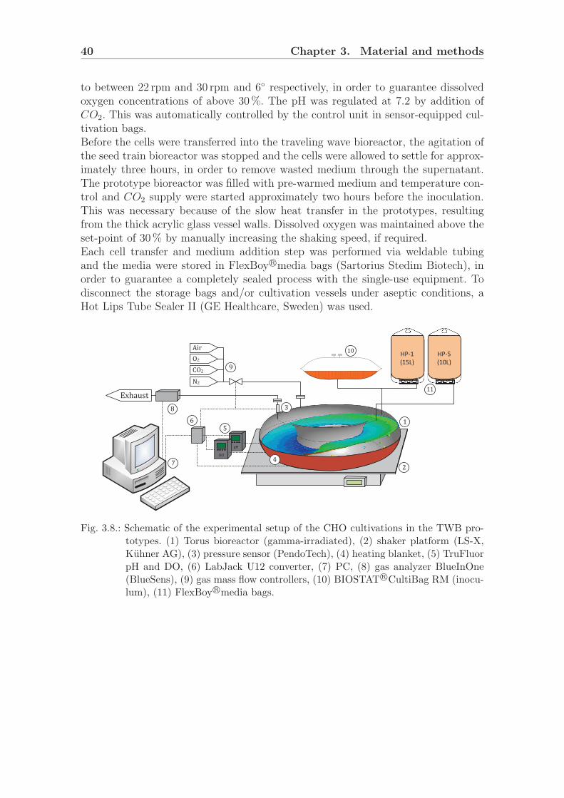
40 Chapter 3. Material and methods
to between 22 rpm and 30 rpm and 6 respectively, in order to guarantee dissolvedoxygen concentrations of above 30%. The pH was regulated at 7.2 by addition ofCO2. This was automatically controlled by the control unit in sensor-equipped cul-tivation bags.Before the cells were transferred into the traveling wave bioreactor, the agitation ofthe seed train bioreactor was stopped and the cells were allowed to settle for approx-imately three hours, in order to remove wasted medium through the supernatant.The prototype bioreactor was filled with pre-warmed medium and temperature con-trol and CO2 supply were started approximately two hours before the inoculation.This was necessary because of the slow heat transfer in the prototypes, resultingfrom the thick acrylic glass vessel walls. Dissolved oxygen was maintained above theset-point of 30% by manually increasing the shaking speed, if required.Each cell transfer and medium addition step was performed via weldable tubingand the media were stored in FlexBoy R©media bags (Sartorius Stedim Biotech), inorder to guarantee a completely sealed process with the single-use equipment. Todisconnect the storage bags and/or cultivation vessels under aseptic conditions, aHot Lips Tube Sealer II (GE Healthcare, Sweden) was used.
AirO2CO2N2
DO
pH
ExhaustHP-1(15L)
HP-5(10L)
12
3
456
7
89 10
11
Fig. 3.8.: Schematic of the experimental setup of the CHO cultivations in the TWB pro-totypes. (1) Torus bioreactor (gamma-irradiated), (2) shaker platform (LS-X,Kuhner AG), (3) pressure sensor (PendoTech), (4) heating blanket, (5) TruFluorpH and DO, (6) LabJack U12 converter, (7) PC, (8) gas analyzer BlueInOne(BlueSens), (9) gas mass flow controllers, (10) BIOSTAT R©CultiBag RM (inocu-lum), (11) FlexBoy R©media bags.

3.3. Numerical investigations 41
3.3. Numerical investigations
CAD construction and meshing
The 3D geometries of the applied bioreactor systems were mostly developed us-ing Autodesk Inventor CAD software package. Exchange files with *.stp file formatwere exported and imported into the DesignModeller that is integrated into ANSYSworkbench. Only the fluid domains of the bioreactors were considered for the CFDmodels. Subdomains were introduced into the stirred systems around the impellerin order to implement the impeller rotation by means of Moving reference frame orSliding mesh schemes.Meshing was performed by the ANSYS meshing tool, which provides effective mesh-ing algorithms for surface and volume meshes. Details of the generated meshes aregiven in the case studies (see section 4.1, 4.2 and 4.3). In general, unstructuredgrids consisting of tetrahedral elements were generated. The mesh quality was eval-uated by equi-volume cell skewness6, which is defined as the relationship betweenthe shape of the cell and the shape of an equilateral cell of equivalent volume [148].The maximum CV skewness in the meshes used was below 0.93, with only a fewelements (<5 % of the total number) having a skewness above 0.8, since it is well-known that a high number of highly skewed cells may lead to convergence issuesduring simulations. After meshing, boundary conditions were defined, depending onthe fluid flow of interest.
Boundary conditions and solver settings
The CFD simulations were carried out using an ANSYS Fluent7 finite volume solver.The density based solver was used. All walls were treated with non-slip standard wallfunctions, while the liquid surfaces in the stirred single-phase systems were treatedas symmetry planes, where the fluid velocities normal to the face were set to zero. Inthe case of the gas-liquid two-phase model of the Mobius R©CellReady, a gas volumewas introduced on top of the liquid domain and pressure outlet boundary conditionswere applied to the top surface, which means that the top surface being exposedto atmospheric pressure. Only gas was allowed to enter the domain for backflowboundary conditions. In general, water (ρL = 982 kgm−3, µL = 1.002 · 10−3 Pa s, σ= 0.072 Nm) and air (ρG = 1.25 kgm−3, µG = 1.7894 · 10−5 Pa s) under standardconditions (20 C, 101.325 Pa) were assumed in the models. Local bubble sizes weremodelled by means of a discrete PBE model. Bubble breakup and coalescence werepredicted with the Luo’s closure models provided in Fluent. The bubble sizes werediscretized, based on experimental observations, into 15 bins with minimum and
6As a rule of thumb, the maximum skewness for a triangular/tetrahedral mesh should be smallerthan 0.95, with an average value that is significantly lower.
7Versions 13.0 and 14.0 were used, but the applied models were identical according to the docu-mentation provided.

42 Chapter 3. Material and methods
maximum limits of 0.05 mm and 2.5 mm respectively. The distribution was based onthe geometric ratio:
dB,i = dB,i−1 (2q)1/3 (3.5)
where q is the ratio exponent (q = 1.215). According to a proposed correlation8
for metal porous spargers [185], given by Eq. 3.6, the initial bubble is not stronglydependent on the superficial gas velocity (d32,i ∝ uGS
0.06). Therefore, it was setto 0.47 mm for each case, which was similar to the experimentally observed meanbubble size at the sparger surface.
d32,i = 7.35 dS
[We−1.7 Re0.1 Fr1.8
(dPdS
)1.7]0.2
(3.6)
If not otherwise mentioned, the SIMPLE and the phase-coupled SIMPLE algorithmswere used for pressure-velocity coupling in single- and multi-phase models, respec-tively. Furthermore, unless otherwise stated First-Order Upwind (FOU) schemeswere used for the discretization of the mass, momentum and turbulence transportequations. Convergence was assumed when the residuals dropped below 104 and 105
in transient and steady-state simulations, respectively.In order to reduce the turnaround time, the CFD simulations were parallelized usingthe parallel solver version of ANSYS Fluent. For this purpose, the computationaldomain was automatically split into a number of partitions (see Fig. 3.9) using thePrincipal Axes method9 and each partition was sent to a computing node. Typicallyup to four nodes were used for meshes with up to ≈ 2 · 106 control volumes. Furtherincreases in computing nodes resulted in lower efficiency, since the communicationtime between the nodes increased with further parallelization (see Fig. 3.9).
Grid density
Accuracy
Turnaround time
No. of CPUs
Exact solution
a b
Fig. 3.9.: Parallelization of the CFD fluid domain. (a) Example of fluid domain partitioninginto four computing nodes; (b) Qualitative relationship of computation time,parallelization (number of nodes) and grid density with respect to numericalaccuracy (taken from [14]).
8In Eq. 3.6, dP and dS represent the pore diameter and sparger diameter respectively, whileFr = ugs
2/dS g, We = ρLugs2dSσ and Re = ρLugsdS/µL and where ugs is the superficial gas
velocity related to the sparger inlet surface.9According to [148], the Principal Axes method bisects the domain based on a coordinate frame
aligned with the principal axes of the domain.

4. Characterization and optimization ofbioreactors and bioprocesses using CFD:case studies
4.1. Engineering characterization of theMobius R©CellReady 3L bioreactor
4.1.1. Introduction
When performing engineering characterization of the Mobius R©CellReady bioreactor,liquid volumes of between 1.0 L and 2.4 L were considered. These volumes representthe lower and upper limits of the manufacturer recommended working volume [186].Impeller speeds between 60 rpm and 300 rpm, corresponding to tip speeds of approx-imately 0.2 ms−1 and 1.2 ms−1 respectively, were considered. The latter is the upperlimit for avoiding vortex formation in the unbaffled vessel of the Mobius R©CellReadybioreactor. As described in section 3.3, the fluid domains were discretized by un-structured meshes consisting of tetrahedral elements that accurately describe thebioreactor geometry. In order to investigate the grid sensitivity, the grid density wasvaried, with between 202 595 and 1 270 712 control volumes generated (see Tab. 4.1and Fig. 4.1). Based on the results of the grid sensitivity study (see below), meshesof between 537 433 (1.0 L) and 907 259 (2.4 L) were used for the single-phase simu-lations. A higher grid density is recommended in the impeller zone due to the larger(velocity) gradients near the impeller.For the multi-phase models, which were used to estimate the gas distribution andthe oxygen mass transfer at 2 L working volume (see below), a conversion algo-rithm, part of the Fluent CFD solver, was used to generate a polyhedral mesh with393 006 control volumes (see Fig. 4.1b). This mesh conversion was required in or-der to improve process stability and achieve acceptable turn around times with theEuler-Euler framework. Although polyhedral meshes require larger storage capac-ities [187], they are superior in terms of improved convergence and require fewercontrol elements to obtain the same accuracy as with tetrahedrals [188]. In all mod-els, the MRF approach was employed at the interface between the two zones (rotorand stator), with the inner containing the impeller, to interpolate the momentumand turbulence variables.
43

44Chapter 4. Characterization and optimization of bioreactors and
bioprocesses using CFD: case studies
Tab. 4.1.: Mesh details of the Mobius R©CellReady bioreactor models.
Working Number of control volumesGrid density
Skewnessvolume Total Impeller zone Bulk zone Max. Mean
(L) (-) (-) (-) (CV/mm3) (-) (-)
1.00 537 433a 275 568 261 865 537.4 0.91 0.281.25 611 302a 348 433 262 869 489.0 0.90 0.271.50 682 032a 419 404 262 628 454.7 0.88 0.262.00 202 595a 53 081 149 514 101.3 0.92 0.262.00 409 516a 300 077 109 439 204.8 0.88 0.262.00 564 943a 335 200 229 743 282.5 0.86 0.272.00 810 175a 553 217 256 958 405.1 0.81 0.262.00 1 010 041a 741 805 268 236 505.0 0.82 0.262.00 1 270 712a 899 248 371 464 635.4 0.81 0.252.00 393 006b 54 187 338 819 163.8 - -2.40 907 259a 648 523 258 736 378.0 0.87 0.25
a tetrahedral mesh; b polyhedral mesh
a b
Fig. 4.1.: Computational meshes used for modeling of the Mobius R©CellReady bioreactor.(a) Mesh with tetrahedral elements for single-phase simulations, (b) mesh withpolyhedral elements for multiphase simulations.

4.1. Engineering characterization of the Mobius R©CellReady 3Lbioreactor 45
4.1.2. Results from single-phase modeling
Fluid flow pattern
Contrary to first expectations, the single phase simulations did not reveal a clearaxial flow profile with a typical single flow loop for clock-wise impeller rotation,but rather a strong effect of the radial flow component. As a result, the fluid wasdischarged towards the vessel wall. The impeller jet was inclined approximately 25
upwards from the horizontal plane, based on the pitch of the impeller blades. Thefluid then impinged on the outer walls at a vertical position of z/HL ≈0.20, whereit divided and formed two counter-rotating vortices in the regions below and abovethe impeller (see Fig. 4.2a).As expected, the highest fluid velocities were predicted in close proximity to the im-peller blades and corresponded well to the impeller tip speed (see Eq. 2.10), whichwas 0.8 m s−1 for a rotational speed of 200 rpm. The fluid velocities in the lowerportion of the vessel (z/HL ≤ 0.25) were primarily between 0.1 utip and 0.3 utip.This was significantly lower than the 0.55 utip measured with an up-pumping 45
pitched blade impeller [189], but was comparable to the 0.26 utip for a down-pumping3-bladed hydrofoil axial impeller (dR/D = 0.33 and a trailing edge angle of ≈10)[190] and similar to 0.25 utip for a propeller agitator [191]. The velocities in the up-per portion of the vessel were considerably lower, with values below 0.1 utip. Thus,it can be argued that the impeller had only a small influence on this zone. Thiseffect was enhanced by increasing filling volumes, which resulted in weak mixing.Furthermore, small dead zones were observed at the inlet of the drain and open pipesparging port where the fluid velocities were almost zero. In cultivation experimentswith CHO suspension cells, cell sedimentation and accumulation were observed inthese regions. The viability of those cells decreased significantly, which was probablya result of insufficient nutrient and oxygen supply.The CFD-predicted fluid flow pattern agreed well with our own PIV measurements(see Fig. 4.4 and Fig. 4.5) and published data [192]. In fact, the published data werethe first to provide time and phase-resolved information on local velocities and tur-bulence in the Mobius R©CellReady 3L bioreactor. Odeleye et al. (2014) [192] foundthat a trailing vortex developed from the tip of the blade at an angle of 15 afterthe blade passage, which detaches from the tip of the blade at 30 and decreases instrength after a complete blade passage at 60. This was consistent with our ownCFD model. However, the CFD model over estimated the inclination of the impellerjet (25 compared to 15 in the PIV measurements) and the fluid velocities in thebioreactor center (r < 0.5R) were under estimated by up to two-fold. Neverthe-less, deviations between the CFD model and PIV data could be explained by bothnumerical and experimental uncertainties. The measurement accuracy was affectedby optical distortion, resulting from the round vessel bottom, and oscillation of theimpeller shaft as a consequence of an inadequate bearing. Furthermore, the impellerspeed varied by approximately ±5 rpm, according to the readings from the controlunit. Ultimately, the overall agreement was satisfactory enough to justify the use ofthe CFD models for further investigations.

46Chapter 4. Characterization and optimization of bioreactors and
bioprocesses using CFD: case studies
a
b
Ne = 0.280
Ne = 0.285
No
rmal
ized
flu
id v
elo
city
u/u
tip (
-)
1.00
0.90
0.80
0.70
0.60
0.50
0.40
0.30
0.20
0.10
0.00
No
rmal
ized
flu
id v
elo
city
u/u
tip (
-)
1.00
0.90
0.80
0.70
0.60
0.50
0.40
0.30
0.20
0.10
0.00
Fig. 4.2.: Normalized fluid velocities in the stirred SU Mobius R©CellReady 3L bioreactorat 200 rpm (utip ≈0.8 ms−1, Re ≈17 300 ) with a 2 L filling volume and withoutaeration. (a) Clockwise rotation; (b) counter-clockwise rotation. The velocitiesare shown for the z-y-plane (front view, left) and the mid-impeller plane (topview, right). The vectors are projected onto the given planes.
Interestingly, a typical axial fluid flow pattern was predicted for counter-clockwiserotation, as shown in Fig. 4.2b. The fluid was discharged downwards from the im-peller and impinged on the lower vessel wall at r/R ≈ 0.65 before it was transportedupwards near the outer vessel walls. At the temperature probe, a recirculation zonewas found, where up and down flows met each other. While the maximum fluid ve-locities were again predicted at the impeller tips, and agreed well with the impeller’stip speed, the bulk velocities were higher than for clockwise rotation, with valuesbetween 0.2 utip and 0.3 utip. They were also more homogeneous in comparison toclockwise impeller rotation. Downward fluid flow in the vessel center may be ad-vantageous in terms of mass transfer, since bubble residence time and the relativevelocity between fluid and rising bubbles are increased, even though contrary re-sults have been found for an A315 impeller [193]. Nevertheless, subsequent studiesprimarily focussed on clockwise rotation, because this is the default rotation direc-tion for most control units used to control the Mobius R©CellReady bioreactor andcomparable benchtop scale systems.

4.1. Engineering characterization of the Mobius R©CellReady 3Lbioreactor 47
Use of the sliding mesh approach
While the previously described simulations were performed using the Moving Ref-erence Frame (MRF) technique, which uses a space-fixed mesh and considers im-peller rotation through source terms in the momentum balance, the influence of thetransient Sliding mesh (SM) approach was also investigated. Both methods havepreviously been used to model the fluid flows in stirred tanks at widely rangingscales [194–198]. In contrast to formerly used impeller boundary condition models[199, 200], which inherently rely on suitable experimental data, the MRF and SMmethods allow much greater generality [194]. Nevertheless, the sliding mesh tech-nique gave the best agreement with experimental data with regard to mean flowquantities in several comparison studies [194].In the present work, the boundary conditions of the MRF model were also usedfor the SM simulation, whereas the mesh was slightly adapted in order to meet therequirements of the SM technique in Fluent. In particular, conform surface mesheswere required for the initial state on the zone interface of the static (stator) andmoving zone (rotor). During the calculation, the cell zones rotate relative to eachother along the mesh interface in discrete steps. In doing so, the mesh faces do notneed to be aligned on the interface, but the fluxes across the interfaces are computedfor two non-conformal interface zones [148].The fluid flow was determined for a rotational speed of 150 rpm (corresponding to atip speed of 0.6 m s−1) and a time step size of 5 · 10−4 s was used, which correspondedto 0.045 degree per time step and provided time-step independent results. In Fig.4.3, the fluid flow for a snapshot of the SM model at steady-state conditions1 iscompared with the MRF simulation. The main characteristics of the flow pattern inthe Mobius R©CellReady bioreactor, as described in detail above, were also found inthe SM model. Furthermore, the distributions of fluid velocities predicted with bothmodels were nearly identical. The local fluid velocities differed by absolute values ofbelow 0.12 m s−1 for the entire fluid domain and the mean relative deviation of thevelocity magnitude was ≈2 %. Furthermore, no gain in accuracy compared to thePIV measurements was obtained by the sliding mesh approach (data not shown).Not entirely surprisingly, the power numbers determined by the impeller torque,as described below, were also very similar with values of Ne = 0.28 (MRF) andNe = 0.26 (SM). Considering the acceptable differences between the two methods,the MRF technique was used for all subsequent investigations because of the signifi-cantly lower computational costs. In the present case, the calculation of 3 s physicaltime (i.e. 8 impeller revolutions) using 4 CPUs lasted approximately 10 days.
1Steady-state conditions were evaluated through constant values of the power input, the volumeintegral of the turbulence dissipation rate and the volume-average of the velocity magnitude.

48Chapter 4. Characterization and optimization of bioreactors and
bioprocesses using CFD: case studies
Moving reference frameSliding mesh
No
rmal
ized
flu
id v
elo
city
u/u
tip (
-)
1.00
0.90
0.80
0.70
0.60
0.50
0.40
0.30
0.20
0.10
0.00
Fig. 4.3.: Comparison of fluid flow pattern predicted with the Sliding mesh (left) andMoving Reference Frame (right) techniques. The vectors are given with a fixedlength of 10 mm and projected to the given planes.
Grid sensitivity
The grid sensitivity was evaluated with respect to the fluid velocity u and the strainrate magnitude TS, which is related to the second invariant of the rate-of-deformationtensor τ , as given by Eq. 4.1, and is a measure of all velocity gradients within thecontrol volumes.
TS =
√1
2tr (τ + τT )2 (4.1)
The two parameters are given as a function of the radial coordinate r for horizontallines at z/HL = 0.165, z/HL = 0.5 and z/HL = 0.83 in Fig. 4.4. As expected, theinfluence of the grid density on the velocity was less pronounced than for the gra-dient related strain rate. Above a grid density of 810 000 CVs there was no gain inaccuracy for the fluid velocities with the finer grids. The mean relative deviation ofthe velocities (along the horizontal line) obtained with the coarser grids was below3 % compared to the finest mesh. Even though slightly higher deviations were foundfor the strain rate magnitude, the results from the mesh with 810 000 CVs were con-sidered to be grid-independent. Therefore, the meshing scheme was used to generatethe computational domains of the other working volumes, where the average edgelength of the CVs was set to 2.1 mm and 3.5 mm in the impeller and the bulk region,respectively. The blade thickness of 1 mm was described by two CVs.The resulting meshes correspond to mean grid densities in the range of 378 CVmm−3
to 537 CVmm−3. In the literature, only a few studies using the RANS approach inconjunction with the k-ε turbulence model were found that consider such high griddensities [201, 202] (see Tab. A.1). In those investigations, meshes of 373 388 and843 008 CVs were used to discretize a 0.33 L spinner flask and a 2 L New BrunswickBioFlo 110 bioreactor respectively. An unnstructured hybrid mesh consisting oftetrahedral, pyramidal, wedge-shaped and hexahedral elements was used in the lat-ter study [202]. In the majority of the cases, the mean grid density was significantly

4.1. Engineering characterization of the Mobius R©CellReady 3Lbioreactor 49
below 100 CVmm−3.Even though it is difficult to draw general conclusions, based on the present data,CFD results obtained from grids that are too coarse should be treated with caution,in particular if gradient-associated parameters, such as shear rates and turbulenceparameters (i.e. turbulent kinetic energy, turbulent dissipation rate), are considered.This is also important since many two-phase models for the calculation of oxygenmass transfer rates use the turbulent dissipation rate ε, based on Higbie’s penetra-tion theory (see also below). However, it should be emphasized that, keeping the griddensity constant in scaling-up studies can result in tremendous computational ef-forts at larger scales, depending on the volume of interest. Hence, often compromisesbetween numerical uncertainties and computational efforts have to be made.
Vel
oci
ty m
agn
itu
de
u (
m s
-1)
0.00
0.02
0.04
0.06
0.08
0.10
0.12
0.14
0.16
203k CV0.025rR203k vs 0.025V203k: 0.09 410k CV0.025rR410k vs 0.025V410k: 0.68 810k CV1010k CV1217k CVPIV
Vel
oci
ty m
agn
itu
de
u (
m s
-1)
0.00
0.01
0.02
0.03
0.04
0.05
0.06
0.07
0.08
0.09
203k CV410k CV0.075rR410k vs 0.075V410k: 0.48 810k CV1010k CV1271k CVPIV
Radial coordinate r/R (-)
0.0 0.2 0.4 0.6 0.8 1.0
Vel
oci
ty m
agn
itu
de
u (
m s
-1)
0.00
0.01
0.02
0.03
0.04
0.05
0.06
0.07
0.08
0.09
203k CV0.1rR203k vs 0.1V203k: 0.07 410k CV0.1rR410k vs 0.1V410k: 0.53 810k CV1010k CV1271k CVPIV
a
Stra
in r
ate
mag
nit
ud
e T
S (s
-1)
1
10
100
1000
203k CV0.025rR203k vs 0.025T203k: 0.09 410k CV0.025rR410k vs 0.025T410k: 0.68 810k CV1010k CV1271k CV
Stra
in r
ate
mag
nit
ud
e T
S (s
-1)
1
10
100
203k CV410k CV0.075rR410k vs 0.075T410k: 0.48 810k CV1010k CV1271k CV
Radial coordinate r/R (-)
0.0 0.2 0.4 0.6 0.8 1.0
Stra
in r
ate
mag
nit
ud
e T
S (s
-1)
1
10
100
203k CV0.1rR203k vs 0.1T203k: 0.07 410k CV0.1rR410k vs 0.1T410k: 0.53 810k CV1010k CV1271k CV
b
z/HL = 0.165
z/HL = 0.500
z/HL = 0.830
z/HL = 0.165
z/HL = 0.500
z/HL = 0.830
Vel
oci
ty m
agn
itu
de
u (
m s
-1)
0.00
0.02
0.04
0.06
0.08
0.10
0.12
0.14
0.16
203k CV0.025rR203k vs 0.025V203k: 0.09 410k CV0.025rR410k vs 0.025V410k: 0.68 810k CV1010k CV1217k CVPIV
Vel
oci
ty m
agn
itu
de
u (
m s
-1)
0.00
0.01
0.02
0.03
0.04
0.05
0.06
0.07
0.08
0.09
203k CV410k CV0.075rR410k vs 0.075V410k: 0.48 810k CV1010k CV1271k CVPIV
Radial coordinate r/R (-)
0.0 0.2 0.4 0.6 0.8 1.0
Vel
oci
ty m
agn
itu
de
u (
m s
-1)
0.00
0.01
0.02
0.03
0.04
0.05
0.06
0.07
0.08
0.09
203k CV0.1rR203k vs 0.1V203k: 0.07 410k CV0.1rR410k vs 0.1V410k: 0.53 810k CV1010k CV1271k CVPIV
Vel
oci
ty m
agn
itu
de
u (
m s
-1)
0.00
0.02
0.04
0.06
0.08
0.10
0.12
0.14
0.16
203k CV0.025rR203k vs 0.025V203k: 0.09 410k CV0.025rR410k vs 0.025V410k: 0.68 810k CV1010k CV1217k CVPIV
Vel
oci
ty m
agn
itu
de
u (
m s
-1)
0.00
0.01
0.02
0.03
0.04
0.05
0.06
0.07
0.08
0.09
203k CV410k CV0.075rR410k vs 0.075V410k: 0.48 810k CV1010k CV1271k CVPIV
Radial coordinate r/R (-)
0.0 0.2 0.4 0.6 0.8 1.0
Vel
oci
ty m
agn
itu
de
u (
m s
-1)
0.00
0.01
0.02
0.03
0.04
0.05
0.06
0.07
0.08
0.09
203k CV0.1rR203k vs 0.1V203k: 0.07 410k CV0.1rR410k vs 0.1V410k: 0.53 810k CV1010k CV1271k CVPIV
203 k CVs
410 k CVs
810 k CVs
1010 k CVs PIV
1217 k CVs
Vel
oci
ty m
agn
itu
de
u (
m s
-1)
0.00
0.02
0.04
0.06
0.08
0.10
0.12
0.14
0.16
203k CV0.025rR203k vs 0.025V203k: 0.09 410k CV0.025rR410k vs 0.025V410k: 0.68 810k CV1010k CV1217k CVPIV
Vel
oci
ty m
agn
itu
de
u (
m s
-1)
0.00
0.01
0.02
0.03
0.04
0.05
0.06
0.07
0.08
0.09
203k CV410k CV0.075rR410k vs 0.075V410k: 0.48 810k CV1010k CV1271k CVPIV
Radial coordinate r/R (-)
0.0 0.2 0.4 0.6 0.8 1.0
Vel
oci
ty m
agn
itu
de
u (
m s
-1)
0.00
0.01
0.02
0.03
0.04
0.05
0.06
0.07
0.08
0.09
203k CV0.1rR203k vs 0.1V203k: 0.07 410k CV0.1rR410k vs 0.1V410k: 0.53 810k CV1010k CV1271k CVPIV
Vel
oci
ty m
agn
itu
de
u (
m s
-1)
0.00
0.02
0.04
0.06
0.08
0.10
0.12
0.14
0.16
203k CV0.025rR203k vs 0.025V203k: 0.09 410k CV0.025rR410k vs 0.025V410k: 0.68 810k CV1010k CV1217k CVPIV
Vel
oci
ty m
agn
itu
de
u (
m s
-1)
0.00
0.01
0.02
0.03
0.04
0.05
0.06
0.07
0.08
0.09
203k CV410k CV0.075rR410k vs 0.075V410k: 0.48 810k CV1010k CV1271k CVPIV
Radial coordinate r/R (-)
0.0 0.2 0.4 0.6 0.8 1.0
Vel
oci
ty m
agn
itu
de
u (
m s
-1)
0.00
0.01
0.02
0.03
0.04
0.05
0.06
0.07
0.08
0.09
203k CV0.1rR203k vs 0.1V203k: 0.07 410k CV0.1rR410k vs 0.1V410k: 0.53 810k CV1010k CV1271k CVPIV
203 k CVs
410 k CVs
810 k CVs
1010 k CVs PIV
1217 k CVs
Fig. 4.4.: Results of the grid sensitivity study for the Mobius R©CellReady bioreactor. (a)The fluid velocity and (b) the strain rate magnitude as a function of the radialco-ordinate r at z/HL = 0.165 (first row), z/HL = 0.5 (second row) and z/HL =0.83 (third row). The gray rectangle indicates the location of the impeller shaft.

50Chapter 4. Characterization and optimization of bioreactors and
bioprocesses using CFD: case studies
Influence of turbulence modeling
In order to investigate the influence of different turbulence models on the CFD re-sults, simulations were performed using two equation turbulence models from thek-ε and k-ω families and the Reynolds stress model (RSM)2. In general, the standardk-ε turbulence model is known to over-estimate turbulent viscosities in stagnant re-gions and may have limitations for systems with high streamline curvature, swirlingflows or vortex generation [203–205]. Since the RSM calculates each Reynolds stressterm, it is superior in describing the anisotropy of the turbulence that is known tobe dominating in close proximity to the vessel wall and the impeller [142, 206].Fig. 4.5a shows the mean fluid velocities calculated for horizontal lines at z/HL =0.165, z/HL = 0.5 and z/HL = 0.83. Good qualitative agreement was obtained withall turbulence models, and compared to PIV measurements. In general, the results ofthe k-ω and the RSM model agree better than the k-ε turbulence models, a findingthat was in agreement with expectations. An advantage of the k-ω SST model canbe seen in the effective combination of robust formulations for near-wall regions andthe free-stream independence of the k-ε model in the far field [149]. Furthermore,the formulation in the inner part of the boundary layer makes the model directlyusable all the way down to the wall through the viscous sub-layer. Hence, it canbe used as a Low-Re turbulence model without any extra damping functions [207].Significant differences were obtained above the impeller (z/HL = 0.4) near the im-peller tips (r/R = 0.6) where the calculated velocities near the impeller shaft withk-ε were twice as high as the velocities obtained with the other models. It is wellknown that the turbulent flow in the discharge region is not isotropic, but in therest of the tank the flow can be considered to be locally isotropic [208, 209]. The k-εmodel fails in flow regimes with strong streamline curvature and vortex generation[205]. In contrast, the k-ω SST model over estimated the turbulence levels in re-gions with large normal strains, such as stagnation regions and regions with strongaccelerations. This may be the explanation for the significantly higher turbulencedissipation rates, which differ by approximately one order of magnitude (see Fig.4.5b). However, it should be kept in mind, that ε was obtained indirectly from thek-ω SST model, through the definition of ω (i.e. ε = ω k) instead of using a separatetransport equation. Since no experimental data on the turbulence distribution wereavailable for validation and only minor differences in the local fluid velocities wereobtaind, the k-ω SST turbulence model was used for subsequent investigations, ifnot mentioned otherwise. This model was very stable and showed good convergenceover a wide range of operational conditions.
2Numerical details of the applied turbulence models are given in the appendix at page 181ff.

4.1. Engineering characterization of the Mobius R©CellReady 3Lbioreactor 51
Vel
oci
ty m
agn
itu
de
u (
m s
-1)
0.01
0.02
0.03
0.04
0.05
0.06
0.07
0.08
0.09
0.10
Vel
oci
ty m
agn
itu
de
u (
m s
-1)
0.02
0.04
0.06
0.08
0.10
0.12
0.14
0.16
RSM0.025 x-Koord vs RSM VelMag: 0.33 k- Std.0.025 x-Koord vs kepsStd VelMag: 0.76 k- realizable
k- RNG
k- Std.
k- SSTPIV
Radial coordinate r/R (-)
0.0 0.2 0.4 0.6 0.8 1.0
Vel
oci
ty m
agn
itu
de
u (
m s
-1)
0.00
0.01
0.02
0.03
0.04
0.05
0.06
0.07
0.08
0.09
0.10
Tu
rbu
len
t d
issi
pat
ion
rat
e (
m2 s
-3)
0.01
0.10
1.00
10.00
Tu
rbu
len
t d
issi
pat
ion
rat
e (
m2 s
-3)
0.1
1.0
10.0
100.0
1000.0
Col 33 vs Col 34 k- Std.Col 33 vs k-eps Standard: 0.76 k- realizable
k- RNG
k- Std.
k- SST
Radial coordinate r/R (-)
0.0 0.2 0.4 0.6 0.8 1.0
Tu
rbu
len
t d
issi
pat
ion
rat
e (
m2 s
-3)
0.01
0.10
1.00
10.00
b
Vel
oci
ty m
agn
itu
de
u (
m s
-1)
0.01
0.02
0.03
0.04
0.05
0.06
0.07
0.08
0.09
0.10
Vel
oci
ty m
agn
itu
de
u (
m s
-1)
0.02
0.04
0.06
0.08
0.10
0.12
0.14
0.16
RSM
k- Std.0.025 x-Koord vs kepsStd VelMag: 0.76 k- realizable
k- RNG
k- Std.
k- SSTPIV
Radial coordinate r/R (-)
0.0 0.2 0.4 0.6 0.8 1.0
Vel
oci
ty m
agn
itu
de
u (
m s
-1)
0.00
0.01
0.02
0.03
0.04
0.05
0.06
0.07
0.08
0.09
0.10
Vel
oci
ty m
agn
itu
de
u (
m s
-1)
0.01
0.02
0.03
0.04
0.05
0.06
0.07
0.08
0.09
0.10
Vel
oci
ty m
agn
itu
de
u (
m s
-1)
0.02
0.04
0.06
0.08
0.10
0.12
0.14
0.16
RSM
k- Std.0.025 x-Koord vs kepsStd VelMag: 0.76 k- realizable
k- RNG
k- Std.
k- SSTPIV
Radial coordinate r/R (-)
0.0 0.2 0.4 0.6 0.8 1.0
Vel
oci
ty m
agn
itu
de
u (
m s
-1)
0.00
0.01
0.02
0.03
0.04
0.05
0.06
0.07
0.08
0.09
0.10Vel
oci
ty m
agn
itu
de
u (
m s
-1)
0.01
0.02
0.03
0.04
0.05
0.06
0.07
0.08
0.09
0.10
Vel
oci
ty m
agn
itu
de
u (
m s
-1)
0.02
0.04
0.06
0.08
0.10
0.12
0.14
0.16
RSM
k- Std.0.025 x-Koord vs kepsStd VelMag: 0.76 k- realizable
k- RNG
k- Std.
k- SSTPIV
Radial coordinate r/R (-)
0.0 0.2 0.4 0.6 0.8 1.0
Vel
oci
ty m
agn
itu
de
u (
m s
-1)
0.00
0.01
0.02
0.03
0.04
0.05
0.06
0.07
0.08
0.09
0.10 Vel
oci
ty m
agn
itu
de
u (
m s
-1)
0.01
0.02
0.03
0.04
0.05
0.06
0.07
0.08
0.09
0.10
Vel
oci
ty m
agn
itu
de
u (
m s
-1)
0.02
0.04
0.06
0.08
0.10
0.12
0.14
0.16
RSM
k- Std.0.025 x-Koord vs kepsStd VelMag: 0.76 k- realizable
k- RNG
k- Std.
k- SSTPIV
Radial coordinate r/R (-)
0.0 0.2 0.4 0.6 0.8 1.0
Vel
oci
ty m
agn
itu
de
u (
m s
-1)
0.00
0.01
0.02
0.03
0.04
0.05
0.06
0.07
0.08
0.09
0.10
Vel
oci
ty m
agn
itu
de
u (
m s
-1)
0.01
0.02
0.03
0.04
0.05
0.06
0.07
0.08
0.09
0.10
Vel
oci
ty m
agn
itu
de
u (
m s
-1)
0.02
0.04
0.06
0.08
0.10
0.12
0.14
0.16
RSM
k- Std.0.025 x-Koord vs kepsStd VelMag: 0.76 k- realizable
k- RNG
k- Std.
k- SSTPIV
Radial coordinate r/R (-)
0.0 0.2 0.4 0.6 0.8 1.0
Vel
oci
ty m
agn
itu
de
u (
m s
-1)
0.00
0.01
0.02
0.03
0.04
0.05
0.06
0.07
0.08
0.09
0.10
a
Tu
rbu
len
t d
issi
pat
ion
ra
te ε
(m
2 s
-3)
Tu
rbu
len
t d
issi
pat
ion
ra
te ε
(m
2 s
-3)
Tu
rbu
len
t d
issi
pat
ion
ra
te ε
(m
2 s
-3)
Vel
oci
ty m
agn
itu
de
u (
m s
-1)
0.01
0.02
0.03
0.04
0.05
0.06
0.07
0.08
0.09
0.10
Vel
oci
ty m
agn
itu
de
u (
m s
-1)
0.02
0.04
0.06
0.08
0.10
0.12
0.14
0.16
RSM
k- Std.0.025 x-Koord vs kepsStd VelMag: 0.76 k- realizable
k- RNG
k- Std.
k- SSTPIV
Radial coordinate r/R (-)
0.0 0.2 0.4 0.6 0.8 1.0
Vel
oci
ty m
agn
itu
de
u (
m s
-1)
0.00
0.01
0.02
0.03
0.04
0.05
0.06
0.07
0.08
0.09
0.10
Vel
oci
ty m
agn
itu
de
u (
m s
-1)
0.01
0.02
0.03
0.04
0.05
0.06
0.07
0.08
0.09
0.10
Vel
oci
ty m
agn
itu
de
u (
m s
-1)
0.02
0.04
0.06
0.08
0.10
0.12
0.14
0.16
RSM
k- Std.0.025 x-Koord vs kepsStd VelMag: 0.76 k- realizable
k- RNG
k- Std.
k- SSTPIV
Radial coordinate r/R (-)
0.0 0.2 0.4 0.6 0.8 1.0
Vel
oci
ty m
agn
itu
de
u (
m s
-1)
0.00
0.01
0.02
0.03
0.04
0.05
0.06
0.07
0.08
0.09
0.10Vel
oci
ty m
agn
itu
de
u (
m s
-1)
0.01
0.02
0.03
0.04
0.05
0.06
0.07
0.08
0.09
0.10
Vel
oci
ty m
agn
itu
de
u (
m s
-1)
0.02
0.04
0.06
0.08
0.10
0.12
0.14
0.16
RSM
k- Std.0.025 x-Koord vs kepsStd VelMag: 0.76 k- realizable
k- RNG
k- Std.
k- SSTPIV
Radial coordinate r/R (-)
0.0 0.2 0.4 0.6 0.8 1.0
Vel
oci
ty m
agn
itu
de
u (
m s
-1)
0.00
0.01
0.02
0.03
0.04
0.05
0.06
0.07
0.08
0.09
0.10 Vel
oci
ty m
agn
itu
de
u (
m s
-1)
0.01
0.02
0.03
0.04
0.05
0.06
0.07
0.08
0.09
0.10
Vel
oci
ty m
agn
itu
de
u (
m s
-1)
0.02
0.04
0.06
0.08
0.10
0.12
0.14
0.16
RSM
k- Std.0.025 x-Koord vs kepsStd VelMag: 0.76 k- realizable
k- RNG
k- Std.
k- SSTPIV
Radial coordinate r/R (-)
0.0 0.2 0.4 0.6 0.8 1.0
Vel
oci
ty m
agn
itu
de
u (
m s
-1)
0.00
0.01
0.02
0.03
0.04
0.05
0.06
0.07
0.08
0.09
0.10
Vel
oci
ty m
agn
itu
de
u (
m s
-1)
0.01
0.02
0.03
0.04
0.05
0.06
0.07
0.08
0.09
0.10
Vel
oci
ty m
agn
itu
de
u (
m s
-1)
0.02
0.04
0.06
0.08
0.10
0.12
0.14
0.16
RSM
k- Std.0.025 x-Koord vs kepsStd VelMag: 0.76 k- realizable
k- RNG
k- Std.
k- SSTPIV
Radial coordinate r/R (-)
0.0 0.2 0.4 0.6 0.8 1.0
Vel
oci
ty m
agn
itu
de
u (
m s
-1)
0.00
0.01
0.02
0.03
0.04
0.05
0.06
0.07
0.08
0.09
0.10
Vel
oci
ty m
agn
itu
de
u (
m s
-1)
0.01
0.02
0.03
0.04
0.05
0.06
0.07
0.08
0.09
0.10
Vel
oci
ty m
agn
itu
de
u (
m s
-1)
0.02
0.04
0.06
0.08
0.10
0.12
0.14
0.16
RSM
k- Std.0.025 x-Koord vs kepsStd VelMag: 0.76 k- realizable
k- RNG
k- Std.
k- SSTPIV
Radial coordinate r/R (-)
0.0 0.2 0.4 0.6 0.8 1.0
Vel
oci
ty m
agn
itu
de
u (
m s
-1)
0.00
0.01
0.02
0.03
0.04
0.05
0.06
0.07
0.08
0.09
0.10
Vel
oci
ty m
agn
itu
de
u (
m s
-1)
0.01
0.02
0.03
0.04
0.05
0.06
0.07
0.08
0.09
0.10
Vel
oci
ty m
agn
itu
de
u (
m s
-1)
0.02
0.04
0.06
0.08
0.10
0.12
0.14
0.16
RSM
k- Std.0.025 x-Koord vs kepsStd VelMag: 0.76 k- realizable
k- RNG
k- Std.
k- SSTPIV
Radial coordinate r/R (-)
0.0 0.2 0.4 0.6 0.8 1.0
Vel
oci
ty m
agn
itu
de
u (
m s
-1)
0.00
0.01
0.02
0.03
0.04
0.05
0.06
0.07
0.08
0.09
0.10
z/HL = 0.165
z/HL = 0.500
z/HL = 0.830
z/HL = 0.165
z/HL = 0.500
z/HL = 0.830
Fig. 4.5.: Influence of turbulence models on CFD results in the Mobius R©CellReady 3Lbioreactor. (a) Velocity magnitude, (b) turbulence dissipation rate. The flowparameters were estimated on three horizontal lines at z/HL = 0.165 (first row),z/HL = 0.5 (second row) and z/HL = 0.83 (third row) respectively. The grayrectangle indicates the location of the impeller shaft.

52Chapter 4. Characterization and optimization of bioreactors and
bioprocesses using CFD: case studies
Prediction of power input
Based on the steady-state fluid flow pattern, the power input was calculated fromthe stirrer torque (see Eq. 4.2), which was determined by integration of the forcesacting on the impeller and the shaft. From the power input the dimensionless powernumber Ne was calculated, according to Eq. 2.12.
P = 2π NR
∫~F × ~r dA (4.2)
As can be seen from Fig. 4.6, the power number decreased as the Reynolds num-ber increased up to a critical value of ≈1 · 104. Lower Reynolds numbers are onlyachieved if the viscosity of the culture broth is enhanced. This is generally ob-served in well-growing plant cell cultures, where a strong increase of the liquidviscosity is caused by the secretion of polysaccharides and the increasing biomass[18, 75, 210, 211]. However, this phenomenon is not typical for animal or humancell cultivations, where Newtonian fluids with water-like viscosities prevail. Underturbulent conditions, the fluid flow is characterized by local and time depend fluctu-ations of the fluid velocity, and the power number becomes constant with Ne ≈ 0.3in the present case, which can be explained by neglecting vortex formation. Thispower number was comparable to literature data reported for pitched blade im-pellers and propeller impellers, respectively [65, 66]. Furthermore, good agreementwas found between the CFD predictions and the experimental results, even thoughthe dependency between experimental Ne and Re was higher in the transient rangebelow fully turbulent conditions. In addition, the power number is expected to fur-ther decrease as the Reynolds number increases above 3 · 104, as a result of vortexformation, which was neglected in the present CFD model.
Reynolds number Re (-)
100 1000 10000 100000
Po
wer
nu
mb
er N
e (-
)
0.0
0.2
0.4
0.6
0.8
1.0
ExperimentCFD
Regression
Fig. 4.6.: Power number prediction for the Mobius R©CellReady 3L bioreactor with 2 Lworking volume. The open and filled symbols represent experimental and CFDdata respectively. The solid line was obtained by regression analysis of the ex-perimental torque measurements.

4.1. Engineering characterization of the Mobius R©CellReady 3Lbioreactor 53
An alternative approach for estimating the power input has been proposed by inte-grating the turbulent dissipation rate, as given in Eq. 4.3 [212].
P = ρL
∫ε dV (4.3)
However, the predicted power number for fully turbulent conditions was significantlyunder predicted (see Tab. 4.2), and a strong influence of the grid density was found.Similar results have also been found for single and double stage Rushton turbines[212, 213]. The summation of the turbulent dissipation over the liquid domain mayunderestimate the power input because ε only accounts for the turbulent eddy dissi-pation, while the viscous dissipation ΦV , which can be expressed in terms of a shearstress, as defined by Eq. 4.4, was neglected.
ΦV = 2µ
[(∂ux∂x
)2
+
(∂uy∂y
)2
+
(∂uz∂z
)2]
+ µ
(∂ux∂y
+∂uy∂x
)2
+ µ
(∂uy∂z
+∂uz∂uy
)2
+ µ
(∂ux∂z
+∂uz∂x
)2
(4.4)
Based on this definition, the total power input may be predicted by Eq. 4.5, whichconsiders both turbulent and viscous dissipation.
P =
∫(ρ ε+ ΦV ) dV (4.5)
As can be seen from Tab. 4.2, the power numbers based on Eq. 4.5 were still sig-nificantly lower (by ≥ 50 % using the k-ε model) than the predictions based on theimpeller torque. In addition, the strong influence of the grid density was still ev-ident. Furthermore, the results based on the dissipation rates varied significantlybetween different turbulence models. While the power number was over-predictedby at least 35 % (based on Eq. 4.5) using k-ω turbulence models, under-predictionwas found for submodels of the k-ε family and the more sophisticated RSM model.This indicates that the energy dissipation rates estimated from the CFD models maybe unreliable, a fact that should be taken into account for further investigations onmechanical stress and oxygen mass transfer (see following sections).Keeping in mind the good agreement with the experimental data, it can be arguedthat, when using CFD models to predict power input, the impeller torque shouldbe favoured. This is supported by the well-predicted power inputs reported for con-ventional [162, 169, 214–216] and other single-use bioreactors [59, 115].

54Chapter 4. Characterization and optimization of bioreactors and
bioprocesses using CFD: case studies
Tab. 4.2.: Summary of CFD predicted power numbers in the Mobius R©CellReady bioreac-tor obtained using the torque and energy dissipation approach for different griddensities and turbulence models.
Turbulencemodel
No. of CVs(-)
Power number Ne (-)Eq. 4.2 Eq. 4.3 Eq. 4.5
k-ε Std. 202 595 0.27 0.06 0.07k-ε Std. 409 516 0.26 0.06 0.08k-ε Std. 564 943 0.30 0.10 0.14k-ε Std. 810 175 0.29 0.11 0.16k-ε Std. 1 010 041 0.29 0.11 0.16k-ε Std. 1 270 712 0.30 0.13 0.20k-ε RNG 810 175 0.28 0.09 0.14
k-ε realizable 810 175 0.29 0.09 0.14k-ω Std. 810 175 0.29 0.39 0.41k-ω SST 810 175 0.29 0.44 0.45
RSM 810 175 0.28 0.05 0.10
Prediction of mixing times
Mixing times were calculated based on the steady-state fluid flow patterns in dif-ferent working volumes (1.5 L to 2.5 L) and at impeller tip speeds from 0.8 ms−1
to 1.2 ms−1. For this purpose, the species transport equation of the tracer’s massfraction Yi, given by Eq. 4.6, was solved in a time-dependent simulation.
∂
∂t(ρ Yi) +∇ · (ρ ~u Yi) = −∇ · ~Ji (4.6)
with
~Ji = −(ρDm +
µtScT
)∇Yi (4.7)
The time step size was set to 0.005 s, which resulted in mixing times that were in-dependent of the temporal discretization, as confirmed by results from a sensitivityanalysis (see Fig. 4.7a). Even at the highest impeller speed (300 rpm) and lowestfilling volume 1 L, only minor changes in the tracer response profile were found forthis time step size compared to the smallest time step size tested (0.001 s). Thetracer was assumed to be chemically inert and to have identical fluid properties (i.e.density and viscosity) as the vessel content [99, 213, 217]. The turbulent Schmidtnumber (Sct ≡ νt/Dt) was set to the default value 0.7, while the (default) laminardiffusion coefficient3 was 2.88 · 10−5 m2s−1.
3Accurate definition of the laminar diffusion is generally not necessary, since turbulent diffusionoverwhelms laminar contribution by several orders of magnitude. Even though the defaultlaminar diffusion coefficient was relatively high, a sensitivity study showed even negligible effectswhen reducing the value by six orders of magnitude.

4.1. Engineering characterization of the Mobius R©CellReady 3Lbioreactor 55
In general, the RANS approach in conjunction with two-equation turbulence mod-els is known to fail to predict reasonable tracer response curves due to the under-prediction of turbulent fluctuations [217, 218]. Furthermore, the effects of numericaldiffusion in the Euler framework should not be overlooked. The early iteration stagesare particularly important because of the large differences in local concentrations,and the numerical diffusion is even enhanced by using single-precision solvers [213].In order to reduce these effects, the second-order upwind scheme and the double-precision solver provided by Fluent were used.Good agreement between the CFD predicted and measured mixing times wereachieved in the present study with relative differences of 42 % or less (see Tab.4.3). The largest deviation was found for the maximum working volume of 2.4 L andan impeller tip speed of 0.8 ms−1, where the mixing time was significantly over pre-dicted (14.5 s) compared to the experimental data (10.2 s). This may be explainedby under prediction of the fluid velocities in the upper part of the vessel (in the farfield of the impeller), the region where the tracer substance was introduced. Theassumption was also supported by PIV measurements, as mentioned above.The CFD-predicted mixing times could be correlated with specific power inputs andfilling volumes with a mean relative deviation of ±11 % (see Fig. 4.7b), resulting inthe relationship:
tm,95% ∝(P
VL
)−0.277 (HL
dR
)1.565
(4.8)
Thus, the exponent of the specific power input (−0.277) was slightly lower than thetheoretical value (−1/3) for fully-turbulent conditions, where the mixing number,cH , is constant [65]:
cH = tmNR = const. (4.9)
As can be seen from Tab. 4.3, the dimensionless mixing number was only almostconstant if the impeller tip speed exceeded 0.8 ms−1, otherwise it decreased as theimpeller speed increased.
a
∞
P/VL
-0.277HL/d
1.565
0 1 2 3 4 5
Mix
ing
tim
e t 9
5%
(s)
0
10
20
30
40
50
60
Col 4 vs tmixExp CFDCol 5 vs Model Col 5 vs Model+15% Col 5 vs Model-15%
-15%
+15%
Flow time t (s)
0 1 2 3 4 5 6 7
No
rmal
ized
tra
cer
con
cen
trat
ion
c/
c (
-)
0.0
0.2
0.4
0.6
0.8
1.0
1.2
1.4
1.6
1.8
t = 0.001 s t = 0.005 s t = 0.010 s t = 0.050 s
∞
b
(P/VL)-0.277(HL/dR)1.565
0 1 2 3 4 5
Mix
ing
tim
e t 9
5%
(s)
0
10
20
30
40
50
60
ExperimentCFD
-15%
+15%
Flow time t (s)
0 1 2 3 4 5 6 7No
rmal
ized
tra
cer
con
cen
trat
ion
c/
c (
-)
0.0
0.2
0.4
0.6
0.8
1.0
1.2
1.4
1.6
1.8
t = 0.001 s t = 0.005 s t = 0.010 s t = 0.050 s
+15 %
-15 %
Fig. 4.7.: CFD predictions for mixing in the Mobius R©CellReady 3L bioreactor. (a) De-pendency of CFD results on time step size; (b) Correlation of CFD predictedmixing times with specific power input P/VL and geometric ratio HL/d.

56Chapter 4. Characterization and optimization of bioreactors and
bioprocesses using CFD: case studies
Tab. 4.3.: Results from numerically predicted mixing times for the benchtopMobius R©CellReady bioreactor. The CFD predictions were compared to exper-imental results using the de-colorization method.
Volume Tip speed Mixing time tm(s) Mixing number cH(−) Rel. deviationVL (L) utip(ms−1) CFD Exp. CFD Exp. (-)
1.5 0.40 12.9 14.9 21.6 25.0 0.131.5 0.60 7.0 7.3 17.6 18.3 0.041.5 0.80 4.8 4.8 16.1 16.1 0.001.5 0.99 3.9 3.4 16.2 14.1 0.152.0 0.40 22.3 23.7 37.4 39.7 0.062.0 0.60 11.8 12.4 29.7 31.2 0.052.0 0.80 9.3 8.6 31.2 28.8 0.082.0 0.99 8.8 7.0 36.5 29.0 0.262.4 0.40 28.4 25.8 71.4 64.8 0.102.4 0.60 20.9 15.9 70.0 53.3 0.312.4 0.80 14.5 10.2 60.1 42.3 0.42
However, it should be emphasized that the fluid flow was in the transition range forseveral conditions tested (utip ≤ 0.8ms−1) and, therefore, the influence of inertialforces was more pronounced. Furthermore, the exponent of the geometrical ratioHL/d (1.565) was lower than a value reported in the literature (2.43 [120]), whichwas originally established using data from multi-stage impellers. Nevertheless, thisvalue has also been found to describe the influence of the filling height observedin a large-scale animal cell culture bioreactor (8 m3) with an aspect ratio of 1.3and a single impeller working in draw and fill mode [120, 123]. Furthermore, CFD-predicted mixing times in the BIOSTAT R©CultiBag STR family bioreactors werefound to follow the same trend for working volumes of up to 1000 L [59]. Obviously,the influence of the filling height on mixing times in the Mobius R©CellReady 3Lbioreactor was less pronounced, but it should be noted that the filling volume wasonly varied by a factor of 2 in the present study.
Prediction of hydrodynamic stresses
Mechanical stress on cells is related to both turbulence and time-independent ve-locity gradients (i.e. shear and normal gradients) [69, 112, 134, 219], however therelative importance of both parameters is controversially discussed in the literature.The Kolmogoroff or micro-scale of turbulence λT , given by Eq. 4.10 under the as-sumption of local isotropic turbulence, is often considered to be an indicator ofpotential for cell damage.
λT =
(µL
3
ρL3 ε
)0.25
(4.10)
Even though the theory of damage due to turbulence is yet unproven, it suggests thatcell cultures are damaged by eddies of comparable sizes like the cells. Significantly

4.1. Engineering characterization of the Mobius R©CellReady 3Lbioreactor 57
smaller eddies are considered to have too little energy and larger eddies merely carrythe cells convectively. Considering typical specific power inputs (in the order of upto 250 Wm−3 for cell culture applications), Kolmogoroff microscales of 45 µm canbe obtained based on Eq. 4.10. If εmax/ε ratios indicated in the literature [133] of≈30 are assumed, λT is approximately 19 µm. This supports the assumption thatthe agitation does not cause cell damage, since typical animal cell sizes are between15 µm and 18µm. However, it should be emphasized that a wide range of εmax/εratios of up to 270 have been reported for Rushton turbines [220], not least becauseof difficulties measuring ε exactly in close proximity to impellers. Most reportedvalues of εmax/ε are smaller than 100 [221–225].For hybridoma cells, it has been found that intense flows in capillary tubes, whichproduced eddy sizes equivalent to the hybridoma cell size, resulted in cell damage[226]. In studies with a microfluidic channel, it has been shown that no cell damageoccurred until local, maximum energy dissipation rates in the order of 1 · 107 W m−3
had been reached. This equates to eddy sizes of 3 µm for water-like media. Theturbulence theory of cell damage is also supported by the observation that viscosi-fying additives reduce cell damage [227]. In contrast, rapid cell death of an insectcell suspension with ten times higher viscosity than water (i.e. µL ≈ 10 mPa s) hasbeen observed for a specific power input of 2.3 · 10−3 W kg−1. Even if εmax/ε ≈200is assumed, this results in a minimum Kolmogoroff microscale of 240 µm, which isconsiderably larger than the size of an insect cell.It should be emphasized that different studies have suggested anisotropic turbulencein the impeller region [228]. However, theoretical considerations and experimentalevidence have shown that the fine-scale structure of most anisotropic turbulent flowsis locally isotropic [229], which indicates the applicability of λT within the completefluid domain. In Fig. 4.8a, the distribution of the dimensionless turbulent kineticenergy k/utip
2 for a rotational speed of 200 rpm (corresponding to a tip speed of0.8 m s−1) is shown. In agreement with previous findings for standard and SU stirredbioreactors [230], convection of turbulence by the mean flow in the impeller jet isevident, where the highest turbulent energies in the order of k/utip
2 ≈ 1 · 10−2 werefound. Thus, the maximum values were in the same order of magnitude as experi-mental data obtained by PIV measurements at the impeller tips (0.01 - 0.03 k/utip
2)[192]. Furthermore, relatively high turbulent energy values (k/utip
2 ≥ 1 · 10−3) werefound near the sensor probes, but considerably lower values (k/utip
2 ≤5 · 10−5) werepredicted in the bulk region, in particular near the fluid surface. Thus, it can bestated that the turbulence distribution in the Mobius R©CellReady was very hetero-geneous. This was also reflected by the volume-weighted frequency distribution ofthe Kolmogoroff micro-scale of turbulence, shown in Fig. 4.8b. Interestingly, localmaxima of approximately 120 µm were obtained for all working volumes investi-gated. This can be explained by a constant impeller swept volume4, which was ap-proximately 45 mL in the present study. As the filling volume increased, secondarymaxima, which were shifted to larger microscales (from 150 µm at 1.0 L to ≈270 µmat 2.4 L), became increasingly pronounced.
4The impeller swept volume was defined by VRS = 0.25π dR3 sin(αR)hP /d [231]. For the marine
impeller in the Mobius R©CellReady bioreactor the pitch angle was approximated to 25.

58Chapter 4. Characterization and optimization of bioreactors and
bioprocesses using CFD: case studies
Kolmogoroff turbulence microscale ( m)
10 100 1000
Vo
lum
e fr
acti
on
V (
-)
0.00
0.02
0.04
0.06
0.081.00 L, 16.0 Wm-3
1.25 L, 14.6 Wm-3
1.50 L, 12.6 Wm-3
2.00 L, 9.9 Wm-3
2.40 L, 8.2 Wm-3
1.00·10-2
7.08·10-3
5.01·10-3
3.55·10-3
2.51·10-3
1.78·10-3
1.26·10-3
8.91·10-4
6.31·10-4
4.47·10-4
3.16·10-4
2.24·10-4
1.58·10-4
1.12·10-4
7.94·10-5
5.62·10-5
3.98·10-5
2.82·10-5
2.00·10-5
1.41·10-5
1.00·10-5
Dim
ensi
on
less
tu
rbu
len
t k
inet
ic
ener
gy k
/uti
p2 (
-)
a b1.00·10-2
5.01·10-3
2.51·10-3
1.26·10-3
6.31·10-4
3.16·10-4
1.58·10-4
7.94·10-5
3.98·10-5
2.00·10-5
1.00·10-5
Vo
lum
e fr
acti
on
ФV (
-)
Kolmogoroff turbulence microscale λT (µm)
10 100 1000
0.08
0.06
0.04
0.02
0.00
Fig. 4.8.: Turbulence related hydrodynamic stress in the Mobius R©CellReady. (a) CFD-predicted distribution of dimensionless turbulent kinetic energy k/uutip
2 for200 rpm; (b) volume-weighted frequency distribution of the Kolmogoroff mi-croscale of turbulence for 200 rpm (utip ≈0.8 m s−1). The colormap of the contourplot is scaled logarithmically. The distribution was obtained by discretization offluid data into 200 classes.
While the minimum mircoscales of turbulence were only loosely dependent on theworking volume at defined specific power inputs (with no clear relationship betweenthe eddy size and specific power input), the volume-weighted means of the turbulencemicroscales (in µm) could be correlated by Eq. 4.11, where P/VL has the unit W m−3
(see also Fig. 4.10b).
λT = 369.8
(P
VL
)−0.357 (HL
D
)0.67
(4.11)
In contrast to findings for several benchtop and large scale stirred SU bioreactors,including UniVessel R©SU and BIOSTAT R©CultiBag STR (50 L - 1000 L) bioreactors,the exponent of the specific power input (−0.357) was significantly larger than thetheoretical value (−0.25) that is obtained when the mass-related power input is in-troduced in Eq. 4.10 (i.e. ε = P/mL). Nevertheless, a similar exponent was foundfor the minimum microscales of turbulence (−0.34), indicating an almost constantratio λmin/λ (and consequently ε/εmax). Furthermore, the significant influence ofthe filling height on the mean Kolmogoroff microscales was surprising. For stirredBIOSTAT R©CultiBag STR bioreactors up to 1000 L scale, it has been found thatthe turbulence microscales were independent of the reactor size when compared atconstant specific power inputs [71]. However, it should be emphasized that onlymaximum working volumes for each scale have been considered in previous studies.As can be seen from Fig. 4.10a, mean Kolmogoroff microscales between 60 µm and700 µm were predicted, which is at least threefold larger than typical cell diameters.Nevertheless, minimum eddy sizes in the order of 6 µm to 20µm were predicted,depending on the specific power input. Thus, eddies of comparable and smaller sizes

4.1. Engineering characterization of the Mobius R©CellReady 3Lbioreactor 59
to animal cells were obtained and, consequently, cell damage due to turbulence mayoccur. However, keeping in mind that the k-ω turbulence model over predicted thevolume-integral of the turbulence dissipation rate compared to the specific powerinput obtained by the impeller torque, the eddy sizes may be under predicted.Comparing different turbulence models, both the minimum and volume-averagededdy sizes differed significantly between the applied models. For fully turbulent con-ditions (utip = 0.8 ms−1), the minimum Kolmogoroff microscales predicted by thetwo turbulence submodels of the k-ω family (7 - 8.1 µm) were smaller than those pre-dicted by the k-ε (≈9.6 µm) and the RSM (9.6 µm) turbulence models. Interestingly,the results were reversed (≈ 37.7 µm against (21.5± 0.2) µm) at impeller speeds inthe transition range (utip = 0.2 ms−1) (see Tab. 4.4), which may be explained by thedamping function of turbulence in the k-ω turbulence models.Furthermore, it should be emphasized that the smallest eddy sizes occurred in onlyminor volume fractions of the fluid domain (in the order of 1 · 10−8 m3 to 1 · 10−7 m3,corresponding to volume fractions as low as 2 · 10−4 %, depending on the filling vol-ume). Therefore, the residence time distribution should be taken into account forevaluating cell damage. For droplets, it has been found that the Sauter mean diame-ter of different stirrer types can be well predicted if the maximum energy dissipationand the circulation time, which determines the droplets/cells’ residence time in highshear regions, are considered simultaneously [225]. The determination of circula-tion times in stirred tanks by means of CFD based on a particle tracking approachhas been described [232], but this was beyond the scope of the present study. Fur-thermore, such determinations have not yet been described for animal cells, unlikecorresponding studies for blood cells in hemolysis experiments [233–235].A major drawback of the Kolmogoroff approach is that it does not take the physicalparameters of the cells into consideration, even though it is well-known that cellshear sensitivity depends on the cell type [236], culture conditions, passage number,use of protective agents (e.g., serum, pluronic F-68 etc.) [110, 237, 238] as well asseveral other factors [16]. Only a few attempts to characterize the mechanical prop-erties of single cells have been published to date [239]. Based on a micromanipulationtechnique, a model for cell-hydrodynamic interactions leading to animal cell disrup-tion in turbulent capillary flows has been proposed. By assuming that eddies withsimilar or smaller sizes than the cells cause local surface deformation and result incell disruption if the cells’ bursting membrane tension and bursting surface energyare exceeded, good agreement between experiments and model predictions could beachieved, with an underestimation of cell disruption of approximately 30 % [239].Besides the turbulent stresses, the hydrodynamic stress related to velocity gradientscan also be predicted by means of CFD. Furthermore, shear and normal gradientscan be distinguished based on a transformation of the coordinate system [231, 240].By introducing local coordinates defined by x, y and z, which are orientated alongthe fluid flow direction, local velocity gradients γnt (shear) and γnn (normal) werecalculated from corrected fluid velocities wi, based on Eq. 4.12 and Eq. 4.13, respec-tively.

60Chapter 4. Characterization and optimization of bioreactors and
bioprocesses using CFD: case studies
Tab. 4.4.: CFD-predicted parameters related to hydrodynamic stress in the benchtopMobius R©CellReady bioreactor using different turbulence models for 2 L workingvolume at impeller tip speeds of 0.2 m s−1 (50 rpm) and 0.8 m s−1 (200 rpm).
Turbulencemodel
Tip speedutip(ms−1)
KMST1
λT (µm)SSG2
τnt (10−3 Pa)SNG3
τnn (10−3 Pa)SRM4
TS (s−1)
k-εstandard
0.2 21.5/553 1182/0.8 1609/2.2 1830/3.00.8 9.7/202 7757/3.1 12909/9.6 13462/13.5
k-ε RNG0.2 21.7/557 1181/0.8 1602/2.2 1833/3.10.8 9.8/215 7721/3.3 12881/10.6 11906/14.5
k-εrealizable
0.2 21.6/628 1191/0.8 1613/2.2 1862/3.00.8 9.7/214 7779/3.1 13095/9.5 11887/13.2
k-ωstandard
0.2 37.8/1154 1042/0.8 1506/2.2 1710/3.20.8 7.0/186 4339/3.0 7853/8.2 11041/12.7
k-ω SST0.2 37.7/730 1046/0.8 1514/2.2 1724/3.10.8 8.1/152 4333/2.9 7873/7.8 11605/12.1
RSM0.2 21.3/904 1236/0.8 1578/2.3 1854/3.30.8 9.6/273 7792/3.5 12809/11.1 11548/15.3
1 KMST - Kolmogoroff microscale of turbulence, given as minimum/volume-average2 SSG - Stresses from shear gradients, given as maximum/volume-average2 SNG - Stresses from normal gradients, given as maximum/volume-average2 SRM - Strain rate magnitude, given as maximum/volume-average
γnt =
√(∂wx∂y
+∂wy∂x
)2
+
(∂wx∂z
+∂wz∂x
)2
(4.12)
γnn =
√2
(∂wx∂x
)2
(4.13)
Assuming Newtonian media, local stresses, τnt and τnn, were calculated accordingto Newton’s law:
τi = µL γi (4.14)
The spatial distribution of shear and normal stresses in a working volume of 2.0 Lfor an impeller speed of 200 rpm is given in Fig. 4.9. Not entirely surprisingly, thehighest shear stresses were predicted in close proximity to the impeller and the im-pellers’ discharge, where values of over 2.5 · 10−2 Pa were determined. In contrast,considerably lower values of below 5 · 10−4 Pa were obtained in the bulk region (withz/HL > 0.5). It was found that the volume-weighted distributions of the shear andnormal stresses (see Fig. A.4 in the appendix), determined similarly to the dis-tributions of the Kolmogoroff microscales of turbulence, could be approximated bylogarithmically normal functions. It should be noted that slight tailing was observedwith increasing working volume at low impellers speeds.

4.1. Engineering characterization of the Mobius R©CellReady 3Lbioreactor 61
5.00·10-1
2.13·10-1
9.10·10-2
3.88·10-2
1.66·10-2
7.07·10-3
3.02·10-3
1.29·10-3
5.49·10-4
2.34·10-4
1.00·10-4
Lo
cal s
tres
ses τ i
(P
a)
a b
Fig. 4.9.: CFD-predicted local stresses at 200 rpm in the Mobius R©CellReady with 2 Lworking volume. (a) Shear stresses τnt; (b) normal stresses τnn. The colormap isscaled logarithmically.
Furthermore, it was evident that local shear stresses were more pronounced thannormal stresses, which are suspected to cause higher cell damage [241]. Thus, themean and maximum shear stresses were about one order of magnitude greater thanthe corresponding normal stresses. For a 3×24 pitched blade impeller, it was foundthat the volume-related mean shear stresses were only 10 % higher than the normalstresses [231]. Interestingly, the volume fractions of the median values of the distri-butions (i.e. the shear stress with the largest volume fraction) were independent ofthe stirrers’ power inputs, which is in qualitative agreement with previous findingsfor different single-use and conventional stirred bioreactors [62, 115]. Furthermore,high shear stresses (≥0.1 Pa) have very small volume fractions of below 0.1 % of thetotal liquid volume.Considering the different turbulence models, it became evident that, compared toKolmogoroff microscales, the maximum shear stresses differ significantly less be-tween the turbulence models, in particular for the lower impeller speeds (see Tab.4.4). For the k-ε and the RSM models, relative deviations of the volume-averagedshear and normal stresses were still up to 15 %. Even larger differences of up to 40 %were again found with the k-ω turbulence models for both the volume-averaged andthe maximum stress values at 200 rpm (corresponding to utip = 0.8 ms−1; turbulentconditions). This was rather unexpected, since the macroscopic fluid flow patternsseemed to be nearly identical. Hence, it can be concluded that, based on the presentresults, the choice of the turbulence model not only affects predictions of turbulencerelated stresses but also time-independent velocity gradients, a subject rarely dis-cussed in the literature.The predicted volume-average and maximum shear stresses are given in Fig. 4.10bas a function of the specific power input for all operational conditions investigated.Both parameters were found to follow similar trends:
τnt ∝(P
VL
)−0.344
(4.15)

62Chapter 4. Characterization and optimization of bioreactors and
bioprocesses using CFD: case studies
Thus, direct proportionality between the shear stresses and the impeller speed(τ ∝ NR) was evident. This relationship was theoretically derived for laminar flowswith Newtonian fluids, by assuming that the specific power input is a function ofNR
2 (i.e. Ne = C/Re) [242]. A similar correlation has been reported based on a CFDstudy for non-Newtonian fluids in a transitional flow regime [243]. Further correla-tions with γ ∝ NR are given in Tab. 4.5. For fully-turbulent conditions (Re > 104)in standard stirred tanks, the relationship defined by γ ∝ NR
3/2 has been proposed,which leads to γ ∝ P 0.5 (and consequently τ ∝ P 0.5), which assumes a constantpower number. This was also confirmed by experimental data obtained from [242].Thus, the influence of the specific power input on both mean and maximum shearstresses in the present study was lower than suggested. This may be explained bythe low influence of the impeller in the upper bulk region, but it should be empha-sized that the τ ∝ NR relationship has also been found for the double-stage agitatedUniVessel R©SU 2L [115].Nevertheless, the magnitudes of both mean and maximum shear stresses were foundto be significantly lower than critical values (1 - 3 · 102 Pa) that cause substantialcell damage reported in the literature [16]. Nevertheless, physiological effects, whichdo not necessarily require a physical breakage of the cells, have also been observed atmoderate levels of stress from 0.5 Pa to 5 Pa [244]. Even though these values are inthe same order of magnitude as the predicted maximum shear stresses in the presentstudy, it is difficult to draw general conclusions. Using industrially relevant Chinesehamster ovary (CHO) and Spodoptera frugiperda (clone 9, Sf-9 ) suspension cells,medium viable cell densities of approximately 4 - 6 · 106 cells mL−1 (in chemicallydefined minimal culture media) and ≈1 · 107 cells mL−1 (non-infected cells) with vi-abilities above 95 % have been routinely achieved with moderate agitation (P/VL≈10 Wm−3 to 30 Wm−3) in our laboratories (data not shown).
Specific power input P/VL (W m-3)
0 10 20 30 40 50 60 70
Tu
rbu
len
ce m
icro
scal
e T (
m)
1
10
100
1000
1.00 L1.25 L1.50 L2.00 L2.40 L
Specific power input P/VL (W m-3)
0 10 20 30 40 50 60 70
Lo
cal s
hea
r st
ress
es
nt (
Pa)
0.001
0.01
0.1
1
10
100
1.00 L1.25 L1.50 L2.00 L2.40 L
Specific power input P/VL (W m-3)
0 10 20 30 40 50 60 70
Tu
rbu
len
ce m
icro
scal
e T (
m)
1
10
100
1000
1.00 L1.25 L1.50 L2.00 L2.40 L
Specific power input P/VL (W m-3)
0 10 20 30 40 50 60 70
Lo
cal s
hea
r st
ress
es
nt (
Pa)
0.001
0.01
0.1
1
10
100
1.00 L1.25 L1.50 L2.00 L2.40 L
a b
Tu
rbu
len
ce m
icro
scal
e λ T
(µ
m)
Lo
cal s
hea
r st
ress
τn
t (P
a)average
averageminimum
maximum
Fig. 4.10.: Correlations of parameters related to hydrodynamic stress for theMobius R©CellReady. (a) Minimum (open symbols) and volume-averaged (filledsymbols) turbulence microscales; (b) maximum (open symbols) and volume-average (filled symbols) shear stresses. The solid lines were obtained from re-gression analysis.

4.1
.E
ngin
eerin
gch
ara
cteriza
tion
of
the
Mobiu
sR©
CellR
eady
3L
bio
reacto
r63
Tab. 4.5.: Summary of correlations for mean and maximum shear stresses in stirred tanks.
Correlation Conditions Originalreference
γave = kiNRLaminar and transition range, non-Newtonian fluids,
Rushton turbine[245]
γave = ki(dRD
)0.5NR
Transition and turbulent range, non-Newtonian
fluids, radial and axial impellers[246]
γave = 0.367µL
(PVL
(VL
VS Ne
)0.42)0.55
Turbulent range, Newtonian fluids, radial and axial
impellers[247]
γave = 33.3NRTransition range, Newtonian and non-Newtonian
fluids, A315 axial flow hydrofoil impeller[243]
γave = 33.1NR1.4 Transition range, Newtonian and non-Newtonian
fluids, A315 axial flow hydrofoil impeller[242]
γave = 12.25NR1.88 QG
0.15 Turbulent range, Rushton turbine, non-Newtonian
fluid, aerated (0.1 vvm)[248]
γave =(0.2733NR
0.326QG−0.176K−0.014 n−0.686
)(1−0.521(1−n)) Turbulent range, Elephant-ear impeller, Newtonian
and non-Newtonian fluids, aerated (0.4 - 1.2 vvm)[249]
γave = 3.615 10−3
µL
(PVL
)0.344 Transition and turbulent range, Newtonian fluids,
marine impellerthis work
γmax = NR (1 + 5.3n)1/n(NR
2−n dR2 ρL
K
)1/(1+n)Turbulent range, turbine impeller [250]
γmax = 9.7µLNR
(dRD
)0.3 dRW
Turbulent range, turbine impeller [251]
γmax = 3.3NR1.5 dR νL
0.5 Transient range, Newtonian fluids, Rushton turbine [252]
γmax = 5.33µL
ρ√ε νL
Theoretical work based on trajectory of small
particles through flow field[253]
γmax = 2.496µL
(PVL
)0.344 Transition and turbulent range, Newtonian fluids,
marine impellerthis work

64Chapter 4. Characterization and optimization of bioreactors and
bioprocesses using CFD: case studies
4.1.3. Results from two-phase modeling
Fluid flow pattern
In order to predict oxygen mass transfer, the fluid flow and gas distribution at differ-ent impeller speeds (from 100 rpm to 200 rpm) and aeration rates (from 0.025 vvmto 0.1 vvm), representing typical operational conditions for suspension cell cultures,were calculated based on an Euler-Euler approach. The drag force, which was con-sidered to be the most important interphase force resulting from the relative velocitybetween the two phases, was predicted using the standard correlation given by Eq.2.37. Similar to the single-phase models MRF methodology was applied to considerthe stirrer rotation and the turbulence was described by the k-ε realizable turbu-lence model. Due to the low volume fraction of the secondary phase, the dispersedturbulence model5 was used (see ref. [148] for numerical details).The fluid flow pattern for a rotational speed of 200 rpm (equivalent to a tip speedof 0.8 m s−1) and an aeration rate of 0.05 vvm is shown in Fig. 4.11. Owing to thelow gassing rate and the resulting low momentum exchange, the shape of the flowpattern was not profoundly affected by the gas introduced. Again the impeller dis-charge was directed towards the vessel wall and two flow loops occurred: one in thelower portion of the vessel (z/HL ≈0.45) and another in the upper part of the ves-sel. In the upper flow loop, the fluid moved upwards along the wall and downwardsin the vessel center. The highest fluid velocities were again found at the impellertips and agreed well with theoretical tip speeds. Compared to the single-phase flow,negligible effects of aeration on the fluid flow were predicted for the lower part ofthe vessel, where only very low gas volume fractions were present (see below).
No
rmal
ized
flu
id v
elo
city
u/u
tip (
-)
1.00
0.90
0.80
0.70
0.60
0.50
0.40
0.30
0.20
0.10
0.00y
x
y
z
x
z
Fig. 4.11.: Normalized fluid velocities in the stirred SU Mobius R©CellReady 3L bioreactorunder aerated conditions. The impeller speed was 200 rpm (utip ≈0.8 m s−1)for a 2 L filling volume and 0.05 vvm. The vectors are projected onto the givenplanes with a fixed length of 10 mm. The horizontal black line indicates thelocation of the initial air-liquid interface.
5In the dispersed k-ε model, the turbulence for the continuous phase is predicted using the stan-dard k-ε turbulence model supplemented with extra terms for interphase turbulent momentumtransfer, while the dispersed phase turbulence quantities are obtained using the Tchen theoryof dispersion [148].

4.1. Engineering characterization of the Mobius R©CellReady 3Lbioreactor 65
This was in agreement with findings for the region below the sparger in a gassedvessel agitated by a Rushton turbine [254]. The fluid velocities in the upper part ofthe vessel were reduced by up to ≈40 %, which may be explained by the rising gasbubbles which compensated for the downward directed flow. Nevertheless, it shouldbe noted that the multiphase model was solved in a transient simulation, whereas thesingle-phase model was solved in a steady-state simulation. In the literature, gas-liquid multiphase models of stirred vessels have been described with steady-state[214, 255] or transient formulation [159, 166, 254]. In the present study, steady-state simulations were only possible under the assumption of uniform bubble size.In contrast, the steady-state solution of the PBE multiphase models was not stabledue to divergence.
Gas distribution and power input
The influence of the bubble size on the gas distribution was investigated for an im-peller speed of 200 rpm (utip = 0.8 m s−1) and an air flow rate of 0.1 L min−1 (βG =0.05 vvm). Constant bubble sizes of 0.4 mm and 1.0 mm, which represented exper-imentally observed mean bubble sizes at the sparger surface and in the bulk, wereconsidered and compared with the outcomes from the PBE multiphase model.As can be seen from Fig. 4.12, the bubble size (distribution) had a considerable effecton the gas-distribution, which was in agreement with expectations. When consid-ering the smallest (initial) bubble size, the gas moved upwards from the spargerand was distributed almost throughout the entire fluid domain by the impeller. Inthe region above the impeller, the local gas volume fraction was above 0.1 % withvolume-weighted mean and maximum values of 1.2 % and 77.5 % (in direct proximityof the gas inlet). Due to the low drag force of the small bubbles, small volume frac-tions were even transported downwards in the near-wall region to the height of theimpeller. In contrast, significantly reduced gas dispersion was found for the largerbubble size. Due to their increased buoyancy, the rising velocity was approximately4-fold higher, which resulted in very low gas volume fractions of below 0.05 % in themajority of the fluid domain. Local gas volume fractions above the volume-averageof 0.16 % were only predicted near the impeller shaft (z/R ≥ 0.35) and close to theimpeller.These observations were qualitatively validated by experimental observations us-ing pure water and cell culture medium (Gibco R©CD CHO medium). As a conse-quence of suppressed bubble coalescence, the bubble sizes in the culture mediumwere smaller than in pure water (see also Fig. A.6 in the appendix on page 175),with a≈24 % lower Sauter diameter (water: d32 = (1.24± 0.03) mm, culture medium:d32 = (1.01± 0.08) mm) and, therefore, the gas dispersion in the culture mediumwas improved and bubbles appeared to be more homogeneously distributed. TheCFD-predicted global gas hold-up was ≈65 % lower for 1.0 mm (αG = 0.16 %) thanfor 0.4 mm bubbles (αG = 0.25 %), as given in Tab. 4.6. A similar tendency has beenreported for a 70 L vessel agitated by a Rushton turbine [256]. However, it shouldbe emphasized that these low gas fractions are impossible to measure via changes in

66Chapter 4. Characterization and optimization of bioreactors and
bioprocesses using CFD: case studies
liquid height, as is often done in larger tank vessels with higher aeration rates (e.g.,by [257]).When using the PBE multiphase model, the gas volume fractions in the inner partof the vessel (r/R ≤ 0.5) were similar to the calculation with the larger bubbles(dB = 1.0 mm), even though the peak value of αG near the shaft (r/R ≈0.05) wasapproximately 1.5-fold. Nevertheless, the local gas volume fractions of ≈0.15 % inthe near wall region above the impeller (r/R ≥ 0.75) were well comparable to thecalculation with the small bubbles (dB = 0.4 mm). This indicates the importance ofconsidering non-uniform bubble sizes, which has previously been emphasized in sev-eral studies on stirred bioreactors [159, 173, 183, 258] and bubble columns [259–262].
0.020
0.018
0.016
0.014
0.012
0.010
0.008
0.006
0.004
0.002
0.000
Lo
cal g
as v
olu
me
frac
tio
n α
G (
-)
dB = 0.4 mm dB = 1.0 mm PBE
Fig. 4.12.: Gas distribution in the Mobius R©CellReady bioreactor considering constant andvariable bubble sizes. The contours are given for the mid-vessel plane (x-y-plane) and the colormap is scaled to the upper limit of αG = 0.02. The blackhorizontal lines indicate the initial gas-liquid interfaces.
Tab. 4.6.: CFD-predicted power inputs and power numbers for the Mobius R©CellReadybioreactor under aerated conditions. The symbols NeG and PG represent thepower input and dimensionless power number under aerated conditions.
NR Re QG Q ≡ FG
NR dR3 αG PG/VL NeG PG/P
(rpm) (−) (vvm) (x 104) (%) (W m−3) (−) (−)
100 9620 0.025[1] 1.14 0.135 1.63 0.278 0.93
100 9620 0.050[1] 2.28 0.156 1.46 0.25 0.83
100 9620 0.100[1] 4.56 0.202 1.33 0.23 0.76
150 14400 0.050[1] 1.52 0.159 5.28 0.27 0.89
150 14400 0.100[1] 3.04 0.204 5.12 0.26 0.86
200 19200 0.050[1] 1.14 0.214 13.23 0.28 0.94
200 19200 0.050[2] 1.14 0.163 13.36 0.29 0.95
200 19200 0.050[3] 1.14 0.356 13.64 0.29 0.97[1] with PBE model, [2] with dB = 1 mm, [3] with dB = 0.4 mm

4.1. Engineering characterization of the Mobius R©CellReady 3Lbioreactor 67
Furthermore, it has been stated that oxygen mass transfer prediction is significantlyimproved when bubble size distributions are considered [173]. In the present study,the behaviour of differently-sized bubbles appeared to be well-captured, which willbe discussed in more detail below. Surprisingly, a significant effect of aeration onthe predicted power input was found when using the PBE model, in particularfor the highest aeration rates where PG/P was as low as 0.76 (see Tab. 4.6). Ingeneral, a decrease in stirrer power input under aerated conditions is a well-knownphenomenon, which can be explained by the formation of gas cavities in the low-pressure region behind the impeller blades [65]. Using an Euler-Euler multiphasemodel, gas accumulation behind the blades of a Rushton turbine has been described[256]. However, the authors state that the actual gas cavities were not properlycaptured, because the gas accumulations did not consist of 100 % gas and there wasno abrupt gas fraction change across the boundaries of the gas accumulation, asis the case in real systems. No gas cavities were found in the CFD model of theMobius R©CellReady bioreactor. Furthermore, no significant reduction in the aeratedpower input was found for aeration rates of below 0.25 vvm in experiments usingtorque measurement, even though the measurement accuracy was relatively poor forlow impeller speeds. Thus, the influence of aeration on power input was consideredto be overestimated in the CFD model.
Bubble sizes
As can be seen from Fig. 4.13, the largest bubble sizes of up to 2.5 mm, whichwas the maximum bubble size in the PBE model, were predicted around the im-peller, in particular in the low-pressure region behind the impeller blades. This isin qualitative agreement with findings for a 3 L New Brunswick BioFlo 110 biore-actor agitated by a three-blade segment impeller [159]. The volume fractions of thelargest bubbles were up to 75 % (see also Fig. A.7 in the appendix). Although thecalculated bubble breakup rates were very low (see below), the bubble diameter inthe vessel center decreased with increasing liquid height (see Fig. 4.13). This hasalso been found in a previously mentioned reference [159]. In the outer part of thevessel (r/R ≥ 0.5), bubble sizes of between 0.8 mm and 1.1 mm dominated, whichcan again be explained by the low gas dispersion of the marine impeller. The small-est bubble sizes of less than 0.7 mm were predicted below the impeller (and in theheadspace). With an increase in the aeration rate from 0.025 vvm to 0.05 vvm, thebubble size in the bulk region increased by up to 20 %. This was in agreement withexperimental findings and can be explained by an increase in the bubble coalescencerate, which was modelled by the product of the coalescence probability PC and thecoalescence efficiency ωC (see next section), which depends on the bubble numberdensity [263].The increase in the impeller speed to 200 rpm also resulted in an increase in thepredicted local Sauter diameters by up to 50 % near the impeller shaft and near thevessel bottom. This can be explained by the improved gas dispersion under morerigorous agitation, which improved gas dispersion and prolonged the residence timeof larger bubbles. Since turbulence was relatively low at the investigated impeller

68Chapter 4. Characterization and optimization of bioreactors and
bioprocesses using CFD: case studies
speeds (Re ≈19 250 at 200 rpm), bubble breakup events were unlikely (see furtherdiscussion below).It should be noted that experimentally determined bubble sizes for 200 rpm werebetween 7 % and 35 % smaller than for 100 rpm, which is in contrast to the CFD pre-dictions. This discrepancy could be a result of the CFD model and the experimentalbubble size determination, since the measurement was less accurate at the higheragitation rate. Many bubbles overlapped on the images and it was more difficult torecognize individual bubbles. Furthermore, many bubbles were out of the focal plane.Nevertheless, acceptable agreement between CFD predictions and the experimentswas found for the low agitation conditions in particular. For 100 rpm, the mean andmaximum deviations of the determined bubble Sauter diameters in the differentregions were 20 % and 38 % respectively. The mean and maximum deviations for200 rpm were 50 % and 115 % respectively. In most regions, the experimental deter-mined bubble sizes were smaller than the CFD predictions. Thus, the developmentof small bubbles through bubble breakage was underpredicted and/or formation oflarger bubbles by bubble coalescence was overestimated. It was beyond the scope ofthe present study to determine local breakage and coalescence rates in experiments,but different models taken from the literature were compared to the present modelin order to evaluate if they could improve the simulation results. This is discussedin the following section.
2.520
2.270
2.020
1.780
1.530
1.280
1.040
0.079
0.054
0.030
0.005
Sau
ter
dia
met
er d
32 (
mm
) 0.55*
1.25*
1.13(1.10)
1.11(1.02)
1.18(1.15)
1.04(1.03)
0.98(1.00)
1.19 (1.18)
0.73*0.76*
0.51*
1.69(1.30)
1.40*
1.68(1.38)
1.65(1.22)
0.64*
1.13*
0.98(0.84)
1.03(0.82)
1.12(0.83)
1.04(0.96)
1.04(0.87)
1.22(0.82)
0.91*0.87*
0.78*
1.78(0.90)
1.31*
1.74(0.93)
1.70(0.79)
0.54*
1.14*
1.12 (1.03)
0.90 (0.74)
1.08(1.33)
0.86 (0.88)
0.83 (0.62)
1.05(1.42)
0.66*0.73*
0.51*
1.54 (1.21)
1.29*
1.54 (1.41)
1.53 (1.11)
NR = 100 rpm, QG = 0.025 vvm NR = 100 rpm, QG = 0.050 vvm NR = 200 rpm, QG = 0.050 vvm
Fig. 4.13.: CFD-predicted local bubble diameters in the Mobius R©CellReady bioreactor.Local CFD data are given for a mid-vessel plane with a 20 angle to the x-y-plane. Surface-averages and experimental data in brackets are given for theindicated sections. No experimental data were available for regions with a star.

4.1. Engineering characterization of the Mobius R©CellReady 3Lbioreactor 69
Breakup and coalescence
In general, bubble breakage is considered to depend on the balance between sur-face/viscous stresses, which prevent deformation, and external stresses that disruptthe bubble [264]. In this study, the breakup model proposed by Luo & Svendsen(1996) [155] was used. It provides the bubble breakage rate ΩB(dB : dBfBV ) as afunction of the breakage volume fraction fBV , representing the volumetric ratio ofa daughter bubble (d′B) to its “mother” (dB) with fBV = (d′B/dB)3, as follows:
ΩB(dB : dBfBV ) =
∫ dB
λmin
PB(dB : dBfBV , λ)ωB(dB) dλ (4.16)
where PB and ωB represent the breakage probability and the collision frequency ofeddies and bubbles of size dB. The model is based on the assumption that bubblerupture occur as a result of interactions with eddies of comparable size. Since verysmall eddies have low energy and very short lifetimes, only eddies in the inertialsubrange with an eddy size above λmin are considered:
λmin = 11.4
(µL
3
ρL3 εT
)0.25
(4.17)
The total breakage rate of bubbles ΩB(dB) with size dB can be obtained by inte-grating fBV over the complete interval [0,1]:
ΩB(dB) = 0.5
∫ 1
0
ΩB(dB : dBfBV ) dfBV (4.18)
where the factor 0.5 takes into account that the effective range of fBV is either 0 - 0.5or 0.5 - 1 because of the symmetry of fBV . The breakage probability PB is obtainedfrom the ratio of the kinetic energy of arriving eddies (ei(λ)) and the minimumenergy required for the surface area increase due to particle fragmentation (ei(dB))[155].
PB(dB : dBfBV , λ) = exp
−ei(dB)
ei(λ)
= exp
−6σL
(fBV
2/3 + (1− fBV )2/3 − 1)
ρL ε2/3 dB5/3ξ11/3
(4.19)
where ξ = λ/dB. The collision frequency ωB is obtained by the mean turbulentvelocity of eddies uλ and the number density of eddies nλ and bubbles nB:
ωB =π
4(dB + λ)2 uλ nλ nB ≈ 0.913 (dB + λ)2 (ε λ)1/3 (1− αG)
λ4nB (4.20)
The dimensionless daughter size distribution β(dB : dBfBV )dB can be obtained byits definition for a continuous fBV from the following equation:
β(dB : dBfBV )dB =2∫ 1
ξmin(1 + ξ)2 ξ11/3 PB(dB : dBfBV , λ) dξ∫ 1
0
∫ 1
ξmin(1 + ξ)2 ξ11/3 PB(dB : dBfBV , λ) dξ dfBV
(4.21)

70Chapter 4. Characterization and optimization of bioreactors and
bioprocesses using CFD: case studies
Considering a turbulence dissipation rate of ε = 1 m2 s−3 and a gas volume fraction ofαG = 5 %, the predicted total breakage rate and the dimensionless daughter bubblesize distribution are compared to three models from the literature [157, 158, 259].The numerical details of these models are summarized in the appendix on pageA.3.2ff. As can be seen from Fig. 4.14a, the predicted breakup rates differed by sev-eral orders of magnitude between the models. Luo’s and Zhao’s model includes a crit-ical bubble diameter, below which no bubble breakage occurs, which was ≈0.8 mmin the present study. Above this bubble size, Luo’s and Laakkonen’s models agreedbetter compared with the other models, but the breakage rates were still in a widerange of between 0.01 m3 s−1 and 10 m3 s−1 and Laakkonen’s model showed a lowerdependency on the bubble diameter. Significantly lower breakage rates were pre-dicted by Lehr’s and Zhao’s models, in particular for bubbles sizes below 1.5 mm,which was the mean bubble Sauter diameter in the impeller region, i.e. the regionof highest turbulence.Considerable differences between the models were also found for the daughter sizedistribution (see Fig. 4.14b). While Luo’s and Zhao’s model takes the size distribu-tion directly from the breakup model, lognormal and beta distributions are intro-duced in Lehr’s and Laakkonen’s models respectively. Thus, the latter two providesimple mathematical expressions which require significantly less computational ef-fort. Furthermore, they produce zero probability for daughter bubbles equal to thesize of the mother bubble and for infinitely small daughter bubbles, a deficit of Luo’smodel [156]. The M-shaped distributions also have a local minimum at fBV = 0.5,which is consistent with experimental observations, but avoids the zero probability ofthe evolution of equal-sized bubbles. However, Laakonen’s model neglects the phys-ical processes affecting the probability of breakage [157]. Furthermore, many experi-ments have resulted in U-shaped daughter size distributions, meaning unequal-sizedbreakup predominates bisections [158], which was only determined using Luo’s andZhao’s models. Nevertheless, the size distribution of Luo’s model reaches its max-imum when the breakup fraction tends to either zero or one. This is contrary tothe underlying physical picture, since the capillary pressure on the bubble surface ofvery small bubbles becomes extremely high when its radius of curvature approacheszero and therefore the formation of tiny daughter bubbles is unlikely [158].

4.1. Engineering characterization of the Mobius R©CellReady 3Lbioreactor 71
Volumetric ratio fBV
(-)
0.0 0.1 0.2 0.3 0.4 0.5 0.6 0.7 0.8 0.9 1.0
Dim
ensi
on
less
dau
ghte
r si
ze
dis
trib
uti
on
b(d
B)
(-)
0
2
4
6
8
10
12
14
16
18
20Zhao et al., 2007Luo&Svendsen, 1996Lehr et al., 2002Lakkonnen, 2006
Volumetric ratio fBV
(-)
0.0 0.2 0.4 0.6 0.8 1.0 1.2 1.4 1.6 1.8 2.0 2.2 2.4
Dim
ensi
on
less
dau
ghte
r si
ze
dis
trib
uti
on
b(d
B)
(-)
101
10-2
10-5
10-8
10-11
10-14
10-17
10-20
Zhao et al., 2007 Luo&Svendsen, 1996 Lehr et al., 2002 Laakkonen, 2006
a bVolumetric ratio fBV
(-)
0.0 0.1 0.2 0.3 0.4 0.5 0.6 0.7 0.8 0.9 1.0
Dim
ensi
on
less
dau
ghte
r si
ze
dis
trib
uti
on
b(d
B)
(-)
0
2
4
6
8
10
12
14
16
18
20Zhao et al., 2007Luo&Svendsen, 1996Lehr et al., 2002Lakkonnen, 2006
Volumetric ratio fBV
(-)
0.0 0.2 0.4 0.6 0.8 1.0 1.2 1.4 1.6 1.8 2.0 2.2 2.4
Dim
ensi
on
less
dau
ghte
r si
ze
dis
trib
uti
on
b(d
B)
(-)
101
10-2
10-5
10-8
10-11
10-14
10-17
10-20
Zhao et al., 2007 Luo&Svendsen, 1996 Lehr et al., 2002 Laakkonen, 2006
Fig. 4.14.: Comparison of bubble breakup models. (a) Total breakup rate as a function ofbubble diameter dB in the range observed in the experiments; (b) Dimensionlessdaughter bubble size distributions after the breakage of a 2.5 mm bubble as afunction of the volumetric size ratio fBV . The following parameters were used:ρL = 998.2 kg m−3, ρG = 1.25 kg m−3, µL = 1.02 mPa s, σL = 0.07 N m−1, ε =1 m2 s−3, αG = 0.05.
Besides bubble breakup, bubble coalescence also influences the bubble size distri-bution. In Fluent, Luo’s aggregation model was used to predict coalescence. Thismodel provided the coalescence rate h(di, dj) between two bubbles with sizes di anddj as the product of the bubble collision frequency ωC(di, dj) and the coalescenceprobability Pc(di, dj):
h(di, dj) =1.43π
4(di + dj)
2 (ε di)1/3
︸ ︷︷ ︸ωC(di,dj)
exp
−√√√√Weij
0.75 (1 + ξij2) + (1 + ξij
3)(ρGρL
+ 0.5)
(1 + ξij)2/3
︸ ︷︷ ︸Pc(di,dj)
(4.22)
where ξij = di/dj and Weij represent the Weber6 number based on the characteristicvelocity of collision of two bubbles.
Weij =ρL di u
2ij
σL(4.23)
Considering the initial bubble size in the Mobius R©CellReady bioreactor (0.4 mm),the coalescence rates obtained by the model used were compared to three alterna-tive models described in the literature (see Fig. 4.15). Interestingly, the maximumcoalescence rate in all models was obtained when the size ratio tended to zero, i.e.one bubble is much smaller than the other. Most coalescence models are based on
6The German engineer Moritz Gustav Weber (1871 - 1951) worked on the motion of Halley’sComet, the Lagrange-d’Alembert principle, Lagrangian equations of motion and the similaritytheory.

72Chapter 4. Characterization and optimization of bioreactors and
bioprocesses using CFD: case studies
the assumption that bubbles merge if the time required for film drainage betweenthe bubbles is shorter than the contact time between two bubbles. Therefore, thecoalescence efficiency for two equal-sized bubbles tends to one as bubble size de-creases [157].Nevertheless, the coalescence rates differed by several orders of magnitude, underlow turbulent conditions (ε = 0.01 m2 s−3) in particular. The model used in this workpredicted the highest coalescence rates, with 1.57 · 10−8 m3 s−1 (ε = 0.01 m2 s−3) and6.67 · 10−8 m3 s−1 (ε = 1.0 m2 s−3) for equally sized bubbles. Very similar profileswere found with the Coulaloglou & Tavlarides (1977) [265] and the Prince& Blanch(1990) [266] models, which differ in the formulation of the coalescence efficiency (seeappendix on page A.3.2ff). The lowest coalescence rates for both turbulence condi-tions were predicted by the Lehr et al. model (2002) [259]. For a 200 L stirred tank,it has been found that Lehr’s model predicted narrow bubble size distributions withtoo few small and large bubbles compared to measurement data [157]. Based on thiscomparison, it could be concluded that the overestimation of bubble Sauter diam-eters was probably caused by a too high coalescence rate. Alternative coalescencemodels can be implemented in Fluent by means of user-defined functions, but thiswas beyond the scope of the present study.
Bubble size ratio ij (-)
0 1 2 3 4 5 6 7 8 9 10
Co
ales
cen
ce r
ate
h(d
i,dj)
(m
3 s
-1)
10-13
10-12
10-11
10-10
10-9
10-8
10-7
10-6
10-5
10-4
Prince&Blanch, 1990Luo, 1993Lehr et al., 2002Coulaloglou&Tavlarides, 1977
Bubble size ratio ij (-)
0 1 2 3 4 5 6 7 8 9 10
Co
ales
cen
ce r
ate
h(d
i,dj)
(m
3 s
-1)
10-13
10-12
10-11
10-10
10-9
10-8
10-7
10-6
10-5
10-4
Prince&Blanch, 1990Luo, 1993Lehr et al., 2002Coulaloglou&Tavlarides, 1977
Bubble size ratio ij (-)
0 1 2 3 4 5 6 7 8 9 10
Co
ales
cen
ce r
ate
h(d
i,dj)
(m
3 s
-1)
10-13
10-12
10-11
10-10
10-9
10-8
10-7
10-6
10-5
10-4
Prince&Blanch, 1990Luo, 1993Lehr et al., 2002Coulaloglou&Tavlarides, 1977
Bubble size ratio ij (-)
0 1 2 3 4 5 6 7 8 9 10
Co
ales
cen
ce r
ate
h(d
i,dj)
(m
3 s
-1)
10-13
10-12
10-11
10-10
10-9
10-8
10-7
10-6
10-5
10-4
Prince&Blanch, 1990Luo, 1993Lehr et al., 2002Coulaloglou&Tavlarides, 1977
a b
Fig. 4.15.: Comparison of bubble coalescence models for different turbulent dissipationrates. (a) ε = 0.01 m2 s−3; (b) ε = 1.0 m2 s−3. The following parameters wereused: ρL = 998.2 kg m−3, ρG = 1.25 kg m−3, µL = 1.02 mPa s, σL = 0.07 N m−1,αG = 0.01, dB,i = 0.4 mm.

4.1. Engineering characterization of the Mobius R©CellReady 3Lbioreactor 73
Oxygen mass transfer
Based on the gas-liquid distribution and the discussed bubble size distribution, thespecific oxygen mass transfer coefficient was calculated as the product of the liquidoxygen mass transfer coefficient kL and the specific surface area a. Two commonmodels were used to predict kL: penetration theory [267] and the surface renewalmodel [268]. Higbie’s penetration theory relates the mass transfer coefficient to thecontact time of a fluid element with the bubble surface, which is expressed by theslip velocity uslip and the bubble diamezter dB, and the diffusion coefficient DO2
(2.01 · 10−9 m2 s−1 at 20 C). The slip velocity was obtained from the differences inthe phase velocities from the Euler-Euler multiphase model.
kL =2√π
√DO2 uslipdB
(4.24)
Based on Danckwerts’ surface renewal model, kL was calculated from Eq. 4.25,which suggests that the rate of surface-element replacement can be obtained fromKolmogoroff’s theory of isotropic turbulence [269].
kL = K√DO2
(ε ρLµL
)0.25
(4.25)
Two values for the constant K were found in the literature: 0.4 [183, 270] and2/√π [159, 271]. Results for both constants are summarized in Tab. 4.7. Following
various CFD studies [159, 183, 271], the (local) specific interface surface area aG wascalculated from:
aG =AO,G
VL + VG=
6αGd32
(4.26)
It should be emphasized that this equation differs from the definition of the specificsurface area, relating the interface surface area to the liquid volume, which can beexpressed as follows:
aG =AO,GVL
=6αG
(1− αG) dB(4.27)
Obviously, the results from both equations differed by 1/(1−αG), which resulted invery high aG values in regions with αG ≈1, when using Eq. 4.27. For example, thevolume-averaged specific surface area from Eq. 4.27 was ≈1600 m2 m−3 for 100 rpmand 0.1vvm, whereas ≈8.96 m2 m−3 was obtained with Eq. 4.26. The latter was morerealistic when considering the experimentally determined oxygen mass transfer rates(see Tab. 4.7).In Fig. 4.16, the CFD-predicted local oxygen mass transfer rates are presented fordifferent operational conditions. In agreement with expectations, the highest localkL values in the liquid domain were found near the gas inlet, impeller and gas-liquidinterface. This was also found to be the case for a 5 L vessel agitated by a seg-ment blade impeller [159]. Based on Eq. 4.25, maximum kL values in the order of

74Chapter 4. Characterization and optimization of bioreactors and
bioprocesses using CFD: case studies
60 · 10−4 m s−1 were predicted (with K = 2/√π), whereas the volume-average kL
values were between 2.35 · 10−4 m s−1 and 3.52 · 10−4 m s−1, depending on the im-peller speed and aeration rate (see Tab. 4.7). Surprisingly, rather high kL values ofup to ≈20 · 10−4 m s−1 were also predicted in the head space, but those values werenot considered for the prediction of the overall oxygen mass transfer coefficient.The distribution of the specific surface area aG was directly related to the local gasvolume fraction and bubble size. Due to the large bubble density near the sparger,the specific surface area was highest in this region. As a result of the low gas volumefractions, the specific surface area was nearly zero below the impeller. As aerationand impeller speeds increased the specific interface surface area also increased, as onewould expect. The overall specific surface areas varied between 7.2 m2 m−3 (100 rpm,0.025 vvm) and 11.7 m2 m−3 (200 rpm, 0.05 vvm).The local kLa values depended greatly on the specific surface area, as indicated bythe nearly identical color profiles in Fig. 4.16 (middle and right column). Thus, bear-ing in mind the heterogeneous spatial gas distribution, it can be argued that oxygenmass transfer also depends greatly on the location. Often this is only emphasizedfor large-scale bioreactors, but it also holds true for laboratory scale bioreactors. Al-though the overall gas volume fraction was also enhanced by higher impeller speeds,the effect of the aeration was more significant in the investigated operating range.It should be emphasized that relatively large differences were obtained between thedifferent kL models, with kL differing by up to 2.8-fold. Based on Higbie’s model,volume-averaged kL values of (4.63± 0.13) · 10−4 m s−1 were predicted, independentof the impeller speed and aeration rate. Hence, the differences in the volume-averagedkLa values mainly depended on the local gas dispersion. When using Higbie’s model,an almost linear relationship between the aeration rate and the kLa value was found(if the highest rotational speed of 200 rpm was not considered). Considering thatturbulence at the bubble’s surface is the driving force for mass transfer, one wouldexpect that increases in both aeration and agitation would result in higher kLa val-ues.However, this was only found in experiments if a non-coalescent sodium sulfatesolution (0.5 mol L−1) was used. In this case, the overall kLa values at maximum fill-ing volume in the Mobius R©CellReady bioreactor can be predicted by the followingstatistical model7 [115]:
kLa = 4.25− 10.6utip + 60QG + 4.61utip2 − 161.7QG
2 + 160.4utipQG (4.28)
Using pure water (coalescence system), experimental data could be correlated basedon 12 individual data points8 with Eq. 4.29, where kLa (in h−1) is obtained fromthe aeration rate βG (in vvm.).
kLa = 46.2QG + 2.19 (4.29)
7In Eq. 4.28, the kLa (in h−1) is obtained from the aeration rate βG (in vvm) and the impellertip speed utip (in ms−1).
8The aeration rate βG was varied between 0.05 vvm and 0.25 vvm at impeller speeds in the rangeof 100 rpm and 200 rpm based on a three-level full factorial design of experiments.

4.1. Engineering characterization of the Mobius R©CellReady 3Lbioreactor 75
Spec
ific
inte
rfac
e su
rfac
e ar
ea
a G (
m2 m
-3)
100 rpm, 0.05 vvm
Lo
cal o
xyge
n m
ass
tran
sfer
co
effi
cien
t k
L (
s-1)
Spec
ific
inte
rfac
e su
rfac
e ar
ea
a G (
m2 m
-3)
Spec
ific
oxy
gen
mas
s tr
ansf
er
coef
fici
ent
kLa
(h-1
)200 rpm, 0.05 vvm
1.0· 103
2.5· 102
6.3· 101
1.6· 101
4.0· 100
1.0· 100
2.5· 10-1
6.3· 10-2
1.6· 10-2
4.0· 10-3
1.0· 10-3
Spec
ific
inte
rfac
e su
rfac
e ar
ea
a G (
m2 m
-3)
100 rpm, 0.025 vvmL
oca
l oxy
gen
mas
s tr
ansf
er
coef
fici
ent
kL (
s-1)
Lo
cal o
xyge
n m
ass
tran
sfer
co
effi
cien
t k
L (
s-1)
1.0· 103
7.9· 102
6.3· 101
5.0· 101
4.0· 100
3.2· 100
2.5· 10-1
2.0· 10-2
1.6· 10-2
1.3· 10-3
1.0· 10-3
Spec
ific
oxy
gen
mas
s tr
ansf
er
coef
fici
ent
kLa
(h-1
)Sp
ecif
ic o
xyge
n m
ass
tran
sfer
co
effi
cien
t k
La
(h-1
)
1.0· 103
2.5· 102
6.3· 101
1.6· 101
4.0· 100
1.0· 100
2.5· 10-1
6.3· 10-2
1.6· 10-2
4.0· 10-3
1.0· 10-3
1.0· 103
7.9· 102
6.3· 101
5.0· 101
4.0· 100
3.2· 100
2.5· 10-1
2.0· 10-2
1.6· 10-2
1.3· 10-3
1.0· 10-3
1.0· 103
7.9· 102
6.3· 101
5.0· 101
4.0· 100
3.2· 100
2.5· 10-1
2.0· 10-2
1.6· 10-2
1.3· 10-3
1.0· 10-3
1.0· 103
2.5· 102
6.3· 101
1.6· 101
4.0· 100
1.0· 100
2.5· 10-1
6.3· 10-2
1.6· 10-2
4.0· 10-3
1.0· 10-3
1.0· 103
2.5· 102
6.3· 101
1.6· 101
4.0· 100
1.0· 100
2.5· 10-1
6.3· 10-2
1.6· 10-2
4.0· 10-3
1.0· 10-3
1.0· 103
2.5· 102
6.3· 101
1.6· 101
4.0· 100
1.0· 100
2.5· 10-1
6.3· 10-2
1.6· 10-2
4.0· 10-3
1.0· 10-3
1.0· 103
2.5· 102
6.3· 101
1.6· 101
4.0· 100
1.0· 100
2.5· 10-1
6.3· 10-2
1.6· 10-2
4.0· 10-3
1.0· 10-3
Fig. 4.16.: CFD-predicted local oxygen mass transfer in the Mobius R©CellReady 3L biore-actor. The black horizontal line indicates the location of the initial air-liquidinterface. The colormaps are scaled logarithmically with fixed limits. The localkLa values were determined with Eq. 4.25 and K = 2/
√π.
When compared to experimental results, the kLa values from Higbie’s model wereoverestimated for most operational conditions by factors of up to 3.4, and a signifi-cantly lower dependency on the aeration rate is indicated by Eq. 4.30, even thoughthe upper limit of the aeration was only 0.1 vvm in the CFD models.
kLa = 26.24QG + 8.11 (4.30)
The predicted kL values from Eq. 4.25 varied between 2.35 · 10−4 m s−1 (100 rpm,0.025 vvm) and 3.52 · 10−4 m s−1 (200 rpm, 0.05 vvm), when K was set to 2/
√π.

76Chapter 4. Characterization and optimization of bioreactors and
bioprocesses using CFD: case studies
However, the overall kLa values were again overpredicted compared with the experi-mental data (by factors of up to 5.2 for the lowest impeller speed and aeration rate).Better agreement was found for K = 0.4, with a mean deviation between the CFDmodels and experiments of 25 %. Considering the predicted bubble size distributionsat the higher agitation and keeping in mind that they were shifted to larger bubblesizes compared to experimental data (see discussion above), the remaining discrep-ancy may be ascribed to an underpredicted specific interface surface area obtainedfrom the PBE model. Nevertheless, it can be stated that determined overall kLavalues were in the same order of magnitude as the experimental data.
Tab. 4.7.: Results for the oxygen mass transfer predicted by the two-phase model withPBE including coalescence models. The symbols NR, βG, aG and kLa representthe impeller speed, aeration rate, overall specific surface area and overall oxy-gen mass transfer coefficient respectively. All CFD-predicted values representvolume-averages of the liquid domain (without headspace zone). The experi-mental kLa data are given for pure water (coalescent medium).
NR
(rpm)QG
(vvm)aG
(m−1)kLa (h−1)
Eq. 4.24 Eq. 4.25 Eq. 4.25 Exp.(K = 2/
√π) (K = 0.4)
100 0.025 7.23 9.3 15.1 5.3 2.9100 0.050 7.74 10.6 15.6 5.5 3.6100 0.100 8.96 13.2 17.6 6.2 7.2150 0.050 8.07 11.1 16.1 5.7 7.3150 0.100 9.15 13.5 17.8 6.3 6.2200 0.050 11.66 17.1 21.31 7.6 5.0

4.2. Development and optimization of microcarrier-based humanmesenchymal stem cell expansion at small and benchtop scales 77
4.2. Development and optimization ofmicrocarrier-based human mesenchymal stemcell expansion at small and benchtop scales
4.2.1. Introduction
Due to their proliferation and differential potential as well as their immunosupres-sive, immunoregulating, migrating and trophic properties, human mesenchymal stemcells (hMSCs) have become increasingly important for cell-based therapies [272–275]. Numerous clinical studies have revealed the potential of hMSCs for the treat-ment of diabetes mellitus, Crohn’s disease, graft versus host disease, metachromaticleukodystrophy, and myocardial infarction as well as for solid organ transplantationfor regeneration of bone, cartilage and cardiomuscular tissues [276–285]. BecausehMSCs can be isolated from bone marrow stroma9, umbilical cord or adult adiposetissue, mesenchymal stem cells (MSCs) are, like induced pluripotent stem cells (iP-SCs), ethically less questionable and there are fewer regulatory restrictions than forembryonic stem cells (ESCs). However, up to 40 · 106 hMSCs per kg body weight areassumed to be required for only one single dose for cell-based therapies [287], whichmakes effective and scalable in-vitro cell generation with high amounts of hMSCs ofa satisfactory quality essential.Nowadays, static, planar culture systems, such as multilayer Cell Factories andCellSTACKS R©, still prevail in hMSC production processes [288], because of their ad-herence. However, these systems are limited in scale due to limitations in mass trans-fer and mixing, which may lead to temperature and concentration gradients withinthe cultivation chamber. Furthermore, these bioreactors are non-instrumented, whichmakes it difficult or even impossible to guarantee reproducible culture conditions andprocess control to produce consistently high quality cells.As an alternative, microcarrier (MC) based suspension cultures in stirred biore-actors at milliliter and benchtop scales have successfully been used [8, 289, 290].Cell amounts of up to 5.4 · 108 cells per batch in a 2 L working volume have beenreported [288]. The use of SU systems reduces the contamination risk, which is ben-eficial for cell therapeutic applications where the cells themselves are the productand sophisticated down-streaming should be avoided. In this context, the reductionin serum content, which is normally maintained at concentrations of 10 % to 20 %(FBS) to enhance cell proliferation and adhesion, is another focus of hMSC produc-tion. Nevertheless, most stirred SU bioreactors have been designed for cultivations ofpermanent cell lines, which have a lower sensitivity to shear stresses, or are operatedat suboptimal conditions for hMSC expansion. It has been found that shear stresscan result in high doubling times, low cell yields and/or differentiation, as has beenreported for human stem cells [291] and mouse embryonic stem cells [292].The first objective of the present study was to characterize the fluid flow of small
9The adherent fraction of bone marrow stroma is still the main source of hMSCs after the firstisolation by Friedstein et al. [286] in the 1960s.

78Chapter 4. Characterization and optimization of bioreactors and
bioprocesses using CFD: case studies
scale Spinner flasks, which have been used in numerous screening experiments atmilliliter scale, in order to predict (specific) power inputs and shear stresses fortypical culture conditions (see Fig. 4.17). However, the main focus was on the opti-mization of the geometry of the UniVessel R©SU (Sartorius Stedim Biotech), in orderto reduce the shear stresses in the benchtop scale system when using high MC con-centrations. Since the culture media has already been optimized, increasing the MCconcentration was considered to be the parameter of choice to increase the hMSCamounts. Based on spinner flask experiments, it was proposed that maintaining sus-pension criteria (NS1, NS1u) minimizes shear stresses, while providing homogeneousdispersion of the microcarriers throughout the culture. However, relatively high im-peller speeds of up to 140 rpm (depending on the MC type and concentration) wererequired in the standard UniVessel R©SU in order to cause the MC particles to rise,which resulted in low cell proliferation or even cell death. Nine impeller modifica-tions were investigated and the impeller diameter, off-bottom clearance and bladeangle were varied in order to improve MC suspension (see section 4.2.3).
Impeller geometry
modification of benchtop scale UniVessel® SU
Flow field prediction in small-scale
spinner flask
Power input and shear stresses for
suspension criteria
Fig. 4.17.: Objective of the CFD study for microcarrier-based cell expansion of mesenchy-mal stem cells.
4.2.2. Preliminary studies in small scale spinner flasks
Fluid flow pattern
The fluid flow pattern of the medium-microcarrier system in the spinner flask waspredicted by means of a fully-resolved Euler-Euler RANS approach, considering bothphases as interacting continua. The impeller rotation was treated by means of theMRF method, similar to the Mobius R©CellReady bioreactor. Considering the im-peller Reynolds number, defined by Eq. 2.46, a flow in the transitional range wasexpected (e.g. for 60 rpm ReR = 1600). Hence, the k-ω SST turbulence model withlow-Re correction was used. An unstructured mesh consisting of 710 000 CVs, whichwas found to give grid-independent results for the shear stresses (data not shown),was used.The drag force was assumed to be the dominant interphase force, since it has beenreported that other forces have no considerable effect on solid-liquid hydrodynamics

4.2. Development and optimization of microcarrier-based humanmesenchymal stem cell expansion at small and benchtop scales 79
in stirred tanks [293] and was therefore the only source of interphase momentum ex-change considered. Assuming that the maximum relative velocity between the MCsand the surrounding liquid can be approximated by the MC sedimentation velocityin a stagnant liquid, which was experimentally determined to be (2.3± 0.1) mms−1,a maximum particle Reynolds number of ReP = 0.45 was obtained from Eq. 4.31.
ReP =dP | ~uP − ~uL| ρP
µL(4.31)
At such low particle Reynolds numbers, the predictions for the drag coefficient cDwere nearly identical for all the common drag law models provided by Fluent (e.g.from [154, 294–296], see Fig. A.5 in the appendix). Hence, the standard drag model,given by Eq. 2.37, was used in the present study. Only the MC type I and II (see3.1) were investigated in the spinner flask. Assuming uniform spherical particles, themaximum volume fraction of the disperse phase was limited to 0.63 (packing limit).Initially, the fluid flow was predicted using a steady-state assumption, as proposedby ref. [214]. However, a 37-fold increase in the mass integral of the volume fractionof the dispersed phase10 was observed over the simulation process. If the total MCamount was not stable, the outcomes of the simulations, in particular the spatial MCdistribution, would be considered questionable. Hence, transient simulations with aconstant time step size of 0.003 s (corresponding to 1.08 per time step for 60 rpm)were realized, until a quasi steady-state has been achieved. Under these conditions,neither the liquid velocities nor the MC phase volume fraction altered significantlywith longer process time (≤5 %).As shown in Fig. 4.18, the flow in the spinner flask was primarily tangential withlow axial and radial velocity components, properties that have also been found for120 mL and 250 mL filled spinner flasks [297, 298]. As a result of the wide impellerblade and the absence of baffling, the tangential velocity was the highest velocitycomponent, with values of up to 1.1 utip, while the maximum axial velocity wasonly 0.4 utip. In agreement with expectations, the maximum velocities correlatedwell with the impeller tip speed (0.134 ms−1, see Eq. 2.10) and were predicted nearthe impeller tips (r/R ≈ 0.7) and behind the blades. Fluid recirculation was identi-fied below the stirrer blade, where the fluid flowed towards the wake region (regionbehind the impeller). Due to the strong flow convergence below the stirrer bar, theflow was nearly stagnant in the vessel center when compared with the main flow.It was in this region that sedimentation and agglomeration of the solids were mostlikely, which was confirmed by both numerical investigations and suspension exper-iments (see below).
10The mass integral of the volume fraction of the dispersed phase represents the total MC amountand was recorded once every time step.

80Chapter 4. Characterization and optimization of bioreactors and
bioprocesses using CFD: case studies
a b
c d
No
rmal
ized
flu
id v
elo
city
u/u
tip (
-) 1.00
0.90
0.80
0.70
0.60
0.50
0.40
0.30
0.20
0.10
0.00
No
rmal
ized
flu
id v
elo
city
u/u
tip (
-) 1.00
0.90
0.80
0.70
0.60
0.50
0.40
0.30
0.20
0.10
0.00
No
rmal
ized
flu
id v
elo
city
u/u
tip (
-) 1.00
0.90
0.80
0.70
0.60
0.50
0.40
0.30
0.20
0.10
0.00
No
rmal
ized
flu
id v
elo
city
u/u
tip (
-) 1.00
0.90
0.80
0.70
0.60
0.50
0.40
0.30
0.20
0.10
0.00
Fig. 4.18.: CFD-predicted flow pattern for a spinner flask with 100 mL working volume.(a) Contour plot on x-z-plane (front view); (b) contour plot on x-y-plane (rightview); (c) vector/contour plot on mid-impeller plane (top view); (d) vector ploton x-z- and x-y-plane (isometric view). The vectors are given for a fixed lengthof 5 mm.
As shown in Fig. 4.19, very good agreement was obtained with experimental ve-locity data obtained from PIV measurements, with deviations of below 0.04 ms−1
(less than 30 % relative to the impeller tip speed). On the profiles shown, the rel-ative discrepancy, as defined by [299, 300], was less than 25 % for at least 200 datapoints. However, it should be mentioned, that only small differences were predictedbetween the multi-phase Euler-Euler model and a single-phase RANS model thatneglected the dispersed phase. This could be explained by the low volume fraction(≈0.014 %) and the low relative density difference (≈3 %) of the dispersed phase par-ticles. Thus, only a small momentum exchange could be expected. Hence, it couldbe concluded that the influence of the dispersed phase on the overall fluid flow wasnegligible. Based on this, the impeller optimization studies for the UniVessel R©SU(see below) were performed using single-phase steady-state simulations, which re-sulted in a considerable reduction in computational time required for the simulation.While a typical steady-state calculation lasted approximately five to six hours, thetransient two-phase simulations required several days until a stationary solutionswas obtained, depending on the impeller speed and MC concentration.

4.2. Development and optimization of microcarrier-based humanmesenchymal stem cell expansion at small and benchtop scales 81
Dimensionless radial coordinate r/R (-)
0.0 0.1 0.2 0.3 0.4 0.5 0.6 0.7 0.8 0.9 1.0Dim
ensi
on
less
tan
gen
tial
vel
oci
tyu
/uti
p (
-)
0.0
0.1
0.2
0.3
0.4
0.5
0.6
0.7
0.8
CFD, single-phaseCFD, two-phasePIV measurement
Dimensionless radial coordinate r/R (-)
0.0 0.1 0.2 0.3 0.4 0.5 0.6 0.7 0.8 0.9 1.0Dim
ensi
on
less
tan
gen
tial
vel
oci
tyu
/uti
p (
-)
0.0
0.1
0.2
0.3
0.4
0.5
0.6
0.7
0.8
PIV measurementCFD, single-phaseCFD, two-phase
Dimensionless radial coordinate r/R (-)
0.0 0.1 0.2 0.3 0.4 0.5 0.6 0.7 0.8 0.9 1.0Dim
ensi
on
less
tan
gen
tial
vel
oci
tyu
/uti
p (
-)
0.0
0.1
0.2
0.3
0.4
0.5
0.6
0.7
0.8
CFD, single-phaseCFD, two-phasePIV measurement
Dimensionless radial coordinate r/R (-)
0.0 0.1 0.2 0.3 0.4 0.5 0.6 0.7 0.8 0.9 1.0Dim
ensi
on
less
tan
gen
tial
vel
oci
tyu
/uti
p (
-)
0.0
0.1
0.2
0.3
0.4
0.5
0.6
0.7
0.8
PIV measurementCFD, single-phaseCFD, two-phase
a b
uθ/u
tip (
-)
uθ/u
tip (
-)
Fig. 4.19.: Comparison of normalized tangential fluid velocities predicted by the multi-phase Euler-Euler model and a single-phase RANS model. The CFD deta rep-resented by the line plots are given for two horizontal lines (a) above (z/HL
= 0.71) and (b) below (z/HL = 0.19) the impeller bar. The symbols representPIV data.
Microcarrier distribution
In Fig. 4.20, the particle distributions at NS90 and NS1u conditions for the micro-carrier types I and II, for which the experimentally determined impeller speeds aresummarized in Tab. 4.8, are shown. As already mentioned in section 2.2.2, NS90
was achieved at very low impeller speeds of 26 rpm and 7 rpm for MC type I andMC type II, respectively. Obviously, very heterogeneous solid fractions were found atthese low impeller speeds, which were a major constraint with respect to mixing andmass transfer. Therefore, NS90 conditions were not considered in further investiga-tions. Nevertheless, it should be noted that the CFD predictions captured the soliddistributions qualitatively well (see Fig. 4.20a), since the position and shape of theCFD-predicted MC agglomeration were a good approximation to the experimentalobservations. As delineated above, the MCs accumulated below the impeller bar,because of the low fluid velocities, and only a few microcarriers were lifted upwardswhen operating at NS90 criteria. The maximum volume fractions below the impellerwere up to 0.39 (MC type I) and 0.27 (MC type II). The higher volume fraction ofthe MC type I could be explained by the higher density and larger (mean) particlediameter compared to the MC type II.As impeller speed increased, the microcarriers became more homogeneously dis-tributed, which resulted in lower concentration maxima below the impeller. Thepredicted local maxima at NS1u criteria were only 0.16 (MC type I) and 0.04 (MCtype II). Even though no quantitative comparison was carried out in the presentstudy, the volume fraction for both microcarrier types would appear to be overes-timated for the NS1u criteria, since only a few solid particles were observed at thebottom of the vessel during the experiments. This may be explained by an under-estimation of near-wall fluid velocities in the vessel center below the impeller bar.However, it was also difficult to accurately measure fluid velocities by PIV in thisregion, because of optical distortions through the rounded edge of the vessel bottom.

82Chapter 4. Characterization and optimization of bioreactors and
bioprocesses using CFD: case studies
Tab. 4.8.: Experimentally determined suspension criteria for both MC types in spinnerflasks with 100 mL working volume.
MC typeConcentration Suspension criteria (rpm)cMC (gL−1) NS90 NS1u NS1
MC type I 10.0 26 82 105
MC type II 14.3 7 49 63
Dimensionless radial coordinate r/R (-)
-1.00 -0.75 -0.50 -0.25 0.00 0.25 0.50 0.75 1.00
Soli
d v
olu
me
frac
tio
n
P (
-)
0.00
0.05
0.10
0.15
0.20
0.25
0.30
0.35
0.40
MC type IMC type II
Dimensionless radial coordinate r/R (-)
-1.00 -0.75 -0.50 -0.25 0.00 0.25 0.50 0.75 1.00
Soli
d v
olu
me
frac
tio
n
P (
-)
0.00
0.02
0.04
0.06
0.08
0.10
0.12
0.14
0.16
0.18
MC type IMC type II
a
b
MC type IIMC type I
MC type IIMC type I
Dimensionless radial coordinate r/R (-)
-1.00 -0.75 -0.50 -0.25 0.00 0.25 0.50 0.75 1.00
Soli
d v
olu
me
frac
tio
n
P (
-)
0.00
0.05
0.10
0.15
0.20
0.25
0.30
0.35
0.40
MC type IMC type II
Dimensionless radial coordinate r/R (-)
-1.00 -0.75 -0.50 -0.25 0.00 0.25 0.50 0.75 1.00
Soli
d v
olu
me
frac
tio
n
P (
-)
0.00
0.02
0.04
0.06
0.08
0.10
0.12
0.14
0.16
0.18
MC type IMC type II
CFDNR = NS90
CFDNR = NS1u
Soli
d v
olu
me
frac
tio
n α
P (
-)So
lid
vo
lum
e fr
acti
on
αP (
-)
Dimensionless radial coordinate r/R (-)
-1.00 -0.75 -0.50 -0.25 0.00 0.25 0.50 0.75 1.00
Soli
d v
olu
me
frac
tio
n
P (
-)
0.00
0.05
0.10
0.15
0.20
0.25
0.30
0.35
0.40
MC type IMC type II
Dimensionless radial coordinate r/R (-)
-1.00 -0.75 -0.50 -0.25 0.00 0.25 0.50 0.75 1.00
Soli
d v
olu
me
frac
tio
n
P (
-)0.00
0.02
0.04
0.06
0.08
0.10
0.12
0.14
0.16
0.18
MC type IMC type II
Fig. 4.20.: Predicted solid particle distributions in the spinner flask with 100 mL workingvolume meeting suspension criteria. (a) NS90; (b) NS1u. The solid fractions,represented by iso-surfaces on αS = 0.04, are compared with experimentalobservations (left). The particle volume fractions in the diagrams are given fora mid-vessel horizontal line below the stirrer bar (right).
Mechanical stress
In order to relate the CFD-predicted shear stresses to hMSC cell growth, adipose-derived stem cells were cultivated at three different impeller speeds (49 rpm, 60 rpm,82 rpm), representing the NS1u criteria of both microcarriers (MC type I and II)and a reference value used in previous screening studies (60 rpm). The cultivationprocedure and process conditions are described in detail in ref. [128].As can be seen from Fig. 4.21, experiments with MC type II resulted in 50 % to 60 %

4.2. Development and optimization of microcarrier-based humanmesenchymal stem cell expansion at small and benchtop scales 83
higher increases in cell numbers (expansion factors between 26.4 and 31.4), whereascells were expanded by a factor of 16.3 and 18.3 on the MC type II. Furthermore, sta-tistically significantly higher cell expansion factors (p< 0.05, n = 4) were obtainedusing the MC type II when stirred at 49 rpm (31.4± 3.6) compared to stirring at60 rpm (26.4± 3.1). However, differences at the even higher impeller speed of 82 rpm(28.0± 2.4) were not statistically significant (p< 0.05, n = 4). Hence, the highestincrease in cell numbers on MC type II was obtained at 49 rpm and at 60 rpm for MCtype I, which supported the assumption that the lowest speed required to bring themicrocarriers into full suspension resulted in the highest cell expansion rate. Similarresults were obtained for bone-marrow derived hMSC in our laboratory (data notshown).The hydrodynamic stress in the spinner flask was evaluated based on local shearstresses, according to Eq. 4.12, and the turbulence dissipation rate and the Kolmogo-roff microscale of turbulence, as defined by Eq. 4.10. The results are summarized inTab. 4.9. The maximum turbulent dissipation rates were between 0.062 m2s−3 and0.579 m2s−3, depending on the impeller speed. In 250 mL spinner flasks operatedwith Re = 6700, dissipation rates based on the mean velocity gradients, which areexpected to be lower than the turbulent dissipation, of 0.27 m2s−3 have been de-termined by means of 3D particle tracking velocimetry (3D-PTV) [103]. From theturbulent dissipation rates, minimum Kolmogorov eddy sizes as low as 44 µm (for82 rpm) were predicted. While suspension cells are assumed to be affected by tur-bulent eddies of comparable sizes (see discussion in section 4.1.2), those growing onMCs appear to be more sensitive. This is probably because the cells are attached torelatively large particles that are more prone to collisions with the potential to dam-age cells [127, 133]. Hence, it has been proposed that MC attached cells are damagedif eddies of one-half to two-thirds of the MC diameter occur [227], meaning from≈100 µm to 130µm in the present study. Based on the CFD prediction, the volumefraction of λT ≤ 100µm increased from 1 % to 12 % as the impeller speed increasedfrom 50 rpm to 105 rpm. However, based on cell counting no cell death was detected.Microscopic examination was performed after DAPI staining, where dead cells wereremoved by washing steps. However, the total cell densities of supernatant sampleswere below the detection limit of the NucleoCounter
TMNC-100 cell counting device.
This was significant because dead or dying cells are known to spontaneously detachfrom the microcarrier surface [127, 301].Not entirely surprisingly, the mean and maximum values of both the local shearstresses and the turbulence dissipation rate increased as the impeller speed increased.For example, the mean shear stresses increased 2.6-fold from 2.9 · 10−3 Pa (50 rpm) to7.5 · 10−3 Pa (105 rpm). By considering the cultivation results, it could be concludedthat the applied primary adipose-derived hMSCs tolerated mean and maximumshear stresses in the order of 0.004 Nm−2 to 0.2 Nm−2, respectively. These valueswere considered to be benchmarks for the modified geometries of the UniVessel R©SUdescribed in the following section.

84Chapter 4. Characterization and optimization of bioreactors and
bioprocesses using CFD: case studies
Impeller speed (rpm)
49 60 82
Cel
l exp
ansi
on
fact
or
(-)
0
10
20
30
40
MC type IMC type II
Fig. 4.21.: Expansion factors achieved at different stirrer speeds using MC type I andII. Error bars represent simple standard deviation of four individual spinners(n=4) inoculated from a single cell stock.
Tab. 4.9.: Summary of estimated shear stress levels, turbulent dissipation rate and Kol-mogorov microscale of turbulence for different impeller speeds
Impellerspeed
Tip speedReynoldsnumber
LSSa TEDRb KMSTc
NR (rpm) utip (ms−1) Re (-) τnt (10−3Nm−2) ε (10−3m2s−3) λT (µm)
50 0.109 1435 2.9 / 141 0.6 / 62 66 / 22860 0.130 1722 3.0 / 180 1.1 / 93 60 / 19175 0.163 2153 4.3 / 195 1.8 / 147 56 / 17382 0.178 2354 6.0 / 250 2.1 / 308 44 / 157105 0.228 3014 7.5 / 265 4.1 / 579 38 / 133
a) LSS, local shear stress given as volume-weighted mean / maximum values; b) TEDR,
turbulent energy dissipation rate given as volume-weighted mean / maximum values; c)
KMST, Kolmogorov’s microscale of turbulence given as volume-weighted mean / minimum
values.

4.2. Development and optimization of microcarrier-based humanmesenchymal stem cell expansion at small and benchtop scales 85
4.2.3. Design modifications of the UniVessel R©SU bioreactor
Using the standard UniVessel R©SU for the expansion of adipose-tissue derived hMSCs,cell densities of up to 0.31 · 106 cellsmL−1, corresponding to expansion factors of upto 35.4, have been achieved [9]. These expansion factors were comparable to smallscale spinner flask experiments, which were carried out in the same study. However,contrary to spinner flasks, no increase in cell density could be achieved by increas-ing the MC concentration (i.e. available growth area) above ≥5 gL−1. At these MCconcentrations, the expansion factors declined dramatically to ≤4 and cell growthbecame linear [9], which has been proposed to originate from shear stresses [127].Furthermore, it should be emphasized that, even at the lower MC concentrations,the impeller speeds had to be maintained below the NS1u criteria in order to obtainacceptable cell growth [9], which reduced the effective growth surface area becauseof sedimented MC particles.Hence, the impeller configuration of the UniVessel R©SU bioreactor was modified withthe objective of reducing required impeller speeds and consequent shear stresses.Since various authors have shown that axial velocities have a significant impact onMC suspensions [302, 303], their improvement, in particular near the vessel bottom,was the main optimization criterion for the CFD study. Nine geometries were con-sidered, where the impeller diameter (dR), the impeller blade angle (βB) and theoff-bottom clearance (hRm) were modified (see Tab. 4.10). It should be noted thatadaptation of the sparger and harvest tube was required for geometries #1, #2, #4,#7 and #9.Besides the shear stresses and the (specific) power inputs, the dimensionless pri-mary axial recirculation or pumping number Flz,p, defined by Eq. 4.32 [302], wasalso evaluated. The integral was determined closest to the impellers in the pumpingdirection and integrated over the impeller radius (r = dR/2).
Flz,p =2π
NR dR3
∫ r=dR/2
r=0
r uz(r) dr (4.32)
Tab. 4.10.: Geometric parameters for the modifications of the UniVessel R©SU bioreactorcompared with the standard vessel (Std.).
UniVessel modificationParameter Std. #1 #2 #3 #4 #5 #6 #7 #8 #9
dR (mm) 54 54 54 72 72 72 54 54 72 72hRm (mm) 54 35 35 54 35 54 54 35 54 35zR (mm) 70 73 73 64 73 64 64 73 64 73βB () 30 30 45 30 30 45 20 20 20 20dR/D (-) 0.42 0.42 0.42 0.55 0.55 0.55 0.42 0.42 0.55 0.55hRm/D (-) 0.42 0.27 0.27 0.42 0.27 0.42 0.42 0.27 0.42 0.27zR/dR (-) 1.30 1.35 1.35 0.89 1.01 0.89 1.19 1.35 0.89 1.01

86Chapter 4. Characterization and optimization of bioreactors and
bioprocesses using CFD: case studies
By relating the flow number to the (dimensionless) power input, the impeller effi-ciency Ez,p, i.e. the effectiveness of an impeller for a given power [120], was obtained,as follows:
Ez,p =Flz,p
3
Ne
(dRD
)4
(4.33)
In Fig. 4.22, the fluid flow patterns in the nine modified vessels are compared tothe Standard UniVessel R©SU bioreactor configuration, for which the flow has beendescribed in detail elsewhere [59, 115, 304]. The overall fluid flow pattern showedan axial profile, but the discharge from the lower impeller was inclined towards tovessel wall where the fluid impinged at z/HL ≈ 0.2, resulting in a secondary flowloop below the impeller. Here, the fluid was transported towards the vessel centerand very low fluid velocities of below 0.13utip occurred. These properties were ex-pected to be responsible for the experimentally observed MC accumulation belowthe impeller.In agreement with expectations, axial flow profiles with down-pumping impeller jetswere found in all the geometry modifications. Consequently, one main flow loop de-veloped in most models, except geometries #7 and #9 which developed two flowloops. In the latter, the two loops met each other half way between the two impellers,which may be explained by the larger distance between the impellers, combined withthe low blade angle and the dominance of the radial flow component.In geometry #1, the overall fluid flow pattern was comparable to the standard ge-ometry, but the velocities in the lower part of the vessel were increased by the loweroff-bottom clearance, an unsurprising observation. Because of the lower position ofthe impeller, the impeller jet hit the lower vessel wall (at z/HL ≈ 0.05) and no near-bottom swirl was found in this geometry. According to the literature (e.g. [65]), theoff-bottom clearance should be in the range of 0.2 − 0.45hR,m/D for vessels withH/D ≈ 1 in order to guarantee optimal solid suspensions. The off-bottom clearanceof geometry #1 was well within this range, while it was at the upper limit of thisrange in the case of the standard geometry. It should be noted that, according to theliterature [303], impeller height has been found to have only a small effect on solidsuspension in vessels with round-shaped bottoms. The power number and the flownumber were nearly identical to the standard geometry (Ne#1 = 1.2 vs. NeStd = 1.3and Ez,p = 0.6 · 10−3).Increasing the blade angle to 45 (geometry #2) enhanced the axial componentof the impeller’s discharge, which also resulted in a higher axial flow number (seeTab. 4.11). The flow number of geometry #2 was comparable to a pitched bladeturbine, for which a value of 0.73 has been reported [120]. As a consequence of theimproved axial pumping, the impeller discharge impinged on the vessel bottom atr/R ≈ 0.5. This was considered to significantly improve the suspension character-istics, which was confirmed by experimental observations (see below). Even thoughthe power number of geometry #2 increased to Ne = 2.07, the impeller efficiencywas 10.7 · 10−3, which was a 17-fold increase compared to the standard geometry.

4.2. Development and optimization of microcarrier-based humanmesenchymal stem cell expansion at small and benchtop scales 87
#5
a
#9#8#7#6#5
Vel
oci
ty m
agn
itu
de
u (
m s
-1)
0.400.380.360.340.320.300.280.260.240.220.200.180.160.140.120.100.080.060.040.020.00
Std.
#9#8#7#6
#4#3#2#1
Axi
al v
elo
city
uax
(m
s-1
)
0.400.380.360.340.320.300.280.260.240.220.200.180.160.140.120.100.080.060.040.020.00
b
Std. #4#3#2#1
0.40
0.36
0.32
0.28
0.24
0.20
0.16
0.12
0.08
0.04
0.00
0.40
0.36
0.32
0.28
0.24
0.20
0.16
0.12
0.08
0.04
0.00
Fig. 4.22.: Fluid flow patterns in the modified UniVessel R©SU bioreactors. (a) Vector plotsof the velocity magnitude; (b) contour plot of the axial velocity. The velocitiesare shown on the x-y-plane (front view) and the vector’s length was set to aconstant (5 mm). All simulations were performed with a rotational speed of100 rpm, which was the NS1u criterion in the standard geometry for a MC typeII concentration of 5 gL−1.
Interestingly, the impellers with larger diameters of 72 mm and the original bladeangle of 30 (#3 and #4) again delivered lower flow numbers of 0.52 and 0.49 thangeometry #2. Furthermore, a secondary flow loop was again found for geometry#3, which indicated that decreasing the off-bottom clearance was more effectivethan increasing the impeller diameter to avoid the near-bottom swirl. Similar togeometry #1, the discharge of the lower impeller in geometry #4 impinged on thenear-bottom vessel wall (at z/HL ≈ 0.07) and no near-bottom swirl was found.Because of the larger impeller diameter, the maximum fluid velocities were approx-imately 0.37 ms−1, compared to 0.28 ms−1 with the smaller impeller diameter at

88Chapter 4. Characterization and optimization of bioreactors and
bioprocesses using CFD: case studies
identical rotational impeller speeds. The required agitation rates to achieve sus-pension criteria in geometry #4 were not significantly lower than in geometry #2(data not shown), however the specific power input increased 2.5-fold (see Tab. 4.11).When using a 45 blade angle combined with an impeller diameter of 72 mm (dR/D =0.55, geometry #5), it was not possible to set the off-bottom clearance to thelower value of hRm/D = 0.27 because the impeller would have collided with thesparger. However, when using the original off-bottom clearance, a secondary swirlnear the vessel bottom was again observed. Furthermore, the specific power input(11.9 Wm−3) and the volume-averaged shear stresses (5.39 · 10−3 Nm−2) were con-siderably higher than for the standard geometry (1.4 Wm−3 and 0.81 · 10−3 Nm−2).This is particularly important, since the suspension criteria were comparable to ge-ometry #2 and thus only ≈20 % lower than the standard vessel.In contrast to the aforementioned geometries, only weak mixing, in particular nearthe vessel bottom, was found for the impeller geometries with blade angles of 20,independent of the impeller diameter and off-bottom clearance. Even though theaxial flow numbers of geometries #6 and #7 (0.67 and 0.60) were only reduced byone third compared to the value of #2 (0.87), the near-bottom axial velocities wereconsiderably lower (≤ 0.025utip). As the impeller diameter increased, the axial flownumbers further decreased (0.45 in #8 and 0.39 in #9) and, therefore, even lesseffective MC suspension was expected. Based on this, impellers with blade anglesof 20 were not considered in subsequent investigations, even though the impellerefficiency was significantly better than in the original vessel.
Tab. 4.11.: Summary of flow and engineering parameters obtained for the nine impellermodifications and the standard model. All simulations were performed witha constant impeller speed of 100 rpm, which was the NS1u criterion in thestandard geometry for MC type II concentration of 5 gL−1.
Parameter UniVessel modificationStd #1 #2 #3 #4 #5 #6 #7 #8 #9
utip (ms−1) 0.28 0.28 0.28 0.38 0.38 0.38 0.28 0.28 0.38 0.38
P/VL (Wm−3) 1.4 1.3 2.2 5.8 5.4 11.9 1.0 1.1 3.6 4.0
Nea (-)1.3 1.2 2.1 1.3 1.2 2.7 1.0 1.0 0.8 0.91.4 1.3 2.0 1.4 - 2.1 - - - -
τntb
(10−3Nm−2)2.63 2.20 2.08 6.27 5.66 5.39 1.58 1.73 5.45 2.72656 806 554 1454 1401 1463 697 664 1651 1724
τnnc
(10−3Nm−2)0.81 0.93 0.65 3.12 2.64 2.28 0.53 0.82 2.55 1.52482 798 429 1015 1078 659 618 661 1193 3177
Flz,p (-) 0.29 0.28 0.87 0.52 0.49 0.7 0.67 0.60 0.45 0.39
Ez,p (10−3) 0.6 0.6 10.7 11.4 10.3 13.6 10.2 7.0 12.0 7.0
a) Ne, CFD-predicted power number (upper row) and experimentally determined values
(lower row); b) τnt, local shear stresses given as volume-weighted mean (upper row) and
maximum values (lower row); c) τnn, local normal stresses given as volume-weighted mean
(upper row) and maximum values (lower row).

4.2. Development and optimization of microcarrier-based humanmesenchymal stem cell expansion at small and benchtop scales 89
It should be emphasized that measured power inputs agreed well with the CFDpredicted values, with a mean relative deviation of 10 % (see Tab. 4.11). Only geom-etry #5 had a higher deviation of 20 % (NeCFD = 2.7 vs. NeExp = 2.1), which wasstill acceptable when considering the small liquid volume11 of 2 L. Furthermore, theCFD predicted flow pattern agreed well with PIV data (see below), indicating thatthe CFD models used were valid and could be used for further analysis, includingprediction of shear stress and MC distribution in an Euler-Euler framework.In Fig. 4.23, the results of the CFD model are compared with PIV measurements.Good qualitative agreement was found. For example, the secondary flow loop nearthe bottom of the standard UniVessel R©SU was well-captured in the PIV data, eventhough the location of the swirl center shifted slightly towards the vessel center. Thelow near-bottom axial velocities of below 0.1utip were also confirmed by the PIVmeasurements. Furthermore, the location and magnitude of the impeller dischargeagreed well with the CFD models for both geometries, where the impeller dischargeof the modified UniVessel R©SU impinged on the vessel bottom, as predicted by theCFD model. While the velocities in the impeller discharges and in the large flowloop, in which the fluid moved upwards near the vessel wall, from the model andexperiment agreed quantitatively well, the fluid velocities in the upper part of thevessel were slightly under predicted by the CFD model12. This was also found forthe Mobius R©CellReady bioreactor, as described in section 4.1.2, and may be ex-plained by deficits in the CFD model in the far field of the impeller, but also byinaccurate PIV measurements (e.g., by non-slip free, settling fluorescence particles).Nevertheless, the quantitative comparison of axial velocities below the impeller, theregion of interest in the optimization study, showed excellent agreement (see Fig.4.23b). The absolute and relative deviations, as defined in works by [299] and [300],were as low as 10 % and 8 % for the standard UniVessel R©SU and only slightly higher(15 % and 18 %) for the modified UniVessel R©SU. The local maxima at r/R = 0.3and r/R = 0.85 in particular were over predicted by the CFD model. Nevertheless,overall agreement was satisfactory.Interestingly, NS1 and NS1u exhibited even greater dependency on the MC concen-tration for the MC type III (see Eq. 4.34 and Eq. 4.35), even though R2 values wereonly between 0.669 and 0.958.
NS1 =
3.30 cMC + 108.30 geometry std.
5.16 cMC + 66.20 geometry #2(4.34)
NS1u =
1.30 cMC + 124.90 geometry std.
6.10 cMC + 49.73 geometry #2(4.35)
11It is a well-known fact that measurement accuracy for power input decreases in small volumesbecause of the low absolute torque acting on the impeller shaft related to the resolution ofavailable torque sensors.
12It should be noted that it was not possible to use identical settings for the color maps in theCFD and PIV programs.
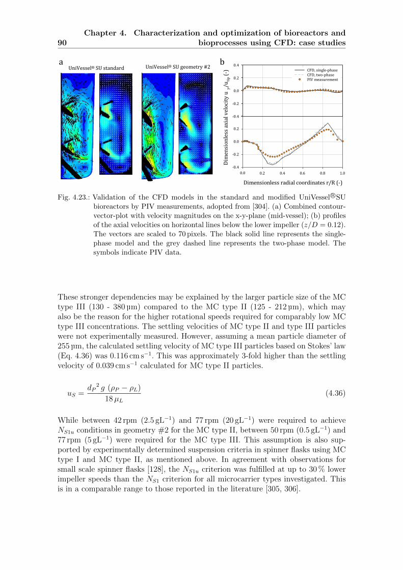
90Chapter 4. Characterization and optimization of bioreactors and
bioprocesses using CFD: case studies
Dimensionless radial coordinates r/R (-)
0.0 0.2 0.4 0.6 0.8 1.0
Dim
ensi
on
less
axi
al v
elo
city
uy/u
tip (
-)
-0.4
-0.2
0.0
0.2
CFD, single-phaseCol 9 vs Col 10 CFD, two-phase
-0.4
-0.2
0.0
0.2
0.4
Dimensionless radial coordinates r/R (-)
0.0 0.2 0.4 0.6 0.8 1.0D
imen
sio
nle
ss a
xial
vel
oci
ty u
y/u
tip (
-)-0.4
-0.2
0.0
0.2
CFD, single-phaseCol 9 vs Col 10 CFD, two-phase
-0.4
-0.2
0.0
0.2
0.4
0.0 0.2 0.4 0.6 0.8 1.0
UniVessel® SU standard UniVessel® SU geometry #2a b
Dimensionless radial coordinates r/R (-)
0.0 0.2 0.4 0.6 0.8 1.0
Dim
ensi
on
less
axi
al v
elo
city
uy/
uti
p (
-)
-0.4
-0.2
0.0
0.2
CFD, single-phaseCFD, two-phasePIV measurement
Fig. 4.23.: Validation of the CFD models in the standard and modified UniVessel R©SUbioreactors by PIV measurements, adopted from [304]. (a) Combined contour-vector-plot with velocity magnitudes on the x-y-plane (mid-vessel); (b) profilesof the axial velocities on horizontal lines below the lower impeller (z/D = 0.12).The vectors are scaled to 70 pixels. The black solid line represents the single-phase model and the grey dashed line represents the two-phase model. Thesymbols indicate PIV data.
These stronger dependencies may be explained by the larger particle size of the MCtype III (130 - 380 µm) compared to the MC type II (125 - 212µm), which mayalso be the reason for the higher rotational speeds required for comparably low MCtype III concentrations. The settling velocities of MC type II and type III particleswere not experimentally measured. However, assuming a mean particle diameter of255 µm, the calculated settling velocity of MC type III particles based on Stokes’ law(Eq. 4.36) was 0.116 cm s−1. This was approximately 3-fold higher than the settlingvelocity of 0.039 cm s−1 calculated for MC type II particles.
uS =dP
2 g (ρP − ρL)
18µL(4.36)
While between 42 rpm (2.5 gL−1) and 77 rpm (20 gL−1) were required to achieveNS1u conditions in geometry #2 for the MC type II, between 50 rpm (0.5 gL−1) and77 rpm (5 gL−1) were required for the MC type III. This assumption is also sup-ported by experimentally determined suspension criteria in spinner flasks using MCtype I and MC type II, as mentioned above. In agreement with observations forsmall scale spinner flasks [128], the NS1u criterion was fulfilled at up to 30 % lowerimpeller speeds than the NS1 criterion for all microcarrier types investigated. Thisis in a comparable range to those reported in the literature [305, 306].
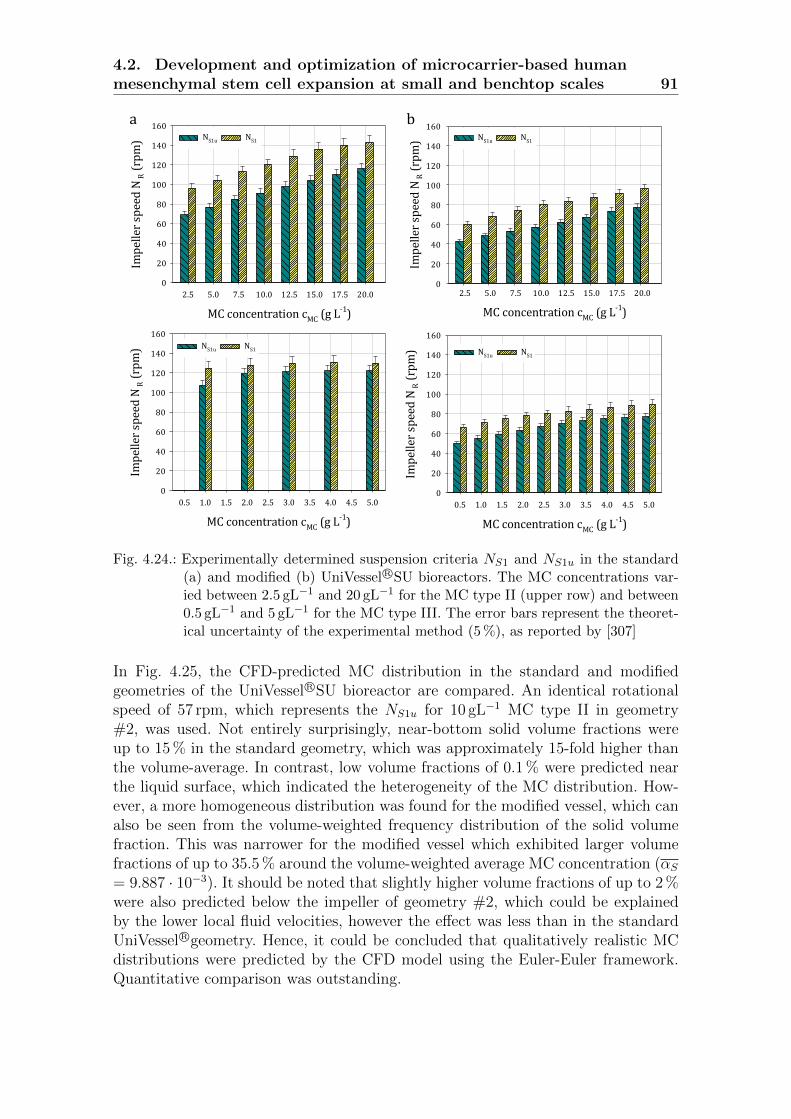
4.2. Development and optimization of microcarrier-based humanmesenchymal stem cell expansion at small and benchtop scales 91
MC concentration cMC
(g L-1)
2.5 5.0 7.5 10.0 12.5 15.0 17.5 20.0
Imp
elle
r sp
eed
NR (
rpm
)
0
20
40
60
80
100
120
140
160
NS1u NS1
MC concentration cMC
(g L-1)
2.5 5.0 7.5 10.0 12.5 15.0 17.5 20.0
Imp
elle
r sp
eed
NR (
rpm
)
0
20
40
60
80
100
120
140
160
NS1u NS1
MC concentration cMC
(g L-1)
2.5 5.0 7.5 10.0 12.5 15.0 17.5 20.0
Imp
elle
r sp
eed
NR (
rpm
)
0
20
40
60
80
100
120
140
160
NS1u NS1
MC concentration cMC
(g L-1)
2.5 5.0 7.5 10.0 12.5 15.0 17.5 20.0
Imp
elle
r sp
eed
NR (
rpm
)
0
20
40
60
80
100
120
140
160
NS1u NS1
MC concentration cMC
(g L-1)
2.5 5.0 7.5 10.0 12.5 15.0 17.5 20.0
Imp
elle
r sp
eed
NR (
rpm
)
0
20
40
60
80
100
120
140
160
NS1u NS1
MC concentration cMC
(g L-1)
2.5 5.0 7.5 10.0 12.5 15.0 17.5 20.0
Imp
elle
r sp
eed
NR (
rpm
)
0
20
40
60
80
100
120
140
160
NS1u NS1
a b
MC concentration cMC
(g L-1)
0.5 1.0 1.5 2.0 2.5 3.0 3.5 4.0 4.5 5.0
Imp
elle
r sp
eed
NR (
rpm
)
0
20
40
60
80
100
120
140
160
Col 12 Col 16
MC concentration cMC (g L-1)
0.5 1.0 1.5 2.0 2.5 3.0 3.5 4.0 4.5 5.0
Imp
elle
r sp
eed
NR (
rpm
)
0
20
40
60
80
100
120
140
160
Col 14 Col 18
MC concentration cMC
(g L-1)
2.5 5.0 7.5 10.0 12.5 15.0 17.5 20.0
Imp
elle
r sp
eed
NR (
rpm
)
0
20
40
60
80
100
120
140
160
NS1u NS1
MC concentration cMC
(g L-1)
2.5 5.0 7.5 10.0 12.5 15.0 17.5 20.0
Imp
elle
r sp
eed
NR (
rpm
)
0
20
40
60
80
100
120
140
160
NS1u NS1
MC concentration cMC
(g L-1)
0.5 1.0 1.5 2.0 2.5 3.0 3.5 4.0 4.5 5.0
Imp
elle
r sp
eed
NR (
rpm
)
0
20
40
60
80
100
120
140
160
Col 12 Col 16
MC concentration cMC (g L-1)
0.5 1.0 1.5 2.0 2.5 3.0 3.5 4.0 4.5 5.0
Imp
elle
r sp
eed
NR (
rpm
)
0
20
40
60
80
100
120
140
160
Col 14 Col 18
MC concentration cMC
(g L-1)
2.5 5.0 7.5 10.0 12.5 15.0 17.5 20.0
Imp
elle
r sp
eed
NR (
rpm
)
0
20
40
60
80
100
120
140
160
NS1u NS1
MC concentration cMC
(g L-1)
2.5 5.0 7.5 10.0 12.5 15.0 17.5 20.0
Imp
elle
r sp
eed
NR (
rpm
)
0
20
40
60
80
100
120
140
160
NS1u NS1
Fig. 4.24.: Experimentally determined suspension criteria NS1 and NS1u in the standard(a) and modified (b) UniVessel R©SU bioreactors. The MC concentrations var-ied between 2.5 gL−1 and 20 gL−1 for the MC type II (upper row) and between0.5 gL−1 and 5 gL−1 for the MC type III. The error bars represent the theoret-ical uncertainty of the experimental method (5 %), as reported by [307]
In Fig. 4.25, the CFD-predicted MC distribution in the standard and modifiedgeometries of the UniVessel R©SU bioreactor are compared. An identical rotationalspeed of 57 rpm, which represents the NS1u for 10 gL−1 MC type II in geometry#2, was used. Not entirely surprisingly, near-bottom solid volume fractions wereup to 15 % in the standard geometry, which was approximately 15-fold higher thanthe volume-average. In contrast, low volume fractions of 0.1 % were predicted nearthe liquid surface, which indicated the heterogeneity of the MC distribution. How-ever, a more homogeneous distribution was found for the modified vessel, which canalso be seen from the volume-weighted frequency distribution of the solid volumefraction. This was narrower for the modified vessel which exhibited larger volumefractions of up to 35.5 % around the volume-weighted average MC concentration (αS= 9.887 · 10−3). It should be noted that slightly higher volume fractions of up to 2 %were also predicted below the impeller of geometry #2, which could be explainedby the lower local fluid velocities, however the effect was less than in the standardUniVessel R©geometry. Hence, it could be concluded that qualitatively realistic MCdistributions were predicted by the CFD model using the Euler-Euler framework.Quantitative comparison was outstanding.

92Chapter 4. Characterization and optimization of bioreactors and
bioprocesses using CFD: case studies
Solid volume fraction S (-)
0.006 0.008 0.010 0.012 0.014 0.016 0.018
Rel
ativ
e v
olu
me
S (-)
0.00
0.05
0.10
0.15
0.20
0.25
0.30
0.35
0.40
0.006 0.008 0.010 0.012 0.014 0.016 0.018 0.020
Rel
ativ
e v
olu
me Ф
S (
-)
Solid volume fraction αS (-)
Fig. 4.25.: CFD-predicted MC distribution in the standard and modified geometries of theUniVessel R©SU bioreactor. The impeller speed was set to 57 rpm, representingthe NS1u criterion for geometry #2 using 10 gL−1 (αS = 9.887 · 10−3) MC typeII. The volume-weighted frequency distributions were obtained by discretiza-tion of the MC volume fraction into 200 bins. The contour plots were scaledlogarithmically with limits of 1 · 10−3 and 0.2.
CFD-predicted specific power inputs for MC concentrations of up to 20 gL−1 weredetermined by considering the experimentally determined impeller speeds for NS1
conditions when using MC type II (see Fig. 4.26). Almost linear relationships be-tween the specific power inputs and the MC concentrations were evident, for boththe standard UniVessel R©SU and the modified geometry. Under fully turbulent con-ditions, one would expect a non-linear increase with P/VL ∝ NS1
3 and NS1 ∝ cMC
(i.e. P/VL ∝ cMC3). However, the flow was in the transition flow range, where the
power number decreased as the impeller speed increased.
Dimensionless radial coordinate r/R (-)
0.0 2.5 5.0 7.5 10.0 12.5 15.0 17.5 20.0
Spec
ific
po
wer
inp
ut
(P/V
L) N
S1 (
W m
-3)
0
1
2
3
4
5
6
7
Spinner flaskMobius CellReadyUniVessel SU, standardUniVessel SU, geometry #2BIOSTAT STR 50L
MC concentration cMC (g L-1)
0.0 2.5 5.0 7.5 10.0 12.5 15.0 17.5 20.0
Spec
ific
po
wer
in
pu
t P
/VL
,NS1
(W
m-3
)
0
1
2
3
4
5
6
7
Spinner flaskMobius CellReadyBIOSTAT STR 50LUniVessel SU, standardUniVessel SU, geometry #2
Fig. 4.26.: Power inputs for NS1 conditions in different single-use bioreactors. The requiredimpeller speeds were determined experimentally using the MC type II at variousconcentrations.

4.2. Development and optimization of microcarrier-based humanmesenchymal stem cell expansion at small and benchtop scales 93
The impeller modification resulted in approximately threefold lower specific powerinputs, which were between 2.2 Wm−3 (for 2.5 gL−1) and 6.6 Wm−3 (for 20 gL−1) inthe standard UniVessel R©SU, but only up to 2.2 Wm−3 were required at the highestMC concentration in geometry #2. Hence, the higher power number of the im-peller with the 45 blade angle (Ne ≈ 2.1) was effectively compensated for by themuch lower impeller speeds required to suspend the MCs. Interestingly, the spe-cific power input for the modified geometry was nearly identical to spinner flasksoperating at identical MC concentrations. This could be a reason for the compa-rable hMSC growth in both systems [304]. However, it should be noted that evenlower specific power inputs were required in the single-use Mobius R©CellReady 3Lbioreactor, in which P/VL was, depending on the MC concentration, only between0.2 Wm−3 and 0.3 Wm−3. Using serum-supplemented culture medium (10 %), celldensities of up to 2.7 · 105 cellsmL−1 have been reported for a hBM-MSC culture inthe Mobius R©CellReady 3L bioreactor [289, 290]. In an adipose-tissue derived stemcell (ADSC) culture expanded on MC type II, even higher maximum cell densitiesof 5.5 · 105 hMSCsmL−1 have been achieved under low serum conditions (<10 %) inthe same bioreactor operated with impeller speeds similar to the NS1 criteria [1].Furthermore, the cell growth in small scale spinner flasks was nearly identical interms of doubling times, expansion factors and peak cell densities.As can be seen from Tab. 4.12, not only were the global specific power inputs re-duced by the impeller modification, but also the local shear stresses (in terms ofvolume-average and maximum values). While (mean) local shear stresses between0.6 · 10−3 Nm−2 (for 5 gL−1 MC) and 0.91 · 10−3 Nm−2 (for 10 gL−1 MC) were pre-dicted for the standard UniVessel R©SU, approximately 50 % lower values of between0.42 · 10−3 Nm−2 (for 5 gL−1 MC) and 0.51 · 10−3 Nm−2 (for 10 gL−1 MC) were de-termined for geometry #2. Interestingly, the relationships between mean local shearstresses and their maximum values were comparable for both impeller configurations.It should be noted that even lower mean shear stress levels (≤0.2 · 10−3 Nm−2) weredetermined for the Mobius R©CellReady bioreactor when operated at NS1 suspensioncriteria with the MC type II. Nevertheless, the maximum shear stress levels werecomparable to geometry #2, which may be a result of the more heterogeneous fluidflow pattern of the Mobius R©CellReady bioreactor.Finally, it should be emphasized that maximum obtained shear stresses in geometry#2 were comparable to those of the spinner flask (compare Tab. 4.9). For a typ-ically used impeller speed in the spinner flask (60 rpm), the maximum local shearstress was predicted to be 180 · 10−3 Nm−2, while it was between 183 · 10−3 Nm−2
and 213 · 10−3 Nm−2 in the modified UniVessel R©SU (see Tab. 4.12). For NS1u con-ditions, the maximum shear stresses were two-fold higher in the standard geometry.In contrast, the mean local shear stresses in both benchtop scale systems were sig-nificantly lower (by a factor of up to 6) than in the small scale spinner flask. Whenconsidering the cultivation results given below, it can be concluded that the maxi-mum local shear stress levels may have a greater impact on hMSC growth than thevolume-average values, even though the maximum values only occur in very smallvolumes, which reduces the probability of the MSCs being exposed to maximumshear stress during the cultivation.

94Chapter 4. Characterization and optimization of bioreactors and
bioprocesses using CFD: case studies
Tab. 4.12.: Predicted shear stress levels at impeller speeds for the NS1u suspension crite-rion in the original and modified UniVessel R©SU and the Mobius R©CellReady3L bioreactors. The values for τnt are given as mean and maximum, while λTis given as a minimum and a mean.
BioreactorMC conc. NS1u utip Re LSSa KMST b
cMC (gL−1) (rpm) (ms−1) (-) τnt (10−3Nm−2) λT (µm)
UniVessel R©SUStd.
5 77 0.22 3737 0.60 / 420 34 / 2208 87 0.25 4211 0.79 / 475 32 / 20210 91 0.26 4405 0.91 / 502 27 / 184
UniVessel R©SUmod. #2
5 48 0.14 2324 0.42 / 183 43 / 2748 55 0.16 2662 0.46 / 195 39 / 25210 57 0.16 2759 0.51 / 213 35 / 235
Mobius R©CellReady5 28 0.11 1619 0.12 / 183 70 / 14748 31 0.12 1793 0.13 / 185 66 / 138310 35 0.14 2024 0.20 / 236 67 / 507
a) LSS, local shear stress given as volume-weighted mean / maximum values; b) KMST,Kolmogorov’s microscale of turbulence given as volume-weighted mean / minimum values.
Comparative growth courses for adipose-tissue derived MSCs in the standard andmodified UniVessel R©SU bioreactors are shown in Fig. 4.27a. Depending on themicrocarrier concentration, maximum cell densities of (2.65± 0.22) · 105 cellsmL−1
(7.5 gL−1) and (0.67± 0.05) · 105 cellsmL−1 (10 gL−1) were achieved in the standardUniVessel R©SU, when operated at Ns1u conditions. While the expansion factor at thelower MC concentration was 35.4, only a 13.3-fold increase of the cell density wasachieved at a MC concentration of 10 gL−1. Furthermore, nearly linear cell growthwas observed after a two-day lag-phase. The significantly lower cell growth wasattributed to the higher impeller speed required to prevent the MCs from sedimen-tating and the resulting shear stress at Ns1u conditions. For identical MC concen-trations, expansion factors of up to 58.4± 12.4 have been reported for cells13 andculture media in small scale spinner flasks [9].In the modified UniVessel R©SU, exponential cell growth was observed for five days,with a mean growth rate of 0.038 h−1, corresponding to a doubling time of 18.6 h. Af-terwards, the cells entered the stationary phase, which can be explained by the pro-gressing confluence of the MCs. A maximum expansion factor of 71.8 was obtained onday 7 [308], which corresponded to a peak cell density of (7.2± 0.4) · 105 cellsmL−1,an increase by a factor of 10.7 compared to the standard geometry with an identicalmicrocarrier concentration. This is, to the best of the authors knowledge, the high-est value has been achieved for hADSCs cultivated under serum-reduced conditionsat benchtop scale. For the single-use Mobius R©CellReady bioreactor, an expansionfactor of 5.2 with a peak cell density of 0.75 · 105 cellsmL−1 has been reported [8]and an approximately 2.5-fold higher cell density of 1.68 · 105 cellsmL−1 has been
13The cultivations in the standard UniVessel R©SU and the spinner flask were both inoculated froma single cell stock.

4.2. Development and optimization of microcarrier-based humanmesenchymal stem cell expansion at small and benchtop scales 95
achieved in a 5 L stirred bioreactor [56]. More recently, hADSCs have successfullybeen cultivated at pilot scale with a maximum working volume of 35 L, where a celldensity of 0.31 · 106 cellsmL−1 and an expansion factor of 34.5 have been achieved[9]. It should be noted that scaling-up has also been realized based on the NS1u
suspension criterion.These improved cultivation results for the modified UniVessel R©SU were confirmedfor human bone-marrow derived stem cells (hBM-MSC), as shown in Fig. 4.27b. Apeak cell density of only (1.9± 0.2) · 105 cellsmL−1 was achieved within eight daysin the standard vessel when using MC type III at NS1u conditions. In contrast, max-imum cell densities of up to (5.3± 0.1) · 105 cellsmL−1 were obtained after nine daysin the modified UniVessel R©SU [304]. The mean growth rate was 0.744 d−1 and thedoubling time was 22.4 h, meaning 1.4-fold faster cell growth was achieved in themodified cultivation vessel. Even though it is difficult to draw general conclusions,the impeller optimization seemed to be beneficial for various MSC cell types cul-tivated on MCs, in particular at elevated MC concentrations, by providing a largegrowth surface area.
a b Process time t (d)
0 1 2 3 4 5 6 7 8C
ell d
ensi
ty C
D (
10
5 c
ells
mL
-1)
0
1
2
3
4
5
6
7
8
Standard, 10 g L-1
Geometry #2, 10 g L-1
Standard, 7.5 g L-1
Process time t (d)
0 1 2 3 4 5 6 7 8 9 10
Cel
l den
sity
CD
(1
05 c
ells
mL
-1)
0
1
2
3
4
5
6
UniVessel, geometry #2UniVessel, standard
Process time t (d)
0 1 2 3 4 5 6 7 8
Cel
l den
sity
CD
(1
05 c
ells
mL
-1)
0
1
2
3
4
5
6
7
8
Standard, 10 g L-1
Geometry #2, 10 g L-1
Standard, 7.5 g L-1
Process time t (d)
0 1 2 3 4 5 6 7 8 9 10
Cel
l den
sity
CD
(1
05 c
ells
mL
-1)
0
1
2
3
4
5
6
UniVessel, geometry #2UniVessel, standard
Fig. 4.27.: Growth courses obtained for hMSC in the modified UniVessel R©SU bioreactorcompared to its standard counterpart. (a) Cell densities of adipose-tissue de-rived hMSCs in 8-days cultures ; (b) cell densities of bone-marrow derivedhMSCs in 9-days cultures.

96

4.3. Development of the traveling wave bioreactor 97
4.3. Development of the traveling wave bioreactor
4.3.1. Introduction
In 2008, the patent for a novel bioreactor consisting of a toroidal shaped vessel wasfiled [309]. Toroidal shaped reactors, which operate on the same principle as loopreactors, have proven themselves to be suitable for a variety of cultivations, sincethey are easily scalable, have no dead zones and and provide efficient mixing withlow power consumption [310, 311]. While the first torus reactors were used for thepolymerization of olefins where highly viscous fluids are processed [312], more recentapplications include xanthan production [313], the hydrolysis of wheat proteins [314]and the acetylation of pea isolate [315]. All of these studies used torus reactors withdifferent kinds of built-in impellers for agitation, which require sealing and bear-ings. In contrast, the vessel contents of partially filled, orbitally shaken bioreactorsis mixed by the motion of a platform.This mixing principle is also used in the traveling wave bioreactor (TWB). Theplatform motion is intended to set up a quasi-periodic, self-reproducing wave withcharacteristics that are dependent on the vessel geometry (e.g., torus diameter), theshaking parameters (e.g., frequency, amplitude) and the liquid’s properties (e.g.,density, viscosity), as schematically shown in Fig. 4.28. Furthermore, the fluid flowis predicted to be affected by protuberances mounted on the inner surface walls.The objective of this case study was to develop CFD models to predict fluid flowsinside a traveling wave bioreactor, for different bioreactor geometries and agitationparameters. This chapter discusses the potential and limitations of using CFD forearly design studies to reduce the need for large numbers of prototypes.
Fig. 4.28.: Schematic of the desired working principle of the traveling wave bioreactor.
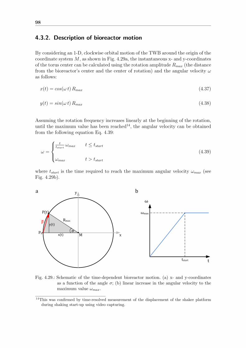
98
4.3.2. Description of bioreactor motion
By considering an 1-D, clockwise orbital motion of the TWB around the origin of thecoordinate system M , as shown in Fig. 4.29a, the instantaneous x- and y-coordinatesof the torus center can be calculated using the rotation amplitude Rmax (the distancefrom the bioreactor’s center and the center of rotation) and the angular velocity ωas follows:
x(t) = cos(ω t)Rmax (4.37)
y(t) = sin(ω t)Rmax (4.38)
Assuming the rotation frequency increases linearly at the beginning of the rotation,until the maximum value has been reached14, the angular velocity can be obtainedfrom the following equation Eq. 4.39:
ω =
t
tstartωmax t ≤ tstart
ωmax t > tstart
(4.39)
where tstart is the time required to reach the maximum angular velocity ωmax (seeFig. 4.29b).
M
y(t)Rmax
P0
P(t)
x(t)
y
x
p
σ
ω
ttstart
ωmax
a b
Fig. 4.29.: Schematic of the time-dependent bioreactor motion. (a) x- and y-coordinatesas a function of the angle σ; (b) linear increase in the angular velocity to themaximum value ωmax.
14This was confirmed by time-resolved measurement of the displacement of the shaker platformduring shaking start-up using video capturing.

4.3. Development of the traveling wave bioreactor 99
In this case, the time-dependent angle σ can be calculated as follows:
σ =
ωmax
2 tstartt2 t ≤ tstart
ωmax (t− tstart) + σstart t > tstart
(4.40)
By inserting Eq. 4.40 into equations 4.37 and 4.38, the following equations for thetime-dependent x- and y-coordinates of the torus center are obtained:
x(t) =
cos(
ωmax
2 tstartt2)Rmax t ≤ tstart
cos (ωmax (t− tstart) + σstart) Rmax t > tstart(4.41)
y(t) =
sin(
ωmax
2 tstartt2)Rmax t ≤ tstart
sin (ωmax (t− tstart) + σstart) Rmax t > tstart(4.42)
The velocity of the torus movement along the x- and y-axis expressed by vx(t)and vy(t) can then be obtained from the first derivatives of Eq. 4.41 and Eq. 4.42respectively.
vx(t) =dx(t)
dt
ωmaxRmax
tstartsin(ωmax t2
2 tstart
)t t ≤ tstart
−ωmaxRmax sin (ωmax (t− tstart) + σstart) t > tstart
(4.43)
vy(t) =dy(t)
dt
ωmaxRmax
tstartcos(ωmax t2
2 tstart
)t t ≤ tstart
−ωmaxRmax cos (ωmax (t− tstart) + σstart) t > tstart
(4.44)
This approach can be applied in ANSYS Fluent by using an user-defined function(UDF) that defines the translation of the mesh with respect to time (mesh motion),as shown by [128]. However, it is necessary to record the mesh for every time stepof interest, which resulted in tremendous data storage requirements (e.g., 2.4 GB for20 s physical time, simulated with a grid of 1 · 106 controlvolumes15).As an alternative, the simulations were simplified by assuming that the mesh doesnot move during the simulation, while the direction of the earth gravity vector ismodified with respect to time. This is a much more practical alternative, fully equiv-alent from a computational point of view, and has already been applied in previousstudies modeling rocker-type wave bioreactors [62, 316]. Furthermore, improved nu-merical convergence behaviour was found using this method, where the residuals
15In this particular case, the data have only been recorded every two seconds.

100
decreased five-fold compared to the dynamic mesh method (data not shown). Thevalues for acceleration along the x- and y-axis were obtained from the second deriva-tive of the x- and y-coordinates with respect to time, resulting in Eq. 4.45 and Eq.4.46.
ax(t) =d2x(t)
dt2
ωmaxRmax
tstart
[sin(ωmax t2
2 tstart
)+ ωmax
tstartcos(ωmax t2
2 tstart
)t2]
t ≤ tstart
−ωmax2Rmax cos (ωmax (t− tstart) + σstart) t > tstart(4.45)
ay(t) =d2y(t)
dt2
−ωmaxRmax
tstart
[cos(ωmax t2
2 tstart
)− ωmax
tstartsin(ωmax t2
2 tstart
)t2]
t ≤ tstart
−ωmax2Rmax sin (ωmax (t− tstart) + σstart) t > tstart(4.46)
The acceleration in the z-direction corresponds to gravitational acceleration and,therefore, was set to a constant value of 9.81 ms−2. This approach was implementedin ANSYS Fluent by means of a user-defined text scheme, which imported the actualvalues of the gravity vector from a tabular text file that was generated by means ofan own MATLAB R©script.The time-dependent fluid flow was modelled in a VOF framework until quasi-steadystate velocity profiles at predefined cross-sections had been predicted. The time stepwas set to 5 · 10−3 s, corresponding to approximately 0.25 of rotation per time stepat the highest investigated rotational speed. A sensitivity study revealed that theresults were almost completely independent of the time discretization when usingthis time step size (see A.8 in the appendix on page 176).
4.3.3. Results of fluid flow prediction
The fluid flow patterns for filling volumes of 15 L, 25 L and 35 L were modelled forrotational speeds of between 20 rpm and 50 rpm. The lower limit was taken from theminimum shaking frequency of the platform used in the experiments (LS-X shaker,Kuhner AG). If not otherwise stated, the shaking amplitude Amax was set to 25 mmin order to match the shaking diameter d0 of 50 mm used in the experiments.The time-dependent development of the air-water phase distribution for the outersurface of the unbaffled annulus is shown in Fig. 4.30. The wave started to developafter approximately three seconds, at which point the maximum rotational speedwas reached. As expected, the wave propagated in a clockwise direction followingthe torus movement and a quasi-periodic flow was achieved after approximately tenseconds, when the height of the wave crest was relatively constant and the velocityof circulation was equal to the rotational speed of the torus. This was also reflected

4.3. Development of the traveling wave bioreactor 101
by the fluid velocities at defined cross sections, where periodic profiles with dis-tances between two consecutive peaks corresponding to the shaking frequency wereobtained (see Fig. A.10 in the appendix on page 176). In agreement with expecta-tions, the height of the liquid was higher near the outer surface than at the innerwall of the vessel, as a result of centrifugal acceleration.Fig. 4.31 shows the velocities for defined cross sections at half initial filling height(z/HL = 0.5) and equally distributed angles around the circumference (0, 90, 180,270). As expected, the fluid flowed clockwise, as shown by the fluid velocity vectors.The highest fluid velocity of 1.72 ms−1 was found behind the wave front and corre-lated well with the theoretical maximum speed of 1.67 ms−1 at the vessel wall (Eq.4.47). The difference was thus below 5 %, which could be attributed to numericaluncertainties. However, for stirred vessels agitated by Rushton turbines, peak veloc-ities in the trailing vortices were found to be up to 1.4-fold the impeller tip speed[317]. Therefore, the differences between theoretical and CFD predicted maximumvelocities may also be explained by turbulence production, since the highest levelsof turbulence were found in regions of higher velocities.
uw,max =ωmax
2(D + d0) (4.47)
0.0 s 3.0 s 5.0 s
6.0 s 7.5 s 10 s
12.5 s 15 s 20 s
Fig. 4.30.: CFD predicted air-liquid distribution for the unbaffled traveling wave bioreactorat different points in time. Water is represented by blue and air by red.

102
Significantly lower liquid velocities of below 0.1 ms−1 were predicted at the innerradius of the torus, in front of the traveling wave. Furthermore, fluid velocity gra-dients were found between the outer and inner radii of the torus, which matchedexpectations and could be explained by centrifugal acceleration. However, the dis-tribution of liquid velocities appeared to be relatively homogeneous. It was foundthat velocities, which were higher than half the maximum velocity (≥ 0.9 ms−1),occurred in approximately 30 % of the liquid volume.It is worth noting that - except for a small region at the inner radius of the annulus- the velocity vectors were orientated in a circumferential direction and, therefore,the flow was comparable to a circulating plug flow reactor. This may have causedlow back-mixing of the vessel content and a consequent negative effect on mixingcapacity. As a result, mixing times may become undesirably long and/or concentra-tion gradients are likely to occur, something which was confirmed by experimentalinvestigations (see below).
0° 90° 180° 270°
0°
90°
180°
270°
0.84
0.75
0.67
0.59
0.50
0.42
0.34
0.25
0.17
0.08
0.00No
rmal
ized
vel
oci
ty m
agn
itu
de
u/u
max
,w (
-)
Fig. 4.31.: Fluid flow in the traveling wave at a rotational speed of 40 rpm and amplitudeof 25 mm after 15 seconds (9.5 rotations). Cross section at half initial fillingheight equal to z = 0.049 m (above); cross sections at different angles (below).The liquid velocity vectors are projected onto the given plane with a fixedlength of 25 mm.

4.3. Development of the traveling wave bioreactor 103
4.3.4. Model validation
The CFD models were validated by estimating the liquid distribution at the outerlateral torus wall (see section 3.2.5). Liquid volumes of 15, 25 and 35 L and rotationalspeeds of 20, 30 and 40 rpm were considered. A similar approach has been describedfor orbitally shaken flasks and microtiter plates [89, 318]. Even though there weresome minor deviations, in particular for 15 L at 20 rpm and for 35 L at 40 rpm, boththe qualitative and quantitative agreement was excellent (see Fig. 4.32). Differencesmay be ascribed to both numerical uncertainties and inaccuracies in experimentalmeasurements. The speed of the shaking platform was not completely constant, andvaried by up to±3 rpm, depending on the filling volume. In general, higher variationswere found for larger volumes, as a result of the increased inertial momentum of theliquid. The angular velocities assumed in the CFD models were, however, constant.Furthermore, optical distortion of the liquid height measurements was greater at verylow (<50 mm) and very high (>150 mm) liquid heights due to the curvature of thetorus. Interestingly, the CFD model underestimated the wave heights of the severalsecondary waves for 15 L at 20 rpm and at the largest filling volume. Nevertheless, itcan be stated that, based on this verification approach, the CFD models were validand could be used for further investigations.
Circumferential angle (°)
0 30 60 90 120 150 180 210 240 270 300 330
Liq
uid
hei
ght
y (
mm
)
0
20
40
60
80
100
120
140
160
Circumferential angle (°)
0 30 60 90 120 150 180 210 240 270 300 330
Circumferential angle (°)
0 30 60 90 120 150 180 210 240 270 300 330 360
Liq
uid
hei
ght
y (
mm
)
0
20
40
60
80
100
120
140
160
Liq
uid
hei
ght
y (
mm
)
0
20
40
60
80
100
120
140
160L
iqu
id h
eigh
t y
(m
m)
0
20
40
60
80
100
120
140
160
Liq
uid
hei
ght
y (
mm
)
0
20
40
60
80
100
120
140
160
180
Liq
uid
hei
ght
y (
mm
)0
20
40
60
80
100
120
140
160
180
VL 15 L 25 L 35 L
NS
α α α
0 60 120 180 240 300 0 60 120 180 240 300 0 60 120 180 240 300 360
Circumferential angle (°)
0 30 60 90 120 150 180 210 240 270 300 330
Liq
uid
hei
ght
y (
mm
)
0
20
40
60
80
100
120
140
160
Circumferential angle (°)
0 30 60 90 120 150 180 210 240 270 300 330
Circumferential angle (°)
0 30 60 90 120 150 180 210 240 270 300 330 360
Liq
uid
hei
ght
y (
mm
)
0
20
40
60
80
100
120
140
160
Liq
uid
hei
ght
y (
mm
)
0
20
40
60
80
100
120
140
160
Liq
uid
hei
ght
y (
mm
)
0
20
40
60
80
100
120
140
160
Liq
uid
hei
ght
y (
mm
)
0
20
40
60
80
100
120
140
160
180L
iqu
id h
eigh
t y
(m
m)
0
20
40
60
80
100
120
140
160
180
Circumferential angle (°)
0 30 60 90 120 150 180 210 240 270 300 330
Liq
uid
hei
ght
y (
mm
)
0
20
40
60
80
100
120
140
160
Circumferential angle (°)
0 30 60 90 120 150 180 210 240 270 300 330
Circumferential angle (°)
0 30 60 90 120 150 180 210 240 270 300 330 360
Liq
uid
hei
ght
y (
mm
)
0
20
40
60
80
100
120
140
160
Liq
uid
hei
ght
y (
mm
)
0
20
40
60
80
100
120
140
160
Liq
uid
hei
ght
y (
mm
)
0
20
40
60
80
100
120
140
160
Liq
uid
hei
ght
y (
mm
)
0
20
40
60
80
100
120
140
160
180
Liq
uid
hei
ght
y (
mm
)
0
20
40
60
80
100
120
140
160
180
20
rp
m
30
rp
m
40
rp
m
Fig. 4.32.: Model verification of the TWB for various operating conditions. horizontal:15 L (left), 25 L (middle), 35 L (right); vertical: 40 rpm (top), 30 rpm (middle),20 rpm (bottom). Experimental data represented by symbols and CFD predic-tions by solid lines.

104
4.3.5. Turbulence prediction
In order to quantify the turbulence in the TWB, a Reynolds number was definedthat was based on channel flows [319, 320]. The general definition of the Reynoldsnumber, given in Eq. 4.48, requires the characteristic length lc and the characteris-tic velocity vc, while the kinematic viscosity νL is defined by the liquid properties(1.022 · 10−6 m2s−1 in the present case).
Re =lc ucνL
(4.48)
As shown above, the main proportion of the fluid flowed through the cross sectionalarea of the annular pipe and, therefore, the characteristic fluid velocity could bedefined as the area weighted average of the fluid velocity in the flow direction:
uc = uL =1
A
∫ui dA (4.49)
The characteristic length was given by the hydraulic diameter dH , which was de-termined using the cross sectional area of the fluid A and the wetted perimeter U ,both of which are functions of the liquid height hL (see Eq. 4.50 and Fig. A.9 inthe appendix). Assuming that the liquid height under steady-state conditions canbe approximated by taking circular cross sections with segment heights equal to theinitial filling height, the hydraulic diameter was obtained using Eq. 4.50.
dH =4ACU
=VL
π r R arccos(1− HL
r
) (4.50)
With the following geometrical definitions:
A = π r2 (4.51)
and
VL = 2π2 αL r R (4.52)
the Reynolds number of the TWB was calculated from the following equation:
Re =αL∫ui dA
2 r arccos(1− HL
r
)νL
(4.53)
In Fig. 4.33, the CFD predicted, time-averaged Reynolds numbers for the unbaf-fled TWB are shown for a wide range of operating conditions. It was obvious thatthe Reynolds number increased as the shaking frequency increased, given that noout-of-phase conditions were present. For example, Re at 25 L working volume in-creased from 0.3 · 104 (20 rpm) to 5 · 104 (40 rpm), but decreased at higher shakingfrequencies (to 1.6 · 104 at 50 rpm). Increasing Reynolds numbers for higher shakingfrequencies were expected, since Re is directly proportional to the fluid velocitiesthrough the annulus cross sections, which are related to the circulation time of the

4.3. Development of the traveling wave bioreactor 105
liquid in the annulus. Furthermore, it was found that Re increased as the shakingamplitude increased, which was consistent with data reported for orbitally shakenErlenmeyer flasks and cylindrical vessels [81, 92]. For the investigated operating con-ditions, Reynolds numbers in the range of 0.17 · 104 to 11.3 · 104 were predicted. Thecritical Reynolds number for pipe flows, above which fully-turbulent conditions arefound, is Re ≈ 2300 and is also applicable for open channel flows [319]. Thus it canbe argued, that the flow inside the annular bioreactor was turbulent for most of theinvestigated operating conditions. For water-like media, non-turbulent conditionswere only expected at low filling volumes (<10 L) and at low shaking frequencies (≤20 rpm) and amplitudes (≤ 12.5 mm).Interestingly, the predicted Reynolds numbers were much smaller (by a factor of 2to 70) than one would have expected if frictionless, regular circulation of the liquidhas been assumed. If the total liquid volume is expected to flow through the annuluscross section within a single period, the mean fluid velocity can be expressed by Eq.4.54.
w∗ =4VLNmax
π dH2 (4.54)
However, this assumption neglects back mixing and the out-of-phase phenomenon(see below). Furthermore, there seems to be a critical shaking frequency, which mustbe exceeded in order to achieve liquid rotation. This has also been described for or-bitally shaken cylindrical vessels [92] and is the minimal required shaking frequencyneeded to overcome the inertial forces and, consequently, to provoke the fluid flowdescribed above. However, this was not possible to determine experimentally be-cause of the minimum shaking speed of the shaker platform of 20 rpm.
Shaking rate NR (rpm)
20 30 40 50Av
erag
ed R
eyn
old
s n
um
ber
(x1
04)
0
1
2
3
4
5
6
7
8
9
10
11
1212.5 mmShaking rate Nmax (rpm) vs Col 14 - Col 14 Shaking rate Nmax (rpm) vs Col 24 - Col 24
Shaking rate NR (rpm)
20 30 40 50Av
erag
ed R
eyn
old
s n
um
ber
(x1
04)
0
1
2
3
4
5
6
7
8
9
10
11
12
Shaking rate Nmax (rpm) vs Col 9 - Col 9 Shaking rate Nmax (rpm) vs Col 14 - Col 14 Shaking rate Nmax (rpm) vs Col 19 - Col 19
Shaking rate NR (rpm)
20 30 40 50Av
erag
ed R
eyn
old
s n
um
ber
(x1
04)
0
1
2
3
4
5
6
7
8
9
10
11
1212.5 mmShaking rate Nmax (rpm) vs Col 14 - Col 14 Shaking rate Nmax (rpm) vs Col 24 - Col 24
Shaking rate NR (rpm)
20 30 40 50Av
erag
ed R
eyn
old
s n
um
ber
(x1
04)
0
1
2
3
4
5
6
7
8
9
10
11
12
Shaking rate Nmax (rpm) vs Col 9 - Col 9 Shaking rate Nmax (rpm) vs Col 14 - Col 14 Shaking rate Nmax (rpm) vs Col 19 - Col 19
a b
**
** *
*
Shaking rate NR (rpm)
20 30 40 50Av
erag
ed R
eyn
old
s n
um
ber
(x1
04)
0
1
2
3
4
5
6
7
8
9
10
11
1212.5 mmShaking rate Nmax (rpm) vs Col 14 - Col 14 Shaking rate Nmax (rpm) vs Col 24 - Col 24
Shaking rate NR (rpm)
20 30 40 50Av
erag
ed R
eyn
old
s n
um
ber
(x1
04)
0
1
2
3
4
5
6
7
8
9
10
11
12
Shaking rate Nmax (rpm) vs Col 9 - Col 9 Shaking rate Nmax (rpm) vs Col 14 - Col 14 Shaking rate Nmax (rpm) vs Col 19 - Col 19
Shaking rate NR (rpm)
20 30 40 50Av
erag
ed R
eyn
old
s n
um
ber
(x1
04)
0
1
2
3
4
5
6
7
8
9
10
11
1212.5 mmShaking rate Nmax (rpm) vs Col 14 - Col 14 Shaking rate Nmax (rpm) vs Col 24 - Col 24
Shaking rate NR (rpm)
20 30 40 50Av
erag
ed R
eyn
old
s n
um
ber
(x1
04)
0
1
2
3
4
5
6
7
8
9
10
11
12
Shaking rate Nmax (rpm) vs Col 9 - Col 9 Shaking rate Nmax (rpm) vs Col 14 - Col 14 Shaking rate Nmax (rpm) vs Col 19 - Col 19 15 L
25 L 35 L
Shaking rate NR (rpm)
20 30 40 50Av
erag
ed R
eyn
old
s n
um
ber
(x1
04)
0
1
2
3
4
5
6
7
8
9
10
11
1212.5 mmShaking rate Nmax (rpm) vs Col 14 - Col 14 Shaking rate Nmax (rpm) vs Col 24 - Col 24
Shaking rate NR (rpm)
20 30 40 50Av
erag
ed R
eyn
old
s n
um
ber
(x1
04)
0
1
2
3
4
5
6
7
8
9
10
11
12
Shaking rate Nmax (rpm) vs Col 9 - Col 9 Shaking rate Nmax (rpm) vs Col 14 - Col 14 Shaking rate Nmax (rpm) vs Col 19 - Col 19
Shaking rate NR (rpm)
20 30 40 50Av
erag
ed R
eyn
old
s n
um
ber
(x1
04)
0
1
2
3
4
5
6
7
8
9
10
11
1212.5 mmShaking rate Nmax (rpm) vs Col 14 - Col 14 Shaking rate Nmax (rpm) vs Col 24 - Col 24
Shaking rate NR (rpm)
20 30 40 50Av
erag
ed R
eyn
old
s n
um
ber
(x1
04)
0
1
2
3
4
5
6
7
8
9
10
11
12
Shaking rate Nmax (rpm) vs Col 9 - Col 9 Shaking rate Nmax (rpm) vs Col 14 - Col 14 Shaking rate Nmax (rpm) vs Col 19 - Col 19
12.5 mm25.0 mm35.0 mm
Shaking rate NS (rpm) Shaking rate NS (rpm)Shaking rate NR (rpm)
30 40 50
Av
erag
ed R
eyn
old
s n
um
ber
R
e (x
10
4)
0
1
2
3
4
5
6
15 L25 L35 L
Shaking rate NR (rpm)
30 40 50Spec
ific
po
wer
in
pu
t P
/VL (
W m
-3)
0
10
20
30
40
50
60
70
80
90
100
15 L25 L35 L
Shaking rate NR (rpm)
30 40 50
Av
erag
ed R
eyn
old
s n
um
ber
R
e (x
10
4)
0
1
2
3
4
5
6
15 L25 L35 L
Shaking rate NR (rpm)
30 40 50Spec
ific
po
wer
in
pu
t P
/VL (
W m
-3)
0
10
20
30
40
50
60
70
80
90
100
15 L25 L35 L
Fig. 4.33.: CFD predicted Reynolds numbers for the TWB for various operational condi-tions. (a) Influence of the filling volume at a fixed shaking amplitude of 25 mm;(b) Influence of the shaking amplitude at a fixed filling volume of 25 L. Thestars indicate out-of-phase conditions. All simulations were carried out for atotal volume of 52.1 L with r/R=0.36.

106
Compared to the Reynolds number introduced for orbitally shaken Erlenmeyer flasksand cylindrical vessels ReS, as defined by Eq. 2.5, the present definition requires thefluid velocities through the annulus cross sections. These depend, for a given vesselgeometry, on the liquid properties as well as on the shaking frequency and amplitude.However, this relation is a priori unknown. An alternative definition of the Reynoldsnumber could be obtained if the characteristic velocity uc was expressed by therotational velocity with:
uc = ωmaxRmax = 2π NS Rmax (4.55)
Thus, all parameters would be given from known operational conditions, howeverit should be emphasized that ReS does not consider the out-of-phase phenomenon,which occurs at high rotational speeds and/or enhanced viscosities [81]. For thisreason, the phase number Ph has been introduced (see section 2.2.1). Out-of-phaseconditions are characterized by the fact that the liquid cannot follow the orbitalmotion of the platform/vessel and the frictional forces exceed centrifugal forces.This leads the bulk of the liquid to remain at the base of the flask with only minorrelative motion at the surface. Out-of-phase operation in orbitally shaken reactors isassociated with a strong decrease in power input, mixing and (oxygen) mass transfer[92]. This has also been reported for orbitally-shaken pillow-shaped bags [178] andhas been also observed in the TWB (see section 4.3.6).Out-of-phase conditions in the TWB were well-captured by the CFD simulations,which is another indication for the validity of the CFD model. To illustrate this, atime series of the liquid distribution predicted by CFD for 15 L and 40 rpm is shownin Fig. A.11 in the appendix on page 177. While quantitative relationships betweencritical shaking speeds, the working volume and liquid viscosity were established, nocorrelations with local (instantaneous) fluid velocities and/or turbulence parameterswere found yet.The experimentally determined critical shaking frequencies (in rpm) above whichout-of-phase conditions occur in the unbaffled annulus, could be correlated with thefilling volume VL (in m3) and the kinematic viscosity (in ms−1), as given by Eq.4.56, where the influence of the liquid volume is more pronounced than that of theliquid viscosity (see also Fig. A.12).
NC,OP = 119.11VL0.61 νL
−0.128 (4.56)
As can be seen from Fig. 4.33, the Reynolds number of the TWB decreased whenout-of-phase conditions were achieved. For example, Re for 25 L was 5.04 · 104 at40 rpm but only 1.58 · 104 at 50 rpm, when out-of-phase conditions were present.This can be explained by the fact that under these conditions, the wave motionand, consequently, the liquid velocities through the annulus cross sections dimin-ished. According to the CFD predictions, out-of-phase conditions were more likelyfor small liquid volumes and shaking amplitudes, which was consistent with experi-mental observations and the literature [82, 92].

4.3. Development of the traveling wave bioreactor 107
4.3.6. Determination of engineering parameters
Specific power input
As described in section 4.1.2, the CFD predictions agreed well with experimentaldata when the power input was determined using the wall momentum. This wasalso found for orbitally shaken cylindrical vessels up to 50 L scale [92]. In contrast,the specific power input for shake flasks has been previously under predicted byapproximately 35 % compared to experimental data, when the power input wasdetermined by summation of turbulent dissipation rates in the VOF framework [90].Interestingly, a constant ratio between numerical and experimental power inputshas been found for a wide range of operational conditions [90]. Nevertheless, theunder prediction using the turbulent dissipations rates has already been discussedfor stirred systems (see section 4.1.2). Based on this, the total specific power inputof the TWB was predicted by Eq. 4.57, with the wall momentum MW obtained byintegrating the momentum over the outer lateral wall.
P
VL=
2π NSMW
VL(4.57)
In Fig. 4.34, the CFD predicted specific power inputs for various operating condi-tions are shown. Not entirely surprisingly, the power input increased as the shakingfrequency and amplitude increased. For given shaking parameters, the specific powerinput decreased as the filling volume increased, which was consistent with expecta-tions. Using a 25 L working volume, a maximum specific power input of 148 Wm−3
was predicted at a rotational speed of 50 rpm and an amplitude of 35 mm. This valueis in the range of typical power inputs described for orbitally shaken animal cell cul-tures. Depending on the filling volume, further increases in shaking frequency ledto reductions in the power input, which could be ascribed to out-of-phase operatingconditions. For the working volume of 25 L, the following relationship was found forshaking amplitudes of 25 mm and 35 mm:
P
VL∝ NS
5.57 (4.58)
For shaking flasks, a considerably lower dependency of power input on the shakingrate (P/VL ∝ NS
2.8) has been reported for operating conditions where the bottom ofthe flask runs partially dry [82]. Nevertheless, a higher dependency on the shakingrate, similar to the findings in this study, has been found for shake flasks operatedunder conditions where the vessel bottom was completely wet (P ∝ NS
5.75) [321].Furthermore, power input data for an orbitally shaken 20 L vessel with 50 % fillingvolume and agitated with 50 mm shaking diameter, provided by [322], could becorrelated with a similar dependency of P/VL ∝ NS
5.99 (with R2 = 0.987). It hasbeen proposed that the higher dependency of P/VL on NS is related to the increasingfriction area between the vessel wall and the rotating liquid at increased shakingfrequencies [82].

108
Shaking rate NR (rpm)
20 30 40 50
Spec
ific
po
wer
in
pu
t P
/VL (
W m
-3)
0.01
0.1
1
10
100
1000
12.5 mm25.0 mm35.0 mm
Shaking rate NR (rpm)
20 30 40 50
Spec
ific
po
wer
in
pu
t P
/VL (
W m
-3)
0.01
0.1
1
10
100
1000
15 L25 L35 L
Shaking rate NR (rpm)
20 30 40 50Spec
ific
po
wer
in
pu
t P
/VL (
W m
-3)
0.01
0.1
1
10
100
1000
Col 7 vs Specific power input P/VL (W/m3) - Specific power input P/VL (W/m3) Col 7 vs Col 12 - Col 12 Col 7 vs Col 20 - Col 20
Shaking rate NR (rpm)
20 30 40 50Spec
ific
po
wer
in
pu
t P
/VL (
W m
-3)
0.01
0.1
1
10
100
1000
Col 7 vs Power Input P (W) - Power Input P (W) Col 7 vs Col 12 - Col 12 Col 7 vs Col 16 - Col 16
a
*
*
* * **
Shaking rate NR (rpm)
20 30 40 50Spec
ific
po
wer
in
pu
t P
/VL (
W m
-3)
0.01
0.1
1
10
100
1000
Col 7 vs Specific power input P/VL (W/m3) - Specific power input P/VL (W/m3) Col 7 vs Col 12 - Col 12 Col 7 vs Col 20 - Col 20
Shaking rate NR (rpm)
20 30 40 50Spec
ific
po
wer
in
pu
t P
/VL (
W m
-3)
0.01
0.1
1
10
100
1000
Col 7 vs Power Input P (W) - Power Input P (W) Col 7 vs Col 12 - Col 12 Col 7 vs Col 16 - Col 16
Shaking rate NR (rpm)
20 30 40 50Spec
ific
po
wer
in
pu
t P
/VL (
W m
-3)
0.01
0.1
1
10
100
1000
Col 7 vs Specific power input P/VL (W/m3) - Specific power input P/VL (W/m3) Col 7 vs Col 12 - Col 12 Col 7 vs Col 20 - Col 20
Shaking rate NR (rpm)
20 30 40 50Spec
ific
po
wer
in
pu
t P
/VL (
W m
-3)
0.01
0.1
1
10
100
1000
Col 7 vs Power Input P (W) - Power Input P (W) Col 7 vs Col 12 - Col 12 Col 7 vs Col 16 - Col 16
1000
100
10
1
0.1
0.01
1000
100
10
1
0.1
0.01
b
15 L 25 L 35 L
Shaking rate NR (rpm)
20 30 40 50Av
erag
ed R
eyn
old
s n
um
ber
(x1
04)
0
1
2
3
4
5
6
7
8
9
10
11
1212.5 mmShaking rate Nmax (rpm) vs Col 14 - Col 14 Shaking rate Nmax (rpm) vs Col 24 - Col 24
Shaking rate NR (rpm)
20 30 40 50Av
erag
ed R
eyn
old
s n
um
ber
(x1
04)
0
1
2
3
4
5
6
7
8
9
10
11
12
Shaking rate Nmax (rpm) vs Col 9 - Col 9 Shaking rate Nmax (rpm) vs Col 14 - Col 14 Shaking rate Nmax (rpm) vs Col 19 - Col 19
Shaking rate NR (rpm)
20 30 40 50Av
erag
ed R
eyn
old
s n
um
ber
(x1
04)
0
1
2
3
4
5
6
7
8
9
10
11
1212.5 mmShaking rate Nmax (rpm) vs Col 14 - Col 14 Shaking rate Nmax (rpm) vs Col 24 - Col 24
Shaking rate NR (rpm)
20 30 40 50Av
erag
ed R
eyn
old
s n
um
ber
(x1
04)
0
1
2
3
4
5
6
7
8
9
10
11
12
Shaking rate Nmax (rpm) vs Col 9 - Col 9 Shaking rate Nmax (rpm) vs Col 14 - Col 14 Shaking rate Nmax (rpm) vs Col 19 - Col 19
Shaking rate NR (rpm)
20 30 40 50Ave
rage
d R
eyno
lds
num
ber
(x10
4)
0
1
2
3
4
5
6
7
8
9
10
11
1212.5 mmShaking rate Nmax (rpm) vs Col 14 - Col 14 Shaking rate Nmax (rpm) vs Col 24 - Col 24
Shaking rate NR (rpm)
20 30 40 50Ave
rage
d R
eyno
lds
num
ber
(x10
4)
0
1
2
3
4
5
6
7
8
9
10
11
12
Shaking rate Nmax (rpm) vs Col 9 - Col 9 Shaking rate Nmax (rpm) vs Col 14 - Col 14 Shaking rate Nmax (rpm) vs Col 19 - Col 19
Shaking rate NR (rpm)
20 30 40 50Aver
aged
Rey
nold
s nu
mbe
r (x
104)
0
1
2
3
4
5
6
7
8
9
10
11
1212.5 mmShaking rate Nmax (rpm) vs Col 14 - Col 14 Shaking rate Nmax (rpm) vs Col 24 - Col 24
Shaking rate NR (rpm)
20 30 40 50Aver
aged
Rey
nold
s nu
mbe
r (x
104)
0
1
2
3
4
5
6
7
8
9
10
11
12
Shaking rate Nmax (rpm) vs Col 9 - Col 9 Shaking rate Nmax (rpm) vs Col 14 - Col 14 Shaking rate Nmax (rpm) vs Col 19 - Col 19
12.5 mm25.0 mm35.0 mm
Shaking rate NS (rpm) Shaking rate NS (rpm)
Fig. 4.34.: CFD predicted specific power inputs for the TWB for various operating condi-tions. (a) Influence of the filling volume at a fixed shaking amplitude of 25 mm;(b) Influence of the shaking amplitude at a fixed filling volume of 25 L. All sim-ulations were carried out for an unbaffled torus with a total volume of 52.1 Land r/R=0.36.
In addition to the volume-averaged power inputs, local turbulent dissipation rateswere evaluated for a working volume of 25 L. Only control volumes containing liquidwere considered16. As can be seen from Fig. 4.35a, the highest dissipation rates ofup to ε/ε = 300 were predicted near the free-surface and the wave front, wherethe largest surface renewal rates were expected. Considerably lower values of below0.1ε were predicted in the bulk region. Similar distributions were found for the tworotational speeds of 30 rpm and 40 rpm, indicating comparable dissipation profiles,as expected under turbulent flow conditions.For Erlenmeyer flasks, it has been found that the ratio of εmax/ε is only one to seven,compared to approximately 100 - 200 in stirred tank reactors [84, 230, 322], meaningthat the power input into the liquid is more homogeneous. This has been ascribedto the fact that the reactor wall (as the power introducing element) is, relativeto the filling volume, significantly larger than the size of a stirrer in conventionalbioreactors. Consequently, it has been stated that, at the same level of volumetricpower input, the hydrodynamical stress is lower in the orbitally shaken bioreactors[322]. Even though similarly high εmax/ε ratios of up to 500 were found in the presentstudy, a more even distribution was found for the TWB. This can be explained by twofacts. Firstly, very high ε/ε ratios of above 100 were found in volume fractions of theliquid phase as low as 0.07 %, which may be, at least partially, ascribed to numericaluncertainties. Secondly, the total range of ε/ε ratios is narrower for the TWB thanthe two stirred benchtop (Mobius R©CellReady) and pilot scale (BIOSTAT R©CultiBagSTR 50L) bioreactors, as shown in Fig. 4.35b.
16For this purpose, the ”jump” function j = (1−αG) |1−αG|2 (1−αG) was used. When used as a Custom Field
Function in Fluent, it produces ”1” for all control volumes with αG < 1 (i.e. water is present)and ”0” for all control volumes with αG = 1 (i.e. only gas present).

4.3. Development of the traveling wave bioreactor 109
As a result, very low ε/ε ratios of below 0.1 were predicted in only 10 % of the liquidvolume, while it was about 50 % in the case of the Mobius R©CellReady. Similarly,dissipation rates above the volume-average (i.e. ε/ε > 1) were predicted in 20 % ofthe liquid volume. It should be emphasized that these volume fractions were evenhigher for the BIOSTAT R©CultiBag STR 50L bioreactor (27.5 %), possibly becauseof its two-stage impeller configuration.
Fig. 4.35.: Local energy dissipation rate in the liquid phase of the TWB. (a) CFD-predictedspatial distribution of the normalized turbulence dissipation rate ε/ε for two ro-tational speeds (of 30 rpm and 40 rpm); (b) volume-weighted sum distributionsof ε/ε in the TWB in comparison to two stirred SU bioreactors operated atcomparable specific power inputs of ≈10 W m−3. The contour plots are scaledlogarithmically. The sum distribution was obtained by discretizing local flowdata into 200 bins.
Mixing time
Because of the transient two-phase flow, predicting mixing times in the TWB wasrather complex. Using a ”frozen“ fluid flow, as applied to stirred bioreactors underthe steady-state assumption (see section 4.1), resulted in an unrealistic accumulationof the tracer substance in segregated flow regions near the wave crest (see appendixFig. A.13). Therefore, the distribution of the tracer was calculated transiently, byconsidering the time-dependent flow field. Experimentally determined mixing timeswere in the range of 32 s to 350 s, depending on the liquid volume and the shakingparameters [1]. Since, a complete simulation process simultaneously solving the fluidflow and tracer concentration would require an enormous calculation effort17, a hy-brid solution (schematically shown in Fig. A.14) was applied. The procedure, whichwas implemented in ANSYS Fluent by means of a user-defined routine (”executivecommands”), can be summarized as follows:
17The calculation of 20 s of physical time required approximately seven days using four CPUs inparallel.

110
1. Calculate the flow pattern for the defined operating conditions until quasi-periodic flow conditions has been reached.
2. Calculate the flow pattern for one additional period and export the flow fieldto text files (”ip-files”) for each time step.
3. Initialize the tracer concentration field and predict the tracer distribution by:
• Importing the flow field from text files for the specific time point withinthe period.
• Solving the tracer concentration field at the specific time point, based onthe instantaneous fluid flow.
• Storing the tracer distribution and importing the flow field for the nexttime step.
• At the end of the flow period, start again at the beginning of the period.
4. Repeat step 3 for the flow period until the tracer field is homogeneous.
This approach resulted in a more realistic tracer distribution, which qualitativelyagreed with experimental observations. However, the volume-integral of the tracerconcentration (equal to the total tracer volume) increased tremendously over thesimulation process. While the initial value was only 2.381 · 10−6 m3, the final vol-ume was approximately 0.075 m3 (corresponding to about one third of the workingvolume). Therefore, a normalization function was introduced by means of a user-defined function (UDF), which compared the actual volume integral of the tracerspecies in every time step with the initial tracer amount (V 0
Y,i) and corrected thelocal tracer concentrations using the following relationship:
Yi,corr = Yi,pred
∫VYi
V 0Y,i
(4.59)
In Fig. 4.36, a time series of the tracer distribution in 25 L working volume at 40 rpmand 25 mm amplitude is shown. In contrast to the previously described approach,qualitatively and quantitatively realistic behaviour of the tracer distribution wasachieved during the considered flow period of 40 s (corresponding to 30 rotations).Starting from the point of addition, the tracer was distributed in a liquid flow regioncorresponding to approximately one third of the fluid domain. In agreement withexpectations, the tracer was only slightly mixed in an axial direction because of thelow level of back mixing. There was also a tendency for stratification, which was inagreement with experimental observations. Consequently, the tracer was transportedcircumferentially in a periodic manner, which was also reflected by the profiles ofthe surface-averaged tracer mass fractions at defined cross sections (see Fig. 4.37a).During each rotation, the tracer concentration at the defined cross sections (e.g.180) increased rapidly to a peak value, before it decreased continuously until thefollowing peak occurred. The distance between two consecutive peaks correspondedto the shaking frequency and the mean circulation time (i.e. 1.5 s) respectively. This

4.3. Development of the traveling wave bioreactor 111
periodic behaviour matched expectations and has also been found in stirred torusbioreactors [315, 323, 324].Based on an axially dispersed plug flow with complete recirculation, Eq. 4.60 hasbeen proposed to describe the tracer concentration as a function of dimensionlesstime θ = t/tc, where PeL = UC Lt/Dax is the Peclet18 number [323].
Yi(θ)
Yi,∞=
1
2
√PeLπ θ
+∞∑j=−∞
exp
(−PeL (j + z′ − θ)2
4 θ
)(4.60)
0 s
1 s
2 s
3 s
4 s
5 s
7 s
10 s
15 s
20 s
30 s
40 s
Fig. 4.36.: Time series of the tracer volume fraction using an unsteady flow pattern. Thedark blue surface indicates the iso-surface of a tracer mass fraction equal to thevolume-average concentration. The light blue surface represents the iso-surfaceof a water volume fraction equal to 0.5, considered to be the air-water interface.The simulation was conducted at a shaking rate of 40 rpm and an amplitudeof 25 mmm.
18Jean Claude Eugene Peclet (1793 - 1857) was a French physicist and co-founder of the engineeringschool Ecole Centrale des Arts et Manufactures in Paris.

112
Flow time t (s)
0 10 20 30 40 50 60 70 80 90 100
To
tal t
race
r v
olu
me
VT (
mL
)
2.10
2.13
2.16
2.19
2.22
2.25
2.28
2.31
2.34
2.37
2.40
Flow time t (s)
0 10 20 30 40 50 60 70 80 90 100
Tra
cer
vo
lum
e fr
acti
on
YT (
x10
-3)
0.00
0.03
0.06
0.09
0.12
0.15
0.18
0.21
0.24
0.27
0.30
CFD predictionDispersion model
Flow time t (s)
90 92 94 96 98 100
Tra
cer
vo
lum
e fr
acti
on
YT (
x10
-3)
0.00
0.02
0.04
0.06
0.08
0.10
0.12
0.14
a
Flow time t (s)
0 10 20 30 40 50 60 70 80 90 100
To
tal t
race
r v
olu
me
VT (
mL
)
2.10
2.13
2.16
2.19
2.22
2.25
2.28
2.31
2.34
2.37
2.40
Flow time t (s)
0 10 20 30 40 50 60 70 80 90 100
Tra
cer
vo
lum
e fr
acti
on
YT (
x10
-3)
0.00
0.03
0.06
0.09
0.12
0.15
0.18
0.21
0.24
0.27
0.30
CFD predictionDispersion model
Flow time t (s)
90 92 94 96 98 100
Tra
cer
vo
lum
e fr
acti
on
YT (
x10
-3)
0.00
0.02
0.04
0.06
0.08
0.10
0.12
0.14
Flow time t (s)
0 10 20 30 40 50 60 70 80 90 100
To
tal t
race
r v
olu
me
VT (
mL
)
2.10
2.13
2.16
2.19
2.22
2.25
2.28
2.31
2.34
2.37
2.40
Flow time t (s)
0 10 20 30 40 50 60 70 80 90 100
Tra
cer
vo
lum
e fr
acti
on
YT (
x10
-3)
0.00
0.03
0.06
0.09
0.12
0.15
0.18
0.21
0.24
0.27
0.30
CFD predictionDispersion model
Flow time t (s)
90 92 94 96 98 100
Tra
cer
vo
lum
e fr
acti
on
YT (
x10
-3)
0.00
0.02
0.04
0.06
0.08
0.10
0.12
0.14
b
Fig. 4.37.: CFD-predicted tracer concentrations using a transient approach within theVOF framework. (a) Surface-averaged concentrations at defined cross sections(180) are compared to model predictions, based on Eq. 4.60 using a Pecletnumber of 1500; (b) total tracer volume in the CFD simulations. The simula-tion was conducted at a shaking rate of 40 rpm and 25 mmm amplitude.
As can be seen from Fig. 4.37a, the dispersion model predicted decreasing fluctua-tions of the instantaneous tracer volume fractions, similar to the CFD model. Thelocal maximum values of 0.3 · 10−3 m3 at the beginning of the mixing process (i.e.after 3.25 s) were comparable between both models. However, the dispersion modelhad a more regular shape and the local tracer concentrations reached zero withineach period by 30 s of flow time, which was in contrast to the CFD predictions. Byfitting the CFD data to Eq. 4.60 and assuming a mean circulation time equal tothe rotation time of the shaker platform, a Peclet mumber of 1500 was obtained.Assuming that the mean reactor length Lt is represented by the mean annulus cir-cumference (Lt = πD), an axial dispersion coefficient Dax of 3.3 · 10−4 m2s−1 wasobtained.It should be emphasized that the total tracer amount still varied over the simulationprocess (see Fig. 4.37b), even though the applied UDF reduced deviations signifi-cantly. Thus, the total tracer volume decreased from the initial value of 2.38 mL to2.21 mL before it increased again and fluctuated around 2.30 mL (i.e. about 3.5 %below the initial value) until the end of the calculation. A similar concentrationdecrease was observed for a stirred bioreactor using the VOF model for free liquid-surface prediction under a steady-state assumption (data not shown). Therefore, theerror is not expected to be related to the transient flow prediction approach used inthe present case study. However, it may be caused by the species transport modelbeing used in conjunction with the VOF framework. To the best of the author’sknowledge, no studies examining the VOF model in combination with the speciestransport model have been published for large-scale bioreactors. Only a few studiesare available for single bubbles and bubble swarms (e.g., [325]).The approach presented inherently relies on periodic flow conditions, which are infact only achieved above critical rotational speeds (approximately 30 rpm, depend-ing on the filling volume) and below out-of-phase conditions. Furthermore, the time

4.3. Development of the traveling wave bioreactor 113
required to simulate 50 s flow time was still approximately 190 hours CPU time19
and, therefore, this model approach was not used for further investigations on thebioreactor optimization.
Oxygen mass transfer
To estimate oxygen mass transfer, expressed by the volumetric mass transfer co-efficient kLa, the liquid-side mass transfer coefficient kL and the specific surfacearea a are required. In contrast to submerse aerated systems, the specific surfacearea in surface-aerated bioreactors, such as wave-mixed and orbitally shaken sys-tems, is determined by the free gas-liquid surface. However, in most CFD codes,including ANSYS Fluent, the surface of the gas-liquid interface is not available forpost-processing, even though it is tracked during the simulation, e.g. by the Geo-Reconstruction scheme (see section 2.3.1). Therefore, the interface is often repre-sented by an iso-surface at a defined (liquid) volume fraction, which is then relatedto the total liquid volume VL, as follows:
aG =
∑ni=1 | Ai,α=0.5 |
VL(4.61)
As can be seen from Fig. 4.38a, the selected volume fraction significantly influencedthe results. The lowest value of 13.5 m2 m−3 was obtained using an iso-surface witha liquid volume fraction of 0.5 (Ai,α=0.5), which is the most often used value inthe literature [89, 90]. Furthermore, the iso-surface of the higher volume-fractions ismore heavily influenced by the shape of the control volumes. Thus, it was decided touse the approximation with Ai,α=0.5, which is particularly meaningful for cases withsmooth free surfaces and no bubble entrainment, as normally observed in unbaffledorbitally shaken vessels. As shown in Fig. 4.38b, the predicted specific surface areawas similar to the theoretical value, based on Eq. 4.62, which takes the initial,stagnant fluid into consideration. However, any additional surface area created byentrapped bubbles or droplets, as forms in the baffled annulus geometries (see below),was not considered in this approach.
aG =2 πD
√d hL − hL2
VL(4.62)
For shake flasks [90] and single wells of microtiter plates [89], it has been proposedthat liquid mass transfer coefficient can be predicted based on Higbie’s penetrationtheory, resulting in Eq. 4.63 with DO2,L representing the oxygen diffusivity in theliquid.
kL = 2
√DO2,L
π tc(4.63)
19A single CPU was used for the simulation process, in order to simplify the UDF required for thenormalization function.

114
It has been proposed that the gas-liquid contact time tc can be calculated fromthe position of the gas-liquid interface and the local velocity of the liquid phase,using a modified approximation of the originally proposed method based on the“length of moving path” and corresponding average velocity [89]. However, in termsof the experimentally determined kLa values, no correlation between the local surfacerenewal rate and the local velocity of the liquid phase along the moving directionwas found.Therefore, kL was estimated based on the following relationship (Eq. 4.64) thatwas derived from an eddy cell model, under the assumption that mass transfer ismainly dependent on the motion of small-scale eddies in the dissipation range ofthe spectrum [269]. Based on this, the mean rate of surface-element replacementwas calculated by considering the surface-averaged turbulence dissipation rate εT
S
at the gas-liquid interface.
kL ∝√DO2,L
(εT
S
νL
)0.25
(4.64)
Shaking rate NR (rpm)
20 30 40 50 Theory
Spec
ific
su
rfac
e ar
ea a
L (
m2 m
-3)
0
5
10
15
20
2515 L 25 L 35 L
Measured mass transfer
coefficient kLa
Exp (h-1)
0 3 6 9 12 15 18 21 24
CF
D p
red
icte
d m
ass
tran
sfer
co
effi
cien
t k
La C
FD (
h-1
)
0
3
6
9
12
15
18
21
24
Shaking rate NR (rpm)
20 30 40 50 Theory
Spec
ific
su
rfac
e ar
ea a
L (
m2 m
-3)
0
5
10
15
20
2515 L 25 L 35 L
Measured mass transfer
coefficient kLa
Exp (h-1)
0 3 6 9 12 15 18 21 24
CF
D p
red
icte
d m
ass
tran
sfer
co
effi
cien
t k
La C
FD (
h-1
)
0
3
6
9
12
15
18
21
24
b c
a
a = 13.5 m2 m-3 a = 17.8 m2 m-3a = 15.3 m2 m-3
Shaking rate NR (rpm)
20 30 40 50 Theory
Spec
ific
su
rfac
e ar
ea a
L (
m2 m
-3)
0
5
10
15
20
2515 L 25 L 35 L
Measured mass transfer
coefficient kLa
Exp (h-1)
0 3 6 9 12 15 18 21 24
CF
D p
red
icte
d m
ass
tran
sfer
co
effi
cien
t k
La C
FD (
h-1
)
0
3
6
9
12
15
18
21
24
Shaking rate NR (rpm)
20 30 40 50 Theory
Spec
ific
su
rfac
e ar
ea a
L (
m2 m
-3)
0
5
10
15
20
2515 L 25 L 35 L
Measured mass transfer
coefficient kLa
Exp (h-1)
0 3 6 9 12 15 18 21 24
CF
D p
red
icte
d m
ass
tran
sfer
co
effi
cien
t k
La C
FD (
h-1
)
0
3
6
9
12
15
18
21
24
Shaking rate NS (rpm)
Fig. 4.38.: CFD-prediction of mass transfer in the TWB. (a) Influence of selected iso-surfaces on the specific surface area a; (b) predicted specific surface areas (basedon Aα=0.5) for different operating conditions compared with the theoreticalvalue according to Eq. 4.62; (c) parity plot of CFD-predicted kLa values againstexperimental data for the unbaffled torus bioreactor.

4.3. Development of the traveling wave bioreactor 115
The best fit with experimental data was found by using a proportionality factor of0.36, resulting in Eq. 4.65.
kL = 0.36√DO2,L
(εT
S
νL
)0.25
(4.65)
Interestingly, this relationship was similar to that found in the original work by ref.[269], however the overall accuracy of the model was very poor (with R2 = 0.34),as can be seen in Fig. 4.38c. Even though the CFD-predicted values were in theright order of magnitude for most operating conditions, no general trend could beidentified. While the CFD-predicted kLa values for a working volume of 15 L wereover-predicted at all shaking speeds, the values for 25 L and 35 L are distributedabove and below the experimental results. Since it was not expected that the specificsurface area would change dramatically between the different operating conditions,the uncertainties may have been related to the prediction of the (surface-averaged)turbulence dissipation rate. Based on these results, the correlation given by Eq.4.65 could only used to obtain a qualitative relationship for the subsequent designsstudies, and the quantitative data were not expected to be reliable enough to be offurther use.
4.3.7. Design modifications
In order to study its influence on fluid flow, the diameter ratio d/D was var-ied between 0.2 and 0.7, while keeping the total torus volume constant (Vtot =52.2±0.43 L). Furthermore, seven geometries with protuberances that acted as baf-fles were investigated. The geometry details are summarized in Tab. 4.13. As de-scribed in section 4.3.3, the unbaffled annulus geometry favours an axial flow pat-tern with low back mixing and, consequently, long mixing times. The baffles wereintended to improve the axial dispersion by affecting the mixing and mass transfer.Two baffle designs were considered: cork-screw shaped and concentric rings (see Fig.4.39).
Cork screw Concentric rings
Fig. 4.39.: Two geometries used in the TWB design studies.

116
Tab. 4.13.: Details of the investigated torus geometries.
DesignNo. ofwindings/ rings
TorusdiameterD (m)
Diameterratiod/D (−)
BaffleradiusrB/R (−)
TotalvolumeVtot (L)
Surface areaSurfaceAS (m2)
SectionAT (m2)
original 0 0.275 0.36 - 52.06 1.064 0.0302mod #1 0 0.405 0.20 - 52.37 1.295 0.0206mod #2 0 0.309 0.30 - 52.70 1.134 0.0272mod #3 0 0.220 0.50 - 52.50 0.955 0.0380mod #4 0 0.194 0.60 - 51.48 0.888 0.0423mod #5 0 0.175 0.70 - 52.19 0.849 0.0475mod #61 6 0.275 0.36 0.11 51.42 1.111 0.0302mod #71 10 0.275 0.36 0.11 50.98 1.130 0.0302mod #81 6 0.275 0.36 0.22 49.56 1.136 0.0302mod #91 6 0.275 0.36 0.33 46.96 1.147 0.0302mod #102 6 0.275 0.36 0.11 51.28 1.099 0.0302mod #112 6 0.275 0.36 0.22 49.32 1.118 0.0302
1 cork-screw shaped baffles; 2 ring shaped baffles.
Based on the previously described investigations, the fluid domains of the unbaf-fled bioreactor geometries were discretized by unstructured meshes consisting ofbetween 948 500 and 1 003 600 CVs. For the baffled geometries, meshes consistingof between 947 453 and 1 023 942 CVs were used. The grid density at the protuber-ances was refined in order to accurately describe the geometries (see Fig. A.15 inthe appendix).
4.3.7.1. Influence of the annulus diameter ratio
The fluid velocities at a rotational speed of 40 rpm and 50 mm shaking amplitudeare shown for a defined cross section at half initial filling height (z/HL = 0.5) inFig. 4.40a. The fluid flow patterns are only slightly influenced by the diameter ratio,except for the smallest ratio of d/D = 0.2, where out-of-phase conditions occurred.It should be noted that the shaking diameter was double that of previous investiga-tions. According to the correlation of the phase number given by Eq. 2.9, out-of-phaseconditions are more likely for larger vessel diameters, but are prevented by increasedshaking diameters [82]. The latter was confirmed for a bioreactor geometry with and/D ratio of 0.36, as shown in section 4.3.5. As a result of the out-of-phase condition,two regions with flows moving in the opposite direction to each other were present ingeometry modification #2. Nevertheless, the fluid velocities were considerably lower(≤ 0.1 utip) for these conditions, a situation that is undesirable in terms of mixingand mass transfer.For those geometries with in-phase conditions, the fluid velocities in the bulk de-creased as the diameter ratio d/D increased. This can be explained by the decreasingtip speed utip at constant rotational speeds and the decreasing wet surface area onthe outer vessel wall available for momentum transfer. This was determined as the

4.3. Development of the traveling wave bioreactor 117
surface integral of the liquid volume fraction (αL) on the lateral annulus surface un-der quasi periodic conditions and was found to be proportionally related as follows:
AM ∝ (d/D)−0.39 (4.66)
Interestingly, the momentum transfer area (i.e. wet lateral surface) was very similarto the wetted surface at rest (1 ≤ AM/AW ≤ 1.05), which can be calculated withthe annulus dimensions from Eq. 4.67. The largest ratio was found for the torus withd/D = 0.3, whereas it decreased to AM/AW = 1.01 for d/D = 0.7. Thus, not onlythe specific oxygen transfer area but also the relative momentum transfer area wasreduced with increased d/D ratios.
AW =1
2π dD (4.67)
Because of the lower fluid velocities, decreasing specific power inputs of between106.6 Wm−3 for d/D = 0.3 and 8.8 Wm−3 for d/D = 0.7 (see Eq. 4.68) were predictedat a constant rotational speed of 40 rpm (see Fig. 4.40b). The distribution of shearstress and normal stresses did not differ significantly between the different geometries(data not shown).
P/VL ∝ (d/D)−2.89 (4.68)
In addition to the decrease in power input, the specific surface area of the air-waterinterface also decreased as d/D increased, which is a logical consequence of the torusgeometry. The initial specific surface area aL,0 (without bioreactor motion) can becalculated using the filling height hL:
aL,0 =2 π (D − d)
√d hL − hL2
VL(4.69)
In the case of a half-filled torus, this is simplified to:
aL,0 =π d (D − d)
VL(4.70)
If one considers an iso-surface of equal air/liquid volume fractions to be the interfacesurface area (αL = αG = 0.5), the specific surface areas of all investigated geometriesdecreased as a function of the flow time (see Fig. 4.40c). It is worth mentioningthat the initial values were slightly higher than the theoretical values, which canbe explained by uncertainties related to the volume meshes. However, the relativedecrease at the quasi-steady state (t ≥ 15 s) was smallest for the geometry with d/D= 0.7 (≈0.2 %) and highest for the geometry with d/D = 0.3 (≈2.5 %). Nevertheless,the significant reduction in the specific surfaces for the smaller vessel diameters mayhave an adverse effect on oxygen mass transfer during cultivations and, therefore,the initial d/D ratio of 0.36 was used for further investigations.

118
Flow time t (s)
0.2 0.3 0.4 0.5 0.6 0.7 0.8
Mo
men
tum
tra
nsf
er a
rea
AM
(m
2)
0.0
0.3
0.6
0.9
1.2
1.5
1.8
2.1
2.4
Spec
ific
po
wer
in
pu
t P
/VL (
W m
-3)
0
15
30
45
60
75
90
105
120
Momentum transfer areaCol 10 vs Col 12 Col 10 vs Col 11
Flow time t (s)
0 2 4 6 8 10 12 14 16 18 20No
rmal
ized
su
rfac
e ar
ea a
L/a
L,0
(-)
0.95
0.96
0.97
0.98
0.99
1.00
1.01
1.02
1.03r/R = 0.3r/R = 0.5r/R = 0.6r/R = 0.7
Flow time t (s)
0.2 0.3 0.4 0.5 0.6 0.7 0.8
Mo
men
tum
tra
nsf
er a
rea
AM
(m
2)
0.0
0.3
0.6
0.9
1.2
1.5
1.8
2.1
2.4
Spec
ific
po
wer
in
pu
t P
/VL (
W m
-3)
0
15
30
45
60
75
90
105
120
Momentum transfer areaCol 10 vs Col 12 Col 10 vs Col 11
Flow time t (s)
0 2 4 6 8 10 12 14 16 18 20No
rmal
ized
su
rfac
e ar
ea a
L/a
L,0
(-)
0.95
0.96
0.97
0.98
0.99
1.00
1.01
1.02
1.03r/R = 0.3r/R = 0.5r/R = 0.6r/R = 0.7
r/R=0.2aD
imen
sio
nle
ss v
elo
city
mag
nit
ud
e u
/uti
p (
-) 1.00
0.90
0.80
0.70
0.60
0.50
0.40
0.30
0.20
0.10
0.00
r/R=0.3 r/R=0.5
c
r/R=0.6 r/R=0.7
b
892.L R/rV/P
390.M R/rA
Flow time t (s)
0.2 0.3 0.4 0.5 0.6 0.7 0.8
Mo
men
tum
tra
nsf
er a
rea
AM
(m
2)
0.0
0.3
0.6
0.9
1.2
1.5
1.8
2.1
2.4
Spec
ific
po
wer
in
pu
t P
/VL (
W m
-3)
0
15
30
45
60
75
90
105
120
Momentum transfer areaSpecific power input
Fig. 4.40.: Influence of the diameter ratio of the TWB on fluid flow. (a) CFD predicted fluidvelocities in the TWB for different diameter ratios. The dimensionless velocitiesare given for cross sections at half initial filling height (z/HL = 0.5) and thevectors are projected onto the given planes. The planes are not equally scaledfor improved clarity. (b) Dependency of the power input on the diameter ratio.(c) Normalized interface surface area as a function of time. Only the geometrieswith in-phase conditions were considered for the regression analyses.

4.3. Development of the traveling wave bioreactor 119
4.3.7.2. Influence of protuberances
The time-dependent air-liquid distributions in the two baffled bioreactor modifi-cations #6 and #10 with identical motion parameters (speed: 40 rpm, amplitude:25 mm) are shown in Fig. 4.41. The baffles had a distinct effect on the travelingwave, whereby the liquid was lifted up along the baffles and even reached the upperside of the annulus. This flow behaviour was comparable to orbitally shaken vesselswith helical tracks on the outer wall, where the fluid moves upward onto the tracksresulting in a significant increase in oxygen mass transfer [89]. As can be seen fromthe air-liquid distributions, the baffles entrapped air bubbles as the wave propa-gated. If one considers oxygen mass transfer, it is favourable to increase the specificsurface area and turbulence at the air-water interface, as was the case for both baffledesigns.This was confirmed for bioreactor modification #10 by experimentally determinedoxygen transfer coefficients. Depending on the filling volume and shaking frequency,up to 80 % higher maximum kLa values were obtained with the baffling [1]. As canbe seen from Fig. 4.42a, the experimentally determined maximum kLa values forthe unbaffled model were between 7.7 h−1 (at 7.5 L) and 19.7 h−1 (at 25 L), whilebetween 8.7 h−1 (at 7.5 L) and 32.5 h−1 (at 25 L) were achieved in the baffled proto-type. Interestingly, the maximum kLa values at 25 L (32.5 h−1) and 35 L (32.3 h−1)were nearly identical in the baffled geometry, but it decreased by about 35 % in theunbaffled vessel, even though the specific surface area at rest decreased to the sameextent. However, significant bubble entrapment and improved mixing may have com-pensated for the higher filling level. It should be noted that lower kLa values weredetermined in the baffled vessel filled with 12.5 L and 25 L compared to the unbaffledvessel for the maximum shaking speeds (40 rpm and 50 rpm), which could again beattributed to out-of-phase conditions.
15 s 16 s 17 s 18 s
15 s 16 s 17 s 18 s
Fig. 4.41.: Time series of the air-liquid distribution in two baffled TWB geometries. Theupper line shows results of bioreactor modifications #6 , the lower line formodification #10. Red represents air and blue represents pure water.
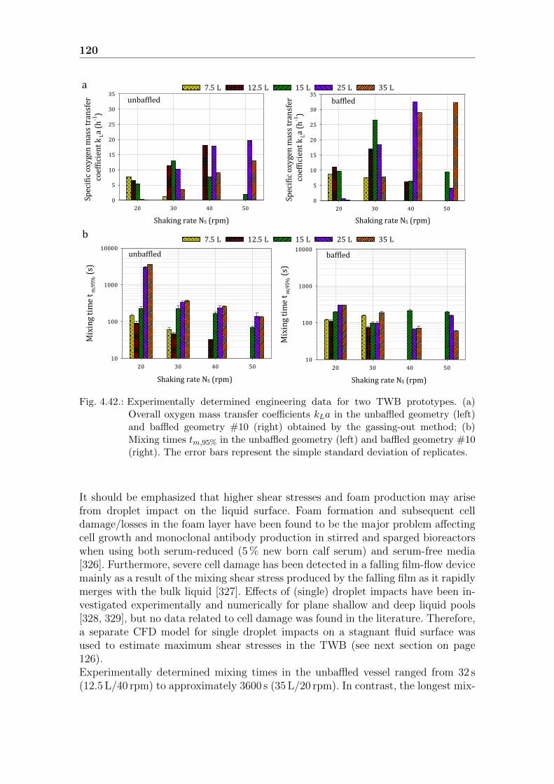
120
Shaking rate NR (rpm)
20 30 40 50
Mix
ing
tim
e t m
,95
% (
s)
10
100
1000
100007.5 L Col 12 Col 20 Col 28 Col 36
Shaking rate NR (rpm)
20 30 40 50
Mix
ing
tim
e t m
,95
% (
s)
10
100
1000
100007.5 L Col 15 Col 23 Col 31 Col 39
Shaking rate NR (rpm)
20 30 40 50
Spec
ific
oxy
gen
mas
s tr
ansf
er
coef
fici
ent
kLa
(h-1
)
0
5
10
15
20
25
30
35
7.5 L 12.5 L 15 L 25 L 35 Lb
a
unbaffled
Shaking rate NR (rpm)
20 30 40 50
Mix
ing
tim
e t m
,95
% (
s)
10
100
1000
100007.5 L Col 12 Col 20 Col 28 Col 36
Shaking rate NR (rpm)
20 30 40 50
Mix
ing
tim
e t m
,95
% (
s)
10
100
1000
100007.5 L Col 15 Col 23 Col 31 Col 39
baffled
Shaking rate NR (rpm)
20 30 40 50
Spec
ific
oxy
gen
mas
s tr
ansf
er
coef
fici
ent
kLa
(h-1
)
0
5
10
15
20
25
30
357.5 L Shaking rate (rpm) vs Col 11 - Col 11 Shaking rate (rpm) vs Col 19 - Col 19 Shaking rate (rpm) vs Col 27 - Col 27 Shaking rate (rpm) vs Col 35 - Col 35
Shaking rate NR (rpm)
20 30 40 50
Spec
ific
oxy
gen
mas
s tr
ansf
er
coef
fici
ent
kLa
(h-1
)
0
5
10
15
20
25
30
357.5 L Shaking rate (rpm) vs Col 14 - Col 14 Shaking rate (rpm) vs Col 22 - Col 22 Shaking rate (rpm) vs Col 30 - Col 30 Shaking rate (rpm) vs Col 38 - Col 38
unbaffled
Shaking rate NR (rpm)
20 30 40 50
Spec
ific
oxy
gen
mas
s tr
ansf
er
coef
fici
ent
kLa
(h-1
)
0
5
10
15
20
25
30
35
7.5 L 12.5 L 15 L 25 L 35 L
Shaking rate NS (rpm) Shaking rate NS (rpm)
Shaking rate NS (rpm)Shaking rate NS (rpm)
Fig. 4.42.: Experimentally determined engineering data for two TWB prototypes. (a)Overall oxygen mass transfer coefficients kLa in the unbaffled geometry (left)and baffled geometry #10 (right) obtained by the gassing-out method; (b)Mixing times tm,95% in the unbaffled geometry (left) and baffled geometry #10(right). The error bars represent the simple standard deviation of replicates.
It should be emphasized that higher shear stresses and foam production may arisefrom droplet impact on the liquid surface. Foam formation and subsequent celldamage/losses in the foam layer have been found to be the major problem affectingcell growth and monoclonal antibody production in stirred and sparged bioreactorswhen using both serum-reduced (5 % new born calf serum) and serum-free media[326]. Furthermore, severe cell damage has been detected in a falling film-flow devicemainly as a result of the mixing shear stress produced by the falling film as it rapidlymerges with the bulk liquid [327]. Effects of (single) droplet impacts have been in-vestigated experimentally and numerically for plane shallow and deep liquid pools[328, 329], but no data related to cell damage was found in the literature. Therefore,a separate CFD model for single droplet impacts on a stagnant fluid surface wasused to estimate maximum shear stresses in the TWB (see next section on page126).Experimentally determined mixing times in the unbaffled vessel ranged from 32 s(12.5 L/40 rpm) to approximately 3600 s (35 L/20 rpm). In contrast, the longest mix-

4.3. Development of the traveling wave bioreactor 121
ing time in the baffled vessel was about 300 s, a decrease of a factor of 12. It should beemphasized that mixing times in the baffled geometry were still significantly longerthan in stirred and orbitally shaken bioreactors at comparable power inputs. For ex-ample, mixing times of below 20 s have been reported for the BIOSTAT R©CultiBagSTR and S.U.B. Hyclone bioreactors operated at specific power inputs of between20 and 100 W m−3 [59]. Mixing times of between 10 s and 150 s have been measuredin orbitally shaken cylindrical bioreactors at 30 L scale [330]. Nevertheless, longermixing times in the order of 500 s have also been reported for wave-mixed systemsand orbitally shaken flasks, using water-like media under different operating con-ditions [14], however these long mixing times are often not accepted in industrialproduction.Fig. 4.43 presents the fluid flow inside the baffled torus of modifications #6 and #10after 20 s of flow time, under quasi-periodic flow conditions. In agreement with ex-pectations, the highest fluid velocities of approximately 1.85 ms−1 were found nearthe wave crest, which was about 20 % higher than in the unbaffled vessel underidentical operational conditions. Similarly to the unbaffled geometry, velocity gradi-ents were found between the inner and outer radius as a result of centrifugal forces.Significantly lower liquid velocities of ≤ 0.1 utip were predicted in front of the trav-eling wave. However, a recirculation zone was created in the baffled vessel, where acounter-clockwise flow was found in approximately a quarter of the annulus, whilethe main part of the liquid kept flowing in a clockwise direction, as one would ex-pect. The two flow directions met in close proximity to the traveling wave, whichwas expected to significantly improve mixing. Interestingly, this flow feature waspredicted for both baffle designs, with cork-screw and concentric ring shaped pro-tuberances. Furthermore, the protuberances induced local flow structures that weredirected towards the center of the annulus, as can be seen in the detail views of Fig.4.43. As a result of the relatively lower pressure behind each baffle, small vorticesoccurred in these regions, which may have further improved mixing in the baffledvessels compared to the unbaffled design. Again, this was confirmed by experimen-tally determined mixing times, as shown in Fig. 4.42b.Nevertheless, it was found that the out-of-phase phenomenon occurred at signifi-cantly lower rotational speeds in the baffled vessels compared to the unbaffled ge-ometry, provided they are operated with equal filling volumes and identical liquidproperties. This was confirmed by experimental observations and is in agreementwith findings for shaken flasks [81]. The critical shaking speed, above which out-of-phase conditions occurred, could be correlated by Eq. 4.71 and Eq. 4.7220. Thus,the influences of both the filling volume and the kinematic viscosity were lower forthe baffled vessel than for the unbaffled geometry.
NCS,baffled = 105.6VL0.422 νL
−0.052 (4.71)
For the unbaffled TWB the following correlation was found:
NCS,unbaffled = 119.1VL0.61 νL
−0.128 (4.72)
20The terms VL and νL should be inserted with standard SI units according to the list of symbolsin order to calculate NCS in rpm.

122
a b
90°
180°
270°
0°
90°
180°
270°
0°
0°
180°
90°270°
0°
180°
90°270°
Liq
uid
vel
oci
ty m
agn
itu
de
uL (
m s
-1)
Liq
uid
vel
oci
ty m
agn
itu
de
uL (
m s
-1)
1.10
0.99
0.88
0.77
0.66
0.55
0.44
0.33
0.22
0.11
0.00
1.10
0.99
0.88
0.77
0.66
0.55
0.44
0.33
0.22
0.11
0.00
Fig. 4.43.: CFD predicted fluid velocities in the baffled modifications #6 and #10. (a)Cork-screwed shape protuberances; (b) concentric ring shaped protuberances.Colored iso-surfaces at half initial filling height z/HL = 0.5 and defined crosssections are presented with vectors of fixed length (25 mm) and projected tothe given planes.
In Fig. 4.44, the CFD predicted power inputs of the six baffled geometry modifi-cations at a shaking frequency of 40 rpm and amplitude of 25 mm are presented.The power input increased after the starting phase (3 s of flow time) and periodicflow conditions were achieved after approximately 18 s, when the specific power in-put fluctuated around mean values of between 10.5 Wm−3 (modification #9) and86 Wm−3 (modification #10). This was consistent with the profiles of velocitiesthrough the annulus cross sections (data not shown). The local peaks in the profilesof the specific power inputs could be attributed to the collision of the wave frontwith the protuberances. Six and ten peaks were found within one rotational periodfor the geometries with six and ten baffles respectively.Comparing the mean specific power inputs at quasi-periodic conditions, it becameobvious that, at an amplitude of 25 mm, the highest specific power input of 86 Wm−3
was predicted for modification #10 (6 concentric rings with rB/R = 0.11), as shownin Fig. 4.45a. A very similar specific power input of 82.4 Wm−3 was determined withan identical number of cork-screws (in modification #6). Increasing both, the num-ber of screws/rings and the diameter of the protuberances, resulted in decreasingspecific power inputs, whereas the lowest value for modification #9 with rB/R =0.33 could be attributed to out-of-phase conditions where only low fluid velocitiesof up to 0.4utip were predicted, and almost no wave motion was recognizable. Thelower specific power inputs, even under in-phase conditions, may be explained bylower average fluid velocities in the direction of rotation, which can be attributed toreversed flow. Surprisingly, the differences between the different baffle designs wereless pronounced when a shaking amplitude of 50 mm was used. Under these condi-tions, specific power inputs between 209.6 Wm−3 (modification #6) and 255.7 Wm−3
(modification #8) were predicted, which are at the upper limit for cell culture ap-plications [133].

4.3. Development of the traveling wave bioreactor 123
Spec
ific
po
wer
inp
ut
P/V
L (
W m
-3)
0
50
100
150
200
250
300
Spec
ific
po
wer
inp
ut
P/V
L (
W m
-3)
0
50
100
150
200
250
Flow time t (s)
0 2 4 6 8 10 12 14 16 18
Spec
ific
po
wer
inp
ut
P/V
L (
W m
-3)
0
50
100
150
200
250
Flow time t (s)
0 2 4 6 8 10 12 14 16 18 20
Mod#6: 6 windings, a/R = 0.11 Mod#7: 10 windings, a/R = 0.11
Mod#8: 6 windings, a/R = 0.22 Mod#9: 6 windings, a/R = 0.33
Mod#10: 6 rings, a/R = 0.11 Mod#11: 6 rings, a/R = 0.22
Fig. 4.44.: Profiles of the specific power input in the baffled torus geometries as a functionof time. The local peaks can be ascribed to collisions of the wave front with theprotuberances. For the modification #9 out-of-phase conditions were found atoperational conditions of 40 rpm and 25 mm amplitude. The dashed lines indi-cate the time-averaged specific power inputs after reaching periodic conditions(see also Fig. 4.45a).
Considering the iso-surface for an air volume fraction of 0.5, it could be statedthat the volume specific gas-liquid surface area aL increased as the radius of theprotuberances increased, which can be explained by enhanced liquid splashing andbubble entrainment. While aL was 13.2 m2m−3 in modification #6 (rB/R = 0.11), itwas 13.8 m2m−3 in modification #8 (rB/R = 0.22), at a shaking amplitude of 25 mmafter 20 s of flow time (see Fig. 4.45b). A further increase in the specific surface forrB/R = 0.33 (modification #9) was only achieved at the higher shaking amplitude,which could again be ascribed to out-of-phase conditions. Interestingly, the increaseof aL was obvious for both protuberance shapes, but the effect of increasing rB/Rratios seemed to be less pronounced for the cork-screws (e.g. from ≈13.3 m2m−3 atrB/R = 0.11 to ≈13.4 m2m−3 at rB/R = 0.22) compared to the concentric rings(≈13.3 m2m−3 to ≈13.8 m2m−3 for identical geometric ratios).

124
Geometry
Mod #6 Mod #7 Mod #8 Mod #9Mod #10Mod #11Original
Spec
ific
su
rfac
e ar
ea a
L (
m2 m
-3)
12.0
12.5
13.0
13.5
14.0
14.5
15.0
15.5
16.0
25 mm50 mm
Geometry
Mod #6 Mod #7 Mod #8 Mod #9Mod #10Mod #11OriginalSpec
ific
po
wer
in
pu
t P
/VL (
W m
-3)
0
50
100
150
200
250
30050 mm25 mm
a b
Geometry
Mod #6 Mod #7 Mod #8 Mod #9Mod #10Mod #11Original
Spec
ific
su
rfac
e ar
ea a
L (
m2 m
-3)
12.0
12.5
13.0
13.5
14.0
14.5
15.0
15.5
16.0
25 mm50 mm
Geometry
Mod #6 Mod #7 Mod #8 Mod #9Mod #10Mod #11OriginalSpec
ific
po
wer
in
pu
t P
/VL (
W m
-3)
0
50
100
150
200
250
30050 mm25 mm
Mo
d #
6
Mo
d #
7
Mo
d #
8
Mo
d #
9
Mo
d #
10
Mo
d #
11
Ori
gin
al
Mo
d #
6
Mo
d #
7
Mo
d #
8
Mo
d #
9
Mo
d #
10
Mo
d #
11
Ori
gin
al
Fig. 4.45.: CFD predictions for different baffled torus designs. (a) Specific power inputP/VL; (b) specific gas-liquid surface area (iso-surface at αG = 0.5). All simu-lations were realized for a rotational speed of 40 rpm with shaking amplitudesof 25 mm and 50 mm respectively.
Showing comparable fluid behaviour to modification #6, design #10 was favoured forfurther prototype experiments because of its simpler vessel construction. As knownfrom other SU bioreactors, the manufacturing of flexible bags instead of rigid cul-tivation containers is more cost-effective and simplifies handling and storage. Eventhough the cork-screwed protuberances may also be integrated as rigid plastic partsin flexible film bags, it was believed that concentric rings would be easier to buildfor bioreactor prototyping and future bioreactor manufacturing21.In Fig. 4.46, the CFD predicted Reynolds numbers and specific power inputs areshown for various operating conditions, for shaking speeds in the range of 30 rpmand 50 rpm and filling volumes from 15 L to 35 L and a constant shaking amplitudeof 25 mm. Not entirely surprisingly, the Reynolds number increased as the shakingrate and filling volume increased, which has already been described for the unbaf-fled annulus (see section 4.3.5). At working volumes of 15 L and 25 L, out-of-phaseoperation was observed for shaking rates above 30 rpm and 40 rpm respectively,which agreed with experimental observations. Considering in-phase conditions, de-termined time-averaged Reynolds numbers, based on Eq. 4.53, ranged from 0.8× 10⁴
to 4.83× 10⁴, indicating fully turbulent conditions for all operating conditions. Nev-ertheless, despite the more rigorous mixing introduced by the protuberances, theReynolds numbers were up to a factor of 2.4 lower than in the unbaffled vessel.This could be explained by the reverse flow regions inside the baffled annulus, whichlowered the characteristic velocity.In contrast, the specific power inputs under in-phase conditions were higher than inthe unbaffled counterpart, which may be explained by a higher momentum transferarea resulting from the liquid splashing on the protuberances. Specific power inputs
21Within the scope of the present thesis, only a few prototypes were constructed for proof-of-concept cultivations using CHO suspension cells (see section 4.3.8).

4.3. Development of the traveling wave bioreactor 125
in the range of 6.0 Wm−3 (30 rpm/35 L) and 86 Wm−3 (40 rpm/25 L) were deter-mined (see Fig. 4.46), which is up to 2.4-fold higher than in the unbaffled geometry(for identical shaking parameters). For low viscosity fluids, it has been reportedthat, for identical Reynolds numbers, the volumetric power consumption in baffledshake flasks is about one order of magnitude higher than in unbaffled shake flasks[84]. Even though the operational range of the baffled geometry is restricted (sinceout-of-phase conditions are more likely) based on the CFD models, typical specificpower inputs for cell culture applications are achievable with moderate agitation.Furthermore, the agitation may be reduced, compared to the unbaffled annulus, be-cause of the higher mass transfer in the baffled vessel.The predicted shear stresses in the baffled annulus are compared with those for theunbaffled geometry in Fig. 4.47. Similar to the unbaffled geometry, the highest localshear stresses were found near the wave crest and exceeded the volume-averagedshear stresses by about two orders of magnitude. Particularly around entrappedair bubbles and near the protuberances, shear stresses of up to 0.7 Pa were pre-dicted, depending on the operational conditions. This was an increase by a factorof up to 7.4 (for 15 L at 50 rpm and 25 mm) compared to the unbaffled geometry,while the mean increase was approximately four-fold. In both geometries, the localnormal stresses were approximately 50 % lower than the shear stresses for identi-cal operational conditions, which was in agreement with expectations. Interestingly,the volume-averaged local shear stresses in both geometries could be approximatedby a single correlation (τnt ∝ (P/VL)0.318; see Fig. 4.47b) and the results for mostoperational conditions were within a confidence interval of ±30 %. In contrast, twoseparate correlations were obtained for the maximum shear stresses, which indicateda different ratio of maximum and volume-averaged local shear stresses (τnt,max/τnt)in the baffled annulus compared to its unbaffled counterpart.
Shaking rate NR (rpm)
30 40 50
Av
erag
ed R
eyn
old
s n
um
ber
R
e (x
10
4)
0
1
2
3
4
5
6
15 L25 L35 L
Shaking rate NR (rpm)
30 40 50Spec
ific
po
wer
in
pu
t P
/VL (
W m
-3)
0
10
20
30
40
50
60
70
80
90
100
15 L25 L35 L
Shaking rate NR (rpm)
30 40 50
Av
erag
ed R
eyn
old
s n
um
ber
R
e (x
10
4)
0
1
2
3
4
5
6
15 L25 L35 L
Shaking rate NR (rpm)
30 40 50Spec
ific
po
wer
in
pu
t P
/VL (
W m
-3)
0
10
20
30
40
50
60
70
80
90
100
15 L25 L35 L
a b
*
*****
Shaking rate NS (rpm) Shaking rate NS (rpm)
Fig. 4.46.: CFD predicted fluid flow data for the baffled geometry modification #10 undervarious operating conditions. (a) Averaged Reynolds number; (b) specific powerinput. The stars indicate out-of-phase conditions.
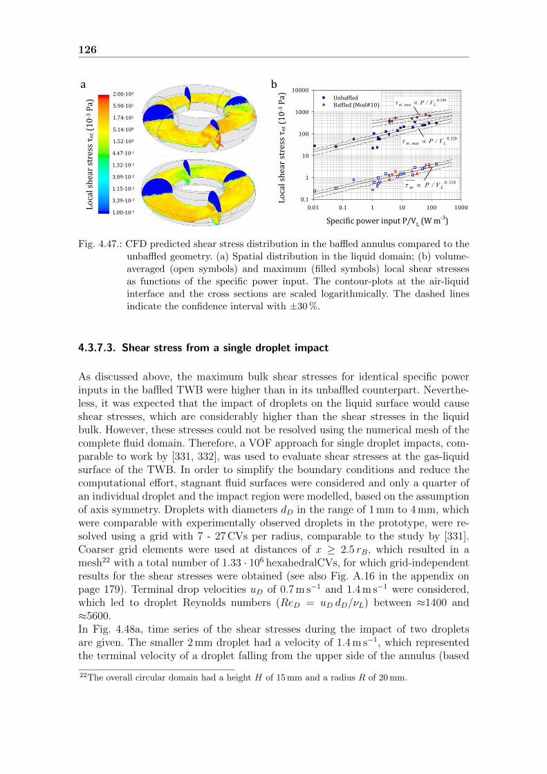
126
Specific power input P/VL (W m-3)
0.01 0.1 1 10 100 1000
Lo
cal s
hea
r st
ress
n
t (1
0-3
Pa)
0.1
1
10
100
1000
10000
UnbaffledBaffled (Mod#10)
2.00·102
5.90·101
1.74·101
5.14·100
1.52·100
4.47·10-1
1.32·10-1
3.89·10-2
1.15·10-2
3.39·10-3
1.00·10-3
a b1890.
Lmax,nt V/P
3280.Lmax,nt V/P
3180 .Lnt V/P
Lo
cal s
hea
r st
ress
τn
t (1
0-3
Pa)
Lo
cal s
hea
r st
ress
τn
t (1
0-3
Pa)
Fig. 4.47.: CFD predicted shear stress distribution in the baffled annulus compared to theunbaffled geometry. (a) Spatial distribution in the liquid domain; (b) volume-averaged (open symbols) and maximum (filled symbols) local shear stressesas functions of the specific power input. The contour-plots at the air-liquidinterface and the cross sections are scaled logarithmically. The dashed linesindicate the confidence interval with ±30 %.
4.3.7.3. Shear stress from a single droplet impact
As discussed above, the maximum bulk shear stresses for identical specific powerinputs in the baffled TWB were higher than in its unbaffled counterpart. Neverthe-less, it was expected that the impact of droplets on the liquid surface would causeshear stresses, which are considerably higher than the shear stresses in the liquidbulk. However, these stresses could not be resolved using the numerical mesh of thecomplete fluid domain. Therefore, a VOF approach for single droplet impacts, com-parable to work by [331, 332], was used to evaluate shear stresses at the gas-liquidsurface of the TWB. In order to simplify the boundary conditions and reduce thecomputational effort, stagnant fluid surfaces were considered and only a quarter ofan individual droplet and the impact region were modelled, based on the assumptionof axis symmetry. Droplets with diameters dD in the range of 1 mm to 4 mm, whichwere comparable with experimentally observed droplets in the prototype, were re-solved using a grid with 7 - 27 CVs per radius, comparable to the study by [331].Coarser grid elements were used at distances of x ≥ 2.5 rB, which resulted in amesh22 with a total number of 1.33 · 106 hexahedralCVs, for which grid-independentresults for the shear stresses were obtained (see also Fig. A.16 in the appendix onpage 179). Terminal drop velocities uD of 0.7 m s−1 and 1.4 m s−1 were considered,which led to droplet Reynolds numbers (ReD = uD dD/νL) between ≈1400 and≈5600.In Fig. 4.48a, time series of the shear stresses during the impact of two dropletsare given. The smaller 2 mm droplet had a velocity of 1.4 m s−1, which representedthe terminal velocity of a droplet falling from the upper side of the annulus (based
22The overall circular domain had a height H of 15 mm and a radius R of 20 mm.

4.3. Development of the traveling wave bioreactor 127
on uD =√
2Rg). The larger 4 mm droplet had a velocity of 0.7 m s−1, leading toan identical Reynolds number (Re = 2800). Both droplets caused similarly shapedcraters, even though the crater was deeper for the larger bubble. In both cases, tinyair bubbles with dB ≈5 · 10−5 m were entrapped, which was comparable to exper-imental observations described in the literature [332]. Keeping in mind, that verysmall bubbles cause very high local power inputs during bubble rupture at the liquidsurface, their appearance may be a reason for increased shear stresses. However, itwas not possible to estimate their contribution to the total shear stress because thegrid resolution was still too coarse.
x-coordinate x (mm)
-4 -3 -2 -1 0 1 2 3 4
y-c
oo
rdin
ate
y (
mm
)
-5
-4
-3
-2
-1
0
1
2
3
41.67 ms, CFD5.80 ms, CFD10.8 ms, CFD15.83 ms, CFD
1.67 m, Exp. [332]5.83 ms, Exp. [332]10.83 ms, Exp. [332]15.83 ms, Exp. [332]
Droplet Reynolds number ReD (-)
0 1000 2000 3000 4000 5000 6000
Max
imu
m s
hea
r st
ress
n
t,max
(P
a)
0.1
1
10
100
1000
dD = 1 mm
dD = 2 mm
dD = 3 mm
dD = 4 mm
30 ms
a
Lo
cal s
hea
r st
ress
τn
t (P
a)
1.00·101
2.51·100
6.31·10-1
1.58·10-1
3.98·10-2
1.00·10-2
2.51·10-3
6.31·10-4
1.58·10-4
3.98·10-5
1.00·10-5
7.5 ms
12.5 ms
18 ms
30 ms
dD = 4 mm; ws = 0.7 m s-1dD = 2 mm; ws = 1.4 m s-1
5.0 ms
11 ms
15 ms
25 ms
Max
imu
m s
hea
r st
ress
τ n
t,m
ax (
Pa)
b c
Fig. 4.48.: Results of the local shear stress analysis for single droplet impact on gas-liquidsurface. (a) Time series of the shear stresses during the impact of two droplets;(b) maximum shear stresses during the impact phase for different dropletsfalling at 0.7 m s−1 (filled symbols) and 1.4 m s−1 (open symbols); (c) modelvalidation with experimental data from the literature [332]. The horizontaldashed line represents the maximum shear rate in the bulk region of the TWB.

128
Another source of shear stress may be the jet formation as the liquid at the crater’sbottom moved upwards. Indeed the maximum local shear stresses, which were pre-dicted to be 0.23 - 4.67 · 102 Pa, were mostly determined during this phase. Nofunctional relationship between the maximum shear stress and the droplet Reynoldsnumber (or the droplet Weber number) was found, but all maximum stresses wereconsiderably larger, by at least one order of magnitude, than predicted values inthe bulk of the baffled TWB (see Fig. 4.48b). The latter were below 0.7 Pa for allinvestigated operational conditions. As already discussed in section 4.1.2, reportedcritical values that cause substantial cell damage are in the order of 1 - 3 · 102 Pa[16].It should be emphasized, that the single-drop impact CFD studies were not vali-dated by any experimental data. However one test case for a 2.95 mm droplet fallingwith 1.05 m s−1 was compared with a study from the literature [332], that was val-idated by high-speed video sequences. Even though the boundary conditions werenot identical, the overall agreement between the present CFD model and that fromthe literature was satisfying (see Fig. 4.48c).Based on these results, it could be concluded, that cell damage in the (baffled) TWBwas only expected under rigorous agitation with significant splashing and bubble en-trapment at the gas-liquid interface. In order to verify the suitability of the TWBfor cell culture applications, CHO suspension cells were cultivated using chemicallydefined media, as described in detail in the following section.
4.3.8. Proof-of-concept cultivation
In order to evaluate the applicability of the TWB for cell culture growth, fed-batchexperiments with a Chinese Hamster Ovary (CHO XM111-10 ) cell line were per-formed in the unbaffled and baffled prototypes. The initial volume was 12.5 L, repre-senting the minimum recommended working volume based on the engineering char-acterization. In order to avoid substrate limitations (i.e. cgluc < 0.6 gL−1), two mediafeeds of 2.5 L HP-1 and 10 L HP-5 growth media were performed after ≈30 h and(41± 1) h respectively. The shaking speed of the unbaffled vessel was set to between30 rpm and 35 rpm, depending on the filling volume. Due to the higher power input,shaking speeds between 25 rpm and 32 rpm were used in the baffled prototype, inorder to meet specific power inputs in the range of 20 Wm−3 to 30 Wm−3 and kLavalues above 10 h−1. The air flow rate was varied from 0.25 L min−1 to 0.5 L min−1,corresponding to volumetric aeration rates of approximately 0.02 vvm. Since oxygenmass transfer was not influenced by the aeration rate, as determined by kLa mea-surements (data not shown), these low aeration rates were expected to be sufficient,while evaporation was effectively minimized.Comparison cultivations in the rocker-type wave-mixed SmartRocker
TMbioreactor
(Finesse Solutions, Inc.) using the identical cultivation procedure were also carriedout. In the first run, the rocking rate and angle were set to 20 - 24 rpm and 6 respec-tively, which represented routinely used agitation parameters. In the second run, theagitation was increased to 35 rpm and the angle set to 10 after the second medium

4.3. Development of the traveling wave bioreactor 129
addition in order to mimic the bubble entrainment and foam formation observedin the TWB (see discussion below). In both runs, dissolved oxygen concentrationswere maintained above 30 % without the supply of pure oxygen (comparable to theTWB), which provided sufficient oxygen transfer rates, even though no kLa valueswere available for the wave-mixed cultivation system.In Fig. 4.49a, the profiles of viable cell densities and viabilities for the baffled and un-baffled prototypes are compared with those of the wave-mixed cultivation system.During the first 60 hours, the cell growth was comparable in all the cultivations.Starting from the inoculation density of (0.50± 0.05) · 106 cellsmL−1, the viable celldensity increased exponentially to values between 1.82 · 106 cellsmL−1 (SmartRocker,Run#2) and 2.31 · 106 cellsmL−1 (TWB, unbaffled) before the first media additions.Average growth rates of (1.116± 0.026) d−1 and doubling times of (14.9± 0.3) hwere determined, which were also in good agreement with the cell expansions in thewave-mixed CultiBag R©RM 10L bioreactor. Here, growth rates of (1.056± 0.012) d−1
were obtained, which indicated that comparable cell growth was maintained duringthe scaling-up process.Directly after the second medium feed step, viable cell densities of between approxi-mately 1.28 · 106 cellsmL−1 (SmartRocker, Run#1) and 1.66 · 106 cellsmL−1 (TWB,unbaffled) were measured. Afterwards, the cells grew exponentially for durations ofbetween 15 h and 30 h with specific growth rates of (0.818± 0.115) d−1 before theyentered the stationary phase. These corresponded to doubling time of (20± 26) hoursand were, therefore, approximately 35 % longer than before the second media addi-tion, which could be a result of elevated ammonium and lactate levels of≤0.85 mmolL−1
and ≤1.2 gL−1 respectively (see Fig. 4.49b and c). However, the growth rates werestill comparable to several studies accomplished with the same cell line and culturemedia in different single-use bioreactor systems from benchtop to pilot scale (seeTab. 4.14). The specific growth rate usually ranged from 0.72 h−1 to 0.96 h−1. In thepresent study, the peak viable cell densities of between 3.27 · 106 cellsmL−1 (TWB,baffled) and 5.4 · 106 cellsmL−1 (TWB, unbaffled) were measured after 66.3 h and87.8 h of process time respectively. Thus, the highest viable cell density was deter-mined in the unbaffled TWB prototype. It should be noted, that the accuracy ofthe cell density determination could be slightly affected by cell sedimentation inthe TWB. At the end of the process, the total cell densities of two samples, onetaken from the sampling port and the other via the liquid surface, deviated fromeach other by approximately 10 % (with the higher value determined at the vesselbottom, i.e. through the sampling port).Furthermore, it should be emphasized that cell viability remained above 90 % untilthe end of the exponential growth phases in all cultivations. Interestingly, the cell via-bility in the baffled vessel decreased to ≈93 % after the second media addition, whichwas probably due to the continuous entrainment of gas bubbles and foam formation.This could be associated with the wave breaking and liquid splashing near the protu-berances, even though the agitation speed was lower than in the unbaffled geometry(with comparable mass transfer rates and power inputs). Because of the foam forma-tion, the addition of an anti-foam agent (Antifoam Solution C, Sigma-Aldrich) wasrequired in order to prevent filter clogging and foam-entrapment of the cells. Similar

130
behaviour was also observed in the wave-mixed rocker-type SmartRocker bioreac-tor (run #2) operated at higher agitation, where the cell viability also decreasedto ≈93 % and the peak cell density of 3.94 · 106 cellsmL−1 was approximately 15 %lower than in the low agitation run. Several studies have indicated that cell damagein sparged cultures is more likely than in bubble-free processes [69].Nevertheless, similar metabolic profiles were found in all cultures, where the mainsubstrate glucose was consumed until complete depletion approximately 88 hourspost inoculation in each run (see Fig. 4.49b). Glutamine was usually depleted after50 h of process time. At the end of the exponential growth phase, the cells startedto consume lactate as a secondary substrate. This metabolic shift was accompaniedby an increase in the ammonia formation rate. The maximum ammonium concen-trations ranged from 2.03 mmolL−1 to 2.72 mmolL−1, which is within usual rangesat the end of the cultivation.The online data from the experiment with the unbaffled vessel are given in Fig. 4.49dto Fig. 4.49f. The dissolved oxygen concentration was maintained above 35 % overthe complete process. Prior to the first medium addition, the DO level decreasedcontinuously to approximately 40 %. After each media addition, the DO level in-creased because of the dilution of cells, while the mass transfer rate was similar foreach filling volume, based on the engineering characterization (see section 4.3.7). Asthe viable cell density decreased, the DO level increased to 70 %, due to the loweroxygen consumption of the culture. Due to oxygen consumption during the exponen-tial cell growth phase the oxygen concentration in the off-gas showed a decreasingtrend until the end of the growth phase (see Fig. 4.49e). After 56 h of process time,the carbon dioxide supply for pH regulation was reduced manually, because the pHvalue was below 6.9. This reduction led to an increase in the oxygen concentrationin the exhaust gas. The oxygen increase at the end of the process could be explainedby progressive cell death.As can be seen from Fig. 4.49f, good agreement was found between online data ofthe pH value, which was determined by the optical sensors, and the offline analysisusing an electrochemical probe (Mettler Toledo, Switzerland). Due to the reductionof carbon dioxide in the gas supply after 56 h, the pH value increased after havingcontinuously decreased due to acid formation and carbon dioxide accumulation asa result of the metabolic activity. The final increase in pH could again be ascribedto cell death.In summary, it was demonstrated that the TWB is suitable for the cultivation ofCHO suspension cells in chemically-defined minimal media. Considering that onlytwo proof-of-concept cultivations were realized without further process optimization,maximum cell densities of up to 5.5 · 106 cellsmL−1 represent a promising basis forfurther investigations, which should also evaluate the reproducibility of obtainedresults. Considering the present results, the unbaffled bioreactor seems to providehigher cell densities of the used cell line, even though the mixing and mass transfercapacities are lower than in the baffled geometry. Nevertheless, it is difficult to drawgeneral conclusions without further optimization studies.

4.3. Development of the traveling wave bioreactor 131
Tab. 4.14.: Summary of reported cultivation results with the CHO XM111-10 cell lineusing chemically defined medium in different single-use bioreactors.
Cultivation systemSpecificpower input
Aerationrate
Specificgrowth rate
Doublingtime Ref.
P/VL (Wm−3) QG (vvm) µ (d−1) tD (h)
Mobius R©CellReady3L bioreactor
0.9 - 3 n.a. 0.72 23 [4]5 - 14 0.1 - 0.2a 0.50 - 0.96 17.3 - 30.1 [333]
UniVessel 2L SU ≈ 15 0.1 - 0.2a 0.89 - 0.94 17.8 - 18.7 [71]
BIOSTAT R©CultiBagRM20 (optical)
n.a. 0.01 - 0.1b 0.94 - 1.10 15.2 - 17.5 [334]n.a. 0.1 - 0.2b 0.72 23.0 [128]
Hyclone S.U.B. 50L ≈ 30 0.01 - 0.1a 0.77 - 0.91 18.2 - 21.7 [334]
BIOSTAT R©CultiBagSTR 50L
15 - 90 0.1 - 0.3a ≈ 0.91 ≈ 18.2 [71]n.a. n.a. 1.01 16.5 [335]
BIOSTAT R©CultiBagSTR 200L
60 0.1 - 0.4a ≈ 0.65 ≈ 25.7 [71]
TWB prototype ≈ 30 0.02b 0.84 - 1.15 14.4 - 20this
studya Submersed aeration with air and oxygen supply; b surface aeration with air. n.a. - datanot available.

132
Process time t (h)
0 12 24 36 48 60 72 84 96 108 120
Via
ble
ce
ll d
en
sity
VC
D (
10
6 c
ell
s m
L-1
)
0
1
2
3
4
5
6
Via
bil
ity
v (
%)
10
25
40
55
70
85
100
VCD, unbaffled
VCD, baffled
VCD, SB#1
VCD, SB#2
Viability, unbaffled
Viability, baffled
Viability, SB#1
Viability, SB#2
Process time t (h)
0 12 24 36 48 60 72 84 96 108 120
Glu
cose
co
nce
ntr
ati
on
cG
luc (
g L
-1)
0
1
2
3
4
5
La
cta
te c
on
cen
tra
tio
n c
La
c (
g L
-1)
0.0
0.5
1.0
1.5
2.0
2.5
Gluc, unbaffled
Gluc, baffled
Gluc, SB#1
Gluc, SB#2
Lac, unbaffled
Lac, baffled
Lac, SB#1
Lac, SB#2
Process time t (h)
0 12 24 36 48 60 72 84 96 108 120
Glu
tam
ine
co
nce
ntr
ati
on
cG
ln (
mM
)
0.0
0.1
0.2
0.3
0.4
0.5
0.6
0.7
Am
mo
niu
m c
on
cen
tra
tio
n c
NH
4+ (
mM
)
0.0
0.4
0.8
1.2
1.6
2.0
2.4
2.8
Gln, unbaffledGln, baffled Gln, SB#1 Gln, SB#2
NH4
+, unbaffled
NH4
+, baffled
NH4
+, SB#1
NH4
+, SB#2
Process time t (h)
0 12 24 36 48 60 72 84 96 108 120
Dis
solv
ed
ox
yg
en
DO
(%
sat)
Sh
ak
ing
ra
te N
R (
rpm
)
0
10
20
30
40
50
60
70
80
90
100
Dissolved oxygen
Shaking rate
Process time t (h)
0 12 24 36 48 60 72 84 96 108 120
Ox
yg
en
co
nce
ntr
ati
on
cO
2
(v
ol%
)
16.0
16.4
16.8
17.2
17.6
18.0
18.4
18.8
Process time t (h)
0 12 24 36 48 60 72 84 96 108 120
pH
va
lue
(-)
6.0
6.4
6.8
7.2
7.6
8.0
pH, online
pH, offline
a b c
d e f
Fig. 4.49.: Results from a proof-of-concept cultivation in the TWB. (a) Profiles of viable cell density and viability; (b) Profiles of glucoseand lactate; (c) Glutamine and ammonium; (d) Dissolved oxygen and shaking rate; (e) Oxygen concentration in the off-gas;(f) Comparison of online and offline measured pH values. The arrows indicate media additions of 2.5 L ChoMaster R©HP-1 after≈30 h and 10 L ChoMaster R©HP-5 after (41± 1) h respectively.

5. Concluding remarks and outlook
The main focus of this work was Computational Fluid Dynamics and its use forthe development and optimization of single-use bioreactors and biopharmaceuti-cal processes. Since complex hydrodynamics can be found in most bioreactors, andespecially in single-use bioreactors, their detailed characterization is challenging.This involves spatially resolved determination of shear stresses and turbulence whichmay affect cell growth and product expression, leading to reduced product quanti-ties and/or quality. Although different invasive and non-invasive measurement tech-niques, such as Laser Doppler Anemometry (LDA) or Particle Image Velocimetry(PIV), are reliable and required for validation of simulation results, these techniquesare too time consuming for the complete characterization of flows in bioreactors[105]. Furthermore, optical accessibility can be a problem, especially for large scaleSU bioreactors of up to 2 m3 that are commercially available [59].To overcome these limitations, numerical methods may be an effective and cost-efficient alternative, if they are correctly used. Due to their universal mathematicalformulation, based on general conservation equations for mass, momentum and en-ergy, CFD models can potentially be used to describe the fluid flows in bioreactorsover a wide range of scales and operating conditions. However, while CFD modelsare well established in the aerospace and automotive industries, and have been usedfor chemical engineering tasks over decades, interest in the (bio)pharmaceutical areais relatively new.Three potential fields for CFD characterization and optimization of (single-use)bioreactors, which partially overlap, have been identified and discussed in this study:
1. Advanced characterization of single- and multi-phase flows for existing bioreac-tors with the aim of identifying suitable operational conditions and/or scale-upcriteria.
2. Modification and optimization of existing bioreactors with the aim of devel-oping, intensifying and/or optimizing production processes.
3. Development of bioreactors based on conceptional designs.
Based on the findings in this work, the following conclusions can be drawn:
The prediction of general mean flow quantities in single-phase (stirred) bioreac-tors can be expected to be valid, in particular for single-stage impellers, even ifless sophisticated RANS methods are used. Thus, it was shown that reliableengineering parameters of SU bioreactors can be obtained from CFD sim-ulations if the correct models are selected. In the first case study, local flowstructures of the Mobius R©CellReady bioreactor were investigated using numericalmethods for the first time. Acceptable agreements with own PIV measurements andliterature data [192] were found, which revealed a complex fluid flow of the marineimpeller that greatly differed from classic stirrers used in conventional bioreactors.Furthermore, key engineering parameters, such as mixing time and power input,
133

134 Chapter 5. Concluding remarks and outlook
were determined, which also agreed well with experimental measurements and well-established correlations (e.g. Eq. 4.8). While several case studies reported the specificpower input of single- and multi-stage impellers in SU bioreactors (e.g. [62]), onlylimited experimental data on the power input in SU bioreactors were available, inparticular at benchtop scale. For the Mobius R©CellReady bioreactor, power numberswere estimated, both numerically and experimentally, over a wide turbulence rangecovering transitional and fully turbulent conditions. In this context, it was demon-strated that the power input should be determined from the torque actingon the impeller’s surface, instead of summing up the turbulent dissipa-tion rates, as proposed by [212, 213]. The latter method greatly depends on boththe used turbulence model and the grid density and often underestimates the powerinput. This was confirmed for the SU spinner flasks and the UniVessel R©SU used inthe second case study.For these systems, stationary simulations (i.e. under steady-state assumption) us-ing the MRF methodology gave satisfying results and provided a significant savingin computing time compared to time-dependent methods, such as the sliding meshapproach. Even though time savings of a factor of 10 are mentioned in the literature[255], the effective saving in computational time also depends on the chosen conver-gence criteria, the number of CPUs used and the time step size, and can thereforebe even higher (up to 100-fold in own studies, data not shown). Nevertheless, flowprediction with the sliding mesh technique may be required for time dependent flowpatterns where steady state assumptions are not justified and in multiple impellersystems where significant interactions between the impellers occur. Therefore, it hasbeen highlighted that the impeller interaction has been underestimated by the MRFapproach in several studies (e.g. by [213]).The prediction of the turbulence parameter and related phenomena ismuch less accurate [14] and relies on the selection of an appropriate tur-bulence model. As it was shown for the Mobius R©CellReady bioreactor from thefirst case study, turbulence related parameters, such as turbulence dissipation rateor turbulence intensity, significantly differed between the models, which has previ-ously been demonstrated only for conventional stirred systems with fully developedturbulence (e.g. [205]). However, cell culture bioreactors, in particular at milliliterand small liter scale, are usually operated in the transitional range.This is important, because turbulence in bioreactors is associated with hydrody-namic stress on the cells, which is often related to the Kolmogoroff’s microscales ofturbulence [133]. However, based on the results of the first and second case study, itcan concluded that CFD predicted turbulent eddy sizes should be treatedwith caution, in particular when modeling bioreactors with volumes above a fewliters using poor grid resolutions. Besides the grid resolution, the selected turbulencemodel considerably affected the outcomes, a fact that is often neglected in the liter-ature. If hydrodynamic stress of cell cultures is related to Kolmogoroff’s microscalesof turbulence, the turbulent dissipations rates should be determined experimentallyfor validation, for example by time-resolved PIV measurements.Besides turbulence, velocity gradients (often referred to “shear”) are associated withhydrodynamic stress in cell cultures [16, 133, 242, 253]. Several studies from the lit-

135
erature have considered the magnitude of the strain tensor as characteristic shearstress quantity (e.g. [233]), even though it does not describe the shear rate accord-ing to its classical definition (i.e. velocity gradient normal to the flow direction).Nevertheless, CFD models are capable to distinguish between shear andnormal stresses, as proposed by Krause (2007) [240] and Wollny (2010) [231],which allows to study their individual influences on cell cultures. In thepresent study, it was found that the local shear stresses in the Mobius R©CellReadybioreactor exceeded the normal stresses by approximately one order of magnitude.Nevertheless, local flow structures, such as rising gas bubbles [2] or bursting bubblesat liquid surfaces [137], should be taken into account when shear stresses are pre-dicted by CFD, because local shear stresses related to these phenomena may exceedthe values in the bioreactor bulk by several orders of magnitude. For the travellingwave bioreactor, it was assumed that local shear stresses that occur during the im-pact of single droplets at the liquid surface were the highest. Even though somedrop impact studies on liquid films and deep pools have previously been published[331, 332], none of them provided data on shear stresses. Using a high resolutionCFD model of single droplets impacting on a still surface, it was demonstrated thatthe above assumption was correct. Hence, it can be concluded that, while it isoften hard or even impossible to resolve local flow structures in full-scalebioreactor models, the use of high-resolution CFD simulations can shedsome light on local flow phenomena and their influence on shear stress incell cultures.For small scale systems, the grid density can usually increased until grid-independentresults are achieved, a criterion that often cannot be fulfilled for large scale biore-actors. However, this fact is rarely discussed in the literature and still remains anopen question for scale-up studies up to m3 scale. Furthermore, fully-resolved directnumerical simulations are usually not possible in typical bioreactors, because of theenormous computational efforts and the large amounts of generated data [336]. Acompromise between numerical effort and physical accuracy can be seen in the useof Large-Eddy-Simulations (LES) or Detached-Eddy-Simulations (DES), which haveincreasingly been introduced for the modeling of stirred vessels [141–145, 195] andbubble columns [146] during the last decade. Most of these studies have indicatedsubstantially improved predictions with LES, but the tremendous computationalcost, e.g. approximately 30 days of CPU time for a typical multiphase flow simula-tion [89], makes LES still unacceptable in engineering applications.Ever increasing computational power (in terms of processor and memory speed)means that models can be solved faster and larger grids can be handled [12]. Par-allel computing and graphical processor units (GPUs) are currently being used toaccelerate computational processes [337, 338]. However, the increase in performancein parallel computing may be limited by bottlenecks in data exchange between mul-tiple computing nodes. Furthermore, grid generation and post-processing of CFDdata is becoming increasingly time-consuming when using very large meshes. Largerdata storage is also required, especially if transient simulations are performed. Forexample, approximately 4 - 5 GB of data were generated for each travelling wavebioreactor simulation, even though data for only one out of 200 time steps was

136 Chapter 5. Concluding remarks and outlook
stored.Over the last decades, substantial progress has been made in the modeling of multi-phase flows, for both gas-liquid and solid-liquid systems, which are of interest for theprediction of (oxygen) mass transfer and solids suspension. In the case studies fromthe present thesis, Euler-Euler approaches were used, even though the relatively lowvolume fractions of the dispersed phases (≤2 %) could also have been handled, froman computational point of view, by a Euler-Lagrange approach. However, Euler-Euler models are currently applicable over a wider range of process conditions, inparticular with respect to the dispersed phase volume fraction.In the second case study, the solid distributions of microcarriers in smalland benchtop scale bioreactors were modelled with good agreement toexperimental data, for both the fluid flow pattern and the solid distributions.In conjunction with experimental data for suspension criteria, bioengineering datawere obtained which were used for the successful expansion of human mesenchymalstem cells under low serum conditions (≤10 %) [339]. In addition, the approach wasused for scaling-up the hMSC expansion to pilot scales of up to 35 L culture volune[9]. This, however, was not part of the present work.Furthermore, the design of the single-use UniVessel R©SU bioreactor was modified inorder to improve microcarrier suspension, as described in section 4.2.3. Using CFDfor design studies, the number of prototypes was considerably reduced,whereas only the most favourable impeller configurations were tested in the labo-ratory. In contrast to the automotive and chemical industry where CFD codes areexcessively used for design optimizations, only few examples on using CFD for re-actor and process optimizations in the biotechnological field have been published sofar (e.g. [168, 176]). However, using the example of a hMSC expansion process withmicrocarriers, it was shown that CFD can be used for process optimizationby studying the influence of different impellers designs on the fluid flowand resulting shear stresses. Based on the CFD-optimized bioreactor design, thecell yield of therapeutically relevant hADSCs was increased ten-fold, and even themore sensitive hBM-MSCs reached almost threefold higher peak cell densities in theoptimized bioreactor type.While the second case study started with an existing bioreactor, the novel bioreactorconcept for the travelling wave bioreactor was developed only based on the concep-tional design of an orbitally shaken, annular-shaped cultivation chamber, withoutany physical precursor. This again demonstrates the generality of the under-lying physics and solutions algorithms and confirms the advantage usageof CFD models for design studies. Again, the number of prototypes could bereduced, and a few prototypes were constructed in order to verify numerical uncer-tainties and finally prove the applicability for cell culture applications.Some discrepancies were found in the prediction of oxygen mass transfer. For sub-mers aerated vessels, it is well-known that correct prediction of the the bubble sizedistribution, which determines the (local) gas volume fraction and the availablespecific interface surface area, is essential. While previous CFD models assumedconstant bubble sizes, it is current practice to incorporate PBE models thatconsider for bubble size distributions. A main problem in utilizing PBEs is

137
generalizing the closure models to predict for coalescence and break-up rate as afunction of local fluid dynamics and the system’s physical properties. While earlybubble breakup models involved two or more empirical parameters [340, 341], morerecently developed models are more fundamental, because phenomenological break-age (and coalescence) closures are not fully predictive. Current breakup models relyon the assumption of binary breakup. This was indicated to be true for low to mod-erate Weber numbers [342], which can however be assumed to be the case in mostbioreactor, in particular for cell culture applications.While in a former publication a uniform bubble size in the Mobius R©CellReady biore-actor has been assumed [115], the CFD model in the present work was extended bya PBE model with 15 discrete bubble size classes. Substantial differences betweendifferent closure models for the prediction of bubble breakup and coalescence wereidentified. Therefore, the models and boundary conditions must be se-lected carefully, depending on the system of interest, and experimentalvalidation is essential. Whereas acceptable agreement with measurements on thelocal bubble sizes was found, considerable differences in the (local) oxygen trans-fer coefficients were identified, depending on the mass transfer theory used. Eventhough different models have been used in literature studies, there is - to the best ofthe author’s knowledge - no detailed comparative study on the question which masstransfer model is favourable for prediction of oxygen mass transfer in bioreactors oraerated tanks, neither for cell culture applications nor for microbial systems. Thisis further supported by the statement that simple kLa volume averages from CFDsimulations, without knowledge of their correlation with local driving forces, are oflittle practical use, since they would tend to be larger than the global kLa valuesobtained experimentally [183].Besides the classes method (CM) used in the first case study in this thesis, theQuadrature Method Of Moments (QMOM), an improvement of the method of mo-ments (MOM), is increasingly being used to solve PBMs (e.g. [183, 343]). In theseapproaches, bubble sizes are not described directly but via the moments of the sizedistributions, which requires the solution of a limited number of additional trans-port equations (approximately six), thus resulting in far cheaper computational costswhen compared to the CM models. For the future, it is expected that CFD modelsincorporating PBE models will increasingly be used in conjunction with reactionkinetics, as already found in several examples from the literature [168, 344]. Thesecombined models may also shed some light on physiological responses from biologi-cal entities that depend on the local hydrodynamics in the bioreactors, even thoughmathematical descriptions of biological reactions, in particular for cell cultures, arestill unavailable because of the complexity of the underlying reactions.Finally, investigations considering fluid-structure interactions may become attrac-tive. These may be of particular interest for single-use bioreactors made of flexiblebags, where the shapes of the cultivation bags can be influenced by the liquid motion[14].

138

Bibliography
[1] S.C. Kaiser, R. Eibl, M. Kraume, and D. Eibl. Single-use bioreactors foranimal and human cells. In M. Al-Rubeai, editor, Cell Engineering vol. 9:Animal Cell Culture, page in press. Springer, 2014.
[2] A. Koynov, G. Tryggvason, and J.G. Khinast. Characterization of the local-ized hydrodynamic shear forces and dissolved oxygen distribution in spargedbioreactors. Biotechnol. Bioeng., 97(2):317–331, 2007.
[3] BioPlan. 9th Annular Report and Survey of Biopharmaceutical ManufacturingCapacity and Production. 2012.
[4] D. Eibl, T. Peuker, and R. Eibl. Single-use equipment in biopharmaceuticalmanufacture: a brief introduction. In R. Eibl and D. Eibl, editors, Single-usetechnology in biopharmaceutical manufacture, pages 3–11. John Wiley & Sons,Hoboken, NJ, USA, 2010.
[5] R. Eibl, N. Steiger, C. Fritz, D. Eisenkratzer, J. Bar, D. Muller, and D. Eibl.Recommendation for Leachables Studies Standardized cell culture test for theearly identification of critical films. DECHEMA Gesellschaft fur ChemischeTechnik und Biotechnologie e.V., Frankfurt am Main, 2014.
[6] W. Shakespeare. Safety of disposable systems. In S.K. Niazi, editor, Disposablebioprocessing systems, pages 23 – 44. CRC Press, Boca Raton, FL, 2012.
[7] G.J. Madlambayan, I. Rogers, K.A. Purpura, C. Ito, M. Yu, D. Kirouac, R.F.Casper, and P.W. Zandstra. Clinically relevant expansion of hematopoieticstem cells with conserved function in a single-use, closed-system bioprocess.Biol. Blood Marrow Transplant., 12:1020–1030, 2006.
[8] D. Kehoe, A. Schnitzler, J. Simler, A. DiLeo, and A. Ball. Scale-up of hu-man mesenchymal stem cells on microcarriers in suspension in a single-usebioreactor. BioProcess Int., 25(2):28–38, 2012.
[9] C. Schirmaier, V. Jossen, S. C. Kaiser, F. Jungerkes, S. Brill, A. Safavi-Nab,A. Siehoff, C. van den Bos, D. Eibl, and R. Eibl. Scale-up of adipose tissue-derived mesenchymal stem cell production in stirred single-use bioreactorsunder low-serum conditions. Eng. Life Sci., 14(3):292–303, 2014.
[10] W.G. Whitford, J.C. Hardy, and J.J.S. Cadwell. Single-use, continuous pro-cessing of primary stem cells. BioProcess Int., 12(3s):26–33, 2014.
[11] W.J. Kelly. Using computational fluid dynamics to characterize and improvebioreactor performance. Biotechnol. Appl. Biochem., 49(Pt 4):225–238, 2008.
[12] Z.D. Fang. Applying computational fluid dynamics technology in bioprocesses- Part 1 computational fluid dynamics is a powerful tool to optimize processes.BioPharm Int., 23(4), 2010.
139

140 Bibliography
[13] Z.D. Fang. Applying computational fluid dynamics technology in bioprocesses- Part 2 Computational fluid dynamics can resolve performance problems.BioPharm Int., 23(5), 2010.
[14] S. Werner, S.C. Kaiser, M. Kraume, and D. Eibl. Computational fluid dynam-ics as a modern tool for engineering characterization of bioreactors. Pharma-ceutical Bioprocessing, 2(1):85–99, 2014.
[15] A.R Paschedag. CFD in der Verfahrenstechnik - Allgemeine Grundlagen undmehrphasige Anwendungen. Wiley-VCH, Weinheim, 2004.
[16] Y. Chisti. Hydrodynamic damage to animal cells. Crit. Rev. Biotechnol.,21(2):67–110, 2001.
[17] J.-P. Ducos, B. Terrier, and D. Courtois. Disposable bioreactors for plant mi-cropropagation and mass plant cell culture. Adv. Biochem. Eng./Biotechnol.,115:89–115, 2009.
[18] N. Raven, S. Schillberg, J. Kirchhoff, J. Brandli, N. Imseng, and R. Eibl.Growth of BY-2 suspension cells and plantibody production in single-usebioreactors. In R. Eibl and D. Eibl, editors, Single-Use Technology in Bio-pharmaceutical Manufacture, pages 251–262. Wiley&Sons, Inc., Hoboken, NJ,USA, 2010.
[19] N. Lehmann, H. Rischer, D. Eibl, and R. Eibl. Wave-mixed and orbitallyshaken single-use photobioreactors for Diatom algae propagation. Chem. Ing.Tech., 85(1-2):197–201, 2013.
[20] F. Hillig, M. Pilarek, S. Junne, and P. Neubauer. Cultivation of marine mi-croorganisms in single-use systems. Adv. Biochem. Eng./Biotechnol., 138:179–206, 2014.
[21] J. Glazyrina, E.-M. Materne, T. Dreher, D. Storm, S. Junne, T. Adams,G. Greller, and P. Neubauer. High cell density cultivation and recombinantprotein production with Escherichia coli in a rocking-motion-type bioreactor.Microb. Cell Fact., 9:42–53, 2010.
[22] P . Galliher. Achieving high-efficiency production with microbial technologyin a single-use bioreactor platform. BioPharm Int., 6(11):60–65, 2008.
[23] P.M. Galliher, G. Hodge, P. Guertin, L. Chew, and T. Deloggio. Single-usebioreactor platform for microbial fermentation. In R. Eibl and D. Eibl, edi-tors, Single-use technology in biopharmaceutical manufacture, pages 241–250.Wiley&Sons, Inc., Hoboken, NJ, USA, 2010.
[24] T. Dreher, U. Husemann, C. Zahnow, D. de Wilde, T. Adams, and G. Greller.High cell density Escherichia coli cultivation in different single-use bioreactorsystems. Chem. Ing. Tech., 85(1-2):162–171, February 2013.

Bibliography 141
[25] S. Junne, T. Solymosi, N. Oosterhuis, and P. Neubauer. Cultivation of cells andmicroorganisms in wave-mixed disposable bag bioreactors at different scales.Chem. Ing. Tech., 85(1-2):57–66, 2013.
[26] R. Heidemann, M. Mered, D.Q. Wang, B. Gardner, C. Zhang, J. Michaels,H. Henzler, N. Abbas, and K. Konstantinov. A new seed-train expansionmethod for recombinant mammalian cell lines. Cytotechnology, 38(1-3):99–108, 2002.
[27] N.C. Bogli, C. Ries, T. Adams, G. Greller, D. Eibl, and R. Eibl. Large-scale,insect-cell-based vaccine development. BioProcess Int., 10(5):40–49, 2012.
[28] A. Alahari. Implementing cost reduction strategies for HuMab manufacturingprocesses. BioProcess Int., 7(S1):48–54, 2009.
[29] Y. Tao, J. Shih, M. Sinacore, T. Ryll, and H. Yusuf-Makagiansar. Developmentand implementation of a perfusion-based high cell density cell banking process.Biotechnol. Prog., 27(3):824–9, 2011.
[30] Y.J. Tang, R. Ohashi, and J.F.P. Hamel. Perfusion culture of hybridoma cellsfor hyperproduction of IgG(2a) monoclonal antibody in a wave bioreactor-perfusion culture system. Biotechnol. Prog., 23(1):255–264, 2007.
[31] T. Adams, U. Noack, T. Frick, G. Greller, and C. Fenge. Increasing efficiencyin protein supply and cell production by combining single-use bioreactor tech-nology and perfusion. BioPharm Int. Suppl., May2011:S4–11, 2011.
[32] E. Cameau, G. De Abreu, A. Desgeorges, H. Kornmann, and E. Charbaut.Evaluation of a single-use bioreactor for the fed-batch production of a mono-clonal antibody. BioPharm Int. Suppl., pages 12–15, 2010.
[33] S. Diekmann, C. Durr, A. Herrmann, I. Lindner, and D. Jozic. Single usebioreactors for the clinical production of monoclonal antibodies - a study toanalyze the performance of a CHO cell line and the quality of the producedmonoclonal antibody. BMC proceedings, 5 Suppl 8:P103, 2011.
[34] J.P. Smelko, K.R. Wiltberger, E.F. Hickman, B.J. Morris, T. J. Blackburn,and T. Ryll. Performance of high intensity fed-batch mammalian cell culturesin disposable bioreactor systems. Biotechnol. Prog., 27(5):1358–1364, 2011.
[35] S.-T. Yang and X. Liu. Cell culture processes for biologics manufacturing:recent developments and trends. Pharmaceutical Bioprocessing, 1(2):133–136,2013.
[36] R. Zouwenga, A. D’Avino, and G.M. Zijlstra. Improving productivity in biore-actors. Genet. Eng. Biotechnol. News, 30(7):1–4, 2010.
[37] P. Ball, C. Brown, and K. Lindstrom. 21st century vaccine manufacturing.BioProcess Int., 7(4):18–26, 2009.

142 Bibliography
[38] J.-F. Chaubard, S. Dessoy, Y. Ghislain, P. Gerkens, B. Barbier, R. Battisti,and L. Peeters. Disposable bioreactors for viral vaccine production: challengesand opportunities. BioPharm Int. Suppl., 2010.
[39] A.Y.-C. Hu, T.-C. Weng, Y.-F. Tseng, Y.-S. Chen, C.-H. Wu, S. Hsiao, A.-H.Chou, H.-J. Chao, A. Gu, S.-C. Wu, P. Chong, and M.-S. Lee. Microcarrier-based MDCK cell culture system for the production of influenza H5N1 vac-cines. Vaccine, 26(45):5736–5740, 2008.
[40] M. Hirschel. Novel uses for hollow fiber bioreactors. Genet. Eng. Biotechnol.News, 31(12):42–44, 2011.
[41] F. Moncaubeig. Simpler and more efficient viaral vaccine manufacturing. Bio-Process Int., 11(9):8–11, 2013.
[42] Y. Genzel, I. Behrendt, S. Konig, H. Sann, and U. Reichl. Metabolism ofMDCK cells during cell growth and influenza virus production in large-scalemicrocarrier culture. Vaccine, 22(17-18):2202–8, 2004.
[43] Y. Genzel, M. Fischer, and U. Reichl. Serum-free influenza virus productionavoiding washing steps and medium exchange in large-scale microcarrier cul-ture. Vaccine, 24(16):3261–72, 2006.
[44] B. Hundt, C. Best, N. Schlawin, H. Kassner, Y. Genzel, and U. Reichl. Estab-lishment of a mink enteritis vaccine production process in stirred-tank reactorand wave bioreactor microcarrier culture in 1-10 L scale. Vaccine, 25(20):3987–95, 2007.
[45] M. George, M. Farooq, T. Dang, B. Cortes, J. Liu, and L. Maranga. Productionof cell culture (MDCK) derived live attenuated influenza vaccine (LAIV) in afully disposable platform process. Biotechnol. Bioeng., 106(6):906–917, 2010.
[46] J.E. Schouwenberg, T. van der Velden-de Groot, and G. Blueml. Vaccineproduction utilizing the potential of microcarriers in disposable bioreactor. InThomas Noll, editor, Cells and culture, ESACT Proceedings, pages 795–801.Springer, 2010.
[47] Y.E. Thomassen, J.E. van der Welle, G. van Eikenhorst, L.A. van der Pol, andW.A.M. Bakker. Transfer of an adherent Vero cell culture method betweentwo different rocking motion type bioreactors with respect to cell growth andmetabolic rates. Process Biochem., 47(2):288–296, 2012.
[48] A. Lennaertz, S. Knowles, J.-C. Drugmand, and J. Castillo. Viral vectorproduction in the integrity R© iCELLis R© single-use fixed-bed bioreactor, frombench-scale to industrial scale. BMC Proceedings, 7(Suppl 6):P59, 2013.
[49] T. Hatton, S. Barnett, and K. Rashid. CHO Cell culture with single-useNew Brunswick
TMCelliGen R© BLU Packed-Bed Fibra-Cel R© basket. Technical
report, 2012.

Bibliography 143
[50] B. Sun, X. Yu, W. Kong, S. Sun, P. Yang, C. Zhu, H. Zhang, Y. Wu, Y. Chen,Y. Shi, X. Zhang, and C. Jiang. Production of influenza H1N1 vaccine fromMDCK cells using a novel disposable packed-bed bioreactor. Appl. Microbiol.Biotechnol., 97(3):1063–70, 2013.
[51] M.M.J. Cox. Recombinant protein vaccines produced in insect cells. Vaccine,30(10):1759–66, February 2012.
[52] W.A. De Jongh, S. Salgueiro, and C. Dyring. The use of Drosophila S2 cellsin R&D and bioprocessing. Pharm. Bioprocess., 1:197–213, 2013.
[53] C.A. Tran, L. Burton, D. Russom, J.R. Wagner, M.C. Jensen, S.J. Forman,and D.L. DiGiusto. Manufacturing of large numbers of patient-specific Tcells for adoptive immunotherapy: an approach to improving product safety,composition, and production capacity. J. Immunother., 30(6):644–654, 2007.
[54] D. Hollyman, J. Stefanski, M. Przybylowski, S. Bartido, O. Borques-Ojeda,C. Taylor, R. Yeh, V. Capacio, M. Olszewska, J. Hosey, M. Sadelain, R.J.Brentjens, and J. Rivieere. Manufacturing validation of biologically functionalT cells targeted to CD 19 antigen for autologous adoptive cell therapy. J.Immunother., 32(2):169–180, 2009.
[55] T. Sutlu, B. Stellan, M. Gilljam, H.C. Quezada, H. Nahi, G. Gahrton, andE. Alici. Clinical-grade, large-scale, feeder-free expansion of highly activehuman natural killer cells for adoptive immunotherapy using an automatedbioreactor. Cytotherapy, 12(8):1044–55, 2010.
[56] Q.A. Rafiq, K.M. Brosnan, K. Coopman, A.W. Nienow, and C.J. Hewitt.Culture of human mesenchymal stem cells on microcarriers in a 5 l stirred-tank bioreactor. Biotechnol. Lett., 35(8):1233–1245, 2013.
[57] R. Kilian. Managing contamination risk while maintaining quality in cell-therapy manufacturing. BioProcess Int., 11(S3):26–29, 2013.
[58] J. Rowley, E. Abraham, A. Campbell, H. Brandwein, and S. Oh. Meeting lot-size challenges of manufacturing adherent cells for therapy. BioProcess Int.,10(3):16–22, 2012.
[59] C. Loffelholz, S.C. Kaiser, M. Kraume, R. Eibl, and D. Eibl. Dynamicsingle-use bioreactors used in modern liter- and m(3)- scale biotechnolog-ical processes: Engineering characteristics and scaling Up. Adv. Biochem.Eng./Biotechnol., 138:1–44, 2013.
[60] R. Eibl and D. Eibl. Single-use bioreactors: an overview. In R. Eibl and D. Eibl,editors, Single-Use Technology in Biopharmaceutical manufacturemanufacture,pages 33–51. WILEY-VCH Verlag, 2011.
[61] C. Ries. Untersuchung zum Einsatz von Einwegbioreaktoren fur die auf In-sektenzellen basierte Produktion von internen und externen Proteinen, ZurichUnivserity of Applied Sciences. Diploma-Thesis. Technical report, 2008.

144 Bibliography
[62] C. Loffelholz, S.C. Kaiser, S. Werner, and D. Eibl. CFD as tool to characterizesingle-use bioreactors. In Regine Eibl and Dieter Eibl, editors, Single-usetechnology in biopharmaceutical manufacture, pages 264–279. John Wiley &Sons, Inc., 2010.
[63] J. Dekarski. Scalability of the Mobius CellReady single-use bioreactor systems.BioPharm Int. Suppl., 26(4):s11–s17, 2013.
[64] U. Noack, D. De Wilde, F. Verhoeye, E. Balbirnie, W. Kahlert, T. Adams,G. Greller, and O.-W. Reif. Single-use stirred tank reactor BIOSTAT CultiBagSTR: characterisation and applications. In R. Eibl and D. Eibl, editors,Single-Use Technology in Biopharmaceutical Manufacture, pages 225–240. Wi-ley, Hoboken, 2011.
[65] F. Liepe, R. Sperling, and S. Jembere. Ruhrwerke - Theoretische Grundlagen,Auslegung und Bewertung. Eigenverlag FH Anhalt, Kothen, 1998.
[66] M. Zlokarnik. Ruhrtechnik – Theorie und Praxis. Springer-Verlag: Berlin,Heidelberg, New York, 1999.
[67] A. Weber, U. Husemann, S. Chaussin, T. Adams, D. de Wilde, S. Gerighausen,G. Greller, and C. Fenge. Development and qualification of a scalable, dis-posable bioreactor for GMP-compliant cell culture. BioPharm Int. Suppl.,11(4):6–17, 2013.
[68] H. Zhu, A.W. Nienow, W. Bujalski, and M.J.H. Simmons. Mixing studies in amodel aerated bioreactor equipped with an up- or a down-pumping ’ElephantEar’ agitator : Power, hold-up and aerated flow field measurements. Chem.Eng. Res. Des., 87:307–317, 2009.
[69] Y. Chisti. Animal-cell damage in sparged bioreactors. Trends Biotechnol.,18(10):420–432, 2000.
[70] S.C. Kaiser, C. Loffelholz, S. Werner, and D. Eibl. InTech (open access). InIgor V. Minin and Oleg V. Minin, editors, Computational Fluid DynamicsTechnologies and Applications, pages 97–122. John Wiley & Sons, Inc., 2011.
[71] C. Loffelholz. CFD als Instrument zur bioverfahrenstechnischen Charak-terisierung von single-use Bioreaktoren und zum Scale-up fur Prozesse zurEtablierung und Produktion von Biotherapeutika. PhD thesis, BrandenburgUniversity of Technology, 2013.
[72] R. Mirro and K. Voll. Which impeller is right for your cell line? A guideto impeller selection for stirred-tank bioreactors. BioProcess Int., 7(1):52–57,2009.
[73] R. Eibl, S. Werner, and D. Eibl. Bag bioreactor based on wave-induced motion:characteristics and applications. Adv. Biochem. Eng./Biotechnol., 115:55–87,2010.

Bibliography 145
[74] V. Singh. Method for culturing cells using wave-induced agitation, 2001.
[75] R. Eibl, S. Werner, and D. Eibl. Disposable bioreactors for plant liquid culturesat litre-scale. Eng. Life Sci., 9(3):156–164, 2009.
[76] V. Singh. Disposable bioreactor for cell culture using wave-induced agitation.Cytotechnology, 30:149–158, 1999.
[77] N. Imseng. Biomass and terpenoid production of Nicotiana tabacum hairyroots in single-use bioreactors, Zurich University of Applied Sciences. Masterthesis. Technical report, 2011.
[78] M. Muller. Realisierung eines zweistufigen Prozesses zur Plantibody-Produktion mit BY-2-Suspensionszellen im AppliFlex R©-Bioreaktor, AnhaltUniversity of Applied Sciences. Bachelor thesis. Technical report, Zurich Uni-versity of Applied Sciences, 2010.
[79] N.M.G. Oosterhuis and P. van der Heiden. Mass transfer in the CELL-tainer R©
disposable bioreactor. In T. Noll, editor, Cells and Culture, ESACT Proceed-ings 4, pages 371–373. Springer, 2010.
[80] F. Kensy, H.F. Zimmermann, I. Knabben, T. Anderlei, H. Trauthwein,U. Dingerdissen, and J. Buchs. Oxygen transfer phenomena in 48-well mi-crotiter plates: determination by optical monitoring of sulfite oxidation andverification by real-time measurement during microbial growth. Biotechnol.Bioeng., 89(6):698–708, 2005.
[81] J. Buchs, U. Maier, C. Milbradt, and B. Zoels. Power consumption in shakingflasks on rotary shaking machines: II. Nondimensional description of specificpower consumption and flow regimes in unbaffled flasks at elevated liquidviscosity. Biotechnol. Bioeng., 68(6):594–601, 2000.
[82] J. Buchs, U. Maier, C. Milbradt, and B. Zoels. Power consumption in shak-ing flasks on rotary shaking machines: I. Power consumption measurement inunbaffled flasks at low liquid viscosity. Biotechnol. Bioeng., 68(6):589–593,2000.
[83] M. Micheletti, T. Barrett, S.D. Doig, F. Baganz, M.S. Levy, J.M. Woodley,and G.J. Lye. Fluid mixing in shaken bioreactors: Implications for scale-up predictions from microlitre-scale microbial and mammalian cell cultures.Chem. Eng. Sci., 61:2939–2949, 2006.
[84] C.P. Peter, Y. Suzuki, and J. Buchs. Hydromechanical stress in shake flasks:correlation for the maximum local energy dissipation rate. Biotechnol. Bioeng.,93(6):1164–1176, 2006.
[85] H. Zhang, W. Wang, C. Quan, and S. Fan. Engineering considerations forprocess development in mammalian cell cultivation. Curr. Pharm. Biotechnol.,11(1):103–112, 2010.

146 Bibliography
[86] S. Werner, R. Eibl, C. Lettenbauer, M. Roll, D. Eibl, M. De Jesus, X. Zhang,M. Stettler, S. Tissot, C. Burki, G. Broccard, M. Kuhner, R. Tanner, L. Baldi,D. Hackera, and F.M. Wurm. Innovative, non-stirred bioreactors in scales frommilliliters up to 1000 liters for suspension cultures of cells using disposable bagsand containers – A Swiss contribution. CHIMIA, 64(11):819–823, 2010.
[87] R.-K. Tan, W. Eberhard, and J. Buchs. Measurement and characterization ofmixing time in shake flasks. Chem. Eng. Sci., 66(3):440–447, 2011.
[88] Y. Wen, R. Zang, X. Zhang, and S.-T. Yang. A 24-microwell plate with im-proved mixing and scalable performance for high throughput cell cultures.Process Biochem., 47(4):612–618, 2012.
[89] H. Zhang, S.R. Lamping, S.C.R. Pickering, G.J. Lye, and P.A. Shamlou. En-gineering characterisation of a single well from 24-well and 96-well microtitreplates. Biochem. Eng. J., 40(1):138–149, 2008.
[90] H. Zhang, W. Williams-Dalson, E. Keshavarz-Moore, and P.A. Shamlou.Computational-fluid-dynamics (CFD) analysis of mixing and gas-liquid masstransfer in shake flasks. Biotechnol. Appl. Biochem., 41(Pt 1):1–8, 2005.
[91] S. Tissot, A. Oberbek, M. Reclari, M. Dreyer, D.L Hacker, L. Baldi, M. Farhat,and F.M Wurm. Efficient and reproducible mammalian cell bioprocesses with-out probes and controllers? New Biotechnol., 28(4):382–390, 2011.
[92] W. Klockner, R. Gacem, T. Anderlei, N. Raven, S. Schillberg, C. Lattermann,and J. Buchs. Correlation between mass transfer coefficient kLa and relevantoperating parameters in cylindrical disposable shaken bioreactors on a bench-to-pilot scale. J. Biol. Eng., 7(1):28–42, 2013.
[93] W. Weheliye, A. Yianneskis, and M. Ducci. On the flow dynamics and out-of-phase phenomena in orbitally shaken bioreactors. In 16th Int Symp onApplications of Laser Techniques to Fluid Mechanics, Lisbon, Portugal, 2012.
[94] N. Muller, P. Girard, D.L. Hacker, M. Jordan, and F.M. Wurm. Orbital shakertechnology for the cultivation of mammalian cells in suspension. Biotechnol.Bioeng., 89(4):400–406, 2005.
[95] M. Stettler, X. Zhang, T. Anderlei, M. De Jesus, P. Lefebvre, D.L. Hacker,and F.M. Wurm. Development of pilot-scale orbital shake bioreactors: Idealfor cost-effective and efficient transient gene expression. In T. Noll, editor,Proceedings of the 20th ESACT Meeting, Dresden, Germany, pages 183–185,2010.
[96] S. Tissot, M. Reclari, S. Quinodoz, M. Dreyer, D.T. Monteil, L. Baldi, D.L.Hacker, M. Farhat, M. Discacciati, A. Quarteroni, and F.M. Wurm. Hydrody-namic stress in orbitally shaken bioreactors. BMC proceedings, 5 Suppl 8:P39,2011.

Bibliography 147
[97] X. Zhang, M. Stettler, O. Reif, A. Kocourek, M. De Jesus, D.L. Hacker, andF.M. Wurm. Shaken helical track bioreactors: Providing oxygen to high-density cultures of mammalian cells at volumes up to 1000 L by surface aera-tion with air. New Biotechnol., 25(1):68–75, 2008.
[98] M. Hildinger, F. Wurm, M. Stettler, and M. De Jesus. Cell cultivation andproduction of recombinant proteins by means of an orbital shake bioreactorsystem with disposable bags at the 1,500 liter scale, patent, US 2009/0233334A1, 2009.
[99] Q. Zhang, Y. Yong, Z.-S. Mao, C. Yang, and C. Zhao. Experimental determi-nation and numerical simulation of mixing time in a gas-liquid stirred tank.Chem. Eng. Sci., 64:2926–2933, 2009.
[100] T. Anderlei, C. Cesana, C. Burki, M. De Jesus, M. Kuhner, F. Wurm, andR. Lohser. Shaken bioreactors provide culture alternative. Genet. Eng.Biotechnol. News, 29:44, 2009.
[101] W. Storhas. Bioverfahrensentwicklung. Wiley-VCH, Weinheim, 2003.
[102] R.V. Venkat, L.R. Stock, and J.J. Chalmers. Study of hydrodynamics inmicrocarrier culture spinner vessels: A particle tracking velocimetry approach.Biotechnol. Bioeng., 49(4):456–466, 1996.
[103] R.V. Venkat and J.J. Chalmers. Characterization of agitation environmentsin 250 ml spinner vessel, 3 L, and 20 L reactor vessels used for animal cellmicrocarrier culture. Cytotechnology, 22:95–102, 1996.
[104] K. Dhanasekharan. Design and scale-up of bioreactors using computer simu-lations. BioProcess Int., 4(3):34–42, 2006.
[105] D.W. Hutmacher and H. Singh. Computational fluid dynamics for improvedbioreactor design and 3D culture. Trends Biotechnol., 26(4):166–172, 2008.
[106] B. Letellier, C. Xuereb, P. Swaels, P. Hobbes, and J. Bertrand. Scale-up inlaminar and transient regimes of a multi-stage stirrer, a CFD approach. Chem.Eng. Sci., 57:4617 —- 4632, 2002.
[107] X. Zou, J.-Y. Xia, J. Chu, Y.-p. Zhuang, and S. Zhang. Real-time fluid dy-namics investigation and physiological response for erythromycin fermentationscale-up from 50 L to 132 m3 fermenter. Bioprocess Biosyst. Eng., 35:789–800,2012.
[108] V. Gossain and R. Mirro. Linear scale-up of cell cultures. BioProcess Int.,8(11):56–62, 2010.
[109] K.T. Kunas and E.T. Papoutsakis. Damage mechanisms of suspended animalcells in agitated bioreactors with and without bubble entrainment. Biotechnol.Bioeng., 36(5):476–483, 1990.

148 Bibliography
[110] C G Smith and P F Greenfield. Mechanical agitation of hybridoma suspensioncultures: Metabolic effects of serum, pluronic F68, and albumin supplements.Biotechnol. Bioeng., 40(9):1045–1055, 1992.
[111] N. Shiragami. Effect of shear rate on hybridoma cell metabolism. BioprocessEngineering, 16(6):345–347, 1997.
[112] C. Fenge, Cornelia Klein, C. Heuer, U. Siegel, and E. Fraune. Agitation,aeration and perfusion modules for cell culture bioreactors. Cytotechnology,11(3):233–244, 1993.
[113] J. Varley and J. Birch. Reactor design for large scale suspension animal cellculture. Cytotechnology, 29(3):177–205, 1999.
[114] I. Abu-Reesh and F. Kargi. Biological responses of hybridoma cells to hydrody-namic shear in an agitated bioreactor. Enzyme Microb. Technol., 13(11):913–919, 1991.
[115] S.C Kaiser, R. Eibl, and D. Eibl. Engineering characteristics of a single-usestirred bioreactor at bench-scale: The Mobius CellReady 3L bioreactor as acase study. Eng. Life Sci., 11(4):359–368, 2011.
[116] M. Al-Rubeai, R.P. Singh, M.H. Goldman, and A.N. Emery. Death mecha-nisms of animal cells in conditions of intensive agitation. Biotechnol. Bioeng.,45(6):463–472, 1995.
[117] O. Platas-Barradas, U. Jandt, L.D. Minh Phan, M.E. Villanueva, M. Schalet-zky, A. Rath, S. Freund, U. Reichl, E. Skerhutt, S. Scholz, T. Noll, V. Sandig,R. Portner, and A.-P. Zeng. Evaluation of criteria for bioreactor comparisonand operation standardization for mammalian cell culture. Eng. Life Sci.,12(5):518–528, 2012.
[118] R.L. Bates, P.L. Fondy, and R.R. Corpstein. An examination of some ge-ometric parameters of impeller power. Ind. Eng. Chem. Process Des. Dev.,2(4):310–314, 1963.
[119] A.W. Nienow. Impeller selection for animal cell culture. In M.C. Flickinger,editor, Encyclopedia of Industrial Biotechnology: Bioprocess, Bioseparation,and Cell Technology, pages 1–12. John Wiley & Sons, Inc., 2010.
[120] A.W. Nienow. On impeller circulation and mixing effectiveness in the turbu-lent flow regime. Chem. Eng. Sci., 52(15):2557–2565, 1997.
[121] B.H. Junker. Scale-up methodologies for Escherichia coli and yeast fermenta-tion processes. J. Biosci. Bioeng., 97(6):347–364, 2004.
[122] Z. Xing, B.M. Kenty, Z.J. Li, and S.S. Lee. Scale-up analysis for a CHO cellculture process in large-scale bioreactors. Biotechnol. Bioeng., 103(4):733–746,2009.

Bibliography 149
[123] C. Langheinrich and A.W. Nienow. Control of pH in large-scale, free suspen-sion animal cell bioreactors: alkali addition and pH excursions. Biotechnol.Bioeng., 66(3):171–179, 1999.
[124] J.J. Osman, J. Birch, and J. Varley. The response of GS-NS0 myeloma cellsto pH shifts and pH perturbations. Biotechnol. Bioeng., 75(1):63–73, 2001.
[125] J.J. Osman, J. Birch, and J. Varley. The response of GS-NS0 myeloma cellsto single and multiple pH perturbations. Biotechnol. Bioeng., 79(4):398–407,2002.
[126] J. Vorlop and J. Lehmann. Scale-up of bioreactors for fermentation of mam-malian cell cultures, with special reference to oxygen supply and microcarriermixing. Chem. Eng. Technol., 11:171–178, 1988.
[127] C.J. Hewitt, K. Lee, A.W. Nienow, R.J. Thomas, M. Smith, and C.R. Thomas.Expansion of human mesenchymal stem cells on microcarriers. Biotechnol.Lett., 33(11):2325–2335, 2011.
[128] S.C. Kaiser, M. Kraume, and D. Eibl. Development of the travelling wavebioreactor - A concept study. Chem. Ing. Tech., 85(1-2):136–143, 2013.
[129] M.A. Hanson, K.A. Brorson, A.R. Moreira, and G. Rao. Comparisons ofoptically monitored small-scale stirred tank vessels to optically controlled dis-posable bag bioreactors. Microb. Cell Fact., 8:44–51, 2009.
[130] Brett A Wagner, Sujatha Venkataraman, and Garry R Buettner. The rateof oxygen utilization by cells. Free radical biology & medicine, 51(3):700–12,August 2011.
[131] A. Schumpe, I. Adler, and W.-D. Deckwer. Solubility of oxygen in electrolytesolutions. Biotechnol. Bioeng., 20:145–150, 1978.
[132] K. Van’t Riet. Review of measuring methods and results in mass transfer instirred vessels. Ind. Eng. Chem. Process Des. Dev., 18(3):357–364, 1979.
[133] A.W. Nienow. Reactor engineering in large scale animal cell culture. Cytotech-nology, 50(1-3):9–33, 2006.
[134] S.K.W. Oh, A.W. Nienow, M. AI-Rubeai, and A.N. Emery. Further studies ofthe culture of mouse hybridomas in an agitated bioreactor with and withoutcontinuous sparging. J. Biotechnol., 22:245–270, 1992.
[135] N. Kioukia, A.W. Nienow, M. Al-Rubeai, and A.N. Emery. Influence of agita-tion and sparging on the growth rate and infection of insect cells in bioreactorsand a comparison with hybridoma culture. Biotechnol. Prog., 12(6):779–785,1996.

150 Bibliography
[136] N. Ma, K.W. Koelling, and J.J. Chalmers. Fabrication and use of a transientcontractional flow device to quantify the sensitivity of mammalian and insectcells to hydrodynamic forces. Biotechnol. Bioeng., 80(4):428–437, 2002.
[137] J.M. Boulton-Stone and J.R. Blake. Gas bubbles bursting at a free surface.J. Fluid Mech., 254:437–466, 1993.
[138] J.M. Boulton-Stone. The effect of surfactant on bursting gas bubbles. J. FluidMech., 302:231–252, 1995.
[139] D.C. Wilcox. Turbulence modeling for CFD. DCW Industries, Inc., La Canada,California, USA, 1994.
[140] J.H. Ferziger and M. Peric. Computational methods for fluid dynamics.Springer, Berlin, 2002.
[141] A. Delafosse, A. Line, J. Morchain, and P. Guiraud. LES and URANS sim-ulations of hydrodynamics in mixing tank: Comparison to PIV experiments.Chem. Eng. Res. Des., 86:1322–1330, 2008.
[142] B.N. Murthy and J.B. Joshi. Assessment of standard k-ε, RSM and LES tur-bulence models in a baffled stirred vessel agitated by various impeller designs.Chem. Eng. Sci., 63:5468–5495, 2008.
[143] D. Guha, P.A. Ramachandran, M.P. Dudukovic, and J.J. Derksen. Evaluationof large eddy simulation and Euler-Euler cfd models for solids flow dynamicsin a stirred tank reactor. AIChE Journal, 54:766–778, 2008.
[144] X. Feng, J. Cheng, X. Li, C. Yang, and Z.-S. Mao. Numerical simulation ofturbulent flow in a baffled stirred tank with an explicit algebraic stress model.Chem. Eng. Sci., 69(1):30–44, February 2012.
[145] P. Lliovic, I.D. Sutalo, R. Stewart, V. Glattauer, and L. Meagher. Fluid flowand stresses on microcarriers in spinner flask bioreactors. In Ninth Interna-tional Conference on CFD in the Minerals and Process Industries CSIRO,pages 1–6, Melbourne, Australia, 2012.
[146] A.A. Kulkarni, K. Ekambara, and J.B. Joshi. On the development of flowpattern in a bubble column reactor: Experiments and CFD. Chem. Eng. Sci.,62(4):1049–1072, 2007.
[147] B.E. Launder and D.B. Spalding. The numerical computation of turbulentflows. Comput. Meth. Appl. Mech. Eng., 3(2):269–289, 1974.
[148] Fluent. ANSYS FLUENT Theory Guide. Technical report, 2014.
[149] F.R. Menter. Two-equation eddy-viscosity turbulence modeks for engineeringapplications. AIAA Journal, 32:1598–1605, 1994.

Bibliography 151
[150] J.U Brackbill, D.B Kothe, and C. Zemach. A continuum method for modelingsurface tension. J. Comput. Phys., 100(2):335–354, 1992.
[151] D.L. Youngs. Time-dependent multi-material flow with large fluid distortion.In K.W. Morton and M. J. Baines, editors, Numerical Methods for Fluid Dy-namics. Academic Press, New York, 1982.
[152] T.B. Anderson and R. Jackson. Fluid mechanical description of fluidized beds.Equations of motion. Ind. Eng. Chem. Fundam., 6(4):527–539, 1967.
[153] R.M. Bowen. Theory of Mixtures. In A. C. Eringen, editor, ContinuumPhysics, pages 1–127. Academic Press, New York, 1976.
[154] L. Schiller and A. Naumann. Uber die grundlegenden Berechnungen bei derSchwerkraftaufbereitung. Verein Deutscher Ingenieure, 77:319–320, 1933.
[155] H. Luo and H.F. Svendsen. Theoretical model for drop and bubble breakupin turbulent dispersions. AIChE Journal, 42(5):1225–1233, 1996.
[156] T. Wang, J. Wang, and Y. Jin. Population balance model for gas-liquid flows:influence of bubble coalescence and breakup models. Ind. Eng. Chem. Res,44:7540–7549, 2005.
[157] M. Laakkonen, V. Alopaeus, and J. Aittamaa. Validation of bubble break-age, coalescence and mass transfer models for gas-liquid dispersion in agitatedvessel. Chem. Eng. Sci., 61:218–228, 2006.
[158] H. Zhao and W. Ge. A theoretical bubble breakup model for slurry beds orthree-phase fluidized beds under high pressure. Chem. Eng. Sci., 62:109–115,2007.
[159] F. Kerdouss, A. Bannari, P. Proulx, R. Bannari, M. Skrga, and Y. Labrecque.Two-phase mass transfer coefficient prediction in stirred vessel with a CFDmodel. Comput. Chem. Eng., 32:1943–1955, 2008.
[160] S.R. Lamping, H. Zhang, B. Allen, and P. Ayazi Shamlou. Design of a pro-totype miniature bioreactor for high throughput automated bioprocessing.Chem. Eng. Sci., 58(3):747–758, 2003.
[161] E.S. Szalai, P. Arratia, K. Johnson, and F.J. Muzzio. Mixing analysis in atank stirred with Ekato Intermig impellers. Chem. Eng. Sci., 59(18):3793–3805, 2004.
[162] J. Aubin and C. Xuereb. Design of multiple impeller stirred tanks for themixing of highly viscous fluids using CFD. Chem. Eng. Sci., 61(9):2913–2920,2006.

152 Bibliography
[163] A.K.M. Mohiuddin, N. Adeyemi, M.E.S. Mirghani, A.M. Aibinu, R.A. Aziz,F. Firmansyah, and Y.T. Anbese. Simulation and experimental validation:Waste cooking oil transesterification using Rushton and Elephant Ear im-pellers. In Computational Intelligence and Bioinformatics / 755: Modelling,Identification, and Simulation, pages 228–230, Calgary,AB,Canada, 2011. AC-TAPRESS.
[164] D. Bulnes-Abundis, L.M. Carrillo-Cocom, D. Araiz-Hernandez, A. Garcıa-Ulloa, M. Granados-Pastor, P.B. Sanchez-Arreola, G. Murugappan, and M.M.Alvarez. A simple eccentric stirred tank mini-bioreactor: mixing charac-terization and mammalian cell culture experiments. Biotechnol. Bioeng.,110(4):1106–1118, 2013.
[165] F. Ein-Mozaffari and S.R. Upreti. Investigation of mixing in shear thinning flu-ids using Computational Fluid Dynamics. In H.W. Oh, editor, ComputationalFluid Dynamics, pages 77–102. InTech, 2010.
[166] F. Kerdouss, A. Bannari, and P. Proulx. CFD modeling of gas dispersion andbubble size in a double turbine stirred tank. Chem. Eng. Sci., 61:3313–3322,2006.
[167] S.U. Ahmed, P. Ranganathan, A. Pandey, and S. Sivaraman. Computationalfluid dynamics modeling of gas dispersion in multi impeller bioreactor. J.Biosci. Bioeng., 109(6):588–597, 2010.
[168] J. Ding, X. Wang, X.-F. Zhou, N.-Q. Ren, and W.-Q. Guo. CFD optimiza-tion of continuous stirred-tank (CSTR) reactor for biohydrogen production.Bioresour. Technol., 101(18):7016–7024, 2010.
[169] M. Taghavi, R. Zadghaffari, J. Moghaddas, and Y. Moghaddas. Experimentaland CFD investigation of power consumption in a dual Rushton turbine stirredtank. Chem. Eng Res. Des., 89(3):280–290, 2011.
[170] B. Bilgen and G.A. Barabino. Modeling of bioreactor hydrodynamic envi-ronment and its effects on tissue growth. Methods Mol. Biol., 868:237–255,2012.
[171] R. Spall, Nephi Jones, and Clinton Staheli. Computational fluid dynamicsanalysis of fluid mixing in single-use bioreactors. In Proceedings of the ASME2010 International Mechanical Engineering Congress & Exposition, Vancou-ver, British Columbia, Canada, 2010.
[172] A. Farouk and F. Moncaubeig. Engineering analysis of mixing in ATMI’sbioreactors using computational fluid dynamics. Poster presented at 22ndESACT, Vienna, 2011.
[173] P. Moilanen, M. Laakkonen, and J. Aittamaa. Modeling aerated fermenterswith computational fluid dynamics. Ind. Eng. Chem. Res, 45:8656–8663, 2006.

Bibliography 153
[174] P. Yu, T.S. Lee, Y. Zeng, and H.T. Low. A 3D analysis of oxygen transfer ina low-cost micro-bioreactor for animal cell suspension culture. Comput. Meth.Prog. Bio., 85(1):59–68, 2007.
[175] M. Martın, F.J. Montes, and M.A. Galan. Mass transfer rates from bubbles instirred tanks operating with viscous fluids. Chem. Eng. Sci., 65(12):3814–3824,2010.
[176] R. Gelves, A. Dietrich, and R. Takors. Modeling of gas-liquid mass transferin a stirred tank bioreactor agitated by a Rushton turbine or a new pitchedblade impeller. Bioprocess Biosyst. Eng., 37(3):365–375, 2014.
[177] T.A. Barrett, A. Wu, H. Zhang, M.S. Levy, and G.J. Lye. Microwell en-gineering characterization for mammalian cell culture process development.Biotechnol. Bioeng., 105(2):260–275, 2010.
[178] S. Werner, J. Olownia, D. Egger, and D. Eibl. An approach for scale-up ofgeometrically dissimilar orbitally shaken single-use bioreactors. Chem. Ing.Tech., 85(1-2):118–126, February 2013.
[179] H.M. Kim and J.P. Kizito. Stirring free surface flows due to horizontal cir-culatory oscillation of a partially filled container. Chem. Eng. Commun.,196(11):1300–1321, 2009.
[180] H. Hang, Y. Guo, J. Liu, L. Bai, J. Xia, M. Guo, and M. Hui. Computationalfluid dynamics modeling of an inverted frustoconical shaking bioreactor formammalian cell suspension culture. Biotechnol. Bioprocess Eng., 16(3):567–575, 2011.
[181] C. Loffelholz, U. Husemann, G. Greller, W. Meusel, J. Kauling, P. Ay,M. Kraume, R. Eibl, and D. Eibl. Bioengineering parameters for single-usebioreactors: Overview and evaluation of suitable methods. Chem. Ing. Tech.,85(1-2):40–56, 2013.
[182] P. Menzel, M. Jensch, R. Kapulla, A. Leder, and M. Witte. Quantitativecomparison of LDA- and PIV-measurements. In Fachtagung Lasermethodenin der Stromungsmesstechnik, Cottbus, 2010.
[183] J. Gimbun, C.D. Rielly, and Z.K. Nagy. Modelling of mass transfer in gas-liquid stirred tanks agitated by rushton turbine and CD-6 impeller: A scale-upstudy. Chem. Eng. Res. Des., 87:437–451, 2009.
[184] J. Ritter and M. Kraume. On-line measurement technique for drop size dis-tributions in liquid/liquid systems at high dispersed phase fractions. Chem.Eng. Technol., 23(7):579–581, 2000.
[185] N.A. Kazakis, A.A. Mouza, and S.V. Paras. Experimental study of bubble for-mation at metal porous spargers: Effect of liquid properties and sparger charac-teristics on the initial bubble size distribution. Chem. Eng. J., 137(2):265–281,2008.
154 Bibliography
[186] Millipore. Mobius R© CellReady 3L Bioreactor Specification Sheet. Technicalreport, 2014.
[187] A.R. Paschedag, V. Kassera, and R. Sperling. Aktuelle Entwicklungen in derCFD fur geruhrte Systeme. Chem. Ing. Tech., 79:983–999, 2007.
[188] M. Spiegel, T. Redel, Y.J. Zhang, T. Struffert, J. Hornegger, R.G. Grossman,A. Doerfler, and C. Karmonik. Tetrahedral vs. polyhedral mesh size evaluationon flow velocity and wall shear stress for cerebral hemodynamic simulation.Comput. Methods Biomech. Biomed. Engin., 14(1):9–22, 2011.
[189] A. Gabriele, A.W. Nienow, and M.J.H. Simmons. Use of angle resolved PIVto estimate local specific energy dissipation rates for up- and down-pumpingpitched blade agitators in a stirred tank. Chem. Eng. Sci., 64:126–143, 2009.
[190] S. Baldi, D. Hann, and M. Yianneskis. On the measurement of turbulenceenergy dissipation in stirred vessels with PIV techniques. In Proceedings of the11th International Symposium on Applied Laser Techniques in Fluid Mechanic,pages 1–12, Lisbon, 2002.
[191] P. Plion, J. Costes, and J.P. Couderc. Study by laser Doppler anemometry ofthe flow induced by a propeller in a stirred tank - Influence of baffles. In 5thEuropean Conference on Mixing, pages 341–353, Wurzburg, Germany, 1985.
[192] A.O.O. Odeleye, D.T.J. Marsh, M.D. Osborne, G.J. Lye, and M. Micheletti.On the fluid dynamics of a laboratory scale single-use stirred bioreactor. Chem.Eng. Sci., 111(100):299–312, 2014.
[193] R. Sardeing, J. Aubin, M. Poux, and C. Xuereb. Gas-liquid mass transfer.A comparison of down- and up-pumping axial flow impellers with radial im-pellers. Chem. Eng. Res. Des., 82(9):1161–1168, 2004.
[194] A. Brucato, M.C.F. Grisafi, and G. Micale. Numerical prediction of flow fieldsin baffled stirred vessels: A comparison of alternative modelling approaches.Chem. Eng. Sci., 53(21):3653–3684, 1998.
[195] S.L. Yeoh, G. Papadakis, and M. Yianneskis. Numerical simulation of tur-bulent flow characteristics in a stirred vessel using the LES and RANS ap-proaches with the sliding-deforming mesh methodology. Chem. Eng. Res.Des., 82(A7):834–848, 2004.
[196] K.H. Javed, T. Mahmud, and J.M. Zhu. Numerical simulation of turbulentbatch mixing in a vessel agitated by a Rushton turbine. Chem. Eng. Process.,45:99–112, 2006.
[197] R. Zadghaffari, J.S. Moghaddas, and J. Revstedt. A mixing study in a double-Rushton stirred tank. Comput. Chem. Eng., 33:1240–1246, 2009.

Bibliography 155
[198] T. Hormann, D. Suzzi, and J.G. Khinast. Mixing and dissolution processes ofpharmaceutical bulk materials in stirred tanks: Experimental and numericalinvestigations. Ind. Eng. Chem. Res., 50(21):12011–12025, 2011.
[199] K.A. Pericleous and M.K. Patel. The modelling of tangential and axial agita-tors in chemical reactors. Physico. Chem. Hydrodyn., 8(2):105–123, 1987.
[200] J. Placek, L.L. Tavlarides, G.W. Smith, and I. Fort. Turbulent flow in stirredtanks. Part II: A two-scale model of turbulence. AIChE Journal, 32(11):1771–1786, 1986.
[201] G.A. Bilgen, B.and Barabino. Location of scaffolds in bioreactors modulatesthe hydrodynamic environment experienced by engineered tissues. Biotechnol.Bioeng., 98(1):282–294, 2007.
[202] A.S. Rathore, C. Sharma, and A. Persad. Use of computational fluid dynamicsas a tool for establishing process design space for mixing in a bioreactor.Biotechnol. Prog., 28(2):291–382, 2012.
[203] R. Alcamo, G. Micale, F. Grisafi, A. Brucato, and M. Ciofalo. Large-eddysimulation of turbulent flowin an unbaffled stirred tank driven by a Rushtonturbine. Chem. Eng. Sci., 60:2303–2316, 2005.
[204] M. Ciofalo. Turbulent flow in closed and free-surface unbaffled tanks stirredby radial impellers. Chem. Eng. Sci., 51(14):3557–3573, 1996.
[205] M. Jenne and M. Reuss. A critical assessment on the use of k-ε turbulence mod-els for simulation of the turbulent liquid flow induced by a Rushton-turbinein baffled stirred-tank reactors. Chem. Eng. Sci., 54:3921–3941, 1999.
[206] N. Qi, H. Wang, K. Zhang, and H. Zhang. Numerical simulation of fluiddynamics in the stirred tank by the SSG Reynolds Stress Model. Front. Chem.Eng. China, 4(4):506–514, 2010.
[207] V.K. Garg and A.A. Ameri. Two-equation turbulence models for prediction ofheat transfer on a transonic turbine blade. Int. J. Heat Fluid Flow, 22(6):593–602, 2001.
[208] V.V. Ranade and J.B. Joshi. Flow generated by pitched blade turbines I: mea-surements using Laser Doppler anemometer. Chem. Eng. Commun., 81:197–224, 1989.
[209] Z. Jaworski, A.W. Nienow, and K.N. Dyster. An LDA study of the turbulentflow field in a baffled vessel agitated by an axial, down-pumping hydrofoilimpeller. Can. J. Chem. Eng., 74:3–15, 1996.
[210] P.A. Conrad, L.L.W. Binari, and R.H. Racusen. Rapidly-secreting, culturedoat cells serve as a model system for the study of cellular exocytosis. Charac-terization of cells and isolated secretory vesicles. Protoplasma, 112(3):196–204,1982.

156 Bibliography
[211] P.M. Kieran, P.F. MacLoughlin, and D.M. Malone. Plant cell suspensioncultures: some engineering considerations. J. Biotechnol., 59:39–52, 1997.
[212] G.L. Lane and P.T.L. Koh. CFD simulation of a Rushton turbine in a baffledtank. International Conference on CFD in the Minarals and Process Indus-tries, CSIRO, pages 377–386, 1997.
[213] Z. Jaworski, W. Bujalski, N. Otomo, and A.W. Nienow. CFD study of homog-enization with wual Rushton turbines - Comparison with experimental resultspart I: Initial studies. Chem. Eng. Res. Des., 78(3):327–333, 2000.
[214] B.N. Murthy, R.S. Ghadge, and J.B. Joshi. CFD simulations of gas-liquid-solid stirred reactor: Prediction of critical impeller speed for solid suspension.Chem. Eng. Sci., 62:7184–7195, 2007.
[215] M. Li, G. White, D. Wilkinson, and K.J. Roberts. Scale up study of retreatcurve impeller stirred tanks using LDA measurements and CFD simulation.Chem. Eng. J., 108(1-2):81–90, 2005.
[216] H. Ameur, M. Bouzit, and M. Helmaoui. Numerical study of fluid flow andpower consumption in a stirred vessel with a Scaba 6SRGT impeller. Chem.Process Eng., 32(4):351–366, 2011.
[217] J. Min and Z. Gao. Large eddy simulations of mixing time in a stirred tank.Chin. J. Chem. Eng., 14:1–7, 2006.
[218] M. Jahoda, M. Mostek, A. Kukukova, and V. Machon. CFD modelling ofliquid homogenization in stirred tanks with one and two impellers using largeeddy simulation. Chem. Eng. Res. Des., 85:616–625, 2007.
[219] I. Jobses, D. Martens, and J. Tramper. Lethal events during gas sparging inanimal cell culture. Biotechnol. Bioeng., 37:484–490, 1991.
[220] L.A. Cutter. Flow and turbulence in a stirred tank. AIChE Journal, 12(1):35–45, 1966.
[221] J. Costes and J.P. Couderc. Study by laser Doppler anemometry of the turbu-lent flow induced by a Rushton turbine in a stirred tank: Influence of the sizeof the units I. Mean flow and turbulence. Chem. Eng. Sci., 43(10):2751–2764,1988.
[222] H. Wu, G.K. Patterson, and M. Van Doorn. Distribution of turbulence energydissipation rates in a Rushton turbine stirred mixer. Exp. Fluids, 8:153–160,1989.
[223] G. Zhou and S.M. Kresta. Distribution of energy between convective andturbulent flow for three frequently used impellers. Chem. Eng. Res. Des,74(3):379–389, 1996.

Bibliography 157
[224] G. Zhou and S.M. Kresta. Impact of tank geometry on the maximum turbu-lence energy dissipation rate for impellers. AIChE Journal, 42(9):2476–2490,1996.
[225] G. Zhou and S.M. Kresta. Correlation of mean drop size and minimum dropsize with the turbulence energy dissipation and the flow in an agitated tank.Chem. Eng. Sci., 53(11):2063–2079, 1998.
[226] A. McQueen, E. Meilhoc, and J.E. Bailey. Flow effects on the viability andlysis of suspended mammalian cells. Biotechnol. Lett., 9(12):831–836, 1987.
[227] M.S. Croughan, E.S. Sayre, and D.I. Wang. Viscous reduction of turbulentdamage in animal cell culture. Biotechnol. Bioeng., 33(7):862–872, February1989.
[228] M. Nishikawa, Y. Okamoto, K. Hashimoto, and S. Nagata. Turbulence energyspectra in baffled mixing vessels. J. Chem. Eng. Jpn., 9(6):489–494, 1976.
[229] J.O. Hinze. Turbulence: An introduction to its mechanism and theory. Mcgraw-Hill; (1959), 1st edition, 1959.
[230] M. Hofken, M. Schafer, and F. Durst. Detaillierte Untersuchung desStromungsfeldes innerhalb eines Sechs-Blatt-Scheibenruhrers. Chem. Ing.Tech., 68:803–809, 1996.
[231] S. Wollny. Experimentelle und numerische Untersuchungen zur Partikel-beanspruchung in geruhrten (Bio-)Reaktoren. PhD thesis, Technische Uni-versitat Berlin, 2010.
[232] K.M. Davidson, Charles D. Sushil, S.E., and M.R. Marten. Using compu-tational fluid dynamics software to estimate circulation time distributions inbioreactors. Biotechnol. Prog., 19:1480–1486, 2003.
[233] M. Giersiepen, L.J. Wurzinger, R. Optz, and H. Reul. Estimation of shearstress-related blood damage in heart valve protheses - in vitro comparison of25 aortic valves. Int. J. Artif. Organs, 13:300–306, 1990.
[234] M. Grigioni, U. Morbiducci, G. D’Avenio, G. Di Benedetto, and C. Del Gau-dio. A novel formulation for blood trauma prediction by a modified power-law mathematical model. Biomechanics and Modeling in Mechanobiology,4(4):249–260, 2005.
[235] M.E. Taskin, K.H. Fraser, T. Zhang, B. Gellman, A. Fleischli, K.A. Dasse, B.P.Griffith, and Z.J. Wu. Computational characterization of flow and hemolyticperformance of the UltraMag blood pump for circulatory support. Artif. Or-gans, 34(12):1099–1113, 2010.
[236] M. Garcia-Briones and J.J. Chalmers. Flow parameters associated with hy-drodynamic cell injury. Biotechnol. Bioeng., 44:1089–1098, 1994.
158 Bibliography
[237] S.S. Ozturk and B.O. Palsson. Examination of serum and bovine serum al-bumin as shear protective agents in agitated cultures of hybridoma cells. J.Biotechnol., 18(1-2):13–28, 1991.
[238] T. Tharmalingam, H. Ghebeh, T. Wuerz, and M. Butler. Pluronic enhancesthe robustness and reduces the cell attachment of mammalian cells. Mol.Biotechnol., 39(2):167–177, 2008.
[239] Z. Zhang, M.A Ferenczi, and C.R. Thomas. A micromanipulation techniquewith a theoretical cell model for determining mechanical properties of singlemammalian cells. Chem. Eng. Sci., 47(6):1347–1354, 1992.
[240] B. Krause. Stromungsabhangige Darstellung der Geschwindigkeitsgradienten.In 10. Kothener Ruhrerkolloquium, Kothen, Germany, 2007.
[241] G. Langer and A. Deppe. Zum Verstandnis der hydrodynamischenBeanspruchung von Partikeln in turbulenten Ruhrerstromungen. Chem. Ing.Tech., 72(1–2):31–41, 2000.
[242] J. Sanchez Perez, E. Rodrıguez Porcel, J. Casas Lopez, J. Fernandez Sevilla,and Y. Chisti. Shear rate in stirred tank and bubble column bioreactors.Chem. Eng. J., 124(1-3):1–5, 2006.
[243] W. Kelly and B. Gigas. Using CFD to predict the behavior of power law fluidsnear axial-flow impellers operating in the transitional flow regime. Chem. Eng.Sci., 58(10):2141–2152, 2003.
[244] S.S. Yim and P.A. Shamlou. The engineering effects of fluids flow on freelysuspended biological macro-materials and macromolecules. Adv. Biochem.Eng./Biotechnol., 67:83–122, 2000.
[245] A.B. Metzner and R.E. Otto. Agitation of non-Newtonian fluids. AIChEJournal, 3(1):3–10, 1957.
[246] P.H. Calderbank and M.B. Moo-Young. The prediction of power consumptionin the agitation of non-newtonian fluids. Trans. Inst. Chem. Eng., 39:338–347,1961.
[247] J. Hoffmann, K. Buscher, and D.C. Hempel. Ermittlung von maximalen Sch-erspannungen in Ruhrbehaltern. Chem. Ing. Tech., 67(2):210–214, February1995.
[248] A. Campesi, M.O. Cerri, C.O. Hokka, and A.C. Badino. Determination ofthe average shear rate in a stirred and aerated tank bioreactor. BioprocessBiosyst. Eng., 32(2):241–248, February 2009.
[249] M.C.C. Bustamante, M.O. Cerri, and Alberto C. Badino. Comparison betweenaverage shear rates in conventional bioreactor with Rushton and Elephant earimpellers. Chem. Eng. Sci., 90:92–100, 2013.

Bibliography 159
[250] K. Wichterle, M. Kadlec, L. Zak, and P. Mitschka. Shear rates on turbineimpeller blades. Chem. Eng. Commun., 26(1-3):25–32, 1984.
[251] R.L. Bowen. Unraveling the mysteries of shear-sensitive mixing systems.Chem. Eng., 9:55–63, 1986.
[252] B. Robertson and J.J. Ulbrecht. Measurement of shear rate on an agitatorin a fermentation broth. In C.S. Ho and J.Y. Oldshue, editors, BiotechnologyProcesses: Scale-up and Mixing, pages 72–81. American Institute of ChemicalEngineers, New York, USA, 1987.
[253] R.S. Cherry and K.Y. Kwon. Transient shear stresses on a suspension cell inturbulence. Biotechnol. Bioeng., 36(6):563–571, 1990.
[254] G. Montante, A. Paglianti, and F. Magelli. Experimental analysis and compu-tational modelling of gas-liquid stirred vessels. Chem. Eng. Res. Des., 85:647–653, 2007.
[255] G.L. Lane, M.P. Schwarz, and G.M. Evans. Predicting gas-liquid flow in amechanically-stirred tank. International Conference on CFD in the Minaralsand Process Industries, CSIRO, pages 357–362, 1999.
[256] F. Scargiali, A. DOrazio, F. Grisafi, and A. Brucato. Modelling and simulationof gas-liquid hydrodynamics in mechanically stirred tanks. Chem. Eng. Res.Des., 85(5):637–646, 2007.
[257] M. Bouaifi and M. Roustan. Power consumption, mixing time and homogenisa-tion energy in dual-impeller agitated gas-liquid reactors. Chem. Eng. Process.,40(2):87–95, February 2001.
[258] B.C.H. Venneker, J.J. Derksen, and H.E.A. van den Akker. Population balancemodeling of aerated stirred vessels based on CFD. AIChE Journal, 48(4):673–685, 2002.
[259] F. Lehr, M. Millies, and D. Mewes. Bubble-size distributions and flow fieldsin bubble columns. AIChE Journal, 48:2426–2443, 2002.
[260] R. Bannari, F. Kerdouss, B. Selma, A. Bannari, and P. Proulx. Three-dimensional mathematical modeling of dispersed two-phase flow using classmethod of population balance in bubble columns. Comput. Chem. Eng.,32:3224–3237, 2008.
[261] M.R. Bhole, J.B. Joshi, and D. Ramkrishna. CFD simulation of bub-ble columns incorporating population balance modeling. Chem. Eng. Sci.,63:2267–2282, 2008.
[262] K. Ekambara, K. Nandakumar, and J.B. Joshi. CFD simulation of bubblecolumn reactor using population balance. Ind. Eng. Chem. Res, 47:8505–8516,2008.

160 Bibliography
[263] H. Luo. Coalescence, breakup and liquid circulation in bubble column reactors.PhD thesis, Norwegian Institute of Technology, Trondheim, Norway, 1993.
[264] J.O. Hinze. Fundamentals of the hydrodynamic mechanism of splitting indispersion processes. AIChE J., 1(3):289–295, 1955.
[265] C.A. Coulaloglou and L.L. Tavlarides. Description of interaction processes inagitated liquid-liquid dispersions. Chem. Eng. Sci., 32(11):1289–1297, 1977.
[266] M.J. Prince and H.W. Blanch. Bubble coalescence and breakup in air-spargedbubble columns. AIChE J., 36:1485–1499, 1990.
[267] R. Higbie. The rate of absorption of a pure gas into a still liquid during shortperiods of exposure. Trans. Am. Inst. Chem. Eng., 31:365–389, 1935.
[268] P.V. Danckwerts. Significance of liquid-film coefficients in gas absorption. Ind.Eng. Chem., 43(6):1460–1467, 1951.
[269] J.C. Lamont and D.S. Scott. An eddy cell model of mass transfer into surfaceof a turbulent liquid. AIChE Journal, 16:513–519, 1970.
[270] S.S. Alves, J.M.T. Vasconcelos, and S.P. Orvalho. Mass transfer to cleanbubbles at low turbulent energy dissipation. Chem. Eng. Sci., 61:1334–1337,2006.
[271] K.M. Dhanasekharan, J. Sanyal, A. Jain, and A. Haidari. A generalized ap-proach to model oxygen transfer in bioreactors using population balances andcomputational fluid dynamics. Chem. Eng. Sci., 60:213–218, 2005.
[272] Y. Chen, J.-Z. Shao, L.-X. Xiang, X.-J. Dong, and G.-R. Zhang. Mesenchymalstem cells: a promising candidate in regenerative medicine. Int. J. Biochem.Cell Biol., 40(5):815–820, 2008.
[273] A.K.-L. Chen, S. Reuveny, and S.K.W. Oh. Application of human mesenchy-mal and pluripotent stem cell microcarrier cultures in cellular therapy: achieve-ments and future direction. Biotechnol. Adv., 31(7):1032–1046, 2013.
[274] J.M. Gimble, A.J. Katz, and B.A. Bunnell. Adipose-derived stem cells forregenerative medicine. Circ. Res., 100:1249–1260, 2007.
[275] N. Tandon, D. Marolt, E. Cimetta, and G. Vunjak-Novakovic. Bioreactor en-gineering of stem cell environments. Biotechnol. Adv., 31(7):1020–1031, 2013.
[276] I. Rasmusson. Immune modulation by mesenchymal stem cells. Exp. CellRes., 312(12):2169–2179, 2006.
[277] J.M. Hare, J.H. Traverse, T.D. Henry, N. Dib, R.K. Strumpf, S.P. Schulman,G. Gerstenblith, A.N. DeMaria, A.E. Denktas, R.S. Gammon, J.B. Hermiller,M.A. Reisman, G.L. Schaer, and W. Sherman. A randomized, double-blind,

Bibliography 161
placebo-controlled, dose-escalation study of intravenous adult human mes-enchymal stem cells (prochymal) after acute myocardial infarction. J. Am.Coll. Cardiol., 54(24):2277–2286, 2009.
[278] J.H. Park, D.Y. Kim, I.Y. Sung, G.H. Choi, M.H. Jeon, K.K. Kim, and S.R.Jeon. Long-term results of spinal cord injury therapy using mesenchymal stemcells derived from bone marrow in humans. Neurosurgery, 70(5):1238–1247,2012.
[279] M.T. Harting, F. Jimenez, H. Xue, U.M. Fischer, J. Baumgartner, P.K. Dash,and C.S. Cox. Intravenous mesenchymal stem cell therapy for traumatic braininjury. J. Neurosurg., 110(6):1189–1197, 2009.
[280] E. Jones and X. Yang. Mesenchymal stem cells and bone regeneration: currentstatus. Injury, 42(6):562–568, 2011.
[281] S.P. Batzios and D.I. Zafeiriou. Developing treatment options for metachro-matic leukodystrophy. Mol. Genet. Metab., 105(1):56–63, 2012.
[282] I. Molendijk, M. Duijvestein, A.E. van der Meulen-de Jong, W.K. van Deen,M. Swets, D.W. Hommes, and H.W. Verspaget. Immunomodulatory effects ofmesenchymal stromal cells in Crohn’s disease. J. Allergy, 2012:187408, 2012.
[283] M. Roemeling-van Rhijn, W. Weimar, and M.J. Hoogduijn. Mesenchymalstem cells: application for solid-organ transplantation. Curr. Opin. OrganTransplant., 17(1):55–62, 2012.
[284] J. Voswinkel, S. Francois, N.-C. Gorin, and A. Chapel. Gastro-intestinal au-toimmunity: preclinical experiences and successful therapy of fistulizing boweldiseases and gut Graft versus host disease by mesenchymal stromal cells. Im-munol. Res., 56(2-3):241–248, 2013.
[285] N. El-Badri and M.A. Ghoneim. Mesenchymal stem cell therapy in diabetesmellitus: progress and challenges. J. Nucleic Acids, 2013:194858, 2013.
[286] A.J. Friedenstein, I.I. Piatetzky-Shapiro, and K.V. Petrakova. Osteogenesis intransplants of bone marrow cells. J. Embryol. Exp. Morphol., 16(3):381–390,1966.
[287] G. Ren, X. Chen, F. Dong, W. Li, X. Ren, Y. Zhang, and Y. Shi. Concisereview: mesenchymal stem cells and translational medicine: emerging issues.Stem Cells Transl. Med., 1(1):51–58, 2012.
[288] Q.A. Rafiq, K. Coopman, and C.J. Hewitt. Scale-up of human mesenchymalstem cell culture: current technologies and future challenges. Curr. Opin.Chem. Eng., 2(1):8–16, 2013.
[289] K. Cierpka, C.L. Elseberg, K. Niss, M. Kassem, D. Salzig, and P. Czermak.hMSC production in disposable bioreactors with regards to GMP and PAT.Chem. Ing. Tech., 85(1-2):67–75, February 2013.

162 Bibliography
[290] D. Jing, N. Sunil, S. Punreddy, M. Aysola, D. Kehoe, J. Murrel, M. Rook, andK. Niss. Growth kinetics of human mesenchymal stem cells in a 3-L single-use,stirred-tank bioreactor. BioPharm Int., 26(4):28–38, 2013.
[291] S. Sart, Y.-J. Schneider, and S.N. Agathos. Impact of growth factors onthe proliferation of ear mesenchymal stem cells on porous microcarriers. InN. Jenkins, N. Barron, and P. Alves, editors, Proceedings of the 21st AnnualMeeting of the European Society for Animal Cell Technology, pages 161–176,Dublin, Ireland, 2009. Springer Science+Business Media B.V.
[292] Y.-C. Toh and J. Voldman. Fluid shear stress primes mouse embryonic stemcells for differentiation in a self-renewing environment via heparan sulfate pro-teoglycans transduction. The FASEB Journal, 25:1208–1217, 2011.
[293] G. Montante, G. Micale, F. Magelli, and A. Brucato. Experiments and CFDpredictions of solid particle distribution in a vessel agitated with four pitchedblade turbines. Chem. Eng. Res. Des., 79(8):1005–1010, 2001.
[294] C.Y. Wen and Y.H. Yu. Mechanics of fluidization. Chem. Eng. Progr. Sym-posium Ser., 62:Chem. Eng. Progr. Symposium, 1966.
[295] D. Gidaspow, R. Bezburuah, and J. Ding. Hydrodynamics of circulating flu-idized beds: Kinetic theory approach. In 7th international conference on flu-idization, Gold Coast (Australia), 1992.
[296] S.A. Morsi and A.J. Alexander. An investigation of particle trajectories intwo-phase flow systems. J. Fluid Mech., 55(2):193–208, 1972.
[297] B. Bilgen, I.M. Chang-Mateu, and G.A. Barabino. Characterization of mixingin a novel wavy-walled bioreactor for tissue engineering. Biotechnol. Bioeng.,92(7):907–919, 2005.
[298] B. Bilgen, P. Sucosky, G.P. Neitzel, and G.A. Barabino. Flow characteriza-tion of a wavy-walled bioreactor for cartilage tissue engineering. Biotechnol.Bioeng., 95(6):1009–1022, 2006.
[299] F. Hernandez-Jimenez, S. Sanchez-Delgado, a. Gomez-Garcıa, and a. Acosta-Iborra. Comparison between two-fluid model simulations and particle imageanalysis & velocimetry (PIV) results for a two-dimensional gas-solid fluidizedbed. Chem. Eng. Sci., 66(17):3753–3772, 2011.
[300] B. Su, Leok P. Chua, and X. Wang. Validation of an axial flow blood pump:computational fluid dynamics results using particle image velocimetry. Artif.Organs, 36(4):359–367, 2012.
[301] R. Portner. Characteristics of mammalian cells and requirements for cultiva-tion. In R. Eibl, D. Eibl, R. Portner, P. Czermak, and G. Catapano, editors,Cell and Tissue Reaction Engineering, pages 13–53. Springer, Berlin, Heidel-berg, 2009.

Bibliography 163
[302] A.W. Patwardhan and J.B. Joshi. Relation between flow pattern and blendingin stirred tanks. Ind. Eng. Chem. Res., 38(8):3131–3143, 1999.
[303] I. Ayranci, M.B. Machado, A.M. Madej, J.J. Derksen, D.S. Nobes, and S.M.Kresta. Effect of geometry on the mechanisms for off-bottom solids suspensionin a stirred tank. Chem. Eng. Sci., 79:163–176, 2012.
[304] V. Jossen, S.C. Kaiser, C. Schirmaier, J. Hermann, A. Tappe, D. Eibl,A. Siehoff, C. Van Den Bos, and R. Eibl. Design and qualification of anoptimized single-ı¿1
2use bioreactor for the expansion of mesenchymal human
stem cells at bench top scale. Pharm. Bioprocess, in press, 2014.
[305] M.-L. Collignon, A. Delafosse, M. Crine, and D. Toye. Axial impeller selectionfor anchorage dependent animal cell culture in stirred bioreactors: Methodol-ogy based on the impeller comparison at just-suspended speed of rotation.Chem. Eng. Sci., 65:5929–5941, 2010.
[306] F. Rieger, T. Jirout, D. Ceres, and P. Seichter. Effect of impeller shape onsolid particle suspension. Chem. Process Eng., 34(1):139–152, 2013.
[307] M. Bohnet and G. Niesmak. Distribution of solids in stirred suspensions. Ger.Chem. Eng., 3:57–65, 1980.
[308] V. Jossen. Beitrag zur Optimierung geruhrter Einwegbioreaktoren fur Stam-mzellexpansion, Zurich University of Applied Sciences. Master-Thesis. Tech-nical report, 2014.
[309] M. Selker and B. Paldus. Disposable bioreactor system, patent, US2008/0274541 A1, 2008.
[310] Y. Sato, M. Yasuhiro, H. Tsutomu, H. Yoshiyuki, O. Shinichi, and I. Masataka.Flow pattern, circulation velocity and pressure loss in loop reactor. J. Chem.Eng. Jpn., 12(6):448–453, 1979.
[311] N. Nasrallah, J. Legrand, A. Bensmaili, and L. Nouri. Effect of impeller typeon the mixing in torus reactors. Chem. Eng. Process., 47(12):2175–2183, 2008.
[312] D.D. Norwood. Method and apparatus for the production of solid polymersof olefins, patent, US3248179 A, 1962.
[313] U. Krebser, H.-P. Meyer, and A. Fiechter. A comparison between the perfor-mance of continuously stirred-tank bioreactors and a torus bioreactor withrespect to highly viscous culture broths. J. Chem. Technol. Biotechnol.,43(2):107–116, 1988.
[314] L. Nouri, J. Legrand, Y. Popineau, and P. Belleville. Enzymatic hydrolysis ofwheat proteins Part 2: comparison of performance of batch-stirred and torusreactors. Chem. Eng. J., 65(3):195–199, 1997.

164 Bibliography
[315] J. Legrand, J. Gueguen, S. Berot, Y. Popineau, and L. Nouri. Acetylation ofpea isolate in a torus microreactor. Biotechnol. Bioeng., 53(4):409–414, 1997.
[316] A.A. Oncul, A. Kalmbach, Y. Genzel, U. Reichl, and D. Thevenin. Character-isation of flow conditions in 2 L and 20 L wave bioreactor using computationalfluid dynamics. Biotechnol. Prog., 26(1):101–110, 2010.
[317] C.M. Stoots and R.V. Calabrese. Mean velocity field relative to a Rushtonturbine blade. AIChE Journal, 41(1):1–11, 1995.
[318] X. Zhang, M. Stettler, D. De Sanctis, M. Perrone, N. Parolini, M. Discacciati,M. De Jesus, D. Hacker, A. Quarteroni, and F.M. Wurm. Use of orbital shakendisposable bioreactors for mammalian cell cultures from the milliliter-scale tothe 1,000-liter scale. Adv. Biochem. Eng./Biotechnol., 115:33–53, 2009.
[319] E.A. Truckenbrodt. Fluidmechanik: Grundlagen und elementareStromungsvorgange dichtebestandiger Fluide. Springer, Berlin, 4th edi-tio edition, 2008.
[320] G.H. Jirka and C. Lang. Einfuhrung in die Gerinnehydraulik. Univer-sitatsverlag Karlsruhe, Karlsruhe, 2009.
[321] Y. Kato, S. Hiraoka, Y. Tada, S.T. Koh, and Y.S. Lee. Mixing time and powerconsumption for a liquid in a vertical cylindrical vessel, shaken in a horizontalcircle. Chem. Eng. Res. Des., 74(A):451–455, 1996.
[322] W. Klockner, S. Diederichs, and J. Buchs. Orbitally shaken single-use biore-actors. Adv. Biochem. Eng./Biotechnol., 138:45–60, 2014.
[323] H. Benkhelifa, J. Legrand, P. Legentilhomme, and A. Montillet. Study of thehydrodynamic behaviour of the batch and continuous torus reactor in laminarand turbulent flow regimes by means of tracer methods. Chem. Eng. Sci.,55(10):1871–1882, 2000.
[324] L. Pramparo, I. Sanchez, F. Stuber, J. Font, A. Fortuny, A. Fabregat, P. Leg-entilhomme, J. Pruvost, J. Legrand, and C. Bengoa. Numerical simulation ofa torus reactor. In CHISA 2006 - 17th International Congress of Chemicaland Process Engineering, 2006.
[325] A. Alke, D. Bothe, M. Kroeger, and H.-J. Warnecke. VOF-based simulation ofconjugate mass transfer from freely moving fluid particles. In A.A. Mammoliand C.A. Brebbia, editors, Computational Methods in Multiphase Flow V.WIT Press, 2009.
[326] S. Zhang, A. Handa-Corrigan, and R.E. Spier. Foaming and media surfactanteffects on the cultivation of animal cells in stirred and sparged bioreactors. J.Biotechnol., 25(3):289–306, 1992.

Bibliography 165
[327] J. Wu, A.J. Daugulis, P. Faulkner, and M.F. Goosen. Protective effects of poly-mer additives on animal cells exposed to rapidly falling liquid films. Biotechnol.Prog., 11(2):127–132, 1995.
[328] H.N. Oguz and A. Prosperetti. Bubble entrainment by the impact of drops onliquid surfaces. J . Fluid Mech., 219:143–179, 1990.
[329] S. Asadi and H. Panahi. A numerical study of a droplet impinging on a liquidsurface. WASET, 79:720–724, 2011.
[330] S. Tissot, X. Zhang, M. Stettler, D. De Sanctis, M. Perone, C. Burki, M. De Je-sus, M. Farhat, M. Discacciati, O.W. Reif, M. Kuhner, L. Baldi, D.L. Hacker,A. Quarteroni, and F.M. Wurm. Engineering principles and cell culture per-formance of orbitally shaken cylindrical bioreactors. In Proceedings of the 21stAnnual Meeting of the European Society for Animal Cell Technology (ESACT),pages 407–412, Dublin, Ireland, 2009. Springer Science+Business Media B.V.
[331] S.F. Lunkad, V.V. Buwa, and K.D.P. Nigam. Numerical simulations of dropimpact and spreading on horizontal and inclined surfaces. Chem. Eng. Sci.,62:7214–7224, 2007.
[332] S. Fest-Santini, M. Guilizzoni, M. Santini, and G.E. Cossali. Water drop im-pact into a deep pool: influence of the liquid temperature. In DIPSI Workshop2011 on Droplet Impact Phenomena & Spray Investigation, pages 16–22, Berg-amo, Italy, 2012.
[333] N. Kulling. Inbetriebnahme und Evaluierung einer PC-basierten Steuerung furZellkulturprozesse, Zurich Univsersity of Applied Sciences, Insitute of Biorech-nology. Bachelor-Thesis. Technical report, 2011.
[334] F. Fietz. Evaluierung eines neuen Abgasanalysators fur Applikationen in derZellkultur, Anhalt University of Applied Sciences. Master-Thesis. Technicalreport, 2013.
[335] K. Blaschczok, C. Loffelholz, R. Eibl, and D. Eibl. Combining single-use stirredbioreactor with standard cross-flow technology in biphasic protein productionprocesses at pilot scale. Eng. Life Sci., 14(3):327–331, 2014.
[336] C. Bartels, M. Breuer, K. Wechsler, and F. Durst. Computational fluid dynam-ics applications on parallel-vector computers : computations of stirred vesselflows. Comput. Fluids, 31(1):69–97, 2002.
[337] A. Khajeh-Saeed and J.B. Perot. Computational fluid dynamics simulationsusing many graphics processors. Comput. Sci. Eng., 14(3):10–19, 2012.
[338] K.E. Niemeyer and C.-J. Sung. Recent progress and challenges in exploitinggraphics processors in computational fluid dynamics. The Journal of Super-computing, 67(2):528–564, 2013.

166 Bibliography
[339] S.C. Kaiser, V. Jossen, C. Schirmaier, D. Eibl, S. Brill, C. van den Bos, andR. Eibl. Fluid flow and cell proliferation of mesenchymal adipose-derivedstem cells in small-scale, stirred, single-use bioreactors. Chem. Ing. Tech.,85(1-2):95–102, 2013.
[340] R.P. Hesketh, A.W. Etchells, and T.W.F. Russell. Bubble breakage in pipelineflow. Chem. Eng. Sci., 46(1):1–9, 1991.
[341] E. Chatzi and J.M. Lee. Analysis of interactions for liquid-liquid dispersionsin agitated vessels. Ind. Eng. Chem. Res., 26(11):2263–2267, 1987.
[342] C. Martınez-Bazan, J.L. Montanes, and J.C. Lasheras. On the breakup of anair bubble injected into a fully developed turbulent flow. Part 2. Size PDF ofthe resulting daughter bubbles. J. Fluid Mech., 401(11):183–207, 1999.
[343] M. Petitti, M. Vanni, D.L. Marchisio, A. Buffo, and F. Podenzani. Simulationof coalescence, break-up and mass transfer in a gas-liquid stirred tank withCQMOM. Chem. Eng. J., 228:1182–1194, 2013.
[344] M. Elqotbi, S.D. Vlaev, L. Montastruc, and I. Nikov. CFD modelling of two-phase stirred bioreaction systems by segregated solution of the Euler-Eulermodel. Comput. Chem. Eng., 48:113–120, 2013.
[345] M. Elqotbi, L. Montastruc, S.D. Vlaev, and I. Nikov. CFD simulation of glu-conic acid production in a stirred gas-liquid fermenter. In F. Magelli, G. Baldi,and A. Brucato, editors, Proceedings of the 12th European Conference on Mix-ing, pages 583–590, Bologna, Italy, 2006.
[346] A.R. Khopkar, J. Aubin, C. Xuereb, N.L. Sauze, J. Bertrand, and V. V.Ranade. Gas-liquid flow generated by a pitched-blade turbine: Particle im-age velocimetry measurements and computational fluid dynamics simulations.Ind. Eng. Chem. Res, 42:5318–5332, 2003.
[347] N.G. Deen, T. Solberg, and B.H. Hjertager. Flow generated by an aeratedRushton impeller: Two-phase PIV experiments and numerical simulations.Can. J. Chem. Eng., 80:1–15, 2002.
[348] G.R. Kasat, A.R. Khopkar, V.V. Ranade, and A.B. Pandit. CFD simula-tion of liquid-phase mixing in solid-liquid stirred reactor. Chem. Eng. Sci.,63(15):3877–3885, 2008.
[349] P. Moilanen, M. Laakkonen, O. Visuri, and J. Aittamaa. Modeling local gas-liquid mass transfer in agitated viscous shear-thinning dispersions with CFD.Ind. Eng. Chem. Res., 46(22):7289–7299, 2007.
[350] V. Alopaeus, J. Koskinen, K.I. Keskinen, and J. Majander. Simulation of thepopulation balances for liquid-liquid systems in a nonideal stirred tank. Part2: parameter fitting and the use of the multiblock model for dense dispersions.Chem. Eng. Sci., 57(10):1815–1825, 2002.

167
[351] G. Narsimhan, J.P. Gupta, and D. Ramkrishna. A model for transitionalbreakage probability of droplets in agitated lean liquid-liquid dispersions.Chem. Eng. Sci., 34:257–265, 1979.

168
A. Appendix
A.1. Complete list of publications and presentations
Peer-reviewed publications
R. Eibl, S.C. Kaiser, R. Lombriser, D. Eibl (2010). Disbosabe bioreactors: thecurrent state-of-the-art and recommended applications in biotechnology. AppliedMicrobiology and Biotechnology, 86, 41-49. DOI: 10.1007/s00253-009-2422-9
S.C. Kaiser, R. Eibl, D. Eibl (2011) Engineering characteristics of a single-usestirred bioreactor at benchtop scale: The Mobius CellReady 3 L bioreactor as casestudy, Engineering in Life Sciences 4, 359-368. DOI: 10.1002/elsc.201000171.
S.C. Kaiser, C. Loffelholz, S. Werner, D. Eibl (2011) CFD for CharacterizingStandard and Single-use Stirred Cell Culture Bioreactors, In: Computational FluidDynamics, Igor Minin (ed.), InTech - Open Access Publisher (ISBN 978-953-307-169-5). DOI: 10.5772/23496.
S.C. Kaiser, M. Kraume, D. Eibl (2013) Development of the Travelling WaveBioreactor - A Concept Study, Chemie Ingenieur Technik 85, 136-143.DOI: 10.1002/cite.201200127
S.C. Kaiser, V. Jossen, C. Schirmaier, D. Eibl, S. Brill, C. van den Bos, R. Eibl(2013) Fluid Flow and Cell Proliferation of Mesenchymal Adipose-Derived StemCells in Small-Scale, Stirred, Single-Use Bioreactors, Chemie Ingenieur Technik 85,95-102. DOI: 10.1002/cite.201200180
I. Dittler, S.C. Kaiser, K. Blaschczok, C. Loffelholz,P. Bosch, W. Dornfeld, R.Schob, J. Rojahn, M. Kraume, D. Eibl (2014). A cost effective and reliable methodto predict mechanical stress in single-use and standard pumps, Engineering in LifeSciences 14(3), 311-317. DOI: 10.1002/elsc.201300068
C. Loffelholz, S.C. Kaiser, M. Kraume, R. Eibl, D. Eibl (2013). Dynamic Single-Use Bioreactors Used in Modern Liter- and m3- Scale Biotechnological Processes:Engineering Characteristics and Scaling Up. In: R. Eibl, D. Eibl (eds.). Advances inBiochemical Engineering/Biotechnology. Disposable Bioreactors II. Springer: Berlin,Heidelberg.
K. Blaschczok, S.C. Kaiser, C. Loffelholz, N. Imseng, J. Burkart, P. Bosch, W.Dornfeld, R. Eibl, D. Eibl (2013). Investigations on Mechanical Stress Caused toCHO Suspension Cells by Standard and Single-Use Pumps. Chemie Ingenieur Tech-nik, 85, 144-152. DOI: 10.1002/cite.201200135
169

170 Appendix A. Appendix
C. Schirmaier, V. Jossen, S.C. Kaiser, F. Jungerkes, S. Brill, A. Safavi-Nab, A.Siehoff, C. van den Bos, D. Eibl, and R. Eibl. Scale-up of adipose tissue-derivedmesenchymal stem cell production in stirred single-use bioreactors under low-serumconditions (2014). Engineering in Life Sciences 14(3), 292-303.DOI: 10.1002/elsc.201300134
V. Jossen, S.C. Kaiser, C. Schirmaier, J. Hermann, A. Tappe, D. Eibl, A. Siehoff,C. van den Bos, and R. Eibl (2014). Design and qualification of an optimized single-use bioreactor for the expansion of mesenchymal human stem cells at bench topscale. Pharmaceutical Bioprocessing, in press.
Non-reviewed publications
S.C. Kaiser, C. Loffelholz, S. Werner, D. Eibl (2010) Numerische Fluiddynamik inder Biotechnologie. Nachrichten aus der Chemie, 58 (9): 897 - 899.
C. Loffelholz, S.C. Kaiser, S. Werner, E. Eibl (2011). CFD as tool in order tocharacterize single-use bioreactors. In: D. Eibl, R. Eibl (eds.). Single-Use Technol-ogy in Biopharmaceutical Manufacture, 263-280. Hoboken: John Wiley and Sons.
C. Loffelholz, S.C. Kaiser, S. Werner, P. Ay, D. Eibl, (2012). Beitrag zur Charak-terisierung und zum Einsatz des 50 L Single-Use Bioreactor (S.U.B.) in der bio-pharmazeutischen Industrie. In: R. Sperling, M. Heiser (eds.) 14. Kothener Ruhrer-Kolloquium, 52-67. Kothen/Anhalt.
S.C. Kaiser, D. Eibl (2013) Single-use Pumpen in der Prozesstechnologie. Chemie-Xtra, 10-2013. 30-31.
S.C. Kaiser, K. Blaschczok, D. Eibl (2013) Cultivation of CHO Suspension Cellsand SEAP Expression in the Finesse Glass Bioreactor, BioProcess International11(7), 30
Oral presentations
S.C. Kaiser, C. Loffelholz, S. Werner, P. Ay, M. Kraume, D. Eibl. Beitrag zurCharakterisierung und Optimierung von Zellkulturreaktoren fur die biopharmazeutis-che Industrie mit Hilfe von CFD 14. Kothener Ruhrer-Kolloquium. 06/2010. Kothen,Germany
S.C. Kaiser, R. Eibl, D. Eibl. Disposables in biomanufacturing: An overview 1st
Biberach Pharmaceutical Biotechnology Meeting. 10/2011. Biberach, Germany.
A.1. Complete list of publications and presentations 171
C. Loffelholz, S. Werner, S.C. Kaiser, U. Husemann, A. Tappe, G. Greller, D.Eibl. Comparative studies of single-use stirred bioreactors by means of traditionalmethods, CFD and cultivation experiments. ACHEMA Congress. 06/2013. Frank-furt a.M., Germany
S.C. Kaiser, C. Loffelholz, N. Imseng, K. Blaschczok, N. Lehmann, P. Bosch, W.Dornfeld, D. Eibl, Investigations on mechanical stress caused to CHO suspensioncells by standard and single-use pumps. ACHEMA Congress. 06/2013. Frankfurta.M., Germany
S.C. Kaiser, K. Blaschczok, C. L offelholz, I. Dittler, W. Dornfeld, P. Bosch, R.Schob, D. Eibl. New Levitronix single-use pump series PuraLev R©: characteristicsand investigations of mechanical stress. BioTech 2013 conference, Single-use tech-nology in biopharmaceutical manufacturing. 06/2013. Wadenswil, Switzerland.
S.C. Kaiser, R. Eibl, D. Eibl. Single-use equipment in biomanufacturing: a currentoverview. Biopharma 2013. 09/2013. Budva, Montenegro
S. Werner, S.C. Kaiser, M. Kraume, D. Eibl. Neue Bioreaktor-Konzepte mit orbital-geschuttelter Bewegung, ProcessNet Jahrestreffen der Fachgruppen Kristallisationund Mischvorgange. 03/2013. Magdeburg, Germany
S.C. Kaiser, D. Eibl, R. Eibl. Single-use bioreactors for animal and human cellcultures: current state-of-art and future trends 13th Annual biological productionsummit. 05/2014. Dublin, Ireland
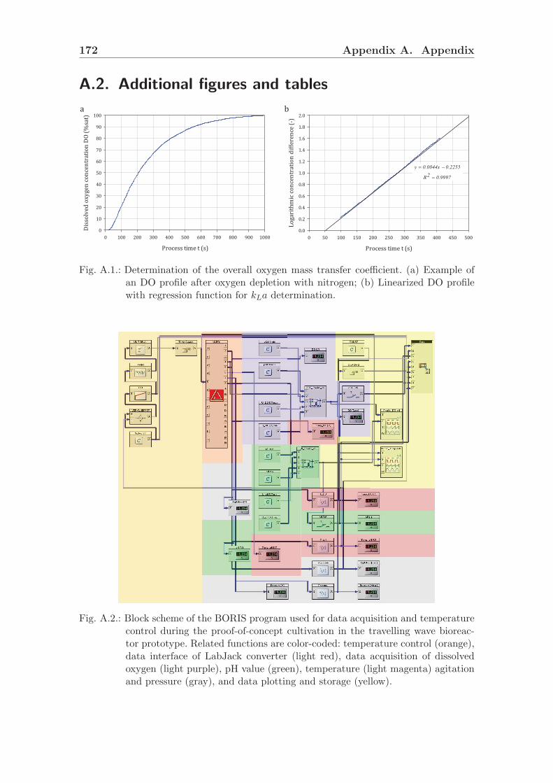
172 Appendix A. Appendix
A.2. Additional figures and tables
Process time t (s)0 100 200 300 400 500 600 700 800 900 1000Dissolved oxy
gen concentrat
ion DO (%sat)
0102030405060708090100
Process time t (s)0 50 100 150 200 250 300 350 400 450 500Logarithmic co
ncentration d
ifference (-)
0.00.20.40.60.81.01.21.41.61.82.0a b
Fig. A.1.: Determination of the overall oxygen mass transfer coefficient. (a) Example ofan DO profile after oxygen depletion with nitrogen; (b) Linearized DO profilewith regression function for kLa determination.
Fig. A.2.: Block scheme of the BORIS program used for data acquisition and temperaturecontrol during the proof-of-concept cultivation in the travelling wave bioreac-tor prototype. Related functions are color-coded: temperature control (orange),data interface of LabJack converter (light red), data acquisition of dissolvedoxygen (light purple), pH value (green), temperature (light magenta) agitationand pressure (gray), and data plotting and storage (yellow).

A.2. Additional figures and tables 173
a b c
d e f
Fig. A.3.: Computational meshes used for the grid sensitivity study of the benchtopMobius R©CellReady bioreactor. The grids had total numbers of control volumesof (a) 202 595, (b) 409 516, (c) 564 943, (d) 810 175, (e) 1 010 041, (f) 1 270 712.The probes are not shown in order to improve clarity.

174 Appendix A. Appendix
a b
Shear gradient nt (s-1)
0.01 0.1 1 10 100 1000
Vo
lum
e fr
acti
on
V (
-)
0.000
0.005
0.010
0.015
0.020
0.025
0.030
0.035
0.040
0.045
1.00 L1.25 L1.50 L2.00 L2.40 L
Shear gradient nt (s-1)
0.01 0.1 1 10 100 1000
Vo
lum
e fr
acti
on
V (
-)
0.000
0.005
0.010
0.015
0.020
0.025
0.030
0.035
0.040
0.045
1.00 L 1.25 L 1.50 L 2.00 L 2.40 L
Fig. A.4.: Volume-weighted frequency distribution of shear and normal stresses in theMobius R©CellReady for different working volumes. (a) Local shear stresses, (b)Local normal stresses. The distributions were obtained by discretization with200 bins.
Particle Reynolds number ReP (-)
10-5 10-4 10-3 10-2 10-1 100 101 102 103 104 105 106 107
Dra
g c
oe
ffic
ien
t c D
(-)
10-3
10-2
10-1
100
101
102
103
104
105
106
107
Schiller, 1933
Gidaspow, 1992
Wen & Yu, 1966
Syamlal-O'Brien, 1989
Clift et al., 1978
Schuh, 2005
Lane, 2005
Khopkar, 2005
Morsi & Alexander, 1972
Fig. A.5.: Results for the drag coefficient obtained with different models available in theliterature.

A.2. Additional figures and tables 175
Bubble diameter dB (mm)
0.0 0.5 1.0 1.5 2.0 2.5
No
rmal
ized
bu
bb
le n
um
ber
den
sity
NB/N
Bto
t (-)
0.000
0.024
0.048
0.072
0.096
0.120
No
rmal
ized
bu
bb
le s
um
dis
trib
uti
on
hB (
-)
0.0
0.2
0.4
0.6
0.8
1.0
Bubble diameter dB (mm)
0.0 0.5 1.0 1.5 2.0 2.5
No
rmal
ized
bu
bb
le n
um
ber
den
sity
NB/N
Bto
t (-)
0.000
0.024
0.048
0.072
0.096
0.120
No
rmal
ized
bu
bb
le s
um
dis
trib
uti
on
h
B (
-)0.0
0.2
0.4
0.6
0.8
1.0
Bubble diameter dB (mm)
0.0 0.5 1.0 1.5 2.0 2.5
No
rmal
ized
bu
bb
le n
um
ber
den
sity
NB/N
Bto
t (-)
0.000
0.024
0.048
0.072
0.096
0.120
No
rmal
ized
bu
bb
le s
um
dis
trib
uti
on
h
B (
-)
0.0
0.2
0.4
0.6
0.8
1.0
Bubble diameter dB (mm)
0.0 0.5 1.0 1.5 2.0 2.5
No
rmal
ized
bu
bb
le n
um
ber
den
sity
NB/N
Bto
t (-)
0.000
0.024
0.048
0.072
0.096
0.120
No
rmal
ized
bu
bb
le s
um
dis
trib
uti
on
hB (
-)0.0
0.2
0.4
0.6
0.8
1.0
Bubble diameter dB (mm)
0.0 0.5 1.0 1.5 2.0 2.5
No
rmal
ized
bu
bb
le n
um
ber
den
sity
NB/N
Bto
t (-)
0.000
0.024
0.048
0.072
0.096
0.120
No
rmal
ized
bu
bb
le s
um
dis
trib
uti
on
hB (
-)
0.0
0.2
0.4
0.6
0.8
1.0
100 rpm, 0.025 vvm
100 rpm, 0.050 vvm
200 rpm, 0.025 vvm
Bubble diameter dB (mm)
0.0 0.5 1.0 1.5 2.0 2.5
No
rmal
ized
bu
bb
le n
um
ber
den
sity
NB/N
Bto
t (-)
0.000
0.024
0.048
0.072
0.096
0.120
No
rmal
ized
bu
bb
le s
um
dis
trib
uti
on
hB (
-)
0.0
0.2
0.4
0.6
0.8
1.0
Bubble diameter dB (mm)
0.0 0.5 1.0 1.5 2.0 2.5
No
rmal
ized
bu
bb
le n
um
ber
den
sity
NB/N
Bto
t (-)
0.000
0.024
0.048
0.072
0.096
0.120
No
rmal
ized
bu
bb
le s
um
dis
trib
uti
on
hB (
-)
0.0
0.2
0.4
0.6
0.8
1.0
Bubble diameter dB (mm)
0.0 0.5 1.0 1.5 2.0 2.5
No
rmal
ized
bu
bb
le n
um
ber
den
sity
NB/N
Bto
t (-)
0.000
0.024
0.048
0.072
0.096
0.120
No
rmal
ized
bu
bb
le s
um
dis
trib
uti
on
hB (
-)
0.0
0.2
0.4
0.6
0.8
1.0
Bubble diameter dB (mm)
0.0 0.5 1.0 1.5 2.0 2.5
No
rmal
ized
bu
bb
le n
um
ber
den
sity
NB/N
Bto
t (-)
0.000
0.024
0.048
0.072
0.096
0.120
No
rmal
ized
bu
bb
le s
um
dis
trib
uti
on
hB (
-)
0.0
0.2
0.4
0.6
0.8
1.0
Bubble diameter dB (mm)
0.0 0.5 1.0 1.5 2.0 2.5
No
rmal
ized
bu
bb
le n
um
ber
den
sity
NB/N
Bto
t (-)
0.000
0.024
0.048
0.072
0.096
0.120
No
rmal
ized
bu
bb
le s
um
dis
trib
uti
on
hB (
-)
0.0
0.2
0.4
0.6
0.8
1.0
Bubble diameter dB (mm)
0.0 0.5 1.0 1.5 2.0 2.5
No
rmal
ized
bu
bb
le n
um
ber
den
sity
NB/N
Bto
t (-)
0.000
0.024
0.048
0.072
0.096
0.120
No
rmal
ized
bu
bb
le s
um
dis
trib
uti
on
hB (
-)
0.0
0.2
0.4
0.6
0.8
1.0
Bubble diameter dB (mm)
0.0 0.5 1.0 1.5 2.0 2.5
No
rmal
ized
bu
bb
le n
um
ber
den
sity
NB/N
Bto
t (-)
0.000
0.024
0.048
0.072
0.096
0.120
No
rmal
ized
bu
bb
le s
um
dis
trib
uti
on
hB (
-)
0.0
0.2
0.4
0.6
0.8
1.0
100 rpm, 0.025 vvm
100 rpm, 0.050 vvm
200 rpm, 0.025 vvm
Bubble diameter dB (mm)
0.0 0.5 1.0 1.5 2.0 2.5
No
rmal
ized
bu
bb
le n
um
ber
den
sity
NB/N
Bto
t (-)
0.000
0.024
0.048
0.072
0.096
0.120
No
rmal
ized
bu
bb
le s
um
dis
trib
uti
on
hB (
-)
0.0
0.2
0.4
0.6
0.8
1.0
a b
Fig. A.6.: Measured bubble size distributions in the benchtop Mobius R©CellReady biore-actor. (a) Culture medium; (b) Pure water.
1.00 0.950.90 0.85 0.80 0.75 0.70 0.65 0.60 0.55 0.50 0.45 0.40 0.35 0.30 0.25 0.20 0.15 0.100.050.00
Bu
bb
le s
ize
vo
lum
e fr
acti
on
αf (
-)
2.54 mm 1.92 mm 1.45 mm 1.10 mm 0.83 mm
0.63 mm 0.47 mm 0.36 mm 0.27 mm 0.20 mm
Fig. A.7.: Distributions of different bubble sizes in the Mobius R©CellReady bioreactor at200 rpm and 0.1 slpm (0.05 vvm). Only ten out of 15 bubble sizes used in theCFD model are presented.

176 Appendix A. Appendix
Flow time t (s)
6 7 8 9 10 11 12 13 14
Surf
ace
aver
aged
vel
oci
ty u
(m
s-1
)
0.0
0.1
0.2
0.3
0.4
0.5
0.6
dt = 0.005 sdt = 0.010 sdt = 0.001 s
Flow time t (s)
6 7 8 9 10 11 12 13 14
Surf
ace
aver
aged
vel
oci
ty u
(m
s-1
)
0.0
0.1
0.2
0.3
0.4
0.5
0.6
dt = 0.005 sdt = 0.010 sdt = 0.001 s
a b
Fig. A.8.: Sensitivity of CFD results on the time step size. The surface-averaged fluidvelocities on two cross sections with (a) 90 and (b) 270 relative to the x-z-plane are given.
β r
s
R
u
h
Filling ratio VL/Vtot (-)
0.0 0.1 0.2 0.3 0.4 0.5 0.6 0.7 0.8 0.9 1.0
Wet
ted
cir
cum
fere
nce
U (
m)
0.0
0.1
0.2
0.3
0.4
0.5
0.6
Hy
dra
uli
c d
iam
eter
dH
(m
)
0.00
0.05
0.10
0.15
0.20
0.25
0.30
Wetted circumference Hydraulic diameter
a b
Fig. A.9.: Definition of the Reynolds number for the travelling wave bioreactor. (a) De-pendency of the wetted circumference uL and the hydraulic diameter dH on thefilling level α (ratio of liquid volume to total torus volume)
.
Flow time t (s)
0 2 4 6 8 10 12 14 16
Rey
no
lds
nu
mb
er R
e (x
10
3)
0
10
20
30
40
50
270 °90 °
Flow time t (s)
0 2 4 6 8 10 12 14 16
Rey
no
lds
nu
mb
er R
e (x
10
3)
0
10
20
30
40
50
270 °90 °
a b
Fig. A.10.: Predicted Reynolds numbers at two cross sections as a function of time. (a)25 L, 30 rpm, 25 mm; (b) 25 L, 40 rpm, 25 mm

A.2. Additional figures and tables 177
3.0 s 5.0 s 6.0 s 7.5 s
10.0 s 15.0 s 17.5 s 20.0 s
Fig. A.11.: Time series of the liquid surface shape in the unbaffled TWB geometry underout-of-phase conditions. The simulation was realized for a working volumeof 15 L and agitation of 50 rpm and 25 mm. Out-of-phase operation was alsoobserved in experiments with identical operational conditions.
VL0.61 L
-0.128
0.15 0.20 0.25 0.30 0.35 0.40 0.45 0.50
Cri
tica
l sh
akin
g ra
te N
R,c
rit (
rpm
)
0
10
20
30
40
50
60
70
-15%
+15%
VL0.422 L
-0.052
0.15 0.20 0.25 0.30 0.35 0.40 0.45 0.50
Cri
tica
l sh
akin
g ra
te N
R,c
rit (
rpm
)
0
10
20
30
40
50
60
70
-10%
+10%
ba
Fig. A.12.: Correlation of the critical shaking frequency above which out-of-phase condi-tions occur in the travelling wave bioreactor. (a) unbaffled vessel; (b) baffledvessel (geometry #10). The data were determined experimentally by visual ob-servation through increasing the shaking frequency stepwise. The filled symbolsindicate out-of-phase conditions predicted by CFD simulations.

178 Appendix A. Appendix
0 s
1 s
2 s
5 s
25 s
50 s
Fig. A.13.: Time series of the tracer volume fraction assuming steady-state flow (”frozen”flow approach). The dark blue surface indicates the iso-surface of a tracermass fraction equal to the volume-average concentration. The light blue surfacerepresents the iso-surface of a water volume fraction equal to 0.5, considered asair-water interface. The simulation was conducted for a shaking rate of 40 rpmand 25mmm amplitude.
Calculation of fluid flow until periodic conditions
Calculation of fluid flow for one additional period
Initialization of tracer concentration field
Store fluid flow for each time step
Calculation of tracer concentration for the first
time step
Load fluid flow for next time step
Calculation of tracer concentration field
Tracer homogenous? Stop calculation
yes
no
Profile of the surface-averaged fluid velocities. The red dots indicate the time points of data storage
for the mixing time prediction.
Profile of surface-averaged fluid velocities. The red dots indicate the time points of data storage
for the mixing time prediction
Normalized time t/ωR (-)
Nor
mal
ized
flui
d ve
loci
ty u
/um
ax (-
)
Fig. A.14.: Schematic of the work flow for the mixing time prediction in the TWB.

A.2. Additional figures and tables 179
a
ed f
b c
Fig. A.15.: Meshes of the TWB modifications.
Fig. A.16.: Mesh used for the single droplet impact study. Only a quarter of the fluiddomain was considered by means of symmetry planes, whereas the grid in themiddle of the domain was refined.

180
App
endix
A.
App
endix
Tab. A.1.: Summary of computational meshes used in studies based on the RANS approach reported in literature.a calculated based ongeometric data; b Hybrid mesh consisting of tetrahedrals, pyramid, wedge and hexahedral elements; c assuming symmetry, onlyone half of the vessel was meshed; n.d. not defined.
Meshtype
SystemWorkingvolume(L)
Numberof CV(-)
Griddensity(CV/mm3)
Reyndolsnumber(-)
Turbulencemodel
Stirrerrotationmodel
Purpose of the study Ref.
un
stru
ctu
red
,te
trah
edal
s
Spinnerflask
0.33 373 388 1131.5 1246realizablek-ε
SMHydrodynamic stress on scaffoldsused in tissue engineering
[201]
Pilot scalebioreactors
≈ 134 280 000 ≈ 2.1 71000standardk-ε MRF
Gas dispersion, bubble sizedistribution and oxygen masstransfer in double-impeller tank
[166]
≈ 50 320 000 ≈ 6.4 < 1000 n.d. SRFOxygen mass transfer and reactionrates in microbial gluconic acidproduction
[345]
un
stru
ctu
red
,hyb
ridb
NewBrunswickBioFlo110bioreactor
2 483 450 241.7 37 500standardk-ε
MRFGas dispersion, bubble sizedistribution and oxygen masstransfer at agitation with SBI
[159]
2843 000 421.5 56 250
standardk-ε
MRFOxygen mass transfer rates atagitation with SBI [202]
stru
ctu
red
,h
exah
edra
l
Laboratoryscalebioreactors
15 153 900 10.3 33 000standardk-ε
Sourceterm
Gas dispersion, oxygen masstransfer and energy dissipation intriple-impeller agitated bioreactor
[99]
5.4317 952 58.9 45 000
standardk-ε
Snapshotmodel
Gas-liquid flow pattern generatedby pitched-blade turbine [346]
8.692 736 -370 944c
10.8 - 43.1 33 000standardk-ε
SMSingle- and two-phase flows of anaerated Rushton turbine [347]
10.969 120 -233 280
6.3 - 21.432 000 -64 000
standardk-ε
n.d.Mixing times in an aerated tankagitated by a Rushton turbine [99]
21.1298 000 -600 000c
14.1 - 28.4standardk-ε
MRFInfluence of solid suspension onliquid phase mixing in solid-liquidreactor
[348]≤ 400 000
Pilot scalebioreactors
20085 000 -750 000c
0.4 - 3.8 ≤ 1500laminar,k-ω, k-ε,RSM
MRFMixing and oxygen mass transferin shear thinning liquids (xanthan)
[349]

181
A.3. Details of applied numerical models
A.3.1. Turbulence models
The standard k-ε turbulence model
The standard k-ε turbulence model developed by [147] provides Eq. A.1 and Eq.A.2 for the calculation of the turbulent kinetic energy and the turbulent dissipationrate respectively. While Eq. A.1 is derived from the exact equation, Eq. A.2 wasobtained using physical reasoning and bears little resemblance to its mathematicallyexact counterpart. Here, σk and σε denote the turbulent Prandtl numbers for kand ε respectively. The terms Gk and YM describe the turbulence production fromvelocity gradients and effects of flow with high Mach numbers respectively. Theempirical constants Cµ, C1ε and C2ε are summarized in Tab. A.2. These defaultvalues have been determined from experiments with air and water for fundamentalturbulent shear flows including homogeneous shear flows and decaying isotropicgrid turbulence. They have been found to work fairly well for a wide range of wallbounded and free shear flows [148].
∂ (ρk)
∂t+∇ (~uρk) = ∇
((µ+
µTσk
)· ∇k
)− ρε+Gk − YM (A.1)
∂ (ρε)
∂t+∇ (~uρε) = ∇
((µ+
µTσε
)· ∇ε
)− C1ε
ε
kGk − C2ερ
ε2
k(A.2)
The production of turbulent energy can be derived from the Boussinesq hypothesisresulting in Eq. A.3, where S represents the tensor of the mean velocity gradients.
Gk = µT S2 (A.3)
with
S =√
2SijSij (A.4)
The turbulent viscosity µT is derived from:
µT = ρCµk2
ε(A.5)
Tab. A.2.: Constants in the standard k-ε turbulence model
Cµ C1ε C2ε σε σk0.09 1.44 1.92 1.30 1.00

182
The renormalization group (RNG) k-ε turbulence model
The RNG k-ε turbulence model can be derived from the instantaneous Navier-Stokesequations and is similar to the standard k-ε turbulence model. Through the intro-duction of additional terms, the accuracy for rapidly strained flows is improved. Fur-thermore, the effect of swirl on turbulence is included in the RNG model, enhancingaccuracy for swirling flows. The RNG theory provides an analytically-derived differ-ential formula for effective viscosity that accounts for low-Reynolds-number effects.The RNG model provides Eq. A.6 for calculation of k, where the terms have thesame meaning like in the standard k-ε model. The ratio of the turbulent to thelaminar (molecular) viscosity ν is derived from the differential equation Eq. A.7.
∂ (ρk)
∂t+∇ (~uρk) = ∇ (αkµeff∇k)− ρε+Gk +Gb − YM (A.6)
d
(ρ2k√εµ
)= 1.72
ν√ν3 − 1 + Cν
dν (A.7)
For the calculation of ε Eq. A.8 is solved.
∂ (ρε)
∂t+∇ (~uρε) = ∇ (αεµeff∇ε) + C1ε
ε
k(Gk + C3εGb)− C2ερ
ε2
k−Rε (A.8)
The term Rε in Eq. A.9 represents the main difference to the standard k − ε modeland is defined as follows:
Rε =Cµρη
3 (1− η/η0)
1 + βη3
ε2
k(A.9)
The parameters αk and αε are calculated from Eq. A.10, which can be derivedanalytically from the RNG theory. Here, α0 = 1 and αε = αk ≈ 1.393 for highReynolds numbers (µmol/µeff << 1).
∣∣∣∣ α− 1.3929
α0 − 1.3929
∣∣∣∣0.6321 ∣∣∣∣ α + 2.3929
α0 + 2.3929
∣∣∣∣0.3679
=µmolµeff
(A.10)
Tab. A.3.: Constants in the RNG k-ε turbulence model
Cµ C1ε C2ε α0 η0 β0.0854 1.42 1.68 1.00 4.38 0.012

A.3. Details of applied numerical models 183
Realizable k-ε turbulence model
Compared with the standard k-ε turbulence model, the realizable model differs inthe formulation of the turbulent viscosity and has an adapted transport equationfor ε, which derived from an exact equation for the transport of the mean-squarevorticity fluctuation. An immediate benefit of the realizable k-ε model is the moreaccurate prediction of the spreading rate of both planar and round jets. It is alsolikely to provide superior performance for flows involving rotation, boundary layersunder strong adverse pressure gradients, separation, and recirculation [148]. Thetransport equations for k and ε can be written as follows Eq. A.11 and Eq. A.12:
∂ (ρk)
∂t+∇ (~uρk) = ∇
((µ+
µtσk
)∇k)− ρε+Gk +Gb − YM (A.11)
∂ (ρε)
∂t+∇ (~uρε) = ∇
((µ+
µtσε
)∇ε)
+ρC1Sε−ρC2ε2
k +√νε
+C1εε
kC3εGb (A.12)
The following relations can be given:
C1 = max
[0.43,
η
η + 5
](A.13)
η = Sk
ε(A.14)
η = Sk
ε(A.15)
S =√
2SijSij (A.16)
In contrast to the previously described models, the value of Cµ is not a constant,but is derived from:
Cµ =1
AO + ASkUε
(A.17)
with
U =
√SijSji + ΩijΩji (A.18)
and
Ωij = Ωij − 3εijkωk (A.19)

184
Here, Ωij represents the mean rate-of-rotation tensor viewed in a rotating referenceframe with the angular velocity ωk. The other model parameters are given by: A0 =4.04
AS =√
6cos
(1
3arccos
(√
6SijSjkSki
(SijSij)(3/2)
))(A.20)
with
Sij =1
2
(dujdxi
+duidxj
)(A.21)
The standard k-ω turbulence model
The standard k − ω turbulence model contains modifications for effects related toturbulence, compressibility and shear flows. The transport equations for the turbu-lent kinetic energy k and the specific turbulent dissipation rate ω, which is the ratioof k and ε, can be written as follows:
∂ (ρk)
∂t+∇ (~uρk) = ∇
((µ+
µtσk
)∇k)
+Gk − Yk (A.22)
∂ (ρω)
∂t+∇ (~uρω) = ∇
((µ+
µtσω
)∇ω)
+Gk − Yω (A.23)
Here, Gk and Gω represent production terms of the turbulent kinetic energy andthe dissipation rate through shear respectively. The terms σk and σω represent theturbulent Prandtl numbers of k and ω respectively. The turbulent viscosity µt isderived from the combination of k and ω:
µt = αρk
σω(A.24)
The coefficient α damps the turbulent viscosity causing a low-Reynolds-numbercorrection. It is given by
α = α∞
(α0 +Ret/Rk
1 +Ret/Rk
)(A.25)
where Ret = ρkµω
, Rk = 6, α0 = 0.024, α∞ = 1 The production term Gk can be
derived from the transport equation of k (Eq. A.26) and Gω is defined by Eq. A.27.
Gk = −ρ ¯u′iu′j
∂uj∂xi
(A.26)
Gω = αω
kGk (A.27)

A.3. Details of applied numerical models 185
where α = α∞α
(α0+Ret/Rω
1+Ret/Rω
), Rω=2.95. The dissipation rates of k and ω are modelled
through Eq. A.28 and Eq. A.29.
Yk = ρβfβkω (A.28)
Yω = ρβfβω2 (A.29)
The following definitions were used:
f =
1 χk ≤ 0
1+680χ2k
1+400χ2k
χk > 0(A.30)
χk =1
ω3
∂k
∂xj
∂ω
∂xj(A.31)
β = β∞
(4/15 + (Ret/Rβ)4
1 + (Ret/Rβ)4
)(A.32)
fβ =1 + 70χω1 + 80χω
(A.33)
χk =
∣∣∣∣∣∣∣ΩijΩikSki(β∞ω
)3
∣∣∣∣∣∣∣ (A.34)
Ωij =1
2
(∂ui∂xj− ∂uj∂xi
)(A.35)
β = βi
[1 + ζF (Mt)
](A.36)
β = βi
(1 +
βiβiχF (Mt)
)(A.37)
F (Mt) =
0 Mt ≤Mt0
M2t −M2
t0 Mt > Mt0
(A.38)
M2t =
2k
γRT(A.39)

186
Tab. A.4.: Constants in the standard k-ω turbulence model
χ Rβ Rk Rω Mt0 α∞ α∞ α0 β∞ βi σk σω1.5 8 6 2.95 0.25 1 0.52 1/9 0.09 0.072 2 2
Reynolds Stress Model
The exact transport equation for the Reynolds stress terms ρ ¯u′iu′j can be written as
follows:
∂
∂t
(ρ u′iu
′j
)︸ ︷︷ ︸accumulation
=− ∂
∂xk
(ρ uk u′i u
′j
)︸ ︷︷ ︸Cij ≡ convection
+∂
∂xk
(ρ u′iu
′ju′k + p
(δkju′i + δkiju′j
))︸ ︷︷ ︸
DT,ij ≡ turbulent diffusion
(A.40)
+∂
∂xk
(µ
∂
∂xku′iu′j
)︸ ︷︷ ︸DL,ij ≡ molecular diffusion
+ ρ
(u′iu′k
∂uj∂xk
+ u′ju′k
∂ui∂xk
)︸ ︷︷ ︸
Pij ≡ stress production
+ p
(∂u′i∂xj
+∂u′j∂xi
)︸ ︷︷ ︸Φij ≡ pressure strain
− ρ β(gi u′jΘ + gj u′iΘ
)︸ ︷︷ ︸Gij ≡ buoyancy production
− 2µ∂u′i∂xk
∂u′j∂xk︸ ︷︷ ︸
εij ≡ dissipation
− 2 ρΩk
(u′ju
′m εikm + u′iu
′m εjkm
)︸ ︷︷ ︸Fij ≡ production by system rotation
While the terms Cij, DL,ij, Pij and Fij can be solved exactly, models are requiredfor the closure of DT,ij, Gij, Φij and εij. The turbulent diffusion is solved in Fluentwith a simplified equation A.41, which reduces the numerical instabilities. Here, theturbulent viscosity is derived from Eq. A.5 and the value of σk (0.82) is differentfrom that in the standard and realizable k-ε models (see also Tab. A.2).
DT,ij =∂
∂xk
(µtσk
∂u′iu′j
∂σk
)(A.41)
The pressure term Φij is modelled with Eq. A.42, where the Φij is the sum of theslow pressure-strain Φij,1, the rapid pressure-strain Φij,2 and wall-reflections Φij,W .The latter is responsible for the redistribution of normal stresses near the wall. Ittends to damp the normal stress perpendicular to the wall, while enhancing thestresses parallel to the wall. A value of σk = 0.82 has been derived from by applyingthe generalized gradient-diffusion model to the case of a planar homogeneous shearflow. The constants C ′1, C ′2 ,Cµ have values of 0.5, 0.3 and 0.09 respectively. The κis the von Karman constant (κ=0.4187).
Φij = Φij,1 + Φij,2 + Φij,W (A.42)

A.3. Details of applied numerical models 187
with
Φij,1 =− C1 ρε
k
[u′iu′j −
2
3δijk
](A.43)
Φij,2 =− C2
[(Pij + Fij +
5
6Gij − Cij
)− 2
3δij
(1
2Pkk +
5
12Gkk −
1
2Ckk
)](A.44)
Φij,2 =− C ′1ε
ku′ku
′m nk nm δij −
3
2u′iu′k nj nk −
3
2u′ju
′k ni nk
C3/4µ k3/2
κ ε d
+C ′2 φkm,2 nk nm δij −3
2φik,2 nj nk −
3
2φjk,2 ni nk
C3/4µ k3/2
κ ε d(A.45)
In these equations, the nk is the component xk of the unit vector normal to thewall and d is the normalized wall distance. The production terms due to buoyancyare modelled by Eq. A.46, where Prt and β are the turbulent Prandtl number forenergy, with a default value of 0.85, and the coefficient of thermal expansion.
Gij = βµtPrt
(gi∂T
∂xj+ gj
∂T
∂xi
)(A.46)
The turbulent kinetic energy is in general calculated from Eq. A.47, which is derivedby taking the trace of the Reynolds stress tensor.
k =1
2u′iu′i (A.47)
The dissipation tensor εij is modelled with Eq. A.48, where the coefficient YM rep-resents an additional “dilatant” dissipation, which is calculated with the turbulentMach number MT .
εij =2
3δij (ρε+ YM) (A.48)
with YM = 2ρεM2t , Mt =
√k/a2 and a ≡
√γRT . The scalar of the turbulent
dissipation rate ε is derived from its transport equation similar to the standard k-εturbulence model (Eq. A.49), where the coefficient C3ε is calculated by Eq. A.50with u and v representing the fluid velocities normal and orthogonal to the gravityvector.
∂ (ρ ε)
∂t+∇ (~u ρ ε) = ∇
((µ+
µTσε
)· ∇ε
)− C1ε
1
2[Pij + C3εGii]
ε
k− C2ε ρ
ε2
k
(A.49)
C3ε = tanh∣∣∣vu
∣∣∣ (A.50)
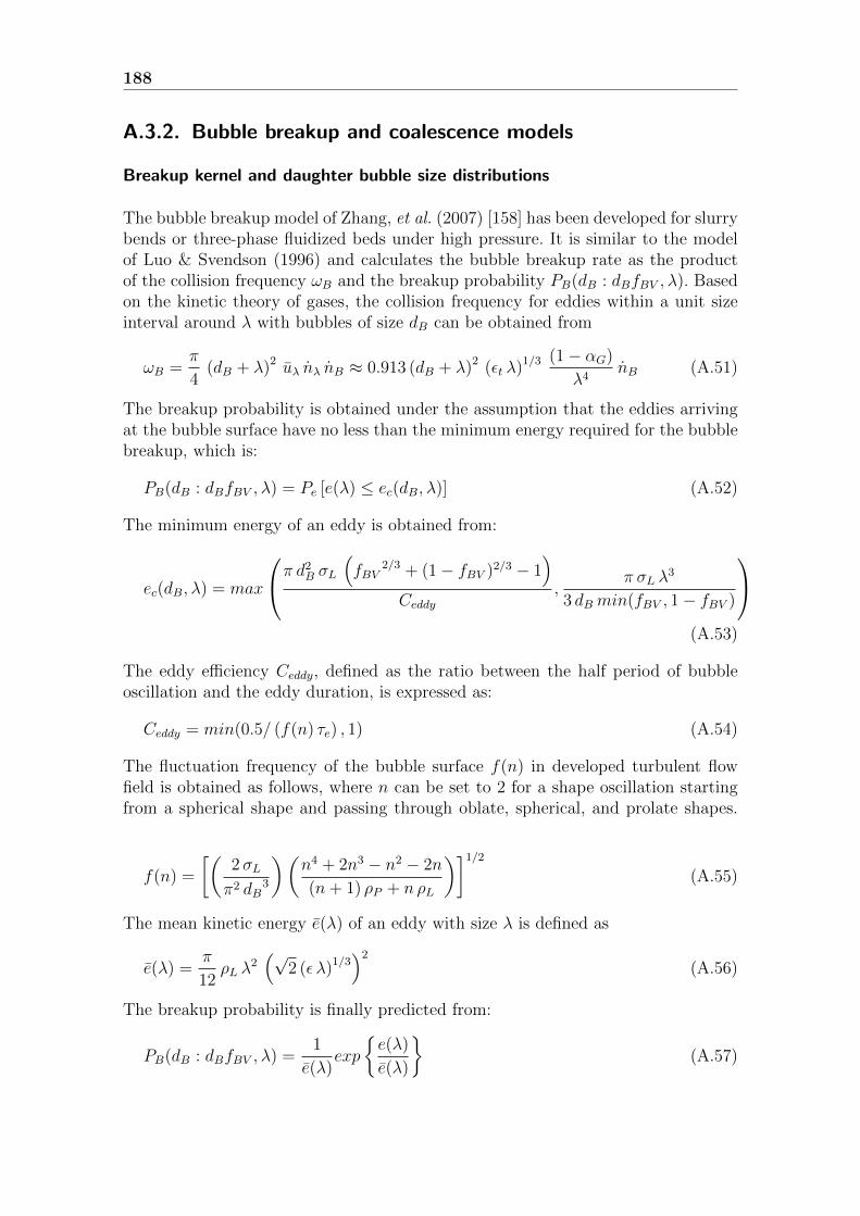
188
A.3.2. Bubble breakup and coalescence models
Breakup kernel and daughter bubble size distributions
The bubble breakup model of Zhang, et al. (2007) [158] has been developed for slurrybends or three-phase fluidized beds under high pressure. It is similar to the modelof Luo & Svendson (1996) and calculates the bubble breakup rate as the productof the collision frequency ωB and the breakup probability PB(dB : dBfBV , λ). Basedon the kinetic theory of gases, the collision frequency for eddies within a unit sizeinterval around λ with bubbles of size dB can be obtained from
ωB =π
4(dB + λ)2 uλ nλ nB ≈ 0.913 (dB + λ)2 (εt λ)1/3 (1− αG)
λ4nB (A.51)
The breakup probability is obtained under the assumption that the eddies arrivingat the bubble surface have no less than the minimum energy required for the bubblebreakup, which is:
PB(dB : dBfBV , λ) = Pe [e(λ) ≤ ec(dB, λ)] (A.52)
The minimum energy of an eddy is obtained from:
ec(dB, λ) = max
π d2B σL
(fBV
2/3 + (1− fBV )2/3 − 1)
Ceddy,
π σL λ3
3 dBmin(fBV , 1− fBV )
(A.53)
The eddy efficiency Ceddy, defined as the ratio between the half period of bubbleoscillation and the eddy duration, is expressed as:
Ceddy = min(0.5/ (f(n) τe) , 1) (A.54)
The fluctuation frequency of the bubble surface f(n) in developed turbulent flowfield is obtained as follows, where n can be set to 2 for a shape oscillation startingfrom a spherical shape and passing through oblate, spherical, and prolate shapes.
f(n) =
[(2σL
π2 dB3
)(n4 + 2n3 − n2 − 2n
(n+ 1) ρP + n ρL
)]1/2
(A.55)
The mean kinetic energy e(λ) of an eddy with size λ is defined as
e(λ) =π
12ρL λ
2(√
2 (ε λ)1/3)2
(A.56)
The breakup probability is finally predicted from:
PB(dB : dBfBV , λ) =1
e(λ)exp
e(λ)
e(λ)
(A.57)

A.3. Details of applied numerical models 189
Based on this model, the dimensionless daughter size distribution β(dB, fBV ), whereβ(dB, fBV ) ∆fBV represents the fraction of bubbles of diameter dB that break intobubbles of volumetric ratio between fBV and fBV + ∆fBV , is expressed as:
β(dB, fBV ) =dB ωB(dB, d
′B)PB(dB, d
′B)
3 fBV2/3 Ω(dB)
+dB ωB(dB, d
′′B)PB(dB, d
′′B)
3 (1− fBV )2/3 Ω(dB)(A.58)
where
Ω(dB) =
∫ dB
λmin
ωB(dB, d′B)PB(dB, d
′B) dλ (A.59)
with
d′B = dB fBV2/3 (A.60)
In the breakup model of Lehr, et al. (2002) [259], the probability that collisionsbetween eddies and bubbles result in breakages is obtained from a force balance.Furthermore, it is proposed that the size of the resulting bubble fragments dependson the kinetic energy of the eddy [259]. The bubble breakup kernel and the daughterbubble size distribution are given in dimensionless form as follows:
f ∗Z = 0.5 d∗B5/3 exp
−√
2
d∗B3
(A.61)
and
β∗(v′∗B , v∗B) =
6
π3/2 d′∗B
exp−9
4
[ln(22/5 d′∗B
3)]2
1 + erf[
32ln(21/15 d∗B)
] 0 ≤ v′∗B ≤v∗B2
β∗(v′∗B , vB) = β∗(v∗B − v′∗B , v∗B)v∗B2< v′∗B ≤ v∗B (A.62)
The following definitions are used for the dimensionless bubble diameter d∗B, eddylength scale λ∗, bubble volumes v∗B, breakup kernel function r∗1(v′∗, v∗), breakupfrequency f ∗Z and daughter size distribution β∗(v′∗B , v
∗B):
d∗B =dBL
(A.63)
λ∗ =λ
L(A.64)
v∗B =vBL3
(A.65)
r∗1(v′∗B , v∗B) = r1(v′B, vB)L3 T (A.66)
f ∗Z = fZ T (A.67)
β∗(v′∗B , v∗B) (A.68)

190
The dimensionless length and time scales L and T are expressed with:
L =
(σLρL
)3/51
ε2/5(A.69)
and
T =
(σLρL
)2/51
ε3/5(A.70)
The bubble breakup model of Laakkonen (2006) [157] is based on a formulation ofAlopaeus et al. (2002) [350] who extended the model of Narsimhan et al. (1979)[351] for droplets by including viscous stresses as a resisting force for breakage. Thebreakage rate is expressed as:
g(d) = 2.52 ε1/3 erf
√0.04σL
ρL ε2/3dB5/3
+ 0.01µL
√ρL ρG ε1/3 dB
4/3
(A.71)
In the viscous term of this formulation, the dispersed phase viscosity is replacedby the continuous phase viscosity, since it is assumed that viscous stresses, whichresist the breakage, are proportional to the viscosity of liquid surrounding the bubblerather than the low viscosity of gas.
Coalescence rates
The details of the Luo’s coalescence model [263] were already given in section 4.1.3.Similarly, Lehr’s model [259] assume that coalescence of two bubbles with diametersdi and dj occurs as a result of collisions arising from turbulent fluctuations and fromthe difference in rise velocities of bubbles of different size. A characteristic velocityuC is introduced, which is either defined by the turbulent eddy velocity with thelength scale of the bubbles or the difference in rise velocities of the bubbles:
uC = max
(√2 ε1/3
√di
2/3 + dj2/3, |~ui − ~uj|
)(A.72)
For the distilled water and air, it was found experimentally that bubbles coalescenceonly below a critical velocity of 0.08 m s−1, independent on the size of the bubbles.Thus, the coalescence kernel function was derived as follows:
h(di, dj) =π
4(di + dj)
2 min(uC , 0.08) exp
−(αG,max
1/3
αG1/3− 1
)2
(A.73)
where αmax = 0.6 denotes the maximum packing density of the bubbles.In the models of Coulaloglou & Tavlarides (1977) [265] and Prince & Blanch (1990)

A.3. Details of applied numerical models 191
[266], the following expression for the coalescence rate is used, which is mainlyderived on assumptions in analogy to the kinetic gas theory:
h(di, dj) = C8 ε1/3 (di + dj)
2(d
2/3i + d
2/3j
)1/2
λ(di, dj) (A.74)
where C8 is a constant with theoretical values between 0.28 and 1.11, dependingon the effective collision cross-sectional area and the expression for the turbulentfluctuations [157]. A constant value of C8 = 0.8 was used in the present work. Bothmodels distinguish from each other in the formulation of the coalescence efficiencyλ(di, dj), which is based on a film drainage process. Coulaloglou’s model considersthe film drainage between deforming droplets with immobile surfaces with:
λ(di, dj) = exp
−C9
µL ρL ε
σL2
(di djdi + dj
)4
(A.75)
It has been found that predicted local bubble size distributions in a stirred tankcan be best fitted to experimental data if C9 is set to 6 · 109 [157]. Prince’s modelassumes that the inertia of draining liquid and surface tension forces control thedrainage of a fully mobile bubble surface, which led to the following expression:
λ(di, dj) = exp
−C10
√ρL ε2/3 dij
5/3
σL
(A.76)
The constant C10 is of magnitude 2.3 [266]. The equivalent bubble diameter dij isobtained from:
dij = 2
(1
di+
1
dj
)−1
(A.77)

192
A.4. Publication reprints

Research Article
Engineering characteristics of a single-usestirred bioreactor at bench-scale: The MobiusCellReady 3L bioreactor as a case study
Stirred single-use bioreactors can be used as substitutes for their conventionalcounterparts made of glass or stainless steel in the development and production ofbiopharmaceuticals wherever possible. Various studies have confirmed theircomparability in cell growth as well as in product quantity and quality. However,information about their engineering characteristics is still rare. This study focuseson the stirred Mobiuss CellReady 3L bioreactor. The main engineering parametersfor typical operation conditions used in animal cell cultivations are presented forthe first time. Numerical simulations with a commercial CFD package (Fluent 6.3)were accomplished to obtain data on the single- and multi-phase fluid flow, powerinput, mixing time and oxygen mass transfer. The results, which were comparedwith data from experiments and from the literature, reveal the suitability of theMobiuss CellReady 3L bioreactor for cell expansion and protein production withanimal cell cultures. Furthermore, the data enable comparisons with other single-use and reusable cell culture bioreactors at bench-scale.
Keywords: CFD / Engineering characteristics / Single-use bioreactor
Received: September 26, 2010; revised: January 20, 2011; accepted: March 16, 2011
DOI: 10.1002/elsc.201000171
1 Introduction
Stirred single-use (disposable) bioreactors, which have a flex-ible plastic cultivation vessel in contrast to their re-useablecounterparts made of glass or stainless steel, have beencommercially available since 2006. At that time, wave-mixedbag bioreactors (e.g. Wave Bioreactor from GE Healthcare orBioWave from Wavebiotech) dominated alongside well-known, stirred standard cell culture bioreactors. The broadacceptance of the wave systems can be explained by similar oreven better results in cell cultivations, higher process flexibility,easy handling and reduced process costs [1]. Consequently,many producers of biopharmaceuticals have replaced rollerand spinner flasks as well as stirred re-useable bioreactors forcell production at small and medium volume scale by wave-mixed systems, which were also established in process devel-opment and commercial vaccine productions [2]. However,with the exception of cell expansion and processes with shearsensitive cell cultures or foaming culture media, wave-mixed
bag bioreactors are currently used less frequently than stirredsingle-use bioreactors. Hence, it is not surprising that thelatter, which are available up to working volumes of 2 m3, arethe most commonly used single-use bioreactor systems today.Normally, their cultivation container is equipped with dispo-sable or standard sensors to guarantee optimal processconditions for cell growth and product expression [3]. Acomprehensive current overview describing the commerciallyavailable single-use bioreactors, their characteristics andrecommended applications are given by Eibl et al. [1].
Nowadays, there are five stirred single-use bag systems for pilotand industrial scale (S.U.B.; BIOSTAT CultiBag STR; NucleoBioreactor; XDR-DSTB, animal; XDR-DSTB, microbial) and threelaboratory-scale systems with rigid plastic vessels (Mobius Cell-Ready 3L bioreactor, CelliGens BLU SUB, SuperSpinner D1000)on the market. The introduction of the Mobiuss CellReady 3Lbioreactor in summer 2009 bridged the gap for stirred single-usebioreactors between laboratory and pilot scale. This unbaffledbioreactor has a rigid plastic cultivation vessel with a total volumeof 3 L, in which mixing is guaranteed by a marine impeller. Amicro-sparger is installed below the impeller for aeration.
For process development, comparability of single-use andconventional cell culture bioreactors is essential, especiallywhen both systems have to be used side-by-side in hybridsolutions. A need for single-use bioreactors with design andset-up comparable to the reusable alternative is therefore
Stephan C. Kaiser
Regine Eibl
Dieter Eibl
Zurich University of Applied
Sciences, School of Life
Sciences and Facility
Management, Institute of
Biotechnology, Campus
Gr .uental, W.adenswil,
Switzerland
Abbreviations: CFD, computational fluid dynamics; MRF, multiple
reference frame
Correspondence: Stephan C. Kaiser ([email protected]), Zurich
University of Applied Sciences, School of Life Sciences and Facility
Management, Institute of Biotechnology, Campus Gr .uental, P. O. Box,
CH-8820 W.adenswil, Switzerland
& 2011 WILEY-VCH Verlag GmbH & Co. KGaA, Weinheim http://www.els-journal.com
Eng. Life Sci. 2011, 11, No. 4, 359–368 359
A.4. Publication reprints 193
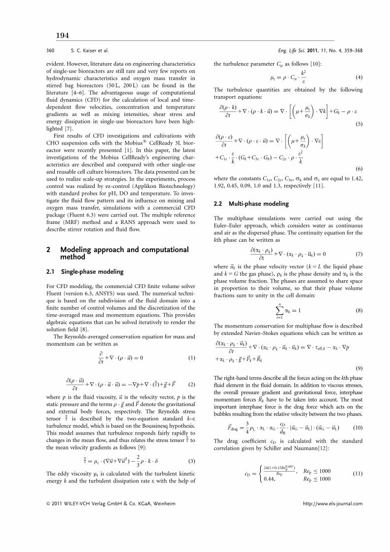
evident. However, literature data on engineering characteristicsof single-use bioreactors are still rare and very few reports onhydrodynamic characteristics and oxygen mass transfer instirred bag bioreactors (50 L, 200 L) can be found in theliterature [4–6]. The advantageous usage of computationalfluid dynamics (CFD) for the calculation of local and time-dependent flow velocities, concentration and temperaturegradients as well as mixing intensities, shear stress andenergy dissipation in single-use bioreactors have been high-lighted [7].
First results of CFD investigations and cultivations withCHO suspension cells with the Mobiuss CellReady 3L bior-eactor were recently presented [1]. In this paper, the latestinvestigations of the Mobius CellReady’s engineering char-acteristics are described and compared with other single-useand reusable cell culture bioreactors. The data presented can beused to realize scale-up strategies. In the experiments, processcontrol was realized by ez-control (Applikon Biotechnology)with standard probes for pH, DO and temperature. To inves-tigate the fluid flow pattern and its influence on mixing andoxygen mass transfer, simulations with a commercial CFDpackage (Fluent 6.3) were carried out. The multiple referenceframe (MRF) method and a RANS approach were used todescribe stirrer rotation and fluid flow.
2 Modeling approach and computationalmethod
2.1 Single-phase modeling
For CFD modeling, the commercial CFD finite volume solverFluent (version 6.3, ANSYS) was used. The numerical techni-que is based on the subdivision of the fluid domain into afinite number of control volumes and the discretization of thetime-averaged mass and momentum equations. This providesalgebraic equations that can be solved iteratively to render thesolution field [8].
The Reynolds-averaged conservation equation for mass andmomentum can be written as
@
@t1r ðr ~uÞ ¼ 0 ð1Þ
@ðr ~uÞ@t
1r ðr ~u ~uÞ ¼ rp1r ðtÞ1~g1~F ð2Þ
where r is the fluid viscosity, ~u is the velocity vector, p is thestatic pressure and the terms r ~g and ~F denote the gravitationaland external body forces, respectively. The Reynolds stresstensor t is described by the two-equation standard k–eturbulence model, which is based on the Boussinesq hypothesis.This model assumes that turbulence responds fairly rapidly tochanges in the mean flow, and thus relates the stress tensor t tothe mean velocity gradients as follows [9]:
t ¼ mt ðr~u1r~uTÞ 2
3r k d ð3Þ
The eddy viscosity mt is calculated with the turbulent kineticenergy k and the turbulent dissipation rate e with the help of
the turbulence parameter Cm as follows [10]:
mt ¼ r Cm k2
eð4Þ
The turbulence quantities are obtained by the followingtransport equations:
@ðr kÞ@t
1r ðr k ~uÞ ¼ r m1mt
sk
rk
1Gk r e
ð5Þ
@ðr eÞ@t
1r r e ~uð Þ ¼ r m1mt
sk
re
1C1e ek ðGk1C3e GbÞ C2e r
e2
kð6Þ
where the constants C1e, C2e, C3e, sk and se are equal to 1.42,1.92, 0.45, 0.09, 1.0 and 1.3, respectively [11].
2.2 Multi-phase modeling
The multiphase simulations were carried out using theEuler–Euler approach, which considers water as continuousand air as the dispersed phase. The continuity equation for thekth phase can be written as
@ðak rkÞ
@t1r ðak rk ~ukÞ ¼ 0 ð7Þ
where ~uk is the phase velocity vector (k 5 L the liquid phaseand k 5 G the gas phase), rk is the phase density and ak is thephase volume fraction. The phases are assumed to share spacein proportion to their volume, so that their phase volumefractions sum to unity in the cell domain:
Xn
i¼1
ak ¼ 1 ð8Þ
The momentum conservation for multiphase flow is describedby extended Navier–Stokes equations which can be written as
@ðak rk ~ukÞ
@t1r ðak rk ~uk ~ukÞ ¼ r teff ;k ak rp
1ak rk ~g1~Fk1~Rk
ð9Þ
The right-hand terms describe all the forces acting on the kth phasefluid element in the fluid domain. In addition to viscous stresses,the overall pressure gradient and gravitational force, interphasemomentum forces ~Rk have to be taken into account. The mostimportant interphase force is the drag force which acts on thebubbles resulting from the relative velocity between the two phases.
~Fdrag ¼3
4rL aL aG
cD
dB j~uG ~uLj ð~uG ~uLÞ ð10Þ
The drag coefficient cD is calculated with the standardcorrelation given by Schiller and Naumann[12]:
cD ¼
24ð110:15Re0:687p Þ
Rep; Rep 1000
0:44; Rep 1000
(ð11Þ
360 S. C. Kaiser et al. Eng. Life Sci. 2011, 11, No. 4, 359–368
& 2011 WILEY-VCH Verlag GmbH & Co. KGaA, Weinheim http://www.els-journal.com
194

The particle Reynolds number Rep is defined as:
Rep ¼rLj~uG ~uLj dB
ZL
ð12Þ
Additionally, virtual mass ~Fvm was taken into account in thisstudy using the default treatment included in Fluent, whichcan be written as [8]:
~Fvm ¼ 0:5 rL aG D~uG
Dt
D~uL
Dt
ð13Þ
The term ~Fk in Eq. (9) represents the Coriolis and centrifugalforces which are given for multi-phase flows by [13]:
~Fk ¼ 2ak rk ~N ~uk ak rk
~N ð~N ~rÞ ð14Þ
The Reynolds stress tensor for the gas–liquid system in Eq. (9)is calculated using the dispersed k–e turbulence model, as thesecondary phase is dilute and the primary phase is clearlycontinuous. The dispersed k–e model predicts turbulence forthe continuous phase using the standard k–e turbulence modelsupplemented with extra terms that include interphaseturbulent momentum transfer [8]. For the dispersed phase,turbulence quantities are obtained using the Tchen theory ofdispersion of discrete particles by homogeneous turbulence[8]. The turbulent liquid viscosity is calculated analogous tothe single-phase system using
mt;L ¼ rL Cm k2
L
eLð15Þ
The transport equations for kL and eL are given as
@
@tðrL aL kLÞ1r ðrL aL ~uL kLÞ
¼ r aL mt;L
sk rkL
1aL GkL aL rL eL1aL rL kL
ð16Þ
@
@tðrL aL eLÞ1r ðrL aL ~uL eLÞ
¼ r aL mt;L
sk reL
1aL
eL
kL ðC1e GkL C2e rL eLÞ
1aL rL eL
ð17Þ
where GkL represents the production rate of turbulent kineticenergy. The terms
QkL and
QeL denote the influence of the
interphase interaction, which are modeled following Rizk andElgobashi [14]. All other parameters have the same meaning andvalues as in the single-phase k–e turbulence model (see above).
2.3 Numerical details and boundary conditions
Simulations were realized for working volumes of 1.5, 2.0 and2.5 liters. In each case, a hybrid mesh was generated using thepreprocessor GAMBIT (version 2.4) as proposed by Naude etal. [15] and by Lu et al. [16]. Owing to the complex geometryand based on the accurate description of the impeller, thebottom and impeller zone were divided into unstructuredtetrahedral cells. The bulk of the tank was meshed withstructured hexahedral cells to decrease the cost of calculation.
A previous grid sensitivity study had confirmed that the gridsused with 306 000, 492 000 and 588 000 cells for the differentfluid volumes show grid-independent results (data not shown).
The tank walls, the impeller and the probes were treated asnon-slip boundaries with standard wall functions. The stirrerrotation was implemented using the MRF model, which is a goodcompromise between physical accuracy and reasonable compu-tational effort. In steady simulations convergence was assumedwhen the residuals dropped below a value of 106, and fortransient cases a convergence criterion of 104 was chosen.
In multi-phase simulation, the higher order QUICK schemewas chosen for mass and momentum conservation equations. Forpressure–velocity coupling the phase-coupled SIMPLE algorithmwas used [8]. The gas flow rate at the sparger was defined via inlet-velocity boundary conditions with a gas volume fraction equal tounity. The inlet bubble diameter was assumed to be uniform and avalue of 0.4 mm was defined, as observed in experiments. At thefluid surface, only gas was allowed to escape from the vessel. Toreduce calculation time, single-phase flow field was used forinitialization of multi-phase transient calculation [13].
3 Experimental investigations of mixingtime and oxygen mass transfer
3.1 Bioreactor
The single-use Mobiuss CellReady bioreactor has a rigidplastic tank with a dished bottom and a total volume of 3 L.The diameter of the unbaffled vessel is 0.137 with an H/D ratioof 1.82. Mixing is driven by a marine impeller with a diameterequal to 1/2 the tank diameter and an off-bottom clearance of0.028 m. For aeration, a microsparger (sintered polyethylene,15–30 mm pore size) is installed below the impeller.
3.2 Mixing time analysis
Mixing time was defined as the time required to achieve 95%homogeneity following addition of a tracer on the surface of theliquid [17]. The tracer was 1 M sodium thiosulfate, which wasadded instantaneously to a starchy iodine solution (10 g/Lstarch) by pipette. The measurement was performed for work-ing volumes of 1.5, 2.0 and 2.5 L under non-aerated conditions.The agitation speed was varied at a range between 50 and250 rpm, corresponding to tip speeds of 0.2 and 1 m/s, respec-tively. Each run was performed in triplicate. As the volume ofeach addition (200mL) was less than 0.05% of the total volume,the effect on the volume change was negligible.
3.3 Oxygen mass transfer
The oxygen mass transfer coefficient kLa was determined usinga dynamic method described by Kerdouss et al. [13]. Thedissolved oxygen concentration was measured with a polaro-graphic membrane oxygen probe (Mettler Toledo) andmonitored with a computer interface. The measurement wastaken in distilled water and in a 0.5 M Na2SO4 aqueous solu-
Eng. Life Sci. 2011, 11, No. 4, 359–368 Engineering characteristics of a single-use stirred bioreactor 361
& 2011 WILEY-VCH Verlag GmbH & Co. KGaA, Weinheim http://www.els-journal.com
A.4. Publication reprints 195

tion at 201C, representing non-viscous coalescent and non-coalescent media, respectively. Aeration was varied in a rangefrom 0.05 to 0.25 vvm, corresponding to superficial gas velo-cities of 1.13 and 5.65 104 m/s.
The kLa was determined from dissolved oxygen concen-tration measured as a function of time when aeration wasturned on following complete oxygen removal by nitrogen.Assuming that the gas phase is well mixed and the dissolvedoxygen concentration is uniform inside the liquid, the rate ofoxygen transfer can be described by the following equation:
OTR ¼dcO2
dt¼ kLa ðcO2
cO2 Þ ð18Þ
where cO2is the saturation concentration given by Henry’s law:
pO2 ¼ H cO2ð19Þ
By integration of Eq. 18 with cO2 ðt ¼ 0Þ ¼ cO2 ;0, thefollowing equation is obtained:
lncO2 cO2 ðtÞ
cO2 cO2 ; 0
!¼ kLa t ð20Þ
The kLa can be obtained as the slope when the left-handside of Eq. (20) is plotted against time. The oxygen saturationconcentration for the sodium sulfate solution was calculated inaccordance with [18].
4 Results and discussion
4.1 Single-phase flow pattern
Figue 1 shows the flow pattern obtained at 2-L working volume.It is worth noting that the fluid velocity vectors are projected onthe mid-tank plane for improved clearness, and therefore cannot
represent a three-dimensional direction. Contrary to initialexpectations, the single-phase simulations reveal no clear axialflow profile, but a dominance of the impeller’s radial componentfor clockwise rotation. In this flow pattern the fluid is dischargedtoward the vessel wall, where the impeller discharge is divided andre-circulates in two flow loops per half of the vessel axially fromthe top and bottom to the stirrer (see Fig. 1). Owing to the pitchof the impeller blades, the impeller discharge is inclined towardthe surface of the fluid at circa 251. These results were qualita-tively confirmed in experiments with the addition of small plasticparticles to the fluid and visual observation of the particletrajectory (data not shown).
As expected, the highest fluid velocities are found in closeproximity to the impeller blades and correspond to the tipspeed, which is defined as
utip ¼ p NR dR ð21Þ
The highest rotational speed of 250 rpm gives a tip speed of0.997 m/s. In the simulation, the maximum fluid velocity was0.989 m/s, which is very close to the theoretical value. The fluidvelocities in the lower part of the vessel (hohF/2) are primarilybetween 0.1 and 0.4 m/s. In the upper part of the vessel,considerably lower velocities with values below 10% of the tipspeed are obtained. Thus, it can be argued that the impeller onlyhas a small influence on this zone [19]. This effect is emphasizedby an increasing filling level, which results in longer mixingtimes (see below). Xing et al. showed that inefficient mixing isaccompanied by a decrease in oxygen mass transfer, which caninduce oxygen concentration gradients in the case of bubbleaeration [20]. Furthermore, a small dead zone is found in theinlet of the drain where the fluid velocities are nearly 0 m/s. Incultivation experiments with Chinese hamster ovary (CHO)suspension cells carried out in our laboratory, cell sedimentationand accumulation were observed in this region. The viability ofthese cells decreased significantly, which is probably the result ofan insufficient nutrient and oxygen supply.
4.2 Power input
The power input was estimated by CFD as the momentumacting on the stirrer and the stirrer shaft, given by Eq. (22). Inthis study, no experimental determination of power input wascarried out. Nevertheless, Lane and Koh and Patwardhandemonstrated that CFD-predicted and measured power inputsare in good agreement, the deviation being about 10% [21, 22]
PR ¼ 2p MR NR ð22Þ
Depending on the working volume and stirrer speed, thevolume-specific power input P/V varies in a range between 0.26and 38.3 W/m3 for 50 rpm (2.0 L) and 250 rpm (1.5 L) respec-tively. From the power input, the dimensionless power number(also known as the Newton number, Ne) is calculated as
Ne ¼PR
rL N3R d
5R
ð23ÞFigure 1. Fluid velocities in single-phase flow with 2.0 L workingvolume at 150 rpm. Velocity profiles are shown normalized bythe tip speed as contour and vector plots for the x– y-plane.
362 S. C. Kaiser et al. Eng. Life Sci. 2011, 11, No. 4, 359–368
& 2011 WILEY-VCH Verlag GmbH & Co. KGaA, Weinheim http://www.els-journal.com
196

CFD simulations revealed that above a critical Reynolds numberof RecritE104 a full turbulent flow pattern is achieved in whichthe Newton number becomes constant with a value of 0.30.Although dominance of the impeller’s radial component isindicated by the CFD simulation, the power number iscomparable to typical axial pumping stirrers such as pitched-blade impellers or propeller stirrers as described by Liepe et al.[23]. Furthermore, although it is well known that the powernumber further decreases in unbaffled tanks as a result of a vortexformation, this phenomenon was not taken into account in thesingle-phase simulation. However, experimental determination ofthe stirrer torque realized by Millipore also reveals a powernumber of 0.31 for the investigated stirrer speeds (D. Kraus,Millipore Corporation, November 2009, personal communica-tion), which matches the above-mentioned value very closely.
4.3 Mixing time
Mixing experiments show decreasing mixing times withincreasing stirrer speeds. For 2.0 L working volume mixing timesof 54.7 and 7.0 s are measured with tip speeds of 0.2 and 1.0 m/s,respectively. This is unsurprising because turbulence increaseswith higher rotational speed, which results in a higher mixingintensity [23, 24]. As already shown by the CFD simulations, thefluid velocity in the upper part of the vessel is rather low and theeffect is more significant at higher filling levels. As a consequence,the mixing time increases significantly with higher workingvolumes due to the weakly mixed region near the liquid surface,where color remained the longest in the mixing experiments.Thus, with a tip speed of 0.2 m/s, the mixing time was 31.5 and78.6 s for 1.5 and 2.5 L volume, respectively.
The mixing times measured can be correlated with thespecific power input P/V predicted by the CFD simulations assuggested by Nienow [24]. Taking only cases with fullyturbulent conditions and filling heights of HF/DZ1 intoaccount, the following correlation was found:
t95% ¼ 26:54 ðP=VÞ0:36ð24Þ
Based on turbulence theory, Nienow [24] suggests that themixing time should be independent of impeller type andprovides a correlation of the mixing time with the third radicalof the specific power input (P/V), which is valid for vesselswith H/D-ratios E1 and Re410 000 [24]. The exponent ofP/V found in this study is very close to the given value of 1/3but, in order to achieve a defined mixing time, a higher specificpower input is required in the bioreactor investigated than thecorrelation of Nienow [24], as shown in Fig. 2. Nevertheless,the dimensionless mixing number cH (representing thenumber of stirrer rotations required to achieve the desiredhomogeneity) has a value of 3473.3 for fully turbulentconditions. Thus, the marine impeller is within the perfor-mance range of conventional stirrers such as the Rushtonturbine or a 6 451 pitched-blade impeller, for which Liepeet al. reported cH values of 24 and 30, respectively [23].
cH ¼ t95% NR ð25Þ
In CFD simulations, it is assumed that the tracer hasidentical fluid properties and does not influence the fluid flowpattern [25–28]. It is well known that the RANS approachunderestimates the turbulent fluctuation of the flow field,which results in failure to predict reasonable tracer responsecurves [26, 28]. Nevertheless, good agreement between CFD-predicted and measured mixing times is usually achieved. InTable 1, the CFD-predicted mixing times are summarized andcompared with the experimental data. In most cases, themixing time calculated lies between or close to the measure-ment tolerance. Higher differences are only observed for aworking volume of 1.5 L at 100 rpm and 2.5 L at 150 rpm.
4.4 Multiphase fluid flow pattern and gasdistribution
The fluid flow pattern for a rotational speed of 150 rpm(equivalent to a tip speed of 0.6 m/s) and an aeration rate of0.1 vvm is shown in Fig. 3. Owing to the low gassing rate, theshape of the flow pattern is not profoundly affected by the gasintroduced. The dominance of the radial component is againobvious and the highest fluid velocities are found at theimpeller tips. Small differences in fluid velocities betweenaerated and non-aerated cases are obtained below the impeller,because only low gas volume fractions (below 0.01%) arepresent in this region. As expected, significant effects of the gasintroduced are detected near the gas inlet and in regions wherethe gas rises, which suggests that the flow is controlled not onlyby the impeller but also by the rising gas. In these regions, thefluid velocities were up to five times higher than those of thesingle-phase system and achieved values of 0.2 utip.
The spatial gas distribution is shown in Fig. 4. The greaterpart of the gas rises with low dispersion as the disruptive forcesinduced by the marine impeller rotation are insufficient toovercome buoyancy. This result has been qualitativelyconfirmed by visual observation, which revealed that thebubbles rise in a relatively undisturbed way through a confined
Figure 2. Measured mixing times as a function of specific powerinput predicted by CFD simulations. Experimental data arecompared with a correlation provided by Nienow [24].
Eng. Life Sci. 2011, 11, No. 4, 359–368 Engineering characteristics of a single-use stirred bioreactor 363
& 2011 WILEY-VCH Verlag GmbH & Co. KGaA, Weinheim http://www.els-journal.com
A.4. Publication reprints 197
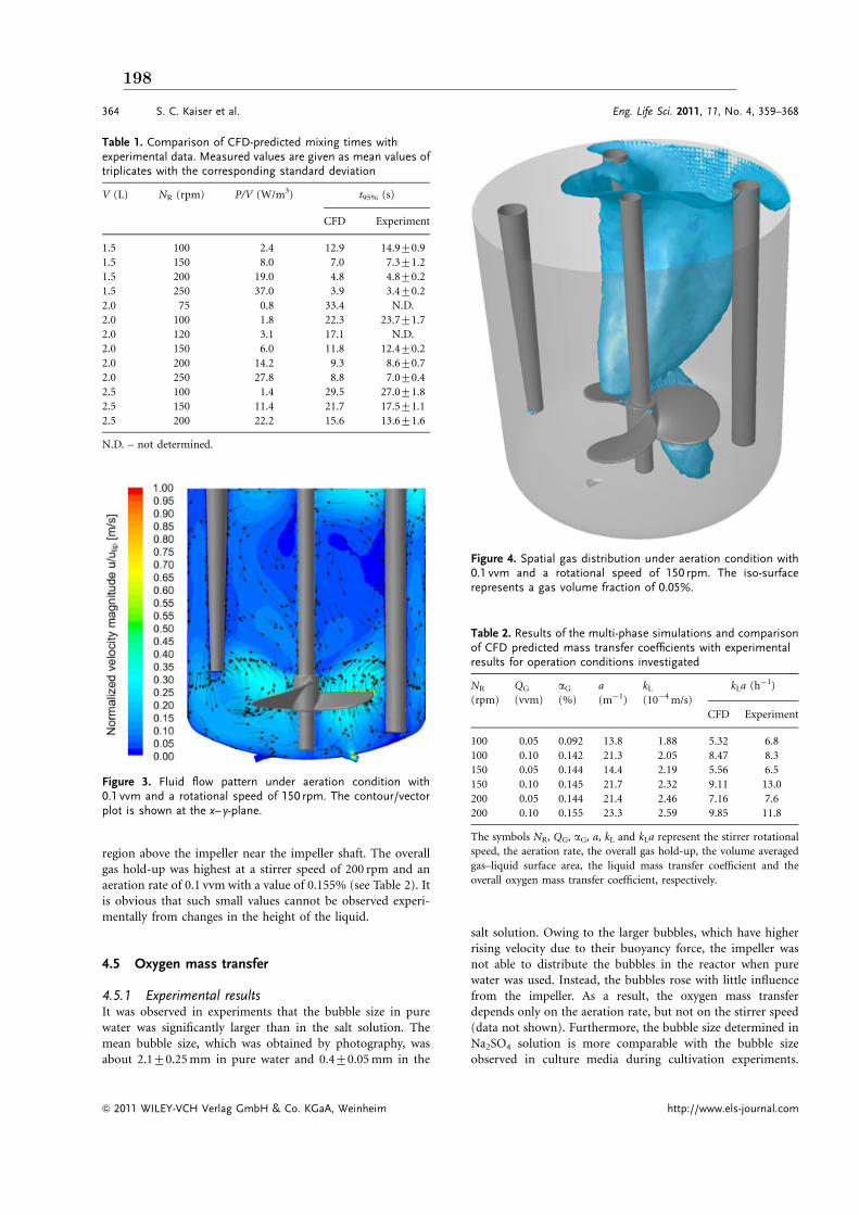
region above the impeller near the impeller shaft. The overallgas hold-up was highest at a stirrer speed of 200 rpm and anaeration rate of 0.1 vvm with a value of 0.155% (see Table 2). Itis obvious that such small values cannot be observed experi-mentally from changes in the height of the liquid.
4.5 Oxygen mass transfer
4.5.1 Experimental resultsIt was observed in experiments that the bubble size in purewater was significantly larger than in the salt solution. Themean bubble size, which was obtained by photography, wasabout 2.170.25 mm in pure water and 0.470.05 mm in the
salt solution. Owing to the larger bubbles, which have higherrising velocity due to their buoyancy force, the impeller wasnot able to distribute the bubbles in the reactor when purewater was used. Instead, the bubbles rose with little influencefrom the impeller. As a result, the oxygen mass transferdepends only on the aeration rate, but not on the stirrer speed(data not shown). Furthermore, the bubble size determined inNa2SO4 solution is more comparable with the bubble sizeobserved in culture media during cultivation experiments.
Table 1. Comparison of CFD-predicted mixing times withexperimental data. Measured values are given as mean values oftriplicates with the corresponding standard deviation
V (L) NR (rpm) P/V (W/m3) t95% (s)
CFD Experiment
1.5 100 2.4 12.9 14.970.9
1.5 150 8.0 7.0 7.371.2
1.5 200 19.0 4.8 4.870.2
1.5 250 37.0 3.9 3.470.2
2.0 75 0.8 33.4 N.D.
2.0 100 1.8 22.3 23.771.7
2.0 120 3.1 17.1 N.D.
2.0 150 6.0 11.8 12.470.2
2.0 200 14.2 9.3 8.670.7
2.0 250 27.8 8.8 7.070.4
2.5 100 1.4 29.5 27.071.8
2.5 150 11.4 21.7 17.571.1
2.5 200 22.2 15.6 13.671.6
N.D. – not determined.
Figure 3. Fluid flow pattern under aeration condition with0.1 vvm and a rotational speed of 150 rpm. The contour/vectorplot is shown at the x– y-plane.
Figure 4. Spatial gas distribution under aeration condition with0.1 vvm and a rotational speed of 150 rpm. The iso-surfacerepresents a gas volume fraction of 0.05%.
Table 2. Results of the multi-phase simulations and comparisonof CFD predicted mass transfer coefficients with experimentalresults for operation conditions investigated
NR
(rpm)
QG
(vvm)
aG
(%)
a
(m1)
kL
(104 m/s)
kLa (h1)
CFD Experiment
100 0.05 0.092 13.8 1.88 5.32 6.8
100 0.10 0.142 21.3 2.05 8.47 8.3
150 0.05 0.144 14.4 2.19 5.56 6.5
150 0.10 0.145 21.7 2.32 9.11 13.0
200 0.05 0.144 21.4 2.46 7.16 7.6
200 0.10 0.155 23.3 2.59 9.85 11.8
The symbols NR, QG, aG, a, kL and kLa represent the stirrer rotational
speed, the aeration rate, the overall gas hold-up, the volume averaged
gas–liquid surface area, the liquid mass transfer coefficient and the
overall oxygen mass transfer coefficient, respectively.
364 S. C. Kaiser et al. Eng. Life Sci. 2011, 11, No. 4, 359–368
& 2011 WILEY-VCH Verlag GmbH & Co. KGaA, Weinheim http://www.els-journal.com
198

Consequently, only results for oxygen mass transfer obtainedwith non-coalescent media are presented below.
In Fig. 5, mass transfer coefficients measured with differentstirrer speeds are shown as a function of the aeration rate _QG
given as
_QG ¼FG
VLð26Þ
where FG is the gas volume flow rate. Clearly, the oxygen masstransfer depends on the aeration rate and the impeller speed, asexpected [29, 30]. The highest kLa value is 35.9 h1 for arotational speed of 0.8 m/s and an aeration rate of 0.25 vvm.This value is slightly higher than results for the conventionalstirred glass bioreactor Biostat BPlus 2L equipped with a ringsparger (Sartorius Stedim Biotech), for which kLa values up to30 h1 were obtained in our laboratory. Typical kLa values inanimal cell cultures are in the range of 1 and 10 h1 [30, 31].The higher kLa value for the single-use bioreactor can beexplained by the micro-sparger used producing smallerbubbles than a ring sparger. Corresponding to the reports ofZhang et al. and Nehring et al., micron-sized bubbles ensureoxygen transfer rates of up to 100 h1 [32, 33]. However,different authors have reported that smaller bubbles causegreater cell damage than larger ones at the same volumetric airflow rate due to higher local energy dissipation at bubblerupture [34, 35]. Additionally, smaller bubbles lead to thegeneration of more stable foam layers on the surface of theliquid, and hence a higher demand for antifoam.
Based on the experimental results, an empirical modelwas set up which gives a correlation between the impeller tipspeed utip (in m/s), aeration rate QG (in vvm) and the masstransfer coefficient kLa (in h1) in the range of operationinvestigated. The model approach is given by the followingequation:
kLa ¼ 4:249 10:61 utip160:0 QG14:606 u2tip 161:7 Q2
G1160:4 utip QG
ð27Þ
Good agreement is achieved between the statistical modeland experimental data with a correlation coefficient ofR2 5 0.97. Mass transfer is enhanced by increasing impeller tipspeed and aeration rate but, contrary to correlations given byLinek et al., the influence of the aeration rate is more signifi-cant [36]. This can be explained by higher gas hold-ups beingachieved at higher aeration rates as the specific surface areaincreases (see Eq. 28). Although the overall gas volume fractionis also enhanced by higher impeller speed, the effect of theaeration is more significant in the range of operation investi-gated, as also indicated by CFD simulations (see Table 2).
4.5.2 Numerical resultsUsing the CFD simulation, the volumetric mass transfer coef-ficient kLa is calculated as the product of the liquid mass transfercoefficient kL and the specific surface area a. Assuming sphericalbubble shape, which is guaranteed up to a bubble diameter of3 mm [37], the specific surface area a is calculated by:
a ¼6 aG
dBð28Þ
For the liquid mass transfer coefficient kL the followingcorrelation, which is based on Higbie’s penetration theory, isgiven by Alves et al. [38]
kL ¼ C ffiffiffiffiffiffiffiffiDO2
pL
L
0:25
ð29Þ
where DO2 is the diffusion coefficient (2.01 109 m2/s at 201C)and C is a constant with a value of 0.4. The volume-averagedvalues for the gas hold-up, the gas–liquid surface area, the liquidmass transfer coefficient and the overall oxygen mass transfercoefficient (see Table 2) were calculated according to [8]
U ¼1
V
ZUdV ¼
1
VXn
i¼1
Ui jVij ð30Þ
where F, Vi and V represent the volume-averaged parameter,the cell volume and the total domain volume, respectively.
The highest local kL values of up to 0.0023 m/s(for 150 rpm) were found near the impeller and the gas inlet,since the turbulence properties determining the surfacerenewal time for liquid film around the bubbles have thehighest values in these regions. The overall kL values werebetween 1.88 104 m/s and 2.59 104 m/s, depending onthe stirrer speed and aeration rate (see Table 2). Thus, bearingin mind the heterogeneous spatial gas distribution, it can beargued that oxygen mass transfer also greatly depends on thelocation. Often this is only emphasized for large-scale bior-eactors, but it also holds for bioreactors at laboratory scale.
Despite the assumption of a uniform bubble size, acomparison between CFD-predicted and the overall masstransfer coefficients measured shows good agreement(see Table 2). The mean variance was calculated as about20%. Only in the case of 200 rpm and 0.1 vvm higher differ-ences of about 40% were obtained. At higher stirrer speed, theturbulence inside the fluid is enhanced. Thus, a possibleexplanation for the deviation in the predicted kLa values could
Figure 5. Experimental determined mass transfer coefficients insodium sulfate solution for various operation conditions. Thedots indicate measurements and the line plots represent theregression model (Eq. 27).
Eng. Life Sci. 2011, 11, No. 4, 359–368 Engineering characteristics of a single-use stirred bioreactor 365
& 2011 WILEY-VCH Verlag GmbH & Co. KGaA, Weinheim http://www.els-journal.com
A.4. Publication reprints 199

be seen in the basic drag correlation by Schiller and Naumann[12], used in this work. This model only applies to bubblesmoving in a quiescent liquid and does not apply to bubblesmoving in turbulent liquid. Hence, modified drag laws thattake into account the effect of turbulence are more favorable. Asimple approach is the definition of a modified viscosity termin the relative Reynolds number as [13]
Rep ¼rL dB j~uL ~uGj
mL1ct mt;L
ð31Þ
where mL is the laminar/molecular viscosity, mt,L is theturbulent viscosity, and ct is a model parameter introducedto account for the effect of the turbulence in reducing slipvelocity [39–41].
Furthermore, although bubble breakup phenomena areemphasized by increased turbulence, they are not considered inthe CFD model presented. Various attempts to calculate bubblesize distribution inside stirred vessels using population balanceequations (PBE) are described in the literature [13, 39–43].However, the computation using PBE becomes more complexand time consuming because additional transport equations forbubble size distribution are introduced into the simulation.
5 Concluding remarks
In this study, comprehensive experimental and numericalinvestigations for the determination of engineering parametersin the single-use Mobiuss CellReady 3L bioreactor arepresented. CFD simulations with a RANS approach and theMRF method revealed no clear axial fluid flow pattern but thedominance of the impeller’s radial component in single andmulti-phase flow. The CFD results show fully turbulent condi-tions above Reynolds numbers of circa 104, which correspond toa tip speed of about 0.4 m/s. Under such flow conditions,turbulent theory can be used to analyze the fluid mechanics inthe bioreactor and constant values of 0.3 and 34 were obtainedfor the power number and dimensionless mixing time, respec-tively. These data indicate that the single-use marine impeller isin the performance range of conventional stirrers such as theRushton turbine or pitched-blade impellers [23]. For theoperation conditions investigated, the specific power input liesbetween 0.26 and 38.3 W/m3, which is in the order of typicalvalues given by Nienow[34] for cell culture bioreactors [34].
Multi-phase simulations with an Euler–Euler approach anda two-phase k–e turbulence model revealed highly hetero-geneous gas distribution and oxygen mass transfer. Although auniform bubble size was assumed, good agreement betweenCFD-predicted and measured overall kLa were obtained.Depending on the stirrer speed and the aeration rate, themeasured kLa were between 6.5 and 35 h1 in Newtonianculture broths. Mobiuss CellReady’s determined kLa valueswere slightly higher than results for the stirred Biostat BPlus 2L(cell culture performance), the most frequently used re-usablesystem in our lab. It is assumed that the higher values found inthe Mobiuss CellReady arise from the microsparger installedin the single-use system, which produced smaller bubbles(of about 0.4 mm in diameter in sodium sulfate solution)compared with ring-sparger aeration systems.
In summary, it can be argued that the stirred single-useMobiuss CellReady 3L bioreactor shows comparable engi-neering characteristics to conventional cell culture bioreactorsat bench-scale. Owing to the low mechanical stress, resultingfrom low specific power input and sufficient oxygen transfercapacity, the bioreactor is suitable for the cultivation of shear-sensitive cells with low to medium oxygen demands. Thus, it isnot surprising that cell growth and protein productionexperiments with CHO and Hi-5TM suspension cells realizedin our laboratory gained comparable results to those obtainedfrom its reusable counterparts. Moreover, the data clearlyindicate that the Mobiuss CellReady 3L bioreactor representsa viable alternative to conventional cell culture bioreactors atbench-scale.
Nomenclature
a [m1] specific interphase area
cD [] drag coefficient
cH [] mixing number (dimensionless mixing
time)
cO2[kg/m3] liquid phase dissolved oxygen saturation
concentration
cO2 [kg/m3] dissolved oxygen concentration in liquid
phase
dR [m] impeller diameter
dB [m] bubble diameter
D [m] vessel diameter
DO2 [m2/s] oxygen diffusion coefficient
F [N] (external body) forces
FG [m3/s] gas flow rate
g [9.81 m/s2] acceleration due to gravity
h [m] liquid height
H [Pa kg1 m3] Henry’s constant
k [m2/s2] turbulent kinetic energy
kL [m/s] liquid mass transfer coefficient
kLa [s1] specific oxygen mass transfer coefficient
MR [N m] stirrer moment
NR [s1] stirrer rotational speed
Ne [] Power number (Newton number)
OTR [kmol m3 s1] oxygen transfer rate
p [Pa] pressure
pO2 [Pa] partial pressure of oxygen
PR [W] impeller power input
QG [vvm] aeration rate
Re [] Reynolds number
t95% (s) mixing time
u [m/s] velocity
utip [m/s] impeller tip speed
vG [m/s] superficial gas velocity
x, y, z [m] spatial coordinates
Greek letters
a [] phase volume fraction
dij [] Kronecker’s symbol
e [m2/s3] turbulent dissipation rate
m [Pa s] viscosity
r [m/s] densityt [kg m1 s2] stress tensor
The authors have declared no conflict of interest.
366 S. C. Kaiser et al. Eng. Life Sci. 2011, 11, No. 4, 359–368
& 2011 WILEY-VCH Verlag GmbH & Co. KGaA, Weinheim http://www.els-journal.com
200

6 References
[1] Eibl, R., Kaiser, S., Lombriser, R., Eibl, D., Disposable bior-
eactors: the current state-of-the-art and recommended
applications in biotechnology. Appl. Microbiol. Biotechnol.
2010, 86, 41–49.
[2] Brecht, R., Disposable Bioreactors: Maturation into Phar-
maceutical Glycoprotein Manufacturing. In Eibl, R., Eibl D.
(Eds.), Disposable Bioreactors. Springer Series Advances in
Biochemical Engineering/Biotechnology, Vol. 115, Springer,
Berlin 2009, pp. 1–31.
[3] Rao, G., Moreira, A., Brorson, K., Disposable bioprocessing:
the future has arrived. Biotechnol. Bioeng. 2009, 102,
348–356.
[4] DeWilde, D., Noack, U., Kahlert, W., Barbaroux, M., Greller,
G., Bridging the gap from reusable to single-use manu-
facturing with stirred, single-use bioreactors. BioProcess Int.
2009, 7, 36–41.
[5] Eibl, R., Werner, S., Eibl, D., Disposable bioreactors for plant
liquid cultures at L-scale: review. Eng. Life Sci. 2009, 9,
156–164.
[6] Eibl, R., Eibl, D., Application of Disposable Bag Bioreactors
in Tissue Engineering and for the Production of Therapeutic
Agents, in: Kasper, G., van Griensven, M., Portner, R. (Eds.),
Bioreactor Systems for Tissue Engineering. Springer Series
Advances in Biochemical Engineering/Biotechnology, Vol.
112, Springer, Berlin 2009, pp. 183–207.
[7] Loffelholz, C., Kaiser, S. C., Werner, S., Eibl, D., CFD as a
Tool to Characterize Single-use Bioreactors, in: Eibl, R., Eibl,
D. (Eds.), Single-use Technology in Biopharmaceutical
Manufacture, Wiley, NJ 2011.
[8] User’s Manual to FLUENT 6.3, Centerra Resource Park, 10
Cavendish Court, Lebanon, USA, Fluent Inc., 2006.
[9] Paschedag A. R., CFD in der Verfahrenstechnik allgemeine
Grundlagen und mehrphasige Anwendungen, Wiley, Wein-
heim 2004.
[10] Launder, B., Spalding, D., The numerical computation of
turbulent flows. Comp. Meth. Appl. Mech. Eng. 1974, 3,
269–289.
[11] Armenante, P., Chou, C.-C., Velocity profiles in a baffled
vessel with single or double pitched-blade turbines. AIChE
J. 1996, 42, 42–54.
[12] Ishii, M., Zuber, N., Drag coefficient and relative velocity in
bubbly, droplet or particulate flows. AIChE J. 1979, 25,
843–855.
[13] Kerdouss, F., Bannari, A., Proulx, P., Bannari, R. et al., Two-
phase mass transfer coefficient prediction in stirred vessel
with a CFD model. Comp. Chem. Eng. 2008, 32, 1943–1955.
[14] Rizk, M. A., Elgobashi, S. E., A two-equation turbulence
model for dispersed dilute confined two-phase flows. Int.
J. Multiphase Flow 1989, 15, 119–133.
[15] Naude, I., Xuereb, C., Bewand, J., Direct prediction of
the flows induced by a propeller in an agitated vessel
using an unstructured mesh. Can. J. Chem. Eng. 1998, 76,
631–640.
[16] Lu, Z. Y., Liao, Y., Qian, D. Y., Large eddy simulations of a
stirred tank using the Lattice Boltzmann method on a
nonuniform grid. J. Comput. Phys. 2002, 181, 675–704.
[17] Hiraoka, S., Kato, Y., Tada, Y., Ozaki, N. et al., Power
consumption and mixing time in an agitated vessel with
double impeller. Chem. Eng. Res. Des. 2001, 79, 805–810.
[18] Schumpe, A., Adler, I., Deckwer, W.-D., Solubility of oxygen
in electrolyte solutions. Biotechnol. Bioeng. 1978, 20,
145–150.
[19] Hockey, R. M., Nouri, J., Turbulent flow in a baffled vessel
stirred by a 601 pitched blade impeller. Chem. Eng. Sci. 1996,
51, 4405–4421.
[20] Xing, Z., Kenty, B. M., Li, Z. J., Lee, S. S., Scale-up analysis
for a CHO cell culture process in large-scale bioreactors.
Biotechnol. Bioeng. 2009, 103, 733–746.
[21] Lane, G. L., Koh, P. T. L., CFD Simulation of a Rushton
turbine in a baffled tank, International Conference on CFD in
Mineral and Metal Processing and Power Generation CSIRO
1997, 377–385.
[22] Patwardhan, A., Prediction of flow characteristics and energy
balance for a variety of downflow impellers. Ind. Eng. Chem.
Res. 2001, 40, 3806–3816.
[23] Liepe, F., Sperling, R., Jembere, S., R .uhrwerke – Theoretische
Grundlagen, Auslegung und Bewertung. Eigenverlag FH
Anhalt, Kothen 1998.
[24] Nienow, A. W., On impeller circulation and mixing effec-
tiveness in the turbulent flow regime. Chem. Eng. Sci. 1997,
52, 2557–2565.
[25] Jaworski, Z., Bujalski, W., Otomo, N., Nienow, A., CFD study
of homogenization with dual rushton turbines – comparison
with experimental results, Part I: initial studies. Chem. Eng.
Res. Des. 2000, 78, 327–333.
[26] Min, J., Gao, Z., Large eddy simulations of mixing time in a
stirred tank. Chin. J. Chem. Eng. 2006, 14, 1–7.
[27] Zadghaffari, R., Moghaddas, J., Revstedt, J., A mixing study
in a double-Rushton stirred tank. Comp. Chem. Eng. 2009,
33, 1240–1246.
[28] Jahoda, M., Mostek, M., Kukukova, A., Machon, V., CFD
modelling of liquid homogenization in stirred tanks with one
and two impellers using large eddy simulation. Chem. Eng.
Res. Des. 2007, 85, 616–625.
[29] Van’t Riet, K., Review of measuring methods and results in
nonviscous gas–liquid mass transfer in stirred vessels. Ind.
Eng. Chem. Process Des. Dev. 1979, 18, 357–364.
[30] Henzler, H.-J., Kauling, D. J., Oxygenation of cell cultures.
Bioprocess Biosys. Eng. 1993, 9, 61–75.
[31] Langheinrich, C., Nienow, A. W., Eddleston, T., Stevenson,
N. C. et al., Oxygen transfer in stirred bioreactors under
animal cell culture conditions. Food Bioprod. Process. 2002,
80, 39–44.
[32] Zhang, S., Handa-Corrigan, A., Spier, R. E., Oxygen transfer
properties of bubbles in animal cell culture media. Biotech-
nol. Bioeng. 1992, 40, 252–259.
[33] Nehring, D., Czermak, P., Vorlop, J., L .ubben, H., Experi-
mental study of a ceramic microsparging aeration system in a
pilot-scale animal cell culture. Biotechnol. Prog. 2004, 20,
1710–1717.
[34] Nienow, A. W., Reactor engineering in large scale animal cell
culture. Cytotechnology 2006, 50, 9–33.
[35] Chisti, Y., Animal-cell damage in sparged bioreactors. Trends
Biotechnol. 2000, 18, 420–432.
Eng. Life Sci. 2011, 11, No. 4, 359–368 Engineering characteristics of a single-use stirred bioreactor 367
& 2011 WILEY-VCH Verlag GmbH & Co. KGaA, Weinheim http://www.els-journal.com
A.4. Publication reprints 201

[36] Linek, V., Vacek, V., Benes, P., A critical review and experi-
mental verification of the correct use of the dynamic method
for the determination of oxygen transfer in aerated agitated
vessels to water, electrolyte solutions and viscous liquids.
Chem. Eng. J. 1987, 34, 11–34.
[37] Gimbun, J., Rielly, C., Nagy, Z., Modelling of mass transfer in
gas–liquid stirred tanks agitated by Rushton turbine and CD-
6 impeller: a scale-up study. Chem. Eng. Res. Des. 2009, 87,
437–451.
[38] Alves, S., Vasconcelos, J., Orvalho, S., Mass transfer to clean
bubbles at low turbulent energy dissipation. Chem. Eng. Sci.
2006, 61, 1334–1337.
[39] Kerdouss, F., Bannari, A., Proulx, P., CFD modeling of gas
dispersion and bubble size in a double turbine stirred tank.
Chem. Eng. Sci. 2006, 61, 3313–3322.
[40] Laakkonen, M., Alopaeus, V., Aittamassa, J., Validation of
bubble breakage, coalescence and mass transfer models for
gas–liquid dispersion in agitated vessel. Chem. Eng. Sci. 2006,
61, 218–228.
[41] Lane, G. L., Schwarz, M. P., Evans, G. M., Numerical
modeling of gas–liquid flow in stirred tank. Chem. Eng. Sci.
2005, 60, 2203–2214.
[42] Dhanasekharan, K., Sanyal, J., Jain, A., Haidari, A., A
generalized approach to model oxygen transfer in bioreactors
using population balances and computational fluid dynam-
ics. Chem. Eng. Sci. 2005, 60, 213–218.
[43] Zhang, H., Zhang, K., Fan, S., CFD simulation coupled with
population balance equations for aerated stirred bioreactors.
Eng. Life Sci. 2009, 9, 421–430.
368 S. C. Kaiser et al. Eng. Life Sci. 2011, 11, No. 4, 359–368
& 2011 WILEY-VCH Verlag GmbH & Co. KGaA, Weinheim http://www.els-journal.com
202

4
CFD for Characterizing Standard and Single-use Stirred Cell Culture Bioreactors
Stephan C. Kaiser, Christian Löffelholz, Sören Werner and Dieter Eibl Zurich University of Applied Sciences, School of Life Sciences and Facility Management
Switzerland
1. Introduction Driven by global competition and rising cost pressure in the pharmaceutical industry, over the last ten years single-use bioreactors have been increasingly used for animal cell cultivations in screening experiments, seed inoculum and seed train productions as well as in small and medium scale production processes of proteins (in particular, antibodies and vaccines). In contrast to re-usable bioreactors made of glass or stainless steel, single-use bioreactors consist of a flexible or rigid cultivation vessel which has been gamma-sterilized and made ready for the purchaser to use. After harvest, the cultivation vessel is discarded, which results in a lower risk of cross-contamination, and eliminates the need for steam sterilization and cleaning [Eibl et al. (2010)]. Nowadays a multitude of single-use bioreactors are commercially available, which can be categorized according to the type of power input into static and dynamic systems. The latter can be further subdivided into hydraulically, pneumatically and mechanically driven bioreactors and their combinations, the so-called hybrid systems [Eibl et al. (2011)]. Mechanically driven single-use bioreactors represent the largest group and are mixed by either orbital-shaken, wave-induced or stirrer motion. While wave-mixed bioreactors (e.g. from GE Healthcare, Sartorius Stedim Biotech, Applikon Biotechnology) were initially dominant, nowadays stirred bag systems (such as Hyclone® Single Use Bioreactor S.U.B., BIOSTAT® CultiBag STR, XDR™-DSTB animal) are more frequently used, mainly due to the broad experience already obtained with conventional stirred cell culture bioreactors [Eibl et al. (2011)]. The flexible cultivation bags are fixed and shaped by a temperature-controlled stainless steel container. This design is also used in the BIOSTAT® CultiBag STR from Sartorius Stedim Biotech, which is available at different scales from 50 to 1,000 L. The bag geometry, the impellers and the aeration system are designed in a similar way to Sartorius Stedim’s re-usable stirred cell culture bioreactors to ensure comparability of single-use and classical processes, and thus facilitate integration of single-use bioreactor technologies into modern cultivation processes [De Wilde et al. (2009); Noack et al. (2011)]. Until summer 2009, stirred bag bioreactors were available only at working volumes exceeding 50 L for manufacturing and cost reasons. The introduction of the first single-use stirred bioreactors with a rigid cultivation vessel (Mobius® CellReady 3L bioreactor and CelliGen® BLU SUB) bridged the gap for stirred systems between laboratory and pilot scale
A.4. Publication reprints 203

Computational Fluid Dynamics Technologies and Applications
98
[Kaiser et al. (2010)]. With the recent development of the UniVessel® single-use, Sartorius Stedim Biotech have extended their portfolio of the BIOSTAT® product family at bench scale. This novel cell culture bioreactor comes as close as possible to the conventional UniVessel®, but differs slightly in geometry due to the manufacturing process. Furthermore, the positioning of installations, such as harvest tubes or probes, are customized in the re-usable bioreactor, but fixed in the single-use alternative. Comparability of single-use and conventional cell culture bioreactors is essential for process development, especially when both systems have to be used side by side in hybrid solutions. A need for single-use bioreactors with design and set-up comparable to the re-usable alternative is therefore evident. Hence, the aim of this case study is a comparison of the UniVessel® 2L single-use bioreactor with its conventional counterpart made out of glass (in the following, also referred to as ‘small scale‘). For this purpose, fluid flow investigations using computational fluid dynamics (CFD) are carried out for the single-use and conventional bioreactor to show that the small changes in the geometry of the single-use UniVessel® have no significant effect on its fluid flow. The commercial CFD software package ANSYS Fluent (version 12.1.3) is applied and engineering parameters, such as power input, mixing time and oxygen mass transfer, are determined for the first time. With regard to scale-up, the results are compared with those of the disposable BIOSTAT® CultiBag STR at 50 L scale (in the following, also referred to as ‘large scale’).
2. Issues related to scale-up in stirred cell cultures For biomanufacturing processes requiring larger volumes, scalability of the bioreactor system is a crucial factor, because similar process characteristics have to be guaranteed over the different scales [Storhas (2003)]. The conventional scale-up of bioprocesses is based on physicochemical and geometrical similarity [Zlokarnik (2006)]. However, keeping one process parameter constant will change several others. Hence, the key parameters with the strongest influence on cell growth and productivity have to be identified. In aerobic cultivations, these are primarily oxygen mass transfer and carbon dioxide removal, mechanical stress and mixing intensity. According to Storhas (2006), all these parameters are influenced by the specific power input (power input per volume of culture broth), even though in different proportions (see Fig. 1). For example, mixing time in fully turbulent flows is proportional to the third radical of the specific power input (Eq. 1), resulting in longer mixing times at larger scales.
( ) 1/3mθ P/V
−∝ (1)
In contrast, the highest local energy input εmax, which is often related to mechanical stress, is proportional to the specific power input:
3
tipmax
uP/V
dε ∝ ∝ (2)
Besides the specific power input, impeller tip speed utip, impeller Reynolds number Re, mixing time θm, oxygen mass transfer coefficient kLa and the Kolmogorov eddy length le are applied as scale-up/down criteria in biotechnology. However, the difficulty in the scale-up of cell culture processes results from a lack of preservation of local flow structures as the
204

CFD for Characterizing Standard and Single-use Stirred Cell Culture Bioreactors
99
reactor vessels are scaled-up [Venkat & Chalmers (1996)]. It is well-known that highly localized regions of high energy dissipation exist and that local flow structures greatly depend on the geometry and operation conditions of the vessels, and cannot be described adequately by global scale-up parameters. Therefore, spatial resolved data obtained by experimental [Venkat & Chalmers (1996)] and numerical techniques are increasingly being introduced in scale-up studies [Letellier et al. (2002)].
Fig. 1. Influence of scale on different process parameters at constant P/V
As previously mentioned, oxygen mass transfer is another important parameter for scale-up. Due to its low solubility in aqueous media, oxygen has to be continuously supplied to the culture. Animal cells have lower metabolic rates and oxygen demands compared with yeast and bacteria, but in high cell density processes or in cases where aeration is limited by mechanical stress tolerance, oxygen mass transfer can become a limiting factor [Ozturk (1996)]. Although some other options for oxygen supply are available, the use of sparging systems (e.g. ring sparger or microsparger) remains the most practicable method, especially at large scale [Arathoon & Birch (1986); Chisti (1993); Chalmers (1994)]. However, various reports of bubble-associated cell damage can be found in the literature [Handa et al. (1987); Oh et al. (1992); Kioukia et al. (1996)]. Because most agitated bioreactors used in cell culture operate at relatively low mechanical power input, mechanical stress caused by bubbles can exceed that of agitation. Bubble rupture at the liquid surface was found to have the highest effect due to the high local energy density occurring when bubbles burst [Jöbses et al. (1991); Chisti (2000)]. Cell cultures respond to external stresses by changes in morphology, proliferation, differentiation, metabolism or even cell death [Weyand et al. (2009)]. Nevertheless, the biological effects of mechanical stress also depend on culture broth properties (viscosity, oxygen saturation, metabolite concentration, additives, etc.) and can significantly differ between the cell types, cell lines and their characteristics (such as origin, age, subcultivation number etc.) [Meneses-Acosta et al. (2001); Krampe & Al-Rubeai (2010)]. Due to the complexity of the cell damage mechanisms and the variety of factors described in literature, it is still difficult to draw any general conclusions. However, it is accepted that minimum levels of energy dissipation are desirable for scale-up in order to provide sufficient mixing and avoid sedimentation, oxygen depletion and inhomogeneities [Venkat & Chalmers (1996)].
A.4. Publication reprints 205

Computational Fluid Dynamics Technologies and Applications
100
3. Numerical methodology 3.1 Description of bioreactors In this study, the fluid flow patterns in stirred cell culture bioreactors at two different scales (2 L and 50 L) were investigated. The small scale bioreactors from the Sartorius Stedim Biotech’s product family BIOSTAT® with the vessels UniVessel® 2L (made of glass) and its single-use counterpart, (UniVessel® 2L SU), have nearly identical geometries (see Tab. 1). Both systems have a cylindrical vessel with a dished bottom and are agitated by a combination of a Rushton turbine (RT) and a three-blade segment impeller (SBI), which are 53 mm and 55 mm in diameter respectively. Due to the manufacturing process, the diameter of the plastic vessel broadens towards the top (from 118 to 126 mm), its bottom has a different shape, and the diameter of the stirrer shaft is larger (at 15.2 mm). Furthermore, the positioning of installations, such as harvest tubes or probes, are fixed in the single-use alternative but customized in the re-usable bioreactor. For the CFD simulation of the glass vessel, the probes were designed based on the bioreactors which are used in our laboratory (see Fig. 2d).
Symbol BIOSTAT®
CultiBag STR 50 L UniVessel® 2L
single-use UniVessel® 2L
re-usable
Filling height H 490 180 165
Vessel diameter D 370 118 – 1261) 130
Stirrer diameter
RT d1 143 53 53
SBI d2 143 55 55
Stirrer height
RT w1 27 10.5 10.5
SBI w2 68.6 30.4 30.4
Off-bottom clearance (distance from the bottom to the mid-plane of the lower impeller)
h 89.5 48.5 48.5
Clearance between stirrers (distance between the mid-planes of the impellers)
c 186 70 70
Shaft diameter s 20 15.2 10
Table 1. Geometrical dimensions of the bioreactors investigated. All values are given in millimetres and the symbols are indicated in Fig. 2a. 1) The single-use UniVessel® features a slight inclination of 1° due to the manufacturing process as compared to the re-usable vessel. Hence, the range of the vessel diameters is given. The mean value of 122 mm was used in calculations
206

CFD for Characterizing Standard and Single-use Stirred Cell Culture Bioreactors
101
Fig. 2. CAD-models of the four bioreactors used in this study: BIOSTAT® CultiBag STR 50 L with two stirrer configurations (a) and (b), and the UniVessel® 2L single-use (c) with its conventional counterpart (d)
The geometry of the BIOSTAT CultiBag STR 50 L differs from the smaller scales primarily in its differently-shaped bottom (see Figs. 2a and 2b). Other parameters (e.g. d/D, H/D, c/D etc.) are geometrically similar. Inside the bag, no baffles are integrated and inside the vessel no additional elements, such as probes, are present because measurements of the pH value and oxygen concentration are realized by small optical sensors installed at the bottom of the bag near the wall. Their influence on the fluid flow is negligible.
3.2 Model equations and numerical details The CFD investigations were realized using a RANS approach with the commercial software package Fluent (ANSYS, Inc. (version 12.1.3)). Using the pre-processor GAMBIT (version 2.4) the accurate bioreactor geometries, shown in Fig. 2, were discretized by body-fitted unstructured meshes. The tetrahedral control volumes were subsequently transformed to polyhedral cells as they have advantages of both tetrahedral and hexahedral cells [Paschedag et al. (2007)]. Prior to the investigations, the grid sensitivity of the CFD results was tested, indicating that meshes with about 130,000 cells for the UniVessel® and 180,000 cells for the BIOSTAT® CultiBag 50L are good compromises between acceptable calculation time and accuracy for further studies. The governing equation for mass and momentum for single-phase flows can be written as:
( )u 0tρ ρ∂ +∇ ⋅ ⋅ =
∂
(3)
( ) ( )u
u u p g Ft
ρρ τ ρ
∂ ⋅+∇ ⋅ ⋅ ⋅ = − ∇ +∇⋅ + ⋅ +
∂
(4)
where ρ is the fluid viscosity, u
is the velocity vector, p is the static pressure, and the terms gρ ⋅
and F
denote the gravitational and external body forces respectively. The Reynolds stress tensor τ was described by the standard k-ε turbulence model [Fluent (2006)].
A.4. Publication reprints 207

Computational Fluid Dynamics Technologies and Applications
102
For multi-phase simulations, an Euler-Euler approach was applied, which considers water as continuous and air as the dispersed phase. The mass and momentum conservation equations for the kth phase are given as:
( ) ( )k k
k k ku 0t
α ρα ρ
∂ ⋅+∇ ⋅ ⋅ ⋅ =
∂
(5)
( ) ( )k k k
k k k k eff,k k k k k ku
u u p g F Rt
α ρα ρ τ α α ρ
∂ ⋅ ⋅+∇ ⋅ ⋅ ⋅ ⋅ = ∇ ⋅ − ⋅∇ + ⋅ ⋅ + +
∂
(6)
where ku
is the phase velocity vector (k = L the liquid phase and k = G the gas phase), ρk the phase density and αk the phase volume fraction. A multi-phase k-ε turbulence model provided by Fluent was used with default settings [Fluent (2006)]. The drag force was modelled by a standard drag model with a correlation for the drag coefficient given by Ishii & Zuber (1979). In both single- and multi-phase simulations, the vessel walls, the impeller and the probes were treated as non-slip boundaries with standard wall functions. Stirrer rotation was implemented using the Multiple Reference Frame model (MRF) in steady state simulations, which is a good compromise between physical accuracy and reasonable computational time. All equations were discretized using the First Order Upwind scheme, and the (phase-coupled) SIMPLE algorithm was chosen for pressure-velocity coupling. Convergence was assumed when the residuals decreased below 10-5. For the simulation of mixing process, the flow field obtained was used for a transient calculation of the concentration distribution of an inert tracer superimposed on the flow field. Assuming tracer distribution by convection and diffusion, the species transport equation is given by:
( ) ( ) ( )effu D
t
ρ βρ β ρ β
∂ ⋅+∇ ⋅ ⋅ ⋅ = − ∇⋅ ⋅ ⋅∇
∂
(7)
where β is the mass fraction of the tracer and Deff is the effective diffusion coefficient, which is calculated using the following equation [Fluent (2006)]:
teff m
tD D
Scη= + (8)
where Dm, tη and Sct represent the molecular diffusion coefficient, the turbulent viscosity and the turbulent Schmidt number (which is 0.7 by default) respectively. The tracer was injected at the liquid surface (at r/R = 0.5) and the concentration was monitored at eight different points inside the bioreactor. The mixing time was defined as the time required to achieve 95% homogeneity defined by Eq. 9, where β∞ is the mass fraction in its equilibrium value.
(t)
H(t) β β
β∞
∞
−= (9)
208

CFD for Characterizing Standard and Single-use Stirred Cell Culture Bioreactors
103
4. Results and discussion 4.1 Single-phase flow pattern As described above, animal cell cultures are sensitive to shear stress, which is often related to the impeller tip speed. Although there are some doubts from the fluid dynamic perspective, maximum tolerable tip speeds are described in the literature [Fenge, et al. (1993); Varley & Birch (1999)]. Maximum tolerable tip speeds differ between cell lines: hybridoma cells were found to tolerate the highest values of up to 1.8 m·s-1 [Chisti (2001)]. Hence, the flow fields in this study were simulated for various rotational speeds up to 625 rpm (corresponding to utip = 1.8 m·s-1) in the UniVessel® system. The tip speeds were subsequently adopted for the simulations of the 50 L scale BIOSTAT® CultiBag STR. In the following sections, the predicted single-phase fluid flow patterns are described and compared in respect of the two small scale bioreactors. Important engineering characteristics, such as power input and mixing time, are subsequently described. Furthermore, attempts to predict mechanical stress on the cells are presented. The CFD-predicted fluid flow pattern for the two small scale cell culture bioreactors under unaerated conditions are given in Fig. 3. In both vessels, the upper segment blade impeller (SBI) shows a clear axial flow profile in down-pumping mode while the lower Rushton turbine (RT) discharges the fluid radially towards the vessel wall. The fluid impinges on the outer wall, splits and moves upwards and downwards forming two recirculation loops per half-vessel. In the lower loop, the highest velocities in the order of 0.5 · utip are observed in the vicinity of the RT, dropping to 0.1 · utip near the vessel bottom. In the vicinity of the upper impeller, fluid velocities reach about 0.4 · utip, but are significantly lower near the liquid surface. As described by Alcamo et al. (2005), the jet of the RT has a slight downward inclination, which can be explained by the absence of baffles. In contrast, slight upwardly inclined radial jets have been found in experimental [Yianneskis et al. (1987)] and numerical [Montante et al. (2001)] studies on fully baffled vessels with Rushton turbines. An interaction of the two impellers can be neglected due to the distance between their mid-plains of c/d ≈ 1.25 [Liepe et al. (1998); Vrabel et al. (2000)], which is also confirmed by the estimated power input (see Section 4.2.1). A more quantitative analysis of the velocity field is presented in Figs. 4 and 5, which show normalised radial, tangential and axial fluid velocities at different positions inside the vessel. In each case, nearly identical fluid velocities are obtained in the UniVessel® single-use and its glass counterpart. The small remaining differences can be ascribed to numerical errors and the fact that the meshes are almost, but not completely, identical. The maximum radial velocity in the RT’s discharge is located below the mid-impeller plain, resulting in an asymmetric profile (see Fig. 4a). Compared with data given by Alcamo et al. (2005) for a single Rushton turbine in an unbaffled vessel, qualitative agreement is achieved, although higher values of radial velocity of up to 0.4 · utip are obtained in this study. This might be an effect of the indirect baffling caused by the probes used in this study since the radial velocities obtained for the completely unbaffled BIOSTAT® CultiBag 50L are more similar to data given in the literature [Alcamo et al (2005)]. In contrast, Delafosse et al. (2008) and Kresta & Wood (1991) give maximum radial velocities in the stirrer discharge of up to 0.8 · utip.
A.4. Publication reprints 209

Computational Fluid Dynamics Technologies and Applications
104
Fig. 3. Velocity distribution in the two small scale vessels UniVessel® single-use (a) and UniVessel® re-usable (b) represented by dimensionless velocity u/utip. The velocity magnitude is indicated by contour plots. The velocity vectors are projected to the given plains with fixed length
Fig. 4. Comparison of dimensionless radial (a) and tangential velocities (b) between the bioreactors investigated. The radial velocities are given at a distance of 2r/d = 0.57 from the impeller tip and the tangential velocities are shown for z/D = 0.2
Similar results are found for tangential velocity, where good agreements between the two small scale vessels are again found. The maximum tangential velocity of 0.3 · utip is predicted near r/R = 0.4, which is qualitatively comparable to the findings of Alcamo et al. (2005). Due to the higher radial component found in this study, the tangential velocity is lower than those reported, whereas the values for the 50 L scale vessel are more comparable to those described in literature [Alcamo et al (2005)].
210

CFD for Characterizing Standard and Single-use Stirred Cell Culture Bioreactors
105
In Fig. 5, radial profiles of the axial velocities directly above and below the upper impeller are shown. The maximum axial velocities in the impeller’s discharge are located at r/R = 0.4 in both cases and have values of uz ≈ 0.2 · utip. Zhu et al. (2009) give PIV data of an axial pumping “elephant ear” impeller (Applikon Biotechnology) in an unbaffled vessel with similar geometries to that of the SBI. Good qualitative agreement is obtained between PIV measurements and our CFD results. The recirculation points, where up- and down-flow meet and axial velocities become zero, are nearly identical between the two impellers. However, the maximum velocities determined in the impeller’s discharge and near the vessel wall have lower values for the segment impeller with uz = 0.2 · utip and uz = 0.05 · utip respectively (see Fig. 5a). If the axial velocities of the small scale vessels are compared with the 50 L scale, good quantitative agreement is evident below the impeller, but some differences occur above the SBI. Thus, maximum velocity in the discharge of the larger impeller is shifted to the left (to r/R = 0.1) and lower values of uz ≈ 0.02 · utip are found near the wall (see Fig. 5b).
Fig. 5. Dimensionless axial velocities uz/utip as a function of the radial co-ordinate below (a) and above (b) the upper impeller (with Δz/d = 0.27)
For further comparison, the dimensionless axial and radial circulation or pumping numbers Flz and Flr of the two impellers were calculated using the predicted flow field. Primary and secondary pumping numbers Flz,p and Flz,s as defined by Patwardhan et al. (1999) were calculated for the axial impeller using Eqs. 10 and 11. Both integrals were evaluated closest to the impeller in the pumping direction, whereas the axial flow was integrated over the impeller radius and to the point of reversal of the flow (r = Rr).
r d/2
z,p z3r 0
2Fl r v (r) dr
N dπ =
=
= ⋅⋅ (10)
rr R
z,p z3r 0
2Fl r v (r) dr
N dπ =
=
= ⋅⋅ (11)
2
1
z
r r3z
2Fl r v (z) dz
N dπ
= ⋅⋅ (12)
In doing so, radial flow numbers for the Rushton turbine of 0.56 and 0.36 are determined in the small and large scale vessels respectively. Again no differences are found between the
A.4. Publication reprints 211

Computational Fluid Dynamics Technologies and Applications
106
plastic and the glass bioreactor. However, as a result of the downward inclined stirrer jet investigated in this study, both values are lower than 0.71, as the value reported for fully baffled tanks by Revstedt et al. (1998). The primary and secondary axial flow numbers for the small scale vessel are found to be 0.4 and 0.77. Zhu et al. (2009) obtained a primary flow number of 0.7 for the “elephant ear” impeller and Liepe et al. (1998) reported values for the secondary flow number between 0.7 and 2.2 for different axial pumping stirrers. The latter indicate that the pumping capacity could be increased by about 30 % when baffling is used.
4.2 Engineering characteristics and scale-up issues 4.2.1 Power input Using the predicted flow, the impellers’ power inputs were obtained from the torque acting on the stirrer and the shaft. The dimensionless power number (also called Newton number) was calculated as:
R
3 5 2 5
2 MPNe
N d N dπ
ρ ρ⋅
= =⋅ ⋅ ⋅ ⋅
(13)
In Fig. 6a, the determined power numbers are given as a function of the impeller Reynolds number. Decreasing values for Ne are obtained in all investigated cases up to critical Reynolds numbers of Recrit ≈ 104, which is most often found in typical agitated systems [Zlokarnik (1999)]. Above the critical Reynolds number, the stirrer torque is not fully compensated by wall shear stresses and the power number becomes constant [Liepe et al. (1998)]. The CFD simulations resulted in values for the power number of 3.33 and 3.14 in the bioreactors agitated by RT and SBI at small and large scale respectively. As already indicated by the flow field, the probes seem to have a small effect on the power input. For the configuration with two SBIs the Newton number is lower at a value of 1.13. It is well-known that impellers in unbaffled vessels show a continuous decrease in the Newton number over a range of 0 < Re <≈ 5 · 105 due to vortex formation [Liepe et al. (1998)]. However, this effect was not taken into account in this study and the predicted values are in good agreement with experimental data provided by Sartorius Stedim Biotech. These were obtained by torque measurements and revealed power numbers of 3.4 with RT and SBI, and 1.2 with two SBIs [Personal communication, Ute Noack, Sartorius Stedim Biotech, 2010]. In Fig. 6b, the specific power input is shown as a function of the tip speed. For the maximum tip speed investigated in this study (1.8 m·s-1), the highest specific power input at 50 L scale is 240 W·m-3. The configuration with the two SBIs reaches only 86 W·m-3 due to the lower power number. Typical values of specific power input are about 100 W·m-3 [Henzler & Kauling (1993)], although Nienow (2006) gives a range of 10 to 250 W·m-3. However, if the impeller tip speed is used as a scale-up/down criterion, the power input at small scale increases significantly, as the relationship in Eq. 14 confirms:
tipuP/V
d∝ (14)
Thus, at a tip speed of 1.8 m·s-1 the specific power input increases up to 960 W·m-3 in the small scale bioreactors investigated, which is unreasonably high for cell culture applications. On the other hand, if the tip speed for moderate power input in small scale systems (e.g. 0.37 m·s-1 for about 10 W·m-3) is adopted in the larger scale CultiBag STR 50L, the P/V drops significantly (to about 1 W·m-3). Thus, maintaining tip speed at such low values is a major
212

CFD for Characterizing Standard and Single-use Stirred Cell Culture Bioreactors
107
constraint with severe implications for mass transfer as well as homogeneity (see Section 4.2.2). Although impeller tip speed is often used for scaling-up in the pharmaceutical industry, these results emphasize that the tip speed does not appear to be an important parameter for scale-up, which aligns with the findings of Nienow (2006).
Fig. 6. Power characteristics of the four bioreactor configurations investigated (a). Specific power input as a function of tip speed (b). Note that the symbols for the UniVessel® 2L single-use are partly hidden by those of the UniVessel® re-usable
4.2.2 Mixing time Mixing time was determined by addition of an inert tracer based on predicted flow field. The volume of the added tracer was equal to 0.1 % of the vessel content in all cases investigated. Typical tracer response curves for different tip speeds at a point near the upper impeller in the UniVessel® 2L single-use are given in Fig. 7. As reported by Min & Gao (2006) and Jahoda et al. (2007), the RANS approach with standard k-ε turbulence model fails to predict reasonable tracer response curves due to the under-prediction of turbulent fluctuations. However, good agreement of the mixing time with experimental results is usually obtained, as previously found in several studies in our laboratory on different glass and single-use bioreactors [Kaiser (2009); Löffelholz et al. (2011)].
Fig. 7. Tracer response curve for different tip speeds at a point near the upper stirrer in the UniVessel 2L single-use. For better comparison, time is given as dimensionless
A.4. Publication reprints 213
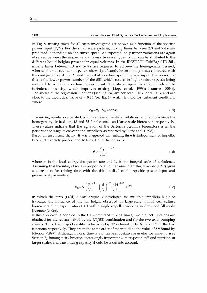
Computational Fluid Dynamics Technologies and Applications
108
In Fig. 8, mixing times for all cases investigated are shown as a function of the specific power input (P/V). For the small scale systems, mixing times between 2.3 and 7.4 s are predicted, depending on the stirrer speed. As expected, only minor variations are again observed between the single-use and re-usable vessel types, which can be attributed to the different liquid heights present for equal volumes. In the BIOSTAT® CultiBag STR 50L, mixing times between 10 and 59.8 s are required to achieve the homogeneity desired, whereas the two segment impellers show significantly lower mixing times compared with the configuration of the RT and the SBI at a certain specific power input. The reason for this is the lower power number of the SBI, which results in higher stirrer speeds being required to achieve a certain power input. The stirrer speed is directly related to turbulence intensity, which improves mixing [Liepe et al. (1998); Kraume (2003)]. The slopes of the regression functions (see Fig. 8a) are between —0.36 and —0.3, and are close to the theoretical value of —0.33 (see Eq. 1), which is valid for turbulent conditions where
H m Rc N const.θ= ⋅ = (15)
The mixing numbers calculated, which represent the stirrer rotations required to achieve the homogeneity desired, are 18 and 35 for the small and large scale bioreactors respectively. These values indicate that the agitation of the Sartorius Stedim’s bioreactors is in the performance range of conventional impellers, as reported by Liepe et al. (1998). Based on turbulence theory, it was suggested that mixing time is independent of impeller type and inversely proportional to turbulent diffusion so that:
1/3
Tm 2
cLεθ
− ∝
(16)
where εT is the local energy dissipation rate and Lc is the integral scale of turbulence. Assuming that the integral scale is proportional to the vessel diameter, Nienow (1997) gives a correlation for mixing time with the third radical of the specific power input and geometrical parameters:
1/3 1/3 2.43
2/3m
P d HA D
V D dθ
− − = ⋅ ⋅ ⋅ ⋅
(17)
in which the term (H/d)2.43 was originally developed for multiple impellers but also indicates the influence of the fill height observed in large-scale animal cell culture bioreactors at an aspect ratio of 1.3 with a single impeller working in draw and fill mode [Nienow (2006)]. If this approach is adapted to the CFD-predicted mixing times, two distinct functions are obtained for the reactor mixed by the RT/SBI combination and for the two axial pumping stirrers. Thus, the proportionality factor A in Eq. 17 is found to be 6.5 and 8.7 in the two functions respectively. They are in the same order of magnitude to the value of 5.9 found by Nienow (1997). Although mixing time is not an appropriate parameter for scale-up (see Section 2), homogeneity becomes increasingly important with respect to pH and nutrients at larger scales, and thus mixing capacity should be taken into account.
214

CFD for Characterizing Standard and Single-use Stirred Cell Culture Bioreactors
109
Fig. 8. Mixing time as a function of specific power input for all bioreactor configurations investigated (a). Comparison of the CFD-predicted mixing times with the correlation by Eq. 17 for all bioreactor configurations investigated (b)
4.2.3 Gas distribution and oxygen mass transfer The gas phase distribution was modelled using an Euler-Euler approach, assuming a uniform bubble size with a diameter of 1 mm. This value was found to be the mean bubble size, determined by photography in the re-usable UniVessel® filled with pure water (2 L filling volume). Spatial gas phase distribution and oxygen mass transfer were investigated for different stirrer tip speeds in the range of 0.15 to 1.8 m·s-1 for two aeration rates of 0.1 and 0.2 vvm (volume gas per volume liquid and minute), which were defined via gas inlet velocity with gas volume fractions at the inlet surface equal to one. Due to the low gassing rate, as often used in cell culture applications, no profound effect on the shape of the flow pattern is found, which is in qualitative agreement with the findings of Zhu et al. (2009). Small effects on the liquid velocity are predicted in the jet of the radial impeller, which becomes less intensive, as well as near the stirrer shaft, where the rising gas partly compensates for the downwards directed fluid flow (data not shown). In Fig. 9, the spatial gas phase distribution is given for impeller tip speeds of 0.37 m·s-1 and 0.94 m·s-1 at an aeration rate of 0.1 vvm and compared with experimental observations of the re-usable UniVessel®. Good qualitative agreement is achieved for all operation conditions investigated. At low agitation, the greater part of the gas rises with low dispersion as the disruptive forces induced by the RT are insufficient to overcome buoyancy, although the RT is designed and commonly used to achieve homogeneous gas-liquid dispersions. However, at such low agitation, the stirrer is considered to be “flooded” [Liepe et al. (1998); Zlokarnik (1999)]. The gas dispersion is clearly enhanced by the higher stirrer speed, as shown in Figs. 9c and 9d. Under such conditions, the air introduced is dispersed radially by the lower stirrer and reaches the vessel wall, but almost no gas is found near the bottom. This is again in qualitative agreement with experimental observations (see Fig. 9c) and is also found in experimental [Zhu et al. (2009)] and numerical investigations [Kerdouss et al. (2008] at comparable operation conditions in other gas-liquid agitated vessels.
A.4. Publication reprints 215
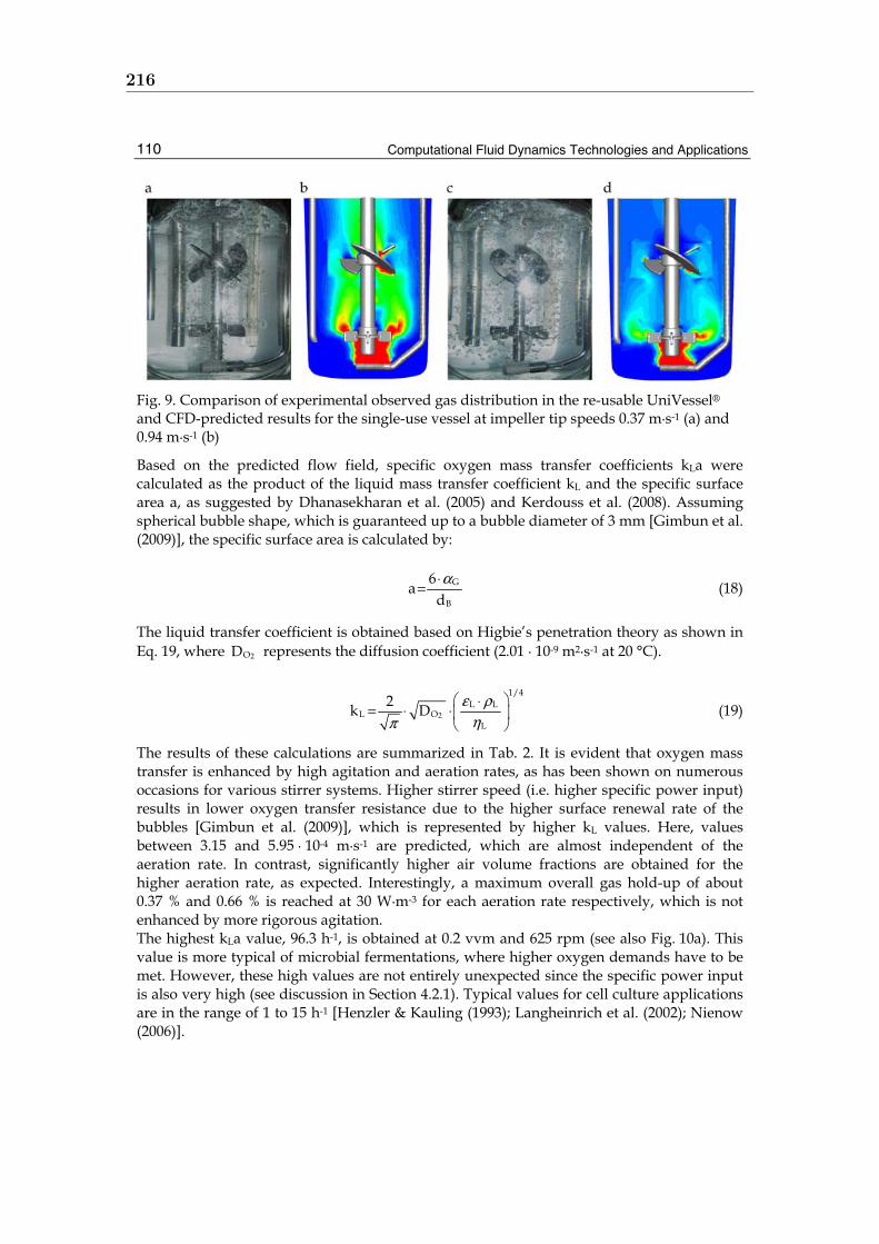
Computational Fluid Dynamics Technologies and Applications
110
Fig. 9. Comparison of experimental observed gas distribution in the re-usable UniVessel® and CFD-predicted results for the single-use vessel at impeller tip speeds 0.37 m·s-1 (a) and 0.94 m·s-1 (b)
Based on the predicted flow field, specific oxygen mass transfer coefficients kLa were calculated as the product of the liquid mass transfer coefficient kL and the specific surface area a, as suggested by Dhanasekharan et al. (2005) and Kerdouss et al. (2008). Assuming spherical bubble shape, which is guaranteed up to a bubble diameter of 3 mm [Gimbun et al. (2009)], the specific surface area is calculated by:
G
B
6a
dα⋅
= (18)
The liquid transfer coefficient is obtained based on Higbie’s penetration theory as shown in Eq. 19, where 2OD represents the diffusion coefficient (2.01 · 10-9 m2·s-1 at 20 °C).
2
1/4L L
L OL
2k D
ε ρηπ
⋅= ⋅ ⋅
(19)
The results of these calculations are summarized in Tab. 2. It is evident that oxygen mass transfer is enhanced by high agitation and aeration rates, as has been shown on numerous occasions for various stirrer systems. Higher stirrer speed (i.e. higher specific power input) results in lower oxygen transfer resistance due to the higher surface renewal rate of the bubbles [Gimbun et al. (2009)], which is represented by higher kL values. Here, values between 3.15 and 5.95 · 10-4 m·s-1 are predicted, which are almost independent of the aeration rate. In contrast, significantly higher air volume fractions are obtained for the higher aeration rate, as expected. Interestingly, a maximum overall gas hold-up of about 0.37 % and 0.66 % is reached at 30 W·m-3 for each aeration rate respectively, which is not enhanced by more rigorous agitation. The highest kLa value, 96.3 h-1, is obtained at 0.2 vvm and 625 rpm (see also Fig. 10a). This value is more typical of microbial fermentations, where higher oxygen demands have to be met. However, these high values are not entirely unexpected since the specific power input is also very high (see discussion in Section 4.2.1). Typical values for cell culture applications are in the range of 1 to 15 h-1 [Henzler & Kauling (1993); Langheinrich et al. (2002); Nienow (2006)].
216

CFD for Characterizing Standard and Single-use Stirred Cell Culture Bioreactors
111
Q [vvm] P/V [W·m-3] kL [10-4 m·s-1] a [m2·m-3] α [%] kLa [h-1]
0.1 0.6 3.15 14.0 0.23 18.7
0.1 9.1 3.06 18.8 0.31 25.7
0.1 30.0 3.25 21.9 0.37 31.5
0.1 136.6 4.07 19.1 0.32 34.2
0.1 558.6 5.32 18.9 0.32 44.4
0.1 962.6 5.95 19.3 0.32 51.0
0.2 0.6 3.16 22.5 0.38 32.5
0.2 9.1 3.09 32.5 0.54 45.0
0.2 30.0 3.23 39.6 0.66 56.4
0.2 136.6 4.02 37.5 0.63 64.9
0.2 558.6 5.26 37.1 0.62 84.1
0.2 962.6 5.90 38.0 0.63 96.3
Table 2. Summary of the results of the multi-phase simulations in the UniVessel® single-use. The symbols Q, P/V, kL, a, α and kLa represent the aeration rate, the specific power input, the liquid oxygen mass transfer coefficient, the specific surface area, and the overall oxygen mass transfer coefficient
To meet the oxygen demand of cells under steady-state conditions, the oxygen uptake rate OUR needs to be equal to the oxygen transfer rate OTR. The latter depends on mass transfer and the driving force on the gas-liquid surface, given as:
( )2 2 2s
O L O O
OUR OTR
q X k a c c⋅ = ⋅ − (20)
where 2Oq , X, 2Oc and 2sOc represent the specific oxygen uptake rate, cell concentration,
oxygen concentration and oxygen saturation concentration respectively. Typical specific oxygen demands reported for mammalian and insect cells range from about 1· 10-9 to 1· 10-8 mmol·cell-1·day-1 (see also Tab. 3 for more details). Assuming oxygen solubility in cell culture media of 5 mg·L-1 and working at 30 % saturation, which are typical values in cell culture applications, the required kLa values for a cell density of 5 · 106 cells·mL-1 are between 1.1 and 36.8 h-1, depending on the cell line. These values are already reached at an aeration rate of 0.1 vvm with a specific power input of about 140 W·m-3, and with an even lower power input of about 10 W·m-3 at 0.2 vvm. In the CultiBag STR 50L a maximum kLa value of 35 h-1 was determined experimentally by Sartorius Stedim at an aeration rate of 0.1 vvm [Personal communication, Ute Noack, Sartorius Stedim Biotech, 2010], giving comparable results for the large scale bioreactor.
A.4. Publication reprints 217

Computational Fluid Dynamics Technologies and Applications
112
Cell line qO2 [10-13 mol·cell-1·h-1] kLareq [h-1]
C1a (hybridoma) 2.34 10.7
FS-4 (human diploid cells) 0.5 2.3
AB2-143.2(hybridoma) 1.9 – 4.0 8.7 – 18.3
167.4G5.3 (hybridoma) 0.23 – 0.87 1.1 – 4.0
NSO (myeloma) 2.19 – 4.06 10.0 – 18.6
MAK (hybridoma) 4.6 21.0
X-D (hybridoma) 2.3 – 4.2 10.5 – 19.2
DG44 (CHO) 2.0 9.1
CHO 5.0 – 8.04 22.9 – 36.8
HFN7.1 (hybridoma) 2.0 9.1
Table 3. Specific oxygen uptake rates of various cell lines adopted from Ruffieux et al. (1998) and Xiu et al. (1999) and required oxygen mass transfer coefficients at defined cell densities of 5·106 cells·mL-1 and oxygen concentrations of 5 mg·L-1 (see Eq. 20)
In spite of the numerous literature data in respect of oxygen mass transfer, no correlation was found for the particular stirrer configuration and operation conditions used in this study. Thus, a correlation was developed following an approach suggested by van’t Riet (1979), where the kLa value is related to the specific power input and the superficial gas velocity (introduced gas per cross sectional area of the bioreactor):
( )a bL gk a C P/V u= ⋅ ⋅ (21)
As shown in Fig. 10, very good agreements between the model and CFD-predicted kLa values are achieved for the two aeration rates investigated (with R2 = 0.98). The coefficients C, a and b are found to be 6.51, 0.14 and 0.87 respectively (see Eq. 20). Hence, a rather high dependency of the kLa value on the superficial gas velocity (aeration rate) is evident and the specific power input is only of minor importance. This is in contrast to most correlations found in the literature, where the values for a and b are 0.5 ± 0.1 [Nienow (2006)]. Nevertheless, Van’t Riet (1979) gives a wider range of reported values in the ranges of 0.4 < a < 1 and 0 < b < 0.7.
( )0.14 0.87L gk a 6.51 P/V u= ⋅ ⋅ (22)
The strong effect of the superficial gas velocity obtained in this study can be explained by the fact that the stirrer does not completely disperse the introduced gas at low agitation rates, and thus the aeration is comparable to a bubble column (see Fig. 9a). Similar results were recently found in our laboratory with other single-use stirred bioreactors (e.g. the Mobius® CellReady 3L bioreactor) [Kaiser et al. (2011)]. However, we would like to point
218

CFD for Characterizing Standard and Single-use Stirred Cell Culture Bioreactors
113
out that only twelve data points were used for the correlation in this first attempt and the results were only obtained by CFD simulations, which have to be validated by experimental data in further studies.
Fig. 10. CFD-predicted volume-averaged specific oxygen mass transfer coefficient kLa as a function of specific power input for the two aeration rates investigated. In addition to CFD-predicted data points, the function obtained by Eq. 22 is given
4.3 Mechanical stress 4.3.1 Mechanical stress caused by turbulence Mechanical stress on cells is related to both turbulence and time-independent velocity-gradients (shear and normal gradients) [Jöbses et al. (1991); Oh et al. (1992); Chisti (2000); Fenge et al. (2003)]. A popular, but yet unproven, theory of cell damage due to turbulence suggests that the biological entity is damaged by eddies of a comparable size. Significantly smaller eddies have too little energy and larger eddies merely carry the cells convectively. Assuming local isotropic turbulence, the size of the smallest eddies is defined by the Kolmogorov length le (Eq. 23). Although Ranade & Joshi (1989) and Jaworski et al. (1991) state that turbulence in the impeller jet is anisotropic, theoretical considerations and experimental evidence have shown that the fine-scale structure of most anisotropic turbulent flows is actually almost isotropic locally [Hinze (1959)]. Thus, Kolmogorov‘s definition of eddy size would appear suitable for the complete fluid domain.
1/43
e 3lη
ρ ε
= ⋅ (23)
In Fig. 11a, the dimensionless turbulent kinetic energy k/utip2 is shown. As expected, and in agreement with Hockey & Nouri (1996), convection of turbulence by the mean flow in the impeller jet, where the highest turbulent energies are found, is evident. The axial profiles of the turbulence kinetic energy in impeller jets are found to qualitatively agree with data given by Kresta & Wood (1991), although the predicted values are, by a factor of 5, lower in our study (data not shown). Rather high turbulence is also located near the installations, but significantly lower values are found in the bulk between the impellers and near the liquid surface. Thus, it can be argued that the turbulence distribution is very heterogeneous. For
A.4. Publication reprints 219

Computational Fluid Dynamics Technologies and Applications
114
standard Rushton turbines, Höfken et al. (1996) found differences between maximum and mean turbulent dissipation rates by two orders of magnitude ( max / 40...200ε ε = ).
Fig. 11. Spatial distributions of the dimensionless turbulent kinetic energy k/utip2 (a) and the Kolmogorov eddy size le (b) at P/V = 230 W·m-3 in the UniVessel® 2L single-use
As mentioned in Section 4.2.1, typical values for the specific power input are in the range of 10 to 250 W·m-3 [Nienow (2006)]. Calculating the Kolmogorov eddy size gives le = 45 µm for ε = (P/V) (see Eq. 23). If, as found by Höfken et al (1996) near the impeller of a Rushton turbine, εmax = 200 · (P/V) is assumed, le decreases to about 12 µm. Since animal cells are of the order of 15-20 µm, the first cell damage would be expected at the maximum power input. In this study, the estimated Kolmogorov eddy size is lower than typical cell sizes above a specific power input of 230 W·m-3 (see Fig. 11b) in close proximity to the impellers and installations, which is in agreement with the literature data. Zhang et al. (1993) investigated animal cell disruption in turbulent capillary flows and developed a model of cell-hydrodynamic interactions using cell mechanical properties determined by micromanipulation. Assuming that eddies with similar or smaller sizes than the cells cause local surface deformation, they proposed that cell disruption occurs when the cells’ bursting membrane tension and bursting surface energy are exceeded. Good agreement between experiments and model predictions (with an underestimation of cell disruption by about 15%) were achieved [Zhang et al. (1993)]. Garcia-Briones et al. (1994) compared CFD-predicted energy dissipation rates with those in unaerated flow devices (capillaries and viscometers). They concluded that energy dissipation rates in the order of 5.81 · 102 W·m-3 did not damage cells significantly, but values of ≈ 2.25 · 104 W·m-3 caused considerable damage. Using Eq. 22, the latter value gives an eddy length scale of 14.5 µm for water-like media, which is comparable to the size of animal cells (≈15…20 µm). The turbulence theory of cell damage is also supported by the observation that viscosifying additives reduce cell damage. Croughan et al. (1989) have associated cell death protection by serum with the turbulence-dampening effect of the additive. In contrast, observing an insect cell suspension with ten times higher viscosity to water (with η ≈ 10 mPa·s and ρ ≈ 1000 kg·m-3), Tramper et al. (1996) found that cell death rapidly occurred from a specific power
220

CFD for Characterizing Standard and Single-use Stirred Cell Culture Bioreactors
115
input of 2.3· 10-3 W·kg-1. Even if max / 200ε ε ≈ is assumed, this gives a minimum
Kolmogorov length scale of le = 240 µm, which is considerably larger than an insect cell. Hence, it has been concluded that maximum shear stress is the more appropriate parameter for scale-up than the minimum eddy length scale [Tramper et al. (1996)]. However, bearing in mind the heterogeneous distribution of turbulence, it is important to take residence time distribution into account for the evaluation of cell damage (see Section 4.3.2 for further discussion). However, to the knowledge of the authors, such attempts have not yet been described for animal cells, unlike corresponding studies for blood cells in hemolysis experiments. Thus, the hemolysis level is often correlated with shear stress and residence time, as suggested, for example, by Giersiepen et al. (1990).
4.3.2 Mechanical stress caused by velocity gradients (shear stress) In most CFD studies, the mechanical stress on cells is only related to the strain rate magnitude D, which is an invariant velocity gradient consisting of both shear and normal gradients. However, based on model experiments, various authors have shown that cells are differently affected by shear or normal gradients [e.g. Langer & Deppe (2000)]. It is therefore advantageous if each of them is quantified separately for the evaluation of cell damage. Recently, Wollny (2010) found that local shear and normal gradients ( nt γ and nnγ ) can be obtained from shear strain tensor using a coordinate system transformation, which results in Eqs. 24 and 25. Here, w are velocities in the local co-ordinate systems defined by the co-ordinates x, y and z , which are orientated along the fluid flow direction. Detailed descriptions of the mathematical derivation can be found elsewhere [Wollny (2010)].
2
xnn
w2
xγ ∂ = ⋅ ∂
(24)
2 2
yx x znt
ww w wy x z x
γ ∂∂ ∂ ∂ = + + + ∂ ∂ ∂ ∂
(25)
From the CFD-predicted flow fields, the local shear and normal gradients as well as the corresponding volume fractions were determined. Subsequently, the distribution was discretized into 250 bins (see Fig. 12a). It was found that the distribution follows a logarithmically normal function, which was confirmed by a chi-quadrate-test at a confidence level of 0.05 (data not shown). From Fig. 12a it is evident that the highest volume fractions (of about 4.5 %) are found at very low velocity gradients. Depending on the impeller speed, the median value (velocity gradient with the highest volume fraction) is in the order of 1 – 30 s-1. Interestingly, the median differs from the volume-averaged velocity gradient and the highest volume fraction is nearly independent of the stirrers’ power input. This is in qualitative agreement with our previous findings for different single-use and conventional stirred bioreactors [Löffelholz et al. (2011)]. Furthermore, high velocity gradients (> 100 s-1) have very small volume fractions below 0.5 % of the total liquid volume. Wollny (2010) found quantitatively comparable values for a baffled bioreactor equipped with a 3x24° pitched blade impeller or a standard Rushton
A.4. Publication reprints 221
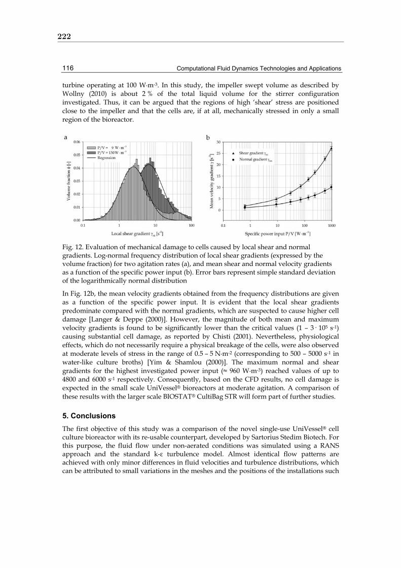
Computational Fluid Dynamics Technologies and Applications
116
turbine operating at 100 W·m-3. In this study, the impeller swept volume as described by Wollny (2010) is about 2 % of the total liquid volume for the stirrer configuration investigated. Thus, it can be argued that the regions of high ‘shear’ stress are positioned close to the impeller and that the cells are, if at all, mechanically stressed in only a small region of the bioreactor.
Fig. 12. Evaluation of mechanical damage to cells caused by local shear and normal gradients. Log-normal frequency distribution of local shear gradients (expressed by the volume fraction) for two agitation rates (a), and mean shear and normal velocity gradients as a function of the specific power input (b). Error bars represent simple standard deviation of the logarithmically normal distribution
In Fig. 12b, the mean velocity gradients obtained from the frequency distributions are given as a function of the specific power input. It is evident that the local shear gradients predominate compared with the normal gradients, which are suspected to cause higher cell damage [Langer & Deppe (2000)]. However, the magnitude of both mean and maximum velocity gradients is found to be significantly lower than the critical values (1 – 3· 105 s-1) causing substantial cell damage, as reported by Chisti (2001). Nevertheless, physiological effects, which do not necessarily require a physical breakage of the cells, were also observed at moderate levels of stress in the range of 0.5 – 5 N·m-2 (corresponding to 500 – 5000 s-1 in water-like culture broths) [Yim & Shamlou (2000)]. The maximum normal and shear gradients for the highest investigated power input (≈ 960 W·m-3) reached values of up to 4800 and 6000 s-1 respectively. Consequently, based on the CFD results, no cell damage is expected in the small scale UniVessel® bioreactors at moderate agitation. A comparison of these results with the larger scale BIOSTAT® CultiBag STR will form part of further studies.
5. Conclusions The first objective of this study was a comparison of the novel single-use UniVessel® cell culture bioreactor with its re-usable counterpart, developed by Sartorius Stedim Biotech. For this purpose, the fluid flow under non-aerated conditions was simulated using a RANS approach and the standard k-ε turbulence model. Almost identical flow patterns are achieved with only minor differences in fluid velocities and turbulence distributions, which can be attributed to small variations in the meshes and the positions of the installations such
222

CFD for Characterizing Standard and Single-use Stirred Cell Culture Bioreactors
117
as probes and harvest tubes. The CFD simulations reveal a rather complex flow pattern, in which the radial pumping Rushton turbine induced two flow loops per half-vessel and the segment blade impeller shows a typical axial flow in down-pumping mode. Predicted fluid velocities as well as flow numbers show good qualitative and quantitative agreement with literature data. Based on these results, it can be argued that the differences in geometry between the two small scale bioreactors have no influence on the overall fluid flow. From the fluid flow perspective, the UniVessel® 2L single-use is identical to its counterpart made of glass and thus no differences in cell cultivations are expected. This hypothesis clearly needs to be verified in cultivation experiments, which will be carried out in our laboratory in the near future. In a second part, key engineering parameters, such as power input, mixing capacity and oxygen mass transfer, for the UniVessel® 2L single-use are presented for the first time and compared with data on its conventional counterpart as well as with those on the BIOSTAT® CultiBag STR 50L. The power numbers Ne of the two small scale systems are identical (with a value of 3.33) and somewhat lower in the CultiBag STR 50L (Ne = 3.14) at the same stirrer configuration (RT and SBI). It is shown that unreasonably high specific power inputs for cell culture applications are obtained in the UniVessel® bioreactors, if the maximum tip speed of 1.8 m·s-1 is used as a scale-up/down parameter for the CultiBag STR 50L. Thus, it can be concluded that (maximum) specific power input P/V is a more appropriate constraint for scale-up than tip speed when viewed from the perspective of adequate mixing and shear sensitivity of the cells, which is in agreement with the literature data. Furthermore, correlations for the mixing time are provided which are independent of the bioreactor scale, as suggested by Nienow (1997), and can thus be used in scale-up/down studies. From multi-phase simulations using an Euler-Euler approach, gas phase distribution and oxygen mass transfer were modelled for various agitation and aeration rates. In this first attempt, a constant bubble size of 1 mm, as obtained using photography at the BIOSTAT® B plus is assumed. It is well-known that bubble size depends on media properties, such as viscosity, salt content etc., and is usually non-uniform. In addition, bubble size distribution depends on aeration (e.g. the sparger design) and the agitation system (e.g. impeller type), and is further influenced by bubble break-up and coalescence. In the last two decades, bubble size distributions have been increasingly modelled using population balance models (PBM) [e.g. Kerdouss et al. (2008); Dhanasekharan et al. (2005)]. Nevertheless, computation using PBMs becomes more complex and time-consuming due to the additional transport equations for bubble size distribution. Hence, this approach is not adopted for the first engineering characterization of the UniVessel®, but will be used in further studies in the near future. Based on the results obtained so far, it can be concluded that the oxygen transfer capacity of the UniVessel® 2L single-use has no limitations for medium cell densities achieved at gentle agitation and aeration. In addition to the results presented, the fluid flow in the small scale UniVessel® equipped with two segment blade impellers will be investigated in further studies, because Sartorius Stedim decided to provide the UniVessel® single-use with this stirrer configuration mainly due to the broad acceptance by the costumers. In a third part, two approaches for the evaluation of mechanical stress on cells are presented. The first, which is based on the Kolmogorov turbulence theory, indicates that cell damage could occur above specific power inputs of 230 W·m-3. This value is also given as the upper limit of typical power inputs by Nienow (2006). However, it is shown that the
A.4. Publication reprints 223

Computational Fluid Dynamics Technologies and Applications
118
turbulence distribution inside the bioreactor is very heterogeneous. Hence, volume-weighted distributions of velocity gradients are predicted in the second approach. These velocity gradients are additionally subdivided into local shear and normal gradients, as suggested by Wollny (2010), which may allow a more detailed evaluation of cell damage mechanisms. Compared with turbulence, velocity gradients indicate lower cell stress potential. Although no cell damage is expected under typical operation conditions, it is difficult to draw general conclusions since biological effects depend on various factors, such as the cell line used, cell characteristics, culture media, additives and so on. Nevertheless, the results obtained indicate that Sartorius Stedim’s novel UniVessel® 2L single-use is a viable alternative to conventional stirred cell culture bioreactors at bench scale.
6. Acknowledgment The results presented are part of PhD theses. The authors are grateful to Dipl.-Ing. Ute Noack, Dr. Alexander Tappe, Dr. Gerhard Greller, Dr. Bhaskar Bandarapu, Dr. Thorsten Peuker, Dipl.-Ing. Lars Böttcher, Martin Saballus and Alexander Halt from Sartorius Stedim Biotech for providing details about the geometries of the bioreactors investigated and the experimental results of the BIOSTAT® CultiBag STR 50L as well as for their participation in helpful discussions.
7. References Alcamo, R.; Micale, G.; Grisafi, F.; Brucato, A. & Ciofalo, M. (2005). Large-eddy simulation of
turbulent flow in an unbaffled stirred tank driven by a Rushton turbine. Chemical Engineering Science, Vol. 60, pp. 2303-2316
Arathoon, W. & Birch, J. (1986). Large scale cell culture in biotechnology. Science, Vol. 232, pp. 1390-1395
Chalmers, J. J. (1994). Cells and bubbles in sparged bioreactors. Cytotechnology, Vol. 15, pp. 311-320
Chisti, Y. (1993). Animal cell culture in stirred bioreactors: Observations on scale-up. Bioprocess Engineering, Vol. 9, pp. 191-196
Chisti, Y. (2000). Animal-cell damage in sparged bioreactors. Trends in Biotechnology, Vol. 18, pp. 420-432
Chisti, Y. (2001). Hydrodynamic damage to animal cells. Critical Reviews in Biotechnology, Vol. 21, pp. 67-110
Croughan, M. S.; Sayre, E. S. & Wang, D. I. (1989). Viscous reduction of turbulent damage in animal cell culture. Biotechnology and Bioengineering, Vol. 33, pp. 862-872
De Wilde, D.; Noack, U.; Kahlert, W.; Barbaroux, M. & Greller, G. (2009). Bridging the gap from reusable to single-use manufacturing with stirred, single-use bioreactors. BioProcess International, Vol. 7, pp. 36-41
Delafosse, A.; Line, A.; Morchain, J. & Guiraud, P. (2008). LES and URANS simulations of hydrodynamics in mixing tank: comparison to PIV experiments. Chemical Engineering Research and Design, Vol. 86, pp. 1322-1330
Dhanasekharan, K. M.; Sanyal, J.; Jain, A. & Haidari, A. (2005). A generalized approach to model oxygen transfer in bioreactors using population balances and computational fluid dynamics. Chemical Engineering Science, Vol. 60, pp. 213-218
224

CFD for Characterizing Standard and Single-use Stirred Cell Culture Bioreactors
119
Eibl, R.; Kaiser, S.; Lombriser, R. & Eibl, D. (2010). Disposable bioreactors: the current state-of-the-art and recommended applications in biotechnology. Applied Microbiology Biotechnology, Vol. 86, pp. 41-49
Eibl, R.; Löffelholz, C. & Eibl, D. (2011). Single-use bioreactors - an overview, In: Single-use Technology in Biopharmaceutical Manufacture, R. Eibl & D. Eibl, (Eds.), 34-51, John Wiley & Sons, New Jersey, USA
Fenge, C.; Klein, C.; Heuer, C.; Siegel, U. & Fraune, E. (1993). Agitation, aeration and perfusion modules for cell culture bioreactors. CytotechnoIogy , Vol. 11, pp. 233-244
Fluent 6.3 user’s guide (2006), Centerra Resource Park, 10 Cavendish Court, Lebanon, USA: Fluent Inc., Available from http://my.fit.edu/itresources/manuals/fluent6.3/help/pdf/ug/flug.pdf
Garcia-Briones, M. & Chalmers, J. J. (1994). Flow parameters associated with hydrodynamic cell injury. Biotechnology and Bioengineering, Vol. 44, pp. 1089-1098
Giersiepen, M.; Wurzinger, L.; Optz, R. & Reul, H. (1990). Estimation of shear stress-related blood damage in heart valve protheses - in vitro comparison of 25 aortic valves. International Journal of Artificial Organs, Vol. 13, pp. 300-306
Gimbun, J.; Rielly, C. & Nagy, Z. (2009). Modelling of mass transfer in gas–liquid stirred tanks agitated by rushton turbine and CD-6 impeller: A scale-up study. Chemical Engineering Research and Design, Vol. 87, pp. 437-451
Handa, A.; Emery, A. & Spier, R. (1987). On the evaluation of gas-liquid interfacial effects on hybridoma viability in bubble column bioreactors. Developments in Biological Standardization, Vol. 66, pp. 241-253
Henzler, H.-J. & Kauling, D. J. (1993). Oxygenation of cell cultures. Bioprocess and Biosystems Engineering, Vol. 9, pp. 61-75
Hinze, J.O. (1959). Turbulence. McGraw-Hill, New York. Hockey, R. M. & Nouri, J. (1996). Turbulent flow in a baffled vessel stirred by a 60° pitched
blade impeller. Chemical Engineering Science, Vol. 51, pp. 4405-4421 Höfken, M.; Schäfer, M. & Durst, F. (1996). Detaillierte Untersuchung des Strömungsfeldes
innerhalb eines Sechs-Blatt-Scheibenrührers. Chemie lngenieur Technik, Vol. 68, pp. 803-809
Ishii, M. & Zuber, N. (1979). Drag coefficient and relative velocity in bubbly, droplet or particulate flows. AIChE Journal, Vol. 25, pp. 843-855
Jahoda, M.; Mostek, M.; Kukuková, A. & Machon, V. (2007). CFD modelling of liquid homogenization in stirred tanks with one and two impellers using large eddy simulation. Chemical Engineering Research and Design, Vol. 85, pp. 616-625
Jaworski, Z.; Nienow, A. W.; Koutsakos, E.; Dyster, K. & Bujalski, W. (1991). An LDA study of turbulent flow in a baffled vessel agitated by a pitched blade turbine. Chemical Engineering Research and Design, Vol. 69, pp. 313-320
Jöbses, I.; Martens, D. & Tramper, J. (1991). Lethal events during gas sparging in animal cell culture. Biotechnology and Bioengineering, Vol. 37, pp. 484-490
Kaiser, S.C. (2009). Theoretische und experimentelle Untersuchungen zur Bestimmung der Mischzeit und des Sauerstoffeintrages in Bioreaktoren. Master Thesis. Hochschule Anhalt (FH), Köthen..
Kaiser, S. C.; Eibl, R. & Eibl, D. (2011). Engineering characteristics of a single-use stirred bioreactor at bench-scale: The Mobius CellReady 3L bioreactor as a case study, Engineering Life Sciences, in submission.
A.4. Publication reprints 225
Computational Fluid Dynamics Technologies and Applications
120
Kerdouss, F.; Bannari, A.; Proulx, P.; Bannari, R.; Skrga, M. & Labrecque, Y. (2008). Two-phase mass transfer coefficient prediction in stirred vessel with a CFD model. Computers and Chemical Engineering, Vol. 32, pp. 1943-1955
Kioukia, N.; Nienow, A. W.; Al-Rubeai, M. & Emery, A. N. (1996). Influence of agitation and sparging on the growth rate and infection of insect cells in bioreactors and a comparison with hybridoma culture. Biotechnol. Prog., Vol. 12, pp. 779-785
Krampe, B. & Al-Rubeai, M. (2010). Cell death in mammalian cell culture: molecular mechanisms and cell line engineering strategies. Cytotechnology, Vol. 62, pp. 175-188
Kraume, M. (2003). Mischen und Rühren. Grundlagen und moderne Verfahren. Wiley-VCH Kresta, S. & Wood, P. (1991). Prediction of the three-dimensional turbulent flow in stirred
tanks. AIChE Journal, Vol. 37, pp. 448-460 Langer, G. & Deppe, A.(2000). Zum Verständnis der hydrodynamischen Beanspruchung
von Partikeln in turbulenten Rührerströmungen. Chemie Ingenieur Technik, Vol. 72, pp. 31-41
Langheinrich, C.; Nienow, A. W.; Eddleston, T.; Stevenson, N. C.; Emery, A. N.; Clayton, T. M. & Slater, N. K. H. (2002). Oxygen transfer in stirred bioreactors under animal cell culture conditions. Food and Bioproducts Processing, Vol. 80, pp. 39-44
Letellier, B.; Xuereb, C.; Swaels, P.; Hobbes, P. & Bertrand, J. (2002). Scale-up in laminar and transient regimes of a multi-stage stirrer, a CFD approach. Chemical Engineering Science, Vol. 57, pp. 4617 - 4632
Liepe, F.; Sperling, R. & Jembere, S. (1998). Rührwerke - Theoretische Grundlagen, Auslegung und Bewertung. Eigenverlag FH Anhalt, Köthen
Löffelholz, C.; Kaiser, S.; Werner, S. & Eibl, D. (2011). CFD as a tool to characterize single-use bioreactors, In: Single-use Technology in Biopharmaceutical Manufacture, R. Eibl & D. Eibl, (Eds.), 34-51, John Wiley & Sons, New Jersey, USA
Meneses-Acosta, A.; Mendonca, R. Z.; Merchant, H.; Covarrubias, L. & Ramírez, O. T. (2001). Comparative characterization of cell death between Sf9 insect cells and hybridoma cultures. Biotechnology and Bioengineering, Vol. 72, pp. 441-457
Min, J. & Gao, Z. (2006). Large eddy simulation of mixing time in a stirred tank. Chinese Journal Chemical Engineering, Vol. 14, pp. 1-7
Montante, G.; Lee, K.; Brucato, A. & Yianneskis, M. (2001). Numerical simulations of the dependency of flow pattern on impeller clearance in stirred vessels. Chemical Engineering Science, Vol. 56, pp. 3751-3770
Nienow, A. W. (1997). On impeller circulation and mixing effectiveness in the turbulent flow regime. Chemical Engineering Science, Vol. 52, pp. 2557-2565
Nienow, A. W. (2006). Reactor engineering in large scale animal cell culture. Cytotechnology, Vol. 50, pp. 9-33
Noack, U.; De Wilde, D.; Verhoeye, F.; Balbirnie, E.; Kahlert, W.; Adams, T.; Greller, G. & Reif, O. (2011). Single-use stirred tank reactor BIOSTAT CultiBag STR: Characterization and applications, In: Single-use Technology in Biopharmaceutical Manufacture, R. Eibl & D. Eibl, (Eds.), 34-51, John Wiley & Sons, New Jersey, USA
Oh, S.; Nienow, A.; AI-Rubeai, M. & Emery, A. (1992). Further studies of the culture of mouse hybridomas in an agitated bioreactor with and without continuous sparging. Journal of Biotechnology, Vol. 22, pp. 245-270
Ozturk, S. S. (1996). Engineering challenges in high density cell culture systems. Cytotechnology, Vol. 22, pp. 3-16
226

CFD for Characterizing Standard and Single-use Stirred Cell Culture Bioreactors
121
Paschedag, A. R.; Kassera, V. & Sperling, R. (2007). Aktuelle Entwicklungen in der CFD für gerührte Systeme. Chemie Ingenieur Technik, Vol. 79, pp. 983-999
Patwardhan, A. W. & Joshi, J. B. (1999). Relation between flow pattern and blending in stirred tanks. Industrial& Engineering Chemistry Research, Vol. 38, pp. 3131-3143
Ranade, V. V. & Joshi, J. B. (1989). Flow generated by pitched blade turbines I: measurements using laser Doppler anemometer. Chemical Engineering Communications, Vol. 81, pp. 197-224
Revstedt, J.; Fuchs, L. & Trägardh, C. (1998). Large eddy simulations of the turbulent flow in a stirred reactor. Chemical Engineering Science, Vol. 53, pp. 4041-4053
Ruffieux, P.-A.; von Stockar, U. & Marison, I. W. (1998). Measurement of volumetric (OUR) and determination of specific (qO2) oxygen uptake rates in animal cell cultures. Journal of Biotechnology, Vol. 63, pp. 85-95
Tramper, J.; Vlak, J. & de Gooijer, C. (1996). Scale up aspects of sparged insect-cell bioreactors. Cytotechnology, Vol. 20, pp. 221-229
Storhas, W. (2003). Bioverfahrensentwicklung. Wiley-VCH, Weinheim. Van’t Riet, K. (1979). Review of measuring methods and results in nonviscous gas-liquid
mass transfer in stirred vessels. Industrial & Engineering Chemistry Process Design and Development, Vol. 18, pp. 1979 357
Varley, J. & Birch, J. (1999). Reactor design for large scale suspension animal cell culture. Cytotechnology, Vol. 29, pp. 177-205
Venkat, R. V. & Chalmers, J. J. (1996). Characterization of agitation environments in 250 ml spinner vessel, 3 L, and 20 L reactor vessels used for animal cell microcarrier culture. Cytotechnology, Vol. 22, pp. 95-102
Vrabel, P.; van der Lans, R. G. J. M.; Luyben, K. C. A. M.; Boon, L. & Nienow, A. W. (2000). Mixing in large-scale vessels stirred with multiple radial or radial and axial up-pumping impellers: modelling and measurements. Chemical Engineering Science, Vol. 55, pp. 5881-5896
Weyand, B.; Israelowitz, M.; von Schroeder, H. & Vogt, P. (2009). Fluid dynamics in bioreactor design: considerations for the theoretical and practical approach, In: Bioreactor Systems for Tissue Engineering, C. Kasper, M. van Griensven & R. Pörtner (Eds.), 251-268
Wollny, S. (2010). Experimentelle und numerische Untersuchungen zur Partikelbean-spruchung in gerührten (Bio-)Reaktoren. PhD thesis. Technische Universität Berlin, Deutschland
Xiu, Z.-L.; Deckwer, W.-D. & Zeng, A.-P. (1999). Estimation of rates of oxygen uptake and carbon dioxide evolution of animal cell culture using material and energy balances. Cytotechnology, Vol. 29, pp. 159-166
Yianneskis, M.; Popiolek, Z. & Whitelaw, J. (1987). An experimental study of the steady and unsteady flow characteristics of stirred reactors. Journal of Fluid Mechanics, Vol. 175, pp. 537-555
Yim, S. S. & Shamlou, P. A. (2000). The engineering effects of fluids flow on freely suspended biological macro-materials and macromolecules, In: Influence of Stress on Cell Growth and Product Formation, K. Schügerl & G. Kretzmer, (Eds.), 83-122, Springer
Zhang, Z.; Al-Rubeai, M. & Thomas, C. R. (1993). Estimation of disruption of animal cells by turbulent capillary flow. Biotechnology and Bioengineering, Vol. 42, pp. 987-993
A.4. Publication reprints 227

Computational Fluid Dynamics Technologies and Applications
122
Zhu, H.; Nienow, A. W.; Bujalski, W. & Simmons, M. J. (2009). Mixing studies in a model aerated bioreactor equipped with an up- or a down-pumping ‘Elephant Ear’ agitator: Power, hold-up and aerated flow field measurements. Chemical Engineering Research and Design, Vol. 87, pp. 307-317
Zlokarnik, M.(1999). Rührtechnik - Theorie und Praxis. Springer, Berlin, Heidelberg, New York Zlokarnik, M. (2006). Scale-Up in Chemical Engineering (second, completely revised and extended
edition). Wiley-VCH, Weinheim
228

Research Article
Fluid Flow and Cell Proliferation of MesenchymalAdipose-Derived Stem Cells in Small-Scale,Stirred, Single-Use BioreactorsStephan C. Kaiser1,*, Valentin Jossen1, Carmen Schirmaier1, Dieter Eibl1, Silke Brill2,Christian van den Bos2, and Regine Eibl1
DOI: 10.1002/cite.201200180
The fluid flow and suspension characteristics inside small-scale, stirred, single-use bioreactors were investigated experi-
mentally and by means of computational fluid dynamics. The required impeller speeds for homogenous suspension were
determined for two microcarrier types. The shear stress level and turbulence distribution were predicted using a numerical
model, which was verified by particle image velocimetry measurements. In subsequent cultivations of primary mesency-
mal adipose-derived stem cells, up to 31.4-fold expansion in cell number was achieved for serum concentrations as low as
5 %.
Keywords: Adipose-derived stem cells, CFD model, Microcarrier, Paricle image velocimetry, Single-use spinner flask
Received: October 18, 2012; revised: November 21, 2012; accepted: December 10, 2012
1 Introduction
Adipose-derived stem cells (ASCs) have great potential fortissue engineering and regenerative medicine because oftheir multipotency and their ability to differentiate alongmultiple lineage pathways [1]. Possible applications rangefrom healing wounds to osteo-chondral and functional car-diac repair [2]. As a result of how they are sourced, me-senchymal stem cells (MSCs) are ethically less questionablethan embryonic stem cells (ESCs) or induced pluripotentstem cells (iPSCs). Furthermore, numerous studies have pro-vided preclinical data on the safety and efficacy of ASCs, sup-porting the use of these cells in future clinical applications [3].
Despite the significant progress made in cultivation ofMSCs, the availability of these cells remains a challenge forboth scientists and clinicians pursuing regenerative medi-cine [1]. Usually, MSCs are anchorage-dependent and are,therefore, expanded in static cultivation systems (so-calledplanar flask cultures), but growth parameters are difficult tomonitor and scale-up is limited for these systems. Becauseof the improved mass transfer they offer, dynamic cultiva-
tion systems, including packed-bed systems [4, 5] and in par-ticular stirred systems using microcarriers, are preferred[6 – 8].
A dynamic culture environment improves the flow of oxy-gen and nutrients to cells as well as the removal of wasteproducts from the cells. However, fluid shear stress is gener-ated, which is known to influence the properties and beha-vior of MSC cell cultures [9 – 11]. However, only limited datais available in the literature for fluid flow and shear stress insuitable stirred bioreactors, such as spinner flasks. Spinnerflasks are most often used for small-scale stem cell expan-sion [8, 12] and have also been used for screening experi-ments in our laboratories.
In this report, computational fluid dynamics (CFD) stu-dies were examined that have been conducted to evaluateoverall fluid flow and estimate shear stress levels in spinnerflasks. By taking the solid microcarrier into account, suspen-sion characteristics were determined for various impellerspeeds. The model was validated using particle image velo-cimetry (PIV) measurements.
2 Experimental Setup
2.1 Bioreactor and Microcarrier Characteristics
All experiments were performed using pre-sterilized Corn-ing® 125-mL single-use spinner flasks (Corning, USA) witha 70-mm top cap and two angled side ports. The working
ChemieIngenieurTechnik
Chemie Ingenieur Technik 2013, 85, No. 1–2, 1–9 © 2013 Wiley-VCH Verlag GmbH & Co. KGaA, Weinheim www.cit-journal.com
–1Stephan Kaiser ([email protected]), Valentin Jossen, Car-men Schirmaier, Prof. Dieter Eibl, Prof. Regine Eibl, Zurich Univer-sity of Applied Sciences, School of Life Sciences and Facility Man-agement, Grüental, 8820 Wädenswil, Switzerland; 2Dr. Silke Brill,Christian van den Bos, Lonza Cologne GmbH, Nattermannallee 1,50829 Köln, Germany.
Adipose-derived stem cells 1
A.4. Publication reprints 229

volume was 100 mL for all cultivations and suspension in-vestigations. The top-mounted impeller consisted of a bladeand a bar with a maximum diameter of 41.5 mm. The im-peller speed was adjusted by a magnetic drive on the plat-form. A tachometer focused on the stir bar axis was used totrack the impeller speed in the suspension experiments andPIV investigations. Suspension criteria were evaluated by vi-sual observation at increasing impeller speeds. A mirrorwas placed below the spinner flask for better optical accessi-bility of the flask bottom.
Two different microcarrier types were used. The Hillex®-II (SoloHill) microcarriers have an amine treated surfaceand consist of particles with densities ranging from 1090 –1150 kg m–3, for sizes between 160 and 200 lm. The ProNec-tin®-F-coated microcarriers (SoloHill), subsequently shor-tened with ProNectin®-F, are coated styrene microcarrierswith densities in the range of 1022 – 1030 kg m–3 and parti-cle sizes between 125 and 212 lm.
2.2 Particle Image Velocimetry
Particle image velocimetry (PIV) measurements were madeusing a FlowMaster PIV system (LaVision, Germany) inconjunction with a double-pulsed Nd:YAG laser (litron nanopiv) with a wavelength of 532 nm. The 1-mm thick laser wasorientated horizontally to aim through the spinner bioreac-tor at three different heights, which were adjusted by a tra-verse system. A CCD camera (Imager Pro X 4M) with aresolution of 2048 × 2048 pixels was used for image captur-ing and was positioned above the bioreactor with the field ofview parallel to the fluid surface. The camera, traverse systemand laser were controlled by DaVis 7.2 software (LaVision).Rhodamin coated fluorescence particles with a density of1.19 kg m–3 (LaVision) were used. The velocity field was ob-tained from a set of 1000 images, based on an interrogationwindow of 32 × 32 pixels with a overlap of 50 %. The velocitycomponents were predicted by deducing the instantaneousdisplacement of the illuminated particles at two instants intime using cross correlation. Phase-locked measurementswere recorded by means of a photoelectric barrier focusedon the stirrer axis.
2.3 Cultivation Procedure
Cryopreserved adipose-derived mesenchymal stem cells, ob-tained from a single informed and consenting donor (hAD-MSCs, second passage, PDL = 10), were provided by LonzaCologne GmbH. The cells were routinely cultivated inEGM-2 MV medium (Lonza) with 5 % serum for six days at37 °C, 80 % humidity and 5 % CO2. The microcarriers wereprepared and sterilized in an autoclave, as recommended bythe vendor. The final microcarrier concentration was ad-justed to achieve a mean surface area of 515 cm2 per spinnerflask for a working volume of 100 mL.
The cells were inoculated at 2.9 · 103 cells cm–2, corre-sponding to about 1.5 · 104 cells mL–1. No stirring was per-formed during the first three hours to promote cell attach-ment. After this period, the impeller tip speeds were set tovalues between 0.105 and 0.175 m s–1 and the culture wascontinuously stirred. On day 4, the microcarriers wereallowed to settle and 50 % of the growth medium wasreplaced by fresh medium. The concentrations of substratesand metabolites were measured using a BioProfile 100 plusmulti-sensor analyzer (Laborsysteme Flükiger, Germany)directly after inoculation, before and after medium ex-change as well as on day 6 when the cultivation had beenterminated. On day 6, cell densities were measured automa-tically using a NucleoCounter NC-100 (chemometec, Den-mark) and cells were collected for DAPI staining. All experi-ments were performed using four spinner flasks in paralleland data was expressed as the mean and simple standarddeviation.
3 Numerical Details
The fluid flow inside the spinner flask was modeled usingthe finite volume solver Fluent13 (ANSYS). The governingequation for mass and momentum of the single-phase flowcan be written as follows:
∂q∂t
∇ u q 0 (1)
∂ q u ∂t
∇ q u u ∇p ∇ s q g F (2)
where q is the fluid density, u is the velocity vector, p is thestatic pressure. The term F denotes the Coriolis and centri-fugal forces applied in the rotating reference frame for theimpeller rotation, which can be written as
F q 2 x ×ur x × x ×r (3)
The Reynolds stress tensor s was modeled using the stan-dard k-e turbulence model developed by Launder and Spald-ing [13], where the turbulent kinetic energy k and the turbu-lent dissipation rate e are calculated by two separatetransport equations [14].
In addition to single-phase flow, the microcarrier distribu-tion was investigated for different impeller speeds by takingthe solid particles into account as a solid Eulerian phase.The mass and momentum equations of the qth phase can bewritten as:
∂ ai qi ∂t
∇ ai ui qi 0 (4)
www.cit-journal.com © 2013 WILEY-VCH Verlag GmbH & Co. KGaA, Weinheim Chemie Ingenieur Technik 2013, 85, No. 1–2, 1–9
2 S. Kaiser et al.
230
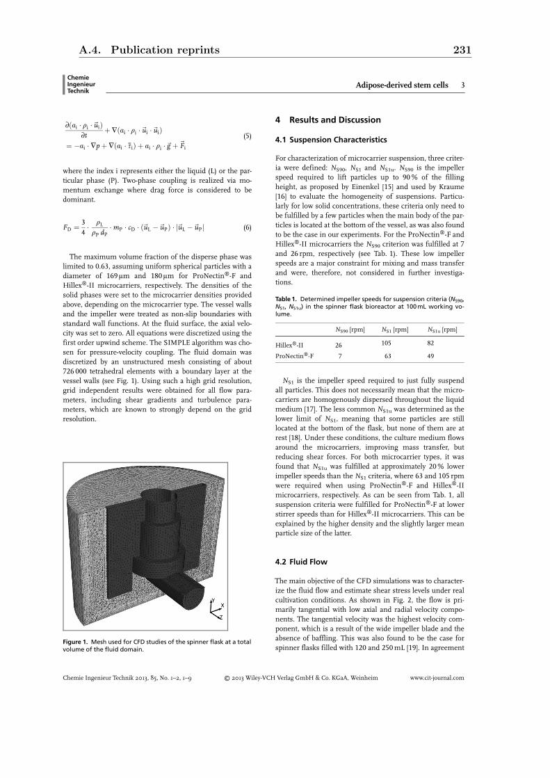
∂ ai qi ui ∂t
∇ ai qi ui ui ai ∇p ∇ ai si ai qi g Fi
(5)
where the index i represents either the liquid (L) or the par-ticular phase (P). Two-phase coupling is realized via mo-mentum exchange where drag force is considered to bedominant.
FD 34 qL
qP dP mP cD uL uP uL uP (6)
The maximum volume fraction of the disperse phase waslimited to 0.63, assuming uniform spherical particles with adiameter of 169 lm and 180 lm for ProNectin®-F andHillex®-II microcarriers, respectively. The densities of thesolid phases were set to the microcarrier densities providedabove, depending on the microcarrier type. The vessel wallsand the impeller were treated as non-slip boundaries withstandard wall functions. At the fluid surface, the axial velo-city was set to zero. All equations were discretized using thefirst order upwind scheme. The SIMPLE algorithm was cho-sen for pressure-velocity coupling. The fluid domain wasdiscretized by an unstructured mesh consisting of about726 000 tetrahedral elements with a boundary layer at thevessel walls (see Fig. 1). Using such a high grid resolution,grid independent results were obtained for all flow para-meters, including shear gradients and turbulence para-meters, which are known to strongly depend on the gridresolution.
4 Results and Discussion
4.1 Suspension Characteristics
For characterization of microcarrier suspension, three criter-ia were defined: NS90, NS1 and NS1u. NS90 is the impellerspeed required to lift particles up to 90 % of the fillingheight, as proposed by Einenkel [15] and used by Kraume[16] to evaluate the homogeneity of suspensions. Particu-larly for low solid concentrations, these criteria only need tobe fulfilled by a few particles when the main body of the par-ticles is located at the bottom of the vessel, as was also foundto be the case in our experiments. For the ProNectin®-F andHillex®-II microcarriers the NS90 criterion was fulfilled at 7and 26 rpm, respectively (see Tab. 1). These low impellerspeeds are a major constraint for mixing and mass transferand were, therefore, not considered in further investiga-tions.
NS1 is the impeller speed required to just fully suspendall particles. This does not necessarily mean that the micro-carriers are homogenously dispersed throughout the liquidmedium [17]. The less common NS1u was determined as thelower limit of NS1, meaning that some particles are stilllocated at the bottom of the flask, but none of them are atrest [18]. Under these conditions, the culture medium flowsaround the microcarriers, improving mass transfer, butreducing shear forces. For both microcarrier types, it wasfound that NS1u was fulfilled at approximately 20 % lowerimpeller speeds than the NS1 criteria, where 63 and 105 rpmwere required when using ProNectin®-F and Hillex®-IImicrocarriers, respectively. As can be seen from Tab. 1, allsuspension criteria were fulfilled for ProNectin®-F at lowerstirrer speeds than for Hillex®-II microcarriers. This can beexplained by the higher density and the slightly larger meanparticle size of the latter.
4.2 Fluid Flow
The main objective of the CFD simulations was to character-ize the fluid flow and estimate shear stress levels under realcultivation conditions. As shown in Fig. 2, the flow is pri-marily tangential with low axial and radial velocity compo-nents. The tangential velocity was the highest velocity com-ponent, which is a result of the wide impeller blade and theabsence of baffling. This was also found to be the case forspinner flasks filled with 120 and 250 mL [19]. In agreement
ChemieIngenieurTechnik
Chemie Ingenieur Technik 2013, 85, No. 1–2, 1–9 © 2013 Wiley-VCH Verlag GmbH & Co. KGaA, Weinheim www.cit-journal.com
Figure 1. Mesh used for CFD studies of the spinner flask at a totalvolume of the fluid domain.
Table 1. Determined impeller speeds for suspension criteria (NS90,NS1, NS1u) in the spinner flask bioreactor at 100 mL working vo-lume.
NS90 [rpm] NS1 [rpm] NS1u [rpm]
Hillex®-II 26 105 82
ProNectin®-F 7 63 49
Adipose-derived stem cells 3
A.4. Publication reprints 231

with our expectations, the velocities were highest near theimpeller tips and behind the blades, correlating well withthe impeller tip speeds (utip= pdR NR). Recirculation is foundbelow the impeller blade, where the fluid flows towards thewake region (region behind the impeller). Due to the strongflow convergence below the impeller bar, the flow in the ves-sel center is nearly stagnant in comparison to the main flow.In this region, sedimentation and agglomeration of thesolids are most likely, which was confirmed by both numeri-cal investigations and suspension experiments.
In Fig. 3, the CFD-predicted tangential velocities of thesingle- and multiphase models were compared with PIVmeasurements along two lines parallel to the impeller
blade, above and below the impeller bar, respectively. Ob-viously, only minor differences in the velocity profiles werepredicted between the single- and multiphase CFD models.This may be a result of the small microcarrier size and den-sity difference, which allows the microcarriers to follow thefluid flow almost slip-free, without significant momentumexchange. Very good qualitative and quantitative agreementis found between PIV measurements and CFD data, with amean relative deviation below 7 %. Above the impeller, theCFD-predicted profiles are flatter and the maximum tangen-tial velocity is underpredicted compared to the PIV mea-surement. Below the impeller bar, PIV data is only availablefor radial coordinates r/R > 0.17 because of the verticalimpeller blade. Furthermore, some fluctuations in the PIVdata were observed below the impeller bar (Fig. 3b). Theseuncertainties can be explained by sedimentation of the PIVfluorescence particles at the low impeller speed of 60 rpm,resulting in an increased number of incorrect vectors. How-ever, the CFD velocity profiles were well captured and theoverall agreement of PIV and CFD was satisfactory.
The CFD-predicted microcarrier distributions are com-pared with experimental observations in two snapshots forHillex®-II and ProNectin®-F microcarriers in Fig. 4. From aqualitative perspective, the images and the numerical re-sults for solids distribution agreed well. This can be seen inthe way that position and shape of the CFD-predicted micro-carrier agglomeration is a good approximation to the experi-mental observations. As described above, the Hillex®-II andProNectin®-F microcarriers accumulated below the impellerbar and only few microcarriers were lifted upwards whenoperating below the NS1u criteria. With increasing impellerspeed, the microcarriers became more homogenously dis-tributed, which resulted in lower concentration maximabelow the impeller (see Fig. 5). Again, the higher densityand size of the Hillex®-II microcarrier led to increased vo-lume fractions in the vessel centre of between 0.1 and 0.4,compared to 0.04 and 0.26 for the ProNectin®-F microcar-
www.cit-journal.com © 2013 WILEY-VCH Verlag GmbH & Co. KGaA, Weinheim Chemie Ingenieur Technik 2013, 85, No. 1–2, 1–9
Figure 2. Fluid flow inside the spinner, represented by combined vector and contour plots. The flow is presentedin the mid-blade plane (left) and in a horizontal plane at mid-bar height. The vectors are projected to the givenplanes with fixed lengths of 1.8 mm.
Figure 3. Comparison of PIV measured (symbols) and CFD-pre-dicted fluid velocities (solid line – single-phase; dashed line – mul-tiphase) through two horizontal lines above (A) and below (B)the impeller bar.
4 S. Kaiser et al.
232

riers. However, it should be noted that the volume fractionfor both microcarrier types would appear to be overestimatedfor the NS1 criteria, where no solid accumulation was ob-served experimentally. However, no quantitative comparisonhas yet been carried out.
4.3 Shear Stress and Turbulence
Once the fluid flow has been determined, the shear stressdistribution within the bioreactor may be computed. Thethree local velocity gradients and their magnitude were cal-culated and volume-weighted distributions were obtained by
discretization into 200 bins (see Fig. 6).Logarithmical normal distributions werefound similar to other conventional andsingle-use small-scale bioreactors [20],where the mean shear stress values in-creased from 2.9 to 7.5 · 10–3 Pa for im-peller speeds of 50 and 105 rpm, respec-tively (see Tab. 2). The shear rates at theimpeller blades of a Rushton turbinewere estimated to be more than threeorders of magnitude higher than thebulk shear rates [21]. In the present case,factors of only 50 to 60 were obtained be-tween the mean and maximum values.By considering the cultivation results, itcan be concluded that the applied pri-mary ASCs tolerate mean and maximumshear stresses in the order of 0.004 to0.2 N m–2, respectively.
Another popular method for evaluating hydrodynamicstress is based on Kolmogorov’s theory of isotropic turbu-lence [22, 23]. While suspension cells are assumed to beaffected by turbulent eddies of comparable size, those grow-ing on microcarriers appear to be more sensitive. This isprobably because they are attached to relatively large parti-cles that are more prone to collisions that might damage thecells [24]. For fibroblasts it was found that cell damage be-came significant when the Kolmogorov microscale wasabout two-thirds the size of the microcarriers [25]. To applyKolmogorov’s theory, where Kolmogorov’s microscale of tur-bulence is defined by Eq. (7), the flow must be highly turbu-lent. Taking into account that Re < 104 (see Tab. 2), the flowis in the transition region of Reynolds numbers, betweenlaminar and fully turbulent conditions, i.e. it would be morereasonable to describe it as moderately turbulent [26]. How-ever, maximum dissipation rates are commonly higher by a
ChemieIngenieurTechnik
Chemie Ingenieur Technik 2013, 85, No. 1–2, 1–9 © 2013 Wiley-VCH Verlag GmbH & Co. KGaA, Weinheim www.cit-journal.com
Figure 4. Comparison of observed (top) and CFD-predicted (bottom) microcarrier distribu-tions for the ProNectin®-F (left) and Hillex®-II (right) microcarriers for NS90 criteria.
Figure 5. CFD-predicted microcarrier volume fraction forProNectin®-F (top) and Hillex®-II (bottom) along a line throughthe spinner flask at the vessel bottom.
Figure 6. Volume-weighted frequency distribution of the localshear stresses for impeller speeds of 50 and 105 rpm. The distribu-tion was discretized in 200 bins.
Adipose-derived stem cells 5
A.4. Publication reprints 233

factor of one or two in the impeller’s swept volume than inthe bulk [27, 28], as was also found in the present study(see Tab. 2).
lk l3
q3 e
025
(7)
Despite the minimum Kolmogorov microscale, whichwas predicted to be as low as 44 lm for 82 rpm (i.e. muchlower than the proposed 2/3 microcarrier size), no cell deathwas detected. Microscopic examination was performed afterDAPI staining, where dead cells were removed by washingsteps. However, the total cell densities of supernatant sam-ples were below the detection limit of the NucleoCounterNC-100. This is significant because dead or dying cells areknown to spontaneously detach from the microcarrier sur-face [24]. It should, therefore, be noted that the smallest tur-bulent eddies are only found in a very small volume, whichlowers the risk that the microcarriers might come into con-tact with these eddies. In the present case, the volume ofk < 100 lm increased from 1 to 12 % as the impeller speedincreased from 50 to 105 rpm.
4.4 Cultivation Runs
ASCs were cultivated at the two impeller speeds, represent-ing the NS1u criteria of both microcarrier types, and at60 rpm (see Tab. 1). This was used as a reference derivedfrom previous screening experiments. In all cases, viablecells retained their morphology and, therefore, it was as-sumed that the cells maintained their phenotype since thereis no clearly defined, established set of surface expressedmarkers for the used ASCs. In general, higher cell expan-sion rates were obtained with ProNectin®-F microcarriersthan with the Hillex®-II cultures. As is obvious from Fig. 7,experiments with ProNectin®-F microcarriers resulted in 50to 60 % higher increases of cell number (expansion factorsbetween 26.4 and 31.4), whereas cells were expanded by afactor of 16.3 and 18.3 on the Hillex®-II microcarriers. Thisincrease in cell number is, to the best of our knowledge, the
highest for primary ASCs in spinnerflasks for serum concentrations below10 %. Santos et al. achieved expansionfactors of 14 ± 7 with ASCs in serum-freemedium after 14 days [30].
Furthermore, significantly higher cellexpansion factors (p < 0.05, n = 4) wereobtained using the ProNectin®-F micro-carrier type when stirred at 49 rpm(31.4 ± 3.6) compared to stirring at60 rpm (26.4 ± 3.1). However, differencesat the even higher impeller speed of82 rpm (28.0 ± 2.4) were not statisticallysignificant (p < 0.05, n = 4). Hence, thehighest increase in cell number on Pro-Nectin®-F was obtained at 49 rpm and at
60 rpm for Hillex-II, supporting the data that the lowestspeed required to bring the microcarriers into full suspen-sion results in the highest cell expansion. Cultivations withHillex®-II microcarriers also showed strong microcarrier ag-gregate formation after four days of cultivation, in particularat 49 rpm.
5 Conclusions
Investigations of fluid flow and microcarrier suspension insmall-scale single-use spinner flasks were accomplished bymeans of CFD. Provided that the models are validated, CFDmodeling is one of the most effective techniques for charac-terization of flow fields [31]. Although experimental meth-ods, such as particle image velocimetry, are reliable, they aretoo time-consuming to characterize the complete 3D fluidflow within a typical bioreactor. However, it is widely ac-cepted that the flow inside the bioreactors may significantlyinfluence stem cell growth and must be well-characterized.
The developed CFD model considers the two phases asinterpenetrating continua and takes the granular character-
www.cit-journal.com © 2013 WILEY-VCH Verlag GmbH & Co. KGaA, Weinheim Chemie Ingenieur Technik 2013, 85, No. 1–2, 1–9
Table 2. Summary of estimated shear stress levels, turbulent dissipation rate and Kolmo-gorov microscale of turbulence for different impeller speeds.
ImpellerspeedNR [rpm]
Tip speedutip [m s–1]
ReynoldsnumberRe [–]
LSSa
snt[10–3 N m–2]TEDRb
e [10–3 m2s–3]KMSTc
lD [lm]
50 0.109 1435 2.9 / 141 0.6 / 62 66 / 228
60 0.130 1722 3.0 / 180 1.1 / 93 60 / 191
75 0.163 2153 4.3 / 195 1.8 / 147 56 / 173
82 0.178 2354 6.0 / 250 2.1 / 308 44 / 157
105 0.228 3014 7.5 / 265 4.1 / 579 38 / 133
a) LSS, local shear stress given with volume-weighted mean / maximum values; b) TEDR, turbulentenergy dissipation rate given with volume-weighted mean / maximum values; c) KMST, Kolmogo-rov’s microscale of turbulence given with volume-weighted mean / minimum values.
Figure 7. Expansion factors achieved at different stirrer speedsusing Hillex®-II and ProNectin®-F microcarriers. Error bars repre-sent simple standard deviation of four individual spinners inocu-lated from a single cell stock.
6 S. Kaiser et al.
234

istics of the solid microcarriers into account. Good qualita-tive and quantitative agreement was obtained with particleimage velocimetry and suspension experiments. The CFDmodel can thus be used for subsequent scale-up studies toinvestigate stirred single-use bench-top bioreactors for theirsuitability for MSC expansion. Since single-use bioreactorsoffer the advantage of lower turnaround times, increasedflexibility when changing products and lower risks of cellcontamination, these systems are attractive for both pre-clin-ical and clinical applications [32].
Furthermore, it was demonstrated that the microcarriertype significantly influences the impeller speed required toachieve the desired suspension characteristics. Due to thelighter and smaller beads, the ProNectin®-F microcarriertype required much lower impeller speeds to achieve ahomogenous suspension compared to Hillex®-II. In termsof scale-up it, therefore, seems meaningful to determine theimpeller speed (or power input) required for homogenousmicrocarrier suspension, without exceeding critical shearstress levels.
Finally, this bioengineering data could be successfullyused to grow adipose-derived primary stem cells in single-use spinner flasks at low serum concentrations and withsuitable microcarriers. Although reproducible and robustexpansion of hMSC still remains challenging, since thesecultures are influenced by various important engineeringand biological factors most of which are not fully under-stood, the present study shows promise for further investi-gations.
The work was financially supported by the Swiss Com-mission for Technology and Innovation (CTI) withinthe Development of a technology platform for scalable pro-duction of therapeutically relevant stem cells project(12893.1 VOUCH-LS).
Symbolys used
cD [–] drag coefficientdP [m] particle diameterdR [m] impeller diameterg [m s–2] gravitational acceleration
(vector)F [N] force (vector)FD [N] drag forcek [m2s–2] turbulent kinetic energylC [m] Kolmogorov microscale of
turbulence (turbulent eddysize)
mP [kg] particle massNR [s–1] impeller rotational speedNS1, NS1u, NS90 [s–1] suspension criteriap [Pa] pressure
Re [–] Reynolds numbert [s] timeu [m s–1] velocity (vector)utip [m s–1] impeller tip speedx, y, z [m] spatial co-ordinates
Greek symbols
a [–] phase volume fractione [m2s–3] turbulent energy dissipation
ratel [Pa s] laminar (molecular) viscositym [m2s–1] kinematic viscosityq [kg m–3] densitys [N m–2] shear stresss [N m–2] Reynolds stress tensorx [s–1] angular velocity
Abbreviations
ASC adipose-derived stem cellsCCD charge-coupled devicesCFD computational fluid dynamicsDAPI 4′,6-diamidino-2-phenylindoleESC embryonic stem cellshMSC human mesenchymal stem cellsiPSC induced pluripotent stem cellsMSC mesenchymal stem cellsPDL population doubling levelPIV particle image velocimetrySIMPLE semi-implicit method for pressure linked
equations
References
[1] J. M. Gimble et al., Circ. Res. 2007, 100 (9), 1249. DOI:10.1161/01.RES.0000265074.83288.09
[2] V. Zachar et al., in Mesenchymal Stem Cell Assays and Applica-tions (Eds: M.C. Vemuri, L. G. Chase, M. S. Ra), Springer, Ber-lin 2011.
[3] M. Tobita et al., Discov. Med. 2011, 11 (57), 160.[4] F. Zhao, T. Ma, Biotechnol. Bioeng. 2005, 91 (4), 482. DOI:
10.1002/bit.20532[5] T. Mygind et al., Biomaterials 2007, 28 (6), 1036. DOI: 10.1016/
j.biomaterials.2006.10.003[6] J. E. Frith et al., Tissue Eng., Part C 2010, 16 (4), 735. DOI:
10.1089/ten.tec.2009.0432[7] R. Alfred et al., Biotechnol. Bioeng. 2010, 106 (5), 829. DOI:
10.1002/bit.22727[8] G. Eibes et al., J. Biotechnol. 2010, 146 (4), 194. DOI: 10.1016/
j.jbiotec.2010.02.015[9] L. Meinel et al., Ann. Biomed. Eng. 2004, 32 (1), 112. DOI:
10.1023/B:ABME.0000007796.48329.b4[10] N. Datta et al., Proc. Natl. Acad. Sci. U.S.A. 2006, 103 (8), 2488.
DOI: 10.1073/pnas.0505661103
ChemieIngenieurTechnik
Chemie Ingenieur Technik 2013, 85, No. 1–2, 1–9 © 2013 Wiley-VCH Verlag GmbH & Co. KGaA, Weinheim www.cit-journal.com
Adipose-derived stem cells 7
A.4. Publication reprints 235

[11] F. Zhao et al., Biotechnol. Bioeng. 2007, 96 (3), 584. DOI:10.1002/bit.21184
[12] S. K. Oh et al., Stem Cell Res. 2009, 2 (3), 219. DOI: 10.1002/bit.20650
[13] B. Launder, D. Spalding, Comput. Methods Appl. Mech. Eng.1974, 3 (2), 269. DOI: 10.1016/0045-7825(74)90029-2
[14] Fluent 6.3 User’s Guide, ANSYS, Lebanon, NH 2006.[15] W. D. Einenkel, A. Mersmann, VT, Verfahrenstech. 1977, 11 (2),
90.[16] M. Kraume, Chem. Eng. Technol. 1992, 15 (5), 313. DOI:
10.1002/ceat.270150505[17] S. Ibrahim, A. W. Nienow, Chem. Eng. Res. Des. 2004, 82 (9),
1082. DOI: 10.1205/cerd.82.9.1082.44161[18] F. Liepe et al., Rührwerke – Theoretische Grundlagen, Auslegung
und Bewertung, Eigenverlag FH Anhalt, Köthen 1998.[19] B. Bilgen et al., Biotechnol. Bioeng. 2005, 92 (7), 907. DOI:
10.1002/bit.20667[20] S. C. Kaiser et al., in Computational Fluid Dynamics Technologies
and Applications (Eds: I. V. Minin, O. V. Minin), InTech, 2011.[21] J. Wu et al., AIChE J. 2006, 52 (7), 2323. DOI:10.1002/
aic.10857[22] C. R. Thomas, Z. Zhang, in Advances in Bioprocess Engineering
(Eds: E. Galindo, O. T. Ramirez), Kluwer, Dordrecht 1998.
[23] A. W. Nienow, Cytotechnology 2006, 50 (1 – 3), 9. DOI: 10.1007/s10616-006-9005-8
[24] C. J. Hewitt, Biotechnol. Lett. 2011, 33 (11), 2325. DOI:10.1007/s10529-011-0695-4
[25] M. S. Croughan et al., Biotechnol. Bioeng. 2006, 95 (2), 295.DOI: 10.1002/bit.21158
[26] R. V. Venkat et al., Biotechnol. Bioeng. 1996, 49 (4), 456 – 466.DOI: 10.1002/(SICI)1097-0290(19960220)49:4<456::AID-BIT13>3.0.CO;2-8
[27] H. Wu et al., Exp. Fluids 1989, 8 (3), 153. DOI: 10.1007/BF00195789
[28] M. Höfken et al., Chem. Ing. Tech. 1996, 68 (7), 803. DOI:10.1002/cite.330680707
[29] E. Abranches et al., Biotechnol. Bioeng. 2007, 6 (6), 1211. DOI:10.1002/bit.21191
[30] F. dos Santos et al., Tissue Eng., Part C 2011, 17 (12), 1201.DOI: 10.1089/ten.tec.2011.0255
[31] D. W. Hutmacher, H. Singh, Trends Biotechnol. 2008, 26 (4),166. DOI: 10.1016/j.tibtech.2007.11.012
[32] R. Eibl et al., Appl. Microbiol. Biotechnol. 2010, 86 (1), 41. DOI:10.1007/s00253-009-2422-9
www.cit-journal.com © 2013 WILEY-VCH Verlag GmbH & Co. KGaA, Weinheim Chemie Ingenieur Technik 2013, 85, No. 1–2, 1–9
8 S. Kaiser et al.
236

Research Article
Development of the Travelling Wave Bioreactor –A Concept StudyStephan C. Kaiser1,*, Matthias Kraume2, and Dieter Eibl1
DOI: 10.1002/cite.201200127
This study presents the concept of the travelling wave single-use bioreactor, based on an orbitally shaken, annular-shaped
vessel. A numerical model was developed for early design studies in order to reduce the number of prototypes. The flow
characteristics in two different vessel shapes were investigated. It was shown that the orbital motion combined with the
toroidal shape of the bioreactor create the desired wave characteristics in the contents of the vessel.
Keywords: Computational fluid dynamics, Design study, Single-use bioreactor, Travelling wave
Received: July 28, 2012; revised: September 18, 2012; accepted: September 28, 2012
1 Introduction
Over the last decades a variety of single-use cell culture bio-reactors have been developed that differ in design, scale,instrumentation and mixing method. A comprehensiveoverview is provided by Eibl et al. [1]. There are two maintypes of single-use bioreactors: (i) stirred tank vessels and(ii) pillow- or rocker bag style, also referred to as wave-mixedbioreactors. Single-use stirred bioreactors largely mimic thefunction and form of their traditional counterparts, whichare made of glass or stainless steel. To avoid breaking thesterile barrier, most single-use stirrers have a magnetic cou-pling, making bag production expensive. Furthermore, it iswell-known that stirrers induce heterogeneous energy dissi-pation in the growth medium, with high shear regions nearthe impellers [2]. Therefore, the rocker style wave-mixed bagbioreactors are a promising alternative for the growth ofshear-sensitive cultures. This type of disposable bioreactorutilizes a wave motion, induced by movement about a singleaxis, to both mix and aerate the contents of the bioreactor.However, they have only limited oxygen mass transfer capa-city and are, therefore, only suitable for cultures with low tomedium oxygen demands [3]. Higher oxygen demands aremet by Cellution’s CELL-tainer [4].
In 2008, Finesse Solutions LLC patented a novel bioreac-tor concept based on an annular-shaped vessel, using anorbital movement to induce a travelling wave (details givenbelow) [5]. The single-use vessel is intended to provide
enhanced mixing and aeration of the growth medium, whilesimultaneously generating reduced mechanical shearforces. The objective of this study is to develop a model tosimulate fluid flow inside the bioreactor using computa-tional fluid dynamics (CFD). CFD can be used for earlydesign studies to investigate the effect of bioreactor geome-try on flow characteristics, mixing and mass transfer, whilereducing the need for large numbers of prototypes. Thefinite volume solver Fluent (ANSYS, Inc.) was used to createnumerical models. The initial results from examinations ofthe flow characteristics in two different bioreactor geome-tries are presented.
2 Bioreactor Concept
The bioreactor consists of an annular-shaped vessel with acircular cross section (see Fig. 1), which is partly filled withgrowth medium. The toroidal vessel is moved orbitallyaround the center position by a platform equipped with anelectric motor or other drive system. The orbital motion,combined with the toroidal shape of the bioreactor, is in-tended to set up a travelling wave in the bioreactor growthmedium. The characteristics of the wave, which promotesmixing and mass transfer inside the bioreactor, is expectedto depend on the vessel shape, filling level, rotational fre-quency and amplitude, as well as medium properties, as isthe case in other wave-mixed bioreactors [3].
In the present study, the bioreactor had a total volume ofabout 50 L and an outer annulus radius (R) of about 0.37 m.The ratio of torus to pipe diameter (r) was approximately3.8, meaning that the pipe radius was 0.098 m. Rotationalspeeds of between 20 rpm and 40 rpm and amplitudes ofbetween 25 mm and 50 mm were tested for filling levels of25 L. Two configurations were compared, whereas the first
ChemieIngenieurTechnik
Chemie Ingenieur Technik 2013, 85, No. 1–2, 1–9 © 2013 Wiley-VCH Verlag GmbH & Co. KGaA, Weinheim www.cit-journal.com
–1Stephan C. Kaiser ([email protected]), Prof. Dieter Eibl,Zurich University of Applied Sciences, Institute of Biotechnology,Grüental, 8820 Wädenswil, Switzerland; 2Prof. Matthias Kraume,Technische Universität Berlin, Chair of Chemical and Process Engi-neering, Straße des 17. Juni 135, 10623 Berlin, Germany.
Single-use bioreactor 1
A.4. Publication reprints 237

was a simple torus without any installations and the secondincorporated baffles on the inner surface of the vessel(see Fig. 1). The pre-molded baffles (11 mm height) had acork-screw shape and were regularly wound around the cir-cumference with six complete turns. The protuberanceswere expected to increase mass transfer at the air-water in-terface.
Oxygen supply is intended to be provided through surfaceaeration, whereby the gas is introduced via ports positionedat the top of the torus. This may have the advantage of lowfoaming as seen in classical wave-mixed bioreactors andorbitally shaken bioreactors, such as shake flasks [6]. Sub-merged aeration could also be performed by delivering theoxygen or air through a multitude of orifices in the floorand/or walls of the vessel, but this was not considered in thepresent study.
3 Movement of the Bioreactor
The bioreactor moves in an orbitally shaken manner. Thus,the x- and y-coordinates of the torus center can be calculatedusing the rotational amplitude Amax and the angle of displa-cement r as follows:
xt sin rttAmax Amax (1)
yt cos rt tAmax (2)
If it is assumed that rotational frequency increases line-arly from the start of rotation until the maximum value is
reached, the time-dependent angle r can be calculated asfollows:
rt xmax
2tstartt2 t ≤ tstart
xmax t tstart rstart t tstart
(3)
Here, rstart represents the angle of rotation at time pointtstart. In the Fluent CFD solver, the bioreactor movement isintegrated by means of velocities, which can be obtainedfrom the first derivatives of the x- and y-coordinates, definedby Eqs. (1) and (2), respectively.
vxt dxt
dt(4)
Thus, the following equations, which were entered intoFluent as a user-defined function, describe the movement ofthe torus center in the Cartesian coordinate system. Thisapproach is referred as the dynamic mesh method.
vxtxmax Amax
tstartt sin
xmax
2tstartt2
t ≤ tstart
xmax Amax sin xmax t tstart rstart t tstart
(5)
vyt xmax Amax
tstartt cos
xmax
2tstartt2
t ≤ tstart
xmax Amax cos xmax t tstart rstart t tstart
(6)
In a second approach, also referred to as the gravity meth-od, the simulations were simplified by assuming that thetorus is not rotating during the simulation, but the directionof the earth gravity vector is modified with respect to time.This is a much more convenient alternative, fully equivalentfrom a computational point of view, and has already beenapplied in previous studies [7] and by Öncül et al. [8] tosimulate rocker-type wave bioreactors. Thus, accelerationalong the x- and y-axis are obtained from the second deriva-tive of the x- and y-coordinates with respect to time. Theacceleration in the z-direction corresponds to gravitationalacceleration and was therefore set to a constant value of9.81 m s–2. This procedure was implemented through auser-defined scheme script.
Both methods led to very similar flow profiles and sur-face-averaged fluid velocities at defined cross sections withrespect to time (see Fig. 2). For a rotational frequency of30 rpm, amplitude of 25 mm and a working volume of 25 L(half-filled bioreactor), significant differences were noted forthe maximum velocities near the wave crest, where the grav-ity method predicted surface-averaged velocities of about
www.cit-journal.com © 2013 WILEY-VCH Verlag GmbH & Co. KGaA, Weinheim Chemie Ingenieur Technik 2013, 85, No. 1–2, 1–9
Figure 1. Schematic view of the annular shaped traveling wavebioreactor with (below) and without (above) baffling.
2 S. C. Kaiser et al.
238

0.21 m s–1 compared to about 0.25 m s–1 obtained by thedynamic mesh method. Since both methods described areidentical from a computational view, the differences can beascribed to numerical uncertainties, related to the motion ofthe fluid domain in the dynamic mesh method. This is sup-ported by the five-fold decrease in the residuals obtainedusing the gravity method, where no mesh motion is present.Therefore, the gravity method was selected for subsequentinvestigations, which has the additional advantage of lowerdata storage thanks to its space-fixed grid.
4 Numerical Details
Since the main characteristic of the travelling wave is theshape and motion of the liquid interface, which determinesboth mixing and mass transfer, the Volume-of-Fluid (VOF)approach was used in the simulations. A single set of mo-mentum equations, based on the Reynolds-averaged Navier-Stokes equations were solved. The interface between thephases is tracked over time using a balance equation for thefractional volume or color function a(x,t). Neglecting masstransfer, this equation has the following form for the qth
phase:
∂∂t
aqqq
∇ aqqqwq
0 (7)
where wq is the fluid velocity vector and qq denotes the fluiddensity. A single momentum equation is solved throughoutthe domain, assuming the resulting velocity field is sharedamong the phases, i.e., all phases share the same velocity.
∂∂t
qw ∇ qqww
∇p ∇ l ∇w ∇wT
qg F
(8)
Here, the density and the viscosity are the weighted meanvalues defined as follows:
q
aqqq (9)
l
aqlq (10)
where the phase volume fractions are computed based onthe following constraint:
n
q1
aq 1 (11)
In Eq. (8), F represents all the volumetric forces exceptgravity. The most important interfacial force in the VOFmodel is surface tension, which is modeled according to thecontinuum surface force model proposed by Brackbill et al.[9]. For turbulent flow conditions, turbulence was modeledusing k-e realizable and k-x SST model. In each model a sin-gle set of transport equations for the turbulent kinetic en-ergy k and the turbulence dissipation rate e or the specificturbulent dissipation rate x is used. Model details are givenin [10].
The geometry of the annular-shaped vessel was discre-tized by body-fitted mesh with tetrahedral elements(see Fig. 3). In a grid sensitivity study, it was found that gridindependent results were obtained using about 106 controlvolumes (data not shown). The velocity-pressure couplingand prediction of volume fractions were performed usingthe SIMPLE algorithm and geo-reconstruction method pro-
ChemieIngenieurTechnik
Chemie Ingenieur Technik 2013, 85, No. 1–2, 1–9 © 2013 Wiley-VCH Verlag GmbH & Co. KGaA, Weinheim www.cit-journal.com
Figure 2. Comparison of surface-averaged fluid velocities for adefined cross section as a function of time obtained by thedynamic mesh and gravity methods. The rotational speed andamplitude were set at 30 rpm and 25 mm, respectively.
Figure 3. Outer surfaces of the meshes generated for the annu-lar-shaped bioreactor with (below) and without (above) baffles.
Single-use bioreactor 3
A.4. Publication reprints 239

vided by Fluent. First order upwindschemes were applied to solve themomentum and turbulence transportequations. The time step size wasfixed at 0.005 s, corresponding toabout four time steps per degree ofrotation at the highest investigatedrotational speed. This was a goodcompromise between accuracy andcalculation effort. Convergence wasassumed when the residuals droppedbelow 10–4, but the number of itera-tions per time step were restricted to50 in order to limit CPU turnaroundtime.
5 Results
5.1 Fluid Flow
The air-water phase distribution forthe outer surface of the unbaffledannulus is shown in Fig. 4. The wavestarts to develop after about 3 s, whenthe maximum rotational speed isreached. As expected, it subsequentlypropagates in a clockwise directionfollowing the torus movement. After about 10 s, the wavemotion becomes quasi-periodic with a relatively constantwave crest height and a frequency of rotation that is equal tothe rotational speed of the torus. This is also reflected by theprofiles of the surface-averaged fluid velocities (see Fig. 2).The height of the liquid is higher near the outer surfacethan at the inner side, as a result of centrifugal acceleration.Further, the liquid height depends on the rotational fre-quency with increasing magnitude at higher speeds (datanot shown).
The flow field for the unbaffled bioreactor is shown inFig. 5. As expected, the fluid flows clockwise, as shown bythe fluid velocity vectors. The highest fluid velocities of
1.72 m s–1 are found behind the wave front and correlatewell with the theoretical maximum speed of 1.67 m s–1 atthe vessel wall (Eq. (12)). The difference is thus below 5 %,which could be ascribed to numerical uncertainties. How-ever, for stirred vessels agitated by Rushton turbines, it wasfound that turbulence behind the impeller leads to fluidvelocities about 40 % higher than the impeller tip speed[11]. Since the highest levels of turbulence are found in theregion of higher velocities, the differences may also beexplained by turbulence production, which should be inves-tigated further.
umax 2p Nmax R r Amax (12)
Significantly lower liquid velocitiesof below 0.1 m s–1 are predicted at theinner radius of the torus, in front ofthe travelling wave. Furthermore,fluid velocity gradients are found be-tween the outer and inner radiuses ofthe torus, which matches expecta-tions and can be explained by centri-fugal acceleration. However, the dis-tribution of liquid velocities seems tobe relatively homogeneous. It wasfound that velocities, which are high-er than half the maximum velocity(> 0.9 m s–1), occur in about 30 % of
www.cit-journal.com © 2013 WILEY-VCH Verlag GmbH & Co. KGaA, Weinheim Chemie Ingenieur Technik 2013, 85, No. 1–2, 1–9
Figure 4. CFD predicted air-liquid distribution for the travelling wave bioreactor at differenttime steps. Dark and light grey colors represent pure water and air, respectively.
Figure 5. Fluid flow in the travelling wave at a rotational speed of 40 rpm and amplitude of25 mm after 15 s (9.5 rotations). Cross section at half initial filling height equal to z = 0.049 m(above); cross sections at different angles (below). The liquid velocity vectors are projected tothe given plane with a fixed length of 25 mm.
4 S. C. Kaiser et al.
240

the liquid volume. More detailed analysis will be part of sub-sequent studies.
It is worth noting that – except for a small region at theinner radius of the annulus – the velocity vectors are orien-tated in a circumferential direction and the flow is thereforecomparable to a circulating plug flow reactor. This maycause low back-mixing of the growth medium with negativeeffects on mixing capacity, resulting in undesirably longmixing times and/or concentration gradients. Thus, a sec-ond bioreactor design with cork-screw shaped baffles wasinvestigated.
The air-liquid distribution of the baffled annular bioreac-tor, with identical motion parameters (speed: 40 rpm, ampli-tude: 25 mm), is shown in Fig. 6. The baffles have a distincteffect on the travelling wave, whereby the liquid is lifted upalong the baffles and even reaches the upper side of thetorus. This effect is reduced if the rotational speed is low-ered, but mixing is still enhanced when compared to anunbaffled design (data not shown). Another effect of the baf-fles can be seen in the entrapment of air bubbles as thewave propagates (see Fig. 6). If one considers oxygen trans-fer, it is favorable to increase the specific surface area andturbulence at the air-water interface, which is provided bythe cork-screwed baffles. Nevertheless, it should be notedthat higher shear stress and foam production could arisefrom droplet impact at the liquid surface. Foam formationand subsequent cell damage/losses in the foam layer werefound to be the major problems affecting cell growth andmonoclonal antibody production in stirred and spargedbioreactors for both serum-supple-mented and serum-free media [12].Furthermore, severe cell damage wasdetected in a falling film-flow devicemainly as a result of the mixing shearstress produced by the falling film asit rapidly merged with the bulk liquid[13]. Effects of (single) droplet im-pacts were investigated experimen-tally and numerically for plane shal-low and deep liquid pools [14, 15], butno data related to cell damage wasfound in the literature.
Fig. 7 presents the fluid flow insidethe baffled torus after 20 s, wherequasi-periodic flow conditions areachieved. The highest fluid velocitiesare found at the wave crest and arepredicted to be about 1.85 m s–1,which is about 20 % higher than inan unbaffled vessel. Again velocitygradients are found between the in-ner and outer radius and significantlylower liquid velocities are predictedin front of the travelling wave. How-ever, a recirculation zone is created inthe baffled vessel, which is in clear
contrast to the unbaffled design. While the main part of theliquid keeps flowing in a clockwise direction, as one wouldexpect, a counter-clockwise flow can be found in approxi-mately a quarter of the annulus. The two flow directionsmeet in close proximity to the travelling wave, which maysignificantly improve mixing. The ratio of liquid flowing in
ChemieIngenieurTechnik
Chemie Ingenieur Technik 2013, 85, No. 1–2, 1–9 © 2013 Wiley-VCH Verlag GmbH & Co. KGaA, Weinheim www.cit-journal.com
Figure 6. Air-liquid distribution in the baffled travelling wavebioreactor at 6 s (above) and 20.5 s (below).
Figure 7. Fluid flow in the baffled annular bioreactor at 20 s. A cross section at half initial fill-ing height (z = 0.049 m) is shown above, while cross sections at different angles are providedbelow. The liquid velocity vectors are projected to the given plane with a fixed length of25 mm.
Single-use bioreactor 5
A.4. Publication reprints 241

the opposite direction to the rotation seems to depend onthe rotational frequency and amplitude as well as the fillingvolume; however, detailed analysis is not part of this study.
An additional improvement in mixing is expected to occurclose to the baffles, where the liquid is redirected towardsthe middle of the pipe. Small recirculation zones are alsopredicted behind the baffles (see detail view in Fig. 7). Here,upward and downward axial flows can be found, dependingon the time and relative position of the wave crest.
5.2 Turbulence
Turbulent flow conditions are characterized by defining theReynolds number based on channel flows [16, 17]. The Rey-nolds number (Re) is in general defined by Eq. (13), wherevc represents a characteristic velocity, lc denotes a character-istic length and tL is the liquid kinematic viscosity.
Re vc lctL
(13)
As shown above, the main proportion of the fluid flowsthrough the cross sectional area of the annular pipe and,therefore, the characteristic fluid velocity can be defined asthe area weighted average of the fluid velocity in the flow di-rection.
vC wL 1A
wi dA (14)
The characteristic length is given by the hydraulic dia-meter dH, which can be obtained using the following equa-tion:
dH 4AU
(15)
where A is the cross sectional area of the fluid and U is thewetted perimeter, which are a function of the liquid heighthL (see Fig. 8). Thus, one can obtain the hydraulic diameterdH as follows:
dH VL
p R r arccos 1 hL
r
(16)
For the operating conditions described above, it wasfound that the Reynolds number is in the range of 0.5 to5 · 104 (see Fig. 9). The critical Reynolds number for pipeflows is 2300 and is also applicable for open channel flows[16]. Thus it can be argued, that the flow inside the annularbioreactor is turbulent, meaning turbulence models shouldbe used for simulation purposes. In Fig. 9, surface-averagedfluid velocities (Eq. (14)) for a cross section are given, andprofiles obtained with and without turbulence models arecompared. The realizable k-e and shear-stress transport(SST) k-x models provided by Fluent were used for this cal-culation. The realizable k-e model is likely to provide super-ior performance for flows involving rotation and boundarylayers [10]. The SST k-x model was developed by Menter[18] to combine the positive features of the standard k-xmodel and the k-e model relating to near-wall and far fieldregions, respectively. Only marginal differences in resultswere delivered by the two turbulence models, in terms ofcross-sectional flow velocities. However, both profiles dif-fered from results obtained using laminar flow assump-tions, especially for the lowest fluid velocities found in frontof the wave crest and the increasing velocities before themaximum velocity is reached. Furthermore, the maximumfluid velocities are under-predicted by the laminar flow mod-el, therefore, the k-x SST turbulence model will be used forsubsequent investigations.
Fig. 10 summarizes the Reynolds numbers predicted byCFD, which were obtained from four cross sections evenlydistributed around the circumference and averaged overtime for two complete rotational periods. Rotational fre-quencies of between 20 and 40 rpm were simulated forshaking amplitudes of 25 and 50 mm, respectively. It is pre-dicted that the Reynolds numbers will increase almost line-
www.cit-journal.com © 2013 WILEY-VCH Verlag GmbH & Co. KGaA, Weinheim Chemie Ingenieur Technik 2013, 85, No. 1–2, 1–9
Figure 8. Dependency of the wetted circumference uL and thehydraulic diameter dH on the filling ratio (ratio of liquid volumeto total torus volume).
Figure 9. Comparison of surface-averaged profiles of the Rey-nolds number in the torus cross section (360°), with and withoutturbulence modeling.
6 S. C. Kaiser et al.
242

arly as shaking frequency increases. The smallest Reynoldsnumber is 3050 for 20 rpm at 25 mm amplitude and thehighest value is about 60 800, meaning an increase of a fac-tor of 20. This is not entirely surprising since the character-istic velocity in turbulent conditions is expected to be pro-portional to the rotational speed. Obviously the predictedReynolds numbers are higher than the critical value of 2300for channel and pipe flows. However, by decreasing the rota-tional speed and amplitude to below 20 rpm and 25 mm,one would expect to reach transitional or even laminar flowconditions, but these conditions have not yet been investi-gated. It should be further emphasized that the values aretime and local averages, meaning much lower values occurlocally. This is especially important considering that mostturbulence models fail for transitional flow regimes. Finally,turbulent conditions are more desirable from an engineer-ing point of view, since turbulence enhances mixing andmass transfer.
6 Conclusions and Outlook
The travelling wave bioreactor is a novel single-use cell cul-ture bioreactor concept, which is intended to provideenhanced mixing and mass transfer, while simultaneouslyexerting reduced mechanical shear force. A CFD model wasdeveloped enabling investigations of fluid flow for differentbioreactor geometries and operational parameters, such asorbital shaking frequency, shaking amplitude and fillinglevel.
In contrast to stirred vessels, where the fluid flow can besimulated by assuming steady-state conditions, the quasi-periodic flow of the travelling wave bioreactor requires atransient calculation, which makes CFD simulations time-intensive. The turn-around time for calculating a 15-s period
(approximate time required to achieve periodic conditions)was, depending on grid density, up to 8 days using four pro-cessors (Intel Xeon, 2.26 GHz, 6GB RAM) in parallel. How-ever, CFD has become a valuable tool for design studies dur-ing the last decades as the number of physical prototypescan be reduced and designs can be investigated in virtualprototypes [19]. Furthermore, parameters are obtained,which are difficult to measure experimentally [20]. Never-theless, experimental verification is required; a topic thatwill form part of subsequent studies. Measurements of fluidvelocities via particle image velocimetry, a technology oftenused for CFD model verification (e.g. [21 – 23]), and time-resolved determination of liquid height (as described in [8])are being prepared for the first rigid vessel prototypes.
A first approach for engineering characterization wasgiven by the description of turbulent flow conditions bydefining a Reynolds number adopted from pipe and chan-nel flows. Thus, turbulence is likely to be influenced by bio-reactor geometry (ratio of the cross sectional area and ringdiameter, baffles etc.), operating parameters (shaking fre-quency and amplitude as well as filling level) and liquidproperties (density and viscosity), which has already beenshown for certain parameters above. Under the operatingconditions investigated, the flow is turbulent, somethingthat is favorable in terms of mixing and mass transfer. How-ever, mechanical stress acting on cell cultures should alsobe considered. Unfortunately, no general conclusions canbe drawn concerning the relationship between fluid dy-namics and cell damage/death, despite numerous studiesthat have been published on investigating cell damage inbioreactors, e.g. [24, 25]. Therefore, the behavior of differentcell cultures in novel bioreactors types should be investi-gated experimentally due to the variety of influencing fac-tors related to bioreactor design, operating conditions, bio-logical identity etc.
Symbols used
A [m2] surface areaAmax [m] maximum amplitude of orbital
motiondH [m] hydraulic diameterF [N] force (vector)g [m s–2] gravitational acceleration (vector)hL [m] liquid heightk [m2s–2] turbulent kinetic energylC [m] characteristic lengthNmax [s–1] rotational frequencyp [Pa] pressurer [m] radius of the torus pipeR [m] radius of the torusRe [–] Reynolds numbert [s] timeU [m] wetted circumferenceumax [m s–1] maximum rotational speed
ChemieIngenieurTechnik
Chemie Ingenieur Technik 2013, 85, No. 1–2, 1–9 © 2013 Wiley-VCH Verlag GmbH & Co. KGaA, Weinheim www.cit-journal.com
Figure 10. Predicted Reynolds number at different rotationalspeeds for shaking amplitudes of 25 mm and 50 mm. The valuesare means of four cross sections evenly distributed around the cir-cumference, and time-averaged over two complete rotationalperiods.
Single-use bioreactor 7
A.4. Publication reprints 243

v [m s–1] velocity (scalar)VL [m3] liquid volumew [m s–1] velocity (vector)x, y, z [m] spatial co-ordinates
Greek symbols
a [–] phase volume fractione [m2s–3] turbulent energy dissipation ratel [Pa s] laminar (molecular) viscosityt [m2s–1] kinematic viscosityq [kg m–3] densityr [–] angle of displacementx [s–1] angular velocity / specific turbu-
lent dissipation rate
References
[1] R. Eibl et al., Appl. Biotechn. Bioeng. 2010, 86 (1), 41. DOI:10.1007/s00253-009-2422-9
[2] A. W. Nienow, Cytotechnology 2006, 50 (1 – 3), 9. DOI: 10.1007/s10616-006-9005-8
[3] R. Eibl et al., Adv. Biochem. Eng. Biotechnol. 2010, 155, 55. DOI:10.1007/10_2008_15
[4] N. M. G. Oosterhuis, P. van der Heiden, in 4th Cells and Cul-ture ESACT Proc. (Ed: T. Noll), Springer Netherlands, 2010.
[5] B. Paldus, M. Selker, US Patent 20080274541, 2008.[6] J. Büchs, Biochem. Eng. J. 2001, 7 (2), 91. DOI: 10.1016/
j.bej.2006.12.005[7] C. Löffelholz et al., in Single-use technology in biopharmaceutical
manufacture (Eds:, R. Eibl, D. Eibl), Wiley-VCH, Weinheim2010.
[8] A. A. Öncül et al., Biotechnol. Prog. 2010, 26 (1), 101. DOI:10.1002/btpr.312
[9] J. U. Brackbill et al., J. Comput. Phys. 1992, 100 (2), 335. DOI:10.1016/0021-9991(92)90240-Y
[10] Fluent 6.3 User’s Guide, ANSYS, Lebanon, NH 2006.[11] C. M. Stoots, R. V. Calabrese, AIChE J. 1995, 41 (1), 1. DOI:
10.1002/aic.690410102[12] S. Zhang et al., J. Biotechnol. 1992, 25 (3), 289. DOI: 10.1016/
0168-1656(92)90162-3[13] J. Wu et al., Biotechnol. Prog. 1995, 11 (2), 127. DOI: 10.1021/
bp00032a002[14] H. N. Oguz, A. Prosperetti, J. Fluid Mech. 1990, 219, 143 – 179.
DOI: 10.1017/S0022112090002890[15] S. Asadi, H. Panahi, Eng. Technol. 2011, 79, 720.[16] E. A. Truckenbrodt, Fluidmechanik: Grundlagen und elementare
Strömungsvorgänge dichtebeständiger Fluide, 4th ed., Springer,Berlin 2008.
[17] G. H. Jirka, C. Lang, Einführung in die Gerinnehydraulik, Uni-versitätsverlag Karlsruhe, Karlsruhe 2009.
[18] F. R. Menter, AIAA J. 1994, 32 (8), 1598. DOI: 10.2514/3.12149
[19] B. Andersson et al., Computational Fluid Dynamics for Engi-neers, Cambridge University Press, Cambridge 2011.
[20] A. R. Paschedag, CFD in der Verfahrenstechnik – AllgemeineGrundlagen und mehrphasige Anwendungen, Wiley-VCH,Weinheim 2004.
[21] J. Sheng et al., Can. J. Chem. Eng. 1998, 76 (3), 611. DOI:10.1002/cjce.5450760333
[22] X. Liu et al., Chin. J. Chem. Eng. 2008, 16 (5), 700.[23] A. R. Khopkar et al., Ind. Eng. Chem. Res. 2003, 42 (21), 5318.
DOI: 10.1021/ie020954t[24] I. Abu-Reesh, F. Kargi, Enzyme Microb. Technol. 1991, 13 (11),
913. DOI: 10.1016/0141-0229(91)90108-M[25] K. T. Kunas, E. T. Papoutsakis, Biotechnol. Bioeng. 1990, 36 (5),
476. DOI: 10.1002/bit.260360507
www.cit-journal.com © 2013 WILEY-VCH Verlag GmbH & Co. KGaA, Weinheim Chemie Ingenieur Technik 2013, 85, No. 1–2, 1–9
8 S. C. Kaiser et al.
244
Copyright © 2022 FDOKUMEN