51

Chapter Three

Finite Element

3-1 Background and applications:-

The finite element method (FEM) is not new technique; it

was first Introduction in the 19 and has been continually

developed and improved then. It is now an extremely

sophisticated tool for solving numerous engineering problems

and is widely used and accepted in many branches of industry. Its

development has not been paralleled by any other numerical

analysis techniques and experiment testing meth ods redundant.

Clearly the areas of applications and the potential of FEM are

enormous. The growth of the technique is attributable directly to

the rapid advance in computer technology and computing power.

The number and size of software comparies developing and

supporting commercial finite element packages has grown to

meet the demand for the programs, it is now a multimillions

dollars industry itself. There are three broad problem areas that

can be investigated by the FEM; these are

I. Steady state problems.

II. Eigen value problems steady with time .

III. Transient problems.

51

3-2 Method of solution of boundary value

problem(Bvp)

A (BVP) is one which governed by one or more differential

equation (D.E.) whichin a specified domain and by boundary

conditions on the periphery of that domain.

Ø= field variable it could be:-

Scalar (Temperature, Pressure, density, viscosity)

Vector (Velocity, displacement, acceleration, …..)

Tensor ( Stress, Strain, ……)

Ø (S)- steady state problems, s= space dimension (1D, 2D or 3D)

Ø (S, t) –Transient problem t=time Generally speaking, the

methods of solution of BVP may be classified as follows

BVP Methods of solution

-Direct Integration

-Separation Of Variables

-Fourier Trans Forms

-Laplace Trans Forms

-Infinites Series

Exactor Closed Solution Approximate Solution

Trial functions FDM

Weighted residual A Varitional Approach

-Rayleigh-Ritz method -Galerkin method

1870-1909 -Point least squares

-Point collocation method

-Integration least

FEM

BEM

51

3-3 Calculus of variation:-

A simple problem in the theory of the Calculus of variation

seeks to find a function u (x) that minimizes the integral ;

∫ )

(x),….)dx ,………………(1-1)

In this simple problems, we will also specify the values of u(x)at

x1 and x2 that is, bounds conditions

U(x1)=u1

U(x2)=u2………………………………….…...(1-2)

To Find u(x) ,we are going to consider every possible function

that satisfies equ.(1-2). From all these possible function we will

be seeking the one that gives its minimum value. This set of

possible function may be represented simply by W( X,£) where,

W(X,£) =u(x) + £ (x)

(X,£) = (x) + £ (x)………………………(1-3)

Where:-

u(x)=Desired Function that minimize

(x)=variation of u(x)= u

(x)=Any continuously differentially function(x)

£=parameter controls the difference between u&w

The functions u(x) and w(x,£) are shows in Fig .(1-1)

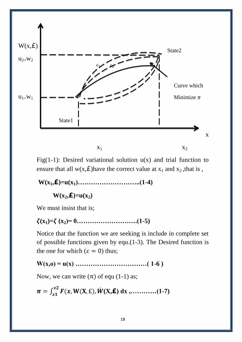
51

W(x,£)

u2=w2

u1=w1

x

x1 x2

Fig(1-1): Desired variational solution u(x) and trial function to

ensure that all w(x,£)have the correct value at x1 and x2 ,that is ,

W(x1,£)=u(x1)………………………..(1-4)

W(x2,£)=u(x2)

We must insist that is;

(x1)= (x2)= 0……………………….(1-5)

Notice that the function we are seeking is include in complete set

of possible functions given by equ.(1-3). The Desired function is

the one for which ( ) thus;

W(x,o) = u(x) ……………………………( 1-6 )

Now, we can write ( ) of equ (1-1) as;

∫ )

(X,£) dx ,…………(1-7)

Curve which

Minimize

State1

State2

51

Observe that this integral is a function of (£) and when (£=0),

equ.(1-7)

Reduces to equ(1-1) with the aid of (1-6).this means that we

want ) have a minimum when (£=0)

To find a minimum of ),we must first differentiate it

w.r.t.(£).since the limits of integration are not function of (£), we

may use Leibnitz rule to write;

)

∫

)

(X,£)dx ……..(1-8)

The chain rule of calculus may now be employed to give:-

)

∫ [

]

dx ,…….…….(1-9)

But;

= (x)

And

= (x)=

)

Thus;

)

∫ [

)

)

]

dx ,……….(1-10)

The second term may be integrated by parts gives

)

∫ [

)

)]

∫ )

.

.…….(1-11)

The integrated term vanishes with the aid equ.(1-5)thus;

)

∫ ) [

)]

. .………(1-12)

02

We will now insist that this be equal to zero when ( £=0) so that

(0) will be minimum .thus

∫ ) [

)]

. .…(1-13)

Observe that , from equ.(1-3) when Є=0 ,when w(x,Є)=u(x)

and (x,Є)= (x).

Since }(x) is arbitrary, the term in square bracelets in equ.(1-

13)must be zero to ensure this integral will be zero .therefore

,for( )to be aminimum;

(

) …………….(1-14) Euler log range equ.

This differential equation is called the Euler Lagrange equation.

its B.es in this simple problem are given by equ.(1-2)> the

solution u(x) to this differential equation will be the functionthat

minimizes the original integral

In equ.(1-3),ʅ(x) represents the variation of u(x), that is ( u) .In

their words, we may write

=∫ [

)]

u dx………...............(1-15)

Or in a general form;

=∫ ) )

u dx=0……….(1-16)

Where ( ) is the functional or variational statement and

Lu(x)=P(x)……. ……………………....(1-17)

Is the differential equation of the problem considered, sin u the

Euler Lagrange equation in equ. (1-15) is the variation of original

differential equation

Ex: find the function u(x) which minimize the integral

05

∫

) with u(o)=o+ u (

)=1

Sol: by comparing with equ.(1-1); the function (f) is

F=

( )

Now

&

Substitute into Euler Lagrange equ.(1-14)

-u-

)

Thus,the function u(x) which minimizes is the function which

satisfied equ.(1) and the B.CS. The and

∫ )

any other function foru(x)

that satisfied only B.CS.(Not Euler equ) would give larger value

for this in for Example (u(x)= 2x/ ) gives ( =0.0565).

00

3-4 FEM Methodology

The basic principles under lying the FEM are simple

consider for example, a body in which the distribution of an

unknown variable ( such as temperature or displacement ) is

required first the region is divided into an assembly of

subdivision called elements,which are considered to be inter

connected at joints, known as nodes , the variable is assumed to

act over each element in a predefined manner with the number

and type of elements chosen so that the variable distribution

through the whole body is adequately approximated by combined

element of representation .the distribution

Across each element may be defined

By polynomial ( linear, quadratic …)

Or trigonometric function .

After the problem has been discretized , the governing

equation of each element are calculate and then assembled to give

the system of equation usually , the equations of a particular type

of element for a specific problem are a ( stress or ther mal )have a

constant format. Thus, once the general format of equations of an

element type is derived,the calculation of the equation for each

occurrence of that element in the body is straight forward ,it is

simply a equation of substituting .the nodal coordinates, material

properties and loading conditions of the element into the general

format.

The individual element equations are assembly to obtain the

system equations, which describe the behaviors of the body as a

whole. These generally take the form

[k]{U}={F} …………………………….(1-24)

02

Where [k] is a square matrix ,known as the stiffness matrix; {U}

is the vector of unknown nodal displacements or temperatures;

and {F}is the vector of applied nodal forces. After applying the

boundary condition into (1-24), the resulting system of equations

are then solved , for the unknown nodal values

3-5 Steps of FEM Implementation

1- Variational statement of the problem.

2- Discretization of the domain.

3- Shape function and Interpolations.

4- Element equations.

5- Assembly of element equations.

6- Incorporation of Boundary conditions.

7- Solution of the equations.

8- Further calculations and maripulations.

3-6 Shape functions and Interpolations

Introduction :-

The FEM works by assuming a given distribution of the un

known variables through each element . The equation ,defining

the approximating distribution are known as (( inter pollution

function )) ,and can take any mathematical form, although in

practice they are usually polynomials. Polynomials are popular

because they are easy to for emulate and computerized ,and in

particular their differentiation and integration are straight for war

to implement on computer . with polynomials functions the

accuracy of the analysis can also be simply improved by

increasing the order of the polynomial off course, there is a price

to pay for the increase accuracy as the order of the Interpolation

function increases .

02

Typically , a quadratic element will require two or three

times the a mount of computer time that a linear element will

need. In some problems therefore, it may be more economical to

use a finer mesh of linear elements. For 1D thermal rod ,we may

write the following Interpolation functions

Linear: T= + X X

Quadratic: T= + X+ X2

Cubic: T= + X+ X2 + X

3

For 2D problem ,the following Interpolation functions may be

written:

Linear: T= + X + y

Quadratic: T= + X+ y+ Xy+ X2 + y

2

Note: for 2D element ,Pascale's Triangle may be used.

Linear: T= + X + y

Quadratic: T= + X+ y+ Xy+ X2 + y

2

Cubic: T= + X+ y+ Xy+ Xy2+ yx

2 +

X2+ y

2+ X

3+ y

3

Usually, there is no requirement to use pure linear quadratic or

cubic types of functions.

The 2D polynomic( T= + X+ y+ Xy )is Avery popular

Interpolation function. If has four un known constants with four

nodes defining a rectangular element

01

3-7 Linear Interpolation polynomials for simplex

Element

In this section two and three dimensional simplex elements

are introduced in which each element is identified by general

node labels such as I ,j and k . In modeling ,these labels are

substituted by the real node numbers . The location of the first

and last node is immaterial, provided that the elements are

labeled consistently for example, in an antic lock wise direction

for 2D triangular element.

The 1D simplex Element

The general form of the Interpolation function is ;

Ø= + X …………………( 1-25)

At x=xi Ø=Øi

x=xj Ø=Øj

=

=

=

=

Hence

=

+

x …………(1-26)

Or

=

+

Øj …..………(1-27)

Or

Ø= Ni Øi +NjØj= [ N ] {Ø } ……………(1- 28)

01

Where (Ni ) and (Nj) are called (( Shape function)) .Each

Shape function is associated with one particular node identified

by the subscript .It is a property of a Shape function that it equals

unity at its own assigned node and zero at the other nodes of the

element . Also, the sum of all the Shape functions at any point in

an element equals one. For convenience the Shape functions are

stored in a Shape function matrix [N] ,and the node variables are

stored in a vector {Ø } . Note that the Shape function ,like the

original interpolation polynomial , are linear function of x. It is

always the case that the Shape function are polynomials of the

same order as the interpolation function, see Fig (1.4).

N

Ni Nj Ni NK Nj

Xi Xj Xi Xk Xj

Fig (1.4): variation of the Shape function for 1D element.

X X

01

3-8 Natural coordinates ( local coordinates )

When the governing elements equations are derived in next

section , it will be found that many turns need to be calculated by

the integration of function of the Shape function [N]. This is not

difficult since the Shape function are simple turns of (x,y) and (Z)

but it can be made even easier by the introduction of natural

(local ) . coordinates these are coordinate system that are local

(i.c. individual ) to each element but are dimensionless and have a

maximum absolute magnitude of unity .

1-D Natural coordinates

For a 1-D element A point P is identified by two natural

coordinates:

L1=

1-

=1-

L1=

-0 =

Looking back to equ. (1-27 ) it is clear that the natural ( local )

coordinates are directly equivalent to the Shape function for the

element that is

L1= Ni =1-

L2= Nj= …………….(1-41)

Instead of the variation of Ø through the element the natural

coordinates can be used to describe the geometry of the element.

This is of little value for 1-D element but 2D and 3D elements

and particularly higher order elements it is very important

concept . in 1D element:

01

X= L1 Xi +L2 Xj= Ni Xi + NjXj………………..( 1-42 )

It has been proved that the integration over the element of

function incorporating L1 and L2 raised to the powers and P

can be easily calculated by applying the formula

Therefore sohce (L1= Ni) and (L2=Nj)the same equation can also

be applied when integrating function of Shape functions.

2-D local coordinates

When the concept of natural coordinates is applied to 2D. the

result is an area ( triangular ) coordinate

L1=A1 1A L2=A2 1A L3=A31A…………..( 1-44)

A1+ A2+A3=A

Or

+

+

=L1+L2+L3= 1

A1=A PjK

A=total area

Also

L1=Ni L2=Nj L3=Nk

And

X= L1Xi+L2Xj+L3Xk

Y= L1Yi+ L2Yj+ L3Yk

Also

A2

A1

A3

i

j

k

P

01

∫

)

Where (H) is the distance between two nodes on aside of the

element and

∫

)

)

Ex.(1-4): the stiffness inatxix of the element a2-D field problem

is to be evaluated

H ∫ [

]

dA

sol:

∫ ∫

∫

)

∫ ∫

)

Hence we can show not the integral will equal to:

[

]

22

3-9 Assembly of Element Equations

Assembly of Element Equations into the system Equations

is simply question of adding the coefficients of each element

stiffness matrix into the corresponding places of the global

stiffness matrix and summing the force vector coefficients of

each element force vector into the ( global force vector )the

processes are the same regardless of the type of problem and the

number and type of element used.

The easiest way to assemble the element is to label each raw

and column of the( nnexnne ) element matrix ( nne=ho. Of nodes

n element) with its corresponding degree of freedom ( Øi ,i=1 to

nne) And then to work through the coefficients of the matrix,

adding each into the (nnxnn) global matrix (nn=total no. of

nodes) which has been similarly labeled. the same way is done

with the force vector.

Element equation= Ke]nnexnne{

}nnex1={Fe}nnex1 K=∑

e

element equation = K]nnexnne { }nnex1={F}nnex1 F=∑

e

for example consider the mesh shown in the figure assume for

the sake of this example that the element equations of the first

three elements are:

element(1)

[

]

{

}

={ }

Global numbering

9

1

3

7

2

4

6

8

1

(2)

(3) (4)

(8)

(1)

(6)

(7)

(1)

5

25

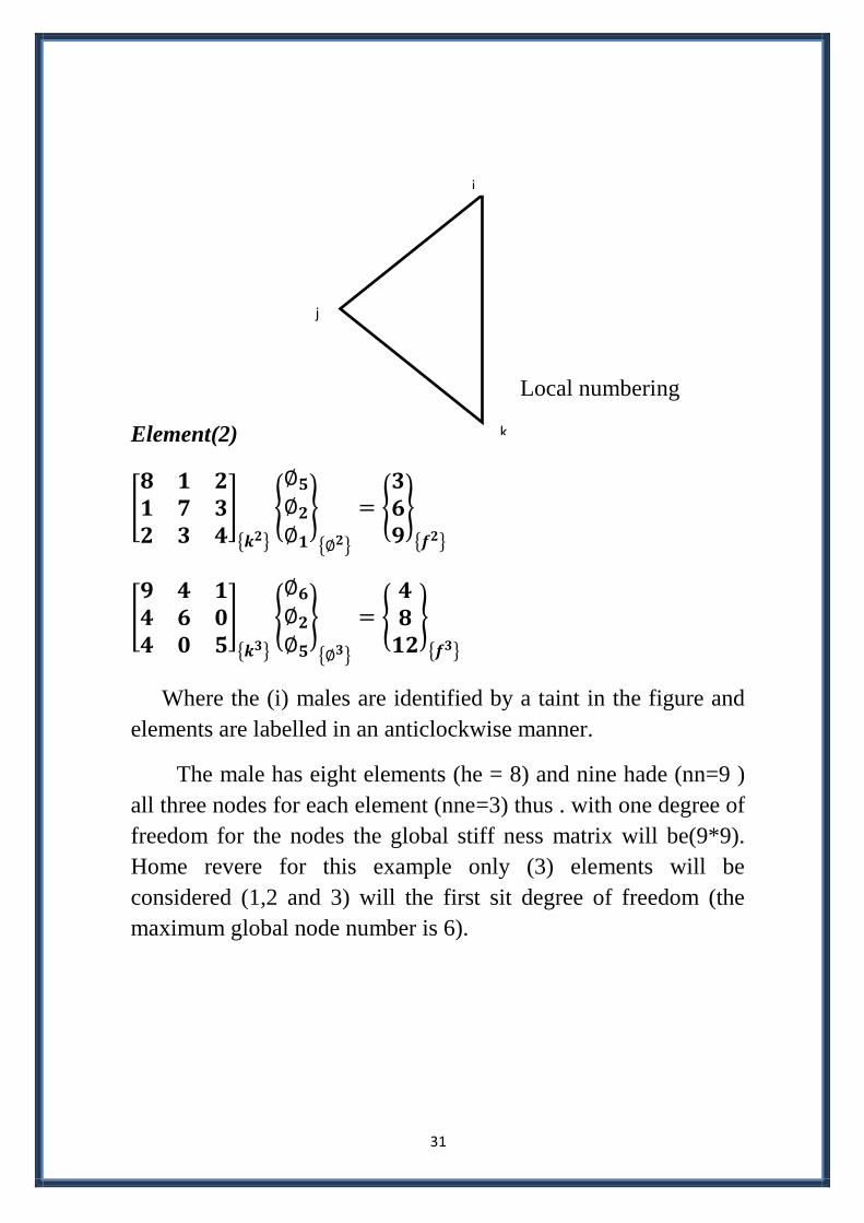
Local numbering

Element(2)

[

]

{ }

{

}

{ }

{ }

{ }

[

]

{ }

{

}

{ }

{

}

{ }

Where the (i) males are identified by a taint in the figure and

elements are labelled in an anticlockwise manner.

The male has eight elements (he = 8) and nine hade (nn=9 )

all three nodes for each element (nne=3) thus . with one degree of

freedom for the nodes the global stiff ness matrix will be(9*9).

Home revere for this example only (3) elements will be

considered (1,2 and 3) will the first sit degree of freedom (the

maximum global node number is 6).

i

j

k

20

i.e. the resulting fort of the global matrix and vector will be (6x6)

and (6x1) respectively.

Element (1): the rows and columns are identified in order (1-4-5)

is the (node) and (4) and (5) follows an anti cloclc wise direction.

The matrix and vectors of the element are added into the empty

global matrix and vector as follows

[

]

[

]

[K1] [K] global

{ }

{

}

{

Element (2)

[

]

[ )

)

)

)

]

[K2] [K]

22

{ }

{

}

{F2} {F}global

Element (3)

[

]

[ )

)

)

)

]

[K3] [K]global

{

}

{

}

{F3} {F}global

Thus the find global equation will be

22

[

]

{

}

{

=

{

}

{

Note that after adding in a details of the first three element ,

some of the sluts in the global matrix am still equal to zero. The

reason for this is that none of the three elements links the

associated degrees of. For example, the coefficient in the position

(4,2) and (2,4 )in the (K) matrix zero. Reference to the figure

shows that node (4) is common to elements (1,5 and 6) , whereas

node (2) only occurs in elements (2,3 and 4 ): hence, the( )of

nodes (2) and (4) are not linked. Similarly, in the force vector, the

coefficient in the position (3) is zero, since node (3) is not

involved in the system.

3-10 Incorporation of the Bounders Conditions

There are several ways in which the boundary conditions can

be incorporated into the system equation one method is to

rearrange the equation, for example

[

] {

{

{ } = {

{

{ } ……….(1-107)

Where { is the vector of unknown degrees of freedom

while those in the vector { are all specified ( known ). Fours

and { will contain the unknown reactions .Equation (1.107)

can be rewritten as two equations;

{ + { ={ …………..(1-108)

{ + { ={ …………..(1-109)

21

(1-108) can be written

{ ={ - { ={ ……..(1-110)

Since { is known, the terms on the RHS can be reduced to

a vector { , and the resulting equation can then be solved for

the unknown variable { , and equ. (1-109) may be solved for

{ . This method is straight forward, but it requires the equation

to be renumbered. Another method may be used which does not

need reordering the equation. To understand this method,

consider equ. (1-109). This can be written using (1-110) as:

[

] {

{

{ } = {

{ {

{ } ={

{

{ }

……………………(1-111)

If the equation In the 2nd line of the above matrix are stored

in a temporary matrix for later us, then equ. (1-111) can be

written as;

[

] {{

{ } = {

{

{

}…………(1-112)

Where is the with all the of diagonal terms site

equal to zero, and { is the correct product of (

{ ). The

second line is of no use (sin u { ={

= { , but it

does allow the matrix and vectors to remain the same size, and

the process can be performed without reordering equation

[

]

{

}

=

{

}

21

the B.cs.r:

Ø2 =20 and Ø4 = 50

Applying the second raw of equ.(1-112), the system equation are;

[

]

{

}

=

{

}

Row the element column coefficients that multiply Ø2 and Ø4

are eliminated by transferring the terms to the RHS. For example,

the first term in the force vector becomes.

300-(-12*20)-(-5*50)=740

The final system will be:

[

]

{

}

=

{

}

Note that the equation are still symmetric and bounded

58*20

48*50

21

Solution Of The Equations

When the boundary condition hare been incorporated into the

system equations , the final step is the solution for the unknown

variables there are many techniques available , and these are

discussed in detail in relevant mathematic and numerical analysis

textbooks. Probably the most common methods for equilibrium

problem that can be used are Gaussian elimination and cholesky

decomposition. However there is one other solution technique

that is widely used, particular in commercial finite element

packages, and that is the" ware front" or "frontal " method.