CHAPTER 3 Transport and Dispersion of Air Pollution - US ...
22
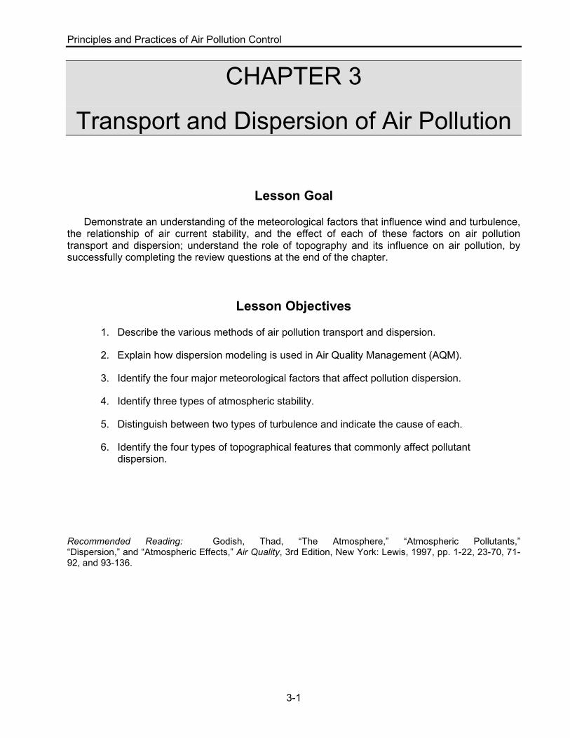
Principles and Practices of Air Pollution Control 3-1 CHAPTER 3 Transport and Dispersion of Air Pollution Lesson Goal Demonstrate an understanding of the meteorological factors that influence wind and turbulence, the relationship of air current stability, and the effect of each of these factors on air pollution transport and dispersion; understand the role of topography and its influence on air pollution, by successfully completing the review questions at the end of the chapter. Lesson Objectives 1. Describe the various methods of air pollution transport and dispersion. 2. Explain how dispersion modeling is used in Air Quality Management (AQM). 3. Identify the four major meteorological factors that affect pollution dispersion. 4. Identify three types of atmospheric stability. 5. Distinguish between two types of turbulence and indicate the cause of each. 6. Identify the four types of topographical features that commonly affect pollutant dispersion. Recommended Reading: Godish, Thad, “The Atmosphere,” “Atmospheric Pollutants,” “Dispersion,” and “Atmospheric Effects,” Air Quality, 3rd Edition, New York: Lewis, 1997, pp. 1-22, 23-70, 71- 92, and 93-136.
-
Upload
khangminh22 -
Category
Documents
-
view
1 -
download
0
Transcript of CHAPTER 3 Transport and Dispersion of Air Pollution - US ...
Principles and Practices of Air Pollution Control
3-1
CHAPTER 3
Transport and Dispersion of Air Pollution
Lesson Goal
Demonstrate an understanding of the meteorological factors that influence wind and turbulence, the relationship of air current stability, and the effect of each of these factors on air pollution transport and dispersion; understand the role of topography and its influence on air pollution, by successfully completing the review questions at the end of the chapter.
Lesson Objectives
1. Describe the various methods of air pollution transport and dispersion.
2. Explain how dispersion modeling is used in Air Quality Management (AQM).
3. Identify the four major meteorological factors that affect pollution dispersion.
4. Identify three types of atmospheric stability.
5. Distinguish between two types of turbulence and indicate the cause of each.
6. Identify the four types of topographical features that commonly affect pollutant dispersion.
Recommended Reading: Godish, Thad, “The Atmosphere,” “Atmospheric Pollutants,” “Dispersion,” and “Atmospheric Effects,” Air Quality, 3rd Edition, New York: Lewis, 1997, pp. 1-22, 23-70, 71-92, and 93-136.
Transport and Dispersion of Air Pollution
3-2
References
Bowne, N.E., “Atmospheric Dispersion,” S. Calvert and H. Englund (Eds.), Handbook
of Air Pollution Technology, New York: John Wiley & Sons, Inc., 1984, pp. 859-893. Briggs, G.A. Plume Rise, Washington, D.C.: AEC Critical Review Series, 1969. Byers, H.R., General Meteorology, New York: McGraw-Hill Publishers, 1956. Dobbins, R.A., Atmospheric Motion and Air Pollution, New York: John Wiley & Sons,
1979. Donn, W.L., Meteorology, New York: McGraw-Hill Publishers, 1975.
Godish, Thad, Air Quality, New York: Academic Press, 1997, p. 72. Hewson, E. Wendell, “Meteorological Measurements,” A.C. Stern (Ed.), Air Pollution, Vol. I.,
Air Pollutants, Their Transformation and Transport, 3rd ed., New York: Academic Press, 1976, pp. 569-575.
Lyons, T.J. and W.D. Scott. Principles of Air Pollution Meteorology, Boston: CRC Press, 1990,
pp. 185-189. Scorer, R.S, Meteorology of Air Pollution Implications for the Environment and its
Future, New York: Ellis Horwood, 1990. Singer, I.A. and P.C. Freudentahl, “State of the Art of Air Pollution Meteorology,” Bull.
Amer. Meteor. Soc., 1972, pp. 53:545-547. Slade, D.H. (Ed.), Meteorology and Atomic Energy, Washington, D.C.: AEC, 1968.
Strom, G.H., “Transport and Diffusion of Stack Effluents,” A.C. Stern (Ed.), Air Pollution, Vol. I, Air Pollutants, Their Transformation and Transport, 3rd ed., New York: Academic Press,1977, pp. 401-448.
Turner, D.B., Workbook for Atmospheric Dispersion Estimates, USEPA Publication No. AP-26, 1969.
Turner, D.B., Workbook of Atmospheric Dispersion Estimates: An Introduction to Dispersion Modeling, Boca Raton, Florida: CRC/Lewis Publishers, 1969.
U.S. EPA, Air Course 411: Meteorology – Instructor’s Guide, EPA Publication No. EPA/450/2-81-0113, 1981.
U.S. EPA, Air Quality Criteria for Carbon Monoxide, EPA Publication No. EPA/600/8-90/04f, 1991.
U.S. EPA, Air Toxics Monitoring Concept Paper, Revised Draft, February 29, 2000, p. 7.
Wanta, Raymond C. and William P. Lowery, “The Meteorological Setting for Dispersal of Air
Principles and Practices of Air Pollution Control
3-3
Pollutants,” A.C. Stern (Ed.), Air Pollution, Vol. I., Air Pollutants, Their Transformation and Transport, 3rd ed., Academic Press: New York, 1977, p. 328.
Zannetti, Paolo, Air Pollution Modeling: Theories, Computational Methods and Available Software, New York: Van Nostrand Reinhold, 1990, p. 362.
Transport and Dispersion of Air Pollution
3-4
Transport and Dispersion of Air Pollution
ir pollution meteorology is the study of how pollutants are delivered and dispersed into the ambient air (Wanta, 1977). The environmental
scientist is particularly interested in the data obtained from dispersion modeling because it provides critical information about the fate and effect of pollutants upon human health and the environment. In fact, the ability to predict the behavior of pollution in the ambient air is essential when attempting to manage and control its impact.
Knowledge of air pollution meteorology is essential to air quality planning activities. Understanding the way air pollution is transported and dispersed may indicate where to properly locate air pollution monitoring stations. Meteorological data may also be used to develop implementation plans and predict the atmospheric processes that will ultimately affect an area’s ability to comply with National Ambient Air Quality Standards (NAAQS). The purpose of this chapter is to introduce you to the atmospheric and topographical factors that influence nature’s ability to transport and disperse air pollution.
A
Air Pollution meteorology studies how pollutants are delivered and dispersed into the ambient air.
Principles and Practices of Air Pollution Control
3-5
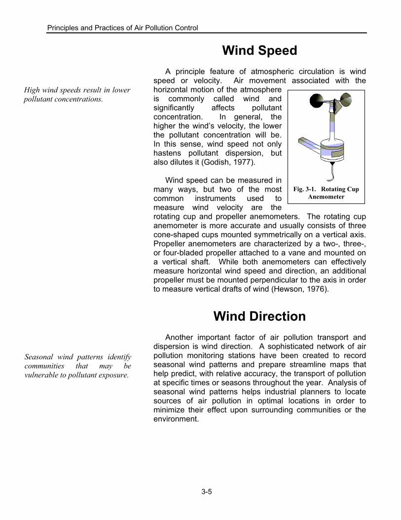
Wind Speed A principle feature of atmospheric circulation is wind
speed or velocity. Air movement associated with the horizontal motion of the atmosphere is commonly called wind and significantly affects pollutant concentration. In general, the higher the wind’s velocity, the lower the pollutant concentration will be. In this sense, wind speed not only hastens pollutant dispersion, but also dilutes it (Godish, 1977).
Wind speed can be measured in
many ways, but two of the most common instruments used to measure wind velocity are the rotating cup and propeller anemometers. The rotating cup anemometer is more accurate and usually consists of three cone-shaped cups mounted symmetrically on a vertical axis. Propeller anemometers are characterized by a two-, three-, or four-bladed propeller attached to a vane and mounted on a vertical shaft. While both anemometers can effectively measure horizontal wind speed and direction, an additional propeller must be mounted perpendicular to the axis in order to measure vertical drafts of wind (Hewson, 1976).
Wind Direction
Another important factor of air pollution transport and
dispersion is wind direction. A sophisticated network of air pollution monitoring stations have been created to record seasonal wind patterns and prepare streamline maps that help predict, with relative accuracy, the transport of pollution at specific times or seasons throughout the year. Analysis of seasonal wind patterns helps industrial planners to locate sources of air pollution in optimal locations in order to minimize their effect upon surrounding communities or the environment.
High wind speeds result in lower pollutant concentrations.
Seasonal wind patterns identify communities that may be vulnerable to pollutant exposure.
Fig. 3-1. Rotating Cup
Anemometer
Transport and Dispersion of Air Pollution
3-6
In urban areas, for example, a record of wind direction is used to estimate average concentrations of hydrocarbons, sulfur dioxide, and other pollutants. Recent research indicates that urban pollutants such as NO2, SO2, and O3 are of the most concern. Chronic lung disease is attributed to NO2 levels at just 50 ppm and can be lethal at 150 ppm. Urban measurements of SO2 at 0.05 ppm can result in respiratory complications, and high concentrations of O3 (0.01 ppm) have been found to result in significant changes in lung function among school children (Lyons and Scott, 1990). For this reason, it is extremely important to properly manage the formation and release of these air pollutants in urban-industrial settings where dense populations quickly multiply their effect upon human health.
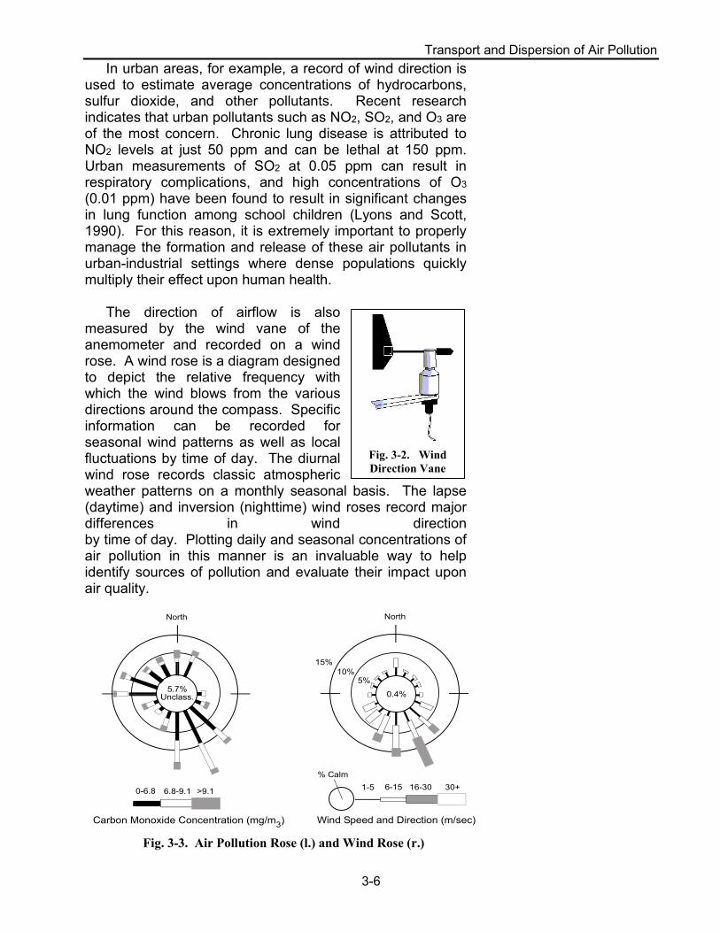
The direction of airflow is also
measured by the wind vane of the anemometer and recorded on a wind rose. A wind rose is a diagram designed to depict the relative frequency with which the wind blows from the various directions around the compass. Specific information can be recorded for seasonal wind patterns as well as local fluctuations by time of day. The diurnal wind rose records classic atmospheric weather patterns on a monthly seasonal basis. The lapse (daytime) and inversion (nighttime) wind roses record major differences in wind direction by time of day. Plotting daily and seasonal concentrations of air pollution in this manner is an invaluable way to help identify sources of pollution and evaluate their impact upon air quality.
Fig. 3-2. Wind Direction Vane
North
0.4%
5%10%
15%
Wind Speed and Direction (m/sec)
6-15 16-30 30+% Calm
1-5
5.7%Unclass.
0-6.8 6.8-9.1 >9.1
Carbon Monoxide Concentration (mg/m3)
North
Fig. 3-3. Air Pollution Rose (l.) and Wind Rose (r.)
Principles and Practices of Air Pollution Control
3-7
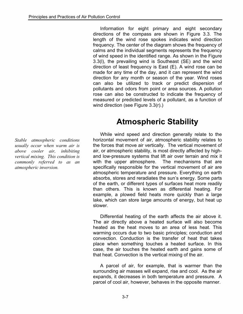
Information for eight primary and eight secondary directions of the compass are shown in Figure 3.3. The length of the wind rose spokes indicates wind direction frequency. The center of the diagram shows the frequency of calms and the individual segments represents the frequency of wind speed in the identified range. As shown in the Figure 3.3(l), the prevailing wind is Southeast (SE) and the wind direction of least frequency is East (E). A wind rose can be made for any time of the day, and it can represent the wind direction for any month or season of the year. Wind roses can also be utilized to track or predict dispersion of pollutants and odors from point or area sources. A pollution rose can also be constructed to indicate the frequency of measured or predicted levels of a pollutant, as a function of wind direction (see Figure 3.3(r).)
Atmospheric Stability
While wind speed and direction generally relate to the
horizontal movement of air, atmospheric stability relates to the forces that move air vertically. The vertical movement of air, or atmospheric stability, is most directly affected by high- and low-pressure systems that lift air over terrain and mix it with the upper atmosphere. The mechanisms that are specifically responsible for the vertical movement of air are atmospheric temperature and pressure. Everything on earth absorbs, stores and reradiates the sun’s energy. Some parts of the earth, or different types of surfaces heat more readily than others. This is known as differential heating. For example, a plowed field heats more quickly than a large lake, which can store large amounts of energy, but heat up slower.
Differential heating of the earth affects the air above it.
The air directly above a heated surface will also become heated as the heat moves to an area of less heat. This warming occurs due to two basic principles; conduction and convection. Conduction is the transfer of heat that takes place when something touches a heated surface. In this case, the air touches the heated earth and gains some of that heat. Convection is the vertical mixing of the air.
A parcel of air, for example, that is warmer than the surrounding air masses will expand, rise and cool. As the air expands, it decreases in both temperature and pressure. A parcel of cool air, however, behaves in the opposite manner.
Stable atmospheric conditions usually occur when warm air is above cooler air, inhibiting vertical mixing. This condition is commonly referred to as an atmospheric inversion.
Transport and Dispersion of Air Pollution
3-8
As warm air rises, it cools; as cool air descends, it warms.
Air circulates on the earth in a three-dimensionally movement not only vertically and horizontally. This movement is called turbulence. Turbulence occurs from two different processes: (1) mechanical or (2) thermal turbulence. Thermal turbulence results from atmospheric heating and mechanical turbulence from the movement of air past an obstruction. Both types of turbulence usually occur in during any atmospheric air movements, although one type or the other may dominate under certain circumstances. For example; on clear sunny days with light winds, thermal turbulence is dominant. Where as, mechanical turbulence is dominant on windy night with neutral atmospheric stability. The net effect of turbulence is to enhance the pollutant dispersion process. However, mechanical turbulence can cause downwash from a pollution source, which can result in high concentrations of pollutants, immediately downwind.
Adiabatic and Environmental Lapse Rate The temperature in the troposphere decreases with
height up to an elevation of about 10 kilometers. Decreasing temperature with height is described as the lapse rate. On average this decrease is –0.65°C/100 m and is stated as the normal lapse rate. If a parcel of air were lifted in the atmosphere, then allowed to expand and cool or compress and warm, with a change in atmospheric pressure and no interchange of heat, it would be an adiabatic process. The air parcel must also be unsaturated and the rate of adiabatic cooling or warming remains constant. The rate of heating or cooling for unsaturated air is 10°C/1000 meters, with the water remaining in the gaseous state, and is referred as the dry adiabatic lapse rate.
Individual vertical temperature measurements can vary
considerably from either the normal or dry adiabatic lapse rate. This change of temperature with height for a specific measured location is the environmental lapse rate. The environmental lapse rate values characterize the atmospheric stability and have a direct bearing on the vertical air movement and pollutant dispersion (Godish, 1997).
A critical relationship exists between atmospheric stability
and pollutant concentrations. Pollutants that cannot be
Types of Smokestack Plumes: • Looping • Fanning • Coning • Lofting • Trapping • Fumigating
Principles and Practices of Air Pollution Control
3-9
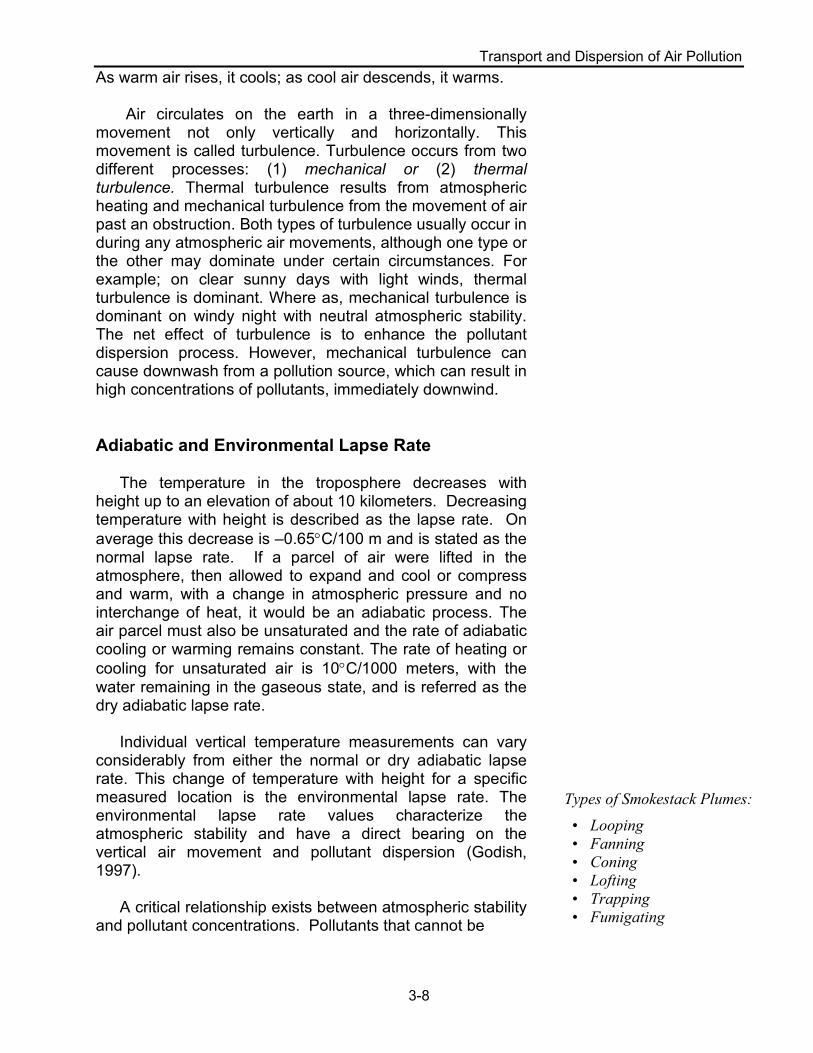
transported or dispersed into the upper atmosphere quickly become trapped at ground level and pose a significant risk to human health and the environment. This relationship can be visualized in the behavior of emission plumes from industrial smoke stacks. Six types of air pollution plumes illustrate the relationship between atmospheric stability and pollutant emissions: looping plumes, fanning plumes, coning plumes, lofting plumes, fumigating plumes, and trapping plumes.
Looping plumes. Pollution that
is released into an unstable atmosphere forms looping plumes. Rapid changes in temperature and pressure may result in plumes that appear billowing and puffy. While unstable conditions are usually favorable for pollutant dispersion, high concentrations of air pollution forced down by cooling air can be harmful if trapped at ground level. This can occur on sunny days with light to moderate winds, which combine with rising and sinking air to cause the stack gases to move up and down in a wavy pattern producing a looping plume (Godish, 1997).
Fanning plumes. A fanning plume occurs during stable conditions and is characterized by long, flat streams of pollutant emissions. Because atmospheric pressure is stable, there is neither a tendency for emissions to rise nor descend permitting (horizontal) wind velocity to transport and disperse the pollutant. Fanning plumes are usually seen during the early morning hours just before the sun begins to warm the atmosphere and winds are light (Godish, 1997).
Temperature
Environmental Lapse RateAdiabaticLapse Rate
Fig. 3-4. Looping Plume
Temperature
Environmental Lapse RateAdiabatic Lapse Rate
Fig. 3-5. Fanning Plume
Transport and Dispersion of Air Pollution
3-10
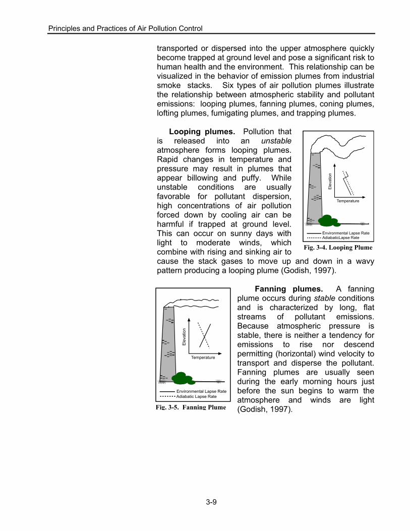
Coning plumes. Neutral or slightly unstable conditions create a coning plume that is distinguished by large billows or puffs of pollutants. Coning plumes are typically formed on partly cloudy days when there is an alternate warming and cooling of the atmosphere. Warm gases released into cool, ambient air mix, expand, and rise into the upper atmosphere (Godish, 1977).
Lofting plumes. When the
atmosphere is relatively stable, warm air remains above cool air and creates an inversion layer. Pollutants released below the inversion layer will remain trapped at ground level and, in the absence of any atmospheric instability, prevent the upward transport of the pollutant. When there is little or no vertical mixing, pollutants tend to form in high concentrations at ground level. When conditions are unstable or neutral above the inversion layer, stack gases above that level form a lofting plume that can effectively disperse the pollutant into the upper atmosphere (Godish, 1997).
Fumigating plumes. In the early
morning, if the plume is released just below the inversion layer, a very serious air pollution episode could develop. When pollutants are released below the inversion layer, gaseous emissions quickly cool and descend to ground level. This condition is known as fumigation and results in a high concentration of pollution that can be damaging to both humans and the environment alike. This atmospheric condition characterizes the most destructive type of air pollution episode possible
Temperature
Environmental Lapse RateAdiabatic Lapse Rate
Fig. 3-6. Coning Plume
Temperature
Environmental Lapse RateAdiabatic Lapse Rate
Fig. 3-7. Lofting Plume
Temperature
Environmental Lapse RateAdiabatic Lapse Rate
Fig. 3-8. Fumigating Plume
Principles and Practices of Air Pollution Control
3-11
(Godish, 1997).
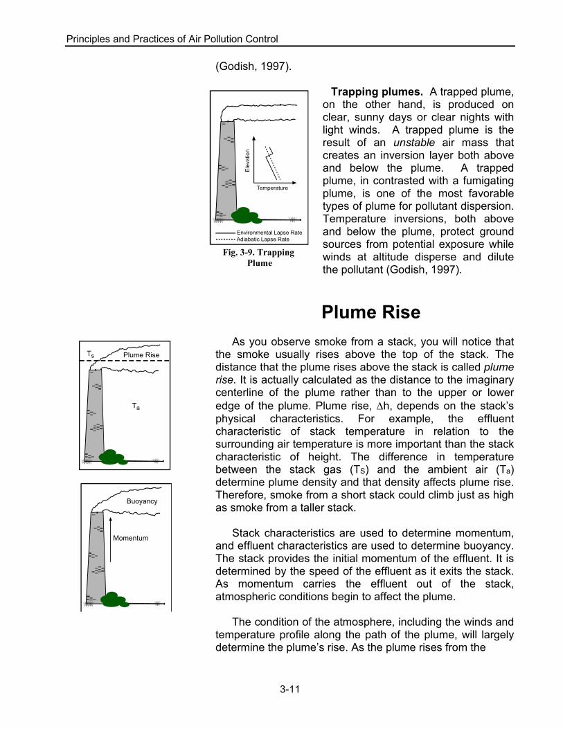
Trapping plumes. A trapped plume, on the other hand, is produced on clear, sunny days or clear nights with light winds. A trapped plume is the result of an unstable air mass that creates an inversion layer both above and below the plume. A trapped plume, in contrasted with a fumigating plume, is one of the most favorable types of plume for pollutant dispersion. Temperature inversions, both above and below the plume, protect ground sources from potential exposure while winds at altitude disperse and dilute the pollutant (Godish, 1997).
Plume Rise As you observe smoke from a stack, you will notice that
the smoke usually rises above the top of the stack. The distance that the plume rises above the stack is called plume rise. It is actually calculated as the distance to the imaginary centerline of the plume rather than to the upper or lower edge of the plume. Plume rise, ∆h, depends on the stack’s physical characteristics. For example, the effluent characteristic of stack temperature in relation to the surrounding air temperature is more important than the stack characteristic of height. The difference in temperature between the stack gas (TS) and the ambient air (Ta) determine plume density and that density affects plume rise. Therefore, smoke from a short stack could climb just as high as smoke from a taller stack.
Stack characteristics are used to determine momentum,
and effluent characteristics are used to determine buoyancy. The stack provides the initial momentum of the effluent. It is determined by the speed of the effluent as it exits the stack. As momentum carries the effluent out of the stack, atmospheric conditions begin to affect the plume.
The condition of the atmosphere, including the winds and
temperature profile along the path of the plume, will largely determine the plume’s rise. As the plume rises from the
Momentum
Buoyancy
Plume Rise
Ta
Ts
Temperature
Environmental Lapse RateAdiabatic Lapse Rate
Fig. 3-9. Trapping Plume
Transport and Dispersion of Air Pollution
3-12
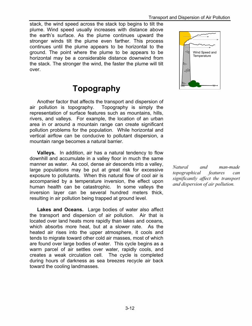
stack, the wind speed across the stack top begins to tilt the plume. Wind speed usually increases with distance above the earth’s surface. As the plume continues upward the stronger winds tilt the plume even farther. This process continues until the plume appears to be horizontal to the ground. The point where the plume to be appears to be horizontal may be a considerable distance downwind from the stack. The stronger the wind, the faster the plume will tilt over.
Topography Another factor that affects the transport and dispersion of
air pollution is topography. Topography is simply the representation of surface features such as mountains, hills, rivers, and valleys. For example, the location of an urban area in or around a mountain range can create significant pollution problems for the population. While horizontal and vertical airflow can be conducive to pollutant dispersion, a mountain range becomes a natural barrier.
Valleys. In addition, air has a natural tendency to flow
downhill and accumulate in a valley floor in much the same manner as water. As cool, dense air descends into a valley, large populations may be put at great risk for excessive exposure to pollutants. When this natural flow of cool air is accompanied by a temperature inversion, the effect upon human health can be catastrophic. In some valleys the inversion layer can be several hundred meters thick, resulting in air pollution being trapped at ground level.
Lakes and Oceans. Large bodies of water also affect
the transport and dispersion of air pollution. Air that is located over land heats more rapidly than lakes and oceans, which absorbs more heat, but at a slower rate. As the heated air rises into the upper atmosphere, it cools and tends to migrate toward other cold air masses, most of which are found over large bodies of water. This cycle begins as a warm parcel of air settles over water, rapidly cools, and creates a weak circulation cell. The cycle is completed during hours of darkness as sea breezes recycle air back toward the cooling landmasses.
Natural and man-made topographical features can significantly affect the transport and dispersion of air pollution.
Wind Speed andTemperature
Principles and Practices of Air Pollution Control
3-13
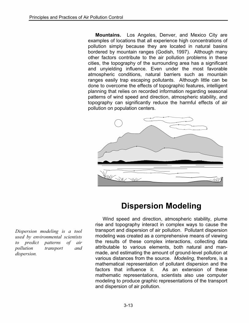
Mountains. Los Angeles, Denver, and Mexico City are
examples of locations that all experience high concentrations of pollution simply because they are located in natural basins bordered by mountain ranges (Godish, 1997). Although many other factors contribute to the air pollution problems in these cities, the topography of the surrounding area has a significant and unyielding influence. Even under the most favorable atmospheric conditions, natural barriers such as mountain ranges easily trap escaping pollutants. Although little can be done to overcome the effects of topographic features, intelligent planning that relies on recorded information regarding seasonal patterns of wind speed and direction, atmospheric stability, and topography can significantly reduce the harmful effects of air pollution on population centers.
Dispersion Modeling Wind speed and direction, atmospheric stability, plume
rise and topography interact in complex ways to cause the transport and dispersion of air pollution. Pollutant dispersion modeling was created as a comprehensive means of viewing the results of these complex interactions, collecting data attributable to various elements, both natural and man-made, and estimating the amount of ground-level pollution at various distances from the source. Modeling, therefore, is a mathematical representation of pollutant dispersion and the factors that influence it. As an extension of these mathematic representations, scientists also use computer modeling to produce graphic representations of the transport and dispersion of air pollution.
Dispersion modeling is a tool used by environmental scientists to predict patterns of air pollution transport and dispersion.
Transport and Dispersion of Air Pollution
3-14
In order to develop a precise model or method to
illustrate the manner in which air pollution is transported and dispersed for a given locale, information about the pollutant source is needed. This information generally includes surrounding geographic features, features, quantity and types of pollutants emitted, effluent gas conditions, stack
height, and influential meteorological factors. Using these types of data as input for a computer model, scientists can effectively predict how pollutants will be dispersed into the atmosphere. In addition, levels of pollutant concentration can be estimated for various distances and directions from the site of the smokestack.
U.S. environmental regulations have been formalized into a series of procedures that deal with permitting requirements that can affect both existing and new industrial facilities. Within this permitting process the use of selected air pollution dispersion models can aid in the determination of whether a specific facility should be constructed, modified based on the submitted plans, or need more efficient controls to be in compliance. An important advantage in the application of air pollution models for permitting is that the same set of procedures is applied for all One of the most important regulatory processes is the process of evaluating an application for a “permit to construct” or a New applicants. This allows an objective evaluation of air quality impact generated by the proposed or modified pollutant emitting facility.
New Source Review (NSR). The NSR process can vary
depending on the new source location. If the area where the
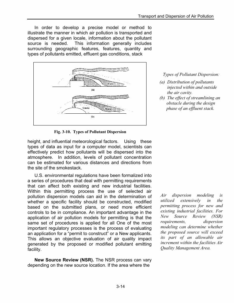
Types of Pollutant Dispersion: (a) Distribution of pollutants
injected within and outside the air cavity.
(b) The effect of streamlining an obstacle during the design phase of an effluent stack.
Air dispersion modeling is utilized extensively in the permitting process for new and existing industrial facilities. For New Source Review (NSR) requirements, dispersion modeling can determine whether the proposed source will exceed its part of an allowable air increment within the facilities Air Quality Management Area.
Fig. 3-10. Types of Pollutant Dispersion
Principles and Practices of Air Pollution Control
3-15
new plant is being located is attainment for all National Ambient Air Quality Standard Criteria pollutants, then the facility is subject to the Prevention of Significant Deterioration (PSD) doctrine. The PSD review process uses an appropriate dispersion model to evaluate whether the proposed source will exceed its part of the allowable air increment within the sites’ AQM area.
Guidelines on air quality modeling are found in 40 CFR
Part 51 Appendix W. The air quality modeling procedures discussed in the guideline document can be categorized into four generic classes: Gaussian, numerical, statistical or empirical, and physical.
Within these classes, especially Gaussian and numerical
models, a large number of individual “computational algorithms” may exist, each with its own specific applications. While each of the algorithms may have the same generic basis, it is accepted practice to refer to them individually as models. Gaussian models are the most widely used techniques for estimating the impact of non-reactive pollutants.
Numerical models may be more appropriate than Gaussian models for area source urban applications that involve reactive pollutants, but they require much more extensive input databases and resources and therefore are not as widely applied. Physical modeling involves the use of wind tunnels or other fluid modeling facilities. This class of modeling is a complex process requiring a high level of technical expertise, as well as access to the necessary facilities. Physical modeling may be useful for complex flow situations, such as building, terrain or stack downwash conditions, plume impact on elevated terrain diffusion in an urban environment, or diffusion in complex terrain. The dispersion models are categorized by two levels of sophistication: (1) Screening models, which provide conservative estimates of air quality impacts, and (2) Refined models, which provide a more detailed treatment of physical and chemical processes, but require more detailed and precise data for input in addition to higher computational costs.
Recommended air quality models are also divided into “preferred” and “alternative” model by the U.S. EPA. Preferred are models that EPA has either found better to perform than others in a given category, or has been chosen on factors such as faster use, public familiarity, and cost or resource requirements. As long as the preferred models are
40 CFR Part 51 contains guidelines on use of air quality modeling. Gaussian models as described in these guidelines are the most widely used technique for estimating the impact of non-reactive pollutants.
Transport and Dispersion of Air Pollution
3-16
applied as indicated by the U.S. EPA they can be used without a formal demonstration of applicability. Alternative models can be utilized when (1) an alternative model can be shown to produce concentration estimates equivalent to estimates obtained from a preferred model use (2) the alternative model performs better for the specific application than the preferred model based on a statistical performance evaluation; (3) a refined model is needed to satisfy regulatory requirements but, no preferred model for the specific application exists.
Two common models used by the U.S. EPA are the Assessment population Exposure Model (ASPEN) and the Industrial Source Complex (ISC) Model. These two models are frequently used in the permitting process and for environmental health impacts, because they can indicate how existing and additional pollutant sources will affect the ambient air concentrations and potentially the exposed populations’ health risk.
Assessment Population Exposure Model (ASPEN).
The Assessment Population Exposure Model calculates ambient air levels based on meteorology, chemistry, and rates which air toxics are emitted into the atmosphere. Currently ASPEN’s ambient concentration outputs are then used in conjunction with the Hazardous Air Pollutant Exposure Model (HAPEM4), as a screening tool to examine national exposure levels of specific toxic air pollutants. Estimated exposures can then be combined with quantitative health impact information to estimate population health risk estimates (U.S. EPA, 2000).
Industrial Source Complex Model (ISC). The Industrial
Source Complex Model is a more specific and precise tool than the HEM. It uses local data and predicts pollutant levels at specific locations. The ISC is a steady-state Gaussian plume model that can be used to estimate air pollutant concentrations from a wide variety of sources associated with an industrial source complex (Zannetti, 1990). Both models, however, are simply tools to help scientists make evaluations of air pollution dispersion. The accuracy of the models is limited by the inherent problems of trying to simplify complex and interrelated factors that affect the transport and dispersion of air pollution.
In conclusion, meteorology plays an important role in the
dispersion and transport of air pollution. It is inherently
The ASPEN and ISC are two commonly used models that can be used to estimate ambient air concentrations. Estimated ambient concentrations outputs from these models can also be utilized to calculate human exposure and population health risk.
Principles and Practices of Air Pollution Control
3-17
important to study its role within the strategies to control air pollution control and as part of air pollution dispersion modeling studies. As emissions released from one region continue to affect the population and ecosystems of another, air pollution dispersion modelers must attempt to understand the complex effects of meteorology upon the transport and dispersion of air pollutants.
3-18
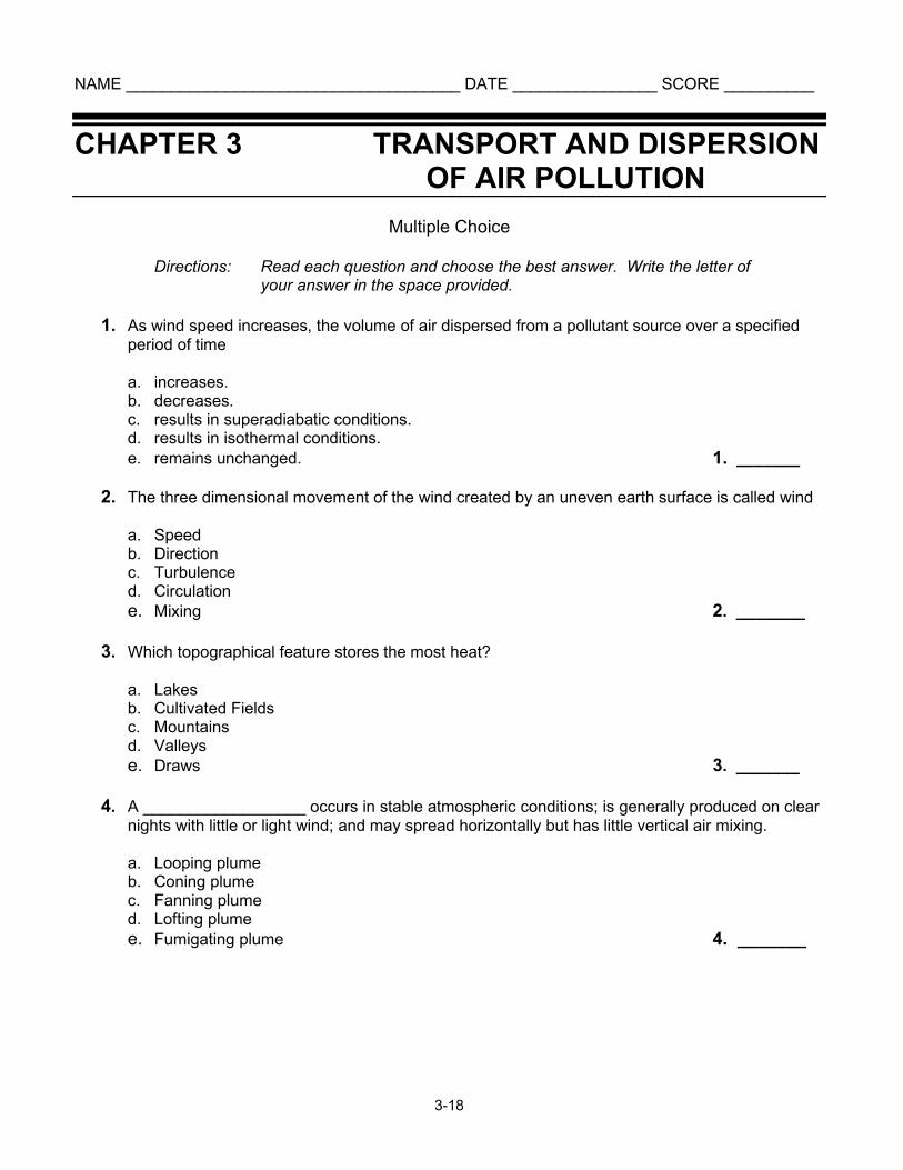
NAME _____________________________________ DATE ________________ SCORE __________
CHAPTER 3 TRANSPORT AND DISPERSION OF AIR POLLUTION
Multiple Choice Directions: Read each question and choose the best answer. Write the letter of your answer in the space provided.
1. As wind speed increases, the volume of air dispersed from a pollutant source over a specified period of time
a. increases. b. decreases. c. results in superadiabatic conditions. d. results in isothermal conditions. e. remains unchanged. 1. _______
2. The three dimensional movement of the wind created by an uneven earth surface is called wind
a. Speed b. Direction c. Turbulence d. Circulation e. Mixing 2. _______
3. Which topographical feature stores the most heat?
a. Lakes b. Cultivated Fields c. Mountains d. Valleys e. Draws 3. _______
4. A __________________ occurs in stable atmospheric conditions; is generally produced on clear
nights with little or light wind; and may spread horizontally but has little vertical air mixing. a. Looping plume b. Coning plume c. Fanning plume d. Lofting plume e. Fumigating plume 4. _______
Principles and Practices of Air Pollution Control
3-19
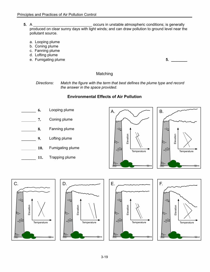
5. A ____________________________ occurs in unstable atmospheric conditions; is generally produced on clear sunny days with light winds; and can draw pollution to ground level near the pollutant source.
a. Looping plume b. Coning plume c. Fanning plume d. Lofting plume e. Fumigating plume 5. _______
Matching Directions: Match the figure with the term that best defines the plume type and record
the answer in the space provided.
Environmental Effects of Air Pollution
Temperature
A.
Temperature
B.
Temperature Temperature Temperature Temperature
E. F.C. D.
_______ 6. Looping plume _______ 7. Coning plume _______ 8. Fanning plume _______ 9. Lofting plume _______ 10. Fumigating plume _______ 11. Trapping plume
Transport and Dispersion of Air Pollution
3-20
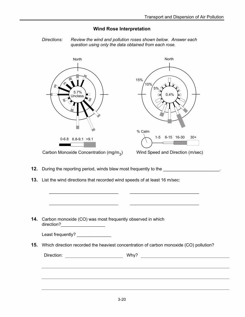
Wind Rose Interpretation Directions: Review the wind and pollution roses shown below. Answer each
question using only the data obtained from each rose.
12. During the reporting period, winds blew most frequently to the _______________________.
13. List the wind directions that recorded wind speeds of at least 16 m/sec:
14. Carbon monoxide (CO) was most frequently observed in which
direction?__________________
Least frequently? ______________
15. Which direction recorded the heaviest concentration of carbon monoxide (CO) pollution?
Direction: Why?
North
0.4%
5%10%
15%
Wind Speed and Direction (m/sec)
6-15 16-30 30+% Calm
1-5
5.7%Unclass.
0-6.8 6.8-9.1 >9.1
Carbon Monoxide Concentration (mg/m3)
North
Principles and Practices of Air Pollution Control
3-21
16. Describe the relationship between wind speed and direction and pollutant concentration.
Transport and Dispersion of Air Pollution
3-22
REVIEW ANSWERS
No. Answer Location/ Page Number of Answer 1. A 3-4
2. C 3-6
3. A 3-11, 3-6
4. C 3-8
5. A 3-8
6. A 3-8 3-10
7. D
8. C
9. B
10. F
11. E