Channel-Adaptive Schedulers with State-of-the-Art Channel Predictors

A. Aguiar 1, A. Wolisz, Telecommunication Networks Group, Technical University BerlinH. Lederer, Siemens AG, COM

H. Karl, University of Paderborn

Abstract: In this paper we study the effects of usingstate-of-the-art channel predictors with two channel-awareschedulers: a channel-aware round robin, and the propor-tional fair scheduler. We evaluate the performance for thecase when the scheduler queues are always full and for thecase when this does not happens. The round robin sched-uler proves to be only marginally influenced by the inaccu-rate predictor in both cases. The proportional fair sched-uler, however, can become very unfair when few wirelessterminals have data to be scheduled, some of them havea very good channel and the channel prediction is slightlyinaccurate. When the queues are not full, however, this be-haviour is no longer a problem. But, in this case, thereis not much to win by the use of a complex schedulerand complex channel predictor; a simple channel-awareround robin and a one-step predictor achieve similar per-formance.

1. Introduction

Channel-adaptive modulation or scheduling are effi-cient means of improving communication over wirelesschannels [4, 13, 8, 5, 9, 3]. These mechanisms requireknowledge of future channel behaviour, so that trans-mission parameters can be adapted to its variations. Al-though investigation about the potential of such mecha-nisms usually assumes accurate channel prediction, realchannel prediction algorithms are not perfect (the re-sult of the prediction does not completely correspond tothe channel behaviour). Furthermore, the difference be-tween the predicted value and the real one — the predic-tion error — are bigger for longer prediction horizons(the instant for which prediction is requested with re-spect to the instant when the prediction is made). In pre-vious work [1] we investigated the sensitivity of channel-adaptive mechanisms to channel prediction errors usingMonte Carlo simulations and a model for prediction er-rors. The model for prediction errors was developed be-cause it produced results that could be generalised; theuse of concrete prediction algorithms would make theresults of the investigation valid only for that preciseprediction algorithm. Moreover, at that time, we didnot have access to any real prediction algorithm, onlyto results presented in the literature [6, 11], so we couldnot check how close our model was to reality. Now were-did the studies using real prediction algorithms avail-able from a Matlab toolbox developed by Semmelrodtat the University of Kassel [12]. We used channel mea-surement traces [2] and generated channel prediction for15 ms prediction horizon using the toolbox. These trace

1This work is funded by the Foundation for Science and Tech-nology of the Portuguese Government and of the European SocialFund under PhD scholarship number SFRH/BD/4610/2001 and by theGerman Ministry of Education and Research under the Project 3GET(01BU354).

files were then used in the simulation environment.In Section2. we discuss the prediction algorithms in

more detail. Section3. describes the channel adaptivetechniques we used and in Section4. we present simula-tion results. We conclude the paper in Section5..

2. Channel Prediction Algorithms

The performance of the channel-aware schedulers pre-sented in Section3. using accurate prediction(ACC) arecompared with their performance when using the chan-nel prediction obtained with the algorithms presented be-low.2.1. Modified Covariance

Semmelrodt in [10] describes and compares severalalgorithms for the prediction of Rayleigh fading, fromwhich we chose the one that performed best: the Modi-fied Covariance algorithm(MC) . The received Rayleighfading signaly(n) is modeled as an auto-regressive (AR)process whose parametersai vary in time ande(n) is aGaussian random variable.

y(n) =p∑

i=1

ai · y(n− i) + e(n)

The future behaviour of the received signal can be esti-mated by a linear predictor (LP):

y(n) =p∑

i=1

ai · y(n− i)

, where we used a model order of 15, as recommendedin [10]. Since the conditions of the channel change withtime, the parameters of the AR modelai have to be esti-mated every time that prediction is required by solving asystem of linear equations using a least-squares method.

This LP only allows a single signal sample to be pre-dicted at each time, which may be a very short predictionhorizon, even if the signal sampling rate is close to thelowest possible. Therefore, to predict several samples inthe future, several LP are cascaded after another, eachusing the previously extrapolated signal samples as in-put.2.2. One Step Prediction

A simple practical approach to fading prediction oftenused in the praxis is the One Step prediction(OS). Inthis case, the last received channel value is used as theprediction for the next one.

y(n) = y(n− 1)

The accuracy of this method is highly dependent on theprediction horizon and the speed of the variations, which

1

increases with the maximum Doppler frequency of thefast fading

fD =v

cf (1)

, wherev is the speed of the wireless terminal (WT),fis the carrier frequency andc is the speed of light.

3. Channel-Adaptive Schedulers

First we use a Channel-aware Round Robin (CaRR)scheduler, which serves the backlogged queues one afterthe other, as long as the channel is good enough to guar-antee a maximum acceptable packet error rate (PER). Ifthe channel is not good enough, the queue is served onlyin the next round. Since adaptive modulation is state-of-the-art in most current wireless products it is also in-cluded in this study. For each packet we chose the mod-ulation that achieves the highest transmission rate whileguaranteeing a maximum packet error rate (PER). Thethresholds for changing the modulation are shown in Ta-ble1.

Packet Length [bits]# Bits/Symbol

536 3536 7536 11536

1 6.24 7.74 8.24 8.482 9.26 10.76 11.24 11.513 14.21 15.81 16.33 16.594 19.75 21.45 21.99 22.275 25.47 27.25 27.81 28.096 31.28 33.12 33.70 33.99

Table 1:SNR thresholds in dB for the choice of modu-lation for the different packet lengths used.

Further, we use the Proportional Fair (PF) schedulerproposed in [7]. This is also a channel-aware schedulerwhich serves the WT which has the highest ratio of ac-tual possible data rate to average data rate in the recentpast, where we used a history of 100 ms. The actualpossible data rate is calculated using the prediction ofthe channel behaviour as explained in the previous para-graph; in case there is no available modulation that canguarantee a PER lower than the maximum acceptable,the flow is not eligible for transmission.

4. Evaluation

4.1. Simulations SetupSeveral Wireless Terminals (WT) are evenly dis-

tributed in a 1 Km cell and communicate with an AccessPoint (AP); we consider only downlink one-hop commu-nication. The channel has a raw capacity of 2 MBaud;asynchronous time multiplexing is assumed, i. e. the APcan send packets of any length at any time the chan-nel is free. A MAC header of 272 bits and a PHYheader of 192 bits (values used for WLAN) are addedto every packet. The headers are transmitted using thelowest available modulation, using 1 bit per symbol, sothat each packet has on the link a constant overhead of146µs. The simulated time is 300 s for each run.

0

5

10

15

20

25

30

35

0 10 20 30 40 50 60 70

Rec

eive

d S

NR

[dB

]

time [s]

(a) Channel 0 (Archi 1)

0

5

10

15

20

25

30

35

0 10 20 30 40 50 60 70

Rec

eive

d S

NR

[dB

]

time [s]

(b) Channel 1 (Road 3)

0

5

10

15

20

25

30

35

40

0 10 20 30 40 50 60 70

Rec

eive

d S

NR

[dB

]

time [s]

(c) Channel 2 (Maths 1)

5

10

15

20

25

30

35

40

45

0 10 20 30 40 50 60 70

Rec

eive

d S

NR

[dB

]

time [s]

(d) Channel 3 (Maths 2)

-5

0

5

10

15

20

25

30

0 10 20 30 40 50 60 70

Rec

eive

d S

NR

[dB

]

time [s]

(e) Channel 4 (Archi 3)

-5

0

5

10

15

20

25

30

35

0 20 40 60 80 100 120

Rec

eive

d S

NR

[dB

]

time [s]

(f) Channel 5 (Sta-dium1 1)

Figure 1:Received signal traces.

-10

-5

0

5

10

15

20

25

0 10 20 30 40 50 60 70

Rec

eive

d S

NR

[dB

]

time [s]

(a) Channel 6 (Road 1)

5

10

15

20

25

30

35

40

45

50

0 10 20 30 40 50 60 70

Rec

eive

d S

NR

[dB

]

time [s]

(b) Channel 7 (Sta-dium1 2)

0

5

10

15

20

25

30

35

40

0 10 20 30 40 50 60 70

Rec

eive

d S

NR

[dB

]

time [s]

(c) Channel 8 (Walk 3)

0

5

10

15

20

25

30

35

40

0 20 40 60 80 100 120

Rec

eive

d S

NR

[dB

]

time [s]

(d) Channel 9 (Sta-dium2 2)

-10

-5

0

5

10

15

20

25

30

0 10 20 30 40 50 60 70

Rec

eive

d S

NR

[dB

]

time [s]

(e) Channel 10 (Walk 2)

0

5

10

15

20

25

30

35

40

0 10 20 30 40 50 60 70

Rec

eive

d S

NR

[dB

]

time [s]

(f) Channel 11 (Sta-dium2 1)

Figure 2:Received signal traces.

2

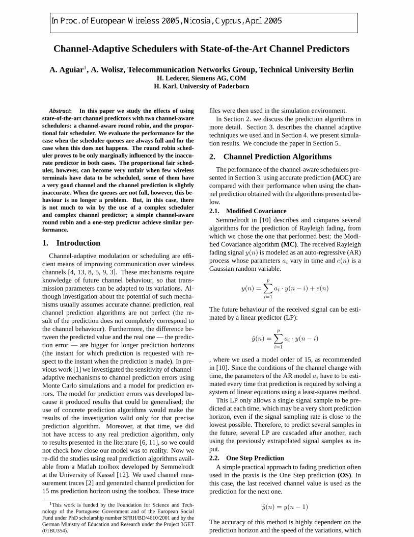
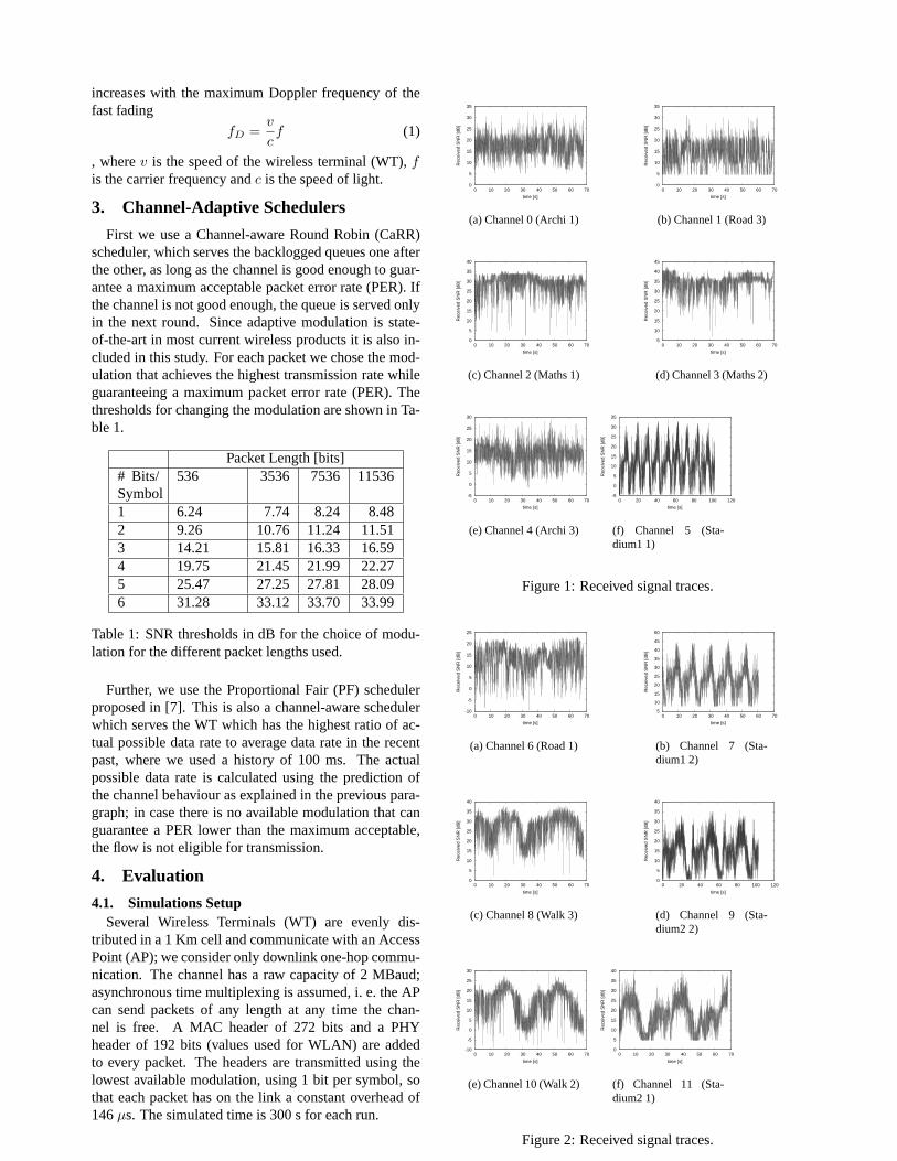
The signals received by the WTs vary in time andare subject to Rayleigh fading independently from one-another. We used fading processes obtained from aWLAN measurement campaign in low mobility environ-ments described in reference [2]. The SNR behaviour ofthe channels used for the simulations can be seen in Fig-ures1 and2.4.2. Capacity

We study the capacity gain achieved by the PF sched-uler with respect to the CaRR and its possible degrada-tion in the presence of inaccurate prediction, using sim-ulations where we varied the number of WT in the cell.Each WT receives CBR load with back-to-back pack-ets (this guarantees that all queues are always full) withvarying packet size.

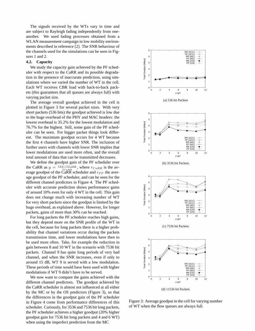
The average overall goodput achieved in the cell isplotted in Figure3 for several packet sizes. With veryshort packets (536 bits) the goodput achieved is low dueto the huge overhead of the PHY and MAC headers: thelowest overhead is 35.2% for the lowest modulation and76.7% for the highest. Still, some gain of the PF sched-uler can be seen. For bigger packet things look differ-ent. The maximum goodput occurs for 4 WT becausethe first 4 channels have higher SNR. The inclusion offurther users with channels with lower SNR implies thatlower modulations are used more often, and the overalltotal amount of data that can be transmitted decreases.

We define the goodput gain of the PF scheduler overthe CaRR asg = rP F−rCaRR

rCaRR, whererCaRR is the av-

erage goodput of the CaRR scheduler andrPF the aver-age goodput of the PF scheduler, and can be seen for thedifferent channel predictors in Figure4. The PF sched-uler with accurate prediction shows performance gainsof around 10% even for only 4 WT in the cell. This gaindoes not change much with increasing number of WTfor very short packets since the goodput is limited by thehuge overhead, as explained above. However, for longerpackets, gains of more than 30% can be reached.

For long packets the PF scheduler reaches high gains,but they depend more on the SNR profile of the WT inthe cell, because for long packets there is a higher prob-ability that channel variations occur during the packetstransmission time, and lower modulations have then tobe used more often. Take, for example the reduction ingain between 8 and 10 WT in the scenario with 7536 bitpackets. Channel 9 has quite long periods of very badchannel, and when the SNR increases, even if only toaround 15 dB, WT 9 is served with a low modulation.These periods of time would have been used with highermodulations if WT 9 didn’t have to be served.

We now want to compare the gains achieved with thedifferent channel predictors. The goodput achieved bythe CaRR scheduler is almost not influenced at all eitherby the MC or by the OS predictors (Figure3), so thatthe differences in the goodput gain of the PF schedulerin Figure4 come from performance differences of thisscheduler. Curiously, for 3536 and 7536 bit long packets,the PF scheduler achieves a higher goodput (20% highergoodput gain for 7536 bit long packets and 4 and 6 WT)when using the imperfect prediction from the MC

0

1

2

3

4

5

6

0 2 4 6 8 10 12

Tot

al G

oodp

ut [M

bps]

# WT

RR (ACC)PF (ACC)RR (MC)PF (MC)RR (OS)PF (OS)

(a) 536 bit Packets

0

1

2

3

4

5

6

0 2 4 6 8 10 12

Tot

al G

oodp

ut [M

bps]

# WT

RR (ACC)PF (ACC)RR (MC)PF (MC)RR (OS)PF (OS)

(b) 3536 bit Packets

0

1

2

3

4

5

6

0 2 4 6 8 10 12

Tot

al G

oodp

ut [M

bps]

# WT

RR (ACC)PF (ACC)RR (MC)PF (MC)RR (OS)PF (OS)

(c) 7536 bit Packets

0

1

2

3

4

5

6

0 2 4 6 8 10 12

Tot

al G

oodp

ut [M

bps]

# WT

RR (ACC)PF (ACC)RR (MC)PF (MC)RR (OS)PF (OS)

(d) 11536 bit Packets

Figure 3:Average goodput in the cell for varying numberof WT when the flow queues are always full.

3

than using perfect prediction. We looked at the good-put per WT, and in all cases where the use of MC pro-duces higher goodput than the use of the ACC, the good-put gain comes from a very high increase in the goodputof the WT with channels with high average SNR (WT 2,3). We ran the simulations again with the channels in thereverse order per WT, and noticed that the goodput gainwhen using inaccurate prediction occurred for more than10 WT (which is when channels 2 and 3 are used again),confirming our hypothesis. As already seen in reference[1], the prediction errors affect adaptive modulation sig-nificantly if the average SNR of the channel lies aroundthe thresholds used for modulation choice (Table1). Fora channel with average SNR of 39 dB, a signal predictionerror of even 5 dB does not influence the choice of themodulation at all. However, if the actual signal valuesis 18 dB, the same prediction error definitely leads to thechoice of a “wrong” modulation. If higher than the chan-nel actually allows, it may cause a transmission error, iflower, the channel will be “under-used” in the sense thatless data per unit time is sent than channel condition ac-tually allows. Since the PF scheduler chooses the WTwith the highest possible relative modulation and fewprediction errors lead to choosing a wrong modulationfor the very good channels, these WT are chosen moreoften (see histograms in Figure5) and a higher modula-tion is used more often, what explains the high overallgoodput gain. However, this behaviour is highly unfair.Although the goodput of WT 2 and 3 increases a lot, thegoodput of the WT with worse channels decreases a lot.For this scenario, WT 0 sees a throughput decrease of44% and WT 5 of 25% (see Table2), partly due to chan-nel errors, partly due to less channel allocations. As thetotal amount of WT in the cell increases, this effect hasless and less influence in the results because the proba-bility is higher that a WT other than the ones with goodchannels have the highest relative modulation.

Since the amount of WT with high or low SNR can-not be controlled by the system, these cases cannot beseen as insignificant, and this unfair behaviour of the PFscheduler will be seen whenever some WT in the cellhave an average SNR that is far from the thresholds. Forthe OS scheduler this is not observed due to the muchbigger prediction errors, which lead also more often toerrors in the choice of modulation for the WT with verygood channels.

For very long packets, the PF scheduler with the MCpredictor no longer shows a gain with respect to the ac-curate predictor. This happens because the predictionerrors are bigger. For longer packets, the necessary pre-diction horizon is longer, and the prediction errors arebigger, leading also for the good channels to bigger pre-diction errors. Consequently, more often a WT is chosenwhich does not actually have the best relative modulationand the average overall goodput decreases.

0

10

20

30

40

50

0 2 4 6 8 10 12

Goo

dput

Gai

n [%

]

# WT

ACCMCOS

(a) 536 bit Packets

0

10

20

30

40

50

0 2 4 6 8 10 12

Goo

dput

Gai

n [%

]

# WT

ACCMCOS

(b) 3536 bit Packets

0

10

20

30

40

50

0 2 4 6 8 10 12

Goo

dput

Gai

n [%

]

# WT

ACCMCOS

(c) 7536 bit Packets

0

10

20

30

40

50

0 2 4 6 8 10 12

Goo

dput

Gai

n [%

]

# WT

ACCMCOS

(d) 11536 bit Packets

Figure 4: Gain in average goodput for varying numberof WT when the flow queues are always full.

4

0

10000

20000

30000

40000

50000

60000

70000

80000

-1 0 1 2 3 4 5 6

# A

lloca

tions

WT

ACC

(a) Allocation histogram for PF with ACC

0

10000

20000

30000

40000

50000

60000

70000

80000

-1 0 1 2 3 4 5 6

# A

lloca

tions

WT

MC

(b) Allocation histogram for PF with MC

0

10000

20000

30000

40000

50000

60000

70000

80000

-1 0 1 2 3 4 5 6

# A

lloca

tions

WT

OS

(c) Allocation histogram for PF with OS

Figure 5:Allocation histogram of the PF scheduler for 6WT and 7536 bit packets, using the accurate and the MCpredictors.

Using the OS predictor, the reduction in average good-put gain does not exceed 10% (for 6 WT and 7536 bitpackets and for 8 WT and 3536 bit packets). In mostcases it lies around 5%. This indicates that up to thefrequency used (2.4 GHz) and for channels not varyingfaster, the OS predictor can be trusted without big perfor-mance degradation. Furthermore, this also indicates thatthe use of the much more complex MC predictor doesnot greatly improve the performance of the scheduler.4.3. Goodput using a Traffic Mix

In the previous case, all queues were always full, sothat the channel with the best possible modulation couldactually be served. This is not a realistic traffic scenario,so we also show here results for a CBR traffic mix whenthere are 12 WT in the cell. Half of the WT send 1632 bitlong packets every 20 ms (corresponds to a VoIP G.711

WT PF with ACC PF with MC Rel. difference0 1857817.26 1036321.87 -0.4421 452203.11 451286.93 -0.0022 1249246.44 1823464.17 0.4603 672268.35 1683823.43 1.5054 216797.55 228076.69 0.0525 336630.68 252286.95 -0.251

Table 2: Absolute throughput and relative throughputdifference per WT for 7536 bit packets and 6 WT in thecell.

codec), and the other half sends 536 bit long packets ev-ery 2 ms.

Figures6 and7 show the average goodput in the celland the percentage of correctly transmitted applicationdata. The first thing we notice is that the PF scheduleronly achieves a minor improvement with respect to theCaRR scheduler. The maximum achieved improvementin percentage of the offered data that can be correctlytransmitted is 4% (Figure7) for accurate prediction. Theperformance decreases to 0.6% for MC and 3.7% for OS,which is not significant. We also ran simulations when3536 bit long packets are sent every 8 ms instead of the536 bit long packets, and the maximum improvement inpercentage of correctly transmitted data achieved thenwas 1%, and the decrease due to real predictors insignif-icant.

Figures6 and 7 show a slight performance increaseof the RR scheduler using the OS predictor compared towhen using the ACC predictor. This can happen for thesame reason that it happens for the PF scheduler. How-ever, the RR scheduler is less sensitive to channel pre-diction errors. The influence of prediction errors on theperformance of the RR scheduler is restricted to some-times a WT not being scheduled although it could be-cause its channel is predicted as bad or transmission er-rors occuring because the predictor falsely estimated thechannel to be good. Furthermore, these errors only actu-ally influence the performance if they occurr for the flowwhich had its turn to be scheduled. It the PF case, chan-nel prediction errors influence the “priority” ordering ofthe flows.

1.81 1.79 1.82 1.931.821.92

0

0.5

1

1.5

2

2.5

3

ACC MC OS

Prediction Algorithm

To

tal G

oo

dp

ut [

Mb

ps]

RR

PF

Figure 6:Total goodput for the CBR traffic mix.

5. Conclusions

We study the performance of a Channel-aware RoundRobin scheduler and the Proportional Fair scheduler

5

79.9 79.3 80.584.2

79.983.9

0

20

40

60

80

100

ACC MC OS

Prediction Algorithm

% C

orr

ectly

Del

iver

ed D

ata

RR

PF

Figure 7:Percentage of correctly transmitted data for theCBR traffic mix.

when state-of-the-art channel predictors are used.We compare the average overall goodput achieved in

the cell when the queues are always full for increasingnumber of WT. The results show that the CaRR does notsignificantly suffer the influence of the realistic, inaccu-rate prediction algorithms. The PF scheduler, if thereare some WT with a very good channel (with regard tothe thresholds used for modulation adaptation), becomesunfair, and serves preferably those WT; this behaviourmay increase the overall goodput in the cell but is notdesirable from a fairness perspective. The OS predictordegrades the overall goodput gain, mostly between 5 and10%. Still gains of up to 20% are achieved. These resultsindicate that it is good enough for use in frequencies upto 2,4 GHz and similar mobility environments.

We also run simulations for a CBR traffic mix for12 WT when the flow queues at the AP are not alwaysfull. The use of real channel predictors causes almostno degradation of the performance of either the PF orthe CaRR schedulers. For the best improvement (3.9%in Figure7), the percentage of correctly transmitted datadecreased to 0.6% for the MC algorithm and to 3.7% forthe OS algorithm, which is not significant. Under theseconditions, the performance of the CaRR scheduler withthe OS predictor in terms of goodput cannot be improvedmuch either by the use of the more complex scheduler orthe more complex channel predictor.

REFERENCES

[1] A. Aguiar, H. Karl, and A. Wolisz. Channel adap-tive techniques in the presence of channel predic-tion inaccuracy. InProc. of European Wireless2004, Feb 2004.

[2] A. Aguiar and J. Klaue. Bi-directional wlan chan-nel measurements in different mobility scenarios.In Proc. Vehicular Technology Conference (VTCSpring), Milan, Italy, May 2004.

[3] P. Bhagwat, P. Bhattacharya, A. Krishna, andS. Tripathi. Enhancing throughput over wirelesslans using channel state dependent packet schedul-ing. In IEEE INFOCOM ’96, Mar 1996.

[4] S. Falahati, Svensson, M. Sternad, and T. Ekman.Adaptive modulation systems for predicted wire-less channels. InProc. of IEEE Globecom, Dec2003.

[5] C. Fragouli, V. Sivaraman, and M. Srivastava. Con-trolled multimedia wireless link sharing via en-hanced class-based queueinf with channel-state-dependent packet schedulin. InINFOCOM. IEEE,1998.

[6] S. Hu, A. Duel-Hallen, and H. Hallen. Long-rangeprediction of fading signals.IEEE Signal Process-ing Magazine, 17:62–75, May 2000.

[7] A. Jalali, R. Padovani, and R. Pankaj. Datathroughput of cdma-hdr a high efficiency-high datarate personal communication wireless system. InProc. of IEEE Vehicular Technology Conf. Spring,pages 1854–1858, May 2000.

[8] S. Lu, T. Nandagopal, and V. Bharghavan. Designand analysis of an algorithm for fair service in errorprone channels.ACM/Baltzer Wireless NetworksJournal, Vol. 6(4), pp. 323-343, Aug 2000.

[9] T. S. Eugene Ng, I. Stoica, and H. Zhang. Packetfair queueing algorithms for wireless networkswith location-dependent errors. InProceedingsof the 17th Annual Joint Conference of the IEEEComputer and Communications Societies — IN-FOCOM ’98, volume 3, pages 1103–1111, Mar1998.

[10] S. Semmelrodt and R. Kattenbach. Performanceanalysis and comparison of different fading fore-cast schemes for flat radio channels. COST Tech-nical Report, Jan 2003.

[11] M. Sternad, T. Ekman, and A. Ahlen. Power pre-diction on broadband channels. InProceedings ofthe 53rd IEEE Vehicular Technology Conference— VTC 2001 Spring, volume 4, pages 2328–2332,May 2001.

[12] Department of RF-Techniques / Communica-tion Systems University of Kassel. Spectral analy-sis and linear prediction toolbox. http://www.uni-kassel.de/fb16/hfk/neu/toolbox/, 2004.

[13] S. Vishwanath and A. Goldsmith. Adaptive turbo-coded modulation for flat-fading channels.IEEETrans. on Communications, 51(6):964–972, Jun2003.

6