Central Hardwoods ecosystem vulnerability assessment and ...

ForestService

Central Hardwoods Ecosystem Vulnerability Assessment and Synthesis:A Report from the Central Hardwoods Climate Change Response Framework Project

United States Department of Agriculture

General TechnicalReport NRS-124

NorthernResearch Station February 2014

Visit our homepage at: http://www.nrs.fs.fed.us/

Published by: For additional copies, contact:

USDA FOREST SERVICE USDA Forest Service11 CAMPUS BLVD., SUITE 200 Publications DistributionNEWTOWN SQUARE, PA 19073-3294 359 Main Road Delaware, OH 43015-8640February 2014 Fax: 740-368-0152

Manuscript received for publication July 2013

The forests in the Central Hardwoods Region will be affected directly and indirectly by a changing climate over the next 100 years. This assessment evaluates the vulnerability of terrestrial ecosystems in the Central Hardwoods Region of Illinois, Indiana, and Missouri to a range of future climates. We synthesized and summarized information on the contemporary landscape, provided information on past climate trends, and illustrated a range of projected future climates. This information was used to parameterize and contextualize multiple vegetation impact models, which provided a range of potential vegetative responses to climate. Finally, we brought these results before a multidisciplinary panel of scientists and land managers to assess ecosystems through a formal consensus-based expert elicitation process. The summary of the contemporary landscape identifies major stressors currently threatening forests and other terrestrial ecosystems in the region. Major current threats to forests in the area include invasive species, habitat fragmentation, oak decline, and a decrease in fire in fire-adapted systems.

Observed trends in climate over the historical record reveal that precipitation increased in the area, and that daily maximum temperatures decreased while minimum temperatures increased. Climate trends projected for the next 100 years by using downscaled global climate model data indicate a potential increase in mean annual temperature of 2 to 7 °F for this region. Projections for precipitation show an increase in winter and spring precipitation; summer and fall precipitation projections differ by model. We identified potential impacts on forests by incorporating these climate projections into three forest impact models (Tree Atlas, LINKAGES, and LANDIS PRO). Model projections suggest that northern mesic species such as sugar maple, American beech, and white ash may fare worse under future compared to current climate conditions, but other species such as post oak and shortleaf and loblolly pine may benefit from projected changes in climate. Changes in northern red, scarlet, and black oak differ by climate model.

We assessed ecosystem vulnerability for nine natural community types in the region by using these model results along with projected changes in other factors such as wildfire, invasive species, and diseases. The basic assessment was conducted through a formal elicitation process of 20 science and management experts from across the region, who considered vulnerability in terms of potential impacts on a system and the adaptive capacity of the system. Mesic upland forests were determined to be the most vulnerable, whereas many systems adapted to fire and drought, such as open woodlands, savannas, and glades, were perceived as less vulnerable to projected changes in climate. These projected changes in climate and the associated impacts and vulnerabilities will have important implications for economically important timber species, forest-dependent wildlife and plants, recreation, and long-range planning.

ABSTRACT

Cover PhotoClosed woodland. Photo by Paul Nelson, Mark Twain National Forest.

Central Hardwoods Ecosystem Vulnerability Assessment and Synthesis:

A Report from the Central Hardwoods Climate Change Response Framework Project

Leslie Brandt, Hong He, Louis Iverson, Frank R. Thompson III, Patricia Butler, Stephen Handler, Maria Janowiak, P. Danielle Shannon, Chris Swanston, Matthew Albrecht, Richard Blume-Weaver, Paul Deizman, John DePuy,

William D. Dijak, Gary Dinkel, Songlin Fei, D. Todd Jones-Farrand, Michael Leahy, Stephen N. Matthews, Paul Nelson, Brad Oberle, Judi Perez, Matthew Peters,

Anantha Prasad, Jeffrey E. Schneiderman, John Shuey, Adam B. Smith, Charles Studyvin, John M. Tirpak, Jeffery W. Walk, Wen J. Wang, Laura Watts,

Dale Weigel, and Steve Westin

Authors

LESLIE BRANDT is a climate change specialist with the Northern Institute of Applied Climate Science, U.S. Forest Service, 1992 Folwell Avenue, St. Paul, MN 55108, [email protected].

HONG HE is a professor at the University of Missouri-Columbia, School of Natural Resources, 203 Anheuser-Busch Natural Resources Building, Columbia, MO 65211, [email protected].

LOUIS IVERSON is a landscape ecologist with the U.S. Forest Service, Northern Research Station, 359 Main Road, Delaware, OH 43015, [email protected].

FRANK R. THOMPSON III is a research wildlife biologist with the U.S. Forest Service, Northern Research Station, 202 Anheuser-Busch Natural Resources Building, University of Missouri-Columbia, Columbia, MO 65211, [email protected].

PATRICIA BUTLER is a climate change outreach specialist with the Northern Institute of Applied Climate Science, Michigan Technological University, School of Forest Resources and Environmental Science, 1400 Townsend Drive, Houghton, MI 49931, [email protected].

STEPHEN HANDLER is a climate change specialist with the Northern Institute of Applied Climate Science, U.S. Forest Service, 410 MacInnes Drive, Houghton, MI 49931, [email protected].

MARIA JANOWIAK is a climate change adaptation and carbon management scientist with the Northern Institute of Applied Climate Science, U.S. Forest Service, 410 MacInnes Drive, Houghton, MI 49931, [email protected].

P. DANIELLE SHANNON is a climate change specialist with the Northern Institute of Applied Climate Science, U.S. Forest Service, 410 MacInnes Drive, Houghton, MI 49931, [email protected].

CHRIS SWANSTON is a research ecologist with the U.S. Forest Service, Northern Research Station, and director of the Northern Institute of Applied Climate Science, 410 MacInnes Drive, Houghton, MI 49931, [email protected].

MATTHEW ALBRECHT is an assistant curator of conservation biology with the Missouri Botanical Garden, Center for Conservation and Sustainable Development, P.O. Box 299, St. Louis, MO 63166, [email protected].

RICHARD BLUME-WEAVER is a planning and resources staff officer with the Shawnee National Forest, 50 Highway 145 South, Harrisburg, IL 62946, [email protected].

PAUL DEIZMAN is the coordinator for forest management and utilization, and forest stewardship and forest legacy, programs with the Illinois Department of Natural Resources, Division of Forest Resources, 1 Natural Resources Way, Springfield, IL 62702, [email protected].

JOHN DEPUY is a soil scientist with the Shawnee National Forest, 50 Highway 145 South, Harrisburg, IL 62946, [email protected].

WILLIAM D. DIJAK is a wildlife biologist and geographic information systems specialist with the U.S. Forest Service, Northern Research Station, 202 Anheuser-Busch Natural Resources Building, University of Missouri-Columbia, Columbia, MO 65211, [email protected].

GARY DINKEL is an ecosystem program manager with the Hoosier National Forest, 248 15th Street, Tell City, IN 47586, [email protected].

SONGLIN FEI is an assistant professor at Purdue University, Department of Forestry and Natural Resources, FORS 111, 195 Marsteller Street, West Lafayette, IN 47907, [email protected].

D. TODD JONES-FARRAND is science coordinator for the University of Missouri-Columbia, Central Hardwoods Joint Venture, 302 Anheuser-Busch Natural Resources Building, Columbia, MO 65211, [email protected].

MICHAEL LEAHY is the natural areas coordinator for the Missouri Department of Conservation, P.O. Box 180, Jefferson City, MO 65102, [email protected].

STEPHEN N. MATTHEWS is a research assistant professor at Ohio State University, School of Environment and Natural Resources, and an ecologist with the U.S. Forest Service, Northern Research Station, 359 Main Road, Delaware, OH 43015, [email protected].

PAUL NELSON (retired) was a forest ecologist with the Mark Twain National Forest, 401 Fairgrounds Road, Rolla, MO 65401.

BRAD OBERLE is a postdoctoral research associate at George Washington University, Department of Biological Sciences, 2023 G Street NW., Washington, DC 20053, [email protected].

JUDI PEREZ is a planning and public affairs staff officer with the Hoosier National Forest, 811 Constitution Avenue, Bedford, IN 47421, [email protected].

MATTHEW PETERS is a geographic information systems technician with the U.S. Forest Service, Northern Research Station, 359 Main Road, Delaware, OH 43015, [email protected].

ANANTHA PRASAD is an ecologist with the U.S. Forest Service, Northern Research Station, 359 Main Road, Delaware, OH 43015, [email protected].

JEFFREY E. SCHNEIDERMAN is a Ph.D. candidate at the University of Missouri-Columbia, School of Natural Resources, Anheuser-Busch Natural Resources Building, Columbia, MO 65211, [email protected].

JOHN SHUEY is director of conservation science with The Nature Conservancy Indiana Chapter, 620 East Ohio Street, Indianapolis, IN 46202, [email protected].

ADAM B. SMITH is an ecologist with the Missouri Botanical Garden, Center for Conservation and Sustainable Development, P.O. Box 299, St. Louis, MO 63166, [email protected].

CHARLES STUDYVIN (retired) was a forest silviculturist with the Mark Twain National Forest, 401 Fairgrounds Road, Rolla, MO 65401.

JOHN M. TIRPAK is science coordinator for the Gulf Coastal Plains and Ozarks Landscape Conservation Cooperative, 700 Cajundome Boulevard, Lafayette, LA 70506, [email protected].

JEFFERY W. WALK is director of science with The Nature Conservancy Illinois Chapter, 301 SW Adams Street, Suite 1007, Peoria, IL 61602, [email protected].

WEN J. WANG is a postdoctoral fellow at the University of Missouri-Columbia, School of Natural Resources, Anheuser-Busch Natural Resources Building, Columbia, MO 65211, [email protected].

LAURA WATTS is a forest planner with the Mark Twain National Forest, 401 Fairgrounds Road, Rolla, MO 65401, [email protected].

DALE WEIGEL is a forester with the Hoosier National Forest, 811 Constitution Avenue, Bedford, IN 47421, [email protected].

STEVE WESTIN is the forestry program supervisor with the Missouri Department of Conservation, Forestry Division, Planning & Emerging Issues, P.O. Box 180, Jefferson City, MO 65102, [email protected].

Page intentionally left blank

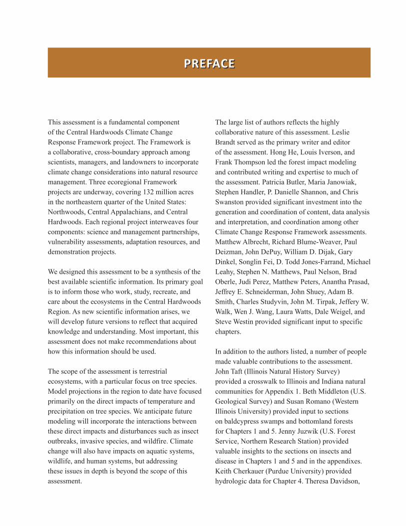
PrefAce

This assessment is a fundamental component of the Central Hardwoods Climate Change Response Framework project. The Framework is a collaborative, cross-boundary approach among scientists, managers, and landowners to incorporate climate change considerations into natural resource management. Three ecoregional Framework projects are underway, covering 132 million acres in the northeastern quarter of the United States: Northwoods, Central Appalachians, and Central Hardwoods. Each regional project interweaves four components: science and management partnerships, vulnerability assessments, adaptation resources, and demonstration projects.

We designed this assessment to be a synthesis of the best available scientific information. Its primary goal is to inform those who work, study, recreate, and care about the ecosystems in the Central Hardwoods Region. As new scientific information arises, we will develop future versions to reflect that acquired knowledge and understanding. Most important, this assessment does not make recommendations about how this information should be used.

The scope of the assessment is terrestrial ecosystems, with a particular focus on tree species. Model projections in the region to date have focused primarily on the direct impacts of temperature and precipitation on tree species. We anticipate future modeling will incorporate the interactions between these direct impacts and disturbances such as insect outbreaks, invasive species, and wildfire. Climate change will also have impacts on aquatic systems, wildlife, and human systems, but addressing these issues in depth is beyond the scope of this assessment.

The large list of authors reflects the highly collaborative nature of this assessment. Leslie Brandt served as the primary writer and editor of the assessment. Hong He, Louis Iverson, and Frank Thompson led the forest impact modeling and contributed writing and expertise to much of the assessment. Patricia Butler, Maria Janowiak, Stephen Handler, P. Danielle Shannon, and Chris Swanston provided significant investment into the generation and coordination of content, data analysis and interpretation, and coordination among other Climate Change Response Framework assessments. Matthew Albrecht, Richard Blume-Weaver, Paul Deizman, John DePuy, William D. Dijak, Gary Dinkel, Songlin Fei, D. Todd Jones-Farrand, Michael Leahy, Stephen N. Matthews, Paul Nelson, Brad Oberle, Judi Perez, Matthew Peters, Anantha Prasad, Jeffrey E. Schneiderman, John Shuey, Adam B. Smith, Charles Studyvin, John M. Tirpak, Jeffery W. Walk, Wen J. Wang, Laura Watts, Dale Weigel, and Steve Westin provided significant input to specific chapters.

In addition to the authors listed, a number of people made valuable contributions to the assessment. John Taft (Illinois Natural History Survey) provided a crosswalk to Illinois and Indiana natural communities for Appendix 1. Beth Middleton (U.S. Geological Survey) and Susan Romano (Western Illinois University) provided input to sections on baldcypress swamps and bottomland forests for Chapters 1 and 5. Jenny Juzwik (U.S. Forest Service, Northern Research Station) provided valuable insights to the sections on insects and disease in Chapters 1 and 5 and in the appendixes. Keith Cherkauer (Purdue University) provided hydrologic data for Chapter 4. Theresa Davidson,

Nancy Feakes, Keri Hicks, and Bennie Terrell (Mark Twain National Forest); Charles Sams (U.S. Forest Service, Eastern and Southern Regions); Jan Schultz and Linda Schmidt (U.S. Forest Service, Eastern Region); and Nick Kuhn (Missouri Department of Conservation) provided input to sections in Chapter 7.

We would especially like to thank David Diamond (University of Missouri), Steve Shifley (U.S. Forest Service, Northern Research Station), and Mike Jenkins (Purdue University), who provided formal technical reviews of the assessment. Their thorough review greatly improved the quality of this assessment.

contents

Executive Summary . . . . . . . . . . . . . . . . . . . . . . . . . . . . . . . . . . . . . . . . . . . . . . . . . . . . . . . . . . . . . . . . .1

Introduction . . . . . . . . . . . . . . . . . . . . . . . . . . . . . . . . . . . . . . . . . . . . . . . . . . . . . . . . . . . . . . . . . . . . . . .7

Chapter 1: The Contemporary Landscape . . . . . . . . . . . . . . . . . . . . . . . . . . . . . . . . . . . . . . . . . . . . . 10

Chapter 2: Climate Change Science and Modeling . . . . . . . . . . . . . . . . . . . . . . . . . . . . . . . . . . . . . . 45

Chapter 3: Past Climate Changes and Current Trends . . . . . . . . . . . . . . . . . . . . . . . . . . . . . . . . . . . . 60

Chapter 4: Projected Changes in Climate and Other Physical Processes . . . . . . . . . . . . . . . . . . . . . 79

Chapter 5: Future Climate Change Impacts on Forests . . . . . . . . . . . . . . . . . . . . . . . . . . . . . . . . . . . 94

Chapter 6: Ecosystem Vulnerabilities . . . . . . . . . . . . . . . . . . . . . . . . . . . . . . . . . . . . . . . . . . . . . . . . 118

Chapter 7: Management Implications. . . . . . . . . . . . . . . . . . . . . . . . . . . . . . . . . . . . . . . . . . . . . . . . 147

Glossary . . . . . . . . . . . . . . . . . . . . . . . . . . . . . . . . . . . . . . . . . . . . . . . . . . . . . . . . . . . . . . . . . . . . . . . . 162

Literature Cited . . . . . . . . . . . . . . . . . . . . . . . . . . . . . . . . . . . . . . . . . . . . . . . . . . . . . . . . . . . . . . . . . . 171

Appendix 1: Common and Scientific Names of Flora and Fauna . . . . . . . . . . . . . . . . . . . . . . . . . . 199

Appendix 2: Crosswalk of Natural Communities . . . . . . . . . . . . . . . . . . . . . . . . . . . . . . . . . . . . . . . 202

Appendix 3: Forest Types . . . . . . . . . . . . . . . . . . . . . . . . . . . . . . . . . . . . . . . . . . . . . . . . . . . . . . . . . . 210

Appendix 4: Common Nonnative Invasive Species in the Central Hardwoods Region . . . . . . . . . 212

Appendix 5: Common Diseases in the Central Hardwoods Region. . . . . . . . . . . . . . . . . . . . . . . . . 215

Appendix 6: Common Insect Pests in the Central Hardwoods Region . . . . . . . . . . . . . . . . . . . . . . 216

Appendix 7: Trend Analysis and Historical Climate Data . . . . . . . . . . . . . . . . . . . . . . . . . . . . . . . . . 217

Appendix 8: Additional Climate Projection Data and Maps . . . . . . . . . . . . . . . . . . . . . . . . . . . . . . 221

Appendix 9: Additional Impact Model Results . . . . . . . . . . . . . . . . . . . . . . . . . . . . . . . . . . . . . . . . . 231

Appendix 10: Vulnerability and Confidence Determination . . . . . . . . . . . . . . . . . . . . . . . . . . . . . . 246

Appendix 11: Expert Panelists . . . . . . . . . . . . . . . . . . . . . . . . . . . . . . . . . . . . . . . . . . . . . . . . . . . . . . 254

Page intentionally left blank

1

executive summAry

This assessment evaluates key ecosystem vulnerabilities to a range of future climate scenarios across the Central Hardwoods Region of Missouri, Illinois, and Indiana (Fig. 1). This assessment is part of the Central Hardwoods Climate Change Response Framework project, a collaborative approach among researchers, managers, and landowners to incorporate climate change considerations into forest management.

The assessment summarizes current conditions and key stressors and identifies past and projected trends in climate. This information is then incorporated into model projections of future forest change. These projections, along with local knowledge and expertise, are used to identify what factors contribute to the vulnerability of forests across the Central Hardwoods Region and what forest community types may be more vulnerable than others over the next 100 years. A final chapter summarizes the implications of these impacts and vulnerabilities for forest management across the region.

Figure 1.—Assessment area (in color).

chAPter 1: the contemPorAry LAnDscAPe

summaryThis chapter describes the forests and related ecosystems across the Central Hardwoods landscape and summarizes current threats and management trends. This information lays the foundation for understanding how shifts in climate may contribute to changes in Central Hardwoods ecosystems, and how climate may interact with other stressors on the landscape.

main Points● Forty percent of the area is forested, of which

about 80 percent is privately owned. ● Current major stressors and threats to forest

ecosystems in the region include:▪ Fragmentationandlossofforestcover▪ Lossofhistoricalfireregimeinfire-adapted

systems▪ Nonnativespeciesinvasion▪ Insectsanddisease▪ Lossofsoil▪ Overgrazingandoverbrowsing▪ Extremeweatherevents▪ Reduceddiversityofspeciesandageclasses▪ Lackofmanagementonprivatelands

● Management practices over the past several decades have increasingly emphasized restoring fire-adapted ecosystems while providing sustainable forest products.

2

executive summAry

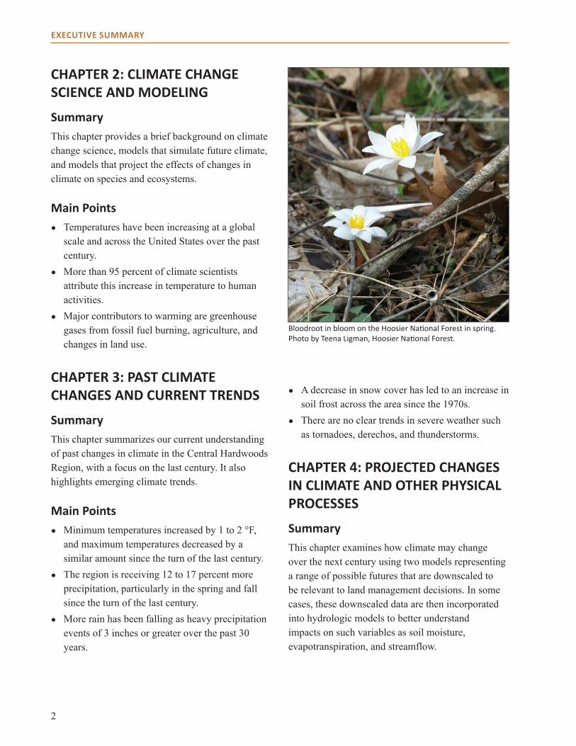
chAPter 2: cLimAte chAnGe science AnD moDeLinG

summaryThis chapter provides a brief background on climate change science, models that simulate future climate, and models that project the effects of changes in climate on species and ecosystems.

main Points● Temperatures have been increasing at a global

scale and across the United States over the past century.

● More than 95 percent of climate scientists attribute this increase in temperature to human activities.

● Major contributors to warming are greenhouse gases from fossil fuel burning, agriculture, and changes in land use.

chAPter 3: PAst cLimAte chAnGes AnD current trenDs

summaryThis chapter summarizes our current understanding of past changes in climate in the Central Hardwoods Region, with a focus on the last century. It also highlights emerging climate trends.

main Points● Minimum temperatures increased by 1 to 2 °F,

and maximum temperatures decreased by a similar amount since the turn of the last century.

● The region is receiving 12 to 17 percent more precipitation, particularly in the spring and fall since the turn of the last century.

● More rain has been falling as heavy precipitation events of 3 inches or greater over the past 30 years.

● A decrease in snow cover has led to an increase in soil frost across the area since the 1970s.

● There are no clear trends in severe weather such as tornadoes, derechos, and thunderstorms.

chAPter 4: ProJecteD chAnGes in cLimAte AnD other PhysicAL Processes

summaryThis chapter examines how climate may change over the next century using two models representing a range of possible futures that are downscaled to be relevant to land management decisions. In some cases, these downscaled data are then incorporated into hydrologic models to better understand impacts on such variables as soil moisture, evapotranspiration, and streamflow.

Bloodroot in bloom on the Hoosier National Forest in spring. Photo by Teena Ligman, Hoosier National Forest.

3

executive summAry

main Points● Model projections suggest an increase in

temperature over the next century across all seasons by 2 to 7 °F.

● Precipitation is projected to increase in winter and spring by 2 to 5 inches for the two seasons combined.

● The climate models examined disagree about how precipitation may change in summer, with one projecting an increase of up to 3 inches in summer and the other a decrease of up to 8 inches.

● Little information is currently available regarding how extreme weather events such as tornadoes and thunderstorms may change.

● Hydrologic model projections indicate that soil moisture, runoff, and streamflow may increase during the spring as precipitation increases.

● Model projections suggest that snow cover and duration will continue to decrease over the next century.

chAPter 5: future cLimAte chAnGe imPActs on forests

summaryThis chapter summarizes the potential impacts of climate change on forests in the Central Hardwoods Region over the next century, with an emphasis on changes in tree species distribution and abundance using three different impact models.

main Points● All three models project habitat suitability for

sugar maple will decline over the next century across the region.

● Models also project that habitat suitability for shortleaf pine will increase, along with post and blackjack oak.

● Model projections for northern red, scarlet, and black oak vary by impact model and climate scenario across much of the region.

● Changes in climate are not projected to have a dramatic effect on many common species in the region, including eastern redcedar and white oak.

● The modeled projections of tree species do not account for many other physical and biological factors that may change under a changing climate. Other factors include:▪ Droughtstress▪ Changesinhydrologyandfloodregime▪ Soilerosion▪ Wildfirefrequencyandseverity▪ Increasedcarbondioxide▪ Alterednutrientcycling▪ Changesininvasivespecies,pests,and

pathogens▪ Changesinherbivory

chAPter 6: ecosystem vuLnerABiLities

summaryThis chapter focuses on the collective vulnerability of natural communities in the Central Hardwoods Region to climate change over the next 100 years, focusing on shifts in dominant species, system drivers, and stressors. The adaptive capacity of systems within the Central Hardwoods Region was also examined as a key component to overall vulnerability to climate change. Finally, relative vulnerability of nine major forest community types in the region was assessed (Table 1).

4

executive summAry

vulnerability of the regionPotential Impacts on Drivers and Stressors:● Temperatures will increase (robust evidence,

high agreement). All global climate models project that temperatures will increase due to a rise in greenhouse gas concentrations both locally and globally.

● Growing seasons will lengthen (medium evidence, high agreement). There is a strong agreement among information that an increase in temperature will lead to longer growing seasons, but few studies have specifically examined projected growing season length in the assessment area.

● The nature and timing of precipitation will change (robust evidence, high agreement). A large number of global climate models agree that precipitation patterns will change at both local and global scales.

● An increase in heavy precipitation events (medium evidence, medium agreement) may result in flood risks (limited evidence, medium agreement) and soil erosion (limited evidence, medium agreement). There is disagreement among models about whether heavy precipitation events will continue to increase in the assessment area. If they do increase, it is expected that flooding and soil erosion will increase as well, but these effects have not been modeled for this region.

● Snow will decrease, with subsequent decreases in soil frost (high evidence, high agreement). Evidence suggests that winter temperatures will increase in the area, even under low emissions, leading to changes in snow and soil frost.

● Soil moisture patterns will change (medium evidence, high agreement), with drier soil conditions later in the growing season (medium evidence, low agreement). Some studies show that climate change will have impacts on soil moisture, but there is disagreement among climate and impact models on how soil moisture will change during the growing season.

● Droughts will increase in duration and area (medium evidence, low agreement). A study using multiple climate models suggests that drought may increase in extent and area, but another suggests a decrease in drought.

● Climate conditions will increase fire risks by the end of the century (medium evidence, high agreement). National and global studies agree that wildfire risk will increase in the area, but few studies have specifically looked at the Central Hardwoods Region.

● Many invasive species, insect pests, and pathogens will increase or become more severe (medium evidence, high agreement). Evidence suggests that an increase in temperature and greater ecosystem stress will lead to increases in these threats, but research to date has examined few species.

Community Type Vulnerability Evidence Agreement

Dry-mesic upland forest Low-Moderate Medium Medium-HighMesic upland forest High Medium Medium-HighMesic bottomland forest Moderate Limited -Medium MediumWet bottomland forest Moderate- High Limited-Medium MediumFlatwoods Low-Moderate Limited-Medium MediumClosed woodland Low Limited MediumOpen woodland Low Limited-Medium MediumBarrens and savannas Low Medium Medium-HighGlade Low-Moderate Medium Medium-High

Table 1.—Vulnerability determinations by natural community type.

5

executive summAry

Potential Impacts on Ecosystems ● Suitable habitat for northern species will

decline (medium evidence, high agreement). All three impact models project a decrease in suitability for northern species such as sugar maple, American beech, and white ash.

● Habitat will become more suitable for southern species (medium evidence, high agreement). All three forest impact models project an increase in suitability for southern species such as shortleaf pine.

● Communities will shift across the landscape (low evidence, high agreement). Although few models have examined community shifts specifically, model results from individual species and ecological principles suggest communities may also shift.

● Increased fire frequency and harvesting may accelerate shifts in forest composition across the landscape (medium evidence, medium agreement). Studies from other regions (e.g., northern hardwoods and boreal forests) show that increased fire frequency can accelerate the decline of species negatively affected by climate warming and accelerate the northward migration of southern tree species.

● A major transition in forest composition is not expected to occur in the coming decades (medium evidence, medium agreement). Although some models indicate major changes in habitat suitability, results from spatially dynamic forest landscape models indicate that a major shift in forest composition across the landscape may take 100 years or more in the absence of major disturbances.

● Little net change in forest productivity is expected (medium evidence, low agreement). Although a number of studies have examined the impact of climate change on forest productivity, they disagree on how multiple factors may interact to influence it.

Adaptive Capacity Factors● Low diversity systems are at greater risk

(medium evidence. high agreement). Studies in other areas have consistently shown that diverse systems are more resilient to disturbance, but studies examining this relationship have not been conducted in the assessment area.

● Species in fragmented systems will have a reduced ability to expand into new areas (limited evidence, high agreement). Evidence suggests that species may not be able to disperse the distances required to keep up with climate change, but little research has been done in the region on this topic.

● Fire-adapted systems will be more resilient to climate change (high evidence, medium agreement). Studies have shown that fire-adapted systems are better able to recover after disturbances and can promote many of the species that are projected to do well under a changing climate.

● Systems that are highly limited by hydrologic regime or geologic features may be constrained (limited evidence, medium agreement). Our current understanding of the ecology of Central Hardwoods systems suggests that some rare communities will be too topographically constrained to migrate to new areas.

chAPter 7: mAnAGement imPLicAtions

summaryThis chapter summarizes climate change impacts on decisionmaking and management for public and private lands across the Central Hardwoods Region. These impacts will vary by ecosystem, ownership, and management objective. This chapter does not make recommendations as to how management should be adjusted to deal with these impacts.

�

main Points● Plants, animals, and people that depend on forests

may face additional challenges as temperatures increase and precipitation patterns shift.

● Greater financial investments may be required to maintain healthy forests and resilient infrastructure and to prepare for severe weather events.

● The seasonal timing of management activities such as prescribed burns or recreation activities such as waterfowl hunting may need to be altered as temperatures and precipitation patterns change.

● Confronting the challenge of climate change presents opportunities for managers and other decisionmakers to plan ahead, foster resilient landscapes, and ensure that the benefits that forests provide are sustained into the future.

Open woodland. Photo by Paul Nelson, Mark Twain National Forest.

7

introDuction

contextThis assessment is part of a regional effort across the Central Hardwoods Region of Illinois, Indiana, and Missouri called the Central Hardwoods Climate Change Response Framework (Framework; www.forestadaptation.org). The Framework project was initiated in 2011, and is one of three ecoregional projects in the Midwest, Mid-Atlantic, and Northeast. These projects build off the lessons learned from a pilot project in northern Wisconsin, initiated in 2009, which has since expanded into the Northwoods project. The overarching goal of all three Framework projects is to incorporate climate change considerations into forest management. To meet the challenges brought about by climate change, a team of federal and state land management agencies, universities, conservation organizations, and others have come together to accomplish three objectives:

● Provide a forum to share the experiences and lessons learned of managers and scientists regarding forest management and climate change in the Central Hardwoods Region of Missouri, Illinois, and Indiana.

● Develop new user-friendly tools that can help public and private land managers include climate change considerations in decisionmaking, including a forest ecosystem vulnerability assessment and a forest adaptation resources document.

● Support efforts by public land managers, private landowners, and conservation organizations to put these new tools to work on the ground across the Central Hardwoods Region.

The Framework is designed to work at multiple scales. The Central Hardwoods Framework is coordinated across the region, but activities are generally conducted at the state level to allow for greater specificity. The assessment is written to encompass three states within the Central Hardwoods Region, but information is provided at the level of individual states whenever possible.

The Central Hardwoods Climate Change Response Framework has been supported in large part by the U.S. Department of Agriculture (USDA), Forest Service, but is guided by the greater community of the Central Hardwoods Region to serve the needs of multiple end-users. Current partners in the effort include:

● Northern Institute of Applied Climate Science● U.S. Forest Service, Eastern Region● U.S. Forest Service, Northern Research Station● U.S. Forest Service, Northeastern Area (State &

Private Forestry)● Illinois Department of Natural Resources● Missouri Department of Conservation● The Nature Conservancy● The Central Hardwoods Joint Venture● The Gulf Coastal Plains and Ozarks Landscape

Conservation Cooperative ● Missouri Botanical Garden● Purdue University● University of Missouri

The assessment bears some similarity to other synthesis documents about climate change science, such as the National Climate Assessment (draft

8

introDuction

report at http://ncadac.globalchange.gov/) and the Intergovernmental Panel on Climate Change (IPCC) reports (e.g., IPCC 2007). Where appropriate, we refer to these larger-scale documents when discussing national and global-scale changes. However, this assessment differs from these reports in a number of ways. This assessment was neither commissioned by any federal government agency nor does it give advice or recommendations to any federal government agency. It also does not evaluate policy options or provide input into federal priorities. Instead, this report was developed by the authors to fulfill a joint need of understanding local impacts of climate change on forests and assessing which tree species and forest communities may be the most vulnerable in the Central Hardwoods Region. Although it was written to be a resource for forest managers, it is first and foremost a scientific document that represents the views of the authors.

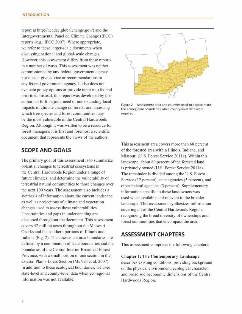
scoPe AnD GoALsThe primary goal of this assessment is to summarize potential changes to terrestrial ecosystems in the Central Hardwoods Region under a range of future climates, and determine the vulnerability of terrestrial natural communities to those changes over the next 100 years. The assessment also includes a synthesis of information about the current landscape as well as projections of climate and vegetation changes used to assess these vulnerabilities. Uncertainties and gaps in understanding are discussed throughout the document. This assessment covers 42 million acres throughout the Missouri Ozarks and the southern portions of Illinois and Indiana (Fig. 2). The assessment area boundaries are defined by a combination of state boundaries and the boundaries of the Central Interior Broadleaf Forest Province, with a small portion of one section in the Coastal Plains-Loess Section (McNab et al. 2007). In addition to these ecological boundaries, we used state-level and county-level data when ecoregional information was not available.

Figure 2.—Assessment area and counties used to approximate the ecoregional boundaries when county-level data were required.

This assessment area covers more than �8 percent of the forested area within Illinois, Indiana, and Missouri (U.S. Forest Service 2011a). Within this landscape, about 80 percent of the forested land is privately owned (U.S. Forest Service 2011a). The remainder is divided among the U.S. Forest Service (12 percent), state agencies (5 percent), and other federal agencies (3 percent). Supplementary information specific to these landowners was used when available and relevant to the broader landscape. This assessment synthesizes information covering all of the Central Hardwoods Region, recognizing the broad diversity of ownerships and forest communities that encompass the area.

Assessment chAPtersThis assessment comprises the following chapters:

Chapter 1: The Contemporary Landscape describes existing conditions, providing background on the physical environment, ecological character, and broad socioeconomic dimensions of the Central Hardwoods Region.

9

introDuction

Chapter 2: Climate Change Science and Modeling contains background information on climate change science, projection models, and impact models. It also describes the techniques used in developing climate projections to provide context for the model results presented in later chapters.

Chapter 3: Past Climate Changes and Current Trends provides information on the past and current climate of the Central Hardwoods Region, summarized from The Nature Conservancy’s interactive ClimateWizard database and published literature. This chapter also summarizes some relevant ecological indicators of observed climate change.

Chapter 4: Projected Changes in Climate and other Physical Processes presents downscaled climate change projections for the assessment area, including future temperature and precipitation data. It also includes summaries of other climate-related trends that have been projected for Illinois, Indiana, and Missouri, and the Midwest.

Chapter 5: Future Climate Change Impacts on Forests summarizes model projections of forest change that were prepared for this assessment. Different modeling approaches were used to model climate change impacts on forests: a species distribution model (Climate Change Tree Atlas), a forest simulation model (LANDIS PRO), and an ecosystem model (LINKAGES). This chapter also includes a review of literature about other climate-related impacts on forests.

Chapter 6: Ecosystem Vulnerabilities synthesizes the potential effects of climate change on forested and other terrestrial communities in the Central Hardwoods Region and provides detailed vulnerability determinations for nine terrestrial natural communities common to the region.

Chapter 7: Management Implications addresses some of the implications of a changing climate for major components of the forest sector within the Central Hardwoods Region, including forest products, recreation, cultural resources, and forest-dependent wildlife.

Missouri Ozarks in fall. Photo by Steve Shifley, U.S. Forest Service.

10


The Central Hardwoods Region represents a mosaic of forests, woodlands, savannas, and other ecosystems dominated by oak, hickory, and other hardwood species (for common and scientific names of species, see Appendix 1). This landscape sustains the people of the region by providing economically important forest products, outdoor recreation opportunities, and other benefits. Here we describe the forests and related ecosystems across the Central Hardwoods landscape and summarize current threats and management trends. This information lays the foundation for understanding how shifts in climate may contribute to changes in Central Hardwoods ecosystems, and how climate may interact with other stressors on the landscape.

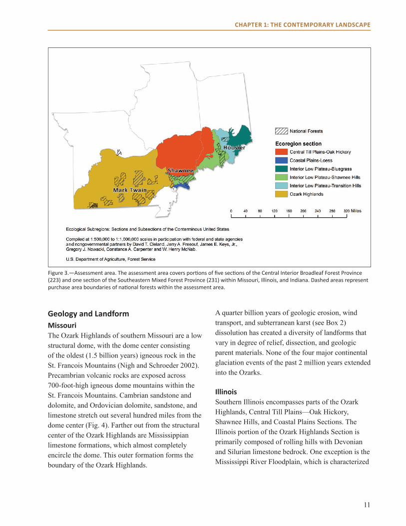
LAnDscAPe settinGThis assessment covers the part of Ecological Province 223 (Central Interior Broadleaf Forest; McNab et al. 2007) that falls within five sections in Missouri, Illinois, and Indiana (Fig. 3). The assessment also covers one section (Coastal Plains-Loess) in Ecological Province 231 (Southeastern Mixed Forest). Sections are based on differences in geologic parent material, elevation, plant distribution, and regional climate within the U.S. Forest Service National Hierarchical Framework of Ecological Units (McNab and Avers 1994, McNab et al. 2007). The area covers three national forests and many other federal, state, and private lands. Below, we summarize the major physical and biological features of the assessment area. Additional descriptions of the landscape setting can be found in the resources listed in Box 1.

Physical EnvironmentclimateThe current climate of the Central Hardwoods Region of Illinois, Indiana, and Missouri is generally characterized as a humid continental climate, with cool winters and long, hot summers. Due to a general lack of influence by topography or large bodies of water, the region is influenced by large air masses from the Arctic in the winter and the Gulf of Mexico in the summer. Average annual temperatures follow an east-west gradient, and range from 54.4 °F (12.3 °C) in Indiana to 55.� °F (13.1 °C) in Missouri (see Chapter 3). Annual average precipitation ranges from 44.9 inches in Indiana to 42.9 inches in Illinois, with Missouri being in between the two (43.9 inches; see Chapter 3).

Conditions are distinct between winter and summer, and extreme weather events occur throughout the year. Precipitation often falls as snow between December and February. Summers are hot, averaging 75.� ºF (24.2 °C) in the Missouri and Illinois portions of the assessment area, and 73.8 ºF (23.2 °C) in the Indiana portion of the assessment area (see Chapter 3). Extreme weather events in the area include high-intensity rains, long drought periods, heat waves and cold waves, ice storms, windstorms, and tornadoes. Missouri is ranked 9th, Illinois is ranked 8th, and Indiana is ranked 21st among states for the number of tornadoes experienced annually from 1981 to 2010 (National Weather Service, Storm Prediction Center 2012). A more detailed description of past and contemporary climate of the region can be found in Chapter 3.

11


Figure 3.—Assessment area. The assessment area covers portions of five sections of the Central Interior Broadleaf Forest Province (223) and one section of the Southeastern Mixed Forest Province (231) within Missouri, Illinois, and Indiana. Dashed areas represent purchase area boundaries of national forests within the assessment area.

Geology and Landform missouriThe Ozark Highlands of southern Missouri are a low structural dome, with the dome center consisting of the oldest (1.5 billion years) igneous rock in the St. Francois Mountains (Nigh and Schroeder 2002). Precambrian volcanic rocks are exposed across 700-foot-high igneous dome mountains within the St. Francois Mountains. Cambrian sandstone and dolomite, and Ordovician dolomite, sandstone, and limestone stretch out several hundred miles from the dome center (Fig. 4). Farther out from the structural center of the Ozark Highlands are Mississippian limestone formations, which almost completely encircle the dome. This outer formation forms the boundary of the Ozark Highlands.

A quarter billion years of geologic erosion, wind transport, and subterranean karst (see Box 2) dissolution has created a diversity of landforms that vary in degree of relief, dissection, and geologic parent materials. None of the four major continental glaciation events of the past 2 million years extended into the Ozarks.

illinoisSouthern Illinois encompasses parts of the Ozark Highlands, Central Till Plains—Oak Hickory, Shawnee Hills, and Coastal Plains Sections. The Illinois portion of the Ozark Highlands Section is primarily composed of rolling hills with Devonian and Silurian limestone bedrock. One exception is the Mississippi River Floodplain, which is characterized

12


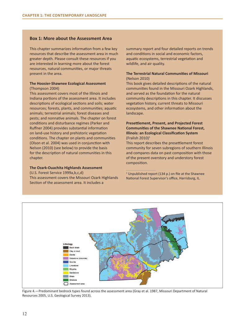
Box 1: more about the Assessment Area

This chapter summarizes information from a few key resources that describe the assessment area in much greater depth. Please consult these resources if you are interested in learning more about the forest resources, natural communities, or major threats present in the area.

The Hoosier-Shawnee Ecological Assessment (Thompson 2004)This assessment covers most of the Illinois and Indiana portions of the assessment area. It includes descriptions of ecological sections and soils; water resources; forests, plants, and communities; aquatic animals; terrestrial animals; forest diseases and pests; and nonnative animals. The chapter on forest conditions and disturbance regimes (Parker and Ruffner 2004) provides substantial information on land-use history and prehistoric vegetation conditions. The chapter on plants and communities (Olson et al. 2004) was used in conjunction with Nelson (2010) (see below) to provide the basis for the description of natural communities in this chapter.

The Ozark-Ouachita Highlands Assessment (U.S. Forest Service 1999a,b,c,d)This assessment covers the Missouri Ozark Highlands Section of the assessment area. It includes a

summary report and four detailed reports on trends and conditions in social and economic factors, aquatic ecosystems, terrestrial vegetation and wildlife, and air quality.

The Terrestrial Natural Communities of Missouri(Nelson 2010)This book gives detailed descriptions of the natural communities found in the Missouri Ozark Highlands, and served as the foundation for the natural community descriptions in this chapter. It discusses vegetation history, current threats to Missouri ecosystems, and other information about the landscape.

Presettlement, Present, and Projected Forest Communities of the Shawnee National Forest, Illinois: an Ecological Classification System(Fralish 2010)1

This report describes the presettlement forest community for seven subregions of southern Illinois and compares data on past composition with those of the present overstory and understory forest composition.

1 Unpublished report (134 p.) on file at the Shawnee National Forest Supervisor’s office, Harrisburg, IL.

Figure 4.—Predominant bedrock types found across the assessment area (Gray et al. 1987, Missouri Department of Natural Resources 2005, U.S. Geological Survey 2013).

13


Box 2: Karst Topography

The assessment area is known for its karst topography. Karst landscapes occur where the topography and its distinctive features are formed by the dissolution of soluble rock, especially dolomite and limestone (Fig. 5). The resulting surface features include subterranean drainages, caves, sinkholes, springs, disappearing streams, dry valleys and hollows, natural bridges, arches, and other related features (Rea 1992). Sinkholes are karst features that develop as a result of a collapse of surface material into nearby cavities (usually caves). Coldwater springs are characterized by a continuous flow of mineralized groundwater when surface precipitation percolates through fractures in bedrock including sinkholes, losing streams, caves, and bedrock aquifers.

The Missouri Ozark Highlands contain the assessment area’s largest karst regions. Five distinct karst regions occur in the Ozarks, each physically distinct and harboring its own endemic subterranean aquatic and terrestrial species (Culver et al. 2003). Karst features are also found in southern Illinois and Indiana, primarily in the Mitchell Plateau, Crawford Escarpment, and Crawford Uplands Subsections, where the Hoosier National Forest is located (McCreedy et al. 2004).

Caves provide habitat to rare and endangered species in the assessment area. More than 600 caves are recorded on the Mark Twain National Forest (about 10 percent of 6,400 known Missouri caves). More than 190 caves have been identified on the Hoosier National Forest, with 50 designated as nationally significant by the Eastern Regional Forester. The Shawnee National Forest has identified 15 caves (McCreedy et al. 2004). Forty-six aquatic and 31 terrestrial species that are dependent on caves are recorded in Missouri’s caves and springs (Culver et al. 2003). Most species of state or global viability concern in the Indiana and Illinois portions of the assessment area live in cave and karst habitats (McCreedy et al. 2004). The Indiana bat is probably the most well-known of these threatened or endangered cave-dwelling organisms. Little is known about the ecology and life history of many of the cave-dwelling species in the assessment area, making it difficult to determine whether they may be affected by a changing climate. Figure 5.—Karst topography. Diagram by Mark Raithel,

Missouri Department of Conservation.

by low-lying areas of unconsolidated Tertiary and Quaternary alluvium (gravel, sand, silt, and clay) overlying bedrock (McNab and Avers 1994).

The Central Till Plains—Oak Hickory Section is largely covered by glacial till from the Illinoian glacier, which ended 130,000 years ago (McNab and Avers 1994). The area was not covered by the most recent Wisconsin glaciation, but loess and slackwater lake deposits from this glacier can be found in the area (McNab and Avers 1994). Parts of the area

also contain exposed Mississippian limestone and sandstone as well Pennsylvanian sandstone and shale.

Sandstone bluffs, steep-sided ridges and hills, gentler hills and broader valleys, karst terrain, gently rolling lowland plains, and bottomlands characterize the Shawnee Hills Section (McNab and Avers 1994). Elevation ranges from 325 to 1,0�0 feet. About 50 percent of the underlying bedrock is Pennsylvanian sandstone, with minor amounts of

14


siltstone, shale, and coal. Mississippian limestone forms the bedrock along the southern border of the Section in Illinois.

The Coastal Plain is composed primarily of marine sediments from the Cenozoic era, with smaller amounts of Mesozoic marine sediments (McNab and Avers 1994). The area is flat, rarely exceeding relief of greater than 100 feet.

IndianaMuch of the assessment area in southern Indiana incorporates the Shawnee Hills and the Transition Hills Sections with a small amount of the Bluegrass Section. This area is derived primarily from Pennsylvanian and Mississippian bedrock units. Bedrock is exposed in the south-central part of the state. The limestone plateau developed on Mississippian limestone extends south to the Ohio River. Layers of rock (limestone, sandstone, and shale) more than 400 feet thick were built up by ancient seas that once covered this area.

Two well-developed areas of karst topography occur in the southern part of Indiana, the Mitchell Plateau and the Muscatatuck Plateau (Hasenmueller et al. 2011). Erosion has worn away the upper layers in the Mitchell Plateau, making karst features such as sinkholes and disappearing streams common elements across the landscape. West of the Mitchell Plateau is the Crawford Upland. The Crawford Upland retains the upper strata of shale and sandstone over limestone. The area’s drainage is still subterranean, and exhibits dry-beds, rises, sinking streams, swallow holes, and other karst features.

The part of Indiana within the assessment area was largely unglaciated by the most recent (Wisconsin) glaciation. A substantial portion of the assessment area was covered by older ice sheets, but the boundaries of these glaciations are unclear due to subsequent weathering (Gray 2009).

soilsmissouri Soils of the Ozark Highlands are moderately well drained to well drained and have slow to moderate permeability. Soils are generally old, shallow, stony, highly weathered, and acidic, except on some broad ridges and bottomlands (McNab and Avers 1994). Some soils, particularly those on steeper ground, have very gravelly or stony surfaces and more than 35 percent rock fragments by volume throughout the profile.

Soils that have formed from local sandstone and dolomite bedrock are very deep, well-drained mineral soils. Alluvial soils, consisting mainly of stratified silt, sand, and gravel, are usually found on valley floor floodplains. These soils are usually well drained, although valley bottoms and areas with perched water tables can have areas of poor drainage.

illinoisSoils vary across southern Illinois, depending on section and topography. The Ozark Highlands soils are similar to those found in Missouri (old, shallow, and highly weathered). In the Central Till Plains Section, soils are developed from thin loess and till. Upland soils are light colored and strongly developed, with poor internal drainage because of fragipan and claypan layers (McNab and Avers 1994). Soils in the Shawnee Hills vary from poorly drained on a few soils to well drained on the majority of soils. Soils in the Coastal Plain are generally deep and medium textured, and have adequate moisture supply throughout the year (McNab and Avers 1994).

Indiana Weathered siltstone, fine-grained sandstone, shale, and limestone bedrock, as well as alluvium along streams, provide the parent materials for soils in the

15


assessment area in southern Indiana. In the Shawnee Hills Section of southern Indiana, loess covers some of the material weathered from bedrock. Soils are generally well drained to moderately well drained, and many have silt loam or loam textures. On steep slopes, soils are typically thin with gravelly or channery (containing thin, flat fragments of rock) textures. Subsoil permeability for upland soils is generally slow to very slow, and floodplain soils typically have slow to moderately slow permeability. The soils occur on gently sloping to very steep topography, often on narrow ridges bordered by steep slopes and bedrock outcrops. Permeability on ridge tops is generally slow to very slow.

The Transition Hills Section occurs as two main bodies in southern Indiana. The eastern portion is separated by deep stream valleys and is mostly wooded hillside land with little suitable cropland. The western portion of the Section has stony hillside lands with rock outcrops, but more area of productive land (Ponder 2004).

Bluegrass Section soils are fine textured and most are deep (McNab and Avers 1994). The area features wide alluvial and lacustrine plains bordering major streams. Since glacial drift partially filled the northern portion of the section, lowlands are not well defined. Conversely, lowlands become more defined in the southern portion. Topography in this Section is relatively homogenous. Several prominent moraines can be found, especially in the west-central part of the state.

HydrologymissouriThe Missouri Ozark Highlands are deeply dissected by thousands of miles of spring-fed streams and rivers. For example, more than 350 miles of floatable streams are found within the boundary of the Mark Twain National Forest. Streams within the Missouri Ozark Highlands tend to be in better

condition than those in the United States as a whole, due to relatively high forest cover (U.S. Forest Service 1999a).

The characteristics of spring flows and the quality of their water chemistry in the Ozark Highlands are primarily a function of the ability of the land surface to capture rainwater. Prior to European settlement, deep soils covered by deep-rooted, long-lived perennial grasses and forbs beneath open oak and pine woodlands captured precipitation. This water-absorbing soil process moved water into the water table, which likely buffered coldwater spring flows and fed streams for longer time periods. Changes in vegetation cover and soil erosion from past land management practices have led to a reduction in this important process, leading to effects on local hydrology.

illinoisSouthern Illinois is flanked by the Wabash, Ohio, and Mississippi Rivers and is populated with many rivers and smaller perennial and ephemeral streams. Riparian areas in the assessment area include forested, agricultural, and other developed lands (Whiles and Garvey 2004). A survey on the Shawnee National Forest showed that streams that drained primarily forested uplands were of higher water quality and biological integrity than those that drained primarily agricultural areas (Hite et al. 1990). Efforts have been made to increase water quality in agricultural zones in the area through the use of conservation easements, but benefits thus far have been marginal due to insufficient recovery time and lack of placement in the most effective areas (Davie and Lant 1994, Lant 1991). A 1999 assessment of water quality of watersheds in southern Illinois using the U.S. Environmental Protection Agency (EPA)’s Index of Watershed Indicators found that most were considered of poor quality due to high levels of nutrients and contaminants (Whiles and Garvey 2004).

1�


Although there are no natural lakes in the Illinois portion of the assessment area, thousands of lakes and reservoirs have been created for water supply, recreational, and flood control purposes (Whiles and Garvey 2004). Despite the many benefits, these reservoirs can upset natural stream flow and lead to water loss from evaporation (Whiles and Garvey 2004).

The area has had a dramatic decline in wetlands, which once were common. Illinois has lost more than 70 percent of its natural wetlands, which have been primarily drained for agricultural use (Whiles and Garvey 2004). Wetland area has declined in other states in the assessment area for the same reason. Other estimates suggest Illinois, Indiana, and Missouri lost more than 80 percent of their original wetlands between 1780 and 1980 (Mitsch and Gosselink 2007). This loss of wetlands can change local hydrology by increasing susceptibility to floods and loss of base flows.

IndianaSimilar to patterns in Illinois, past land management practices and development have affected watersheds across southern Indiana. The Ohio River makes up Indiana’s southern boundary, and the Wabash River marks the western boundary of the state within the assessment area. Many larger watercourses traverse southern Indiana. Tributaries of the White River, the Little Blue River, and the Lost River flow through the Hoosier National Forest. No natural lakes occur in the Indiana portion of the assessment area, but two large reservoirs, Monroe and Patoka, provide water for surrounding homes and communities. Unnatural stream channels also occur throughout the Indiana portion of the assessment area. These are often composed of drainage ditches and channels to connect other water bodies. Many of these constructed features follow historical channels, but the channelized ditches have replaced the natural features (Whiles and Garvey 2004).

Prior to settlement, extensive wetlands and rich riparian areas were found in abundance. European settlers cleared and drained floodplains for farmland. Road placement and channelization of streams have changed water flow patterns over time. Riparian habitat structure and function have been altered as streams lost their floodplains and riparian vegetation was removed. Contaminants, discharges, nutrient pollution, and wastewater have been identified as the main factors affecting water quality in the assessment area within Indiana. Most of the watersheds are considered of poor water quality according to the EPA’s Index of Watershed Indicators (Whiles and Garvey 2004).

Land Use and Vegetation CoverLand Cover and CompositionThe assessment area covers more than 42 million acres of land, of which 40 percent is classified as forest land by the U.S. Forest Service’s Forest Inventory and Analysis (FIA) Program (U.S. Forest Service 2011a) (Fig. �, Table 2). About two-thirds of the assessment area that is classified as forest land is in Missouri, and the remaining third is divided roughly equally between Indiana and Illinois (Table 2). About 98 percent of the forest land in the assessment area is classified as timberland (U.S. Forest Service 2011a). Timberland is forest land that is currently producing or capable of producing more than 20 cubic feet of wood per acre per year. This pattern is similar across the three states.

Satellite imagery from the National Land Cover Dataset (NLCD) (Fry et al. 2011) estimates forest cover at a slightly higher percentage (44.9 percent). According to the NLCD, the remaining land cover is classified as agricultural land (43.1 percent), developed (7.5 percent), water (1.� percent), herbaceous (1.5 percent), and wetlands (1 percent). Shrublands and barren land (containing no vegetation) make up less than 1 percent of the assessment area. The relative breakdown of these

17


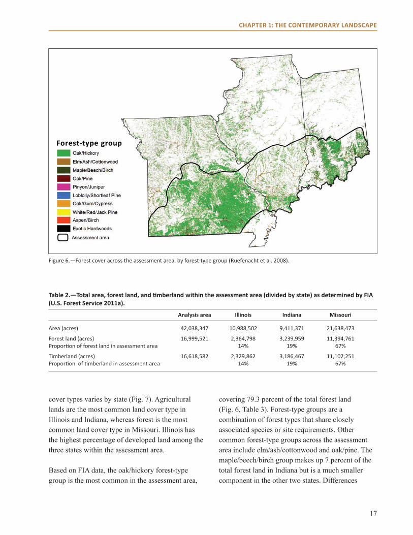
Figure 6.—Forest cover across the assessment area, by forest-type group (Ruefenacht et al. 2008).

Analysis area Illinois Indiana Missouri

Area (acres) 42,038,347 10,988,502 9,411,371 21,638,473

Forest land (acres) 16,999,521 2,364,798 3,239,959 11,394,761Proportion of forest land in assessment area 14% 19% 67%

Timberland (acres) 16,618,582 2,329,862 3,186,467 11,102,251Proportion of timberland in assessment area 14% 19% 67%

Table 2.—Total area, forest land, and timberland within the assessment area (divided by state) as determined by FIA (U.S. Forest Service 2011a).

cover types varies by state (Fig. 7). Agricultural lands are the most common land cover type in Illinois and Indiana, whereas forest is the most common land cover type in Missouri. Illinois has the highest percentage of developed land among the three states within the assessment area.

Based on FIA data, the oak/hickory forest-type group is the most common in the assessment area,

covering 79.3 percent of the total forest land (Fig. �, Table 3). Forest-type groups are a combination of forest types that share closely associated species or site requirements. Other common forest-type groups across the assessment area include elm/ash/cottonwood and oak/pine. The maple/beech/birch group makes up 7 percent of the total forest land in Indiana but is a much smaller component in the other two states. Differences

18


Assessment area Illinois Indiana Missouri Proportion Proportion Proportion ProportionForest-type group Area of total Area of total Area of total Area of total

Oak/hickory 13,484,660 79.3 1,500,096 63.4 2,444,838 75.5 9,539,726 83.7Elm/ash/cottonwood 1,376,266 8.1 711,126 30.1 306,676 9.5 358,465 3.1Oak/pine 1,010,816 5.9 49,233 2.1 109,267 3.4 852,316 7.5Other eastern softwoods 351,161 2.1 2,273 0.1 16658 0.5 332229 2.9Maple/beech/birch 307,763 1.8 31,981 1.4 229,898 7.1 45,883 0.4Loblolly/shortleaf pine 276,840 1.6 26,061 1.1 35,400 1.1 215,378 1.9Oak/gum/cypress 123,382 0.7 34,819 1.5 62,123 1.9 26,439 0.2Other hardwoods 34,203 0.2 7,436 0.3 8,419 0.3 18,348 0.2White/red/jack pine 22,527 0.1 1,773 0.1 20,754 0.6 — —Aspen/birch 4,207 0.0 — — 4,207 0.1 — —Exotic hardwoods 4,171 0.0 — — 800 0.0 3,372 0.0Exotic softwoods 3,525 0.0 — — 919 0.0 2,605 0.0

Total forest land (acres) 16,999,521 100 2,364,798 100 3,239,959 100 11,394,761 100

Table 3.—Forest land (in acres and as a percentage of total forest land) by FIA forest-type group (U.S. Forest Service 2011a).

Figure 7.—Percent cover within the assessment area, divided by state boundaries (Fry et al. 2011).

0

0.1

0.2

0.3

0.4

0.5

0.6

0.7

Illinois Indiana Missouri

19


among forest types can influence the amount of carbon stored aboveground and belowground (see Box 3). These forest-type groups are broader than the natural communities described later in this

chapter, and may include areas dominated by trees that would be classified as woodlands, savannas, or swamps based on their structure (see Box 4).

Box 3: forest carbon

Each year, the United States releases about 1.5 billion metric tons of carbon into the atmosphere, largely due to combustion of fossil fuels (U.S. EPA 2013). One ton of carbon is equivalent to 3.7 metric tons of carbon dioxide. Forests in the Central Hardwoods Region play an important role in storing carbon and thus reducing the amount of greenhouse gases in the atmosphere. Across the assessment area, an average of 53 metric tons per acre is stored aboveground and belowground (U.S. Forest Service 2011a). Carbon storage density (the mass of carbon per unit area) in this region is lower than in some parts of the United States, such as the Pacific Northwest, the northern Great Lakes, and the Appalachians (Heath et al. 2011). However, carbon density is still greater than many forests in the Rocky Mountain region, and much greater than that of most nonforested lands.

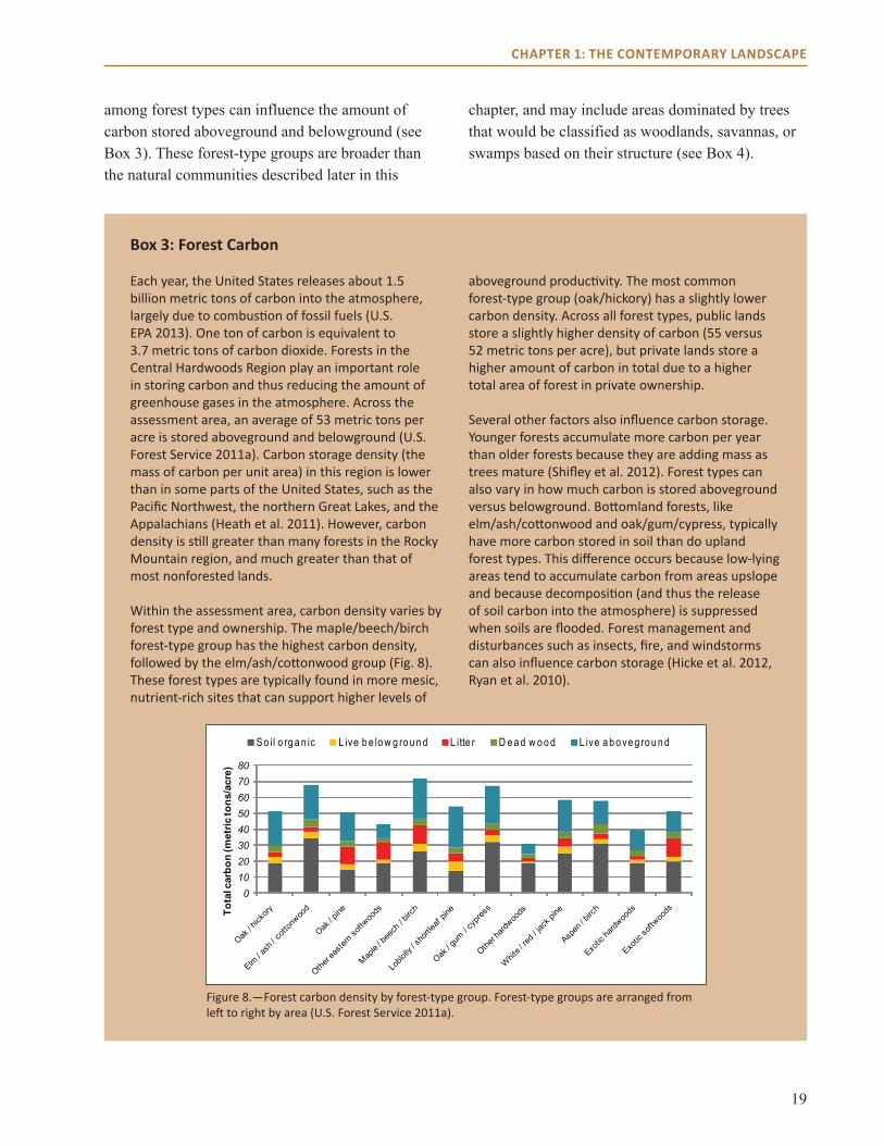
Within the assessment area, carbon density varies by forest type and ownership. The maple/beech/birch forest-type group has the highest carbon density, followed by the elm/ash/cottonwood group (Fig. 8). These forest types are typically found in more mesic, nutrient-rich sites that can support higher levels of

aboveground productivity. The most common forest-type group (oak/hickory) has a slightly lower carbon density. Across all forest types, public lands store a slightly higher density of carbon (55 versus 52 metric tons per acre), but private lands store a higher amount of carbon in total due to a higher total area of forest in private ownership.

Several other factors also influence carbon storage. Younger forests accumulate more carbon per year than older forests because they are adding mass as trees mature (Shifley et al. 2012). Forest types can also vary in how much carbon is stored aboveground versus belowground. Bottomland forests, like elm/ash/cottonwood and oak/gum/cypress, typically have more carbon stored in soil than do upland forest types. This difference occurs because low-lying areas tend to accumulate carbon from areas upslope and because decomposition (and thus the release of soil carbon into the atmosphere) is suppressed when soils are flooded. Forest management and disturbances such as insects, fire, and windstorms can also influence carbon storage (Hicke et al. 2012, Ryan et al. 2010).

Figure 8.—Forest carbon density by forest-type group. Forest-type groups are arranged from left to right by area (U.S. Forest Service 2011a).

01020304050607080

Tota

lcar

bon

(met

ricto

ns/a

cre)

S o il o rg a n ic L ive b e lo w g ro u n d L itte r D e a d w o o d L ive a b o ve g ro u n d

20


Box 4: Forest Types and Natural Communities

In this assessment, we describe two different ways of classifying forests: FIA forest-type groups and natural communities. These classification systems are used for different reasons and convey different types of information. Although there are some general relationships between the systems, they are organized differently enough that one cannot be substituted for the other. Both types of information are relevant to this assessment, so we use both classification systems.

Forest Inventory and Analysis classifications describe existing vegetation, and only for vegetated areas dominated by trees (i.e., forests). Forest-type groups are defined as a combination of forest types that share closely associated species or site requirements. Forest types are a classification of forest land based upon and named for the dominant tree species. There are several advantages to the FIA classification system. The FIA system measures tree species composition on a set of systematic plots across the country and uses that information to provide area estimates for each forest type, making it a good way of estimating what is currently on the landscape and the relative abundance of different forest types. However, it does not make any inferences about what vegetation was historically on the landscape and does not distinguish between naturally occurring and human-influenced conditions. Something that

is classified as “forest land” by FIA may have been historically a prairie, glade, woodland, or savanna. Likewise, areas dominated by tree species that are not native to the area would still be assigned to a forest type and forest-type group based on dominant species. Finally, the coarse scale of FIA measurements may miss small, but ecologically important, types.

By contrast, natural community classifications describe an assemblage of native plants and animals and their physical environment that reflects the composition, structure, and function that would have occurred under the historical range of natural variability (Nelson 2010). Forests are just one type of natural community. Natural communities also include other terrestrial and aquatic assemblages not dominated by trees. The advantage of the natural community system is that it is based on ecological relationships between native organisms and their physical environment. Therefore, natural communities describe what would have been present at a particular location if the landscape had been left unaltered by European settlement. The disadvantage of using natural community classifications is that they have not yet been quantified spatially and described in a consistent manner across the country.

Land Ownership and UseAbout 20 percent of forest land within the assessment area is publicly owned and managed (U.S. Forest Service 2011a) (Table 4). National forests make up the largest percentage of public forest land within the area. Other major public entities include state agencies, federal agencies such as the U.S. Department of Defense and the Department of the Interior, U.S. Fish and Wildlife Service; and county and municipal governments.

The majority of forests in the assessment area, however, are privately owned. Most of the privately owned forest lands are held by hundreds of thousands of individual nonindustrial family forest owners (Butler 2008). According to the National Woodland Owners Survey, primary reasons for forest ownership are for enjoyment of scenery, protection of nature, long-term investment, or recreational purposes (Butler 2008). Making forest products was a much less common reason for ownership in the assessment area. In addition, most privately owned forests in the assessment area lack a management plan.

21


Assessment area Illinois Indiana Missouri Proportion Proportion Proportion ProportionOwnership Area of total Area of total Area of total Area of total

Private 13,551,052 79.7 1,886,251 79.8 2,617,377 80.8 9,047,425 79.4National forest 1,970,093 11.6 294,360 12.4 194,641 6.0 1,481,094 13.0State 895,059 5.3 102,077 4.3 272,339 8.4 520,643 4.6County and municipal 91,066 0.5 42,089 1.8 7,022 0.2 41,956 0.4Federal 492,246 2.9 40,022 1.7 148,580 4.6 303,644 2.7 National Park Service 65,352 0.4 — 0.0 — 0.0 65,352 0.6 Fish and Wildlife Service 87,491 0.5 23,888 1.0 44,419 1.4 19,184 0.2 Department of Defense 269,718 1.6 7,227 0.3 85,916 2.7 176,575 1.5 Other federal 69,685 0.4 8,907 0.4 18,245 0.6 42,533 0.4

Total forest land 16,999,516 100 2,364,799 100 3,239,959 100 11,394,762 100

Table 4.—Forest land (in acres and as a percentage of total forest land) owned by different entities within the assessment area and by state within the assessment area (U.S. Forest Service 2011a).

sociAL AnD economic conDitionsAbout 7.1 million people reside within the assessment area (Headwaters Economics 2012). Fifty-three percent of the population is located in Missouri, 27 percent is in Indiana, and the remaining 20 percent is in Illinois. The Missouri portion of the assessment area has experienced the largest population growth over the past 40 years (50 percent). Indiana has experienced modest growth during that time (27 percent), and the population in Illinois has had only a minor increase of 4 percent. These trends for larger population and growth in Missouri are primarily due to the presence of the St. Louis metropolitan area within the assessment area boundary. By contrast, the largest metropolitan areas in Illinois and Indiana are located north of the assessment area boundaries in those states. In addition, several areas in Missouri have grown because they serve as retirement destinations (U.S. Forest Service 1999b). Despite this growth, population density in the Missouri portion is relatively low, at 110 people per square mile. Population density is highest in the Indiana portion (129 people per square mile), and lowest in the Illinois portion (83 people per square mile).

The economic well-being of the people of the assessment area varies across the three states. Unemployment has been highest in the Illinois portion of the assessment area over the past 20 years, and lower in Missouri and Indiana (Headwaters Economics 2012). In Missouri, growth in employment and personal income over the last 40 years has been greater in the Ozark Highlands section than in the state as a whole, and similar trends have occurred in southern Indiana (Headwaters Economics 2012). The entire assessment area has had an increase in unemployment since 2007, similar to trends across the United States (Headwaters Economics 2012).

Forest Products Industry The forest products industry represents a significant proportion of the total economy of each state, as measured by percentage of gross domestic product (GDP) (Table 5). However, it is a much larger percentage of GDP in Indiana and Missouri than in Illinois. The timber industry represents 1.1 percent of total employment for Indiana, 0.7 percent for Missouri, and 0.5 percent for Illinois (Headwaters Economics 2012). Major timber-related businesses in the three states include sawmills, paper mills, and paper products manufacturing. Wood office furniture

22


GDP Illinois Indiana Missouri

All industries 651.5 275.7 244Forest products industry 2.5 7.5 5.7Percentage of GDP 0.4 2.7 2.3

Table 5.—Gross domestic product (GDP) (billions of dollars for all industries and for the forest products industry. Note: Data are for the entire state. Sources: Bureau of Economic Analysis (2012), ILDNR (2010), INDNR (2010), MDC (2010).

manufacturing is a major industry in Indiana, ranking first in the nation (Bratkovich et al. 2007). Between 1998 and 2009, timber-related employment decreased about 33 percent for the three-state area (Headwaters Economics 2012), which is similar to trends for the United States as a whole.

Hardwood species (primarily oak, hickory, and walnut) make up the majority of timber harvested in the area (Treiman and Piva 2005, U.S. Forest Service 2011a). In addition, shortleaf pine constitutes a substantial portion of timber harvested in Missouri. In the eastern part of the assessment area, maple species, black cherry, and yellow-poplar are also important timber species.

AgricultureMost of the assessment area in Illinois and Indiana, and a large portion in Missouri, is used for agriculture (Fry et al. 2011), making agriculture-related industry a large part of the economy in the assessment area. Crop and animal production accounts for about 1 percent of GDP in all three states (Bureau of Economic Analysis 2012). Food manufacturing accounts for an additional 1.5 to 2 percent of GDP in the three states (Bureau of Economic Analysis 2012). About 143,000 people are employed in the farming industry within the assessment area (Headwaters Economics 2012). Farming accounts for about 4 percent of total employment in the Illinois portion of the assessment area, and 3 percent in Indiana and Missouri.

The primary crops in all three states are corn and soybeans. Other important crops in the assessment area include winter wheat, sorghum, oats, and hay. Illinois ranks second in the country for corn and soybean production and fourth in hog production (National Agricultural Statistics Service [NASS] 2012). Indiana is known for its production of peppermint and spearmint, which are primarily used in chewing gum (NASS 2012). Missouri is also a major producer of rice, cotton, and potatoes (NASS 2012).

RecreationThe forested lands within the assessment area are a primary destination for recreation, which is also economically important to the region. Travel and tourism-related employment in the three-state area makes up 13.9 percent of total employment (Headwaters Economics 2012). Total spending on local and non-local visits to the three national forests within the assessment area is approximately $39 million per year (National Visitor Use Monitoring Program [NVUM] 2011). About half of the spending occurs on the Mark Twain National Forest ($19 million) and the other half is divided roughly equally between the Shawnee and Hoosier National Forests. The majority (55 percent) of visits are for local day use by people living 50 or fewer miles from the national forests. Primary activities people undertake while visiting national forests are viewing natural features, hiking, hunting, fishing, camping, and horseback riding (NVUM 2011). Total expenditures on fishing, hunting, and wildlife viewing for the three-state area on all public and private lands are about $�.5 billion (Table �).

Fishing Hunting Wildlife viewing Total

Illinois 722 334 1,030 2,086Indiana 627 223 934 1,784Missouri 955 892 739 2,586

Total 2,304 1,449 2,703 6,456

Table 6.—Total expenditures (millions of dollars) on wildlife-related recreation activities by state. Note: Estimates are for entire state (U.S. Fish and Wildlife Service and U.S. Census Bureau 2006).

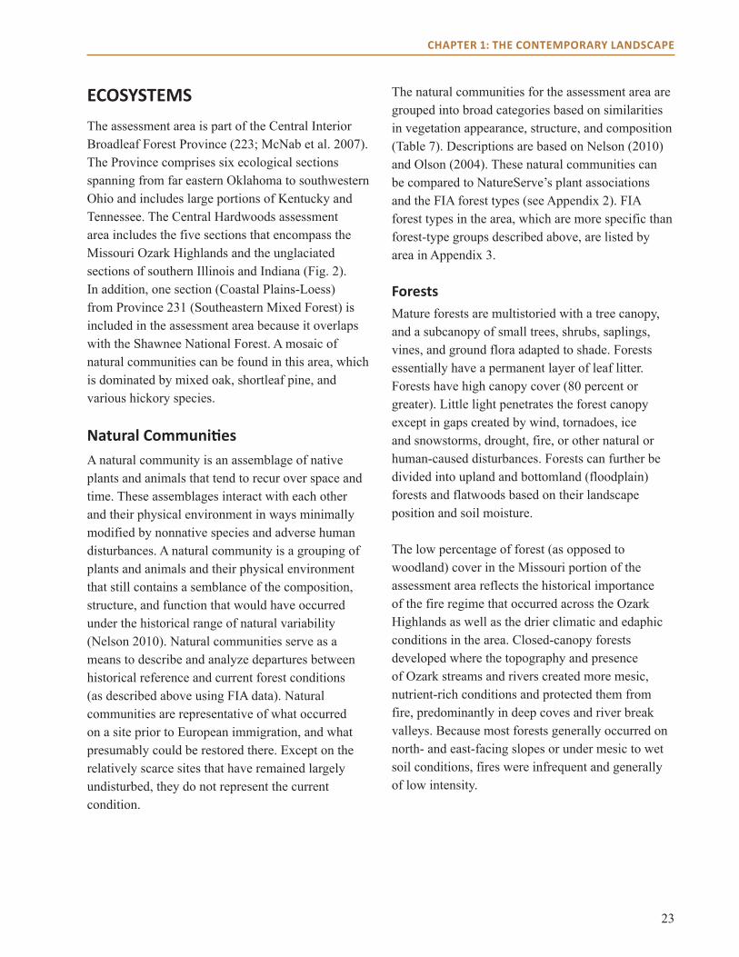
23


ecosystems The assessment area is part of the Central Interior Broadleaf Forest Province (223; McNab et al. 2007). The Province comprises six ecological sections spanning from far eastern Oklahoma to southwestern Ohio and includes large portions of Kentucky and Tennessee. The Central Hardwoods assessment area includes the five sections that encompass the Missouri Ozark Highlands and the unglaciated sections of southern Illinois and Indiana (Fig. 2). In addition, one section (Coastal Plains-Loess) from Province 231 (Southeastern Mixed Forest) is included in the assessment area because it overlaps with the Shawnee National Forest. A mosaic of natural communities can be found in this area, which is dominated by mixed oak, shortleaf pine, and various hickory species.

Natural CommunitiesA natural community is an assemblage of native plants and animals that tend to recur over space and time. These assemblages interact with each other and their physical environment in ways minimally modified by nonnative species and adverse human disturbances. A natural community is a grouping of plants and animals and their physical environment that still contains a semblance of the composition, structure, and function that would have occurred under the historical range of natural variability (Nelson 2010). Natural communities serve as a means to describe and analyze departures between historical reference and current forest conditions (as described above using FIA data). Natural communities are representative of what occurred on a site prior to European immigration, and what presumably could be restored there. Except on the relatively scarce sites that have remained largely undisturbed, they do not represent the current condition.

The natural communities for the assessment area are grouped into broad categories based on similarities in vegetation appearance, structure, and composition (Table 7). Descriptions are based on Nelson (2010) and Olson (2004). These natural communities can be compared to NatureServe’s plant associations and the FIA forest types (see Appendix 2). FIA forest types in the area, which are more specific than forest-type groups described above, are listed by area in Appendix 3.

forestsMature forests are multistoried with a tree canopy, and a subcanopy of small trees, shrubs, saplings, vines, and ground flora adapted to shade. Forests essentially have a permanent layer of leaf litter. Forests have high canopy cover (80 percent or greater). Little light penetrates the forest canopy except in gaps created by wind, tornadoes, ice and snowstorms, drought, fire, or other natural or human-caused disturbances. Forests can further be divided into upland and bottomland (floodplain) forests and flatwoods based on their landscape position and soil moisture.

The low percentage of forest (as opposed to woodland) cover in the Missouri portion of the assessment area reflects the historical importance of the fire regime that occurred across the Ozark Highlands as well as the drier climatic and edaphic conditions in the area. Closed-canopy forests developed where the topography and presence of Ozark streams and rivers created more mesic, nutrient-rich conditions and protected them from fire, predominantly in deep coves and river break valleys. Because most forests generally occurred on north- and east-facing slopes or under mesic to wet soil conditions, fires were infrequent and generally of low intensity.

24


Community Type Community Sub-type community Dominant Tree Species

Forest Upland forest Dry-Mesic* black, white, northern red, and scarlet oak; shagbark, pignut, bitternut, and mockernut hickory; sugar and red maple, yellow-poplar, shortleaf pine (MO)

Mesic* IL and IN: sugar maple, American beech, northern red and white oak, yellow-poplar, bitternut hickory, white ash, black cherry

MO: white and northern red oak, sugar maple, American basswood

Bottomland (floodplain) forest

Mesic* white and bur oak, sycamore, eastern cottonwood, sugar maple, American and slippery elm, American beech, hackberry, black walnut

Wet-Mesic American and slippery elm, sweetgum, honeylocust, black walnut

Wet* river birch; green ash; silver and red maple; shellbark and water hickory; boxelder; eastern cottonwood; black willow; pin, willow, and overcup oak

Flatwoods* pin, post, and blackjack oak; shortleaf pine, mockernut and shagbark hickory; blackgum

Woodland Open woodland* white, post, black, blackjack, scarlet, and chinquapin oak; shortleaf pine; mockernut, shagbark, and black hickory; eastern redcedar

Closed woodland* shortleaf pine; white, black, and scarlet oak; mockernut and shagbark hickory

Savanna Savanna* post and chinquapin oak

Barrens* black, blackjack, post, scarlet, white, bur, and chestnut oak; blackgum; shagbark and black hickory; eastern redcedar

Prairie not applicable

Glade* post oak; eastern redcedar

Wetlands Fen not applicable

Seep not applicable

Spring not applicable

Swamp baldcypress, water tupelo; water hickory, pumpkin ash, water locust, red maple

Table 7.—Natural community types and dominant tree species found within each type. Modified from Olson et al. (2004). *Assessed for climate change vulnerability in Chapter 6.

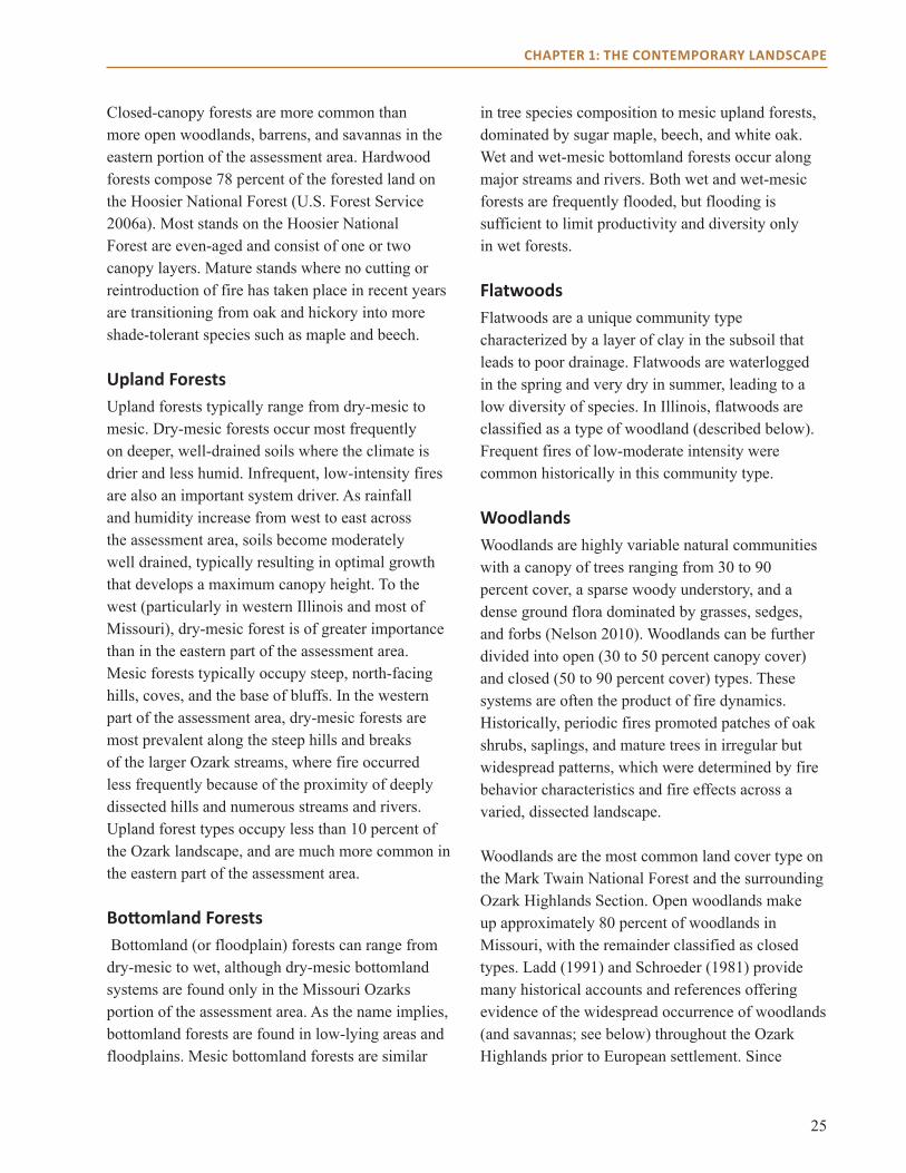
25


Closed-canopy forests are more common than more open woodlands, barrens, and savannas in the eastern portion of the assessment area. Hardwood forests compose 78 percent of the forested land on the Hoosier National Forest (U.S. Forest Service 200�a). Most stands on the Hoosier National Forest are even-aged and consist of one or two canopy layers. Mature stands where no cutting or reintroduction of fire has taken place in recent years are transitioning from oak and hickory into more shade-tolerant species such as maple and beech.

Upland ForestsUpland forests typically range from dry-mesic to mesic. Dry-mesic forests occur most frequently on deeper, well-drained soils where the climate is drier and less humid. Infrequent, low-intensity fires are also an important system driver. As rainfall and humidity increase from west to east across the assessment area, soils become moderately well drained, typically resulting in optimal growth that develops a maximum canopy height. To the west (particularly in western Illinois and most of Missouri), dry-mesic forest is of greater importance than in the eastern part of the assessment area. Mesic forests typically occupy steep, north-facing hills, coves, and the base of bluffs. In the western part of the assessment area, dry-mesic forests are most prevalent along the steep hills and breaks of the larger Ozark streams, where fire occurred less frequently because of the proximity of deeply dissected hills and numerous streams and rivers. Upland forest types occupy less than 10 percent of the Ozark landscape, and are much more common in the eastern part of the assessment area.

Bottomland Forests Bottomland (or floodplain) forests can range from dry-mesic to wet, although dry-mesic bottomland systems are found only in the Missouri Ozarks portion of the assessment area. As the name implies, bottomland forests are found in low-lying areas and floodplains. Mesic bottomland forests are similar

in tree species composition to mesic upland forests, dominated by sugar maple, beech, and white oak. Wet and wet-mesic bottomland forests occur along major streams and rivers. Both wet and wet-mesic forests are frequently flooded, but flooding is sufficient to limit productivity and diversity only in wet forests.

FlatwoodsFlatwoods are a unique community type characterized by a layer of clay in the subsoil that leads to poor drainage. Flatwoods are waterlogged in the spring and very dry in summer, leading to a low diversity of species. In Illinois, flatwoods are classified as a type of woodland (described below). Frequent fires of low-moderate intensity were common historically in this community type.

WoodlandsWoodlands are highly variable natural communities with a canopy of trees ranging from 30 to 90 percent cover, a sparse woody understory, and a dense ground flora dominated by grasses, sedges, and forbs (Nelson 2010). Woodlands can be further divided into open (30 to 50 percent canopy cover) and closed (50 to 90 percent cover) types. These systems are often the product of fire dynamics. Historically, periodic fires promoted patches of oak shrubs, saplings, and mature trees in irregular but widespread patterns, which were determined by fire behavior characteristics and fire effects across a varied, dissected landscape.

Woodlands are the most common land cover type on the Mark Twain National Forest and the surrounding Ozark Highlands Section. Open woodlands make up approximately 80 percent of woodlands in Missouri, with the remainder classified as closed types. Ladd (1991) and Schroeder (1981) provide many historical accounts and references offering evidence of the widespread occurrence of woodlands (and savannas; see below) throughout the Ozark Highlands prior to European settlement. Since

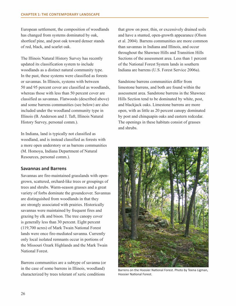
2�


European settlement, the composition of woodlands has changed from systems dominated by oak, shortleaf pine, and post oak toward denser stands of red, black, and scarlet oak.

The Illinois Natural History Survey has recently updated its classification system to include woodlands as a distinct natural community type. In the past, these systems were classified as forests or savannas. In Illinois, systems with between 50 and 95 percent cover are classified as woodlands, whereas those with less than 50 percent cover are classified as savannas. Flatwoods (described above) and some barrens communities (see below) are also included under the woodland community type in Illinois (B. Anderson and J. Taft, Illinois Natural History Survey, personal comm.).

In Indiana, land is typically not classified as woodland, and is instead classified as forests with a more open understory or as barrens communities (M. Homoya, Indiana Department of Natural Resources, personal comm.).

Savannas and BarrensSavannas are fire-maintained grasslands with open-grown, scattered, orchard-like trees or groupings of trees and shrubs. Warm-season grasses and a great variety of forbs dominate the groundcover. Savannas are distinguished from woodlands in that they are strongly associated with prairies. Historically savannas were maintained by frequent fires and grazing by elk and bison. The tree canopy cover is generally less than 30 percent. Eight percent (119,700 acres) of Mark Twain National Forest lands were once fire-mediated savanna. Currently only local isolated remnants occur in portions of the Missouri Ozark Highlands and the Mark Twain National Forest.

Barrens communities are a subtype of savanna (or in the case of some barrens in Illinois, woodland) characterized by trees tolerant of xeric conditions

that grow on poor, thin, or excessively drained soils and have a stunted, open-growth appearance (Olson et al. 2004). Barrens communities are more common than savannas in Indiana and Illinois, and occur throughout the Shawnee Hills and Transition Hills Sections of the assessment area. Less than 1 percent of the National Forest System lands in southern Indiana are barrens (U.S. Forest Service 200�a).

Sandstone barrens communities differ from limestone barrens, and both are found within the assessment area. Sandstone barrens in the Shawnee Hills Section tend to be dominated by white, post, and blackjack oaks. Limestone barrens are more open, with as little as 20 percent canopy dominated by post and chinquapin oaks and eastern redcedar. The openings in these habitats consist of grasses and shrubs.

Barrens on the Hoosier National Forest. Photo by Teena Ligman, Hoosier National Forest.

27


PrairiesPrairies are natural communities dominated by perennial grasses and forbs with scattered shrubs and very few trees (less than 10 percent canopy cover). Historically prairies were maintained by frequent fires and grazing by elk and bison. In Missouri, most prairies are degraded or destroyed except for a few patches on deep loess-glacial till soils of the Cedar Creek unit of the Mark Twain National Forest. Prairies are not currently a notable component of the Illinois or Indiana portions of the assessment area, although evidence suggests they were present historically (Samson and Knopf 1994).

GladesGlades are open areas of exposed bedrock or shallow soil over rock dominated by drought-adapted herbaceous vegetation. Tree growth is absent or stunted, but shrubs are present. Glades often contain seeps and are associated with bordering open woodlands. Their size ranges from those creating canopy gaps in woodlands to complexes of up to 1,000 acres.

The largest glades occur mostly on dolomite in the White River Hills Subsection and on igneous substrates in the St. Francois Knobs and Basins Subsection of the Ozark Highlands of Missouri. Small glades, generally less than 10 acres, occur on limestone and sandstone rock. Glades cover approximately 8�,000 acres on and adjacent to the Mark Twain National Forest. Historically, fire and native ungulate grazing played an important role in maintaining their character. Missouri glades contain several endemic species, many of which are listed as species of concern. Most glades are threatened by eastern redcedar invasion and nonnative invasive species.

Glades are also present in the Illinois and Indiana portions of the assessment area, and vegetation

structure is similar to that found in Missouri (Baskin and Baskin 2000). However, parent material is typically limestone in these areas. Dominant vegetation is perennial warm-season grasses, and thus some have suggested that these areas could be classified instead as prairies (Baskin and Baskin 2000). Areas that would be classified as glades elsewhere are often referred to as barrens communities in Indiana (see Appendix 2).

WetlandsWetlands include seeps, springs, fens, and swamps. Seeps, springs, and fens are associated with a constant supply of groundwater seepage, creating conditions that form peaty, mucky shallow to deep marly soils. Swamps are tree-dominated communities with surface freshwater throughout all or most of the year.

The Missouri Natural Heritage Database identifies 42 significant fens and seeps, totaling 3,905 acres, occurring on the Mark Twain National Forest (Missouri Department of Conservation [MDC] 2013b). These include Ozark fens, forested fens, and acid seeps. A host of distinctive and often restricted plant and animal species characterize this bog-like natural feature.

Swamps are found in far southern parts of the Illinois and southwestern Indiana portions of the assessment area and in Missouri directly southeast of the assessment area. Swamps are located on areas of flat topography or with small depressions, and are often covered by floodwaters 10 feet deep or greater. In Indiana, they mostly occur along major watercourses, such as the Ohio and Wabash Rivers.

Other CommunitiesIn addition to the natural communities described above, other communities not natural to the assessment area are present in significant amounts.

28


Pine PlantationsNonnative pine plantations are common throughout the Illinois and Indiana portions of the assessment area. Sixteen percent of the forested area on the Hoosier National Forest is now planted to nonnative pines. In Illinois, about 45,000 acres of the Shawnee National Forest is occupied by nonnative pine plantations (U.S. Forest Service 200�b). These species were planted mainly from the 1940s to the 1980s when previously farmed lands were put into the National Forest System and reforested. These plantations were created with the intent of keeping fragile, over-farmed soils in place and controlling erosion. A variety of pines were planted, including red pine, shortleaf pine, Virginia pine, and white pine. Of the four varieties, shortleaf pine and white pine were the most frequently planted species on National Forest System lands. The mortality rate in pines is dependent on the species. Red pine shows the greatest adverse effect of being planted off site and is experiencing a high mortality rate and little regeneration. Both white and shortleaf pine seem more adapted to the area, grow well, and are able to regenerate, although shortleaf is north of its normal range and white pine is south of its normal range. In the past several years, the Hoosier National Forest has been removing these pine stands to replace them with native hardwood species.

Almost all of the pine plantations on the Mark Twain National Forest were planted with native shortleaf pine, with a small amount (less than 0.5 percent of total acreage) of white pine planted in the 1930s and 1940s. Most of the nonnative pine has now been harvested, blown down, or died out, although some remnants remain.

Associated Species WildlifeWildlife species depend on and, to some extent, shape the many natural communities within the assessment area. Hundreds of mammal, bird, and

other vertebrate species can be found throughout the area and can serve as indicators of overall ecosystem health.

Birds The assessment area falls within the Central Hardwoods Bird Conservation Region and is home to more than 100 species of birds of conservation concern, many of them Neotropical migrants (McCreedy et al. 2004). These species rely on the many unique natural communities of the assessment area, and a major threat to these species is the destruction and fragmentation of habitat (Thompson et al. 1992).

A variety of bird species rely on habitats of different successional stages within the assessment area. Many reports indicate that the number of species that use early successional habitat is declining (Oliver and Larson 199�, Thompson and Dessecker 1997). For example, habitat loss and maturation of forests in Indiana are contributing to population declines of American woodcock (McAuley and Clugston 1998). Species including the black-and-white and worm-eating warblers prefer the high stem densities and closed canopy characteristics of mid-successional habitats (Thompson et al. 1995). Juvenile migratory birds have been documented using early and mid-successional habitats (Marshall et al. 2003, Pagen

Ruffed grouse. Photo by Darren Noorington, Hoosier National Forest.

29


et al. 2000, Rappole and Ballard 1987). Late successional forest stands benefit interior songbirds, in addition to many other vertebrate species that depend on large snags and downed woody material (Shifley et al. 1997).

The Mississippi River floodplain bottomlands of the Shawnee National Forest are dotted with remnant wetlands. Restoration of the bottomland hardwood ecosystems with a strong wetland component provides needed habitat for a host of migratory birds. Hundreds of thousands of shorebirds, marsh birds, ducks, and geese use these wetlands as critical resting and feeding habitat.

Game Species White-tailed deer are common throughout the assessment area, relying on the many edges created through fragmentation of forest land. The white-tailed deer population is fairly stable to increasing in Missouri. The goal of Missouri’s deer regulations over the past decade has been to decrease deer numbers in many parts of the state. Visible browse-lines in some areas in Missouri and on the Mark Twain National Forest indicate that the deer population may be too high, although definitive data are lacking.

Deer populations in southern Indiana and Illinois are in a stable pattern. Deer browsing can influence plant composition and regeneration, particularly in the understory. There is little sign in the Shawnee or Hoosier National Forest of deer overpopulation, generally evidenced by herbivory browse-lines. Overpopulation may be affecting more-protected areas where there is little hunting pressure, and heavily fragmented forests in Illinois and Indiana (Hurley et al. 2012, Ruzicka et al. 2010). However, hunting is permitted in a large percentage of public land in southern Indiana, which helps control these impacts. Providing more habitat across the southern part of the state also encourages more movement, thus reducing potential for pressure on any one area (C. Stewart, personal comm.).

The eastern wild turkey is another important game species in the assessment area. The oak/hickory forest type provides an ideal habitat to the species. The population is fairly stable in Missouri, with the exception of a few counties in the southwestern part of the state where there has been a decrease. The Missouri Department of Conservation determined that the 2011 turkey population was around 308,000 birds. Hunters harvested 4�,000 turkeys in spring 2010 in Missouri (MDC 2012). The eastern wild turkey population in Illinois is about 150,000, with residents in every county. Illinois hunters harvested about 1�,400 turkeys in 2011 (Illinois Department of Natural Resources [ILDNR] 2013). In Indiana, eastern wild turkey roadside counts show a 4-percent increase in turkeys compared to 2010. The 2011 harvest data showed that 11,��9 turkeys were harvested in 2011, with more than 7,200 coming from within the assessment area (Backs 2012).

Large mammalsOther large mammal species can be found throughout the assessment area. The Shawnee National Forest has bobcats in residence. The black bear population in Missouri appears to be increasing; the MDC is conducting studies to determine population size, habitat preferences, and movements. Mountain lion sightings have been increasing in Missouri in recent years. The MDC reintroduced elk to Carter County, Missouri in 2011, and another small group of elk has also been reported in Taney County. It is likely that these animals will use Mark Twain National Forest lands as they expand their range.

Management Indicator SpeciesThe national forests in the assessment area monitor ecosystem health by using a few key management indicator species. Management indicator species are identified in the land and resource management plans of each national forest. They are selected because they represent habitat types typical of their forest or because they are thought to be sensitive to management activities. The Mark Twain National

30


Forest has selected the northern bobwhite, summer tanager, Bachman’s sparrow, worm-eating warbler, and red bat as their management indicator species. Northern bobwhite, summer tanager, Bachman’s sparrow, and the red bat were chosen specifically due to the loss of open-canopy oak and pine woodlands in the area. On the Shawnee National Forest, the northern bobwhite and worm-eating warbler were also selected, in addition to the wood thrush, scarlet tanager, and yellow-breasted chat. The Hoosier National Forest has selected the yellow-breasted chat, American woodcock, Louisiana waterthrush, wood thrush, and Acadian flycatcher.

Rare and Endangered SpeciesThe natural communities within the Central Hardwoods Region also support a variety of rare and endangered plant and animal species. Although these species are uncommon, they can serve as indicators of overall ecosystem health. Many of these species rely on unique habitats within the assessment area, such as seeps, prairies, glades, rock outcrops, and caves (U.S. Forest Service 1999d). In addition, management decisions are often made to conserve or restore habitat of these species.

InvertebratesThe endangered Hine’s emerald dragonfly occurs on the Mark Twain National Forest. Critical habitat was designated on 13 units on the Forest in 2010. As a result of recent genetic research, it was discovered that some of the sites may not be occupied by Hine’s emerald dragonfly, but rather another closely related species. There are now six fens that have confirmed occupancy by Hine’s emerald dragonfly and seven unconfirmed sites.

Tumbling Creek cavesnail is an endangered species with designated critical habitat. The species has been documented from only one cave in the world (Tumbling Creek Cave). It is on private land adjacent to Mark Twain National Forest lands in the Ozark Highlands of Missouri, and approximately

23 percent of the recharge area for the aquatic ecosystem of the cave is on Mark Twain National Forest lands. Critical habitat does not occur on the Forest, but activities in the recharge area may impact critical habitat.

vertebratesThe endangered Ozark hellbender occurs in the Eleven Point River, Current River, and North Fork of the White River on the Mark Twain National Forest. The Forest has partnered with the MDC to monitor the population status of the species on the Forest and in Missouri. The species continues to decline across its range.

The bald eagle has continued a remarkable recovery from the near devastation of the populations during the 19�0s and 1970s. During this time, populations plummeted to critical levels due to a loss of habitat, illegal shooting, and the widespread use of certain persistent pesticides. Both Illinois and Missouri are important winter areas for bald eagles. Missouri has one of the highest wintering populations of bald eagle in the lower 48 states, with about 2,200 birds recorded each winter. Between 75 and 100 nests are recorded, and that number is increasing annually. Both bald eagle nesting and winter use have continued to rise. In Indiana, a small population of bald eagles winter along major rivers and large water bodies such as the Monroe and Patoka reservoirs. Midwinter eagle surveys conducted since 1979 show an increase in the number of eagles wintering in Indiana (INDNR 2001).

Both the Indiana bat and the gray bat are protected under the Endangered Species Act and are found throughout the assessment area. Nationwide, the winter population level of Indiana bats has declined about 17 percent, but this decline is not as large in the assessment area.

White-nosed syndrome is a fungal disease infecting bats across much of the Midwestern and northeastern

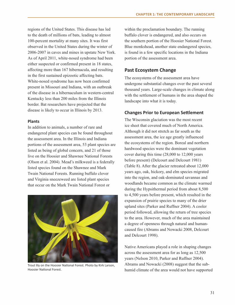
31


regions of the United States. This disease has led to the death of millions of bats, leading to almost 100-percent mortality at many sites. It was first observed in the United States during the winter of 200�-2007 in caves and mines in upstate New York. As of April 2011, white-nosed syndrome had been either suspected or confirmed present in 18 states, affecting more than 1�7 hibernacula, and resulting in the first sustained epizootic affecting bats. White-nosed syndrome has now been confirmed present in Missouri and Indiana, with an outbreak of the disease in a hibernaculum in western-central Kentucky less than 200 miles from the Illinois border. Bat researchers have projected that the disease is likely to occur in Illinois by 2013.

PlantsIn addition to animals, a number of rare and endangered plant species can be found throughout the assessment area. In the Illinois and Indiana portions of the assessment area, 53 plant species are listed as being of global concern, and 21 of those live on the Hoosier and Shawnee National Forests (Olson et al. 2004). Mead’s milkweed is a federally listed species found on the Shawnee and Mark Twain National Forests. Running buffalo clover and Virginia sneezeweed are listed plant species that occur on the Mark Twain National Forest or

within the proclamation boundary. The running buffalo clover is endangered, and also occurs on the southern portion of the Hoosier National Forest. Blue monkshead, another state endangered species, is found in a few specific locations in the Indiana portion of the assessment area.

Past Ecosystem ChangeThe ecosystems of the assessment area have undergone substantial changes over the past several thousand years. Large-scale changes in climate along with the settlement of humans in the area shaped the landscape into what it is today.

Changes Prior to European Settlement The Wisconsin glaciation was the most recent ice sheet that covered much of North America. Although it did not stretch as far south as the assessment area, the ice age greatly influenced the ecosystems of the region. Boreal and northern hardwood species were the dominant vegetation cover during this time (28,000 to 12,000 years before present) (Delcourt and Delcourt 1981) (Table 8). After the glacier retreated about 12,000 years ago, oak, hickory, and elm species migrated into the region, and oak-dominated savannas and woodlands became common as the climate warmed during the Hypsithermal period from about 8,500 to 4,500 years before present, which resulted in the expansion of prairie species to many of the drier upland sites (Parker and Ruffner 2004). A cooler period followed, allowing the return of tree species to the area. However, much of the area maintained a degree of openness through natural and human-caused fire (Abrams and Nowacki 2008, Delcourt and Delcourt 1998).

Native Americans played a role in shaping changes across the assessment area for as long as 12,500 years (Nelson 2010, Parker and Ruffner 2004). Abrams and Nowacki (2008) suggest that the sub-humid climate of the area would not have supported

Trout lily on the Hoosier National Forest. Photo by Kirk Larson, Hoosier National Forest.

32


time (years before present) Vegetation Human activities

Pre-12,000 Boreal forest Initial settlement-big game hunters

12,000 to 8,500 Mesic oak savanna in north, oak-ironwood woodland southeast

Mobile hunter-gatherers, numerous short-term settlements, widespread use of fire

8,500 to 4,500 Large expanses of grassland intrude into region, oak-hickory savanna

Same as above

4,500 to 1,000 Shortleaf pine moves in, variable canopy woodland and forest in southeast, prairie savanna in northwest

Semi-sedentary to sedentary hunter-gatherers, appearance of domesticated plants, increasing impacts from settlements, increased fire use, clearance of bottomlands for fields

1,000 to 200 Pre-European appearance Same as above, plus agricultural settlements along river bottoms

200-present Remaining forested lands more dense than what was historically present, increase in maple component, nonnative pines planted

Land cleared for agriculture, urban development; some areas reforested, fire suppression during mid-20th century

Table 8.—Changes in vegetation in the Central Hardwoods Region over the last 12,000 years. Adapted from Nelson (2010).

prairie, savanna, and open woodland without the influence of Native Americans through the use of fire. In addition to hunter-gatherer societies, agricultural communities were established along river bottoms from about 1,000 to 500 years ago, cultivating corn, beans, and squash. However, these communities disintegrated prior to European settlement, returning some formerly developed lands back to forest. Smaller tribal groups of native people continued to manipulate some areas with fire into the 19th century (Parker and Ruffner 2004). By the time of European contact (circa 1�50), the landscape resembled a mosaic pattern of croplands near settlements, abandoned clearings with early successional species, and open forest stands dominated by fire-adapted species of oak, hickory, and walnut (Abrams and Nowacki 2008, Delcourt 1987, Delcourt and Delcourt 1998).

Presettlement Vegetation Presettlement conditions are used as a reference condition for evaluating ecological integrity and determining restoration goals. The Missouri

Historic Vegetation Survey data indicate that the Ozark Highlands contained more than 25 different tree associations, many of them attributed to the influences of fire, topography, and geology. According to General Land Office witness tree survey records, oak species, shortleaf pine, and a variety of hickory species were dominant species in the early 19th century (Hanberry et al. 2012). According to models of witness tree structure and openness (a measure of diameter and distance from section corners and section lines), much of the Ozarks was open in character, thus confirming the historical presence of savanna and open woodlands (Batek et al. 1999, Hanberry et al. 2012, Nelson 2010). Forest was confined to dissected river breaks.

Pre-European-settlement forests of southern Illinois can be categorized into four basic types: (1) oak-hickory, (2) mixed hardwoods, (3) lowland-depression forests, and (4) floodplain forests (Parker and Ruffner 2004). Fragments of prairie and savanna were present in the upland, north-central portions of the area, and hills and bluffs along the Mississippi

33


River (Fralish 2010, Fralish et al. 1991). Small native populations of shortleaf pine occurred on extremely xeric uplands of the Ozark Hills (Davis and Ruffner 2002). Mesophytic species, such as American beech and sugar maple, were restricted to the low and alluvial sites mainly in the Illinois Ozark Hills and, to a lesser extent, in the Lesser and Greater Shawnee Hills (Fralish and McArdle 2009).

Prior to European settlement, common vegetation in southern Indiana consisted of mainly deciduous forests similar to those found in southern Illinois. American beech, hickories, oaks, yellow-poplar, and sugar maple were generally found on well-drained upland sites (Parker and Ruffner 2004). On the more shallow upland sites, scrub oaks including blackjack and scarlet oak were common. The Transition Hills Section of southern Indiana is believed to have been primarily forested with maple and beech due to a low influence of Native Americans in the area (Parker and Ruffner 2004). Although the area was primarily forested, prairies and savannas could also be found.

Post-settlement Changes Forest harvesting over the past 200 years has greatly shaped the landscape into what it is today, which is markedly different from its presettlement condition (reviewed in Parker and Ruffner 2004). Although past management across this region is quite variable, a few trends generally occurred. Settlers harvested timber across the area throughout the 19th century, cutting most of the old-growth forests (Fralish 1988). As sawmills were introduced into the area with the rapid increase in towns and villages, the harvest of timber for high-value products greatly accelerated. The practice of cutting only desirable high-value species left residual stands of trees that were generally of little economic value (Den Uyl 19�2, Westveld 1949).

By 1900, most of the forests in the assessment area had been cut, subjected to grazing, or burned (Parker and Ruffner 2004). In addition, wetlands had been drained and prairies had been converted to farmland. Generally, more land was cleared in the flat

Hickory nuts. Photo by Teena Ligman, Hoosier National Forest.

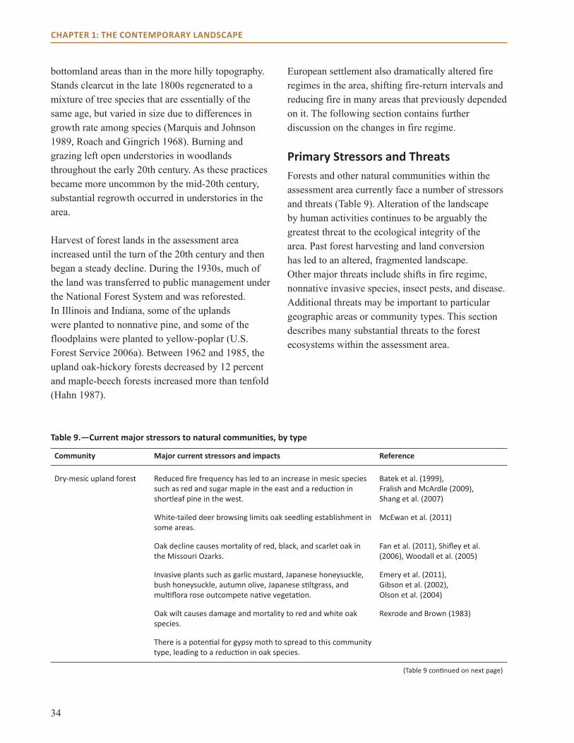
34


bottomland areas than in the more hilly topography. Stands clearcut in the late 1800s regenerated to a mixture of tree species that are essentially of the same age, but varied in size due to differences in growth rate among species (Marquis and Johnson 1989, Roach and Gingrich 19�8). Burning and grazing left open understories in woodlands throughout the early 20th century. As these practices became more uncommon by the mid-20th century, substantial regrowth occurred in understories in the area.

Harvest of forest lands in the assessment area increased until the turn of the 20th century and then began a steady decline. During the 1930s, much of the land was transferred to public management under the National Forest System and was reforested. In Illinois and Indiana, some of the uplands were planted to nonnative pine, and some of the floodplains were planted to yellow-poplar (U.S. Forest Service 200�a). Between 19�2 and 1985, the upland oak-hickory forests decreased by 12 percent and maple-beech forests increased more than tenfold (Hahn 1987).

European settlement also dramatically altered fire regimes in the area, shifting fire-return intervals and reducing fire in many areas that previously depended on it. The following section contains further discussion on the changes in fire regime.

Primary Stressors and ThreatsForests and other natural communities within the assessment area currently face a number of stressors and threats (Table 9). Alteration of the landscape by human activities continues to be arguably the greatest threat to the ecological integrity of the area. Past forest harvesting and land conversion has led to an altered, fragmented landscape. Other major threats include shifts in fire regime, nonnative invasive species, insect pests, and disease. Additional threats may be important to particular geographic areas or community types. This section describes many substantial threats to the forest ecosystems within the assessment area.

community Major current stressors and impacts Reference

Dry-mesic upland forest Reduced fire frequency has led to an increase in mesic species such as red and sugar maple in the east and a reduction in shortleaf pine in the west.

Batek et al. (1999), Fralish and McArdle (2009), Shang et al. (2007)

White-tailed deer browsing limits oak seedling establishment in some areas.

McEwan et al. (2011)

Oak decline causes mortality of red, black, and scarlet oak in the Missouri Ozarks.

Fan et al. (2011), Shifley et al. (2006), Woodall et al. (2005)

Invasive plants such as garlic mustard, Japanese honeysuckle, bush honeysuckle, autumn olive, Japanese stiltgrass, and multiflora rose outcompete native vegetation.

Emery et al. (2011), Gibson et al. (2002), Olson et al. (2004)

Oak wilt causes damage and mortality to red and white oak species.

Rexrode and Brown (1983)

There is a potential for gypsy moth to spread to this community type, leading to a reduction in oak species.

(Table 9 continued on next page)

Table 9.—Current major stressors to natural communities, by type

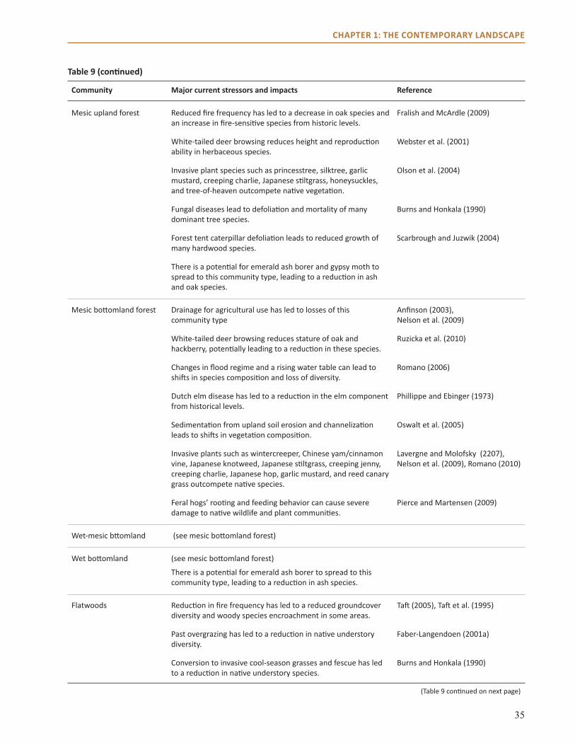
35



Mesic upland forest Reduced fire frequency has led to a decrease in oak species and an increase in fire-sensitive species from historic levels.

Fralish and McArdle (2009)

White-tailed deer browsing reduces height and reproduction ability in herbaceous species.

Webster et al. (2001)

Invasive plant species such as princesstree, silktree, garlic mustard, creeping charlie, Japanese stiltgrass, honeysuckles, and tree-of-heaven outcompete native vegetation.

Olson et al. (2004)

Fungal diseases lead to defoliation and mortality of many dominant tree species.

Burns and Honkala (1990)

Forest tent caterpillar defoliation leads to reduced growth of many hardwood species.

Scarbrough and Juzwik (2004)

There is a potential for emerald ash borer and gypsy moth to spread to this community type, leading to a reduction in ash and oak species.

Mesic bottomland forest Drainage for agricultural use has led to losses of this community type

Anfinson (2003), Nelson et al. (2009)

White-tailed deer browsing reduces stature of oak and hackberry, potentially leading to a reduction in these species.

Ruzicka et al. (2010)

Changes in flood regime and a rising water table can lead to shifts in species composition and loss of diversity.

Romano (2006)

Dutch elm disease has led to a reduction in the elm component from historical levels.

Phillippe and Ebinger (1973)

Sedimentation from upland soil erosion and channelization leads to shifts in vegetation composition.

Oswalt et al. (2005)

Invasive plants such as wintercreeper, Chinese yam/cinnamon vine, Japanese knotweed, Japanese stiltgrass, creeping jenny, creeping charlie, Japanese hop, garlic mustard, and reed canary grass outcompete native species.

Lavergne and Molofsky (2207), Nelson et al. (2009), Romano (2010)

Feral hogs’ rooting and feeding behavior can cause severe damage to native wildlife and plant communities.

Pierce and Martensen (2009)

Wet-mesic bttomland (see mesic bottomland forest)

Wet bottomland (see mesic bottomland forest)

There is a potential for emerald ash borer to spread to this community type, leading to a reduction in ash species.

Flatwoods Reduction in fire frequency has led to a reduced groundcover diversity and woody species encroachment in some areas.

Taft (2005), Taft et al. (1995)

Past overgrazing has led to a reduction in native understory diversity.

Faber-Langendoen (2001a)

Conversion to invasive cool-season grasses and fescue has led to a reduction in native understory species.



Table 9 (continued)

3�



Open woodland Past harvesting of shortleaf pine has led to a reduction in the shortleaf pine component in Missouri compared to the early 20th century.

Tremain et al. (2007)

Reduced fire frequency has led to a reduction in shortleaf pine (in Missouri) and an increase in woody species in the understory compared to presettlement conditions.

Batek et al. (1999)



Invasive species such as sericea lespideza, yellow sweetclover, crown vetch, Oriental bittersweet, garlic mustard, common periwinkle, multiflora rose, Japanese honeysuckle, bush honeysuckle, and autumn olive outcompete native vegetation.

Olson et al. (2004)

Eastern redcedar encroachment crowds out native understory vegetation.

Hanberry et al. (2012)

Insect attack by Nantucket pine tip moth, redheaded sawfly, and reproduction weevils causes mortality in young shortleaf pine.




Closed woodland Past harvesting of shortleaf pine has led to a reduction in that species in Missouri compared to the early 20th century.

Tremain et al. (2007)

Reduced fire frequency has led to a reduction in shortleaf pine (in Missouri) compared to presettlement conditions and an increase this community type.

Batek et al. (1999)



Invasive species such as garlic mustard, Japanese honeysuckle, bush honeysuckle, autumn olive, Japanese stiltgrass, and multiflora rose outcompete native vegetation.

Olson et al. (2004)

Insect attack by Nantucket pine tip moth, redheaded sawfly, and weevils causes mortality in young shortleaf pine.




Savanna Conversion to agriculture has led to a dramatic loss of this community type on the landscape, making remnants highly fragmented.

Nuzzo (1986)

Reduced fire frequency has led to encroachment of woody and shade-tolerant species that out-compete shade-intolerant understory vegetation.

Bowles and McBride (1998)

Invasive species such as autumn olive, multiflora rose, teasel, garlic mustard, white and yellow sweetclover, sericea lespideza, and spotted knapweed outcompete native vegetation.

Olson et al. (2004)


Table 9 (continued)

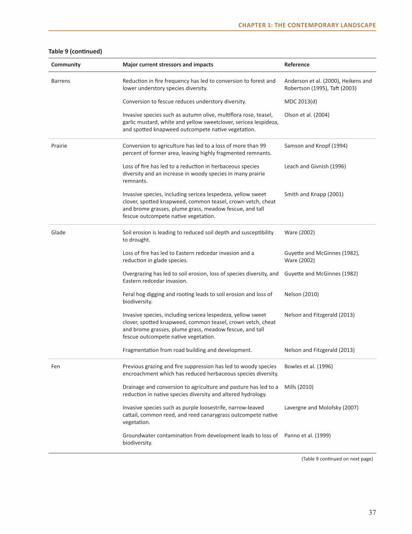
37



Barrens Reduction in fire frequency has led to conversion to forest and lower understory species diversity.

Anderson et al. (2000), Heikens and Robertson (1995), Taft (2003)

Conversion to fescue reduces understory diversity. MDC 2013(d)

Invasive species such as autumn olive, multiflora rose, teasel, garlic mustard, white and yellow sweetclover, sericea lespideza, and spotted knapweed outcompete native vegetation.

Olson et al. (2004)

Prairie Conversion to agriculture has led to a loss of more than 99 percent of former area, leaving highly fragmented remnants.

Samson and Knopf (1994)

Loss of fire has led to a reduction in herbaceous species diversity and an increase in woody species in many prairie remnants.

Leach and Givnish (1996)

Invasive species, including sericea lespedeza, yellow sweet clover, spotted knapweed, common teasel, crown vetch, cheat and brome grasses, plume grass, meadow fescue, and tall fescue outcompete native vegetation.

Smith and Knapp (2001)

Glade Soil erosion is leading to reduced soil depth and susceptibility to drought.

Ware (2002)

Loss of fire has led to Eastern redcedar invasion and a reduction in glade species.

Guyette and McGinnes (1982), Ware (2002)

Overgrazing has led to soil erosion, loss of species diversity, and Eastern redcedar invasion.

Guyette and McGinnes (1982)

Feral hog digging and rooting leads to soil erosion and loss of biodiversity.

Nelson (2010)

Invasive species, including sericea lespedeza, yellow sweet clover, spotted knapweed, common teasel, crown vetch, cheat and brome grasses, plume grass, meadow fescue, and tall fescue outcompete native vegetation.

Nelson and Fitzgerald (2013)

Fragmentation from road building and development. Nelson and Fitzgerald (2013)

Fen Previous grazing and fire suppression has led to woody species encroachment which has reduced herbaceous species diversity.

Bowles et al. (1996)

Drainage and conversion to agriculture and pasture has led to a reduction in native species diversity and altered hydrology.

Mills (2010)

Invasive species such as purple loosestrife, narrow-leaved cattail, common reed, and reed canarygrass outcompete native vegetation.

Lavergne and Molofsky (2007)

Groundwater contamination from development leads to loss of biodiversity.

Panno et al. (1999)


Table 9 (continued)

38


Table 9 (continued)


Seeps and springs Pollution from agricultural runoff and livestock waste may eliminate some aquatic species that are very sensitive to water quality.

Faber-Langendoen (2001b)

Grazing or ditching can reduce site quality.

Swamp Agricultural development, which has led to altered hydrology and habitat fragmentation, alters seedbank composition and distribution.

Middleton (2003), Middleton and Wu (2008)

Fungal attack causes a brown pocket rot known as “pecky cypress” that damages the heartwood of living baldcypress trees.


Various insect species can cause defoliation of baldcypress. Burns and Honkala (1990)

Nutria clip or uproot newly planted cypress seedlings, leading to seedling death.

Conner et al. (1987)

Fragmentation and Land-use ChangeEuropean settlement led to development and fragmentation of the landscape across the assessment area, resulting in a patchwork of public and private parcels of natural, agricultural, and developed lands. As mentioned earlier, 43 percent of the assessment area is now agricultural land and about 8 percent is now developed land (Fry et al. 2011). In addition, remaining forest land is often heavily dissected by roads, private property, trails, and utility lines. Forests in the assessment area are much more heavily fragmented than forests in the northern Great Lakes and Appalachians, but are less fragmented than the northern portions of each state, as measured by the percentage of interior forest in each county (U.S. Forest Service 2011b). Fragmentation of natural landscapes creates isolated populations that are unable to migrate easily and exchange genetic information, leading to a reduction in biological and genetic diversity (Fahrig 2003, Harrison and Bruna 1999, Robinson et al. 1995). It also leads to increased incidence of edges along forest boundaries (Sisk et al. 1997).

Fragmentation and land-use change were cited as the number one issue facing forests in Indiana, based on a survey conducted as part of the Indiana Statewide Forest Assessment (INDNR 2010). It was also listed as a major issue of concern in Missouri’s Forest Resource Assessment and Strategy (MDC 2010). Housing growth, particularly in rural areas, can lead to forest fragmentation and nonnative species invasions (Radeloff et al. 2005, 2010). Ecoregions in southern Missouri have had particularly high growth in rural sprawl compared with much of the Midwest (Radeloff et al. 2005). In addition, Indiana forests have the highest housing density surrounding them in the entire Midwest (Radeloff et al. 2005). By contrast, the central Ozarks in Missouri represent some of the least fragmented forests in the Midwest and are therefore of high conservation value (Radeloff et al. 2005). Housing growth from 1940 to 2000 within 30 miles of national forests in the Central Hardwoods Region varied by forest. The Mark Twain National Forest underwent the highest growth (greater than 400,000 new units), followed by the Hoosier (200,000 to 300,000 new units), and

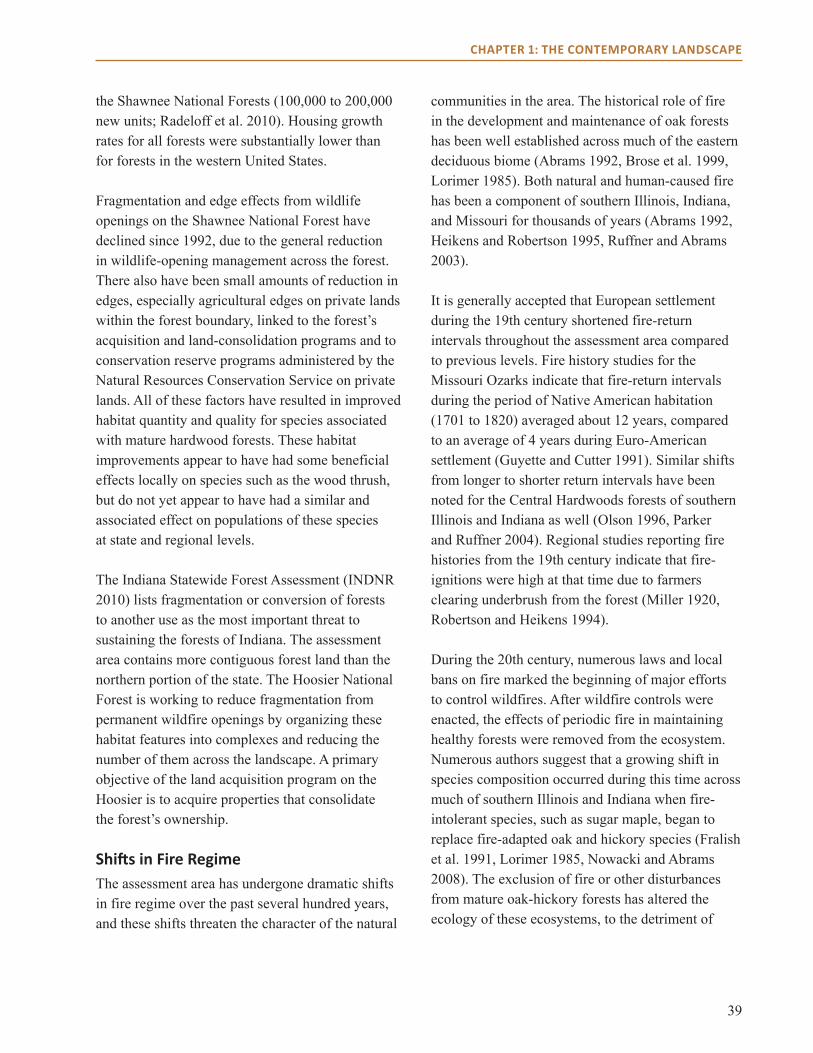
39


the Shawnee National Forests (100,000 to 200,000 new units; Radeloff et al. 2010). Housing growth rates for all forests were substantially lower than for forests in the western United States.

Fragmentation and edge effects from wildlife openings on the Shawnee National Forest have declined since 1992, due to the general reduction in wildlife-opening management across the forest. There also have been small amounts of reduction in edges, especially agricultural edges on private lands within the forest boundary, linked to the forest’s acquisition and land-consolidation programs and to conservation reserve programs administered by the Natural Resources Conservation Service on private lands. All of these factors have resulted in improved habitat quantity and quality for species associated with mature hardwood forests. These habitat improvements appear to have had some beneficial effects locally on species such as the wood thrush, but do not yet appear to have had a similar and associated effect on populations of these species at state and regional levels.

The Indiana Statewide Forest Assessment (INDNR 2010) lists fragmentation or conversion of forests to another use as the most important threat to sustaining the forests of Indiana. The assessment area contains more contiguous forest land than the northern portion of the state. The Hoosier National Forest is working to reduce fragmentation from permanent wildfire openings by organizing these habitat features into complexes and reducing the number of them across the landscape. A primary objective of the land acquisition program on the Hoosier is to acquire properties that consolidate the forest’s ownership.

Shifts in Fire RegimeThe assessment area has undergone dramatic shifts in fire regime over the past several hundred years, and these shifts threaten the character of the natural

communities in the area. The historical role of fire in the development and maintenance of oak forests has been well established across much of the eastern deciduous biome (Abrams 1992, Brose et al. 1999, Lorimer 1985). Both natural and human-caused fire has been a component of southern Illinois, Indiana, and Missouri for thousands of years (Abrams 1992, Heikens and Robertson 1995, Ruffner and Abrams 2003).

It is generally accepted that European settlement during the 19th century shortened fire-return intervals throughout the assessment area compared to previous levels. Fire history studies for the Missouri Ozarks indicate that fire-return intervals during the period of Native American habitation (1701 to 1820) averaged about 12 years, compared to an average of 4 years during Euro-American settlement (Guyette and Cutter 1991). Similar shifts from longer to shorter return intervals have been noted for the Central Hardwoods forests of southern Illinois and Indiana as well (Olson 199�, Parker and Ruffner 2004). Regional studies reporting fire histories from the 19th century indicate that fire-ignitions were high at that time due to farmers clearing underbrush from the forest (Miller 1920, Robertson and Heikens 1994).

During the 20th century, numerous laws and local bans on fire marked the beginning of major efforts to control wildfires. After wildfire controls were enacted, the effects of periodic fire in maintaining healthy forests were removed from the ecosystem. Numerous authors suggest that a growing shift in species composition occurred during this time across much of southern Illinois and Indiana when fire-intolerant species, such as sugar maple, began to replace fire-adapted oak and hickory species (Fralish et al. 1991, Lorimer 1985, Nowacki and Abrams 2008). The exclusion of fire or other disturbances from mature oak-hickory forests has altered the ecology of these ecosystems, to the detriment of

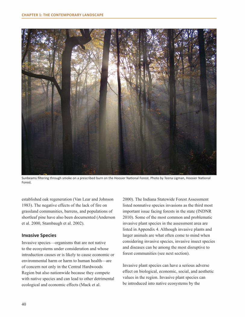
40


established oak regeneration (Van Lear and Johnson 1983). The negative effects of the lack of fire on grassland communities, barrens, and populations of shortleaf pine have also been documented (Anderson et al. 2000, Stambaugh et al. 2002).

Invasive SpeciesInvasive species—organisms that are not native to the ecosystems under consideration and whose introduction causes or is likely to cause economic or environmental harm or harm to human health—are of concern not only in the Central Hardwoods Region but also nationwide because they compete with native species and can lead to other detrimental ecological and economic effects (Mack et al.

2000). The Indiana Statewide Forest Assessment listed nonnative species invasions as the third most important issue facing forests in the state (INDNR 2010). Some of the most common and problematic invasive plant species in the assessment area are listed in Appendix 4. Although invasive plants and larger animals are what often come to mind when considering invasive species, invasive insect species and diseases can be among the most disruptive to forest communities (see next section).

Invasive plant species can have a serious adverse effect on biological, economic, social, and aesthetic values in the region. Invasive plant species can be introduced into native ecosystems by the

Sunbeams filtering through smoke on a prescribed burn on the Hoosier National Forest. Photo by Teena Ligman, Hoosier National Forest.

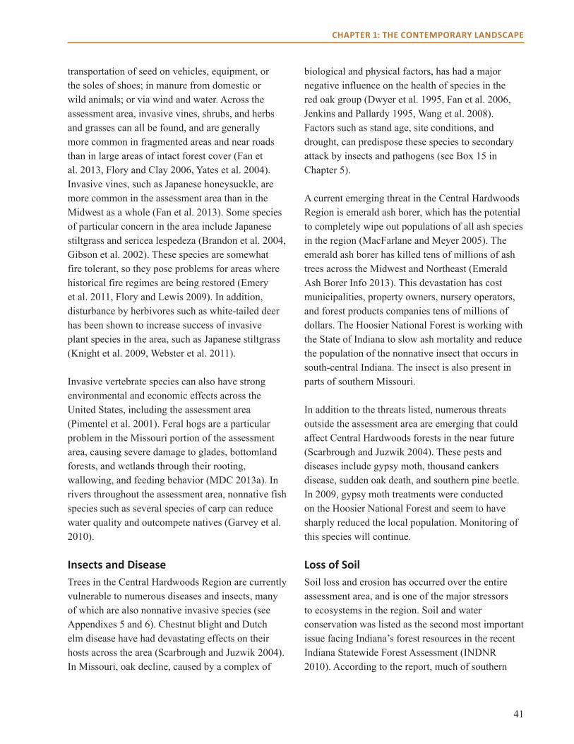
41


transportation of seed on vehicles, equipment, or the soles of shoes; in manure from domestic or wild animals; or via wind and water. Across the assessment area, invasive vines, shrubs, and herbs and grasses can all be found, and are generally more common in fragmented areas and near roads than in large areas of intact forest cover (Fan et al. 2013, Flory and Clay 200�, Yates et al. 2004). Invasive vines, such as Japanese honeysuckle, are more common in the assessment area than in the Midwest as a whole (Fan et al. 2013). Some species of particular concern in the area include Japanese stiltgrass and sericea lespedeza (Brandon et al. 2004, Gibson et al. 2002). These species are somewhat fire tolerant, so they pose problems for areas where historical fire regimes are being restored (Emery et al. 2011, Flory and Lewis 2009). In addition, disturbance by herbivores such as white-tailed deer has been shown to increase success of invasive plant species in the area, such as Japanese stiltgrass (Knight et al. 2009, Webster et al. 2011).

Invasive vertebrate species can also have strong environmental and economic effects across the United States, including the assessment area (Pimentel et al. 2001). Feral hogs are a particular problem in the Missouri portion of the assessment area, causing severe damage to glades, bottomland forests, and wetlands through their rooting, wallowing, and feeding behavior (MDC 2013a). In rivers throughout the assessment area, nonnative fish species such as several species of carp can reduce water quality and outcompete natives (Garvey et al. 2010).

Insects and Disease Trees in the Central Hardwoods Region are currently vulnerable to numerous diseases and insects, many of which are also nonnative invasive species (see Appendixes 5 and �). Chestnut blight and Dutch elm disease have had devastating effects on their hosts across the area (Scarbrough and Juzwik 2004). In Missouri, oak decline, caused by a complex of

biological and physical factors, has had a major negative influence on the health of species in the red oak group (Dwyer et al. 1995, Fan et al. 200�, Jenkins and Pallardy 1995, Wang et al. 2008). Factors such as stand age, site conditions, and drought, can predispose these species to secondary attack by insects and pathogens (see Box 15 in Chapter 5).

A current emerging threat in the Central Hardwoods Region is emerald ash borer, which has the potential to completely wipe out populations of all ash species in the region (MacFarlane and Meyer 2005). The emerald ash borer has killed tens of millions of ash trees across the Midwest and Northeast (Emerald Ash Borer Info 2013). This devastation has cost municipalities, property owners, nursery operators, and forest products companies tens of millions of dollars. The Hoosier National Forest is working with the State of Indiana to slow ash mortality and reduce the population of the nonnative insect that occurs in south-central Indiana. The insect is also present in parts of southern Missouri.

In addition to the threats listed, numerous threats outside the assessment area are emerging that could affect Central Hardwoods forests in the near future (Scarbrough and Juzwik 2004). These pests and diseases include gypsy moth, thousand cankers disease, sudden oak death, and southern pine beetle. In 2009, gypsy moth treatments were conducted on the Hoosier National Forest and seem to have sharply reduced the local population. Monitoring of this species will continue.

Loss of soil Soil loss and erosion has occurred over the entire assessment area, and is one of the major stressors to ecosystems in the region. Soil and water conservation was listed as the second most important issue facing Indiana’s forest resources in the recent Indiana Statewide Forest Assessment (INDNR 2010). According to the report, much of southern

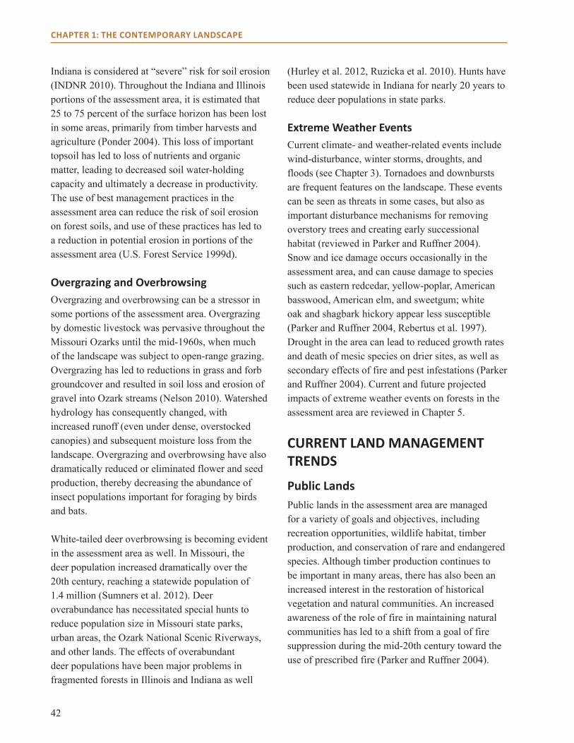
42


Indiana is considered at “severe” risk for soil erosion (INDNR 2010). Throughout the Indiana and Illinois portions of the assessment area, it is estimated that 25 to 75 percent of the surface horizon has been lost in some areas, primarily from timber harvests and agriculture (Ponder 2004). This loss of important topsoil has led to loss of nutrients and organic matter, leading to decreased soil water-holding capacity and ultimately a decrease in productivity. The use of best management practices in the assessment area can reduce the risk of soil erosion on forest soils, and use of these practices has led to a reduction in potential erosion in portions of the assessment area (U.S. Forest Service 1999d).

Overgrazing and OverbrowsingOvergrazing and overbrowsing can be a stressor in some portions of the assessment area. Overgrazing by domestic livestock was pervasive throughout the Missouri Ozarks until the mid-19�0s, when much of the landscape was subject to open-range grazing. Overgrazing has led to reductions in grass and forb groundcover and resulted in soil loss and erosion of gravel into Ozark streams (Nelson 2010). Watershed hydrology has consequently changed, with increased runoff (even under dense, overstocked canopies) and subsequent moisture loss from the landscape. Overgrazing and overbrowsing have also dramatically reduced or eliminated flower and seed production, thereby decreasing the abundance of insect populations important for foraging by birds and bats.

White-tailed deer overbrowsing is becoming evident in the assessment area as well. In Missouri, the deer population increased dramatically over the 20th century, reaching a statewide population of 1.4 million (Sumners et al. 2012). Deer overabundance has necessitated special hunts to reduce population size in Missouri state parks, urban areas, the Ozark National Scenic Riverways, and other lands. The effects of overabundant deer populations have been major problems in fragmented forests in Illinois and Indiana as well

(Hurley et al. 2012, Ruzicka et al. 2010). Hunts have been used statewide in Indiana for nearly 20 years to reduce deer populations in state parks.

Extreme Weather Events Current climate- and weather-related events include wind-disturbance, winter storms, droughts, and floods (see Chapter 3). Tornadoes and downbursts are frequent features on the landscape. These events can be seen as threats in some cases, but also as important disturbance mechanisms for removing overstory trees and creating early successional habitat (reviewed in Parker and Ruffner 2004). Snow and ice damage occurs occasionally in the assessment area, and can cause damage to species such as eastern redcedar, yellow-poplar, American basswood, American elm, and sweetgum; white oak and shagbark hickory appear less susceptible (Parker and Ruffner 2004, Rebertus et al. 1997). Drought in the area can lead to reduced growth rates and death of mesic species on drier sites, as well as secondary effects of fire and pest infestations (Parker and Ruffner 2004). Current and future projected impacts of extreme weather events on forests in the assessment area are reviewed in Chapter 5.

current LAnD mAnAGement trenDs

Public LandsPublic lands in the assessment area are managed for a variety of goals and objectives, including recreation opportunities, wildlife habitat, timber production, and conservation of rare and endangered species. Although timber production continues to be important in many areas, there has also been an increased interest in the restoration of historical vegetation and natural communities. An increased awareness of the role of fire in maintaining natural communities has led to a shift from a goal of fire suppression during the mid-20th century toward the use of prescribed fire (Parker and Ruffner 2004).

43


Prescribed FirePrescribed fire is a primary tool used to maintain or restore the dominance of oak and other fire-adapted species on the Central Hardwoods landscape (Abrams 2005, Van Lear et al. 2000). Oaks have several adaptive features that enable them to survive periodic fire, including thick bark and the ability to re-sprout vigorously from dormant buds at the base of the tree when the bole has been topkilled (Lorimer 1985). Fire can also reduce acorn predation by insects and rodents (Galford et al. 1988, Lorimer 1985). Maples, by contrast, are susceptible to fire because these trees are thin barked and have seedlings that suffer high mortality due to both rootkill and topkill. Studies have documented the beneficial effects of prescribed fire to foster oak regeneration and reduce competing mesophytic species in forest lands, but effects can vary with burn regime, season, and stem diameter of trees in a particular stand (Brose et al. 2012, Ruffner and Groninger 200�).

Prescribed fire is also a primary tool to restore other historical vegetation and fire-dependent natural communities. Fire has been shown to help perpetuate barrens communities, where many threatened, endangered, and sensitive species occur (Anderson and Schwegman 1971). It is also used to restore the understory and improve wildlife habitat in shortleaf pine systems (U.S. Forest Service 1999d). The use of prescribed fire to maintain unique vegetation and habitats in glades and oak savannas has also been noted (Parker and Ruffner 2004).

Use of prescribed fire has increased over the past several decades across the assessment area. Publicly managed forests in southern Illinois have been using fire since the mid-1980s (Parker and Ruffner 2004). The Shawnee National Forest 200� Land Management Plan anticipates 124,389 acres of prescribed burning forest-wide over a 10-year period (U.S. Forest Service 200�). To date, about 5,000 to �,000 acres of prescribed burning occur in a given year. The Mark Twain National Forest’s use of

prescribed fire has increased from 8,000 to 10,000 acres per year in the mid-1990s and early 2000s to an average of 30,000 acres per year currently. Since implementing the 200� Land Management Plan, prescribed burns on the Hoosier National Forest have averaged about 1,��4 acres per year, with a high of 2,583 acres in 2009 (J. Perez, Hoosier National Forest, personal comm.).

Timber Harvest Timber harvests are still a component of forest management on public lands in the assessment area. In the past several decades, clearcut harvests in Missouri have been virtually eliminated in favor of other silvicultural techniques such as the shelterwood and seed-tree methods (U.S. Forest Service 1999d). Likewise, the shelterwood technique is a primary timber management technique anticipated on the Shawnee National Forest (U.S. Forest Service 200�a). Clearcutting is still one of the primary techniques to remove nonnative pine species on the Hoosier National Forest, along with group selection, shelterwood, and single tree selection techniques (U.S. Forest Service 200�b). Once trees are harvested, most hardwood species are allowed to regenerate naturally, whereas artificial regeneration is generally used for shortleaf pine in Missouri (U.S. Forest Service 1999d).

In Missouri, statewide harvest removals were estimated at 1,7�0 million board feet (mmbf) in 2010, a 13-percent increase from 2005 (Moser et al. 2011). The amount of timber sold by the Mark Twain National Forest has averaged about 4� mmbf per year over the last 5 years (Periodic Timber Sale Accomplishment Reports [PTSAR] 2012). This amount is an increase from an average of 34 mmbf between 199� and 2005, but below the 198� to 1995 average of �2 mmbf. The sale quantity has ranged from a high of 79 mmbf in 1987 to a low of 13 in 2001. Oak, predominantly black and scarlet, makes up on average 78 percent of the total, with shortleaf pine composing the rest.

44


In Illinois, timber harvests showed a dramatic increase from 19�0 to the early 1980s, but have since declined (ILDNR 2010). Of the harvests that occur currently, the majority take place on private lands. Statewide, annual harvest removals were estimated at 505 mmbf in 2011 (Crocker 2012). Timber removals are low in public lands in Illinois, and the Shawnee National Forest in particular. According to the 200� Shawnee National Forest Land Management Plan, maximum probable timber harvests from combined management activities would be about � mmbf per year for the next 10 years, but actual harvests have not yet occurred (U.S. Forest Service 200�b). There have been no timber sales on the Shawnee National Forest in nearly 20 years because of a number of factors.

Across Indiana, harvest removals were estimated at 907 mmbf in 2011, a 13-percent increase from 2007 (Woodall and Gallion 2012). Timber harvests on the Hoosier National Forest have averaged 7 mmbf per year from 2007 to 2011 under the current land management plan (PTSAR 2012).

Private Lands As mentioned earlier in the chapter, about 80 percent of forested land in the Central Hardwoods Region is privately owned, and these private lands account for the majority of timber harvested on the landscape. The majority of these lands lack a specific management plan (Butler 2008). However, several programs exist to provide incentives to private landowners in the region for the development of management plans in order to ensure long-term sustainability of forest resources.

National programs for forest certification on these private lands include the Sustainable Forestry Initiative (SFI), Forest Stewardship Council (FSC), and American Tree Farm System. These programs help landowners develop sustainable forestry practices. Products from these sustainably

managed forests are tracked over time from harvest to purchase, allowing consumers to purchase forest products that they know are produced in the most sustainable way. It is projected that consumer demand for these products will grow, providing a market incentive for certified wood products, and thus sustainable forest management. Currently, there are 14�,235 acres of FSC land in Missouri, 1,794 acres in Illinois, and �7�,370 acres in Indiana. In Indiana, 148,019 acres are dual certified as SFI, and 528,351 are dual certified as Tree Farm (Pingrey 2011).

chAPter summAryThe climate, geology, and soils of the Central Hardwoods Region of Missouri, Illinois, and Indiana support a mosaic of natural communities dominated by oak and hickory species. These communities supply important benefits to the people of the area, including forest products and recreation opportunities. Past changes in climate, fire regime, and land use have shaped the landscape into its current condition. About half of the land in the area has been converted to agriculture or developed for industrial or residential use. Many of the remaining forests on the landscape are less open and contain more mesophytic species such as sugar maple than before European settlement. Shifts in fire regime, habitat fragmentation, species invasions, insect pests and diseases, and other alterations to the landscape threaten the integrity and diversity of the ecosystems and the benefits they provide these ecosystems. Management on public lands in recent decades has focused on reducing these stressors and improving ecosystem function. About 80 percent of the forested land in area is privately owned, however, and the majority of these lands lack a management plan. New opportunities and incentives have arisen in recent years to help private and public land managers to restore and conserve the ecosystems of the Central Hardwoods systems for future generations.

45

CHAPTER 2: CLIMATE CHANGE SCIENCE AND MODELING

This chapter provides a brief background on climate change science, models that simulate future climate, and models that project the effects of changes in climate on species and ecosystems. Throughout the chapter, boxes point to recent nontechnical reports based on the best available science. A more detailed review of climate change science, trends, and modeling can be found in the Intergovernmental Panel on Climate Change (IPCC) Fourth Assessment Report (IPCC 2007).

CLIMATE CHANGEClimate is not the same thing as weather. Weather is a set of the meteorological conditions for a given point in time in one particular place (such as the temperature at 3:00 p.m. on June 22 in St. Louis). Climate, in contrast, is the average, long-term (30 years or more) meteorological conditions and patterns for a geographic area. The IPCC (2007: 30) defines climate change as “a change in the state of the climate that can be identified (e.g., by using statistical tests) by changes in the mean and/or the variability of its properties, and that persists for an extended period, typically decades or longer.” A key finding of the IPCC in its Fourth Assessment Report (IPCC 2007) was that “warming of the climate system is unequivocal.” This was the first assessment report in which the IPCC considered the evidence strong enough to make such a statement. Current observations of higher global surface, air, and ocean temperatures and thousands of long-term (more than 20 years) data sets from all continents and oceans contributed to this conclusion. These data sets showed significant changes in snow, ice, and frozen ground; hydrology; coastal processes;

and terrestrial, marine, and biological systems. The IPCC’s Fifth Assessment Report is underway and scheduled to be released in 2014. The United States Global Change Research Program has released a series of reports detailing the past and projected changes in climate at a national level, with a comprehensive report (National Climate Assessment [NCA]) scheduled to be released in 2014 (see Box 5 for more information).

The Warming TrendThe Earth is warming, and the rate of warming is increasing (IPCC 2007, Raupach et al. 2007). Measurements from weather stations across the globe indicate that the global mean temperature has risen by 1.4 °F (0.8 °C) over the past 50 years, nearly twice the rate of the last 100 years (IPCC 2007) (Fig. 9). Including 2012, all 12 years to date in the 21st century rank among the warmest 14 years in the 133-year period of record of global temperature (National Oceanic and Atmospheric Administration [NOAA], National Climatic Data Center [NCDC] 2012). Temperatures in the United States have risen by 2 °F (1.1 °C) in the last 50 years (Karl et al. 2009). The 2012 continental U.S. average annual temperature of 55.3 °F was 3.3 °F above the 20th-century average, and was the warmest year in the 1895 through 2012 period of record for the nation (NOAA NCDC 2013).

Average temperature increases are just one aspect of a more complex and wide-ranging set of climate changes. For example, the frequency of cold days, cold nights, and frosts has decreased over many regions of the world while the frequency of hot

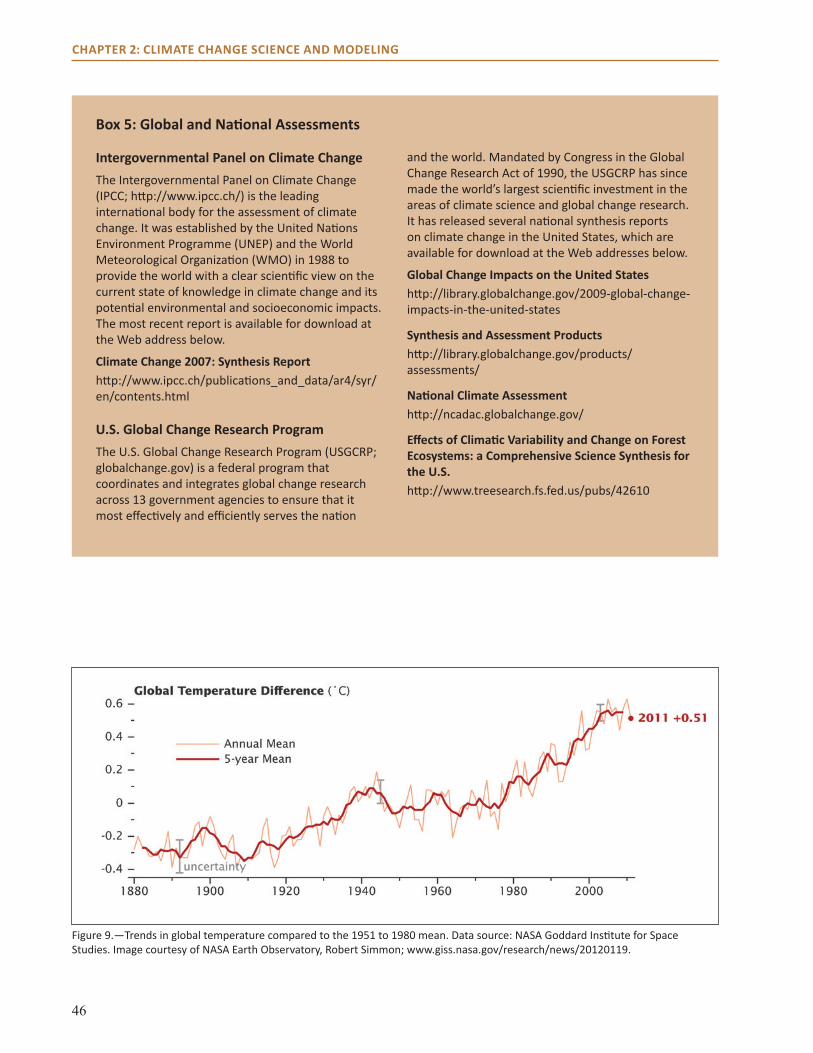
46


Box 5: Global and National Assessments

Intergovernmental Panel on Climate ChangeThe Intergovernmental Panel on Climate Change (IPCC; http://www.ipcc.ch/) is the leading international body for the assessment of climate change. It was established by the United Nations Environment Programme (UNEP) and the World Meteorological Organization (WMO) in 1988 to provide the world with a clear scientific view on the current state of knowledge in climate change and its potential environmental and socioeconomic impacts. The most recent report is available for download at the Web address below.

Climate Change 2007: Synthesis Report http://www.ipcc.ch/publications_and_data/ar4/syr/en/contents.html

U.S. Global Change Research ProgramThe U.S. Global Change Research Program (USGCRP; globalchange.gov) is a federal program that coordinates and integrates global change research across 13 government agencies to ensure that it most effectively and efficiently serves the nation

and the world. Mandated by Congress in the Global Change Research Act of 1990, the USGCRP has since made the world’s largest scientific investment in the areas of climate science and global change research. It has released several national synthesis reports on climate change in the United States, which are available for download at the Web addresses below.

Global Change Impacts on the United Stateshttp://library.globalchange.gov/2009-global-change-impacts-in-the-united-states

Synthesis and Assessment Productshttp://library.globalchange.gov/products/assessments/

National Climate Assessmenthttp://ncadac.globalchange.gov/

Effects of Climatic Variability and Change on Forest Ecosystems: a Comprehensive Science Synthesis for the U.S.http://www.treesearch.fs.fed.us/pubs/42610

Figure 9.—Trends in global temperature compared to the 1951 to 1980 mean. Data source: NASA Goddard Institute for Space Studies. Image courtesy of NASA Earth Observatory, Robert Simmon; www.giss.nasa.gov/research/news/20120119.

47


days and nights has increased (IPCC 2007). The frequency of heat waves and heavy precipitation events has increased over this period, with new records for both heat and precipitation in portions of the United States in July 2011 and March 2012 (NOAA NCDC 2012). Global rises in sea level, decreasing extent of snow and ice, and shrinking of mountain glaciers have all been observed over the past 50 years, and are consistent with a warming climate (IPCC 2007).

Average temperature increases of a few degrees may seem small, but even small increases can result in substantial changes to the severity of storms, the nature and timing of precipitation, droughts and heat waves, ocean temperature and volume, and snow and ice—all of which affect humans and ecosystems. Increases of more than 3.6 °F (2 °C) above the average temperature are expected to cause major societal and environmental disruptions through the rest of the century and beyond (Richardson et al. 2009). The synthesis report of the International Scientific Congress on Climate Change concluded that “recent observations show that societies and ecosystems are highly vulnerable to even modest levels of climate change, with poor nations and communities, ecosystem services and biodiversity particularly at risk” (Richardson et al. 2009: 12).

Based on available evidence, 97 percent of the climate science community attributes this increase in temperature and associated changes in precipitation and other weather events to human activities (Anderegg et al. 2010, Doran and Zimmerman 2009, Stott et al. 2010). Scientists have been able to attribute these changes to human causes by using climate model simulations of the past, both with and without human-induced changes in the atmosphere, and then comparing those simulations to observational data. Overall, these studies have shown a clear human effect on recent changes in temperature, precipitation, and other climate variables due to changes in greenhouse gases and particulate matter in the air (Stott et al. 2010).

Chapter 3 provides specific information about recent climate trends for the assessment area.

The Greenhouse EffectThe greenhouse effect is the process by which certain gases in the atmosphere absorb and re-emit energy that would otherwise be lost into space (Fig. 10). This greenhouse effect is necessary for human survival: without it, Earth would have an average temperature of about 0 °F (-18 °C) and be covered in ice, rather than a comfortable 59 °F (15 °C). Several naturally occurring greenhouse gases in the atmosphere, including carbon dioxide (CO2), methane (CH4), nitrous oxide (N2O), and water vapor, contribute to the greenhouse effect. Water vapor is the most abundant greenhouse gas; its residence time in the atmosphere, however, is on the order of days as it quickly responds to changes in temperature and other factors. Carbon dioxide, CH4, N2O, and other greenhouse gases reside in the atmosphere for decades to centuries. Thus, these other long-lived gases are of primary concern with respect to long-term warming.

Human Influences on Greenhouse GasesHumans have increased the concentrations of CO2, CH4, and N2O in the atmosphere since the beginning of the industrial era (Fig. 11). More CO2 has been released by humans into the atmosphere than any other greenhouse gas. In the United States, the average person releases about 17.3 metric tons of CO2 per year, more than twice as much per person as in China or European countries (Olivier et al. 2012). Carbon dioxide levels increased at a rate of 1.4 parts per million (ppm) per year from 1960 to 2005 (IPCC 2007), and reached an average of 395 ppm in January 2013 (Tans and Keeling 2013). In recent decades, fossil fuel burning has accounted for an estimated 83 to 94 percent of the human-induced increase in CO2. The remaining 6 to 17 percent of human-induced emissions comes primarily from deforestation and degradation of land for conversion to agriculture, which releases CO2 when forests burn

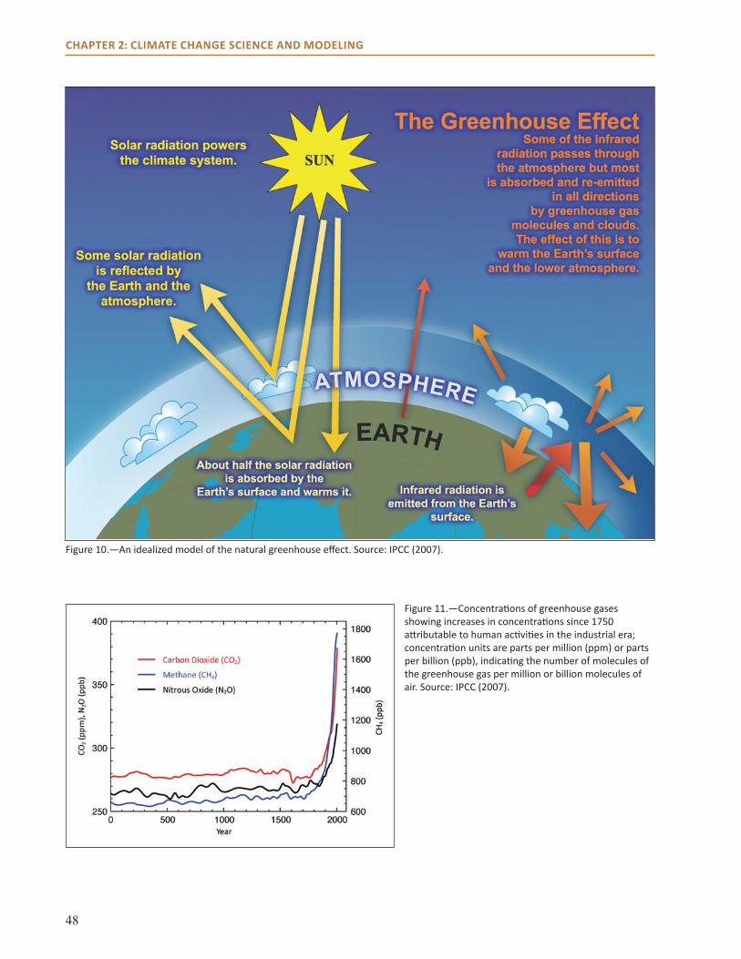
48


Figure 10.—An idealized model of the natural greenhouse effect. Source: IPCC (2007).

Figure 11.—Concentrations of greenhouse gases showing increases in concentrations since 1750 attributable to human activities in the industrial era; concentration units are parts per million (ppm) or parts per billion (ppb), indicating the number of molecules of the greenhouse gas per million or billion molecules of air. Source: IPCC (2007).

49


or decompose (van der Werf et al. 2009). However, increases in fossil fuel emissions over the past decade mean that the contribution from land-use changes has become a smaller proportion of the total (Le Quéré et al. 2009).

Methane is responsible for approximately 14 percent of greenhouse gas emissions (IPCC 2007). Methane concentrations in the atmosphere have also increased over the past century as a result of human activities, such as raising livestock and growing rice. Livestock production is responsible for 35 to 40 percent of global CH4 emissions, primarily from fermentation in the guts of cattle and other ruminants (Steinfeld et al. 2006). Rice production, the second largest source of CH4 emissions, requires wet conditions that are also ideal for microbial CH4 production. Other human-caused sources of CH4 include biomass burning, microbial emissions from landfills, fossil fuel combustion, and leakage of natural gas during mining and distribution.

Nitrous oxide accounts for about 8 percent of global greenhouse gas emissions (IPCC 2007). The primary human source of N2O is agriculture. Increased fertilizer use (both synthetic and animal-based) increases emissions from soil as microbes break down nitrogen-containing products. In addition, converting tropical forests to agricultural lands increases microbial N2O production. Another main source of N2O is the combustion of fossil fuels.

Humans have reduced stratospheric ozone in the atmosphere through the use of chlorofluorocarbons (CFCs) in refrigeration, air conditioning, and other applications. Restrictions against the use of CFCs under the Montreal Protocol led to a decline in CFC emissions and reductions in ozone have subsequently slowed. After CFCs were banned, another class of halocarbons, hydrofluorocarbons (HFCs, also known as F-gases), largely replaced CFCs in refrigeration and air conditioning. Although HFCs do not deplete stratospheric ozone, many are

powerful greenhouse gases. Currently HFCs account for about 1 percent of greenhouse gas emissions (IPCC 2007).

CLIMATE MODELSScientists use models, which are simplified representations of reality, to simulate future climates. Models can be theoretical, mathematical, conceptual, or physical. General circulation models (GCMs), which combine complex mathematical formulas representing physical processes in the ocean, atmosphere, and land surface within large computer simulations, are important in climate science. They are used in short-term weather forecasting as well as long-term climate projections.

General Circulation ModelsGeneral circulation models simulate physical processes (such as the exchange of energy and the movement of matter) in the Earth’s surface, oceans, and atmosphere through time using mathematical equations in three-dimensional space. They work in time steps as small as minutes or hours and in simulations covering decades to centuries. Because of their complexity, GCMs require the intensive computing power of supercomputers.

Although GCMs use highly sophisticated computers, limits on computing power mean that projections of future climate are limited to relatively coarse spatial scales. Instead of simulating climate for every single point on Earth, modelers divide the land surface, ocean, and atmosphere into a three-dimensional grid (Fig. 12). Each cell within the grid is able to interact with adjacent cells (making it “spatially dynamic”). Although there is variation, grid cells are usually between 2 and 3º latitude and longitude. For the middle latitudes, this is about one-quarter of the size of Missouri. Cells are stacked in interconnected vertical layers that simulate ocean depth or atmospheric thickness at increments usually ranging from 656 to 3,280 feet.

50


Figure 12.—Schematic describing climate models, which are systems of differential equations based on the basic laws of physics, fluid motion, and chemistry. The planet is divided into a three-dimensional grid that is used to apply basic equations and evaluate results. Atmospheric models calculate winds, heat transfer, radiation, relative humidity, and surface hydrology within each grid and evaluate interactions with neighboring points. Source: NOAA (2008).

Several GCMs have been used in climate projections for the IPCC reports and elsewhere (see Box 6). These models have been developed by internationally renowned climate research centers such as NOAA’s Geophysical Fluid Dynamics Laboratory (GFDL CM2; Delworth et al. 2006), the United Kingdom’s Hadley Centre (HadCM3; Pope et al. 2000), and the National Center for Atmospheric

Research (PCM; Washington et al. 2000). These models use slightly different grid sizes and differ in the way they represent physical processes. They also differ in sensitivity to changes in greenhouse gas concentrations, which means that some models will tend to project higher increases in temperature than others under similar increases in greenhouse gas concentrations.

51


Box 6: More Resources on Climate Models and Emissions Scenarios

U.S. Forest ServiceClimate Projections FAQwww.treesearch.fs.fed.us/pubs/40614

U.S. Global Change Research ProgramClimate Models: an Assessment of Strengths and Limitationslibrary.globalchange.gov/sap-3-1-climate-models-an-assessment-of-strengths-and-limitations

Intergovernmental Panel on Climate ChangeChapter 8: Climate Models and Their Evaluationwww.ipcc.ch/publications_and_data/ar4/wg1/en/ch8.html

Special Report on Emissions Scenarios: Summary for Policymakershttp://www.ipcc.ch/ipccreports/sres/emission/index.php?idp=0

Like all models, GCMs have strengths and weaknesses (see Box 7). In general, they are useful because they are based on well-understood physical processes. Simulations of past climates by GCMs generally correspond well with measured and proxy-based reconstructions of past climate. However, GCM projections are not perfect. Climate scientists’ understanding of some climate processes is incomplete, and some influential climate processes occur at spatial scales that are too small to be modeled given current computing power. Technological advances in computing along with scientific advances in our understanding of Earth’s physical processes will allow future improvements in GCM projections.

Emissions ScenariosGeneral circulation models require significant amounts of information to project future climates. Some of this information, like future greenhouse gas concentrations, is not known and must be estimated. Although human populations, economies, and technological developments will certainly affect future greenhouse gas concentrations, they cannot be completely foreseen. One common approach for dealing with uncertainty about future greenhouse gas concentrations is to develop storylines about how the future may unfold and calculate the potential greenhouse gas concentrations for each storyline. The IPCC’s set of standard emissions scenarios is a

widely accepted set of such storylines (IPCC 2007). In GCMs, the use of different emissions scenarios results in different climate projections.

Emissions scenarios quantify the effects of alternative demographic, technological, or environmental developments on atmospheric greenhouse gas concentrations. None of the current scenarios include any changes in national or international policies directed specifically at climate change such as the Kyoto Protocol. However, some of the scenarios that include a reduction in greenhouse gases through other means suggest what we could expect if these policies were implemented. Six different emissions scenarios are commonly used in model projections for reports such as the IPCC Fourth Assessment Report (Fig. 13).

The A1FI scenario is the most fossil-fuel intensive, and thus projects the highest future greenhouse gas concentrations; GCM simulations using the A1FI scenario project the highest future warming. On the other end of the spectrum, the B1 scenario represents a future where alternative energies decrease our reliance on fossil fuels and greenhouse gas concentrations increase the least. GCM simulations using the B1 scenario project the lowest increase in global temperature. Although these scenarios were designed to describe a range of future emissions over the coming decades, it is important to note that

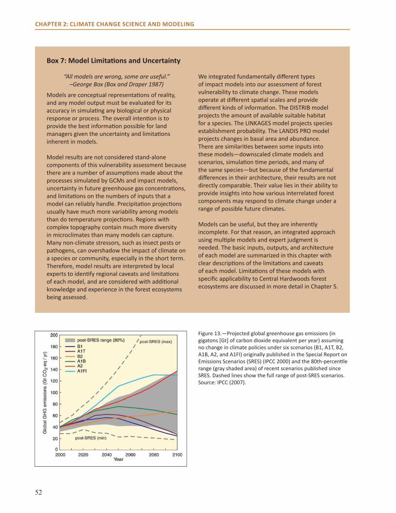
52


Box 7: Model Limitations and Uncertainty

“All models are wrong, some are useful.” –George Box (Box and Draper 1987)

Models are conceptual representations of reality, and any model output must be evaluated for its accuracy in simulating any biological or physical response or process. The overall intention is to provide the best information possible for land managers given the uncertainty and limitations inherent in models.

Model results are not considered stand-alone components of this vulnerability assessment because there are a number of assumptions made about the processes simulated by GCMs and impact models, uncertainty in future greenhouse gas concentrations, and limitations on the numbers of inputs that a model can reliably handle. Precipitation projections usually have much more variability among models than do temperature projections. Regions with complex topography contain much more diversity in microclimates than many models can capture. Many non-climate stressors, such as insect pests or pathogens, can overshadow the impact of climate on a species or community, especially in the short term. Therefore, model results are interpreted by local experts to identify regional caveats and limitations of each model, and are considered with additional knowledge and experience in the forest ecosystems being assessed.

We integrated fundamentally different types of impact models into our assessment of forest vulnerability to climate change. These models operate at different spatial scales and provide different kinds of information. The DISTRIB model projects the amount of available suitable habitat for a species. The LINKAGES model projects species establishment probability. The LANDIS PRO model projects changes in basal area and abundance. There are similarities between some inputs into these models—downscaled climate models and scenarios, simulation time periods, and many of the same species—but because of the fundamental differences in their architecture, their results are not directly comparable. Their value lies in their ability to provide insights into how various interrelated forest components may respond to climate change under a range of possible future climates.

Models can be useful, but they are inherently incomplete. For that reason, an integrated approach using multiple models and expert judgment is needed. The basic inputs, outputs, and architecture of each model are summarized in this chapter with clear descriptions of the limitations and caveats of each model. Limitations of these models with specific applicability to Central Hardwoods forest ecosystems are discussed in more detail in Chapter 5.

Figure 13.—Projected global greenhouse gas emissions (in gigatons [Gt] of carbon dioxide equivalent per year) assuming no change in climate policies under six scenarios (B1, A1T, B2, A1B, A2, and A1FI) originally published in the Special Report on Emissions Scenarios (SRES) (IPCC 2000) and the 80th-percentile range (gray shaded area) of recent scenarios published since SRES. Dashed lines show the full range of post-SRES scenarios. Source: IPCC (2007).

53


the future will conceivably be different from any of the developed scenarios. It is highly improbable that future greenhouse gas emissions will be less than described by the B1 scenario even if national or international policies were implemented immediately. In fact, current emissions more closely track the greenhouse gas emissions of the A1FI scenario, and global emissions since the year 2000 have even exceeded the A1FI scenario values in some years (Raupach et al. 2007).

DownscalingAs mentioned previously, GCMs simulate climate conditions only for relatively large areas. To examine the future climate of areas within the Central Hardwoods Region, a smaller grid scale is needed. One method of projecting climate on smaller spatial scales is statistical downscaling, a technique by which statistical relationships between GCM model outputs and on-the-ground measurements are derived for the past. These statistical relationships are then used to adjust large-scale GCM simulations of the future for much smaller spatial scales. Resolution for downscaled climate projections is typically around 6.2 miles.

Statistical downscaling has advantages and disadvantages (Daniels et al. 2012). It is a relatively simple and inexpensive way to produce smaller-scale projections from GCMs. However, statistical downscaling assumes that past relationships between modeled and observed temperature and precipitation will hold true under future change, which may or may not be true. Statistical downscaling also depends on local climatological data. If there are no weather stations in the area of interest, it may be difficult to obtain a good downscaled estimate of future climate for that area. Finally, local influences on climate that occur at finer scales (such as land cover type, lake-effect snow, topography, or particulate matter) also add to uncertainty when climate projections are downscaled.

Another approach, dynamical downscaling, uses a regional climate model (RCM) embedded within a GCM. Like GCMs, RCMs simulate physical processes through mathematical representations on a grid. However, RCMs operate on a finer resolution than GCMs, typically ranging from 15.5 to 31.0 miles, but can be as fine as 6.2 miles or less. Thus, they can simulate the effects of topography, land cover, lakes, and regional circulation patterns that operate on smaller scales.

As with statistical downscaling, dynamical downscaling has pros and cons (Daniels et al. 2012). It is advantageous for simulating the effects of climate change on regional phenomena such as lake-effect snow and extreme weather events. However, like GCMs, RCMs require a lot of computational power. Therefore, dynamically downscaled data are usually available only for one or two GCMs or emissions scenarios and for limited geographic areas. Because dynamically downscaled data are currently limited for the assessment area, we use statistically downscaled data in this report.

Downscaled GCMs Used in this Report In this assessment, we report statistically downscaled climate projections for two model-emissions scenario combinations: GFDL A1FI and PCM B1 (unless otherwise noted). Both models and both scenarios were included in the IPCC Fourth Assessment Report (IPCC 2007). The latest version of the NCA (in development) also draws on statistically downscaled data based on IPCC models and scenarios but uses the A2 scenario as an upper bound, which projects lower emissions compared to A1FI. The IPCC Assessment includes several other models, which are represented as a multi-model average in its reports. The NCA takes a similar approach in using a multi-model average. For this assessment, we instead selected two models that simulated climate in the eastern United States fairly accurately and that bracketed a range of

54


temperature and precipitation futures. This approach gives readers a better understanding of the level of agreement among models and provides a range of alternative scenarios that can be used by managers in planning and decisionmaking. Working with a range of plausible futures helps managers avoid placing false confidence in a single scenario given uncertainty in projecting future climate.

The Geophysical Fluid Dynamics Laboratory’s Climate Model (GFDL CM2; Delworth et al. 2006) is considered moderately sensitive to changes in radiative forcing. In other words, any change in greenhouse gas concentration included in the model would lead to a change in temperature that is higher than some models and lower than others. The National Center for Atmospheric Research’s Parallel Climate Model (PCM; Washington et al. 2000), by contrast, is considered to have low sensitivity to radiative forcing. As mentioned above, the A1FI scenario is the highest greenhouse gas emissions scenario used in the 2007 IPCC assessment, and is the most similar to current trends in greenhouse gas emissions globally. The B1 scenario is the lowest greenhouse gas emissions scenario used in the 2007 IPCC assessment, and is thus much lower than the trajectory of greenhouse gas emissions over the past decade. Therefore, the two model-scenario combinations span a large range of possible futures, with the GFDL A1FI model-scenario combination leading to a high-end projection of possible future temperature increases, and the PCM B1 projecting a low end of the range. Although both projections are possible, the GFDL A1FI scenario represents a more realistic projection of future greenhouse gas emissions and temperature increases (Raupach et al. 2007). It is important to note that it is possible that actual emissions and temperature increases could be lower or higher than these projections.

This assessment uses a statistically downscaled data set for the continental United States (Hayhoe 2010a). Daily mean, maximum, and minimum

temperature and total daily precipitation were downscaled to an approximately 7.5-mile resolution grid across the United States. This data set uses a sophisticated statistical approach (asynchronous quantile regression) to downscale daily GCM output and historical climate data (Stoner et al. 2012). This approach is advantageous because GCM and historical data do not need to be temporally correlated, and it is much better at capturing extreme temperatures and precipitation events than a linear regression approach. This statistically downscaled data set is different from that used in the NCA, which uses a simpler “delta” approach (Kunkel et al. 2013). This data set was chosen for several reasons. First, the data set covered the entire United States, and thus allowed a consistent data set to be used in this and other regional vulnerability assessments being conducted simultaneously. Second, it included downscaled projections for the A1FI emissions scenario, which is the scenario that most closely matches current trends in global greenhouse gas emissions (Raupach et al. 2007). Third, the availability of data at daily time steps was advantageous because it was needed for some impact models used in this report and provides the opportunity to examine questions related to growing season length, heavy precipitation events, and droughts. Fourth, the statistical technique used is more accurate at reproducing extreme values at daily time steps than simpler statistical downscaling methods (Hayhoe 2010b). Finally, the resolution was fine enough to be useful for informing land management decisions.

To show projected changes in temperature and precipitation in Chapter 4, we calculated the average daily mean, maximum, and minimum temperature for each season and the entire year for three 30-year time periods (2010 to 2039, 2040 to 2069, 2070 to 2099). Mean cumulative precipitation was also calculated for each season and annually for the same time periods. We then subtracted these values from the corresponding 1971 to 2000 averages

55


to determine the departure from current climate conditions. Historical climate data used for the departure analysis were taken from ClimateWizard based on the PRISM data set (see Chapter 3 and Appendix 7).

This data set was also used in the forest impact models described below. Some of these models require monthly precipitation and temperature values as inputs, and thus daily data were summed or averaged for each month when necessary. They also operate on grid scales that may be larger or smaller than the grid scale of the downscaled data set, and grid scales of the downscaled data were adjusted accordingly.

IMPACT MODELS Downscaled climate projections from GCMs provide important information about future climate, but they tell us nothing about how climate change might affect soil moisture, hydrology, forest composition, or productivity. Other models, commonly called impact models, are needed to project impacts on physical and biological processes (Fig. 14). Impact

models use downscaled GCM projections as inputs, as well as information such as soil types, landform, tree species distribution, and life history traits.

Hydrology plays a key role in forest ecosystem functioning and processing. The ways in which hydrology drives individual trees and ecosystems depend on precipitation, soil moisture, soil water-holding capacity, and rate of evapotranspiration. Precipitation itself may vary in physical form, amount, timing, and regularity. To project future change in hydrologic cycling, one model that is commonly used is the Variable Infiltration Capacity model (VIC) (Liang et al. 1994). This large-scale hydrologic process model is similar to many land surface models that are commonly coupled to GCMs. The land surface is modeled on a 0.6-mile or greater grid scale based on drivers such as precipitation, air temperature, and wind speed and using daily time steps. Flow of water and energy between the land and atmosphere are also simulated at daily time steps. Model outputs can include evapotranspiration, frozen soil formation, snow, runoff, and hydrologic dynamics in lakes and wetlands. Each grid cell is simulated independently

Figure 14.—Steps in the development of climate impact models using projections from general circulation models (GCMs) and specific steps taken in this assessment.

1. Emissionscenariosdevelopedand used as

inputs

2. Modelprojectionsare run by

using GCMs

3. GCMprojections

aredownscaledto a smaller

grid scale

4.DownscaledGCM data and

otherinformationare used asinputs into

impactmodels

B1 or A1FI PCM or GFDL ~3 o 1/8 olong./lat

LANDIS PRO,LINKAGES,Tree Atlas

56


without horizontal water flow, and stream flow is simulated using a separate model. More information about this model can be found on the model Web site: www.hydro.washington.edu/Lettenmaier/.

In Chapters 3 and 4, we discuss the results of several published studies that used the VIC model to project changes in hydrology. Future climate models and scenarios used as inputs into the VIC model are slightly different from those used for much of the rest of the assessment. Two models (GFDL and Hadley CM3) for each of three future emissions scenarios (A2, A1B, and B1) were used to address questions about past and future changes in climate across the Midwest related to streamflow and runoff (Cherkauer and Sinha 2010), drought (Mishra et al. 2010), and soil frost (Sinha and Cherkauer 2010, Sinha et al. 2010). The highest emissions scenario analyzed (A2) does not project as high of greenhouse gas emissions as the A1FI scenario, and A1B is a mid-range scenario. Therefore, projections presented for the highest emissions scenarios from these studies indicate more modest temperature increases than the GFDL A1FI scenario. Hadley and GFDL are also more sensitive to changes in radiative forcing than PCM, so the low-emissions scenario used in the VIC model (GFDL B1) simulates slightly greater warming than PCM B1.

Models for Assessing Forest ChangeForest impact models generally fall in one of two main categories: species distribution models and process models. This assessment uses one SDM, the Climate Change Tree Atlas (Prasad et al. 2007-ongoing), and two process models, LANDIS PRO (Wang et al. 2013, in press) and LINKAGES (v2.2; Wullschleger et al. 2003). For an overview of differences between these three models, see Table 11 in Chapter 5. These models operate at different spatial scales and provide different kinds of information about potential future forest composition and productivity. They provide useful information on potential climate change impacts on ecosystems in

our geographic area of interest, and have stood up to rigorous scientific review.

Species distribution models establish a statistical relationship between the current distribution of a species or ecosystem and key attributes of its habitat. This relationship is used to make projections about how the range of the species will shift as climate change affects those attributes. Much less computationally expensive than process models, SDMs can typically provide projections for the suitable habitat of many species over a larger area. There are some caveats that users should be aware of when using them, however (Wiens et al. 2009). These models use a species’ realized niche instead of its fundamental niche. The realized niche is the actual habitat a species occupies given predation, disease, and competition with other species. A fundamental niche of a species, in contrast, is the habitat it could potentially occupy in the absence of competition, disease, or herbivory. Given that a species’ fundamental niche may be greater than its realized niche, SDMs may underestimate current niche size and future suitable habitat. In addition, species distributions in the future might be constrained by competition, disease, and predation in ways that do not currently occur. If so, SDMs could overestimate the amount of suitable habitat in the future. If some constraints are removed due to future change, the opposite could also occur. Furthermore, fragmentation or other physical barriers to migration may create obstacles for species otherwise poised to occupy new habitat.

In contrast to SDMs, process models simulate ecosystem and tree species dynamics based on interactive mathematical representations of physical and biological processes. Process models can simulate future change in tree species dispersal, succession, biomass, and nutrient dynamics over space and time. Because these models simulate spatial or temporal dynamics, or both, of a variety of complex processes and at a finer scale, they

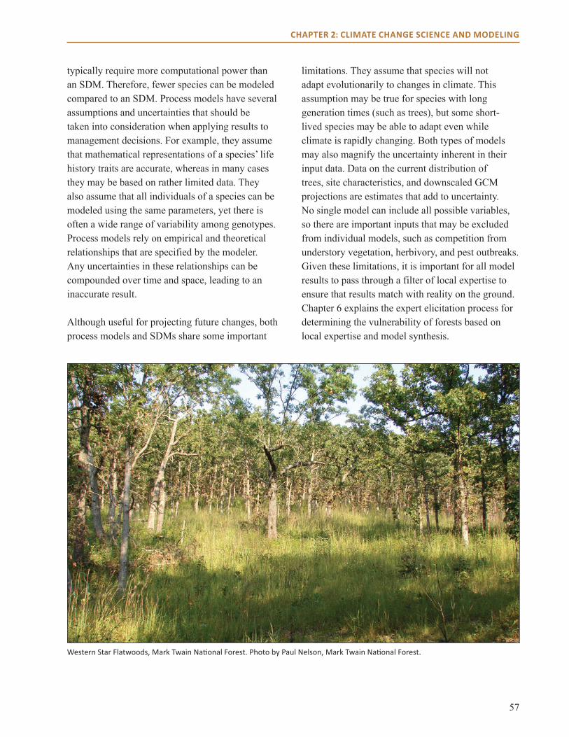
57


typically require more computational power than an SDM. Therefore, fewer species can be modeled compared to an SDM. Process models have several assumptions and uncertainties that should be taken into consideration when applying results to management decisions. For example, they assume that mathematical representations of a species’ life history traits are accurate, whereas in many cases they may be based on rather limited data. They also assume that all individuals of a species can be modeled using the same parameters, yet there is often a wide range of variability among genotypes. Process models rely on empirical and theoretical relationships that are specified by the modeler. Any uncertainties in these relationships can be compounded over time and space, leading to an inaccurate result.

Although useful for projecting future changes, both process models and SDMs share some important

limitations. They assume that species will not adapt evolutionarily to changes in climate. This assumption may be true for species with long generation times (such as trees), but some short-lived species may be able to adapt even while climate is rapidly changing. Both types of models may also magnify the uncertainty inherent in their input data. Data on the current distribution of trees, site characteristics, and downscaled GCM projections are estimates that add to uncertainty. No single model can include all possible variables, so there are important inputs that may be excluded from individual models, such as competition from understory vegetation, herbivory, and pest outbreaks. Given these limitations, it is important for all model results to pass through a filter of local expertise to ensure that results match with reality on the ground. Chapter 6 explains the expert elicitation process for determining the vulnerability of forests based on local expertise and model synthesis.

Western Star Flatwoods, Mark Twain National Forest. Photo by Paul Nelson, Mark Twain National Forest.

58


Climate Change Tree Atlas The Climate Change Tree Atlas incorporates a diverse set of information about potential shifts in the distribution of tree species’ habitat in the eastern United States over the next century (www.nrs.fs.fed.us/atlas; Iverson et al. 2008, Prasad et al. 2007-ongoing). The species distribution model DISTRIB measures relative abundance, referred to as importance values, for 134 eastern tree species. Inputs are tree species distribution data from the U.S. Forest Service, Forest Inventory and Analysis (FIA) program and environmental variables (pertaining to climate, soil properties, elevation, land use, and fragmentation), which are used to statistically model current species abundance with respect to current habitat distributions. Then DISTRIB projects future importance values and suitable habitat for individual tree species by using projections of future climate conditions on a 12-mile grid (Prasad et al. 2007-ongoing).

Additionally, projected future distributions for each tree species are further evaluated for factors not accounted for in the statistical models (Matthews et al. 2011b). These modifying factors (Appendix 9) are supplementary information on life history characteristics such as dispersal ability or fire tolerance as well as information on current pests and diseases that have been having negative effects on the species. This supplementary information allows us to identify when an individual species may do better or worse than model projections would suggest.

For this assessment, DISTRIB uses the GFDL A1FI and PCM B1 model-scenario combinations. The results provided in Chapter 5 differ from the online Climate Change Tree Atlas because they are specific to the assessment area and use the new statistically downscaled data set described above.

LANDIS PRO LANDIS PRO (Fraser et al. 2013; Wang et al. 2013, in press) is a spatially dynamic process model that simulates tree dispersal, establishment, and growth, along with disturbances and management. It is derived from the LANDIS model (Mladenoff 2004), but has been modified extensively from its original version. The LANDIS PRO model can simulate very large landscapes (millions of acres) at relatively fine spatial and temporal resolutions (typically 200 to 300 feet and 1- to 10-year time steps). One new feature of the model compared to previous versions is that inputs and outputs of tree species data in LANDIS PRO include tree density and volume and are compatible with FIA data. Thus, the model can be directly initialized, calibrated, and validated by using FIA data. This compatibility ensures the starting simulation conditions reflect conditions on the ground and allows the modelers to quantify the uncertainties embedded in the initial data.

The LANDIS PRO model can simulate landscape-level processes such as fire, wind, insect outbreaks, disease spread, nonnative species invasions, forest harvesting, fuel treatments, and silvicultural treatments. Basic inputs to LANDIS PRO are maps of species composition, land types, stands, management areas, and disturbance patterns. Species characteristics such as longevity, maturity, shade tolerance, average seed production per mature tree, and maximum diameter at breast height are given as inputs into the model. Basic outputs are the number of trees, basal area, biomass, age, and carbon, by species or by species age cohort as well as disturbance and harvest history across space and time. The spatially dynamic nature of the model and its fine spatial resolution are unique advantages of LANDIS PRO compared to LINKAGES (described below) and statistically based models. Disadvantages of LANDIS PRO are that it is too computationally

59


intensive to be run for a large number of species (in contrast to Tree Atlas) and does not account for ecosystem processes such as nitrogen cycling or decomposition (in contrast to LINKAGES).

For this assessment, LANDIS PRO simulates changes in basal area and trees per acre at a 295-foot resolution over the next century for six dominant tree species and species groups across the Missouri Ozarks part of the assessment area. The model projects changes in forest composition using downscaled daily mean temperature and precipitation from GFDL A1FI and PCM B1, and compares these projections with those under a current climate scenario.

LINKAGES LINKAGES (v2.2; Wullschleger et al. 2003) is a forest succession and ecosystem dynamics process model modified from an earlier version of LINKAGES (Pastor and Post 1985). The LINKAGES model integrates establishment and growth of individual trees with ecosystem functions such as soil-water balance, litter decomposition, nitrogen cycling, soil hydrology, and evapotranspiration. Inputs to the model include daily temperature, precipitation, wind speed, and solar radiation. Model inputs also include soil moisture capacity for multiple soil layers, wilting point, percentage of rock, percentage of clay, percentage of sand, initial organic matter, and nitrogen contents. Outputs from the model include tree species composition, number of stems, biomass, leaf litter, available nitrogen, humus, and organic matter, as well as hydrologic dynamics such as runoff. Simulations are done at yearly time steps on multiple 0.2-acre circular plots, which correspond to the average gap size when a tree dies and falls over. Unlike LANDIS PRO, LINKAGES is not spatially dynamic, and does not simulate tree dispersal or any other spatial interaction among grid cells. Typically,

the model is run for a specified number of plots in an area of interest, and results are averaged to determine relative species biomass and composition across the landscape over time.

For this assessment, LINKAGES simulates changes in tree species establishment probability over the next century for seven dominant tree species and species groups for landforms and subsections across the Missouri Ozarks portion of the assessment area. The model projects changes in forest composition by using downscaled daily mean temperature and precipitation from GFDL A1FI and PCM B1, and compares these projections with those under a current climate scenario. Species establishment probabilities from LINKAGES under each climate scenario are used as inputs into LANDIS PRO.

CHAPTER SUMMARYTemperatures have been increasing in recent decades at global and national scales, and the overwhelming majority of scientists attribute this change to increases in greenhouse gases from human activities. Even if dramatic changes are made to help curtail greenhouse gas emissions, these greenhouse gases will persist in our atmosphere for decades to come. Scientists can model how these increases in greenhouse gases may affect global temperature and precipitation patterns by using general circulation models. These large-scale climate models can be downscaled and incorporated into other types of models that project changes in forest composition and ecosystem processes to inform local decisions. Although there are inherent uncertainties in what the future holds, all of these types of models can help us frame a range of possible futures. This information can then be used in combination with the local expertise of researchers and managers to provide important insights about the potential effects of climate change on forest ecosystems.

60

CHAPTER 3: PAST CLIMATE CHANGES AND CURRENT TRENDS

Climate is the average weather conditions for a region over a period of decades. Year-to-year variation in local weather patterns can be influenced by ocean circulation patterns such as the El Niño Southern Oscillation and the Pacific Decadal Oscillation. Changes in particles in the atmosphere from volcanic eruptions or slight variations in solar activity can also lead to hotter or cooler conditions from the long-term average. Over longer time periods (thousands to millions of years), climate has changed considerably on a global scale, ranging from ice ages to warm periods, all of which are influenced by many factors. This chapter summarizes our current understanding of past changes in climate in the Central Hardwoods Region, with a focus on the last century.

HOLOCENE PALEOCLIMATETo understand climate prior to the historical record, scientists rely on proxies such as ice cores, lake sediments, tree cores, changes in isotopic ratios, and fossil pollen. Although proxy data specific to the Central Hardwoods Region are limited, the available data indicate that the area has experienced large shifts in climate over the past 12,000 years that have led to subsequent shifts in vegetation (see Chapter 1). Early Holocene (12,000 to 9,000 years ago) climate appears to have been moderately cool and moist enough to support oak savannas in the region (Denniston et al. 2000). Between approximately 9,000 and 5,000 years ago, the climate became considerably warmer and drier, supporting steppe vegetation dominated by warm-season short grasses (Denniston et al. 1999). Some evidence suggests that extended arid periods

occurred in the region between 3,500 and 2,500 years ago and again between 1,200 and 900 years ago, but these dry periods did not include a corresponding shift in temperature (Denniston et al. 2007).

Proxy data indicate that long, severe droughts have occurred in the region over the past 2,000 years, some of which were longer or more severe than the “Dust Bowl” era of the 1930s (Woodhouse and Overpeck 1998). Tree-ring data from Missouri and Iowa show that several multi-decadal drought periods have occurred in the region over the past millennium (Stambaugh et al. 2011). The Stambaugh et al. (2011) study suggests that the longest drought occurred over a 61-year period at the end of the 12th century, corresponding to the middle of the Medieval Warm Period. Long-term reconstructions of climate by using tree rings also reveal a 20-year drought cycle (in other words, peak droughts occurred about every 20 years) in the region over the past millennium, although the causes for this pattern are still unknown (Stambaugh et al. 2011).

HISTORICAL CLIMATE Measurements of temperature and precipitation at weather stations in the area have been recorded for a little over 100 years. We used the ClimateWizard custom analysis tool to present the changes in temperature and precipitation across the assessment area (ClimateWizard 2012, Girvetz et al. 2009). Data for the tool are derived from PRISM (Parameter-elevation Regressions on Independent Slopes Model; Gibson et al. 2002), which models historical, measured point data onto a continuous

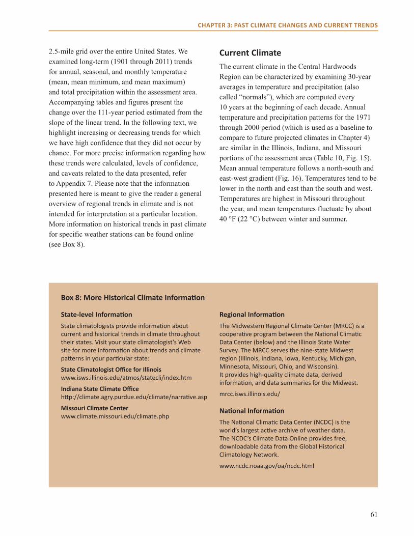
61


2.5-mile grid over the entire United States. We examined long-term (1901 through 2011) trends for annual, seasonal, and monthly temperature (mean, mean minimum, and mean maximum) and total precipitation within the assessment area. Accompanying tables and figures present the change over the 111-year period estimated from the slope of the linear trend. In the following text, we highlight increasing or decreasing trends for which we have high confidence that they did not occur by chance. For more precise information regarding how these trends were calculated, levels of confidence, and caveats related to the data presented, refer to Appendix 7. Please note that the information presented here is meant to give the reader a general overview of regional trends in climate and is not intended for interpretation at a particular location. More information on historical trends in past climate for specific weather stations can be found online (see Box 8).

Current ClimateThe current climate in the Central Hardwoods Region can be characterized by examining 30-year averages in temperature and precipitation (also called “normals”), which are computed every 10 years at the beginning of each decade. Annual temperature and precipitation patterns for the 1971 through 2000 period (which is used as a baseline to compare to future projected climates in Chapter 4) are similar in the Illinois, Indiana, and Missouri portions of the assessment area (Table 10, Fig. 15). Mean annual temperature follows a north-south and east-west gradient (Fig. 16). Temperatures tend to be lower in the north and east than the south and west. Temperatures are highest in Missouri throughout the year, and mean temperatures fluctuate by about 40 °F (22 °C) between winter and summer.

Box 8: More Historical Climate Information

State-level Information State climatologists provide information about current and historical trends in climate throughout their states. Visit your state climatologist’s Web site for more information about trends and climate patterns in your particular state:

State Climatologist Office for Illinoiswww.isws.illinois.edu/atmos/statecli/index.htm

Indiana State Climate Office http://climate.agry.purdue.edu/climate/narrative.asp

Missouri Climate Center www.climate.missouri.edu/climate.php

Regional InformationThe Midwestern Regional Climate Center (MRCC) is a cooperative program between the National Climatic Data Center (below) and the Illinois State Water Survey. The MRCC serves the nine-state Midwest region (Illinois, Indiana, Iowa, Kentucky, Michigan, Minnesota, Missouri, Ohio, and Wisconsin). It provides high-quality climate data, derived information, and data summaries for the Midwest.

mrcc.isws.illinois.edu/

National Information The National Climatic Data Center (NCDC) is the world’s largest active archive of weather data. The NCDC’s Climate Data Online provides free, downloadable data from the Global Historical Climatology Network.

www.ncdc.noaa.gov/oa/ncdc.html

62


Missouri Ozarks Southern Illinois Southern Indiana Temperature Precipitation Temperature Precipitation Temperature Precipitation (mean, °F) (inches) (mean, °F) (inches) (mean, °F) (inches)

Annual 55.6 43.92 55 42.9 54.2 44.94Winter 34.2 8 32.7 8.6 32.6 9.24Spring 55.4 12.91 54.8 12.72 53.7 13.32Summer 75.6 11.25 75.5 11.29 74.2 12.22Autumn 57 11.76 56.7 10.26 56 10.13

Table 10.—Average mean temperature and total precipitation (1971 through 2000) for the assessment area, by state.

Figure 15.—Average (1971 through 2000) total precipitation and mean temperature, by month, for the assessment area divided by state boundaries.

0

1

2

3

4

5

6

Tota

lPre

cipita

tion

(in)

IL IN MO

0

10

20

30

40

50

60

70

80

90

Mea

nTe

mpe

ratu

re(ΣF

)(°

F)

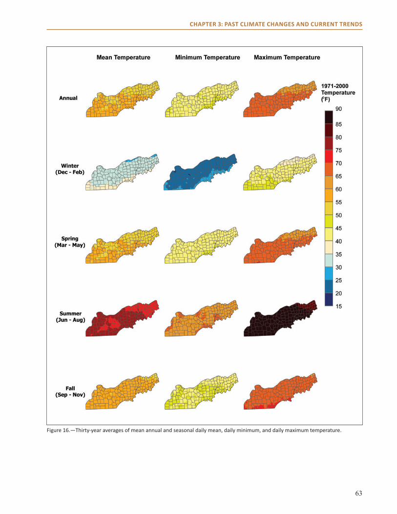
63


Figure 16.—Thirty-year averages of mean annual and seasonal daily mean, daily minimum, and daily maximum temperature.

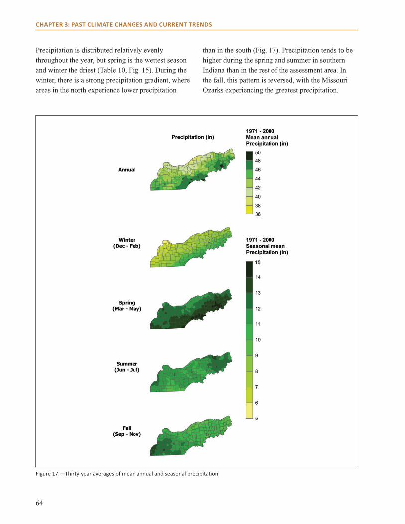
64


Precipitation is distributed relatively evenly throughout the year, but spring is the wettest season and winter the driest (Table 10, Fig. 15). During the winter, there is a strong precipitation gradient, where areas in the north experience lower precipitation

than in the south (Fig. 17). Precipitation tends to be higher during the spring and summer in southern Indiana than in the rest of the assessment area. In the fall, this pattern is reversed, with the Missouri Ozarks experiencing the greatest precipitation.

Figure 17.—Thirty-year averages of mean annual and seasonal precipitation.

65


Observed Trends in Precipitation and Temperature (1901 through 2011)Spatially interpolated trends in temperature and precipitation are available through 2011 and are presented below. For a discussion of recent trends in temperature and precipitation over the past decade, see Box 9. Between 1901 and 2011, mean annual temperatures fluctuated from year to year by several

degrees across the assessment area (Fig. 18). The warmest year on record for the assessment area as a whole was 1921. Temperatures were warmer than the long-term average during the “Dust Bowl” era of the 1930s. That period had many of the warmest and driest years on record, and summers were particularly hot and dry. By contrast, temperatures were cooler during the 1970s and early 1980s.

Box 9: Early 21st-Century Climate Changes

In this chapter, we present changes in climate over the entire historical record for which spatially interpolated data trends are available for the assessment area. Looking across the entire record is helpful in detecting long-term changes, but it can also obscure short-term trends.

The decade from 2001 to 2010 was the warmest on record both globally and averaged across North America (World Meteorological Organization [WMO] 2012). Across the assessment area, temperatures were also generally warmer than average between 2000 and 2012. However, with the exception of 2012, temperatures were not as warm as the 1930s or 1950s. The year 2012 was the warmest year on record for Missouri and Illinois and one of the warmest in Indiana (NOAA NCDC 2013). Until 2012, 1921 had been the warmest year on record for most of the region, with the exception of the western Missouri Ozarks, which had its highest temperature in 1954.

Trends in precipitation from 2000 to 2011 across the assessment area indicate a continuing pattern toward wetter conditions. Several locations in southern Illinois, southern Indiana, and southeastern Missouri had their wettest years on record in 2011 (NOAA 2012), and 2011 was in the top five wettest years across most of the assessment area excepting the Missouri Ozarks (Southern Climate Impacts Planning Partnership [SCIPP] 2012). The year 2012 was an exception to the trend of wetter conditions, with the area experiencing drought conditions that had not been experienced in the region for many decades (NOAA NCDC 2013).

And what about the “warming hole” patterns of low summer temperatures and high spring and summer precipitation? Across the assessment area, summer temperatures during 2010, 2011, and 2012 were much higher than the long-term average for the area (SCIPP 2012). Although it is too early to determine whether this is a trend, those years were the warmest summers most of the region had experienced since 1954 (with the exception of southwestern Missouri, which had its previous warmest summer in 1980). Although the recent warming temperatures suggest a possible reversal of the “warming hole,” precipitation trends have not changed markedly in recent years. Spring and summer precipitation continued to increase across southern Indiana, with 2008 and 2011 among the wettest years on record. In Illinois, spring precipitation also continued to be high, and summer precipitation was about average. Spring precipitation in Missouri was also high during the early 21st century, and summer precipitation showed a slight decrease. The 2012 drought was an obvious exception to this overall trend.

Overall, the climate information from the past decade seems to be consistent with the trends over the past century in some ways but not others. The area is still getting generally wetter, and the 1930s continues to be the warmest decade on record. The past decade was warmer than the late 20th century, but there is currently insufficient information to tell whether the higher temperatures represent a trend toward increasing temperature in the region.

66


Figure 18.—Time series showing annual mean temperature and total precipitation across the assessment area, 1901 through 2011. Open circles represent mean for each year. The blue line shows the 5-year moving average, and the red line is the slope of the linear regression. Note high temperatures and low precipitation values between 1930 and 1940 (ClimateWizard 2012).

Change rate = 0 °F/yr; p-value = 0.90828; r-squared = NA.

Annu

al M

ean

Tem

pera

ture

(°F)

58

57

56

55

54

53

1900 1920 1940 1960 1980 2000

Year

Change rate = 0.052 inches/yr; p-value = 0.005; r-squared = NA.

Annu

al M

ean

Prec

ipita

tion

(inch

es)

1900 1920 1940 1960 1980 2000

Year

55

50

45

40

35

30

67


TemperatureEven though temperatures increased both globally and across the United States over the same time period, the mean annual temperature in the Central Hardwoods Region actually decreased slightly in some areas; the change was small enough, however, that it could have occurred by chance (Fig. 19). We also evaluated trends beginning in the years 1951 and 1971, but did not find dramatic changes in the direction of these trends (data not shown). Although

mean seasonal temperatures did not change overall, there were a few trends when changes by month were examined (Fig. 20). January temperatures appear to have decreased and February temperatures to have increased. However, the year-to-year and spatial variation during these months was high, and these trends could be due to chance. Mean temperatures increased in April, particularly in Illinois and Indiana, and decreased in September and October slightly, especially in Illinois.

Figure 19.—Change in annual and seasonal mean daily mean, daily minimum, and daily maximum temperature, 1901 through 2011. Stippling indicates there is less than 10-percent probability that the trend could have occurred by chance alone.

68


Figure 20.—Change in mean daily mean, daily minimum, and daily maximum monthly temperature for the assessment area by state, 1901 through 2011. Asterisks indicate there is less than 10-percent probability that the trend could have occurred by chance alone.

-4

-3

-2

-1

0

1

2

3

Chan

gein

Mea

n(Σ

F)

Month

Illinois Indiana Missouri* *

**

*

-3

-2

-1

0

1

2

3

4

Chan

gein

Mea

nM

inim

um(Σ

F)

Month

**

* ***

***

*

*

-4

-3

-2

-1

0

1

2

3

4

Chan

gein

Mea

nM

axim

um(Σ

F)

Month

*

*

*

*

*

**

*

*

*

**

(°F)

(°F)

(°F)

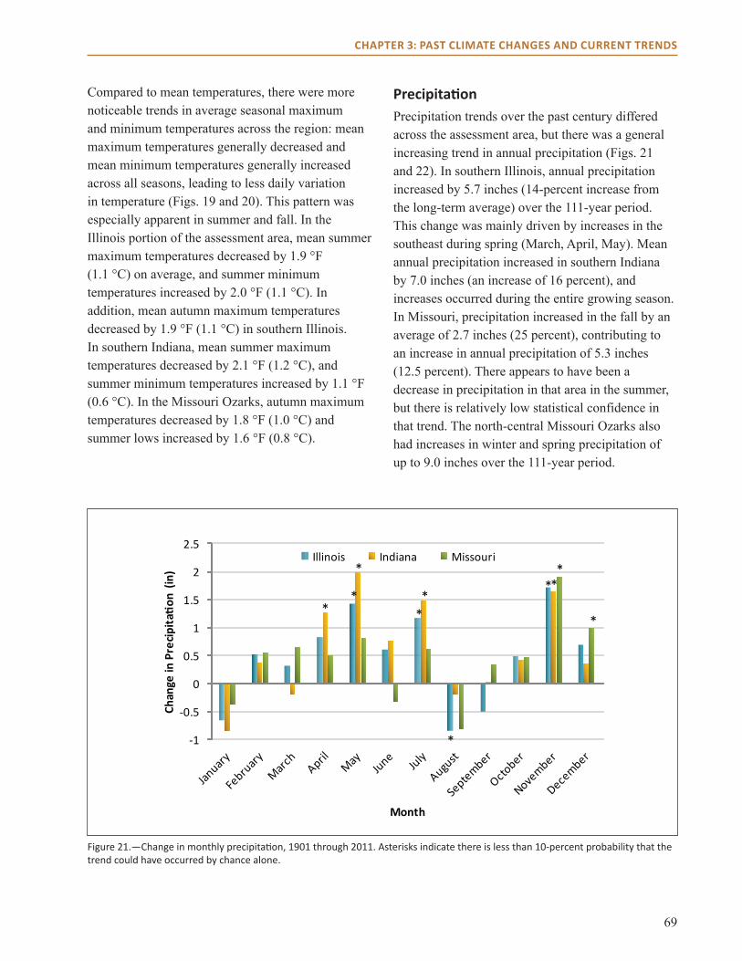
69


Compared to mean temperatures, there were more noticeable trends in average seasonal maximum and minimum temperatures across the region: mean maximum temperatures generally decreased and mean minimum temperatures generally increased across all seasons, leading to less daily variation in temperature (Figs. 19 and 20). This pattern was especially apparent in summer and fall. In the Illinois portion of the assessment area, mean summer maximum temperatures decreased by 1.9 °F (1.1 °C) on average, and summer minimum temperatures increased by 2.0 °F (1.1 °C). In addition, mean autumn maximum temperatures decreased by 1.9 °F (1.1 °C) in southern Illinois. In southern Indiana, mean summer maximum temperatures decreased by 2.1 °F (1.2 °C), and summer minimum temperatures increased by 1.1 °F (0.6 °C). In the Missouri Ozarks, autumn maximum temperatures decreased by 1.8 °F (1.0 °C) and summer lows increased by 1.6 °F (0.8 °C).

PrecipitationPrecipitation trends over the past century differed across the assessment area, but there was a general increasing trend in annual precipitation (Figs. 21 and 22). In southern Illinois, annual precipitation increased by 5.7 inches (14-percent increase from the long-term average) over the 111-year period. This change was mainly driven by increases in the southeast during spring (March, April, May). Mean annual precipitation increased in southern Indiana by 7.0 inches (an increase of 16 percent), and increases occurred during the entire growing season. In Missouri, precipitation increased in the fall by an average of 2.7 inches (25 percent), contributing to an increase in annual precipitation of 5.3 inches (12.5 percent). There appears to have been a decrease in precipitation in that area in the summer, but there is relatively low statistical confidence in that trend. The north-central Missouri Ozarks also had increases in winter and spring precipitation of up to 9.0 inches over the 111-year period.

Figure 21.—Change in monthly precipitation, 1901 through 2011. Asterisks indicate there is less than 10-percent probability that the trend could have occurred by chance alone.

-1

-0.5

0

0.5

1

1.5

2

2.5

Chan

gein

Prec

ipita

tion

(in)

Month

Illinois Indiana Missouri

**

*

*

***

*

*

*

70


Figure 22.—Change in annual and seasonal precipitation, 1901 through 2011. Stippling indicates there is less than 10-percent probability that this trend could have occurred by chance alone.

71


The “Warming Hole”Several studies have observed a decrease in temperatures, especially summer highs, in the southeastern and central United States over the past century, in what has been referred to as a “warming hole” (Kunkel et al. 2006, Pan et al. 2004, Portmann et al. 2009). These decreases in summer high temperature appear to be related to increases in precipitation (Pan et al. 2004, Portmann et al. 2009). A recent study suggests the higher precipitation and lower temperature may be due to an increase in aerosols (particulate matter in the air), which increase cloud formation and light scattering (Leibensperger et al. 2012). Others suggest it may be due to feedbacks from increased soil moisture availability (Pan et al. 2004). Still other studies suggest that the local temperature decrease may be driven by sea-surface temperatures in the North Atlantic and central Pacific (Kunkel et al. 2006).

Further research is needed to understand the “warming hole” and its implications for the region as global temperatures continue to rise. If the decreasing temperature trends were indeed caused by increased aerosols, it is possible that these trends will be reversed because of current regulations and improvements in air quality (Leibensperger et al. 2012). In fact, an analysis of recent climate trends in the region suggests that the warming hole may have already disappeared, but that study examined trends in only mean annual temperature and not summer highs (Tebaldi et al. 2012). However, if the temperature trends were instead due to other climatic processes, it is possible that these trends could continue into the future (see Chapter 4).

TRENDS IN EXTREME WEATHER EVENTSExtreme weather events, such as tornadoes, thunderstorms, and winter storms are important disturbance agents in forested systems. Some evidence suggests that extreme events have been

increasing across the United States and globally over recent decades, and this increase is consistent with global climate change (Coumou and Rahmstorf 2012, Kunkel et al. 2008). Below, we summarize changes in extreme events that have been observed in the Central Hardwoods Region.

Tornadoes and Wind StormsTornadoes are a common phenomenon in the Central Hardwoods Region. The central United States has the highest frequency of tornadoes in the world (Bates 1962). Among the 50 states, Missouri, Illinois, and Indiana are ranked 9th, 8th, and 21st, respectively, for the annual number of tornadoes that occurred from 1981 through 2010 (National Weather Service, Storm Prediction Center 2012). Peak tornado season in the Central Hardwoods Region is from March through June, when interactions between warm, moist air and the jet stream make conditions favorable (Wilson and Changnon 1971). The largest tornado on record in the United States occurred in the assessment area in 1925, crossing all three states at 70 miles per hour and killing 625 people. Although the total number of tornadoes detected in the region increased over the 20th century, this increase was probably due to greater detection of low-severity tornadoes (Kunkel et al. 2008) (see Box 10).

On May 8, 2009 the majority of the assessment area was struck by a new class of storm named a “super derecho” by the National Weather Service. Derechos are widespread, long-lived wind storms that are associated with a band of rapidly moving showers or thunderstorms. Although a derecho can produce destruction similar to that of tornadoes, the damage typically is directed in one direction along a relatively straight swath. Because of its unusual shape on radar, displaying an eye-like center, and extremely high winds gusting beyond 100 miles per hour, the storm was called an “inland hurricane.” Tens of thousands of trees were uprooted, snapped off, or knocked down across the affected area by

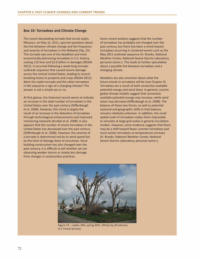
72


Box 10: Tornadoes and Climate Change

The recent devastating tornado that struck Joplin, Missouri, on May 22, 2011, spurred questions about the link between climate change and the frequency and severity of tornadoes in the Midwest (Fig. 23). This tornado was one of the deadliest and most economically distressing tornadoes in U.S. history, costing 116 lives and $2.6 billion in damages (NOAA 2012). It occurred following a week-long tornado outbreak sequence that caused severe damage across the central United States, leading to record-breaking losses to property and crops (NOAA 2012). Were the Joplin tornado and the other tornadoes in the sequence a sign of a changing climate? The answer is not a simple yes or no.

At first glance, the historical record seems to indicate an increase in the total number of tornadoes in the United States over the past century (Diffenbaugh et al. 2008). However, this trend is largely the result of an increase in the detection of tornadoes through technological enhancements and improved monitoring networks (Kunkel et al. 2008). It also appears that the number of severe tornadoes in the United States has decreased over the past century (Diffenbaugh et al. 2008). However, the severity of a tornado is determined not by its wind speed but by the level of damage done to structures. Since building construction has also changed over the past century, it is difficult to tell whether we are observing weaker storms or simply less damage from changes in construction practices.

Some recent analysis suggests that the number of tornadoes has probably not changed over the past century, but there has been a trend toward tornadoes occurring in clustered events such as the May 2011 outbreak sequence (H. Brooks, National Weather Center, National Severe Storms Laboratory, personal comm.). This leads to further speculation about a possible link between tornadoes and a changing climate.

Modelers are also uncertain about what the future trends in tornadoes will be (see Chapter 4). Tornadoes are a result of both convective available potential energy and wind shear. In general, current global climate models suggest that convective available potential energy may increase, while wind shear may decrease (Diffenbaugh et al. 2008). The balance of these two forces, as well as potential seasonal and geographic shifts in that balance, remains relatively unknown. In addition, the small spatial scale of tornadoes makes them impossible to simulate at large grid scales in general circulation models. However, some evidence suggests that there may be a shift toward fewer summer tornadoes and more winter tornadoes as temperatures increase (H. Brooks, National Weather Center, National Severe Storms Laboratory, personal comm.).

Figure 23.—Joplin, MO, spring 2011. (Photo by Jill Johnson, U.S. Forest Service)

73


the intense, straight-line winds. Because this storm is an isolated event, it is impossible to attribute it to local changes in climate. However, current model projections suggest that the convective conditions necessary to create these types of storms may become more frequent (see Chapter 4).

Thunderstorms and Heavy Precipitation EventsThunderstorms are frequent during summer months throughout the assessment area. Thunderstorms account for 50 to 60 percent of annual precipitation in Illinois, and are most prevalent in the southwestern corner of the state (Angel 2012a). Since recordkeeping began in the 1800s, thunderstorms have occurred an average of 40 to 55 days per year across the assessment area (Changnon 2003). The highest incidence has occurred in western Missouri, representing a regional maximum in storm frequency (Changnon 2003). About half of these storms occur during the summer (June, July, August), with the remainder distributed across spring and fall (Changnon 2003). There is no evidence of a change in the severity or frequency of thunderstorms across the United States over the past 100 years (Kunkel et al. 2008). Thunderstorms are reported as days when thunder audibly occurs and, therefore, there is a propensity toward human error and inconsistency in recordkeeping for these measurements (Changnon 2003).

However, studies suggest that heavy precipitation has become more frequent and intense in the United States over the past several decades (Groisman et al. 2012, Kunkel et al. 2008). Across the entire central United States (including the assessment area), moderately heavy precipitation events (0.5 to 1.0 inches) became less frequent, but very heavy precipitation events (greater than 3 inches) increased between 1979 and 2009 compared to the 1948 to 1978 period (Groisman et al. 2012). In addition, the number of extreme precipitation events (greater than 6 inches) has increased up to 40 percent (Groisman

et al. 2012). A recent report examined trends in heavy precipitation events in the Midwest from 1961 to 2011 (Saunders et al. 2012). The authors found that the number of precipitation events of 3 inches or more nearly doubled in Illinois and Missouri, and increases were even greater in Indiana (Saunders et al. 2012).

Winter Storms The assessment area in Illinois, Indiana, and Missouri can experience both ice storms and snowstorms, although the incidence is relatively rare. Snowstorms occur about once per year on average in the area, and decreased over the last century in Missouri and southern Illinois (Changnon 2006). The frequency of snowstorms was similar at the beginning and end of the last century across most of southern Indiana (Changnon 2006). In a study examining winter storms from 1949 to 2003, there appeared to be neither a negative nor positive trend in the number of winter storms in the central United States (including the assessment area). However, there was a trend toward an increasing amount of damage from those storms due to both an increase in infrastructure and an increase in storm intensity, which was interpreted as a trend consistent with increased warming (Changnon 2007).

Although rare, ice storms can be particularly damaging to forests in the region, leading to stem and branch breakage and crown loss (Brommit et al. 2004, Rebertus et al. 1997). Ice storms are a severe form of freezing-rain event. The Central Hardwoods Region has on average 3 to 4 days of freezing-rain events per year, which can occur between November and April, with a peak in January (Changnon and Karl 2003). A study examining changes in freezing rain over the United States from 1949 to 1999 showed no positive or negative trend in the number of freezing-rain events for much of the Central Hardwoods Region, with the exception of far southeastern Indiana, which had a decrease (Changnon and Bigley 2005).

74


CHANGES IN SOILS AND HYDROLOGYIncreases in global temperature are resulting in an intensification of the global water cycle, leading to changes in soil moisture, groundwater availability, and streamflow (Huntington 2006). These variables can have important influences on terrestrial and aquatic ecosystems.

DroughtDroughts are among the greatest stressors on forest ecosystems, and can often lead to secondary effects of insect and disease outbreaks on stressed trees and increased fire risk. Drought can be characterized in several ways, notably as meteorological, hydrologic, or agricultural drought. Meteorological drought is a function of precipitation frequency, and hydrologic drought is a measure of how much water is available in a watershed. Agricultural drought takes into account changes in the amount of water that evaporates from the soil and is transpired by plants, as well as information about soil moisture and groundwater supply. All three indicators can be important in understanding the effects on forest water supply. However, examining agricultural drought can give a more holistic picture of the effects on vegetation in the soil.

Over the past century (1916 to 2007), the frequency of extreme and exceptional droughts (meteorological, hydrologic, and agricultural) in Illinois and Indiana decreased (Mishra et al. 2010). (Data were not analyzed for Missouri.) Exceptional droughts are the most severe form of drought experienced in the region, and extreme droughts are the second most severe. Until the recent drought of 2012, all of the exceptional droughts were before 1970, and most of them occurred during the “Dust Bowl” era of the 1930s. In general, more recent drought events have been less intense in their severity, duration, and spatial extent compared

to earlier in the 20th century. However, the 1988 drought was the fifth-driest year on record in llinois, which led to severe water shortages throughout the assessment area (Lamb 1992). In addition, the 2012 drought was the most extensive drought on record across the United States since 1956 (NCDC 2012). One study examined the drought trends during specific points in the growing season in Illinois and Indiana from 1916 to 2007 (Mishra and Cherkauer 2010). They found an overall decrease in drought severity and frequency in southern Indiana and no change in southern Illinois in spring (March through May), summer (June through August), and the entire growing season (May through October).

SnowAlthough snow does not play as large a role in the Central Hardwoods Region as it does in states farther north, it is still an important aspect of hydrology for the region. The amount of snow influences annual runoff, recharge, and water supplies and can have local effects on temperature through its reflectivity (albedo). In addition, rapid melting following a large snowfall event can lead to flooding. Between 1981 and 2010, the region received on average roughly 6 to 12 inches of snow per year (Kunkel et al. 2013). Long-term records reveal a general decrease in snowfall in Missouri since the 1930s (Kunkel et al. 2009). Trends in snowfall in southern Illinois and Indiana are less clear, with some stations reporting increases and others decreases, over the past 80 years (Kunkel et al. 2009). The ratio of snow to total precipitation during the winter decreased in the area between 1949 and 2005 due to both a decrease in snowfall and an increase in rain during that time (Feng and Hu 2007). According to the Illinois state climatology office, statewide snowfall has decreased in the most recent 20 years and is below the long-term average (Angel 2012b). There is also a trend toward earlier snowmelt and decreasing snow depth in the area (Dyer and Mote 2006).

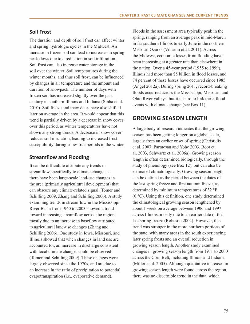
75


Soil FrostThe duration and depth of soil frost can affect winter and spring hydrologic cycles in the Midwest. An increase in frozen soil can lead to increases in spring peak flows due to a reduction in soil infiltration. Soil frost can also increase water storage in the soil over the winter. Soil temperatures during the winter months, and thus soil frost, can be influenced by changes in air temperature and the amount and duration of snowpack. The number of days with frozen soil has increased slightly over the past century in southern Illinois and Indiana (Sinha et al. 2010). Soil freeze and thaw dates have also shifted later on average in the area. It would appear that this trend is partially driven by a decrease in snow cover over this period, as winter temperatures have not shown any strong trends. A decrease in snow cover reduces soil insulation, leading to increased frost susceptibility during snow-free periods in the winter.

Streamflow and FloodingIt can be difficult to attribute any trends in streamflow specifically to climate change, as there have been large-scale land-use changes in the area (primarily agricultural development) that can obscure any climate-related signal (Tomer and Schilling 2009, Zhang and Schilling 2006). A study examining trends in streamflow in the Mississippi River Basin from 1940 to 2003 showed a trend toward increasing streamflow across the region, mostly due to an increase in baseflow attributed to agricultural land-use changes (Zhang and Schilling 2006). One study in Iowa, Missouri, and Illinois showed that when changes in land use are accounted for, an increase in discharge consistent with local climate changes could be observed (Tomer and Schilling 2009). These changes were largely observed since the 1970s, and are due to an increase in the ratio of precipitation to potential evapotranspiration (i.e., evaporative demand).

Floods in the assessment area typically peak in the spring, ranging from an average peak in mid-March in far southern Illinois to early June in the northern Missouri Ozarks (Villarini et al. 2011). Across the Midwest, economic losses from flooding have been increasing at a greater rate than elsewhere in the nation. Over a 45-year period (1955 to 1999), Illinois had more than $5 billion in flood losses, and 74 percent of these losses have occurred since 1985 (Angel 2012a). During spring 2011, record-breaking floods occurred across the Mississippi, Missouri, and Ohio River valleys, but it is hard to link these flood events with climate change (see Box 11).

GROWING SEASON LENGTHA large body of research indicates that the growing season has been getting longer on a global scale, largely from an earlier onset of spring (Christidis et al. 2007, Parmesan and Yohe 2003, Root et al. 2003, Schwartz et al. 2006a). Growing season length is often determined biologically, through the study of phenology (see Box 12), but can also be estimated climatologically. Growing season length can be defined as the period between the dates of the last spring freeze and first autumn freeze, as determined by minimum temperatures of 32 °F (0 °C). Using this definition, one study determined the climatological growing season lengthened by about 1 week on average between 1906 and 1997 across Illinois, mostly due to an earlier date of the last spring freeze (Robeson 2002). However, this trend was stronger in the more northern portions of the state, with many areas in the south experiencing later spring frosts and an overall reduction in growing season length. Another study examined changes in growing season length from 1911 to 2000 across the Corn Belt, including Illinois and Indiana (Miller et al. 2005). Although qualitative increases in growing season length were found across the region, there was no discernible trend in the data, which

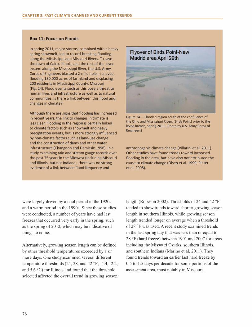
76


Box 11: Focus on Floods

In spring 2011, major storms, combined with a heavy spring snowmelt, led to record-breaking flooding along the Mississippi and Missouri Rivers. To save the town of Cairo, Illinois, and the rest of the levee system along the Mississippi River, the U.S. Army Corps of Engineers blasted a 2-mile hole in a levee, flooding 130,000 acres of farmland and displacing 200 residents in Mississippi County, Missouri (Fig. 24). Flood events such as this pose a threat to human lives and infrastructure as well as to natural communities. Is there a link between this flood and changes in climate?

Although there are signs that flooding has increased in recent years, the link to changes in climate is less clear. Flooding in the region is partially linked to climate factors such as snowmelt and heavy precipitation events, but is more strongly influenced by non-climate factors such as land-use change and the construction of dams and other water infrastructure (Changnon and Demissie 1996). In a study examining rain and stream gauge records over the past 75 years in the Midwest (including Missouri and Illinois, but not Indiana), there was no strong evidence of a link between flood frequency and

anthropogenic climate change (Villarini et al. 2011). Other studies have found trends toward increased flooding in the area, but have also not attributed the cause to climate change (Olsen et al. 1999, Pinter et al. 2008).

Figure 24.—Flooded region south of the confluence of the Ohio and Mississippi Rivers (Birds Point) prior to the levee breach, spring 2011. (Photo by U.S. Army Corps of Engineers)

were largely driven by a cool period in the 1920s and a warm period in the 1990s. Since these studies were conducted, a number of years have had last freezes that occurred very early in the spring, such as the spring of 2012, which may be indicative of things to come.

Alternatively, growing season length can be defined by other threshold temperatures exceeded by 1 or more days. One study examined several different temperature thresholds (24, 28, and 42 °F; -4.4, -2.2, and 5.6 °C) for Illinois and found that the threshold selected affected the overall trend in growing season

length (Robeson 2002). Thresholds of 24 and 42 °F tended to show trends toward shorter growing season length in southern Illinois, while growing season length trended longer on average when a threshold of 28 °F was used. A recent study examined trends in the last spring day that was less than or equal to 28 °F (hard freeze) between 1901 and 2007 for areas including the Missouri Ozarks, southern Illinois, and southern Indiana (Marino et al. 2011). They found trends toward an earlier last hard freeze by 0.5 to 1.5 days per decade for some portions of the assessment area, most notably in Missouri.

77


Box 12: Phenological Indicators of Change

Changes in growing season length can be observed through changes in phenology. Phenology is the study of recurring plant and animal life-cycle stages, such as leaf-out and senescence, flowering, maturation of agricultural plants, emergence of insects, and migration of birds. A few studies examining changes in phenology in the Central Hardwoods Region indicate recent changes:

• In a survey of 270 flowering plants in southwestern Ohio, 60 percent showed earlier spring flowering over the period from 1976 to 2003 of about 10 to 32 days (McEwan et al. 2010). The variation among species may be attributed to differences in sensitivity to climate as a clue to begin flowering as opposed to other indicators such as day-length.

• A study examining the migratory patterns of eight species of North American wood warblers between southern Illinois and northern Minnesota from 1903 to 2002 showed that their migration season was being compressed by up to 20 days due to later springs in Illinois and earlier springs in Minnesota (Strode 2003). Spring onset was determined by the date when 300 degree-days over 41 °F (5 °C) were reached, which is the beginning of the peak in spruce budworm caterpillar activity, a primary food consumed by many warbler species. This study shows that, although average temperatures have not changed significantly in the spring in southern Illinois, certain climate indicators important to biological functioning have changed.

• Despite global and national trends, there do not appear to be trends toward an earlier start of the growing season as determined by leaf emergence in Missouri, southern Illinois, or southern Indiana between 1901 and 2007 (Marino et al. 2011). In fact, there is a general trend (though not significant) toward later leaf emergence in much of the area by 5 to 10 days over the period examined. By contrast, the date of the last hard freeze in the area does appear to be about 5 to 16 days earlier (Marino et al. 2011). This trend indicates an overall decrease of risk of “false springs,” where leaf emergence occurs before the last hard frost (Marino et al. 2011).

• A study using satellite data of forest leaf emergence found a trend toward a later end of the growing season between 1989 and 2008 across much of the eastern United States, including the Missouri Ozarks and southern Indiana (Dragoni and Rahman 2012).

• Measurements of tree leaf-out and photosynthesis taken in a forest in south-central Indiana indicate that the growing season lengthened by 30 days from 1998 to 2008 (Dragoni et al. 2011). This study measured carbon uptake as well as leaf emergence and senescence, and determined that the end of the season trended later over the course of the 10 years. The authors attributed this increase to a warming trend in air and soil temperatures and a decrease in cold degree-days (the sum of the deviation of daily mean air temperature from the 10-year average) during the summer. A caveat to this study is that it was for one isolated site over a short period.

CHAPTER SUMMARYThe climate of the Central Hardwoods Region has changed considerably over thousands of years, but recent changes over the past 100 years have been more subtle. Temperatures have increased both globally and across the United States over the same time period, yet the mean annual temperature in

the Central Hardwoods Region actually decreased slightly in some areas—a change small enough that it could have occurred by chance. The difference between daily high and low temperatures also appears to be decreasing. High temperatures during summer months have decreased by about 2 °F over the last century while summer lows have increased by about the same amount. Data indicate that

78


Box 13: Species Range Shifts

Given that there are some indications of warming temperatures across the Northern Hemisphere, one might expect that species may be starting to move northward along with their climatological niches. Evidence across the globe is beginning to support this hypothesis (Chen et al. 2011, Parmesan and Yohe 2003). Is there any evidence of northward migration in the Central Hardwoods Region?

In order to determine species range shifts, long-term data over large spatial scales must be available. The Forest Service’s Forest Inventory and Analysis (FIA) Program is one source of this type of information. A recent study using FIA data (Woodall et al. 2009) examined range shifts in tree species across the eastern United States by comparing the mean latitude of seedlings to that of mature trees. The researchers found a strong northward shift in northern species such as sugar maple and basswood. However, trends in southern species were more mixed, with some species shifting northward (shortleaf pine, yellow-poplar) and others shifting southward (southern red oak, blackjack oak).

In a subsequent study using FIA data, Zhu et al. (2011) examined changes in the 5th and 95th percentile of latitudinal bands for seedlings, saplings, and mature trees in order to examine latitudinal shifts in range limits (as opposed to averages) in the eastern United States. In contrast to the Woodall et al. (2009) study, this study found that the majority of trees did not undergo northward migration, but rather showed range contraction, where seedlings had smaller northern and southern range limits than mature trees. One caveat to that study was that few plots fall into the 5th and 95th percentiles, meaning sample size was low.

These studies indicate that biological responses to climate change are not always clear or predictable. In addition, they suggest that there may be barriers to northward migration for some tree species, such as habitat fragmentation or inherent biological differences in seed dispersal ability. Finally, the methods used for determining northward migration (mean latitude versus range limit changes) can lead to different conclusions.

much of the area is receiving between 12 and 17 percent more precipitation annually, with increases in heavy precipitation events and decreases in severe droughts. There is insufficient information to determine whether tornadoes and thunderstorms are more frequent now than they have been since measurements began, but there is some evidence that winter storms, though less frequent now than in the past, are more intense when they do occur. Flooding in the area has increased, but this increase has been

attributed to changes in human land use and not climate. Although there are no strong indications of changes in winter temperature, soil frost has increased in the area, which has been attributed to a decrease in snow. In addition, some evidence suggests that stream discharge has increased in some areas, which has important implications for local hydrology. These changes in climate in the region may already be leading to forest response (see Box 13).

79

CHAPTER 4: PROJECTED CHANGES IN CLIMATE AND OTHER PHYSICAL PROCESSES

In Chapter 3, we examined how climate has changed in the assessment area over the past based on measurements and proxy data. In this chapter, we examine how climate may change over the next century. General circulation models (GCMs) are used to project future change at coarse spatial scales and then downscaled to be relevant at scales where land management decisions are made. In some cases, these downscaled data are then incorporated into hydrologic models to better understand impacts on such variables as soil moisture, evapotranspiration, and streamflow. Downscaled data are also incorporated into forest species distribution models and process models (see Chapters 2 and 5). If you are unfamiliar with GCMs, downscaling, and impact models, an overview and suggestions for further reading are provided in Chapter 2.

TEMPERATURE AND PRECIPITATION PROJECTIONS In this chapter, we report downscaled climate projections for two model-emissions scenario combinations: GFDL A1FI and PCM B1 (unless otherwise noted). The GFDL A1FI model-scenario combination represents a higher-end projection for future temperature increases, and the PCM B1 represents a lower end (see Chapter 2). It is possible that actual emissions and temperature increases could be lower or higher than either of these projections. However, the GFDL A1FI scenario represents a more realistic projection of future greenhouse gas emissions and temperature increases based on current trends. The future will probably be different from any of the developed scenarios, so we encourage readers to consider the range of possible

climate conditions over the coming decades rather than one particular scenario.

Daily mean, maximum, and minimum temperature and total daily precipitation were downscaled to an approximately 7.5-mile grid across the United States (see Chapter 2). To visualize changes, we calculated the modeled average daily mean, maximum, and minimum temperature for each season and the entire year for three 30-year time periods (2010 to 2039, 2040 to 2069, 2070 to 2099). Daily precipitation values were summed by year and season, and 30-year means were calculated. We subtracted temperature and precipitation values from the 1971 to 2000 mean values as a baseline to determine the departure from current climate conditions. Historical climate data used for the departure analysis were taken from ClimateWizard based on the PRISM data set (Girvetz et al. 2009; see Chapter 3 and Appendix 7).

Temperature Both models project increases in mean, minimum, and maximum temperatures across all time periods and for all seasons. Mean annual temperature across the assessment area is projected to increase by 7.3 °F (4.0 °C) under the GFDL A1FI scenario and 1.6 °F (0.9 °C) under PCM B1 for the final 30 years of the 21st century (Fig. 25; see also Table 20 in Appendix 8) compared to the 1971 to 2000 baseline. The most dramatic increase in temperature is projected for winter for the PCM B1 scenario and summer for the GFDL A1FI scenario. Temperature increases are projected to be greatest in Missouri and least in Indiana, especially for the PCM B1 scenario (Fig. 26).

80


Figure 25.—Daily mean, minimum, and maximum temperature averaged over 30-year time periods. Annual, winter (December through February), spring (March through May), summer (June through August), and fall (September through November) values are shown. The 1971 through 2000 value is based on observational data from weather stations. The 21st-century data are averages of downscaled daily projections under two climate model-emissions scenario combinations.

20

30

40

50

60

70

80

90

100

1971 - 2000 2010 - 2039 2040 - 2069 2070 - 2099

Tem

pera

ture

(°F)

Annual

20

30

40

50

60

70

80

90

100

1971 - 2000 2010 - 2039 2040 - 2069 2070 - 2099

Tem

pera

ture

(°F)

Winter

20

30

40

50

60

70

80

90

100

1971 - 2000 2010 - 2039 2040 - 2069 2070 - 2099

Tem

pera

ture

(°F)

Spring

20

30

40

50

60

70

80

90

100

1971 - 2000 2010 - 2039 2040 - 2069 2070 - 2099

Tem

pera

ture

(°F)

Summer

20

30

40

50

60

70

80

90

100

1971 - 2000 2010 - 2039 2040 - 2069 2070 - 2099

Tem

pera

ture

(°F)

Fall

GFDL A1FI mean

PCM B1 mean

GFDL A1FI minimum

PCM B1 minimum

GFDL A1FI maximum

PCM B1 maximum

▲▄

▲▄

▲▄

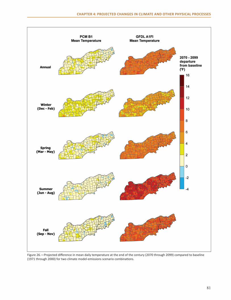
81


Figure 26.—Projected difference in mean daily temperature at the end of the century (2070 through 2099) compared to baseline (1971 through 2000) for two climate model-emissions scenario combinations.

82


The average daily minimum temperature is projected to increase 7.0 °F (3.9 °C) under the GFDL A1FI scenario and 1.0 °F (0.6 °C) under PCM B1for the final 30 years of the 21st century compared to the 1971 to 2000 baseline. Similar to daily means, increases are greatest in the summer for GFDL and

greatest in the winter for PCM. Southern Illinois is projected to have the greatest increase in minimum temperatures, and Indiana the least, across all seasons (Fig. 27). These patterns are generally true for the 2010 to 2039 and 2040 to 2069 periods as well (see Appendix 8 for these time periods).

Figure 27.—Projected difference in mean daily minimum temperature at the end of the century (2070 through 2099) compared to baseline (1971 through 2000) for two climate model-emissions scenario combinations.

83


The average daily maximum temperature is projected to increase 7.6 °F (4.2 °C) under the GFDL A1FI scenario and 1.6 °F (0.9 °C) under PCM B1 for the final 30 years of the 21st century, a slightly greater increase than for daily mean and minimum temperatures. As with daily means and minimums, the most dramatic increase in daily maximum temperatures appears to be during the winter for PCM and summer for GFDL (see Box 14). Increases in daily maximum temperatures are projected to be greatest in Missouri, especially in winter (Fig. 28).

These patterns are also true for the earlier 30-year periods (see Appendix 8).

Differences between the two model-scenario combinations are projected to be more distinct by the end of the century (Fig. 26). In general, changes in temperature are projected to be similar between the two scenarios for the 2010 to 2039 period. By the end of the century, however, temperatures are projected to be much higher under the GFDL A1FI scenario than PCM B1.

Box 14: Revisiting the “Warming Hole”

In Chapter 3, we discussed the “warming hole” that has been observed across the central United States, characterized by a reduction in summer high temperatures over the past several decades. Will this pattern continue into the future? If we examine just the statistically downscaled GCM data presented in this chapter, we might conclude that the warming hole will be gone in the next century.

However, at least one study suggests that the large grid-scale of GCMs fails to account for regional-scale processes that are important contributors to the warming hole (Liang et al. 2006). Using a dynamical downscaling approach with the PCM model as an input, this study found a large discrepancy between the downscaled projections and the original coarse-scale PCM projections in summer temperatures in the central United States, particularly Missouri and southern Illinois. Although both projected an

increase in summer temperature, the dynamically downscaled model projected an increase of less than 0.5 °F (1 °C), while the coarse-scale PCM projected an increase of 5.4 °F (3 °C) or more at mid-century. The statistically downscaled projections for PCM presented in this chapter also suggest a more modest increase in summer temperatures.

So what do these projections mean for the “warming hole”? The results suggest that, as with past observations, there may continue to be regional climate processes that reduce the amount of warming experienced during the summer in the central United States, at least over the short term. However, dynamical downscaling studies such as this one remain limited, justifying the consideration of a range of potential future climate scenarios when preparing for future climate change.

84


Figure 28.—Projected difference in mean daily maximum temperature at the end of the century (2070 through 2099) compared to baseline (1971 through 2000) for two climate model-emissions scenario combinations.

85


PrecipitationThe magnitude and seasonal direction of projected changes in precipitation are not consistent between the two models used in this assessment. Mean annual precipitation is projected to decrease by 3.1 inches under the GFDL A1FI scenario for the final 30 years of the 21st century (Fig. 29; see also Table 21 in

Appendix 8) compared to the 1971 to 2000 baseline. Annual decreases are projected to be greatest in Missouri under that scenario (Fig. 30). By contrast, annual precipitation is projected to increase under the PCM B1 scenario by an average of 2.9 inches for the final 30 years of the century.

Figure 29.—Annual and seasonal precipitation for the assessment area over 30-year time periods. The 1971 through 2000 value is based on observational data from weather stations. The 21st-century data are averages of downscaled daily projections under two climate model-emissions scenario combinations.

40

41

42

43

44

45

46

47

48

1971 - 2000 2010 - 2039 2040 - 2069 2070 - 2099

Prec

ipita

tion

(inch

es)

Annual

0

2

4

6

8

10

12

14

16

18

1971 - 2000 2010 - 2039 2040 - 2069 2070 - 2099

Prec

ipita

tion

(inch

es)

Winter

0

2

4

6

8

10

12

14

16

18

1971 - 2000 2010 - 2039 2040 - 2069 2070 - 2099

Prec

ipita

tion

(inch

es)

Summer

Annual

0

2

4

6

8

10

12

14

16

18

1971 - 2000 2010 - 2039 2040 - 2069 2070 - 2099

Prec

ipita

tion

(inch

es)

Spring

0

2

4

6

8

10

12

14

16

18

1971 - 2000 2010 - 2039 2040 - 2069 2070 - 2099

Prec

ipita

tion

(inch

es)

Fall

P CM B 1

G F DL A1F I

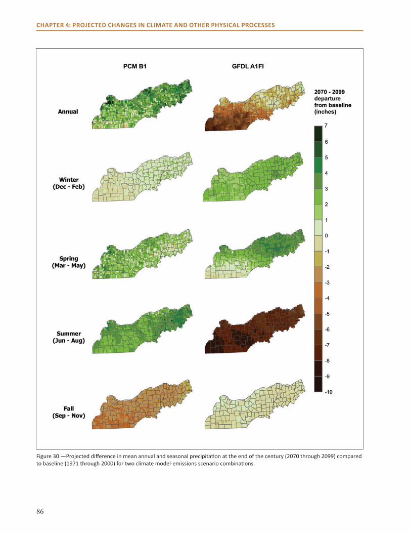
86


Figure 30.—Projected difference in mean annual and seasonal precipitation at the end of the century (2070 through 2099) compared to baseline (1971 through 2000) for two climate model-emissions scenario combinations.

87


Changes in precipitation are projected to vary greatly by season. Under the GFDL A1FI scenario, precipitation is projected to be higher in the winter and spring and much lower in the summer across all parts of the assessment area. The increases are projected to be slightly more modest and the decreases greater in Missouri compared to the eastern portion of the assessment area. Under the PCM B1 scenario, winter precipitation increases are projected to be much more modest than under GFDL, and projections for spring projections are similar to GFDL. Summer precipitation under the PCM B1 scenario is projected to increase—the opposite of what is projected under the GFDL model. Fall projections for both scenarios show decreases in precipitation, with more consistent decreases under PCM B1.

Unlike changes in temperature, projected changes in precipitation do not consistently follow a linear path over time in all seasons (Fig. 29). Projected changes in summer precipitation are relatively linear for both models, but in opposite directions. During winter, both models project an increase in precipitation over the next century, but PCM B1 projects the greatest increase will be between 2040 and 2069, whereas GFDL A1FI projects the greatest increase at the end of the century. Spring precipitation increases initially and then decreases slightly under PCM, while it remains steady under GFDL. The GFDL A1FI scenario projects fall precipitation amounts just slightly below historical averages for the 2040 to 2069 and 2070 to 2099 periods, but shows a dip in precipitation during the 2010 to 2039 period. By contrast, PCM, shows a linear decrease in precipitation during the fall.

EXTREME WEATHER EVENTSAs mentioned in Chapter 3, extreme weather events such as tornadoes and thunderstorms can be devastating to natural and human systems. In general, there is less confidence in model projections of the magnitude and direction of change in extreme

events over the next century compared with general temperature and precipitation changes, but recent research is beginning to provide more evidence for projected increases in many extreme weather events across the Midwest (Kunkel et al. 2013).

Heavy Precipitation EventsClimate models project an overall increase in the number of heavy precipitation events globally by the end of the century (Intergovernmental Panel on Climate Change [IPCC] 2007, 2012). There is greater agreement among models at high latitudes and in the tropics, but model projections for the central United States suggest a potential increase in these events, especially during winter months (IPCC 2012). Other future climate projections indicate that the Midwest may experience 2 to 4 more days of extreme precipitation by the end of the century (Diffenbaugh et al. 2005). However, downscaled projections for the Midwest indicate less projected change in heavy precipitation events (greater than 1 inch) in the Central Hardwoods Region than the Midwest as a whole (Kunkel et al. 2013). With the exception of south-central Indiana, fewer than 50 percent of climate models project an increase in the number of heavy precipitation events in the region (Kunkel et al. 2013).

ThunderstormsAlthough GCMs do not operate at a scale small enough to model thunderstorms explicitly, evidence suggests that temperature increases will lead to conditions more favorable to convective storms such as thunderstorms (Kunkel et al. 2008; Trapp et al. 2007, 2009). One study examined changes in thunderstorm potential over the 21st century using a mid-range emissions scenario (A1B; Trapp et al. 2009). A slight increase was found in the frequency of conditions favorable for intense thunderstorms in the Midwest. A similar study found an increase in thunderstorm potential in the region at the end of the century under a higher emissions scenario (A2; Trapp et al. 2007).

88


Tornadoes and HailVery little is known about how the frequency, severity, and seasonal patterns of tornadoes and hail may change over the next century. A recent synthesis report on extreme weather events stated that “there is low confidence in projections of small spatial-scale phenomena such as tornadoes and hail because competing physical processes may affect future trends and because current climate models do not simulate such phenomena” (IPCC 2012). As the sophistication of global and regional climate models increases, so will our understanding of how patterns in hail and tornadoes may change in the future.

Winter StormsAlthough winter storms such as snowstorms and ice storms are relatively rare in the area, they can nonetheless be devastating when they do occur. Warming temperatures may lead to a decrease in the overall frequency of ice storms and snowstorms due to a reduction in the number of days that are cold enough for those events to occur. However, there is also some evidence to suggest that these events could be more intense when they do happen. Wang and Zhang (2008) examined changes in risk of extreme precipitation during the winter months under the A2 emissions scenario using statistically downscaled climate projections. They found an increased risk for extreme winter events at the end of the century for the central United States, which includes the western part of the assessment area. Whether these events occur as rain, snow, or ice will depend on the exact timing of these events and their interaction with projected changes in temperature. In general, more research is needed before we can determine the most likely effects of future climate change on winter storms.

Temperature ExtremesIn addition to changes in means, temperature extremes are also projected to shift across the region. Studies from across the Midwest indicate that there will be more days per year that are warmer than

95 °F (35 °C) and a greater frequency of multi-day heat waves over the 21st century (Diffenbaugh et al. 2005, Kunkel et al. 2013, Winkler et al. 2012). Within the Midwest, the Central Hardwoods Region is projected to see the greatest increase in such events, and could experience 20 to 30 more extremely hot days by mid-century (Kunkel et al. 2013). The number of consecutive days above 95 °F (35 °C) could increase by 8 to 16 days in the Central Hardwoods Region by mid-century (Kunkel et al. 2013). Downscaled climate scenarios also project that the Midwest will experience between 25 and 38 fewer days below freezing by the end of the 21st century (Sinha and Cherkauer 2010). However, less of a decrease is projected in the western Midwest (Kunkel et al. 2013). A decrease in extreme cold days (less than 10 °F [-12 °C]) is projected to be more moderate in the Central Hardwoods Region, where there are not as many extremely cold days to begin with, than in the rest of the Midwest (Kunkel et al. 2013).

HYDROLOGIC IMPLICATIONSInformation regarding how temperature and precipitation patterns may change across the assessment area can further be used to examine how these changes may affect the cycling of water in terrestrial and aquatic ecosystems. Across the globe, increases in temperature are projected to intensify the hydrologic cycle, leading to greater evaporative losses and more heavy precipitation events (IPCC 2007).

By examining soil moisture, evapotranspiration, and various drought indices, we can gain an important understanding of how these changes may affect water availability for trees, understory plants, wetlands, and rivers. In addition, examining changes in runoff and streamflow can help us assess potential flood risks and changes in watershed dynamics. The dynamics of snow and frozen soil can affect soil water availability, soil temperatures, streamflow dynamics, and soil erosion processes.

89


Many of the results presented below use the Variable Infiltration Capacity (VIC) hydrologic model, which is described in more detail in Chapter 2. Model results are currently available only for the Illinois and Indiana portions of the assessment area, so implications for the Missouri Ozarks are not yet known. However, because the soil types and projected changes in climate for the Missouri Ozarks are similar to southwestern Illinois, it can be assumed that the general patterns observed there will be similar, especially in the east.

EvapotranspirationEvapotranspiration, the combination of evaporation from the soil and transpiration from plants, is an important indicator of moisture availability in an ecosystem and the amount of water available to be lost as runoff. According to one study using statistically downscaled GCM projections under two emissions scenarios, evapotranspiration is projected to increase during the winter and spring and decrease during the summer in southern Illinois and Indiana by the end of the 21st century (2070 to 2099) compared to the 1977 to 2006 average (Cherkauer and Sinha 2010). These trends are strongly tied to projected increases in winter and spring precipitation and decreases in summer precipitation in the region.

As more water becomes available, more can be evaporated or transpired. Temperature can also increase evapotranspiration, but is limited by the amount of water that is available in the soil, water bodies, and atmosphere.

Projected changes in evapotranspiration vary considerably by hydrologic model and climate models used, and whether changes in vegetation are also considered. Another recent study, using the same hydrologic model as above but different climate projections, found an increase in evapotranspiration across the assessment area in spring, summer, and fall and no change in winter from 2071 through 2100 (Ashfaq et al. 2010). As we will discuss in Chapters 5 and 6, climate change is also projected to affect the distribution of trees and other plant species, which could also affect evapotranspiration on the landscape. Increases in carbon dioxide are expected to lead to changes in water use efficiency of vegetation (Drake et al. 1997), but these changes are not currently accounted for in model projections of evapotranspiration across the region.

Examining changes in seasonal ratios of evapotranspiration to precipitation can give a general sense of how much water is available in the soil and watershed. Ratios greater than 1.0 signify evapotranspiration exceeds precipitation, an indication of drier conditions. Ratios less than 1.0 signify precipitation exceeds evapotranspiration, an indication of wetter conditions. Changes in this ratio were calculated by using data from Cherkauer and Sinha (2010), and mapped (Fig. 31). An increase in the ratio over time signifies a decrease in water availability compared to historical levels, and a decrease indicates an increase in water availability. The data indicate a slight increase in water availability on an annual basis. Spring precipitation was projected to show the biggest increase in water availability, and a decrease was projected for summer.

Waterfall on the Hoosier National Forest. Photo by Gerald Scott, Hoosier National Forest.

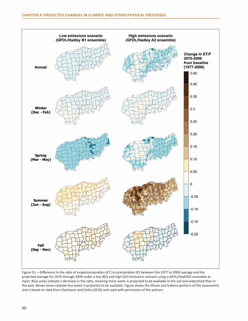
90


Figure 31.—Diff erence in the ra o of evapotranspira on (ET) to precipita on (P) between the 1977 to 2006 average and the projected average for 2070 through 2099 under a low (B1) and high (A2) emissions scenario using a GFDL/HadCM3 ensemble as input. Blue areas indicate a decrease in the ra o, meaning more water is projected to be available in the soil and watershed than in the past. Brown areas indicate less water is projected to be available. Figure shows the Illinois and Indiana por ons of the assessment and is based on data from Cherkauer and Sinha (2010) and used with permission of the authors.

91


Soil Moisture and DroughtChanges in soil moisture are largely driven by the balance of precipitation and evapotranspiration, and thus there is some uncertainty about future changes. Based on projected decreases in precipitation during summer and fall and increases in temperature throughout the year, one study found that surface soil moisture was projected to decrease in the area over the next century (2009 to 2099) by a small amount (1.2 to 1.6 percent, depending on scenario; Mishra et al. 2010). Total soil moisture was also projected to decrease in the late summer and fall and increase in the winter and spring. Another study in the region suggests a decrease in soil moisture during winter and early spring and increases in soil moisture during the growing season (Winter and Eltahir 2012). The difference between the two studies suggests that model assumptions made and scenarios chosen can have a large impact on projections of future soil moisture in the Midwest. Currently, most climate models project a decrease or no change in precipitation during summer months over the assessment area, leading to an overall decrease in summer soil moisture when coupled with increased temperature (Wang 2005). However, there is a lot of variation among models, and an increase in precipitation (and also soil moisture) is not outside the realm of possibility.

Changes in precipitation are also expected to lead to changes in drought characteristics, such as intensity, duration, frequency, and spatial extent. According to one study, the projected changes in duration of drought periods in Illinois and Indiana over the next century differ among models, scenario, and time period, with most projecting an increase in drought duration (Mishra et al. 2010). That study also suggested the spatial extent of droughts may increase, indicating that future droughts may shift from more local to more regional phenomena (Mishra et al. 2010). However, the number of exceptional droughts (the most severe type of

drought) and the number of multi-year droughts was not projected to change much from the number experienced in the 20th century (Mishra et al. 2010). Another study projected an increase in drought frequency and severity when climate models that projected a decrease in precipitation were used as inputs, but no change in drought for those projecting a precipitation increase (Wang et al. 2011). This study was conducted for a primarily agricultural area north of the assessment area, so it is unclear if these results can be translated directly to the soils and vegetation types in the Central Hardwoods Region. No current information is available related to drought characteristics for the Missouri Ozarks.

Runoff, Streamflow, and FloodingRunoff in southern Illinois and Indiana is projected to increase slightly over the next century compared to the 30-year average from 1977 to 2006, particularly in the winter and spring (Cherkauer and Sinha 2010). This increase reflects in part projected increases in precipitation during these seasons. Future changes in summer and fall runoff are less certain, with some scenarios and locations projecting a decrease in runoff and others projecting no change or an increase (Cherkauer and Sinha 2010).

Streamflow is also projected to change in the area, with changes varying by season. In recent decades, winter and spring have had the highest number of high-flow days, and, in general, the number of high-flow days is projected to increase further during these seasons (Cherkauer and Sinha 2010). Projected changes in high-flow days in the summer and fall are more mixed and vary based on location. Changes in low-flow days also will vary by season: the number of low-flow days is projected to increase in summer and fall and decrease in the winter and spring. Simulations for streamflow in the Wabash River watershed showed increases of about 20 percent for both peak and mean streamflow by the end of the century (Cherkauer and Sinha 2010). Similarly,

92


mid-century projections of the Upper Mississippi basin showed a 50-percent increase in annual average streamflow, with the largest increase occurring in spring and summer as a result of increases in snowfall, snowmelt, runoff, and recharge upstream of those areas (Jha et al. 2004).

Change in flood risk under future climate change is difficult to determine because there are currently insufficient records to even determine flood risk at a particular location, irrespective of climate (Stedinger and Griffis 2011). As discussed in Chapter 3, flooding is caused by a combination of climate, infrastructure, and human land-use factors, so the relative amount of change in these different factors will determine the overall flood risk. The studies described above suggest that the magnitude of flooding could potentially increase in the winter and spring due to increases in total runoff and peak streamflow during those times (Cherkauer and Sinha 2010). During the summer and fall, there could be an increase in “flashiness,” with periods of very low flow followed by rapid flooding in response to heavy rain events (Cherkauer and Sinha 2010). Because of the lack of research specifically addressing future flood dynamics in the region, we currently have low certainty about future changes in flooding.

Snow and Other Winter ProcessesIncreases in temperature during winter months are expected to lead to decreases in snow duration and extent across the region in the coming decades. Simulations of changes in snow cover extent in North America over the 21st century suggest that it will continue to decrease, and at a faster rate than it did during the 20th century (Frei and Gong 2005). Similarly, another study projected declining snow cover duration in the eastern United States over the 21st century (Brown and Mote 2009). Trends in the annual maximum snow water equivalent (i.e., the amount of water contained in snowpack) over the

21st century are less clear, but most models project a decrease across the assessment area (Brown and Mote 2009). These broader trends are expected to be manifested as a reduction in snow across the Central Hardwoods Region, as it is already a marginal area for snow.

To examine changes in winter processes at a more regional level, Sinha and Cherkauer (2010) simulated changes in snow water equivalent, soil frost, and other winter processes by using two downscaled GCMs (HadCM3 and GFDL) and B1, A1B, and A2 emissions scenarios as inputs into the VIC model for Illinois and Indiana. With the exception of the high emissions scenario in the 2010 to 2039 period, their study projected an overall reduction in the amount of snow water equivalent, which was due to an increase in temperature and a decrease in snowfall (Sinha and Cherkauer 2010). Their study also indicated a reduction in the number of days the soil is frozen in the middle and late century, and suggested that far southern Illinois and Indiana may experience years without soil frost at the end of the century. Although a reduction in soil frost days could increase water infiltration into the soil and reduce runoff, it could also lead to greater soil water losses through increased evapotranspiration and an increased susceptibility to pest outbreaks (Sinha and Cherkauer 2010).

Freeze-thaw cycles can be important determinants of soil erosion risk. All other things being equal, fewer freeze-thaw cycles may result in less erosion. Southern Illinois and Indiana are projected to experience as many as three fewer freeze-thaw cycles by the end of the century under both high and low emissions scenarios (Sinha and Cherkauer 2010). Because much of the area currently experiences three or fewer cycles in an average year, this projection indicates that many years at the end of the century may not have any freeze-thaw cycles.

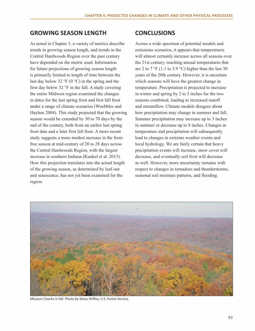
93


GROWING SEASON LENGTHAs noted in Chapter 3, a variety of metrics describe trends in growing season length, and trends in the Central Hardwoods Region over the past century have depended on the metric used. Information for future projections of growing season length is primarily limited to length of time between the last day below 32 °F (0 °C) in the spring and the first day below 32 °F in the fall. A study covering the entire Midwest region examined the changes in dates for the last spring frost and first fall frost under a range of climate scenarios (Wuebbles and Hayhoe 2004). This study projected that the growing season would be extended by 30 to 70 days by the end of the century, both from an earlier last spring frost date and a later first fall frost. A more recent study suggests a more modest increase in the frost-free season at mid-century of 20 to 28 days across the Central Hardwoods Region, with the largest increase in southern Indiana (Kunkel et al. 2013). How this projection translates into the actual length of the growing season, as determined by leaf-out and senescence, has not yet been examined for the region.

CONCLUSIONSAcross a wide spectrum of potential models and emissions scenarios, it appears that temperatures will almost certainly increase across all seasons over the 21st century, reaching annual temperatures that are 2 to 7 °F (1.1 to 3.9 °C) higher than the last 30 years of the 20th century. However, it is uncertain which seasons will have the greatest change in temperature. Precipitation is projected to increase in winter and spring by 2 to 5 inches for the two seasons combined, leading to increased runoff and streamflow. Climate models disagree about how precipitation may change in summer and fall. Summer precipitation may increase up to 3 inches in summer or decrease up to 8 inches. Changes in temperature and precipitation will subsequently lead to changes in extreme weather events and local hydrology. We are fairly certain that heavy precipitation events will increase, snow cover will decrease, and eventually soil frost will decrease as well. However, more uncertainty remains with respect to changes in tornadoes and thunderstorms, seasonal soil moisture patterns, and flooding.

Missouri Ozarks in fall. Photo by Steve Shifley, U.S. Forest Service.

94

CHAPTER 5: FUTURE CLIMATE CHANGE IMPACTS ON FORESTS

Changes in climate have the potential to have profound effects on forests of the Central Hardwoods Region. Many tree species that are currently present may fare worse under warmer temperatures and altered precipitation patterns. Other species may do better under these conditions, and some species not currently present may have the potential to do well if conditions allow them to disperse to newly suitable areas. In addition, climate change can have indirect effects on forests in the region by changing insect pests, pathogens, invasive species, nutrient cycling, and the probability, severity, and extent of wildfire and severe storms. This chapter summarizes the potential impacts of climate change on forests in the Central Hardwoods Region over the next century, with an emphasis on changes in tree species distribution and abundance.

MODELED PROJECTIONS OF FOREST CHANGE Climate change has the potential to alter the distribution of tree species across the Central Hardwoods Region. Over the past several thousand years, species ranges in the Central Hardwoods Region have fluctuated with large-scale changes in climate (see Chapter 1). The ranges of tree species in eastern North America have generally shifted northward as the climate has warmed over the past several thousand years since the last ice age (Davis 1981, Delcourt and Delcourt 1987, Webb et al. 1987). Evidence is mounting that plant and animal species are currently undergoing range shifts in response to a changing climate (Woodall et al. 2005, 2009; see Chapter 3). Such shifts are expected to continue and even accelerate in the coming decades as the rate of temperature increase accelerates.

Projections of potential tree species distribution and abundance across the Central Hardwoods Region are currently available from three modeling efforts: Tree Atlas, LINKAGES, and LANDIS PRO (Table 11). These models use two sets of projected changes in temperature and precipitation (PCM B1 and GFDL A1FI; Chapter 4) to forecast alterations in tree species distribution and abundance. Tree Atlas provides projections for dozens of tree species over large areas, but does not include dynamic processes such as nutrient cycling or migration. The LINKAGES model provides projections for fewer species, but at finer scales, and incorporates changes in nutrient cycling. The LANDIS PRO model also focuses on fewer species, but works on a fine-scale, spatially dynamic grid to simulate succession and species migrations. Each model projects slightly different variables that relate to distribution and abundance. For a more thorough description of the different models, and their strengths and limitations, see Chapter 2.

Tree AtlasImportance values of 134 eastern tree species were modeled for potential habitat suitability in the assessment area by using the DISTRIB model, a component of the Tree Atlas toolset (Iverson and Prasad 2002, Iverson et al. 2008). Importance value is an index of the relative abundance of a species in a given community, and can range from 0 (not present) to 100 (one species covering the entire area). Cell-by-cell importance values are then summed across the assessment area to reach the area-weighted importance value for a species, so area-weighted importance values can be well above 100. In Missouri, 79 of the 134 species were of interest because they currently have or are projected

95


Tree Atlas LINKAGES LANDIS PRO

Model type species distribution model (DISTRIB) plus supplementary information (modifying factors)

temporally dynamic process model

spatially and temporally dynamic process model

Primary output area-weighted importance values by species

establishment probability by species

basal area, trees per acre by species, biomass, importance values

Number of species evaluated 80 7 species or species groups 6 species or species groups

Areas evaluated IL, IN, MO MO MO

Spatial resolution 12-mile grid landforms in subsections 295-foot grid

Climate periods evaluated 2010 to 2039 1980 to 2003 1980 to 2003

2040 to 2069 2080 to 2099 2001 to 2100

2070 to 2099

Simulation period n/a 30 years 100 years

Migration simulated No No Yes

Disturbance simulated No (but addressed through modifying factors)

No simulated current harvest and suppressed fire

Succession simulated No No Yes

Nutrient and water dynamics simulated

No Yes No

Table 11.—Overview of models used in this assessment.

to have suitable habitat in the area. For Illinois there were 75, and 82 species were of interest in Indiana.

The following tables show the projected change in potential suitable habitat for these species of interest for 2070 to 2099 compared to present values. Species were categorized based upon whether the results from the two climate-emissions scenarios projected an increase, decrease, or no change in suitable habitat compared to current conditions, or if the model results were mixed. Further, some tree species that are currently not present in the assessment area were identified as having potential suitable habitat in the future under one or both scenarios. See Appendix 9 for projections of importance values under each model-scenario combination for three periods (2010 to 2039, 2040 to 2069, and 2070 to 2099).

A plus or minus sign after a species name indicates that certain modifying factors could lead it to fare better or worse than model projections. Modifying factors include life history traits or environmental factors that make a species more or less likely to persist on the landscape (Matthews et al. 2011b). Examples of modifying factors are fire or drought tolerance, dispersal ability, shade tolerance, site specificity, and susceptibility to insect pests and diseases. These factors can then be weighted by their intensity, level of uncertainty about their impacts, and relative importance to future changes to arrive at a numerical score (Matthews et al. 2011) (see Appendix 9). Modifying factors are highly related to the adaptive capacity of a species (see Chapter 6). A species with a large number of very strong positive modifying factors would have a high adaptive capacity, and a species with a large number of very

96


strong negative modifying factors would have a low adaptive capacity (Table 12). See Appendix 9 for specific modifying factors for each species and a description of the numerical scoring system.

When examining these results, it is important to keep in mind that model reliability was generally higher for more common species than for rare species. See Appendix 9 for specific rankings of model reliability for each species.

IllinoisOf the 75 species examined for the Illinois portion of the assessment area, suitable habitat for 12 of them was projected to decline or be extirpated under both climate scenarios (Table 13). One species, butternut, was projected to lose all suitable habitat in the area. Butternut is expected to experience additional negative impacts from butternut canker. Among the major species in the area, more were projected to experience small decreases than large decreases in suitable habitat. Some decreasers, such as sugar maple (Fig. 32), chestnut oak, and white oak have positive modifying factors that could allow them to do better than expected. Chestnut oak and white oak are tolerant of drought and fire, which may allow them to persist if these factors become

more prevalent across the landscape. Other species, such as white ash, are expected to get a double hit from negative climate impacts coupled with pest and disease impacts.

Suitable habitat for 12 species in the Illinois portion of the assessment area was projected to remain relatively stable under projected climate change. Some species may actually increase in importance given their positive modifying factors. Because of strong dispersal and seedling establishment ability, red maple is expected to fare well across much of the assessment area, as long as individuals are not exposed to fire. Pin oak, pecan, and black willow have various factors that could cause them to decline despite being relatively unaffected by changes in climate alone. Twenty-two species were projected to have an increase in suitable habitat in the assessment area. Species such as bur oak and blackjack oak have several adaptations such as drought and fire tolerance that could further benefit the species. Some species may not be as successful as projections would suggest, however. Shortleaf pine, for example, is highly susceptible to southern pine beetle attack, which may expand into the area as

Species Factorsthataffectrating(modifyingfactors)

Highestadaptivecapacity1. red maple high probability of seedling establishment, wide range of habitats, shade-tolerant, high dispersal ability2. boxelder high probability of seedling establishment, shade-tolerant, high dispersal ability, wide range of temperature tolerances, drought-tolerant3. sourwood shade-tolerant, wide range of habitats4. Nuttall oak wide range of habitats5. bur oak drought-tolerant, fire-tolerant

Lowestadaptivecapacity1. pecan fire-intolerant, susceptibility to insect pests, shade-intolerant2. butternut shade-intolerant, drought-intolerant, butternut canker, susceptible to fire topkill3. white ash emerald ash borer, drought-intolerant, susceptible to fire topkill 4. blue ash emerald ash borer, drought-intolerant, susceptible to fire topkill, shade-intolerant, narrow habitat range 5. swamp tupelo drought-intolerant, susceptible to fire topkill, shade-intolerant, narrow habitat range

Table12.—Specieswiththefivehighestandlowestratingsforadaptivecapacity,basedonadaptabilityscoredeterminedfrommodifyingfactors(seeAppendix9).

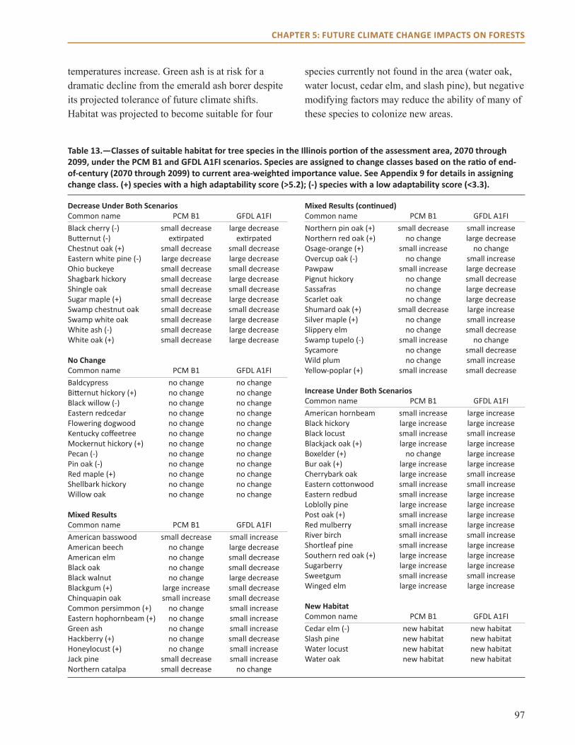
97


Decrease Under Both Scenarios Common name PCM B1 GFDL A1FIBlack cherry (-) small decrease large decreaseButternut (-) extirpated extirpated Chestnut oak (+) small decrease small decreaseEastern white pine (-) large decrease large decreaseOhio buckeye small decrease small decreaseShagbark hickory small decrease large decreaseShingle oak small decrease small decreaseSugar maple (+) small decrease large decreaseSwamp chestnut oak small decrease small decreaseSwamp white oak small decrease large decreaseWhite ash (-) small decrease large decreaseWhite oak (+) small decrease large decrease

NoChangeCommon name PCM B1 GFDL A1FIBaldcypress no change no changeBitternut hickory (+) no change no changeBlack willow (-) no change no changeEastern redcedar no change no changeFlowering dogwood no change no changeKentucky coffeetree no change no changeMockernut hickory (+) no change no changePecan (-) no change no changePin oak (-) no change no changeRed maple (+) no change no changeShellbark hickory no change no changeWillow oak no change no change

MixedResultsCommon name PCM B1 GFDL A1FIAmerican basswood small decrease small increaseAmerican beech no change large decreaseAmerican elm no change small decreaseBlack oak no change small decreaseBlack walnut no change large decreaseBlackgum (+) large increase small decreaseChinquapin oak small increase small decreaseCommon persimmon (+) no change small increaseEastern hophornbeam (+) no change small increaseGreen ash no change small increaseHackberry (+) no change small decreaseHoneylocust (+) no change small increaseJack pine small decrease small increaseNorthern catalpa small decrease no change

MixedResults(continued)Common name PCM B1 GFDL A1FINorthern pin oak (+) small decrease small increaseNorthern red oak (+) no change large decreaseOsage-orange (+) small increase no changeOvercup oak (-) no change small increasePawpaw small increase large decreasePignut hickory no change small decreaseSassafras no change large decreaseScarlet oak no change large decreaseShumard oak (+) small decrease large increaseSilver maple (+) no change small increaseSlippery elm no change small decreaseSwamp tupelo (-) small increase no changeSycamore no change small decreaseWild plum no change small increaseYellow-poplar (+) small increase small decrease

Increase Under Both Scenarios Common name PCM B1 GFDL A1FIAmerican hornbeam small increase large increaseBlack hickory large increase large increaseBlack locust small increase small increaseBlackjack oak (+) large increase large increaseBoxelder (+) no change large increaseBur oak (+) large increase large increaseCherrybark oak large increase small increaseEastern cottonwood small increase small increaseEastern redbud small increase large increaseLoblolly pine large increase large increasePost oak (+) small increase large increaseRed mulberry small increase large increaseRiver birch small increase small increaseShortleaf pine small increase large increaseSouthern red oak (+) large increase large increaseSugarberry large increase large increaseSweetgum small increase small increaseWinged elm large increase large increase

New Habitat Common name PCM B1 GFDL A1FICedar elm (-) new habitat new habitatSlash pine new habitat new habitatWater locust new habitat new habitatWater oak new habitat new habitat

Table13.—ClassesofsuitablehabitatfortreespeciesintheIllinoisportionoftheassessmentarea,2070through2099,underthePCMB1andGFDLA1FIscenarios.Speciesareassignedtochangeclassesbasedontheratioofend-of-century(2070through2099)tocurrentarea-weightedimportancevalue.SeeAppendix9fordetailsinassigningchangeclass.(+)specieswithahighadaptabilityscore(>5.2);(-)specieswithalowadaptabilityscore(<3.3).

temperatures increase. Green ash is at risk for a dramatic decline from the emerald ash borer despite its projected tolerance of future climate shifts. Habitat was projected to become suitable for four

species currently not found in the area (water oak, water locust, cedar elm, and slash pine), but negative modifying factors may reduce the ability of many of these species to colonize new areas.

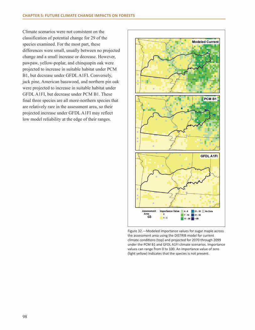
98


Climate scenarios were not consistent on the classification of potential change for 29 of the species examined. For the most part, these differences were small, usually between no projected change and a small increase or decrease. However, pawpaw, yellow-poplar, and chinquapin oak were projected to increase in suitable habitat under PCM B1, but decrease under GFDL A1FI. Conversely, jack pine, American basswood, and northern pin oak were projected to increase in suitable habitat under GFDL A1FI, but decrease under PCM B1. These final three species are all more-northern species that are relatively rare in the assessment area, so their projected increase under GFDL A1FI may reflect low model reliability at the edge of their ranges.

Figure 32.—Modeled importance values for sugar maple across the assessment area using the DISTRIB model for current climate conditions (top) and projected for 2070 through 2099 under the PCM B1 and GFDL A1FI climate scenarios. Importance values can range from 0 to 100. An importance value of zero (light yellow) indicates that the species is not present.

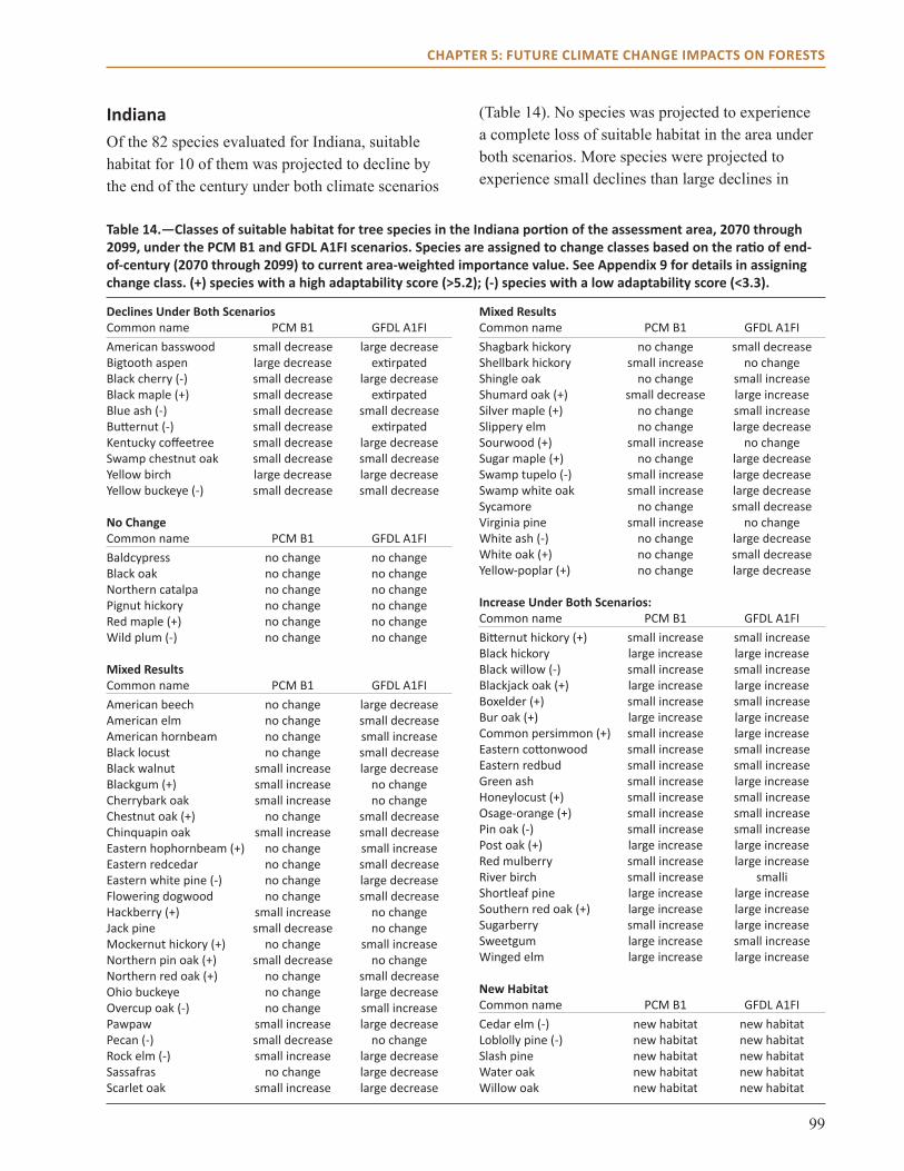
99


Declines Under Both ScenariosCommon name PCM B1 GFDL A1FIAmerican basswood small decrease large decreaseBigtooth aspen large decrease extirpatedBlack cherry (-) small decrease large decreaseBlack maple (+) small decrease extirpatedBlue ash (-) small decrease small decreaseButternut (-) small decrease extirpatedKentucky coffeetree small decrease large decreaseSwamp chestnut oak small decrease small decreaseYellow birch large decrease large decreaseYellow buckeye (-) small decrease small decrease

NoChangeCommon name PCM B1 GFDL A1FIBaldcypress no change no change Black oak no change no change Northern catalpa no change no change Pignut hickory no change no change Red maple (+) no change no change Wild plum (-) no change no change

MixedResultsCommon name PCM B1 GFDL A1FIAmerican beech no change large decreaseAmerican elm no change small decreaseAmerican hornbeam no change small increaseBlack locust no change small decreaseBlack walnut small increase large decreaseBlackgum (+) small increase no change Cherrybark oak small increase no change Chestnut oak (+) no change small decreaseChinquapin oak small increase small decreaseEastern hophornbeam (+) no change small increaseEastern redcedar no change small decreaseEastern white pine (-) no change large decreaseFlowering dogwood no change small decreaseHackberry (+) small increase no change Jack pine small decrease no change Mockernut hickory (+) no change small increaseNorthern pin oak (+) small decrease no change Northern red oak (+) no change small decreaseOhio buckeye no change large decreaseOvercup oak (-) no change small increasePawpaw small increase large decreasePecan (-) small decrease no change Rock elm (-) small increase large decreaseSassafras no change large decreaseScarlet oak small increase large decrease

MixedResultsCommon name PCM B1 GFDL A1FIShagbark hickory no change small decreaseShellbark hickory small increase no change Shingle oak no change small increaseShumard oak (+) small decrease large increaseSilver maple (+) no change small increaseSlippery elm no change large decreaseSourwood (+) small increase no change Sugar maple (+) no change large decreaseSwamp tupelo (-) small increase large decreaseSwamp white oak small increase large decreaseSycamore no change small decreaseVirginia pine small increase no change White ash (-) no change large decreaseWhite oak (+) no change small decreaseYellow-poplar (+) no change large decrease

Increase Under Both Scenarios: Common name PCM B1 GFDL A1FIBitternut hickory (+) small increase small increaseBlack hickory large increase large increaseBlack willow (-) small increase small increaseBlackjack oak (+) large increase large increaseBoxelder (+) small increase small increaseBur oak (+) large increase large increaseCommon persimmon (+) small increase large increaseEastern cottonwood small increase small increaseEastern redbud small increase small increaseGreen ash small increase large increaseHoneylocust (+) small increase small increaseOsage-orange (+) small increase small increasePin oak (-) small increase small increasePost oak (+) large increase large increaseRed mulberry small increase large increaseRiver birch small increase smalliShortleaf pine large increase large increaseSouthern red oak (+) large increase large increaseSugarberry small increase large increaseSweetgum large increase small increaseWinged elm large increase large increase

New HabitatCommon name PCM B1 GFDL A1FICedar elm (-) new habitat new habitatLoblolly pine (-) new habitat new habitatSlash pine new habitat new habitatWater oak new habitat new habitatWillow oak new habitat new habitat

Table14.—ClassesofsuitablehabitatfortreespeciesintheIndianaportionoftheassessmentarea,2070through2099,underthePCMB1andGFDLA1FIscenarios.Speciesareassignedtochangeclassesbasedontheratioofend-of-century(2070through2099)tocurrentarea-weightedimportancevalue.SeeAppendix9fordetailsinassigningchangeclass.(+)specieswithahighadaptabilityscore(>5.2);(-)specieswithalowadaptabilityscore(<3.3).

IndianaOf the 82 species evaluated for Indiana, suitable habitat for 10 of them was projected to decline by the end of the century under both climate scenarios

(Table 14). No species was projected to experience a complete loss of suitable habitat in the area under both scenarios. More species were projected to experience small declines than large declines in

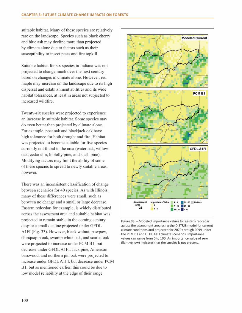
100


suitable habitat. Many of these species are relatively rare on the landscape. Species such as black cherry and blue ash may decline more than projected by climate alone due to factors such as their susceptibility to insect pests and fire topkill.

Suitable habitat for six species in Indiana was not projected to change much over the next century based on changes in climate alone. However, red maple may increase on the landscape due to its high dispersal and establishment abilities and its wide habitat tolerances, at least in areas not subjected to increased wildfire.

Twenty-six species were projected to experience an increase in suitable habitat. Some species may do even better than projected by climate alone. For example, post oak and blackjack oak have high tolerance for both drought and fire. Habitat was projected to become suitable for five species currently not found in the area (water oak, willow oak, cedar elm, loblolly pine, and slash pine). Modifying factors may limit the ability of some of these species to spread to newly suitable areas, however.

There was an inconsistent classification of change between scenarios for 40 species. As with Illinois, many of these differences were small, such as between no change and a small or large decrease. Eastern redcedar, for example, is widely distributed across the assessment area and suitable habitat was projected to remain stable in the coming century, despite a small decline projected under GFDL A1FI (Fig. 33). However, black walnut, pawpaw, chinquapin oak, swamp white oak, and scarlet oak were projected to increase under PCM B1, but decrease under GFDL A1FI. Jack pine, American basswood, and northern pin oak were projected to increase under GFDL A1FI, but decrease under PCM B1, but as mentioned earlier, this could be due to low model reliability at the edge of their range.

Figure 33.—Modeled importance values for eastern redcedar across the assessment area using the DISTRIB model for current climate conditions and projected for 2070 through 2099 under the PCM B1 and GFDL A1FI climate scenarios. Importance values can range from 0 to 100. An importance value of zero (light yellow) indicates that the species is not present.

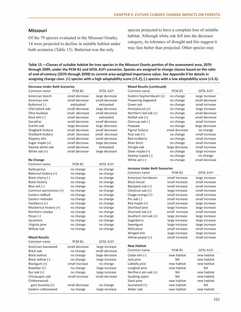
101


Decrease Under Both Scenarios Common name PCM B1 GFDL A1FIAmerican beech small decrease large decreaseAmerican elm small decrease small decreaseButternut (-) extirpated extirpatedCherrybark oak small decrease large decreaseOhio buckeye small decrease small decreaseRock elm (-) small decrease extirpatedSassafras small decrease small decreaseScarlet oak large decrease large decreaseShagbark hickory small decrease small decreaseShellbark hickory small decrease small decreaseSlippery elm small decrease small decreaseSugar maple (+) small decrease large decreaseSwamp white oak small decrease extirpatedWhite oak (+) small decrease large decrease

NoChangeCommon name PCM B1 GFDL A1FIBaldcypress no change no changeBitternut hickory (+) no change no changeBlack cherry (-) no change no changeBlack hickory no change no changeBlue ash (-) no change no changeCommon persimmon (+) no change no changeEastern redbud no change no changeEastern redcedar no change no changeHackberry (+) no change no changeMockernut hickory (+) no change no changeNorthern catalpa no change no changePecan (-) no change no changeSycamore no change no changeVirginia pine no change no changeWillow oak no change no change

MixedResultsCommon name PCM B1 GFDL A1FIAmerican basswood small decrease large increaseBlack oak no change small decreaseBlack walnut no change large decreaseBlack willow (-) no change large increaseBlackgum (+) small increase no changeBoxelder (+) no change large increaseBur oak (+) no change large increaseChinquapin oak small increase small decreaseChittamwood: gum bumelia (+) small decrease no changeEastern cottonwood no change large increase

MixedResults(continued)Common name PCM B1 GFDL A1FIEastern hophornbeam (+) no change large increaseFlowering dogwood no change small decreaseGreen ash no change small increaseHoneylocust (+) no change large increaseNorthern red oak (+) no change small decreaseNuttall oak (+) no change small decreaseOvercup oak (-) no change small increasePawpaw no change large decreasePignut hickory small decrease no changePost oak (+) no change small increaseRed mulberry no change small increaseRiver birch no change small increaseShingle oak large decrease small increaseSilver maple (+) no change large increaseSwamp tupelo (-) no change no changeWhite ash (-) no change small decrease

Increase Under Both Scenarios Common name PCM B1 GFDL A1FIAmerican hornbeam small increase large increaseBlack locust small increase small increaseBlackjack oak (+) small increase small increaseChestnut oak (+) large increase small increaseOsage-orange (+) small increase small increasePin oak (-) small increase small increaseRed maple (+) small increase large increaseShortleaf pine large increase large increaseShumard oak (+) small increase small increaseSouthern red oak (+) large increase large increaseSugarberry large increase large increaseSweetgum large increase large increaseWild plum small increase small increaseWinged elm large increase large increaseYellow-poplar (+) small increase small increase

New Habitat Common name PCM B1 GFDL A1FICedar elm (-) new habitat new habitatJack pine NA new habitatLoblolly pine new habitat new habitatLongleaf pine new habitat NANorthern pin oak (+) NA new habitatQuaking aspen NA new habitatSlash pine new habitat new habitatSourwood (+) new habitat NAWater oak new habitat new habitat

Table15.—ClassesofsuitablehabitatfortreespeciesintheMissouriOzarksportionoftheassessmentarea,2070through2099,underthePCMB1andGFDLA1FIscenarios.Speciesareassignedtochangeclassesbasedontheratioofend-of-century(2070through2099)tocurrentarea-weightedimportancevalue.SeeAppendix9fordetailsinassigningchangeclass.(+)specieswithahighadaptabilityscore(>5.2);(-)specieswithalowadaptabilityscore(<3.3).

MissouriOf the 79 species evaluated in the Missouri Ozarks, 14 were projected to decline in suitable habitat under both scenarios (Table 15). Butternut was the only

species projected to have a complete loss of suitable habitat. Although white oak fell into the decrease category, its tolerance of drought and fire suggest it may fare better than projected. Other species may

102


fare even worse than projected. For example, rock elm has a narrow habitat specificity and has poor seedling establishment.

Suitable habitat for 15 species was projected to stay similar to today when modifying factors are not considered. Some species may do worse than projected, however. For example, black cherry is susceptible to fire topkill and insect outbreaks, and blue ash is susceptible to emerald ash borer. Other species may fare better than projected. Bitternut hickory and hackberry can both tolerate drought, which may allow them to do better than other species if droughts become more widespread.

Twenty-four species were projected to increase in suitable habitat, of which nine are not currently found in the assessment area. Suitable habitat for shortleaf pine, for example, is projected to expand beyond its current range (Fig. 34). Many of these species possess modifying factors that could affect their ability to expand into newly suitable habitats. Winged elm may fare worse than projected due to its susceptibility to Dutch elm disease. The strong dispersal ability of red maple may allow it to disperse into new areas. Blackjack oak is both fire- and drought-tolerant, making it resilient to many of the stressors that are expected to increase as the climate changes. All oak species are dispersal limited to some extent, however, due to their heavy seeds.

Model projections showed some disagreement between scenarios in the classification of change for 25 of the species examined, but most of these differences were small. Black walnut was projected to remain stable under PCM B1 but experience a large decrease under GFDL A1FI. Shingle oak and American basswood were projected to decrease in suitable habitat under PCM B1, but increase under GFDL A1FI.

Figure 34.—Modeled importance values for shortleaf pine across the assessment area using the DISTRIB model for current climate conditions (top) and projected for 2070 through 2099 under the PCM B1 and GFDL A1FI climate scenarios. Importance values can range from 0 to 100. An importance value of zero (light yellow) indicates that the species is not present.

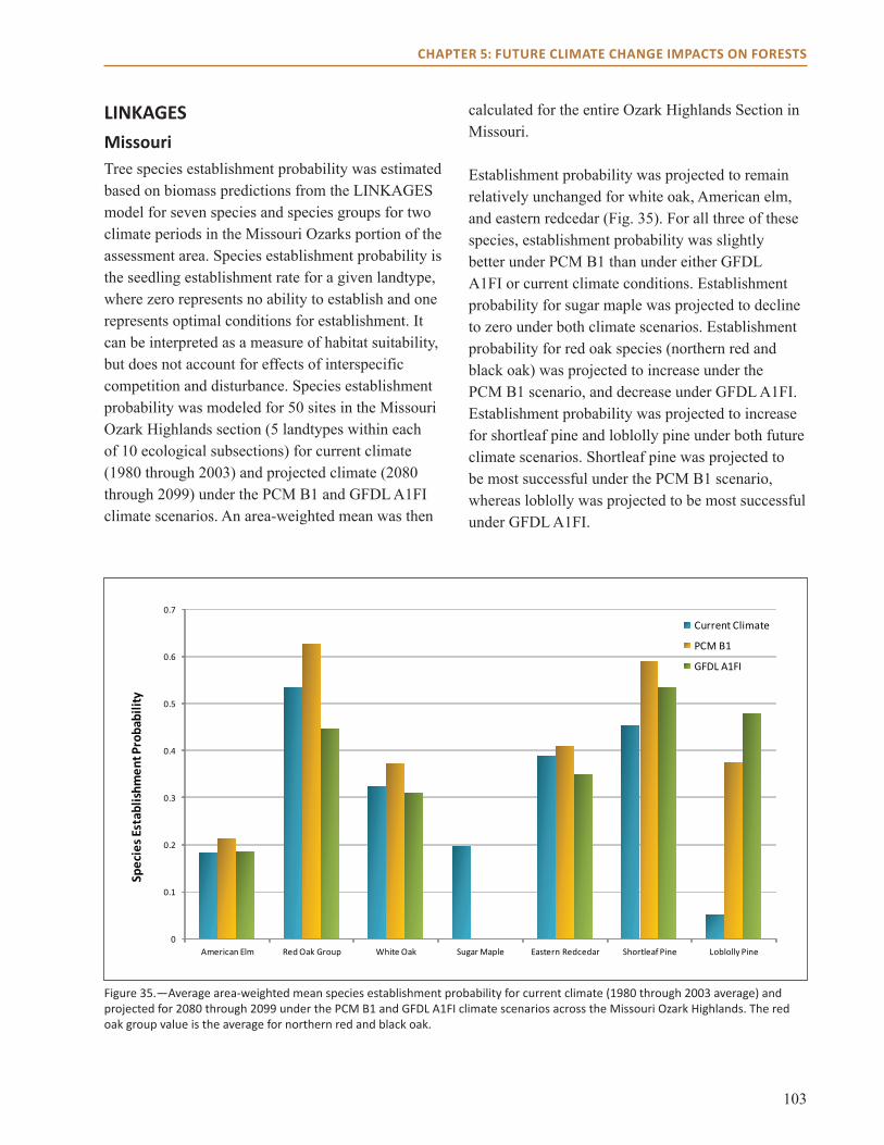
103


LINKAGES MissouriTree species establishment probability was estimated based on biomass predictions from the LINKAGES model for seven species and species groups for two climate periods in the Missouri Ozarks portion of the assessment area. Species establishment probability is the seedling establishment rate for a given landtype, where zero represents no ability to establish and one represents optimal conditions for establishment. It can be interpreted as a measure of habitat suitability, but does not account for effects of interspecific competition and disturbance. Species establishment probability was modeled for 50 sites in the Missouri Ozark Highlands section (5 landtypes within each of 10 ecological subsections) for current climate (1980 through 2003) and projected climate (2080 through 2099) under the PCM B1 and GFDL A1FI climate scenarios. An area-weighted mean was then

calculated for the entire Ozark Highlands Section in Missouri.

Establishment probability was projected to remain relatively unchanged for white oak, American elm, and eastern redcedar (Fig. 35). For all three of these species, establishment probability was slightly better under PCM B1 than under either GFDL A1FI or current climate conditions. Establishment probability for sugar maple was projected to decline to zero under both climate scenarios. Establishment probability for red oak species (northern red and black oak) was projected to increase under the PCM B1 scenario, and decrease under GFDL A1FI. Establishment probability was projected to increase for shortleaf pine and loblolly pine under both future climate scenarios. Shortleaf pine was projected to be most successful under the PCM B1 scenario, whereas loblolly was projected to be most successful under GFDL A1FI.

Figure 35.—Average area-weighted mean species establishment probability for current climate (1980 through 2003 average) and projected for 2080 through 2099 under the PCM B1 and GFDL A1FI climate scenarios across the Missouri Ozark Highlands. The red oak group value is the average for northern red and black oak.

0

0.1

0.2

0.3

0.4

0.5

0.6

0.7

American Elm Red Oak Group White Oak Sugar Maple Eastern Redcedar Shortleaf Pine Loblolly Pine

Spec

iesE

stab

lishm

entP

roba

bilit

y

Current Climate

PCM B1

GFDL A1FI

104


LANDIS PROMissouriLandscape change was modeled over the 21st century for the Missouri Ozarks with the LANDIS PRO model for current climate (1980 through 2003) and projected climate (2001 through 2100) by using the species establishment probabilities developed from the LINKAGES model. Changes in basal area (cross-sectional area of tree boles measured at a height of 21.5 inches above the ground) and the number of trees per acre by species or species group were simulated over a 100-year period. The LANDIS PRO model uses the two climate change model-emissions scenarios used by the other impact models (PCM B1 and GFDL A1FI) and a current climate scenario. Percentage change in future compared to current climate was summarized at years 2040, 2070, 2090, and 2100 (Figs. 36 and 37). In contrast to LINKAGES, LANDIS PRO is able to simulate stand- and landscape-level processes such as competition, seed dispersal, and disturbance. In the scenarios below, however, these factors were held constant among model simulations so that differences between the current climate and future climate scenarios are limited to the effects of precipitation and temperature on species establishment probabilities. Model simulations assumed current harvest levels on public and private lands, and fire was suppressed. However, it is expected that both of these factors will also change in the future as climate changes. The species establishment probabilities were determined by using LINKAGES as described in the previous section. Species establishment probabilities changed over time during the simulations to match the expected changes in temperature and precipitation for each scenario.

No dramatic changes in basal area or trees per acre were projected for the soft hardwoods group (American elm, slippery elm, and willow species).

The number of trees per acre is projected to increase by 3 to 6 percent by the end of the century relative to current climate, depending on future climate scenario. Changes in basal area are even more subtle, reaching a 2- to 4-percent increase by 2100. A slightly higher basal area and trees per acre were projected under the GFDL A1FI scenario than under the PCM B1 scenario.

The LANDIS PRO model projected a dramatic decrease in the number of sugar maple trees per acre over the next century under the PCB B1 and GFDL A1FI climate scenarios compared to the current climate scenario, reaching about 80-percent decline by 2100. This projection indicates that maple seedlings may be unable to establish on the landscape and replace older trees as they die. The model projects a less dramatic, but still substantial, decrease in basal area under both climate model-emissions scenarios, suggesting that larger, older trees may persist on the landscape. Over a longer timeframe, these projections suggest that sugar maple species would disappear from the landscape as mature trees die and new trees fail to establish because of a lack of regeneration under both future climate scenarios as projected in LINKAGES.

Projected changes in the red oak group (northern red, black, southern red, pin, Shumard, scarlet, and blackjack oak) varied by climate scenario. Red oak group species had an increase in basal area and trees per acre under the PCM B1 scenario, possibly due to increased seedling establishment projected in LINKAGES. The GFDL A1FI scenario resulted in decreased trees per acre, attributable to low seedling establishment projected in LINKAGES. Basal area was projected to stay relatively constant under GFDL A1FI. Conditions thus are projected to continue to be suitable for mature trees, at least in the short term, but lack of establishment of new individuals may eventually lead to decline in the species once the older individuals die.

105


Figure 36.—Projected changes in basal area for six species and species groups across the Missouri Ozark Highlands using the LANDIS PRO model. Values represent the percentage change in basal area between projected and current climate at simulation year 2040, 2070, 2090, and 2100 under two future climate scenarios: PCM B1 and GFDL A1FI. A positive value indicates an increase relative to current climate and a negative value a decrease. Eastern soft hardwoods group: American elm, with slippery elm and, to a lesser extent, willow species. Red oak group: northern red, black, southern red, pin, Shumard, scarlet, and blackjack oak. White oak group: white, post, swamp white, and bur oak.

Basal area and the number of trees per acre in the white oak group (white, post, swamp white, and bur oak) were projected to increase slightly under both future climate scenarios. A greater increase in both basal area and trees per acre was projected in GFDL A1FI than in PCM B1. This result is in contrast to

the projections in LINKAGES, which suggested white oak group species may be most successful under the PCM B1 scenario. One explanation for this difference is that establishment was projected to be higher for the white oak group under GFDL A1FI conditions and higher for the red oak group under

-40

-35

-30

-25

-20

-15

-10

-5

0

5

10

2040 2070 2090 2100

%Ch

ange

inBa

salA

rea

Eastern Soft Hardwoods

-40

-35

-30

-25

-20

-15

-10

-5

0

5

10

2040 2070 2090 2100

%Ch

ange

inBa

salA

rea

Red Oak Group

-40

-35

-30

-25

-20

-15

-10

-5

0

5

10

2040 2070 2090 2100

%Ch

ange

inBa

salA

rea

White Oak Group

-40

-35

-30

-25

-20

-15

-10

-5

0

5

10

2040 2070 2090 2100

%Ch

ange

inBa

salA

rea

Sugar Maple

-40

-35

-30

-25

-20

-15

-10

-5

0

5

10

2040 2070 2090 2100

%Ch

ange

inBa

salA

rea

Eastern Redcedar

-40

-35

-30

-25

-20

-15

-10

-5

0

5

10

2040 2070 2090 2100

%Ch

ange

inBa

salA

rea

Shortleaf Pine

PCM B1

GFDL A1FI

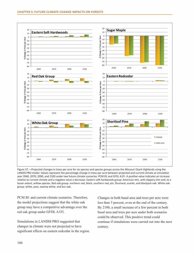
106


-80

-70

-60

-50

-40

-30

-20

-10

0

10

20

2040 2070 2090 2100

%Ch

ange

inTr

eesp

erAc

re

Eastern Soft Hardwoods

-80

-70

-60

-50

-40

-30

-20

-10

0

10

20

2040 2070 2090 2100

%Ch

ange

inTr

eesp

erAc

re

Red Oak Group

-80

-70

-60

-50

-40

-30

-20

-10

0

10

20

2040 2070 2090 2100

%Ch

ange

inTr

eesp

erAc

re

White Oak Group

-80

-70

-60

-50

-40

-30

-20

-10

0

10

20

2040 2070 2090 2100

%Ch

ange

inTr

eesp

erAc

re

Sugar Maple

-80

-70

-60

-50

-40

-30

-20

-10

0

10

20

2040 2070 2090 2100

%Ch

ange

inTr

eesp

erAc

re

Eastern Redcedar

-80

-70

-60

-50

-40

-30

-20

-10

0

10

20

2040 2070 2090 2100

%Ch

ange

inTr

eesp

erAc

re

Shortleaf Pine

PCM B1

GFDL A1FI

Figure 37.—Projected changes in trees per acre for six species and species groups across the Missouri Ozark Highlands using the LANDIS PRO model. Values represent the percentage change in trees per acre between projected and current climate at simulation year 2040, 2070, 2090, and 2100 under two future climate scenarios: PCM B1 and GFDL A1FI. A positive value indicates an increase relative to current climate and a negative value a decrease. Eastern soft hardwoods group: American elm, with slippery elm and, to a lesser extent, willow species. Red oak group: northern red, black, southern red, pin, Shumard, scarlet, and blackjack oak. White oak group: white, post, swamp white, and bur oak.

PCM B1 and current climate scenarios. Therefore, the model projections suggest that the white oak group may have a competitive advantage over the red oak group under GFDL A1FI.

Simulations in LANDIS PRO suggested that changes in climate were not projected to have significant effects on eastern redcedar in the region.

Changes in both basal area and trees per acre were less than 3 percent, even at the end of the century. By 2100, a small increase of a few percent in both basal area and trees per acre under both scenarios could be observed. This positive trend could continue if simulations were carried out into the next century.

107


Basal area and number of trees per acre of shortleaf pine were projected to increase under both future climate scenarios relative to the current climate scenario. Increases in both values were modest, reaching 18 percent more trees per acre and 6 percent greater basal area under the GFDL A1FI scenario. The number of trees per acre was projected to increase more rapidly than basal area, reflecting the establishment of new individuals on the landscape rather than enhanced growth of established trees. In contrast to LINKAGES, model results for LANDIS PRO suggested establishment and growth would be greatest under the GFDL A1FI scenario. This difference in result was probably driven by shortleaf pine colonizing newly suitable areas made available by declining species in the LANDIS PRO simulations.

Comparison of Model ResultsDespite the differences in approach and variables modeled, all three models show some remarkable similarities in projected species distribution over the next century. For example, all three models suggest that habitat suitability for sugar maple may decline over the next century, while suitability for shortleaf pine may increase. The modeling approach used by the Tree Atlas (DISTRIB) allows a greater area and number of species to be modeled, so it is unclear if the model projections for species and geographic areas not modeled by LINKAGES and LANDIS PRO might be similar to DISTRIB projections. Below is a comparison of the similarities and differences in projections for those species that were modeled using all three approaches.

Eastern RedcedarAll three models suggest that conditions are projected to continue to be favorable for eastern redcedar across the landscape, and changes in climate are not projected to have a dramatic effect on the ability of this species to spread to new areas. Both LINKAGES and DISTRIB project slightly more favorable conditions for eastern redcedar under the PCM B1 scenario than under current climate

conditions. By contrast LANDIS PRO projections suggest that eastern redcedar may have slightly greater growth (as measured by basal area) under the GFDL A1FI scenario than under PCM B1. Nevertheless, the wide distribution of this species suggests that it will probably continue to do well under a range of climate conditions.

EasternSoftHardwoodsSimulations in LINKAGES and LANDIS PRO suggest that changes in climate may not have a strong effect on American elm and associated species. The DISTRIB model suggests these species may react differently to projected climate, however, with slight increases for willow and slight decreases for the elm species. These results suggest that this species group as a whole may remain relatively stable, but conditions may favor a slight increase in hackberry and a slight decrease in elm species.

White Oak GroupProjections for white oak group species among the three models were mixed, and may be indicative of the differences in modeling approach. Results in LANDIS PRO, which combined white, post, swamp white, and bur oak into one species group, suggested that conditions may be slightly more favorable for this group of species under future climate conditions compared to current climate. By contrast, LINKAGES did not project a substantial change in establishment probability for white oak, which was slightly more favorable under PCM B1. The DISTRIB model, which modeled individual species, projected an increase in habitat suitability for post oak and bur oak under the GFDL scenario, and a decrease for white and swamp white oak under both scenarios in Missouri. Neither LINKAGES nor DISTRIB accounts for competition among species, which could explain some of the discrepancy between these two models and LANDIS PRO. Another possible explanation for the difference among projections is whether the species were grouped or modeled separately.

108


Red Oak GroupBoth LINKAGES and LANDIS PRO projected an increase in establishment for red oak group species under PCM B1, but decreases under the GFDL A1FI scenario. This result is probably because PCM projects an increase in summer precipitation over the next century, whereas GFDL projects a decrease. Many red oak group species are sensitive to these seasonal precipitation changes, and are projected to expand or contract depending on whether precipitation increases or decreases during the summer. The DISTRIB model did not show a consistent difference between the two climate models for this group of species as a whole. Projections for northern red oak are consistent with this pattern, however, suggesting a slight increase in habitat suitability under PCM B1 and decrease under GFDL A1FI. The projected changes using the DISTRIB model for other red oak group species suggest that black and scarlet oak may decline in habitat suitability under one or both scenarios, and blackjack, pin, Shumard, and southern red oak may increase in habitat suitability.

SugarMapleThe LINKAGES model projected a decline in establishment probability near 100 percent for sugar maple for both future climate scenarios. Simulations in LANDIS PRO for sugar maple showed that basal area was not projected to decline as dramatically as trees per acres over the next century, suggesting that older trees may persist on the landscape. By contrast, the DISTRIB model projected only a slight decline in suitable habitat for sugar maple under the PCM B1 scenario but a large decline under the GFDL A1FI scenario. Despite these subtle differences, it appears that conditions generally will be unfavorable for this species.

ShortleafandLoblollyPineAll three models projected favorable conditions for shortleaf pine across the assessment area. However, there were some slight differences among models

regarding which climate scenario would be most favorable. Both LANDIS PRO and DISTRIB projected slightly more favorable conditions under the GFDL A1FI scenario, but LINKAGES projected the greatest increase under the PCM B1 scenario. Both the DISTRIB and the LINKAGES models projected favorable conditions for loblolly pine to expand into the area, with greater increases under the GFDL A1FI scenario. Loblolly pine was not modeled with LANDIS PRO because the model simulated change only for species already present on the landscape. In general, conditions are expected to be favorable for both of these species across a range of future climates.

SUMMARY OF CURRENT SCIENTIFIC KNOWLEDGE ON FOREST IMPACTSThe results presented above provide us with important projections of tree species distributions across a range of future climates, but these models do not account for all factors that may influence tree species and forest communities under a changing climate. Climate change has the potential to alter the distribution, abundance, and productivity of forests and their associated species in a variety of ways (Climate Change Science Program 2008, Vose et al. 2012). These effects can broadly be divided into the direct effects of temperature and precipitation on forests and the indirect effects on forests through the alteration of current stressors or the development of additional stressors. For the most part, models such as the ones described above consider only direct effects such as average temperature and precipitation. Information regarding the current state of our scientific knowledge on additional direct and indirect effects of climate change on forests in the Central Hardwoods Region is described below.

DroughtStressandMortalitySevere and long-term droughts can have dramatic impacts on the forests of the Central Hardwoods

109


Region. For example, drought events can lead to the mortality of species in the red oak group via oak decline (Starkey et al. 2004, Voelker et al. 2008) (see Box 15). Research in dry-mesic upland forests in the Missouri Ozarks suggests a positive relationship between a species’ vessel (part of the anatomical structure of the tree that carries water) length and mortality during drought events (Fig. 38). Species such as sassafras and scarlet oak have long vessels and appear to be particularly susceptible to drought-related mortality, whereas species such as red maple and black cherry have shorter vessels and lower mortality. If drought duration and area increase as

projected (Mishra et al. 2010), drought-susceptible tree species could be particularly vulnerable to mortality.

BlowdownsBlowdowns from large and small windstorms can have an important influence on the structure and species composition of forests in the Central Hardwoods Region. Some model projections suggest there may be an overall increase in the average windspeed in the area, but there does not appear to be a projected increase in the number of extreme wind events in the central United States

Box15.OakDecline

Oak decline is a phenomenon affecting species in the red oak group, especially northern red, black, and scarlet oak. It is a disease complex caused by a combination of physical and biological stressors. Older trees growing on sites with shallow soils can become stressed from drought in particular, but also from pollution, late spring frosts, or other environmental stressors. These physical stressors can make them more vulnerable to attack by insects and pathogens. The result is a decline in species in the red oak group. Within the assessment area, oak decline is a chronic problem in the Ozark Highlands, affecting hundreds of thousands of acres.

Insects involved in oak decline include the red oak borer, carpenterworm, and two-lined chestnut borer. Infestation by the red oak borer appears to increase when trees are drought stressed (Haavik et al. 2008), and infestation also increases in conjunction with warmer mean annual and mean annual minimum temperatures (Muzika and Guyette 2004). Although these infestations are often associated with oak decline, they alone are not typically responsible for mortality (Fan et al. 2008, Haavik et al. 2008).

Armillaria and Hypoxylon fungi are two pathogens involved in oak decline. Hypoxylon species commonly cause a canker-like disease on red and black oaks

that have been stressed by drought, and can lead to tree death. Armillaria species normally act as decomposers, but can become parasitic when trees become stressed and, thus, contribute to tree death. If climate change increases the duration and extent of drought or increases the amount of defoliation by insects due to warmer temperatures, trees could be more susceptible to attack by this pathogen (Dukes et al. 2009).

Historical and dendrochronological records indicate a strong relationship between drought years and oak decline (Dwyer et al. 1995, Jenkins and Pallardy 1995). As droughts are projected to increase in duration and aerial extent (Mishra et al. 2010), oak decline could become an even larger problem for species in the red oak group across the Missouri Ozarks, especially for older trees on marginal sites. Oak decline could be exacerbated by other stressors: insect defoliation may increase with rising temperatures, and red oak species may already be stressed due to a decline in habitat suitability as projected by the tree species models, especially under the GFDL A1FI scenario. As these species decline, new opportunities could open up for other species that are better adapted to projected climate, such as pine and white oak group species.

110


Figure 38.—Species vessel length correlates with cumulative mortality between 1981 and 1988 summer droughts at the Tyson Research Center, St. Louis County, MO. Species with high ranks for vessel length are more likely to have high ranks for mortality than expected by chance. Increasing rank denotes increasing values on each axis. Figure used with permission of Brad Oberle and Amy Zanne, George Washington University.

(IPCC 2012). In addition, the amount of evidence to date of changes in extreme storms in this region is rather limited (IPCC 2012) (see Chapters 3 and 4). Therefore, it is unclear whether blowdowns will increase across the region. If blowdowns do increase, the species that are most susceptible are expected to vary across the assessment area because of differences in species composition and stand characteristics. In the southeast Missouri Ozarks region, past blowdown events appear to have disproportionately affected older scarlet oaks, as well as trees on north- and east-facing slopes (Rebertus and Meier 2001). These events appear to have created opportunities for regeneration of white oak, flowering dogwood, and various hickory species. In the Shawnee National Forest, a recent blowdown primarily affected oak species and provided more opportunity for succession by immature shade-tolerant species in the understory (Holzmueller et al. 2012). Blowdowns are expected to continue to be an important disturbance in

many Central Hardwoods ecosystems, but existing scientific literature provides no clear indication of how blowdowns will be affected by the changing climate.

WinterStormDamageSnow and ice damage occurs occasionally across the area, and is projected to decrease with warmer temperatures (Chapter 4). This trend could decrease mortality of trees that are susceptible to damage from these events. Species such as eastern redcedar, yellow-poplar, and sweetgum appear to be particularly susceptible to top breakage and uprooting from these events (Parker and Ruffner 2004). A study of a 1994 ice storm in Missouri found that basswood and American elm were the species most susceptible to ice storm damage, whereas white oak and shagbark hickory were less susceptible (Rebertus et al. 1997). Within species, damage appears to be greater in older, taller individuals and those on mesic aspects and lower slopes (Rebertus et al. 1997). These events also create gaps, allowing growth and expansion of immature trees in the understory. If these events decrease or are eliminated from the area, recruitment of shade-intolerant species in particular may be reduced.

Although snow and ice are projected to decrease across the area, some evidence suggests that storm events may actually increase during the winter (Wang and Zhang 2008). With the projected increases in temperatures, these events may result more often in flooding and wind damage than in snow and ice damage, suggesting winter storms may function more like summer storms across the region.

HydrologicImpactsonForestsAlthough all forests are expected to be affected to some extent, bottomland forests are the most susceptible to the effects of altered hydrologic regimes as temperatures increase and precipitation patterns change. Past forest management practices,

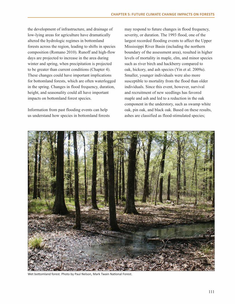
111


the development of infrastructure, and drainage of low-lying areas for agriculture have dramatically altered the hydrologic regimes in bottomland forests across the region, leading to shifts in species composition (Romano 2010). Runoff and high-flow days are projected to increase in the area during winter and spring, when precipitation is projected to be greater than current conditions (Chapter 4). These changes could have important implications for bottomland forests, which are often waterlogged in the spring. Changes in flood frequency, duration, height, and seasonality could all have important impacts on bottomland forest species.

Information from past flooding events can help us understand how species in bottomland forests

may respond to future changes in flood frequency, severity, or duration. The 1993 flood, one of the largest recorded flooding events to affect the Upper Mississippi River Basin (including the northern boundary of the assessment area), resulted in higher levels of mortality in maple, elm, and minor species such as river birch and hackberry compared to oak, hickory, and ash species (Yin et al. 2009a). Smaller, younger individuals were also more susceptible to mortality from the flood than older individuals. Since this event, however, survival and recruitment of new seedlings has favored maple and ash and led to a reduction in the oak component in the understory, such as swamp white oak, pin oak, and black oak. Based on these results, ashes are classified as flood-stimulated species;

Wet bottomland forest. Photo by Paul Nelson, Mark Twain National Forest.

112


maple, hickory, and a variety of minor species are considered flood-tolerant species; and oaks and elms are considered flood-intolerant species (Yin et al. 2009a). Research suggests that oak species in bottomland systems could potentially decline and hickory species could increase if floods as severe as the 1993 event occur more than once every 100 years (Yin et al. 2009b). Flood severity and duration can also affect species composition. Model results indicate that maple and oak species are favored under floods that are less severe than the 1993 flood, and ash is favored when floods are more severe (Yin et al. 2009b). An observational study of the Upper Mississippi watershed north of the assessment area suggests that areas that remain flooded for more than 40 percent of the growing season are severely limited in species diversity (De Jager et al. 2012).

Other research in the region suggests that changes in flood regime can affect species composition. An analysis of the forest community on the Lower Kaskaskia River, one of the largest contiguous floodplain forests remaining in the region, indicated that a hydrologic modification resulting in high flood frequency and duration would support floodplain forest assemblages dominated by boxelder, silver maple, and green ash. Conversely, lower flood frequency and duration would support river birch and American elm assemblages (Romano 2006). A recent study in the Ozarks examined the flood tolerance of six species in a Missouri river floodplain under three different flood regimes (Kabrick et al. 2012). Pecan and black walnut were found to be flood-intolerant. Eastern cottonwood survival was negatively affected by flooding, but the growth of surviving individuals appeared to not be affected. Contrary to the study in the Upper Mississippi River Basin above, swamp white oak was found to do well even under the most severe flooding, suggesting this species has the potential to do well in the absence of competition from shade-tolerant species like maple and ash. Pin and bur oak, however, appear to suffer negative impacts on

growth when inundated by standing water for longer periods of time, suggesting an increase in flood duration could negatively impact these species.

Bottomland forests can withstand periodic flooding but cannot tolerate being waterlogged throughout the year. Swamps, by contrast, are flooded year-round and are populated by species adapted to standing water throughout the year. These systems, dominated by species such as baldcypress, reach their northern extent in the assessment area, and have the potential to respond favorably to altered conditions as long as natural hydrologic regimes are kept intact (see Box 16).

Soil ErosionSoil erosion is considered one of the major threats to the Central Hardwoods Region (Chapter 1). Some research suggests that an increase in heavy rainfall events that is projected to occur (and is already occurring) will lead to an even greater increase in soil erosion (Nearing et al. 2004, 2005). One study estimates that for every 1-percent increase in rainfall, erosion could increase by 2 percent (Nearing et al. 2004). No studies to date have examined the effects of climate change on soil erosion specifically in the Central Hardwoods Region. One study examined changes in erosivity across the United States at a very large spatial resolution and found that erosion may increase or decrease in the assessment area depending on climate model (Nearing 2001). This study looked only at broad-scale changes in precipitation, and does not account for other factors that may affect the vulnerability of soil to erosion such as vegetation cover, slope, or soil type.

Other climate change factors may also affect soil erosion in the Central Hardwoods Region. As mentioned in Chapter 4, soil freeze-thaw cycles may decrease in the area by the end of the century, which could reduce the susceptibility of soil to erosion (Sinha and Cherkauer 2010). Vegetation

113


Box16.BaldcypressSwamps

Southwestern Indiana, southern Illinois, and southeastern Missouri represent the northern extent of the range of baldcypress swamps in the Mississippi Alluvial Valley. These unique habitats are among the world’s most prolific producers of biomass, and thus serve as an important carbon sink. They also provide important habitat or food for fish and wildlife, including bald eagles, wild turkeys, and wood ducks. Baldcypress swamps also help reduce the severity and damage of flooding during the growing season by absorbing water and increasing infiltration into the soil.

The northern extent of the range for baldcypress in lowlands is determined primarily by an interaction of freezing water and recruitment limitations because of lack of upstream seed dispersal—not because of tree physiological constraints (B. Middleton, U.S. Geological Survey, National Wetlands Research Center, personal comm.). In fact, mature trees that are planted on upland sites can withstand very cold temperatures (-29 to -34 °C) (Burns and Honkala 1990).

Baldcypress swamps are of course dependent on appropriate topographic conditions, but also on precipitation and periodic flooding, which are expected to change across the Central Hardwoods Region based on current model projections. Regeneration and recruitment of baldcypress and associated species are determined by specific periodic flooding regimes (Middleton 2000, Middleton and Wu 2008). A reduction in precipitation, which is projected to occur later in the growing season, could result in reduced recruitment of rare species in this community such as American featherfoil and increased recruitment of other species such as buttonbush (Middleton 2006).

The northern extent of baldcypress swamps may serve as a refuge to more southern species

associated with this community type (Middleton 2006). Dispersal of associated southern species to the north may be limited, however, as seeds disperse by water, and the prevailing direction of the watersheds where they are located is southward (Middleton and McKee 2004). In addition, baldcypress swamps have become more fragmented in the north as they have been drained for agriculture and as local rivers have been dammed, making dispersal even more difficult (Middleton and Wu 2008).

Baldcypress productivity may increase at its northern extent with increasing temperature due to an extended growing season (Middleton and McKee 2004). More research is needed to assess whether genetic variation across its current range may limit this effect in northern genotypes (Kusumi et al. 2010).

Associated species within baldcypress swamps may vary in seedling recruitment and seedling biomass in their response to warming (Middleton and McKee 2011). For example, Virginia threeseed mercury is currently near its northern range limit, and responds to increasing temperature through increases in root biomass (Middleton and McKee 2011). Warmer future spring temperatures to the north of its current range could allow this annual species to expand northward, depending on dispersal constraints (Middleton and McKee 2011). However, other species in these systems do not show a strong response to temperature or have a much greater northern range extent than baldcypress swamps themselves.

Overall, baldcypress swamps and their associated species have the potential to adapt positively to increases in temperature in Illinois, Indiana, and Missouri, but only if connectivity and hydrologic function are restored.

114


also protects soil from erosion by reducing rainfall impacts through the canopy and litter layer, and by stabilizing soil through roots. Reductions in biomass and vegetative cover, resulting from a variety of climate impacts such as drought, insects, diseases, or catastrophic wildfire, could thus lead to an increase in erosion susceptibility (Nearing 2001).

WildfireFires, both natural and human-caused, have played an important role in the forests of the Central Hardwoods Region for thousands of years (Abrams 1992, Nowacki and Abrams 2008). Regardless of the cause, the risk and severity of fire depend on the atmospheric conditions present before, during, and after the time of ignition (Guyette et al. 2012).

At a global scale, the scientific consensus is that fire risk may increase by 10 to 30 percent over the next century because of higher summer

temperatures (IPCC 2007). Studies using climate models suggest that fire potential could increase across North America from increases in temperature and decreases in precipitation in some areas, and fire seasons in the southeastern United States could nearly double in length (Liu et al. 2010). In addition, fire severity in the Southeast could increase by up to 30 percent, depending on the general circulation model (GCM) used (Flannigan et al. 2000). An analysis of fire probability across the globe projected by 16 downscaled climate models found low agreement among projections of climate change effects on fire probability in the central United States in the near term (2010 to 2039), but the majority of models projected an increase in wildfire probability by the end of the century (2070 to 2099) (Moritz et al. 2012).

How a change in fire risk across the region translates to effects at local scales in Central

Prescribed fire in shortleaf pine woodland. Photo by Steve Shifley, U.S. Forest Service.

115


Hardwoods forests depends on land use and management decisions. Currently, no fine-scale projections of these interactions are available. The model projections presented in this chapter using LANDIS PRO assumed no climate-induced changes in wildfire or management regime, but future simulations could explore these interactions.

A study across the entire United States conducted model simulations of vegetation types under both suppressed and unsuppressed wildfire by using two emissions scenarios (A2 and B2) to examine the relationship among climate change, potential vegetation cover, and wildfire (Lenihan et al. 2008). When future wildfires were not suppressed, the Central Hardwoods Region was projected to convert from a temperate deciduous forest type to a woodland or savanna type. When fire was suppressed, on the other hand, the temperate deciduous forest type was projected to remain similar in the assessment area while moving northward across the eastern United States. A projected shift in potential vegetation type with unsuppressed fire was driven by climatic conditions that made the area more susceptible to wildfire, including increased temperature, drought, and flammability of coarse and fine fuels (Lenihan et al. 2008). These results underscore the importance of fire management in determining potential climate effects on vegetation. However, it is also important to note that these model simulations were run by using potential vegetation across the area. They do not include human-induced alterations to the landscape such as agriculture and urban areas, nor do they account for human intervention once a fire is ignited.

CarbonDioxideIncreasesIn addition to effects on climate, carbon dioxide (CO2) itself can affect plant productivity and species composition. Elevated CO2 may enhance growth and water use efficiency of some species (Ainsworth and Rogers 2007, Norby et al. 2005),

potentially offsetting the negative effects of drier growing seasons. There is already some evidence for increased forest growth under elevated CO2 in the eastern United States (Cole et al. 2010, McMahon et al. 2010), but it remains unclear if long-term enhanced growth can be sustained (Bonan 2008, Foster et al. 2010). Nutrient and water availability, ozone pollution, and tree age and size all play major roles in the ability of trees to capitalize on CO2 fertilization (Ainsworth and Long 2005). Ecosystem community shifts may take place as some species are genetically better able to take advantage of CO2 fertilization than others (Souza et al. 2010). Some models are available that account for changes in CO2, but these models tend to focus on nutrient cycling and general vegetation types, and not specific species (Lenihan et al. 2008, Ollinger et al. 2008).

ChangesinNutrientCyclingAs air temperatures warm and precipitation patterns change, changes in the way nutrients are cycled between plants, soils, and the atmosphere may also occur. These changes have important implications for the productivity of trees, which are often limited by nutrients such as phosphorus and nitrogen (N). To date, research has not been done to specifically examine the effects of climate change on nutrient cycling in the Central Hardwoods Region. Studies in other areas and at broader scales can give some insight into potential effects, however.

Decomposition of vegetation is carried out primarily by enzymes released from bacteria and fungi. These enzymes are sensitive to changes in temperature, and there is generally a positive effect of temperature on the rate of enzymatic activity as long as moisture is also sufficient (Brzostek et al. 2012, Rustad et al. 2001). In addition to increases in temperature, changes in drought, flooding, and the interaction among these factors can affect nutrient cycling and the availability of N to trees and other vegetation (Rennenberg et al. 2009, and references therein).

116


Many studies have examined the effects of extended dry periods followed by moisture pulses on nutrient cycling (Borken and Matzner 2009, and references therein). Although these moisture pulses lead to a flush of mineral N, it is not sufficient to compensate for the lack of microbial activity during dry periods. Thus, an increase in wet-dry cycles appears to lead to a reduction in nutrient availability for trees.

Invasive Plant SpeciesAs described in Chapter 1, nonnative invasive species are a major threat to forests in the Central Hardwoods Region. Many invasive species that currently threaten forests in the Central Hardwoods Region may benefit from projected climate change as well. Some species, such as sericea lespedeza (Gucker 2010), are tolerant of drought and fire and may be at an even greater advantage in the future. Although Japanese stiltgrass reproduction is inhibited during drought years, its large, long-lived seedbank enables it to recover in wetter years (Gibson et al. 2002). In addition, deer herbivory of native vegetation following a drought event can maintain dominance of stiltgrass (Webster et al. 2008). Other species, such as garlic mustard, are not particularly drought-tolerant and may fare worse if summer drying increases (Byers and Quinn 1998). Currently, however, no modeling efforts have been undertaken to assess the influence of climate change on invasive species that have already been established in the area.

Changes in climate may allow some invasive plant species to survive farther north than they had previously (Dukes et al. 2009). Kudzu is an invasive vine that has devastated forests in the southeastern United States. Economic damage to managed forests and agricultural land is estimated at $100 to $500 million per year (Blaustein 2001). The current northern distribution of kudzu is limited by winter temperature. One study found the risk for kudzu invasion at the end of the century in Missouri, Illinois, and Indiana could be heightened under

future projected warming (Bradley et al. 2010). Another examined the potential future distribution of kudzu for the year 2035 using trends in observed climate data and found habitat suitability may increase slightly in Indiana but may decrease slightly in western Missouri (Jarnevich and Stohlgren 2009).

Chinese and European privet are invasive flowering shrubs that crowd out native species and form dense thickets. Model projections suggest that the risks for privet invasion into Missouri, Illinois, and Indiana may be even greater than that of kudzu by the end of the century (Bradley et al. 2010). Some areas in the Ozark Highlands and south-central Indiana were projected to be most susceptible, with a medium-high risk; that is, the majority of GCMs and impact models project an increase in suitable habitat.

InsectPestsandPathogensWarmer temperatures and stressed trees may increase the abundance of pests and pathogens that are currently present in the assessment area. Many insects and their associated pathogens are exacerbated by drought including forest tent caterpillar, hickory bark beetle and its associated canker pathogen, bacterial leaf scorch, and Diplodia shoot blight (Babin-Fenske and Anand 2011, Park et al. 2013, Sinclair and Lyon 2005, U.S. Forest Service 1985). High spring precipitation has been associated with severe outbreaks of bur oak blight in Iowa (Harrington et al. 2012). Another important stressor that could be exacerbated by climate change is oak decline, which is largely driven by drought conditions that predispose species to insect pest and pathogen attack (see Box 15).

Warmer temperatures are also expected to increase the susceptibility of tree species to pests and diseases that are not currently a problem in the assessment area. Projections of gypsy moth population dynamics under a changing climate suggest substantial increases in the probability of establishment in the coming decades (Logan et al. 2003). The spread of

117


the gypsy moth could put at risk oak species that would otherwise do well under a changing climate. However, wetter springs could curtail its spread to some extent: a fungal pathogen of the larvae has been shown to reduce populations in years with wet springs (Andreadis and Weseloh 1990). In addition, future northward range expansion attributed to warming temperatures has been projected for southern pine beetle (Ungerer et al. 1999), which could become a problem if shortleaf pine expands in the region and stand density is not kept in check.

EffectsofVertebrateSpeciesHerbivory, seed predation, and disturbance by vertebrates can be important stressors in the Central Hardwoods Region. Deer browsing, seed predation, or disturbance by feral hogs may reduce the overall success of species that are otherwise projected to do well under future climate change (Ibañez et al. 2008). Currently, there is little evidence to indicate how deer, feral hogs, and other vertebrate species will respond to climate change in the Central Hardwoods Region. An analysis of climate change impacts on white-tailed deer in Wisconsin suggests that deer in that area are expected to experience a mixture of positive impacts from milder winters coupled with negative impacts from increased disease outbreaks (Wisconsin Initiative on Climate Change Impacts 2011). How these two factors may influence deer populations in Missouri, Illinois, and Indiana remains unknown.

CONCLUSIONS Results from three independent modeling efforts suggest that habitat suitability for many tree species may shift across the Central Hardwoods Region, leading to declines in some species and increases in others. The Tree Atlas, LANDIS PRO, and LINKAGES models all project a potential decline in suitability for sugar maple compared to current climate conditions. These models also agree that conditions should become more favorable for shortleaf pine. Model projections vary for oak and hickory species and will depend in part on how precipitation patterns shift in the coming years. Other factors that are not included in models, such as changes in invasive species, insects and diseases, wildfire, and soil conditions, may also affect species composition and forest productivity. Increased drought stress could increase susceptibility to oak decline in red oak group species, and higher temperatures could facilitate invasion of kudzu, privet, and southern pine beetle. Climate conditions are also expected to make conditions more favorable to wildfire and soil erosion. All of these factors need to be taken into account when evaluating the vulnerability of Central Hardwoods forests to climate change.

118

CHAPTER 6: ECOSYSTEM VULNERABILITIES

Changes in species distribution and abundance due to climate change can have important implications for the habitats in which those species live, leading to shifts in community composition and changes in ecosystem processes (Climate Change Science Program [CCSP] 2008, Vose et al. 2012). In addition, climate change itself can alter system drivers and exacerbate or ameliorate current stressors (CCSP 2008, Vose et al. 2012). This chapter focuses on the collective vulnerability of natural communities in the Central Hardwoods Region to climate change, emphasizing shifts in dominant species, system drivers, and stressors over the next century. Vulnerability is the susceptibility of a system to the adverse effects of climate change (Intergovernmental Panel on Climate Change [IPCC] 2007). It is a function of potential climate change impacts and the adaptive capacity of the system. We consider a system to be vulnerable if it is at risk for no longer being recognizable as that community type, or if the system is anticipated to suffer substantial declines in health or productivity. The vulnerability of a system to climate change is independent of the economic or social values associated with the system, and the ultimate decision of whether to conserve vulnerable systems or allow them to shift to an alternate state will depend on the individual objectives of land management organizations.

This chapter is organized into two sections. First, we present an overall synthesis of vulnerability of the Central Hardwoods Region, organized according to drivers and stressors, ecosystem impacts, and factors that influence adaptive capacity. This synthesis is based on the current scientific

consensus of published literature (Chapters 4 and 5). In the following section, we present individual vulnerability determinations for the nine natural community types considered in this assessment.

VULNERABILITY OF THE CENTRAL HARDWOODS REGION

Potential Impacts on Drivers and Stressors Many physical and biological factors contribute to the current state of Central Hardwoods systems. Some of these factors serve as drivers, defining variables that make that system what it is. Other factors can serve as stressors, reducing forest productivity or increasing mortality. Many factors, such as flooding or fire, may be drivers in one situation and stressors in another.

Potential impacts are the direct and indirect consequences of climate change on systems. Impacts are a function of exposure of a system to climate change and its sensitivity to any resulting changes. Impacts could be beneficial or harmful to a particular forest or ecosystem type. The summary below includes the potential impacts of climate change on major drivers and stressors in the Central Hardwoods Region over the next century based on the current scientific consensus of published literature, which is described in more detail in the preceding chapters.

After each statement is a confidence statement, phrased according to the IPCC’s guidance for

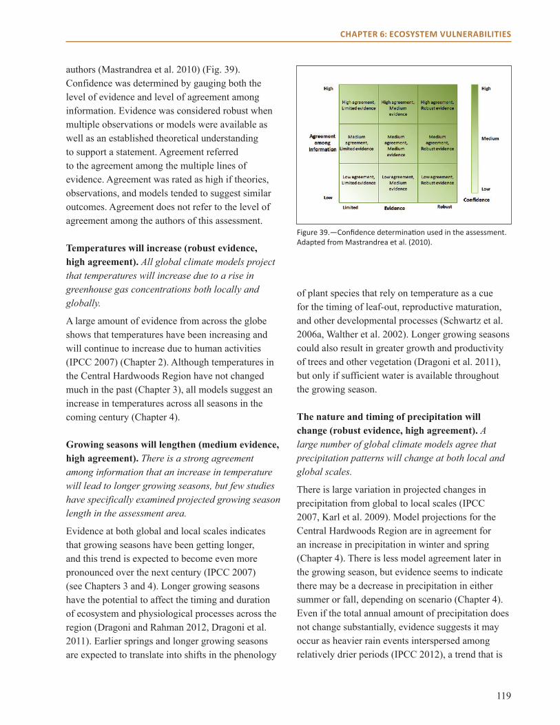
119


authors (Mastrandrea et al. 2010) (Fig. 39). Confidence was determined by gauging both the level of evidence and level of agreement among information. Evidence was considered robust when multiple observations or models were available as well as an established theoretical understanding to support a statement. Agreement referred to the agreement among the multiple lines of evidence. Agreement was rated as high if theories, observations, and models tended to suggest similar outcomes. Agreement does not refer to the level of agreement among the authors of this assessment.

Temperatures will increase (robust evidence, high agreement). All global climate models project that temperatures will increase due to a rise in greenhouse gas concentrations both locally and globally.

A large amount of evidence from across the globe shows that temperatures have been increasing and will continue to increase due to human activities (IPCC 2007) (Chapter 2). Although temperatures in the Central Hardwoods Region have not changed much in the past (Chapter 3), all models suggest an increase in temperatures across all seasons in the coming century (Chapter 4).

Growing seasons will lengthen (medium evidence, high agreement). There is a strong agreement among information that an increase in temperature will lead to longer growing seasons, but few studies have specifically examined projected growing season length in the assessment area.

Evidence at both global and local scales indicates that growing seasons have been getting longer, and this trend is expected to become even more pronounced over the next century (IPCC 2007) (see Chapters 3 and 4). Longer growing seasons have the potential to affect the timing and duration of ecosystem and physiological processes across the region (Dragoni and Rahman 2012, Dragoni et al. 2011). Earlier springs and longer growing seasons are expected to translate into shifts in the phenology

Figure 39.—Confidence determination used in the assessment. Adapted from Mastrandrea et al. (2010).

of plant species that rely on temperature as a cue for the timing of leaf-out, reproductive maturation, and other developmental processes (Schwartz et al. 2006a, Walther et al. 2002). Longer growing seasons could also result in greater growth and productivity of trees and other vegetation (Dragoni et al. 2011), but only if sufficient water is available throughout the growing season.

The nature and timing of precipitation will change (robust evidence, high agreement). A large number of global climate models agree that precipitation patterns will change at both local and global scales.

There is large variation in projected changes in precipitation from global to local scales (IPCC 2007, Karl et al. 2009). Model projections for the Central Hardwoods Region are in agreement for an increase in precipitation in winter and spring (Chapter 4). There is less model agreement later in the growing season, but evidence seems to indicate there may be a decrease in precipitation in either summer or fall, depending on scenario (Chapter 4). Even if the total annual amount of precipitation does not change substantially, evidence suggests it may occur as heavier rain events interspersed among relatively drier periods (IPCC 2012), a trend that is

120


already occurring in the area (Saunders et al. 2012). In addition, more winter precipitation is expected to shift from snow or ice to rain as winter temperatures rise (Brown and Mote 2009, Frei and Gong 2005).

An increase in heavy precipitation events (medium evidence, medium agreement) will increase flood risks (limited evidence, medium agreement) and soil erosion (limited evidence, medium agreement). There is disagreement among models about whether the number of heavy precipitation events will continue to increase in the assessment area. If the number does increase, it is expected that flooding and soil erosion will increase as well, but these effects have not been modeled for this region.

Heavy precipitation events have already been increasing in number and severity in the area (Groisman et al. 2012, Saunders et al. 2012), and some models suggest an increase over the next century (IPCC 2007, 2012). The magnitude or frequency of flooding could potentially increase in the winter and spring due to increases in total runoff and peak streamflow during those time periods (Cherkauer and Sinha 2010). Flood risks will ultimately depend on local geology and soils as well as human infrastructure and land use, however. Increases in runoff following heavy precipitation events, especially following periods of drought, could also lead to an increase in soil erosion, which may be exacerbated by a reduction in vegetation cover from climate stress and fire (Nearing et al. 2004). However, a reduction in soil freeze-thaw cycles across the region may help reduce soil erosion to some extent (Sinha and Cherkauer 2010) because freezing and thawing can break up soil aggregates, making soil more susceptible to erosion.

Snow will decrease, with subsequent decreases in soil frost (high evidence, high agreement). Evidence suggests that winter temperatures will increase in the area, even under low emissions, leading to changes in snow and soil frost.

The Central Hardwoods Region is already experiencing a decline in snowfall, depth, and cover (Chapter 3). Decreased snowfall and increased snowmelt from higher temperatures are projected to decrease the amount of snow on the ground in the region, and may make some locations snow-free in some years (Sinha and Cherkauer 2010). In recent years, this reduction in snow cover has led to an increase in soil frost from decreased snow insulation (Sinha et al. 2010). However, as temperatures increase in the coming decades, this pattern is projected to reverse, and far southern Illinois and Indiana may no longer experience freezing soil conditions by the end of the century (Sinha and Cherkauer 2010). Although these conditions could increase water infiltration into the soil and reduce runoff, they could also lead to greater soil water losses through increased evapotranspiration. This decrease in snow cover and frozen soil is projected to be coupled with more heavy precipitation events during winter, which are expected to occur as rain instead of snow (Wang and Zhang 2008).

Soil moisture patterns will change (medium evidence, high agreement), with drier soil conditions later in the growing season (medium evidence, low agreement). Some studies show that climate change will have impacts on soil moisture, but there is disagreement among impact model projections on how soil moisture will change during the growing season.

Due to projected decreases in precipitation during summer or fall and increases in temperature throughout the year, some evidence suggests a slight decrease in surface soil moisture in the Central Hardwoods Region over the next century (Mishra et al. 2010). In addition, total soil moisture is projected to increase during winter and spring and decrease in the late summer and autumn (Diffenbaugh and Ashfaq 2010, Mishra et al. 2010). Even if there are increases in precipitation in the summer, as a few models suggest, increases in evapotranspiration are projected to lead to lower

121


soil water availability (Mishra et al. 2010, Ollinger et al. 2008). Even a slight decrease in soil moisture could lead to dramatic declines in tree species, especially broadleaf species (Choat et al. 2012). However, model projections vary, and at least one study in Illinois suggests that increases in summer precipitation may be sufficient to offset increases in evapotranspiration (Winter and Eltahir 2012).

Droughts will increase in duration and area (medium evidence, low agreement). A study using multiple climate models suggests that drought may increase in extent and area, but another suggests a decrease in drought.

The 2012 drought dramatically affected the assessment area, with many areas reaching “exceptional” drought status. However, droughts have generally been decreasing in frequency across the area, and overall there is relatively low confidence in the projected future trajectory of agricultural, meteorological, and hydrologic droughts across the central United States (IPCC 2012) (see Chapters 3 and 4). The projected changes in duration of droughts in Illinois and Indiana over the next century vary among model, scenario, and time period, with most projecting an increase in drought duration (Mishra et al. 2010). In addition, the spatial extent of droughts is projected to increase, indicating that future droughts may shift from local to more regional phenomena (Mishra et al. 2010). Since many species are already functioning at their hydraulic limits, even a small increase in drought could lead to widespread decline and mortality (Choat et al. 2012). However, there is still the possibility that conditions will become wetter in the area during summer months, decreasing the possibility of drought (Winter and Eltahir 2012). The intensity of precipitation events and associated infiltration or runoff will strongly affect how ecosystems experience drought.

Climate conditions will increase fire risks by the end of the century (medium evidence, high agreement). National and global studies agree that wildfire risk will increase in the area, but few studies have specifically looked at the Central Hardwoods Region.

At a global scale, the scientific consensus is that fire risk will increase by 10 to 30 percent due to higher summer temperatures and occasional increased periods of droughts (IPCC 2007). Projections for the central United States show low agreement among climate models on changes in fire probability in the near term, but the majority of models project an increase in wildfire probability by the end of the century (Moritz et al. 2012). Fire seasons in the southeastern United States could nearly double in length and increase in severity (Flannigan et al. 2000, Liu et al. 2010). In addition to the direct effects of temperature and precipitation, increases in fuel loads from pest-induced mortality could also increase fire risk, but the precise relationship between these two factors can be complex (Hicke et al. 2012). The extensive fragmentation of forests by roads, agriculture, and other land uses in much of the Central Hardwoods may limit the scale of individual fires even as fire risk increases.

Many invasive plants, insect pests, and pathogens will increase or become more severe (medium evidence, high agreement). Evidence suggests that an increase in temperature and greater ecosystem stress will lead to increases in these threats, but research to date has examined few species.

A warming climate is allowing some invasive plant species, insect pests, and pathogens to survive farther north than they had previously (CCSP 2008, Dukes et al. 2009). One particular emerging threat to the region is the southern pine beetle, which attacks shortleaf and other pines (Ungerer et al. 1999). Oak decline, a disease complex brought about by drought

122


and other stressors, is expected to become a larger problem in the red oak group as droughts become longer and more widespread (Haavik et al. 2011). Some drought- and fire-tolerant invasive plants, such as sericea lespedeza, may also benefit from projected climate changes. In addition, a warming climate may make conditions more favorable for invasive species that are currently invading from south of the area, such as kudzu (Bradley et al. 2010).

Potential Impacts on Ecosystems Shifts in drivers and stressors mentioned above are expected to lead to shifts in suitable habitat for some dominant species and changes in composition and function of the natural communities in the Central Hardwoods Region.

Suitable habitat for northern species will decline (medium evidence, high agreement). All three impact models project a decrease in suitability for northern species such as sugar maple, American beech, and white ash compared to current climate conditions.

Across northern latitudes, warmer temperatures will be more favorable to species that are located at the northern extent of their range and less favorable to those in the southern extent (Parmesan and Yohe 2003). Results from climate impact models suggest a decline in suitable habitat for northern species such as sugar maple, white ash, and American beech when compared with habitat suitability under current climates (Chapter 5). These northern species may be able to persist in some southern portions of their range if potential new competitors from farther south are unable to colonize these areas (Iverson et al. 2008), although they are expected to have reduced vigor and be under greater stress.

Habitat is projected to become more suitable for southern species (medium evidence, high agreement). All three forest impact models project an increase in suitability for southern species such as shortleaf pine.

Model results suggest an increase in suitable habitat for many species at or near the northern extent of their current range, including shortleaf pine, post oak, and blackjack oak (Chapter 5). In addition, habitat may become favorable to species not currently found in the assessment area, such as loblolly pine. However, habitat fragmentation and the limited dispersal ability of seeds are expected to hinder the northward movement of the more southerly species despite the increase in habitat suitability (Ibañez et al. 2008). Most species can be expected to migrate more slowly than their habitats will shift (Davis and Shaw 2001). Indeed, in a simulation for five species, only a maximum of 15 percent of newly suitable habitat would have much of a chance of getting colonized over 100 years (Iverson et al. 2004a,b).

Communities will shift across the landscape (low evidence, high agreement). Few models have examined community shifts specifically, but model results from individual species and ecological principles suggest a potential shift in communities.

Decoupling of drivers, stressors, and dominant species that defined communities is expected to lead to a rearrangement across the landscape of suitable conditions for natural communities within the assessment area. As a result, traditional community relationships may dissolve, as has occurred in the past according to paleoecological evidence (Davis et al. 2005, Root et al. 2003, Webb and Bartlein 1992). Shifts in overstory structure may follow more predictable pathways based on shifts in soil moisture, fire frequency, and flooding. However, future species composition, especially in the understory, may not be representative of what currently composes these systems (Root et al. 2003). If associated species such as pollinators and mycorrhizae do not migrate into newly suitable areas, further constraints could be placed on native species colonization (Clark 1998). Thus, nonnative invasive plants may be better able to fill newly created niches (Hellmann et al. 2008).

123


Increased fire frequency and harvesting may accelerate shifts in forest composition across the landscape (medium evidence, medium agreement). Studies from other regions (e.g., northern hardwoods and boreal forests) show that increased fire frequency can accelerate the decline of species negatively affected by climate warming and accelerate the northward migration of southern tree species.

Frequent, low-intensity fires can reduce or inhibit the seedling establishment of tree species negatively impacted by climate warming such as sugar maple. In addition, infrequent, high-intensity fires can remove mature trees and release growing space for tree species that may be better adapted to future conditions. Sites exposed to fire (including low-intensity prescribed fire) are expected to undergo an accelerated transition in forest composition compared to those under fire suppression (He et al. 2002, Shang et al. 2004). In addition, forest harvesting in the Central Hardwoods Region is often targeted at species that are dominant under current climate conditions. Evidence from other regions suggests harvesting of declining species may help promote the growth of other species that are better adapted to projected changes, thereby accelerating a shift in forest composition (He et al. 2002).

A major transition in forest composition is not expected to occur in the coming decades (medium evidence, medium agreement). Although some models indicate major changes in habitat suitability, results from spatially dynamic forest landscape models indicate that a major shift in forest composition across the landscape may take 100 years or more in the absence of major disturbances.

Model results from Tree Atlas and LINKAGES indicate substantial changes in habitat suitability or establishment probability for many species on the landscape, but do not account for migration constraints or differences among age classes.

Forest landscape models such as LANDIS PRO can incorporate spatial configurations of current forest ecosystems, seed dispersal, and potential interactions between native species and the invasion and establishment of nonnative plant species (He et al. 1999, 2005). In addition, forest landscape models can account for differences among age classes, and have generally found mature trees to be more tolerant of warming (He and Mladenoff 1999). Because mature trees are expected to remain on the landscape, and recruitment of new species is expected to be limited, it is not expected that major shifts in species composition will be observed in the near future, except in areas that undergo harvests or major stand-replacing disturbance events (CCSP 2008). Climate change is projected to increase the intensity, scope, or frequency of some stand-replacing events such as wildfire and insect outbreaks, making major shifts in species composition possible where these events occur (CCSP 2008).

Little net change in forest productivity is expected (medium evidence, low agreement). A few studies have examined the impact of climate change on forest productivity, but they disagree on how multiple factors may interact to influence it.

Increases in drought, invasive plants, insects, disease, and wildfire are expected to negatively affect forest productivity in some parts of the region (Hanson and Weltzin 2000). Lags in migration of species to newly suitable habitat may also result in reduced productivity, at least in the short term. However, some of these declines may be offset by the positive effects increased carbon dioxide (CO2) has on photosynthetic rates and water use efficiency, and by a longer growing season (Drake et al. 1997). Changes in productivity may be mixed and localized, with warming and CO2-induced increases in some areas and decreases from pests, diseases, and other stressors in others (Medlyn et al. 2011).

124


Adaptive Capacity FactorsAdaptive capacity is the ability of a species or ecosystem to accommodate or cope with potential climate change impacts with minimal disruption. It is strongly related to the concept of resilience (CCSP 2009). Summarized below are factors that could affect the adaptive capacity of systems within the Central Hardwoods Region, influencing overall vulnerability to climate change.

Low-diversity systems are at greater risk (medium evidence. high agreement). Studies in other areas have consistently shown that diverse systems are more resilient to disturbance, but studies examining this relationship have not been conducted in the assessment area.

Species-rich communities have exhibited greater resilience to extreme environmental conditions and greater potential to recover from disturbance (Tilman 1996, 1999). Conversely, ecosystems that have low species diversity or low functional diversity (where multiple species occupy the same niche) may be less resilient to climate change, its associated stressors, or both (Peterson et al. 1998; Walker 1992, 1999). For example, the mountain pine beetle has devastated the conifer-dominated forests in the Rocky Mountains; stands with low diversity of species, age classes, and genotypes have been more vulnerable to outbreaks than diverse stands (Raffa et al. 2008). Genetic diversity within species is also critical for the ability of populations to adapt to climate change, because species with high genetic variation tend to have more individuals that can withstand a wide range of environmental stressors (Reusch et al. 2005).

Species in fragmented systems will have a reduced ability to expand into new areas (limited evidence, high agreement). Evidence suggests that species may not be able to disperse the distances required to keep up with climate change, but little research has been done in the region on this topic.

Habitat fragmentation can hinder the ability of species to migrate to more suitable habitat on the landscape, especially if the surrounding area is nonforested (Iverson et al. 2004a,b; Noss 2001). Modeling results in this assessment and elsewhere indicate that trees would need to migrate at rates of hundreds of feet to several miles per year to keep pace with the changes in climate that are projected to occur over the next century (Iverson and Prasad 2002, Petit et al. 2008). Species in community types that tend to be more rare and fragmented may be at a particular disadvantage (CCSP 2009). This rate of migration may be unattainable through natural means, even in the absence of fragmentation (Davis and Shaw 2001, McLachlan et al. 2005). Humans may be able to assist in the migration of species to newly suitable areas, but this kind of intervention remains a contentious issue for many species, especially those of conservation concern (Pedlar et al. 2012, Schwartz et al. 2012).

Fire-adapted systems will be more resilient to climate change (high evidence, medium agreement). Studies have shown that fire-adapted systems are better able to recover after disturbances and can promote many of the species that are expected to do well under a changing climate.

In general, fire-adapted systems that have a more open structure and composition are less prone to high-severity wildfire (Shang et al. 2004). Frequent low-severity fire has also been shown to promote many species projected to do well under future climate projections, such as shortleaf pine and many oak species (Brose et al. 2012, Dey and Hartman 2005, Stambaugh et al. 2002). Fire-suppressed systems, on the other hand, tend to have heavy encroachment of woody species in the understory that reduce regeneration potential for these fire-adapted trees (Fralish et al. 1991, Lorimer 1985, Nowacki and Abrams 2008). In addition, fire-suppressed systems can be more vulnerable to insect attack (McCullough et al. 1998). Since the mid-1900s, lack of fire has led to at least a temporary

125


increase in sugar maple in the eastern portion of the assessment area (Ozier et al. 2006), and this species is not projected to fare well under projected climate change (Chapter 5). However, it is important to note that effects of fire on species regeneration and disturbances can vary by site, species, and burn regime (Brose et al. 2012, McCullough et al. 1998).

Systems that are highly limited by hydrologic regime or geologic features may be topographically constrained (limited evidence, medium agreement). Our current understanding of the ecology of Central Hardwoods systems suggests that some communities will be too topographically constrained to migrate to new areas.

Communities that require specific hydrologic regimes, unique soils or geology, or narrow elevation ranges may not be able to migrate to new areas, even if conditions are favorable. For example, flatwoods ecosystems have soils that are seasonally saturated in the spring and dry in the summer or fall. Even though future climate conditions should favor species adapted to this soil moisture pattern, these systems are constrained to areas with a low-permeability soil layer (Taft et al. 1995), making it doubtful they will spread to new areas. Glade ecosystems are also strongly tied to specific geologic features (Kucera and Martin 1957), and thus are not expected to expand to new areas even though climate conditions may be favorable. If conditions worsen for these systems, it is doubtful that alternate sites will be hospitable for these communities.

ASSESSING VULNERABILITY OF CENTRAL HARDWOODS COMMUNITIES Shifts in drivers, stressors, and dominant tree species are expected to affect each natural community within the assessment area in a unique way, and some communities may have a greater capacity to adapt to these changes than others. These considerations can lead to relative differences in vulnerability among natural communities to projected changes in climate over the next century. Vulnerability was assessed for

nine community types selected from those described in Chapter 1 (Table 16). A panel of 20 experts from across the assessment area evaluated the evidence on the potential impacts and adaptive capacity of each community type and assigned a level of confidence in that evidence by using the same confidence scale described above. For a description of the methods used to determine vulnerability, see Appendix 10.

Vulnerability of the nine communities assessed ranged from low to high (Table 17). In general, there was more consistency in the experts’ assessment of potential impacts than in their assessment of adaptive capacity (see Appendix 10). The ratings of agreement among information and the amount of evidence tended to be in the medium range. In general, ratings were slightly higher for agreement than for evidence. Evidence appears not to be as robust as the experts would like, but what evidence is available leads to a similar conclusion.

As an input to determining vulnerability, projected changes in distributions (summarized in Chapter 5) of tree species that are dominant in each community type were synthesized across models and organized into four categories (Table 18). “Winners” were species that were projected to increase under both climate scenarios and both forest impact models (if available). “Losers” were species projected to decrease. Those labeled as “little change” had only slight projected increases or decreases, or modifying factors cancelled out any projected changes. Species labeled as “conflicting evidence” showed some discrepancy among climate scenarios or impact models on whether they will increase or decrease. In cases where there is geographic variation in potential outcomes, state abbreviations indicate the area that would be affected.

The specific impacts on drivers, stressors, and dominant tree species that contribute to the potential impacts on each community type are summarized on the following pages. Factors contributing to the adaptive capacity of each community type are also summarized.

126


Community Type Current Major Drivers Current Major Stressors

Dry-mesic upland forest dry-mesic moisture regime; low fire frequency decrease in fire frequency; oak decline; reduction in shortleaf pine; nonnative species invasion

Mesic upland forest cooler temperatures; mesic moisture regime; absence of fire

deer overbrowsing; emerald ash borer; nonnative species invasion

Mesic bottomland forest short, infrequent floods; mesic moisture regime changes to flood regime; nonnative species invasion; sedimentation from erosion

Wet bottomland forest prolonged, frequent flooding; wet, poorly drained soils

changes to flood regime; nonnative species invasion; sedimentation from erosion; emerald ash borer

Flatwoods soils wet in cool season, dry in summer; claypan or fragipan layer; frequent, low-moderate intensity fires

woody plant invasion; overgrazing; conversion to nonnative cool-season grasses and fescue

Closed woodland well-drained soils; steeper slopes than open woodland; frequent, low-intensity fires

fire exclusion; woody species encroachment in understory; oak decline; nonnative species invasion

Open woodland well-drained soils; frequent, low-intensity fires fire exclusion; woody species encroachment in understory; oak decline; nonnative species invasion; overgrazing

Barrens and savanna frequent low-intensity fires; shallow, excessively well drained soils (barrens); deeper, more nutrient-rich soils (savannas)

fire exclusion; nonnative species invasion; overgrazing; conversion to fescue; fragmentation

Glade shallow soils with exposed bedrock; frequent, low-intensity fires

soil erosion; feral hogs; overgrazing; fire exclusion; eastern redcedar invasion

Table 16.—Natural communities assessed for vulnerability. For a more complete description of these communities and their major drivers and stressors, see Chapter 1.

Community Type Potential Impacts Adaptive Capacity Vulnerability Evidence Agreement

Dry-mesic upland forest Moderate High Low-Moderate Medium Medium-High

Mesic upland forest Negative Low High Medium Medium-High

Mesic bottomland forest Moderate Moderate Moderate Limited -Medium Medium

Wet bottomland forest Moderate-Negative Moderate Moderate-High Limited-Medium Medium

Flatwoods Moderate- Positive Moderate Low-Moderate Limited-Medium Medium

Closed woodland Positive High Low Limited Medium

Open woodland Positive High Low Limited-Medium Medium

Barrens and savanna Positive Moderate Low Medium Medium-High

Glade Moderate- Positive Moderate Low-Moderate Medium Medium-High

Table 17.—Vulnerability determinations by natural community type. See Appendix 10 for a description of the relative ratings.

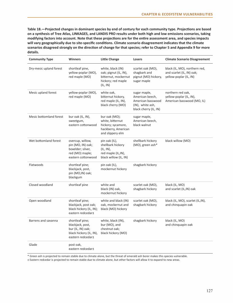
127


Table 18.—Projected changes in dominant species by end of century for each community type. Projections are based on a synthesis of Tree Atlas, LINKAGES, and LANDIS PRO results under both high and low emissions scenarios, taking modifying factors into account. Note that these projections are for the entire assessment area, and species impacts will vary geographically due to site-specific conditions. Climate scenario disagreement indicates that the climate scenarios disagreed strongly on the direction of change for that species; refer to Chapter 5 and Appendix 9 for more details.

Community Type Winners Little Change Losers Climate Scenario Disagreement

Dry-mesic upland forest shortleaf pine, yellow-poplar (MO), red maple (MO)

white, black (IN) oak; pignut (IL, IN), bitternut, mockernut hickory; red maple (IL, IN)

scarlet oak (MO), shagbark and pignut (MO) hickory, sugar maple

black (IL, MO), northern red, and scarlet (IL, IN) oak; yellow-poplar (IL, IN)

Mesic upland forest yellow-poplar (MO), red maple (MO)

white oak, bitternut hickory, red maple (IL, IN), black cherry (MO)

sugar maple, American beech, American basswood (IN), white ash, black cherry (IL, IN)

northern red oak, yellow-poplar (IL, IN), American basswood (MO, IL)

Mesic bottomland forest bur oak (IL, IN), sweetgum, eastern cottonwood

bur oak (MO); white, bitternut hickory; sycamore, hackberry, American and slippery elm

sugar maple, American beech, black walnut

Wet bottomland forest overcup, willow, pin (MO, IN) oak; boxelder; silver, red (MO) maple; eastern cottonwood

pin oak (IL), shellbark hickory (IL, IN), red maple (IL,IN), black willow (IL, IN)

shellbark hickory (MO), green ash*

black willow (MO)

Flatwoods shortleaf pine; blackjack, post, pin (MO,IN) oak; blackgum

pin oak (IL), mockernut hickory

shagbark hickory

Closed woodland shortleaf pine white and black (IN) oak, mockernut hickory

scarlet oak (MO), shagbark hickory

black (IL, MO) and scarlet (IL,IN) oak

Open woodland shortleaf pine; blackjack, post oak; black hickory (IL, IN); eastern redcedar±

white and black (IN) oak, mockernut and black (MO) hickory

scarlet oak (MO), shagbark hickory

black (IL, MO), scarlet (IL,IN), and chinquapin oak

Barrens and savanna shortleaf pine; blackjack, post, bur (IL, IN) oak; black hickory (IL, IN), eastern redcedar±

white, black (IN), bur (MO), and chestnut oak; black hickory (MO)

shagbark hickory black (IL, MO) and chinquapin oak

Glade post oak, eastern redcedar±

* Green ash is projected to remain stable due to climate alone, but the threat of emerald ash borer makes this species vulnerable. ± Eastern redcedar is projected to remain stable due to climate alone, but other factors will allow it to expand to new areas.

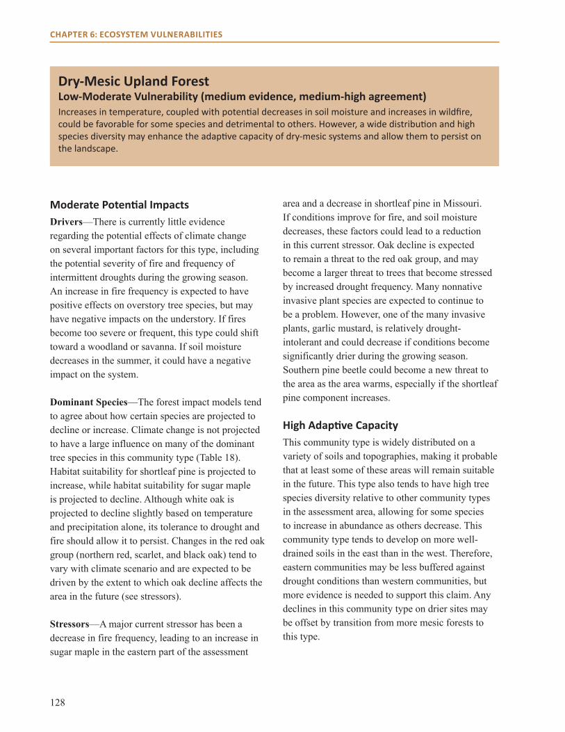
128


Dry-Mesic Upland ForestLow-Moderate Vulnerability (medium evidence, medium-high agreement) Increases in temperature, coupled with potential decreases in soil moisture and increases in wildfire, could be favorable for some species and detrimental to others. However, a wide distribution and high species diversity may enhance the adaptive capacity of dry-mesic systems and allow them to persist on the landscape.

Moderate Potential Impacts Drivers—There is currently little evidence regarding the potential effects of climate change on several important factors for this type, including the potential severity of fire and frequency of intermittent droughts during the growing season. An increase in fire frequency is expected to have positive effects on overstory tree species, but may have negative impacts on the understory. If fires become too severe or frequent, this type could shift toward a woodland or savanna. If soil moisture decreases in the summer, it could have a negative impact on the system.

Dominant Species—The forest impact models tend to agree about how certain species are projected to decline or increase. Climate change is not projected to have a large influence on many of the dominant tree species in this community type (Table 18). Habitat suitability for shortleaf pine is projected to increase, while habitat suitability for sugar maple is projected to decline. Although white oak is projected to decline slightly based on temperature and precipitation alone, its tolerance to drought and fire should allow it to persist. Changes in the red oak group (northern red, scarlet, and black oak) tend to vary with climate scenario and are expected to be driven by the extent to which oak decline affects the area in the future (see stressors).

Stressors—A major current stressor has been a decrease in fire frequency, leading to an increase in sugar maple in the eastern part of the assessment

area and a decrease in shortleaf pine in Missouri. If conditions improve for fire, and soil moisture decreases, these factors could lead to a reduction in this current stressor. Oak decline is expected to remain a threat to the red oak group, and may become a larger threat to trees that become stressed by increased drought frequency. Many nonnative invasive plant species are expected to continue to be a problem. However, one of the many invasive plants, garlic mustard, is relatively drought-intolerant and could decrease if conditions become significantly drier during the growing season. Southern pine beetle could become a new threat to the area as the area warms, especially if the shortleaf pine component increases.

High Adaptive Capacity This community type is widely distributed on a variety of soils and topographies, making it probable that at least some of these areas will remain suitable in the future. This type also tends to have high tree species diversity relative to other community types in the assessment area, allowing for some species to increase in abundance as others decrease. This community type tends to develop on more well-drained soils in the east than in the west. Therefore, eastern communities may be less buffered against drought conditions than western communities, but more evidence is needed to support this claim. Any declines in this community type on drier sites may be offset by transition from more mesic forests to this type.

129


Dry-mesic upland forest. Photo by Paul Nelson, Mark Twain National Forest.

Missouri Ozark forests in autumn. Photo by Steve Shifley, U.S. Forest Service.

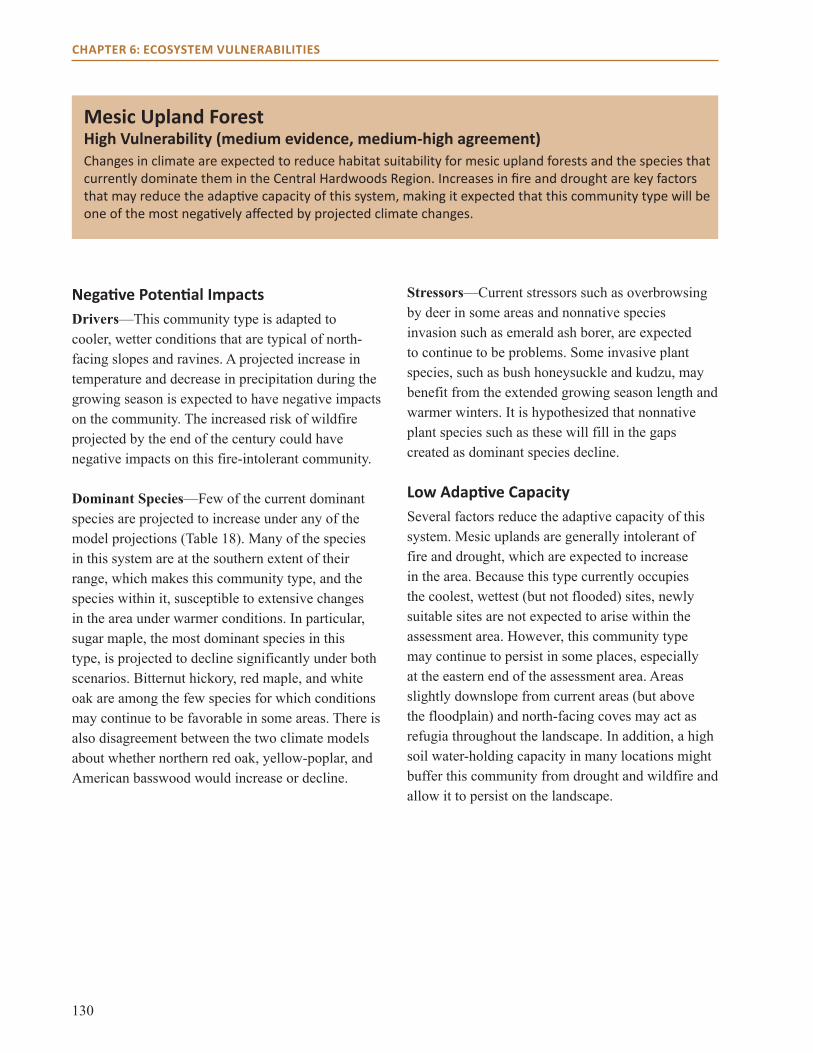
130


Mesic Upland Forest High Vulnerability (medium evidence, medium-high agreement) Changes in climate are expected to reduce habitat suitability for mesic upland forests and the species that currently dominate them in the Central Hardwoods Region. Increases in fire and drought are key factors that may reduce the adaptive capacity of this system, making it expected that this community type will be one of the most negatively affected by projected climate changes.

Negative Potential Impacts Drivers—This community type is adapted to cooler, wetter conditions that are typical of north-facing slopes and ravines. A projected increase in temperature and decrease in precipitation during the growing season is expected to have negative impacts on the community. The increased risk of wildfire projected by the end of the century could have negative impacts on this fire-intolerant community.

Dominant Species—Few of the current dominant species are projected to increase under any of the model projections (Table 18). Many of the species in this system are at the southern extent of their range, which makes this community type, and the species within it, susceptible to extensive changes in the area under warmer conditions. In particular, sugar maple, the most dominant species in this type, is projected to decline significantly under both scenarios. Bitternut hickory, red maple, and white oak are among the few species for which conditions may continue to be favorable in some areas. There is also disagreement between the two climate models about whether northern red oak, yellow-poplar, and American basswood would increase or decline.

Stressors—Current stressors such as overbrowsing by deer in some areas and nonnative species invasion such as emerald ash borer, are expected to continue to be problems. Some invasive plant species, such as bush honeysuckle and kudzu, may benefit from the extended growing season length and warmer winters. It is hypothesized that nonnative plant species such as these will fill in the gaps created as dominant species decline.

Low Adaptive Capacity Several factors reduce the adaptive capacity of this system. Mesic uplands are generally intolerant of fire and drought, which are expected to increase in the area. Because this type currently occupies the coolest, wettest (but not flooded) sites, newly suitable sites are not expected to arise within the assessment area. However, this community type may continue to persist in some places, especially at the eastern end of the assessment area. Areas slightly downslope from current areas (but above the floodplain) and north-facing coves may act as refugia throughout the landscape. In addition, a high soil water-holding capacity in many locations might buffer this community from drought and wildfire and allow it to persist on the landscape.

131


Mesic upland forest. Photo by Paul Nelson, Mark Twain National Forest.



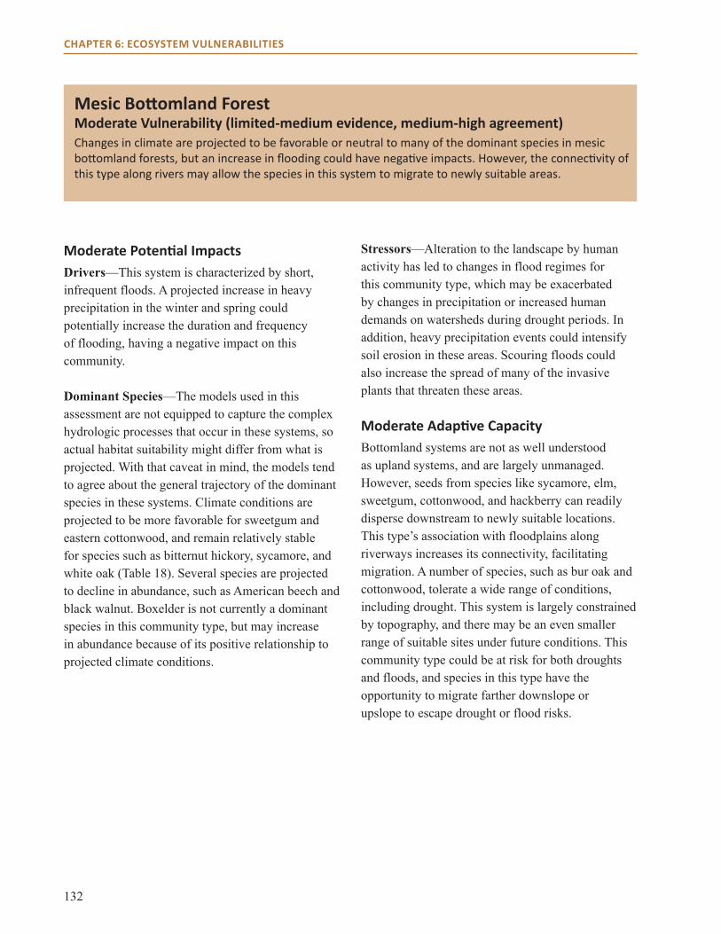
132


Mesic Bottomland ForestModerate Vulnerability (limited-medium evidence, medium-high agreement) Changes in climate are projected to be favorable or neutral to many of the dominant species in mesic bottomland forests, but an increase in flooding could have negative impacts. However, the connectivity of this type along rivers may allow the species in this system to migrate to newly suitable areas.

Moderate Potential ImpactsDrivers—This system is characterized by short, infrequent floods. A projected increase in heavy precipitation in the winter and spring could potentially increase the duration and frequency of flooding, having a negative impact on this community.

Dominant Species—The models used in this assessment are not equipped to capture the complex hydrologic processes that occur in these systems, so actual habitat suitability might differ from what is projected. With that caveat in mind, the models tend to agree about the general trajectory of the dominant species in these systems. Climate conditions are projected to be more favorable for sweetgum and eastern cottonwood, and remain relatively stable for species such as bitternut hickory, sycamore, and white oak (Table 18). Several species are projected to decline in abundance, such as American beech and black walnut. Boxelder is not currently a dominant species in this community type, but may increase in abundance because of its positive relationship to projected climate conditions.

Stressors—Alteration to the landscape by human activity has led to changes in flood regimes for this community type, which may be exacerbated by changes in precipitation or increased human demands on watersheds during drought periods. In addition, heavy precipitation events could intensify soil erosion in these areas. Scouring floods could also increase the spread of many of the invasive plants that threaten these areas.

Moderate Adaptive CapacityBottomland systems are not as well understood as upland systems, and are largely unmanaged. However, seeds from species like sycamore, elm, sweetgum, cottonwood, and hackberry can readily disperse downstream to newly suitable locations. This type’s association with floodplains along riverways increases its connectivity, facilitating migration. A number of species, such as bur oak and cottonwood, tolerate a wide range of conditions, including drought. This system is largely constrained by topography, and there may be an even smaller range of suitable sites under future conditions. This community type could be at risk for both droughts and floods, and species in this type have the opportunity to migrate farther downslope or upslope to escape drought or flood risks.

133


Mesic bottomland forest. Photo by Paul Nelson, Mark Twain National Forest.

Riparian forest along the Cache River, Illinois. Photo by Susan Crocker, U.S. Forest Service.

Wet mesic bottomland. Photo by Paul Nelson, Mark Twain National Forest.

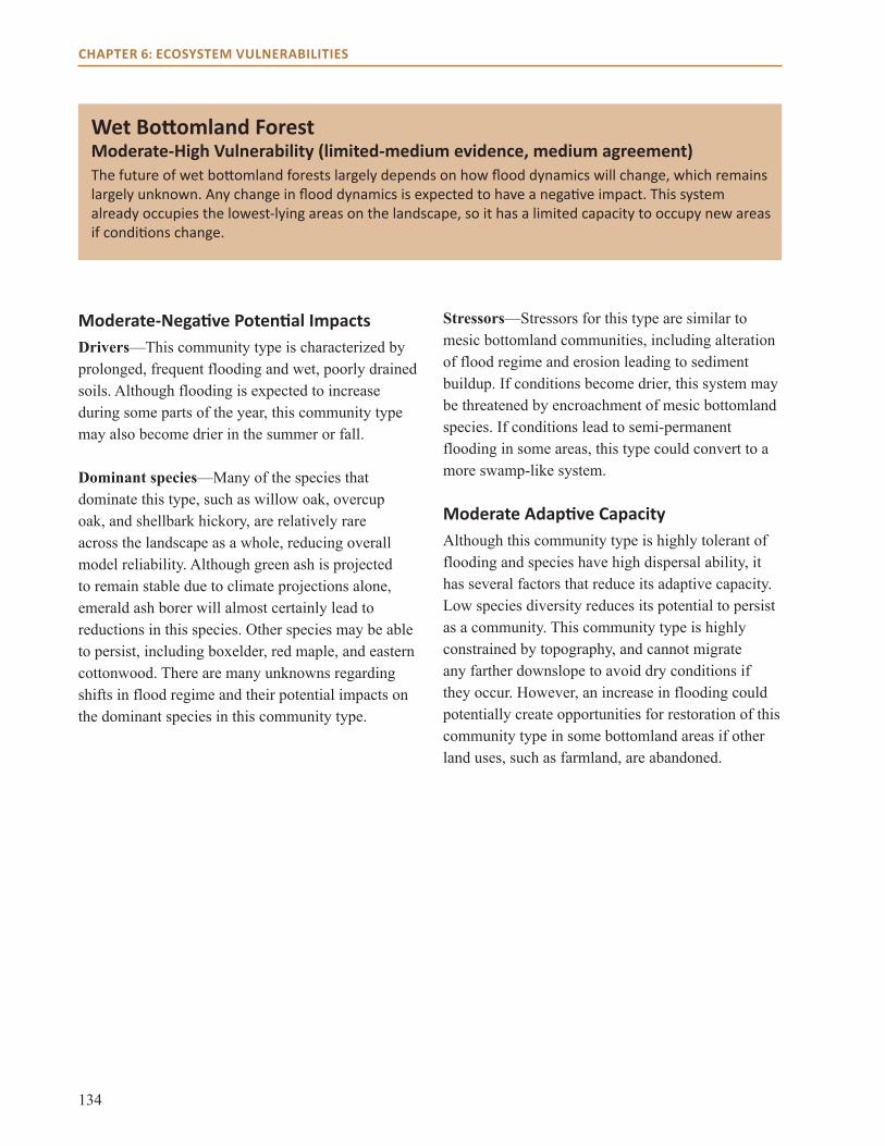
134


Wet Bottomland Forest Moderate-High Vulnerability (limited-medium evidence, medium agreement) The future of wet bottomland forests largely depends on how flood dynamics will change, which remains largely unknown. Any change in flood dynamics is expected to have a negative impact. This system already occupies the lowest-lying areas on the landscape, so it has a limited capacity to occupy new areas if conditions change.

Moderate-Negative Potential Impacts Drivers—This community type is characterized by prolonged, frequent flooding and wet, poorly drained soils. Although flooding is expected to increase during some parts of the year, this community type may also become drier in the summer or fall.

Dominant species—Many of the species that dominate this type, such as willow oak, overcup oak, and shellbark hickory, are relatively rare across the landscape as a whole, reducing overall model reliability. Although green ash is projected to remain stable due to climate projections alone, emerald ash borer will almost certainly lead to reductions in this species. Other species may be able to persist, including boxelder, red maple, and eastern cottonwood. There are many unknowns regarding shifts in flood regime and their potential impacts on the dominant species in this community type.

Stressors—Stressors for this type are similar to mesic bottomland communities, including alteration of flood regime and erosion leading to sediment buildup. If conditions become drier, this system may be threatened by encroachment of mesic bottomland species. If conditions lead to semi-permanent flooding in some areas, this type could convert to a more swamp-like system.

Moderate Adaptive Capacity Although this community type is highly tolerant of flooding and species have high dispersal ability, it has several factors that reduce its adaptive capacity. Low species diversity reduces its potential to persist as a community. This community type is highly constrained by topography, and cannot migrate any farther downslope to avoid dry conditions if they occur. However, an increase in flooding could potentially create opportunities for restoration of this community type in some bottomland areas if other land uses, such as farmland, are abandoned.

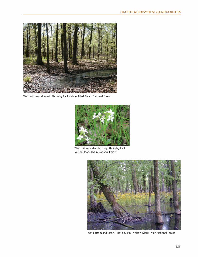
135




Wet bottomland understory. Photo by Paul Nelson. Mark Twain National Forest.

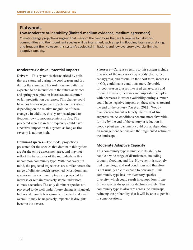
136


Flatwoods Low-Moderate Vulnerability (limited-medium evidence, medium agreement) Climate change projections suggest that many of the conditions that are favorable to flatwoods communities and their dominant species will be intensified, such as spring flooding, late season drying, and frequent fire. However, this system’s geological limitations and low overstory diversity limit its adaptive capacity.

Moderate-Positive Potential ImpactsDrivers—This system is characterized by soils that are saturated during the cool season and dry during the summer. This soil moisture pattern is expected to be intensified in the future as winter and spring precipitation increases and summer or fall precipitation decreases. This change could have positive or negative impacts on the system depending on the relative magnitude of these changes. In addition, this system is adapted to frequent low- to moderate-intensity fire. The projected increase in fire frequency could have a positive impact on this system as long as fire severity is not too high.

Dominant species—The model projections presented for the species that dominate this system are for the entire assessment area, and may not reflect the trajectories of the individuals in this uncommon community type. With that caveat in mind, the projected trajectories are similar across the range of climate models presented. Most dominant species in this community type are projected to increase or remain relatively stable under both climate scenarios. The only dominant species not projected to do well under future change is shagbark hickory. Although blackgum is projected to do well overall, it may be negatively impacted if droughts become too severe.

Stressors—Current stressors to this system include invasion of the understory by woody plants, reed canarygrass, and fescue. In the short term, increases in CO2 could make conditions more favorable for cool-season grasses like reed canarygrass and fescue. However, increases in temperature coupled with decreases in water availability during summer could have negative impacts on these species toward the end of the century (Yu et al. 2012). Woody plant encroachment is largely the result of fire suppression. As conditions become more favorable for fire by the end of the century, a reduction in woody plant encroachment could occur, depending on management actions and the fragmented nature of the landscape.

Moderate Adaptive CapacityThis community type is unique in its ability to handle a wide range of disturbances, including drought, flooding, and fire. However, it is strongly tied to geologic and soil conditions and therefore is not usually able to expand to new areas. This community type has low overstory species diversity, which could result in canopy loss if one or two species disappear or decline severely. This community type is also rare across the landscape, reducing the probability that it will be able to persist in some locations.

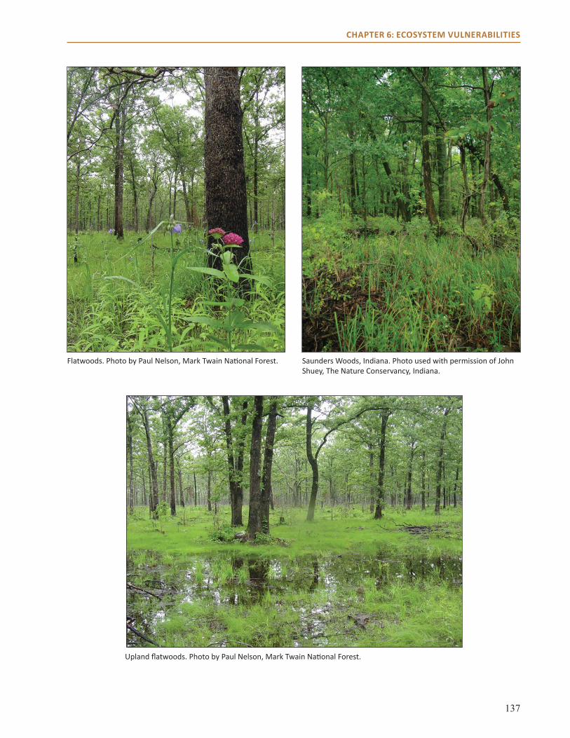
137


Flatwoods. Photo by Paul Nelson, Mark Twain National Forest. Saunders Woods, Indiana. Photo used with permission of John Shuey, The Nature Conservancy, Indiana.

Upland flatwoods. Photo by Paul Nelson, Mark Twain National Forest.

138


Closed Woodland Low Vulnerability (limited evidence, medium agreement) The vulnerability of closed woodlands largely depends on how both natural and human-caused fire dynamics may change over the next century. However, most of the overstory species are expected to persist under projected climate change over a range of fire conditions. In addition, the wide distribution and high tolerance to disturbance of this system should be beneficial.

Positive Potential ImpactsDrivers—This community type is characterized by frequent, low-intensity fires, which are expected to become more common as conditions become warmer and drier. However, if fire severity increases too greatly, fire could have a negative impact. This type is common on excessively well-drained soils with steeper slopes than open woodlands. Because this type is adapted to low soil moisture conditions, decreases in soil moisture during the growing season should not have a strong negative impact.

Dominant Species—The modeled trajectory of the species that dominate these systems is mixed, but the model projections tend to agree with one another. Species in this system should do well in general. Only one of the dominant species in this community type, shagbark hickory, is projected to decline (Table 18). Shortleaf pine is projected to increase, while white oak and mockernut hickory are projected to remain relatively stable. Changes in black and scarlet oak may depend on whether summer precipitation increases or decreases. In addition, this system is also defined by its herbaceous layer, and no information is available on how these species may respond to future climatic conditions.

Stressors—Past fire exclusion has led to an increase in woody species in the understory. This change in composition has suppressed regeneration of overstory species in the eastern part of this

community type’s range, and suppressed herbaceous species establishment in the western part. An increase in fire frequency could help reduce this stressor. Oak decline is expected to remain a threat to black and scarlet oak, and may become a larger threat to trees that become stressed by an increased duration and extent of drought conditions, which appear to be more likely under the GFDL A1FI scenario. Nonnative invasive plants are expected to continue to be a problem in the future, but increased drought could decrease garlic mustard invasion. Southern pine beetle could become a new threat to the area in communities dominated by shortleaf pine.

High Adaptive CapacityThis community type is widely distributed across the western half of the assessment area and is tolerant of fire and drought. This type has the potential to expand if sites currently characterized as dry-mesic communities become drier and subject to more frequent fire. The extent to which fire is a component of the system may ultimately determine the success of this community type. If the system experiences frequent fire, this system could benefit or undergo transition to an open woodland. If fire is suppressed, it could shift to a dry-mesic forest. The long-term fate of this system may also vary dramatically from east to west, especially if black and scarlet oak decline in the west because of increased drought.

139


Closed woodland. Photo by Mike Leahy, Missouri Department of Conservation.

Shortleaf pine woodland. Photo used with permission of L-A-D Foundation.

Closed woodland. Photo by Paul Nelson, Mark Twain National Forest.

140


Open WoodlandLow Vulnerability (limited-medium evidence, medium agreement) Future conditions should be favorable for open woodlands and many of the species that dominate them, but some current and potential stressors could be exacerbated by future climate conditions. In general, this community type is expected to persist due to its drought tolerance and wide distribution.

Positive Potential ImpactsDrivers— This system is similar to closed woodland systems but receives more frequent fire and tends to be on flatter ridge-tops. Dry soils during the summer coupled with conditions suitable for fire should be beneficial for this type unless conditions become so severe that dominant species can no longer tolerate them. Early-season increases in precipitation that result in vegetation growth, followed by summer drought, may increase fire probability.

Dominant Species— Many tree species in this community type are projected to do better under future climate conditions, such as shortleaf pine, blackjack and post oak, and black hickory (Table 18). Changes in black, chinquapin, and scarlet oak may depend on whether summer precipitation increases or decreases. Eastern redcedar, which outcompetes herbaceous vegetation, is projected to remain relatively stable under future climate changes and could expand for other reasons. This outcome could have a negative impact on the community. Importantly, this community type is largely defined by its species in the herbaceous layer, and no information is available on how these species may respond to future climatic conditions.

Stressors— An increase in fire frequency could help reduce the stress of woody species invasion, but eastern redcedar could continue to be a problem in this type. Nonnative invasive plants are expected

to continue to be a problem in the future. Sericea lespedeza invasion is a particular problem in this community type and responds positively to both drought and fire, making it potentially an even greater problem in the future. Increased sericea lespideza abundance could reduce regeneration of tree species and change community structure. Other herbaceous invasive species are less tolerant of fire and may be reduced if fire frequency, severity, or both increase. Southern pine beetle could become a new threat to the area if shortleaf pine increases.

High Adaptive CapacityThis community type is widely distributed across the western half of the assessment area and is fire- and drought-tolerant. Across the assessment area, the open woodland community type will probably not decrease substantially and may even increase. In general, this type may be most successful in the western part of the assessment area, where soils tend to be drier. Decreases in this community type in areas that become too dry or fire-prone could be offset by transition from closed woodlands to this type. In these new areas, overstory woody species may do better than understory herbaceous species because many of the endemic herbaceous species are not present in the seedbank and have a limited ability to disperse. As with closed woodland systems, the success of this type depends largely on fire regime and long-term soil moisture.

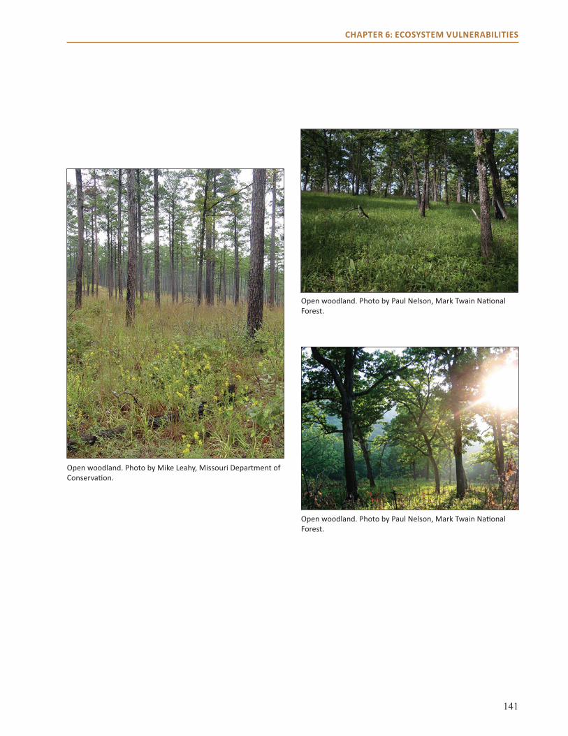
141


Open woodland. Photo by Mike Leahy, Missouri Department of Conservation.



142


Barrens and SavannaLow Vulnerability (medium evidence, medium-high agreement) Conditions should generally be favorable to the species that dominate barrens and savannas, which are generally adapted to fire and drought. However, a high level of fragmentation and a fragile understory community could reduce the ability of this community type to take advantage of these favorable conditions.

Positive Potential Impacts Drivers—Barrens communities develop on extremely shallow, well-drained soils, making them well adapted to drought conditions. However, the low water-holding capacity typical of soils in barrens communities could increase stress under extreme drought conditions. Savanna communities, which are similar in structure to barrens, are characterized by deeper, more nutrient-rich soils and may be more buffered against drought. Barrens and savannas are also fire-adapted and may benefit from increased fire frequency as long as fires do not become frequent enough to shift the system to a grassland community.

Dominant Species—Many species in this community type are projected to do better under future climate conditions, such as shortleaf pine, blackjack oak, post oak, and black hickory (Table 18). Changes in black and chinquapin oak may depend on whether summer precipitation increases or decreases. Eastern redcedar, which can encroach on glades, is projected to remain relatively stable under future climate changes and could expand for other reasons. Expansion of this species could have a negative impact on the community. As with woodlands, this system is largely defined by its herbaceous species, and no information is available on how these species may respond to future climatic conditions.

Stressors—An increase in fire frequency could help reduce the stress of woody species invasion, but eastern redcedar could continue to be a problem in this type. Nonnative invasive species are expected to continue to be a problem in the future, as many are drought-tolerant. These include autumn olive, multiflora rose, teasel, white and yellow sweetclover, sericea lespideza, and spotted knapweed. Garlic mustard is among the few invasive plant species that is not drought-tolerant. Southern pine beetle could become a new threat to the area if shortleaf pine increases.

Moderate Adaptive Capacity Barrens and savanna systems are tolerant of both drought and fire. As conditions become hotter, and potentially drier, open woodlands could shift into more open barrens or savanna systems. This transition could lead to an increase in area occupied by this type, which is currently extremely low (about 1 percent of the assessment area). As with open woodlands, increased fire frequency and drought duration could allow other communities to convert structurally to barrens or savannas. However, herbaceous and graminoid species that are typically found in the understory in these communities may be dispersal limited. Barrens and savanna communities are currently rare and highly fragmented; many lack a healthy herbaceous community. The adaptive capacity of these systems is also largely dependent on fire regime and whether they are on thin or more well-developed soils.

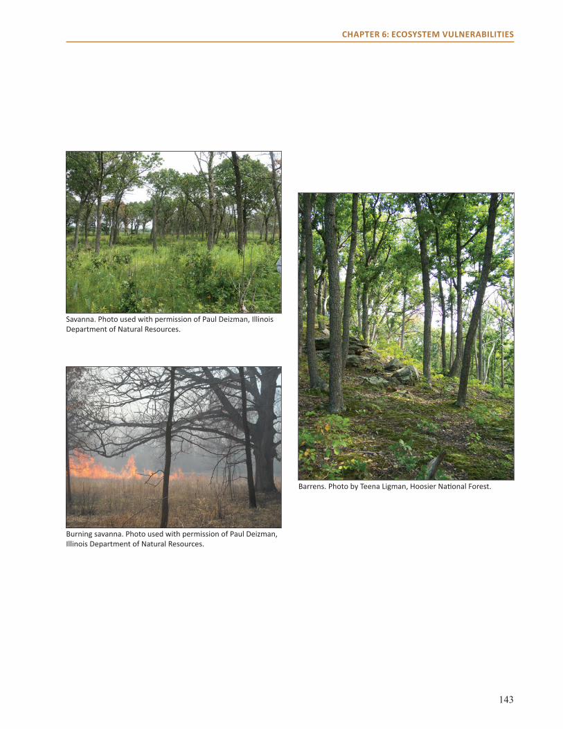
143


Barrens. Photo by Teena Ligman, Hoosier National Forest.

Savanna. Photo used with permission of Paul Deizman, Illinois Department of Natural Resources.

Burning savanna. Photo used with permission of Paul Deizman, Illinois Department of Natural Resources.

144


GladeLow-Moderate Vulnerability (medium evidence, medium-high agreement) Glade species tend to be tolerant of hot, dry conditions, which should allow them to persist. However, there is a potential for increased soil erosion with increased heavy precipitation events, which could have a negative impact on glades in the western part of the assessment area in particular. Areas that are invaded by eastern redcedar may have a reduced capacity to adapt to projected changes.

Moderate-Positive Potential ImpactsDrivers—This community type develops on areas of exposed bedrock with very thin soils. Thus it is adapted to hot, xeric conditions during the growing season, which are projected to become more common in the future. This system is also adapted to frequent, low-intensity fires, which could possibly increase by the end of the century.

Dominant Species—Unlike the other communities assessed, glades are dominated by herbaceous species, with a few sparse trees distributed throughout. Although future distribution of these herbaceous species has not been modeled, many are adapted to the hot, dry conditions that are expected to become more common. Despite this advantage, several modeling studies in other areas have shown that species with narrow geographic distributions, like many glade species, are more at-risk to climate change (Broennimann et al. 2006, Damschen et al. 2010, Loarie et al. 2008). Post oak is typically found in glade systems, and is projected to increase. Eastern redcedar invasion has led to dominance of this species in glades, and it is projected to expand in the future because of other factors besides climate change.

Stressors—Soil erosion due to past overgrazing and feral hog invasion may be exacerbated by heavy precipitation events, especially in the western part of the assessment area, where glades are located on steeper slopes. Soil erosion may be less of an issue in glades east of the Mississippi, which are on more level terrain. Eastern redcedar invasion may continue to be a problem in this community type, as climate change is not projected to dramatically impact that species. Increases in winter and spring precipitation could benefit eastern redcedar thickets where spring water is channeled.

Moderate Adaptive Capacity This community type and the species that live within it are adapted to extreme drought and heat. Other community types, such as barrens, could potentially shift to glades if conditions become sufficiently hot and dry. However, this is a rare, highly fragmented system that is limited to specific geologic features, limiting opportunity for expansion to new areas. In addition, past invasion of eastern redcedar decreases the ability of this system to positively respond to potential increases in fire frequency. Intact glades that have not been heavily invaded by redcedar will probably fare better.

145


Dolomite glade. Photo used with permission of Matthew Albrecht, Missouri Botanical Garden.

Glade. Photo by Paul Nelson, Mark Twain National Forest.

Glade. Used with permission of Matthew Albrecht, Missouri Botanical Garden.

146


CONCLUSIONSNumerous factors contribute to the overall vulnerability of the Central Hardwoods Region to climate change; some communities are more vulnerable than others. Impacts such as increased temperature, changes in precipitation, and shifts in wildfire regime are expected to combine to influence the distribution and productivity of tree species. In general, species that are adapted to wetter, cooler conditions are expected to fare worse, such as sugar maple or American beech.

Species adapted to warmer, drier climates may fare better, such as shortleaf pine and post oak. These changes can lead to shifts in community structure and composition. Communities that lack the ability to withstand disturbances, such as mesic upland forests, or are constrained by topographic barriers, such as bottomland forests, may be particularly vulnerable. Communities that are adapted to a wide range of disturbances and can persist on a wide range of topographies, such as dry-mesic forests and woodlands, are expected to be less vulnerable to a changing climate.

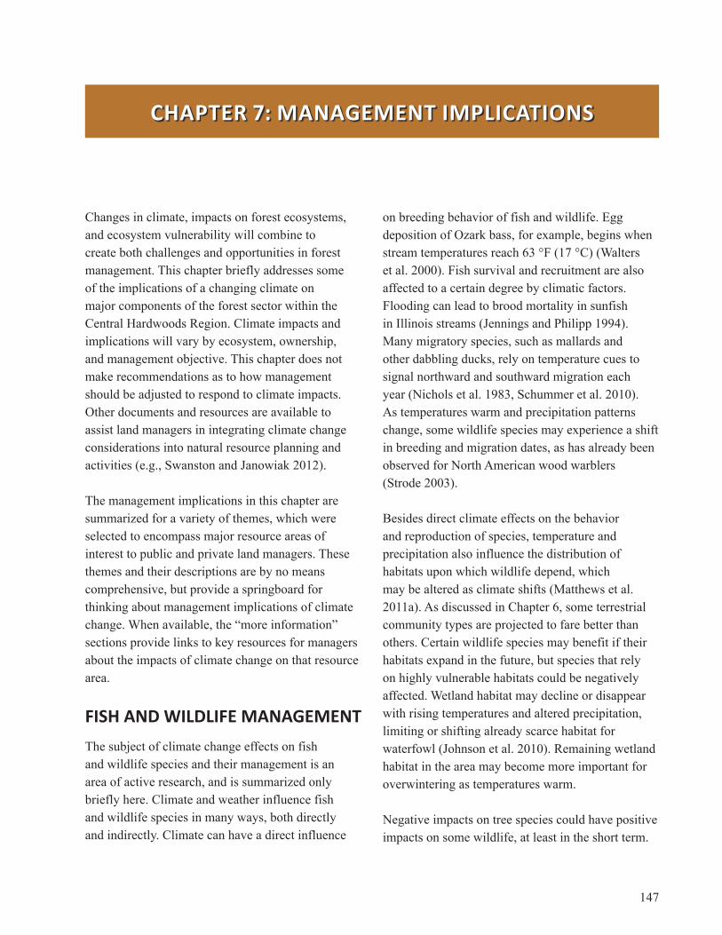
147

CHAPTER 7: MANAGEMENT IMPLICATIONS

Changes in climate, impacts on forest ecosystems, and ecosystem vulnerability will combine to create both challenges and opportunities in forest management. This chapter briefly addresses some of the implications of a changing climate on major components of the forest sector within the Central Hardwoods Region. Climate impacts and implications will vary by ecosystem, ownership, and management objective. This chapter does not make recommendations as to how management should be adjusted to respond to climate impacts. Other documents and resources are available to assist land managers in integrating climate change considerations into natural resource planning and activities (e.g., Swanston and Janowiak 2012).

The management implications in this chapter are summarized for a variety of themes, which were selected to encompass major resource areas of interest to public and private land managers. These themes and their descriptions are by no means comprehensive, but provide a springboard for thinking about management implications of climate change. When available, the “more information” sections provide links to key resources for managers about the impacts of climate change on that resource area.

FISH AND WILDLIFE MANAGEMENTThe subject of climate change effects on fish and wildlife species and their management is an area of active research, and is summarized only briefly here. Climate and weather influence fish and wildlife species in many ways, both directly and indirectly. Climate can have a direct influence

on breeding behavior of fish and wildlife. Egg deposition of Ozark bass, for example, begins when stream temperatures reach 63 °F (17 °C) (Walters et al. 2000). Fish survival and recruitment are also affected to a certain degree by climatic factors. Flooding can lead to brood mortality in sunfish in Illinois streams (Jennings and Philipp 1994). Many migratory species, such as mallards and other dabbling ducks, rely on temperature cues to signal northward and southward migration each year (Nichols et al. 1983, Schummer et al. 2010). As temperatures warm and precipitation patterns change, some wildlife species may experience a shift in breeding and migration dates, as has already been observed for North American wood warblers (Strode 2003).

Besides direct climate effects on the behavior and reproduction of species, temperature and precipitation also influence the distribution of habitats upon which wildlife depend, which may be altered as climate shifts (Matthews et al. 2011a). As discussed in Chapter 6, some terrestrial community types are projected to fare better than others. Certain wildlife species may benefit if their habitats expand in the future, but species that rely on highly vulnerable habitats could be negatively affected. Wetland habitat may decline or disappear with rising temperatures and altered precipitation, limiting or shifting already scarce habitat for waterfowl (Johnson et al. 2010). Remaining wetland habitat in the area may become more important for overwintering as temperatures warm.

Negative impacts on tree species could have positive impacts on some wildlife, at least in the short term.

148


If changes in flood conditions lead to increased mortality in bottomland forests, for example, there could be an increase in snag habitat for terrestrial species that require such habitat, such as the Indiana bat (Carter and Feldhamer 2005). However, more frequent, severe, or longer flooding could destroy habitat for other terrestrial species.

Fish and other aquatic organisms are also expected to be affected by a combination of both direct and indirect climate change effects. Many fish species in the region are sensitive to even slight changes in water temperatures and experience negative effects on growth at extremely high water temperatures (Jennings and Philipp 1994, Jones et al. 2011, Michaletz et al. 2012, Smale and Rabeni 1995, Whitledge et al. 2006). Degradation of aquatic habitats could occur in streams and riparian areas, which are important in maintaining habitat structure and temperature control (Whitledge et al. 2006). Water levels in lakes could also change, although the magnitude and direction of those changes remain uncertain (Angel and Kunkel 2010). In drought periods, lake levels could drop and temperatures could increase, causing fish kills and reducing food availability for other species.

Many potential impacts on wildlife and their habitats remain unknown. Animal species that are already rare, threatened, or endangered, or that live in a very narrow habitat range, may be particularly vulnerable to shifts in temperature and precipitation (Walk et al. 2011). However, the limited range of these species also makes it difficult to model the effects of climate and climate change on their distribution and abundance (Schwartz et al. 2006b). Many diseases that threaten wildlife species may be able to expand, increasing stress and mortality in species already threatened by direct climate effects (Harvell et al. 2002). No research on climate change effects on wildlife diseases in the Central Hardwoods Region is currently available, however. The effects of climate change on cave-dwelling species are also unknown.

More Information• The Climate Change Bird Atlas is a companion

to the Climate Change Tree Atlas and projects changes in bird species distributions by using information about direct climate change effects and changes in habitat. www.nrs.fs.fed.us/atlas/bird

• Many states are working to incorporate climate change information into their state wildlife action plans. Voluntary guidance has been provided by the Association of Fish and Wildlife Agencies. www.fishwildlife.org/files/AFWA-Voluntary-Guidance-Incorporating-Climate-Change_SWAP.pdf

• In Illinois, an update to the Illinois Wildlife Action plan was created by The Nature Conservancy to assess wildlife vulnerabilities to climate change. The report can be downloaded at: https://adapt.nd.edu/resources/223/download/IWAP_Climate_Change_Update_11May2011.pdf

PLANT SPECIES OF CONCERNChanges in climate may impose increased challenges for the conservation of rare, threatened, or endangered plant species. The characteristics that make these species rare, such as narrow niche specificity, low dispersal ability, and highly fragmented populations, reduce the adaptive capacity of these species and make them more vulnerable to climate change than more common species (Broennimann et al. 2006). In addition, many of these species rely on specific pollinator species to reproduce. Pollinator species, such as butterflies and bees, are expected to be affected by changes in climate, asynchrony in phenology, and colony collapse (Potts et al. 2010).

Research that specifically examines the effects of climate change on plant species of concern in the Central Hardwoods Region is underway. Researchers at the Missouri Botanical Garden are examining

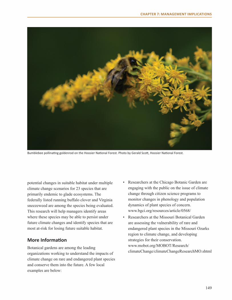
149


potential changes in suitable habitat under multiple climate change scenarios for 23 species that are primarily endemic to glade ecosystems. The federally listed running buffalo clover and Virginia sneezeweed are among the species being evaluated. This research will help managers identify areas where these species may be able to persist under future climate changes and identify species that are most at-risk for losing future suitable habitat.

More InformationBotanical gardens are among the leading organizations working to understand the impacts of climate change on rare and endangered plant species and conserve them into the future. A few local examples are below:

• Researchers at the Chicago Botanic Garden are engaging with the public on the issue of climate change through citizen science programs to monitor changes in phenology and population dynamics of plant species of concern. www.bgci.org/resources/article/0568/

• Researchers at the Missouri Botanical Garden are assessing the vulnerability of rare and endangered plant species in the Missouri Ozarks region to climate change, and developing strategies for their conservation. www.mobot.org/MOBOT/Research/climateChange/climateChangeResearchMO.shtml

Bumblebee pollinating goldenrod on the Hoosier National Forest. Photo by Gerald Scott, Hoosier National Forest.

150


INVASIVE SPECIES MANAGEMENTAs summarized in Chapters 5 and 6, climate change is expected to expand the distribution and abundance of many nonnative invasive plant species across the region. Many plant species that currently threaten the region, such as Japanese stiltgrass and sericea lespedeza, are expected to withstand or even benefit from projected changes in climate. Reducing or preventing the spread of those species will thus remain a challenge in the coming decades. Resources are already insufficient to control these species under current conditions, so this problem may be exacerbated. A few invasive species adapted to more mesic conditions, such as garlic mustard, may potentially be negatively affected by a reduction in late-season soil moisture on drier sites. Although it is possible that changes in climate could reduce the need for management of a few species, this benefit may be offset by increases in management needs for other species.

Changes in climate will also create additional management challenges as conditions become more favorable for invasive plant species not currently prevalent in the assessment area. Available modeling research suggests that conditions are projected to be more favorable for kudzu and Chinese and European privet as temperatures increase across the area (Bradley et al. 2010, Jarnevich and Stohlgren 2009). Additional resources may be required to prevent the spread of these species into new areas and control them if they do invade.

More Information• The Midwest Invasive Plant Network’s mission is

to reduce the impact of invasive plant species in the Midwest. mipn.org

FIRE AND FUELS MANAGEMENT Weather and climate are major drivers of fire behavior. Unlike most parts of the country, the prescribed fire season and wildfire season tend to occur during the same times in the Central Hardwoods Region: fall and spring. However, if higher-than-average temperatures or dry conditions occur, wildfires can occur at any time of year, causing damage to natural resources and other resources, as well as endangering the public. For example, the summer of 2012 was abnormally hot and dry, and fires in the Midwest behaved more like what is typically experienced in the western United States.

Projected changes in climate could affect fire and fuels management in the Central Hardwoods Region. The data presented in Chapter 4 suggest that the summer or fall could be drier. Drier conditions later in the growing season following wet springs could cause some tree mortality, increasing forest fuel loads and the potential for more intense fires. High-intensity wildfire can result in species mortality, increases in invasive species, changes in soil dynamics (e.g., compaction, altered nutrient cycling, sterilization), or altered hydrology (e.g., increased runoff or erosion). Under intense fire weather conditions, large-scale fires could also become a hazard and safety risk to the public, firefighters, and infrastructure. More resources may be needed to reduce fuel loads to prevent these catastrophic wildfires, fight them when they do occur, and restore ecosystems after a catastrophic event.

Changes in climate may also affect the ability to use fire as a restoration tool. For example, wetter springs could make it difficult to conduct prescribed burns during that season, leaving opportunities for dormant-season burning for the fall. On the other hand, if fall becomes too dry, prescribed burning opportunities could also be reduced.

151


Although some ecosystems may be negatively affected by wildfire, the projected increases in wildfire could also be beneficial in some areas. Increased fire potential may increase opportunities for restoring open woodlands, barrens, and savannas, for example.

More Information • The Oak Woodlands and Forests Fire Consortium

provides fire science information to resource managers, landowners, and the public about the use, application, and effects of fire across the Central Hardwoods Region. Climate change is one of the consortium’s “hot topics.” www.oakfirescience.com

SOIL, WATER, AND AIR QUALITY Changes in climate may have implications for the management of soil, water, and air resources. Soils in the region are projected to experience an increase in waterlogging in the spring, followed by a potential decrease in moisture later in the growing season (Chapter 4). These stressors could be exacerbated in soils with a fragipan or claypan layer, which are common in flatwoods communities. Increased efforts to control soil erosion may be needed to cope with the effects of increased heavy precipitation events across the region, especially on steeper slopes (Nearing 2001, Nearing et al. 2004). In addition, soil nutrient availability is expected to be affected by changes in temperature, moisture, and species composition, but the magnitude and direction of these changes remain uncertain (Rennenberg et al. 2009).

Water quality may be affected by warming temperatures and shifts in precipitation and hydrology. Increased temperatures can lead to decreases in dissolved oxygen, increased toxicity of pollutants, and increases in harmful algae and bacteria (Lofgren and Gronewold 2012,

and references therein). Heavy precipitation and increased runoff could also reduce river and lake quality through increased sedimentation, pollution, and nutrient deposition. More resources may be needed to lower stream temperatures and reduce runoff.

The direct and indirect effects of a changing climate have important implications for air quality and its management. A number of studies have shown that tropospheric ozone is projected to increase with increasing temperature, especially in urban areas (Jacob and Winner 2009). Particulate matter may also be affected by changes in climate, although changes are less predictable than for ozone (Jacob and Winner 2009). An increase in wildfire frequency, as projected to occur by the end of the century, could lead to increases in particulate matter and other pollutants in the area.

More Information• A recent report submitted for the National

Climate Assessment summarizes the impacts of climate change on water resources across the Midwest, including the assessment area. The report can be downloaded at glisa.msu.edu/docs/NCA/MTIT_WaterResources.pdf

CARBON MANAGEMENTAs the climate changes in the Central Hardwoods Region, changes in carbon dynamics are also expected to occur. Many of these changes remain uncertain. As mentioned in Chapters 5 and 6, the benefits of a longer growing season and carbon dioxide fertilization may be offset by an increase in physical and biological disturbances, leading to increases in carbon storage and sequestration in some areas and decreases in others (Hicke et al. 2012). In this region, mesic hardwood forests dominated by species like sugar maple and American

152


beech tend to be the most carbon-dense (i.e., have greater amounts of carbon per acre) (see Chapter 1), so declines in these species may also lead to decreased carbon storage in these forests. However, the majority of forest land in the area is dominated by oak and hickory species, which are projected to persist on the landscape.

Changes in climate may present both challenges and opportunities for carbon management in the Central Hardwoods Region. Future conditions are projected to be more favorable for more open systems, such as barrens, glades, and open woodlands that are driven by fire. These systems tend to be less carbon-dense than more mesic systems. Systems that are adapted to disturbance and are less carbon-dense may also have a lower risk of major carbon losses from large-scale disturbances that are expected to become more prevalent in the future (Hurteau and Brooks 2011). The relative carbon losses from managing for more open systems versus the benefit of avoided losses from events such as severe wildfire have not been explored specifically for the Central Hardwoods Region (Bowman et al. 2013).

More information• The Forest Service’s Climate Change Resource

Center provides several synthesis products on ecosystem carbon. Included are a written summary of how climate change may affect the ability of forests to store carbon, video series on forest and grassland carbon, and a compilation of tools for measuring carbon. www.fs.fed.us/ccrc/topics/forests-carbon/

• A recent article, “A Synthesis of the Science on Forests and Carbon for U.S. Forests,” summarizes the key issues related to forest management and carbon. www.fs.fed.us/rm/pubs_other/rmrs_2010_ryan_m002.pdf

FOREST PRODUCTSInformation presented in Chapters 5 and 6 indicates that species composition in the Central Hardwoods Region is expected to change over the long term, which could have important implications for the forest products industry. Some important timber species may experience negative effects. In Illinois and Indiana, hardwood species like black cherry, American beech, and white ash are projected to decline in habitat suitability under both climate scenarios. Although these species are highly valued for their timber elsewhere, they do not constitute a large portion of the timber industry in southern Illinois and Indiana and are not as valuable locally as in areas north and east of the assessment area. One potential exception may be sugar maple, which is projected to decline across the assessment area and is economically important in Indiana (but still less so than areas north and east). Black walnut is also projected to experience declines, and is very valuable for timber across the assessment area.

The Central Hardwoods Region is an important producer of oak and hickory for wood products. Some oak species are projected to decline, but others are projected to remain stable or even increase. There is more uncertainty about the fate of red oak group species, such as scarlet, northern red, and black oak, than the fate of white oak group species like white and post oak. Even if some oak species become less common, standing oaks that remain may become more valuable. Some economically important species of hickory are expected to decline as well, such as shagbark hickory. Other species of hickory are expected to remain similar to the current distribution, such as mockernut and bitternut hickory, and may continue to be part of the local economy.

Some higher-valued species are projected to benefit from the changing climate. Habitat suitability for

153


sweetgum is anticipated to increase as a result of changing climate. Sweetgum wood is used for flooring, furniture, veneers, and other lumber applications. Shortleaf pine, an economically important species in Missouri, is another species where suitable habitat is projected to increase across the assessment area. The economic importance of shortleaf pine has decreased since the turn of the last century, but it is still important for general construction, pulpwood, and exterior and interior finishing. The economic importance of shortleaf pine could potentially expand in the future if the forest products industry takes advantage of its tolerance to projected future climate.

Projected increases in severe weather events could increase the amount of salvage harvests versus green harvests that are undertaken. Harvesting green timber allows resource managers to strategically achieve desired objectives and outcomes. Salvage harvesting following a severe weather event, by contrast, generally arises from a more immediate need to decrease fuel loading or open impacted forest areas. Salvage sales also do not garner the same amount of financial return as does a green timber sale opportunity.

Timber sale on the Hoosier National Forest. Photo by Chris Zimmer, Hoosier National Forest.

154


More Information• The 2010 Resources Planning Act Assessment

includes future projections for forest products and other resources through the year 2060 and examines social, economic, land-use, and climate change influences. The report can be downloaded here: www.fs.fed.us/research/rpa

NONTIMBER FOREST PRODUCTSChanges in climate could also have important implications for nontimber forest products. Black walnut and pecan are both grown for their nuts in the Central Hardwoods Region, primarily in the Missouri Ozarks. Habitat suitability for pecan is projected to increase across the assessment area, which could open up opportunities for pecan nut production. Black walnut, however, is projected to undergo declines in habitat suitability, which could make it more difficult to cultivate for nuts in the coming decades.

Christmas tree production is an important industry throughout the Midwest that could be affected by a changing climate. In Indiana, for example, Christmas tree sales are a $12.5 million industry (Bratkovich et al. 2007). Many species of Christmas trees, especially young seedlings, do not tolerate drought or extremely wet conditions, and are susceptible to diseases from being planted close together in monoculture. Scotch and white pines are the predominant Christmas trees grown in the Central Hardwoods Region. We have not modeled potential changes in habitat suitability for nonnative Scotch pine, but our projections suggest that habitat suitability will be dramatically reduced for white pine. Irrigation and other management techniques employed by Christmas tree farmers may allow white pine to persist, however. The short rotation length of Christmas trees also presents an opportunity for tree growers to plant new species

and varieties that may be better suited to a changing climate.

Maple syrup is another nontimber product that is made in small amounts in Indiana. A survey from the Indiana Department of Natural Resources reported that about 200 families produce a little over 5,000 gallons annually in the state (Bratkovich et al. 2007). Maple sap flow is driven by temperatures that fluctuate around the freezing point in the late winter or early spring. As spring temperatures increase, the prime season for syrup production may shift to earlier in the season, and the number of sap flow days could eventually decrease in areas at the southern extent of the species’ range (Skinner et al. 2010).

Climate change may have implications for economically and culturally valuable forest understory species. For example, black cohosh is a herbaceous species native to the eastern United States that is important for a variety of medicinal uses. Native Americans and alternative medicine practitioners have used it for centuries to treat conditions such as rheumatism, menopause symptoms, and menstrual problems. Economic demand for this species has been increasing in the past few decades. Black cohosh ranked as the eighth top-selling herb in the United States in 2005, with a reported value of $9.7 million (Blumenthal et al. 2006). The species is considered critically imperiled in Illinois and vulnerable in Indiana, due to a combination of habitat loss and overharvesting of wild populations (NatureServe 2013). Within the Central Hardwoods Region, black cohosh is primarily found in mesic upland forests dominated by ash, beech, and sugar maple, a community type that was found to be highly vulnerable to climate change in the region. Therefore, conservation efforts to maintain this species within the Central Hardwoods Region may face additional challenges from a changing climate in the coming decades.

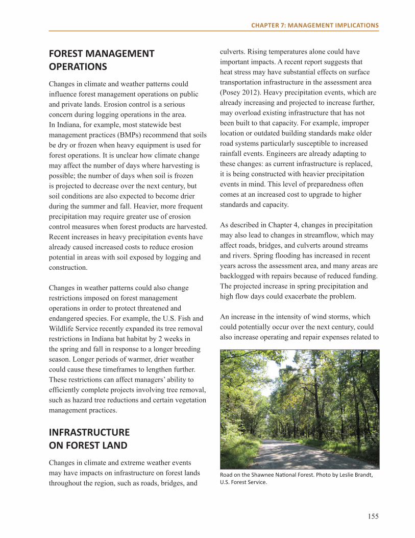
155


FOREST MANAGEMENT OPERATIONSChanges in climate and weather patterns could influence forest management operations on public and private lands. Erosion control is a serious concern during logging operations in the area. In Indiana, for example, most statewide best management practices (BMPs) recommend that soils be dry or frozen when heavy equipment is used for forest operations. It is unclear how climate change may affect the number of days where harvesting is possible; the number of days when soil is frozen is projected to decrease over the next century, but soil conditions are also expected to become drier during the summer and fall. Heavier, more frequent precipitation may require greater use of erosion control measures when forest products are harvested. Recent increases in heavy precipitation events have already caused increased costs to reduce erosion potential in areas with soil exposed by logging and construction.

Changes in weather patterns could also change restrictions imposed on forest management operations in order to protect threatened and endangered species. For example, the U.S. Fish and Wildlife Service recently expanded its tree removal restrictions in Indiana bat habitat by 2 weeks in the spring and fall in response to a longer breeding season. Longer periods of warmer, drier weather could cause these timeframes to lengthen further. These restrictions can affect managers’ ability to efficiently complete projects involving tree removal, such as hazard tree reductions and certain vegetation management practices.

INFRASTRUCTURE ON FOREST LANDChanges in climate and extreme weather events may have impacts on infrastructure on forest lands throughout the region, such as roads, bridges, and

culverts. Rising temperatures alone could have important impacts. A recent report suggests that heat stress may have substantial effects on surface transportation infrastructure in the assessment area (Posey 2012). Heavy precipitation events, which are already increasing and projected to increase further, may overload existing infrastructure that has not been built to that capacity. For example, improper location or outdated building standards make older road systems particularly susceptible to increased rainfall events. Engineers are already adapting to these changes: as current infrastructure is replaced, it is being constructed with heavier precipitation events in mind. This level of preparedness often comes at an increased cost to upgrade to higher standards and capacity.

As described in Chapter 4, changes in precipitation may also lead to changes in streamflow, which may affect roads, bridges, and culverts around streams and rivers. Spring flooding has increased in recent years across the assessment area, and many areas are backlogged with repairs because of reduced funding. The projected increase in spring precipitation and high flow days could exacerbate the problem.

An increase in the intensity of wind storms, which could potentially occur over the next century, could also increase operating and repair expenses related to

Road on the Shawnee National Forest. Photo by Leslie Brandt, U.S. Forest Service.

156


infrastructure. For example, frequent high-intensity windstorms across the assessment area in 2012 led to major damage to infrastructure. As a result, roads and trails had to be cleared and facilities repaired.

More Information• A technical report summarizing climate change

impacts on the transportation sector (including infrastructure) was recently released as input for the Midwest Region for the National Climate Assessment: glisa.msu.edu/docs/NCA/MTIT_Transportation.pdf

CULTURAL RESOURCESClimate change may present challenges for managers of cultural resources on public lands in the Central Hardwoods Region. Extreme wind events such as tornadoes and derechos present challenges for the management of cultural resources for several reasons. These events can directly damage cultural resources such as buildings and other structures. Cultural resources damaged by storms may be further damaged by subsequent salvage harvest operations because unsafe walking conditions and low ground surface visibility often make it impossible to take a cultural resources inventory before the salvage sale.

A change in the frequency, severity, or duration of heavy precipitation and flooding could affect cultural resources as well. Historic and prehistoric habitation sites are often located near waterways. Flood events result in increased erosion or obliteration of significant archaeological sites located along stream and river banks. Similarly, torrential rains can trigger or exacerbate erosion of cultural resources. When built reservoir levels drop (because of drought or intentional levee breaks), prehistoric human remains and other cultural resources are at risk of being exposed by wave action.

Projected changes in wildfire could also affect cultural resources in the region. Wildfire and wildfire suppression activities have the potential to destroy or damage cultural resources. Aboveground combustible features are the most at-risk, although extreme heat can damage noncombustible features or artifacts such as rock art, ceramics, and lithic artifacts (e.g., projectile points).

Optimal fieldwork conditions for cultural resource managers are largely determined by weather and climate. Identification of cultural resources is hindered by leaf-on conditions. The highest quality cultural resource inventories and monitoring of known sites occur during fall, winter, and early spring in the Central Hardwoods Region. Similarly, field opportunities for volunteers, such as the Mark Twain National Forest’s Passport in Time projects, are scheduled during leaf-off conditions when the weather and climate are mild and biting insects such as ticks and chiggers are less abundant, typically fall or late spring. A lengthening growing season could reduce periods of optimal conditions for fieldwork related to cultural resource management.

Historic properties with no standing structures are sometimes identified in the field by legacy vegetation or “cultural resources indicator species.” If any of these indicator species (typically nonnative ornamentals planted by Euro-American inhabitants) are vulnerable to climate change and vanish from the landscape, historic properties (such as unmarked graves) may escape field identification and suffer unintentional damage from ground-disturbing activities.

More Information• The report Wildland Fire in Ecosystems: Effects

of Fire on Cultural Resources and Archeology summarizes the impacts of fire and fire management activities on cultural resources. www.fs.fed.us/rm/pubs/rmrs_gtr042_3.html

157


• The document Climate Change and World Heritage: Report on Predicting and Managing the Impacts of Climate change on World Heritage includes a list of climate change threats to cultural heritage sites. whc.unesco.org/documents/publi_wh_papers_22_en.pdf

RECREATION Outdoor recreation across the Central Hardwoods Region is typically highest in spring and fall. Warmer springs and falls may improve conditions for outdoor recreation activities such as camping, boating, and kayaking (Nicholls 2012). Lengthening of the spring and fall recreation seasons may have implications for staffing, especially for recreation-related businesses that rely on student labor that will be unavailable during the school year (Nicholls 2012). However, shifts in precipitation could also have negative impacts on spring and fall recreation activities. Increased spring precipitation could increase risks for flash flooding or simply lead to unpleasant conditions for recreation. Severe storms and flooding might threaten resources such as visitor centers, campsites, and trails. Fall, on the other hand, will potentially be drier, which could cause lower water levels and reduce boating and kayaking opportunities. Warmer, drier conditions in the fall may also increase the risk of wildfire, increasing visitor safety risk and restrictions on open flames.

Winter recreation in the Central Hardwoods Region is typically an extension of spring and fall activities, as snow and ice are often insufficient for activities such as skiing or ice skating. Currently, a moderate amount of hiking; camping; picnicking; horseback riding; and off-road vehicle, motorcycle, and mountain bike riding occurs throughout the winter. Visitors find it easier to enjoy the views of the rock formations and other scenery from a distance during leaf-off. On the rivers, boating and catch-and-release

fishing are typical winter activities. As winter temperatures increase in the coming decades, more people could potentially take advantage of milder conditions for recreation activities.

A recent study suggests that climate conditions during the summer will become unfavorable for tourism in the region by mid-century under a high emissions scenario (Nicholls 2012). Under that scenario, the number of extremely hot days is projected to increase significantly, which could reduce demand for camping facilities and make outdoor physical activity unpleasant or potentially dangerous to sensitive individuals. One exception may be recreation on rivers. Evidence from previous summers across the area suggests that local residents increase their visits to rivers to cool off during extremely hot periods. The increase in temperature could lead to fewer visits to public lands in the area overall during the summer, and potential declines in summer tourism revenue. These changes could be particularly important for recreation-dependent communities, such as the Lake of the Ozarks.

Climate can also have important influences on hunting and fishing. The timing of certain hunts or fishing seasons correspond to seasonal events, which are partially driven by climate. Waterfowl hunting seasons, for example, are designed to correspond to the times when birds are migrating south in the fall, an event that could shift later in the year as temperatures warm. A recent study in Illinois showed that the number of mallards and other dabbling ducks taken during the hunting season improved as low temperatures during the hunting season became colder (Stafford et al. 2010). These results suggest that rising fall temperatures could potentially reduce success rates. If reductions in precipitation and increases in evaporation decrease waterfowl habitat, waterfowl could also shift their migration patterns to new areas, further reducing hunting opportunities.

158


More Information• A recent report submitted for the National

Climate Assessment summarizes the impacts of climate change on outdoor recreational tourism across the Midwest, including the assessment area. glisa.msu.edu/docs/NCA/MTIT_RecTourism.pdf

• Season’s End, a collaboration of numerous hunting and conservation organizations, includes many resources on how climate change may affect hunting and fishing. www.seasonsend.org

WILDERNESS The Central Hardwoods Region is home to 17 wilderness areas administered by federal agencies. The primary effect of weather and climate on wilderness management is through recreation use, but other resource management decisions can also be affected. For example, managers try to remove trees that are posing immediate safety threats to visitors on a regular basis. Weather-related mortality from storm events, drought, or insect and disease attack can increase the need for this activity. Weather conditions also affect the need for maintenance of the trail tread, particularly when heavy rains cause excessive erosion, or when wind events uproot trees and leave craters that include part of the trail.

Projected change in climate and extreme weather events may affect wilderness management to some extent. Wilderness managers may need to provide additional information to the public and increase wilderness education, so potential visitors will be better prepared for the changing challenges and hazards that they may encounter in the wilderness. These changes may also create a need for increased monitoring of the trail conditions and the locations of invasive species, so that appropriate management actions may be taken. Changes in forest community composition may not affect vegetation management

in wilderness areas because of the requirement that wildernesses be natural and untrammeled by humans. However, if these changes significantly alter fuels, insects and disease, or other resource functions, inclusion of wilderness areas in large-scale management proposals may need to be evaluated. This evaluation may also need to take place if changes to species of concern result in management proposals that would include wilderness.

More Information• The Wilderness.net Climate Change Toolbox

provides information about climate change and wilderness, including management guidelines and strategies. www.wilderness.net/climate

• The wilderness and climate change topic page on the Climate Change Resource Center provides a summary of the considerations for management of wilderness within the context of climate change. www.fs.fed.us/ccrc/topics/wilderness

LAND ACQUISITION Changes in climate may affect decisions related to land acquisition across the Central Hardwoods Region. For example, projections of suitable habitat under a changing climate can be used to identify lands that have the best potential to serve as refugia for a species or community that is projected to decline (Keppel et al. 2012). Lands that may be most suitable for species or communities to migrate to new areas can also be identified (Anderson et al. 2012).

Current land acquisition projects across the region may help forests withstand the effects of climate change. In Missouri, The Nature Conservancy, The Conservation Fund, and the Mark Twain National

159


Forest are working to consolidate federal and state ownership in the Current River watershed, one of the last extensive areas in the region with intact forest cover. The planned acquisitions are part of a long-term goal to lower forest fragmentation and help to create continuous riparian zones along the Current River and its tributaries. These efforts may potentially reduce the impacts of soil erosion and increased stream temperatures, and may also help facilitate the migration of species to newly suitable habitats.

In Indiana, The Nature Conservancy and the Hoosier National Forest are working to acquire key parcels in the Lost River area, increasing blocks of forest land to allow species movement. Acquisition of a parcel south of the Lost River may aid in conserving the Lost River Cave System, which is expected to improve opportunities for bats to find optimum microclimates during winter months. Consolidation could help reduce the possible movement of invasive species into the core areas of existing lands on the national forest. All of the proposed parcels have been identified through The Nature Conservancy’s ecoregional planning process as parcels of high ecological value. Additionally, each ecoregional priority site plan has been analyzed for climate viability and adaptation, taking into account site specifics such as buffers, corridors, and refugia.

In Illinois, the American Land Conservancy assisted the Shawnee National Forest with the acquisition of 792 acres along the Middle Mississippi River, in the heart of the internationally significant Mississippi Flyway. The mid-continental region of the flyway has become increasingly important in recent years as the wintering populations of many migratory bird species have moved northward in part because of climate change. Continued warming will further increase the importance of habitat and foraging conditions in the Middle Mississippi River area, as species that in the past utilized the area only temporarily during the fall and spring migrations now linger longer and in greater numbers. In

addition, this project is part of a larger conservation strategy aimed at providing forested north-to-south running corridors to enhance habitat connectivity along the Middle Mississippi River, similar to ongoing efforts by multiple agencies that are occurring in the Upper and Lower Mississippi River.

PLANNINGUntil recently, climate change has not played a large role in natural resource planning on public lands. However, many federal and state-level land management agencies are beginning to address the issue. For example, the Forest Service’s 2012 Planning Rule directly addresses the impacts and ramifications of climate change. In fact, climate change was among the stated purposes for revising the rule (U.S. Forest Service 2012). Climate change is named as one of several “system drivers” that must be considered in assessing the existing conditions of planning areas, in developing plan components that maintain or restore ecological integrity of ecosystems, and in developing plan components for multiple uses of National Forest System lands. The 2012 Planning Rule also specifically requires the monitoring of “measurable changes on the plan area related to climate change...”

Land Management Plans on national forests are written to guide management for a 10- to 15-year period, and within this short planning horizon itmay be more difficult to foresee given projected shifts in climate. Major storm events that result in downed trees cannot be planned for, and often force managers on national forests to deviate from planned analysis or treatment cycles to quickly deal with the salvage of the downed materials. If climate change results in more of these storm events, it may alter planned management on national forests more significantly than in the past. Likewise, an increase in invasive plant species could lead to a change in the goals, objectives, and priorities in order to attempt to deal with the spread of these plants.

160


Future plan revision efforts on national forests within the assessment area (and nationally) will have to consider, analyze, and disclose the impacts of climate change on the natural resources of the plan area, as required by the 2012 Planning Rule. New information about potential impacts and vulnerabilities of communities within the area could lead to different plan objectives. For example, the Mark Twain National Forest Plan is centered on maintaining and restoring distinct natural communities that have historically occurred in the Ozarks. This approach may help make this forest more resilient to disturbances brought about by a changing climate in the coming decades. However, if long-term shifts in climate make conditions unfavorable to communities that historically occupied the area, future Plans may need to account for community-level shifts.

Other state and federal agencies are also beginning to address climate change in their planning. State agencies are beginning to address climate change in their state forest assessments and strategies and their state wildlife action plans. Missouri, for example, has highlighted climate change as a major issue facing forests in the state. Agencies in the Department of the Interior, such as the Fish and Wildlife Service and Park Service, are also developing strategies for incorporating climate change considerations into their planning.

More Information• Missouri’s Forest Resource and Assessment

Strategy includes climate change as one of 11 Issue Themes used to discuss the conditions, trends, threats, and opportunities facing Missouri forests. mdc.mo.gov/sites/default/files/resources/2010/08/9437_6407.pdf

• More information on the Forest Service’s 2012 Planning Rule can be found here: www.fs.usda.gov/planningrule

URBAN FORESTRYClimate change is expected to affect urban forests in the assessment area as well. Urban environments can pose additional stresses to trees not experienced in natural environments, such as pollution from vehicle exhaust, road salts, and fertilizer runoff. Urban environments also cause a “heat island effect,” and thus warming in cities will be even greater than that experienced in natural communities. Impervious surfaces can make urban environments more susceptible to flash floods, placing flood-intolerant species at risk. Tall buildings can create wind tunnels that make street trees more susceptible to wind damage. All of these abiotic stressors can make urban forests more susceptible to exotic species invasion and insect and pathogen attack, especially because a limited range of species and genotypes is often planted in urban areas.

Projected changes in climate can pose both challenges and opportunities for the management of urban forests. Shifts in temperature and changes in extreme events may have effects on selection of species for planting. Deciding what species would be appropriate to plant given future climate change may pose a new challenge, but the practice of planting species novel to an area is not a new concept for city foresters. Because of urban effects on climate, many city foresters already select species for planting that are from one planting zone south of the area or select nonnative species or cultivars that tolerate a wide range of climate conditions. Once trees are planted, changes in climate may require more maintenance, such as watering, irrigation, mulch application, pruning, and staking, to allow them to survive more severe weather events.

Severe weather events, which may become more frequent or intense in the future, will also require response after they occur. Cities will need to remove trees and branches causing traffic obstructions, downed power lines, or damage to property. More

161


people and larger budgets may be required to handle an increase in the frequency or intensity of these events, which may become more difficult as many cities have reduced their budgets and staffing in recent years. In addition, some events may be too large to budget for on a city level, such as the recent Harrisburg and Joplin tornadoes. These events may require state or federal assistance if they do occur.

Public outreach and education will be another major consideration for the urban forestry community with respect to climate change. Because the effects of decisions related to the planting and maintenance of urban trees are highly visible, any changes made to prepare for shifts in climate will need to be explained to the public in a way that is accessible and apolitical. Some members of the public will also be seeking advice on the best trees to plant in their

yards. Extension specialists may need additional resources and training to help inform the public of the most suitable species to plant to withstand higher temperatures and more severe weather events.

More Information• British Columbia has developed an urban forestry

climate adaptation guide that includes some general considerations for adapting urban forests to climate change. www.toolkit.bc.ca/Resource/Urban-Forests-Climate-Adaptation-Guide

CHAPTER SUMMARYChanges in climate and impacts on trees and forest ecosystems can have important implications for management in the Central Hardwoods Region. Some key timber species may experience negative effects, such as sugar maple, black cherry, and white ash. Improved conditions for shortleaf pine could make it a potentially more important timber species in the future if markets develop to take advantage of its success. Improved climate conditions for invasive species such as kudzu and privet could mean more resources will be required to control their spread. The seasonal timing of management activities such as prescribed burns or recreation activities such as waterfowl hunting may need to be altered as temperatures and precipitation patterns change. However, confronting the challenge of climate change also presents opportunities for managers and other decisionmakers to plan ahead, build resilient landscapes, and ensure that the benefits that forests provide are sustained into the future.

Teena Ligman and Tom Thake plant trees at the Moffit Wetland on the Hoosier National Forest. Photo by Pat Merchant, Hoosier National Forest.

162

Glossary

aerosola suspension of fine solid particles or liquid droplets in a gas, such as smoke, oceanic haze, air pollution, and smog. Aerosols may influence climate either by scattering and absorbing radiation or by acting as condensation nuclei for cloud formation or modifying the properties and lifetime of clouds (IPCC 2007).

agricultural droughta phenomenon that occurs when there is not enough moisture to support average crop production on farms or average grass production on range land. Although agricultural drought often occurs during dry, hot periods of low precipitation, it can also occur during periods of average precipitation when soil conditions or agricultural techniques require extra water.

adaptive capacitythe general ability of institutions, systems, and individuals to moderate the risks of climate change, or to realize benefits, through changes in their characteristics or behavior. Adaptive capacity can be an inherent property or it could have been developed as a result of previous policy, planning, or design decisions.

agreementthe extent to which evidence is consistent in support of a vulnerability statement or rating (see also confidence, evidence).

allelopathica plant species that has the ability to suppress the growth of another due to the release of toxic substances.

alluviuma deposit of clay, silt, sand, and gravel left by flowing streams in a river valley or delta, typically producing fertile soil.

asynchronous quantile regressiona type of regression used in statistical downscaling. Quantile regression models the relation between a set of predictor variables and specific percentiles (or quantiles) of the response variable.

barrensa subtype of savanna characterized by trees tolerant of xeric conditions which have a stunted, open-growth appearance and which grow on poor, thin, or excessively drained soils.

basal areathe cross-sectional area of all stems of a species or all stems in a stand measured at 4.5 feet above the ground and expressed per unit of land area.

biomassthe mass of living organic matter (plant and animal) in an ecosystem; biomass also refers to organic matter (living and dead) available on a renewable basis for use as a fuel; biomass includes trees and plants (both terrestrial and aquatic), agricultural crops and wastes, wood and wood wastes, forest and mill residues, animal wastes, livestock operation residues, and some municipal and industrial wastes.

carbon dioxide (Co2) fertilization increased plant uptake of CO2 through photosynthesis in response to higher concentrations of atmospheric CO2.

163

Glossary

claypana dense, compact, slowly permeable layer in the subsoil having a much higher clay content than the overlying material, from which it is separated by a sharply defined boundary. Claypans are usually hard when dry, and plastic and sticky when wet. They limit or slow the downward movement of water through the soil.

clearcutthe cutting of essentially all trees, producing a fully exposed microclimate for the development of a new age class. Note 1: Regeneration can be from natural seeding, direct seeding, planted seedlings, or advance reproduction. Note 2: Cutting may be done in groups or patches (group or patch clearcutting), or in strips (strip clearcutting). Note 3: The management unit or stand in which regeneration, growth, and yield are regulated consists of the individual clearcut stand.

climate change a change in the state of the climate that can be identified (e.g., by using statistical tests) by changes in the mean and/or the variability of its properties, and that persists for an extended period, typically decades or longer. Climate change may be due to natural internal processes or external factors, or to persistent anthropogenic changes in the composition of the atmosphere or in land use.

climate modelsee general circulation model.

climate normalthe arithmetic mean of a climatological element computed over three consecutive decades.

communityan assemblage of plants and animals living together and occupying a given area.

confidencea qualitative assessment of uncertainty as determined through evaluation of evidence and agreement (see also evidence, agreement).

convective available potential energy a measure of the amount of energy available for convection. It is directly related to the maximum potential vertical speed within an updraft; thus, higher values indicate greater potential for severe weather.

convective stormconvection is a process whereby heat is transported vertically within the atmosphere. Convective storms result from a combination of convection, moisture, and instability. Convective storms can produce thunderstorms, tornadoes, hail, heavy rains, and straight-line winds.

degree-days a measure of accumulated heat used in the study of phenology. Degree-days are calculated by subtracting a baseline temperature (e.g. 5 °F) from the average of the maximum and minimum temperature for each day and summing.

derechowidespread and long-lived convective windstorm that is associated with a band of rapidly moving showers or thunderstorms characterized by wind gusts that are greater than 57 miles per hour and that may exceed 100 miles per hour.

disturbancestresses and destructive agents such as invasive species, diseases, and fire; changes in climate and serious weather events such as hurricanes and ice storms; pollution of the air, water, and soil; real estate development of forest lands; and timber harvest. Some of these are caused by humans, in part or entirely; others are not.

164

Glossary

downscalinga method for obtaining high-resolution climate or climate change information from relatively coarse-resolution general circulation models (GCMs); involves examining the statistical relationship between past climate data and on-the-ground measurements.

driverany natural or human-induced factor that directly or indirectly causes a change in an ecosystem.

drought see agricultural, hydrologic, and meteorological drought.

dynamical downscalinga method for obtaining high-resolution climate or climate change information from relatively coarse-resolution general circulation models (GCMs) using a limited-area, high-resolution model (a regional climate model, or RCM) driven by boundary conditions from a GCM to derive smaller-scale information.

ecoregiona region characterized by a repetitive pattern of ecosystems associated with commonalities in soil and landform.

ecological provinceclimatic subzones, controlled primarily by continental weather patterns such as length of dry season and duration of cold temperatures. Provinces are also characterized by similar soil orders and are evident as extensive areas of similar potential natural vegetation.

ecosystem a system of living organisms interacting with each other and their physical environment. The boundaries of what could be called an ecosystem are somewhat arbitrary, depending on the focus of interest or study. Thus, the extent of an ecosystem may range from very small spatial scales to, ultimately, the entire Earth.

edaphicof or pertaining to soil characteristics.

El Niño-Southern Oscillation (ENSO) The term El Niño was initially used to describe a warm-water current that periodically flows along the coast of Ecuador and Peru, disrupting the local fishery. It has since become identified with a basin-wide warming of the tropical Pacific Ocean east of the dateline. This oceanic event is associated with a fluctuation of a global-scale tropical and subtropical surface pressure pattern called the Southern Oscillation. This coupled atmosphere-ocean phenomenon, with preferred time scales of 2 to about 7 years, is collectively known as the El Niño-Southern Oscillation (ENSO). It is often measured by the surface pressure anomaly difference between Darwin and Tahiti and the sea surface temperatures in the central and eastern equatorial Pacific. During an ENSO event, the prevailing trade winds weaken, reducing upwelling and altering ocean currents such that the sea surface temperatures warm, further weakening the trade winds. This event has a great impact on the wind, sea surface temperature, and precipitation patterns in the tropical Pacific. It has climatic effects throughout the Pacific region and in many other parts of the world, through global teleconnections. The cold phase of ENSO is called La Niña.

165

Glossary

emissions scenarioa plausible representation of the future development of emissions of greenhouse gases and aerosols that are potentially radiatively active, based on certain demographic, technological, or environmental developments.

ensemble averagethe average value of a large number of output values from a climate model; a way to address some of the uncertainties in the system.

evapotranspirationthe sum of evaporation from the soil and transpiration from plants.

evidencemechanistic understanding, theory, data, models, or expert judgment used to determine the level of confidence in a vulnerability statement or rating (see also agreement, confidence).

fena wetland fed by surface water or groundwater, or both; characterized by the chemistry of the water, which is neutral or alkaline.

fire-return intervalthe number of years between two successive fire events at a specific location.

forestmultistoried communities with a canopy, subcanopy of small trees, shrubs, saplings, and vines; and ground flora adapted to shade and essentially permanent leaf litter. Forests have high canopy cover (80 percent or greater).

forest landland that is at least 10 percent stocked by forest trees of any size, or land formerly having such tree cover, and not currently developed for a nonforest use.

forest typea classification of forest land based on the dominant species present, as well as associate species commonly occurring with the dominant species.

forest-type group based on FIA definitions, a combination of forest types that share closely associated species or site requirements and are generally combined for brevity of reporting.

fragipana natural subsurface horizon which has very low organic matter and high bulk density; is slowly or very slowly permeable to water; is considered root restricting; and usually has few to many bleached, roughly vertical planes that are faces of coarse or very coarse polyhedrons or prisms. A fragipan has hard or very hard consistency (seemingly cemented) when dry but shows a moderate to weak brittleness when moist.

fragmentationa disruption of ecosystem or habitat connectivity, caused by human or natural disturbance, creating a mosaic of successional and developmental stages within or between forested tracts of varying patch size, isolation (distance between patches), and edge length.

functional diversitythe value, range, and relative abundance of functional traits in a given ecosystem.

fundamental nichethe total habitat available to a species based on climate, soils, and land cover type in the absence of competitors, diseases, or predators.

166

Glossary

general circulation model (GCM)numerical representation of the climate system based on the physical, chemical, and biological properties of its components, and their interactions and feedback processes, and accounting for all or some of its known properties (also called climate model).

gladean open area of exposed bedrock or shallow soil over rock dominated by drought-adapted herbaceous vegetation.

greenhouse effectthe rise in temperature that the Earth experiences because certain gases in the atmosphere (water vapor, carbon dioxide, nitrous oxide, and methane, for example) absorb and emit energy from the sun.

growing seasonthe period in each year when the temperature is favorable for plant growth.

hardwooda dicotyledonous tree, usually broad-leaved and deciduous. Hardwoods can be split into soft hardwoods (red maple, paper birch, quaking aspen, and American elm) and hard hardwoods (sugar maple, yellow birch, black walnut, and oaks).

Holocenea geologic period that started approximately 12,000 years ago following the last glacial period and continues to the present.

hydrologic droughta phenomenon that occurs when water reserves in aquifers, lakes, and reservoirs fall below an established statistical average. Hydrologic drought can happen even during times of average or above-average precipitation, if human demand for water is high and increased usage has lowered the water reserves.

Hypsithermala period from 7,500 to 5,000 years ago when global temperatures were higher than modern temperatures.

impactdirect and indirect consequences of climate change on systems, particularly those that would occur without adaptation.

impact modelsimulations of impacts on trees, animals, and ecosystems; these models use GCM projections as inputs, and include additional inputs such as tree species, soil types, and life history traits of individual species.

importance valuean index of the relative abundance of a species in a given community (0 = least abundant, 50 = most abundant).

intensityamount of precipitation falling per unit of time.

invasive speciesany species that is nonnative (or alien) to the ecosystem under consideration and whose introduction causes or is likely to cause damage, injury, or disruption to ecosystem processes or other species within that ecosystem.

karstgeologic formation shaped by the dissolution of a layer or layers of soluble bedrock, usually carbonate rock such as limestone or dolomite.

Kyoto Protocoladopted at the 1997 Third Session of the Conference of Parties to the UN Framework Convention on Climate Change in Kyoto, Japan, it contains legally binding commitments to reduce anthropogenic greenhouse gas emissions by at least 5 percent below 1990 levels in the period 2008-2012.

167

Glossary

lacustrine pertaining to or formed in a lake.

marlyhaving a loose or crumbling deposit of sand, silt, or clay that contains a substantial amount of calcium carbonate.

Medieval Warm Perioda period from approximately 950 to 1250 AD that was warmer than average in the North Atlantic and northeastern North America.

mesicpertaining to sites or habitats characterized by intermediate (moist, but not wet nor dry) soil moisture conditions.

meteorological droughtoccurs when there is a prolonged period of below-average precipitation, which creates a natural shortage of available water.

model reliability scorefor the Tree Atlas: a “tri-model” approach to assess reliability of model predictions for each species, classified as high, medium, or low.

modifying factorenvironmental variables (e.g., site conditions, interspecies competition, disturbance, dispersal ability) that influence the way a tree may respond to climate change.

natural community an assemblage of native plants and animals that tend to recur over space and time, which interact with each other and their physical environment in ways minimally modified by exotic species and negative human disturbances.

parcelizationthe subdivision of a single forest ownership into two or more ownerships. Parcelization may result in fragmentation if habitat is altered under new ownership.

peak flowthe maximum instantaneous discharge of a stream or river at a given location.

phenologythe timing of natural events such as the date that migrating birds return, the first flower dates for plants, and the date on which a lake freezes in the autumn or opens in the spring. Also refers to the study of this subject.

process modela model that relies on computer simulations based on mathematical representations of physical and biological processes that interact over space and time.

projection a potential future evolution of a quantity or set of quantities, often computed with the aid of a model. Projections are distinguished from predictions in order to emphasize that projections involve assumptions concerning, for example, future socioeconomic and technological developments that may or may not be realized, and are therefore subject to substantial uncertainty.

prairie a natural community dominated by perennial grasses and forbs with scattered shrubs and very few trees (less than 10 percent canopy cover).

productivity the rate at which biomass is produced per unit area by any class of organisms, or the rate of energy utilization by organisms.

168

Glossary

proxya local record that is interpreted, using physical and biophysical principles, to represent some combination of climate-related variations back in time. Climate-related data derived in this way are referred to as proxy data. Examples of proxies include pollen analysis, tree ring records, characteristics of corals, and various data derived from ice cores.

pulpwoodroundwood, whole-tree chips, or wood residues used for the production of wood pulp for making paper and paperboard products.

radiative forcingthe change in net irradiance between different layers of the atmosphere. A positive forcing (more incoming energy) tends to warm the system. A negative forcing (more outgoing energy) tends to cool it. Causes include changes in solar radiation or concentrations of radiatively active gases and aerosols.

realized nichethe portion of potential habitat a species occupies; usually it is less than what is available because of predation, disease, and competition with other species.

refugialocations and habitats that support populations of organisms that are limited to small fragments of their previous geographic range.

resilience capacity of a system to absorb a disturbance and continue to develop with similar fundamental function, structure, identity, and feedbacks.

runoffthat part of the precipitation that appears in surface streams. It is the same as streamflow unaffected by artificial diversions or storage.

savannafire-maintained grasslands with open-grown, scattered, orchard-like trees or groupings of trees and shrubs.

scenario a plausible and often simplified description of how the future may develop, based on a coherent and internally consistent set of assumptions about driving forces and key relationships. Scenarios may be derived from projections, but are often based on additional information from other sources, sometimes combined with a narrative storyline. See also emissions scenario.

seed tree methodthe cutting of all trees except for a small number of widely dispersed trees retained for seed production and to produce a new age class in fully exposed microenvironment. Note: Seed trees are usually removed after regeneration is established.

seepa small area of groundwater discharge, either nonforested or shaded by trees rooted in adjacent, upland habitats.

severitythe proportion of aboveground vegetation killed and the degree of forest floor and soil disruption.

169

Glossary

shelterwood the cutting of most trees, leaving those needed to produce sufficient shade to produce a new age class in a moderated microenvironment. Note: The sequence of treatments can include three types of cuttings: (1) an optional preparatory cut to enhance conditions for seed production, (2) an establishment cut to prepare the seed bed and to create a new age class, and (3) a removal cut to release established regeneration from competition with the overwood; cutting may be done uniformly throughout the stand (uniform shelterwood), in groups or patches (group shelterwood), or in strips (strip shelterwood); in a strip shelterwood, regeneration cuttings may progress against the prevailing wind.

significant trendsleast-squares regression p-values of observed climate trends. In this report, significant trends (p<0.10) are shown by stippling on maps of observed climate trends. Where no stippling appears (p>0.10), observed trends have a higher probability of being due to chance alone.

silvicultural pertaining to the art and science of controlling the establishment, growth, composition, health, and quality of forests and woodlands to meet the diverse needs and values of landowners and society on a sustainable basis.

snow water equivalent the amount of water contained in snowpack. It is a way of measuring the amount of snow while accounting for differences in density.

snowpacklayers of accumulated snow that usually melts during warmer months.

softwooda coniferous tree, usually evergreen, having needles or scale-like leaves.

species distribution modela model that uses statistical relationships to project future change.

springa continual or intermittent natural flow of water from the ground following a rather well-defined channel.

statistical downscalinga method for obtaining high-resolution climate or climate change information from relatively coarse-resolution general circulation models (GCMs) by deriving statistical relationships between observed small-scale (often station-level) variables and larger- (GCM-) scale variables. Future values of the large-scale variables obtained from GCM projections of future climate are then used to drive the statistical relationships and so estimate the smaller-scale details of future climate.

stratospherethe layer of the Earth’s atmosphere which lies between 6 and 30 miles above the Earth.

streamflow discharge that occurs in a natural surface stream course whether or not it is diverted or regulated.

stressor an agent, condition, change in condition, or other stimulus that causes stress to an organism.

suitable habitatin the context of the Climate Change Tree Atlas (a species distribution model), the area-weighted importance value, or the product of tree species abundance and the number of cells with projected occupancy.

swampfreshwater, woody communities with surface water throughout most of the year.

170

Glossary

timberlandforest land that is producing or capable of producing >20 cubic feet per acre per year of wood.

transpirationliquid water phase change occurring inside plants with the vapor diffusing to the atmosphere.

tropospherethe lowest part of the atmosphere from the surface to about 6 miles in altitude in mid-latitudes (ranging from 5.5 miles in high latitudes to 10 miles in the tropics on average), where clouds and weather phenomena occur.

topkilldeath of aboveground tree stem and branches.

uncertainty an expression of the degree to which a value (such as the future state of the climate system) is unknown. Uncertainty can result from lack of information or from disagreement about what is known or even knowable. It may have many types of sources, from quantifiable errors in the data to ambiguously defined concepts or terminology, or uncertain projections of human behavior. Uncertainty can be described using quantitative measures or by qualitative statements.

veneera roundwood product from which veneer is sliced or sawn and that usually meets certain standards of minimum diameter and length, and maximum defect.

vulnerability the degree to which a system is susceptible to, and unable to cope with, adverse effects of climate change, including climate variability and extremes. Vulnerability is a function of the impacts and adaptive capacity of a system.

weather the state of the atmosphere at a given time and place, with respect to variables such as temperature, moisture, wind velocity, and barometric pressure.

wind shear the rate at which wind velocity changes from point to point in a given direction.

woodlandhighly variable natural communities with a canopy of trees ranging from 30 to 100 percent openness, a sparse understory, and a dense ground flora rich in grasses, sedges, and forbs.

xericpertaining to sites or habitats characterized by decidedly dry conditions.

171

literature Cited

Abrams, M.D. 1992. Fire and the development of oak forests in eastern North America, oak distribution reflects a variety of ecological paths and disturbance conditions. BioScience. 42(5): 346-353.

Abrams, M.D. 2005. Prescribing fire in eastern oak forests: Is time running out? Northern Journal of Applied Forestry. 22(3): 190-196.

Abrams, M.D.; Nowacki, G.J. 2008. Native Americans as active and passive promoters of mast and fruit trees in the eastern USA. Holocene. 18(7): 1123-1137.

Anderegg, W.R.L.; Prall, J.W.; Harold, J.; Schneider, S.H. 2010. Expert credibility in climate change. Proceedings of the National Academy of Sciences. 107(27): 12107-12109.

Anderson, M.G.; Clark, M.; Sheldon, A.O. 2012. Resilient sites for terrestrial conservation in the Northeast and Mid-Atlantic region. The Nature Conservancy, Eastern Conservation Science. 168 p.

Anderson, R.C.; Schwegman, J.E. 1971. The response of southern Illinois barrens vegetation to prescribed burning. Transactions of the Illinois Academy of Science. 64: 287-291.

Anderson, R.C.; Schwegman, J.E.; Anderson, M.R. 2000. Micro-scale restoration: a 25-year history of a southern Illinois barrens. Restoration Ecology. 8(3): 296-306.

Andreadis, T.G.; Weseloh, R.M. 1990. Discovery of Entomophaga maimaiga in North American gypsy moth, Lymantria dispar. Proceedings of the National Academy of Sciences. 87(7): 2461-2465.

Anfinson, J.O. 2003. The river we have wrought. Minneapolis, MN: University of Minnesota Press. 366 p.

Angel, J.R. 2012a. Climate of Illinois narrative. Available at http://www.isws.illinois.edu/atmos/statecli/General/Illinois-climate-narrative.pdf. (Accessed March 22, 2012).

Angel, J.R. 2012b. Snowfall trends in Illinois. Available online: http://www.isws.illinois.edu/atmos/statecli/climate-change/ilsnow.htm. (Accessed January 10, 2013).

Angel, J.R.; Kunkel, K.E. 2010. The response of Great Lakes water levels to future climate scenarios with an emphasis on Lake Michigan-Huron. Journal of Great Lakes Research. 36: 51-58.

Ashfaq, M.; Bowling, L.C.; Cherkauer, K.; Pal, J.S.; Diffenbaugh, N.S. 2010. Influence of climate model biases and daily-scale temperature and precipitation events on hydrological impacts assessment: a case study of the United States. Journal of Geophysical Research-Atmospheres. 115: D14.

Babin-Fenske, J.; Anand, M. 2011. Agent-based simulation of effects of stress on forest tent caterpillar (Malacosoma disstria Hubner) population dynamics. Ecological Modelling. 222(14): 2561-2569.

Backs, S.E. 2012. 2011 Fall wild turkey harvest results. Available at http://www.in.gov/dnr/fishwild/files/fw-MR_1033_Fall_2011_Wild_Turkey_Harvest.pdf. (Accessed August 8, 2013).

172

literature Cited

Baskin, J.M.; Baskin, C.C. 2000. Vegetation of limestone and dolomite glades in the Ozarks and midwest regions of the United States. Annals of the Missouri Botanical Garden. 87(2): 286-294.

Batek, M.J.; Rebertus, A.J.; Schroeder, W.A.; Haithcoat, T.L.; Compas, E.; Guyette, R.P. 1999. Reconstruction of early nineteenth-century vegetation and fire regimes in the Missouri Ozarks. Journal of Biogeography. 26(2): 397-412.

Bates, F.C. 1962. Tornadoes in the central United States. Transactions Kansas Academy of Science. 65: 215-246.

Blaustein, R.J. 2001. Kudzu’s invasion into Southern United States life and culture. In: McNeeley. J.A., ed. The great reshuffling: human dimensions of invasive species. Gland, Switzerland and Cambridge, UK: IUCN, The World Conservation Union: 55-62.

Blumenthal, M.; Ferrier, G.K.L.; Cavaliere, C. 2006. Total sales of herbal supplements in the United States show steady growth. Herbalgram. 71: 64-65.

Bonan, G.B. 2008. Forests and climate change: Forcings, feedbacks, and the climate benefits of forests. Science. 320 (5882): 1444-1449.

Borken, W.; Matzner, E. 2009. Reappraisal of drying and wetting effects on C and N mineralization and fluxes in soils. Global Change Biology. 15(4): 808-824.

Bowles, M.; McBride, J.; Stoynoff, N.; Johnson, K. 1996. Temporal changes in vegetation composition and structure in a fire-managed prairie fen. Natural Areas Journal. 16(4): 275-288.

Bowles, M.L.; McBride, J.L. 1998. Vegetation composition, structure, and chronological change in a decadent midwestern North American savanna remnant. Natural Areas Journal. 18(1): 14-27.

Bowman, D.M.J.S.; Murphy, B.P.; Boer, M.M.; Bradstock, R.A.; Cary, G.J.; Cochrane, M.A.; Fensham, R.J.; Krawchuk, M.A.; Price, O.F.; Williams, R.J. 2013. Forest fire management, climate change, and the risk of catastrophic carbon losses. Frontiers in Ecology and the Environment. 11(2): 66-67.

Box, G.E.P.; Draper, N.R. 1987. Empirical model-building and response surfaces. New York: Wiley. 669 p.

Bradley, B.; Wilcove, D.; Oppenheimer, M. 2010. Climate change increases risk of plant invasion in the Eastern United States. Biological Invasions. 12(6): 1855-1872.

Brandon, A.L.; Gibson, D.J.; Middleton, B.A. 2004. Mechanisms for dominance in an early successional old field by the invasive non-native Lespedeza cuneata (Dum. Cours.) G. Don. Biological Invasions. 6(4): 483-493.

Bratkovich, S.; Gallion, J.; Leatherberry, E.; Hoover, W.; Reading, W.; Durham, G. 2007. Forests of Indiana: their economic importance. OTHER-NA-TP-02-04. U.S. Departmnt of Agriculture, Forest Service, North Central Research Station; the U.S. Department of Commerce; the Indiana Department of Commerce; Indiana Department of Natural Resources-Division of Forestry; and Purdue University. Available at http://na.fs.fed.us/spfo/pubs/forestprod/indiana_forest04/forests_of_IN04.htm. (Accessed August 23, 2013).

Broennimann, O.; Thuiller, W.; Hughes, G.; Midgley, G.F.; Alkemades, J.M.; Guisan, A. 2006. Do geographic distribution, niche property and life form explain plants’ vulnerability to global change? Global Change Biology. 12: 1079-1093.

Brommit, A.G.; Charbonneau, N.; Contreras, T.A.; Fahrig, L. 2004. Crown loss and subsequent branch sprouting of forest trees in response to a major ice storm. Journal of the Torrey Botanical Society. 131(2): 169-176.

173

literature Cited

Brose, P.; Van Lear, D.; Cooper, R. 1999. Using shelterwood harvests and prescribed fire to regenerate oak stands on productive upland sites. Forest Ecology and Management. 113(2-3): 125-141.

Brose, P.H.; Dey, D.C.; Phillips, R.J.; Waldrop, T.J. 2012. A meta-analysis of the fire-oak hypothesis: Does prescribed burning promote oak reproduction in eastern North America? Forest Science. DOI: http://dx.doi.org/10.5849/forsci.12-039.

Brown, R.D.; Mote, P.W. 2009. The response of northern hemisphere snow cover to a changing climate. Journal of Climate. 22(8): 2124-2145.

Brzostek, E.R.; Blair, J.M.; Dukes, J.S.; Frey, S.D.; Hobbie, S.E.; Melillo, J.M.; Mitchell, R.J.; Pendall, E.; Reich, P.B.; Shaver, G.R.; Stefanski, A.; Tjoelker, M.G.; Finzi, A.C. 2012. The effect of experimental warming and precipitation change on proteolytic enzyme activity: positive feedbacks to nitrogen availability are not universal. Global Change Biology. 18(8): 2617-2625.

Bureau of Economic Analysis. 2012. Regional economic accounts. Available at http://www.bea.gov/regional/index.htm. (Accessed February 23, 2012).

Burns, R.M.; Honkala, B.H. 1990. Silvics of North America: 2. Hardwoods. Agric. Handb. 654. Washington, DC: U.S. Department of Agriculture, Forest Service. 877 p.

Butler, B.J. 2008. Family forest owners of the United States, 2006. Gen. Tech. Rep. NRS-27. Newtown Square, PA: U.S. Department of Agriculture, Forest Service, Northern Research Station. 72 p.

Byers, D.L.; Quinn, J.A. 1998. Demographic variation in Alliaria petiolata (Brassicaceae) in four contrasting habitats. Journal of the Torrey Botanical Society. 125(2): 138-149.

Carter, T.C.; Feldhamer, G.A. 2005. Roost tree use by maternity colonies of Indiana bats and northern long-eared bats in southern Illinois. Forest Ecology and Management. 219(2-3): 259-268.

Climate Change Science Program [CCSP]. 2008. The effects of climate change on agriculture, land resources, water resources, and biodiversity in the United States. A report by the U.S. Climate Change Science Program and the Subcommittee on Global Change Research. Backlund, P.; Janetos, A.; Schimel, D.; Hatfield, J.; Boote, K.; Fay, P.; Hahn, L.; Izaurralde, C.; Kimball, B.A.; Mader, T.; Morgan, J.; Ort, D.; Polley, W.; Thomson, A.; Wolfe, D.; Ryan, M.G.; Archer, S.R.; Birdsey, R.; Dahm, C.; Heath, L.; Hicke, J.; Hollinger, D.; Huxman, T.; Okin, G.; Oren, R.; Randerson, J.; Schlesinger, W.; Lettenmaier, D.; Major, D.; Poff, L.; Running, S.; Hansen, L.; Inouye, D.; Kelly, B.P.; Meyerson, L.; Peterson, B.; Shaw, R. Washington, DC: U.S. Department of Agriculture. 362 p.

Climate Change Science Program [CCSP]. 2009. Thresholds of climate change in ecosystems. A report by the U.S. Climate Change Science Program and the Subcommittee on Global Change Research. Fagre, D.B.; Charles, C.W.; Allen, C.D.; Birkeland, C.; Chapin, F.S., III; Groffman, P.M.; Guntenspergen, G.R.; Knapp, A.K.; McGuire, A.D.; Mulholland, P.J.; Peters, D.P.C.; Roby, D.D.; Sugihara, G. Reston, VA: U.S. Geological Survey. 70 p.

Changnon, D.; Bigley, R. 2005. Fluctuations in U.S. freezing rain days. Climatic Change. 69(2-3): 229-244.

Changnon, S.A. 2003. Geographical and temporal variations in thunderstorms in the contiguous United States during the 20th century. Physical Geography. 24(2): 138-152.

174

literature Cited

Changnon, S.A. 2006. Frequency distributions of heavy snowfall from snowstorms in the United States. Journal of Hydrologic Engineering. 11(5): 427-431.

Changnon, S.A. 2007. Catastrophic winter storms: an escalating problem. Climatic Change. 84(2): 131-139.

Changnon, S.A.; Demissie, M. 1996. Detection of changes in streamflow and floods resulting from climate fluctuations and land use-drainage changes. Climatic Change. 32(4): 411-421.

Changnon, S.A.; Karl, T.R. 2003. Temporal and spatial variations of freezing rain in the contiguous United States: 1948-2000. Journal of Applied Meteorology. 42(9): 1302-1315.

Chen, I.C.; Hill, J.K.; Ohlemüller, R.; Roy, D.B.; Thomas, C.D. 2011. Rapid range shifts of species associated with high levels of climate warming. Science. 333(6045): 1024-1026.

Cherkauer, K.A.; Sinha, T. 2010. Hydrologic impacts of projected future climate change in the Lake Michigan region. Journal of Great Lakes Research. 36: 33-50.

Choat, B.; Jansen, S.; Brodribb, T.J.; Cochard, H.; Delzon, S.; Bhaskar, R.; Bucci, S.J.; Feild, T.S.; Gleason, S.M.; Hacke, U.G.; Jacobsen, A.L.; Lens, F.; Maherali, H.; Martinez-Vilalta, J.; Mayr, S.; Mencuccini, M.; Mitchell, P.J.; Nardini, A.; Pittermann, J.; Pratt, R.B.; Sperry, J.S.; Westoby, M.; Wright, I.J.; Zanne, A.E. 2012. Global convergence in the vulnerability of forests to drought. Nature. 491(7426): 752-755.

Christidis, N.; Stott, P.A.; Brown, S.; Karoly, D.J.; Caesar, J. 2007. Human contribution to the lengthening of the growing season during 1950-99. Journal of Climate. 20(21): 5441-5454.

Clark, J.S. 1998. Why trees migrate so fast: confronting theory with dispersal biology and the paleorecord. American Naturalist. 152(2): 204-224.

ClimateWizard. 2011. Custom analysis tool. Available at http://climatewizardcustom.org/. (Accessed May 21, 2012).

Cole, C.T.; Anderson, J.E.; Lindroth, R.L.; Waller, D.M. 2010. Rising concentrations of atmospheric CO2 have increased growth in natural stands of quaking aspen (Populus tremuloides). Global Change Biology. 16(8): 2186-2197.

Conner, W.H.; Toliver, J.R. 1987. Vexar seedling protectors did not reduce nutria damage to planted baldcypress seedlings. Tree Planter’s Notes. 38(3): 26-29.

Coumou, D.; Rahmstorf, S. 2012. A decade of weather extremes. Nature Climate Change. 2: 491-496.

Crocker, S.J. 2012. Illinois’ forest resources, 2011. Res. Note. NRS-145. Newtown Square, PA: U.S. Department of Agriculture, Forest Service, Northern Research Station. 4 p.

Culver, D.C.; Christman, M.C.; Elliott, W.R.; Hobbs, H.H., III; Reddell, J.R. 2003. The North American obligate cave fauna: regional patterns. Biodiversity and Conservation. 12: 441-468.

Damschen, E.I.; Harrison, S.; Grace, J.B. 2010. Climate change effects on an endemic-rich edaphic flora: resurveying Robert H. Whittaker’s Siskiyou sites (Oregon, USA). Ecology. 91: 3609-3619.

Daniels, A.E.; Morrison, J.F.; Joyce, L.A.; Crookston, N.L.; Chen, S.C.; McNulty, S.G. 2012. Climate projections FAQ. Gen. Tech. Rep. RMRS-GTR-277WWW. Fort Collins, CO: U.S. Department of Agriculture, Forest Service, Rocky Mountain Research Station. 32 p.

175

literature Cited

Davie, D.K.; Lant, C.L. 1994. The effect of CRP enrollment on sediment loads in two southern Illinois streams. Journal of Soil and Water Conservation. 49(4): 407-412.

Davis, M.B.; Shaw, R.G. 2001. Range shifts and adaptive responses to Quaternary climate change. Science. 292(5517): 673-679.

Davis, M.B.; Shaw, R.G.; Etterson, J.R. 2005. Evolutionary responses to changing climate. Ecology. 86(7): 1704-1714.

Davis, M.E.; Ruffner, C.M. 2002. Fire history and successional dynamics of shortleaf pine-mixed oak forests at LaRue Pine Hills RNA, southern Illinois [abstract]. Southeastern Biology. 49(2): 134.

De Jager, N.R.; Thomsen, M.; Yin, Y. 2012. Threshold effects of flood duration on the vegetation and soils of the Upper Mississippi River floodplain, USA. Forest Ecology and Management. 270: 135-146.

Delcourt, H.R. 1987. The impact of prehistoric agriculture and land occupation on natural vegetation. Trends in Ecology & Evolution. 2(2): 39-44.

Delcourt, P.A.; Delcourt, H.R. 1981. Vegetation maps for eastern North America: 40,000 yr B.P. to the present. In: Romans, R.C., ed. Geobotany II. New York: Plenum Press: 123-165.

Delcourt, P.A.; Delcourt, H.R. 1998. Paleoecological insights on conservation of biodiversity: a focus on species, ecosystems, and landscapes. Ecological Applications. 8(4): 921-934.

Delworth, T.L.; Broccoli, A.J.; Rosati, A.; Stouffer, R.J.; Balaji, V.; Beesley, J.A.; Cooke, W.F.; Dixon, K.W.; Dunne, J.; Dunne, K.A.; Durachta, J.W.; Findell, K.L.; Ginoux, P.; Gnanadesikan, A.; Gordon, C.T.; Griffies, S.M.; Gudgel, R.; Harrison, M.J.; Held, I.M.; Hemler, R.S.; Horowitz, L.W.; Klein, S.A.; Knutson, T.R.; Kushner, P.J.; Langenhorst, A.R.; Lee, H.C.; Lin, S.J.; Lu, J.; Malyshev, S.L.; Milly, P.C.D.; Ramaswamy, V.; Russell, J.; Schwarzkopf, M.D.; Shevliakova, E.; Sirutis, J.J.; Spelman, M.J.; Stern, W.F.; Winton, M.; Wittenberg, A.T.; Wyman, B.; Zeng, F.; Zhang, R. 2006. GFDL’s CM2 global coupled climate models. Part I: Formulation and simulation characteristics. Journal of Climate. 19(5): 643-674.

Den Uyl, D. 1962. The central region. In Barrett, J.W., ed. Regional silviculture of the United States. New York: Ronald Press. 643 p.

Denniston, R.F.; DuPree, M.; Dorale, J.A.; Asmerom, Y.; Polyak, V.J.; Carpenter, S.J. 2007. Episodes of late Holocene aridity recorded by stalagmites from Devil’s Icebox Cave, central Missouri, USA. Quaternary Research. 68(1): 45-52.

Denniston, R.F.; Gonzalez, L.A.; Asmerom, Y.; Reagan, M.K.; Recelli-Snyder, H. 2000. Speleothem carbon isotopic records of Holocene environments in the Ozark Highlands, USA. Quaternary International. 67: 21-27.

Denniston, R.F.; Gonzalez, L.A.; Semken, H.A.; Asmerom, Y.; Baker, R.G.; Recelli-Snyder, H.; Reagan, M.K.; Bettis, E.A. 1999. Integrating stalagmite, vertebrate, and pollen sequences to investigate Holocene vegetation and climate change in the Southern Midwestern United States. Quaternary Research. 52(3): 381-387.

176

literature Cited

Dey, D.C.; Hartman, G. 2005. Returning fire to Ozark Highland forest ecosystems: effects on advance regeneration. Forest Ecology and Management. 217: 37-53.

Diffenbaugh, N.S.; Ashfaq, M. 2010. Intensification of hot extremes in the United States. Geophysical Research Letters. 37(15): L15701.

Diffenbaugh, N.S.; Pal, J.S.; Trapp, R.J.; Giorgi, F. 2005. Fine-scale processes regulate the response of extreme events to global climate change. Proceedings of the National Academy of Sciences of the United States of America. 102(44): 15774-15778.

Diffenbaugh, N.S.; Trapp, R.J.; Brooks, H. 2008. Does global warming influence tornado activity? Eos, Transactions of the American Geophysical Union. 89(53): 553-554.

Doran, P.T.; Zimmerman, M.K. 2009. Examining the scientific consensus on climate change. Eos, Transactions American Geophysical Union. 90(3): 22-23.

Dragoni, D.; Rahman, A.F. 2012. Trends in fall phenology across the deciduous forests of the Eastern USA. Agricultural and Forest Meteorology. 157: 96-105.

Dragoni, D.; Schmid, H.P.; Wayson, C.A.; Potter, H.; Grimmond, C.S.B.; Randolph, J.C. 2011. Evidence of increased net ecosystem productivity associated with a longer vegetated season in a deciduous forest in south-central Indiana, USA. Global Change Biology. 17(2): 886-897.

Drake, B.G.; Gonzalez-Meler, M.A.; Long, S.P. 1997. More efficient plants: A consequence of rising atmospheric CO2? Annual Review of Plant Physiology and Plant Molecular Biology. 48: 609-639.

Dukes, J.S.; Pontius, J.; Orwig, D.; Garnas, J.R.; Rodgers, V.L.; Brazee, N.; Cooke, B.; Theoharides, K.A.; Stange, E.E.; Harrington, R.; Ehrenfeld, J.; Gurevitch, J.; Lerdau, M.; Stinson, K.; Wick, R.; Ayres, M. 2009. Responses of insect pests, pathogens, and invasive plant species to climate change in the forests of northeastern North America: What can we predict? Canadian Journal of Forest Research. 39(2): 231-248.

Dwyer, J.P.; Cutter, B.E.; Wetteroff, J.J. 1995. A dendrochronological study of black and scarlet oak decline in the Missouri Ozarks. Forest Ecology and Management. 75(1-3): 69-75.

Dyer, J.L.; Mote, T.L. 2006. Spatial variability and trends in observed snow depth over North America. Geophysical Research Letters. 33(16): L16503.

Emerald Ash Borer Info. 2013. Web site. Available at http://www.emeraldashborer.info/. (Accessed June 7, 2013).

Emery, S.M.; Uwimbabazi, J.; Flory, S.L. 2011. Fire intensity effects on seed germination of native and invasive Eastern deciduous forest understory plants. Forest Ecology and Management. 261(8): 1401-1408.

Faber-Langendoen, D. 2001a. Appendix: association descriptions (Indiana subset). In: Faber-Langendoen, D., ed. Plant communities of the Midwest: classification in an ecological context. Arlington, VA: Association for Biodiversity Information. 61 p. Available at http://www.natureserve.org/library/indianasubset.pdf. (Accessed August 28, 2013).

Faber-Langendoen, D. 2001b. Appendix: association descriptions (Missouri subset). In: Faber-Langendoen, D., ed. Plant communities of the Midwest: classification in an ecological context. Arlington, VA: Association for Biodiversity Information. 61 p. Available at http://www.natureserve.org/library/missourisubset.pdf. (Accessed August 28, 2013).

177

literature Cited

Fahrig, L. 2003. Effects of habitat fragmentation on biodiversity. Annual Review of Ecology Evolution and Systematics. 34: 487-515.

Fan, Z.F.; Fan, X.L.; Spetich, M.A.; Shifley, S.R.; Moser, W.K.; Jensen, R.G.; Kabrick, J.M. 2011. Developing a stand hazard index for oak decline in upland oak forests of the Ozark Highlands, Missouri. Northern Journal of Applied Forestry. 28(1): 19-26.

Fan, Z.F.; Kabrick, J.M.; Shifley, S.R. 2006. Classification and regression tree based survival analysis in oak-dominated forests of Missouri’s Ozark highlands. Canadian Journal of Forest Research. 36(7): 1740-1748.

Fan, Z.F.; Kabrick, J.M.; Spetich, M.A.; Shifley, S.R.; Jensen, R.G. 2008. Oak mortality associated with crown dieback and oak borer attack in the Ozark Highlands. Forest Ecology and Management. 255(7): 2297-2305.

Fan, Z.F.; Moser, W.K.; Hansen, M.H.; Nelson, M.D. 2013. Regional patterns of major nonnative invasive plants and associated factors in Upper Midwest forests. Forest Science. 59(1): 38-49.

Feng, S.; Hu, Q. 2007. Changes in winter snowfall/precipitation ratio in the contiguous United States. Journal of Geophysical Research. 112(D15): D15109.

Flannigan, M.D.; Stocks, B.J.; Wotton, B.M. 2000. Climate change and forest fires. Science of the Total Environment. 262(3): 221-229.

Flory, S.L.; Clay, K. 2006. Invasive shrub distribution varies with distance to roads and stand age in eastern deciduous forests in Indiana, USA. Plant Ecology. 184(1): 131-141.

Flory, S.L.; Lewis, J. 2009. Nonchemical methods for managing Japanese stiltgrass (Microstegium vimineum). Invasive Plant Science and Management. 2(4): 301-308.

Fralish, J.S. 1988. Predicting potential stand composition from site characteristics in the Shawnee Hills forest of Illinois. American Midland Naturalist. 120: 79-101.

Fralish, J.S.; Crooks, F.B.; Chambers, J.L.; Harty, F.M. 1991. Comparison of presettlement, 2nd-growth and old-growth forest on 6 site types in the Illinois Shawnee Hills. American Midland Naturalist. 125(2): 294-309.

Fralish, J.S.; McArdle, T.G. 2009. Forest dynamics across three century-length disturbance regimes in the Illinois Ozark Hills. American Midland Naturalist. 162(2): 418-449.

Fraser, J.S.; He, H.S.; Shifley, S.R.; Wang, W.J.; Thompson, F.R. 2013. Simulating stand-level harvest prescriptions across landscapes: LANDIS PRO harvest module design. Canadian Journal of Forest Research. 43(10): 972-978.

Frei, A.; Gong, G. 2005. Decadal to century scale trends in North American snow extent in coupled atmosphere-ocean general circulation models. Geophysical Research Letters. 32(18): L18502.

Fry, J.; Xian, G.; Jin, S.; Dewitz, J.; Homer, C.; Yang, L.; Barnes, C.; Herold, N.; and Wickham, J. 2011. Completion of the 2006 National Land Cover Database for the conterminous United States. Photogrammetric Engineering & Remote Sensing. 77(9): 858-864.

Galford, J.R.; Peacock, J.W.; Wright, S.L. 1988. Insects and other pests affecting oak regeneration. In: Smith, H.C.; Perkey, A.W.; Kidd, E.W., eds. Guidelines for regenerating Appalachian hardwood stands. Morgantown, WV: West Virginia University: 219-225.

Gibson, D.J.; Spyreas, G.; Benedict, J. 2002. Life history of Microstegium vimineum (Poaceae), an invasive grass in southern Illinois. Journal of the Torrey Botanical Society. 129(3): 207-219.

178

literature Cited

Gibson, W.P.; Daly, C.; Kittel, T.; Nychka, D.; Johns, C.; Rosenbloom, N.; McNab, A.; Taylor, G. 2002. Development of a 103-year high-resolution climate data set for the conterminous United States. In: Proceedings of the 13th American Meteorological Society Conference on Applied Climatology: 181-183.

Girvetz, E.H.; Zganjar, C.; Raber, G.T.; Kareiva, P.; Lawler, J.J. 2009. Applied climate-change analysis: The Climate Wizard Tool. PLoS ONE. 4(12): e8320. doi:10.1371/journal.pone.0008320.

Gray, H.H. 2009. Indiana glacial boundaries. Available at http://igs.indiana.edu/Surficial/indboundries.cfm. (Accessed February 21, 2012).

Gray, H.H.; Ault, C.H.; Keller, S.J. 1987. Bedrock geologic map of Indiana. Indiana Geological Survey Miscellaneous Map 48. Available at http://mrdata.usgs.gov/geology/state/state.php?state=IN. (Accessed April 25, 2013).

Groisman, P.Y.; Knight, R.W.; Karl, T.R. 2012. Changes in intense precipitation over the central United States. Journal of Hydrometeorology. 13(1): 47-66.

Gucker, C. 2010. (Revised from Munger, G.T., 2004). Lespedeza cuneata. In: Fire Effects Information System, [Online]. U.S. Department of Agriculture, Forest Service, Rocky Mountain Research Station, Fire Sciences Laboratory (Producer). Available at http://www.fs.fed.us/database/feis/. (Accessed October 15, 2012).

Guyette, R.P.; Cutter, B.E. 1991. Tree-ring analysis of fire history of a post oak savanna in the Missouri Ozarks. Natural Areas Journal. 11: 93-99.

Guyette, R.P.; McGinnes, Jr., E.A. 1982. Fire history of an Ozark glade in Missouri. Transactions of the Missouri Academy of Science. 16: 85-89.

Guyette, R.P.; Stambaugh, M.C.; Dey, D.C.; Muzika, R.-M. 2012. Predicting fire frequency with chemistry and climate. Ecosystems. 15(2): 322-335.

Haavik, L.J.; Stahle, D.W.; Stephen, F.M. 2011. Temporal aspects of Quercus rubra decline and relationship to climate in the Ozark and Ouachita Mountains, Arkansas. Canadian Journal of Forest Research. 41(4): 773-781.

Haavik, L.J.; Stephen, F.M.; Fierke, M.K.; Salisbury, V.B.; Leavitt, S.W.; Billings, S.A. 2008. Dendrochronological parameters of northern red oak (Quercus rubra L. (Fagaceae)) infested with red oak borer (Enaphalodes rufulus (Haldeman) (Coleoptera : Cerambycidae)). Forest Ecology and Management. 255(5-6): 1501-1509.

Hahn, J.T. 1987. Illinois forest statistics, 1985. Resour. Bull. NC-103. St. Paul, MN: U.S. Department of Agriculture, Forest Service, North Central Forest Experiment Station. 100 p.

Hanberry, B.B.; Dey, D.C.; He, H.S. 2012. Regime shifts and weakened environmental gradients in open oak and pine ecosystems. PLoS ONE. 7(7): e41337.

Hanson, P.J.; Weltzin, J.F. 2000. Drought disturbance from climate change: response of United States forests. Science of the Total Environment. 262(3): 205-220.

Harrington, T.C.; McNew, D.; Yun, H.Y. 2012. Bur oak blight, a new disease on Quercus macrocarpa caused by Tubakia iowensis sp. nov. Mycologia 104: 79-92.

Harrison, S.; Bruna, E. 1999. Habitat fragmentation and large-scale conservation: What do we know for sure? Ecography. 22(3): 225-232.

179

literature Cited

Harvell, C.D.; Mitchell, C.E.; Ward, J.R.; Altizer, S.; Dobson, A.P.; Ostfeld, R.S.; Samuel, M.D. 2002. Climate warming and disease risks for terrestrial and marine biota. Science. 296(5576): 2158-2162.

Hasenmueller, N.R.; Powell, R.L.; Buehler, M.A.; Sowder, K.H. 2011. Bedrock geology, karst in Indiana. Available at http://igs.indiana.edu/Bedfrock/Karst.cfm. (Accessed October 28, 2011).

Hayhoe, K. 2010a. 1/8 degree CONUS daily downscaled climate projections *PROVISIONAL*. USGS Geodata Portal [Online]: Texas Tech University, Center for Integrated Data Analytics. Available at http://cida.usgs.gov/thredds/catalog.html?dataset=cida.usgs.gov/thredds/dcp/conus. (Accessed July 11, 2011).

Hayhoe, K.A. 2010b. A standardized framework for evaluating the skill of regional climate downscaling techniques. Urbana-Champaign, IL: University of Illinois at Urbana-Champaign. 153 p. Ph.D. dissertation.

He, H.S.; Hao, Z.; Mladenoff, D.J.; Shao, G.; Hu, Y.; Chang, Y. 2005. Simulating forest ecosystem response to climate warming incorporating spatial effects in Northeastern China. Journal of Biogeography. 32: 2043-2056.

He, H.S.; Mladenoff, D.J. 1999. The effects of seed dispersal in the simulation of long-term forest landscape change. Ecosystems. 2: 308-319.

He, H.S.; Mladenoff, D.J.; Crow, T.R. 1999. Linking an ecosystem model and a landscape model to study forest species response to climate warming. Ecological Modelling. 114: 213-233.

He, H.S.; Mladenoff, D.J.; Gustafson, E.J. 2002. Study of landscape change under forest harvesting and climate warming-induced fire disturbance. Forest Ecology and Management. 155: 257-270.

Headwaters Economics. 2012. Economic Profile System-Human Dimensions Toolkit. Available at http://headwaterseconomics.org/tools/eps-hdt. (Accessed February 21, 2012).

Heath, L.S.; Smith, J.E.; Woodall, C.W.; Azuma, D.L.; Waddell, K.L. 2011. Carbon stocks on forestland of the United States, with emphasis on USDA Forest Service ownership. Ecosphere. 2(1): art6.

Heikens, A.L.; Robertson, P.A. 1995. Classification of barrens and other natural xeric forest openings in southern Illinois. Bulletin of the Torrey Botanical Club. 122(3): 203-214.

Hellmann, J.J.; Byers, J.E.; Bierwagen, B.G.; Dukes, J.S. 2008. Five potential consequences of climate change for invasive species. Conservation Biology. 22(3): 534-543.

Hicke, J.A.; Allen, C.D.; Desai, A.R.; Dietze, M.C.; Hall, R.J.; Hogg, E.H.; Kashian, D.M.; Moore, D.; Raffa, K.F.; Sturrock, R.N.; Vogelmann, J. 2011. Effects of biotic disturbances on forest carbon cycling in the United States and Canada. Global Change Biology. 7-34.

Hicke, J.A.; Johnson, M.C.; Jane, L.H.D.; Preisler, H.K. 2012. Effects of bark beetle-caused tree mortality on wildfire. Forest Ecology and Management. 271: 81-90.

Hite, R.L.; Bicker, C.A.; King, M.M. 1990. An intensive survey of Shawnee National Forest region streams of southern Illinois 1986-1987. Springfield, IL: Illinois Environmental Protection Agency, Division of Water Pollution Control, Planning Section.

Holzmueller, E.J.; Gibson, D.J.; Suchecki, P.F. 2012. Accelerated succession following an intense wind storm in an oak-dominated forest. Forest Ecology and Management. 279: 141-146.

180

literature Cited

Huntington, T.G. 2006. Evidence for intensification of the global water cycle: Review and synthesis. Journal of Hydrology. 319: 83-95.

Hurley, P.M.; Webster, C.R.; Flaspohler, D.J.; Parker, G.R. 2012. Untangling the landscape of deer overabundance: reserve size versus landscape context in the agricultural Midwest. Biological Conservation. 146(1): 62-71.

Hurteau, M.D.; Brooks, M.L. 2011. Short- and long-term effects of fire on carbon in US dry temperate forest systems. Bioscience. 61(2): 139-146.

Ibañez, I.; Clark, J.S.; Dietze, M.C. 2008. Evaluating the sources of potential migrant species: implications under climate change. Ecological Applications. 18(7): 1664-1678.

Illinois Department of Natural Resources [ILDNR]. 2010. Illinois statewide forest resource assessments and strategies. Available at http://www.stateforesters.org/files/IL-Assess-Strategy-20100528.pdf. (Accessed January 3, 2013).

Illinois Department of Natural Resources [ILDNR]. 2013. IDNR direct harvest results search page. Available at http://www.dnr.illinois.gov/hunting/Pages/IDNRHarvestQuery.aspx. (Accessed January 3, 2013).

Indiana Department of Natural Resources [INDNR]. 2001. Midwinter bald eagle survey. Available at http://www.in.gov/dnr/fishwild/3390.htm. (Accessed January 3, 2013).

Indiana Department of Natural Resources [INDNR]. 2010. Indiana statewide forest assessment. 73 p. Available at http://www.in.gov/dnr/forestry/files/fo-Assessment_6_2010.pdf. (Accessed January 3, 2013).

Intergovernmental Panel on Climate Change [IPCC]. 2007. Climate change 2007: synthesis report. Contribution of Working Groups I, II, and III to the fourth assessment report of the Intergovernmental Panel on Climate Change [Core Writing Team, Pachauri, R.K. and Reisinger, A. (eds.)]. Geneva, Switzerland: Intergovernmental Panel on Climate Change. 104. Available at http://www.ipcc.ch/publications_and_data/publications_ipcc_fourth_assessment_report_synthesis_report.htm. (Accessed January 11, 2013).

Intergovernmental Panel on Climate Change [IPCC]. 2012. Managing the risks of extreme events and disasters to advance climate change adaptation. A special report of Working Groups I and II of the Intergovernmental Panel on Climate Change [Field, C.B.; Barros, V.; Stocker, T.F.; Qin, D;. Dokken, D.J.; Ebi, K.L.; Mastrandrea, M.D.; Mach, K.J.; Plattner, G.-K.; Allen, S.K.; Tignor, M.; Midgley, P.M., eds.]. Cambridge, UK, and New York: Cambridge University Press. 582 p.

Iverson, L.R.; Prasad, A.M. 2002. Potential redistribution of tree species habitat under five climate change scenarios in the eastern US. Forest Ecology and Management. 155: 205-222.

Iverson, L.R.; Prasad, A.M.; Matthews, S.N.; Peters, M. 2008. Estimating potential habitat for 134 eastern U.S. tree species under six climate scenarios. Forest Ecology and Management. 254(3): 390-406.

Iverson, L.R.; Schwartz, M.W.; Prasad, A.M. 2004a. How fast and far might tree species migrate in the eastern United States due to climate change? Global Ecology and Biogeography. 13(3): 209-219.

181

literature Cited

Iverson, L.R.; Schwartz, M.W.; Prasad, A.M. 2004b. Potential colonization of newly available tree-species habitat under climate change: an analysis for five eastern US species. Landscape Ecology. 19(7): 787-799.

Jacob, D.J.; Winner, D.A. 2009. Effect of climate change on air quality. Atmospheric Environment. 43(1): 51-63.

Jarnevich, C.; Stohlgren, T. 2009. Near term climate projections for invasive species distributions. Biological Invasions. 11(6): 1373-1379.

Jenkins, M.A.; Pallardy, S.G. 1995. The influence of drought on red oak group species growth and mortality in the Missouri Ozarks. Canadian Journal of Forest Research. 25(7): 1119-1127.

Jennings, M.J.; Philipp, D.P. 1994. Biotic and abiotic factors affecting survival of earlylife history intervals of a stream-dwelling sunfish. Environmental Biology of Fishes. 39(2): 153-159.

Jha, M.; Pan, Z.; Takle, E.S.; Gu, R. 2004. Impacts of climate change on streamflow in the Upper Mississippi River Basin: a regional climate model perspective. Journal of Geophysical Research. 109(D9): D09105.

Johnson, W.C.; Werner, B.; Guntenspergen, G.R.; Voldseth, R.A.; Millett, B.; Naugle, D.E.; Tulbure, M.; Carroll, R.W.H.; Tracy, J.; Olawsky, C. 2010. Prairie wetland complexes as landscape functional units in a changing climate. Bioscience. 60(2): 128-140.

Jones, J.R.; Knowlton, M.F.; Obrecht, D.V.; Graham, J.L. 2011. Temperature and oxygen in Missouri reservoirs. Lake and Reservoir Management. 27(2): 173-182.

Kabrick, J.M.; Dey, D.C.; Van Sambeek, J.W.; Coggeshall, M.V.; Jacobs, D.F. 2012. Quantifying flooding effects on hardwood seedling survival and growth for bottomland restoration. New Forests. 43: 695-710.

Karl, T.R.; Melillo, J.M.; Peterson, T.C., eds. 2009. Global climate change impacts in the United States: a state of knowledge report from the U.S. Global Change Research Program. New York: Cambridge University Press. 189 p.

Keppel, G.; Van Niel, K.P.; Wardell-Johnson, G.W.; Yates, C.J.; Byrne, M.; Mucina, L.; Schut, A.G.T.; Hopper, S.D.; Franklin, S.E. 2012. Refugia: identifying and understanding safe havens for biodiversity under climate change. Global Ecology and Biogeography. 21(4): 393-404.

Knight, T.M.; Dunn, J.L.; Smith, L.A.; Davis, J.; Kalisz, S. 2009. Deer facilitate invasive plant success in a Pennsylvania forest understory. Natural Areas Journal. 29(2): 110-116.

Kucera, C.L.; Martin, S.C. 1957. Vegetation and soil relationships in the glade region of the southwestern Missouri Ozarks. Ecology. 38(2): 285-291.

Kunkel, K.E.; Bromirski, P.D.; Brooks, H.E.; Cavazos, T.; Douglas, A.V.; Easterling, D.R.; Emanuel, K.A.; Groisman, P.Y.; Holland, G.J.; Knutson, T.R.; Kossin, J.P.; Komar, P.D.; Levinson, D.H.; Smith, R.L. 2008. Observed changes in weather and climate extremes. In: Karl, T.R.; Meehl, G.A.; Miller, C.D.; Hassol, S.J.; Waple, A.M.; Murray, W.L., eds. Weather and climate extremes in a changing climate. Regions of focus: North America, Hawaii, Caribbean, and US Pacific Islands. Synthesis and Assessment Product 3.3. Washington, DC: U.S. Climate Change Science Program: 35-80.

182

literature Cited

Kunkel, K.E.; Liang, X.-Z.; Zhu, J.; Lin, Y. 2006. Can CGCMs simulate the twentieth-century “warming hole” in the central United States? Journal of Climate. 19(17): 4137-4153.

Kunkel, K.E.; Palecki, M.; Ensor, L.; Hubbard, K.G.; Robinson, D.; Redmond, K.; Easterling, D. 2009. Trends in twentieth-century U.S. snowfall using a quality-controlled dataset. Journal of Atmospheric and Oceanic Technology. 26(1): 33-44.

Kunkel, K.E.; Stevens L.E.; Stevens, S.E.; Sun, L.; Janssen, E.; Wuebbles, D.; Hilber, S.D.; Timlin, M.S.; Stoecker, L.; Westcott, N.E.; Dobson, J.G. 2013. Regional climate trends and scenarios for the U.S. National Climate Asssessment. Part 3. Climate of the Midwest. U.S. NOAA Technical Report NESDIS 142-3. Washington, DC: U.S. Department of Commerce, National Oceanic and Atmospheric Administration. 103 p.

Kusumi, J.; Li, Z.D.; Kado, T.; Tsumura, Y.; Middleton, B.A.; Tachida, H. 2010. Multilocus patterns of nucleotide polymorphism and demographic change in Taxodium distichum (Cupressaceae) in the Lower Mississippi River Alluvial Valley. American Journal of Botany. 97(11): 1848-1857.

Ladd, D. 1991. Reexamination of the role of fire in Missouri oak woodlands. In: Burger, G.V.; Ebinger, J.E.; Wilhelm, G.S., eds. Proceedings of the oak woods management workshop. Charleston, IL: Eastern Illinois University: 67-80.

Lamb, P. 1992. The 1988-89 drought in Illinois: causes, dimensions, and impacts. Illinois State Water Survey Research Report 121. 154 p.

Lant, C.L. 1991. Potential of the conservation reserve program to control agricultural surface-water pollution. Environmental Management. 15(4): 507-518.

Lavergne, S.; Molofsky, J. 2007. Increased genetic variation and evolutionary potential drive the success of an invasive grass. Proceedings of the National Academy of Sciences of the United States of America. 104(10): 3883-3888.

Le Quéré, C.; Raupach, M.R.; Canadell, J.G.; Marland, G. 2009. Trends in the sources and sinks of carbon dioxide. Nature Geoscience. 2: 831-836.

Leach, M.K.; Givnish, T.J. 1996. Ecological determinants of species loss in remnant prairies. Science. 273(5281): 1555-1558.

Leibensperger, E.M.; Mickley, L.J.; Jacob, D.J.; Chen, W.T.; Seinfeld, J.H.; Nenes, A.; Adams, P.J.; Streets, D.G.; Kumar, N.; Rind, D. 2012. Climatic effects of 1950-2050 changes in US anthropogenic aerosols - Part 2: climate response. Atmospheric Chemistry and Physics. 12(7): 3349-3362.

Lenihan, J.M.; Bachelet, D.; Neilson, R.P.; Drapek, R. 2008. Simulated response of conterminous United States ecosystems to climate change at different levels of fire suppression, CO2 emission rate, and growth response to CO2. Global and Planetary Change. 64(1-2): 16-25.

Liang, X.; Lettenmaier, D.P.; Wood, E.F.; Burges, S.J. 1994. A simple hydrologically based model of land surface water and energy fluxes for general circulation models. Journal of Geophysical Research. 99(D&): 14415-14428.

Liang, X.Z.; Pan, J.P.; Zhu, J.H.; Kunkel, K.E.; Wang, J.X.L.; Dai, A. 2006. Regional climate model downscaling of the U.S. summer climate and future change. Journal of Geophysical Research-Atmospheres. 111(D10): D10108. doi:10.1029/2005JD006685.

183

literature Cited

Liu, Y.Q.; Stanturf, J.; Goodrick, S. 2010. Trends in global wildfire potential in a changing climate. Forest Ecology and Management. 259(4): 685-697.

Logan, J.A.; Régnière, J.; Gray, D.R.; Munson, A.S. 2007. Risk assessment in the face of a changing environment: gypsy moth and climate change in Utah. Ecological Applications. 17(1): 101-117.

Loarie, S.R.; Carter, B.E.; Hayhoe, K.; McMahon, S.; Moe, R.; Knight, C.A.; Ackerly, D.D. 2008. Climate change and the future of California’s endemic flora. PLoS ONE. 3: e2502.

Lofgren, B.; Gronewold, A. 2012. Water resources. In: Winkler, J.; Andresen, J.; Hatfield, J.; Bidwell, D.; Brown, D., coords. U.S. National Climate Assessment Midwest technical input report. Available at http://glisa.msu.edu/docs/NCA/MTIT_WaterResources.pdf. (Accessed May 15, 2013).

Lorimer, C.G. 1985. Methodological considerations in the analysis of forest disturbance history. Canadian Journal of Forest Research. 15(1): 200-213.

MacFarlane, D.W.; Meyer, S.P. 2005. Characteristics and distribution of potential ash tree hosts for emerald ash borer. Forest Ecology and Management. 213(1-3): 15-24.

Mack, R.N.; Simberloff, D.; Lonsdale, W.M.; Evans, H.; Clout, M.; Bazzaz, F.A. 2000. Biotic invasions: causes, epidemiology, global consequences, and control. Ecological Applications. 10(3): 689-710.

Marino, G.P.; Kaiser, D.P.; Gu, L.H.; Ricciuto, D.M. 2011. Reconstruction of false spring occurrences over the southeastern United States, 1901-2007: An increasing risk of spring freeze damage? Environmental Research Letters. 6(2): 024015.

Marquis, D.A; Johnson, R.L. 1989. Silviculture of eastern hardwoods. In: Burns, R.M., tech. comp. The scientific basis for silvicultural and management decisions in the National Forest System. Gen. Tech. Rep. WO-55. Washington, DC: U.S. Department of Agriculture, Forest Service: 9-15.

Marshall, M.R.; DeCecco, J.A.; Williams, A.B.; Gale, G.A.; Cooper, R.J. 2003. Use of regenerating clearcuts by late-successional bird species and their young during the post-fledging period. Forest Ecology and Management. 183(1-3): 127-135.

Marshall, P.T. 2010. Indiana forest health highlights. Available at http://fhm.fs.fed.us/fhh/fhh_10/in_fhh_10.pdf. (Accessed April 30, 2013).

Mastrandrea, M.D.; Field, C.B.; Stocker, T.F.; Edenhofer, O.; Ebi, K.L.; Frame, D.J.; Held, H.; Kriegler, E.; Mach, K.J.; Matschoss, P.R.; Plattner, G.K.; Yohe, G.W.; Zwiers, F.W. 2010. Guidance note for lead authors of the IPCC fifth assessment report on consistent treatment of uncertainties. Intergovernmental Panel on Climate Change (IPCC). Available at http://www.ipcc.ch/pdf/supporting-material/uncertainty-guidance-note.pdf. (Accessed May 15, 2013).

Matthews, S.N.; Iverson, L.R.; Prasad, A.M.; Peters, M.P. 2011a. Changes in potential habitat of 147 North American breeding bird species in response to redistribution of trees and climate following predicted climate change. Ecography. 34(6): 933-945.

Matthews, S.N.; Iverson, L.R.; Prasad, A.M.; Peters, M.P.; Rodewald, P.G. 2011b. Modifying climate change habitat models using tree species-specific assessments of model uncertainty and life history-factors. Forest Ecology and Management. 262(8): 1460-1472.

184

literature Cited

McAuley, D.; Clugston, D.A. 1998. American woodcock. In: Mac, M.J.; Opler, P.A.; Puckett, H., eds. Status and trends of the nation’s biological resources. Reston, VA: U.S. Department of the Interior, Geological Survey: 193-197. Vol. 1.

McCreedy, C.D.; Reynolds, K.A.; Basile, C.M.; Nicholson, M.C.; Dugger, K.M.; Gross, M.E.; Mohr, G.M., Jr. 2004. Terrestrial animal species in the Hoosier-Shawnee ecological assessment area. In: Thompson, F.R., III, ed. The Hoosier-Shawnee ecological assessment. Gen. Tech. Rep. NC-244. St. Paul, MN: U.S. Department of Agriculture, Forest Service, North Central Research Station. 267 p.

McCullough, D.G.; Werner, R.A.; Neumann, D. 1998. Fire and insects in northern and boreal forest ecosystems of North America. Annual Review of Entomology. 43: 107-127.

McEwan, R.W.; Brecha, R.J.; Geiger, D.R.; John, G.P. 2010. Flowering phenology change and climate warming in southwestern Ohio. Plant Ecology. 212(1): 55-61.

McEwan, R.W.; Dyer, J.M.; Pederson, N. 2011. Multiple interacting ecosystem drivers: toward an encompassing hypothesis of oak forest dynamics across eastern North America. Ecography. 34(2): 244-256.

McLachlan, J.S.; Clark, J.S.; Manos, P.S. 2005. Molecular indicators of tree migration capacity under rapid climate change. Ecology. 86(8): 2088-2098.

McMahon, S.M.; Parker, G.G.; Miller, D.R. 2010. Evidence for a recent increase in forest growth. Proceedings of the National Academy of Sciences of the United States of America. 107(8): 3611-3615.

McNab, W.H.; Avers, P.E. 1994. Ecological subregions of the United States: section descriptions. Ecosystem Management Report WO-WSA-5. Washington, DC: U.S. Department of Agriculture, Forest Service. 284 p.

McNab, W.H.; Cleland, D.T.; Freeouf, J.A.; Keys, J.E., Jr.; Nowacki, G.J.; Carpenter, C.A., comps. 2007. Description of ecological subregions: sections of the conterminous United States [CD-ROM]. Gen. Tech. Report WO-76B. Washington, DC: U.S. Department of Agriculture, Forest Service. 80 p.

Medlyn, B.E.; Duursma, R.A.; Zeppel, M.J.B. 2011. Forest productivity under climate change: a checklist for evaluating model studies. Wiley Interdisciplinary Reviews-Climate Change. 2(3): 332-355.

Michaletz, P.H.; Bajer, P.G.; Hayward, R.S. 2012. Seasonal patterns in white crappies’ consumption and growth: influences of varying water temperatures and prey availability. Transactions of the American Fisheries Society. 141(3): 681-696.

Middleton, B. 2000. Hydrochory, seed banks, and regeneration dynamics along the landscape boundaries of a forested wetland. Plant Ecology. 146(2): 169-184.

Middleton, B.; Wu, X.B. 2008. Landscape pattern of seed banks and anthropogenic impacts in forested wetlands of the northern Mississippi River Alluvial Valley. Ecoscience. 15(2): 231-240.

Middleton, B.A. 2003. Soil seed banks and the potential restoration of forested wetlands after farming. Journal of Applied Ecology. 40(6): 1025-1034.

Middleton, B.A. 2006. Baldcypress swamp management and climate change. Open-File Report 2006-1269. Reston, VA: U.S. Department of the Interior, Geological Survey. 3 p.

185

literature Cited

Middleton, B.A.; McKee, K.L. 2004. Use of a latitudinal gradient in bald cypress (Taxodium distichum) production to examine physiological controls of biotic boundaries and potential responses to environmental change. Global Ecology and Biogeography. 13(3): 247-258.

Middleton, B.A.; McKee, K.L. 2011. Soil warming alters seed bank responses across the geographic range of freshwater Taxodium distichum (Cupressaceae) swamps. American Journal of Botany. 98: 1943-1955.

Miller, F. 2011. 2010 Illinois forest health highlights. Available at http://fhm.fs.fed.us/fhh/fhh_10/il_fhh_10.pdf. (Accessed April 30, 2013).

Miller, P.; Mitchell, M.; Lopez, J. 2005. Climate change: length of growing-season in the US Corn Belt, 1911-2000. Physical Geography. 26(2): 85-98.

Miller, R.B. 1920. Fire prevention in Illinois. Forestry Circular No. 2. Springfield, IL: Illinois Natural History Survey.

Mills, L. 2010. Ozark fens: Treasures along the trail. The Trail Builder. Available at http://www.ozarktrail.com/newsletters/spring10.pdf. (Accessed August 28, 2013).

Mishra, V.; Cherkauer, K.A. 2010. Retrospective droughts in the crop growing season: implications to corn and soybean yield in the Midwestern United States. Agricultural and Forest Meteorology. 150(7-8): 1030-1045.

Mishra, V.; Cherkauer, K.A.; Shukla, S. 2010. Assessment of drought due to historic climate variability and projected future climate change in the Midwestern United States. Journal of Hydrometeorology. 11(1): 46-68.

Missouri Department of Conservation [MDC]. 2010. Missouri’s forest resource assessment and strategy. Available at http://mdc.mo.gov/sites/default/files/resources/2010/08/9437_6407.pdf. (Accessed Jan. 3, 2013).

Missouri Department of Conservation [MDC]. 2012. Turkey reports. Available at http://mdc.mo.gov/hunting-trapping/reports/turkey-reports/turkey-harvest-summary-2010. (Accessed April 30, 2012).

Missouri Department of Conservation [MDC]. 2013a. Feral hog. MDC Field Guide. Available at http://mdc.mo.gov/node/4292. (Accessed April 25, 2013).

Missouri Department of Conservation [MDC]. 2013b. Heritage Program. Available at http://mdc.mo.gov/your-property/greener-communities/heritage-program. (Accessed February 21, 2013).

Missouri Department of Conservation [MDC]. 2013c. Invasive species. MDC Field Guide. Available at http://mdc.mo.gov/node/21445. (Accessed April 25, 2013).

Missouri Department of Conservation [MDC]. 2013d. Tall fescue control. Available at http://mdc.mo.gov/node/5602. (Accessed August 28, 2013).

Missouri forest health highlights. 2010. Available at http://fhm.fs.fed.us/fhh/fhh_10/mo_fhh_10.pdf. (Accessed April 30, 2013).

Mitsch, W.J.; Gosselink, J.G. 2007. Wetlands. 4th ed. New York: John Wiley & Sons, Inc. 582 p.

Mladenoff, D.J. 2004. LANDIS and forest landscape models. Ecological Modeling. 180: 7-19.

Moritz, M.A.; Parisien, M.A.; Batllori, E.; Krawchuk, M.A.; Van Dorn, J.; Ganz, D.J.; Hayhoe, K. 2012. Climate change and disruptions to global fire activity. Ecosphere. 3(6): art49.

Moser, W.K.; Barnett, C.H.; Hansen, M.H.; Kurtz, C.M.; Treiman, T.B. 2011. Missouri’s forest resources, 2010. Res. Note NRS-117. Newtown Square, PA: U.S. Department of Agriculture, Forest Service, Northern Research Station. 4 p.

186

literature Cited

Muzika, R.M.; Guyette, R.P. 2004. Dendrochronological analysis of red oak borer abundance. In: Spetich, M.A., ed. 2004. Upland oak ecology symposium: history, current conditions, and sustainability. Gen. Tech. Rep. SRS-73. Asheville, NC: U.S. Department of Agriculture, Forest Service, Southern Research Station. 311 p.

National Agricultural Statistics Service [NASS]. 2012. Statistics by state. Available at http://www.nass.usda.gov/Statistics_by_State/index.asp. (Accessed February 22, 2012).

National Oceanic and Atmospheric Administration [NOAA]. 2008. Breakthrough article on the first climate model. Washington, DC : U.S. Department of Commerce, National Oceanic and Atmospheric Administration. Available at http://celebrating200years.noaa.gov/breakthroughs/climate_model/welcome.html. (Accessed August 26, 2013).

National Oceanic and Atmospheric Administration [NOAA]. 2012. United States tornadoes of 2011. Available at http://www.spc.ncep.noaa.gov/wcm/2011-NOAA-NWS-tornado-facts.pdf. (Accessed January 10, 2013).

National Oceanic and Atmospheric Administration, National Climatic Data Center [NOAA NCDC]. 2012. State of the climate: national overview for July 2012. Available at http://www.ncdc.noaa.gov/sotc/national/2012/7. (Accessed January 10, 2013).

National Oceanic and Atmospheric Administration, National Climatic Data Center [NOAA NCDC]. 2013. State of the climate: national overview – annual 2012. Available at http://www.ncdc.noaa.gov/sotc/national/2012/13. (Accessed January 9, 2013).

National Visitor Use Monitoring Program [NVUM]. 2011. Online tool. Available at http://apps.fs.fed.us/nrm/nvum/results/. (Accessed September 27, 2011).

National Weather Service, Storm Prediction Center. 2012. Annual average number of tornadoes by state. Map. Available at http://www.spc.noaa.gov/wcm/. (Accessed January 10, 2013).

NatureServe. 2013. NatureServe Explorer: an online encyclopedia of life [Web application]. Version 7.1. Arlington, VA: NatureServe. Available at http://www.natureserve.org/explorer. (Accessed February 11, 2013).

Nearing, M.A. 2001. Potential changes in rainfall erosivity in the U.S. with climate change during the 21st century. Journal of Soil and Water Conservation. 56(3): 229-232.

Nearing, M.A.; Jetten, V.; Baffaut, C.; Cerdan, O.; Couturier, A.; Hernandez, M.; Le Bissonnais, Y.; Nichols, M.H.; Nunes, J.P.; Renschler, C.S.; Souchere, V.; van Oost, K. 2005. Modeling response of soil erosion and runoff to changes in precipitation and cover. Catena. 61(2-3): 131-154.

Nearing, M.A.; Pruski, F.F.; O’Neal, M.R. 2004. Expected climate change impacts on soil erosion rates: a review. Journal of Soil and Water Conservation. 59(1): 43-50.

Nelson, J.C. 1997. Presettlement vegetation patterns along the 5th Principal Meridian, Missouri territory, 1815. American Midland Naturalist. 137(1): 79-94.

Nelson, J.L.; Groninger, J.W.; Ruffner, C.M.; Battaglia, L.L. 2009. Past land use, disturbance regime change, and vegetation response in a southern Illinois bottomland conservation area. Journal of the Torrey Botanical Society. 136(2): 242-256.

Nelson, P.W. 1997. The terrestrial natural communities of Missouri. 2nd ed. Jefferson City, MO: Missouri Department of Natural Resources, Missouri Natural Areas Committee.

187

literature Cited

Nelson, P.W. 2010. The terrestrial natural communities of Missouri. Jefferson City, MO: Missouri Department of Conservation, Missouri Natural Areas Committee. 500 p.

Nelson, P.W.; Fitzgerald, J.A.; Larson, K.; McCoy, R.; Schotz, A.; Taft, J.; Witsell, T.; Yahn, B. 2013. Central Hardwoods Joint Venture Glade Conservation Assessment for the Interior Highlands and Interior Low Plateaus of the Central Hardwoods Region. Central Hardwoods Joint Venture. 98 p. Available at http://api.ning.com/files/CHJVGladeAssessmentfinal18April2013FINALPRINTversionlinksname.pdf. (Accessed August 23, 2013).

Nicholls, S. 2012: Outdoor recreation and tourism. In: U.S. National Climate Assessment Midwest technical input report. In: Winkler, J.; Andresen, J.; Hatfield, J.; Bidwell, D.; Brown, D., coords. Available at http://glisa.msu.edu/docs/NCA/MTIT_RecTourism.pdf. (Accessed May 15, 2013).

Nichols, J.D.; Reinecke, K.J.; Hines, J.E. 1983. Factors affecting the distribution of mallards wintering in the Mississippi Alluvial Valley. Auk. 100(4): 932-946.

Nigh, T.A.; Schroeder, W.A. 2002. Atlas of Missouri ecoregions. Jefferson City, MO: Missouri Department of Conservation. 212 p.

Norby, R.J., DeLucia, E.H.; Gielen, B.; Calfapietra, C.; Giardina, C.P.; King, J.S.; Ledford, J.; McCarthy, H.R.; Moore, D.J.P.; Ceulemans, R.; De Angelis, P.; Finzi, A.C.; Karnosky, D.F.; Kubiske, M.E.; Lukac, M.; Pregitzer, K.S.; Scarascia-Mugnozza, G.E.; Schlesinger, W.H.; Oren, R. 2005. Forest response to elevated CO2 is conserved across a broad range of productivity. Proceedings of the National Academy of Sciences. 102(50): 18052-18056.

Noss, R.F. 2001. Beyond Kyoto: forest management in a time of rapid climate change. Conservation Biology. 15(3): 578-590.

Nowacki, G.J.; Abrams, M.D. 2008. The demise of fire and “mesophication” of forests in the eastern United States. BioScience. 58(2): 123-138.

Nuzzo, V.A. 1986. Extent and status of Midwest oak savanna: presettlement and 1985. Natural Areas Journal. 6: 6-36.

Oliver, C.D.; Larson, B.C. 1996. Forest stand dynamics. New York: John Wiley and Sons. 467 p.

Olivier, J.G.J.; Janssens-Maenhout, G.; Peter, J.A.H.W. 2012. Trends in global CO2 emissions: 2012 report. The Hague: PBL Netherlands Environmental Assessment Agency; Ispra: Joint Research Centre. 29 p.

Ollinger, S.V.; Goodale, C.L.; Hayhoe, K.; Jenkins, J.P. 2008. Potential effects of climate change and rising CO2 on ecosystem processes in northeastern US forests. Mitigation and Adaptation Strategies for Global Change. 13(5-6): 467-485.

Olsen, J.R.; Stedinger, J.R.; Matalas, N.C.; Stakhiv, E.Z. 1999. Climate variability and flood frequency estimation for the Upper Mississippi and Lower Missouri Rivers. Journal of the American Water Resources Association. 35(6): 1509-1523.

Olson, S.D. 1996. The historical occurrence of fire in the central hardwoods, with emphasis on south-central Indiana. Natural Areas Journal. 16: 248-256.

Olson, S.D.; Homoya, M.A.; Shimp, E.L. 2004. Native plants and communities and exotic plants within the Hoosier-Shawnee ecological assessment area. In: Thompson, Frank R., III, ed. The Hoosier-Shawnee ecological assessment. Gen. Tech. Rep. NC-244. St. Paul, MN: U.S. Department of Agriculture, Forest Service, North Central Research Station: 59-80.

188

literature Cited

Oswalt, S.N.; King, S.L. 2005. Channelization and floodplain forests: impacts of accelerated sedimentation and valley plug formation on floodplain forests of the Middle Fork Forked Deer River, Tennessee, USA. Forest Ecology and Management. 215(1-3): 69-83.

Ozier, T.B.; Groninger, J.W.; Ruffner, C.M. 2006. Community composition and structural changes in a managed Illinois Ozark Hills forest. American Midland Naturalist. 155(2): 253-269.

Pagen, R.W.; Thompson, F.R.; Burhans, D.E. 2000. Breeding and post-breeding habitat use by forest migrant songbirds in the Missouri Ozarks. Condor. 102: 738-747.

Pan, Z.; Arritt, R.W.; Takle, E.S.; Gutowski, W.J., Jr.; Anderson, C.J.; Segal, M. 2004. Altered hydrologic feedback in a warming climate introduces a “warming hole.” Geophysical Research Letters. 31(17): L17109.

Panno, S.; Nuzzo, V.; Cartwright, K.; Hensel, B.; Krapac, I. 1999. Impact of urban development on the chemical composition of ground water in a fen-wetland complex. Wetlands. 19(1): 236-245.

Park, J.-H.; Juzwik, J.; Cavender-Bares, J. 2013. Multiple Ceratocystis smalleyi infections associated with reduced stem water transport in bitternut hickory. Phytopathology. 103(6): 565-574.

Parker, G.R.; Ruffner, C.M. 2004. Current and historical forest conditions and disturbance regimes in the Hoosier-Shawnee ecological assessment area. In: Thompson, Frank R., III, ed. The Hoosier-Shawnee ecological assessment. Gen. Tech. Rep. NC-244. St. Paul, MN: U.S. Department of Agriculture, Forest Service, North Central Research Station: 23-58.

Parmesan, C.; Yohe, G. 2003. A globally coherent fingerprint of climate change impacts across natural systems. Nature. 421(6918): 37-42.

Pastor, J.; Post, W.M. 1985. Development of a linked forest productivity-soil process model. ORNL/TM-9519. Oak Ridge, Tennessee. 100 p. Available at http://www.esd.ornl.gov/~wmp/LINKAGES/doc/ornl-9519.pdf. (Accessed August 6, 2013).

Pedlar, J.H.; McKenney, D.W.; Aubin, I.; Beardmore, T.; Beaulieu, J.; Iverson, L.; O’Neill, G.A.; Winder, R.S.; Ste-Marie, C. 2012. Placing forestry in the assisted migration debate. Bioscience. 62(9): 835-842.

Periodic Timber Sale Accomplishment Reports [PTSAR]. 2012. Available at http://www.fs.fed.us/forestmanagement/products/ptsar/index.shtml. (Accessed May 4, 2012).

Peterson, G.; Allen, C.R.; Holling, C.S. 1998. Ecological resilience, biodiversity, and scale. Ecosystems. 1(1): 6-18.

Petit, R.J.; Hu, F.S.; Dick, C.W. 2008. Forests of the past: a window to future changes. Science. 320(5882): 1450-1452.

Phillippe, P.E.; Ebinger, J.E. 1973. Vegetation survey of some lowland forests along the Wabash River. Castanea. 38: 339-349.

Pierce, R.A., II; Martensen, R. 2009. Feral hogs in Missouri: damage prevention and control. MU Guide G9457. Columbia, MO: University of Missouri Extension. Available at http://extension.missouri.edu/p/G9457. (Accessed August 28, 2013).

Pimentel, D.; McNair, S.; Janecka, J.; Wightman, J.; Simmonds, C.; O’Connell, C.; Wong, E.; Russel, L.; Zern, J.; Aquino, T.; Tsomondo, T. 2001. Economic and environmental threats of alien plant, animal, and microbe invasions. Agriculture Ecosystems & Environment. 84(1): 1-20.

189

literature Cited

Pingrey, P. 2011. 2011 FSC-U.S. Forest Management and Chain of Custody Data and Graphics. Minneapolis, MN: Forest Stewardship Council. 17 p.

Pinter, N.; Jemberie, A.A.; Remo, J.W.F.; Heine, R.A.; Ickes, B.S. 2008. Flood trends and river engineering on the Mississippi River system. Geophysical Research Letters. 35(23).

Plant Conservation Alliance [PCA]. 2013. Least wanted: alien plant invaders of natural areas. Available at http://www.nps.gov/plants/alien/factmain.htm. (Accessed April 30, 2013).

Ponder, F., Jr. 2004. Ecological regions and soil conditions in the Hoosier-Shawnee ecological assessment area. In: Thompson, F.R., III, ed. The Hoosier-Shawnee Ecological assessment. Gen. Tech. Rep. NC-244. St. Paul, MN: U.S. Department of Agriculture, Forest Service, North Central Research Station: 9-22.

Pope, V.; Gallani, M.L.; Rowntree, P.R.; Stratton, R.A. 2000. The impact of new physical parameterizations in the Hadley Centre climate model: HadCM3. Climate Dynamics. 16: 123-146.

Portmann, R.W.; Solomon, S.; Hegerl, G.C. 2009. Spatial and seasonal patterns in climate change, temperatures, and precipitation across the United States. Proceedings of the National Academy of Sciences. 106(18): 7324-7329.

Posey, J., 2012. Climate change impacts on transportation in the Midwest. In: Winkler, J.; Andresen, J.; Hatfield, J.; Bidwell, D.; Brown, D., coords. U.S. National Climate Assessment Midwest technical input report. Available at http://glisa.msu.edu/docs/NCA/MTIT_Transportation.pdf. (Accessed May 15, 2013).

Potts, S.G.; Biesmeijer, J.C.; Kremen, C.; Neumann, P.; Schweiger, O.; Kunin, W.E. 2010. Global pollinator declines: trends, impacts and drivers. Trends in Ecology & Evolution. 25(6): 345-353.

Prasad, A.M.; Iverson, L.R.; Matthews, S.N.; Peters, M. 2007-ongoing. A climate change atlas for 134 forest tree species of the Eastern United States [database]. Delaware, OH: U.S. Department of Agriculture, Northern Research Station. Available at http://www.nrs.fs.fed.us/atlas/tree/tree_atlas.html. (Accessed May 15, 2013).

Radeloff, V.C.; Hammer, R.B.; Stewart, S.I. 2005. Rural and suburban sprawl in the US Midwest from 1940 to 2000 and its relation to forest fragmentation. Conservation Biology. 19(3): 793-805.

Radeloff, V.C.; Stewart, S.I.; Hawbaker, T.J.; Gimmi, U.; Pidgeon, A.M.; Flather, C.H.; Hammer, R.B.; Helmers, D.P. 2010. Housing growth in and near United States protected areas limits their conservation value. Proceedings of the National Academy of Sciences of the United States of America. 107(2): 940-945.

Raffa, K.F.; Aukema, B.H.; Bentz, B.J.; Carroll, A.L.; Hicke, J.A.; Turner, M.G.; Romme, W.H. 2008. Cross-scale drivers of natural disturbances prone to anthropogenic amplification: the dynamics of bark beetle eruptions. Bioscience. 58(6): 501-517.

Rappole, J.H.; Ballard, K. 1987. Postbreeding movements of selected species of birds in Athens, Georgia. Wilson Bulletin. 99: 475-480.

Raupach, M.R.; Marland, G.; Ciais, P.; Le Quéré, C.; Canadell, J.G.; Klepper, G.; Field, C.B. 2007. Global and regional drivers of accelerating CO2 emissions. Proceedings of the National Academy of Sciences. 104(24): 10288-10293.

190

literature Cited

Rea, T. 1992. Caving basics. 3rd ed. Huntsville, AL: National Speleological Society. 187 p.

Rebertus, A.J.; Meier, A.J. 2001. Blowdown dynamics in oak-hickory forests of the Missouri Ozarks. Journal of the Torrey Botanical Society. 128(4): 362-369.

Rebertus, A.J.; Shifley, S.R.; Richards, R.H.; Roovers, L.M. 1997. Ice storm damage to an old-growth oak-hickory forest in Missouri. American Midland Naturalist. 137(1): 48-61.

Rennenberg, H.; Dannenmann, M.; Gessler, A.; Kreuzwieser, J.; Simon, J.; Papen, H. 2009. Nitrogen balance in forest soils: nutritional limitation of plants under climate change stresses. Plant Biology. 11: 4-23.

Reusch, T.B.H.; Ehlers, A.; Hammerli, A.; Worm, B. 2005. Ecosystem recovery after climatic extremes enhanced by genotypic diversity. Proceedings of the National Academy of Sciences of the United States of America. 102(8): 2826-2831.

Rexrode, C.O.; Brown, D. 1983. Oak wilt. Forest Insect & Disease Leaflet 29, U.S. Department of Agriculture, Forest Service. Available at http://www.na.fs.fed.us/spfo/pubs/fidls/oakwilt/oakwilt.htm. (Accessed August 28, 2013).

Richardson, K.; Steffen, W.; Schellnhuber, H.J.; Alcamo, J.; Barker, T.; Kammen, D.; Leemans, R.; Liverman, D.; Monasinghe, M.; Osman-Elasha, B.; Stern, N.; Waever, O. 2009. Climate change: global risks challenges and decisions. University of Copenhagen. Available at http://edepot.wur.nl/10197. (Accessed May 15, 2013).

Roach, B.A.; Gingrich, S.F. 1968. Even-aged silviculture for upland central hardwoods. Washington, DC: U.S. Department of Agriculture, Forest Service. Agric. Handb. 355. 39 p.

Robertson, P.A.; Heikens, A.L. 1994. Fire frequency in oak-hickory forests of southern Illinois. Castanea. 59: 286-291.

Robeson, S.M. 2002. Increasing growing-season length in Illinois during the 20th century. Climatic Change. 52(1-2): 219-238.

Robinson, S.K.; Thompson, F.R.; Donovan, T.M.; Whitehead, D.R.; Faaborg, J. 1995. Regional forest fragmentation and the nesting success of migratory birds. Science. 267(5206): 1987-1990.

Romano, S.P. 2006. Forest strata assemblage relationships and tree growth response to flooding in a hydrologically modified floodplain, Southwestern Illinois, USA. Carbondale, IL: Southern Illinois University. 164 p. Dissertation.

Romano, S.P. 2010. Our current understanding of the Upper Mississippi River System floodplain forest. Hydrobiologia. 640(1): 115-124.

Root, T.L.; Price, J.T.; Hall, K.R.; Schneider, S.H.; Rosenzweig, C.; Pounds, J.A. 2003. Fingerprints of global warming on wild animals and plants. Nature. 421(6918): 57-60.

Ruefenacht, B.; Finco, M.V.; Nelson, M.D.; Czaplewski, R.; Helmer, E.H.; Blackard, J.A.; Holden, G.R.; Lister, A.J.; Salajanu, D.; Weyermann, D.; Winterberger, K. 2008. Conterminous U.S. and Alaska forest type mapping using Forest Inventory and Analysis data. Photogrammetric Engineering & Remote Sensing. 74(11): 1379-1388.

Ruffner, C.M.; Abrams, M.D. 2003. Disturbance history and stand dynamics along a topographic gradient in old-growth hemlock-northern hardwood forests of the Allegheny Plateau, USA. Natural Areas Journal. 23(2): 98-113.

Ruffner, C.M.; Groninger, J.W. 2006. Making the case for fire in southern Illinois forests. Journal of Forestry. 104(2): 78-83.

191

literature Cited

Rustad, L.E.; Campbell, J.L.; Marion, G.M.; Norby, R.J.; Mitchell, M.J.; Hartley, A.E.; Cornelissen, J.H.C.; Gurevitch, J.; Gcte, N. 2001. A meta-analysis of the response of soil respiration, net nitrogen mineralization, and aboveground plant growth to experimental ecosystem warming. Oecologia. 126(4): 543-562.

Ruzicka, K.J.; Groninger, J.W.; Zaczek, J.J. 2010. Deer browsing, forest edge effects, and vegetation dynamics following bottomland forest restoration. Restoration Ecology. 18(5): 702-710.

Ryan, M.G.; Harmon, M.E.; Birdsey, R.A.; Giardina, C.P.; Heath, L.S.; Houghton, R.A.; Jackson, R.B.; McKinley, D.C.; Morrison, J.F. 2010. A synthesis of the science on forests and carbon for U.S. forests. Issues in Ecology. 13: 1-16.

Samson, F.; Knopf, F. 1994. Prairie conservation in North America. BioScience. 44(6): 418-421.

Saunders, S.; Findlay, D.; Easley, T.; Spencer, T. 2012. Doubled trouble: more Midwestern extreme storms. The Rocky Mountain Climate Organization and the Natural Resources Defense Council. 39 p. Available at http://www.rockymountainclimate.org/images/Doubled%20Trouble.pdf. (Accessed August 8, 2013).

Scarbrough, D.; Juzwik, J. 2004. Native and exotic insects and diseases in forest ecosystems in the Hoosier-Shawnee ecological assessment area. In: Thompson, F.R., III, ed. The Hoosier-Shawnee ecological assessment. Gen. Tech. Rep. NC-244. St. Paul, MN: U.S. Department of Agriculture, Forest Service, North Central Research Station: 222-235.

Schroeder, W.A. 1981. Presettlement prairie of Missouri. Missouri Department of Conservation, Natural History Series No. 2. Jefferson City, MO: Missouri Department of Conservation.

Schummer, M.L.; Kaminski, R.M.; Raedeke, A.H.; Graber, D.A. 2010. Weather-related indices of autumn-winter dabbling duck abundance in middle North America. Journal of Wildlife Management. 74(1): 94-101.

Schwartz, M.D.; Ahas, R.; Aasa, A. 2006. Onset of spring starting earlier across the Northern Hemisphere. Global Change Biology. 12(2): 343-351.

Schwartz, M.W.; Hellmann, J.J.; Jason, M.M.; Sax, D.F.; Borevitz, J.O.; Brennan, J.; Camacho, A.E.; Ceballos, G.; Clark, J.R.; Doremus, H.; Early, R.; Etterson, J.R.; Fielder, D.; Gill, J.L.; Gonzalez, P.; Green, N.; Hannah, L.; Jamieson, D.W.; Javeline, D.; Minteer, B.A.; Odenbaugh, J.; Polasky, S.; Richardson, D.M.; Root, T.L.; Safford, H.D.; Sala, O.; Schneider, S.H.; Thompson, A.R.; Williams, J.W.; Vellend, M.; Vitt, P.; Zellmer, S. 2012. Managed relocation: integrating the scientific, regulatory, and ethical challenges. BioScience. 62(8): 732-743.

Schwartz, M.W.; Iverson, L.R.; Prasad, A.M.; Matthews, S.N.; O’Connor, R.J. 2006. Predicting extinctions as a result of climate change. Ecology. 87(7): 1611-1615.

Shang Z.B.; He, H.S.; Crow, T.R.; Shifley, R.S. 2004. Fuel load reductions and fire risk in central hardwood forests of the United States: a spatial simulation study. Ecological Modelling. 180: 89-102.

Shang, Z.B.; He, H.S.; Lytle, D.E.; Shifley, S.R.; Crow, T.R. 2007. Modeling the long-term effects of fire suppression on central hardwood forests in Missouri Ozarks, using LANDIS. Forest Ecology and Management. 242(2-3): 776-790.

192

literature Cited

Shifley, S.R.; Aguilar, F.X.; Song, N.; Stewart, S.I.; Nowak, D.J.; Gormanson, D.D.; Moser, W.K.; Wormstead, S.; Greenfield, E.J. 2012. Forests of the Northern United States. Gen. Tech. Rep. NRS-90. Newtown Square, PA: U.S. Department of Agriculture, Forest Service, Northern Research Station. 202 p.

Shifley, S.R.; Brookshire, B.L.; Larsen, D.R.; Herbeck, L.A. 1997. Snags and down wood in Missouri old-growth and mature second-growth forests. Northern Journal of Applied Forestry. 14(4): 165-172.

Shifley, S.R.; Fan, Z.F.; Kabrick, J.M.; Jensen, R.G. 2006. Oak mortality risk factors and mortality estimation. Forest Ecology and Management. 229(1-3): 16-26.

Sinclair, W.; Lyon, H.H. 2005. Diseases of trees and shrubs. Ithaca, NY: Comstock Publishing Associates. 680 p.

Sinha, T.; Cherkauer, K.A. 2010. Impacts of future climate change on soil frost in the midwestern United States. Journal of Geophysical Research-Atmospheres. 115(D08): D08105. doi:10.1029/2009JD012188.

Sinha, T.; Cherkauer, K.A.; Mishra, V. 2010. Impacts of historic climate variability on seasonal soil frost in the Midwestern United States. Journal of Hydrometeorology. 11(2): 229-252.

Sisk, T.D.; Haddad, N.M.; Ehrlich, P.R. 1997. Bird assemblages in patchy woodlands: modeling the effects of edge and matrix habitats. Ecological Applications. 7(4): 1170-1180.

Skinner, C.B.; DeGaetano, A.T.; Chabot, B.F. 2010. Implications of twenty-first century climate change on northeastern United States maple syrup production: impacts and adaptations. Climatic Change. 100: 685-702.

Smale, M.A.; Rabeni, C.F. 1995. Hypoxia and hyperthermia tolerances of headwater stream fishes. Transactions of the American Fisheries Society. 124(5): 698-710.

Smith, M.D.; Knapp, A.K. 2001. Physiological and morphological traits of exotic, invasive exotic, and native plant species in tallgrass prairie. International Journal of Plant Sciences. 162(4): 785-792.

Southern Climate Impacts Planning Partnership [SCIPP]. 2012. Average Monthly Temperature and Precipitation Tool. Available at http://www.southernclimate.org/products/temp_precip.php. (Accessed May 21, 2012).

Souza, L.; Belote, R.T.; Kardol, P.; Weltzin, J.F.; Norby, R.J. 2010. CO2 enrichment accelerates successional development of an understory plant community. Journal of Plant Ecology. 3(1): 33-39.

Stafford, J.D.; Pearse, A.T.; Hine, C.S.; Yetter, A.P.; Horath, M.M. 2010. Factors associated with hunter success for ducks on state-owned lands in Illinois, USA. Wildlife Biology. 16(2): 113-122.

Stambaugh, M.C.; Guyette, R.P.; McMurry, E.R.; Cook, E.R.; Meko, D.M.; Lupo, A.R. 2011. Drought duration and frequency in the US Corn Belt during the last millennium (AD 992-2004). Agricultural and Forest Meteorology. 151(2): 154-162.

Stambaugh, M.C.; Muzika, R.M.; Guyette, R.P. 2002. Disturbance characteristics and overstory composition of an old-growth shortleaf pine (Pinus echinata Mill.) forest in the Ozark Highlands, Missouri, USA. Natural Areas Journal. 22(2): 108-119.

193

literature Cited

Starkey, D.A.; Oliveria, F.; Mangini, A.; Mielke, M. 2004. Oak decline and red oak borer in the interior highlands of Arkansas and Missouri: natural phenomena, severe occurrences. In: Spetich, M.A., ed. Upland oak ecology symposium: history, current conditions, and sustainability, Gen. Tech. Rep. SRS-73. Asheville, NC: U.S. Department of Agriculture, Southern Research Station: 217-222.

Stedinger, J.R.; Griffis, V.W. 2011. Getting from here to where? Flood frequency analysis and climate. Journal of the American Water Resources Association. 47(3): 506-513.

Steinfeld, H.; Gerber, P.; Wassenaar, T.; Castel, V.; Rosales, M.; Haan, C. 2006. Livestock’s long shadow: environmental issues and options. Report. Rome, Italy: Food and Agriculture Organization of the United Nations. 375 p.

Stott, P.A.; Gillett, N.P.; Hegerl, G.C.; Karoly, D.J.; Stone, D.A.; Zhang, X.; Zwiers, F. 2010. Detection and attribution of climate change: a regional perspective. Wiley Interdisciplinary Reviews: Climate Change. 1(2): 192-211.

Stoner, A.M.K.; Hayhoe, K.; Yang, X.; Wuebbles, D.J. 2012. An asynchronous regional regression model for statistical downscaling of daily climate variables. International Journal of Climatology. doi:10.1002/joc.3603.

Strode, P.K. 2003. Implications of climate change for North American wood warblers (Parulidae). Global Change Biology. 9(8): 1137-1144.

Sumners, J.; Flinn, E.; Hansen, L. 2012. Missouri deer population status report and deer season summary. Missouri Department of Conservation, Resource Science Division. 22 p. Available at http://mdc.mo.gov/sites/default/files/resources/2011/10/2011-12_missouri_deer_population_status_report_and_deer_season_summary.pdf. (Accessed April 26, 2013).

Swanston, C.; Janowiak, M., eds. 2012. Forest adaptation resources: climate change tools and approaches for land managers. Gen. Tech. Rep. NRS-87. Newtown Square, PA: U.S. Department of Agriculture, Forest Service, Northern Research Station. 121 p.

Taft, J.B. 2003. Fire effects on community structure, composition, and diversity in a dry sandstone barrens. Journal of the Torrey Botanical Society. 130(3): 170-192.

Taft, J.B. 2005. Fire effects on structure, composition, and diversity in a south-central Illinois flatwoods remnant. Castanea. 70(4): 298-313.

Taft, J.B.; Schwartz, M.W.; Loy, R.P. 1995. Vegetation ecology of flatwoods on the Illinoian till plain. Journal of Vegetation Science. 6(5): 647-666.

Tans, P.; Keeling, R. 2013. Trends in atmospheric carbon dioxide. Available at http://www.esrl.noaa.gov/gmd/ccgg/trends/. (Accessed Feb. 13, 2013).

Tebaldi, C.; Adams-Smith, D.; Heller, N. 2012. The heat is on: US temperature trends. Princeton, NJ: Climate Central. 22 p.

Thompson, F.R., III, ed. 2004. The Hoosier-Shawnee ecological assessment. Gen. Tech. Rep. NC-244. St. Paul, MN: U.S. Department of Agriculture, Forest Service, North Central Research Station. 267 p.

Thompson, F.R., III; Dessecker, D.R. 1997. Management of early-successional communities in central hardwood forest with special emphasis on the ecology and management of oaks, ruffed grouse and forest songbirds. Gen. Tech. Rep. NC-195. St. Paul, MN: U.S. Department of Agriculture, Forest Service, North Central Forest Experiment Station. 33 p.

194

literature Cited

Thompson, F.R, III; Lewies, S.J.; Green, J.; Ewert, D. 1992. Status of Neotropical migrant landbirds in the Midwest: identifying species of management concern. In: Finch, D.M.; Stangel, P.W., eds. Status and management of Neotropical migratory birds. Gen Tech. Rep. RM-229. Fort Collins, CO: U.S. Department of Agriculture, Forest Service, Rocky Mountain Forest and Range Experiment Station: 145-158.

Thompson, F.R., III; Probst, J.R.; Raphael, M.G. 1995. Impacts of silviculture: overview and management recommendations. In: Martin, T.E.; Finch, E.M., eds. Ecology and management of Neotropical migratory birds. Oxford, UK: Oxford University Press: 201-221.

Tilman, D. 1996. Biodiversity: population versus ecosystem stability. Ecology. 77(2): 350-363.

Tilman, D. 1999. The ecological consequences of changes in biodiversity: A search for general principles. Ecology. 80(5): 1455-1474.

Tomer, M.D.; Schilling, K.E. 2009. A simple approach to distinguish land-use and climate-change effects on watershed hydrology. Journal of Hydrology. 376(1-2): 24-33.

Trapp, R.J.; Diffenbaugh, N.S.; Brooks, H.E.; Baldwin, M.E.; Robinson, E.D.; Pal, J.S. 2007. Changes in severe thunderstorm environment frequency during the 21st century caused by anthropogenically enhanced global radiative forcing. Proceedings of the National Academy of Sciences. 104(50): 19719-19723.

Trapp, R.J.; Diffenbaugh, N.S.; Gluhovsky, A. 2009. Transient response of severe thunderstorm forcing to elevated greenhouse gas concentrations. Geophysical Research Letters. 36(1): L01703. doi:10.1029/2008GL036203.

Treiman, T.; Piva, R. 2005. Missouri timber industry--an assessment of timber product output and use, 2003. Resour. Bull. NC-250. St. Paul, MN: U.S. Department of Agriculture, Forest Service, North Central Research Station. 74 p.

Treiman, T.B.; Piva, R.J.; Moser, W.K. 2007. Timber harvest levels and pressure on shortleaf pine in Missouri. In: Kabrick, J.M.; Dey, D.C.; Gwaze, D., eds. Shortleaf pine restoration and ecology in the Ozarks: proceedings of a symposium; 2006 November 7-9; Springfield, MO. Gen. Tech. Rep. NRS-P-15. Newtown Square, PA: U.S. Department of Agriculture, Forest Service, Northern Research Station: 179-185.

Trenberth, K.E.; Jones, P.D.; Ambenje, P.; Bojariu, R.; Easterling, D.; Klein Tank, A.; Parker, D.; Rahimzadeh, F.; Renwick, J.A.; Rusticucci, M.; Soden, B.; Zhai, P. 2007. Observations: surface and atmospheric climate change. In: Climate change 2007: the physical science basis. Contribution of Working Group I to the 4th assessment report of the Intergovernmental Panel on Climate Change [Solomon, S., D. Qin, M. Manning, Z. Chen, M. Marquis, K.B. Averyt, M. Tignor, and H.L. Miller, (eds.)]. Cambridge, UK, and New York: Cambridge University Press.

Ungerer, M.J.; Ayres, M.P.; Lombardero, M. 1999. Climate and the northern distribution limits of Dendroctonus frontalis Zimmermann (Coleoptera: Scolytidae). Journal of Biogeography. 2: 1133-1145.

U.S. Environmental Protection Agency [EPA]. 2013. Draft inventory of U.S. greenhouse gas emissions and sinks: 1990 - 2011. Washington, DC: U.S. Environmental Protection. Available at http://www.epa.gov/climatechange/ghgemissions/usinventoryreport.html. (Accessed April 5, 2013).

U.S. Fish and Wildlife Service and U.S. Census Bureau. 2006. National survey of fishing, hunting, and wildlife-associated recreation. Available at: http://www.census.gov/prod/www/abs/fishing.html. (Accessed January 3, 2013).

U.S. Forest Service. 1985. Insects of eastern forests. Misc. Publ. 1426. Washington, DC: U.S. Department of Agriculture, Forest Service. 608 p.

195

literature Cited

U.S. Forest Service. 1999a. Ozark-Ouachita Highlands assessment: aquatic conditions. Gen. Tech. Rep. SRS-33. Asheville, NC: U.S. Department of Agriculture, Forest Service, Southern Research Station. 317 p.

U.S. Forest Service. 1999b. Ozark-Ouachita Highlands assessment: social and economic conditions. Gen. Tech. Rep. SRS-34. Asheville, NC: U.S. Department of Agriculture, Forest Service, Southern Research Station. 299 p.

U.S. Forest Service 1999c. Ozark-Ouachita Highlands assessment: summary report. Gen. Tech. Rep. SRS-31. Asheville, NC: U.S. Department of Agriculture, Forest Service, Southern Research Station. 56 p.

U.S. Forest Service. 1999d. Ozark-Ouachita Highlands assessment: terrestrial vegetation and wildlife. Gen. Tech. Rep. SRS-35. Asheville, NC: U.S. Department of Agriculture, Forest Service, Southern Research Station. 201 p.

U.S. Forest Service. 2005. Land and resource management plan: Mark Twain National Forest. Milwaukee, WI: U.S. Department of Agriculture, Forest Service, Eastern Region. 234 p.

U.S. Forest Service. 2006a. Final environmental impact statement, land and resource management plan Hoosier National Forest. Bedford, IN: Hoosier National Forest. 379 p.

U.S. Forest Service. 2006b. Land and resource management plan: Hoosier National Forest. Milwaukee, WI: U.S. Department of Agriculture, Forest Service, Eastern Region. 179 p.

U.S. Forest Service. 2006c. Land and resource management plan: Shawnee National Forest. Milwaukee, WI: U.S. Department of Agriculture, Forest Service, Eastern Region. 304 p.

U.S. Forest Service. 2011a. FIA datamart: FIADB Version 4.0 Microsoft Access 2007. Online database. Available at http://apps.fs.fed.us/fiadb-downloads/datamart.html. (Accessed October 27, 2011).

U.S. Forest Service. 2011b. National report on sustainable forests-2010. Washington, DC: U.S. Department of Agriculture, Forest Service. FS-979. 214 p.

U.S. Forest Service. 2012. National Forest System land management planning (final rule and record of decision). Federal Register 77:68 (April 9, 2012) pp. 21162-21164. http://www.fs.usda.gov/Internet/FSE_DOCUMENTS/stelprdb5362536.pdf. (Accessed April 10, 2012).

U.S. Geological Survey. 1999. Ecological status and trends of the Upper Mississippi River System 1998: a report of the Long Term Resource Monitoring Program. LTRMP 99-T001. LaCrosse, WI: U.S. Geological Survey, Upper Midwest Environmental Sciences Center. 236 p.

U.S. Geological Survey. 2013a. Illinois geologic map data. Available at http://mrdata.usgs.gov/geology/state/state.php?state=IL. (Accessed April 25, 2013).

U.S. Geological Survey. 2013b. Missouri geologic map data. Available at http://mrdata.usgs.gov/geology/state/state.php?state=MO. (Accessed August 31, 2013).

van der Werf, G.R.; Morton, D.C.; DeFries, R.S.; Olivier, J.G.J.; Kasibhatla, P.S.; Jackson, R.B.; Collatz, G.J.; Randerson, J.T. 2009. CO2 emissions from forest loss. Nature Geosciences. 2(11): 737-738.

196

literature Cited

Van Lear, D.H.; Brose, P.H.; Keyser, P.D. 2000. Using prescribed fire to regenerate oaks. In: Yaussy, D.A., comp. 2000. Proceedings: workshop on fire, people, and the Central Hardwoods landscape; 2000 March 12-14; Richmond, KY. Gen. Tech. Rep. NE-274. Newtown Square, PA: U.S. Department of Agriculture, Forest Service, Northeastern Research Station: 97-102.

Van Lear, D.H.; Johnson, V.J. 1983. Effects of prescribed fire in the southern Appalachian and Upper Piedmont forests: a review. For. Bull. 36. Clemson, SC: Clemson University.

Villarini, G.; Smith, J.A.; Baeck, M.L.; Krajewski, W.F. 2011. Examining flood frequency distributions in the Midwest US. Journal of the American Water Resources Association. 47(3): 447-463.

Voelker, S.L.; Muzika, R.M.; Guyette, R.P. 2008. Individual tree and stand level influences on the growth, vigor, and decline of red oaks in the Ozarks. Forest Science. 54(1): 8-20.

Vose, J.M.; Peterson, D.L.; Patel-Weynand, T., eds. 2012. Effects of climatic variability and change on forest ecosystems: a comprehensive science synthesis for the U.S. forest sector. Gen. Tech. Rep. PNW-GTR-870. Portland, OR: U.S. Department of Agriculture, Forest Service, Pacific Northwest Research Station. 265 p.

Walk, J.; Hagen, S.; Lange, A. 2011. Adapting conservation to a changing climate: an update to the Illinois Wildlife Action Plan. Peoria, IL: Illinois Chapter of the Nature Conservancy. 121 p. Available at https://adapt.nd.edu/resources/223/download/IWAP_Climate_Change_Update_11May2011.pdf. (Accessed August 23, 2013).

Walker, B.; Kinzig, A.; Langridge, J. 1999. Plant attribute diversity, resilience, and ecosystem function: the nature and significance of dominant and minor species. Ecosystems. 2(2): 95-113.

Walker, B.H. 1992. Biodiversity and ecological redundancy. Conservation Biology. 6(1): 18-23.

Walters, J.; Annett, C.; Siegwarth, G. 2000. Breeding ecology and behavior of Ozark bass Ambloplites constellatus. American Midland Naturalist. 144(2): 423-427.

Walther, G.R.; Post, E.; Convey, P.; Menzel, A.; Parmesan, C.; Beebee, T.J.C.; Fromentin, J.M.; Hoegh-Guldberg, O.; Bairlein, F. 2002. Ecological responses to recent climate change. Nature. 416(6879): 389-395.

Wang, C.Z.; He, H.S.; Kabrick, J.M. 2008. A remote sensing-assisted risk rating study to predict oak decline and recovery in the Missouri Ozark Highlands, USA. GIS Science & Remote Sensing. 45(4): 406-425.

Wang, D.B.; Hejazi, M.; Cai, X.M.; Valocchi, A.J. 2011. Climate change impact on meteorological, agricultural, and hydrological drought in central Illinois. Water Resources Research. 47: W09527. doi:10.1029/2010WR009845.

Wang, G.L. 2005. Agricultural drought in a future climate: results from 15 global climate models participating in the IPCC 4th assessment. Climate Dynamics. 25(7-8): 739-753.

Wang, J.F.; Zhang, X.B. 2008. Downscaling and projection of winter extreme daily precipitation over North America. Journal of Climate. 21(5): 923-937.

197

literature Cited

Wang, W.J.; He, H.S.; Spetich, M.A.; Shifley, S.R.; Thompson, F.R., III; Larson, D.R.; Fraser, J.S. 2013. A large-scale forest landscape model incorporating multi-scale processes and utilizing forest inventory data. Ecosphere. 4(9): art106.

Wang, W.J.; He, H.S.; Fraser, J.S.; Shifley, S.R.; Thompson, F.R., III; Spetich, M.A. [In press]. LANDIS PRO: a landscape model that predicts forest composition and structure change at regional scales. Ecography.

Ware, S. 2002. Rock outcrop plant communities (glades) in the Ozarks: a synthesis. Southwestern Naturalist. 47(4): 585-597.

Washington, W.M.; Weatherly, J.W.; Meehl, G.A.; Semtner, A.J., Jr.; Bettge, T.W.; Craig, A.P.; Strand, W.G., Jr.; Arblaster, J.; Wayland, V.B.; James, R.; Zhang, Y. 2000. Parallel climate model (PCM) control and transient simulations. Climate Dynamics. 16(10): 755-774.

Webb, T.; Bartlein, P.J. 1992. Global changes during the last 3 million years - climatic controls and biotic responses. Annual Review of Ecology and Systematics. 23: 141-173.

Webster, C.R.; Jenkins, M.A.; Parker, G.R. 2001. A field test of herbaceous plant indicators of deer browsing intensity in mesic hardwood forests of Indiana, USA. Natural Areas Journal. 21(2): 149-158.

Webster, C.R.; Rock, J.H.; Froese, R.E.; Jenkins, M.A. 2008. Drought-herbivory interaction disrupts competitive displacement of native plants by Microstegium vimineum, 10-year results. Oecologia. 157(3): 497-508.

Westveld, R.H., 1949. Applied silviculture in the United States. New York: Wiley. 590 p.

Whiles, M.R.; Garvey, J.E. 2004. Freshwater resources in the Hoosier-Shawnee ecological assessment area. In: Thompson, Frank R., III, ed. The Hoosier-Shawnee ecological assessment. Gen. Tech. Rep. NC-244. St. Paul, MN: U.S. Department of Agriculture, Forest Service, North Central Research Station: 81-108.

Whitledge, G.W.; Rabeni, C.F.; Annis, G.; Sowa, S.P. 2006. Riparian shading and groundwater enhance growth potential for smallmouth bass in Ozark streams. Ecological Applications. 16(4): 1461-1473.

Wiens, J.A.; Stralberg, D.; Jongsomjit, D.; Howell, C.A.; Snyder, M.A. 2009. Niches, models, and climate change: assessing the assumptions and uncertainties. Proceedings of the National Academy of Sciences. 106(Supplement 2): 19729-19736.

Wilson, J.W.; Changnon, S.A. 1971. Illinois tornadoes. Circular 103, Illinois State Water Survey. 58 p.

Winkler, J.A.; Arritt, R.; Pryor, S. 2012. Climate projections for the Midwest: availability, interpretation and synthesis. In: Winkler, J.; Andresen, J.; Hatfield, J.; Bidwell, D.; Brown, D., coords. U.S. National Climate Assessment Midwest technical input report. Available at http://glisa.msu.edu/docs/NCA/MTIT_Future.pdf. (Accessed May 15, 2013).

Winter, J.M.; Eltahir, E.A.B. 2012. Modeling the hydroclimatology of the midwestern United States. Part 2: future climate. Climate Dynamics. 38(3-4): 595-611.

Wisconsin Initiative on Climate Change Impacts (WICCI). 2011. Wildlife Working Group report. 52 p. Available at http://www.wicci.wisc.edu/report/Wildlife.pdf. (Accessed December 2012).

198

literature Cited

Woodall, C.W.; Gallion, J. 2012. Indiana’s forest resources, 2011. Res. Note NRS-131. Newtown Square, PA: U.S. Department of Agriculture, Forest Service, Northern Research Station. 4 p.

Woodall, C.W.; Grambusch, P.L.; Thomas, W.; Moser, W.K. 2005. Survival analysis for a large-scale forest health issue: Missouri oak decline. Environmental Monitoring and Assessment. 108(1-3): 295-307.

Woodall, C.W.; Oswalt, C.M.; Westfall, J.A.; Perry, C.H.; Nelson, M.D.; Finley, A.O. 2009. An indicator of tree migration in forests of the eastern United States. Forest Ecology and Management. 257(5): 1434-1444.

Woodhouse, C.A.; Overpeck, J.T. 1998. 2000 years of drought variability in the central United States. Bulletin of the American Meteorological Society. 79(12): 2693-2714.

World Meteorological Organization (WMO). 2012. WMO statement on the status of the global climate in 2011. Available at http://www.wmo.int/pages/prog/wcp/wcdmp/documents/1085_en.pdf. (Accessed January 10, 2013).

Wuebbles, D.J.; Hayhoe, K. 2004. Climate change projections for the United States Midwest. Mitigation and Adaptation Strategies for Global Change. 9: 335-363.

Wullschleger, S.D.; Gunderson, C.A.; Tharp, M.L.; Post, W.M.; West, D.C. 2003. Simulated patterns of forest succession and productivity as a consequence of altered precipitation. In: Hanson, P.J.; Wullschleger, S.D., eds. North American temperate deciduous forest responses to changing precipitation regimes. New York: Springer-Verlag: 433-446.

Yates, E.D.; Levia, D.F.; Williams, C.L. 2004. Recruitment of three non-native invasive plants into a fragmented forest in southern Illinois. Forest Ecology and Management. 190(2-3): 119-130.

Yin, Y.; Wu, Y.G.; Bartell, S.M. 2009a. A spatial simulation model for forest succession in the Upper Mississippi River floodplain. Ecological Complexity. 6(4): 494-502.

Yin, Y.; Wu, Y.G.; Bartell, S.M.; Cosgriff, R. 2009b. Patterns of forest succession and impacts of flood in the Upper Mississippi River floodplain ecosystem. Ecological Complexity. 6(4): 463-472.

Yu, J.J.; Chen, L.H.; Xu, M.; Huang, B.R. 2012. Effects of elevated CO2 on physiological responses of tall fescue to elevated temperature, drought stress, and the combined stresses. Crop Science. 52(4): 1848-1858.

Zhang, Y.K.; Schilling, K.E. 2006. Increasing streamflow and baseflow in Mississippi River since the 1940s: effect of land use change. Journal of Hydrology. 324(1-4): 412-422.

Zhu, K.; Woodall, C.W.; Clark, J.S. 2011. Failure to migrate: lack of tree range expansion in response to climate change. Global Change Biology. 18(3): 1042-1052.

199

APPENDIX 1: COMMON AND SCIENTIFIC NAMES OF FLORA AND FAUNA

Common Name Scientific Name

American basswood Tilia americana

American beech Fagus grandifolia

American elm Ulmus americana

American featherfoil Hottonia inflata

American hornbeam Carpinus caroliniana

autumn olive Elaeagnus umbellata

baldcypress Taxodium distichum

bigtooth aspen Populus grandidentata

bitternut hickory Carya cordiformis

black cherry Prunus serotina

black cohosh Actaea racemosa

black hickory Carya texana

black locust Robinia pseudoacacia

black oak Quercus velutina

black walnut Juglans nigra

black willow Salix nigra

blackgum Nyssa sylvatica

blackjack oak Quercus marilandica

blue ash Fraxinus quadrangulata

blue monkshead Aconitum uncinatum

boxelder Acer negundo

bur oak Quercus macrocarpa

bush honeysuckles Lonicera maackii, L. tatarica, L. morrowii

buttonbush Cephalanthus occidentalis

cedar elm Ulmus crassifolia

cheatgrass Bromus tectorum

cherrybark oak Quercus falcata var.pagodifolia

chestnut oak Quercus prinus

Chinese privet Ligustrum sinense

Chinese yam/cinnamon vine Dioscorea oppositifolia

chinquapin oak Quercus muehlenbergii

common periwinkle Vinca minor


common persimmon Diospyros virginiana

common teasel Dipsacus fullonum

creeping charlie Glechoma hederacea

creeping jenny Lysimachia nummularia

crown vetch Coronilla varia

curly leaf pondweed Potamogeton crispus

cut-leaved teasel Dipsacus laciniatus

eastern cottonwood Populus deltoides

eastern hophornbeam Ostrya virginiana

eastern redbud Cercis canadensis

eastern redcedar Juniperus virginiana

eastern whitepine Pinus strobus

Eurasian water-milfoil Myriophyllum spicatum

European privet Ligustrum vulgare

flowering dogwood Cornus florida

garlic mustard Alliaria petiolata

green ash Fraxinus pennsylvanica

hackberry Celtis occidentalis

honeylocust Gleditsia triacanthos

Japanese honeysuckle Lonicera japonica

Japanese hop Humulus japonicus

Japanese knotweed Fallopia japonica

Japanese stiltgrass Microstegium vimineum

johnsongrass Sorghum halepense

Kentucky coffeetree Gymnocladus dioicus

kudzu Pueraria lobata

loblolly pine Pinus taeda

longleaf pine Pinus palustris

mahaleb cherry Prunus mahaleb

Mead’s milkweed Asclepias meadii

mockernut hickory Carya tomentosa

multiflora rose Rosa multiflora

musk thistle Carduus nutans

FLORA

(Appendix 1 continued on next page)

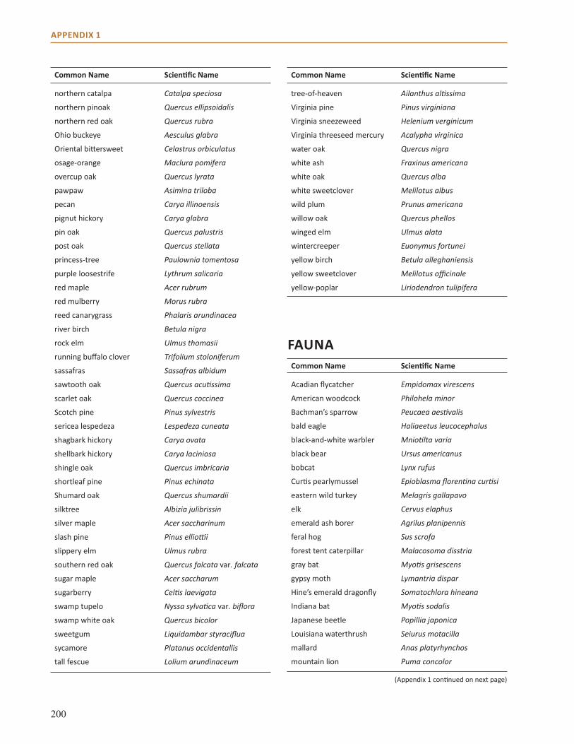
200

APPENDIX 1


northern catalpa Catalpa speciosa

northern pinoak Quercus ellipsoidalis

northern red oak Quercus rubra

Ohio buckeye Aesculus glabra

Oriental bittersweet Celastrus orbiculatus

osage-orange Maclura pomifera

overcup oak Quercus lyrata

pawpaw Asimina triloba

pecan Carya illinoensis

pignut hickory Carya glabra

pin oak Quercus palustris

post oak Quercus stellata

princess-tree Paulownia tomentosa

purple loosestrife Lythrum salicaria

red maple Acer rubrum

red mulberry Morus rubra

reed canarygrass Phalaris arundinacea

river birch Betula nigra

rock elm Ulmus thomasii

running buffalo clover Trifolium stoloniferum

sassafras Sassafras albidum

sawtooth oak Quercus acutissima

scarlet oak Quercus coccinea

Scotch pine Pinus sylvestris

sericea lespedeza Lespedeza cuneata

shagbark hickory Carya ovata

shellbark hickory Carya laciniosa

shingle oak Quercus imbricaria

shortleaf pine Pinus echinata

Shumard oak Quercus shumardii

silktree Albizia julibrissin

silver maple Acer saccharinum

slash pine Pinus elliottii

slippery elm Ulmus rubra

southern red oak Quercus falcata var. falcata

sugar maple Acer saccharum

sugarberry Celtis laevigata

swamp tupelo Nyssa sylvatica var. biflora

swamp white oak Quercus bicolor

sweetgum Liquidambar styraciflua

sycamore Platanus occidentallis

tall fescue Lolium arundinaceum


tree-of-heaven Ailanthus altissima

Virginia pine Pinus virginiana

Virginia sneezeweed Helenium verginicum

Virginia threeseed mercury Acalypha virginica

water oak Quercus nigra

white ash Fraxinus americana

white oak Quercus alba

white sweetclover Melilotus albus

wild plum Prunus americana

willow oak Quercus phellos

winged elm Ulmus alata

wintercreeper Euonymus fortunei

yellow birch Betula alleghaniensis

yellow sweetclover Melilotus officinale

yellow-poplar Liriodendron tulipifera


Acadian flycatcher Empidomax virescens

American woodcock Philohela minor

Bachman’s sparrow Peucaea aestivalis

bald eagle Haliaeetus leucocephalus

black-and-white warbler Mniotilta varia

black bear Ursus americanus

bobcat Lynx rufus

Curtis pearlymussel Epioblasma florentina curtisi

eastern wild turkey Melagris gallapavo

elk Cervus elaphus

emerald ash borer Agrilus planipennis

feral hog Sus scrofa

forest tent caterpillar Malacosoma disstria

gray bat Myotis grisescens

gypsy moth Lymantria dispar

Hine’s emerald dragonfly Somatochlora hineana

Indiana bat Myotis sodalis

Japanese beetle Popillia japonica

Louisiana waterthrush Seiurus motacilla

mallard Anas platyrhynchos

mountain lion Puma concolor

FAUNA


201

APPENDIX 1


northern bobwhite Colinus virginianus

Ozark bass Ambloplites constellatus

Ozark hellbender Cryptobranchus alleganiensis bishopi

red bat Lasiurus borealis

ruffed grouse Bonasa umbellus

scaleshell Leptodea leptodon

scarlet tanager Piranga olivacea


southern pine beetle Dendroctonus frontalis

summer tanager Piranga rubra

Tumbling Creek cavesnail Antrobia culveri

white-tailed deer Odocoileus virginianus

wood thrush Hylocichla mustelina

worm-eating warbler Helmitheris vermivora

yellow-breasted chat Icteria virens

202

APPENDIX 2: CROSSWALK OF NATURAL COMMUNITIES

Natural community

(this assessment)

Illinois natural community

classification*

Indiana natural community

classification*

Terrestrial natural

communities of Missouri

(Nelson 2010)NatureServe associations FIA forest type

Artifact (out of character) association

mesic upland forest

mesic upland forest

mesic upland forest

mesic loess/glacial till

forest

American beech, maple unglaciated

forest

sugar maple/beech/yellow

birch

red oak-sugar maple forest

central maple, American basswood

forest

hard maple/basswood

red oak-sugar maple forest

white oak-northern red oak-sugar maple

mesic forest

white oak/red oak/hickory

white oak-sugar maple

mesic limestone/dolomite

forest

white oak-red oak-sugar maple mesic

forest


mixed oak-red cedar

central maple, American basswood

forest

hard maple/basswood

sugar maple, elm, boxelder

mesic sandstone

forest

white oak-red oak-sugar maple mesic

forest


departures in overstory composition

mesic sand forest

beech-maple unglaciated forest

sugar maple/beech/yellow

birchnone known

dry-mesic upland forest



dry-mesic limestone/dolomite

forest

white oak-mixed oak/dry-mesic alkaline forest

white oak mixed oak-red cedar

dry-mesic chert forest

white oak-dogwood dry-mesic forest white oak red/black oak,

some red cedar

white oak-red oak dry-mesic acid forest


red/black oak, some red cedar

interior highlands shortleaf pine-oak dry-mesic forest

shortleaf pine/oak

white oak/red oak

dry-mesic sandstone

forest


shortleaf pine/oak

white oak/red oak

white oak-red oak dry-mesic acid forest


red/black oak decline


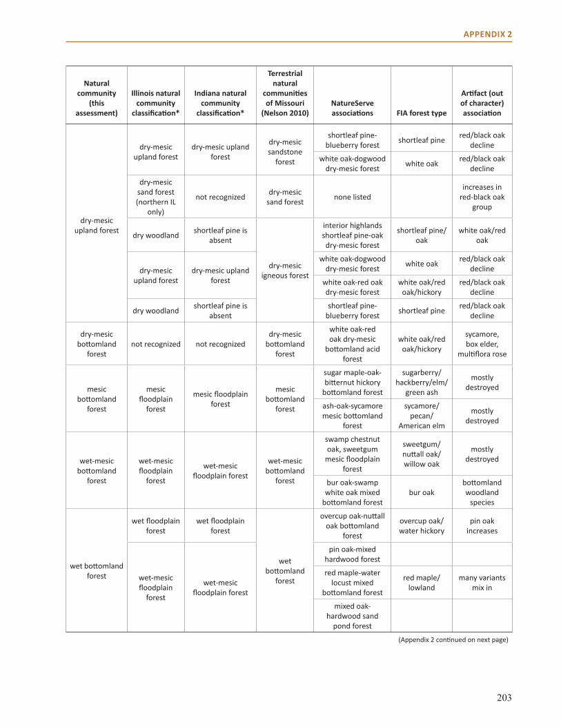
203

APPENDIX 2

Natural community

(this assessment)


classification*


classification*

Terrestrial natural







dry-mesic sandstone

forest

shortleaf pine-blueberry forest shortleaf pine red/black oak

decline

white oak-dogwood dry-mesic forest white oak red/black oak

decline

dry-mesic sand forest (northern IL

only)

not recognized dry-mesic sand forest none listed

increases in red-black oak

group

dry woodland shortleaf pine is absent

dry-mesic igneous forest


shortleaf pine/oak

white oak/red oak



white oak-dogwood dry-mesic forest white oak red/black oak

decline

white oak-red oak dry-mesic forest



dry woodland shortleaf pine is absent

shortleaf pine-blueberry forest shortleaf pine red/black oak

decline

dry-mesic bottomland

forestnot recognized not recognized

dry-mesic bottomland

forest

white oak-red oak dry-mesic

bottomland acid forest


sycamore, box elder,

multiflora rose

mesic bottomland

forest

mesic floodplain

forest

mesic floodplain forest

mesic bottomland

forest

sugar maple-oak-bitternut hickory

bottomland forest

sugarberry/hackberry/elm/

green ash

mostly destroyed

ash-oak-sycamore mesic bottomland

forest

sycamore/pecan/

American elm

mostly destroyed

wet-mesic bottomland

forest

wet-mesic floodplain

forest

wet-mesic floodplain forest


forest

swamp chestnut oak, sweetgum


sweetgum/nuttall oak/willow oak

mostly destroyed

bur oak-swamp white oak mixed

bottomland forestbur oak

bottomland woodland

species

wet bottomland forest

wet floodplain forest


wet bottomland

forest

overcup oak-nuttall oak bottomland

forest

overcup oak/water hickory

pin oak increases


forest


pin oak-mixed hardwood forest

red maple-water locust mixed

bottomland forest

red maple/lowland

many variants mix in

mixed oak-hardwood sand

pond forest


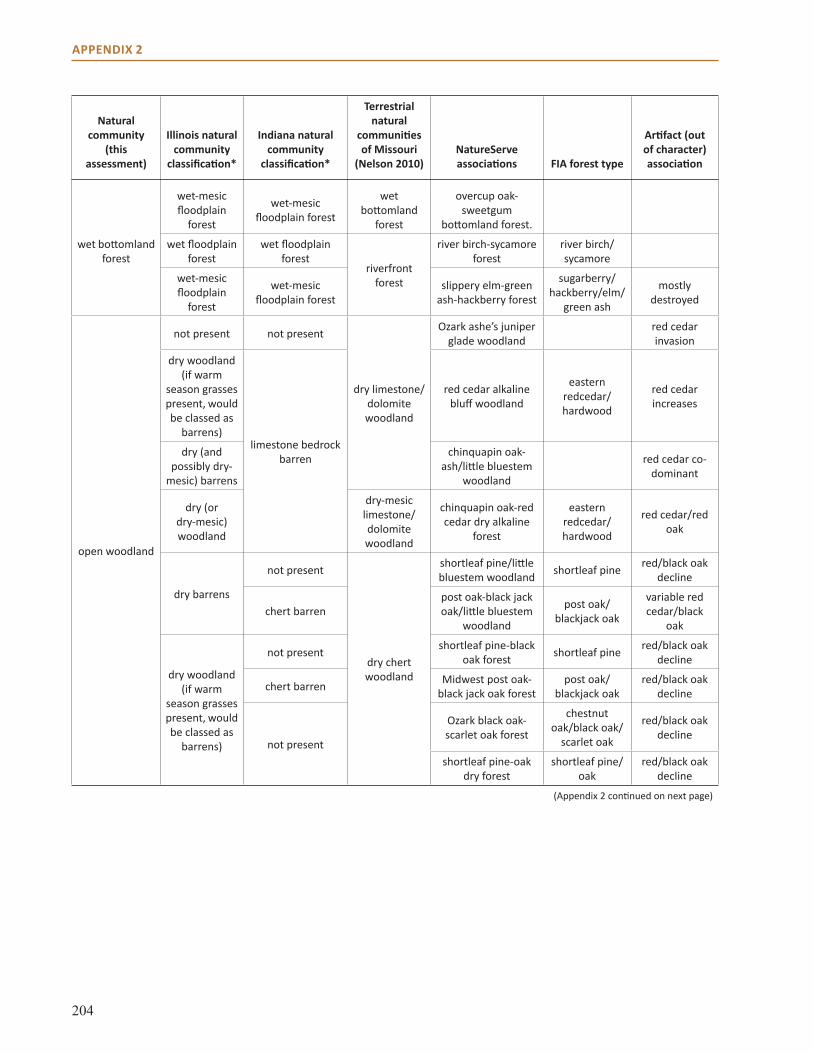
204

APPENDIX 2

Natural community

(this assessment)


classification*


classification*

Terrestrial natural




wet bottomland forest


forest


wet bottomland

forest

overcup oak-sweetgum

bottomland forest.



riverfront forest

river birch-sycamore forest

river birch/sycamore


forest


slippery elm-green ash-hackberry forest

sugarberry/hackberry/elm/

green ash

mostly destroyed

open woodland

not present not present

dry limestone/dolomite woodland

Ozark ashe’s juniper glade woodland

red cedar invasion

dry woodland (if warm

season grasses present, would be classed as

barrens)limestone bedrock

barren

red cedar alkaline bluff woodland

eastern redcedar/hardwood

red cedar increases

dry (and possibly dry-

mesic) barrens

chinquapin oak-ash/little bluestem

woodland

red cedar co-dominant

dry (or dry-mesic) woodland

dry-mesic limestone/dolomite woodland

chinquapin oak-red cedar dry alkaline

forest

eastern redcedar/hardwood

red cedar/red oak

dry barrens

not present

dry chert woodland

shortleaf pine/little bluestem woodland shortleaf pine red/black oak

decline

chert barrenpost oak-black jack oak/little bluestem

woodland

post oak/blackjack oak

variable red cedar/black

oak

dry woodland (if warm

season grasses present, would be classed as

barrens)

not present shortleaf pine-black oak forest shortleaf pine red/black oak

decline

chert barren Midwest post oak-black jack oak forest



not present

Ozark black oak-scarlet oak forest

chestnut oak/black oak/

scarlet oak


shortleaf pine-oak dry forest

shortleaf pine/oak



205

APPENDIX 2

Natural community

(this assessment)


classification*


classification*

Terrestrial natural




open woodland

dry barrens

not present

dry sandstone woodland

shortleaf pine/little bluestem woodland shortleaf pine red/black oak

decline

shortleaf pine-black oak forest

shortleaf pine/oak


sandstone barren

post oak-black jack oak/little bluestem

woodland



dry woodland

Midwest post oak-black jack oak forest





scarlet oak


not present

shortleaf pine-oak dry woodland

shortleaf pine/oak


dry igneous woodland

shortleaf pine-black oak forest

shortleaf pine/oak


barren or dry upland forest; no igneous substrate

in in


woodland



dry barrens shortleaf pine/little bluestem woodland


dry woodland

Midwest post oak-black jack oak forest





scarlet oak


not present

shortleaf pine-oak dry woodland

shortleaf pine/oak


dry-mesic woodland dry-mesic

igneous woodland

shortleaf pine-oak dry-mesic woodland

shortleaf pine/oak


dry-mesic barrens (red

oak would not be expected)

barren (undifferentiated)

or dry upland forest; no igneous

substrate in in

white oak-post oak/bluestem woodland white oak red/black oak

decline

dry-mesic chert

woodland


decline

dry barrens dry sand woodland


woodland



not recognized sand barren post oak-mixed oak sand woodland



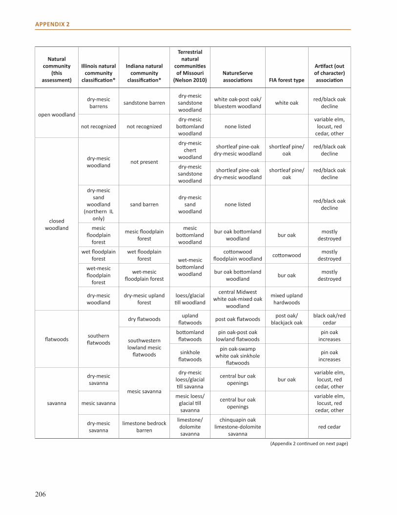
206

APPENDIX 2

Natural community

(this assessment)


classification*


classification*

Terrestrial natural




open woodland

dry-mesic barrens sandstone barren

dry-mesic sandstone woodland


decline

not recognized not recognizeddry-mesic

bottomland woodland

none listedvariable elm,

locust, red cedar, other

closed woodland

dry-mesic woodland not present

dry-mesic chert

woodland


shortleaf pine/oak


dry-mesic sandstone woodland


shortleaf pine/oak


dry-mesic sand

woodland (northern IL

only)

sand barrendry-mesic

sand woodland

none listed red/black oak decline

mesic floodplain

forest


mesic bottomland woodland

bur oak bottomland woodland bur oak mostly

destroyed


wet floodplain forest wet-mesic

bottomland woodland

cottonwood floodplain woodland cottonwood mostly

destroyed


forest


bur oak bottomland woodland bur oak mostly

destroyed

dry-mesic woodland


loess/glacial till woodland

central Midwest white oak-mixed oak

woodland

mixed upland hardwoods

flatwoods southern flatwoods

dry flatwoods upland flatwoods post oak flatwoods post oak/

blackjack oakblack oak/red

cedar

southwestern lowland mesic

flatwoods

bottomland flatwoods

pin oak-post oak lowland flatwoods

pin oak increases

sinkhole flatwoods

pin oak-swamp white oak sinkhole

flatwoods

pin oak increases

savanna

dry-mesic savanna

mesic savanna

dry-mesic loess/glacial till savanna

central bur oak openings bur oak

variable elm, locust, red

cedar, other

mesic savannamesic loess/

glacial till savanna

central bur oak openings

variable elm, locust, red

cedar, other

dry-mesic savanna

limestone bedrock barren

limestone/dolomite savanna

chinquapin oak limestone-dolomite

savannared cedar


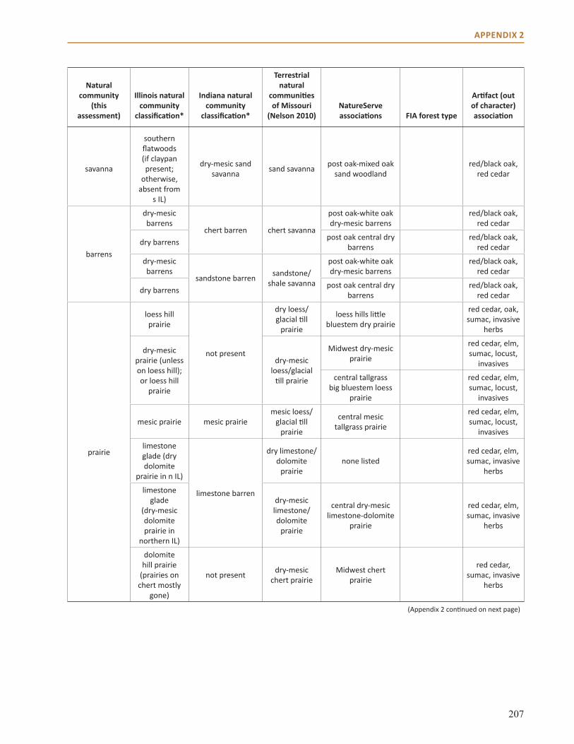
207

APPENDIX 2

Natural community

(this assessment)


classification*


classification*

Terrestrial natural




savanna

southern flatwoods (if claypan present;

otherwise, absent from

s IL)

dry-mesic sand savanna sand savanna post oak-mixed oak

sand woodlandred/black oak,

red cedar

barrens

dry-mesic barrens

chert barren chert savanna

post oak-white oak dry-mesic barrens

red/black oak, red cedar

dry barrens post oak central dry barrens


dry-mesic barrens

sandstone barren sandstone/shale savanna

post oak-white oak dry-mesic barrens


dry barrens post oak central dry barrens


prairie

loess hill prairie

not present

dry loess/glacial till

prairie

loess hills little bluestem dry prairie

red cedar, oak, sumac, invasive

herbs

dry-mesic prairie (unless on loess hill); or loess hill

prairie

dry-mesic loess/glacial

till prairie

Midwest dry-mesic prairie

red cedar, elm, sumac, locust,

invasives

central tallgrass big bluestem loess

prairie


invasives

mesic prairie mesic prairiemesic loess/

glacial till prairie

central mesic tallgrass prairie


invasives

limestone glade (dry dolomite

prairie in n IL)

limestone barren

dry limestone/dolomite

prairienone listed

red cedar, elm, sumac, invasive

herbs

limestone glade

(dry-mesic dolomite prairie in

northern IL)

dry-mesic limestone/dolomite

prairie

central dry-mesic limestone-dolomite

prairie

red cedar, elm, sumac, invasive

herbs

dolomite hill prairie

(prairies on chert mostly

gone)

not present dry-mesic chert prairie

Midwest chert prairie

red cedar, sumac, invasive

herbs


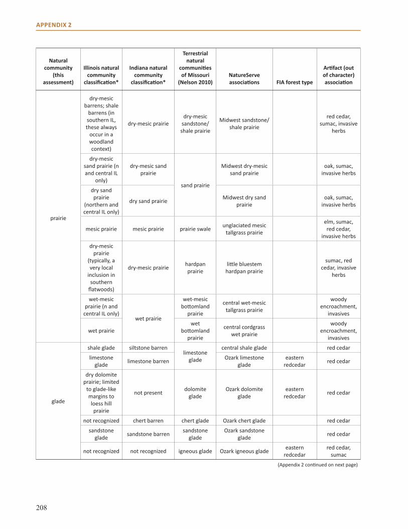
208

APPENDIX 2

Natural community

(this assessment)


classification*


classification*

Terrestrial natural




prairie

dry-mesic barrens; shale

barrens (in southern IL, these always

occur in a woodland context)

dry-mesic prairiedry-mesic

sandstone/shale prairie

Midwest sandstone/shale prairie

red cedar, sumac, invasive

herbs

dry-mesic sand prairie (n and central IL

only)

dry-mesic sand prairie

sand prairie

Midwest dry-mesic sand prairie

oak, sumac, invasive herbs

dry sand prairie

(northern and central IL only)

dry sand prairie Midwest dry sand prairie

oak, sumac, invasive herbs

mesic prairie mesic prairie prairie swale unglaciated mesic tallgrass prairie

elm, sumac, red cedar,

invasive herbs

dry-mesic prairie

(typically, a very local

inclusion in southern

flatwoods)

dry-mesic prairie hardpan prairie

little bluestem hardpan prairie

sumac, red cedar, invasive

herbs

wet-mesic prairie (n and

central IL only)wet prairie


prairie

central wet-mesic tallgrass prairie

woody encroachment,

invasives

wet prairiewet

bottomland prairie

central cordgrass wet prairie

woody encroachment,

invasives

glade

shale glade siltstone barrenlimestone

glade

central shale glade red cedar

limestone glade limestone barren Ozark limestone

gladeeastern

redcedar red cedar

dry dolomite prairie; limited

to glade-like margins to loess hill prairie

not present dolomite glade

Ozark dolomite glade

eastern redcedar red cedar

not recognized chert barren chert glade Ozark chert glade red cedar

sandstone glade sandstone barren sandstone

gladeOzark sandstone

glade red cedar

not recognized not recognized igneous glade Ozark igneous glade eastern redcedar

red cedar, sumac


209

APPENDIX 2

Natural community

(this assessment)


classification*


classification*

Terrestrial natural




swamp

shrub swamp shrub swamp shrub swamp

northern buttonbush swamp

drained, dehydrated,

farmed, exotics

southern buttonbush swamp

intact if not overgrazed or

drained

swamp forest swamp

swamp

water tupelo swamp forest

mostly destroyed

bald cypress-(water tupelo) swamp

baldcypress/water tupelo

altered flood regimes

pond shrub swamp

buttonbush sinkhole pond swamp

some drained and overgrazed

pond swamp

water tupelo sinkhole pond

swamp

baldcypress/water tupelo


overcup oak pond forest

overcup oak/water hickory


fen

forested fen (n and central IL

only)forested fen

Ozark fen Ozark fen many drained and overgrazed

Ozark prairie fen Ozark prairie fen many drained

and overgrazed

forested fen red maple forested seep

red maple/lowland

many drained and overgrazed

graminoid fen (depending on

structure)fen

glacial fencentral tallgrass fen many drained

and overgrazed

seep circumneutral seep great plains neutral seep


seep

acid gravel seep

acid seep

great plains acid seep


sand seep Midwest sand seep many drained and overgrazed

acid gravel seep Midwest acid seep many drained

and overgrazed

brackish marsh not present saline seep eastern great plains

saline marshmany drained

and overgrazed

spring calcareous seep calcareous seep

limestone/dolomite

springnone listed

invasive plants; culturally

altered sites

*Crosswalk for Illinois and Indiana provided by John Taft, Illinois Natural History Survey. The crosswalk classification for natural communities in Illinois and Indiana focuses primarily on the FIA and NatureServe designations because in some cases the Missouri classification is too broad and other times too specific for direct crosswalk comparison on a 1:1 basis.

210

APPENDIX 3: FOREST TYPES

Forest type* Assessment area Illinois Indiana Missouri (acres) (acres) (acres) (acres)

White oak / red oak / hickory 7,335,073 819,004 1,028,712 5,487,357White oak 1,651,005 128,258 136,787 1,385,959Post oak / blackjack oak 1,413,711 44,731 - 1,368,980Mixed upland hardwoods 879,481 223,341 252,869 403,271Eastern redcedar / hardwood 584,346 30,709 60,541 493,095Sugarberry / hackberry / elm / green ash 509,837 290,304 76,776 142,756Cherry / white ash / yellow-poplar 388,612 55,891 304,287 28,434Shortleaf pine / oak 375,485 13,130 4,618 357,737Chestnut oak / black oak / scarlet oak 358,860 2,269 57,695 298,896Eastern redcedar 351,161 2,273 16,658 332,229Shortleaf pine 254,980 24,731 14,870 215,378Elm / ash / black locust 240,723 68,338 74,513 97,871River birch / sycamore 222,072 66,845 68,644 86,582Sassafras / persimmon 210,723 27,558 84,717 98,448Silver maple / American elm 207,866 143,132 36,819 27,915Sugar maple / beech / yellow birch 207,390 25,154 149,594 32,642Sycamore / pecan / American elm 199,103 84,864 42,874 71,366Scarlet oak 165,322 - 6,031 159,291Yellow-poplar 159,104 15,168 142,771 1,164Yellow-poplar / white oak / northern red oak 147,150 21,680 125,470 -Sweetgum / yellow-poplar 141,197 52,612 80,140 8,444Northern red oak 131,818 11,084 19,863 100,870Black walnut 116,043 5,238 25,695 85,110Hard maple / basswood 100,227 6,681 80,304 13,241Cottonwood 62,451 29,766 25,960 6,725Chestnut oak 50,199 1,773 48,426 -Willow 49,492 25,887 11,341 12,264Black locust 48,699 15,435 24,975 8,289Sweetbay / swamp tupelo / red maple 45,973 3,885 42,088 -Cottonwood / willow 45,549 30,426 15,124 -Black ash / American elm / red maple 43,847 18,864 16,213 8,770Red maple / oak 42,772 7,714 31,887 3,170Red maple / lowland 36,049 21,039 12,925 2,085Other hardwoods 34,203 7,436 8,419 18,348Virginia pine / southern red oak 28,072 - 28,072 -Eastern white pine / northern red oak / white ash 22,833 5,394 15,955 1,485Swamp chestnut oak / cherrybark oak 21,571 1,797 6,616 13,158Virginia pine 20,531 - 20,531 -Sweetgum / Nuttall oak / willow oak 20,200 - 11,576 8,624Overcup oak / water hickory 19,631 13,130 1,844 4,657


211

APPENDIX 3

Baldcypress / water tupelo 16,008 16,008 - -Eastern white pine 11,285 1,773 9,512 -Red pine 11,242 - 11,242 -Aspen 4,207 - 4,207 -Other exotic hardwoods 4,171 - 800 3,372Bur oak 4,171 - - 4,171Scotch pine 3,525 - 919 2,605Loblolly pine 1,330 1,330 - -Black cherry 146 146 - -Other pine / hardwood 80 - 80 -

Forest type* Assessment area Illinois Indiana Missouri (acres) (acres) (acres) (acres)

*Forest types in the assessment area are based on U.S. Forest Service, Forest Inventory and Analysis. Source: U.S. Forest Service (2011a).

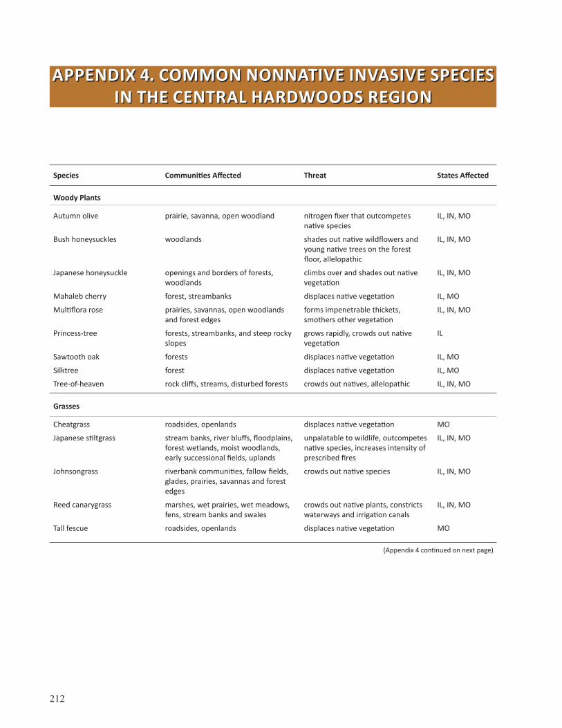
212

APPENDIX 4. COMMON NONNATIVE INVASIVE SPECIES IN THE CENTRAL HARDWOODS REGION

Species Communities Affected Threat States Affected

Woody Plants

Autumn olive prairie, savanna, open woodland nitrogen fixer that outcompetes native species

IL, IN, MO

Bush honeysuckles woodlands shades out native wildflowers and young native trees on the forest floor, allelopathic

IL, IN, MO

Japanese honeysuckle openings and borders of forests, woodlands

climbs over and shades out native vegetation

IL, IN, MO

Mahaleb cherry forest, streambanks displaces native vegetation IL, MO

Multiflora rose prairies, savannas, open woodlands and forest edges

forms impenetrable thickets, smothers other vegetation

IL, IN, MO

Princess-tree forests, streambanks, and steep rocky slopes

grows rapidly, crowds out native vegetation

IL

Sawtooth oak forests displaces native vegetation IL, MO

Silktree forest displaces native vegetation IL, MO

Tree-of-heaven rock cliffs, streams, disturbed forests crowds out natives, allelopathic IL, IN, MO

Grasses

Cheatgrass roadsides, openlands displaces native vegetation MO

Japanese stiltgrass stream banks, river bluffs, floodplains, forest wetlands, moist woodlands, early successional fields, uplands

unpalatable to wildlife, outcompetes native species, increases intensity of prescribed fires

IL, IN, MO

Johnsongrass riverbank communities, fallow fields, glades, prairies, savannas and forest edges

crowds out native species IL, IN, MO

Reed canarygrass marshes, wet prairies, wet meadows, fens, stream banks and swales

crowds out native plants, constricts waterways and irrigation canals

IL, IN, MO

Tall fescue roadsides, openlands displaces native vegetation MO


213

APPENDIX 4


Herbaceous Plants

Common periwinkle woodlands forms thick mats IL, IN, MO

Common and cut-leaved teasel prairie, savanna outcompete natives IL, IN, MO

Creeping jenny floodplain forests outcompetes natives IL, IN, MO

Crown vetch roadsides, riparian spreads vegetatively, outcompetes natives

IL, IN, MO

Garlic mustard upland and floodplain forests, savannas, open woodlands

allelopathic, crowds out native plants IL, IN, MO

Ground ivy/creeping charlie floodplain and mesic upland forests forms thick mats IL, IN, MO

Japanese knotweed riparian and floodplain forests forms dense thickets that exclude native vegetation

Musk thistle prairies crowds out native plant and grassland species through competition for resources

IL, IN, MO

Purple loosestrife marshes, fens, sedge meadows, and wet prairies

destroys marshes and wet prairies and chokes waterways

IL, IN, MO

Sericea lespedeza open woodlands, prairies, borders of ponds and swamps, meadows

unpalatable to grazers, which in turn overgraze the surrounding native plants

IL, IN, MO

White and yellow sweetclover prairies, savannas, open woodlands and forest edges

outcompete natives IL, IN, MO

Vines

Chinese yam/cinnamon vine bottomland forests, riparian areas shades out understory plants and trees, eventually killing them

IL, IN, MO

Japanese hop riparian and floodplain forests displaces native vegetation, prevents the emergence of new plants, kills newly planted trees

IL, IN, MO

Kudzu potentially all, currently limited by cold winters

forms dense mats over the ground, shrubs, mature trees; kills understory plants and trees

IL, IN, MO

Oriental bittersweet disturbed forest edges, woodlands climbs over and smothers vegetation, which may die from excessive shading or breakage

IL, IN, MO

Wintercreeper floodplain forest, moist and dry-moist forest, and banks of streams and rivers

forms a dense groundcover that reduces or eliminates native plant species

IL, IN, MO

Aquatic Plants

Curly leaf pondweed ponds, lakes, slow-moving streams prevents light penetration for native aquatic plants

IL, IN, MO

Eurasian watermilfoil ponds, lakes, slow-moving streams prevents light penetration for native aquatic plants

IL, IN, MO


214

APPENDIX 4


Terrestrial Invertebrates

Emerald ash borer forests, any area with ash trees present

kills healthy ash trees IL, IN, MO

Gypsy moth oak species, basswood, poplar species, hawthorn species

defoliates trees; repeated defoliation leads to death

IL, IN, MO (but not prevalent in assessment area)

Japanese beetle all adults defoliate broad-leaved species; larvae consume grass roots

IL, IN, MO

Terrestrial Vertebrates

Feral hog bottomland forests, seeps, glades, fens, springs, and streams

behavior causes soil erosion, reduces water quality; acorn are consumed

IL, IN, MO

Sources: Missouri Department of Conservation (2013c), Olson et al. (2004), Plant Conservation Alliance (2013).

215

APPENDIX 5: COMMON DISEASES IN THE CENTRAL HARDWOODS REGION

Disease name Species affected Climate factors States affected

Annosus root rot conifers (esp. red and white pine) drought, stress IL, IN, MO

Anthracnose diseases ash, basswood, birch, catalpa, elm, hickory, horse chestnut, maple, oak, sycamore, yellow-poplar, and walnut

thrives in cool, wet environments IL, IN, MO

Armillaria root disease hardwoods and conifers warming would allow decay to occur for longer periods in the year; drought-stressed trees more susceptible

IL, IN, MO

Bacterial leaf scorch elm, oak species (esp. pin, northern, and southern red oak), sycamore

drought stress exacerbates the disease IL, IN, MO

Branch flagging and tip dieback

oak species (esp. white) N/A IL, IN, MO

Butternut canker butternut N/A IL, IN, MO

Bur oak blight bur oak (only on variety oliviformis) spring precipitation favors disease (Harrington et al. 2012)

IL, MO

Chestnut blight American chestnut N/A IN

Diplodia blight of pines pines and other conifers can be deadly when combined with drought

IL, IN, MO

Dogwood anthracnose flowering dogwood more problematic in cool, wet climates MO, IN

Dothistroma needle blight pine species conidia dispersed in wet weather IL, IN, MO

Dutch elm disease elm species N/A IL, IN, MO

Fomes annosus pine species drought, stress

Hypoxylon canker oaks and other hardwoods drought throughout the South

Littleleaf disease shortleaf pine N/A (currently none, possible in MO)

Oak decline northern red, southern red, scarlet, and black oak

drought-stressed trees more susceptible

IL, IN, MO

Oak wilt oak species (esp. black, blackjack, bur, northern red, pin and shingle)

earlier warming in spring changes susceptibility period for insect transmission

IL, IN, MO

Verticillium wilt boxwood, Kentucky coffee tree, horse-chestnut, Ohio buckeye, magnolia, maple, privet, redbud, serviceberry, sumac, tulip tree, viburnum, and many others

N/A IL, IN, MO

Sources: Marshall (2010), Miller (2011), Missouri Forest Health Highlights (2010), Scarbrough and Juzwik (2004).

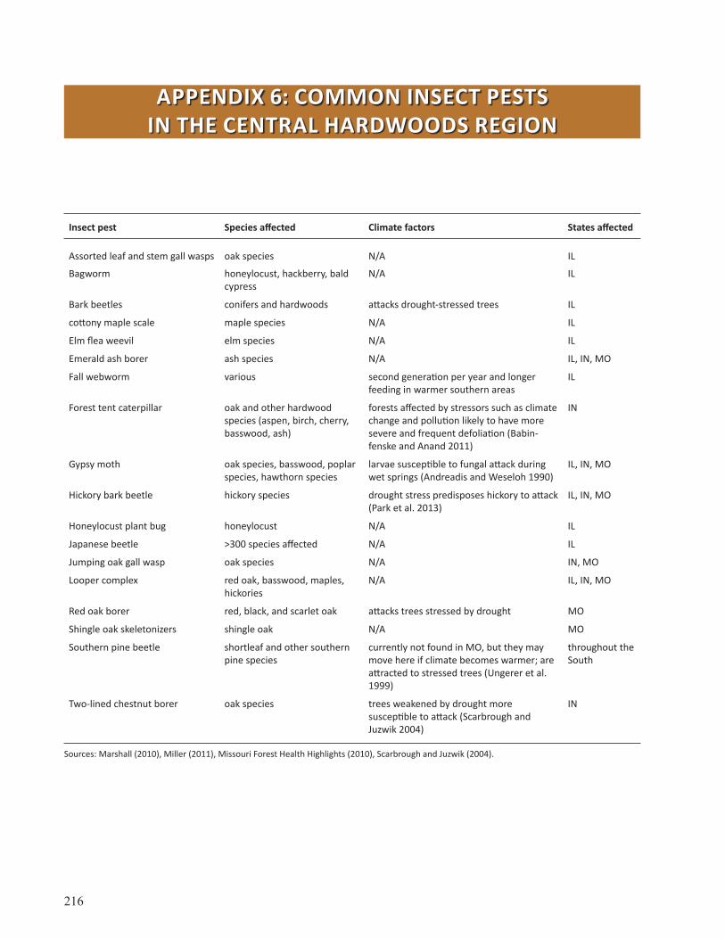
216

APPENDIX 6: COMMON INSECT PESTS IN THE CENTRAL HARDWOODS REGION

Insect pest Species affected Climate factors States affected

Assorted leaf and stem gall wasps oak species N/A IL

Bagworm honeylocust, hackberry, bald cypress

N/A IL

Bark beetles conifers and hardwoods attacks drought-stressed trees IL

cottony maple scale maple species N/A IL

Elm flea weevil elm species N/A IL

Emerald ash borer ash species N/A IL, IN, MO

Fall webworm various second generation per year and longer feeding in warmer southern areas

IL

Forest tent caterpillar oak and other hardwood species (aspen, birch, cherry, basswood, ash)

forests affected by stressors such as climate change and pollution likely to have more severe and frequent defoliation (Babin-fenske and Anand 2011)

IN

Gypsy moth oak species, basswood, poplar species, hawthorn species

larvae susceptible to fungal attack during wet springs (Andreadis and Weseloh 1990)

IL, IN, MO

Hickory bark beetle hickory species drought stress predisposes hickory to attack (Park et al. 2013)

IL, IN, MO

Honeylocust plant bug honeylocust N/A IL

Japanese beetle >300 species affected N/A IL

Jumping oak gall wasp oak species N/A IN, MO

Looper complex red oak, basswood, maples, hickories

N/A IL, IN, MO

Red oak borer red, black, and scarlet oak attacks trees stressed by drought MO

Shingle oak skeletonizers shingle oak N/A MO

Southern pine beetle shortleaf and other southern pine species

currently not found in MO, but they may move here if climate becomes warmer; are attracted to stressed trees (Ungerer et al. 1999)

throughout the South

Two-lined chestnut borer oak species trees weakened by drought more susceptible to attack (Scarbrough and Juzwik 2004)

IN

Sources: Marshall (2010), Miller (2011), Missouri Forest Health Highlights (2010), Scarbrough and Juzwik (2004).

217

APPENDIX 7: TREND ANALYSIS AND HISTORICAL CLIMATE DATA

To examine historical trends in precipitation and temperature for the analysis area, we used the ClimateWizard Custom Analysis Tool (ClimateWizard 2012, Girvetz et al. 2009). Data for ClimateWizard are derived from PRISM (Parameter-elevation Regressions on Independent Slopes Model, Gibson et al. 2002). The PRISM model interpolates historical data from the National Weather Service cooperative stations, the Midwest Climate Data Center, and the Historical Climate Network, among others. Data undergo strict quality control procedures to check for errors in station measurements. The PRISM model finds linear relationships between these station measurements and local elevation by using a digital elevation model (digital gridded version of a topographic map). Temperature and precipitation are then derived for each pixel on a 2.5-mile grid across the conterminous United States. The closer a station is in distance and elevation to a grid cell of interest, and the more similar it is in its proximity to coasts or topographic features, the higher the weight the station will have on the final, predicted value for that cell. More information on PRISM can be found at: http://www.prism.oregonstate.edu/.

This historical gridded data set is different from that used in the National Climate Assessment, which uses a new gridded historical data set (CDDv2) from the National Climatic Data Center (NCDC) (Kunkel et al. 2013). The new gridded data set had not been peer reviewed and published at the time this assessment was completed, and therefore we cannot fully compare this new version with the one available through PRISM. However, both are based on cooperative weather station data, cover the

period from 1895 through 2011, and have similar resolutions (3.1-mile vs. 2.5-mile grid). In addition, the overall trends reported as input into the National Climate Assessment are generally consistent with those reported in this assessment (Kunkel et al. 2013).

Linear trend analysis for the period from 1901 through 2011 was performed by using restricted maximum likelihood (REML) estimation (Girvetz et al. 2009). Restricted maximum likelihood methods were used for trend analysis of past climate for the Intergovernmental Panel on Climate Change Working Group 1 Report and are considered an effective way to determine trends in climate data over time (Trenbarth et al. 2007). A first-order autoregression was assumed for the residuals, meaning that values one time step away from each other are assumed to be correlated. This method was used to examine trends for every 2.5-mile grid cell. The slope and p-values for the linear trend over time were calculated annually, seasonally, for each month, and for each climate variable, and then mapped. An overall trend for an area is based on the trend analysis of the average value for all grid cells within the area over time (Table 19).

Developers of the ClimateWizard Tool advise users to interpret the linear trend maps in relation to the respective map of statistical confidence (Figs. 40 and 41). In this case, statistical confidence is described by using p-values from a t-test applied to the linear regression. A p-value can be interpreted as the probability of the slope being different from zero by chance alone. For this assessment, p-values of <0.1 were considered to have sufficient statistical

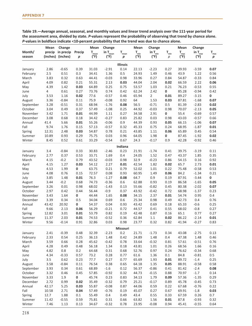
218

APPENDIX 7

Table 19.—Average annual, seasonal, and monthly values and linear trend analysis over the 111-year period for the assessment area, divided by state. P-values represent the probability of observing that trend by chance alone. P-values in boldface indicate <10-percent probability that the trend was due to chance alone. Mean Change Mean Change Mean Change Mean ChangeMonth/ precip in precip Precip Tmean in Tmean Tmean Tmin in Tmin Tmin Tmax in Tmax Tmaxseason (inches) (inches) p (°F) (°F) p (°F) (°F) p (°F) (°F) p

IllinoisJanuary 2.86 -0.65 0.39 31.03 -2.91 0.14 22.13 -2.23 0.27 39.93 -3.59 0.07February 2.5 0.51 0.3 34.41 1.36 0.5 24.93 1.49 0.46 43.9 1.22 0.56March 3.83 0.32 0.63 44.41 -0.03 0.98 33.96 0.27 0.84 54.87 -0.33 0.84April 4.09 0.82 0.21 55.31 2.13 0.03 44.04 2.04 0.02 66.59 2.22 0.06May 4.39 1.42 0.03 64.89 0.25 0.75 53.57 1.03 0.21 76.23 -0.53 0.55June 4 0.61 0.27 73.76 0.74 0.42 62.24 2.42 0 85.28 -0.94 0.42July 3.53 1.16 0.02 77.6 -0.57 0.46 65.94 2 0.01 89.27 -3.15 0August 3.36 -0.84 0.11 75.9 -0.08 0.92 64 1.53 0.03 87.81 -1.68 0.07September 3.28 -0.51 0.31 68.94 -1.76 0.08 56.5 -0.71 0.5 81.39 -2.83 0.02October 3.04 0.49 0.37 57.49 -1.08 0.25 44.92 -0.03 0.98 70.07 -2.13 0.05November 3.42 1.71 0.01 44.99 1.11 0.27 34.58 2.91 0 55.4 -0.69 0.57December 3.08 0.68 0.18 34.42 -0.27 0.83 25.82 0.03 0.98 43.03 -0.57 0.66Annual 41.4 5.66 0.01 55.26 -0.06 0.9 44.39 0.93 0.05 66.15 -1.06 0.07Fall 9.74 1.76 0.15 57.13 -0.57 0.32 45.33 0.75 0.24 68.95 -1.87 0.01Spring 12.31 2.48 0.03 54.87 0.78 0.21 43.85 1.11 0.06 65.89 0.45 0.54Summer 10.89 0.93 0.29 75.75 0.03 0.96 64.05 1.98 0 87.45 -1.92 0.02Winter 8.45 0.52 0.61 33.29 -0.54 0.67 24.3 -0.17 0.9 42.28 -0.92 0.46

IndianaJanuary 3.4 -0.84 0.33 30.83 -2.46 0.23 21.91 -1.74 0.41 39.75 -3.19 0.11February 2.77 0.37 0.53 33.71 1.69 0.4 24.05 1.52 0.47 43.37 1.85 0.35March 4.15 -0.2 0.79 43.52 -0.03 0.98 32.9 -0.23 0.86 54.15 0.16 0.92April 4.15 1.27 0.03 54.12 2.27 0.01 42.54 1.82 0.02 65.7 2.73 0.01May 4.53 1.99 0 63.75 0.21 0.79 52.02 1.01 0.22 75.48 -0.58 0.53June 4.08 0.76 0.15 72.57 0.08 0.93 60.95 1.49 0.06 84.2 -1.34 0.21July 3.85 1.48 0.01 76.3 -1.27 0.08 64.7 0.9 0.19 87.91 -3.44 0August 3.44 -0.2 0.68 74.73 -0.36 0.6 62.88 0.93 0.19 86.58 -1.65 0.05September 3.26 0.01 0.98 68.02 -1.43 0.13 55.66 -0.82 0.45 80.38 -2.02 0.07October 2.97 0.42 0.44 56.44 -0.9 0.37 43.92 -0.42 0.72 68.98 -1.37 0.23November 3.43 1.64 0 44.44 1.65 0.08 34.15 2.37 0.01 54.74 0.95 0.4December 3.39 0.34 0.5 34.04 0.69 0.6 25.34 0.98 0.49 42.73 0.4 0.76Annual 43.42 20.92 0 54.37 0.04 0.93 43.42 0.69 0.18 65.33 -0.6 0.25Fall 9.66 2.13 0.06 56.29 -0.21 0.72 44.57 0.41 0.55 68.02 -0.8 0.27Spring 12.82 3.01 0.01 53.79 0.82 0.19 42.48 0.87 0.16 65.1 0.77 0.27Summer 11.37 2.03 0.01 74.53 -0.52 0.36 62.84 1.1 0.02 86.22 -2.14 0.01Winter 9.56 -0.14 0.91 32.86 0.03 0.98 23.77 0.32 0.82 41.94 -0.27 0.83

MissouriJanuary 2.41 -0.39 0.48 32.39 -2.23 0.2 21.71 -1.73 0.34 43.08 -2.75 0.13February 2.33 0.54 0.25 36.13 1.48 0.42 24.89 1.48 0.4 47.38 1.48 0.46March 3.59 0.66 0.28 45.62 -0.42 0.78 33.64 -0.32 0.81 57.61 -0.51 0.76April 4.28 0.49 0.48 56.18 1.34 0.18 43.81 1.01 0.26 68.56 1.66 0.16May 4.82 0.8 0.2 64.68 0.31 0.68 52.76 0.97 0.24 76.62 -0.34 0.68June 4.34 -0.33 0.57 73.2 0.28 0.77 61.6 1.36 0.1 84.8 -0.81 0.5July 3.5 0.62 0.23 77.7 0.27 0.77 65.69 1.93 0.01 89.72 -1.4 0.25August 3.58 -0.84 0.11 76.54 0.38 0.65 64.18 1.35 0.05 88.91 -0.58 0.58September 3.93 0.34 0.61 68.89 -1.6 0.12 56.37 -0.86 0.41 81.42 -2.4 0.08October 3.32 0.46 0.45 57.85 -0.92 0.32 44.73 -0.15 0.88 70.97 -1.7 0.14November 3.33 1.9 0 45.74 0.23 0.83 34.13 1.79 0.09 57.36 -1.35 0.29December 2.72 0.99 0.02 35.49 -0.32 0.79 25.21 -0.17 0.89 45.78 -0.45 0.73Annual 42.17 5.25 0.03 55.87 -0.08 0.87 44.06 0.59 0.22 67.68 -0.76 0.22Fall 10.58 2.71 0.04 57.49 -0.76 0.19 45.07 0.27 0.67 69.91 -1.8 0.03Spring 12.7 1.88 0.1 55.49 0.4 0.49 43.4 0.55 0.33 67.59 0.26 0.7Summer 11.42 -0.55 0.59 75.81 0.31 0.66 63.82 1.56 0.01 87.8 -0.93 0.32Winter 7.46 1.13 0.13 34.67 -0.32 0.78 23.95 -0.08 0.94 45.41 -0.55 0.64

219

APPENDIX 7

Figure 40.—Map of statistical confidence (p-values for the linear regression) of the 111-year time series for temperature. Gray values represent areas of low statistical confidence.

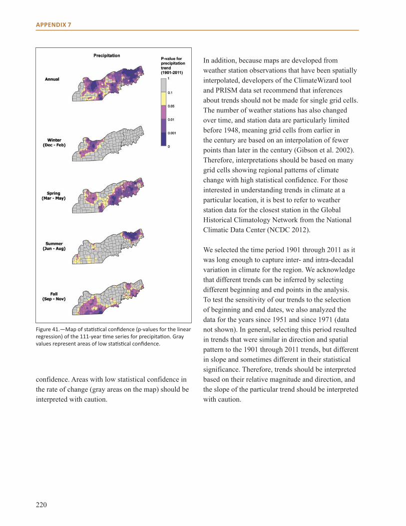
220

APPENDIX 7

Figure 41.—Map of statistical confidence (p-values for the linear regression) of the 111-year time series for precipitation. Gray values represent areas of low statistical confidence.

confidence. Areas with low statistical confidence in the rate of change (gray areas on the map) should be interpreted with caution.

In addition, because maps are developed from weather station observations that have been spatially interpolated, developers of the ClimateWizard tool and PRISM data set recommend that inferences about trends should not be made for single grid cells. The number of weather stations has also changed over time, and station data are particularly limited before 1948, meaning grid cells from earlier in the century are based on an interpolation of fewer points than later in the century (Gibson et al. 2002). Therefore, interpretations should be based on many grid cells showing regional patterns of climate change with high statistical confidence. For those interested in understanding trends in climate at a particular location, it is best to refer to weather station data for the closest station in the Global Historical Climatology Network from the National Climatic Data Center (NCDC 2012).

We selected the time period 1901 through 2011 as it was long enough to capture inter- and intra-decadal variation in climate for the region. We acknowledge that different trends can be inferred by selecting different beginning and end points in the analysis. To test the sensitivity of our trends to the selection of beginning and end dates, we also analyzed the data for the years since 1951 and since 1971 (data not shown). In general, selecting this period resulted in trends that were similar in direction and spatial pattern to the 1901 through 2011 trends, but different in slope and sometimes different in their statistical significance. Therefore, trends should be interpreted based on their relative magnitude and direction, and the slope of the particular trend should be interpreted with caution.

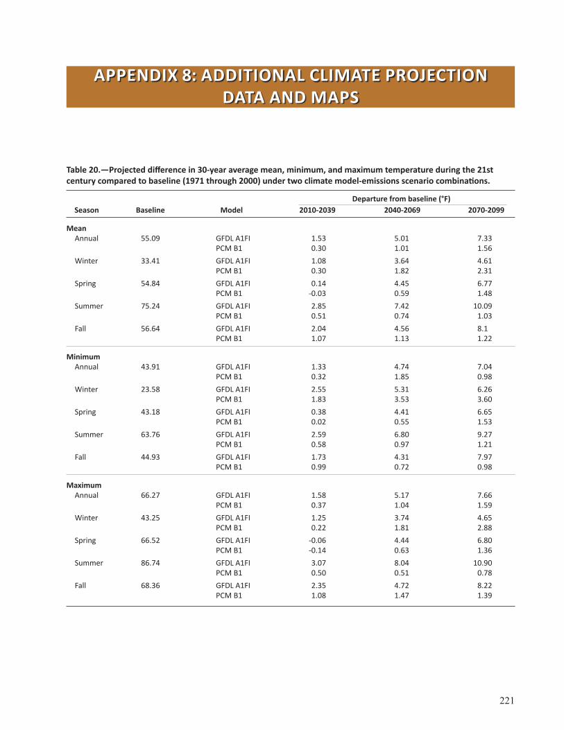
221

APPENDIX 8: ADDITIONAL CLIMATE PROJECTION DATA AND MAPS

Departure from baseline (°F) Season Baseline Model 2010-2039 2040-2069 2070-2099

Mean Annual 55.09 GFDL A1FI 1.53 5.01 7.33 PCM B1 0.30 1.01 1.56 Winter 33.41 GFDL A1FI 1.08 3.64 4.61 PCM B1 0.30 1.82 2.31 Spring 54.84 GFDL A1FI 0.14 4.45 6.77 PCM B1 -0.03 0.59 1.48 Summer 75.24 GFDL A1FI 2.85 7.42 10.09 PCM B1 0.51 0.74 1.03 Fall 56.64 GFDL A1FI 2.04 4.56 8.1 PCM B1 1.07 1.13 1.22

Minimum Annual 43.91 GFDL A1FI 1.33 4.74 7.04 PCM B1 0.32 1.85 0.98 Winter 23.58 GFDL A1FI 2.55 5.31 6.26 PCM B1 1.83 3.53 3.60 Spring 43.18 GFDL A1FI 0.38 4.41 6.65 PCM B1 0.02 0.55 1.53 Summer 63.76 GFDL A1FI 2.59 6.80 9.27 PCM B1 0.58 0.97 1.21 Fall 44.93 GFDL A1FI 1.73 4.31 7.97 PCM B1 0.99 0.72 0.98

Maximum Annual 66.27 GFDL A1FI 1.58 5.17 7.66 PCM B1 0.37 1.04 1.59 Winter 43.25 GFDL A1FI 1.25 3.74 4.65 PCM B1 0.22 1.81 2.88 Spring 66.52 GFDL A1FI -0.06 4.44 6.80 PCM B1 -0.14 0.63 1.36 Summer 86.74 GFDL A1FI 3.07 8.04 10.90 PCM B1 0.50 0.51 0.78 Fall 68.36 GFDL A1FI 2.35 4.72 8.22 PCM B1 1.08 1.47 1.39

Table 20.—Projected difference in 30-year average mean, minimum, and maximum temperature during the 21st century compared to baseline (1971 through 2000) under two climate model-emissions scenario combinations.

222

APPENDIX 8

Departure from baseline (inches) Season Baseline Model 2010-2039 2040-2069 2070-2099

Annual 43.84 GFDL A1FI -3.17 -3.65 -3.12 PCM B1 2.04 2.28 2.85 Winter 8.38 GFDL A1FI 0.55 1.16 2.34 PCM B1 0.23 0.76 0.37 Spring 12.94 GFDL A1FI 1.10 1.80 2.31 PCM B1 1.92 1.42 1.86 Summer 11.5 GFDL A1FI -3.25 -6.04 -7.57 PCM B1 1.87 2.43 3.17 Fall 11.01 GFDL A1FI -1.61 -0.61 -0.24 PCM B1 -2.02 -2.37 -2.68

Table 21.—Projected difference in 30-year average annual and seasonal precipitation during the 21st century compared to baseline (1971 through 2000) under two climate model-emissions scenario combinations.

223

APPENDIX 8

Figure 42.—Projected difference in mean daily temperature at the beginning of the century (2010 through 2039) compared to baseline (1971 through 2000), under two climate model-emissions scenario combinations.

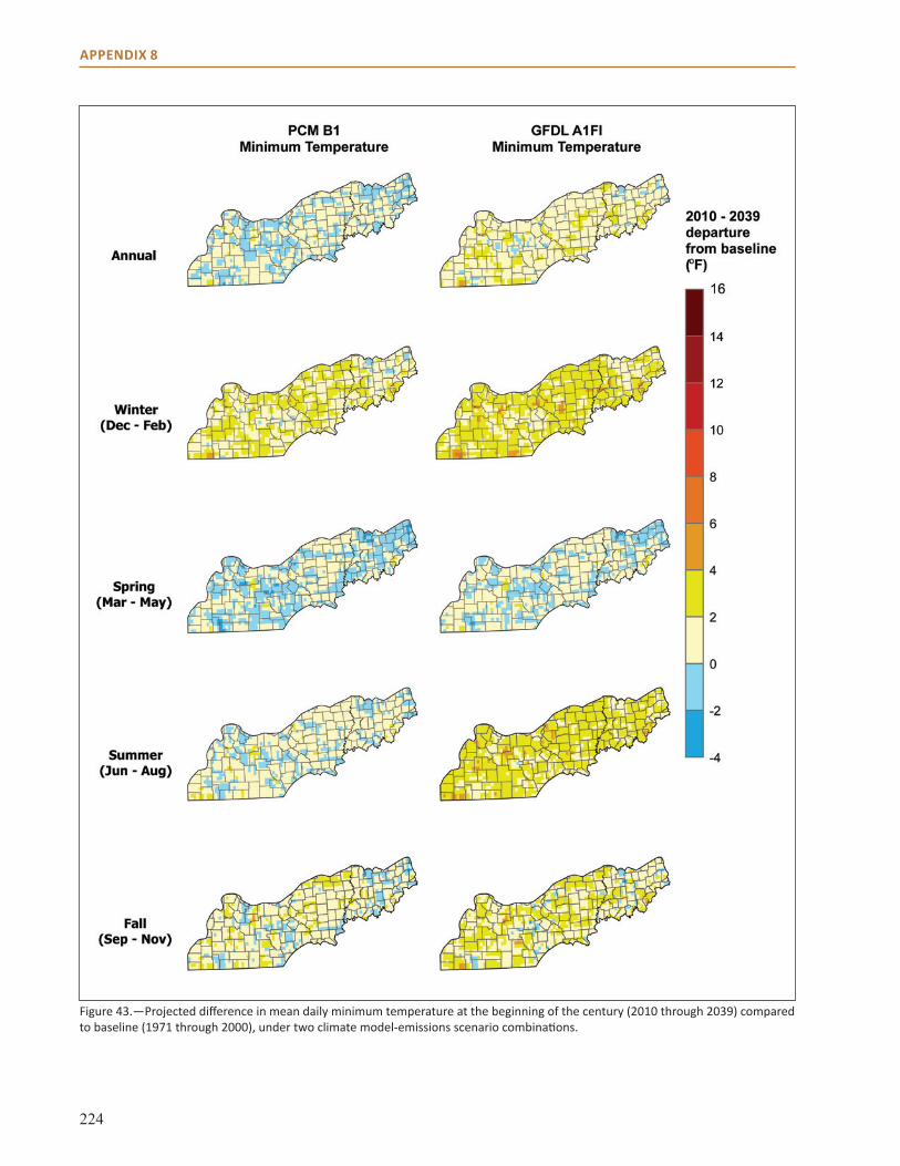
224

APPENDIX 8

Figure 43.—Projected difference in mean daily minimum temperature at the beginning of the century (2010 through 2039) compared to baseline (1971 through 2000), under two climate model-emissions scenario combinations.

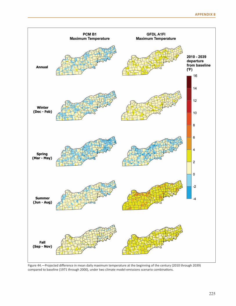
225

APPENDIX 8

Figure 44.—Projected difference in mean daily maximum temperature at the beginning of the century (2010 through 2039) compared to baseline (1971 through 2000), under two climate model-emissions scenario combinations.

226

APPENDIX 8

Figure 45.—Projected difference in mean daily temperature at mid-century (2040 through 2069) compared to baseline (1971 through 2000), under two climate model-emissions scenario combinations.

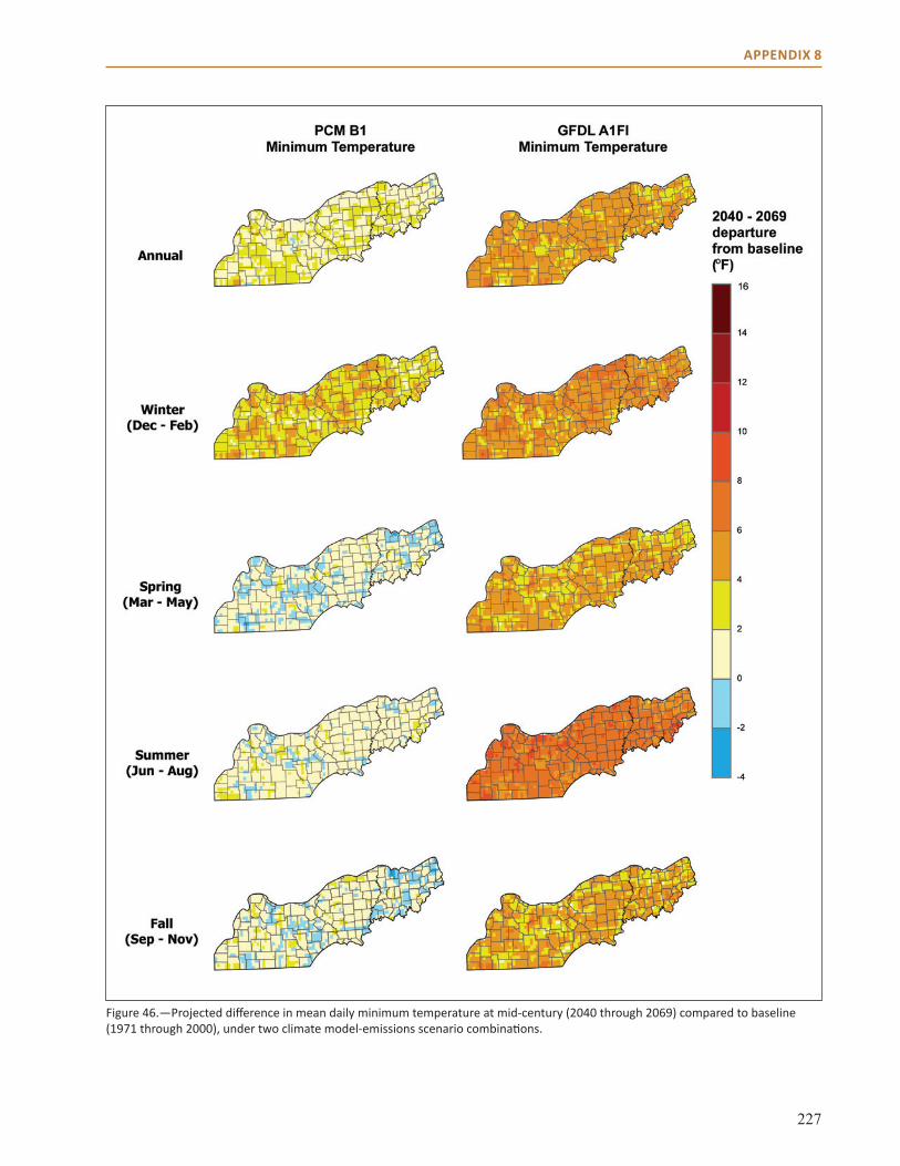
227

APPENDIX 8

Figure 46.—Projected difference in mean daily minimum temperature at mid-century (2040 through 2069) compared to baseline (1971 through 2000), under two climate model-emissions scenario combinations.

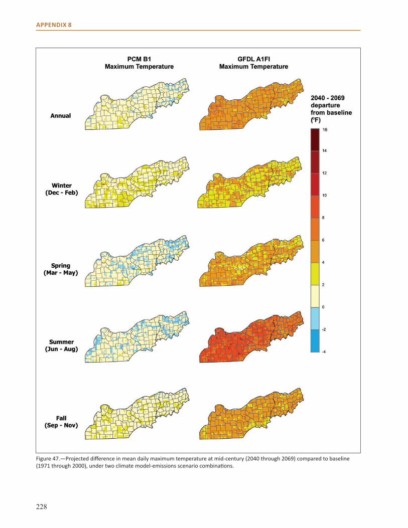
228

APPENDIX 8

Figure 47.—Projected difference in mean daily maximum temperature at mid-century (2040 through 2069) compared to baseline (1971 through 2000), under two climate model-emissions scenario combinations.

229

APPENDIX 8

Figure 48.—Projected difference in mean annual and seasonal precipitation at the beginning of the century (2010 through 2039) compared to baseline (1971 through 2000), under two climate model-emissions scenario combinations.

230

APPENDIX 8

Figure 49.—Projected difference in mean annual and seasonal precipitation at mid-century (2040 through 2069) compared to baseline (1971 through 2000), under two climate model-emissions scenario combinations.

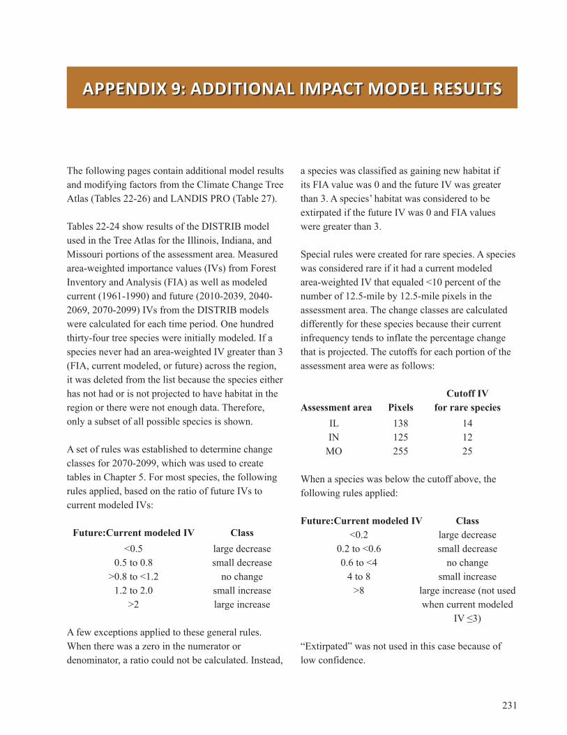
231

APPENDIX 9: ADDITIONAL IMPACT MODEL RESULTS

The following pages contain additional model results and modifying factors from the Climate Change Tree Atlas (Tables 22-26) and LANDIS PRO (Table 27).

Tables 22-24 show results of the DISTRIB model used in the Tree Atlas for the Illinois, Indiana, and Missouri portions of the assessment area. Measured area-weighted importance values (IVs) from Forest Inventory and Analysis (FIA) as well as modeled current (1961-1990) and future (2010-2039, 2040-2069, 2070-2099) IVs from the DISTRIB models were calculated for each time period. One hundred thirty-four tree species were initially modeled. If a species never had an area-weighted IV greater than 3 (FIA, current modeled, or future) across the region, it was deleted from the list because the species either has not had or is not projected to have habitat in the region or there were not enough data. Therefore, only a subset of all possible species is shown.

A set of rules was established to determine change classes for 2070-2099, which was used to create tables in Chapter 5. For most species, the following rules applied, based on the ratio of future IVs to current modeled IVs:

Future:CurrentmodeledIV Class <0.5 large decrease 0.5 to 0.8 small decrease >0.8 to <1.2 no change 1.2 to 2.0 small increase >2 large increase

A few exceptions applied to these general rules. When there was a zero in the numerator or denominator, a ratio could not be calculated. Instead,

a species was classified as gaining new habitat if its FIA value was 0 and the future IV was greater than 3. A species’ habitat was considered to be extirpated if the future IV was 0 and FIA values were greater than 3.

Special rules were created for rare species. A species was considered rare if it had a current modeled area-weighted IV that equaled <10 percent of the number of 12.5-mile by 12.5-mile pixels in the assessment area. The change classes are calculated differently for these species because their current infrequency tends to inflate the percentage change that is projected. The cutoffs for each portion of the assessment area were as follows:

CutoffIVAssessmentarea Pixels forrarespecies IL 138 14 IN 125 12 MO 255 25

When a species was below the cutoff above, the following rules applied:

Future:CurrentmodeledIV Class <0.2 large decrease 0.2 to <0.6 small decrease 0.6 to <4 no change 4 to 8 small increase >8 large increase (not used when current modeled IV≤3)

“Extirpated” was not used in this case because of low confidence.

232

APPENDIX 9

Special rules also applied to species that were known to be present (current FIA IV >0) but not modeled as present (current modeled = 0). In these cases, the FIA IV was used in place of the current modeled IV to calculate ratios. Then, change class rules were applied based on the FIA IV.

Tables 25 and 26 describe the modifying factors and adaptability scores used in the Tree Atlas. These factors were developed using a literature-based scoring system to capture the potential adaptability of species to changes in climate that cannot be adequately captured by the DISTRIB model (Matthews et al. 2011b). This approach was used to assess the capacity for each species to adapt and considered nine biological traits reflecting innate characteristics like competition for light and edaphic specificity. Twelve disturbance characteristics addressed the general response of a species to events such as drought, insect pests, and fire. This information draws distinction between species likely to be more tolerant (or sensitive) to environmental changes than the habitat models alone suggest.

For each biological and disturbance factor, a species was scored on a scale from -3 to +3. A score of -3 indicated a very negative response of that species to that factor. A score of +3 indicated a very positive response to that factor. To account for confidence in the literature about these factors, each of these scores was then multiplied by 0.5, 0.75, or 1, with 0.5 indicating low confidence and 1 indicating high

confidence. The score was further weighted by its relevance to future projected climate change by multiplying it by a relevance factor. A 4 indicated highly relevant and a 1 indicated not highly relevant to climate change. Means for individual biological scores and disturbance scores were then calculated to arrive at an overall biological and disturbance score for the species.

To arrive at an overall adaptability score for the species that could be compared across all modeled tree species, the mean, rescaled (0-6) values for biological and disturbance characteristics were plotted to form two sides of a right triangle; the hypotenuse was then a combination (disturbance and biological characteristics) metric, ranging from 0 to 8.5 (Fig. 50).

Note that modifying factors and adaptability scores are calculated for a species across its entire range. Many species may have higher or lower adaptability in certain areas. For example, a species with a low flooding tolerance may have higher adaptability in areas not subject to flooding. Likewise, local impacts of insects and disease may reduce the adaptability of a species in that area.

Only the traits that elicited a combination of a strong positive or negative response, high certainty, and high future relevance for a combined score of 4.5 or greater are listed in the tables for each species.

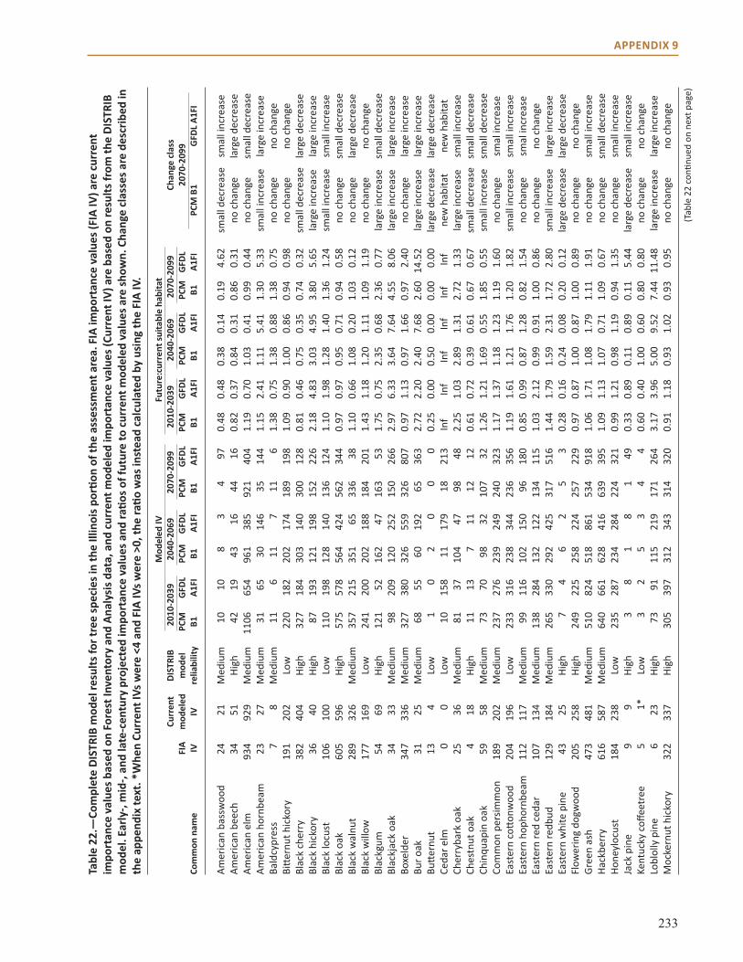
233

APPENDIX 9

Amer

ican

bas

swoo

d 24

21

M

ediu

m

10

10

8 3

4 97

0.

48

0.48

0.

38

0.14

0.

19

4.62

sm

all d

ecre

ase

smal

l inc

reas

eAm

eric

an b

eech

34

51

Hi

gh

42

19

43

16

44

16

0.82

0.

37

0.84

0.

31

0.86

0.

31

no c

hang

e la

rge

decr

ease

Amer

ican

elm

93

4 92

9 M

ediu

m

1106

65

4 96

1 38

5 92

1 40

4 1.

19

0.70

1.

03

0.41

0.

99

0.44

no

cha

nge

smal

l dec

reas

eAm

eric

an h

ornb

eam

23

27

M

ediu

m

31

65

30

146

35

144

1.15

2.

41

1.11

5.

41

1.30

5.

33

smal

l inc

reas

e la

rge

incr

ease

Bald

cypr

ess

7 8

Med

ium

11

6

11

7 11

6

1.38

0.

75

1.38

0.

88

1.38

0.

75

no c

hang

e no

cha

nge

Bitte

rnut

hic

kory

19

1 20

2 Lo

w

220

182

202

174

189

198

1.09

0.

90

1.00

0.

86

0.94

0.

98

no c

hang

e no

cha

nge

Blac

k ch

erry

38

2 40

4 Hi

gh

327

184

303

140

300

128

0.81

0.

46

0.75

0.

35

0.74

0.

32

smal

l dec

reas

e la

rge

decr

ease

Blac

k hi

ckor

y 36

40

Hi

gh

87

193

121

198

152

226

2.18

4.

83

3.03

4.

95

3.80

5.

65

larg

e in

crea

se

larg

e in

crea

seBl

ack

locu

st

106

100

Low

11

0 19

8 12

8 14

0 13

6 12

4 1.

10

1.98

1.

28

1.40

1.

36

1.24

sm

all i

ncre

ase

smal

l inc

reas

eBl

ack

oak

605

596

High

57

5 57

8 56

4 42

4 56

2 34

4 0.

97

0.97

0.

95

0.71

0.

94

0.58

no

cha

nge

smal

l dec

reas

eBl

ack

wal

nut

289

326

Med

ium

35

7 21

5 35

1 65

33

6 38

1.

10

0.66

1.

08

0.20

1.

03

0.12

no

cha

nge

larg

e de

crea

seBl

ack

will

ow

177

169

Low

24

1 20

0 20

2 18

8 18

4 20

1 1.

43

1.18

1.

20

1.11

1.

09

1.19

no

cha

nge

no c

hang

eBl

ackg

um

54

69

High

12

1 52

16

2 47

16

3 53

1.

75

0.75

2.

35

0.68

2.

36

0.77

la

rge

incr

ease

sm

all d

ecre

ase

Blac

kjac

k oa

k 34

33

M

ediu

m

98

209

120

252

150

266

2.97

6.

33

3.64

7.

64

4.55

8.

06

larg

e in

crea

se

larg

e in

crea

seBo

xeld

er

347

336

Med

ium

32

7 38

0 32

6 55

9 32

6 80

7 0.

97

1.13

0.

97

1.66

0.

97

2.40

no

cha

nge

larg

e in

crea

seBu

r oak

31

25

M

ediu

m

68

55

60

192

65

363

2.72

2.

20

2.40

7.

68

2.60

14

.52

larg

e in

crea

se

larg

e in

crea

seBu

ttern

ut

13

4 Lo

w

1 0

2 0

0 0

0.25

0.

00

0.50

0.

00

0.00

0.

00

larg

e de

crea

se

larg

e de

crea

seCe

dar e

lm

0 0

Low

10

15

8 11

17

9 18

21

3 In

f In

f In

f In

f In

f In

f ne

w h

abita

t ne

w h

abita

tCh

erry

bark

oak

25

36

M

ediu

m

81

37

104

47

98

48

2.25

1.

03

2.89

1.

31

2.72

1.

33

larg

e in

crea

se

smal

l inc

reas

eCh

estn

ut o

ak

4 18

Hi

gh

11

13

7 11

12

12

0.

61

0.72

0.

39

0.61

0.

67

0.67

sm

all d

ecre

ase

smal

l dec

reas

eCh

inqu

apin

oak

59

58

M

ediu

m

73

70

98

32

107

32

1.26

1.

21

1.69

0.

55

1.85

0.

55

smal

l inc

reas

e sm

all d

ecre

ase

Com

mon

per

simm

on

189

202

Med

ium

23

7 27

6 23

9 24

9 24

0 32

3 1.

17

1.37

1.

18

1.23

1.

19

1.60

no

cha

nge

smal

incr

ease

East

ern

cotto

nwoo

d 20

4 19

6 Lo

w

233

316

238

344

236

356

1.19

1.

61

1.21

1.

76

1.20

1.

82

smal

l inc

reas

e sm

all i

ncre

ase

East

ern

hoph

ornb

eam

11

2 11

7 M

ediu

m

99

116

102

150

96

180

0.85

0.

99

0.87

1.

28

0.82

1.

54

no c

hang

e sm

al in

crea

seEa

ster

n re

d ce

dar

107

134

Med

ium

13

8 28

4 13

2 12

2 13

4 11

5 1.

03

2.12

0.

99

0.91

1.

00

0.86

no

cha

nge

no c

hang

eEa

ster

n re

dbud

12

9 18

4 M

ediu

m

265

330

292

425

317

516

1.44

1.

79

1.59

2.

31

1.72

2.

80

smal

l inc

reas

e la

rge

incr

ease

East

ern

whi

te p

ine

43

25

High

7

4 6

2 5

3 0.

28

0.16

0.

24

0.08

0.

20

0.12

la

rge

decr

ease

la

rge

decr

ease

Flow

erin

g do

gwoo

d 20

5 25

8 Hi

gh

249

225

258

224

257

229

0.97

0.

87

1.00

0.

87

1.00

0.

89

no c

hang

e no

cha

nge

Gree

n as

h 47

3 48

1 M

ediu

m

510

824

518

861

534

918

1.06

1.

71

1.08

1.

79

1.11

1.

91

no c

hang

e sm

all i

ncre

ase

Hack

berr

y 61

6 58

7 M

ediu

m

640

661

628

416

639

395

1.09

1.

13

1.07

0.

71

1.09

0.

67

no c

hang

e sm

all d

ecre

ase

Hone

yloc

ust

184

238

Low

23

5 28

7 23

4 28

4 22

4 32

1 0.

99

1.21

0.

98

1.19

0.

94

1.35

no

cha

nge

smal

l inc

reas

eJa

ck p

ine

9 9

High

3

8 1

8 1

49

0.33

0.

89

0.11

0.

89

0.11

5.

44

larg

e de

crea

se

smal

l inc

reas

eKe

ntuc

ky c

offee

tree

5

1*

Low

3

2 5

3 4

4 0.

60

0.40

1.

00

0.60

0.

80

0.80

no

cha

nge

no c

hang

eLo

blol

ly p

ine

6 23

Hi

gh

73

91

115

219

171

264

3.17

3.

96

5.00

9.

52

7.44

11

.48

larg

e in

crea

se

larg

e in

crea

seM

ocke

rnut

hic

kory

32

2 33

7 Hi

gh

305

397

312

343

314

320

0.91

1.

18

0.93

1.

02

0.93

0.

95

no c

hang

e no

cha

nge

Tabl

e 22

.—Co

mpl

ete

DIST

RIB

mod

el re

sults

for t

ree

spec

ies i

n th

e Ill

inoi

s por

tion

of th

e as

sess

men

t are

a. F

IA im

port

ance

val

ues (

FIA

IV) a

re c

urre

nt

impo

rtan

ce v

alue

s bas

ed o

n Fo

rest

Inve

ntor

y an

d An

alys

is d

ata,

and

cur

rent

mod

eled

impo

rtan

ce v

alue

s (Cu

rren

t IV)

are

bas

ed o

n re

sults

from

the

DIST

RIB

mod

el. E

arly

-, m

id-,

and

late

-cen

tury

pro

ject

ed im

port

ance

val

ues a

nd ra

tios o

f fut

ure

to c

urre

nt m

odel

ed v

alue

s are

show

n. C

hang

e cl

asse

s are

des

crib

ed in

th

e ap

pend

ix te

xt. *

Whe

n Cu

rren

t IVs

wer

e <4

and

FIA

IVs w

ere

>0, t

he ra

tio w

as in

stea

d ca

lcul

ated

by

usin

g th

e FI

A IV

.

(Tab

le 2

2 co

ntinu

ed o

n ne

xt p

age)

M

odel

ed IV

Fu

ture

:cur

rent

suita

ble

habi

tat

Curr

ent

DIST

RIB

2010

-203

9 20

40-2

069

2070

-209

9 20

10-2

039

2040

-206

9 20

70-2

099

Chan

ge c

lass

FI

A m

odel

ed

mod

el

PCM

G

FDL

PCM

G

FDL

PCM

G

FDL

PCM

G

FDL

PCM

G

FDL

PCM

G

FDL

2070

-209

9Co

mm

on n

ame

IV

IV

relia

bilit

y B1

A1

FI

B1

A1FI

B1

A1

FI

B1

A1FI

B1

A1

FI

B1

A1FI

PC

M B

1 G

FDL

A1FI

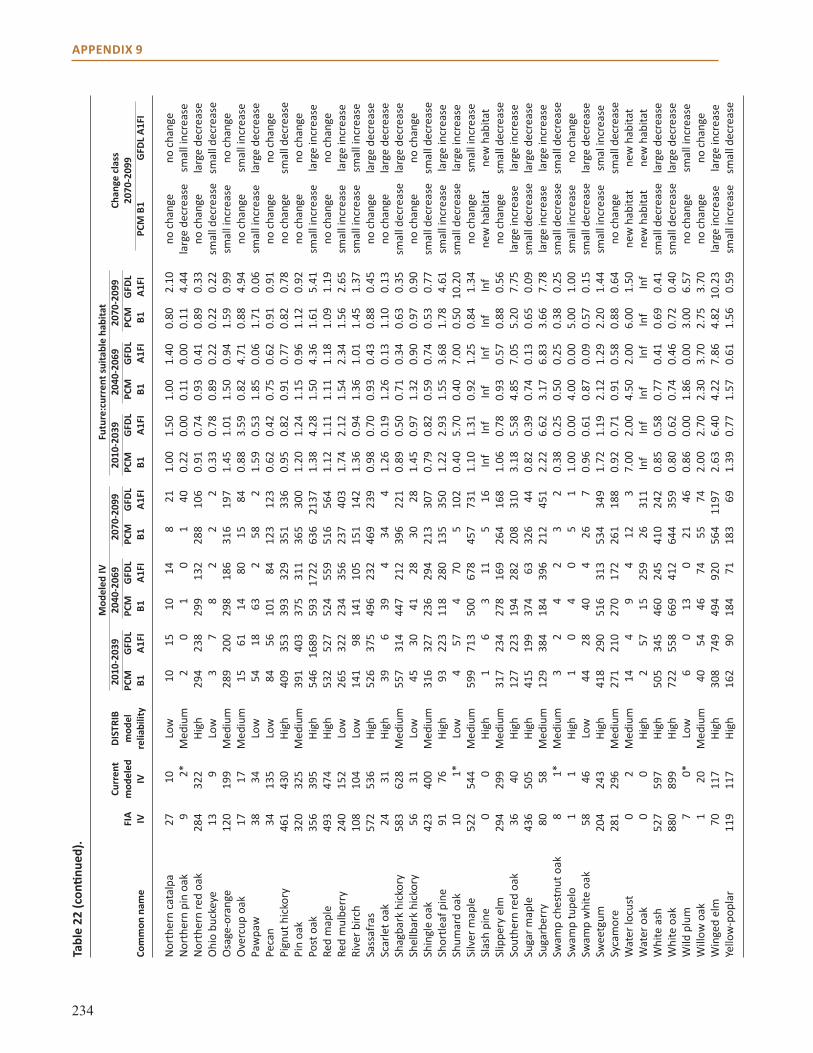
234

APPENDIX 9

Nor

ther

n ca

talp

a 27

10

Lo

w

10

15

10

14

8 21

1.

00

1.50

1.

00

1.40

0.

80

2.10

no

cha

nge

no c

hang

eN

orth

ern

pin

oak

9 2*

M

ediu

m

2 0

1 0

1 40

0.

22

0.00

0.

11

0.00

0.

11

4.44

la

rge

decr

ease

sm

all i

ncre

ase

Nor

ther

n re

d oa

k 28

4 32

2 Hi

gh

294

238

299

132

288

106

0.91

0.

74

0.93

0.

41

0.89

0.

33

no c

hang

e la

rge

decr

ease

Ohi

o bu

ckey

e 13

9

Low

3

7 8

2 2

2 0.

33

0.78

0.

89

0.22

0.

22

0.22

sm

all d

ecre

ase

smal

l dec

reas

eO

sage

-ora

nge

120

199

Med

ium

28

9 20

0 29

8 18

6 31

6 19

7 1.

45

1.01

1.

50

0.94

1.

59

0.99

sm

all i

ncre

ase

no c

hang

eO

verc

up o

ak

17

17

Med

ium

15

61

14

80

15

84

0.

88

3.59

0.

82

4.71

0.

88

4.94

no

cha

nge

smal

l inc

reas

ePa

wpa

w

38

34

Low

54

18

63

2

58

2 1.

59

0.53

1.

85

0.06

1.

71

0.06

sm

all i

ncre

ase

larg

e de

crea

sePe

can

34

135

Low

84

56

10

1 84

12

3 12

3 0.

62

0.42

0.

75

0.62

0.

91

0.91

no

cha

nge

no c

hang

ePi

gnut

hic

kory

46

1 43

0 Hi

gh

409

353

393

329

351

336

0.95

0.

82

0.91

0.

77

0.82

0.

78

no c

hang

e sm

all d

ecre

ase

Pin

oak

320

325

Med

ium

39

1 40

3 37

5 31

1 36

5 30

0 1.

20

1.24

1.

15

0.96

1.

12

0.92

no

cha

nge

no c

hang

ePo

st o

ak

356

395

High

54

6 16

89

593

1722

63

6 21

37

1.38

4.

28

1.50

4.

36

1.61

5.

41

smal

l inc

reas

e la

rge

incr

ease

Red

map

le

493

474

High

53

2 52

7 52

4 55

9 51

6 56

4 1.

12

1.11

1.

11

1.18

1.

09

1.19

no

cha

nge

no c

hang

eRe

d m

ulbe

rry

240

152

Low

26

5 32

2 23

4 35

6 23

7 40

3 1.

74

2.12

1.

54

2.34

1.

56

2.65

sm

all i

ncre

ase

larg

e in

crea

seRi

ver b

irch

108

104

Low

14

1 98

14

1 10

5 15

1 14

2 1.

36

0.94

1.

36

1.01

1.

45

1.37

sm

all i

ncre

ase

smal

l inc

reas

eSa

ssaf

ras

572

536

High

52

6 37

5 49

6 23

2 46

9 23

9 0.

98

0.70

0.

93

0.43

0.

88

0.45

no

cha

nge

larg

e de

crea

seSc

arle

t oak

24

31

Hi

gh

39

6 39

4

34

4 1.

26

0.19

1.

26

0.13

1.

10

0.13

no

cha

nge

larg

e de

crea

seSh

agba

rk h

icko

ry

583

628

Med

ium

55

7 31

4 44

7 21

2 39

6 22

1 0.

89

0.50

0.

71

0.34

0.

63

0.35

sm

all d

ecre

ase

larg

e de

crea

seSh

ellb

ark

hick

ory

56

31

Low

45

30

41

28

30

28

1.

45

0.97

1.

32

0.90

0.

97

0.90

no

cha

nge

no c

hang

eSh

ingl

e oa

k 42

3 40

0 M

ediu

m

316

327

236

294

213

307

0.79

0.

82

0.59

0.

74

0.53

0.

77

smal

l dec

reas

e sm

all d

ecre

ase

Shor

tleaf

pin

e 91

76

Hi

gh

93

223

118

280

135

350

1.22

2.

93

1.55

3.

68

1.78

4.

61

smal

l inc

reas

e la

rge

incr

ease

Shum

ard

oak

10

1*

Low

4

57

4 70

5

102

0.40

5.

70

0.40

7.

00

0.50

10

.20

smal

l dec

reas

e la

rge

incr

ease

Silv

er m

aple

52

2 54

4 M

ediu

m

599

713

500

678

457

731

1.10

1.

31

0.92

1.

25

0.84

1.

34

no c

hang

e sm

all i

ncre

ase

Slas

h pi

ne

0 0

High

1

6 3

11

5 16

In

f In

f In

f In

f In

f In

f ne

w h

abita

t ne

w h

abita

tSl

ippe

ry e

lm

294

299

Med

ium

31

7 23

4 27

8 16

9 26

4 16

8 1.

06

0.78

0.

93

0.57

0.

88

0.56

no

cha

nge

smal

l dec

reas

eSo

uthe

rn re

d oa

k 36

40

Hi

gh

127

223

194

282

208

310

3.18

5.

58

4.85

7.

05

5.20

7.

75

larg

e in

crea

se

larg

e in

crea

seSu

gar m

aple

43

6 50

5 Hi

gh

415

199

374

63

326

44

0.82

0.

39

0.74

0.

13

0.65

0.

09

smal

l dec

reas

e la

rge

decr

ease

Suga

rber

ry

80

58

Med

ium

12

9 38

4 18

4 39

6 21

2 45

1 2.

22

6.62

3.

17

6.83

3.

66

7.78

la

rge

incr

ease

la

rge

incr

ease

Swam

p ch

estn

ut o

ak

8 1*

M

ediu

m

3 2

4 2

3 2

0.38

0.

25

0.50

0.

25

0.38

0.

25

smal

l dec

reas

e sm

all d

ecre

ase

Swam

p tu

pelo

1

1 Hi

gh

1 0

4 0

5 1

1.00

0.

00

4.00

0.

00

5.00

1.

00

smal

l inc

reas

e no

cha

nge

Swam

p w

hite

oak

58

46

Lo

w

44

28

40

4 26

7

0.96

0.

61

0.87

0.

09

0.57

0.

15

smal

l dec

reas

e la

rge

decr

ease

Swee

tgum

20

4 24

3 Hi

gh

418

290

516

313

534

349

1.72

1.

19

2.12

1.

29

2.20

1.

44

smal

l inc

reas

e sm

al in

crea

seSy

cam

ore

281

296

Med

ium

27

1 21

0 27

0 17

2 26

1 18

8 0.

92

0.71

0.

91

0.58

0.

88

0.64

no

cha

nge

smal

l dec

reas

eW

ater

locu

st

0 2

Med

ium

14

4

9 4

12

3 7.

00

2.00

4.

50

2.00

6.

00

1.50

ne

w h

abita

t ne

w h

abita

tW

ater

oak

0

0 Hi

gh

2 57

15

25

9 26

31

1 In

f In

f In

f In

f In

f In

f ne

w h

abita

t ne

w h

abita

tW

hite

ash

52

7 59

7 Hi

gh

505

345

460

245

410

242

0.85

0.

58

0.77

0.

41

0.69

0.

41

smal

l dec

reas

e la

rge

decr

ease

Whi

te o

ak

880

899

High

72

2 55

8 66

9 41

2 64

4 35

9 0.

80

0.62

0.

74

0.46

0.

72

0.40

sm

all d

ecre

ase

larg

e de

crea

seW

ild p

lum

7

0*

Low

6

0 13

0

21

46

0.86

0.

00

1.86

0.

00

3.00

6.

57

no c

hang

e sm

all i

ncre

ase

Will

ow o

ak

1 20

M

ediu

m

40

54

46

74

55

74

2.00

2.

70

2.30

3.

70

2.75

3.

70

no c

hang

e no

cha

nge

Win

ged

elm

70

11

7 Hi

gh

308

749

494

920

564

1197

2.

63

6.40

4.

22

7.86

4.

82

10.2

3 la

rge

incr

ease

la

rge

incr

ease

Yello

w-p

opla

r 11

9 11

7 Hi

gh

162

90

184

71

183

69

1.39

0.

77

1.57

0.

61

1.56

0.

59

smal

l inc

reas

e sm

all d

ecre

ase

Tabl

e 22

(con

tinue

d).

M

odel

ed IV

Fu

ture

:cur

rent

suita

ble

habi

tat

Curr

ent

DIST

RIB

2010

-203

9 20

40-2

069

2070

-209

9 20

10-2

039

2040

-206

9 20

70-2

099

Chan

ge c

lass

FI

A m

odel

ed

mod

el

PCM

G

FDL

PCM

G

FDL

PCM

G

FDL

PCM

G

FDL

PCM

G

FDL

PCM

G

FDL

2070

-209

9Co

mm

on n

ame

IV

IV

relia

bilit

y B1

A1

FI

B1

A1FI

B1

A1

FI

B1

A1FI

B1

A1

FI

B1

A1FI

PC

M B

1 G

FDL

A1FI

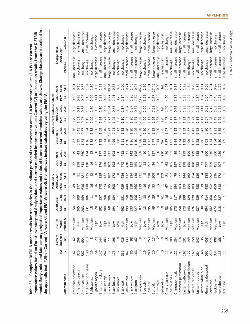
235

APPENDIX 9

Amer

ican

bas

swoo

d 62

62

M

ediu

m

54

22

49

0 37

19

0.

87

0.36

0.

79

0.00

0.

60

0.31

sm

all d

ecre

ase

larg

e de

crea

seAm

eric

an b

eech

32

5 26

8 Hi

gh

265

109

277

51

258

43

0.99

0.

41

1.03

0.

19

0.96

0.

16

no c

hang

e la

rge

decr

ease

Amer

ican

elm

56

2 65

4 M

ediu

m

803

569

636

381

643

360

1.23

0.

87

0.97

0.

58

0.98

0.

55

no c

hang

e sm

all d

ecre

ase

Amer

ican

hor

nbea

m

139

113

Med

ium

13

1 10

6 13

0 17

5 13

0 17

4 1.

16

0.94

1.

15

1.55

1.

15

1.54

no

cha

nge

smal

l inc

reas

eBa

ldcy

pres

s 19

8

Med

ium

15

11

16

12

16

12

1.

88

1.38

2.

00

1.50

2.

00

1.50

no

cha

nge

no c

hang

e Bi

gtoo

th a

spen

54

29

Hi

gh

20

0 16

0

12

0 0.

69

0.00

0.

55

0.00

0.

41

0.00

la

rge

decr

ease

ex

tirpa

ted

Bitte

rnut

hic

kory

14

7 14

4 Lo

w

192

157

178

159

176

177

1.33

1.

09

1.24

1.

10

1.22

1.

23

smal

l inc

reas

e sm

all i

ncre

ase

Blac

k ch

erry

26

7 38

3 Hi

gh

284

268

273

127

260

133

0.74

0.

70

0.71

0.

33

0.68

0.

35

smal

l dec

reas

e la

rge

decr

ease

Blac

k hi

ckor

y 2

11

High

68

20

6 85

28

2 10

2 33

7 6.

18

18.7

3 7.

73

25.6

4 9.

27

30.6

4 la

rge

incr

ease

la

rge

incr

ease

Blac

k lo

cust

17

5 19

6 Lo

w

194

184

208

173

198

103

0.99

0.

94

1.06

0.

88

1.01

0.

53

no c

hang

e sm

all d

ecre

ase

Blac

k m

aple

12

8

Low

7

1 7

0 6

0 0.

88

0.13

0.

88

0.00

0.

75

0.00

no

cha

nge

larg

e de

crea

seBl

ack

oak

335

416

High

46

2 55

1 45

9 48

6 47

3 41

5 1.

11

1.33

1.

10

1.17

1.

14

1.00

no

cha

nge

no c

hang

e Bl

ack

wal

nut

347

333

Med

ium

39

9 25

8 44

0 11

2 43

0 71

1.

20

0.78

1.

32

0.34

1.

29

0.21

sm

all i

ncre

ase

larg

e de

crea

seBl

ack

will

ow

86

98

Low

13

3 11

8 11

8 13

4 12

3 14

2 1.

36

1.20

1.

20

1.37

1.

26

1.45

sm

all i

ncre

ase

smal

l inc

reas

eBl

ackg

um

166

162

High

22

7 15

6 26

6 13

8 26

5 15

8 1.

40

0.96

1.

64

0.85

1.

64

0.98

sm

all i

ncre

ase

no c

hang

e Bl

ackj

ack

oak

3 8

Med

ium

87

22

7 13

9 33

1 16

2 36

8 10

.88

28.3

8 17

.38

41.3

8 20

.25

46.0

0 la

rge

incr

ease

la

rge

incr

ease

Blue

ash

19

4

Low

13

10

16

8

13

10

3.25

2.

50

4.00

2.

00

3.25

2.

50

no c

hang

e no

cha

nge

Boxe

lder

28

0 25

3 M

ediu

m

295

276

296

318

292

482

1.17

1.

09

1.17

1.

26

1.15

1.

91

smal

l inc

reas

e sm

all i

ncre

ase

Bur o

ak

20

13

Med

ium

49

29

33

10

0 36

22

7 3.

77

2.23

2.

54

7.69

2.

77

17.4

6 la

rge

incr

ease

la

rge

incr

ease

Butte

rnut

9

2*

Low

4

0 3

0 2

0 0.

44

0.00

0.

33

0.00

0.

22

0.00

sm

all d

ecre

ase

larg

e de

crea

seCe

dar e

lm

0 0

Low

0

61

1 19

9 3

230

NA

Inf

Inf

Inf

Inf

Inf

new

hab

itat

new

hab

itat

Cher

ryba

rk o

ak

11

15

Med

ium

58

16

67

21

63

29

3.

87

1.07

4.

47

1.40

4.

20

1.93

sm

all i

ncre

ase

no c

hang

e Ch

estn

ut o

ak

97

100

High

10

5 61

11

1 52

10

5 51

1.

05

0.61

1.

11

0.52

1.

05

0.51

no

cha

nge

smal

l dec

reas

eCh

inqu

apin

oak

12

1 10

4 M

ediu

m

170

117

194

79

197

59

1.64

1.

13

1.87

0.

76

1.89

0.

57

smal

l inc

reas

e sm

all d

ecre

ase

Com

mon

per

simm

on

91

118

Med

ium

15

8 29

6 16

3 27

7 17

1 32

7 1.

34

2.51

1.

38

2.35

1.

45

2.77

sm

all i

ncre

ase

larg

e in

crea

seEa

ster

n co

ttonw

ood

162

131

Low

17

3 19

9 17

3 24

4 17

8 25

9 1.

32

1.52

1.

32

1.86

1.

36

1.98

sm

all i

ncre

ase

smal

l inc

reas

eEa

ster

n ho

phor

nbea

m

127

149

Med

ium

14

3 12

9 15

4 16

2 15

5 19

9 0.

96

0.87

1.

03

1.09

1.

04

1.34

no

cha

nge

smal

l inc

reas

eEa

ster

n re

d ce

dar

167

150

Med

ium

17

6 22

0 18

3 15

4 18

0 11

9 1.

17

1.47

1.

22

1.03

1.

20

0.79

no

cha

nge

smal

l dec

reas

eEa

ster

n re

dbud

28

4 34

2 M

ediu

m

427

439

458

530

458

635

1.25

1.

28

1.34

1.

55

1.34

1.

86

smal

l inc

reas

e sm

all i

ncre

ase

East

ern

whi

te p

ine

48

35

High

30

15

39

4

33

4 0.

86

0.43

1.

11

0.11

0.

94

0.11

no

cha

nge

larg

e de

crea

seFl

ower

ing

dogw

ood

565

458

High

49

4 41

4 48

8 28

8 47

7 30

0 1.

08

0.90

1.

07

0.63

1.

04

0.66

no

cha

nge

smal

l dec

reas

eGr

een

ash

279

275

Med

ium

34

2 46

0 35

2 59

2 35

9 63

6 1.

24

1.67

1.

28

2.15

1.

31

2.31

sm

all i

ncre

ase

larg

e in

crea

seHa

ckbe

rry

334

308

Med

ium

47

4 37

5 45

9 33

6 45

1 30

0 1.

54

1.22

1.

49

1.09

1.

46

0.97

sm

all i

ncre

ase

no c

hang

e Ho

neyl

ocus

t 13

5 16

8 Lo

w

218

227

210

272

207

289

1.30

1.

35

1.25

1.

62

1.23

1.

72

smal

l inc

reas

e sm

all i

ncre

ase

Jack

pin

e 11

1*

Hi

gh

1 1

1 1

1 9

0.09

0.

09

0.09

0.

09

0.09

0.

82

larg

e de

crea

se

no c

hang

e

Tabl

e 23

.—Co

mpl

ete

DIST

RIB

mod

el re

sults

for t

ree

spec

ies i

n th

e In

dian

a po

rtion

of t

he a

sses

smen

t are

a. F

IA im

port

ance

val

ues (

FIA

IV) a

re c

urre

nt

impo

rtan

ce v

alue

s bas

ed o

n Fo

rest

Inve

ntor

y an

d An

alys

is d

ata,

and

cur

rent

mod

eled

impo

rtan

ce v

alue

s (Cu

rren

t IV)

are

bas

ed o

n re

sults

from

the

DIST

RIB

mod

el. E

arly

-, m

id-,

and

late

-cen

tury

pro

ject

ed im

port

ance

val

ues a

nd ra

tios o

f fut

ure

to c

urre

nt m

odel

ed v

alue

s are

show

n. C

hang

e cl

asse

s are

des

crib

ed in

th

e ap

pend

ix te

xt. *

Whe

n Cu

rren

t IVs

wer

e <4

and

FIA

IVs w

ere

>0, t

he ra

tio w

as in

stea

d ca

lcul

ated

by

usin

g th

e FI

A IV

.

(Tab

le 2

3 co

ntinu

ed o

n ne

xt p

age)

M

odel

ed IV

Fu

ture

:cur

rent

suita

ble

habi

tat

Curr

ent

DIST

RIB

2010

-203

9 20

40-2

069

2070

-209

9 20

10-2

039

2040

-206

9 20

70-2

099

Chan

ge c

lass

FI

A m

odel

ed

mod

el

PCM

G

FDL

PCM

G

FDL

PCM

G

FDL

PCM

G

FDL

PCM

G

FDL

PCM

G

FDL

2070

-209

9Co

mm

on n

ame

IV

IV

relia

bilit

y B1

A1

FI

B1

A1FI

B1

A1

FI

B1

A1FI

B1

A1

FI

B1

A1FI

PC

M B

1 G

FDL

A1FI

236

APPENDIX 9

Kent

ucky

coff

eetr

ee

19

1*

Low

7

3 8

1 8

4 0.

37

0.16

0.

42

0.05

0.

42

0.21

sm

all d

ecre

ase

larg

e de

crea

seLo

blol

ly p

ine

0 12

Hi

gh

50

50

94

140

106

233

4.17

4.

17

7.83

11

.67

8.83

19

.42

new

hab

itat

new

hab

itat

Moc

kern

ut h

icko

ry

96

212

High

19

7 27

8 21

9 27

3 21

7 27

2 0.

93

1.31

1.

03

1.29

1.

02

1.28

no

cha

nge

smal

l inc

reas

eN

orth

ern

cata

lpa

23

7 Lo

w

9 13

9

11

7 21

1.

29

1.86

1.

29

1.57

1.

00

3.00

no

cha

nge

no c

hang

e N

orth

ern

pin

oak

21

6 M

ediu

m

4 1

1 0

1 8

0.67

0.

17

0.17

0.

00

0.17

1.

33

larg

e de

crea

se

no c

hang

e N

orth

ern

red

oak

260

306

High

31

1 25

3 32

8 20

4 32

5 16

1 1.

02

0.83

1.

07

0.67

1.

06

0.53

no

cha

nge

smal

l dec

reas

eO

hio

buck

eye

67

37

Low

49

34

46

13

36

9

1.32

0.

92

1.24

0.

35

0.97

0.

24

no c

hang

e la

rge

decr

ease

Osa

ge-o

rang

e 13

5 12

2 M

ediu

m

226

139

234

161

233

169

1.85

1.

14

1.92

1.

32

1.91

1.

39

smal

l inc

reas

e sm

all i

ncre

ase

Ove

rcup

oak

5

7 M

ediu

m

7 24

7

33

8 35

1.

00

3.43

1.

00

4.71

1.

14

5.00

no

cha

nge

smal

l inc

reas

ePa

wpa

w

69

72

Low

10

1 44

10

9 12

10

8 9

1.40

0.

61

1.51

0.

17

1.50

0.

13

smal

l inc

reas

e la

rge

decr

ease

Peca

n 25

10

4 Lo

w

76

56

73

97

79

113

0.73

0.

54

0.70

0.

93

0.76

1.

09

smal

l dec

reas

e no

cha

nge

Pign

ut h

icko

ry

290

333

High

34

8 35

0 34

7 33

3 34

4 33

1 1.

05

1.05

1.

04

1.00

1.

03

0.99

no

cha

nge

no c

hang

e Pi

n oa

k 13

6 14

0 M

ediu

m

266

209

242

242

249

228

1.90

1.

49

1.73

1.

73

1.78

1.

63

smal

l inc

reas

e sm

all i

ncre

ase

Post

oak

42

13

0 Hi

gh

337

1439

38

7 17

98

431

2048

2.

59

11.0

7 2.

98

13.8

3 3.

32

15.7

5 la

rge

incr

ease

la

rge

incr

ease

Red

map

le

416

485

High

49

3 42

2 50

5 45

3 48

9 48

5 1.

02

0.87

1.

04

0.93

1.

01

1.00

no

cha

nge

no c

hang

e Re

d m

ulbe

rry

53

63

Low

10

5 16

8 10

2 19

1 10

5 23

5 1.

67

2.67

1.

62

3.03

1.

67

3.73

sm

all i

ncre

ase

larg

e in

crea

seRi

ver b

irch

72

54

Low

83

68

85

77

87

10

2 1.

54

1.26

1.

57

1.43

1.

61

1.89

sm

all i

ncre

ase

smal

liRo

ck e

lm

37

11

Low

50

24

68

10

58

3

4.55

2.

18

6.18

0.

91

5.27

0.

27

smal

l inc

reas

e sm

all d

ecre

ase

Sass

afra

s 59

2 50

8 Hi

gh

571

389

551

251

534

238

1.12

0.

77

1.09

0.

49

1.05

0.

47

no c

hang

e la

rge

decr

ease

Scar

let o

ak

53

77

High

85

79

97

29

94

20

1.

10

1.03

1.

26

0.38

1.

22

0.26

sm

all i

ncre

ase

larg

e de

crea

seSh

agba

rk h

icko

ry

326

333

Med

ium

38

2 27

5 34

0 18

4 34

0 18

1 1.

15

0.83

1.

02

0.55

1.

02

0.54

no

cha

nge

smal

l dec

reas

eSh

ellb

ark

hick

ory

64

24

Low

46

43

37

31

33

28

1.

92

1.79

1.

54

1.29

1.

38

1.17

sm

all i

ncre

ase

no c

hang

e Sh

ingl

e oa

k 84

10

6 M

ediu

m

144

139

125

139

118

141

1.36

1.

31

1.18

1.

31

1.11

1.

33

no c

hang

e sm

all i

ncre

ase

Shor

tleaf

pin

e 42

43

Hi

gh

76

275

95

379

105

591

1.77

6.

40

2.21

8.

81

2.44

13

.74

larg

e in

crea

se

larg

e in

crea

seSh

umar

d oa

k 7

0*

Low

2

25

1 98

2

124

0.29

3.

57

0.14

14

.00

0.29

17

.71

smal

l dec

reas

e la

rge

incr

ease

Silv

er m

aple

33

6 28

7 M

ediu

m

368

446

326

507

317

526

1.28

1.

55

1.14

1.

77

1.11

1.

83

no c

hang

e sm

all i

ncre

ase

Slas

h pi

ne

0 0

High

1

1 11

2

8 7

Inf

Inf

Inf

Inf

Inf

Inf

new

hab

itat

new

hab

itat

Slip

pery

elm

33

3 30

0 M

ediu

m

316

259

288

157

281

148

1.05

0.

86

0.96

0.

52

0.94

0.

49

no c

hang

e la

rge

decr

ease

Sour

woo

d 1

4 Hi

gh

3 1

8 1

8 1

3.00

1.

00

8.00

1.

00

8.00

1.

00

smal

l inc

reas

e no

cha

nge

Sout

hern

red

oak

7 22

Hi

gh

83

209

132

277

136

402

3.77

9.

50

6.00

12

.59

6.18

18

.27

larg

e in

crea

se

larg

e in

crea

seSu

gar m

aple

11

86

1082

Hi

gh

1035

38

9 97

9 11

2 90

4 56

0.

96

0.36

0.

91

0.10

0.

84

0.05

no

cha

nge

larg

e de

crea

seSu

garb

erry

8

20

Med

ium

50

20

8 10

3 37

0 11

7 42

7 2.

50

10.4

0 5.

15

18.5

0 5.

85

21.3

5 sm

all i

ncre

ase

larg

e in

crea

seSw

amp

ches

tnut

oak

10

0*

M

ediu

m

4 2

4 2

4 3

0.40

0.

20

0.40

0.

20

0.40

0.

30

smal

l dec

reas

e sm

all d

ecre

ase

Swam

p tu

pelo

18

1*

Hi

gh

6 2

30

1 32

3

0.33

0.

11

1.67

0.

06

1.78

0.

17

no c

hang

e la

rge

decr

ease

Swam

p w

hite

oak

37

34

Lo

w

53

25

49

8 44

4

1.56

0.

74

1.44

0.

24

1.29

0.

12

smal

l inc

reas

e la

rge

decr

ease

Swee

tgum

25

2 21

1 Hi

gh

353

252

435

238

431

354

1.67

1.

19

2.06

1.

13

2.04

1.

68

larg

e in

crea

se

smal

l inc

reas

eSy

cam

ore

317

282

Med

ium

29

5 26

0 30

0 19

8 28

9 19

1 1.

05

0.92

1.

06

0.70

1.

03

0.68

no

cha

nge

smal

l dec

reas

eVi

rgin

ia p

ine

99

69

High

89

63

10

7 62

93

69

1.

29

0.91

1.

55

0.90

1.

35

1.00

sm

all i

ncre

ase

no c

hang

e

Tabl

e 23

(con

tinue

d).

M

odel

ed IV

Fu

ture

:cur

rent

suita

ble

habi

tat

Curr

ent

DIST

RIB

2010

-203

9 20

40-2

069

2070

-209

9 20

10-2

039

2040

-206

9 20

70-2

099

Chan

ge c

lass

FI

A m

odel

ed

mod

el

PCM

G

FDL

PCM

G

FDL

PCM

G

FDL

PCM

G

FDL

PCM

G

FDL

PCM

G

FDL

2070

-209

9Co

mm

on n

ame

IV

IV

relia

bilit

y B1

A1

FI

B1

A1FI

B1

A1

FI

B1

A1FI

B1

A1

FI

B1

A1FI

PC

M B

1 G

FDL

A1FI

(Tab

le 2

3 co

ntinu

ed o

n ne

xt p

age)

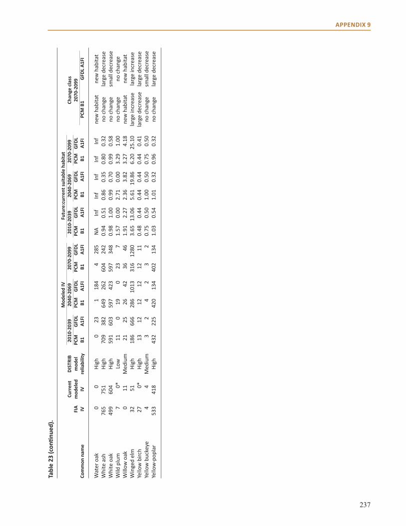
237

APPENDIX 9

Wat

er o

ak

0 0

High

0

23

1 18

4 4

285

NA

Inf

Inf

Inf

Inf

Inf

new

hab

itat

new

hab

itat

Whi

te a

sh

765

751

High

70

9 38

2 64

9 26

2 60

4 24

2 0.

94

0.51

0.

86

0.35

0.

80

0.32

no

cha

nge

larg

e de

crea

seW

hite

oak

49

9 60

4 Hi

gh

591

603

597

423

597

348

0.98

1.

00

0.99

0.

70

0.99

0.

58

no c

hang

e sm

all d

ecre

ase

Wild

plu

m

7 0*

Lo

w

11

0 19

0

23

7 1.

57

0.00

2.

71

0.00

3.

29

1.00

no

cha

nge

no c

hang

e W

illow

oak

0

11

Med

ium

21

25

26

42

36

46

1.

91

2.27

2.

36

3.82

3.

27

4.18

ne

w h

abita

t ne

w h

abita

tW

inge

d el

m

32

51

High

18

6 66

6 28

6 10

13

316

1280

3.

65

13.0

6 5.

61

19.8

6 6.

20

25.1

0 la

rge

incr

ease

la

rge

incr

ease

Yello

w b

irch

27

0*

High

13

12

12

12

12

11

0.

48

0.44

0.

44

0.44

0.

44

0.41

la

rge

decr

ease

la

rge

decr

ease

Yello

w b

ucke

ye

4 4

Med

ium

3

2 4

2 3

2 0.

75

0.50

1.

00

0.50

0.

75

0.50

no

cha

nge

smal

l dec

reas

eYe

llow

-pop

lar

533

418

High

43

2 22

5 42

0 13

4 40

2 13

4 1.

03

0.54

1.

01

0.32

0.

96

0.32

no

cha

nge

larg

e de

crea

se

Tabl

e 23

(con

tinue

d).

M

odel

ed IV

Fu

ture

:cur

rent

suita

ble

habi

tat

Curr

ent

DIST

RIB

2010

-203

9 20

40-2

069

2070

-209

9 20

10-2

039

2040

-206

9 20

70-2

099

Chan

ge c

lass

FI

A m

odel

ed

mod

el

PCM

G

FDL

PCM

G

FDL

PCM

G

FDL

PCM

G

FDL

PCM

G

FDL

PCM

G

FDL

2070

-209

9Co

mm

on n

ame

IV

IV

relia

bilit

y B1

A1

FI

B1

A1FI

B1

A1

FI

B1

A1FI

B1

A1

FI

B1

A1FI

PC

M B

1 G

FDL

A1FI

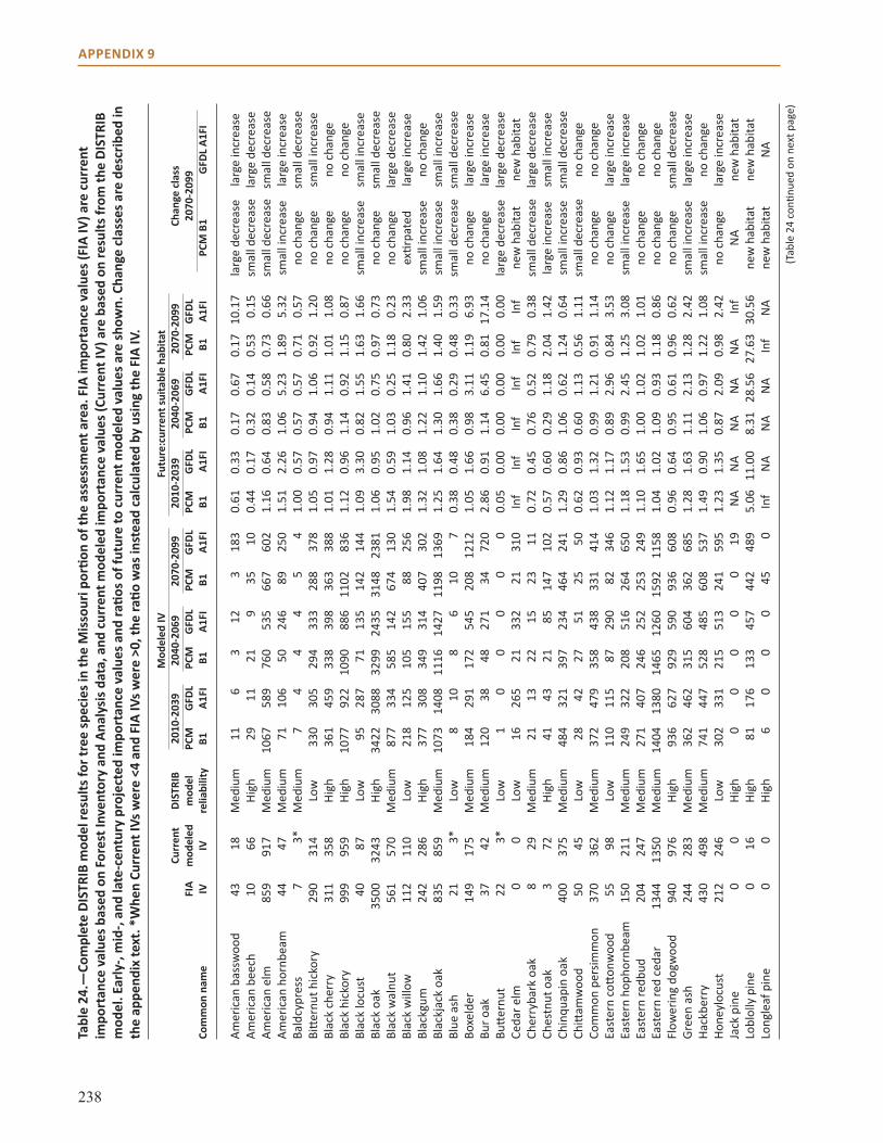
238

APPENDIX 9

Amer

ican

bas

swoo

d 43

18

M

ediu

m

11

6 3

12

3 18

3 0.

61

0.33

0.

17

0.67

0.

17

10.1

7 la

rge

decr

ease

la

rge

incr

ease

Amer

ican

bee

ch

10

66

High

29

11

21

9

35

10

0.44

0.

17

0.32

0.

14

0.53

0.

15

smal

l dec

reas

e la

rge

decr

ease

Amer

ican

elm

85

9 91

7 M

ediu

m

1067

58

9 76

0 53

5 66

7 60

2 1.

16

0.64

0.

83

0.58

0.

73

0.66

sm

all d

ecre

ase

smal

l dec

reas

eAm

eric

an h

ornb

eam

44

47

M

ediu

m

71

106

50

246

89

250

1.51

2.

26

1.06

5.

23

1.89

5.

32

smal

l inc

reas

e la

rge

incr

ease

Bald

cypr

ess

7 3*

M

ediu

m

7 4

4 4

5 4

1.00

0.

57

0.57

0.

57

0.71

0.

57

no c

hang

e sm

all d

ecre

ase

Bitte

rnut

hic

kory

29

0 31

4 Lo

w

330

305

294

333

288

378

1.05

0.

97

0.94

1.

06

0.92

1.

20

no c

hang

e sm

all i

ncre

ase

Blac

k ch

erry

31

1 35

8 Hi

gh

361

459

338

398

363

388

1.01

1.

28

0.94

1.

11

1.01

1.

08

no c

hang

e no

cha

nge

Blac

k hi

ckor

y 99

9 95

9 Hi

gh

1077

92

2 10

90

886

1102

83

6 1.

12

0.96

1.

14

0.92

1.

15

0.87

no

cha

nge

no c

hang

eBl

ack

locu

st

40

87

Low

95

28

7 71

13

5 14

2 14

4 1.

09

3.30

0.

82

1.55

1.

63

1.66

sm

all i

ncre

ase

smal

l inc

reas

eBl

ack

oak

3500

32

43

High

34

22

3088

32

99

2435

31

48

2381

1.

06

0.95

1.

02

0.75

0.

97

0.73

no

cha

nge

smal

l dec

reas

eBl

ack

wal

nut

561

570

Med

ium

87

7 33

4 58

5 14

2 67

4 13

0 1.

54

0.59

1.

03

0.25

1.

18

0.23

no

cha

nge

larg

e de

crea

seBl

ack

will

ow

112

110

Low

21

8 12

5 10

5 15

5 88

25

6 1.

98

1.14

0.

96

1.41

0.

80

2.33

ex

tirpa

ted

larg

e in

crea

seBl

ackg

um

242

286

High

37

7 30

8 34

9 31

4 40

7 30

2 1.

32

1.08

1.

22

1.10

1.

42

1.06

sm

all i

ncre

ase

no c

hang

eBl

ackj

ack

oak

835

859

Med

ium

10

73

1408

11

16

1427

11

98

1369

1.

25

1.64

1.

30

1.66

1.

40

1.59

sm

all i

ncre

ase

smal

l inc

reas

eBl

ue a

sh

21

3*

Low

8

10

8 6

10

7 0.

38

0.48

0.

38

0.29

0.

48

0.33

sm

all d

ecre

ase

smal

l dec

reas

eBo

xeld

er

149

175

Med

ium

18

4 29

1 17

2 54

5 20

8 12

12

1.05

1.

66

0.98

3.

11

1.19

6.

93

no c

hang

e la

rge

incr

ease

Bur o

ak

37

42

Med

ium

12

0 38

48

27

1 34

72

0 2.

86

0.91

1.

14

6.45

0.

81

17.1

4 no

cha

nge

larg

e in

crea

seBu

ttern

ut

22

3*

Low

1

0 0

0 0

0 0.

05

0.00

0.

00

0.00

0.

00

0.00

la

rge

decr

ease

la

rge

decr

ease

Ceda

r elm

0

0 Lo

w

16

265

21

332

21

310

Inf

Inf

Inf

Inf

Inf

Inf

new

hab

itat

new

hab

itat

Cher

ryba

rk o

ak

8 29

M

ediu

m

21

13

22

15

23

11

0.72

0.

45

0.76

0.

52

0.79

0.

38

smal

l dec

reas

e la

rge

decr

ease

Ches

tnut

oak

3

72

High

41

43

21

85

14

7 10

2 0.

57

0.60

0.

29

1.18

2.

04

1.42

la

rge

incr

ease

sm

all i

ncre

ase

Chin

quap

in o

ak

400

375

Med

ium

48

4 32

1 39

7 23

4 46

4 24

1 1.

29

0.86

1.

06

0.62

1.

24

0.64

sm

all i

ncre

ase

smal

l dec

reas

eCh

ittam

woo

d 50

45

Lo

w

28

42

27

51

25

50

0.62

0.

93

0.60

1.

13

0.56

1.

11

smal

l dec

reas

e no

cha

nge

Com

mon

per

simm

on

370

362

Med

ium

37

2 47

9 35

8 43

8 33

1 41

4 1.

03

1.32

0.

99

1.21

0.

91

1.14

no

cha

nge

no c

hang

eEa

ster

n co

ttonw

ood

55

98

Low

11

0 11

5 87

29

0 82

34

6 1.

12

1.17

0.

89

2.96

0.

84

3.53

no

cha

nge

larg

e in

crea

seEa

ster

n ho

phor

nbea

m

150

211

Med

ium

24

9 32

2 20

8 51

6 26

4 65

0 1.

18

1.53

0.

99

2.45

1.

25

3.08

sm

all i

ncre

ase

larg

e in

crea

seEa

ster

n re

dbud

20

4 24

7 M

ediu

m

271

407

246

252

253

249

1.10

1.

65

1.00

1.

02

1.02

1.

01

no c

hang

e no

cha

nge

East

ern

red

ceda

r 13

44

1350

M

ediu

m

1404

13

80

1465

12

60

1592

11

58

1.04

1.

02

1.09

0.

93

1.18

0.

86

no c

hang

e no

cha

nge

Flow

erin

g do

gwoo

d 94

0 97

6 Hi

gh

936

627

929

590

936

608

0.96

0.

64

0.95

0.

61

0.96

0.

62

no c

hang

e sm

all d

ecre

ase

Gree

n as

h 24

4 28

3 M

ediu

m

362

462

315

604

362

685

1.28

1.

63

1.11

2.

13

1.28

2.

42

smal

l inc

reas

e la

rge

incr

ease

Hack

berr

y 43

0 49

8 M

ediu

m

741

447

528

485

608

537

1.49

0.

90

1.06

0.

97

1.22

1.

08

smal

l inc

reas

e no

cha

nge

Hone

yloc

ust

212

246

Low

30

2 33

1 21

5 51

3 24

1 59

5 1.

23

1.35

0.

87

2.09

0.

98

2.42

no

cha

nge

larg

e in

crea

seJa

ck p

ine

0 0

High

0

0 0

0 0

19

NA

NA

NA

NA

NA

Inf

NA

new

hab

itat

Lobl

olly

pin

e 0

16

High

81

17

6 13

3 45

7 44

2 48

9 5.

06

11.0

0 8.

31

28.5

6 27

.63

30.5

6 ne

w h

abita

t ne

w h

abita

tLo

ngle

af p

ine

0 0

High

6

0 0

0 45

0

Inf

NA

NA

NA

Inf

NA

new

hab

itat

NA

Tabl

e 24

.—Co

mpl

ete

DIST

RIB

mod

el re

sults

for t

ree

spec

ies i

n th

e M

isso

uri p

ortio

n of

the

asse

ssm

ent a

rea.

FIA

impo

rtan

ce v

alue

s (FI

A IV

) are

cur

rent

im

port

ance

val

ues b

ased

on

Fore

st In

vent

ory

and

Anal

ysis

dat

a, a

nd c

urre

nt m

odel

ed im

port

ance

val

ues (

Curr

ent I

V) a

re b

ased

on

resu

lts fr

om th

e DI

STRI

B m

odel

. Ear

ly-,

mid

-, an

d la

te-c

entu

ry p

roje

cted

impo

rtan

ce v

alue

s and

ratio

s of f

utur

e to

cur

rent

mod

eled

val

ues a

re sh

own.

Cha

nge

clas

ses a

re d

escr

ibed

in

the

appe

ndix

text

. *W

hen

Curr

ent I

Vs w

ere

<4 a

nd F

IA IV

s wer

e >0

, the

ratio

was

inst

ead

calc

ulat

ed b

y us

ing

the

FIA

IV.

(Tab

le 2

4 co

ntinu

ed o

n ne

xt p

age)

M

odel

ed IV

Fu

ture

:cur

rent

suita

ble

habi

tat

Curr

ent

DIST

RIB

2010

-203

9 20

40-2

069

2070

-209

9 20

10-2

039

2040

-206

9 20

70-2

099

Chan

ge c

lass

FI

A m

odel

ed

mod

el

PCM

G

FDL

PCM

G

FDL

PCM

G

FDL

PCM

G

FDL

PCM

G

FDL

PCM

G

FDL

2070

-209

9Co

mm

on n

ame

IV

IV

relia

bilit

y B1

A1

FI

B1

A1FI

B1

A1

FI

B1

A1FI

B1

A1

FI

B1

A1FI

PC

M B

1 G

FDL

A1FI

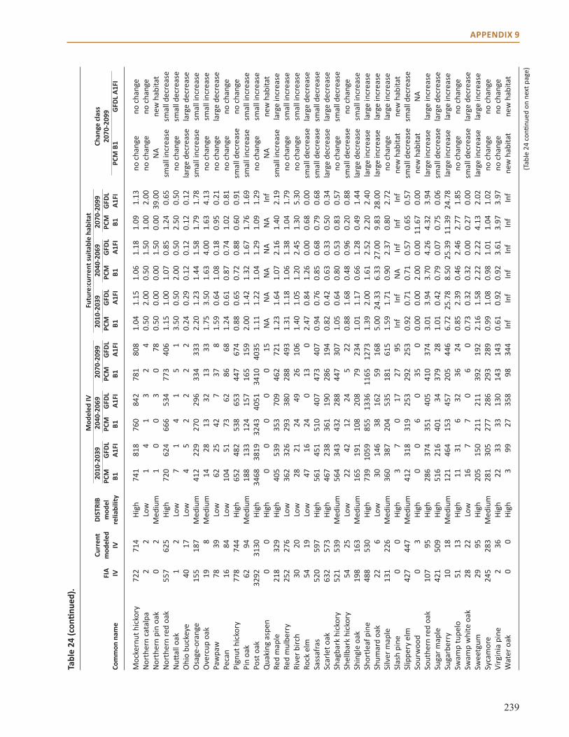
239

APPENDIX 9

Moc

kern

ut h

icko

ry

722

714

High

74

1 81

8 76

0 84

2 78

1 80

8 1.

04

1.15

1.

06

1.18

1.

09

1.13

no

cha

nge

no c

hang

eN

orth

ern

cata

lpa

2 2

Low

1

4 1

3 2

4 0.

50

2.00

0.

50

1.50

1.

00

2.00

no

cha

nge

no c

hang

eN

orth

ern

pin

oak

0 2

Med

ium

1

0 0

3 0

78

0.50

0.

00

0.00

1.

50

0.00

39

.00

NA

new

hab

itat

Nor

ther

n re

d oa

k 55

7 62

5 Hi

gh

720

624

666

534

773

406

1.15

1.

00

1.07

0.

85

1.24

0.

65

smal

l inc

reas

e sm

all d

ecre

ase

Nutt

all o

ak

1 2

Low

7

1 4

1 5

1 3.

50

0.50

2.

00

0.50

2.

50

0.50

no

cha

nge

smal

l dec

reas

eO

hio

buck

eye

40

17

Low

4

5 2

2 2

2 0.

24

0.29

0.

12

0.12

0.

12

0.12

la

rge

decr

ease

la

rge

decr

ease

Osa

ge-o

rang

e 15

5 18

7 M

ediu

m

412

229

270

296

334

333

2.20

1.

23

1.44

1.

58

1.79

1.

78

smal

l inc

reas

e sm

all i

ncre

ase

Ove

rcup

oak

19

8

Med

ium

14

28

13

32

13

33

1.

75

3.50

1.

63

4.00

1.

63

4.13

no

cha

nge

smal

l inc

reas

ePa

wpa

w

78

39

Low

62

25

42

7

37

8 1.

59

0.64

1.

08

0.18

0.

95

0.21

no

cha

nge

larg

e de

crea

sePe

can

16

84

Low

10

4 51

73

62

86

68

1.

24

0.61

0.

87

0.74

1.

02

0.81

no

cha

nge

no c

hang

ePi

gnut

hic

kory

77

8 74

4 Hi

gh

652

482

538

653

447

674

0.88

0.

65

0.72

0.

88

0.60

0.

91

smal

l dec

reas

e no

cha

nge

Pin

oak

62

94

Med

ium

18

8 13

3 12

4 15

7 16

5 15

9 2.

00

1.42

1.

32

1.67

1.

76

1.69

sm

all i

ncre

ase

smal

l inc

reas

ePo

st o

ak

3292

31

30

High

34

68

3819

32

43

4051

34

10

4035

1.

11

1.22

1.

04

1.29

1.

09

1.29

no

cha

nge

smal

l inc

reas

eQ

uaki

ng a

spen

0

0 Hi

gh

0 0

0 0

0 15

N

A N

A N

A N

A N

A In

f N

A ne

w h

abita

tRe

d m

aple

21

8 32

9 Hi

gh

405

539

353

709

462

721

1.23

1.

64

1.07

2.

16

1.40

2.

19

smal

l inc

reas

e la

rge

incr

ease

Red

mul

berr

y 25

2 27

6 Lo

w

362

326

293

380

288

493

1.31

1.

18

1.06

1.

38

1.04

1.

79

no c

hang

e sm

all i

ncre

ase

Rive

r birc

h 30

20

Lo

w

28

21

24

49

26

106

1.40

1.

05

1.20

2.

45

1.30

5.

30

no c

hang

e sm

all i

ncre

ase

Rock

elm

54

19

Lo

w

47

16

24

0 13

0

2.47

0.

84

1.26

0.

00

0.68

0.

00

smal

l dec

reas

e la

rge

decr

ease

Sass

afra

s 52

0 59

7 Hi

gh

561

451

510

407

473

407

0.94

0.

76

0.85

0.

68

0.79

0.

68

smal

l dec

reas

e sm

all d

ecre

ase

Scar

let o

ak

632

573

High

46

7 23

8 36

1 19

0 28

6 19

4 0.

82

0.42

0.

63

0.33

0.

50

0.34

la

rge

decr

ease

la

rge

decr

ease

Shag

bark

hic

kory

52

1 53

9 M

ediu

m

564

343

432

288

447

307

1.05

0.

64

0.80

0.

53

0.83

0.

57

no c

hang

e sm

all d

ecre

ase

Shel

lbar

k hi

ckor

y 54

25

Lo

w

22

42

12

24

5 22

0.

88

1.68

0.

48

0.96

0.

20

0.88

sm

all d

ecre

ase

no c

hang

eSh

ingl

e oa

k 19

8 16

3 M

ediu

m

165

191

108

208

79

234

1.01

1.

17

0.66

1.

28

0.49

1.

44

larg

e de

crea

se

smal

l inc

reas

eSh

ortle

af p

ine

488

530

High

73

9 10

59

855

1336

11

65

1273

1.

39

2.00

1.

61

2.52

2.

20

2.40

la

rge

incr

ease

la

rge

incr

ease

Shum

ard

oak

22

6 Lo

w

30

146

38

162

59

168

5.00

24

.33

6.33

27

.00

9.83

28

.00

larg

e in

crea

se

larg

e in

crea

seSi

lver

map

le

131

226

Med

ium

36

0 38

7 20

4 53

5 18

1 61

5 1.

59

1.71

0.

90

2.37

0.

80

2.72

no

cha

nge

larg

e in

crea

seSl

ash

pine

0

0 Hi

gh

3 7

0 17

27

95

In

f In

f N

A In

f In

f In

f ne

w h

abita

t ne

w h

abita

tSl

ippe

ry e

lm

427

447

Med

ium

41

2 31

8 31

9 25

3 29

2 25

3 0.

92

0.71

0.

71

0.57

0.

65

0.57

sm

all d

ecre

ase

smal

l dec

reas

eSo

urw

ood

0 3

High

0

0 6

0 35

0

0.00

0.

00

2.00

0.

00

11.6

7 0.

00

new

hab

itat

NA

Sout

hern

red

oak

107

95

High

28

6 37

4 35

1 40

5 41

0 37

4 3.

01

3.94

3.

70

4.26

4.

32

3.94

la

rge

incr

ease

la

rge

incr

ease

Suga

r map

le

421

509

High

51

6 21

6 40

1 34

37

9 28

1.

01

0.42

0.

79

0.07

0.

75

0.06

sm

all d

ecre

ase

larg

e de

crea

seSu

garb

erry

10

18

M

ediu

m

121

464

153

457

205

446

6.72

25

.78

8.50

25

.39

11.3

9 24

.78

larg

e in

crea

se

larg

e in

crea

seSw

amp

tupe

lo

51

13

High

11

31

6

32

36

24

0.85

2.

39

0.46

2.

46

2.77

1.

85

no c

hang

e no

cha

nge

Swam

p w

hite

oak

28

22

Lo

w

16

7 7

0 6

0 0.

73

0.32

0.

32

0.00

0.

27

0.00

sm

all d

ecre

ase

larg

e de

crea

seSw

eetg

um

29

95

High

20

5 15

0 21

1 21

1 39

2 19

2 2.

16

1.58

2.

22

2.22

4.

13

2.02

la

rge

incr

ease

la

rge

incr

ease

Syca

mor

e 24

5 28

3 M

ediu

m

281

305

277

286

293

289

0.99

1.

08

0.98

1.

01

1.04

1.

02

no c

hang

e no

cha

nge

Virg

inia

pin

e 2

36

High

22

33

33

13

0 14

3 14

3 0.

61

0.92

0.

92

3.61

3.

97

3.97

no

cha

nge

no c

hang

eW

ater

oak

0

0 Hi

gh

3 99

27

35

8 98

34

4 In

f In

f In

f In

f In

f In

f ne

w h

abita

t ne

w h

abita

t

Tabl

e 24

(con

tinue

d).

M

odel

ed IV

Fu

ture

:cur

rent

suita

ble

habi

tat

Curr

ent

DIST

RIB

2010

-203

9 20

40-2

069

2070

-209

9 20

10-2

039

2040

-206

9 20

70-2

099

Chan

ge c

lass

FI

A m

odel

ed

mod

el

PCM

G

FDL

PCM

G

FDL

PCM

G

FDL

PCM

G

FDL

PCM

G

FDL

PCM

G

FDL

2070

-209

9Co

mm

on n

ame

IV

IV

relia

bilit

y B1

A1

FI

B1

A1FI

B1

A1

FI

B1

A1FI

B1

A1

FI

B1

A1FI

PC

M B

1 G

FDL

A1FI

(Tab

le 2

4 co

ntinu

ed o

n ne

xt p

age)

240

APPENDIX 9

Whi

te a

sh

552

597

High

52

7 45

9 49

4 40

5 50

5 41

0 0.

88

0.77

0.

83

0.68

0.

85

0.69

no

cha

nge

smal

l dec

reas

eW

hite

oak

33

00

3061

Hi

gh

2600

20

82

2561

15

58

2360

14

89

0.85

0.

68

0.84

0.

51

0.77

0.

49

smal

l dec

reas

e la

rge

decr

ease

Wild

plu

m

70

12

Low

11

7 31

43

13

81

94

9.

75

2.58

3.

58

1.08

6.

75

7.83

sm

all i

ncre

ase

smal

l inc

reas

eW

illow

oak

5

19

Med

ium

16

24

18

30

34

27

0.

84

1.26

0.

95

1.58

1.

79

1.42

no

cha

nge

no c

hang

eW

inge

d el

m

239

243

High

58

6 13

16

773

1406

91

2 11

97

2.41

5.

42

3.18

5.

79

3.75

4.

93

larg

e in

crea

se

larg

e in

crea

seYe

llow

-pop

lar

28

116

High

10

1 94

11

4 14

2 21

4 17

4 0.

87

0.81

0.

98

1.22

1.

85

1.50

sm

all i

ncre

ase

smal

l inc

reas

e

Tabl

e 24

(con

tinue

d).

M

odel

ed IV

Fu

ture

:cur

rent

suita

ble

habi

tat

Curr

ent

DIST

RIB

2010

-203

9 20

40-2

069

2070

-209

9 20

10-2

039

2040

-206

9 20

70-2

099

Chan

ge c

lass

FI

A m

odel

ed

mod

el

PCM

G

FDL

PCM

G

FDL

PCM

G

FDL

PCM

G

FDL

PCM

G

FDL

PCM

G

FDL

2070

-209

9Co

mm

on n

ame

IV

IV

relia

bilit

y B1

A1

FI

B1

A1FI

B1

A1

FI

B1

A1FI

B1

A1

FI

B1

A1FI

PC

M B

1 G

FDL

A1FI

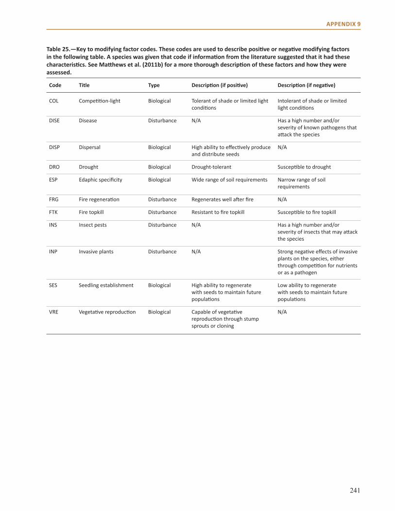
241

APPENDIX 9

Code Title Type Description (if positive) Description (if negative)

COL Competition-light Biological Tolerant of shade or limited light conditions

Intolerant of shade or limited light conditions

DISE Disease Disturbance N/A Has a high number and/or severity of known pathogens that attack the species

DISP Dispersal Biological High ability to effectively produce and distribute seeds

N/A

DRO Drought Biological Drought-tolerant Susceptible to drought

ESP Edaphic specificity Biological Wide range of soil requirements Narrow range of soil requirements

FRG Fire regeneration Disturbance Regenerates well after fire N/A

FTK Fire topkill Disturbance Resistant to fire topkill Susceptible to fire topkill

INS Insect pests Disturbance N/A Has a high number and/or severity of insects that may attack the species

INP Invasive plants Disturbance N/A Strong negative effects of invasive plants on the species, either through competition for nutrients or as a pathogen

SES Seedling establishment Biological High ability to regenerate with seeds to maintain future populations

Low ability to regenerate with seeds to maintain future populations

VRE Vegetative reproduction Biological Capable of vegetative reproduction through stump sprouts or cloning

N/A

Table 25.—Key to modifying factor codes. These codes are used to describe positive or negative modifying factors in the following table. A species was given that code if information from the literature suggested that it had these characteristics. See Matthews et al. (2011b) for a more thorough description of these factors and how they were assessed.

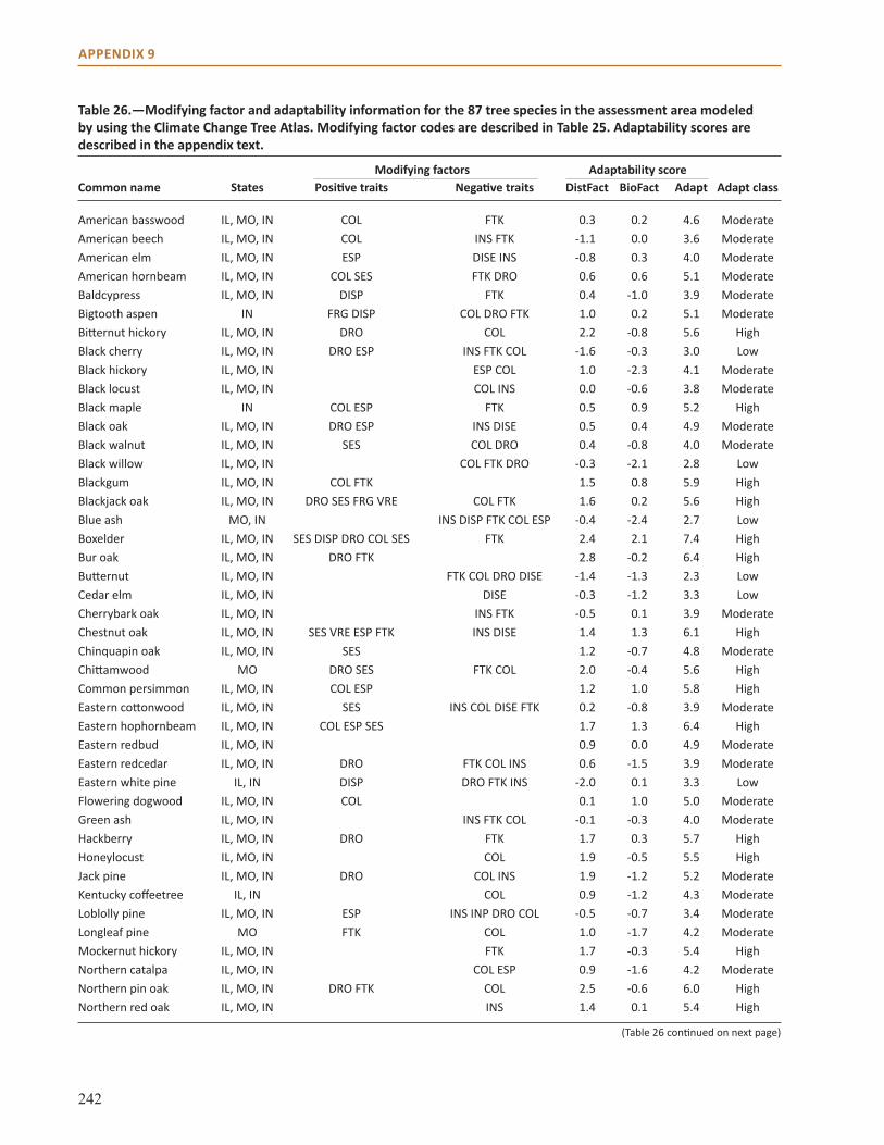
242

APPENDIX 9

American basswood IL, MO, IN COL FTK 0.3 0.2 4.6 ModerateAmerican beech IL, MO, IN COL INS FTK -1.1 0.0 3.6 ModerateAmerican elm IL, MO, IN ESP DISE INS -0.8 0.3 4.0 ModerateAmerican hornbeam IL, MO, IN COL SES FTK DRO 0.6 0.6 5.1 ModerateBaldcypress IL, MO, IN DISP FTK 0.4 -1.0 3.9 ModerateBigtooth aspen IN FRG DISP COL DRO FTK 1.0 0.2 5.1 ModerateBitternut hickory IL, MO, IN DRO COL 2.2 -0.8 5.6 HighBlack cherry IL, MO, IN DRO ESP INS FTK COL -1.6 -0.3 3.0 LowBlack hickory IL, MO, IN ESP COL 1.0 -2.3 4.1 ModerateBlack locust IL, MO, IN COL INS 0.0 -0.6 3.8 ModerateBlack maple IN COL ESP FTK 0.5 0.9 5.2 HighBlack oak IL, MO, IN DRO ESP INS DISE 0.5 0.4 4.9 ModerateBlack walnut IL, MO, IN SES COL DRO 0.4 -0.8 4.0 ModerateBlack willow IL, MO, IN COL FTK DRO -0.3 -2.1 2.8 LowBlackgum IL, MO, IN COL FTK 1.5 0.8 5.9 HighBlackjack oak IL, MO, IN DRO SES FRG VRE COL FTK 1.6 0.2 5.6 HighBlue ash MO, IN INS DISP FTK COL ESP -0.4 -2.4 2.7 LowBoxelder IL, MO, IN SES DISP DRO COL SES FTK 2.4 2.1 7.4 HighBur oak IL, MO, IN DRO FTK 2.8 -0.2 6.4 HighButternut IL, MO, IN FTK COL DRO DISE -1.4 -1.3 2.3 LowCedar elm IL, MO, IN DISE -0.3 -1.2 3.3 LowCherrybark oak IL, MO, IN INS FTK -0.5 0.1 3.9 ModerateChestnut oak IL, MO, IN SES VRE ESP FTK INS DISE 1.4 1.3 6.1 HighChinquapin oak IL, MO, IN SES 1.2 -0.7 4.8 ModerateChittamwood MO DRO SES FTK COL 2.0 -0.4 5.6 HighCommon persimmon IL, MO, IN COL ESP 1.2 1.0 5.8 HighEastern cottonwood IL, MO, IN SES INS COL DISE FTK 0.2 -0.8 3.9 ModerateEastern hophornbeam IL, MO, IN COL ESP SES 1.7 1.3 6.4 HighEastern redbud IL, MO, IN 0.9 0.0 4.9 ModerateEastern redcedar IL, MO, IN DRO FTK COL INS 0.6 -1.5 3.9 ModerateEastern white pine IL, IN DISP DRO FTK INS -2.0 0.1 3.3 LowFlowering dogwood IL, MO, IN COL 0.1 1.0 5.0 ModerateGreen ash IL, MO, IN INS FTK COL -0.1 -0.3 4.0 ModerateHackberry IL, MO, IN DRO FTK 1.7 0.3 5.7 HighHoneylocust IL, MO, IN COL 1.9 -0.5 5.5 HighJack pine IL, MO, IN DRO COL INS 1.9 -1.2 5.2 ModerateKentucky coffeetree IL, IN COL 0.9 -1.2 4.3 ModerateLoblolly pine IL, MO, IN ESP INS INP DRO COL -0.5 -0.7 3.4 ModerateLongleaf pine MO FTK COL 1.0 -1.7 4.2 ModerateMockernut hickory IL, MO, IN FTK 1.7 -0.3 5.4 HighNorthern catalpa IL, MO, IN COL ESP 0.9 -1.6 4.2 ModerateNorthern pin oak IL, MO, IN DRO FTK COL 2.5 -0.6 6.0 HighNorthern red oak IL, MO, IN INS 1.4 0.1 5.4 High

Modifying factors Adaptability scoreCommon name States Positive traits Negative traits DistFact BioFact Adapt Adapt class

Table 26.—Modifying factor and adaptability information for the 87 tree species in the assessment area modeled by using the Climate Change Tree Atlas. Modifying factor codes are described in Table 25. Adaptability scores are described in the appendix text.


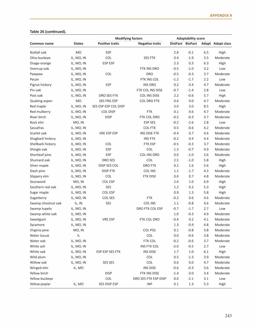
243

APPENDIX 9

Nuttall oak MO ESP 2.8 -0.1 6.5 HighOhio buckeye IL, MO, IN COL SES FTK 0.4 -1.9 3.5 ModerateOsage-orange IL, MO, IN ESP ESP 2.3 0.3 6.3 HighOvercup oak IL, MO, IN FTK INS DRO -0.5 -1.0 3.2 LowPawpaw IL, MO, IN COL DRO -0.5 -0.3 3.7 ModeratePecan IL, MO, IN FTK INS COL -1.2 -1.7 2.2 LowPignut hickory IL, MO, IN ESP INS DRO 0.2 0.4 4.7 ModeratePin oak IL, MO, IN FTK COL INS DISE -0.7 -1.4 2.8 LowPost oak IL, MO, IN DRO SES FTK COL INS DISE 2.2 -0.6 5.7 HighQuaking aspen MO SES FRG ESP COL DRO FTK 0.6 0.0 4.7 ModerateRed maple IL, MO, IN SES ESP ESP COL DISP 3.0 3.0 8.5 HighRed mulberry IL, MO, IN COL DISP FTK 0.1 0.6 4.7 ModerateRiver birch IL, MO, IN DISP FTK COL DRO -0.5 -0.3 3.7 ModerateRock elm MO, IN ESP SES -0.2 -2.6 2.8 LowSassafras IL, MO, IN COL FTK 0.5 -0.6 4.2 ModerateScarlet oak IL, MO, IN VRE ESP ESP INS DISE FTK -0.4 0.7 4.6 ModerateShagbark hickory IL, MO, IN INS FTK -0.2 0.4 4.4 ModerateShellbark hickory IL, MO, IN COL FTK ESP -0.5 -0.3 3.7 ModerateShingle oak IL, MO, IN ESP COL 1.3 -0.7 4.9 ModerateShortleaf pine IL, MO, IN ESP COL INS DRO 0.0 -1.0 3.6 ModerateShumard oak IL, MO, IN DRO SES COL 2.5 -1.0 5.8 HighSilver maple IL, MO, IN DISP SES COL DRO FTK 0.1 1.6 5.6 HighSlash pine IL, MO, IN DISP FTK COL INS 1.1 -1.7 4.3 ModerateSlippery elm IL, MO, IN COL FTK DISE 0.0 0.7 4.8 ModerateSourwood MO, IN COL ESP 2.6 1.0 6.9 HighSouthern red oak IL, MO, IN SES 1.2 0.2 5.3 HighSugar maple IL, MO, IN COL ESP 0.9 1.3 5.8 HighSugarberry IL, MO, IN COL SES FTK -0.2 0.6 4.6 ModerateSwamp chestnut oak IL, IN SES COL INS 1.1 -0.8 4.6 ModerateSwamp tupelo IL, MO, IN DRO FTK COL ESP -0.7 -1.7 2.7 LowSwamp white oak IL, MO, IN 1.0 -0.3 4.9 ModerateSweetgum IL, MO, IN VRE ESP FTK COL DRO -0.4 0.2 4.1 ModerateSycamore IL, MO, IN 1.3 -0.9 4.8 ModerateVirginia pine MO, IN COL POL 0.1 -0.8 3.8 ModerateWater locust IL COL 0.0 -0.6 3.8 ModerateWater oak IL, MO, IN FTK COL -0.2 -0.6 3.7 ModerateWhite ash IL, MO, IN INS FTK COL -2.0 -0.5 2.7 LowWhite oak IL, MO, IN ESP ESP SES FTK INS DISE 1.7 1.0 6.1 HighWild plum IL, MO, IN COL 0.5 -1.3 3.9 ModerateWillow oak IL, MO, IN SES SES COL 0.6 0.0 4.7 ModerateWinged elm IL, MO INS DISE -0.6 -0.3 3.6 ModerateYellow birch DISP FTK INS DISE -1.4 0.0 3.4 ModerateYellow buckeye COL DRO SES FTK ESP DISP 0.0 -2.1 3.1 LowYellow-poplar IL, MO SES DISP ESP INP 0.1 1.3 5.3 High

Modifying factors Adaptability scoreCommon name States Positive traits Negative traits DistFact BioFact Adapt Adapt class

Table 26 (continued).

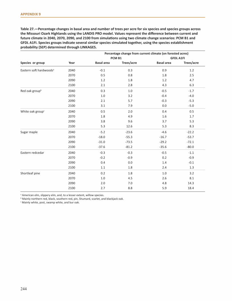
244

APPENDIX 9

a American elm, slippery elm, and, to a lesser extent, willow species. b Mainly northern red, black, southern red, pin, Shumard, scarlet, and blackjack oak. c Mainly white, post, swamp white, and bur oak.

Table 27.—Percentage changes in basal area and number of trees per acre for six species and species groups across the Missouri Ozark Highlands using the LANDIS PRO model. Values represent the difference between current and future climate in 2040, 2070, 2090, and 2100 from simulations using two climate change scenarios: PCM B1 and GFDL A1FI. Species groups indicate several similar species simulated together, using the species establishment probability (SEP) determined through LINKAGES.

Percentage change from current climate (on forested acres) PCM B1 GFDL A1FISpecies or group Year Basal area Trees/acre Basal area Trees/acre

Eastern soft hardwoodsa 2040 -0.1 0.3 0.9 1.2 2070 0.5 0.8 1.8 2.5 2090 1.2 1.8 1.2 4.7 2100 2.1 2.8 4.3 6.3

Red oak groupb 2040 0.3 1.0 -0.5 -1.7 2070 1.0 3.2 -0.4 -4.0 2090 2.1 5.7 -0.3 -5.3 2100 3.1 7.9 0.0 -5.0

White oak groupc 2040 0.5 2.0 0.4 0.5 2070 1.8 4.9 1.6 1.7 2090 3.8 9.6 3.7 5.3 2100 5.3 12.6 5.3 8.3

Sugar maple 2040 -5.2 -23.6 -4.6 -22.2 2070 -18.0 -55.3 -16.7 -53.7 2090 -31.0 -73.5 -29.2 -72.1 2100 -37.6 -81.2 -35.6 -80.0

Eastern redcedar 2040 -0.3 -0.3 -0.5 -1.1 2070 -0.2 -0.9 0.2 -0.9 2090 0.4 0.0 1.4 -0.1 2100 1.1 1.8 2.4 1.3

Shortleaf pine 2040 0.2 1.8 1.0 3.2 2070 1.0 4.5 2.6 8.1 2090 2.0 7.0 4.8 14.3 2100 2.7 8.8 5.9 18.4

245

APPENDIX 9

biol

ogic

alsc

ore

Highestpossibleadaptabilityscore: 8.5

0 1 2 3-3 -2 -1-3

-2

-1

0

1

2

3

disturbance score

Lowestpossibleadaptabilityscore: 0

Mid-rangeadaptabilityscore: 4.25

High biological, lowdisturbance scores

High disturbance,low biologicalscores

Length0 6

Leng

th0

6

Figure 50.—Illustration of range of possible adaptability scores based on biological and disturbance modifying factors.

246

APPENDIX 10: VULNERABILITY AND CONFIDENCE DETERMINATION

METHODSTo assess vulnerabilities to climate change for each natural community type, we elicited informed opinions from a panel of 20 experts (see Appendix 11) from across the assessment area. The primary criterion for selection on the panel was extensive knowledge about the ecology, management, or climate change impacts on forests in the Central Hardwoods Region. In addition, we strived for a wide representation across the geographic area and across institutions.

Natural Communities Assessed We selected nine natural community types of interest from across the assessment area to be evaluated for vulnerability to climate change from the 16 types described in Chapter 1. We focused on systems for which tree species were a significant component of vegetation cover. These communities were selected based on their relative abundance across the landscape, the amount of information available about the climate change impacts on that community type, and whether panelists felt they had sufficient knowledge and expertise to evaluate that community type.

For each community type, the panel was given a description of the major system drivers, dominant species, and stressors that characterize that community based on published sources (summarized in Chapter 1). The panel was asked to comment on and suggest modifications to the community description in a spreadsheet. If there were no disagreements, those suggestions were incorporated into the descriptions.

Potential Impacts Potential impacts are the direct and indirect consequences of climate change on systems. Impacts are a function of a system’s exposure to climate change and its sensitivity to any changes. Impacts could be beneficial or harmful to a particular forest or ecosystem type. To examine potential impacts, the panel was given several sources of background information on past and future climate change in the region (summarized in Chapters 3 and 4) and projected impacts on dominant tree species (summarized in Chapter 5). The panel was directed to consider impacts on each community type from 2010 through 2099, but more weight was given to the 2070 through 2099 period. The panel was also asked to assess impacts under two climate model-emissions scenarios: Hadley A1FI and PCM B1.

The Hadley A1F1 scenario was originally chosen as the “high-end” scenario instead of GFDL. It projects slightly higher temperatures and more modest decreases in summer precipitation than GFDL, but otherwise is similar. The GFDL A1FI scenario was later chosen as the high-end scenario for this assessment to enable comparison with other assessments in the Upper Great Lakes, for which Hadley model results were unreliable. All results summarized in Chapter 6 were vetted with the panelists to ensure their vulnerability rankings were still consistent with GFDL projections.

Potential impacts on each community driver and stressor were summarized in a spreadsheet based on climate model projections, the published literature, and insights from the panelists. Impacts on drivers were considered positive or negative if they would

247

APPENDIX 10

alter system drivers in a way that would be more or less favorable for that community type. Impacts on stressors were considered negative if they increased the influence of that stressor, or positive if they decreased the influence of that stressor, on the community type.

For each dominant species listed in the community spreadsheet, the panel considered the Tree Atlas, LANDIS PRO, and LINKAGES model results, as well as the life history traits and ecology of those species. Examining the projected changes in tree species habitat and distribution, panelists evaluated the agreement among models, between climate scenarios, and across space and time. If all of these factors suggested a decline in habitat suitability for a species of interest, it was given a negative impact rating. If all information projected an increase in habitat suitability, the species was given a positive impact rating. Species that were not projected to have a substantial increase or decrease were given a moderate rating. A mix of projected increases and decreases among models also led to a moderate rating for potential impacts, but the species was given a reduced level of confidence for that rating.

For each community type, each panelist was asked to identify which impacts he or she felt were most important to that system by using an individual worksheet (see example at end of this appendix). Each panelist determined an overall rating of potential impacts for each community type based on the summation of the impacts on drivers, stressors, and dominant species across a continuum from negative to positive.

Adaptive CapacityAdaptive capacity is the ability of a species or ecosystem to accommodate or cope with potential climate change impacts with minimal disruption. Panelists examined adaptive capacity for each community type based on their prior knowledge of the community types in the assessment area. The

panel was told to focus on community characteristics that would increase or decrease the adaptive capacity of that system. Adaptive capacity factors for each community type were delineated in a spreadsheet. A system was considered to have high adaptive capacity if it had: a high ability to spread to new areas; a wide geographic distribution; a high ability to tolerate or recover from a wide variety of disturbances; and high species, functional, and genetic diversity. A system had lower adaptive capacity if it lacked some or all of these attributes. Rankings were based on a continuous spectrum, so a mid-range score would indicate strength in some areas and a deficit in others. The panelists were directed to base these characteristics on the current condition of the system, given past and current management regimes, and with no consideration of potential management changes (adaptation) that could influence future adaptive capacity. As with potential impacts, panelists were asked to list the major factors that would contribute to the adaptive capacity of that system on an individual worksheet, and base their ranking on those factors.

VulnerabilityVulnerability is the susceptibility of a system to the adverse effects of climate change. It is a function of its potential impacts and its adaptive capacity. After extensive group discussion and recording of all impacts and adaptive capacity factors, panelists individually used their determination of the potential impacts and adaptive capacity of each community type (described above) to arrive at a vulnerability rating. Panelists were directed to mark their rating in two-dimensional space on an individual worksheet first and then on a group poster (Fig. 51a). Among the group, individual ratings were compared and discussed, with the goal of coming to a group determination through consensus. In many cases, the group determination was at or near the mean of all individual determinations. However, sometimes the group determination deviated from the mean because further discussion caused some group

248

APPENDIX 10

members to alter their original response. The group vulnerability determination was placed into one of five categories (low, low-moderate, moderate, moderate-high, and high) based on the discussion and consensus within the group, as well as the placement of the group determination on the figure. For example, if a vulnerability determination was on the border between low and moderate and the group agreed that it did not completely fall into one or the other category, it would receive a low-moderate determination.

Confidence Panelists were also directed to give a confidence rating to each of their individual vulnerability determinations (based on Mastrandrea et al. 2010) (Fig. 51b). Panelists were asked to individually evaluate the amount of evidence that supported the impacts and adaptive capacity factors that led to their vulnerability determination and the level of agreement among that evidence. Panelists evaluated confidence individually first and then as a group in a similar fashion to the vulnerability determination.

Community-level DeterminationsCommunity-level determinations of vulnerability and confidence were made for nine communities in the Central Hardwoods Region (Figs. 52-60). The

vulnerability determinations described above, along with information and ideas put forward during the group discussions, were collected and interpreted to develop the community-level descriptions presented in Chapter 6.

Vulnerability StatementsRecurring themes and patterns that transcended individual community types were identified and developed into the vulnerability statements (in boldface) and supporting text in Chapter 6. The lead author developed the statements and supporting text from workshop notes and literature that was related to each statement. An initial confidence determination (evidence and agreement) was assigned based on the lead author’s interpretation of the amount of information available to support each statement and the extent to which the information agreed. Each statement and its supporting literature discussion were sent to the panel for review. Panelists were asked to review each statement for accuracy, whether the confidence determination should be raised or lowered, if there was additional literature that was overlooked, and if any additional statements should be made. Any changes suggested by a single panelist were brought forth for discussion and approved by the entire panel.

Figure 51.—(a) Figure used for vulnerability determination by expert panelists. Adapted from Swanston and Janowiak (2012). (b) Figure used for confidence rating among expert panelists. Adapted from Mastrandrea et al. (2010).

(a) (b)

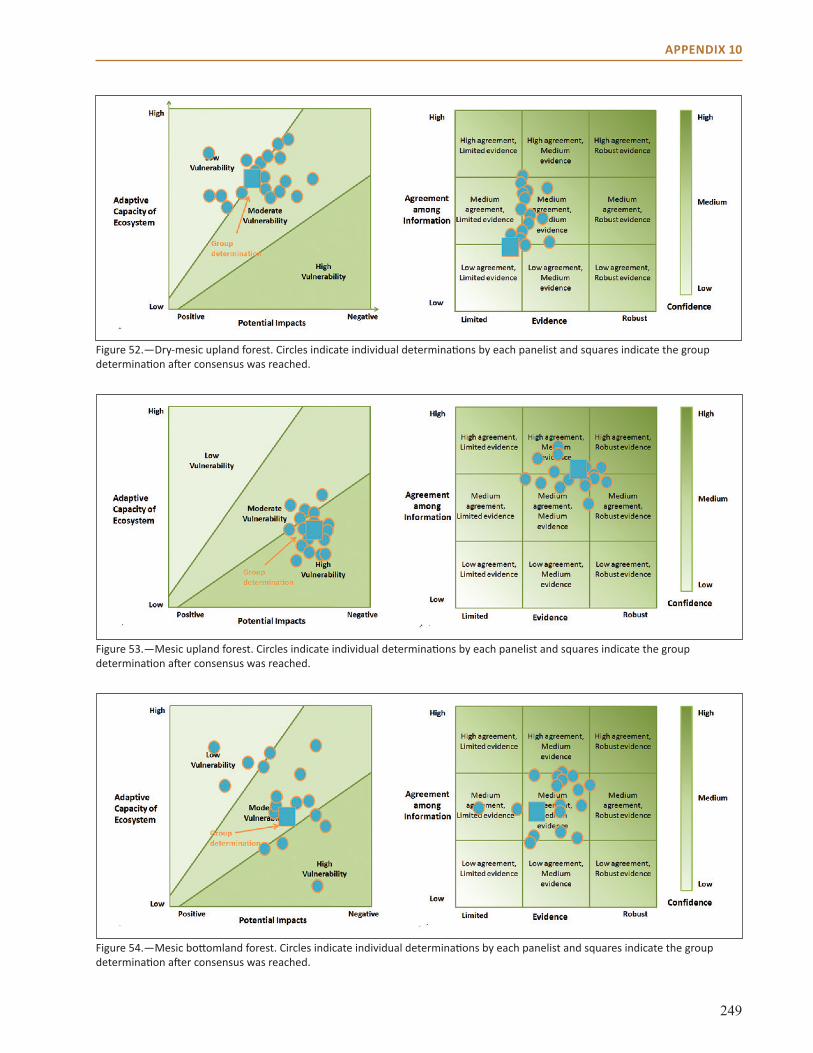
249

APPENDIX 10

Figure 52.—Dry-mesic upland forest. Circles indicate individual determinations by each panelist and squares indicate the group determination after consensus was reached.

Figure 54.—Mesic bottomland forest. Circles indicate individual determinations by each panelist and squares indicate the group determination after consensus was reached.

Figure 53.—Mesic upland forest. Circles indicate individual determinations by each panelist and squares indicate the group determination after consensus was reached.

250

APPENDIX 10

Figure 55.—Wet bottomland forest. Circles indicate individual determinations by each panelist and squares indicate the group determination after consensus was reached.

Figure 56.—Flatwoods. Circles indicate individual determinations by each panelist and squares indicate the group determination after consensus was reached.

Figure 57.—Closed woodland. Circles indicate individual determinations by each panelist and squares indicate the group determination after consensus was reached.

251

APPENDIX 10

Figure 58.—Open woodland. Circles indicate individual determinations by each panelist and squares indicate the group determination after consensus was reached.

Figure 59.—Barrens and savanna. Circles indicate individual determinations by each panelist and squares indicate the group determination after consensus was reached.

Figure 60.—Glade. Circles indicate individual determinations by each panelist and squares indicate the group determination after consensus was reached.

252

APPENDIX 10

Example Vulnerability Determination Worksheet

Name: Ecosystem/Forest Type:

How familiar are you with this ecosystem? (circle one)

What do you think are the greatest potential impacts to the ecosystem?

What factors do you think contribute most to the adaptive capacity of the ecosystem?

MediumI do some management

or research in this system, or have read

a lot about it.

LowI have some basic

knowledge about this system and how it

operates

HighI regularly do

management or research in this system

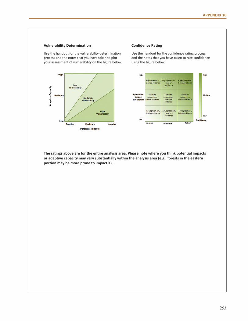
253

APPENDIX 10

Vulnerability Determination

Use the handout for the vulnerability determination process and the notes that you have taken to plot your assessment of vulnerability on the figure below.

Confidence Rating

Use the handout for the confidence rating process and the notes that you have taken to rate confidence using the figure below.

The ratings above are for the entire analysis area. Please note where you think potential impacts or adaptive capacity may vary substantially within the analysis area (e.g., forests in the eastern portion may be more prone to impact X).

254

APPENDIX 11: EXPERT PANELISTS

Name AffiliationMatthew Albrecht Missouri Botanical GardenPaul Deizman Illinois Department of Natural Resources, Division of Forest ResourcesJohn DePuy Shawnee National ForestGary Dinkel Hoosier National ForestSonglin Fei Purdue University Hong He University of Missouri-ColumbiaLouis Iverson U.S. Forest Service, Northern Research StationD. Todd Jones-Farrand Central Hardwoods Joint VentureMichael Leahy Missouri Department of Conservation Brad Oberle George Washington UniversityJeffrey E. Schneiderman University of Missouri-ColumbiaJohn Shuey The Nature ConservancyAdam B. Smith Missouri Botanical GardenCharles Studyvin Mark Twain National ForestFrank Thompson U.S. Forest Service, Northern Research StationJohn M. Tirpak Gulf Coastal Plains and Ozarks Landscape Conservation Cooperative Jeffery W. Walk The Nature ConservancyWen J. Wang University of Missouri-ColumbiaLaura Watts Mark Twain National ForestSteve Westin Missouri Department of Conservation

Printed on recycled paper

Brandt, Leslie; He, Hong; Iverson, Louis; Thompson, Frank R., III; Butler, Patricia; Handler, Stephen; Janowiak, Maria; Shannon, P. Danielle; Swanston, Chris; Albrecht, Matthew; Blume-Weaver, Richard; Deizman, Paul; DePuy, John; Dijak, William D.; Dinkel, Gary; Fei, Songlin; Jones-Farrand, D. Todd; Leahy, Michael; Matthews, Stephen; Nelson, Paul; Oberle, Brad; Perez, Judi; Peters, Matthew; Prasad, Anantha; Schneiderman, Jeffrey E.; Shuey, John; Smith, Adam B.; Studyvin, Charles; Tirpak, John M.; Walk, Jeffery W.; Wang, Wen J.; Watts, Laura; Weigel, Dale; Westin, Steve. 2014. Central Hardwoods ecosystem vulnerability assessment and synthesis: a report from the Central Hardwoods Climate Change Response Framework project. Gen. Tech. Rep. NRS-124. Newtown Square, PA: U.S. Department of Agriculture, Forest Service, Northern Research Station. 254 p.

The forests in the Central Hardwoods Region will be affected directly and indirectly by a changing climate over the next 100 years. This assessment evaluates the vulnerability of terrestrial ecosystems in the Central Hardwoods Region of Illinois, Indiana, and Missouri to a range of future climates. Information on current forest conditions, observed climate trends, projected climate changes, and impacts to forest ecosystems was considered in order to assess vulnerability to climate change. Mesic upland forests were determined to be the most vulnerable to projected changes in climate, whereas many systems adapted to fire and drought, such as open woodlands, savannas, and glades, were perceived as less vulnerable. Projected changes in climate and the associated ecosystem impacts and vulnerabilities will have important implications for economically valuable timber species, forest-dependent wildlife and plants, recreation, and long-range planning.

KEy WORDS: climate change, vulnerability, adaptive capacity, Missouri, Illinois, Indiana, Climate Change Atlas, LINKAGES, LANDIS PRO, expert elicitation

The U.S. Department of Agriculture (USDA) prohibits discrimination in all its programs and activities on the basis of race, color, national origin, age, disability, and where applicable, sex, marital status, familial status, parental status, religion, sexual orientation, genetic information, political beliefs, reprisal, or because all or part of an individual’s income is derived from any public assistance program. (Not all prohibited bases apply to all programs.) Persons with disabilities who require alternate means for communication of program information (Braille, large print, audiotape, etc.) should contact USDA’s TARGET Center at 202-720-2600 (voice and TDD). To file a complaint of discrimination, write to USDA, Director, Office of Civil Rights, 1400 Independence Avenue, S.W., Washington, DC 20250-9410, or call 800-795-3272 (voice) or 202-720-6382 (TDD). USDA is an equal opportunity provider and employer.

Northern Research Station

www.nrs.fs.fed.us

Central Hardwoods ecosystem vulnerability assessment and ...

Documents

Transcript of Central Hardwoods ecosystem vulnerability assessment and ...