CE221 Engineering Surveying

LABORATORY

MANUAL

CE221 Engineering Surveying

INSTRUCTOR: Eng. Rasheed ELHAJ

9341 محرمنسخة

September 2017

C i vil

Eng i neeri ng

Department

Al Imam Mohammad Ibn Saud

Islamic University

C E 2 2 1 : E N G I N E E R I N G S U R V E Y I N G

Laboratory Manual

INSTRUCTOR: Eng. Rasheed ELHAJ

Email: [email protected]

9341 محرم

September 2017

mailto:[email protected]

1

Table of contents

Page

Lab 0 Introduction to the practical work 2 Lab 1 Familiarization with surveying instruments 6 Lab 2 Measurement of angles with theodolite 13 Lab 3 Measurements for inaccessible points 17 Lab 3b

Measurements for inaccessible points (two instrument stations)

20

Lab 4 Differential Leveling 23 Lab 5 traversing with a total station 27 Lab 6 Stakingout a simple building enveloppe with total station 30 Lab 7 Horizontal Curve Design 32 Lab 8 Trigonometric Leveling 38 Lab 9 Aliging Ranging and taping 44

2

INTRODUCTION TO THE PRACTICAL WORK

Aim:

1. Understand the conduct of practical work. 2. Awareness of student responsibilities. 3. Awareness of safety rules.

Field Groups

The class should be divided into groups, each group between 3-5 students. A group

leader should be appointed for each lab assignment. The group leader will be in

charge of that particular lab and will be responsible for checking out and returning

the equipment at the end of the lab session.

Survey Equipment

Equipment for each lab assignment will be checked out at the beginning of the lab

and when the assignment is finished. Some important things to remember about the

use and care of the equipment are as follows:

1. Much of the equipments are very expensive and quite sensitive, great care should be

taken to protect the equipments from damage.

2. Instruments should be transported in their cases when taken to and from the field.

These instruments may be carried on the tripod from station to station as long as

they are held vertically at all times.

3. Do not operate the machine/ equipments without permission of the instructor; and

do not force anything to move beyond its operating range.

4. Malfunctioning equipment should immediately be reported to the instructor.

LAB

0

3

5. Also, if any defect or damage happens to the instruments, the matter should be

immediately reported to the instructor.

Behavior to be maintained in lab sessions

1. Study the manual thoroughly before entering the lab.

2. The observations should be entered in the lab manual or in the field book in pencil

(no pen or eraser) during the practical class itself; when corrections are needed,

strikethrough the wrong reading and the new one is to be entered under the old one.

3. If any calculation has to be done, it should be finished during the practical class itself,

unless the instructor permits to complete it at a later stage.

4. The record should be submitted within the prescribed time according to the

directions of the instructor.

5. Lab should be kept clean.

Materials:

1. Spiral bound field book

2. 2H or 3H pencil for field notes

3. Combination for field sketches (graduated rule, bracket, protractor,etc.)

4. Scientific calculator.

Grading: Final lab-Exam: 12%

Field Books: 3%

Quezzes: 5%

Reports: 10%

Total= 30%

For each lab, students will be graded on their participation using the following

scale. Your lab grade will be determined by this.

Full mark obtained by the group: Participated in all aspects of lab

Half of the mark obtained by the group: Did not participate during some of lab

0pt : Did not participate at all.

4

Lab reports:

The assigned lab reports are to be completed in a neat, organized and professional

manner on engineering paper. Use the cover page given on the next page and Print

your group number at the top of each page. Use only the front side of the paper

and box your final answer. Staple multiple sheets and remember pages

numbering.

Lab reports will be due at the beginning of the class period. A record of each

field assignment shall be kept in your field book. Your field book shall be kept neat

and orderly as it will be collected and graded periodically throughout the semester.

Each lab report shall include, at minimum, the following informations:

Lab title, dates of field work, group members, group member assignments, list of

equipment used, weather conditions, field measurements, calculations and sketching.

Safety rules:

As a surveyor you will operate tools that, if not used correctly can cause harm.

Thus you must:

1. Pay attention to the weather and dress accordingly (Labs will be held outdoor).

2. Do not aim with the telescope of surveying equipment towards the sun to avoid

any possibility of damaging your eyes. Appropriate face shields or goggles can

protect you from this danger.

3. Use safety slip resistance footwear with sole and heel designed and constructed for

work activities that present foot injury hazards from failing or moving objects,

scalding, cutting and penetration.

4. Wear high-visibility safety vest to evoid traffic hazards at wich you are exposed (we

cross roads to reach the field where most of our outdoor work is done).

5. Wear protective helmets.

5

LABORATORY REPORT

Title:

Field work dates: ____________________________ ____________________________ ____________________________ Submission date: ____________________________ Groupe #:__________

Group members and assignements:

Student Name Student I.D.

Assignement Field work Attendance (Yes, No)

involvement in the report

(Yes, No)

1

2

3

4

5

6

Al Imam Mohammad Ibn Saud

Islamic University

CE221: Engineering Surveying

6

FAMILIARIZATION WITH SURVEYING INSTRUMENTS

Aim:

1. Discover the use of surveying instruments. 2. Know how to take care of equipment. 3. Comprehend the field notes requirements. 4. Learn about: Units, Rounding off numbers and Significant figures.

Measuring instruments for practical work available in our laboratory:

Instruments are shown and their uses are explained by the instructor. The session may end with an assessment quiz.

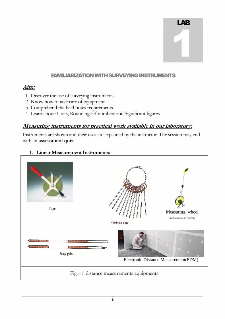
1. Linear Measurement Instruments:

Tape

Measuring wheel

(not available in our lab)

Electronic Distance Measurement(EDM)

Fig1-1: distance measurements equipments

LAB

1

7

2. Level and Leveling Instruments:

Automatic Level Self-adjusting mechanism of autolevel

Digital autolevel

Laser level

Fig1-2: Leveling equipments

8

Graduated Leveling Rod Reading:

Leveling Staff (or graduated leveling

Rod)

Fig1-3: Leveling Rod Reading

Top reading =

Botum reading =

Leveling reading =

9

3. Theodolite and Angle Measurements:

Fig1-4: Main axes of a theodolite

Fig1-5: Main organs of an opto-mechanical theodolite

10

Fig1-6: ElectronicTheodolite

Fill in the name

1- -------------------------------------------

2- -------------------------------------------

3- -------------------------------------------

4- -------------------------------------------

5- -------------------------------------------

6- -------------------------------------------

7- -------------------------------------------

8- -------------------------------------------

9- -------------------------------------------

10- -------------------------------------------

11- -------------------------------------------

12- -------------------------------------------

13- -------------------------------------------

14- -------------------------------------------

15- -------------------------------------------

16- -------------------------------------------

17- -------------------------------------------

18- -------------------------------------------

19- -------------------------------------------

20- -------------------------------------------

11

Fig1-7: Total station

Fill in the name

1- ---------------------------------------

2- ---------------------------------------

3- ---------------------------------------

4- ---------------------------------------

5- ---------------------------------------

6- ---------------------------------------

7- ---------------------------------------

8- ---------------------------------------

9- ---------------------------------------

10- --------------------------------------

11- --------------------------------------

12- --------------------------------------

13- --------------------------------------

14- --------------------------------------

15- --------------------------------------

16- --------------------------------------

17- --------------------------------------

18- --------------------------------------

19- --------------------------------------

20- --------------------------------------

21- --------------------------------------

22- --------------------------------------

23- --------------------------------------

24- --------------------------------------

25- --------------------------------------

12

Prism

Fig1-8: The principle of the electronic distance measurement

Setting up a Theodolite or a Total Station:

To properly measure angles and distances with a Theodolite or a Total Station, the

instrument must be level (otherwise the sight plan will not be vertical). And, you must be

able to set the instrument up directly over a prescribed point on the ground (this is called

the Centering of the instrument). If errors are made while setting up, inaccurate

measurements will result.

Units, Rounding off numbers and Significant figures The meter is the basic unit for length in the metric or SI system. Subdivisions of the meter

(m) are the millimeter (mm), centimeter (cm), and decimeter (dm), equal to 0.001, 0.01, and

0.1 m, respectively. A kilometer (km) equals 1000 m.

The unit of angle used in surveying is the degree, defined as 1/360 of a circle. One degree

(1°) equals 60 min, and 1 min equals 60 sec. Divisions of seconds are given in tenths,

hundredths, and thousandths. Other methods are also used to subdivide a circle, for

example, 400 grads. Another term, gons, is now used interchangeably with grads.

A radian is the angle subtended by an arc of a circle having a length equal to the radius of

the circle. Therefore, 2π rad=360o and 0.01745 rad ≈ 1°.

By definition, the number of significant figures in any observed value includes the positive

(certain) digits plus one (only one) digit that is estimated or rounded off, and therefore

questionable. It is essential that data be recorded with the correct number of significant

figures. If a significant figure is dropped in recording a value, the time spent in acquiring

certain precision has been wasted. On the other hand, if data are recorded with more

figures than those that are significant, false precision will be implied.

→ HW: Solve problems 2.14 and 2.15 in your textbook (Page 43).

13

MEASUREMENTS OF ANGLES WITH THEODOLITE

Aim:

1. Learn to measure the zenith and horizontal angles with a Theodolite 2. Learn the calculation of horizontal and vertical distances from measured

data with stadia method. 3. Discuss about relative accuracy of stadia method.

Instruments Required:

1. Theodolite; 2. Tripod, 3. Leveling Rod (or Staff)

Theoretical background

The measurement of an horizontal angle is a _ _ _ _ _ _ _ _ _ _ _ _ _ _ _ _ _ _ _ _ It can be measured by direct reading (dir) or Reverse reading (rev) The average of the two readings is more accurate than each of them. Average of the Reading of Horizontal angle = HAaverage=

LAB

2

Fig 2-1: Horizontal angle measurement principle

14

For each sighted point one vertical angle is measured.

Zenith angle average= ZAaverage=

Procedure:

1. Set up the theodolite on a judiciously selected point.

2. Point the instrument to the first target object A (with direct (or left face)

position)

3. Lock both vertical and horizontal motions, perfect the pointing

4. Read and record the zenith and horizontal angles.

5. Record the top, medium and bottom reading on the leveling rod.

6. Repeat steps 2 through 5 for reverse (or right face) readings (the readings on

the leveling staff should be the same as those recorded in step 5)

7. Sight respectively on B and C following the same procedure for point A and

record all the data using the table2-1 given in the next page.

Required work:

1. Find the horizontal angles β1, β2 and β3. 2. Find the horizontal angles α1, α 2 and α 3. 3. Find the horizontal angles λ1, λ 2 and λ 3. 4. Find the horizontal distances SA, SB, SC, AB, AC and BC. 5. Find the area of ABC. 6. Determine the elevation of points B and C (assume that the elevation of the

point A is 800m: ZA=800m). 7. Sketching.

B

C

A

β1

β2

β3

λ1

λ2 λ3

α1

α2

α3

S

Fig 2-2: Vertical angle measurement and associated formulas

Fig 2-3: Field work illustration (not to scale)

15

Field data sheet for angle measurement lab

Date:

Operators:

Sketch

Table2-1: Field Measurements hiS=

Station target

Horizontal Angle (in °) Zenith Angle (in °) Rod readings

Reading Average Reading Average

S

A

Dir -

-

- Rev

B

Dir -

-

- Rev

C

Dir -

-

- Rev

Dir -

-

- Rev

Assumed elevation of point A: ZA=800 m Elevation difference: ∆Z=100*(TR-BR)*Sin(z)*Cos(z)+hi-LR Horizontal distance: HD=100*(TR-BR)*Sin2(z)

With: ∆Z= Elevation difference HD= Horizontal Distance TR= Top Stadia Reading LR= Middle Stadia Reading BR= Bottom Stadia Reading z= Zenith Angle

TR

LR

BR

B

ΔZSB HD

Fig 2-4: Stadia method formulas

16

Calculations:

1- Angel values :

β 1 =

β 2 =

β 3 =

2- Horizontal Distances Values :

SA =

SB =

SC =

AB =

AC =

BC =

3- Angles: α1, α 2, α 3 , λ1, λ 2 and λ 3

4- Triangle areas (m2)

ST 1 =

ST 2 =

ST 3 =

Total area= (m2)

17

L A B

3

MEASUREMENTS FOR INACCESSIBLE POINTS

Aim:

To find the reduced level of lighting pole using a Theodolite (By using

one instrument station and stadia method for linear measurements)


2. Theodolite; 2. Tripod, 3. Leveling Rod

Principle:

From the selected instrument stations S:

Take the zenithal angle to the base of the lighting pole B.

Take the zenithal angle to the top of the lighting pole T.

Measure the horizontal distance between S and T using the Stadia method.

Determine the height and the elevation of the lighting pole using the rules

established from the sketch below.

Fig 3-1: Determination of inaccessible point: formulas

18

Procedure:

Set up the Theodolite over given station S and:

Read the staff held on the B (Top, Bottom and leveling stadia readings).

Read the corresponding zenith angle (zB’).

With same horizontal angle reading (same vertical plane) read the zenith

angle (zT) on the T (central stadia hair on T).

Required work:

Find the Reduced Level of lighting pole: ZT.

Find height of lighting pole: hT.

ff

S

B

B’

hB

’

hT

zB’ HT

HDSB

ΔZ

SB

Fig 3-2: Determination of inaccessible point: field work illustration

19

Field data sheet for inaccessible point lab

Date:

Operators:

Sketch

Field Measurements

hiS=

Instrument Station

Staff

Zenith Angle (°) Rod readings

(m)

Station Reading Average

S

Dir

- -

1.000

B Rev

Dir

T Rev

Assumed elevation of point S: ZS=700 m

Elevation difference: ∆Z=100*(TR-BR)*Sin(z)*Cos(z)+hi-LR

Horizontal distance: HD=100*(TR-BR)*Sin2(z)

Where:

∆Z= Elevation difference HD= Horizontal Distance TR= Top Stadia Reading LR= Middle Stadia Reading BR= Bottom Stadia Reading z= Zenith Angle

20

L A B

3b

MEASUREMENTS FOR INACCESSIBLE POINTS

(WITH TWO INSTRUMENT STATIONS)

Aim:

1. Learn to measure the zenith and horizontal angles with a Theodolite.

2. To find the reduced level of tower using theodolite (By using two

instrument station A and B not in the same vertical plane as the elevated

object P)


3. Theodolite

4. Tripod

5. Leveling Rod

Principle:

From the selected instrument stations A and B, take the vertical angle to

the object P (α and β). Also from station A measure the interior horizontal

angle between B and object P. From station B measure the interior

horizontal angle between A and object P. Measure the horizontal distance

between A and B using the Stadia method.

21

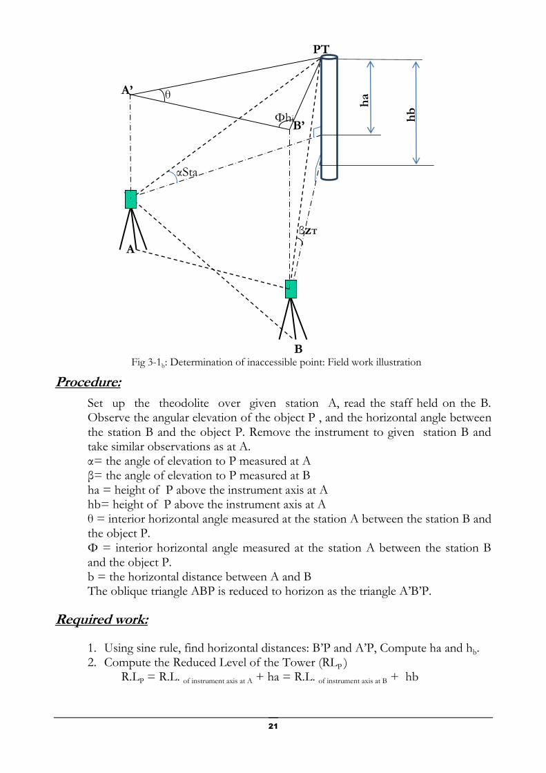
Procedure:

Set up the theodolite over given station A, read the staff held on the B. Observe the angular elevation of the object P , and the horizontal angle between the station B and the object P. Remove the instrument to given station B and take similar observations as at A. α= the angle of elevation to P measured at A β= the angle of elevation to P measured at B ha = height of P above the instrument axis at A hb= height of P above the instrument axis at A θ = interior horizontal angle measured at the station A between the station B and the object P. Φ = interior horizontal angle measured at the station A between the station B and the object P. b = the horizontal distance between A and B The oblique triangle ABP is reduced to horizon as the triangle A’B’P.

Required work:

1. Using sine rule, find horizontal distances: B’P and A’P, Compute ha and hb. 2. Compute the Reduced Level of the Tower (RLP )

R.LP = R.L. of instrument axis at A + ha = R.L. of instrument axis at B + hb

αSta

βzT

A

A’ θ

Φhi B’

ha

PT

B

hb

Fig 3-1b: Determination of inaccessible point: Field work illustration

22

DATA SHEET FOR INACCESSIBLE POINTS (TWO INSTRUMENT STATIONS) Operators:

Field Measurements

hiA= hiB=

Instrument

Station Staff

Horizontal Angle (°) Zenith Angle (°) Rod readings

Station Reading Average Reading Average

A

Dir

- - -

B

Rev

Dir

P

Rev

B

Dir

- - -

A

Rev

Dir

P

Rev

Dir

- - -

Rev

Dir

Rev

Assumed elevation of point A: ZA=100 m

23

DIFFERENTIAL LEVELING

Aim:

1. Introduce the method of differential leveling;

2. Set up the Automatic level and learn basic techniques of leveling;

3. Practice standard note taking protocol for fieldwork;

4. Fully calculate the elevations of all turning points and check accuracy.


1. Automatic Level 2. Tripod 3. Leveling Rod/staff

Overview:

Differential leveling is the most common method for determining elevations of monuments or objects. In this method, a telescope with suitable magnification is used to read graduated rods held on fixed points.

Hi= Height of the Axis sight

of the instrument BS= Back-sight FS= fore-signt ZA= elevation of point A ZB= elevation of point B

LAB

4

Fig 4-1: Principle of levelling

24

Setting up an Automatic Level

In this lab you will become familiar with the set-up and operation of Automatic Level. A level is used to determine difference in elevation, and it is therefore important to correctly level the instrument so as not to introduce error. The Level has a self-adjusting mechanism that will keep the optics level as long as you are “close.”(Not out of a fixed range of the self-adjusting mechanism of the instrument)

Attach the Level to the tripod roughly and level it by adjusting the leveling screws to move the bubble into the bulls-eye. Once the bubble is in the bulls-eye, you will be ready to take readings.

Procedure

Steps to be done: 1- Run a leveling loop around the survey area;

2- Start from the fixed reference point BM.

3- Set up the level and run a closed circuit with 4 instrument set up.

4- Keep BS and FS lengths approximately equal by pacing and check by computation.

5- Complete the notes and find out the loop misclosure.

6- Adjust the notes for misclosure and comment on the level of precision achieved.

The allowable misclosure in millimeters is 5√n; where n is the number of times the

instrument is set up.

7- Tables4-1 and 4-2 should be completed in the field and commented.

Required work:

1- Describe all the difficulties encountered in the field and indicate how you have

overcome them.

2- Fill the table 4-3 and adjust the notes for misclosure and compute the adjusted

elevations of all turning points.

3- Drew the profile BM, TP1, TP2, TP3, BM.

4- Comment the results.

BS-BM

FS-TP1

BM

TP3

TP1 TP2

Fig 4-2: Leveling: Illustration of the field work

25

DATA SHEET FOR DIFFERENTIAL LEVELING

Date:

Operators:

Table4-1: Field measurements Previwed Profile

Point Back sight reading (m)

Gap

[(T+B)/2]-

L

Length

Of back

For sight reading (m)

Gap

[(T+B)/2]-

L

Length

Of for

Top

hair

Leveling

hair

Bottom

hair

(mm)

Sight

(m)

Top

hair

Leveling

hair

Bottom

hair

(mm)

Sight

(m)

BM

TP1

TP2

TP3

BM

∑BSR=

∑FSR=

Table4-2: Pacing checks

Station points

Number of paces

Type of observation

Adjustments:

Total misclosure:

∑BSR - ∑FSR =

Comment:

BM – Inst. 1 BS

Inst1 – TP1 FS

TP1 – Inst.2 BS

Inst.2 – TP2 FS

TP2 – Inst.3 BS

Inst. 3 – TP3 FS

TP3 – Inst.4 BS

Inst. 4 – BM FS Adjustment for each differential leveling=

26

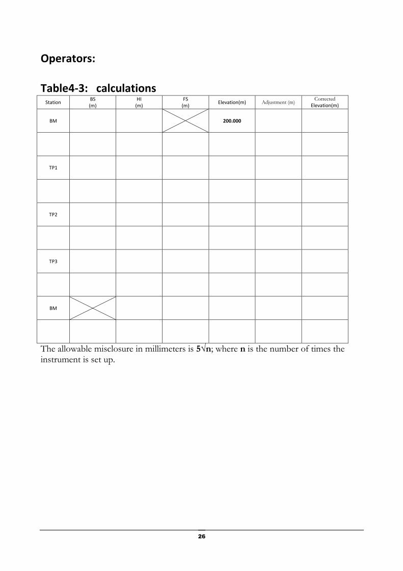
Operators:

Table4-3: calculations Station

BS (m)

HI (m)

FS (m)

Elevation(m) Adjustment (m) Corrected

Elevation(m)

BM 200.000

TP1

TP2

TP3

BM

The allowable misclosure in millimeters is 5√n; where n is the number of times the instrument is set up.

27

TRAVERSING WITH A TOTAL STATION

Aim:

1. Get familiar with the use of a Total station in the mode "observation".

2. Learn the principles of running a closed field traverse.

3. Determine the error of closure and compute the accuracy of the work.

4. Learn how to properly adjust the measured values of a closed traverse to achieve mathematical closure.

5. Learn how to calculate the area of a closed traverse.


1. Total station 2. Tripod 3. Prism and prism pole

Procedure:

1. Measure the interior angles of the 3-sided traverse

2. Tabulate the observations and calculations for interior angles

3. Compute the sum of all interior angles and find error with respect to the theoretical value

Total Adjustment of Angular Missclosure= [(n-2)×180]-∑(Measured Angles)

Where; n=number of sides of polygon.

4. Equally (nearly equally) adjust the measured interior angles.

5. Compute all sides azimuths with the hypothesis that azimuth AB=290o

6. Measure the length of each traverse side.

7. Compute latitudes and departures from average length and azimuth.

8. Find latitude and departure misclosures and comment.

9. Compute adjusted latitudes and departures.

L A B

5

N

A

B

C

α

β

ᵞ

AZAB Fig 5-1: Illustration of the field

work

28

Fig 5-1: Operation panel

Table 5-1: Sokkia CX105- Basic Key Operation

Key Function

{FUNC} Toggle between OBS mode screen pages (when more than 4 softkeys are allocated)

{SHIFT} Switches between target types (Prism/Sheet/ N-Prism (reflectorless)) Switch between numeric and alphabetic characters.

{0} to {9} During numeric input, input number of the key. During alphabetic input, input the characters displayed above the key in the order they are listed.

{.}/{±} Input a decimal point/plus or minus sign during numeric input. During alphabetic input, input the characters displayed above the key in the order they are listed.

{K}/{L} Right and left cursor/Select other option.

{ESC} Cancel the input data.

{B.S.} Delete a character on the left.

{ENT} Select/accept input word/value.

Practical work steps:

1- Rough centering; rough leveling than accurate centering on Point A.

2- On than OK

3- Check the tilt: x≈ 0; ` y≈0 than Ok.

4- Go to OBS mode (if it is not)

5- Set prism constant on PC = - 30

6- Point to B than press Meas.

7- Record horizontal angle (be sure that it is right angle) and distance readings (use SHV button

to switch between angles and distances displays.

8- Select MLM mode than press Ent button.

9- Sight to Point C than press MLM button

10- Record MLM distances.

11- Escape than escape to go to OBS mode

12- Record horizontal angle and distance readings from station A to point B.

13- Repeat same steps for total station set up on B than on C.

14- Following tables should be completed.

29

DATA SHEET FOR TRAVERSING WITH TOTAL STATION

Date:

Operators:

Sketch Table5-2:

Station Target point

Reading of Interior

Angle (Dir)

Measure of Interior Angle

Adjustment of Interior Angle

Adjusted interior angle

Azimuth Distance

(m)

A

C

B 290o 00’00’’

B

A

C

C

B

A

Sum:

Table5-3: Computation with MLM Function:

Side

Length (m) Average Azimuth

Latitude Departure Instrument Station in A

Instrument Station in B

Instrument Station in C

Average

AB

MLM:

BC

MLM:

CA

MLM:

30

STAKING OUT A SIMPLE BUILDING

ENVELOPE WITH A TOTAL STATION

Aim:

1. Finish final calculations needed to Stakeout simple building.

2. Stakeout building.


1. Total station

2. Tripod

3. Prism and prism pole

4. Stakes (or nails) and hammer

Procedure:

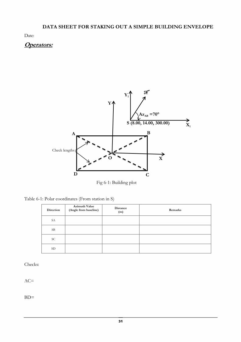
The dimensions of a rectangular building ABCD are 30m x 12m.

The point O is located in the "center" of the building.

1. Use the given building plot to compute polar coordinates (fixed point S, baseline SN, clockwise direction) of the points A,B,C and D and complete the table6-1 below.

2. Set up the total station in S coordinates XS = 8.00m, YS = 14.00m and ZS = 300.00m

3. Stakeout building envelope with total station un check distances AC and BD.

L A B

6

31

DATA SHEET FOR STAKING OUT A SIMPLE BUILDING ENVELOPE

Date:

Operators:

Table 6-1: Polar coordinates (From station in S)

Direction Azimuth Value

(Angle from baseline)

Distance (m)

Remarks

SA

SB

SC

SD

Checks:

AC=

BD=

Check lengths

N

A

D C

B

O

S (8.00, 14.00, 300.00) X1

Y1

X

Y

AzAB =70°

Fig 6-1: Building plot

32

Horizontal Curve Design

Aim:

1. Become familiar with the geometry of horizontal curve.

2. Design one curve that includes a horizontal curve.


1. Combination for sketches (graduated rule, bracket, protractor,…)

2. Scientific calculator.

Horizontal Curve:

A curve gives a smooth transition from one line of direction to another. The most

common applications are roads, railroads, water channels, and curb returns for drainage

purposes.

Parameters of a curve

1. The radius is the most important parameter of a curve. It defines how sharp or

flat the curve is.

2. The tangent into and out of a curve is perpendicular to the radius.

L A B

7

33

3. The central angle determines the length of the curve.

4. The chord is a straight line between the two ends of a curve.

5. Deflection angle is formed by the intersection of the two tangents. It is equal to

the central angle (prove this to yourself).

The five variables indicated above are all mathematically related. When two of these

five variables are known, the other three can be calculated using geometry and

trigonometry. Once a curve is defined by the radius and central angle, any point on the

curve can be located. Its relationship with all of the other points on the curve and its

location can be calculated.

Most important points in describing a curve:

1. The point of curvature (PC) (also called the beginning of curve or BC),

2. The point of tangency (PT) (also called the end of curve or EC),

3. The point of intersection of the two tangents (PI) (See the Figure).

If an angle is described at PI, it is the deflection angle of the intersection of the two

tangents and is equal to I (or Δ).

All data for a horizontal curve can be calculated from this basic curve information,

including the area enclosed or excluded by the curve. This means that from any point

on the curve or tangent, the location of equidistant points along the curve (i.e., every 20

m for example), or any other point on the curve can be computed by determining a

distance and a deflection angle.

If the coordinates of the basic curve elements are known, the position of every point is

fixed within the coordinate system. This fact makes curve layout easier because the

curve can be laid out from any point within the coordinate system and not just from

points on the curve or tangent.

34

For more information, see Chapter 24 (page 715) in your textbook.

Horizontal curve definitions

Where: I or Δ=Intersection or Central Angle

R = Radius of the curve

T = Tangent

L = Curve Length

LC = Long Chord

E = External distance

M = Mid-Ordinate

I (sometimes defined as Δ), R, T, L, and LC are the five basic variables, of which two

must be known (usually these are I and R).

Degree of Curve

The degree of curve (D), which can be related to the radius (R), is used by many

highway agencies to define the sharpness of a curve, especially on curves with large

35

radii. Highway design usually employs the arc definition of the degree of curve.

Railroad design often uses the chord definition of the degree of curve.

Arc definition

Chord definition

Laying Out a Curve

1. Curves are staked out using deflection angles and sub-chords

2. Stations for a curve are measured along the arc of the curve.

36

Laying out a horizontal curve

Moving Up on a Curve

1. To move up on a curve and retain the original field notes, occupy any station and

back sight to any other station with the angle set to the total deflections of the stations

sighted.

2. Make sure the deflections are on the correct side of 0°.

3. Continue to deflect angles as per the notes.

Example curve problem

Given: back tangent bearing to PI =

Forward tangent bearing from PI =

PI station =

D =

Find: deflection angles and chord distances to all 100m stations.

37

Calculations:

=

R =

T =

L =

Station of PC =

Station of PT =

IX =

δX= (IX /2)

Station Point Lx Ix Deflection Short Chord

Distance

Long Chord

Distance

PC

PT

38

TRIGONOMETRIC LEVELING

Aim:

1. Become familiar with the calculation of horizontal and vertical distances

from measured data.

2. Use theodolite in leveling works (trigonometric leveling)

3. Compare the relative accuracy of different techniques.


1. Theodolite

2. Tripod

3. Leveling Rod

Setting up a Theodolite (or Total Station)

As known, to properly measure angles and distances with the theodolite (or

Total Station), the instrument must be level and set up directly over a

prescribed point on the ground. If errors are made while setting up, inaccurate

L A B

8

39

measurements will result. The following steps will guide you through the

process of setting up a Theodolite (or Total Station):

1. Release the legs and raise the platform of the tripod up to chest height

and re-lock the legs (be sure to place all personal items and equipment away

from tripod legs to avoid a tripping hazard).

2. Open the legs of the tripod in an equilateral triangle, placing the feet

about 80 cm apart with the desired point in the center with the platform

roughly horizontal. (On sloped ground put two of the legs downhill, and one of

the legs poking into the hill).

3. Set the Theodolite (or Total Station) on the center of the platform and

tighten the screw that holds it in place from the bottom.

4. Step one of the legs into the ground, and then take a hold of the other

two legs and reposition them until the laser (or optical plummet) is directly on

the desired point, then step the other two legs into the ground. This is called a

coarse adjustment of centring.

5. Make sure that when you step the legs of the tripod into the ground that

they go in as deep as possible (For sloped ground step the uphill leg into the

ground and adjust the two downhill legs).

6. Now, as needed, adjust the length of any of the legs one at a time until the

spirit bubble of the rough or circle bubble is in the center of the circle. Choose

a leg that closely lines up with the direction you need the bubble to move to get

into the circle. By doing this, you will spend less time rough leveling the tripod

(putting the bubble in the circle). The bubble will move closer to the leg if you

raise it and away from the leg if you lower it.

40

7. Once again check your centering by the optical plummet. If needed,

loosen the screw holding the Theodolite (or Total Station) to the platform and

slide it over the point, and re-tighten the screw.

8. After loosening the horizontal motion knob, turn the Theodolite (or Total

Station) so that the rectangular plate level is parallel with two of the leveling

screws. Now adjust the two screws so that the long rectangular plate bubble is

in the center of the plate; between the bolded black lines capped with dots.

Make sure you turn each of the screws (one in each hand) the same amount,

but in opposite directions.

9. Now turn the Theodolite (or Total Station) 90° so that the plate level is

perpendicular to the first two screws. Using only the third screw, adjust so that

the rectangular plate bubble is once again centered.

10. Check your leveling by turning the Total Station to a random angle and

check the rectangular plate level. If needed repeat steps 7-9.

11. Once again check your centering position. If you are not over the point

anymore, repeat steps 7-10, otherwise, go to step 12.

12. Double check the leveling and you’re ready to go!

13. Until you have had a lot of practice you may find it hard to fine level the

instrument. Level it as closely as possible, and if you encounter problems ask

the instructor.

41

Procedure:

1. Set up the theodolite on a judiciously selected point.

2. Point the instrument to the first target object A

3. Lock both vertical and horizontal motions, perfect the pointing

4. Set the horizontal circle to zero to simplify the calculations (although not

mathematically necessary).

5. Read and record the zenith and horizontal angles

6. Record the top, medium and bottom reading on the leveling rod.

7. Sight respectively on B, C, D, and E following the same procedure 1-3

and record the zenith and horizontal angles.

8. Following table should be completed.

Required work:

1. Find the horizontal angles β1, β2, β3, β4 and β5. 2. Find the horizontal angles α1, α 2, α3, α 4 and α 5. 3. Find the horizontal angles λ1, λ 2, λ3, λ 4 and λ 5. 4. Find the horizontal distances SA, SB, SC, SD, SE, AB, BC, CD, DE and

EA. 5. Find the area of ABCDE.

6. Determine the elevation of points : A, B, C, D and E (assume that the elevation of the point A is 300m: ZA=300m).

7. Sketching

S

A

E

B

C

D

β5

β1

β2

β3 β4

42

Operators:

Table 1: Measurements and Calculations

Instrument

station

Staff

station

Rod readings

(m)

Zenith Angle

Z (°)

Horizontal

angle H (°)

Elevation

difference

Elevationn

(m)

Horizontal

distance (m)

S

A

B

C

D

E

Elevation difference: ∆Z=100*(TSR-BSR)*sin(z)*cos((z)+hj-MSR

Horizontal distance: HD=100*(TSR-BSR)*sin2(z)

Where:

∆Z= Elevation difference HD= Horizontal Distance TSR= Top Stadia Reading MSR= Middle Stadia Reading BSR= Bottum Stadia Reading z= Zenith Angle

43

Calculations:

Table 2: Angel values :

β 1 =

β 2 =

β 3 =

β4 =

β5 =

Table 3: Area calculations:

Triangle areas (m2)

T 1 =

T 2 =

T 3 =

T4 =

T5 =

Total area= (m2)

44

ALIGNING, RANGING AND CHAINING

Aim:

To find the distance between two given points by aligning, ranging and chaining a line.


1. Tape (20 m)

2. Four ranging rods

3. Two Arrows or two Pegs

Procedure:

The method of measuring the distance with a tape is called Chaining.

1. A and B are the survey stations. Distance between A and B is to be measured.

2. Intermediate points P1 and P2 are positioned between A and B to facilitate the alignment

of the chain in a straight line (By ranging).

3. A and B are connected in straight line by chains.

4. Number of full chains is counted and is multiplied by 20 m and note down the fractional

distance in meter from the last chain. Total distance is found out by adding full chain length and

fractional distance in meters.

L A B

9

45

Aligning method

Table: measurements

Number of full

Chains

Fractional distance

(m)

Total distance

(m)

Forward (from A to B)

Backward (from B to A)

Average=

A B P1 P

2

Ranging Rod

Ranging Rod

47

ERRORS IN MEASUREMENTS

I- INTRODUTION

• Measurement is an observation made to determine an unknown quantity (Usually read from a

graduated scale on a measurement device).

• Except counting which can be exact, any measurement is contaminated by a set of "inaccuracies"

classified in errors and faults (errors cannot be avoided).

The length of the lab room is 8,50m: This number must be completed with an indication

of the degree of precision with which the measurement was made, but:

The “True” Value of a Measurement is Never Known

The “Exact” Error Present is Always Unknown

II- Mistakes or Blunders:

Inaccuracies due to the Carelessness, Poor Judgment or Incompetence... etc. of the operator must be

eliminated by the attention of the operator and the by means of control of measurements. Their

magnitudes are usually large.

III- Errors:

Uncertainties due to imperfect measurement devices and our senses are subdivided in systematic errors

and random errors.

1- Systematic errors:

Their origin is generally computable imperfection of the measurement system. They always act in the

same direction; which facilitates their detection and estimation. They can be eliminated (or reduced) by a

suitable procedure. Their magnitudes are generally large compared to random errors.

Examples: Default in perpendicularity of the axis of a theodolite, measuring a distance with a not

calibrated chain (longer or shorter).

Systematic errors are Cumulative (occur each time a measurement is made), but can be eliminated by

making corrections to your measurements

2- Random errors:

They act unpredictably, either in one direction (+) or the other (-). They follow, therefore, a random rule

and are more difficult to assess. To reduce the range of uncertainty of a measurement, proceed by

adjusting the measured values. This compensation is performed either by referring to a repetition of the

measurement (averaging measurements of the length of a line), or by making Redundant measurements

(those taken in excess of the minimum required so that mathematical conditions can be applied to

measurements: such as sum of angles of a plane triangle = 180° or sum of latitudes and departures in a

plane loop traverse equal zero).

Remark:

Some errors are partly systematic and partly accidental and it is not always easy to determine.

3- Theory of random errors

a- Properties of random errors

Definition: An error in measurements is the difference between an observed value for a quantity and its

“true value”.

E: Error in measurement X: Observed value of the measured quantity

48

Distribution curve distribution curve

67% of the area under the curve

- -ep ep

Frequency

Error

50% of the area under the curve

T = 2 , 7 -T= -2,7

The true value of the measured quantity

But the true value of a quantity being measured is never known. The arithmetic mean (average) of a set

of measurements is considered the most probable value of the measured quantity (MPV is the sum of all

of the measurements divided by the total number of measurements)

Than the error is calculated for each performed measurement by:

Surveying measurements tend to follow a normal distribution or “bell” curve:

Normal distribution curve

Observations:

Small errors occur more frequently than larger ones

Positive and negative errors of the same magnitude occur with equal frequency

The number of large errors is very low (or are probably mistakes)

Conclusion: To lessen the random error on the MPV we have to increase the number of measurements of

a physical quantity.

b- Different types of random errors

b.1 - Standard deviation:

The accuracy of a measuring instrument is calculated by the following formula. The probability of the true

error being greater than the standard deviation is 33%.

b.2 – Most probable error:

The most probable error is defined as the error for which there are equal chances of the true error being less and greater than probable error. In other words, the probability of the true error being less than the probable error is 50% and the probability of the true error being greater than the probable error is also 50%. The most probable error is given by:

ep = 0.6745.

b.3 – Maximum error:

The probability of the true error being greater than the maximum error is 1%. It is expressed by:

1...

σ22

221

n

eee n

49

22

21

21

22X σσσ xx

nσn.σσ 2X

2n

23

22

21X σ....σσσσ

eM = 2,7. = T

This error is usually taken as the tolerance (maximum error allowed in a measuring process).

b.4 – Error propagation:

The calculation of quantities such as areas, volumes, difference in height, determining coordinates of a

point from the measurement of a distance and an angle, etc., using the measured quantities distances

and angles, is done through mathematical relationships between the computed quantities and the

measured quantities. Since the measured quantities have errors, it is inevitable that the quantities

computed from them will not have errors. Evaluation of the errors in the computed quantities as the

function of errors in the measurements is called error propagation.

Let X = f (x1 + x2 + x3 + ... + xn) a measured quantity function of elementary measurement (x1, x2, x3,

..., xn) than the standard deviation of X is expressed by:

When a physical quantity is expressed with a long formula the above equation becomes very difficult to

use, than we can use a numerical method (or approximate method):

We considerf/x ).ex = Fx= f (x + ex, y, z ) - f (x ,y ,z ): acceptable approximation.

Than we compute

1. F = f ( x , y , z )

2. Fx = f ( x + ex, y , z ) - f ( x , y , z ); Fy = f ( x , y + ey , z ) - f ( x , y , z ); Fz

= f ( x , y , z + ez ) - f ( x , y , z ); as many times as there are variables.

3. Compute Fx = Fx - F Fy = Fy - F Fz = Fz – F also as many times as there are

variables.

4. Than eF = ±

Let us apply this formula to the following common situations and check the given standard deviation

formulas:

Case Formula ; Condition Standard deviation

Sum

X = x1 x2 x3 ….. xn

If 1 = 2 =….= n =

product X = x1 . x2

arithmetic

mean with :

2n

223

2

3

22

2

2

21

2

1

2X σ.)(...σ.)(σ.)(σ.)(σ

nxf

xf

xf

xf

n

σσmoy

n

xxxAverage n

....21

σσ....σσ n21

50

EXERCISES

1. Accuracy is a term which indicates the degree of conformity of a measurement to its

(a) most probable value. (b) mean value.

(c) true value. (d) standard error.

2. 2. Precision is a term which indicates the degree of conformity of

(a) measured value to its true value.

(b) measured value to its mean value.

(c) measured value to its weighted mean value.

(d) repeated measurements of the same quantity to each other.

Exercise 1:

A straight length is measured in several times. The results are as follows:

Observation pacing taping EDM

1 571 567.17 567.133

2 563 567.08 567.124

3 566 567.12 567.129

4 588 567.38 567.165

5 557 567.01 567.144

average

Which is more precise? Which is more accurate?

Exercise 2: The sides of a rectangular lot were measured as 82.397 m and 66.132 m with a 30 m metallic tape too

short by 25 mm. calculate the error in the area of the lot.

Exercise 3:

Two sides and the included angle of a triangle were measured as under:

Length AB : 44,35m 0,02m

Length AC : 49,55m 0,02m

Angle : 42,603o0,005 o

Find the area of the triangle and the standard error.

A C

B

CE221 Engineering Surveying

Documents

Transcript of CE221 Engineering Surveying