CBFEM-MPI: A Parallelized Version of Characteristic Basis Finite Element Method for Extraction of...

164 IEEE TRANSACTIONS ON ADVANCED PACKAGING, VOL. 32, NO. 1, FEBRUARY 2009

CBFEM-MPI: A Parallelized Version ofCharacteristic Basis Finite Element Method for

Extraction of 3-D Interconnect CapacitancesOzlem Ozgun, Raj Mittra, Life Fellow, IEEE, and Mustafa Kuzuoglu, Member, IEEE

Abstract—In this paper, we present a novel, non-iterative do-main decomposition method, which has been parallelized by usingthe message passing interface (MPI) library, and used to efficientlyextract the capacitance matrixes of 3-D interconnect structures,by employing characteristic basis functions (CBFs) in the contextof the finite element method (FEM). In this method, which iscalled CBFEM-MPI, the computational domain is partitionedinto a number of nonoverlapping subdomains in which the CBFsare constructed by employing a procedure that is different fromwhat has been used in the past for generating them. Specifically,the CBFs for the problem at hand are determined by calculatingthe potentials due to a finite number of point charges locatedhypothetically along the boundaries of the conductors. Two majoradvantages of the method are substantial reduction of the matrixsize—enabling the use of direct solvers—and the utilization ofparallel processing techniques that provide a substantial decreasein the overall computation time. Numerical examples are includedto illustrate the application of the proposed approach to a numberof representative problems.

Index Terms—Capacitance extraction, characteristic basis func-tions (CBFs), domain decomposition (DD), finite element method(FEM), message passing interface (MPI) library, parallel program-ming.

I. INTRODUCTION

E FFICIENT electromagnetic modeling and simulation of3-D interconnect structures that include vias, crossovers

and bends in multilayered dielectric media plays a crucial role inreliable design of electronic packages. For example, the extrac-tion of interconnect capacitance matrixes in integrated circuitsis essential for the prediction of certain adverse effects, suchas signal delay and crosstalk, which degrade the system perfor-mance. An efficient computation tool is needed to estimate theseeffects accurately, so that such high-speed digital systems can bedesigned reliably.

Manuscript received January 23, 2008; revised May 13, 2008. Current versionpublished February 13, 2009. This work was supported in part by a grant fromThe Scientific and Technological Research Council of Turkey (TUBITAK). Thiswork was recommended for publication by Associate Editor J. Tan upon evalu-ation of the reviewers comments.

O. Ozgun was with the Electromagnetic Communication Laboratory, Penn-sylvania State University, University Park, PA 16802 USA. She is now withthe Department of Electrical Engineering, Middle East Technical University,Northern Cyprus Campus, 10 Mersin, Turkey (e-mail: [email protected]).

R. Mittra is with the Electromagnetic Communication Laboratory, Pennsyl-vania State University, University Park, PA 16802 USA (e-mail: [email protected]).

M. Kuzuoglu is with the Department of Electrical Engineering, Middle EastTechnical University, 06531 Ankara, Turkey (e-mail: [email protected]).

Color versions of one or more of the figures in this paper are available onlineat http://ieeexplore.ieee.org.

Digital Object Identifier 10.1109/TADVP.2008.2002910

Typically, the numerical methods that have been developedto compute the capacitance matrixes of interconnect configura-tions require considerable memory and computation time whenthe package to be analyzed is complex and has fine features. Anumber of strategies have been devised to circumvent the bottle-neck on the CPU memory and time in the context of both integraland differential equation methods. For instance, boundary ele-ment method (BEM) is an integral-equation-based electrostaticsolver, which derives the capacitances directly from the surfacecharge distributions on the conductors, and hence, yields a rel-atively “small” but “full” matrix [1], as compared to that ob-tained when a finite method is used. One of the most widelyused versions of the BEM is FastCap [2], which is based on thefast multipole method (FMM). The FMM is an efficient integralequation solver for the Laplace’s equation that utilizes a fast it-erative technique. However, the FMM is a kernel-dependent ap-proach that is typically applied only in a homogeneous open-re-gion environment, which rarely exists in realistic interconnectconfigurations. An alternative is to use the closed-form Green’sfunction approach to handle infinite and multilayered planar di-electric media [3]. However, this approach still cannot modelrealistic interconnect structures, and alternative methods, suchas the random walk technique (incorporated in a code calledQuickCap), has been proposed in the literature [4] for layeredconformal dielectrics. Some other techniques that are designedto solve integral equations in an iterative manner, include HiCap[5], LCap [6], TriCap [7], and [8]. We note that althoughintegral-equation-based solvers lead to “smaller” matrixes incomparison to differential equation methods, the cost of theanalysis in integral-equation-based solvers drastically increasesin terms of both computation time and memory, with an increasein the number of conductors and dielectric layers.

Differential equation-based methods, such as the finite ele-ment method (FEM) [9], the finite difference method (FDM)[10], and the measured equation of invariance (MEI) approach[11], have also been utilized to extract the capacitance matrixes.All of these methods solve for the potential distribution inthe entire volume, after discretizing the entire computationaldomain by a volume mesh. Of these, the FEM is the one that iswidely used because of its versatility and ability to efficientlymodel arbitrary geometries and material inhomogeneities. Forinstance, the FEM can conveniently handle thin multilayereddielectrics with rapidly varying constitutive parameters by em-ploying finer meshes in these layers to realize high numericalprecision. There exist several commercial tools that are basedon the finite methods, such as SPICELINK [12], CLEVER [13],CAMACO [14], and SCAP [15], all of which are based on the

1521-3323/$25.00 © 2009 IEEE

OZGUN et al.: CBFEM-MPI: A PARALLELIZED VERSION OF CHARACTERISTIC BASIS FINITE ELEMENT METHOD 165

FEM; and, RAPHAEL [16] and CAPCAL [17], which employthe FDM. In general, the finite methods lead to matrixes largerthan those in the BEM, forcing us the use of iterative solversalmost exclusively. However, the associated matrix is highly“sparse” and can be stored by using a compressed storagescheme. Even so, for large problems, the solution of thesematrixes may place a heavy burden on CPU memory and timebecause of the slow and unstable nature of the convergence ofiterative solvers, even with the use of preconditioners. Hence,alternative techniques, such as the domain decompositionmethods in the context of the FDM [18], [19], have beenutilized to solve such large-scale problems especially in thesubmicron range.

In this paper, we present a novel domain-decompositionfinite-element algorithm, called CBFEM-MPI, which is nonit-erative and well-suited for parallel computation of interconnectcapacitance matrixes using the message passing interface (MPI)library [20]—an international standard for parallel processing.The proposed technique utilizes a set of specially-definedcharacteristic basis functions (CBFs) in conjunction with adomain decomposition scheme that divides the computationaldomain into nonoverlapping subdomains. The CBFs are macrobasis functions that are generated for each subdomain, in a waysuch that the physics of the problem is taken into account. Inthe past, the characteristic basis function method (CBFM) hasbeen used to solve time-harmonic electromagnetic problems inthe context of the method of moments (MoM) [21], [22], butemploying overlapping subdomains. The CBFs have been em-ployed in the FEM [23], as well as in the finite difference timedomain (FDTD) method [24], both of which partition the orig-inal domain into overlapping subdomains. The CBFEM-MPIdiffers from all of these previous works because it is an FEMtechnique, which solves electrostatic problems by partitioningthe original domain into a suitable number of nonoverlappingsubdomains, and constructs the CBFs in each subdomain usinga novel procedure, in which the CBFs are derived by calculatingthe potential generated by a finite number of fictitious pointcharges located along the boundaries of the conductors. Oneof the major advantages of this technique is that it leads to asubstantially reduced-matrix, which can be easily handled byusing direct solvers. Furthermore, the CBFEM-MPI algorithmis highly parallelizable, and leads to a substantial decrease inthe overall computation time when run on multiple processors.

The organization of this paper is as follows. In Section II, wepresent the theoretical formulation of the CBFEM-MPI tech-nique along with some basic principles of its implementationprocedure. Then, in Section III, we focus on the parallel struc-ture of the CBFEM-MPI algorithm, with particular emphasison the functionalities of the parallel modules. In Section IV, wepresent some numerical applications that demonstrate the effec-tiveness of the method when analyzing a variety of interconnectconfigurations. Finally, we draw some conclusions in Section Vregarding the features of the technique proposed in this paper.

II. FORMULATION

A. General Formulation

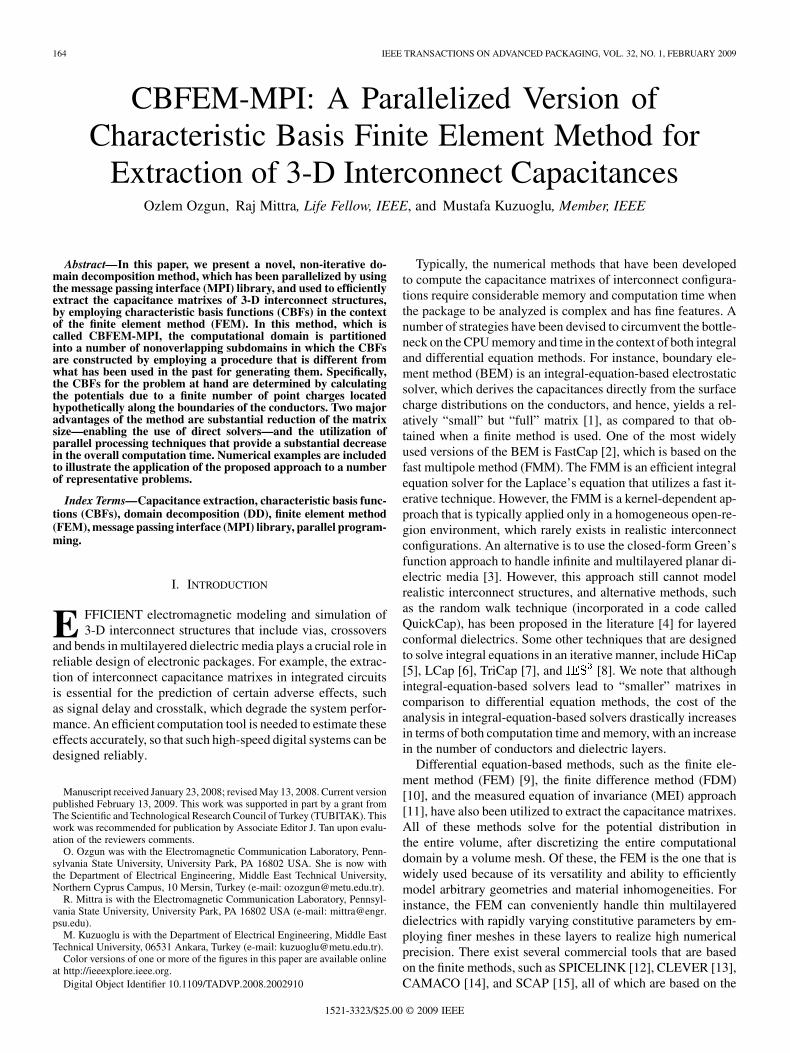
Without loss of generality, we consider the cross-sectionalmodel, shown in Fig. 1, which consists of a number of conduc-

Fig. 1. Illustration of a general model for multi-layered two-net structure(cross-sectional view).

tors embedded in a multi-layered dielectric environment. In thismodel, the computational domain is terminated with a perfectlymatched layer (PML) to simulate the open-region geometry ofthe problem at hand. However, if the conductors are placed in ashielded box, as is the case in many realistic systems, the formu-lation presented in this paper can still be applied in a straight-forward manner; and, in fact, the mesh truncation problem evenbecomes simpler. In a general capacitance extraction problemfor multiconductor structures, we solve a set of electrostaticboundary value problems (BVPs) with given boundary condi-tions (BCs) as follows:

(1)

(2)

where is the potential distribution inside the entire domain.In homogeneous dielectric medium, the BVP in (1) refers to theLaplace’s equation. The FEM formulation of (1) transforms intoa sparse global matrix system as follows:

(3)

where is the unknown potential vector on the nodes of thefinite element mesh, is the nodal global matrix, and isthe known right-hand-side (RHS) vector, which is obtained viathe imposition of the boundary conditions. To determine the en-tries of the capacitance matrix , whose size is equal to thenumber of conductor nets , the matrix system in (3) mustbe solved anew for RHS vectors corresponding to excitationsof each of the nets. In other words, the matrix system must besolved times by considering different ex-citations to compute the entries of the capacitance matrix .The entries in the matrix are then obtained by computing theelectrostatic energy stored in the system using the potential dis-tribution in the computational domain for different excitations.More specifically, we first calculate the positive-valued coeffi-cients of the capacitance and the negative-valued coeffi-cients of the induction ( , ), where and denote the IDsof the conductor nets (Note: due to reciprocity). Inorder to calculate the th entry of the coefficient matrix ,we set the potential on the net- to 1 volt and ground the other


nets, and find the energy stored in the system . Then, thecoefficient is calculated from (see [25])

(4)

After has been evaluated for each conductor net, we obtainthe coefficients by using the energy , calculated by ap-plying a unit voltage to both th and th conductor nets, as fol-lows:

(5)

The energy stored in the system , computed by exciting bothth and th conductor nets and grounding other nets, is obtained

by using the following well-known expression:

(6)

In FEM, the stored energy is evaluated by summing up all en-ergies stored in all elements, as shown in the second line of (6).Here, is the number of elements in the entire computa-tional domain; and is the volume, is the electric field, and

is the permittivity, all corresponding to the th element.Then, the “actual” entries of the capacitance matrix are ex-

pressed by using the coefficients of capacitance and inductionin (4) and (5), respectively, as follows (assuming unit voltageon the excited conductors):

(7a)

(7b)

B. CBFEM-MPI Formulation

In the CBFEM-MPI technique, the matrix system in (3) issolved efficiently by partitioning the entire computational do-main into a number of subdomains, and by employing the CBFsthat are specially-defined in each subdomain. The partitioningscheme of the entire domain is quite arbitrary, and each sub-domain may include multiple conductors and/or dielectrics. Inthis method, which is noniterative and highly parallelizable, theunknown potential distribution is expressed in terms of a se-ries of CBFs corresponding to the subdomains, as well as theinterfaces. Next, the matrix system in (3) is transformed into a“smaller” one by using the Galerkin method, which employs theCBFs both as basis and testing functions. After solving the re-sulting “reduced” matrix for the unknown coefficients, the fieldquantities inside the entire domain are determined by substi-tuting the coefficients, computed above, into the series expres-sions. The most distinguished feature of the technique is thatthe reduced matrix can still be solved by direct solvers (LU fac-torization), even when the original problem size was very large.Thus, this technique can efficiently handle multiple RHS vectorswith little additional computational effort when calculating the

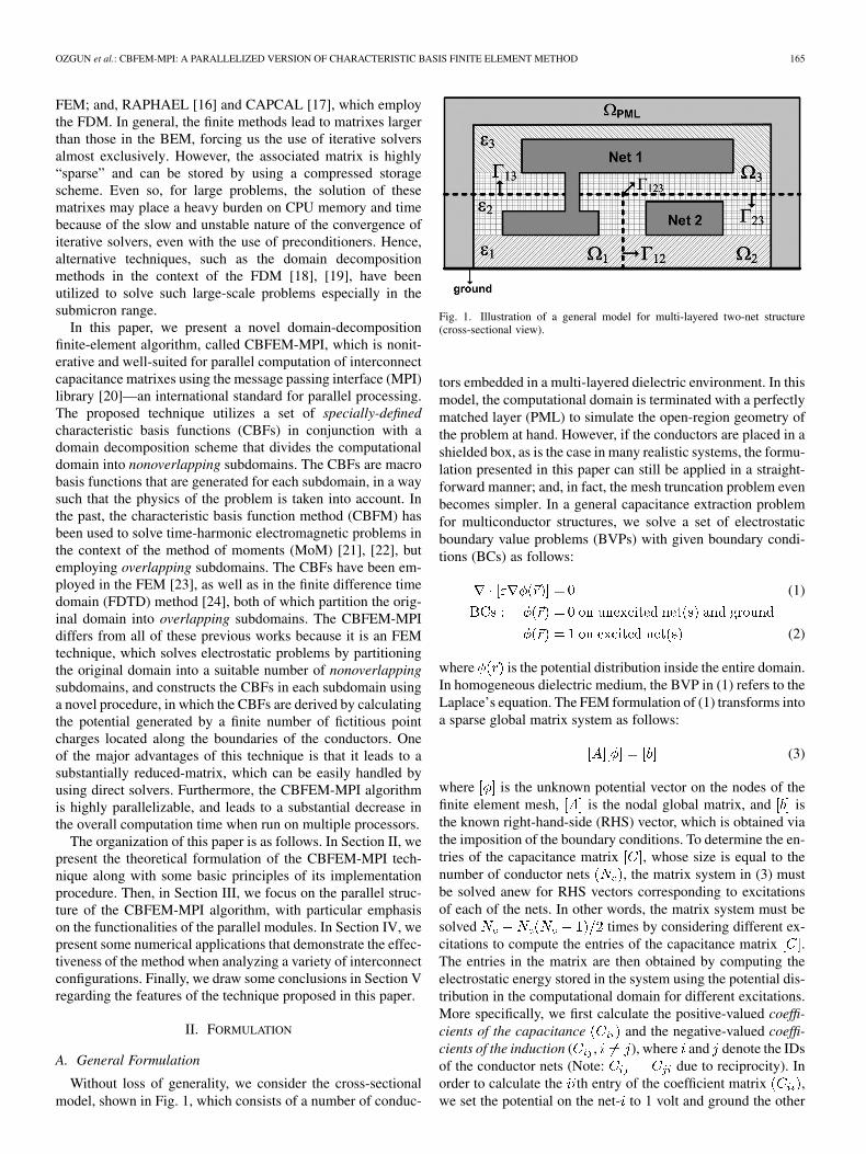
Fig. 2. Illustration of the CBFEM-MPI model via point charges (black-dotted).

entries of the capacitance matrix, as described in Section II-A.In contrast to this approach, it becomes very time consumingto handle multiple excitations, when the number of such excita-tions is large, and iterative techniques are used to solve (3).

We describe the proposed technique using the model in Fig. 2,which is the equivalent of the original one presented in Fig. 1.The initial step in the algorithm is to locate a finite numberof fictitious point charges on the conductors, as illustrated bythe black dots in Fig. 2. The potentials of these charges form thenatural basis functions for the potential distribution inside theentire computational domain, and they incorporate the physicsof the problem. In other words, if the charge density is knownalong the boundaries of the conductors, as well as along theconductors surrounding the structure (such as ground plane orshielding box), then the potential distribution can be expressedas a convolution of the charge density along the conductors withthe free-space Green’s function that can be simply expressedas . Thus, the point charges may also be placed on theground plane in Fig. 2. However, we will demonstrate belowthat the charges placed only on the conductors of the structureare sufficient to obtain reliable results. The locations of the pointcharges can easily be chosen at the nodal coordinates of theusual FEM mesh pertaining to the conductor boundaries. How-ever, if the mesh is very fine, then the distances between con-tiguous charges are chosen to be much larger than the edge-sizeof the elements located on the conductor boundaries, to reducethe number of charges and, hence, the computation time. Forexample, if the element size is 1/20 , then it is safe to choosethe distance between contiguous charges to be 1/10 , withoutlosing accuracy. Although we might think that the distance be-tween contiguous charges should be chosen as small as possibleto increase the accuracy, such a choice invariably introduces re-dundancies in the potential values. Even for moderate separa-tions, we employ the singular value decomposition (SVD) ap-proach with a threshold to reduce the redundancy. This proce-dure is detailed in the following.

The three main steps of the algorithm will now be described.They are:

Step 1) Construction of CBFs along interfaces: In thisstep, we first determine number of poten-tial distributions (CBFs or excitation functions),along each individual interface , which has no


common nodes with all other interfaces. Specifi-cally, we calculate the excitation functions alongeach “dual-” (i.e., where inFig. 2), “triple-” (i.e., where inFig. 2), and “quadruple-” interfaces where two,three, and four subdomains intersect, respectively.We note that at most four subdomains can intersectin this partitioning scheme. We calculate the poten-tial values at points along the interfaces using thepoint charges, assuming that there are no conductorsinside the domain. If the medium is uniform with apermittivity of , then the potential due to a singlepoint charge is calculated by using the followingwell-known expression [25]:

(8)

where is the distance between the position of thecharge and the point whose potential is to be calcu-lated. If the medium has multiple dielectric layers,then the principles of the “image theory” can beapplied to find the potential values [25]. Alterna-tively, if the medium has arbitrarily-positioned di-electric layers, which may even be nonplanar, thenwe can simply use the dielectric constant of thelayer, where the interface point is located, to findthe potential in (8). While calculating the potentialat each point on an individual interface, we do notconsider all charges, but only the charges—calledpioneering charges—which are located inside theprimary layer(s) where the interface under consid-eration is present, as well as inside the neighboringlayer(s) of the primary layer(s). This is because thecharges located at distances far away from an in-terface have a negligible effect on that interface.This charge selection scheme helps to decrease thenumber of charges used in the implementation, andthus to decrease the redundancy in the excitationfunctions prior to the application of the SVD pro-cedure. After determining the pioneering chargesfor each interface, we calculate the excitation func-tions on each individual interface, where

refers to the ID of the point charge. Wethen apply the SVD approach to remove the redun-dancy in these excitation functions, by orthogonal-izing them. We first let

(9)where is the number of points along each inter-face . Using the SVD procedure, we get

(10)The elements of the diagonal matrix

arethe ordered singular values of .

Next, we retain the entries whose singular valuesare above a threshold, by retaining the first

excitation functions such that. Then, we express the

post-SVD excitation functions as follows:

(11)These functions in (11) are basically the CBFs asso-ciated with each interface, and they are used to deter-mine the reduced matrix system, in a way explainedbelow. It is worthwhile to note that the procedure inthis step can be performed in parallel for each indi-vidual interface.

Step 2) Construction of CBFs in subdomains: In this step,we obtain the CBFs in each subdomain by solvingthe boundary value problem using certain excitationfunctions located on the boundaries of the subdo-main. One approach is to use some combinations ofthe post-SVD excitation functions derived in Step 1.However, a more efficient way is to calculate newexcitation functions along the boundaries of eachsubdomain. That is, we first concatenate the pointson the interfaces where each subdomain has beenterminated, and thus, find the points on the boundaryof each subdomain (e.g., on the boundary ofwhich is in Fig. 2). Sim-ilarly, following Step 1, we compute numberof post-SVD excitation functions along for theth subdomain using the pioneering charges located

in layers where the interface resides, and alsoin their neighboring layers. Then, we express thepost-SVD excitation functions as follows:

(12)where is the number of points along . Ineach subdomain, the boundary value problem issolved by using the functions in (12) to findnumber of CBFs for the th subdomain. Specifically,in the th subdomain, the following subproblemis solved for each along the boundary

(13)

It is evident that each solution of (13) requires only anew boundary condition; and, hence, only the RHSvector need be modified to generate each new solu-tion. Therefore, if an LU decomposition is utilizedfor (13), then the solutions for multiple RHS vec-tors can be generated in an efficient manner by usingonly forward and backward substitutions, withouthaving to use Gaussian elimination each time. We


then express the initial CBFs in each subdomain asfollows:

(14)where is the number of unknowns inside the thsubdomain (excluding its boundaries). At this stage,it is necessary to apply the SVD to (14) to ensure thatthe final reduced matrix system is well-conditioned.Hence, we express (14) as

(15)

Similarly, we retain the first number of CBFssuch that the singular values of (15) are below athreshold value. Finally, we express the post-SVDCBFs for each subdomain as follows:

(16)

In common with Step 1, the procedures in this stepcan also be performed, for each subdomain, in aparallel manner.

Step 3) Construction of the reduced matrix system: Weexpress the unknowns in the th subdomain as aweighted sum of CBFs derived in Step 2, in termsof a set of coefficients yet to be determined, as fol-lows:

(17)

where are the weight coef-ficients of the CBFs. Similarly, we express the un-knowns for each individual interface as a weightedsum of CBFs derived in Step 1 as shown below

(18)

where are the weight co-efficients of the CBFs. The system equation in (3)can be arranged—particularly for the geometry in

Fig. 2—by considering each subdomain and inter-face separately as shown in (19) at the bottom of thepage, where each corresponds to the couplingbetween the unknowns in the inner part of the thsubdomain (or on the th interface, ) and theunknowns in the inner part of the th subdomain (oron the th interface, ). It is worthwhile topoint out that the submatrixes in (19) do not overlapwith each other since the inner parts of the subdo-mains and the interfaces do not share the unknowns,but deal with their own separate set of the same in-stead.

Next, we substitute the expressions in (17) and (18) into thematrix system in (19), and obtain an overdetermined system ofthe form

(20)

where is a matrix whose size is

, where is the numberof subdomains ( for the geometry in Fig. 2).

After left-multiplying both sides of (20) with,

we obtain the following matrix system:

(21)

where is a square matrix whose size is. The entries of , whose

structure is similar to in (19), are given by

(22)

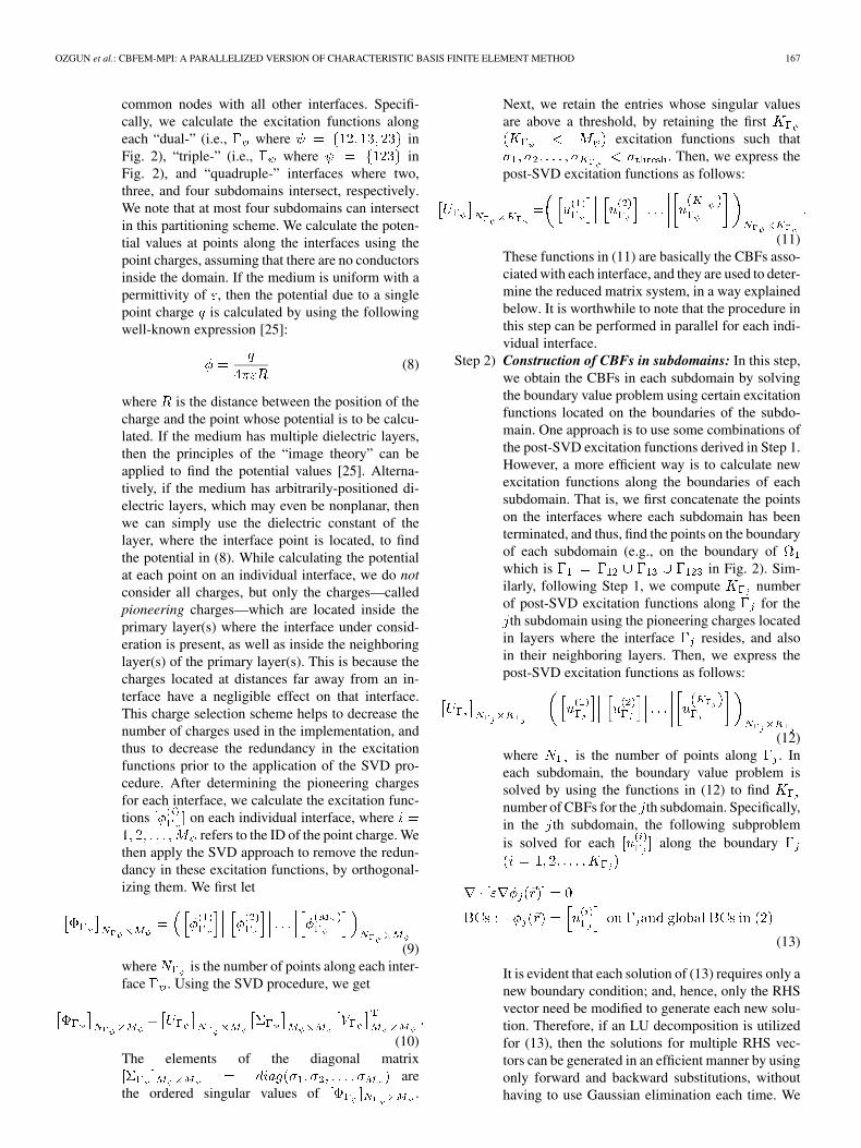
(19)


where and are “dummy” subscripts corresponding to thesubdomain and/or interface IDs. For instance, is com-puted by using and as follows:

(23)Furthermore, the new RHS vector is obtained by

(24)The sparse matrix equation in (21) can be solved for the

weight coefficients either directly, or by using the Schur-com-plement approach [26], which further reduces the size of thematrix by decoupling the unknowns on the interfaces. In orderto facilitate the application of the Schur-complement approach,the system of equations in (21) can be arranged by concatenatingthe interface unknowns as shown below

(25)where . The Schur-complement system for (25) isexpressed by

(26)

where

(27)

(28)

After the system in (26) has been solved for the interface un-knowns, the unknowns inside each subdomain can be deter-mined by solving the following subproblem :

(29)

where

(30)

The system of equations in (29) can be solved in parallel sincethey are independent of each other. It is worth mentioning thatthe matrixes in (26) and (29) are denser, though smaller andbetter-conditioned than the reduced-matrix in (21). Therefore,the solution of (26) and (29)—as well as the inverse operationin (27) and (28)—can be conveniently performed by utilizing

full-matrix direct solution techniques (such as the LU decom-position). Finally, the potential distribution inside the entire do-main can be obtained by substituting the coefficients into (17)and (18).

C. Static Locally-Conformal PML Implementation

In the models in Figs. 1 and 2, the computational domainis truncated by the perfectly matched layer (PML) in order tosolve the boundary value problem in an unbounded domain. ThePML is implemented by a new approach which extends the lo-cally-conformal PML method [27] to the static problems. Exclu-sive features of this method make it easier to implement it in theCBFEM-MPI technique, especially in the initial phase wherethe potential distribution is computed by using the point chargesalong the interfaces residing inside the PML region. In this ap-proach, the coordinates inside the PML region are replaced withtheir counterparts calculated via the coordinate transformationgiven below. In other words, we just deal with the transformedcoordinates inside the PML region and, compute the potentialsdue to the charges by using these new coordinates along the in-terfaces. In the static locally-conformal PML method, we de-fine the coordinate transformation, which maps each point P in

to in the transformed region , as follows:

(31)

where and are the position vectors of the points P and inreal spaces, respectively. In (31), is the parameter defined by

, and is the position vector of thepoint located on the inner boundary of the PML ,where the latter is the solution of the minimization problem:

. Furthermore, is the unit vector de-fined by , and is a monotonically in-creasing function of as follows:

(32)

where is a positive parameter, is a positive integer (typically2 or 3), and is the position vector of the point locatedon the outer boundary of the PML . The details of thelocally-conformal PML technique can be found in [27] and [28].In the examples given in Section IV, the PML is designed withthe parameters, and equal to 5 and 2, respectively.

III. PARALLEL CBFEM-MPI ARCHITECTURE

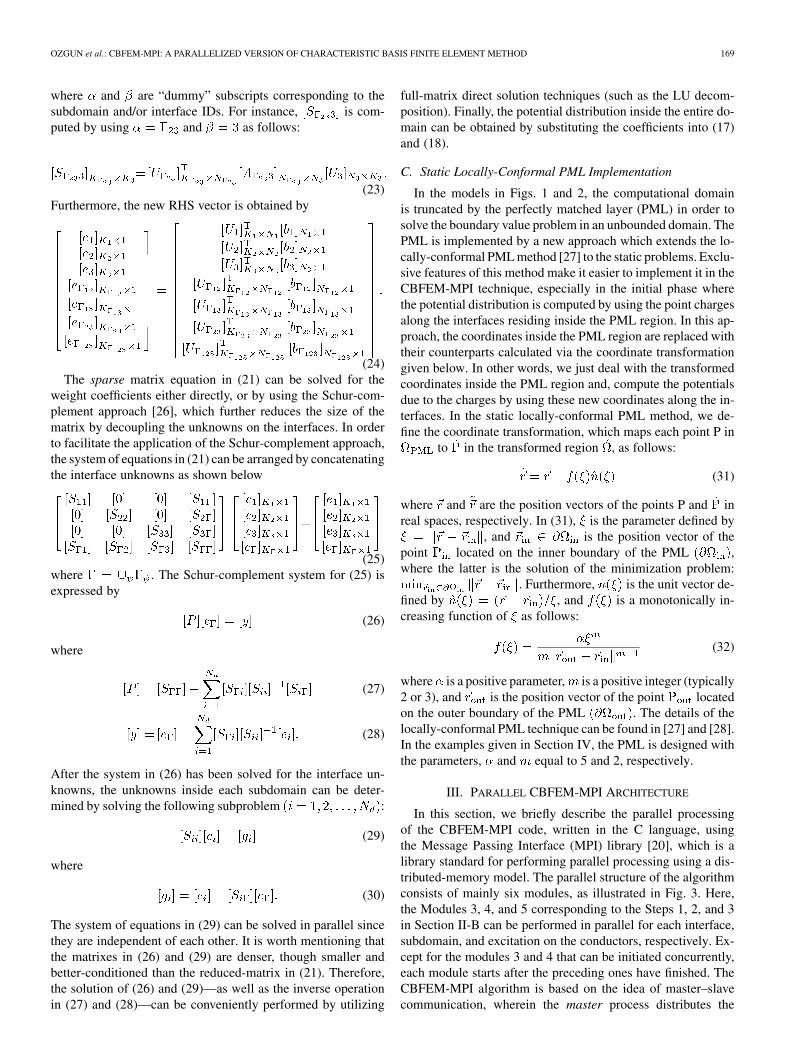
In this section, we briefly describe the parallel processingof the CBFEM-MPI code, written in the C language, usingthe Message Passing Interface (MPI) library [20], which is alibrary standard for performing parallel processing using a dis-tributed-memory model. The parallel structure of the algorithmconsists of mainly six modules, as illustrated in Fig. 3. Here,the Modules 3, 4, and 5 corresponding to the Steps 1, 2, and 3in Section II-B can be performed in parallel for each interface,subdomain, and excitation on the conductors, respectively. Ex-cept for the modules 3 and 4 that can be initiated concurrently,each module starts after the preceding ones have finished. TheCBFEM-MPI algorithm is based on the idea of master–slavecommunication, wherein the master process distributes the


Fig. 3. Parallel architecture of the CBFEM-MPI algorithm.

parallel jobs to the available processors (slaves), and arrangesthe timing of all modules in the code sequence. Multiple pro-cesses realized in these modules communicate with only themaster process through the MPI routines (such as MPI_Recv,MPI_Send, etc.) and certain data files. An important salutaryfeature of the parallel structure shown in Fig. 3 is that the CBFsare calculated only once for each excitation on the conductors.In other words, only Step 3 (or Module-5)—which involvesthe construction of the reduced matrix—is performed multipletimes to generate each entry of the capacitance matrix. The sixmain phases in Fig. 3 can be summarized as follows.

Module 1: (Preprocessing) Finite element mesh is gen-erated using tetrahedral elements and partitioned into anumber of subdomains.Module 2: The global FEM matrix is constructed in a com-pressed sparse row (CSR) format. Then, the submatrixescorresponding to domain–domain, domain–interface, andinterface–interface couplings are extracted from the globalmatrix.Module 3: (Step 1) CBFs are calculated in a parallelmanner along each interface, using the potential distribu-tion due to the point charges.Module 4: (Step 2) CBFs are calculated in parallel in eachsubdomain, by employing the charges and setting the po-tential on the conductor net inside the subdomain to 1 and0 V.Module 5: (Step 3) The reduced matrix is constructed byusing the Schur-complement approach, and is solved forthe unknown coefficients of the CBFs, for each excitation

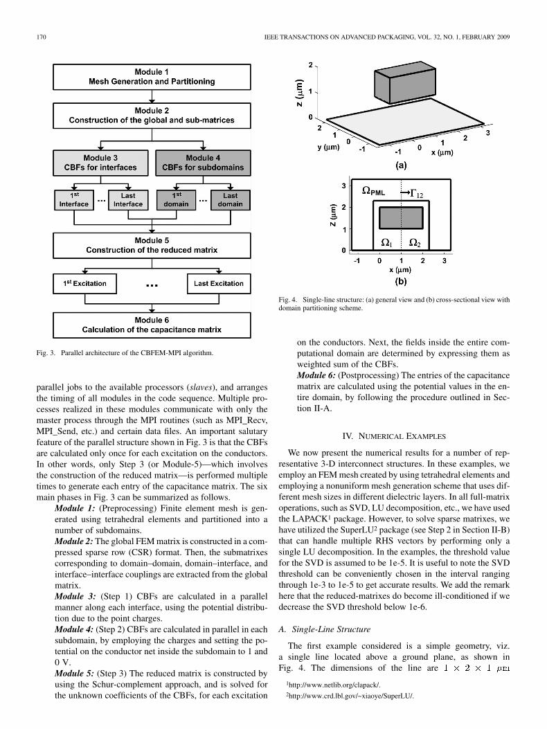
Fig. 4. Single-line structure: (a) general view and (b) cross-sectional view withdomain partitioning scheme.

on the conductors. Next, the fields inside the entire com-putational domain are determined by expressing them asweighted sum of the CBFs.Module 6: (Postprocessing) The entries of the capacitancematrix are calculated using the potential values in the en-tire domain, by following the procedure outlined in Sec-tion II-A.

IV. NUMERICAL EXAMPLES

We now present the numerical results for a number of rep-resentative 3-D interconnect structures. In these examples, weemploy an FEM mesh created by using tetrahedral elements andemploying a nonuniform mesh generation scheme that uses dif-ferent mesh sizes in different dielectric layers. In all full-matrixoperations, such as SVD, LU decomposition, etc., we have usedthe LAPACK1 package. However, to solve sparse matrixes, wehave utilized the SuperLU2 package (see Step 2 in Section II-B)that can handle multiple RHS vectors by performing only asingle LU decomposition. In the examples, the threshold valuefor the SVD is assumed to be 1e-5. It is useful to note the SVDthreshold can be conveniently chosen in the interval rangingthrough 1e-3 to 1e-5 to get accurate results. We add the remarkhere that the reduced-matrixes do become ill-conditioned if wedecrease the SVD threshold below 1e-6.

A. Single-Line Structure

The first example considered is a simple geometry, viz.a single line located above a ground plane, as shown inFig. 4. The dimensions of the line are

1http://www.netlib.org/clapack/.2http://www.crd.lbl.gov/~xiaoye/SuperLU/.


Fig. 5. Contour of potential distribution inside the entire domain for single-linestructure (cross-sectional view): (a) conventional FEM and (b) CBFEM-MPI.

width . The line (1 above theground plane) is embedded in dielectric medium with relativepermittivity . The original domain is partitionedinto two subdomains, as shown in Fig. 4(b). For the originalproblem, the number of unknowns (nodes or matrix size)is 57 587. Total number of point charges chosen along theboundary of the conductor is 1002. The size of the final re-duced-matrix is 942 (considerably less than the original matrixsize) when the Schur-complement approach is used. This matrixsize also represents the number of CBFs along the interface.The number of CBFs used in each subdomain is 899.

The capacitance value (coefficient of capacitance) is calcu-lated as in the CBFEM-MPI algorithm, and

in the conventional FEM approach. For the pur-pose of comparison, the capacitance is given asin [18], whereas the FastCap program yields the result

. The latter is slightly different than those found byusing the finite methods (by about 3%–5%) for two reasons.First, FastCap is an integral-equation type solver, and assumesthat the conductors are embedded in a homogeneous dielectricmedium. Second, it references all capacitance values to the po-tential at infinity. Consequently, the effect of the ground plane,which exists in realistic interconnect structures, is not accountedfor in FastCap. In order to make the FastCap model equivalent

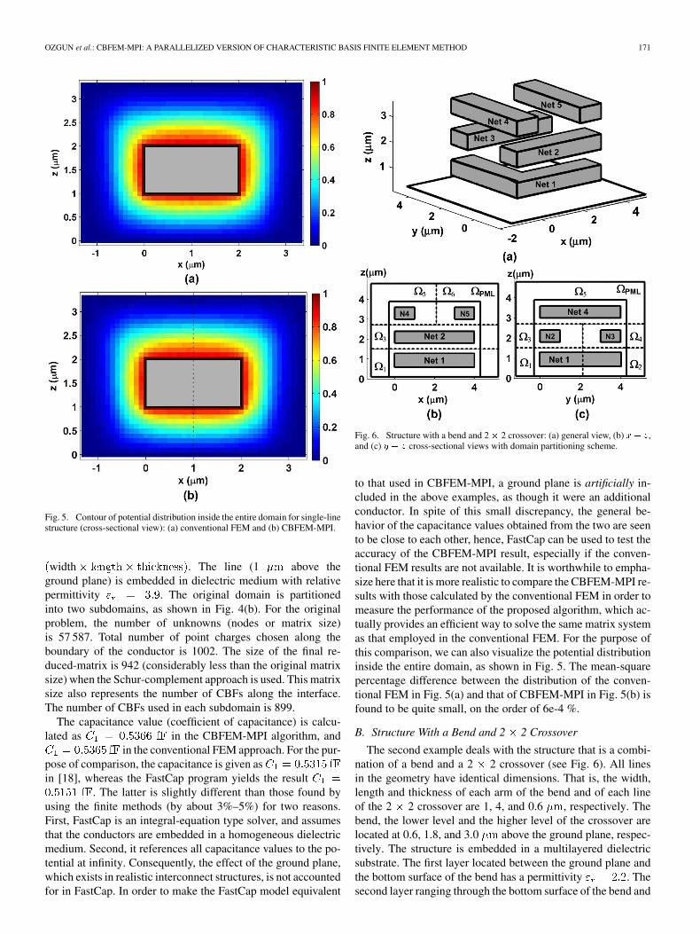
Fig. 6. Structure with a bend and 2� 2 crossover: (a) general view, (b) �� ,and (c) � � � cross-sectional views with domain partitioning scheme.

to that used in CBFEM-MPI, a ground plane is artificially in-cluded in the above examples, as though it were an additionalconductor. In spite of this small discrepancy, the general be-havior of the capacitance values obtained from the two are seento be close to each other, hence, FastCap can be used to test theaccuracy of the CBFEM-MPI result, especially if the conven-tional FEM results are not available. It is worthwhile to empha-size here that it is more realistic to compare the CBFEM-MPI re-sults with those calculated by the conventional FEM in order tomeasure the performance of the proposed algorithm, which ac-tually provides an efficient way to solve the same matrix systemas that employed in the conventional FEM. For the purpose ofthis comparison, we can also visualize the potential distributioninside the entire domain, as shown in Fig. 5. The mean-squarepercentage difference between the distribution of the conven-tional FEM in Fig. 5(a) and that of CBFEM-MPI in Fig. 5(b) isfound to be quite small, on the order of 6e-4 %.

B. Structure With a Bend and 2 2 Crossover

The second example deals with the structure that is a combi-nation of a bend and a 2 2 crossover (see Fig. 6). All linesin the geometry have identical dimensions. That is, the width,length and thickness of each arm of the bend and of each lineof the 2 2 crossover are 1, 4, and 0.6 , respectively. Thebend, the lower level and the higher level of the crossover arelocated at 0.6, 1.8, and 3.0 above the ground plane, respec-tively. The structure is embedded in a multilayered dielectricsubstrate. The first layer located between the ground plane andthe bottom surface of the bend has a permittivity . Thesecond layer ranging through the bottom surface of the bend and


TABLE ICAPACITANCE MATRIX FOR THE STRUCTURE WITH A BEND AND

2 � 2 CROSSOVER (femtoFarad)

that of the lower level of the crossover has a dielectric param-eter . The third layer positioned between the bottomsurfaces of the lower and upper levels of the crossover has apermittivity . The medium above the bottom surfaceof the upper level of the crossover is air. The entire domain ispartitioned into six subdomains, as shown in Fig. 6(b) and (c),which show two different cross-sectional views. The mesh par-titioning algorithm creates 15 individual interfaces. For the orig-inal problem, the global matrix size is 59 252. For this case, weuse 2995 point charges located along the boundaries of the con-ductors. The size of the final reduced-matrix obtained via theSchur approach is only 1844. The entries of the capacitance ma-trix are presented in Table I, which compares the results withthose computed by the conventional FEM. For the CBFEM-MPIcode, which has been run on a LINUX 3.2-GHz cluster with 16processors, the wall-time is 25 min, the CPU time is 5 min, andthe physical memory is 0.93 MB. The CPU time is actually thecorrect way of measuring the performance of the algorithm in abatch-queuing system, because it only measures the time duringwhich the processor is actively working on a certain task, anddoes not include the time due to programmed delays or whenwaiting for resources to become available. In the conventionalFEM approach employing a standard “iterative” solver (such asthe minimum residual method), the computation time for thesolution of a single matrix equation is approximately 30 mins(including both the wall and CPU times on a single processor).Since we have 5 nets , we have to solve the matrixequation 15 times (i.e., ) to derive the en-tries of the capacitance matrix. Therefore, on a “nonparallel”platform, it takes 7 1/2 h to compute the capacitance matrix.It is obvious that “small” matrixes can be handled using directsolvers in the conventional FEM. However, when the numberof conductors and dielectric layers is large, and/or the relativepermittivity is high, then, it is no longer viable to employ di-rect solvers because the matrix size is too large, and the use

Fig. 7. Two-net interconnect structure: (a) general view, (b) ��, and (c) ��

cross-sectional views with domain partitioning scheme.

of iterative solvers becomes inevitable. The time comparison,given above, serves to provide us a rough idea about the relativecomputational efficiencies of the CBFEM-MPI and the conven-tional FEM employing iterative solvers. It is evident that therelative advantage of the CBFEM-MPI approach becomes morepronounced for larger matrix systems that are not amenable todirect solution.

C. Two-Net Interconnect Structure

In the third example, we present the results of a two-net struc-ture including two vias, as illustrated in Fig. 7. All lines at thelower level have identical dimensions. Their width, length, andthickness are 1, 7, and 1 , respectively. The width, length,and thickness of the line at the upper level corresponding to theNet 1 are 1, 9, and 1 , respectively; and corresponding tothe Net 2 are 2, 9, and 1 , respectively. The lower level ispositioned at 1 above the ground plane, and the separationbetween the two layers is 2 . The interconnect structure isembedded in a homogeneous dielectric medium, whose relativepermittivity is 3.9. The number of subdomains and individualinterfaces are 6 and 25, respectively, as shown in Fig. 7. Theoriginal and reduced-matrix matrix sizes are 104 008 and 2507,respectively—so the reduction is considerable. The number ofpoint charges on the boundaries of the conductors is 6104. Theentries of the capacitance matrix are tabulated in Table II, whichalso includes the results calculated by the conventional FEM andFastCap.


TABLE IICAPACITANCE MATRIX FOR THE TWO-NET INTERCONNECT

STRUCTURE (femtoFarad)

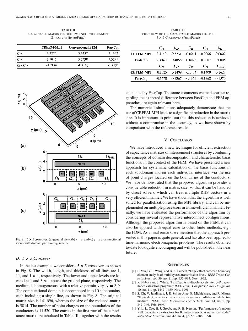
Fig. 8. 5� 5 crossover: (a) general view, (b) ��, and (c) �� cross-sectionalviews with domain partitioning scheme.

D. 5 5 Crossover

In the last example, we consider a 5 5 crossover, as shownin Fig. 8. The width, length, and thickness of all lines are 1,11, and 1 , respectively. The lower and upper levels are lo-cated at 1 and 3 above the ground plane, respectively. Themedium is homogeneous, with a relative permittivity .The computational domain is decomposed into 10 subdomains,each including a single line, as shown in Fig. 8. The originalmatrix size is 141 696, whereas the size of the reduced-matrixis 5814. The number of point charges on the boundaries of theconductors is 11 520. The entries in the first row of the capaci-tance matrix are tabulated in Table III, together with the results

TABLE IIIFIRST ROW OF THE CAPACITANCE MATRIX FOR THE

5 � 5 CROSSOVER (femtoFarad)

calculated by FastCap. The same comments we made earlier re-garding the expected difference between FastCap and FEM ap-proaches are again relevant here.

The numerical simulations adequately demonsrate that theuse of CBFEM-MPI leads to a significant reduction in the matrixsize. It is important to point out that this reduction is achievedwithout a compromise in the accuracy, as we have shown bycomparison with the reference results.

V. CONCLUSION

We have introduced a new technique for efficient extractionof capacitance matrixes of interconnect structures by combiningthe concepts of domain decomposition and characteristic basisfunctions, in the context of the FEM. We have presented a newapproach for systematic calculation of the basis functions ineach subdomain and on each individual interface, via the useof point charges located on the boundaries of the conductors.We have demonstrated that the proposed algorithm provides aconsiderable reduction in matrix size, so that it can be handledby direct solvers, which can treat multiple RHS vectors in avery efficient manner. We have shown that the algorithm is wellsuited for parallelization using the MPI library, and can be im-plemented on multiple processors in a time-efficient manner. Fi-nally, we have evaluated the performance of the algorithm byconsidering several representative interconnect configurations.Although the proposed algorithm is based on the FEM, it canalso be applied with equal ease to other finite methods, e.g.,the FDM. As a final remark, we mention that the approach pre-sented in this paper is quite general, and has also been applied totime-harmonic electromagnetic problems. The results obtainedto-date look quite encouraging and will be published in the nearfuture.

REFERENCES

[1] P. Van, G. F. Wang, and B. K. Gilbert, “Edge effect enforced boundaryelement analysis of multilayered transmission lines,” IEEE Trans. Cir-cuits Syst., vol. 39, no. 11, pp. 955–963, Nov. 1992.

[2] K. Nabors and J. White, “FastCap: A multipole accelerated 3-D capac-itance extraction program,” IEEE Trans. Computer-Aided Design vol.10, no. 11, pp. 1447–1459, Nov. 1991.

[3] S. Oh, V. Jandhyala, J. E. Schutt-Aine, E. Michielssen, and R. Mittra,“Equivalent capacitance of a strip crossover in a multilayered dielectricmedium,” IEEE Trans. Microwave Theory Tech., vol. 44, no. 2, pp.347–349, Feb. 1996.

[4] Y. L. L. Coz, H. J. Greub, and R. B. Iverson, “Performance of randomwalk capacitance extractors for IC interconnects: A numerical study,”Solid State Electron., vol. 42, no. 4, pp. 581–588, 1998.


[5] W. Shi, J. Liu, N. Kakani, and T. Yu, “A fast hierarchical algorithmfor three-dimensional capacitance extraction,” IEEE Trans. Computer-Aided Design Integr. Circuits Syst., vol. 21, no. 3, pp. 330–336, Mar.2002.

[6] Z. Yang, Z. Wang, and S. Fang, “A virtual 3-D multipole acceleratedextractor for VLSI parasitic interconnect capacitance,” in Proc. AsiaSouth Pacific—Design Automation Conf., 2001, pp. 214–217.

[7] M. Troscher, H. Hartmann, G. Klein, and A. Plettner, “TRICAP—Athree dimensional capacitance solver for arbitrarily shaped conductorson printed circuit boards and VLSI interconnections,” in Proc. Conf.Eur. Design Automation, 1994, pp. 116–121.

[8] S. Kapur and D. E. Long, “ �� : Efficient electrostatic and electro-magnetic simulation,” IEEE Comput. Sci. Eng., vol. 5, no. 4, pp. 60–67,Oct./Dec. 1998.

[9] I. Costache, “Finite element method applied to skin-effect problems instrip transmission lines,” IEEE Trans. Microwave Theory Tech., vol.35, no. 11, pp. 1009–1013, Nov. 1987.

[10] V. V. Veremey and R. Mittra, “A technique for fast calculation of ca-pacitance matrixes of interconnect structures,” IEEE Trans. Compon.,Packag., Manuf. Tech.—Part B, vol. 21, no. 3, pp. 241–249, Aug. 1998.

[11] W. Sun, W. W. M. Dai, and W. Hong, “Fast parameter extraction ofgeneral interconnects using geometry independent measured equationof invariance,” IEEE Trans. Microwave Theory Tech., vol. 45, no. 5, pp.827–836, May 1997.

[12] SPICELINK. Ansoft Inc., Pittsburgh, PA.[13] CLEVER. Silvaco, Santa Clara, CA.[14] A. Hieke, CAMACO—3-D FEM computation of mutual capacitances

of arbitrarily shaped objects Siemens Microelectronics, SIEMENSTech. Rep. R_99_1098_PI, 1998.

[15] R. Bauer, SCAP User’s Guide. Vienna, Austria: Inst. Microelectron..,Tech. Univ. Vienna, 1994.

[16] RAPHAEL. Technology Modeling Associates (TMA), Inc., Sunny-vale, CA.

[17] A. Seidl, H. Klose, M. Sivoboda, J. Oberndorfer, and W. Rosner,“CAPCAL—A 3-D capacitance solver for support of CAD systems,”IEEE Trans. Computer-Aided Design Integr. Circuits Syst., vol. 7, no.5, pp. 549–556, May 1988.

[18] V. V. Veremey and R. Mittra, “Efficient computation of interconnectcapacitances using the domain decomposition approach,” IEEE Trans.Adv. Packag., vol. 22, no. 3, pp. 348–355, Aug. 1999.

[19] Z. Zhu, H. Ji, and W. Hong, “An efficient algorithm for the parameterextraction of 3-D interconnect structures in the VLSI circuits: Domaindecomposition method,” IEEE Trans. Microwave Theory Tech., vol. 45,no. 8, pp. 1179–1184, Aug. 1997.

[20] W. Gropp, E. Lusk, and A. Skjellum, Using MPI: Portable ParallelProgramming With the Message-Passing Interface. Cambridge, MA:MIT Press, 1994.

[21] V. V. S. Prakash and R. Mittra, “Characteristic basis function method:A new technique for efficient solution of method of moments matrixequations,” Micro. Opt. Tech. Lett., vol. 36, pp. 95–100, 2003.

[22] G. Tiberi, A. Monorchio, G. Manara, and R. Mittra, “A spectral do-main integral equation method utilizing analytically derived character-istic basis functions for the scattering from large faceted objects,” IEEETrans. Antennas Propag., vol. 54, no. 9, pp. 2508–2514, Sep. 2006.

[23] M. Kuzuoglu, “Fast solution of electromagnetic boundary value prob-lems by the characteristic basis functions/FEM approach,” in IEEE An-tennas Propag. Soc. Int. Symp., Columbus, OH, Jun. 22–27, 2003, vol.2, pp. 1072–1075.

[24] H. Abd-El-Raouf, R. Mittra, and J.-F. Ma, “Solving very large EMproblems ( �� DoFs or greater) using the MPI-CBFDTD method,”in 2005 IEEE Anten. Prop. Soc. Int. Symp., Washington, DC, Jul. 3–8,2005, vol. 2B, pp. 2–5.

[25] R. Plonsey and R. E. Collin, Principles and Applications of Electro-magnetic Fields. New York: McGraw-Hill, 1961.

[26] T. N. Philips, “Preconditioned iterative methods for elliptic problemson decomposed domains,” Int. J. Comp. Math., vol. 44, pp. 5–18, 1992.

[27] O. Ozgun and M. Kuzuoglu, “Non-Maxwellian locally-conformalPML absorbers for finite element mesh truncation,” IEEE Trans.Antennas Propag., vol. 55, no. 3, pp. 931–937, Mar. 2007.

[28] O. Ozgun and M. Kuzuoglu, “Near-field performance analysis of lo-cally-conformal perfectly matched absorbers via Monte Carlo simula-tions,” J. Comput. Phys., vol. 227, no. 2, pp. 1225–1245, 2007.

Ozlem Ozgun received the B.Sc. and M.Sc. degreesin electrical engineering from Bilkent University,Ankara, Turkey in 1998 and 2001, respectively, andthe Ph.D. degree in electrical engineering from theMiddle East Technical University (METU), Ankara,Turkey, in 2007.

From 2007 to 2008, she was a postdoctoralresearch fellow in the Electromagnetic Communi-cation Laboratory, Pennsylvania State University,University Park. From 2000 to 2004, she workedin the Scientific and Technical Research Council of

Turkey (TUBITAK), National Research Institute of Electronics and Cryptology(UEKAE), Ankara, Turkey. From 2004 to 2005, she worked in the Aselsan Inc.,Microwave and System Technologies Division, Ankara, Turkey. In September2008, she joined the Northern Cyprus Campus of the Middle East TechnicalUniversity, as an Assistant Professor. Her main research interests includecomputational electromagnetics, electromagnetic propagation and scattering,and metamaterials.

Dr. Ozgun received the “METU Thesis of the year award” given by METUGraduate School of Natural and Applied Sciences in 2007.

Raj Mittra (S’54–M’57–SM’69–F’71–LF’96) isProfessor in the Electrical Engineering Department,Pennsylvania State University, University Park.He is also the Director of the ElectromagneticCommunication Laboratory, which is affiliated withthe Communication and Space Sciences Laboratoryof the Electrical Engineering Department. Prior tojoining Pennsylvania State University, he was aProfessor in Electrical and Computer Engineeringat the University of Illinois–Urbana Champaign. Hehas been a Visiting Professor at Oxford University,

Oxford, U.K., and at the Technical University of Denmark, Lyngby, Denmark.He has also served as the North American Editor of the journal AEÜ. Hisprofessional interests include the areas of communication antenna design,RF circuits, computational electromagnetics, electromagnetic modeling andsimulation of electronic packages, EMC analysis, radar scattering, frequencyselective surfaces, microwave and millimeter wave integrated circuits, andsatellite antennas. He has published about 1000 journal and symposiumpapers and more than 40 books or book chapters on various topics related toelectromagnetics, antennas, microwaves, and electronic packaging. He also hasthree patents on communication antennas to his credit. He has supervised over100 Ph.D. dissertations, about 90 M.S. theses, and has mentored more than50 postdocs and visiting scholars. He has directed, as well as lectured in, nu-merous short courses on computational electromagnetics, electronic packaging,wireless antennas and metamaterials, both nationally and internationally.

Dr. Mittra received the Guggenheim Fellowship Award in 1965, the IEEECentennial Medal in 1984, the IEEE Millennium medal in 2000, the IEEE/AP-SDistinguished Achievement Award in 2002, the AP-S Chen-To Tai Distin-guished Educator Award in 2004, and the IEEE Electromagnetics Award in2006. He is a Past President of IEEE Antennas and Propagation Society and hehas served as the Editor of the IEEE TRANSACTIONS OF THE ANTENNAS AND

PROPAGATION.

Mustafa Kuzuoglu (M’92) received the B.Sc.,M.Sc., and Ph.D. degrees in electrical engineeringfrom the Middle East Technical University (METU),Ankara, Turkey, in 1979, 1981, and 1986, respec-tively.

He is currently a Professor at the Middle EastTechnical University. His research interests includecomputational electromagnetics, inverse problems,and radars.

CBFEM-MPI: A Parallelized Version of Characteristic Basis Finite Element Method for Extraction of...

Documents

Transcript of CBFEM-MPI: A Parallelized Version of Characteristic Basis Finite Element Method for Extraction of...