Empirica 27: 83–107, 2000.© 2000Kluwer Academic Publishers. Printed in the Netherlands.

83

Causes of Inflation in Europe, the United States andJapan: Some Lessons for Maintaining PriceStability in the EMU from a Structural VARApproach?

GERT D. WEHINGEROesterreichische Nationalbank, Vienna, Austria and OECD, Paris, FranceE-mail: Gert.WEHINGER@oecd.org

Abstract. Price stability being among the primary goals of EMU monetary policy, it should beinteresting to analyse the factors that led to the disinflationary developments of the last years. Using astructural VAR approach with long-run identifying restrictions derived from an open-economy macromodel, various factors of inflation for Austria, Germany, Italy, the United Kingdom, the United Statesand Japan and the extent to which they have contributed to inflation are analysed. These factors areenergy price shocks, supply shocks, wage setting influences, demand and exchange rate disturbancesand money supply surprises. The latter three are also used to calculate core inflation. Within asmaller model for aggregate EMU data, supply and demand influences are analysed. While supplyand demand factors have generally contributed to the inflation decline, monetary policy, enhancedcompetition, low energy prices and moderate wage setting are featuring most prominent in the recentdisinflation process.

Key words: inflation, monetary policy, vector autoregression

JEL codes:C32, E31, E37, E52

I. Introduction

Throughout Europe as in many other regions of the world inflation has been fallingin the past years, certainly due to various economic factors – besides the maininstitutional explanation given for Europe, the run-up to the European MonetaryUnion, which required potential member countries to meet the stability-oriented

? The author gratefully acknowledges helpful comments on an earlier version from Fritz Breuss,Eduard Hochreiter, Reinhard Neck, Axel A. Weber, Katrin Wesche as well as from participantsof the session on “European Monetary Integration I” at the 47th International Atlantic EconomicConference, Vienna, and from an anonymous referee on this version of the paper. Of course, allremaining errors are those of the author. The views expressed are the author’s and do not necessarilycorrespond to those of the Oesterreichische Nationalbank or those of the OECD. The study wasconducted while the author was at the Oesterreichische Nationalbank.

84 GERT D. WIHINGER

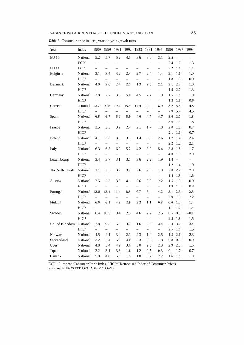
Maastricht criteria1 (see Table I). For the future, price stability is also one of theprimary goals of the European Central Bank (ECB).2

From an economic policy viewpoint and especially for policy-makers in thestability-oriented EMU it would be interesting to spot some of the underlyingfactors responsible for the decline in inflation (and, of course, its rise or move-ments in general), for then these factors could eventually be addressed by policy inimplementing price stability with a welfare-optimal mix of instruments.3 While thelatter issue goes beyond the scope of this paper, the present study will try to identifysome possible economic factors of inflation and to which extent they played a rolein the inflation process.

We proceed in the next section, II, by presenting a stylised theoretical open-economy macro model. The shock structure of the long-run rational expectationssolution of this model then allows one to identify structural shocks of an estimatedvector-autoregression (VAR) model as expounded in the rest of that section. Thismodelling and estimation procedure is then applied to data for Austria, Germany,Italy, the United Kingdom, the United States and Japan. Due to data availability, areduced version of the procedure is applied to aggregate data of the European Mon-etary Union (EMU, “Euroland” or “EU-11”). The results of our analyses includinga measure of core inflation are presented and discussed in Section III. Section IVconcludes, suggesting some guidelines for the stability-oriented policy in the EMU.

II. Identifying Causes of Inflation

1. THE MODELLING APPROACH

In the following we present a stylised open-economy macro model which canbe used to empirically identify structural shocks (which have an “economicallymeaningful” interpretation) from VAR estimates and to analyse the extent to whichsuch shocks have driven the inflation process. The identification scheme is derivedfrom the long-run rational expectations solution of the theoretical model. Such anapproach to structural VAR modelling using long-run identifying restrictions waspioneered by Blanchard and Quah (1989) and has, in various forms, often beenapplied since.4

Using long-run restrictions instead of the often-applied contemporaneous ones5

to identify structural shocks has several advantages. First of all, it involves nojudgement about short run rigidities (an information which could alternatively beused in the identification scheme), but instead, the restrictions are based on gen-eral mainstream assumptions about the economy in the long run. Secondly, whatfollows from the first point, these general assumptions should make it possible toapply the identification scheme to various countries, and furthermore, it can alsobe applied to aggregate data, in our case regarding the European Monetary Union.

Besides such extensions this analysis also serves to derive a measure of coreinflation, excluding certain types of shocks.6 This may be important as commonlyused inflation measures such as the Consumer Price Index (CPI) are susceptible

CAUSES OF INFLATION IN EUROPE, THE UNITED STATES AND JAPAN 85

Table I. Consumer price indices, year-on-year growth rates

Year Index 1989 1990 1991 1992 1993 1994 1995 1996 1997 1998

EU 15 National 5.2 5.7 5.2 4.5 3.6 3.0 3.1 2.5 – –

ECPI – – – – – – – 2.4 1.7 1.3

EU 11 ECPI – – – – – – – 2.2 1.6 1.1

Belgium National 3.1 3.4 3.2 2.4 2.7 2.4 1.4 2.1 1.6 1.0

HICP – – – – – – – 1.8 1.5 0.9

Denmark National 4.8 2.6 2.4 2.1 1.3 2.0 2.1 2.1 2.2 1.8

HICP – – – – – – – 1.9 2.0 1.3

Germany National 2.8 2.7 3.6 5.0 4.5 2.7 1.9 1.5 1.8 1.0

HICP – – – – – – – 1.2 1.5 0.6

Greece National 13.7 20.5 19.4 15.9 14.4 10.9 8.9 8.2 5.5 4.8

HICP – – – – – – – 7.9 5.4 4.5

Spain National 6.8 6.7 5.9 5.9 4.6 4.7 4.7 3.6 2.0 1.8

HICP – – – – – – – 3.6 1.9 1.8

France National 3.5 3.5 3.2 2.4 2.1 1.7 1.8 2.0 1.2 0.7

HICP – – – – – – – 2.1 1.3 0.7

Ireland National 4.1 3.3 3.2 3.1 1.4 2.3 2.6 1.7 1.4 2.4

HICP – – – – – – – 2.2 1.2 2.1

Italy National 6.3 6.5 6.2 5.2 4.2 3.9 5.4 3.8 1.8 1.7

HICP – – – – – – – 4.0 1.9 2.0

Luxembourg National 3.4 3.7 3.1 3.1 3.6 2.2 1.9 1.4 – –

HICP – – – – – – – 1.2 1.4 1.0

The Netherlands National 1.1 2.5 3.2 3.2 2.6 2.8 1.9 2.0 2.2 2.0

HICP – – – – – – – 1.4 1.9 1.8

Austria National 2.5 3.3 3.3 4.1 3.6 3.0 2.2 1.5 1.3 0.9

HICP – – – – – – – 1.8 1.2 0.8

Portugal National 12.6 13.4 11.4 8.9 6.7 5.4 4.2 3.1 2.3 2.8

HICP – – – – – – – 2.9 1.9 2.2

Finland National 6.6 6.1 4.3 2.9 2.2 1.1 0.8 0.6 1.2 1.4

HICP – – – – – – – 1.1 1.2 1.4

Sweden National 6.4 10.5 9.4 2.3 4.6 2.2 2.5 0.5 0.5−0.1

HICP – – – – – – – 2.5 1.8 1.5

United Kingdom National 7.8 9.5 5.8 3.7 1.6 2.5 3.4 2.4 3.2 3.4

HICP – – – – – – – 2.5 1.8 1.5

Norway National 4.5 4.1 3.4 2.3 2.3 1.4 2.5 1.3 2.6 2.3

Switzerland National 3.2 5.4 5.9 4.0 3.3 0.8 1.8 0.8 0.5 0.0

USA National 4.8 5.4 4.2 3.0 3.0 2.6 2.8 2.9 2.3 1.6

Japan National 2.2 3.1 3.3 1.6 1.2 0.5−0.3 −0.1 1.7 0.7

Canada National 5.0 4.8 5.6 1.5 1.8 0.2 2.2 1.6 1.6 1.0

ECPI: European Consumer Price Index, HICP: Harmonised Index of Consumer Prices.Sources: EUROSTAT, OECD, WIFO; OeNB.

86 GERT D. WIHINGER

to specific disturbances that are unrelated to the “pure” (or core) inflation process.As a result, measured inflation may give a misleading picture of underlying pricetrends relevant for monetary policy. Core inflation measures, however, should beable to provide information on underlying price movements relevant for monetarypolicy.

2. A STYLISED THEORETICAL MODEL

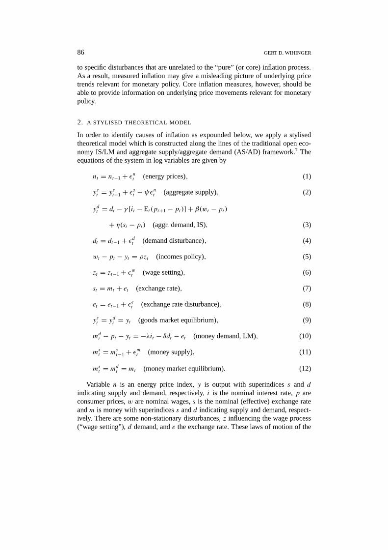
In order to identify causes of inflation as expounded below, we apply a stylisedtheoretical model which is constructed along the lines of the traditional open eco-nomy IS/LM and aggregate supply/aggregate demand (AS/AD) framework.7 Theequations of the system in log variables are given by

nt = nt−1+ εnt (energy prices), (1)

yst = yst−1+ εst − ψεnt (aggregate supply), (2)

ydt = dt − γ [it − Et (pt+1− pt)] + β(wt − pt)+ η(st − pt) (aggr. demand, IS), (3)

dt = dt−1+ εdt (demand disturbance), (4)

wt − pt − yt = ρzt (incomes policy), (5)

zt = zt−1+ εwt (wage setting), (6)

st = mt + et (exchange rate), (7)

et = et−1+ εet (exchange rate disturbance), (8)

yst = ydt = yt (goods market equilibrium), (9)

mdt − pt − yt = −λit − δdt − et (money demand, LM), (10)

mst = mst−1+ εmt (money supply), (11)

mst = mdt = mt (money market equilibrium). (12)

Variable n is an energy price index,y is output with superindicess and dindicating supply and demand, respectively,i is the nominal interest rate,p areconsumer prices,w are nominal wages,s is the nominal (effective) exchange rateandm is money with superindicess andd indicating supply and demand, respect-ively. There are some non-stationary disturbances,z influencing the wage process(“wage setting”),d demand, ande the exchange rate. These laws of motion of the

CAUSES OF INFLATION IN EUROPE, THE UNITED STATES AND JAPAN 87

economy, including energy prices, aggregate supply and money supply, are drivenby six “structural”, uncorrelated and stationary shocks with zero mean and finitevariance. Two of them,εs andεd , refer to the basic aggregate supply and aggregatedemand shocks,εw to wages (or wage setting behaviour),εe to the exchange rate,andεm to money supply. The parameters (elasticities) of the model are given byψ ,γ , β, η, λ, andδ. Generally, they are assumed positive, but we do not restrict them.8

For future prices,pt+1, expected at timet , we apply the expectations operator Et .As can be seen from (1), energy prices are completely exogenous and are only

driven by their own shocks. In (2) we have aggregate supply as a non-stationaryprocess driven by supply and energy shocks. The latter have a potentially negativeimpact on output, depending on the sign and size ofψ . Aggregate demand ismodelled in (3), where its arguments are, as in a standard IS equation, expectedreal interest rates[it −Et (pt+1− pt)], real wages(wt − pt) and the real exchangerate (st − pt);9 the demand disturbancedt , the process of which is given in (4),captures autonomous and other (e.g., government demand) elements of aggregatedemand.

As shown in (5), real wages are targeted according to an incomes policy whichaims at a constant wage share in output, besides an autonomous wage policy ele-mentzt . The latter is simply modelled as a non-stationary process given in (6) andcan be responsible for permanent shifts in the wage share. The exchange rate ismodelled in (7) with reference to the monetary approach, where home money isone argument and all other (mainly foreign) effects are captured by a disturbancetermet , the process of which is specified in (8). The equilibrium condition for thegoods market is then stated in (9).

Real money demand (10) is negatively related to both the nominal interest rateit , the exchange rate and demand disturbanceset and dt , respectively, the latterbeing interpreted as velocity shifts (individuals reduce, c.p., their cash holdings ifthey want to increase spending). For the money supply in (11) it is assumed thatthe central bank targets (implicitly, at least) a constant money growth rate, with anautonomous monetary policy elementεm.10 Finally, the money market equilibriumcondition in (12) closes the model.

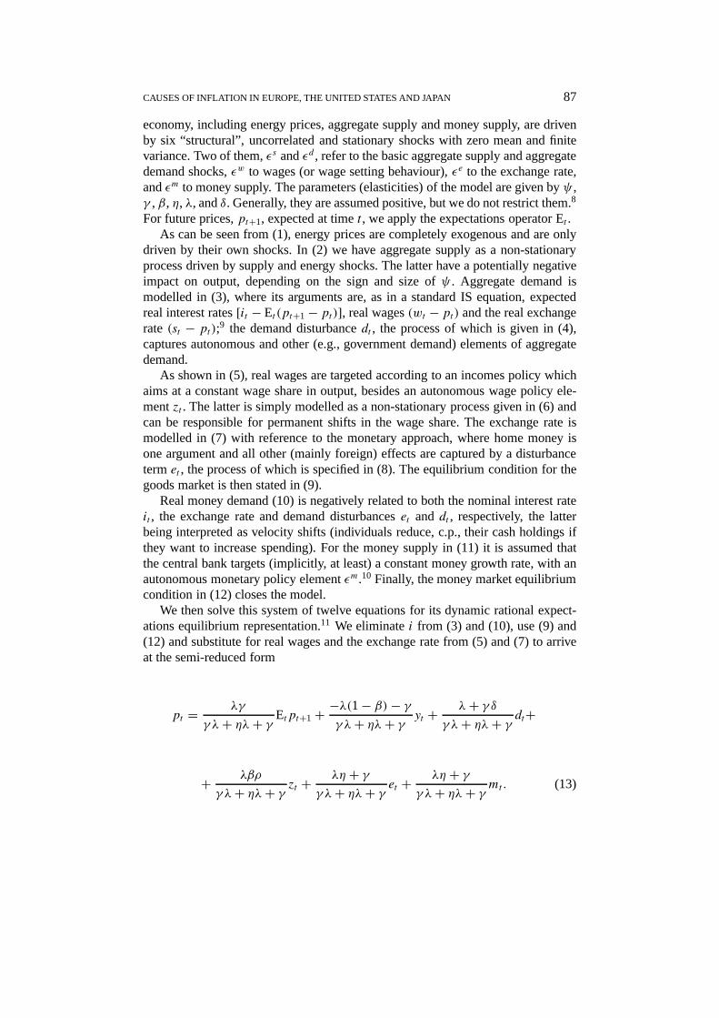
We then solve this system of twelve equations for its dynamic rational expect-ations equilibrium representation.11 We eliminatei from (3) and (10), use (9) and(12) and substitute for real wages and the exchange rate from (5) and (7) to arriveat the semi-reduced form

pt = λγ

γ λ+ ηλ+ γ Etpt+1+ −λ(1− β)− γγ λ+ ηλ+ γ yt + λ+ γ δ

γ λ+ ηλ+ γ dt+

+ λβρ

γ λ+ ηλ+ γ zt +λη + γ

γ λ+ ηλ+ γ et +λη + γ

γ λ+ ηλ+ γ mt . (13)

88 GERT D. WIHINGER

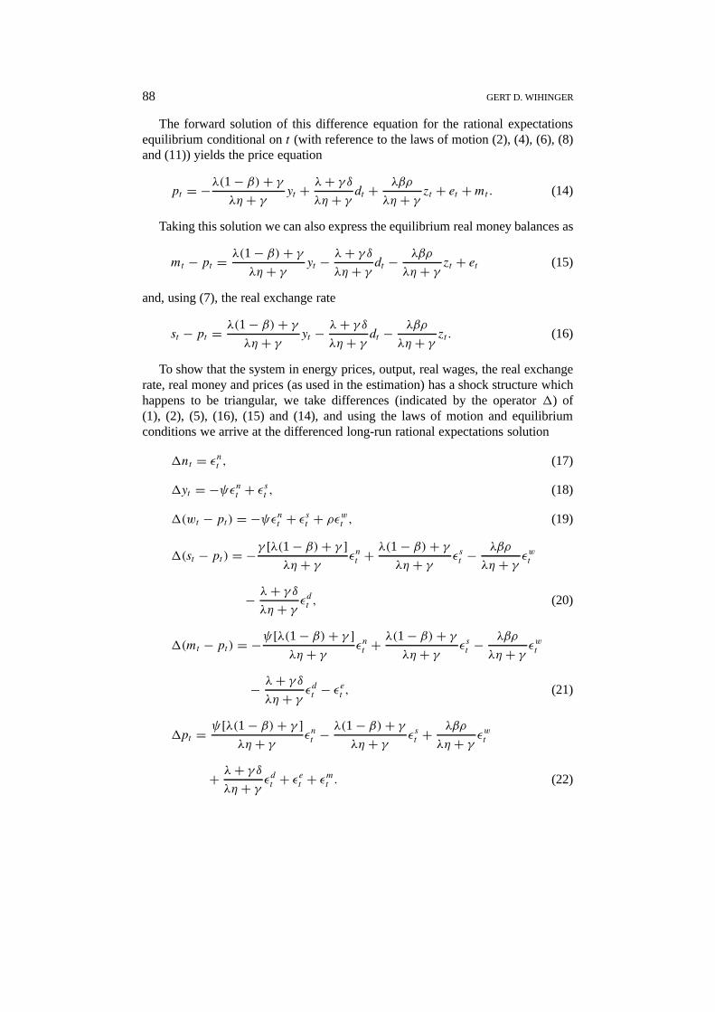
The forward solution of this difference equation for the rational expectationsequilibrium conditional ont (with reference to the laws of motion (2), (4), (6), (8)and (11)) yields the price equation

pt = −λ(1− β)+ γλη + γ yt + λ+ γ δ

λη + γ dt +λβρ

λη + γ zt + et +mt . (14)

Taking this solution we can also express the equilibrium real money balances as

mt − pt = λ(1− β)+ γλη + γ yt − λ+ γ δ

λη + γ dt −λβρ

λη + γ zt + et (15)

and, using (7), the real exchange rate

st − pt = λ(1− β)+ γλη + γ yt − λ+ γ δ

λη + γ dt −λβρ

λη + γ zt . (16)

To show that the system in energy prices, output, real wages, the real exchangerate, real money and prices (as used in the estimation) has a shock structure whichhappens to be triangular, we take differences (indicated by the operator1) of(1), (2), (5), (16), (15) and (14), and using the laws of motion and equilibriumconditions we arrive at the differenced long-run rational expectations solution

1nt = εnt , (17)

1yt = −ψεnt + εst , (18)

1(wt − pt) = −ψεnt + εst + ρεwt , (19)

1(st − pt) = −γ [λ(1− β)+ γ ]λη + γ εnt +

λ(1− β)+ γλη + γ εst −

λβρ

λη + γ εwt

− λ+ γ δλη + γ ε

dt , (20)

1(mt − pt) = −ψ[λ(1− β)+ γ ]λη + γ εnt +

λ(1− β)+ γλη + γ εst −

λβρ

λη + γ εwt

− λ+ γ δλη + γ ε

dt − εet , (21)

1pt = ψ[λ(1− β)+ γ ]λη + γ εnt −

λ(1− β)+ γλη + γ εst +

λβρ

λη + γ εwt

+ λ+ γ δλη + γ ε

dt + εet + εmt . (22)

CAUSES OF INFLATION IN EUROPE, THE UNITED STATES AND JAPAN 89

We see that all level variables have unit roots, and in the long run output is drivenby supply as well as energy price shocks, and real wages are driven by energy price,supply and wage setting shocks. All these shocks and the demand shock influencethe real exchange rate, all former shocks and the exchange rate shock influencereal money balances, and consumer prices are driven by all six structural shocks,including the one regarding monetary policy.

3. MODEL ESTIMATION AND IDENTIFICATION

Assume that a vector1x of variables follows a covariance stationary process witha moving average representation of the form

1xt = C(L)ut . (23)

In our case1x = [1n, 1y, 1(w − p), 1(s − p), 1(m − p), 1p] (with thevariables defined above) andC(L) is a lag polynomial where theC’s are coefficientmatrices at the respective lags of the serially uncorrelated errorsu with E(uu′) =6.We normalise the first coefficient matrix of the polynomial,C0, to be the identitymatrix I .

A normalised moving average representation of the process can be given as

1xt = E(L)et , (24)

with E(ee′) = I (by assumption) and the shocks are uncorrelated across time andacross variables.

Only the cross-correlated errorsu, but not the “structural”, uncorrelated errorse can be estimated directly from the VAR. Since the former have non-zero covari-ance terms, the problem is thus to transform these estimated errors to orthogonal,uncorrelated shocks which allow for a structural (“economically meaningful”) in-terpretation of the disturbances. As we have assumedC0 = I and we assume a linearrelation betweenC(L) andE(L) we can write

ut = E0et . (25)

Thus, in order to extract the independent errorse from the estimatedu’s, theE0-matrix has to be derived. Thereby we assume that the estimated shocks are linearcombinations of the underlying structural disturbances.

To identify E0 we have to imposek × k restrictions, wherek is the number ofvariables in the model and thusk × k is the dimension ofE0. Fromee′ = I anduu′= 6 we have with (25)

6 = E0E′0. (26)

Due to the symmetry property of6 this factorisation yieldsk(k + 1)/2 non-linear restrictions, for the rest ofk(k − 1)/2 we impose long-term neutrality

90 GERT D. WIHINGER

conditions on certain errors driving the respective variables as derived from the the-oretical model. As we have seen from the solution of that model, these restrictionshave a triangular structure.

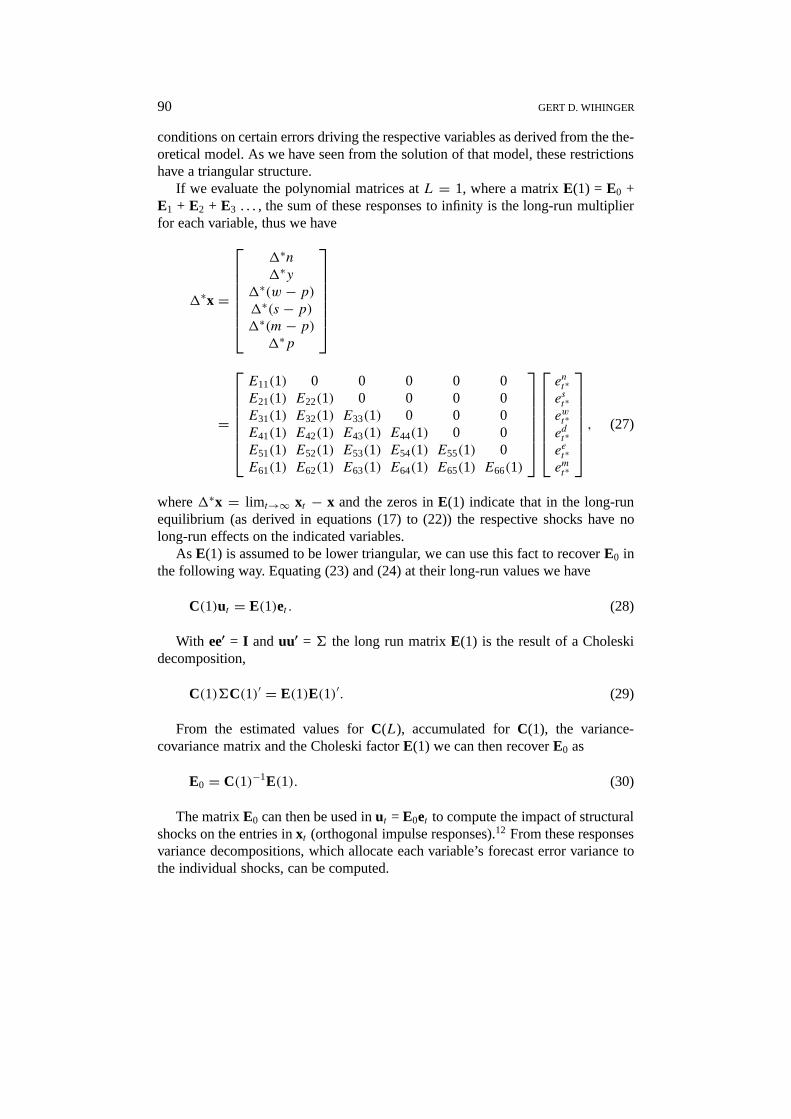
If we evaluate the polynomial matrices atL = 1, where a matrixE(1) = E0 +E1 + E2 + E3 . . . , the sum of these responses to infinity is the long-run multiplierfor each variable, thus we have

1∗x =

1∗n1∗y

1∗(w − p)1∗(s − p)1∗(m− p)1∗p

=

E11(1) 0 0 0 0 0E21(1) E22(1) 0 0 0 0E31(1) E32(1) E33(1) 0 0 0E41(1) E42(1) E43(1) E44(1) 0 0E51(1) E52(1) E53(1) E54(1) E55(1) 0E61(1) E62(1) E63(1) E64(1) E65(1) E66(1)

ent∗est∗ewt∗edt∗eet∗emt∗

, (27)

where1∗x = lim t→∞ xt − x and the zeros inE(1) indicate that in the long-runequilibrium (as derived in equations (17) to (22)) the respective shocks have nolong-run effects on the indicated variables.

As E(1) is assumed to be lower triangular, we can use this fact to recoverE0 inthe following way. Equating (23) and (24) at their long-run values we have

C(1)ut = E(1)et . (28)

With ee′ = I anduu′ = 6 the long run matrixE(1) is the result of a Choleskidecomposition,

C(1)6C(1)′ = E(1)E(1)′. (29)

From the estimated values forC(L), accumulated forC(1), the variance-covariance matrix and the Choleski factorE(1) we can then recoverE0 as

E0 = C(1)−1E(1). (30)

The matrixE0 can then be used inut = E0et to compute the impact of structuralshocks on the entries inxt (orthogonal impulse responses).12 From these responsesvariance decompositions, which allocate each variable’s forecast error variance tothe individual shocks, can be computed.

CAUSES OF INFLATION IN EUROPE, THE UNITED STATES AND JAPAN 91

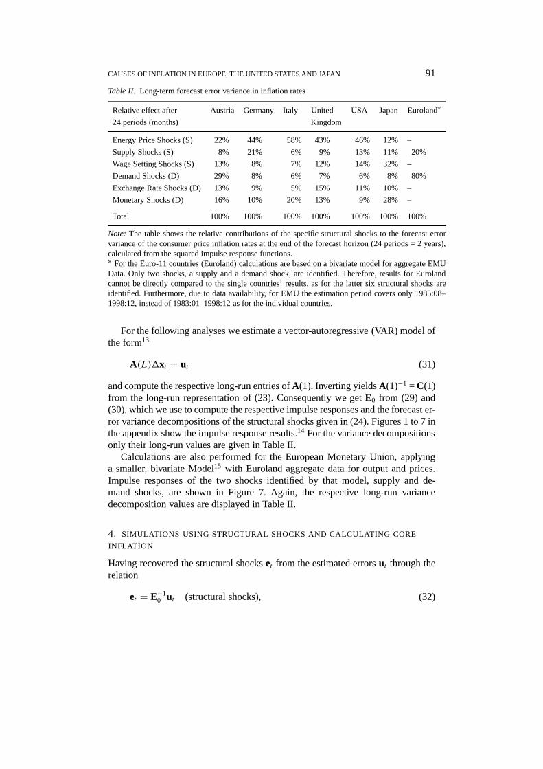
Table II. Long-term forecast error variance in inflation rates

Relative effect after Austria Germany Italy United USA Japan Euroland∗24 periods (months) Kingdom

Energy Price Shocks (S) 22% 44% 58% 43% 46% 12% –

Supply Shocks (S) 8% 21% 6% 9% 13% 11% 20%

Wage Setting Shocks (S) 13% 8% 7% 12% 14% 32% –

Demand Shocks (D) 29% 8% 6% 7% 6% 8% 80%

Exchange Rate Shocks (D) 13% 9% 5% 15% 11% 10% –

Monetary Shocks (D) 16% 10% 20% 13% 9% 28% –

Total 100% 100% 100% 100% 100% 100% 100%

Note: The table shows the relative contributions of the specific structural shocks to the forecast errorvariance of the consumer price inflation rates at the end of the forecast horizon (24 periods = 2 years),calculated from the squared impulse response functions.∗ For the Euro-11 countries (Euroland) calculations are based on a bivariate model for aggregate EMUData. Only two shocks, a supply and a demand shock, are identified. Therefore, results for Eurolandcannot be directly compared to the single countries’ results, as for the latter six structural shocks areidentified. Furthermore, due to data availability, for EMU the estimation period covers only 1985:08–1998:12, instead of 1983:01–1998:12 as for the individual countries.

For the following analyses we estimate a vector-autoregressive (VAR) model ofthe form13

A(L)1xt = ut (31)

and compute the respective long-run entries ofA(1). Inverting yieldsA(1)−1 = C(1)from the long-run representation of (23). Consequently we getE0 from (29) and(30), which we use to compute the respective impulse responses and the forecast er-ror variance decompositions of the structural shocks given in (24). Figures 1 to 7 inthe appendix show the impulse response results.14 For the variance decompositionsonly their long-run values are given in Table II.

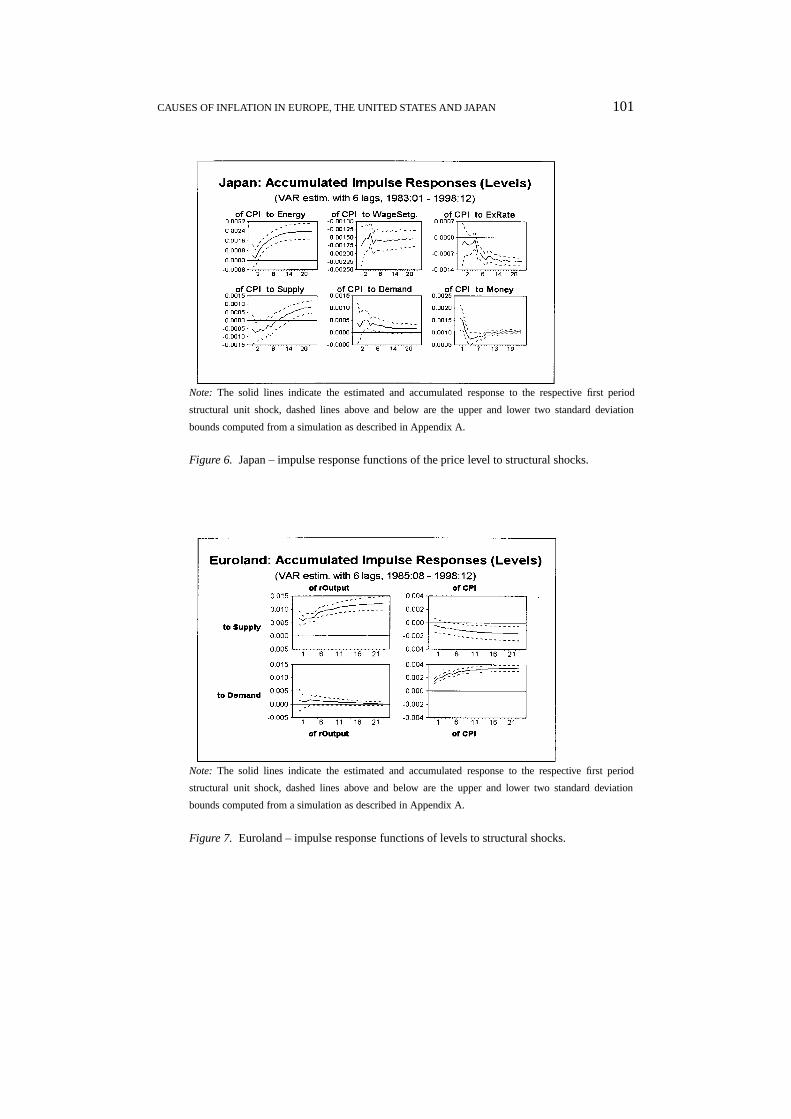
Calculations are also performed for the European Monetary Union, applyinga smaller, bivariate Model15 with Euroland aggregate data for output and prices.Impulse responses of the two shocks identified by that model, supply and de-mand shocks, are shown in Figure 7. Again, the respective long-run variancedecomposition values are displayed in Table II.

4. SIMULATIONS USING STRUCTURAL SHOCKS AND CALCULATING CORE

INFLATION

Having recovered the structural shockset from the estimated errorsut through therelation

et = E−10 ut (structural shocks), (32)

92 GERT D. WIHINGER

forecast simulations can be computed by dropping certain elements of the shockvector.

The simulations pursued here seten′t = [0, est , ewt , edt , eet , emt ]′ for the simula-

tions “absent energy price shocks”,es′t = [ent ,0, ewt , edt , eet , emt ]′ for the simulations

“absent supply shocks”,ew′

t = [ent , est ,0, edt , eet , emt ]′ for the simulations “absentwage setting shocks”,ed

′t = [ent , est , ewt ,0, eet , emt ]′ for the simulations “absent de-

mand shocks”,ee′t = [ent , est , ewt , edt ,0, emt ]′ for the simulations “absent exchange

rate shocks”, andem′

t = [ent , est , e

wt , e

dt , e

et ,0]′ for the simulations “absent monetary

shocks”. The errorsux′t (x = n, s,w, d, e,m) to be used for the forecasts with the

estimated VAR models will be recovered throughux′t = E0ex

′t

As the originally estimated variables are differences, we accumulate the results(including a mean that had been subtracted before estimation) in order to see howthe simulated levels of the variables (in particular: the price level) would evolveunder the different assumptions.

To calculatecore inflation, we adjust the simulations as described and seteCt =[0,0,0, edt , eet , emt ]′ (simulations absent energy price shocks, absent supply shocks,and absent wage setting shocks). The errors to be used for the forecasts with theestimated VAR models will be recovered throughuCt = E0eCt .

For the bivariate model of Euroland we perform the respective simulations usingthe supply and demand shocks, and we calculate core inflation as inflation absentsupply shocks.16

Not all simulation results are reported.17 In the graphs of the appendix we onlyshow deviations of the actual from the simulated paths of inflation absent specificshocks (Figure 9) and core inflation computations (Figure 10). The accumulatedpaths of the structural shocks are shown in Figure 8.

III. Empirical Results

1. DATA PREPARATORY TESTING

A VAR model as described was analysed for Austria, Germany, Italy, the UnitedKingdom, the United States and Japan. A reduced version, a bivariate model inoutput and prices, was estimated for aggregate data of the European MonetaryUnion (Euroland). We use monthly data from 1982:06-1998:12 for the individualcountries. Due to data availability, for the EMU aggregate the data set covers ashorter period, from 1985:01–1998:12. Data were taken from the OECD databaseas well as the databases of the BIS and the Oesterreichische Nationalbank (OeNB).The price index (p) used for the inflation analysis is the CPI as available from thementioned sources. To properly compare results among European countries, how-ever, it would have been appropriate to use the EU harmonised index of consumerprices (HICP) for those cases, but back-calculations of that index were not availablefor long enough periods. Energy prices were taken as the respective component ofthe price data. As output (y) we used industrial production, this being one of thefew relevant output variables measured on a monthly basis. Wages are the index

CAUSES OF INFLATION IN EUROPE, THE UNITED STATES AND JAPAN 93

of “wage rates in the economy”. The real exchange rate variable is an index assupplied by the OECD and the BIS.18 M1 was used as a monetary aggregate ingeneral. Due to data availability, for the United Kingdom we used the broaderaggregate M4.

With the exception of energy prices, seasonal adjustment was performed for alldata applying an X-11 filter.19 For estimation we used the monthly log-differencesof the data. Before estimation, augmented Dickey–Fuller20 (ADF) as well asPhillips–Perron21 tests were applied to levels and differenced data, indicatingstationarity of the differenced variables.22 For the VAR estimation we generallyused 6 lags of the variables, this structure being supported by various informationcriteria.23

2. INTERPRETATION

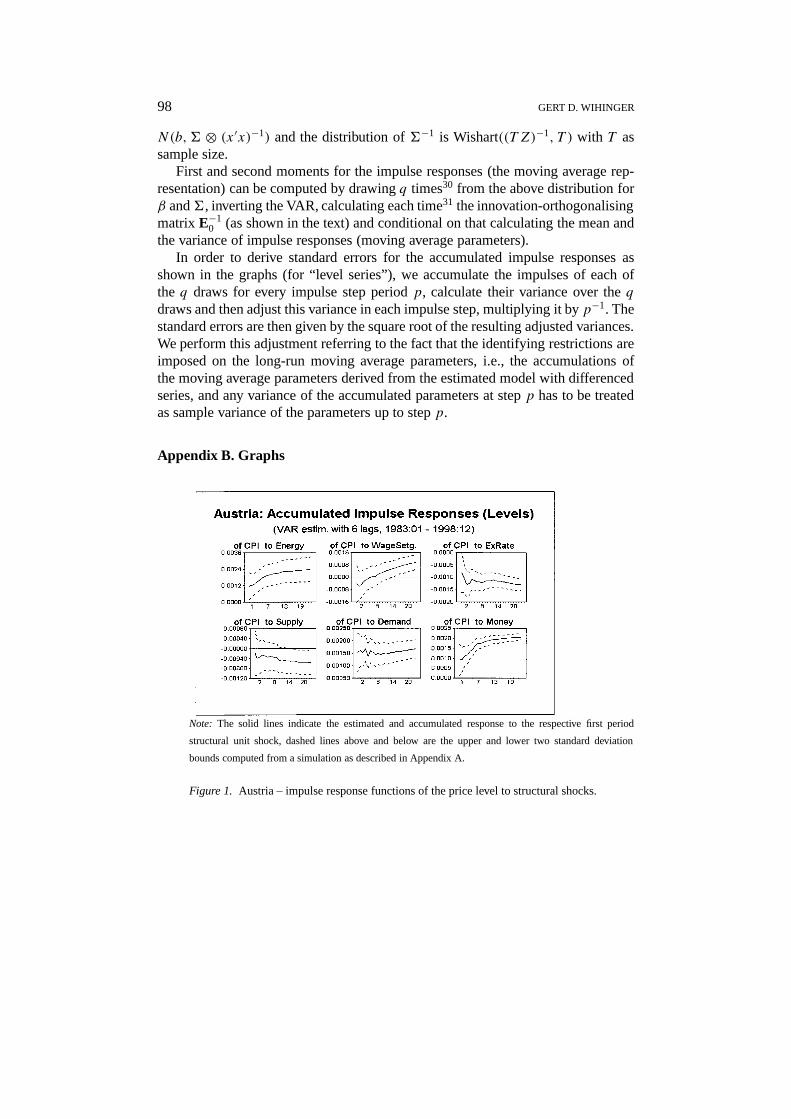
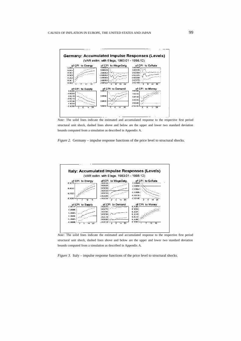
The figures in the appendix and Table II show the results of the various ana-lyses performed. All impulse responses (Figures 1 to 7) are graphed with twostandard deviation bounds, the calculation of which is outlined in Appendix A.In the following, we will describe the impact of the identified shocks on consumerprices.24

Impulse Responses

Figures 1 to 7 in the appendix show the impulse responses of prices to the structuralshocks over a period of two years (24 months) after the shock occurred. In general,they show the signs expected from theory. Energy price shocks, demand and moneyshocks lead to an increased price level in the short and long run. Supply shockshave a dampening effect on prices in all cases, with the exception of Italy, where aninitial negative supply impact on prices is being reversed over time. However, theeffects in this case are not very significant. Supply shocks are also not significantin the United Kingdom, and significant only in the long run in Austria.

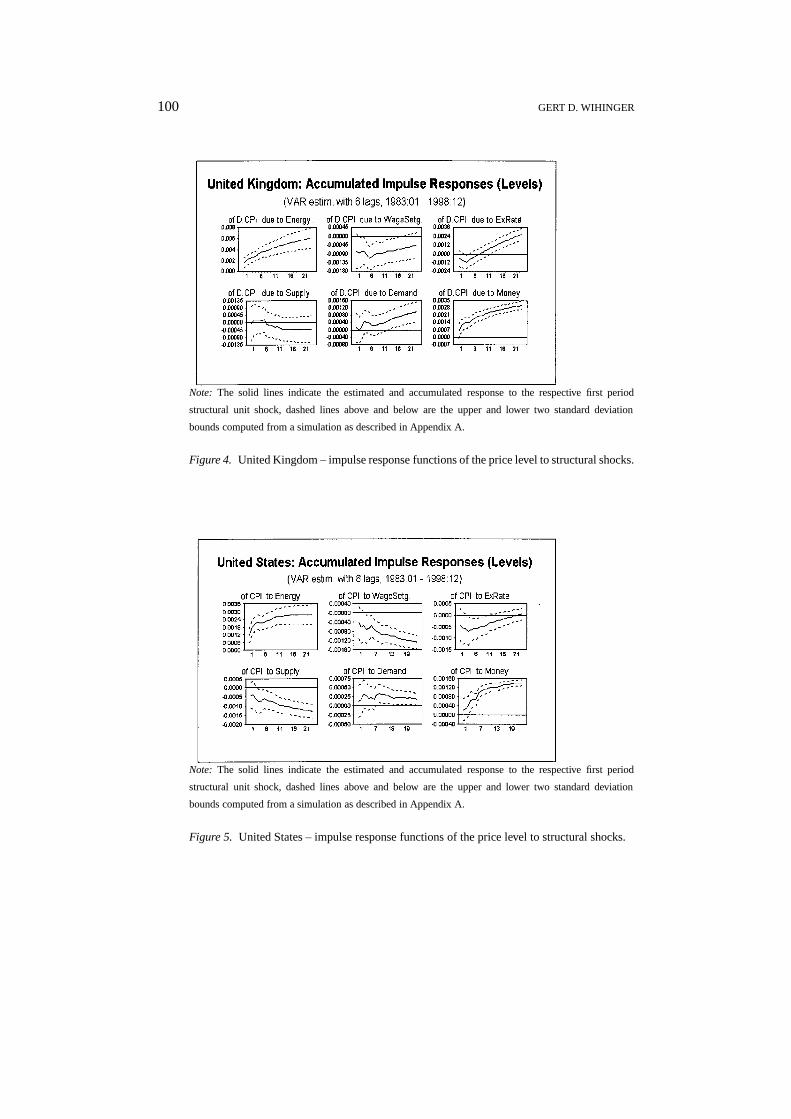
The exchange rate shock, i.e., a nominal appreciation of the respective country’scurrency,25 reduces the price level in all cases. While for most countries this effectis persistent, in the United Kingdom and the United States the negative effects arereversed after four months, but in the United States this reversal is not significantin the long run. In Germany, the (negative) exchange-rate effects on prices are notsignificant neither in the short nor the long run.

The initial impacts of the wage setting shocks on prices are negative in all cases.This points to the fact that, in the short run, an increase in the labour share ofincome can only be achieved by real wage increases (cf. Equation (5)). However,long-run results will differ depending on the structure of the economy in generaland the reaction of its agents in particular, among them the response of the mon-etary policy authorities and the social partners. We see that the negative impactpersists in almost all countries. Only in Austria and Italy wage setting shocks raisethe price level in the long run. That is, in the latter cases initial real wage gains

94 GERT D. WIHINGER

tend to be more than offset by price increases after two to three quarters. Somehowthis could also indicate relatively high real wage flexibility. For Italy, however, weshould note that the effects are not significant. The price effects of wage settingare somewhat reversed but stay negative in the United Kingdom, although with nolong-run significance. Low long-run significance is also given for the (negative)effects in Germany.

The Influences of Shocks in the Past: Simulations Absent Structural Shocks

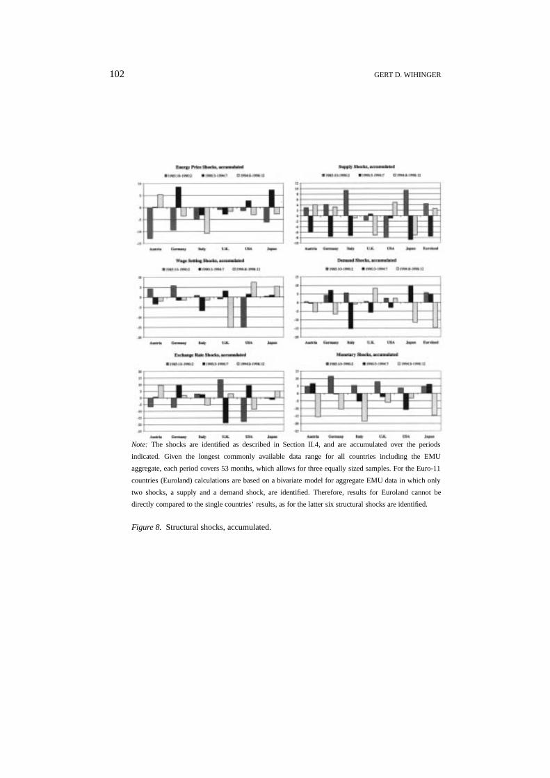
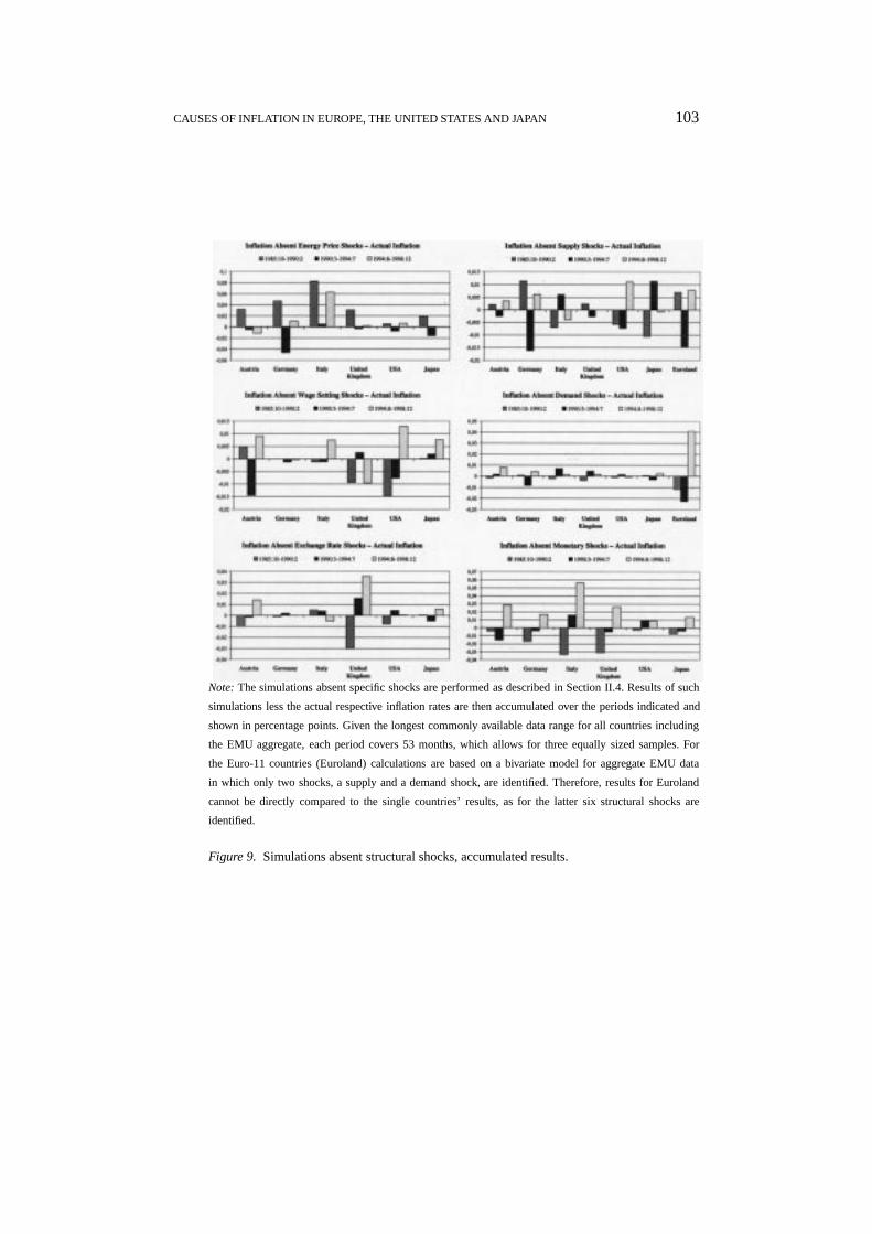
Impulse response functions measure the impact of a one-period positive shock.While this gives an idea of the reaction of variables to various shocks in general,one should also look at the impact of the historical realisation of a series of shocksas identified by the model. This is done by simulations as described in SectionII.4. They are performed excluding certain types of shocks. The accumulated pathsof the structural shocks are shown in Figure 8 in the appendix, which helps in-terpretation and corroborate the outcomes of the simulations. Figure 9 shows theresults of such simulations less the actual respective inflation rates. All values areaccumulated over three separate periods, each comprising 53 months: 1985:10–1990:02 (a period which will be referred to as the “second half of the eighties”),1990:03–1994:07 (“first half of the nineties”), and 1994:08–1998:12 (“second halfof the nineties” or “recent years”). Given the longest commonly available datarange for all countries including the EMU aggregate, this allows for three equallysized samples.

To help interpretation of the graphs, they show in percentage points to whichextent simulated inflation (absent the specific shocks) would have been above orbelow actual inflation, or, in other words, to which extent the respective shockwas responsible for actual inflation to be relatively low or high. One should alsonote that for the Euro-11 countries (Euroland) calculations are based on a bivariatemodel for aggregate EMU Data. In this model only two shocks, a supply and ademand shock, are identified. Therefore the results for Euroland cannot be directlycompared to the single countries’ results, as for the latter six structural shocks areidentified.

In all cases energy price shocks were mostly negative in the second half of theeighties and, with the exception of Austria, also in the second half of the nineties(Figure 8). As can be seen in Figure 9 (upper left panel), the dampening effectof falling energy prices did materialise in the respective countries. Especially forItaly and Germany it can be seen that inflation would have been much higher in thesecond half of the eighties and the second half of the nineties, had such negativeenergy price shocks not occurred.

Wage setting shocks seem to have moderated inflation in the recent years inAustria, Italy, the United States and Japan, and increased inflation in the UnitedKingdom (see Figure 9, second left panel from top). For Germany, the effects arevery small in all periods, and in Italy they are small in the first two periods.26 Inthe United States wages have put a relatively large upward pressure on inflation in

CAUSES OF INFLATION IN EUROPE, THE UNITED STATES AND JAPAN 95

the second half of the eighties and the first half of the nineties. For Austria, suchan upward pressure can be observed for the first half of the nineties only.

As far as monetary shocks are concerned, Figure 8 (lower right panel) clearlyshows a more restrictive monetary stance in the second half of the nineties, asopposed to somewhat more expansive policies earlier, in the second half of theeighties. This holds for all countries under consideration, and Figure 9 (lower rightpanel) reveals the recently moderating and formerly accelerating effects on infla-tion. That is, in the second half of the nineties inflation would have been higherwithout (negative) monetary policy shocks, and it would have been lower in thesecond half of the eighties without (then positive) monetary shocks.

For supply, demand and exchange rate shocks the patterns are more diverse, andwe will discuss the issues when interpreting core inflation.

The Importance of Shocks: Variance Decompositions

Looking at the variance decompositions in Table II, we can judge the relative“importance” of each shock. As we are concerned with price developments, onlythe relative contributions of the shocks to the forecast error variance of inflation aredisplayed. Furthermore, we only show their respective long-run values, namely twoyears after the shock occurred (24 periods). This allows for a more straightforwardinterpretation, as here we will be concerned with long-run effects only.

Energy price shocks are responsible for the relatively largest shares of the fore-cast error variance in all countries but Austria and Japan. In the United States, theseshocks are most prominent even in absolute terms, with a respective value of 58%.In Austria, the largest relative share of about one third (29%) is taken by demandshocks, and in Japan the wage setting shocks (32%) and also monetary shocks(28%) are most prominent. Monetary shocks are also of second most importancein Italy (20%). Probably due to the steady course of monetary policy in Germany,such shocks there account for only 10% of the long-run forecast error variance.In Germany the supply shocks feature more strongly in this respect (21%). Withthe exception of Japan (as mentioned), the wage setting shocks account for onlyless than 15% in all cases. Exchange rate shocks do not to contribute much tothe forecast error variance, with the highest respective value of 15% in the UnitedKingdom.

For the bivariate model applied to Euroland data, extracting supply and demandshocks, we see that inflation is mainly demand driven, as the respective shocksaccount for 80% of the long-run forecast error variance.

Measuring Core Inflation

We construct a measure of core inflation eliminating supply-side influences, i.e.,energy price, supply and wage setting shocks from measured inflation (and elim-inating only supply shocks for the bivariate Euroland model), using a simulationtechnique as expounded in Section II.4. The results of core inflation computations

96 GERT D. WIHINGER

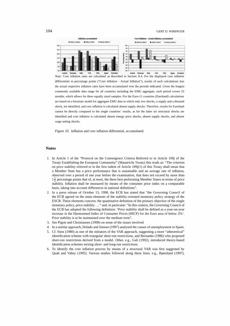
are displayed in Figure 10. As in the simulations’ cases (and as explained there,above), we show values accumulated over three periods to allow a more con-cise interpretation of the results: 1985:10–1990:02 (“second half of the eighties”),1990:03–1994:07 (“first half of the nineties”), and 1994:08–1998:12 (“second halfof the nineties”, “recent years”). Furthermore, besides such values for inflation, weonly show the respective deviations of core inflation from actual inflation. That is,we show how much a “purely demand driven” inflation (the core inflation measure)would exceed or stay below the actual inflation measure. Again, results for theEuro-11 countries (Euroland) cannot be directly compared to the single countries’results, as for the former calculations are based on a bivariate model with only twoshocks (supply and demand shocks, where supply shocks are eliminated for coreinflation), and for the latter six structural shocks are identified (and three supplyside shocks are suppressed for core inflation).

First of all, we observe the general decrease of inflation during the last yearsin all cases (left panel of Figure 10). The fact that core inflation is above actualinflation for the second half of the nineties in all countries but the United Kingdom(see right panel of Figure 10) indicates that in those countries, besides moderatingdemand side effects, supply side effects have featured strongly to bring down actualinflation in recent years. Such effects are, though, negligible in Austria, but verystrong in Italy and also the United States. Such dampening supply-side influenceson inflation can also be strongly noticed in Italy, Germany, Austria and the UnitedKingdom for the earliest period under consideration, the second half of the eighties.Demand driven or core inflation was never very far below actual inflation (with re-spect to the shown accumulated values), with the exception of Germany, where coreinflation was relatively low in the first half of the nineties. This can be attributed toa strong influence of negative supply shocks (cf. the upper right panels of Figures8 and 9).27

IV. Conclusions

In this study some driving forces of the inflation process are empirically analysedfor Austria, Germany, Italy, the United Kingdom, the United States and Japan aswell as for EMU aggregate data. Using a structural VAR approach with long-runidentifying restrictions, we derive these restrictions from a stylised open-economymacro model. Energy price shocks, supply and demand shocks, wage setting influ-ences, exchange rate disturbances and money supply surprises (and only supply anddemand shocks in the case of the EMU aggregate) are identified as factors drivinginflation. Supply and demand factors have contributed to the observed disinflationof the nineties in general. While declining energy prices were partly responsiblefor these developments, from the policymaker’s viewpoint it is interesting to notethat monetary policy in particular featured prominently as determinant of the disin-flation process. Furthermore, wage setting plays a decisive role in the propagationof inflationary shocks.

CAUSES OF INFLATION IN EUROPE, THE UNITED STATES AND JAPAN 97

Extending the applied simulation technique excluding certain structural shocks,we also calculate indices of core inflation eliminating all supply-side influencesfrom measured inflation. Thereby we find evidence that in general the observeddisinflation was due to (negative) demand effects especially in the first half of thenineties, and that recently moderating supply side effects seemed to have gainedimportance.

Taking into consideration the continuing disinflation, in particular in EU coun-tries, and the latter fact that disinflation tended to become more supply-driven,some lessons for policy-makers, especially for policy-makers in the stability-oriented EMU, may be drawn. Firstly, competition policy should further enhanceliberalisation and price transparency, as large price differentials still exist amongEMU countries, which cannot all be attributed to differences in productivity, trans-portation costs, or the like. Secondly, wage and income policies are important inmaintaining price stability. While wage earners can profit from the real wage effectsof stronger competition and increased productivity, they will play a key element inthe propagation mechanism of inflation, also in moderating inflationary shocks ifenergy prices rise again after the pronounced decreases in the course of the nineties.Thirdly, when favourable price developments come from the supply side, there issome room for manoeuvre for monetary policy. In general, knowledge about thesources driving the inflation process will allow policy reactions which can moreaccurately support the economic growth process without endangering the objectiveof price stability.

Appendix A: Confidence Bands of Impulse Response Functions

In order to report two-standard error bands in the graphs of the impulse responsefunctions as shown below we apply a Monte-Carlo approach. Although there is acommon procedure for the “traditional” VARs that use short-term restrictions toidentify the structural shocks, the calculation of the error bands for VARs usinglong-run restrictions are not widely known among model builders. So far, alsoan analytical approach - which is given by Lütkepohl (1993, p.313ff) for “tradi-tional” VARs – has not been finally designed in the context of long-run identifyingrestrictions.28 Here we use a slightly modified version of a technique expoundedin, e.g., Mélitz and Weber (1996).29

If we write the VAR as

yt = (I ⊗ xt )β + ut ,

where⊗ is the Kronecker product,xt is the vector of laggedyit ’s (i = 1,2, . . . m),β is a vector containing the stacked version of the structural VAR lag polynomialmatrices,A(L), and ut is i.i.d. with distributionN(0, 6). The OLS estimatesof β and 6 are denoted byb and Z. Assuming that the prior distribution ofβ is f (β,6)∞|6|−(n+1)/2, the posterior distribution ofβ, conditional on6, is

98 GERT D. WIHINGER

N(b,6 ⊗ (x′x)−1) and the distribution of6−1 is Wishart((T Z)−1, T ) with T assample size.

First and second moments for the impulse responses (the moving average rep-resentation) can be computed by drawingq times30 from the above distribution forβ and6, inverting the VAR, calculating each time31 the innovation-orthogonalisingmatrix E−1

0 (as shown in the text) and conditional on that calculating the mean andthe variance of impulse responses (moving average parameters).

In order to derive standard errors for the accumulated impulse responses asshown in the graphs (for “level series”), we accumulate the impulses of each ofthe q draws for every impulse step periodp, calculate their variance over theqdraws and then adjust this variance in each impulse step, multiplying it byp−1. Thestandard errors are then given by the square root of the resulting adjusted variances.We perform this adjustment referring to the fact that the identifying restrictions areimposed on the long-run moving average parameters, i.e., the accumulations ofthe moving average parameters derived from the estimated model with differencedseries, and any variance of the accumulated parameters at stepp has to be treatedas sample variance of the parameters up to stepp.

Appendix B. Graphs

Note: The solid lines indicate the estimated and accumulated response to the respective first period

structural unit shock, dashed lines above and below are the upper and lower two standard deviation

bounds computed from a simulation as described in Appendix A.

Figure 1. Austria – impulse response functions of the price level to structural shocks.

CAUSES OF INFLATION IN EUROPE, THE UNITED STATES AND JAPAN 99

Note: The solid lines indicate the estimated and accumulated response to the respective first period

structural unit shock, dashed lines above and below are the upper and lower two standard deviation

bounds computed from a simulation as described in Appendix A.

Figure 2. Germany – impulse response functions of the price level to structural shocks.

Note: The solid lines indicate the estimated and accumulated response to the respective first period

structural unit shock, dashed lines above and below are the upper and lower two standard deviation

bounds computed from a simulation as described in Appendix A.

Figure 3. Italy – impulse response functions of the price level to structural shocks.

100 GERT D. WIHINGER

Note: The solid lines indicate the estimated and accumulated response to the respective first period

structural unit shock, dashed lines above and below are the upper and lower two standard deviation

bounds computed from a simulation as described in Appendix A.

Figure 4. United Kingdom – impulse response functions of the price level to structural shocks.

Note: The solid lines indicate the estimated and accumulated response to the respective first period

structural unit shock, dashed lines above and below are the upper and lower two standard deviation

bounds computed from a simulation as described in Appendix A.

Figure 5. United States – impulse response functions of the price level to structural shocks.

CAUSES OF INFLATION IN EUROPE, THE UNITED STATES AND JAPAN 101

Note: The solid lines indicate the estimated and accumulated response to the respective first period

structural unit shock, dashed lines above and below are the upper and lower two standard deviation

bounds computed from a simulation as described in Appendix A.

Figure 6. Japan – impulse response functions of the price level to structural shocks.

Note: The solid lines indicate the estimated and accumulated response to the respective first period

structural unit shock, dashed lines above and below are the upper and lower two standard deviation

bounds computed from a simulation as described in Appendix A.

Figure 7. Euroland – impulse response functions of levels to structural shocks.

102 GERT D. WIHINGER

Note: The shocks are identified as described in Section II.4, and are accumulated over the periods

indicated. Given the longest commonly available data range for all countries including the EMU

aggregate, each period covers 53 months, which allows for three equally sized samples. For the Euro-11

countries (Euroland) calculations are based on a bivariate model for aggregate EMU data in which only

two shocks, a supply and a demand shock, are identified. Therefore, results for Euroland cannot be

directly compared to the single countries’ results, as for the latter six structural shocks are identified.

Figure 8. Structural shocks, accumulated.

CAUSES OF INFLATION IN EUROPE, THE UNITED STATES AND JAPAN 103

Note:The simulations absent specific shocks are performed as described in Section II.4. Results of such

simulations less the actual respective inflation rates are then accumulated over the periods indicated and

shown in percentage points. Given the longest commonly available data range for all countries including

the EMU aggregate, each period covers 53 months, which allows for three equally sized samples. For

the Euro-11 countries (Euroland) calculations are based on a bivariate model for aggregate EMU data

in which only two shocks, a supply and a demand shock, are identified. Therefore, results for Euroland

cannot be directly compared to the single countries’ results, as for the latter six structural shocks are

identified.

Figure 9. Simulations absent structural shocks, accumulated results.

104 GERT D. WIHINGER

Note: Core inflation rates are calculated as described in Section II.4. For the displayed core inflation

differentials in percentage points (“Core Inflation - Actual Inflation”), results of such calculations less

the actual respective inflation rates have been accumulated over the periods indicated. Given the longest

commonly available data range for all countries including the EMU aggregate, each period covers 53

months, which allows for three equally sized samples. For the Euro-11 countries (Euroland) calculations

are based on a bivariate model for aggregate EMU data in which only two shocks, a supply and a demand

shock, are identified, and core inflation is calculated absent supply shocks. Therefore, results for Euroland

cannot be directly compared to the single countries’ results, as for the latter six structural shocks are

identified and core inflation is calculated absent energy price shocks, absent supply shocks, and absent

wage setting shocks.

Figure 10. Inflation and core inflation differential, accumulated.

Notes

1. In Article 1 of the “Protocol on the Convergence Criteria Referred to in Article 109j of theTreaty Establishing the European Community” (Maastricht Treaty) this reads as: “The criterionon price stability referred to in the first indent of Article 109j(1) of this Treaty shall mean thata Member State has a price performance that is sustainable and an average rate of inflation,observed over a period of one year before the examination, that does not exceed by more than11

2 percentage points that of, at most, the three best performing Member States in terms of pricestability. Inflation shall be measured by means of the consumer price index on a comparablebasis, taking into account differences in national definitions”.

2. In a press release of October 13, 1998, the ECB has stated that “the Governing Council ofthe ECB agreed on the main elements of the stability-oriented monetary policy strategy of theESCB. These elements concern: the quantitative definition of the primary objective of the singlemonetary policy, price stability. . . ” and, in particular: “In this context, the Governing Council ofthe ECB has adopted the following definition: ‘Price stability shall be defined as a year-on-yearincrease in the Harmonised Index of Consumer Prices (HICP) for the Euro area of below 2%’.Price stability is to be maintained over the medium term”.

3. See Pigott and Christiansen (1998) on some of the issues involved.4. In a similar approach, Dolado and Jimeno (1997) analysed the causes of unemployment in Spain.5. Cf. Sims (1980) as one of the initiators of the VAR approach, suggesting a more “atheoretical”

identification scheme with triangular short-run restrictions, and Bernanke (1986) who proposedshort-run restrictions derived from a model. Other, e.g., Galí (1992), introduced theory-basedidentification schemes mixing short- and long-run restrictions.

6. To identify the core inflation process by means of a structural VAR was first suggested byQuah and Vahey (1995). Various studies followed along these lines, e.g., Bjørnland (1997),

CAUSES OF INFLATION IN EUROPE, THE UNITED STATES AND JAPAN 105

Blix (1995), Dewachter and Lustig (1997), Fase and Folkertsma (1997), Jacquinot (1998), andGartner and Wehinger (1998).

7. Similar models can be found in, e.g., Clarida and Galí (1994) and Weber (1997).8. As will be seen from the solution of the model below, the only restriction we have to apply in

order to arrive at a stationary solution is that(λη + γ ) 6= 0.9. Foreign prices are assumed to be scaled to zero and any influences stemming from that side

would be captured by the disturbance terme hitting the nominal exchange rate as shown in (7),which seems a reasonable simplification for our illustrative purposes.

10. Due to its exchange-rate peg to the DEM, this would theoretically be true also in the Austriancase, where Austrian money supply growth would, c.p., have to equal the German money growthtarget.

11. A detailed description of the solution procedure is available from the author upon request.12. As an increase of real relative balances (m–p) due to a structural shock would have to be

interpreted as a negative relative velocity shock (cf. Equation (10)), in implementing the identi-fication procedure we multiply all elements of the fourth column ofE0 by−1 to get a positiveinterpretation of the demand (velocity) shock.

13. For an extensive description of the procedures involved in VAR analyses, cf., e.g., Hamilton(1994), pp. 291–350, or Judge et al. (1988), pp. 720–775.

14. For impulse responses only their accumulated paths are displayed. This is more useful ininterpreting effects on the levels of variables (and not differences, as used for estimation).

15. Cf. Gartner and Wehinger (1998).16. Cf. also Gartner and Wehinger (1998).17. All results are available from the author upon request.18. In order to have definitions in line with the theoretical model, for our purposes we inverted the

index.19. In some cases, CPI or monetary aggregates did not show a strong seasonal component. However,

the results did not differ significantly if non-deseasonalised data were used for these cases.20. See Dickey and Fuller (1979, 1981).21. See Perron (1988) and Pillips and Perron (1988).22. Although price indices are usually known to be stationary only in their second differences (i.e.,

they are I(2) processes) with regard to quarter-on-quarter or year-on-year changes, monthlydifferences of price levels (and other variables, which otherwise show I(2) properties) tend tobe stationary.

23. Three information criteria were used to determine the lag length for the respective VARestimation: the Akaike Information Criterion (AIC; Akaike, 1973), the Schwarz InformationCriterion (SC; Schwarz, 1978; for both cf., e.g., Judge et al. (1988), p. 870ff), and the Hannanand Quinn Information Criterion (HQ; Hannan and Quinn, 1979), using the formulae

AIC = log |6| + 2j

T, SC= log |6| + j logT

T, HQ= log |6| + 2j log(logT )

T,

where |6| is the determinant of the variance-covariance matrix of the VAR residuals,j isthe number of parameters in the model andT is the number of observations.

In general, of course, the different criteria will suggest different optimal lag lengths. As inour cases estimations with different lag lengths have shown no qualitative differences in theirresults, the generally supported lag length of six was used for producing the final results.

24. The impacts of shocks and simulations have also been computed and analysed for the othervariables; results are available from the author upon request.

25. This interpretation is due to the fact that the shock enters, through Equation (8), with a negativesign in Equation (10).

106 GERT D. WIHINGER

26. Note that a small effect for the accumulated values shown can also be due to the choice of theaccumulation period, during which positive and negative effects could have offset each other.In fact, looking at the time series of the respective simulation differentials (not shown), we seethis is true for Germany, where some extensive periods of positive differentials up to the earlynineties can be observed.

27. But as this was also a period of relatively high inflation (see left panel of Figure 10), to someextent the negative differential might also be attributed to an averaging effect when calculatingcore inflation.

28. But see the suggestion by Vlaar (1998).29. For the calculations we modify a RATS program procedure given in Doan (1992, p.10–5).30. We usedq = 300 for our calculations. This number is relatively high given the fact that in our

cases the results did not change significantly after 100 replications, and even 50 draws tended tobe enough to produce fairly stable bounds.

31. Here we differ from the approach as given in Melitz and Weber (1996); they perform thecalculations conditional onE−1

0 as derived from the initial estimation.

References

Akaike, H. (1973) ‘Information Theory and an Extension of the Maximum Likelihood Principle’,in B. Petrov and F. Csake (eds.),Second International Symposium on Information Theory,Akademiai Kiado, Budapest.

Bernanke, B. (1986) ‘Alternative Explanations of the Money-Income Correlation’,Carnegie–Rochester Conference Series on Public Policy25, 49–100.

Blanchard, O.J. and Quah, D. (1989) ‘The Dynamic Effects of Aggregate Demand and SupplyDisturbances’,American Economic Review79(4), 655–673.

Blix, M. (1995) Underlying Inflation – A Common Trends Approach, Sveriges Riksbank Arbetsrap-port Nr. 23. Stockholm.

Bjørnland, H.C. (1997)Estimating Core Inflation – The Role of Oil Price Shocks and ImportedInflation, Statistics Norway, Research Department Discussion Paper no. 200. Oslo.

Clarida, R. and Gali, J. (1994) ‘Sources of Real Exchange-Rate Fluctuations: How Important areNominal Shocks?’,Carnegie-Rochester Conference Series on Public Policy41; 1–56.

Dewachter, H. and Lustig, H. (1997)A Cross-country Comparison of CPI as a Measure of Inflation,Centre for Economic Studies Discussion Paper DPS 97. 06. Leuven.

Dickey, D.A. and Fuller, W.A. (1979) ‘Distribution of the Estimators for Autoregressive Time SeriesWith a Unit Root’,Journal of the American Statistical Association74, 427–431.

Dickey, D.A. and Fuller, W.A. (1981) ‘Likelihood Ratio Statistics for Autoregressive Time SeriesWith a Unit Root’,Econometrica49, 1057–1072.

Doan, Thomas A. (1992)RATS – Regression Analysis of Time Series. Version 4.0, Estima, Evanston,IL.

Dolado, J.J. and Jimeno, J.F. (1997) ‘The Causes of Spanish Unemployment: A Structural VARApproach’,European Economic Review41, 1281–1307.

Fase, M.M.G. and Folkertsma, C.K. (1997)Measuring Inflation: An Attempt to Operationalize CarlMenger’s Concept of the Inner Value of Money, De Nederlandsche Bank Staff Report 8/97.Amsterdam.

Galí, J. (1992) ‘How Well Does the IS-LM Model Fit Postwar U.S. Data?’,Quarterly Journal ofEconomics107, 709–738.

Gartner, C. and Wehinger, G.D. (1998)Core Inflation in Selected European Union Countries, OeNBWorking Paper 33. Oesterreichische Nationalbank, Vienna.

Hamilton, J.D. (1994)Time Series Analysis, Princeton University Press, Princeton, NJ.

CAUSES OF INFLATION IN EUROPE, THE UNITED STATES AND JAPAN 107

Hannan and Quinn (1979) ‘The Determination of the Order of an Autoregression’,Journal of theRoyal Statistical SocietyB41, 190–195.

Jacquinot, P. (1998)L’inflation sous-jacente a partir d’une approche structurelle des VAR: une ap-plication a la France, L’Allemagne et au Royaume-Uni, Note d’études et de recherche no. 51,Banque de France, Paris.

Johansen, S. (1991) ‘Estimation and Hypothesis Testing of Cointegration Vectors in Gaussian VectorAutoregressive Models’,Econometrica59, 1551–1580.

Judge, G. G., Griffiths, W.E., Carter, R., Lütkepohl, H., and Tsoung-Chao, L. (1985)The Theory andPractice of Econometrics, Second Edition, John Wiley and Sons, New York.

Judge, G. G., Griffiths, W.E., Carter, R., Lütkepohl, H., and Tsoung-Chao, L. (1988)Introduction tothe Theory and Practice of Econometrics, Second Edition, John Wiley and Sons, New York.

Lütkepohl, H. (1993)Introduction to Multiple Time Series Analysis, Second Edition, Berlin et al.Mélitz, J. and Weber, A. A. (1996)The Costs/Benefits of a Common Monetary Policy in France

and Germany and Possible Lessons for Monetary Union, Centre for Economic Policy Research(CEPR) Discussion Paper No.1374, CEPR, London.

Perron, P. (1988) ‘Trends and Random Walks in Macroeconomic Time Series, Further Evidence froma New Approach’,Journal of Economic Dynamics and Control12, 297–332.

Phillips, P.C.B. and Perron, P. (1988) ‘Testing for a Unit Root in Time Series Regression’,Biometrika75, 335–346.

Pigott, C. and Christiansen, H. (1998)Monetary Policy When Inflation is Low, OECD EconomicsDepartment Working Paper No.191. OECD, Paris.

Schwarz, G. (1978) ’Estimating the Dimension of a Model’,Annals of Statistics6, 461–464.Sims, C.A. (1980) ‘Macroeconomics and Reality’,Econometrica48, 1–48.Vlaar, P.J.G. (1998)On the Asymptotic Distribution of Impulse Response Functions with Long Run

Restrictions, DNB Staff Report. De Nederlandsche Bank, Amsterdam.Weber, A.A. (1997)Sources of Currency Crises: An Empirical Analysis, OeNB Working Paper 25,

Oesterreichische Nationalbank, Vienna.