Carlos Pestana Barros & Nicolas Peypoch

A Comparative Analysis of Productivity Change in Italian and Portuguese Airports

WP 006/2007/DE _________________________________________________________

J. Carlos Lopes, João Dias and J. Ferreira do Amaral

Assessing Economic Complexity with Input-Output Based

Measures

WP 49/2008/DE/UECE

Department of Economics

WORKING PAPERS

ISSN Nº 0874-4548

School of Economics and Management TECHNICAL UNIVERSITY OF LISBON

ASSESSING ECONOMIC COMPLEXITY WITH INPUT-OUTPUT BASED MEASURES J. CARLOS LOPES*, JOÃO DIAS, and J. FERREIRA DO AMARAL ISEG - School of Economics and Management, Technical University of Lisbon, and UECE - Research Unit on Complexity and Economics

Economic complexity can be defined as the level of interdependence between the component parts of an economy. In input-output systems, intersectoral connectedness is a crucial feature of analysis, and there are many different methods for measuring it. Most of the measures, however, have drawbacks that prevent them from being used as a good indicator of economic complexity, because they were not explicitly made with this purpose in mind. In this paper, we present, discuss and compare empirically different indexes of economic complexity as intersectoral connectedness, using the interindustry tables of several OECD countries. Keywords: input-output analysis; intersectoral connectedness; economic complexity JEL classifications: C67, D57, R15

* Corresponding author: e-mail: jcflopes@iseg.utl.pt Full address: Prof. João Carlos Lopes ISEG - UECE Rua Miguel Lupi, nº 20 1249-078 Lisboa Portugal The financial support of FCT (Fundação para a Ciência e a Tecnologia), Portugal, is gratefully acknowledged. This paper is part of the Multi-annual Funding Project (POCTI/0436/2003)

2

ASSESSING ECONOMIC COMPLEXITY WITH INPUT-OUTPUT BASED MEASURES

1. INTRODUCTION

Complexity is a multidimensional phenomenon with several approaches and many

theoretical definitions that we will not discuss in detail here (see Waldrop 1992; Adami

2002). Originating in the physical and biological sciences, the notion of complexity has been

usefully extended to the analysis of social and economic systems (see e.g., Arthur 1999;

Rosser 1999; Durlauf 2003; LeBaron and Tesfatsion 2008).

In the economic context, one interesting dimension of complexity is the level of

interdependence between the component parts of an economy. The Leontief input-output

model is, by its very nature, one of the best theoretical and empirical methodologies for

studying this.

In fact, intersectoral connectedness is the central feature of input-output analysis, and

there are, as expected, many different ways of measuring it, from the earlier and classical

indicators of Chenery and Watanable (1958), Rasmussen (1956) and Hirschman (1958) to

more sophisticated methods, such as the interrelatedness measure of Yan and Ames (1963),

the cycling measure of Finn (1976) and Ulanovicz (1983), the dominant eigenvalue measure

of Dietzenbacher (1992) and many others. Among the more recent examples of

interconnectedness measures, proving the resurgence of interest in this kind of research, are

the average propagation length (weighted or unweighted) proposed by Dietzenbacher and

Romero (2007) and the complexity as interdependence measures of Amaral et al. (2007).

The study of economic complexity in an input-output framework has been an interesting

subject for economic analysis and policy-making purposes (see e.g., Robinson and

3

Markandya 1973; Sonis et al. 1998; Dridi and Hewings 2002; Amaral et al. 2007). For

example, in a more complex economy, the effects of (global) policy measures tend to be

easily and rapidly propagated and more evenly distributed among sectors, and the same goes

for unexpected (desirable or undesirable) shocks of any nature (Sonis et al. 1995,

Dietzenbacher and Los 2002, Steinback 2004, Okuyama 2007).

On the other hand, one might expect the complexity of an economy to be negatively

correlated with the relative weight of its so-called key sectors and this may eventually make

(dominant sectors directed) policy interventions less efficient. (Laumas 1975, Dietzenbacher

1992, Sonis et al. 1995, Muñiz et al. 2008).

For understandable reasons, it is also to be expected that, in general, regional economies

will be less complex than national economies, small economies less complex than large

economies and open economies less complex than closed economies, but the exhaustive

study of these comparisons would need careful theoretical and empirical research into areas

that are well beyond the scope of this paper.

It is also predictable that the effects of measurement errors in collecting interindustry data

and the robustness of input-output projections from ESA and SNA Tables are in some sense

related to the complexity of an economy. This may be an important issue for empirical

researchers and statistical units, and so an appropriate measure of sectoral complexity can be

supplemented with these input-output tables, in line with the robustness measure proposed by

Wolff (2005).

The intersectoral measures of complexity analyzed and quantified in this paper can also

be useful in other fields of research, namely for studying the ecological complexity of natural

4

(living) systems (Finn 1976, Zucchetto 1981, Bosserman 1982, Ulanovicz 1983) and the

complexity of social networks (Wasserman and Faust 1994, Jackson 2006).

These measures were chosen from among those input-output methodologies directly

giving (or making it possible to deduce) holistic indexes of connectedness that can be

considered good indicators or proxies of complexity as sectoral interdependence. In order to

fully understand and quantify economic complexity in this sense, these measures should be

complemented with other forms of uncovering structures, such as qualitative input-output

analysis based on the theory of directed graphs (Czamansky 1974, Campbell 1975, Aroche-

Reys 2003), minimum flow analysis (Schnable 1994, 1995), fields of influence and feedback

loops analysis (Sonis and Hewings 1991, Sonis et al. 1997, van der Linden et al. 2000), the

concept of important coefficients (Jensen and West 1980, Aroche-Reys 1966), the

fundamental economic structure approach (Simpson and Tsukui 1965, Jensen et al. 1987,

Thakur 2008), and the neural network approach to input-output analysis (Wang 2001),

among others.

The structure of this paper is as follows: in section 2, the measures of complexity are

presented and briefly discussed; in section 3, a detailed quantification is made of economic

complexity as connectedness, applying the rich menu of (input-output) measures presented in

the previous section and confronting them empirically, using the interindustry tables of

several OECD countries; and section 4 concludes the paper.

5

2. MEASURES OF INPUT-OUTPUT CONNECTEDNESS

There are several measures of connectedness in input-output analysis. Although not

explicitly made for this purpose, they can be considered as alternative measures of economic

complexity as sectoral interrelatedness. And it is also an interesting exercise per se to rank

economies according to the level of interrelatedness obtained for each of them.

In this section, we present a (not exhaustive) list of measures, from the traditional ones to

some that are more recent and more theoretically elaborate. Most of these measures have

been proposed by authors writing in the field of economics, but there are also some that have

been proposed by biologists and have an ecological content (useful surveys of some of these

measures are to be found in Hamilton and Jensen 1983, Szyrmer 1985, Basu and Johnson

1996, Cai and Leung 2004, Amaral et al. 2007).

One of the first indicators of the connectedness of an input-output system is the

Percentage Intermediate Transactions (M1 – PINT) of Chenery and Watanable (1958),

defined as “the percentage of the production of industries in the economy which is used to

satisfy needs for intermediate inputs”, and defined as:

xixi

''100PINT A

= (1)

where A is the production (technical) coefficients matrix, x is the vector of sectoral gross

outputs, i is a unit vector of appropriate dimension, and ´ means transpose.

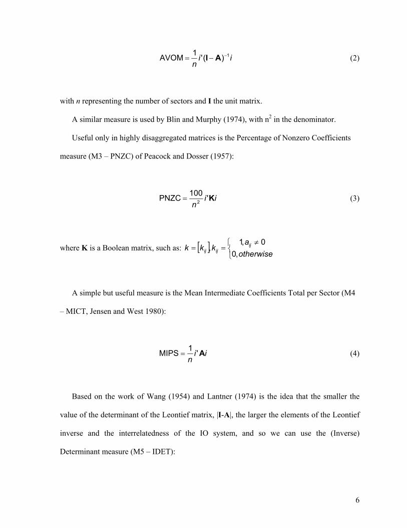
Another classical measure of connectedness is the Average Output Multiplier (M2 –

AVOM), based on Rasmussen (1956) and Hirschman (1958):

6

iin

1)('1AVOM −−= AI (2)

with n representing the number of sectors and I the unit matrix.

A similar measure is used by Blin and Murphy (1974), with n2 in the denominator.

Useful only in highly disaggregated matrices is the Percentage of Nonzero Coefficients

measure (M3 – PNZC) of Peacock and Dosser (1957):

iin

K'100PNZC 2= (3)

where K is a Boolean matrix, such as: [ ] ≠

==otherwisea

kkk ijijij ,0

0,1,

A simple but useful measure is the Mean Intermediate Coefficients Total per Sector (M4

– MICT, Jensen and West 1980):

iinA'1MIPS = (4)

Based on the work of Wang (1954) and Lantner (1974) is the idea that the smaller the

value of the determinant of the Leontief matrix, |I-A|, the larger the elements of the Leontief

inverse and the interrelatedness of the IO system, and so we can use the (Inverse)

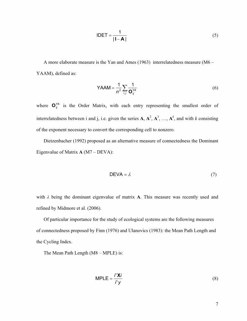
Determinant measure (M5 – IDET):

7

||1IDETAI−

= (5)

A more elaborate measure is the Yan and Ames (1963) interrelatedness measure (M6 –

YAAM), defined as:

∑=ji

YAijn ,

2

11YAAMO

(6)

where YAijO is the Order Matrix, with each entry representing the smallest order of

interrelatedness between i and j, i.e. given the series A, A2, A3, …, Ak, and with k consisting

of the exponent necessary to convert the corresponding cell to nonzero.

Dietzenbacher (1992) proposed as an alternative measure of connectedness the Dominant

Eigenvalue of Matrix A (M7 – DEVA):

λ=DEVA (7)

with λ being the dominant eigenvalue of matrix A. This measure was recently used and

refined by Midmore et al. (2006).

Of particular importance for the study of ecological systems are the following measures

of connectedness proposed by Finn (1976) and Ulanovics (1983): the Mean Path Length and

the Cycling Index.

The Mean Path Length (M8 – MPLE) is:

yiii

''MPLE X

= (8)

8

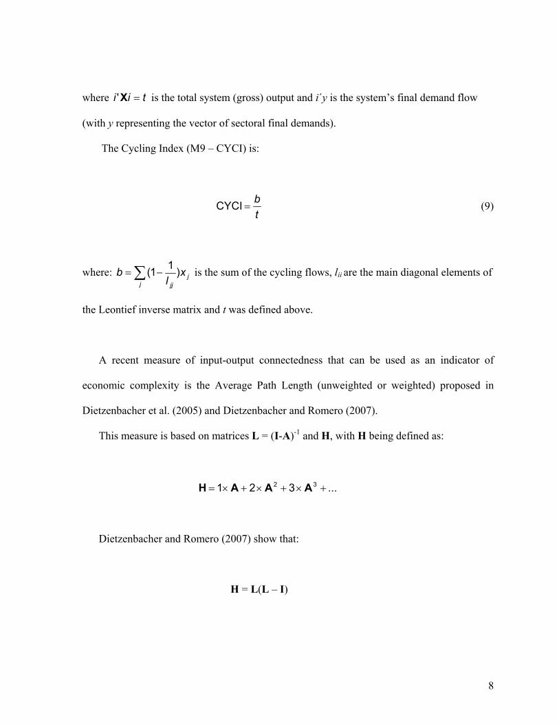
where tii =X' is the total system (gross) output and i´y is the system’s final demand flow

(with y representing the vector of sectoral final demands).

The Cycling Index (M9 – CYCI) is:

tb

=CYCI (9)

where: jj jj

xl

b )11(∑ −= is the sum of the cycling flows, lii are the main diagonal elements of

the Leontief inverse matrix and t was defined above.

A recent measure of input-output connectedness that can be used as an indicator of

economic complexity is the Average Path Length (unweighted or weighted) proposed in

Dietzenbacher et al. (2005) and Dietzenbacher and Romero (2007).

This measure is based on matrices L = (I-A)-1 and H, with H being defined as:

...321 32 +×+×+×= AAAH

Dietzenbacher and Romero (2007) show that:

H = L(L – I)

9

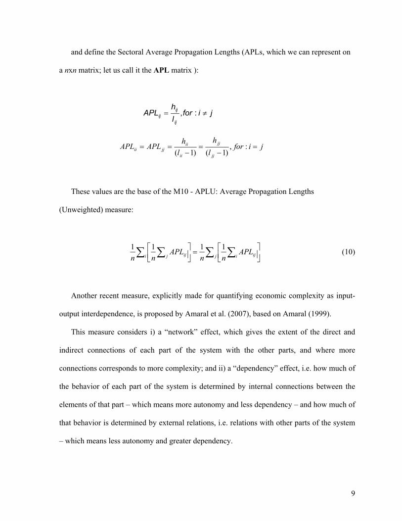
and define the Sectoral Average Propagation Lengths (APLs, which we can represent on

a nxn matrix; let us call it the APL matrix ):

jiforlh

APLij

ijij ≠= :,

jiforl

hl

hAPLAPL

jj

jj

ii

iijjii =

−=

−== :,

)1()1(

These values are the base of the M10 - APLU: Average Propagation Lengths

(Unweighted) measure:

∑ ∑∑ ∑

=

j i iji j ij APLnn

APLnn

1111 (10)

Another recent measure, explicitly made for quantifying economic complexity as input-

output interdependence, is proposed by Amaral et al. (2007), based on Amaral (1999).

This measure considers i) a “network” effect, which gives the extent of the direct and

indirect connections of each part of the system with the other parts, and where more

connections corresponds to more complexity; and ii) a “dependency” effect, i.e. how much of

the behavior of each part of the system is determined by internal connections between the

elements of that part – which means more autonomy and less dependency – and how much of

that behavior is determined by external relations, i.e. relations with other parts of the system

– which means less autonomy and greater dependency.

10

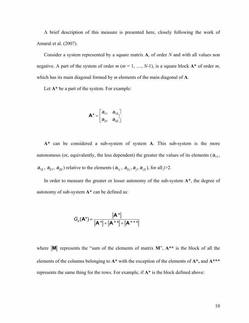
A brief description of this measure is presented here, closely following the work of

Amaral et al. (2007).

Consider a system represented by a square matrix A, of order N and with all values non

negative. A part of the system of order m (m = 1, …, N-1), is a square block A* of order m,

which has its main diagonal formed by m elements of the main diagonal of A.

Let A* be a part of the system. For example:

=

2221

1211*aaaa

A

A* can be considered a sub-system of system A. This sub-system is the more

autonomous (or, equivalently, the less dependent) the greater the values of its elements ( 11a ,

12a , 21a , 22a ) relative to the elements ( ja1 , ja2 , 1ja 2ja ), for all j>2.

In order to measure the greater or lesser autonomy of the sub-system A*, the degree of

autonomy of sub-system A* can be defined as:

*******

*)(AAA

AA

++=aG

where M represents the “sum of the elements of matrix M”, A** is the block of all the

elements of the columns belonging to A* with the exception of the elements of A*, and A***

represents the same thing for the rows. For example, if A* is the block defined above:

11

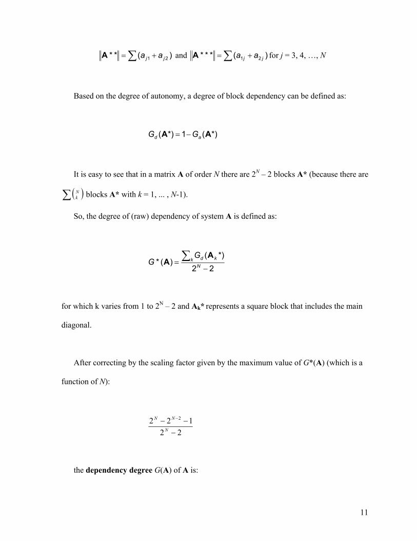
)(** 21 jj aa += ∑A and )(*** 21 jj aa += ∑A for j = 3, 4, …, N

Based on the degree of autonomy, a degree of block dependency can be defined as:

*)(1*)( AA ad GG −=

It is easy to see that in a matrix A of order N there are 2N – 2 blocks A* (because there are

( )∑ Nk blocks A* with k = 1, ... , N-1).

So, the degree of (raw) dependency of system A is defined as:

22*)(

)(*−

= ∑ Nk kdGG

AA

for which k varies from 1 to 2N – 2 and Ak* represents a square block that includes the main

diagonal.

After correcting by the scaling factor given by the maximum value of G*(A) (which is a

function of N):

22122 2

−−− −

N

NN

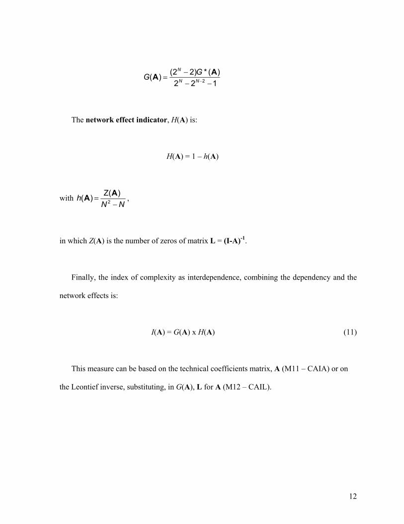
the dependency degree G(A) of A is:

12

122)(*)22()( 2 −−

−=

−NN

N GG AA

The network effect indicator, H(A) is:

H(A) = 1 – h(A)

with NN

h−

= 2

)Z( )( AA ,

in which Z(A) is the number of zeros of matrix L = (I-A)-1.

Finally, the index of complexity as interdependence, combining the dependency and the

network effects is:

I(A) = G(A) x H(A) (11)

This measure can be based on the technical coefficients matrix, A (M11 – CAIA) or on

the Leontief inverse, substituting, in G(A), L for A (M12 – CAIL).

13

3. MEASURING CONNECTEDNESS AND COMPLEXITY WITH OECD IO DATA

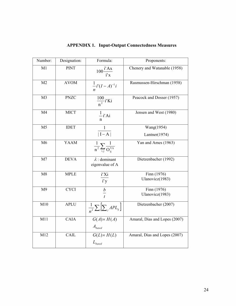
From the previous section, we end up with 12 measures of complexity as input-output

connectedness, listed in the table presented in Appendix 1.

In this section, we present the results of an empirical application of all these measures using

the Input-Output Tables of nine OECD economies in the early 1970s and early 1990s.

For the convenience of analysis, the original data is aggregated into the 17 sectors

presented in Appendix 2.

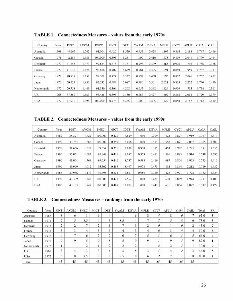
Tables 1 and 2 show the main results, i.e. the values of all the measures for all the

countries in the early 1970s and early 1990s.

INSERT TABLES 1 AND 2

A broad inspection of these values confirms the expected conclusions that the large

economies (Japan and USA) were in fact more complex, and that smaller economies tended

to be less complex (the Netherlands and Denmark), both in the 1970s and 1990s.

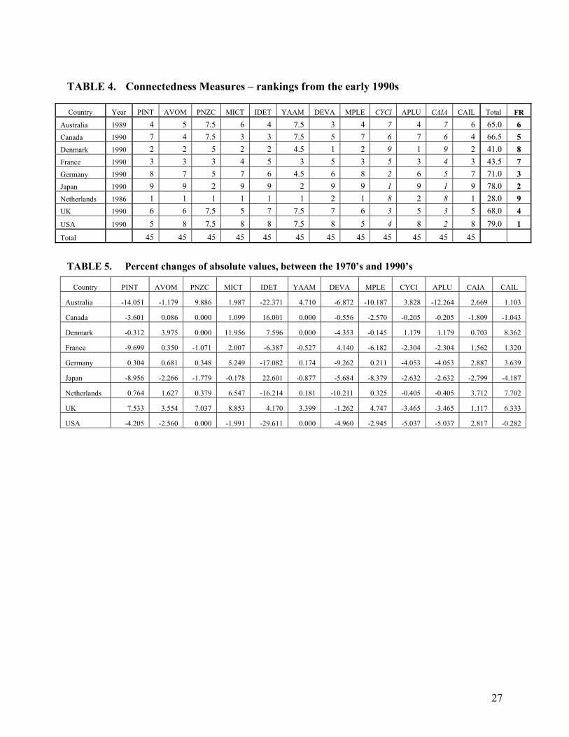
This can be clearly seen in Tables 3 and 4, where we present the rankings of countries for

each measure (9 points for the largest value, 1 point for the smallest) and the final ranking

based on all the measures (total number of points and relative position of each country).

INSERT TABLES 3 AND 4

14

Looking at the absolute values of the connectedness measures and their percentage

changes (Table 5) we also note a slight (and perhaps unexpected) reduction in the average

economic complexity, with a decreasing dispersion of countries along the “interrelatedness

scale function” but no significant relative changes, except in the UK, which rose from 8th in

the 1970s to 4th in the 1990s.

INSERT TABLE 5

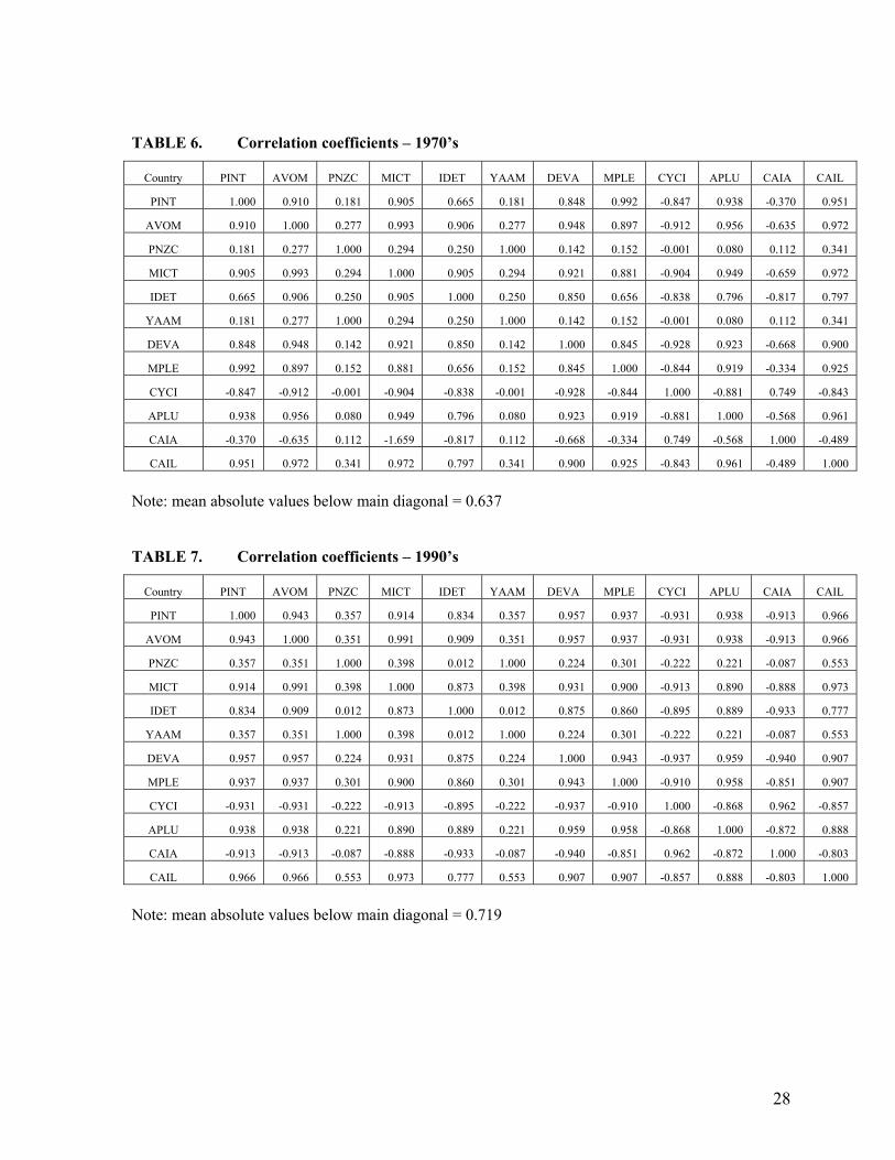
A closer inspection of the absolute values and rankings calls for a careful association of

the measures corresponding to different methodologies or conceptualizations of economic

complexity. This task can be better accomplished by analyzing the correlation coefficients

presented in Tables 6 and 7 and using the following definitions and results.

INSERT TABLES 6 AND 7

Let M be the set of the measures mi, r(i,j) the absolute value of the correlation coefficient

between mi and mj, and c the number 0 ≤ c ≤ 1.

Definition 1: A bundle B of measures of M is a set of elements of M such that, for every

pair (mi , mj ) of B, we have r(i,j) ≥ c and, for every mk of M-B, we have at least one mi of B

such that r(i,k) < c.

Two bundles B1 and B2 are perfectly separated when, for every mk of B1, we have r(k,i)

< c for every mi of B2.

15

Definition 2: An isolated measure ml is one in which the bundle where it belongs is the

degenerate bundle {ml}.

It is easy to see that the family of bundles of the measures of M is a partition of M as the

union of disjoint sets. However the set M may be partitioned in several ways.

Assumption (emergent concepts): For a set M that is partitioned into perfectly

separated bundles, each bundle B is interpreted as the emergence at the surface of a hidden

concept of interrelatedness.

When the bundles are not perfectly separated, the hidden concepts of interrelatedness are

called fuzzy concepts.

It is easy to see that if there is a perfectly separated partition it is the only perfectly

separated partition that exists.

Applying these concepts to the results of Tables 6 and 7, and taking as the value of c for

each of the years respectively the average of all the correlation coefficients, we have two

perfectly separated bundles for the 1990s:

B1 = {PINT, AVOM, MICT, IDET, DEVA, MPLE, CYCI, APLU, CAIA, CAIL}

B2 ={ PNZC, YAAM}.

This result indicates a clear distinction (at this level of aggregation – 17 sectors) between

measures based on Boolean (B2) and non-Boolean (B1) methods, which is probably only

interesting, or useful, for highly disaggregated matrices.

16

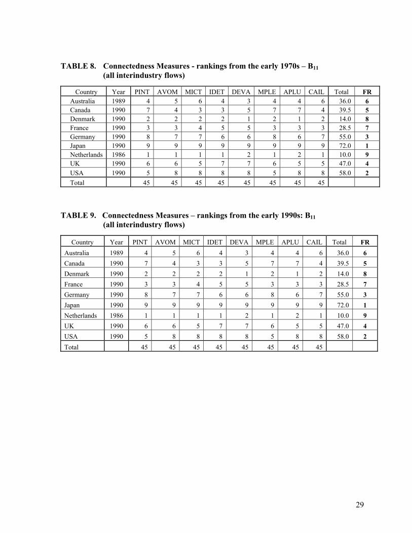
Another, more useful distinction is obtained by considering, within the domain of

strongly correlated non-Boolean measures, the correlation coefficients with positive and

negative signs, pointing to a further separation of bundles of this kind:

B11 = {PINT, AVOM, MICT, IDET, DEVA, MPLE, APLU, CAIL}

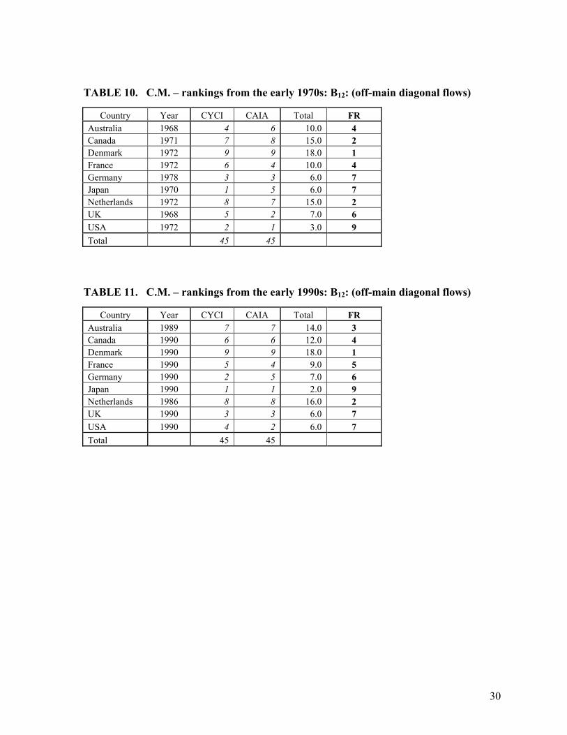
B12 = {CYCI, CAIA}

The closely related behavior of measures CYCI and CAIA is supposedly explained by the

fact that they explicitly exclude (direct) intra-dependence flows (the values of self-supplying

inputs or the coefficients in the main diagonal of matrix A), and that, in the sense of

complexity as (sectoral) interdependence, these are probably the most appropriate measures.

To explore this distinction further, it is useful to calculate the rankings of economic

complexity based on bundle B11 (Tables 8 and 9) and bundle B12 (Tables 10 and 11).

INSERT TABLES 8, 9, 10 AND 11

The interesting result is, of course, that, according to this particular notion of complexity

as interdependence, large economies appear to be less complex than small ones and

complexity does not necessarily increase as economies grow and develop. But the full

understanding of all the forces behind this surprising result would require further research.

17

Looking at the correlation coefficients of the early 1970s, a degenerate bundle exists with

the isolated measure M11 - CAIA, pointing to an autonomous emergent concept of economic

complexity, which did not persist into the 1990s.

4. CONCLUDING REMARKS

Connectedness is a crucial feature of input-output analysis, which can be used for

studying economic complexity as sectoral interdependence.

There are many ways to quantify connectedness, and it is a useful exercise to compare

different measures, both theoretically and empirically.

In this paper, a menu of twelve measures is presented and briefly discussed. All these

measures are quantified using an input-output database of nine OECD countries in the early

1970s and 1990s, which gives us an interesting inter-country comparison and shows us two

decades in the evolution of economic complexity as sectoral interdependence.

Looking at the absolute values of the measures, it appears that large economies (Japan

and USA) are more “intensely connected” (and so, more complex) than small ones (the

Netherlands, Denmark). It also appears that there is a slight reduction in complexity and a

decreasing dispersion of countries along the “interrelatedness scale”, with one peculiar

exception of complex upgrading (the UK).

A closer inspection of the values, applying a method of identifying emergent concepts

using the correlation coefficients, points to the emergence of three bundles of measures: a

Boolean-based group of two measures with weak correlation with all the others; a group of

eight measures based on all technical coefficients (and production multipliers), with strong

positive correlations between them and weak positive correlations with the Boolean group; a

18

bundle of two measures that explicitly exclude intra-sectoral flows, negatively correlated

with all the others, but probably the most appropriate for measuring complexity as (sectoral)

interdependence.

According to the majority bundle of (more conventional) measures of connectedness,

large economies seem to be more complex than small ones. The bundle of two measures

excluding (direct) intra-sectoral flows, on the other hand, points to the opposite conclusion,

but this surprising result needs to be confirmed with further theoretical and empirical

research.

REFERENCES Adami, C. 2002. What is complexity? BioEssays 24: 1085-94.

Amaral, J. F. 1999. Complexity and Information in Economic Systems. In Perspectives on

Complexity in Economics, ed. F. Louçã, ISEG-UTL, Lisbon Technical University.

Amaral, J. F., J. Dias and J. Lopes. 2007. Complexity as interdependence in input-output

systems. Environment and Planning A 39: 1170-82.

Aroche-Reyes, F. 1996. Important coefficients and structural change: a multi-layer approach.

Economic Systems Research 8: 235-46.

Aroche-Reyes, F. 2003. A qualitative input-output method to find basic economic structures.

Papers in Regional Science. 82: 581-90.

Arthur, B. 1999. Complexity and the Economy. Science 284: 107-9.

Basu, R. and T. G. Johnson. 1996. The development of a measure of intersectoral

connectedness by using structural path analysis. Environment and Planning A 28: 709-30.

19

Blin, J. M. and F. H. Murphy. 1974. On measuring economic interrelatedness. Review of

Economics and Statistics 41: 437-40.

Bosserman, R. W. 1982. Complexity measures for evaluation of ecosystems networks.

International Society for Ecological Modeling Journal 4: 37-9.

Cai, J. and P. Leung, 2004. Linkage measures: A revisit and a suggested alternative.

Economic Systems Research 16: 65-85.

Campbell, J. 1975. Application of Graph Theoretic Analysis to Interindustry Relationships.

Regional Science and Urban Economics. 5: 91-106.

Chenery, H. B. and T. Watanabe. 1958. Interregional comparisons of the structure of

production. Econometrica 26: 487-521.

Czamansky, S. 1974. Study of Clustering of Industries. Institute of Public Affairs, Dalhousie

University, Halifax, Canada.

Dietzenbacher, E. 1992. The measurement of interindustry linkages: Key sectors in the

Netherlands. Economic Modelling 9: 419-37.

Dietzenbacher, E., and B. Los. 2002. Externalities of R&D Expenditures. Economic Systems

Research 14: 407-25.

Dietzenbacher, E., I. Romero Luna and N. S. Bosma. 2005. Using average propagation

lengths to identify production chains in the Andalusian economy. Estudios de

Economía Aplicada 23: 405-22.

Dietzenbacher, E. and I. Romero. 2007. Production Chains in an Interregional Framework:

Identification by Means of Average Propagation Lengths. International Regional

Science Review 30: 362-83.

20

Dridi, C. and G. Hewings. 2002. Industry Associations, Association Loops and Economic

Complexity: Application to Canada and the United States. Economic Systems Research

14: 275-96.

Durlauf, S. 2003. Complexity and Empirical Economics. Santa Fe Institute Working Paper.

Finn, J. T. 1976. Measures of ecosystem structure and function derived from analysis of

flows. Journal of Theoretical Biology 56: 363-80.

Hamilton, J. R. and R. C. Jensen.1983. Summary measures of interconnectedness for input-

output models. Environment and Planning A 15: 55-65.

Hirshman, A. O. 1958. The Strategy of Economic Development. Yale University Press, New

Haven, CT.

Jackson, M. O. 2006. The economics of social networks. In Advances in Economics and

Econometrics. Theory and Applications, Ninth World Congress of the Econometric

Society, vol. 1, eds. R. Blundell, W. Newey and T. Persson. Cambridge: Cambridge

University Press.

Jensen, R. C. and G. West. 1980. The effect of relative coefficient size on input-output

multipliers. Environment and Planning A 12: 659-70.

Jensen, R. C., G. Hewings and G. West. 1987. On a Taxonomy of Economies, Australian

Journal of Regional Studies 2: 3-24.

Lantner, R. 1974. Théorie de la Dominance Economique. Dunod, Paris.

Lantner, R., and R. Carluer. 2004. Spatial dominance: a new approach to the estimation of

interconnectedness in regional input-output tables. The Annals of Regional Science, 38:

451-67.

Laumas, P. S. 1975. Key sectors in some underdeveloped countries, Kyklos 28: 62-79.

21

LeBaron, B., and L. Tesfatsion 2008. Modeling Macroeconomies as Open-Ended Dynamic

Systems of Interacting Agents, American Economic Review, 98: 246-50.

Midmore, P., M. Munday and A. Roberts. 2006. Assessing Industry Linkages Using

Regional Input-Output Tables. Regional Studies 40: 329-43.

Muñiz, A., A. Raya and C. Carvajal. 2008. Key Sectors: A New Proposal from Network

Theory. Regional Studies: online/08/000001-18.

Okuyama, Y. 2007. Economic Modeling for Disaster Impact Analysis. Economic Systems

Research 19: 115-24.

Peacock, A. T. and D. Dosser. 1957. Input-output analysis in an underdeveloped country: a

case study. The Review of Economic Studies 25: 21-4.

Rasmussen, P. N. 1957. Studies in Intersectoral Relations. North-Holland, Amsterdam.

Robinson, S. and A. Markandya. 1973. Complexity and adjustment in input-output systems.

Oxford Bulletin of Economics and Statistics 35: 119-34.

Rosser, Jr. J. 1999. On the Complexity of Complex Economic Dynamics. Journal of

Economic Perspectives 13: 169-92.

Schnabl, H. 1994. The evolution of production structures analysed by a multi-layer

procedure. Economic Systems Research 6: 51-68.

Schnabl, H. 1995. The Subsystem-MFA: A Qualitative Method for Analyzing National

Innovation Systems – The Case of Germany. Economic Systems Research 7: 383-96.

Simpson, D. and M. Tsukui. 1965. The fundamental structure of input-output tables, an

international comparison, Review of Economics and Statistics 47: 434-46.

22

Sonis, M. and G. J. D. Hewings. 1991. Fields of influence and extended input-output

analysis: a theoretical account. In Anselin L. and M. Madden, eds. New Directions in

Regional Analysis: Integrated and Multiregional Approaches. Pinter, London.

Sonis, M., J. Guilhoto, G. J. D. Hewings and E. Martins. 1995. Linkages, key sectors and

structural change: some new perspectives, The Developing Economies 33: 233-70.

Sonis, M., G. J. G. Hewings and E. Haddad. 1996. A typology of propagation of changes on

the structure of a multiregional economic system: The case of the European Union,

1975-1985. Annals of Regional Science 30: 391-408.

Sonis, M. and G. J. D. Hewings. 1998. Economic complexity as network complication:

Multiregional input-output structural path analysis. Annals of Regional Science 32: 407-

36.

Steinback, S. R. 2004. Using ready-made regional input-output models to estimate backward-

linkage effects of exogenous output shocks. Review of Regional Studies 34: 57-71.

Szyrmer, J. M. 1985. Measuring connectedness of input-output models: 1. Survey of the

measures. Environment and Planning A 17: 1567-600.

Szyrmer, J. M. 1986. Measuring connectedness of input-output models: 2. Total flow

concept. Environment and Planning A 18: 107-21.

Takur, S. 2008. Identification of temporal fundamental economic structure (FES) of India:

An input-output and cross-entropy analysis. Structural Change and Economic

Dynamics 19: 132-51.

Ulanovicz, R E. 1983. Identifying the structure of cycling in ecosystems. Mathematical

Biosciences 65: 219-37.

23

Van Der Linden, J., J. Oosterhaven, F. Cuello, G. Hewings and M. Sonis. 2000. Fields of

influence of productivity change in EU inter-country input-output tables, 1970-1980.

Environment and Planning A 32: 1287-305.

Wang, S. 2001. The Neural Network Approach to Input-Output Analysis for Economic

Systems. Neural Computing & Applications 10: 22-8.

Waldrop, M. 1992. Complexity: The Emerging Science at the Edge of Order and Chaos,

Penguin Books, London.

Wasserman, S. and K. Faust. 1994. Social Network Analysis: Methods and Applications,

(Structural Analysis in the Social Sciences). Cambridge University Press, New York.

Wong, Y. K. 1954. Some mathematical concepts for linear economic models. In Economic

Activity Analysis, ed. O. Morgenstern, 283-341. Wiley, New York.

Yan, C. and E. Ames. 1965. Economic Interrelatedness. The Review of Economic Studies 32:

290-310.

Zucchetto, J. 1981. Energy diversity of regional economies. In Energy and Ecological

Modeling, eds. W. S. Mitsch, R. W. Bosserman, and J. M. Klopatek, 543-48. Elsevier,

Amsterdam.

24

APPENDIX 1. Input-Output Connectedness Measures

Number: Designation: Formula: Proponents:

M1 PINT

x'iAx'i100

Chenery and Watanable (1958)

M2

AVOM

iAIi

n1)('1 −−

Rasmussen-Hirschman (1958)

M3

PNZC

Ki'i

n100

2 Peacock and Dosser (1957)

M4

MICT

Ai'i

n1

Jensen and West (1980)

M5 IDET

|AI|1−

Wang(1954)

Lantner(1974)

M6

YAAM ∑

j,iYAij

2 O1

n1

Yan and Ames (1963)

M7 DEVA

λ : dominant eigenvalue of A

Dietzenbacher (1992)

M8

MPLE

y'iXi'i

Finn (1976)

Ulanovicz(1983)

M9

CYCI

tb

Finn (1976)

Ulanovicz(1983)

M10

APLU

[ ]∑ ∑i j ijAPL

n2

1 Dietzenbacher (2007)

M11

CAIA

basedAAHAG )()( ×

Amaral, Dias and Lopes (2007)

M12

CAIL

basedLLHLG )()( ×

Amaral, Dias and Lopes (2007)

25

APPENDIX 2. Sectors used in analysis

1 Agriculture, mining & quarrying

2 Food, beverages & tobacco

3 Textiles, apparel & leather

4 Wood and paper

5 Chemicals, drugs, oil and plastics

6 Minerals and metals

7 Electrical and non-electrical equipment

8 Transport equipment

9 Other manufacturing

10 Electricity, gas & water

11 Construction

12 Wholesale & retail trade

13 Restaurants & hotels

14 Transport & storage

15 Communication

16 Finance & insurance

17 Other sectors

26

TABLE 1. Connectedness Measures – values from the early 1970s

Country Year PINT AVOM PNZC MICT IDET YAAM DEVA MPLE CYCI APLU CAIA CAIL

Australia 1968 44.667 1.742 91.004 0.420 8.539 0.955 0.428 1.807 0.864 2.188 0.747 0.406

Canada 1971 42.287 1.685 100.000 0.395 5.231 1.000 0.416 1.733 0.899 2.041 0.779 0.404

Denmark 1972 31.755 1.473 99.654 0.318 3.381 0.998 0.329 1.465 0.926 1.705 0.786 0.328

France 1972 41.030 1.678 96.886 0.407 8.639 0.984 0.395 1.691 0.869 1.959 0.737 0.381

Germany 1978 40.939 1.757 99.308 0.424 10.537 0.997 0.458 1.693 0.857 2.046 0.732 0.402

Japan 1970 50.524 1.956 97.232 0.484 15.087 0.986 0.501 2.021 0.825 2.272 0.740 0.450

Netherlands 1972 29.758 1.449 91.350 0.304 4.298 0.957 0.368 1.424 0.909 1.735 0.754 0.301

UK 1968 37.560 1.683 93.426 0.393 9.180 0.967 0.427 1.602 0.868 2.014 0.729 0.379

USA 1972 41.916 1.898 100.000 0.478 18.285 1.000 0.465 1.722 0.858 2.187 0.712 0.430 TABLE 2. Connectedness Measures – values from the early 1990s

Country Year PINT AVOM PNZC MICT IDET YAAM DEVA MPLE CYCI APLU CAIA CAIL

Australia 1989 38.391 1.722 100.000 0.429 6.629 1.000 0.399 1.623 0.897 1.919 0.767 0.410

Canada 1990 40.764 1.686 100.000 0.399 6.068 1.000 0.414 1.688 0.891 2.037 0.765 0.400

Denmark 1990 31.656 1.532 99.654 0.356 3.638 0.998 0.315 1.463 0.922 1.725 0.791 0.355

France 1990 37.051 1.683 95.848 0.416 8.087 0.979 0.411 1.586 0.883 1.914 0.748 0.386

Germany 1990 41.064 1.769 99.654 0.446 8.737 0.998 0.416 1.697 0.864 1.963 0.753 0.416

Japan 1990 45.999 1.912 95.502 0.483 18.497 0.978 0.473 1.852 0.844 2.212 0.719 0.432

Netherlands 1986 29.986 1.473 91.696 0.324 3.601 0.959 0.330 1.428 0.921 1.728 0.782 0.324

UK 1990 40.389 1.743 100.000 0.428 9.562 1.000 0.421 1.678 0.859 1.944 0.737 0.403

USA 1990 40.153 1.849 100.000 0.468 12.871 1.000 0.442 1.671 0.864 2.077 0.732 0.429

TABLE 3. Connectedness Measures – rankings from the early 1970s

Country Year PINT AVOM PNZC MICT IDET YAAM DEVA MPLE CYCI APLU CAIA CAIL Total FR

Australia 1968 8 6 1 6 4 1 6 8 4 8 6 7 65.0 5 Canada 1971 7 5 8.5 4 3 8.5 4 7 7 5 8 6 73.0 3 Denmark 1972 2 2 7 2 1 7 1 2 9 1 9 2 45.0 7 France 1972 5 3 4 5 5 4 3 4 6 3 4 4 50.0 6 Germany 1978 4 7 6 7 7 6 7 5 3 6 3 5 66.0 4 Japan 1970 9 9 5 9 8 5 9 9 1 9 5 9 87.0 1 Netherlands 1972 1 1 2 1 2 2 2 1 8 2 7 1 30.0 9 UK 1968 3 4 3 3 6 3 5 3 5 4 2 3 44.0 8 USA 1972 6 8 8.5 8 9 8.5 8 6 2 7 1 8 80.0 2 Total 45 45 45 45 45 45 45 45 45 45 45 45

27

TABLE 4. Connectedness Measures – rankings from the early 1990s

TABLE 5. Percent changes of absolute values, between the 1970’s and 1990’s

Country Year PINT AVOM PNZC MICT IDET YAAM DEVA MPLE CYCI APLU CAIA CAIL Total FR

Australia 1989 4 5 7.5 6 4 7.5 3 4 7 4 7 6 65.0 6 Canada 1990 7 4 7.5 3 3 7.5 5 7 6 7 6 4 66.5 5 Denmark 1990 2 2 5 2 2 4.5 1 2 9 1 9 2 41.0 8 France 1990 3 3 3 4 5 3 5 3 5 3 4 3 43.5 7 Germany 1990 8 7 5 7 6 4.5 6 8 2 6 5 7 71.0 3 Japan 1990 9 9 2 9 9 2 9 9 1 9 1 9 78.0 2 Netherlands 1986 1 1 1 1 1 1 2 1 8 2 8 1 28.0 9 UK 1990 6 6 7.5 5 7 7.5 7 6 3 5 3 5 68.0 4 USA 1990 5 8 7.5 8 8 7.5 8 5 4 8 2 8 79.0 1 Total 45 45 45 45 45 45 45 45 45 45 45 45

Country PINT AVOM PNZC MICT IDET YAAM DEVA MPLE CYCI APLU CAIA CAIL

Australia -14.051 -1.179 9.886 1.987 -22.371 4.710 -6.872 -10.187 3.828 -12.264 2.669 1.103

Canada -3.601 0.086 0.000 1.099 16.001 0.000 -0.556 -2.570 -0.205 -0.205 -1.809 -1.043

Denmark -0.312 3.975 0.000 11.956 7.596 0.000 -4.353 -0.145 1.179 1.179 0.703 8.362

France -9.699 0.350 -1.071 2.007 -6.387 -0.527 4.140 -6.182 -2.304 -2.304 1.562 1.320

Germany 0.304 0.681 0.348 5.249 -17.082 0.174 -9.262 0.211 -4.053 -4.053 2.887 3.639

Japan -8.956 -2.266 -1.779 -0.178 22.601 -0.877 -5.684 -8.379 -2.632 -2.632 -2.799 -4.187

Netherlands 0.764 1.627 0.379 6.547 -16.214 0.181 -10.211 0.325 -0.405 -0.405 3.712 7.702

UK 7.533 3.554 7.037 8.853 4.170 3.399 -1.262 4.747 -3.465 -3.465 1.117 6.333

USA -4.205 -2.560 0.000 -1.991 -29.611 0.000 -4.960 -2.945 -5.037 -5.037 2.817 -0.282

28

TABLE 6. Correlation coefficients – 1970’s

Country PINT AVOM PNZC MICT IDET YAAM DEVA MPLE CYCI APLU CAIA CAIL

PINT 1.000 0.910 0.181 0.905 0.665 0.181 0.848 0.992 -0.847 0.938 -0.370 0.951

AVOM 0.910 1.000 0.277 0.993 0.906 0.277 0.948 0.897 -0.912 0.956 -0.635 0.972

PNZC 0.181 0.277 1.000 0.294 0.250 1.000 0.142 0.152 -0.001 0.080 0.112 0.341

MICT 0.905 0.993 0.294 1.000 0.905 0.294 0.921 0.881 -0.904 0.949 -0.659 0.972

IDET 0.665 0.906 0.250 0.905 1.000 0.250 0.850 0.656 -0.838 0.796 -0.817 0.797

YAAM 0.181 0.277 1.000 0.294 0.250 1.000 0.142 0.152 -0.001 0.080 0.112 0.341

DEVA 0.848 0.948 0.142 0.921 0.850 0.142 1.000 0.845 -0.928 0.923 -0.668 0.900

MPLE 0.992 0.897 0.152 0.881 0.656 0.152 0.845 1.000 -0.844 0.919 -0.334 0.925

CYCI -0.847 -0.912 -0.001 -0.904 -0.838 -0.001 -0.928 -0.844 1.000 -0.881 0.749 -0.843

APLU 0.938 0.956 0.080 0.949 0.796 0.080 0.923 0.919 -0.881 1.000 -0.568 0.961

CAIA -0.370 -0.635 0.112 -1.659 -0.817 0.112 -0.668 -0.334 0.749 -0.568 1.000 -0.489

CAIL 0.951 0.972 0.341 0.972 0.797 0.341 0.900 0.925 -0.843 0.961 -0.489 1.000

Note: mean absolute values below main diagonal = 0.637

TABLE 7. Correlation coefficients – 1990’s

Country PINT AVOM PNZC MICT IDET YAAM DEVA MPLE CYCI APLU CAIA CAIL

PINT 1.000 0.943 0.357 0.914 0.834 0.357 0.957 0.937 -0.931 0.938 -0.913 0.966

AVOM 0.943 1.000 0.351 0.991 0.909 0.351 0.957 0.937 -0.931 0.938 -0.913 0.966

PNZC 0.357 0.351 1.000 0.398 0.012 1.000 0.224 0.301 -0.222 0.221 -0.087 0.553

MICT 0.914 0.991 0.398 1.000 0.873 0.398 0.931 0.900 -0.913 0.890 -0.888 0.973

IDET 0.834 0.909 0.012 0.873 1.000 0.012 0.875 0.860 -0.895 0.889 -0.933 0.777

YAAM 0.357 0.351 1.000 0.398 0.012 1.000 0.224 0.301 -0.222 0.221 -0.087 0.553

DEVA 0.957 0.957 0.224 0.931 0.875 0.224 1.000 0.943 -0.937 0.959 -0.940 0.907

MPLE 0.937 0.937 0.301 0.900 0.860 0.301 0.943 1.000 -0.910 0.958 -0.851 0.907

CYCI -0.931 -0.931 -0.222 -0.913 -0.895 -0.222 -0.937 -0.910 1.000 -0.868 0.962 -0.857

APLU 0.938 0.938 0.221 0.890 0.889 0.221 0.959 0.958 -0.868 1.000 -0.872 0.888

CAIA -0.913 -0.913 -0.087 -0.888 -0.933 -0.087 -0.940 -0.851 0.962 -0.872 1.000 -0.803

CAIL 0.966 0.966 0.553 0.973 0.777 0.553 0.907 0.907 -0.857 0.888 -0.803 1.000

Note: mean absolute values below main diagonal = 0.719

29

TABLE 8. Connectedness Measures - rankings from the early 1970s – B11 (all interindustry flows)

Country Year PINT AVOM MICT IDET DEVA MPLE APLU CAIL Total FR Australia 1989 4 5 6 4 3 4 4 6 36.0 6 Canada 1990 7 4 3 3 5 7 7 4 39.5 5 Denmark 1990 2 2 2 2 1 2 1 2 14.0 8 France 1990 3 3 4 5 5 3 3 3 28.5 7 Germany 1990 8 7 7 6 6 8 6 7 55.0 3 Japan 1990 9 9 9 9 9 9 9 9 72.0 1 Netherlands 1986 1 1 1 1 2 1 2 1 10.0 9 UK 1990 6 6 5 7 7 6 5 5 47.0 4 USA 1990 5 8 8 8 8 5 8 8 58.0 2 Total 45 45 45 45 45 45 45 45

TABLE 9. Connectedness Measures – rankings from the early 1990s: B11

(all interindustry flows)

Country Year PINT AVOM MICT IDET DEVA MPLE APLU CAIL Total FR Australia 1989 4 5 6 4 3 4 4 6 36.0 6 Canada 1990 7 4 3 3 5 7 7 4 39.5 5 Denmark 1990 2 2 2 2 1 2 1 2 14.0 8 France 1990 3 3 4 5 5 3 3 3 28.5 7 Germany 1990 8 7 7 6 6 8 6 7 55.0 3 Japan 1990 9 9 9 9 9 9 9 9 72.0 1 Netherlands 1986 1 1 1 1 2 1 2 1 10.0 9 UK 1990 6 6 5 7 7 6 5 5 47.0 4 USA 1990 5 8 8 8 8 5 8 8 58.0 2 Total 45 45 45 45 45 45 45 45

30

TABLE 10. C.M. – rankings from the early 1970s: B12: (off-main diagonal flows)

Country Year CYCI CAIA Total FR Australia 1968 4 6 10.0 4 Canada 1971 7 8 15.0 2 Denmark 1972 9 9 18.0 1 France 1972 6 4 10.0 4 Germany 1978 3 3 6.0 7 Japan 1970 1 5 6.0 7 Netherlands 1972 8 7 15.0 2 UK 1968 5 2 7.0 6 USA 1972 2 1 3.0 9 Total 45 45

TABLE 11. C.M. – rankings from the early 1990s: B12: (off-main diagonal flows)

Country Year CYCI CAIA Total FR Australia 1989 7 7 14.0 3 Canada 1990 6 6 12.0 4 Denmark 1990 9 9 18.0 1 France 1990 5 4 9.0 5 Germany 1990 2 5 7.0 6 Japan 1990 1 1 2.0 9 Netherlands 1986 8 8 16.0 2 UK 1990 3 3 6.0 7 USA 1990 4 2 6.0 7 Total 45 45