arX

iv:h

ep-t

h/99

1015

7v3

22

Nov

200

0

IITAP-99-012 INR-1029/99 hep-th/9910157

Canonical Formulation of the Light-Front Gluodynamics

and Quantization of the Non-Abelian Plane Waves

Victor T. Kim†&, Victor A. Matveev‡, Grigorii B. Pivovarov‡&

andJames P. Vary §&

† : St.Petersburg Nuclear Physics Institute, Gatchina 188350, Russia‡ : Institute for Nuclear Research, Moscow 117312, Russia

§ : Department of Physics and Astronomy,

Iowa State University, Ames, Iowa 50011, USA

& : International Institute of Theoretical and Applied Physics,

Iowa State University, Ames, Iowa 50011-3022, USA

Abstract

Without a gauge fixing, canonical variables for the light-front SU(2) gluo-

dynamics are determined. The Gauss law is written in terms of the canonical

variables. The system is qualified as a generalized dynamical system with first

class constraints. Abeliazation is a specific feature of the formulation (most

of the canonical variables transform nontrivially only under the action of an

Abelian subgroup of the gauge transformations). At finite volume, a discrete

spectrum of the light-front Hamiltonian P+ is obtained in the sector of van-

ishing P−. We obtain, therefore, a quantized form of the classical solutions

previously known as non-Abelian plane waves. Then, considering the infinite

volume limit, we find that the presence of the mass gap depends on the way

the infinite volume limit is taken, which may suggest the presence of different

“phases” of the infinite volume theory. We also check that the formulation

obtained is in accord with the standard perturbation theory if the latter is

taken in the covariant gauges.

to appear in Physical Review D

PACS numbers: 12.38.Aw, 12.38.Lg

Typeset using REVTEX

1

I. INTRODUCTION

The light-front formulation of relativistic dynamics has been widely discussed since thework of Dirac [1]. Its virtue is the presence of a kinematic semi-positive observable, themomentum component P−. It generates shifts along the longitudinal direction x− = (x0 −x3)/

√2 at a fixed light-front time x+ = (x0 + x3)/

√2. As such, it should be quadratic

in the canonical variables even in the presence of an interaction (such variables are calledkinematic). For a system with no tachyons (P 2 = P−P+ − P 2

⊥ ≥ 0, P0 ≥ 0), P− is semi-positive, and the subspace annihilated by P− contains the translation invariant vacuumstate. In addition, for a system with no massless states (i.e. having a mass gap), the abovesubspace contains only the states of vanishing four-momentum. Therefore, in the light-frontformulation, finding the vacuum state and the Fock space of such a system are kinematicproblems.

The light-front formulation also induces a specific kind of intuition believed to be valu-able in many physical situations (for a review, see Refs. [2]). For example, the light-frontformulation turns out to be closely related to the infinite momentum frame limit [3], and tothe notion of constituent quarks [4]. We also note that the light-front formulation in a finitevolume appears in discussions of recent developments of M-theory [5].

Thus, the light-front formulation of gauge theories and, in particular, of gluodynamics,is a worthwhile goal. However, up to the moment, the light-front formulation of the gaugetheories is less well developed, in our opinion, than the conventional equal-time formulation.The reason for the above assertion is that, to overcome technical difficulties, the light-frontformulation has been confined to fixed gauges (almost always, to the light-cone gauge [6–8],or to other gauges [9,10]). On the other hand, a general formulation of a gauge theory(see, e.g., Ref. [11]) may better start with a determination of the canonical variables priorto any gauge fixing. In the case of the equal-time formulation of the gauge theories, thecanonical variables are E and A. With this accomplished, one is to find the constraintsand calculate the algebra of the Poisson brackets involving the constraints and the Hamil-tonian. After that, the system is qualified as a generalized dynamical system with firstclass constraints (the case of the equal-time formulation of the gauge theories), and a well-developed machinery to treat such a system, in particular, by fixing a gauge and introducingthe Faddeev–Popov ghosts, becomes available.

In this paper, we determine the canonical variables of the light-front SU(2) gluodynamicswithout a gauge fixing. The light-front version of the Gauss law is also determined, andthe system is qualified as a generalized dynamical system with first class constraints. Thus,the light-front formulation of a gauge theory is established on a par with the conventionalequal-time formulation.

A specific feature of the formulation obtained is that it has a form of an Abelian gaugetheory, because most of the canonical variables transform nontrivially only under the actionof the Abelian subgroup of the gauge transformations which leaves the component A− ofthe gauge field invariant. Thus, we obtain a version of the Abelian projection [12] withouta gauge fixing.

Quantization of the dynamical system obtained involves the ambiguity of ordering. Wefix it in the simplest way, and then check that our choice leads to the standard Feynmanrules in the covariant gauges.

2

We also consider a gauge invariant reduction of the dynamics to the configurations ofzero P−. To this end, we diagonalize P−, i.e., identify the excitations carrying the nonzeroquanta of the longitudinal momentum. Then, the reduction is obtained by nullifying thecanonical variables corresponding to these quanta. If there is a mass gap in gluodynamics,and the light-front formulation is “correct” (i.e., equivalent to the equal-time formulation),we expect the light-front Hamiltonian P+ to be vanishing on the equations of motion of thisreduced dynamics. While the reduced dynamics is indeed much simpler than the completeone, the vanishing of P+ is not evident.

This brings up another important issue, namely, the dependence of the formulation onthe infrared regularization. To determine the canonical variables, we need to introduce agauge invariant infrared cutoff. In this paper, we use a compactification on a torus imposingperiodic boundary conditions on the gauge fields along the x− direction. Then, it turns outthat the reduced P+ does vanish on field configurations decaying fast enough at the infinityof the transverse plane, and is nontrivial on the configurations of nonzero asymptotics at thetransverse infinity. Not surprisingly, in the latter case, the above reduced dynamics turnsout to be a dynamics of the zero modes [13], i.e., of the fields with an imposed dependenceon the longitudinal and transverse space coordinates. The classical solutions of the gaugefield equations obtained in the framework of the reduced dynamics coincide up to a gaugewith the previously known “non-Abelian plane wave” solutions due to Coleman [14]. Theinvariance of the quantum theory with respect to certain “large” gauge transformations givesa quantization condition for these non-Abelian plane waves. Therefore, the spectrum of P+

on the subspace of vanishing P− turns out in this case to be discrete, bounded from below,and the quantum of the spectrum is proportional to (g2L)/V⊥, where V⊥ is the volumeof the compactified transverse plane, g is the gauge coupling, and L is the length of thecompactified direction x−. Note that this scaling of the quantum of the light-front energyholds for any nonzero number of the transverse dimensions, and the presence of the couplingmakes the dimension correct.

We conclude that there is no mass gap in the finite volume light-front gluodynamics. Onthe other hand, the spectrum of the light-front gluodynamics at infinite volume is qualita-tively dependent on the way the infinite volume limit is taken. If L is taken to infinity first,the mass gap can be generated. If V⊥ is taken to infinity before L, the resulting theory, if itexists, has no mass gap. Therefore, this can indicate that the finite volume theory containsmarkers (V⊥ and L) for different “phases” of the infinite volume theory.

The rest of the paper is organized as follows. In Section 2, we define the canonicalvariables for SU(2) gluodynamics without a gauge fixing, using Faddeev-Jackiw approachto constrained systems [15]. Then, in Section 3, we present the light-front Gauss law,which, in analogy with the equal-time formulation, generate the local gauge transformationsof the canonical variables. In Section 4, we write the equation for the zero modes which isnecessary to determine the light-front Hamiltonian. In Section 5, we discuss the quantizationambiguity, and check that the simplest prescription for fixing the ambiguity leads to thestandard Feynman rules in the covariant gauges. In Section 6, we show that the reduceddynamics at P− = 0 leads to non-Abelian plane waves solutions, and we find their quantumspectrum. Section 6 contains discussion and conclusion.

3

II. CANONICAL VARIABLES

We start with the action of the SU(2) gluodynamics:

Sglue =∫

dx+dx−dx⊥[1

2F a

+−Fa+− + F a

−kFa+k −

1

2F a

12Fa12

]

, (1)

where x± = (x0 ± x3)/√

2; x⊥ = x1,2; F aµν = ∂µA

aν − ∂νA

aµ + gǫabcAb

µAcν is a strength tensor

of the gauge field Aaµ; a, b, c, ... are color indices running from 1 to 3, and k is a Lorentz

transverse index running from 1 to 2.Our aim is to give a canonical formulation of the system (1) with x+ as time. To this end,

we will make a chain of transformations of the field variables. Every transformation will beone-to-one, or will introduce new auxiliary variables expressible via the initial variables. Ateach step, we will keep track of the form that the terms of the action with the time derivativesassume. Ultimately we will obtain the canonical form,

∑

i piqi (the overdot denotes the timederivative), for these terms, and will recognize pi and qi as canonically conjugated variables.This way of treatment is in the spirit of the Faddeev–Jackiw approach to constrained systems[15].

What complicates this program is the way the time derivatives of Aak enter the action

(1): (D−Ak)aAa

k, where (D−Φ)a = ∂−Φa + gǫabcAb−Φc is the covariant derivative in the x−

direction. A simplification of this term is the reason to confine the formulation to the light-cone gauge [7,8]. This approach is not available for us, as we explained above. Instead, tosimplify this term, we suggest a transformation to new variables for Aa

k. We will denotethem Aa

k. The correspondence between the initial variables Aak and the new variables Aa

k

taken at the same moment of time is one-to-one and depends on the configuration of Aa− at

the same moment of time.Another ingredient of treating the term with the time derivatives of Aa

k is taken in concordwith Refs. [7,8]. That is, we compactify the theory along the x− direction. Namely, all thefields are considered to be periodic in x−: Aa

µ(x− = −L/2) = Aaµ(x− = L/2). In this case,

the spectrum of D− is discrete, and it becomes evident that the components of Aak nullified

by D− are nondynamical. One may neglect this subtlety at the expense of appearance ofinfrared divergences in the formulation.

To begin our chain of variable transformations, we start with the less problematic termswith the time derivative of Aa

−. The first term in the square brackets of Eq. (1) containsa square of the time derivative of Aa

−. In the case of the equal-time formulation, the timederivatives of all space components of the gauge field enter the action in this way. In thecase under consideration, we will treat the time derivatives of the component A− in analogywith the equal-time formulation [11]. Namely, to get an action linear in time derivatives, wesubstitute the action (1) by an equivalent action:

Sglue =∫

dx+dx−dx⊥[

EaF a+− + F a

−kFa+k −

1

2(EaEa + F a

12Fa12)

]

, (2)

where Ea is considered as an independent variable. To see the equivalence, take the variationwith respect to Ea and substitute back in (2) its extremal value F a

+−. Now Eq. (2) is linearin the time derivatives, and the content of the round bracket gives the light-front energy

4

yielded by the Noether procedure: P+ =∫

dx−dx⊥(F a+−F

a+− + F a

12Fa12)/2. The Ea will enter

the definition of the canonical variable Ea = Ea + ... conjugated to Aa− (see below Eq. (15)).

The terms of Ea denoted by the dots will come from the terms with the time derivatives ofAa

k expressed in terms of the new variables Aak.

The new variables Aak of the next stage of the variable transformations are connected

with the initial variables Aak by a gauge transformation depending on Aa

−:

Aak

σa

2= U †

(

Aak

σa

2− 1

ig∂k

)

U, (3)

where σa are the Pauli matrices, and U is a matrix of SU(2) depending on Aa−. The gauge

transformation is the one that connects the initial field configuration to the correspondingconfiguration in the light-cone gauge: Aa

−σa/2 ≡ U †(Aa

−σa/2 − ∂−/(ig))U = σ3α/2, where

α is a functional of Aa− independent of x−. Below we systematically use the tilde over a

quantity to denote the quantity gauge transformed to the light-cone gauge. The crucialpoint is that the transformation from Aa

k to Aak is one-to-one at fixed Aa

−. Obviously, the

transformation from Aa− to Aa

− is not one-to-one. The transformation from Aa+ to Aa

+ isone-to-one, but it involves time derivatives of Aa

−. Thus, we keep the initial configurations

Aa± as independent variables and consider the variables Aa

± as functionals of the independentvariables. For an illuminating discussion of the gauge transformation to the light-cone gaugesee, for example, Ref. [16], where explicit formulas for U can be found.

We now need to express the term F a−kF

a+k of Eq. (2), which contains the time derivatives

of Aak, in terms of the new set of variables Aa

±, Aak. By the gauge invariance, the form of

F a−kF

a+k in terms of Aa

±, Aak is known: it is F a

−kFa+k. Thus, we need to express Aa

± in terms of

Aa±. The connection between Aa

− and α (recall that Aa− = δ3aα) is easy to find considering

a gauge invariant quantity expressible in terms of the component Aa− alone. It is the trace

of the large Wilson loop embracing the whole span of the compactified direction x−. Thus,in what follows, we will treat α as a known functional of Aa

−.

To express Aa+ in terms of Aa

±, we need to introduce special bases in the space of fieldconfigurations. The connection will be found between the coefficients of the expansions ofthe tilded and untilded fields over the tilded and untilded bases. These expansions are animportant ingredient of our approach.

From now on, we switch over from the components with color indices to matrices: Aµ =Aa

µσa/2, σa are the Pauli matrices. We will consider two sets of bases in the space of field

configurations, χp and χp, where p is an index described below, and every χp, χp is a tracelessmatrix field depending on the space-time coordinates.

The bases are complete and orthonormal, 〈χp|χp′〉 = δpp′, 〈χp|χp′〉 = δpp′, with respect tothe following scalar product in the space of matrix fields:

〈Φ|Ψ〉 =∫

dx− 2 TrΦ†Ψ. (4)

Therefore, any field is expressible as a sum over the bases: Aµ =∑

p χp〈χp|Aµ〉, Aµ =∑

p χp〈χp|Aµ〉. For the components of the fields with respect to the bases, we will use thenotation Ap

µ = 〈χp|Aµ〉. The fields will be expanded only over the corresponding bases:

5

tilded over tilded basis, untilded over untilded. Note that the expansion coefficients areindependent of x−.

The bases χp and χp are the bases of eigenfunctions of the operators p ≡ D−/i andˆp ≡ D−/i, respectively:

pχp = pχp, ˆpχp = pχp. (5)

Note that both p and ˆp are Hermitian with the scalar product (4). Intuitively, the eigenvaluesp correspond to the values of the quanta of the longitudinal momentum P−. It is easy tounderstand that they are gauge invariant. Thus, there is no tilde over the eigenvalue p in thesecond of the Eqs. (5). We also indiscriminately interchange the label on the eigenfunctionand the eigenvalue.

Now we give an explicit form of χp. Recalling the definitions Aa− = δ3aα and D−Φ =

∂−Φ − ig[A−,Φ], it is easy to see that the eigenvalues of ˆp are

p(n, σ) =2πn

L+ σgα, σ = −1, 0,+1, (6)

where n is a number of the Fourier mode, and σ is an index to label the splitting of the leveldue to the presence of the gauge field. And the corresponding eigenfunctions are

χp(n,0) =exp(i2πn

Lx−)σ3

2√L

, χp(n,±) =exp(i2πn

Lx−)(σ1 ∓ iσ2)

2√

2L. (7)

Now, we give a representation for χp. If U is the unitary matrix of the gauge transfor-mation from Aµ to Aµ, Aµ = U(Aµ − ∂µ/(ig))U

†, it is easy to check that

χp = UχpU†. (8)

In words: the eigenfunctions are transformed uniformly under the gauge transformations.The crucial difference between the tilded and untilded bases is that the one correspondingto the light-cone gauge is independent of the time and transverse space coordinates. We willexploit this property of the tilded basis in what follows.

Now we are ready to express Ap+ in terms of Ap

±. To this end, consider a gauge invariantobject 〈χp|F−+〉 at nonzero p (it is gauge invariant, because both χp and F−+ are transformeduniformly and the scalar product involves the trace). Calculated in the light-cone gauge, it

is ipAp+ (to see this, note that 〈χp| ˙A−〉 is vanishing at nonzero p). While in terms of the

initial variables, it is ipAp+ − Ap

−. Thus, we have

Ap+ =

1

ipF p−+ = Ap

+ − 1

ipAp

−, p 6= 0. (9)

These expressions are summarized as follows: A+ is linear in A+ and A−. This observationhelps to keep track of the terms of the action involving the time derivatives of A−.

To express the zero mode of A+, 〈χ0|A+〉 ≡ A0+, in terms of A±, we consider another

gauge invariant object, 〈χp|D+χp〉, for an eigenvector χp with nonzero commutator [χp, χ†p] =

ǫ(p)χ0. The function ǫ(p) above is gauge invariant and easy to calculate using Eq. (7).

6

Calculated in the light-cone gauge, 〈χp|D+χp〉 = −igǫ(p)A0+, while in the initial variables it

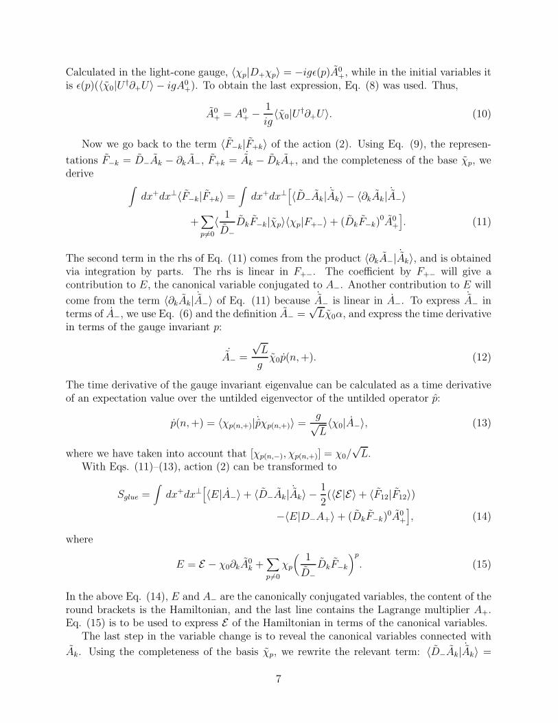
is ǫ(p)(〈χ0|U †∂+U〉 − igA0+). To obtain the last expression, Eq. (8) was used. Thus,

A0+ = A0

+ − 1

ig〈χ0|U †∂+U〉. (10)

Now we go back to the term 〈F−k|F+k〉 of the action (2). Using Eq. (9), the represen-

tations F−k = D−Ak − ∂kA−, F+k = ˙Ak − DkA+, and the completeness of the base χp, wederive

∫

dx+dx⊥〈F−k|F+k〉 =∫

dx+dx⊥[

〈D−Ak| ˙Ak〉 − 〈∂kAk| ˙A−〉

+∑

p 6=0

〈 1

D−

DkF−k|χp〉〈χp|F+−〉 + (DkF−k)0A0

+

]

. (11)

The second term in the rhs of Eq. (11) comes from the product 〈∂kA−| ˙Ak〉, and is obtainedvia integration by parts. The rhs is linear in F+−. The coefficient by F+− will give acontribution to E, the canonical variable conjugated to A−. Another contribution to E will

come from the term 〈∂kAk| ˙A−〉 of Eq. (11) because ˙A− is linear in A−. To express ˙A− interms of A−, we use Eq. (6) and the definition A− =

√Lχ0α, and express the time derivative

in terms of the gauge invariant p:

˙A− =

√L

gχ0p(n,+). (12)

The time derivative of the gauge invariant eigenvalue can be calculated as a time derivativeof an expectation value over the untilded eigenvector of the untilded operator p:

p(n,+) = 〈χp(n,+)| ˙pχp(n,+)〉 =g√L〈χ0|A−〉, (13)

where we have taken into account that [χp(n,−), χp(n,+)] = χ0/√L.

With Eqs. (11)–(13), action (2) can be transformed to

Sglue =∫

dx+dx⊥[

〈E|A−〉 + 〈D−Ak| ˙Ak〉 −1

2(〈E|E〉+ 〈F12|F12〉)

−〈E|D−A+〉 + (DkF−k)0A0

+

]

, (14)

where

E = E − χ0∂kA0k +

∑

p 6=0

χp

(

1

D−

DkF−k

)p

. (15)

In the above Eq. (14), E and A− are the canonically conjugated variables, the content of theround brackets is the Hamiltonian, and the last line contains the Lagrange multiplier A+.Eq. (15) is to be used to express E of the Hamiltonian in terms of the canonical variables.

The last step in the variable change is to reveal the canonical variables connected with

Ak. Using the completeness of the basis χp, we rewrite the relevant term: 〈D−Ak| ˙Ak〉 =

7

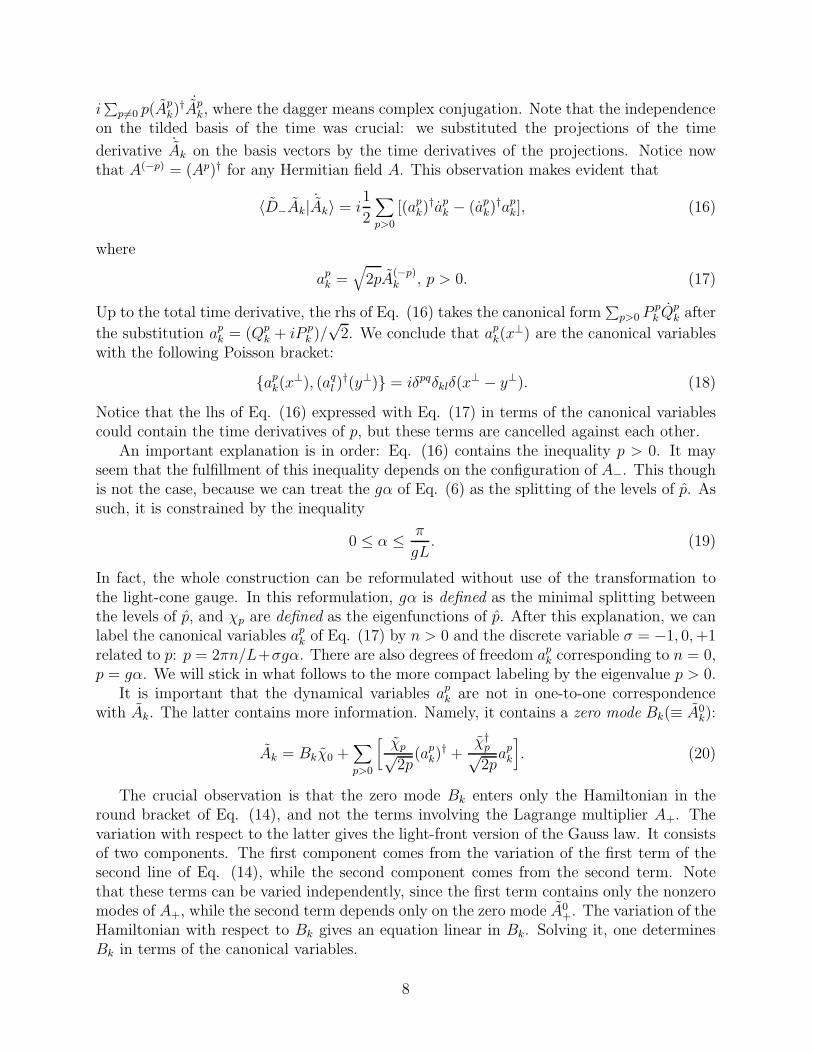
i∑

p 6=0 p(Apk)

† ˙Apk, where the dagger means complex conjugation. Note that the independence

on the tilded basis of the time was crucial: we substituted the projections of the time

derivative ˙Ak on the basis vectors by the time derivatives of the projections. Notice nowthat A(−p) = (Ap)† for any Hermitian field A. This observation makes evident that

〈D−Ak| ˙Ak〉 = i1

2

∑

p>0

[(apk)

†apk − (ap

k)†ap

k], (16)

where

apk =

√

2pA(−p)k , p > 0. (17)

Up to the total time derivative, the rhs of Eq. (16) takes the canonical form∑

p>0 Ppk Q

pk after

the substitution apk = (Qp

k + iP pk )/

√2. We conclude that ap

k(x⊥) are the canonical variables

with the following Poisson bracket:

{apk(x

⊥), (aql )

†(y⊥)} = iδpqδklδ(x⊥ − y⊥). (18)

Notice that the lhs of Eq. (16) expressed with Eq. (17) in terms of the canonical variablescould contain the time derivatives of p, but these terms are cancelled against each other.

An important explanation is in order: Eq. (16) contains the inequality p > 0. It mayseem that the fulfillment of this inequality depends on the configuration of A−. This thoughis not the case, because we can treat the gα of Eq. (6) as the splitting of the levels of p. Assuch, it is constrained by the inequality

0 ≤ α ≤ π

gL. (19)

In fact, the whole construction can be reformulated without use of the transformation tothe light-cone gauge. In this reformulation, gα is defined as the minimal splitting betweenthe levels of p, and χp are defined as the eigenfunctions of p. After this explanation, we canlabel the canonical variables ap

k of Eq. (17) by n > 0 and the discrete variable σ = −1, 0,+1related to p: p = 2πn/L+σgα. There are also degrees of freedom ap

k corresponding to n = 0,p = gα. We will stick in what follows to the more compact labeling by the eigenvalue p > 0.

It is important that the dynamical variables apk are not in one-to-one correspondence

with Ak. The latter contains more information. Namely, it contains a zero mode Bk(≡ A0k):

Ak = Bkχ0 +∑

p>0

[

χp√2p

(apk)

† +χ†

p√2pap

k

]

. (20)

The crucial observation is that the zero mode Bk enters only the Hamiltonian in theround bracket of Eq. (14), and not the terms involving the Lagrange multiplier A+. Thevariation with respect to the latter gives the light-front version of the Gauss law. It consistsof two components. The first component comes from the variation of the first term of thesecond line of Eq. (14), while the second component comes from the second term. Notethat these terms can be varied independently, since the first term contains only the nonzeromodes of A+, while the second term depends only on the zero mode A0

+. The variation of theHamiltonian with respect to Bk gives an equation linear in Bk. Solving it, one determinesBk in terms of the canonical variables.

8

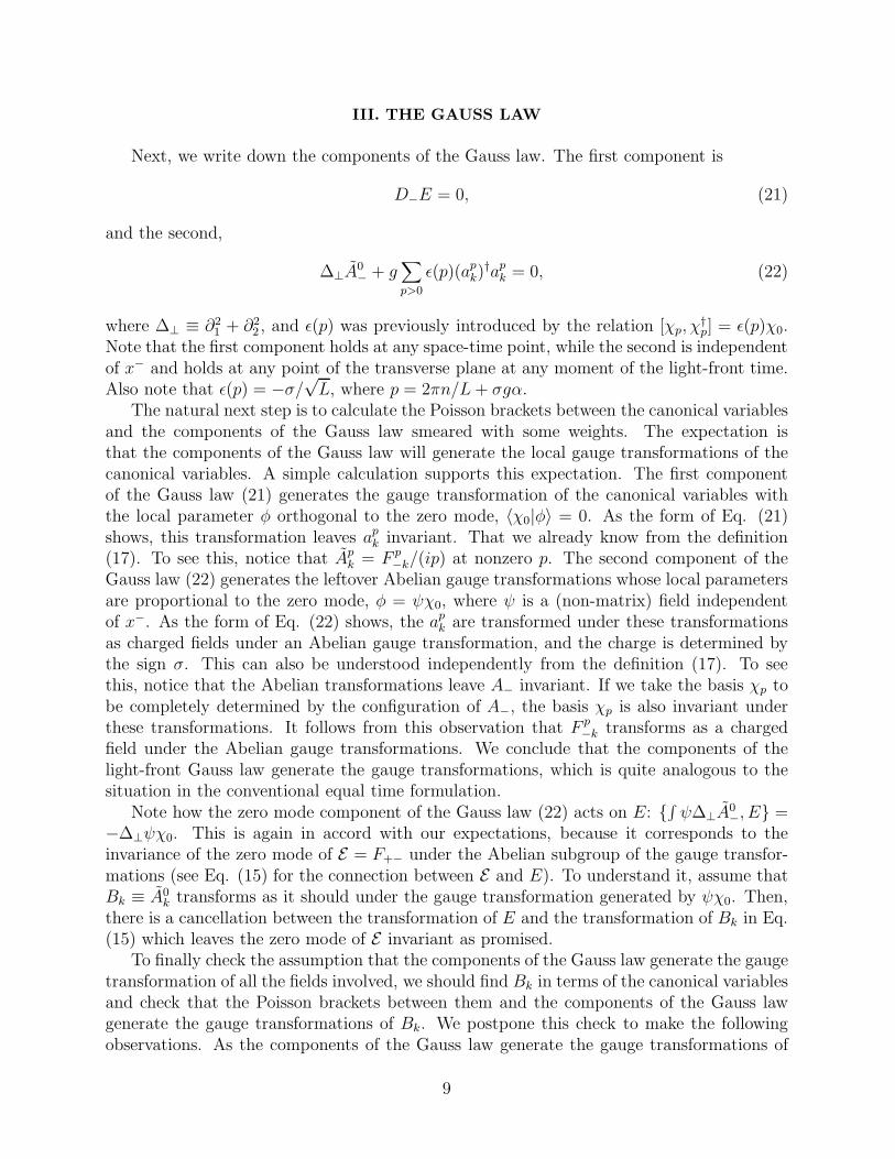
III. THE GAUSS LAW

Next, we write down the components of the Gauss law. The first component is

D−E = 0, (21)

and the second,

∆⊥A0− + g

∑

p>0

ǫ(p)(apk)

†apk = 0, (22)

where ∆⊥ ≡ ∂21 + ∂2

2 , and ǫ(p) was previously introduced by the relation [χp, χ†p] = ǫ(p)χ0.

Note that the first component holds at any space-time point, while the second is independentof x− and holds at any point of the transverse plane at any moment of the light-front time.Also note that ǫ(p) = −σ/

√L, where p = 2πn/L+ σgα.

The natural next step is to calculate the Poisson brackets between the canonical variablesand the components of the Gauss law smeared with some weights. The expectation isthat the components of the Gauss law will generate the local gauge transformations of thecanonical variables. A simple calculation supports this expectation. The first componentof the Gauss law (21) generates the gauge transformation of the canonical variables withthe local parameter φ orthogonal to the zero mode, 〈χ0|φ〉 = 0. As the form of Eq. (21)shows, this transformation leaves ap

k invariant. That we already know from the definition(17). To see this, notice that Ap

k = F p−k/(ip) at nonzero p. The second component of the

Gauss law (22) generates the leftover Abelian gauge transformations whose local parametersare proportional to the zero mode, φ = ψχ0, where ψ is a (non-matrix) field independentof x−. As the form of Eq. (22) shows, the ap

k are transformed under these transformationsas charged fields under an Abelian gauge transformation, and the charge is determined bythe sign σ. This can also be understood independently from the definition (17). To seethis, notice that the Abelian transformations leave A− invariant. If we take the basis χp tobe completely determined by the configuration of A−, the basis χp is also invariant underthese transformations. It follows from this observation that F p

−k transforms as a chargedfield under the Abelian gauge transformations. We conclude that the components of thelight-front Gauss law generate the gauge transformations, which is quite analogous to thesituation in the conventional equal time formulation.

Note how the zero mode component of the Gauss law (22) acts on E: {∫

ψ∆⊥A0−, E} =

−∆⊥ψχ0. This is again in accord with our expectations, because it corresponds to theinvariance of the zero mode of E = F+− under the Abelian subgroup of the gauge transfor-mations (see Eq. (15) for the connection between E and E). To understand it, assume thatBk ≡ A0

k transforms as it should under the gauge transformation generated by ψχ0. Then,there is a cancellation between the transformation of E and the transformation of Bk in Eq.(15) which leaves the zero mode of E invariant as promised.

To finally check the assumption that the components of the Gauss law generate the gaugetransformation of all the fields involved, we should find Bk in terms of the canonical variablesand check that the Poisson brackets between them and the components of the Gauss lawgenerate the gauge transformations of Bk. We postpone this check to make the followingobservations. As the components of the Gauss law generate the gauge transformations of

9

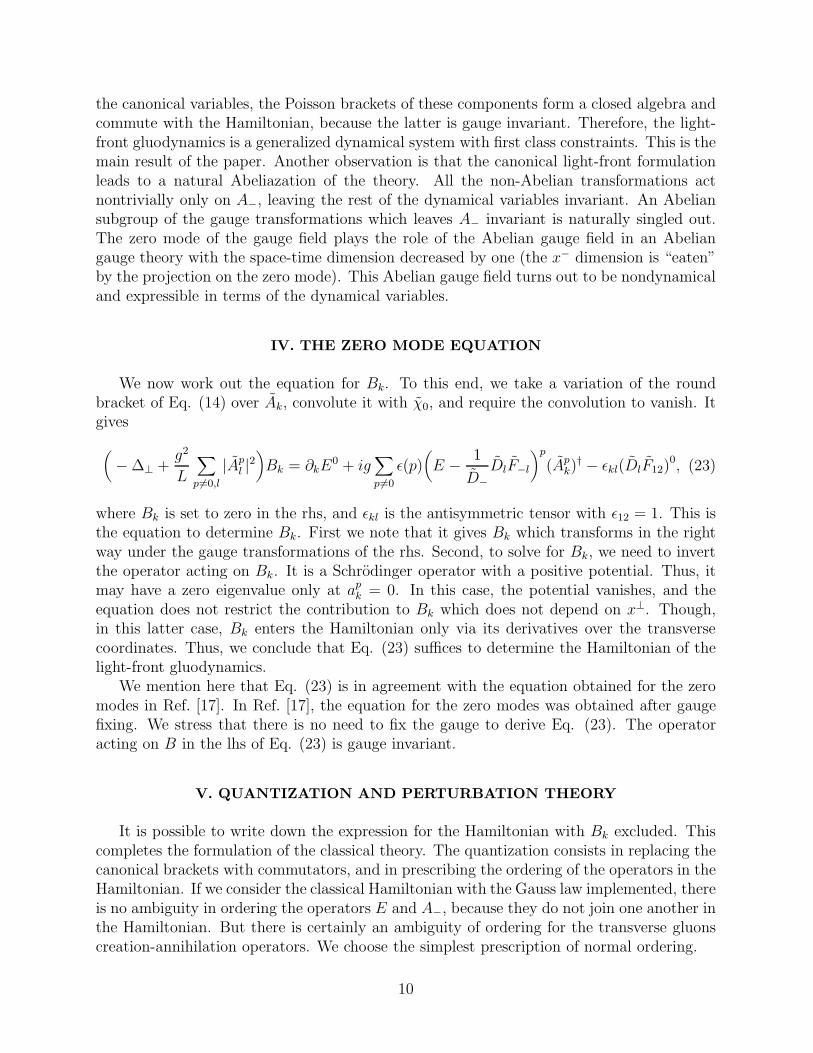
the canonical variables, the Poisson brackets of these components form a closed algebra andcommute with the Hamiltonian, because the latter is gauge invariant. Therefore, the light-front gluodynamics is a generalized dynamical system with first class constraints. This is themain result of the paper. Another observation is that the canonical light-front formulationleads to a natural Abeliazation of the theory. All the non-Abelian transformations actnontrivially only on A−, leaving the rest of the dynamical variables invariant. An Abeliansubgroup of the gauge transformations which leaves A− invariant is naturally singled out.The zero mode of the gauge field plays the role of the Abelian gauge field in an Abeliangauge theory with the space-time dimension decreased by one (the x− dimension is “eaten”by the projection on the zero mode). This Abelian gauge field turns out to be nondynamicaland expressible in terms of the dynamical variables.

IV. THE ZERO MODE EQUATION

We now work out the equation for Bk. To this end, we take a variation of the roundbracket of Eq. (14) over Ak, convolute it with χ0, and require the convolution to vanish. Itgives

(

− ∆⊥ +g2

L

∑

p 6=0,l

|Apl |2

)

Bk = ∂kE0 + ig

∑

p 6=0

ǫ(p)(

E − 1

D−

DlF−l

)p

(Apk)

† − ǫkl(DlF12)0, (23)

where Bk is set to zero in the rhs, and ǫkl is the antisymmetric tensor with ǫ12 = 1. This isthe equation to determine Bk. First we note that it gives Bk which transforms in the rightway under the gauge transformations of the rhs. Second, to solve for Bk, we need to invertthe operator acting on Bk. It is a Schrodinger operator with a positive potential. Thus, itmay have a zero eigenvalue only at ap

k = 0. In this case, the potential vanishes, and theequation does not restrict the contribution to Bk which does not depend on x⊥. Though,in this latter case, Bk enters the Hamiltonian only via its derivatives over the transversecoordinates. Thus, we conclude that Eq. (23) suffices to determine the Hamiltonian of thelight-front gluodynamics.

We mention here that Eq. (23) is in agreement with the equation obtained for the zeromodes in Ref. [17]. In Ref. [17], the equation for the zero modes was obtained after gaugefixing. We stress that there is no need to fix the gauge to derive Eq. (23). The operatoracting on B in the lhs of Eq. (23) is gauge invariant.

V. QUANTIZATION AND PERTURBATION THEORY

It is possible to write down the expression for the Hamiltonian with Bk excluded. Thiscompletes the formulation of the classical theory. The quantization consists in replacing thecanonical brackets with commutators, and in prescribing the ordering of the operators in theHamiltonian. If we consider the classical Hamiltonian with the Gauss law implemented, thereis no ambiguity in ordering the operators E and A−, because they do not join one another inthe Hamiltonian. But there is certainly an ambiguity of ordering for the transverse gluonscreation-annihilation operators. We choose the simplest prescription of normal ordering.

10

Making this choice, we may contradict the results of the equal-time quantization, whereits own ordering is assumed. That is, equal-time normal ordering may not coincide with thelight-front normal ordering we have chosen. Thus, we must confirm that our prescriptiondoes not lead to a contradiction.

Here we demonstrate that there is no contradiction between the normal ordering light-front quantization and the standard perturbation theory in covariant gauges.

In checking this, we benefit from the fact that the obtained formulation is standard, andwe can use the methods of Ref. [11] to write down the functional integral representationfor vacuum expectations of the time ordered products of gauge invariant local operators(for example, for the products of F 2

µν). The time ordering is understood with respect tothe light-front time x+. In accord with that standard methods, the functional integral willrun over the canonical variables, and the additional integration over A+, A

0+ will impose the

Gauss law on the states featuring the derivation of the functional integral representation.To simplify the treatment we do not impose any boundary conditions, and consider insteada finite span 2T of the light-front time x+ for the fields in the functional integral. When, inthe limit T → ∞(1 − iǫ), the vacuum expectation is reproduced (up to normalization) dueto the presence of iǫ in the time span.

Next, we derive the Hamiltonian in the reverse route: introduce Bk in the functionalintegral and restore it back in the action, go over from the integration over a†, a, Bk to theintegration over Ak (see Eq. (20)), shift E to E (see Eq. (15), and, finally, integrate E out.This gives us the standard representation in terms of the functional integral over Aµ, withthe standard action Sglue in the exponential. However, there is a subtle point: on the wayback we pick up some determinants. They will potentially cause a difference between ourformulation and the standard equal-time formulation. We now show that this differencevanishes in the limit of infinite volume, if dimensional regularization is used to regularizethe infinite volume theory.

We pick up the first determinant when the integration over Bk is introduced. Bk en-ters the Hamiltonian quadratically. So, integrating out Bk will return the initial expressionfor the Hamiltonian with Bk excluded via Eq. (23), and also will produce a power of thedeterminant of the operator featuring the lhs of Eq. (23), det(−∆⊥ + g2 ∑

p |Ap|2/L). Thedependence of this determinant on the fields is explicitly suppressed by the inverse L. There-fore, in the limit of infinite L, this determinant introduces only an (infinite) multiplicationconstant in the measure of integration.

The second determinant appears when we go over from the integration over Bk, a†, a

to the integration over Ak. It is related to the presence of the denominators√

2p in Eq.(23). Since p are the eigenvalues of D−, the new determinant is a power of the determinantof D−. And it is known that detD− is a constant independent of A−, if the dimensionalregularization is used to regularize the infrared divergences (see, for example, Ref. [18]).

We conclude that no determinants appear in the limit of infinite volume when the di-mensional regularization is used.

The next step is to fix the gauge in the functional integral. Here we again enjoy ourindependence of the gauge fixing: we are not forced to consider the light-cone gauge, whichhas extra singularities in the gluon propagator. Instead, we consider covariant gauges,introducing Faddeev-Popov ghosts in the standard way.

As a result, we obtain the standard representation for the Green’s functions in terms

11

of the functional integral. The only trace of the light-front approach left is the restrictionof the fields to the strip −T ≤ x+ ≤ T . As we do not restrict the boundary values at|x+| = T of the fields under the functional integration in any way, the classical solution ofthe linearized equations of motion related to the determination of the propagators shouldvanish on the boundaries of the strip. It is easy to check that the imaginary shift in T allowsthe presence of the unique solution to the classical linearized field equations which boundaryvalues vanish at T → ∞(1 − iǫ). Then, it is easy to check that the propagators appearinghave the Feynman iǫ in the denominators.

We conclude that the normal ordering light-front quantization reproduces the standardFeynman rules in covariant gauges. We stress that the above derivation is possible onlybecause the definition of the canonical variables we found does not depend on any gaugefixing.

VI. THE NON-ABELIAN PLANE WAVES REDUCTION

Now we turn to the analysis of the reduced dynamics by requiring P− to vanish. To seethe restriction this requirement sets on the dynamical variables, consider P− as it is yieldedby the Noether procedure:

P− =∫

dx⊥〈F−k|F−k〉. (24)

In terms of the canonical variables, it is

P− =∫

dx⊥[∑

p>0

p(apk)

†apk − A0

−∆⊥A0−]. (25)

With the zero mode component of the Gauss law (22) and the relation A− =√Lαχ0 taken

into account, it is

P− =∫

dx⊥∑

p>0

2πn

L(ap

k)†ap

k, (26)

where n is related to p by p = 2πn/L+ σgα. Thus, we see that vanishing of apk with p > gα

is necessary and sufficient for vanishing of P−. We note in passing that P− is independentof the canonical pair E, A−. A− enters P− only indirectly via the zero mode componentof the Gauss law (22). The latter restricts the possible configurations of ap

k. In particular,integrating Eq. (22) over the transverse plane we see that the total sum of the Abeliancharges over the transverse plane should vanish all the time. This, in fact, implies that theonly ap

k which is allowed by the vanishing of P− (p = gα) is forbidden by the Gauss law,because it has definite Abelian charge, and nothing can compensate it. Thus, we concludethat the reduction to the configurations of vanishing P− is equivalent to the reduction tovanishing ap

k, i.e., to the reduction from Eq. (20) to Ak = Bkχ0.This reduction simplifies the action (14) dramatically. The second term of the square

bracket vanishes, the round bracket is simplified because E becomes just E + χ0∂kBk (seeEq. (15) and recall that Bk ≡ A0

k), F12 becomes (∂1B2 − ∂2B1)χ0, and the last term of the

12

square bracket becomes (∂kA0−∂kA

0+). At no compactification over the x− direction, in the

light-cone gauge A− = 0, and at boundary conditions on E at the x− infinity suppressingthe zero mode E0, the classical equations of the reduced dynamics implied by this actionare ∂−A+ = 0, ∆⊥A+ = 0, Ak = 0. This reduction of the classical gauge equations is knownsince the work of Coleman [14]. Thus, we may say that the reduced dynamics of the papergeneralizes one of Coleman’s non-Abelian plane waves for the case of the compactified x−.Our next aim is to see the Hamiltonian formulation of the paper at work. We will find thequantum spectrum of the non-Abelian plane waves.

To this end, we will work in the gauge D−A+ = 0, A0+ = 0, which is the light-front

analog of the Weyl gauge. In this gauge, the reduced system is a Hamiltonian system withthe Hamiltonian

Hred(B) =∫

dx⊥1

2

[

(E0 + ∂kBk)2 + (∂1B2 − ∂2B1)

2]

. (27)

Minimization with respect to Bk gives

Hred =1

2E2V⊥, (28)

where

E ≡∫ dx⊥

V⊥〈χ0|E〉, (29)

and V⊥ ≡ ∫

dx⊥ is the volume of the transverse plane. Apart from the Hamiltonian (28),the reduced system is defined by the Gauss law D−E = 0, ∆⊥A

0− = 0. Notice that the

Hamiltonian vanishes in the limit of the infinite transverse volume on the configurations ofE with finite

∫

dx⊥E0, because E ∼ 1/V⊥ in this case.Let us demonstrate that the phase space of the reduced system is parameterized by two

variables. One is E, another is A ≡ ∫

dx⊥A0−/V⊥. This is so because of all Ep only E0

is nonzero by the component of the Gauss law D−E = 0, and, under a gauge transfor-mation, E0 can be shifted by the transverse Laplacian of a gauge parameter field (recallthat {∫

ψ∆⊥A0−, E} = −∆⊥ψχ0). Thus, the only piece of E which is simultaneously gauge

invariant and allowed by the Gauss law is E. The same holds with respect to A−: the onlygauge invariant component of A− is A0

−, and it should be independent of the transversecoordinates by the zero mode of the Gauss law. The reduction to a single gauge invariantcomponent is achievable because A− can be transformed to A0

− by a gauge transfromation,and the latter is a gauge invariant expressible in terms of the gauge invariant trace of aWilson loop.

Notice the specific duality between E and A−: The Gauss law forbids nonzero Ep atp 6= 0, while the gauge invariance admits only constant E0; for A−, the Gauss law and thegauge invariance interchange their roles in the reduction, i.e., the gauge invariance forbidsnonzero Ap

− at nonzero p, while the Gauss law admits only constant contributions to A0−. In

this reasoning, we assumed that the theory is compactified also in the transverse directionsx1,2.

Thus, we introduce two variables Q ≡ A−, and P ≡ V⊥E. They suffice to parameterizethe phase space of the reduced system, and the normalization is chosen to make them

13

canonically conjugated: {P,Q} = 1. The Hamiltonian (28) in terms of these variables isHred = P 2/(2V⊥). Notice that V⊥ plays the role of the mass of a free nonrelativistic particle.The next crucial point is that Q, in fact, should be compactified.

To see this, consider a “large” gauge transformation generated by the Hermitian trace-less matrix ω ≡ gx−(2π/g

√L)χ0. The transformed gauge field AU

− = U(A− − ∂−/(ig))U†,

U = exp(iω), is periodic in x−, if A− is. Thus, U is indeed a gauge transformation of thecompactified theory. Notice that this is not the case for any ω′ = λω, where λ is noninte-ger. Because of this, the above transformation cannot be continuously transformed to thetrivial transformation. The presence of the “large” gauge transformations in a compactifiedtheory is known since the work [19]. In the context of the light-front formulation, “large”gauge transformations have also been considered in Ref. [8], and utilized in Ref. [20] for theSchwinger model. The particular “large” gauge transformation we are considering here is alight-front analog of the equal-time finite-volume “central conjugations” of Ref. [21]. It iseasy to check that this transformation leaves P invariant, and shifts Q: Q→ Q+ 2π/g

√L.

Thus, the theory should be invariant with respect to this shift, because it is a remnantgauge transformation. The invariance is achieved by the condition on the wavefunctions inthe Q-representation:

Ψ(

Q+2π

g√L

)

= eiθΨ(Q), (30)

where θ is an angle, 0 ≤ θ < 2π, parameterizing the theory.In fact, the allowed values for the θ in Eq. (30) are 0 and π. This is the case because the

double action of the above large gauge transformation on the gauge fields leaves both P andQ invariant. To see this, notice that Q is expressible in terms of the trace of a large Wilsonloop, and the latter changes its sign under the single action of U . For more explanations,see Refs. [19,21]. In what follows, we introduce the label e for the superselection sectors ofthe theory: e = 0 for θ = 0 and e = 1 for θ = π. The notation is in accord with the one ofRefs. [19,21] and is to remind of the connection with the values of the electric flux.

Then, in the sector e = 0 the wave functions are periodic, and in the sector e = 1,antiperiodic:

Ψ(0) = (−1)eΨ(

2π

g√L

)

. (31)

Condition (31) singles out a discrete spectrum of the admissible values for P :

P (n) = g√L

(

n+e

2

)

, (32)

where n is an integer, and e is either zero or unit “electric flux”. Recalling that Hred =P 2/(2V⊥) = P+|(P

−=0)

, we conclude that the spectrum of P+ in the subspace P− = 0 is

P+|(P−

=0)(n) =

g2L

2V⊥

(

n+e

2

)2

. (33)

At n = 0 and e = 1, it coincides with the “free energy of an electric flux” of ’t Hooft, seeEq. (9.2) of Ref. [19].

14

VII. DISCUSSION AND CONCLUSION

Our central result, Eq. (33), shows that the presence of a mass gap in infinite volumetheory depends on the ordering of the limiting procedure. If one takes first the limit V⊥ → ∞then there is no mass gap, and if one takes first L→ ∞ then there is a mass gap.

We note that the dependence of the thermodynamic state on the limiting procedure isalso present in statistical mechanics, where a non-unique limit is generally associated withsome sort of first-order phase transition and may indeed be considered as a possible definitionof a phase transition [22]. On a physically motivated way to select the “right” state see Ref.[23].

Thus, we interpret the nonexistence of the infinite volume limit in our case as the in-dication of the presence of the first-order phase transition in gluodynamics. This is anacceptable feature in view of the expected presence of the deconfinement phase transitionand quark-gluon plasma in QCD [24]. Obviously, significant work is needed to reconcile ourapproach with what is known about the phase structure of QCD.

Having arrived at such simple spectrum, Eq. (33), could explain how previous approx-imate treatments yielded results seemingly valid beyond limitations of underlying assump-tions [25].

There is similarity of our results with recent works on Yang-Mills fields decomposition[26,27] which leads to the Abelian dominance [12]. However, those equal time approachesare linked with choice of a proper gauge [26] or with a nonlocal variable transformation[27], while we have obtained our results without a gauge fixing in finite volume light-frontformulation.

The next steps for development are the generalization to the SU(N) case and the inclu-sion of fermions. In general, the results for the theory with fermions can differ drasticallyfrom pure gauge theory such as the gluodynamics considered here.

Note that the finite volume light-front formulation may play an important role for stringtheory, where one has to quantize a compactified theory. Since we have obtained a light-frontformulation without a gauge fixing and in finite volume our results can stimulate a deeperunderstanding of a relation with novel M-theory developments [5].

To conclude, we gave a canonical formulation of the light-front SU(2) gluodynamicswithout a gauge fixing. The Gauss law was determined and the system was qualified asa generalized dynamical system with first class constraints. The formulation obtained re-produces the standard Feynman rules in the covariant gauges. The spectrum (33) of thelight-front Hamiltonian P+ was determined in the subspace of zero P− for the case of thetheory compactified on a torus. An unexpected feature of the spectrum is that the distancebetween the levels of P+ may vanish in the limit of infinite volume, depending on the waythe limit is taken. This suggests the possibility of the presence of massless states in cer-tain “phases” of the infinite volume theory obtained via the limiting procedures with thevanishing quantum of P+. There are obvious possibilities to further develop the formalism:to generalize for SU(N), to include fermions, to develop the perturbation theory in variousgauges at finite and at infinite volume, etc. Some of these problems will be addressed inRef. [28].

15

ACKNOWLEDGMENTS

The authors are grateful to I. Ya. Aref’eva, V. A. Franke, V. A. Kuzmin, L. Martinovic,Yu. V. Novozhilov, A. A. Ovchinnikov, H. Pirner, E. V. Prokhvatilov, V. A. Rubakov andS. V. Troitskii for stimulating discussions. They also thank R. Jackiw for communicationand for pointing out Ref. [6]. VTK and GBP thank the Fermilab Theory Group for theirwarm hospitality and support. This work was supported in parts by the Russian Foundationfor Basic Research, grant No. 00-02-17432, by the NATO Science Programme, grant No.PST.CLG.976521, by NSF, grant No. 9970778, and by the U. S. Department of Energy,grant No. DE-FG02-87ER40371.

16

REFERENCES

[1] P. A. M. Dirac, Rev. Mod. Phys. 21, 392 (1949).[2] S. J. Brodsky, H.-C. Pauli, and S. S. Pinsky, Phys. Rept. C301, 299 (1998);

J. Carbonell, B. Desplanques, V. A. Karmanov and J. F. Mathiot, Phys. Rept. C300,215 (1998);K. Yamawaki, Proc. X Annual Summer School and Symposium on Nuclear Physics(NUSS’97), Seoul, Korea, June 23 - 28, 1997, eds: C.-R. Ji and D.-P. Min (World Sci-entific, Singapore, 1998), hep-th/9802037;R. J. Perry, Proc. NATO Advanced Study Institute on Confinement, Duality and Non-perturbative Aspects of QCD, Cambridge, England, June 23 - July 4, 1997, ed. P. VanBaal (Plenum Press, New York, 1998), hep-th/9710175;T. Heinzl, Light-Cone Dynamics of Particles and Fields, hep-th/9812190;P. P. Srivastava, Perspectives of Light-Front Quantized Field Theory: Some New Re-sults, SLAC-PUB-8219, Stanford, 1999, hep-ph/9908492;Review lectures at School on Light-Front Quantization and Non-Perturbative QCD,May 6 - June 2, 1996, Ames, Iowa, eds: J. P. Vary and F. Wolz (IITAP, Ames, 1997),http://www.iitap.iastate.edu.

[3] S. Weinberg, Phys. Rev. 150, 1313 (1966);S. Fubini and G. Furlan, Physics 1, 229 (1965);S. Adler, Phys. Rev. Lett. 14, 1051 (1965).

[4] K. G. Wilson, T. S. Walhout, A. Harindranath, W.-M. Zhang, R. J. Perry and S. D.Glazek, Phys. Rev. D 49, 6720 (1994).

[5] L. Susskind, Another Conjecture about M(atrix) Theory, SU-ITP-97-11, Stanford, 1997,hep-th/9704080;S. Hellerman and J. Polchinski, Phys. Rev. D 59, 125002 (1999);J. Polchinski, Progr. Theor. Phys. Suppl. 134, 158 (1999);N. Seiberg and E. Witten, JHEP 9909, 032 (1999).

[6] E. Tomboulis, Phys. Rev. D 8, 2736 (1973).[7] V. A. Franke, Yu. V. Novozhilov, S. A. Paston and E. V. Prokhvatilov, in: Quan-

tum Theory in Honor of Vladimir A. Fock (UNESCO, St. Petersburg U., Euro-AsianPhysical Society, 1998) Part 1, pp. 38-97, hep-th/9901029.

[8] H.-C. Pauli, A. C. Kalloniatis and S. S. Pinsky, Phys. Rev. D 52, 1176 (1995).[9] J. A. Przeszowski, The Light Front SU(N) Yang-Mills Theory for the Weyl Gauge,

Warsaw, 1999, hep-th/9906037.[10] P. P. Srivastava and S. J. Brodsky, Phys. Rev. D 61, 025013 (2000).[11] L. D. Faddeev and A. A. Slavnov, Gauge Fields: an Introduction to Quantum Theory,

2nd ed. (Addison Wesley Longman, 1990).[12] G. ’t Hooft, Acta Phys. Austriaca, Suppl. 22, 531 (1980); Nucl. Phys. B190, 455 (1981);

Phys. Scripta 25, 133 (1982).[13] T. Maskawa and K. Yamawaki, Prog. Theor. Phys. 56, 270 (1976).[14] S. Coleman, Phys. Lett. 70B, 59 (1977).[15] L. D. Faddeev and R. Jackiw, Phys. Rev. Lett. 60, 1692 (1988).[16] O. Jahn and F. Lenz, Phys. Rev. D 58, 085006 (1998).

17

[17] V. A. Franke, Yu. V. Novozhilov and E. V. Prokhvatilov, Lett. Math. Phys. 5, 437(1981).

[18] A. Bassetto, G. Nardelli and R. Soldati, Yang-Mills Theories in Algebraic Non-Covariant Gauges (World Scientific, Singapore, 1991).

[19] G. ’t Hooft, Nucl. Phys. B153, 141 (1979).[20] L. Martinovic, Large Gauge Transformations and the Light-Front Vacuum Structure,

Iowa State Univ., Ames, 1998, hep-th/9811182.[21] M. Luscher, Nucl. Phys. B219, 233 (1983).[22] R. B. Griffiths, in Phase Transitions and Critical Phenomena, Vol. 1, eds: C. Domb

and M. S. Green, pp. 7-109 (Academic Press, London, 1972).[23] N. N. Bogoliubov, Physica 26, S1 (1960);

N. N. Bogoliubov, Quasiaverages in Problems of Statistical Mechanics, JINR R-1451,Dubna, 1963 (in Russian) reprinted in N. N. Bogoliubov, Lectures on Quantum Statis-tics. Volume 2. Quasiaverages, translation eds: L. Klein and S. Glass, pp. 1-75 (Gordon& Breach, New York, 1970) and in N. N. Bogoliubov. Selected Works. Volume III, pp.174-243 (Naukova Dumka, Kiev, 1971, in Russian).

[24] L. McLerran, Rev. Mod. Phys. 58, 1021 (1986);E. V. Shuryak, The QCD Vacuum, Hadrons and the Superdense Matter (World Scien-tific, Singapore, 1988);for a recent review see, e.g., H. Satz, QCD & QGP: a Summary, Theory Summary,3rd Intern. Conf. on the Physics and Astrophysics of the Quark-Gluon Plasma (ICPA-QGP’97), March 17-21, 1997, Jaipur, India, hep-ph/9706342.

[25] H. W. L. Naus, H. J. Pirner, T. J. Fields and J. P. Vary, Phys. Rev. D 58, 8062 (1997).[26] L. D. Faddeev and A. J. Niemi, Phys. Rev. Lett. 82, 1624 (1999); Phys. Lett. 449B,

214 (1999).[27] S. V. Shabanov, Phys. Lett. 463B, 263 (1999).[28] in preparation.

18