Callan et al.: LVQ-SOM and Retrocochlear Diagnosis Neural Networks Applied to Retrocochlear...

Callan et al.: LVQ-SOM and Retrocochlear Diagnosis 287

Daniel E. Callan*Robert E. Lasky**

Cynthia G. FowlerUniversity of Wisconsin–Madison

Department of CommunicativeDisorders

Methodologies have been developed, based on insights from signal detectiontheory, to evaluate quantitatively the diagnostic performance of tests. Severalstudies have demonstrated that, in fact, performance of a test battery can beinferior to the best of the tests it includes. These studies have been quite persuasivein damping enthusiasm for the test battery approach. Because the results of alltests in a battery were weighted equally in these studies, it is not surprising thatan individual test with good sensitivity and specificity is more effective diagnosti-cally than a combination of tests with poorer sensitivity and specificity. Theauthors of many of these studies were well aware of the limitations of thisapproach. In the present study, neural networks were applied to evaluateaudiological tests used to predict retrocochlear pathology by differentiallyweighting the results of the tests in the battery. This technique avoids some of thelimitations of previous approaches. Of the audiological tests evaluated in thepresent analysis, the superiority of the auditory brainstem evoked response (ABR)in predicting retrocochlear disease was again demonstrated. However, the resultsalso demonstrated that identification accuracy could be improved by combiningthe ABR with other tests (in this case contralateral acoustic reflex at 2000 Hz,ipsilateral acoustic reflex at 2000 Hz, tone decay, and word recognition score).Further, it was demonstrated that performance could be improved over thatobtained using dichotomous test measures (i.e., positive or negative presence ofpathology) by using raw test measures in conjunction with ABR.

KEY WORDS: self-organizing map, learning vector quantization, retrocochlear,test battery diagnostic

Neural Networks Applied toRetrocochlear Diagnosis

Journal of Speech, Language, and Hearing Research • Vol. 42 • 287–299 • April 1999 • ©American Speech-Language-Hearing Association 2871092-4388/99/4202-0287

Vestibular schwannomas account for about 6–10% of all intracra-nial tumors and between 75–80% of tumors in the cerebello-pontine angle (Ludman, 1988; Mahaley, Mettlin, & Natarajan,

1990; Woolsey & Eldred, 1977). Ninety-five percent of vestibular schwan-nomas are unilateral. Bilateral vestibular schwannomas (neurofibro-matosis type 2), in general, result from the NF-2 gene on chromosome22. The incidence of vestibular schwannomas is 1:100,000; however, atautopsy, the prevalence of vestibular schwannomas may be as high as900:100,000 (NIH Consensus Panel, 1991). Vestibular schwannomasare typically slow growing. Clinical symptoms usually present them-selves in individuals between 40 and 60 years of age for unilateral cases(rarely before puberty) and between 20 and 40 years of age for NF-2(NIH Consensus Panel; Schuknecht, 1993). Symptoms include audi-tory and vestibular dysfunction, and, in late stages, the compressive

*Currently affiliated with ATR Human Information Processing Research Laboratories, Kyoto,Japan.

**Department of Neurology.

288 Journal of Speech, Language, and Hearing Research • Vol. 42 • 287–299 • April 1999

effects of the tumor on neighboring structures (cranialnerves, brainstem, and cortex).

The most common auditory symptom resulting froma vestibular schwannoma is hearing loss—generally aunilateral high frequency loss. There is often poorerunderstanding of speech than expected from thresholdresults. Tinnitus and fullness of the ears are also symp-toms, typically localized to the side of the tumor.

Prior to the development of definitive tests, such asmagnetic resonance imaging (MRI), many auditory testswere used to identify retrocochlear pathology. The testbattery concept was promulgated in response to the needto identify retrocochlear lesions diagnostically. As Turner(1991) has articulated, the test battery concept involvedthree assumptions: (1) More tests mean more informa-tion; (2) additional information can be used; and (3) atest battery outperforms any test in that battery. Be-cause of the increasing use of auditory brainstem evokedresponses (ABRs) to diagnose retrocochlear pathology,the test battery concept was being questioned by thelate 1970s. The measurement properties of the ABR wereso good relative to other tests included in test batteriesthat performing the additional tests seemed at best su-perfluous. That argument can be made even morestrongly concerning MRI. Currently MRI is consideredthe gold standard; however, there are still reasons whyABR may be preferred over MRI. The number of indi-viduals with asymmetric hearing loss and tinnitus isquite large compared to the number of actual tumorcases. Therefore, screening would require that manyindividuals without tumors be tested. Even though theprice of MRI screening is becoming less expensive withthe advent of new recording techniques (Allen et al.,1997), it still has only limited availability. On the otherhand, ABR is widely available, and with new techniquessuch as the stacked derived-band ABR, it has improvedsensitivity and specificity over that of standard ABR(Don, Masuda, Nelson, & Brackmann, 1997). It shouldalso be noted that although MRI has better predictiveperformance than ABR, there are cases in which the MRIproduces false positives (von Glass, Haid, Cidlinsky,Stenglein, & Christ, 1991).

The ability of a test to predict an outcome is a com-mon concern in health care disciplines. Analytic meth-odologies have been developed to evaluate quantitativelythe diagnostic performance of these tests. Insights fromsignal detection theory (Jerger, 1983; Swets, 1964; Yanz,1984) have been applied to this issue, and a better un-derstanding of testing has resulted. Sensitivity andspecificity, hits and false alarm rates, and receiver op-erating characteristics are parameters widely used toevaluate the efficacy of testing. Turner (1988, 1991) hasmade a significant contribution to audiology by apply-ing these concepts to tests for retrocochlear lesions. In

addition, Turner (1988) developed a rigorous approachto evaluate the performance of a test battery. Formally,Turner combined the performance characteristics (e.g.,the hits and false alarms) of individual tests in a testbattery to predict the performance of the entire battery.In order to do so, Turner had to specify how those testswere to be combined. In addition, Turner had to esti-mate the correlation among the tests in order to esti-mate the independent contribution of those tests to thediagnosis. Turner’s approach allowed him to evaluatequantitatively the test battery concept. This was a sig-nificant contribution because, until that time, the effi-cacy of a test battery in diagnosing retrocochlear pa-thology was unclear, although strong opinions on allsides were expressed. Turner, Shepard, and Frazier(1984) demonstrated that, in fact, performance of a testbattery can be inferior to the best of the tests it includes.Turner’s reasoning has been quite persuasive in damp-ing enthusiasm for the test battery approach.

Turner conceived of the clinical decisions involvedin evaluating a test battery as a series or parallel evalu-ation of test results to which strict (all tests results mustbe the same) or loose (only one of the test results mustindicate pathology) criteria are applied. Therefore, it isnot surprising that an individual test with good sensi-tivity and specificity (high hit and low false alarm rates)is more effective diagnostically than a combination oftests with poorer sensitivity and specificity. Turner waswell aware of the limitations of his approach.

Most of the work in this chapter is based on sim-plifying assumptions. Tests were permitted tohave only two outcomes….We required that thecriterion for parallel protocols be either strict orloose. Is there any advantage to an intermediatecriterion…? What about weighting different testsin a protocol differently so that some tests countmore than other tests? Additional theoreticalwork is needed to develop more powerful, lessrestrictive techniques. (Turner, 1991, p. 737)

The general problem of predicting an outcome (thedependent variable) given a number of predictor (inde-pendent) variables is a familiar one. A variety of mul-tiple regression techniques have been developed to ad-dress this general problem (Kleinbaum & Kupper, 1978).These techniques vary in the statistical assumptionsthey make concerning the data. In addition to regres-sion techniques, another way in which multiple testmeasures can be optimally weighted to predict outcomeis through the use of artificial neural networks. In thisarticle, neural networks will be applied to distinguishindividuals with retrocochlear pathology from thosewithout retrocochlear pathology but with similar symp-toms. In general, neural networks accomplish optimalweighting by means of a training procedure in which


input data samples are iteratively presented and theweights are adapted to reflect class boundaries (denotedby their respective probability distributions in the in-put data) of the groups under study.

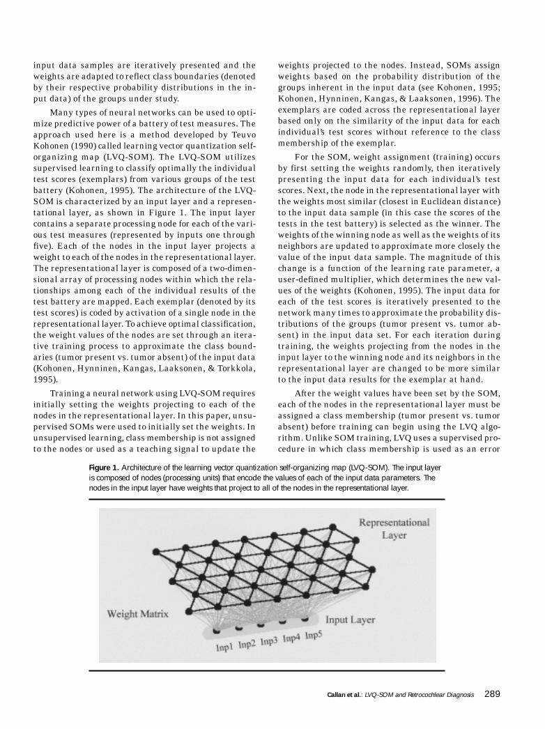
Many types of neural networks can be used to opti-mize predictive power of a battery of test measures. Theapproach used here is a method developed by TeuvoKohonen (1990) called learning vector quantization self-organizing map (LVQ-SOM). The LVQ-SOM utilizessupervised learning to classify optimally the individualtest scores (exemplars) from various groups of the testbattery (Kohonen, 1995). The architecture of the LVQ-SOM is characterized by an input layer and a represen-tational layer, as shown in Figure 1. The input layercontains a separate processing node for each of the vari-ous test measures (represented by inputs one throughfive). Each of the nodes in the input layer projects aweight to each of the nodes in the representational layer.The representational layer is composed of a two-dimen-sional array of processing nodes within which the rela-tionships among each of the individual results of thetest battery are mapped. Each exemplar (denoted by itstest scores) is coded by activation of a single node in therepresentational layer. To achieve optimal classification,the weight values of the nodes are set through an itera-tive training process to approximate the class bound-aries (tumor present vs. tumor absent) of the input data(Kohonen, Hynninen, Kangas, Laaksonen, & Torkkola,1995).

Training a neural network using LVQ-SOM requiresinitially setting the weights projecting to each of thenodes in the representational layer. In this paper, unsu-pervised SOMs were used to initially set the weights. Inunsupervised learning, class membership is not assignedto the nodes or used as a teaching signal to update the

weights projected to the nodes. Instead, SOMs assignweights based on the probability distribution of thegroups inherent in the input data (see Kohonen, 1995;Kohonen, Hynninen, Kangas, & Laaksonen, 1996). Theexemplars are coded across the representational layerbased only on the similarity of the input data for eachindividual’s test scores without reference to the classmembership of the exemplar.

For the SOM, weight assignment (training) occursby first setting the weights randomly, then iterativelypresenting the input data for each individual’s testscores. Next, the node in the representational layer withthe weights most similar (closest in Euclidean distance)to the input data sample (in this case the scores of thetests in the test battery) is selected as the winner. Theweights of the winning node as well as the weights of itsneighbors are updated to approximate more closely thevalue of the input data sample. The magnitude of thischange is a function of the learning rate parameter, auser-defined multiplier, which determines the new val-ues of the weights (Kohonen, 1995). The input data foreach of the test scores is iteratively presented to thenetwork many times to approximate the probability dis-tributions of the groups (tumor present vs. tumor ab-sent) in the input data set. For each iteration duringtraining, the weights projecting from the nodes in theinput layer to the winning node and its neighbors in therepresentational layer are changed to be more similarto the input data results for the exemplar at hand.

After the weight values have been set by the SOM,each of the nodes in the representational layer must beassigned a class membership (tumor present vs. tumorabsent) before training can begin using the LVQ algo-rithm. Unlike SOM training, LVQ uses a supervised pro-cedure in which class membership is used as an error

Figure 1. Architecture of the learning vector quantization self-organizing map (LVQ-SOM). The input layeris composed of nodes (processing units) that encode the values of each of the input data parameters. Thenodes in the input layer have weights that project to all of the nodes in the representational layer.


signal to update the weights projecting to each of thenodes in the representational layer. The class member-ship is used as a teaching signal to update the projectedweights to the nodes in the representational layer. Train-ing is conducted by iteratively presenting the input datasamples (individual test scores) and updating theweights of the nodes so that the exemplars can be clas-sified more accurately. When the winning node sharesthe same class membership as the input data sample,its weights are updated to better approximate the valueof the input data sample. Alternatively, when the win-ning node does not share the same class membership,the weights are updated in the opposite direction. Themagnitude of the weight change is controlled by thelearning rate parameter. For each iteration during train-ing, the weights projecting from the nodes in the inputlayer to the winning node in the representational layerare changed to be closer to the input data results for theexemplar at hand, if it shares the same class member-ship as the winning node. If class membership of theexemplar and the winning node are different, theweights are changed to be farther away from the inputdata results for the exemplar at hand. After the net-work has been trained on many iterations through theinput data set, it can then be tested to determine itsaccuracy (see Kohonen, 1995; Kohonen et al., 1995 for amore extensive description of LVQ).

Neural networks, and particularly those that uti-lize SOMs, provide many advantages over more tradi-tional multivariate statistical analyses (e.g., discrimi-nant analysis; Callan, Kent, Roy, & Tasko, 1999). Thetwo-dimensional nature of the representational layerprovides an easy way to visualize and evaluate the dis-tribution of exemplars from the various classificationgroups. Both the number of exemplars, from each of thegroups classified similarly, as well as the dispersion ofthe exemplars, can be easily discerned across the sur-face of the representational layer. Another advantage ofneural networks (due to their nonlinear nature) overthat of more traditional statistical analysis is, in somecases, better classification performance. Whereas theweighting coefficients of the input variables used in tra-ditional statistical analyses for classification of exem-plars are often difficult to discern, the two-dimensionalnature of the SOM allows for easy visualization of therelative weighting of the input variables responsible fordefining the distribution of exemplars into groups acrossthe surface of the representational layer. Exemplars withsimilar test results are grouped close to each other alongthe surface of the representational layer, whereas ex-emplars with differing test results are widely separatedalong the surface of the representational layer.

The purpose of this article is to quantify the valueof commonly used tests to diagnose retrocochlear pa-thology in a relevant clinical context using LVQ-SOM

neural networks. Most frequently, the diagnosis ofretrocochlear pathology becomes an issue for cases pre-senting unilateral or asymmetrical hearing loss. Conse-quently, the improvement associated with using LVQ-SOM trained on the results of multiple audiological tests,auditory brain stem response (ABR), contralateral acous-tic reflex threshold (ARC), ipsilateral acoustic reflexthreshold (ARI), tone decay (TD), and word recognitionscore (WRS), over that of the single most predictive testin the battery (i.e., ABR) will be determined for indi-viduals with asymmetrical hearing losses. For one groupof individuals, a vestibular schwannoma was respon-sible for their hearing loss (tumor present group),whereas for the other group it was not (tumor absentgroup). This is a much more difficult diagnostic deci-sion than distinguishing vestibular schwannoma casesfrom normal hearing individuals (negative test results).It is also a much more clinically relevant decision.

MethodParticipants

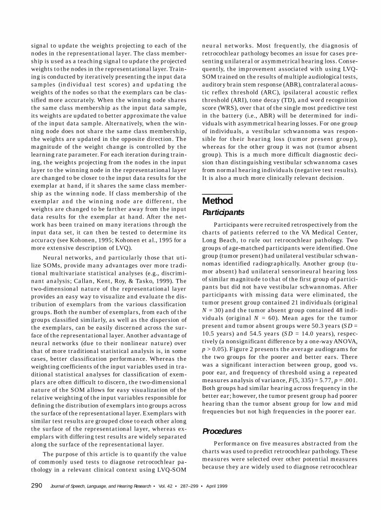
Participants were recruited retrospectively from thecharts of patients referred to the VA Medical Center,Long Beach, to rule out retrocochlear pathology. Twogroups of age-matched participants were identified. Onegroup (tumor present) had unilateral vestibular schwan-nomas identified radiographically. Another group (tu-mor absent) had unilateral sensorineural hearing lossof similar magnitude to that of the first group of partici-pants but did not have vestibular schwannomas. Afterparticipants with missing data were eliminated, thetumor present group contained 21 individuals (originalN = 30) and the tumor absent group contained 48 indi-viduals (original N = 60). Mean ages for the tumorpresent and tumor absent groups were 50.3 years (SD =10.5 years) and 54.5 years (SD = 14.0 years), respec-tively (a nonsignificant difference by a one-way ANOVA,p > 0.05). Figure 2 presents the average audiograms forthe two groups for the poorer and better ears. Therewas a significant interaction between group, good vs.poor ear, and frequency of threshold using a repeatedmeasures analysis of variance, F(5, 335) = 5.77, p = .001.Both groups had similar hearing across frequency in thebetter ear; however, the tumor present group had poorerhearing than the tumor absent group for low and midfrequencies but not high frequencies in the poorer ear.

ProceduresPerformance on five measures abstracted from the

charts was used to predict retrocochlear pathology. Thesemeasures were selected over other potential measuresbecause they are widely used to diagnose retrocochlear


pathology, they have been thought to contribute somewhatdifferent information in the diagnosis, and they had theleast amount of missing data. The five measures are listedbelow. The following criteria were used to define a posi-tive result for each of these five measures:

1. ABR: An interaural Wave V latency difference>.35 ms and/or a Wave V-I latency difference >4.5 msdefined a positive (ABR). No correction was used forhearing loss. The stimulus intensity was 85–95 dB nHLand was set to attempt to be 20 dB greater than aver-age pure tone thresholds for each individual. Raw datawere not available for the ABR test results.

2. ARC: Contralateral acoustic reflex threshold at2000 Hz. The ARC measure was considered positive ifthe contralateral acoustic reflex threshold was absentand pure tone thresholds at 2000 Hz were better than70 dB HL. The ARC measure was also positive if thecontralateral acoustic reflex was present but elevated(>95 dB SPL) and pure tone thresholds were better than40 dB HL. Raw scores were available. For absent re-flexes, a value of 115 dB HL was assigned.

3. ARI: Ipsilateral acoustic reflex threshold at 2000Hz. The ARI measure was considered positive if the ip-silateral acoustic reflex threshold was absent and puretone thresholds at 2000 Hz were better than 70 dB HL.The ARI measure was also positive if the ipsilateralacoustic reflex was present but elevated (>95 dB SPL)and pure tone thresholds were better than 40 dB HL.Raw scores were available. For absent reflexes a valueof 115 dB HL was assigned.

4. TD: Tone decay was positive if it was 35 dB orgreater. Raw scores were available.

5. WRS: A word recognition score was defined as apositive result according to the Yellin, Jerger, and Fifer(1989) norms. Raw scores were available.

Neural Network ImplementationInput to LVQ-SOM

Two data sets were used to train two separate LVQ-SOM neural networks. Each of the data sets includedvalues for the five measures (ABR, ARC, ARI, TD, andWRS) of the 21 individuals with tumors present and the48 individuals with tumors absent. The set used to trainthe first neural network (Data Set 1) consisted only ofdichotomous pass-fail data based on the criteria listedabove for each of the five measures. The set used to trainthe second neural network (Data Set 2) consisted of di-chotomous pass-fail data for ABR and raw scores for allother test measures (ARC, ARI, TD, and WRS). The val-ues in the second data set were normalized to have amean of zero and a variance of one.

Architecture of the LVQ-SOMThe LVQ-SOM neural network, trained using the

first data set, contained a five-node input layer withweights fully projected to a three-by-two node repre-sentational layer. The nodes of the input layer encodethe five test measures listed above (ABR, ARC, ARI,TD, and WRS). The relatively small size of the repre-sentational layer was selected because the input datawere dichotomous in nature, and tight clustering wasdesired. For the initialization phase of training usingSOM, a hexagonal neighborhood lattice across the rep-resentational layer was used. This is recommended byKohonen (1995) to enhance visual inspection of the re-sultant map. The number of rings of surrounding nodes(defining the neighbors) that can be affected by activa-tion of a particular node is defined by the neighbor-hood radius. The neighborhood radius is diminished insize throughout training of the SOM. The lines connect-ing the nodes in Figures 3 and 4 represent the underly-ing hexagonal neighborhood lattice of the LVQ-SOM.In the case of the LVQ, part of training only the win-ning node was modified during training (neighbors werenot modified).

The LVQ-SOM neural network, trained using thesecond data set, contained a five-node input layer withweights fully projected to a four-by-four node represen-tational layer. The nodes of the input layer encode thefive test measures listed above (ABR, ARC, ARI, TD,and WRS). The representational layer was somewhatlarger than that used for the first neural network be-cause raw data measures were used as input. The useof raw data allows for greater diversity in clustering. Alarger map is needed to capture this diversity. A hex-agonal neighborhood lattice and a decreasing neighbor-hood radius were used during training of the SOM, justas for the first neural network.

Figure 2. Mean auditory thresholds for the better ear (BE) and thepoorer ear (PE) for the tumor present and tumor absent groups.


Training of the LVQ-SOMThe first LVQ-SOM1 neural network was trained

using as input the dichotomous pass-fail test measures(Data Set 1) according to the following procedures:Weights were first set using a three-by-two node SOM.Map formation was accomplished by iteratively present-ing the test scores for each individual (exemplar) andallowing for the projected weights to the representationallayer to be corrected toward the input data. For moredetails regarding the SOM training algorithm, seeKohonen (1995) and Kohonen et al. (1996).

Using the SOM for initially setting the weights al-lows for the data to be spatially ordered across the two-dimensional map. Ten maps were trained with differ-ent initial random weight values, and the map with thesmallest quantization error was selected for additionaltraining using LVQ. Training using SOM was conductedin two steps. The first step was for 1000 iterationsthrough the entire data set with a neighborhood radiusof 3 and a learning rate that began at .09 and decreasedto 0 with successive iterations. The second step was for5000 iterations through the data with a neighborhoodradius of 1 and a learning rate that began at .02 anddecreased to 0 with successive iterations. The first stageof training was carried out with a larger initial neigh-borhood radius and learning rate to allow for properordering of the weights of the nodes in the representa-tional layer (Kohonen et al., 1996).

After the weight values have been set by the SOM,each of the nodes in the representational layer was as-signed a class membership (tumor present vs. tumorabsent). Class membership of each of the nodes in therepresentational layer was determined by the group (tu-mor present or tumor absent) with the greatest numberof exemplars that fell on a particular node. If the samenumber of exemplars was coded by the same node, or anode did not code for any exemplars, node representa-tion was determined by means of majority voting of thegroup membership of the five nearest exemplars (inEuclidean space) to the node in question.

Training using LVQ was conducted for 2500 itera-tions through the entire data set with a learning rate thatbegan at .09 and decreased to 0 with successive iterations.After training, the approximate Euclidean separation ofthe nodes in two-dimensional space was determinedusing a Sammon mapping (Sammon, 1969) across theweight values for the five input data test measures (ABR,ARC, ARI, TD, and WRS) associated with the nodes inthe representational layer. The Sammon mapping pro-vides a coordinate value in two-dimensional space foreach of the nodes in the representational layer. The sepa-ration of the nodes in two-dimensional space is reflec-tive of the distance between the projected weights of the

five input data test measures to each of the nodes in therepresentational layer. The separation and position ofthe nodes in Figures 3 through 5 is determined by theSammon mapping. All figures were constructed usingMatlab (Version 4.2c.1, MathWorks, 1994). All statisti-cal analyses were conducted using SPSS (Version 7.5.1,SPSS, 1996).

The second LVQ-SOM2 neural network was trainedusing Data Set 2 according to a procedure similar to thefirst neural network except for the following differences:The weights were initially set using a four-by-four nodeSOM. The SOMs were trained in two steps. The firststep was for 1000 iterations through the entire data setwith a neighborhood radius of 4 and a learning rate thatbegan at .07 and decreased to 0 with successive itera-tions. The second step was for 5000 iterations throughthe data with a neighborhood radius of 1 and a learningrate that began at .02 and decreased to 0 with succes-sive iterations. Training using LVQ was conducted for1000 iterations through the entire data set with a learn-ing rate that began at .09 and decreased to 0 with suc-cessive iterations.

Results and DiscussionIn order to determine how well the various tests

(ABR, ARC, ARI, TD, WRS, LVQ-SOM1 dichotomousdata, LVQ-SOM2 raw data) predicted the presence andabsence of a tumor, several measures of performancewere conducted. The measures are as follows:

1. # of hits hs: This value denotes the number of pre-dicted tumor exemplars that do in fact have a tumor.

2. # of correct rejections cs: This value denotes thenumber of predicted non-tumor exemplars that arein fact absent of a tumor.

3. hit rate HR (Sensitivity) = hs/tp, where tp = totalnumber of exemplars with a tumor present.

4. correct rejection rate CR (Specificity) = cs/ta, whereta = total number of exemplars with a tumor absent.

5. A′: This value denotes a single measure of test per-formance that takes into account both sensitivityand specificity:

A′ = 0.5 + [HR – (1 – CR)] × [1 + HR – (1 – CR)]

4(HR × CR)

6. efficiency EF: is the percentage of the results thatare correct, taking into account the prevalence ofthe disease. EF = HR × PD + (CR) × (1 – PD), wherePD = prevalence of the disease (percent of the popu-lation that has the disease at the time of testing).The same value of prevalence (.05) was used as inthe Turner (1991) study.


Sensitivity measures the degree to which a test pre-dicts the presence of a disorder when it is in fact present.Specificity measures the degree to which a test predictsthe absence of a disorder when it is in fact absent. Indetermining the true predictive power of a test it isimportant to look at both sensitivity and specificity. Asingle measure that takes into account both sensitivityand specificity is called A′. A sensitivity of 100% and aspecificity of 100% would constitute perfect performanceand a corresponding A′ of 1. In the case when the dis-eased and nondiseased distributions are skewed or donot have the same standard deviation, A′ is a more ap-propriate measure to use than d′ (Turner, 1991). Anothersingle measure that is used to determine the predictiveperformance of a test is efficiency. Efficiency, like A′,takes into account both sensitivity and specificity. In ad-dition, it also takes into account the prevalence of thedisease—that is, the percent of the population that hasthe disease at the time of testing (Turner, 1991). As withA′ a score of 1 denotes a perfect efficiency score. One cansee from the equation above that when prevalence is small,specificity drives efficiency more than sensitivity.

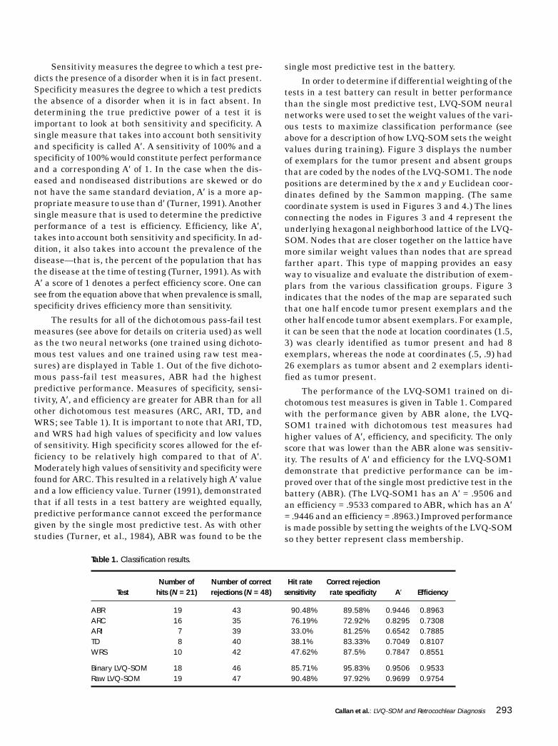
The results for all of the dichotomous pass-fail testmeasures (see above for details on criteria used) as wellas the two neural networks (one trained using dichoto-mous test values and one trained using raw test mea-sures) are displayed in Table 1. Out of the five dichoto-mous pass-fail test measures, ABR had the highestpredictive performance. Measures of specificity, sensi-tivity, A′, and efficiency are greater for ABR than for allother dichotomous test measures (ARC, ARI, TD, andWRS; see Table 1). It is important to note that ARI, TD,and WRS had high values of specificity and low valuesof sensitivity. High specificity scores allowed for the ef-ficiency to be relatively high compared to that of A′.Moderately high values of sensitivity and specificity werefound for ARC. This resulted in a relatively high A′ valueand a low efficiency value. Turner (1991), demonstratedthat if all tests in a test battery are weighted equally,predictive performance cannot exceed the performancegiven by the single most predictive test. As with otherstudies (Turner, et al., 1984), ABR was found to be the

single most predictive test in the battery.

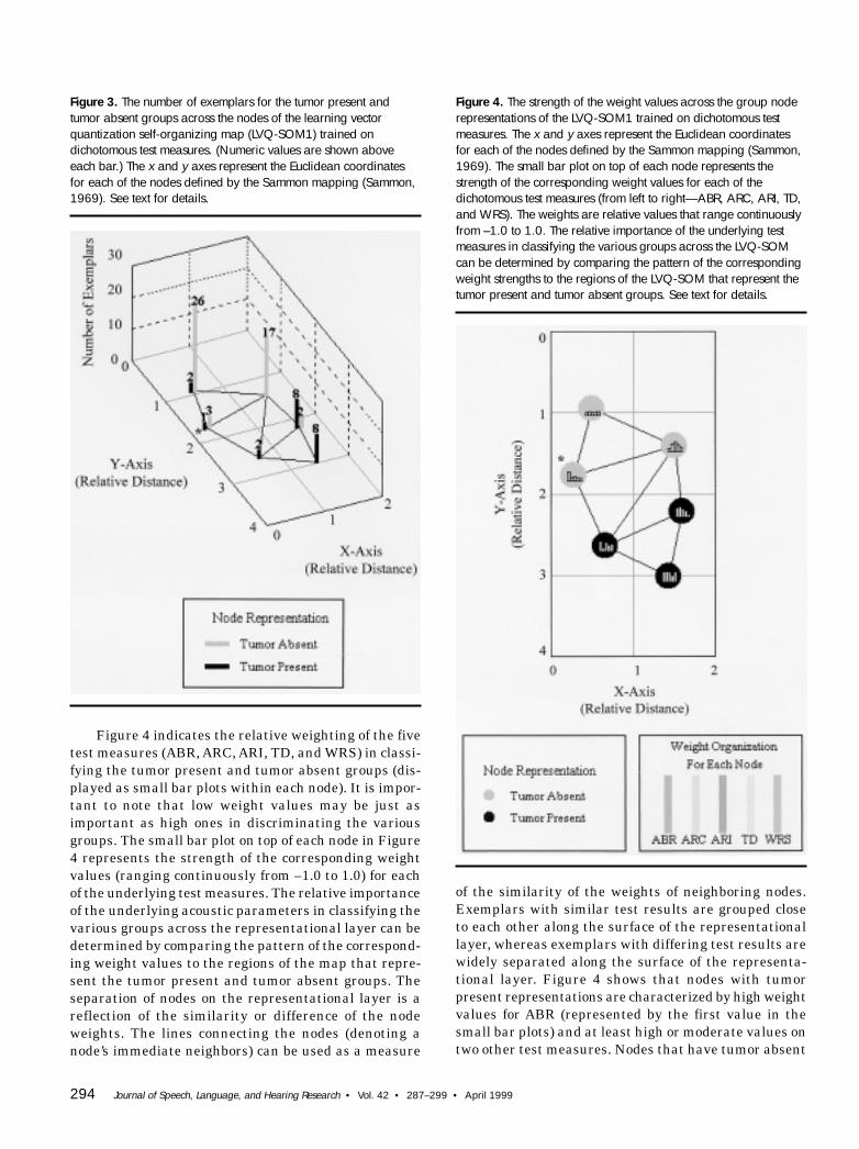
In order to determine if differential weighting of thetests in a test battery can result in better performancethan the single most predictive test, LVQ-SOM neuralnetworks were used to set the weight values of the vari-ous tests to maximize classification performance (seeabove for a description of how LVQ-SOM sets the weightvalues during training). Figure 3 displays the numberof exemplars for the tumor present and absent groupsthat are coded by the nodes of the LVQ-SOM1. The nodepositions are determined by the x and y Euclidean coor-dinates defined by the Sammon mapping. (The samecoordinate system is used in Figures 3 and 4.) The linesconnecting the nodes in Figures 3 and 4 represent theunderlying hexagonal neighborhood lattice of the LVQ-SOM. Nodes that are closer together on the lattice havemore similar weight values than nodes that are spreadfarther apart. This type of mapping provides an easyway to visualize and evaluate the distribution of exem-plars from the various classification groups. Figure 3indicates that the nodes of the map are separated suchthat one half encode tumor present exemplars and theother half encode tumor absent exemplars. For example,it can be seen that the node at location coordinates (1.5,3) was clearly identified as tumor present and had 8exemplars, whereas the node at coordinates (.5, .9) had26 exemplars as tumor absent and 2 exemplars identi-fied as tumor present.

The performance of the LVQ-SOM1 trained on di-chotomous test measures is given in Table 1. Comparedwith the performance given by ABR alone, the LVQ-SOM1 trained with dichotomous test measures hadhigher values of A′, efficiency, and specificity. The onlyscore that was lower than the ABR alone was sensitiv-ity. The results of A′ and efficiency for the LVQ-SOM1demonstrate that predictive performance can be im-proved over that of the single most predictive test in thebattery (ABR). (The LVQ-SOM1 has an A′ = .9506 andan efficiency = .9533 compared to ABR, which has an A′= .9446 and an efficiency = .8963.) Improved performanceis made possible by setting the weights of the LVQ-SOMso they better represent class membership.

Table 1. Classification results.

Number of Number of correct Hit rate Correct rejectionTest hits (N = 21) rejections (N = 48) sensitivity rate specificity A′ Efficiency

ABR 19 43 90.48% 89.58% 0.9446 0.8963ARC 16 35 76.19% 72.92% 0.8295 0.7308ARI 7 39 33.0% 81.25% 0.6542 0.7885TD 8 40 38.1% 83.33% 0.7049 0.8107WRS 10 42 47.62% 87.5% 0.7847 0.8551

Binary LVQ-SOM 18 46 85.71% 95.83% 0.9506 0.9533Raw LVQ-SOM 19 47 90.48% 97.92% 0.9699 0.9754


Figure 4 indicates the relative weighting of the fivetest measures (ABR, ARC, ARI, TD, and WRS) in classi-fying the tumor present and tumor absent groups (dis-played as small bar plots within each node). It is impor-tant to note that low weight values may be just asimportant as high ones in discriminating the variousgroups. The small bar plot on top of each node in Figure4 represents the strength of the corresponding weightvalues (ranging continuously from –1.0 to 1.0) for eachof the underlying test measures. The relative importanceof the underlying acoustic parameters in classifying thevarious groups across the representational layer can bedetermined by comparing the pattern of the correspond-ing weight values to the regions of the map that repre-sent the tumor present and tumor absent groups. Theseparation of nodes on the representational layer is areflection of the similarity or difference of the nodeweights. The lines connecting the nodes (denoting anode’s immediate neighbors) can be used as a measure

Figure 4. The strength of the weight values across the group noderepresentations of the LVQ-SOM1 trained on dichotomous testmeasures. The x and y axes represent the Euclidean coordinatesfor each of the nodes defined by the Sammon mapping (Sammon,1969). The small bar plot on top of each node represents thestrength of the corresponding weight values for each of thedichotomous test measures (from left to right—ABR, ARC, ARI, TD,and WRS). The weights are relative values that range continuouslyfrom –1.0 to 1.0. The relative importance of the underlying testmeasures in classifying the various groups across the LVQ-SOMcan be determined by comparing the pattern of the correspondingweight strengths to the regions of the LVQ-SOM that represent thetumor present and tumor absent groups. See text for details.

Figure 3. The number of exemplars for the tumor present andtumor absent groups across the nodes of the learning vectorquantization self-organizing map (LVQ-SOM1) trained ondichotomous test measures. (Numeric values are shown aboveeach bar.) The x and y axes represent the Euclidean coordinatesfor each of the nodes defined by the Sammon mapping (Sammon,1969). See text for details.

of the similarity of the weights of neighboring nodes.Exemplars with similar test results are grouped closeto each other along the surface of the representationallayer, whereas exemplars with differing test results arewidely separated along the surface of the representa-tional layer. Figure 4 shows that nodes with tumorpresent representations are characterized by high weightvalues for ABR (represented by the first value in thesmall bar plots) and at least high or moderate values ontwo other test measures. Nodes that have tumor absent


representations are characterized by low values of ABRexcept in the case when ABR is high and all other testmeasures are low. The improved performance of the LVQ-SOM over that of ABR alone was made possible by thenode located at coordinates (.33, 1.75) (denoted by anasterisk) that encodes tumor absent in the presence ofpositive ABR results and negative results for all othertests (see Figures 3 and 4). The weight configuration ofthe exemplars incorrectly classified by the LVQ-SOM1can be seen by comparison of Figures 3 and 4. Two tu-mor present exemplars were misclassified (miss) by thetumor absent node in the upper left corner of the repre-sentational layer located at coordinates (.5, .9). It canbe seen in Figures 3 and 4 that these two exemplars arecharacterized by relatively low weight values for all fivetest measures. In the case of this LVQ-SOM, low weightvalues are indicative of predicting a negative (tumor ab-sent) dichotomous test result. The center node on theleft side located at coordinates (.33, 1.75) misclassified(miss) one tumor present exemplar as tumor absent. Thisnode is characterized by high weight values (tumorpresent) for ABR and low weight values (tumor absent)for all other test measures (see Figure 4). The centernode on the right side, located at coordinates (1.5, 2.25),misclassified (false alarm) two tumor absent exemplarsas tumor present. This node is characterized by rela-tively high weight values for all test measures exceptfor WRS (fifth bar; see Figure 4).

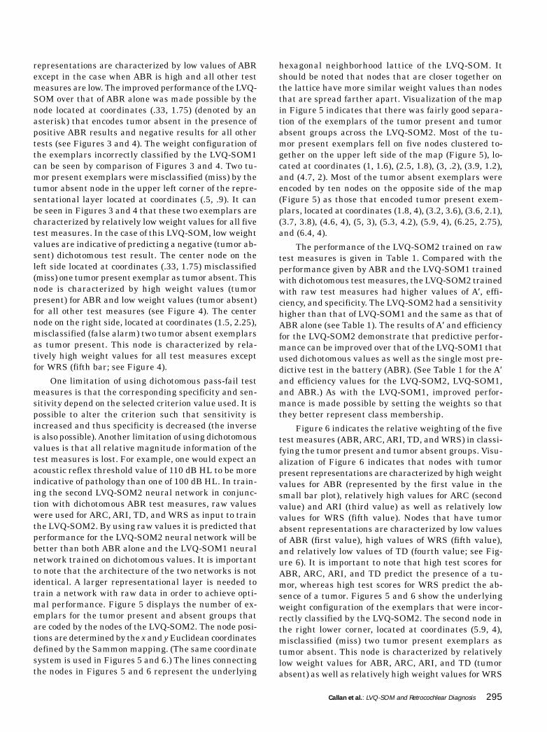
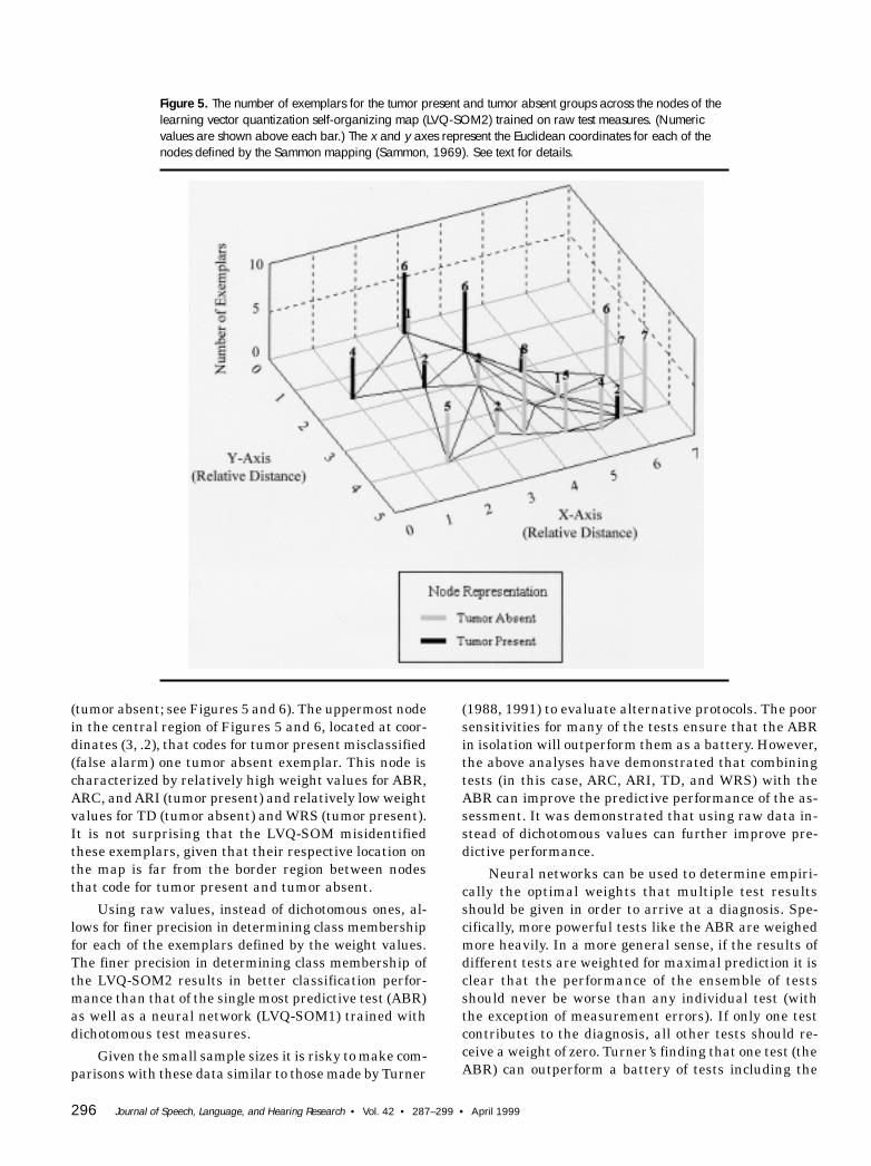
One limitation of using dichotomous pass-fail testmeasures is that the corresponding specificity and sen-sitivity depend on the selected criterion value used. It ispossible to alter the criterion such that sensitivity isincreased and thus specificity is decreased (the inverseis also possible). Another limitation of using dichotomousvalues is that all relative magnitude information of thetest measures is lost. For example, one would expect anacoustic reflex threshold value of 110 dB HL to be moreindicative of pathology than one of 100 dB HL. In train-ing the second LVQ-SOM2 neural network in conjunc-tion with dichotomous ABR test measures, raw valueswere used for ARC, ARI, TD, and WRS as input to trainthe LVQ-SOM2. By using raw values it is predicted thatperformance for the LVQ-SOM2 neural network will bebetter than both ABR alone and the LVQ-SOM1 neuralnetwork trained on dichotomous values. It is importantto note that the architecture of the two networks is notidentical. A larger representational layer is needed totrain a network with raw data in order to achieve opti-mal performance. Figure 5 displays the number of ex-emplars for the tumor present and absent groups thatare coded by the nodes of the LVQ-SOM2. The node posi-tions are determined by the x and y Euclidean coordinatesdefined by the Sammon mapping. (The same coordinatesystem is used in Figures 5 and 6.) The lines connectingthe nodes in Figures 5 and 6 represent the underlying

hexagonal neighborhood lattice of the LVQ-SOM. Itshould be noted that nodes that are closer together onthe lattice have more similar weight values than nodesthat are spread farther apart. Visualization of the mapin Figure 5 indicates that there was fairly good separa-tion of the exemplars of the tumor present and tumorabsent groups across the LVQ-SOM2. Most of the tu-mor present exemplars fell on five nodes clustered to-gether on the upper left side of the map (Figure 5), lo-cated at coordinates (1, 1.6), (2.5, 1.8), (3, .2), (3.9, 1.2),and (4.7, 2). Most of the tumor absent exemplars wereencoded by ten nodes on the opposite side of the map(Figure 5) as those that encoded tumor present exem-plars, located at coordinates (1.8, 4), (3.2, 3.6), (3.6, 2.1),(3.7, 3.8), (4.6, 4), (5, 3), (5.3, 4.2), (5.9, 4), (6.25, 2.75),and (6.4, 4).

The performance of the LVQ-SOM2 trained on rawtest measures is given in Table 1. Compared with theperformance given by ABR and the LVQ-SOM1 trainedwith dichotomous test measures, the LVQ-SOM2 trainedwith raw test measures had higher values of A′, effi-ciency, and specificity. The LVQ-SOM2 had a sensitivityhigher than that of LVQ-SOM1 and the same as that ofABR alone (see Table 1). The results of A′ and efficiencyfor the LVQ-SOM2 demonstrate that predictive perfor-mance can be improved over that of the LVQ-SOM1 thatused dichotomous values as well as the single most pre-dictive test in the battery (ABR). (See Table 1 for the A′and efficiency values for the LVQ-SOM2, LVQ-SOM1,and ABR.) As with the LVQ-SOM1, improved perfor-mance is made possible by setting the weights so thatthey better represent class membership.

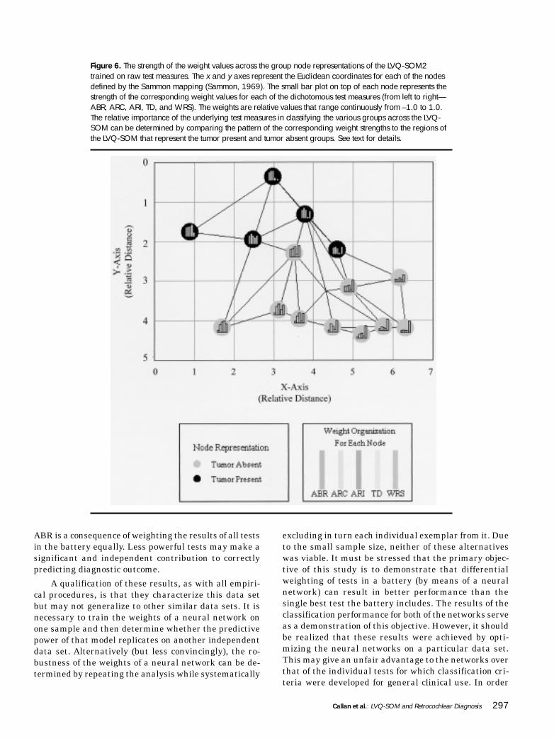
Figure 6 indicates the relative weighting of the fivetest measures (ABR, ARC, ARI, TD, and WRS) in classi-fying the tumor present and tumor absent groups. Visu-alization of Figure 6 indicates that nodes with tumorpresent representations are characterized by high weightvalues for ABR (represented by the first value in thesmall bar plot), relatively high values for ARC (secondvalue) and ARI (third value) as well as relatively lowvalues for WRS (fifth value). Nodes that have tumorabsent representations are characterized by low valuesof ABR (first value), high values of WRS (fifth value),and relatively low values of TD (fourth value; see Fig-ure 6). It is important to note that high test scores forABR, ARC, ARI, and TD predict the presence of a tu-mor, whereas high test scores for WRS predict the ab-sence of a tumor. Figures 5 and 6 show the underlyingweight configuration of the exemplars that were incor-rectly classified by the LVQ-SOM2. The second node inthe right lower corner, located at coordinates (5.9, 4),misclassified (miss) two tumor present exemplars astumor absent. This node is characterized by relativelylow weight values for ABR, ARC, ARI, and TD (tumorabsent) as well as relatively high weight values for WRS


(tumor absent; see Figures 5 and 6). The uppermost nodein the central region of Figures 5 and 6, located at coor-dinates (3, .2), that codes for tumor present misclassified(false alarm) one tumor absent exemplar. This node ischaracterized by relatively high weight values for ABR,ARC, and ARI (tumor present) and relatively low weightvalues for TD (tumor absent) and WRS (tumor present).It is not surprising that the LVQ-SOM misidentifiedthese exemplars, given that their respective location onthe map is far from the border region between nodesthat code for tumor present and tumor absent.

Using raw values, instead of dichotomous ones, al-lows for finer precision in determining class membershipfor each of the exemplars defined by the weight values.The finer precision in determining class membership ofthe LVQ-SOM2 results in better classification perfor-mance than that of the single most predictive test (ABR)as well as a neural network (LVQ-SOM1) trained withdichotomous test measures.

Given the small sample sizes it is risky to make com-parisons with these data similar to those made by Turner

(1988, 1991) to evaluate alternative protocols. The poorsensitivities for many of the tests ensure that the ABRin isolation will outperform them as a battery. However,the above analyses have demonstrated that combiningtests (in this case, ARC, ARI, TD, and WRS) with theABR can improve the predictive performance of the as-sessment. It was demonstrated that using raw data in-stead of dichotomous values can further improve pre-dictive performance.

Neural networks can be used to determine empiri-cally the optimal weights that multiple test resultsshould be given in order to arrive at a diagnosis. Spe-cifically, more powerful tests like the ABR are weighedmore heavily. In a more general sense, if the results ofdifferent tests are weighted for maximal prediction it isclear that the performance of the ensemble of testsshould never be worse than any individual test (withthe exception of measurement errors). If only one testcontributes to the diagnosis, all other tests should re-ceive a weight of zero. Turner’s finding that one test (theABR) can outperform a battery of tests including the

Figure 5. The number of exemplars for the tumor present and tumor absent groups across the nodes of thelearning vector quantization self-organizing map (LVQ-SOM2) trained on raw test measures. (Numericvalues are shown above each bar.) The x and y axes represent the Euclidean coordinates for each of thenodes defined by the Sammon mapping (Sammon, 1969). See text for details.


Figure 6. The strength of the weight values across the group node representations of the LVQ-SOM2trained on raw test measures. The x and y axes represent the Euclidean coordinates for each of the nodesdefined by the Sammon mapping (Sammon, 1969). The small bar plot on top of each node represents thestrength of the corresponding weight values for each of the dichotomous test measures (from left to right—ABR, ARC, ARI, TD, and WRS). The weights are relative values that range continuously from –1.0 to 1.0.The relative importance of the underlying test measures in classifying the various groups across the LVQ-SOM can be determined by comparing the pattern of the corresponding weight strengths to the regions ofthe LVQ-SOM that represent the tumor present and tumor absent groups. See text for details.

ABR is a consequence of weighting the results of all testsin the battery equally. Less powerful tests may make asignificant and independent contribution to correctlypredicting diagnostic outcome.

A qualification of these results, as with all empiri-cal procedures, is that they characterize this data setbut may not generalize to other similar data sets. It isnecessary to train the weights of a neural network onone sample and then determine whether the predictivepower of that model replicates on another independentdata set. Alternatively (but less convincingly), the ro-bustness of the weights of a neural network can be de-termined by repeating the analysis while systematically

excluding in turn each individual exemplar from it. Dueto the small sample size, neither of these alternativeswas viable. It must be stressed that the primary objec-tive of this study is to demonstrate that differentialweighting of tests in a battery (by means of a neuralnetwork) can result in better performance than thesingle best test the battery includes. The results of theclassification performance for both of the networks serveas a demonstration of this objective. However, it shouldbe realized that these results were achieved by opti-mizing the neural networks on a particular data set.This may give an unfair advantage to the networks overthat of the individual tests for which classification cri-teria were developed for general clinical use. In order


for classification results of the LVQ-SOM to be usefuldiagnostically in a clinical setting it will be necessaryfor training to be carried out over hundreds of samplesfrom each of the diagnostic groups. A large sample sizefor training is necessary to ensure that the probabilitydistribution indicative of the various diagnostic groupsis learned (instantiated in the weights) by the neuralnetwork. In so much as novel data are similar to thedistribution of exemplars upon which the network istrained, classification performance will be quite good,even better than traditional statistical approaches insome cases. This has been demonstrated in neural net-works applied to the diagnosis of breast lesions, pros-tate cancer, and atrial fibrillation (Markopoulos et al.,1997; Snow, Smith, & Catalona, 1994; Yang, Devine, &Macfarlane, 1994).

ConclusionNeural networks can help determine whether tests

accurately predict outcome, the independent contribu-tions of multiple tests predicting the same outcome, andhow to combine the results from multiple tests for opti-mal diagnostic outcome. In the present study, it wasdemonstrated that combining tests (in this case, ARC,ARI, TD, and WRS) with the ABR can improve the pre-dictive performance of the assessment. It was also dem-onstrated that using raw data instead of dichotomousvalues can further improve predictive performance. Thistype of insight into the data is not easily obtained fromthe protocol analysis proposed by Turner (1988). An ad-ditional advantage of using LVQ-SOM neural networksis that their two-dimensional nature provides an easyway to visualize and evaluate the weighting of the in-put parameters involved with classification of the vari-ous groups.

An advantage of neural network approaches to theproblem of diagnosing retrocochlear pathology from anumber of test results is that they quantify what clini-cians seem to do informally. Patients are highly vari-able in their presentation of symptoms and individualtests may not be definitive. Clinicians consider a vari-ety of test results, weight some more heavily than oth-ers, and combine them to formulate a diagnosis. Clini-cians are reassured by convergent test results. Neuralnetworks empirically determine the optimal weightsassociated with each test result to reach a correct diag-nosis. Furthermore, those weights can be used to iden-tify less expensive and more available tests to screenfor more expensive and inaccessible definitive tests.Neural network approaches would seem to be of valuein evaluating the merits of various tests to predictretrocochlear pathology and similar diagnostic issues inaudiology.

AcknowledgmentsWe would like to thank Elizabeth L. Leigh and Jonathan

Smillie for their editorial comments.

ReferencesAllen, R., Harnsberger, H., Shelton, C., King, B., Bell,

D., Miller, R., Parkin, J., Apfelbaum, R., & Parker, D.(1997). Low-cost high-resolution fast spin-echo MR ofacoustic schwannoma: An alternative to enhancedconventional spin-echo MR? American Journal of Neuro-radiology, 17(7), 1205–1210.

Callan, D., Kent, R., Roy, N., & Tasko, S. (1999). Self-organizing map for the classification of normal anddisordered female voices. Journal of Speech, Language,and Hearing Research, 42, 355–366.

Don, M., Masuda, A., Nelson, R., & Brackmann, D.(1997). Successful detection of small acoustic tumors usingthe stacked derived-band auditory brain stem responseamplitude. American Journal of Otology, 18(5), 608–621;discussion 682–685.

Jerger, S. (1983). Decision matrix and information theoryanalyses in the evaluation of neuroaudiologic tests.Seminars in Hearing, 4(2), 121–132.

Kleinbaum, D. G., & Kupper, L. L. (1978). Appliedregression analysis and other multivariable methods.Boston: Duxbury Press.

Kohonen, T. (1990). Improved versions of learning vectorquantization. Proceedings of the International JointConference on Neural Networks, San Diego, CA, 545–550.

Kohonen, T. (1995). Self-organizing maps. Berlin: Springer.

Kohonen, T., Hynninen, J., Kangas, J., & Laaksonen, J.(1996). SOM-PAK: The self-organizing map programpackage (Report A31). Helsinki University of Technology:Laboratory of Computer and Information Science.

Kohonen, T., Hynninen, J., Kangas, J., Laaksonen, J.,& Torkkola, K. (1995). LVQ-PAK: The learning vectorquantization program package. Helsinki University ofTechnology: Laboratory of Computer and InformationScience.

Ludman, H. (1988). Tumors of the inner ear. In Mawson(Ed.), Diseases of the ear (pp. 648–663). Chicago: YearBook Medical Publishers.

Mahaley, M. S., Jr., Mettlin, C., & Natarajan, N. (1990).Analysis of patterns of care of brain tumor patients in theUnited States: A study of the brain tumor section of theAANS and CNS and the Commission on Cancer of theACS. Clinical Neurosurgery, 96, 347–352.

Markopoulos, C., Karakitsos, P., Botsoli-Stergiou, E.,Pouliakis, A., Ioakim-Liossi, A., Kyrkou, K., & Gogas,J. (1997). Application of the learning vector quantizer tothe classification of breast lesions. Analytical & Quantita-tive Cytology & Histology, 19(5), 453–60.

NIH Consensus Panel. (1991). Acoustic neuroma. NIHConsensus Statement, 9(4), 1–24.

Sammon, J. (1969). A non-linear mapping for data structureanalysis. IEEE Transactions on Computers, 18, 401–409.

Schuknecht, H. F. (1993). Pathology of the ear. Philadel-phia: Lea and Febiger.


Snow, P., Smith, D., & Catalona, W. (1994). Artificialneural networks in the diagnosis and prognosis of prostatecancer: A pilot study (Part 2). Journal of Urology, 152(5),1923–1926.

Swets, J. A. (1964). Signal detection and recognition byhuman observers. New York: John Wiley.

Turner, R. G. (1988). Techniques to determine test protocolperformance. Ear and Hearing, 9, 177–189.

Turner, R. G. (1991). Making clinical decisions. In W. F.Rintelmann (Ed.), Hearing assessment (pp. 679–739).Austin, TX: Pro-Ed.

Turner, R. G., Shepard, N. T., & Frazer, G. J. (1984).Clinical performance of audiological and related diagnostictests. Ear and Hearing, 5, 187–194.

von Glass, W., Haid, C., Cidlinsky, K., Stenglein, C., &Christ, P. (1991). False-positive MR imaging in thediagnosis of acoustic neurinomas. Otolaryngology-Headand Neck Surgery: Case Reports, 104, 863–867.

Woolsey, T. D., & Eldred, C. A. (1977). A summary reporton the survey of intracranial neoplasms. National Institutes

of Health, National Institute of Neurological and Commu-nicative Disorders and Stroke, Office of Biometry andEpidemiology, Rockville, MD.

Yang, T., Devine, B., & Macfarlane, P. (1994). Artificialneural networks for the diagnosis of atrial fibrillation.Medical & Biological Engineering & Computing, 32(6),615–619.

Yanz, J. (1984). The application of the theory of signaldetection to the assessment of speech perception. Ear andHearing, 5(2), 64–71.

Yellin, M., Jerger, J., & Fifer, R. (1989). Norms fordisproportionate loss in speech intelligibility. Ear andHearing. 10(4), 231–234.

Received April 17, 1998

Accepted October 30, 1998

Contact author: Daniel E. Callan, ATR Human InformationProcessing Research Laboratories, 2-2 Hikaridai, Seika-cho, Soraku-gun, Kyoto, Japan 619-0288.Email: [email protected]

1999;42;287-299 J Speech Lang Hear Res Daniel E. Callan, Robert E. Lasky, and Cynthia G. Fowler

Neural Networks Applied to Retrocochlear Diagnosis

http://jslhr.asha.org/cgi/content/abstract/42/2/287#otherarticlesfree at:

This article has been cited by 1 HighWire-hosted article(s) which you can access for

This information is current as of March 5, 2013

http://jslhr.asha.org/cgi/content/abstract/42/2/287located on the World Wide Web at:

This article, along with updated information and services, is

http://jslhr.asha.org/cgi/content/abstract/42/2/287#otherarticles

http://jslhr.asha.org/cgi/content/abstract/42/2/287

Callan et al.: LVQ-SOM and Retrocochlear Diagnosis Neural Networks Applied to Retrocochlear...

Documents

Transcript of Callan et al.: LVQ-SOM and Retrocochlear Diagnosis Neural Networks Applied to Retrocochlear...