CAFF Technical Report No. 21 August 2010

PROCEEDINGS OF THE FIFTH INTERNATIONAL WORKSHOP - CAFF FLORA GROUPCIRCUMBOREAL VEGETATION MAPPING WORKSHOP, NOVEMBER 2008

ARCTIC COUNCIL

The Conservation of Arctic Flora and Fauna (CAFF) is a Working Group of the Arctic Council. CAFF Designated Agencies:

• Directorate for Nature Management, Trondheim, Norway

• Environment Canada, Ottawa, Canada

• Faroese Museum of Natural History, Tórshavn, Faroe Islands (Kingdom of Denmark)

• Finnish Ministry of the Environment, Helsinki, Finland

• Icelandic Institute of Natural History, Reykjavik, Iceland

• The Ministry of Domestic Affairs, Nature and Environment, Greenland

• Russian Federation Ministry of Natural Resources, Moscow, Russia

• Swedish Environmental Protection Agency, Stockholm, Sweden

• United States Department of the Interior, Fish and Wildlife Service, Anchorage, Alaska

CAFF Permanent Participant Organisations:

• Aleut International Association (AIA)

• Arctic Athabaskan Council (AAC)

• Gwich’in Council International (GCI)

• Inuit Circumpolar Conference - (ICC) Greenland, Alaska and Canada

• Russian Indigenous Peoples of the North (RAIPON)

• Saami Council

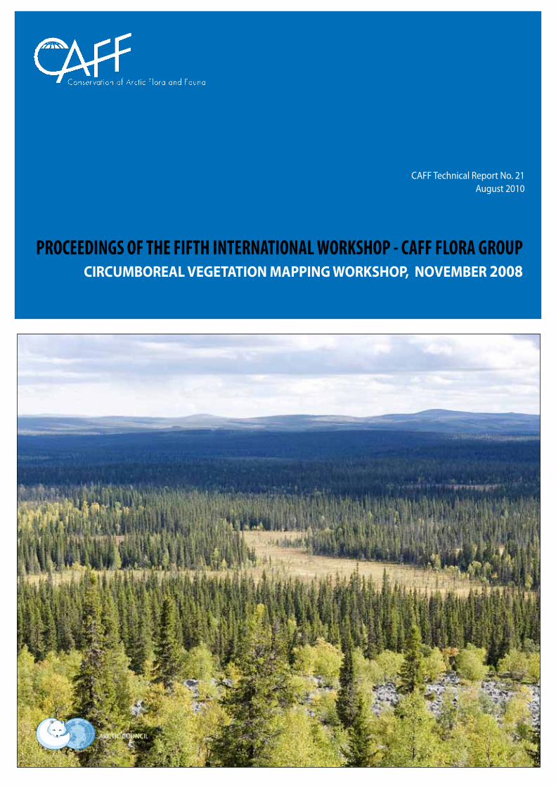
This publication should be cited as: Talbot, S., Charron, T., Barry, T. (eds.). 2010. Proceedings of the Fifth International Workshop: Conservation of Arctic Flora and Fauna (CAFF) Flora Group. Cir-cumboreal Vegetation Mapping (CBVM) Workshop, Helsinki, Finland, November 3-6th, 2008. CAFF International Secretariat, CAFF Flora Expert Group (CFG), CAFF Technical Report No. 21.

Cover photo by Ari-Pekka Auvinen. The Nuortti River in North Eastern Finnish Lapland.

For more information please contact:CAFF International SecretariatBorgir, Nordurslod600 Akureyri, IcelandPhone: +354 462-3350Fax: +354 462-3390Email: caff@caff.isInternet: http://www.caff.is

Acknowledgments

___ CAFF Designated Area

Udo Bohn 18 January 1939 - 13 August 2010

This report is in honor of the late Dr. Udo Bohn for his major contributions in the field of vegetation science. To experience and learn from nature was his lifeblood. His work was a true inspiration for the Circumpolar Arctic Vegetation Map (CAVM) and continues

to be as we move forward with the Circumboreal Vegetation Map (CBVM). Udo may have been the only person who still had the full European vegetation mapping

heritage in his blood and could integrate the Braun-Blanquet approach with mapping at big scales.

We will move forward in his absence, but we really needed him. His death is big loss for the project both from a scientific standpoint and on a personal level.

We enjoyed his warm presence at our workshops. He was a great person.

Table of Contents

Circumboreal Vegetation Mapping (CBVM) Project: Introduction and Objectives - Stephen S. Talbot & Donald A. Walker . . . . . . . . . . . . . . . . . . . . . . . . . . . . . . . . . . . . . . . . . . . . . . . . . . . . . . . . . . . . . . . . . . . . . . . 1

A Vegetation Map of Arctic Tundra & Boreal Forest Regions: Integrating the CAVM with the Circumboreal Vegetation Map - Donald A. Walker . . . . . . . . . . . . . . . . . . . . . . . . . . . . . . . . . . . . . . . . . . . . . . . . . . . . . . . . . . . . 4

Vegetation Mapping and Classification for Canada - Kenneth A. Baldwin . . . . . . . . . . . . . . . . . . . . . . . . . . . . . . 16

Experiences in Mapping the Boreal Zone in Canada - Jean-Pierre Saucier & Del Meidinger . . . . . . . . . . . . . . . . . . 22

Map of the Natural Vegetation of Europe and Its Contribution to the CBVM - Udo Bohn . . . . . . . . . . . . . . . . . . . 31

Development of a Boreal Vegetation Map of the Asian Part of Russia as a Part of the CBVM - Nikolai Ermakov . . . . . 38

The Integrated Mapping of Actual Vegetation of Asia - Kazue Fujiwara . . . . . . . . . . . . . . . . . . . . . . . . . . . . . . . 39

Datasets Useful for the Circumboreal Vegetation Mapping Project - Carl Markon . . . . . . . . . . . . . . . . . . . . . . . . . 41

Ecological-Geographical Base for Biodiversity of Boreal Forests in Russia - Galina N. Ogureeva . . . . . . . . . . . . . . . 42

Zones and Altitudinal Zonality Types of Vegetation of Russia and Adjacent Territories - Galina N. Ogureeva . . . . . . 52

Vegetation Mapping in Boreal Alaska - Stephen S. Talbot . . . . . . . . . . . . . . . . . . . . . . . . . . . . . . . . . . . . . . . 74

A Geobotanical Impression of South Greenland with Some Remarks on Its “Boreal Zone” - Fred J. A. Daniёls . . . . . . 85

Large-Scale Vegetation Mapping in Iceland - Gudmundur Gudjonsson, Hördur Kristinsson, & Eythor Einarsson . . . 93

The Vegetation of the Faroe Islands - Anna Maria Fosaa . . . . . . . . . . . . . . . . . . . . . . . . . . . . . . . . . . . . . . . . 95

The Plant Cover of the Kamchatka Peninsula (North of the Russian Far East) & Its Geobotanical Subdivision - Valetina Yu. Neshataeva . . . . . . . . . . . . . . . . . . . . . . . . . . . . . . . . . . . . . . . . . . . . . . . . . . . . . . . . . . . . . . . . . . 98

Ecological-Floristic Approach to Typology of Forests for European Russian - L.B. Zaugolnova & T. Yu Braslavskaya . . . . . . . . . . . . . . . . . . . . . . . . . . . . . . . . . . . . . . . . . . . . . . . . . . . . . . . . . . . . . . . . . . . . . . . . . . . . . . . . 104

The Finnish Concept of Vegetation and Zones of Natural Forests and Mires - Tapio Lindholm & Raimo Heikkilä . . . 106

The Importance of Mire Complexes for the Development of a Circumboreal Vegetation Map (CBVM) - Klaus Dierssen . . . . . . . . . . . . . . . . . . . . . . . . . . . . . . . . . . . . . . . . . . . . . . . . . . . . . . . . . . . . . . . . . . . . . . . . . . . . . 112

Forest and Mire Vegetation on the Maps of two Nature Reserves: Comparison of European and Western Siberian Northern Taiga Regions - Vasily Neshatayev . . . . . . . . . . . . . . . . . . . . . . . . . . . . . . . . . . . . . . . . . . . . . . 113

An Approach to Mapping the North American Boreal Zone - James Brandt . . . . . . . . . . . . . . . . . . . . . . . . . . . 122

Bioclimatic Framework for the CBVM Project - Daniel Sánchez-Mata & Salvador Rivas-Martínez . . . . . . . . . . . . . . 132

Bioclimates and Distribution of Zonal Types of Boreal Vegetation in Northeast Asia - Pavel V. Krestov & Alexander M. Omelko . . . . . . .. . . . . . . . . . . . . . . . . . . . . . . . . . . . . . . . . . . . . . . . . . . . . . . . . . . . . . . . . . . . . . 137

GIMMS–NDVI Based Mapping of the Growing Season North of 50°N - Stein Rune Karlsen, Kjell-Arild Høgda, Bernt Johansen, Arve Elvebakk, Violetta Fedotova & Anne Tolvanen . . . . . . . . . . . . . . . . . . . . . . . . . . . . . . . . . . . 143

Mapping of the Eurasian Circumboreal Forest–Tundra Transition Zone by Remote Sensing - Gareth Rees, Olga Tutub-alina, Hans Tømmervik, Mikhail Zimin, Anna Mikheeva, Elena Golubeva, Kelly Dolan, Annika Hofgaard . . . . . . . 144

On the Importance of Accounting for Disturbance Regimes and Forest Succession Ecosystem Dynamics in Bo-real Vegetation Mapping - Steven G. Cumming, Yves Bergeron, & Sylvie Gauthier . . . . . . . . . . . . . . . . . . . . . . 151

Role of Disturbed Vegetation in Mapping the Boreal Zone in Northern Eurasia - Annika Hofgaard, Gareth Rees, Hans Tømmervik, Olga Tutubalina, Elena Golubeva, Ekaterina Shipigina, Kjell Arild Høgda; Stein Rune Karlsen, Mikhail Zimin, Viacheslav Kharuk . . . . .. . . . . . . . . . . . . . . . . . . . . . . . . . . . . . . . . . . . . . . . . . . . . . . . . . . . . . . . 153

Mapping of Natural and Anthropogenic Disturbances on Vegetation in Kola Peninsula - Tatjana Chernenkova, Mi-hail Puzachenko, Elena Tikhonova, Elena Basova . . . . . . . . . . . . . . . . . . . . . . . . . . . . . . . . . . . . . . . . . . . 162

Circumboreal Forest Cover Mapping and Monitoring Using MODIS Time Series Imagery - Peter V. Potapov, Matthew C. Hansen & Stephen V. Stehman . . . . . . . . . . . . . . . . . . . . . . . . . . . . . . . . . . . . . . . . . . . . . . . . . . . . . . 169

Vegetation Mapping & Disturbances Assessment in the Boreal Zone Using Time-Series of Moderate-Resolution Re-mote Sensing Data - Sergey Bartalev . . . . . . . . . . . . . . . . . . . . . . . . . . . . . . . . . . . . . . . . . . . . . . . . . . . .173

Comparison of Finnish and Russian Approaches for Large-Scale Vegetation Mapping: a Case Study - Olga Galanina & Raimo Heikkilä . . . . . . . . . . . . . . . . . . . . . . . . . . . . . . . . . . . . . . . . . . . . . . . . . . . . . . . . . . . . .. . . . . . 174

Integrated Ecoforest Mapping of the Northern Portion of the Continuous Boreal Forest, Québec, Canada - Andre Robitaille . . . . . . . . . . . . . . . . . . . . . . . . . . . . . . . . . . . . . . . . . . . . . . . . . . . . . . . . . . . . . . . . . . . . . . 180

Analysis of Terrain Relationships to Improve Mapping of Boreal Ecosystems - Torre Jorgenson . . . . . . . . . . . . . . 184

Appendices

Appendix I. Proposal for an IAVS Circumboreal Vegetation Map (CBVM) Working Group . . . . . . . . . . . . . . . . . . . 185

Appendix II. Resolution from the CBVM Workshop, Helsinki, Finland, November 3–6, 2008 . . . . . . . . . . . . . . . . . 186

Appendix III. CBVM Organizational Chart . . . . . . . . . . . . . . . . . . . . . . . . . . . . . . . . . . . . . . . . . . . . . . 186

Appendix IV. CBVM Thematic Composition . . . . . . . . . . . . . . . . . . . . . . . . . . . . . . . . . . . . . . . . . . . . . 187

Appendix V. CBVM Regional Team Composition . . . . . . . . . . . . . . . . . . . . . . . . . . . . . . . . . . . . . . . . . . 187

Appendix VI. CBVM Timeline . . . . . . . . . . . . . . . . . . . . . . . . . . . . . . . . . . . . . . . . . . . . . . . . . . . . . . . . . 188

Appendix VII. CBVM Leadership . . . . . . . . . . . . . . . . . . . . . . . . . . . . . . . . . . . . . . . . . . . . . . . . . . . . 188

1

Stephen S. Talbot1 & Donald A. Walker2

1U.S. Fish and Wildlife Service, Anchorage, Alaska, U.S.A., stephen_talbot@fws.gov, 2Institute of Arctic Biology, University of Alaska Fairbanks, Alaska, U.S.A., ffdaw@uaf.edu

Introduction

Our aim is to produce the first boreal vegetation map of the entire global Arctic biome at a comparable resolution for understanding the region. Like the Circumpolar Arctic Vegetation Map (CAVM), the Circumboreal Vegetation Map (CBVM) project will be one of the first detailed vegetation maps of an entire global biome. A common legend and language for the various ecosystems that make up the boreal region are needed as well as a map that provides a broad view and a consistent treatment of the vegetation of the entire biome through legend descriptions, photographs, lists of major vegetation types, and supplementary maps. It is also important that the map recognizes the boreal region as a single geo-ecosystem with a common set of cultural, political, and economic issues. Currently, various maps already exist of the boreal biome, but they do not rely on a unified international method for classifying and mapping boreal vegetation.

Unified Classification

Boreal forests are particularly appropriate for unified classification because of their high level of floristic, physiognomic, and syntaxonomic similarity across the entire biome. The map can also serve as a key component of circumboreal geographical information systems (GIS), and such a map is needed for resource development, land-use planning, studies of boreal biota and biodiversity, education, anticipated global changes, and human interactions. Documenting the current distribution of the boreal is a first step toward monitoring these long-term changes. Our workshop brings together an international group of vegetation scientists to present the latest information regarding boreal syntaxonomy, geobotany, mapping, and new computer programs for studying boreal plant communities. The basic workshop rationale is that global-scale boreal research programs, modelling

efforts, educational materials, and conservation efforts require a common language for describing boreal ecosystems.

Creating a Compatible Map with the Circumpolar Arctic Vegetation Map

A secondary goal is to make the CBVM compatible with the CAVM (scale 1:7,500,000) to the north. Linking these two global-scale maps is necessary because very few issues relevant to the Arctic or the boreal regions stop at tree line. For example, most rivers flowing into the Arctic Ocean have their origin far to the south of the tree line. Climate and vegetation-change models, analysis of animal migrations, roads and industrial developments, and arctic–human interaction all require maps that include both the Arctic tundra and boreal forest regions. B

Project History

The need for such a Circumboreal Vegetation Map was discussed at the Second International Workshop on Circumpolar Vegetation Classification and Mapping held in Tromsø (Sommarøy), Norway, in June 2004. This need was further discussed at the Third Conservation of Arctic Flora and Fauna (CAFF) Flora Group Workshop in Helsinki, Finland, in May 2005, and a proposal for funding was initiated. An organizational meeting was held in Fairbanks, Alaska, in March 2006, and a funding proposal was further developed; attendees at this meeting were: Teresa Hollingsworth (Boreal Ecology Cooperative Research Unit, Pacific Northwest Research Station, U.S. Department of Agriculture Forest Service, Fairbanks), Stephen Talbot (U.S. Fish & Wildlife Service, Anchorage), and Donald “Skip” Walker (University of Alaska Fairbanks).

At the CAFF XI Biennial Meeting in Yllas, Finland, in March 2006, the CAFF National Representatives endorsed a Circumboreal Vegetation Map (CBVM).

Circumboreal Vegetation Mapping (CBVM) Project: Introduction and Objectives

2

This approval was followed by an endorsement by the Senior Arctic Officials representing the eight Arctic States. In the interim, the CAFF Flora Group received support from Environment Canada, Faroe Islands Homeland Government, and the U.S. Department of State to fund the Fourth International Conservation of Arctic Flora and Fauna (CAFF) Flora Group Workshop, 15–18 May 2007, Tórshavn, Faroe Islands. This workshop helped pave the way for the present Circumboreal Vegetation Map (CBVM) workshop in Helsinki (Talbot, 2008). Workshop funding for the CBVM was obtained from the Nordic Council of Ministers by Finland.

Project Goal

The goal of this international project is to produce a map of the natural vegetation of the boreal region. Currently, there are a number of useful remote-sensing products that display vast areas of the North (Bartalev et al., 2004; Hansen et al., 2003). These provide important data and perspective, but our intent is to develop a true vegetation map such as the one produced for Europe (Bohn et al., 2005). Accordingly, it is essential that phytosociologists or vegetation ecologists—guided by sound vegetation science principles—be directly involved in making the map. Our map should display the character of the vegetation using the philosophical approaches to vegetation mapping that are understood, debated, and developed in the great schools of vegetation mapping. Our boreal vegetation mapping effort should be accomplished based on a uniform concept using the most current knowledge and by the means of close international cooperation of geobotanists from nearly all boreal countries (cf. Bohn et al., 2005).

Objectives

We convene this international workshop to develop a strategy to map the vegetation of the circumboreal zone. Our workshop objectives are to:

1. review the status of boreal vegetation mapping in each of the boreal countries;

2. present examples of possible approaches for making the map;

3. define the region to be mapped;

4. establish the project goals;

5. form a mapping team with representatives from each boreal country;

6. develop a plan for making the map (identify international collaborators, establish a floristic and hierarchical legend approach, set a schedule for making the CBVM);

7. develop a plan for writing a proposal or series of proposals that would result in the final CBVM; and

8. publish the results of the workshop.

We need to keep the scope of this initial workshop limited to these objectives and not lose sight of them. I stress the objectives above so that we focus on them at the very beginning of our workshop as there may be peripheral issues that arise. The Nordic Council of Ministers funded this workshop to address these objectives, and they are to be kept in mind throughout the workshop. Toward the conclusion of the workshop, we will address each objective individually to make certain each is fulfilled.

Organizational Structure

A solid organizational structure will be key in developing the map. It will be important to have one strong senior person as the designated organizer from each country; this person will be primarily responsible for pulling the section maps of that country together. The scientists responsible for the actual mapping, however, might be young people that are just starting their careers. Canada might be divided into two to three sections, possibly on the basis of floristic provinces, but one person will be responsible for synthesizing maps of the whole country. Russia, similarly, might be divided into four to five floristic regions, but one overall leader will need to be identified from the beginning who will integrate the whole Russian map. At the biome scale, someone needs to be identified from the beginning as the overall CBVM project leader, who will be responsible for synthesizing all the maps from the various countries into a single circumboreal map.

Map Units

The basic map units will be physiognomic and/or a combination of physiognomic-floristic units. As the mapping effort will involve scientists from many countries, the internationally recognized Braun-

3

Blanquet plant-community nomenclatural system, or the closest equivalent that can be provided, is a logical choice as the preferred foundation for cataloging plant communities.

Determining Products

We should determine from the outset if we want a vegetation map or a much larger document that includes a book with discussion of the regional floras, species distribution maps, vegetation dynamics, etc. Initially, these extras probably should not be included, because this project will go on for decades with a budget that no one will be able to support. Our immediate need is a good circumpolar portrayal of boreal vegetation with a consistent legend that is acceptable to the majority of vegetation scientists. Other products could follow, but we need to keep the scope of this initial project limited to the map and not lose sight of this.

Transboundary Perspective

Viewing the world from a global perspective is an opportunity to explore the potential for regional environmental cooperation with the dual purpose of conserving biodiversity and fostering friendly relations among neighboring countries. By opening to a transboundary perspective one hopes to achieve an increased level of understanding that puts aside local approaches and schools of vegetation mapping for a truly international transfrontier approach.

References

Bartalev, S. A., Ershov, D. V., Isaev, A. S., Potapov, P. V., Turubanova, S. A., & Yaroshenko, A. Yu. 2004. Russia’s Forests: Dominating Forest Types and Their Canopy Density; Scale 1: 14,000, 000; Space Research Institute of the Russian Academy of Sciences (RAN), Forest Ecology and Production Center of the Russian Academy of Sciences (RAN), Global Forest Watch, Greenpeace Russia, Moscow.

Bohn, U., Hettwer, C., & Gollub, G., eds. 2005. Anwendung und Auswertung der Karte der natürlichen Vegetation Europas / Application and Analysis of the Map of the Natural Vegetation of Europe. – Bonn (Bundesamt für Naturschutz) – BfN-Skripten 156: 1–452.

Hansen, M. C., DeFries, R. S., Townshend, J. R. G., Carroll, M., Dimiceli, C., & Sohlberg, R. A. 2003. Global percent tree cover at a spatial resolution of 500 meters: First Results of the MODIS Vegetation Continuous Fields Algorithm. Earth Interactions 7 (10): 1–15.

Talbot, S. S., ed. 2008. Proceedings of the Fourth International Conservation of Arctic Flora and Fauna (CAFF) Flora Group Workshop, 15–18 May 2007, Tórshavn, Faroe Islands. CAFF Technical Report No. 15. Akureyri, Iceland.

rtment of Agriculture Forest Service, Fairbanks), Stephen Talbot (U.S. Fish & Wildlife Service, Anchorage), and

4

Donald A. Walker

Institute of Arctic Biology, University of Alaska Fairbanks, Alaska, U.S.A. ffdaw@uaf.edu

A Vegetation Map of Arctic Tundra and Boreal Forest Regions: Integrating the CAVM with the Circumboreal Vegetation Map

Abstract

The Circumpolar Arctic Vegetation Map (CAVM) is a map developed by Arctic vegetation specialists that depicts the vegetation of the global tundra biome at a scale that is useful for regional and global-change analysis and modelling. The proposed Circumboreal Vegetation Map (CBVM) has a similar goal. This paper presents an overview of the processes and hurdles involved in making the CAVM. Several suggestions are presented that would allow combining the CBVM and CAVM into one map that portrays the vegetation of both the Arctic and boreal biomes. These suggestions involve: (1) selecting the right team and leadership; (2) funding; (3) agreement on a plan for making the map; (4) defining the extent, scale, projection, and base for making the map; (5) phytogeographic subdivisions; (6) map content; (7) legend approach; and (8) summary tables of dominant plant communities.

Keywords: Braun-Blanquet approach, floristic approach, GIS, hierarchical mapping, physiognomic units, tundra.

Introduction

The worldwide efforts to understand the effects of global climate change have awakened vegetation scientists to the need for new international vegetation maps that cover entire global biomes. These maps would allow more detailed analysis and modelling of the global system and the interactions between the land, oceans, and atmosphere. A map that would portray both the arctic tundra and boreal forest regions is especially needed because of the many linkages that unite these into a single global system centered on the Arctic Ocean and the watersheds that flow into it.

The Circumpolar Arctic Vegetation Map (CAVM) was

the first attempt to make a map of an entire global biome with enough detail for regional and global ecosystem studies. The Circumboreal Vegetation Map (CBVM) will be the second. In this paper, a brief overview is provided of the process used in making the CAVM, focusing on some of they key elements that would also be useful for the CBVM. At the end, I present suggestions for integrating the CAVM with the CBVM to create one vegetation map of the northern part of the Earth.

A Short History of the Circumpolar Arctic Vegetation Map

The Circumboreal Vegetation Map is being initiated in a spirit much like that of the Circumpolar Arctic Vegetation Map (CAVM). In March 1992, a group of arctic vegetation scientists at the International Workshop on Classification of Arctic Vegetation at the University of Colorado saw an urgent need for a more detailed map of the vegetation in the circumpolar region and formed a resolution to make the CAVM. At that time the only maps that portrayed the vegetation of the whole Arctic were coarse-scale maps (greater than 1:10 M scale) that showed only broad zones—usually a treeless region north of the forested areas subdivided into tundra and polar desert. These maps were too coarse for circumpolar tundra ecosystem studies such as modelling the flux of trace-gases and global vegetation-change models. Many more detailed maps existed for small regions of the Arctic, but these used many different scales, classification schemes, and base maps that prevented a straightforward synthesis. Often, political boundaries defined the edges of the maps instead of natural vegetation boundaries. More critically, the maps that were in use did not portray the vegetation of the Arctic with terms that were compatible with the actual vegetation—most were developed by modelers or remote-sensing specialists for their

5

specific purposes and had inconsistent terminology to portray the vegetation of this vast and heterogeneous region. There was, thus, a big need for a map that was acceptable to the international group of arctic vegetation specialists who worked in the Arctic and intimately knew the vegetation. Following the Boulder workshop, a proposal was co-funded by the U.S. National Science Foundation and the U.S. Fish and Wildlife Service to hold the first CAVM workshop devoted entirely to arctic vegetation mapping.

Lakta Workshop 1994

In March 1994 the Komarov Botanical Institute hosted the workshop in the small village of Lakta near St. Petersburg, Russia (Walker & Markon, 1996). It is useful to review this workshop in some detail because, in many respects, it was similar in intent to this Helsinki workshop—it laid the foundation for making the eventual map. At the Lakta meeting, 51 participants reviewed the status of arctic vegetation mapping in each of the circumpolar countries and developed a strategy for making a new series of maps to portray the current knowledge of arctic vegetation.

An executive committee headed by D. A. Walker was established with representatives from each of the circumpolar countries with territories north of the arctic treeline. Separate teams were identified for mapping Canada, Greenland, Iceland, Russian, Norway, and Alaska. The participants agreed to make the following products before the next workshop: (1) a review of arctic vegetation maps; (2) maps showing zonal divisions and floristic sectors according to the scheme of Yurtsev (Yurtsev, 1994, 1996) and the arctic treeline; (3) an image of the maximum Normalized Difference Vegetation Index (NDVI) for the whole Arctic to portray relative biomass or vegetation density; and (4) a satellite-derived false color image of the circumpolar region in a snow-free state that would be used as the base-map for image interpretation of vegetation at 1:7.5 M scale.

The group also agreed that the spatial domain for the map would follow that of the Panarctic Flora (PAF) initiative (Elvebakk et al., 1999), which considered the Arctic to be equivalent to the Arctic Bioclimate Zone. The tree line, which is the southern boundary of the CAVM, was based on a variety of sources.

The Lakta workshop led to three publications. The first paper (Walker, 1995), published in Arctic and Alpine Research, gave an overview of the workshop and set forth a plan for making the maps. The second paper reviewed the current status of vegetation mapping in each of the circumpolar countries (Walker et al., 1995). The third publication was a compilation of all the abstracts and papers presented at the Lakta workshop (Walker & Markon, 1996); it summarized the various approaches to vegetation mapping in the Arctic and also contained the two above-mentioned publications as appendices.

Following the Lakta workshop, the project received the endorsement of the International Arctic Science Committee (IASC) and the U.S. Polar Research Board (PRB) and was recognized as a priority task of the Conservation of Arctic Flora and Fauna (CAFF) Project.

In summary, the essential events that occurred at the Lakta workshop were: (1) the goals and products of the mapping effort were defined; (2) the spatial domain, map-scale, map projection, and boundaries of the map were defined; (3) a thorough review of the existing maps in the Arctic was presented; (4) the Arctic was divided into manageable regions with leaders assigned to each region; (5) a plan was defined for making a circumpolar base image from satellite data; and (6) three key publications were outlined and eventually published.

Arendal Workshop 1996

The CAVM team members met at Arendal, Norway 19–24 May 1996 (Walker & Lillie, 1997). This was a key meeting because a detailed method for making the map was developed and agreed to by all the members of the CAVM team (Walker, 1999) (Fig. 1).

Additional Meetings

Additional meetings were necessary to discuss prototype approaches for making the map (Anchorage, Alaska, 1997; cf. Walker & Lillie [1997]) and to review the progress being made in each of the countries (St. Petersburg, Russia, 1999, Moscow, 2001; cf. Raynolds & Markon [2001]), and Tromsø, 2004; cf. Daniëls et al. [2005]). Once the funding for the map

6

was secured in 1998, it took five more years until the final map was published (CAVM Team, 2003), and two more years for the final journal publication where the method was described and the map analyzed (Walker et al., 2005)—in total 13 years passed from initiation of the idea in Boulder until the final publication.

Key Aspects of the CAVM Relevant to the CBVM

The CAVM content and analysis are well described elsewhere (Walker et al., 2005). My primary intention here is to summarize some of the key aspects that could be applied to the CBVM.

Selecting the Right Team and Leadership

At the outset everyone agreed that the final map would be a true vegetation map in the tradition of the vegetation mapping schools in Europe and Russia. It was not, however, easy to find participants with

the right combination of talents to make the maps. It required vegetation experts with broad knowledge of Arctic vegetation who were also experienced with making maps, and who were also interested in the project and who had the necessary time and resources to commit to the project. Thirty-four regional experts were involved in producing the map and another 17 helped in the review of specific areas of the map. A relatively small group (essentially one or two from each country) took responsibility for the final CAVM synthesis.

The map required a strong group of leaders who were willing to commit to the project until it was finished. The larger countries were divided into subregions with their own subleaders. When someone dropped out because of sickness, death, lack of interest, or other reasons, it slowed the process considerably because it required finding a replacement. The overall leader had to have good knowledge of the Arctic, its

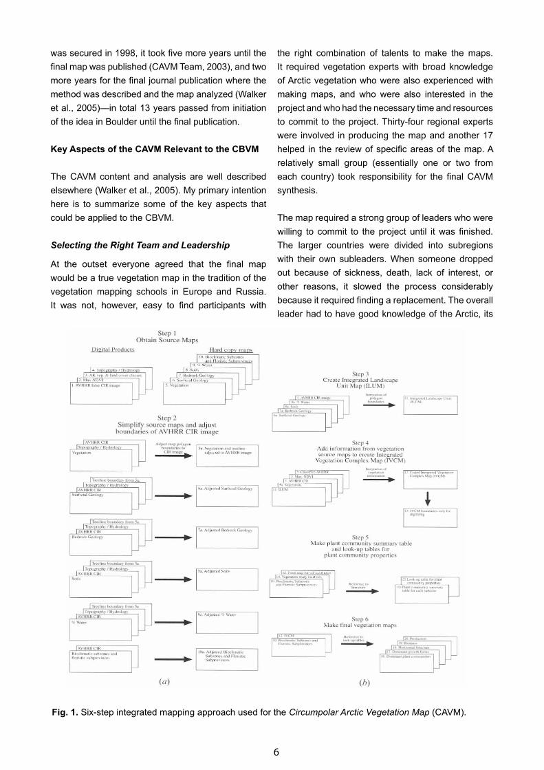
Fig. 1. Six-step integrated mapping approach used for the Circumpolar Arctic Vegetation Map (CAVM).

7Carsten Egevang/ARC-PIC.COM

vegetation and cartographic methods, and also had to be committed to achieving unanimous consensus among the countries regarding the mapping methods and the legend. He also needed the ability to obtain the necessary funding to complete the map.

Funding

Achieving the necessary funding was a major hurdle. In the beginning progress was slow because of lack of funds. Progress was achieved through a series of small workshops and meetings that were funded primarily through the U.S. Fish and Wildlife Service with moral support from the Conservation of Arctic Flora Fauna (CAFF) Group. In 1998, five years after the project was initiated, The U.S. National Science Foundation provided $225,000 for the CAVM as part of a grant to examine trace-gas fluxes in the Arctic (Arctic Transitions in the Land Atmosphere System (ATLAS) project). The map would not have been completed without this major grant. Additional funds came from the U.S. Fish and Wildlife Service, primarily for meetings. Individual researchers and their host institutions contributed most of the work involved in making the regional maps.

Agreement on a Plan for Making the Map

At the outset, the team agreed that a purely remote-sensing classification approach would not be appropriate because of problems with spectral similarity of key mapping units in the Arctic and the very difficult process that would be involved with creating a sophisticated automated approach to classifying such a diverse region. Also, the team agreed that a more traditional mapping approach, such as that used for the Map of the Natural Vegetation of Europe (Bohn et al., 2000), would yield a more satisfactory product.

A six-step integrated mapping approach (Fig. 1) was adopted. This was similar in principal to a variety of landscape-guided mapping approaches (Walker et al., 1986; Zonneveld, 1988; Dangermond & Harnden, 1990; Melnikov & Minkin, 1998). The boundaries of major terrain features such as areas of hills, large wetlands, large floodplains, and mountainous areas were used as the first criteria to delineate map polygon boundaries. Vegetation map boundaries were further defined by using a combination of information from several map sources all registered to the same scale as the circumpolar false color-infrared (FCIR) base

map (derived from AVHRR satellite imagery). These source maps included digital products (the AVHRR FCIR base image, maximum NDVI, and topography/hydrology) and hard copy maps registered to the same scale as the base map (e.g., maps of bedrock geology, surficial geology, soils, vegetation, percent water, and the phytogeographic boundaries of Yurtsev). The boundaries were derived in a series of steps shown in Figure 1 and described in Walker et al. (2002).

The integrated mapping method (Fig. 1) was an essential element that allowed everyone to follow a standard approach for interpreting information on the AVHRR base map. It was particularly useful for establishing probable vegetation on landscapes where there was little mapped information (e.g., Arctic Canada, Alaska, Greenland). Not everyone followed this method because vegetation maps were already available at comparable scale for all of Russia, Svalbard, and Iceland. In these areas, existing map-polygon boundaries were adjusted to the base image and the legends made compatible with the CAVM legend. Much of Russia was mapped using a Landschaft approach developed at the Earth Cryosphere Institute (Melnikov & Minkin, 1998) and based on existing vegetation maps. Svalbard and Iceland were mapped based on existing maps.

The mapping effort was divided according to countries. Russia was divided into five sections (European Russia, West Siberia, Taimyr, East Siberia, and Chukotka). Eventually, the Earth Cryosphere Institute in Moscow, under the leadership of N. G. Moskalenko, was responsible for synthesizing the separate draft maps into a single map for all of Russia. W. A. Gould, with help from S. A. Edlund, L. C. Bliss, and M. K. Raynolds, completed the mapping of Canada. Alaska was divided into three regions (Arctic North Slope, Seward Peninsula, and the Yukon-Kuskokwim river delta and Alaska Peninsula); Raynolds was responsible for synthesizing these into a single Arctic Alaska map. Raynolds also synthesized all the regional circumpolar maps together into the final CAVM.

Defining the Map Extent, Scale, and Projection

Defining the boundaries of the map had to be done early in the project, but was a surprisingly difficult task because initially there was not a consensus

8Carsten Egevang/ARC-PIC.COM

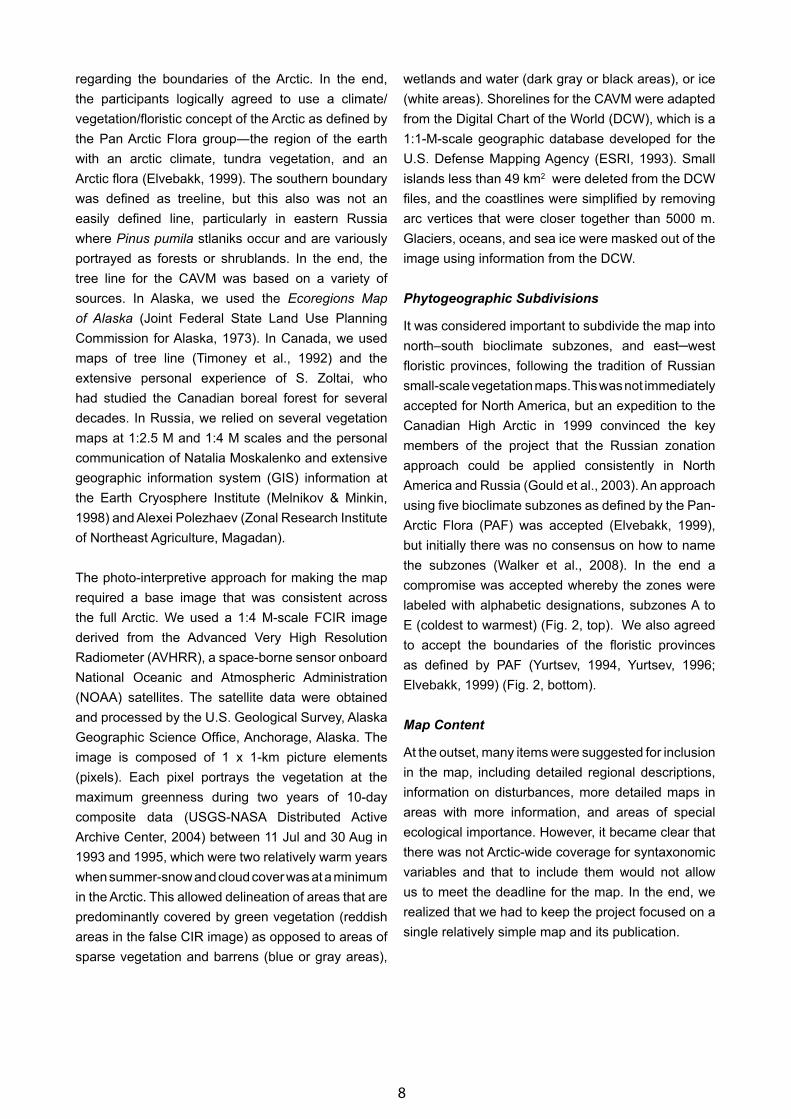
regarding the boundaries of the Arctic. In the end, the participants logically agreed to use a climate/vegetation/floristic concept of the Arctic as defined by the Pan Arctic Flora group―the region of the earth with an arctic climate, tundra vegetation, and an Arctic flora (Elvebakk, 1999). The southern boundary was defined as treeline, but this also was not an easily defined line, particularly in eastern Russia where Pinus pumila stlaniks occur and are variously portrayed as forests or shrublands. In the end, the tree line for the CAVM was based on a variety of sources. In Alaska, we used the Ecoregions Map of Alaska (Joint Federal State Land Use Planning Commission for Alaska, 1973). In Canada, we used maps of tree line (Timoney et al., 1992) and the extensive personal experience of S. Zoltai, who had studied the Canadian boreal forest for several decades. In Russia, we relied on several vegetation maps at 1:2.5 M and 1:4 M scales and the personal communication of Natalia Moskalenko and extensive geographic information system (GIS) information at the Earth Cryosphere Institute (Melnikov & Minkin, 1998) and Alexei Polezhaev (Zonal Research Institute of Northeast Agriculture, Magadan).

The photo-interpretive approach for making the map required a base image that was consistent across the full Arctic. We used a 1:4 M-scale FCIR image derived from the Advanced Very High Resolution Radiometer (AVHRR), a space-borne sensor onboard National Oceanic and Atmospheric Administration (NOAA) satellites. The satellite data were obtained and processed by the U.S. Geological Survey, Alaska Geographic Science Office, Anchorage, Alaska. The image is composed of 1 x 1-km picture elements (pixels). Each pixel portrays the vegetation at the maximum greenness during two years of 10-day composite data (USGS-NASA Distributed Active Archive Center, 2004) between 11 Jul and 30 Aug in 1993 and 1995, which were two relatively warm years when summer-snow and cloud cover was at a minimum in the Arctic. This allowed delineation of areas that are predominantly covered by green vegetation (reddish areas in the false CIR image) as opposed to areas of sparse vegetation and barrens (blue or gray areas),

wetlands and water (dark gray or black areas), or ice (white areas). Shorelines for the CAVM were adapted from the Digital Chart of the World (DCW), which is a 1:1-M-scale geographic database developed for the U.S. Defense Mapping Agency (ESRI, 1993). Small islands less than 49 km2 were deleted from the DCW files, and the coastlines were simplified by removing arc vertices that were closer together than 5000 m. Glaciers, oceans, and sea ice were masked out of the image using information from the DCW.

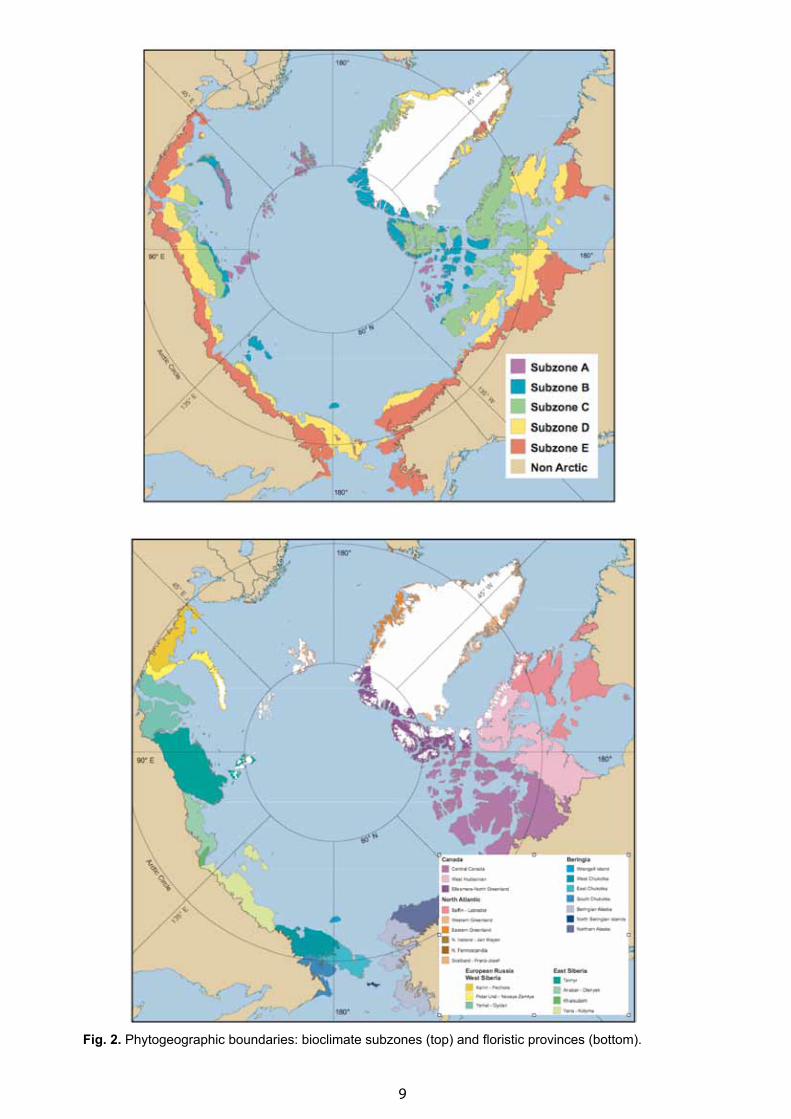
Phytogeographic Subdivisions

It was considered important to subdivide the map into north–south bioclimate subzones, and east─west floristic provinces, following the tradition of Russian small-scale vegetation maps. This was not immediately accepted for North America, but an expedition to the Canadian High Arctic in 1999 convinced the key members of the project that the Russian zonation approach could be applied consistently in North America and Russia (Gould et al., 2003). An approach using five bioclimate subzones as defined by the Pan-Arctic Flora (PAF) was accepted (Elvebakk, 1999), but initially there was no consensus on how to name the subzones (Walker et al., 2008). In the end a compromise was accepted whereby the zones were labeled with alphabetic designations, subzones A to E (coldest to warmest) (Fig. 2, top). We also agreed to accept the boundaries of the floristic provinces as defined by PAF (Yurtsev, 1994, Yurtsev, 1996; Elvebakk, 1999) (Fig. 2, bottom).

Map Content

At the outset, many items were suggested for inclusion in the map, including detailed regional descriptions, information on disturbances, more detailed maps in areas with more information, and areas of special ecological importance. However, it became clear that there was not Arctic-wide coverage for syntaxonomic variables and that to include them would not allow us to meet the deadline for the map. In the end, we realized that we had to keep the project focused on a single relatively simple map and its publication.

9

Fig. 2. Phytogeographic boundaries: bioclimate subzones (top) and floristic provinces (bottom).

10

Legend

The final legend condensed over 400 known plant communities into 15 physiognomic mapping units:

B – BarrensB1: Cryptogam, herb barren

B2: Cryptogam barren complex (bedrock, shield areas)

B3: Non-carbonate mountain complex

B4: Carbonate mountain complex

G – Graminoid-dominated tundrasG1: Rush/grass, forb, cryptogam tundra

G2: Graminoid, prostrate dwarf-shrub, forb tundra

G3: Non-tussock sedge, dwarf-shrub, moss tundra

G4: Tussock graminoid, dwarf-shrub, moss tundra

P – Prostrate dwarf-shrub dominated tundras

P1: Prostrate dwarf-shrub, herb tundra

P2: Prostrate/ hemi-prostrate dwarf-shrub tundra

S – Erect dwarf-shrub dominated tundra

S1: Erect dwarf-shrub tundra

S2: Low-shrub tundra

W – Wetlands

W1: Sedge/grass, moss wetland

W2: Sedge, moss, dwarf-shrub wetland

W3: Sedge, moss, low-shrub wetland

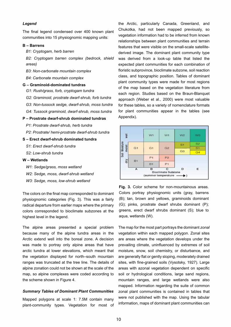
The colors on the final map corresponded to dominant physiognomic categories (Fig. 3). This was a fairly radical departure from earlier maps where the primary colors corresponded to bioclimate subzones at the highest level in the legend.

The alpine areas presented a special problem because many of the alpine tundra areas in the Arctic extend well into the boreal zone. A decision was made to portray only alpine areas that have arctic tundra at lower elevations, which meant that the vegetation displayed for north–south mountain ranges was truncated at the tree line. The details of alpine zonation could not be shown at the scale of the map, so alpine complexes were coded according to the scheme shown in Figure 4.

Summary Tables of Dominant Plant Communities

Mapped polygons at scale 1: 7.5M contain many plant-community types. Vegetation for most of

the Arctic, particularly Canada, Greenland, and Chukotka, had not been mapped previously, so vegetation information had to be inferred from known relationships between plant communities and terrain features that were visible on the small-scale satellite-derived image. The dominant plant community type was derived from a look-up table that listed the expected plant communities for each combination of floristic subprovince, bioclimate subzone, soil reaction class, and topographic position. Tables of dominant plant community types were made for most regions of the map based on the vegetation literature from each region. Studies based on the Braun-Blanquet approach (Weber et al., 2000) were most valuable for these tables, so a variety of nomenclature formats for plant communities appear in the tables (see Appendix).

The map for the most part portrays the dominant zonal vegetation within each mapped polygon. Zonal sites are areas where the vegetation develops under the prevailing climate, uninfluenced by extremes of soil moisture, snow, soil chemistry, or disturbance, and are generally flat or gently sloping, moderately drained sites, with fine-grained soils (Vysotsky, 1927). Large areas with azonal vegetation dependent on specific soil or hydrological conditions, large sand regions, mountain ranges, and large wetlands were also mapped. Information regarding the suite of common zonal plant communities is contained in tables that were not published with the map. Using the tabular information, maps of dominant plant communities can

Fig. 3. Color scheme for non-mountainous areas. Colors portray physiognomic units (gray, barrens (B); tan, brown and yellows, graminoids dominant (G); pinks, prostrate dwarf shrubs dominant (P); greens, erect dwarf shrubs dominant (S); blue to aqua, wetlands (W).

11

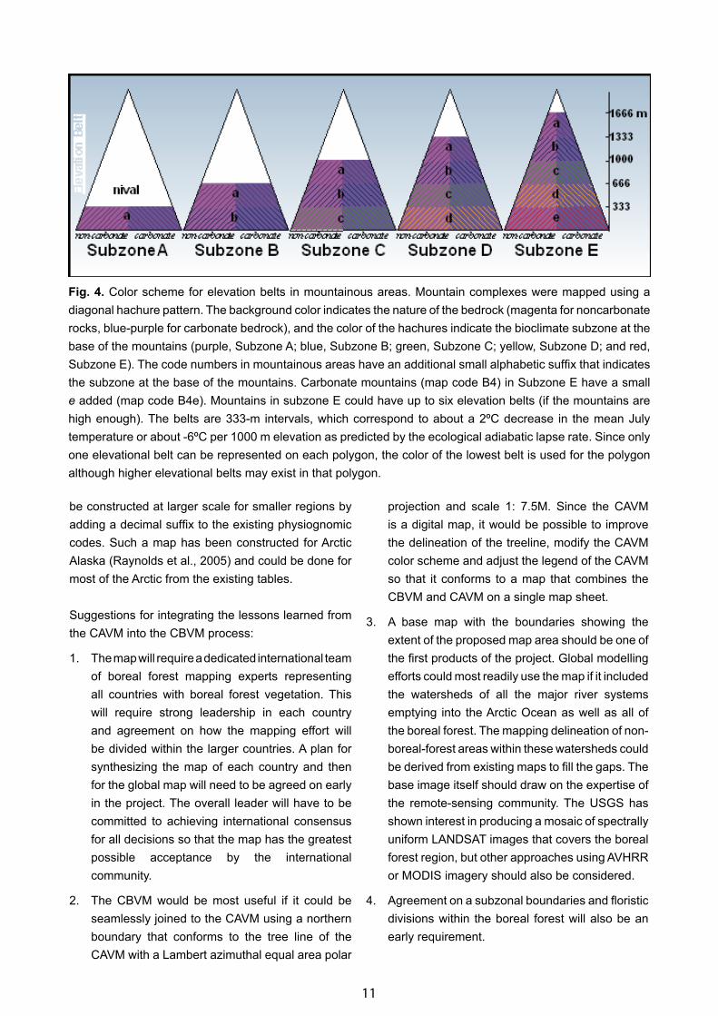
Fig. 4. Color scheme for elevation belts in mountainous areas. Mountain complexes were mapped using a diagonal hachure pattern. The background color indicates the nature of the bedrock (magenta for noncarbonate rocks, blue-purple for carbonate bedrock), and the color of the hachures indicate the bioclimate subzone at the base of the mountains (purple, Subzone A; blue, Subzone B; green, Subzone C; yellow, Subzone D; and red, Subzone E). The code numbers in mountainous areas have an additional small alphabetic suffix that indicates the subzone at the base of the mountains. Carbonate mountains (map code B4) in Subzone E have a small e added (map code B4e). Mountains in subzone E could have up to six elevation belts (if the mountains are high enough). The belts are 333-m intervals, which correspond to about a 2ºC decrease in the mean July temperature or about -6ºC per 1000 m elevation as predicted by the ecological adiabatic lapse rate. Since only one elevational belt can be represented on each polygon, the color of the lowest belt is used for the polygon although higher elevational belts may exist in that polygon.

be constructed at larger scale for smaller regions by adding a decimal suffix to the existing physiognomic codes. Such a map has been constructed for Arctic Alaska (Raynolds et al., 2005) and could be done for most of the Arctic from the existing tables.

Suggestions for integrating the lessons learned from the CAVM into the CBVM process:

1. The map will require a dedicated international team of boreal forest mapping experts representing all countries with boreal forest vegetation. This will require strong leadership in each country and agreement on how the mapping effort will be divided within the larger countries. A plan for synthesizing the map of each country and then for the global map will need to be agreed on early in the project. The overall leader will have to be committed to achieving international consensus for all decisions so that the map has the greatest possible acceptance by the international community.

2. The CBVM would be most useful if it could be seamlessly joined to the CAVM using a northern boundary that conforms to the tree line of the CAVM with a Lambert azimuthal equal area polar

projection and scale 1: 7.5M. Since the CAVM is a digital map, it would be possible to improve the delineation of the treeline, modify the CAVM color scheme and adjust the legend of the CAVM so that it conforms to a map that combines the CBVM and CAVM on a single map sheet.

3. A base map with the boundaries showing the extent of the proposed map area should be one of the first products of the project. Global modelling efforts could most readily use the map if it included the watersheds of all the major river systems emptying into the Arctic Ocean as well as all of the boreal forest. The mapping delineation of non-boreal-forest areas within these watersheds could be derived from existing maps to fill the gaps. The base image itself should draw on the expertise of the remote-sensing community. The USGS has shown interest in producing a mosaic of spectrally uniform LANDSAT images that covers the boreal forest region, but other approaches using AVHRR or MODIS imagery should also be considered.

4. Agreement on a subzonal boundaries and floristic divisions within the boreal forest will also be an early requirement.

12

5. An integrated landscape-guided mapping approach similar to that used for the CAVM should be considered, as it will be necessary to have a consistent method that all team members can follow for image interpretation.

6. A tabular method for cataloging the known primary plant communities that occur along typical toposequences in each bioclimate subzone and floristic province could prove useful for the CBVM as it was for the CAVM. At present it is unknown if this is feasible for all areas of the map. There should be early agreement on the use of the internationally recognized Braun-Blanquet plant–community nomenclature system as the preferred foundation for cataloging plant communities.

7. The final legend should place vegetation physiognomy at the highest level in the legend hierarchy.

8. Because of problems of inconsistent definitions and application of terms used among vegetation scientists in different countries with different schools of vegetation science, it is imperative that the terms used on the map be clearly defined and agreed to by the group of vegetation scientists. This may be among the hardest tasks faced by the group.

9. It is important to keep the project focused and relatively simple, with a single defined product, the CBVM. It is suggested that the projectshould consider combining the Arctic and Boreal biome maps in the final published map. This will require some adjustments to the CAVM. Although disturbances (fire, insects, agriculture) are important factors that cover large areas of the boreal zone, it is recommended that the map show potential natural vegetation with the focus on the zonal vegetation except in large areas of nonzonal conditions (e.g., large wetlands, very large river systems, extensive nonzonal soil conditions such as sand plains, shield areas with near-surface bedrock, and mountainous areas).

10. The biggest challenge for the CBVM is the same as that faced by the CAVM—how to develop a legend framework with terminology that is acceptable to all the circumboreal countries. Differences in language, different definitions of common terms, and different mapping traditions will cause major barriers for this international

synthesis. These differences are not trivial and must be addressed and compromises will be necessary.

I will advocate strongly for adopting the Braun-Blanquet method as the foundation for the map. This method has a long and successful heritage of application of vegetation mapping at all scales in Europe and more recently in Russia, and it has the greatest potential as an international approach. It is the most comprehensive method for vegetation sampling classification and analysis in the world. It addresses all phases of vegetation description, including the field methods, the analytical methods, and perhaps most importantly, a formal international hierarchical classification framework that allows the plant-community units to be compared with other internationally published vegetation literature. The B-B method can be likened to the Linnean approach to describing and classifying plant species or the U.S. soil taxonomy approach for describing and classifying soils (Soil Survey Staff, 1999). It is the only method that can be considered an international vegetation classification approach.

The U.S. National Classification System (The Nature Conservancy and Environmental Systems Research Institute, 1994) is a recent attempt at standardization for classification in North America. The method is still being developed and is not widely used outside of North America. Currently at the plant-community level there are no standards for field sampling, table analysis, naming, and publishing the plant community data. Researchers have a hard time understanding, accessing and standardizing the source data, and building on existing work. However, both the European and North American approaches recognize the necessity for using physiognomic units at the higher mapping levels for developing the biome-scale mapping units.

Developing a consistent nomenclature system will be a difficult task. I would like to promote a spirit of international cooperation and compromise when necessary in developing the legend we will adopt. This will be necessary because many of the words crucial to our science have different meanings in different countries, but I think we all recognize the underlying kernels of similarity in all the approaches.

13

With regard to collaboration on the assembly of the synthesized regional maps into a single vegetation map of the Arctic and boreal biomes, the task is much more challenging for the boreal forest than it was for the Arctic. I am hoping that we can learn from the Russian and Canadian approaches to mapping the boreal forest and also from the previous European collaborative. The European Vegetation map already faced many of our same challenges at the continental scale. Now we are faced with the same challenge at the global scale.

References

Bohn, U., Gollub, G., & Hetwer, C., eds. 2000. Karte der natürlichen Vegetation Europas 1:2 500 000 Karten/Maps. Bundesamt für Naturschutz, Bonn.

CAVM Team. 2003. Circumpolar Arctic Vegetation Map. Conservation of Arctic Flora and Fauna (CAFF) Map No. 1, U.S. Fish and Wildlife Service, Anchorage, Alaska.

Dangermond, J. & Harnden, E. 1990. Map data standardization: a methodology for integrating thematic cartographic data before automation. ARC News 12: 16–19.

Daniëls, F. J. Elvebakk, A., A., Talbot, S. S., & Walker, D. A. 2005. Classification and mapping of arctic vegetation: A tribute to Boris A. Yurtsev. Phytocoenologia 35: 715–1079.

Elias, S. A., S. K. Short, D. A. Walker, and N. A. Auerbach. 1996. Historical biodiversity at remote Air Force sites in Alaska. Final report to U.S. Department of Defense, Legacy Project #0742, University of Colorado, Boulder, CO, Institute of Arctic and Alpine Research.

Elvebakk, A. 1999. Bioclimatic delimitation and subdivision of the Arctic. Pages 81–112 in Nordal, I. &. Razzhivin, V. Y, eds. The Species Concept in the High North–A Panarctic Flora Initiative. The Norwegian Academy of Science and Letters, Oslo.

Elvebakk, A., Elven, R., & Razzhivin, V. Y. 1999. Delimitation, zonal and sectorial subdivision of the Arctic for the Panarctic Flora Project. Pages 375-386 in Nordal, I. and Razzhivin, V. Y., eds. The Species Concept in the High North – A Panarctic Flora Initiative. The Norwegian Academy of Science and Letters, Oslo.

ESRI. 1993. The Digital Chart of the World for use with ARC/INFO Data Dictionary. Environmental Systems Research Institute, Redlands, California.

Gould, W. A., Walker, D. A., & Biesboer, D. 2003. Combining research and education: bioclimatic zonation along a Canadian Arctic Transect. Arctic 56: 45–54.

Joint Federal State Land Use Planning Commission for Alaska. 1973. Major Ecosystems of Alaska. Map by U.S. Geological Survey, Fairbanks, Alaska.

Melnikov, E. S. & Minkin, M. A. 1998. About strategy of development of electronic geoinformation systems (GIS) and databases in geocryology. Earth Cryosphere (in Russian) II: 70–76.

Raynolds, M. K. & Markon, C. J., eds. 2001. U.S. Geological Survey Open File Report 02-181. Pages 98 in Fourth International Circumpolar Arctic Vegetation Mapping Workshop, Russian Academy of Sciences, Moscow, Russia.

Raynolds, M. K., Walker, D. A., & Maier, H. A. 2005. Alaska Arctic Vegetation Map, Scale 1:4 000 000. Conservation of Arctic Flora and Fauna (CAFF) Map No. 2. U.S. Fish and Wildlife Service, Anchorage, Alaska.

Schickhoff, U., Walker, M. D., & Walker, D. A. 2002. Riparian willow communities on the arctic Slope of Alaska and their environmental relationships: a classification and ordination analysis. Phytocoenologia 32: 145–204.

Soil Survey Staff. 1999. Soil Taxonomy: A Basic System of Soil Classification for Making and Interpreting Soil Surveys. U.S. Department of Agriculture Handbook No. 436, Washington D.C.

The Nature Conservancy & Environmental Systems Research Institute. 1994. Standardized National Vegetation Classification System. Report to the United States Department of the Interior, National Biological Survey and National Park Service.

Timoney, K. P., La Roi, G. H., Zoltai, S. C., & Robinson, A. L. 1992. The high subarctic forest-tundra of northwestern Canada: position, width, and vegetation gradients in relation to climate. Arctic 45: 1–9.

U.S. Geological Survey-National Aeronautics and Space Administration Distributed Active Archive Center. 2004. FTP access to global AVHRR 10-day composite data, URL http://edcdaac.usgs.gov/1KM/comp10d.asp.

Vysotsky, G. N. 1927. Theses on soil and moisture (conspectus and terminology). Pages 67–79 in Lesovedenie, ed. Sbornik Lesnogo Obschestva v Leningrade, Leningrad. (In Russian).

14

Walker, D. A. 1977. The analysis of the effectiveness of a television scanning densitometer for indicating geobotanical features in an ice-wedge polygon complex at Barrow, Alaska. M.A. University of Colorado, Boulder.

Walker, D. A. 1985. Vegetation and environmental gradients of the Prudhoe Bay region, Alaska. CRREL Report 85–114, U.S. Army Cold Regions Research and Engineering Laboratory, Hanover, New Hampshire.

Walker, D. A. 1995. Toward a new Circumpolar Arctic Vegetation Map. Arctic and Alpine Research 31: 169–178.

Walker, D. A. 1999. An integrated vegetation mapping approach for northern Alaska (1:4 M scale). International Journal of Remote Sensing 20: 2895–2920.

Walker, D. A., Bay, C., Daniëls, F. J. A., Einarsson, E., Elvebakk, A., Johansen, B. E., Kapitsa, A., Kholod, S. S., Murray, D. F., Talbot, S. S., Yurtsev, B. A., & Zoltai, S. C. 1995. Toward a new arctic vegetation map: a review of existing maps. Journal of Vegetation Science 6: 427–436.

Walker, D. A., Gould, W. A., Maier, H. A., & Raynolds, M. K. 2002. The Circumpolar Arctic Vegetation Map: AVHRR-derived base maps, environmental controls, and integrated mapping procedures. International Journal of Remote Sensing 23: 4551–4570.

Walker, D. A. & Lillie, A. C. 1997. Proceedings of the Second Circumpolar Arctic Vegetation Mapping Workshop, Arendal, Norway, 19-24 May 1996 and the CAVM-North America Workshop, Anchorage, Alaska, USA, 14–16 January 1997. Pages 61 in D. A. Walker and A. C. Lillie, eds. Institute of Arctic and Alpine Research Occasional Paper.

Walker, D. A., & Markon, C. J. 1996. Circumpolar Arctic Vegetation Mapping workshop: abstracts and short papers. Open File Report 96–251, Reston, Virginia.

Walker, D. A., Raynolds, M. K., Daniëls, F. J. A., Einarsson, E., Elvebakk, A., Gould, W. A., Katenin, A. E., Kholod, S. S., Markon, C. J., Melnikov, E. S., Moskalenko, M. N.G., Talbot, S. S., Yurtsev, B. A., & CAVM Team. 2005. The Circumpolar Arctic Vegetation Map. Journal of Vegetation Science 16: 267–282.

Walker, D. A., Raynolds, M. K., & Gould, W. A. 2008. Fred Daniëls, Sub-zone A, and the North

American Arctic Transect. Abhandlungen aus dem Westfälischen Museum für Naturkunde 70: 387–400.

Walker, D. A., Webber, P. J., Walker, M. D., Lederer, N. D., Meehan, R. H., & Nordstrand, E. A. 1986. Use of geobotanical maps and automated mapping techniques to examine cumulative impacts in the Prudhoe Bay Oilfield, Alaska. Environmental Conservation 13:149–160.

Webber, P. J. 1978. Spatial and temporal variation in the vegetation and its productivity, Barrow, Alaska. Pages 37–112 in L. L. Tieszen, ed. Vegetation and Production Ecology of an Alaskan Arctic Tundra. Springer-Verlag, New York.

Weber, H. E., Moravec, J., & Therurillat, J.-P. 2000. International Code of Phytosociological Nomenclature. 3rd Edition. Journal of Vegetation Science 11: 739–768.

Yurtsev, B. A. 1994. Floristic division of the Arctic. Journal of Vegetation Science 5: 765–776.

Yurtsev, B. A. 1996. Latitudinal (zonal) and longitudinal (sectoral) phytogeographic division of the circumpolar arctic in relation to the structure of the vegetation map legend. Pages 77-83 in Walker, D. A. & Markon, C. J., eds. Circumpolar Arctic Vegetation Mapping Workshop, Komarov Botanical Institute, St. Petersburg, Russia, March 21–25, 1994.

Zonneveld, I. S. 1988. The ITC method of mapping natural and semi-natural vegetation. Pages 401-426 in Küchler, A. W. & Zonneveld, I. S., eds. Vegetation Mapping. Kluwer Academic Publishers, Boston.

Appendix

Table A.1 is an example table of dominant plant communities for Subzone C, Northern Alaska floristic subprovince. See Fig. A.1 for circumpolar maps of bioclimate subzones, floristic provinces, substrate pH, and the conceptual mesotopographic gradient. Dominant plant functional types and species are listed where data were available. The units contain the dominant plant functional types from the top of the plant canopy to the base of the canopy, followed by the dominant plant species for each plant functional type (in parentheses). Literature citations in the table include unit names, habitat, citation and location. Similar tables were constructed for each combination of floristic subprovince and bioclimate subzone.

15

Fig. A.1

Table A.1. Subzone C (Northern part of the Arctic Coastal Plain).Table A.1. Subzone C (Northern part of Arctic Coastal Plain).

Habitat along the meso-topographic gradient

Acidic substrates (community # 1--7)

Non-acidic substrates (community # 8--12)

Dry exposed sites 1. Prostrate dwarf-shrub (Salix rotundifolia), lichen (Alectoria nigricans, Bryocaulon divergens, Dactylina arctica), rush (Luzula confusa, L. arctica), grass (Arctagrostis latifolia), forb (Potentilla nana, Pedicularis kanei), bryophyte (Polytrichum strictum, Dicranum elongatum, Gymnomitrion corallioides). Nodum II; Sphaerophorus globosus-Luzula confusa comm., subtype Salix rotundifolia (Elias et al., 1996) (Barrow, dry beach and river terraces).

8. Prostrate dwarf-shrub (Dryas integrifolia), sedge (Carex rupestris), lichen (Lecanora epibryon, Thamnolia subuliformis). Type B12, coastal dry nonacidic gravelly sites (Walker, 1985) (North Slope, Alaska).

Moist sites 2. Sedge (Carex aquatilis, Eriophorum angustifolium), grass (Poa arctica, Dupontia fisheri), rush (Luzula arctica), prostrate dwarf-shrub (Salix rotundifolia), forb (Saxifraga cernua, S. hieraciifolia, S. hirculus, Cardamine pratensis, Petasites frigidus, Ranunculus nivalis), moss (Oncophorus wahlenbergii, Sarmenthypnum sarmentosum, Aulacomnium turgidum). Nodum IV (Webber, 1978); Type 6 and 7 (Walker, 1977); Saxifraga cernua-Carex aquatilis comm. (Elias et al., 1996) (Barrow, moist, fine-grained soils). 3. Rush (Luzula confusa, L. arctica), grass (Poa arctica), forb (Potentilla nana, Pedicularis kanei), lichen (Alectoria nigricans, Sphaerophorus globosus, Dactylina arctica, Cladonia spp., Ochrolechia frigida), moss (Polytrichastrum alpinum, Polytrichum strictum, Sarmenthypnum sarmentosum). Nodum I (Webber, 1978); Type 5 (Walker, 1977); Sphaerophorus globosus-Luzula confusa comm., subtype Saxifraga foliolosa (Elias et al., 1996) (mesic high-centered polygons, zonal vegetation in Barrow area).

9. Sedge (Carex aquatilis), prostrate dwarf-shrub (Salix pulchra, S. reticulata, Dryas integrifolia), moss (Tomentypnum nitens, Oncophorus wahlenbergii, Campylium stellatum, Distichium capillaceum). Type U12, moist calcareous coastal meadows (Walker, 1985) (North Slope, Alaska).

Wet sites 4. Sedge (Eriophorum angustifolium, Carex aquatilis), grass (Dupontia fisheri, Arctophila fulva), moss (Sarmenthypnum sarmentosum, Limprichtia revolvens). Noda V and VI (Webber, 1978); Types 9, 10, 12 and 13 (Walker, 1977); Eriophorum angustifolium-Carex aquatilis comm. (Elias et al., 1996) (Barrow, wet sites without standing water).

10. Sedge (Carex aquatilis, Eriophorum angustifolium), grass (Dupontia fisheri), moss (Drepanocladus brevifolius). Type M10 , wet calcareous coastal meadows (Walker, 1985) (North Slope, Alaska).

Snow beds 5. Prostrate dwarf shrub (Salix rotundifolia), lichen (Cetrariella delisei). Salix rotundifolia-Cetraria delisei comm. (Elias et al. 1996) (Barrow, early-melting snow beds). 6. Grass (Phippsia algida, Alopecurus alpinus), forb (Cochlearia groenlandica, Ranunculus pygmaeus, Stellaria humifusa, Saxifraga rivularis). Nodum VIII; Type 15 (Barrow, late-melting snow beds).

11. No data. Probably similar to snowbeds in Subzone D.

Riparian areas 7. Grass (Phippsia algida, Alopecurus alpinus), forb (Cochlearia officinalis, Ranunculus pygmaeus, Stellaria humifusa, Saxifraga rivularis). Nodum VIII (Webber, 1978); Type 15 (Walker, 1977) (Barrow, unstable stream margins).

12. Forb (Epilobium latifolium, Artemisia arctica, A. campestris ssp. borealis, Papaver lapponicum, Polemonium boreale, Astragalus alpinus, Wilhelmsia physodes, Parrya nudicaulis). Epilobio latifolii-Salicetum alaxensis ass. prov. (Schickhoff et al., 2002) (North Slope, coastal active floodplains).

16

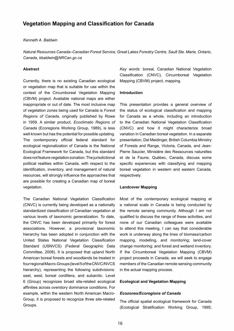
Vegetation Mapping and Classification for Canada

Kenneth A. Baldwin

Natural Resources Canada–Canadian Forest Service, Great Lakes Forestry Centre, Sault Ste. Marie, Ontario, Canada, kbaldwin@NRCan.gc.ca

Abstract

Currently, there is no existing Canadian ecological or vegetation map that is suitable for use within the context of the Circumboreal Vegetation Mapping (CBVM) project. Available national maps are either inappropriate or out of date. The most inclusive map of vegetation zones being used for Canada is Forest Regions of Canada, originally published by Rowe in 1959. A similar product, Ecoclimatic Regions of Canada (Ecoregions Working Group, 1989), is less well known but has the potential for possible updating. The contemporary official federal standard for ecological regionalization of Canada is the National Ecological Framework for Canada, but this standard does not feature vegetation zonation. The jurisdictional political realities within Canada, with respect to the identification, inventory, and management of natural resources, will strongly influence the approaches that are possible for creating a Canadian map of boreal vegetation.

The Canadian National Vegetation Classification (CNVC) is currently being developed as a nationally standardized classification of Canadian vegetation at various levels of taxonomic generalization. To date, the CNVC has been developed primarily for forest associations. However, a provisional taxonomic hierarchy has been adopted in conjunction with the United States National Vegetation Classification Standard (USNVCS) (Federal Geographic Data Committee, 2008). It is proposed that upland North American boreal forests and woodlands be treated in four regional Macro-Groups (level 5 of the CNVC/NVCS hierarchy), representing the following subdivisions: east, west, boreal cordillera, and subarctic. Level 6 (Group) recognizes broad site-related ecological affinities across overstory dominance conditions. For example, within the western North American Macro-Group, it is proposed to recognize three site-related Groups.

Key words: boreal, Canadian National Vegetation Classification (CNVC), Circumboreal Vegetation Mapping (CBVM) project, mapping.

Introduction

This presentation provides a general overview of the status of ecological classification and mapping for Canada as a whole, including an introduction to the Canadian National Vegetation Classification (CNVC) and how it might characterize broad variation in Canadian boreal vegetation. In a separate presentation, Del Meidinger, British Columbia Ministry of Forests and Range, Victoria, Canada, and Jean-Pierre Saucier, Ministère des Ressources naturelles et de la Faune, Québec, Canada, discuss some specific experiences with classifying and mapping boreal vegetation in western and eastern Canada, respectively.

Landcover Mapping

Most of the contemporary ecological mapping at a national scale in Canada is being conducted by the remote sensing community. Although I am not qualified to discuss the range of these activities, and none of our Canadian colleagues were available to attend this meeting, I can say that considerable work is underway along the lines of biomass/carbon mapping, modelling, and monitoring; land-cover change monitoring; and forest and wetland inventory. If the Circumboreal Vegetation Mapping (CBVM) project proceeds in Canada, we will seek to engage members of the Canadian remote sensing community in the actual mapping process.

Ecological and Vegetation Mapping

Ecozones/Ecoregions of Canada

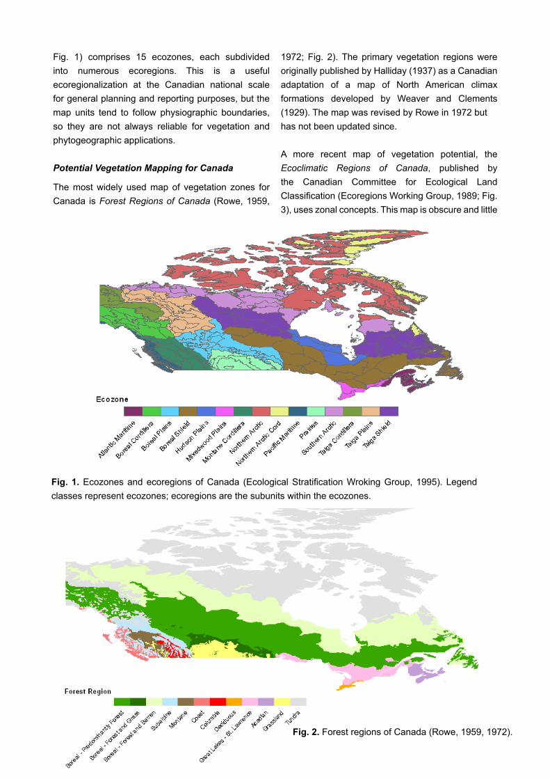
The official spatial ecological framework for Canada (Ecological Stratification Working Group, 1995;

17

Fig. 1) comprises 15 ecozones, each subdivided into numerous ecoregions. This is a useful ecoregionalization at the Canadian national scale for general planning and reporting purposes, but the map units tend to follow physiographic boundaries, so they are not always reliable for vegetation and phytogeographic applications.

Potential Vegetation Mapping for Canada

The most widely used map of vegetation zones for Canada is Forest Regions of Canada (Rowe, 1959,

1972; Fig. 2). The primary vegetation regions were originally published by Halliday (1937) as a Canadian adaptation of a map of North American climax formations developed by Weaver and Clements (1929). The map was revised by Rowe in 1972 buthas not been updated since.

A more recent map of vegetation potential, the Ecoclimatic Regions of Canada, published by the Canadian Committee for Ecological Land Classification (Ecoregions Working Group, 1989; Fig. 3), uses zonal concepts. This map is obscure and little

Fig. 2. Forest regions of Canada (Rowe, 1959, 1972).

Fig. 1. Ecozones and ecoregions of Canada (Ecological Stratification Wroking Group, 1995). Legend classes represent ecozones; ecoregions are the subunits within the ecozones.

18

Fig. 3. Ecoclimatic provinces and regions of Canada (Ecoregions Working Group, 1989). Legend classes represent ecoclimatic provinces; ecoclimatic regions are the subunits within the ecoclimatic provinces.

used by ecologists but has the potential to be updated with new data and climatic modelling methods.

Provincial/Territorial Ecological Classification and Mapping

Canada is a federation comprising 10 provinces (mostly south of latitude 60º) and three territories in the north. Constitutionally, most matters of resource management and stewardship are under provincial/territorial jurisdiction. Over the last 20–30 years, the role of the federal government in ecological classification and inventory has been largely to support the provinces and territories with their jurisdictional programs. Over this time period, most jurisdictions have developed classifications and inventories, especially of their forests, but there has been no effort to coordinate or crosswalk the systems across provincial/territorial borders. The result is a patchwork of mapped classification systems across the country, often broken at jurisdictional boundaries (Fig. 4). Since the most recent ecological classification, provinces and territories have conducted inventory and mapping activities, and this is where the current expertise and data now reside across Canada. Any effort to develop a nationally consistent vegetation mapping product for Canada will require cooperation from the provinces and territories for two reasons: (1)

access to their data and expertise and (2) for buy-in at the provincial/territorial level that will facilitate acceptance of the new product and its use as a new Canadian standard.

Canadian National Vegetation Classification

The Canadian National Vegetation Classification (CNVC) is a project that is developing a national standard for vegetation classification in a cooperative partnership involving all relevant jurisdictions in Canada. The CNVC is coordinated by the federal government (Natural Resources Canada), with data and expertise provided by the provinces and territories. The primary objectives of the CNVC are:

• to classify the natural vegetation of Canada in an ecologically meaningful manner on the basis of growth-form, physiognomy, dominance, floristics, and diagnostic indicator value;

• to coordinate classification standards and correlate CNVC classification units with Canadian provincial, territorial, and regional classifications, as well as with the U.S. National Vegetation Classification Standard (USNVCS) (Federal Geographic Data Committee, 2008), to provide a mechanism for the exchange of ecological information across jurisdictional boundaries; and

19

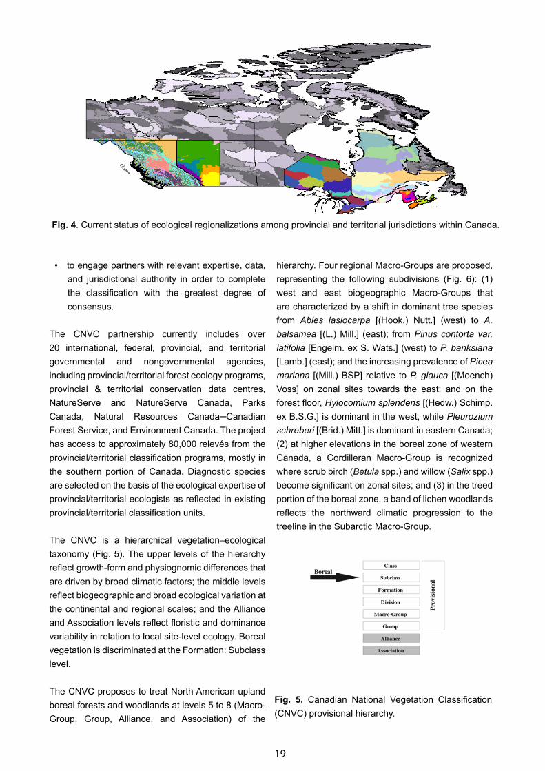
Fig. 4. Current status of ecological regionalizations among provincial and territorial jurisdictions within Canada.

• to engage partners with relevant expertise, data, and jurisdictional authority in order to complete the classification with the greatest degree of consensus.

The CNVC partnership currently includes over 20 international, federal, provincial, and territorial governmental and nongovernmental agencies, including provincial/territorial forest ecology programs, provincial & territorial conservation data centres, NatureServe and NatureServe Canada, Parks Canada, Natural Resources Canada─Canadian Forest Service, and Environment Canada. The project has access to approximately 80,000 relevés from the provincial/territorial classification programs, mostly in the southern portion of Canada. Diagnostic species are selected on the basis of the ecological expertise of provincial/territorial ecologists as reflected in existing provincial/territorial classification units.

The CNVC is a hierarchical vegetation–ecological taxonomy (Fig. 5). The upper levels of the hierarchy reflect growth-form and physiognomic differences that are driven by broad climatic factors; the middle levels reflect biogeographic and broad ecological variation at the continental and regional scales; and the Alliance and Association levels reflect floristic and dominance variability in relation to local site-level ecology. Boreal vegetation is discriminated at the Formation: Subclass level.

The CNVC proposes to treat North American upland boreal forests and woodlands at levels 5 to 8 (Macro-Group, Group, Alliance, and Association) of the

hierarchy. Four regional Macro-Groups are proposed, representing the following subdivisions (Fig. 6): (1) west and east biogeographic Macro-Groups that are characterized by a shift in dominant tree species from Abies lasiocarpa [(Hook.) Nutt.] (west) to A. balsamea [(L.) Mill.] (east); from Pinus contorta var. latifolia [Engelm. ex S. Wats.] (west) to P. banksiana [Lamb.] (east); and the increasing prevalence of Picea mariana [(Mill.) BSP] relative to P. glauca [(Moench) Voss] on zonal sites towards the east; and on the forest floor, Hylocomium splendens [(Hedw.) Schimp. ex B.S.G.] is dominant in the west, while Pleurozium schreberi [(Brid.) Mitt.] is dominant in eastern Canada; (2) at higher elevations in the boreal zone of western Canada, a Cordilleran Macro-Group is recognized where scrub birch (Betula spp.) and willow (Salix spp.) become significant on zonal sites; and (3) in the treed portion of the boreal zone, a band of lichen woodlands reflects the northward climatic progression to the treeline in the Subarctic Macro-Group.

Fig. 5. Canadian National Vegetation Classification (CNVC) provisional hierarchy.

20

Using the western Macro-Group as an example (Fig. 7), it is proposed to be subdivided into three groups that reflect broad site-related ecological affinities across overstory dominance conditions. These groups can be mapped into coordinate envelopes of the edatope to reflect generalized local or regional site-level moisture and nutrient gradients. Groups comprise multiple alliances and associations, which describe phytosociological variability in terms of community-scale dominance and floristic composition.

Conclusion

There is probably no existing Canadian ecological or vegetation map that is suitable for use within the context of the proposed Circumboreal Vegetation Mapping (CBVM) project. The existing national maps are either

inappropriate (ecozones) or out of date (forest regions and ecoclimatic regions). The most current ecological regionalizations exist only for individual provinces or territories.

There are two general approaches for developing a new Canadian vegetation map that can serve as a component of the CBVM―an executive process or a process that emphasizes federal/provincial/territorial cooperation. In order to mobilize the greatest amount of expertise, data, and endorsement, the latter approach is recommended. Development of a Canadian component of the CBVM by interjurisdictional cooperation within Canada will take time but will result in the best product.

The Canadian National Vegetation Classification (CNVC) partnership is a good governance model for the Canadian component of the CBVM. Its incipient taxonomy, which is derived from recently collected relevé data, and the CNVC partnership can inform the development of a CBVM map for Canada.

References

Ecological Stratification Working Group. 1995. A National Ecological Framework for Canada. Agriculture and Agri-Food Canada, Research Branch, Centre for Land and Biological Resources Research and Environment Canada, State of the Environment Directorate, Ecozone Analysis Branch. Ottawa, Ontario / Hull, Québec, Canada. 125 pp and map at 1:7 500 000 scale.

Ecoregions Working Group. 1989. Ecoclimatic Regions of Canada, first approximation. Ecoregions Working Group of the Canada Committee on Ecological Land Classification. Ecological Land Classification Series, No. 23. Sustainable Development Branch, Canadian Wildlife Service, Conservation and Protection, Environment Canada, Ottawa, Ontario, Canada. 119 pp and map at 1:7 500 000 scale.

Federal Geographic Data Committee (FGDC) 2008. National Vegetation Classification Standard, FGDC-STD-005, Version 2. Washington, D.C., U.S.A. http://www.fgdc.gov/standards/projects/FGDC-standards-projects/vegetation/NVCS_V2_FINAL_2008-02.pdf.

Halliday, W. E. D. 1937. A Forest Classification for Canada. Department of Mines and Resources, Lands, Parks and Forests Branch, Forest Service.

Fig. 6. Proposed Canadian National Vegetation Classification (CNVC) Macro-Groups with diagnostic dominant species for North American upland boreal forests and woodlands.

Fig. 7. Proposed Canadian National Vegetation Classification (CNVC) Groups with generalized edatopic coordinates for the Western North American upland boreal forests and woodlands Macro-Group. On the edatope axes: p–poor; r–rich; d–dry; w–wet.

21

Bulletin 89. Ottawa, Ontario, Canada. 50 pp and map at 1:6 336 000.

Rowe, J. S. 1959. Forest Regions of Canada. Department of Northern Affairs and National Resources, Forestry Branch. Bulletin 123. Ottawa, Ontario, Canada. 71 pp and map at 1:6 600 000 scale.

Rowe, J. S. 1972. Forest Regions of Canada. Department of the Environment, Canadian Forestry Service. Publ. No. 1300. Ottawa, Ontario, Canada. 172 pp and map at 1:6 600 000 scale.

Weaver, J. E. and F. E. Clements. 1929. Plant Ecology. McGraw-Hill Book Company, Inc. New York, U.S.A. and London, United Kingdom. 601 pp.

22

Experiences in Mapping the Boreal Zone in Canada

Jean-Pierre Saucier1 & Del Meidinger2

1Ministère des Ressources naturelles, Québec, Canada, jean-pierre.saucier@mrnf.gouv.qc.ca, 2British Columbia Ministry of Forests and Range, Victoria, Canada

Abstract

Canada has a strong tradition of ecosystem classification and mapping, one that combines climate, vegetation, and soil conditions to classify ecosystems rather than relying upon vegetation alone. These classifications and maps are particularly useful for forest and other resource management, as they not only contain information on current vegetation, but also the potential vegetation within an ecological context. However, each province in Canada follows a different conceptual mapping system.

For example, two different systems for mapping the boreal region are demonstrated in the provinces of Québec and British Columbia, which contain a vast portion of the North American boreal region. The role of vegetation within ecosystem classification is critical to developing the various hierarchical classification schemes of both the eastern and western regions.

In the east, coniferous forests of the boreal region transition to mixed-wood forests and then to temperate hardwood forests, so it is relatively straightforward to delineate the boreal zone on the basis of conifer-hardwood composition. In the west, however, coniferous forests dominate both the boreal and temperate forests, so a combination of tree species composition and overall flora is needed to differentiate the boreal from the temperate zone.

Ecological and forest cover maps are available at various scales, but only a few products currently exist that map the entire boreal region of both provinces.

Keywords: boreal zone, British Columbia, Canada, ecological mapping, elevation gradient, forest ecosystem classification, Québec.

Introduction

Although the boreal zone occurs across Canada, a map of boreal vegetation, using consistent criteria is complicated by the political landscape where the responsibility for resource management lies with the provinces. As such, provincial agencies produce the resource maps required for management within their boundaries, and provincial agencies have the data upon which a vegetation map could be produced.

Canada has a strong tradition of ecosystem classification and mapping, one that combines climate, vegetation, and soil conditions to classify ecosystems rather than relying upon vegetation alone. These classifications and maps are particularly useful for forest and other resource management, as they not only contain information on current vegetation, but also the potential vegetation within an ecological context. However, each province follows a different conceptual system.

The approaches in two provinces―Quebec and British Columbia―demonstrate two different mapping systems and their strengths and weaknesses for developing a map of the boreal zone.

British Columbia

Ecological Classification System

British Columbia’s ecological classification system is called Biogeoclimatic Ecosystem Classification (BEC) (Pojar et al., 1987). The system is a hierarchical classification scheme that combines three classifications: climatic (or zonal), vegetation, and site (Fig. 1). At a regional level, vegetation and soil relationships are used to infer the regional climate; this climatic or zonal classification defines biogeoclimatic units. At the local level, ecosystems are classified, by

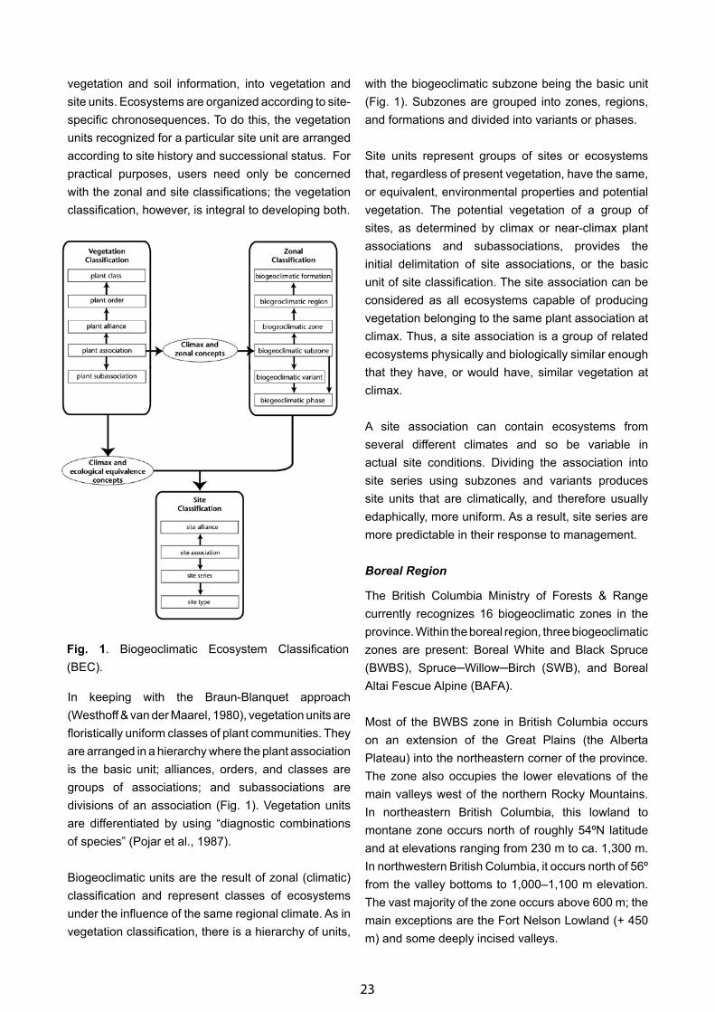
23

vegetation and soil information, into vegetation and site units. Ecosystems are organized according to site-specific chronosequences. To do this, the vegetation units recognized for a particular site unit are arranged according to site history and successional status. For practical purposes, users need only be concerned with the zonal and site classifications; the vegetation classification, however, is integral to developing both.

In keeping with the Braun-Blanquet approach (Westhoff & van der Maarel, 1980), vegetation units are floristically uniform classes of plant communities. They are arranged in a hierarchy where the plant association is the basic unit; alliances, orders, and classes are groups of associations; and subassociations are divisions of an association (Fig. 1). Vegetation units are differentiated by using “diagnostic combinations of species” (Pojar et al., 1987).

Biogeoclimatic units are the result of zonal (climatic) classification and represent classes of ecosystems under the influence of the same regional climate. As in vegetation classification, there is a hierarchy of units,

with the biogeoclimatic subzone being the basic unit (Fig. 1). Subzones are grouped into zones, regions, and formations and divided into variants or phases.

Site units represent groups of sites or ecosystems that, regardless of present vegetation, have the same, or equivalent, environmental properties and potential vegetation. The potential vegetation of a group of sites, as determined by climax or near-climax plant associations and subassociations, provides the initial delimitation of site associations, or the basic unit of site classification. The site association can be considered as all ecosystems capable of producing vegetation belonging to the same plant association at climax. Thus, a site association is a group of related ecosystems physically and biologically similar enough that they have, or would have, similar vegetation at climax.

A site association can contain ecosystems from several different climates and so be variable in actual site conditions. Dividing the association into site series using subzones and variants produces site units that are climatically, and therefore usually edaphically, more uniform. As a result, site series are more predictable in their response to management.

Boreal Region

The British Columbia Ministry of Forests & Range currently recognizes 16 biogeoclimatic zones in the province. Within the boreal region, three biogeoclimatic zones are present: Boreal White and Black Spruce (BWBS), Spruce─Willow─Birch (SWB), and Boreal Altai Fescue Alpine (BAFA).

Most of the BWBS zone in British Columbia occurs on an extension of the Great Plains (the Alberta Plateau) into the northeastern corner of the province. The zone also occupies the lower elevations of the main valleys west of the northern Rocky Mountains. In northeastern British Columbia, this lowland to montane zone occurs north of roughly 54ºN latitude and at elevations ranging from 230 m to ca. 1,300 m. In northwestern British Columbia, it occurs north of 56º from the valley bottoms to 1,000–1,100 m elevation. The vast majority of the zone occurs above 600 m; the main exceptions are the Fort Nelson Lowland (+ 450 m) and some deeply incised valleys.

Fig. 1. Biogeoclimatic Ecosystem Classification (BEC).

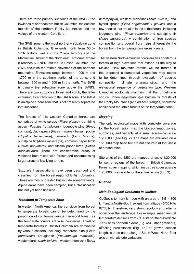
24

There are three primary subzones of the BWBS: the lowlands of northeastern British Columbia; the eastern foothills of the northern Rocky Mountains; and the valleys of the western Cordillera.

The SWB zone is the most northerly subalpine zone in British Columbia. It extends north from 56.5–57ºN latitude, well into the Yukon Territory and the Mackenzie District of the Northwest Territories, where it reaches 60–70ºN latitude. In British Columbia, the SWB occupies the middle elevations of the northern mountains. Elevations range between 1,000 m and 1,700 m in the southern portion of the zone, and between 900 m and 1,500 m in the north. The SWB is usually the subalpine zone above the BWBS. There are two subzones: forest and scrub, the latter occurring as a transition to the BAFA zone. The BAFA is an alpine tundra zone that is not presently separated into subzones.

The forests of this western Canadian boreal are comprised of white spruce (Picea glauca), trembling aspen (Populus tremuloides), lodgepole pine (Pinus contorta), black spruce (Picea mariana), balsam poplar (Populus balsamifera), tamarack (Larix laricina), subalpine fir (Abies lasiocarpa), common paper birch (Betula papyrifera), and Alaska paper birch (Betula neoalaskana). There are considerable areas of wetlands both mixed with forests and encompassing larger areas of low-lying terrain.

Sixty plant associations have been described and classified from the boreal region of British Columbia. These are mostly forested but include some wetlands. Alpine areas have been sampled, but a classification has not yet been finalized.

Transition to Temperate Zone

In western North America, the transition from boreal to temperate forests cannot be determined by the proportion of coniferous versus hardwood forest, as the temperate forests are also coniferous. Lowland temperate forests in British Columbia are dominated by various conifers, including Ponderosa pine (Pinus ponderosa), Douglas-fir (Pseudotsuga menziesii), western larch (Larix laricina), western hemlock (Tsuga

heterophylla), western redcedar (Thuja plicata), and hybrid spruce (Picea engelmannii x glauca), and a few species that are also found in the boreal, including lodgepole pine (Pinus contorta) and subalpine fir (Abies lasiocarpa). A combination of tree species composition and overall flora helps differentiate the boreal from the temperate coniferous forests.

The western North American cordillera has coniferous forests at high elevations that extend all the way to Mexico. How mountain forests will be treated in the proposed circumboreal vegetation map needs to be determined through evaluation of species composition, climate characteristics, and the elevational sequence of vegetation type. Western Canadian ecologists maintain that the Engelmann spruce (Picea engelmannii)–subalpine fir forests of the Rocky Mountains (and adjacent ranges) should be considered mountain forests of the temperate zone.

Mapping

The only ecological maps with complete coverage for the boreal region map the biogeoclimatic zones, subzones, and variants at a small scale―ca. scale 1:250,000 (see Fig. 2). The maps are available on a 1:20,000 map base but are not accurate at that scale of presentation.

Site units of the BEC are mapped at scale 1:20,000 for some regions of the boreal in British Columbia. Forest cover mapping, which maps tree cover at scale 1:20,000, is available for the entire region (Fig. 3).

Québec

Main Ecological Gradients in Québec

Québec’s territory is huge with an area of 1,514,100 km2 and a North–South extent from latitude 45º00’N to 62º30’N. Therefore, very strong ecological gradients occur over the landscape. For example, mean annual temperature declines from 7ºC at its southern border to -11ºC at its northern extent (Fig. 4a). Other gradients, affecting precipitation (Fig. 4b) or growth season length, can be seen along a South-West–North-East axis or with altitude variations.

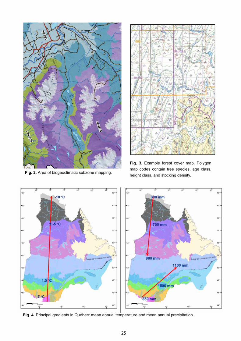
25

Fig. 2. Area of biogeoclimatic subzone mapping.

Fig. 3. Example forest cover map. Polygon map codes contain tree species, age class, height class, and stocking density.

Fig. 4. Principal gradients in Québec: mean annual temperature and mean annual precipitation.

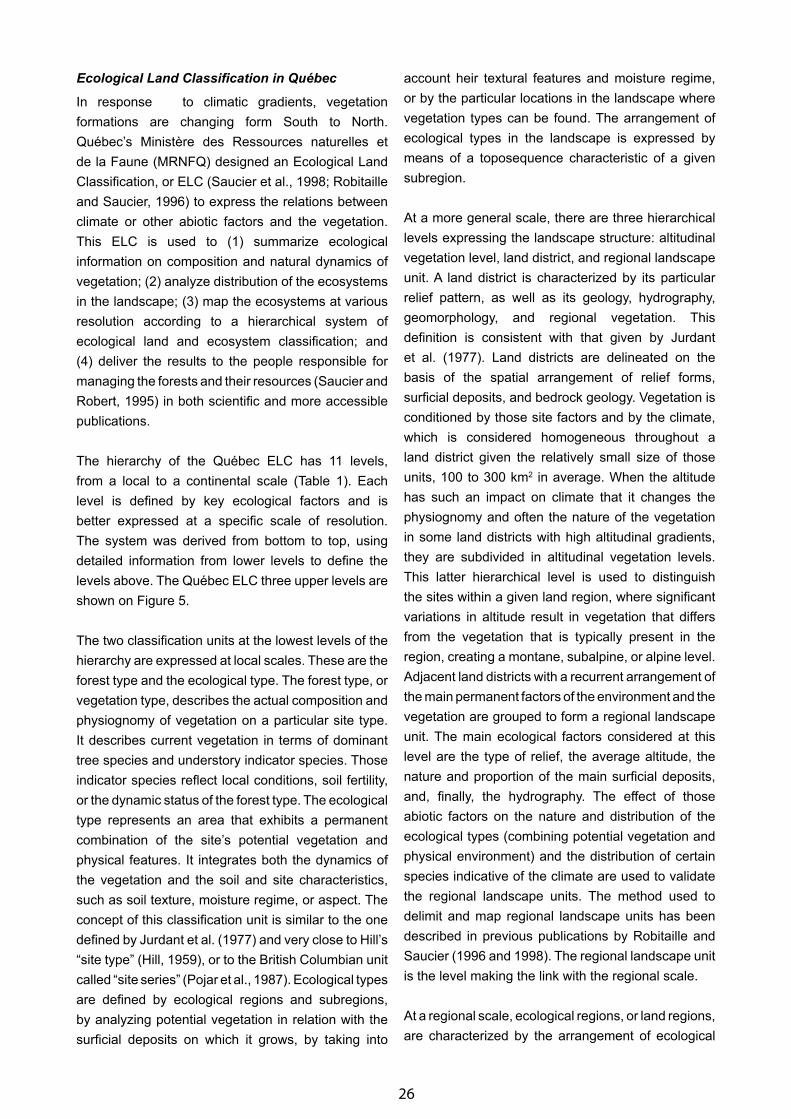
26

Ecological Land Classification in Québec

In response to climatic gradients, vegetation formations are changing form South to North. Québec’s Ministère des Ressources naturelles et de la Faune (MRNFQ) designed an Ecological Land Classification, or ELC (Saucier et al., 1998; Robitaille and Saucier, 1996) to express the relations between climate or other abiotic factors and the vegetation. This ELC is used to (1) summarize ecological information on composition and natural dynamics of vegetation; (2) analyze distribution of the ecosystems in the landscape; (3) map the ecosystems at various resolution according to a hierarchical system of ecological land and ecosystem classification; and (4) deliver the results to the people responsible for managing the forests and their resources (Saucier and Robert, 1995) in both scientific and more accessible publications.

The hierarchy of the Québec ELC has 11 levels, from a local to a continental scale (Table 1). Each level is defined by key ecological factors and is better expressed at a specific scale of resolution. The system was derived from bottom to top, using detailed information from lower levels to define the levels above. The Québec ELC three upper levels are shown on Figure 5.

The two classification units at the lowest levels of the hierarchy are expressed at local scales. These are the forest type and the ecological type. The forest type, or vegetation type, describes the actual composition and physiognomy of vegetation on a particular site type. It describes current vegetation in terms of dominant tree species and understory indicator species. Those indicator species reflect local conditions, soil fertility, or the dynamic status of the forest type. The ecological type represents an area that exhibits a permanent combination of the site’s potential vegetation and physical features. It integrates both the dynamics of the vegetation and the soil and site characteristics, such as soil texture, moisture regime, or aspect. The concept of this classification unit is similar to the one defined by Jurdant et al. (1977) and very close to Hill’s “site type” (Hill, 1959), or to the British Columbian unit called “site series” (Pojar et al., 1987). Ecological types are defined by ecological regions and subregions, by analyzing potential vegetation in relation with the surficial deposits on which it grows, by taking into

account heir textural features and moisture regime, or by the particular locations in the landscape where vegetation types can be found. The arrangement of ecological types in the landscape is expressed by means of a toposequence characteristic of a given subregion.

At a more general scale, there are three hierarchical levels expressing the landscape structure: altitudinal vegetation level, land district, and regional landscape unit. A land district is characterized by its particular relief pattern, as well as its geology, hydrography, geomorphology, and regional vegetation. This definition is consistent with that given by Jurdant et al. (1977). Land districts are delineated on the basis of the spatial arrangement of relief forms, surficial deposits, and bedrock geology. Vegetation is conditioned by those site factors and by the climate, which is considered homogeneous throughout a land district given the relatively small size of those units, 100 to 300 km2 in average. When the altitude has such an impact on climate that it changes the physiognomy and often the nature of the vegetation in some land districts with high altitudinal gradients, they are subdivided in altitudinal vegetation levels. This latter hierarchical level is used to distinguish the sites within a given land region, where significant variations in altitude result in vegetation that differs from the vegetation that is typically present in the region, creating a montane, subalpine, or alpine level. Adjacent land districts with a recurrent arrangement of the main permanent factors of the environment and the vegetation are grouped to form a regional landscape unit. The main ecological factors considered at this level are the type of relief, the average altitude, the nature and proportion of the main surficial deposits, and, finally, the hydrography. The effect of those abiotic factors on the nature and distribution of the ecological types (combining potential vegetation and physical environment) and the distribution of certain species indicative of the climate are used to validate the regional landscape units. The method used to delimit and map regional landscape units has been described in previous publications by Robitaille and Saucier (1996 and 1998). The regional landscape unit is the level making the link with the regional scale.

At a regional scale, ecological regions, or land regions, are characterized by the arrangement of ecological

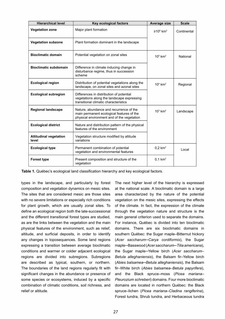
27

Table 1. Québec’s ecological land classification hierarchy and key ecological factors.

types in the landscape, and particularly by forest composition and vegetation dynamics on mesic sites. The sites that are considered mesic are those sites with no severe limitations or especially rich conditions for plant growth, which are usually zonal sites. To define an ecological region both the late-successional and the different transitional forest types are studied, as are the links between the vegetation and the main physical features of the environment, such as relief, altitude, and surficial deposits, in order to identify any changes in toposequences. Some land regions expressing a transition between average bioclimatic conditions and warmer or colder adjacent ecological regions are divided into subregions. Subregions are described as typical, southern, or northern. The boundaries of the land regions regularly fit with significant changes in the abundance or presence of some species or ecosystems, induced by a specific combination of climatic conditions, soil richness, and relief or altitude.

The next higher level of the hierarchy is expressed at the national scale. A bioclimatic domain is a large area characterized by the nature of the potential vegetation on the mesic sites, expressing the effects of the climate. In fact, the expression of the climate through the vegetation nature and structure is the main general criterion used to separate the domains. For instance, Québec is divided into ten bioclimatic domains. There are six bioclimatic domains in southern Québec: the Sugar maple–Bitternut hickory (Acer saccharum─Carya cordiformis), the Sugar maple─Basswood (Acer saccharum─Tilia americana), the Sugar maple─Yellow birch (Acer saccharum–Betula alleghaniensis), the Balsam fir–Yellow birch (Abies balsamea─Betula alleghaniensis), the Balsam fir–White birch (Abies balsamea–Betula papyrifera), and the Black spruce–moss (Picea mariana–Pleurozium schreberi) domains. Four more bioclimatic domains are located in northern Québec: the Black spruce–lichen (Picea mariana–Cladina rangiferina), Forest tundra, Shrub tundra, and Herbaceous tundra

Hierarchical level Key ecological factors Average size Scale

Vegetation zone Major plant formation≥106 km2 Continental

Vegetation subzone Plant formation dominant in the landscape

Bioclimatic domain Potential vegetation on zonal sites105 km2 National

Bioclimatic subdomain Difference in climate inducing change in disturbance regime, thus in succession scheme

Ecological region Distribution of potential vegetations along the landscape, on zonal sites and azonal sites

104 km2 Regional

Ecological subregion Differences in distribution of potential vegetations along the landscape expressing transitional climatic characteristics

Regional landscape Nature, abundance and recurrence of the main permanent ecological features of the physical environment and of the vegetation

103 km2 Landscape

Ecological district Nature and distribution pattern of the physical features of the environment

Altitudinal vegetation level

Vegetation structure modified by altitude variations

Ecological type Permanent combination of potential vegetation and environmental features

0,2 km2

Local

Forest type Present composition and structure of the vegetation

0,1 km2

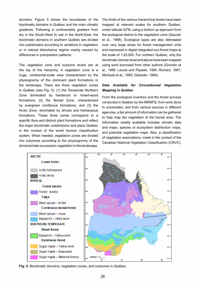
28

Fig. 5. Bioclimatic domains, vegetation zones, and subzones in Québec.

domains. Figure 5 shows the boundaries of the bioclimatic domains in Québec and the main climatic gradients. Following a continentality gradient from dry in the South-West to wet in the North-East, the bioclimatic domains in southern Québec are divided into subdomains according to variations in vegetation or in natural disturbance regime mainly caused by differences in precipitation patterns.

The vegetation zone and subzone levels are at the top of the hierarchy. A vegetation zone is a huge, continental-scale area characterized by the physiognomy of the dominant plant formations in the landscape. There are three vegetation zones in Québec (see Fig. 5): (1) the Temperate Northern Zone dominated by hardwood or mixed-wood formations; (2) the Boreal Zone, characterized by evergreen coniferous formations; and (3) the Arctic Zone, dominated by shrubs and herbaceous formations. These three zones correspond to a specific flora and distinct plant formations and reflect the major bioclimatic subdivisions and place Québec in the context of the world biomes classification system. When needed, vegetation zones are divided into subzones according to the physiognomy of the dominant late-succession vegetation in the landscape.

The limits of the various hierarchical levels have been mapped at relevant scales for southern Québec, under latitude 52ºN, using a bottom up approach from the ecological district to the vegetation zone (Saucier et al., 1998). Ecological types are also delineated over very large areas for forest management units and expressed in digital integrated eco-forest maps at the scale of 1:20,000. For northern Québec, only the bioclimatic domain level and above have been mapped using work borrowed from other authors (Grondin et al., 1996; Lavoie and Payette, 1994; Richard, 1987; Morisset et al., 1983; Gérardin, 1980).

Data Available for Circumboreal Vegetation Mapping in Québec

From the ecological inventory and the forest surveys conducted in Québec by the MRNFQ, from work done in universities, and from various sources in different agencies, a fair amount of information can be gathered to help map the vegetation of the boreal area. The information readily available includes climatic data and maps, species or ecosystem distribution maps, and potential vegetation maps. Also, a classification of vegetation associations, made in the context of the Canadian National Vegetation Classification (CNVC),

29

will be available for the southern part of the boreal. The associations defined by this project are close matches to the Braun-Blanquet association concept.

Conclusion

Using examples from two Provinces of Canada, we show that there is current data that can be used to help complete the Circumboreal Vegetation Mapping project (CBVM). Most of this information resides in provincial agencies and universities, so the collaboration of those agencies is key for a precise and accurate circumboreal vegetation map in Canada.

To achieve this project for Canada and North America, discussion should be carried out to clearly define the concepts that are to be mapped. Transition areas between boreal and temperate zones can become problematic. For example, in Québec the boreal excludes the temperate mixed forest in the south, which is not the case everywhere. The northern limit of the boreal is more straightforward as it is the tree limit.

A zonal approach to mapping has advantages in British Columbia and Québec because site series or potential vegetation units are available and mapped already for large parts of the boreal region. Some high elevation mountainous areas of British Columbia should not be included as boreal, even if they are dominated by coniferous species, because their climate is too mild and they extend very far south in areas that are clearly not boreal. This ambiguity emphasizes again that defining concepts is an essential step toward obtaining consistent results in North America.

We believe that the CBVM should map the “true” boreal, excluding the areas transitional to the temperate zone, for two reasons: (1) the concept of these areas appears to vary more across jurisdictions, and depending upon concept, could add considerable area to the boreal map; and (2) these areas are very sensitive to climate change, quickly changing to temperate vegetation.

With climate change, the area considered boreal will also change, and northern and southern boundaries will effectively move northward. However, vegetation response will lag behind climate change, leaving

remnants of boreal vegetation where they are presently found. It is important to generate a boreal map soon in order to characterize the present distribution of the boreal, as portions of the boreal in British Columbia seem very sensitive to climate changes.

In summary, due to the jurisdictional nature of Canadian work on the boreal, clear definition of concepts is essential to obtaining consistent results in North America. The hierarchical level of vegetation classification to map will influence scale and timing of the final product, with a “higher-level” classification unit (e.g., formation) easier to map with presently available information.

Acknowledgments

We would like to thank the organizers of the CBVM workshop in Helsinki for providing a forum for the initiation of this project and for supporting our participation.

References

Gérardin, V. 1980. L’inventaire du Capital-Nature du territoire de la baie James. Les régions écologiques et la végétation des sols minéraux, tome 1. Méthodologie et descriptions. Service des études écologiques régionales, Min. Environ., Québec. 398 pp.

Grondin, P. et al. 1996. Écologie forestière. Pages 133–279 in Coté, M., Bérard, J.A., eds., Manuel de foresterie, Ordre des ingénieurs forestiers du Québec, Presses de l’Université Laval, Québec.

Hill, G. A. 1959. A Ready Reference to the Description of the Land of Ontario and its Productivity. Division of Research, Department of Lands and Forests, Toronto, Ontario. 142 pp.

Jurdant, M., Bélair, J. -L., Gérardin, V., & Ducruc, J. -P. 1977. L’inventaire du Capital-Nature. Pêches et Environ. Can., Série de la classification écologique du territoire, no 2. 202 pp.

Lavoie, C. & Payette, S. 1994. Recent fluctuations of the lichen-spruce forest limit in Subarctic Quebec. J. Ecol. 82 : 725–734.

Morisset, P., Payette S., & Deshaye, J. 1983. The vascular flora of the northern Quebec-Labrador peninsula: Phytogeographical structure with respect to the tree-line. Nordicana 47: 141–151.

30

Pojar, J., Klinka, K., & Meidinger, D. V. 1987. Biogeclimatic ecosystem classification in British Columbia. Forest Ecology and Management 22: 119–154.

Richard, P. J. H. 1987. Le couvert végétal du Québec-Labrador et son histoire postglaciaire. Dép. Géogr., Univ. Montréal, Notes Doc., 87-01. 74 pp. (with color map of the vegetation of Québec-Labrador).

Robitaille, A. & Saucier, J. -P. 1996. Land district, ecophysio-graphic units and areas: the landscape mapping of the Ministère des Ressources naturelles du Québec. Environmental Monitoring and Assessment 39 (1–3): 127–148.

Robitaille, A. & Saucier, J. -P. 1998. Les paysages régionaux du Québec méridional. Les publications du Québec, Québec. 213 pp.

Saucier, J. -P., Bergeron, J. -F. Grondin, P., & Robitaille, A. 1998. Les régions écologiques du Québec méridional (3rd version): un des éléments du système hiérarchique de classification écologique du territoire mis au point par le ministère des Ressources naturelles du Québec. Supplément de L’aubelle, no 124. 12 pp.

Saucier, J. -P. & Robert, D. 1995. Présentation du programme de connaissance des écosystèmes forestiers du Ministère des Ressources naturelles du Québec. Revue forestière française XLVII(1): 71–74.

Westhoff, V. & van der Maarel, E. 1980. The Braun-Blanquet approach. Pages 287–399 in Whittaker, R. H., ed. Classification of Plant Communities. Dr. W. Junk, The Hague.

31

Map of the Natural Vegetation of Europe and Its Contribution to the Circumboreal Vegetation Map

Udo Bohn

Formerly: Federal Agency for Nature Conservation, Bonn, Germany, u.bohn@arcor.de

Abstract

The Map of the Natural Vegetation of Europe, produced by close international co-operation, was published in printed form and as an interactive CD-ROM. The printed work consists of three parts: maps at the scales 1:2.5M and 1:10M, a legend volume containing all mapping units in hierarchical order, and an extensive explanatory textbook. All the map and textual information is also available on an interactive CD-ROM in English and German versions. This allows multiple use and analysis of the comprehensive database.

On the Map of the Natural Vegetation of Europe the boreal zone comprises nine different main vegetation formations. These consist of five zonal (A, B, C, D, E) and four azonal (P, S, T, U) formations. The boreal core formations are birch forests (formation C) and coniferous forests (formation D). All formations are hierarchically classified according to zonal, altitudinal, geographical, and edaphic criteria. Within the boreal zone of Europe, there are 90 mapping units, each of them described in detail by standardized data sheets.

The European classification system is on the higher levels to a great extent compatible with that of the Circumpolar Arctic Vegetation Map (CAVM). Thus, it will not be difficult to link up the Map of the Natural Vegetation of Europe with the CAVM. Because of its detailed information and digital database, the Map of the Natural Vegetation of Europe provides an ideal regional base map for the planned Circumboreal Vegetation Map.

Keywords: digital vegetation map; Europe; hierarchic classification system, potential natural vegetation.

Introduction

The Map of the Natural Vegetation of Europe was published in printed form and as an interactive CD-ROM. The printed work (Bohn et al., 2000/2003) consists of three parts: maps of the (potential) natural vegetation of Europe on nine sheets, scale 1:2.5M, along with a colored legend sheet and an overview map, General Map of the Natural Vegetation of Europe, scale 1:10M; a legend volume containing all 700 mapping units in hierarchical order with German and English texts; and an extensive German explanatory textbook, inter alia with information on the project history, the concept of the vegetation map, description of the natural vegetation on different levels of classification, and detailed information for each mapping unit on standardized data sheets (on CD-ROM). The interactive CD-ROM (Bohn et al., 2004) contains all map and text information related to the complete printed work in digital form, both in German and English. It allows multiple use and analyses of the European vegetation data. Finally, the contributions and results of an international workshop on “Application and Analysis of the Map of the Natural Vegetation of Europe” were published (Bohn et al., 2005).

The mapping area covers all of Europe, including the Urals and Caucasus in the east, as well as Iceland, Svalbard, Franz Josef Land, and Novaya Zemlya in the north, but excludes the Atlantic islands of Azores, Madeira, and the Canary Islands. In this international mapping project, which extended over two decades (from 1979 to 2003), more than 100 vegetation scientists from 31 European countries were involved, including experts from all Nordic countries (Iceland, Denmark, Norway, Sweden, Finland, and Russia) that participate substantially in the arctic and boreal zones.

32

The three main coordination centers for the project implementation were located in Bonn (Federal Agency for Nature Conservation, BfN), Průhonice near Prague (Botanical Institute of the Czech Academy of Sciences), and St. Petersburg (Komarov Botanical Institute of the Russian Academy of Sciences, Dept. of Vegetation Geography and Cartography).

Methods

A fundamental requirement for the production of a unified European vegetation map was the common development of a classification system, nomenclature, and mapping concept that could be used by all contributors from the different phytosociological “schools” in Europe. Therefore, the titles of hierarchic items and mapping units were named in a neutral, generally understandable form.

The map legend as well as the vegetation map are clearly hierarchically structured and take into account that vegetation structure and species combination are decisive criteria at any level of classification. The highest units of classification are formed by 19 vegetation formations based on physiognomic-ecological features, of which 14 are zonal units, representing the main macroclimatic zones in a sequence from north to south, or altitudinal belts in the mountains from higher to lower levels. Five formations represent azonal vegetation, which is shaped firstly by edaphic factors, that is, specific soil and hydrological conditions, and is modified only secondarily by macroclimatic factors. All formations are characterized by their vegetation structure (life forms etc.), species combination (mainly dominant species), and ecology.

Corresponding vegetation types with similar structure and species composition, such as polar deserts and subnival vegetation of high mountains, or tundras and alpine vegetation, are combined in one formation group because of their close structural, floristic, and climatic relations.

The main vegetation formations are coded by the capital letters A-U, in alphabetical order, with their further subdivision indicated by numbers. The main formations are depicted in the vegetation map and legend by basic colors, which are shaded according to their subdivision along macroclimatic gradients

from north to south, or indicating altitudinal belts in mountains.

List of Main Vegetation Formations

(Classification according to physiognomy and environmental conditions)

Zonal and extra zonal vegetation (depending primarily on climate):

A. – Polar deserts and subnival-nival vegetation of high mountains

B. – Arctic tundras and alpine vegetation

C. – Subarctic, boreal, and nemoral-montane open woodlands, as well as subalpine and oro-Mediterranean vegetation

D. – Mesophytic and hygromesophytic coniferous and mixed broad-leaved-coniferous forests

E. – Atlantic dwarf shrub heaths

F. – Mesophytic deciduous broad-leaved and mixed coniferous-broad-leaved forests

G. – Thermophilous mixed deciduous broad-leaved forests

H. – Hygro-thermophilous mixed deciduous broad-leaved forests

J. – Mediterranean sclerophyllous forests and scrub

K. – Xerophytic coniferous forests, woodlands, and scrub

L. – Forest steppes (meadow steppes alternating with deciduous broad-leaved forests) and dry grasslands alternating with xerophytic scrub

M. – Steppes

N. – Oroxerophytic vegetation (thorn-cushion communities, tomillares, mountain steppes, partly scrub)

O. – Deserts

Azonal vegetation (depending on specific soil and hydrological conditions)

P. – Coastal vegetation and inland halophytic vegetation

R. – Tall reed vegetation and tall sedge swamps, aquatic vegetation

S. – Mires

T. – Swamp and fen forests

U. – Vegetation of flood plains, estuaries and fresh-water polders, and other moist or wet sites

33

The main vegetation formations are classified into subgroups according to dominant species and species composition depending on spatial macroclimatic and edaphic variation. The zonal vegetation, such as birch, spruce, or pine forests in the boreal zone, is firstly differentiated along temperature (N–S, altitudes) and oceanity (W–E) gradients. The hierarchic classification system applied to the Map of the Natural Vegetation of Europe is demonstrated in detail by the European boreal vegetation.

The circumboreal phytogeographical zone is principally characterized by dominating birch, spruce and pine forests at low and middle altitudes. Its northern boundary corresponds with the northern natural tree line; the southern boundary follows the southern natural distribution limit of coherent (more or less closed) coniferous forests. The hemiboreal subzone of mixed broad-leafed-coniferous forests adjoining to the south is already assigned to the temperate zone according to the numerous nemoral plant species occurring there.

The phytogeographical map of Europe (Meusel & Jäger 1992) provides a system of global zones that are divided into floristic regions, subregions, provinces, and subprovinces. Thus, the boreal zone is subdivided from west to east into the boreo-Atlantic, Scandinavian, and boreo-Russian provinces, and within these provinces it is subdivided from north to south into floristic subprovinces. This map provides basic information for the geographical vegetation classification.

Results

In the Map of the Natural Vegetation of Europe, the boreal zone comprises five zonal (A─E) and four azonal (P, S, T, U) main formations, with altogether 90 mapping units. Because of the high mountain ranges in Iceland, Scandinavia, and the Urals, besides the W─E and N─S oriented variation of the birch and coniferous forests (formations C, D), there is also a decisive altitudinal differentiation reaching up into the treeless alpine (formation B) and subnival-nival (formation A) vegetation belts. Characteristic azonal formations appearing in the boreal zone are: coastal sand-dune, rock and halophytic vegetation (formation P), mires (formation S), swamp and fen

forests (formation T), and vegetation of flood plains (formation U). These formations are represented by specific boreal vegetation types and mapping units.

Due to the small scale of the European vegetation map, the mapping units represent landscape-specific vegetation complexes consisting of various natural plant communities and, as a rule, are named after the dominating plant community(ies). The characteristic features and contents of the individual mapping units are described in detail in standardized data sheets.

Zonal Boreal Forest Vegetation

The boreal forest vegetation of Europe is composed of two core formations: formation C represents subarctic and boreal open woodlands dominated, especially in the western part, by birch trees and shrubs (mostly Betula pubescens s.l.), and formation D represents coniferous forests with different dominating tree species, such as spruce, fir, and pine.

Formation C – Subarctic, boreal, and nemoral-montane open woodlands – consists of two geographically differentiated subgroups:

C.1 represents the eastern boreal open woodlands with different combinations of the main tree species Betula pubescens subsp. czerepanovii, Picea obovata, and Pinus sylvestris.

C.2 represents the western boreal birch forests, partly in complex with pine forests, in the more oceanic influenced regions, especially western Scandinavia and Iceland.

Formation D – Mesophytic and hygromesophytic coniferous forests—are mainly distributed in the central and eastern parts of northern Europe, and in the higher mountains. It is divided into six subgroups according to the dominant conifer species. Three of these subgroups are predominantly distributed in the boreal zone and are characterized by a more continental climate:

D.1 represents the western boreal spruce forests dominated by Picea abies, P. obovata (in the eastern part), and their hybrid.

D.2 represents the eastern boreal pine-spruce and fir-spruce forests that are composed of Siberian conifer species, such as Picea obovata, Pinus sibirica, Abies sibirica, and Larix sibirica, spreading

34

from western Siberia over the Urals into the east European lowland.

D.5 consists of pine forests, with Pinus sylvestris being predominant, and changing admixture of birch and spruce trees. These forest types naturally occur only under extreme soil conditions: on nutrient-poor and dry sandy or rocky, or wet and peaty sites. Pine forests are not restricted to the boreal zone and extend on suitable sites further south into the temperate zone.

The subdivision of western boreal spruce forests (subformation D.1) follows the climatic gradient from north to south into northern, middle, and southern boreal subzones and types. This subdivision is mainly caused by different lengths of the growing season. But the delimitation of the three subzones is also based on floristic, structural, and ecological features; however, the boundaries between these subzones are more or less blurred. In the mountain regions of Scandinavia the three subzones represent altitudinal belts.

The tree layer of the eastern boreal coniferous forests (subformation D.2) consists of Siberian conifer species that spread over the Urals to a varying extent into its western foothills and lowland. These form dark coniferous forests, the so-called “dark taiga.” Even in their shrub and herb layers, many Uralian─Siberian species occur in addition to widely distributed boreal species. The group of eastern boreal coniferous forests is on the first level subdivided into lowland-colline and (submontane-) montane (Ural) types, and on the second level within the lowland-colline subgroup also into northern, middle, and southern boreal types.

The third group of boreal coniferous forests (subformation D.5) consists of pine forests with dominating Pinus sylvestris. Because of the lack of climatic indicator species, pine forests are divided only into two subzones: the northern, and the middle and southern boreal types. On the second level there is an altitudinal differentiation into lowland-colline and montane types. Montane types have been identified only in Scotland and the southern Urals.

Unwooded Zonal Vegetation Within the Boreal Zone

Another typical but unwooded vegetation formation

within the boreal zone comprises mountain tundras and boreo-alpine vegetation (formation B). The units concerned are mainly distributed in mountain regions of Iceland, the Faroe Islands, Scandinavia, and the northern Urals and occur as altitudinal belts above the belt of birch and open spruce woodlands in the boreal zone. Because of gradual transitions between arctic and boreal vegetation, it is difficult in many cases to decide whether these units belong to arctic tundras or to the boreal alpine vegetation.

Subformation B.1.5 – Mountain tundras and sparse mountain vegetation—is distributed in the mountains of Iceland, Kola Peninsola, and in the northernmost part of the Urals. Mountain tundras are situated in the transition zone between arctic and boreal vegetation and, therefore, are closely related to tundra vegetation in the southernmost part of the arctic zone.

Subnival-nival vegetation of high mountains (subformation A.2) and alpine vegetation in the boreal zone (subformation B.2) are mainly distributed in the Scandinavian high mountains, in small outposts also in the interior mountains of the Kola Peninsula, in the Scottish Highlands, and on the Faroe Islands.

Azonal Vegetation Within the Boreal Zone

Within the boreal zone, besides zonal vegetation, natural azonal vegetation occurs on large areas too and plays an important role. It belongs to the following main vegetation formations:

P – Coastal vegetation

S – Mires

T – Swamp and fen forests

U – Vegetation of flood plains

These formations, their zonal subgroups and mapping units are also characteristic elements of the natural vegetation of the boreal zone and therefore should be mapped.

Formation P – Coastal vegetation—comprises the vegetation of coastal sand dunes, of shingle beaches, and of rocky seashores, as well as coastal halophytic vegetation. Boreo–Atlantic sand dune vegetation is mapped for example in a larger area on the flat coast of south-western Iceland.

Formation S – Mire vegetation—in different types and complexes represents the most widespread and

35

characteristic azonal vegetation in the boreal zone. Its main level of classification focuses on the nutrient supply of ground water in three groups:

S – Mires in the boreal zone (16 Mapping Units)

1 – Ombrotrophic mires (bogs) (7 MU)

1.1 – Sphagnum fuscum-raised bog complexes in the boreal zone (S1-S4)

1.2 – Sphagnum papillosum-blanket bog and raised bog complexes with Erica tetralix and Narthecium ossifragum in the oceanic regions (S6-S8)

2 – Ombro-minerotrophic mires (1MU)

2.2 – Palsa mires (S14)

3 – Minerotrophic mires (fens) (8 MU)

3.1 – Boreal aapa mire complexes (S15, S16)

3.2 – Transitional mires (incl. nutrient-poor fens) (S17-S20)

3.3 – Small sedge-brown-moss fens (S22-S24)

The most characteristic and widespread mire types of the boreal zone are palsa and aapa mires. Palsa mires are bound to the subarctic and northern boreal subzones, whereas aapa mire complexes are widespread in the northern and middle boreal subzones.

Correlation Between Maps

With regard to the planned Circumboreal Vegetation Map (CBVM), questions arise how the Circumpolar Arctic Vegetation Map (CAVM) and the Map of the Natural Vegetation of Europe correlate in the North European contact area. For this purpose I have compared details of the CAVM with corresponding sections of the Map of the Natural Vegetation of Europe at different scales. The examined map sections lie in the northeastern part of European Russia (Fig. 1).

In Figure 1 a section of the CAVM (scale 1:7.5M) is compared with a detail of the General Map of the Natural Vegetation of Europe at the scale of 1:10M.

Fig. 1. Comparison of corresponding map sections (northeast European Russia) from the Circumpolar Arctic Vegetation Map and the overview map, General Map of the Natural Vegetation of Europe.

Detail of CAVM, scale

1:7.5 million,

NE European Russia

S Erect-shrub tundras

G Graminoid tundras

B Mountain complexes

W Wetlands

Detail of European

General Map, scale

1:10 million,

NE European Russia

B Arctic tundras and alpine vegetation

C Open woodlands

D Coniferous forests

P Coastal vegetation

S Mires

U Alluvial vegetation

Detail of CAVM, scale

1:7.5 million,

NE European Russia

S Erect-shrub tundras

G Graminoid tundras

B Mountain complexes

W Wetlands

Detail of European

General Map, scale

1:10 million,

NE European Russia

B Arctic tundras and alpine vegetation

C Open woodlands

D Coniferous forests

P Coastal vegetation

S Mires

U Alluvial vegetation

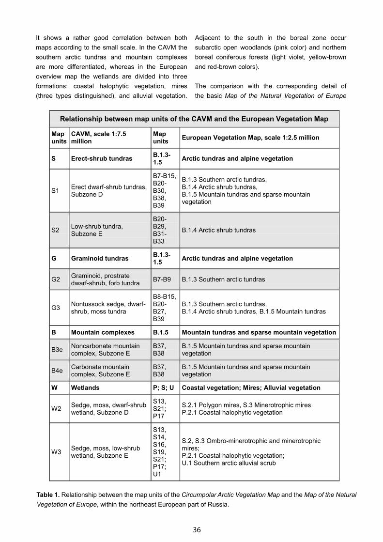
36

It shows a rather good correlation between both maps according to the small scale. In the CAVM the southern arctic tundras and mountain complexes are more differentiated, whereas in the European overview map the wetlands are divided into three formations: coastal halophytic vegetation, mires (three types distinguished), and alluvial vegetation.

Adjacent to the south in the boreal zone occur subarctic open woodlands (pink color) and northern boreal coniferous forests (light violet, yellow-brown and red-brown colors).

The comparison with the corresponding detail of the basic Map of the Natural Vegetation of Europe

Table 1. Relationship between the map units of the Circumpolar Arctic Vegetation Map and the Map of the Natural Vegetation of Europe, within the northeast European part of Russia.

Relationship between map units of the CAVM and the European Vegetation Map

Map units

CAVM, scale 1:7.5 million

Map units European Vegetation Map, scale 1:2.5 million

S Erect-shrub tundras B.1.3-1.5 Arctic tundras and alpine vegetation

S1 Erect dwarf-shrub tundras, Subzone D

B7-B15, B20-B30, B38, B39

B.1.3 Southern arctic tundras, B.1.4 Arctic shrub tundras, B.1.5 Mountain tundras and sparse mountain vegetation

S2 Low-shrub tundra, Subzone E

B20-B29, B31-B33

B.1.4 Arctic shrub tundras

G Graminoid tundras B.1.3-1.5 Arctic tundras and alpine vegetation

G2 Graminoid, prostrate dwarf-shrub, forb tundra B7-B9 B.1.3 Southern arctic tundras

G3 Nontussock sedge, dwarf-shrub, moss tundra

B8-B15, B20-B27, B39

B.1.3 Southern arctic tundras, B.1.4 Arctic shrub tundras, B.1.5 Mountain tundras

B Mountain complexes B.1.5 Mountain tundras and sparse mountain vegetation

B3e Noncarbonate mountain complex, Subzone E

B37, B38

B.1.5 Mountain tundras and sparse mountain vegetation

B4e Carbonate mountain complex, Subzone E

B37, B38

B.1.5 Mountain tundras and sparse mountain vegetation

W Wetlands P; S; U Coastal vegetation; Mires; Alluvial vegetation

W2 Sedge, moss, dwarf-shrub wetland, Subzone D

S13, S21; P17

S.2.1 Polygon mires, S.3 Minerotrophic mires P.2.1 Coastal halophytic vegetation

W3 Sedge, moss, low-shrub wetland, Subzone E

S13, S14, S16, S19, S21; P17; U1

S.2, S.3 Ombro-minerotrophic and minerotrophic mires; P.2.1 Coastal halophytic vegetation; U.1 Southern arctic alluvial scrub

37

(EuroVegMap) at the scale of 1:2.5M shows a similar but more detailed result. In Table 1 the relationship between the mapping units of the CAVM and those of the Map of the Natural Vegetation of Europe for the same southern arctic map section is shown. The result is that within tundra vegetation a close relationship occurs only between the unit S2 (CAVM) and the EuroVegMap units of B.1.4, as well as between unit G2 (CAVM) and the EuroVegMap units of B.1.3 (marked by grey color). Whereas the units S1 and G3 of the CAVM have no clear corresponding group of mapping units in the Map of the Natural Vegetation of Europe.

The mountain complexes B3e and B4e of the CAVM are closely correlated to the map units of group B.1.5 in the EuroVegMap, but on the CAVM they are further differentiated due to carbonate and noncarbonate bedrock. On the other hand, the wetland units W2 and W3 of the CAVM are divided and assigned in the EuroVegMap to three different formations: coastal halophytic vegetation, mires, and alluvial vegetation.

Conclusion

The classification system of the legend of the Map of the Natural Vegetation of Europe is on the higher levels widely corresponding to that of the Circumpolar Arctic Vegetation Map, but the differentiation into mapping units as well as their codes and colors are different; however, it should not be difficult to link the European vegetation map with the CAVM. Moreover, the European classification system is to a great extent compatible with the Russian-Siberian and the North American systems. Thus, the Map of the Natural Vegetation of Europe at the scale 1:2.5 million provides an ideal regional base map for the Circumboreal Vegetation Map that can be generalized

and modified without major difficulties according to the mapping concept that will be developed by the project team.

References

Bohn, U., Neuhäusl, R., unter Mitarbeit von Gollub, G., Hettwer, C, Neuhäuslová, Z., Schlüter, H., & Weber, H. 2000/2003. Karte der natürlichen Vegetation Europas/Map of the Natural Vegetation of Europe, Maßstab/Scale 1:2.500.000, Teil 1/Part 1: Erläute-rungstext/Explanatory Text, 655 S./pp., Teil 2/Part 2: Legende/Legend, 153 S./pp., Teil 3/Part 3: Karten/ Maps, Münster, Landwirtschaftsverlag.

Bohn, U., Gollub, G., Hettwer, C, Neuhäuslová, Z., Raus, Th., Schlüter, H., & Weber, H., Bearb./eds. 2004. Karte der natürlichen Vegetation Europas / Map of the Natural Vegetation of Europe, Maßstab/Scale 1:2.500.000, Interaktive/Interactive CD-ROM – Er-läuterungstext, Legende, Karten/Explanatory Text, Legend, Maps, Münster, Landwirtschaftsverlag. http://www.floraweb.de/vegetation/dnld_eurovegmap.html

Bohn, U., Hettwer, G., & Gollub, G., bearb/eds. 2005. Anwendung und Auswertung der Karte der natürlichen Vegetation Europas/Application and Analysis of the Map of the Natural Vegetation of Europe. Bonn (Bundesamt für Naturschutz), BfN-Skripten 156, 452 S./pp. (Download: http://www.bfn.de, BfN-Skripten 156, 2007).

CAVM Team. 2003. Circumpolar Arctic Vegetation Map. Conservation of Arctic Flora and Fauna (CAFF) Map No. 1, U.S. Fish and Wildlife Service, Anchorage, Alaska.

Meusel, H. & Jäger, E. 1992. Vergleichende Chorologie der zentraleuropäischen Flora, Karten, Bd. 3, Jena u. a., G. Fischer, 689 S.

38

Development of a Boreal Vegetation Map of the Asian Part of Russia as a Part of the Circumboreal Vegetation Map

Nikolai Ermakov

Central Siberian Botanical Garden SB RAS, Novosibirsk, Russia

Extended Abstract

Small-scale vegetation maps covering large territories of whole continents may be produced only on the basis of international cooperation and through the synthesis of national traditions and resources. Currently, the Map of the Natural Vegetation of Europe is the foremost example of international efforts with a unified approach to mapping small-scale regularities of vegetation across an entire continent. Ideology and methodology of that project could be used as a starting point for the proposed Circumboreal Vegetation Map (CBVM). Since the Asian part of Russia is an adjacent region to Europe, it would follow that some of the same basic approaches in the creation of the Map of the Natural Vegetation of Europe could be applied to mapping the vegetation of Eurasia. For example, some of the principles of vegetation classification applied in the Map of the Natural Vegetation of Europe (Bohn et al., 2000–2004) could be taken into account for the proposed Vegetation Map of the Asian Part of Russia and the Circumboreal Vegetation Map (CBVM). Specifically, the hierarchical system of mapping units could be applied, such as the structure and physiognomy of the plant cover at the highest level and the characteristic species combinations and further floristic differentiations on the basis of geographical and site variability at lower levels.

The principle of “the dominant species at middle level” used for the legend of the Map of the Natural Vegetation of Europe cannot be applied for boreal vegetation because dominants of boreal forests are represented by very few tree species with wide ecological amplitudes and geographical ranges. Thus, floristic compositions of plant communities indicate latitudinal, longitudinal, altitudinal, and regional ecological subdivisions of boreal vegetation better than dominant species. The second level of hierarchical system may be based on the classification of boreal vegetation performed with the use of the Braun-Blanquet approach. The system of higher units

(classes, orders and alliances) produced for Northern Asia during last 20 years reflects new essential regularities of vegetation in relation to latitudinal and altitudinal zonations, oceanity-continentality of climate and site conditions.

Vast areas of the boreal zone in the Asian part of Russia are covered by nonforest azonal vegetation, including mires and high-mountain subalpine and tundra landscapes. These areas comprise various vegetation types of different ecology and floristic composition. Accordingly, an important principle of small-scale boreal vegetation mapping is the acceptance of a system of vegetation complexes and combinations. This approach is also used for oro-boreal vegetation in mountain systems as well, where the scale of 1:7.5M allows combinations of ecologically different forest and non-forest plant communities within altitudinal sub-belts at the lowest hierarchical level.

Geographic Information Systems (GIS) - platforms and techniques provide new approaches for vegetation mapping and for cartographic modelling of vegetation on the basis of thematic maps of relief and climate.

The use of satellite images (Landsat-7, Terra-Modis, etc) for distinguishing primary and secondary vegetation types in the boreal zone is the most reliable and unified cartographic basis for developing small-scale maps of natural vegetation across vast areas.

References

Bohn, U., Neuhäusl, R., Hettwer, C., Gollub, G., & Weber, H. (2000–2004). Karte der natürlichen Vegetation Europas–Map of the Natural Vegetation of Europe. Scale 1: 2.5M. Part 1: Explanatory Text (in German) with CDROM. Part 2: Legend (German/English), Part 3: Map. Bundesamt für Naturschutz, Bonn.

39

The Integrated Mapping of Actual Vegetation of Asia

Kazue Fujiwara

Yokohama National University, Institute & Graduate School of Environment and Information Sciences, Yokohama, Japan, kazue@ynu.ac.jp

Extended Abstract

When the European vegetation map appeared in 1997 at the 40th International Association for Vegetation Science (IAVS) symposium in the Czech Republic, I was shocked to see it. The map was a natural vegetation map that integrated the whole area of Europe with one physiognomic legend. At the time, I questioned whether scientists in Asia could make an integrated map of the entire continent. One of the obstacles to creating such a map is that there are not enough vegetation scientists in each country in Asia.

Many scientists from all over Europe put efforts toward creating the map. When the Institute of Biology & Soil Science Vladivostok held an international symposium in 2003, Dr. Irina Safronova, Komarov Botanical Institute of the Russian Academy of Sciences, showed a large map of Russia based on natural vegetation and suggested an integrated vegetation map of all of Asia be made. As it was a long time goal, I talked with Japanese vegetation scientists about making a vegetation map of Asia that integrated the whole area of Asia from the Far East to northern Southeast Asia and with an integrated physiognomic legend. I received a grant for this project, “Integrated Vegetation Mapping.” Prof. Yukito Nakamura, Tokyo University of Agriculture, and Dr. Pavel Krestov, Institute of Biology and Soil Science, Russia, provided fieldwork and information for Far East Russia and alpine vegetation in Asia. Dr. Irina Safronova provided information about the western part of Asian Russia. Although Dr. Nikorai Ermakov, Central Siberian Botanical Garden, Russian Academy of Sciences could not attend fieldwork, he gave us information about central Asian Russia.

Consequently, the project, “Integrated Vegetation Mapping in Asia,” was funded by a Grant-in-Aid for Scientific Research Grant 16255003. For the project, we had great Prof. Yong-Chan Song and young Prof. Liangjun Da, Chinese Eastern Normal University Shanghai, in China. They are excellent vegetation

scientists in China and also experts of evergreen broad-leaved forests. They provided fieldwork and information for the vegetation of middle and southern China.

We also included in fieldwork, a discussion of making an integrated vegetation map of Asia with Prof. Elgene Box, University of Georgia, U.S.A., with his global perspective and experiences working with Dr. H. Walter (Walter & Box, 1983). For the vegetation mapping, we included remote sensing scientists who have verified actual vegetation types in Asia based on satellite data with fieldwork and vegetation scientists who have verified vegetation types by ground-truthing. The initial draft of a legend for a vegetation map of Asia was based on the global, pheno-physiognomic vegetation classification system developed at Tokyo University for mapping both potential and actual vegetation at the global scale (Box, 1995; Box & Fujiwara, 2005). This classification, with 50 basic vegetation types, was designed to be useable for both climate-based and satellite-based global vegetation mapping because of its strict definition of vegetation types by pheno-physiognomy (i.e., physical structure and its seasonal variations).

These types were first adapted for the Asian vegetation map at a team meeting at Chiba University, Japan, in January 2005. They were updated and improved each year thereafter at other Chiba meetings. The final version before actual mapping (from January 2007) was used to guide development of the first map drafts, keeping the pheno-physiognomic approach while adding other landcover types, such as cropland. Much discussion centered on considerations of scale, dynamics, and vegetation mosaics. The study area included a region from the northern part of Southeast Asia to Asian Russia. The map was produced from satellite data and thus represents actual vegetation.

The satellite data used for the vegetation mapping in this project were the Moderate Resolution Imaging

40

Spectroradiometer (MODIS) data observed in 2003. The MODIS sensor, installed on the Terra satellite, was launched into space by NASA in December 1999. The source of MODIS data is the “MODIS/TERRA Nadir BRDF- Adjusted Reflectance 16-DAY L3 Global 1 KM SIN Grid Product (MOD43B4 NBAR)” from the U.S. Geological Survey. The source MODIS data were processed further at the Center for Environmental Remote Sensing (CEReS), Chiba University. This processing included mosaicking, reprojection, and clearing contamination by cloud pixels.

It was not possible to show all the vegetation types known from fieldwork or from the literature, sometimes due to the small areas mapped and at other times due to the lack of training sites guiding the satellite recognition algorithm. Some original vegetation types were at once very extensive but have been greatly reduced, appearing now only as very small, widely scattered areas on the map, even though they may still represent the potential natural vegetation over

large areas. Many of the legend units were based on zonal vegetation types, that is, physiognomically fairly uniform types of potential natural vegetation of the major bioclimatic zones.

References

Box, E. O. 1995. Global and local climatic relations of the forests of East and Southeast Asia. Pages 23–55 in Box, E.O. et al., eds. Vegetation Science in Forestry, Handbook Vegetation Sci., vol. 12/1. Dordrecht.

Box, E. O. & Fujiwara, K. 2001. Ecosystems of Asia. Pages 261–291 in Levin, S. et al., eds. Encyclopedia of Biodiversity, vol. 1. Academic Press, San Diego.

Walter, H. & Box, E. O. 1983. Chapters 2–9 (deserts of Eurasia) in Temperate Deserts and Semi-Deserts (West, N. E., ed.). Ecosystems of the World, vol. 5. Elsevier, Amsterdam. New York: Springer-Verlag.

41

Datasets Useful for the Circumboreal Vegetation Mapping Project

Carl Markon

Alaska Science Center, U.S. Geological Survey, Anchorage, Alaska, U.S.A., markon@usgs.gov

Extended Abstract

There are a number of available databases that could be used to support the Circumboreal Vegetation Mapping project. The databases are of three general types: those that are provided as one contiguous data set; those that are either provided on a continental or regional basis; and those that are of landscape levels. Contiguous global datasets include data from the United Nations Environment Programme (UNEP), Global Resource Information Database (GRID) global datasets; the NASA Goddard Space Flight Center, Global Change Master Directory; the International Research Institute (IRI) for Climate and Society, Data Library; and the U.S. Geological Survey, Global Land Cover Characterization dataset and its counterpart, the Global Land Cover Characteristics Database. Associated global data sets of interest may also include information on different climate variables, such as that provided by the National Ocean and Atmospheric Administration (NOAA), National Climate and Data Center. Other databases provide information on more continental or regional areas such as the

United Nations Economic Commission for Europe (UNECE), Forest Resources Assessment (regional to global assessments); Environment Canada, State of the Environment INFOBASE, and Earth Observations Data Service; Global Forest Watch (circumboreal regional maps); Centre National De La Recherche Scientifique (CNRS; phenology over European forests); NATO International Scientific Exchange Programmes (Norwegian-Russian Border area), and UNEP World Conservation Monitoring Centre (UNEP-WCMC; circumboreal regional maps). In addition to static datasets, there exists a large number of satellite image databases that could be used, including global data holdings of Landsat and Advanced Very High Resolution Radiometer (AVHRR) imagery, both accessible through the U.S. Geological Survey, Earth Resources Observation Systems Data Center; and Moderate Resolution Imaging Spectroradiometer (MODIS) imagery, available through NASA.

Keywords: AVHRR, circumboreal, datasets, forests, imagery, landcover, Landsat, MODIS.

42

Ecological-Geographical Base for Biodiversity of Boreal Forests in RussiaGalina N. Ogureeva

M.V. Lomonosov Moscow State University, Moscow, the Russian Federation

Abstract

In Russia the boreal forests (taiga) occupy vast continuous areas, thus reflecting the zonal distribution of vegetation. The share of boreal forests in this country is estimated as more than 70% of the total forest-covered territory in Eurasia. The boundary of the boreal forest zone is determined by bioclimatic indices. The most significant indices are the amounts of heat (mean annual temperature, the sum of active temperatures >10ºC, duration of the vegetation period) and moisture (mean annual precipitation and the regime of their seasonal distribution) as well as their interrelation within geographical regions.

Dark-and light-coniferous forests mainly represented by spruce, fir, and pine larch, respectively, dominate the taiga zone. Boreal forest diversity is intrinsically tied to landscape variety. General regularities in changing vegetation cover are evidenced by gradual changes in species abundance, productivity, and structure of plant communities taking place from north to south and from west to east. Due to these differences in vegetation at the landscape level the taiga zone is divided into five subzones.

In these subzones, ecological regions (ecoregions) are distinguished as comparable to the structure of ecological units with geographical taiga variants inherent to them. This is an averaged link of biogeographic subdivisions of boreal forests reflecting regional peculiarities in the bioclimatic potential (taking into complete account the experience gained in elaborating global and regional models by means of such indices as air temperature and precipitation) and the landscape structure of the territory.

In the map Zones and Altitudinal Zonality Types of Vegetation in Russia (Ogureeva et al., 1999) at 1:8M scale, boreal forest divisions are based upon a three-dimensional model: (1) according to gradient of warmth, five subzones are distinguished southwards,

including forest tundra, northern, middle, southern taiga, and the subzone of hemiboreal forests; (2) according to gradient of the distance from the ocean (continentality extent), there are three oceanic and three continental sectors; and (3) according to gradient of heat, moisture, and pressure in mountains, altitudinal belts and climatic strips of taiga forests are distinguished. Thus, the zone of boreal forests is represented by 28 ecoregions, with 14 ecoregions in plains and 14 ecoregions in mountains.

To characterize vegetation cover in ecoregions, it seemed reasonable to use information about the main geographic-genetic complexes of plant formations. The coenotic composition of edificators and different plant species, as well as the available endemic relic communities and species occurring due to particular historical development of biotic complexes, are indicated for dominant plant formations. The plant communities accompanying the zonal taiga type, which are predominant in some regions, for instance, the mires in the taiga zone of West Siberia, characterize the geographical variants of boreal forests.

The structure of altitudinal zonality indicating the vegetation belts and their altitude limits is shown for mountain ecoregions. In the mountains, the following complexes of plant formations represent boreal forests: Ural-Siberian, Eastern-Siberian, Okchotian, and Beringian. The main formations of mountain-taiga forests with peculiar plant species of initial communities are also given.

Keywords: biodiversity, boreal forests, ecoregion, taiga, vegetation mapping, zone.

Introduction

The biome of boreal forests (taiga) is widespread and occupies vast continuous areas, thus reflecting the zonal distribution of vegetation in Russia. Boreal forests occupy more than 70% of the total forest-

43

covered territory in Eurasia. In Siberia alone, the taiga covers nearly 90,000 km2.

The bioclimatic situation and various landscape conditions determine the diversity of boreal forests in Russia. An ecological-geographical approach to mapping the boreal forest reflects forest diversity as dependent upon the natural conditions of the mapped territory at different regional levels. Such a subdivision of the biosphere as biomes, ecoregions, biogeographical areas, and landscapes may be taken as registration units in the biodiversity of the forest-covered territory.

Mapping of Vegetation Complexes

In Zones and Altitudinal Zonality Types of the Natural Vegetation in Russia, at scale 1:8M, there were advantages to using a zonal approach to vegetation mapping. The scientific concept of this map is to display general regularities in the distribution of vegetation cover in plains and altitudinal belts and their regional peculiar features. On this map the spatial regularities of vegetation macrostructures correspond to real climatic and landscape conditions. The mountain vegetation is classified according to types of altitudinal zonality.

Within every subzone, ecological regions (ecoregions) are distinguished as comparable in their structure of ecological units with the geographical taiga variants inherent to them. The ecoregion is an averaged link of biogeographical subdivisions of boreal forests, reflecting regional peculiarities in the bioclimatic potential and the landscape structure of the territory.

Geographical taiga variants are identified within every ecoregion. Regional maps of vegetation with detailed characteristics of the forest coenotic diversity are compiled for a great number of vast areas.

Biodiversity of Boreal Forests in Russia

The diversity of boreal forests is dependent on different climatic conditions and the variety of landscapes for all of the forest-covered territory. General regularities in the changing vegetation are evidenced by gradual changes in species abundance, productivity, and

the structure of plant communities taking place from north to south, from west to east, and from plains to mountains as well.

A regional biogeographic analysis of the boreal zone shows the natural differentiation of the territory. It is directed to identify vegetation macrostructures and their interrelation with the environment including:

• identifying the types of phytocoenotic structures at different levels of their organization; special attention is paid to distributing the macrostructures of the vegetation cover in plains and altitudinal zonality types in mountains;

• classifying the types of phytocoenotic structures, the estimation of their structural-morphological peculiarities; and

• mapping the phytocoenotic structures at local and regional levels.

Limits of Boreal Forests in Russia

The boundaries of the boreal forest zone are determined by bioclimatic indices. The most significant are amounts of heat (mean annual temperature, average sums of active temperatures above 10ºC, duration of the vegetation period) and moisture (mean annual precipitation and the regime of their seasonal distribution) as well as their relationships within geographical regions.

There is a bioclimatic model of vegetation zones, subzones, and sectors in climatic space (Nazimova et al., 2004). This model is based on data obtained in 650 climatic stations of Scandinavian countries and Russia and reflects the geographical position of zones and subzones in accordance with temperature gradient (the sum of active temperatures above 10ºC) and continentality extent. The following bioclimatic sectors are represented: Atlantic-European; Central-European; East-European; West-Siberian; Central-Siberian; East-Siberian; Far East continental; Far East oceanic. In each sector the position of the boreal forest, which has distributional limits, is determined by the coefficient of continental climate from the Atlantic Ocean towards the Pacific Ocean. The common limits of boreal forest distribution are derived from the sum of active temperatures above 10ºC–1700ºC

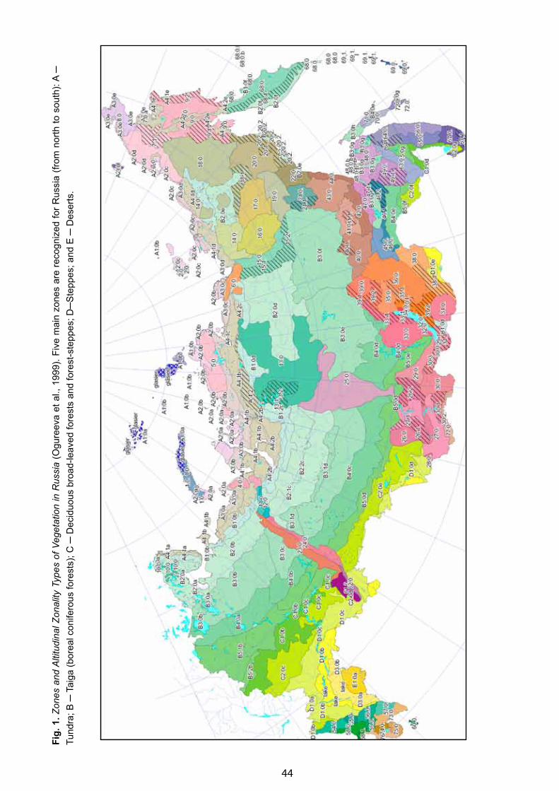
44

Fig.

1. Z

ones

and

Alti

tudi

nal Z

onal

ity T

ypes

of V

eget

atio

n in

Rus

sia

(Ogu

reev

a et

al.,

199

9). F

ive

mai

n zo

nes

are

reco

gniz

ed fo

r Rus

sia

(from

nor

th to

sou

th):

A ─

Tu

ndra

; B ─

Tai

ga (b

orea

l con

ifero

us fo

rest

s); C

─ D

ecid

uous

bro

ad-le

aved

fore

sts

and

fore

st-s

tepp

es; D

─S

tepp

es; a

nd E

─ D

eser

ts.

45

–1850ºC in the north and up to 1900ºC–2000ºC in the south. The 10ºC isotherm closely coincides with the northernmost limit of the tree growth. It serves as a dividing line between the boreal forest region and the treeless tundra. The mean annual precipitation varies from 500 mm to 800 mm.

The zone and provincial position of boreal forests determine the composition of plant communities.

Zonal Characteristics of the Boreal Vegetation

The map Zones and Altitudinal Zonality Types of Vegetation in Russia, scale 1:8M was compiled as a series of maps for higher education in Russia. It reflects macrostructures of the vegetation cover in conformity with the environmental conditions. Five main zones are recognized for Russia (from north to south): A – Tundra; B – Taiga (boreal coniferous forests); C – Deciduous broad-leaved forests and forest-steppes; D – Steppes; and E – Deserts (Fig. 1).

On this map, boreal forest division is based upon a three-dimensional model: (1) according to the temperature gradient of latitudinal differentiation, five subzones are distinguished southwards; (2) according to the gradient of the distance from the ocean (continentality extent), there are two oceanic and six continental sectors, including 32 geographical variants of the boreal forest formations complex; and (3) according to the gradient of temperature, precipitation, and pressure in the mountains, the altitudinal belts and climatic strips of taiga forests are distinguished. Thus, 55 altitudinal zonality types together with boreal forest belts are identified for the total territory of Russia.

Due to these differences the taiga zone is divided into five subzones: forest tundra (B.1), northern (B.2), middle (B.3), southern (B.4) taiga and subtaiga, or hemiboreal mixed broadleaved-coniferous forests (B.5). In the map there are 32 mapping units of boreal forests in the plains (geographical variants of combinations of plant formations). Special attention is given to characteristics of vegetation macrostructures and description of their floristic and coenotic peculiarities. The prevalence of one or several boreal forest formations depends on climatic conditions in the zone and provincial position. The forest zone is a heterogenous structural unit of the forest cover.

Therefore, it is characterized by zonal vegetation combined with azonal plant communities such as mires, floodplains, and coastal or halophytic areas.

Due to differences in the climate and topography from west to east every subzone reveals regional plant community combinations of different forest formations. These geographical variants are named according to certain geographical locations or landscapes. Characteristic plant species are selected for the main subunits–subzonal and regional combinations of plant formations.

For example, the subzone of southern taiga (B.4)—dwarf-shrub and herb-moss coniferous forests in combination with mires—is divided into five geographical variants:

— East European taiga (B.4a) consists of spruce (Picea abies) and pine (Pinus sylvestris) forests with Oxalis acetosella and nemoral herb species (Galeobdolon luteum, Hepatica nobilis, Stellaria holostea, Pulmonaria obscura);

— Pre-Ural taiga (B.4b) consists of spruce and fir-spruce (Picea obovata, Abies sibirica) forests with nemoral herbs (Pulmonaria obscura, Asarum europaeum, Aegopodium podagraria) and Siberian tall forb species (Aconitum septentrionale, Crepis sibirica, Cacalia hastata);

— West Siberian taiga (B.4c) ─ fir-spruce (Picea obovata), pine sibirica - fir (Abies sibirica, Pinus sibirica), and pine forests (Pinus sylvestris) with the herb (Carex macroura, Circaea alpina)-moss layer;

— Central Siberian taiga (B.4d) ─ larch (Larix sibirica), pine (Pinus sylvestris) and fir-spruce forests with the herb–dwarf-shrub (Carex macroura, Vaccinium uliginosum) – moss layer; and

— East Siberian–Far East taiga (B.4e) contains larch (Larix gmelinii) and pine (Pinus sylvestris) forests with the shrub layer (Rhododendron dauricum, Ledum palustre).

As a result, subzones include the following geographical variants of taiga complexes: forest–tundra ─ 6, northern taiga ─ 6, middle taiga ─ 8, southern taiga ─ 5, and subtaiga ─ 6. The Eastern European subtaiga (mixed broadleaved-

46

dark-coniferous forests) has three variants of forest formations. In Siberia there are three variants of the subtaiga (small-leaved forests). This subzone is often considered as an individual zone.

Characteristics of Mountain Boreal Vegetation

Integral manifestations of latitudinal and altitudinal zonal peculiarities in the distribution of vegetation is typical for mountains (Ogureeva, 2000). Each altitudinal belt has a specific vegetation type (the combination of plant communities of several formations). The main regional unit for differentiating the mountain vegetation is an altitudinal zonality type. The name of each type reflects particular features of altitudinal belts, indicating the specific composition of the main plant communities and their detailed geographic position. In the map there are 55 units of mountain vegetation (55 altitudinal zonality types, with 25 geographical variants and 43 subtypes).

For example, Central Altai type (N 27) consists of several belts: Nival (Waldheimia tridactylites, Lupinaster ezimium, Saussurea glacialis) ─ alpine tundra (Ranunculus altaicus, Seseli monstrosa, Schultzia crinita, Sibbaldia procumbens) ─ subalpine (tall and low herb meadows, pine, fir, larch open woodlands, dwarf birch thickets with Betula rotundifolia) ─ dark coniferous forests (taiga with Pinus sibirica, Abies sibirica, Picea obovata) ─ light coniferous taiga (forests with Larix sibirica, Pinus sylvestris) ─ forest steppes (forests in combination with bunch-grass steppes).

A higher correlation exists between the bioclimatic parameters of altitudinal belts and the altitudinal climatic gradients. For example, the temperature factor determines the boundaries between belts such as taiga and subalpine, although humidity acts more locally and indicates the diversity of plant formations and their changes within belts, for instance, light-and dark-coniferous forests.

Every belt has a characteristic floristic-coenotic complex. The mountain boreal forests are represented by complexes of plant formations such as Ural-Southern Siberian, Angaridian, Beringian, Ochotian, and Mandshurian. The main formations of mountain-taiga forests with peculiar plant species of initial communities are also identified.

Classification of Altitudinal Zonality Types

The geographic-genetic principle is used for classifying altitudinal zonality types. The types are divided into groups, subclasses, and classes, reflecting structural-genetic peculiarities of the mountain vegetation at the regional level and its connection with zones and phytogeographic areas (Table 1).

Classes and groups of altitudinal zonality types bear the main geographic-genetic information about the mountain vegetation. The class integrates groups of types with their unified complex of genetically associated plant formations in the main belt, locating them by similar ecological conditions and by similar structural-dynamic properties. A set of plant communities in similar belts of different types can be determined, reflecting regional peculiarities of mountain territories. Subclasses represent regional specific features of plant communities.

A group integrates altitudinal zonality types with the same set of altitudinal belts within the geographically uniform area. The analysis of vegetation macrostructures in mountains of Russia distinguishes 44 altitudinal zonality types of mountain boreal forests; 23 types are included into four groups of Hypoarctic subclass (taiga-open woodlands); and 32 types are included in nine groups of Boreal class.

Characteristics of Ecoregions in the Boreal Zone

In each subzone the ecological units (ecological regions) are distinguished as comparable in their structure with the geographical taiga variants inherent to them. These ecoregions are considered as an averaged link of biogeographical subdivisions of boreal forests, reflecting regional peculiarities of the bioclimatic potential and the landscape structure of the territory. In mountains the ecoregions correspond to groups of altitudinal zonal types. Thus, the zone of boreal forests is divided into 28 ecoregions, among them 14 in plains and 14 in mountains (Fig. 2).

Information about the main geographic-genetic complexes of plant formations was used to characterize the vegetation cover of ecoregions. Not only are the coenotic composition of edificators and different plant species indicated for dominant plant formations, but also the available endemic relic communities and

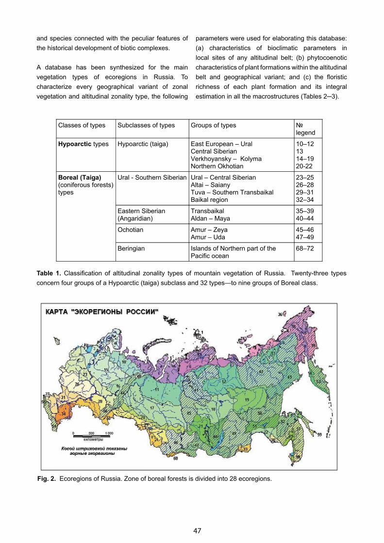
47

Table 1. Classification of altitudinal zonality types of mountain vegetation of Russia. Twenty-three types concern four groups of a Hypoarctic (taiga) subclass and 32 types—to nine groups of Boreal class.

Fig. 2. Ecoregions of Russia. Zone of boreal forests is divided into 28 ecoregions.

and species connected with the peculiar features of the historical development of biotic complexes.

A database has been synthesized for the main vegetation types of ecoregions in Russia. To characterize every geographical variant of zonal vegetation and altitudinal zonality type, the following

parameters were used for elaborating this database: (a) characteristics of bioclimatic parameters in local sites of any altitudinal belt; (b) phytocoenotic characteristics of plant formations within the altitudinal belt and geographical variant; and (c) the floristic richness of each plant formation and its integral estimation in all the macrostructures (Tables 2─3).

“Ecoregions of Russia”

Classes of types Subclasses of types Groups of types № legend

Hypoarctic types Hypoarctic (taiga) East European – UralCentral SiberianVerkhoyansky – KolymaNorthern Okhotian

10–121314–1920-22

Boreal (Taiga) (coniferous forests) types

Ural - Southern Siberian Ural – Central Siberian Altai – SaianyTuva – Southern TransbaikalBaikal region

23–2526–2829–3132–34

Eastern Siberian (Angaridiаn)

TransbaikalAldan – Maya

35–3940–44

Ochotian Аmur – ZeyaAmur – Uda

45–4647–49

Beringian Islands of Northern part of the Pacific ocean

68–72

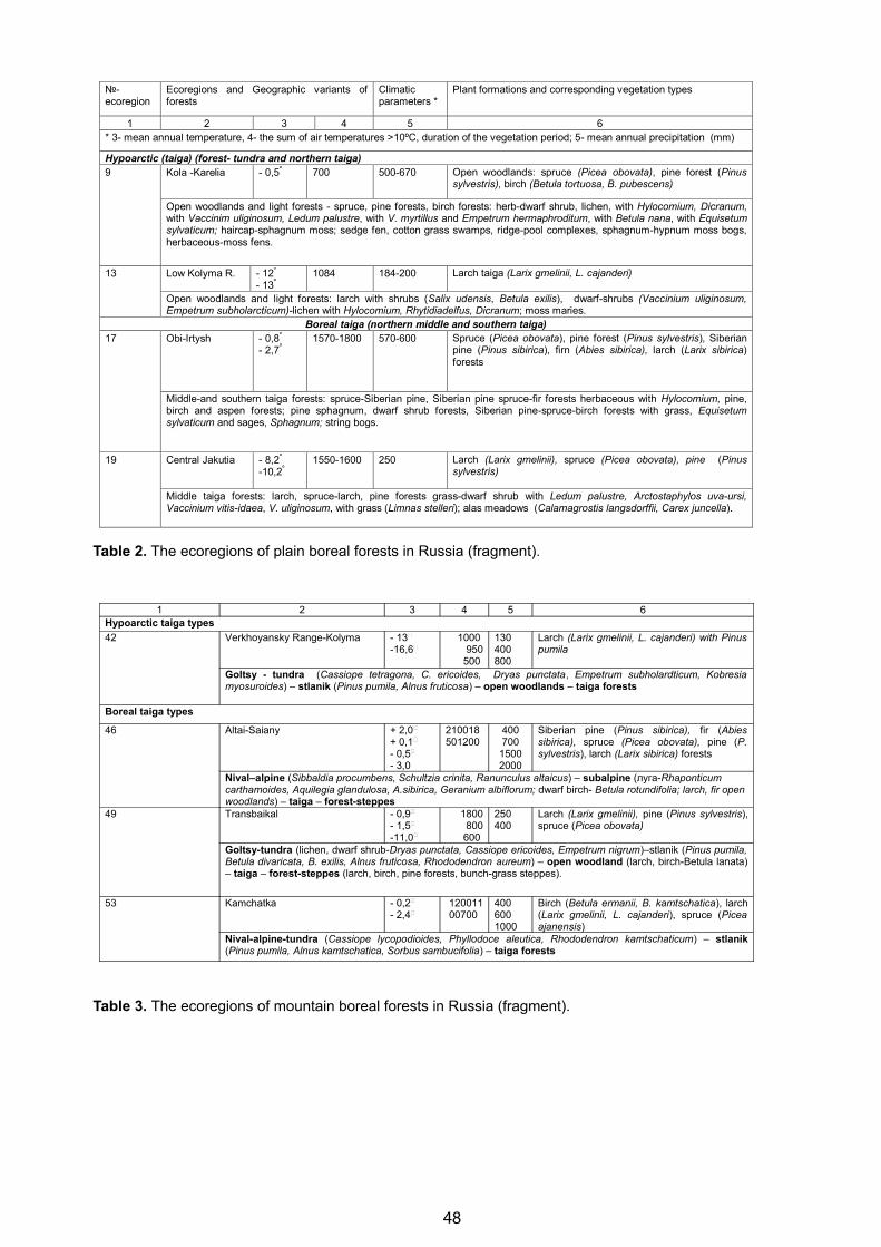
48

Table 2. The ecoregions of plain boreal forests in Russia (fragment).

Table 3. The ecoregions of mountain boreal forests in Russia (fragment).

№- ecoregion

Ecoregions and Geographic variants of forests

Climatic parameters *

Plant formations and corresponding vegetation types

1 2 3 4 5 6 * 3- mean annual temperature, 4- the sum of air temperatures >10ºC, duration of the vegetation period; 5- mean annual precipitation (mm)

Hypoarctic (taiga) (forest- tundra and northern taiga) 9 Kola -Karelia - 0,5º 700 500-670 Open woodlands: spruce (Picea obovata), pine forest (Pinus

sylvestris), birch (Betula tortuosa, B. pubescens)

Open woodlands and light forests - spruce, pine forests, birch forests: herb-dwarf shrub, lichen, with Hylocomium, Dicranum, with Vaccinim uliginosum, Ledum palustre, with V. myrtillus and Empetrum hermaphroditum, with Betula nana, with Equisetum sylvaticum; haircap-sphagnum moss; sedge fen, cotton grass swamps, ridge-pool complexes, sphagnum-hypnum moss bogs, herbaceous-moss fens.

13 Low Kolyma R. - 12º

- 13º 1084 184-200 Larch taiga (Larix gmelinii, L. cajanderi)

Open woodlands and light forests: larch with shrubs (Salix udensis, Betula exilis), dwarf-shrubs (Vaccinium uliginosum, Empetrum subholarcticum)-lichen with Hylocomium, Rhytidiadelfus, Dicranum; moss maries.

Boreal taiga (northern middle and southern taiga) 17 Obi-Irtysh

- 0,8º

- 2,7º 1570-1800 570-600 Spruce (Picea obovata), pine forest (Pinus sylvestris), Siberian

pine (Pinus sibirica), firn (Abies sibirica), larch (Larix sibirica) forests

Middle-and southern taiga forests: spruce-Siberian pine, Siberian pine spruce-fir forests herbaceous with Hylocomium, pine, birch and aspen forests; pine sphagnum, dwarf shrub forests, Siberian pine-spruce-birch forests with grass, Equisetum sylvaticum and sages, Sphagnum; string bogs.

19 Central Jakutia - 8,2º

-10,2º 1550-1600 250 Larch (Larix gmelinii), spruce (Picea obovata), pine (Pinus

sylvestris)

Middle taiga forests: larch, spruce-larch, pine forests grass-dwarf shrub with Ledum palustre, Arctostaphylos uva-ursi, Vaccinium vitis-idaea, V. uliginosum, with grass (Limnas stelleri); alas meadows (Calamagrostis langsdorffii, Carex juncella).

1 2 3 4 5 6

Hypoarctic taiga types

42 Verkhoyansky Range-Kolyma - 13

-16,6

1000 950

500

130 400 800

Larch (Larix gmelinii, L. cajanderi) with Pinus pumila

Goltsy - tundra (Cassiope tetragona, C. ericoides, Dryas punctata, Empetrum subholardticum, Kobresia myosuroides) – stlanik (Pinus pumila, Alnus fruticosa) – open woodlands – taiga forests

Boreal taiga types

46 Altai-Saiany + 2,0

+ 0,1

- 0,5

- 3,0

210018501200

400 700

1500 2000

Siberian pine (Pinus sibirica), fir (Abies sibirica), spruce (Picea obovata), pine (P. sуlvestris), larch (Larix sibirica) forests

Nival–alpine (Sibbaldia procumbens, Schultzia crinita, Ranunculus altaicus) – subalpine (луга-Rhaponticum carthamoides, Aquilegia glandulosa, A.sibirica, Geranium albiflorum; dwarf birch- Betula rotundifolia; larch, fir open woodlands) – taiga – forest-steppes

49 Transbaikal - 0,9

- 1,5

-11,0

1800 800 600

250 400

Larch (Larix gmelinii), pine (Pinus sуlvestris), spruce (Picea obovata)

Goltsy-tundra (lichen, dwarf shrub-Dryas punctata, Cassiope ericoides, Empetrum nigrum)–stlanik (Pinus pumila, Betula divaricata, B. exilis, Alnus fruticosa, Rhododendron aureum) – open woodland (larch, birch-Betula lanata) – taiga – forest-steppes (larch, birch, pine forests, bunch-grass steppes).

53 Kamchatka - 0,2

- 2,4

12001100700

400 600 1000

Birch (Betula ermanii, B. kamtschatica), larch (Larix gmelinii, L. cajanderi), spruce (Picea ajanensis)

Nival-alpine-tundra (Cassiope lycopodioides, Phyllodoce aleutica, Rhododendron kamtschaticum) – stlanik (Pinus pumila, Alnus kamtschatica, Sorbus sambucifolia) – taiga forests

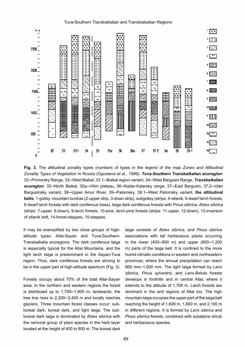
49

It may be exemplified by two close groups of high-altitude types: Altai-Sayan and Tuva-Southern-Transbaikalia ecoregions. The dark coniferous taiga is especially typical for the Altai Mountains, and the light larch taiga is predominant in the Sayan-Tuva region. Thus, dark coniferous forests are striving to be in the upper part of high-altitude spectrum (Fig. 3).

Forests occupy about 70% of the total Altai-Sayan area. In the northern and western regions the forest is distributed up to 1,700─1,800 m; landwards, the tree line rises to 2,200─2,400 m and locally reaches glaciers. Three mountain forest classes occur: sub-boreal dark, boreal dark, and light taiga. The sub-boreal dark taiga is dominated by Abies sibirica with the nemoral group of plant species in the herb layer located at the height of 400 to 800 m. The boreal dark

taiga consists of Abies sibirica, and Pinus sibirica associations with tall herbaceous plants occurring in the lower (400─800 m) and upper (800─1,200 m) parts of the taiga belt. It is confined to the more humid climatic conditions in western and northeastern provinces, where the annual precipitation can reach 800 mm–1,000 mm. The light taiga formed by Larix sibirica, Pinus sylvestris, and Larix-Betula forests develops in foothills and in central Altai, where it extends to the altitude of 1,700 m. Larch forests are dominant in the arid regions of Altai too. The high mountain taiga occupies the upper part of the taiga belt reaching the height of 1,600 m, 1,800 m, and 2,100 m in different regions. It is formed by Larix sibirica and Pinus sibirica forests, combined with subalpine shrub and herbaceous species.

Fig. 3. The altitudinal zonality types (numbers of types in the legend of the map Zones and Altitudinal Zonality Types of Vegetation in Russia (Ogureeva et al., 1999). Tuva-Southern Transbaikalian ecoregion: 32─Primorsky Range, 33─West Baikal, 33.1─Baikal region variant, 34─West Bargusin Range, Transbaikalian ecoregion: 35─North Baikal, 35a─Vitim plateau, 36─Kadar-Kalarsky range, 37─East Bargusin, 37.2─Ulan Bargusinsky variant, 38─Upper Amur River, 39─Patomsky, 39.1─West Patomsky variant; the altitudinal belts: 1-goltsy, mountain tundras (2-upper strip, 3-down strip), subgoltsy (strips: 4-stlanik, 5-dwarf larch forests, 6-dwarf larch forests with dark coniferous trees), taiga dark coniferous forests with Pinus sibirica, Abies sibirica (strips: 7-upper, 8-down), 9-larch forests, 10-pine, larch-pine forests (strips: 11-upper, 12-down), 13-inversion of stlanik belt, 14-forest-steppes, 15-steppes.

Tuva-Southern Transbaikalian and Transibaikalian Regions

50

The highly variable topography of the Sayan Mountains causes the very complicated altitudinal zonality to change from west to east. In the northeastern part with the more continental climate, the forests are composed of Pinus sylvestris and Larix sibirica with a rich herbaceous cover occupying the lower mountains. Forests composed of Pinus sibirica and Abies sibirica have the most prominent position, extending across the middle mountains. In contrast to the Altai and Western Sayan Range, the upper part of the mountains is covered by Pinus pumila and heath passing into mountain tundra.

Experience was gained by mapping mountain boreal forests at different scales and reflected a variety of forest formations in connection with the altitudinal belt structure of mountain territories (Ogureeva, 2002; Jurkovskaja at al., 2005).

The map Ecoregions of Russia should be considered a good basis for compiling a circumboreal vegetation map, with the latter being useful for phytogeographic classification of the territory at the upper level of the legend. Ecoregions represent the landscape-specific vegetation complexes in various environmental conditions. The map can be also used for the estimation of natural floristic, plant community, and ecosystem biodiversity.

Conclusion

The diversity of boreal forests in Russia is rather high due to a great variety of environmental conditions over vast areas. Experience gained in mapping boreal forests at different scales makes it possible to show regional specifics of natural forests. As a mapping approach, it is feasible to use ecological-geographical principles to differentiate the territory, proceeding from the zonal and altitudinal-zonal structure of the vegetation cover at the highest levels of the legend. The maps Zones and Altitudinal Zonality Types of Vegetation of Russia (map scale 1:8M) and Ecoregions of Russia (map scale 1:8M) contain information on the main bioregions of boreal forests and regional variants of combinations of forest communities. Flat and mountain forest regions should be reflected in a corresponding map legend rubric.

The basic mapping unit should be a combination

of physiognomic and floristic plant community for vegetation classification. Zonal types of plant communities can be supplemented by characteristics of accompanying vegetation types, such as bog, floodplain vegetation, etc., which should be shown as independent units on the map. A variety of mountain forests can be reflected, proceeding from their altitudinal-belt position in the structure of mountain territory. The high-mountainous vegetation can reflect regional areas specific to high-mountain belts and can be shown according to regional features of altitudinal zonality types and geographical position.

Acknowledgments

I am grateful to Dr. Udo Bohn for support in my work related to vegetation mapping. I am also grateful to my colleagues. The theme content of the map Zones and Altitudinal Zonality Types of the Vegetation of Russia (scale 1: 8M) (1999) was prepared by G. Ogureeva, & I. Miklaeva from The M. V. Lomonosov Moscow State University and I. Safronova & T. Jurkovskaya from The Komarov Botanical Institute of Academy Sciences of Russia. The cartographical editing was done by T. Kotova from MSU.

References

Jurkovskaja, T. K., Iljina, I. S., Saphronova, I. N. 2005. The vegetation of Russia (map scale 1: 15,000,000). National Atlas of Russia. Т.1:.370–371.

Nazimova, D. I., Ermakov, N. B., Andreeva, N. M., & Stepanov, N. V. 2004. Concept model of the structure biodiversity of the zonal classes of the forest ecosystems in Northern Asia. Siberian Ecological Journal 13-5: 745–756.

Ogureeva, G. N., Mikljaeva, I. M., Safronova I. N., & Jurkovskaja, T. K. 1999. Zones and altitudinal zonality types of the vegetation of Russia (map scale 1: 8,000,000). The map on two sheets and a book of the legend with the text, 64 p. M.: Ecor.

Ogureeva, G. N. 2002. Diversification of mountain vegetation of Russia: Altitudinal zonality types, their classification and mapping. Pages 185–187 in Intern. Mountain Research Report. Mountain Regions: a Research Subject? Grenoble, France.

Ogureeva, G. N., Danilenko, A. K., Leonova, N. B., & Rumanzev, V. J. 2004. Biome diversity

51

and ecoregions of Russia. Pages 392–398 in Geography, Society and Environment. Volume III: Natural Resources, Their Use and Protection. Gorodez, Russia.

References (in Russian)

Карта Зоны и типы поясности растительности России и сопредельных территорий (масштаб 1: 8,000,000). 1999. Карта на 2-х листах ипояснительный текст к карте с легендой, 64 с. М: ЭКОР. [Ред.: Г.Н. Огуреева. Авторы: Огуреева Г.Н., Микляева И.М., Сафронова И.Н. и Юрковская Т.К.].

Назимова, Д.И., Ермаков, Н.Б., Андреева, Н.М., & Степанов, Н.В. 2004. Концептуальная модель структурного биоразнообразия зональных классов лесных экосистем Северной Евразии. Сибирский экологический журнал, т. 13-5: 745─756.

Огуреева, Г.Н., Даниленко, А.К., Леонова, Н.Б., Румянцев, В.Ю. 2004. Биомное разнообразие и экорегионы России. География, общество, окружающая среда. Том III: Природные ресурсы, их использование и охрана. М.: Издательский Дом Городец: 392─398.

Юрковская Т.К., Ильина И.С., Сафронова И.Н. 2005. Растительность [карта] м. 1: 15,000,000. Национальный атлас России. Т.1:.370─371.

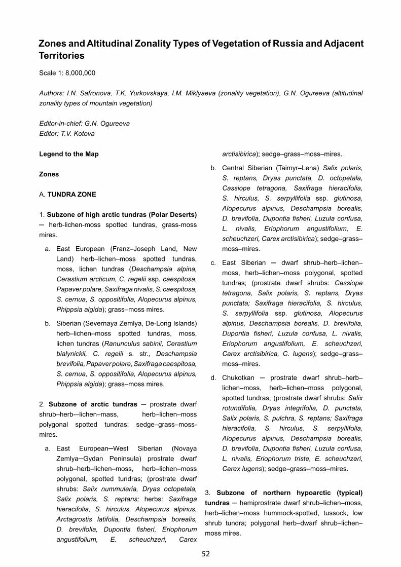
52

Zones and Altitudinal Zonality Types of Vegetation of Russia and Adjacent Territories

Scale 1: 8,000,000

Authors: I.N. Safronova, T.K. Yurkovskaya, I.M. Miklyaeva (zonality vegetation), G.N. Ogureeva (altitudinal zonality types of mountain vegetation)

Editor-in-chief: G.N. OgureevaEditor: T.V. Kotova

Legend to the Map

Zones

A. TUNDRA ZONE

1. Subzone of high arctic tundras (Polar Deserts) ─ herb-lichen-moss spotted tundras, grass-moss mires.

a. East European (Franz–Joseph Land, New Land) herb–lichen–moss spotted tundras, moss, lichen tundras (Deschampsia alpina, Cerastium arcticum, C. regelii ssp. caespitosa, Papaver polare, Saxifraga nivalis, S. caespitosa, S. cernua, S. oppositifolia, Alopecurus alpinus, Phippsia algida); grass–moss mires.

b. Siberian (Severnaya Zemlya, De-Long Islands) herb–lichen–moss spotted tundras, moss, lichen tundras (Ranunculus sabinii, Cerastium bialynickii, C. regelii s. str., Deschampsia brevifolia, Papaver polare, Saxifraga caespitosa, S. cernua, S. oppositifolia, Alopecurus alpinus, Phippsia algida); grass–moss mires.

2. Subzone of arctic tundras ─ prostrate dwarf shrub–herb-–lichen–mass, herb–lichen–moss polygonal spotted tundras; sedge–grass–moss-mires.

a. East European─West Siberian (Novaya Zemlya─Gydan Peninsula) prostrate dwarf shrub–herb–lichen–moss, herb–lichen–moss polygonal, spotted tundras; (prostrate dwarf shrubs: Salix nummularia, Dryas octopetala, Salix polaris, S. reptans; herbs: Saxifraga hieracifolia, S. hirculus, Alopecurus alpinus, Arctagrostis latifolia, Deschampsia borealis, D. brevifolia, Dupontia fisheri, Eriophorum angustifolium, E. scheuchzeri, Carex

arctisibirica); sedge–grass–moss–mires.

b. Central Siberian (Taimyr–Lena) Salix polaris, S. reptans, Dryas punctata, D. octopetala, Cassiope tetragona, Saxifraga hieracifolia, S. hirculus, S. serpyllifolia ssp. glutinosa, Alopecurus alpinus, Deschampsia borealis, D. brevifolia, Dupontia fisheri, Luzula confusa, L. nivalis, Eriophorum angustifolium, E. scheuchzeri, Carex arctisibirica); sedge–grass–moss–mires.

c. East Siberian ─ dwarf shrub–herb–lichen–moss, herb–lichen–moss polygonal, spotted tundras; (prostrate dwarf shrubs: Cassiope tetragona, Salix polaris, S. reptans, Dryas punctata; Saxifraga hieracifolia, S. hirculus, S. serpyllifolia ssp. glutinosa, Alopecurus alpinus, Deschampsia borealis, D. brevifolia, Dupontia fisheri, Luzula confusa, L. nivalis, Eriophorum angustifolium, E. scheuchzeri, Carex arctisibirica, C. lugens); sedge–grass–moss–mires.

d. Chukotkan ─ prostrate dwarf shrub–herb–lichen–moss, herb–lichen–moss polygonal, spotted tundras; (prostrate dwarf shrubs: Salix rotundifolia, Dryas integrifolia, D. punctata, Salix polaris, S. pulchra, S. reptans; Saxifraga hieracifolia, S. hirculus, S. serpyllifolia, Alopecurus alpinus, Deschampsia borealis, D. brevifolia, Dupontia fisheri, Luzula confusa, L. nivalis, Eriophorum triste, E. scheuchzeri, Carex lugens); sedge–grass–moss–mires.

3. Subzone of northern hypoarctic (typical) tundras ─ hemiprostrate dwarf shrub–lichen–moss, herb–lichen–moss hummock-spotted, tussock, low shrub tundra; polygonal herb–dwarf shrub–lichen–moss mires.

53

a. East European (Kolguev Island-Bolshaya Zemlya) ─ hemiprostrate dwarf shrub–lichen–moss, (Loiseleuria procumbens, Phyllodoce caerulea, Arctous alpina, Dryas octopetala, Empetrum hermaphroditum, Vaccinium uliginosum ssp. microphyllum, V. vitis-idaea ssp. minus), tussock (Eriophorum angustifolium), herb-lichen-moss hummock-spotted (Arctagrostis latifolia, Dupontia psilosantha, D. fisheri, Deschampsia borealis, D. brevifolia), low shrub tundras (Betula nana, Salix glauca, S. lanata), polygonal herb–dwarf shrub–lichen–moss mires.

b. Ural–West Siberian (Yugor–Gydan Peninsula) ─ prostrate dwarf shrub–lichen–moss (Cassiope tetragona, Empetrum subholarcticum, Arctous alpina, Dryas octopetala, Vaccinium uliginosum ssp. microphyllum, V. vitis-idaea ssp. minus, Ledum decumbens), tussock (Eriphorum angustifolium) herb–lichen–moss (Carex arctisibirica), Arctagrostis latifolia, Dupontia fisheri, D. psilosantha, Deschampsia borealis, D. brevifolia), low shrub (Betula nana, Salix arctica, S. glauca, S. lanata) tundras; polygonal herb–dwarf shrub–lichen–moss mires.

c. Central Siberian (Taimyr Peninsula) ─ hemiprostrate dwarf shrub–lichen–moss (Cassiope tetragona, Dryas punctata, D. octopetala, Empetrum subholarcticum, Arctous alpina, Vaccinium uliginosum ssp. microphyllum, V. vitis-idaea ssp. minus, Ledum decumbens), tussock (Eriophorum vaginatum, E. angustifolium), herb-lichen-moss (Arctagrostis latifolia, Carex arctisibirica, Deschampsia borealis, D. brevifolia), low shrub (Betula nana, B. exilis, Salix glauca, S. lanata, S. pulchra) tundras; polygonal herb–dwarf shrub–lichen–moss mires.

d. East Siberian (Yana–Kolyma RR.) ─ prostrate dwarf shrub–lichen–moss (Salix fuscescens, Arctous alpina, Dryas punctata, Vaccinium uliginosum ssp. microphyllum, V. vitis-idaea ssp. minus, Ledum decumbens, Empetrum subholarcticum), tussock (Eriophorum vaginatum, E. angustifolium), herb–lichen–moss (Carex arctisibirica, Arctagrostis latifolia, Dupontia psilosantha, D. fisheri, Deschampsia borealis, D. brevifolia), low shrub (Betula

exilis, Salix richardsonii, S. glauca, S. pulchra) tundras; polygonal herb–dwarf shrub–lichen–moss mires.

e. Chukotkan ─ hemiprostrate dwarf shrub-lichen-moss (Loiseleuria procumbens, Cassiope tetragona, Rhododendron camtschaticum ─ on Eastern part, Salix fuscescens, Arctous alpina, Dryas punctata, D. integrifolia, Vaccinium uliginosum ssp. microphyllum, V. vitis-idaea ssp. minus, Empetrum subholarcticum, Ledum decumbens), tussock (Eriophorum vaginatum, Carex lugens), herb–lichen–moss (Carex lugens, Arctagrostis latifolia, Dupontia psilosantha, Deschampsia borealis, D. brevifolia), low shrub (Betula exilis, Salix krylovii, S. richardsonii, S. glauca, S. pulchra) tundras; polygonal herb–dwarf shrub–lichen–moss mires.

4. Subzone of southern hypoarctic tundras ─ shrub and tussock tundras; palsa (in Europe) and polygonal herb–dwarf shrub–lichen–moss (in Asia) mires. (A 41

─ northern strip, A 42 ─ southern strip):

a. East Scandinavian (Kola Peninsula) ─ shrub (Betula nana, Salix lanata, S. phylicifolia, S. glauca) tundras, herb–dwarf shrub (Empetrum hermaphroditum, Salix herbacea; Calluna vulgaris, Carex bigelowii, Deschampsia flexuosa, Festuca ovina) tundras; palsa dwarf shrub–moss–lichen mires.

b. East European–West Siberian (Kanin Peninsula) shrub (Betula nana, Salix lapponum, S. phylicifolia, S. dasyclados, S. glauca, S. lanata), herb–dwarf shrub (Empetrum hermaphroditum; Vaccinium myrtillus, V. uliginosum ssp. microphyllum, V. vitis-idaea ssp. minus s.str., Deschampsia flexuosa, Festuca ovina, Aconitum septentrionale, Cirsium helenioides, Trolius europaeus, T. asiaticus) tundras; palsa dwarf shrub–moss–lichen and polygonal herb–dwarf shrub–lichen–moss mires.

c. Central Siberian (Yeniseik) ─ shrub (Betula exilis, B. nana, Salix alaxensis, S. boganidensis, S. glauca, S. pulchra, S. lanata), alder (Alnus fruticosa), tussock (Eriophorum vaginatum), herb- dwarf shrub (Carex arctisibirica, Ledum decumbens, Vaccinium uliginosum ssp. microphyllum, Dryas punctata, D. octopetala,

54

Cassiope tetragona) tundras; polygonal herb–dwarf shrub–lichen–moss mires.

d. East Siberian (Lena–Kolyma RR.) ─ shrub (Betula exilis, Salix alaxensis, S. boganidensis, S. pulchra, S. glauca, S. reptans, S. richardsonii), alder (Alnus fruticosa), tussock (Eriophorum vaginatum), herb–dwarf shrub (Ledum decumbens, Vaccinium vitis-idaea ssp. minus) tundras; polygonal herb–dwarf shrub–lichen–moss mires.

e. Chukotka–Koryakian ─ shrub (Betula exilis, Salix pulchra, S. glauca, S. krylovii, S. alaxensis, S. boganidensis, S. richardsonii), alder (Alnus fruticosa), tussock (Eriophorum vaginatum, Carex lugens) tundras; herb and palsa-shrub mires.

B. TAIGA ZONE

1. Subzone of forest–tundra ─ pretundra open woodlands in combination with southern hypoarctic tundras; herb-lichen-moss palsa and herb–Sphagnum–Hypnum aapa mires. B11 ─ northern strip; B12 ─ southern strip):

a. East Scandinavian (Kola Peninsula) ─ birch (Betula czerepanovii) herb–dwarf shrub, lichen and moss open woodlands; palsa dwarf shrubmoss-lichen and herb–Sphagnum–Hypnum aapa mires.

b. East European (Kanin Peninsula–Ural Mts.) ─ spruce (Picea obovata), birch (Betula czerepanovii) shrub (Betula nana, Salix lapponum) dwarf shrub-lichen-moss open woodlands; palsa and dwarf shrub moss-lichen and herb–Sphagnum–Hypnum aapa mires.

c. West Siberian ─ larch, spruce-larch (Larix sibirica, Picea obovata) shrub (Betula nana, Salix phylicifolia, S. dasiclada, S. lapponum) dwarf shrub-lichen-moss open woodlands; palsa dwarf shrub–moss–lichen mires.

d. Central Siberian (Kotuy–Lena RR.) ─ larch (Larix gmelinii, spruce (Picea obovata) shrub (Betula exilis) dwarf shrub–lichen, moss–lichen open woodlands.

e. East Siberian (Indigirka–Kolyma RR.)─larch (Larix gmelinii, L. cajanderi) shrub (Salix

udensis, S. schwerin) dwarf shrub–lichen–moss; sparce

f. woodlands; open woodlands; flood plain forests (Chosenia arbutifolia, Populus suaveolens).

g. East Kamchatkan ─ birch (Betula ermanii) open woodlands; stlanik (Pinus pumila); herb-Sphagnum with Myrica tomentosa mires.

2. Subzone of northern taiga ─ coniferous dwarf-shrub-lichen-moss open woodlands and sparse forests; in Europe ─ with ridge-hollow herb-peatmoss-hypnum aapa and raised bogs, in West Siberia ─ with palsa herb-peatmoss and sedge-hypnum mires; in Kamchatka ─ with suboceanic mires. (B21 ─ northern strip, B22 ─ southern strip)

a. East Scandinavian (Kola–Karelia) ─ pine (Pinus sylvestris, P. friesiana), spruce (Picea obovata) dwarf-shrub–lichen–moss (Calluna vulgaris, Empetrum hermaphroditum, Vaccinium myrtillus, V. vitis-idaea, V. uliginosum, Ledum palustre) sparse forests; ridge-hollow herb–peatmoss–Hypnum aapa and raised bogs.

b. East European (Onega R.–Ural Mts.) ─ spruce (Picea obovata, P. abies x P. obovata), pine (Pinus sylvestris) dwarf-shrub (Empetrum hermaphroditum, Vaccinium myrtillus, V. uliginosum, Ledum palustre) –moss, lichen–moss sparse forests; ridge-hollow herb–peatmoss–Hypnum aapa and raised bogs.

c. West Siberian ─ larch, larch–spruce, larch–pine, larch–spruce–Siberian pine (Picea obovata, Larix sibirica, Pinus sibirica, P. sylvestris) forests; dwarf-shrub–lichen–moss (Ledum palustre, Vaccinium vitis-idaea, V. uliginosum; V. myrtillus, Empetrum subholarcticum, Betula nana) sparse forests; palsa herb–peatmoss and sedge–Hypnum mires.

d. Central Siberian (Olenek–Lena RR.) ─ larch, spruce-–arch (Larix gmelinii, Picea obovata) dwarf–lichen–moss (Ledum palustre, Vaccinium vitis-idaea, V. uliginosum, Empetrum subholarcticum, Betula exilis) forests; larch peatmoss shrub bog.

e. East Siberian (Indigirka–Kolyma RR.) ─ larch (Larix gmelinii, L. cajanderi) moss, dwarf-shrub (Vaccinium uliginosum, Empetrum

55

subholarcticum, Betula exilis)–moss–lichen forests; moss mires.

f. West Kamchatkan ─ birch open forests (Betula ermanii); suboceanic mires (Empetrum sibiricum, Myrica tomentosa, Carex middendorfii).

3. Subzone of middle taiga ─ coniferous short herb (Maianthemum bifolium, Trientalis europaea, Orthilia secunda, Pyrola spp., Luzula pilosa) – dwarf shrub-moss forests; in Central Siberia ─ with moss muskegs, in East Siberia ─ with alas meadows, ridge-hollow peatmoss raised bogs and herb–Hypnum–peatmoss string fens. (B31 ─ northern strip, B32 ─ southern strip)

a. East Scandinavian (Karelia) pine (Pinus sylvestris), spruce (Picea abies, P. abies x P. obovata, Betula pendula, B. pubescens) short herb–dwarf shrub–moss (Vaccinium myrtillus, V. vitis-idaea, Calluna vulgaris, Linnaea borealis), dwarf shrub-lichen, dwarf shrub–moss, moss forests; ridge-hollow peatmoss raised bogs and herb–Hypnum–peatmoss string fens.

b. East European (Ladoga Lake–Vychegda R.) ─ spruce (Picea abies, P. abies x P. obovata, P. obovata, Betula pendula, B. pubescens), pine (Pinus sylvestris) short herb–dwarf shrub–moss (Vaccinium myrtillus, V. vitis-idaea, Linnaea borealis) forests; palsa raised bogs and herb–Hypnum–peatmoss string fens.

c. Ural ─ spruce, fir-spruce, pine with Pinus sibirica (Picea obovata, Abies sibirica, Pinus sylvestris, P. sibirica, Betula pendula, B. pubescens) short herb–dwarf shrub–moss (Linnaea borealis, Vaccinium myrtillus, V. vitis-idaea) forests; palsa raised bogs and herb–Hypnum–peatmoss string fens.

d. West Siberian ─ spruce-Pinus sibirica-fir with larch, pine (Pinus sibirica, Picea obovata, Abies sibirica, Larix sibirica, Pinus sylvestris, Betula pendula, B. pubescens) short herb–dwarf shrub–moss (Vaccinium vitis-idaea, V. myrtillus, Linnaea borealis, Ledum palustre) forests; raised bogs.

e. Central Siberian (Tunguska R.) ─ larch (Larix gmelinii) with Picea obovata, Abies sibirica, Pinus sibirica), pine (Pinus sylvestris) short herb–dwarf shrub–moss (Arctostaphylos uva-ursi, Ledum palustre, Vaccinium vitis-idaea) forests; raised mires with Betula fruticosa.

f. East Siberian (Lena–Aldan RR.) ─ larch, spruce-larch, pine (Larix gmelinii, Picea obovata, Pinus sylvestris, Betula cajanderi) short herb–dwarf shrub–moss (Vaccinium vitis-idaea, V. uliginosum, Arctostaphylos uva-ursi, Ledum palustre) forests; larch forests with grass (Limnas stelleri) and alas meadows (Carex juncella, Calamagrostis langsdorffii).

g. Far East ─ larch (Larix gmelinii), fir-spruce with larch (Picea ajanensis, Abies nephrolepis, Betula platyphylla, B. mandshurica) dwarf-shrub-moss (Ledum palustre, Vaccinium vitisidaea, V. uliginosum) forests; raised mires with Larix gmelinii and shrubs (Betula exilis, B. divaricata, B. fruticosa).

h. Sakhalin ─ spruce-larch (Larix gmelinii, Picea ajanensis) with stlanik (Pinus pumila) dwarf-shrub-moss (Ledum palustre) forests; suboceanic mires (Empetrum nigrum, Myrica tomentosa).

4. Subzone of southern taiga ─ coniferous dwarf shrub and herb–moss forests; in Far East ─ with dwarf birch-larch muskegs, Sphagnum raised bogs.

a. East European (Baltic-Vetluga R.) ─ spruce (Picea abies, Betula pendula, B. pubescens, Populus tremula, Alnus glutinosa), pine (Pinus sylvestris) nemoral-herb (Oxalis acetosella, Galeobdolon luteum, Hepatica nobilis, Stellaria holostea, Pulmonaria obscura, Convallaria majalis), forests; Sphagnum raised bogs.

b. Ural ─ spruce, fir-spruce, with lime-trees (Picea obovata, Abies sibirica, Pinus sylvestris, Betula pendula, B. pubescens, Populus tremula, Tilia cordata), nemoral-herb (Pulmonaria obscura, Asarum europaeum, Aegopodium podagraria) with Oxalis acetosella forests, dwarf-shrub-herb forests with Siberian tall herbs (Aconitum septentrionale, Crepis sibirica, Cacalia hastata) and fen forests.

c. West Siberian ─ Pinus sibirica–spruce–fir, spruce-fir, pine with lime-trees (Abies sibirica, Picea obovata, Pinus sibirica, Pinus sylvestris, Betula pendula, B. pubescens, Populus tremula, Tilia cordata) short-herb–moss (Oxalis acetosella, Carex macroura, Stellaria bungeana, Circae alpina) forests; Sphagnum raised bogs.

56

d. Central Siberian (Angara R.) ─ larch, pine-larch, spruce-fir (Larix sibirica, Pinus sylvestris, Abies sibirica, Picea obovata, Betula pendula, B. pubescens, Populus tremula) dwarf–shrub–herb–moss (Carex macroura, Vaccinium uliginosum) with Rhododendron dauricum forests.

e. East Siberian–Far East ─ larch (Larix gmelinii, Betula platyphylla), pine (Pinus sylvestris) shrub (Rhododendron dauricum, Alnus manshurica) dwarf-shrub-herb (Calamagrostis langsdorfii, Vaccinium vitis-idaea) forests; shrubs (Betula fruticosa, B. ovalifolia), larch mires and herb bogs.

5. Subzone of subtaiga ─ coniferous, coniferous - broad-leaved (mixed), nemoral in European part of Russia (with black alder swamps) and in Far East (with dwarf birch─larch muskegs); in West Siberia ─ small-leaved grass-herb forests (with pine-dwarf shrub-peat moss raised bogs and herb poor fens). (B51 ─ northern strip, B52 ─ southern strip)

a. East European (Baltic) ─ spruce-broad-leaved, pine-broad-leaved (Quercus robur, Fraxinus excelsior, Ulmus laevis, U. glabra, Picea abies, Pinus sylvestris) forests (with Carpinus betulus, Fagus sylvatica – in Western part); alder (Alnus glutinosa) forests, subatlantic herb and peat moss raised bogs with Myrica gale.

b. East European (Baltic–Vetluga R.) ─ spruce-broad-leaved, pine-broad-leaved, pine (Quercus robur, Tilia cordata, Acer platanoides, Ulmus laevis, U. glabra, Picea abies, Pinus sylvestris) forests; alder swamps (Alnus glutinosa); peat moss raised bogs and herbaceous swamps.

c. Ural ─ spruce-broad-leaved, lime tree-spruce-fir, broad-leaved-fir-spruce, broad-leaved-pine (Quercus robur, Tilia cordata, Acer platanoides, Ulmus glabra, Picea obovata, P. abies x P. obovata, Abies sibirica, Pinus sylvestris) forests.

d. West Siberian ─ birch, aspen (Betula pendula, Populus tremula) herb─grass (Calamagrostis arundinacea, Brachypodium pinnatum, Aegopodium podagraria) forests, pine (Pinus sylvestris) dwarf shrub-herb forests; herbaceous swamps.

e. Central Siberian (Angara R.) ─ pine, larch-pine (Pinus sylvestris, Larix sibirica) shrub

(Rhododendron dauricum, Alnus fruticosa) dwarf shrub (Vaccinium vitis-idaea, Arctostaphulos uva-ursi) forests; sedge fen-hypnum bogs with Betula exilis.

f. Far East (Amur R.) ─ oak-pine, oak-larch (Pinus sylvestris, Larix gmelinii, Quercus mongolica, Betula davurica, B. platyphylla) shrub (Lespideza bicolor, Rhododendron dauricum) forests.

g. Far East (Manchzhuria) ─ oak-larch, oak-pine, spruce-fir with broad-leaved trees (Larix gmelinii, Quercus mongolica, Abies nephrolepis, Picea ajanensis, Tilia amurensis, Acer mono) forests; birch–larch mires and shrubs (Betula ovalifolia, B. fruticosa).

C. BROAD-LEAVED FOREST ZONE

1. Subzone of broad-leaved forests ─ broad-leaved nemoral forests.

a. Central European (Carpathians–Dnieper R.) ─ beech, oak-hornbeam, oak (Fagus sylvatica, Carpinus betulus, Quercus robur) shrub (Cornus mas, Crataegus monogyna, Viburnum lantana) forests.

b. East European (Dnieper–Volga R.) ─ oak, ash-oak, broadleaved, pine-broadleaved (Quercus robur, Tilia cordata, Acer platanoides, Fraxinus excelsior, Pinus sylvestris), shrub (Euonymus europaea, E. verrucosa, Corylus avellana, Acer campestre) forests; alder swamps (Alnus glutinosa).

c. Trans Volga ─ oak-lime tree, lime tree, broadleaved (Tilia cordata, Quercus robur, Acer platanoides, Ulmus glabra) shrub (Euonymus europaea, E. verrucosa, Corylus avellana, Lonicera xylosteum) forests.

d. Far East (Manchzhuria) ─ lime tree-oak (Quercus mon-golica, Tilia amurensis, Betula davurica) shrub (Corylus manshu-rica, C. heterophylla, Spiraea ussuriensis) fen-herbaceous forests.

2. Subzone of forest-steppe ─ meadow steppes and steppificated meadows in combination with broad-leaved and small-leaved forests. (C21 ─ northern strip, C22 ─ southern strip)

a. Dniester–Dnieper RR. ─ oak forest-steppes

57

(Quercus robur; Stipa pulcherrima, S. tirsa, S. dasyphylla, Bromopsis riparia, B. inermis, Poa angustifolia, Phleum phleoides, Carex humilis, Filipendula vulgaris, Salvia stepposa, Galium verum, Trifolium montanum).

b. Crimea–Caucasus ─ oak forest-steppes (Quercus robur, Q. petraea, Stipa pulcherrima, S. pontica, S. tirsa, Bromopsis riparia, B. inermis, Carex humilis, Filipendula vulgaris, Salvia stepposa, Galium verum, Trifolium montanum).

c. East European (Dnieper–Volga RR.) ─ lime tree-oak forest-steppes (Quercus robur; Tilia cordata, Acer platanoides; Stipa pulcherrima, S. tirsa, S. dasyphylla, S. pennata, Bromopsis riparia, B. inermis, Poa angustifolia, Phleum phleoides, Helictotrichon schellianum, Carex humilis, Filipendula vulgaris, Salvia stepposa, Galium verum, Trifolium montanum, T. alpestre).

d. Trans Volga ─ maple-lime tree-oak forest-steppes (Quercus robur; Tilia cordata, Acer platanoides; Stipa pulcherrima, S. dasyphylla, S. tirsa, S. zalesskii, S. pennata, Bromopsis riparia, B. inermis, Poa angustifolia, Calamagrostis epigeios, Phleum phleoides, Helictotrichon schellianum, H. desertorum, Salvia pratensis, Filipendula vulgaris, Trifolium alpestre).

e. West Siberian ─ kolki small-leaved forest-steppes (Betula pendula, Populus tremula; Stipa tirsa, S. zalesskii, Bromopsis inermis, Poa angustifolia, Calamagrostis epigeios, Phleum phleoides, Helictotrichon schellianum, Carex pediformis, Filipendula vulgaris, Salvia pratensis, Peucedanum morisonii, Vicia unijuga, Trifolium lupinaster).

f. Far East (Amur R.) ─ oak forest-steppes (Quercus mongolica, Betula davurica; Arundinella anomala, Filifolium sibiricum, Clematis hexapetala).

g. Far East (Manchzhuria oak forest-steppes (Quercus mongolica, Ulmus pumila, Pinus funebris; Corylus heterophylla, Lespedeza bicolor, L. juncea).

D. STEPPE ZONE

1. Subzone of northern (forb-bunchgrass) steppes ─ forb-bunchgrass steppes.

a. East European (West and East Black Sea region) ─ forb-bunchgrass steppes (Stipa ucrainica, S. tirsa, S. dasyphylla, S. anomala, S. capillata, S. lessingiana, Helictotrichon schellianum, Festuca valesiaca, Koeleria cristata, Bromopsis riparia, Filipendula vulgaris, Trifolium montanum, Medicago romanica, Salvia nutans, Euphorbia stepposa, Carex humilis), with shrubs (Cerasus fruticosa, Prunus spinosa).

b. Trans Volga (Volga–Ural RR.) ─ forb-bunchgrass steppes (Stipa zalesskii, S. capillata, S. tirsa, S. lessingiana, S. pennata, S. korshinskyi, Helictotrichon desertorum, Festuca valesiaca, Koeleria cristata, Salvia stepposa, Filipendula vulgaris, Medicago romanica, Pulsatilla multifida, Carex humilis), with shrubs (Rosa majalis, Cytisus ruthenicus, Amygdalus nana, Spiraea crenata, S. hypericifolia).

c. West Siberia–North Kazakhstan ─ forb-bunchgrass steppes (Stipa zalesskii, S. capillata, S. lessingiana, S. pennata, S. korshinskyi, Helictotrichon desertorum, Festuca valesiaca, Koeleria cristata, Peucedanum morisonii, P. ruthenicum, Pulsatilla flavescens, Salvia stepposa, Filipendula vulgaris, Seseli krylovii, Artemisia frigida, Carex supina) with shrubs (Spiraea hypericifolia, S. crenata, Caragana frutex).

d. Dahuria–Mongolian (Onon R.) ─ forb-bunchgrass steppes (Stipa baicalensis, Leymus chinensis, Festuca lenensis, Clematis hexapetala, Hemerocallis minor, Phlojodicarpus sibiricus).

2. Subzone of middle (dry) steppes ─ bunchgrass steppes.

a. Black Sea region ─ bunchgrass steppes (Stipa ucrainica, S. lessingiana, S. brauneri, S. capillata, Festuca valesiaca, Leymus ramosus, Tanacetum odessanum, Linaria biebersteinii, Iris pumila, Crinitaria villosa, Artemisia austriaca, Carex supina).

58

b. East European (Don–Volga RR.) ─ bunchgrass steppes (Stipa ucrainica, S. lessingiana, S. capillata, Festuca valesiaca, Leymus ramosus, Tanacetum achilleifolium, Iris pumila, Crinitaria villosa, C. tatarica, Artemisia austriaca, Carex supina).

c. Trans Volga–Kazakhstan ─ bunchgrass steppes (Stipa lessingiana, S. capillata, S. pennata, S. korshinskyi, S. kirghisorum, Festuca valesiaca, Leymus ramosus, Tanacetum achilleifolium, Crinitaria villosa, C. tatarica, Artemisia austriaca, Carex supina), shrubs (Spiraea hypericifolia, Caragana frutex, C. pumila).

d. Dahuria–Mongolian (Onon–Argun RR.) ─ low bunchgrass (4-bunchgrass) steppes (Stipa krylovii, Cleistogenes squarrosa, Koeleria cristata, Festuca lenesis, Agropyron cristatum, Poa botryoides, Leymus chinensis, Artemisia frigida, Carex duriuscula).

3. Subzone of southern (desertified) steppes ─ dwarf semishrub–bunchgrass steppes.

a. Caspian Sea region ─ sagebrush semidesert-bunchgrass steppes (Stipa sareptana, S. capillata, S. lessingiana, S. pennata, Festuca valesiaca, Agropyron desertorum, Leymus ramosus, Kochia prostrata, Tanacetum achilleifolium, Artemisia lerchiana, A. marschalliana, A. nitrosa, A. pauciflora, with A. taurica as dominant in Sivash region).

b. Trans Volga–West Kazakhstan ─ sagebrush semidesert-bunchgrass steppes (Stipa sareptana, S. capillata, S. lessingiana, S. pennata, Festuca valesiaca, Agropyron desertorum, Leymus ramosus, Kochia prostrata, Artemisia lerchiana, A. semiarida, A. nitrosa, A. pauciflora, A. marschalliana, Tanacetum achilleifolium), shrub (Spiraea hypericifolia, Caragana frutex, C. balchashensis).

c. East Kazakhstan ─ sagebrush semidesert–bunchgrass steppes (Stipa sareptana, S. capillata, S. lessingiana, S. pennata, S. kirghisorum, Festuca valesiaca, Agropyron desertorum, Kochia prostrata, Artemisia sublessingiana, A. gracilescens, A. marschalliana, A. nitrosa) with shrubs (Spiraea hypericifolia, Caragana frutex, C. balchaschensis).

E. DESERT ZONE

1. Subzone of northern deserts ─ dwarf semishrub, psammophytic shrub deserts.

a. Caspian Sea region ─ sagebrush deserts (Artemisia lerchiana, A. pauciflora, A. arenaria, with bunchgrass – Poa bulbosa, Stipa sareptana, S. lessingiana, Agropyron fragile), dwarf shrubs deserts (Anabasis salsa, Atriplex cana), salt bush deserts (Halocnemum strobilaceum, Halimione verrucifera), psammophytic shrub deserts (Calligonum aphyllum, Tamarix ramosissima, T. laxa).

b. West-North Turan (North Aral Sea region) ─ sagebrush deserts (Artemisia semiarida, A. pauciflora, A. arenaria, A. lerchiana, with bunchgrass – Poa bulbosa, Stipa sareptana, Agropyron fragile), dwarf shrubs deserts (Anabasis salsa, Atriplex cana, Krascheninnikovia ceratoides), salt bush deserts (Halocnemum strobilaceum, Halimione verrucifera), psammophytic shrub deserts (Calligonum spp., Haloxylon aphyllum).

c. Central–North Turan ─ sagebrush deserts (Artemisia semiarida, A. terrae-albae, with bunchgrass – Stipa sareptana, S. richteriana, Agropyron fragile A. pauciflora, A. schrenkiana), dwarf shrubs deserts (Anabasis salsa, Atriplex cana, Krascheninnikovia ceratoides), salt bush deserts (Salsola arbusculiformis, Halimione verrucifera, Halocnemum strobilaceum)

2. Subzone of middle deserts ─ dwarf semishrub, petrophytic and psammophytic shrub deserts.

a. West–North Turan (Mangyshlak–Usturt) ─ sagebrush deserts (Artemisia terrae-albae, A. gurganica, A. santolina, A. tschernieviana, with bunchgrass – Stipa caspia, Agropyron fragile, Poa bulbosa, Carex physodes), dwarf shrubs deserts (Anabasis salsa, Salsola orientalis, Nanophyton erinaceum), petrophytic and psammophytic shrub deserts (Atraphaxis replicata, Salsola arbuscula, Astragalus spp., Krascheninnikovia ceratoides, Calligonum spp.), Haloxylon desert woodlands (Haloxylon aphyllum, H. persicum), salt bush deserts (Halocnemum strobilaceum, Kalidium caspicum).

59

b. Central–North Turan ─ sagebrush deserts (Artemisia terrae-albae, A. turanica, A. santolina, with bunchgrass – Stipa hohenakeriana, Agropyron fragile, Carex physodes), dwarf shrubs deserts (Anabasis salsa, Salsola orientalis, Nanophyron erinaceum, Salsola arbusculiformis, Krascheninnikovia ceratoides), psammophytic shrub deserts (Calligonum spp.), Haloxylon desert woodlands (Haloxylon aphyllum), астрагаловые (Astragalus spp.), salt bush deserts, Haloxylon desert woodlands (Halocnemum strobilaceum, Kalidium schrenkianum).

c. East–North Turan ─ sagebrush deserts (Artemisia terrae-albae, A. albicerata, A. santolina, Carex physodes, Agropyron fragile), dwarf shrubs deserts (Anabasis salsa, Salsola orientalis, Krascheninnikovia ceratoides, Salsola arbusculiformis), psammophytic shrub deserts (Calligonum spp.), Haloxylon desert woodlands (Haloxylon aphyllum, H. persicum), salt bush deserts (Halocnemum strobilaceum, Kalidium schrenkianum).

3. Subzone of southern deserts ─ psammophytic shrub, dwarf semishrub deserts.

a. West–South Turan (Caspian Sea region-Kara-Kum) ─ sagebrush deserts (Artemisia kemrudica A. santolina, A. kelleri, Carex physodes, Poa bulbosa), dwarf shrubs deserts (Salsola gemmascens, S. orientalis), Haloxylon desert woodlands (Haloxylon persicum, H. aphyllum), psammophytic shrub deserts (Calligonum spp., Ephedra strobilacea, Salsola arbuscula, S. richteri), salt bush deserts (Halocnemum strobilaceum, Halostachys caspica, Salsola dendroides).

4. Subzone of southern foot-hill deserts ─ ephemeroid sagebrush, ephemeroid-perennial saltwort deserts.

a. Trans Caucasus region ─ ephemeroid sagebrush, ephemeroid-perennial saltwort deserts (Artemisia fragrans, Salsola nodulosa, S. ericoides, Poa bulbosa).

ALTITUDINAL ZONALITY TYPES OF MOUNTAIN VEGETATION

ARCTIC TYPES

1. Nival ─ high arctic tundra (Phippsia algida, Cerastium arcticum, Puccinellia vahliana, P. angustata, Deschampsia borealis) ─ arctic tundra (Hypnum-cottongrass, sedge-moss, dryas tundras -Dryas octopetala, Salix polaris, Carex arctisibirica) [Novaya Zemlya Isl.].

2. High arctic tundra ─ arctic tundra (Salix polaris, Cerastium bialynickii, Alopecurus alpinus, Luzula confusa, Eriophorum brachyantherum, Dryas punctata, Salix reptans) [New Siberian Isls.].

3. High arctic tundra ─ arctic tundra (Carex lugens, C. rupestris, Cerastium bialynickii, Alopecurus alpinus, Deschampsia borealis, Puccinellia colpodioides, Luzula confusa, L. nivalis, Minuartia macrocarpa, Papaver spp., Salix polaris, S. phlebophylla, S. rotundifolia, S. reptans, S. pulchra, Dryas punctata, D. integrifolia) [Wrangel Isl.].

HYPOARCTIC TYPES (tundra)

Ural─North Siberian group

4. Nival ─ high arctic tundra (Cassiope hypnoides, Luzula confusa, L. nivalis, Salix rotundifolia) ─ arctic tundra (Salix arctica, S. nummularia, S. polaris) ─ northern tundra (Carex arctisibirica, C. rupestris, Dryas octopetala, Rhodiola quadrifida) ─ southern tundra (Betula nana, Salix glauca, S. lanata, S. pulchra, Alnus fruticosa) [Polar Ural].

4a. Arctic tundra ─ southern tundra subtype [Pay Khoy Mts.].

5. Nival ─ high arctic tundra (Phippsia algida, Petasites frigidus, Equisetum variegatum) ─ arctic tundra (Dupontia fischeri, Salix polaris, S. arctica) ─ northern tundra (herb- dwarf willow-moss, sedge-dwarf willow, dryas spotted tundras ─ Dryas punctata, D. octopetala, Cassiope tetragona, Salix arctica, S. polaris, S. pulchra, S. reptans, S. lanata ssp. richardsonii, Acomastylis glacialis, Kobresia myosuroides) ─ southern tundra (Betula exilis, B. nana, Salix lanata, S. pulchra, S. alaxensis) [East Byrranga Mst.].

5a. Arctic tundra [North Byrranga Mts.];

1.

2.

3.

5.

4.

60

5b. Arctic tundra ─ northern tundra (sedge-cottongrass, spotted moss, grass, dwarfshrub-sedge tundras ─ Eriophorum polystachion, Alopecurus alpinus, Deschampsia borealis, Carex bigelowii, Dryas punctata, Cassiope tetragona) ─ southern tundra (Salix pulchra, S. lanata, S. reptan, S. richardsonii, Betula nana) [West Byrranga Mts.].

6. High arctic tundra (Alopecurus alpinus, Poa abbreviata) ─ arctic tundra (Dryas punctata, Cassiope tetragona, Salix arctica, S. stenophylla, S. nummularia) ─ southern tundra (Betula exilis, Salix glauca, S. pulchra) ─ open woodland (Larix cajanderi) [Khara–Ulakh Mts.].

6а. Arctic tundra ─ southern tundra [Chekanovsky Range].

Chukotka─Koryakiya group

7. High arctic tundra ─ arctic tundra ─ northern tundra (tussock tundras ─ Eriophorum vaginatum, Carex lugens, dwarf shrub tundras ─ Diapensia obovata, Dryas punctata, Empetrum subholarcticum, Huperzia arctica, Rhododendron parvifolium, Lycopodium dubium, Vaccinium uliginosum ssp. microphyllum, V. vitis-idaea ssp. minus, Kobresia communities ─ Kobresieta) ─ southern tundra (shrub tundras ─ Alnus fruticosa, Salix glauca, S. krylovii, S. pulchra, S. tschuktschorum, S. phlebophylla, S. alaxensis, S. boganidensis, Betula extremiorientalis, Ledum decumbens with fragments of cryophytic steppes – Festuca lenensis, Carex duriuscula, C. pediformis, C. obtusata, C. spaniocarpa, Poa arctostepporum, Helictotrichon krylovii, Artemisia arctisibirica) [West Chukotka].

7.1. Anadir variant (southern dwarfshrub - moss tundras ─ Cassiope ericoides in combination with groves ─ Pinus pumila, Betula exilis, B. divaricata, B. extremiorientalis).

7a. Montane tundra.

8. High arctic tundra (Saxifraga hyperborea, Phippsia algida) ─ northern tundra (Eriophorum vaginatum, E. triste, Carex lugens, Hedysarum mackenzii, H. hedysaroides

ssp. tschuktschorum, Cassiope ericoides, Loiseleuria procumbens, Phyllodoce caerulea, Dryas ajanensis ssp. beringensis, D. punctata ssp. punctata, D. punctata ssp. alaxensis) ─ southern tundra (Betula exilis, Salix pulchra, S. lanata, Ledum decumbens, Rhododendron camtschaticum) [East Chukotka].

9. Nival ─ high arctic tundra (Dicentra peregrina, Phyllodoce caerulea) ─ tundra (Eriophorum vaginatum, Carex lugens, C. soczavaeana, Empetrum subholarcticum, Cassiope ericoides) ─ stlanik (stlanik – thickets of large creeping shrubs ─ Pinus pumila, Alnus fruticosa, Betula exilis, B. divaricata, Rhododendron aureum, R. camtschaticum) with alluvial forests of Chosenia macrolepis, Populus suaveolens and fragments of open woodlands ─ Larix cajanderi, Betula cajanderi, B. ermanii) [Penzhina R.-–Koryakiya].

9.1. Southern Kolymian variant (sedge-cottongrass, spotted moss, grass, dwarfshrub-sedge tundras; stlanik with Pinus pumila, Alnus fruticosa; tall herb meadows);

9.2. East Koryakiy variant (stlanik with Pinus pumila, Alnus fruticosa; tall herb meadows).

HYPOARCTIC TYPES (taiga)

East-European group

10. Subnival (Salix polaris, S. herbacea) -–montane tundra (Empetrum hermaphroditum, Dryas octopetala, Diapensia lapponica, Harrimanella hypnoides, Salix polaris, S. nummularia, S. herbacea, Vaccinium myrtillus, Carex bigelowii) ─ dwarf birch thickets (Betula nana, Salix hastata, S. myrsinites, S. pulchra, S. glauca, Luzula arcuata) ─ open woodland (Betula tortuosa, B. kusmisscheffii) ─ taiga forests (Picea abies, P. obovata, Pinus sylvestris) [Khibiny Mts.].

10a. Montane tundra ─ dwarf birch thickets ─ open woodland ─ taiga forest [Kandalaksha].

11. Nival ─ goltsy ─ tundra (Betula nana, Salix phylicifolia, Carex globularis with mesophilic meadows) ─ open woodland (Betula tortuosa,

6.

7.

8.

9.

10.

11.

61

Picea obovata) [West–North–Ural].

12. Nival ─ goltsy ─ northern tundra (Empetrum nigrum, Arctostaphylos uvaursi, Dryas octopetala, Pyllodoce caerulea) ─ southern tundra (Betula nana, Salix glauca, S. lanata, S. pulchra, Ledum palustre) ─ stlanik (Alnus fruticosa) ─ open woodland (Betula tortuosa, Larix sibirica) [East –North–Ural].

Central Siberian group

13. Goltsy (crustaceous lichens ─ Rhizocarpon geographicum, Umbillicaria) ─ tundra (lichen, moss, herb, dwarf shrub tundras - Dryas octopetala, D. punctata, Arctous alpina, Vaccinium uliginosum, Cassiope tetragona) ─ dwarf birch thickets (Betula exilis, Rhododendron aureum, Salix pulchra, S. myrtilloides, S. polaris) ─ open woodland (Betula tortuosa, B. cajanderi, B. pubescens)─ taiga forests (Larix gmelinii) [Putorana Mts.].

13.1. West Putorana variant (inversion belt of larch sparse forests around the lakes, open woodlands with participation of Siberian and East-European species -–Larix sibirica, Picea obovata; alder groves -– Alnus fruticosa; subgoltsy shrubs and open woodlands – Betula nana, B. tortuosa, B. cajanderi).

13a. Goltsy ─ tundra (Kobresia myosuroides) ─ open woodland (nothern territories of Putorana plateau);

13b. Montane tundra (Dryas crenulata, Rhododendron adamsii) ─ open woodland (with participation of cryophytic steppe communities) (on limestone);

13c. Montane tundra ─ stlanik (Alnus fruticosa) ─ open woodland (Larix cajanderi) [Anabara plateau];

13d. Montane tundra ─ open woodland ─ taiga forest (forests with south Siberian elements) (on ancient lava sheets);

13e. Open woodland ─ taiga forest (alder, ledum moss larch forests – Larix gmelinii, thickets of prostrate alder) [Vilyui Plateau, on trapps].

Verkhoyansky Range─Kolyma (North Angarida) group

14. Goltsy (Rhodiola borealis, Senecio jacuticus) ─ tundra (Salix polaris, S. reticulata, Cassiope tetragona, С. ericoides, Dryas punctata, D. incisa, Kobresia myosuroides, K. sibirica, Empetrum subholarcticum) ─ stlanik (Alnus fruticosa, Betula exilis) ─ open woodland─ taiga forest (Larix cajanderi with fragments of northern taiga forests; sedge cottongrass mires ─ Eriophorum vaginatum, Carex arctisibirica) ─ (sparse forests of Larix cajanderi) [Polousnyi Range].

14a. Stlanik ─ open woodland ─ taiga forest [Kondakovskaya upland].

15. Goltsy (crustaceous lichens ─ Rhizocarpon geographicum, Umbillicaria ssp., Haematomma ventosum, tundras ─ Cassiope ericoides, Luzula confusa, Artemisia lagocephala, Salix berberifolia) ─ tundra (lichen, dwarf shrub tundras, Kobresia communities – Dryas punctata, Cassiope tetragona, Carex arctisibirica, C. concolor, Kobresia myosuroides) ─ creeping birch thickets (Betula exilis, B. divaricata, Alnus fruticosa, Rhododendron parvifolium, Ledum decumbens) ─ open woodland ─ taiga forest (Larix cajanderi) [Verkhoyansky Range ].

15.1. West Verkhoyansky variant (alder, creeping pine thickets, larch dwarf birch, alder open woodlands with participation of siberian species; fragments of spruce forests ─ Picea obovata);

15.2. South Verkhoyansky variant (larch forests, locally steppe communities).

16. Goltsy ─ tundra ─ stlanik (Pinus pumila, Alnus fruticosa) ─ open woodland ─ taiga forest ─ forest-steppe (forests ─ Larix gmelinii, L. cajanderi; steppes ─ Helictotrichon krylovii, Festuca lenensis, F. kolymensis, Stipa krylovii, Carex duriuscula, C. pediformis, Poa botryoides, Pulsatilla flavescens) [Yana Range].

16a. Goltsy ─ tundra ─ stlanik ─ open woodland [northern part of Chersky Range];

16b. Mountain tundra ─ open woodland [Elginskoye plateau].

12.

62

17. Goltsy ─ tundra (cryophytic steppes ─ Festuca auriculata, F. altaica, Koeleria cristata, Poa botryoides; dwarf birch ─ Betula exilis; Kobresia communities ─ Kobresia myosuroides) ─ stlanik (Pinus pumila) ─ open woodland ─ taiga forest (Larix cajanderi) ─ forest-steppe (steppe larch forests ─ Larix gmelinii, L. cajanderi, Poa botryoides, Betula extremiorientalis, B. fruticosa, B. exilis; cryophytic steppes ─ Koeleria cristata, Agropyron cristatum, Poa botryoides, Carex obtusata, C. pediformis, C. rupestris, Helictotrichon krylovii, Artemisia frigida, Pulsatilla multifida) [Indigirka Range].

17a. Stlanik ─ open woodland (creeping larch with Betula exilis) [Nerskoye plateau].

18. Goltsy ─ tundra (Arctous alpina, Dryas punctata, Cassiope ericoides, C. tetragona, Salix tschuktschorum, Diapensia obovata, Rhododendron redowskianum, Loiseleuria procumbens, Empetrum nigrum s.l.) creeping pine thicket (stlanik – Pinus pumila) ─ open woodland (open woodlands of Larix cajanderi with poplar and Chosenia forests along river valleys [Omolon Range].

18.1 North ─ Momsky Range variant (predominance of sparse larch forests.

18a. Stlanik ─ open woodland [Alazeyskoye plateau];

18b. Stlanik ─ open woodland [Jukagirskoye plateau];

18c. Creeping dwarf birch thicket (Betula exilis, B. divaricata) ─ mire ─ open woodland (with fragments of montane steppes ─ Artemisia frigida, Carex duriuscula, Festuca kolymensis, Helictotrichon krylovii in Omolon valley) [Omolon depression].

19. Nival ─ goltsy (Minuartia ssp., Arenaria ssp., Androsace ssp., Saxifraga ssp.) ─ tundra (Cassiope ericoides, Dryas punctata, Salix tschuktschorum, S. pulchra, Betula exilis; Kobresia myosuroides, Carex rupestris; alpine meadows ─ Claytonia arctica, Valeriana capitata, Anemone sibirica) ─ stlanik (Pinus pumila, Rhododendron parvifolium, Betula exilis, Ledum decumbens) ─ open woodland (Larix cajanderi) [Oimyakon].

19a. Stlanik ─ open woodland [Oimyakon plateau].

North Okhotian group

20. Goltsy ─ tundra (Dryas punctata, Cassiope tetragona, Carex arctisibirica, Dicentra peregrina, Artemisia arctica) ─ stlanik (Pinus pumila, Alnus fruticosa, Salix krylovii, Betula divaricata) ─ open woodland (Betula lanata, Larix cajanderi, with fragments of montane steppes ─ Agropyron jakutorum, Poa attenuata, P. botryoides, Festuca kolymensis, Artemisia gmelinii, A. lagocephala) [Upper Kolyma Range].

20.1. Olsky variant (Dryas tundras with wet swampy herb-moss and dwarf shrub-moss tundras ─ Salix arctica, S. polaris; groves of Betula lanata, thickets of Caragana jubata) [Olsky basalt plateau];

20.2. North Okhotian coastal variant (montane tundras, stlaniks with Kamtchatkan elements ─ Salix richardsonii, S. tschuktschorum, Rhododendron camtschaticum, R. redowskianum, Cassiope ericoides, Sorbus sambucifolia, Artemisia lagopus, Saxifraga punctata; birch and birch larch open woodlands).

21. Goltsy─tundra (Cassiope ericoides, Rhododendron redowskianum, Artemisia lagocephala) ─ stlanik (Pinus pumila) ─ open woodland (Betula lanata, Larix gmelinii, L. cajanderi, Picea obovata) [Judoma].

21.1. Sette-Daban Range variant (montane taiga forests in combination with dwarf birch thickets).

22. Nival ─ goltsy ─ tundra (Empetrum nigrum, Cassiope ericoides) ─ stlanik (Pinus pumila, Betula divaricata, Alnus fruticosa, A. kamtschaticus) ─ open woodland (Betula lanata) ─ taiga forest (Larix cajanderi) [North Okhotian].

22a. Stlanik ─ open woodland ─ taiga forest [Urakskoye plateau].

63

BOREAL (TAIGA) TYPES

Ural─Central Siberian group

23. Goltsy ─ tundra (Empetrum nigrum, Arctous alpina, Dryas octopetala, Vaccinium myrtyllus, V. uliginosum) ─ dwarf birch thicket (Betula nana) ─ open woodland (Betula tortuosa) ─ taiga (pine spruce, fir spruce forests with Picea obovata, Pinus sibirica, Abies sibirica) [West─Middle─Ural].

23a. Montane tundra ─ dark coniferous taiga (spruce fir, pine fir forests and open woodlands) [western macroslope of Middle Ural].

24. Goltsy ─ tundra ─ dwarf birch thicket (Betula nana) ─ open woodland (Betula tortuosa) ─ taiga (Pinus sylvestris, Larix sibirica) [East─Middle─Ural].

24a. Montane tundra ─ taiga (dark coniferous with Pinus sibirica, Picea obovata, Abies sibirica, pine larch forests) [eastern macroslope of Middle Ural].

25. Montane tundra ─ dwarf birch thicket (Betula nana, B.exilis, Juniperus communis) ─ open woodland (Betula tortuosa, Larix sibirica) ─ taiga (dark coniferous forests - Abies sibirica, Pinus sibirica, Picea obovata, Larix sibirica) [Eniseysky kryazh].

25a. Light coniferous taiga (light coniferous forests – Pinus sylvestris, Larix sibirica) [Severnye Uvaly].

Altai-Sayan group

26. Alpine (alpine tundra vegetation ─ Seseli monstrosa, Doronicum altaicum, Sibbaldia procumbens, Anthoxanthum odoratum, Deschampsia caespitosa) ─ subalpine (meadows ─ Rhaponticum carthamoides, Trollius asiaticus, Saussurea latifolia; dwarf willow birch thickets ─ Betula rotundifolia, Salix glauca, S. vestita) ─ taiga (subnemoral taiga forests ─ Abies sibirica, Pinus sibirica, Populus tremula, Sorbus sibirica) [North Altai].

26.1. North-East Altai variant (various fir forests

with complex of nemoral species of Atlantic group);

26.2. West–East Sayany variant (fir forests poor of species with participation of nemoral species of Pacific group).

26a. Montane taiga (subnemoral taiga forests) [Salairsky Range and Kuznetsky Alatau];

26b. Montane taiga (subnemoral taiga forests) ─ forest-steppe (pine, birch forests and meadow steppes) [Kuznetskaya depression].

27. Nival (Waldheimia tridactylites, Lupinaster ezimium, Saussurea glacialis) ─ alpine (Ranunculus altaicus, Seseli monstrosa, Schulzia crinita. Paraquilegia, Sibbaldia procumbens) ─ subalpine (meadows─Rhaponticum carthamoides, Aquilegia glandulosa, A. sibirica, Geranium albiflorum; pine, larch open woodlands; dwarf birch thickets─Betula rotundifolia) ─ taiga (dark coniferous fir, pine fir forests – Pinus sibirica, Abies sibirica, Picea obovata) – forest ─ steppe (forests – Larix sibirica; bunchgrass steppes – Stipa capillata, Koeleria gracilis, Festuca pseudovina, Helictotrichon desertorum, Cleistogenes squarrosa) [Central Altai].

27.1. Salair ─ Kuznetsk variant (pine larch forests and larch birch forest steppe).

27a. Taiga ─ forest-steppe (forests ─ Betula pendula, Populus tremula; meadow steppes) [North Altai];

27b. Taiga ─ forest-steppe (forests ─ Larix sibirica, Pinus sibirica, birch, larch forest ─ steppe ─ meadowsteppes ─ Calamagrostis epigeios, Poa angustifolia, Phleum phleoides; bunchgrass steppes ─ Festuca pseudovina, Koeleria cristata, Cleistogenes squarrosa, Poa botryoides, Carex duriuscula, Artemisia frigida) [Minusinskaya kotlovina].

28. Alpine ─ subalpine ─ taiga (dark coniferous forests with Pinus sibirica, Abies sibirica) ─ shrub (Caragana arborescens, C. frutex, Lonicera tatarica, Rosa pimpinellifolia, Rosa ssp., Spiraea media, S. chamaedrifolia, S. crenata, S. hypericifolia, Cotoneaster melanocarpa; ─ forest-steppe (shrubs; forests

64

fir, aspen, pine; forb ─ bunchgrass steppes ─ Stipa pennata, Poa attenuata, Carex pediformis, Peucedanum morissonii, Iris ruthenica) ─ steppe (bunchgrass steppes) [West Altai].

Tuva─Southern Transbaikal group

29. Nival (Rhodiola quadrifida, Saxifraga oppositifolia, Oxygraphis glacialis) ─ goltsy ─ tundra (Dryas oxyodonta, Phyllodoce caerulea, Rhododendron adamsii); shrub ─ (Betula rotundifolia, Salix glauca, S. lanata, S. krylovii, Alnus fruticosa) ─ taiga (dark coniferous forests - Pinus sibirica, Abies sibirica, Picea obovata and light ─ Larix sibirica, Pinus sylvestris) [East Sayans].

29.1. Khamar─Daban variant (subnemoral taiga forests with Abies sibirica, Pinus sibirica, pine stlanik ─ Pinus pumila).

30. Nival ─ goltsy (nival meadows and heath) ─ tundra (Dryas oxyodonta, Betula rotundifolia, Salix glauca, Caragana jubata, Festuca kryloviana, Kobresia myosuroides, K. simpliciuscula, K. filifolia) ─ taiga (Larix sibirica, Pinus sibirica, P. sylvestris) ─ forest steppe (forests ─ Larix sibirica, Betula pubescens, steppes ─ Festuca lenensis, Poa botryoides, Carex pediformis, Koeleria cristata, Iris ruthenica) ─ steppe (Stipa krylovii, S. capillata, Helictotrichon desertorum, Agropyron cristatum, Carex duriuscula) [Sayan─Tuva].

30.1. Central Tuva variant (grass ─ wormwood steppes ─ Artemisia caespitosa, A. obtusiloba, Stipa orientalis, Cleistogenes squarrosa, Poa attenuata, Festuca valesiaca, Koeleria cristata, Nanophyton erinaceum, Caragana pygmaea, C. spinosa, C. bungei; larch forests with Iris ruthenica, Carex pediformis in forest─steppe belt);

30.2. Northern Tannuola Range variant (in high belt ─ shrubs with Betula rotundifolia, Rhododendron parvifolium, Caragana jubata);

30.3. Okinsky variant (forests ─ Larix sibirica, Pinus sylvestris, P. sibirica; steppes ─ Festuca lenensis, Stipa krylovii, Poa botryoides, Сarex duriuscula, Artemisia

commutata).

30а. Subgoltsy ─ taiga ─ forest-steppe (steppificated larch, pine forests; bunchgrass, meadow steppes) [Tunkinskaya depression];

30b. Montane taiga (larch, pine forests) [Todzhinskaya depression].

31. Goltsy ─ tundra (Dryas oxyodonta) ─ taiga (Larix sibirica, Pinus sibirica, Picea obovata) ─ forest steppe (larch, pine forests; steppes of Filifolium sibiricum) ─ steppe (Koeleria gracilis, Cleistogenes squarrosa, Festuca lenensis) [Western Transbaikal region].

31.1. Dzhidinsky variant (larch, birch forest steppe, reduced belt of pine forests).

31a. Forest-steppe ─ steppe (Caragana microphylla, C. pygmaea, C. spinosa, thickets of Amygdalus pedunculata) [Kyakhta];

31b. Montane taiga ─ forest-steppe ─ steppe (pine–larch forests with Rhododendron dahuricum) [Selenga upland].

Baikal region group

32. Montane tundra ─ stlanik (Pinus pumila) ─ taiga (Abies sibirica, Pinus sibirica) ─ forest-steppe (pine, larch forests with Pinus sylvestris, Larix sibirica, Rhododendron dahuricum; bunchgrass steppes – Stipa krylovii, Agropyron cristatum, Koeleria cristata, Poa attenuata, Festuca lenensis, Cleistogenes squarrosa) [Primorsky Range].

32а. Stlanik (Pinus pumila) ─ taiga ─ forest-steppe (pine-larch forests ─ Pinus sylvestris, Larix sibirica; bunch-grass steppes) [Onotskaya upland].

33. Goltsy (nival meadows) ─ tundra (Cassiope ericoides, Ledum decumbens, Salix saxatilis) ─ stlanik (Pinus pumila, Betula divaricata, B. rotundifolia, Rhododendron aureum) ─ open woodland (fir, birch sparse forests – Betula lanata) ─ taiga (fir ─ pine, larch forests ─ Larix gmelinii, Abies sibirica, Pinus sibirica with creeping pine with Bergenia crassifolia)

65

─ forest-steppe (pine, larch forests, grass ─ wormwood steppes ─ Agropyron cristatum, Artemisia sericea, A. commutata) [West Baikal].

33.1. Baikal region variant (predominance of pine larch, larch forests with Rhododendron and Ledum; pseudosubgoltsy belt of creeping pine).

33а. Montane taiga (polydominant dark coniferous taiga of Siberian trees) [Lena-Angara plateau].

34. Alpine (meadows ─ Sibbaldia procumbens, Pyrethrum pulchellum, Ranunculus altaicus, Viola altaica, Doronicum altaicum) ─ tundra (Dryas punctata, Kobresia myosuroides) ─ stlanik (Pinus pumila, Betula exilis) ─ open woodland(sparse fir, birch ─ Betula lanata, spruce forests with subalpine meadows ─ Aquilegia glandulosa, Trollius asiaticus, Anemonastrum narcissiflorum, Geranium albiflorum) ─ taiga (Abies sibirica, Pinus sibirica, Picea obovata, Pinus sylvestris) ─ pseudosubgoltsy (creeping pine and sparse larch forests ─ Larix sibirica with Arctous alpina and Empetrun nigrum) [West Bargusin Range].

Transbaikal

35. Goltsy (lichens, fragments of lichen tundras) ─ tundra (Empetrum nigrum, Cassiope ericoides, Dryas punctata, D. crenulata, D. octopetala, Salix sphenophylla, S. cuneata) ─ stlanik (Pinus pumila, Betula divaricata, B. exilis, Alnus fruticosa, Rhododendron aureum) ─ open woodland (larch, spruce, birch ─ Betula lanata ─ sparse forests) ─ taiga (larch forests – Larix gmelinii with dwarf birch, creeping pine, alder) [North Baikal].

35.1. Tsypinsky variant (larch, pine ─ larch forests with Vaccinium vitis-idaea and Rhododendron dahuricum with participation of dark coniferous trees ─ Picea obovata, Abies sibirica, Pinus sibirica; in hollows ─ Calamagrostis meadows and sedge, cottongrass mires).

35а. Stlanik ─ open woodland ─ taiga (larch forests with Betula exilis and Ledum palustre; dwarf birch thickets ─ Betula

exilis, B. fruticosa, B. divaricata; sedge ─ Calamagrostis meadows and herb mires ─ Calamagrostis langsdorffii, Carex schmidtii) [Vitim plateau];

35b. Montane taiga (larch, pine forests with Rhododendron dahuricum, Betula exilis, Alnus fruticosa; dwarf birch, alder) ─ forest steppes (herb─dwarf shrub larch, pine forests, steppes – Helictotrichon schellianum, Poa angustifolia, P. attenuata, Carex pediformis, C. argunensis, Pulsatilla davurica; dwarf birch thickets ─ Betula fruticosa; Alnus fruticosa; Calamagrostis-equisetum-sedge mires) [Upper Angara depression];

35c. Montane taiga (larch forests ─ Larix gmelinii with Pinus sylvestris, dwarf birch thickets, meadows, mires Carex wiluica, C. caespitosa) [Muiskaya depression].

36. Goltsy ─ tundra (Diapensia obovata, Cassiope tetragona) ─ stlanik (Pinus pumila, Betula divaricata, Rhododendron aureum, R. parvifolium) ─ open woodland (birch ─ Betula lanata, spruce ─ Picea obovata, larch ─ Larix gmelinii) ─ taiga (forests of Larix gmelinii, with dwarf birch – Betula divaricata, B. exilis, alder, Alnus fruticosa, pine larch forests with Rhododendron dahuricum) [Kodar-Kalarsky Range].

36а. Stlanik ─ taiga (forests of Larix gmelinii with Betula exilis, Alnus fruticosa, Ledum palustre, dwarf birch thickets ─ Betula fruticosa, B. exilis, B. divaricata, Ledum palustre; mires) [Olekminsky stanovik].

37. Goltsy ─ tundra (Dryas octopetala, Cassiope tetragona, Ledum decumbens, Salix berberifolia; meadows ─ Viola biflora, Veronica densiflora, Doronicum altaicum, Campanula dasyantha, Trollius asiaticus) ─ stlanik (Pinus pumila, Betula divaricata, Rhododendron aureum, Sorbus polaris, Alnus fruticosa) ─ open woodland (larch, birch) ─ taiga (forests ─ Pinus sibirica, Larix gmelinii, Pinus sylvestris) ─ forest steppe (pine forests, larch steppe forests; ─ Larix sibirica; bunchgrass steppes ─ Stipa tirsa, Koeleria gracilis, Artemisia subviscosa) [East Bargusin].

66

37.1. Ikatsky variant (larch pine forests, dwarf shrub moss larch forests with Rhododendron dahuricum and Bergenia crassifolia, Vaccinium ssp.);

37.2. Ulan–Barguzinsky variant (with sub-belt of pine forests with Rhododendron dahuricum, Alnus fruticosa, Vaccinium ssp.).

37а. Stlanik ─ open woodland (sparse forests with Abies sibirica, Pinus sibirica, Larix sibirica) ─ taiga ─ forest steppe (pine steppe forests ─ forb ─ grass, steppes) [Svyatoinos Peninsula];

37b. Stlanik ─ taiga ─ forest steppe (pine steppe forests, forb ─ grass, forb ─ sedge steppes ─ Carex duriuscula, Stipa tirsa, Poa transbaikalica, Agropyron cristatum, Koeleria gracilis, Potentilla acailis, P. bifurca) [Barguzin depression].

38. Open woodland (larch woodlands with Pinus pumila and Betula exilis) ─ taiga (pine-larch and larch forests with Ledum palustre, Rhododendron dahuricum, birch─Betula platyphylla forests with elements of Amur subtaiga ─ Betula davurica) [Upper Amur R.].

38.1. Schilkinskya variant (pine, larch forests with Rhododendron dauricum, Betula platyphylla; steppes with Filifolium sibiricum, Ulmus macrocarpa, Armeniaca sibirica; steppe meadows ─ Pulsatilla multifida; dwarf birch ─ Betula fusca).

39. Goltsy ─ tundra ─ stlanik (Pinus pumila) ─ open woodland (Betula lanata) ─ taiga (larch forests─Larix gmelinii with Pinus pumila, Betula exilis, Ledum palustre) [Patomsky].

39.1. West Patomsky variant (forests of Larix gmelinii with participation of Siberian dark coniferous trees ─ Pinus sibirica, seldom Abies sibirica);

39.2. Momsky variant (forests of Larix gmelinii with Pinus sibirica).

Aldan–Maya

40. Goltsy ─ tundra (lichens, dwarf shrubs ─ Dryas punctata, Loiseleuria procumbens, Cassiope

tetragona, Diapensia obovata, Phyllodoce caerulea, Rhododendron redowskianum) ─ stlanik (Pinus pumila, Betula exilis, B. divaricata, Rhododendron aureum, R. parvifolium)─open woodland (Betula lanata) ─ taiga (Larix gmelinii, L. sibirica, Pinus sibirica, Picea obovata) [Upper Aldan].

40.1. Amginsky variant (pine larch forests of Limnas stelleri group with Picea obovata, Pinus sibirica).

40а. Montane taiga (larch forests with Alnus fruticosa, Betula exilis) [Olekma─Chara plateau];

40b. Stlanik ─ taiga (bogged larch forests and open woodlands) [Nimnyrskoye plateau];

40c. Stlanik ─ open woodland ─ taiga (larch forests with Ledum palustre and Betula exilis) [Chulmanskoye plateau].

41. Goltsy ─ tundra (lichen, heath tundras) ─ stlanik (Pinus pumila) ─ open woodland (larch, birch with Betula lanata) ─ taiga (Larix gmelinii, L. sibirica, Pinus sylvestris, Picea ajanensis) [Uchur-Sunnaginsky].

41.1. Gynym─Uchursky variant (bogged tundras, in taiga belt pine forests with Limnas stellerii, Rhododendron dahuricum; larch dwarf shrub-moss forests with Dryas viscosa on limestone).

42. Goltsy ─ tundra (Dryas ajanensis, Cassiope ericoides, Diapensia obovata, Phyllodoce caerulea, Loiseleuria procumbens) ─ stlanik (Pinus pumila, Rhododendron aureum, Betula divaricata, Alnus fruticosa) ─ open wood (Betula lanata) ─ taiga (Larix gmelinii, Picea ajanensis) [Tokinsky].

42а. Stlanik ─ open woodland (Sphagnum, lichen larch woodlands with Pinus pumila) ─ taiga [Depression of Toko Lake].

43. Goltsy ─ tundra (Cassiope ericoides, Sieversia pusilla, Dryas ajanensis) ─ stlanik (Pinus pumila, Rhododendron aureum, Alnus fruticosa) ─ open woodland (peatmoss, lichen, creeping pine – larch woodlands, woodlands of Betula lanata) ─ taiga (Larix gmelinii, Pinus sylvestris,

67

Picea ajanensis) [West Dzhugdzur].

43а. Stlanik ─ taiga (larch and pine forests of Limnas stelleri group) [Nizhne-Mayskoye plateau /on limestone];

43b. Montane tudra ─ stlanik ─ open woodland [Nelkanskoye plateau].

44. Goltsy ─ tundra (lichen–moss, creeping pine larch woodlands) ─ stlanik (Pinus pumila, Alnus fruticosa, Rhododendron aureum, R. parvifolium) ─ open woodland (larch lichen-moss woodlads with Pinus pumila) ─ taiga (larch ─ Larix gmelinii, dark coniferous ─ Abies nephrolepis, Picea ajanensis forests with forests of Chosenia macrolepis and Populus suaveolens in valley rivers) [Pribrezhnyi Range].

Amur─Zeya group

45. Goltsy ─ tundra (Arctostaphylos uvaursi, Cassiope tetragona) ─ stlanik (Pinus pumila) ─ open woodland (Larix gmelinii) ─ taiga (larch forests of Larix gmelinii with Pinus pumila, Ledum palustre, Betula exilis) [Upper Gilyusky].

45а. Stlanik ─ open woodland ─ taiga (pines, larch forests with Ledum palustre, Rhododendron dahuricum in combination with mires and dwarf birch thiket) [Gilyusko-Nyukzhinskoye interfluve];

45b. Open woodland ─ dwarf birch thicket (Betula fruticosa) ─ taiga (larch forests with Ledum palustre, Betula exilis and mires [Tungir–Olekma interfluve].

46. Goltsy ─ tundra (Dryas ajanensis, Diapensia obovata, Loiseleuria procumbens, Phyllodoce caerulea, Rhododendron redowskianum, Empetrum nigrum, Arctous alpina, Salix sphenophylla, Artemisia lagocephala) ─ stlanik (Pinus pumila, Alnus fruticosa, Betula divaricata, B. exilis, Juniperus sibirica) ─ open woodland (spruce, larch, birch forests ─ Picea ajanensis, Larix gmelinii, Betula lanata) ─ taiga (larch forests with Rhododendron dauricum, spruce forests with Picea ajanensis) [Yankan-Tukuringra Range].

46.1. Lower Gilyui variant (forests with participation Quercus mongolica, Tilia amurensis, Betula davurica);

46.2. Selemdzha variant (forests with participation Abies nephrolepis, Picea ajanensis).

Amur─Uda group

47. Goltsy ─ tundra (Cassiope ericoides, Dryas ajanensis, Arctous alpina, Rhododendron redowskianum, Salix sphenophilla, S. phlebophylla, Carex rigidioides, Artemisia lagocephala) ─ stlanik (Pinus pumila, Alnus fruticosa, Betula divaricata, Rhododendron aureum, R. parvifolium, Sorbaria pallasii; meadows ─ Geranium albiflorum, Festuca altaica, Aquiledia amurensis) ─ open woodland (larch, spruce birch woodlands with Betula lanata) ─ taiga (Larix gmelinii, Picea ajanensis) [Upper Zeya].

47.1 Maisky variant (lower strip of montane taiga belt – pine–larch forests with Betula dahurica).

48. Goltsy ─ tundra (Cassiope ericoides, Rhododendron redowskianum, R. camtschaticum, Arctous alpina, Ledum hypoleucum with eastern species -–Selaginella, Claytonia acutifolia. Dicentra peregrina, Artemisia lagocephala) ─ stlanik (Pinus pumila, Alnus fruticosa, Weigela middendorfii, Sorbus sambucifolia) ─ open woodland (Betula lanata, Larix gmelinii) ─ taiga (nothern fir-spruce, spruce forests ─ Picea ajanensis, Abies nephrolepis) with poplar – Chosenia forests along river valleys (Populus maximowiczii, Padus asiatica, Chosenia arbutifolia) and with herb – peatmoss mires (Carex meyeriana, C. juncella) [South Okhotik].

48а. Stlanik ─ dark coniferous taiga (spruce─fir forests) [Amgun river basin];

48b. Stlanik (Pinus pumila, Duschekia kamtschatica, Rhododendron camtschaticum, Sorbus sambucifolia, Vaccinium praestans, Salix kimurana, S. udensis) ─ taiga (spruce, birch–larch–

68

spruce forests ─ Picea ajanensis, Larix gmelinii, Betula lanata) [Schantarskiye Isls.].

49. Goltsy ─ tundra (Cassiope redowskii, Rhododendron redowskianum) ─ stlanik (Pinus pumila, Alnus fruticosa) ─ open woodland (fir-spruce, larch, birch – Betula lanata) ─ taiga (dark coniferous forests – Picea ajanensis, Abies nephrolepis) [Bureinsky].

49.1. Turansky variant (larch - spruce, larch forests).

NEMORAL (BROAD - LEAVED FORESTS)

Central Carpatians group

50. Alpine (Carex curvula, C. sempervirens, Juncus trifidus, Festuca supina, Sesleria bielzii, Hamogyne alpina) ─ meadow ─ (Nardus stricta, Carex leporina) ─ stlanik (Pinus mughus, Alnus viridis) ─ open woodland ─ dark coniferous (forests with Abies alba, Picea abies) ─ broad-leaved forests (Fagus sylvatica) [Carpatians].

50.1. Chernogoria variant (fir–beech, spruce–beech forests).

51. Alpine (Campanula polymorpha, Soldanella montana, Festuca picta) ─ meadow (Nardus stricta, Vaccinium myrtillus, Aconitum firmum, Heracleum palmatum, Archangelica officinalis, Campanula latifolia, Telekia speciosa) ─ stlanik (Rhododendron kotschyi, Alnus viridis, Juniperus sibirica) ─ open woodland (Fagus sylvatica) ─ coniferous-broadleaved (Fagus sylvatica, Abies alba) ─ broadleaved forests (Quercus robur, Q. petraea, Fagus sylvatica, Tilia cordata, T. tomentosa, Ulmus scabra, Fraxinus excelsa) [Transcarpathian].

Crimea group

52. Meadow-steppes (jaila) (Festuca taurica, Koeleria cristata, K. brevis, Carex humilis, Teucrium chamaedrys, Thymus tauricus) ─ broad-leaved forest (beech: hornbeam-beech forests – Fagus orientalis, F. sylvatica, Carpinus betulus, oak forests – Quercus petraea, pine forests – Pinus pallasiana, P. sylvestris) ─ shibliak (Q. pubescens, Carpinus orientalis, Paliurus spina-christi, Jasminum fruticans,

Cotinus coggygria) ─ coniferous-broad-leaved forests (Quecus pubescens, Arbutus andrachne, Juniperus excelsa, J. oxycedrus, Pistacia mutica with evergreen plants) [South Crimea].

52а. Broad-leaved forests ─ shibliak ─ forest-steppe (forests – Q. pubescens, Carpinus orientalis, Pyrus elaeagrifolia, steppes ─ Stipa syreistschikowii, Festuca valesiaca, Asphodelina taurica) [East Crimea].

53. Meadow-steppe (jaila) ─ broad-leaved forest (Quercus petraea, Q. pubescens, Fraxinus excelsior, Fagus orientalis) ─ forest-steppes with fragments of shibliak ─ Dactylis glomerata, Poa pratensis, Phleum phleoides, Festuca valesiaca, Bromopsis riparia, Filipendula vulgaris, Adonis vernalis, Bothriochloa ischaemum, Paeonia tenuifolia) [North Crimea].

North Caucasus group

54. Nival ─ alpine ─ subalpine (meadows – Festuca airoides, Koeleria ledebourii, Carex pontica, Geum speciosa; thickets – Rhododendron caucasicum; elfin wood ─ Betula litwinowii, B. raddeana, Acer trautvetteri, Fagus orientalis) ─ forest (dark coniferous forests ─ Picea orientalis, Abies nordmanniana; broad-leaved forests ─ Quercus petraea, Q. robur, Fraxinus excelsior, Fagus orientalis, Carpinus betulus) ─ forest-steppe [Kuban].

54а. Montane forest ─ shibliak (Quercus pubescens, Q. petraea, Fagus orientalis, Juniperus excelsa, J. oxycedrus, J. foetidissima) [Novorossiysk].

55. Nival ─ alpine ─ subalpine (meadows –Festuca varia, Bromus variegatus; thickets; elfin wood – Betula litwinowii, B. raddeana, Acer trautvetteri) ─ forests (pine-birch forests ─ Pinus hamata, Betula pendula, broad-leaved forests ─ Quercus petraea, Q. robur, Fagus orientalis, Carpinus betulus) ─ forest-steppe [Elbrus].

56. Nival ─ alpine ─ subalpine (meadows; high mountaineus steppes; elfin woods ─ Betula litwinowii, B. raddeana, Acer trautvetteri, pine forests ─ Pinus hamata) ─ forests ─ Quercus

69

petraea, Q. robur, Carpinus betulus, Fagus orientalis) ─ meadow - steppe [Terek].

56а. Forest-steppe [Sunzhinsky Ridge].

57. Alpine─subalpine (xerophilic meadows; thickets of Rhododendron caucasicum; elfin woods ─ Betula litwinowii, B. raddeana, Acer trautvetteri; pine forest ─ Pinus hamata) ─ broad-leaved forest (Quercus pedunculiflora, Q. pubescens, Q. iberica, Q. robur, Carpinus betulus, Fagus orientalis) ─ arid open woodland (Palliurus spina-christi, Rhamnus pallasii with shibliak) ─ steppe (wormwood -grass steppes ─ Stipa tirsa, S. dagestanica, Bothriochloa ischaemum) [Daghestan].

Caucasus (subtropic) group58. Nival ─ alpine ─ subalpine (meadows;

thickets of Rhododendron caucasicum; elfin woods and sparse forests ─ Betula litwinowii, Acer trautvetteri, Fagus orientalis) ─ subtropic forest (dark coniferous forests ─ Abies nordmanniana, Picea orientalis; colchis broad-leaved forests ─ Castanea sativa, Fagus orientalis, Carpinus betulus, Acer laetum, Quercus imeretina, Q. hartwissiana, Tilia begoniifolia with understorey of evergreen shrubs ─ Rhododendron ponticum, Laurocerasus officinalis, Vaccinium ovalifolium) [Colchis lowland].

58.1. Small Caucasus.

58а. Subtropic forests (beech, hornbeam, oak forests) [Imeret upland];

58b. Boggy - broad-leaved forest (alder forests ─ Alnus barbata, Pterocarya fraxinifolia, Rhododendron ponticum; broad-leaved forests; mires ─ Carex remota, Osmunda regalis) [Colchis lowland].

59. Nival ─ alpine ─ subalpine (meadows; elfin woods Betula litwinowii, Acer trautvetteri) and sparse forests ─ Fagus orientalis, Pinus kochiana) ─ forests (dark coniferous forests ─ Abies nordmanniana, Picea orientalis, broad-leaved forests ─ Quercus iberica, Carpinus betulus, Acer laetum, A. hyrcanum) ─ forest-steppes (arid open woodlands and shibliaksi

forests ─ Quercus robur, Carpinus orientalis) [South Osetiya].

59а. Alpine ─ subalpine ─ forests (oak, hornbeam, pine, beech forests) ─ forest-steppe [Trialetsky Range].

60. Montane steppe (steppes with tragacanth thickets, phrygana, shibliak) ─ subtropic forest (growths of Quercus macranthera with meadows, broad-leaved forests ─ Quercus iberica, Fagus orientalis, Carpinus betulus; subtropic forests ─ Quercus castaneifolia, Parrotia persica, Acer velutinum, Fraxinus coriariifolia, Albizia julibrissin, Zelkova carpinifolia) [Talysh].

Southern Ural group

61. Goltsy ─ subalpine (tall herb meadows) ─ taiga (Picea obovata, Abies sibirica)─broad-leaved forest (Quercus robur, Tilia cordata, Acer platanoides, Ulmus laevis) [Southern─West Ural].

61а. Open woodland (sparse forests with Quercus robur) ─ broad-leaved forest (Syrts);

61b. Broad-leaved forests ─ forest-steppes [Zilair plateau].

62. Montane tundra ─ taiga ─ forest-steppes (forests – Pinus sylvestris, Larix sibirica; meadows, forb-bunchgrass steppes) [South East Ural].

Amur─Sikhot-Alin group

63. Goltsy ─ tundra (tundras – Cassiope redowski, C. ericoides, Empetrum nigrum, Weigela suavis, Sorbaria pallasii with alpinotipic meadows ─ Aquilegia turczaninovii, Sieversia pentapetala, Potentilla elegans, Mertensia rivularis, Viola biflora) ─ stlanik (Pinus pumila, Rhododendron aureum, Weigela middendorfiana, Alnus fruticosa) ─ open woodland (fir, spruce, larch, birch open woodlands – Betula lanata) ─ taiga (Abies nephrolepis, Picea ajanensis) ─ coniferous - broad-leaved forest (northern pine-broad-leaved forests) [Malyi Khingan Range].

70

64. Montane tundra ─ stlanik (Pinus pumila, Rhododendron mucronulatum, Bergenia pacifica) ─ open woodland (Betula lanata, Larix gmelinii) ─ taiga (northern pine forests with Tilia amurensis, Acer mono, Betula costata; amur dark coniferous forests with Abies nephrolepis Picea ajanensis, Larix gmelinii; nemoral spruce forests) [Nothern Sikhote–Alin].

64.1. Middle Amur variant (fir-spruce forests with participation of nemoral species).

65. Montane tundra (Empetrum nigrum, Arctous alpina, Cassiope ericoides, C. redowskii, Ledum hypoleucum, Rhododendron redowskianum) ─ stlanik (Juniperus sibirica, Alnus fruticosa, Microbiota decussata) ─ open woodland (Betula lanata, Bergenia pacifica) ─ taiga (Picea ajanensis, Abies nephrolepis, Sorbus amurensis, Acer ukurunduense) ─ coniferous and broad-leaved forest (Pinus koraiensis, Quercus mongolica, Acer mono, A. ukurunduense, A. tegmentosum, Betula costata, Tilia amurensis, Fraxinus rhynchophylla) [Western Sikhote–Alin].

66. Montane tundra (Arctous alpina, Cassiope

ericoides, Bergenia pacifica) ─ stlanik ─ open woodland ─ taiga ─ coniferous and broad-leaved forest (Pinus koraiensis, Abies nephrolepis, Tilia amurensis, Fraxinus rhynchophylla with belt of oak forests ─ Quercus mongolica along sea shore) [Eastern Sikhote-Alin].

67. Montane tundra (Diapensia obovata, Ledum macrophyllum, Cassiope ericoides) ─ stlanik (Microbiota decussata, Syringa wolfii, Pinus pumila) ─ open woodland (Betula lanata, Abies nephrolepis, Picea ajanensis, Weigela middendorffiana) ─ taiga (Abies nephrolepis, Picea koraiensis, Oplopanax elatus, Clintonia udensis) ─ coniferous-broad-leaved forests (Pinus koraiensis, Tilia amurensis, T. mandshurica, Acer mono, A. pseudosieboldianum, Fraxinus rhynchophylla, Actinidia kolomikta, Vitis amurensis) ─ broad-leaved forest (Quercus mongolica, Betula davurica) [Southern Sikhote–Alin].

67.1. Yalu-Suchan variant (polydominant broad-leaved forests ─ Abies holophylla, Pinus koraiensis, Tilia taquetii, Betula schmidtii, Carpinus cordata, Acer komarovii, Kalopanax septemlobus, Actinidia arguta, Schisandra chinensis).

67а. Coniferous-broad-leaved forest (polydominant oak – maple – lime forests) [Pogranichny Range];

67b. Forest-steppe (Quercus dentata, Rhododendron schlippenbachii, Weigela praecox, Lonicera cyrtobotrya, Arundinella anomala) [Khasan Lake].

North Pacific Islands Group

68. Nival (Saxifraga merkii, Poa malacantha, Ranunculus escholtzii, Sibbaldia procumbens) ─ alpine (meadows ─ Trollius riederianus, Primula cuneifolia, Dryopteris expansa, Geranium erianthum) ─ tundra (Cassiope lycopodioides, Arctous alpina, Vaccinium minus, Dryas punctata, Phyllodoce aleutica, P. caerulea, Diapensia obovata, Bryanthus gmelinii, Harrimanella stelleriana, Rhododendron redowskianum, R. aureum, R. camtschaticum) ─ stlanik (Pinus pumila, Alnus kamtschatica, Sorbus sambucifolia) ─ open woodland (Betula ermanii, Vaccinium praestans, Daphne kamtschatica, Ledum decumbens; meadows “ushkha”─Calamagrostis langsdorffii, Filipendula camtschatica, Heracleum lanatum, Senecio palmatus, Mertensia pubescens, Cirsium kamtschaticum, Angelica ursina) ─ taiga (Betula ernanii, B. kamtschatica, Larix cajanderi, Picea ajanensis,) with the belt of coastal heaths (Empetrum sibirica, E. nigrum) [Kamtchatka].

68.1. West Kamtchatka variant (alpine meadows ─ Artemisia arctica, Trisetum sibiricum, Festuca rubra, Veronica stelleri, V. grandiflora, Aster consanquineus, Lagotis gmelinii, Viola langsdorffii, Gentiana glauca).

68.а. Montane tundra (Empetrum nigrum, Cassiope lycopodioides, Harrimanella stelleriana, Dryas kamtschatica, Rhododendron camtschaticum)─stlanik (Pinus pumila, Alnus kamtschatica) [Southern Kamtchatka, Northern Kurile Islands.];

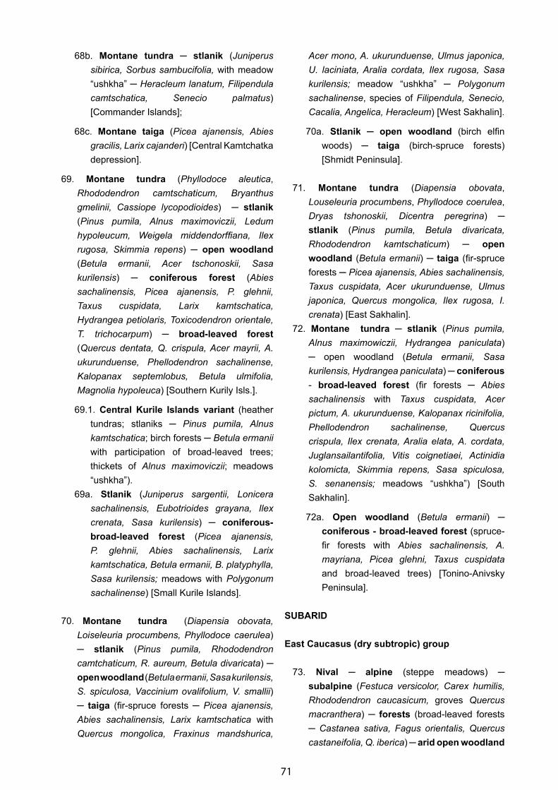
71

68b. Montane tundra ─ stlanik (Juniperus sibirica, Sorbus sambucifolia, with meadow “ushkha” ─ Heracleum lanatum, Filipendula camtschatica, Senecio palmatus) [Commander Islands];

68c. Montane taiga (Picea ajanensis, Abies gracilis, Larix cajanderi) [Central Kamtchatka depression].

69. Montane tundra (Phyllodoce aleutica, Rhododendron camtschaticum, Bryanthus gmelinii, Cassiope lycopodioides) ─ stlanik (Pinus pumila, Alnus maximoviczii, Ledum hypoleucum, Weigela middendorffiana, Ilex rugosa, Skimmia repens) ─ open woodland (Betula ermanii, Acer tschonoskii, Sasa kurilensis) ─ coniferous forest (Abies sachalinensis, Picea ajanensis, P. glehnii, Taxus cuspidata, Larix kamtschatica, Hydrangea petiolaris, Toxicodendron orientale, T. trichocarpum) ─ broad-leaved forest (Quercus dentata, Q. crispula, Acer mayrii, A. ukurunduense, Phellodendron sachalinense, Kalopanax septemlobus, Betula ulmifolia, Magnolia hypoleuca) [Southern Kurily Isls.].

69.1. Central Kurile Islands variant (heather tundras; stlaniks ─ Pinus pumila, Alnus kamtschatica; birch forests ─ Betula ermanii with participation of broad-leaved trees; thickets of Alnus maximoviczii; meadows “ushkha”).

69а. Stlanik (Juniperus sargentii, Lonicera sachalinensis, Eubotrioides grayana, Ilex crenata, Sasa kurilensis) ─ coniferous-broad-leaved forest (Picea ajanensis, P. glehnii, Abies sachalinensis, Larix kamtschatica, Betula ermanii, B. platyphylla, Sasa kurilensis; meadows with Polygonum sachalinense) [Small Kurile Islands].

70. Montane tundra (Diapensia obovata, Loiseleuria procumbens, Phyllodoce caerulea) ─ stlanik (Pinus pumila, Rhododendron сamtchaticum, R. aureum, Betula divaricata) ─ open woodland (Betula ermanii, Sasa kurilensis, S. spiculosa, Vaccinium ovalifolium, V. smallii) ─ taiga (fir-spruce forests ─ Picea ajanensis, Abies sachalinensis, Larix kamtschatica with Quercus mongolica, Fraxinus mandshurica,

Acer mono, A. ukurunduense, Ulmus japonica, U. laciniata, Aralia cordata, Ilex rugosa, Sasa kurilensis; meadow “ushkha” ─ Polygonum sachalinense, species of Filipendula, Senecio, Cacalia, Angelica, Heracleum) [West Sakhalin].

70а. Stlanik ─ open woodland (birch elfin woods) ─ taiga (birch-spruce forests) [Shmidt Peninsula].

71. Montane tundra (Diapensia obovata, Louseleuria procumbens, Phyllodoce coerulea, Dryas tshonoskii, Dicentra peregrina) ─ stlanik (Pinus pumila, Betula divaricata, Rhododendron kamtschaticum) ─ open woodland (Betula ermanii) ─ taiga (fir-spruce forests ─ Picea ajanensis, Abies sachalinensis, Taxus cuspidata, Acer ukurunduense, Ulmus japonica, Quercus mongolica, Ilex rugosa, I. crenata) [East Sakhalin].

72. Montane tundra ─ stlanik (Pinus pumila, Alnus maximowiczii, Hydrangea paniculata) ─ open woodland (Betula ermanii, Sasa kurilensis, Hydrangea paniculata) ─ coniferous - broad-leaved forest (fir forests ─ Abies sachalinensis with Taxus cuspidata, Acer pictum, A. ukurunduense, Kalopanax ricinifolia, Phellodendron sachalinense, Quercus crispula, Ilex crenata, Aralia elata, A. cordata, Juglansailantifolia, Vitis coignetiaei, Actinidia kolomicta, Skimmia repens, Sasa spiculosa, S. senanensis; meadows “ushkha”) [South Sakhalin].

72а. Open woodland (Betula ermanii) ─ coniferous - broad-leaved forest (spruce-fir forests with Abies sachalinensis, A. mayriana, Picea glehni, Taxus cuspidata and broad-leaved trees) [Tonino-Anivsky Peninsula].

SUBARID

East Caucasus (dry subtropic) group

73. Nival ─ alpine (steppe meadows) ─ subalpine (Festuca versicolor, Carex humilis, Rhododendron caucasicum, groves Quercus macranthera) ─ forests (broad-leaved forests ─ Castanea sativa, Fagus orientalis, Quercus castaneifolia, Q. iberica) ─ arid open woodland

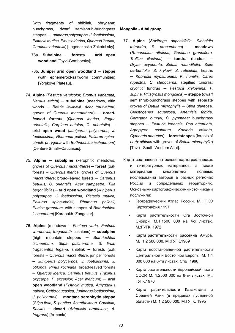
72

(with fragments of shibliak, phrygana; bunchgrass, dwarf semishrub-bunchgrass steppes ─ Juniperus polycarpos, J. foetidissima, Pistacia mutica, Pinus eldarica, Quercus iberica, Carpinus orientalis) [Lagodekhsko-Zakatal sky].

73а. Subalpine ─ forests ─ arid open woodland [Tsyvi-Gomborsky];

73b. Juniper arid open woodland ─ steppe (with ephemeroid-saltworm communities) [Yorskoye Plateau].

74. Alpine (Festuca versicolor, Bromus variegata, Nardus stricta) ─ subalpine (meadows, elfin woods ─ Betula litwiniwii, Acer trautvetteri, groves of Quercus macranthera) ─ broad-leaved forests (Quercus iberica, Fagus orientalis, Carpinus betulus, C. orientalis) ─ arid open wood (Juniperus polycarpos, J. foetidissima, Rhamnus pallasi, Paliurus spina-christi, phrygana with Bothriochloa ischaemum) [Centere Small─Caucasus].

75. Alpine ─ subalpine (xerophitic meadows, groves of Quercus macranthera) ─ forest (oak forests – Quercus iberica, groves of Quercus macranthera; broad-leaved forests ─ Carpinus betulus, C. orientalis, Acer campestre, Tilia begoniifolia) ─ arid open woodland (Juniperus polycarpos, J. foetidissima, Pistacia mutica, Paliurus spina-christi, Rhamnus pallasii, Punica granatum, with steppes of Bothriochloa ischaemum) [Karabakh–Zangezur].

76. Alpine (meadows – Festuca varia, Festuca woronowii; tragacanth cushions) ─ subalpine (high mountain steppes ─ Bothriochloa ischaemum, Stipa pulcherrima, S. tirsa; tragacanths frigana, shibliak ─ forests (oak forests – Quercus macranthera, juniper forests ─ Juniperus polycarpos, J. foetidissima, J. oblonga, Pinus kochiana, broad-leaved forests ─ Quercus iberica, Carpinus betulus, Fraxinus oxycarpa, F. excelsior, Acer ibericum) ─ arid open woodland (Pistacia mutica, Amygdalus nairica, Celtis caucasica, Juniperus foetidissima, J. polycarpos) ─ montane xerophytic steppe (Stipa tirsa, S. pontica, Acantholimon, Cousinia, Salvia) ─ desert (Artemisia armeniaca, A. fragrans) [Armenia].

Mongolia - Altai group

77. Alpine (Saxifraga oppositifolia, Sibbaldia tetrandra, S. procumbens) ─ meadows (Ranunculus altaicus, Gentiana grandiflora, Trollius lilacinus) ─ tundra (tundras ─ Dryas oxyodonta, Betula rotundifolia, Salix berberifolia, S. krylovii, S. reticulata, heaths ─ Kobresia myosuroides, K. humilis, Carex rupestris, C. stenocarpa, stepified tundras; cryofitic tundras ─ Festuca kryloviana, F. supina, Ptilagrostis mongolica) ─ steppe (dwarf semishrub-bunchgrass steppes with separate groves of Betula microphylla ─ Stipa glareosa, Cleistogenes squarrosa, Artemisia frigida, Caragana bungei, C. pygmaea; bunchgrass steppes ─ Festuca lenensis, Poa attenuata, Agropyron cristatum, Koeleria cristata, Cymbaria dahurica) ─ foreststeppes (forests of Larix sibirica with groves of Betula microphylla) [Tuva –South Western Altai].

Карта составлена на основе картографических и литературных материалов, а также материалов многолетних полевых исследований авторов в разных регионах России и сопредельных территориях. Основными картографическими источниками послужили:

• Географический Атлас России. М.: ПКО Картография.1997

• Карта растительности Юга Восточной Сибири. М.1:1500 000 на 4-х листах. М.:ГУГК, 1972

• Карта растительности бассейна Амура. М. 1:2 500 000. М.:ГУГК.1969

• Карта восстановленной растительности Центральной и Восточной Европы. М. 1:4 000 000 на 6-ти листах. СпБ. 1996

• Карта растительности Европейской части СССР. М. 1:2500 000 на 6-ти листах. М.: ГУГК.1976

• Карта растительности Казахстана и Средней Азии (в пределах пустынной области) М. 1:2 500 000. М.ГУГК. 1995

73

• Корреляционная эколого-фитоценотическая карта Азиатской России. М.1:8 000000. СО АН СССР. Ин-т. географии Сибири и ДВ.

• Растительность Алтайского края. М.:1600 000 [карта] //Атлас Алтайского края.Т.1. М.-Барнаул: ГУГК.1978

• Растительность Западно-Сибирской равнины. М. 1:1500 000 на листах [карта].М.:ГУГК. 1976

• Растительность Сахалинской области. М.1:1500 000 [карта]// Атлас Сахалинской области. М.:ГУГК. 1976

• Растительность СССР. М.: 1:4 000 000 на 4-х листах [карта]. Для высших учебных заведений. М.: ГУГК. 1990.

• Растительность Якутской АСССР. М.1:5 000 000 [карта] //Атлас Якутской АСР. М.:ГУГК. 1981

ОСНОВНАЯ ЛИТЕРАТУРА

1. Александрова В.Д. Геоботаническое районирование Арктики и Антарктики// Комаровские чтения. XXIX. Л.: Наука, 1977.

2. Александрова В.Д., Юрковская Т.К. (ред). Геоботаническое районирование Нечерноземья Европейской части РСФСР. Л.: Наука, 1989.

3. Василевич В.И. О растительных ассоциациях ельников Северо-Запада // Ботан. журн. Т.68, N 12, 1983.

4. Гребенщиков О.С. Вертикальная поясность растительности в горах восточной части Западной Европы //Биол. ж. Т.42, N 6,1957.

5. Камелин Р.В. Материалы по истории флоры Азии (Алтайская горная страна). Барнаул, 1998.

6. Комаров В.Л. Растительность Сибири. Избр. соч. Т.IX. М.: АН СССР, 1953.

7. Лавренко Е.М. Типы вертикальной поясности растительности в горах СССР// Современные проблемы географии. М., 1964.

8. Лавренко Е.М., Карамышева З.В., Никулина Р.И. Степи Евразии. Л.1991.

9. Огуреева Г.Н. Ботаническая география Алтая. М.: Наука, 1980.

10. Павлов Н.В. Ботаническая география СССР. Алма-Ата, 1948.

11. Растительность Европейской части СССР. Л.: Наука, 1980.

12. Растительный покров СССР. Т.I-II. М., 1956.

13. Растительный покров Западно-Сибирской равнины. Новосибирск., 1985.

14. Сочава В.Б. Классификация и картографирование высших подразделений растительности Земли //Современные проблемы географии. М.: Наука, 1964.

15. Сочава В.Б. Географические аспекты сибирской тайги. Новосибирск, 1980.

16. Станюкович К.В. Основные типы поясности в горах СССР// Изв. ВГО. Т.87, вып. 3, 1955.

17. Толмачев А.И. К истории возникновения и развития темнохвойной тайги. М.-Л., 1954.

18. Шумилова Л.В. Ботаническая география Сибири. Томск, 1962.

19. Юрковская Т.К. Классификация и картографирование болот Европейской части СССР. Спб: Наука, 1997

20. Юрцев Б.А. Гипоарктический ботанико-географический пояс и происхождение его флоры М.-Л., 1966.

74

Vegetation Mapping in Boreal Alaska

Stephen S. Talbot

U.S. Fish and Wildlife Service, Anchorage, Alaska, 99503, U.S.A., stephen_talbot@fws.gov

Abstract

One of the first tasks to be addressed within the Circumboreal Vegetation Mapping (CBVM) project was to review the status of boreal vegetation mapping in each of the circumboreal countries. This paper summarizes the vegetation maps presently available for boreal Alaska. The large number of maps of Alaska varies widely in detail and quality, ranging from intermediate-scale maps of large areas to large-scale maps of small areas, and from maps based on photographic interpretation to those based on computer classified digital data. Collectively, these maps could provide a valuable resource for reinterpreting and synthesizing the boreal vegetation of Alaska into a single map. Representative examples are provided to indicate the spectrum of vegetation units displayed in some of these maps.

Introduction

The goal of the Circumboreal Vegetation Mapping (CBVM) project is to provide a common international framework for understanding the boreal region. Currently, various maps exist of the boreal biome, but they do not rely on a unified international method for classifying and mapping boreal vegetation. By recognizing the boreal region as a single geo-ecosystem with a common set of cultural, political, and economic issues, the CBVM will be the first detailed vegetation map of the entire global biome. Information on boreal vegetation has increased markedly in recent years, and one of the first tasks to be addressed was reviewing the status of boreal vegetation mapping in each of the circumboreal countries. This paper compiles a bibliography of all relevant boreal Alaska vegetation maps and assesses preliminarily if these data are adequate for making a small-scale (1:4 M) vegetation map of boreal Alaska.

Inventorying available vegetation maps of the boreal zone is a logical first step in mapping the vegetation of

boreal Alaska (Gribova & Isachenko, 1972). The term “boreal” has been variously defined. As used here, the term includes the northern, middle, and southern boreal subzones of Tuhkanen (1984) south of the southern limit of the Arctic as defined by Walker et al. (2005) but excludes the hemiboreal subzone as the southern limit of the zone. This report identifies the major vegetation maps that are currently available. From these maps, representative examples are provided of the vegetation units that have been portrayed. These examples were selected to indicate the spectrum of mapping efforts and their products. Mapping studies are organized first from an historical perspective—starting with the early period from 1901 to 1963—then by more recent, small-scale mapping studies that cover all Alaska. These examples are followed by large-scale mapping surveys of small areas that in turn are followed by medium-scale computer classified mapping projects. In the latter category the studies are sometimes arranged by the agency that supported the mapping and sometimes by the area of Alaska where the mapping took place.

The references that follow indicate there are a large number of Alaska boreal vegetation maps, and they vary widely in their detail and quality. They range from intermediate-scale maps of large areas to large-scale maps of small areas, and from maps based on photographic interpretation to those based on computer classified digital data.

Status of Vegetation Mapping

Early Period

The first catalog of vegetation maps of Alaska was published by Küchler & McCormick (1965); it lists 27 maps from boreal Alaska published during the period 1901–1963 and 48 small-scale maps of North America, all of which were derived from photographic interpretation. Their catalog provides a wealth of information arranged in three groups: title of the map, date of preparation and color and scale; map

75

legend; and author of the map with date and place of publication. Smaller-scale maps of Alaska depict broad types of vegetation, with map units ranging from two or three types, such as “timbered” and “timberless,” to one study delimiting nine types (Spetzman, 1963): (1) very high evergreen hemlock-spruce forest; (2) high evergreen spruce forest; (3) moderately high mixed evergreen and deciduous forest; (4) low mixed evergreen and deciduous forest; (5) high brush; (6) low brush-muskeg; (7) moist tundra; (8) wet tundra and coastal marsh; and (9) barren and sparse dry tundra. Most of these maps appear to have been prepared from an economic, forestry perspective. Larger-scale maps vary in their degree of generalization. Some maps indicate broad types, such as those of Whittier, Alaska in the Southcentral Region, which portray hemlock and muskeg, hemlock and alder, timberline transition, alpine vegetation, and snow alder (Thompson, 1954). Others are more detailed, such as the map of Fort Greely, Alaska in the Interior Region, which delineates 16 map units (Benninghoff, 1957): Forest─evergreen forest, mixed evergreen-deciduous forest, deciduous forest, and black spruce muskeg; Scrub and/or shrub─evergreen scrub, mixed evergreen-deciduous scrub, and deciduous scrub; Tundra─shrub tundra, rock desert, and bog; Meadow–meadow and marsh; Vegetation of Local Significance─lichen barrens and aquatic communities; and areas not mapped with respect to vegetation─barren flood plain areas and areas disturbed by culture.

Small-Scale Maps Covering Alaska

More recent efforts have produced several small-scale vegetation maps of Alaska (scale 1:2.5–10M) that depict subclasses of the boreal such as those of Knapp (1965), Küchler (1970), Viereck & Little (1972), Joint Federal-State Planning Commission for Alaska (1973), Tuhkanen (1984), Brown et al. (1998), and Rivas-Martinez et al. (1999). As an example of the kind of types delimited, Rivas-Martinez et al. (1999) indicated 11 subsector types within Alaska within two provinces: the Yukonian-Alaskan Province, including the Continental Alaskan Sector (Boreal Subcontinental Alaskan Subsector; Boreal Eucontinental Alaskan Subsector; Boreal Alaskan Subsector) and the Boreal Oceanic Alaskan Province, including the Boreal Oceanic Western Alaskan Sector (Kenai Peninsula Subsector, Kodiak Island Subsector); the Boreal

Oceanic Eastern Alaskan Sector (Glacier Coast Subsector, Haines-Juneau Subsector); the Aleutian and Alaska Peninsula Sector (Aleutian Islands Subsector, Alaska Peninsula Subsector); and the Canadian Coastal Mountains Sector (North Canadian Coastal Mountains Subsector, Queen Charlotte and Prince of Wales Islands Subsector). Ecoregion maps have been published by Gallant et al. (1995), Commission for Environmental Cooperation (1997), and Nowacki et al. (2001).

Large-Scale Maps of Small Areas

Large-scale studies are focused on rather small areas distributed throughout the boreal. For the Aleutian Islands, vegetation maps exist only for the Naval Complex on Adak Island (Soil Conservation Service, 1990), Bogoslof Island, in part (Byrd et al. 1980), Buldir Island (Byrd, 1984), Amchitka Island (Amundsen, 1977), Atka Island, in part (Friedman, 1984), Kodiak Island, in part (Tande & Boggs, 1995; Tande, 2003, Tande & Michaelson, 2004), Choweit Island, Semidi Islands (Hatch, 1978, unpub. rpt.), Elmendorf Air Force Base (Tande, 1984), Hazen Bay, Yukon Delta National Wildlife Refuge, in part (Tande & Jennings, 1987), Semidi Islands (Hatch, 1978, unpub. rpt.), and Simeonof Island (Talbot et al., 1984, unpub. rpt.). For south-central Alaska, Klein (1999) used conventional aerial photographic interpretation to map Anchorage parks and greenbelts, and similarly for central Alaska, Mount Prindle (Juday, 1988). By example, the map units depicted by Juday (1988) include birch (dry) upland (dwarf) shrub, ericad (dry) upland (dwarf) shrub, foliose lichen, rock and felsic lichen, snowbed herb-graminoid meadow, tall shrub, upland tussock meadow, white spruce, and flood plain willow tall shrub.

Computer Classified Landsat and Related Maps

In response to factors such as increasing resource development, planning mandates, and wildlife-habitat relationships, federal and state agencies sought efficient vegetation mapping methods to inventory regions within the boreal. Beginning in the 1980s vast boreal landscapes were mapped using satellite images at intermediate scales, 1:250,000, and maps covering the greatest portions of boreal Alaska are at this scale (Markon, 1995). It should be noted that vegetation plot data are available for many of these

76

areas and could be used as ground reference data. Two major approaches were used with Landsat data: visual-interpretation and computer classification. Visually-interpreted Landsat maps and conventional aerial photograph interpretation were prepared for several national parks and wildlife refuges: Lake Clark National Park (Racine & Young, 1978; Tande, 1996), Katmai western extension (Young & Racine, 1978); Kenai Lowlands (Gracz et al., 2008), Fort Wainwright (Jorgenson et al., 1999), and Kodiak National Wildlife Refuge (Northern Technical Services 1984; Tande, 2003; Tande & Michaelson, 2004). Computer classification of digital data included several portions of western Alaska–Alaska Peninsula and Bristol Bay area (Wibbenmeyer et al., 1982) and Izembek Lagoon (Ward & Stehn, 1989). An ecological subsection map was produced for Aniakchak National Monument and Preserve (Tande & Michaelson, 2001).

Most of these intermediate-scale maps, and many of the large-scale maps, are based on physiognomic-ecological classifications. Map units reflect the structure of the vegetation and are sometimes supplemented with ecological information. The most frequently used descriptor is moisture with terms such as wet, moist, and dry. Other map unit characteristics include terms such as riparian, dune, and marsh. Dominant species are occasionally included, but their use is often inconsistent, even within a map legend.

Computer classification using digital Landsat data included a number of National Wildlife Refuges such as Kenai (Talbot et al., 1985), Innoko (Talbot & Markon, 1986, Talbot & Markon, 1988), Kanuti (Talbot et al., 1986, unpub. rpt.), Kodiak (Fleming & Spencer, 2005; U.S. Fish & Wildlife Service, 2006), Nowitna (Talbot & Markon, 1986), Tetlin (Talbot et al., 1984, unpub. rpt.), and Yukon Delta (in part) (Talbot et al., 1986, unpub. rpt.). A number of vegetation land cover maps were produced by the U.S. Geological Survey for large portions of Alaska: Nowitna National Wildlife Refuge (Markon, 1988a), Upper Kuskokwim resource management area (Markon, 1988b), Selawik National Wildlife Refuge (Markon 1988c), Innoko National Wildlife Refuge (Markon, 1987), Meade River (U.S. Geological Survey, 1988c), Tetlin NWR (U.S. Geological Survey, 1987), Valdez (U.S. Geological Survey, 1987), Fairbanks (U.S. Geological Survey, 1988b), Dillingham (U.S. Geological Survey, 1988a),

and Copper River-Wrangell Mountains (University of Alaska & U.S. Forest Service, 1977). Land cover maps are also available for southeast Alaska–Glacier Bay National Park and Preserve (Boggs et al., 2008); Interior Alaska–Denali National Park and Preserve (Dean & Heebner, 1982; Boggs et al., 2001), Yukon-Charley Rivers National Preserve (Boggs & Sturdy, 2005), Steese White Mountains (Markon, 1993, unpub. rpt.); and for Southcentral Alaska─Kenai Fiords National Park (Boggs et al., 2008), Kenai Lowlands (Gracz et al., 2008), and Katmai National Park and Preserve (Boggs et al. 2003). As an example, Boggs et al. (2003) distinguished 25 land cover types: dense-open spruce forest, open-woodland spruce forest, open-woodland stunted spruce, broadleaf forest, mixed spruce-broadleaf forest, alder shrub, willow shrub, closed low birch shrub, low shrub birch-ericaceous-willow, low shrub-sedge, peatland, herbaceous/shrub, dwarf shrub, dwarf shrub-rock, dry-mesic herbaceous, wet herbaceous, aquatic herbaceous, sparse vegetation, bare ground, snow/ice, shadow indeterminate, silty water, clear water, burn, and cloud.

Ecological land surveys (ELS) view landscapes not merely as aggregations of separate biological and earth resources, but as ecological systems with functionally related parts that can provide a consistent conceptual framework for ecological applications. Generally, these surveys map at three spatial scales: ecotypes (1:50,000 scale) are delineated areas with homogenous topography, terrain, soil, surface-form, hydrology, and vegetation; ecosections (1:100,000 scale) are homogeneous with respect to geomorphic features and water regime and, thus, have recurring patterns of soils and vegetation; and ecodistricts (1:500,000) are broader areas with similar geology, geomorphology, and physiography. These surveys were prepared for Pogo Mining area (Burgess et al., 2000, unpub. rpt.), Fort Greely (Jorgenson et al., 2001), Fort Wainwright (Jorgenson et al., 1999), Poker-Caribou Creek Watershed (Jorgenson et al., 1984, Jorgenson et al., 1986, unpub. rpt.), Fort Richardson (Jorgenson et al., 2003), and Wrangell-St. Elias National Park and Preserve (Jorgenson et al., 2008). By example, the land cover map of Jorgenson et al. (2008) was developed through classification of 11 Landsat scenes. Their rule-based modelling of ecotypes integrated physiography, soil, and vegetation

77

composition into 69 classes, 47 of which were boreal ecotypes. For forest ecotypes they distinguished six types: boreal subalpine poplar forest, boreal subalpine spruce woodland, boreal upland aspen forest, boreal upland birch forest, boreal upland spruce-birch forest, and boreal upland white spruce forest.

A soil survey of Denali National Park area, including landtype association maps and ecological sites, was produced by Clark & Duffy (2006) and is available online (http://soildatamart.nrcs.usda.gov/Manuscripts/AK651/0/DenaliPark.pdf). A number of soil surveys are available online (http://soils.usda.gov/survey/online_surveys/alaska/) and contain information on plant communities for the following areas: Anchorage (2001), Copper River (1999), Delta River (2005), Fort Greely and Donnelly Training (2005), Fort Wainwright (2006), Gerstle River (2001), Goldstream-Nenana (1977), Greater Fairbanks (2004), Greater Nenana (2007), Gulcana River (1999), Haines (1998), Kantishna (2001), Kobuk Preserve (1995), Lower Kenai Peninsula (2000), Matanuska-Susitna (1998), Northeastern Kodiak Island (1960), Northstar (2000), Salcha-Big Delta (1973), Stewart River (2005), Totchaket (1980), Upper Tanana (1999), Western Interior Rivers (2008), Western Kenai Peninsula (2005), and Yetna (1998).

A number of maps were published by the U.S. Department of the Interior, Bureau of Land Management (BLM) as Technical Reports in collaboration with Ducks Unlimited and various government agencies, for example, BLM, U.S. Fish and Wildlife Service, U.S. Air Force, and National Park Service, and are available online (www.blm.gov/ak/st/en/info/gen_pubs/tr.html). Soil and Vegetation Survey of the Gulkana River Area, Alaska (Clark & Kautz, 1999, Tech. Rpt. 20); Galena Military Operations Area/Nowitna National Wildlife Refuge Earth Cover Classification (2002, Tech. Rpt. 23); Haines Earth Cover Classification (2002, Tech. Rpt. 26); Kanuti National Wildlife Refuge/Ray Mountains/Hogatza River Earth Cover Classification (2002, Tech. Rpt. 28); Vegetation Survey of Campbell Tract Facility, Anchorage, Alaska (Guyer, 2000, Tech. Rpt. 35); Steese─White Mountains Earth Cover Classification (2002, Tech. Rpt. 42); Stony River Military Operations Area Earth Cover Classification (2002, Tech. Rpt. 43); Susitna Military Operations Area Earth Cover Classification (2002, Tech. Rpt. 44); Tiekel Watershed Earth Cover Classification (2002, Tech. Rpt. 46); Innoko Earth Cover Classification (2002,Tech. Rpt. 47); Yukon-Charley/Black River/Fortymile Earth Cover Classification (2002, Tech. Rpt. 48); and Soil and Vegetation Survey of the Delta River (Clark, 2005, Tech. Rpt. 55). There are a number of Earth Cover

Fig. 1. Alaska Earth Cover Initiative.

78

Classification reports that are works in progress and are pending: Bering Glacier, Copper River Delta, Goodnews Bay, Gulkana River Watershed, Illiamna, Kenai Peninsula, Koyukuk/Melozitna, Kvichak, Minto Flats, and Naknek, and Northern and Southern Yukon. The location of these projects is indicated in Fig. 1.

The technical reports published by the BLM (listed above) vary greatly in their detail and quality. For example, the Steese─White Mountains Earth Cover Classification (2002, Tech. Rpt. 42) is a physiognomic classification that uses a classification scheme developed at a BLM Earth Cover Workshop; it includes the names of some tree species; this is significant because it adds a diversity component expanding the ecological value of the map: 1.0 Forest (1.1 Closed Needleleaf, 1.2 Open Needleleaf, 1.21 Open Needleaf Lichen, 1.3 Woodland Needleleaf, 1.31 Woodland Needleaf Lichen, 1.4 Closed Deciduous, 1.41 Closed Birch, 1.42 Closed Aspen, 1.43 Closed Cottonwood/Balsam Poplar, 1.44 Closed Mixed Deciduous, 1.5 Open Deciduous, 1.51 Open Birch, 1.52 Open Aspen, 1.53 Open Cottonwood/Balsam Poplar, 1.54 Open Mixed Deciduous, 1.6 Closed Mixed Needleleaf/Deciduous, 1.7 Open Mixed Needleleaf/Deciduous); 2.0 Shrub (2.1 Tall Shrub, 2.2 Low Shrub, 2.21 Willow/Alder Low Shrub, 2.22 Other Low Shrub/Tussock Tundra, 2.23 Other Low Shrub/Lichen, 2.24 Other Low Shrub, 2.3 Dwarf Shrub, 2.31 Dwarf Shrub/Lichen, 2.32 Other Dwarf Shrub); 3.0 Herbaceous (3.1 Bryoid, 3.11 Lichen, 3.12 Moss, 3.2 Wet Herbaceous, 3.21 Wet Graminoid, 3.22 Wet Forb, 3.3 Mesic/Dry Herbaceous, 3.31 Tussock Tundra, 3.311 Tussock Tundra/Lichen, 3.312 Tussock Tundra, 3.32 Mesic/Dry Sedge Meadow, 3.33 Mesic/Dry Grass Meadow, 3.34 Mesic/Dry Graminoid; 4.0 Aquatic Vegetation (4.1 Aquatic Bed, 4.2 Emergent Vegetation); 5.0 Water (5.1 Snow, 5.2 Ice, 5.3 Clear Water, 5.4 Turbid Water); 6.0 Barren (6.1 Sparsely Vegetated, 6.2 Rock/Gravel, 6.3 Mud/Silt/Sand); 7.0 Urban; 8.0 Agriculture; 9.0 Cloud/Shadow (9.1 Cloud, 9.2 Shadow); 10.0 Other (burn). While the Vegetation Survey of Campbell Tract Facility, Anchorage, Alaska (Guyer, 2000, Tech. Rpt. 35) mapped cover types including balsam poplar closed forest, balsam poplar/willow scrub, black spruce/greenleaf alder forest, disturbed site, low shrub birch mixed scrub, paper birch closed forest, paper birch open forest, paper birch-white spruce open forest, paper birch woodland, spruce/moss forest, sweetgale/bluejoint bog, white

spruce/paper birch forest, white spruce woodland, and developed.

A geospatial dataset of forest biomass across the United States is available on the U.S. Department of Agriculture, Forest Service (USFS) Geodata Clearinghouse (http://svinetfc4.fs.fed.us/rastergateway/biomass/) (Blackard et al., 2008, Ruefenacht et al., 2008). The predictor data were a geospatial dataset with a spatial resolution of 250 m. Among the predictor layers used were digital elevation models (DEM) and DEM derivatives; Moderate Resolution Imaging Spectroradiometer (MODIS) multi-date composites, vegetation indices, and vegetation continuous fields; class summaries from the 1992 National Land Cover Dataset (NLCD); various ecologic zones; and summarized PRISM climate data. Six forest type groups were mapped for Alaska: (1) aspen/birch; (2) elm/ash/cottonwood; (3) fir-spruce-mountain hemlock; (4) hemlock/Sitka spruce; (5) lodgepole pine; and (6) spruce/fir.

The National Land Cover Database (NLCD) 2001 is a Landsat-derived, 30 m spatial resolution land cover map that describes land cover of Alaska (http://alaska.usgs.gov/science/geography/nlcd.html) and a national page (http://www.mrlc.gov/). Eighteen land cover types are depicted: open water; perennial ice/snow; developed, low intensity; developed, medium intensity; developed, high intensity; barren land; deciduous forest; evergreen forest; mixed forest; dwarf scrub; shrub/scrub; grassland/herbaceous; sedge/herbaceous; moss; pasture/hay; cultivated crops; woody wetlands; and emergent herbaceous wetlands.

LANDFIRE is a five-year, multipartner project producing consistent and comprehensive maps and data describing vegetation, wildland fuel, and fire regimes across the United States (http://www.landfire.gov/). Their legend is based on ecological systems; these are defined as a group of plant communities that tend to co-occur within landscapes with similar ecological processes, substrates, and/or environmental gradients. Alaska LANDFIRE is a work in progress with a projected completion date of September 2010. NLCD and LANDFIRE both provide a consistent legend and scale for the entire state.

79

National Wetlands Inventory Maps

Detailed National Wetlands Inventory maps are published for south-central, east-central and south-east Alaska, and Kodiak Island (http://alaska.fws.gov/fisheries/nwi/pdf/NWI_AK_Status_1-08.pdf); Cowardin et al. (1979). Systems form the highest level of the classification hierarchy, and five classifications are defined: marine, estuarine, riverine, lacustrine, and palustrine. Marine and estuarine systems each have two subsystems, subtidal and intertidal; the riverine system has four subsystems, tidal, lower perennial, upper perennial, and intermittent; the lacustrine has two subsystems, littoral and limnetic; and the palustrine has no subsystems. Within the subsystems, classes are based on substrate material and flooding regime, or life form. The same classes may appear under one or more of the systems or subsystems. Six classes are based on substrate and flooding regime: rock bottom with a substrate of bedrock, boulders, or stones; unconsolidated bottom with a substrate of cobbles, gravel, sand, mud, or organic material; rocky shore with the same substrates as rock bottom; unconsolidated shore with the same substrates as unconsolidated bottom; streambed with any of the substrates; and reef with a substrate composed of the living and dead remains of invertebrates (corals, mollusks, or worms). The bottom classes are flooded all or most of the time and the shore classes are exposed most of the time. The class streambed is restricted to channels of intermittent streams and tidal channels that are dewatered at low tide. The life form of the dominant vegetation defines the five classes based on structure: aquatic bed, dominated by plants that grow principally on or below the surface of the water; moss-lichen wetland, dominated by mosses or lichens; emergent wetland, dominated by emergent herbaceous angiosperms; scrub-shrub wetland, dominated by shrubs or small trees; and forested wetland, dominated by large trees. The dominance type, named for the dominant plant or animal forms, is the lowest level of the classification hierarchy. Only examples are provided for this level; dominance types must be developed by individual users of the classification. Modifying terms applied to the classes or subclasses are essential for use of the system. In tidal areas, the type and duration of flooding are described by four water regime modifiers: subtidal, irregularly exposed, regularly flooded, and irregularly flooded. In nontidal areas, eight regimes are used: permanently

flooded, intermittently exposed, semipermanently flooded, seasonally flooded, saturated, temporarily flooded, intermittently flooded, and artificially flooded. A hierarchical system of water chemistry modifiers is used to describe the salinity of the water. Fresh waters are further divided on the basis of pH. Use of a hierarchical system of soil modifiers taken directly from U.S. soil taxonomy is also required. Special modifiers are used where appropriate: excavated, impounded, diked, partly drained, farmed, and artificial.

Other Maps and Works of Interest

Soils maps could serve as a valuable asset in mapping the vegetation, as each mapped soil unit includes information on its associated vegetation. For example, an exploratory soil survey of Alaska is available at a scale of 1:1M and includes information on the vegetation (Rieger et al., 1979), and more detailed soils surveys are available for certain areas. Natural Resources Conservation Service (NRCS) is processing an update of the statewide soil map, referred to as the Alaska STATSGO. Interim products including a map at 1:250,000 scale and tabular attribute dataset are planned for December 2009. The map stratifies the state by physiographic area based on the Natural Resources Conservation Service Major Land Resource Areas (MLRA). Map units group soils based on similar landform, lithology, and life zone.

The Alaska Vegetation Classification of Viereck et al. (1992) summarizes vegetation types in a hierarchical arrangement and provides citations to published works. These referenced papers provide a useful supplement for specific areas in interpreting vegetation from conventional aerial photography and Landsat images. A new literature review of plant community studies in Alaska would be useful to update the work of Viereck et al (1992); an update was initiated by G. F. Tande and is filed at Alaska Natural Heritage Program, Anchorage.

Toward a Small-Scale Vegetation Map of Boreal Alaska

At present, there is no true vegetation map for the Alaska boreal such as those produced in one of the major vegetation mapping schools of Germany, France, Japan, or Russia. Small-scale maps that cover all of Alaska, such as the province and subsector

80

maps of Rivas-Martinez et al. (1999) and the climatic-phytogeographical system of Tuhkanen (1984) help provide insight into mapping upper-level map units. In addition, there are several manually interpreted and useful maps of the entire state, such as the vegetation map of Spetzman (1963). However, Walker (1999b) stated that the Spetzman (1963) map is based on information assembled before the vegetation was as well known as it is presently. Walker (1999b) also noted that the map portrays very broad vegetation units that may be difficult to resolve with modern vegetation maps based on satellite imagery.

Although they vary widely in their detail and quality, there is a wealth of information in the Alaska maps. This information in combination with soil maps such as Rieger et al. (1979) and The Alaska Vegetation Classification of Viereck et al. (1992) could be beneficial. The integrated mapping approach of Walker (1999a & 1999b) that proved successful in mapping the circumpolar Arctic vegetation could provide a useful approach to mapping the circumboreal region. It may be possible to use intermediate-scale maps of large areas and large-scale maps of small areas as guides to interpret AVHRR digital data for production of a true circumboreal vegetation map. On the positive side, a number of computer-generated vegetation maps are now available and cover a major portion of the Alaska boreal and account for the majority of boreal vegetation diversity along both an east-west longitudinal gradient and a north-south latitudinal gradient. However, there are areas within the boreal such as the Aleutian Islands for which little mapping has been accomplished.

Acknowledgments

I gratefully thank the following, listed alphabetically, for discussions and making map sources available: Keith Boggs (Alaska Natural Heritage Program), Mark Clark (Natural Resources Conservation Service [NRCS]), Dan Fehringer (Ducks Unlimited), Amy E. Miller & Beth Koltun (National Park Service [NPS]), Torre Jorgenson (ABR, Inc.), Carl Markon (U.S. Geological Survey [USGS]), Gerry Tande (U.S. Fish and Wildlife Service [USFWS]), and Ken Winterberger (U.S. Forest Service [USFS]).

References

Burgess, R. M., Jorgenson, M. T., Roth, J. E., Lawhead, B. E., & Anderson, B. A. 2000. Wildlife Habitat Assessment for the Pogo Project Area. Unpublished Report prepared for Tech Corp., Fairbanks, Alaska, by ABR, Inc., Fairbanks, Alaska.

Byrd, G. V. 1984. Vascular vegetation of Buldir Island, Aleutian Islands, Alaska, compared to another Aleutian Island. Arctic 37(1): 37–48.

Byrd, G. V., Divoky, G. J., & Bailey, E. 1980. Changes in marine bird and mammal populations on an active volcano in Alaska. The Murrelet 61:50–62.

Clark, M. H. & Duffy, M. S. 2006. Soil survey of Denali National Park area, Alaska. Internet: http://soildatamart.nrcs.usda.gov/Manuscripts/AK651?0?DenaliPark.pdf. Department of Agriculture, Natural Resources Conservation Service, Washingon, D.C.

Commission for Environmental Cooperation. 1997. Ecological regions of North America: Toward a common perspective. Internet: http://www.cec.org. CEC, 393, rue St – Jacques Ouest, bureau 200, Montreal, Quebec.

Cowardin, L. M., Carter, V., Golet, F. C., & LaRoe, E. T. 1979. Classification of wetlands and deepwater habitats of the United States. U.S. Department of the Interior, Fish and Wildlife Service, Washington, D.C. Jamestown, North Dakota: Northern Prairie Wildlife Research Center Online. http://www.npwrc.usgs.gov/resource/wetlands/classwet/index.htm (Version04DEC1998).

Dean, F. C. & Heebner, D. K. 1982. Landsat-based vegetation mapping of Mount McKinley National Park Region, Alaska. Final Report for the National Park Service Contract No. CX-9000-6-E084. Alaska Cooperative Park Studies Unit, University of Alaska, Fairbanks, Alaska.

Fleming, M. & Spencer, P. 2005. Habitat mapping of the Kodiak Archipelago. Digital data files, maps, and user’s guide. Alaska Geographic Science Center, U.S. Geological Survey, Anchorage, Alaska.

Friedman, B. 1984. Vegetation. Pages 3–4, 5–28 in Biological Environmental, Section 3. Feasibility study data collection program for the proposed hydroelectric project at Atka, Alaska. Prepared for Alaska Power Authority by NORTEC, Inc., Anchorage, Alaska.

81

Gallant, A. L., Binnian, E. F., Omernik, J. M., & Shasby, M. B. 1995. Ecoregions of Alaska. U.S. Geological Survey, Washington, D.C.

Gracz, M., North, P., Noyes, K., & Tande, G. F. 2008. Wetland mapping and classification of the Kenai Lowland, Alaska. Prep. for: U. S. Environmental Protection Agency, Kenai, Alaska. Kenai River Center, Soldotna, Alaska and Alaska Natural Heritage Program, Environment and Natural Resources Institute, Univ. of Alaska Anchorage, Anchorage, Alaska. http://www.kenaiwetlands.org/.

Gribova, S. A. & Isachenko, T. I. 1972. Vegetation mapping in survey scales. Pages 137–308 in Lavrenko, E. M., ed. Field geobotany, Vol. 4. Academy of Sciences, USSR. Botanical Institute, Nauka Press, Leningrad. (In Russian).

Hatch, M. A. 1978. Flora of Chowiet Island in the Semidi National Wildlife Refuge, Alaska. Unpublished report on file at the U.S. Department of Agriculture, Forest Service, Institute for Northern Forestry, Fairbanks, Alaska.

Joint Federal-State Land Use Planning Commission for Alaska. 1973. Major ecosystems of Alaska. U.S. Geological Survey, Washington, D.C.

Jorgenson, M. T., Slaughter C. W., & Viereck, L. A. 1984. Vegetation mapping utilizing a hierarchical vegetation classification system in central Alaska. Page 295 in Inventorying forest and other vegetation of the high latitude and high altitude regions. Proceedings of an International Symposium, Society of American Foresters Regional Technical Conference. Fairbanks, Alaska. Society of American Foresters, Bethesda, Maryland.

Jorgenson, M. T.; Slaughter, C. W., & Viereck, L. A. 1986. Reconnaissance Survey of Vegetation and Terrain Relationships in the Caribou-Poker Creeks Research Watershed, central Alaska. Institute of Northern Forestry, U.S. Forest Service, Fairbanks,Alaska. Unpublished report. 89 pp.

Jorgenson, M. T., Roth, J. E., Smith M. D., Schlentner, S., Lentz, W., & Pullman, E. R. 2001. An Ecological Land Survey for Fort Greely, Alaska. U.S. Army Cold Regions Research and Engineering Laboratory, Hanover, New Hampshire. ERDC/CRREL TR-01-04.

Jorgenson, M. T., Roth, J. E., Raynolds, M., Smith, M. D., Lentz, W., Zusi-Cobb, A., & Racine, C. H. 1999. An Ecological Land Survey for Fort Wainwright,

Alaska. U.S. Army Cold Regions Research and Engineering Laboratory, Hanover, NH. CRREL Report 99-9. U.S. Army Cold Regions Research Engineering Laboratory, Hanover, New Hampshire.

Jorgenson, M. T., Roth, J. E., Schlentner, S. F., Pullman, E. R., Macander, M., & Racine, C. H. 2003. An ecological land survey for Fort Richardson, Alaska. U.S. Army Cold Regions TR03-19. Hanover, New Hampshire.

Jorgenson, M. T., Roth, J. E., Loomis, P. F., Pullman, E. R., Cater, T. C., Duffy, M. S., Davis, W. A., Macander, M. J., & Grunblatt, J. 2008. An Ecological Land Survey for Land Cover Mapping of Wrangell-St. Elias National Park and Preserve. Natural Resource Program Center, National Park Service, Fort Collins, CO. Natural Resources Technical Report NPS/WRST/NRTR-2008/094.

Juday, G. P. 1988. Alaska Research Natural Area: 1. Mount Prindle. Gen. Tech. Rep. PNW-GTR-224. U.S. Dept. of Agriculture, Forest Service, Pacific Northwest Research Station, Portland, Oregon.

Klein, S. C. 1999. Map of Forested Habitats in Anchorage’s Parks and Greenbelts. Alaska Natural Heritage Program, Environment and Natural Resources Institute, University of Alaska, Anchorage.

Knapp, R. 1965. Die Vegetation von Nord- und Mittelamerika und der Hawaii-Inseln. Gustaf Fisher, Stuttgart.

Küchler, A. W. 1970. Potential natural vegetation of Alaska. Pages 90–91 in The National Atlas of the United States of America. U.S. Government Printing Office, Washington, D.C.

Küchler, A. W. & McCormick, J. 1965. Vegetation maps of North America. University of Kansas Publications, Library Series No. 21.

Markon, C. J. 1987. Innoko National Wildlife Refuge land cover mapping project user’s guide. NMD, USGS/EROS, Anchorage Field Office, Anchorage, Alaska.

Markon, C. J. 1988a. Nowitna National Wildlife Refuge land cover mapping project user’s guide. NMD, USGS/EROS, Anchorage Field Office, Anchorage, Alaska.

Markon, C. J. 1988b. Land cover mapping of the upper Kuskokwim resource management area using Landsat and digital database approach. NMD,

82

USGS/EROS, Anchorage Field Office, Anchorage, Alaska.

Markon, C. J. 1988c. Selawik National Wildlife Refuge land cover mapping project user’s guide. NMD, USGS/EROS, Anchorage Field Office, Anchorage, Akaska.

Markon, C. J. 1993. Steese White Mountains land cover mapping user’s guide. Unpublished report, USGS/EROS, Anchorage Field Office, Anchorage, Alaska.

Markon, C. J. 1995. History and use of remote sensing for conservation and management of federal lands in Alaska, U.S.A. Natural Areas Journal 15: 329–338.

Northern Technical Services (NORTEC). 1984. Kodiak National Wildlife Refuge Mapping Project. A final report for the Kodiak Comprehensive Conservation Plan from Contract #14-16-0007-83-5262. Maps prepared by T. Cox & E. Helmstetter, Arctic Geo Resource Associates, Anchorage, Alaska.

Nowacki, G., Spencer, P., Fleming, M., Brock, T., & Jorgenson, T. 2001. Unified Ecoregions of Alaska. U.S. Geological Survey Open File Report 02-297.

Racine, C. H. & Young, S. B. 1978. Ecosystems of the proposed Lake Clark National Park, Alaska. Contributions from the Center for Northern Studies 16. Center for Northern Studies, Wolcott, Vermont.

Rieger, S., Schoephorster, D. B., & Furbush, C. E. 1979. Exploratory soil survey of Alaska. U.S. Department of Agriculture, Soil Cons. Serv., Anchorage, Alaska.

Rivas-Martinez, S., Sánchez-Mata, D., & Costa, M. 1999. North American boreal and western temperate forest vegetation (Syntaxonomical synopsis of the potential natural plant communities of North America, II). Itinera Geobotanica 12: 5–316 + a color biogeographic map of North America. University of Leon, Spain.

Ruefenacht, B., Finco, M. V., Nelson, M. D., Czaplewski, R., Helmer, E. H., Blackard, J. A., Holden, G. R., Lister, A. J., Salajanu, D., Weyermann, D., & Winterberger, K. 2008. Conterminous U.S. and Alaska Forest Type Mapping Using Forest Inventory and Analysis Data. American Society for Photogrammetry and Remote Sensing 74 (11): 1379–1388.

Soil Conservation Service. 1990. Natural resources

management plan: Naval Complex, Adak, Alaska. USDA, Soil Conservation Service, Anchorage, Alaska.

Spetzman, L. A. 1963. Terrain studies of Alaska, Part V. Vegetation. Office, Chief of Engineers, Department of the Army, Washington, D.C.

Talbot, S. S., Savage, W. F., & Hedrick, M. B. 1984. Range inventory of Simeonof Island, Alaska. Unpublished report. U.S. Fish and Wildlife Service, Anchorage, Alaska.

Talbot, S. S., M. B. Shasby, & T. N. Bailey. 1985. Landsat-facilitated vegetation classification of Kenai National Wildlife Refuge and adjacent areas, Alaska. Pages 333–345 in Proceedings of the Tenth William T. Pecora Memorial Remote Sensing Symposium, August 20-22, 1985, Colorado State University, Ft. Collins, Colorado. American Society for Photogrammetry and Remote Sensing, Falls Church, Virginia.

Talbot, S. S., Fleming, M. D., & Markon, C. J. 1986. May 1985 draft: Landsat-facilitated vegetation classification and vegetation reconnaissance of Yukon Delta National Wildlife Refuge, Alaska. Unpublished report. U.S. Fish and Wildlife Service, Anchorage, Alaska.

Talbot, S. S. & Markon, C. J. 1986. Vegetation mapping of Nowitna National Wildlife Refuge, Alaska using Landsat MSS digital data. Photogrammetric Engineering and Remote Sensing 52: 791–799.

Talbot, S. S. & Markon, C. J. 1987. Landsat-assisted vegetation mapping of Innoko National Wildlife Refuge, Alaska. Pages 269–277 in Eklundh, J-O., ed. Proceedings of the Fifth Scandinavian Conference on Image Analysis, Stockholm, Sweden, June 2–5, 1987. International Society for Pattern Recognition.

Talbot, S. S. & Markon, C. J. 1988. Intermediate-scale vegetation mapping of Innoko National Wildlife Refuge, Alaska using Landsat MSS digital data. Photogrammetric Engineering and Remote Sensing 54: 377–383.

Talbot, S. S., Fleming, M. D., & Markon, C. J. 1986. Intermediate-scale vegetation mapping of Kanuti National Wildlife Refuge, Alaska using Landsat MSS digital data. Pages 392–406 in Proceedings of the 1986 ASPRS-ACSM Fall Convention, September 28-October 3, 1986, Anchorage, Alaska. American Society for Photogrammetry and Remote Sensing,

83

Falls Church, Virginia.

Talbot, S. S., Shasby, M. B., & Bailey, T. N. 1985. Landsat-facilitated vegetation classification of Kenai National Wildlife Refuge and adjacent areas, Alaska. Pages 333-345 in Proceedings of the Tenth William T. Pecora Memorial Remote Sensing Symposium, August 20–22, 1985, Colorado State University, Ft. Collins, Colorado. American Society for Photogrammetry and Remote Sensing, Falls Church, Virginia.

Talbot, S. S., Markon, C. J., & Shasby, M. B. 1984. Landsat-facilitated vegetation classification of Tetlin National Wildlife Refuge, Alaska. Pages 143–151 in LaBau, V. J. & C. L. Kerr, eds. Inventorying forest and other vegetation of the high latitude and high altitude regions. Proceedings of an International Symposium, Society of American Foresters Regional Technical conference, 23–26 July 1984, Fairbanks, Alaska. Society of American Foresters, Bethesda, Maryland.

Tande, G. F. 1984. Vegetation. Pages 13–85 + Appendix C in Rothe, T., Lanigan, S., Martin, P., & Tande, G. F. Part I: Natural resource inventory of Elmendorf Air Force Base, Alaska. Part II: Management recommendations. Special Studies, U.S. Fish and Wildlife Service, Anchorage, Alaska.

Tande, G. F. 1996. Mapping and classification of coastal marshes—Lake Clark National Park and Preserve, Alaska. Unpubl. Rep. Prepared for: Lake Clark National Park and Preserve, P.O. Box 2643, Kenai, Alaska. 56 pp. and ArcView GIS database layer. Metadata is available at: http://www.nps.gov/akso/gis/metadata/marsh.faq.html.

Tande, G. F. 2003. Delineation and classification of wetland vegetation: Sections 21, 22, 27-31 T31S, R19W, and Section 6 T32S, R19W, Narrow Cape, Kodiak Island, Alaska. Prepared for: Environmental Compliance, Space and Missile Defense Command (SMDC), 106 Wynn Drive, Huntsville, AL 35807-3801. Alaska Natural Heritage Program, Environ. and Nat. Resources Inst., Univ. of Alaska Anchorage, Alaska.

Tande, G. F. & Boggs, K. 1995. Vegetation inventory and mapping. Appendix 3, Pages 1–14 in Cuccarese, S. V. et al., eds. Environmental baseline of Narrow Cape, Kodiak Island, Alaska. Prepared for: Alaska Aerospace Development Corporation. Environ. and Nat. Resources Inst., University of Alaska, Anchorage, Alaska.

Tande, G.F. & Jennings, T.W. 1987. Classification and mapping of tundra near Hazen Bay, Yukon Delta National Wildlife Refuge, Alaska. U.S. Fish and Wildlife Service: Alaska Investigations, Wetlands and Marine Ecology Branch. FWS/A1-87/1. 187 pp. (ARC-INFO geographic information system database).

Tande, G.F. & Michaelson, J. 2001. Ecological Subsections of Kenai Fjords National Park, Alaska: Final Report. Prepared for the U. S. National Park Service by the Alaska Natural Heritage Program, Environment and Natural Resources Institute, University of Alaska, Anchorage, Alaska.

Tande, G.F. & Michaelson J. 2004. Production of an ArcView geographic information system for Narrow Cape, Kodiak Island, Alaska: Map base and vegetation layer. Prepared for: Alaska Aerospace Development Corporation, 4300 B Street, Suite 101, Anchorage, Alaska 99503. Alaska Natural Heritage Program, Environ. and Nat. Resources Inst., Univ. of Alaska Anchorage, Alaska.

Thompson, W. F. 1954. Environmental handbook for Whittier, Alaska. Headquarters Quartermaster Research & Development Command, Environmental Protection Division Report No. 226. Natick, Maryland.

Tuhkanen, S. 1984. A circumboreal system of climatic-phytogeographical regions. Acta Bot. Fenn. 127: 1–50 + appendices.

University of Alaska & U.S. Forest Service. 1977. Copper River─Wrangell Mountains regional study: landform─vegetation maps. Fairbanks, Alaska. 4 pp. plus 3 folded charts and 5 folded maps.

U.S. Geological Survey. 1987. Tetlin National Wildlife Refuge, Alaska, 1:250,000-scale vegetation and land cover. Miscellaneous Investigations Series I-1813. U.S. Geological Survey, Fairbanks, Alaska.

U.S. Geological Survey. 1987. Valdez, Alaska, vegetation and land cover. L-209. U.S. Geological Survey, Information Services, Denver, Colorado.

U.S. Geological Survey. 1988a. Dillingham, Alaska, vegetation and land cover, 1974–77. L-210. U.S. Geological Survey, Information Services, Denver, Colorado.

U.S. Geological Survey. 1988b. Fairbanks, Alaska, vegetation and land cover, 1977–79. L-208. U.S. Geological Survey, Information Services, Denver, Colorado.

84

U.S. Geological Survey. 1988c. Meade River, Alaska, vegetation and land cover, 1975–76. L-205. U.S. Geological Survey, Information Services, Denver, Colorado.

U.S. Fish & Wildlife Service. 2006. Revised comprehensive conservation plan and environmental impact statement, Kodiak National Wildlife Refuge. U.S. Fish & Wildlife Service, Anchorage, Alaska.

Viereck, L.A., Dyrness, C.T., Batten, A.R. & Wenzlick, K.J. 1992. The Alaska vegetation classification. Gen. Tech. Rep. PNW-GTR-286. U.S. Department of Agriculture, Forest Service, Pacific Northwest Research Station, Portland, Oregon.

Viereck, L. A. & Little, E. L. 1972. Alaska trees and shrubs. U.S. Department of Agriculture, Forest Service Agricultural Handbook No. 410. Washington, D.C.

Walker, D. A. 1999a. An integrated vegetation mapping approach for the Circumpolar Arctic Vegetation Map. Pages 47–78 in Markon, C. J. & Walker, D. A., eds. Proceedings of the Third International Circumpolar Arctic Vegetation Mapping Workshop. Open File Report 99─551. U.S. Geological Survey, Anchorage, Alaska.

Walker, D. A. 1999b. An integrated vegetation mapping approach for northern Alaska (1:4 M scale). Int. J. Remote Sensing 20 (15 & 16): 2895–2920.

Walker, D. A., Raynolds, M. K., Daniëls, F. J. A., Einarsson, E., Elvebakk, A., Gould, W. A., Katenin, A. E., Kholod, S. S., Markon, C. J., Melnikov, E. E., Moskalenko, N. G., Talbot, S. S., Yurtsev, B. A., & the CAVM Team. 2005. The Circumpolar Arctic Vegetation Map. Journal of Vegetation Science 16: 267─282.

Ward, D. H. & Stehn, R. A. 1989. Response of brant and other geese to aircraft disturbance at Izembek Lagoon, Alaska. Final Report. Contract No. 14-12-0001-30332. U.S. Fish and Wildlife Service, Alaska Fish and Wildlife Research Center, Anchorage, Alaska.

Wibbenmeyer, M., Grunblatt, J., & Shea, L. 1982. User’s guide for Bristol Bay land cover maps. Bristol Bay Cooperative Management Plan. Department of Natural Resources, State of Alaska and U.S. Department of Interior, Anchorage, Alaska.

Young, S. B. & Racine, C. H. 1978. Ecosystems of the proposed Katmai western extension, Bristol Bay lowlands, Alaska. Contributions from the Center for Northern Studies 15. Center for Northern Studies, Wolcott, Vermont.

85

A Geobotanical Impression of South Greenland with Some Remarks on its “Boreal Zone”

Fred J. A. Daniёls

Institute of Plant Ecology, Münster, Germany

Abstract

This paper addresses the non-arctic area of Greenland, which is confined to the inland area of southernmost Greenland. Some key literature pertaining to this area is presented, and some general information of relevance for vegetation and landscape is given. The vegetation of Narsarsuaq, a core boreal area of South Greenland, is also briefly described. Characterization and extension of a boreal zone in Greenland should be primarily based on the actual and potential natural zonal woodland vegetation as an expression of the climatological conditions. In Greenland where native coniferous trees are completely lacking, Betula pubescens and Sorbus groenlandica, both occurring on mesic, zonal sites, are considered key indicators of a boreal zone in southernmost Greenland. Betula pubescens woodland is considered the zonal vegetation in the lowlands; however, intensive land use, especially farming in the past and present, strongly reduced woodland extension. Alnus crispa occurs up to 67ºN in Southwest Greenland and is mainly confined to azonal, moist habitats. Vegetation studies according to the Braun-Blanquet approach are recommended for characterization and delimitation of vegetation and vegetation zones.

Keywords: Betula pubescens forest, climate, farming, Narsarsuaq, syntaxa, tree-growth, tundra, zonal vegetation.

Introduction

According to the Circumpolar Arctic Vegetation Map (CAVM) (Walker et al., 2005) almost the entire ice-free territory of Greenland is considered arctic and subdivided into five bioclimatic subzones. The characterization and delimitation of these subzones are based both on floristical-vegetational and meteorological-climatological features pertaining to the zonal vegetation of the lowlands (<300 m).

Only the southernmost inland part of Greenland is considered non-arctic (Daniёls et al., 2000) and does not match the features of the arctic subzone E in the CAVM (Walker et al., 2005). This non-arctic “boreal,” “subarctic,” or “hemi-arctic” area is named here “boreal.” Its extension is difficult to assess mainly because of insufficient meteorological data from the inland, variation in local climate due to diversity of topography, inadequate vegetation studies, and scantiness of actual natural tree growth (cf. also Tuhkanen, 1984).

Just as in Iceland, nearly all of the natural forest disappeared in South Greenland due to intensive land use. Deforestation began with the introduction of agriculture and tree cutting by the Norse settlers living in the area from ca. 924–1500 A.D. and resulted in devastation of the landscape. Further degradation of the landscape occurred with the introduction of modern sheep farming in the beginning of the 20th century with tree cutting, overgrazing, and soil erosion counteracting forest regeneration (Fig. 1), (cf. Fredskild & Ødum, 1991; Hansen, 1991; Hester et al., 2005).

The present contribution aims to present some general information on South Greenland and to give a short floristical and vegetational impression of the non-arctic area around Narsarsuaq (Fig. 2).

Fig. 1. Degradated, treeless landscape by overgrazing. Qassiarsuk, July, 2008; photo, Fred Daniёls.

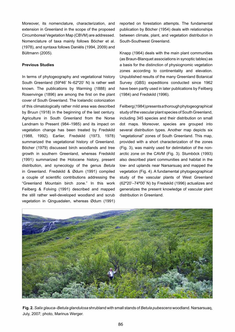
86

Moreover, its nomenclature, characterization, and extension in Greenland in the scope of the proposed Circumboreal Vegetation Map (CBVM) are addressed. Nomenclature of taxa mainly follows Böcher et al. (1978), and syntaxa follows Daniёls (1994, 2009) and Bültmann (2005).

Previous Studies

In terms of phytogeography and vegetational history South Greenland (59º46’ N–62º20’ N) is rather well known. The publications by Warming (1888) and Rosenvinge (1896) are among the first on the plant cover of South Greenland. The Icelandic colonization of this climatologically rather mild area was described by Bruun (1918) in the beginning of the last century. Agriculture in South Greenland from the Norse Landnam to Present (984–1985) and its impact on vegetation change has been treated by Fredskild (1988, 1992). Earlier, Fredskild (1973, 1978) summarized the vegetational history of Greenland. Böcher (1979) discussed birch woodlands and tree growth in southern Greenland, whereas Fredskild (1991) summarized the Holocene history, present distribution, and synecology of the genus Betula in Greenland. Fredskild & Ødum (1991) compiled a couple of scientific contributions addressing the “Greenland Mountain birch zone.” In this work Feilberg & Folving (1991) described and mapped the still rather well-developed woodland and scrub vegetation in Qinguadalen, whereas Ødum (1991)

reported on forestation attempts. The fundamental publication by Böcher (1954) deals with relationships between climate, plant, and vegetation distribution in South-Southwest Greenland.

Knapp (1964) deals with the main plant communities (as Braun-Blanquet associations in synoptic tables) as a basis for the distinction of physiognomic vegetation zones according to continentality and elevation. Unpublished results of the many Greenland Botanical Survey (GBS) expeditions conducted since 1962 have been partly used in later publications by Feilberg (1984) and Fredskild (1996).

Feilberg (1984) presents a thorough phytogeographical study of the vascular plant species of South Greenland, including 345 species and their distribution on small dot maps. Moreover, species are grouped into several distribution types. Another map depicts six “vegetational” zones of South Greenland. This map, provided with a short characterization of the zones (Fig. 3), was mainly used for delimitation of the non-arctic zone on the CAVM (Fig. 3). Stumböck (1993) also described plant communities and habitat in the low- and uplands near Narsarsuaq and mapped the vegetation (Fig. 4). A fundamental phytogeographical study of the vascular plants of West Greenland (62º20’–74º00’ N) by Fredskild (1996) actualizes and generalizes the present knowledge of vascular plant distribution in Greenland.

Fig. 2. Salix glauca–Betula glandulosa shrubland with small stands of Betula pubescens woodland. Narsarsuaq, July, 2007; photo, Marinus Werger.

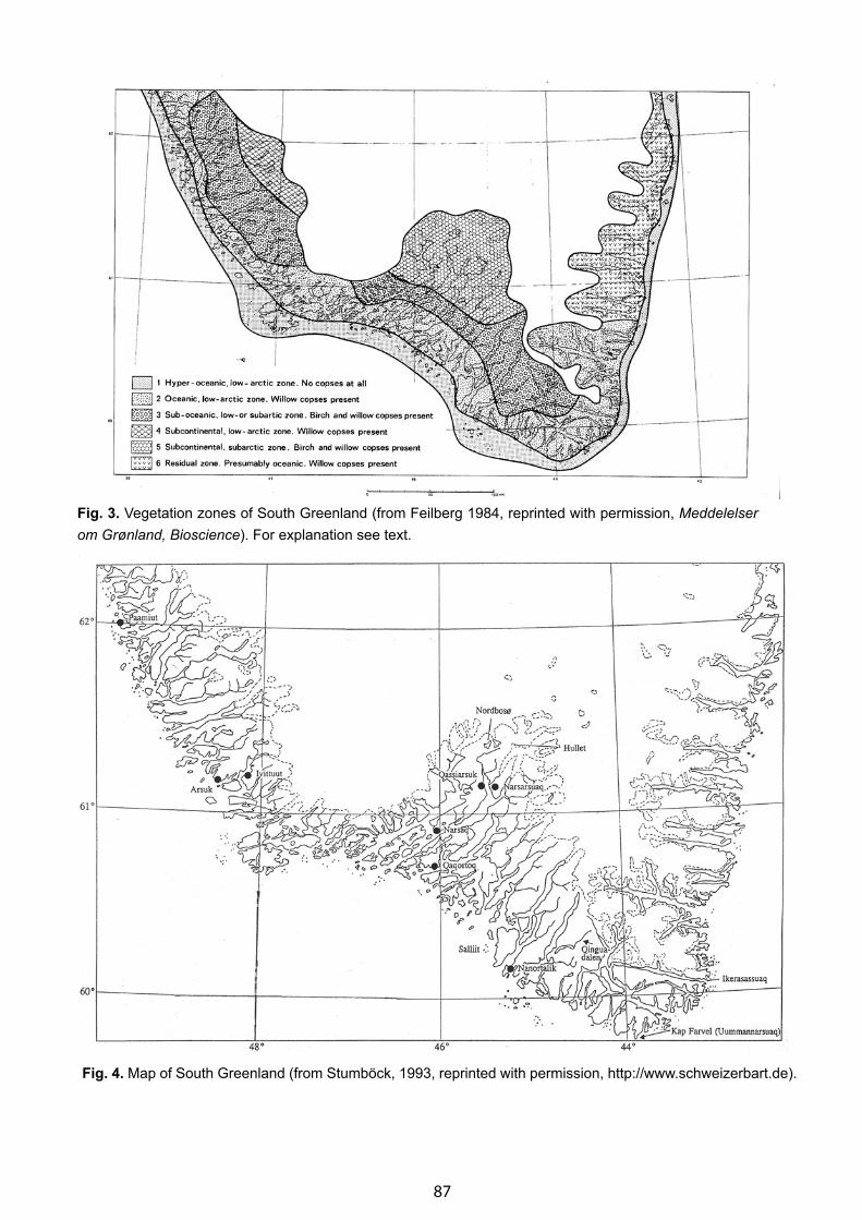
87

Fig. 3. Vegetation zones of South Greenland (from Feilberg 1984, reprinted with permission, Meddelelser om Grønland, Bioscience). For explanation see text.

Fig. 4. Map of South Greenland (from Stumböck, 1993, reprinted with permission, http://www.schweizerbart.de).

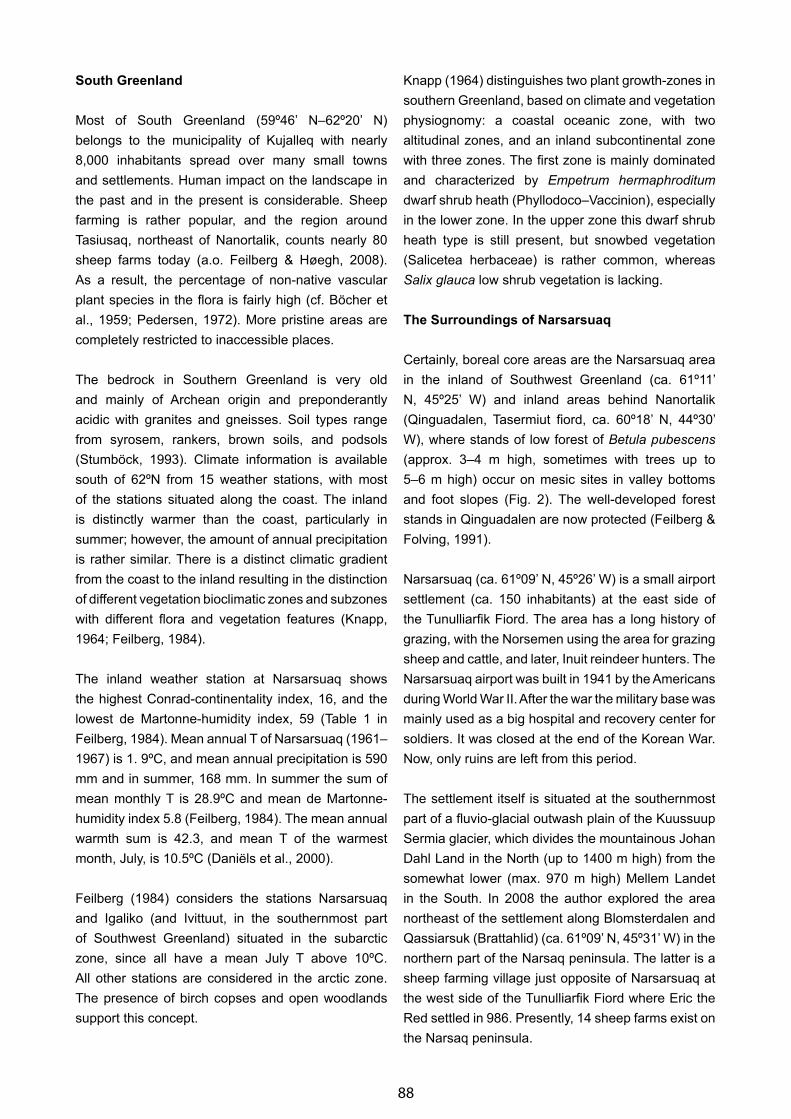
88

South Greenland

Most of South Greenland (59º46’ N–62º20’ N) belongs to the municipality of Kujalleq with nearly 8,000 inhabitants spread over many small towns and settlements. Human impact on the landscape in the past and in the present is considerable. Sheep farming is rather popular, and the region around Tasiusaq, northeast of Nanortalik, counts nearly 80 sheep farms today (a.o. Feilberg & Høegh, 2008). As a result, the percentage of non-native vascular plant species in the flora is fairly high (cf. Böcher et al., 1959; Pedersen, 1972). More pristine areas are completely restricted to inaccessible places.

The bedrock in Southern Greenland is very old and mainly of Archean origin and preponderantly acidic with granites and gneisses. Soil types range from syrosem, rankers, brown soils, and podsols (Stumböck, 1993). Climate information is available south of 62ºN from 15 weather stations, with most of the stations situated along the coast. The inland is distinctly warmer than the coast, particularly in summer; however, the amount of annual precipitation is rather similar. There is a distinct climatic gradient from the coast to the inland resulting in the distinction of different vegetation bioclimatic zones and subzones with different flora and vegetation features (Knapp, 1964; Feilberg, 1984).

The inland weather station at Narsarsuaq shows the highest Conrad-continentality index, 16, and the lowest de Martonne-humidity index, 59 (Table 1 in Feilberg, 1984). Mean annual T of Narsarsuaq (1961–1967) is 1. 9ºC, and mean annual precipitation is 590 mm and in summer, 168 mm. In summer the sum of mean monthly T is 28.9ºC and mean de Martonne-humidity index 5.8 (Feilberg, 1984). The mean annual warmth sum is 42.3, and mean T of the warmest month, July, is 10.5ºC (Daniëls et al., 2000).

Feilberg (1984) considers the stations Narsarsuaq and Igaliko (and Ivittuut, in the southernmost part of Southwest Greenland) situated in the subarctic zone, since all have a mean July T above 10ºC. All other stations are considered in the arctic zone. The presence of birch copses and open woodlands support this concept.

Knapp (1964) distinguishes two plant growth-zones in southern Greenland, based on climate and vegetation physiognomy: a coastal oceanic zone, with two altitudinal zones, and an inland subcontinental zone with three zones. The first zone is mainly dominated and characterized by Empetrum hermaphroditum dwarf shrub heath (Phyllodoco–Vaccinion), especially in the lower zone. In the upper zone this dwarf shrub heath type is still present, but snowbed vegetation (Salicetea herbaceae) is rather common, whereas Salix glauca low shrub vegetation is lacking.

The Surroundings of Narsarsuaq

Certainly, boreal core areas are the Narsarsuaq area in the inland of Southwest Greenland (ca. 61º11’ N, 45º25’ W) and inland areas behind Nanortalik (Qinguadalen, Tasermiut fiord, ca. 60º18’ N, 44º30’ W), where stands of low forest of Betula pubescens (approx. 3–4 m high, sometimes with trees up to 5–6 m high) occur on mesic sites in valley bottoms and foot slopes (Fig. 2). The well-developed forest stands in Qinguadalen are now protected (Feilberg & Folving, 1991).

Narsarsuaq (ca. 61º09’ N, 45º26’ W) is a small airport settlement (ca. 150 inhabitants) at the east side of the Tunulliarfik Fiord. The area has a long history of grazing, with the Norsemen using the area for grazing sheep and cattle, and later, Inuit reindeer hunters. The Narsarsuaq airport was built in 1941 by the Americans during World War II. After the war the military base was mainly used as a big hospital and recovery center for soldiers. It was closed at the end of the Korean War. Now, only ruins are left from this period.

The settlement itself is situated at the southernmost part of a fluvio-glacial outwash plain of the Kuussuup Sermia glacier, which divides the mountainous Johan Dahl Land in the North (up to 1400 m high) from the somewhat lower (max. 970 m high) Mellem Landet in the South. In 2008 the author explored the area northeast of the settlement along Blomsterdalen and Qassiarsuk (Brattahlid) (ca. 61º09’ N, 45º31’ W) in the northern part of the Narsaq peninsula. The latter is a sheep farming village just opposite of Narsarsuaq at the west side of the Tunulliarfik Fiord where Eric the Red settled in 986. Presently, 14 sheep farms exist on the Narsaq peninsula.

89

The Narsarsuaq area is situated in the subcontinental zone, and three altitudinal zones are distinguished here (Knapp, 1964, see also Stumböck, 1993). The lower Betula–Elyna-Zone is characterized by many plant community types, including a.o. mire vegetation, low Betula pubescens–Deschampsia flexuosa forest (Fig. 2), Salix glauca shrub vegetation types (Salix glauca–Deschampsia flexuosa type, Salix glauca type), dwarf shrub vegetation (Rhododendro–Vaccinietum), herb vegetation (Alchemilla alpina–Carex scirpoidea-Ass.), and lichen-rich dry grassland vegetation (Agrostis borealis─Carex scirpoidea-Ass.) (Agrostio─Rumicion acetosellae).

The middle Vaccinium─Cetraria-Zone is characterized by some low shrub vegetation (Salix glauca─Coptis groenlandica), lichen-rich dwarf shrub communities (Sphaerophoro-Vaccinietum, other Loiseleurio-Diapension vegetation and Dryadion integrifoliae communities), herb vegetation (Alchemilla glomerulans–Oxyria digyna-Ass.), snow patch vegetation (Anthoxanthum alpina vegetation), snowbed vegetation (Salicetea herbaceae), and lichen vegetation (Cladonion arbusculae). The upper zone Dryas─Rhacomitrium-Zone) is mainly characterized by very open vegetation, the prominence of Rhacomitrium lanuginosum-dominance, wind-exposed dwarf shrub heaths (Loiseleurio-Diapension), Juncus trifidus─Carex scirpoidea-Ass. (Juncion trifidi), Carici-Dryadetum, chionophobous lichen vegetation (Cetrarion nivalis), and snowbed vegetation (Salicetea herbaceae).

Vegetation types observed in and near the Narsarsuaq settlement in the lowland include a.o. Honkenyo–Elymetum mollis, Chamaenerietum latifolii, Eriophoretum scheuchzeri, Juncetum arctici, Caricetum microglochinis, Rhododendro–Vaccinietum, and herb-rich Salix glauca─Betula glandulosa scrub (Fig. 2) with Ranunculus acris and Angelica archangelica. Hippuridetum vulgaris and Sparganium hyperboreum occur in ponds. Mire vegetation (with several Scheuchzerio–Caricetea associations) is well developed in the valley bottom of Blomsterdalen.

In the farming areas of Qassiarsuk, pastures with a.o. Festuca rubra, Plantago maritima, Leontodon autumnalis, Rhinanthus cf. borealis, Poa pratensis,

and Achillea millefolium, and hay meadows with Alopecurus and Poa are common (“Molinio–Arrhenateretea”). Rey fields contain the European weeds Capsella bursa pastoris, Polygonum aviculare, Stellaria media, Matricaria discoides, and Cardamine pratense (“Stellarietea mediae”). Along rivulets Montia rivularis and Agrostis stolonifera are common. As in South Greenlandic settlements, several crops (e.g., potatoes, carrots) are raised in small fields mainly for private consumption.

In Narsarsuaq boreal species such as Lathyrus maritimus, Chamaenerion angustifolium, Elymus arenarius, Thymus drucei, Anthoxanthum odoratum ssp. alpinum, and Juniperus nana and the low arctic Betula glandulosa and Angelica archangelia are extremely common and very conspicuous. The Arboretum Groenlandicae (inofficially established in 1976, officially opened 2004) contains many North-American non-native coniferous species. Their height is still less than 10 m. Older plantations of coniferous trees are still in existence in South and Southwest Greenland, and nowadays several forestry projects on tree raising and cultivation are carried out.

Total number of vascular plant species in the Narsarsuaq area is estimated as 309 (Feilberg, 1984).

Vegetation types of the following classes could be identified for the Narsarsuaq and Qassiarsuk surroundings: Asplenietea trichomanis (fern and herb vegetation of rock fissures and ledges), Thlaspietea rotundifolii (herb vegetation of screes and alluvial plains), Caricetea curvulae (dry herb- and grass heath on acidic, mineral soil), Loiseleurio–Vaccinietea (acidic dwarf shrub heath), Carici–Kobresietea (grass- and dwarf shrub heath on weakly acidic-basic soil), Salicetea herbaceae (snowbed vegetation) (incl. Ranunculo–Anthoxanthion alpinae herb and grass vegetation, Knapp, 1964), Mulgedio─Aconitetea (hygrophytic tall herb, low shrub and low Betula pubescens forest vegetation), Montio–Cardaminetea (spring vegetation), Scheuchzerio–Caricetea (mire and rich fen vegetation), Honckenyo–Elymetea (vegetation of sandy-stony beaches), Juncetea maritimi (coastal salt-marsh vegetation), Littorelletea (amphiphytic vegetation on poor substrate), Phragmito–Magno–Caricetea (tall sedge-, grass-, and

90

herb vegetation swamp vegetation), Utricularietea (oligo-dystrophic aquatic vegetation), and Potametea (other aquatic vegetation) (cf. Daniёls, 1994, 2009; Daniёls et al., 2000). Well-developed vegetation of the classes Saxifrago tricuspidatae–Calamagrostietea purpurascentis (boreal and low arctic North-American steppe and associated vegetation (cf. Drees & Daniёls, 2009) and Oxycocco–Sphagnetea (bog vegetation) have not been observed yet.

Vegetation of hay meadows and pastures most likely belongs to the class Molinio–Arrhenatheretea and the weed vegetation of arable fields to the class Stellarietea mediae, both typical for the European culture landscapes.

Discussion

The characterization and delimitation of the non-arctic inland mountain birch area in Greenland was already discussed by Tukhanen (1984). On Tukhanen’s global map of circumboreal climatic-geographical regions (1984, App. 1, fig. 18) a small part of the southwestern coastal fringe area of Greenland is considered Northern Boreal, enclosed by a narrow Hemi-Arctic belt up to ca. 63ºN. The non-arctic inland area appears to be hemi-arctic in his scheme. However, the small-scale map does not allow a precise assessment of the extension of the regions.

Böcher (1979) rightly argues that south of 67ºN in Southwest Greenland thermic conditions occur in the inland of the fiords, which principally allow tree growth; however, Betula pubescens and Sorbus groenlandica are only found to occur in the southernmost inland part of this area. Human activities certainly prevented and still prevent hardwood tree growth as can be concluded from pollen diagrams (e.g., Fredskild, 1991), however the same is true for climate features, such as low summer temperatures at the outer coast and low precipitation (thus dryness) in very continental areas like in the Søndre Strømfjord area (ca. 67º00’ N, 50º40’ W), which prevent tree growth as well. Böcher considers these continental inland areas without native trees climatologically subarctic, whereas the CAVM vegetation map considers these areas as low arctic (Subzone 5, Walker et al., 2005) with low shrub vegetation; Calamagrostio lapponicae–Salicetum glaucae as zonal vegetation [cf. Sieg et al., 2006]).

In Böcher (1954) the non-arctic core area in South Greenland is situated in the region with his subarctic oceanic-suboceanic climate regime, and the extension of this climate regime largely coincides with the non-arctic area depicted on the CAVM map (Walker et al., 2005).

Feilberg (1984) (Fig. 3) considers the coastal fringe of the south and southwest coast belonging to his hyper-oceanic, low arctic zone (1), characterized by the total absence of copses. The adjacent oceanic, low arctic zone (2) has willow copses and the presence of Luzula parviflora. The adjacent suboceanic, low or subarctic zone (3) has willow and birch copses with Sorbus groenlandica. The western inland part of South Greenland is considered subcontinental, low arctic (4) with willow copses and the coincident occurrence of Carex supina and Kobresia myosuroides, whereas the innermost part of South Greenland with the Narsarsuaq area is considered subcontinental subarctic (5) with birch and willow copses and the coincident occurrence of the boreal species Eleocharis quinqueflora and Sagina nodosa.

The inland part of the Tugtutoq and Tasermiut districts and the entire Narsarsuaq district in the inland of the southwestern region of South Greenland (cf. Feilberg, 1984) can be considered boreal. This area coincides with the eastern part of Feilberg’s suboceanic, low- or subarctic zone (3) and the subcontinental, subarctic zone (5). Thus, on the CAVM, Feilberg’s zone 5 and the eastern part of zone 3 are considered non-arctic, representing roughly the inland part of South Greenland between approx. 44ºW and 47ºW.

In my opinion, the actual natural or potential natural zonal woodland vegetation with trees and shrubs (>2m) in the North should be a key criterion for considering an area either arctic or boreal (syn. subarctic, hemi-arctic) in a phytogeographical-bioclimatical context. In Greenland, where native coniferous trees are completely lacking, Betula pubescens and Sorbus groenlandica (Fig. 5) should be considered key indicators; this is not true of the native and azonal Alnus crispa, which forms thickets on moist soil in middle fiord or inland parts between 67ºN and 61ºN.

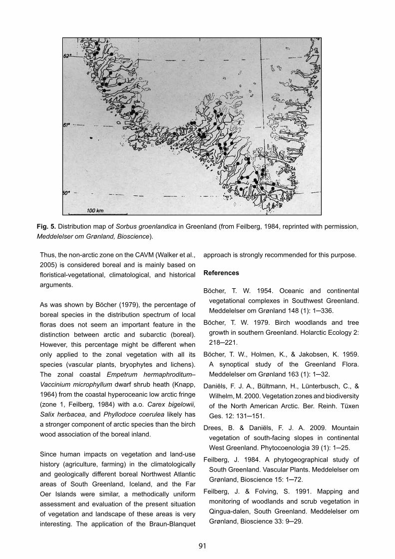
91

Thus, the non-arctic zone on the CAVM (Walker et al., 2005) is considered boreal and is mainly based on floristical-vegetational, climatological, and historical arguments.

As was shown by Böcher (1979), the percentage of boreal species in the distribution spectrum of local floras does not seem an important feature in the distinction between arctic and subarctic (boreal). However, this percentage might be different when only applied to the zonal vegetation with all its species (vascular plants, bryophytes and lichens). The zonal coastal Empetrum hermaphroditum–Vaccinium microphyllum dwarf shrub heath (Knapp, 1964) from the coastal hyperoceanic low arctic fringe (zone 1, Feilberg, 1984) with a.o. Carex bigelowii, Salix herbacea, and Phyllodoce coerulea likely has a stronger component of arctic species than the birch wood association of the boreal inland.

Since human impacts on vegetation and land-use history (agriculture, farming) in the climatologically and geologically different boreal Northwest Atlantic areas of South Greenland, Iceland, and the Far Oer Islands were similar, a methodically uniform assessment and evaluation of the present situation of vegetation and landscape of these areas is very interesting. The application of the Braun-Blanquet

approach is strongly recommended for this purpose.

References

Böcher, T. W. 1954. Oceanic and continental vegetational complexes in Southwest Greenland. Meddelelser om Grønland 148 (1): 1─336.

Böcher, T. W. 1979. Birch woodlands and tree growth in southern Greenland. Holarctic Ecology 2: 218─221.

Böcher, T. W., Holmen, K., & Jakobsen, K. 1959. A synoptical study of the Greenland Flora. Meddelelser om Grønland 163 (1): 1─32.

Daniёls, F. J. A., Bültmann, H., Lünterbusch, C., & Wilhelm, M. 2000. Vegetation zones and biodiversity of the North American Arctic. Ber. Reinh. Tüxen Ges. 12: 131─151.

Drees, B. & Daniёls, F. J. A. 2009. Mountain vegetation of south-facing slopes in continental West Greenland. Phytocoenologia 39 (1): 1─25.

Feilberg, J. 1984. A phytogeographical study of South Greenland. Vascular Plants. Meddelelser om Grønland, Bioscience 15: 1─72.

Feilberg, J. & Folving, S. 1991. Mapping and monitoring of woodlands and scrub vegetation in Qingua-dalen, South Greenland. Meddelelser om Grønland, Bioscience 33: 9─29.

Fig. 5. Distribution map of Sorbus groenlandica in Greenland (from Feilberg, 1984, reprinted with permission, Meddelelser om Grønland, Bioscience).

92

Feilberg, J. & Høegh, K. 2008. Greenland. NTNU Rapport Zoologisk Serie 2008─3: 44─53. Norwegian University of Science and Technology (NTNU), Science Museum, Section of Natural History, 7491, Trondheim.

Fredskild, B. 1973. Studies in the vegetational history of Greenland. Meddelelser om Grønland 198 (4): 1─245.

Fredskild, B. 1978. Paleobotanical investigations of some peat deposits of Norge age at Qagssiarssuk, South Greenland. Meddelelser om Grønland 204 (5): 1─41.

Fredskild, B. 1988. Agriculture in a Marginal Area-South Greenland from the Norse Landnam (985 A.D.) to the Present (1985 A.D.). Pages 381─393 in Birks, H.H., Birks, H.J.H., Kaland, P.E., & Moe, D., eds. The Cultural Landscape-Past, Present and Future. Cambridge University Press, Cambridge.

Fredskild, B. 1991. The genus Betula in Greenland—Holocene history, present distribution and synecology. Nord. J. Bot. 11: 393─412.

Fredskild, B. 1992. Erosion and vegetational changes in South Greenland caused by agriculture. Geogr. Tidsskr. 92: 14─21.

Fredskild, B. 1996. A phytogeographical study of the vascular plants of West Greenland (62º20’-74º00’N). Meddelelser om Grønland, Bioscience 45: 1─157.

Fredskild, B. & Ødum, S. 1991. The Greenland Mountain birch zone, Southwest Greenland. Meddelelser om Grønland, Bioscience 33: 1─80.

Hansen, B.U. 1991. Monitoring natural vegetation in southern Greenland using NOAA AVHRR and field measurements. Arctic 44, supp 1: 94─101.

Hester, A. J., Lempa, K., Neuvonen, S., Hoegh, K., Feilberg, J., Arnthorsdottir, S., & Iason, G. 2005.

Birch sapling responses to severity and timing of domestic herbivore browsing-implications for management. Ecological Studies 180: 139─155.

Knapp, R. 1964. Über Eigenschaften arktischer und subarktischer Vegetation am Beispiel der Pflanzenwelt in einigen Gebieten des südlichen Grönland. Ber. Oberhess. Ges. f Natur- und Heilk. zu Gießen, N.F, Naturwiss. Abt. 33: 91─129.

Ødum, S. 1991. Afforestation experiments reflecting the treeline conditions in Southwest Greenland. Meddelelser om Grønland, Bioscience 33: 43─61.

Pedersen, A. 1972. Adventitious plants and cultivated plants in Greenland. Meddelelser om Grønland 178 (7): 1─99.

Rosenvinge, L. K. 1896. Det sydligste Grønlands vegetation. Meddelelser om Grønland 15: 73─249.

Sieg, B., Drees, B., & Daniёls, F. J. A. 2006. Vegetation and altitudinal zonation in continental West Greenland. Meddelelser om Grønland, Bioscience 57: 1─93.

Stumböck, M. 1993. Vegetation und Ökologie von Narsarsuaq, Südwestgrönland. Diss. Bot. 203.

Tuhkanen, S. 1984. A circumboreal system of climatic-phytogeographical regions. Acta Bot. Fenn. 127: 1─50.

Walker, D. A., Raynolds, M. K., Daniëls, F. J. A., Einarsson, E., Elvebakk, A., Gould, W. A., Katenin, A. E., Kholod, S. S., Markon, C. J., Melnikov, E. S., Moskalenko, N. G., Talbot, S. S., Yurtsev, B. A., & the other members of the CAVM Team. 2005. The Circumpolar Arctic Vegetation Map. J. Veg. Sci. 16 (3): 267─282.

Warming, E. 1888. Om Grønlands vegetation. Meddelelser om Grønland 12: 1─245.

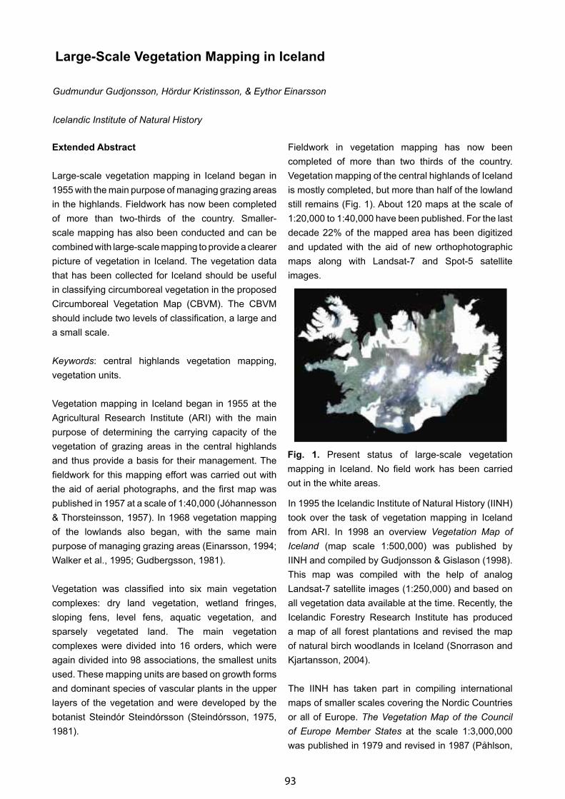
93

Large-Scale Vegetation Mapping in Iceland

Gudmundur Gudjonsson, Hördur Kristinsson, & Eythor Einarsson

Icelandic Institute of Natural History

Extended Abstract

Large-scale vegetation mapping in Iceland began in 1955 with the main purpose of managing grazing areas in the highlands. Fieldwork has now been completed of more than two-thirds of the country. Smaller-scale mapping has also been conducted and can be combined with large-scale mapping to provide a clearer picture of vegetation in Iceland. The vegetation data that has been collected for Iceland should be useful in classifying circumboreal vegetation in the proposed Circumboreal Vegetation Map (CBVM). The CBVM should include two levels of classification, a large and a small scale.

Keywords: central highlands vegetation mapping, vegetation units.

Vegetation mapping in Iceland began in 1955 at the Agricultural Research Institute (ARI) with the main purpose of determining the carrying capacity of the vegetation of grazing areas in the central highlands and thus provide a basis for their management. The fieldwork for this mapping effort was carried out with the aid of aerial photographs, and the first map was published in 1957 at a scale of 1:40,000 (Jóhannesson & Thorsteinsson, 1957). In 1968 vegetation mapping of the lowlands also began, with the same main purpose of managing grazing areas (Einarsson, 1994; Walker et al., 1995; Gudbergsson, 1981).

Vegetation was classified into six main vegetation complexes: dry land vegetation, wetland fringes, sloping fens, level fens, aquatic vegetation, and sparsely vegetated land. The main vegetation complexes were divided into 16 orders, which were again divided into 98 associations, the smallest units used. These mapping units are based on growth forms and dominant species of vascular plants in the upper layers of the vegetation and were developed by the botanist Steindór Steindórsson (Steindórsson, 1975, 1981).

Fieldwork in vegetation mapping has now been completed of more than two thirds of the country. Vegetation mapping of the central highlands of Iceland is mostly completed, but more than half of the lowland still remains (Fig. 1). About 120 maps at the scale of 1:20,000 to 1:40,000 have been published. For the last decade 22% of the mapped area has been digitized and updated with the aid of new orthophotographic maps along with Landsat-7 and Spot-5 satellite images.

In 1995 the Icelandic Institute of Natural History (IINH) took over the task of vegetation mapping in Iceland from ARI. In 1998 an overview Vegetation Map of Iceland (map scale 1:500,000) was published by IINH and compiled by Gudjonsson & Gislason (1998). This map was compiled with the help of analog Landsat-7 satellite images (1:250,000) and based on all vegetation data available at the time. Recently, the Icelandic Forestry Research Institute has produced a map of all forest plantations and revised the map of natural birch woodlands in Iceland (Snorrason and Kjartansson, 2004).

The IINH has taken part in compiling international maps of smaller scales covering the Nordic Countries or all of Europe. The Vegetation Map of the Council of Europe Member States at the scale 1:3,000,000 was published in 1979 and revised in 1987 (Påhlson,

Fig. 1. Present status of large-scale vegetation mapping in Iceland. No field work has been carried out in the white areas.

94

1994). The Map of the Physical Geographic Regions was mainly based on natural vegetation and was published by the Nordic Council of Ministers (Nordiska Ministerrådet, 1984). Maps of the Natural Vegetation of Europe including Iceland were published in the year 2000 in two scales, 1:10,000,000 and 1:2,500,000 (Bohn et al., 2000). Finally, the IIHN took part in compiling the Circumpolar Artic Vegetation Map in scale 1: 7,500,000 (CAVM, 2003).

Now, when it has been decided to proceed and extend the Circumpolar Arctic Vegetation Map to cover also the boreal area, we suggest the following steps:

• The CBVM project should be approached in a similar way as the CAVM.

• The status of boreal vegetation mapping in each of the boreal countries should be reviewed.

• Classification should be conducted the same way, with additions to cover the boreal vegetation.

• A mapping team should be established that ensures all participants work along the same lines from the beginning.

• The southern limit should be defined.

• Present vegetation maps should be collected from the respective countries, and a common classification key for the whole area should be produced.

• Mapping should include two levels of classification, a larger scale and a smaller scale.

• The final map scale should be about 1:7,500,000.

References

Bohn, U., Gollub, G., & Hettwer, C. (compilers). 2000. Karte der Naturlichen Vegetation Europas. Buntersamt Fur Naturschutz, Bonn. 153 pp. + maps.

CAVM Team. 2003. Circumpolar Arctic Vegetation Map. Conservation of Arctic Flora and Fauna (CAFF) Map No. 1, U.S. Fish and Wildlife Service, Anchorage, Alaska.

Einarsson, E. 1994. Vegetation Mapping in Iceland. Pages 52─53 in Walker D. A. & Markon, C. J., eds. Circumpolar Arctic Vegetation Mapping Workshop. Open File Report 96–251. U.S. Department of the Interior, U.S. Geological Survey, National Mapping Division. http://mapping-ak.wr.usgs.gov/research/cavm/pdf/CAVM.pdf.

Gudbergsson, G. 1981: Vegetation mapping in Iceland. Journ. of Agricult. Research in Iceland. 12: (2) 59–83.

Gudjonsson, G. & Gislason, E. 1998: Vegetation Map of Iceland. 1:500000. General overview. Icelandic Institute of Natural History, Reykjavik (1st edition).

Jóhannesson, B & Thorsteinsson, I. 1957. Gródurkort og lýsing Gnúpverjaafréttar. Dept. of Agricult. Reports. Ecol. Surveys No.1. University Research Institute. 31 pp.

Nordiska Minesterrådet, Stockholm. 1984. Naturgeografisk regionindeling av Norden. 289 pp + map.

Påhlsson, L., ed. 1994. Vegetationtyper í Norden. Nordisk Minesterråd, Köbenhavn. 627 pp.

Snorrason, A. & Kjartansson, B. 2004. Íslensk skógarúttekt─Verkefni um landsúttekt á skóglendum á Íslandi. Skógræktarritið 2004 (2): 101–108.

Steindórsson, S. 1975. Studies on the Mire-Vegetation of Iceland. Societas Scientiarum Islandica XLI.. Reykjavik. 226 pp.

Steindórsson, S. 1981: Vegetation classification in Iceland. Journ. of Agricult. Research in Iceland. 12 (2): 11–57.

Walker, D. A., Bay, C., Daniёls, F. J. A., Einarsson, E., Elvebakk, A., Johansen, B. E., Kapitsa, A., Kholod, S. S., Murray, D. F., Talbot, S. S., Yurtsev, B. A., & Zoltai, S. C. 1995. Toward a new Arctic vegetation map: a review of existing maps. J. Veget. Science 6 (3) 427–436.

95

The Vegetation of the Faroe Islands

Anna Maria Fosaa

Faroese Museum of Natural History, Tórshavn, Faroe Islands, anmarfos@ngs.fo

Extended Abstract

Due to the lack of natural trees, the vegetation in the Faroe Islands has been difficult to classify. The lowland part of the islands was classified by Tuhkanen (1987) as a highly oceanic part of the hemiboreal subzone. The predominant vegetation is grassland, which is found from sea level to the mountaintop, while the lowland is characterized by heathland vegetation. Moist-dwarf shrub and heathland vegetation is often found in plant communities that are similar to those of the lowland zone in coastal Norway, which would indicate that the lower elevation areas of the Faroe Island (up to 200 m a.s.l.) falls into the middle boreal zone (Fosaa, 2004). A preliminary map was drawn from topographic maps, scale 1:20,000, and digitized. This map divides the islands into the main classes of grassland, heaths, mires, lakes, and fell-field. From this map, an approximate areal cover of each of these vegetation types is given. In this presentation, an overview of these vegetation types is given as well as their distribution and the changes that have formed the vegetation that we have in the Faroe Islands today.

Climate

The Faroe Islands are a small (1400 km2), but relatively steep (highest peak 882 m a.s.l.), archipelago (18 islands) situated in the Northeastern Atlantic (62ºN, 7ºW). The climate of the islands is humid and windy. On daily timescales, it is highly variable, but the strong influence from the North Atlantic Current helps maintain a small seasonal temperature variation.

Vegetation Change

In the first period after the last ice age, natural climate fluctuations had the greatest impact on the vegetation. After human settlement, the influence of humans has become the main impact. In the Preboreal period (10,000–9,000 B.P.), the Faroe Islands have been

described as arctic continental, based on the presence of Betula nana (Jóhansen, 1972, 1985). This species disappeared again as the climate changed towards more oceanic conditions. In the Boreal period (9,000–8,000 B.P.), species such as Juniperus communis and Salix spp. took over, together with Poaceae and Cyperaceae, which covered the lowland at that time. The climate became wetter in the Atlantic period (8,000–5,000 B.P.) with evidence of strong leaching of the soil. Peat was formed and Calluna vulgaris invaded. Juniperus communis and Salix spp. decreased but did not disappear completely. When the climate became drier again (Sub-boreal 5,000–2,500 B.P.), the two species increased again.

In the period from Sub-boreal (5,000–2,500 B.P.) to Subatlantic (2,500 B.C.–0 A.D.), the vegetation changes are described as a decline in tall-herb vegetation and shrub, with an increase in the distribution of Calluna vulgaris (Jóhansen, 1985).

It was previously believed that the decline in Juniperus and Salix spp. was due to human settlement. Newer results based on macrofossil studies show, however, that woodland species were already retreating prior to human settlement, before the occurrence of peatland and heathland species, and that the settlement only accelerated the degradation process initiated by climate change (Hannon, 2000; Hannon et al., 2001). It is therefore unclear whether the treeless grasslands and heathlands that characterize the islands today are a cultural product due to sheep grazing, as has been demonstrated elsewhere in northern Europe, or have developed as a result of recent climatic change.

Distribution of Vegetation Types

The main vegetation type of the islands is grassland that goes from lowland to the top of the mountains and covers ca. 77% of the total area. The grassland can be divided into two main types, which are wet grassland and dry grassland. Wet grassland is mainly found

96

in the lowland, while dry grassland is more common on the minerogenic soils in the highland. Common species are Festuca vivipara, F. rubra, Agrostis canina, A. capillaris, Nardus stricta, Deschampsia flexuosa, and Anthoxanthum odoratum.

Heathland covers 2.9% of the total area, mainly in the lowland vegetation belt up to 200 m a.s.l. Three main heath communities in the Faroe Islands are defined by increasing moisture from dry heath to relatively wet heath. The driest of the heaths is the Calluna vulgaris─Erica cinerea community. When the humidity increases, the Calluna vulgaris–Erica cinerea community is replaced by the Calluna vulgaris community and again by the Empetrum–Vaccinium community. In these wet heaths, Narthecium ossifragum and Juncus sqarrosus are frequent (Böcher, 1940). Common species are Calluna vulgaris, Empetrum nigrum, Erica cinerea, Vaccinium myrtillus, V. uliginosum, Potentilla erecta, Nardus stricta, Carex pilulifera, Galium saxatilis, and Hypericum pulcrum.

Mires cover 1.4% of the total area. Three different kinds of mires are defined: topogenic mires with their origin in overgrown lakes or tarns, soligenic mires on hills and slopes, and ombrogenic mires in valleys. Common species that are growing in the Sphagnum moss are Eriophorum angustifolium, Juncus squarrosus, Scirpus cespitosus, Narthecium ossifragum, Carex panicea, Carex nigra, and Pinguicula vulgaris.

Lakes cover 0.9% of the total area. Most lakes are small, less than 100 m2, and poor in nutrients. In shallow water on the shores of the lakes, Litorella uniflora often hides the bottom like a mat. On gravel bottoms, the most common plants are Isoëtes echinospora, I. lacustris, Littorella uniflora, Ranunculus flammula, Subularia aquatica, and Juncus bulbosus. On soft bottoms, the common species are Sparganium angustifolium and Myriophyllum alterniflorum, and species of Potamogeton, such as P. natans, P. gramineus, and P. perfoliatus.

The alpine zone covers 8% of the total area and includes the flat mountaintops forming “fell fields.” These fell-fields are formed as a result of erosion and are found from an elevation of a few hundred metres up to the highest mountaintop (882 m). Such plateau-like areas are exposed to strong winds, and the

substrate freezes and thaws repeatedly. Most of these areas consist of a mosaic of cliff surfaces with moss and lichens, and a few higher plants. The vegetation is very distinctive, though sparse. It is the instability of the ground and its constant movement that causes the scarcity of flora. Snow cover is very important in alpine areas, protecting the soil surface from frost penetration in winter. Due to mild winter temperatures plants must be able to withstand a winter with only occasional snow cover, which is liable to disturb the winter period of inactivity. Only limited information on the duration of the snow cover in the alpine areas is available from the Faroe Islands. Meteorological information on the duration of snow cover in Tórshavn in the period 1961–1991 shows that January had the maximum number of days of snow cover (10.8 days), while the period from May to October had no snow cover.

The most common plants in the alpine zone are Koenigia islandica, Cardaminopsis petreae, Luzula spicata, Alchemilla alpina, Bistorta vivipara, Saxifraga rosacea, Loiseleuria procumbens, Sibbaldia procumbens, Salix herbacea, and Ranunculus glacialis.

Due to their shape, some of the pointed mountaintops are not as exposed to wind as are the flat mountains. On these pointed peaks, wind passage past the mountain leaves a relatively calm area on the top. These mountaintops have an almost 100% cover of the grayish moss Racomitrium lanuginosum. This vegetation typically covers a region from the top and around 100 m down where the mountain again is exposed to strong wind and the vegetation becomes sparse. The Racomitrium heath vegetation is found on sloping terrain on relatively dry soil protected from wind. Racomitrium lanuginosum is widely distributed at all elevations in the islands and is also typical for areas where the snow melts late. In these areas we find so called snow-bed communities with Sibbaldia procumbens, Saxifraga oppositifolia, Silene acaulis, and Alchemilla alpina.

As no details on specific plant communities are given on the topographic map used to map the vegetation types, it is not possible to tell how much of the islands are covered with Racomitrium heath. Most likely, Racomitrium heath is included in the grassland type.

97

Three altitudinal vegetation zones can be defined: heathland in the lowland and up to 200 m a.s.l.; a transition zone up to 400 m a.s.l., which has wet grassland as the characteristic vegetation; and from 400 m a.s.l. up to the mountain tops, Racomitrium vegetation and dry-vegetation.

References

Böcher, T. W. 1940. Studies on the plant-geography of the North-Atlantic heath-formation. I The heath of the Faroes. Kgl. Dan. Vid. Selsk. Biol. Medd. 15: 1–64.

Fosaa, A. M. 2004. Altitudinal distribution of plant communities in the Faroe Islands. Fróðskaparrit 51: 200–211.

Hannon, G. 2000. Impact of timing of the first human settlement on vegetation in the Faroe Islands. Quarternary Research 54: 404–413.

Hannon, G. E., Wastegård, S., Bradshaw, E., & Bradshaw, R. H. W. 2001. Humane impact and landscape degradation on the Faroe Islands. Biology and Environment: Procedings of the Royal Irish Academy 101B (1–2): 129–139.

Jóhansen, J. 1972. A palaeobotanical study indicating a preViking settlement in the village of Tørnuvík, Faroe Islands. Fróðskaparrit 19: 45–157.

Jóhansen, J. 1985. Studies in the vegetational history of the Faroe and Shetland Islands. Fróðskaparrit, Tórshavn, 117 pp.

Tuhkanen, S. 1987. The phytogeographical position of the Faroe Islands and their ecoclimatic correspondence on the other continents: Problems associated with highly oceanic areas. Ann. Bot. Fennici. 24: 111–135.

98

The Plant Cover of the Kamchatka Peninsula (North of the Russian Far East) and Its Geobotanical Subdivision

Valentina Yu. Neshataeva

Komarov Botanical Institute, Russian Academy of Sciences, Saint Petersburg, Russia, vneshataeva@yandex.ru

Abstract

Y.Y. Vasiljev (1947) carried out the first geobotanical subdivision of Kamchatka Peninsula and distinguished the territory as the Kamchatka herb-rich and broad-leaved-forest region. At present it is considered to be a special Kamchatka deciduous forest subregion of the Euro-Asiatic taiga region. The plant cover of the subregion was initially characterized by the predominance of stone-birch (Betula ermanii) forests on the plains. The area was subdivided into six geobotanical provinces and 20 districts. Three provinces of plains were distinguished: I – Eastern Kamchatka suboceanic province, characterized by the predominance of herb- and shrub-rich stone-birch forests and dwarf-shrub heath communities dominated by Empetrum nigrum; II – Western Kamchatka maritime province, which differed from the other provinces by the prevalence of grass- and short-herb-rich stone-birch forests, tall-herb meadows with Angelica ursina, and blanket bogs; and III – Central Kamchatka subcontinental province, characterized by the predominance of larch (Larix cajanderi) and spruce (Picea ajanensis) taiga forests and secondary Japanese-birch (Betula platyphylla) forests. Three mountain provinces were distinguished: IV – Middle Kamchatka mountain province with the predominance of Siberian dwarf-pine (Pinus pumila) elfin woods and mountain tundra; V – Eastern Kamchatka volcanic mountain province, with the special volcanogenic variant of altitudinal zonality and the prevalence of serial plant communities and secondary permanent associations at the volcanic plateaus; and VI – Southern Kamchatka mountain province, with a suboceanic subtype of altitudinal zonality and the prevalence of dwarf-alder (Alnus fruticosa s.l.) shrubs and suboceanic dwarf-shrub heaths. It was shown that the differentiation of Kamchatka vegetation cover was subordinated mainly to zonal and altitudinal patterns. Permanent volcanogenic influences caused irreversible plant succession processes. As a result of

Holocene volcanic activities, serial plant communities and secondary permanent associations are prevalent in the vast areas of Central Kamchatka: Japanese-birch (Betula platyphylla) forests and larch (Larix cajanderi) forests covering the central part of the peninsula replaced the virgin primeval spruce (Picea ajanensis) and stone-birch (Betula ermani) forests.

Keywords: altitudinal zonality, geobotanical subdivision, Kamchatka Peninsula, vegetation cover.

Introduction

The Kamchatka Peninsula is situated north of the Russian Far-East between 50º 52’–60º 52’ N and 155º 34’–164º 00’ E. The area of the peninsula is 350,000 km2. The extent of the peninsula from the north to the south is 1,200 km, with a maximal width of 480 km. The northern border of the Kamchatka Peninsula passes through the line from the Rekinniki Bay to the gulf of Anapka, separating the peninsula from the continental part of the Kamchatka administrative region.

Relief and Geology

Several high mountain ridges divide the territory of the peninsula. The largest of them, the Sredinny and Vostochny ranges, are meridional and stretch for a thousand kilometers. The main plains—the Central Kamchatka depression, the Western Kamchatka, and the Eastern Kamchatka lowlands—are meridional too. The tectonic structure of the peninsula, the location of volcanoes, river valley patterns, and the character of the coastline are determined by large fractures stretched in northeast and northwest directions. The active tectonic movements are still in progress causing the high seismicity of the peninsula and the modern volcanism. The Kamchatka Peninsula is notable for its active volcanoes, geysers, and hot springs. At present, there are 30 active and 120 dormant volcanoes on the peninsula; most of them are concentrated in

99

the eastern, central, and southern volcanic regions. Volcanic eruptions with the ejection of 1–10 million m3 of igneous rock are registered almost every year. Volcanic eruptions of high magnitude (ejection of more than 1 km3 of igneous rock) occur almost every 400 years and cause regional catastrophes. Gigantic catastrophic eruptions with a volume of 10–100 km3 damage the plant cover over an area of 10–100,000 km2. During the Holocene, 24 of such gigantic eruptions occurred within Kamchatka.

Climate

The climate of the peninsula is cold and extremely wet with a high snow cover. The annual sum of active temperatures more than 10ºC doesn’t exceed 1200ºC. The average temperature of the warmest month is not more than 15ºC, and of the coldest month, no less than -20ºC. The annual amount of precipitation is from 350 mm for the Central Valley of Kamchatka up to 1,000 mm at the coastline and from 1,200 mm to 1,400 mm at the oceanic peninsulas and in the mountains. The average thickness of snow cover is 100 cm. The most mild and wet climate is at the eastern coast. The climate of the western coast is colder; the annual average temperature is below zero and the annual precipitation is lower than at the Eastern coast. The Central Kamchatka depression is characterized by the subcontinental climate. In summer the temperature is usually up to 25─30ºC and in winter falls to -40ºC. The regime of humidification is contrasting: there is a dry spring season and a rainy autumn period. The coldest climate is at the northern parts of the peninsula. The annual average temperature is -2.5ºC. The climatic differences between the eastern and the western coasts of the peninsula are determined by the different heat regimes of the Sea of Okhotsk, the Bering Sea, and the Pacific Ocean and by the patterns of the seasonal atmospheric circulation.

Soils

The specific soils of Kamchatka are formed on acid volcanic rocks under the influence of a cold and wet climate. The volcanic eruptions cause the heavy ash-, sand- and scoria falls. The thickness of the soil profile increases with the ash-falls. The volcanic soils have the stratified structure and the polygenic soil profile consisting of several elementary soil profiles and several volcanic-ash layers. They are characterized by

the high concentration of copper (Cu), the deficiency of chrome (Cr), nickel (Ni), tin (Sn), strontium (Sr), molybdenum (Mo), and silver (Ag) and by the high extent of water permeability.

Methods

The plant cover of Kamchatka was studied for a period of 18 field seasons using sample plots and transects. Sample plots measuring 400 m2 for forests and 100 m2 for other plant communities were laid along the altitude transects. The location of each sample plot was estimated with the help of a GPS personal navigator. The species composition, including vascular plants, bryophytes, and lichens, and the percentage cover of each species, were estimated. More than 4,000 relevés were analyzed using a standard phytosociological table method, and several vegetation maps of key areas were compiled at the scales of 1:1,000 and 1:5,000. For the means of a geobotanical subdivision of the vegetation cover of Kamchatka forest type, topographic maps and aerial photographs were used. The phytosociological plant community classification was described. The plant communities were classified, taking into account not only the floristic composition, but also the presence and abundance of species. The syntaxonomic range of relevé groups obtained was ranked according to the Russian phytosociological tradition using the principles first elaborated by Sukatchov (1928). The plant communities of the Kamchatka Peninsula belong to 145 associations representing 96 formations, 25 classes of formations, and seven vegetation types.

Results and Discussion

Zonal Patterns

The main zonal patterns of the vegetation cover are developed at vast maritime lowlands and wide intermontane plains that are meridional as well. The territory of Kamchatka is related to the Taiga (conifer forest) zone. The phytogeographic phenomenon of the prevalence of primary stone-birch (Betula ermanii) forests replacing the coniferous forests at the sea shores is connected to the cold and moist maritime climate of eastern and southern coasts of the peninsula and particularly with the lack of the summer heat. The same phenomenon was first described by Hämet-Ahti (1963, 1987) and Hämet-Ahti (1969) for

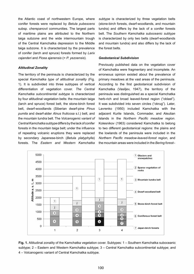
100

the Atlantic coast of northwestern Europe, where conifer forests were replaced by Betula pubescens subsp. cherepanovii communities. The largest parts of maritime plains are attributed to the Northern taiga subzone and the wide intermountain trough of the Central Kamchatka depression to the Middle taiga subzone. It is characterized by the prevalence of conifer (larch and spruce) forests formed by Larix cajanderi and Picea ajanensis (= P. yezoensis).

Altitudinal Zonality

The territory of the peninsula is characterized by the special Kamchatka type of altitudinal zonality (Fig. 1). It is subdivided into three subtypes of vertical differentiation of vegetation cover. The Central Kamchatka subcontinental subtype is characterized by four altitudinal vegetation belts: the mountain taiga (larch and spruce) forest belt, the stone-birch forest belt, dwarf-woodlands (Siberian dwarf-pine Pinus pumila and dwarf-alder Alnus fruticosa s.l.) belt, and the mountain tundra belt. The Volcanogenic variant of Central Kamchatka subtype differs by the lack of conifer forests in the mountain taiga belt; under the influence of repeating volcanic eruptions they were replaced by secondary Japanese-birch (Betula platyphylla) forests. The Eastern and Western Kamchatka

subtype is characterized by three vegetation belts (stone-birch forests, dwarf-woodlands, and mountain tundra) and differs by the lack of a conifer forests belt. The Southern Kamchatka suboceanic subtype is characterized by only two belts (dwarf-woodlands and mountain tundra) and also differs by the lack of the forest belts.

Geobotanical Subdivision

Previously published data on the vegetation cover of Kamchatka were fragmentary and incomplete. An erroneous opinion existed about the prevalence of primary meadows at the vast areas of the peninsula. According to the first geobotanical subdivision of Kamchatka (Vasiljev, 1947), the territory of the peninsula was distinguished as a special Kamchatka herb-rich and broad leaved-forest region (“oblast”). It was subdivided into seven circles (“okrug”). Later, Lavrenko (1950) included Kamchatka with the adjacent Kurile Islands, Commader, and Aleutian Islands in the Northern Pacific meadow region. Kolesnikov (1963) considered Kamchatka to belong to two different geobotanical regions: the plains and the lowlands of the peninsula were included in the Northern Pacific meadow-leaved-forest region, and the mountain areas were included in the Bering forest–

Fig. 1. Altitudinal zonality of the Kamchatka vegetation cover. Subtypes: 1 – Southern Kamchatka suboceanic subtype; 2 – Eastern and Western Kamchatka subtype; 3 – Central Kamchatka subcontinental subtype; and 4 – Volcanogenic variant of Central Kamchatka subtype.

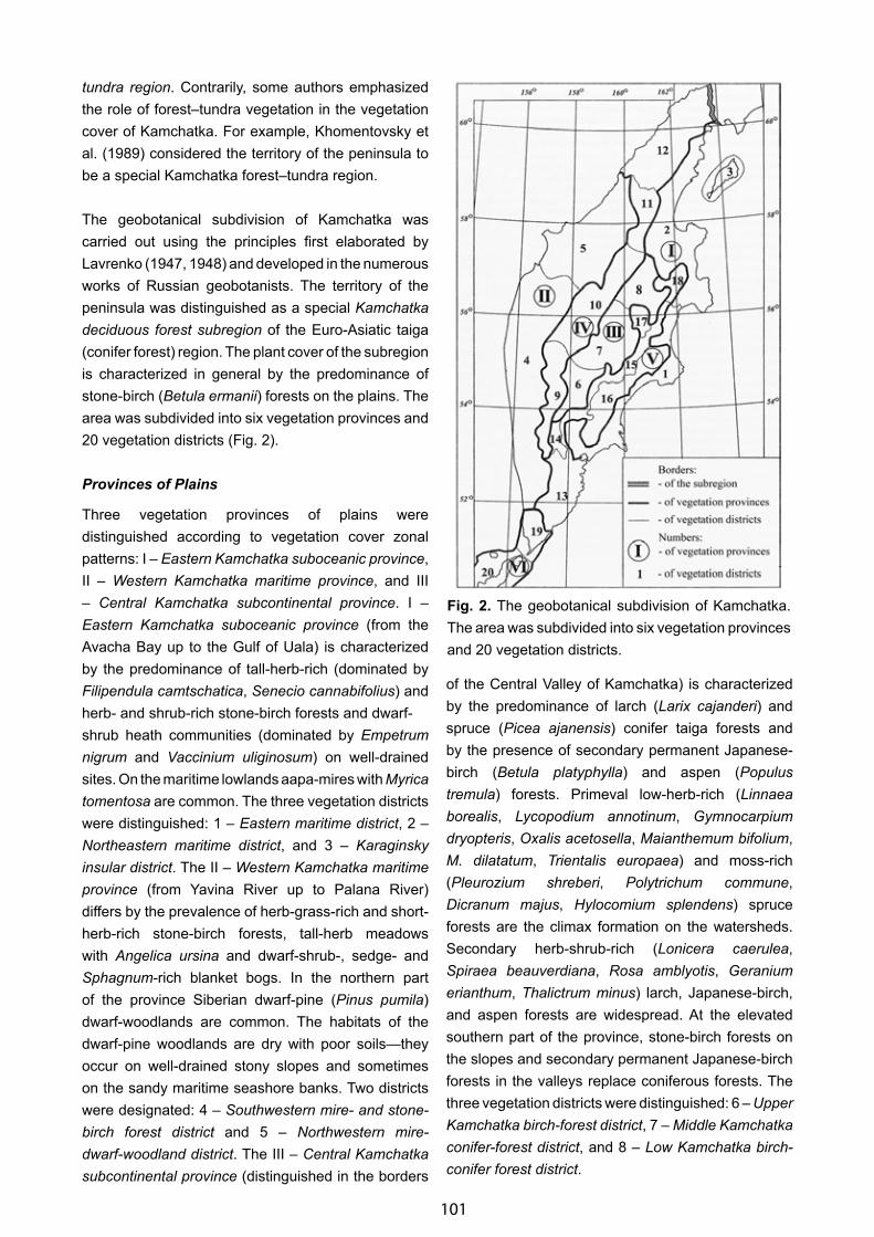
101

tundra region. Contrarily, some authors emphasized the role of forest–tundra vegetation in the vegetation cover of Kamchatka. For example, Khomentovsky et al. (1989) considered the territory of the peninsula to be a special Kamchatka forest–tundra region.

The geobotanical subdivision of Kamchatka was carried out using the principles first elaborated by Lavrenko (1947, 1948) and developed in the numerous works of Russian geobotanists. The territory of the peninsula was distinguished as a special Kamchatka deciduous forest subregion of the Euro-Asiatic taiga (conifer forest) region. The plant cover of the subregion is characterized in general by the predominance of stone-birch (Betula ermanii) forests on the plains. The area was subdivided into six vegetation provinces and 20 vegetation districts (Fig. 2).

Provinces of Plains

Three vegetation provinces of plains were distinguished according to vegetation cover zonal patterns: I – Eastern Kamchatka suboceanic province, II – Western Kamchatka maritime province, and III – Central Kamchatka subcontinental province. I – Eastern Kamchatka suboceanic province (from the Avacha Bay up to the Gulf of Uala) is characterized by the predominance of tall-herb-rich (dominated by Filipendula camtschatica, Senecio cannabifolius) and herb- and shrub-rich stone-birch forests and dwarf-shrub heath communities (dominated by Empetrum nigrum and Vaccinium uliginosum) on well-drained sites. On the maritime lowlands aapa-mires with Myrica tomentosa are common. The three vegetation districts were distinguished: 1 – Eastern maritime district, 2 – Northeastern maritime district, and 3 – Karaginsky insular district. The II – Western Kamchatka maritime province (from Yavina River up to Palana River) differs by the prevalence of herb-grass-rich and short-herb-rich stone-birch forests, tall-herb meadows with Angelica ursina and dwarf-shrub-, sedge- and Sphagnum-rich blanket bogs. In the northern part of the province Siberian dwarf-pine (Pinus pumila) dwarf-woodlands are common. The habitats of the dwarf-pine woodlands are dry with poor soils—they occur on well-drained stony slopes and sometimes on the sandy maritime seashore banks. Two districts were designated: 4 – Southwestern mire- and stone-birch forest district and 5 – Northwestern mire-dwarf-woodland district. The III – Central Kamchatka subcontinental province (distinguished in the borders

of the Central Valley of Kamchatka) is characterized by the predominance of larch (Larix cajanderi) and spruce (Picea ajanensis) conifer taiga forests and by the presence of secondary permanent Japanese-birch (Betula platyphylla) and aspen (Populus tremula) forests. Primeval low-herb-rich (Linnaea borealis, Lycopodium annotinum, Gymnocarpium dryopteris, Oxalis acetosella, Maianthemum bifolium, M. dilatatum, Trientalis europaea) and moss-rich (Pleurozium shreberi, Polytrichum commune, Dicranum majus, Hylocomium splendens) spruce forests are the climax formation on the watersheds. Secondary herb-shrub-rich (Lonicera caerulea, Spiraea beauverdiana, Rosa amblyotis, Geranium erianthum, Thalictrum minus) larch, Japanese-birch, and aspen forests are widespread. At the elevated southern part of the province, stone-birch forests on the slopes and secondary permanent Japanese-birch forests in the valleys replace coniferous forests. The three vegetation districts were distinguished: 6 – Upper Kamchatka birch-forest district, 7 – Middle Kamchatka conifer-forest district, and 8 – Low Kamchatka birch-conifer forest district.

Fig. 2. The geobotanical subdivision of Kamchatka. The area was subdivided into six vegetation provinces and 20 vegetation districts.

102

Mountain Provinces

Three mountain vegetation provinces were distinguished according to the plant cover vertical differentiation patterns: IV – Middle Kamchatka mountain province, V – Eastern Kamchatka volcanic mountain province, and VI – Southern Kamchatka suboceanic mountain province (from the Plotnikova river valley up to the end of the Sredinny ridge). The vegetation cover was characterized by the predominance of Siberian dwarf-pine (Pinus pumila) elfin woods and mountain tundra communities (formed by Rhododendron aureum, Phyllodoce caerulea, Cassiope tetragona, Cladonia spp.). The mountain tundra belt is widely spread at the mountain plateaus and low-grade slopes of the mountains at the altitudes from 1,100 m to 1,400 m above sea level. Four vegetation districts were distinguished: 9 – Khangar high-mountain district, 10 – Ichinsky volcanic district, 11 – Khuvkoitunsky high-mountain district, and 12 – Shamansky low-mountain district. The V – Eastern Kamchatka volcanic mountain province includes eastern mountain areas of the peninsula, Kluchevskaya volcano group, and Shiveluch volcano. Larch open-forests with the understory formed by Siberian dwarf-pine shrubs are common at the upper forest limit. Mountain tundra communities (dominated by Vaccinium uliginosum, Phyllodoce caerulea, Dryas punctata, Diapensia obovata, Cassiope lycopodioides) are widespread at the mountain plateaus. Subalpine meadows (Geranium erianthum, Thalictrum minus, Saussurea pseudo-tilesii, Artemisia arctica) are common in the moderately wet sites at the dwarf-woodland belt. On the well-drained slopes of scoria cones dry alpine meadows (with Kobresia myosuroides, Carex rupestris, Pulsatilla nutalliana, Leontopodium kamchaticum) are found. The vegetation cover of this province was characterized by the special volcanogenic variant of altitudinal zonality and the prevalence of serial plant communities and secondary permanent associations at the vast areas of volcanic plateaus. Primary vegetation cover was strongly damaged by Holocene volcanic eruptions. Six vegetation districts were distinguished: 13 – Southern volcanic district, 14 – Ganalsky low-mountain district, 15 – Eastern high-mountain district, 16 – Eastern volcanic district, 17 – Kluchevskoy volcanic district, 18 – Shiveluch volcanic district. The VI – Southern Kamchatka suboceanic mountain province (from the

Avacha Bay up to the Cape of Lopatka) includes the southernmost area of the Kamchatka Peninsula and the northern group of the Kurile Islands. The plant cover was characterized by the suboceanic subtype of altitudinal zonality and the prevalence of fern- and grass-rich dwarf-alder thickets (Alnus fruticosa s.l., Calamagrostis langsdorffii, Glyceria alnasteretum, Athyrium filix-femina, Dryopteris expansa) and suboceanic dwarf-shrub heaths. Dwarf-alder communities were predominant on the wet maritime slopes of volcanic plateaus and the seashore slopes of peninsulas, where they could be found at the sea level. Dwarf-shrub heath communities (formed by Empetrum nigrum, Vaccinium uliginosum, V. minus, Ledum decumbens) were predominant on the well-drained maritime terraces of the plains of the Western coast and in the Lopatka Peninsula. They were considered to be analogous to the mountain tundra dwarf-shrub communities. Mountain tundra belt was widely spread at the plateaus and low grade slopes at the altitudes from 800 m to 1,200 m and was represented by Ericaceae shrub and lichen communities. At the surroundings of snow-patches, specific nival meadow communities (formed by Primula cuneifolia, Sibbaldia procumbens, Sieversia pentapetala, Lagotis glauca, Phyllodoce aleutica) are common. The two vegetation districts were distinguished: 19 – South Kamchatka dwarf-woodland district and 20 – Lopatka-Northern Kurile dwarf-shrub-heath district.

It was shown that the differentiation of Kamchatka vegetation cover was subordinated mainly to zonal and altitudinal patterns (Neshataeva, 2006). Permanent volcanogenic influences cause irreversible plant succession processes. As a result of Holocene volcanic activities, serial plant communities and secondary permanent associations at the vast areas of Central Kamchatka are prevalent: Japanese-birch (Betula platyphylla) forests and larch (Larix cajanderi) forests covering the central part of the peninsula replaced the virgin primeval spruce (Picea ajanensis) and stone-birch (Betula ermani) forests.

Acknowledgments

This study was supported by the Russian Foundation for Basic Research (grants № 05-04-48035 and № 08-04-01294).

103

References

Hämet-Ahti, L. 1963. Zonation of the mountain birch forests in northernmost Fennoscandia. Ann. Bot. Soc. Vanamo 34(4): 1–127.

Hämet-Ahti, L. 1987. Mountain birch and mountain birch woodland in NW Europe. Phytocoenologia 15(4): 449–453.

Hämet-Ahti, L. & Ahti, T. 1969. The homologies of the Fennoscandian mountain and coastal birch forests in Eurasia and North America. Vegetatio 19(1-6): 208–219.

Khomentovsky, P. A., Kazakov, N. V., & Chernyagina, O. A. 1989. Tundroles’je Kamchatki: problemy sokhranenija i ispol’zovanija. Pages 30─46 in Problemy prirodopolzovanija v tajozhnoi zone. (Хоментовский, П.А., Казаков, Н.В., Чернягина, О.А. 1989. Тундролесье Камчатки: проблемы сохранения и использования. Pages 30–46 in Проблемы природопользования в таежной зоне.) In Russian.

Kolesnikov, B. P. 1963. Geobotanicheskoje raionirovanije Dal’nego Vostoka I zakonomernosti razmeschenija ego rastitel’nych resursov. Voprosy geografii Dal’nego Vostoka 6:158–182. (Колесников, Б.П. 1963. Геоботаническое районирование Дальнего Востока и закономерности размещения его растительных ресурсов. Вопр. геогр. Дальнего Востока 6: 158–182). In Russian.

Lavrenko, E. M. 1947. Printsipy i edinitsy geobotanicheskogo raionirovanija. Pages 9–13

in Geobotanicheskoye raionirovanije SSSR. (Лавренко, Е.М. 1947. Принципы и единицы геоботанического районирования. Pages 9–13 in Геоботаническое районирование СССР). In Russian.

Lavrenko, E. M. 1948. O printsipach botaniko-geograficheskogo raschlenenija Palearktiki. Botanicheskiy Zhurnal 33(1):157.(Лавренко, Е.М. 1948. О принципах ботанико-географического расчленения Палеарктики. Ботан. Журн.33(1):157). In Russian.

Lavrenko, E. M. 1950. Osnovnyje cherty botaniko-geograficheskogo razdelenija SSSR i sopredel’nych stran. Problemy botaniki (1) 530-548. (Лавренко, Е. М. 1950. Основные черты ботанико-географического разделения СССР и сопредельных стран. Проблемы ботаники. (1) 530-548). In Russian.

Neshataeva, V. Yu. 2006. Rastitel ‘nost’ poluostrova Kamchatka. 62 pp. (Нешатаева, В.Ю. 2006. Растительность полуострова Камчатка. Автореферат докт. дисс. 62 pp). In Russian.

Sukatchov, V. N. 1928. Rastitel’nye soobschestva. Vvedenije v fitosociologiju. 232 pp. (Сукачев, В.Н. 1928. Pастительные сообщества. Введение в фитосоциологию. 232 pp). In Russian.

Vasiljev, Y. Y. 1947. Kamchatskaya travyano-listvenno-lesnaya oblast. Pages 61─62 in Geobotanicheskoye raionirovanije SSSR. (Васильев, Я.Я. 1947. Камчатская травяно-лиственно-лесная область. Pages 61–62 in Геоботаническое районирование СССР). In Russian.

104

Ecological-Floristic Approach to Typology of Forests for European Russia

L.B. Zaugolnova1 & T.Yu Braslavskaya2

1Centre for Problems of Forest Ecology and Productivity of RAS, Moscow, Russia, ludmila@cepl.rssi.ru, 2Centre for Problems of Forest Ecology and Productivity of RAS, Moscow, Russia, t_braslavskaya@yahoo.com

Extended Abstract

Recently proposed variants of forest typology for European Russia (Zaugolnova & Morozova, 2006) take into account tree dominance and cover ratio of different ecological-coenotic groups of species in the ground layer. Because of the significant zonal particularities of woody and herbaceous flora, a system of typological units was separately derived for the following different botanical belts: boreal, hemi-boreal, and nemoral. Information about this typology is presented in the Website COENOFUND (http://mfd.cepl.rssi.ru/flora/).

Keywords: forest classification, floristic composition, species groups, tree dominants.

Early typological schemes of Russian forests were based primarily on the principles of forest type dominance (Soukachev, 1938; Vorobiev, 1953). But today, full floristic composition of communities is in focus because of biodiversity problems. So, it is necessary to renew forest typology for European Russia by using methods of detailed floristic analysis and its ecological interpretation and by also accounting for the many geobotanical forest relevés conducted in recent years.

Such work was recently executed by Zaugolnova & Morozova (2006). New variants of forest typology use two contemporary classifying features: (1) tree dominance and (2) cover ratio of different ecological-coenotic groups of species in the ground layer. This treatment arranges the typological scheme as a matrix (two-way table). Columns of the typology matrix correspond to the categories designated by tree dominants (forest formations in traditional terms of Russian phytocoenology), whereas rows illustrate categories segregated by ecological composition of ground layer (each row presents a subsection and

several neighboring rows constitute a section). A subsection in the typology is usually determined to be an analog of an association in the Braun-Blanquet system.

According to the zonal particularities of woody and herbaceous flora, different variants of the typology matrix are designed for the following botanical belts (zones) of European Russia: boreal (including northern taiga & middle taiga), hemi-boreal (including southern taiga & subtaiga zones), and nemoral (including broad-leaved forests & forest-steppe zones). The typology matrices for the northern & middle taiga and the hemi-boreal belt are now presented in the COENOFUND website (http://mfd.cepl.rssi.ru/flora/). Materials from the nemoral belt are in preparation.

The ecological-coenotic species groups, differentiated in the ground layer, are lichens, green mosses, sphagnous mosses, dwarf shrubs, nemoral-forest herbs, boreal-forest small and tall herbs, swampy herbs, wet-meadow herbs, dry-meadow herbs, and some others (full list of each group is presented in the COENOFUND website). Each ecological-coenotic group of species is considered as a collective dominant in the ground layer: species belonging to it are ecologically interchangeable. (For example, communities dominated by boreal small herb Oxalis acetosella L. are considered analogous to other communities dominated by boreal small herb Maianthemum bifolium (L.) F. Schmidt.). So, cover differences between such species are supposed as circumstantial and not principal for classification, and cover ratio between different ecological-coenotic groups is the main feature used in classification.

In parallel, the segregation of formations is also based on collective dominants, or groups of tree species that have closely related ecological properties (for example, small-leaved formation is formed by both

105

birch or popular, dark-conifer formation by spruce or fir, and light-conifer by pine or larch).

One cell of the matrix corresponds to a base unit of the designed typology and is nominated as the Group of Forest Types (GFT). A GFT includes forest communities of several types (or associations, segregated by dominant principles) that are similar in being dominated by ecologically close species from the same ecological-coenotic groups and by the same tree formation. In contrast, when comparing a GFT with a relative Braun-Blanquet association, it can be shown that the GFT is usually a narrower unit and fits to one of its variants.

In such typology where matrices are formally constructed from a number of species groups, some

cells can be empty because respective combinations between tree and herb species are ecologically unrealizable. On the other hand, some gaps in the matrix help to reveal and to highlight forest types that are poorly studied.

References

Soukachev, V. N. 1938. Dendrology with Bases of Forest Geobotany. Moscow. 572 pp. (In Russian).

Vorobiev, D. V. 1953. Forest Types Within European Part of the USSR. Moscow. 450 pp. (In Russian).

Zaugolnova, L. B. & Morozova, O. V. 2006. Typology and classification of forests in European Russia: methodical approaches and their realization. Lesovedenie 1: 34–48. (In Russian; English abstract).

106

The Finnish Concept of Vegetation and Zones of Natural Forests and Mires

Tapio Lindholm1 & Raimo Heikkilä2

1Finnish Environment Institute, Helsinki, Finland, tapio.lindholm@ymparisto.fi, 2Finnish Environment Institute, Joensuu, Finland, raimo.heikkila@ymparisto.fi

Abstract

The Finnish forest site type system is based on the assumption that the presence of different plant species is determined by the ecology of the habitat. The forest habitat is constant, but the vegetation can change, for instance, due to forest fire, or by tree cutting. The primary vegetation can vary to some extent, but in succession, primary habitat factors determine the final structure of vegetation. These factors do not change. The secondary factors are the state of tree stand, tree species, amount of light, etc., and they can affect the vegetation, but they do not change the site itself. The habitat characterized by certain vegetation reflects also the potential productivity of the site. In practice, the identification of a forest site type is easier in mature forest, where the effect of secondary factors is least.

The forest site types were originally described in southern Finland, but soon it became evident that forest vegetation and productivity of forests are different in north Finland. Forests are divided in hemiboreal, southern boreal, middle boreal, northern boreal, and orohemiarctic zones, and in each zone, there is a series of site types from dry heath forests to herb-rich sites.

The Finnish mire site type system was developed parallel to forest site types. The idea was that the plant community is determined by the ecology of the habitat.

In the Finnish approach, mires and forests have been understood to form a continuum. In a botanical sense, the marginal habitats are classified as mires if the vegetation is dominated by mire species (e.g., Sphagna) and there is a peat layer, even though in forestry they are classified as forests on the basis of the density, size, and growth of tree layer. Botanically,

approximately 80 mire site types have been designated in Finland, and the vegetation depends mainly on the moisture and acidity of the habitat.

From south to north there are seven climatic mire massif zones in Finland: plateau bogs, concentric bogs, eccentric bogs, sedge aapamires, flark aapamires, pounikko aapamires, and palsamires. Pounikko aapamires contain spatially and temporally varying ground frost, and in palsamires there are up to 7 m high peat mounds with permafrost cores. In northernmost Finland, there are also snowmelt water influenced orohemiarctic mires on fells above the tree limit.

Keywords: Finland; forest; mire; site type; vegetation zone.

Introduction

A.K. Cajander started the school of forest site types in Finland more than 100 years ago, about the same time as G.F. Morozov started studies in Russia. Originating from botany, Cajander used the understory vegetation as an indicator of forest productivity. Morozov, as a forester, based his forest type classification on soil condition. Cajander’s principles for the classification of forests, and a little later of mires, became well known all over the world (Sukatšev, 1960).

Although situated between the Scandinavian and Russian schools of geobotany, the present tradition of geobotany in Finland has been different from both neighbouring traditions. It also differs from the central European and British traditions. Johan Petter Norrlin (1842–1917) put forth the founding ideas for Finnish geobotany (e.g., Norrlin, 1871), and his ideas can be seen in Aimo Kaarlo Cajander’s (1879–1943) Finnish forest site type system (Cajander, 1909) and mire site type system (Cajander, 1913). Many

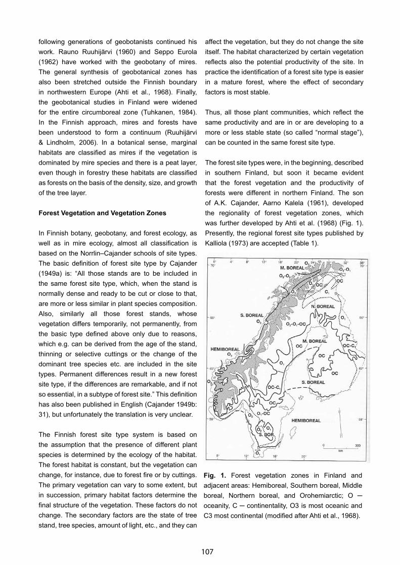
107

following generations of geobotanists continued his work. Rauno Ruuhijärvi (1960) and Seppo Eurola (1962) have worked with the geobotany of mires. The general synthesis of geobotanical zones has also been stretched outside the Finnish boundary in northwestern Europe (Ahti et al., 1968). Finally, the geobotanical studies in Finland were widened for the entire circumboreal zone (Tuhkanen, 1984). In the Finnish approach, mires and forests have been understood to form a continuum (Ruuhijärvi & Lindholm, 2006). In a botanical sense, marginal habitats are classified as mires if the vegetation is dominated by mire species and there is a peat layer, even though in forestry these habitats are classified as forests on the basis of the density, size, and growth of the tree layer.

Forest Vegetation and Vegetation Zones

In Finnish botany, geobotany, and forest ecology, as well as in mire ecology, almost all classification is based on the Norrlin–Cajander schools of site types. The basic definition of forest site type by Cajander (1949a) is: “All those stands are to be included in the same forest site type, which, when the stand is normally dense and ready to be cut or close to that, are more or less similar in plant species composition. Also, similarly all those forest stands, whose vegetation differs temporarily, not permanently, from the basic type defined above only due to reasons, which e.g. can be derived from the age of the stand, thinning or selective cuttings or the change of the dominant tree species etc. are included in the site types. Permanent differences result in a new forest site type, if the differences are remarkable, and if not so essential, in a subtype of forest site.” This definition has also been published in English (Cajander 1949b: 31), but unfortunately the translation is very unclear.

The Finnish forest site type system is based on the assumption that the presence of different plant species is determined by the ecology of the habitat. The forest habitat is constant, but the vegetation can change, for instance, due to forest fire or by cuttings. The primary vegetation can vary to some extent, but in succession, primary habitat factors determine the final structure of the vegetation. These factors do not change. The secondary factors are the state of tree stand, tree species, amount of light, etc., and they can

affect the vegetation, but they do not change the site itself. The habitat characterized by certain vegetation reflects also the potential productivity of the site. In practice the identification of a forest site type is easier in a mature forest, where the effect of secondary factors is most stable.

Thus, all those plant communities, which reflect the same productivity and are in or are developing to a more or less stable state (so called “normal stage”), can be counted in the same forest site type.

The forest site types were, in the beginning, described in southern Finland, but soon it became evident that the forest vegetation and the productivity of forests were different in northern Finland. The son of A.K. Cajander, Aarno Kalela (1961), developed the regionality of forest vegetation zones, which was further developed by Ahti et al. (1968) (Fig. 1). Presently, the regional forest site types published by Kalliola (1973) are accepted (Table 1).

Fig. 1. Forest vegetation zones in Finland and adjacent areas: Hemiboreal, Southern boreal, Middle boreal, Northern boreal, and Orohemiarctic; O ─ oceanity, C ─ continentality, O3 is most oceanic and C3 most continental (modified after Ahti et al., 1968).

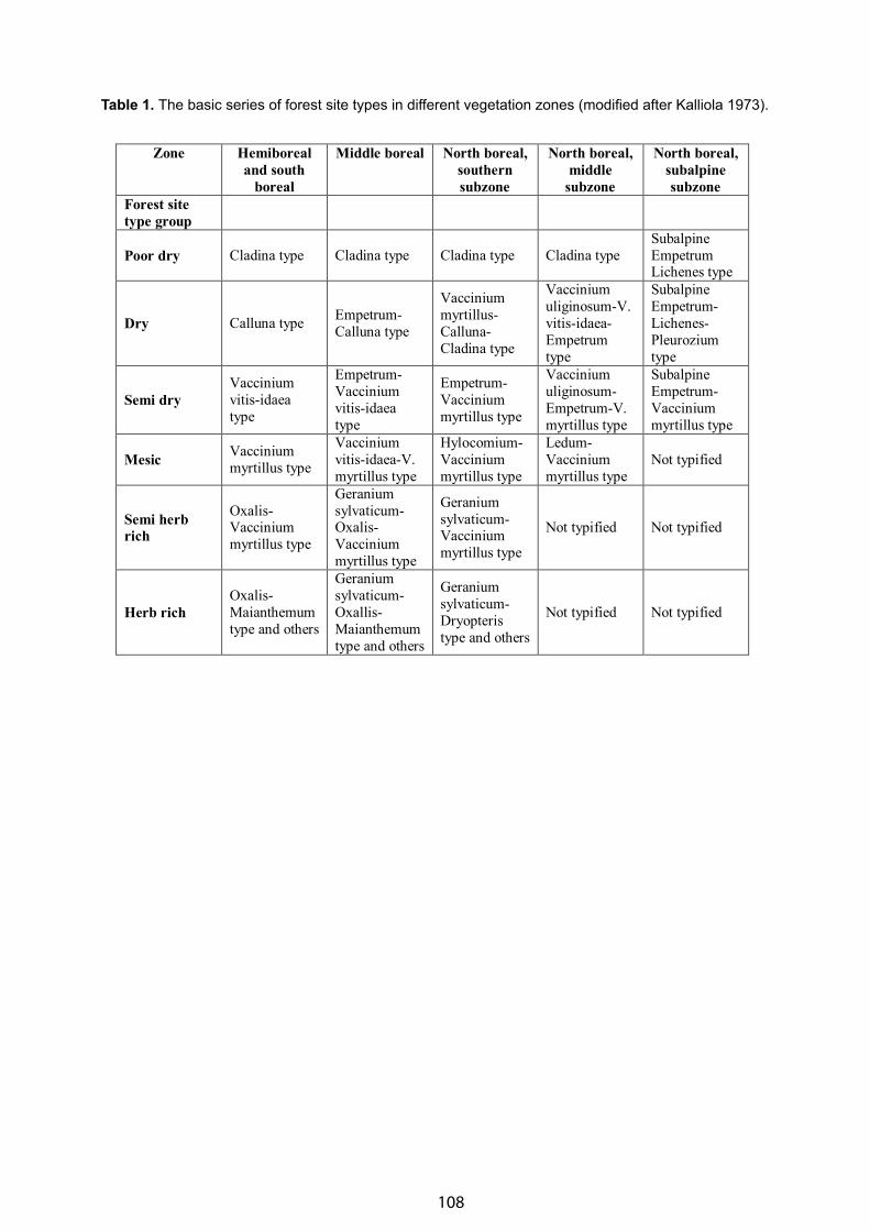
108

Table 1. The basic series of forest site types in different vegetation zones (modified after Kalliola 1973).Table 1. The basic series of forest site types in different vegetation zones (modified after Kalliola 1973).

Zone Hemiboreal and south

boreal

Middle boreal North boreal, southern subzone

North boreal, middle

subzone

North boreal, subalpine subzone

Forest site type group

Poor dry Cladina type Cladina type Cladina type Cladina type Subalpine Empetrum Lichenes type

Dry Calluna type Empetrum-Calluna type

Vaccinium myrtillus-Calluna-Cladina type

Vaccinium uliginosum-V. vitis-idaea-Empetrum type

Subalpine Empetrum-Lichenes-Pleurozium type

Semi dry Vaccinium vitis-idaea type

Empetrum-Vaccinium vitis-idaea type

Empetrum-Vaccinium myrtillus type

Vaccinium uliginosum-Empetrum-V. myrtillus type

Subalpine Empetrum-Vaccinium myrtillus type

Mesic Vaccinium myrtillus type

Vaccinium vitis-idaea-V. myrtillus type

Hylocomium-Vaccinium myrtillus type

Ledum-Vaccinium myrtillus type

Not typified

Semi herb rich

Oxalis-Vaccinium myrtillus type

Geranium sylvaticum-Oxalis-Vaccinium myrtillus type

Geranium sylvaticum-Vaccinium myrtillus type

Not typified Not typified

Herb rich Oxalis-Maianthemum type and others

Geranium sylvaticum-Oxallis-Maianthemum type and others

Geranium sylvaticum-Dryopteris type and others

Not typified Not typified

109

Mire Vegetation

The classification of mire vegetation in the Finnish school was created parallel to forest site types. It is based on ecological gradients, mainly moisture and base content. The original aim for mire vegetation classification was to create a system suitable for practical purposes, for the evaluation of productivity potential of mires for agriculture and forestry (Cajander, 1913). Mire vegetation was divided into four main groups: spruce mires, pine bogs, open mires, and rich fens. This system was further developed by Ruuhijärvi (1960) and Eurola (1962). Later, two more main groups were added, spring fens and flooded swamps (Ruuhijärvi, 1983; Eurola et al., 1984). The reasoning behind the creation of these ecological gradients was recently clarified by Ruuhijärvi & Lindholm (2006). In many cases one habitat gradually changes into another, and, thus, habitats can be seen as continuums (Fig. 2). Topography and, for example, bedrock conditions can cause more abrupt boundaries. At present, in botanical classification there are approximately 80 different mire site types. For practical purposes, like forestry, some 30 site types are separated (Laine & Vasander, 2005).

In the Finnish approach, mires and forests have been understood to form a continuum. In a botanical sense, marginal habitats are classified as mires if

the vegetation is dominated by mire species (e.g., Sphagna) and there is a peat layer, even though in forestry they are classified as forests on the basis of the density, size, and growth of tree layer.

Mire Zones

Mire massif types have basically been defined by Cajander (1913), and the system was developed further by Ruuhijärvi (1960) and Eurola (1962). When good aerial photographs became available of the entire country in the late 1970s, the zonation was re-evaluated (Ruuhijärvi, 1983; Lindholm & Heikkilä, 2006) (Fig. 3).

Bog Massifs

Bog massifs are divided into three main climatic zones. In addition, there are also azonal bog massifs, which occur across the entire country in places suitable for bogs (Sphagnum fuscum bogs and pine forest bogs).

Plateau bogs are typical in southwestern Finland. The weakly developed low hummock ridges and hollows are not clearly oriented in the plain centre of the massif. There is no concentric structure. In the largest plateau bogs there are bog pools. In the margins of the central plateau there is more clear orientation of the hummock ridges and hollows.

Fig. 2. Finnish mire site type system arranged along the main ecological gradients (Ruuhijärvi & Lindholm, 2006).

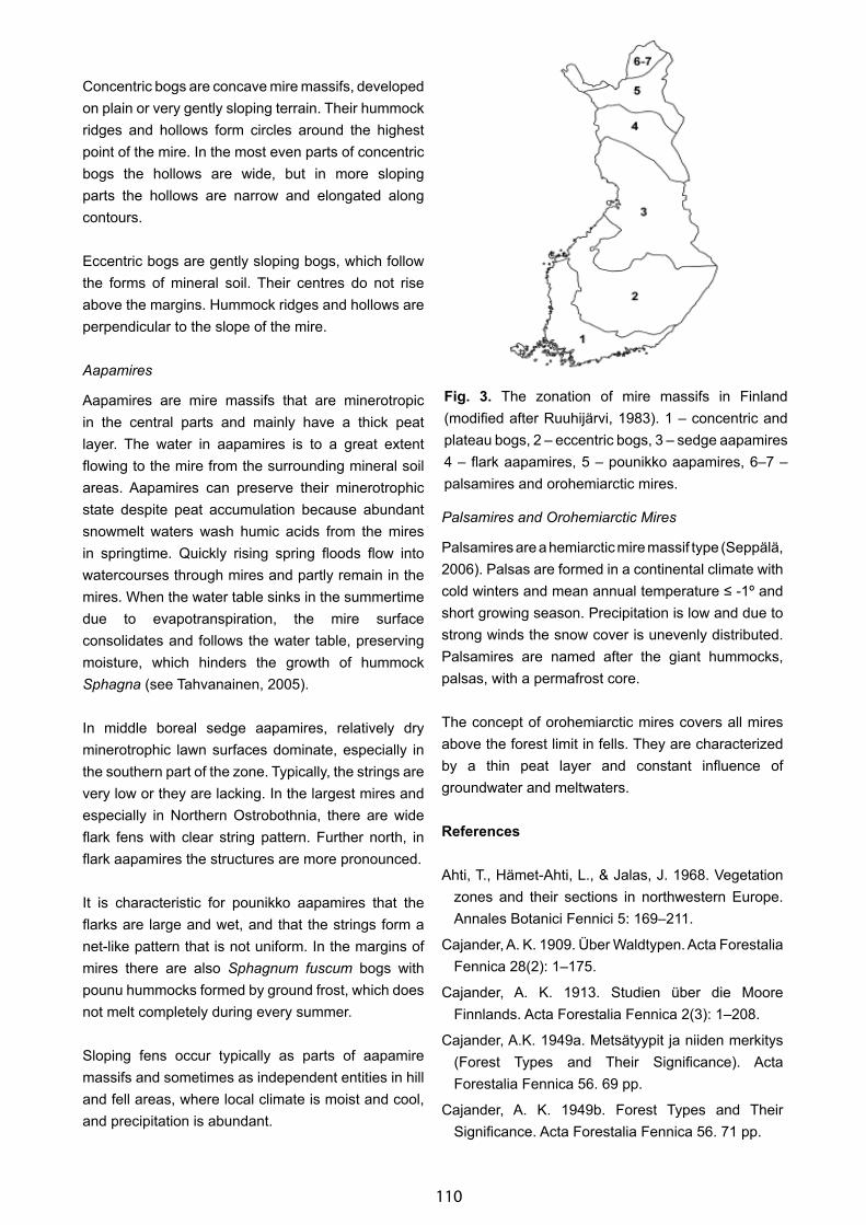
110

Concentric bogs are concave mire massifs, developed on plain or very gently sloping terrain. Their hummock ridges and hollows form circles around the highest point of the mire. In the most even parts of concentric bogs the hollows are wide, but in more sloping parts the hollows are narrow and elongated along contours.

Eccentric bogs are gently sloping bogs, which follow the forms of mineral soil. Their centres do not rise above the margins. Hummock ridges and hollows are perpendicular to the slope of the mire.

Aapamires

Aapamires are mire massifs that are minerotropic in the central parts and mainly have a thick peat layer. The water in aapamires is to a great extent flowing to the mire from the surrounding mineral soil areas. Aapamires can preserve their minerotrophic state despite peat accumulation because abundant snowmelt waters wash humic acids from the mires in springtime. Quickly rising spring floods flow into watercourses through mires and partly remain in the mires. When the water table sinks in the summertime due to evapotranspiration, the mire surface consolidates and follows the water table, preserving moisture, which hinders the growth of hummock Sphagna (see Tahvanainen, 2005).

In middle boreal sedge aapamires, relatively dry minerotrophic lawn surfaces dominate, especially in the southern part of the zone. Typically, the strings are very low or they are lacking. In the largest mires and especially in Northern Ostrobothnia, there are wide flark fens with clear string pattern. Further north, in flark aapamires the structures are more pronounced.

It is characteristic for pounikko aapamires that the flarks are large and wet, and that the strings form a net-like pattern that is not uniform. In the margins of mires there are also Sphagnum fuscum bogs with pounu hummocks formed by ground frost, which does not melt completely during every summer.

Sloping fens occur typically as parts of aapamire massifs and sometimes as independent entities in hill and fell areas, where local climate is moist and cool, and precipitation is abundant.

Palsamires and Orohemiarctic Mires

Palsamires are a hemiarctic mire massif type (Seppälä, 2006). Palsas are formed in a continental climate with cold winters and mean annual temperature ≤ -1º and short growing season. Precipitation is low and due to strong winds the snow cover is unevenly distributed. Palsamires are named after the giant hummocks, palsas, with a permafrost core.

The concept of orohemiarctic mires covers all mires above the forest limit in fells. They are characterized by a thin peat layer and constant influence of groundwater and meltwaters.

References

Ahti, T., Hämet-Ahti, L., & Jalas, J. 1968. Vegetation zones and their sections in northwestern Europe. Annales Botanici Fennici 5: 169–211.

Cajander, A. K. 1909. Über Waldtypen. Acta Forestalia Fennica 28(2): 1–175.

Cajander, A. K. 1913. Studien über die Moore Finnlands. Acta Forestalia Fennica 2(3): 1–208.

Cajander, A.K. 1949a. Metsätyypit ja niiden merkitys (Forest Types and Their Significance). Acta Forestalia Fennica 56. 69 pp.

Cajander, A. K. 1949b. Forest Types and Their Significance. Acta Forestalia Fennica 56. 71 pp.

Fig. 3. The zonation of mire massifs in Finland (modified after Ruuhijärvi, 1983). 1 – concentric and plateau bogs, 2 – eccentric bogs, 3 – sedge aapamires 4 – flark aapamires, 5 – pounikko aapamires, 6–7 – palsamires and orohemiarctic mires.

111

Eurola, S. 1962. Über die regionale Einteilung der südfinnischen Moore. Annales Botanici Societatis Zoologicae Botanicae Fennicae Vanamo 33(2): 1–243.

Eurola, S., Hicks, S,. & Kaakinen, E. 1984. Key to Finnish mire types. Pages 11–117 in Moore, P.D., ed. European Mires. Academic Press, London.

Kalela, A. 1961. Waldvegetationszonen und ihre klimatischen Paralleltypen. Archivum Societatis Zoologicae Botanicae Fennicae Vanamo 16 Supplementum: 65–83.

Kalliola, R. 1973. Suomen kasvimaantiede. (The Geobotany of Finland)–WSOY. Porvoo–Helsinki. 308 pp.

Laine, J. & Vasander, H. 2005. Suotyypit ja niiden tunnistaminen (Mire Site Types and Their Identification). Metsäkirjat, Hämeenlinna. 110 pp.

Lindholm, T. & Heikkilä, R. 2006. Geobotany of Finnish forests and mires: the Finnish approach. Pages 95–103 in Lindholm, T. & Heikkilä, R., eds. Finland—Land of Mires. The Finnish Environment 23/2006. http://www.ymparisto.fi/default.asp?contentid=194173&lan=en.

Norrlin, J. P. 1871. Om Onega-Karelens vegetation och Finlands jemte Skandinaviens naturhistoriska gräns i öster. (On the vegetation of Onega Karelia and the nature historical eastern boundary of Scandinavia) Notiser ur Sällskapets pro Fauna et Flora Fennica Förhandlingar 11: 1─132.

Ruuhijärvi, R. 1960. Über die regionale Einteilung der nordfinnischen Moore. Annales Botanici Societatis Zoologicae Botanicae Fennicae Vanamo 31(1): 1─360.

Ruuhijärvi, R. 1983. The Finnish mire types and their regional distribution. Pages 47─67 in Gore, A.J.P., ed. Mires: Swamp, Bog, Fen and Moor. Ecosystems of the World 4B: Elsevier, Amsterdam.

Ruuhijärvi, R. & Lindholm, T. 2006. Ecological gradients as the basis of Finnish mire site type system. Pages 119─126 in Lindholm, T. & Heikkilä, R., eds. Finland—Land of Mires. The Finnish Environment 23/2006. http://www.ymparisto.fi/default.asp?contentid=194173&lan=en.

Seppälä, M. 2006. Palsa mires in Finland. Pages 155–162 in Lindholm, T. & Heikkilä, R., eds. Finland—Land of Mires. The Finnish Environment 23/2006. http://www.ymparisto.fi/default.asp?contentid=194173&lan=en.

Sukatšev, V. 1960. Metsätyyppien tutkimisen opas (Forest Site Type Guide, Finnish translation from Russian). Silva Fennica 99. 182 pp.

Tahvanainen, T. 2005. Diversity of water chemistry and vegetation of mires in the Kainuu region, middle boreal Finland. University of Joensuu, Ph.D. Dissertations in Biology 33: 1─26.

Tuhkanen, S. 1984. A circumboreal system of climatic phytogeographical regions. Acta Botanica Fennica 127: 1─50.

112

The Importance of Mire Complexes for the Development of a Circumboreal Vegetation Map (CBVM)

Klaus Dierssen

kdierssen@ecology.uni-kiel.de, Ecology Centre, University of Kiel, Germany

Extended Abstract

A circumboreal vegetation map will be primarily based on the distribution patterns of the various taiga systems that make up the boreal biome. These patterns will reflect the floristic differences of site conditions and regionally different climate and vegetation developments since the last glaciation.

Besides the predominating forest systems, particularly in Canada and Russia, vast areas of nonforested wetlands and peatland systems comprise the boreal. Mire systems may occur over broad areas, especially in oceanic parts of the northern boreal zone, and cover more than 50% of the land surface. On a global scale, these mire systems contain by far the largest peat deposits.

Mires were commonly seen as azonal vegetation complexes because their species composition strongly depends on the hydrology of the catchment

area features; these hydrological features may be more important than climatic conditions. This is especially true for the vegetation types of microsites, for instance ombrotrophic bogs show similar large-scale species composition, although clear regional (zonal) differences are illustrated when mapping their community complexes and structural composition.

Currently, the structural pattern of palsa and mixed string fens, for example, can be distinguished quite easily from the different surface structures of raised bogs by using satellite imagery. One key task for broad-scale phytogeographical mapping in boreal zones will be to characterize potential regional coincidences between mire and forest systems.

Following the approach used in the Circumpolar Arctic Vegetation Map (CAVM), the internationally recognized Braun-Blanquet plant community nomenclatural system may be applied for the development of the mapping units and legend hierarchy.

113

Vasily Neshatayev

Saint-Petersburg State Forest-Technical Academy, Saint-Petersburg, Russia

Forest and Mire Vegetation on the Maps of Two Nature Reserves: Comparison of European and Western Siberian Northern Taiga Regions

Abstract

Vegetation was studied in the Russian northern taiga state nature reserves of Lapland (Lapland State Reserve [LSR], Murmansk region) and Verhne-Tazovsky (Verhne-Tazovsky Reserve [VTSR] western Siberia. Six-hundred eighty-two relevés containing data on floristic composition; tree-stand age, height, diameter, basal area, soils and environmental conditions and disturbances (especially fire); and 336 relevés with tree layer, soil profile, and forest type were recorded. Forest vegetation was classified by the following using a two-dimensional approach: (1) association series taking into account the similarity of ground layer vegetation, position in the succession after disturbances, environmental conditions, and soil properties (especially wetness and fertility); and (2) associations, formations, and types of vegetation (taking into account dominant species and life forms). Vegetation dynamics after forest fires was studied. Mire vegetation was classified taking into account dominant species, life forms, and floristic composition indicating wetness and fertility of peat. Vegetation maps at scale 1:50,000 (LSR, 3,200 km2) and 1:100,000 (VTSR, 6,000 km2) were compiled. The diversity of the plant cover of the reserves appeared similar, differing mostly in the presence of Pinus sibirica, Larix sibirica, and Abies sibirica in VTSR and Siberian herb species herb-rich forests on wet soils with running water. Satellite imagery aided in the mapping of the vegetation at scale 1:50,000 and smaller.

Keywords: boreal vegetation, Europe, forest fires, northern taiga, plant succession, satellite imagery, vegetation mapping, west-Siberia.

Introduction

Vegetation was studied in the Russian northern taiga regions of Murmansk and Western Siberia. Before

the beginning of our investigations, the Murmansk region was studied intensively; however, the Verhne-Tazovsky Reserve was one of the least studied areas of northwestern Siberia. The targets of our study were: (1) to determine the diversity of the plant and soil cover of the two regions; (2) to determine correlations between vegetation, soils, and climate; (3) to elucidate the influence of forest fires on boreal vegetation; and (4) to interpret the vegetation from satellite imagery for the purpose of mapping the vegetation at scale 1:50,000 and smaller.

Materials and Methods

Study Areas

The study was carried out in Lapland State Reserve – LSR (area - 3,200 km2), located in the central part of Murmansk Region, and in Verhne-Tazovsky Reserve – VTSR area - 6,300 km2), located in western Siberia on the watershed between Ob, Taz, and Enisei River Basins. In LSR altitude varies from 143 m to 980 m above sea level and in VTSR from 48 m to 285 m above sea level. In both reserves well-drained sandy-loams and sandy soils are predominant, and in LSR granites and gneiss rocks are predominant. According to geobotanical subdivisions, LSR and VTSR are located in the northern taiga subzone.

Vegetation Survey and Classification

The study of LSR vegetation was based on data obtained at 240 sample plots in the forest belt of LSR in 1986 and 1987, and in 132 sample plots located in mires in 2000 and 2008. Sample plots were located at transects crossing the main relief elements and the key-areas representing the different parts of the Reserves. In LSR 90 permanent sample plots were surveyed in 1987 and again in 2006 and 2007. The study of VTSR vegetation was based on data obtained at 718 sample plots in 1991, 1993, 1997, and 1999.

114

In both reserves the dimension of sample plots located in forests was 50 х 50 m and 20 x 20 m and in shrub, grassy, and moss communities, 10 х 10 m, and in natural boundaries of communities, 5 x 5 m. The total density of the tree layer, average and maximal height and diameter of stems, and the basal areas of tree cohorts were measured at sample plots. At each sample plot the association was determined. The age of trees was determined by the scoring of tree rings on the cores. The coverage of layers and species was estimated at 372 sample plots in LSR and at 310 sample plots in VTSR.

For each sample plot the time of succession of vegetation without the influence of fires (TF) was determined by counting tree rings from trees with fire damage or by using files of the reserve. For the stands that appeared later, TF was accepted to be equal to the age of the oldest tree generation without fire damage. For spruce (Picea obovata) and Siberian pine (Pinus sibirica) forests with no trace of fire, TF was considered to be equal to the time that passed since appearance of these tree species in the study area (3,000 in LSR and 4,000 years in VTSR).

Probability of fires for 10 years (PF) was determined for each sample plot in VTSR. For vegetation with TF < 10 years it was considered to be equal to 1.0. For vegetation with TF ≥ 10 years it was calculated as the quotient from division of the number of fires registered on the sample plot by the age of the oldest tree generation (the maximal age - Т) expressed in tens of years.

In LSR the probability of fires was determined for each forest type for the period from 1895 to 1987 (92 years) using a vegetation map, forest plans, and a fire history map compiled by Pushkina (1960) and updated in 1987 on the basis of LSR files (see Neshatayev, 1991). The probability of fire was determined as a proportion of burnt areas for each forest type. Fire rotation period (R) was estimated according to the following equations: R = 10/PF (for VTSR); R = 93/PF (for LSR).

Classification included preliminary sorting of relevés and their ordination based on ecological scales of plants after L.G. Ramensky (Aleksandrova, 1973) and ordination of sample plots and species using

the method of reciprocal averaging by Hill (1973). Interpretation of the rank of the preliminary relevés groups was in accordance with the traditions of the Soviet-Russian phytosociological school of V.N. Sukachev (Aleksandrova, 1973). The classification of the forest vegetation included two subdivisional pathways. One of them was based on the floristic composition of the subordinate layers and the similarity of the land type. The main syntaxa based on these features was the series (cycle) of associations similar to the forest type by Cajander (1909). The cycle of associations steadily progressed toward a climax or subclimax community and those that could pass through it during the life of one generation of the main tree dominant did so under the conditions of existing geomorphological and climatic features.

The other successional path took into consideration dominant tree species and the density of the tree canopy. Using dominant associations, groups of associations, formations, and classes of formations, vegetation types were established. The associations were distinguished by dominants and characteristic combinations of ecological-phytosociological groups of species. Associations were established by taking into consideration the results of the study of vegetation dynamics on different site types.

The formation united communities with identical or ecologically and biomorphologically similar dominants of the main layer (the layer with maximal phytomass production). In the case of polydominant communities, formations were distinguished by the dominant life forms and the structure of the communities. The formations with similar life form dominants and those having similar ecological optimums of site wetness and temperature factors were united into vegetation types.

Vegetation Mapping

The LSR vegetation map at scale 1:50,000 was compiled in 1987 by the Laboratory of Geography and Cartography of Vegetation of the Komarov Botanic Institute, Russian Academy of Sciences. The project was led by the head of the laboratory, T.K. Yurkovskaya. Forest vegetation was mapped by V.Y. Neshataev and B.B. Kovalenko, tundra belt vegetation by S.S. Holod, and mire vegetation by T.K. Yurkovskaya. In the course of forest vegetation mapping, the aerial

115

photos at scale 1:40,000 were interpreted. As training data for aerial photo interpretation, data was collected at sample plots. Three key-areas (20-30 km2 each) were mapped by visiting each contour. Observations along routes 150 km length, forest inventory materials implemented in 1983 by the North-Western Forest Inventory Enterprise, and a fire history map compiled by N.M. Pushkina were used.

In 2007–2008 on the basis of post-fire dynamics, analysis was carried out on the sample plots (including 90 permanent plots), N.M. Pushkina’s successional scheme (1960) was reconsidered, and new quantitative evidence that characterized the rate of post fire succession was received. Using this evidence, the information on community type and forest stand age in 1986–1987, and information from a fire history map, the type of community of every unit was actualized (for 2007). As a result an actual vegetation map of LSR at scale 1:50,000 was compiled. Supervised classification of Landsat images (2005) was used to estimate the possibilities of computer-assisted vegetation mapping of LSR.

The vegetation cover of five key areas (3–10 km2) in VTSR in 1991, 1993, 1997, and 1999 was mapped at the scale 1:25,000 by visiting each map contour previously distinguished and by comparing aerial photography with topographic maps. Vegetation was mapped based on five transects (length 5–10 km) that crossed the reserve.

For each sample plot, the successional period without the influence of fires (TF) was determined by counting tree rings from years covering fire damage or by using files of the reserve. For the stands that appeared later, TF was equal to the age of the oldest tree generation that had no fire damage. TF for fir and cedar forests, with no trace of fire, was considered to be 4,000 years. That is the time that would have passed since the moment of the appearance of the cedar on the terrain. The probability of fires for 10 years (PF) was determined for each sample plot. For TF < 10 years it was assumed to be equal to 1.0. For TF ≥ 10 years it was calculated as the quotient from division of the number of fires registered on the sample plot (NF) by the age of the oldest tree generation (the maximal age - Т) expressed in tens of years.

Supervised classification of Landsat for LSR and KATE-200 satellite images were used for VTSR to compile vegetation maps at scale 1:50,000 (LSR) and 1:100,000 (VTSR). As a teaching sample only half of the relevé data were used. The other half of the relevé data was used for testing the precision or accuracy of the map. For testing the map’s precision (P) we applied the original equation:

P=100*(N- Σ(Ei,j / Em))/N i=1,…,N, j=1,…,N,

where Ei,j – Euclidean distance between centroids of i-th observed and j-th mapped syntaxon, Em – Euclidean distance between centroids of herb-rich spruce forest and lichen-rich pine forest (maximal possible distance in our case, species cover used), N – the number of sample plots used in the sample test.

Results and Discussion

Relationship Between Forest Vegetation and Soil and Climate

In LSR spruce (with Picea obovata) is predominant, and pine (Pinus sylvestris) and birch (Betula pubescens subsp. subarctica) forest occur in the lowland forest belt. Populus tremula is rare in LSR. The mountain birch open forests (Betula pubescens subsp. czerepanovii) form a specific belt in mountains at altitude 400-500 m a.s.l. Pinus sibirica and Pinus sylvestris forests are predominant in VTSR, and larch (Larix sibirica), birch (Betula pubescens), aspen (Populus tremula), and willow (Salix viminalis) flood-plain forests are common in VTSR. Fir forests (Abies sibirica) are very rare in VTSR.

Diagnostic species of vegetation series were established (D – dominants, * - only in LSR, ** - dominants at the first stages of post fire succession, *** - only in VTSR). Petrophyto-Cladinosa* (on primitive soils on rocks): Calluna vulgaris* (D), Vaccinium vitis-idaea (D), Vaccinium myrtillus (D), Empetrum hermaphroditum (D), Arctostaphylos uva-ursi (D), Diphasiastrum complanatum, Carex ericetorum, Cladonia cariosa, Rhacomitrium microcarpum, Parmelia centrifuga, Cornicularia odontella, Stereocaulon grande, Cladina stellaris (D), C. arbuscula (D), C. rangiferina (D), Cladonia borealis, C. cornuta (D), C. amaurocraea, C. uncialis (D), C. gracilis, Cetraria nivalis, Stereocaulon alpinum, S. paschale (D), Umbilicaria sp., Polytrichum

116

juniperinum (D)**, P. piliferum (D)**, Ceratodon purpureus (D)**, Pohlia nutans (D)**; Cladinosa (on well drained sands): Calluna vulgaris* (D), Vaccinium vitis-idaea (D), Vaccinium myrtillus (D), Empetrum hermaphroditum (D), Arctostaphylos uva-ursi (D), Diphasiastrum complanatum, Carex ericetorum, Cladina stellaris (D), C. arbuscula incl. C. arbuscula subsp. mitis, (D), C. rangiferina (D), Cladonia borealis, C. cornuta (D), C. amaurocraea, C. uncialis, C. gracilis, C. crispata, C. furcata, Cetraria nivalis, Stereocaulon alpinum, S. paschale (D), Polytrichum juniperinum (D)**, P. piliferum (D)**, Ceratodon purpureus (D)**, Pohlia nutans (D)**; Hylocomioso-Cladinosa (on well-drained sands): – intermediate type between Cladinosa and Empetroso-Vacciniosa; Empetroso-Vacciniosa (on well-drained sands): Calluna vulgaris* (D), Vaccinium vitis-idaea (D), Vaccinium myrtillus (D*), Empetrum hermaphroditum (D), Pleurozium schreberi (D), Dicranum sp. (D); Fruticuloso-Hylocomiosa (on poorly drained sands, normally drained loam sands and loams): Empetrum hermaphroditum (D), Vaccinium myrtillus (D), Vaccinium vitis-idaea (D), Vaccinium uliginosum (D), Equisetum sylvaticum (D), Lerchenfeldia flexuosa* (D**) Linnaea borealis, Solidago virgaurea, Luzula pilosa, Trientalis europaea, Pleurozium schreberi (D), Hylocomium splendens (D), Dicranum sp. (D), Peltigera aphtosa, Nephroma arcticum, Polytrichum commune; Fruticuloso-Polytrichosa (poorly drained sands, loam sands and loams): ─ intermediate type between Fruticuloso-Hylocomiosa and Sphagnosa girgensohnii; Sphagnosa girgensohnii (peatland or gley soils): Vaccinium vitis-idaea (D), V. myrtillus (D), V. uliginosum (D), Empetrum hermaphroditum (D), Equisetum sylvaticum (D), Ledum palustre (D), Rubus chamaemorus (D), Carex globularis (D), Betula nana (D), Sphagnum girgensohnii (D), S. angustifolium (D), Polytrichum commune (D) **, S. nemoreum, S. russowii, S. warnstorfii; Sphagnosa angustifolii (peatland): Vaccinium uliginosum (D), Ledum palustre (D), Oxycoccus palustris, Carex vaginata, Eriophorum vaginatum, Andromeda polifolia, Rubus chamaemorus, Carex globularis, Betula nana (D), Sphagnum angustifolium (D), S. nemoreum, S. fuscum (D); Sphagnoso-Herbosa (peatland): ─ intermediate type between Sphagnosa girgensohnii and Herbosa; Geraniosa*: Geranium sylvaticum (D), Geum rivale (D), Calamagrostis canescens (D), C. langsdorffii (D), Linnaea borealis, Solidago virgaurea, Luzula

pilosa, Trientalis europaea, Filipendula ulmaria, Viola epipsila, Equisetum pratense, Trollius europaeus, Dryopteris linneana, D. expansa, Athyrium filix-femina, Pleurozium schreberi (D), Hylocomium splendens (D), Rhytidiadelpus triquetrus (D); Fruticoso-Herbosa***: Veratrum lobelianum***, Atragene sibirica***, Cacalia hastata***, Aconitum septentrionale***, Thalictrum flavum***, Stellaria bungeana***, Calamagrostis langsdorffii (D), Filipendula ulmaria, Senecio nemorensis***, Delphinium elatum***, Aconitum volubile***, Heracleum dissectum***, Trientalis europaea, Pyrola rotundifolia (D), Linnaea borealis (D), Maianthemum bifolium, Orthilia secunda, Geranium krylovii***, Galium boreale, Hylocomium splendens (D), Ptilium crista-castrensis, Rhytidiadelphus triquetrus; Herbosa: Carex cespitosa (D), Filipendula ulmaria (D), Calamagrostis canescens* (D), C. langsdorffii (D), Comarum palustre, Linnaea borealis, Solidago virgaurea, Luzula pilosa, Trientalis europaea, Geranium sylvaticum*, G. krylovii***, Geum rivale, Comarum palustre, Viola epipsila, Equisetum pratense, Rubus arcticus, Trollius europaeus*, T. asiaticus***, Hylocomium splendens (D), Rhytidiadelpus triquetrus (D), Sphagnum squarrosum (D), Drepanocladus uncinatus (D), Rhizomnium pseudopunctatum (D), Rhizomnium punctatum (D).

Forest diversity in the reserves appeared similar, differing mostly in the presence of Pinus sibirica, Larix sibirica, Abies sibirica, aspen stands, and Siberian herb species in herb-rich forests on wet soils with running water in VTSR and with the absence of forests on rocks in VTSR.

The comparison of northern and southern taiga vegetation described in literature (Neshatayev & Neshatayeva, 1993; Neshatayeva & Neshatayev, 1993, 1995; Dierßen, 1996; Fedorchuk et al., 2005) showed that northern taiga forests on well drained sites and southern taiga at mires were rich with dwarf shrubs (Ledum palustre, Vaccinium uliginosum, Empetrum nigrum s.l., Betula nana) and poor with herbs (Maianthemum bifolium, Oxalis acetosella, etc.), grasses (Calamagrostis arundinacea), and ferns. Some forest types such as Piceetum cladinosum, Pinetum sibirici cladinosum, Betuletum cladinosum, Piceetum angustifolii sphagnosum occurred only in northern taiga.

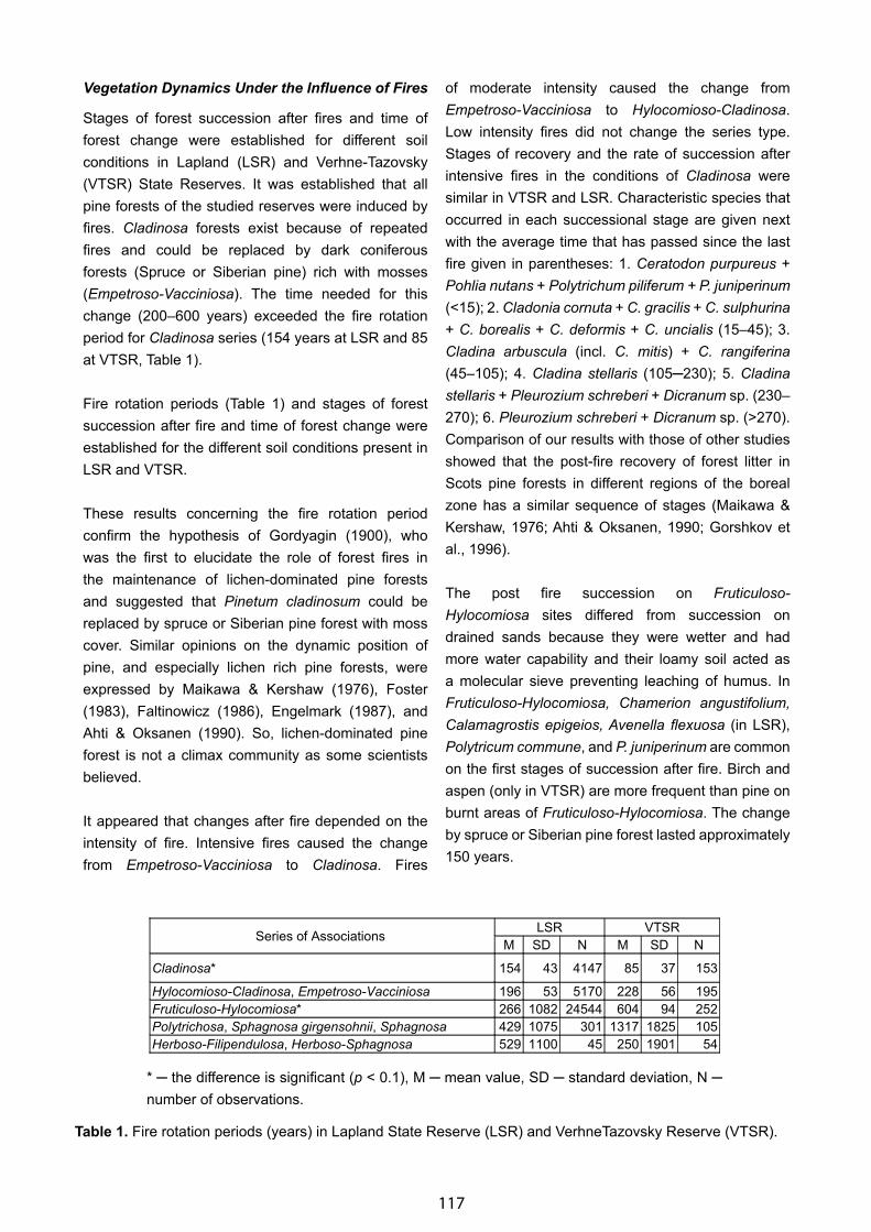
117

Vegetation Dynamics Under the Influence of Fires

Stages of forest succession after fires and time of forest change were established for different soil conditions in Lapland (LSR) and Verhne-Tazovsky (VTSR) State Reserves. It was established that all pine forests of the studied reserves were induced by fires. Cladinosa forests exist because of repeated fires and could be replaced by dark coniferous forests (Spruce or Siberian pine) rich with mosses (Empetroso-Vacciniosa). The time needed for this change (200–600 years) exceeded the fire rotation period for Cladinosa series (154 years at LSR and 85 at VTSR, Table 1).

Fire rotation periods (Table 1) and stages of forest succession after fire and time of forest change were established for the different soil conditions present in LSR and VTSR.

These results concerning the fire rotation period confirm the hypothesis of Gordyagin (1900), who was the first to elucidate the role of forest fires in the maintenance of lichen-dominated pine forests and suggested that Pinetum cladinosum could be replaced by spruce or Siberian pine forest with moss cover. Similar opinions on the dynamic position of pine, and especially lichen rich pine forests, were expressed by Maikawa & Kershaw (1976), Foster (1983), Faltinowicz (1986), Engelmark (1987), and Ahti & Oksanen (1990). So, lichen-dominated pine forest is not a climax community as some scientists believed.

It appeared that changes after fire depended on the intensity of fire. Intensive fires caused the change from Empetroso-Vacciniosa to Cladinosa. Fires

of moderate intensity caused the change from Empetroso-Vacciniosa to Hylocomioso-Cladinosa. Low intensity fires did not change the series type. Stages of recovery and the rate of succession after intensive fires in the conditions of Cladinosa were similar in VTSR and LSR. Characteristic species that occurred in each successional stage are given next with the average time that has passed since the last fire given in parentheses: 1. Ceratodon purpureus + Pohlia nutans + Polytrichum piliferum + P. juniperinum (<15); 2. Cladonia cornuta + C. gracilis + C. sulphurina + C. borealis + C. deformis + C. uncialis (15–45); 3. Cladina arbuscula (incl. C. mitis) + C. rangiferina (45–105); 4. Cladina stellaris (105─230); 5. Cladina stellaris + Pleurozium schreberi + Dicranum sp. (230–270); 6. Pleurozium schreberi + Dicranum sp. (>270). Comparison of our results with those of other studies showed that the post-fire recovery of forest litter in Scots pine forests in different regions of the boreal zone has a similar sequence of stages (Maikawa & Kershaw, 1976; Ahti & Oksanen, 1990; Gorshkov et al., 1996).

The post fire succession on Fruticuloso-Hylocomiosa sites differed from succession on drained sands because they were wetter and had more water capability and their loamy soil acted as a molecular sieve preventing leaching of humus. In Fruticuloso-Hylocomiosa, Chamerion angustifolium, Calamagrostis epigeios, Avenella flexuosa (in LSR), Polytricum commune, and P. juniperinum are common on the first stages of succession after fire. Birch and aspen (only in VTSR) are more frequent than pine on burnt areas of Fruticuloso-Hylocomiosa. The change by spruce or Siberian pine forest lasted approximately 150 years.

Table 1. Fire rotation periods (years) in Lapland State Reserve (LSR) and VerhneTazovsky Reserve (VTSR).

* ─ the difference is significant (p < 0.1), M ─ mean value, SD ─ standard deviation, N ─ number of observations.

Series of Associations LSR VTSR

M SD N M SD N

Cladinosa* 154 43 4147 85 37 153

Hylocomioso-Cladinosa, Empetroso-Vacciniosa 196 53 5170 228 56 195

Fruticuloso-Hylocomiosa* 266 1082 24544 604 94 252

Polytrichosa, Sphagnosa girgensohnii, Sphagnosa 429 1075 301 1317 1825 105

Herboso-Filipendulosa, Herboso-Sphagnosa 529 1100 45 250 1901 54

118

Fires on wet habitats occurred only in very dry years (Table 1). Fires on these sites as a rule led to the total destruction of tree layer consisting of spruce, Siberian pine, or birch. Three stages of post fire succession were found on wet sites with stagnant water (Fruticuloso-Polytrichosa, Sphagnosa girgensohnii, Sphagnosa angustifolii): (1) Marchantia polymorfa + Funaria hygrometrica + Leptobryum pyriforme + Polytrichum commune + P. strictum (lasted approximately 10 years); (2) Polytrichum commune, P. strictum (10–50 years); and (3) Sphagnum girgensohnii (>50 years).

On burnt areas on wet habitats with running water (Geraniosa, Fruticoso-Herbosa, and Herbosa) birch usually regenerated. The full prevalence of spruce or Siberian pine on these habitats occurred rarely, even after a long period of succession. Time of stabilization of species composition of the tree stand was approximately equal to 250 years. In the grass layer during the first years after fire, the same species were predominant as in the forests with no traces of fire (Filipendula ulmaria, Calamagrostis canescens, C. langsdorffii, Carex aquatilis, C. cespitosa). As a whole the floristic structure of communities under the influence of fires on wet habitats with running water sites varied insignificantly.

Mire Vegetation

For mire communities we distinguished six main formations including their dominants (D) and diagnostic species (DS).

1. Sphagneta angustifolii – oligotrophic dwarf-shrub bog moss communities. DS: Empetrum hermaphroditum, Ledum palustre, Betula nana, Vaccinium uliginosum, Chamaedaphne calyculata (rare in LSR), Andromeda polifolia, Oxycoccus palustris, O. microcarpus, Drosera rotundifolia, Sphagnum fuscum (D), S. angustifolium (D). Includes the association Sphagnetum pinoso sibirici-cladinosum*** ─ slightly moist oligotrophic permafrost mire. DS: Pinus sibirica***, Vaccinium vitis-idaea, Pleurozium schreberi, Cladina stellaris, C. rangiferina, C. arbuscula s.l.; association Sphagnetum magnopinosum (slightly moist oligotrophic mire, DS: Pinus sylvestris f. litvinovii ); Sphagnetum nanopinosum (slightly

moist oligotrophic mire, DS: Pinus sylvestris f. wilkomii); Sphagnetum pinosum sibirici*** (slightly moist oligotrophic mire); association Sphagnetum fruticuloso-cladinosum - slightly moist oligotrophic mire with lichens, DS: Cladina rangiferina, C. arbuscula s.l.; Sphagnetum fruticulosum – moderately moist oligotrophic mire.

2. Sphagneta cuspidti – extremely moist oligotrophic mire with Sphagnum sect. Cuspidata as dominants, DS: Carex limosa (D), Scheuchzeria palustris (D), Eriophorum vaginatum (D), Drosera rotundifolia, D. anglica, Sphagnum majus (D), S. balticum (D).

3. Herbosphagneta ─ mesotrophic sedge and herb rich bog moss communities. DS: Andromeda polifolia, Oxycoccus palustris, Carex limosa, C. chordorrhiza, C. lasiocarpa, C. rostrata, C. rotundata, Eriophorum polystachyon, Menyanthes trifoliata, Comarum palustre, Equisetum palustre, E. fluviatile, Drosera rotundifolia, D. anglica, Sphagnum angustifolium (D), S. flexuosum, S. majus (D), S. fallax (D), S. centrale, S. warnstorfii, S. riparium, Aulacomnium palustre, C. stramineum, Calliergon cordifolium, Warnstorfia exannulata. Includes moderately moist mesotrophic mires: association with open stands of trees─Herbosphagnetum betuloso-pinosum (DS: Betula pubescens, Pinus sylvestris); dwarf shrubs as dominants association Herbosphagnetum fruticuloso-caricosum (DS: Ledum palustre, Betula nana, Vaccinium uliginosum, Chamaedaphne calyculata); associations of extremely moist mesotrophic mires with herbs: Herbosphagnetum menyanthosum and sedges Herbosphagnetum caricosum limosae; Herbosphagnetum caricosum rostratae, Herbosphagnetum caricosum lasiocarpae, Herbosphagnetum caricosum rotundatae, Herbosphagnetum caricosum chordorrhizae, Herbosphagnetum eriophoretum polystachionis.

4. Magnocariceta ─ sedge eutrophic mire: Carex acuta (D), C. aquatilis (D), Warnstorfia exannulata, Sphagnum squarrosum, Plagiomnium ellipticum, Pseudobryum cinclidioides.

119

5. Limnoherbeta ─ herb vegetation of secondary mire lakes: Menyanthes trifoliata (D), Comarum palustre (D), Equisetum fluviatile.

Types of mires based on predominant combinations of plant communities were established:

1. Palsa mire*** – Sphagnetum pinoso sibirici-cladinosum + Herbosphagneta;

2. Ridges-hollow bog – Sphagnetum nanopinosum + Sphagnetum fruticuloso-cladinosum + Sphagnetum fruticulosum, Sphagneta cuspidti;

3. Dwarf shrub bog – Sphagnetum fruticulosum;

4. Dwarf shrub bog with open stands of coniferous trees Sphagnetum magnopinosum, Sphagnetum pinosum sibirici*** ;

5. Ridges-hollow aapa mire – Herbosphagnetum fruticuloso-caricosum + Limnoherbeta;

6. Sedge swamp – Herbosphagneta (excluding Herbosphagnetum betuloso-pinosum);

7. Sedge bog with open tree stand Herbosphagnetum betuloso-pinosum; and

8. Sedge fen – Magnocariceta.

Vegetation Maps

The spectral differences of the vegetation units made it possible to produce an algorithm for the computer-assisted identification of forest associations or groups. Using image texture, analyses of satellite imagery helped identify bog and aapa mire complexes. Additional information on mire vegetation was obtained from topographic maps where dwarf shrub, sedge cover, and mire woodlands were shown. On the basis of classification and satellite imagery interpretation, vegetation maps (scale 1: 50,000–1:1M) were compiled for LSR and VTSR.

An ecological-dynamic approach was the basis for the legend. In the legend created for the LSR vegetation map, forest vegetation is represented as vegetation of two belts: taiga─forest and mountain birch. For VTSR, there is only one belt, the taiga─forest. The largest subdivisions of forest vegetation and secondary vegetation within the taiga-forest belt were habitat types distinguished by wetness and soil texture characteristics. Next, in every habitat type, series of associations were distinguished that united forests and nonforested areas similar in their composition

and structure of herb–dwarf shrub and moss–lichen layers. Further subdivision was made according to the prevailing tree species (or lack of tree layer on burnt area), tree age class, and dominant species groups characterizing post-fire stages dynamics. The LSR map also showed communities located in the atmospheric pollution zone with a significantly damaged moss-lichen layer and forest stands.

The structure of the legend for forest vegetation and mires with open tree stands is shown below. The abbreviations for tree dominants occurring in each series are given (*** ─ only in VTSR): S ─ Picea obovata, C ─ Pinus sibirica***, L ─ Larix sibirica***, P ─ Pinus sylvestris, F ─ Abies sibirica ***, A ─ Populus tremula ***, B ─ Betula pubescens.

A. Forests and potential forest vegetation (secondary communities on burnt and cut areas) on the extremely and normally drained sands and loamy sands:

— Cladinosa (S, C, P, L, B)

— Hylocomioso-Cladinosa, (S, C, P,L, B)

— Empetroso-Vacciniosa (S, C, P, L, B, A)

B. Forests and potential forest vegetation on the poorly drained sands, normally drained loam sands and loams (thickness of soil organic horizon less then 10 cm):

— Fruticuloso-Hylocomiosa (S, C, P, L, B, A)

C. Forests on thin, initial soils of hard-rock outcrops and secondary communities (only in LSR)

— Petrophyto-Cladinosa (P)

D. Forests and potential forest vegetation on the poorly drained sites and secondary communities or combination of A and D:

— Fruticuloso-Polytrichosa (S, C, P, L, B)

E. Forests and potential forest vegetation, sometimes in a complex with bogs covered by open tree stands on poorly drained habitats with stagnant water (thickness of peat more then 15 cm):

— Sphagnosa girgensohnii (S, C, P, L, B)

— Sphagnoso-Herbosa (S, C, P, B)

— Sphagnosa angustifolii (S, C, P, L)

F. Forests and potential forest vegetation and open woodlands on wet habitats with running water:

120

— Geraniosa (S, B)

— Fruticoso-Herbosa (S, C, P, F, B, A)

— Herbosa (S, C, P, B).

Types of mires were also shown on the maps. Analyses of mapping precision showed that the best results (P 86%-96%) were obtained when we used supervised classification of the satellite imagery of near-infrared and red bands, normalized vegetation index (NVI–combination of red and green bands), and visual interpretation of mire types from a topographic map and satellite imagery. Spectral brightness of near-infrared bands were correlated with wetness of the soil surface; spectral brightness of red bands depended on the proportion of coniferous trees in the stand, and the NVI was correlated with main vegetation types, such as heath and mire, bush, open forest, and closed forest. These correlations are in agreement with basic observations of vegetation reflectance that were established earlier by Kuchler & Zonneveld, 1990.

Acknowledgments

The author is highly grateful to T.K. Yurkovskaia who was a supervisor of the LSR vegetation mapping in 1987, I.A. Balonenko, A.A. Degtyarev, S.S. Degtyareva; A.V. Fridman, S.S. Kholod, B.B. Kovalenko, T.V. Arsenieva, E. Yatskevich, and V.V. Yatskevich who took part in the field works in LSR in 1987; A.A. Potokin, I.F. Tomaeva, A.A. Egorov and I.V. Cherniadieva who took part in the field works in VTSR, A.A. Dobrysh (Komarov Botanical Institute of Russian Academy of Sciences), who participated in the field works in 1987, 2006, and 2007 in LSR and in 1997 and 1999 in VTSR; M.V. Neshataev and A.O. Pesterov (Saint-Petersburg State Forestry Academy) ,who took part in the field works in LSR in 2006 and 2007; N.Yu. Nazvaladze, one of my partners in studying mires of LSR in 2000, 2007; V. Sh. Barkan (LSR) for the assistance in organizing field works in 2006 and 2007; and my partner in many expeditions and coauthor V. Yu. Neshatayeva. The field works in 2007 were a part of the Interreg-Tacis project Northern boreal forests. Special thanks to ACONIT Ltd. for financial and technical support.

References

Ahti, T. & Oksanen, J. 1990. Epigeic lichen communities of taiga and tundra regions. Vegetatio 86: 3–70.

Aleksandrova, V. D. 1973. Russian approaches to classification of vegetation. Pages 495–527 in Whittaker, R. H., ed. Ordination and Classification of Communities. Junk, The Hague.

Cajander, A. K. 1909. Uber Waldtypen. Acta Forestalia Fennica 1(1): 1–175.

Fedorchuk V. N., Neshatayev V. Yu., & Kuznetsova M. L. 2005. Forest Ecosystems of the North-Western Regions of Russia: Typology, Dynamics, Forest Management Features. Saint-Petersburg. 382 pp.

Gordyagin, A. Ya. 1900. Materials for the study of soils and vegetation of the Western Siberia. Proceedings of the Society of Naturalists of the Emperor’s Kazan University 34 (22): 222 [In Russian].

Dierßen, K. 1996. Vegetation Nordeuropas. Stutgart (Hohenheim),Ulmer. 838 pp.

Engelmark, O. 1987. Fire history correlations to forest type and topography in Northern Sweden. Ann. Bot. Fenn. 24: 317–324.

Faltinowicz, W. 1986. The dynamics and role of lichens in a managed Cladonia-Scotch pine forest (Cladonio-Pinetum). Monogr. Bot. 69: 1–96.

Foster, D. R. 1983. The history and pattern of fire in the boreal forest of southeasten Labrador. Can. J. Bot. 61: 2459–2471.

Gorshkov, V. V., Bakkal I. J., & Stavrova N. I. 1996. Postfire recovery of forest litter in Scots pine forests in two different regions of boreal zone. Silva Fennica 30 (2-3): 209–219.

Hill, M. O. 1973. Reciprocal averaging: an eigenvector method of ordination. Journ. of ecology 61 (1): 237–249.

Kuchler, A. W. & I. S. Zonneveld. 1988. Vegetation Mapping (Handbook of Vegetation Science, v. 10). Kluwer Academic Publishers, Dordrecht. Maikawa, E. & Kershaw, K.A. 1976. Studies on lichen-dominated systems. XIX. The postfire recovery sequence of Black Spruce-lichen woodland in the Abitau Lake area, N.W.T. Can. J. Bot. 54: 2679–2687.

121

Neshatayev, V. Yu. 1991. Vegetation mapping and forest succession after fires in the Lapland State Reserve at the Kola Peninsula. Pages 361–364 in J. B. Falinski, ed. Phytocoenosis, Vol. 3 (N.S.). Supplementum Cartographiae geobotanicae 2. Warszawa-Bialowieza.

Neshatayev, V.Yu., ed. 2002. Vegetation Flora and Soils of Verhne-Tazovskii State Reserve.State Nature Reserve “Verhne-Tazovskii,” Saint-Petersburg. 154 pp. [In Russian].

Neshatayev, V. Yu. & Neshatayeva, V. Yu. 1993. Birch forests of the Lapland State Reserve. Aerial pollution in Kola Peninsula. Pages 328─338 in Aerial pollution

in Kola Peninsula. Proc. International Workshop 14─16 April 1992, St. Petersburg, Russia. Kola Science Centre, Apatity.

Neshatayeva V. Yu. & Neshatayev V. Yu. 1993. Forest vegetation of Ponoi River Valley (the unpolluted area). Pages 346─360 in Aerial pollution in Kola Peninsula. Proc. International Workshop 14─16 April 1992, St. Petersburg, Russia. Kola Science Centre, Apatity.

Pushkina, N. M. 1960. Natural regeneration of vegetation on burned forests. Proc. State National Park, Lapland, No. 4, 5─125 [in Russian].

122

An Approach to Mapping the North American Boreal Zone

James Brandt

Canadian Forest Service, Natural Resources Canada, Ontario, Canada, jbrandt@nrcan.gc.ca

Abstract

The circumpolar boreal zone is one of the world’s largest and most important biogeoclimatic zones, covering much of North America and Eurasia with forests, woodlands, wetlands, and lakes. Because the zone provides important biological and ecological services and covers an extensive area, it is vitally important to the economies of Canada, Finland, Norway, Russia, and Sweden. The boreal zone is also an important source of raw materials in China, Kazakhstan, and Mongolia, even though boreal forests cover a relatively small proportion of these countries. Poor agreement exists amongst scientists regarding this zone’s delimitation and the areal extent of boreal forests, even though the zone has been well studied. This paper discusses previous literature on the phytogeography of the boreal zone and the use of a geographic information system (GIS) to create maps delineating the North American boreal zone and the hemiboreal subzone, which is the transitional area lying immediately to the south of the boreal zone that is usually included in the definition of the boreal zone by Europeans but excluded by North Americans.

Keywords: boreal forest, hemiboreal, map, North America, phytogeography.

Introduction

The circumpolar boreal biome, or zone, is one of the world’s largest and most important biogeoclimatic areas. It covers a large portion of North America and Eurasia with coniferous forests, woodlands, wetlands, and lakes. The circumpolar boreal zone is vitally important to the economies of the principal boreal countries of Canada, Finland, Norway, Russia, and Sweden. The boreal zone is also important to China, Kazakhstan, and Mongolia, even though forests cover a relatively small proportion of the areas of these countries (Finch 1999; United Nations Economic Commission for Europe Committee on Environmental Policy 2000; Wang et al. 2001; Kushlin et al. 2003).

There are large discrepancies in the literature as to the extent of forests within the circumpolar boreal zone. Similar problems affect the definition of other forests worldwide. Most maps of the boreal zone are of such low resolution that they are of little value for estimating areal extent. Furthermore, the methodologies and terminologies of various phytoclimatologists, phytogeographers, and phytosociologists have varied substantially, resulting in differing opinions as to the exact limits of the boreal zone in various regions (Hämet-Ahti, 1981; Tuhkanen, 1984). Also, papers on forests in the boreal zone (or global forests in general), on forest fires, and on the global carbon budget, as well as reports from various environmental organizations, have provided widely different estimates of various parameters used to describe the boreal zone and its forests. These reports, often conflicting, have caused confusion amongst scientists, governmental and nongovernmental organizations, and the public as to the exact nature and extent of the boreal zone. Language barriers also impede an understanding of the boreal zone as the relevant literature has been written in several different languages (e.g., Chinese, English, Finnish, French, Japanese, Korean, Mongolian, Norwegian, Swedish, and Russian).

Two maps of the boreal zone in North America are considered to provide adequate baseline information. When J.S. Rowe published his Forest Regions of Canada in 1972 it was viewed as an accurate depiction and description of Canadian forests at a national scale (Krajina, 1973), and it continues to be cited in current scientific literature. The map in Alaska Trees and Shrubs by Viereck & Little (1972) is the most recent map of the boreal zone in Alaska.

Geographic information systems (GIS) have improved our ability to produce spatially accurate maps. This technology, however, is limited by the accuracy and resolution of the accessed spatial data. Several recent vegetation studies within the boreal zone and other recently developed spatial data sets provide new data

123

that can be used in combination with GIS to develop an improved map of the North American boreal zone.

This presentation focuses on a previous study by the author where existing maps of the North American boreal zone were examined and a new map of the zone was developed, including summaries of relevant areal statistics (see Brandt, 2009). A new map and the corresponding statistics of the North American boreal zone can be viewed as a significant step toward providing scientists, regulators, and environmental groups with a common baseline or standard with which to measure changes in attributes and conservation efforts for a substantial portion of the circumpolar boreal zone. A baseline map is especially important because of the anticipated changes expected within the zone resulting from climate warming as well as the negative effects of various industrial sectors or other anthropogenic activities that are likely to have an additive or synergistic impact.

Creating a New Map of the Boreal Zone

Defining Vegetation Zones

Five major bioclimatic zones have generally been recognized in the northern hemisphere: arctic, boreal, temperate, subtropical, and tropical. The arctic zone is defined primarily by the absence of trees, the occurrence of continuous permafrost, and the presence of tundra vegetation dominated by low-growing shrubs, herbaceous plants, mosses, and lichens (Walker et al., 2002). The tree limit was used by Walker et al. (2002) as the southern boundary of the arctic zone in the Circumpolar Arctic Vegetation Map (CAVM Team, 2003).

The boreal zone is defined as the broad, circumpolar vegetation zone of high northern latitudes covered principally with forests and other wooded land consisting of cold-tolerant trees species primarily within the genera Abies, Larix, Picea, or Pinus but also Populus and Betula; the zone also includes lakes, rivers, and wetlands, and naturally treeless areas such as alpine areas on mountains, heathlands in areas influenced by oceanic climatic conditions, and some grasslands in drier areas. Within the boreal zone, three broad subzones are generally recognized: the forest─tundra interface at the north (subarctic zone of Löve, 1970, or hemiarctic zone of Ahti et al., 1968, and Tuhkanen, 1984); the closed forest generally

occupying the mid portion of the boreal zone; and the hemiboreal (or sub-boreal) at the south. Like Walker et al. (2002), the tree limit was used to define the northern boundary of the forest─tundra in the study described here. The closed forest of the boreal zone is defined by the dominance of closed-crown forests of tree species that tolerate extreme cold (i.e., tolerant of temperatures of –80ºC or lower) within the genera Abies, Larix, Picea, and Pinus but also Populus and Betula. Although other features such as podzolic soils, surplus moisture leading to runoff in rivers and creeks, stable lake levels, the formation of wetlands or peatlands, and permafrost are also considered to be of importance in defining the boreal zone (Sjörs, 1963; Ahti et al., 1968; Walter, 1973; Hogg, 1994; Hogg & Bernier, 2005), these were not considered. The hemiboreal subzone is defined by the co-occurrence of cold-intolerant species, cold-tolerant species, and species with intermediate cold-tolerance, with the cold-tolerant species contributing substantially to the forest cover. The temperate zone is defined by the dominance on most sites of tree species intolerant of extremely cold winter temperatures (i.e., they require temperatures above –45ºC to survive). The interior of both continents is arid, and no temperate forests exist in the latitudinal belt south of the boreal zone where they would exist if temperature was the only critical factor governing their presence. Instead, grasslands occupy the continental temperate zone, and the occurrence of grasslands is dictated more by drought rather than temperature. The hemiboreal subzone in the continental interior of North America consists of grasslands interspersed with drought-tolerant hardwoods, mainly Populus tremuloides but also Quercus macrocarpa.

Source Maps and Approach

Most maps of North America’s boreal zone and its forests were scanned, digitized, and converted to GIS shapefiles. Several maps were available as GIS files. Other maps were consulted but not digitized because these maps (1) had insufficient or inadequate control points to properly geo-reference them for GIS input; (2) lacked sufficient detail to warrant digitization; (3) were of the same pedigree as an acceptable existing map; (4) were superceded by more recent maps; or (5) were adjacent to but outside the boreal zone. All coverages were converted to the same projection and datum.

124

A GIS was used to view and compare the boundaries of 32 maps of the boreal zone. Scale, methods and materials used to create the maps, and the criteria used by the authors to delineate map boundaries were analyzed (Brandt, 2009). To develop a revised map of the North American boreal zone and the hemiboreal subzone using consistent criteria and the most current information, the maps of Rowe (1972) for Canada and Viereck & Little (1972) for Alaska were used as starting points because they are generally perceived as being accurate for the scale at which they are depicted and are still widely used in the scientific literature even though they are 36 years old. One of the limitations of both maps that is not widely recognized or acknowledged is that the authors describe only briefly the materials and methods they used to compile their maps.

Thus, the ecotone boundary depicted on the older maps was replaced with a boundary from a more recent study when (1) the more recent study used a criterion the same as or similar to a criterion described above, and (2) the more recent study provided a thorough description of materials and methods that would allow repeatable results. Two examples of studies that meet both of these conditions are those of Timoney (1988) and Payette (1983). In some situations the scale or resolution of data also became a factor, and preference was given to maps at larger scales and data of higher resolution. For boundaries for which a more recent study was not found and for which other data were not readily available, the default boundary was that of either Rowe (1972) or Viereck & Little (1972). The hemiboreal subzone was not mapped by Rowe (1972) or Viereck & Little (1972). For this subzone, boundaries were selected from studies meeting the two conditions listed above. See Brandt (2009) for a complete list of maps that were viewed in the GIS for each boundary and region considered.

There are problematic areas that defy classification on the basis of the definitions and criteria described above. These include treeless coastal areas and islands, mountain areas that result in belts of vegetation, and outliers of distinct vegetation found at different elevations than the surrounding areas. Coastal areas and islands covered with heaths (i.e., treeless), having cool climates moderated by the

ocean (i.e., eastern Labrador, parts of Newfoundland, the Aleutians), and lying adjacent to the boreal zone were also placed within the boreal zone (Meades, 1983; Yurtsev, 1994; Talbot et al., 2006). Belts of vegetation in mountain areas have traditionally been classified as montane, subalpine, or alpine.

In the study, mountain areas were assigned by adhering to the following rules: (1) if the lowest elevations of the valley fall within the boreal zone, then forests at higher elevation are also in the boreal zone; therefore, areas above the tree limit were classified as alpine but within the boreal zone; and (2) if the lowest elevations of a valley fall within the hemiboreal subzone, then forests at higher elevation consisting of cold-tolerant species were placed in the boreal zone; otherwise, they were classified as hemiboreal (i.e., forests consisting of species of intermediate cold-tolerance). Areas above the tree limit were treated as alpine; these alpine areas were included in the boreal zone when forests immediately below these areas were classified as boreal, or were included in the hemiboreal subzone when the forests immediately below these areas were classified as hemiboreal; (3) if the lowest elevations of the valley fall within the temperate zone, then forests at higher elevation were classified as being in the hemiboreal subzone if they consisted of species of intermediate cold-tolerance and were contiguous with the hemiboreal subzone. If they are not contiguous with forests classified as being in the hemiboreal zone, then they were considered montane or subalpine subzones or belts of the temperate zone.

Areas above the tree limit were treated as alpine; these alpine areas were included in the hemiboreal subzone when the forests immediately below these areas were classified as hemiboreal. In British Columbia, there are several outlying areas of vegetation usually lying in isolated valleys that are distinct from the surrounding vegetation; these outliers were included in the same zone or subzone as the surrounding vegetation. For example, there are valleys covering a relatively small area with temperate species (i.e., Thuja plicata and Tsuga heterophylla) in northwestern British Columbia east of Skagway, Alaska, that were included in the boreal zone. Other outliers in non-mountainous terrain found at different elevations and with vegetation distinct from surrounding areas were

125

treated similarly; these outliers were also included in the zone or subzone of the surrounding areas. Examples include the Cypress Hills in southern Alberta and Saskatchewan, which was placed in the temperate zone, and the Spruce Woods in Manitoba, which was placed in the hemiboreal subzone.

Locating Boreal Forest Ecotones

Forest─Tundra Ecotone

Working from east to west across the northern forest–tundra of North America, the boundary of Feilberg’s (1984) subarctic zone was used as the boundary of the forest–tundra ecotone in Greenland for three reasons. First, Feilberg’s definition of the subarctic zone meets the criterion for the forest–tundra ecotone (i.e., the boundary of his zone was defined by the tree line). Second, Feilberg’s boundary provides greater resolution than the only other map of the region (i.e., that of Tuhkanen, 1984). Finally, Fielberg provides a thorough description of his methods.

The northern tree limit mapped by Payette (1983) was used as the northern boundary of the boreal zone in northern Labrador and that of Saucier et al. (1998), which was adapted from Gerardin (1980), Richard (1987), Lavoie & Payette (1994), and Grondin et al. (1996), was used in northern Quebec. These boundaries were chosen because they also used the tree line as their boundary. Payette’s methods are also well described and repeatable. He used transects along meridians at 30-minute intervals and along parallels near Hudson Bay, aerial photography, and aerial surveys to map the tree limit in this region. To the southeast, islands along the Atlantic coast off Labrador and Newfoundland and extensive areas on the island of Newfoundland proper are treeless and covered primarily by heathlands (Rowe, 1972; Meades, 1983); these areas were also included in the boreal zone.

Moving west, James Bay and Hudson Bay define the northern limits of the boreal zone in Ontario. There is a narrow coastal belt along the shores of both of these bays a few kilometres wide that is treeless (Sjörs, 1961). The northern tree limit from Churchill, Manitoba, on the west coast of Hudson Bay to the border between the Yukon Territory and the Northwest Territories is provided by Timoney (1988). Like the

methods of Payette (1983) and Saucier et al. (1998), Timoney’s (1988) methods are well described and repeatable. He used aerial photography and ground-truthing, as well as definitions similar to those of Payette (1983), to map the northern tree limit west of Hudson Bay.

The regional and local topography of the Yukon Territory and Mackenzie Mountains section of the boreal zone is complex because several mountain ranges dissect this vast area. In mountainous terrain the climate, as affected by altitude, is one of the most important factors dictating the tree limit, but factors such as aspect, slope, cold air drainage, precipitation, and soil also have an influence. To improve on the accuracy of previous maps of the region, digital elevation data (Natural Resources Canada, 2001), the ecoregion map of Oswald & Senyk (1977), and tree-limit elevation data from various regional studies (Porsild, 1945; Drew & Shanks, 1965; Douglas, 1974; Oswald & Senyk, 1977; Ritchie, 1982; MacDonald, 1983; Cwynar & Spear, 1991; Szeicz & MacDonald, 1995; Szeicz et al., 1995) were used to delineate the northern tree limit as well as alpine areas above the elevational tree limit in each of the ecoregions of Oswald & Senyk, (1977), and the Mackenzie Mountains of the Northwest Territories. The results of this process are the boundaries of the northern tree limit and alpine areas depicted in Brandt (2009).

In Alaska the boundaries of the boreal zone were adapted from the scheme of Viereck & Little (1972) and Yurtsev (1994). The boreal zone includes the following vegetation types as described by Viereck & Little (1972): closed spruce-hardwoods; open, low-growing spruce; and treeless bogs. However, because of the various mountain ranges distributed across Alaska and the small scale of the map of Viereck & Little (1972), digital elevation data and tree-limit elevation data from several published studies (Thompson, 1969; Hettinger & Janz, 1974; Anderson, 1975; Denton & Karlén, 1977; Viereck et al., 1983; Goldstein et al., 1985; Cooper, 1986; Short et al., 1986; Sveinbjörnsson et al., 1995; Suarez et al., 1999; Lloyd & Fastie, 2002; Epting & Verbyla, 2005) were used to delineate the northern tree limit as well as alpine areas above the elevational tree limit. There were also several small outliers mapped by Viereck & Little (1972) that were excluded from the boreal zone

126

(see Brandt, 2009). The boreal zone in this region also includes the Alaska Peninsula and the Aleutian Islands because the vegetation in these areas has many boreal taxa but lacks trees (i.e., treeless heaths) (Yurtsev, 1994; Talbot et al., 2006).

Boreal–Hemiboreal Ecotone

Again, working from east to west across North America, the southern boundary of the boreal zone used in eastern North America is that of Saucier et al. (1998) in Quebec and Halliday (1937) in Ontario as modified by Rowe (1972). The boundaries of Saucier et al. (1998) were based on ecological plots, forest inventory plots, data analysis, elevation data, and other existing maps.

In the western interior of North America, Zoltai (1975) mapped the southern limits of the distribution of Larix laricina, Picea mariana, Picea glauca, Pinus banksiana, and Pinus contorta var. latifolia in the southern prairie provinces by using a series of transects. A new boundary line was generated on the basis of the presence of at least two of these five boreal conifers using Zoltai’s data. This line is the southern boundary of the boreal zone in this region, except in southwestern Alberta and southeastern Manitoba, which fell outside Zoltai’s study area. Thus, the new line generated from Zoltai’s data was edge-matched with the boundary of the foothills natural region of the Natural Regions Committee (NRC, 2006) in southwestern Alberta and with Rowe’s (1972) boreal forest region boundary in southeastern Manitoba. Although the Spruce Woods in Manitoba has several boreal conifers it is excluded from this paper’s boreal zone because it is an outlier surrounded by aspen parkland.

In the western cordillera, the mountainous terrain of British Columbia and western Alberta complicates the task of delineating the boundaries of the boreal zone and the hemiboreal subzone. In many valleys several distinct vegetation types may occur as relatively narrow horizontal belts from valley bottom to mountain peak. The boreal zone in this region has been adapted from NRC (2006) and British Columbia Ministry of Forests and Range (BCMFR, 2006). Basically, the upper and lower foothills subregions and the subalpine natural subregion north of the upper Red Deer River near the continental divide (at about 51º38’ N) from NCR

(2006) are included in the boreal zone. In British Columbia, the boreal white and black spruce and the spruce–willow–birch biogeoclimatic zones of BCMFR (2006) are included in boreal zone as both their flora and climate show strong affinities to the boreal zone. Also included are forests of the Engelmann spruce–subalpine fir biogeoclimatic zone that are contiguous with forests of the boreal white and black spruce biogeoclimatic zone in northern British Columbia and east of the Rocky Mountains in British Columbia.

The map of NRC (2006) was produced at a scale of 1:250,000. Contour lines based on data from a provincial digital elevation model were used in many cases to delineate ecological boundaries. The map of BCMFR (2006) is a result of detailed surveys and mapping. About 60% of the province was mapped at a scale of 1:20,000, about 30% at 1:250,000, and the remainder at 1:600,000.

In Alaska, the boreal zone includes closed spruce-hardwoods; open, low-growing spruce; and treeless bogs as described by Viereck & Little (1972) and the Alaska Peninsula and the Aleutian Islands (Yurtsev, 1994). The coastal spruce–hemlock forests of Viereck & Little (1972) were considered part of the temperate zone of western North America. There is no transitional hemiboreal subzone in Alaska because alpine areas and icefields along the coastal mountains separate the boreal and temperate zones.

Hemiboreal–Temperate Ecotone

Crossing North America from east to west, the hemiboreal subzone in the Atlantic Maritimes, northeastern United States, and Great Lakes region includes Rowe’s (1972) Acadian forest region and most of the so-called “spruce–fir forest vegetation type” of Shantz and Zon (1936) that is contiguous with forests of the former forest region. The patches of higher elevation spruce–fir forests in the Adirondack Mountains of New York, the Green Mountains of Vermont and Massachusetts, and the White Mountains of New Hampshire mapped by Hawley and Hawes (1912), Bray (1915), Dana and Greeley (1930), Westveld (1930, 1956), and Hotchkiss (1932) are not considered part of the hemiboreal subzone.

In Quebec, the hemiboreal subzone includes the mixed forest vegetation subzone of Saucier et al.

127

(1998). It also includes land subregion 3d-S (Collines du Mont-Mégantic) of the deciduous forest vegetation subzone considered by Saucier et al. (1998) to be transitional between the sugar maple–yellow birch and the balsam fir–yellow birch bioclimatic domains. Edge-matching was required at the Quebec–Maine border. Thus, contour lines were followed from Quebec into Maine to match the various polygons taken from Shantz and Zon (1936) and from Saucier et al. (1998).

In the Great Lakes region of Ontario, Rowe’s (1972) sections L.9–L.12 are included in the hemiboreal subzone of the study. These areas can be considered transitional because of the abundance of boreal conifers here (Maycock & Curtis, 1960; Rowe, 1972; Jackson et al., 2000). In Michigan, Minnesota, and Wisconsin, pre-settlement forests of spruce, pine, and mixedwoods mapped by Marschner (1974), Finley (1976), and Comer et al. (1995a, 1995b) are included in the hemiboreal subzone. These forests are included because they are similar to Canadian hemiboreal forests on the opposite side of the Great Lakes on the basis of data presented by Daubenmire (1936), Cunningham & White (1941), Braun (1950), Buell & Cantlon (1951), Buell & Niering (1957), Maycock & Curtis (1960), Maycock, (1961), Janssen (1967), Janke et al. (1978), Frelich & Reich (1995), Schmidt et al. (1996), and Friedman et al. (2001).

The southern boundary of the hemiboreal subzone in the western interior parkland of North America is that of the southern boundary of the aspen parkland as mapped by Bird (1961) in Manitoba, Archibold & Wilson (1980) in Saskatchewan, and NRC (2006) in Alberta as the central parkland and foothills parkland natural subregions. The boundary of the parkland in Minnesota is based on the boundaries depicted by Marschner (1974).

In the western cordillera of Alberta, NRC’s (2006) montane natural subregion north of the height of land separating the Livingstone River and Highwood River watersheds (Wilkinson Summit at about 50º11’ N) to the Athabasca River valley near Jasper is included in the hemiboreal subzone. In British Columbia, areas within BCMFR’s (2006) sub-boreal spruce and sub-boreal pine–spruce biogeoclimatic zones are included in the hemiboreal subzone as are forests within the Engelmann spruce–subalpine

fir biogeoclimatic zone lying at higher elevations. Isolated patches of sub-boreal spruce and sub-boreal pine–spruce biogeoclimatic zones are not included in the hemiboreal subzone if they are surrounded by forests consisting of cold-intolerant tree species characteristic of the temperate zone. The bunchgrass, coastal Douglas-fir, coastal western hemlock, interior cedar–hemlock, interior Douglas-fir, and ponderosa pine biogeoclimatic zones are considered temperate.

Conclusion

The map of the North American boreal zone and hemiboreal subzone should be considered a refinement of the maps of Rowe (1972) and Viereck & Little (1972). Boundaries on these maps were altered based on more recent studies that have provided well-described methods. These changes reflect an improvement in technology and data sets since the development of the earlier maps.

Given the circumpolar boreal zone’s importance to the economies of many nations and its key role in regulating global and regional climates and biogeochemical cycles, it is vital that a common definition of the boreal zone be agreed upon. Scientists, regulators, and environmental groups can use the map and the corresponding statistics of the North American boreal zone in Brandt (2009) as a common baseline against which future changes in the zone and the success of conservation efforts can be measured. The approach briefly outlined here could be applied to developing a map of, and comparable statistics for, the Eurasian portion of the boreal zone.

Acknowledgments

J. Weber, R. Brett, M. Gartrell, and M. Newman assisted with the GIS work. J.-P. Saucier of Québec’s Ministère des Ressources naturelles et Faune provided access to GIS coverages of Quebec’s Ecological Land Classification hierarchy. T. Scupien of the United States Department of Agriculture, Forest Service provided GIS coverages of original vegetation in Michigan, Minnesota, and Wisconsin, U.S.A. T. Hogg, B. Meades, J. Volney, and the anonymous reviewers of Environmental Reviews are thanked for their contribution in improving the manuscript. B. Laishley and J. Thomas edited earlier drafts.

128

References

Ahti, T., Hämet-Ahti, L., & Jalas, J. 1968. Vegetation zones and their sections in northwestern Europe. Annales Botanici Fennici 5(3): 169–211.

Anderson, J. H. 1975. A palynological study of late Holocene vegetation and climate in the Healy Lake area of Alaska. Arctic 28(1): 62–69.

Archibold, O. W. & Wilson, M. R. 1980. The natural vegetation of Saskatchewan prior to agricultural settlement. Canadian Journal of Botany 58(19): 2031–2042.

Bird, R. D. 1961. Ecology of the aspen parkland of western Canada in relation to land use. Res. Branch, Can. Dep. Agric., Ottawa, Ontario. Publication 1066.

Brandt, J. P. 2009. The extent of the North American boreal zone. Environmental Reviews 17: 101–161.

Braun, E. L. 1950. Deciduous Forests of Eastern North America. Blakiston Co., Toronto, Ontario.

Bray, W. L. 1915. The development of the vegetation of New York State. New York State Coll. For., Syracuse Univ., Syracuse, NY. Vol. 16, No. 2, Technical Publication 3.

British Columbia Ministry of Forests and Range (BCMFR). 2006. Provincial biogeoclimatic subzone/variant mapping (Version 6, January 2006). Biogeoclimatic Ecosystem Classification Program, Research Branch, Ministry of Forests and Range. Victoria, British Columbia. Available from http://www.for.gov.bc.ca/hre/becweb/resources/maps/gis_products.html [accessed December 2006].

Buell, M. F., & Cantlon, J. E. 1951. A study of two forest stands in Minnesota with an interpretation of the prairie-forest margin. Ecology (Wash. D.C.), 32(2): 294–316.

Buell, M. F., & Niering, W. A. 1957. Fir-spruce-birch forest in northern Minnesota. Ecology (Wash. D.C.), 38(4): 602–610.

CAVM Team. 2003. Circumpolar Arctic Vegetation Map. Conservation of Arctic Flora and Fauna (CAFF) Map No. 1, U.S. Fish and Wildlife Service, Anchorage, Alaska.

Comer, P. J., Albert, D. A., Wells, H. A., Hart, B. L., Raab, J. B., Price, D. L., Kashian, D. M., Corner, R. A., & Schuen, D. W. 1995a. Michigan’s native landscape, as interpreted from the General Land Office surveys 1816–1856. Report to U.S. E.P.A.

Water Division and Wildlife Division, Michigan Dep. Nat. Resour. Michigan Natural Features Inventory. Lansing, Michigan.

Comer, P. J., Albert, D. A., Wells, H. A., Hart, B. L., Raab, J. B., Price, D. L., Kashian, D. M., Corner, R. A., & Schuen, D. W. (map interpretation); Leifreid, T. R., Austin, M. B., DeLain, C. J., Prange-Gregory, L., Scrimger, L. J., & Spitzley. J. G. (digital map production). 1995b. Michigan’s presettlement vegetation, as interpreted from the General Land Office surveys 1816–1856. Michigan Natural Features Inventory. Digital map. Lansing, Michigan.

Cooper, D. J. 1986. White spruce above and beyond treeline in the Arrigetch Peaks region, Brooks Range, Alaska. Arctic 39(3): 247–252.

Cunningham, R. N., & White, H. G. 1941. Forest resources of the upper peninsula of Michigan. USDA, Washington, D.C. Miscellaneous Publication 429.

Cwynar, L. C., & Spear, R. W. 1991. Reversion of forest to tundra in the central Yukon. Ecology (Washington, D.C.), 72(1): 202–212.

Dana, S. T., & Greeley, W. B. 1930. Timber growing and logging practice in the northeast. Measures necessary to keep forest land productive and to produce full timber crops. USDA For. Serv., Washington, D.C. Technical Bulletin 166.

Daubenmire, R. F. 1936. The “Big Woods” of Minnesota: its structure, and relation to climate, fire, and soils. Ecological Monographs 6(2): 233–268.

Denton, G. H., & Karlén, W. 1977. Holocene glacial and tree-line variations in the White River valley and Skolai Pass, Alaska and Yukon Territory. Quaternary Research 7(1): 63–111.

Douglas, G. W. 1974. Montane zone vegetation of the Alsek River region, southwestern Yukon. Canadian Journal of Botany 52(12): 2505–2532.

Drew, J. V., & Shanks, R. E. 1965. Landscape relationships of soils and vegetation in the forest-tundra ecotone, upper Firth River valley, Alaska-Canada. Ecological Monographs 35(3): 285–306.

Epting, J., & Verbyla, D. 2005. Landscape-level interactions of prefire vegetation, burn severity, and postfire vegetation over a 16-year period in interior Alaska. Canadian Journal of Forest Research 35(6): 1367–1377.

Feilberg, J. 1984. A phytogeographical study of

129

south Greenland. Vascular plants. Meddr. Grönl. Bioscience 15.

Finch, C., ed. 1999. Mongolia’s Wild Heritage: Biological Diversity, Protected Areas, and Conservation in the Land of Ghingis Khaan. Mongolia Minist. Nat. Environ., Acad. Sci. Natl. Univ., Mong. Biodivers. Proj., and World Wide Fund Nat. Avery Press, Boulder, Colorado.

Finley, R. W. 1976. The original vegetation cover of Wisconsin. USDA For. Serv., North Central For. Exp. Stn., St. Paul, MN. Map (1:500000) and accompanying text.

Frelich, L. E., & Reich, P. B. 1995. Spatial patterns and succession in a Minnesota southern-boreal forest. Ecological Monographs 65(3): 325–346.

Friedman, S. K., Reich, P. B., & Frelich, L. E. 2001. Multiple scale composition and spatial distribution patterns of the north-eastern Minnesota presettlement forest. Journal of Ecology 89(4): 538–554.

Gerardin, V. 1980. L’Inventaire du Capital-Nature du territoire de la Baie-James: les régions écologiques et la végétation des sols minéraux. Tome 1: méthodologie et description. Environ. Can., Direction générale des terres. Ottawa, Ontario.

Goldstein, G. H., Brubaker, L. B., & Hinkley, T. M. 1985. Water relations of white spruce (Picea glauca (Moench) Voss) at tree line in north central Alaska. Canadian Journal of Forest Research 15(6): 1080–1087.

Grondin, P., Ansseau, C., Bélanger, L., Belkger, J. -F., Bergeron, Y., Bouchard, A., Brisson, J., De Grandpré, L., Gagnon, G., Lavoie, C., Lessard, G., Payette, S., Richard, P. J. H., Saucier, J. -P., Sirois, L., & Vasseur, L. 1996. Écologie forestière. Pages 134–279 in Bérard, J. A. & Côté, M., eds., Manuel de foresterie. Ordre des ingénieurs forestiers du Québec. Les Presses de l’Université Laval. Saint-Nicolas, Québec.

Halliday, W.E.D. 1937. A forest classification for Canada. For. Serv., Lands, Parks For. Branch, Can. Dep. Mines Resour. Ottawa, Ontario. Bulletin 89.

Hämet-Ahti, L. 1981. The boreal zone and its biotic subdivision. Fennia 159(1): 69–75.

Hawley, R. C., & Hawes, A. F. 1912. Forestry in New England. John Wiley & Sons. New York, New York.

Hettinger, L., & Janz, A. 1974. Vegetation and soils

of northeastern Alaska. Arctic Gas Biological Report Series, Vol. 21.

Hogg, E. H. 1994. Climate and the southern limit of the western Canadian boreal forest. Canadian Journal of Forest Research 24(9): 1835–1845.

Hogg, E. H., & Bernier, P. Y. 2005. Climate change impacts on drought-prone forests in western Canada. Forestry Chronicle 81(5): 675–682.

Hotchkiss, N. 1932. A botanical survey of the Tug Hill plateau. New York State Museum Bulletin 287.

Jackson, S. M., Pinto, F., Malcolm, J. R., & Wilson, E. R. 2000. A comparison of pre-European settlement (1857) and current (1981–1995) forest composition in central Ontario. Canadian Journal of Forest Research 30(4): 605─612.

Janke, R. A., McKaig, D., & Raymond, R. 1978. Comparison of presettlement and modern upland boreal forests on Isle Royale National Park. Forest Science 24(1): 115–121.

Janssen, C. R. 1967. A floristic study of forests and bog vegetation, northwestern Minnesota. Ecology (Washington, D.C.) 48(5): 751–765.

Krajina, V. J. 1973. Reviews: forest regions of Canada. Forestry Chronicle 49(6): 261–262.

Kushlin, A., van Veen, T. S., & Sutton, W. 2003. Kazakhstan: forest sector in transition: the resource, the users and sustainable use. Eur. Cent. Asia Environ. Soc. Sustain. Dev. Ser., Washington, D.C. World Bank Technical Paper.

Lavoie, C., & Payette, S. 1994. Recent fluctuations of the lichen–spruce forest limit in subarctic Québec. Journal of Ecology 82(4): 725–734.

Lloyd, A. H. & Fastie, C. L. 2002. Spatial and temporal variability in the growth and climate response of treeline trees in Alaska. Climatic Change 52(4): 481–509.

Löve, D. 1970. Subarctic and subalpine: where and what? Arctic and Alpine Research 2(1): 63–73.

MacDonald, G. M. 1983. Holocene vegetation history of the upper Natla River area, Northwest Territories, Canada. Arctic and Alpine Research 15(2): 169–180.

Marschner, F. J. 1974. The original vegetation of Minnesota. A map compiled in 1930 by F.J. Marschner from U.S. General Land Office notes. Published in 1974 under the direction of M.L. Heinselman. U.S. Department of Agriculture, Forest Service, St.

130

Paul, Minnesota. Cartography Laboratory of the Department of Geography, University of Minnesota. Map (1:500,000) and accompanying text.

Maycock, P. F. 1961. The spruce─fir forests of the Keweenaw Peninsula, northern Michigan. Ecology (Washington, D.C.) 42(2): 357–365.

Maycock, P. F. & Curtis, J. T. 1960. The phytosociology of boreal conifer─hardwood forests of the Great Lakes region. Ecological Monographs 30(1): 1–35.

Meades, W. J. 1983. Heathlands. Pages 267–318 in South, G. R., ed. Biogeography and Ecology of the Island of Newfoundland. Dr. W. Junk Publishers. The Hague.

Natural Regions Committee (NRC). 2006. Natural regions and subregions of Alberta. Compiled by D.J. Downing and W.W. Pettapiece. Government of Alberta. Publication No. T/852. Available from http://www.cd.gov.ab.ca/preserving/parks/anhic/docs/NRSRcomplete%20May_06.pdf [accessed December 2006].

Natural Resources Canada. 2001. Canada3D: product standard. Geomatics Can., Nat. Resour. Can., Cent. Topogr. Inf., Sherbrooke, QC.

Oswald, E. T., & Senyk, J. P. 1977. Ecoregions of Yukon Territory. Fish. Environ. Can., Can. For. Serv., Pac. For. Res. Cent., Victoria, BC. Information Report BC-X-164.

Payette, S. 1983. The forest tundra and present tree-lines of the northern Québec-Labrador Peninsula. Pages 3-23 in Morisset, P. & Payette, S., eds. Tree-line ecology: Proceedings of the northern Québec tree-line conference. Cent. d’études nord., Univ. Laval, QC. Collection Nordicana No. 47.

Porsild, A. E. 1945. The alpine flora of the east slope of Mackenzie Mountains, Northwest Territories. Can. Dep. Mines Resour., Mines Geol. Branch. National Museum of Canada Bulletin 101.

Richard, P. J. H. 1987. Le couvert végétal du Québec-Labrador et son histoire postglaciare. Dép. Géogr., Univ. Montréal, Notes et Documents, 87-01.

Ritchie, J. C. 1982. The modern and late-Quaternary vegetation of the Doll Creek area, north Yukon, Canada. New Phytologist 90(3): 563–603.

Rowe, J. S. 1972. Forest regions of Canada. Dep. Environ., Can. For. Serv., Ottawa, ON. Publication No. 1300.

Saucier, J. -P., Bergeron, J. -F., Grondin, P., & Robitaille, A. 1998. Les régions écologiques du

Québec méridional : un des éléments du système hiérarchique de classification écologique du territoire mis au point par le ministère des Ressources naturelles. L’Aubelle, février-mars 1998, 8 pp.

Schmidt, T. L., Spencer, J. S., Jr., & Hansen, M. H. 1996. Old and potential old forest in the Lake States, U.S.A. Forest Ecology and Management 86(1–3): 81–96.

Shantz, H. L. & Zon, R. 1936. Natural vegetation. 1924. In Atlas of American agriculture: physical basis including land relief, climate, soils, and natural vegetation of the United States. U.S. Department of Agriculture, Washington, D.C.

Short, S. K., Andrews, J. T., & Webber, P. J. 1986. Pollen, vegetation, and climate relationships along the Dalton Highway, Alaska, U.S.A.: a basis for Holocene paleoecological and paleoclimatic studies. Arctic and Alpine Research 18(1): 57–72.

Sjörs, H. 1961. Forest and peatland at Hawley Lake, northern Ontario. Pages 1─31 in National Museum of Canada Bulletin 171.

Sjörs, H. 1963. Amphi-Atlantic zonation, nemoral to arctic. Pages 109–125 in Löve A & Löve, D., eds. North Atlantic biota and their history. Symposium proceedings, July, 1962. Univ. Iceland, Reykjavík, Iceland. Pergamon Press, Oxford, United Kingdom.

Suarez, F., Binkley, D., & Kaye, M. W. 1999. Expansion of forest stands into tundra in the Noatak National Preserve, northwest Alaska. Ecoscience 6(3): 465–470.

Sveinbjörnsson, B., Davis, J., Abadie, W., & Butler, A. 1995. Soil carbon and nitrogen mineralization at different elevations in the Chugach Mountains of south-central Alaska, U.S.A. Arctic and Alpine Research 27(1): 29–37.

Szeicz, J. M. & MacDonald, G. M. 1995. Recent white spruce dynamics at the subarctic alpine treeline of north-western Canada. Journal of Ecology. 83(5): 873–885

Szeicz, J. M., MacDonald, G. M., & Duk-Rodkin, A. 1995. Late Quaternary vegetation history of the central Mackenzie Mountains, Northwest Territories, Canada. Palaeogeography, Palaeoclimatology, Palaeoecology 113(2–3): 351–371.

Talbot, S. S., Talbot, S. L., & Schofield, W. B. 2006. Vascular flora of Izembek National Wildlife Refuge, westernmost Alaska Peninsula, Alaska. Rhodora 108(935): 249–293.

131

Thompson, W. F. 1969. A test of the Holdridge System at subarctic timberlines. Proceedings of the Association of American Geographers 1:149–153.

Timoney, K. 1988. A geobotanical investigation of the subarctic forest-tundra of the Northwest Territories. [dissertation]. [Edmonton (AB)]: University of Alberta.

Tuhkanen, S. 1984. A circumpolar system of climate-phytogeographical regions. Acta Botanica Fennica 127:1–50 + Appendices.

United Nations Economic Commission for Europe, Committee on Environmental Policy. 2000. Environmental performance review of Kazakhstan. UN Econ. Comm. Eur., Comm. Environ. Policy.

Viereck, L. A., & Little, E. L., Jr. 1972. Alaska trees and shrubs. Agriculture Handbook No. 410. U.S. Department of Agriculture, Forest Service, Washington, D.C.

Viereck, L. A., Dyrness, C. T., Van Cleve, K., & Foote, M. J. 1983. Vegetation, soils, and forest productivity in selected forest types in interior Alaska. Canadian Journal of Forest Research 13(5): 703–720.

Walker, D. A., Gould, W. A., Maier, H. A., & Raynolds, M. K. 2002. The Circumpolar Arctic Vegetation Map: AVHRR-derived base maps, environmental

controls, and integrated mapping procedures. International Journal of Remote Sensing 23(21): 4451–4570.

Walter, H. 1973. Vegetation of the Earth in relation to climate and the eco-physiological conditions. (Translated from the 2nd German, Ed. by J. Weiser). English Universities Press Ltd., Springer-Verlag, London, United Kingdom.

Wang, C., Gower, S. T., Wang, Y., Zhao, H., Yan, P., & Bond-Lamberty, B. P. 2001. The influence of fire on carbon distribution and net primary production of boreal Larix gmelinii forests in north-eastern China. Global Change Biology 7(6): 719–730.

Westveld, M. 1930. Suggestions for the management of spruce stands in the northeast. U.S. Department of Agriculture, Washington, D.C. Circular 134.

Westveld, M. 1956. Natural forest vegetation zones of New England. Journal of Forestry 54: 332–338.

Yurtsev, B. A, 1994. Floristic division of the Arctic. Journal of Vegatation Science 5: 765–776.

Zoltai, S. C. 1975. Southern limit of coniferous trees on the Canadian prairies. Environ. Can., For. Serv., North. For. Res. Cent., Edmonton, AB. Information Report NOR-X-128.

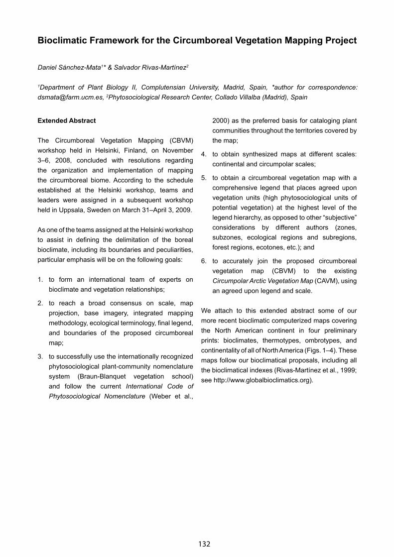
132

Bioclimatic Framework for the Circumboreal Vegetation Mapping Project

Daniel Sánchez-Mata1* & Salvador Rivas-Martínez2

1Department of Plant Biology II, Complutensian University, Madrid, Spain, *author for correspondence: dsmata@farm.ucm.es, 2Phytosociological Research Center, Collado Villalba (Madrid), Spain

Extended Abstract

The Circumboreal Vegetation Mapping (CBVM) workshop held in Helsinki, Finland, on November 3–6, 2008, concluded with resolutions regarding the organization and implementation of mapping the circumboreal biome. According to the schedule established at the Helsinki workshop, teams and leaders were assigned in a subsequent workshop held in Uppsala, Sweden on March 31–April 3, 2009.

As one of the teams assigned at the Helsinki workshop to assist in defining the delimitation of the boreal bioclimate, including its boundaries and peculiarities, particular emphasis will be on the following goals:

1. to form an international team of experts on bioclimate and vegetation relationships;

2. to reach a broad consensus on scale, map projection, base imagery, integrated mapping methodology, ecological terminology, final legend, and boundaries of the proposed circumboreal map;

3. to successfully use the internationally recognized phytosociological plant-community nomenclature system (Braun-Blanquet vegetation school) and follow the current International Code of Phytosociological Nomenclature (Weber et al.,

2000) as the preferred basis for cataloging plant communities throughout the territories covered by the map;

4. to obtain synthesized maps at different scales: continental and circumpolar scales;

5. to obtain a circumboreal vegetation map with a comprehensive legend that places agreed upon vegetation units (high phytosociological units of potential vegetation) at the highest level of the legend hierarchy, as opposed to other “subjective” considerations by different authors (zones, subzones, ecological regions and subregions, forest regions, ecotones, etc.); and

6. to accurately join the proposed circumboreal vegetation map (CBVM) to the existing Circumpolar Arctic Vegetation Map (CAVM), using an agreed upon legend and scale.

We attach to this extended abstract some of our more recent bioclimatic computerized maps covering the North American continent in four preliminary prints: bioclimates, thermotypes, ombrotypes, and continentality of all of North America (Figs. 1–4). These maps follow our bioclimatical proposals, including all the bioclimatical indexes (Rivas-Martínez et al., 1999; see http://www.globalbioclimatics.org).

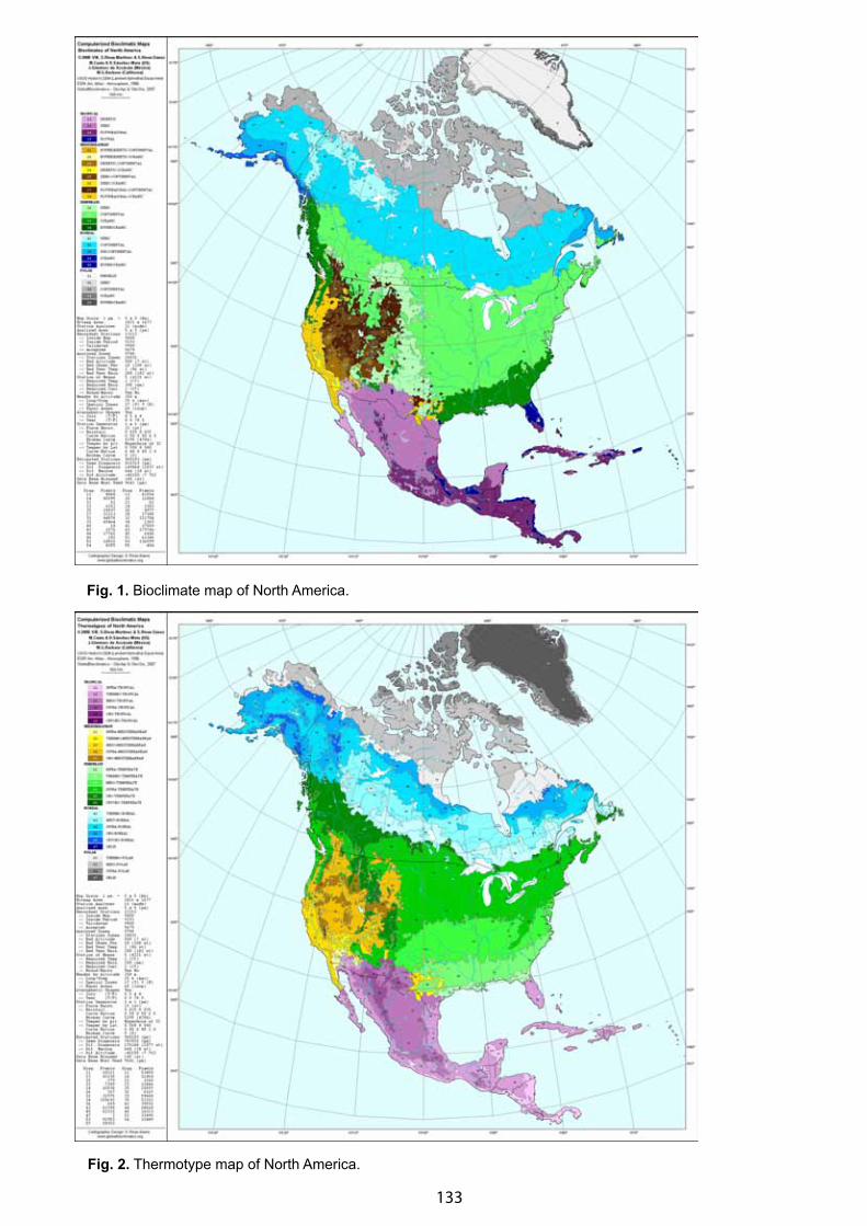
133

Fig. 1. Bioclimate map of North America.

Fig. 2. Thermotype map of North America.

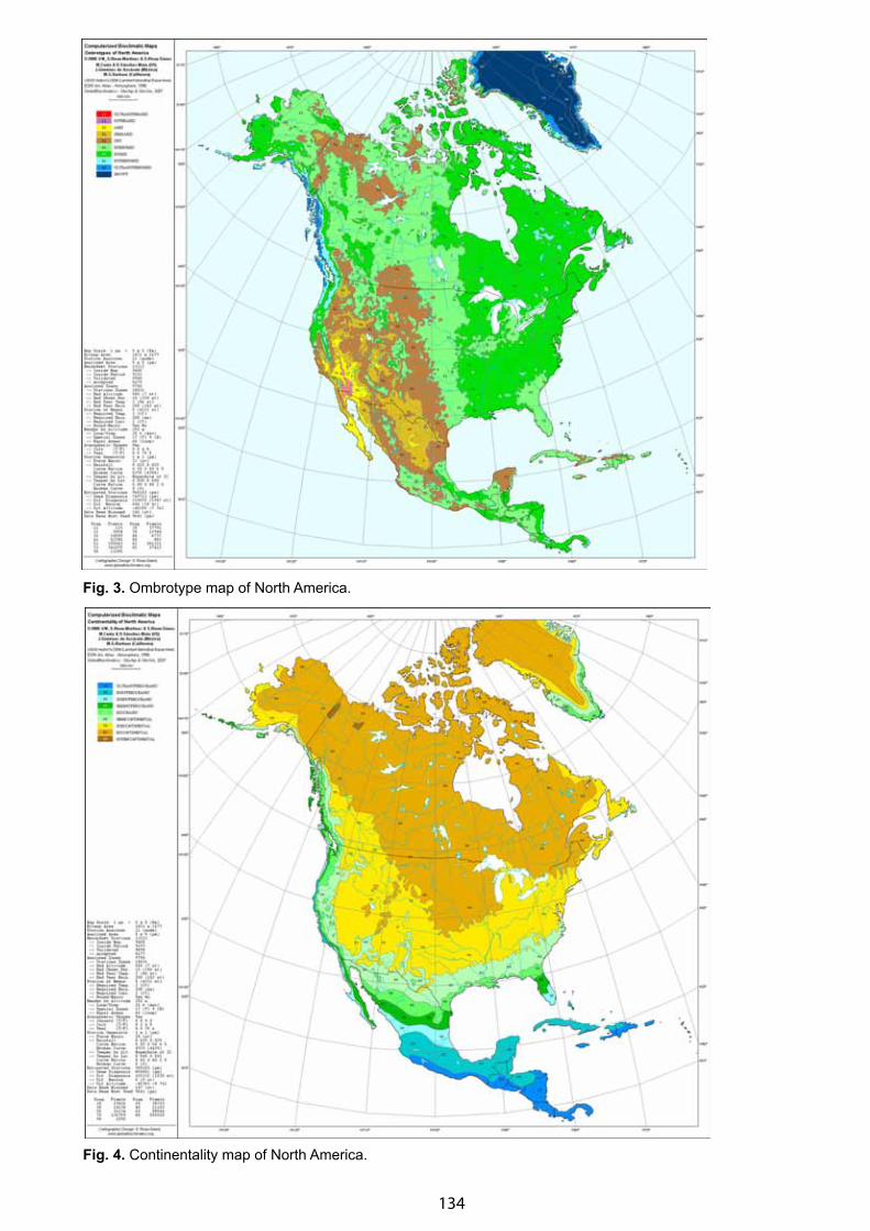
134

Fig. 3. Ombrotype map of North America.

Fig. 4. Continentality map of North America.

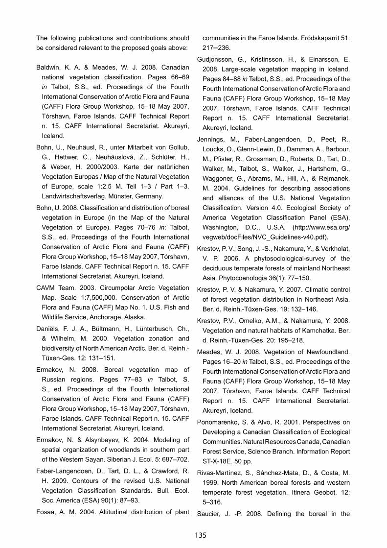
135

The following publications and contributions should be considered relevant to the proposed goals above:

Baldwin, K. A. & Meades, W. J. 2008. Canadian national vegetation classification. Pages 66–69 in Talbot, S.S., ed. Proceedings of the Fourth International Conservation of Arctic Flora and Fauna (CAFF) Flora Group Workshop, 15–18 May 2007, Tórshavn, Faroe Islands. CAFF Technical Report n. 15. CAFF International Secretariat. Akureyri, Iceland.

Bohn, U., Neuhäusl, R., unter Mitarbeit von Gollub, G., Hettwer, C., Neuhäuslová, Z., Schlüter, H., & Weber, H. 2000/2003. Karte der natürlichen Vegetation Europas / Map of the Natural Vegetation of Europe, scale 1:2.5 M. Teil 1–3 / Part 1–3. Landwirtschaftsverlag. Münster, Germany.

Bohn, U. 2008. Classification and distribution of boreal vegetation in Europe (in the Map of the Natural Vegetation of Europe). Pages 70–76 in: Talbot, S.S., ed. Proceedings of the Fourth International Conservation of Arctic Flora and Fauna (CAFF) Flora Group Workshop, 15–18 May 2007, Tórshavn, Faroe Islands. CAFF Technical Report n. 15. CAFF International Secretariat. Akureyri, Iceland.

CAVM Team. 2003. Circumpolar Arctic Vegetation Map. Scale 1:7,500,000. Conservation of Arctic Flora and Fauna (CAFF) Map No. 1. U.S. Fish and Wildlife Service, Anchorage, Alaska.

Daniëls, F. J. A., Bültmann, H., Lünterbusch, Ch., & Wilhelm, M. 2000. Vegetation zonation and biodiversity of North American Arctic. Ber. d. Reinh.-Tüxen-Ges. 12: 131–151.

Ermakov, N. 2008. Boreal vegetation map of Russian regions. Pages 77–83 in Talbot, S. S., ed. Proceedings of the Fourth International Conservation of Arctic Flora and Fauna (CAFF) Flora Group Workshop, 15–18 May 2007, Tórshavn, Faroe Islands. CAFF Technical Report n. 15. CAFF International Secretariat. Akureyri, Iceland.

Ermakov, N. & Alsynbayev, K. 2004. Modeling of spatial organization of woodlands in southern part of the Western Sayan. Siberian J. Ecol. 5: 687–702.

Faber-Langendoen, D., Tart, D. L., & Crawford, R. H. 2009. Contours of the revised U.S. National Vegetation Classification Standards. Bull. Ecol. Soc. America (ESA) 90(1): 87–93.

Fosaa, A. M. 2004. Altitudinal distribution of plant

communities in the Faroe Islands. Fródskaparrit 51: 217─236.

Gudjonsson, G., Kristinsson, H., & Einarsson, E. 2008. Large-scale vegetation mapping in Iceland. Pages 84–88 in Talbot, S.S., ed. Proceedings of the Fourth International Conservation of Arctic Flora and Fauna (CAFF) Flora Group Workshop, 15–18 May 2007, Tórshavn, Faroe Islands. CAFF Technical Report n. 15. CAFF International Secretariat. Akureyri, Iceland.

Jennings, M., Faber-Langendoen, D., Peet, R., Loucks, O., Glenn-Lewin, D., Damman, A., Barbour, M., Pfister, R., Grossman, D., Roberts, D., Tart, D., Walker, M., Talbot, S., Walker, J., Hartshorn, G., Waggoner, G., Abrams, M., Hill, A., & Rejmanek, M. 2004. Guidelines for describing associations and alliances of the U.S. National Vegetation Classification. Version 4.0. Ecological Society of America Vegetation Classification Panel (ESA), Washington, D.C., U.S.A. (http://www.esa.org/vegweb/docFiles/NVC_Guidelines-v40.pdf).

Krestov, P. V., Song, J. -S., Nakamura, Y., & Verkholat, V. P. 2006. A phytosociological-survey of the deciduous temperate forests of mainland Northeast Asia. Phytocoenologia 36(1): 77–150.

Krestov, P. V. & Nakamura, Y. 2007. Climatic control of forest vegetation distribution in Northeast Asia. Ber. d. Reinh.-Tüxen-Ges. 19: 132–146.

Krestov, P.V., Omelko, A.M., & Nakamura, Y. 2008. Vegetation and natural habitats of Kamchatka. Ber. d. Reinh.-Tüxen-Ges. 20: 195–218.

Meades, W. J. 2008. Vegetation of Newfoundland. Pages 16–20 in Talbot, S.S., ed. Proceedings of the Fourth International Conservation of Arctic Flora and Fauna (CAFF) Flora Group Workshop, 15–18 May 2007, Tórshavn, Faroe Islands. CAFF Technical Report n. 15. CAFF International Secretariat. Akureyri, Iceland.

Ponomarenko, S. & Alvo, R. 2001. Perspectives on Developing a Canadian Classification of Ecological Communities. Natural Resources Canada, Canadian Forest Service, Science Branch. Information Report ST-X-18E. 50 pp.

Rivas-Martínez, S., Sánchez-Mata, D., & Costa, M. 1999. North American boreal forests and western temperate forest vegetation. Itinera Geobot. 12: 5–316.

Saucier, J. -P. 2008. Defining the boreal in the

136

ecological land classification for Québec (Canada). Pages 53–57 in Talbot, S.S., ed. Proceedings of the Fourth International Conservation of Arctic Flora and Fauna (CAFF) Flora Group Workshop, 15–18 May 2007, Tórshavn, Faroe Islands. CAFF Technical Report n. 15. CAFF International Secretariat. Akureyri, Iceland.

Sieg, B., Drees, B., & Daniëls, F. J. A. 2006. Vegetation and altitudinal zonation in continental West Greenland. Bioscience 57: 5–93.

Svoboda, M. 2008. The Circumpolar Biodiversity Monitoring Program (CBMP). Pages 58–59 in Talbot, S.S., ed. Proceedings of the Fourth International Conservation of Arctic Flora and Fauna (CAFF) Flora Group Workshop, 15–18 May 2007, Tórshavn, Faroe Islands. CAFF Technical Report n. 15. CAFF International Secretariat. Akureyri, Iceland.

Talbot, S. S., Leblanc, M. C., & Aiken, S. G. 2008. Floristic subregions of the Canadian Arctic Archipelago. Pages 42–45 in Talbot, S.S., ed., Proceedings of the Fourth International

Conservation of Arctic Flora and Fauna (CAFF) Flora Group Workshop, 15–18 May 2007, Tórshavn, Faroe Islands. CAFF Technical Report n. 15. CAFF International Secretariat. Akureyri, Iceland.

Walker, D. A., Raynolds, M. K., Daniëls, F. J. A., Einarsson, E., Elvebakk, A., Gould, W. A., Katenin, A. E., Kholod, S. S., Markon, C. J., Melnikov, E. S., Moskalenko, M. N. G., Talbot, S. S., Yurtsev, B. A., and CAVM Team. 2005. The Circumpolar Arctic Vegetation Map. J. Veg. Sci.16: 267–282.

Walker, D. A. 2008. Circumpolar Arctic Vegetation Map, the Alaska Arctic Tundra Vegetation Map, and the Arctic Geobotanical Atlas. Pages 60–62 in Talbot, S.S., ed. Proceedings of the Fourth International Conservation of Arctic Flora and Fauna (CAFF) Flora Group Workshop, 15–18 May 2007, Tórshavn, Faroe Islands. CAFF Technical Report n. 15. CAFF International Secretariat. Akureyri, Iceland.

Weber, H. E., Moravec, J., & Theurillat, J. -P. 2000. International Code of Phytosociological Nomenclature. 3rd ed. J. Veg. Sci. 11: 739─768.

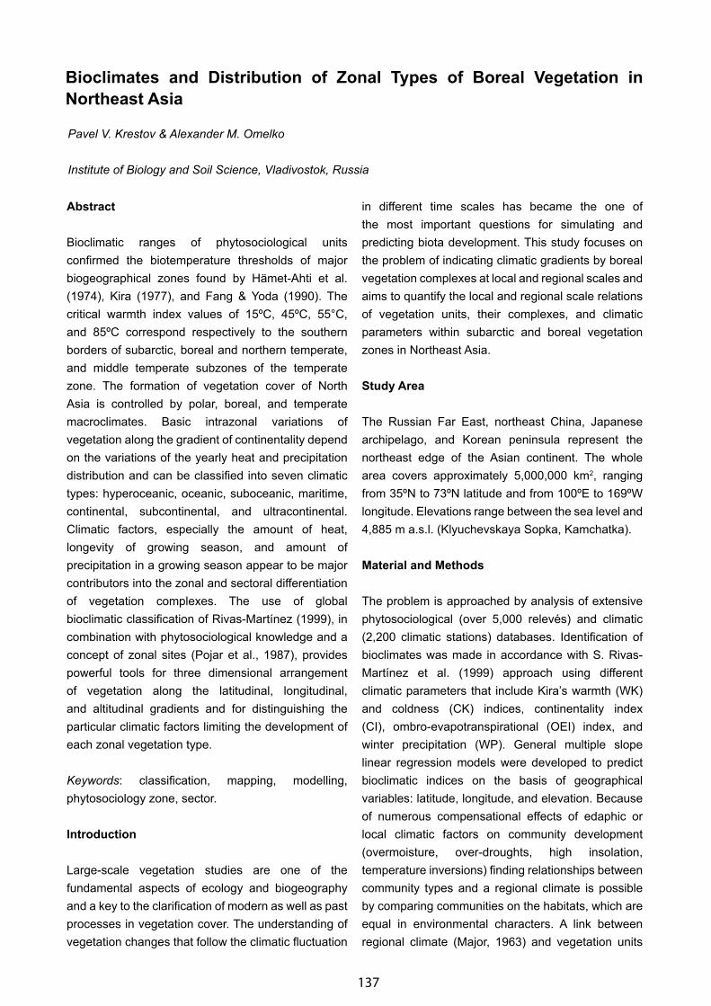
137

Bioclimates and Distribution of Zonal Types of Boreal Vegetation in Northeast Asia

Pavel V. Krestov & Alexander M. Omelko

Institute of Biology and Soil Science, Vladivostok, Russia

Abstract

Bioclimatic ranges of phytosociological units confirmed the biotemperature thresholds of major biogeographical zones found by Hämet-Ahti et al. (1974), Kira (1977), and Fang & Yoda (1990). The critical warmth index values of 15ºC, 45ºC, 55°C, and 85ºC correspond respectively to the southern borders of subarctic, boreal and northern temperate, and middle temperate subzones of the temperate zone. The formation of vegetation cover of North Asia is controlled by polar, boreal, and temperate macroclimates. Basic intrazonal variations of vegetation along the gradient of continentality depend on the variations of the yearly heat and precipitation distribution and can be classified into seven climatic types: hyperoceanic, oceanic, suboceanic, maritime, continental, subcontinental, and ultracontinental. Climatic factors, especially the amount of heat, longevity of growing season, and amount of precipitation in a growing season appear to be major contributors into the zonal and sectoral differentiation of vegetation complexes. The use of global bioclimatic classification of Rivas-Martínez (1999), in combination with phytosociological knowledge and a concept of zonal sites (Pojar et al., 1987), provides powerful tools for three dimensional arrangement of vegetation along the latitudinal, longitudinal, and altitudinal gradients and for distinguishing the particular climatic factors limiting the development of each zonal vegetation type.

Keywords: classification, mapping, modelling, phytosociology zone, sector.

Introduction

Large-scale vegetation studies are one of the fundamental aspects of ecology and biogeography and a key to the clarification of modern as well as past processes in vegetation cover. The understanding of vegetation changes that follow the climatic fluctuation

in different time scales has became the one of the most important questions for simulating and predicting biota development. This study focuses on the problem of indicating climatic gradients by boreal vegetation complexes at local and regional scales and aims to quantify the local and regional scale relations of vegetation units, their complexes, and climatic parameters within subarctic and boreal vegetation zones in Northeast Asia.

Study Area

The Russian Far East, northeast China, Japanese archipelago, and Korean peninsula represent the northeast edge of the Asian continent. The whole area covers approximately 5,000,000 km2, ranging from 35ºN to 73ºN latitude and from 100ºE to 169ºW longitude. Elevations range between the sea level and 4,885 m a.s.l. (Klyuchevskaya Sopka, Kamchatka).

Material and Methods

The problem is approached by analysis of extensive phytosociological (over 5,000 relevés) and climatic (2,200 climatic stations) databases. Identification of bioclimates was made in accordance with S. Rivas-Martínez et al. (1999) approach using different climatic parameters that include Kira’s warmth (WK) and coldness (CK) indices, continentality index (CI), ombro-evapotranspirational (OEI) index, and winter precipitation (WP). General multiple slope linear regression models were developed to predict bioclimatic indices on the basis of geographical variables: latitude, longitude, and elevation. Because of numerous compensational effects of edaphic or local climatic factors on community development (overmoisture, over-droughts, high insolation, temperature inversions) finding relationships between community types and a regional climate is possible by comparing communities on the habitats, which are equal in environmental characters. A link between regional climate (Major, 1963) and vegetation units

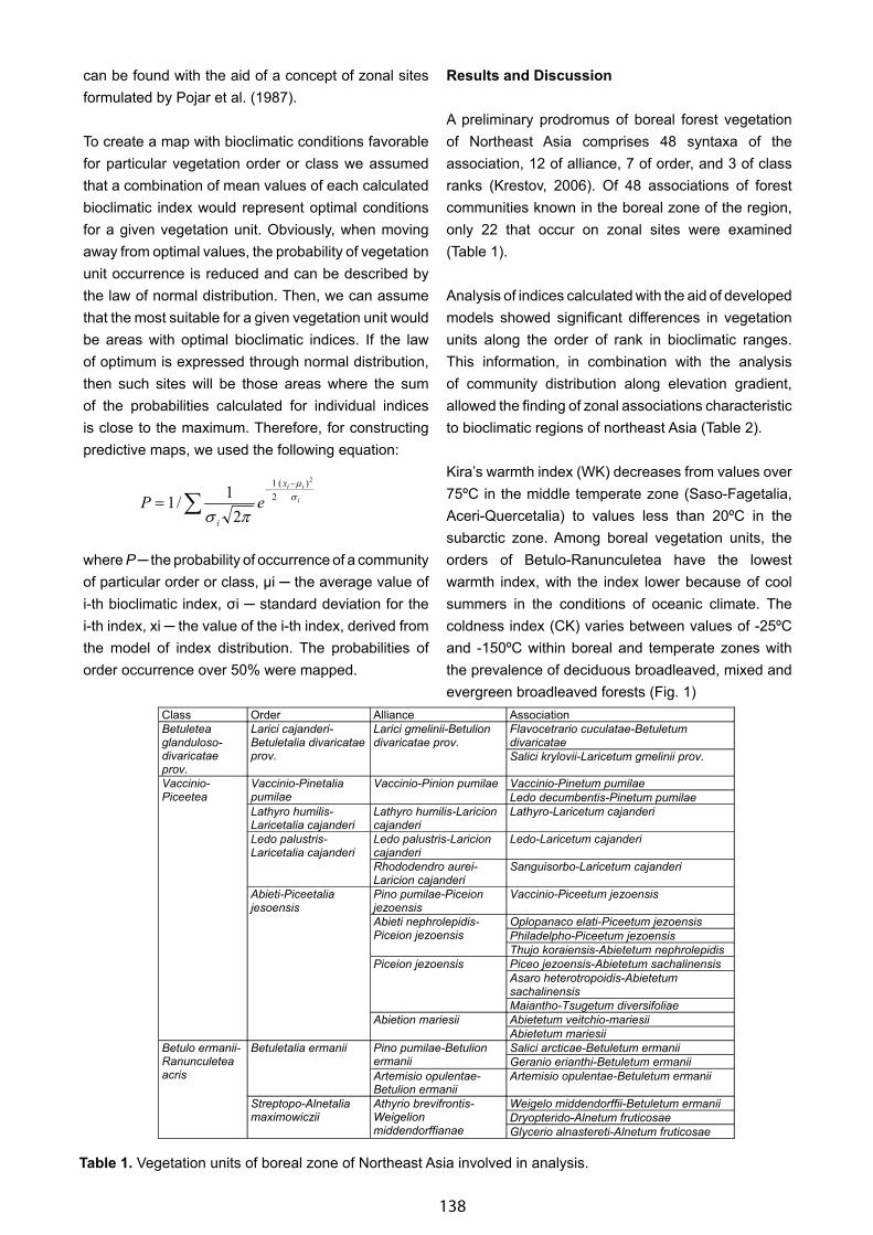
138

can be found with the aid of a concept of zonal sites formulated by Pojar et al. (1987).

To create a map with bioclimatic conditions favorable for particular vegetation order or class we assumed that a combination of mean values of each calculated bioclimatic index would represent optimal conditions for a given vegetation unit. Obviously, when moving away from optimal values, the probability of vegetation unit occurrence is reduced and can be described by the law of normal distribution. Then, we can assume that the most suitable for a given vegetation unit would be areas with optimal bioclimatic indices. If the law of optimum is expressed through normal distribution, then such sites will be those areas where the sum of the probabilities calculated for individual indices is close to the maximum. Therefore, for constructing predictive maps, we used the following equation:

where P ─ the probability of occurrence of a community of particular order or class, μi ─ the average value of i-th bioclimatic index, σi ─ standard deviation for the i-th index, xi ─ the value of the i-th index, derived from the model of index distribution. The probabilities of order occurrence over 50% were mapped.

Results and Discussion

A preliminary prodromus of boreal forest vegetation of Northeast Asia comprises 48 syntaxa of the association, 12 of alliance, 7 of order, and 3 of class ranks (Krestov, 2006). Of 48 associations of forest communities known in the boreal zone of the region, only 22 that occur on zonal sites were examined (Table 1).

Analysis of indices calculated with the aid of developed models showed significant differences in vegetation units along the order of rank in bioclimatic ranges. This information, in combination with the analysis of community distribution along elevation gradient, allowed the finding of zonal associations characteristic to bioclimatic regions of northeast Asia (Table 2).

Kira’s warmth index (WK) decreases from values over 75ºC in the middle temperate zone (Saso-Fagetalia, Aceri-Quercetalia) to values less than 20ºC in the subarctic zone. Among boreal vegetation units, the orders of Betulo-Ranunculetea have the lowest warmth index, with the index lower because of cool summers in the conditions of oceanic climate. The coldness index (CK) varies between values of -25ºC and -150ºC within boreal and temperate zones with the prevalence of deciduous broadleaved, mixed and evergreen broadleaved forests (Fig. 1)

Table 1. Vegetation units of boreal zone of Northeast Asia involved in analysis.

∑−

−

= i

iix

i

eP σµ

πσ

2)(21

21/1

Class Order Alliance Association

Betuletea glanduloso-divaricatae prov.

Larici cajanderi-Betuletalia divaricatae prov.

Larici gmelinii-Betulion divaricatae prov.

Flavocetrario cuculatae-Betuletum divaricatae

Salici krylovii-Laricetum gmelinii prov.

Vaccinio-Piceetea

Vaccinio-Pinetalia pumilae

Vaccinio-Pinion pumilae Vaccinio-Pinetum pumilae

Ledo decumbentis-Pinetum pumilae

Lathyro humilis-Laricetalia cajanderi

Lathyro humilis-Laricion cajanderi

Lathyro-Laricetum cajanderi

Ledo palustris-Laricetalia cajanderi

Ledo palustris-Laricion cajanderi

Ledo-Laricetum cajanderi

Rhododendro aurei-Laricion cajanderi

Sanguisorbo-Laricetum cajanderi

Abieti-Piceetalia jesoensis

Pino pumilae-Piceion jezoensis

Vaccinio-Piceetum jezoensis

Abieti nephrolepidis-Piceion jezoensis

Oplopanaco elati-Piceetum jezoensis

Philadelpho-Piceetum jezoensis

Thujo koraiensis-Abietetum nephrolepidis

Piceion jezoensis Piceo jezoensis-Abietetum sachalinensis

Asaro heterotropoidis-Abietetum sachalinensis

Maiantho-Tsugetum diversifoliae

Abietion mariesii Abietetum veitchio-mariesii

Abietetum mariesii

Betulo ermanii-Ranunculetea acris

Betuletalia ermanii Pino pumilae-Betulion ermanii

Salici arcticae-Betuletum ermanii

Geranio erianthi-Betuletum ermanii

Artemisio opulentae-Betulion ermanii

Artemisio opulentae-Betuletum ermanii

Streptopo-Alnetalia maximowiczii

Athyrio brevifrontis-Weigelion middendorffianae

Weigelo middendorffii-Betuletum ermanii

Dryopterido-Alnetum fruticosae

Glycerio alnastereti-Alnetum fruticosae

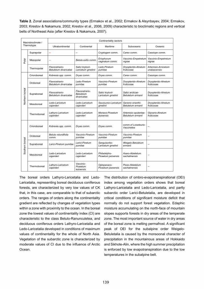
139

Table 2. Zonal associations/community types (Ermakov et al., 2002; Ermakov & Alsynbayev, 2004; Ermakov, 2003; Krestov & Nakamura, 2002; Krestov et al., 2006, 2009) characteristic to bioclimatic regions and vertical belts of Northeast Asia (after Krestov & Nakamura, 2007).

The boreal orders Lathyro-Laricetalia and Ledo-Laricetalia, representing boreal deciduous coniferous forests, are characterized by very low values of CK that, in this case, are comparable to that of subarctic orders. The ranges of orders along the continentality gradient are reflected by changes of vegetation types within a zone with proximity to the ocean. In the boreal zone the lowest values of continentality index (CI) are characteristic to the class Betulo-Ranunculetea, and deciduous coniferous orders Lathyro-Laricetalia and Ledo-Laricetalia developed in conditions of maximum values of continentality for the whole of North Asia. Vegetation of the subarctic zone is characterized by moderate values of CI due to the influence of Arctic Ocean.

The distribution of ombro-evapotranspirational (OEI) index among vegetation orders shows that boreal Lathyro-Laricetalia and Ledo-Laricetalia, and partly subarctic order Larici-Betuletalia, are developed in critical conditions of significant moisture deficit that normally do not support forest vegetation. Edaphic moisture accumulating on the north-face of mountain slopes supports forests in dry areas of the temperate zone. The most important source of water in dry areas of the boreal zone is melting permafrost. A significant peak of OEI for the subalpine order Weigelo-Betuletalia is caused by the monsoonal character of precipitation in the mountainous areas of Hokkaido and Sikhote-Alin, where the high summer precipitation is enforced by low evapotranspiration due to the low temperatures in the subalpine belt.

Macrobioclimate / Thermotype

Continentality sectors

Ultrabontinental Continental Maritime Suboceanic Oceanic

Po

lar

Suprapolar -- -- Cryptogam comm. Carex comm. Cassiope comm.

Mesopolar -- Betula exilis comm.Eriophorum vaginatum comm.

Vaccinio-Empetretum nigrae

Vaccinio-Empetretum nigrae

ThermopolarFlavocetrario-Betuletum divaricatae

Salici krylovii-Laricetum gmelinii

Ledo-Pinetum pumilae

Dryopterido-Alnetum fruticosae

Artemisio-Arnicetum unalascensis

Nort

he

rn b

ore

al

Crioroboreal Kobresia spp. comm. Dryas comm. Dryas comm. Carex comm. Cassiope comm.

OroborealFlavocetrario-Betuletum divaricatae

Ledo-Pinetum pumilae

Vaccinio-Pinetum pumilae

Dryopterido-Alnetum fruticosae

Dryopterido-Alnetum fruticosae

SupraborealFlavocetrario-Betuletum divaricatae

Flavocetrario-Betuletum divaricatae

Salici krylovii-Laricetum gmelinii

Salici arcticae-Betuletum ermanii

Dryopterido-Alnetum fruticosae

MesoborealLedo-Laricetum cajanderi

Ledo-Laricetum cajanderi

Saussureo-Laricetum gmelinii

Geranio erianthi-Betuletum ermanii

Dryopterido-Alnetum fruticosae

ThermoborealLathyro-Laricetum cajanderi

Ledo-Laricetum cajanderi

Moneco-Piceetum jezoensis

Artemisio opulentae-Betuletum ermanii

Glycerio-Alnetum fruticosae

So

uth

ern

bore

al

Crioroboreal Kobresia spp. comm. Dryas comm. Dryas comm.comm.of Loiseleurio-Vaccinetea

--

OroborealBetula rotundifolia comm.

Vaccinio-Pinetum pumilae

Vaccinio-Pinetum pumilae

Vaccinio-Pinetum pumilae

--

Supraboreal Larici-Pinetum pumilaeLarici-Pinetum pumilae

Sanguisorbo-Laricetum gmelinii

Weigelo-Betuletum ermanii

--

MesoborealLedo-Laricetum cajanderi

Ledo-Laricetum cajanderi

Philadelpho-Piceetum jezoensis

Asaro-Abietetum sachalinensis

--

ThermoborealLathyro-Laricetum cajanderi

Vaccinio-Piceetum jezoensis

Oplopanaco-Piceetum jezoensis

Piceo-Abietetum sachalinensis

--

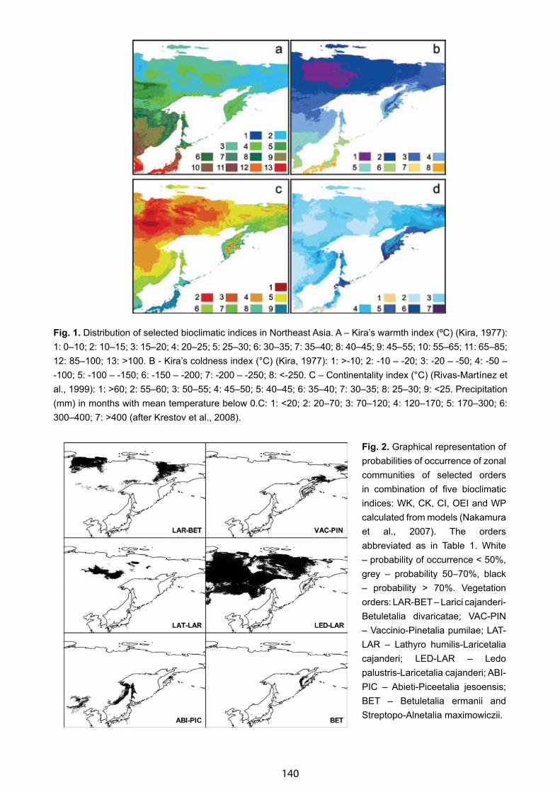
140

Fig. 2. Graphical representation of probabilities of occurrence of zonal communities of selected orders in combination of five bioclimatic indices: WK, CK, CI, OEI and WP calculated from models (Nakamura et al., 2007). The orders abbreviated as in Table 1. White – probability of occurrence < 50%, grey – probability 50–70%, black – probability > 70%. Vegetation orders: LAR-BET – Larici cajanderi-Betuletalia divaricatae; VAC-PIN – Vaccinio-Pinetalia pumilae; LAT-LAR – Lathyro humilis-Laricetalia cajanderi; LED-LAR – Ledo palustris-Laricetalia cajanderi; ABI-PIC – Abieti-Piceetalia jesoensis; BET – Betuletalia ermanii and Streptopo-Alnetalia maximowiczii.

Fig. 1. Distribution of selected bioclimatic indices in Northeast Asia. A – Kira’s warmth index (ºС) (Kira, 1977): 1: 0–10; 2: 10–15; 3: 15–20; 4: 20–25; 5: 25–30; 6: 30–35; 7: 35–40; 8: 40–45; 9: 45–55; 10: 55–65; 11: 65–85; 12: 85–100; 13: >100. B - Kira’s coldness index (°С) (Kira, 1977): 1: >-10; 2: -10 – -20; 3: -20 – -50; 4: -50 – -100; 5: -100 – -150; 6: -150 – -200; 7: -200 – -250; 8: <-250. C – Continentality index (°С) (Rivas-Martínez et al., 1999): 1: >60; 2: 55–60; 3: 50–55; 4: 45–50; 5: 40–45; 6: 35–40; 7: 30–35; 8: 25–30; 9: <25. Precipitation (mm) in months with mean temperature below 0.C: 1: <20; 2: 20–70; 3: 70–120; 4: 120–170; 5: 170–300; 6: 300–400; 7: >400 (after Krestov et al., 2008).

141

The relationships among vegetation units with snow cover become significant in the conditions of the oceanic sector of the boreal zone, where the strong accumulation of snow causes a 2─3 week delay of its melting and a considerable shortening of the growing season. The communities of Betula ermanii, Alnus fruticosa, and tall-forb meadows are characteristic to the regions with slower-melting heavy snow deposits.

Figure 2 shows probabilities of occurrence (over 50%) of certain vegetation orders on the zonal sites in conditions calculated from the distributional models for five bioclimatic indices: CI, WK, CK, OEI, and WP. Simulated ranges in general correspond to the actual vegetation distribution on the maps (Lavrenko & Sochava, 1954; Anonymous, 1982; Miyawaki, 1981–1982); however, some simulated ranges show a high probability of suitable climatic conditions in these areas where the corresponding vegetation unit lacks at present. Most remarkable discrepancies are the following: (1) climatic conditions of the area currently occupied by tundra are suitable for larch forests and woodlands belonging to the orders Ledo-Laricetalia cajanderi and Larici-Betuletalia divaricatae; (2) models of bioclimatic indices showed suitable conditions for the order Vaccinio-Pinetalia pumilae on the mountains of Chukotka peninsula, where Siberian dwarf pine does not form any continuous thickets as it does in Kamchatka and Koryakia; and (3) simulated range of Abieti-Piceetalia is very close to its actual geographical range along the Pacific coast, but combinations of bioclimatic indices of the inland part of the present order distribution better correspond to the Ledo-Laricetalia cajanderi. These discrepancies suggest that the current vegetation pattern of North Asia is not in equilibrium with present climatic conditions.

Comparative floristic analysis showed that southern and coastal floras as well as floras of mountainous regions include the most taxa of northern and continental floras. Zonal subarctic vegetation is represented by communities of the provisional class Betuletea glanduloso-divaricatae and composed of species complexes of Pacific coastal mountainous regions. In the boreal zone, vegetation of Asian ultracontinental to maritime sectors is represented by communities of Vaccinio-Piceetea, and in Asian suboceanic to hyperoceanic sectors, by communities of Betulo-Ranunculetea. The boreal classes were

likely differentiated in Pre-Pleistocene time due to the well-developed floristic centres under the different climatic situations.

Acknowledgments

This study was supported by the Russian foundation for basic research (06-04-91451, 07-04-00654) and the Russian Academy of Sciences (09-III-А06-172, 09-I-Π16-01).

References

Anonymous. 1982. Vegetation Map of China (with 19 pages of text). Scale 1:4000000. Chinese Map Publisher, Beijing. (in Chinese).

Ermakov, N.B. 2003. Diversity of Boreal Vegetation of Northern Asia. Hemiboreal Forests. Classification and Ordination. Izdatelstvo SO RAN, Novosibirsk. 232 pp. (in Russian).

Ermakov, N. & Alsynbayev, K. 2004. Modeling of spatial organization of woodlands in southern part of the Western Sayan. Siberian J. Ecol. 5: 687–702.

Ermakov, N., Cherosov, M., & Gogoleva, P. 2002. Classification of ultracontinental boreal forests in central Yakutia. Folia Geobot. 37: 419–440.

Fang, J.Y. & Yoda, K. 1990. Climate and vegetation in China. IV. Distribution of tree species along the thermal gradient. Ecol. Res. 5: 291–302.

Hämet-Ahti, L., Ahti, T., & Koponen, T. 1974. A scheme of vegetation zones for Japan and adjacent regions. Ann. Bot. Fennici 11: 59–88.

Kira, T.A 1977. Climatological interpretation of Japanese vegetation zones. Pages 21–30 in Miyawaki, A. & Tüxen, R., eds. Vegetation Science and Environmental Protection. Maruzen, Tokyo.

Krestov, P.V. 2006. Vegetation cover and phytogeographical lines on northern Pacifica. D.Sc. Thesis, Institute of Biology and Soil Sci., Vladivostok, Russia. 424 pp.

Krestov, P.V., Ermakov, N.B., Osipov, S.V., & Nakamura, Y. 2009. Classification and phytogeography of larch forests of Northeast Asia. Folia Geobotanica 44. (In press).

Krestov, P.V. & Nakamura, Y. 2002. A phytosociological study of the Picea jezoensis forests of the Far East. Folia Geobotanica 37(4): 441–473.

142

Krestov, P.V. & Nakamura, Y. 2007. Climatic controls of forest vegetation distribution in Northeast Asia. Berichte der Reinhold-Tuxen-Gesellschaft 19: 132–146.

Krestov, P.V., Nakamura, Y., & Omelko, A.M. 2008. Vegetation and natural habitats of Kamchatka Berichte der Reinhold-Tuxen-Gesellschaft 20: 195–218.

Krestov, P.V., Song, J.-S., Nakamura, Y., & Verkholat, V.P. 2006. A phytosociological survey of the deciduous temperate forests of mainland Northeast Asia. Phytocoenologia 36(1): 77–150.

Lavrenko, E.M. & Sochava, V.B., eds. 1954. Geobotanical Map of the USSR. Scale 1:4000000. Botanical institute of the Russian Academy of Sciences, Leningrad. (in Russian).

Major, J. 1963. A climatic index to vascular plant activity. Ecology 44: 485–498.

Miyawaki, A., ed. 1981–1982. Actual Vegetation map 1:50000 from Hokkaido to Okinawa. The 2nd National Survey on the Natural Environment (Vegetation), 1249 leafs. Environmental Agency, Tokyo. (in Japanese).

Nakamura, Y., Krestov, P.V., & Omelko, A.M. 2007. Bioclimate and vegetation complexes in Northeast Asia: a first approximation to integrated study. Phytocoenologia. 37: 443–470.

Pojar, J., Klinka, K., & Meidinger, D.V. 1987. Biogeoclimatic ecosystem classification in British Columbia. For. Ecol. Manag. 22: 119–154.

Rivas-Martínez, S., Sánchez-Mata, D., & Costa, M. 1999. North American boreal and western temperate forest vegetation. Itinera Geobotanica 12: 5–316.

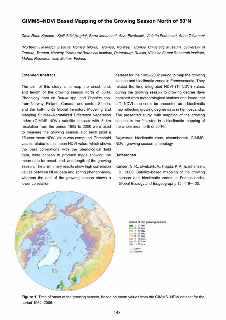
143

Stein Rune Karlsen1, Kjell-Arild Høgda1, Bernt Johansen1, Arve Elvebakk2, Violetta Fedotova3, Anne Tolvanen4

1Northern Research Institute Tromsø (Norut), Tromsø, Norway, 2Tromsø University Museum, University of Tromsø, Tromsø, Norway, 3Komarov Botanical Institute, Petersburg, Russia, 4Finnish Forest Research Institute, Muhos Research Unit, Muhos, Finland

GIMMS–NDVI Based Mapping of the Growing Season North of 50°N

Extended Abstract

The aim of this study is to map the onset, end, and length of the growing season north of 50ºN. Phenology data on Betula spp. and Populus spp. from Norway, Finland, Canada, and central Siberia, and the half-month Global Inventory Modeling and Mapping Studies–Normalized Difference Vegetation Index (GIMMS–NDVI) satellite dataset with 8 km resolution from the period 1982 to 2006 were used to measure the growing season. For each pixel a 25-year mean NDVI value was computed. Threshold values related to this mean NDVI value, which shows the best correlations with the phenological field data, were chosen to produce maps showing the mean date for onset, end, and length of the growing season. The preliminary results show high correlation values between NDVI data and spring phenophases, whereas the end of the growing season shows a lower correlation.

Recently, Karlsen et al. (2006) used the GIMMS–NDVI

dataset for the 1982–2002 period to map the growing season and bioclimatic zones in Fennoscandia. They related the time integrated NDVI (TI NDVI) values during the growing season to growing degree days obtained from meteorological stations and found that a TI NDVI map could be presented as a bioclimatic map reflecting growing degree days in Fennoscandia. The presented study, with mapping of the growing season, is the first step in a bioclimatic mapping of the whole area north of 50ºN.

Keywords: bioclimatic zone, circumboreal, GIMMS-NDVI, growing season, phenology.

References

Karlsen, S. R., Elvebakk, A., Høgda, K. A., & Johansen, B.. 2006. Satellite-based mapping of the growing season and bioclimatic zones in Fennoscandia. Global Ecology and Biogeography 15: 416─430.

Figure 1. Time of onset of the growing season, based on mean values from the GIMMS–NDVI dataset for the period 1982–2006.

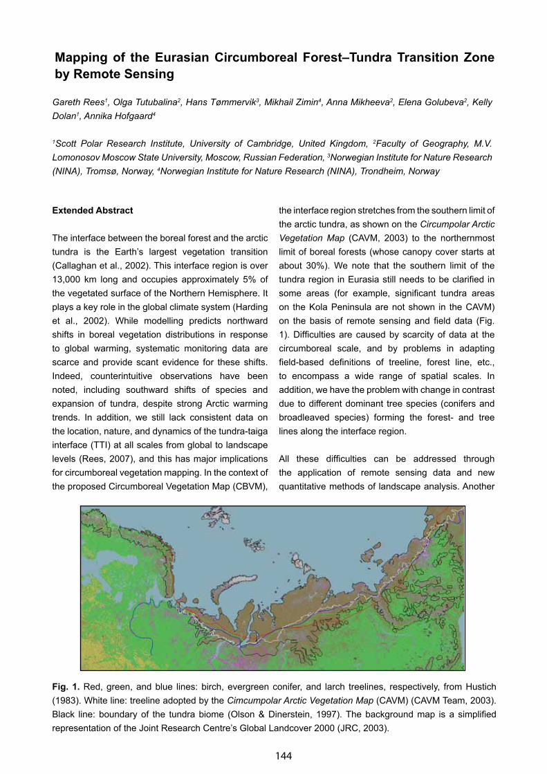
144

Mapping of the Eurasian Circumboreal Forest–Tundra Transition Zone by Remote Sensing

Gareth Rees1, Olga Tutubalina2, Hans Tømmervik3, Mikhail Zimin4, Anna Mikheeva2, Elena Golubeva2, Kelly Dolan1, Annika Hofgaard4

1Scott Polar Research Institute, University of Cambridge, United Kingdom, 2Faculty of Geography, M.V. Lomonosov Moscow State University, Moscow, Russian Federation, 3Norwegian Institute for Nature Research (NINA), Tromsø, Norway, 4Norwegian Institute for Nature Research (NINA), Trondheim, Norway

Extended Abstract

The interface between the boreal forest and the arctic tundra is the Earth’s largest vegetation transition (Callaghan et al., 2002). This interface region is over 13,000 km long and occupies approximately 5% of the vegetated surface of the Northern Hemisphere. It plays a key role in the global climate system (Harding et al., 2002). While modelling predicts northward shifts in boreal vegetation distributions in response to global warming, systematic monitoring data are scarce and provide scant evidence for these shifts. Indeed, counterintuitive observations have been noted, including southward shifts of species and expansion of tundra, despite strong Arctic warming trends. In addition, we still lack consistent data on the location, nature, and dynamics of the tundra-taiga interface (TTI) at all scales from global to landscape levels (Rees, 2007), and this has major implications for circumboreal vegetation mapping. In the context of the proposed Circumboreal Vegetation Map (CBVM),

the interface region stretches from the southern limit of the arctic tundra, as shown on the Circumpolar Arctic Vegetation Map (CAVM, 2003) to the northernmost limit of boreal forests (whose canopy cover starts at about 30%). We note that the southern limit of the tundra region in Eurasia still needs to be clarified in some areas (for example, significant tundra areas on the Kola Peninsula are not shown in the CAVM) on the basis of remote sensing and field data (Fig. 1). Difficulties are caused by scarcity of data at the circumboreal scale, and by problems in adapting field-based definitions of treeline, forest line, etc., to encompass a wide range of spatial scales. In addition, we have the problem with change in contrast due to different dominant tree species (conifers and broadleaved species) forming the forest- and tree lines along the interface region.

All these difficulties can be addressed through the application of remote sensing data and new quantitative methods of landscape analysis. Another

Fig. 1. Red, green, and blue lines: birch, evergreen conifer, and larch treelines, respectively, from Hustich (1983). White line: treeline adopted by the Cimcumpolar Arctic Vegetation Map (CAVM) (CAVM Team, 2003). Black line: boundary of the tundra biome (Olson & Dinerstein, 1997). The background map is a simplified representation of the Joint Research Centre’s Global Landcover 2000 (JRC, 2003).

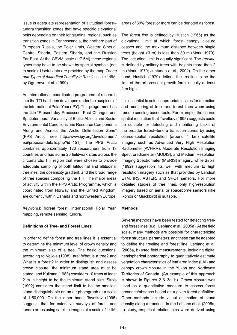
145

issue is adequate representation of altitudinal forest–tundra transition zones that have specific elevational belts depending on their longitudinal regions, such as transition zones in Fennoscandia, the northern part of European Russia, the Polar Urals, Western Siberia, Central Siberia, Eastern Siberia, and the Russian Far East. At the CBVM scale (1:7.5M) these regional types may have to be shown by special symbols (not to scale). Useful data are provided by the map Zones and Types of Altitudinal Zonality in Russia, scale 1:8M, by Ogureeva et al. (1999)

An international, coordinated programme of research into the TTI has been developed under the auspices of the International Polar Year (IPY). This programme has the title “Present-day Processes, Past Changes and Spatiotemporal Variability of Biotic, Abiotic and Socio-Environmental Conditions and Resource Components Along and Across the Arctic Delimitation Zone” (PPS Arctic, see http://www.ipy.org/development/eoi/proposal-details.php?id=151). The PPS Arctic combines approximately 120 researchers from 13 countries and has some 20 fieldwork sites across the circumarctic TTI region that were chosen to provide adequate sampling of both latitudinal and altitudinal treelines, the oceanicity gradient, and the broad range of tree species composing the TTI. The major areas of activity within the PPS Arctic Programme, which is coordinated from Norway and the United Kingdom, are currently within Canada and northwestern Europe.

Keywords: boreal forest, International Polar Year, mapping, remote sensing, tundra.

Definitions of Tree- and Forest Lines

In order to define forest and tree lines it is essential to determine the minimum level of crown density and the minimum size of a tree. The basic questions, according to Veijola (1998), are: What is a tree? and What is a forest? In order to distinguish and assess crown closure, the minimum stand area must be stated, and Kullman (1983) considers 10 trees at least 2 m in height to be the minimum stand size. Sirois (1992) considers the stand limit to be the smallest stand distinguishable on an air photograph at a scale of 1:50,000. On the other hand, Tsvetkov (1995) suggests that for extensive surveys of forest and tundra areas using satellite images at a scale of 1:1M,

areas of 30% forest or more can be denoted as forest.

The forest line is defined by Hustich (1966) as the elevational limit at which forest canopy closure ceases and the maximum distance between single trees (height >3 m) is less than 30 m (Mork, 1970). The latitudinal limit is equally significant. The treeline is defined by solitary trees with heights more than 2 m (Mork, 1970; Juntunen et al., 2002). On the other hand, Hustich (1979) defines the treeline to be the limit of the arborescent growth form, usually at least 2 m high.

It is essential to select appropriate scales for detection and monitoring of tree- and forest lines when using remote sensing based tools. For example, the coarse spatial resolution that Tsvetkov (1995) suggests could be suitable for detecting and monitoring tasks of the broader forest─tundra transition zones by using coarse-spatial resolution (around 1 km) satellite imagery such as Advanced Very High Resolution Radiometer (AVHRR), Moderate Resolution Imaging Spectroradiometer (MODIS), and Medium Resolution Imaging Spectrometer (MERIS) imagery, while Sirois’ (1992) suggestion fits well with medium to high resolution imagery such as that provided by Landsat ETM, IRS, ASTER, and SPOT sensors. For more detailed studies of tree lines, only high-resolution imagery based on aerial or spaceborne sensors (like Ikonos or Quickbird) is suitable.

Methods

Several methods have been tested for detecting tree- and forest lines (e.g., Leblanc et al., 2005a). At the field scale, many methods are possible for characterizing forest structural parameters, and these can be adapted to define the treeline and forest line. Leblanc et al. (2005a, b) used field measurements, including digital hemispherical photography to quantitatively estimate vegetation characteristics of leaf area index (LAI) and canopy crown closure in the Yukon and Northwest Territories of Canada. (An example of this approach is shown in Figures 2 & 3a, b). Crown closure was used as a quantitative measure to assess forest presence/absence based on a given forest definition. Other methods include visual estimation of stand density along a transect. In the Leblanc et al. (2005a, b) study, empirical relationships were derived using

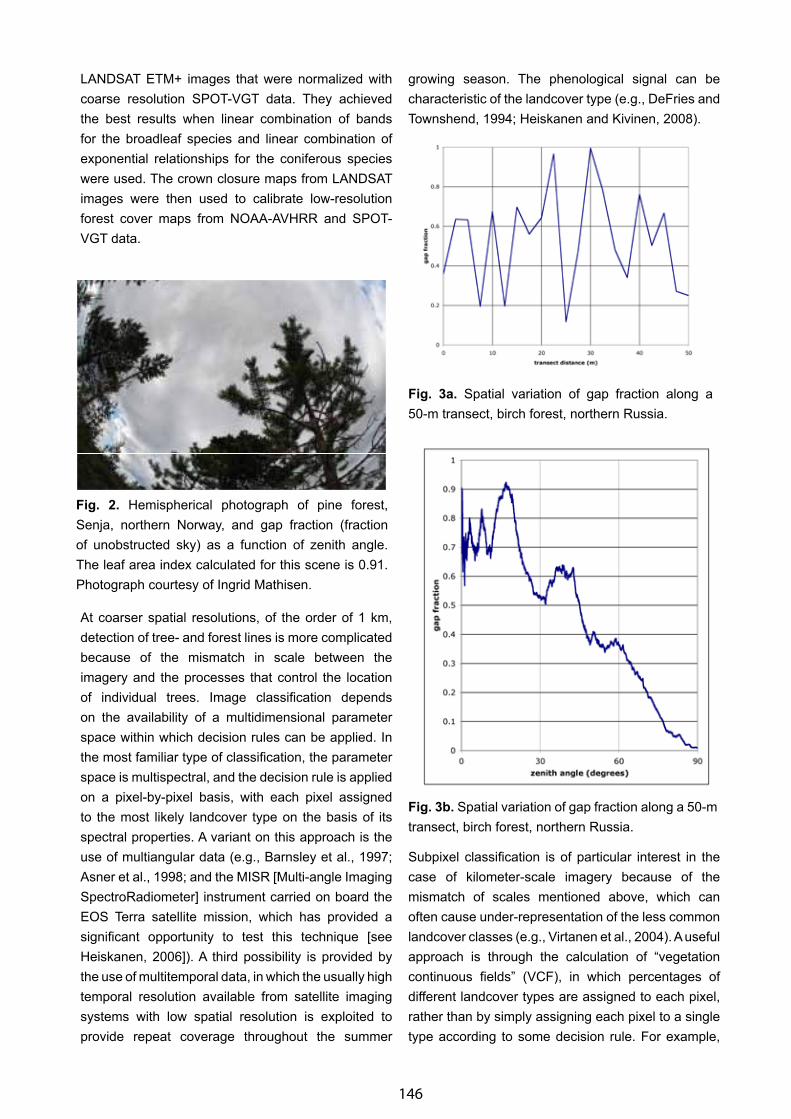
146

LANDSAT ETM+ images that were normalized with coarse resolution SPOT-VGT data. They achieved the best results when linear combination of bands for the broadleaf species and linear combination of exponential relationships for the coniferous species were used. The crown closure maps from LANDSAT images were then used to calibrate low-resolution forest cover maps from NOAA-AVHRR and SPOT-VGT data.

At coarser spatial resolutions, of the order of 1 km, detection of tree- and forest lines is more complicated because of the mismatch in scale between the imagery and the processes that control the location of individual trees. Image classification depends on the availability of a multidimensional parameter space within which decision rules can be applied. In the most familiar type of classification, the parameter space is multispectral, and the decision rule is applied on a pixel-by-pixel basis, with each pixel assigned to the most likely landcover type on the basis of its spectral properties. A variant on this approach is the use of multiangular data (e.g., Barnsley et al., 1997; Asner et al., 1998; and the MISR [Multi-angle Imaging SpectroRadiometer] instrument carried on board the EOS Terra satellite mission, which has provided a significant opportunity to test this technique [see Heiskanen, 2006]). A third possibility is provided by the use of multitemporal data, in which the usually high temporal resolution available from satellite imaging systems with low spatial resolution is exploited to provide repeat coverage throughout the summer

growing season. The phenological signal can be characteristic of the landcover type (e.g., DeFries and Townshend, 1994; Heiskanen and Kivinen, 2008).

Subpixel classification is of particular interest in the case of kilometer-scale imagery because of the mismatch of scales mentioned above, which can often cause under-representation of the less common landcover classes (e.g., Virtanen et al., 2004). A useful approach is through the calculation of “vegetation continuous fields” (VCF), in which percentages of different landcover types are assigned to each pixel, rather than by simply assigning each pixel to a single type according to some decision rule. For example,

Fig. 2. Hemispherical photograph of pine forest, Senja, northern Norway, and gap fraction (fraction of unobstructed sky) as a function of zenith angle. The leaf area index calculated for this scene is 0.91. Photograph courtesy of Ingrid Mathisen.

Fig. 3a. Spatial variation of gap fraction along a 50-m transect, birch forest, northern Russia.

Fig. 3b. Spatial variation of gap fraction along a 50-m transect, birch forest, northern Russia.

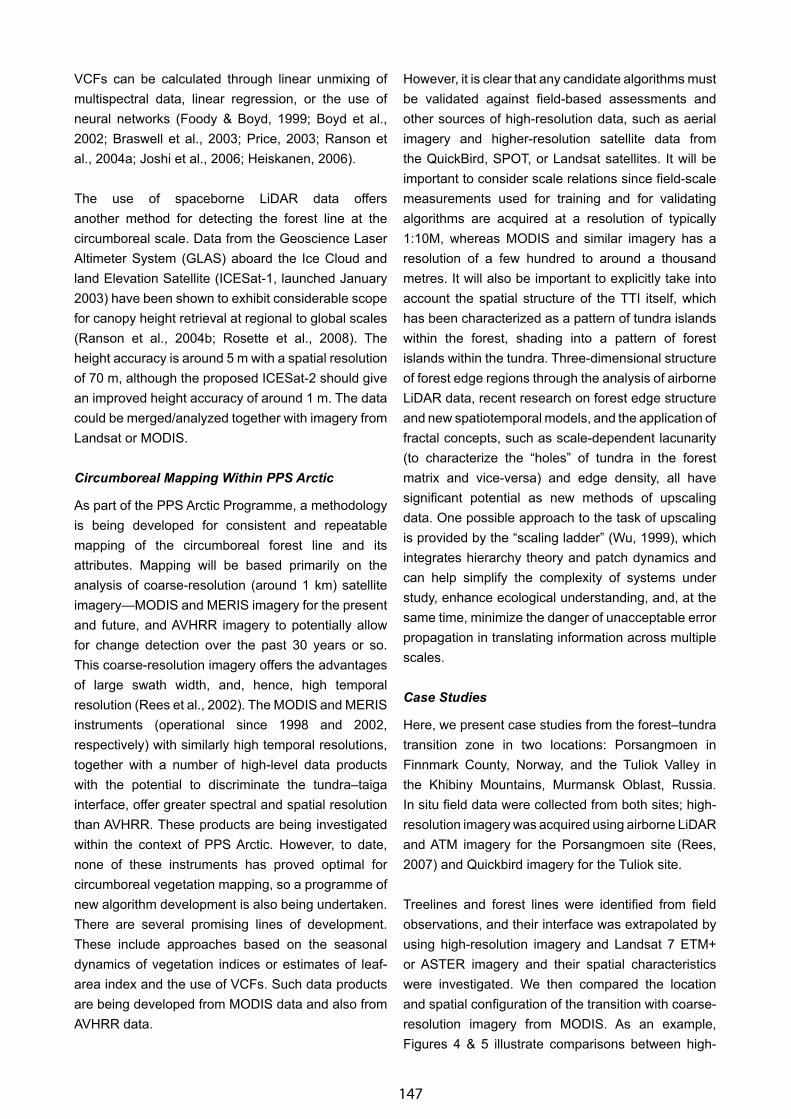
147

VCFs can be calculated through linear unmixing of multispectral data, linear regression, or the use of neural networks (Foody & Boyd, 1999; Boyd et al., 2002; Braswell et al., 2003; Price, 2003; Ranson et al., 2004a; Joshi et al., 2006; Heiskanen, 2006).

The use of spaceborne LiDAR data offers another method for detecting the forest line at the circumboreal scale. Data from the Geoscience Laser Altimeter System (GLAS) aboard the Ice Cloud and land Elevation Satellite (ICESat-1, launched January 2003) have been shown to exhibit considerable scope for canopy height retrieval at regional to global scales (Ranson et al., 2004b; Rosette et al., 2008). The height accuracy is around 5 m with a spatial resolution of 70 m, although the proposed ICESat-2 should give an improved height accuracy of around 1 m. The data could be merged/analyzed together with imagery from Landsat or MODIS.

Circumboreal Mapping Within PPS Arctic

As part of the PPS Arctic Programme, a methodology is being developed for consistent and repeatable mapping of the circumboreal forest line and its attributes. Mapping will be based primarily on the analysis of coarse-resolution (around 1 km) satellite imagery—MODIS and MERIS imagery for the present and future, and AVHRR imagery to potentially allow for change detection over the past 30 years or so. This coarse-resolution imagery offers the advantages of large swath width, and, hence, high temporal resolution (Rees et al., 2002). The MODIS and MERIS instruments (operational since 1998 and 2002, respectively) with similarly high temporal resolutions, together with a number of high-level data products with the potential to discriminate the tundra–taiga interface, offer greater spectral and spatial resolution than AVHRR. These products are being investigated within the context of PPS Arctic. However, to date, none of these instruments has proved optimal for circumboreal vegetation mapping, so a programme of new algorithm development is also being undertaken. There are several promising lines of development. These include approaches based on the seasonal dynamics of vegetation indices or estimates of leaf-area index and the use of VCFs. Such data products are being developed from MODIS data and also from AVHRR data.

However, it is clear that any candidate algorithms must be validated against field-based assessments and other sources of high-resolution data, such as aerial imagery and higher-resolution satellite data from the QuickBird, SPOT, or Landsat satellites. It will be important to consider scale relations since field-scale measurements used for training and for validating algorithms are acquired at a resolution of typically 1:10M, whereas MODIS and similar imagery has a resolution of a few hundred to around a thousand metres. It will also be important to explicitly take into account the spatial structure of the TTI itself, which has been characterized as a pattern of tundra islands within the forest, shading into a pattern of forest islands within the tundra. Three-dimensional structure of forest edge regions through the analysis of airborne LiDAR data, recent research on forest edge structure and new spatiotemporal models, and the application of fractal concepts, such as scale-dependent lacunarity (to characterize the “holes” of tundra in the forest matrix and vice-versa) and edge density, all have significant potential as new methods of upscaling data. One possible approach to the task of upscaling is provided by the “scaling ladder” (Wu, 1999), which integrates hierarchy theory and patch dynamics and can help simplify the complexity of systems under study, enhance ecological understanding, and, at the same time, minimize the danger of unacceptable error propagation in translating information across multiple scales.

Case Studies

Here, we present case studies from the forest–tundra transition zone in two locations: Porsangmoen in Finnmark County, Norway, and the Tuliok Valley in the Khibiny Mountains, Murmansk Oblast, Russia. In situ field data were collected from both sites; high-resolution imagery was acquired using airborne LiDAR and ATM imagery for the Porsangmoen site (Rees, 2007) and Quickbird imagery for the Tuliok site.

Treelines and forest lines were identified from field observations, and their interface was extrapolated by using high-resolution imagery and Landsat 7 ETM+ or ASTER imagery and their spatial characteristics were investigated. We then compared the location and spatial configuration of the transition with coarse-resolution imagery from MODIS. As an example, Figures 4 & 5 illustrate comparisons between high-

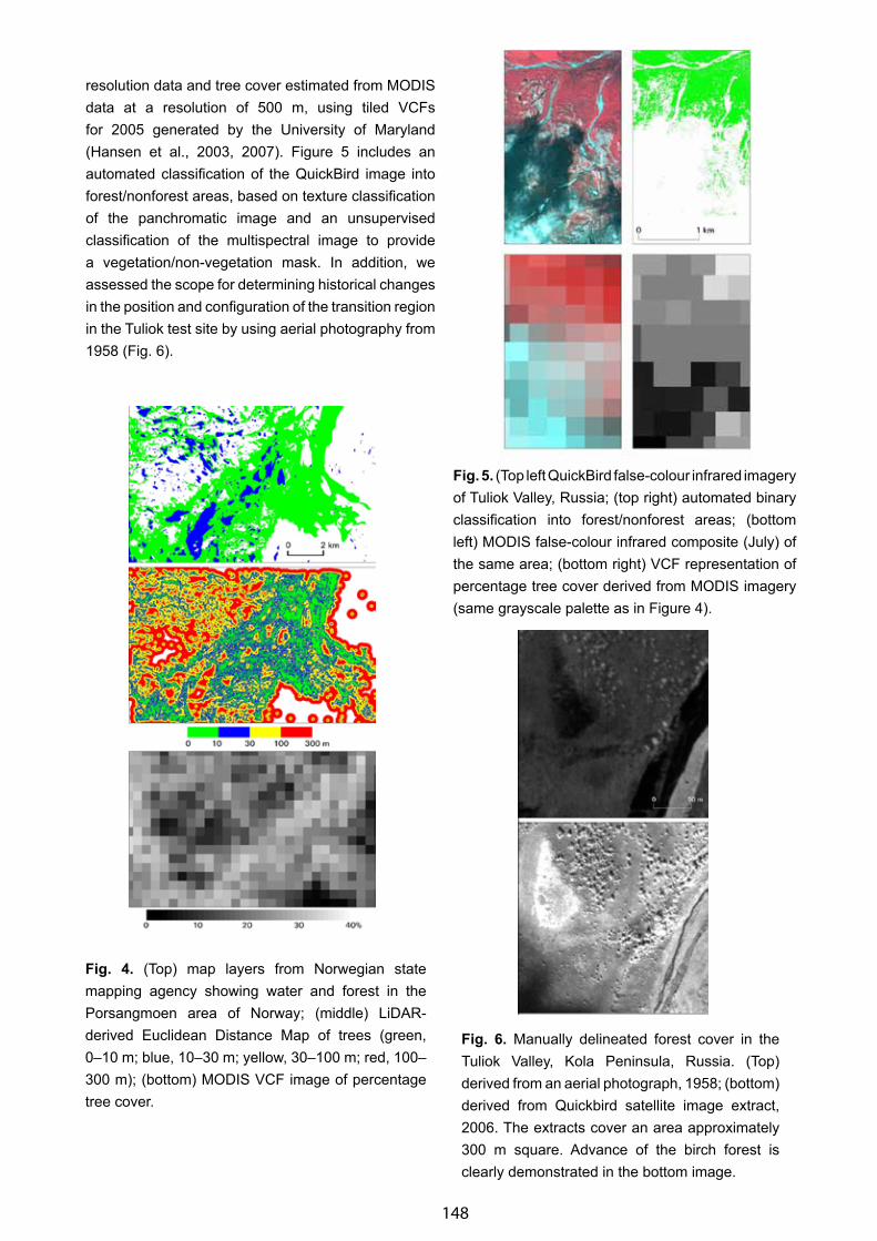
148

resolution data and tree cover estimated from MODIS data at a resolution of 500 m, using tiled VCFs for 2005 generated by the University of Maryland (Hansen et al., 2003, 2007). Figure 5 includes an automated classification of the QuickBird image into forest/nonforest areas, based on texture classification of the panchromatic image and an unsupervised classification of the multispectral image to provide a vegetation/non-vegetation mask. In addition, we assessed the scope for determining historical changes in the position and configuration of the transition region in the Tuliok test site by using aerial photography from 1958 (Fig. 6).

Fig. 5. (Top left QuickBird false-colour infrared imagery of Tuliok Valley, Russia; (top right) automated binary classification into forest/nonforest areas; (bottom left) MODIS false-colour infrared composite (July) of the same area; (bottom right) VCF representation of percentage tree cover derived from MODIS imagery (same grayscale palette as in Figure 4).

Fig. 4. (Top) map layers from Norwegian state mapping agency showing water and forest in the Porsangmoen area of Norway; (middle) LiDAR-derived Euclidean Distance Map of trees (green, 0–10 m; blue, 10–30 m; yellow, 30–100 m; red, 100–300 m); (bottom) MODIS VCF image of percentage tree cover.

Fig. 6. Manually delineated forest cover in the Tuliok Valley, Kola Peninsula, Russia. (Top) derived from an aerial photograph, 1958; (bottom) derived from Quickbird satellite image extract, 2006. The extracts cover an area approximately 300 m square. Advance of the birch forest is clearly demonstrated in the bottom image.

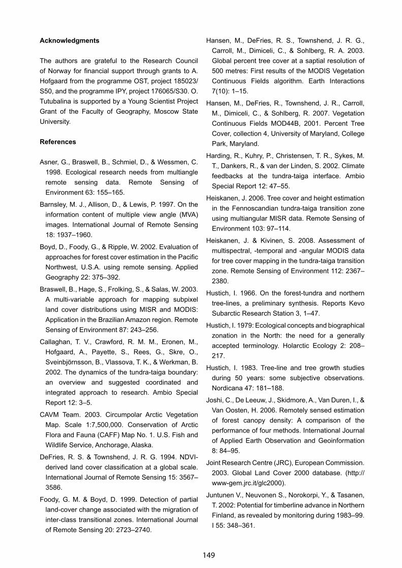
149

Acknowledgments

The authors are grateful to the Research Council of Norway for financial support through grants to A. Hofgaard from the programme OST, project 185023/S50, and the programme IPY, project 176065/S30. O. Tutubalina is supported by a Young Scientist Project Grant of the Faculty of Geography, Moscow State University.

References

Asner, G., Braswell, B., Schmiel, D., & Wessmen, C. 1998. Ecological research needs from multiangle remote sensing data. Remote Sensing of Environment 63: 155–165.

Barnsley, M. J., Allison, D., & Lewis, P. 1997. On the information content of multiple view angle (MVA) images. International Journal of Remote Sensing 18: 1937–1960.

Boyd, D., Foody, G., & Ripple, W. 2002. Evaluation of approaches for forest cover estimation in the Pacific Northwest, U.S.A. using remote sensing. Applied Geography 22: 375–392.

Braswell, B., Hage, S., Frolking, S., & Salas, W. 2003. A multi-variable approach for mapping subpixel land cover distributions using MISR and MODIS: Application in the Brazilian Amazon region. Remote Sensing of Environment 87: 243–256.

Callaghan, T. V., Crawford, R. M. M., Eronen, M., Hofgaard, A., Payette, S., Rees, G., Skre, O., Sveinbjörnsson, B., Vlassova, T. K., & Werkman, B. 2002. The dynamics of the tundra-taiga boundary: an overview and suggested coordinated and integrated approach to research. Ambio Special Report 12: 3–5.

CAVM Team. 2003. Circumpolar Arctic Vegetation Map. Scale 1:7,500,000. Conservation of Arctic Flora and Fauna (CAFF) Map No. 1. U.S. Fish and Wildlife Service, Anchorage, Alaska.

DeFries, R. S. & Townshend, J. R. G. 1994. NDVI-derived land cover classification at a global scale. International Journal of Remote Sensing 15: 3567–3586.

Foody, G. M. & Boyd, D. 1999. Detection of partial land-cover change associated with the migration of inter-class transitional zones. International Journal of Remote Sensing 20: 2723–2740.

Hansen, M., DeFries, R. S., Townshend, J. R. G., Carroll, M., Dimiceli, C., & Sohlberg, R. A. 2003. Global percent tree cover at a saptial resolution of 500 metres: First results of the MODIS Vegetation Continuous Fields algorithm. Earth Interactions 7(10): 1–15.

Hansen, M., DeFries, R., Townshend, J. R., Carroll, M., Dimiceli, C., & Sohlberg, R. 2007. Vegetation Continuous Fields MOD44B, 2001. Percent Tree Cover, collection 4, University of Maryland, College Park, Maryland.

Harding, R., Kuhry, P., Christensen, T. R., Sykes, M. T., Dankers, R., & van der Linden, S. 2002. Climate feedbacks at the tundra-taiga interface. Ambio Special Report 12: 47–55.

Heiskanen, J. 2006. Tree cover and height estimation in the Fennoscandian tundra-taiga transition zone using multiangular MISR data. Remote Sensing of Environment 103: 97–114.

Heiskanen, J. & Kivinen, S. 2008. Assessment of multispectral, -temporal and -angular MODIS data for tree cover mapping in the tundra-taiga transition zone. Remote Sensing of Environment 112: 2367–2380.

Hustich, I. 1966. On the forest-tundra and northern tree-lines, a preliminary synthesis. Reports Kevo Subarctic Research Station 3, 1–47.

Hustich, I. 1979: Ecological concepts and biographical zonation in the North: the need for a generally accepted terminology. Holarctic Ecology 2: 208–217.

Hustich, I. 1983. Tree-line and tree growth studies during 50 years: some subjective observations. Nordicana 47: 181–188.

Joshi, C., De Leeuw, J., Skidmore, A., Van Duren, I., & Van Oosten, H. 2006. Remotely sensed estimation of forest canopy density: A comparison of the performance of four methods. International Journal of Applied Earth Observation and Geoinformation 8: 84–95.

Joint Research Centre (JRC), European Commission. 2003. Global Land Cover 2000 database. (http://www-gem.jrc.it/glc2000).

Juntunen V., Neuvonen S., Norokorpi, Y., & Tasanen, T. 2002: Potential for timberline advance in Northern Finland, as revealed by monitoring during 1983–99. I 55: 348–361.

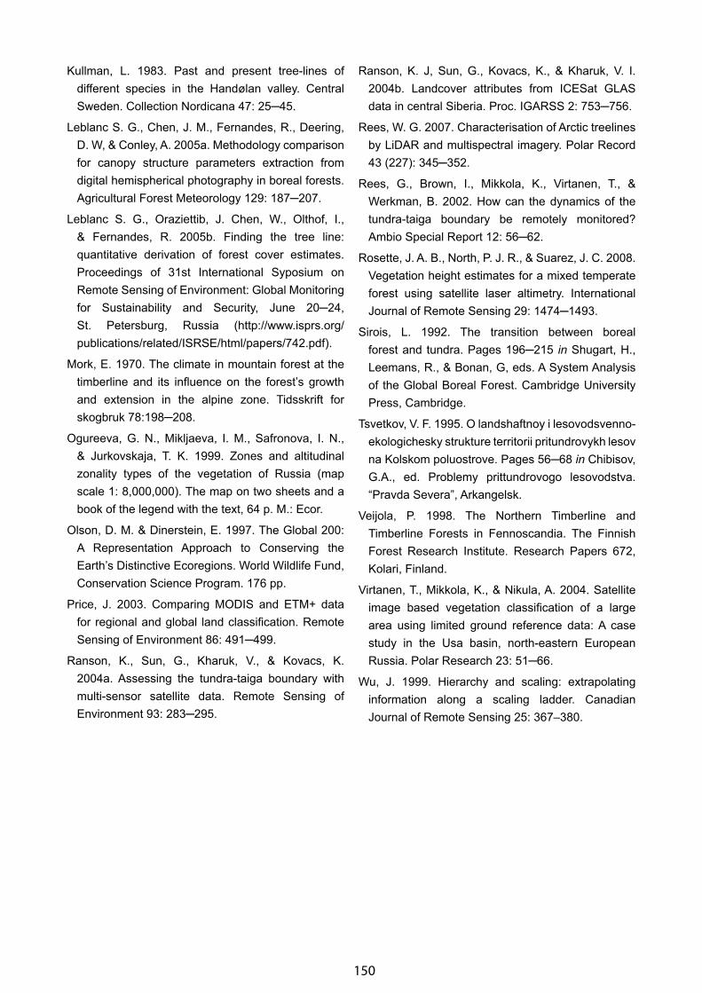
150

Kullman, L. 1983. Past and present tree-lines of different species in the Handølan valley. Central Sweden. Collection Nordicana 47: 25─45.

Leblanc S. G., Chen, J. M., Fernandes, R., Deering, D. W, & Conley, A. 2005a. Methodology comparison for canopy structure parameters extraction from digital hemispherical photography in boreal forests. Agricultural Forest Meteorology 129: 187─207.

Leblanc S. G., Oraziettib, J. Chen, W., Olthof, I., & Fernandes, R. 2005b. Finding the tree line: quantitative derivation of forest cover estimates. Proceedings of 31st International Syposium on Remote Sensing of Environment: Global Monitoring for Sustainability and Security, June 20─24, St. Petersburg, Russia (http://www.isprs.org/publications/related/ISRSE/html/papers/742.pdf).

Mork, E. 1970. The climate in mountain forest at the timberline and its influence on the forest’s growth and extension in the alpine zone. Tidsskrift for skogbruk 78:198─208.

Ogureeva, G. N., Mikljaeva, I. M., Safronova, I. N., & Jurkovskaja, T. K. 1999. Zones and altitudinal zonality types of the vegetation of Russia (map scale 1: 8,000,000). The map on two sheets and a book of the legend with the text, 64 p. M.: Ecor.

Olson, D. M. & Dinerstein, E. 1997. The Global 200: A Representation Approach to Conserving the Earth’s Distinctive Ecoregions. World Wildlife Fund, Conservation Science Program. 176 pp.

Price, J. 2003. Comparing MODIS and ETM+ data for regional and global land classification. Remote Sensing of Environment 86: 491─499.

Ranson, K., Sun, G., Kharuk, V., & Kovacs, K. 2004a. Assessing the tundra-taiga boundary with multi-sensor satellite data. Remote Sensing of Environment 93: 283─295.

Ranson, K. J, Sun, G., Kovacs, K., & Kharuk, V. I. 2004b. Landcover attributes from ICESat GLAS data in central Siberia. Proc. IGARSS 2: 753─756.

Rees, W. G. 2007. Characterisation of Arctic treelines by LiDAR and multispectral imagery. Polar Record 43 (227): 345─352.

Rees, G., Brown, I., Mikkola, K., Virtanen, T., & Werkman, B. 2002. How can the dynamics of the tundra-taiga boundary be remotely monitored? Ambio Special Report 12: 56─62.

Rosette, J. A. B., North, P. J. R., & Suarez, J. C. 2008. Vegetation height estimates for a mixed temperate forest using satellite laser altimetry. International Journal of Remote Sensing 29: 1474─1493.

Sirois, L. 1992. The transition between boreal forest and tundra. Pages 196─215 in Shugart, H., Leemans, R., & Bonan, G, eds. A System Analysis of the Global Boreal Forest. Cambridge University Press, Cambridge.

Tsvetkov, V. F. 1995. O landshaftnoy i lesovodsvenno-ekologichesky strukture territorii pritundrovykh lesov na Kolskom poluostrove. Pages 56─68 in Chibisov, G.A., ed. Problemy prittundrovogo lesovodstva. “Pravda Severa”, Arkangelsk.

Veijola, P. 1998. The Northern Timberline and Timberline Forests in Fennoscandia. The Finnish Forest Research Institute. Research Papers 672, Kolari, Finland.

Virtanen, T., Mikkola, K., & Nikula, A. 2004. Satellite image based vegetation classification of a large area using limited ground reference data: A case study in the Usa basin, north-eastern European Russia. Polar Research 23: 51─66.

Wu, J. 1999. Hierarchy and scaling: extrapolating information along a scaling ladder. Canadian Journal of Remote Sensing 25: 367–380.

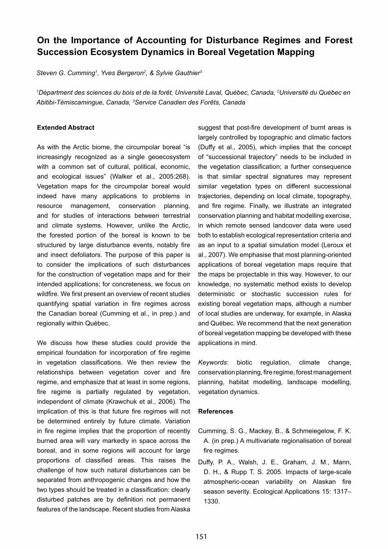
151

On the Importance of Accounting for Disturbance Regimes and Forest Succession Ecosystem Dynamics in Boreal Vegetation Mapping

Steven G. Cumming1, Yves Bergeron2, & Sylvie Gauthier3

1Départment des sciences du bois et de la forêt, Université Laval, Québec, Canada, 2Université du Québec en Abitibi-Témiscamingue, Canada, 3Service Canadien des Forêts, Canada

Extended Abstract

As with the Arctic biome, the circumpolar boreal “is increasingly recognized as a single geoecosystem with a common set of cultural, political, economic, and ecological issues” (Walker et al., 2005:268). Vegetation maps for the circumpolar boreal would indeed have many applications to problems in resource management, conservation planning, and for studies of interactions between terrestrial and climate systems. However, unlike the Arctic, the forested portion of the boreal is known to be structured by large disturbance events, notably fire and insect defoliators. The purpose of this paper is to consider the implications of such disturbances for the construction of vegetation maps and for their intended applications; for concreteness, we focus on wildfire. We first present an overview of recent studies quantifying spatial variation in fire regimes across the Canadian boreal (Cumming et al., in prep.) and regionally within Québec.

We discuss how these studies could provide the empirical foundation for incorporation of fire regime in vegetation classifications. We then review the relationships between vegetation cover and fire regime, and emphasize that at least in some regions, fire regime is partially regulated by vegetation, independent of climate (Krawchuk et al., 2006). The implication of this is that future fire regimes will not be determined entirely by future climate. Variation in fire regime implies that the proportion of recently burned area will vary markedly in space across the boreal, and in some regions will account for large proportions of classified areas. This raises the challenge of how such natural disturbances can be separated from anthropogenic changes and how the two types should be treated in a classification: clearly disturbed patches are by definition not permanent features of the landscape. Recent studies from Alaska

suggest that post-fire development of burnt areas is largely controlled by topographic and climatic factors (Duffy et al., 2005), which implies that the concept of “successional trajectory” needs to be included in the vegetation classification; a further consequence is that similar spectral signatures may represent similar vegetation types on different successional trajectories, depending on local climate, topography, and fire regime. Finally, we illustrate an integrated conservation planning and habitat modelling exercise, in which remote sensed landcover data were used both to establish ecological representation criteria and as an input to a spatial simulation model (Leroux et al., 2007). We emphasise that most planning-oriented applications of boreal vegetation maps require that the maps be projectable in this way. However, to our knowledge, no systematic method exists to develop deterministic or stochastic succession rules for existing boreal vegetation maps, although a number of local studies are underway, for example, in Alaska and Québec. We recommend that the next generation of boreal vegetation mapping be developed with these applications in mind.

Keywords: biotic regulation, climate change, conservation planning, fire regime, forest management planning, habitat modelling, landscape modelling, vegetation dynamics.

References

Cumming, S. G., Mackey, B., & Schmeiegelow, F. K. A. (in prep.) A multivariate regionalisation of boreal fire regimes.

Duffy, P. A., Walsh, J. E., Graham, J. M., Mann, D. H., & Rupp T. S. 2005. Impacts of large-scale atmospheric-ocean variability on Alaskan fire season severity. Ecological Applications 15: 1317–1330.

152

Krawchuk, M. A., Cumming, S. G., Flannigan, M. D., & Wein, R. W. 2006. Biotic and abiotic regulation of lightning fire initiation in the mixedwood boreal forest. Ecology 87:458–468.

Leroux, S. J., Schmiegelow, F. K. A., Cumming, S. G., Lessard, R. B., & Nagy, J. 2007 Accounting for system dynamics in reserve design. Ecological Applications 17: 1954–1966.

Walker, D. A., Raynolds, M. K., Daniëls, F. J. A., Einarsson, E., Elvebakk, A., Gould, W. A., Katenin, A. E., Kholod, S. S., Markon, C. J., Melnikov, E. E., Moskalenko, N. G., Talbot, S. S., Yurtsev, B. A., & the CAVM Team. 2005. The Circumpolar Arctic Vegetation Map. Journal of Vegetation Science 16: 267─282.

153

Role of Disturbed Vegetation in Mapping the Boreal Zone in Northern Eurasia

Annika Hofgaard1, Gareth Rees2, Hans Tømmervik3, Olga Tutubalina4, Elena Golubeva4, Ekaterina Shipigina4, Kjell Arild Høgda5, Stein Rune Karlsen5, Mikhail Zimin1, Viacheslav Kharuk6

1Norwegian Institute for Nature Research (NINA), Trondheim, Norway, 2Scott Polar Research Institute, University of Cambridge, United Kingdom, 3Norwegian Institute for Nature Research (NINA), Tromsø, Norway, 4Faculty of Geography, M.V. Lomonosov Moscow State University, Moscow, Russian Federation, 5Northern Research Institute (NORUT), Tromsø, Norway, 6Sukachev Forest Institute, Akademgorodok Krasnoyarsk, Russian Federation

Extended Abstract

Arctic, subarctic, and northern boreal habitats are notable for the significance of their “disturbance” (Shugart et al., 1992; Crawford, 1997). A commonly used definition of disturbance is the one by Pickett and White (1985): “any relatively discrete event in time that disrupts ecosystem, community, or population structure and changes resources, substrate availability, or the physical environment.” This description may also be considered as influences of limited spatial or temporal extent superimposed on the broader-scale background conditions. However, when considering changes in the boreal zone and its transition to the arctic region in a long-term perspective, this definition of disturbance with focus on limited spatial or temporal extent is not satisfactory or complete. Disturbance is a highly scale-dependent concept, and consideration has to be given to both the spatial and short- and long-term extent of any disturbance. Disturbances occur at widely different spatial and temporal scales, and their evident significance depends on the time scale at which we are observing the system. In addition, many different kinds of disturbances may interact over time.

Disturbances can be both naturally occurring and anthropogenic. Examples of the former are provided by climate and herbivory, and of the latter, by locally generated air pollution, forest logging, changed grazing regime, mineral exploitation, and disturbances due to oil and gas development, etc. Another example, fire, can be both naturally occurring and man-caused. In some parts of the circumboreal zone, these and other disturbances are dominant in controlling the characteristics of the boreal forests

and the forest–tundra transition, and this fact needs to be represented in any map of the zone.

Boreal disturbance regimes may have an episodic character, a chronic character, or a character interweaving the two (cf. Hofgaard, 1997). Boreal communities are shaped through episodic disturbances (e.g., fire and insect outbreaks) and longer term, chronic disturbances (e.g., climate stress, pollution, and grazing) occurring at all spatial scales, from the landscape or region to individual forest stands or single trees. In addition, a disturbance event such as fire or logging may trigger development of a chronic disturbance state through an intensified grazing regime or increased climate vulnerability.

A relevant question that should be asked and kept in mind both when studying and mapping the system is: “What is natural vegetation in a changing environment?” When examined more closely, regions and areas dominated by supposed natural vegetation in balance with the environment are in most cases products of current and/or previous natural or man-altered disturbance regimes (Sprugel, 1991). The current vegetation structure is somewhere along the road towards recovery from previous disturbances. However, equilibrium with the environment will never be reached in regions where environmental variability and change is a natural and dominating part of the reality, as in arctic, subarctic and boreal regions. Recovery after disturbance is not a straightforward matter either in the time needed for recovery or involved succession steps towards pre-disturbance conditions. Although disturbance driven dynamics are challenging when constructing vegetation maps for the zone, there is a need for the inclusion of disturbed

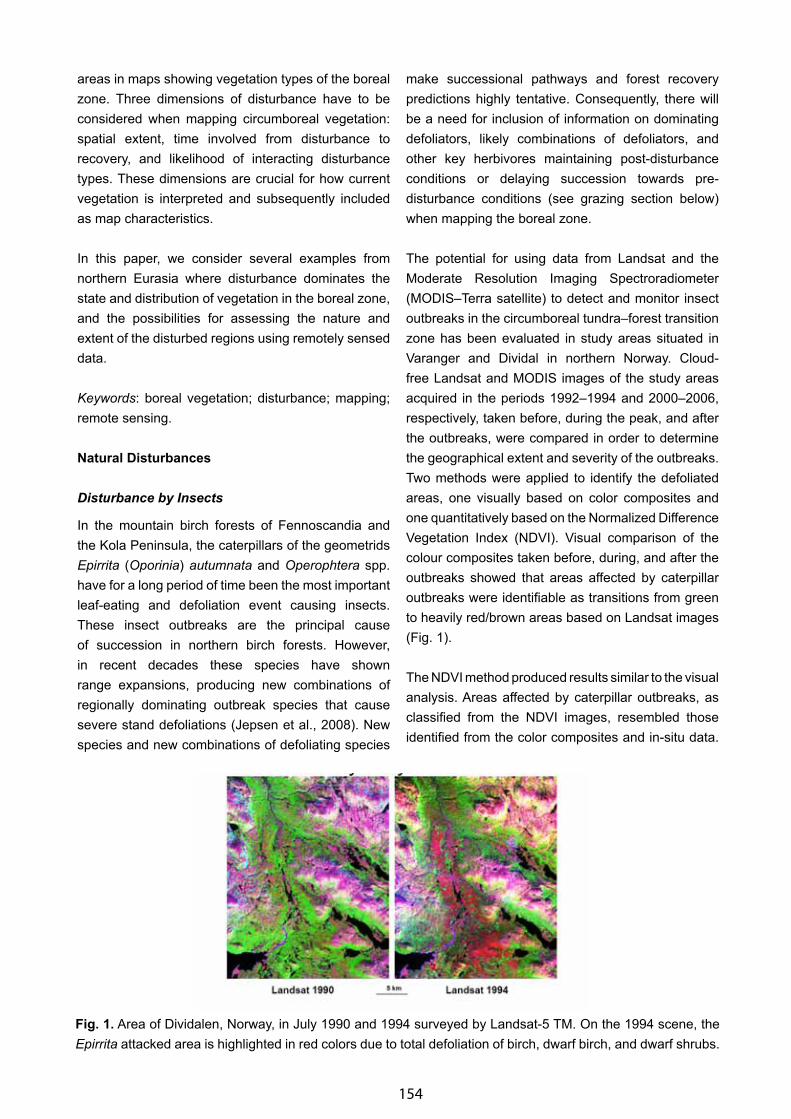
154

areas in maps showing vegetation types of the boreal zone. Three dimensions of disturbance have to be considered when mapping circumboreal vegetation: spatial extent, time involved from disturbance to recovery, and likelihood of interacting disturbance types. These dimensions are crucial for how current vegetation is interpreted and subsequently included as map characteristics.

In this paper, we consider several examples from northern Eurasia where disturbance dominates the state and distribution of vegetation in the boreal zone, and the possibilities for assessing the nature and extent of the disturbed regions using remotely sensed data.

Keywords: boreal vegetation; disturbance; mapping; remote sensing.

Natural Disturbances

Disturbance by Insects

In the mountain birch forests of Fennoscandia and the Kola Peninsula, the caterpillars of the geometrids Epirrita (Oporinia) autumnata and Operophtera spp. have for a long period of time been the most important leaf-eating and defoliation event causing insects. These insect outbreaks are the principal cause of succession in northern birch forests. However, in recent decades these species have shown range expansions, producing new combinations of regionally dominating outbreak species that cause severe stand defoliations (Jepsen et al., 2008). New species and new combinations of defoliating species

make successional pathways and forest recovery predictions highly tentative. Consequently, there will be a need for inclusion of information on dominating defoliators, likely combinations of defoliators, and other key herbivores maintaining post-disturbance conditions or delaying succession towards pre-disturbance conditions (see grazing section below) when mapping the boreal zone.

The potential for using data from Landsat and the Moderate Resolution Imaging Spectroradiometer (MODIS–Terra satellite) to detect and monitor insect outbreaks in the circumboreal tundra–forest transition zone has been evaluated in study areas situated in Varanger and Dividal in northern Norway. Cloud-free Landsat and MODIS images of the study areas acquired in the periods 1992–1994 and 2000–2006, respectively, taken before, during the peak, and after the outbreaks, were compared in order to determine the geographical extent and severity of the outbreaks. Two methods were applied to identify the defoliated areas, one visually based on color composites and one quantitatively based on the Normalized Difference Vegetation Index (NDVI). Visual comparison of the colour composites taken before, during, and after the outbreaks showed that areas affected by caterpillar outbreaks were identifiable as transitions from green to heavily red/brown areas based on Landsat images (Fig. 1).

The NDVI method produced results similar to the visual analysis. Areas affected by caterpillar outbreaks, as classified from the NDVI images, resembled those identified from the color composites and in-situ data.

Fig. 1. Area of Dividalen, Norway, in July 1990 and 1994 surveyed by Landsat-5 TM. On the 1994 scene, the Epirrita attacked area is highlighted in red colors due to total defoliation of birch, dwarf birch, and dwarf shrubs.

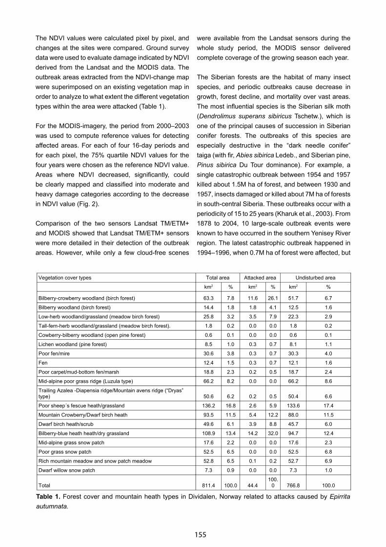
155

The NDVI values were calculated pixel by pixel, and changes at the sites were compared. Ground survey data were used to evaluate damage indicated by NDVI derived from the Landsat and the MODIS data. The outbreak areas extracted from the NDVI-change map were superimposed on an existing vegetation map in order to analyze to what extent the different vegetation types within the area were attacked (Table 1).

For the MODIS-imagery, the period from 2000–2003 was used to compute reference values for detecting affected areas. For each of four 16-day periods and for each pixel, the 75% quartile NDVI values for the four years were chosen as the reference NDVI value. Areas where NDVI decreased, significantly, could be clearly mapped and classified into moderate and heavy damage categories according to the decrease in NDVI value (Fig. 2).

Comparison of the two sensors Landsat TM/ETM+ and MODIS showed that Landsat TM/ETM+ sensors were more detailed in their detection of the outbreak areas. However, while only a few cloud-free scenes

were available from the Landsat sensors during the whole study period, the MODIS sensor delivered complete coverage of the growing season each year.

The Siberian forests are the habitat of many insect species, and periodic outbreaks cause decrease in growth, forest decline, and mortality over vast areas. The most influential species is the Siberian silk moth (Dendrolimus superans sibiricus Tschetw.), which is one of the principal causes of succession in Siberian conifer forests. The outbreaks of this species are especially destructive in the “dark needle conifer” taiga (with fir, Abies sibirica Ledeb., and Siberian pine, Pinus sibirica Du Tour dominance). For example, a single catastrophic outbreak between 1954 and 1957 killed about 1.5M ha of forest, and between 1930 and 1957, insects damaged or killed about 7M ha of forests in south-central Siberia. These outbreaks occur with a periodicity of 15 to 25 years (Kharuk et al., 2003). From 1878 to 2004, 10 large-scale outbreak events were known to have occurred in the southern Yenisey River region. The latest catastrophic outbreak happened in 1994–1996, when 0.7M ha of forest were affected, but

Table 1. Forest cover and mountain heath types in Dividalen, Norway related to attacks caused by Epirrita autumnata.

Vegetation cover types Total area Attacked area Undisturbed area

km2 % km2 % km2 %

Bilberry-crowberry woodland (birch forest) 63.3 7.8 11.6 26.1 51.7 6.7

Bilberry woodland (birch forest) 14.4 1.8 1.8 4.1 12.5 1.6

Low-herb woodland/grassland (meadow birch forest) 25.8 3.2 3.5 7.9 22.3 2.9

Tall-fern-herb woodland/grassland (meadow birch forest). 1.8 0.2 0.0 0.0 1.8 0.2

Cowberry-bilberry woodland (open pine forest) 0.6 0.1 0.0 0.0 0.6 0.1

Lichen woodland (pine forest) 8.5 1.0 0.3 0.7 8.1 1.1

Poor fen/mire 30.6 3.8 0.3 0.7 30.3 4.0

Fen 12.4 1.5 0.3 0.7 12.1 1.6

Poor carpet/mud-bottom fen/marsh 18.8 2.3 0.2 0.5 18.7 2.4

Mid-alpine poor grass ridge (Luzula type) 66.2 8.2 0.0 0.0 66.2 8.6

Trailing Azalea -Diapensia ridge/Mountain avens ridge (“Dryas” type) 50.6 6.2 0.2 0.5 50.4 6.6

Poor sheep´s fescue heath/grassland 136.2 16.8 2.6 5.9 133.6 17.4

Mountain Crowberry/Dwarf birch heath 93.5 11.5 5.4 12.2 88.0 11.5

Dwarf birch heath/scrub 49.6 6.1 3.9 8.8 45.7 6.0

Bilberry-blue heath heath/dry grassland 108.9 13.4 14.2 32.0 94.7 12.4

Mid-alpine grass snow patch 17.6 2.2 0.0 0.0 17.6 2.3

Poor grass snow patch 52.5 6.5 0.0 0.0 52.5 6.8

Rich mountain meadow and snow patch meadow 52.8 6.5 0.1 0.2 52.7 6.9

Dwarf willow snow patch 7.3 0.9 0.0 0.0 7.3 1.0

Total 811.4 100.0 44.4100.

0 766.8 100.0

156

the last outbreak in the south Siberian mountain taiga occurred in 2002–2003. Landsat, Terra/MODIS, and Spot Vegetation satellite data were applied for mapping insect-affected territories from the 1994–1996 event (Kharuk et al., 2003). The dynamics of the outbreaks were analyzed based on NDVI temporal profiles, which showed good correlation between satellite and in-situ data. The relationship between forest stand mortality from insects and topographic features (azimuth, elevation, slope steepness) was analyzed using a high-resolution digital elevation model. The outbreak began between the elevations of ~430–480 m and on southwest slopes with a steepness <5º, and these conditions appear to be the most favourable Siberian silk moth habitat. During the mid-phase of the outbreak, the insects moved both up- and down-slope, resulting in an elevation distribution split within a range of ~390–540 m and slope steepness up to 15º. In the final phase, the azimuth distribution of damaged stands became uniform, showing that the insect at this phase settled in non-optimal habitat. Data obtained show that satellite data sensors are applicable for monitoring not only extent of, but also the dynamic nature of Siberian silk moth outbreaks in taiga landscapes vulnerable to outbreaks. Both are essential when mapping the zone.

Disturbance by Fire

In large parts of the boreal region, the dominating natural disturbance agent is fire. The frequency, areal extent, and intensity of these fires varies between geographical regions and time periods and are principally set by the dominating climate regime of the regions and changes of these climate regimes. However, fire regimes are also to some extent affected by insect outbreak regimes. Outbreaks of insects promote wildfires because killed stands accumulate combustible material in the form of dead wood, and because more fire receptive post-outbreak communities, such as grass and shrub communities, are a result of the outbreaks.

For the zone of larch dominance (Larix sibirica Ledeb.; Larix gmelinii (Rupr.) Kuzen) in Central Siberia a decrease of the fire return intervals from about 100 years in the 19th century to 65 years in the 20th century has been found, which can mostly be attributed to changes in climate. However, similar changes in the “larch-mixed taiga” ecotone with a change in fire return interval from 97 years to 50 years has been interpreted as mainly caused by anthropogenic impacts (Kharuk et al., 2008; Ranson & Dvinskaya, 2008).

Disturbance by Grazing

Northern boreal systems are regionally important grazing areas to ungulate populations. The impact by these grazers is significant in regions where dominant stand-forming tree species are favourable food to these herbivores at some stage in their life cycle. Further, both post-insect outbreak and post-fire vegetation communities attract ungulate grazers through the assembly of palatable sprouts and the grass and herb dominated communities. Consequently, grazing by ungulates can act as an agent preserving conditions after severe disturbances, such as fire and an insect outbreak, for a prolonged period. Thus, grazing may cause substantial lag in successional development after disturbance and act as a chronic disturbance to both previously disturbed as well as to previously undisturbed communities.

For example, high densities of reindeer can lead to removal of birch seedlings and saplings with subsequent decrease in mountain birch forest extent. The effect will be pronounced in the transition zone

Fig. 2. Decrease in NDVI value in 2004 caused by insect (Epirrita autumnata) defoliation of birch forest (shown in red), Tana-Varanger area in north-easternmost Norway. Birch forests are shown in green. As indicated on the map, both moderate (5–20%) and severe damage categories (> 20%) could be mapped.

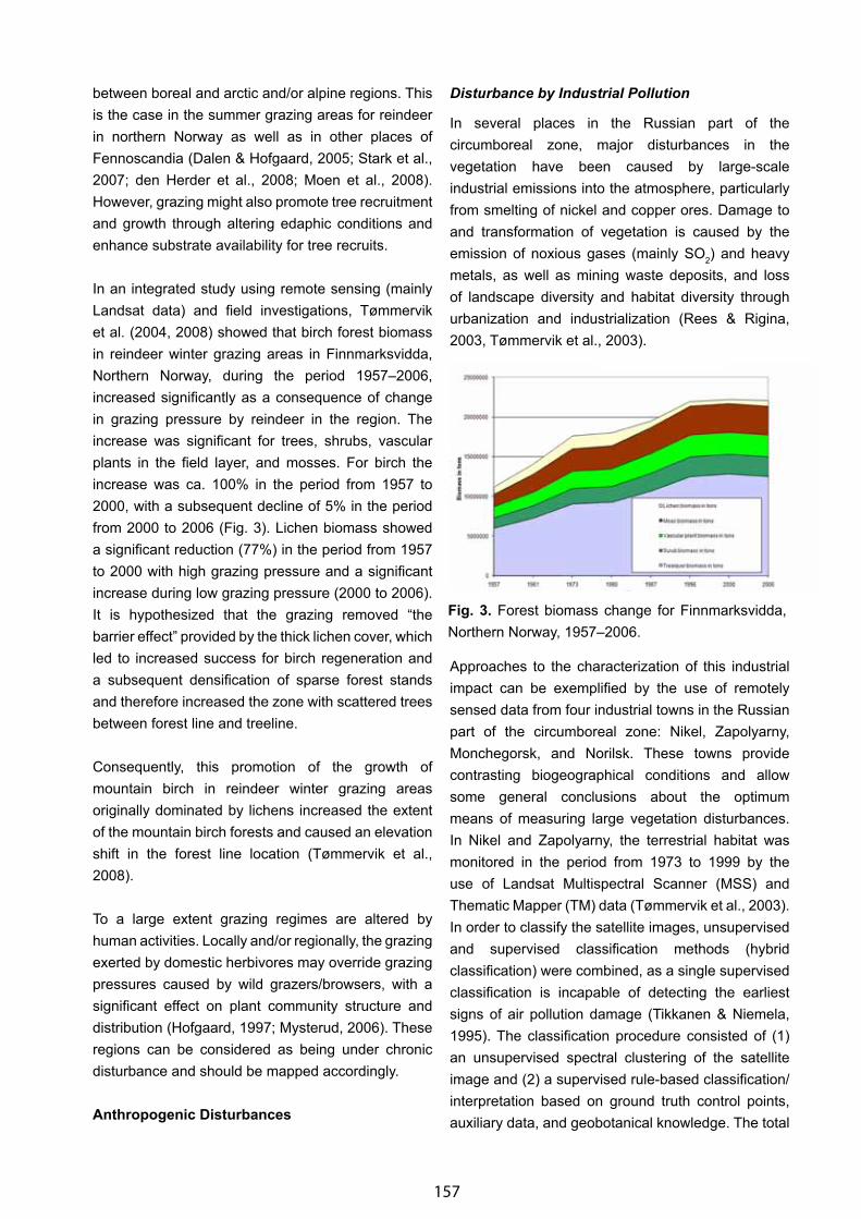
157

between boreal and arctic and/or alpine regions. This is the case in the summer grazing areas for reindeer in northern Norway as well as in other places of Fennoscandia (Dalen & Hofgaard, 2005; Stark et al., 2007; den Herder et al., 2008; Moen et al., 2008). However, grazing might also promote tree recruitment and growth through altering edaphic conditions and enhance substrate availability for tree recruits.

In an integrated study using remote sensing (mainly Landsat data) and field investigations, Tømmervik et al. (2004, 2008) showed that birch forest biomass in reindeer winter grazing areas in Finnmarksvidda, Northern Norway, during the period 1957–2006, increased significantly as a consequence of change in grazing pressure by reindeer in the region. The increase was significant for trees, shrubs, vascular plants in the field layer, and mosses. For birch the increase was ca. 100% in the period from 1957 to 2000, with a subsequent decline of 5% in the period from 2000 to 2006 (Fig. 3). Lichen biomass showed a significant reduction (77%) in the period from 1957 to 2000 with high grazing pressure and a significant increase during low grazing pressure (2000 to 2006). It is hypothesized that the grazing removed “the barrier effect” provided by the thick lichen cover, which led to increased success for birch regeneration and a subsequent densification of sparse forest stands and therefore increased the zone with scattered trees between forest line and treeline.

Consequently, this promotion of the growth of mountain birch in reindeer winter grazing areas originally dominated by lichens increased the extent of the mountain birch forests and caused an elevation shift in the forest line location (Tømmervik et al., 2008).

To a large extent grazing regimes are altered by human activities. Locally and/or regionally, the grazing exerted by domestic herbivores may override grazing pressures caused by wild grazers/browsers, with a significant effect on plant community structure and distribution (Hofgaard, 1997; Mysterud, 2006). These regions can be considered as being under chronic disturbance and should be mapped accordingly.

Anthropogenic Disturbances

Disturbance by Industrial Pollution

In several places in the Russian part of the circumboreal zone, major disturbances in the vegetation have been caused by large-scale industrial emissions into the atmosphere, particularly from smelting of nickel and copper ores. Damage to and transformation of vegetation is caused by the emission of noxious gases (mainly SO2) and heavy metals, as well as mining waste deposits, and loss of landscape diversity and habitat diversity through urbanization and industrialization (Rees & Rigina, 2003, Tømmervik et al., 2003).

Approaches to the characterization of this industrial impact can be exemplified by the use of remotely sensed data from four industrial towns in the Russian part of the circumboreal zone: Nikel, Zapolyarny, Monchegorsk, and Norilsk. These towns provide contrasting biogeographical conditions and allow some general conclusions about the optimum means of measuring large vegetation disturbances. In Nikel and Zapolyarny, the terrestrial habitat was monitored in the period from 1973 to 1999 by the use of Landsat Multispectral Scanner (MSS) and Thematic Mapper (TM) data (Tømmervik et al., 2003). In order to classify the satellite images, unsupervised and supervised classification methods (hybrid classification) were combined, as a single supervised classification is incapable of detecting the earliest signs of air pollution damage (Tikkanen & Niemela, 1995). The classification procedure consisted of (1) an unsupervised spectral clustering of the satellite image and (2) a supervised rule-based classification/interpretation based on ground truth control points, auxiliary data, and geobotanical knowledge. The total

Fig. 3. Forest biomass change for Finnmarksvidda, Northern Norway, 1957–2006.

158

overall accuracy of the vegetation maps produced in the period varied between 75%─83%. It was concluded that the main effect of air pollution was a reduction in areas of lichen-dominated forests and mountain heaths (Cladonia spp.): there was a decrease from 37% in 1973 to 10% in 1994, followed by a slight increase to 12% in 1999. The lichen-dominated vegetation types were changed into barrens, partly damaged vegetation entities, and dwarf shrub (e.g., Vaccinium myrtillus)-dominated vegetation (Fig. 4). Rees & Williams (1997) also successfully used this mapping method in the Monchegorsk area.

Disturbance by Forest Logging

According to the Atlas of Russia’s Intact Forest Landscapes (Aksenov et al., 2002), only 26% (289M hectares) of Russia’s forests remain in areas that have no signs of infrastructure or modern land use and are at least 50,000 ha in size. Most of these forests are in the boreal zone. Eastern Siberia is the most pristine region, with 39% of the forest zone in intact forest landscapes, followed by the Russian Far East (30%) and Western Siberia (25%). European Russia is by far the least pristine region, with only 9% of the forest intact. In Fennoscandia, less than 5% of the boreal forest zone was considered pristine in the late 1990’s (Niemi et al., 1998). However, it is also concluded that over 99% of the boreal forests in Fennoscandia have been altered by forestry practices (Griesser et al., 2007). Consequently, the waste majority of Scandinavian boreal forests have man-made disturbance patterns and stand characteristics.

The Arkhangelsk region presents a typical example of intensive logging in Russian boreal forests, with large logging areas and associated deciduous mixed coniferous successions easily detectable in medium-resolution remote sensing data, such as those from Landsat satellites.

Disturbance by Oil and Gas Development

Parts of the boreal zone in Russia are significantly developed for oil and gas extraction and transport. Oil is piped westwards from the Nenets Okrug, and gas from the West Siberian basin. Construction of pipelines and associated roads requires forest logging and can lead to erosion, damming of water courses, wetland formation, and other disturbances. Disturbance is also caused by oil spills (Vilchek & Tishkov, 1997). All

of these types of disturbances are easily detectable in medium-resolution remote sensing data.

Disturbance by Fire

Disturbance by anthropogenic caused fires has varied through time and space due to a region specific history of change in land use patterns. Regionally, fire has been used as a tool to increase grazing conditions in forested areas. In populated parts of Scandinavia, a general change from high-frequency human-caused fires during centuries pre-dating industrial times to current low-frequency, spatially limited fire events is evident (Zackrisson, 1979).

Predominantly, anthropogenic fire regimes affect large areas in Kola Peninsula, Siberia, and the Far East. Burnt areas in northern Eurasia in 2002─2006 varied from 6M to 40M hectares (TerraNorte, 2008); of these, the majority are in the boreal forests with some proportion of steppe fires, mostly in south Siberia. Thus, up to a few percent of the total area of the boreal forests in northern Eurasia were affected by fire each year during this period. Forest fires can be connected with intensified logging activity, with some of the fire-affected forests licensed for logging (Radford, 2005). Forest fire activity is monitored by national and international bodies using coarse-resolution MODIS and Advanced Very High Resolution Radiometer (AVHRR) data, and forest fire disturbance maps can be readily produced.

Disturbance and Mapping of Border Zones

It is generally considered that transition zones or border zones between plant communities/regions, such as the forest–tundra transition zone, represent a delicate balance between opposing forces of nature and should therefore be modified by slight changes in the environment (cf. Hofgaard, 1997). Disturbance as the central factor in boreal vegetation dynamics and in translating environmental change in vegetational response will thus be of prominent importance at transition zones. Consequently, knowledge of the disturbance regime is essential for understanding, mapping, and modelling system responses, particularly in this region.

There is a lack of consistent data on the location, nature, and dynamics of the forest─tundra transition zone at all scales from global to landscape (Rees, 2007), and

159

Fig.4. Landcover map over the Pasvik–Nikel area from 1999. Lichen-dominated heathland and woodland vegetation types (light yellow and brown colors); dwarf shrub dominated forests and heaths (green colors); and barrens and damaged environments (air pollution) around the smelters in Nikel and Zapolyarny, Russia (violet colors).

this has major implications for circumboreal vegetation mapping. An international, coordinated program of research into this topic has been developed under the auspices of the International Polar Year (IPY). This program has the title “Present-Day Processes, Past Changes and Spatiotemporal Variability of Biotic, Abiotic and Socio-Environmental Conditions and Resource Components Along and Across the Arctic Delimitation Zone” (PPS Arctic) (http://www.ipy.org/development/eoi/proposal-details.php?id=151). The PPS Arctic has around 110 researchers from 13 countries active at ca. 30 field sites across the circumarctic region, chosen to provide adequate sampling of both latitudinal and altitudinal treeline ecotones, the oceanicity gradient, and the broad range of tree species composing the circumpolar forest–tundra transition. The major areas of activity within the PPS Arctic program, which is coordinated from Norway and the United Kingdom, are currently within Canada and northwestern Europe.

At a large scale, mapping of the forest─tundra transition zone is based primarily on the analysis of coarse-resolution (around 1 km) satellite imagery—MODIS and Medium Resolution Imaging Spectrometer (MERIS) imagery—for the present and future, and AVHRR imagery to potentially allow for change detection over the past 30 years or so. This coarse-resolution imagery offers the advantages of large swath width, and, hence, high temporal resolution (Rees et al., 2002). However, by the use of high-resolution data and selected test areas, mapping precision of the forest–tundra transition is further developed within the PPS Arctic program (cf. Rees et al., this volume).

Conclusion

Disturbed vegetation occupies significant areas in the boreal zone, and related vegetation successions should be adequately represented when mapping this

160

region. If the proposed Circumboreal Vegetation Map will focus on showing the potential vegetation types, it would still be useful to show the types of disturbances and successions through a system of color hatchings, symbols and lines, overlaid on the vegetation type contours, and to present this information as separate layers in a corresponding geographic information system (GIS) database.

Acknowledgments

The authors are grateful to the Research Council of Norway for financial support through grants to A. Hofgaard from the program OST, project 185023/S50, and program IPY, project 176065/S30.

References

Aksenov, D., Dobrynin, D., Dubinin, M., Egorov, A., Isaev, A., Karpachevskiy, M., Laestadius, L. Potapov, P., Purekhovskiy, A., Turubanova, S., & Yaroshenko, A. 2002. Atlas of Russia’s Intact Forest Landscapes. GWF Russia, Moscow (see: http://www.forest.ru/eng/publications/intact/).

Crawford, R. M. M, 1997. Preface, page xi in Crawford, R. M. M., ed. Disturbance and Recovery in Arctic Lands: An Ecological Perspective. Kluwer Academic Publishers, Dordrecht (NATO ASI Series).

Dalen, L. & Hofgaard, A. 2005. Differential regional treeline dynamics in the Scandes Mountains. Arctic Antarctic and Alpine Research 37: 284–296.

den Herder, M., Virtanen, R., & Roininen, H., 2008. Reindeer herbivory reduces willow growth and grouse forage in a forest-tundra ecotone. Basic and Applied Ecology 9: 324–331.

Hofgaard, A. 1997. Structural changes in the forest-tundra ecotone: A dynamic process. Pages 255─263 in Huntley, B., Cramer, W., Morgan, A.V., Prentice, H.C., & Allen, J.R.M., eds. Past and Future Rapid Environmental Changes: the Spatial and Evolutionary Responses of Terrestrial Biota. NATO ASI Series, Vol. I 47. Springer Verlag.

Griesser, M., Nystrand, Eggers, S., & Ekman, J. 2007. Impact of forestry practices on fitness correlates and population productivity in an open-nesting bird species. Conservation Biology 21: 767–774.

Jepsen, J. U., Hagen, S. B., Ims, R. A., & Yoccoz, N. G. 2008. Climate change and outbreaks of the

geometrids Operophtera brumata and Epirrita autumnata in subarctic birch forest: evidence of recent outbreak range expansion. J. Animal Ecology 77: 257–264.

Kharuk V. I., Ranson K. J., Kuz’michev V. V., & Im, S. T. 2003. Landsat-based analysis of insect outbreaks in southern Siberia. Canadian Journal of Remote Sensing 29: 286–297.

Kharuk V. I., Ranson, K. J., & Im, S. T., 2008. Siberian silkmoth outbreak pattern analysis based on SPOT VEGETATION data. International Journal of Remote Sensing. In press.

Moen, J., Cairns, D. M., & Lafon, C. W. 2008. Factors structuring the treeline ecotone in Fennoscandia. Plant Ecology & Diversity 1:77–87.

Mysterud, A. 2006. The concept of overgrazing and its role in management of large herbivores. Wildlife Biology 12: 129–141.

Niemi, G., Hanowski, J., Helle, P., Howe, R., Mönkkönen, M., Venier, L., & Welsh, D. 1998. Ecological sustainability of birds in boreal forests. Conservation Ecology 2: 17 http://www.consecol.org/vol2/iss2/art17/.

Pickett, S. T. A., & White, P. S. 1985. The Ecology of Natural Disturbance and Patch Dynamics. Academic Press, London.

Radford, T. 2005. Huge rise in Siberian forest fires puts planet at risk, scientists warn. The Guardian, Tuesday, 31 May 2005.

Ranson, K. J., & Dvinskaya, M. L. 2008. Wildfire dynamic in the larch dominance zone. Geophysical Research Letter 35: 1–6. L01402, doi: 10.1029/2007GL032291.

Rees, W. G., & Williams, M. 1997. Monitoring changes in land cover induced by atmospheric pollution in the Kola Peninsula, Russia, using Landsat-MSS data. International J. of Remote Sensing 18: 1703–1723.

Rees, W. G., Brown, I., Mikkola, K., Virtanen, T., & Werkman, B. 2002. How can the dynamics of the tundra-taiga boundary be remotely monitored? Ambio Special Report 12: 56–62.

Rees, W. G. & Rigina, O. 2003. Methodologies for remote sensing of the environmental impacts of industrial activity in the Arctic and Sub-arctic. Pages 67–88 in Rasmussen, R. O. & Koroleva, N. E., eds. Social and Environmental Impacts in the North. Kluwer Acad. Publ., Dordrecht (NATO Sci. Series).

161

Rees, W. G. 2007. Characterisation of Arctic treelines by LiDAR and multispectral imagery. Polar Record 43: 345–352.

Rees, W. G., Tutubalina, O., Golubeva, E., Mikheeva, A., Hofgaard, A., Zimin, M., & Tømmervik, H. 2008. Mapping of the Eurasian circumboreal forest-tundra transition zone by remote sensing. CBVM Proceedings, Helsinki 3–6 November 2008.

Shugart, H. H., Leemans, R., & Bonan, G. B., eds. 1992. A system analysis of the global boreal forest. Cambridge University Press.

Sprugel, D. G., 1991. Disturbance, equilibrium, and environmental variability: What is natural in a changing environment? Biological Conserv. 58: 1–18.

Stark, S., Julkunen-Tiitto, R, & Kumpula, J., 2007. Ecological role of reindeer summer grazing in the mountain birch (Betula pubescens ssp. czerepanovii) forests: effects on plant defence, litter decomposition, and soil nutrient cycling. Oecologia 151: 486–498.

TerraNorte: Information system of boreal ecosystem monitoring. 2008. Statistics. (http://terranorte.iki.rssi.ru/?page=stat/graph Accesses 10 August 2008).

Tikkanen, E. & Niemela, I., eds. 1995. Kola Peninsula pollutants and forest ecosystems in Lapland. Final

Report of the Lapland Forest Damage project: Finnish Forest Research Institute, Rovaniemi.

Tømmervik, H., Høgda, K. A., & Solheim, I., 2003. Monitoring vegetation changes in Pasvik (Norway) and Pechenga in Kola Peninsula (Russia) using multi-temporal Landsat MSS/TM data. Remote Sensing of Environment 85: 370–388.

Tømmervik, H., Johansen, B., Tombre, I., Thannheiser, D., Høgda, K. A., Gaare, E., & Wielgolaski, F. E. 2004. Vegetation changes in the mountain birch forests due to climate and/or grazing. Arctic Antarctic and Alpine Research 36: 322–331.

Tømmervik, H., Johansen, B., Riseth, J. Å., Karlsen, S. R., Solberg, B., & Høgda, K. A. 2008. Above ground biomass changes in the mountain birch forests and mountain heaths of Finnmarksvidda, northern Norway, in the period 1957–2006. Forest Ecology and Management. doi: 10.1016/j.foreco.2008.08.038.

Vilchek, G. E. & Tishkov, A. A., 1997. Usinsk oil spill: environmental catastrophe or routine event? Pages 411-420 in Crawford, R. M. M., ed. Disturbance and Recovery in Arctic Lands: An Ecological Perspective. Kluwer Academic Publishers, Dordrecht (NATO ASI Series).

Zackrisson, O. 1979. Influence of forest fires on the North Swedish boreal forest. Oikos 29: 22─32.

162

Mapping of Natural and Anthropogenic Disturbances on Vegetation in the Kola Penninsula

Tatjana Chernenkova1, Mihail Puzachenko2, Elena Tikhonova1, Elena Basova1

1Centre for Problems of Ecology and Productivity of Forests RAS, Moscow, Russia, chernenkova50@mail.ru, 2Institute of Geography RAS, Moscow, Russia, puzak@ork.ru

Abstract

The structure and composition of boreal forests in the Kola Peninsula, northwestern Russia, was investigated between 1981 and 2008. Our examination of northern taiga communities confirmed a close relationship between ecological parameters of forests and the level of anthropogenic influence (fires, air pollution, cutting, recreation). In spite of a reduction in pollution levels (more then five times reduction in the last 10 years), all measured biodiversity parameters were affected by pollution. However, positive forest biodiversity regeneration was also registered. The objective of our research was to reveal the spatial distribution of forest types due to natural dynamics and as the result of industrial pollution, their digression levels and rates of regeneration. Remote sensing data and field research allowed an estimation of species and typological diversity in north-taiga ecosystems in the Imandra Lake basin.

Keywords: biodiversity, forest community, Kola Peninsula, natural and anthropogenic disturbances, remote sensing data, vegetation mapping.

Introduction

There is a concentration of large smelters and other industrial plants (Nikel, Monchegorsk, Zapolyarny and Apatity) in the Kola Peninsula, northwestern Russia. Peculiarity of the study area (Monchegorsk district, Murmansk region) is the high dynamics of natural and anthropogenic transformation of vegetation cover. Environmental factors influencing the area are clear-cutting, fires, and recreation, but it is the air pollution from the Severonikel smelter that has determined the state and condition of forest communities near Monchegorsk over the last 50 years. Damage to vegetation from Severonikel smelter has been the subject of many investigations

in recent years (Tommervik et al., 1995; Mikkola & Ritari, 1992; Doncheva, 1978; Kozlov et al., 1993; Kryuchkov, 1984; Rigina, 1998; Chernenkova, 1995; Lukina & Nikonov, 1996; Chernenkova & Kuperman, 1999; Kapitsy & Risa, 2003).

Since the 1990s the volume of air pollutants from Severonickel has decreased due to processing technological improvements and ore quality change; particularly, the total discharge amount of SO2 has decreased from 232 thousand tons to 45 thousand tons, and metal oxide dust from 15.8 thousand tons to 5.4 thousand tons (Miroevsky et al., 2001). But still, there is little research concerning vegetation regeneration successions in smelter vicinities (Lukina et al., 2005; Kataev, 2005).

The objective of our research was to reveal the features of spatial distribution of forest types due to natural dynamics, and as the result of industrial pollution, their digression levels and rates of regeneration. The aims of our investigation were: (1) to estimate changes in the structure of forest ecosystems along the spatial gradient of air pollution in determination zones with different vegetation cover damage; (2) to characterize regeneration succession in forest ecosystems in vicinities of the Seneronikel smelter under decreasing air emissions, which have decreased five times according to survey data (1981–1983 and 2005–2008); and (3) to map the current state of vegetation cover of the central part of Kola Peninsula.

Materials and Methods

The investigation area (67º55’N, 32º48’E, elevation from 120 m to 1200 m above sea level) is located in the north taiga zone in Kola Peninsula. North taiga nonswampy spruce forests are restricted to the best-drained and warmest habitats on slopes and crests

163

of different glacial formations. In addition to spruce forests, there are pine forests on plains and valleys; peat lands occupy depressions and lake and river beds. At the elevation from 350 m to 450–500 m above sea level, coniferous forests are replaced by crook-stem birch forests. Alpine tundra covers the uppermost parts and tops of hills.

Forest typological structure was defined on regional and landscape levels by using remote sensing data, digital elevation models (DEM), and field data (Isaev, 2008). This work included the following phases: preliminary transformation and classification of remote sensing imagery; defining an optimal set of units for vegetation classification and types of information for autodetection of typological diversity of land cover; conducting field surveys; using training sample sets for statistical modelling and estimation of reliability for defined units; and interpreting thematic data, including field data analysis.

Vegetation condition was estimated in a pre- and post-field period through automated dichotomy classification of Landsat 5 (1986–1992) and Landsat 7 (1999–2002) mosaics of initial images for June and July conditions, respectively, with full sets of spectral bands and resolution 57 m. The number of sample plots in different types of landscapes was ca. 300. Environmental (type of soil, rates of natural and anthropogenic disturbances, etc.) and vegetation parameters (diversity and abundance of mosses, lichens, vascular plants species, vertical distribution, vegetation cover structure) were estimated within 25 x 25 m sample plots.

A geographic information system was developed with existing and renovated topographic materials (1:200,000; 1:25,000) converted to vector format (relief, lakes, settlements, road and rail network), forest inventory and vegetation maps, remote sensing data, and field data points with a connected database of parameters. Vector layers of relief contours, points of relief height, and shorelines were interpolated in ErdasImagine to a raster of relief–digital elevation model (DEM).

Our approach to vegetation mapping using DEM variables and reflected spectral bands of satellite images (including indices—Normalized Difference

Vegetation Index [NDVI], Normalized Difference Snow Index [NDSI], Tasseled Cap and etc.) was based on canonical stepwise discriminant function analysis (Discriminant Function Analysis, 1984–2008), taking into account ecosystem hierarchy (Kozlov et al., 2008; Puzachenko et al., 2006). In analysis, field parameters were used as a test sample, which corresponded with “external” variables: Landsat bands and indices, and relief, with its derivates for different hierarchical levels of organization. Thus, field-measured parameters (biodiversity parameters, land-cover destruction and vegetation typology) were interpolated for all areas of interest, and factors (discriminant analysis functions) controlling vegetation differentiation and distribution were estimated.

The comparison of forest ecosystem conditions at different times (1981–1983 and 2005–2008) was made at permanent sample plots (2 km, 5 km, 10 km, 20 km, and 30 km from the emission source) in the dominant spruce forest type (Piceeta fruticuloso-hylocomiosa) formed on humic-illuvial podzol. A reference site with background levels of atmospheric deposition was selected 80 km to the west from the smelter. Changes in the overstory structure were characterized by estimating the composition and vigor of trees from different age classes. Measurements, including average vitality score (1 to 5) of upperstory, basal area, the diameter at breast height (DBH), and tree height were made for all trees in study plots.

Results

High levels of air pollution during the 1980s and 1990s contributed to significant concentrations of heavy metals in biotic and abiotic compounds in ecosystems surrounding the Severonikel smelter. The prolonged impact of the metallurgical industry has caused negative consequences on extant territory. These consequences are clearly diagnosed by using both ground-based and remote methods (by spectral reflectance characteristics of land cover) (Tutubalina & Schpigina, 2004; Chernenkova, 2006).

Remote sensing data allowed us to estimate the area damaged near the pollution source (Fig. 1). The land cover of the damaged zone is distinguished from undamaged areas by analyzing the reflective spectral properties of low crown density and the projective

164

cover of plants, different life forms (i.e., coniferous trees were replaced by small leaves trees, green moss disappeared, boreal herbs were displaced by dwarf shrubs), quantity and distribution of soil organic layer, and the anthropogenic environment. The area with the most forest ecosystem damage (the impact zone) was within 1,200 km2 of the Severonikel smelter. Visible signs of forest damage were detected over an area ca. 39,000 km2 (Rigina, 1998).

In the impact zone on flat and gentle terraces at the elevation of 150–200 m above sea level, industrial barrens and mixed forests of birch and willow with sparse cover of dwarf shrubs and forest hairgrass (Deschampsia flexuosa) are widely distributed; these mixed forests are replaced at 200–250 m by elfin wood formations and alpine tundra. In the buffer zone of partial damage, pine, spruce, and birch forests with dwarf shrubs and lichens in the ground layer are most common on middle parts of slopes. On the outer boundary of this zone mosses become abundant in forest communities. The crook-stem birch forests have a lower elevational limit (approximately at 300 m above sea level) in the impact zone. The vegetation of the background zone is distinguished from forest communities near the pollution source by lower typological diversity and by spruce forests of the Piceeta fruticuloso-hylocomiosum type, as well as post-fire serial mixed pine and spruce communities

with various combinations of mosses and lichens in the ground cover. In undisturbed reference sites, Spruce fruticuloso-hylocomiosum forests are distributed 350–400 m above sea level. On the uppermost slopes and hill-tops, crook-stem forests and alpine tundra are present.

Vegetation cover was assessed on the basis of discriminant analysis using field data, forest biodiversity parameters were interpolated from remote sensing data and DEMS, and typological units were assigned for the total model area of Imandra lake watershed (1:200,000) and on the zone in the vicinity (3,100 km2) of the smelter area (1:50 000).

When analyzing the typological diversity of land cover from remote sensing data, it is important to define an optimal set of units that are comparable with the spatial scale of the study area. Upper level classification units consist of types similar to the land cover types (nival, stone barrens, alpine tundra, open forests, forests, cutting area, burned area, swamps, flood plains, water, industrial barrens), which were detected with a relative quality of discrimination, 89.3% (Fig. 2). About 32% of the study area is covered by forests; industrial barrens occupy 6.4% (200 km2).

Groups and associations of vegetation are the lowest classification units of vegetation mapping in the study

Fig. 1. Location of the study area and damaged zones near the pollution source.

165

area. For their detection, ecologo-physiognomic classification was used because it is the most applicable for defining species composition and structure of plant communities using remote sensing data. Syntaxonomic units embody information on post-fire and post-cutting successions and reflect digression stages of plant communities due to industrial damage.

Comparing the data of the first observation period (1981–1983) with the second one (2005–2008), we noticed a general trend in vegetation rehabilitation,

which was determined by the number of species and biomass (Fig. 3). Forest stand condition was determined by an average mark of tree vitality. For example, living spruces and pines were not present in the impact zone in both periods. At the same time, abundance of deciduous tree species in the polluted zone, especially young birches, increased two times more in the second period when compared to the first period. Average vitality score of coniferous trees also increased 15–20% (p<0.05) in the area with intermediate levels of deposition (the buffer zone). The spatial distribution of forest stands with a different degree of transformation in the vicinity of the smelter is given in Figure 4 (the impact zone is marked with a dark color (the worst conditions) on the basis of the minimum vitality of forest trees). The discriminant model of tree vitality has a relative quality of 60.1%. Forest stands with good vital condition corresponding to 1-2.5 points are discriminate with the most relative quality of 83.3%. The worst relative quality was for samples of trees with a vitality of three points, which corresponded to trees in the middle vital condition. Species richness in spruce forest in impact and buffer zones increased 30% in comparison to the 1980s. Early succession species (Calamagrostis epigeios, Chamaenerion angustifolium, Deschampsia flexuosa), as well as species of hydromorphic and oligotrophic soils (Betula nana, Calluna vulgaris, Andromeda polifolia, Arctous alpina, Arctostaphylos uva-ursi) and boreal forest species (Orthilia secunda, Pyrola rotundifolia, Trientalis europaea, Linnaea borealis), which were not registered on sample plots in the 1980s, appeared within the disturbed zones.

It is important that lichens and mosses have appeared and increased their abundance in the ground layer in comparison to the 1980s. Impact and buffer zones were characterized by abundance changes due to pioneer species. Changes in species composition are typical for fruticose lichens. Subdominant species composition and ratios between mosses and lichens indicate dynamic processes in communities. Pohlia nutans and Dicranum undullatum have appeared during the last observation period in the impact zone in abundances enough to designate moss layer (20% to 30%). This indicates the beginning of regeneration succession as well as a significant difference with a green moss stage of native and quasi-native communities. Stereocaulon condensatum dominated

Fig. 2. Types of land cover.

Fig. 3. Species diversity changes from 1981 to 2008.

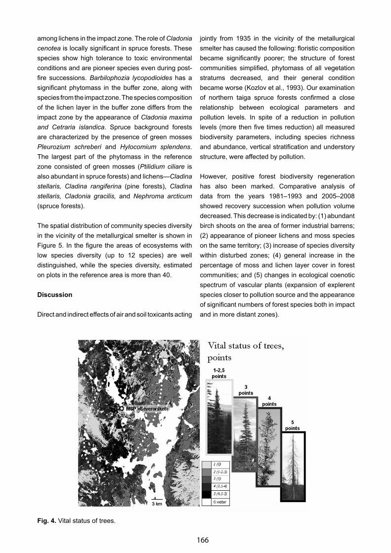
166

among lichens in the impact zone. The role of Cladonia cenotea is locally significant in spruce forests. These species show high tolerance to toxic environmental conditions and are pioneer species even during post-fire successions. Barbilophozia lycopodioides has a significant phytomass in the buffer zone, along with species from the impact zone. The species composition of the lichen layer in the buffer zone differs from the impact zone by the appearance of Cladonia maxima and Cetraria islandica. Spruce background forests are characterized by the presence of green mosses Pleurozium schreberi and Hylocomium splendens. The largest part of the phytomass in the reference zone consisted of green mosses (Ptilidium ciliare is also abundant in spruce forests) and lichens—Cladina stellaris, Cladina rangiferina (pine forests), Cladina stellaris, Сladonia gracilis, and Nephroma arcticum (spruce forests).

The spatial distribution of community species diversity in the vicinity of the metallurgical smelter is shown in Figure 5. In the figure the areas of ecosystems with low species diversity (up to 12 species) are well distinguished, while the species diversity, estimated on plots in the reference area is more than 40.

Discussion

Direct and indirect effects of air and soil toxicants acting

jointly from 1935 in the vicinity of the metallurgical smelter has caused the following: floristic composition became significantly poorer; the structure of forest communities simplified, phytomass of all vegetation stratums decreased, and their general condition became worse (Kozlov et al., 1993). Our examination of northern taiga spruce forests confirmed a close relationship between ecological parameters and pollution levels. In spite of a reduction in pollution levels (more then five times reduction) all measured biodiversity parameters, including species richness and abundance, vertical stratification and understory structure, were affected by pollution.

However, positive forest biodiversity regeneration has also been marked. Comparative analysis of data from the years 1981–1993 and 2005–2008 showed recovery succession when pollution volume decreased. This decrease is indicated by: (1) abundant birch shoots on the area of former industrial barrens; (2) appearance of pioneer lichens and moss species on the same territory; (3) increase of species diversity within disturbed zones; (4) general increase in the percentage of moss and lichen layer cover in forest communities; and (5) changes in ecological coenotic spectrum of vascular plants (expansion of explerent species closer to pollution source and the appearance of significant numbers of forest species both in impact and in more distant zones).

Fig. 4. Vital status of trees.

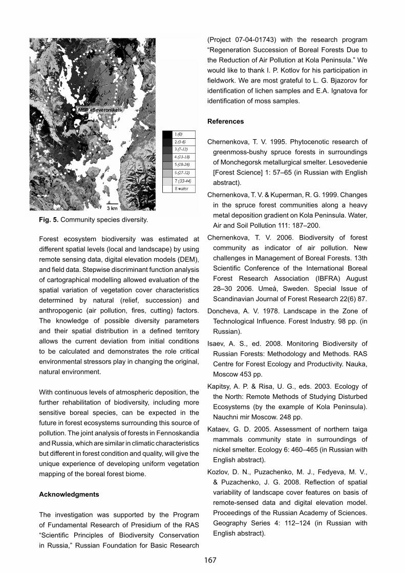
167

Forest ecosystem biodiversity was estimated at different spatial levels (local and landscape) by using remote sensing data, digital elevation models (DEM), and field data. Stepwise discriminant function analysis of cartographical modelling allowed evaluation of the spatial variation of vegetation cover characteristics determined by natural (relief, succession) and anthropogenic (air pollution, fires, cutting) factors. The knowledge of possible diversity parameters and their spatial distribution in a defined territory allows the current deviation from initial conditions to be calculated and demonstrates the role critical environmental stressors play in changing the original, natural environment.

With continuous levels of atmospheric deposition, the further rehabilitation of biodiversity, including more sensitive boreal species, can be expected in the future in forest ecosystems surrounding this source of pollution. The joint analysis of forests in Fennoskandia and Russia, which are similar in climatic characteristics but different in forest condition and quality, will give the unique experience of developing uniform vegetation mapping of the boreal forest biome.

Acknowledgments

The investigation was supported by the Program of Fundamental Research of Presidium of the RAS “Scientific Principles of Biodiversity Conservation in Russia,” Russian Foundation for Basic Research

(Project 07-04-01743) with the research program “Regeneration Succession of Boreal Forests Due to the Reduction of Air Pollution at Kola Peninsula.” We would like to thank I. P. Kotlov for his participation in fieldwork. We are most grateful to L. G. Bjazorov for identification of lichen samples and E.A. Ignatova for identification of moss samples.

References

Chernenkova, T. V. 1995. Phytocenotic research of greenmoss-bushy spruce forests in surroundings of Monchegorsk metallurgical smelter. Lesovedenie [Forest Science] 1: 57–65 (in Russian with English abstract).

Chernenkova, T. V. & Kuperman, R. G. 1999. Changes in the spruce forest communities along a heavy metal deposition gradient on Kola Peninsula. Water, Air and Soil Pollution 111: 187–200.

Chernenkova, T. V. 2006. Biodiversity of forest community as indicator of air pollution. New challenges in Management of Boreal Forests. 13th Scientific Conference of the International Boreal Forest Research Association (IBFRA) August 28–30 2006. Umeå, Sweden. Special Issue of Scandinavian Journal of Forest Research 22(6) 87.

Doncheva, A. V. 1978. Landscape in the Zone of Technological Influence. Forest Industry. 98 pp. (in Russian).

Isaev, A. S., ed. 2008. Monitoring Biodiversity of Russian Forests: Methodology and Methods. RAS Centre for Forest Ecology and Productivity. Nauka, Moscow 453 pp.

Kapitsy, A. P. & Risa, U. G., eds. 2003. Ecology of the North: Remote Methods of Studying Disturbed Ecosystems (by the example of Kola Peninsula). Nauchni mir Moscow. 248 pp.

Kataev, G. D. 2005. Assessment of northern taiga mammals community state in surroundings of nickel smelter. Ecology 6: 460–465 (in Russian with English abstract).

Kozlov, D. N., Puzachenko, M. J., Fedyeva, M. V., & Puzachenko, J. G. 2008. Reflection of spatial variability of landscape cover features on basis of remote-sensed data and digital elevation model. Proceedings of the Russian Academy of Sciences. Geography Series 4: 112–124 (in Russian with English abstract).

Fig. 5. Community species diversity.

168

Kozlov, M. V., Haukioja, E., & Yarmishko, V. T., eds. 1993. Aerial Pollution in Kola Peninsula. Proc. Int. Workshop (14–16 April 1992, St.-Petersburg). Kola Scientific Centre, Apatity, Russia, 417 pp.

Kryuchkov, V. V. 1984. Pages 4–15 in Monitoring of the Kola North Environment. Kola Science Centre, Apatity, Russia.

Lukina, N. V. & Nikonov, V. V. 1996. Biogeochemical Cycles in Northern Forests Under Air Pollution Conditions. Kola Scientific Center of RAS. 2 volumes (v1. 213 pp., v2. 192 pp.) Apatity, Russia (in Russian with English abstract).

Lukina, N. V., Sukhareva, T. A., & Isaeva, L. G. 2005. Technogenic Digressions and Recovery Successions in Northern Taiga Forests. Nauka, Moscow, Russia. 246 pp.

Mikkola, K. & Ritari, A. 1992. The Lapland forest damage project - Interim Report. Kauhanen, H. & Varmola, M, eds. Finnish Forest Research Institute, Rovaniemi. Research Paper 413: 106–114.

Miroevsky, G. P., Demidov, K. A., Dubrovsky, V. L., Karasev, Yu. A., Goncharov, A. V., & Tsumekhman, L. Sh. 2001. State and perspectives of environment conservation on Severonickel plant. Tsvetnye metally [Non-ferrous metals] 2: 80–84 (in Russian with English abstract).

Puzachenko, M. J., Puzachenko, J. G., Kozlov, D. N., & Fedyeva, M. V. 2006. Mapping of organogenic and humus soil layers for forest and bogged soils of south taiga landscape (south-west Valdai Hills) on basis of digital elevation model and remote-sensed data (Landsat-7). Issledovanie Zemli iz Kosmosa 4: 70–78).

Rigina, O. 1998. Introduction into the environmental problems in the Kola Peninsula. Pages 8–34 in Detection of pollution-induced forest decline in the Kola Peninsula using remote sensing and mathematical modeling. Licentiate Thesis. Swedish University of Agricultural Sciences, Report 9.

Tommervik, H., Johansen, B. E., & Pedersen, J. P. 1995. Monitoring the effects of air pollution on terrestrial ecosystems in Varanger (Norway) and Nickel-Pechenga (Russia) using remote sensing. The Science of the Total Environment 160/161: 753–767.

Tutubalina, O. & Shipigina, E. 2004. Metodika komputernoy klassifikatsii po neskolkim kosmicheskim snimkam [Method of computer classification using several satellite images]. ArcReview 4(31): 10–11 (in Russian with English abstract).

169

Circumboreal Forest Cover Mapping and Monitoring Using MODIS Time-Series Imagery

Peter V. Potapov1, Matthew C. Hansen1, & Stephen V. Stehman2

1Geographic Information Science Center of Excellence, South Dakota State University, Peter.Potapov@sdstate.edu, 2College of Environmental Science and Forestry, State University of New York

Abstract

Mapping and monitoring of forest cover is important for boreal forests, which represent the largest forested biome, because of their unique role in global timber stock, carbon sequestration and deposition, and high vulnerability to the effects of global climate change. We used time-series data from the Moderate Resolution Imaging Spectroradiometer (MODIS) to produce circumboreal annual maps of forest cover loss hotspots and forest loss factors. To validate the MODIS data and depict the boreal forest biome with an estimation of change from 2000 to 2005, a probability-based sampling approach was employed. Circumboreal maps of forest cover, total forest loss, and forest loss attributable to fire were achieved through the use of MODIS data inputs calibrated by Landsat sample data.

Area of forest cover gross loss from 2000 to 2005 within the boreal biome is estimated to be 1.63% (standard error 0.10%) of the total biome area and represents a 4.02% reduction from forest cover in 2000. The proportion of identified forest cover loss relative to regional forest area is much higher in North America than in Eurasia (5.6% to 3.0%). Our results reveal significant increases in forest cover loss due to wildfires in 2002 and 2003, with 2003 being the peak year of loss within the 5-year study period. Of the total forest cover loss identified, 58.9% is attributable to wildfires. Validation results show a high correlation between the MODIS- and Landsat-derived forest cover and forest cover loss values for sample blocks. Overall, our results illustrate the robustness of the integrated use of MODIS and Landsat data for forest cover mapping and monitoring.

Keywords: boreal forests, forest cover, forest cover loss, MODIS, monitoring.

Introduction

Forest cover extent is a basic variable in the quantitative analysis of global carbon exchange and timber stock, and for ecological modelling and ecosystem integrity assessment. Timely forest cover change monitoring is especially important for boreal forests, which represent the largest terrestrial biome, because of their unique role in carbon deposition and high vulnerability to global climate change effects. The boreal region is vast with large areas lacking infrastructure, making annual field- and aircraft-based assessment expensive and difficult. Synoptic observations from satellite-based sensors offer an alternative information source for forest cover mapping and monitoring at a fraction of the cost of obtaining extensive ground inventory data. However, satellite-based forest cover monitoring at the global biome scale remains a challenge due to limitations concerning data quality, data access, and processing capabilities.

Our method, presented here, employed an internally consistent and efficient probability-based sampling approach that integrates low and high spatial resolution satellite data sets. We used time-series data from the Moderate Resolution Imaging Spectroradiometer (MODIS) to produce circumboreal annual maps of forest cover loss hotspots and forest loss factors. For the year 2000 a tree canopy cover fraction map derived from MODIS 500m spatial resolution data (part of the global Vegetation Continuous Fields product; Hansen et al., 2002) was used as a baseline for our monitoring. For MODIS product validation and final forest cover and change estimation, we employed a probability-based sampling approach. The stratified random sample of 118 blocks (18.5 km per side) was interpreted for forest cover and forest cover change using high spatial resolution Landsat ETM+ imagery from 2000 and 2005. Circumboreal maps of forest

170

cover, total forest loss, and forest loss attributable to fire were achieved through the use of MODIS data inputs calibrated by Landsat sample data.

Data and Methods

Boreal Forest Biome Boundaries

The boreal forest biome boundary was based on the world terrestrial ecoregion map of Olson et al. (2001). The biome boundaries were modified to add temperate coniferous and mixed forests ecoregions characterized by similar seasonality and presence of seasonal snow cover. Also, forested areas of forest-steppe and forest–tundra transitional ecoregions were included in the boreal biome.

MODIS Data Time-Series Imagery

Visible and infrared bands (1–7) surface reflectance 8-day composites with 500-m spatial resolution from the MODIS/Terra Satellite, along with an 8-day, 1-km land surface temperature product for the years 2000–2005, were used as the primary inputs to our analysis. The initial 8-day composites were combined into 32-day composites that were subsequently transformed to multi-temporal annual metrics that captured the salient points of phenological variation by calculating means of spectral information from 3-, 6- and 9-month composites with the highest Normalized Difference Vegetation Index (NDVI) and surface temperature values. Multi-temporal metrics have been shown to perform as well or better than time-sequential composites in mapping large areas (Hansen et al., 2002).

Circumboreal Forest Cover Mapping and Monitoring

The algorithm of tree canopy cover fractional mapping using MODIS data is described in Hansen et al. (2002). The method employs a regression tree algorithm. The high spatial resolution training data (classified Landsat imagery) were used as the dependent variable, and the annual MODIS metrics for the year 2000 were used as independent variables to create a regression tree model. The model, applied globally, yielded percent tree canopy cover per 500-m MODIS pixel.

The analysis of forest cover loss was performed only

for areas covered by forest in the year 2000. Forest was defined as areas with tree canopy cover greater than 25%. The tree canopy cover threshold limited the presence of forest cover commission errors.

Our method of forest cover loss annual monitoring employs a bagged regression tree algorithm (Breiman, 1996) to create a wall-to-wall biome-wide forest cover loss hotspot map. The algorithm is described in detail in Potapov et al. (2008). Regression trees are derived using a training data set that relates spectral reflectance change signals to percent cover loss. To create training data, pairs of single date MODIS 250-m images for the years 2001 and 2005 were manually classified to no-change and forest loss classes. To build the regression tree model, percent forest cover loss from the training data set was used as the dependent variable, and MODIS annual metrics plus their inter-annual differences were used as independent variables. The regression tree model was then applied to the biome-wide pairs of annual MODIS inputs. The forest cover loss results for the 2000–2005 interval were used to create the 5-year forest cover loss hotspot map, while annual change results were used for the analysis of temporal trends.

The analysis of forest cover loss factors was based on a decision tree classification. The objective was to discern the cause of the cleared forest cover per MODIS pixel: burned forest areas and forest cover loss hotspots attributed to other disturbance factors (logging, tree mortality due to insect outbreaks, and windfalls). An extensive training set was manually created using available ancillary information. The training data related manually assigned forest cover loss class information with MODIS spectral data derived from the year when change was detected. The forest cover loss factors analysis was performed only within the 5-year forest cover loss hotspot mask.

The circumboreal MODIS-derived forest cover and annual forest cover change datasets are available at http://globalmonitoring.sdstate.edu/projects/gfm.

Validation and Calibration of MODIS-Derived Products

The Landsat-based sample block analysis was used to calibrate biome-wide MODIS-derived forest cover and forest cover loss area estimates and to

171

validate the forest cover loss hotspots map. Stratified sampling was implemented to enhance precision by allocating greater sampling effort to areas likely to exhibit change. The strata were determined based on the MODIS-derived forest cover loss hotspot map. A stratified random sample of 118 blocks, 18.5-km per side, was interpreted for forest cover, forest cover loss, and forest change type using Landsat imagery from 2000 and 2005. All blocks used in this analysis can be viewed at http://globalmonitoring.sdstate.edu/projects/gfm.

The relationship between Landsat-based forest cover area and mean Vegetation Continuous Fields (VCF) tree canopy density was used to derive forest extent for the year 2000. A simple linear regression (no intercept) model was employed with mean VCF tree canopy density per block as the independent variable.

A separate regression estimator (i.e., separate regression models and parameter estimates allowed for each stratum) was employed to estimate Landsat-derived forest cover loss area using percent MODIS-derived change hotspots as an auxiliary variable. The same approach was used to estimate burned forest area fraction of total change area.

Results and Discussion

Forest Cover and Forest Cover Loss Area

The extent of the boreal biome used in our analysis was 2,150.9 million hectares (Mha). Using Landsat-derived forest cover classification results, forest extent within the study area was estimated to be 872.3 Mha for year 2000. The estimated forest cover fraction of the biome area is almost the same for North America and Eurasia (43% and 39%, respectively).

Area of forest cover gross loss from 2000 to 2005 within the boreal biome is estimated to be 1.63% (standard error 0.10%) of the total biome area and represents a 4.02% reduction in year 2000 forest cover. This translates to an estimated forest loss area of 35.1 Mha (s.e. +/-2.2 Mha). Gross forest cover loss within the boreal forests is higher than in the humid tropics biome, where forest clearing is estimated to be 1.39% of the biome area, or 27.2 Mha (Hansen et al., 2008). The overall high rates of forest cover loss need to be put into context with a longer-term analysis

in order to determine if they are anomalous or within the historical range.

Forest cover loss is distributed unevenly within the biome. The proportion of identified forest cover loss relative to regional forest area is much higher in North America than in Eurasia (5.63% to 3.00%). The largest forest loss areas occurred within regions of intensive logging operations (southern parts of Ontario, Québec and British Columbia) and of large-scale wildfires (Northern Canada, Alaska, and Eastern Siberia).

Forest Cover Loss Inter-Annual Trend

Inter-annual analysis of forest cover loss highlights years with increased wildfire activity and illustrates differences in change dynamics in North America and Eurasia. The MODIS-derived annual total forest cover loss hotspot area shows significant increases of forest loss in 2002 and 2003, with a subsequent decrease in total forest loss. A significant part of the total forest cover loss in 2002 was connected with fires in Yakutia (East Siberia) and in 2003 with fires in East Siberia and in the Russian Far East. Regions where forest change is primarily related to logging (Europe, Southern Canada) reflected a consistent inter-annual rate of change.

Forest Cover Loss Due to Wildfires

Of the total forest cover loss area, 58.9% was attributed to wildfires and the rest, 41.1%, to other disturbances, including logging, wind and snow damage, and insect outbreaks. The proportional contribution of fire to forest loss is higher in Russia compared to Canada. Fire is a major contributor to forest loss in the interior of North America and Asia. Our method of forest burned areas assessment differs from most official and remote-sensing based analyses, as it was made only within forests with high (above 25%) tree canopy density and quantified only those forested areas affected by stand-replacement fires. Surface fires have a significantly lower impact on tree canopy cover, and the effect of these fires could be negligible in total forest cover loss. Therefore, our forest cover loss area attributed to wildfires is smaller in comparison with national burned forest area estimates, which include surface fire area in total burned area calculation (Achard et al., 2008; Canadian Council of Forest Ministers, 2007). Stand-replacement and surface fires in boreal forests have a different impact on forest cover, direct carbon

172

emissions, albedo change, and post-fire successional trajectories. Our burned forest estimates could more readily be incorporated into carbon emission models and vegetation change analysis than existing fire-affected area estimates because our analysis reflects a strict biophysical interpretation of the presence/absence of tree cover assessed using a synoptic, biome-wide approach.

Calibration and Validation of MODIS Products

The boreal forest cover area and change estimates are derived through the integrated use of MODIS and Landsat data. Area estimates are attained via a probability sample of interpreted Landsat block data. A sampling efficiency is obtained using strata based on MODIS change indicator maps. Stratification successfully improved precision of the overall estimate of forest clearing and reduced the cost of obtaining high-resolution sampling data. The complete coverage (spatially explicit) maps of forest cover, total forest loss, and forest loss attributable to fire were achieved through the use of MODIS data inputs calibrated by the Landsat sample data.

Validation results show a high correlation between the MODIS- and Landsat-derived forest cover and forest cover loss values for sample blocks. The MODIS-based forest cover loss hotspot fraction has an estimated root mean square error (RMSE) of 2.53% and an R2 of 0.75.

Conclusion

Our results illustrate the robustness of the integrated use of MODIS and Landsat data for forest cover mapping and monitoring. The validated wall-to-wall MODIS-based product could then be used for further analyses in combination with: (1) available carbon stock data to improve carbon accounting; (2) high conservation value forest data to facilitate conservation planning; and (3) timber resources and accessibility data for forest use sustainability analysis.Subpixel percent forest cover and change maps offer advantages over convenient classification schemes. Forest fraction maps could better represent land cover heterogeneity and could avoid problems with mapping spatially complex areas. The calibrated percent forest cover change maps are adequate in measuring forest

cover loss over time, even if change occurs at the subpixel scale depicted from MODIS data.

Acknowledgments

This research was supported by National Aeronautics and Space Administration under grant NNG06GD95G managed under the NASA Land-Cover and Land-Use Change Program.

References

Achard, F., Eva, H. D., Mollicone, D., & Beuchle, R. 2008. The effect of climate anomalies and human ignition factor on wildfires in Russian boreal forests. Philosophical Transactions of the Royal Society B 363 (1501): 2331–2339.

Breiman, L. 1996. Bagging predictors. Machine Learning 24: 123–140.

Canadian Council of Forest Ministers. 2007. National Forestry Database Program. Canadian Forest Service, Natural Resources Canada. http://nfdp.ccfm.org/.

Hansen, M. C., DeFries, R. S., Townshend, J. R. G., Sohlberg, R., Carroll, M., & Dimiceli, C. 2002 Towards an operational MODIS continuous field of percent tree cover algorithm: examples using AVHRR and MODIS data. Remote Sensing of Environment 83: 303–319.

Hansen, M. C., Stehman, S. V., Potapov, P. V., Loveland, T. R., Townshend, J. R. G., DeFries, R. S., Pittman, K. W., Stolle, F., Steininger, M. K., Carroll, M., & Dimiceli, C. 2008 Humid tropical forest clearing from 2000 to 2005 quantified using multi-temporal and multi-resolution remotely sensed data. PNAS 105(27): 9439–9444.

Olson, D. M., Dinerstein, E., Wikramanayake, E. D., Burgess, N. D., Powell, G. V. N., Underwood, E. C., Amico, J. A. D., Itoua, I., Strand, H. E., Morrison, J. C. 2001 Terrestrial ecoregions of the world: A new map of life on Earth. BioScience 51(10): 1–6.

Potapov, P., Hansen, M. C., Stehman, S. V., Loveland, T. R., & Pittman, K. 2008 Combining MODIS and Landsat imagery to estimate and map boreal forest cover loss. Remote Sensing of Environment 112(9): 3708–3791.

173

Vegetation Mapping and Disturbances Assessment in the Boreal Zone Using Time-Series of Moderate-Resolution Remote Sensing Data

Sergey Bartalev

Space Research Institute, Russian Academy of Sciences, Moscow, Russia

Extended Abstract

In boreal ecosystems, vegetation changes in phenological tempo, species composition, and biophysical and structural characteristics are not only driven by succession and anthropogenic processes but also by variation in the climate regimes. Large-scale vegetation dynamics in the boreal zone include wildfires, forest logging, conversion of grasslands to agriculture, and land abandonment following institutional changes, as well as the long-term trends of climate change.

In order to facilitate needs of climate change science and natural resources management, a number of thematic products describing the status and dynamics of vegetation cover for Northern Eurasia and the entire boreal zone is currently under development with the use of Satellite Pour l’Observation de la Terre (SPOT) Vegetation data and Moderate Resolution Imaging Spectroradiometer (MODIS) data.

New MODIS data derived from 250 m spatial resolution landcover mapping is updated with monthly and seasonal multi-spectral cloud-free image composites. This mapping approach learned lessons from the Global Land Cover 2000 project, which in particular, produced a 1-km resolution Northern Eurasia landcover map from SPOT-Vegetation data. Better classification accuracy and thematic detail of vegetation cover (such as phenological dynamic features that are elaborated by the combined use of monthly multi-spectral image mosaics and multi-annual temporal profiles of spectral vegetation indexes) can be achieved from the higher spatial resolution of MODIS data.

A new burned area product for the entire boreal zone

for the years 2000–2007 was derived by combining SPOT-Vegetation time series data and Terra-MODIS active fire products. The burnt severity of the forest is an essential input into carbon emission modelling as well as important in the assessment of the environmental and economical impact of fires. A multi-annual burnt severity product was derived from Terra-MODIS data with use of a spectral-temporal mixture analysis technique and is in the process of validation.

An arable lands mask for Russia was derived from time-series 250-m resolution daily MODIS data acquired during 2002–2007 with the use of an advanced automatic method of data processing and analysis and provides essential input into various applications of agricultural monitoring and landcover mapping.

Forest change mapping, with the particular focus on logging areas, is an important component of actual research and development with use of 250-m resolution MODIS data.

The TerraNorte website (http://terranorte.iki.rssi.ru/) was developed to provide a wide community of users with information about the current state of and dynamics of the Earth’s boreal ecosystems, and particularly for Northern Eurasia. The thematic information products and databases presented at the TerraNorte website were derived from Earth Observation data in the framework of scientific projects carried out by the Russian Academy of Sciences’ Space Research Institute in close cooperation with a number of partners. The web interface of the system provides interactive users access to the data and information products in the forms of tables, graphs and digital maps.

174

Comparison of Finnish and Russian Approaches for Large-Scale Vegetation Mapping: A Case Study

Olga Galanina1 & Raimo Heikkilä2

1Komarov Botanical Institute, Russian Academy of Sciences, Saint Petersburg, Russia, 2Finnish Environment Institute, Joensuu, Finland

Abstract

The purpose of this study was to compare Russian and Finnish mire vegetation classifications and large-scale vegetation mapping methods. Two maps were prepared using aerial photo interpretation and field observations for Härkösuo mire in Kuhmo, eastern Finland. Härkösuo mire covers about 20 ha and includes a small area of aapamire, together with spring fen and pine bog types. The maps were compared quantitatively using geographic information system (GIS) techniques. Despite the different vegetation classification approaches, the maps have a great deal in common. The correspondence of vegetation patterns according to the Russian dominant approach and the Finnish site type approach is discussed. The main differences in vegetation classification occurred in the marginal zones of the mire. In the Finnish approach, marginal areas with dense cover of spruce trees are regarded as mire, while in the Russian approach they are classified as forest.

Keywords: aapamire, Fennoscandia, mire site type, vegetation classification, vegetation mapping.

Introduction

At Härkösuo mire, situated in the borderland of Finland and Russia, we made an attempt to apply Finnish and Russian mapping methodologies. The applicability of the two cartographical methods and the value of the results were tested. This article is based on the results presented by Galanina & Heikkilä (2007).

Russian School of Vegetation Mapping

Vegetation mapping in Russia is a well-developed theoretically based discipline, which can be applied and adapted for practical purposes. The Russian school of geobotanical cartography has a long

tradition. It was established by Professor N. Kuznetsov in 1922. The laboratory of geography and vegetation cartography at the Komarov Botanical Institute of the Russian Academy of Sciences became the Russian centre of ideas and development for this discipline (Юрковская, 2004).

Under the leadership of academician Evgeny Lavrenko from 1967 to 1979, the laboratory worked actively and successfully for vegetation mapping and became an international leader. As a result, remarkable maps were published, including for example, “Геоботаническая карта Нечерноземной зоны РСФСР” (Geobotanical Map of Non-Chernozem Zone of The Russian Federation RSFSR), at map scale 1: 1.5 M in 1976 and the Vegetation Map of European Part of USSR, at map scale 1:2.5 M (Исаченко & Лавренко, 1979).

In Russia, vegetation mapping commonly applies to a large area, and the mappings are usually made at a small scale. As a rule, the maps show the general features and regularities of regional vegetation, or they are compiled according to vegetation zones. There is no checklist of forest or mire site types to be used as a starting point, in contrast to the Finnish practice. The mapping starts from an independent preliminary interpretation of morphological and vegetation structures visible in aerial photographs or satellite images. The patterns identified are verified in the field by making vegetation relevés along profiles. The legend to the map usually represents the mapping author’s point of view.

Finnish School of Vegetation Mapping

In Finland, vegetation mapping has a tradition of a few decades. Paasio (1933) was the first to produce a detailed vegetation map of a mire at scale 1:15,000 using aerial photos. Seppälä & Rastas (1980) made

175

the first small-scale vegetation map in northernmost Finnish Lapland on the basis of satellite images, where classes were defined mainly on the basis of tree cover and moisture. Ruuhijärvi (1988) prepared a small-scale map (1:1M) of the mire complexes (massifs) of Finland, using six main mire complex types as mapping units.

Routine vegetation mapping of nature reserves started at the beginning of the 1980s to reveal the biotope diversity of national parks and some other nature reserves. Site types (Ruuhijärvi, 1983; Eurola et al., 1984) were used as mapping units. Site types were identified in the field and delimited on the basis of aerial photo interpretation and field observations. The minimum size of a mire site is generally 100 m2. Sometimes, for example in springs and other key habitats, smaller units are also taken into account. The scale of the maps is usually 1:10,000 or 1:20,000.

Very few scientific mappings have been made in Finland. The maps are required mainly for practical applications in nature conservation or environmental impact assessments. Usually the site type determinations have not been verified with relevés, but floristic lists have been compiled either for the vegetation patterns or square-kilometer quadrats according to the map coordinates (e.g., Heikkilä, 1986; Heikkinen & Kalliola, 1989; Heikkilä et al., 2001). Generally, vegetation mapping is not a theoretical discipline in Finland, and there are no vegetation maps covering the whole country.

Finnish and Russian Classifications of Mire Vegetation

In Finland, approximately 80 mire site types have been defined according to botanical criteria (Ruuhijärvi, 1983; Eurola et al., 1984). For practical applications such as forestry there are 30–35 site types (Laine & Vasander, 2005). The site types are organized into six main groups: spruce mire, pine mire, open bog and fen, rich fen, spring mire, and flooded swamp. They can be also classified according to a pH gradient: bog, poor fen, and rich fen (Tahvanainen et al., 2002). Spruce mire types often have a very dense and tall tree cover, and in central Europe and Russia they are usually regarded as forests.

In Russia, three vegetation classification approaches are commonly used: dominant (ecological-phytocoenotic), floristic (Central-European) and topology-ecological (Scandinavian). Regional reviews of mire vegetation have been compiled, for example, in Leningrad region (Боч & Смагин, 1993) and in the Karelian Republic (Kuznetsov, 2003; Кузнецов, 2005). However, they cannot be considered as mapping units. The dominant approach is the main instrument for vegetation mapping.

Traditionally, three main mire types are commonly distinguished in Russia: верховые (raised bogs), переходные (transitional mires), and низинные (fens). These terms have been applied, for example, in the legend of the vegetation map of Moscow region at scale 1:200,000 (Огуреева et al., 1996). Also, trophic status can be used in map legends: oligotrophic, mesotrophic, and eutrophic.

Карта растительности Европейской части СССР (Map of European Part of USSR) (1979) shows five main mire types: Sphagnum mires, herb-lichen-moss-mires, herb–Sphagnum–Hypnum mires, herb and herb–Hypnum mires, and forest mires. They are distinguished on the basis of predominant (prevailing) vegetation units. The first attempt to compare the Finnish and Russian schools of mire vegetation classification for mapping was published by Antipin et al. (1997).

Materials and Methods

Study Area

Härkösuo mire, covering 20 ha, is located in Kuhmo, eastern Finland, in Elimyssalo nature reserve (64º12’N, 30º26’E, 235 m a.s.l.). The mean annual rainfall is 600 mm and the mean annual temperature 1.2ºC (Alalammi, 1987). The study area is situated in the middle boreal climatic-phytogeographical zone (Ahti et al., 1968; Tuhkanen, 1984) and in the Archaean Karelian province of the Fennoscandian bedrock shield. The bedrock is formed of granite and gneiss (Luukkonen, 1992; Gorkovets & Rayevskaya, 2003).

The length of Härkösuo mire is 1,000 m from east to west, and its mean north–south width is 200 m. The mire slopes gently and is mostly soligenous.

176

Groundwater influence is clear at the southern margin of the western part of the mire. In the southeastern part of the mire the groundwater influence is weaker (Tahvanainen et al., 2002). As a result of the highly variable ecological conditions the vegetation of the mire is very diverse.

Härkösuo mire is situated in a tectonic depression, and the peat layer is very thick. The maximum peat depth is 805 cm. The calibrated radiocarbon age of the bottom layer of the mire is 10,240 years (Kuznetsov et al., 2008).

According to the map of mire provinces of Europe by Кац (1971) the study area lies within the Karelo-Finnish province of middle taiga and Karelian mires of mixed type. According to the Finnish system of mire regions it belongs to the southern aapamire zone (Ruuhijärvi, 1988). Russian literature sources define the study area as belonging to the northern taiga (Юрковская & Паянская-Гвоздева, 1993).

Methods

The vegetation of Härkösuo mire was mapped in detail using a false-color infrared aerial photograph at scale 1:5,000 (taken in 1995). The scale of the aerial photo negative was 1:20,000. In addition, low-altitude oblique aerial color photos from 1997 were used to clarify the patterns. Vegetation patches were delimited visually on the aerial photographs, and the delimitations were verified in the field between 5th and 8th August 2002. The mapping was carried out separately and independently by the Russian author and the Finnish author, each using their own national approach. Every element of pattern identified from the aerial photograph was studied to reveal the vegetation structure and species composition.

The vegetation patches were classified in the field and named according to Ruuhijärvi (1983) and Eurola et al. (1984) by the Finnish author. A more detailed classification using subtypes was also made. Vegetation relevés were made using cover percentage for field and ground layer in one 1 m2 randomly placed plot in the middle of each pattern. In cases where there was a mosaic structure of hummocks, lawns and/or flarks, a separate relevé was made on each surface. In total, 163 relevés were made.

The vegetation patterns in the maps were compared

quantitatively, using ArcGIS9 (ESRI) software with Spatial Analyst extension, to reveal the correspondence of the vegetation units and their joint percent coverage.

Results

Vegetation Maps

Two original vegetation maps and legends were prepared. Pine bog communities are present along the margins except in places where groundwater comes to the surface. Trichophorum communities occupy most of the mire area. Aapa-complexes are distributed in the central deepest part of Härkösuo mire. Further from springs, groundwater influence becomes weaker (Tahvanainen et al., 2002), and poor Scheuchzeria–Sphagnum majus communities replace aapa-complexes. A homogeneous community has developed in the shallow eastern depression of Härkösuo mire.

In the case of the Russian vegetation map, the structure of the legend usually looks like a hierarchical text. The legend shows the physiognomic features of mire vegetation by subtitle. The vegetation of Härkösuo mire is very diverse due to the complex hydrological regime. This diversity is reflected in the legend, where 21 different patterns are distinguished. The numbered categories in the legend characterize the mire communities according to a dominant vegetation classification approach by listing the dominant plants in the vegetation layers. For example, in “Carex rostrata +Scheuchzeria palustris–Sphagnum papillosum,” “+” means that the dominant species are present in the same layer, and they have more or less equal phytosociological value, and “-” means another vegetation layer.

The map compiled by the Finnish author includes 26 different vegetation categories, which are characterized by indices of the Finnish mire type classification. They are arranged in subclasses and in the order of Eurola et al. (1984). Only very small patches of spruce mire occur in the margins, mostly as narrow strips that cannot be shown in the map. Only in the northeast corner of the site is there a typical spruce mire patch (MK, number 1). Poor pine mire types are typical in the margins of the mire and as larger patches in the eastern part (RaR, number 7, LkR, number 25). Open fen types dominate in the

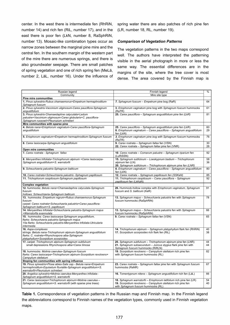
177

center. In the west there is intermediate fen (RhRiN, number 14) and rich fen (RiL, number 17), and in the east there is poor fen (LkN, number 8, RaSphRiN, number 13). Mosaic-like combination types occur as narrow zones between the marginal pine mire and the central fen. In the southern margin of the western part of the mire there are numerous springs, and there is also groundwater seepage. There are small patches of spring vegetation and one of rich spring fen (MeLä, number 2, LäL, number 16). Under the influence of

spring water there are also patches of rich pine fen (LR, number 18, RL, number 19).

Comparison of Vegetation Patterns

The vegetation patterns in the two maps correspond well. The authors have interpreted the patterning visible in the aerial photograph in more or less the same way. The essential differences are in the margins of the site, where the tree cover is most dense. The area covered by the Finnish map is

Table 1. Correspondence of vegetation patterns in the Russian map and Finnish map. In the Finnish legend the abbreviations correspond to Finnish names of the vegetation types, commonly used in Finnish vegetation maps.

Complex vegetation

12. hummocks: Betula nana+Chamaedaphne calyculata-Sphagnum fuscum hollows: Scheuchzeria-Sphagnum balticum

26. Hummock-hollow complex with Eriophorum vaginatum, Sphagnum fuscum and S. balticum (KeR)

91

13. hummocks: Empetrum nigrum+Rubus chamaemorus-Sphagnum fuscum carpet: Carex rostrata+Scheuchzeria palustris+Carex pauciflora-Sphagnum balticum+S. papillosum

13. Sphagnum majus – Scheuchzeria palustris fen with Sphagnum fuscum hummocks (RaSphRiN)

78

14. Menyanthes trifoliata+Scheuchzeria palustris-Sphagnum majus +Warnstorfia exannulata

13. Sphagnum majus – Scheuchzeria palustris fen with Sphagnum fuscum hummocks (RaSphRiN)

66

15. hummocks: Carex lasiocarpa-Sphagnum angustifolium, flarks: Scheuchzeria palustris-Sphagnum majus 15a flarks: Scheuchzeria palustris-Menyanthes trifoliata-Utricularia intermedia

9. Carex rostrata – Sphagnum fallax fen (VSN) 65

16. Aapa-complexesstrings: Betula nana-Trichophorum alpinum-Sphagnum angustifoliumflarks: C. rostrata+Rhynchospora alba-Sphagnum platyphyllum+Scorpidium scorpioides

14. Trichophorum alpinum – Sphagnum platyphyllum flark fen (RhRiN)17. Scorpidium scorpioides rich flark fen (RiL)

4038

17. carpet: Trichophorum alpinum-Sphagnum subfulvum small depressions Rhynchospora alba+Carex limosa

20. Sphagnum subfulvum – Trichophorum alpinum pine fen (LNR)21. Sphagnum subsecundum – Juncus stygius flark pine fen with Sphagnum fuscum hummocks (RiRLN)

4444

18. hummocks: Molinia caerulea–Sphagnum fuscum flarks: Carex lasiocarpa+Trichophorum alpinum-Scorpidium revolvens+ Campylium stellatum

19. Scorpidium revolvens – Campylium stellatum rich pine fen with Sphagnum fuscum hummocks (RL)

82

Sloping fen communities with spring influence

19. Pinus sylvestris+Picea abies-Salix ssp.- Betula nana+Empetrum hermaphroditum-Equisetum fluviatile-Sphagnum angustifolium+S. warnstorfii+Pleurozium schreberi

23. Carex rostrata – Sphagnum fallax pine fen with Sphagnum fuscum hummocks (RaNR)

67

20. Angelica sylvestris+Molinia caerulea-Menyanthes trifoliata–Sphagnum angustifolium+S. warnstorfii

16. Tomentypnum nitens – Sphagnum angustifolium rich fen (LäL) 66

21. Carex lasiocarpa+Trichophorum alpinum+Molinia caerulea –Sphagnum angustifolium+S. warnstorfii (with sparse pine trees)

18. Sphagnum warnstorfii – Eriophorum latifolium rich pine fen (LR)19. Scorpidium revolvens – Campylium stellatum rich pine fen with Sphagnum fuscum hummocks (RL)

5440

Russian legend Finnish legend %

Community Mire site type

Pine mire communities

1. Pinus sylvestris-Rubus chamaemorus+Empetrum hermaphroditum-Sphagnum fuscum

7. Sphagnum fuscum – Empetrum pine bog (RaR) 64

2. Pinus sylvestris-Vaccinium uliginosum-Carex pauciflora-Sphagnum angustifolium

3. Eriophorum vaginatum pine bog with Sphagnum fuscum hummocks (RaTR)

61

3. Pinus sylvestris-Chamaedaphne calyculata+Ledum palustre+Vaccinium uliginosum-Carex globularis+C. pauciflora-Sphagnum russowii+Pleurozium schreberi

25. Carex pauciflora – Sphagnum angustifolium pine fen (LkR) 81

Mire communities with sparse pine

4. Betula nana+Eriophorum vaginatum-Carex pauciflora-Sphagnum angustifolium

25. Carex pauciflora – Sphagnum angustifolium pine fen (LkR)8. Eriophorum vaginatum – Carex pauciflora – Sphagnum angustifolium fen (LkN)

6029

5. Eriophorum vaginatum+Empetrum hermaphroditum-Sphagnum fuscum 3. Eriophorum vaginatum pine bog with Sphagnum fuscum hummocks (RaTR)

76

6. Carex lasiocarpa-Sphagnum angustifolium 9. Carex rostrata – Sphagnum fallax fen (VSN)22. Carex rostrata – Sphagnum fallax pine fen (VNR)

3026

Open mire communities

7. Carex rostrata - Sphagnum fallax 10. Carex rostrata – Comarum palustre – Sphagnum riparium fen (LuRiSSN)

92

8. Menyanthes trifoliata+Trichophorum alpinum +Carex lasiocarpa-Sphagnum angustifolium+S. warnstorfii

15. Sphagnum subfulvum – Loeskypnum badium – Trichophorum alpinum fen (LN)20. Sphagnum subfulvum – Trichophorum alpinum pine fen (LNR)

5836

9. Scheuchzeria palustris-Sphagnum balticum 8. Eriophorum vaginatum – Carex pauciflora – Sphagnum angustifolium fen (LkN)

80

10. Carex rostrata+Scheuchzeria palustris -Sphagnum papillosum 12. Carex rostrata – Sphagnum papillosum fen (SSKaN) 85

11. Trichophorum cespitosum-Sphagnum papillosum 11. Trichophorum cespitosum – Carex pauciflora – Sphagnum papillosum fen (LkKaN)

92

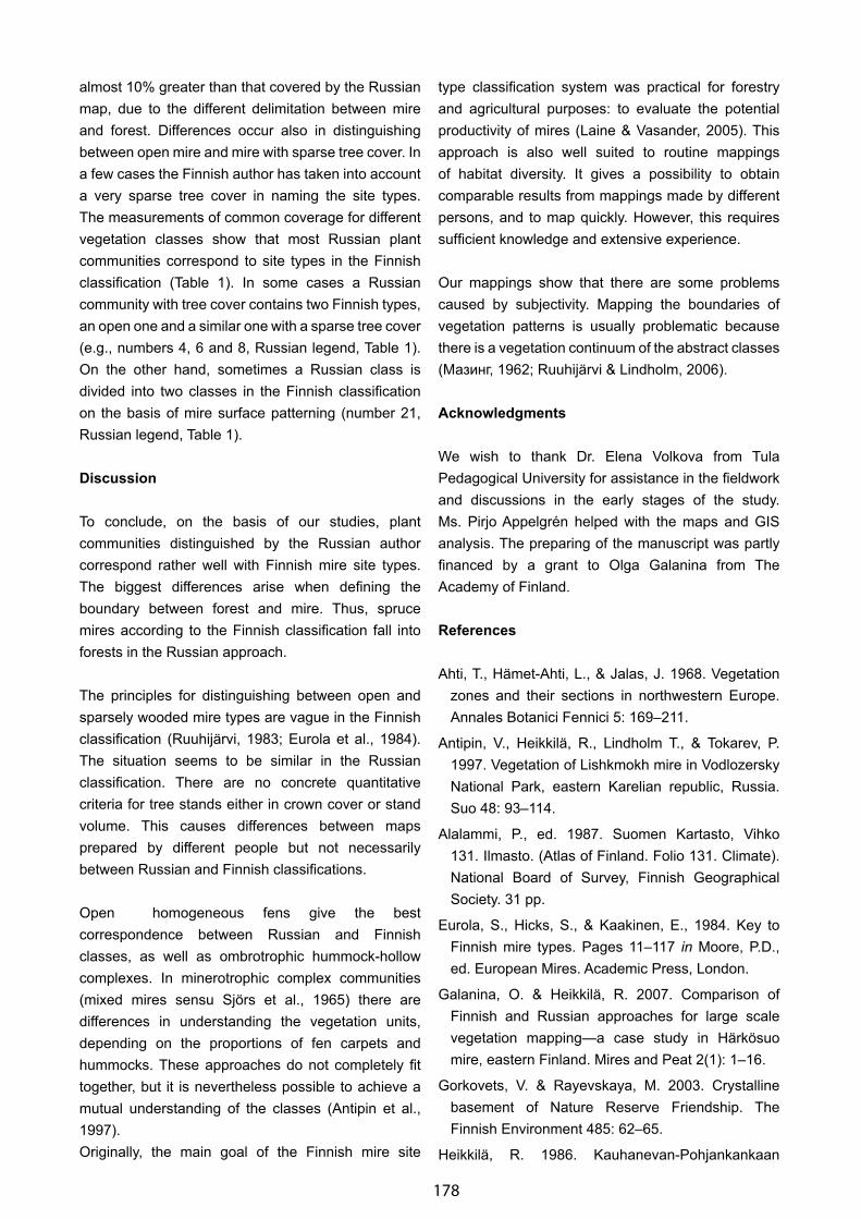
178

almost 10% greater than that covered by the Russian map, due to the different delimitation between mire and forest. Differences occur also in distinguishing between open mire and mire with sparse tree cover. In a few cases the Finnish author has taken into account a very sparse tree cover in naming the site types. The measurements of common coverage for different vegetation classes show that most Russian plant communities correspond to site types in the Finnish classification (Table 1). In some cases a Russian community with tree cover contains two Finnish types, an open one and a similar one with a sparse tree cover (e.g., numbers 4, 6 and 8, Russian legend, Table 1). On the other hand, sometimes a Russian class is divided into two classes in the Finnish classification on the basis of mire surface patterning (number 21, Russian legend, Table 1).

Discussion

To conclude, on the basis of our studies, plant communities distinguished by the Russian author correspond rather well with Finnish mire site types. The biggest differences arise when defining the boundary between forest and mire. Thus, spruce mires according to the Finnish classification fall into forests in the Russian approach.

The principles for distinguishing between open and sparsely wooded mire types are vague in the Finnish classification (Ruuhijärvi, 1983; Eurola et al., 1984). The situation seems to be similar in the Russian classification. There are no concrete quantitative criteria for tree stands either in crown cover or stand volume. This causes differences between maps prepared by different people but not necessarily between Russian and Finnish classifications.

Open homogeneous fens give the best correspondence between Russian and Finnish classes, as well as ombrotrophic hummock-hollow complexes. In minerotrophic complex communities (mixed mires sensu Sjörs et al., 1965) there are differences in understanding the vegetation units, depending on the proportions of fen carpets and hummocks. These approaches do not completely fit together, but it is nevertheless possible to achieve a mutual understanding of the classes (Antipin et al., 1997).Originally, the main goal of the Finnish mire site

type classification system was practical for forestry and agricultural purposes: to evaluate the potential productivity of mires (Laine & Vasander, 2005). This approach is also well suited to routine mappings of habitat diversity. It gives a possibility to obtain comparable results from mappings made by different persons, and to map quickly. However, this requires sufficient knowledge and extensive experience.

Our mappings show that there are some problems caused by subjectivity. Mapping the boundaries of vegetation patterns is usually problematic because there is a vegetation continuum of the abstract classes (Мазинг, 1962; Ruuhijärvi & Lindholm, 2006).

Acknowledgments

We wish to thank Dr. Elena Volkova from Tula Pedagogical University for assistance in the fieldwork and discussions in the early stages of the study. Ms. Pirjo Appelgrén helped with the maps and GIS analysis. The preparing of the manuscript was partly financed by a grant to Olga Galanina from The Academy of Finland.

References

Ahti, T., Hämet-Ahti, L., & Jalas, J. 1968. Vegetation zones and their sections in northwestern Europe. Annales Botanici Fennici 5: 169–211.

Antipin, V., Heikkilä, R., Lindholm T., & Tokarev, P. 1997. Vegetation of Lishkmokh mire in Vodlozersky National Park, eastern Karelian republic, Russia. Suo 48: 93–114.

Alalammi, P., ed. 1987. Suomen Kartasto, Vihko 131. Ilmasto. (Atlas of Finland. Folio 131. Climate). National Board of Survey, Finnish Geographical Society. 31 pp.

Eurola, S., Hicks, S., & Kaakinen, E., 1984. Key to Finnish mire types. Pages 11–117 in Moore, P.D., ed. European Mires. Academic Press, London.

Galanina, O. & Heikkilä, R. 2007. Comparison of Finnish and Russian approaches for large scale vegetation mapping—a case study in Härkösuo mire, eastern Finland. Mires and Peat 2(1): 1–16.

Gorkovets, V. & Rayevskaya, M. 2003. Crystalline basement of Nature Reserve Friendship. The Finnish Environment 485: 62–65.

Heikkilä, R. 1986. Kauhanevan-Pohjankankaan

179

kansallispuiston kasvillisuus [Vegetation of Kauhaneva-Pohjankangas National Park]. Metsähallitus SU 4(75). 52 pp.

Heikkilä, R., Kuznetsov, O., Lindholm, T., Aapala, K., Antipin, V., Djatshkova, T., & Shevelin, P. 2001. Complexes, Vegetation, Flora and Dynamics of Kauhaneva Mire System, Western Finland. The Finnish Environment 489. 97 pp.

Heikkinen, R. K. & Kalliola, R. 1989. Vegetation types and map of the Kevo nature reserve, northernmost Finland. Kevo Notes 8: 1–39.

Kuznetsov, O. .2003. Topology-ecological classification of mire vegetation in the Republic of Karelia (Russia). The Finnish Environment 485: 117–123.

Kuznetsov, O., Heikkilä, R., Lindholm, T., Mäkilä, M., & Filimonova L. 2008. Holocene vegetation dynamics and carbon accumulation of two mires in the Friendship Park, eastern Finland. In: Lindholm, T. & Heikkilä, R. (eds.). Mires from Pole to Pole—Proceedings of the 12th Biennial IMCG Symposium. The Finnish Environment. In press.

Laine, J. & Vasander, H. 2005. Suotyypit ja niiden tunnistaminen. (Mire Site Types and Their Indentification). With multimedia CD-Rom. Metsäkirjat, Hämeenlinna. 110 pp.

Luukkonen, E. J. 1992. Late Archaean and early Proterozoic structural evolution in the Kuhmo-Suomussalmi terrain, eastern Finland. Annales Universitatis Turkuensis Ser. A II. Biologica Geographica-Geologica 78: 1–37.

Paasio, I. 1933. Über die Vegetation der Hochmoore Finnlands. Acta Forestalia Fennica 39: 1─190.

Ruuhijärvi, R. 1983. The Finnish mire types and their regional distribution. Pages 47–67 in Gore, A.J.P., ed. Ecosystems of the World 4B. Mires: Swamp, Bog, Fen and Moor. Regional Studies. Elsevier, Amsterdam.

Ruuhijärvi, R. 1988. Mire vegetation. Atlas of Finland, Folio 141–143. Biogeography, Nature Conservation, 3–4. National Board of Survey, Finnish Geographical Society.

Ruuhijärvi, R. & Lindholm, T. 2006. Ecological gradients as the basis of Finnish mire site type system. The Finnish Environment 23/2006: 119–126.

Seppälä, M. & Rastas, J. 1980. Vegetation map of northernmost Finland with special reference to

subarctic forest limits and natural hazards. Fennia 158: 41–61 + appendix.

Sjörs, H., Björkbäck, F., & Nordqvist, Y. 1965. Northern mires. Acta Phytogeographica Suecica 50: 180–197.

Tahvanainen, T., Sallantaus, T., Heikkilä, R., & Tolonen, K. 2002. Spatial variation of mire surface water chemistry and vegetation in north-eastern Finland. Annales Botanici Fennici 39: 235–251.

Tuhkanen, S. 1984. A circumboreal system of climatic-phytogeographical regions. Acta Botanica Fennica 127: 1–50.

Боч М.С. & Смагин В.А. Флора и растительность болот Северо-Запада России и принципы их охраны. СПб., 1993. 224 с.

Геоботаническая карта Нечерноземной зоны РСФСР (Geobotanical Map of Non-Chernozem Zone of RSFSR). 1976. М., ГУГК, М 1: 1 500 000, 4 л.

Исаченко, Т.И. & Лавренко, Е.М., Ред.1979. Карта растительности Европейской части СССР (Vegetation Map of European Part of USSR). M. м. 1:2 500 000.

Кац Н.Я. Болота Земного шара. М., Наука, 1971. 295 с.

Кузнецов О. Л. 2005. Тополого-экологическая классификация растительности болот Карелии (обротрофные и олиготрофные сообщества) // Биоразнообразие, динамика и ресурсы болотных экосистем Восточной Фенноскандии. Тр. КНЦ, вып. 8. Петрозаводск, С. 15–46.

Мазинг В.В. 1962.Некоторые вопросы крупномасштабного картирования растительности // Принципы и методы геоботанического картографирования. М.-Л., С. 47-53.

Огуреева Г.Н., Микляева И.М., Суслова Е.Г., Швергунова Л.В. 1996.Растительность Московской области. [Vegetation of Moscow region. М 1:200 000. М.,

Юрковская Т.К., Паянская-Гвоздева И.И. 1993. Широтная дифференциация растительности вдоль российско-финской границы // Бот. журн. Т. 78. № 12. С. 72–98.

Юрковская Т. К. Ботанический институт им В. Л. Комарова РАН—центр становления и развития геоботанического картографирования в России. Бот. журн. 2004. Т. 89. № 9. С. 1509-1513.

180

Integrated Ecoforest Mapping of the Northern Portion of the Continuous Boreal Forest, Québec, Canada

André Robitaille, Antoine Leboeuf, Jean-Pierre Létourneau, Jean-Pierre Saucier, and Éric Vaillancourt

Ministère des Ressources naturelles et de la Faune du Québec, Canada, corresponding author: andre.robitaille@mrnf.gouv.qc.ca

Abstract

Since the late 1960s, the Ministère des Ressources naturelles et de la Faune du Québec (MRNFQ) has periodically carried out forest mapping activities at a scale of 1:20,000 in Québec’s forest areas south of 51º 30’ north latitude. In the early 2000s, new needs emerged for information about forest resources in a data-poor area lying between 51º 30’ and 53º north latitude. This huge area, covering 240,000 km2, marks the northern portion of the spruce-moss forest and the southern extent of the spruce-lichen forest, which is characterized by less dense forests and barrens. To perform the work, the MRNFQ decided to explore new automated mapping approaches. The latter had to deliver high-quality products, be relatively inexpensive, and be well adapted to remote or hard-to-reach areas. This paper presents the mapping method, the software used, and the results obtained to date, covering over 150,000 km2.

The mapping program began in 2005 and will end in 2009. Aerial photos have been used for mapping physical environmental variables (surficial deposits, drainage) and satellite imagery for vegetation. Integrating major disturbances with all of these variables completes the integrated ecoforest map, produced at a scale of 1:100,000.

The interpretation of surficial deposits and drainage is initially carried out by analyzing aerial photos on a computer screen in 3D using DVP software in conjunction with ArcMap software. This makes it possible to simultaneously synchronize the topographic map and the photos so that the contours recorded on the screen by the geomorphologist automatically generate a shape file and a database. The polygons generated during this first phase are then integrated into the eCognition software. For

each polygon, the software performs segmentation and classification of the vegetation, based on Landsat imagery. Cover type, density, barrens, spruce-lichen, and spruce-moss forests can be distinguished. The third phase consists of integrating the contours and years of major disturbances, such as forest fires and insect epidemics, into the mapping. These three phases of integrated ecoforest mapping include prior field checks by geomorphology and forestry specialists.

The approach developed by the MRNFQ has turned out to be rewarding in the sense that it provides an excellent picture of the vegetation and physical environment of this previously data-poor portion of Québec.

Keywords: automatized image classification, cover type, digital 3D photo interpretation, map, moisture, surficial deposit.

Introduction

Since the late 1960s, the Ministère des Ressources naturelles et de la Faune du Québec (MRNFQ) has periodically carried out forest mapping activities at a scale of 1:20,000 in Québec’s forest areas south of 51º 30’ north latitude, the territory under forest management. This map covers a little less than 600,000 km2 and is produced every 10 to 15 years. It integrates permanent environment and vegetation variables including potential vegetation. It is produced on a computer screen in 3D aerial photos and is updated annually with regard to forest work and disturbances such as forest fires.

In the early 2000s, new needs emerged for information about forest resources in a data-poor area located between 51º 30’ and 53º north latitude. This huge area,

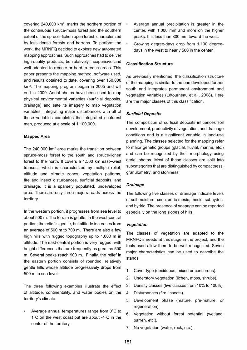
181

covering 240,000 km2, marks the northern portion of the continuous spruce-moss forest and the southern extent of the spruce–lichen open forest, characterized by less dense forests and barrens. To perform the work, the MRNFQ decided to explore new automated mapping approaches. Such approaches had to deliver high-quality products, be relatively inexpensive and well adapted to remote or hard-to-reach areas. This paper presents the mapping method, software used, and results obtained to date, covering over 150,000 km2. The mapping program began in 2005 and will end in 2009. Aerial photos have been used to map physical environmental variables (surficial deposits, drainage) and satellite imagery to map vegetation variables. Integrating major disturbances with all of these variables completes the integrated ecoforest map, produced at a scale of 1:100,000.

Mapped Area

The 240,000 km2 area marks the transition between spruce-moss forest to the south and spruce-lichen forest to the north. It covers a 1,500 km east─west transect, which is characterized by multiple relief, altitude and climate zones, vegetation patterns, fire and insect disturbances, surficial deposits, and drainage. It is a sparsely populated, undeveloped area. There are only three majors roads across the territory.

In the western portion, it progresses from sea level to about 500 m. The terrain is gentle. In the west-central portion, the relief is gentle, but altitude increases from an average of 500 m to 700 m. There are also a few high hills with rugged topography up to 1,000 m in altitude. The east-central portion is very rugged, with height differences that are frequently as great as 500 m. Several peaks reach 900 m. Finally, the relief in the eastern portion consists of rounded, relatively gentle hills whose altitude progressively drops from 500 m to sea level.

The three following examples illustrate the effect of altitude, continentality, and water bodies on the territory’s climate:

• Average annual temperatures range from 0ºC to 1ºC on the west coast but are about -4ºC in the center of the territory.

• Average annual precipitation is greater in the center, with 1,000 mm and more on the higher peaks. It is less than 800 mm toward the west.

• Growing degree-days drop from 1,100 degree-days in the west to nearly 500 in the center.

Classification Structure

As previously mentioned, the classification structure of the mapping is similar to the one developed farther south and integrates permanent environment and vegetation variables (Létourneau et al., 2008). Here are the major classes of this classification.

Surficial Deposits

The composition of surficial deposits influences soil development, productivity of vegetation, and drainage conditions and is a significant variable in land-use planning. The classes selected for the mapping refer to major genetic groups (glacial, fluvial, marine, etc.) and can be recognized by their morphology using aerial photos. Most of these classes are split into subcategories that are distinguished by compactness, granulometry, and stoniness.

Drainage

The following five classes of drainage indicate levels of soil moisture: xeric, xeric-mesic, mesic, subhydric, and hydric. The presence of seepage can be reported especially on the long slopes of hills.

Vegetation

The classes of vegetation are adapted to the MRNFQ’s needs at this stage in the project, and the tools used allow them to be well recognized. Seven major characteristics can be used to describe the stands.

1. Cover type (deciduous, mixed or coniferous).

2. Understory vegetation (lichen, moss, shrubs).

3. Density classes (five classes from 10% to 100%).

4. Disturbances (fire, insects).

5. Development phase (mature, pre-mature, or regeneration).

6. Vegetation without forest potential (wetland, barren, etc.).

7. No vegetation (water, rock, etc.).

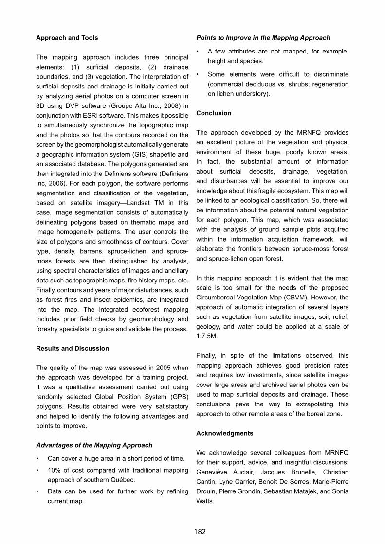
182

Approach and Tools

The mapping approach includes three principal elements: (1) surficial deposits, (2) drainage boundaries, and (3) vegetation. The interpretation of surficial deposits and drainage is initially carried out by analyzing aerial photos on a computer screen in 3D using DVP software (Groupe Alta Inc., 2008) in conjunction with ESRI software. This makes it possible to simultaneously synchronize the topographic map and the photos so that the contours recorded on the screen by the geomorphologist automatically generate a geographic information system (GIS) shapefile and an associated database. The polygons generated are then integrated into the Definiens software (Definiens Inc, 2006). For each polygon, the software performs segmentation and classification of the vegetation, based on satellite imagery—Landsat TM in this case. Image segmentation consists of automatically delineating polygons based on thematic maps and image homogeneity patterns. The user controls the size of polygons and smoothness of contours. Cover type, density, barrens, spruce-lichen, and spruce-moss forests are then distinguished by analysts, using spectral characteristics of images and ancillary data such as topographic maps, fire history maps, etc. Finally, contours and years of major disturbances, such as forest fires and insect epidemics, are integrated into the map. The integrated ecoforest mapping includes prior field checks by geomorphology and forestry specialists to guide and validate the process.

Results and Discussion

The quality of the map was assessed in 2005 when the approach was developed for a training project. It was a qualitative assessment carried out using randomly selected Global Position System (GPS) polygons. Results obtained were very satisfactory and helped to identify the following advantages and points to improve.

Advantages of the Mapping Approach

• Can cover a huge area in a short period of time.

• 10% of cost compared with traditional mapping approach of southern Québec.

• Data can be used for further work by refining current map.

Points to Improve in the Mapping Approach

• A few attributes are not mapped, for example, height and species.

• Some elements were difficult to discriminate (commercial deciduous vs. shrubs; regeneration on lichen understory).

Conclusion

The approach developed by the MRNFQ provides an excellent picture of the vegetation and physical environment of these huge, poorly known areas. In fact, the substantial amount of information about surficial deposits, drainage, vegetation, and disturbances will be essential to improve our knowledge about this fragile ecosystem. This map will be linked to an ecological classification. So, there will be information about the potential natural vegetation for each polygon. This map, which was associated with the analysis of ground sample plots acquired within the information acquisition framework, will elaborate the frontiers between spruce-moss forest and spruce-lichen open forest.

In this mapping approach it is evident that the map scale is too small for the needs of the proposed Circumboreal Vegetation Map (CBVM). However, the approach of automatic integration of several layers such as vegetation from satellite images, soil, relief, geology, and water could be applied at a scale of 1:7.5M.

Finally, in spite of the limitations observed, this mapping approach achieves good precision rates and requires low investments, since satellite images cover large areas and archived aerial photos can be used to map surficial deposits and drainage. These conclusions pave the way to extrapolating this approach to other remote areas of the boreal zone.

Acknowledgments

We acknowledge several colleagues from MRNFQ for their support, advice, and insightful discussions: Geneviève Auclair, Jacques Brunelle, Christian Cantin, Lyne Carrier, Benoît De Serres, Marie-Pierre Drouin, Pierre Grondin, Sebastian Matajek, and Sonia Watts.

183

References

Definiens A. G. 2006. Definiens professional version 5. efiniens A.G., München, Germany.

Groupe Alta inc. 2008. DVP version 7. Québec, Canada.

Létourneau, J. P., Matejek, S., Morneau, C., Robitaille, A., Roméo, T., Brunelle, J., & Leboeuf, A. 2008. Norme de cartographie écoforestière du Programme d’inventaire écoforestier nordique. Ministère des Ressources naturelles et de la Faune du Québec. 51 pp.

184

Analysis of Terrain Relationships to Improve Mapping of Boreal Ecosystems

Torre Jorgenson

Alaska EcoScience, Fairbanks, Alaska, U.S.A., tjorgenson@alaska.net

Extended Abstract

The mapping of boreal and tundra ecosystems at the plant community level is enhanced by incorporating the results of the quantitative analysis of the relationships among vegetation, soils, geomorphology, and physiography. Mapping of vegetation or the broader integration of terrain characteristics into ecosystems by image processing or photo-interpretation is constrained by the ability to differentiate mainly plant canopy structures. This kind of mapping also has limited ability to differentiate plant communities with similar vegetation structures. For example, broadleaf forests on alkaline floodplains have very different composition from birch forests on acidic, upland terrain. Differentiation of plant communities, however, can be enhanced by analyzing the relationships and co-occurrence of plant communities on terrain with differing physiography (e.g., riverine vs. upland), soil texture, geomorphology (e.g., meander overbank deposit vs. hillside colluvium), soil moisture and drainage, soil pH and electrical conductivity, and canopy structure. Quantification of the central tendencies of the co-occurrence of these associations can be used to develop rules that improve mapping of plant communities for both satellite image processing and photo-interpretation. During analysis, we classify

the characteristics of each terrain component independently using standard classification systems, although for vegetation, we identify plant communities through cluster analysis, ordination, and sorted table techniques. We found that 75–85% of our field plots have consistent relationships among terrain components, and the remaining portion are outliers or have inconsistent relationships that are not useful for mapping. We have used this integrated-terrain-unit (ITU) mapping approach for mapping ecosystems in northern, western, central, and south-central Alaska. For image processing, we use the results of the terrain analyses and thematic overlays of physiography, bedrock geology, and digital elevation models to differentiate single vegetation structures (e.g., dwarf shrub) that can be mapped with satellite imagery into plant communities with differing floristics on alpine, riverine, and organic-rich lowland terrain. For photo-interpretation, we use an ITU approach to code each polygon with geomorphology, surface form, and vegetation structure. We then aggregate the large number of ITU combinations into plant communities using rules of terrain relationships developed from analysis of the plot data.

Keywords: Alaska, boreal, classification, ecosystems, mapping, terrain analysis.

185

Appendices

Appendix I. Proposal for an IAVS Circumboreal Vegetation Map Working Group

The goal of the Circumboreal Vegetation Map (CBVM) is to provide a common international framework for understanding the boreal region. Currently, various maps already exist of the boreal biome, but they do not rely on a unified international method for classifying and mapping boreal vegetation. By recognizing the boreal region as a single geo-ecosystem with a common set of cultural, political, and economic issues, the CBVM will be the first detailed vegetation map of the entire global biome. Such a map is needed for a wide variety of purposes related to resource development, land-use planning, studies of boreal biota and biodiversity, education, anticipated global changes, and human interaction. A common legend and language for describing boreal ecosystems is essential for answering questions at a global scale. Boreal forests are particularly appropriate for unified classification because of their high level of floristic, physiognomic, and syntaxonomic similarity across the entire biome. A circumboreal vegetation map will have numerous other application uses for boreal scientists and managers, such as impact studies on wildlife and feedback mechanisms in models or studies of increased emission of greenhouse gases. The CBVM will also contribute to global efforts to improve understanding and communication with policy-makers.

A secondary goal is to make the map compatible with the Circumpolar Arctic Vegetation Map (CAVM, scale 1:7,500,000) to the north. Linking these two global-scale maps is necessary because very few issues relevant to the Arctic or the boreal regions stop at tree line. For example, most rivers flowing into the Arctic Ocean have their origin far to the south of the tree line. Climate and vegetation-change models, analysis of animal migrations, roads and industrial developments, and arctic-human interaction all require maps that include both the Arctic tundra and boreal forest regions.

The tasks listed above are directly related to activities of the International Association for Vegetation Science:

1. The Circumboreal Vegetation Map will synthesize comprehensive knowledge about diversity, ecology, geography, and disturbance of boreal biome;

2. The CBVM is based on international scientific cooperation of phytosociologists from wide spectrum of countries; and

3. The basic scientific problems solved within the frame of the CBVM correspond to the actual thematic activities in the IAVS meetings. These include:

— classifying vegetation of large regions

— developing the system of bioclimatic subdivisions of vegetation

— studying plant-geographical and evolutional regularities in boreal vegetation

— monographic study of entire (largest) biome

— studying dynamics and disturbances of boreal vegetation

— mapping (small-scale geobotanical mapping)

— mapping boreal vegetation with satellite images

Presentations and discussions of these diverse theoretical scientific problems of vegetation science related to the CBVM will be of great interest for the international society of phytosociologists, plant ecologists, and specialists on vegetation mapping.

Toward these goals we held an international workshop in Helsinki, Finland, November 3–6, 2008, to develop a strategy to map the vegetation of the circumboreal zone. Fifty vegetation scientists from 10 northern countries attended. A workshop summary follows with our resolution; outline of the project objectives; organizational chart; composition of mapping teams that includes thematic, remote sensing, biogeoclimatic, funding, regional and subregional divisions; and process and timeline.

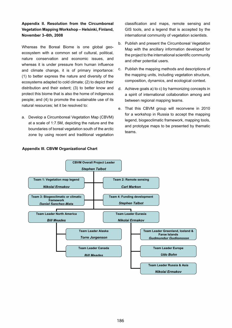
186

Appendix II. Resolution from the Circumboreal Vegetation Mapping Workshop – Helsinki, Finland, November 3–6th, 2008

Whereas the Boreal Biome is one global geo-ecosystem with a common set of cultural, political, nature conservation and economic issues, and whereas it is under pressure from human influence and climate change, it is of primary importance: (1) to better express the nature and diversity of the ecosystems adapted to cold climate; (2) to depict their distribution and their extent; (3) to better know and protect this biome that is also the home of indigenous people; and (4) to promote the sustainable use of its natural resources; let it be resolved to:

a. Develop a Circumboreal Vegetation Map (CBVM) at a scale of 1:7.5M, depicting the nature and the boundaries of boreal vegetation south of the arctic zone by using recent and traditional vegetation

classification and maps, remote sensing and GIS tools, and a legend that is accepted by the international community of vegetation scientists.

b. Publish and present the Circumboreal Vegetation Map with the ancillary information developed for the project to the international scientific community and other potential users.

c. Publish the mapping methods and descriptions of the mapping units, including vegetation structure, composition, dynamics, and ecological context.

d. Achieve goals a) to c) by harmonizing concepts in a spirit of international collaboration among and between regional mapping teams.

e. That this CBVM group will reconvene in 2010 for a workshop in Russia to accept the mapping legend, biogeoclimatic framework, mapping tools, and prototype maps to be presented by thematic teams.

Appendix III. CBVM Organizational Chart

CBVM Overall Project Leader

Stephen Talbot

Team Leader North America

Bill Meades

Team Leader Eurasia

Nikolai Ermakov

Team Leader Alaska

Torre Jorgenson

Team Leader Canada

Bill Meades

Team Leader Greenland, Iceland &Faroe Islands

Gudmundur Gudjonsson

Team Leader Europe

Udo Bohn

Team 1: Vegetation map legend

Nikolai Ermakov

Team 2: Remote sensing

Carl Markon

Team 3: Biogeoclimatic or climatic framework

Daniel Sanchez-Mata

Team 4: Funding development

Stephen Talbot

Team Leader Russia & Asia

Nikolai Ermakov

187

Appendix IV. CBVM Thematic Team Composition

Team 1: Vegetation Map Legend

— Objectives: uniform classification units, potential vegetation concept, legend prototypes

— Team leader: Nikolai Ermakov

— Participants: Klaus Dierssen, Annika Hofgaard, Udo Bohn, Jean-Pierre Saucier

— Subgroup on particular vegetation: alpine vegetation, mires and wetlands, flood plains, maritime heath, coastal vegetation

— Subgroup Leader: Klaus Dierssen

— Participants: Kazue Fujiwara, Del Meidinger, Hans Tommervik, Fred J.A. Daniёls, Raimo Heikkilä, Valentina Neshataeva, Stephen Talbot, Gudmundur Gudjonsson, Anna-Maria Fosaa, Elena Golubeva, Olga Galanina, Yukito Nakamura, Bill Meades, Kharuk Viacheslav

Deadlines

— Deadline 1: Legend prototype for December 2009

— Deadline 2: Legend test for December 2010

Team 2: Remote Sensing

— Objectives: thematic maps, map projection, map scale and resolution, remote sensing products

— Team leader: Carl Markon

— Participants: Sergei Bartlev, Peter Potapov, Ekaterina Shipigina, Gareth Reeds, Olga Tutubalina, Kelly Dolan

— Deadline: December 2010

Team 3: Biogeoclimatic or Climatic Framework

— Objectives: essential climatic indices, boreal definition, extent of the boreal

— Team leader: Daniel Sánchez-Mata

— Participants: Torre Jorgenson, Ken Baldwin, Pavel Krestov, Steve Cumming, Galina Ogureeva, Elgene Box, Teuvo Ahti

— Deadline: December 2010

Team 4: Funding Development — Objectives: obtain funding for the next workshop

and the project

— Team leader: Stephen Talbot

— Participants: Bill Meades

— Deadline: December 2010

Appendix V. CBVM Regional Team Composition

North America

— Objectives: mapping North America (Alaska, Canada, Saint-Pierre et Miquelon)

— Team leader: Bill Meades

— Participants: to be determined

— Alaska Subregion

— Subregion leader: Torre Jorgenson

— Participants: to be determined

— Canada Subregion

— Subregion leader: Bill Meades

— Participants: Ken Baldwin and others to be determined

Deadlines

— Deadline 1: international correlation excursion in summer 2012

— Deadline 2: regional maps in May 2013

Eurasia

— Objectives: mapping Eurasia (Greenland, Iceland, and Faroe Islands, Europe, Russia, and Asia)

— Team leader: Nikolai Ermakov — Participants: to be determined — Greenland, Iceland & Faroe Islands Subregion — Subregion leader: Gudmundur Gudjonsson — Participants: to be determined — Europe (Scandinavia and Finland) Subregion — Subregion leader: Udo Bohn — Participants: to be determined — Russia & Asia Subregion — Subregion leader: Nikolai Ermakov — Participants: to be determined

Deadlines

— Deadline 1: international correlation excursion in summer 2011 and 2012

— Deadline 2: regional maps in May 2013

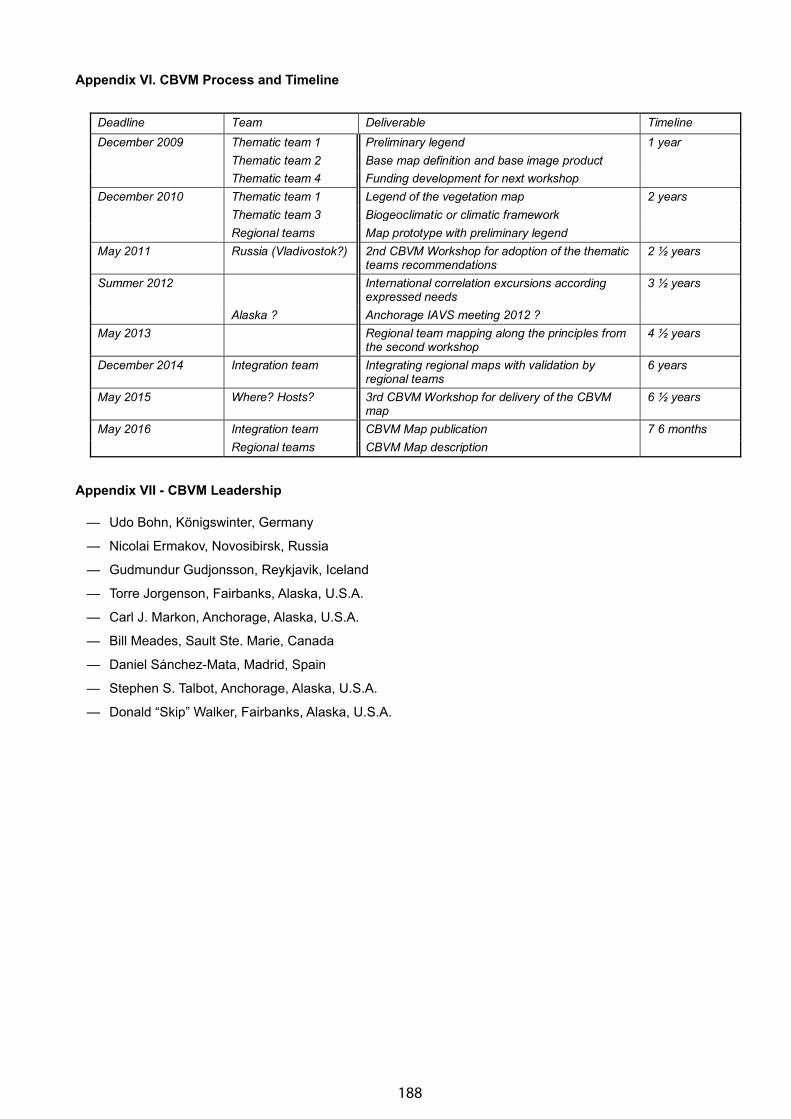
188

Appendix VI. CBVM Process and Timeline

Appendix VII - CBVM Leadership

— Udo Bohn, Königswinter, Germany

— Nicolai Ermakov, Novosibirsk, Russia

— Gudmundur Gudjonsson, Reykjavik, Iceland

— Torre Jorgenson, Fairbanks, Alaska, U.S.A.

— Carl J. Markon, Anchorage, Alaska, U.S.A.

— Bill Meades, Sault Ste. Marie, Canada

— Daniel Sánchez-Mata, Madrid, Spain

— Stephen S. Talbot, Anchorage, Alaska, U.S.A.

— Donald “Skip” Walker, Fairbanks, Alaska, U.S.A.

192

Deadline Team Deliverable Timeline December 2009

Thematic team 1 Preliminary legend 1 year Thematic team 2 Base map definition and base image product Thematic team 4 Funding development for next workshop

December 2010 Thematic team 1 Legend of the vegetation map 2 years Thematic team 3 Biogeoclimatic or climatic framework Regional teams Map prototype with preliminary legend

May 2011 Russia (Vladivostok?) 2nd CBVM Workshop for adoption of the thematic teams recommendations

2 ½ years

Summer 2012

International correlation excursions according expressed needs

3 ½ years

Alaska ? Anchorage IAVS meeting 2012 ? May 2013 Regional team mapping along the principles from

the second workshop 4 ½ years

December 2014 Integration team Integrating regional maps with validation by regional teams

6 years

May 2015 Where? Hosts? 3rd CBVM Workshop for delivery of the CBVM map

6 ½ years

May 2016 Integration team CBVM Map publication 7 6 months Regional teams CBVM Map description