C0015 Exploratory Data Analysis - IRIS Unimore
73
Chapter 3 C0015 Exploratory Data Analysis Mario Li Vigni, Caterina Durante and Marina Cocchi 1 Department of Chemical and Geochemical Sciences, University of Modena and Reggio Emilia, Modena, Italy 1 Corresponding author: [email protected] Chapter Outline 1. The Concept (Let Your Data Talk) 1 2. Descriptive Statistics 4 2.1 Frequency Histograms 5 2.2 Box and Whisker Plots 7 3. Projection Techniques 8 3.1 Principal Component Analysis 10 3.2 Other Projection Techniques 54 4. Clustering Techniques 60 5. Remarks 65 References 66 s0005 1 THE CONCEPT (LET YOUR DATA TALK) p0005 In the food area, as in most research fields, the system complexity to be faced is increasing both in the way of producing food and in the consumer expecta- tions evolved, together with the targets of regulatory authority and society needs and issues. Food production is connected to environmental, socio- economic challenges; food consumption with health, safety and nutritional attitudes. Among the emerging research areas there are the study and making of functional food, the use of nanotechnology, the assessment of food authen- ticity, including provenance and organic production, and the monitoring and improvement of the quality of food processing. From the point of view of food and food-processing characterization this implies that we need to extract information and obtain models capable of inferring the underlying relation- ships that link the compositional profile and the processing conditions to very general end properties of foodstuff, such as the healthiness, the consumer per- ception, the link to a territory and so on. Moreover, the implication of the pro- duction chain on food quality has also to be assessed. p0010 In this respect, the research attitude cannot be purely ‘deductive’: theory- driven hypothesis could be not only inefficient but even difficult to formulate. Comp. by: pdjeapradaban Stage: Proof Chapter No.: 3 Title Name: DHST Date:18/4/13 Time:11:59:50 Page Number: 1 B978-0-444-59528-7.00003-X, 00003 DHST, 978-0-444-59528-7 Data Handling in Science and Technology, Vol. 28. http://dx.doi.org/10.1016/B978-0-444-59528-7.00003-X © 2013 Elsevier B.V. All rights reserved. 1 To protect the rights of the author(s) and publisher we inform you that this PDF is an uncorrected proof for internal business use only by the author(s), editor(s), reviewer(s), Elsevier and typesetter SPi. It is not allowed to publish this proof online or in print. This proof copy is the copyright property of the publisher and is confidential until formal publication.
-
Upload
khangminh22 -
Category
Documents
-
view
0 -
download
0
Transcript of C0015 Exploratory Data Analysis - IRIS Unimore

Chapter 3
C0015 Exploratory Data Analysis
Mario Li Vigni, Caterina Durante and Marina Cocchi1
Department of Chemical and Geochemical Sciences, University of Modena and Reggio Emilia,
Modena, Italy1Corresponding author: [email protected]
Chapter Outline1. The Concept (Let Your
Data Talk) 12. Descriptive Statistics 4
2.1 Frequency Histograms 52.2 Box and Whisker Plots 7
3. Projection Techniques 8
3.1 Principal ComponentAnalysis 10
3.2 Other ProjectionTechniques 54
4. Clustering Techniques 605. Remarks 65References 66
s0005 1 THE CONCEPT (LET YOUR DATA TALK)
p0005 In the food area, as in most research fields, the system complexity to be facedis increasing both in the way of producing food and in the consumer expecta-tions evolved, together with the targets of regulatory authority and societyneeds and issues. Food production is connected to environmental, socio-economic challenges; food consumption with health, safety and nutritionalattitudes. Among the emerging research areas there are the study and makingof functional food, the use of nanotechnology, the assessment of food authen-ticity, including provenance and organic production, and the monitoring andimprovement of the quality of food processing. From the point of view offood and food-processing characterization this implies that we need to extractinformation and obtain models capable of inferring the underlying relation-ships that link the compositional profile and the processing conditions to verygeneral end properties of foodstuff, such as the healthiness, the consumer per-ception, the link to a territory and so on. Moreover, the implication of the pro-duction chain on food quality has also to be assessed.
p0010 In this respect, the research attitude cannot be purely ‘deductive’: theory-driven hypothesis could be not only inefficient but even difficult to formulate.
Comp. by: pdjeapradaban Stage: Proof Chapter No.: 3 Title Name: DHSTDate:18/4/13 Time:11:59:50 Page Number: 1
B978-0-444-59528-7.00003-X, 00003
DHST, 978-0-444-59528-7
Data Handling in Science and Technology, Vol. 28. http://dx.doi.org/10.1016/B978-0-444-59528-7.00003-X
© 2013 Elsevier B.V. All rights reserved. 1
To protect the rights of the author(s) and publisher we inform you that this PDF is an uncorrected proof for internal business useonly by the author(s), editor(s), reviewer(s), Elsevier and typesetter SPi. It is not allowed to publish this proof online or in print.This proof copy is the copyright property of the publisher and is confidential until formal publication.

This is why and where researchers may benefit from new technological tools(analytical instrumentation, hardware and algorithms/software development)to come back to an ‘inductive’ data-driven attitude with a minimum ofa priori hypothesis as a first efficient step to progress faster and further.
p0015 To this aim exploratory data analysis (EDA) is well suited. EDA is wellknown in statistics and sciences as that operative approach to data analysisaimed to improve understanding and accessibility of the results. Without for-getting the soundness of statistical models and hypothesis formulation, whichis intrinsically connected to the concept of ‘analysis’ in its scientific meaning,the focus is moved to ‘exploration’, which, as a word, leads to more exoticthoughts and feelings, such as unravelling mysterious threads or discoveringunknown worlds. As a matter of fact, EDA does relate to the process ofrevealing hidden and unknown information from data in such a form thatthe analyst obtains an immediate, direct and easy-to-understand representationof it. Visual graphs are a mandatory element of this approach, owing to theintrinsic ability of the human brain to get a more direct and trustworthy inter-pretation of similarities, differences, trends, clusters and correlations througha picture, rather than a series of numbers. As a matter of fact, our perceptionof reality is that we believe what we are able to see.
p0020 The other axiom of EDA is that the focus of attention is on the data, ratherthan the hypothesis. This means, figuratively, that it is not the analyst ‘asking’questions to the data, as in an interrogation, instead the data are allowed to‘talk’, giving evidence of their nature, the relationships which characterizethem, the significance of the information which lies beneath what has been eval-uated on them – or even the complete absence of any of this, if it is the case.
p0025 One of the milestone references for EDA is the comprehensive book byTukey [1]. Tukey, in his work, aimed to create a data analysis frameworkwhere the visual examination of data sets, by means of statistically significantrepresentations, plays the pivotal role to aid the analyst to formulate hypoth-eses that could be tested on new data sets. The stress on two concepts suchas dynamic experimenting on data (e.g. evaluating the results on different sub-sets of a same data set, under different data-preprocessing conditions) andexhaustive visualization capabilities offers researchers the possibility to iden-tify outliers, trends and patterns in data, upon which new theories and hypoth-esis can be built. Tukey’s first view on EDA was based on robust andnonparametric statistical concepts such as the assessment of data by meansof empirical distributions, hence the use of the so-called five-number sum-mary of data (range extremes, median and quartiles), which led to one ofhis most known graphical tools for EDA, the box plot.
p0030 This approach well denotes the conceptual shift from confirmatory dataanalysis, where a hypothesis and a distribution are assumed on the data, andstatistical significance is used to test the hypothesis on the basis of the data(where the less reliable the results, the more the data divert from the postu-lated distribution), to EDA, where the data are visualized in a distribution-free
Comp. by: pdjeapradaban Stage: Proof Chapter No.: 3 Title Name: DHSTDate:18/4/13 Time:11:59:50 Page Number: 2
PART I Theory2
B978-0-444-59528-7.00003-X, 00003
DHST, 978-0-444-59528-7
To protect the rights of the author(s) and publisher we inform you that this PDF is an uncorrected proof for internal business useonly by the author(s), editor(s), reviewer(s), Elsevier and typesetter SPi. It is not allowed to publish this proof online or in print.This proof copy is the copyright property of the publisher and is confidential until formal publication.

approach, and hypotheses arise from the observation, if any, of trends andclusters or correlations among them. In practice, the objectives of EDA aim to
u0005 l Highlight phenomena occurring in the observations so that hypothesesabout the causes can be suggested, rather than ‘forcing’ hypotheses onthe observations to explain phenomena known a priori. ‘The combinationof some data and an aching desire for an answer does not ensure that a rea-sonable answer can be extracted from a given body of data’ [2].
u0010 l Provide a basis to assess the assumption for statistical inference, for exam-ple, by evaluating the best selection of statistical tools and techniques, oreven new sampling strategies, for further investigations. ‘Exploratory dataanalysis can never be the whole story, but nothing else can serve as thefoundation stone as the first step’ [1].
p0045 The tools and techniques of EDA are strongly based on the graphicalapproach mentioned so far. Data visualization is given by means of box plots,histograms and scatter plots, all distribution-free instruments which can beextremely useful to probe if the data follow a particular distribution.
p0050 At the beginning of its development, EDA represented a kind of Coperni-can revolution, in the sense that it put data and the information they bring, notthe hypothesis and the information it seeks, at the centre of attention. How-ever, using it in a framework where the common approach was to reduce pro-blems into simpler forms that were solvable, usually by constraining theexperimental domains to uni- or oligovariate models nowadays, shows hugelimitations. When dealing with scientific fields such as chemistry, and in par-ticular analytical chemistry, and food science, where instrumental analysis canprovide at least thousands of variables for each sample, often in a fast way,data complexity has exponentially increased to the point that a multivariateapproach (i.e. the evaluation of the simultaneous effect of all the variableswhich characterize a system on the relationships among its samples) is man-datory. The use of graphical instruments is limited to human ability to inter-pret two-dimensional (2D) and three-dimensional (3D) spaces, which isimpossible to apply when variability is represented through, for example, ananalytical signal. Correlation tables, albeit offering a direct view of whichvariables are related to each other, are often complex to read and interpret.Multivariate analysis methods, especially those based on latent variables pro-jection, provide the best tool to combine the analysis of variable correlationsand sample similarities/differences, the reduction of variable space to lowerdimensions and the possibility of offering graphical outputs that are easy toread and interpret. Thus, the passage from EDA to exploratory multivariatedata analysis (EMDA) is conceptually easier than the one from confirmatorydata analysis to EDA, as it only represents a shift towards the use of methodswhich are based on a multivariate approach to data.
p0055 EMDA stays on the track opened by EDA, in order to grasp the data struc-ture without imposing any model. It has to be stressed that when dealing with
Comp. by: pdjeapradaban Stage: Proof Chapter No.: 3 Title Name: DHSTDate:18/4/13 Time:11:59:50 Page Number: 3
Chapter 3 Exploratory Data Analysis 3
B978-0-444-59528-7.00003-X, 00003
DHST, 978-0-444-59528-7
To protect the rights of the author(s) and publisher we inform you that this PDF is an uncorrected proof for internal business useonly by the author(s), editor(s), reviewer(s), Elsevier and typesetter SPi. It is not allowed to publish this proof online or in print.This proof copy is the copyright property of the publisher and is confidential until formal publication.

a multidimensional space, visualization requires either a projection step or adomain change, for example, from acquired variables to a similarity/dissimi-larity space. Thus, if a priori hypotheses (imposed models) are avoided, mostoften some assumptions on data are adopted. This brings a diversity of com-plementary instruments that can be used, and we may say that EMDA is aroad that several tools allow you to travel.
p0060 The aim of this chapter is to illustrate the most used and effective tools forthe analysis of food-related data, so that the reader is offered some clues aboutwhich tool to choose and what is possible to get out of it.
s0010 2 DESCRIPTIVE STATISTICS
p0065 All those visualization tools which allow the exploration of uni- and oligo-variate data can be considered as instruments of descriptive statistics. Descrip-tive statistics is usually defined as a way to summarize/extract information outof one or a few variables: compared to inferential statistics, whose aim is toassess the validity of a hypothesis made on measured data, descriptive statis-tics is merely explorative. In particular, some salient facts can be extractedabout a variable:
o0005 i. A measure of the central tendency, that is, the central position of a fre-quency distribution of a group of data. In other words, a number whichis better suited to represent the value of the investigated samples withrespect to the measured property. Typical statistics are mean, medianand mode.
o0010 ii. A measure of spread, describing how spread out the measured values arearound the central value. Typical statistics are range, quartiles and stan-dard deviation.
o0015 iii. A measure of asymmetry (skewness) and peakedness (kourtosis) of thefrequency distribution, that is, if the spread of data around the centralvalue is symmetric in both left/right directions, and how sharp/flat isthe distribution in the central position, respectively.
p0085 While useful, these statistics are only a summarization of data and do not offera direct interpretation benefit when compared to a graphical representation ofthe data. The main graphical tools for descriptive statistics are frequency his-tograms, box-whisker graphs and scatter plots. These tools are useful toinspect the statistics reported earlier, the presence of outliers and multiplemodes in the data (histograms), to highlight location and variation changesbetween different groups of data or among several variables (box-whisker),to reveal relationships or associations between two variables (scatter plots),as well as to highlight dependency with respect to some ordering criterion,such as run order, time, position, etc.
p0090 Albeit simple and in spite of the high degree of summarizing theycarry with them, these tools can also be particularly useful prior to EMDA.
Comp. by: pdjeapradaban Stage: Proof Chapter No.: 3 Title Name: DHSTDate:18/4/13 Time:11:59:52 Page Number: 4
PART I Theory4
B978-0-444-59528-7.00003-X, 00003
DHST, 978-0-444-59528-7
To protect the rights of the author(s) and publisher we inform you that this PDF is an uncorrected proof for internal business useonly by the author(s), editor(s), reviewer(s), Elsevier and typesetter SPi. It is not allowed to publish this proof online or in print.This proof copy is the copyright property of the publisher and is confidential until formal publication.

It may seem a paradox, but they are very effective to identify gross errors: forexample, a huge difference between median and mean for a variable could bedue to a misprinted number, or could suggest the need to transform variables(e.g. log transform) and help choosing the appropriate data pretreatment.
s0015 2.1 Frequency Histograms
p0095 To draw a histogram, the range of data is subdivided in a number of equallyspaced bins. Thus, frequency histograms report on the horizontal axis the valuesof the measured variable and on the vertical axis the frequencies, that is, the num-ber of measurements, which fall into each bin. The number of bins influences theefficacy of the representation, thus some attention must be given in their choice.Some common rules have been coded, among which the most used considers anumber of bins k equal to the square root of the number of samples n, or equalto 1þ log2(n). Theoretically derived rules are reviewed in Scott’s book [3], anditerative methods have also been proposed [4]. In most cases, one of the two rulescited earlier is enough to obtain a nice representation of data distribution, but thechoice of k becomes critical when n is huge, for example, if you want to representa frequency histogram of pixels intensity of an image, where the number of ‘sam-ples’ easily goes beyond several hundreds of thousands.
p0100 Figure 1 reports some examples of histograms which are quite common tofind for discrete variables. Figure 1A shows what to expect when the variablehas an almost normal distribution, that is a maximum frequency of occurrencefor a given value (close to the average of the values) and decreasing frequen-cies for higher and lower values. Skewness of the distribution (Figure 1B) isindicated by a higher frequency of occurrence for values which are higheror lower than the most frequent one. Histograms can show the presence ofclusters in the data according to a given value, as can be seen in Figure 1C:here it is possible to see two values of higher frequency, around which twoalmost normal distributions suggest the existence of two clusters. In addition,the presence of outliers (Figure 1D) can be highlighted. An outlier usually hasa value way higher or lower than all the other samples, hence it will appear inthe histogram as a bar both well separated from the main cluster of values andshowing a low frequency of occurrence. As mentioned, histograms can also beused when the number of observations is high (on the other hand, they loseany exploratory meaning when used for data sets where the number of vari-ables is very high and correlated, such as in instrumental signals), as shownin the last two parts of Figure 1. Here, the distribution of pixels of imagesis used. In particular, Figure 1E shows the zoomed view of pixel distributionfor an image acquired on a product (in this case, a bread bun) which is consid-ered a production target (i.e. the colour intensity and homogeneity of itssurface are inside specification values for that product): it is possible to seethat frequencies of occurrence are almost symmetrically distributed acrossthe average value (data have been centred across the mean intensity value).
Comp. by: pdjeapradaban Stage: Proof Chapter No.: 3 Title Name: DHSTDate:18/4/13 Time:11:59:52 Page Number: 5
Chapter 3 Exploratory Data Analysis 5
B978-0-444-59528-7.00003-X, 00003
DHST, 978-0-444-59528-7
To protect the rights of the author(s) and publisher we inform you that this PDF is an uncorrected proof for internal business useonly by the author(s), editor(s), reviewer(s), Elsevier and typesetter SPi. It is not allowed to publish this proof online or in print.This proof copy is the copyright property of the publisher and is confidential until formal publication.

A different shape is manifest in Figure 1F, where an image of a sample withsurface defects (such as darker or paler colour, or the presence of spots andblisters) is considered. In this case, the pixel distribution is skewed towardspositive values and lower frequency occurrence features appear, which arean index of phenomena which deviate from the bulk of the data, such as dar-ker localized spots.
Comp. by: pdjeapradaban Stage: Proof Chapter No.: 3 Title Name: DHSTDate:18/4/13 Time:11:59:52 Page Number: 6
4025
A
C
20
15
10
5
0
20
15
10
5
0
5.5 8.5 11.5 14.5
B
D
30
20
10
03.5 6.5 9.5
Values
ValuesValues
Values
No
of s
ampl
es
40
30
20
10
0
No
of s
ampl
es
No
of s
ampl
esN
o of
sam
ples
12.5 15.5
5.5 8.5 11.5 14.5 17.5 20.55.5 8.5 11.5 14.5 17.5 23.520.5
FE
Values
No
of p
ixel
s
800
100
200
300
400
500
600
700
800
No
of p
ixel
s
0
100
200
300
400
500
600
700
800
100 120 140 160 180 200 220 240
Values
80 100 120 140 160 180 200 220 240
FIGURE 1f0005 Examples of histograms. (A) Almost normal distribution of a discrete variable;(B) skewed distribution (higher values have a higher frequency of occurrence); (C) overlapping
of two distributions centred across a different mean value (possibly indicating the presence of
two clusters); (D) presence of outliers (low frequency of occurrence for high values); (E) pixeldistribution of a reference image; and (F) pixel distribution of an image where defects are detected
(defective pixels bring to the bump in the right tail of frequency distribution and to the frequency
bars detected for values >240). In the pixel distribution cases, a zoom has been taken to highlight
the differences.
PART I Theory6
B978-0-444-59528-7.00003-X, 00003
DHST, 978-0-444-59528-7
To protect the rights of the author(s) and publisher we inform you that this PDF is an uncorrected proof for internal business useonly by the author(s), editor(s), reviewer(s), Elsevier and typesetter SPi. It is not allowed to publish this proof online or in print.This proof copy is the copyright property of the publisher and is confidential until formal publication.

s0020 2.2 Box and Whisker Plots
p0105 Box and whisker plots (box plot in short) [5–7] are very useful to summarizethe kind of information that in inferential statistics we seek by means of anal-ysis of variance (ANOVA). Indeed, they allow a direct comparison of the dis-tribution of several variables (on the order of tens, visualization becomesinefficient) in terms of both central location and variation. Thus, it is a quickway to estimate if a grouping factor has potentially a significant effect on themeasured variables. Typical questions that can be answered are: Does thelocation differ between subgroups? Does the variation differ between sub-groups? Are there any outliers?
p0110 The construction of a box plot requires calculating the median and thequartiles of a given variable for the samples: the lower quartile (LQ) is the25th percentile and the upper quartile (UQ) is the 75th percentile. Then abox is drawn (hence the name) whose edges are the lower and upper quartiles:this box represents the middle 50% of the data and the difference between theupper and lower quartile is indicated as the inter quartile range (IQR). Gener-ally, the median is represented by a line drawn inside the box, and in somerepresentations the mean is also drawn as an asterisk, for example, to betterevaluate the differences between central tendency descriptors. Then a line isdrawn from the LQ to the minimum value and another line from the UQ tothe maximum value and typically a symbol is drawn at these minimum andmaximum points (whiskers). In most implementations, if a data point presentsa value higher than UQþ1.5* IQR or smaller than LQ"1.5* IQR, it is repre-sented by a circle. This helps pointing out potential outliers (the circle may bedrawn with a higher dimension if the LQ or UQ is exceeded by 3*IQR).A single box plot can be drawn for one set of samples with respect to onevariable; alternatively, multiple box plots can be drawn together to compareseveral variables, groups in a single set of samples or multiple data sets.Box plots become difficult to draw and interpret in those cases where it isnecessary to deal with continuous data, such as spectra or signals.
p0115 Figure 2 shows a box plot representation of each of the nine variableswhich characterize the GCbreadProcess data set (see Section 3.1.4 for moredetails on the data set), the concentration of chemical compounds determinedin gas chromatography (GC) at six points of an industrial bread-making pro-cess, namely, S0, S2, S4, D, T and L. As it is possible to regroup data accord-ing to the sampling point, the representation is useful to obtain a screeningevaluation of which variables show different distributions across the phasesof the production process. For example, fumaric acid and malic acid have sim-ilar distributions and values for all six points (the ‘box’, that is the IQR, andthe ‘whiskers’, that is the 95th and 5th percentile range, are almost overlappedfor all the sampling points), thus they will be of little use to differentiate theprocess phases. On the contrary, fructose and glucose show a clear differencein both range and mean and median value (respectively, the star and the
Comp. by: pdjeapradaban Stage: Proof Chapter No.: 3 Title Name: DHSTDate:18/4/13 Time:11:59:55 Page Number: 7
Chapter 3 Exploratory Data Analysis 7
B978-0-444-59528-7.00003-X, 00003
DHST, 978-0-444-59528-7
To protect the rights of the author(s) and publisher we inform you that this PDF is an uncorrected proof for internal business useonly by the author(s), editor(s), reviewer(s), Elsevier and typesetter SPi. It is not allowed to publish this proof online or in print.This proof copy is the copyright property of the publisher and is confidential until formal publication.

horizontal line inside the box) for points S0, S2 and S4 with respect to pointsD, T and L. The presence of potential outliers, that is points which fall beyondthe 95th and 5th percentile limits, is indicated by circles (crossed circles arecharacterized by a 3*IQR distance). This representation can be a startingpoint to decide which variables, or combination of more, are the best to differ-entiate the six points.
s0025 3 PROJECTION TECHNIQUES
p0120 EMDA pursues the same objectives illustrated for uni- and oligovariate EDA,namely giving a graphical representation of multivariate data highlighting thedata patterns and the relationships among objects and variables with noa priori hypothesis formulation. The importance of this step and its relevancein food analysis is worth being stressed. In fact, the multivariate exploratorytools make it feasible to generate hypotheses from the data, notwithstandinghow complex they are, opening to the researcher a way towards the formula-tion of new ideas. In other words, intuition is inspired by the synergy of datareduction and graphical display. In fact, by compressing the data to a fewparameters, without losing information, it becomes possible to look at data,so that the researcher’s mind can capture data variation in terms of groupingand patterns in the natural way.
Comp. by: pdjeapradaban Stage: Proof Chapter No.: 3 Title Name: DHSTDate:18/4/13 Time:11:59:56 Page Number: 8
Succinic acid
Fructose
Sucrose
30 835
30
25
20
6420
20
10
S0 S2 S4 D T L S0 S2 S4 D T L S0 S2 S4 D T L0
Maltose Fumaric acid
Glucose Inositol
Malic acid Glycerol
Val
ues
Val
ues
Val
ues
0.25
0.2
0.15
0.1
0.25
0.33
20
10
0
20 0.15
0.1
0.05
10
0
2
10.2
FIGURE 2f0010 oxplot representation of the nine variables which characterize the GCbreadProcess
data set (see text for details).
PART I Theory8
B978-0-444-59528-7.00003-X, 00003
DHST, 978-0-444-59528-7
To protect the rights of the author(s) and publisher we inform you that this PDF is an uncorrected proof for internal business useonly by the author(s), editor(s), reviewer(s), Elsevier and typesetter SPi. It is not allowed to publish this proof online or in print.This proof copy is the copyright property of the publisher and is confidential until formal publication.

p0125 It is indeed very different, with respect to the possibility of enhancing dis-covery, to operate simplification by reduction at the problem level or datalevel [8]. In the first case, prior knowledge is used to isolate or split the com-plex system into subsystems or steps, for example, in the case of food, tofocus on the quantification of specific constituents or on the modelling of asimplified process, such as thermal degradation or ageing, at laboratory scale,discarding the food processing and the production chain. In the second case,prior knowledge is used, after data reduction by EMDA, to interpret the pat-terns which appear and validate possible conclusions which will guide tonew hypothesis generation. In the first case, interactions among the reducedsubsystems or steps are lost and, at most, the a priori hypothesized mechanis-tic behaviour may be confirmed or rejected; reformulation of the hypothesiswill require a priori adoption of a different causal model. Differently, in thesecond case, the salient features of the system under investigation as a whole,including interactions, interconnections and peculiar behaviours, are learnedfrom data by comparing conclusions induced by graphs to prior knowledge;it is then possible to validate the model and new hypotheses can be generated,so that an interactive cycle of multivariate experiments planning, multivariatesystems characterization and multivariate data analysis is enabled.
p0130 Which food area would require explorative multivariate data analysistools? We have seen in the introduction section that food science todayembraces a wide multidisciplinary ambit, involving chemistry, biology/micro-biology, genetics, medicine, agriculture, technology and environmental sci-ence, and also sensory and consumer analysis as well as economy.
p0135 Moreover, the investigation of the food production chain in an industrialcontext requires the assessment of not only the chemical/biological para-meters but also the process parameters, irregularities, the influence of rawmaterials, etc. From an industrial perspective, the goal is not to produce agiven product with constant technology and materials, which is impossiblein practice, but rather to be able to control the specific, transient traits of pro-duction in order to ensure the same product quality.
p0140 Accordingly, the data used for food and food-processing characterizationare changing [9–11] from traditional physical or chemical data, such as con-ductivity, thermal curves, moisture, acidity and concentrations of specificchemical substances, to fingerprinting data. Examples of this kind of datarange from chromatograms or spectroscopic measurements, that is, completespectra obtained by infrared (IR) [12–14], nuclear magnetic resonance(NMR) [15,16], mass spectrometry (MS), ultraviolet–visible (UV–vis) orfluorescence spectrophotometry, to landscapes obtained by any hyphenatedcombination of the previous techniques [17–21]; from signals obtained bymeans of sensor arrays such as electronic noses or tongues [22], microarraysand so on to imaging and hyperspectral imaging techniques [23–25].
p0145 The nature of this kind of data, the need to consider the many sourcesof variability due to the origin of raw materials, seasonality, agricultural
Comp. by: pdjeapradaban Stage: Proof Chapter No.: 3 Title Name: DHSTDate:18/4/13 Time:11:59:58 Page Number: 9
Chapter 3 Exploratory Data Analysis 9
B978-0-444-59528-7.00003-X, 00003
DHST, 978-0-444-59528-7
To protect the rights of the author(s) and publisher we inform you that this PDF is an uncorrected proof for internal business useonly by the author(s), editor(s), reviewer(s), Elsevier and typesetter SPi. It is not allowed to publish this proof online or in print.This proof copy is the copyright property of the publisher and is confidential until formal publication.

practices and so on, together with the objective of studying the complex foodprocesses as a whole, explain why EMDA is mandatory.
p0150 Multivariate screening tools are needed in order to model the underlyinglatent functional factors which determine what happens in the examined sys-tems, and are the basis for an exploratory, inductive data strategy.
p0155 These tools have to accomplish two tasks:
o0020 i. Data reduction, that is, compression of all the information to a small set ofparameters without introducing distortion of data structure (or at leastkeeping it to a minimum and maintaining control of the disturbance thathas been introduced);
o0025 ii. Efficient graphical representation of the data.
p0170 By far the most effective techniques to achieve these objectives are based onprojection techniques, that is methods to project the data from its J-variables/conditions space to lower dimensionality, that is, A-latent factors/componentsspace. The commonly most used one is principal component analysis (PCA)and its extensions.
s0030 3.1 Principal Component Analysis
p0175 An exhaustive description of PCA historical and applicative perspectives,including a comparative discussion of PCA with respect to related methods,has been given by Joliffe [26] and Jackson [27]; other basic references are thededicated chapters in Massart’s book [28] and Comprehensive Chemometrics[29], and a more didactical view, with reference to the R-project code environ-ment may be found in Varmuza [30] and Wehrens [31]. A description of PCAstrictly oriented to spectroscopic data may be found in the Handbook of NIRSpectroscopy [32], Beebe [33] and in Davies’ column in Spectroscopy Europe[34,35]; other salient references are Wold et al. [36] and Smilde et al. [37].
p0180 Here, PCA will be presented as a basic multivariate explorative tool withemphasis on the data representation and interpretation aiming at giving prac-tical guidelines for usage in this specific context; the reader is referred to theliterature cited earlier for more details.
p0185 PCA is a bilinear decomposition/projection technique capable of condens-ing large amounts of data into few parameters, called principal components(PCs) or latent variables/factors, which capture the levels, differences andsimilarities among the samples and variables constituting the modelled data.This task is achieved by a linear transformation under the constraints of pre-serving data variance and imposing orthogonality of the latent variables.
p0190 The underlying assumption is that the studied systems are ‘indirectlyobservable’ in the sense that the relevant phenomena which are responsiblefor the data variation/patterns are hidden and not directly measurable/observ-able. This explains the term latent variables. Once uncovered, latent variables(PCs) may be represented by scatter plots in a Euclidean plane.
Comp. by: pdjeapradaban Stage: Proof Chapter No.: 3 Title Name: DHSTDate:18/4/13 Time:12:00:00 Page Number: 10
PART I Theory10
B978-0-444-59528-7.00003-X, 00003
DHST, 978-0-444-59528-7
To protect the rights of the author(s) and publisher we inform you that this PDF is an uncorrected proof for internal business useonly by the author(s), editor(s), reviewer(s), Elsevier and typesetter SPi. It is not allowed to publish this proof online or in print.This proof copy is the copyright property of the publisher and is confidential until formal publication.

p0195 An almost unique feature of PCA and strictly related projection techniquesis that it allows a simultaneous and interrelated view of both samples and vari-ables spaces, as it will be shown in detail in the following section.
p0200 For clarity of presentation, the PCA subject will be articulated in subsec-tions: definition and derivation of PCs, including main algorithms; preproces-sing issues; PCA in food data analysis practice.
s0035 3.1.1 Definition and Derivation of PCA
p0205 PCA decomposes the data matrix as follows:
X I,Jð Þ ¼TA&VATþE I,Jð Þ (1)
where A is the number of components, underlying structures or ‘chemical’(effective) rank of the matrix; the score vectors, T¼ [t1,t2, . . .,tA], give thecoordinates of samples in the PC space, hence score scatter plots allowthe inspection of sample similarity/dissimilarity, and the loadings vectors,V¼ [v1,v2, . . .,vA], represent the weight with which each original variable con-tributes to the PCs, so that the correlation structure among the variables maybe inspected through loading scatter plots. E is the residual, or noise or errormatrix, the part of the data which was not explained by the model; it has thesame dimensions as X and it is often used as a diagnostic tool for the identi-fication of outlying samples and/or variables.
p0210 From a geometrical point of view, PCA is an orthogonal projection (a lin-ear mapping) of X in the coordinate system spanned by the loading vectors V.Figure 3A reports an example of a set of samples characterized by two vari-ables x1 and x2, projected on the straight lines defined by the loading vectorv1 and v2. For each of the I samples, a score vector ti is obtained containingthe scores for the sample (i.e. the coordinates on the PC axes).
p0215 Considering the projection of these samples on the PC space (Figure 3B),it emerges that the two categories (black circle and grey squares, respectively)are well separated on the first PC, while the second PC describes mainly non-systematic variability; thus one component (A¼1) is sufficient to retain infor-mation on this set of data.
p0220 Thus, PCA operates a reduction of dimensions from the number of variables Jin X to A underlying virtual variables describing the structured part of data.Hence, a representation of the scores by means of 2D or 3D scatter plots allowsan immediate visualization of where the samples are placed in the PC space,and makes the detection of sample groupings or trends easier (Figure 4A–C).The loadings represent the weight of each of the original variables in determiningthe direction of each of the PCs or, which is the same as PCs are defined as themaximum variance directions, which of the original variables varies the mostfor the samples with different score values on each of the components. A 2D or3D plot of the loadings can be read as follow: variables that present loadings,which are equal or have close values, result correlated (anti-correlated if the signs
Comp. by: pdjeapradaban Stage: Proof Chapter No.: 3 Title Name: DHSTDate:18/4/13 Time:12:00:02 Page Number: 11
Chapter 3 Exploratory Data Analysis 11
B978-0-444-59528-7.00003-X, 00003
DHST, 978-0-444-59528-7
To protect the rights of the author(s) and publisher we inform you that this PDF is an uncorrected proof for internal business useonly by the author(s), editor(s), reviewer(s), Elsevier and typesetter SPi. It is not allowed to publish this proof online or in print.This proof copy is the copyright property of the publisher and is confidential until formal publication.

Comp. by: pdjeapradaban Stage: Proof Chapter No.: 3 Title Name: DHSTDate:18/4/13 Time:12:00:04 Page Number: 12
PC1
PC
2
−1.5−1.5
−1
−1
−0.5
−0.5
0
0
0.5
0.5
1
1
1.5
1.5B
FIGURE 3f0015 Geometry of PCA. A simulated example with 20 samples characterized by two vari-
ables. (A) The samples are plotted in the space of the original variables x1 and x2. The blue (grey,dashed) and red (black, dot–dashed) lines represent the directions of PC1 and PC2 axes, respec-
tively. The coordinates of the blue (grey) arrow are v11 and v21, the loading values of variables
x1 and x2 on the first PC, respectively. The coordinates of the red (black) arrow are the v12 and
v22, the loading values of variable x1 and x2 on the second PC, respectively. The scores valuesare the orthogonal projection of the sample coordinates on the PC axes, as an example the scores
of sample 5 are shown: t51 (PC1 score) and t52 (PC2 score). (B) The 20 samples represented in PC
space: PC1 versus PC2. (For interpretation of the references to colour in this figure legend, the
reader is referred to the online version of this chapter.)
PART I Theory12
B978-0-444-59528-7.00003-X, 00003
DHST, 978-0-444-59528-7
To protect the rights of the author(s) and publisher we inform you that this PDF is an uncorrected proof for internal business useonly by the author(s), editor(s), reviewer(s), Elsevier and typesetter SPi. It is not allowed to publish this proof online or in print.This proof copy is the copyright property of the publisher and is confidential until formal publication.

Comp. by: pdjeapradaban Stage: Proof Chapter No.: 3 Title Name: DHSTDate:18/4/13 Time:12:00:14 Page Number: 13
A
PC1 (38.34%)
PC
2 (2
4.67
%)
−4 −3−3
−2
−2
−1
−1
0
0
1
1
2
2
3
3
4
Ethanol
0.8B
0.7
0.6
0.5
0.4
0.3
0.2
0.1
0
PC
2 (2
4.67
%)
−0.1
−0.2
−0.4 −0.2 0 0.2
PC1 (38.34%)
0.4 0.6
Glicerol
Proanth.
Tartaric Ac.
Malic Ac.
Flavon.
FIGURE 4—Cont’d
Chapter 3 Exploratory Data Analysis 13
B978-0-444-59528-7.00003-X, 00003
DHST, 978-0-444-59528-7
To protect the rights of the author(s) and publisher we inform you that this PDF is an uncorrected proof for internal business useonly by the author(s), editor(s), reviewer(s), Elsevier and typesetter SPi. It is not allowed to publish this proof online or in print.This proof copy is the copyright property of the publisher and is confidential until formal publication.

Comp. by: pdjeapradaban Stage: Proof Chapter No.: 3 Title Name: DHSTDate:18/4/13 Time:12:00:17 Page Number: 14
1
0.8
C
0.6
0.4
0.2
0
−0.2
−0.4
−0.6
−0.8−1.5 −1 −0.5
Scores on PC1
Sco
res
on P
C2
0.50 1
PC
1P
C2
0.2
0.2
0
0.1
0
1400 1500 1600
D
1700 1800 1900 2000 2100 2200
1400 1500 1600 1700 1800
Wavelength (nm)
1900 2000 2100 2200
−0.1
−0.2
−0.2
FIGURE 4f0020 Examples of PCA. PCA of concentrations of six chemical compounds determined in
samples of wine from three different cultivars. (A) PC1 versus PC2 scores plot (cultivar E:squares; cultivar B: circles; cultivar G: black diamonds). (B) PC1 versus PC2 loadings plot.
PCA of NIR signals acquired at different leavening times of dough bread obtained from several
flour mixtures. (C) PC1 versus PC2 scores plot. Upward triangles: beginning of the leavening
(0–10 min); circles: middle time (10–40 min); downward triangles: end of the leavening(40–60 min). A slight trend with leavening time can be observed from negative to positive values
of PC1 and towards positive values for PC2 at the end of leavening. (D) Loadings on PC1 (top)
and loadings on PC2 (bottom): the separate visualization helps interpreting which spectral region
influences each component the most.
PART I Theory14
B978-0-444-59528-7.00003-X, 00003
DHST, 978-0-444-59528-7
To protect the rights of the author(s) and publisher we inform you that this PDF is an uncorrected proof for internal business useonly by the author(s), editor(s), reviewer(s), Elsevier and typesetter SPi. It is not allowed to publish this proof online or in print.This proof copy is the copyright property of the publisher and is confidential until formal publication.

Comp. by: pdjeapradaban Stage: Proof Chapter No.: 3 Title Name: DHSTDate:18/4/13 Time:12:00:20 Page Number: 15
are opposite); an example is illustrated in Figure 4B. When dealing with instru-mental signals it is usually impossible to visualize the loadings with scatter plots,and more information can be obtained by analyzing them component-wise, asshown in Figure 4D and E. In this way it is possible to obtain a profile whichcan be directly compared to the original signal, so that regions which are moreimportant for that PC (higher absolute values of the loadings) can be individuated.
p0225 A loading plot can be discussed together with the corresponding scoreplot, that is, drawn for the same couple of PCs, or directly represented inthe same figure, which is then named a biplot (the mathematics of a biplot,i.e. how to render coherent, in the same coordinate space, the scale of scoreand loading values will be discussed following the mathematical formulationof PCA). In this way, it is easier to explain the groupings or trends one maynotice in the PC space in terms of the original variables, as shown inFigure 5A. Although the biplot representation for spectral data is hard tovisualize, it is possible to highlight some spectral regions which are responsi-ble for the separation of the process steps, as reported in Figure 5B (smallcrosses).
p0230 From an algebraic point of view, PCA can be formulated as a mathemati-cal maximization problem with constraints. We have seen that PCs are a lin-ear combination of the original variables:
ta ¼X&va (2)
where va, the loadings vectors, are subjected to vaTva ¼ 1 (normalization),
vaTvb ¼ 0 (orthogonalization) and maximization of var(ta); hence the expres-sion to be maximized, for a¼1. . .J is
Xvað ÞT Xvað Þ¼ vaTXTXva ¼ va
Tcov Xð Þva (3)
where ‘cov’ stands for covariance (assuming X has been column meancentred) and the solution can be formulated as an eigenvectors/eigenvaluesproblem, for each value of a:
cov Xð Þva ¼lava (4)
p0235 This means that the unknown values for the loadings correspond to the eigen-vectors of the X covariance matrix and l are the corresponding eigenvalues.
p0240 In other words, PCs calculation brings us to the diagonalization of thecovariance matrix of X, when X is column mean centred; in the case that Xhas been autoscaled (for autoscaling procedure, see Section 3.1.3), it bringsus to the diagonalization of the X’s correlation matrix.
p0245 As a consequence, PCs are sort in decreasing variance order and consider-ing the algebraic property of the conservation of the trace, that is, for any non-singular square matrix, B, given its diagonal D, it holds: trace(B)¼ trace(D),the sum of the eigenvalues equals the total variance of the X matrix:
Xala ¼ var Xð Þ (5)
Chapter 3 Exploratory Data Analysis 15
B978-0-444-59528-7.00003-X, 00003
DHST, 978-0-444-59528-7
To protect the rights of the author(s) and publisher we inform you that this PDF is an uncorrected proof for internal business useonly by the author(s), editor(s), reviewer(s), Elsevier and typesetter SPi. It is not allowed to publish this proof online or in print.This proof copy is the copyright property of the publisher and is confidential until formal publication.

Comp. by: pdjeapradaban Stage: Proof Chapter No.: 3 Title Name: DHSTDate:18/4/13 Time:12:00:22 Page Number: 16
0.1
0.05
0
−0.05
Maltose
Sucrose
Succinic
Malic acid
Glucose
GlycerolInositol
Fructose
Fumaricacid
acid
−0.1
−0.15−0.2 −0.15 −0.1 −0.05 0
PC1
AP
C2
0.05 0.1 0.15
0.01
0.005
0
−0.005
−0.01
−0.015−0.025−0.02−0.015−0.01−0.005 0
PC2
B
5420–5460 cm−1
4540–4570 cm−1
4470–4500 cm−1
5340–5380 cm−1
4600–4640 cm−1
4440–4450 cm−1
PC
3
0.005 0.01 0.015 0.02 0.025
FIGURE 5f0025 Examples of biplot representation. (A) GCbreadProcess data set. The biplot repre-
sentation of PC1 versus PC2 allows assessing which chemical compounds (loadings, crosses)are more present in each of the six process steps monitored, visualized as classes for the scores
according to the following coding: empty circles, S0; empty squares, S2; empty diamonds, S4;
filled circles, D; filled squares, T; filled diamonds, L. In particular, all compounds, except for
maltose, are more present in the second phase (filled symbols), and, in both phases, the contentof sucrose, glucose and fructose decreases moving from S0 to S4 and D to L, respectively, while
succinic acid, glycerol and inositol increase. (B) NIRbreadProcess data set. Scores have been
represented according to the same code as in (A). Loadings correspond to each of the 1336 wave-
lengths recorded in the NIR signal (small points).
PART I Theory16
B978-0-444-59528-7.00003-X, 00003
DHST, 978-0-444-59528-7
To protect the rights of the author(s) and publisher we inform you that this PDF is an uncorrected proof for internal business useonly by the author(s), editor(s), reviewer(s), Elsevier and typesetter SPi. It is not allowed to publish this proof online or in print.This proof copy is the copyright property of the publisher and is confidential until formal publication.

p0250 In the case that X has been autoscaled and is full rank, the eigenvaluessum up to the number of variables J.
p0255 Adopting this derivation, the loadings can be obtained by any method foreigenvectors/eigenvalues calculation. Then, score vectors are obtained from
T¼X&VT (6)
p0260 The main algorithms used for eigenvectors/eigenvalues computation differin two aspects: the matrix to work on, either XTX (eigenvalue decomposition(EVD) and the POWER method) or X (singular value decomposition (SVD)and non-linear iterative partial least squares (NIPALS)). However SVD maywork as well on XTX (giving the same results as eigenvalue decomposition).Another difference is whether PCs are obtained simultaneously (EVD andSVD) or sequentially (POWER and NIPALS): for details and comparison ofefficiency see Wu et al. [38]. In all the cases for which rows dimension I ismuch smaller than columns dimension J, one can operate on XXT instead(EVD, POWER, SVD), and on XT (NIPALS).
p0265 The two most widely used algorithms, NIPALS [39,40] and SVD [41,42],are schematically depicted in Figure 6, where the equivalence of loadings,eigenvalues and scores is also illustrated.
p0270 The main advantage of using NIPALS is in it being sequential, so that,especially when J is much larger than I (fat data matrices, such as with spec-troscopic or chromatographic data), it can be stopped after a few componentsare derived. Indeed, in EDA two to four PCs are often what is needed, andgenerally an automatic stopping criterion can be implemented in NIPALSsuch as a desired percentage of explained variance or the reaching of a monot-onous trend in eigenvalues versus the number of components plot. A disad-vantage, however, may be that convergence is not always ensured.
p0275 We have mentioned in the previous section that reporting scores and load-ings values in the same graph, namely a biplot [26,37,43–45], is very useful todiscuss sample trends as a function of variable importance and their synergyin determining them. Biplots are based on SVD:
Comp. by: pdjeapradaban Stage: Proof Chapter No.: 3 Title Name: DHSTDate:18/4/13 Time:12:00:26 Page Number: 17
Eigenvalues decomposition
Singular value decomposition
NIPALS
4. tupd = Xc · b
1. tstart = xj j : xj Î Xc Ù var(xj) = max(var(Xc))2. b = Xc
T · tstart
3. b = b/||b||
5. ∆t = (tstart − tupd)T · (tstart − tupd)convergence check:
8. store: t as t1 in T ∧ b as v1 in VXc = Xres
tstart = tupd
IF {∆t ≤ ε}:ELSE:
7. Xres = Xc − t · bT
GO TO: 2.
X( I,J )Xc = X - 1 · x–1,J
cov(X) = XcT · Xc
cov(X) · V = L· VT = Xc · V
Xc = U · S · VT
T = U · SS = L2
GO TO: 2. and compute next component
DataCentered Data
Covariance Matrix
tupd||tupd||
6. t =
GO TO: 6.
FIGURE 6f0030 PCA derivation according to different algorithms.
Chapter 3 Exploratory Data Analysis 17
B978-0-444-59528-7.00003-X, 00003
DHST, 978-0-444-59528-7
To protect the rights of the author(s) and publisher we inform you that this PDF is an uncorrected proof for internal business useonly by the author(s), editor(s), reviewer(s), Elsevier and typesetter SPi. It is not allowed to publish this proof online or in print.This proof copy is the copyright property of the publisher and is confidential until formal publication.

X¼U&S&VT (7)
p0280 U(I'A) and V(J'A) are orthonormal and S(A'A) is a diagonal matrix
with elements equal to la1=2, where la are the eigenvalues collected in thediagonal matrix L, V is the loadings matrix and the product U & S gives thescores. We can rewrite Equation (7) as
X¼ U&L1=4! "
& L1=4&VT! "
(8)
p0285 We have in this way weighted ‘scores’ and ‘loadings’ equally by theeigenvalues making the lengths of objects and variables vectors in the biplotapproximately equal, thus, in a biplot, for the corresponding components,T*¼ (U&L1/4) and V*¼ (L1/4& VT) are plotted simultaneously. A furtheroption is to take into account the difference in dimensionality between rowsand columns, and use a normalizing factor, for example, (I/J)1/4 and (J/I)1/4
factors for T* and V*, respectively [44].p0290 This, also called symmetric scaling, is not the only adopted choice in
biplot representation; alternatives are obtained considering the general expres-sion, with a varying between 0 and 1:
X¼ U&La=2! "
& L 1"að Þ=2&VT! "
(9)
p0295 The symmetric scaling just described corresponds to a¼0.5. For a detaileddiscussion on the implication of the different choices see Refs. [26,27,37,44].The most common alternatives are a¼0, in which case the plot gives Euclid-ean distance among variables and Mahalanobis distance among objects; anda¼1, in which case the plot gives Euclidean distance among objects andMahalanobis distance among variables.
s0040 3.1.2 Extracting Information from the PCA Model
p0300 A PCA model is determined once the number of PCs to be retained has beenfixed. The maximum number of PCs that can be calculated corresponds to themathematical rank of the data matrix (if data are not significantly correlated,the rank is min(I, J), otherwise it can be lower), but the interest is generally inrecovering the ‘chemical’ rank, that is, the number of underlying phenomena,latent variables sufficient to describe the problem/system at hand.
p0305 When, as illustrated here, PCA is used as an EMDA tool, as the purpose isgraphical representation/inspection of data, the matter of choosing an appropriatenumber of PCs, at first sight, does not seem so relevant. This is true, and not true,at the same time. True because it is always possible to calculate all components upto the rank and identify the most significant PCs by sequential graphical inspec-tion of score plots. Not true because the residual E (the errors part or the not sys-tematic variation in data) does constitute a relevant part of what we also want toknow about our data, such as outliers, noise content. More generally, we may see
Comp. by: pdjeapradaban Stage: Proof Chapter No.: 3 Title Name: DHSTDate:18/4/13 Time:12:00:29 Page Number: 18
PART I Theory18
B978-0-444-59528-7.00003-X, 00003
DHST, 978-0-444-59528-7
To protect the rights of the author(s) and publisher we inform you that this PDF is an uncorrected proof for internal business useonly by the author(s), editor(s), reviewer(s), Elsevier and typesetter SPi. It is not allowed to publish this proof online or in print.This proof copy is the copyright property of the publisher and is confidential until formal publication.

PCA decomposition not only as ‘data structure’þ ‘noise’ but as ‘pertinent infor-mation’þ ‘other structured variation’þ ‘noise’. Thus, establishing the number ofcomponents corresponding to ‘pertinent information’, and hence establishing aPCAmodel, is useful. It has to be stressed that by retaining all components no datareduction is operated (except for the compression from J to the mathematicalrank) and noise is not estimated; only an orthogonal rotation of the variables spaceis accomplished.
p0310 Several criteria and rules of thumb have been formulated [26,28,46] toanswer the question: How many PCs? In EMDA, criteria based on statisticalinference, that is, on formal tests of hypothesis, should be avoided as we donot want to assume, in the model estimation phase, our PCs to follow a spe-cific distribution. In this context, more intuitive criteria, albeit not formal,but simple and working in practice, are preferable, especially graphics-basedcriteria, such as sequential exploration of scores plots and/or inspection ofresiduals plots; plots of eigenvalues (scree plots [47]) or cumulative varianceversus number of components. Different consideration holds when PCA isused to generate data models that are further used, for example, for regression,classification tasks or process monitoring [48,49] (Section 3.1.5), where PCAmodel validation, for example, by cross-validation, in terms of performanceon the assessment of future samples has to be taken into account.
p0315 By exploring scores plots for subsequent components, the number of PCscan be evaluated on the basis of data structure description and one can stopwhen no further salient information about sample patterns is gathered(Figure 7). Residual plots allow checking if some systematic variation is leftin the unmodelled part of the data; in general, residuals should be normallydistributed around zero with no specific trends (Figure 7, bottom third fromleft). The reasoning behind the use of scree or cumulative variance plots isthat components describing systematic variation will both account for a largerportion of data variance and are not likely to account for an equal amount ofvariance each. Instead, components describing unsystematic variability,‘noise’, reflect a situation of equivalent captured variance in almost all direc-tions in the space of the original variables, that is, the situation of randomly oruniformly distributed data. Thus a change from steep to shallow slope in theline connecting the points reported in a scree graph can be considered to cor-respond to an optimal number of components. In Figure 8, for the same dataset shown in Figure 3 the scree plot, reporting both eigenvalue and log(eigen-values), the cumulative variance and the eigenvalue ratio plot are compared;the suggested number of components is 2 (classical scree) or 3 (scree variant)and 4 for cumulative variance. Two PCs, considering that now data have beencentred, are sufficient to extract category-related information.
p0320 Another simple rule is retaining a number of components corresponding toa given percentage of accounted variance, for example, 80–90%. In this case,the kind of data and the type of pretreatment (Section 3.1.3) have to be takeninto account: typically, if the data matrix is not centred, the first component
Comp. by: pdjeapradaban Stage: Proof Chapter No.: 3 Title Name: DHSTDate:18/4/13 Time:12:00:30 Page Number: 19
Chapter 3 Exploratory Data Analysis 19
B978-0-444-59528-7.00003-X, 00003
DHST, 978-0-444-59528-7
To protect the rights of the author(s) and publisher we inform you that this PDF is an uncorrected proof for internal business useonly by the author(s), editor(s), reviewer(s), Elsevier and typesetter SPi. It is not allowed to publish this proof online or in print.This proof copy is the copyright property of the publisher and is confidential until formal publication.

will account for a very large percentage of data variance and will correspondto the average variable profile. Moreover, especially with some kind of spec-tral data, like near-infrared (NIR) signals, the interesting chemical variabilitymay represent a very low portion with respect to other sources of physicalvariability: in these cases, if the sources of non-relevant variability have notbeen removed by pretreatment, patterns will emerge in the last PCs insteadof the first few.
p0325 Other rules are based on numerical evaluation of the eigenvalues: it isassumed that in the case of perfect independence among variables, the PC willbe the same as the original variables (PCA represents an invariant rotation ofaxes) and will account for unitary variance in case of autoscaled data, thus aPC with an eigenvalue less than 1 contains less information of one original var-iable and could be discarded (this rule sometimes is also taken as eigenvalues
Comp. by: pdjeapradaban Stage: Proof Chapter No.: 3 Title Name: DHSTDate:18/4/13 Time:12:00:30 Page Number: 20
FIGURE 7f0035 The analysed data set consists of three categories of animal feed characterized by
NIR spectroscopy. Data are first derivative spectra but are not centred. Scores plots for subsequent
components top and first left bottom. PC1 accounts for 95.6% of data variance and describes just
the distance from the origin (i.e. it resembles the average spectrum), PC2 (1%) and PC3 (0.9%)show the structure, distinguishing the three categories. PC4 describes some peculiar samples.
Further PCs show almost uniform distribution. Residuals versus samples number, coloured
according to category (bottom: second from left). Scree plot (bottom left) suggesting 3–4 PCs.
(For colour version of this figure, the reader is referred to the online version of this chapter.)
PART I Theory20
B978-0-444-59528-7.00003-X, 00003
DHST, 978-0-444-59528-7
To protect the rights of the author(s) and publisher we inform you that this PDF is an uncorrected proof for internal business useonly by the author(s), editor(s), reviewer(s), Elsevier and typesetter SPi. It is not allowed to publish this proof online or in print.This proof copy is the copyright property of the publisher and is confidential until formal publication.

less than 2). This rule has also been extended to not autoscaled data consideringthat PC accounting for a percentage variance less than 100*(Vtot/J), where Vtot
is the total variance of the data set, can be discarded.p0330 It may be argued that these criteria are subjective and it may be difficult
for the user to take a decision. However, it should be remembered that EDAis always a subjective exercise composed of several steps: a chemometric toolmay be wrong or right for a given purpose/set of data, but it will never be theonly one that can be applied, thus the user will have the honour, and the burden,of experimenting different ones. The same holds true for the number of PCs tobe retained: while it is mandatory to be aware of the consequences, in terms ofhow (which feature of) a data set will be modelled as a consequence of thatchoice, the choice itself is a responsibility the user has to take.
p0335 Once a PCA model is obtained, information may be retrieved from eigenva-lues (explained variance, redundancy), scores (on samples, systems, conditions,
Comp. by: pdjeapradaban Stage: Proof Chapter No.: 3 Title Name: DHSTDate:18/4/13 Time:12:00:44 Page Number: 21
Principal component numberPrincipal component number
Cum
ulat
ive
varia
nce
capt
ured
(%
)
Principal component number
Eig
enva
lues
2-7
−6.5
-6
−5.5
-5
−4.5
4 6 8 1020
65
70
75
80
85
90
95
100
8
6
4
2
1
2
3
4
5!10−5
4 6 8 10
2 4 6 8 10
Principal component number
Eig
enva
lue
ratio
2 4 6 8 10
log(
eige
nval
ues)
FIGURE 8f0040 Same set of data as in Figure 7 but PCA has been computed on centred data. Top
left: scree plot, taking 2 PCs seems appropriate. Top right: logarithm of the eigenvalues versus
PC number, the trend is smoothed and suggests taking 3 PCs. Bottom left: plot of cumulative var-iance versus PC number, a plateau is reached with 4 PCs (85% variance explained). Bottom right:
ratio of eigenvalues, starting from eigenvalue PC1/eigenvalue PC2; suggestion is to stop at 3 PCs,
as the ratio of 3 PCs/4 PCs is very small compared to the previous ones. (For colour version of
this figure, the reader is referred to the online version of this chapter.)
Chapter 3 Exploratory Data Analysis 21
B978-0-444-59528-7.00003-X, 00003
DHST, 978-0-444-59528-7
To protect the rights of the author(s) and publisher we inform you that this PDF is an uncorrected proof for internal business useonly by the author(s), editor(s), reviewer(s), Elsevier and typesetter SPi. It is not allowed to publish this proof online or in print.This proof copy is the copyright property of the publisher and is confidential until formal publication.

e.g. time, ageing, etc., depending on what is reported on data table rows), load-ings (on variables, signal regions depending on the kind of data), biplot (recip-rocal behaviour and trends in samples/variables) and residuals matrix E(anomalous/unmodelled samples and variables, model diagnostic). Figure 9offers a schematic view and a reference summary.
p0340 Furthermore, in the specific case in which the PCA score plot reveals theabsence of grouping and clusters, that is, the data set being analyzed is com-posed of samples of the same nature which represent the same system or pop-ulation, it may be assumed that the calculated PCA model represents ahomogeneous set of samples, a specific category, and such a question canbe formulated: How fit is a sample (in the actual data set or a future one) tothis model?
p0345 To get an answer it is useful to calculate two distances: the distance of agiven sample from the PCA model hyper plane and from the centre of the
Comp. by: pdjeapradaban Stage: Proof Chapter No.: 3 Title Name: DHSTDate:18/4/13 Time:12:00:45 Page Number: 22
PCA summary1. Model
2. Objects (samples, systems)
3. Residuals (check for outliers, unmodeled data structure)
4. Variables
5. Variables/objects
% Explained X-Variance: closeness between principal component space
and original data space.
Scores scatter plots t1 vs. t2 etc.: position of objects in the new
components (PCs)—space, grouping, trends. Scores line plots t1, t2 vs. number of sample: e.g. if sample have a
temporal order allows exploring trajectories.
Leverage (diag[TA(TA TTA)−1 TTA]):
how influential is a variable compared to the rest of the data set
Leverage (diag[VA(VA TVA)−1 VTA]):
how influential is a variable compared to the rest of the data set
Biplots t1 & v1 vs. t2 & v2: simultaneous description of samples andvariables reciprocal influence.
Residuals plots: eij vs. x’s values, vs. order of samples aquisition, etc..
Check randomness, omoschedasticity, non-linearity.
Loadings scatter plots v1 vs. v2 etc.: role of original variables in
determining the new PC’s space. Trends, correlation among X variables.
T 2- contribution Q-contribution plot: influence of variable on extreme
samples
T 2 vs. Q plot: influential samples and outliers
Plots of PCA+1 vs. PCA+2 etc.: how much structure/information remains
after A-LV. Colour by categories or other additional information (dates,
batches,..)
FIGURE 9f0045 Summary of PCA outputs.
PART I Theory22
B978-0-444-59528-7.00003-X, 00003
DHST, 978-0-444-59528-7
To protect the rights of the author(s) and publisher we inform you that this PDF is an uncorrected proof for internal business useonly by the author(s), editor(s), reviewer(s), Elsevier and typesetter SPi. It is not allowed to publish this proof online or in print.This proof copy is the copyright property of the publisher and is confidential until formal publication.

model (Figure 10). The sum of squared residuals for each sample, here namedQ (other commonly encountered names are SPE, DModX), is a measure of thedistance of a sample from the PCA model (i.e. the higher Q is, the lower thefit of the model). Q is the sum of squares of each row (sample) of E; that is,for the ith sample in X, xi:
Qi ¼ ei&eiT (10)
where ei is the ith row of E. Q values indicate how well each sample conformsto the PCA model, that is, it is a measure of the difference, or residual,between a sample and its projection into the A PCs retained in the model(the distance of point A, Figure 10, from the PC’s plane).
p0350 The squared elements of a single row of the, I by J, E matrix, ei2, represent
the Q contributions for a given sample, which is an indication of how mucheach variable contributes to the overall Q for the sample, and is particularlyuseful in identifying the variables which contribute most to a given sample’ssum-squared residual error. To retain information about the sign of the devia-tion for a given variable, in some of the most common softwares it is possibleto find some implementations, such as sign(ei)*ei
2, or simply ei, instead of ei2
representing the Q contribution plot.p0355 The sum of normalized squared scores, T2, known as Hotelling’s T2 statistic
[50], is a measure of the variation in each sample within the PCAmodel (the dis-tance of point B, Figure 10, from the centre of the PC’s plane). T2 is defined as
Ti2 ¼ til"1ti
T (11)
where ti refers to the ith row of T, the scores matrix from the PCA model, and lis a diagonal matrix containing the eigenvalues (l1 through lA) correspondingto the A eigenvectors (PCs) retained in the model. T2 contributions describe
Comp. by: pdjeapradaban Stage: Proof Chapter No.: 3 Title Name: DHSTDate:18/4/13 Time:12:00:48 Page Number: 23
PC1
PC2
Q
A
BT2
x3
x1
x2
FIGURE 10f0050 Graphical representation of the PCs space for a two-component model on a three-variable data set.
Chapter 3 Exploratory Data Analysis 23
B978-0-444-59528-7.00003-X, 00003
DHST, 978-0-444-59528-7
To protect the rights of the author(s) and publisher we inform you that this PDF is an uncorrected proof for internal business useonly by the author(s), editor(s), reviewer(s), Elsevier and typesetter SPi. It is not allowed to publish this proof online or in print.This proof copy is the copyright property of the publisher and is confidential until formal publication.
how individual variables contribute to the distance of Hotelling’s T2 value for agiven sample. The contributions to Ti
2 for the ith sample, tcon,i, is a vector cal-culated from
tcon, i ¼ til"1=2PT (12)
and can be considered a scaled version of the data within the PCA model toequalize the variance captured by each PC.
p0360 Assuming a normal distribution of the scores (which may be reasonable inthis specific case, as PCs are derived for a single category and PCs are in gen-eral more normally distributed than original variables), two statistics can beassociated to the two distances: Q statistics [51,52] and Hotelling’s T2 statis-tics [50]; for a discussion and further details on these statistics and their appli-cation the reader is referred to Chapter Au1XXX [53–55].
p0365 From an explorative point of view, the T2 versusQ plot (Figure 11) allows theinspection of peculiar samples. When the confidence limits, calculated accordingto the respective statistics, are added, the plot is split into four regions:
o0030 I. The model space (bottom left) where normally behaving samples belong;o0035 II. The region of extreme samples (bottom right), which show an extreme
behaviour because they respect the variable correlation structure cap-tured by the PCA model but get high values in scores space. These sam-ples, whose T2 values are high, are also said to have high leveragebecause they pull the PC axes towards them;
o0040 III. The region far frommodel samples (top left): these samples, whoseQ valuesare high, look ‘well behaving’ once projected on model space, because theyshare some features with the modelled category, but are not well modelledbecause part of their variation is not accounted for by the model (e.g. a sam-ple which has the same composition as the modelled category but contains achemical compound which is not present in the other ones);
o0045 IV. The outliers region (top right), where all the anomalous, extreme and notmodelled samples belong, having both T2 and Q high values.
p0390 Moreover, by means of contribution plots [56] it is possible to come back tothe original variables and their contribution to each distance, thus understand-ing why the samples behave differently or extremely with respect to theothers. The use of confidence limits [57], additionally, can help in the identi-fication of which contribution is statistically significant: often, considerationson the highest absolute value are not sufficient to highlight contributions forvariables which have a wide variability range and also for not extreme sam-ples, as can be seen in Figure 11.
s0045 3.1.3 Data Pretreatment
p0395 Explorative data analysis aims at looking at/into data. It is a common experi-ence that things may be seen from different angles and perspectives, and
Comp. by: pdjeapradaban Stage: Proof Chapter No.: 3 Title Name: DHSTDate:18/4/13 Time:12:00:50 Page Number: 24
PART I Theory24
B978-0-444-59528-7.00003-X, 00003
DHST, 978-0-444-59528-7
To protect the rights of the author(s) and publisher we inform you that this PDF is an uncorrected proof for internal business useonly by the author(s), editor(s), reviewer(s), Elsevier and typesetter SPi. It is not allowed to publish this proof online or in print.This proof copy is the copyright property of the publisher and is confidential until formal publication.

resolution changes depending on the distance from which things are observed,illumination and so on. The way to introduce different perspectives and reso-lution in looking at data is to apply data pretreatments or preprocessing. Inthis respect, EMDA offers different views depending on which data set hasbeen given as input, raw or processed according to the type of processing,and by comparing these different views it also becomes possible to assessthe effects the applied pretreatment has introduced. Thus EMDA results,while depending on data pretreatment, also provide a diagnostic tool to orientpretreatment choice.
Comp. by: pdjeapradaban Stage: Proof Chapter No.: 3 Title Name: DHSTDate:18/4/13 Time:12:00:51 Page Number: 25
Q contribution of sample BC D
A B
Q contribution for sample C
Q R
esid
ual c
ontr
ibut
ion
Hot
ellin
g T
2 con
trib
utio
nH
otel
ling
T2 c
ontr
ibut
ion
T 2 contribution for sample C
T 2 contribution of sample A
Hotelling T2
Q R
esid
uals
Q R
esid
ual c
ontr
ibut
ion
1−3
−2
−1
0
1
2
3
4
2
prot
eins
moi
stur
e ashe
s
wet
glu
dam
star
ch
fara
bs
fard
ev
fars
tab
ext4
5
moi
stur
em
oist
ure
moi
stur
e
prot
eins
prot
eins
prot
eins
ashe
sas
hes
ashe
s
wet
glu
wet
glu
wet
glu
dam
star
chda
mst
arch
dam
star
ch
FN
FN
FN
fara
bsfa
rabs
fara
bs
fard
evfa
rdev
fard
ev
fars
tab
fars
tab
fars
tab
ext4
5ex
t45
ext4
5
ext9
0ex
t90
ext9
0
ext1
35ex
t135
ext1
35
WW
W
PL
PL
PL
ext9
0
ext1
35
W
PL
FN
3 4 5 6 7 8 9 10 11 12 13 14
−2.5
−2
−1.5
−1
−0.5
0
0.5
1
1.5
−2
−2
−1
0
100
5
10
B
c
A
15
20
25III
I
IV
II
2 4 6 8 10 12 14 16 18 2 3 4 5 6 7 8 9 10 11 12 13 14
1
2
−3
−1.5
−1
−0.5
0
0.5
1
1.5
FIGURE 11f0055 Representation of T2 versus Q values for the samples in the PCA model of Flour-
Rheo Data set and contribution plots to the distances for some illustrative samples. Confidencelimits (dotted black lines) are computed at 95%; for contribution plots they are based on the
5th to 95th percentile range of values for samples in region I. (A) The T2 versus Q plot: the four
regions of the graph (I–IV) are described in the text. (B) Contribution to T2 distance for sample A
in region II: the sample presents an extreme value for parameters W and ext45 (lower value thanthe mean of the model), FN and farstab (higher value). (C) Contribution to Q distance for sample
B in region III: correlation structure is not respected for several parameters, for example, FN, far-
dev and PL. (D) Contribution to T2 and Q distances for sample C in region IV: the sample presents
extreme values for several properties (e.g. W, FN and ext45) and correlation structure is notrespected mostly by FN, W and ext135.
Chapter 3 Exploratory Data Analysis 25
B978-0-444-59528-7.00003-X, 00003
DHST, 978-0-444-59528-7
To protect the rights of the author(s) and publisher we inform you that this PDF is an uncorrected proof for internal business useonly by the author(s), editor(s), reviewer(s), Elsevier and typesetter SPi. It is not allowed to publish this proof online or in print.This proof copy is the copyright property of the publisher and is confidential until formal publication.

p0400 Here, the subject will not be entirely covered, but the main data pretreat-ment tools will be illustrated following the two general cases, consideringthe data table is organized as samples/objects in the rows and variables inthe columns, rows and columns pretreatments.
s0050 3.1.3.1 Column Pretreatment
p0405 These pretreatments include data centring and scaling.p0410 Data centring across columns consists of subtracting a constant term, also
called offset, for all samples (rows) from each variable:
xj ¼X
ixij=I (13)
p0415 From a geometric point of view this operation corresponds to setting thecentre of the coordinates system (both variables and PCs spaces) equal tozero. From a practical point of view this means to look at data from the insideof the data, not from a distance; this is illustrated in Figure 12 where the scat-ter plot of the first two PCs is shown before and after columns centring thedata. Or, in other words, if we considered the variables average as a roughsummary of our samples data, centring may help focusing on the ‘differences’discarding what is a common pattern. Columns mean centring keeps the dis-tances among samples in variable/PCs space unchanged.
Comp. by: pdjeapradaban Stage: Proof Chapter No.: 3 Title Name: DHSTDate:18/4/13 Time:12:00:54 Page Number: 26
Average spectrum
Loadings: PCA data not centred
Loadings: PCA data centred
Data not centred
Centred dataPC1
PC1
PC
2P
C2
−2
−1
1
0
50
−5−10−15
−44.5 −44 −43.5 −43−0.05
0
0.05
−0.05
0
0.05
500 1000 1500 2000
500−10 −5−5
0
0
5
5
1000 1500 2000
1000500 1500 2000
FIGURE 12f0060 The analysed data set consists of three categories of animal feed characterized by
NIR spectroscopy. Spectra are SNV preprocessed. The first PC loadings of not centred data (mid-dle right, black line) closely resemble the average spectrum (top). The PC1 versus PC2 scores plot
(middle left) shows the distance from the 0,0 point. The first PC loadings of centred data (bottom
left, black line) are like the PC2 loadings (middle left, grey line) of not centred data. (For colour
version of this figure, the reader is referred to the online version of this chapter.)
PART I Theory26
B978-0-444-59528-7.00003-X, 00003
DHST, 978-0-444-59528-7
To protect the rights of the author(s) and publisher we inform you that this PDF is an uncorrected proof for internal business useonly by the author(s), editor(s), reviewer(s), Elsevier and typesetter SPi. It is not allowed to publish this proof online or in print.This proof copy is the copyright property of the publisher and is confidential until formal publication.

Comp. by: pdjeapradaban Stage: Proof Chapter No.: 3 Title Name: DHSTDate:18/4/13 Time:12:00:57 Page Number: 27
p0420 Thus, centring may be generally useful, in situations where the previouslymentioned considerations hold true. When centring is appropriate, data rank isgenerally reduced. Also, centring may increase the efficiency of some algo-rithms for PCA estimation, such as NIPALS or POWER method.
p0425 Of course, centring is not a sensible choice when it is meaningful to considerthe distance of the objects from the zero origin, or we are interested to obtainmodels under non-negativity constraints, for example, because ‘chemically’interpretable scores values in terms of chemical concentrations are needed.
p0430 Mathematically speaking, centring may be seen as projecting the data ontoa space where the common offset represented by the column average isremoved [58]. Fitting a PCA model to centred data can be seen as a two-stepprocedure: first, the average is removed; and second, the model is fitted andmodel parameters, for example, loadings and scores, are estimated. Thismay have some drawbacks in specific situations, for example, when dealingwith incomplete data with missing elements. In this case, removing averagesand then fitting a model is non-optimal and may alter the data structure, pro-ducing wrong results, as wrong data dimensionality estimation.
p0435 In food data analysis practice, one aspect has to be taken into consideration:the samples often belong to different conditions, such as same food sampled bydifferent producers or at different locations and/or at different times (seasons,years) and so on. In these cases, different views/information are obtained by sim-ply column centring or centring separately each ‘block’ of samples, even if theresulting column averages are zero in both cases. An example is given inFigure 13, where samples are casks of balsamic vinegar at different ageing (thetime order, from the youngest to the oldest, is indicated by symbols: black aster-isk, light blue cross, magenta triangle, green diamond, red square, blue circle,respectively) belonging to three different producers (C, M and S) characterizedby organic sugars and acid content [59]. It can be seen how columns centringby subtracting the overall column average obscures the trends inside each seriesof casks: anchoring the variation to the overall average, the intra-producers differ-ences are highlighted (Figure 13, top right). By subtracting the average for eachseries separately, the ageing trend within each series is better depicted(Figure 13, bottom left), which reflects typical features, such as the starting ageof the series, the extent of yearly topping up and so on. Moreover, the PC1 versusPC2 scores plot now shows a distinction by cask ageing instead of by producer.
p0440 PCA seeks directions of maximum variance and variance depends on themeasurement scale of the variables, thus it is important to focus our attentionon the kind of variables we have measured to characterize our data: Are thescales comparable? Are we interested in allowing each variable the samechance to contribute to the PCA model? Which is the noise level?
p0445 Scaling will cope with these issues. Columns scaling means to apply aweight to each variable:
Xscaled ¼X &W (14)
Chapter 3 Exploratory Data Analysis 27
B978-0-444-59528-7.00003-X, 00003
DHST, 978-0-444-59528-7
To protect the rights of the author(s) and publisher we inform you that this PDF is an uncorrected proof for internal business useonly by the author(s), editor(s), reviewer(s), Elsevier and typesetter SPi. It is not allowed to publish this proof online or in print.This proof copy is the copyright property of the publisher and is confidential until formal publication.

p0450 The weights matrix W is a diagonal matrix of dimension J'J whose diag-onal elements are weights to be applied to each column. The main purpose ofscaling is to change the importance attached to different parts of the data infitting the model. Thus, in general, scaling may be seen as a way to introduceour knowledge about the nature of the variables, their relevance to our datadescription and so on. The choice of the type of weight to apply depends onthe specific data set and our aims. Three main objectives are pursued by scal-ing: (1) to adjust scale differences; (2) to take into account noise level; and (3)to consider in the same data set variables differing in size and/or kind, forexample, punctual and spectral variables altogether.
p0455 Case 1. The first case arises because a PCA model is based on describingdata variance: as a consequence, the variables showing large variation areimplicitly important, that is, more important than the others. The point is,why do those variables have a bigger variability? In case the variation issolely due to a matter of scale (units of measure) or if it reflects the differentamount of compounds (the presence of major and minor constituents albeit allpotentially interesting to describe/differentiate the studied samples), it isfair to scale variables. On the contrary, if the variation is only due to noise
Comp. by: pdjeapradaban Stage: Proof Chapter No.: 3 Title Name: DHSTDate:18/4/13 Time:12:00:59 Page Number: 28
Centred data (overall column average)
Centred data (column average for each producer)
Producer M
Producer M
Producer M
PC
1 sc
ores
PC
1 sc
ores
PC
2 sc
ores
PC
2 sc
ores
PC1 scores
PC1 scores
Producer C
Producer C
Producer C
Producer S
Producer S
Producer S
Sample
0−2
−2
−3
−1.5
−1
−1
−0.5
0
0
0.5
1
1
1.5
2
2
−2
−2−3
−3
−1
−1
0
0
1
1
2
2 3
3
−2−2
−1.5
−1.5
−1
−1
−0.5
−0.5
0
0
0.5
0.5
1
1
1.5
1.5
2
210 20 30 40 50 60
Sample
0 10 20 30 40 50 60
FIGURE 13f0065 Scores plot of PCA of balsamic vinegar at different ageing corresponding to two
different centring procedures. Top plots: overall average removed; bottom plots: series averageremoved. The different coloured symbols indicate ageing of each cask (three replicates for each
one): the time order, from youngest to oldest, corresponds to the following symbols: black aster-
isks, light blue cross, magenta triangles, green diamonds, red squares, blue circle). Letters indicate
the three different producers: C, M and S. The dashed oblique line in the bottom right figure high-lights a possible separation by cask ageing of three oldest (above the line) from the three youngest
(below the line). (For interpretation of the references to colour in this figure legend, the reader is
referred to the online version of this chapter.)
PART I Theory28
B978-0-444-59528-7.00003-X, 00003
DHST, 978-0-444-59528-7
To protect the rights of the author(s) and publisher we inform you that this PDF is an uncorrected proof for internal business useonly by the author(s), editor(s), reviewer(s), Elsevier and typesetter SPi. It is not allowed to publish this proof online or in print.This proof copy is the copyright property of the publisher and is confidential until formal publication.

(which has to be estimated by replicate measures, unless the uncertainty asso-ciated with the specific method of measurement of the given variable isknown by previous experimentation), the result of scaling enhances unimpor-tant variables, thus leading to a poorer model. In order to adjust for scale dif-ferences, it is common to use as variables weights (scaling factors) a measureof the data dispersion, such as:
u0015 – The inverse of the standard deviation (scaling to unit standard deviation orunit variance);
u0020 – Pareto scaling [60] (uses the inverse of the square root of the standarddeviation, has an effect, that is, somehow intermediate between usingraw variables and scaling, in the sense that large variance variables areless down-weighted);
u0025 – Range scaling [61] (uses the inverse of variable range as weight, thusresulting more sensitive to outliers, a problem which can be avoided byusing robust range estimators);
u0030 – Va.st. (variable stability) scaling [62] (it consists of down-weighting thosevariables that are the least stable and focusing on stable variables, usingthe standard deviation and the so-called coefficient of variation as scalingfactor).
p0480 Case 2. In this case, scaling may be used to account for non-constant noiselevel (error variance), and the applied weight corresponds to the inverse ofresidual variance of each variable (it seems similar to unit variance scalingbut instead of the standard deviation of the variable, the residuals standarddeviation, as assessed by replicates, is used), down-weighting variables whoseuncertainty is higher.
p0485 Case 3. In this case, subjective weights are given to variables. The mostcommon case is the one in which it is necessary to consider subsets of vari-ables of different nature, for instance concentration variables together withspectral variables, such as NMR fingerprint. Because the number of spectralvariables is very high, and each one contributes to data variance, the modelwill focus on explaining only the spectral variables. To solve this issue, thespectral variables can be block-scaled [62] so that their total variation is setequal to the total variation of the metal content variables: in this way bothblocks of data are given an equal chance of influencing data variance. Theweights to accomplish block-scaling are defined as
wjB ¼ffiffiffiffiffiffiffiffiffiffiffiffiffiffiffiffiffiffiffiffiffiffiffiffiffiffiffiffiffiffiffiffiffi
SSTOTSSBLOCK&nBLOCK
r(15)
where wjB is the weight to be assigned to each variable in a given block, B;SSTOT is the total sum of squares (alternatively, variance can be used) overall J’s variables, SSBLOCK is the sum of squares over the J’s variables belong-ing to the given block and nBLOCK is the number of variables inside the block.
Comp. by: pdjeapradaban Stage: Proof Chapter No.: 3 Title Name: DHSTDate:18/4/13 Time:12:01:02 Page Number: 29
Chapter 3 Exploratory Data Analysis 29
B978-0-444-59528-7.00003-X, 00003
DHST, 978-0-444-59528-7
To protect the rights of the author(s) and publisher we inform you that this PDF is an uncorrected proof for internal business useonly by the author(s), editor(s), reviewer(s), Elsevier and typesetter SPi. It is not allowed to publish this proof online or in print.This proof copy is the copyright property of the publisher and is confidential until formal publication.

p0490 Most often, block-scaling is coupled with scaling to unit variance, mean-ing that each variable is weighted by its inverse standard deviation, but a cor-rection term taking into account the number of variables in each block is alsoincluded; that is, the weight to be applied to each variable is
wjB ¼ J= sjB&nBLOCK$ %& '1=2
(16)
p0495 Block scaling is also useful in the case where the variables are of the samenature, for example, chromatographic or spectral signals, but their variationreflects the presence of peaks/bands that account for constituents present atdifferent concentration, such as main/secondary metabolites, metals/tracemetals and so on. In this case, the blocks are defined as signal regions, notnecessarily contiguous, each including peaks of similar variation together withsome baseline regions (in order to avoid up-weighting of noise) as shown inFigure 14.
p0500 Scaling is most often coupled with centring; autoscaling, for instance,refers to columns centring plus dividing by columns standard deviation. Thedistance among samples is not preserved by scaling: Figure 15 shows howPCA scores and loadings are affected by data scaling (data set: FlourRheo-Data, see Section 3.1.4 for more information on it).
s0055 3.1.3.2 Row Pretreatment
p0505 In this section pretreatments applied in the rows direction are discussed; this isalso called data preprocessing and most applications concern data signals, inparticular spectra. Here, we will refer mainly to the preprocessing of NIR
Comp. by: pdjeapradaban Stage: Proof Chapter No.: 3 Title Name: DHSTDate:18/4/13 Time:12:01:02 Page Number: 30
Retention time10
0
100
200
300
200
0
400
20 30 40
10 20 30 40
B
ABlock 2Block 1
FIGURE 14f0070 GC-FID chromatograms of vinegar samples (A) before and (B) after block-scaling;
two blocks were defined and are indicated by numbers and separated by vertical lines.
PART I Theory30
B978-0-444-59528-7.00003-X, 00003
DHST, 978-0-444-59528-7
To protect the rights of the author(s) and publisher we inform you that this PDF is an uncorrected proof for internal business useonly by the author(s), editor(s), reviewer(s), Elsevier and typesetter SPi. It is not allowed to publish this proof online or in print.This proof copy is the copyright property of the publisher and is confidential until formal publication.
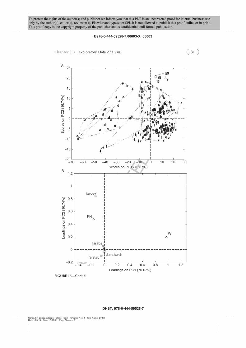
Comp. by: pdjeapradaban Stage: Proof Chapter No.: 3 Title Name: DHSTDate:18/4/13 Time:12:01:05 Page Number: 31
Scores on PC1 (70.67%)
Sco
res
on P
C2
(16.
74%
)
−70
25A
20
15
10
5
0
−5
−10
−15
−20−60 −50 −40 −30 −20 −10 0 10 20 30
W
fardev
farabs
damstarchfarstab
FN
Loadings on PC1 (70.67%)
Load
ings
on
PC
2 (1
6.74
%)
−0.4 −0.2−0.2
0
0
0.2
0.2
0.4
0.4
0.6
0.6
0.8
0.8
1
1
1.2
1.2B
FIGURE 15—Cont’d
Chapter 3 Exploratory Data Analysis 31
B978-0-444-59528-7.00003-X, 00003
DHST, 978-0-444-59528-7
To protect the rights of the author(s) and publisher we inform you that this PDF is an uncorrected proof for internal business useonly by the author(s), editor(s), reviewer(s), Elsevier and typesetter SPi. It is not allowed to publish this proof online or in print.This proof copy is the copyright property of the publisher and is confidential until formal publication.

Comp. by: pdjeapradaban Stage: Proof Chapter No.: 3 Title Name: DHSTDate:18/4/13 Time:12:01:07 Page Number: 32
Sco
res
on P
C2
(15.
37%
)
Scores on PC1 (33.30%)−3
−3
−2
−2
−1
−1
0
0
1
1
2
2
C
3 4 5 6 7
FN
farabs
fardev
proteinswetglu
ext90
ext135PL
farstab
moisture
D
W
ext45ashes
damstarch
Loadings on PC1 (33.30%)
Load
ings
on
PC
2 (1
5.37
%)
−0.4
−0.4
−0.2
−0.2
0
0
0.2
0.2
0.4
0.4
0.6
FIGURE 15f0075 Example of the effect of data scaling on data set FlourRheoData: (A) scores for
PC1 versus PC2 and (B) loadings for PC1 versus PC2 for the mean centred data; (C) scores forPC1 versus PC2 and (D) loadings for PC1 versus PC2 for the autoscaled data.
PART I Theory32
B978-0-444-59528-7.00003-X, 00003
DHST, 978-0-444-59528-7
To protect the rights of the author(s) and publisher we inform you that this PDF is an uncorrected proof for internal business useonly by the author(s), editor(s), reviewer(s), Elsevier and typesetter SPi. It is not allowed to publish this proof online or in print.This proof copy is the copyright property of the publisher and is confidential until formal publication.

spectra, given the high relevance this technique has acquired in food analysis;however, the concepts are generally applicable.
p0510 Signal preprocessing is applied to correct/remove the contribution ofundesired phenomena ranging from stochastic measurement noise to varioussources of systematic errors: non-linear instrument responses, shift problemsand interfering effects of undesired chemical and physical variations. Theseoperations are also known as de-noising, smoothing, background and baselinecorrections, normalization (transforming to a scale of relative intensity), align-ment (removing horizontal shift), and correction for scatter in NIR. Moreover,transforming the signal, for example, by derivative operations, can implicitlyaccomplish normalization, baseline removal and partial band deconvolution.As far as removing horizontal shift is concerned, which is a frequent issuearising in chromatography, in NMR signals, as well as in time series data, sev-eral algorithms [63–67] which can aid to remove misalignments have beenproposed.
p0515 A general distinction in preprocessing methods may be in terms of filter-ing methods, which transform measured data mathematically into a presum-ably ‘better’ version of the same data, leaving out some undesired types ofvariation, and model-based methods, where the ‘better’ version is obtainedbased on a more explicit mathematical model in such a way that the informa-tion filtered out is not lost, as statistical estimates of the mathematical para-meters involved in the filtering are also obtained.
p0520 Among the most used filtering methods for de-noising/smoothing, that is,removing uninformative high-frequency variation, there are moving averageand polynomial Savitsky–Golay filtering [68], which works on the assump-tions that the signal is smooth compared to noise (sum of monotonic func-tions); noise is mainly uncorrelated and will be eliminated by mild methods.Alternatively high-frequency contributions may be removed in frequency(Fourier transform) or wavelet (wavelet transform) domain. Some examplesare given in Figure 16.
p0525 The need to normalize signals, which consists in passing from the mea-surement scale to a relative one, may arise for different reasons in differentcontexts. The normalization issue is relevant for signals where peak inten-sity/area is proportional to concentration and it is not possible to use exactlythe same amount of matter for each sample, for example, in high-resolutionmagic angle spinning-NMR signals where semi-solid samples are used. Otherexamples are those situations in which the intensity of the signal is affected byphysical or chemical variability different from the one we are interested tomodel, such as water content, temperature, and particle size in NIR, whichmay be due to the acquisition condition being different from sample to sam-ple. Normalization avoids that these differences in concentration overwhelmthe variability due to actual differences in the samples. Signals could be nor-malized to unit length, unit area, maximum intensity, or according to a refer-ence, intense, well-resolved peak, which is present in all samples and whose
Comp. by: pdjeapradaban Stage: Proof Chapter No.: 3 Title Name: DHSTDate:18/4/13 Time:12:01:09 Page Number: 33
Chapter 3 Exploratory Data Analysis 33
B978-0-444-59528-7.00003-X, 00003
DHST, 978-0-444-59528-7
To protect the rights of the author(s) and publisher we inform you that this PDF is an uncorrected proof for internal business useonly by the author(s), editor(s), reviewer(s), Elsevier and typesetter SPi. It is not allowed to publish this proof online or in print.This proof copy is the copyright property of the publisher and is confidential until formal publication.

variation is uninteresting (as it will get the unit value for all samples, thusremaining constant over the series of samples considered).
p0530 In cases where a constant offset (vertical shift) is present, it is common toperform row autoscaling, that is, centring and scaling to unit variance alongtime points and wavelength direction and so on (depending on the kind of sig-nal). For NIR signals, this operation is better known as standard normal vari-ate (SNV). This preprocessing, to some extent, implicitly accomplishesnormalization too.
p0535 In the presence of a linear or curvilinear offset, the detrend method can beused. Detrending consists of fitting a polynomial of a given order to the entiresignal range. As this algorithm fits the polynomial to all points, baseline andsignal, it tends to work only when the largest source of variability in eachsample is baseline/background interference, as in NIR signals; this means thatit may remove variations which are interesting to model whenever the varia-tion of interest is a reasonably significant portion of the overall variance.
p0540 When the polynomial is fitted to signal points, which are manuallyselected, that can be attributed only to baseline (background), then baseline(background) removal is achieved and the drawbacks of detrending are over-come. A variant for baseline correction is to do adopt a weighted least squaresautomatic procedure (asymmetric least squares [63]). This is an automaticapproach to determine which points most likely belong to baseline only, by
Comp. by: pdjeapradaban Stage: Proof Chapter No.: 3 Title Name: DHSTDate:18/4/13 Time:12:01:10 Page Number: 34
originaloriginal
smoothed SG 2nd-order 7 points
smoothed SG 2nd-order 21 pointsWT denoised
0.8 0.8
0.79
0.78
0.77
0.76
0.75
0.74
0.73
0.78
0.76
0.74
250 260 270 280
400350300250200150 400
280270260250
350300250200150
0.75
0.8
0.85
0.9
0.95
0.75
0.8
0.85
0.9
0.95
FIGURE 16f0080 An example of a noisy band in a medium-IR spectrum of a balsamic vinegar sam-ple. Left plot: black line corresponds to original signal; grey line the same signal de-noised by a
db1 wavelet filter at level 3 (all detail coefficients from level 1 to 3 were set to zero, only approx-
imations at level 3 were reconstructed). Right plot: black line corresponds to original signal; blue
dashed line to the same signal after smoothing with an SG filter, 7-point window, second-orderpolynomial; grey line to smoothing with an SG filter, 21-point window, second-order polynomial.
(For interpretation of the references to colour in this figure legend, the reader is referred to the
online version of this chapter.)
PART I Theory34
B978-0-444-59528-7.00003-X, 00003
DHST, 978-0-444-59528-7
To protect the rights of the author(s) and publisher we inform you that this PDF is an uncorrected proof for internal business useonly by the author(s), editor(s), reviewer(s), Elsevier and typesetter SPi. It is not allowed to publish this proof online or in print.This proof copy is the copyright property of the publisher and is confidential until formal publication.

iteratively fitting a polynomial to each signal and determining which signalpoints are clearly above the ‘fitted baseline’ and which fall below. Then thepoints below are assumed to be more significant in fitting the baseline andget higher weights in the next iteration of fit. The baseline is usually approxi-mated by low-order polynomial, but a specific baseline reference (backgroundprofile) can also be supplied.
p0545 A different approach, based on the assumption that the baseline/back-ground is a low-frequency contribution, is to filter out this low frequency,for example, by using the wavelet transform [69] with a wide wavelet filterand removing approximation coefficients at a low scale. In Figure 17 acomparison of the same signals of different baseline correction methods isreported.
p0550 Computation of signal derivatives (also referred to as derivative spectra)allows the removal of constant (first derivative) and linear (second deriva-tives) offsets from the signal data [70,71]. Derivatives return the slope of aline at any given point: thus the first derivative of a signal shows a maximumwhere the signal has a maximum slope and crosses zero where the signal has apeak, which renders spectral interpretation more difficult; the second deriva-tive accounts for the rate of slope change in the original signal and has nega-tive peaks corresponding to peaks in the original signal, which allows them tobe better interpreted. Drawbacks of derivatives are that scale is decreased andwhen, as in general, they are computed as differences, noise is increased, sothey are often preceded by smoothing. Moreover, derivatives implicitlyaccomplish band deconvolution and, in general, tend to be far more amenableto use before multivariate analysis of NIR spectra.
Comp. by: pdjeapradaban Stage: Proof Chapter No.: 3 Title Name: DHSTDate:18/4/13 Time:12:01:11 Page Number: 35
originalWLSdetrend 2nd orderWT corrected (db10)
500
0
0.5
1
1.5
2
2.5
3
−0.5
1000 1500 2000
FIGURE 17f0085 An example of baseline/background removal. In case of WT the approximations at
level 9 obtained by a db10 wavelet filter have been removed.
Chapter 3 Exploratory Data Analysis 35
B978-0-444-59528-7.00003-X, 00003
DHST, 978-0-444-59528-7
To protect the rights of the author(s) and publisher we inform you that this PDF is an uncorrected proof for internal business useonly by the author(s), editor(s), reviewer(s), Elsevier and typesetter SPi. It is not allowed to publish this proof online or in print.This proof copy is the copyright property of the publisher and is confidential until formal publication.

p0555 Model-based preprocessing methods [72] assume a mathematical model toaccount for the different contributions to a signal, which can be expressed inthe general form:
x¼ bxref þ tPTþ e (17)
where xref is a reference signal which represents at best the sought unknown‘true’ signal (xtrue) that has to be recovered, and P contains terms modellingdifferent phenomena: P¼ [PPhys, Pchem_irr, Pchem_i], such as physical variabil-ity (PPhys) due, for example, to light scattering (NIR), or thermal conditions;variability due to chemical effects but not relevant to the goals of data analy-sis (Pchem_irr), for example, compositional/structural changes due to seasonalvariability not important for variety discrimination or water content and soon; and informative chemical variability (Pchem_i), for example, due tochanges in concentrations of the analytes to be determined, in general varia-bility which represents interesting information about samples to be captured/modelled by data analysis. In other words, it is assumed that each signal pro-file (chromatographic signals, absorbance spectra, etc.) for a set of relatedsamples may be approximated as physical/chemical modifications of a ‘true’signal.
p0560 The simplest method which corresponds to these terms is multiplicativescatter correction (MSC). In this case, it is assumed that chemical variationis small compared to physical variation (i.e. variation introducing a constant(additive)/proportional (multiplicative) baseline effect) and thus the true ‘sig-nal’ may be replaced by a constant reference signal, usually the mean (ormedian) spectrum, m (it may also be a specific spectrum of the data set).The previous equation becomes
x¼ bmþaþ e (18)
p0565 Solving by least squares, the multiplicative, b, and additive, a, parameterscan be estimated and the signal profile corrected to
xcorr ¼ x"að Þ=b (19)
p0570 This is a very strong simplification because it assumes that chemical var-iations, for example, analyte and possible interferant concentrations, have lit-tle effect on the observed spectra. However, it often works with NIR spectra,where the chemically relevant induced changes mostly manifest as ‘shoulders’on a very strong background profile. A situation where MSC (as well as SNVfor analogous reasons) does not work [72,73] is shown in Figure 18. A possi-ble solution could be to apply MSC only on a given portion of the signalknown to have constant chemical variation, for example, where an interferantat constant concentration is present, and/or belonging only to baseline(absence of chemical variation), as shown in Figure 18.
p0575 It has to be noted that, in the cases shown, derivative spectra would havesolved the problem (see Figure 19).
Comp. by: pdjeapradaban Stage: Proof Chapter No.: 3 Title Name: DHSTDate:18/4/13 Time:12:01:14 Page Number: 36
PART I Theory36
B978-0-444-59528-7.00003-X, 00003
DHST, 978-0-444-59528-7
To protect the rights of the author(s) and publisher we inform you that this PDF is an uncorrected proof for internal business useonly by the author(s), editor(s), reviewer(s), Elsevier and typesetter SPi. It is not allowed to publish this proof online or in print.This proof copy is the copyright property of the publisher and is confidential until formal publication.

p0580 Going back to the general formulation of model-based preprocessing, themodel can be extended (the method in this case is called extended multiplica-tive scatter correction (EMSC) [74]) to include other physical variations, forexample, non-linear terms (not only proportional/multiplicative) with respectto wavelengths:
x¼ bmþaþ clþdl2þ&& &þ e (20)
where l is the abscissa vector and higher-order terms in l may as well beconsidered.
p0585 Finally, to cope with situations which differ from the case where theassumption is made of very small effects of ‘chemical’ variation on spectra,the Pchem_i terms may be introduced in the EMSC model. This can be doneas an example by considering the signal profile of the pure analyte:
x¼ bmþ t PphysPchem"i
& 'Tþ e¼ bmþaþ clþdl2þhxpureþ e (21)
p0590 In this case the a, b, c and d parameters estimated by linear fitting are notconfused with the chemical variation because this is considered in the h xpureterm; hence we can correct for physical unwanted variation by
xcorr ¼ x"a" cl"dl2$ %
=b (22)
p0595 In Figure 20, an example is shown where this approach has been applied;however, because the interferant concentration is not constant, in order to
Comp. by: pdjeapradaban Stage: Proof Chapter No.: 3 Title Name: DHSTDate:18/4/13 Time:12:01:15 Page Number: 37
Simulated data: 1 analyte + 1 interferant
SNV corrected
MSC corrected
MSC corrected, only first 50 points
Analyte peak
increasing conc
interferant
50
1.21
0.80.60.40.2
0.8
0.6
0.4
0.2
1.5
1
0.5
3210
100 150 200 50
1.41.2
10.80.60.40.2
1.41.2
10.80.60.40.2
1.21
0.80.60.40.2
2
1
0
−1
100 150 200
50 100 150 200
50 100 150 200
50 100 150 200
50 100 150 200
50 100 150 200
50 100 150 200
FIGURE 18f0090 Simulated data with two peaks: one analyte of interest at increasing concentration
and one interferant of varying intensity. Left subplots: vertical shift and white noise present, back-ground absent. Right subplots: vertical shift, noise and background present. (For colour version of
this figure, the reader is referred to the online version of this chapter.)
Chapter 3 Exploratory Data Analysis 37
B978-0-444-59528-7.00003-X, 00003
DHST, 978-0-444-59528-7
To protect the rights of the author(s) and publisher we inform you that this PDF is an uncorrected proof for internal business useonly by the author(s), editor(s), reviewer(s), Elsevier and typesetter SPi. It is not allowed to publish this proof online or in print.This proof copy is the copyright property of the publisher and is confidential until formal publication.

Comp. by: pdjeapradaban Stage: Proof Chapter No.: 3 Title Name: DHSTDate:18/4/13 Time:12:01:18 Page Number: 38
0.1 0
5010
015
020
050
0.01 0
−0.0
1
−0.0
2
0.01 0
−0.0
1
−0.0
2
0.01 0
−0.0
1
−0.0
2
0.01 0
−0.0
1
−0.0
2
100
150
200
5010
015
020
0
5010
015
020
0
5010
015
020
0
5010
015
020
0
5010
015
020
0
5010
015
020
0
−0.1 0.1 0
−0.1 0.1 0
−0.1 0.1 0
−0.1
Fir
st d
eriv
ativ
e S
G:
ord
er 2
; w
ind
ow
= 1
1S
eco
nd
der
ivat
ive
SG
: o
rder
2;
win
do
w 1
1
A =
5 I
= 3
A =
10
I = 5
A =
15
I = 2
A =
20
I = 4
A =
5 I
= 3
A =
10
I = 5
A =
15
I = 4
A =
20
I = 4
A =
5 I
= 3
A =
10
I = 5
A =
15
I = 2
A =
20
I = 4
A =
5 I
= 3
A =
10
I = 5
A =
15
I = 4
A =
20
I = 4
50
A
100
150
200
5010
015
020
0
5010
015
020
0
5010
015
020
0
FIGURE19
f009
5Sim
ulated
datawithtwopeaksandoneanalyteofinterest(A
)atincreasingconcentrationandoneinterferant(I)ofvaryingintensity,concentrations
arereported
onthelegend.Left:raw
signals.Middle:firstderivativespectra.
Right:secondderivativespectra.
(Forcolourversion
ofthis
figure,thereader
isreferred
totheonlineversion
ofthischapter.)
B978-0-444-59528-7.00003-X, 00003
DHST, 978-0-444-59528-7
To p
rote
ct th
e rig
hts o
f the
aut
hor(
s) a
nd p
ublis
her w
e in
form
you
that
this
PD
F is
an
unco
rrec
ted
proo
f for
inte
rnal
bus
ines
s use
only
by
the
auth
or(s
), ed
itor(
s), r
evie
wer
(s),
Else
vier
and
type
sette
r SPi
. It i
s not
allo
wed
to p
ublis
h th
is p
roof
onl
ine
or in
prin
t.Th
is p
roof
cop
y is
the
copy
right
pro
perty
of t
he p
ublis
her a
nd is
con
fiden
tial u
ntil
form
al p
ublic
atio
n.

Comp. by: pdjeapradaban Stage: Proof Chapter No.: 3 Title Name: DHSTDate:18/4/13 Time:12:01:20 Page Number: 39
An
alyt
e C
= [
5 1
0 15
20]
EM
SC
cor
r
50
1.2 1
0.8
0.8
0.6
0.6
0.4
0.2
0.2
1.5
0.51
0.4
0.2
0.4
0.3
0.2
0.4
0.3
1.2
1.4 1
0.8
0.81
0.6
0.6
0.4
0.2
0.2
1.5
0.51
0.4
0.2
0.81 1
0.4
0.6
0.2
0.4
0.8
0.6
1.2 1
0.8
0.8
0.6
0.6
0.4
0.2
1.2 1
0.8
0.6
0.4
0.2
0.2
0.4
0.2
0.4
0.3
0.2
0.4
0.3
100
150
200
5010
015
020
0
5010
015
020
0
5010
015
020
0
5010
015
020
050
100
150
200
5010
015
020
0
5010
015
020
0
5010
015
020
0
5010
0
Inte
rfer
ent
Inte
rfer
ent
Inte
rfer
ent
c =
[3 5
4 4
]c
= [3
5 4
4]
c =
[3 5
2 4
]
150
200
5010
015
020
0
5010
015
020
0
5010
015
020
0
5010
015
020
0
5010
015
020
0
EM
SC
cor
r
usin
g th
e
usin
g th
e
spec
tra
of th
e
spec
tra
of th
e
inte
rfer
ent
only
firs
t 50
poin
ts
pure
ana
lyte
and
pure
ana
lyte
EM
SC
cor
r
EM
SC
cor
r
FIGURE20
f010
0Sim
ulateddatawithtwopeaksandoneanalyteofinterestat
increasingconcentrationandoneinterferantofvaryingintensity,concentrationsare
reported
onthelegend.Thesubplotsin
each
columnreferto
adifferentseries
ofrawsignals,whileontherowsthedifferentsubplotsreferto
EMSCappliedwith
differentterm
s,as
reported
ontheleftofeach
series.(Forcolourversion
ofthisfigure,thereader
isreferred
totheonlineversion
ofthischapter.)
B978-0-444-59528-7.00003-X, 00003
DHST, 978-0-444-59528-7
To p
rote
ct th
e rig
hts o
f the
aut
hor(
s) a
nd p
ublis
her w
e in
form
you
that
this
PD
F is
an
unco
rrec
ted
proo
f for
inte
rnal
bus
ines
s use
only
by
the
auth
or(s
), ed
itor(
s), r
evie
wer
(s),
Else
vier
and
type
sette
r SPi
. It i
s not
allo
wed
to p
ublis
h th
is p
roof
onl
ine
or in
prin
t.Th
is p
roof
cop
y is
the
copy
right
pro
perty
of t
he p
ublis
her a
nd is
con
fiden
tial u
ntil
form
al p
ublic
atio
n.

have a suitable correction the interferant pure spectrum information has alsobeen considered in the EMSC model.
p0600 When Pchem_irr is known, for example, by taking a difference spectra oftwo samples known to belong to different batches, years, producers and soon, we can take this term into account in the model and correct for it; in otherterms, EMSC can be seen like a generalized linear model.
p0605 To illustrate the effects of the different preprocessing described until hereon explorative PCA models, the data described in Section 3.1.4, namely NIR-BreadProcess, has been used.
p0610 The results are shown in Figure 21, which shows the effect of signal pre-processing on the average spectra (Figure 21A) for each leavening step and onthe variance inside each step (Figure 21B), and in Figure 22, where the trendsas captured by PCA computed on the different preprocessed data, followed bycolumn mean centring (Figure 22), are shown. For each set, PC2 versus PC3score plots are reported because these two components describe variabilitylinked to the different leavening step, while for all preprocessing the firstcomponent is still describing overall variability not relevant for the leaveningstep separation. The bottom right sub-plot reports a score plot of the PCA onthe concentration of some organic compounds involved in the leavening pro-cess determined by GC on the same samples. It is interesting to note that thepreprocessing which best matches this trend is the second derivative.
p0615 In the more general case, when the preprocessed signals are not to be usedfor explorative purposes only, but for modelling tasks (classification, multi-variate calibration) as well, the Pchem_irr, can also be estimated by multivariatemodelling. For instance, a PCA model can be built with samples measured inthose different conditions that we know a priori which may introduceunwanted variability (batches, seasonality, acidity of the media, humidity con-tent, etc.); then the loadings of the few PCs where this variability is modelledcan be used as Pchem_irr.
p0620 Other model-based preprocessing methods, which are more demandingfrom the computational and validation point of view, are, for example,orthogonal signal correction and orthogonal partial least squares [75]. Whenpreprocessing it is not sufficient to distinguish relevant information fromuninformative sources of variation, it is becoming common to employ vari-able selection techniques which may reveal to be a very useful tool, especiallyfor multivariate calibration problems [76–78].
s0060 3.1.4 PCA in Practice: Exploring Food Data
p0625 As EMDA is a data-driven method, and according to the main target of thisbook which aims to showcase the potentialities of an application-oriented dis-cipline like chemometrics in a challenging world such as food analysis, in thissection PCA will be shown ‘in action’ on data sets obtained from real cases offood analysis, both at laboratory and plant scale.
Comp. by: pdjeapradaban Stage: Proof Chapter No.: 3 Title Name: DHSTDate:18/4/13 Time:12:01:24 Page Number: 40
B978-0-444-59528-7.00003-X, 00003
DHST, 978-0-444-59528-7
PART I Theory40
To protect the rights of the author(s) and publisher we inform you that this PDF is an uncorrected proof for internal business useonly by the author(s), editor(s), reviewer(s), Elsevier and typesetter SPi. It is not allowed to publish this proof online or in print.This proof copy is the copyright property of the publisher and is confidential until formal publication.
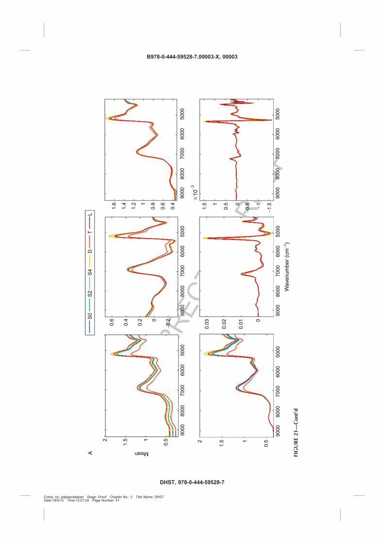
Comp. by: pdjeapradaban Stage: Proof Chapter No.: 3 Title Name: DHSTDate:18/4/13 Time:12:01:24 Page Number: 41
S0
S2
AS
4D
TL
0.6
0.81
1.2
1.4
1.6
0.4
9000
8000
7000
6000
5000
2
1.5
0.5
9000
8000
7000
6000
5000
1
Mean
0.6
0.4
0.2 0
-0.2
9000
8000
7000
6000
5000
1.5
0.5 01
-0.5 -1
-1.5
9000
8000
7000
6000
5000
!10
-3
9000
8000
7000
6000
5000
2
1.5
0.51
0.03
0.02
0.01 0
9000
8000
7000
6000
5000
Wav
enum
ber
(cm
-1)
FIGURE21—Cont’d
B978-0-444-59528-7.00003-X, 00003
DHST, 978-0-444-59528-7
To p
rote
ct th
e rig
hts o
f the
aut
hor(
s) a
nd p
ublis
her w
e in
form
you
that
this
PD
F is
an
unco
rrec
ted
proo
f for
inte
rnal
bus
ines
s use
only
by
the
auth
or(s
), ed
itor(
s), r
evie
wer
(s),
Else
vier
and
type
sette
r SPi
. It i
s not
allo
wed
to p
ublis
h th
is p
roof
onl
ine
or in
prin
t.Th
is p
roof
cop
y is
the
copy
right
pro
perty
of t
he p
ublis
her a
nd is
con
fiden
tial u
ntil
form
al p
ublic
atio
n.

Comp. by: pdjeapradaban Stage: Proof Chapter No.: 3 Title Name: DHSTDate:18/4/13 Time:12:01:29 Page Number: 42
S0
B StdDev
0.05
0.04 3 2 1 0
0.03
0.02
0.01 0
7500
!10
−3
7000
6500
6000
5500
5000
4500
6000
5500
5000
4500
7500
7000
cm−1
6500
6000
5500
5000
4500
S2
DT
LS
4
!10
−47500
7000
6500
6000
5500
5000
4500
0.2
0.15 0.
1
0.05 0
0.06
0.04
0.02 0
7500
7000
6500
2 1 0
7500
7000
6500
6000
5500
5000
4500
0.1
0.08
0.06
0.04
0.02
7000
6000
5000
FIGURE21
f010
5Effectofdifferentspectral
pretreatm
ents
onthedatasetNIRbreadProcess
onsignal
profiles(A
)andonsignal
variance
(B).Thepretreatm
ents
applied
arein
thefollowingorder:none(topleft),themeansignal
foreach
leaveningpoint(see
legend)is
reported;detrend(topmiddle);MSC
(topright);
MSConly
first400signal
points(bottom
left);firstderivative(bottom
middle)andsecondderivative(bottom
right).(Forcolourversion
ofthisfigure,thereader
isreferred
totheonlineversionofthischapter.)
B978-0-444-59528-7.00003-X, 00003
DHST, 978-0-444-59528-7
To p
rote
ct th
e rig
hts o
f the
aut
hor(
s) a
nd p
ublis
her w
e in
form
you
that
this
PD
F is
an
unco
rrec
ted
proo
f for
inte
rnal
bus
ines
s use
only
by
the
auth
or(s
), ed
itor(
s), r
evie
wer
(s),
Else
vier
and
type
sette
r SPi
. It i
s not
allo
wed
to p
ublis
h th
is p
roof
onl
ine
or in
prin
t.Th
is p
roof
cop
y is
the
copy
right
pro
perty
of t
he p
ublis
her a
nd is
con
fiden
tial u
ntil
form
al p
ublic
atio
n.

Comp. by: pdjeapradaban Stage: Proof Chapter No.: 3 Title Name: DHSTDate:18/4/13 Time:12:01:31 Page Number: 43
Det
ren
dM
SC
Raw
sig
nal
s1.
50.
60.
3
0.2
0.1 0
−0.1
−0.2 −0
.50
0.5
0.4
0.2
0.5
1
0
0
−0.2
−0.5
−1−0
.41.
5
1
1
0.5
0.5
0
0
−0.5
−0.5
−1
−1
−1.5 −1
.5−2
Sco
res
on
PC
2 (3
.50%
)S
core
s o
n P
C2
(10.
74%
)S
core
s o
n P
C2
(10.
82%
)
Scores on PC3 (2.28%)
Scores on PC3 (2.17%)
Scores on PC3 (2.53%)
MS
C 1
-400
Sco
res
on
PC
2 (2
.00%
)S
core
s o
n P
C2
(27.
48%
)S
core
s o
n P
C1
(52.
15%
)
PC
A G
C d
ata
Scores on PC3 (0.82%)
Scores on PC3 (2.93%)
Scores on PC2 (17.70%)
0.4
0.2 2
−0.2
−1−0
.50.
5
5
21.
5 10.
5
−0.5 −1
−1.5 −2
−2.5 −3−5
−4−3
−2−1
01
23
4
00
−10
21
−5
10
−0.4
−0.6
2nd
Der
ivat
ive
!10
−4
!10
−3
FIGURE22
f011
0Effectofdifferentspectral
pretreatm
entsondatasetNIRbreadProcess
ondatagroupingas
revealedbyPC2versusPC3scatterplots.See
textfora
descriptionofthemeaningofeach
representation.Thesixprocess
stepsmonitoredarecoded
asfollows:em
ptycircles,S0;em
ptysquares,S2;em
ptydiamonds,
S4;filled
circles,D;filled
squares,T;filled
diamonds,L.
B978-0-444-59528-7.00003-X, 00003
DHST, 978-0-444-59528-7
To p
rote
ct th
e rig
hts o
f the
aut
hor(
s) a
nd p
ublis
her w
e in
form
you
that
this
PD
F is
an
unco
rrec
ted
proo
f for
inte
rnal
bus
ines
s use
only
by
the
auth
or(s
), ed
itor(
s), r
evie
wer
(s),
Else
vier
and
type
sette
r SPi
. It i
s not
allo
wed
to p
ublis
h th
is p
roof
onl
ine
or in
prin
t.Th
is p
roof
cop
y is
the
copy
right
pro
perty
of t
he p
ublis
her a
nd is
con
fiden
tial u
ntil
form
al p
ublic
atio
n.
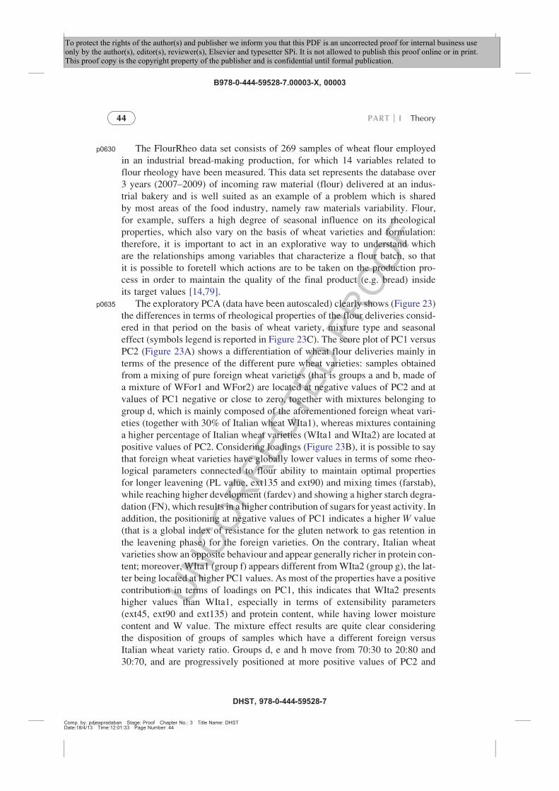
p0630 The FlourRheo data set consists of 269 samples of wheat flour employedin an industrial bread-making production, for which 14 variables related toflour rheology have been measured. This data set represents the database over3 years (2007–2009) of incoming raw material (flour) delivered at an indus-trial bakery and is well suited as an example of a problem which is sharedby most areas of the food industry, namely raw materials variability. Flour,for example, suffers a high degree of seasonal influence on its rheologicalproperties, which also vary on the basis of wheat varieties and formulation:therefore, it is important to act in an explorative way to understand whichare the relationships among variables that characterize a flour batch, so thatit is possible to foretell which actions are to be taken on the production pro-cess in order to maintain the quality of the final product (e.g. bread) insideits target values [14,79].
p0635 The exploratory PCA (data have been autoscaled) clearly shows (Figure 23)the differences in terms of rheological properties of the flour deliveries consid-ered in that period on the basis of wheat variety, mixture type and seasonaleffect (symbols legend is reported in Figure 23C). The score plot of PC1 versusPC2 (Figure 23A) shows a differentiation of wheat flour deliveries mainly interms of the presence of the different pure wheat varieties: samples obtainedfrom a mixing of pure foreign wheat varieties (that is groups a and b, made ofa mixture of WFor1 and WFor2) are located at negative values of PC2 and atvalues of PC1 negative or close to zero, together with mixtures belonging togroup d, which is mainly composed of the aforementioned foreign wheat vari-eties (together with 30% of Italian wheat WIta1), whereas mixtures containinga higher percentage of Italian wheat varieties (WIta1 and WIta2) are located atpositive values of PC2. Considering loadings (Figure 23B), it is possible to saythat foreign wheat varieties have globally lower values in terms of some rheo-logical parameters connected to flour ability to maintain optimal propertiesfor longer leavening (PL value, ext135 and ext90) and mixing times (farstab),while reaching higher development (fardev) and showing a higher starch degra-dation (FN), which results in a higher contribution of sugars for yeast activity. Inaddition, the positioning at negative values of PC1 indicates a higher W value(that is a global index of resistance for the gluten network to gas retention inthe leavening phase) for the foreign varieties. On the contrary, Italian wheatvarieties show an opposite behaviour and appear generally richer in protein con-tent; moreover, WIta1 (group f) appears different fromWIta2 (group g), the lat-ter being located at higher PC1 values. As most of the properties have a positivecontribution in terms of loadings on PC1, this indicates that WIta2 presentshigher values than WIta1, especially in terms of extensibility parameters(ext45, ext90 and ext135) and protein content, while having lower moisturecontent and W value. The mixture effect results are quite clear consideringthe disposition of groups of samples which have a different foreign versusItalian wheat variety ratio. Groups d, e and h move from 70:30 to 20:80 and30:70, and are progressively positioned at more positive values of PC2 and
Comp. by: pdjeapradaban Stage: Proof Chapter No.: 3 Title Name: DHSTDate:18/4/13 Time:12:01:33 Page Number: 44
PART I Theory44
B978-0-444-59528-7.00003-X, 00003
DHST, 978-0-444-59528-7
To protect the rights of the author(s) and publisher we inform you that this PDF is an uncorrected proof for internal business useonly by the author(s), editor(s), reviewer(s), Elsevier and typesetter SPi. It is not allowed to publish this proof online or in print.This proof copy is the copyright property of the publisher and is confidential until formal publication.

Comp. by: pdjeapradaban Stage: Proof Chapter No.: 3 Title Name: DHSTDate:18/4/13 Time:12:01:34 Page Number: 45
Scores on PC1
Sco
res
on P
C2
−3
−3
−2
−1
0
1
2
A
−2 −1 0 1 2 3 4 5 6 7
FN
ashesext45
proteins
damstarch
Loadings on PC1 (33.30%)
B
Load
ings
on
PC
2 (1
5.37
%) moisture
W
farstab
PLext135
ext90wetglu
farabs
−0.4
−0.4
−0.2 0
0
0.2
0.2
0.4
0.4
0.6
−0.2fardev
FIGURE 23—Cont’d
Chapter 3 Exploratory Data Analysis 45
B978-0-444-59528-7.00003-X, 00003
DHST, 978-0-444-59528-7
To protect the rights of the author(s) and publisher we inform you that this PDF is an uncorrected proof for internal business useonly by the author(s), editor(s), reviewer(s), Elsevier and typesetter SPi. It is not allowed to publish this proof online or in print.This proof copy is the copyright property of the publisher and is confidential until formal publication.

PC1, moving from the area of foreign mixtures (quadrant III–IV) to the one ofpure Italian varieties (quadrant I). Some peculiar behaviours appear when con-sidering, for instance, group c: this group is characterized by a particular homo-geneity in terms of inter-delivery variability when compared to other groups,and is positioned in quadrant II. Its mixture composition, having a foreignversus Italian wheat variety ratio of 25:75, does not differ much from the oneof groups h and i, which is 30:70, which show a higher variability. In this case,a wheat variety effect might be present, as the foreign variety differs, but therecan also be a significant seasonal effect. Group c belongs to the beginning ofyear 2008, while h and i were delivered between the end of 2008 and the begin-ning of 2009; this means that the Italian wheat variety also, which is the same,comes from two different harvests, which could have undergone differentweather and growing conditions, thus developing different rheological proper-ties. A seasonal effect may be seen also for groups a and b, which are very closeto each other and homogeneous in terms of variability, both belonging to theyear 2007. All these exploratory considerations can be the basis for a moredetailed evaluation of similarities/differences of new flour deliveries with theones present in the historical database, and for studies on the functional relation-ship of flour formulation on wheat flour rheological performance, thus leadingto other steps of food analysis.
p0640 The NIRbreadProcess and GCbreadProcess concern 14 doughs from anindustrial bread-making production sampled at six different points of theindustrial process (S0, S2 and S4: beginning, middle and final point of thefirst leavening phase; D, T: beginning of the second leavening phase and L:
Comp. by: pdjeapradaban Stage: Proof Chapter No.: 3 Title Name: DHSTDate:18/4/13 Time:12:01:38 Page Number: 46
FIGURE 23f0115 Principal component analysis of the data set FlourRheo. (A) Scores plot and (B)
loadings plot of PC1 versus PC2. The letters identify the mixtures reported in (C). (For colour ver-
sion of this figure, the reader is referred to the online version of this chapter.)
PART I Theory46
B978-0-444-59528-7.00003-X, 00003
DHST, 978-0-444-59528-7
To protect the rights of the author(s) and publisher we inform you that this PDF is an uncorrected proof for internal business useonly by the author(s), editor(s), reviewer(s), Elsevier and typesetter SPi. It is not allowed to publish this proof online or in print.This proof copy is the copyright property of the publisher and is confidential until formal publication.

end of the second leavening phase). In the first data set, the NIR spectrum wasrecorded in the 4350–9500 cm"1 region; in the second data set, the concentra-tion of nine acids, sugars and other compounds related to dough leavening(succinic acid, malic acid, glycerol, fructose, inositol, sucrose, maltose, fuma-ric acid) was determined by means of GC [80].
p0645 In this context, the explorative analysis phase is crucial to check if the ana-lytical techniques are able to collect information on the process. Figure 24Ashows, as a biplot, that GC (data have been autoscaled prior to analysis) isable to capture information on sample composition which is, first of all, ableto clearly differentiate the first leavening phase (negative values on PC1) fromthe second leavening phase (positive values on PC1), and that is indicative ofthe progression of dough leavening, as the trends from positive to negativevalues of PC2 suggest. This is connected to a general change, in terms of vari-ables, from higher concentrations of sugars at the beginning of each leaveningphase towards a higher concentration of some leavening products and the con-sumption of sugars at the final leavening points. As another technique wasconsidered, that is NIR spectroscopy, it is also possible to compare the resultsobtained with both of them. As reported in Figure 24B, the PCA on the NIR-breadProcess data set (preprocessing: Savitsky–Golay second derivative, withsecond-order polynomial smoothing, and mean centring) indicates that theNIR signal can bear information, albeit in different components (in this case,PC2 and PC3), similar to the GC quantification of chemicals present in theleavening phase. Loadings (Figure 24C) illustrate which infrared vibrationsare mainly involved in the samples distribution in the PC’s space. The sam-ples located at positive values of PC2, corresponding to most of the samplesof the second leavening phase, are characterized by higher values for the spec-tral variables around 5200 cm"1, several vibrational modes are absorbed inthis region, such as the asymmetric NH stretching of the CONH2 group, thesecond overtone of the C]O stretching (in CO2R), the first stretching andthe second bending overtones of water OH and the combination bands ofstarch OH. On the other hand, the PC3 loadings are mostly inherent to theNIR region below 4500 cm"1, where contributing combination modes arefound, for example, of CH and CC stretching and of CH and CH2 bending,which can be found in different constituents of flour, such as starch, lipidsand proteins.
p0650 The rather broad nature of NIR signal can be accounted for by the fact thatPC1, the main source of variability, is due to other effects connected to theproduction process which are not discussed here.
p0655 The exploratory analysis of these two data sets offers at least two differentpoints for further analyses:
o0050 1. The NIRbreadProcess data set is shown as being a good representative of aprocess-monitoring approach in the food industry, where online analysersare employed on the production line.
Comp. by: pdjeapradaban Stage: Proof Chapter No.: 3 Title Name: DHSTDate:18/4/13 Time:12:01:40 Page Number: 47
Chapter 3 Exploratory Data Analysis 47
B978-0-444-59528-7.00003-X, 00003
DHST, 978-0-444-59528-7
To protect the rights of the author(s) and publisher we inform you that this PDF is an uncorrected proof for internal business useonly by the author(s), editor(s), reviewer(s), Elsevier and typesetter SPi. It is not allowed to publish this proof online or in print.This proof copy is the copyright property of the publisher and is confidential until formal publication.

Comp. by: pdjeapradaban Stage: Proof Chapter No.: 3 Title Name: DHSTDate:18/4/13 Time:12:01:40 Page Number: 48
GlucoseFructose
Malic acidSucrose
Fumaricacid
Maltose
InositolGlycerolSuccinic
acid
PC10
0
0.05
0.05
A
0.1
0.1
0.15−0.15−0.15
−0.1
−0.1
−0.05
−0.05
−0.2
PC
2
Scores on PC2 (27.48%)
Sco
res
on P
C3
(2.9
3%)
!10−3
!10−4
−1.5 −1−8
−6
−4
−2
0
2
4
6
8
B
−0.5 0 0.5 1 1.5 2 2.5
FIGURE 24—Cont’d
PART I Theory48
B978-0-444-59528-7.00003-X, 00003
DHST, 978-0-444-59528-7
To protect the rights of the author(s) and publisher we inform you that this PDF is an uncorrected proof for internal business useonly by the author(s), editor(s), reviewer(s), Elsevier and typesetter SPi. It is not allowed to publish this proof online or in print.This proof copy is the copyright property of the publisher and is confidential until formal publication.

o0055 2. The fact that the two techniques offer similar views of the same process,that is the leavening progression, is a start for a feasibility study of indirectcalibration models of properties of interest, that is the concentration ofleavening products in dough from the NIR spectrum, thus obtainingimportant information on the process in a matter of seconds (the acquisi-tion of the NIR signal) instead of more than 1 h (the GC run).
p0670 Finally, an example should be provided about a class of methods, which havealso explorative purposes, which will be discussed with more detail and theo-retical depth in Chapter Au1XXX, that is multiway analysis methods [81]. Thesemethods, among which parallel factor analysis (PARAFAC) will be shownhere in action compared to PCA, are to some extent referred to as the concep-tual (and mathematical) extension of PCA to arrays of order higher than two.They show their potentiality when the variability of a data set is related to dif-ferent sources, or conditions, at which a full set of properties for each sampleis measured [17–21]. An example, quite common in the food science analysis,is the excitation–emission fluorescence landscape, where, for each sample, anemission spectrum is recorded at each wavelength of the excitation signal.
p0675 The NIRdoughRising data set contains the Near Infrared Spectrum, in the1376–2245 nm region, recorded at seven leavening times (at the beginning
Comp. by: pdjeapradaban Stage: Proof Chapter No.: 3 Title Name: DHSTDate:18/4/13 Time:12:01:44 Page Number: 49
Wavenumber (cm−1)
9500
0.1
0
PC
3 (2
.93%
)P
C2
(27.
48%
)
−0.1
0.1
0.2
0.3C
0
−0.1
−0.2
8500 8000 7500 7000 6500 6000 5500 5000 45009000
9500 8500 8000 7500 7000 6500 6000 5500 5000 45009000
FIGURE 24f0120 Principal component analysis of data sets. (A) GCbreadProcess: biplot of PC1 ver-sus PC2, (B) NIRbreadProcess: scores plot of PC2 versus PC3 and (C) NIRbreadProcess: loadings
plot of PC2 and PC3. The six process steps monitored are coded as follows: empty circles, S0;
empty squares, S2; empty diamonds, S4; filled circles, D; filled squares, T; filled diamonds, L.
Chapter 3 Exploratory Data Analysis 49
B978-0-444-59528-7.00003-X, 00003
DHST, 978-0-444-59528-7
To protect the rights of the author(s) and publisher we inform you that this PDF is an uncorrected proof for internal business useonly by the author(s), editor(s), reviewer(s), Elsevier and typesetter SPi. It is not allowed to publish this proof online or in print.This proof copy is the copyright property of the publisher and is confidential until formal publication.

and every 10 min up to a 60-min rising phase) for doughs obtained from tenwheat flour mixtures characterized by a different formulation of four wheatvarieties. As it is important to gain knowledge on the effect of wheat flour for-mulation on its rheological properties and on its performance in the leaveningphase, this kind of experiment is useful in order to plan the best mixture to beused in an industrial production [82,83].
p0680 To analyze such a data set in an explorative way, one can chose from twoapproaches: to consider a two-way data set arranged as in Figure 25.a1, wheretime progression for each sample is ‘unfolded’ in different rows and NIR signal(preprocessed with smoothing and SNV) represents the source of variability; orin Figure 25.b1, where a three-way array is composed, having samples in Mode1, NIR spectra in Mode 2 and leavening times in Mode 3. The ‘unfolded’ datamatrix has been pretreated by centring separately each sample mixture withrespect to its mean leavening time (see Section 3.1.3.1 for some remarks on thisprocedure), which corresponds to mean centring across Mode 3, the three-wayarray. PCA shows on PC1 scores (Figure 25.a2) that most flour samples havea similar trend from negative to positive values of PC1 (points are orderedaccording to leavening time), and that two main groups can be present, onewhich has higher variability (e.g. S4–S8) and another one with less variabilitywith time (e.g. S2, S3 and S9). It is important to note that PCA confounds thevariability between and within flour mixtures, considering them altogether.The advantage of using a PARAFACmodel lies in the fact that these two sourcesof variability are explored separately and belong to Mode 1 and Mode 3, respec-tively. This allows obtaining clearer information on similarities and differencesamong samples, fromMode 1 scores plot (Figure 25.b2), where now two clustersappear and sample S4 is highlighted as peculiar, and from Mode 3 loadings plot(Figure 25.b3), which shows that a trend of evolution of the NIR spectrum withtime exists. Mode 2 loadings (Figure 25.b4) and PCA loadings (Figure 25.a3) arequite similar, thus showing that the same information is captured by bothapproaches, but the visualization is particularly different.
s0065 3.1.5 Using PCs and PCA Models Beyond Data Exploration
p0685 In this chapter PCA is discussed as an EMDA tool; however, as discussed inseveral other chapters of this book PCA can be part of a modelling task, forexample, in class modelling (SIMCA) or multivariate calibration (PCR Au2) orin building reference normal operating condition models in multivariate statis-tical process control. PCA derivation does not differ in these contexts untilassessing the right model dimensionality, that is, the number of significantPCs (chemical rank), became critical. Thus the choice of the number of PCsto be retained has to rely on validation, by using methods such as cross-validation, permutation tests and bootstrapping [58,84,85].
p0690 In these contexts, it is also assumed that with PCA a set of similar samplesrepresentative of a given category is modelled; hence, we also aim at
Comp. by: pdjeapradaban Stage: Proof Chapter No.: 3 Title Name: DHSTDate:18/4/13 Time:12:01:46 Page Number: 50
PART I Theory50
B978-0-444-59528-7.00003-X, 00003
DHST, 978-0-444-59528-7
To protect the rights of the author(s) and publisher we inform you that this PDF is an uncorrected proof for internal business useonly by the author(s), editor(s), reviewer(s), Elsevier and typesetter SPi. It is not allowed to publish this proof online or in print.This proof copy is the copyright property of the publisher and is confidential until formal publication.

Comp. by: pdjeapradaban Stage: Proof Chapter No.: 3 Title Name: DHSTDate:18/4/13 Time:12:01:46 Page Number: 51
Sample 1
NIR signal
Time 0
Time 0
Time 60
Time 60
Sample 10
a3
a1
a2
A
Loadings plot of PC01
Wavelength (nm)
1400 1500 1600 1700 1800 1900 2000 2100 2200
S2 S3
A.U
.A
.U.
S6
S4
0.25
0.2
−0.2
0.15
−0.15
0.1
−0.1
0.05
−0.05
0
S5
S7
S10
S9
S8S1
Scores plot of PC011
−1
−1.5
0.5
−0.5
0
Mode 2
b2
b4b3
b1
BMode 1—Samples
S4
S1
S9S10
Factor 1
Factor 2Factor 1
0.25
0.2
0.15
1400
Wavelength (nm)1500 1600 1700 1800 1900 2000 2100 2200
0.1
0.05
0
−0.05
−0.1
−0.15
Mode 2—NIR signalMode 3—Leavening Time
Fact
or 2
A.U
.
−2−2
−1.8 −1.6
−1.5
−1.4 −1.2 −1
−1
−0.5
−0.8 −0.6
0
0.5
1
−0.4
S7S6
S5
t10
t20
t30
t00t40
−0.4−0.6
−0.4
−0.2
−0.2
0.2
0
0.4
0.6
0 0.2 0.4
Factor 1
Fact
or 2
t50
t60
S2
S8
S3
NIR signalMode 3
Mode 1
Time 60
Time 0Sample 1
Sample 10
FIGURE 25f0125 Analysis of the data set NIRdoughRising. (A) Unfolded matrix (for PCA): (a1) data
set scheme; (a2) scores of PC1; (a3) loadings of PC1. (B) Three-way array (for PARAFAC): (b1)
data set scheme; (b2) loadings of F1 versus F2 for Mode 1; (b3) loadings of F1 versus F2 forMode 3; (b4) loadings of F1 and F2 for Mode 2.
B978-0-444-59528-7.00003-X, 00003
DHST, 978-0-444-59528-7
To protect the rights of the author(s) and publisher we inform you that this PDF is an uncorrected proof for internal business useonly by the author(s), editor(s), reviewer(s), Elsevier and typesetter SPi. It is not allowed to publish this proof online or in print.This proof copy is the copyright property of the publisher and is confidential until formal publication.

estimating ‘population’ parameters in PCA space, such as statistics for T2 andQ and their respective confidence intervals. A discussion of inference in PCAmay be found in Refs. [26,53,86].
s0070 3.1.6 Other Derivations of PCA
p0695 We have described PCA as a method to project/compress measurementscollected in a J-dimensional space to an A-dimensional hyperplane (A<J)with the useful property of retaining salient samples/variables patternsunaltered in the reduced space.
p0700 However, only when the measurement errors are independent and follow anormal distribution (homoschedastic noise), PCA estimation of this subspaceis optimal in a maximum likelihood sense [87]. On the contrary, if measure-ment error variances are non-uniform (heteroschedastic noise) and also notindependent, the PCA projection may represent the samples incorrectly ornon-optimally. Non-uniform measurement errors in a data set may arise fromerror sources inherent to a given type of instrumentation or experimentalsetting, for example, variations in noise across measurement channels in spec-trophotometers, or due to the presence of missing information.
p0705 An effective visualization of clusters within the scores plots may behindered by objects dominated by noisy measurements that are projected insuch a way as to obscure the separation of object classes. To overcome thisissue, a different derivation of PCA has been proposed, [87–90] namely max-imum likelihood principal components analysis (MLPCA). Basically, it is ageneralization of PCA to non-ideal error structures which, given reasonablyaccurate characterization of measurement noise, can improve the projectionsof the points into scores space. It does this by performing a separation of noisevariance from other sources of variance in the data and by using maximumlikelihood projection instead of orthogonal projection as standard PCA. Theprojections for the noisy measurements in PCA and MLPCA differ becausePCA ignores noise direction and all projections are orthogonal, while MLPCAbest projection geometrically corresponds to the point of nearest intersectionof the measurement error ellipsoid with the subspace. MLPCA projectionfor a sample i Au3is formulated as
xi ¼ tiVT ¼ xi
Xi"1VA VA
TX
i"1VA
! ""1VT
A (23)
where V is the loading, ti the sample score, A the number of components andSi the error covariance matrix that is needed to project a sample. As in PCA,scores and loadings are orthonormal, and SVD decomposition method may beused, but the solution is not nested, that is, a model with two components can-not be obtained taking the first two PCs from a three-component model.Moreover, the minimization depends not only on the measurements but alsoon its associated error structure. The most common approaches to estimate
Comp. by: pdjeapradaban Stage: Proof Chapter No.: 3 Title Name: DHSTDate:18/4/13 Time:12:01:49 Page Number: 52
PART I Theory52
B978-0-444-59528-7.00003-X, 00003
DHST, 978-0-444-59528-7
To protect the rights of the author(s) and publisher we inform you that this PDF is an uncorrected proof for internal business useonly by the author(s), editor(s), reviewer(s), Elsevier and typesetter SPi. It is not allowed to publish this proof online or in print.This proof copy is the copyright property of the publisher and is confidential until formal publication.
measurement error covariance matrices generally fall into one of the follow-ing: experimental replication, theoretical modelling, or empirical modelling.By experimental replication a submatrix of replicates is obtained from whichthe error covariance can be estimated.
p0710 In Section 3.1.2 the capability of PCA to help identify multivariate outliershas been described as an advantage in the EMDA context; the other side ofthe medal is that PCA is sensitive to outliers: indeed, PCA direction is mostinfluenced by outliers. In fact, outliers artificially increase the variance inan otherwise uninformative direction, and will drive the first PC in that direc-tion. This constitutes a problem if we want to use the PCA model as a reducedinformative view of our data, as we will end up with a distorted or non-optimal view of our samples relations (in fact, not only will the first PCsdirection point to outliers but given the orthogonality constraint, the directionof subsequent PCs will also be influenced, i.e. distorted by the maximum var-iance direction that will represent the samples in the absence of outliers).
p0715 A solution in this case is to use robust models and robust statistics (such asmedian as measure of location and median of absolute deviation around themedian as measure of spread) in estimating PCA parameters. The aim is toconstruct models and estimates clearly describing the majority of the data.Moreover, construction of robust models allows a proper identification of out-lying observations. A review illustrating the basis of robust techniques in dataanalysis and chemometrics can be found in reference [91].
p0720 There are essentially two approaches for robust PCA: the first is based onPCA on a robust covariance matrix, which is rather straightforward as the PCsare the eigenvectors of the covariance matrix. Different robust estimators ofcovariance matrix may be adopted (MVT [92], MVE and MCD [93]) butthe decomposition algorithm is the same. The second approach is based onprojection pursuit (PP), by using a projection aimed at maximizing a robustmeasure of scale, that is, in a PP algorithm, the direction with maximumrobust variance of the projected data is pursued; here different search algo-rithms are proposed.
p0725 A better visualization of data structure is demonstrated in robust PCA asshown in Figure 26.
p0730 The scores plots refer to PCA (robust PCA on the left side of the figureand classic PCA on the right side) of a set of extra virgin olive oil of Greekprovenience whose volatile fraction has been characterized by headspaceGC-MS. In both cases, data have been mean-centred before PCA. The outly-ing sample no. 15 strongly influences both PC1 and PC2 directions (Figure 26,top right), resulting in the fact that these PCs almost only describe the variabil-ity due to this sample. In the Q/T2 plot, Figure 26, bottom right, sample no. 15is seen as extreme in PC space (outside the Hotelling-T2 limit) but not distantfrom the model (inside the Q-statistic limit), because the PC model is drivento describe this sample. By using a robust approach sample 15 is recognizedas an outlier, outside the Q-statistic limit (Figure 26, bottom left), but PC1
Comp. by: pdjeapradaban Stage: Proof Chapter No.: 3 Title Name: DHSTDate:18/4/13 Time:12:01:50 Page Number: 53
Chapter 3 Exploratory Data Analysis 53
B978-0-444-59528-7.00003-X, 00003
DHST, 978-0-444-59528-7
To protect the rights of the author(s) and publisher we inform you that this PDF is an uncorrected proof for internal business useonly by the author(s), editor(s), reviewer(s), Elsevier and typesetter SPi. It is not allowed to publish this proof online or in print.This proof copy is the copyright property of the publisher and is confidential until formal publication.

and PC2 directions are not influenced by this sample as seen in thecorresponding robust PCA scores plot (Figure 26, top left).
p0735 Robust PCA is not so often used in EMDA; however, there are severalfreely available packages to do this, such as robustbase [94] and rrcov [95]in the R environment, TOMCAT from Walczaks’ group [96] and LIBRA tool-box in MATLAB [97].
s0075 3.2 Other Projection Techniques
p0740 As one of the most relevant features of EMDA is its possibility of visualizingdata sets in a graphical form which is easy to understand by the human brainfor further reasoning, many methods that aim at finding low-dimensionalrepresentations of high-dimensional data sets have found applications in thiscontext, PCA being perhaps the most commonly applied in many scientificfields, food analysis in primis. As described earlier, PCA’s target is in findinga projection of data to a lower-dimensional space, which maximizes theexplained variance. However, other methods can be easily introduced by con-sidering a different criterion instead of the one of maximum variance. In thefollowing sections, the most known will be briefly presented, together withexamples and comparisons of the visualization results on some data sets.
Comp. by: pdjeapradaban Stage: Proof Chapter No.: 3 Title Name: DHSTDate:18/4/13 Time:12:01:50 Page Number: 54
Robust PCA Classic PCA
Scores PC1 Scores PC1
T 2T 2
−2 −1.5 −1−1
−0.5
−0.5
0
0
3
3
3
3
3
3
8
8
8
8
8
2
2
2
2
2
2
2
7 7
7
70
1212
12
12
4
4
4
4
4
4
4
55
5
5
5
0
15
15
15
15
13
13
13
13
0.5 1 1.5 2 2.5 3 3.5
14
14
14
14
11
11
11
11
10 10
10
10
10
6
6
6
6
6
6
9
9
9
9
−3 −2−2
−1
−1
0
0
1
1
2
2
3
3
1
1
1
1
1
1
0.5
0.5
1
1
1.5
1.5
!107
!107
!107
!107
!107
!106
2
2
2.5
3
Sco
res
PC
2
Sco
res
PC
2
FIGURE 26f0130 Comparison of classical and robust PCA results. Scores and T2/Q plots for a data
set of extravirgin olive oil from Greece measured by headspace GC–MS. Left top: PC1 versus
PC2 scores plot by Robust PCA; right top: PC1 versus PC2 scores plot by classic PCA; left bot-
tom: T2/Q plot for Robust PCA, dashed lines correspond to confidence limits at 95% forHotelling-T2 and Q statistics, respectively; right bottom: T2/Q plot for classic PCA, dashed lines
correspond to confidence limits at 95% for Hotelling-T2 and Q statistics, respectively.
PART I Theory54
B978-0-444-59528-7.00003-X, 00003
DHST, 978-0-444-59528-7
To protect the rights of the author(s) and publisher we inform you that this PDF is an uncorrected proof for internal business useonly by the author(s), editor(s), reviewer(s), Elsevier and typesetter SPi. It is not allowed to publish this proof online or in print.This proof copy is the copyright property of the publisher and is confidential until formal publication.

s0080 3.2.1 Projection Pursuit and Independent Component Analysis
p0745 The concept behind the PP approach was developed by Friedman and Tukeyin 1974 and it is based on the identification of the most ‘interesting’ projec-tion of data according to the highest degree of deviance from the normal dis-tribution [98,99]. Independent component analysis (ICA) [100–102] is strictlyconnected to PP, as it considers as a criterion the maximum statistical inde-pendence of the estimated components. This can be obtained through a wide(and still debated) number of possible definitions of independence, amongwhich the maximization of non-Gaussianity is probably the most commonlyemployed. The non-Gaussianity-based algorithms, such as fastICA[102,103], are based on the central limit theorem and operate by maximizinga quantity called ‘negentropy’ DS(x), that is the difference of the entropy of anormally distributed random variable S(xG) and the entropy of the variableunder consideration S(x), which can be defined as
S xð Þ¼"ðf xð Þ log f xð Þdx (24)
p0750 The most important aspect of this approach is that ICs are not as affectedby high variability normally distributed variables as PCs are, thus making itpossible to distinguish directions of differentiation for data where relevantinformation is hidden in small, non-normal differences. This means that ICscatter plots can highlight sample clustering or trends different than PCA,and that PCA visualization of object differences can be still present in a ICscatter plot, although in different components. The ICA method, being strictlyrelated to the blind source separation methodology [104,105], is widely usedin the signals and communication fields, working on the assumption that thedata matrix can be resolved into a set of ‘base’ mutually statistically indepen-dent source signals and a ‘mixing’ matrix which contains the proportions bywhich the base signals are overlapped to obtain each original signal. Themethod finds some (albeit not very common) applications in food science[106–108], and presents some differences and potential advantages withrespect to PCA, especially when related to the deconvolution of instrumentalsignals (finding independent sources, rather than orthogonal loadings as inPCA, reduces the number of mathematical artefacts on the signal) [105].One significant issue is to find out which factors are significant and whichare not, thus the individuation of validation procedures, which can be compli-cated by the fact that two consecutive models may differ in the order andsigns of similarly indexed ICs [109,110].
p0755 Figure 27 shows the scatter plots of PC1 versus PC2 for a PCA model(Figure 27A) of the GCbreadProcess data set (preprocess: autoscale) and ofIC1 versus IC3 for a PP–ICA model (preprocess: autoscale) (Figure 27B),and a comparison of both. The information, that is the differentiation of thesix points of the process in five clusters (points D and T being overlapped),
Comp. by: pdjeapradaban Stage: Proof Chapter No.: 3 Title Name: DHSTDate:18/4/13 Time:12:01:53 Page Number: 55
Chapter 3 Exploratory Data Analysis 55
B978-0-444-59528-7.00003-X, 00003
DHST, 978-0-444-59528-7
To protect the rights of the author(s) and publisher we inform you that this PDF is an uncorrected proof for internal business useonly by the author(s), editor(s), reviewer(s), Elsevier and typesetter SPi. It is not allowed to publish this proof online or in print.This proof copy is the copyright property of the publisher and is confidential until formal publication.

is perhaps clearer in PP–ICA, where one component, IC1, indicates the differ-ence between the beginning (positive values, points S0, D and T) and the endof leavening (negative values, points S2, S4 and L), while the other, IC3, dis-tinguishes the first leavening (negative values, points S0, S2 and S4) from thesecond one (positive values, points D, T and L).
Comp. by: pdjeapradaban Stage: Proof Chapter No.: 3 Title Name: DHSTDate:18/4/13 Time:12:01:53 Page Number: 56
2
1
A
0
−1
−2
−3
−4 −3 −2 −1 0
Scores on PC1
Sco
res
on P
C2
1 2 3
IC01
B
IC03
−1.5
−1.5
−1
−0.5
0.5
1
1.5
0
−0.5 0 0.5 1 1.5−1
FIGURE 27f0135 Comparison of (A) principal component analysis and (B) projection pursuit–independent
component analysis for the GCbreadProcess data set. The six bread-making phases are coded thus:
empty symbols: circle S0, triangle S2, square S4; full symbols: circles D, triangles T, squares L.
PART I Theory56
B978-0-444-59528-7.00003-X, 00003
DHST, 978-0-444-59528-7
To protect the rights of the author(s) and publisher we inform you that this PDF is an uncorrected proof for internal business useonly by the author(s), editor(s), reviewer(s), Elsevier and typesetter SPi. It is not allowed to publish this proof online or in print.This proof copy is the copyright property of the publisher and is confidential until formal publication.

s0085 3.2.2 Multidimensional Scaling and Principal CoordinateAnalysis
p0760 The methods discussed so far are based on the projection of a full set of datato a new space of lower dimensionality, that is samples which have been char-acterized by a given number of variables. In some circumstances, however,only item–item similarities/dissimilarities matrixes are available or preferable,thus the explorative evaluation of data must be conducted with a differentapproach. Multidimensional scaling (MDS) methods [111–114] work onitem–item similarity matrixes by assigning to each of the items a location inan N-dimensional space, usually with N small enough so that 2D and 3D visu-alization of data disposition is possible. The goal is to reconstruct a low-dimensional map of samples that leads to the best approximation of the samesimilarity matrix as the original data. Depending on the kind of input matrixand the criterion used to define which approximation is the best, differentMDS algorithms and approaches are possible.
p0765 Metrical MDS operates on an input matrix of dissimilarities, or distances,between pairs of samples, giving as a result a matrix of coordinates whoseconfiguration minimizes a loss function. This method presents an optimizationphase, which can be performed with a variety of loss functions to be consid-ered, and other possible variations of the methods concern the input distancematrix, which can be calculated according to different weights and criteria.When the Euclidean distance is considered, the classical MDS, also knownas the principal coordinates analysis, consists in performing a PCA on thedouble-centred distance matrix and then rotating the solution so that the stresscriterion S is minimized:
S¼X
k<i
dik" eikð Þ2 (25)
where eik corresponds to the input distances and dik are the distances betweenobjects xi and xk in the projection space. The results of the principal coordi-nates analysis of the Euclidean distances of samples are substantially analo-gous to those of PCA of the original data set. The comparison is shown inFigure 28, where the PCA of FlourRheo data set (see Section 3.1.4 for moreinformation on the data) has very similar results to the principal coordinatesanalysis of the distance matrix for the same samples according to the Euclid-ean distance (Figure 28B).
p0770 When a non-parametric, monotonic relationship is searched between thedistance matrix and the distance between objects in the projection space,non-metric MDS is introduced. Usually the approaches differ in the stresscriterion which is chosen to be minimized, and no analytical solution is avail-able, so that other methods must be considered, such as an iterative, gradientdescent optimization in Sammon’s mapping, repeating the mapping severaltimes starting from different sets and with different parameters to avoid local
Comp. by: pdjeapradaban Stage: Proof Chapter No.: 3 Title Name: DHSTDate:18/4/13 Time:12:01:58 Page Number: 57
Chapter 3 Exploratory Data Analysis 57
B978-0-444-59528-7.00003-X, 00003
DHST, 978-0-444-59528-7
To protect the rights of the author(s) and publisher we inform you that this PDF is an uncorrected proof for internal business useonly by the author(s), editor(s), reviewer(s), Elsevier and typesetter SPi. It is not allowed to publish this proof online or in print.This proof copy is the copyright property of the publisher and is confidential until formal publication.

Comp. by: pdjeapradaban Stage: Proof Chapter No.: 3 Title Name: DHSTDate:18/4/13 Time:12:01:58 Page Number: 58
Scores on PC1
AS
core
s on
PC
2
−2
−3
−2
−1
0
1
2
0 2 4 6
PC
oord
2
4
3
2
1
0
−1
−2
−3
−4−6 −4 −2 0 2
PCoord 1
B
4 6 8
FIGURE 28f0140 Comparison of (A) principal component analysis and (B) classical multi-
dimensional scaling–principal coordinate analysis for the FlourRheo data set. See Figure 23 forthe legend.
PART I Theory58
B978-0-444-59528-7.00003-X, 00003
DHST, 978-0-444-59528-7
To protect the rights of the author(s) and publisher we inform you that this PDF is an uncorrected proof for internal business useonly by the author(s), editor(s), reviewer(s), Elsevier and typesetter SPi. It is not allowed to publish this proof online or in print.This proof copy is the copyright property of the publisher and is confidential until formal publication.

optima, or an alternation of search for a good configuration in low-dimensional space, and an appropriate non-monotonic transformation to theoriginal space, as in Kruskal–Wallis mapping.
p0775 The use of MDS in food science is not particularly common, and it is espe-cially used in biological studies, psychic–economic studies on food perceptionand sales, and sensory analysis [115–118]. In all those situations which belongmore to analytical food science it is very rare to see this method applied, per-haps because of the fact that, in such a field, it is quite hard to reason in termsof distances among samples rather than variables, the interest being morefocused both on the visualization of sample similarities and dissimilarities,and on the interpretation of which variables are responsible. When the fulldistance matrix (or the similarity/dissimilarity one) is used, the variable influ-ence is lost, which causes a drawback both in terms of interpretation and interms of lack of a mapping operator to use on new objects in order to projectthem into the lower-dimensional point configuration.
s0090 3.2.3 A Non-Linear Approach: Self-Organizing Kohonen’s Maps
p0780 Most of the methods discussed so far are based on a projection to latent vari-ables which is obtained as a linear combination of the original ones accordingto a given criterion, or on the description of the relationships between samplesby means of distances which work in a metric space. However, it is possibleto come across real cases in which the dissimilarities among samples arecaused by clusters characterized by different densities and distributions, and/or non-linear patterns, that is situations in which a linear, Gaussian-basedmodel shows its limits. In these cases it is possible to consider non-linearapproaches, such as the aforementioned modifications of MDS, or artificialneural network algorithms. The latter family will be discussed in more detailelsewhere in this book, together with a more detailed coverage of one of thesemethods, self-organizing maps (SOMs), which presents many analogies interms of data reduction and visualization when compared to the other techni-ques such as PCA and fits well in an EMDA context.
p0785 SOMs are a type of artificial neural network first introduced by TeuvoKohonen, thus often referred to as Kohonen maps [119–121]. Without enter-ing too much into detail, as another chapter of this book Au1(Chapter XXX) isdedicated to the applications and potentialities of non-linear methods, SOMsare based on an unsupervised learning method to train the network in orderto obtain a low-dimensional (typically 2D) representation of the input spaceof the samples. After the training phase, where the map is built using input‘examples’, the network can be used in a mapping perspective, automaticallyclassifying new input samples. An SOM is made up of a number of compo-nents, called nodes (or neurons), which are each associated to a weight vectorof the same dimensions of the data variables, and disposed in the map spaceaccording to a geometry which characterizes the network, the most common
Comp. by: pdjeapradaban Stage: Proof Chapter No.: 3 Title Name: DHSTDate:18/4/13 Time:12:02:00 Page Number: 59
Chapter 3 Exploratory Data Analysis 59
B978-0-444-59528-7.00003-X, 00003
DHST, 978-0-444-59528-7
To protect the rights of the author(s) and publisher we inform you that this PDF is an uncorrected proof for internal business useonly by the author(s), editor(s), reviewer(s), Elsevier and typesetter SPi. It is not allowed to publish this proof online or in print.This proof copy is the copyright property of the publisher and is confidential until formal publication.

arrangements for a 2D map being a hexagonal or rectangular grid. Themapping from a higher dimensional input to a lower dimensional network isdone by finding the node with the smallest distance (according to the chosenmetric) between the weight vector and the sample vector; in other words, eachnode represents an ‘archetype’ sample, to which all the training samples arecompared. The most similar node (the ‘winning unit’) is then rotated towardsthe object by replacing the weight vector it carries with an average of the oldvalues and the ones of the sample, weighted by a learning rate a, whichdecreases as the training iterations progress. In addition, all the other nodesin the neighbourhood of the winning unit are updated as long as that nodechanges, which results in the fact that, at the end of training, the neighbouringunits are generally more similar than units far away.
p0790 Figure 29 shows the comparison of the results of PCA and SOM on theFlourRheo data set. As far as the SOM is concerned, the map was obtainedwith the R package som [122]. The network was an 8'8 rectangular grid,and the autoscaled data were treated for 500 iterations, under an initiallearning rate a¼0.1. As one may note, PCA scores (Figure 29A) show thatclusters exist, but are characterized by different densities (i.e. internal groupvariability) rather than actual separation on the basis of one or more linearcombination of flour properties (which concur in composing the PCs), thusthe separation is quite difficult to obtain. On the contrary, the self-assemblingmap produces an almost perfect separation of the objects on the nodes of thenet, as shown in Figure 29.b1. Interpretability is granted by the weights,reported in Figure 29.b2, whose importance for each node, and hence forthe separation in each class, is indicated on a grey scale (the lighter, the morepositive in sign; the darker, the more negative in sign).
s0095 4 CLUSTERING TECHNIQUES
p0795 Cluster analysis methods represent a family of EMDA tools alternative orcomplementary to the projection to latent variables tool discussed so far.The main target of cluster analysis is to find groups within a given data set,based on the principle for which similar objects are represented by closepoints in the space of the variables which describe them. The possible meth-ods differ either in how groups are defined or in the algorithm used to createthe groups. Generally speaking, group definition is based on within-groupmeasures (e.g. high similarity between observations) or alternatively onbetween-group measures (e.g. maximum distance between objects), whileclustering algorithms are based on different ways to define proximity, eithersimilarities or dissimilarities. The most intuitive way to define the similaritylevel of samples (the concept of dissimilarity is complementary, that is itsvalue increases the more the objects are different, while similarity increasesthe more the objects are similar) is based on the conversion of the N'M data
Comp. by: pdjeapradaban Stage: Proof Chapter No.: 3 Title Name: DHSTDate:18/4/13 Time:12:02:00 Page Number: 60
PART I Theory60
B978-0-444-59528-7.00003-X, 00003
DHST, 978-0-444-59528-7
To protect the rights of the author(s) and publisher we inform you that this PDF is an uncorrected proof for internal business useonly by the author(s), editor(s), reviewer(s), Elsevier and typesetter SPi. It is not allowed to publish this proof online or in print.This proof copy is the copyright property of the publisher and is confidential until formal publication.

Comp. by: pdjeapradaban Stage: Proof Chapter No.: 3 Title Name: DHSTDate:18/4/13 Time:12:02:03 Page Number: 61
Scores on PC1
Sco
res
on P
C2
−2
−3
−2
−1
0
1
2
A
0 2 4 6
FIGURE 29—Cont’d
Chapter 3 Exploratory Data Analysis 61
B978-0-444-59528-7.00003-X, 00003
DHST, 978-0-444-59528-7
To protect the rights of the author(s) and publisher we inform you that this PDF is an uncorrected proof for internal business useonly by the author(s), editor(s), reviewer(s), Elsevier and typesetter SPi. It is not allowed to publish this proof online or in print.This proof copy is the copyright property of the publisher and is confidential until formal publication.

matrix in an N'N matrix of distances D obtained by defining a metric, suchas the Euclidean distance:
dij ¼
ffiffiffiffiffiffiffiffiffiffiffiffiffiffiffiffiffiffiffiffiffiffiffiffiffiffiffiffiffiffiffiXM
m¼1
xim" xjm$ %2
vuut (26)
where the sum is extended over the M variables which characterize each pairof objects i and j. It is clear that dij¼0 when i¼ j, and dij>0 when i 6¼ j, whichleads to the definition of a similarity matrix S, whose elements are
sij ¼ 1" dijdmax
(27)
p0800 Similarity ranges in the interval [0, 1] and assumes higher values the moresimilar the two objects i and j are. Of course, several different distance mea-surements can be implemented to evaluate similarity among objects, and also
Comp. by: pdjeapradaban Stage: Proof Chapter No.: 3 Title Name: DHSTDate:18/4/13 Time:12:02:05 Page Number: 62
B moisture
2
3
22
1
1 1
1
0
00
0
2 2
11
10
0-1
-1
-0.5
0.5
1.5
2.52
2
1
0
-1
-2
0
-1
-2
1
0
-1
2
1
1
0
00
-1
-1-1
-1
-1
-1
-2
-2
-2
-3
-3
-3
-4
2
1
0
-1
2
1
0
-1
proteins ashes wetglu
damstarch FN farabs fardev
farstab W
ext90 ext135
PL ext45
FIGURE 29f0145 Comparison of (A) principal component analysis and (B) self-organizing Koho-nen’s map for the FlourRheo data set. See Figure 23 for the legend. (b1) Distribution of the sam-
ples of the data set on the different nodes of the map. Dashed lines encompass neighbour nodes,
where samples of the same category are grouped; and (b2) weight profiles for each ofthe variables on the different nodes. (For colour version of this figure, the reader is referred to
the online version of this chapter.)
PART I Theory62
B978-0-444-59528-7.00003-X, 00003
DHST, 978-0-444-59528-7
To protect the rights of the author(s) and publisher we inform you that this PDF is an uncorrected proof for internal business useonly by the author(s), editor(s), reviewer(s), Elsevier and typesetter SPi. It is not allowed to publish this proof online or in print.This proof copy is the copyright property of the publisher and is confidential until formal publication.

different similarity criteria can be established in the algorithm. Moreover, inmany cases, it can be interesting to cluster variables together, instead of sam-ples. In this case, a common technique to relate variables can be the use oftheir correlation coefficient as a proximity index on which to base one ofthe clustering methods which can be used for objects, which will be brieflydescribed in this section.
p0805 As far as clustering algorithms are concerned, the wide choice of methodsis related to the fact that clusters themselves can have very different character-istics in terms of shape, dimension and density, and each different clusteranalysis approach is more oriented towards detecting a particular type ofcluster rather than others, for example they work better when objects formround, dense clusters, rather than having elongated, overlapping distributions.However, although model-based clustering is possible, it goes beyondthe exploratory purpose, as it requires quite a lot of a priori knowledge onthe system: the best approach is then evaluating the outcome of methods suit-able for different situations, and obtaining from their results information onthe kind and degree of clustering which is present in the data.
p0810 As said earlier in this chapter, grouping of objects can be explored in dif-ferent ways; to start with, let us consider visual inspection of scatter plots.When the number of variables, hence scatter plots, to consider grows overthree, cluster analysis methods can offer a simplification advantage as wellas projection to latent variables methods do. Moreover, projection methodscan also benefit from cluster analysis methods, as it is possible to operateon the new, lower-dimensional data set, for example, on the score values ofa PCA, with a clustering method, in order to further enhance the groupingof objects. This is particularly useful when the number of retained compo-nents is quite high, thus requiring the use of several scores scatter plots. Usingcluster analysis on the scores themselves allows obtaining a direct inspectionof clusters in only one graph: however, as in the more general case, no infor-mation can be obtained about which variables (here, PCs) are responsible forthe formation of clusters.
p0815 Clustering algorithms can be divided into two main families [123,124]:partitioning and hierarchical methods. Partitioning [125] aims to segment alarge data set of heterogeneous objects into k clusters, where k is either knowna priori or hypothesized in an explorative way (k-clustering) or ‘discovered’by the algorithm in an iterative way. A method representative of this familyis MacQueen’s k-means [126,127]. On the contrary, hierarchical clusteringoperates on a nested decomposition at various levels of similarity/dissimilar-ity, working either according to a bottom-up or top-down approach. Thebottom-up approach leads to agglomerative clustering methods [128,129],which begin with each data as a distinct cluster and progress by merging clus-ters on the basis of their similarity, up to a stopping criterion (such as a thresh-old in similarity, or even the fact that all objects have been finally linked).Some representative methods of this family are single linkage, average
Comp. by: pdjeapradaban Stage: Proof Chapter No.: 3 Title Name: DHSTDate:18/4/13 Time:12:02:09 Page Number: 63
Chapter 3 Exploratory Data Analysis 63
B978-0-444-59528-7.00003-X, 00003
DHST, 978-0-444-59528-7
To protect the rights of the author(s) and publisher we inform you that this PDF is an uncorrected proof for internal business useonly by the author(s), editor(s), reviewer(s), Elsevier and typesetter SPi. It is not allowed to publish this proof online or in print.This proof copy is the copyright property of the publisher and is confidential until formal publication.

linkage and complete linkage [130,131]. The top-down approach is at thebasis of divisive clustering methods, where, in the beginning, all data are ina single cluster and are continuously separated until the stopping criterion isreached. Each method aims to define clusters, whose position in theM-dimensional space is defined by a centroid, the vector of the means ofthe variables computed over the elements which belong to the cluster. Theinstrument which is used to visualize the clustering result is called a dendro-gram, which reports in a graphic way the degree of similarity at which eachobject and cluster is linked.
p0820 One of the most intuitive ways to describe how cluster analysis works inpractice is by referring to the agglomerative hierarchical cluster analysis(HCA) method. Beside the common preliminary steps already discussed, thatis definition of the metric (Euclidean, Mahalanobis, Manhattan distance, etc.)and calculation of the distance matrix and the corresponding similarity matrix,the analysis continues according to a recursive procedure such as
o0060 1. The two most similar objects are identified (i.e. those which have the high-est similarity degree)
o0065 2. The two objects found at point 1 are linked in a clustero0070 3. A calculation of the similarity index of the new cluster versus all the other
objects is performed. The similarity index calculation criterion differsaccording to the chosen clustering method, but the operation has the com-mon result of substituting in the similarity matrix the rows and columnsrelated to the two objects which have just been linked with a new rowand column that report the similarity index of the new cluster with allthe remaining objects.
p0840 The procedure is repeated by moving to the next pair of most similar objects:it is important to note whether in the beginning the comparison is donebetween objects, whereas in the following steps it is done by comparing clus-ters, according to one of the several similarity criteria which can be consid-ered. For example, the centroid linkage criterion consists in substituting theobjects which form the new cluster with the centroid of the cluster, so thatthe updated similarity matrix contains the distances between the centroids ofthe new clusters. The result of the procedure is represented as a dendrogram,as reported in Figure 30. Here, the objects are reported on the y-axis, while onthe x-axis the similarity or the distance is reported. The lines which departfrom each object are connected according to the degree of similarity at whichthe linkage between objects or clusters happens, so that it is possible to visua-lize in a fast way which level of similarity intercourses among the samples. Inthis example, the GCbreadProcess data set has been considered (preprocess:autoscale) in an agglomerative HCA with the centroid linkage criterion. It ispossible to observe, when compared to other analyses of the same data set(e.g. boxplot, Figure 2, or PCA, Figure 24), that the subdivision in clustersis already present, as well as the common similarity of process phases D
Comp. by: pdjeapradaban Stage: Proof Chapter No.: 3 Title Name: DHSTDate:18/4/13 Time:12:02:09 Page Number: 64
PART I Theory64
B978-0-444-59528-7.00003-X, 00003
DHST, 978-0-444-59528-7
To protect the rights of the author(s) and publisher we inform you that this PDF is an uncorrected proof for internal business useonly by the author(s), editor(s), reviewer(s), Elsevier and typesetter SPi. It is not allowed to publish this proof online or in print.This proof copy is the copyright property of the publisher and is confidential until formal publication.

and T. In this case, HCA represents a fast check on the presence of clusters,and possibly outliers (it is manifest that some samples connect to the mainclasses at higher distances, although belonging to that given process phase).However, information on variable influence is lost, which means that thisgraph should be analysed, for instance, together with a boxplot, to understandwhich variables are responsible for the separation into clusters, although itmight not be able to explore the relationships among them, as it would be pos-sible in PCA.
s0100 5 REMARKS
p0845 In this chapter, we have tried to offer a view, and recommendations for use, ofthe available tools to look at data, however complex and burdened by unsys-tematic variability they can be. Food data analysis is rich of real challenges, inthis context, as we have shown with real application data. The focus has beentwofold: furnishing a guide tour through data exploration and furnishingsalient references to deepen the knowledge of specific aspects and less-known/applied techniques.
p0850 Explorative data analysis and especially EMDA offers an integrated set ofmethods to furnish us computer-aided ‘eyes’ to have a global perception ofthe high-dimensional world, and to do what we, as researchers, appreciate bet-ter: unravel relations, understand/connect patterns, formulate hypothesis andprogress further. In other words, they offer us the possibility of handling sys-tems complexity beyond reductionism.
Comp. by: pdjeapradaban Stage: Proof Chapter No.: 3 Title Name: DHSTDate:18/4/13 Time:12:02:12 Page Number: 65
S4
D & T
L
S2
S0
1 2 3
Distance between cluster centers
4 5
FIGURE 30f0150 HCA of the GCbreadProcess data set: representation of the dendrogram. (For
colour version of this figure, the reader is referred to the online version of this chapter.)
Chapter 3 Exploratory Data Analysis 65
B978-0-444-59528-7.00003-X, 00003
DHST, 978-0-444-59528-7
To protect the rights of the author(s) and publisher we inform you that this PDF is an uncorrected proof for internal business useonly by the author(s), editor(s), reviewer(s), Elsevier and typesetter SPi. It is not allowed to publish this proof online or in print.This proof copy is the copyright property of the publisher and is confidential until formal publication.

REFERENCES
[1] Tukey JW. Exploratory data analysis. Lebanon, IN, USA: Addison-Wesley; 1977.
[2] Tukey JW. Sunset salvo. Am Stat 1986;40:72–6.
[3] Scott D. Multivariate density estimation: theory, practice, and visualization. New York: John
Wiley and Sons; 1992.
[4] Shimazaki H, Shinomoto S. A method for selecting the bin size of a time histogram. Neural
Comput 2007;19:1503–27.
[5] Chambers J, Cleveland W, Kleiner B, Tukey P. Graphical methods for data analysis. Boston:
Wadsworth; 1983.
[6] Massart DL, Smeyers-Verbeke J, Capron X, Schlesier K. Visual presentation of data by
means of box plots. LC–GC Europe 2005;18:215–8.
[7] McGill R, Tukey JW, Larsen WA. Variations of box plots. Am Stat 1978;32:12–6.
[8] Munck L, Nørgaard L, Engelsen SB, Bro R, Andersson CA. Chemometrics in food
science—a demonstration of the feasibility of a highly exploratory, inductive evaluation
strategy of fundamental scientific significance. Chemometr Intell Lab 1998;44:31–60.
[9] Perrota N, Trelea IC, Baudrita C, Trystram G, Bourgine P. Modelling and analysis of com-
plex food systems: state of the art and new trends. Trends Food Sci Technol
2011;22:304–14.
[10] Gonzalvez A, Armenta S, De la Guardia M. Trace-element composition and stable-isotope
ratio for discrimination of foods with protected designation of origin. Trends Anal Chem
2009;28:1295–311.
[11] Reid LM, O’Donnell CP, Downey G. Recent technological advances for the determination
of food authenticity. Trends Food Sci Technol 2006;17:344–53.
[12] Cozzolino D. Recent trends on the use of infrared spectroscopy to trace and authenticate nat-
ural and agricultural food products. Appl Spectrosc Rev 2012;47:518–30.
[13] Bevilacqua M, Bucci R, Magrı AD, Magrı AL, Marini F. Tracing the origin of extra virgin
olive oils by infrared spectroscopy and chemometrics: a case study. Anal Chim Acta
2012;717:39–51.
[14] Li Vigni M, Durante C, Foca G, Marchetti A, Ulrici A, Cocchi M. Near infrared spectros-
copy and multivariate analysis methods for monitoring flour performance in an industrial
bread-making process. Anal Chim Acta 2009;642:69–76.
[15] Belton P, Capozzi F. Special issue: magnetic resonance in food: dealing with complex sys-
tems. Magn Reson Chem 2001;49:S1–S134.
[16] Ritota M, Marini F, Sequi P, Valentini M. Metabolomic characterization of Italian sweet
pepper (Capsicum annum L.) by means of HRMAS-NMR spectroscopy and multivariate
analysis. J Agric Food Chem 2010;58:9675–84.
[17] Callejon RM, Amigo JM, Pairo E, Garmon S, Ocana JA, Morales ML. Classification of
sherry vinegars by combining multidimensional fluorescence, PARAFAC and different clas-
sification approaches. Talanta 2012;88:456–62.
[18] Christensen J, Nørgaard L, Bro R, Engelsen SB. Multivariate autofluorescence of intact food
systems. Chem Rev 2006;106:1979–94.
[19] Cordella CBY, Tekye T, Rutledge DN, Leardi R. A multiway chemometric and kinetic study
for evaluating the thermal stability of edible oils by 1H NMR analysis: comparison of meth-
ods. Talanta 2012;88:358–68.
[20] Cocchi M, Durante C, Grandi M, Manzini D, Marchetti A. Three-way principal component
analysis of the volatile fraction by HS-SPME/GC of aceto balsamico tradizionale of Mod-
ena. Talanta 2008;74:547–54.
Comp. by: pdjeapradaban Stage: Proof Chapter No.: 3 Title Name: DHSTDate:18/4/13 Time:12:02:14 Page Number: 66
PART I Theory66
B978-0-444-59528-7.00003-X, 00003
DHST, 978-0-444-59528-7
To protect the rights of the author(s) and publisher we inform you that this PDF is an uncorrected proof for internal business useonly by the author(s), editor(s), reviewer(s), Elsevier and typesetter SPi. It is not allowed to publish this proof online or in print.This proof copy is the copyright property of the publisher and is confidential until formal publication.

[21] Pereira AC, Reis MS, Saraiva PM, Marques JC. Madeira wine ageing prediction based on
different analytical techniques: UV–vis, GC–MS, HPLC-DAD. Chemometr Intell Lab
2011;105:43–55.
[22] Baldwin EA, Bai J, Plotto A, Dea S. Electronic noses and tongues: applications for the food
and pharmaceutical industries. Sensors 2011;11:4744–66.
[23] Pereira AC, Reis MS, Saraiva PM. Quality control of food products using image analysis and
multivariate statistical tools. Ind Eng Chem Res 2009;48:988–98.
[24] Montalban JM, De Juan A, Ferrer A. Multivariate image analysis: a review with applica-
tions. Chemometr Intell Lab 2011;107:1–23.
[25] Elmasry G, Kamruzzaman M, Sun DW, Allen P. Principles and applications of hyperspectral
imaging in quality evaluation of agro-food products: a review. Crit Rev Food Sci Nutr
2012;52:999–1023.
[26] Joliffe IT. Principal component analysis. 2nd ed. New York: Spinger-Verlag; 2002.
[27] Jackson JE. A user’s guide to principal components. New York: John Wiley and Sons; 1991.
[28] Au5Massart DL. Handbook of chemometrics and qualimetrics: part A. In: Massart DL,
Vandeginste BGM, Buydens LMC, De Jong S, Lewi PJ, Smeyers-Verbeke J, editors. Data
handling in science and technology series, part A, vol. 20. Amsterdam: Elsevier; 1998.
p. 519–56 [chapter 17].
[29] Esbensen KH, Geladi P. Principal component analysis: concept, geometrical interpretation,
mathematical background, algorithms, history, practice. In: Brown SD, Tauler R,
Walczak B, editors. Comprehensive chemometrics: chemical and biochemical data analysis,
vol. 2. Amsterdam: Elsevier Ltd.; 2009. p. 211–27 [chapter 2.13].
[30] Varmuza K, Filzmoser P. Introduction to multivariate statistics analysis in chemometrics.
Boca Raton, FL: CRC Press Taylor & Francis Group; 2009.
[31] Wehrens R. Chemometrics with R: multivariate data analysis in the natural sciences and life
sciences. Heidelberg, Dordrecht, London, New York: Springer; 2011.
[32] Burns DA, Ciurzak EW, editors. Handbook of near infrared analysis. New York: CRC Press
Taylor & Francio Group; 2008. p. 151–88.
[33] Au5Beebe KR, Pell RJ. Seascholtz, chemometrics: a practical guide. New York: John Wiley and
Sons; 1998.
[34] Davies AMC, Fearn T. Back to basics: the principles of principal component analysis. Spec-
trosc Eur 2004;16:20–3.
[35] Davies AMC. Back to basics: application of principal component analysis. Spectrosc Eur
2005;17:30–1.
[36] Wold S, Esbensen KH, Geladi P. Principal component analysis. Chemometr Intell Lab
1987;2:37–52.
[37] Au6Smilde A, Bro R, Geladi P. Models for two-way one-block data analysis: component models.
In: Multi-way analysis with applications, multiway analysis in the chemical sciences. John
Wiley & Sons; 2004. p. 35–45.
[38] Wu W, Massart DL, De Jong S. The kernel PCA algorithms for wide data. Part I: theory and
algorithms. Chemometr Intell Lab 1997;36:165–72.
[39] Wold H. Soft modelling by latent variables: the non-linear iterative partial least squares
(NIPALS) approach. In: Gani J, editor. Perspectives in probability and statistics. Sheffield,
England: Applied Probability Trust; 1975.
[40] Wold H. Nonlinear estimation by iterative least square procedures. In: David FN, editor.
Research papers in statistics, festschrift for J. Neyman. New York: Wiley; 1966. p. 411–44.
[41] Eckart C, Young G. The approximation of one matrix by another of lower rank. Psychome-
trika 1936;1:211–8.
Comp. by: pdjeapradaban Stage: Proof Chapter No.: 3 Title Name: DHSTDate:18/4/13 Time:12:02:16 Page Number: 67
Chapter 3 Exploratory Data Analysis 67
B978-0-444-59528-7.00003-X, 00003
DHST, 978-0-444-59528-7
To protect the rights of the author(s) and publisher we inform you that this PDF is an uncorrected proof for internal business useonly by the author(s), editor(s), reviewer(s), Elsevier and typesetter SPi. It is not allowed to publish this proof online or in print.This proof copy is the copyright property of the publisher and is confidential until formal publication.

[42] Golub GH, Reinsch C. Singular value decomposition and least squares solutions. Numer
Math 1970;14:403–20.
[43] Gabriel KR. The biplot graphic display with application to principal component analysis.
Biometrika 1971;58:453–67.
[44] Krooneberg PM. Applied multiway data analysis. Hoboken, NJ: John Wiley & Sons Inc.;
2008.
[45] Geladi P, Manley M, Lestander T. Scatter plotting in multivariate data analysis. J Chemo-
metr 2003;17:503–11.
[46] Au7Mardia K, Kent J, Bibby J. Multivariate analysis. In: Probability and mathematical statistics
series. New York: Academic Press; 1979.
[47] Cattel RB. The scree test for the number of factors. Multivar Behav Res 1996;1:245–76.
[48] Bro R, Kjeldahl K, Smilde AK, Kiers HAL. Cross-validation of component models: a critical
look at current methods. Anal Bioanal Chem 2008;390:1241–51.
[49] Camacho J, Ferrer A. Cross-validation in PCA models with the element-wise k-fold (ekf)
algorithm: theoretical aspects. J Chemometr 2012;26:361–73.
[50] Hotelling H. Multivariate quality control. In: Eisenhart C, Hastay M, Wallis WA, editors.
Techniques of statistical analysis. New York: MacGraw-Hill; 1947. p. 111–84.
[51] Jackson JE, Mudholkar GS. Control procedures for residuale associated with principal com-
ponent analysis. Technometrics 1979;21:341–9.
[52] Tracy ND, Young JC, Mason RL. Multivariate control charts for individual observations.
J Qual Technol 1992;24:88–95.
[53] Ferrer A. Multivariate statistical process control based on principal component analysis
(MSPC-PCA): some reflections and a case study in an autobody assembly process. Qual
Eng 2007;19:311–25.
[54] Nomikos P, MacGregor JF. Multivariate SPC charts for monitoring batch processes. Techno-
metrics 1995;37:41–59.
[55] Kourti T, MacGregor JF. Multivariate SPC methods for process and product monitoring.
J Qual Technol 1996;28:409–28.
[56] Westerhuis JA, Gurden SP, Smilde AK. Generalized contribution plots in multivariate statis-
tical process monitoring. Chemometr Intell Lab 2000;51:95–114.
[57] Conlin AK, Martin EB, Morris AJ. Confidence limits for contribution plots. J Chemometr
2000;14:725–36.
[58] Bro R, Smilde AK. Centering and scaling in component analysis. J Chemometr
2003;17:16–33.
[59] Cocchi M, Durante C, Grandi M, Lambertini P, Manzini D, Marchetti A. Simultaneous
determination of sugars and organic acids in aged vinegars and chemometric data analysis.
Talanta 2006;69:1166–75.
[60] Au7Eriksson L, Johansson E, Kettaneh-Wold N, Wold S. Scaling. In: Introduction to multi- and
megavariate data analysis using projection methods (PCA & PLS). Umea: Umetrics; 1999.
p. 213–25.
[61] Smilde AK, van der Werf MJ, Bijlsma S, van der Werff-van der Vat B, Jellema RH. Fusion
of mass spectrometry-based metabolomics data. Anal Chem 2005;77:6729–36.
[62] Keun HC, Ebbels TMD, Antti H, Bollard ME, Beckonert O, Holmes E, et al. Improved anal-
ysis of multivariate data by variable stability scaling: application to NMR-based metabolic
profiling. Anal Chim Acta 2003;490:265–76.
[63] Wold S, Johansson E, Cocchi M. PLS: partial least squares projections to latent structures.
In: Kubinyi Hugo, editor. 3D QSAR in drug design: theory, methods and applications.
Leiden: ESCOM Science Publishers; 1983. p. 523–50.
Comp. by: pdjeapradaban Stage: Proof Chapter No.: 3 Title Name: DHSTDate:18/4/13 Time:12:02:16 Page Number: 68
PART I Theory68
B978-0-444-59528-7.00003-X, 00003
DHST, 978-0-444-59528-7
To protect the rights of the author(s) and publisher we inform you that this PDF is an uncorrected proof for internal business useonly by the author(s), editor(s), reviewer(s), Elsevier and typesetter SPi. It is not allowed to publish this proof online or in print.This proof copy is the copyright property of the publisher and is confidential until formal publication.

[64] Eilers PHC. Parametric time warping. Anal Chem 2004;76:404–11.
[65] Forshed J, Schuppe-Koistinen I, Jacobsson SP. Peak alignment of NMR signals by means of
a genetic algorithm. Anal Chim Acta 2003;487:189–99.
[66] Savorani F, Tomasi G, Engelseni SB. COSHIFT, a versatile tool for the rapid alignment of
1D NMR spectra. J Magn Reson 2010;202:190–202.
[67] Tomasi G, Savorani F, Engelsenicoshift SB. An effective tool for the alignment of chro-
matographic data. J Chromatogr A 2011;1218:7832–40.
[68] Savitzky A, Golay MJE. Smoothing and differentiation of data by simplified least squares
procedures. Anal Chem 1964;36:1267.
[69] Au6Van Den Bogaert B. Finding frequencies in signals: the Fourier transform & when frequen-
cies change in time: towards the wavelet transform. In: Walczak B, editor. Wavelet in chem-
istry. Elsevier Science B.V.; 2000. p. 33–56.
[70] Davies AMC. Back to basics: spectral pre-treatments—derivatives. Spectrosc Eur
2007;19:32–3.
[71] Rinnan A, Van Der Berg F, Engelsen SB. Review of the most common pre-processing tech-
niques for near-infrared spectra. Trends Anal Chem 2009;10:1201–22.
[72] Kohler A, Zimonja M, Segtnan V, Martens H. Standard normal variate, multiplicative signal
correction and extended multiplicative signal correction preprocessing in biospectroscopy.
In: Brown SD, Tauler R, Walczak B, editors. Comprehensive chemometrics: chemical and
biochemical data analysis. vol. 2. Amsterdam: Elsevier Ltd.; 2009. p. 211–27 [chapter 2.09].
[73] Davies AMC. Something has happened to my data: potential problems with standard normal
variate and multiplicative scatter correction pre-treatments. Spectrosc Eur 2009;21:16–9.
[74] Afseth NK, Kohler A. Extended multiplicative signal correction in vibrational spectroscopy,
a tutorial. Chemometr Intell Lab 2012;117:92–9.
[75] Bylesjo M, Rantalainen M. Model based preprocessing and background elimination: OSC,
OPLS, and O2PLS. In: Brown SD, Tauler R, Walczak B, editors. Comprehensive chemo-
metrics: chemical and biochemical data analysis. vol. 2. Amsterdam: Elsevier Ltd.; 2009.
p. 129–37 [chapter 2.08].
[76] Norgaard L, Saudland A, Wagner J, Nielsen JP, Munck L, Engelsen SB. Interval partial
least-squares regression (iPLS): a comparative chemometric study with an example from
near-infrared spectroscopy. Appl Spectrosc 2000;54:413–9.
[77] Xiaobo Z, Jiewen Z, Povey MJW, Holmes M, Hanpin M. Variables selection methods in
near-infrared spectroscopy. Anal Chim Acta 2010;667:14–32.
[78] Niazi A, Leardi R. Genetic algorithms in chemometrics. J Chemometr 2012;26:345–51.
[79] Li Vigni M, Baschieri C, Foca G, Marchetti A, Ulrici A, Cocchi M. Monitoring flour perfor-
mance in bread making. In: Preedy VR, Watson RR, Patel VB, editors. Flour and breads and
their fortification in health and disease prevention. London: Academic Press, Elsevier; 2011.
p. 15–25.
[80] Li Vigni M. Wheat flour and industrial bread-making: a multivariate approach to quality and
process monitoring. Doctoral thesis, University of Modena and Reggio Emilia, Italy; 2010.
p. 102–11.
[81] Au8Smilde A, Bro R, Geladi P. Multi-way analysis with applications. In: Multiway analysis in
the chemical sciences. John Wiley & Sons, Ltd.; 2004.
[82] Li Vigni M, Durante C, Foca G, Ulrici A, Møller Jespersen BP, Bro R, et al. Wheat flour
formulation by mixture design and multivariate study of its technological properties. J Che-
mometr 2010;24:523–33.
[83] Li Vigni M, Cocchi M. Near infrared spectroscopy and multivariate analysis to evaluate
wheat flour doughs leavening and bread properties. Anal Chim Acta 2013;764:17–23.
Comp. by: pdjeapradaban Stage: Proof Chapter No.: 3 Title Name: DHSTDate:18/4/13 Time:12:02:19 Page Number: 69
Chapter 3 Exploratory Data Analysis 69
B978-0-444-59528-7.00003-X, 00003
DHST, 978-0-444-59528-7
To protect the rights of the author(s) and publisher we inform you that this PDF is an uncorrected proof for internal business useonly by the author(s), editor(s), reviewer(s), Elsevier and typesetter SPi. It is not allowed to publish this proof online or in print.This proof copy is the copyright property of the publisher and is confidential until formal publication.

[84] Efron B. Nonparametric estimates of standard error: the jackknife, the bootstrap and other
methods. Biometrika 1981;68:589–99.
[85] Lunneborg CE. Data analysis by resampling. USA: Duxbury Press; 2000.
[86] Ferrer A. Statistical control of measures and processes. In: Brown SD, Tauler R,
Walczak B, editors. Comprehensive chemometrics: chemical and biochemical data analy-
sis. Amsterdam: Elsevier Ltd.; 2009.
[87] Wentzell PD. Other topics in soft-modeling: maximum likelihood-based soft-modeling
methods. In: Brown SD, Tauler R, Walczak B, editors. Comprehensive chemometrics:
chemical and biochemical data analysis. Amsterdam: Elsevier Ltd.; 2009.
[88] Wentzell PD, Hou S. Exploratory data analysis with noisy measurements. J Chemometr
2012;26:264–81.
[89] Wentzell PD, Andrews DT, Hamilton DC, Faber K, Kowalski BR. Maximum likelihood
principal component analysis. J Chemometr 1997;11:339–66.
[90] Wentzell PD, Lohnes MT. Maximum likelihood principal component analysis with corre-
lated measurement errors: theoretical and practical considerations. Chemometr Intell Lab
1999;45:65–85.
[91] Daszykowski M, Kaczmarek K, Vander Heyden Y, Walczak B. Robust statistics in data
analysis—a review basic concepts. Chemometr Intell Lab 2007;85:203–19.
[92] Devlin JS, Gnanadesikan R, Kettering JR. Robust estimation of dispersion matrix and prin-
cipal components. J Am Stat Assoc 1981;76:354–62.
[93] Rousseeuw PJ, Leroy AM. Robust regression and outlier detection. New York: John Wiley
& Sons Inc.; 1987.
Au9[94] Rousseeuw P, Croux C, Todorov V, Ruckstuhl A, Salibian-Barrera M, Verbeke T, et al.
robustbase: Basic Robust Statistics. 76:45–54.
[95] Todorov V, Filzmoser P. An object-oriented framework for robust multivariate analysis.
J Stat Softw 2009;32:1–47.
[96] Daszykowski M, Serneels S, Kaczmarek K, Van Espen P, Croux C, Walczak B. TOMCAT:
a MATLAB toolbox for multivariate calibration techniques. Chemometr Intell Lab
2007;85:269–77.
[97] Verboven S, Hubert M. LIBRA: a MATLAB library for robust analysis. Chemometr Intell
Lab 2005;75:127–36.
[98] Friedman JH, Tukey JW. A projection pursuit algorithm for exploratory data analysis.
IEEE Trans Comput 1974;C-23:881–90.
[99] Jones MC, Sibson R. What is projection pursuit? J Roy Stat Soc Ser A (Gen)
1987;150:1–37.
[100] Comon P. Independent component analysis: a new concept? Signal Process
1994;36:287–314.
[101] Lee TW. Independent component analysis: theory and applications. Boston, MA: Kluwer
Academic Publishers; 1998.
[102] Hyvarinen A, Karhunen J, Oja E. Independent component analysis. New York: Wiley;
2001.
[103] Hyvarinen A, Oja E. Independent component analysis: algorithms and application. Neural
Netw 2000;13:411–30.
[104] Comon P, Jutten C. Handbook of blind source separation, independent component analysis
and applications. Oxford, UK: Academic Press; 2010.
[105] Bugli C, Lambert P. Comparison between principal component analysis and independent
component analysis in electroencephalograms modelling. Biometrical J 2006;48:1–16.
Comp. by: pdjeapradaban Stage: Proof Chapter No.: 3 Title Name: DHSTDate:18/4/13 Time:12:02:20 Page Number: 70
PART I Theory70
B978-0-444-59528-7.00003-X, 00003
DHST, 978-0-444-59528-7
To protect the rights of the author(s) and publisher we inform you that this PDF is an uncorrected proof for internal business useonly by the author(s), editor(s), reviewer(s), Elsevier and typesetter SPi. It is not allowed to publish this proof online or in print.This proof copy is the copyright property of the publisher and is confidential until formal publication.

[106] Aguilera T, Lozano J, Paredes JA, Alvarez FJ, Suarez JI. Electronic nose based on indepen-
dent component analysis combined with partial least squares and artificial neural networks
for wine prediction. Sensors 2012;12:8055–72.
[107] Ammari F, Cordella CBY, Boughanmi N, Rutledge DN. Independent components analysis
applied to 3D-front-face fluorescence spectra of edible oils to study the antioxidant effect
of Nigella sativa L. extract on the thermal stability of heated oils. Chemometr Intell Lab
2012;113:32–42.
[108] Westad F. Independent component analysis and regression applied on sensory data. J Che-
mometr 2005;19:171–9.
[109] Bouveresse DJR, Moya-Gonzalez A, Ammari F, Rutledge DN. Two novel methods for the
determination of the number of components in independent components analysis models.
Chemometr Intell Lab 2012;112:24–32.
[110] Westad F, Kermit M. Cross validation and uncertainty estimates in independent component
analysis. Anal Chim Acta 2003;490:341–54.
[111] Au10Cox TF, Cox MAA. Multidimensional scaling. London: Chapman and Hall; 2001.
[112] Au10Borg I, Groenen PJF. Modern multidimensional scaling. 2nd ed. New York: Springer;
2005.
[113] Sammon JW. A nonlinear mapping for data structure analysis. IEEE Trans Comput
1969;18:401–9.
[114] Kruskal JB, Wish M. Multidimensional scaling. Beverly Hills, CA: Sage Publications;
1978.
[115] Gunden C, Thomas T. Assessing consumer attitudes towards fresh fruit and vegetable attri-
butes. J Food Agric Environ 2012;10:85–8.
[116] Ballester J, Patris B, Symoneaux R, Valentin D. Conceptual vs. perceptual wine spaces:
does expertise matter? Food Qual Prefer 2008;19:267–76.
[117] Lee SJ, Noble AC. Use of partial least squares regression and multidimensional scaling on
aroma models of California Chardonnay wines. Am J Enol Viticult 2006;57:363–70.
[118] Taguchi Y, Oono Y. Relational patterns of gene expression via non-metric multidimen-
sional scaling analysis. Bioinformatics 2005;21:730–40.
[119] Kohonen T. Self-organized formation of topologically correct feature maps. Biol Cybern
1982;43:59–69.
[120] Au6Kohonen T. Self-organizing maps. 3rd ed. Springer; 2001.
[121] Prıncipe JC, Miikkulainen R, editors. Advances in self-organizing maps. Springer: Berlin;
2009.
[122] Yan J. Package ‘som’, version 0.3-5; 15 February 2012. http://cran.r-project.org/web/
packages/som/.
[123] Todeschini R. Introduzione alla chemiometria. Napoli: EdiSES; 1998.
[124] Lee I, Yang J. Common clustering algorithms. In: Brown SD, Tauler R, Walczak B,
editors. Comprehensive chemometrics: chemical and biochemical data analysis. vol. 2.
Amsterdam: Elsevier Ltd.; 2009. p. 211–27 [chapter 2.27].
[125] Berry MJA, Linoff GS. Data mining techniques for marketing, sales and customer support.
New York: John Wiley & Sons; 1997.
[126] Au11MacQueen J. Some methods for classification and analysis of multivariate observations. In:
Le Cam L, Neyman J, editors. 5th Berkeley symposium on mathematical statistics and
probability. vol. 1. 1967. p. 281–97.
[127] Huang Z. Extensions to the k-means algorithm for clustering large data sets with categori-
cal values. Data Min Knowl Disc 1998;2:2283–304.
Comp. by: pdjeapradaban Stage: Proof Chapter No.: 3 Title Name: DHSTDate:18/4/13 Time:12:02:20 Page Number: 71
B978-0-444-59528-7.00003-X, 00003
DHST, 978-0-444-59528-7
Chapter 3 Exploratory Data Analysis 71
To protect the rights of the author(s) and publisher we inform you that this PDF is an uncorrected proof for internal business useonly by the author(s), editor(s), reviewer(s), Elsevier and typesetter SPi. It is not allowed to publish this proof online or in print.This proof copy is the copyright property of the publisher and is confidential until formal publication.

[128] Lance GN, Williams WT. A general theory of classificatory sorting strategies: II. Cluster-
ing systems. Comput J 1967;10:271–7.
[129] Gower JC. A comparison of some methods of cluster analysis. Biometrics 1967;23:623–8.
[130] Sneath PHA. The application of computers to taxonomy. J Gen Microbiol 1957;17:201–26.
[131] Ward J. Hierarchical grouping to optimize an objective function. J Am Stat Assoc
1963;58:236–44.
Comp. by: pdjeapradaban Stage: Proof Chapter No.: 3 Title Name: DHSTDate:18/4/13 Time:12:02:22 Page Number: 72
B978-0-444-59528-7.00003-X, 00003
DHST, 978-0-444-59528-7
PART I Theory72
To protect the rights of the author(s) and publisher we inform you that this PDF is an uncorrected proof for internal business useonly by the author(s), editor(s), reviewer(s), Elsevier and typesetter SPi. It is not allowed to publish this proof online or in print.This proof copy is the copyright property of the publisher and is confidential until formal publication.

Non-Print Items
AbstractIn the food research and production field, system complexity is increasing andseveral new challenges are emerging every day. This implies an urgent neces-sity to extract information and obtain models capable of inferring the underly-ing relationships that link all the variability sources which characterize foodor its production process (e.g. compositional profile, processing conditions)to very general end properties of foodstuff, such as the healthiness, the con-sumer perception, the link to a territory and the effect of the production chainitself on food.
This makes a ‘deductive’ theory-driven research approach inefficient, as itis often difficult to formulate hypotheses. Explorative multivariate data anal-ysis methods, together with the most recent analytical instrumentation, offerthe possibility to come back to an ‘inductive’ data-driven attitude with a min-imum of a priori hypotheses, instead helping in formulating new ones fromthe direct observation of data.
The aim of this chapter is to offer the reader an overview of the most sig-nificant tools that can be used in a preliminary, exploratory phase, rangingfrom the most classical descriptive statistics methods, to multivariate analysismethods, with particular attention to projection methods. For all techniques,examples are given so that the main advantage of these techniques, which isa direct, graphical representation of data and their characteristics, can beimmediately experienced by the reader.
Keywords: Descriptive statistics; Projection techniques; Principal componentanalysis; Clusterin Au4g techniques; Multivariate explorarory analysis
Comp. by: pdjeapradaban Stage: Proof Chapter No.: 3 Title Name: DHSTDate:18/4/13 Time:12:02:23 Page Number: 73
B978-0-444-59528-7.00003-X, 00003
DHST, 978-0-444-59528-7
To protect the rights of the author(s) and publisher we inform you that this PDF is an uncorrected proof for internal business useonly by the author(s), editor(s), reviewer(s), Elsevier and typesetter SPi. It is not allowed to publish this proof online or in print.This proof copy is the copyright property of the publisher and is confidential until formal publication.