Built environment correlates of active school transportation: neighborhood and the modifiable areal...
11
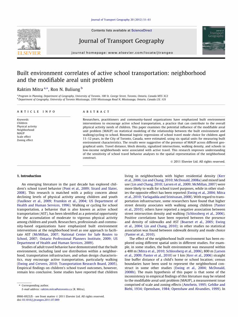
Built environment correlates of active school transportation: neighborhood and the modifiable areal unit problem Raktim Mitra a,⇑ , Ron N. Buliung b a Program in Planning, Department of Geography, University of Toronto, 100 St. George Street, Toronto, Ontario, Canada M5S 3G3 b Department of Geography, University of Toronto Mississauga, 3359 Mississauga Road N, Mississauga, Ontario, Canada L5L 1C6 article info Keywords: Children Physical activity Neighborhood MAUP Scale effect Zoning effect abstract Researchers, practitioners and community-based organizations have emphasized built environment interventions to encourage active school transportation, a practice that can contribute to the overall physical activity needs of children. This paper examines the potential influence of the modifiable areal unit problem (MAUP) on statistical modeling of the relationship between the built environment and walking/cycling to school. Binomial logistic regressions of school travel mode choice for children aged 11–12 years, in the City of Toronto, Canada, were estimated, using six spatial units for measuring built environment characteristics. The results were suggestive of the presence of MAUP across different geo- graphical units. Travel distance, block density, signalized intersections, walking density, and schools in low-income neighborhoods were associated with active travel. This research improves understanding of the sensitivity of school travel behavior analyses to the spatial representation of the neighborhood construct. Ó 2011 Elsevier Ltd. All rights reserved. 1. Introduction An emerging literature in the past decade has explored chil- dren’s school travel behavior (Pont et al., 2009; Sirard and Slater, 2008). This research is matched with a policy concern about declining levels of physical activity among children and youth (Faulkner et al., 2009; Frumkin et al., 2004; US Department of Health and Human Services, 1996). Walking or cycling for school transportation, a behavior that is also known as active school transportation (AST), has been identified as a potential opportunity for the accumulation of moderate to vigorous physical activity among children and youth. Researchers, professionals and commu- nity-based organizations have emphasized built environment interventions at the neighborhood level as one approach to facili- tate AST (McMillan, 2007; National Center for Safe Routes to School, 2007; Ontario Professional Planners Institute, 2009; US Department of Health and Human Services, 2009). Studies of adult travel behavior have demonstrated that the built environment, including land use distribution within a neighbor- hood, transportation infrastructure, and urban design characteris- tics, may encourage active transportation, particularly walking (Ewing and Cervero, 2010; Transportation Research Board, 2005). Empirical findings on children’s school travel outcomes, however, remain less conclusive. Some studies have reported that children living in neighborhoods with higher residential density (Kerr et al., 2006; Lin and Chang, 2010; McDonald, 2008a) and mixed land use (Lin and Chang, 2010; Larsen et al., 2009; McMillan, 2007) were more likely to walk for school travel purposes, while in other stud- ies the opposite effect has been reported (Ewing et al., 2004; Mitra et al., 2010; Yarlagadda and Srinivasan, 2008). With regard to trans- portation infrastructure, some researchers have found that higher street density associates with walking among children (Panter et al., 2010); others have reported a negative association between street intersection density and walking (Schlossberg et al., 2006). Positive correlations have been reported between the presence and density of sidewalks and AST (Boarnet et al., 2005; Ewing et al., 2004; Lin and Chang, 2010); in other studies no statistical association was found between sidewalk density and mode choice (Panter et al., 2010). The effect of the neighborhood built environment has been ex- plored using different spatial units in different studies. For exam- ple, in some studies, the built environment was measured within a 400 m (Mitra et al., 2010; Schlossberg et al., 2006), 800 m (Larsen et al., 2009; Panter et al., 2010) or 1 km (Kerr et al., 2006) straight line buffer distance of a child’s home or school location; census boundaries have been used to represent the neighborhood con- struct in some other studies (Ewing et al., 2004; McDonald, 2008b). The main hypothesis of this paper is that some of the inconsistency in empirical findings of this literature may be related to the modifiable areal unit problem (MAUP), a measurement issue comprised of scale and zoning effects (Amrhein, 1995; Gehlke and Biehl, 1934; Openshaw, 1984; Openshaw and Alvandies, 1999). In 0966-6923/$ - see front matter Ó 2011 Elsevier Ltd. All rights reserved. doi:10.1016/j.jtrangeo.2011.07.009 ⇑ Corresponding author. E-mail address: [email protected] (R. Mitra). Journal of Transport Geography 20 (2012) 51–61 Contents lists available at ScienceDirect Journal of Transport Geography journal homepage: www.elsevier.com/locate/jtrangeo
Transcript of Built environment correlates of active school transportation: neighborhood and the modifiable areal...
Journal of Transport Geography 20 (2012) 51–61
Contents lists available at ScienceDirect
Journal of Transport Geography
journal homepage: www.elsevier .com/ locate / j t rangeo
Built environment correlates of active school transportation: neighborhoodand the modifiable areal unit problem
Raktim Mitra a,⇑, Ron N. Buliung b
a Program in Planning, Department of Geography, University of Toronto, 100 St. George Street, Toronto, Ontario, Canada M5S 3G3b Department of Geography, University of Toronto Mississauga, 3359 Mississauga Road N, Mississauga, Ontario, Canada L5L 1C6
a r t i c l e i n f o
Keywords:ChildrenPhysical activityNeighborhoodMAUPScale effectZoning effect
0966-6923/$ - see front matter � 2011 Elsevier Ltd. Adoi:10.1016/j.jtrangeo.2011.07.009
⇑ Corresponding author.E-mail address: [email protected] (R. Mitr
a b s t r a c t
Researchers, practitioners and community-based organizations have emphasized built environmentinterventions to encourage active school transportation, a practice that can contribute to the overallphysical activity needs of children. This paper examines the potential influence of the modifiable arealunit problem (MAUP) on statistical modeling of the relationship between the built environment andwalking/cycling to school. Binomial logistic regressions of school travel mode choice for children aged11–12 years, in the City of Toronto, Canada, were estimated, using six spatial units for measuring builtenvironment characteristics. The results were suggestive of the presence of MAUP across different geo-graphical units. Travel distance, block density, signalized intersections, walking density, and schools inlow-income neighborhoods were associated with active travel. This research improves understandingof the sensitivity of school travel behavior analyses to the spatial representation of the neighborhoodconstruct.
� 2011 Elsevier Ltd. All rights reserved.
1. Introduction
An emerging literature in the past decade has explored chil-dren’s school travel behavior (Pont et al., 2009; Sirard and Slater,2008). This research is matched with a policy concern aboutdeclining levels of physical activity among children and youth(Faulkner et al., 2009; Frumkin et al., 2004; US Department ofHealth and Human Services, 1996). Walking or cycling for schooltransportation, a behavior that is also known as active schooltransportation (AST), has been identified as a potential opportunityfor the accumulation of moderate to vigorous physical activityamong children and youth. Researchers, professionals and commu-nity-based organizations have emphasized built environmentinterventions at the neighborhood level as one approach to facili-tate AST (McMillan, 2007; National Center for Safe Routes toSchool, 2007; Ontario Professional Planners Institute, 2009; USDepartment of Health and Human Services, 2009).
Studies of adult travel behavior have demonstrated that the builtenvironment, including land use distribution within a neighbor-hood, transportation infrastructure, and urban design characteris-tics, may encourage active transportation, particularly walking(Ewing and Cervero, 2010; Transportation Research Board, 2005).Empirical findings on children’s school travel outcomes, however,remain less conclusive. Some studies have reported that children
ll rights reserved.
a).
living in neighborhoods with higher residential density (Kerret al., 2006; Lin and Chang, 2010; McDonald, 2008a) and mixed landuse (Lin and Chang, 2010; Larsen et al., 2009; McMillan, 2007) weremore likely to walk for school travel purposes, while in other stud-ies the opposite effect has been reported (Ewing et al., 2004; Mitraet al., 2010; Yarlagadda and Srinivasan, 2008). With regard to trans-portation infrastructure, some researchers have found that higherstreet density associates with walking among children (Panteret al., 2010); others have reported a negative association betweenstreet intersection density and walking (Schlossberg et al., 2006).Positive correlations have been reported between the presenceand density of sidewalks and AST (Boarnet et al., 2005; Ewinget al., 2004; Lin and Chang, 2010); in other studies no statisticalassociation was found between sidewalk density and mode choice(Panter et al., 2010).
The effect of the neighborhood built environment has been ex-plored using different spatial units in different studies. For exam-ple, in some studies, the built environment was measured withina 400 m (Mitra et al., 2010; Schlossberg et al., 2006), 800 m (Larsenet al., 2009; Panter et al., 2010) or 1 km (Kerr et al., 2006) straightline buffer distance of a child’s home or school location; censusboundaries have been used to represent the neighborhood con-struct in some other studies (Ewing et al., 2004; McDonald,2008b). The main hypothesis of this paper is that some of theinconsistency in empirical findings of this literature may be relatedto the modifiable areal unit problem (MAUP), a measurement issuecomprised of scale and zoning effects (Amrhein, 1995; Gehlke andBiehl, 1934; Openshaw, 1984; Openshaw and Alvandies, 1999). In

52 R. Mitra, R.N. Buliung / Journal of Transport Geography 20 (2012) 51–61
the context of school travel behavior research, a scale effect may bepresent when analytical results exhibit sensitivity to the size ofspatial units used for built environment measurement. For exam-ple, the use of a relatively small spatial unit, such as a 250 m bufferaround a residential or school location, may produce unreliablestatistical results, because the built environment variables areaggregated using a smaller sample. In contrast, generalizing the va-lue of a built environment metric across a larger geographical unit(e.g., within a 1000 m versus a 250 m buffer) will typically reducethe sample variance for that particular metric, while increasing thecorrelation between separate built environment variables. As a re-sult, an observed statistical association may mask meaningful dif-ferences that are obvious at a smaller scale (Bailey and Gatrell,1995; Fotheringham and Wong, 1991). A zoning effect may bepresent when analytical results are sensitive to the partitioningof space. For example, different zone configurations under a fixedscale may produce dissimilar results.
Despite a long-standing recognition in the geography literatureof the potential sensitivity of analytical results to the geographicaldefinition of spatial units, the MAUP has received less attention inresearch that examines the built environment–transportation rela-tionship. Some researchers have investigated the scale and zoningeffects of different built environment metrics on adults’ active tra-vel and physical activity. For example, Zhang and Kukadia (2005)explored mode choice for work and non-work trips in Boston, Mas-sachusetts, using two different scale and zoning schemes (five buf-fers and three census boundaries). The results indicated thepresence of both scale and zoning effects across spatial units. Berkeet al. (2007) examined the relationship between neighborhoodwalkability, and physical activity or obesity, among the elderly inKing County, Washington. Their results suggested that the builtenvironment influenced walking across all three buffer distancesthat were examined. Lastly, Duncan et al. (2010) investigated phys-ical activity (i.e., walking for transportation) among adults living in154 Census Collection Districts (CCD) in Adelaide, Australia. Theauthors found that the duration of walking trips had a strongerassociation with ‘‘corrected’’ measures of land use mix (i.e., stan-dardized based on the geographical size of CCDs), compared tothe uncorrected land use measures within CCDs. Adjusting forscale effects did not improve the results reported for models walk-ing trip frequency. The MAUP is yet to be addressed in the ASTliterature.
This paper examines the previously unexplored issue of howthe MAUP may be influencing the results of empirical research intothe relationship between objectively measured built environmentcharacteristics and children’s school travel behavior, particularlythe choice of active modes of travel to school. Two research ques-tions are considered using data describing the travel behavior of11–12 year olds in the City of Toronto, Canada: (1) at what scaleand for what type of zone system does the neighborhood builtenvironment have the strongest association with AST? and (2)which built environment characteristics near home and schoollocations are associated with the choice of an active mode for tripsto school? The article contributes a refined understanding of howto model the built environment–active school transportation(BE–AST) relationship, with a view to enhancing cross-study com-parison. The research also improves current knowledge of the envi-ronmental correlates of school travel mode choice in a NorthAmerican context.
2. Study design
The City of Toronto is the largest city in Canada, with a residentpopulation of over 2.5 million (Statistics Canada, 2008). The inner-city neighborhoods in Toronto typically conform to what are
known as main-street neighborhoods (i.e., residential neighbor-hoods with employment-related land uses along the main streets)in both the academic and popular literatures (Sewell, 1993). There-urbanization trend of the last several decades, which has beenhastened in recent years by favorable policy and market condi-tions, has brought pockets of high-rise and high-density residentialdevelopments to these neighborhoods. In contrast, the City of Tor-onto’s suburban places are dominated by Modernist conventionalneighborhoods typically characterized by single-use residentialdevelopment and a street network design (e.g., curvilinear streets)that is often associated with auto-oriented travel behavior.
AST is reasonably well practiced in the City of Toronto. In2006, 49% of children aged 11–13 years actively traveled toschool. For the trips from school to home, the rate was even high-er (56%) (Buliung et al., 2009). Toronto’s diverse urban environ-ment and high rates of walking/cycling for school transportationoffer an excellent opportunity to explore the influence of the builtenvironment characteristics on children’s school travel modechoice processes.
This study aims to examine the potential influence of MAUP onthe statistical modeling of the BE–AST relationship. Several recom-mendations have been made in the literature to explore scale andzoning effects (Fotheringham and Wong, 1991; Openshaw, 1984;Zhang and Kukadia, 2005). Some researchers have suggested anexamination of the underlying pattern in the estimated coefficientsof the built environment variables across different scales and zonesystems (Fotheringham and Wong, 1991; Zhang and Kukadia,2005). This approach is tested here by modeling the BE–AST rela-tionship using different spatial units and analytical scales for therepresentation of neighborhoods. With regard to the correlates ofAST, this study adopts a social–ecological approach and hypothe-sizes that household demographics, travel distance to school, andthe neighborhood environment influence the selection of schooltravel modes (McMillan, 2005; Mitra, 2011; Sirard and Slater,2008).
2.1. Travel data
Data were taken from the 2006 Transportation Tomorrow Sur-vey (TTS). The TTS is a repeated cross-sectional survey of travelbehavior in Southern Ontario, Canada, conducted on a 5% sampleof all households in the study area. The 2006 TTS data were col-lected for a randomly selected weekday, using a computer assistedtelephone interview procedure (Data Management Group, 2008,2009). Household travel data (e.g., origin/destination of trips, tripstart time, purpose, primary travel mode) for all trips by householdmembers aged 11 years and older, associated with the day prior tothe interview, were proxy reported by an adult household member.Previous research indicates that school travel behavior can changewith a child’s age (Buliung et al., 2009; Mitra, 2011; Panter et al.,2008). In order to limit the scope of this study to a relativelyhomogenous population, school travel data for children aged 11–12 years (i.e., likely attending grades 5 or 6) were explored. Allhome-to-school trips between the 6h00–9h30 time interval(n = 2520) were extracted. Travel modes were collapsed into active(i.e., walking and cycling trips) and passive (i.e., trips made by aprivate automobile, public transit or school-bus) modes, usingthe proxy reported data on primary mode of travel for school trips.
2.2. Neighborhood and built environment data
The modern conceptualization of the planned neighborhoodunit emerged in the early 1900s (Banerjee and Baer, 1984; Perry,1939). The design principles of a neighborhood unit emphasizedModernist concepts of spatial separation between home and work,and a hierarchical street system (Banerjee and Baer, 1984; Moudon

R. Mitra, R.N. Buliung / Journal of Transport Geography 20 (2012) 51–61 53
et al., 2006). Elementary schools, community centers and othersmaller urban facilities were planned as central features of a neigh-borhood, with surrounding residential development scaled to bewithin a convenient walking distance (e.g., a 0.25 mi, or 400 m, ra-dial distance) from the these facilities. The post World War II sub-urban developments in Toronto were dominated by a widespreadimplementation of the neighborhood unit idea (Filion and Ham-mond, 2003; Hess, 2009). Urban planners assumed that withinthe boundaries of a neighborhood, non residential activities of res-idents will ‘‘flow toward the core’’ (Banerjee and Baer, 1984, pp183–4). However, this planning goal never fully materialized, per-haps because most neighborhood centers did not offer essentialand desired services. Instead, these suburban neighborhoods haveled to an increased dependency on automobiles. Within this con-text, previous research has indicated that the physical extent of aneighborhood unit may be less important to households, and thata household’s perceived neighborhood boundary can largely be de-fined based on the ‘‘action space’’ within which the householdmembers perform their daily activities, and consume goods andservices (Banerjee and Baer, 1984; Horton and Reynolds, 1971).This observation, perhaps, is applicable to the older inner-city res-idential areas as well, where the borders between the ‘‘neighbor-hoods’’ are less clear. In the context of this concern around theneighborhood boundaries, defining the neighborhood as a unit ofempirical analysis can present a methodical challenge (Moudonet al., 2006).
In this paper, built environment characteristics were measuredwithin six different geographies, and two different scale and zon-ing schemes (Fig. 1 and Table 1). The first scheme involved measur-ing the built environment within various buffer distances around achild’s home and school locations (four buffer distances- 250 m,400 m, 800 m and 1000 m). In the second approach, neighborhoodswere defined using either the census boundary (dissemination area– DA) or traffic analysis zone (TAZ) within which a home or schoolwas located. Selection of these spatial units was informed by theexisting AST literature. The BE–AST associations were examinedat each level of geography, and were compared across different
HOME
250 m buffer400 m buffer
800 m buffer
1,000 m buffer
Fig. 1. Built environment near a hypothetical household location in Toronto,
scales/zoning systems. Environmental characteristics were mea-sured at both the residence and school ends of a school trip. Theindividual environmental variables that were analyzed are listedin Table 2, where the hypothesized relationship with AST is alsoreported.
Minimum travel distance between home and school locationsof a child was computed using Toronto’s street network file(DMTI CanMap� RouteLogistics file, version 2007.3). Other neigh-borhood characteristics related to street network design were alsoobtained from the DMTI data. The employment-to-population ra-tio (EMP_POP) was calculated using the TTS data, based on thenumber of work-trip ends in each TAZ. TTS trip data were alsoused to calculate the density of walking trips (WALK_DSTY) nearthe home and school locations. To calculate block density, thegeographical boundary files from the 2006 population census ofCanada were used. This study situates school travel behaviorwithin a social–ecological framework. Within this theoretical ap-proach, the potential influence of neighborhood socio-economicstatus was examined. LOWINCOME was, thus, conceptualized asan environmental characteristic. In other words, socio-economicstatus was measured at the neighborhood level. The medianhousehold income data from the population census of Canadawere aggregated, within six different geographies around homeand school locations, to identify low income neighborhoods. In-come data for individuals or households were not available foranalysis. Lastly, data on pedestrian and cyclist collisions occurredduring the 2002–2006 period were collected from City of Toron-to’s Transportation Department; the data included the locationsof all fatal and non-fatal collisions reported to the Toronto PoliceService.
2.3. Statistical analysis
Binomial logistic regression was used to explore the correlatesof active versus passive mode choice for school trips (Pampel,2000). A coefficient (b̂i) from the multivariate logistic regressionmodels in this paper represent the un-confounded (i.e., adjusted)
TAZ boundary
DA boundary
HOME
Canada. Note: DA, Census dissemination area; TAZ, Traffic analysis zone.

Table 1Spatial unit definitions.
Definition Description
250 m buffer around home/school location
The use of a 200 or 250 m buffer is most common in empirical research that measures the built environment around travel routes(Schlossberg et al., 2006). A 250 m distance is roughly equivalent to a 2.5-min walking distance for an average adult.
Area: 0.2 sq km400 m buffer around home/
school location400 m is equivalent to a 5-min walking distance for an average child (Mitra et al., 2010). Some researchers have assumed thisdistance to be a reasonable walking distance for children (McMillan, 2007; Mitra et al., 2010; Yarlagadda and Srinivasan, 2008).
Area: 0.5 sq km800 m buffer around home/
school location800 m is equivalent to a 10-min walking distance for an average child (Panter et al., 2010).
Area: 2.01 sq km1000 m buffer around home/
school locationSometimes used in adult active-travel behavior research (Frank et al., 2007), a 1000 m (i.e., 1 km) distance is roughly equivalent to a10-to-12 min walking distance for an average adult. One study on children’s school travel has used this distance to define theneighborhood of residence (Kerr et al., 2006).Area: 3.4 sq km
DA of home/school location Smallest geographical unit for which public census data (i.e., data from Statistics Canada) is available in Canada. Some researchersin the US have measured built environment at the block group level to explore school travel, and have cited a similar reason fortheir choice of geography (McDonald, 2008b).
Area: Mean 0.18 sq km. (sd0.39 sq km.)
TAZ of home/school location Small geographical areas defined for transportation research purposes. Used mostly to explore work-travel behavior. Someresearchers have measured TAZ-level built environment to explore school travel behavior (Ewing et al., 2004).Area: Mean 1.31 sq km. (sd
0.94 sq km.)
Note: sd, standard deviation; DA, census dissemination area; TAZ, traffic analysis zone.
Table 2Independent variables and their hypothesized associations with active school transportation.
Variable Hypothesizedrelationship
Socio-demographicsMALE: The child was a male (reference: female) +CHILD: Number of school-age children below driving age (4–15 years) in the household +/�VEH_LIC: Number of vehicles in the household per licensed driver �FUL_EMP: Number of full-time employees per adult household member (ages 18 to 65 years) �UNEMP: There was unemployed adult(s) in the household (reference: no unemployed adult) +
Built environmentDISTANCE: Minimum travel distance (i.e., shortest path using a street network) between the home and school (km) �EMP_POP: The ratio of employment to the population in a TAZ �
Low (first tertile); Medium (second tertile- reference); High (third tertile)WALK_DSTY: Walking density – total work and school related walking trips produced by residents of a TAZ, normalized by per sq km of area +
Low (first tertile – reference); Medium (second tertile); High (third tertile)BLOCK_DTYa: Number of street-blocks, normalized by per sq km of area +FOURWAY_DTYa: Proportion of 4-way street intersections – the ratio of 4-way intersections to total number of street intersections +/�DEADEND_DTYa: Proportion of dead ends and cul-de-sacs - the ratio of dead-ends plus cul-de-sacs to total number of street intersections �LIGHT_DTYa: Proportion of intersections with street lights- the ratio of signalized intersections to total number of street intersections +LOCAL_RD_DTYa: Length of local roads (km), normalized by per sq km of area +MAJOR_RD_DTYa: Length of major roads (km), normalized by per sq km of area. Major roads include expressways, arterials and collector roads �COLLISIONa: The number of pedestrian and cyclist collisions (fatal and non-fatal) per sq km of area per year, averaged based on the total number of
collisions reported to the police between 2002 and 2006�
LOWINCOMEa,b: The child’s residence/school neighborhood was a low-income neighborhood, i.e., median household income was <CAD 39,400.Median household income was estimated by taking a median of the DA-level median household incomes at a child’s residence/schoollocation
+
Note: DA, census dissemination area; TAZ, traffic analysis zone.Each built environment variable has been estimated separately for the home, and the school location.Variables in italics were excluded from the multivariate logistic regression specifications.
a Variables were calculated separately for each neighborhood definition (i.e., 250 m buffer, 400 m buffer, 800 m buffer, 1000 m buffer, DA and TAZ). Other environmentaldata were available only at the TAZ level.
b Individual household income data was not available. Median household income was calculated using 2006 population census data by Statistics Canada. Averagehousehold size for the sample was 4.3 (sd = 1.28). In a large metropolitan area such as Toronto (i.e., population > 500,000), the low income cut-off, defined by StatisticsCanada, was CAD 39,399 for a four-member household (Statistics Canada, 2010).
54 R. Mitra, R.N. Buliung / Journal of Transport Geography 20 (2012) 51–61
correlation between an individual built environment metric andthe log-odds of walking/cycling to school. The odds ratio or OR(i.e., expb̂i), thus, demonstrates the relationship between a variablei and the odds of active travel (i.e., the change in the odds of an ac-tive mode choice in response to a unit change in the value of var-iable i). Separate binomial logistic regression models werespecified with built environment variables and neighborhood in-come measured within each of the six spatial units outlined in Ta-ble 1. Researchers have argued that beyond a distance of 5 km (i.e.,a 1-h walk for a child), the choice set may become restricted tomotorized alternatives only (Ewing et al., 2004; McDonald,
2008a). For this reason, only children living within 5 km (shortestpath network distance) from their schools were considered formodeling purposes (92% of all school trips by this age group).Adjusting for missing data and outliers, the final dataset included2190 home-to-school trips.
For each school trip, five socio-demographic variables, and tenneighborhood characteristics, in addition to the shortest path net-work distance between home and school locations, were initiallymeasured (Table 2). Prior to the multivariate (i.e., adjusted) logisticregression estimation, a set of unadjusted logistic regressions (i.e.,one model per correlate) were estimated to filter the initial set of

R. Mitra, R.N. Buliung / Journal of Transport Geography 20 (2012) 51–61 55
independent variables down to only those variables holding a sta-tistical significance at p 6 0.05.
The degree of multi-collinearity across the built environmentvariables was also examined, for each level of spatial aggregation(Lee and Moudon, 2006; Mitra et al., 2010). The correlation be-tween variables increased with the scale of spatial analysis. Whentwo variables were correlated (i.e., DEADEND_DTY and FOUR-WAY_DTY; BLOCK_DTY and LOCAL_RD_DTY), those two were en-tered into the multivariate (i.e., adjusted) model one at a time,and the one with a weaker association (i.e., DEADEND_DTY; LO-CAL_RD_DTY) was excluded from the final model specification.The built environment variables around the residence and nearthe school were also highly correlated. To overcome this collinear-ity problem, two sets of multivariate regression models were spec-ified and estimated for each spatial unit, one for built environmentmeasures near the residence, and the other for the built environ-ment near the school. A total of 12 multivariate logistic regressionmodels of active travel to school were estimated. Statistical analy-ses were performed with R� version 2.9.0 (The R Foundation forStatistical Computing).
The presence of scale effects was examined by observingwhether or not the coefficient of a variable remained statisticallysignificant across different scales of aggregation, and to a lesser ex-tent, by assessing changes in the size and sign of the coefficient val-ues across different scales of spatial aggregation, within eachaggregation scheme (i.e., buffers or zones). The presence of poten-tial zoning effects was examined by using the method suggested byFotheringham and Wong (1991) and Zhang and Kukadia (2005),which involved an assessment of the built environment coeffi-cients across two spatial units at a comparable scale, betweenthe two zoning schemes (i.e., 250 m buffer versus DA, and 800 mbuffer versus TAZ). The standard-difference-of-means test [1]was used to test the statistical difference in the estimated coeffi-cients obtained from the logistic regression models:
Table 3Descriptive statistics (n = 2190 students).
Me
Travel modeActivePassive
MALEVEH_LIC 0.7DISTANCE (km) 1.2
250 m buffer
Home School
Mean (sd) % Mean (sd)
BLOCK_DTY (blocks/km2) 25.58 (15.10) 25.33 (14.90)FOURWAY_DTY (prop.) 0.21 (0.19) 0.21 (0.20)LIGHT_DTY (prop.) 0.12 (0.14) 0.11 (0.13)MAJOR_RD_DTY (km/km2) 3.32 (3.85) 2.39 (3.04)LOWINCOME 28.54
800 m buffer
BLOCK_DTY (blocks/km2) 23.51 (11.82) 24.56 (11.32)FOURWAY_DTY (prop.) 0.19 (0.10) 0.20 (0.10)LIGHT_DTY (prop.) 0.10 (0.05) 0.10 (0.05)MAJOR_RD_DTY (km/km2) 2.55 (1.71) 2.36 (1.53)LOWINCOME 7.44
DA
BLOCK_DTY (blocks/km2) 27.60 (20.74) 22.83 (17.04)FOURWAY_DTY (prop.) 0.20 (0.25) 0.21 (0.24)LIGHT_DTY (prop.) 0.11 (0.18) 0.12 (0.20)MAJOR_RD_DTY (km/km2) 3.56 (4.81) 2.30 (2.91)LOWINCOME 22.10
Note: sd, standard deviation; DA, census dissemination area; TAZ, traffic analysis zone.The variables that were measured only at the TAZ level (WALK_DSTY and EMP_POP) aregroups.
t ¼ b̂i � b̂j
SEjb̂i � b̂jjð1Þ
where b̂i = estimated coefficient of a built environment variable i;SE = Standard error (Fotheringham and Wong, 1991).
3. Results
Home-to-school trips by 11–12 year old children (n = 2190),and the associated socio-demographic and environmental attri-butes, were analyzed. Table 3 describes these attributes; summaryof the built environment measures are presented for each of the sixgeographical units, around home and school locations, of all 11–12 year old children. Results from the multivariate logistic regres-sion models are presented in Tables 4 and 5. Most children used anactive mode for school transportation (58%); only 42% traveled toschool using passive modes (Table 3). The average school traveldistance (shortest path network distance) for these students was1.25 km.
3.1. Scale effect
Table 3 suggested that the variance (square of the standarddeviation) of these environmental variables typically decreasedwith an increase in neighborhood size. This type of ‘‘data smooth-ing’’ at larger geographies is not unexpected (Zhang and Kukadia,2005), and adds empirical evidence in support of the hypothesisof decreasing sample variance with an increase in the scale of anal-ysis, as previously mentioned in the introduction (Section 1). Scaleeffects were explored further using the results from the adjustedlogistic regression models, presented in Tables 4 and 5.
The goodness of fit for the estimated models was very similaracross all six specifications (although a general trend of a weaker
an (sd) %
58.4041.6052.15
2 (0.42)5 (1.00)
400 m buffer
Home School
% Mean (sd) % Mean (sd) %
25.19 (13.62) 26.64 (12.83)0.20 (0.14) 0.21 (0.15)0.11 (0.09) 0.10 (0.08)2.99 (2.79) 2.36 (2.44)
20.41 17.17 7.53
1000 m buffer
21.27 (10.34) 22.08 (10.14)0.19 (0.09) 0.20 (0.10)0.10 (0.05) 0.09 (0.05)2.28 (1.34) 2.16 (1.20)
3.52 4.22 3.70
TAZ
23.70 (12.80) 24.46 (12.47)0.20 (0.12) 0.20 (0.12)0.10 (0.09) 0.14 (0.07)2.87 (1.88) 2.74 (1.75)
15.94 10.27 6.53
not shown in this table. Values for these variables were categorized into three equal

Table 4AST–built environment relationship within different buffer distances around home and school locations (n = 2190 students).
250 m buffer 400 m buffer 800 m buffer 1000 m buffer
Home School Home School Home School Home School
Coef. (S.E.) OR Coef. (S.E.) OR Coef. (S.E.) OR Coef. (S.E.) OR Coef. (S.E.) OR Coef. (S.E.) OR Coef. (S.E.) OR Coef. (S.E.) OR
MALE (ref = FEMALE) 0.33 (0.11) 1.40 0.31 (0.11) 1.36 0.32 (0.11) 1.38 0.29 (0.11) 1.34 0.32 (0.11) 1.38 0.30 (0.11) 1.35 0.32 (0.11) 1.38 0.30 (0.11) 1.35VEH_LIC �0.43 (0.13) 0.65 �0.44 (0.13) 0.65 �0.40 (0.13) 0.67 �0.42 (0.13) 0.65 �0.40 (0.13) 0.67 �0.39 (0.13) 0.68 �0.41 (0.13) 0.66 �0.40 (0.13) 0.67DISTANCE �1.83 (0.09) 0.16 �1.84 (0.09) 0.16 �1.84 (0.09) 0.16 �1.83 (0.09) 0.16 �1.84 (0.09) 0.16 �1.82 (0.09) 0.16 �1.84 (0.09) 0.16 �1.82 (0.09) 0.16WALK_DSTY (ref = Low)
Medium 0.37 (0.13) 1.45 0.46 (0.13) 1.59 0.38 (0.13) 1.47 0.45 (0.13) 1.57 0.39 (0.13) 1.48 0.47 (0.13) 1.60 0.38 (0.13) 1.47 0.44 (0.13) 1.56High 0.78 (0.15) 2.18 0.86 (0.15) 2.36 0.76 (0.15) 2.13 0.84 (0.15) 2.31 0.75 (0.16) 2.12 0.66 (0.17) 1.93 0.79 (0.16) 2.21 0.58 (0.17) 1.79
EMP_POP (Ref = Medium)Low 0.09 (0.13) 1.09 0.16 (0.13) 1.17 0.05 (0.14) 1.05 0.06 (0.13) 1.06 0.05 (0.14) 1.05 0.07 (0.13) 1.07 0.05 (0.14) 1.05 0.06 (0.13) 1.07High 0.09 (0.14) 1.09 0.09 (0.14) 1.10 0.13 (0.14) 1.13 0.11 (0.14) 1.12 0.11 (0.14) 1.12 0.10 (0.14) 1.10 0.12 (0.14) 1.12 0.12 (0.14) 1.13
BLOCK_DTYa 0.04 (0.02) 1.04 0.03 (0.02) 1.03 0.02 (0.01) 1.02 0.01 (0.14) 1.01 0.01 (0.00) 1.01 0.00 (0.00) 1.00 0.00 (0.00) 1.00 0.00 (0.00) 1.00FOURWAY_DTYa �0.33 (0.32) 0.72 �0.65 (0.31) 0.52 �0.63 (0.47) 0.53 �0.80 (0.44) 0.45 �0.65 (0.75) 0.52 �0.23 (0.75) 0.79 �0.99 (0.85) 0.37 �1.09 (0.86) 0.33LIGHT_DTYa 1.03 (0.45) 2.80 �0.20 (0.55) 0.82 0.80 (0.70) 2.21 �0.34 (0.86) 0.71 �0.12 (1.28) 0.88 1.08 (1.36) 2.96 0.36 (1.50) 1.43 1.91 (1.72) 6.76MAJOR_RD_DTYa �0.01 (0.01) 0.99 �0.04 (0.02) 0.96 0.01 (0.02) 1.01 �0.04 (0.03) 0.96 0.03 (0.03) 1.03 0.01 (0.04) 1.01 0.02 (0.05) 1.02 �0.03 (0.05) 0.97LOWINCOME(ref = No)a �0.12 (0.13) 0.88 0.00 (0.14) 1.00 0.15 (0.16) 1.16 0.59 (0.25) 1.81 0.36 (0.26) 1.44 0.60 (0.39) 1.83 0.15 (0.31) 1.17 0.89 (0.40) 2.43Intercept 2.06 (0.23) 7.83 2.27 (0.23) 9.66 1.97 (0.24) 7.16 2.39 (0.24) 10.94 20.1 (0.25) 7.47 2.05 (0.25) 7.79 2.08 (0.25) 7.97 2.06 (0.26) 7.87
Summary statistics�2 [L(0) � L(B)] 900.4 894.9 898.4 892.7 897.6 885.7 895.5 290.9AIC 2099.5 2105.0 2101.5 2107.2 2102.3 2114.2 2104.4 2109.0McFadden’s q2 (adj.) 0.303 (0.298) 0.301 (0.297) 0.303 (0.298) 0.300 (0.296) 0.302 (0.297) 0.298 (0.293) 0.301 (0.297) 0.300 (0.295)
Note: AST, active school transportation; DA, census dissemination area; TAZ, traffic analysis zone; OR, odds-ratio; AIC, Akaike information criterion.Coefficients in bold are significant at p 6 0.01, coefficients in bold italics are significant at p 6 0.05; coefficients in italics are significant at p 6 0.10.
a Variables were calculated separately for each neighborhood definition (i.e., 250 m buffer, 400 m buffer, 800 m buffer, 1000 m buffer). Other environmental data were available only at the TAZ level.
56R
.Mitra,R
.N.Buliung
/Journalof
TransportG
eography20
(2012)51–
61

Table 5AST–built environment relationship within the DA and TAZ of home and school (n = 2190 students).
DA TAZ
Home School Home School
Coef. (S.E.) OR Coef. (S.E.) OR Coef. (S.E.) OR Coef. (S.E.) OR
MALE (ref = FEMALE) 0.32 (0.11) 1.37 0.29 (0.11) 1.34 0.32 (0.11) 1.37 0.30 (0.11) 1.34VEH_LIC �0.45 (0.13) 0.64 �0.43 (0.13) 0.65 �0.40 (0.13) 0.67 �0.40 (0.13) 0.67DISTANCE �1.84 (0.09) 0.16 �1.85 (0.09) 0.16 �1.84 (0.09) 0.67 �1.83 (0.16) 0.16WALK_DSTY (ref = Low)
Medium 0.40 (0.13) 1.49 0.44 (0.13) 1.55 0.38 (0.13) 1.46 0.48 (0.13) 1.61High 0.85 (0.14) 2.34 0.86 (0.15) 2.37 0.78 (0.16) 2.17 0.75 (0.16) 2.13
EMP_POP (Ref = Medium)Low 0.09 (0.13) 1.10 0.03 (0.13) 1.03 0.05 (0.14) 1.05 0.00 (0.13) 1.00High 0.11 (0.14) 1.11 0.11 (0.14) 1.12 0.13 (0.14) 1.14 0.13 (0.14) 1.14
BLOCK_DTYa 0.01 (0.00) 1.01 0.01 (0.00) 1.01 0.01 (0.01) 1.01 0.00 (0.01) 1.00FOURWAY_DTYa �0.40 (0.24) 0.67 0.25 (0.27) 1.29 �0.57 (0.56) 0.56 0.23 (0.62) 1.25LIGHT_DTY a 0.54 (0.36) 1.72 �0.20 (0.82) 0.82 0.48 (0.77) 1.62 1.95 (0.89) 7.02MAJOR_RD_DTY a �0.00 (0.01) 1.00 �0.02 (0.02) 0.98 0.03 (0.03) 1.03 0.06 (0.03) 1.06LOWINCOME (ref = No) a �0.16 (0.14) 0.85 0.32 (0.16) 1.38 0.19 (0.21) 1.21 0.31 (0.27) 1.36Intercept 2.14 (0.21) 8.49 2.40 (0.22) 10.98 2.04 (0.24) 7.68 1.75 (0.31) 5.73
Summary Statistics�2 [L(0) � L(B)] 899.4 893.2 896.2 891.2AIC 2100.5 2106.7 2103.7 2108.7McFadden’s q2 (adj.) 0.302 (0.298) 0.300 (0.296) 0.301 (0.297) 0.300 (0.295)
Note: AST, active school transportation; DA, census dissemination area; TAZ, traffic analysis zone; OR, Odds-ratio; AIC, Akaike information criterion.Coefficients in bold are significant at p 6 0.01, coefficients in bold italics are significant at p 6 0.05; coefficients in italics are significant at p 6 0.10.
a Variables were calculated separately for each neighborhood definition (i.e., 250 m buffer, 400 m buffer, 800 m buffer, 1000 m buffer). Other environmental data wereavailable only at the TAZ level.
R. Mitra, R.N. Buliung / Journal of Transport Geography 20 (2012) 51–61 57
model fit with increased neighborhood size is noticeable), but theindividual coefficients related to the neighborhood environmentcharacteristics were inconsistent. The signs of observed associa-tions changed for some variables across spatial unit specifications.For example, for the models estimated with the environmentalvariables measured within a 250 m buffer of residence and schoollocations (hereafter called the 250 m models), both MA-JOR_RD_DTY and LOWINCOME near the home location were nega-tively associated with AST. But, when these measures wereaggregated at the scale of a 400 m buffer (i.e., 400 m models), po-sitive correlations were observed for both variables. However,signs of the statistically significant environmental variables re-mained largely unchanged by adjustments in the scale of geo-graphic aggregation. In contrast, the statistical significance andthe size of the coefficients varied noticeably across different scalesof analysis (Tables 4 and 5). In other words, the impact of each var-iable on AST odds was inconsistent across scales of analysis. Thelargest number of environmental associations with active travelmode choice (3 coefficients at p 6 0.05; combined from home-end and school-end models) was found for the 400 m modelsand the DA models. At larger scales (i.e., 800 m models, 1000 mmodels, TAZ models), fewer environmental characteristics wereshown to associate with the odds of taking active transportation.
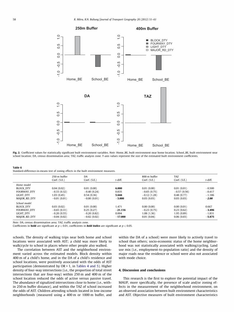
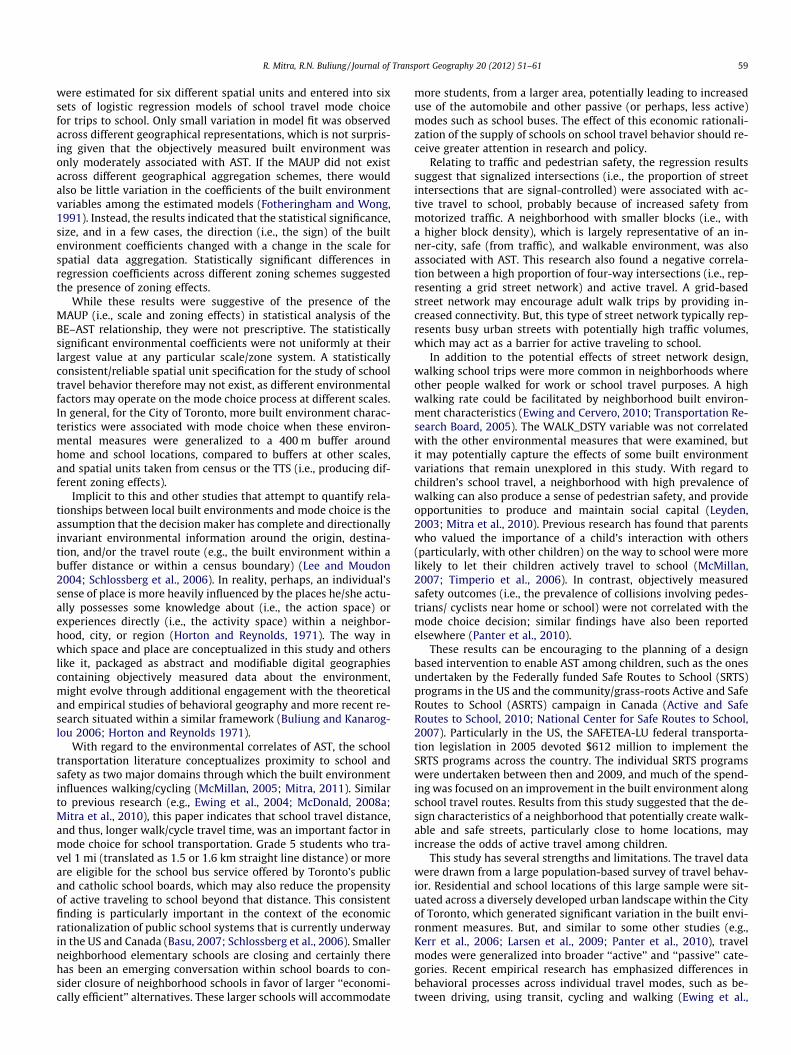
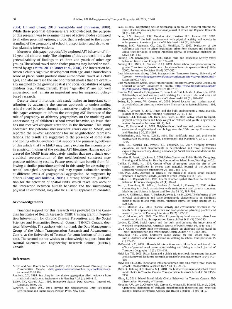
Fig. 2 summarizes the variation in the statistically significantbuilt environment coefficient values across different neighborhooddefinitions. The purpose of this figure was to examine the differ-ence in the coefficient size of a variable, across the scales of mea-surement. Although LOWINCOME was conceptualized in thisstudy as a neighborhood attribute, Fig. 2 focuses specifically onneighborhood design characteristics, and compares estimatedcoefficients for four built environment measures only. None ofthe built environment variables were associated (at p 6 0.05) withAST at the scales of 800 m and 1000 m; these two spatial unitswere therefore not included in this figure. Fig. 2 indicated the pres-ence of scale effects in all built environment measures except MA-JOR_RD_DTY, which was not a statistically significant predictor ofAST at any scale/zone system. Among the three other variables,only FOURWAY_DTY near the school location remained statisti-
cally significant in both 250 m and 400 m models. No other builtenvironment measures were significant (or not-significant) atp 6 0.05 consistently across all scales of geographical aggregation,within each zoning scheme. In addition, the coefficient valuesclearly changed between geographical units of analysis. The figurealso demonstrated that there was no obvious trend in how thecoefficient values changed with geographical scale.
3.2. Zoning effect
The spatial data aggregation methods tested in this study dem-onstrated some zoning effects. Both the statistical significance andsize of the built environment variables changed, somewhat incon-sistently, across different zoning schemes at a comparable scale(e.g., 250 m buffer versus DA) (Tables 4 and 5). In order to examinethe potential zoning effects in further detail, the built environmentcoefficients across spatial units at a similar scale were comparedusing the standard-difference-in-means test [1]. The estimatedcoefficients from the 250 m models were compared with the coef-ficients from the DA models, and the coefficient values from the800 m models were compared with the values obtained from theTAZ models. The results are presented in Table 6. The estimatedcoefficients of half of the built environment variables statisticallyvaried between the two aggregation schemes. No particular pat-tern, however, was present in the observed variation in coefficientestimates. The statistical significance, size and direction of the BE–AST association varied inconsistently between the buffers and cen-sus boundaries at different scales.
3.3. Correlates of AST
All estimated models included the same variables, but the envi-ronmental measures were aggregated based on a different neigh-borhood construct for each set of models. Tables 4 and 5indicated that male students were more likely to use an active tra-vel mode for trips to school. A household’s access to private auto-mobiles was negatively associated with AST. Children were alsomore likely to walk/cycle to school if they lived close to their
250m Buffer 400m Buffer
BLOCK_DTYFOURWAY_DTYLIGHT_DTYMAJOR_RD_DTY
DA TAZ
Home_BE School_BE
-1.0
-0.5
0.0
0.5
1.0
Home_BE School_BE
-1.0
-0.5
0.0
0.5
1.0
Home_BE School_BE-1.0
-0.5
0.0
0.5
1.0
Home_BE School_BE-1.0
-0.5
0.0
0.5
1.0
Fig. 2. Coefficient values for statistically significant built environment variables. Note: Home_BE, built environment near home location; School_BE, built environment nearschool location; DA, census dissemination area; TAZ, traffic analysis zone. Y-axis values represent the size of the estimated built environment coefficients.
Table 6Standard-difference-in-means test of zoning effects in the built environment measures.
250 m buffer DA 800 m buffer TAZCoef. (S.E.) Coef. (S.E.) t-diff. Coef. (S.E.) Coef. (S.E.) t-diff.
Home modelBLOCK_DTY 0.04 (0.02) 0.01 (0.00) 6.000 0.01 (0.00) 0.01 (0.01) �0.500FOURWAY_DTY �0.33 (0.32) �0.40 (0.24) 0.835 �0.65 (0.75) �0.57 (0.56) �0.417LIGHT_DTY 1.03 (0.45) 0.54 (0.36) 5.644 �0.12 (1.28) 0.48 (0.77) �1.186MAJOR_RD_DTY �0.01 (0.01) �0.00 (0.01) �3.000 0.03 (0.03) 0.03 (0.03) �2.00
School modelBLOCK_DTY 0.03 (0.02) 0.01 (0.00) 1.471 0.00 (0.00) 0.00 (0.01) 0.667FOURWAY_DTY �0.65 (0.31) 0.25 (0.27) �21.116 �0.23 (0.75) 0.23 (0.62) �3.496LIGHT_DTY �0.20 (0.55) �0.20 (0.82) 0.004 1.08 (1.36) 1.95 (0.89) �1.831MAJOR_RD_DTY �0.04 (0.02) �0.02 (0.02) �17.000 0.01 (0.04) 0.06 (0.03) �5.875
Note: DA, census dissemination area; TAZ, traffic analysis zone.Coefficients in bold are significant at p 6 0.01, coefficients in bold italics are significant at p 6 0.05.
58 R. Mitra, R.N. Buliung / Journal of Transport Geography 20 (2012) 51–61
schools. The density of walking trips near both home and schoollocations were associated with AST; a child was more likely towalk/cycle to school in places where other people also walked.
The correlation between AST and the neighborhood environ-ment varied across the estimated models. Block density within400 m of a child’s home, and in the DA of a child’s residence andschool locations, were positively associated with the odds of ASTparticipation (demonstrated by OR > 1, in Tables 4 and 5). Higherdensity of four-way intersections (i.e., the proportion of total streetintersections that are four-way) within 250 m and 400 m of theschool location reduced the odds of active versus passive travel.The abundance of signalized intersections close to home (i.e., with-in 250 m buffer distance), and within the TAZ of school increasedthe odds of AST. Children attending schools located in low-incomeneighborhoods (measured using a 400 m or 1000 m buffer, and
within the DA of a school) were more likely to actively travel toschool than others; socio-economic status of the home neighbor-hood was not statistically associated with walking/cycling. Landuse mix (i.e., employment-to-population ratio) and the density ofmajor roads near the residence or school were also not associatedwith mode choice.
4. Discussion and conclusions
This research is the first to explore the potential impact of theMAUP, more specifically, the presence of scale and/or zoning ef-fects in the measurement of the neighborhood environment, onan observed association between built environment characteristicsand AST. Objective measures of built environment characteristics
R. Mitra, R.N. Buliung / Journal of Transport Geography 20 (2012) 51–61 59
were estimated for six different spatial units and entered into sixsets of logistic regression models of school travel mode choicefor trips to school. Only small variation in model fit was observedacross different geographical representations, which is not surpris-ing given that the objectively measured built environment wasonly moderately associated with AST. If the MAUP did not existacross different geographical aggregation schemes, there wouldalso be little variation in the coefficients of the built environmentvariables among the estimated models (Fotheringham and Wong,1991). Instead, the results indicated that the statistical significance,size, and in a few cases, the direction (i.e., the sign) of the builtenvironment coefficients changed with a change in the scale forspatial data aggregation. Statistically significant differences inregression coefficients across different zoning schemes suggestedthe presence of zoning effects.
While these results were suggestive of the presence of theMAUP (i.e., scale and zoning effects) in statistical analysis of theBE–AST relationship, they were not prescriptive. The statisticallysignificant environmental coefficients were not uniformly at theirlargest value at any particular scale/zone system. A statisticallyconsistent/reliable spatial unit specification for the study of schooltravel behavior therefore may not exist, as different environmentalfactors may operate on the mode choice process at different scales.In general, for the City of Toronto, more built environment charac-teristics were associated with mode choice when these environ-mental measures were generalized to a 400 m buffer aroundhome and school locations, compared to buffers at other scales,and spatial units taken from census or the TTS (i.e., producing dif-ferent zoning effects).
Implicit to this and other studies that attempt to quantify rela-tionships between local built environments and mode choice is theassumption that the decision maker has complete and directionallyinvariant environmental information around the origin, destina-tion, and/or the travel route (e.g., the built environment within abuffer distance or within a census boundary) (Lee and Moudon2004; Schlossberg et al., 2006). In reality, perhaps, an individual’ssense of place is more heavily influenced by the places he/she actu-ally possesses some knowledge about (i.e., the action space) orexperiences directly (i.e., the activity space) within a neighbor-hood, city, or region (Horton and Reynolds, 1971). The way inwhich space and place are conceptualized in this study and otherslike it, packaged as abstract and modifiable digital geographiescontaining objectively measured data about the environment,might evolve through additional engagement with the theoreticaland empirical studies of behavioral geography and more recent re-search situated within a similar framework (Buliung and Kanarog-lou 2006; Horton and Reynolds 1971).
With regard to the environmental correlates of AST, the schooltransportation literature conceptualizes proximity to school andsafety as two major domains through which the built environmentinfluences walking/cycling (McMillan, 2005; Mitra, 2011). Similarto previous research (e.g., Ewing et al., 2004; McDonald, 2008a;Mitra et al., 2010), this paper indicates that school travel distance,and thus, longer walk/cycle travel time, was an important factor inmode choice for school transportation. Grade 5 students who tra-vel 1 mi (translated as 1.5 or 1.6 km straight line distance) or moreare eligible for the school bus service offered by Toronto’s publicand catholic school boards, which may also reduce the propensityof active traveling to school beyond that distance. This consistentfinding is particularly important in the context of the economicrationalization of public school systems that is currently underwayin the US and Canada (Basu, 2007; Schlossberg et al., 2006). Smallerneighborhood elementary schools are closing and certainly therehas been an emerging conversation within school boards to con-sider closure of neighborhood schools in favor of larger ‘‘economi-cally efficient’’ alternatives. These larger schools will accommodate
more students, from a larger area, potentially leading to increaseduse of the automobile and other passive (or perhaps, less active)modes such as school buses. The effect of this economic rationali-zation of the supply of schools on school travel behavior should re-ceive greater attention in research and policy.
Relating to traffic and pedestrian safety, the regression resultssuggest that signalized intersections (i.e., the proportion of streetintersections that are signal-controlled) were associated with ac-tive travel to school, probably because of increased safety frommotorized traffic. A neighborhood with smaller blocks (i.e., witha higher block density), which is largely representative of an in-ner-city, safe (from traffic), and walkable environment, was alsoassociated with AST. This research also found a negative correla-tion between a high proportion of four-way intersections (i.e., rep-resenting a grid street network) and active travel. A grid-basedstreet network may encourage adult walk trips by providing in-creased connectivity. But, this type of street network typically rep-resents busy urban streets with potentially high traffic volumes,which may act as a barrier for active traveling to school.
In addition to the potential effects of street network design,walking school trips were more common in neighborhoods whereother people walked for work or school travel purposes. A highwalking rate could be facilitated by neighborhood built environ-ment characteristics (Ewing and Cervero, 2010; Transportation Re-search Board, 2005). The WALK_DSTY variable was not correlatedwith the other environmental measures that were examined, butit may potentially capture the effects of some built environmentvariations that remain unexplored in this study. With regard tochildren’s school travel, a neighborhood with high prevalence ofwalking can also produce a sense of pedestrian safety, and provideopportunities to produce and maintain social capital (Leyden,2003; Mitra et al., 2010). Previous research has found that parentswho valued the importance of a child’s interaction with others(particularly, with other children) on the way to school were morelikely to let their children actively travel to school (McMillan,2007; Timperio et al., 2006). In contrast, objectively measuredsafety outcomes (i.e., the prevalence of collisions involving pedes-trians/ cyclists near home or school) were not correlated with themode choice decision; similar findings have also been reportedelsewhere (Panter et al., 2010).
These results can be encouraging to the planning of a designbased intervention to enable AST among children, such as the onesundertaken by the Federally funded Safe Routes to School (SRTS)programs in the US and the community/grass-roots Active and SafeRoutes to School (ASRTS) campaign in Canada (Active and SafeRoutes to School, 2010; National Center for Safe Routes to School,2007). Particularly in the US, the SAFETEA-LU federal transporta-tion legislation in 2005 devoted $612 million to implement theSRTS programs across the country. The individual SRTS programswere undertaken between then and 2009, and much of the spend-ing was focused on an improvement in the built environment alongschool travel routes. Results from this study suggested that the de-sign characteristics of a neighborhood that potentially create walk-able and safe streets, particularly close to home locations, mayincrease the odds of active travel among children.
This study has several strengths and limitations. The travel datawere drawn from a large population-based survey of travel behav-ior. Residential and school locations of this large sample were sit-uated across a diversely developed urban landscape within the Cityof Toronto, which generated significant variation in the built envi-ronment measures. But, and similar to some other studies (e.g.,Kerr et al., 2006; Larsen et al., 2009; Panter et al., 2010), travelmodes were generalized into broader ‘‘active’’ and ‘‘passive’’ cate-gories. Recent empirical research has emphasized differences inbehavioral processes across individual travel modes, such as be-tween driving, using transit, cycling and walking (Ewing et al.,
60 R. Mitra, R.N. Buliung / Journal of Transport Geography 20 (2012) 51–61
2004; Lin and Chang, 2010; Yarlagadda and Srinivasan, 2008).While these potential differences are acknowledged, the purposeof this research was to examine the use of active modes comparedto all other potential options, a topic that is relevant to the under-standing of the geography of school transportation, and also to ur-ban planning interventions.
Moreover, this paper purposefully explored AST behavior of 11–12 year old children only. The adoption of this approach limits thegeneralizability of findings to children and youth of other agegroups. The school travel mode choice process may indeed be mod-erated by age (Mitra, 2011; Panter et al., 2008). The interaction be-tween a child’s cognitive development with age, and a household’ssense of place, could produce more autonomous travel as a childages, and also increase the use of different modes that are eventu-ally matched to the growing spatial and social capabilities of agingchildren (e.g., taking transit). These ‘‘age effects’’ are not wellunderstood, and remain an important area for empirical, policy-based research.
Despite these limitations, this study makes an important con-tribution by advancing the current approach to understandingschool travel behavior through quantitative analysis. Importantly,this paper attempts to inform the emerging AST literature of therole of geography, or arbitrary geographies, on the modeling andunderstanding of children’s school travel behavior, an issue thathas not received adequate attention in the literature. This studyaddressed the potential measurement errors due to MAUP, andreported the BE–AST associations for six neighborhood represen-tations. The results are suggestive of the presence of some scaleand zoning effects, evidence that supports the primary hypothesisof this article that the MAUP may partly explain the inconsistencyin empirical findings of the existing AST literature. Having not ad-dressed the MAUP issue adequately, studies that use a single geo-graphical representation of the neighborhood construct mayproduce misleading results. Future research can benefit from fol-lowing a similar procedure applied in this study for assessing po-tential ecological uncertainty, and may report estimation resultsat different levels of geographical aggregation. As suggested byothers (Zhang and Kukadia, 2005), a strong behavioral justifica-tion for the selection of spatial units, which takes into accountthe interaction between human behavior and the surroundingphysical environment, may also be a useful approach to consider.
Acknowledgements
Financial support for this research was provided by the Cana-dian Institutes of Health Research (CIHR) training grant in Popula-tion Intervention for Chronic Disease Prevention, and the SocialSciences and Humanities Research Council (SSHRC), Canada, doc-toral fellowship. The authors wish to thank the Data ManagementGroup of the Urban Transportation Research and AdvancementCentre, at the University of Toronto, for contributions of time anddata. The second author wishes to acknowledge support from theNatural Sciences and Engineering Research Council (NSERC),Canada.
References
Active and Safe Routes to School (ASRTS), 2010. School Travel Planning. GreenCommunities Canada. <http://www.saferoutestoschool.ca/schooltravel.asp>(accessed 20.10.10).
Amrhein, C.G., 1995. Searching for the elusive aggregation affect: evidence fromstatistical simulations. Environment & Planning A 27 (1), 105–119.
Bailey, T.C., Gatrell, A.C., 1995. Interactive Spatial Data Analysis, second ed.Longman, Essex, UK.
Banerjee, T., Baer, W.C., 1984. Beyond the Neighborhood Unit: ResidentialEnvironment and Public Policy. Plenum Press, New York.
Basu, R., 2007. Negotiating acts of citizenship in an era of Neoliberal reform: thegame of school closures. International Journal of Urban and Regional Research31 (1), 109–127.
Berke, E.M., Koepsell, T.D., Moudon, A.V., Hoskins, R.E., Larson, E.B., 2007.Association of the built environment with physical activity and obesity inolder persons. American Journal of Public Health 97 (3), 486–492.
Boarnet, M.G., Anderson, C.L., Day, K., McMillan, T., 2005. Evaluation of theCalifornia safe roots to school legislation: urban form changes and children’sactive transportation to school. American Journal of Preventive Medicine 28(2S2), 135–140.
Buliung, R.N., Kanaroglou, P.S., 2006. Urban form and household activity-travelbehavior. Growth and Change 37, 174–201.
Buliung, R.N., Mitra, R., Faulkner, G.E.J., 2009. Active school transportation in thegreater Toronto area, Canada: an exploration of trends in space and time (1986–2006). Preventive Medicine 48 (6), 507–512.
Data Management Group, 2008. Transportation Tomorrow Survey. University ofToronto. <www.dmg.utoronto.ca/transportationtomorrowsurvey/index.html>(accessed 02.07.10).
Data Management Group, 2009.Transportation Tomorrow Survey 2006: Design andConduct of Survey. University of Toronto. <http://www.dmg.utoronto.ca/pdf/tts/2006/conduct2006.pdf> (accessed 03.07.10).
Duncan, M.J., Winkler, E., Sugiyama, T., Cerin, E., duToit, L., Leslie, E., Owen, N., 2010.Relationships of land use mix with walking for transport: do land uses andgeographical scale matter? Journal of Urban Health 87 (5), 782–795.
Ewing, R., Schroeer, W., Greene, W., 2004. School location and student travel:analysis of factors affecting mode choice. Transportation Research Record 1895,55–63.
Ewing, R., Cervero, R., 2010. Travel and the built environment: a meta-analysis.Journal of the American Planning Association 76 (3), 1–30.
Faulkner, G.E.J., Buliung, R.N., Flora, R.K., Fusco, C., 2009. Active school transport,physical activity levels and body weight of children and youth: a systematicreview. Preventive Medicine 48 (1), 3–8.
Filion, P., Hammond, K., 2003. Neighbourhood land use and performance: theevolution of neighbourhood morphology over the 20th century. Environmentand Planning B 20, 271–296.
Fotheringham, A.S., Wong, D.W.S., 1991. The modifiable areal unit problem inmultivariate statistical analysis. Environment and Planning A 23 (7), 1025–1044.
Frank, L.D., Saelens, B.E., Powell, K.E., Chapman, J.E., 2007. Stepping towardscausation: do built environments or neighborhood and travel preferencesexplain physical activity, driving, and obesity? Social Science and Medicine 65,1898–1914.
Frumkin, H., Frank, L., Jackson, R., 2004. Urban Sprawl and Public Health: Designing,Planning and Building for Healthy Communities. Island Press, Washington D.C..
Gehlke, C., Biehl, H., 1934. Certain effects of grouping upon the size of thecorrelation coefficient in census tract material. Journal of the AmericanStatistical Association Supplement 29 (185), 169–170.
Hess, P.M., 2009. Avenues or arterials: the struggle to change street buildingpractices in Toronto, Canada. Journal of urban Design 14 (1), 1–28.
Horton, F.E., Reynolds, D.R., 1971. Effects of urban spatial structure on individualbehavior. Economic Geography 47 (1), 36–48.
Kerr, J., Rosenberg, D., Sallis, J., Saelens, B., Frank, L., Conway, T., 2006. Activecommuting to school: associations with environment and parental concerns.Medicine and Science in Sports and Exercise 38 (4), 787–794.
Larsen, K., Gilliland, J., Hess, P., Tucker, P., Irwin, J., He, M., 2009. The influence of thephysical environment and socio-demographic characteristics on children’smode of travel to and from school. American Journal of Public Health 99 (3),520–526.
Lee, C., Moudon, A.V., 2004. Physical activity and environment research in thehealth field: implications for urban and transportation planning practice andresearch. Journal of Planning Literature 19 (2), 147–181.
Lee, C., Moudon, A.V., 2006. The 3Ds+ R: quantifying land use and urban formcorrelates of walking. Transportation Research Part D 11 (3), 204–215.
Leyden, K., 2003. Social capital and the built environment: the importance ofwalkable neighborhoods. American Journal of Public Health 93, 1546–1551.
Lin, J., Chang, H., 2010. Built environment effects on children’s school travel inTaipei: independence and travel mode. Urban Studies 47 (4), 867–889.
McDonald, N.C., 2008a. Children’s mode choice for the school trip: therole of distance and school location in walking to school. Transportation 35(1), 23–35.
McDonald, N.C., 2008b. Household interactions and children’s school travel: theeffect of parental work patterns on walking and biking to school. Journal ofTransport Geography 16 (5), 324–331.
McMillan, T.E., 2005. Urban form and a child’s trip to school: the current literatureand a framework for future research. Journal of Planning Literature 19 (4), 440–456.
McMillan, T.E., 2007. The relative influence of urban form on a child’s travel mode toschool. Transportation Research Part A 41 (1), 69–79.
Mitra, R., Buliung, R.N., Roorda, M.J., 2010. The built environment and school travelmode choice in Toronto, Canada. Transportation Research Record 2156, 2150–2159.
Mitra, R., 2011. School Travel Mode Choice Behaviour in Toronto, Canada. PhDDissertation, University of Toronto.
Moudon, A.V., Lee, C., Cheadle, A.D., Garvin, C., Johnson, D., Schmid, T.L., et al., 2006.Operational definitions of walkable neighborhood: theoretical and empiricalinsights. Journal of Physical Activity and Health 3 (Suppl. 1), s99–s117.

R. Mitra, R.N. Buliung / Journal of Transport Geography 20 (2012) 51–61 61
National Center for Safe Routes to School, 2007. Safe Routes to School Guide.<http://www.saferoutesinfo.org/guide/> (accessed 12.05.10).
Ontario Professional Planners Institute, 2009. Plan for the Needs of Children andYouth: A Call to Action. OPPI, Ontario, Canada.
Openshaw, S., 1984. The Modifiable Areal Unit Problem. Norwich: Geo Books.<http://qmrg.org.uk/files/2008/11/38-maup-openshaw.pdf>.
Openshaw, S., Alvandies, S., 1999. Applying geocomputation to the analysis ofspatial distributions, . second ed.. In: Longley, L., Goodchild, M., Maguire, D.,Rhind, D. (Eds.), Geograhpic Information Systems: Principles and TechnicalIssues second ed., vol. 1 John Wiley and Sons, Inc New York.
Pampel, F.C., 2000. Logistic Regression: A Primer. Sage Publications, Thousand Oaks,CA.
Panter, J.R., Jones, A.P., van Sluijs, E.M.F., 2008. Environmental determinants ofactive travel in youth: a review and framework for future research.International Journal of Behavioral Nutrition and Physical Activity 5 (34).doi:10.1186/1479-5868-5-34.
Panter, J.R., Jones, A.P., Van Sluijs, E.M.F., Griffin, S.J., 2010. Neighborhood, route, andschool environments and children’s active commuting. American Journal ofPreventive Medicine 38 (3), 268–278.
Perry, C.A., 1939. Housing for the Machine Age. Russel Sage Foundation, New York.Pont, K., Ziviani, J., Wadley, D., Bennett, S., Abbott, R., 2009. Environmental
correlates of children’s active transportation: a systematic literature review.Health and Place 15, 849–862.
Schlossberg, M.J., Greene, P., Phillips, P., Johnson, B., Parker, B., 2006. School trips:effects of urban form and distance on travel mode. Journal of the AmericanPlanning Association 72 (3), 337–346.
Sewell, J., 1993. The Shape of the City: Toronto Struggles with Modern Planning.University of Toronto Press, Toronto.
Sirard, J.R., Slater, M.E., 2008. Walking and bicycling to school: a review. AmericanJournal of Lifestyle Medicine 2 (5), 372–396.
Statistics Canada, 2008. Population and Dwelling Counts, for Canada, Provinces andTerritories, and Census Divisions, 2006 and 2001 Censuses – 100% Data. <http://www12.statcan.ca/english/census06/data/popdwell/Table.cfm?T=702&PR=35&S=0&O=A&RPP=25> (accessed 05.07.10).
Statistics Canada, 2010. Low Income Cut-offs for 2006 and Low Income Measuresfor 2005. <http://www.statcan.gc.ca/bsolc/olc-cel/olc-cel?lang=eng&catno=75F0002M2007004> (accessed 05.07.10).
Timperio, A., Ball, K., Salmon, J., Roberts, R., Giles-Corti, B., Simmons, D., et al., 2006.Personal, family, social, and environmental correlates of active commuting toschool. American Journal of Preventive Medicine 30 (1), 45–51.
Transportation Research Board, 2005. Does the Built Environment InfluencePhysical Activity? Examining the Evidence. Transportation Research BoardSpecial Report No. 282, Washington, D.C.
US Department of Health and Human Services, 1996. Physical Activity and Health: AReport of the Surgeon General. Centers for Disease Control and Prevention,National Center for Chronic Disease Prevention and Health Promotion, Atlanta,GA.
US Department of Health and Human Services, 2009. Proposed Healthy People 2020Objectives. <http://www.healthypeople.gov/hp2020/objectives/TopicAreas.aspx>(accessed 12.05.10).
Yarlagadda, A.K., Srinivasan, S., 2008. Modeling children’s school travel mode andparental escort decisions. Transportation 35 (2), 201–218.
Zhang, M., Kukadia, N., 2005. Metrics of urban form and modifiable areal unitproblem. Transportation Research Record 1902, 71–79.