100 SUMMER STREET, SUITE 3200BOSTON, MASSACHUSETTS 02110

TEL 617-531-2818FAX 617-531-2826

Broadwater LNG A Technical Assessment

Market, Technology, Environmental and Safety Related Impacts

in New York State

Long Island Power Authority

July 2007

LIMITATION ON LIABILITY

This report has been prepared by Levitan & Associates, Inc. (LAI) for the Long Island Power Authority solely for the purpose of conducting an independent assessment of the proposed Broadwater LNG terminal. LAI’s observations and technical findings pertaining to Broadwater’s market and economic impacts depend on the assumptions and inputs to various engineering, economic and mathematical models. Economic results reported in this study are based on market, economic, and regulatory information available to LAI through July 31, 2005. While LAI believes that all factor input assumptions to various models are reasonable, there is no assurance that any specific set of assumptions will occur over the planning horizon.

In conducting technology and safety related due diligence, LAI relied on publicly available documents for the Safety Review and the Technology Review of the Broadwater Project. Any documents marked “Privileged and Confidential,’ “Critical Energy Infrastructure Information” or “Sensitive Security Information” were not available to LAI, and therefore not reviewed by LAI. LAI does not assume any liability for potential inconsistencies or discrepancies between non-public and public information related to the Broadwater Project.

In conducting environmental related due diligence, LAI relied upon field data collected by Broadwater and submitted to the Federal Energy Regulatory Commission and other environmental data in the public domain. LAI did not undertake any independent field sampling or monitoring.

LAI does not make any warranty, expressed or implied, and does not assume any liability with respect to the use of information or methods disclosed in this report.

ACKNOWLEDGEMENTS

Levitan & Associates, Inc. would like to thank the following entities for their invaluable assistance and cooperation throughout this study. The entities referenced below provided Levitan & Associates, Inc. with technical information incorporated in this study. The findings and observations herein are solely and strictly the professional opinion of Levitan & Associates, Inc. and therefore do not necessarily constitute the views of the companies, regulatory or governmental entities, and trade associations acknowledged below.

Consolidated Edison Company

Connecticut Department of Environmental Protection, Marine Fisheries Division

Giuliani Partners

Iroquois Gas Transmission System

KeySpan Energy

Long Island Power Authority

National Fuel Gas

New York State Department of Environmental Conservation

Northeast Gas Association

Sandia National Laboratory

United States Coast Guard

July 2007

Richard M. Kessel, President & Chief Executive Officer Long Island Power Authority 333 Earle Ovington Blvd., Suite 403 Uniondale, New York 11553

Re: Due Diligence - Broadwater LNG Import Terminal

Dear Mr. Kessel,

Levitan & Associates, Inc. (LAI) is pleased to submit to the Long Island Power Authority (LIPA) the results of the due diligence performed on the proposed Broadwater liquefied natural gas (LNG) terminal in Long Island Sound. Over the last two year, LAI has conducted an independent and objective assessment of Broadwater’s impact in New York State, including Long Island Sound. While we have exercised best efforts to take advantage of the vast body of scientific knowledge pertaining to the LNG industry, specifically, the information base related to the Broadwater project, the observations and findings expressed herein are solely the opinion of LAI. Hence, the opinions and conclusions stated in this report represent LAI’s view on Broadwater’s impact in New York State and therefore should not be misconstrued as representative of any other entity’s position on the array of research activities presented herein.

From a New Yorker’s perspective, we have evaluated the market, economic, environmental, and safety related impacts associated with Broadwater’s development of an 8 billion cubic foot floating storage and regasification unit, the largest of its kind, anywhere in the world. Emphasis is placed on the derivation of the expected economic benefits ascribable to Broadwater in the first ten years of the Project’s economic life relative to what New Yorkers would otherwise be expected to pay for natural gas and electricity when the region’s gas supply originates from other supply sources. We have also considered a number of performance and operational attributes pertaining to Broadwater’s design scale-up of conventional floating oil and LNG storage technology components employed by global energy companies elsewhere in the world.

This report is the culmination of technical research largely conducted by LAI from May 2005 through May 2006, augmented by additional analysis performed through July 2007. Following the main body of the report is a chapter wherein LAI provides a regulatory update of Broadwater’s status based on information since June 2006 made available by the Federal Energy Regulatory Commission (FERC), the U.S. Coast Guard, the Government Accountability Office and other agencies.

In conducting this analysis, LAI relied on financial, safety / security, and environmental information in the public domain. We also relied on Broadwater’s certificate application at FERC. LAI consulted with state and federal agency representatives, Iroquois Gas

Richard M. Kessel, President and Chief Executive Officer July 2007 Page 2

Transmission, Consolidated Edison Company, and KeySpan Energy, as well as Broadwater’s staff, including third party advisors. Of critical importance, we note that the Broadwater docket at FERC, relevant U.S. Coast Guard reports, records of public meetings, and other scientific reports number in the thousands of documents. Given the size of the information base, we did not attempt to summarize or otherwise evaluate the file in its totality. Instead, we centered our research on the economic and scientific questions believed to be of vital interest to stakeholders on Long Island and, to a lesser extent, New York City, especially environmental impacts during both the construction and operational phase, and long term safety concerns under an array of hypothetical contingency events.

I would like to recognize the ongoing support and responsiveness of LIPA’s staff, other utilities doing business in New York, as well as the invaluable assistance of various regulatory bodies, without whom LAI would not have been able to meet the goals and objectives set forth in this study. LAI’s project team is available to meet with you and LIPA staff at your convenience to address any areas requiring clarification or additional technical insight.

On behalf of the entire LAI project team, thank you for the privilege of this engagement.

Sincerely yours,

Richard L. Levitan President

cc: Kevin Law Richard Bolbrock Lynda Nicolino

TABLE OF CONTENTS

Introduction

Executive Summary

1. Project Description

2. Market & Economics 2.1. Natural Gas Market Analysis........................................................................................... 5

2.1.1 Introduction............................................................................................................. 5 2.1.2 Market Modeling Approach.................................................................................... 7 2.1.3 Key Factor Inputs for the Business-as-Usual Case................................................. 8 2.1.4 Natural Gas Supply in North America.................................................................... 9 2.1.5 LNG Import Terminals ......................................................................................... 15 2.1.6 New LNG Import Terminals................................................................................. 17 2.1.7 Interstate Pipeline Network................................................................................... 18 2.1.8 Regional Natural Gas Demand ............................................................................. 22 2.1.9 Alternate Infrastructure Cases Tested in GPCM .................................................. 26 2.1.10 Backcast Analysis to Ensure Model Validity ....................................................... 26

2.2. Electric Market Simulation Analysis ............................................................................. 27 2.2.1 Role of Market Simulation in Overall Market Analysis....................................... 27 2.2.2 MarketSym Topology ........................................................................................... 28 2.2.3 Transmission Linkages ......................................................................................... 29 2.2.4 Generation and Load Data .................................................................................... 30 2.2.5 Regional Transmission Expansion Plans .............................................................. 31 2.2.6 Capacity Values and Entry / Exit.......................................................................... 31 2.2.7 NYISO ICAP Demand Curve Mechanism ........................................................... 32 2.2.8 PJM Reliability Pricing Model ............................................................................. 33 2.2.9 ISO-NE Capacity Market...................................................................................... 33 2.2.10 New York Renewable Portfolio Standard............................................................. 34 2.2.11 Emissions Assumptions and Allowance Prices .................................................... 34

2.3. Market Analysis Results ................................................................................................ 36

2.4. Benefits Attributable to Broadwater .............................................................................. 42 2.4.1 Gas Utility and Electric Utility Benefits on Long Island, NYC and Rest of State42 2.4.2 Economic Multiplier Analysis .............................................................................. 46 2.4.3 Discussion of Net Benefits.................................................................................... 47 2.4.4 Benefits Reconciliation......................................................................................... 47 2.4.5 Omitted Variables ................................................................................................. 48

3. Technology Review 3.1. Offshore LNG Technology Options .............................................................................. 50

3.1.1 Cabrillo Port.......................................................................................................... 53 3.1.2 Excelerate Gulf Gateway ...................................................................................... 54 3.1.3 Gulf Landing......................................................................................................... 56

3.2. Technology Components ............................................................................................... 57 3.2.1 Containment System ............................................................................................. 59 3.2.2 Mooring System Technology................................................................................ 63 3.2.3 Cargo Transfer ...................................................................................................... 65 3.2.4 Regasification Process .......................................................................................... 68 3.2.5 Boil-off.................................................................................................................. 70 3.2.6 Emergency Shutdown System .............................................................................. 71 3.2.7 Custody Transfer................................................................................................... 71

3.3. Summary of Findings..................................................................................................... 72

4. Environmental Review 4.1. Potential Impacts to Marine Plants and Animals........................................................... 75

4.1.1 Overview of Marine Plant and Animal Resources in Long Island Sound............ 75 4.1.2 Potential Construction Related Impacts................................................................ 81 4.1.3 Potential Impacts During Project Operations ....................................................... 88

4.2. Potential Impacts to Commercial and Recreational Fishing.......................................... 93 4.2.1 Commercially Important Marine Resources......................................................... 93 4.2.2 Potential Impacts from Construction and Operation ............................................ 94

4.3. Commercial Shipping in Long Island Sound................................................................. 95

5. Safety Review 5.1. LNG Properties ............................................................................................................ 100

5.2. LNG Hazards ............................................................................................................... 103

5.3. LNG Accident History................................................................................................. 107

5.4. Sandia Report............................................................................................................... 109 5.4.1 LNG Spill and Dispersion Experiments ............................................................. 114 5.4.2 Recent LNG Spill Modeling Review.................................................................. 115 5.4.3 Sandia Report Recommended Safety Zones....................................................... 116

5.5. Safety and Security Implementation............................................................................ 117 5.5.1 Gulf Landing Hazard Analysis ........................................................................... 118 5.5.2 Gulf Gateway Hazard Analysis .......................................................................... 118 5.5.3 Main Pass Energy Hub Hazard Analysis ............................................................ 119

5.6. Analysis of Revised Cabrillo Port DEIS (March 2006)............................................... 119 5.6.1 Public Safety: Overview ..................................................................................... 120 5.6.2 Independent Risk Assessment............................................................................. 121 5.6.3 Sandia Review of Independent Risk Assessment ............................................... 125

5.7. Resource Report 11 – Safety and Reliability............................................................... 127 5.7.1 LNG Safety ......................................................................................................... 128

5.8. Other Technical Experts on LNG Safety ..................................................................... 132

5.9. Safety Review Issues ................................................................................................... 132 5.9.1 Safety Parameter Modeling Issues...................................................................... 132 5.9.2 Cascading Event Analysis................................................................................... 133 5.9.3 LAI Extrapolations to Worst-Case Scenario....................................................... 134

5.10. Safety Review Findings ............................................................................................... 135

6. Regulatory Status Update 6.1. Interventions ................................................................................................................ 138

6.1.1 County of Suffolk Intervention........................................................................... 138

6.2. Conferences and Meetings........................................................................................... 139

6.3. U.S. Coast Guard Waterways Suitability Report......................................................... 139 6.3.1 LAI Review of USCG Findings.......................................................................... 139

6.4. Draft Environmental Impact Statement (November 17, 2006).................................... 147 6.4.1 FSRU Reliability and Safety Issues.................................................................... 148 6.4.2 LNG Carrier Reliability and Safety Issues ......................................................... 149 6.4.3 Environmental..................................................................................................... 150

6.5. GAO Report (released on March 14, 2007)................................................................. 153

6.6. MARAD’s Decision on the Cabrillo Port Project........................................................ 154

6.7. New York State Department of State Request for Additional Alternatives Analysis . 155

6.8. Certifying Entity .......................................................................................................... 157

LIST OF EXHIBITS

1. North-South Supply Breakdown for New York State

2. Relative Trends in Shallow and Deepwater Gulf Production

3. Production Isograms for Selected Producing Regions

4. Capital Cost for a New Plant in New York City or Long Island

5. Resource Additions Included in Electric Simulation Model

6. RPS Capacity Additions and Annual Targets

7. Price Effects at Regional Pricing Points

8. Calculation Framework for Economic Benefits

9. Cabrillo Port Summary of FSRU Accident Consequences

LIST OF APPENDICES

1. GPCM Model Theory and Structure

2. Basin Production Curves

3. Fuel Price Forecasts

4. Emissions Allowance Price Forecasts

5. Application Review, including Resource Reports

6. Det Norske Veritas: Broadwater Response to USCG Letter

7. Det Norske Veritas Fire Modeling

8. List of FERC Interveners

TABLE OF FIGURES∗

Figure 1 – FSRU Location and Area Infrastructure........................................................................ 1

Figure 2 – Broadwater FSRU Offshore Terminal........................................................................... 2

Figure 3 – Overview of Broadwater Market Analysis Modeling Process ...................................... 7

Figure 4 –U.S. Natural Gas Production, Consumption and Imports ............................................ 11

Figure 5 – Normalized Gas Production per Well from Gas Wells ............................................... 12

Figure 6 – Basin Production Curves ............................................................................................. 14

Figure 7 – Proved Natural Gas Reserves (2004, Tcf) ................................................................... 16

Figure 8 – Gas Pipelines Serving New York State and the Greater Northeast............................. 19

Figure 9 – Average Monthly Iroquois Deliveries to Long Island and New York City ................ 20

Figure 10 – New York State Gas Use by Sector (2005) ............................................................... 23

Figure 11 – GPCM Backcast Analysis of TZ6-NY Prices ........................................................... 27

Figure 12 – Power System Model Interfaces................................................................................ 28

Figure 13 – Geographic Overview of Market Topology .............................................................. 29

Figure 14 – Estimated Transfer Capabilities, Peak Loads, and Capacities .................................. 30

Figure 15 – Commodity Price Changes at the Henry Hub: BAU v. Alternative Cases .............. 37

Figure 16 – Commodity Price Changes at the Dawn Storage Hub: BAU v. Alternative Cases.. 38

Figure 17 – TZ6-NY Price Change: BAU v. Alternative Cases.................................................. 38

Figure 18 – IGTS-Z2 Price Change: BAU v. Alternative Cases ................................................. 39

Figure 19 – Henry Hub Price Comparison: LNG Overbuild Case ............................................... 40

Figure 20 – Dawn Price Comparison: LNG Overbuild Case ....................................................... 40

Figure 21 – TZ6-NY Price Comparison: LNG Overbuild Case ................................................... 41

Figure 22 – IGTS Z2 Price Comparison: LNG Overbuild Case................................................... 41

Figure 23 – Core Benefits Attributable to Broadwater by Year ................................................... 44

Figure 24 – Core Benefits Attributable to Broadwater by Sub-Area............................................ 44

Figure 25 – Non-Core Benefits Attributable to Broadwater by Year........................................... 45

Figure 26 – Non-Core Benefits Attributable to Broadwater by Sub-Area ................................... 46

Figure 27 – Illustration of Offshore LNG Facility Types............................................................. 51

Figure 28 – Growth Pattern for LNG Vessel Size ........................................................................ 52

∗ Does not include Executive Summary.

Figure 29 – Cabrillo Deepwater Port FSRU................................................................................. 54

Figure 30 – Illustration of STL Technology................................................................................. 55

Figure 31 – LNG Tanker Serving Gulf Gateway Terminal.......................................................... 56

Figure 32 – Illustration of Gulf Landing Terminal....................................................................... 57

Figure 33 – Detail of Broadwater FSRU Offshore Terminal ....................................................... 58

Figure 34 – Proposed Yoke Mooring System............................................................................... 63

Figure 35 – Turret Mooring System ............................................................................................. 64

Figure 36 – Proposed Mooring Tower Structure .......................................................................... 65

Figure 37 – FSRU with Moored LNG Carrier.............................................................................. 66

Figure 38 – Chicksan Unloading Arms ........................................................................................ 68

Figure 39 – Closed-Loop Shell and Tube Vaporizer Configuration............................................. 69

Figure 40 – Generalized Boil-Off Process.................................................................................... 70

Figure 41 – Vessel Traffic Density............................................................................................... 96

Figure 42 – Vessel Tracks in the Vicinity of the FSRU ............................................................... 97

Figure 43 – Shipments To or From Long Island Sound Ports ...................................................... 98

Figure 44 – Flammability Limits for Selected Fuels .................................................................. 102

Figure 45 – Relative Detonation Properties of Common Fuels.................................................. 103

Figure 46 – Sequence of Events Following a Spill..................................................................... 104

Figure 47 – Radiation Effects on Naked Skin ............................................................................ 105

Figure 48 – LNG tanker in Charlestown on its way out of Boston ........................................... 107

Figure 49 – Sandia Report Radiative Flux.................................................................................. 112

Figure 50 – Sandia Report Vapor Dispersion Distances to LFL ................................................ 114

Figure 51 – Sandia Report Safety Zones .................................................................................... 117

Figure 52 – Cabrillo Deepwater Port: Consequence Distances .................................................. 121

Figure 53 – Sandia Calculation of Pool Fire Hazards................................................................. 126

Figure 54 – View of FSRU from Roanoke Landing................................................................... 127

Figure 55 – Anticipated LNG carrier transit route with Zone 1, Zone 2 and Zone 3 ................. 141

Figure 56 – LNG Carrier Anticipated Transit Route and Hazard Zones – The Race................. 143

Figure 57 – LNG Carrier Anticipated Transit Route and Hazard Zones.................................... 144

Figure 58 – Alternative Terminal Sites and Pipeline Routes Considered by Broadwater.......... 156

TABLE OF TABLES∗

Table 1 – North American Supply Region and Basin Production and Proved Reserves ............. 15

Table 2 – LNG Import Terminals in the Business-as-Usual Case................................................ 18

Table 3 – Delivery Areas of Gas Pipelines Serving New York State........................................... 19

Table 4 – Gas Customers by Utility in New York State............................................................... 23

Table 5 – Gas Sales by Utility in New York State ....................................................................... 24

Table 6 – Sources of Load Data Information................................................................................ 31

Table 7 – Average 10-Year Price Results by Case ....................................................................... 42

Table 8 – Market Center Pricing Points........................................................................................ 43

Table 9 – Summary of LAI’s Economic Findings........................................................................ 47

Table 10 – Summary of Offshore LNG Project Specifications .................................................... 53

Table 11 – Containment System Parameters ................................................................................ 61

Table 12 – 2003 Commercial Vessel Traffic To and From Ports in CT and Long Island............ 99

Table 13 – LNG Compositions by Source.................................................................................. 101

Table 14 – Common Approximate Thermal Radiation Damage Levels .................................... 106

Table 15 – Sandia Report Thermal Intensity Level Distances ................................................... 111

Table 16 – Sandia Report Vapor Dispersion Distances to LFL.................................................. 113

Table 17 – Sandia Report Safety Zones...................................................................................... 116

Table 18 – Safety Implementation for other Offshore Projects .................................................. 118

Table 19 – Summary of Consequence Distances........................................................................ 125

Table 20 – Populations in Proximity to LNG Terminals............................................................ 128

Table 21 – Weather and Sea Condition Limits for LNG Carrier Transit ................................... 131

Table 22 – Broadwater Hazard Zones ........................................................................................ 140

Table 23 – Ranked Navigation Safety Events ............................................................................ 146

∗ Does not include Executive Summary.

GLOSSARY

ABS American Bureau of Shipping

ACE Analytical and Computational Energetics, Inc.

ADRP Acid Deposition Reduction Program

AEO Annual Energy Outlook

AEP American Electric Power

APE Area of Potential Effect

APS Allegheny Power System

AQCR Air Quality Control Act

ATBA Area to be Avoided

BAU Business-as-Usual

Bcf(/d) Billion cubic feet (per day)

BLEVE Boiling Liquid Expanding Vapor Explosion

BP Beyond Petroleum (formerly British Petroleum)

CAA Clean Air Act

CAIR Clean Air Interstate Rule

CAPP Central Appalachia

CCMP Comprehensive Conservation and Management Plan

CEC California Energy Commission

CFD Computational Fluid Dynamics

CFR Code of Federal Regulations

CHG&E Central Hudson Gas and Electric

CO2 Carbon Dioxide

CSLC California State Lands Commission

CTDEP Connecticut Department of Environmental Protection

DAM Day-Ahead Market

DEIR Draft Environmental Impact Report

DEIS Draft Environmental Impact Statement

DNV Det Norske Veritas

DO Dissolved Oxygen

DOE Department of Energy

DP Dynamically Positioned

Dth Dekatherm

DTI-SP Dominion South Point

E&P Exploration and Production

EBP Early Benthic Phase

EEA Energy and Environmental Analysis, Inc.

EFH Essential Fish Habitat

EIA Energy Information Agency

EIS Environmental Impact Statement

EPA Environmental Protection Agency

ESA Endangered Species Act

FCM Forward Capacity Market

FDS Fire Dynamics Simulator

FEIS Final Environmental Impact Statement

FERC Federal Energy Regulatory Commission

FDG Flue Gas Desulfurization

FOB Free on Board

FPSO Floating Production, Storage and Offloading

FRU Floating Regasification Unit

FSRU Floating Storage and Regasification Unit

FSU Former Soviet Union

GAO Government Accountability Office

GBS Gravity-Based Structure

GPCM Gas Pipeline Competition Model

HAP Hazardous Air Pollutant

HAZID Hazard Identification Study

HDD Horizontal Directional Drilling

ICAP Installed Capacity

IGTS-Z2 Iroquois Gas Transmission System Zone 2

IRA Independent Risk Assessment

ISO Independent System Operator

ISO-NE Independent System Operator – New England

KEDLI KeySpan Energy Delivery – Long Island

KEDNY KeySpan Energy Delivery – New York

km Kilometer

kW kilowatt

kW/m2 kilowatts per meter squared

LAI Levitan & Associates, Inc.

LDC Local Distribution Company

LFL Lower Flammability Limit

LICAP Locational Installed Capacity

LIPA Long Island Power Authority

LISS Long Island Sound Study

LLNL Lawrence Livermore National Laboratory

LNG Liquefied Natural Gas

LP Linear Programming

LSE Load-Serving Entity

M&N Maritimes and Northeast

m Meter

m2 Square meters

m3 Cubic meters

MAAC Mid-Atlantic Area Council

MACT Maximum Achievable Control Technology

MADMF Massachusetts Division of Marine Fisheries

MARAD Maritime Administration

MDth(/d) Thousand Dekatherms (per day)

mg/L Milligrams per liter

MMBtu Million British thermal units

MMcf(/d) Million cubic feet (per day)

MPA Marine Protected Area

MW Megawatt

MWh Megawatt hour

NAA No Anchoring Area

NAPP Northern Appalachia

NEB National Energy Board

NEI Nuclear Energy Institute

NEPA National Environmental Policy Act

NFGDC National Fuel Gas Distribution Corporation

NFPA National Fire Protection Association

NGA Northeast Gas Association

NGPA Natural Gas Policy Act

NMFS National Marine Fisheries Service

NMPC Niagara Mohawk Power Corporation

NOAA National Oceanic and Atmospheric Administration

NOx Nitrogen oxides

NWC Naval Weapons Center

NYCA New York Control Area

NYCRR New York State Codes Rules and Regulations

NYFS New York Facilities System

NYH New York Harbor

NYISO New York Independent System Operator

NYMEX New York Mercantile Exchange

NYPSC New York Public Service Commission

NYSDEC New York State Department of Environmental Conservation

NYSDOS New York State Department of State

NYSEG New York State Electric and Gas

NYSERDA New York State Energy Research and Development Authority

NYSOGS New York State Office of General Services

O&R Orange and Rockland

OPEC Organization of the Petroleum Exporting Countries

ORV Open Rack Vaporizer

OTC Ozone Transport Commission

PFSP Preliminary Facility Security Plan

PJM PJM Interconnection

PILOT Payments in Lieu of Taxes

ppm Parts per million

PSD Prevention of Significant Deterioration

psi Pounds per square inch

PSVA Preliminary Security and Vulnerability Assessment

R/P Reserves to Production ratio

RFO Residual Fuel Oil

RG&E Rochester Gas & Electric

RGGI Regional Greenhouse Gas Initiative

RPM Reliability Pricing Model

RPS Renewable Portfolio Standard

RPT Rapid Phase Transition

RTEP Regional Transmission Expansion Plan

Sandia Sandia National Laboratories

SCADA Supervisory Control and Data Acquisition

SCR Selective Catalytic Reduction

SCV Submerged Combustion Vaporizer

SEQRA State Environmental Quality Review Act

SIP State Implementation Plan

SNCR Selective Non-Catalytic Reduction

SPCC Spill Prevention, Control and Countermeasure

SPDES State Pollutant Discharge Elimination System

SRV Shuttle Regasification Vessel

STL Submerged Turret Loading

STV Shell and Tube Vaporizer

SVA Security and Vulnerability Assessment

Tcf Trillion cubic feet

tpy Tons per year

TSS Total Suspended Solids

TZ6-NY Transco Zone 6 – New York

UCAP Unforced Capacity

UFL Upper Flammability Limit

USACE U.S. Army Corps of Engineers

USCG U.S. Coast Guard

VOC Volatile Organic Compound

VP Virginia Power

WCSB Western Canada Sedimentary Basin

WHRU Waste Heat Recovery Unit

WSR Waterways Suitability Report

WTI West Texas Intermediate

YMS Yoke Mooring System

INTRODUCTION

Broadwater Energy, LLC (Broadwater or the “Project”), is a joint venture between TransCanada Corporation and Royal Dutch Shell. TransCanada is one of the largest energy companies in North America, primarily known for its natural gas gathering and pipeline system from Alberta to eastern Canada. Royal Dutch Shell is a global oil and gas company – one of the largest suppliers of liquefied natural gas (LNG) around the world. Broadwater has proposed to build a Floating Storage and Regasification Unit (FSRU) to be permanently moored in the middle of Long Island Sound. Like other land-based LNG import terminals elsewhere on the Atlantic seaboard, the FSRU would receive LNG cargoes from overseas liquefaction plants and would have a large storage capacity in order to maintain adequate inventory in the event LNG tankers are delayed either crossing the Atlantic Ocean or entering Long Island Sound. Over 1,200 feet in length, 200 feet in width, and 80 feet above the water line, the FSRU is designed to hold eight separate tanks, a total capacity of 8 billion cubic feet (Bcf). An FSRU of the scale contemplated for Long Island Sound has not been commercialized elsewhere in the world. It therefore represents a substantial scale-up of conventional LNG and floating oil storage technology that has been used by global energy companies for decades.

The FSRU would help meet energy demand throughout the Northeast via a 21.7-mile long subsea pipeline that would connect to a marine tap on the existing Iroquois Gas Transmission System (Iroquois). The Iroquois mainline extends from upstate New York through western Connecticut and across the Sound to Long Island. Iroquois also has a separate high-pressure marine lateral, Eastchester, which connects the north shore of Long Island to New York City. The mainline tap on Iroquois would be located due west of the FSRU in the middle of Long Island Sound. Broadwater expects that the Project would be capable of operating near continuously at a production rate of 1.0 Bcf/d. Broadwater’s proposed in-service date for the Project is late 2010.

In May 2005, the Long Island Power Authority (LIPA) asked Levitan & Associates, Inc. (LAI) to conduct due diligence on Broadwater’s potential market and economic impacts, as well as to address highlights of the proposed technology. LAI also conducted an assessment of Broadwater’s environmental impacts and safety considerations. The assessment conducted herein constitutes an independent and objective assessment of the Project from a New Yorker’s perspective.

From a market and economics standpoint, we have quantified the expected economic benefits ascribable to Broadwater for Long Island, New York City, and Rest of State consistent with Broadwater’s proposed regasification of 1 Bcf/d. Over the ten-year planning horizon, 2010-2020, we have held Broadwater’s operating regime constant in order to derive the economic impact attributable to the Project when its daily output is treated as a baseload gas supply for redelivery across the New York Facilities System (NYFS). The NYFS is the network of local transmission and distribution mains owned and operated by Con Edison and KeySpan to serve gas utility loads and power plants throughout the region. We have conducted a sensitivity analysis in order to gauge the potential value to New York associated with alternatives including pipeline expansions and/or rival LNG import terminals that have been proposed in New England or New Jersey.

ii

From a technology standpoint, we have compared Broadwater’s proposed FSRU to other offshore LNG facilities. We have considered the integrity of the yoke mooring system to the stationary tower in 90 feet of water, and the delivery logistics associated with replenishment of the inventory of LNG stored on the FSRU via LNG carriers that would be escorted by the United States Coast Guard (USCG) through The Race to the FSRU each week. The technology review was based on the draft and final Environmental Impact Statements (EISs) from other proposed and approved LNG projects, industry LNG technology presentations and papers and publicly available reports on LNG technology.

From an environmental standpoint, we have assessed the potential impacts to marine plants and animals during the construction period and the long-term operational phase. We have also evaluated the effectiveness and feasibility of mitigation methods proposed by Broadwater in light of observations at similar projects in Long Island Sound and other marine sites. Finally, we have considered the potential impacts of the Project on boating and commercial fishing, and on other marine traffic in Long Island Sound, including The Race. Our environmental review is based on the Resource Reports and other documents submitted by Broadwater to the Federal Energy Regulatory Commission (FERC), other publicly available reports pertaining to Long Island Sound, and discussions with state officials. LAI also researched post-construction monitoring reports prepared for other marine infrastructure projects constructed in Long Island Sound, and similar marine habitats in the Northeast. The scope of this review encompassed the potential impacts arising from the construction of the 21.7-mile pipeline from the FSRU to the Iroquois mainline, the construction of the yoke mooring system tower and riser pipe, and the operation of the pipeline, FSRU, and LNG cargo vessels.

From a safety standpoint, we have assessed the magnitude of various hazards associated with LNG, including the likely results under a number of postulated bad events. We researched the impact of LNG spills over water for both accidental and intentional events based on both experimental and modeling studies performed by others. We also evaluated safety zones established or proposed for other LNG projects. Finally, we reviewed the Resource Report on Safety and Reliability in Broadwater’s application to FERC. In performing the safety review, LAI relied upon publicly available information developed by Broadwater, as well as other technical studies performed on similar energy projects elsewhere in the U.S. and Canada, in particular, the Cabrillo Deepwater Port (Cabrillo Port) project proposed to be located about 14 miles off the southern California coast. LAI reviewed a technical report issued by Sandia National Laboratories (Sandia) under contract to the U.S. Department of Energy (DOE), on the risk analysis and safety implications of a large LNG spill over water – Sandia has been doing research on nuclear weapons, military technology and homeland security since 1949. LAI assessed the impact of an LNG spill over water based on both experimental and modeling studies referenced by Sandia.

Unless otherwise noted, the observations and findings presented in this report were the product of due diligence conducted from May 2005 through May 2006. LAI’s assessment was conducted after Broadwater filed its Resource Reports at FERC on January 30, 2006, but prior to FERC’s issuance of the Draft EIS (DEIS) on November 17, 2006, the USCG’s issuance of the Waterways Suitability Report (WSR) on September 21, 2006 and the Government Accountability Office’s (GAO’s) maritime security report on March 14, 2007. LAI’s review of

iii

these documents is incorporated in the final section of this report, as an update of the regulatory status of the Project.

EXECUTIVE SUMMARY

The highlights of LAI’s due diligence on market / economics, technology, environmental, and safety are presented by topical area.

Market & Economics

The objectives of LAI’s market and economic analysis were threefold: first, to quantify the economic benefits reasonably ascribable to Broadwater over the ten-year planning horizon for gas utility and electricity customers on Long Island, in New York City and Rest of State; second, to compare the economic benefits associated with Broadwater to other potential pipeline enhancements and/or rival LNG import terminals proposed elsewhere in the Northeast; and, third, to identify noteworthy commercial considerations and risk factors that bear upon the economic merits / demerits of the Broadwater project.

North America is not running out of natural gas. It is just more difficult and therefore costly for gas producers to keep pace with demand. While natural gas supplies across North America are growing ever tighter due to accelerated maturation effects in conventional producing basins – in particular, the Gulf Coast and western Canada – new production will likely be very expensive in ultra deepwater in the Gulf of Mexico, the Mackenzie Delta in northern Canada, and Alaska. In the U.S., the brightest spot production-wise is unconventional production from the Rocky Mountains, but New York is too far away for production in the Rocky Mountains to matter much. Even stellar production sustained by Rocky Mountain producers over the next decade is unlikely to counterbalance the maturation effect on price and supply in conventional basins behind the pipelines that serve Long Island and New York City.

Whether or not Broadwater is developed, the U.S. will surely increase materially its reliance on LNG imports in order to plug the anticipated supply gap between production in North America and domestic demand. Among the crowded field of rival LNG projects proposed for the Atlantic seaboard, in LAI’s opinion, most projects will likely be abandoned. No one knows for sure which ones will succeed. Due to the high capital intensity and geopolitical risks characteristic of the LNG “supply chain,” we believe that the LNG import projects that are indeed commercialized will be those that can take advantage of the balance sheet strength of the global oil and gas companies.

Highlights of our assessment of Broadwater’s market and economic impacts in New York State include the following:

Absent Broadwater, natural gas prices on Long Island and in New York City are likely to remain high, generally indexed to crude oil prices, and broadly reflective of tight market fundamentals across North America. Natural gas prices are also likely to remain volatile, whipsawing during the heating season when pipelines serving New York are periodically constrained. Even if Broadwater is commercialized, its existence will not in and of itself immunize New York from global competition for premium fossil fuels. Assuming Broadwater regasifies 1 Bcf/d, natural gas prices will certainly be much lower on Long Island, in New York City, and Rest of State in relation to what they would otherwise be without a large-scale import terminal at Long Island’s doorstep. Relative to LAI’s

v

Business-as-Usual Case – that is, a long term energy future without Broadwater – when Broadwater is added to the resource mix we estimate that the average price of natural gas for two leading market-area indices over the ten-year forecast period would decrease by $1.35/MMBtu (Transco Zone 6 New York, or “TZ6-NY,” shown in Figure ES1) and $1.61/MMBtu (Iroquois Zone 2, or “IGTS-Z2”), a reduction up to 17%. This average decrease in price is explained by the expected reduction in volatility resulting from Broadwater’s location in the heart of the market center, as well as the heightened competition among rival production basins to serve New York’s gas demand. Natural gas prices will also be lower in New Jersey and Connecticut. Prices will also be somewhat lower in other key market centers along the supply chain from the Gulf Coast to New York State, and from western Canada to New York.

Figure ES1 – Market Area Price Effect Attributable to Broadwater (TZ6-NY)

0

2

4

6

8

10

12

14

16

18

20

Jan-

06

Jan-

07

Jan-

08

Jan-

09

Jan-

10

Jan-

11

Jan-

12

Jan-

13

Jan-

14

Jan-

15

Jan-

16

Jan-

17

Jan-

18

Jan-

19

Jan-

20

Gas

Pric

e (N

omin

al $

/MM

Btu

)

TZ6-NY Business-As-Usual

TZ6-NY Business-As-Usual w/ Broadwater - Average Difference $1.35

Presently, New York State’s natural gas supply is predominantly sourced 1,500 to 2,700 miles away in the Gulf Coast and Alberta, respectively. Con Edison and KeySpan rely on conventional underground storage in Pennsylvania at the Leidy and Ellisburg storage fields, and, to a lesser extent, in southern Ontario at Dawn. Broadwater’s vast storage inventory, up to 8 Bcf, located in the heart of the market will surely reduce commodity prices as well as dissipate or, conceivably, eradicate gas price volatility for the foreseeable future. Due to Broadwater’s storage capacity, we believe that natural gas prices would no longer be nearly as volatile throughout the planning horizon. The potential elimination of price volatility effects is explained by the expected absence of congestion effects along the big pipelines serving New York, in particular, Transco, Texas Eastern, and Iroquois. With Broadwater, we note one key market assumption,

vi

namely, that New York’s gas utilities do not subsequently relinquish their respective primary, long-haul entitlements from both storage centers and production areas to the NYFS.

Long Island’s total current and foreseeable energy requirements – both gas and electric – are much less than New York City’s. If Broadwater is developed, it is likely that the majority of the benefits will flow physically and financially to New York City. From a physical standpoint, most of the gas from Broadwater will flow into New York City via Iroquois’ Eastchester lateral from Northport to the terminus at Hunts Point. A substantial portion of Broadwater’s daily output will be delivered to Long Island at the Northport power plant and at South Commack, the terminus of the Iroquois mainline, for redelivery through the KeySpan local distribution system. The remainder of Broadwater’s daily production will flow via a reversal on Iroquois northward into Connecticut. Only about 20% of the total expected benefits are expected to reside on Long Island. On Long Island, LAI has estimated that over 70% of the benefits would be realized by electricity customers rather than gas utility customers.

Broadwater is not needed now to ensure reliable energy supply for Long Island or New York City, but would clearly represent the most economic solution in the future to meet the region’s robust energy demand growth. Absent Broadwater, the pipelines serving New York have been and can continue to be expanded so long as KeySpan, Con Edison, and their customers are willing to “foot the bill” for increased deliverability. A number of new pipelines are already on the drawing boards but await final authorization, for example, Islander East. If constructed – and that is a major challenge – these new conduits are likely to provide Long Island and, conceivably, New York City, with breathing room for the next decade to satisfy the region’s critical need for pipeline delivery capability to ensure that people stay warm throughout the heating season and the power grid remains secure year-round. However, the all-in delivered cost of natural gas behind the new pipelines or pipeline expansions proposed for New York is an altogether different question, one that puts Broadwater in a favorable light.

The economic benefits of the Broadwater Project have been differentiated by core (gas utility) and non-core (electric) demands for Long Island, New York City and Rest of State. Figure ES2 summarizes the present value of total core benefits for each sub-region from 2010 to 2020. Total benefits for core amount to $4.6 billion as follows: $1.9 billion for New York City (41%), $0.8 billion on Long Island (17%), and $1.9 billion for Rest of State (42%).

vii

Figure ES2 – Gas Utility (Core) Benefits Attributable to Broadwater by Sub-Area (2010-2020)

25,3

76

8,43

3

29,9

32

23,5

12 27,9

93

1,86

4

791 1,

938

7,64

2

0

5,000

10,000

15,000

20,000

25,000

30,000

35,000

New York City Long Island Rest of State

PV o

f Cor

e G

as C

ost (

$MM

)Without Broadwater With Broadwater Differential

Figure ES3 shows the present value of non-core benefits for each sub-region from 2010 to 2020. Total benefits for non-core amount to $10.2 billion as follows: $4.4 billion for New York City (43%), $1.9 billion on Long Island (19%), and $3.9 billion for Rest of State (38%).

The total savings attributable to Broadwater are summarized in Table ES1 with and without an economic adjustment, called the multiplier effect, which takes into account secondary economic impacts from changes in employment, income and other variables. These savings are depicted graphically in Figure ES4 with the economic multiplier adjustment.

viii

Figure ES3 – Electric (Non-Core) Benefits Attributable to Broadwater by Sub-Area (2010-2020)

43,7

93

18,1

08

55,0

65

39,3

59

51,1

90

4,43

4

1,90

1

3,87

5

16,2

07

0

10,000

20,000

30,000

40,000

50,000

60,000

New York City Long Island Rest of State

PV o

f Ele

ctric

Ene

rgy

Cos

t ($M

M)

Without Broadwater With Broadwater Differential

Table ES1 – Savings Attributable to Broadwater

Savings withoutMultiplier Effect

Savings with Multiplier Effect

Long Island $2.7 billion $3.8 billion New York City $6.3 billion $8.8 billion

Rest of State $5.8 billion $8.1 billion Total $14.8 billion $20.7 billion

ix

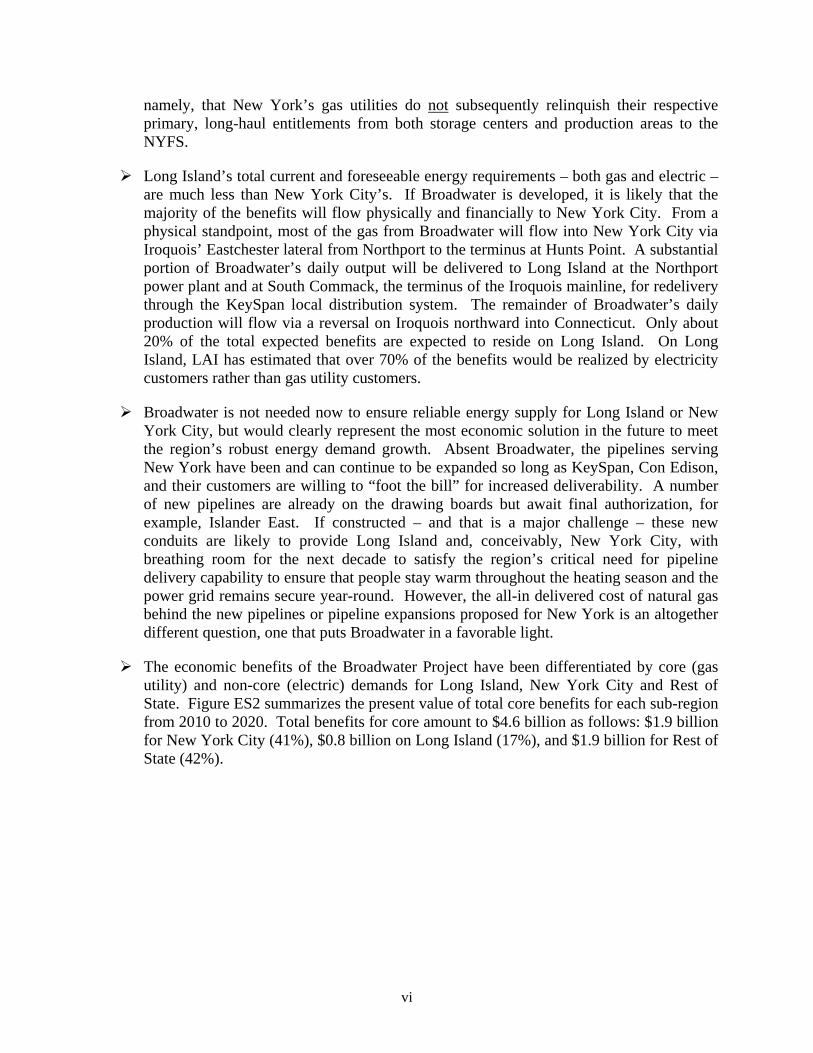
Figure ES4 – Economic Savings Attributable to Broadwater∗

2.61.1

2.7

6.4

6.2

2.7

5.4

14.3

0

5

10

15

20

25

New York City Long Island Rest of State Total

Savi

ngs

($ b

illio

ns)

Gas Utility Electric Generation

8.8

3.8

8.1

20.7

In April 2005, Broadwater told LIPA’s management and trustees that New Yorkers would save $6 billion from 2010 to 2020. Discussions between LAI and Broadwater revealed important structural differences between modeling techniques and assumptions. Broadwater’s model was designed to analyze regional inputs on a high-level basis, and did not consider avoided gas price volatility, core versus non-core procurement patterns, income multiplier effects or potential economic benefits outside of Long Island and New York City. Also, Broadwater did not discount these savings to account for the time value of money. Had they discounted the savings, this number would have been much lower than $6 billion. LAI observes that Broadwater’s representation in April 2005 to LIPA’s Board of Trustees was stated in very conservative terms. On an apples-to-apples basis, LAI has estimated that expected savings in New York State will equal $21.6 billion, well above three times Broadwater’s portrayal. In present value terms, this equates to $14.8 billion expressed in 2010 dollars.

The total expected value to New York State, $20.7 billion – including the adjustment to account for benefits to the economy – requires a number of material adjustments to account for other benefits and costs, quantification of which was outside the scope of this study. Not included in LAI’s estimated total savings are: (i) potential payments in lieu of taxes to “host” communities on Long Island, (ii) the value of potential commercial inducements from Broadwater to one or more anchor customers, (iii) environmental

∗ Adjusted for economic multiplier effect

x

benefits associated with the increased use of natural gas in lieu of oil for power production, including one or more generation asset repowering(s) on Long Island, in New York City or Rest of State that might not otherwise occur, and (iv) miscellaneous capital costs potentially borne by gas utilities and power generators on Long Island and in New York City for the sake of reliability. Regarding this last item – miscellaneous capital costs borne mainly by KeySpan and Con Edison – Broadwater’s daily dispatch regime would materially change the pattern of gas flows on Long Island and New York City. Both KeySpan and Con Edison may therefore need to commit significant capital resources to maintain network reliability in response to much higher receipts at different gate stations on the NYFS, the costs of which would ultimately be recovered from retail gas and electric customers. Other costs borne by KeySpan, Con Edison and power plants to ensure that Broadwater’s gas supply is interchangeable with pipeline rendered supply must also be counted. Other costs may be borne by the region’s gas utilities to ensure that processes at the existing peak-shaving LNG facilities in Suffolk County, Queens and Brooklyn are not impaired as a result of commingling Broadwater’s regasified supply with pipeline-rendered supplies from Canada and the Gulf Coast.

Another economic benefit is associated with both KeySpan’s and Con Edison’s ability to reduce the total cost of pipeline transportation by releasing temporarily their valuable pipeline and storage entitlements on Transco and Texas Eastern. Margin recoupment through capacity release has the potential to be material, but we have not attempted to measure it for purposes of this analysis.

LAI compared how Broadwater stacks up against other plausible infrastructure additions to serve growing gas demand on Long Island and New York City. When we tested how natural gas prices on Long Island and New York City change without Broadwater, but with other postulated infrastructure improvements, including a rival LNG import terminal proposed in New Jersey, we found that Broadwater was by far the best economic outcome for New York State. Central to this determination is the reasonable expectation that in order for Broadwater to capture market share, Broadwater will need to be a price taker, not a price setter. In LAI’s opinion, Broadwater will sell its inventory of natural gas under avoided cost principles, that is, Broadwater’s price of natural gas will need to beat what its customers would otherwise pay to deliver natural gas to Long Island or New York City. Otherwise, Broadwater will not sell very much natural gas. Under the array of factor input assumptions used by LAI in our quantitative analysis, we observe that the addition of the first phase of the proposed Millennium Pipeline and downstream improvements on both Algonquin and Iroquois will not be expected to yield a significant reduction in gas prices on Long Island or New York City. The addition of these upstream pipeline segments would confer vital reliability benefits, however. Other postulated pipeline expansions onto Long Island and New York City would be expected to reduce gas prices in the market area by $0.62/MMBtu, only about one-third the reduction on Long Island attributable to Broadwater. The impact of BP’s proposed Crown Landing LNG import terminal in New Jersey was about the same as the pipeline expansions we tested. While other potential LNG import terminals such as Crown Landing or one of several new import terminals proposed in New England will likely reduce energy prices in New York, the net impact for New Yorkers is not remotely comparable to that of Broadwater. Moreover, rival LNG import terminals’ prospects for success are a

xi

wildcard. Importantly, our findings regarding the economic impact of other contenders in lieu of Broadwater do not incorporate any of the high fixed annual payments payable by utilities and power generators associated with reserving space on new or expanded pipelines into the market center.

Unless Broadwater is contractually obligated to meet commitments on Long Island and in New York City and, perhaps, other adjacent markets, Broadwater, or its marketing affiliate, may divert cargoes destined to New York, electing instead to move charter vessels to the most lucrative spot market across the Atlantic Basin. Until worldwide liquefaction capability in exporting countries catches up to the demand for LNG, competing markets across the Atlantic Basin constitute heightened competition for spot cargoes, in particular, the United Kingdom, Spain, and a number of other European Union countries. Certainly, the best way to assure Broadwater’s operating regime around 1 Bcf/d is to require performance through contractual safeguards oriented around a “take-if-tendered” commercial structure.

Technology

LAI’s technology study objectives were threefold: first, to evaluate the various types of offshore LNG facilities; second, to identify technology limitations associated with the FSRU, its major components, and the yoke mooring system; and, third, to assess operational issues with the FSRU and LNG transfer.

Offshore LNG technology builds on the industry’s record of safety and reliability established over the past four decades. At present there is no FSRU technology on the scale proposed by Broadwater operating anywhere in the world. Nevertheless, each of the essential components of Broadwater’s FSRU has been used safely and reliably in both offshore petroleum and onshore LNG terminal operations around the world. LAI examined each type of offshore LNG facility proposed or operating in the U.S. These include gravity-based structures, a modified LNG tanker unloading to a submerged turret loading buoy and alternative FSRU design technology. LAI evaluated the essential operating components of the FSRU from the perspective of historical use and suitability in Long Island Sound. We evaluated multiple components of Broadwater’s proposed technology, namely, containment, regasification, cargo transfer, emergency shutdown, boil-off, custody transfer, and mooring.

Highlights of our assessment include the following:

There is no evidence of fatal flaws in the FSRU design. Broadwater’s functionality and design combines existing and proven technology from onshore LNG terminals and LNG vessels. In LAI’s opinion, Broadwater will benefit from the technology progress and knowledge gained from over forty years of reliable performance in terms of shipping, storage, and terminal operations around the world. The containment system, individual tank design, and related hull design will undergo rigorous evaluation by the American Bureau of Shipping (ABS) to ensure compliance with all applicable codes and guidelines.

The FSRU includes multiple system redundancies to ensure reliable and safe operation. Examples of system redundancies include an additional gas turbine for electricity

xii

generation, multiple pumps in storage tanks, excess vaporization capacity, an additional loading arm and additional condensers and liquid pumps for the vaporizers.

Offshore cargo transfers are limited by the relative motion between the FSRU and the LNG carrier. LNG deliveries will not be scheduled unless there is a 24-hour weather window within operating limits corresponding to wind speeds less than 33 knots and waves less 6.6 feet. During cargo transfer, the FSRU loading arms are connected to the receiving flanges of the LNG carrier. If weather were to take a sudden and rapid turn for the worse, that is, unanticipated choppy seas and high winds materialize after cargo transfer has commenced, the simultaneous movement of the FSRU and LNG carrier has the potential to unduly stress the loading arms on the FSRU. In such an event, the emergency shutdown system would be activated when the relative motion between the two vessels exceeds threshold tolerances. In LAI’s opinion, the risk involved in offshore cargo transfer can be competently managed through the adherence to prudent operational procedures.

The scale of Broadwater’s storage system significantly exceeds the storage capacity of LNG carriers currently in service or likely to begin service this year or next. However, Broadwater’s eight individual storage tanks of 1 Bcf per tank are similar in size to those planned for new, large LNG vessels currently under construction in shipyards in Korea, Japan and France.

Broadwater’s yoke mooring system is designed to permanently tether the FSRU to the mooring tower. The yoke mooring system is a critical Project component: both reliability and safety depend on the integrity of the yoke mooring system, as there will not be an anchor on board the FSRU in the event of failure. The yoke mooring system is designed to withstand a Category 5 hurricane – comparable to the force of Hurricane Katrina that devastated the Gulf of Mexico in August 2005. The high waves and wind of a Category 5 hurricane would be more severe than a “100-year storm” on Long Island. The worst storm ever recorded on Long Island occurred in 1938, a Category 3 hurricane. Aside from weather-related risk, either a terrorist attack or an accidental vessel collision with the yoke mooring system could conceivably release the FSRU from its mooring. Although the FSRU would have thrusters to maintain a constant heading, its motion would generally be controlled by tug boats. Tugs cannot operate reliably when waves are greater than 2 meters (6.6 feet). Therefore, the yoke mooring system must be designed for maximum safety. Of critical importance, the area around the yoke mooring system must be protected from incoming vessels by an adequate safety zone.

In the final analysis, all technology risk will be borne by Broadwater, not market participants doing business on Long Island or in New York City or Rest of State.

Environmental

LAI’s environmental review objectives were four-fold: first, to identify the most significant potential impacts on marine plant and animal resources in Long Island Sound resulting from the construction and operation of the Project; second, to identify the potential impact on recreational and commercial fishing and boating associated with the construction and operation of the

xiii

Project, including the delineation of Safety Zones around the FSRU and the LNG carriers; third, to identify feasible mitigation methods applicable to Broadwater in the context of how such mitigation methods have been implemented for similar projects; and, fourth, to evaluate the incremental impact of the Project relative to existing infrastructure, commerce, and other uses of Long Island Sound. LAI’s review does not constitute an independent environmental impact statement. We did not perform an independent compliance review or impact assessment with respect to air emissions or water discharge associated with operation of the FSRU and the LNG carriers. If permits are issued by the authorized federal and state agencies, we assume that conditions attached to air permits, the State Pollutant Discharge Elimination System (SPDES) permit, and other permits would be protective of, and prevent deterioration of air quality and marine resources. The decrease in natural gas prices ascribable to the Project may promote repowering of existing steam plants on Long Island and/or conversion of core heating load from oil to gas, thus enabling a net reduction in emissions on NOx, SO2 and CO2. LAI has not quantified this potential benefit. Furthermore, LAI takes no position concerning the so-called “industrialization of Long Island Sound.” This issue must be decided by state and local officials.

Highlights of our environmental assessment include the following:

The selection of the Project site avoids sensitive resources that are located in the nearshore area of Long Island Sound, including shellfish beds, marine bird breeding grounds, and tidal wetlands. The Project site also avoids disturbance of the most heavily contaminated sediments, which tend to be along coastal areas and in the western portion of Long Island Sound. On both the Long Island and Connecticut shorelines, there are no significant environmental impacts associated with the FSRU and the pipeline lateral connecting the FSRU to the Iroquois mainline.

Impacts associated with pipeline construction are well-documented from other marine infrastructure projects in Long Island Sound. The method proposed by Broadwater for excavation of the pipeline trench using a subsea plow is the least environmentally damaging. However, benthic invertebrates in the areas of direct impact from the subsea plow and buried by sidecast spoils will likely be killed. Larger, more mobile invertebrates and fish will likely be able to avoid the disturbance. Avoidance of near-surface bedrock substrate eliminates the need for blasting, which has the highest impact to marine resources. Some finfish species may be susceptible to barotrauma from pressure waves during pile driving for the yoke mooring system tower, but the effects will be short-term and localized. Changes in water quality due to increased turbidity during trenching for the pipeline and yoke mooring system construction will be short lived. Time of year restrictions will help minimize effects to commercially important species such as lobster, and rare, threatened or endangered species such as whales and turtles. Although the area of the seafloor that is expected to be disturbed during construction is over two thousand acres – approximately 0.26% of the total area of Long Island Sound – numerous scientific studies have documented the recovery of benthic marine resources in Long Island Sound and similar environments following disturbance. For other marine infrastructure projects, studies have shown that recolonization occurs within a period of weeks to months, with total recovery to the original condition taking several years.

xiv

Some of the potential operational impacts can be categorized as low risk-high impact. These include contaminant release through fuel spills, whale / turtle entanglement or collisions with marine traffic. These potential impacts are not unique to Broadwater, and are generally mitigated through best management practices and spill prevention, control and countermeasure plans.

The FSRU mooring tower will alter approximately 13,000 square feet (about 0.3 acres) of sea bottom within the four legs of the structure, with an additional 5.7 acres of shading beneath the FSRU. The FSRU’s draft of 40 feet leaves approximately 53 feet of water column underneath the hull to the mudline. Like a weathervane, the FSRU is free to pivot around the mooring tower. Hence, the shaded area will not be fixed, thus minimizing the potential for a zone of oxygen reduction underneath the FSRU. The FSRU and associated Safety Zone would create a different and diverse community underneath the FSRU and on the mooring tower. We understand that the area associated with the Safety Zone will be inaccessible to commercial and recreational boating and fishing for Broadwater’s life, presumably decades. Because commercial and recreational fishing will be excluded from the vicinity of the FSRU, it is possible that a de facto marine protected area will be created around the Project.

The design and operation of the FSRU’s water intake structures are intended to minimize mortality of ichthyoplankton (fish eggs and larvae) and adult fish by impingement and entrainment. Thermal impacts above applicable criteria from cooling water discharge from offloading LNG carriers are expected to be limited to a small localized mixing zone, 0.22 acres or less, between the FSRU and the LNG carrier. No ballast water discharge will be allowed for the LNG tankers within Long Island Sound, reducing the potential for invasive species introduction.

Socioeconomic effects during construction include the inability to access commercial and recreational boating and fishing areas, fishing and lobster gear loss, and potential loss of income for lobster and fin fishermen unable to relocate their effort away from the construction activities. Restricting construction to the October through April window will reduce conflicts with recreational fishing and boating; Broadwater anticipates construction to occur during this time window only, over a two-year period. The FSRU and the associated Safety Zone will cover an area of roughly 1.5 square miles. Broadwater would displace up to five lobster fishermen who currently set pots within that area. Up to twelve fishermen reportedly trawl the area. The actual area lost would be greater for those trawlers who utilize established east / west trawl lanes, because the Safety Zone restriction cuts off access to a greater portion of the lane. Interference with the established east / west trawl lanes could result in fishing conflicts and reduced catches. Broadwater acknowledges that compensation for revenue losses and potential gear losses to commercial fishermen is necessary. Such compensation could be administered either through the State acting as a trustee, a fishermen’s association or another third party.

The FSRU was sited to avoid the predominant east / west and north / south shipping channels and ferry routes in Long Island Sound. However, some vessels that utilize the

xv

east-west shipping channel located through the middle of the Sound would need to modify their routes to avoid the Safety Zone around the FSRU.

Broadwater anticipates that 2 to 3 LNG cargo vessels per week will transit the Sound and dock at the FSRU. This represents an increase of less than 1% of the total commercial traffic currently operating in Long Island Sound, but, more importantly, an increase of 15% of large draft commercial traffic, i.e., greater than 19 feet. On a tonnage basis, LNG imports would represent an increase of about 36% over the tonnage of commodities currently landed or exported through Long Island Sound ports. However, this percentage does not consider the extent to which LNG vessels would displace some of the barge and tanker traffic that currently delivers oil to New York for heating and power production. Petroleum products (other than LNG) currently constitute the largest portion by tonnage of total annual imports into Long Island Sound ports.

LNG cargo vessels would be the largest vessels transiting the Sound. However, the LNG carriers will utilize the central east-west shipping lane where visibility from the shoreline will be minimized. LNG cargo vessels and their associated Safety Zone will interrupt marine traffic for a period of up to approximately 15 minutes as they traverse The Race. The Coast Guard will be responsible for developing and implementing a traffic management plan.

Safety

The objectives of LAI’s safety review were fourfold: first, to assess the hazards associated with an offshore LNG storage facility based on existing scientific studies and reports; second, to assess the impact of an LNG spill from an accidental or intentional event; third, to evaluate the definition of hazard zones based on safety zones established or proposed for other LNG projects; and fourth, to review Broadwater’s Resource Report on Safety and Reliability in its application to FERC. Importantly, we note that LAI’s safety review does not encompass any information that Broadwater has provided government entities on a Privileged and Confidential basis, or other documents considered “Critical Energy Infrastructure Information” or “Sensitive Security Information” at FERC.

There is no other offshore storage and regasification facility like Broadwater. There is no safety record for a facility equal to or substantially similar to Broadwater for purposes of safety analysis. However, LNG vessels have sustained an excellent safety record over the last forty years. In contrast to the number of crude oil spills, including several catastrophic events, there has never been an LNG cargo tank breach of any type despite several LNG groundings around the world since the 1970s.

The most serious potential LNG hazard is thermal radiation resulting from a pool fire or the ignition of a vapor cloud. Thermal radiation is light emitted from the surface of an object due to its temperature. The power of the thermal radiation per unit area, also called the “heat flux,” is conventionally expressed in units of kilowatts per meter squared (kW/m2). In this case, these units have nothing to do with electricity, but instead express the amount of thermal radiation over a given area. For reference, the average radiation from the sun reaching the Earth’s atmosphere is 1.4 kW/m2. At the edge of a pool fire, the thermal radiation exceeds 220 kW/m2. The impact

xvi

on humans from thermal radiation depends both on the intensity of the radiation and the exposure time. According to the National Fire Protection Association, an incident heat flux level of 5 kW/m2 is recommended as the design level that should not be exceeded in areas where more than 50 people might assemble. 5 kW/m2 is also the permissible level for emergency operations lasting several minutes with appropriate clothing. No pain has been shown for thermal fluxes less than 1.7 kW/m2 regardless of exposure time. LAI considers 2 kW/ m2 to be the thermal flux level that should be used as the limit for calculating safe distances from an LNG pool or vapor fire. Table ES2 shows the type of damage that occurs from different levels of heat flux based on an average 10-minute exposure time.

Table ES2 – Thermal Radiation Damage Levels∗

Incident Heat Flux (kW/m2)* Type of Damage

35-37.5 Damage to process equipment including steel tanks, chemical process equipment or machinery - third degree burns, lethal 50% of the time

for a person wearing average clothing

25 Minimum energy to ignite wood at indefinitely long exposure without a flame

18-20 Exposed plastic cable insulation degrades – second degree burns, lethal 1% of the time for a person wearing average clothing

12.5-15 Minimum energy to ignite wood with a flame; melts plastic tubing

5 Permissible level for emergency operations lasting several minutes with appropriate clothing

1.7 No pain regardless of exposure time

Computer models calibrated by limited experiments have been used to estimate how far from a pool fire the resultant heat flux drops to 5 kW/m2 or less. Model results vary depending on the assumptions and the initial conditions at the time of a postulated spill. In performing this review, LAI relied on the Sandia report, Sandia’s assessment of the Cabrillo Port Draft Environmental Impact Report (DEIR), and many other relevant documents. The Cabrillo Port project proposes an FSRU similar to Broadwater 14 miles off the California coast. Sandia calculated heat flux as a function of distance for a possible spill scenario off the coast of southern California. Figure ES5, from Sandia’s review of Cabrillo Port, is an example of how far from the edge of the fire the radiation levels fall below 5 kW/m2. In this case, a minimum distance of 2.4 km (1.5 miles) is required for the heat flux to drop to 5 kW/m2. An additional 1.3 km (0.8 miles) is required to reach a safer level of 2 kW/m2. Therefore, people and property outside 3.7 km (2.3 miles) should be within the safer radiation levels.

∗ Based on Sandia Report and other fire safety documents.

xvii

Figure ES5 – Pool Fire Calculation (Cabrillo Port)

0

20

40

60

80

100

120

140

160

180

200

220

0 500 1000 1500 2000 2500 3000 3500 4000 4500Distance From Flame Axis (m)

Hea

t Flu

x (k

W/m

2 )

2,400 m to 5 kW/m23,700 m to 2 kW/m2

Highlights of LAI’s safety assessment include the following:

Broadwater’s location, about nine miles from the closest shore, minimizes the hazards to the public associated with either an accident or a catastrophe at the FSRU. Broadwater’s homeland security experts assert that the FSRU is likely an unattractive terrorist target because any incident would cause few casualties and would not be very accessible for extensive media coverage. Arguably, the FSRU is a difficult terrorist target with a comparatively low probability of success. Nonetheless, we note that the maximum number of crew on board the FSRU at any one time would be approximately 30 individuals. In the event of a catastrophe, we believe that the FSRU is too far from either shoreline to affect the Long Island or Connecticut population.

The risk of an accident while the LNG carrier is transiting The Race appears very low although the consequences could be high. Elsewhere in the U.S., LNG carriers have regularly transited both high and low density population centers without event for decades. Although the LNG carrier route comes within approximately one mile of land at The Race, an experienced pilot familiar with the route will have boarded the FSRU before it enters the Sound. The USCG will then escort the carrier to the FSRU. Both the USCG and Broadwater are eager to schedule passage during periods which avoid conflict with commercial and recreational vessel traffic, in particular, late night. Furthermore, the LNG carriers will not enter the Sound unless there is a favorable 24-hour unloading weather window within the operating limits corresponding to wind speeds less than 33 knots and waves less than 6.6 feet.

xviii

Safety zones for offshore LNG projects are based on modeling of LNG spills over water. There has never been a large, offshore LNG spill over water – either accidental or experimental. LNG spill experiments conducted by scientists have been limited to volumes that constitute a small percentage of what might conceivably be released under any scenario. In LAI’s opinion, scientists’ inferences from controlled LNG spills are highly theoretical and therefore subject to uncertainty. LAI to date has not encountered any experimental data that counters the recommended safety zone for the Project. DOE’s current study involving large-scale LNG fire experiments may further reduce uncertainties concerning heat impact distances.

Minor hazardous events such as LNG leaks on the FSRU or the LNG carrier are likely to occur from time to time. The FSRU and tugs would be equipped with firefighting equipment, and we expect that the FSRU and LNG carrier crew would be highly trained to handle such emergencies. Nevertheless, cryogenic damage to crew or equipment could take place. Escalation of minor hazards is conceivable under extremely sudden and difficult weather conditions, but improbable with the type of emergency response training that is required. More serious hazardous events, such as release during LNG transfer events, are unlikely. If such a hazardous event were to occur, a pool fire or a minor vapor cloud could ensue. Broadwater’s emergency shutdown system will limit the size of a spill and therefore minimize the probability of escalation.

The most serious hazardous event would involve a collision between a vessel transiting Long Island Sound and the LNG carrier or the FSRU. The USCG has proposed a Safety Zone around the FSRU with a 1.1 km radius (0.68 miles). They have also proposed a moving safety zone around the LNG carrier while it transits the Sound that extends 3.7 km (2.3 miles) in front of the carrier, 1.85 km (1.15 miles) behind, and 0.69 km (0.43 miles) on either side. These Safety Zones will increase the navigational safety and reduce the likelihood of an accident or intentional attack. Furthermore, most of the vessels transiting Long Island Sound are neither large enough nor traveling with the speed required to penetrate the double hull of the FSRU or the LNG carrier.

In the event of a pool fire, the thermal radiation could result in loss of life on the FSRU and might harm vessels and occupants in the area surrounding the FSRU. A pool fire could cause escalation to a multiple tank release, but it would take hours for all the LNG to be released. A worst-case scenario involving the total loss of the FSRU is conceivable, but all the LNG on board would not be instantaneously released. In the event of a worst-case scenario, the existing body of scientific knowledge indicates that the inhabitants of Long Island and Connecticut are far enough away to avoid burns through exposure to high levels of thermal radiation.

Unignited vapor clouds are extremely unlikely to travel more than 2 miles without encountering an ignition source, such as a recreational, commercial or fishing boat. Near the FSRU, an unignited vapor cloud could lead to asphyxiation of crew members or other emergency personnel. Any intentional initiating event will almost certainly provide an ignition source and therefore not lead to a diffusing vapor cloud. Once the vapor cloud is ignited, the flash fire will burn back to the spill source, i.e., presumably the hull of the FSRU.

xix

A secondary hazard that could damage the FSRU is a rapid phase transition. This type of explosion is caused by LNG pouring into warm seawater and vaporizing very quickly due to heat transfer. This rapid expansion from the liquid to the vapor state causes large overpressures. Rapid phase transitions are localized in the vicinity of the LNG leak and may cause some structural damage to the LNG carrier or the FSRU. Although rapid phase transitions on their own do not involve a fire, they may increase the rate of LNG pool spreading and the size of a vapor cloud that could subsequently ignite.

LIPA asked LAI to estimate the impact zone to 2 kW/m2 since a radiation flux of 5 kW/m2 is only a permissible level for emergency operations lasting several minutes with appropriate clothing. Discussions with fire safety engineers and a review of the engineering literature led to the choice of 2 kW/m2 as a “safe” level of radiative flux. LAI found the impact zone to 2 kW/m2 would extend 6 km (3.7 miles) around the FSRU for a credible worst-case scenario. Therefore both shorelines would effectively be buffered by approximately 5 miles.

1. PROJECT DESCRIPTION

The proposed Broadwater LNG terminal would be located in Long Island Sound approximately 9 miles (14.5 km) from Long Island and 10 miles (16 km) from Connecticut (Figure 1). The FSRU is designed as a modified LNG carrier to receive, store and regasify LNG. It will be moored in 90 feet (27 m) of water to a tower via a yoke mooring system (YMS). The FSRU will be free to weathervane around the tower in response to winds and currents. The mooring tower will be secured to the seabed by four legs with the structure covering a total area of 13,180 square feet.

The FSRU is designed to have a double hull similar to a membrane tank LNG carrier. It will be 1,215 feet (370 m) long, 200 feet (61 m) wide and 80 feet (24 m) above the waterline, with 40 feet (12 m) of draft (Figure 2). Broadwater plans for LNG carriers with cargo capacities ranging from 125,000 m3 to 250,000 m3 to deliver LNG to the FSRU two to three times per week.1 Regasification capacity will allow for an average send-out of 1 Bcf/d and a peak sendout of 1.25 Bcf/d. Net storage capacity is 350,000 m3, equivalent to 8 Bcf. After revaporization, the gas will be transported via a 22-mile (35 km), 30-inch subsea lateral to the Iroquois mainline for delivery to Long Island, New York City and Connecticut.

Figure 1 – FSRU Location and Area Infrastructure

CTNY

Long IslandSound

Bridgeport - Port Jefferson Ferry

Connecticut

New HavenDerby

OrangeOld Saybrook

New London

Milford

Bridgeport

Westport

Darien

CTNY

New Lon

don –

Orient

Point

Ferry

Northport

Hauppage

Port Jefferson

Farmingville

Riverhead

Long Island

-1 0 1 2 3 4 5Miles

LegendExisting PipelinesProposed Pipeline Interconnection

IroquoisEastchesterExpansion

IroquoisPipeline

ConnectingPipeline to

Iroquois

ProposedFSRU Location

Expected LNGTanker Route

TheRace

1 Equates to approximately 2.9 Bcf to 5.7 Bcf.

2

Figure 2 – Broadwater FSRU Offshore Terminal

Broadwater’s proposed location, away from the sensitive shoreline and nearshore ecosystems that serve as important nesting, feeding, resting, spawning and nursery areas for many species, is designed to minimize environmental impacts.

The shipyard where the FSRU will be constructed has not yet been chosen, but it will most likely be in the Pacific Rim. Once completed, the FSRU will be towed to Long Island Sound and moored at its permanent location utilizing a YMS. The YMS also serves as the connection from the FSRU to Iroquois.

A detailed review of the proposed project technology can be found in Section 3. The main components of the Broadwater FSRU include the LNG loading arms, the LNG storage tanks, power generation, the regasification plant, the nitrogen plant, an accommodation area and the YMS.

The LNG cargo transfer system consists of four loading arms mounted on the starboard side of the FSRU. The LNG storage tanks are below deck. Each of the eight membrane storage tanks has a storage capacity of 45,000 m3, about 1 Bcf. The LNG is stored at -260oF and a normal operating pressure of 1 to 3 pounds per square inch (psi). Power generation for the FSRU includes three 22-MW gas turbines which would use vaporized LNG for fuel. The regasification plant includes a recondenser for boil-off gas, shell and tube vaporizers (STVs), superheaters and metering and odorization equipment, and is designed to vaporize LNG at a peak capacity of 2,500 m3/hr. The nitrogen plant uses air compressors and membrane nitrogen generating units to generate nitrogen gas which is injected into the regasified LNG to adjust its composition and heating value so that it meets the gas quality standards of the receiving pipeline. The accommodation area will serve as the living, dining, recreational and working areas for up to 30

3

crew members. The YMS is attached to the stationary mooring tower and consists of the jacket, the mooring head and the yoke. The YMS also provides the connection from the outlet of the regasification unit to the pipeline lateral that runs undersea to the Iroquois mainline. In addition, the FSRU will have a water ballast system in order to maintain its draft, trim and stability during loading and regasification. The FSRU’s flare will be used for emergency burning of excess LNG vapors when there is overpressure in the storage tanks or excessive boil-off volumes that cannot be handled by the recondensers.

2. MARKET & ECONOMICS

The primary objective regarding market and economic analyses is the derivation of the expected impact on energy prices on Long Island, New York City and Rest of State ascribable to Broadwater’s provision of baseload natural gas supply. Assuming an FSRU operating regime over the study horizon equal to 1 Bcf/d, LAI has quantified the impact on market clearing prices for natural gas and electricity. Economic benefits are stated on a gross basis, that is, before accounting for sundry costs potentially borne by KeySpan, Con Edison, and generators throughout the region to ensure local gas-side reliability. Economic benefits have been differentiated for core (gas utility) and non-core (electric) demands on Long Island, New York City and Rest of State.2 Potential benefits in New Jersey and Connecticut are not reported in this analysis. The economic benefits associated with Broadwater have also been compared to rival pipeline and/or LNG expansion scenarios in the greater Northeast.3

To quantify Broadwater’s potential economic impacts, LAI analyzed regional market dynamics. We assessed the impact of new LNG supplies on supply / demand balances, gas flows, market area gas prices, and wholesale electricity prices throughout New York. This work effort included an analysis of historical basis differentials and liquidity levels at relevant pricing points across the greater Northeast. LAI used a mathematical optimization model to predict natural gas pricing relationships and price volatility effects in the greater Northeast. Of particular relevance are energy prices on Long Island, New York City, and Rest of State. The primary mathematical modeling system used to determine price effects is “GPCM,” or, more formally, the Gas Pipeline Competition Model. GPCM is a proprietary model licensed by RBAC, Inc. a California software firm. GPCM relies on a proprietary database licensed by Platts, a leading international energy data firm.4 Electric energy price effects were quantified using MarketSym, a chronological modeling system licensed by Global Energy Decisions, Inc., a California energy software firm. Hydraulic analyses of the pipelines serving the market area required steady-state and limited transient flow analyses. LAI’s quantification of pipeline delivery capability was conducted using hydraulic modeling tools licensed by Gregg Engineering, a Texas software firm.

In order to determine Broadwater’s expected price impact, LAI constructed a “but for” test. We asked the question: what are expected natural gas prices on Long Island, New York City, and Rest of State under Business-as-Usual conditions (no Broadwater) over the period 2010 through 2020? We then postulated the addition of Broadwater throughout the forecast period under a steady state operating regime equal to 1 Bcf/d, adjusted for brief intervals to account either for required maintenance or for constraints associated with the timely arrival of LNG tankers to replenish the inventory aboard the FSRU. Known or potential pipeline enhancements into the market area have been incorporated, including adjustments to the pipelines linking production or

2 For the purposes of this analysis, “core” residential, commercial and small industrial customers are served by local distribution companies (LDCs) either through bundled sales or transportation service. “Non-core” customers incorporates all electric generation that is gas-fired and large industrial customers that are either directly connected to an interstate pipeline or purchase transport-only service from the LDC. 3 For purposes of this study, the greater Northeast is defined as New Jersey, New York, and New England. 4 Platts, a division of the McGraw-Hill Companies, specializes in energy industry information and related services.

5

storage centers to New York. The price effects ascribable to planned regional gas infrastructure improvements on existing or new pipelines have been incorporated. Also included are pipeline expansions or new entry on Millennium, Algonquin, Iroquois, Tennessee, and Islander East, as well as an array of adjustments to account for new storage projects and new LNG import terminals in North America.

The impact of different natural gas prices by location was tested using the wholesale electric production simulation model in order to gauge wholesale electricity price changes in regional and local markets. MarketSym was also utilized to determine the amount of gas burned for electricity generation over the forecast horizon under various cases. The economic analysis results have been adjusted for income multiplier effects across the region.

2.1. Natural Gas Market Analysis

2.1.1 Introduction

The natural gas market across North America is a continental market characterized by high connectivity and deliverability. Interstate, intrastate, and inter-provincial pipelines link supply basins and both production area and market area storage fields across the U.S. and Canada to gas utility and power loads across the continent. Whereas the U.S. is heavily dependent on crude oil imports, domestic production of natural gas provides more than 80% of the natural gas consumed in the U.S. Natural gas imported by pipeline from Canada accounts for most of the remainder. Today, LNG imports comprise only about 3% of total U.S. demand. LNG imports are a much greater percentage of New England’s energy balance, however, representing about 23% of the region’s total gas supply. As domestic gas production wanes in the next decade or two, the U.S. is expected to become increasingly dependent on LNG in order to maintain adequate supplies for the Atlantic seaboard, Gulf Coast, and California.

Until the 1980s, the natural gas industry was heavily regulated, including wellhead gas prices and gas transportation rates.5 Deregulation commenced in 1978 under the Natural Gas Policy Act (NGPA), which mandated the lifting of wellhead price controls by 1985. A series of landmark FERC orders in the mid to late 1980s helped transition the pipeline industry from the traditional “merchant” function where natural gas was bundled with interstate transportation for resale in the marketplace, to the transportation or common carrier function typical of railroads. Since the 1980s, as a result of the NGPA and a series of landmark rulings by FERC, gas prices from the wellhead to the citygate have been set by market forces rather than traditional cost of service principles. At the local level, from the citygate to the burner-tip, traditional cost of service regulation remains in place.

The lifting of wellhead price controls coupled with federal tax incentives for gas production resulted in a protracted supply “bubble” from the mid-1980s until the late 1990s. While natural gas prices into-the-pipe fluctuated with market conditions over the last decade, the supply overhang and relatively weak crude oil prices during this period kept natural gas prices both low 5 The wellhead is the point at which natural gas leaves the well and flows into the pipeline gathering and transportation system.

6

and comparatively stable. By the late 1990s, the favorable price outlook made natural gas the fuel of choice for new electricity generation. Since the mid-1990s, over 154,000 MW of gas-fired generation has been added to the generation supply mix throughout the U.S.6 While a portion of this capacity has taken the place of older gas or gas / oil steam turbine generator capacity, nearly all of the new gas-fired capacity represents incremental demand for natural gas.

Producing basins across North America have increasingly shown signs of depletion-induced production declines. The increased demand for natural gas coupled with decreased supply due to the maturation of many conventional natural gas producing fields have put upward pressure on commodity prices. Over the last five years, commodity gas prices have been high as well as volatile. As gas wells in conventional producing basins move well past peak production, it becomes more difficult for producers to maintain production levels. Many producers throughout North America have found themselves on a “treadmill” where accelerated depletion trends cause producers to drill many less productive wells and deeper wells in increasingly remote areas to replenish reserves. Over the forecast period, new sources of supply will need to be developed to augment current production from traditional supply basins. In addition to drilling in ultra deepwater in the Gulf of Mexico, the Rocky Mountains, northern Canada and Alaska, industry experts expect LNG to fill the growing gap between production and consumption.

The addition of Broadwater to the region’s pipeline infrastructure has the potential to lower natural gas prices as well as dampen or even eliminate the pattern of gas price volatility. If Broadwater is commercialized, first-order benefits would be derived from price reductions at key pricing points across the network of pipelines serving New York.7 Of particular relevance are TZ6-NY8 and IGTS-Z2,9 the market area pricing points that demarcate the value of bundled natural gas and transportation around New York City and Long Island, respectively. While the addition of Broadwater in the market center would be expected to directly impact market prices on Long Island and New York City, measurable price effects would be expected to “ripple across” the supply chain back to the Henry Hub, Louisiana, and the Leidy, Pennsylvania and Dawn, Ontario storage hubs, as well as across the supply chain from the Gulf of Mexico or Canada to New York. The Henry Hub, Leidy, and Dawn are pricing points of particular relevance in defining the cost of natural gas for gas utility markets on Long Island, New York City, and Rest of State.

Throughout this chapter, LAI discusses the modeling approach and factor inputs to various simulation models used to conduct the market impact analysis, in particular, GPCM. Many details of LAI’s Business-as-Usual Case are provided. Definition of other supply scenarios on Long Island, New York City and Rest of State are provided. Following the discussion of the gas 6 2005 U.S. Energy Information Agency (EIA) Annual Energy Review. 7 A number of second order benefits associated with potential payments in lieu of taxes (PILOT) to host communities on Long Island, New York and, perhaps, Connecticut, are not included in this analysis. Other benefits associated with potential commercial inducements and the environment have not been quantified in this analysis. Also, various capital costs potentially borne by local distribution companies to ensure local reliability have not been quantified. 8 TZ6-NY is the primary New York City market pricing point for Zone 6 of the Transco pipeline. 9 IGTS-Z2 is the Iroquois Zone 2 pricing point, which is also relevant for Long Island.

7

market modeling approach and factor inputs to GPCM, we review the building blocks of the electric market simulation model.

Readers interested primarily in the results of LAI’s economic analysis are directed to Section 2.3.

2.1.2 Market Modeling Approach

Figure 3 shows the generalized modeling framework LAI employed in order to compute the first order economic impacts of adding Broadwater to the natural gas infrastructure.

Figure 3 – Overview of Broadwater Market Analysis Modeling Process

MarketSym- Transmission Limits- Bidder Behavior- Demand Forecast

Entry/Attrition Model (ROS, NJ, CT)- Demand Curves- Capacity Pricing Assumptions

Resource Mix

Emission PricesAll non-Gas Fuels

Electric Prices

Results & Impact of Broadwater to LIPA Total

System Costs Under Various Scenarios

GPCM- Demand Forecast- Supply Scenarios

Basis and Commodity Gas

Prices Under Supply Scenarios

Fuel Price Forecast- Forwards & NYMEX Futures- EIA Data- Historic Locational Prices

WinFlow Pressure/Flow Modeling- FERC Schedule G Filings- Historical Flows/Receipts/Deliveries

Validated Pipeline Flow Constraints

ElectricGas Demand

Iterate Between GPCM and MarketSym until

Convergence

Gas Prices

MarketSym- Transmission Limits- Bidder Behavior- Demand Forecast

Entry/Attrition Model (ROS, NJ, CT)- Demand Curves- Capacity Pricing Assumptions

Resource Mix

Emission PricesAll non-Gas Fuels

Electric Prices

Results & Impact of Broadwater to LIPA Total

System Costs Under Various Scenarios

GPCM- Demand Forecast- Supply Scenarios

Basis and Commodity Gas

Prices Under Supply Scenarios

Fuel Price Forecast- Forwards & NYMEX Futures- EIA Data- Historic Locational Prices

WinFlow Pressure/Flow Modeling- FERC Schedule G Filings- Historical Flows/Receipts/Deliveries

Validated Pipeline Flow Constraints

ElectricGas Demand

Iterate Between GPCM and MarketSym until

Convergence

Gas Prices

The center of LAI’s modeling framework includes two models: GPCM and MarketSym. LAI’s market analysis was conducted largely through the GPCM optimization modeling system. The optimization model includes a proprietary database (GPCMdat) developed by Platts. Using GPCM, LAI has simulated the market dynamics across the U.S. and Canada from 2010 through 2020. To ensure model integrity, extensive “backcasting” of supply / demand fundamentals throughout the greater Northeast was conducted over a five-year historic period. In conducting the market assessment, emphasis has been placed on regional, state, and local market dynamics. The use of the optimization modeling system provides a consistent platform for the determination of price effects under rival natural gas infrastructure scenarios. The modeling system allows changes in key factor input assumptions pertaining to gas supply and demand to be examined in the context of how changes in factor inputs determine local, regional, and continental natural gas prices.

LAI also utilized pressure / flow simulation models to assess the impact of Broadwater on regional gas flows. As shown in the above schematic (upper-right), WinFlow is the steady state hydraulic simulation framework used to identify potential pipeline constraints limiting the flow of gas on Iroquois, Eastchester, and upstream pipelines that interconnect with Iroquois, i.e., Algonquin, Tennessee, TransCanada. No hydraulic modeling of local transportation constraints across the New York Facilities System has been conducted. The results of the gas optimization and simulation models were integrated into MarketSym to determine the consequent impact of different gas price forecasts on electric energy prices on Long Island, New York City, and Rest

8

of State. Finally, in conjunction with the electric simulation model, LAI has used our financial models in order to adjust the resource mix in the market area for power plant retirements and new entry. The addition of new generation capacity by location in New York State is in accord with existing NYISO reliability criteria – presumably, a constant over the forecast period.

Network models are based on linear programming (LP) techniques. LP is extensively used for solving complex resource allocation problems in the energy industry. Specific applications to the natural gas industry are focused on the sourcing and routing of gas. The flow of natural gas encompasses a sequence of transactions including sales and purchases, shipments, storage, and delivery. The transaction sequence is affected by changes to gas supplies or infrastructure capability. Changes in the transaction sequence “ripple” or cascade down the supply chain from the wellhead to the burner-tip. Hence, postulated changes in gas supply or pipeline / storage infrastructure directly bear on prices across the interconnected network of facilities linking suppliers and consumers.

Gas industry LP models are centered on the (re)establishment of a competitive equilibrium. In achieving the competitive equilibrium, GPCM determines prices by optimizing at each supply and demand node the flow of available supplies, constrained by relevant pipeline and storage delivery constraints.

More detail regarding the theory and structure underlying the use of GPCM for the economic and market analysis conducted by LAI is presented in Appendix 1.

2.1.3 Key Factor Inputs for the Business-as-Usual Case

In order to determine the economic impacts associated with Broadwater, we defined a reference case. The reference case is synonymous with the Business-as-Usual (BAU) Case representing the pipeline and storage infrastructure to serve New York without Broadwater. After completion of the Business-as-Usual Case, LAI postulated the addition of Broadwater. We then traced the value of the changes when Broadwater is added to the resource mix. Other supply related scenarios were tested as well, in particular, competing pipelines into New York, rival LNG import terminals, and changes to the underlying gas supply assumptions, in particular, basin-specific production trends.

LAI reviewed and analyzed the detailed assumptions and model inputs provided with the GPCM and the GPCMdat database developed by Platts. These assumptions and inputs cover a wide range of values regarding gas supply and production, pipeline transportation rates and capacities, individual sector demands by market locations, and sector demand growth rates. Where

9

appropriate, LAI customized GPCMdat to reflect regional deliverability constraints.10 A summary of significant changes is provided in footnote eleven below.11

The primary modifications that LAI incorporated into the GPCM model inputs and database are detailed in Appendices 2 through 4. Following is a discussion of the background and justification for the various assumptions that provide the framework for the Business-as-Usual Case.

2.1.4 Natural Gas Supply in North America

From a New Yorker’s perspective, the most important gas producing regions in North America are the Gulf Coast, which includes gas production from the onshore Gulf Coast and the offshore Gulf of Mexico, and the Western Canada Sedimentary Basin (WCSB).12 These supply areas account for almost two-thirds of the total gas production in North America. The Gulf Coast provides more than half of total U.S. gas production. The WCSB accounts for almost 98% of total Canadian gas production. Most gas imported to the U.S. originates in the WCSB. Production from the Gulf Coast, particularly the offshore continental shelf, has been declining for several years, while WCSB production has essentially leveled. The distribution of gas flows from Canada and the Gulf Coast to New York State is shown in Exhibit 1.

Total U.S. gas production has averaged 19.2 trillion cubic feet (Tcf) each year since 1996. After reaching a peak of 19.8 Tcf in 2001, production declined 3% by 2004.13 Total production in Canada over this period increased by 9%, including production from Sable Island. During the 10 All adjustments to pipeline and storage infrastructure incorporated in this analysis are consistent with LAI’s prior Non-Disclosure Agreements with NYISO, the PJM Interconnection (PJM), the Independent System Operator – New England (ISO-NE), the Independent System Operator (ISO) of Ontario, and the North American Electric Reliability Council. 11 Database adjustments were many, as follows. (i) Atlantic Canada production was materially reduced, reflecting deteriorating production at Sable Island and the Scotian Shelf. (ii) Production and decline rates for the WCSB were changed to conform to the most recent forecasts from the National Energy Board (NEB) and TransCanada. (iii) Offshore Gulf of Mexico production was increased, based on analysis and review of historical production data and forecasts from the National Petroleum Council, U.S. EIA and Simmons & Co. (iv) Supply curves for many of the LNG projects were adjusted to reflect a wider range of landed prices. (v) The timing and number of LNG terminals were varied to avoid long-haul pipeline obsolescence from the Gulf Coast to the market center, among other relevant conditions associated with gas demand over the forecast period along the Atlantic seaboard and California. (vi) Forecasted production and the decline curve in the Permian basin (west Texas) were adjusted. (vii) The capacities of Texas Eastern, Transco, Tennessee, Columbia and Dominion were adjusted based on LAI’s experience and recently available FERC certificate applications. Adjustments to pipeline capacities serving New England were made. (viii) Many adjustments to pipeline tariffs on pipelines serving the greater Northeast were made to reflect the most recent rates. (ix) New York gas demands by sector were revised to conform to the Northeast Gas Association’s (NGA) 2004 New York Gas Report. (x) Electric generation gas demands were modified in accord with MarketSym output. (xi) Gas demand growth rates, by sector, for states in several regions were adjusted upward, particularly in regard to the growth in gas demand for electricity. 12 For the purposes of this comparison, the Gulf Coast Onshore supply region included production from Alabama, southern Louisiana, Mississippi, and southeastern Texas. The WCSB included production from Alberta, Saskatchewan, and British Columbia. 13 Gas production and reserves statistics are sourced primarily from the EIA, but have been augmented with data from BP, the National Petroleum Council and Natural Resources Canada.

10

same period, demand in Canada increased by more than 13%. A significant contributor to this growth in demand involved the highly gas intensive oil sands production which continues to ramp up in response to high global oil prices. As gas production in Canada levels off and then declines while Canadian demand increases, market pressures will likely force a reduction in Canadian exports to the U.S., including New York.

Since 2000, natural gas supplies have not been elastic: high prices have not induced commensurate increases in supply. Depletion at existing producing fields throughout North America, particularly in the Gulf of Mexico, has more than offset the additional production from new wells. Natural gas producers have drilled more wells in response to high prices but production has not increased accordingly. In the U.S., from 1996 to 2004 the total number of gas exploratory and development wells completed more than doubled while reserves increased by about 15% and production increased only 1.6%.

Over the last five years, depletion trends in the Gulf Coast and Canada, pipeline transportation and storage constraints, lackluster production from offshore Nova Scotia, and the addition of gas-fired combined cycle plants throughout many parts of the U.S. have driven gas prices much higher. U.S. demand is projected to increase while North American production is expected to wobble around current levels and then decline; thus, a growing gap or potential supply shortfall is developing. Most industry analysts are looking to increased imports of LNG to cover the expected shortfall. Figure 4 shows historical production and consumption through 2005, along with EIA’s most recent forecast of U.S. natural gas production, demand and imports through 2025.

11

Figure 4 –U.S. Natural Gas Production, Consumption and Imports14

Production

Consumption

0

5

10

15

20

25

30

35

1970

1975

1980

1985

1990

1995

2000

2005

2010

2015

2020

2025

Nat

ural

Gas

Pro

duct

ion

/ Con

sum

ptio

n (T

cf)

Production Consumption

Net Imports

Natural Gas Imports, 2003 & 2025

0

1

2

3

4

5

6

7

Pipeline LNG

Tcf

2003 2025

While the EIA forecast shows U.S. gas production growing at an average annual rate of 0.6% during this period, the forecast of total consumption for the period shows an annual growth rate of 1.5% – ultimately resulting in a gap of almost 9 Tcf to be met by pipeline imports from Canada and LNG imports. In light of the less than encouraging gas supply balance available for exports from Canada, LAI expects that the U.S. will increasingly rely on LNG.

Gas wells in mature supply basins have experienced accelerated depletion in which the initial production rates for new wells decline more rapidly than initial production rates for wells drilled earlier in the life of the basin. In the early 1990s the average base production decline rate for wells drilled in those years was less than 18%. By the late 1990s the decline rate had increased to 22%. The decline rate has recently been estimated to exceed 30%.15

As shown in Figure 5, the drilling treadmill effect requires producers to drill more and more wells to maintain production levels as existing wells reach depletion.

14 Source: EIA, Annual Energy Outlook (AEO) 2005. 15 EOG Resources, February 2005 Presentation, North America Natural Gas.

12

Figure 5 – Normalized Gas Production per Well from Gas Wells (By Year of Production Start, Total U.S) 16

Increased drilling, coupled with technology improvements such as horizontal drilling techniques and full-wave seismic imaging, can partly offset this decline. The degree to which new fields can offset production declines in the future will depend on the remaining resource base. The larger and more geologically diversified the remaining resources, the better the odds of finding and developing sufficient reserves to support current production levels.

Proved reserves in North America, the geological equivalent of gas inventories available for production, currently amount to 246 Tcf, or 9.8 years of production.17 U.S. proved gas reserves have grown 14% since 1996, reaching 189 Tcf in 2004.18 The largest increases in reserves have been in the Rocky Mountains, Arkla East Texas, and Texas Gulf Onshore supply regions. Large decreases in proved reserves have occurred in the Gulf of Mexico shallow water and in the South Louisiana Onshore supply regions. In addition to proved reserves, the total ultimate potential gas supply is referred to as the resource base. The remaining continental natural gas resource base has been estimated to be between 1,847 Tcf and as much as 2,193 Tcf, or sufficient gas for up to 85 years of production at current rates.19 Worldwide proved natural gas reserves amount to 6,337 Tcf or about 67 years of production. The estimated global gas resource base is at least 7 times proved reserves, or more than 400 years of production.20,21

16 Source: IHS Energy and Anadarko. 17 Proved reserves are the estimated quantities which geological and engineering data demonstrate with reasonable certainty to be recoverable from known reservoirs under existing economic and operating conditions. The resource base, which defines the potential universe for ultimate production, includes proved reserves plus the potential undiscovered gas that can be estimated based on current geologic knowledge. 18 EIA U.S. Crude Oil, Natural Gas, and Natural Gas Liquids Reserves Annual Reports. 19 Resource base estimates based on information obtained from the National Petroleum Council, the U.S. EIA, Anadarko Petroleum, Natural Resources Canada, and the Potential Gas Committee. 20 BP Statistical Review of World Energy June 2005.

13

In LAI’s opinion, while North American reserves are adequate and the continental resource base is large, production from these reserves and resources will be more difficult to access, involve harsher operating environments, be more expensive to produce, result in lower production per well, and be located greater distances from markets. Highly capital intensive pipeline infrastructure will need to be added to provide a new conduit from remote basins to market centers, for example, northern Canada, Alaska, and the ultra deepwater off the Outer Continental Shelf in the Gulf of Mexico. North American production is therefore in the midst of a transition from conventional gas reservoirs to increasing production from unconventional gas formations.22 In 2004 about 39% of total production came from unconventional formations. In the next decade, as unconventional gas production continues to grow, gas from these sources will account for almost one-half of total U.S. gas production. Tight sands account for about 19% of total U.S. gas production with shale gas, including the prolific Barnett Shale in Texas, providing about 11%. Coalbed methane, which is the natural gas associated with coal deposits, currently accounts for about 9% of U.S. production and 10% of U.S. proved reserves.23 Typically, these formations require more expensive drilling and completion technologies to produce gas in marketable quantities.

The primary driver for the development of unconventional gas has been the maturation of the North American gas resource base. The maturity of the resource base means that fewer gas reserves and less production are obtained for every dollar spent on exploration and production (E&P). The maturing resource base also means that the long-term floor for gas prices, set by the cost of production, will continue to rise. External to the U.S. and Canada, gas development and production in Africa, the Former Soviet Union (FSU), in particular, Russia, and the Middle East, involve fields that are comparatively in their infancy. The large and generally untapped hydrocarbon resources in Africa, the FSU, and the Middle East offer great promise for global LNG trade in the decade(s) ahead. A building boom to increase the number of LNG carriers is well underway, thereby ensuring that LNG carrier capacity will be available to meet the growing LNG trade.

New production from the Rocky Mountain supply basins, the deepwater Gulf of Mexico, the MacKenzie Delta, and the western regions of the WCSB are potential bright spots in terms of new production frontiers that will help offset production declines from existing fields in the Gulf Coast and conventional fields in the WCSB. Increased coalbed methane production in the Rocky Mountains will also help offset production declines. However, most new wells drilled in existing fields as well as in many of the new fields in the Rocky Mountains and the WCSB are not nearly as prolific as wells drilled years ago in the Gulf Coast and Canada. New wells will be more expensive and make smaller contributions to reserves.

21 This estimate of the global natural gas resource base does not include methane hydrates, a mixture of methane trapped in an ice lattice, that occur in deep ocean waters or in Arctic regions. Methane hydrates have the potential to increase the global resource base 100-fold. 22 Unconventional gas production is from non-traditional reservoirs, which include coalbeds, low permeability “tight” sandstone formations, and shale formations. 23 Coalbed methane occurs within the fractures or cleat system of the coal, in many cases in conjunction with water, and requires extensive dewatering and fracturing before commercial production.

14

GPCM includes supply curves that provide the basis for the forecasts of gas production by basin. The basin production forecasts and related assumptions concerning reserve additions, reserve to production (R/P) ratios, supply costs and supply elasticities were developed by Platts.24 These data are integral to the supply / demand conditions underlying forward prices, basis differentials and gas flows. LAI has analyzed the projected production and reserve addition patterns for the major supply basins contained in GPCM and implemented adjustments where appropriate. Our analysis compared these data and model inputs to similar data including the growth in basin reserves, drilling statistics, production trends and resource evaluations available in the public domain.25

The following basin production curves show the projected production levels for key supply regions in GPCM, including LAI’s adjustments. A comparison of the shallow and deepwater Gulf production basins is shown in Exhibit 2.

Figure 6 – Basin Production Curves

0

5,000

10,000

15,000

20,000

25,000

30,000

35,000

2006 2008 2010 2012 2014 2016 2018 2020

Prod

uctio

n (B

cf)

WCSB

TX Gulf Onshore

San Juan Basin

Rockies

Permian Basin

Other

Mackenzie Delta

LNG

Shallow Gulf Offshore

Deep Gulf Offshore

Arkla-East Texas

Appalachian

Alaska

24 R/P is a ratio of the reserves in a gas field to the annual production and can be used as a guideline to estimate productive life. 25 National Petroleum Council, EIA, U.S. Minerals Management Service, U.S. Geological Survey, the Stanford University Energy Modeling Forum, the Potential Gas Agency at the Colorado School of Mines, Anadarko Petroleum, BP, EOG Resources, TransCanada, Simmons and Co. International, Natural Resources Canada, and NEB Canada.

15

Table 1 provides 2004 production and January 1, 2004, reserves data for each supply region or basin reviewed. These regions and basins accounted for more than 98% of total continental production and 97% of total proved reserves in 2004.

Table 1 – North American Supply Region and Basin Production and Proved Reserves (2004, Bcf)26

Supply Region or Basin Production Proved Reserves Permian Basin 1,516 14,166

ArkLa – East Texas 1,796 18,829 Gulf of Mexico (shallow)27 2,802 12,481

Deep Gulf of Mexico 1,072 10,041 Texas Gulf Onshore 2,293 14,944

South Louisiana Onshore 770 3,745 East Gulf Onshore 299 3,396 Rocky Mountain 2,431 35,282 San Juan Basin 1,531 20,192 Midcontinent 2,726 27,593 North Central 258 3,876

Appalachian Basin 727 12,555 California 294 2,961

Alaska 478 8,285 WCSB 5,761 55,000

Eastern Canada 147 2,000

More detailed discussion of the basin-specific reserve outlooks and depletion trends over the forecast period is presented in Appendix 2. Sample production isograms for selected producers can be found in Exhibit 3.

2.1.5 LNG Import Terminals

Total global proved natural gas reserves are immense and, in relation to oil, the development of natural gas resources worldwide is fledgling. The key concern for the global natural gas markets will be the ability to move natural gas from the areas where vast reserves are presently underutilized – the Middle East and the FSU – to the major consuming regions in North America, Europe, China, India, Japan and Korea. Given the high cost of intercontinental pipeline construction, most of the gas from these reserves will move to global markets as LNG.

26 Source: EIA. 27 Based on production and reserves data from the EIA, the demarcation between Gulf of Mexico shallow and deep water is 200 meters (656 feet).

16

Figure 7 – Proved Natural Gas Reserves (2004, Tcf)28

Asia-Pacific502

WesternEurope

174

Eastern Europe and FSU2,086Middle East

2,571

Africa496

WesternHemisphere

509

The LNG supply chain is extremely capital intensive and consists of five main business segments: E&P, liquefaction, shipping, regasification, and distribution. The total cost of a single LNG supply chain requires investments of $10 to $15 billion. Depending on the relevant politics and siting challenges, it can take five or ten years, perhaps longer, to integrate all the components of an LNG supply chain to enable timely shipments. Investment in E&P, including the gathering and pipeline systems in the host country to move natural gas to the point of liquefaction may also require many billions of dollars. The cost of constructing a liquefaction terminal, building or leasing several LNG tankers, and constructing the import terminal in the downstream market also adds to the investment requirement. Host countries normally require oil and gas companies to enter into long-term commitments in order for the exploration, production and liquefaction of natural gas to ensue. The balance sheet strength of global energy companies is therefore usually required to line up supply under long-term agreements. In light of global competition for LNG across the Atlantic Basin and the Pacific Rim, LAI observes that spot cargoes consistently move to the highest value market. Even contract shipments can sometimes become “destination flexible” cargoes, thereby being diverted on short notice to more profitable markets on either side of the Atlantic Ocean. By 2009 there will be over 100 new LNG carriers added to the worldwide fleet of ocean going vessels that transport LNG, in addition to approximately 230 that are currently in service.29 The addition of these new LNG vessels will promote worldwide liquidity, may put downward pressure on the cost of leasing tanker capacity and will ease

28 Source: BP Statistical Review of World Energy, June 2005. 29 Most of the new LNG vessels have total capacities of about 3 Bcf, or 140,000 m3.

17

transportation constraints from existing points of liquefaction to import terminals throughout the world.

The additional liquefaction capacity, tankers and terminals under construction and in various stages of development assure the rapid growth of the global LNG market. In 2005, global LNG trade totaled 18.4 Bcf/d, equivalent to about 7% of the total world-wide natural gas market. By 2022, the volume of LNG traded globally will likely increase 2½ times, reaching 46 Bcf/d, about 10% of the total world natural gas market. Currently, Asia imports almost two-thirds of all the LNG traded internationally, making Asia by far the largest “sink” for global cargoes. Cargoes for Europe comprise 24% of the global LNG trade. The U.S. represents about 9%. Supply sources in the Atlantic Basin accounted for 2.1 Tcf, about 31% of the total global LNG market of 6.7 Tcf. The primary markets for these Atlantic Basin suppliers are Europe and the U.S. In the Atlantic Basin, the U.S. competes with Spain, Italy, France, Belgium and the U.K. In 2005, Europe and the U.K. received 1.2 Tcf from Atlantic Basin sources. The U.S. imported about 0.6 Tcf.30

During the winter of 2004-05, the Atlantic Basin LNG markets quickly turned highly competitive when several spot LNG cargoes originally destined for Lake Charles were diverted to Spain where mid-winter spot prices exceeded Henry Hub prices. By the spring of 2005 the pricing patterns reversed resulting in diversion of spot cargoes from Europe to the U.S. More than 50 new LNG terminals have been announced for the U.S., Canada, and Mexico. Almost all of the LNG import terminals target the U.S. energy market.31 In LAI’s opinion, the majority of these facilities will be abandoned due to local opposition to terminal construction and global energy companies’ aversion to market saturation. Congressional legislation to federalize the LNG permitting process is unlikely to result in the elimination of all barriers to the siting of major import terminals near population centers or sensitive marine coastlines. Capacity expansions at the existing LNG receiving terminals will bring total import capabilities to 6.6 Bcf/d by 2010, about 10% of the U.S. market. In its 2005 Annual Energy Outlook (AEO), EIA projects LNG imports to increase to 6.4 Tcf by 2020, more than 20% of the U.S. demand. LAI’s Business-as-Usual Case has North American LNG import capacity reaching 4.0 Tcf by 2011, increasing to 7.5 Tcf by 2020. The corresponding forecasts for LNG import volumes are 2.8 Tcf in 2011 and 5.8 Tcf in 2020.

2.1.6 New LNG Import Terminals

The Business-as-Usual Case assumes that all planned expansions to existing LNG terminals will be completed as scheduled. Of note for the Northeast market is Dominion’s near doubling of its Cove Point capacity and daily vaporization capability in Cove Point, MD, in 2009. Downstream of Cove Point, we also assumed Dominion’s expansion of its Leidy line to the storage fields in north central Pennsylvania would be completed. LAI assumed the following new import

30 Source: EIA. The existing LNG terminals in the U.S. include onshore terminals in Everett, MA; Cove Point, MD; Elba Island, GA; and Lake Charles, LA along with the Gulf Gateway terminal located 116 miles offshore of Louisiana in the Gulf of Mexico. 31 The proposed LNG projects equate to about 26 Tcf of annual import capacity.

18

terminals would be operational by 2010: Freeport, Texas (+1.5 Bcf/d), Hackberry, Louisiana (+1.5Bcf/d), and Canaport, New Brunswick (+1.0 Bcf/d).

From 2010 to 2020, LNG entry assumptions included in the Business-as-Usual Case reflect new terminals added primarily in the Gulf Coast where there is sufficient pipeline and storage infrastructure to accommodate daily flows from new import terminals. Relative to the greater Northeast, it is much easier to permit energy facilities in the Gulf Coast. Over the forecast period, new LNG import terminals incorporated in the Business-as-Usual Case include the following:

Table 2 – LNG Import Terminals in the Business-as-Usual Case

Import Terminal Sponsor Location Size In-Service DateFreeport Chenier / Freeport LNG Texas 1.5 2008

Hackberry Sempra Energy Louisiana 1.5 2008 Canaport Repsol / Irving Oil New Brunswick 1.0 2008

Costa Azul Sempra Energy Mexico 1.5 2014 Grand Bahamas AES / Tractebel Bahamas 0.8 2015

Generic N/A Louisiana 1.5 2015 Generic N/A Texas 1.5 2016 Generic N/A Louisiana 1.5 2017 Generic N/A Louisiana 1.8 2018 Generic N/A Louisiana 2.0 2019

By 2020 an additional seven terminals would be operational, an increase in total import capacity of 10.6 Bcf/d.32 As depletion reduces the production levels at gas fields in the onshore and offshore Gulf Coast, any supply shortfall is assumed to be supplanted by LNG imports from new terminals in the production area.

2.1.7 Interstate Pipeline Network

There are nine interstate and intrastate pipelines directly serving New York, as shown in Figure 8, which draw on around 5,000 miles of pipe to transport gas from the production areas described above to the market. The regional service areas of these pipelines are shown in Table 3.

32 LAI has assumed an adequate boundary flow of LNG to meet the dispatch requirements of each import terminal over the forecast period.

19

Figure 8 – Gas Pipelines Serving New York State and the Greater Northeast

Union / TransCanada

Iroquois

PNGTS

M&N

Empire

TennesseeColumbia

Transco

Texas Eastern

AlgonquinDominion

NFG

Table 3 – Delivery Areas of Gas Pipelines Serving New York State

Pipeline Long Island New York City Rest of State Algonquin X Columbia X Dominion X

Empire X Iroquois X X X

National Fuel Gas X Tennessee X X

Texas Eastern X Transco X X

Figure 9 shows Iroquois’s average monthly deliveries to the NYFS at the Northport generation plant, South Commack for delivery to KeySpan, and Hunts Point for delivery to Con Edison. The average monthly delivery profile is from October 2003, through September 2006.

20

Figure 9 – Average Monthly Iroquois Deliveries to Long Island and New York City

0

50

100

150

200

250

300

Oct

-03

Dec

-03

Feb-

04

Apr

-04

Jun-

04

Aug

-04

Oct

-04

Dec

-04

Feb-

05

Apr

-05

Jun-

05

Aug

-05

Oct

-05

Dec

-05

Feb-

06

Apr

-06

Jun-

06

Aug

-06

Del

iver

ies

(MD

th/d

)South Commack Northport Hunt's Point

In addition to these existing pipelines, the Business-as-Usual Case includes major pipeline additions to serve the greater Northeast: first, the expansion of Maritimes & Northeast (M&N) to accommodate new LNG supplies from Canaport, New Brunswick; and, second, Millennium, including the upstream improvements on the Empire Pipeline and new connector from near Rochester, NY, to the Millennium receipt point near Corning, NY. The additional certificated deliverability associated with the expansion of M&N is about 420 MDth/d. The capacity of Millennium is about 525 MDth/d. Hence, total additional capacity in the greater Northeast is 950 MDth/d. Both M&N and Millennium represent large new transportation pathways designed to bring natural gas from western Canada and the Maritimes to New England and New York. Whereas M&N’s expansion will allow regasified LNG from Canaport to capture market share in New England, Millennium will provide New York with access to natural gas from the WCSB, and, perhaps, the Rocky Mountains via the Dawn storage hub in southern Ontario. The anticipated addition of Millennium, in particular, will add a large block of new capacity to downstate New York, but not onto Long Island or New York City.33 Millennium does not serve Long Island or New York City. Downstream improvements on Algonquin and/or Iroquois are

33 Millennium Phase 1 terminates in Ramapo, New York. The extension of Millennium Phase 2 into New York City is not part of the Business-as-Usual Case. Other pipeline expansions, such as Islander East, could also transport the Millennium Phase I supplies to Long Island, but were not included in the Business-as-Usual Case.

21

necessary in order for KeySpan and/or Con Edison to realize the capacity benefits associated with Millennium, or some portion thereof.34

The Duke Energy / KeySpan proposed Islander East Pipeline from Southern Connecticut to Long Island is not included in the Business-as-Usual Case.

2.1.7.1 M&N Phase IV

Expansion of M&N to increase the delivery capability from Atlantic Canada to New England is driven primarily by the proposed new LNG projects in New Brunswick and Nova Scotia. In response to its March 2005 open season, potential shippers requested natural gas transportation service for an additional 1.5 Bcf/d. Interest in M&N’s Open Season would increase pipeline capacity nearly four-fold, from 440 MMcf/d to 1.9 Bcf/d. In the Business-as-Usual Case, we assumed only one new LNG import terminal in the Maritimes, not two. Included is the Repsol Canaport project.35 M&N’s Phase IV expansion was designed to increase the pipeline’s capacity to 800 MMcf/d, primarily through additional compression.

2.1.7.2 Millennium Phase 1

The proposed Millennium Pipeline project, which would receive gas from the Empire pipeline, is sponsored by KeySpan, DTE Energy and NiSource Inc., the owner of the Columbia Pipeline. Empire Pipeline is part of National Fuel Gas’s intrastate pipeline system in upstate New York. Empire’s receipt point is at the Canadian border via an interconnection with TransCanada at the Chippawa Channel of the Niagara River. Empire extends eastward passing Buffalo and Rochester to the terminus of the line northwest of Syracuse. Empire’s existing capacity is over 500 MMcf/d. To meet Millennium’s requirements, Empire plans to construct a north-to-south lateral, an 85-mile segment that would extend from a tap near Rochester to Corning, NY. This project is generally referred to as the Empire Connector. The extension would add about 250 MDth/d of capacity from the existing Empire mainline to Millennium.

FERC issued Millennium a certificate in 2002. Phase I primarily follows right-of-way along Columbia’s existing route system in upstate New York. Most of the upgrade is simple replacement of older, smaller diameter pipe with new segments capable of greater deliverability. Phase 1 consists of a 186-mile section from Corning to Ramapo, and has a capacity of 525 MDth/d. Anchor shippers include KeySpan, Con Edison and Central Hudson Gas and Electric. KeySpan’s entitlement on Millennium equals 150 MDth/d.36 In December 2006, FERC issued certificates for the revised Millennium project and the Empire Connector, along with other downstream projects on Algonquin and Iroquois. In June 2007, Millenium finally commenced construction. These facilities are anticipated to begin commercial operation in November 2008.

34 Expansion of Algonquin and Iroquois within Zone 2 from Brookfield to South Commack or Hunts Point was not included in the Business-as-Usual Case. Subsequent analysis was performed in order to test the price impact in New York City associated with adding 100 MMcf/d. 35 The proposed Bear Head project in Nova Scotia has not been included as construction has been stopped. 36 LAI assumes that KeySpan will arrange upstream entitlements on TransCanada, Union Gas, and/or Empire to bring additional natural gas to Millennium.

22

2.1.7.3 Market Area Storage

In the Business-as-Usual Case, LAI assumed the continuation of all existing storage facilities in New York, Pennsylvania, West Virginia and at Dawn in Ontario. We also included the Phase II expansion of the Stagecoach Storage project located in New York State approximately 100 miles northwest of New York City. The Stagecoach expansion will increase Stagecoach’s working gas storage capacity to 20 Bcf. The maximum withdrawal capacity will be increased to 1 Bcf/d in 2007. We also incorporated the planned improvements along Dominion’s Leidy Line to the storage center in north central Pennsylvania.

2.1.8 Regional Natural Gas Demand

In 2005, total gas consumption in New York State was about 1,150 Bcf. According to EIA data, New York State is the fourth largest state in terms of gas demand –behind Texas, California, and Louisiana. There are approximately 4.6 million natural gas customers served by 11 gas utilities.37

Throughout the greater Northeast, there has been significant industry consolidation over the last ten years.38 About 92% of the total customer base is residential; about one-half of total residential home heating throughout New York is natural gas. As shown in Figure 10, residential use accounts for 34%, commercial / industrial represents 39%, and gas for electricity production represents 27% of total gas use.

37 Central Hudson Gas & Electric (CHG&E), Con Edison, Corning Natural Gas Co. KeySpan Energy Delivery of New York (KEDNY), KeySpan Energy Delivery of Long Island (KEDLI), National Fuel Gas Distribution Corporation (NFGDC), Niagara Mohawk Power Corporation (NMPC), New York State Electric & Gas (NYSEG), Orange & Rockland (O&R), Rochester Gas & Electric (RG&E), and, St. Lawrence Gas. 38 Many mergers and acquisitions have occurred since the mid-1990s, thus decreasing the number of individually owned and operated gas utilities. Energy East, NYSEG’s parent, acquired Rochester Gas & Electric. KeySpan has acquired three utilities in Massachusetts (Boston Gas, Colonial Gas, and Essex County Gas). Con Edison acquired Orange and Rockland Utilities. Energy East acquired Berkshire Gas, Connecticut Natural Gas and Southern Connecticut Gas. National Grid’s acquisition of Niagara Mohawk has been completed.

23

Figure 10 – New York State Gas Use by Sector (2005)39

Residential388 Bcf

34%

Commercial / Industrial454 Bcf

39%

Electric Power

304 Bcf27%

In Table 4 we summarize the number of customers by utility in New York State, including the number of firm and non-firm customers.

Table 4 – Gas Customers by Utility in New York State40

Number of Customers

Utility Residential-Firm

Commercial & Industrial-

Firm

All Non-Firm (Interruptible & Transportation)

Total

CHG&E 57,486 9,031 1,006 67,523 Con Edison 919,966 103,273 31,597 1,054,836

Corning 10,018 807 3,772 14,597 KEDLI 433,768 48,512 28,068 510,348 KEDNY 1,044,978 34,351 80,499 1,159,828 NFGDC 442,444 23,840 49,835 516,119 NMPC 443,376 34,603 79,496 557,475 NYSEG 220,573 24,479 5,025 250,077

O&R 74,717 7,137 39,651 121,505 RG&E 227,932 15,729 47,873 291,534

St. Lawrence 13,638 1,600 70 15,308 Total 3,888,896 303,362 366,892 4,559,150

39 Source: EIA. 40 See footnote 37 for the complete name of each utility short-formed in Table 4. Gas customers are from the 2004 New York Gas Report, Northeast Gas Association, for the 12 months ending October, 2003.

24

Table 5 shows gas sales by utility in New York State.

Table 5 – Gas Sales by Utility in New York State41

Sales (MDth)

Company Residential-Firm

Commercial & Industrial-

Firm

All Non-Firm (Interruptible & Transportation)

Total

CHG&E 5,490 5,394 8,223 19,107 Con Edison 52,156 43,654 145,337 241,147

Corning 1,189 367 6,748 8,304 KEDLI 45,799 26,943 112,670 185,412 KEDNY 78,679 69,486 114,074 262,239 NFGDC 54,544 27,003 48,537 130,084 NMPC 51,406 17,578 112,259 181,243 NYSEG 26,425 8,683 36,594 71,702

O&R 11,249 5,413 18,908 35,570 RG&E 25,292 5,711 32,063 63,066

St. Lawrence 1,893 1,273 9,262 12,428 Total 354,122 211,505 644,675 1,210,302

2.1.8.1 State Policy to Enhance Competition

In 1998, the New York Public Service Commission (NYPSC) issued a Policy Statement that set forth a framework for the evolution of a competitive gas market in New York.42 The Policy Statement encouraged gas utilities to relinquish capacity as contracts expire in order to make vintage interstate transportation and storage capacity available for marketers. Most firm transportation entitlements on pipelines serving New York provide entitlement holders with the right of first refusal to extend their capacity right when the contract term ends. Many storage entitlements are similarly held at Leidy, Ellisburg, and Dawn.

In developing the Business-as-Usual Case, LAI assumed that pipeline infrastructure will be added in order for the region’s gas utilities to keep pace with core and non-core demand growth. We have not made any assumptions regarding KeySpan or Con Edison’s willingness to extend their pipeline or storage entitlements. Similarly, LAI has not made any explicit assumption regarding the allocation of cost responsibility among market participants related to adding new pipeline infrastructure into the NYFS. 41 2004 New York Gas Report, Northeast Gas Association, for the 12 months ending October, 2003. 42 Case 93-G-0932, Proceeding on Motion of the Commission to Address Issues Associated with the Restructuring of the Emerging Competitive Natural Gas Market; Case 97-G-1380 Policy Statement Concerning the Future of the Natural Gas Industry in New York State and Order Terminating Capacity Assignment, November, 1998.

25

2.1.8.2 Status of the New York State Retail Market

Large gas customers in New York have been able to choose from non-utility suppliers since the mid-1980s.43 In 1996, the NYPSC extended the opportunity to purchase gas from non-utility suppliers to all customers. As of Q1 2007, about 12% of New York customers – representing 40% of total sales – had migrated to competitive third-party suppliers.44 Large-volume customers are by far the lion’s share of the New York customers who have migrated, roughly one-half; most large volume customers switched to a non-utility gas supplier years ago. 19% of small commercial and industrial customers and 9% of residential customers have migrated to third-party suppliers.45

Over the forecast period, LAI has assumed that continued migration trends among commercial, industrial and residential customers will have no bearing on either the demand for natural gas or the market clearing price of natural gas on Long Island, New York City, or Rest of State.

2.1.8.3 GPCM Demand Assumptions and Inputs

Historical gas demand data in GPCM is based on EIA’s monthly natural gas use. Demand data by state are summed for three groups: residential/commercial, industrial and power generation. Transportation sector natural gas use is included with industrial demand. The data are parsed into gas utility demands through a number of state regulatory and industry reports. GPCM forecasts of residential / commercial and industrial gas demands are based on statistical analyses of long-term growth rates for an LDC’s service territory, adjusted using publicly available information relating to expected changes in near term growth rates.

Substantial modifications to EIA demand data for New York have been incorporated based largely on the NGA’s 2004 New York Gas Report. LAI also analyzed the underlying sector demand growth rates for major census regions. These growth rates were compared to other forecasts of demand growth including EIA’s. The 2005 EIA AEO projects a 1.5% growth rate in natural gas demand in the U.S. The 2005 forecasts include natural gas demand growth at 1.3% per annum in the Mid-Atlantic region,46 while New England’s growth rate for natural gas is expected to be 1.4% per annum.

Our analysis of the individual sectors resulted in general agreement with the growth rates used for the residential, commercial and industrial sectors. In our view, the underlying growth rate for gas consumption by electric power generation was too low, about 2.6% per annum. This compares with the AEO forecasted growth rate of more than 4.1%. As a result, LAI significantly increased the forecast of natural gas use for electricity generation for the U.S. at large.47 For the

43 There are about 25 marketers in the downstate area, in particular, New York City, and 15 Rest of State. 44 Gas Retail Access Migration Summary Report, March 2007, NYPSC website. 45 Ibid. 46 New Jersey, Pennsylvania, and Maryland. 47 Gas-fired combined cycle plants have been the technology of choice for capacity additions since the early 1990s. According to EIA, gas used for electricity generation increased from 3.8 Tcf in 1991 to 6.0 Tcf in 2004. The share of total U.S. net generation using natural gas increased from 12.4% in 1991 to 17.7% in 2004. In Business-as-Usual,

26

greater Northeast, the growth in gas demand for electricity generation is obtained from LAI’s production simulation of gas use for power generation in NYISO, PJM and ISO-NE. We compared our results with Platts for the GPCM database. While there are a number of significant differences in specific sub-regions, the data are reasonably comparable over the forecast period.

2.1.9 Alternate Infrastructure Cases Tested in GPCM

A number of alternative cases were tested in GPCM in order to derive the economic impact of different combinations of pipeline infrastructure and LNG import terminals of relevance to the greater Northeast. First, LAI ran the Business-as-Usual Case with Broadwater added to the resource mix. Second, LAI suppressed Broadwater and then re-ran the Business-as-Usual Case with the addition of Millennium Phase 2 and Islander East.48 Third, LAI ran the Business-as-Usual Case, but added the Crown Landing LNG import terminal in New Jersey. Fourth, we ran two LNG Overbuild Cases where we tested the price effect associated with the acceleration of the development of the new LNG projects incorporated in the Business-as-Usual Case and the postulated addition of three new import terminals in Nova Scotia and Massachusetts (no Broadwater). However remote the likelihood of occurrence, we then modified the LNG Overbuild Case by combining Broadwater with the three new import terminals in Nova Scotia and Massachusetts.

Under the LNG Overbuild Cases, 11.5 Bcf/d of new capacity comes online by 2010. The three new terminals add 2.6 Bcf/d of LNG import capacity so that by 2020 17.2 Bcf/d of LNG import capacity is online compared with 14.6 Bcf/d in Business-as-Usual.

2.1.10 Backcast Analysis to Ensure Model Validity

In order to calibrate GPCM to reduce measurement error and to assure predictive accuracy over the study horizon, LAI conducted a backcast analysis of market prices in New York City from 1999 through July 2005. The objective of the backcast analysis was to fine-tune a broad array of factor inputs to ensure that the model accurately “predicted” actual market area prices. The market area price of particular significance was TZ6-NY.49 Results of the backcast analysis relative to actual TZ6-NY prices are shown in Figure 11.

environmental restrictions and favorable economics continue to support the modest growth in gas use for power generation over the forecast period. 48 Including required facilities on Algonquin. 49 Although IGTS-Z2 represents the value of natural gas delivered on Long Island, TZ6-NY is a more liquid index, and is easily tradable among market participants, including buyers and sellers on Long Island.

27

Figure 11 – GPCM Backcast Analysis of TZ6-NY Prices

0

2

4

6

8

10

12

14

16

Jan-99 Jan-00 Jan-01 Jan-02 Jan-03 Jan-04 Jan-05

Gas

Pric

e ($

/MM

Btu

)

Historical TZ6-NY BackCast TZ6-NY

The overall goodness of fit was reasonably strong – the correlation coefficient over the backcast period equaled 0.82.50 LAI elected not to incorporate additional model refinements that might have allowed for a closer approximation of historic volatility events on Long Island and in New York City.

2.2. Electric Market Simulation Analysis

2.2.1 Role of Market Simulation in Overall Market Analysis

In order to assess the impact of Broadwater on regional electricity prices and to provide forecasts of the volumes of gas burned for electricity generation over the forecast period, MarketSym was used to simulate regional power markets. GPCM and MarketSym were run in a recursive mode in order to obtain convergence for the level of gas burns and prices over the forecast period.

LAI developed long-term forecasts of delivered fuel prices in order to schedule generation plants in NYISO, PJM, and ISO-NE. Regional delivered fuel prices are key inputs to MarketSym for purposes of forecasting energy prices across New York, PJM and ISO-NE. The modeling system accounts for power plant operations and transmission interchange in the Day Ahead 50 Price volatility effects during the peak heating season, December through February, were consistently underestimated through GPCM, an artifact of the monthly price intervals used for calculation purposes.

28

Market (DAM). A capacity model to account for new entry and generation attrition effects was also run over the planning horizon. In addition to fuel prices, load data, and production cost data for power plants across the relevant control areas, an extensive set of factor inputs to the electric simulation models covering plant performance, emission allowances, transmission capability, and market behavior were also incorporated.

The forecast of wholesale electricity prices throughout New York and the surrounding market areas depends on fuel prices. LAI presents the long term forecast of delivered natural gas, oil, coal, and uranium fuel prices in Appendix 3.

2.2.2 MarketSym Topology

MarketSym simulations were run with three part bids consistent with the bid structures in New York, New England and PJM. Assumptions regarding the MarketSym structure, inputs, interface, and other modeling issues are described in this section. Energy prices can be measured on a zonal or on a nodal basis. An overview of our approach is depicted in Figure 12.51

Figure 12 – Power System Model Interfaces

Capacity Attritions/Additions

Generator Ancillary Revenues

Plant Configurations& Operating Data

Ancillary Services & Uplift

• Plant-Specific Allocation Based On Ancillary Services Potentials

• Operating Reserves, AGC, Uplift, • SRE Protocols

Ancillary Services & Uplift

• Plant-Specific Allocation Based On Ancillary Services Potentials

•• SRE Protocols

Capacity Valuation Model

• Residual Revenue Requirements• Reliability Reserve Requirements• Mid- / Long-Term Pro Forma• Entry / Exit

••• - -•

Load, Fuel Price Forecast

• Economic Growth & DSM• Extreme Weather• Market Uncertainties• Fuel Price Volatility

••••

Energy Prices

MarketSym• Plant Commitment &

Dispatch • Transmissions - Zonal

PowerWorld• Plant Re-dispatch• Transmission- Nodal

•

• - Zonal

• -dispatch• - Nodal

Plant Loading, Incremental Cost

LAI modeled the NYISO, ISO-NE, and the Mid Atlantic, Allegheny Power (APS), American Electric Power (AEP) and Virginia Power (VP) portions of the PJM market areas, as well as the

51 LAI’s proprietary financial and mathematical models are used to derive entry and attrition.

29

imports / exports from First Energy, Quebec and Ontario. Each of these market areas is divided into sub-areas for dispatch and pricing purposes, as shown in Figure 13 below.52

Figure 13 – Geographic Overview of Market Topology

2.2.3 Transmission Linkages

Both the Cross Sound Cable and Neptune are modeled as free-flowing connections in which energy flows will depend on the energy price differentials between the source and the sink. The Cross Sound Cable was modeled as bi-directional and Neptune was modeled as uni-directional to

52 LAI modeled NYISO with five sub-areas: NY-West includes zones A, B, C, D and E; NY-GHI includes zones G, H and I; and zones F, J and K are stand alone sub-areas to capture the price differentials in Albany, New York City, and Long Island, respectively. A detailed description of the NYISO zones can be found in the report entitled, “Locational Installed Capacity Requirements Study covering the New York Control Area,” February 12, 2003. LAI modeled ISO-NE with six sub-areas, in order to optimize cable flows on Y49/Y50, Cross Sound Cable, and Line 1385: NE-Nor includes zones BHE, S-ME and ME; NE-Central includes zones VT, NEMA, WMA, CMA and NH; SEMA-RI includes zones SEMA and RI; and zones SWCT, CT and BOSTON are stand-alone sub-areas to capture locational pricing differentials of relevance to Long Island. A detailed description of the ISO-NE zones can be found in the report entitled, “RTEP02,” November 7, 2002. LAI modeled the Mid-Atlantic Area Council (MAAC) plus APS portion of PJM with three sub-areas: JCP&L is a stand-alone sub-area to capture the price differentials at Sayreville; PJME includes the rest of MAAC’s eastern zone; and PJMW or “RTO” includes the western zone of MAAC plus APS. In addition, the AEP and VP zones were modeled as stand-alone sub-areas to capture locational pricing differentials. FirstEnergy, Quebec and Ontario were modeled as single sub-areas to capture the effects of imports into and exports out of New York, New England and PJM.

30

Long Island. Over the forecast period, we have assumed that Line 1385 is available for free-flowing economic energy transfers between southwestern Connecticut and LIPA.53 The “bubble chart” shown in Figure 14 depicts the topology of the modeled control areas, including transfer limits.

Figure 14 – Estimated Transfer Capabilities, Peak Loads, and Capacities54

ONTARIO

NY_WESTNY_F

NY_GHI

JCP&L

PJMW

PJME NY_J

NY_K

SWCT

SEMA-RI

NE_EAST

NE_CENT

NE_NOR

QUEBEC

PJM

NYISO

1,475

835

1,950

1,850

1,500

1,000

129

0

1,650

1,650

571

1,374

714

2,792

3,726

1,109

280

1,270

945

714 860

0

3,7001,999

250

250

286

286

164

314

1,548

1,710 1,400

1,400

2,8002,800

5001,850

2,314

752

714

492

400

800

800

CT

1,800

40

800

ISO-NE

330

330

FE

AEP

VP

4,3334,333

5,410

8,732

4,300

3,700

3,744 466

8,756

5,003

6,145

8,756

5,003

5,495

660660

ONTARIO

NY_WESTNY_F

NY_GHI

JCP&L

PJMW

PJME NY_J

NY_K

SWCT

SEMA-RI

NE_EAST

NE_CENT

NE_NOR

QUEBEC

PJM

NYISO

1,475

835

1,950

1,850

1,500

1,000

129

0

1,650

1,650

571

1,374

714

2,792

3,726

1,109

280

1,270

945

714 860

0

3,7001,999

250

250

286

286

164

314

1,548

1,710 1,400

1,400

2,8002,800

5001,850

2,314

752

714

492

400

800

800

CT

1,800

40

800

ISO-NE

330

330

FE

AEP

VP

4,3334,333

5,410

8,732

4,300

3,700

3,744 466

8,756

5,003

6,145

8,756

5,003

5,495

660660

The estimated transfer limits have been updated to reflect information from various ISOs.55

2.2.4 Generation and Load Data

LAI used the load and capacity database licensed by Global Energy Decisions, Inc., updated where appropriate with data from NYISO, ISO-NE, and PJM (Table 6).

53 Line 1385 is currently fixed at zero, but is expected to become available for transactions before Broadwater begins operations. 54 These transfer capabilities were used as normal operation. 55 Sources: ISO-NE Draft RTEP04 Report, August 30, 2004; NYISO 2004 Load and Capacity Data Report; NYISO Locational Capacity Requirements Study Report, February 20, 2004; and, PJM – Historical operational limits as posted on www.pjm.com.

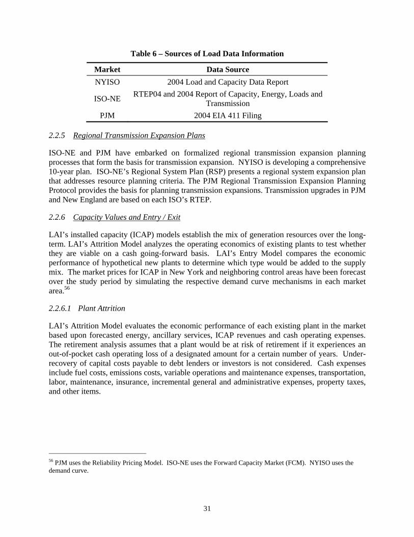
31

Table 6 – Sources of Load Data Information

Market Data Source NYISO 2004 Load and Capacity Data Report

ISO-NE RTEP04 and 2004 Report of Capacity, Energy, Loads and Transmission

PJM 2004 EIA 411 Filing

2.2.5 Regional Transmission Expansion Plans

ISO-NE and PJM have embarked on formalized regional transmission expansion planning processes that form the basis for transmission expansion. NYISO is developing a comprehensive 10-year plan. ISO-NE’s Regional System Plan (RSP) presents a regional system expansion plan that addresses resource planning criteria. The PJM Regional Transmission Expansion Planning Protocol provides the basis for planning transmission expansions. Transmission upgrades in PJM and New England are based on each ISO’s RTEP.

2.2.6 Capacity Values and Entry / Exit

LAI’s installed capacity (ICAP) models establish the mix of generation resources over the long-term. LAI’s Attrition Model analyzes the operating economics of existing plants to test whether they are viable on a cash going-forward basis. LAI’s Entry Model compares the economic performance of hypothetical new plants to determine which type would be added to the supply mix. The market prices for ICAP in New York and neighboring control areas have been forecast over the study period by simulating the respective demand curve mechanisms in each market area.56

2.2.6.1 Plant Attrition

LAI’s Attrition Model evaluates the economic performance of each existing plant in the market based upon forecasted energy, ancillary services, ICAP revenues and cash operating expenses. The retirement analysis assumes that a plant would be at risk of retirement if it experiences an out-of-pocket cash operating loss of a designated amount for a certain number of years. Under-recovery of capital costs payable to debt lenders or investors is not considered. Cash expenses include fuel costs, emissions costs, variable operations and maintenance expenses, transportation, labor, maintenance, insurance, incremental general and administrative expenses, property taxes, and other items.

56 PJM uses the Reliability Pricing Model. ISO-NE uses the Forward Capacity Market (FCM). NYISO uses the demand curve.

32

Capital expenditure requirements to meet the increasingly stringent emissions standards for existing coal and residual fuel oil (RFO)-fired plants may affect the economic viability of plants in the greater Northeast. 57

2.2.6.2 New Entry

New entrants are added to the model as required to maintain reserve margins considering load growth and retirements. In New York, new capacity also includes anticipated renewable generation projects as prescribed by the Renewable Portfolio Standard (RPS). Additional capacity in New York beyond the anticipated RPS projects is assumed to be combustion turbines, either in simple-cycle or combined-cycle mode. In other areas of the study region all generic new entry is assumed to be combustion turbine based.58 LAI’s Entry Model determines the mix of combined-cycle and simple-cycle new generation in each market area. Simple cycle combustion turbines in New York City and on Long Island are assumed to be LM6000 units (or equivalent aero-derivatives) that are somewhat less expensive than combined cycle plants and well suited for fast starts and shutdowns.59 LAI’s entry model incorporates a forecast of all the capital costs of a new plant, including the items in Exhibit 4.

The costs in Exhibit 4 represent the base costs for a new greenfield plant at relatively unconstrained sites on Long Island and New York City. The total capital costs include project development, EPC contract, interconnections, legal and financing, construction supervision, start-up, spares, and financial costs. Financing parameters are generally consistent with prior advisory work performed by LAI for NYISO regarding the demand curve.

Exhibit 5 contains a listing of the resource additions included in the NYISO, PJM and ISO-NE control areas. Additions in Ontario are also identified. The expected start-up date for each project is also listed along with the winter MW rating.

2.2.7 NYISO ICAP Demand Curve Mechanism

The demand curve mechanism is duplicated within the Attrition Model on an annual basis across the forecast horizon. Downward sloping demand curves using published data are generated in the Attrition Model for the entire New York Control Area (NYCA) as well as for the New York City and Long Island zones. NYISO requires those zones to satisfy locational ICAP requirements for which 80% of New York City’s peak load must be met by in-City generators, and 99% of Long Island’s peak load must be met by on-island generators.60 These locational 57 The Attrition Model incorporates investments for additional add-on emission controls to meet federal requirements for particulates, SO2, and NOx, as well as limits on mercury emissions. Upon the retirement of one or more plants, the supply curve in subsequent years is adjusted. 58 As noted in Exhibit 5, PJM has recently added one waste coal-fired plant, the Seward unit. 59 Simple cycle combustion turbines in PJM, New England and Rest of State are assumed to be GE-7FA units that are larger and less expensive on a unit-of-capacity basis. Combined cycle units are assumed to be industrial frame units, employing “F” or “G” technology, that are best suited for thermodynamic efficiency with heat recovery steam generators and steam turbine cycles. 60 Current NYISO rules allow for controllable direct current cables to qualify as on-island generation provided certain conditions are met, including corresponding capacity committed to New York load.

33

requirements are due to the limited ability of the high voltage transmission system to import power into those zones, taking into account normal operating conditions and contingency events. Over the forecast period, LAI has held constant the locational capacity requirements on Long Island and in New York City.

2.2.8 PJM Reliability Pricing Model

At the time the electric simulation modeling was conducted, the capacity market in PJM included daily, monthly, and multi-monthly unforced capacity (UCAP) auctions that determined a single clearing price for the entire PJM footprint. Load-serving entities (LSEs) submitted buy bids in these auctions to satisfy their UCAP requirements or to lay off surplus UCAP, while generators submitted bids to sell non-committed UCAP. These bids were voluntary and are residual, i.e. they did not include UCAP commitments in place either through bilateral contracts or through self-supply. The Reliability Pricing Model (RPM) is generally similar to the NYISO demand curve mechanism, but with many noteworthy distinctions. Consistent with NYISO, UCAP clearing prices would be determined based on the interaction of a demand curve that is set to provide a peaking generator with sufficient revenues to achieve a threshold return.

PJM intends to establish as many as 23 Locational Deliverability Areas to set UCAP prices that reflect locational reliability issues. For purposes of this analysis, LAI assumed that UCAP prices in eastern and southwestern MAAC would ultimately converge over the relevant planning horizon.61 By the fourth planning year, a number of critical transmission upgrades are expected to be completed within PJM, causing locational ICAP prices to converge.

2.2.9 ISO-NE Capacity Market

During our evaluation, ISO-NE had promoted a capacity market mechanism referred to as LICAP. Like NYISO’s demand curve, LICAP would use a sloped demand curve and a supply curve to set market-clearing ICAP prices. This structure would have been very similar to the Spot ICAP Market mechanism in NYISO that has been utilized since 2003. We expected that LICAP would result in the addition of gas turbine peakers or combined cycle plants when net energy and ancillary service revenues cover the incremental capital cost.

LICAP met resistance in New England, and was ultimately replaced by FCM – a product of settlement. FERC approved the FCM settlement, allowing for a multi-year transition period through 2010. FCM will use a descending clock auction process to accept or reject bids from new suppliers, as well as bids to retire from existing suppliers. Like LICAP, FCM is intended to reflect locational factors, in particular, transmission constraints. LAI’s entry assumptions incorporated our then current understanding of LICAP. In LAI’s view, the use of LICAP for purposes of adding new generation capacity does not constitute a significant bias regarding energy prices on Long Island under the Business-as-Usual case.

61 Results of the first PJM auction held in April 2007 for delivery year 2007/2008 indicate that both eastern and southwestern MAAC have substantially higher UCAP prices than the rest of PJM. A second auction was held in July 2007 for delivery year 2008/2009 and introduced material changes associated with transmission limits and the amount of generation in eastern MAAC. A third auction for delivery year 2009/2010 will be held in October 2007.

34

2.2.10 New York Renewable Portfolio Standard

In September 2004, the NYPSC issued an order implementing an RPS that requires at least 24% of the State’s electric energy to come from renewable resources by 2013. Currently, about 19% of the state’s energy requirements are supplied by renewable sources, primarily hydro. The September 2004 order implements a program whereby the New York State Energy Research and Development Authority (NYSERDA) will subsidize developers of new renewable facilities, selected via auction, to increase the state’s renewable portfolio and furnish 24% of total state requirements.62

To achieve the RPS target, the rules require NYSERDA to procure, and New York customers of LSEs to pay for, an incremental block of renewable energy. This incremental block represents roughly 1.4 million MWh per year starting in 2006. The incremental block of renewable generation represents roughly 0.8% of total state energy consumption and 1% of the total energy consumption served by LSEs.

The NYPSC estimates that a total of 3,539 MW of new qualified renewable capacity will need to be added by 2013 to fulfill the RPS requirement, based on assumed capacity factors for the various renewable technologies employed.63 The NYPSC also estimated that, in addition to the capacity required to fulfill the RPS requirements, another 1,006 MW of incremental renewable capacity (i.e., for a total of 4,546 MW) will be developed in NY State in the same time period.64 Of the total 4,546 MW of incremental renewable capacity, the NYPSC projected that a significant majority, 3,029 MW, would come from new wind resources. The remaining renewable capacity is projected to come from hydro imports (1,100 MW), biomass (294 MW), and landfill gas (123 MW).

Given various siting difficulties, limitations in wind turbine manufacturing, and our skepticism of non-RPS renewable capacity development, LAI made the conservative assumption that only approximately 20% of the NYPSC’s estimate of new wind capacity, or 650 MW, will be operational by 2013. We assumed that other forms of renewable capacity, totaling approximately 1,500 MW, will be developed as projected by the NYPSC. The NYPSC projections and LAI-adjusted values are detailed in Exhibit 6.

2.2.11 Emissions Assumptions and Allowance Prices

The Clean Air Act (CAA) and amendments authorized the Environmental Protection Agency (EPA) to establish market-based programs to reduce NOx and SO2 emissions from a variety of stationary sources, including fossil fuel fired electric generating units. Title IV of the CAA set a goal of reducing annual SO2 emissions by 10 million tons below 1980 levels. To achieve these reductions, the law required a two-phase tightening of the restrictions placed on fossil fuel-fired

62 The NYPSC expects an additional 1% of the state’s energy requirements to be met through voluntary purchases of incremental renewable energy. 63 See 03-E-0188, Appendix D, Table 7. 64 The additional capacity is expected to be developed in response to: Executive Order 111 (31 MW), green marketing (551 MW) and New England demand (424 MW).

35

power plants. Phase II, which began in 2000, tightened the annual emissions limits imposed on these plants and also set restrictions on smaller, cleaner plants fired by coal, oil, and gas. The program affects generators with an output capacity of greater than 25 MW. SO2 allowance allocation calculations were made for various types of units. EPA allocated allowances to each unit at an emission rate of 1.2 pounds of SO2/MMBtu of heat input, multiplied by the unit's baseline. Existing plants can meet their budget allocation through the use of compliance coal or low sulfur RFO (0.7% sulfur or less), by operation of flue gas desulfurization (FGD) systems, or by acquiring emissions allowances from the market.

All NOx trading programs have the same goal: reduce the transport of ground-level ozone. However, several programs have developed through different mechanisms, which has led to differences in the number of states involved, the timing of the compliance period each year, and the milestones for the targeted reductions. The Ozone Transport Commission (OTC) member states have been subject to a NOx budget “cap and trade” program since 1999. 65 The OTC program limits the total emissions from affected units in each state during the ozone season (May 1 to September 30) of each year. The most recent NOx budget reductions under the OTC program were implemented in May 2003. Two other regional trading programs, the Section 126 final action (2005) and the NOx State Implementation Plan (SIP) Call, will affect 22 states, including several states in PJM not previously subject to the OTC NOx budget program.66 The most recent NOx SIP Call deadline for Phase I reductions was May 2004. The emission limit used by EPA to calculate the Phase I NOx SIP call budgets, 0.15 lb NOx/MMBtu, represents approximately an 85% reduction from uncontrolled NOx emissions for most large coal-fired power plants. Further reductions must be implemented by the Phase II compliance date in 2007.

In 2005, EPA promulgated the Clean Air Interstate Rule (CAIR), intended to further reduce and permanently cap emissions of SO2 and NOx from electric generating plants. CAIR focuses on the 29 eastern states where power plant emissions significantly contribute to the non-attainment of downwind states with respect to ozone and fine particulates. The rule establishes a cap-and-trade program, which would reduce power plant SO2 emissions by 3.6 million tons in 2010, and 1.8 million tons in 2015. The rule also establishes year-round NOx caps beginning in 2010, with further reductions in 2015. Although each affected state is required to develop its own implementation plan, we expect that coal and oil-fired plants, which currently lack selective catalytic reduction (SCR) and/or FGD will retrofit such systems by 2010. Our capacity model reflects these investments. The expanded emission allowance program, including a non-ozone season market for NOx allowances, also affects our forecast for NOx and SO2 allowance prices.67

65 New England, New York, New Jersey, Delaware, Maryland, Pennsylvania, and the District of Columbia. 66 States and districts covered by the NOx SIP Call are: AL, CT, DC, DE, IL, IN, KY, MA, MD, MI, NC, NJ, NY, OH, PA, RI, SC, TN, VA, WV. GA and MO subject to Phase II only. States and districts covered by the Section 126 final rule are: DC, DE, IN, KY, MD, MI, NC, NJ, NY, OH, PA, VA, WV. 67 Many of the coal-fired plants in New York, PJM, and Ontario have implemented strategies to reduce SO2 and NOx emissions. A number of the larger and more efficient plants have retrofit FGD systems for SO2 control and a somewhat larger number of plants have retrofit SCR or selective non-catalytic reduction systems to control NOx emissions. Other less efficient plants, have implemented CAA compliance strategies that involve less expensive and less effective emission control technologies (low NOx burners) coupled with the purchase of emissions allowances.

36

2.2.11.1 New York Regulations

In 1999, Governor Pataki announced that fossil fuel-fired generators in New York would be required to further reduce SO2 and NOx emissions to protect sensitive regions such as the Adirondacks and the Catskills from the deleterious impacts of acid rain. The Acid Deposition Reduction Program (ADRP) became effective on May 17, 2003.68 In accordance with Part 237, affected sources must collectively reduce NOx emissions during the non-ozone season beginning October 1, 2004 to a level that corresponds with the ozone-season NOx reductions that were achieved in May 2003 under the current NOx budget trading program.69 Part 238 reduces the SO2 emissions to 50% below the levels allowed under the current phase of the federal acid rain program. The SO2 reductions are implemented in two phases, beginning January 1, 2005 and January 1, 2008.

Consistent with LAI’s treatment in prior energy price forecasting studies performed for LIPA, NOx and SO2 allowances are treated as variable operating costs for each fossil fuel generating unit. Energy prices are therefore directly impacted by the allowance markets to reflect generators’ ability to bid allowance costs into the DAM or real-time market. As discussed in Appendix 4, LAI’s forecast incorporates our outlook for the SO2 and NOx allowance markets. The SO2 allowance price forecast shows prices near $700/ton through 2007, followed by a gradual decline to $200/ton by 2014, after which allowance prices will escalate in keeping with inflation. The NOx allowance price forecast shows a similar pattern, with prices around $3,340/ton in 2006, then decreasing to $1,500 in 2012. After 2012, prices will increase with inflation.

2.3. Market Analysis Results

The results of the GPCM modeling cases include the impacts of various assumptions regarding supply, demand, market conditions and infrastructure projects on natural gas prices at continental pricing points and regional pricing points. The continental pricing points of particular relevance are Henry Hub and Dawn. The regional pricing points of particular relevance for Long Island and New York City are TZ6-NY and IGTS-Z2. Rest of State values are indexed to Dominion South Point (DTI-SP). The comparison of these prices with and without Broadwater provides the basis for determining the economic benefits on Long Island, New York City, and Rest of State that are ascribable to Broadwater.

The market has been divided into core and non-core on Long Island, New York City and Rest of State. The core and non-core demands are further divided among relevant pricing points in Canada, the Gulf Coast, storage centers, and the market area. LAI has made assumptions regarding where natural gas is purchased for each company, as well as how existing versus incremental loads are served. In sum, LAI has assumed that the region’s gas utilities purchase all of their natural gas either at production areas or major storage hubs, i.e., Leidy, Ellisburg and

68 6 New York State Codes Rules and Regulations (NYCRR) Parts 237 and 238 69 6 NYCRR Part 204

37

Dawn. We have assumed that power generators on Long Island and New York City purchase natural gas based on TZ6-NY and/or IGTS-Z2 prices.

Figure 15 provides a comparison of the Henry Hub prices for the Business-as-Usual Case. The various price impacts at the Henry Hub when Broadwater is added are shown in dark blue (second line). Commodity prices are shown in green when Millennium Phase 2 and Islander East are added to the resource mix, absent Broadwater. Finally, the impact of Crown Landing on Henry Hub prices is also reported, absent Broadwater. Relative to the Business-as-Usual forecast of gas prices at the Henry Hub, the commodity price difference ranges from a low of $0.03/MMBtu higher with Millennium Phase 2 and Islander East to a high of $0.50/MMBtu lower for Crown Landing. The addition of Broadwater results in commodity prices at the Henry Hub that would average $0.46/MMBtu lower over the forecast period.

Figure 15 – Commodity Price Changes at the Henry Hub: Business-as-Usual v. Alternative Cases (Broadwater, Millennium Phase II + Islander East, Crown Landing)

0

1

2

3

4

5

6

7

8

9

10

Jan-

06

Jan-

07

Jan-

08

Jan-

09

Jan-

10

Jan-

11

Jan-

12

Jan-

13

Jan-

14

Jan-

15

Jan-

16

Jan-

17

Jan-

18

Jan-

19

Jan-

20

Gas

Pric

e (N

omin

al $

/MM

Btu

)

Henry Hub BAU Case

Henry Hub BAU Case w/ Broadwater - Average Difference $0.46

Henry Hub BAU Case w/ Millennium Phase 2 & Islander East - Average Difference -$0.03

Henry Hub BAU Case w/ Crown Landing - Average Difference $0.50

Figure 16, Figure 17 and Figure 18 compare the forecast of prices under the same Business-as-Usual Cases at various continental and regional pricing points of specific relevance to Long Island and New York: Dawn, TZ6-NY, and IGTS-Z2. As shown in Figure 17, the average price reduction in TZ6-NY prices with Broadwater is $1.35/MMBtu over the forecast period. If Crown Landing is built in lieu of Broadwater, the resultant average price decrease in TZ6-NY prices is $0.59/MMBtu. Coincidentally, the price effect attributable to Millennium Phase 2 and Islander East is the same as Crown Landing.

38

Figure 16 – Commodity Price Changes at the Dawn Storage Hub: Business-as-Usual v. Alternative Cases (Broadwater, Millennium Phase II + Islander East, Crown Landing)

0

2

4

6

8

10

12

Jan-

06

Jan-

07

Jan-

08

Jan-

09

Jan-

10

Jan-

11

Jan-

12

Jan-

13

Jan-

14

Jan-

15

Jan-

16

Jan-

17

Jan-

18

Jan-

19

Jan-

20

Gas

Pric

e (N

omin

al $

/MM

Btu

)

Dawn BAU Case

Dawn BAU Case w/ Broadwater - Average Difference $0.49

Dawn BAU Case w/ Millennium Phase 2 & Islander East - Average Difference -$0.03

Dawn Base Case w/ Crown Landing - Average Difference $0.52

Figure 17 – TZ6-NY Price Change: Business-as-Usual v. Alternative Cases (Broadwater, Millennium Phase II + Islander East, Crown Landing)

0

2

4

6

8

10

12

14

16

18

20

Jan-

06

Jan-

07

Jan-

08

Jan-

09

Jan-

10

Jan-

11

Jan-

12

Jan-

13

Jan-

14

Jan-

15

Jan-

16

Jan-

17

Jan-

18

Jan-

19

Jan-

20

Gas

Pric

e (N

omin

al $

/MM

Btu

)

TZ6-NY BAU Case

TZ6-NY BAU Case w/ Broadwater - Average Difference $1.35

TZ6-NY BAU Case w/ Millennium Phase 2 & Islander East - Average Difference $0.59

TZ6-NY BAU Case w/ Crown Landing - Average Difference $0.59

39

Figure 18 – IGTS-Z2 Price Change: Business-as-Usual v. Alternative Cases (Broadwater, Millennium Phase II + Islander East, Crown Landing)

0

2

4

6

8

10

12

14

16

18

20Ja

n-06

Jan-

07

Jan-

08

Jan-

09

Jan-

10

Jan-

11

Jan-

12

Jan-

13

Jan-

14

Jan-

15

Jan-

16

Jan-

17

Jan-

18

Jan-

19

Jan-

20

Gas

Pric

e (N

omin

al $

/MM

Btu

)

IGTS-Z2 BAU Case

IGTS-Z2 BAU Case w/ Broadwater - Average Difference $1.61

IGTS-Z2 BAU Case Millennium Phase 2 & Islander East - Average Difference $0.62

IGTS-Z2 BAU Case w/ Crown Landing - Average Difference $0.55

In Figure 19 through Figure 22 we show the forecast of prices at the Henry Hub, Dawn, TZ6-NY and IGTS-Z2 associated with the LNG Overbuild Case. In the event that there is an LNG Overbuild in the greater Northeast and Broadwater is also added to regional infrastructure, Broadwater’s consequent price effect on Long Island, New York City and Rest of State would still remain high.

40

Figure 19 – Henry Hub Price Comparison: LNG Overbuild Case

0

1

2

3

4

5

6

7

8

9

10

Jan-

06

Jan-

07

Jan-

08

Jan-

09

Jan-

10

Jan-

11

Jan-

12

Jan-

13

Jan-

14

Jan-

15

Jan-

16

Jan-

17

Jan-

18

Jan-

19

Jan-

20

Gas

Pric

e (N

omin

al $

/MM

Btu

)

Henry Hub LNG Overbuild

Henry Hub LNG Overbuild w/ Broadwater - Average Difference $0.28

Figure 20 – Dawn Price Comparison: LNG Overbuild Case

0

1

2

3

4

5

6

7

8

9

10

Jan-

06

Jan-

07

Jan-

08

Jan-

09

Jan-

10

Jan-

11

Jan-

12

Jan-

13

Jan-

14

Jan-

15

Jan-

16

Jan-

17

Jan-

18

Jan-

19

Jan-

20

Gas

Pric

e (N

omin

al $

/MM

Btu

)

Dawn LNG Overbuild

Dawn LNG Overbuild w/ Broadwater - Average Difference $0.33

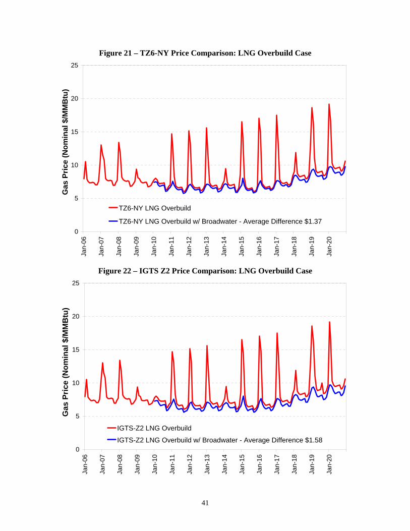
41

Figure 21 – TZ6-NY Price Comparison: LNG Overbuild Case

0

5

10

15

20

25

Jan-

06

Jan-

07

Jan-

08

Jan-

09

Jan-

10

Jan-

11

Jan-

12

Jan-

13

Jan-

14

Jan-

15

Jan-

16

Jan-

17

Jan-

18

Jan-

19

Jan-

20

Gas

Pric

e (N

omin

al $

/MM

Btu

)

TZ6-NY LNG Overbuild

TZ6-NY LNG Overbuild w/ Broadwater - Average Difference $1.37

Figure 22 – IGTS Z2 Price Comparison: LNG Overbuild Case

0

5

10

15

20

25

Jan-

06

Jan-

07

Jan-

08

Jan-

09

Jan-

10

Jan-

11

Jan-

12

Jan-

13

Jan-

14

Jan-

15

Jan-

16

Jan-

17

Jan-

18

Jan-

19

Jan-

20

Gas

Pric

e (N

omin

al $

/MM

Btu

)

IGTS-Z2 LNG Overbuild

IGTS-Z2 LNG Overbuild w/ Broadwater - Average Difference $1.58

42

Table 7 summarizes the average gas price impact over the forecast period for Broadwater, Millennium Phase 2 plus Islander East, Crown Landing, and, finally, the LNG Overbuild Case. Price effects in select years at regional pricing points are shown in Exhibit 7.

Table 7 – Average 10-Year Price Results by Case

Henry Hub Dawn Iroquois

Zone 2 TranscoZ6 NY

Business-as-Usual $7.45 $7.82 $9.54 $9.54 Business-as-Usual + Broadwater $6.99 $7.33 $7.93 $8.19

Broadwater Impact $0.46 $0.49 $1.61 $1.35 Business-as-Usual + Millennium 2 /

Islander East $7.48 $7.85 $8.92 $8.95

Millennium 2 + Islander-East Impact -$0.03 -$0.03 $0.62 $0.59 Business-as-Usual + Crown Landing $6.95 $7.30 $8.99 $8.95

Crown Landing Impact $0.50 $0.52 $0.55 $0.59 LNG Overbuild Case – w/o Broadwater $6.24 $6.69 $8.55 $8.54 LNG Overbuild Case – w/ Broadwater $5.95 $6.35 $6.97 $7.17

Broadwater Impact 70 $0.29 $0.34 $1.58 $1.37

2.4. Benefits Attributable to Broadwater

2.4.1 Gas Utility and Electric Utility Benefits on Long Island, New York City and Rest of State

Natural gas to serve core utility load is sourced primarily from the production area in the Gulf of Mexico and western Canada. Gas that originates from the Gulf of Mexico is priced at the Henry Hub. Gas that originates from western Canada is priced at Dawn. For both KeySpan and Con Edison, we have assumed that 60% of the existing core load originates from the Gulf Coast via the major trunklines connecting the Gulf Coast with New York via the storage facilities in Pennsylvania and New York. The remainder, 40%, is assumed to originate in western Canada and therefore priced at Dawn. Since the pipelines serving New York City and Long Island are fully subscribed, we have assumed that gas utilities in New York meet incremental load growth at a price equal to TZ6-NY.

Quantification of economic benefits for core customers reflects the following pricing points throughout New York State:

70 Results are gauged around prices in the LNG Overbuild Case (no Broadwater) rather than the Business-as-Usual Case.

43

Table 8 – Market Center Pricing Points

Sub-Area Pricing Point New York City TZ6-NY

Long Island IGTS-Z2 / TZ6-NY NY Central & North IGTS-Z1

NY West Niagara NY South DTI-SP

Gas-fired generation bids into NYISO’s DAM reflect the value of natural gas in the market area, i.e., TZ6-NY, IGTS-Z2.71 On Long Island, LIPA pays for the actual costs of generation and power procurement, mostly the “legacy units” owned and operated by KeySpan. These oil and gas fired stations provide most of the energy used on Long Island. Energy prices and fuel use were calculated by MarketSym.72 The hourly product of energy price and load was integrated over each year to establish a wholesale energy supply cost for each region.

The financial logic LAI used to quantify the economic benefits to core and non-core customers on Long Island, New York City and Rest of State is presented in Exhibit 8. LAI has computed the present value in the change in both gas utilities’ natural gas procurement costs over the study horizon as well as the change in electricity prices of relevance by location.73 The first-order change in natural gas costs for core and non-core customers has then been adjusted to account for the second-order income multiplier effects. The use of the income multiplier is discussed in section 2.4.2.

In Figure 23, we report annual savings for core customers attributable to Broadwater for Long Island, New York City and Rest of State. Total savings for core customers in New York State range from above $300 million in 2010 to about $780 million in 2020. In absolute dollars, core utility customers on Long Island are expected to realize much lower benefits than New York City and Rest of State. Broadwater’s beneficial price impact cascades back to upstream market centers; hence, economic benefits for Rest of State are comparable to New York City. In Figure 24 we report the present value of total core benefits by each sub-region. Total benefits for core amount to $4.6 billion as follows: $1.9 billion for New York City (41%), $0.8 billion on Long Island (17%), and $1.9 billion for Rest of State (42%).

71 Gas-fired generation in upstate New York is generally reflective of lower priced indices, i.e., DTI-SP, IGTS-Z1, and Niagara. 72 MarketSym provided total gas burns by area, which were used to refine the GPCM runs. 73 Fixed costs payable to pipelines and storage companies are deemed sunk and therefore not relevant for purposes of quantifying the change in total natural gas costs.

44

Figure 23 – Core Benefits Attributable to Broadwater by Year

0

100

200

300

400

500

600

700

800

900

2010 2011 2012 2013 2014 2015 2016 2017 2018 2019 2020

Ann

ual C

ore

Gas

Loa

d Sa

ving

s ($

MM

)New York City Long Island Rest of State

Figure 24 – Core Benefits Attributable to Broadwater by Sub-Area (2010-2020)

25,3

76

8,43

3

29,9

32

23,5

12 27,9

93

1,86

4

791 1,

938

7,64

2

0

5,000

10,000

15,000

20,000

25,000

30,000

35,000

New York City Long Island Rest of State

PV o

f Cor

e G

as C

ost (

$MM

)

Without Broadwater With Broadwater Differential

45

In Figure 25 we report annual savings for non-core electricity customers attributable to Broadwater for Long Island, New York City and Rest of State. Total savings for non-core customers in New York State range from above $500 million in 2010 to about $2 billion in 2020. Consistent with the relative breakdown of benefits for core customers, in absolute dollars non-core electricity customers on Long Island are expected to realize much lower benefits than New York City and Rest of State. Benefits for Rest of State are roughly comparable to New York City. In Figure 26 we report the present value of total non-core benefits by sub-area. Total benefits for non-core amount to $10.2 billion as follows: $4.4 billion for New York City (43%), $1.9 billion on Long Island (19%), and $3.9 billion for Rest of State (38%).

Figure 25 – Non-Core Benefits Attributable to Broadwater by Year

0

500

1,000

1,500

2,000

2,500

2010 2011 2012 2013 2014 2015 2016 2017 2018 2019 2020

Ann

ual N

on-C

ore

Ener

gy S

savi

ngs

($M

M)

New York City Long Island Rest of State

46

Figure 26 – Non-Core Benefits Attributable to Broadwater by Sub-Area (2010-2020)

43,7

93

18,1

08

55,0

65

39,3

59

51,1

90

4,43

4

1,90

1

3,87

5

16,2

07

0

10,000

20,000

30,000

40,000

50,000

60,000

New York City Long Island Rest of State

PV o

f Ele

ctric

Ene

rgy

Cos

t ($M

M)

Without Broadwater With Broadwater Differential

2.4.2 Economic Multiplier Analysis

In gauging the local economic impacts of the Broadwater facility, it is necessary to estimate the first-order effects as well as the second-order effects associated with increased economic activity due to lower energy prices. Economic multipliers are quantitative factors designed to provide a measure of the secondary economic impacts from changes in employment, income, and other variables. A wide range of economic multipliers can be found in publicly available economic analyses and reports. We endeavored to find an applicable multiplier that reasonably estimated the indirect impacts associated with reduced energy costs. No independent derivation of the economic multiplier was performed in this study. Instead, we relied on a study prepared at Cornell University on New York State’s economy regarding multipliers for the transport and utilities industries. The range reported in the Cornell study for New York State was 1.31 to 1.48.74 There are many other studies with multipliers well above or somewhat below the aforementioned range.75 For purposes of this analysis, LAI applied an economic multiplier equal to 1.4.

74 Economic Multipliers and the New York State Economy, by K. Jack, New York State Department of Labor, and N. Bills & R. Boisvert, Professors in the Department of Agricultural, Resource, and Managerial Economics, December 1996. 75 Another study evaluating DOE spending concluded that economic multipliers tend to be in the range of 1.5 to 2.0. The Nuclear Energy Institute (NEI) evaluated the impact of continued operation of the Indian Point nuclear power plant. Entergy, the owner of Indian Point, calculated multipliers for plant output and local employment on the

47

Other benefits associated with PILOT, job creation, and commercial inducements potentially available from Broadwater are not included.

2.4.3 Discussion of Net Benefits

As shown in Table 9 and reported in Section 2.4.1, the total first-order expected economic benefits on Long Island, New York City and Rest of State amount to $14.8 billion. When these benefits are increased to account for the economic multiplier effect, total benefits increase to $20.7 billion over the forecast period. With or without the multiplier effect, the benefits are stated in present value terms for 2010.76

Table 9 – Summary of LAI’s Economic Findings

Benefits w/o Multiplier

Benefits w/ Multiplier % Total

Long Island $2.7 billion $3.8 billion 18.3 New York City $6.3 billion $8.8 billion 42.6

Rest of State $5.8 billion $8.1 billion 39.1 Total $14.8 billion $20.7 billion

2.4.4 Benefits Reconciliation

In April 2005, Broadwater represented to LIPA’s management and Board of Trustees that the Project would produce energy savings of $6 billion over the first ten years of its operating life. Subsequent discussions between LAI and Broadwater revealed that Broadwater’s model was designed to broadly analyze regional inputs on a high-level basis, and that the purported $6 billion savings was a simple nominal sum over ten years of core and non-core savings on Long Island and New York City. Broadwater did not estimate the value of avoided gas price volatility in the market center. Broadwater did not accurately differentiate core from non-core in terms of natural gas procurement patterns. Broadwater only counted potential economic benefits on Long Island and New York City, not elsewhere in New York State. Broadwater did not count economic multiplier effects. There were many other important structural differences between modeling techniques and assumptions.

Had we applied Broadwater’s financial approach for consistency sake, LAI’s determination of economic benefits would increase from $14.8 billion to $21.6 billion,77 a difference of $15.6 billion from Broadwater’s estimate.

county, state and country. NEI calculated a local multiplier of 1.17 and a state-wide multiplier of 1.25 on plant output, a local multiplier of 1.35, and a state-wide multiplier of 1.45 on labor income. DOE has asserted that utility services generally produce an economic multiplier of 1.66. 76 Discount rate equals 6%. 77 Reflects the nominal pattern of annual savings at a zero percentage discount rate consistent with the $14.8 billion total savings at 6%.

48

2.4.5 Omitted Variables

A number of benefit and cost components have not been quantified in this assessment, but are potentially significant.

• Broadwater’s location in the market center improves reliability across the NYFS by allowing Iroquois to “pack the pipe” throughout the year, including the Eastchester lateral from Northport to New York City. The value of increased pipeline system reliability has not been quantified in this analysis.

• Broadwater’s potential PILOT to host communities have not been considered.

• The value of potential commercial inducements from Broadwater to one or more anchor customers on Long Island or New York City has not been estimated.

• A new, baseload natural gas supply source located in the heart of the market should increase the use of natural gas relative to residual fuel oil for power production on Long Island and, perhaps, New York City. The value of reducing CO2, SO2, NOx, volatile organic compounds, and particulates has not been quantified. The reduction in commodity gas prices as well as damped gas price volatility may induce KeySpan on Long Island and other generation companies in New York City, or Rest of State, to undertake costly generation asset repowering(s) that might not otherwise occur.78 The environmental benefits associated with repowering have not been quantified.

• Broadwater’s daily dispatch regime would materially change the pattern of gas flows on Long Island and New York City. Both KeySpan and Con Edison may therefore need to commit substantial capital resources to maintain network reliability in response to much higher receipts at different gate stations on the NYFS.79 Other costs borne by KeySpan, Con Edison and power plants to ensure that Broadwater’s gas supply is interchangeable with historical pipeline rendered supply must also be counted. Other costs may be borne by the region’s gas utilities to ensure that the level of nitrogen injection to facilitate interchangeability does not cause operating problems at existing peak-shaving LNG facilities in Suffolk County, Queens and Brooklyn. Finally, significant costs may be borne by generators in the region to ensure safe and reliable operation following the introduction of natural gas from Broadwater.

• Economic benefits associated with both KeySpan’s and Con Edison’s ability to reduce their costs by laying off, through FERC approved capacity release, a portion of their

78 To the extent the repowering(s) would happen anyway, there should be no inclusion of environmental benefits attributable to Broadwater. 79 LAI conducted an independent, high-level analysis of potential transmission system reinforcements on the NYFS in order to derive a plausible upper limit to ensure local reliability in New York City. Using the most expensive segment along Iroquois’ Eastchester Expansion into New York City as a data source for high construction costs in-City, LAI estimated that up to $350 million could be required to transport natural gas from the Hunts Point gate station to a new gate station up to 10 miles from the existing terminus. Whether Con Edison would plan to add another gate station is unknown, however. Whether KeySpan would plan to add another gate station has not been determined.

49

valuable pipeline and/or storage entitlements on Transco, Texas Eastern, Tennessee, and in Ontario, as well, has the potential to be significant, but has not been estimated.

3. TECHNOLOGY REVIEW

The anticipated long-term growth in U.S. natural gas demand will require the construction and operation of both onshore and offshore LNG terminals. Recently, several offshore LNG terminals have been proposed to increase LNG deliveries to market centers where onshore facilities cannot realistically be sited. The technologies and experience developed for offshore oil infrastructure and onshore LNG terminals can be applied to the development and operation of offshore LNG terminals. The proposed offshore LNG terminals benefit from the record of safety and reliability that has been achieved by the offshore oil industry and by onshore LNG terminals around the world. Each of the essential components of Broadwater’s FSRU has been used safely and reliably in both offshore petroleum and onshore LNG terminal operations. The main difference is the scale of the application proposed for Broadwater.

Offshore siting innovations for LNG facilities necessitate new rules and guidelines for the design, construction and maintenance of such facilities. Since 1862, ABS has developed such rules and guidelines for the maritime industry. ABS has published a guide for building and classing offshore LNG terminals that puts forth a comprehensive set of criteria.80 The classification process begins with an assessment of design and continues throughout the operational life of the offshore LNG facility. Such oversight ensures the continued adherence to the ABS rules and guidelines and other relevant standards beyond the initiation of service through the installation and operation of the facility.81

LAI’s technology study objectives were threefold: first, to evaluate the various types of offshore LNG facilities; second, to identify the technology limitations of the FSRU, its major components and the YMS; and, third, to assess operational issues with the FSRU and LNG transfer. LAI’s technology review was based on data obtained from the draft and final EISs from other proposed and approved LNG projects, industry LNG technology presentations and papers, and publicly available reports on technology.

LAI’s approach to evaluating Broadwater’s technology involved a high level review of each type of offshore LNG facility proposed or operating in the U.S. including gravity-based structures (GBSs), modified LNG tankers unloading to a submerged turret loading buoy, and other FSRUs. LAI also evaluated each of the essential operating components of the FSRU from the perspective of historical use and assessed their appropriateness for the proposed application. The following LNG systems and components were evaluated: containment, regasification (vaporization), cargo transfer, emergency shutdown, boil-off, custody transfer and mooring.

3.1. Offshore LNG Technology Options

An offshore LNG terminal receives LNG from oceangoing vessels, regasifies the LNG either immediately or subsequent to being stored, and delivers the LNG to the onshore market through a subsea pipeline. While offshore applications have been used successfully for a number of different petroleum products, only recently has interest been focused on LNG. Such interest has 80 American Bureau of Shipping, “Guide for Building and Classing Offshore LNG Terminals,” April 2004. 81 ABS was selected as the third party Certifying Entity for the Project on February 16, 2007.

51

been generated by the need to expand the opportunities to meet market requirements in light of sensitive siting and public safety issues. The development and use of offshore facilities is an extension of the industry’s experience over the past several decades from land-based LNG terminals, LNG ship design, and similar floating applications utilized in the petroleum sector, referred to as Floating Production Storage and Offloading (FPSO) units. Offshore LNG import terminals can be grouped into the following five categories, some of which are illustrated in Figure 27.

• Natural Island Facility – A terminal sited on an island, such as the facility that is proposed in the Bahamas, with the regasified LNG delivered to a mainland location in Florida via an undersea pipeline.

• Artificial Island Facility – A terminal sited on a foundation created by building up the seafloor above the waterline, such as the Safe Harbor project proposed off Long Island.

• Floating Facility – A free-floating structure connected to the sea floor by a mooring system. FSRUs, such as Cabrillo Port and the Broadwater Project, and Floating Regasification Units (FRUs), such as Excelerate’s Gulf Gateway, are included in this category.

• Fixed and Mobile Structure – A facility which depends on the sea floor for support. Such a facility is currently proposed for offshore California (Crystal Clearwater Port) and would make use of an existing offshore platform reconfigured to receive LNG.

• Subsea – A structure predominately or totally below the water surface which rests on the sea floor. Such a facility is also known as a GBS. The proposed Gulf Landing facility to be located 38 miles south of Cameron, Louisiana, is such a project.

Figure 27 – Illustration of Offshore LNG Facility Types82

82 Source: Mossmaritime.

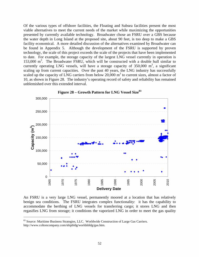
52

Of the various types of offshore facilities, the Floating and Subsea facilities present the most viable alternatives to meet the current needs of the market while maximizing the opportunities presented by currently available technology. Broadwater chose an FSRU over a GBS because the water depth in Long Island at the proposed site, about 90 feet, is too deep to make a GBS facility economical. A more detailed discussion of the alternatives examined by Broadwater can be found in Appendix 5. Although the development of the FSRU is supported by proven technology, the scale of this project exceeds the scale of the projects that have been implemented to date. For example, the storage capacity of the largest LNG vessel currently in operation is 153,000 m3. The Broadwater FSRU, which will be constructed with a double hull similar to currently operating LNG vessels, will have a storage capacity of 350,000 m3, a significant scaling up from current capacities. Over the past 40 years, the LNG industry has successfully scaled up the capacity of LNG carriers from below 20,000 m3 to current sizes, almost a factor of 10, as shown in Figure 28. The industry’s operating record of safety and reliability has remained unblemished over this extended interval.

Figure 28 – Growth Pattern for LNG Vessel Size83

0

50,000

100,000

150,000

200,000

250,000

300,000

1965

1970

1975

1980

1985

1990

1995

2000

2005

2010

Delivery Date

Cap

acity

(m3 )

An FSRU is a very large LNG vessel, permanently moored at a location that has relatively benign sea conditions. The FSRU integrates complex functionality: it has the capability to accommodate the berthing of LNG vessels for transferring cargo; it stores LNG and then regasifies LNG from storage; it conditions the vaporized LNG in order to meet the gas quality 83 Source: Maritime Business Strategies, LLC. Worldwide Construction of Large Gas Carriers. http://www.coltoncompany.com/shipbldg/worldsbldg/gas.htm.

53

conditions specified by the market; it connects to the delivering pipeline; it meters send-out and accounts for process boil-off; and it provides for the necessary monitoring and control systems to ensure safe and reliable operation, including the provision of room and board for the dozens of industry professionals that work round-the-clock. In addition to Broadwater, LAI has examined three other projects with different technologies for purposes of comparison: first, the Cabrillo Port project located offshore of southern California; second, Excelerate’s Gulf Gateway terminal in the Gulf of Mexico; and, third, Shell’s proposed Gulf Landing project located offshore of Louisiana.

Table 10 summarizes the specifications for the offshore LNG projects considered in this evaluation.

Table 10 – Summary of Offshore LNG Project Specifications

Broadwater Cabrillo Port Excelerate Gulf

Landing Class FSRU FSRU FRU GBS

Capacity, m3 350,000 273,000 135,000 180,000 Structure Length, ft 1,215 971 909 1,115 Structure Width, ft 200 213 142 230 Structure Height Above Water, ft (Top of Tank)

80 161 75-100 35-40

Tank Design Membrane Spherical Membrane Membrane Number of Tanks 8 3 4-5 2

Mooring YMS Turret STL NA Unloading Side by Side Side by Side NA Side by Side

Water Depth, ft 90 2,900 290 55 Avg. Vap. Rate, Bcf/d 1.0 0.80 0.5 1.0 Max Vap. Rate, Bcf/d 1.25 1.50 0.7 1.25

Vapor Process STV SCV STV(O/C) ORV(O/C)

Receiving Vessels, m3 125,000-250,000

125,000-250,000 NA 125,000-

200,000

3.1.1 Cabrillo Port

The Cabrillo Port LNG facility proposed for offshore California is an FSRU substantially similar to Broadwater. Cabrillo Port has announced an in-service date of 2010. Significant differences exist in major technology areas such as the cargo containment system and the mooring system. The Cabrillo Port FSRU will use three Moss spherical tanks for the storage of LNG (Figure 29) instead of the eight membrane tanks used by Broadwater. Each of the spherical tanks will have approximately two times the capacity of one of Broadwater’s membrane tanks. To accommodate the selection of the spherical containment system, the FSRU at Cabrillo Port will be

54

approximately 22% shorter (971 feet), 18% wider (213 feet) and 100% higher (161 feet) than the Broadwater FSRU. The storage capacity at Cabrillo Port will be 28% less than Broadwater’s proposed capacity (273,000 m3 v. 350,000 m3). The water depth at Cabrillo Port is 2,900 feet compared to 90 feet at Broadwater’s proposed location. To accommodate the much deeper water at Cabrillo Port, the mooring system would be a turret design instead of the YMS incorporated in the Broadwater design. As with the YMS, the turret permits the FSRU to weathervane as wind and sea conditions dictate. Like Broadwater, Cabrillo Port’s cargo transfer operation would be side-by-side unloading from the LNG vessel. The regasification process would involve eight submerged combustion vaporizers, fueled by the boil-off gas stream.

Figure 29 – Cabrillo Deepwater Port FSRU84

3.1.2 Excelerate Gulf Gateway

The Excelerate Gulf Gateway project was the first LNG offshore terminal to begin commercial operations in the U.S. The facility is located in the Gulf of Mexico, approximately 116 miles south of the Louisiana coastline, in water with a depth of approximately 290 feet. Since commercialization in Q1 2005, Gulf Gateway has received only a few LNG cargoes, including the initial shipment in March 2005, a subsequent full shipment in August 2005, and a partial shipment in August 2006. LNG is regasified directly on the tanker and transferred from the tanker using the Submerged Turret Loading (STL) buoy system (Figure 30). As such there is no LNG cargo transfer operation and no on-site storage capacity. The absence of permanent storage at Gulf Gateway undermines firm deliverability associated with onshore LNG terminals or Broadwater, because LNG can only be revaporized when a ship is positioned at the unloading buoy.

The STL technology was first introduced in 1993 and has been utilized for many years in the North Sea. The STL buoy is connected to the delivery pipeline by a flexible riser, and is

84 Source: BHP Billiton.

55

submerged to a depth of 80 feet when no unloading vessel is in position. When a vessel is ready for delivery, the vessel connects to the terminal by pulling the STL buoy into the onboard STL compartment. The regasified LNG then passes through the STL system into the delivering pipeline on the seabed, as shown in Figure 30.

Figure 30 – Illustration of STL Technology85

The LNG tankers serving the Gulf Gateway terminal are specially outfitted to include facilities for regasification in addition to the equipment necessary for connecting to the STL buoy system, as shown in Figure 31.

85 Source: Excelerate Energy, LLC.

56

Figure 31 – LNG Tanker Serving Gulf Gateway Terminal86

In addition to the STL system, the Gulf Gateway terminal required the construction of a platform to house the custody transfer meters and related equipment to receive the vaporized gas from the LNG vessel and distribute it to the delivering pipelines. The platform includes the incoming gas piping, a flow control manifold, custody transfer metering systems, delivering pipeline connections, power generation, a heliport and a control building. The platform was constructed onshore and transported to the installation site. It is staffed during regasification and from time to time during non-operating periods for maintenance and safety checks.

In addition to its existing facility in the Gulf of Mexico, Excelerate has plans for developing similar installations at offshore locations for New England, Baja Mexico, and California.

3.1.3 Gulf Landing

The other facility evaluated as part of our technology review is Shell’s proposed Gulf Landing terminal in the Gulf of Mexico, which is scheduled to be operational in 2010. This project will be located 38 miles offshore of Cameron, Louisiana, in a water depth of 55 feet. The proposed import terminal is a GBS, comprised of two concrete structures that sit on the sea bed and contain the LNG storage tanks. Each structure will provide for the storage of 90,000 m3. The concrete caisson will provide the secondary containment in the event of a leak in the primary tank. This application requires that the facility be located in relatively shallow water and has no requirement for a mooring, as the entire structure rests on and is supported by the sea floor. The positioning of the GBS structure requires a relatively level seabed in a stable geological environment with adequate geotechnical qualities to support the mass of the structure. The footprint of the structure on the seafloor will be 1,115 feet long and 230 feet wide. The deck of the structure will sit 35 to 40 feet above the water line (Figure 32).

86 Ibid.

57

The regasification process specified for Gulf Landing is an open-loop system, using warm seawater to vaporize the LNG. Such a regasification process presents significant environmental challenges for the project since it uses approximately 136 million gallons of seawater per day. Gulf Landing will be capable of receiving LNG vessels ranging in capacity from 125,000 m3 to 250,000 m3. Similar to onshore terminals, Broadwater and Cabrillo Port, the cargo transfer operation will be a side-by-side process.

Figure 32 – Illustration of Gulf Landing Terminal87

3.2. Technology Components

A general description of Broadwater can be found in Section 1. Figure 33 shows the main components of the proposed FSRU, which are described in more detail below.

87 Source: Shell Global Solutions.

58

Figure 33 – Detail of Broadwater FSRU Offshore Terminal88

• LNG loading arms consist of four loading arms mounted on the starboard side of the FSRU. Two of the four unloading arms are liquid lines, one is a vapor return line and the last is a spare line for liquid or vapor. Each arm has a 5,000 m3/hr capacity and is controlled by the emergency shutdown system.

• LNG storage tanks are below deck. Each of the eight membrane storage tanks has a storage capacity of 45,000 m3, about 1 Bcf. The LNG is stored at -259oF and a normal operating pressure of 1 to 3 psi. The membrane storage tanks have a 1.2-mm stainless steel primary barrier, rigid polyurethane foam insulation and a secondary barrier. The insulation is reinforced with glass fibers and supported between two plywood sheets. The secondary barrier is a laminated composite material of two glass cloths with aluminum foil in between.

• Power generation for the FSRU includes three 22-MW gas turbines with SCR for the control of NOx emissions and waste heat recovery units (WHRUs). The gas turbines would use vaporized LNG for fuel. Only two turbines are needed at any one time; the third turbine would serve as a spare.

• Regasification plant includes a recondenser for boil-off gas, STVs, superheaters, metering and odorization equipment. LNG is pumped to eight STVs by eight individual high pressure pumps. Three superheaters equipped with SCR heat the vaporized gas to the appropriate send-out temperature. The heating medium for the STVs and superheaters is a closed loop 50/50 glycol / water mixture which is heated by gas-fired

88 Source: Broadwater Energy.

59

process heaters and by exhaust from the gas turbine WHRUs. The gas flow is measured and odorized before being transferred to the riser, which is connected to the subsea pipeline. The regasification plant is designed to vaporize LNG at a peak capacity of 2,500 m3/hr.

• Nitrogen plant uses air compressors and membrane nitrogen generating units to generate nitrogen gas. This gas is injected into the regasified LNG up to a maximum of 4% by volume to adjust its composition and heating value so that it meets the gas quality standards of the receiving pipeline.89

• Accommodation area will serve as the living, dining, recreational and working areas for up to 30 crew members.

• YMS is attached to the stationary mooring tower and consists of the jacket, the mooring head and the yoke. The jacket is a tubular steel structure with four legs that attach to four piles driven into the seafloor. The mooring head on top of the jacket supports the tubular steel yoke that connects to the FSRU. The yoke has a ballast system that acts as a counterweight and restores the FSRU to equilibrium. The YMS also provides the connection from the outlet of the regasification unit to the pipeline lateral that runs undersea to the Iroquois mainline.

In addition, the FSRU will have a water ballast system in order to maintain its draft, trim and stability during loading and regasification. The FSRU will discharge ballast water during LNG offloading from the carrier and will take on ballast water to offset the hourly vaporization rate of up to 2,500 m3/hr. The flare is used for emergency burning of excess LNG vapors when there is overpressure in the storage tanks or excessive boil-off volumes that cannot be handled by the recondensers.

LAI evaluated each of the essential operating components of the FSRU – containment, regasification (vaporization), cargo transfer, emergency shutdown, boil-off, custody transfer and mooring – which are discussed in detail in the following sections. The technology alternatives presented by Broadwater are outlined in Resource Report 10, which is discussed in Appendix 5.

3.2.1 Containment System

Broadwater proposes a containment system with a total net storage of approximately 350,000 m3, which will be contained in 8 tanks of equal size, each about 45,000 m3. The scale of the LNG vessel’s total net storage capacity far exceeds what is currently in service (153,000 m3) or contemplated to be in service in the near term (~210,000 m3) or the long term (~260,000 m3). However, the individual storage tanks are similar in size to those planned for use in new large LNG carriers under construction (52,500 m3).90

The LNG containment provides two basic functions: first, to contain the liquid natural gas and second, to maintain the temperature of the liquid by providing adequate insulation.

89 Actual nitrogen injection may be much less, based on local area reliability considerations. 90 http://www.coltoncompany.com.

60

There are three basic materials that can provide the containment function: nickel steel, stainless steel and aluminum. Spherical tank designs include self-supporting (independent) tanks, where the tank is designed to withstand on its own the loading of the liquid cargo. In membrane tanks, a thin membrane contains the liquid and the inner hull of the vessel provides the structural support. Historically, LNG vessels have used both types of storage tank designs: the Moss spherical tank, which is a self-supporting design, and membrane tanks of either the Gaz Transport or Technigaz design. Both systems have been used in LNG vessels since the 1960s and have excellent performance histories regarding safety and reliability. Although the containment systems on about half of the existing LNG vessels are of the membrane design, 70% of the new vessels on order are of membrane design. In both cases, the insulation surrounding the tank allows for some of the liquid to become regasified. Such vapor is known as boil-off and, through its removal from the storage tank, the tank remains at constant pressure and temperature keeping the bulk of the cargo in its liquid state. The elements of all three tank designs can be seen in Table 11.

For both the spherical and membrane designs, the LNG pumps that transfer the cargo from the storage tank to the regasification system are located within the storage tank. The Broadwater design calls for more than one pump in each tank, most likely two or three, providing redundant functionality to allow for continued pumping of LNG for regasification in the event of a malfunction or necessary maintenance.

61

Table 11 – Containment System Parameters91

Membrane Tank Spherical Tank

Gaz Transport Technigaz

Cross section

InsulationTankSkirtPartialsecondarybarrier

Membrane,Insulation

Inner Hull

Membrane

InsulationSecondary Barrier

Inner Hull

Insulation structure

InsulationTank (aluminum alloy)

Steel forlow temperature

Thermal brake(stainless steel)

Aluminum alloy)

PrimaryMembrane

Secondaryinsulation box

Secondarymembrane

Primaryinsulation box

PrimaryMembrane

Secondaryinsulation box

Secondarymembrane

Primaryinsulation box

Membrane Plywood

Polyurethanefoam

Mastic

SecondaryBarrier

Membrane Plywood

Polyurethanefoam

Mastic

SecondaryBarrier

Tank material

Aluminum alloy of 9% nickel steel 36% nickel steel (Invar) Stainless steel

Measures for thermal expansion

and contraction

By thermal expansion and contraction of tank and

skirt

Measures are not required due to very low

coefficient of thermal expansion of membrane

By expansion and contraction of membrane

Insulation material Plastic foam Insulation boxes filled

with perlite Plastic foam

Insulation thickness 220 mm 530 mm 250 mm

Secondary barrier

Drip pan (partial secondary barrier) Same as primary barrier Triplex

Because the height of the Moss spherical tanks can rise as much as 100 feet above the level of the main deck, the use of such tanks in an FSRU results in a higher profile and visibility from the shoreline. This also limits the amount of deck space available for auxiliary processes on the vessel. Proponents of using Moss spherical tanks for FSRU applications cite the significant experience from their use in LNG vessels, their excellent safety and reliability record, the fact that they are less affected by sloshing, have no filling restrictions, and no internal stiffeners.

Membrane technology seems to be the preferred containment system for current LNG vessels in the queue to be constructed. Membrane containment systems are comprised of a very thin metallic cryogenic liner made of either a nickel-steel alloy or stainless steel. All LNG vessels using membrane technology have two membrane liners, the first, or primary, contains the LNG

91 Source: Mitsubishi HI.

62

cargo and the secondary protects the inner hull structure from damage due to the leakage of any LNG.92 The inner hull, which provides structural support, is constructed of a non-cryogenic material and would become brittle and possibly fracture if it were to come in direct contact with LNG. As the ship size is scaled up, the increased tank stability comes from stronger, thicker insulation boxes around the tank. Membrane thickness does not change because the insulation boxes are the load-bearing component of the tank system. With the insulation providing a second layer of protection for the LNG, it would take more than 5 bar of overpressure to rupture a tank.

Unlike LNG carriers whose storage tanks will be either empty or full, the Broadwater FSRU will be continuously loading and discharging, resulting in varying degrees of fullness of the storage tanks. Sloshing in partially filled LNG tanks is a major concern for storage tanks with the membrane design.93 As carriers and their respective storage tanks become larger, the impact magnitudes from sloshing also become more significant.94 The likelihood of sloshing depends on weather conditions, the shape and size of the vessel and the LNG tanks, the filling level in the tanks, and the interaction between the motion of the vessel and the motion of the LNG in the tanks. Therefore, sloshing is more of a concern in offshore applications than in onshore terminals. This is precisely why Broadwater chose to be conservative regarding tank size by using 45,000 m3 storage tanks that are in existing LNG tankers rather than the larger 52,500 m3 size under construction.

Broadwater’s containment system, individual tank design, and related hull design will undergo intense evaluation by the ABS to insure compliance with all applicable codes and guidelines. ABS is currently undertaking an advanced computational fluid dynamics (CFD) study to improve predictions of sloshing pressures and loads and is therefore in a position to ensure the best possible design for Broadwater’s storage tanks concerning sloshing.

The insulating material is either expanded perlite contained in prefabricated plywood boxes or panels of reinforced polyurethane. The function of the insulation is twofold: first to limit the amount of heat being transferred to the cargo, thereby minimizing boil-off, and second, to prevent transfer of the stresses created by the thermal changes in the cargo to the inner hull structure.

The geometry of the membrane technology is more suitable to offshore applications such as an FSRU. These storage tanks fit totally within the hull structure leaving adequate space on the deck for all the ancillary equipment needed to provide regasification and transfer to the delivering pipeline. The membrane LNG vessel’s lower profile minimizes the visual impact of the offshore facility as well as reducing the weathervaning of the vessel resulting from side winds. From a safety perspective, proponents of the membrane technology assert that the space between the inner and outer hulls (water ballast capacity) contributes to the protection of the

92 The secondary containment is supposed to be capable of holding any leakage for a period of 15 days – H. Lawford, “IAMU LNG Round Table: an Underwriter’s Viewpoint”, UK P&I Club (February 28, 2005). 93 Maritime Research Institute, Netherlands: http://www.marin.nl/web/show/id=46003. 94 Press release, “ABS Advances CFD to Improve Predictions of Sloshing Pressures and Loads,” December 4, 2006.

63

containment system in the event of a collision. Although such a collision may impact the inner hull, this impact will be offset by the flexibility of the membrane technology allowing it to maintain its integrity and avoid cargo loss. Finally, unlike the spherical Moss tank design, the Broadwater FSRU’s membrane tank design allows for the deck to serve as a safety barrier between processing areas and LNG storage tanks.

Each Broadwater storage tank will have rollover protection even though rollover is not usually a problem on LNG vessels. Rollover occurs when two layers of LNG with different densities and heat content form and mix suddenly resulting in the release of large volumes of vapor. This LNG vapor would have to be discharged from the tank through safety valves and vents or else the tanks could be damaged.

3.2.2 Mooring System Technology

The Broadwater FSRU will be anchored in Long Island Sound with a YMS. The YMS will be mounted to a tower and attached to the front of the FSRU. This technology has been used for years at offshore sites in China and Nigeria, and also in FPSO units which produce, process and store petroleum products offshore. Figure 34 shows a diagram of the proposed technology.

Figure 34 – Proposed Yoke Mooring System95

The key difference between Broadwater’s YMS and Cabrillo Port’s turret mooring system is that the turret is attached directly to the bow of the FSRU, as shown in Figure 35, while with the YMS a pendulum system separates the vessel and the tower. In addition, the turret is used for

95 Source: Broadwater Energy.

64

mooring in deeper water while the more costly YMS is necessary at the shallower Broadwater site.

Figure 35 – Turret Mooring System96

The anchoring system for the mooring tower will be piles driven into the substrate, as shown in Figure 36. The FSRU is designed to withstand a 1-in-10,000-year weather event, which would be more extreme than the hurricane that hit Long Island in 1938. A storm of that magnitude would generate 9-meter waves. Weather conditions that would prohibit cargo transfer would have a combination of 27-knot winds, 1.5-meter waves, and a 1-knot current. Broadwater reports that such conditions are experienced in Long Island Sound approximately 1% of the time.97

96 LNG Journal Mar/Apr 2004. 97 Moffatt and Nichol International, Broadwater LNG Project: FSRU Marine Operability Study – Downtime Simulations (June 15, 2005).

65

Figure 36 – Proposed Mooring Tower Structure98

The FSRU will be free to weathervane around the mooring tower at all times, including during unloading when an LNG carrier is berthed at its side. The ability of the FSRU to weathervane around the mooring point will simplify the side-by-side cargo transfer process because both the FSRU and the LNG tanker will be experiencing the same wind and wave forces, without being subject to crosswinds.

3.2.3 Cargo Transfer

The offshore ship-to-ship transfer of petroleum cargoes has been in operation for over 30 years in U.S. waters; about 850 such transfers take place in the Gulf of Mexico each year. The expected berthing procedure at the FSRU is very similar to the procedure undertaken at land-based terminals. The preferred method of cargo transfer is the side-by-side process illustrated in Figure 37. Most, if not all, of the current LNG fleet is designed for side-by-side transfer. However, side-by-side transfer is weather sensitive and therefore not suitable for operation during adverse weather conditions.

98 Source: Broadwater Energy.

66

Figure 37 – FSRU with Moored LNG Carrier99

In more severe weather conditions, the preferred method is tandem (bow to stern) ship-to-ship cargo transfer. For petroleum operations, a simple rubber hose provides the flexible connection to withstand the heavy sea conditions. Such a transfer mechanism has yet to be developed for cryogenic products like LNG. A significant effort is currently underway to develop the flexible cryogenic hoses and mechanisms to accommodate such severe maritime weather conditions.

The cargo transfer process consists of four main steps:

• berthing of the LNG vessel to the offshore facility;

• connecting of the unloading arms to the LNG vessel;

• transferring the cargo; and

• disconnecting the unloading arms and unberthing the LNG vessel.

The expected frequency of transfer cargo operations at Broadwater would be two to three times per week and the average time between berthing and unberthing would be twenty hours.

The berthing operation involves a tug-assisted approach of the LNG vessel to the FSRU. During the approach, the FSRU would be maintained in a stable position through the use of its stern thrusters. Once positioned, the LNG vessel would be tied with mooring lines to the FSRU, in a similar manner as if the facility were land-based.

Once berthed, the LNG vessel would be connected to the FSRU using four unloading arms, three to transfer the LNG cargo from the vessel to the terminal and one to return the vapor displaced from the storage tanks on the FSRU to the LNG vessel. The LNG cargo is transferred using

99 Source: Broadwater Energy.

67

pumps located in the LNG vessel’s tanks. Generally, two or three pumps will be located in each tank to provide the necessary redundancy in the event of an equipment failure. The unloading arms, also known as “Chicksan arms” (Figure 38) are engineered in a manner that allows them to accommodate the relative motion of the two vessels caused by the wind and wave action. However, the horizontal motion between the two vessels is monitored during unloading and any acceleration towards the envelope limits will activate the emergency shutdown system. During the transfer operation, a water curtain between the two vessels protects them from thermal shock in the event of an LNG spill. The cargo transfer operation is extremely sensitive and is under the control of the LNG vessel’s cargo officer.

In mid 2005, Broadwater completed an FSRU Marine Operability Study to confirm the Long Island Sound location as suitable for LNG cargo transfer.100 The operations at the FSRU and LNG carrier were modeled in order to determine downtime subject to a variety of limiting environmental conditions. With the carrier waiting to proceed from the Block Island pilot boarding area, the weather forecast was carried out to locate a 40-hour weather window during which none of the operational limits are exceeded. In the Base Case, the approach and departure limits were 2-m significant wave height, 33-knot wind and 0.9-knot current while the side-by-side mooring limits were 3-m significant wave height, 39-knot wind and 0.9-knot current. The conclusion of this work was that only 1% of vessels would be exposed to weather downtime. The scope of the study did not include a comparison between different locations as this was included earlier during the site selection phase of the Project. Weather downtime was a component of why the Atlantic locations did not move forward.101 Taking other factors into account (non-weather), Broadwater concluded that 98% was a reasonable expectation of availability at the proposed location.102

100 The work was completed by Moffatt and Nichol, an internationally recognized firm in the planning and design of ports, harbors and marine terminals (http://www.moffattnichol.com/). 101 Metocean buoy data that was reviewed for the Atlantic locations is publicly available from the National Oceanic and Atmospheric Administration’s (NOAA) website. NOAA moored buoys which are in the general vicinity of the Atlantic side of Long Island include Buoys No. 44017 (near Montauk) and No. 44025 (nearer to the middle of Long Island Sound). The data from these buoys were not the only data reviewed; however, these buoys are closest to the Atlantic locations that were considered. 102 Broadwater Resource Report 11.

68

Figure 38 – Chicksan Unloading Arms103

3.2.4 Regasification Process

The equipment for regasifying the LNG, along with gas turbines for electricity generation, will be located on the FSRU’s deck. The regasification equipment will have a built-in N+1 redundancy, based on a peak day, with all other equipment planned based on a standard N+1 redundancy. Average sendout is purported to be 1 Bcf/d, with a maximum sendout of 1.25 Bcf/d.

There are a number of different types of LNG vaporizers in use today. The five most common applications include:

• Shell and Tube type Vaporizers (STVs),

• Open Rack Vaporizers (ORVs),

• Submerged Combustion Vaporizers (SCVs),

• Combined Heat and Power units with SCVs, and

• Other types, i.e. Ambient air-Heated Vaporizers.

103 Source: http://www.marine-marchande.net.

69

The most significant factors for consideration for an FSRU like Broadwater in the implementation of regasification technology are:

• Availability and quality of seawater,

• Size of equipment relative to deck space available

• Capital cost and fuel cost, and

• Environmental issues such as air and water emissions.

The most common applications for regasifying LNG at receiving terminals are ORVs and SCVs. For the most part, ORVs use seawater to transfer heat to the LNG stream. The capital cost of an ORV is greater than that of the SCV, but it has a lower operating cost. The increased capital cost of the ORV is a result of the added expense of the seawater pumping and treatment facilities in addition to the vaporizer itself. The SCV requires either diesel fuel or natural gas as fuel to fire the vaporizer. It is estimated that the fuel consumption of the SCV is 1-2% of the LNG sendout rate.

Broadwater has chosen closed-loop STVs for its regasification technology, illustrated in Figure 39. Although the use of seawater in an ORV application was considered, the temperature profile of the water in Long Island Sound did not make it a feasible alternative. The choice of STV technology was based on the extensive use of STVs in other regasification applications and the limited amount of deck area to be allocated to the regasification process, although the associated environmental emissions are higher with this technology. Broadwater’s STV system will have a glycol / water solution heated by a boiler as the re-circulating medium.

Figure 39 – Closed-Loop Shell and Tube Vaporizer Configuration

Re-circulating Medium (Heated)

LNG (-260°F) Natural Gas (>40°F)

Re-circulating Medium (Cooled)

HeatExchanger

(Combustion orSteam Heating)

HeatExchanger

The STV can be fueled with boil-off gas or from the vaporized LNG stream. The burner configuration can either be one large single burner or a series of smaller burners to accommodate the modulation necessary to meet varying load requirements. The STV process generates several emission streams, including NOx and CO2. SCR technology will be utilized to reduce the NOx levels, but with an increased cost impact.

70

3.2.5 Boil-off

LNG is stored in large tanks insulated either by loose or compacted perlite or layers of polyurethane panels. The thickness of the insulation depends on the facility. For example, tanks located in LNG vessels have 2-3 feet of insulation while land based facilities have 4-5 feet of loose perlite. In spite of the insulation, there is a certain amount of heat that is transferred to the stored LNG, which causes it to vaporize within the storage tank, a process known as boil-off. In addition to insulation heat leakage, boil-off quantities are a function of barometric pressure changes, heat input from the internal LNG pumps, and “flashing” due to transfer of the LNG cargo from the ship to the storage tank. It is estimated that approximately 0.1 to 0.15% of the volume of LNG stored will boil-off each day. For an installation such as Broadwater, the boil-off volume would equate to 8 to 12 MMcf/d at full capacity. Failure to recover or utilize the boil-off volumes would have significant adverse cost implications for the Project.

Except in an emergency, Broadwater does not plan to not emit any methane into the atmosphere. During unloading, the boil-off will be returned to the LNG vessel through the vapor return line. When there is no cargo transfer, the boil-off will either be re-liquefied, compressed and combined with the sendout vapor or used for fuel. Figure 40 is a simplified diagram of the boil-off handling system for an onshore LNG terminal. Although this example is land-based, the design concept is applicable to offshore projects.

Figure 40 – Generalized Boil-Off Process104

LNGStorage

Tank

LNGStorage

TankLNGShip

To Fuel GasSystem

To LNG Vaporizersand Sendout Pipeline

Rec

onde

nser

Boil-off GasBOG

Quench BOGCompressor

LNG

Vapor

BOGSuctionKnock

OutDrum

A survey of current LNG projects demonstrates that for economic and environmental benefits, the facility design contemplates the maximum use of boil-off for either fuel gas or as part of the sendout stream. In all cases, the design specified a closed system for handling boil-off in a

104 Source: ANEI Bear Head LNG Terminal Environmental Assessment, May 2004.

71

manner that did not allow escape or venting to the atmosphere during non-emergency operating periods.

Under normal operating conditions, all of the boil-off gas would be compressed and flowed to a recondenser. The boil-off gas would be recondensed by a stream of cold LNG pumped from the storage tank and routed to the regasification units. In some cases, the recondenser would be designed to handle all of the boil-off generated including a portion of the flash gas generated during the unloading of an LNG cargo vessel. During periods when there is no regasification being undertaken, the compressed boil-off gas would become part of the fuel gas stream required for FSRU operations.

Under emergency conditions when the storage tank is threatened with over-pressurization, the volume of boil-off gas would far exceed the volume that could be processed by normal operations. As such, an emergency system would be activated which would maintain safe operating pressures within the storage tank by either flaring the excess boil-off or venting directly to the atmosphere through emergency relief valves. At times such valves are heated to increase the buoyancy of the vented gas. The decision to flare or vent to the atmosphere under such conditions would be determined by the emergency conditions and the environmental sensitivities surrounding the project. Broadwater’s design includes a flare for such emergencies.

3.2.6 Emergency Shutdown System

All LNG facilities, whether onshore or offshore, have incorporated in their operation sophisticated and fully redundant monitoring and control systems and subsystems to protect all elements of the facility from the impacts of uncontrolled events. Such events encompass an escape of liquid or vapor, fire, or equipment malfunction.

Each facility is designed with a comprehensive supervisory control and data acquisition (SCADA) system, which interfaces with control systems for each of the processes undertaken at the facility. Such subsystems would include cargo transfer and containment, regasification, boil-off handling, custody transfer, and the utility requirements of the facility. The safety and operational integrity of the entire facility is assured through the monitoring and control capabilities of these systems.

In response to the detection of an uncontrolled event, the SCADA would determine whether the event can be safely addressed through (i) isolation or shutdown of a specific element of the process, (ii) isolation or shutdown of the entire process, (iii) isolation or shutdown of several processes, or (iv) complete shutdown of the entire facility. In extreme situations, action would be initiated to disconnect the unloading arms and release the mooring so that the LNG vessel can depart from the terminal. In addition, the facility would be outfitted with manually activated shutdown capability at strategically sensitive areas.

3.2.7 Custody Transfer

Custody transfer operations take place at the point where the regasified LNG is transferred to a third party for delivery to market. Systems that support this process include compression equipment, pressure reduction equipment, flow control, volume metering (either orifice or turbine), gas chromatography equipment, and odorization facilities. In its liquid state natural gas

72

is odorless, therefore odorant needs to be added to the gas prior to its distribution to the market. Other than the volume metering equipment, the remaining processes are in place to insure that the LNG vapor is delivered in compliance with the pressure, quality and odorant level conditions specified in Iroquois’s tariff.105 The equipment necessary for such operations can be located on the LNG vessel / FSRU, a separate tower located near the LNG vessel / FSRU or at the terminus of the subsea pipeline onshore.

Varying LNG compositions can occur with different sources of LNG supply. Hence, in order to comply with the quality conditions, either air or nitrogen may be blended into the vaporized LNG stream. If air is the chosen medium, the necessary air compression equipment will be included. Broadwater’s design includes the injection of nitrogen as a blending agent. Therefore an air reduction facility will be required to produce and store the nitrogen.

All equipment required for the custody transfer operation will be monitored and controlled by the centralized regasification control system and tied to the facility’s emergency shutdown system.

3.3. Summary of Findings

Highlights of our assessment include the following:

The water depth at the proposed Broadwater site is approximately 90 feet. From a maritime perspective, the sea conditions can be classified as benign. This water depth is too deep for a GBS and too shallow for an STL buoy. A GBS would have to be sited in shallower water closer to shore where the environmental impacts would potentially be greater. An STL buoy would have to be sited outside of Long Island Sound, in the Atlantic, and the length of the connecting pipeline to IGTS would be considerably longer requiring intermediate pressure boosting. Environmental impacts during pipeline construction would be proportionately greater. The FSRU with a YMS is the only feasible technology for this location. Furthermore, the water depth at the site accommodates the draft requirements of most LNG vessels currently in service or under construction.

There is no evidence of fatal flaws in the FSRU design. Broadwater’s functionality and design combine existing and proven technology from onshore LNG terminals and LNG vessels. In LAI’s opinion, Broadwater will benefit from the technology progress and knowledge gained from over forty years of unblemished performance in terms of shipping, storage, and terminal operations around the world. The containment system, individual tank design, and related hull design will undergo rigorous evaluation by the ABS to ensure compliance with all applicable codes and guidelines.

Broadwater has selected the membrane design for its containment storage tanks. These tanks use the FSRU’s inner hull for structural support and are located below the deck level of the FSRU leaving adequate space on deck for the ancillary equipment needed for

105 KeySpan and Con Edison will set forth local tolerance requirements on the NYFS in order to ensure gas interchangeability with pipeline rendered supply from western Canada and the Gulf of Mexico.

73

regasification and transfer to the delivery pipeline. This design contributes significantly to reducing the height of the FSRU to less than half of the alternative technology and minimizes the visual impact from the shoreline. Finally, unlike the spherical Moss tank design, the Broadwater FSRU’s membrane tank design allows for the deck to serve as a safety barrier between processing areas and LNG storage tanks. A minor disadvantage of the membrane system is that the storage tanks are susceptible to sloshing when partially filled. However, Broadwater’s conservative tank size of 45,000 m3 and operating procedures that minimize the occurrence of partially filled tanks should reduce the probability of sloshing to a minimum.

The FSRU includes multiple system redundancies to ensure reliable and safe operation. Examples of system redundancies include an additional gas turbine for electricity generation, multiple pumps in storage tanks, excess vaporization capacity, an additional loading arm and additional condensers and liquid pumps for the vaporizers.

Although it is one of the most sensitive operations involved with the FSRU, side-by-side cargo transfer technology is the only technology available at this time. It is almost exclusively used in onshore receiving terminals and its limitations in offshore applications are well understood. According to Broadwater, such limitations will not allow cargo transfer to be undertaken approximately 2% of the time at the chosen site. As such, this chosen technology will accommodate a wide range of weather conditions experienced at the selected site. Offshore cargo transfers are limited by the relative motion between the FSRU and the LNG carrier. LNG deliveries will not be scheduled unless there is a 24-hour weather window within operating limits corresponding to wind speeds less than 33 knots and waves less than 6.6 feet. During cargo transfer, the FSRU loading arms are connected to the receiving flanges of the LNG carrier. If weather were to take a sudden turn for the worse, that is, unanticipated choppy seas and high winds materialize after cargo transfer has commenced, the simultaneous movement of the FSRU and LNG carrier has the potential unduly to stress the loading arms. Such an event, or any other variation from pre-determined operating parameters, will cause the initiation of an orderly emergency shutdown: disconnecting the unloading arms, shutdown of pumps, operation of appropriate isolation valves and separation of the LNG cargo vessel from the FSRU. In LAI’s opinion, the risk of offshore cargo transfers can be competently managed through the implementation of prudent operational procedures.

The scale of Broadwater’s storage system significantly exceeds the storage capacity of LNG carriers currently in service or likely to begin service this year or next. However, Broadwater’s eight individual storage tanks of 1 Bcf per tank are similar in size to those planned for new, large LNG vessels currently under construction in shipyards in Korea, Japan and France.

The choice of closed-loop STV for regasification technology is based on its compactness and the limited amount of deck space available. In addition, closed-loop technology avoids the environmental trauma generated by the open-loop alternative which requires the use of huge amounts of seawater as the heat transfer medium. All chosen combustion technologies (regasification and power generation) will be equipped with SCR technology to minimize negative atmospheric emissions from such processes.

74

The YMS is the preferred technology choice for mooring vessels similar to the FSRU in shallow waters, i.e. 90 feet. Broadwater’s YMS is designed to permanently tether the FSRU to the mooring tower. The YMS is a critical project component; both reliability and safety depend on the integrity of the YMS. There will not be an anchor on board the FSRU in the event of failure. The YMS is designed to withstand a Category 5 hurricane – the high waves and wind of a storm more severe than the “100-year storm.” The worst storm ever recorded on Long Island occurred in 1938, a Category 3 hurricane. Aside from weather-related risk, either a terrorist attack or an accidental vessel collision with the YMS could conceivably release the FSRU from its mooring. Although the FSRU has thrusters to maintain a constant heading, its motion is generally controlled by tug boats. Tugs cannot operate reliably when waves are greater than 2 meters (6.6 feet). Therefore, the YMS must be designed for maximum safety. Of critical importance, the area around the YMS must be protected from incoming vessels by an adequate safety zone.

4. ENVIRONMENTAL REVIEW

LAI conducted an environmental review of the Project based on information developed by Broadwater and other publicly available reports and data pertaining to the resources of Long Island Sound. A brief summary of each of the publicly available Resource Reports submitted with Broadwater’s application and reviewed by LAI may be found in Appendix 5. LAI also researched post-construction monitoring reports prepared for other marine infrastructure projects constructed in Long Island Sound and other similar marine habitats in the Northeast. The scope of this review encompassed the potential impacts arising from the construction of the buried 21.7-mile pipeline from the FSRU to Iroquois, the construction of the YMS tower and riser pipe, and the operation of the pipeline, FSRU and LNG cargo vessels. This review was not intended to serve as an independent EIS for the Project. Hence, LAI did not perform an alternatives analysis or an evaluation of cumulative impacts. Furthermore, LAI did not perform a detailed assessment of air emissions or water discharge impacts associated with operation of the FSRU and the LNG carriers; we assumed that the Project would be designed to operate in conformance with all required state and federal permits and certificates, and that permit conditions would ensure protection of air and marine resources. Furthermore, socio-economic impacts not directly related to commercial fishing and boating, noise, and visual impacts were evaluated by Broadwater and in the FERC DEIS, but were not independently analyzed by LAI. LAI’s study objectives therefore encompass the following:

• Provide a general overview of the potentially affected resources in Long Island Sound;

• Identify the most significant potential impacts on marine plant and animal resources in Long Island Sound associated with construction and operation of the Project;

• Identify the potential impact on recreational and commercial fishing and boating associated with the construction and operation of the Project, including the delineation of Safety Zones around the FSRU and the LNG carriers;

• Identify technically feasible mitigation methods potentially applicable to Broadwater and research whether these mitigation methods have been successfully implemented for similar projects in similar marine habitats; and

• Evaluate the incremental impact of the Project relative to existing infrastructure, commerce, and other uses of Long Island Sound.

LAI’s environmental review was essentially completed prior to the issuance of FERC’s DEIS. Various state and federal resource agencies subsequently commented on the DEIS. In Section 6.4, LAI summarizes the significant issues and data gaps identified by these resource agencies.

4.1. Potential Impacts to Marine Plants and Animals

4.1.1 Overview of Marine Plant and Animal Resources in Long Island Sound

Long Island Sound is an estuary, a partially enclosed body of water formed where freshwater from rivers and streams flows into and mixes with ocean water. The tidal, sheltered waters of estuaries support unique communities of plants and animals. Estuarine environments are among the most diverse and productive on earth, creating more organic matter each year than

76

comparably-sized areas of forest, grassland, or agricultural land.106 Long Island Sound provides a unique habitat that is sufficiently cool to support some northern species at their southern extent, and warm enough to support some southern species at their northern extent. Birds, mammals, fish, and other wildlife depend on estuarine habitats as places to live, feed, and reproduce. Numerous marine organisms, including most commercially valuable fish and shellfish species, depend on estuaries at some point during their development.

4.1.1.1 Water Quality

The water quality of Long Island Sound is a function of the exchange of saline water from the offshore waters of the New York Bight107 and The Race, and the inflow of freshwater from the rivers, uplands and shorelands surrounding Long Island Sound. Direct and indirect sources of pollution to Long Island Sound include sewage treatment plants, industrial discharges, and nonpoint sources (urban and agricultural runoff, atmospheric deposition). Broadwater is located in water designated by the New York State Department of Environmental Conservation (NYSDEC) as Class SA waters (6 NYCRR Part 701). Class SA waters are deemed suitable for shellfishing, and primary and secondary contact swimming and fishing. As Class SA waters, there are defined water quality criteria that must be maintained in order to secure discharge permits. The Broadwater project is located in an area of the Sound identified under the Federal Clean Water Act Section 303(d) as “impaired waters” – waters that do not support designated uses.

The Long Island Sound Comprehensive Conservation and Management Plan (CCMP) was developed in 1994 as part of the Long Island Sound Study (LISS), a cooperative program undertaken by the EPA, NYSDEC and the Connecticut Department of Environmental Protection (CTDEP). The CCMP identifies low dissolved oxygen (DO), or hypoxia, as the most serious water quality impairment in Long Island Sound. As defined by the LISS, hypoxia exists when DO drops below a concentration of 3 milligrams per liter (mg/L). Hypoxic conditions during the summer are mainly confined to the Narrows and Western Basin of Long Island Sound, west of a line from Stratford, Connecticut to Port Jefferson, Long Island, 108 which encompasses the westernmost 2 to 3 mile segment of the proposed pipeline. The primary cause of this hypoxia is consumption of oxygen due to the death and decay of phytoplankton, which are stimulated to excessive growth by nutrient additions (especially nitrogen) from anthropogenic sources. The extensive hypoxia in Long Island Sound has caused Connecticut and New York to initiate development of a Total Maximum Daily Load for biological oxygen demand.

106 EPA National Estuary Project, http://www.epa.gov/owow/estuaries/about1.htm. 107 Area of Long Island Sound located between Long Island and the New Jersey coast, including the Hudson River outer harbor. 108 CTDEP Water Quality Monitoring Page: http://dep.state.ct.us/wtr/lis/monitoring/lis_page.htm.

77

4.1.1.2 Vegetation

Broadwater’s proposed pipeline from the FSRU to the Iroquois mainline is located in areas where the sea floor is below the photic zone, the maximum depth of light penetration.109 Marine vegetation requires light to survive, and as a result there is no marine vegetation (algae or seaweeds, vascular plants such salt marsh grass, or submerged aquatic vegetation in the form of eelgrass) along the project corridor. Single celled plants called phytoplankton occur in the upper layers of the water column along the project corridor. These are an important element of the food web, recycling nutrients and providing a food source for invertebrates.

4.1.1.3 Invertebrates

Invertebrates in Long Island Sound can be divided into planktonic, those organisms that dwell in the water column, and benthic, those that dwell on the bottom. Plankton organisms include small crustaceans that are permanent residents, as well as the larval life stages of molluscs such as clams and mussels, and crustaceans such as crabs and lobster. Direct sampling of the Project site through sediment collection and video revealed a soft sediment community that is typical for the depth and sediment type, dominated by marine worms, small crustaceans, tunicates (sea squirts) and sea anemones.110

4.1.1.4 Fish

Finfish are commercially and recreationally important, as well as important components of the diverse food webs in Long Island Sound. Fish eggs occur both on the seabed and in the water column, depending on the species. Eggs hatch into a larval stage that matures into juveniles and finally adults. Juvenile and adult fish assemblages are highly variable in time and space throughout Long Island Sound because of their mobility and widely varying sensitivities to environmental factors.

Data on the fish population along the Broadwater corridor can be obtained from two sources: the CTDEP Long Island Sound trawl surveys and the National Marine Fisheries Service (NMFS) habitat designations of Essential Fish Habitat (EFH). CTDEP’s trawl surveys collect demersal (associated with the bottom) and pelagic (associated with the water column) marine fish and shallow water estuarine fish species. The finfish species assemblage has been observed to vary between a cold-water demersal assemblage and warm water migrants.111 The cold-water assemblage is dominated by windowpane, winter flounder, and little skate. Seasonal warming causes these cold-water species to move to deeper waters, with replacement by warm water migrants such as bluefish, butterfish, weakfish and scup.

109 Whether the lateral is owned and operated by Broadwater or Iroquois is outside the scope of this inquiry. LAI assumes that pipeline ownership and operational control has no bearing on environmental impacts. 110 Broadwater Resource Report 3. 111 Gottschall, K.F., M.W. Johnson, and D.G. Simpson. 2000. The Distribution and Size Composition of Finfish, American Lobster, and Long-finned Squid in Long Island Sound based on the Connecticut Fisheries Division Bottom Trawl Survey. 1984-1994. NOAA Tech. Rep. NMFS 148. 195 pp.

78

Appendices to Broadwater’s Resource Report 3 provide information on the major fish species collected during the Long Island Sound Trawl Surveys, with Sound-wide maps of their distribution. However, the information has not been analyzed to identify the potentially affected fish communities along the project corridor, other than a mean finfish count. The NMFS identifies EFH across Long Island Sound. EFH is defined as “those waters and substrate necessary to fish …for spawning, breeding, feeding, or growth to maturity.”112 Long Island Sound is divided into 10 minute by 10 minute squares of latitude and longitude; each quadrat is associated with a list of managed finfish and molluscan (sea scallop, long finned squid) species that utilize the habitats within the quadrat for the individual life stages (generally eggs, larvae, juveniles, adults, and spawning adults). There is a rebuttable presumption that all areas within an EFH quadrat are important for the listed species. A project proponent may argue that specific habitats that occur in a project area preclude the likely presence of a species, or, alternatively, demonstrate that the construction window or nature of project operations will avoid adverse effects to a species. According to Broadwater, the Project’s pipeline corridor contains three EFH quadrats, which provide habitat for 20 of the NMFS-managed species.

4.1.1.5 Commercially Important Shellfish

Molluscs: Commercially harvested molluscan shellfish species in Long Island Sound include hard clam, sea scallop and the eastern oyster. The water depth at the FSRU and pipeline corridor precludes the presence of oysters, which prefer shallower waters, and sea scallops, which prefer deeper waters. Hard clams or quahogs occur in intertidal and subtidal areas of estuaries, with salinities from 10 to 35 parts per trillion. They occur mainly on clean sand substrates with good water circulation.113 The hard clam industry has been steadily increasing from the mid-1990s to over 420,000 bags with a value of over $16 million in 2005. In contrast, the oyster harvest has been steadily declining since two natural diseases resulted in major die-off of oyster stocks in 1997 and 1998. In 2005, the oyster harvest was only valued at $953,050, greatly diminished from a prior level of over $40 million in 1995.114

No live molluscan shellfish (surf clams, hard clams, or oysters) were observed during surveys of the Broadwater corridor.115 Fishermen interviewed by Broadwater indicated that conchs or whelks (also known as scungilli) are collected in the Project area.116 We note that NYSDEC shellfisheries section does not include whelks in its definition of “shellfish.”

Lobsters: The American lobster is one of the most valuable commercial fishery species in Long Island Sound. The lobster has two benthic life stages that may be vulnerable to impacts during construction and operation of the Broadwater project. During the early benthic phase (EBP) of the lobster’s life cycle, which lasts about two years, the organism moves from its planktonic

112 Magnuson-Stevens Act 16 U.S.C. 1801 et seq. 113 Stanley, J.G. and R. DeWitt. 1983. Species Profiles: Life Histories and Environmental Requirements of Coastal Fishes and Invertebrates (North Atlantic). U.S. Fish. Wildlife Service, FWS/OBS-82/11. 114 Connecticut Department of Agriculture Statistics, http://www.ct.gov/doag/cwp/view.asp?a=1369&q=271358. 115 Broadwater Resource Report 3. 116 Ibid.

79

stage to the bottom. The EBP organisms require a cobble substrate for survival. Research indicates that the amount of this substrate can limit population size. During the adult phase, lobsters live on the bottom on a variety of substrates that provide the required shelter. Adult lobster data are acquired both through annual landings data as well as the Long Island Sound Trawl Survey. Lobster abundance (as measured by the Long Island Sound Trawl Survey) and catches have fallen precipitously since 1998. The lobster die off in 1999 was a result of the combination of hypoxia and warm water temperatures, which, combined with over crowding, would have sufficed to produce mortalities. These conditions led to an inhibited immune response and the resultant shell disease. According to recent studies, levels of two of the commonly used pesticides for mosquito control were not a contributing factor, but a third (resmethrin) may have reached dangerous levels in a few embayments.117 The smaller die-off in 2002 was the result of a new lobster disease, calcinosis, related to warm water temperatures. Diminished catches could mean that the lobster population is more vulnerable to other impacts. The diminished lobster catches and resultant commercial impacts make this a highly sensitive issue.

The Project site, including the anticipated Safety Zone, is currently utilized for commercial lobstering. Lobster pot densities provide a measure of the fishing effort, which is high along the Broadwater pipeline corridor. However, no live lobsters were observed during surveys of the Broadwater corridor. Mud burrows typical of lobsters occurred at several locations.118

Crab: Trawl surveys of recreationally important species indicate that abundant crabs in Long Island Sound include spider, lady, rock, blue and flat claw hermit.119 Lady crab and rock crab are the most abundant. The horseshoe crab (actually more closely related to spiders than crabs) is second only to lobster in abundance in the CTDEP trawl surveys.120 The Resource Report adds red crab, a deep water crab to this list; however, only one spider crab was observed during the site specific survey of the Broadwater corridor.

4.1.1.6 Turtles

Five marine turtle species could utilize Long Island Sound: the Atlantic Green Turtle, the Atlantic Ridley Turtle, the Hawksbill Sea Turtle, the Leatherback Turtle, and the Loggerhead Turtle. All are listed as threatened or endangered by the U.S. Fish and Wildlife Service. These species have all been occasionally observed in Long Island Sound in the summer months. Their use of Long Island Sound is restricted to summer feeding activities. The Broadwater application excludes the Hawksbill, which is very rare in Long Island Sound, according to information from the Coastal Education and Research Society of Long Island.

117 Atlantic Marine Fisheries Commission. April 2005. Habitat Hotline Atlantic. Vol. XII. No. 1; Long Island Sound Lobster Health Symposium. Identifying the Driving Forces Behind the 1999 lobster mortality event- fitting together the pieces of the puzzle. 118 Broadwater Resource Report 3. 119 CTDEP 2002, Recreational Fishing Survey. 120 CTDEP. 2002. op. cit.

80

4.1.1.7 Birds

Bird species that utilize open water habitats in Long Island Sound include ducks, gulls and oceanic birds. Recreationally important waterfowl, such as ducks and geese, including sea ducks, overwinter in Long Island Sound.

4.1.1.8 Marine Mammals

Marine mammals are protected by the Marine Mammals Protection Act of 1972 (MMPA, 16 USC Chapter 31), which ensures that these species are maintained or restored to healthy population levels. Eleven species, including four in the dolphin family, four seals, and three whales, occasionally occur in Long Island Sound. Results of a 1999 census indicated a population of more than 6,000 seals within Long Island Sound waters, the highest number in two decades. Harbor porpoises have been occasionally observed in Long Island Sound. Humpback whales have been occasionally noted in the eastern Long Island Sound. Other whale species are rarely observed.

4.1.1.9 Threatened/Endangered Species

Federally Listed Species: The Endangered Species Act of 1973 (ESA, 16 USC Chapter 35) protects federally listed endangered species. The ESA requires that every federal action be reviewed in order to ensure that actions do not jeopardize the continued existence of a federally listed endangered or threatened species or result in the destruction or adverse modification of the designated critical habitat.121

Eight federally and New York State listed marine species could potentially occur in the Broadwater Project area. These include three species of whales and five species of marine turtles. The occasional occurrence of sea turtles in Long Island Sound is solely for feeding purposes during the warmer months (June-November). Whales are infrequent visitors to Long Island Sound. Shortnose sturgeon is also listed as endangered but is unlikely to occur in the Broadwater project area because of its preference for riverine and nearshore marine habitats. Two federally listed bird species, the piping plover and roseate tern, may occur as transients in the Project area.

State-Listed Endangered Species In addition to the eight federally listed species, New York State also lists two marine mammals, the harbor seal and harbor porpoise. These species are discussed above under the marine mammals section. Five species of state-listed turtle, described above, could occur in Long Island Sound. Eight state-listed bird species (two of which are also the federally listed species) occur in coastal Long Island Sound.

121 Critical habitat is defined as “(i) specific areas within the geographic area occupied by the species…on which are found those physical or biological features (I) essential to the conservation of the species, (II) which may require special management considerations or protection, and (ii) specific areas outside the geographical areas outside the geographical area occupied by the species that are…essential for the conservation of the species.”

81

4.1.2 Potential Construction Related Impacts

LAI reviewed Broadwater’s filed Resource Reports, which provide an assessment of potential environmental impacts and propose mitigation methods. LAI compared the Broadwater impact assessment to information derived from other marine pipeline and cable projects that have been constructed in the Northeast and elsewhere, if relevant. Other marine projects undertaken in the last five years, such as the Cross-Sound Cable, Duke’s HubLine pipeline in Boston Harbor, and Iroquois’s Eastchester Pipeline have provided marine construction contractors, project developers, and regulators with extensive field experience. These projects represent the evolving state-of-the-art with respect to marine energy infrastructure construction techniques. They reflect a variety of methods for avoiding, minimizing, and/or mitigating adverse impacts to the marine environment. Where construction or post-construction monitoring data are available, LAI has applied “lessons learned” from these recent projects in evaluating the mitigation methods proposed for Broadwater during construction.

Submarine pipelines utilize a variety of construction methods depending on depth to bedrock, surface substrate conditions, distance from shore, and water depth. Each construction method has an associated impact footprint on the substrate and can cause changes in water quality by causing disturbed sediments to become suspended. Seafloor impacts can extend from the direct footprint of a trench to adjacent areas when sediments removed from the trench are sidecast, or to far field areas where sediments released into the water column are redeposited.122 If excavated sediments are not removed, they may be subject to dispersion into farfield areas by strong currents resulting from storm events. Seafloor impacts may also include the footprint of any anchors or spuds that are used to position and stabilize the installation barge. The recovery of the seafloor to pre-construction conditions depends on the geophysical characteristics of the sediments that were disturbed, on the dynamic environment such as waves and currents, as well as on how the trench is backfilled. Depending on the site conditions, the trench may be mechanically backfilled with indigenous material, backfilled with imported material such as rock, or allowed to naturally backfill by re-sedimentation. Restoration of ecological function depends on factors such as type of preexisting biological community, complexity of the habitat, source of biota for recruitment, and time of year of the impact.

Broadwater plans to use a subsea plow as the primary method for installation of the pipeline. Plowing is typically done following assembly of the pipe and placement on the substrate. For burial of the pipeline to about eight feet below the surface, as for the HubLine project, the plowing technique results in a pipeline trench on the order of 20 to 25 feet wide at the surface of the seabed. The spoil material is displaced on both sides of the trench cut by the plowshares. Depending on the substrate conditions and burial requirements, more than one passage of the plow may be required. After the pipeline is located to the desired depth, the trench spoil may be placed back on top of the pipeline or the excavated materials could be allowed to recover the trench through natural sediment transport processes. While Broadwater proposed to actively backfill only 10% of the pipeline trench, FERC in the DEIS recommended that the entire trench be actively backfilled. Plowing is generally preferable to the jetting method of trenching, in

122 The word “trench” is used in this context to mean the cut created by any construction method.

82

which a high-pressure water or air jet excavates a trench approximately 40 feet wide. Jetting disperses excavated sediments, particularly fine-grained particles, farther from the trench than plowing does. Burial of the pipeline following jetting can be accomplished through the same methods as for plowing. Seafloor impacts may also include the footprint of any anchors or spuds that are used to position and stabilize the installation barge. If slack in the cables contacts the seafloor as the anchors are repositioned by tugs, sediments may also be disturbed. Anchor cable sweep can be minimized by installing mid-line buoys to support the cables.

Geotechnical conditions encountered in the substrate may require contingency planning for certain areas, such as along the Stratford Shoal. In this area, Broadwater proposes to use dredging as a backup method. This would result in a wider trench and somewhat greater disturbance of sediments. As currently envisioned, the installation of the Project pipeline would not entail blasting, horizontal directional drilling (HDD), or construction through contaminated sediments, which are more complex construction techniques. Bedrock areas were avoided during the route selection process because of the expense and environmental impacts of blasting. This is beneficial to marine biota since the environmental effects of blasting can be more significant than other methods for a variety of reasons. Blasting may cause destruction of rare habitat that is difficult to replicate and recovers more slowly than soft substrate. Blasting generally prolongs the duration of construction and may cause concussion impacts to fish or marine mammals. Small areas of bedrock or heavily contaminated sediments would require placing the pipeline on the sea floor and covering it with an armoring of stone rip-rap or concrete mats, which locally alters the substrate and habitat. HDD is typically only employed in near-shore environments. HDD uses a trenchless process, so that there is minimal direct disturbance to the ocean bottom where the pipeline is located. The impacts are usually restricted to the entry and exit points, and includes turbidity, deposition of drilling fluids (inert materials), and disturbance of bottom sediments.

As proposed by Broadwater, the pipeline installation will require three passes: one pass to lay the pipeline, followed by two plowing passes to achieve the minimum burial depth of 7 to 9 feet. Broadwater proposes an 8-point mooring vessel with mid-line buoys on half of the 8 anchor cables. With this configuration, project construction would disturb a total of 2,235.2 acres. The largest contribution would be associated with anchor cable sweep (2,020 acres), plowing of the pipeline trench and sidecasting of spoils (197.3 acres) and the footprint of the anchors (16.5 acres). Impacts from the pipeline installation can be grouped into five basic categories:

• Direct habitat disturbance related to excavation (plowing) of the trench;

• Direct impact to marine species associated with the trench plowing;

• Sediment resuspension (water quality impacts) and deposition (benthic impacts) resulting from trench plowing;

• Substrate disruption related to anchor cable sweep; and

• Permanent habitat alteration related to placement of armoring materials, such as may be used to cover and protect other cables that the pipeline intersects.

Impacts related to the construction of the FSRU could include the following:

83

• Sediment disturbance during installation of the mooring system;

• Noise and other disturbance to mobile marine organisms; and

• Withdrawal and discharge of seawater for hydrostatic testing with potential use of biocides.

The following sections describe potential construction impacts, mitigation methods, and habitat recovery rates, based on experience from similar marine infrastructure projects. The timing of construction affects the type and level of impacts that may occur. Avoiding construction during the sensitive life stages of marine species will minimize potential impacts. These impacts can vary depending on the species. Broadwater expects to restrict all pre-construction and construction activities to the colder weather months. As reported in the DEIS, Broadwater proposes to initiate pre-lay surveys for the pipeline in September 2009. In-water work on the pipeline would take place between October 2009 and April 2010. The YMS and connection to the FSRU would be scheduled for September through November 2010.

4.1.2.1 Water Quality Impacts

Water quality is directly affected by the displacement and disturbance of bottom sediments and the resultant release of sediments into the water column. This causes increased turbidity, which can affect habitat and marine species. The suspension of sediments into the water column can temporarily affect water quality through the reduction of DO and depth of light penetration. Contaminants, if present in the sediments, also may potentially be released. The suspended sediment drifts with the water currents and eventually settles on the bottom. Coarse sediments generally settle quickly, whereas finer sediments remain suspended in a plume for longer periods of time. Water quality impacts associated with construction are generally short in duration. Generally, a turbidity plume generated by bottom disturbance will dissipate within hours of cessation of the activity that caused it. Release of anoxic organic sediments into the water column can also remove dissolved oxygen from the water column in the immediate vicinity of the disturbance. The magnitude of this effect is controlled by a number of factors including water depth, substrate conditions, currents, and construction technique.

Release of contaminants from sediments into the water column does not appear to be a significant concern for the Project. The preferred pipeline route avoids the most contaminated areas in the Sound, which are generally higher in the western region of the Sound and within harbors and coastal embayments. Sediment sampling along the pipeline alignment and review of existing sediment chemistry data showed the presence of metals, volatile organic compounds, and dioxins, but none that exceeded the NYSDEC technical and operational guidance series for sediment and dredged material.123 No polycyclic aromatic hydrocarbons, polychlorinated biphenyls, or pesticides were detected in sediment samples collected along the pipeline route. Broadwater has used these data in the MIKE 3 model, a hydrodynamic model that has been widely used by the U.S. Army Corps of Engineers (USACE) for projects in New York and New

123 Broadwater Resource Report 2.

84

Jersey, including Long Island Sound. Broadwater’s modeling results indicated that estimated contaminant levels would fall within acceptable water quality standards for Class SA water.

4.1.2.2 Impacts on Benthic Communities

Benthic communities may potentially be impacted by direct disturbance of bottom sediments from construction and from the cable sweep during the construction vessel anchoring process, with resultant mortality by displacement or burial. Indirect impacts from the associated turbidity and sediment deposition could include mortality by suffocation beneath silt, interruption of spawning and migration, habitat loss or alteration, and introduction of water pollutants, if present. Benthic invertebrates in the areas of direct impact from the subsea plow and from pile driving for the YMS will likely be killed. Larger, more mobile invertebrates and fish may be able to avoid the disturbance. Loss of the benthic community also results in the loss of habitat value for predators, although scavengers such as lobsters and crabs may be attracted to the newly disturbed substrate because normally buried benthic organisms may be exposed on the surface.

Broadwater reports that the largest portion of the disturbed seafloor area would arise from anchor cable sweep as the construction vessels are positioned along the pipeline corridor. Attaching mid-line buoys to support the anchor cables would minimize the disturbance. In the DEIS, FERC recommended that mid-line buoys be attached to all anchor cables, and suggested that this could substantially reduce the area of impact. The effectiveness of this method continues to be a topic of discussion between Broadwater and FERC.124

Recovery time is dependent on the type of benthic community. The benthic community along the Broadwater corridor is a relatively mature community, typical of stable conditions. This type of community repopulates more slowly than shallower communities that are exposed to more energetic near-shore conditions and more frequent disturbance. Based on similar types of disturbances in similar habitats elsewhere, including along the Cross Sound Cable construction corridor, the benthic assemblage previously existing along the Project pipeline corridor would be expected to repopulate over a period of months to one or two years.125,126,127 However, opportunistic or pioneering species of benthic invertebrates would begin recolonizing within a period of days to weeks, depending on the timing of the disturbance.128,129

Recovery of the fish and shellfish functions is in part dependent on the recovery of the benthic infauna within the sediment, which help create the appropriate food resources and habitat for

124 LeBoeuf, Lamb, Greene & MacRae LLP for Broadwater Energy, LLC, Comments on Draft Environmental Impact Statement, January 23, 2007, and response to Environmental Information Requests, July 10, 2007. 125 Six-Month Post Installation Benthic Monitoring Survey for the Cross-Sound Cable Project, New Haven, CT to Shoreham, NY. October 14 to November 20, 2002. Prepared by Ocean Surveys, Inc. 126 Kropp, R.K., Diaz, R., Hecker, B, Dahlen, D., Boyle, J.D. Hunt. C.D. 2000. 1999 Outfall Benthic Monitoring Report. Boston: Massachusetts Water Resources Authority. Report ENQUAD 2000-15. p. 230. 127 Murray, P.M. and H.L. Saffert. 1999. Monitoring Cruises at the Western Long Island Sound Disposal Site. DAMOS contributing No. 125. U.S. Army Corps of Engineers. Waltham, MA. 80 pp. 128 Rhoads, D.C., P.L. McCall, and J.Y. Yingst. 1978. Disturbance and Production on the Estuarine Sea Floor. 129 Murray, P.M. and H.L. Saffert. 1999. op. cit.

85

larger organisms. Mobile fish and larger invertebrates such as lobster may be able to avoid construction activities and return as part of the habitat recolonization. Other species that rely on substrate-specific characteristics, such as winter flounder and other demersally spawning fish can begin using the habitat as it returns to its previous condition.

4.1.2.3 Lobster and Shellfish

The potential effects of the Broadwater Project on lobsters have received considerable attention due to the commercial importance of the fishery and its apparent vulnerability following recent die-off events in Long Island Sound. The potential impacts from Broadwater may be exacerbated because the population is under stress. Sources of construction-related mortality for lobster may include direct contact with construction equipment, increased exposure to predators if the open trench or cover material acts as a barrier to migration, burial of lobsters in the trench during backfilling, and loss of EBP habitat. Impacts can be minimized by restricting activity to cold water temperature periods when movement of lobsters is at the annual low, and the probability of encounter between lobsters and construction is reduced. Regardless of the time of year, any lobsters residing in the path of the active trenching and side casting activity will likely suffer mortality, but the probability of "new" lobsters entering the area of construction activity is minimized when temperatures are lower. The construction window for marine infrastructure projects in the Northeast is typically November through April.

Preliminary post-construction monitoring data from the HubLine project in Boston Harbor indicates that lobsters recolonized the substrate within what Massachusetts Division of Marine Fisheries (MADMF) terms “a relatively short period of time.”130 Lobster catches along the HubLine corridor have not shown a difference when compared to control areas outside of the HubLine construction area. 131 Although there are clearly ecological differences between Boston Harbor and Long Island Sound, the HubLine experience indicates that mitigation methods to protect lobster habitat can be successfully implemented.

EBP lobsters prefer complex habitat that provides shelter, especially cobble beds.132 This type of habitat is likely to occur mainly in the Stratford Shoals area of the Project corridor. Habitat alteration or loss can be minimized by backfilling a plowed trench with the native gravel and cobble.

130 HubLine, in Boston Harbor, provides useful insights regarding the success of state-of-the-art marine construction mitigation and lobster recolonization. Although it is not located in Long Island Sound, the lobster populations and commercial importance are similar to Broadwater’s Project area. HubLine relied upon time of year work windows to minimize impacts during trenching and pipelaying operations. When construction extended beyond the April 30 deadline, Algonquin, a Duke company, was required to pay $5 million to the Commonwealth of Massachusetts to compensate for impacts to aquatic resources. The compensation is being used for a variety of studies that are being conducted by MADMF. The approval was based on the assumption that it would be less detrimental to marine biota to continue work beyond the traditional work window rather than stop the work, leaving an open trench and exposed pipe in some locations, and resume the following year, interrupting ongoing recovery. 131 MADMF. 2005. Monitoring and Assessment Update 7-7-05. 132 Palma, A.T., R.A. Wahle, and R.S. Steneck. 1998. Different early post-settlement strategies between American lobsters Homarus americanus and rock crabs Cancer irroratus in the Gulf of Maine. Mar. Ecol. Progr. Ser. 162:215-225.

86

Most of the commercially-important molluscan shellfish, including hard clams, oysters and sea scallops, are not harvested within the Broadwater Project area, and therefore impacts to these species are not significant.

4.1.2.4 Finfish Impact Assessment

Finfish have the potential to be affected by construction through direct contact with construction equipment, obstruction of migrations, blasting, pile driving, and degradation of habitat. Fish are mobile organisms that will to a great extent avoid construction activities. Degradation of habitat can occur due to siltation from trenching activities, increased suspended solids affecting water quality, and modification of the habitat following backfilling. Demersal fish that live on the bottom are most susceptible to habitat degradation. Release of pollutants from contaminated sediment is another possible source of habitat degradation, but sediment sampling indicates that this is unlikely to be an issue along the Project site. The offshore location of the Project, in combination with time of year restrictions, will minimize disruption to anadromous fish migration. Fish eggs and larvae are susceptible to increased turbidity and siltation resulting from dredging, especially if the eggs are demersal. Most larvae are poor swimmers and it is not expected that they could avoid any areas of high turbidity. However, it is likely that elevated turbidity would be a short-term condition and only in a small area around active construction.

The primary impact to pelagic species and lifestages would be a temporary increase in suspended sediments in the water column. Increased suspended solids are generally short-lived and not lethal to finfish. Data from the HubLine water quality monitoring support this conclusion.133 Demersal fishes are found in close association with the bottom, and therefore are sensitive to siltation and changes in bottom composition resulting from trenching activities. In the short term, it is expected that most adult demersal fishes will be able to avoid construction activities. However, eggs, larvae, and juveniles, particularly demersal eggs, will be susceptible to siltation and turbidity effects. Eggs are expected to be more resistant to turbidity as their food source is contained within the egg, although eggs from some commercially-important species such as winter flounder and ocean pout, may become silted over and experience mortality. Larvae and to a lesser extent juveniles may be more susceptible to turbidity impacts because they have limited ability to avoid high turbidity and are actively seeking food sources after the yolk-sac stage. Time of year restrictions can be used to minimize impacts.

Pile driving during the construction of the YMS tower for the FSRU may have adverse effects on finfish. Pressure waves from pile driving (and blasting) cause barotrauma on finfish swim bladders.134 The degree of damage varies depending on the species, age, and distance from the activity. According to Broadwater, the pile driving for the tower construction is expected to occur over a period of days to a few weeks. Therefore impacts can be minimized by restricting the activity to the time period when most sensitive species are absent.

133 TRC Environmental Corporation. 2004. HubLine Pipeline Project: Construction Water Quality Monitoring Summary Report, January 30, 2004. 134 Hardyniec, S. and S. Skeen. 2005. Pile Driving and Barotrauma Effects. TRB Paper No. 05-2242.

87

4.1.2.5 Submerged Vegetation

Seagrass and algae beds occur outside of the Broadwater corridor and will not be adversely affected.

4.1.2.6 Birds

Because birds are highly mobile during feeding and migration, construction-related impacts to most marine birds will be negligible. Various species may be displaced temporarily from feeding and resting areas as the construction vessels traverse through particular habitats. However, because of their mobility and large ranges, the birds typically will utilize other available habitat during construction and move back into the work areas quickly after construction is complete. This brief loss, if any, of feeding and resting habitat and the additional energy expended to depart from normal movements generally represent little to no threat to any marine birds. Potential impacts will also be mitigated through time-of-year restrictions on the construction period.

4.1.2.7 Marine Mammals and Sea Turtles

The likelihood of impacts to marine mammals or sea turtles is expected to be limited because project permit and certificate requirements typically prohibit construction during periods when such species would be present in Long Island Sound. Furthermore, agencies are likely to require marine mammal monitoring during construction, and contingency plans in the event of a marine mammal sighting.

4.1.2.8 Other Construction-Related Impacts

Other secondary impacts during construction include increases in vessel traffic, air emissions from construction vessels and onshore support and fabrication facilities, and the risk of vessel collisions or fuels spills. These impacts would be short term. Construction is anticipated to be scheduled during the fall and winter months when fishing and boating activities are reduced and the potential for impacts would be minimized. If authorized, construction would be conducted in compliance with state and federal regulations and permit conditions. Broadwater is currently in discussion with NYSDEC regarding requirements for a State Facility air permit to authorize construction and a Title V operating permit (under NYSDEC’s delegated authority).135

In 2003, during construction of the tie-in at Northport of the Iroquois Eastchester pipeline, odorized gas was vented to the atmosphere. During this venting, weather conditions unexpectedly changed, causing an atmospheric inversion, and many odor complaints were received from neighboring communities. Because the tie-in location for the Broadwater pipeline will be 9 or 10 miles from either shoreline, the potential for odor impacts is significantly reduced. Nonetheless, during the construction, care should be taken to closely monitor weather conditions and only vent when atmospheric conditions are conducive.

135 Most recently, LeBoeuf, Lamb, Greene & MacRae LLP, Response to FERC’s Environmental Information Request, July 10, 2007.

88

4.1.3 Potential Impacts During Project Operations

4.1.3.1 Impacts of Operation on Marine Resources

The footprint of the FSRU will measure approximately 5.7 acres. The extent of the shaded area beneath the FSRU has not been calculated but will vary depending on season and time of day. Since the FSRU is free to pivot around the mooring base, the shaded area will not be fixed but will shift based on wind and currents. The FSRU will lie in approximately 93 feet of water with a draft of approximately 40 feet, leaving approximately 53 feet of water underneath the structure. Broadwater indicates that the YMS tower will be an open structure but will straddle approximately 13,000 square feet of the sea floor, which is the area within the four legs of the tower. As discussed elsewhere in this report, approximately 2 to 3 LNG carrier vessels will arrive at the FSRU per week. Potential operational impacts associated with the operation of the FSRU and LNG carrier vessels include:

• habitat alteration and loss beneath the YMS tower and creation of new habitat along the legs of the tower;

• reduction in water column area and shading of the water column and possibly sea floor beneath the FSRU;

• entrainment/impingement from sea water intake by the FSRU and LNG carriers;

• reduction in the area available for commercial and recreational fishing and boating;

• impacts associated with increased shipping traffic due to increased potential for spill, ballast water discharge, and collisions with marine mammals and turtles;

• increased light and noise from the FSRU and the LNG carrier vessels; and

• possible circulatory changes from the FSRU and YMS tower, and thermal impacts from cooling water discharge and the YMS riser pipe.

Potential impacts on the marine environment from the operation of the pipeline include permanent changes to the substrate if backfilling remains incomplete, potential release of gas and liquid dropout from the pipeline if there is a breach, periodic redisturbance of sediments during pigging of the pipeline, and potential thermal impacts. Broadwater reports that the temperature of the gas traveling through the pipe would range from a maximum of 130°F at the YMS to a low of 50°F at Iroquois.

4.1.3.2 Water Quality Impacts

Operational impacts associated with increased shipping traffic such as spills and discharges will be minimized through adherence to federal regulations and industry standards. The FSRU, LNG carriers, and other support vessels would be expected to conform to the EPA’s Spill Prevention, Control and Countermeasures (SPCC) protocols and Oil Pollution Act, minimizing the potential for contaminant discharge. All discharges from the FSRU would conform to the State’s SPDES standards, protecting water quality and aquatic life from acute and chronic effects.

89

Operational impacts on water quality associated with operation of the pipeline are expected to be minimal, and only associated with an accidental breach of the pipeline. The effects of the pivoting FSRU with a 40 foot draft combined with a subsurface tower with a 13,000 square foot footprint on water circulation are not known but expected to be small because of the size of the water body and distance from the shoreline. No other studies were found that could provide insight into this evaluation. The FSRU is located outside of areas in Long Island Sound considered to hypoxic, with levels of DO between 3.5 and 4.79 mg/L.136 Given that the FSRU is in an area that is at low risk but still potentially vulnerable to a low oxygen event, it would be important for the Project to evaluate this risk thoroughly, possibly through water quality modeling. Since low oxygen has an adverse effect on benthic invertebrates, fish and lobsters, the results will be applicable to these other resources.

Of critical importance in gauging potential water quality impacts, Broadwater indicates that the regasification process will be a closed-loop glycol-water system. Therefore it will not involve any seawater intake or discharge. FSRU water intake will amount to an annual average of 5.5 million gallons per day, principally for ballast with a lesser amount for fire-fighting and other on-board personnel needs. 137 The ballast will be treated with a biocide and discharged as LNG is taken on. Other FSRU discharge will be from the on-board desalinization plant and the on-board waste water treatment plant. All discharge streams from the FSRU will be monitored and required to meet the NYSDEC water quality criteria and SPDES permit limits for protection of Long Island Sound.

Broadwater reports that the LNG carriers will typically be steam powered and will intake an average of 22.7 million gallons per day, consisting of ballast and cooling water. The LNG carriers, like most large commercial vessels in the Sound, would treat cooling water with low doses of a biocide to prevent fouling. The LNG carriers are not expected to discharge any ballast water in Long Island Sound. Broadwater evaluated the thermal impact of cooling water discharge from an LNG carrier while offloading at the FSRU. Broadwater modeled a “worst case” scenario, assuming a type of LNG vessel with a high thermal discharge flow rate and surface water temperatures typical of summer months. The resulting thermal plume is expected to exceed the NYSDEC thermal criterion – 1.5ºF above ambient temperature – for an average distance of 23 m from the point of discharge. Since the discharge port is located about 45 m from the aft of the LNG carrier, the thermal plume would not extend beyond the end of the channel between the FSRU and the carrier vessel, and would have a localized footprint of only 0.22 acres.138

The water intake requirements of the FSRU are relatively small compared to other energy projects situated around Long Island Sound. For example, in Connecticut, Bridgeport Harbor Station is currently permitted to withdraw 152 million gallons per day, New Haven Harbor is permitted to withdraw 410 million gallons per day, and the Millstone nuclear power plant is

136 http://www.dep.state.ct.us/wtr/lis/hypo/fsindex.htm. 137 Broadwater General Project Description, Resource Report 1. 138 LeBoeuf, Lamb, Greene & MacRae, LLP, Broadwater Response to FERC’s March 6, 2007 Environmental Information Request, May 7, 2007.

90

permitted to withdraw 1.5 billion gallons per day. On Long Island, Northport Station is permitted to withdraw 938 million gallons per day and Port Jefferson Station is permitted to withdraw 398 million gallons per day.

Broadwater proposes to use a copper-based anti-fouling paint on the hull of the FSRU and on the YMS tower to retard the growth of organisms. The copper has the potential to leach into seawater. Broadwater modeled this impact and reported that the resulting copper concentration (1.0005 microgram per liter) would be below EPA’s ambient water quality criteria for acute and chronic exposures.139 FERC has requested further information on the type of copper-based paint proposed to be used and also the potential for flaking of paint during periodic hull cleaning.

4.1.3.3 Impacts on Benthic Communities

The pipeline will be buried in a trench with a minimum depth of 7 to 9 feet, which is expected to eliminate any surficial thermal impact. No long term impacts from pipeline operation would be expected, with the exception of the potential for a release. Burial of the pipeline is expected to provide protection from anchor drag damage that might result in a release of gas and condensate. The YMS tower would disturb or eliminate the benthos in a minimum of a 13,000 square foot area when it is installed. Construction details of the tower are not in publicly available volumes of Broadwater’s application, but Broadwater has indicated that a mud net will span the area underneath the tower and provide support for the four legs of the YMS tower during construction. This is a wooden mesh structure that will gradually become covered with sediment. Any hard substrate structures (YMS tower and FSRU hull) would be rapidly colonized with fouling organisms, particularly within the photic zone, unless such growth is effectively retarded by the anti-fouling paint. Unless regularly removed, this would create a food source for larger invertebrates and fish, along with habitat diversity. The soft substrate beneath the mooring tower would be rapidly colonized with pioneering organisms; continuous disturbance from the mooring structure or periodic physical removal would change the benthic community to a pioneering community typical of disturbed conditions.

Increased ship traffic increases the risk of introducing invasive species through ballast water or hull fouling. Broadwater asserts that the LNG cargo vessels will not discharge ballast within Long Island Sound, which will help minimize this risk.

Decommissioning and removing the FSRU after its 30-year life span will remove the associated organisms. Broadwater suggests that the YMS tower could be removed from the seafloor or, alternatively, abandoned in place and used as an aid to navigation.140 Currently, although controversial, the subsurface structures of some oil rigs elsewhere in the U.S. are being left in place rather than remove the diverse fauna that has developed (the rigs-to-reef program).

139 Broadwater Resource Report #2, p.2-66. 140 Broadwater Resource Report 1, p. 1-30.

91

4.1.3.4 Phytoplankton and Vegetation

Because the substrate is below the photic zone, no submerged vegetation (e.g. algae or eel grass) is present around the FSRU site. The only primary producers would be phytoplankton, single celled plants in the portions of the water column that receive light. The amount of production by these plants depends on the presence of light and nutrients. Since the FSRU has a draft of about 40 feet, it may eliminate the area of primary producers under the FSRU and reduce primary production in the shaded areas. However, because the FSRU will pivot around the mooring tower, the shading in any specific location would not be continuous. Water under the FSRU will circulate with the normal currents, reducing the impact of shading. Hard surface areas of the FSRU and YMS tower will be colonized by vegetation such as diatoms and kelps, increasing habitat complexity and food resources for herbivores.

4.1.3.5 Lobster

Potential operational impacts on lobster include barriers to movements and permanent alteration of habitat especially for EBP lobsters. One issue of concern for many marine infrastructure projects has been whether the incompletely backfilled open trench or the sidecast materials surrounding the pipeline pose a barrier to migrating lobsters. Preliminary results from the HubLine project indicate that the open trenches and surface laid pipeline have not been an impediment for lobster movements.141 Diver inspections of the existing Long Island Sound 1385 Cable have not reported observing lobsters in distress. These field observations suggest that other cables on the seafloor in Long Island Sound have not posed a significant obstacle to lobster movement.142

The YMS tower will disturb or eliminate an area of approximately 13,000 square feet for lobster production. Additional details on how the structure will be arrayed on the sea floor are necessary to evaluate the impacts. Hard substrate structures may provide habitat complexity and necessary cover, depending on how the structure is configured. The mesh underneath the tower will collect sediment through natural sediment transport and will colonize with organisms typical of soft substrate. Also unknown is whether the pivoting FSRU and its shading will affect the underlying lobster population. Because lobster harvesting will be precluded beneath the FSRU, and possibly throughout the Safety Zone surrounding the FSRU, lobster population may be beneficially affected in this area.

4.1.3.6 Finfish Impact Assessment

Demersal fishes with specific habitat requirements are most susceptible to the long-term impacts due to habitat modification arising from Project operation. These fishes would include those that have specific preferences for spawning, young-of-year, or feeding habitat. Substrate restoration and other engineering measures to minimize siltation and turbidity can minimize the potential for

141 TRC and Normandeau Associates. 2003. HubLine Pipeline Project Supplemental Monitoring Report, Lobster Assessment. http://ma.gov/dfwele/dmf/programsandprojects/hubline/monitoring.htm#hub. Accessed 7/24/05. 142 Task Force on Long Island Sound, 2003. Comprehensive Assessment and Report, Part II Environmental Resources and Energy Infrastructure of Long Island Sound. June 3, 2003.

92

population-level impacts to demersal fish species. EFH coordination with NMFS should thoroughly evaluate these impacts on a species by species basis based on the type of habitat disturbed and the type of construction method.

Operation of the Project would result in minor but long-term impacts to finfish due to water intake and discharge from the FSRU. Impingement and entrainment through the intake structures will cause losses to ichthyoplankton (fish eggs and larvae) and adults. However, these losses are not expected to affect the overall finfish or lobster population within Long Island Sound.143 Broadwater intends to minimize these losses by locating the intake structure at mid-depth, 40 feet below the surface, where ichthyoplankton densities are lower. Broadwater also proposes to limit intake flow velocities to 0.5 feet per second and use small mesh screen (0.2-inch mesh) across the intake structure to minimize losses. To minimize the growth of organisms within seawater systems on the FSRU, sodium hypochlorite will be injected into the intake stream. Complete or near complete mortality of entrained organisms is expected. Residual chloride levels will also be present in the discharge, but are not expected to have an adverse impact on marine organisms.

The FSRU will reduce or eliminate about 13,000 square feet of demersal fish habitat. Additional details on how the structure will be arrayed on the sea floor are necessary to evaluate the impacts. Hard substrate structures will be colonized by fouling organisms, which will provide a food source for some species. As a result, the finfish assemblage may change locally. It is not known whether the pivoting FSRU and its shading will affect the underlying demersal population. Decommissioning the structure in 30 years will eliminate the community that has developed.

4.1.3.7 Birds

The FSRU and the LNG carrier vessels will be lighted. Lighting may attract some seabird species, especially at night, and may cause disorientation and death. Collisions during migration, particularly during adverse weather conditions, may cause mortality. Broadwater intends to minimize these potential impacts by utilizing best management practices for design and use of lighting and other components on the FSRU. Increased LNG carrier traffic and the FSRU itself may locally interfere with seabird resting and feeding.

4.1.3.8 Marine Mammals and Sea Turtles

Increased ship traffic and the addition of the FSRU and YMS tower may increase the probability of a collision with these species. These species are rare and under federal protection, so any potential impacts should be resolved through agency coordination either through the Marine Mammal Protection Act or Endangered Species Act.

143 FERC Broadwater DEIS, p. 3-58.

93

4.2. Potential Impacts to Commercial and Recreational Fishing

4.2.1 Commercially Important Marine Resources

Research commissioned by the LISS, a cooperative program initiated by the federal government, Connecticut, and New York in 1985, estimated that more than $5 billion is generated annually in the regional economy from boating, commercial and sport fishing, swimming, and beachgoing within and along Long Island Sound. Commercial and recreational fisheries in Long Island Sound are valued at over one billion dollars. In 2001, over 325,000 Connecticut anglers made over 1.7 million fishing trips, catching nearly 6.5 million fish.144 Four species, bluefish, striped bass, scup, and summer flounder, composed over 90% of the catch. Tautog and winter flounder were once important recreational species, but catches have been low in recent years.145 Management efforts are causing only modest increases.

4.2.1.1 Crab

Recreational surveys indicate important crabs in Long Island Sound include spider, lady, rock, blue and flat claw hermit.146 Most abundant are lady crab (most abundant in fall), followed by rock crab (most abundant in spring); the remainder are relatively uncommon. Lady crab catches show evidence of a recent decline, with 2001 catches the lowest since 1992. Spring spider crab and rock crab catches have also been decreasing since 1994-1996. None of these species was mentioned in Broadwater’s interviews with fishermen who frequent the proposed Project site,147 so crab fishing does not appear to be important in the Project area.

4.2.1.2 Lobster

The lobster fishery is important in Long Island Sound and has declined significantly since the 1998 lobster die-off. The Broadwater project is located in an area that is utilized for lobster fishing. Squid are mentioned as an important by-catch species by local fishermen, but it is not clear whether squid harvesting occurs independently in the Project area.148

4.2.1.3 Molluscan Shellfish

Commercially harvested molluscan shellfish species in Long Island Sound include hard clam, sea scallop and the eastern oyster. None of these appear to be harvested in the Project area. No live molluscan shellfish (surf clams, hard clams, or oysters) were observed during surveys of the

144 No equivalent data are readily available for New York. 145 Gottschall et al. 146 CTDEP 2002, A Study of Marine Recreational Fisheries in Connecticut. F 54-R-21. Annual performance report. 147 Broadwater Resource Report 8. 148 Broadwater Resource Report 8.

94

Broadwater corridor.149 Interviews with fishermen that use the Broadwater area included conchs or whelks as important.150 New York does not include whelks in its definition of “shellfish”.

4.2.1.4 Finfish

Commercially important finfish in the Project area include scup, butterfish, bluefish, tautog, striped bass, summer and winter flounder, and windowpane. Recreationally important species include bluefish, scup, summer flounder, striped bass, tautog, and winter flounder.151

4.2.2 Potential Impacts from Construction and Operation

Sections 4.1.2 and 4.1.3 detailed potential impacts to the populations of finfish and shellfish from both construction and operation of the Broadwater Project. Any changes to these populations would potentially affect the industry. Therefore, this section will focus on potential impacts other than related to threats to the population size. Potentially affected species are limited to offshore fisheries and shellfish identified above. Nearshore shellfish beds and fisheries, including oyster and quahog resources, will not be affected by the Project.

4.2.2.1 Construction-Related Effects

Construction-related effects include inability to access commercial and recreational boating and fishing areas, possible fishing and lobster gear loss, and potential loss of income for fishermen unable to relocate their effort away from the construction activities. Lobster fishing occurs year-round. Fishing for various finfish species varies seasonally depending on the species, but also occurs year round. Restricting the construction window to the winter months will reduce recreational conflicts but will not reduce conflict with commercial lobstering and finfishing. This will result in a loss in the ability to fish within the active construction area, and associated income loss for the construction period. Gear conflicts may be reduced by marking the construction locations clearly and publicizing the construction schedule and location.152 While in theory updating the construction schedule on a daily basis could provide other users with the information necessary to make decisions about whether to set fixed gear such as lobster pots in a particular area, typical marine construction programs involve simultaneous activities at multiple locations, so commercial fishermen would likely avoid the entire construction route. Thus gear losses are likely due to entanglement with construction vessels and would require compensation.

4.2.2.2 Operational Effects

Operational effects include those related to any population changes in commercially-important species, discussed in Section 4.1.2 and 4.1.3. Other possible effects include LNG carrier traffic interference with commercial and recreational boating and fishing, the loss of fishing and boating access around the FSRU and the Safety Zone, gear losses associated with increased shipping 149 Broadwater Resource Report 3. 150 Broadwater Resource Report 8. 151 Broadwater Resource Report 8. 152 The HubLine project made use of a website for this purpose and published construction monitoring reports.

95

traffic, and effects related to the creation of an inaccessible and protected community underneath the FSRU and within the Safety Zone. According to the DEIS, “The Project would not interfere with natural coastal processes that supply beach materials to land adjacent to such waters and would not result in flooding or erosion.”153 However, neither the DEIS nor any of the Broadwater Resource Reports specifically address whether increased LNG carrier vessel traffic, particularly in and near The Race, would contribute to increased wave action and shoreline erosion.154

The Broadwater Project will involve approximately two to three LNG cargo vessel dockings per week. This represents an increase in ship traffic, which may increase the likelihood of gear loss. Within the Safety Zone, an area of approximately 1.5 square miles would likely be lost to fishing and recreational boating. Based on Broadwater’s fishermen outreach program, Broadwater determined that up to 5 lobstermen currently set pots within that area. Up to 12 fishermen trawl in this area. The actual area lost would be greater for trawlers, who utilize established east/west trawl lanes. Displacement of these users might increase usage and conflicts in other areas. Broadwater indicates that it has initiated an outreach program to commercial and recreational users. Compensation for gear and revenue losses from lost fishing, lobstering and whelk catch opportunities will likely be necessary and could be administered either through the State as a trustee, a fishermen’s association or other third party. A history of reported catches can provide a basis for compensation for lost catches, but this information is often of uncertain accuracy.

The undersea mooring of the FSRU will become colonized with fouling organisms, which will attract a variety of larger invertebrates and finfish. Oil rigs, which have similar subsurface structures, have become natural reef systems that some finfish are attracted to.155 To the extent that Broadwater intends to have divers remove these organisms periodically, such communities would be short-lived. The absence of fishing could increase the fish and lobster population under the FSRU and associated Safety Zone, acting like a refuge or small Marine Protected Area (MPA). A review of the literature did not uncover any studies that confirmed that MPAs do enhance marine fish and shellfish populations.

4.3. Commercial Shipping in Long Island Sound

Long Island Sound is an important commercial shipping corridor for ports in Connecticut and New York. Formal navigational channels are not delineated in the Sound. However, there are established traffic patterns into the major commercial harbors and along the long east-west axis of the Sound. These are illustrated in Figure 41. The FSRU is proposed to be sited to the north of the primary east-west shipping route, and west of a primary north-south shipping route. As seen in Figure 42, the Safety Zone recommended by the USCG would encroach upon the primary east-west shipping route, requiring some vessel traffic to modify course. 153 FERC, Broadwater DEIS, p. 3-105. 154 The potential for shoreline erosion and other impacts due to a fire on an LNG carrier was addressed in a response to a FERC Environmental Information Request and found to be not significant. LeBoeuf, Lamb, Greene & MacRae, LLP, Response to FERC Environmental Information Request, June 5, 2007. 155 Minerals Management Service. 1997. Offshore oil and natural gas resource management: Cumulative Effects 1992-1994. MMS 97-0027.

96

Figure 41 – Vessel Traffic Density156

156 From FERC Broadwater DEIS, based on vessel trace data compiled by USCG for 2005.

97

Figure 42 – Vessel Tracks in the Vicinity of the FSRU157

157 Ibid.

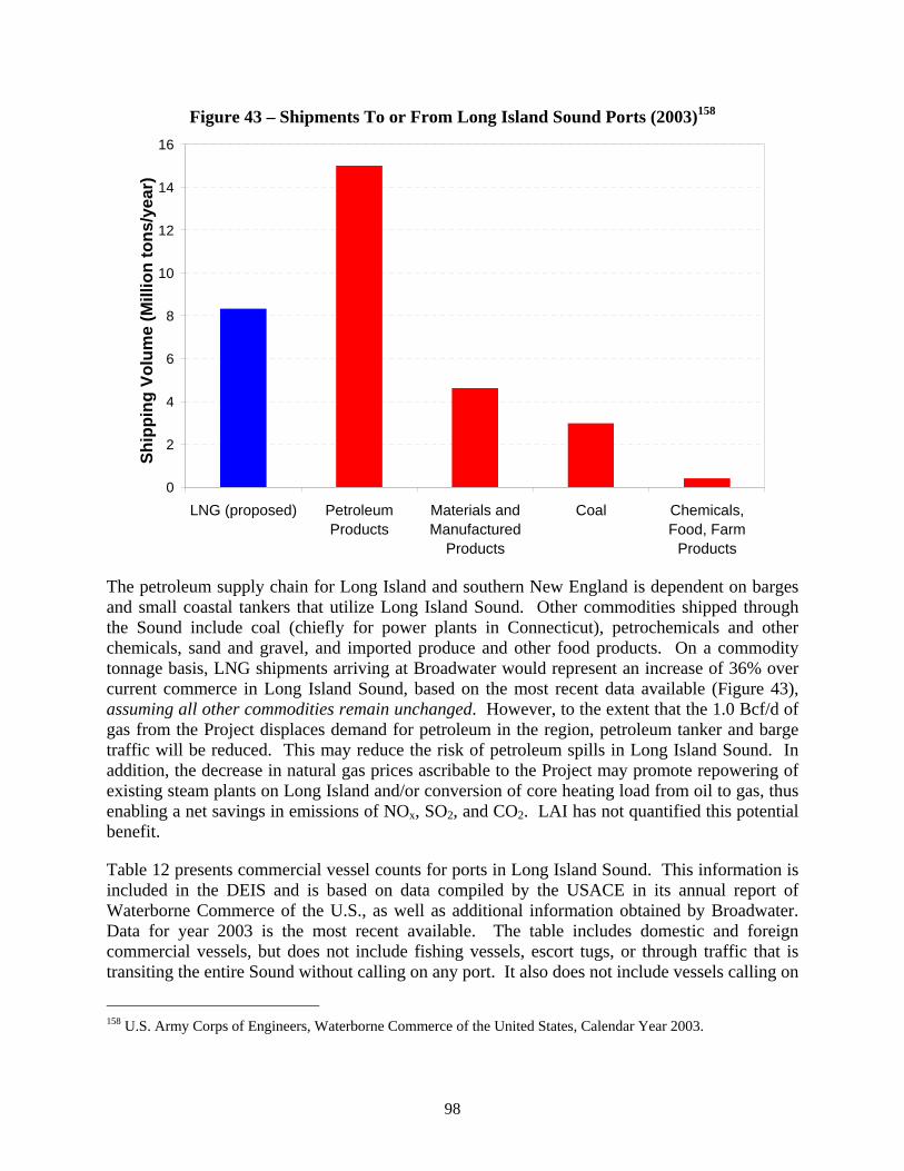
98

Figure 43 – Shipments To or From Long Island Sound Ports (2003)158

0

2

4

6

8

10

12

14

16

LNG (proposed) PetroleumProducts

Materials andManufactured

Products

Coal Chemicals,Food, Farm

Products

Ship

ping

Vol

ume

(Mill

ion

tons

/yea

r)

The petroleum supply chain for Long Island and southern New England is dependent on barges and small coastal tankers that utilize Long Island Sound. Other commodities shipped through the Sound include coal (chiefly for power plants in Connecticut), petrochemicals and other chemicals, sand and gravel, and imported produce and other food products. On a commodity tonnage basis, LNG shipments arriving at Broadwater would represent an increase of 36% over current commerce in Long Island Sound, based on the most recent data available (Figure 43), assuming all other commodities remain unchanged. However, to the extent that the 1.0 Bcf/d of gas from the Project displaces demand for petroleum in the region, petroleum tanker and barge traffic will be reduced. This may reduce the risk of petroleum spills in Long Island Sound. In addition, the decrease in natural gas prices ascribable to the Project may promote repowering of existing steam plants on Long Island and/or conversion of core heating load from oil to gas, thus enabling a net savings in emissions of NOx, SO2, and CO2. LAI has not quantified this potential benefit.

Table 12 presents commercial vessel counts for ports in Long Island Sound. This information is included in the DEIS and is based on data compiled by the USACE in its annual report of Waterborne Commerce of the U.S., as well as additional information obtained by Broadwater. Data for year 2003 is the most recent available. The table includes domestic and foreign commercial vessels, but does not include fishing vessels, escort tugs, or through traffic that is transiting the entire Sound without calling on any port. It also does not include vessels calling on

158 U.S. Army Corps of Engineers, Waterborne Commerce of the United States, Calendar Year 2003.

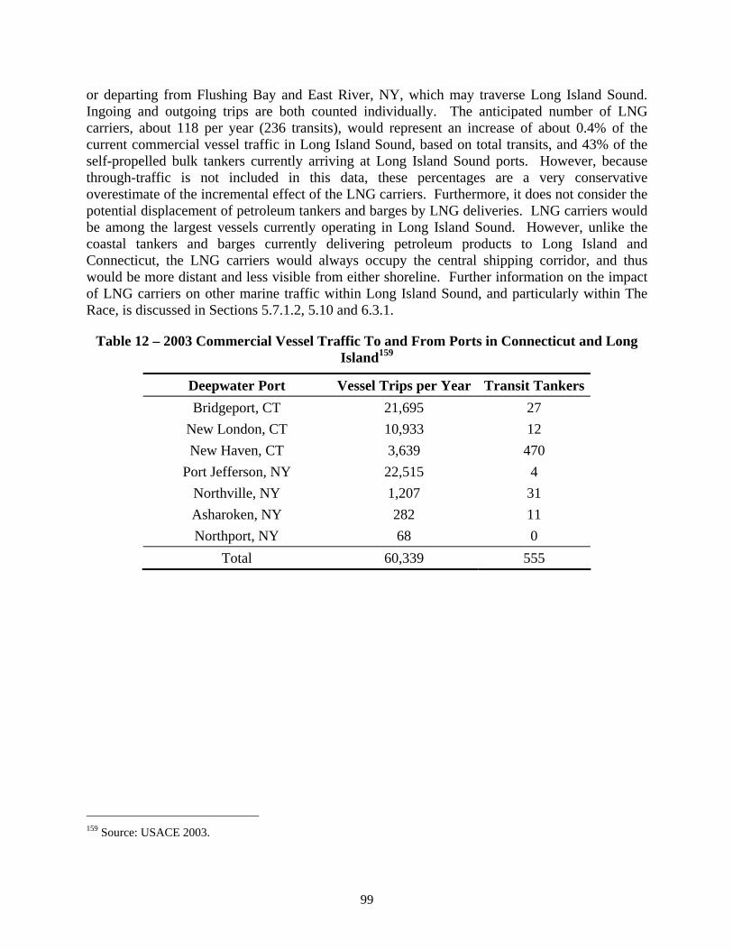
99

or departing from Flushing Bay and East River, NY, which may traverse Long Island Sound. Ingoing and outgoing trips are both counted individually. The anticipated number of LNG carriers, about 118 per year (236 transits), would represent an increase of about 0.4% of the current commercial vessel traffic in Long Island Sound, based on total transits, and 43% of the self-propelled bulk tankers currently arriving at Long Island Sound ports. However, because through-traffic is not included in this data, these percentages are a very conservative overestimate of the incremental effect of the LNG carriers. Furthermore, it does not consider the potential displacement of petroleum tankers and barges by LNG deliveries. LNG carriers would be among the largest vessels currently operating in Long Island Sound. However, unlike the coastal tankers and barges currently delivering petroleum products to Long Island and Connecticut, the LNG carriers would always occupy the central shipping corridor, and thus would be more distant and less visible from either shoreline. Further information on the impact of LNG carriers on other marine traffic within Long Island Sound, and particularly within The Race, is discussed in Sections 5.7.1.2, 5.10 and 6.3.1.

Table 12 – 2003 Commercial Vessel Traffic To and From Ports in Connecticut and Long Island159

Deepwater Port Vessel Trips per Year Transit Tankers Bridgeport, CT 21,695 27

New London, CT 10,933 12 New Haven, CT 3,639 470

Port Jefferson, NY 22,515 4 Northville, NY 1,207 31 Asharoken, NY 282 11 Northport, NY 68 0

Total 60,339 555

159 Source: USACE 2003.

5. SAFETY REVIEW

LAI’s primary objective in conducting the safety review was to assess the hazards associated with an offshore LNG storage facility based on existing scientific studies and reports. Currently, there is no other offshore storage and regasification facility similar to Broadwater anywhere in the world. Therefore there is no comparable safety record for a facility that is equal to or substantially similar to the proposed FSRU. However, LNG cargo vessels have sustained an excellent safety record over the past forty years. There have been no cargo tank breaches of any type despite a number of LNG groundings. The double hull design of the LNG carrier and the stringent safety and security procedures surrounding LNG vessels in U.S. waters are partially responsible for the industry’s historic safety record.

For this review, LAI evaluated the definition of hazard zones for the Project based on the Sandia Report160 and EISs of other LNG projects in the U.S. and Canada. We researched the impact of LNG spills over water both for accidental and intentional events based on publicly available experimental and modeling studies performed to date. Finally, we extensively reviewed Resource Report 11 on Reliability and Safety in Broadwater’s Application to FERC.

5.1. LNG Properties

LNG is a clear cryogenic liquid which boils at -259oF (-162.3oC). It is formed in a liquefaction process by cooling natural gas and reducing its volume by a factor of about 600. This decrease in volume is common to all gases when they are cooled and allows natural gas to be effectively and economically transported from the production site to the consumption site. LNG is less dense than water with a specific gravity of 0.423 and therefore floats on water.161 On the other hand, cold LNG vapor is heavier than air by a factor of 1.52. If LNG spills, it forms a pool which spreads along the water surface or ground as it evaporates. Because the LNG vapor is initially colder than the surrounding air, it forms a visible (white) vapor cloud by the condensation of water. However, when the regasified LNG vapor reaches ambient temperature and pressure, it is lighter than air by a factor of 0.54 and is no longer visible.

LNG is composed mostly of methane (CH4). Thus, the properties of methane serve as a first approximation of LNG’s properties. LNG also contains ethane (C2H6), propane (C3H8), butanes (C4H10) and iso-pentane (C5H12) as well as nitrogen (N2). However, the composition of LNG can vary widely depending on its source, as shown in Table 13, and therefore must be adjusted after regasification to meet a comparatively tight tolerance requirement regarding the chemical composition of the natural gas before it can be deemed pipeline quality.

160 M. Hightower, L. Gritzo, A. Luketa-Hanlin, J. Covan, S. Tieszen, G. Wellman, M. Irwin, M. Kaneshige, B. Melof, C. Morrow and D. Raglan, “Guidance on Risk Analysis and Safety Implications of a Large LNG Spill Over Water”, SAND2004-6258 (Dec. 2004). 161 Specific gravity is a dimensionless ratio of the densities of two materials with the reference material being water.

101

Table 13 – LNG Compositions by Source (% by volume)162

Origin Nitrogen N2

Methane C1

EthaneC2

PropaneC3

iso-ButaneiC4

n-Butane nC4

iso-PentaneiC5

LHV Btu/scf

Trinidad 0.01 96.13 3.40 0.39 0.04 0.03 0.00 1045.09Algeria 0.32 89.57 8.61 1.18 0.13 0.18 0.01 1102.30

Indonesia 0.03 90.15 6.41 2.38 0.50 0.51 0.02 1118.00Nigeria 0.05 90.48 5.05 2.95 0.58 0.87 0.02 1125.75Qatar 0.09 89.18 7.07 2.50 0.46 0.69 0.01 1127.19

Abu Dhabi 0.13 85.82 12.57 1.33 0.06 0.08 0.00 1132.88Malaysia 0.01 87.63 6.88 3.98 0.84 0.66 0.00 1155.70Australia 0.30 86.11 9.04 3.60 0.42 0.52 0.01 1161.79

Oman 0.09 86.52 8.31 3.32 0.85 0.85 0.06 1162.33Variation between high and

low

0.31 10.31 9.17 3.59 0.81 0.84 0.06 117.24

Fuels require oxygen to burn. Therefore LNG itself is not flammable. LNG vapor, which is a mixture of LNG and air, is flammable if its concentration is between 5.5% (the lower flammability limit, or LFL) and 14% (the upper flammability limit, or UFL) by volume in air at 77°F (25°C). Figure 44 shows the flammability limits for selected fuels. It is important to note that methane’s flammability range is narrow compared to hydrogen’s flammability range, which has an LFL of 4.0% and a UFL of 75%.

162 Source: Solar Turbines

102

Figure 44 – Flammability Limits for Selected Fuels163

0

10

20

30

40

50

60

70

80

90

Met

hane

But

ane

Prop

ane

Etha

nol

Oct

ane

Isop

ropy

lAl

coho

l

Ethy

l Eth

er

Xyle

ne

Tolu

ene

Hyd

roge

n

Acet

ylen

e

Flam

mab

ility

Ran

ge b

y Vo

lum

e in

Air

(%)

There are two general classes of explosive combustion: detonation, which is more powerful, and deflagration, which is less powerful. In order for a detonation to occur, the fuel / air mixture must be within the minimum and maximum detonation limits which are narrower than the flammability limits, and shock initiation is required.164 Figure 45 shows that methane is a safer fuel relative to other hydrocarbons because it requires a large quantity of explosive initiator in order to detonate.

163 Sandia Report, Table 4, p29. 164 The detonation limits for various fuels do not seem to be publicly available and are not listed in the Sandia report with the flammability limits.

103

Figure 45 – Relative Detonation Properties of Common Fuels165

0.001

0.01

0.1

1

10

100

Methane Ethane Propane n-Butane iso-Butane

Ethylene Acetylene Hydrogen

Expl

osiv

e In

itiat

or R

equi

red

(kg)

5.2. LNG Hazards

Several types of events can lead to an LNG spill at both onshore and offshore LNG facilities. LNG is stored in insulated storage tanks that are not under pressure, so the LNG is continuously vaporizing. The vapor is released through piping from the tank and either used as fuel for ancillary processes or recondensed. Leaks are, however, more likely to occur when LNG is under pressure for transfer or vaporization. Minor hazardous events, including leaks from low-pressure storage, from high-pressure pumps, vaporizers, metering or piping, are associated with the vaporization and storage of LNG. More serious events are associated with the LNG carrier and transfer of LNG from the carrier to the FSRU. Examples of more serious hazardous events include: an LNG carrier leak or failure, an emergency venting, and a transfer system leak or failure. Major events are associated with an intentional attack or a vessel collision between the FSRU and/or the LNG carrier and a vessel of significant mass such as an oil tanker or cargo ship.166

In the event of a spill from the FSRU or the LNG carrier, a pool of LNG will form on the water’s surface (Figure 46). LNG is not soluble in water and is therefore not a source of seawater contamination. The liquid will vaporize into a cloud which drifts with the wind close to the

165 Sandia Report, Figure 15, p154. 166 For a more detailed list of hazards see: E. Skramstad, S.U. Musaeus and S. Melbo, “Use of Risk Analysis for Emergency Planning of LNG Carriers”, DNV Consulting, 2000 Gastech Conference (November 20, 2000).

104

water surface. The vapor cloud will likely encounter an ignition source, such as a tug or fishing boat, almost immediately. If the gas is in the flammability range (5.5-14% by volume), it will ignite and rapidly burn back to the pool. This event is called a flash fire because it travels very quickly. The pool will continue to burn as long as LNG is leaking from the FSRU or carrier.

Figure 46 – Sequence of Events Following a Spill

Leak

PoolFormation

InitialGas CloudFormation

OngoingLNG Pool

Dense GasDispersion& Ignition

UncombustedGas

Burnt Gases

Combustion Zone

Dispersion& Flash Fire Pool Fire

Initial PoolFire Diameter

Longer TermPool Fire Diameter

Because of its long range effects, the most serious LNG hazard is thermal radiation resulting from a pool fire or the ignition of a vapor cloud. Thermal radiation is light emitted from the surface of an object due to its temperature. The power of the thermal radiation per unit area, also called the heat flux, is expressed in kilowatts per meter squared (kW/m2 – international units). For reference purposes, the average radiation from the sun reaching the earth’s atmosphere is 1.4 kW/m2. At the edge of a pool fire, the thermal radiation may exceed 220 kW/m2. The injury to humans from thermal radiation depends both on the intensity of the radiation and the exposure time (Figure 47). Exposure to heat flux at the edge of a pool fire is strong enough to damage structures and cause death almost instantly. Table 14 shows the type of damage that occurs from different levels of heat flux based on an average 10 minute exposure time.

According to the National Fire Protection Association (NFPA), an incident heat flux level of 5 kW/m2 is recommended as the design level that should not be exceeded in areas where more than 50 people might assemble.167 5 kW/m2 is also the permissible level for emergency operations lasting several minutes with appropriate clothing. At an exposure level of 5 kW/m2, first-degree burns would occur in 20 seconds, second-degree burns in 30 seconds and third-degree burns in 50 seconds with a 1% fatality rate.168 No pain has been shown for thermal fluxes less than 1.7 kW/m2 regardless of exposure time.169 The California Energy Commission’s (CEC) filing at FERC concerning the Long Beach LNG terminal expresses concern that FERC uses a thermal 167 NFPA standard for the production, storage, and handling of LNG - Standard 59A (2001). P.W. Parfomak and A.M. Flynn, “Liquified Natural Gas (LNG) Import Terminals: Siting, Safety and Regulation”, CRS Report for Congress (May 27, 2004). 168 California Energy Commission, December 8, 2005 filing at FERC concerning the Long Beach LNG terminal (CP04-58-000). 169 C.L. Beyler, “Fire Hazard Calculations for Large, Open Hydrocarbon Fires”, Chapter 3-11, SFPE Handbook of Fire Protection Engineering (2002).

105

radiation level of 5 kW/m2 which does not ensure the safety of all populations.170 They recommend a level of 1.4 kW/m2 which is equivalent to the “no observable effects level” that the CEC uses in siting power plants.

FERC relies exclusively on the thermal radiation levels identified in NFPA 59A. It must be noted that in the 2005 NFPA 59A update, the proposed revision to the thermal radiation flux levels, from 5 kW/m2 to 2.5 kW/m2

, was rejected. In Europe, the allowable thermal radiation level for “critical areas”, i.e. areas that are difficult to evacuate on short notice, is 1.5 kW/m2.171 In Austria, the land use planning standard for new facilities is 2.0 kW/m2.172 LAI considers 2 kW/m2 to be the thermal flux level that should be used as the limit for calculating safe distances from an LNG pool or vapor fire.

Figure 47 – Radiation Effects on Naked Skin173

0

5

10

15

20

25

30

35

40

45

50

0 5 10 15 20 25 30 35 40 45 50 55 60Time (seconds)

Rad

iatio

n (k

W/m

)

Fatalities

2 ndDegree Burns

1 stDegree BurnsHeavySunburn

Pain

NoEffect

2

170 California Energy Commission, December 8, 2005 filing at FERC concerning the Long Beach LNG terminal (CP04-58-000). 171 Ibid. 172 Ibid. 173 ANEI Bear Head LNG Terminal Environmental Assessment, Figure 4.9 (May 2004).

106

Table 14 – Common Approximate Thermal Radiation Damage Levels174

Incident Heat Flux (kW/m2) Type of Damage

35-37.5 Damage to process equipment including steel tanks, chemical

process equipment or machinery - third degree burns, lethal 50% of the time for a person wearing average clothing

25 Minimum energy to ignite wood at indefinitely long exposure without a flame

18-20 Exposed plastic cable insulation degrades – second degree burns, lethal 1% of the time for a person wearing average clothing

12.5-15 Minimum energy to ignite wood with a flame; melts plastic tubing

5 Permissible level for emergency operations lasting several

minutes with appropriate clothing – no lethal effects, first degree burns in 20 seconds

1.7 No pain regardless of exposure time

Rapid phase transitions (RPTs) occur when spilled LNG comes into contact with warm water and explosively boils off. This rapid expansion from the liquid to the vapor state causes large overpressures. RPTs are localized in the vicinity of the LNG leak and may cause some structural damage to the LNG carrier or the FSRU. Although RPTs on their own do not involve a fire, they may increase the rate of LNG pool spreading and the size of a vapor cloud that could subsequently ignite. LNG composition is a critical parameter. RPTs are more likely to occur in LNG mixtures containing high fractions of ethane and propane.175

Boiling Liquid Expanding Vapor Explosions (BLEVEs) can fragment a storage tank because vapor cannot escape from the safety valve quickly enough in the event of a fire. BLEVEs are usually associated with incidents involving propane tanks since those are typically under high pressure. There has been one BLEVE incident involving an LNG truck in Europe. During this truck accident, the insulation around the storage tank failed and flames from the fire directly impinged on the tank resulting in superheating of the LNG, extremely rapid vaporization of the contained liquid and fatigue of the containment vessel. The pressure release valve either failed or was unable to handle the excessive vapor. A similar scenario might be possible in the event of a pool fire around an LNG vessel with spherical Moss tanks. However, the cargo tanks in an

174 Based on Sandia Report, Table 6, p. 38, and other fire safety documents. 175 G.A. Melhem, S. Saraf, and H. Ozog, “Understand LNG Rapid Phase Transitions”, ioMosaic Corporation (2005).

107

LNG vessel are not designed for high pressures and material failure would provide pressure relief and would limit the pressure rise to a small amount insufficient to cause a BLEVE.176

Other explosions due to very fast combustion (detonation and deflagration) are unlikely unless the LNG cloud mixes with air and becomes trapped in a confined area such as between ship hulls. Even then, the effects of the explosion would be localized near the spill.

The low temperature of LNG could cause cryogenic burns to FSRU personnel in the event that the LNG is spilled and comes into contact with unprotected skin. Asphyxiation of the FSRU, LNG vessel, tug or pilot boat crews is possible although not considered a major issue because radiation effects from a fire are considered the dominant effect.

5.3. LNG Accident History

The DEIS and FEIS of most LNG terminal projects usually contain a section on LNG carrier safety. LAI reviewed these report sections as well as other safety reports.177 The U.S. LNG experience began with the opening of the Distrigas LNG facility in Everett, Massachusetts, in 1971. Since then, more than 700 cargoes have been delivered to Distrigas without major incidents. As we understand it, there have been no fatalities at or around the Distrigas facility attributable to LNG operations, including offloading cargo. As shown in Figure 48, LNG vessels are in the heart of the city when they enter or exit the port of Boston, coming within 1/8 of a mile or 200 m from shore at the closest point.178 Logan International Airport is briefly shut down when LNG carriers enter Boston Harbor.

Figure 48 – LNG tanker in Charlestown on its way out of Boston 179

176 R.M. Pitblado, J. Baik, G.J. Hughes, C. Ferro and S.J. Shaw, “Consequences of LNG Marine Incidents”, CCPS Conference, Orlando (June 29-July 1, 2004). 177 Det Norske Veritas Technical Report (Project No. 70004197), “LNG Marine Release Consequence Assessment”, (July 2004) 178 Boston Globe, December 21, 2004. 179 Ibid.

108

Over the past 45 years, over 40,000 LNG voyages have taken place worldwide. No serious accidents involving the rupturing of a cargo tank have occurred. LAI categorized LNG carrier accidents into three categories: LNG vessel spills, LNG vessel groundings, and LNG vessel collisions / interactions.

The most noteworthy LNG vessel spills include the following:

• 1979 – Pollenger at Everett, MA ◦ Spill on steel cover of cargo tank caused cracking of steel plate

• 1979 – Mostefa Ben Boulaid at Cove Point, MD

◦ Valve leakage caused spill and deck fracture

• 1985 – Isabella (unknown location) ◦ Cargo tank overflow due to valve failure caused severe cracking of steelwork

• 2001 – Khannur at Everett, MA ◦ 100 gallons of LNG cracked the protective decking over the cargo tank dome

• 2002 – Mostefa Ben Boulaid in Algeria

◦ Cargo tank overflow caused fracturing of the steelwork

The following three LNG vessel groundings are significant:

• 1979 – El Paso Kayser near the Straits of Gibraltar

◦ Damage to hull and secondary membrane, deformation of primary membrane

◦ No LNG released

◦ LNG pumped to another vessel

• 1980 – LNG Taurus near Taboata Harbor, Japan ◦ Cause: rapidly worsening weather

◦ Ship waiting for pilot to board when port was closed

◦ Hull damaged but no loss of cargo

• 2004 – Tenaga Lima near Mopko, South Korea ◦ Cause: strong wind

◦ Water entered the insulation space between primary and secondary membranes

◦ Ship was re-floated and repaired

Two recent incidents involved LNG vessel collisions/interactions with other vessels:

• 2002 – Norman Lady struck by USS Oklahoma City nuclear submarine near the Strait of Gibraltar

◦ Had just unloaded cargo in Spain

109

◦ Minor damage to double hull but not cargo tanks

• 2006 – Golar Freeze broke loose from its moorings and pulled away from pier during unloading at the Elba Island, GA, import terminal

◦ Cause: surge created by the chemical tanker Charleston which was passing by at too high a speed

◦ Emergency shut-off was activated

◦ Unloading arms came detached

◦ No LNG was spilled

◦ Two tugs pushed tanker back to the dock

Review of the LNG accident history to date reveals that there were relatively more accidents in the early stages of the industry (late 1970s-early 1980s). A number of minor accidents led to the development of more stringent safety measures in effect throughout the U.S.

5.4. Sandia Report

The Sandia Report focuses on risk analysis and safety implications of a large LNG spill over water.180 The existing standards for spills or releases of LNG over land do not apply over water. The Sandia report addresses the risk assessment of LNG spills over water, accidental and intentional LNG breaches, spills and corresponding hazard analyses, and risk reduction strategies and recommendations. Although the Sandia Report does not compare the risks of offshore and onshore facilities, other studies have concluded that overall the risks for offshore and onshore facilities are about the same.181

The Sandia Report emphasizes that risk from a potential LNG spill can be reduced by minimizing the three elements of the overall risk of the event:

• Probability of the accidental or intentional event,

• Probability that preventive or mitigating measures fail, and

• Consequences of the event measured in fatalities or cost.

Appendix B of the Sandia Report summarizes finite element modeling of ship collisions between a series of large ships (50,000 metric tons) and an LNG vessel. The Report finds that penetration

180 M. Hightower, L. Gritzo, A. Luketa-Hanlin, J. Covan, S. Tieszen, G. Wellman, M. Irwin, M. Kaneshige, B. Melof, C. Morrow and D. Raglan, “Guidance on Risk Analysis and Safety Implications of a Large LNG Spill Over Water”, SAND2004-6258 (Dec. 2004). 181 Aspen Environmental Group, “International and National Efforts to Address the Safety and Security Risks of Importing Liquified Natural Gas: A Compendium”, California Energy Commission, CEC-600-2005-002 (January 2005). R. Erikson, J.M. Brandstorp and E. Cramer, “Evaluating the Viability of Offshore LNG Production and Storage”, DNV Consulting, Gastech 2002 Conference, Qatar.

110

into the inner hull of a double-hull vessel requires a 3 m outer hull breach and impact velocities exceeding 5-6 knots.

Spill and dispersion/hazard modeling is also used to estimate how far from a pool fire the heat flux drops to 5 kW/m2 or less. The results of the models vary depending on the assumptions of the model and the initial conditions at the time of the spill. One limitation of the spill and dispersion/thermal hazard modeling is the lack of validation against large-scale spill experimental data.

Modeling was used to estimate the sizes of LNG cargo tank breaches for accidents (defined as resulting in hole sizes less than 2 m2) and for intentional breaches (resulting in hole sizes between 2 and 12 m2). Sandia assumed that LNG carrier storage tanks have a 25,000 m3 capacity and that only half of the contents of the tank, 12,500 m3, will spill in the event of a breach. Any single accident is thought to involve releases from only two to three tanks. This cascading release of LNG was analyzed and is not expected to significantly increase the overall fire size or hazard ranges, only the expected fire duration.

Most of the modeling studies assume that a single, coherent pool fire can be maintained for very large pool diameters but this is not thought to be realistic because there would be insufficient air in the interior of a fire to sustain complete combustion. Sandia suggests that “flamelets,” or multiple small pool fires would exist rather than the single large pool fire assumed by the models.

Sandia recognized that variations in location-specific conditions, such as terrain, weather, waves, currents and obstacles, can influence dispersion so a range of hazards is more important than a “specific maximum hazard guideline.” Generally, a fire is likely to occur immediately and burn the LNG pool and/or vapor. However, if the vapor cloud is not ignited it could extend to 2500 m and then be ignited. The thermal radiation from the ignition of a vapor cloud can be very high within the ignited cloud and particularly hazardous to people. The experiments to date do not give a good indication of the atmospheric dispersion of a vapor cloud that would be associated with very large spills.

Sandia performed a sensitivity analysis of thermal radiation intensity level distances for credible accidental and intentional breach and spill scenarios. Using the same burn rate, Sandia calculated pool diameter, burn time and thermal radiation from spills with 1 to 3 tanks breached and hole sizes ranging from 1 to 12 m2. The discharge coefficient and the surface emissive power were varied a little as can be seen in Table 15. From this modeling, Sandia concluded that the high hazard distance corresponding to a heat flux of 37.5 kW/m2 was 250 m for accidental spills and 500 m for intentional spills. Similarly, Sandia concluded that the low hazard distance corresponding to a heat flux of 5 kW/m2 was 600-750 m for accidental spills and 1600 m for intentional spills. These hazard distances form the basis for Sandia’s recommended safety zones.

111

Table 15 – Sandia Report Thermal Intensity Level Distances182

Hole Size (m2)

Tanks Breached

Discharge Coefficient

Burn Rate (m/s)

Surface Emissive

Power (kW/m2)

Pool Diameter

(m)

BurnTime(min)

Distance to 37.5

kW/m2 (m)

Distance to5 kW/m2

(m)

Accidental Events 1 1 0.6 3x10-4 220 148 40 177 554 2 1 0.6 3x10-4 220 209 20 250 784 2 3 0.6 3x10-4 220 362 20 398 1,358

Intentional Events 2 3 0.6 3x10-4 220 209 20 250 784 5 3 0.6 3x10-4 220 572 8.1 630 2,118 5 1 0.6 3x10-4 220 330 8.1 391 1,305 5 1 0.9 3x10-4 220 405 5.4 478 1,579 5 1 0.6 2x10-4 220 395 8.1 454 1,538 5 1 0.6 3x10-4 350 330 8.1 529 1,652 12 1 0.6 3x10-4 220 512 3.4 602 1,920

LAI graphically represented four of the cases from Table 15 in Figure 49 below. These curves are rough estimates of the modeled results based on three data points from Table 15 and indicative of how slowly the radiation decays from its 220 kW/m2 value at the edge of the fire to its 5 kW/m2 value at the edge of the low public safety impact zone.

182 This table is based on data from Table 10. Effect of Parameter Combinations on Pool Diameter in an Accidental Breach and Table 14. Intentional Breach – Effect of Parameter Combinations on Pool Diameter in the Sandia Report. Note that the Sandia report itself has inconsistencies between Tables 10 and 14 and Table 41 of Appendix D which are supposed to include the same results.

112

Figure 49 – Sandia Report Radiative Flux

0

50

100

150

200

250

0 500 1000 1500 2000 2500Distance (m)

Rad

iativ

e Fl

ux (k

W/m

2 )

One Tank Breach, 1 m Three Tank Breach, 2 m

One Tank Breach, 2 m Three Tank Breach, 5 m

2

2 2

2One Tank Breach, 2 m2

Three Tank Breach, 2 m2

For onshore LNG terminals, each LNG container and LNG transfer system must have a dispersion exclusion zone in accordance with NFPA 59 A Sec. 193.2059.183 These regulations aim at minimizing the possibility that flammable vapors reach a property line that can be built upon. Part 193.2059 requires that vapor dispersion distances be calculated for a 2.5% average gas concentration, i.e. ½ LFL.184 Calculating a distance to LFL assumes the travel of a continuously flammable vapor cloud. Due to wind gusts, pockets of flammable vapor may break away from the continuous cloud. A conservative estimate of the downward flammable distance assumes these pockets have dissipated when the cloud concentration is below ½ LFL.185 In the EISs for onshore projects, FERC presents vapor dispersion distances to ½ LFL. It is not clear why the Sandia Report does not present distances to ½ LFL but only distances to LFL.

According to Sandia’s dispersion calculations, for large accidental spills the vapor cloud could extend to beyond 1,600 m from the spill depending on atmospheric conditions. Therefore, LNG vapor dispersion analyses should be conducted using site-specific atmospheric conditions to assess the potential areas and levels of hazards to public safety. For a one tank breach, the

183 NFPA 59A Sec. 193.2059, “Flammable Vapor-Gas Dispersion Protection.” 184 The meteorological conditions for these calculations are (i) conditions that result in the longest downwind distances at least 90% of the time or (ii) maximum downwind distances for Stability Class F, a wind speed of 4.5 mph, 50% relative humidity and the average regional temperature. 185 C.D. Zinn, “LNG Codes and Process Safety”, Paper #109e, AIChE National Meeting Atlanta, Georgia (April, 13, 2005).

113

distances to the LFL were calculated to be 1,536 m with a pool diameter of 148 m and 1,710 m for a pool diameter of 209 m (Table 16).186 The time for the LFL to be reached was approximately 20 minutes. For intentional spills, the distances to LFL were calculated to be 2,450 m for a one tank breach with a pool diameter of 330 m and 3,614 m for a 3 tank breach with a pool diameter of 572 m. The report concludes that high thermal hazards from intentional events can extend significantly from the spill location.

Table 16 – Sandia Report Vapor Dispersion Distances to LFL187

Hole Size (m2)

Tanks Breached

Pool Diameter

(m)

Spill Duration

(min)

Distance to LFL

(m) Accidental Events

1 1 148 40 1,536 2 1 209 20 1,710

Intentional Events 5 1 330 8.1 2,450 5 3 572 8.1 3,614

LAI graphically represented the four cases from Table 16 in Figure 50 below. These curves are rough estimates of the modeled results based on two data points from Table 16 and assuming symmetrical wind conditions. These curves are indicative of how far the vapor cloud extends from the pool but are not an accurate representation of the shape of a vapor cloud. Clearly, the three tank spill creates a larger vapor cloud than a single tank spill. Larger holes with higher LNG spill rates result in a larger vapor cloud than smaller holes with lower spill rates.

186 The Sandia Report does not specify what site-specific conditions were used in these calculations. 187 This table is based on data from Table 11. Dispersion Distances to LFL for Accidental Spills and Table 15. Dispersion Distances to LFL for Intentional Spills in the Sandia Report.

114

Figure 50 – Sandia Report Vapor Dispersion Distances to LFL

-400

-300

-200

-100

0

100

200

300

400

0 500 1000 1500 2000 2500 3000 3500 4000

Vapor Cloud Length (m)

Pool

Wid

th (m

)

One tank, 40 min One tank, 20 minOne tank, 8.1 min Three tanks, 8.1 min

5.4.1 LNG Spill and Dispersion Experiments

The DOE and the Gas Research Institute sponsored two sets of experiments on LNG spills, which were conducted jointly by the Lawrence Livermore National Laboratory (LLNL) and the Naval Weapons Center (NWC). The experiments studied pool spreading, vaporization rates, RPT occurrence, vapor dispersion, detonation, pool fires and vapor cloud fires. The object of the “Burro” experimental series in 1980 was to determine vapor dispersion from LNG spills over water.188 For the Burro field experiments, wind speed and direction, gas concentration, temperature, humidity and heat flux from the ground were recorded. The object of the “Coyote” experimental series in 1981 was to study RPTs and vapor cloud fires.189 For the Coyote experiments, vapor cloud size and environmental variables such as wind speed and direction were related to the destructive potential of the fires.

Appendix C of the Sandia Report presents an overview of the LLNL and NWC spill testing data.190 Sandia used the experimental data to validate a variety of models. However, the

188 R.P. Koopman, R.T. Cederwall, D.L. Ermak, H.C. Goldwire, W.J. Hogan, J.W. McClure, T.G. McRae, D.L. Morgan, H.C. Rodean and J.H. Shinn, “Analysis of Burro Series 40-m3 LNG Spill Experiments”, Journal of Hazardous Materials, 6, pp. 43-83 (1982) 189 H.C. Rodean, W.J. Hogan, P.A. Urtiew, H.C. Goldwire, T.G. McRae and D.L. Morgan, “Vapor Burn Analysis for the Coyote Series LNG Spill Experiments”, UCRL-53530 (1984). 190 Sandia Report Table 33, p. 105.

115

experimental data has limitations. The spill sizes ranged from 0.8 m3 to 66.4 m3 for vapor dispersion experiments and from 3 m3 to 238 m3 for pool and vapor cloud fires. The sizes of these experimental spills are two orders of magnitude smaller than spills from a typical LNG carrier with a capacity of 125,000 m3. Furthermore, most of the LNG spill experiments over water were performed at the NWC, in China Lake, CA. The water test basin at China Lake has an average diameter of only 58 m with an average water depth of 1 m and an average water level about 1.5 m below the surrounding ground level.191 LNG pool size at China Lake is limited by the size of the water test basin and was not measured in most cases.

In these experiments, the downwind distance to the LFL is 380 m for the 20.6-66.4 m3 spills.192 No ice formation was observed for unconfined spills. Experiments indicate that boil-off rates increase by a factor of 1.5-2 when either ethane or propane is added to the methane to alter the composition to a 97% methane mixture. LNG has a higher boiling rate than pure methane on a bound-free surface. During later stages of the spill, there appears to be a decrease in the rate of vaporization due to the changing composition of the pool.

Experiments found that there is a correlation between water temperature and RPT occurrence: RPTs occurred when the water temperature was above 17oC (62.6oF). Time of year would therefore be an important factor in determining whether RPTs would occur if there is an LNG spill in Long Island Sound. There is also a correlation between spill rate and RPT occurrence: 15 m3/min is the critical spill rate above which the strength of the explosive yield increased by five orders of magnitude at the spill rate of 18 m3/min. LAI believes that these are very probable spill rates for hole sizes between 2-12 m2 or for unloading rates of 10,000 m3/hr (163 m3/min).

5.4.2 Recent LNG Spill Modeling Review

Appendix A of the Sandia Report presents an overview of LNG spill modeling studies. Most models for the spread of LNG on water assume that spreading is driven only by gravity and ignore the effect of waves, currents, preferential boiling and pool break-up. Each of the four studies discussed – Lehr, Fay, Quest and Vallejo – examines a different scenario with different assumptions. There are significant differences in thermal hazard estimates and reality must encompass this range of results. Specifically, if we compare the distance required for an object to receive a radiant flux of approximately 5 kW/m2, the Quest study calculates a distance of 490 m, Vallejo calculates 1,290 m and Fay calculates 1,900 m. For these three studies, which all had very similar spill volumes of 12,500-14,300 m3, the fire duration ranged from 3.3 min to 28.6 min, almost a factor of 10. The area of the fuel spill ranged from 9,503 m2 to 200,000 m2, a factor of 10. It appears that when waves are modeled, they decrease the pool radius by a factor of four and increase the vaporization flux by 27% due to the increase in surface area.

191 R.P. Koopman, R.T. Cederwall, D.L. Ermak, H.C. Goldwire, W.J. Hogan, J.W. McClure, T.G. McRae, D.L. Morgan, H.C. Rodean and J.H. Shinn, “Analysis of Burro Series 40-m3 LNG Spill Experiments”, Journal of Hazardous Materials, 6, pp. 43-83 (1982) 192 The pool radius for this spill is not available.

116

Other studies support the conclusion that the varying results are due to the differences in modeling assumptions and the modeling tools used to calculate the hazard distances.193 There are significant deviations between studies and these reduce to some extent when the same modeling assumptions are used. Nevertheless, for the same hole size, for example, pool fire results and dispersion results can vary up to a factor of two.

5.4.3 Sandia Report Recommended Safety Zones

Sandia’s guidance on risk management for accidental and intentional spills defines three types of safety zones (Table 17), which are graphically depicted in Figure 51. The 500 m safety / security zones that have been established for most offshore LNG projects are based on Zone 1 for intentional spills.

Table 17 – Sandia Report Safety Zones194

Accidental Spills Intentional Spills

Zone 1 Severe negative impact from thermal radiation

~250 m (273 yds)

~500 m (547 yds)

Zone 2 Less severe negative impact

from thermal radiation

250-750 m (547-820 yds)

500-1,600 m (547-1,750 yds)

Zone 3 Minimal risk from thermal

radiation

>750 m (820 yds)

>1,600 m (1,750 yds)

193 J. Baik, V. Raghunathan, M. Witlox, “Consequence Modeling of LNG Marine Incidents”, American Society of Safety Engineers, Middle East Chapter, 7th Professional Development Conference & Exhibition, Kingdom of Bahrain, March 18-22, 2006. 194 Sandia Report Section 1.3.1, p. 22.

117

Figure 51 – Sandia Report Safety Zones

Zone 1250 m

750 m

Zone 2

Zone 1

Zone 2

Accidental Spill Intentional Spill

500 m

1600 m

5.5. Safety and Security Implementation

Safety and security for an offshore LNG project can be implemented at several levels with one or more of the following: Safety Zone, Precautionary Area, Area to be Avoided (ATBA), and No Anchoring Area (NAA).

Pre-2006, the Safety Zone for offshore projects was usually 500 m or 547 yards. No traffic unrelated to Port operations is authorized in this area. The USCG has primary responsibility for monitoring, patrolling, and enforcing the law in the Safety Zone.195

A Precautionary Area is printed on new NOAA nautical charts and serves as a notice to mariners of potential LNG carriers and other port operations in the area. The Precautionary Area has recommendations for vessel speed and direction but otherwise does not restrict vessels.

An ATBA is similar to a Precautionary Area with respect to nautical charts, vessel speed and direction. Typically, the maximum speed for an ATBA is 10 knots (19 km/hr). It can be recommendatory or mandatory. Restrictions to vessel movement are enforceable if the ATBA is mandatory.

A NAA can be recommendatory or mandatory. Fishing vessels are excluded if it is mandatory.

Table 18 summarizes the proposed or actual safety implementation for other offshore LNG terminals. Sandia’s recommendation for Zone 1 has been applied in these cases. The following 195 Final Environmental Assessment of the El Paso Energy Bridge Gulf of Mexico, LLC, Deepwater Port Application (November 2003) USCG-2003-14294.

118

subsections present a brief overview of the hazard analysis for each offshore project except Cabrillo Port which is analyzed in detail in Section 5.6.

Table 18 – Safety Implementation for other Offshore Projects

Offshore Project Safety Zone Area to be Avoided(ATBA)

PrecautionaryZone

Main Pass Energy Hub 500 m (547 yds) 3.2 km (2 miles)

Cabrillo Port, CA 500 m196 (547 yds) 3.7 km (2.3 miles)

Excelerate Energy, Gulf of Mexico 500 m (547 yds) 1.0 km

(0.62 miles)

Gulf Landing, LA 500 m (547 yds) 3.2 km (2 miles)

5.5.1 Gulf Landing Hazard Analysis

The Gulf Landing Deepwater Port project proposes two gravity-based structures located 61 km south of Cameron, Louisiana, at a water depth of 16.8 m. The project’s FEIS discusses LNG accident modeling, which consisted of evaluating three scenarios from the literature.197

• DOE Worst-Case Reassessment (Quest Study): ◦ Distance to LFL ranges from 0.5 to 2.5 miles for a 25,000 m3 spill

◦ Distance to 5 kW/m2 of 0.54 km (0.34 miles) for a 25,000 m3 spill

• Ronald P. Koopman198: distance to LFL ranges from 0.4 to 2.8 miles for a 25,000 m3 spill

• James A. Fay199: distance to 5 kW/m2 of 1.1 km (0.68 miles) for a 14,300 m3 spill

5.5.2 Gulf Gateway Hazard Analysis

The Gulf Gateway Deepwater Port is located at a distance of approximately 116 miles from the Louisiana coast in 280 feet of water. The project was constructed in 2004-2005 and includes an STL buoy, a gas metering platform and an Energy Bridge Regasification Vessel. For this

196The safety zone is 500 m from the stern of the FSRU which means about 800 m from the mooring tower. 197 FEIS for the Gulf Landing LLC Deepwater Port License Application (November 2004) USCG-2004-16860-58. 198 Dr. Koopman is Special Projects Manager for the Chem / Bio National Security Program at Lawrence Livermore National Laboratory. Dr. Koopman has 32 years of experience in applied physics at LLNL, including positions as Manager of the Safety Engineering and Analysis Section of the AVLIS Plant Project with responsibility for Nuclear Criticality Safety and Integrated Safety Programs; Associate Energy Program Leader for Program Development; and Leader of the Liquefied Gaseous Fuels Program which created the Spill Test Facility at the Nevada Test Site and conducted major field test programs with industry using hazardous chemicals. 199 Dr. Fay is Professor Emeritus in the Department of Mechanical Engineering at the Massachusetts Institute of Technology.

119

project, the LNG accident modeling in the Final Environmental Assessment relied on the DOE Worst-Case Reassessment (Quest Study):200

• Distance to LFL ranges from 0.5 to 2.5 miles for a 25,000 m3 spill

• Exposure at 300 m from a pool fire would cause pain within 60 s

• Modeled two types of spills ◦ 5 m hole took 37 min to burn the spilled LNG

◦ 1 m hole took 64 min to burn the spilled LNG

5.5.3 Main Pass Energy Hub Hazard Analysis

The Main Pass Energy Hub Deepwater Port is proposed to be located 16 miles southeast of the Louisiana coast in water depth of 210 ft. The project includes modifying existing offshore facilities and constructing two LNG storage platforms with a total capacity of 145,000 m3. The LNG hazard analysis presented in the USCG’s Environmental Assessment focuses on worst case modeling scenarios with a maximum hazard radius of 5 miles.201

5.6. Analysis of Revised Cabrillo Port DEIS (March 2006)

The Revised DEIR for the Cabrillo Port LNG project was analyzed in terms of the safety and security issues that were noted by the Maritime Administration (MARAD), the USCG and Sandia.202 The USCG and the California State Lands Commission (CSLC) retained Ecology and Environment Inc. to write the EIS / EIR. Specifically, the thermal and dispersion exclusion zone issues were studied for both accidental and intentional breach scenarios. It is important to note that this is the most relevant EIS / EIR available since it would consist of an FSRU with a capacity of 273,000 m3, similar to Broadwater. Cabrillo Port is different from Broadwater in that it would be moored 14 miles off the California coast where the ocean depth is about 2,900 ft (884 m). Furthermore, Cabrillo Port is proposed as a spherical Moss LNG carrier type, whereas the Broadwater FSRU would have a membrane storage tank construction.

The Cabrillo Port FSRU would be permanently moored via a turret system that would allow it to rotate around a fixed point. It would be shaped like an LNG vessel with a double-sided and double-bottomed construction and displace 193,050 metric tons of water. LNG ships would unload their cargo in a side-by-side arrangement onto this structure which would be 971 ft (296 m) long and 213 ft (65 m) wide and contain three Moss spherical tanks. Each tank would therefore be capable of storing 91,000 m3 of LNG and in the event of an accident could

200 Final Environmental Assessment of the El Paso Energy Bridge Gulf of Mexico, LLC, Deepwater Port Application (November 2003) USCG-2003-14294. 201 Final Environmental Assessment of the Main Pass Energy Hub Deepwater Port Application (September 2006) USCG-2004-17696. 202 Revised Draft Environmental Impact Report for CabrilloPort Liquified Natural Gas Deepwater Port, CSLC EIR No. 727 (March 2006).

120

potentially spill this much LNG. This project would require a 200 ft (60.9 m) permanent right-of-way in the offshore area where the pipelines would be laid.

5.6.1 Public Safety: Overview

The public safety issues that were raised during public meetings have been addressed in this DEIS. Potential hazards and incident scenarios were evaluated by experts at a Hazard Identification (HAZID) workshop and at a multi-day Security and Vulnerability Assessment (SVA) workshop conducted by the CSLC, the USCG and MARAD.

In order to address the public’s concerns about the safety of the project, an Independent Risk Assessment (IRA) was conducted which evaluated the worst-case consequences associated with this project. The IRA was conducted by Risknology, Inc. with additional analytical support from Analytical and Computational Energetics, Inc. (ACE) and other consultants. The original IRA included an event-tree analysis which uses inductive logic and a graphical depiction to represent the various events that may follow from an initiating event. However, since the IRA contained sensitive security information, it was not publicly available and only the results were summarized in the DEIR. In the revised DEIR, the IRA is included as Appendix C1. The revised IRA was independently reviewed by the authors of the December 2004 Sandia Report and incorporates Sandia’s recommendations.

In the revised DEIR, the USCG extended the Safety Zone around the FSRU from a 500 m radius around the mooring point to a 500 m radius from the stern of the FSRU. Since the FSRU is 296 m long, this in effect makes it an 800 m (½ mile) Safety Zone around the mooring point.

The IRA defines and evaluates representative worst credible cases which would affect one, two, or all three tanks of the FSRU. However, Sandia’s review found that a three-tank simultaneous release was not credible. Accidents at the FSRU would be rare and would not reach shore, even in the case of a worst credible release such as a terrorist attack. However, recreational boaters, fishermen and commercial ships in the area and outside the Safety Zone could be affected. The potential release of LNG due to an operational incident or natural cause would not be expected to affect more than a single tank.

The impact distances from accidental releases and intentional events are much less than the distance to shore and range from 1.56 to 7.27 miles, as shown in Figure 52, with details in Exhibit 9. The coastwise shipping lane is about 2.4 miles away. The hazard to the shipping lane would occur about 30 minutes after the initiating event and the exposure time within the shipping lane would last for about another 30 minutes. An average of three commercial vessels would be exposed to this hazard based on marine traffic estimates. It is important to note that LNG carriers would not present risks or hazards to the general public while in transit to the FSRU because they would use routes that are farther from shore than the FSRU.

121

Figure 52 – Cabrillo Deepwater Port: Consequence Distances203

The USCG would respond to emergencies at the FSRU or an LNG carrier. Two tug vessels would be on continuous standby in the vicinity of the 500 m Safety Zone surrounding the FSRU.

5.6.2 Independent Risk Assessment

The hazardous events that were identified during the HAZID were:

• LNG spill overboard,

• Loading arm failure,

• Presence of an ignition source in the SCVs,

• Ship collision with the FSRU,

203 Source: Cabrillo Port FEIS.

122

• Ballast system malfunction, and

• Fire on LNG carrier or FSRU.

Based on the initial Sandia review, additional threat and hazard analyses, consequence modeling, and process safety considerations were suggested by Sandia.

Based on the HAZID and the SVA, six scenarios were considered.

• Scenario 1: accidental explosion in hull void

• Scenario 2: accidental explosion in moss tank

• Scenario 3: accidental/intentional marine collision

• Scenario 4: accidental explosion between the FSRU and the docked tanker

• Scenario 5: intentional two Moss tank breach

• Scenario 6: accidental/intentional cascading multiple (two or three) Moss tank release

The modeling of the LNG release, spread, and eventual burning was conducted using the Fire Dynamics Simulator (FDS) which is a public domain computer program. The FDS was calibrated to the Burro 8 test data. The IRA concluded that wind speed and orientation (gradient normal to the ground) are the parameters that most strongly control the distance to the LFL. The pool fires were represented using the right circular cylinder model since it is applicable to all heat fluxes.

The following assumptions were made in the IRA modeling.

• LNG releases were modeled as pure methane

• LFL is 0.0276 on a mass fraction basis or 0.05 on a volume basis

• No material was lost during the pool formation process and all such material was available for either the pool fire or vapor dispersion calculations

• The pool was assumed to be fixed in size and the recession process was conservatively ignored

• The ocean temperature was set at 50oF and the air temperature at 70oF

• Tidal or wave action was not considered and their exclusion will produce more conservative results

• Temperature inversion effects were not modeled

• The LNG evaporation rate was set to be 0.028 lb/ft2/s (0.135 kg/m2/s)

• The edge of the fire has an average emissive power of 220 kW/m2

• The atmosphere has an average transmissivity of 0.8

123

• Flame height was found using the industry standard Moorhouse correlation which was developed using large LNG pool fires204

• Thermal radiation thresholds were 5.0, 12.5 and 37.5 kW/m2

• Two LNG loading operations take place per week, each one lasting 20-24 hours

• Relative vessel movement during loading operations is limited to 2.8 m

• Submersible pumps in Moss tank can be maintained without taking the tank out of service

• A 500 m safety zone is set around the FSRU

The following sections contain a more detailed discussion of Scenarios 3-6. Scenarios 1 and 2 will not be discussed here in detail since they are specific to the Moss LNG carrier type. However, Scenario 1 and 2 could apply to the LNG carriers that service the Broadwater FSRU since they could have either spherical Moss or membranes storage tanks.

5.6.2.1 Scenario 3: Accidental / Intentional Marine Collision

This scenario is defined as a large marine vessel colliding with the FSRU with sufficient energy to breach a storage tank. A tanker or a container ship traveling at 13.5 or 16.5 knots respectively could result in a 10 m2 hole in the FSRU.205 The hole size will double to 20 m2 with a 0.5 knot increase in speed. It is important to note that there are no speed limits for ships at sea but rather the speed of a ship should be determined by weather/sea and traffic/safety considerations. Container ships typically have a cruising speed of 25 knots (29 mph) while tankers have a cruising speed of 16 knots (18 mph). The estimated frequency of collision with a tanker is 1.7 x 10-8 (about 1 in 60 million) and with a container 5.9 x 10-7 (roughly 1 in 2 million).

Both a pool fire and vapor dispersion with subsequent vapor cloud fire are investigated. It is assumed that an instantaneous spilling of one half the contents (45,500 m3) of a storage tank will occur and lead to a pool fire with a radiative flux of 5 kW/m2 at a distance of 2,970 m. If immediate ignition does not occur and the vapor cloud disperses down wind, the distance to LFL will vary with the wind speed. For a wind velocity of 2 m/s, the maximum distance to LFL is 5.3 km. If the vapor cloud were to ignite, the radiation distance must be added to the vapor cloud distance. For a radiative flux of 5.0 kW/m2 a distance of 1.3 km must be added to the LFL limit.

5.6.2.2 Scenario 4: Accidental Explosion Between the FSRU and the Docked Tanker

This scenario investigates an explosion due to a spill occurring during off-loading and resulting in a flammable cloud that fills the entire space between the FSRU and the LNG carrier. If this vapor cloud were to ignite, it would burn rapidly in a deflagration mode. The report estimates

204 Moorhouse concluded that the cylindrical flame representation is best for thermal radiation calculations. J. Moorhouse , “Scaling Criteria for Pool Fires Derived from Large Scale Experiments”, I.Chem. E. Symposium Series No. 71 (April 14-16, 1982) 205 Cabrillo Port DEIR, Figure E.4 in Appendix D of Appendix C1.

124

the confined volume between the carrier and the FSRU to be only 6,800 m3 although it appears to be 6 x 60 x 130 = 46,800 m3. The 6,800 m3 volume of methane-air mixture can result from only 1.0 m3 of LNG which is a less than the capacity of the loading arms. The carrier and FSRU are assumed to not move or deform over the explosion time event and the ignition source is set at the physical center of the cloud. The CFD model calculates a maximum overpressure at Tank 2 (the middle tank) of 3.5 psi (24 kPa) and a maximum blast pressure between the ship and the carrier of 13.5 psi (93 kPa). The effect of the blast load profiles on the FSRU was found to be negligible, causing only a small inclination of the FSRU and increasing the separation between the two vessels by about 4 feet. There is the possibility of fire or blast-induced damage to the mooring lines connecting the vessels, but no structural analysis was conducted using the predicted explosion loads. The initiating event frequency for this event tree is the joint probability of exceeding a wave height of 2.8 m at the FSRU and continuing the loading operations. Ignition sources can come from the loading arm decoupling, sparks, static electricity and machinery onboard either vessel. The estimated frequency for this type of event is 4.81 x 10-5, or roughly 1 in 20,000.

5.6.2.3 Scenario 5: Intentional Two Moss Tank Breach

This scenario investigates the consequences of an intentional attack which produces a 7 m2 hole in two adjacent storage tanks. The entire contents of both tanks (91,000 m3 x 2 = 182,000 m3) were assumed to spill. A frequency estimation cannot be conducted for intentional scenarios. The maximum pool diameter was 650 m. In the event of a pool fire, the distance to 5 kW/m2 would be 2.6 km. In the event of a vapor cloud, the distance to LFL would be 11.2 km for a wind speed of 2 m/s and 9.4 km for a wind speed of 4 m/s. After reaching the maximum downwind distance, a flash fire analysis was performed. For the 2 m/s wind speed case, the distance to 5 kW/m2 was 11.7 km and the distance to 2 kW/m2 was 12 km. For the 4 m/s wind speed case, the distance to 5 kW/m2 was 10.9 km.

5.6.2.4 Scenario 6: Accidental/Intentional Cascading Multiple (two or three) Moss Tank Release

This scenario investigates the consequences of cascading tank failures through primary fire events resulting in damage to the storage tanks. An initial storage tank is breached by either an accidental or intentional event and spills its entire contents via a 7 m2 hole. Immediate ignition causes a pool fire which results in the failure of one or two of the other tanks 25 seconds later with the release of 100,000 m3 of LNG (Table 19). No vapor cloud formation was considered due to the immediate ignition. After the LNG pool reaches its maximum size, radiative flux distances were calculated assuming that the LNG pool burned the entire time it formed.

125

Table 19 – Summary of Consequence Distances206

Number of Tanks (Hole Sizes) Distance to 5 kW/m2 Case 1 2 tanks (7 m2, 7 m2) 1.32 km Case 2 2 tanks (7 m2, 1,300 m2) 2.51 km Case 3 3 tanks (7 m2, 1,300 m2, 1,300 m2) 3.23 km

5.6.3 Sandia Review of Independent Risk Assessment

Sandia reviewed the Cabrillo Port IRA.207 LAI presents highlights from this review that are the most relevant and applicable to Broadwater.

Although the 40 year history and safety record of marine LNG import vessels is important and has some bearing on LNG safety, it should not be used as a default for this new facility concept. The FSRU covers a much broader spectrum than simply LNG off-loading by including LNG storage, regasification and pumping gas to shore. There are safety questions about the existence, position and capabilities of barriers between processing areas and the LNG storage tanks. If such barriers do not exist and efforts to fight a process-based fire fail, then propagation and failure of storage tanks may ensue.

Sandia points out that more credible threats exist than are imagined in the IRA, and may be more likely than the catastrophic total release scenario originally considered in the Cabrillo Port IRA. The threats can range from insider threats to intentional external attacks with a range of weapons or delivery modes such as airplanes, ships or boats. The potential threats from off-normal events in the processing area would probably impact initially only one FSRU storage tank. Detailed information on the credible threats was not publicly available.

Sandia found a number of problems with the initial LNG dispersion calculations. Some of these problems are presented here to give a glimpse of how complex the modeling is and how incorrect assumptions for input parameters or boundary conditions can critically change the modeling results.

• An incorrect value to identify the LFL was used in the input file.

• The methane is released into a flow field which is in a transitional state and has excess mixing. Sandia recommended a different boundary condition at the side boundaries parallel to the wind and at the top domain which provide a power-law wind profile uniformly across before the methane is released.

• The reduced temperature of the LNG pool was not correctly reflected. USACE used a “reaction” flag in the input file which assumes a combustion process and increases the methane temperature above atmospheric temperature.

206 Cabrillo Port Revised EIR, Appendix C1, Independent Risk Assessment, Table 3.8 or Table ES-3. 207 Cabrillo Port Revised EIR, Appendix C2, Sandia Review of Independent Risk Assessment.

126

• The mesh size can change the maximum distance to LFL by almost a factor of 2: USACE found 11 km with 20 m width cells while Sandia calculated 7 km with 10 m width cells. Lower resolution simulations result in longer distances to LFL because the extent of turbulent mixing is under resolved.

Sandia’s pool fire results were in close agreement with the ACE results. Sandia’s modeling results were presented in graphical form (Figure 53) and show how slowly the heat flux decays as a function of distance from the pool. In this case, a minimum distance of 2.4 km (1.5 miles) is required for the heat flux to drop to 5 kW/m2. Of special importance from LIPA’s vantage point, an additional 1.3 km (0.8 miles) is required to reach a more protective level of 2 kW/m2.208

Figure 53 – Sandia Calculation of Pool Fire Hazards209

0

20

40

60

80

100

120

140

160

180

200

220

0 500 1000 1500 2000 2500 3000 3500 4000 4500Distance From Flame Axis (m)

Hea

t Flu

x (k

W/m

2 )

2,400 m to 5 kW/m23,700 m to 2 kW/m2

Sandia’s review of the IRA concludes that a credible scenario is that of a two tank breach. Credible threat analyses suggest breach sizes in the 7-12 m2 range should be considered for this type of facility and location. However, no credible consequences (to a radiative flux of 5 kW/m2) extend more than 11.7 km or 7.3 miles from the FSRU.

208 The extrapolation to 2 kW/m2 was done on the original Sandia figure, not on Figure 53. 209 Figure based on Figure 4 (from the Cabrillo Port Revised EIR, Appendix C2, Sandia Review of Independent Risk Assessment). The dashed line is an extrapolation to 220 kW/m2 at the edge of the pool fire and is not exact since the location of the pool axis relative to the pool edge is not reported.

127

5.7. Resource Report 11 – Safety and Reliability

Broadwater’s Resource Report 11 describes the potential effects of project component failures on the public and on the supply of natural gas to customers.210 These failures could be due to natural catastrophes, accidental failures or intentional harmful events. Broadwater’s location, about nine miles from the closest shore, minimizes the hazards to the public associated with either an accident or a catastrophe at the FSRU. On a clear day, the FSRU would barely be visible from either the New York or Connecticut shoreline (Figure 54). Table 20 compares the proximity of populations at existing onshore LNG terminals to the Broadwater location.

Figure 54 – View of FSRU from Roanoke Landing (Riverhead, NY)211

210 Resource Report 11 includes the following appendices:

A. Historical Climatological Information B. Minutes of Meeting New York State Fire Administrator C. LNG Carrier Route Analysis D. HSSE Management System Framework Document

211 Source: Broadwater Energy.

128

Table 20 – Populations in Proximity to LNG Terminals

LNG Facility Estimated Population

within 10 miles Broadwater (NY) 3,443

Everett (MA) 1,745,898 Cove Point (MD) 49,014 Elba Island (GA) 154,193

Lake Charles (LA) 136,825

5.7.1 LNG Safety

Federal Port and Waterways Safety regulations (33 Code of Federal Regulations, “CFR,” Part 160) mandate that LNG carriers give a Notice of Arrival 96 hours prior to arrival, giving their position, last port of call, next port of call, crew roster, cargo manifest, time of arrival and reporting any equipment casualties that could affect safety. The rules further establish safety and security zones in harbors, around vessels carrying hazardous cargoes, including LNG, in specified areas.212 Safety zones provide buffers around enclosed sites or vessels for safety or environmental protection while security zones are for the protection of the enclosed sites or vessels against terrorist acts or accidents. Both zones can be either stationary or move along with a vessel.

5.7.1.1 FSRU

Broadwater contends that the results described in the Sandia Report are applicable to the proposed FSRU since it is similar to an LNG carrier in construction, and its hull should behave like the hull of an LNG carrier in the event of an accidental or intentional breach. Even though the FSRU storage tanks are larger (45,000 m3) than those of the LNG carrier (25,000 m3) considered in the Sandia Report, it can be reasonably assumed that LNG release rates and durations similar to those postulated in the Sandia Report are applicable to the FSRU.213 The USCG questioned this premise and Broadwater commissioned Det Norske Veritas (DNV)214 to prepare a response to the USCG questions.215 A review of this report can be found in Appendix 6 of our report and supersedes information presented in Resource Report 11. The main points from this report are summarized below.

212 33 CFR Part 165. 213 The 200,000 to 250,000 m3 LNG vessels in the production queue today have storage tanks that are approximately the size of the Broadwater storage tanks (45,000 m3). 214 DNV is a worldwide classification society headquartered in Norway which currently classifies more than 5,100 ships (16% of the world’s fleet). 215 Broadwater’s response was dated December 21, 2005.

129

• Larger LNG carriers or the FSRU will experience smaller breach sizes given the same impact energies because of the larger distance between the outer and inner hull. Therefore, the Sandia Report breach sizes are conservatively applicable to the proposed Broadwater FSRU and larger LNG carriers.

• The FSRU release volume will be 35,560 m3 and the LNG carrier release volume will be 27,300 m3 compared to the Sandia Report release volume of 12,500 m3.

• For the largest hole size of 2.52 m, the distance to LFL for a one tank FSRU spill increases to 3.32 km compared to its value of 2.45 km for the Sandia report.

Broadwater completed two HAZIDs in order to identify potential hazards associated with the project. Based on these studies, Broadwater incorporated various measures to protect the public and the environment from potential accidents including:

• Hull and containment system;

• Collision avoidance: radar beacon, radar system and navigational aids;

• LNG spillage containment from unloading and process areas;

• LNG offloading system – linked to an Emergency Shutdown which will automatically stop the cargo transfer when abnormal conditions (such as high tank levels or pressures, fire detection, loss of electrical power or instrument air pressure, detection of high pressure or low temperature within the unloading arms) are detected on the carrier or FSRU or in the event of an LNG carrier mooring failure;

• Thermal and flammable vapor dispersion exclusion zones – zone dimensions are determined by USCG;

• Hazard detection – including a Distributed Control System and an Instrumented Protective System;

• Fire suppression: a fire water system, a dry powder chemical system, a high expansion foam system, a low expansion foam system, a carbon dioxide fire protection system, a water spray system and a water mist system;

• Emergency shutdown – in the event of a total power failure, the emergency generator will start automatically; and

• Emergency response – a Preliminary Emergency Response Plan will identify the resources required and coordination requirements between Broadwater, the USCG and onshore emergency responders.

In order to protect the FSRU against natural catastrophes such as hurricanes, severe winds, tornadoes and lightning strikes, the yoke mooring system was designed to accommodate the most severe weather that can credibly occur in the area. i.e., a 100 year storm event. Specifically, the yoke mooring system was designed to withstand wave heights of 5.7 to 7.0 m and winds of 50.2

130

to 56.8 m/s (112.3 to 127 mph).216 In the event of a severe storm, Broadwater may reduce the manning level of essential personnel, cease natural gas deliveries, while accelerating the scheduled depletion of inventory aboard the FSRU.

Broadwater has developed a menu of terrorism threat scenarios that describe the vectors that could possibly be used to attack the FSRU and the LNG carriers. In order to minimize the risk from these scenarios, Broadwater intends to design appropriate operational procedures and mitigation measures. Broadwater has prepared a Preliminary Security and Vulnerability Assessment (PSVA) as required by the USCG. The PSVA documents the potential security threats to Broadwater operations and an analysis of the consequences that could result if such threats were successful. Finally, Broadwater prepared a Preliminary Facility Security Plan (PFSP) for the FSRU. Both the PSVA and the PFSP are “living” documents not available to the public that will be modified over the course of the FSRU design and construction. After commissioning, Broadwater would conduct a number of security operations on a regular basis.

5.7.1.2 LNG Carriers

Instead of addressing the safety issues associated with potential cargo releases from an LNG carrier during transit or unloading, Broadwater refers the reader to the following three reports:

• Consequence Assessment Methods for Incidents Involving Releases from LNG Carriers – ABS Consulting217

• LNG Marine Release Consequence Assessment – DNV218

• Guidance on Risk Analysis and Safety Implications of a Large LNG Spill over Water – Sandia National Laboratory219

According to Resource Report 11, there are four types of accidental events that could result in the release of LNG from a carrier:

• Vessel collision with an inbound LNG carrier

• Inbound LNG carrier collision with the FSRU or mooring tower

• Vessel collision with a moored LNG carrier

• Grounding of an LNG carrier 216 Resource Report 11, Table 11-9. 217 American Bureau of Shipping, “Consequence Assessment Methods for Incidents Involving Releases from Liquified Natural Gas Carriers, GEMS 1288209, May 13, 2004). LAI also examined the notice from FERC Docket No. AD04-6-000, “Notice of Availability of Staff’s Responses to Comments on the Consequence Assessment Methods for Incidents Involving Releases from Liquified Natural Gas Carriers”, June 18, 2004. 218 DNV Technical Report (Project No. 70004197), “LNG Marine Release Consequence Assessment”, (July 2004). 219 M. Hightower, L. Gritzo, A. Luketa-Hanlin, J. Covan, S. Tieszen, G. Wellman, M. Irwin, M. Kaneshige, B. Melof, C. Morrow and D. Raglan, “Guidance on Risk Analysis and Safety Implications of a Large Liquified Natural Gas (LNG) Spill Over Water”, SAND2004-6258 (Dec. 2004).

131

Only one LNG carrier will approach, berth, unberth and depart Long Island Sound at any given time. When the vessels enter the Long Island Sound through The Race, they will be about 1 mile from Fishers Island. The population on Fishers Island is 275-300 people in the off-season and approximately 6,000 during peak summer weekends. During the remainder of the voyage into the Sound, the vessel will be about 2 miles from the closest shore at one point in time. The USCG will determine the final route of the LNG carriers into Long Island Sound and the nature of the safety and security zone around it. Since the LNG carrier will be traveling at 12 knots, the approximate duration of a traveling safety and security zone at any single point would only be approximately 15 minutes. At approximately 12 knots, LAI observes that there should not be significant marine traffic bottlenecks.

In addition to double-hull construction, there are a number of safety features to minimize LNG spills, including:

• Vessel traffic management,

• LNG carrier procedures,

• Shipboard safety systems,

• Enhanced navigation equipment,

• Crew training, and

• Inspection by USCG and classification societies.

A letter of recommendation from the USCG is required for the project to commence operations and will probably have conditions that must be incorporated within a Vessel Management and Emergency Plan. Broadwater will provide an adequate number of tugboats (one to four) with a bollard pull capacity of 60 metric tons and fire-fighting equipment for each LNG carrier operation. The maximum sea states and other relevant weather conditions that are permissible during LNG carrier transit, berthing and unloading are shown in Table 21.

Table 21 – Weather and Sea Condition Limits for LNG Carrier Transit

Wind 33 knots (17.0 m/s) Tidal currents 0.9 knots (0.45 m/s)

Waves 6.6 feet (2 m)

5.7.1.3 Post application Safety Filing

On February 16, 2006, the USCG requested thermal radiation results for accidental and intentional breaches of the FSRU and LNG cargo tanks. On March 14, 2006, Broadwater sent the USCG a report by DNV in which thermal hazard zones from pool fires due to immediate ignition are presented. An overview of this report can be found in Appendix 7. The FSRU pool fire distances to 5 kW/m2 calculated by DNV range from 606 m to 1,211 m compared to 554 to 1305 m in the Sandia report for the same hole sizes. DNV does not find the effect of wind speeds and stability class to be significant. However, hole size is a significant variable: doubling the hole size will double the calculated distance to 5 kW/m2. The duration of a pool fire depends

132

on hole size, release rate, burning rate and volume released. Sandia used a lower burning rate so DNV repeated their calculations with Sandia’s lower burning rate and found an increase in hazard distances.

5.8. Other Technical Experts on LNG Safety

Dr. Jerry Havens is the developer of the DEGADIS computer model that is recommended by the Department of Transportation regulations (49 CFR Part 193, LNG Facilities: Federal Safety Standards). He states that: “in my judgment, a large LNG pool fire – on water, and therefore uncontained – is of the highest concern.”220 He also states that: “the scientific consensus on the scope of an LNG-on-water fire involving an entire tank of LNG (6 million gallons or 23,000 m3) is that it would be at least a half-mile in diameter… from the edge of the fire to about another half-mile out, people would receive second-degree burns on unprotected skin within about 30 seconds. Obviously, larger fires would result from larger spills.”221 However, Dr. Havens recognizes that models can not yet predict accurately how the fire size will scale with the quantity of spilled LNG.

Dr. James Fay, Professor Emeritus in the Department of Mechanical Engineering at the Massachusetts Institute of Technology, has expressed concern that there exists no relevant industrial experience with fires of the scale that would be involved in a worst-case scenario. Dr. Fay developed a mathematical model for the spills and fires from LNG vessels. He states that: “… the floating LNG pool will burn vigorously. The time to burn spills of the size mentioned (25,000 m3) can be less than five minutes. Fires that burn thousands of tons of fuel in a few minutes are extraordinarily large.”222 Dr. Fay calculates a distance to an average heat flux of 5 kW/m2 of 1,100 m or 3,600 ft.223

5.9. Safety Review Issues

5.9.1 Safety Parameter Modeling Issues

Exclusion zones for protection of people are calculated by a number of different models. These models have been validated by limited data from pool fire, vapor cloud dispersion and vapor cloud fire experiments involving small LNG spills on the order of 1-100 m3. These experimental spills are orders of magnitude smaller than the spills contemplated in the event of an LNG accident or terrorist event, where each of the multiple storage tanks is between 25,000 m3 and 50,000 m3.

220 Havens, J., “Terrorism: Ready to blow?”, Bulletin of the Atomic Scientists, Vol. 59, No. 4, pp. 16-18, July/August 2003. 221 Havens, J., “LNG: safety in science: careful study of the consequences of spill fires can settle terminal siting questions”, Bulletin of the Atomic Scientists, Vol. 60, No. 1, pp. 30-31, Jan/Feb 2004. 222 Fay, J., “Model of spills and fires from LNG and oil tankers”, Journal of Hazardous Materials, Vol. B96, pp. 171-188, (2003). 223 Fay, J., “Spills and fires from LNG tankers in Fall River (MA)”, August 2003.

133

The distances required for an object to receive a radiant flux of approximately 5 kW/m2 calculated by the various published models can vary by up to a factor of 4 for a given spill size. This is not surprising because the calculation depends on the assumptions and approximations used in the model. Although waves are expected to reduce the spread of the LNG pool, the effect of waves is very difficult to quantify and is not included in most models.224 There is very little friction between the LNG pool and the water so the LNG pool will be more responsive to winds than to ocean currents. However, the effect of wind is also difficult to model accurately.

It is well known that confinement of an LNG vapor cloud in the flammability range could result in an explosion (detonation or deflagration). However, buildings and/or obstacles leading to confinement are not treated in any of the models.

Since LNG vapor must be in the flammability range in order to burn, the vapor cloud needs to mix with air. In the case of a very large spill, it is unlikely that one giant fire would occur but rather a breakup into multiple flamelets. This effect is not currently modeled and would lead to a decrease in the radiative flux. Therefore, the distance to a safe radiative flux level would decrease if flamelets are considered. Although LNG’s initial composition is mostly methane, as the pool spreads and evaporates, it becomes enriched in the heavier components. This change in the LNG pool’s composition over time would change its vaporization and burning behavior; this phenomenon is not currently modeled.

5.9.2 Cascading Event Analysis

Both the Sandia Report and the Cabrillo Port revised DEIS discuss the possibility of a cascading event scenario. The scenario would be similar for the LNG carrier or the FSRU following an LNG cargo tank breach. An initial loss of LNG containment could cause cascading failures of additional LNG storage tanks through two mechanisms:

• A primary fire event resulting in damage to support structures or the insulation of neighboring tanks, or

• The embrittlement and brittle failure of structural components from direct contact with LNG.

The inventory of additional tanks would not be released simultaneously with the contents of the initial tank. The Cabrillo Port IRA assumed an accidental or intentional breach in an initial storage tank causing a 7 m2 hole and spilling 100% of the LNG in the tank. Furthermore, the IRA assumed ignition of the pool of spilled LNG and subsequent failure of one or two additional tanks. The release of the contents of the second and/or third tank is assumed to occur 25 seconds after the first tank breach with only half the contents of the additional failed tanks released. No vapor cloud was formed but the additional tank failures increased the expected fire duration and the hazard range.

224 H. Kytomaa and F. Gavelli, “Studies of LNG Spills Over Water Point up Need for Improvement”, Oil and Gas Journal, p. 61-65 (May 9, 2005).

134

5.9.3 LAI Extrapolations to Worst-Case Scenario

LIPA asked LAI to define a worst-case scenario for the Project because no worst-case scenario was presented in Broadwater’s Resource Report 11 Safety and Reliability. In addition, LIPA asked LAI to estimate the distance to a radiative heat flux of 2 kW/m2 in the event of a worst-case scenario involving the FSRU. Selection of 2 kW/m2 as a safe radiative flux is based on discussions with fire safety engineers and review of engineering literature.225

LAI based the worst-case scenarios on review of the literature on both accidental and intentional threats. There is considerable debate concerning the worst-case scenario versus the maximum credible event approach for defining hazard zones.226 To date, sea-borne terrorist attacks have not involved LNG carriers. Moreover, there is minimal public information on terrorist attacks on U.S. ships. The October 2000 attack on the USS Cole in Yemen is one incident that provides an estimate on the size of a hole created by an intentional attack. The hole in the outer hull created by the attack on the USS Cole was estimated to be 60 feet wide by 40 feet high or approximately 200 m2.227 The Sandia results have been extended to larger holes to account for a terrorist event such as the USS Cole attack and result in a vapor cloud and fire that would extend 3 miles from the vessel.228 DNV has reviewed the range of LNG marine incidents from collision, grounding, operational error and terrorism.229 Their maximum credible accidental release from a 0.75-m wide hole has a pool fire hazard range of 440 m. With an associated dispersion and flash fire hazard range to 5 kW/m2 of 920 m. DNV’s calculated maximum credible intentional release from a 1.5 m wide hole has a pool fire hazard range to 5 kW/m2 of 750 m. DNV assumed that no vapor cloud would propagate since immediate ignition is almost certain in an intentional event. DNV qualifies its dispersion results with the statement “actual distances could be larger or smaller at most by a factor of two.”

LAI considered two types of worst case scenarios. The first scenario is a cascading event with sequential rather than simultaneous breaches of all the storage tanks. No vapor cloud hazard is considered for cascading events since the escalation of the hazard is attributed to a pool fire. The second scenario is a vapor cloud which is assumed to encounter an ignition source within a 3.2 km (2 miles) radius around FSRU.

The distance to 5 kW/m2 for a pool or vapor cloud flash fire depends on the hole size, the number of tanks involved, the event sequence, the weather conditions and the wave height. LAI estimated the following range of distances to 5 kW/m2.

225 C.L. Beyler, “Fire Hazard Calculations for Large, Open Hydrocarbon Fires”, Chapter 3-11, SFPE Handbook of Fire Protection Engineering (2002). 226 R. Pitblado, J. Baik and V. Raghunathan, “LNG Decision Making Approaches Compared”, DNV Consulting (2005). 227 http://archives.cnn.com/2000/US/11/02/uss.cole.02/index.html 228 L.A. Husick and S. Gale, “Planning a Sea-Borne Terrorist Attack”, Foreign Policy Research Institute (March 21, 2005) http://www.fpri.org/enotes/20050321.americawar.husickgale.seabornedterroristattack.html 229 R.M. Pitblado, J. Baik, G.J. Hughes, C. Ferro, and S.J. Shaw, “Consequences of LNG Marine Incidents”, CCPS Conference, Orlando (June29 – July 1, 2004).

135

• For a pool fire: 2.5 - 3.2 km (1.6 - 2 miles)

• For a vapor cloud flash fire: 3 - 5 km (1.9 - 3.1 miles)

LAI extrapolated the 5 kW/m2 results to 2 kW/m2 based on pool fire calculations from the Cabrillo Port revised DEIS (see Figure 53).

• For a pool fire: 3.8 – 4.5 km (2.4 - 2.8 miles)

• For a vapor cloud flash fire: 4 – 6 km (2.5 – 3.7 miles)

5.10. Safety Review Findings

Highlights of LAI’s safety assessment include the following:

Broadwater’s location, about nine miles from the closest shore, minimizes the hazards to the public associated with either an accident or a catastrophe at the FSRU. Broadwater’s homeland security experts assert that the FSRU is likely an unattractive terrorist target because any incident would cause few casualties and would not be very accessible for extensive media coverage. Arguably, the FSRU is a difficult terrorist target with a comparatively low probability of success. Nonetheless, we note that the maximum number of crew on board the FSRU at any one time would be approximately 30 individuals. In the event of a catastrophe, we believe that the FSRU is too far from either shoreline to affect the Long Island or Connecticut population.

Based on the history of LNG vessel accidents and review of safety reports, the most likely serious event is a grounding of the LNG carrier due to rapidly worsening weather. However, Broadwater’s operating procedures will not permit an LNG vessel to enter the Sound unless there is a 24-hour weather window corresponding to wind speeds less than 33 knots and waves less than 6.6 feet. Therefore, unless there is a very sudden and negative change in weather, the probability of an LNG vessel grounding in the Sound is extremely low.

The risk of an accident while the LNG carrier is transiting The Race appears very low although the consequences would be high. Elsewhere in the U.S., LNG carriers have regularly transited both high and low density population centers without event for decades. In Boston, for example, LNG carriers come within a quarter mile or less of the city’s waterfront when they enter the harbor, and the 10 mile radius around the Everett terminal includes a population of 1.7 million. Although the Broadwater LNG carrier route comes within approximately one mile of land at The Race, an experienced pilot familiar with the route will have boarded the FSRU before it enters the Sound. The USCG will then escort the carrier to the FSRU. Both the USCG and Broadwater are eager to schedule passage during periods which avoid conflict with commercial and recreational vessel traffic, in particular, late night. Furthermore, the LNG carriers will not enter the Race unless there is a favorable 24-hour unloading weather window within the operating limits corresponding to wind speeds less than 33 knots and waves less than 6.6 feet.

136

Safety zones for offshore LNG projects are based on modeling of LNG spills over water. To date, there have been neither any significant accidental spills nor any intentional LNG spills over water. LNG spill experiments conducted by scientists in the U.S. have been limited to volumes ranging from 1 m3 to 238 m3. Minor events such as an operational spill lasting 10 minutes would release about 1,670 m3 of LNG (FSRU loading rate is 10,000 m3/hr). The breach of one cargo tank on the FSRU or LNG carrier could release anywhere from 12,500 m3 to 35,560 m3. Exclusion zones for injury to people calculated by the various models vary by up to a factor of 4 for a given spill size because of differences in input parameters and model assumptions. When reviewing hazard analyses, the approximations in the modeling results and the uncertainties in the weather conditions at the time of a spill should be taken into consideration.

Minor hazardous events such as LNG leaks on the FSRU or the LNG carrier are likely to occur from time to time. The FSRU and tugs would be equipped with firefighting equipment, and we expect that the FSRU and LNG carrier crew would be highly trained to handle such emergencies. Nevertheless, cryogenic damage to crew or equipment could take place. Escalation of minor hazards is conceivable under extremely sudden and difficult weather conditions, but improbable with Broadwater’s emergency shutdown system and the type of emergency response training that is required.

More serious hazardous events, such as release during LNG transfer events, are unlikely. If such a hazardous event were to occur, a pool fire or a minor vapor cloud could ensue. However, LNG transfers would not be scheduled unless weather conditions were within operating limits. Furthermore, Broadwater’s emergency shutdown system would be activated if the motion between the FSRU and the LNG carrier exceeded threshold tolerances. Other critical process upsets such as loss of electrical power, high LNG tank pressure, fire detection or high pressure in an unloading arm will also trigger the emergency shutdown system and will limit the size of a spill and minimize the probability of escalation.

In the event of a spill on deck, LNG’s cold temperature could cause cryogenic damage to the FSRU or LNG carrier. Additionally, it could cause cryogenic burns to personnel on either vessel if it comes into contact with unprotected skin. Asphyxiation of the FSRU crew and the tug / pilot boat crews is also possible during a large spill.

The most serious hazardous event would involve a collision between a vessel transiting Long Island Sound and the LNG carrier or the FSRU. The USCG has proposed a Safety Zone around the FSRU with a 1.1 km radius (0.68 miles). The USCG has also proposed a moving Safety zone around the LNG carrier while it transits the Sound which extends 3.7 km (2.3 miles) in front of the carrier, 1.85 km (1.15 miles) behind, and 0.69 km (0.43 miles) on either side. These Safety Zones will increase the navigational safety and reduce the likelihood of an accident or intentional attack. Furthermore, most of the vessels transiting Long Island Sound are neither large enough nor traveling with the speed required to penetrate the double hull of the FSRU or the LNG carrier.

In the event of a pool fire, the thermal radiation could result in loss of life on the FSRU and might harm vessels and occupants in the area surrounding the FSRU. A pool fire

137

could cause escalation to a multiple tank release, but it would take hours for all the LNG to be released. A worst-case scenario involving the total loss of the FSRU is conceivable, but all the LNG on board would not be instantaneously released. In the event of a worst-case scenario, the existing body of scientific knowledge indicates that the inhabitants of Long Island and Connecticut are far enough away to avoid burns through exposure to high levels of thermal radiation.

Explosive combustion, such as a detonation or deflagration, is unlikely to occur unless the LNG vapor cloud is within the flammability range (5 to 14% by volume) and becomes trapped in a confined area such as between ship hulls. As such, these events are limited to the vicinity of the LNG carrier or FSRU.

Unignited vapor clouds are extremely unlikely to travel more than 2 miles without encountering an ignition source, such as a recreational, commercial or fishing boat. Near the FSRU, an unignited vapor cloud could lead to asphyxiation of crew members or other emergency personnel. Any intentional initiating event will almost certainly provide an ignition source and therefore not lead to a diffusing vapor cloud. Once the vapor cloud is ignited, the flash fire will burn back to the spill source, i.e., presumably the hull of the FSRU.

A secondary hazard that could damage the FSRU is an RPT. This type of explosion is caused by LNG pouring into warm seawater and vaporizing very quickly due to heat transfer. This rapid expansion from the liquid to the vapor state causes large overpressures. RPTs are localized in the vicinity of the LNG leak and may cause some structural damage to the LNG carrier or FSRU. Although rapid phase transitions on their own do not involve a fire, they may increase the rate of LNG pool spreading and the size of a vapor cloud that could subsequently ignite.

BLEVEs are unlikely to occur at the FSRU or LNG carrier in the event of a fire. The LNG storage tanks are not designed for high pressures and failure of the tank material would limit the pressure rise to a small amount insufficient to cause a BLEVE event.

LIPA asked LAI to estimate the impact zone to 2 kW/m2 since a radiation flux of 5 kW/m2 is only a permissible level for emergency operations lasting several minutes with appropriate clothing. Discussions with fire safety engineers and a review of the engineering literature led to the choice of 2 kW/m2 as a “safe” level of radiative flux. LAI found that the impact zone to 2 kW/m2 would extend 6 km (3.7 miles) around the FSRU for a credible worst-case scenario. Therefore both shorelines would effectively be buffered by approximately 5 miles.

6. REGULATORY STATUS UPDATE

Unless otherwise noted, the observations and findings presented earlier in this report were the product of due diligence conducted from May 2005 through May 2006. LAI’s assessment was conducted after Broadwater filed its Resource Reports at FERC, but prior to FERC’s issuance of the DEIS on November 17, 2006, and the USCG’s issuance of the WSR on September 21, 2006. LAI subsequently reviewed these documents as well as the GAO report on the public safety consequences of a terrorist attack on LNG vessels which was released in early March 2007. In this section we summarize the highlights of these documents. A synopsis of interventions and conferences / meetings for the Project is also included in addition to the latest developments at FERC and the USCG.

6.1. Interventions

Subsequent to the filing of Broadwater’s application, the initial deadline for receipt of comments was March 10, 2006. Following FERC’s issuance of the DEIS, the comment period was open until January 23, 2007. Despite these deadlines, interventions and comments have been filed almost daily. As of the middle of July 2007, there have been 1,535 filings at FERC, including 32 interventions and 1,180 comments / protests. The list of interveners is shown in Appendix 8. FERC received a large number of form-letter type submissions in the Broadwater proceedings. FERC does not individually index each of these filings, but may group them together and note in the description “Comments of (Individual) and 33 others…” Therefore each comment/protest could represent a large number of individuals. In the following sub-section, we summarize the main points in the intervention filed by Suffolk County.

6.1.1 County of Suffolk Intervention

In late August 2006, Suffolk County (the County) passed a law prohibiting the construction of floating LNG facilities in Long Island waters. Subsequently, the County intervened in the Broadwater docket with a filing submitted on November 17, 2006. The intervention focuses on Broadwater’s application to the New York State Office of General Services (NYSOGS) for a submerged land easement to construct and operate a floating LNG terminal in Long Island Sound. The County finds that Broadwater’s easement application is premature because it preceded FERC’s issuance of the DEIS. Furthermore, the County believes that the State Environmental Quality Review Act (SEQRA) analysis should first be completed. The County asserts that the NYSOGS lacks the authority under the Public Lands Law to grant such easements, and Broadwater must instead petition the New York State Legislature. The County states that Broadwater fails to comply with the Requirements of NY Pub L§ 75 of the NYSOGS regulations, principally because Broadwater is not an adjacent upland property owner. The County also finds that an easement for Broadwater would violate the federal Long Island Sound Stewardship Act of 2006. The County asserts that the Broadwater Project is not in the public interest of the residents of Suffolk County since most of the LNG derived from the Project would not be used on Long Island. Furthermore, the County believes that the Project does not meet the NYSOGS regulatory standard since it is not “consistent with the public interest in navigation, commerce, public access, fishing, bathing, recreation and environmental and aesthetic protection.”

139

Based on a report entitled “Maritime Terrorist Threat” issued in February 2006 by the New York State Office of Homeland Security, the intervention outlines the safety and security concerns arising from the Project. The intervention finds the Project to be unsafe and environmentally destructive. Lastly, the County believes the NYSOGS should deny the application or schedule a public hearing to allow the public to understand, evaluate and comment on the Project.

6.2. Conferences and Meetings

A number of conferences and meetings concerning the Broadwater project were held in 2006 and 2007. LAI only attended the FERC Technical Conference on June 6, 2006, in Port Jefferson, New York, and the FERC Technical Meeting on August 22, 2006, in Washington, D.C. These meetings were not open to the public because of the critical energy infrastructure information and security issues discussed. Therefore, the technical issues discussed at the meetings are not reviewed herein.

In addition, FERC and the USACE New York District conducted four public comment meetings as follows: in New London, CT, on January 9, 2007; at Smithtown, NY, on January 10, 2007; at Shoreham, NY, on January 11, 2007; and, at Branford, CT, on January 16, 2007. Finally, the Office of Energy Projects conducted an interagency meeting with Connecticut state agencies and officials on January 16, 2007, in East Haven, CT.230

6.3. U.S. Coast Guard Waterways Suitability Report

The USCG Captain of the Port, Long Island Sound, released the WSR for the proposed Broadwater LNG facility on September 21, 2006. The USCG concluded that the waterway was suitable only with additional safety measures to responsibly manage risks to navigation safety or maritime security associated with LNG marine traffic and the operation of the FSRU. These safety measures include strategies to both reduce risk by reducing the potential that an accident or terrorist attack may be attempted, as well as to reduce consequences if there were a large release of LNG from either the proposed FSRU or an LNG tanker. The WSR recommended a safety zone around the FSRU with a radius of 1,106 m (1,210 yards), which is materially larger than what the USCG proposed for Cabrillo Port off the coast of southern California. The classified threat assessment found that the FSRU’s remote location lessens its attractiveness as a target based on current terrorist target selection criteria.

6.3.1 LAI Review of USCG Findings

Based on the guidelines in the Sandia Report, the USCG defined three hazard zone boundaries:

• Zone 1 – high potential for major injuries or significant damage to structures (≥ 37.5 kW/m2),

• Zone 2 – potential for injuries and some property damage (≥ 5 kW/m2), and

• Zone 3 – outer limit where LNG vapor can be ignited (methane ≥ 5%).

230 LAI did not attend these public meetings.

140

The sizes of the hazard zones in the Sandia Report are based on large releases of LNG from carriers with individual tank capacities of approximately 25,000 m3. The USCG scaled up the hazard zone distances to account for the much larger storage tanks of the FSRU and the new, larger LNG carriers. It is important to note that Zone 3 in the Sandia Report and also in the WSR is based on a simultaneous release from three tanks with a nominal breach of 5 m2 and no immediate ignition source.231

Based on modeling conducted by FERC, all three zones from the Sandia Report were scaled up to account for the larger size of the Broadwater storage tanks relative to the storage tanks postulated in the Sandia Report:

• Zone 1 by 32-35%,

• Zone 2 by 16-18%, and

• Zone 3 by 95-114%.

The hazard zones defined by the USCG for Broadwater are summarized in Table 22 with a comparison to the Sandia Report.

Table 22 – Broadwater Hazard Zones232

Zone 1 (≥ 37.5 kW/m2)

Zone 2 (≥ 5 kW/m2)

Zone 3 (LFL)

Sandia 500 m (546 yds) 1,600 m (1750 yds) 3,500 m (2.2 miles) Broadwater

FSRU 750 yds 2,100 yds 4.7 miles

250,000-m3 LNG Carrier 750 yds 2,050 yds 4.3 miles

None of these hazard zones around the FSRU would impact any population centers due to their distance from land, shown in Figure 55.

231 LAI notes that the USCG has used different size holes in its evaluation of the various deepwater port projects. In the Northeast Gateway DEIS, release scenarios assume breach sizes of 22.3-24 m2 for a single storage compartment and 12 m2 for an intentional event which damages two storage compartments. In the Cabrillo Port DEIS, release scenarios assume breach sizes of 1300 m2 for a single storage compartment (of the Moss spherical type) and 7 m2 for an intentional event which damages two storage compartments. For comparison sake, the hole blown into the side of the USS Cole was reported to be 40 ft high and 60 ft wide, or 223 m2. 232 Waterways Suitability Report, Table 1-3.

141

Figure 55 – Anticipated LNG carrier transit route with Zone 1 (red), Zone 2 (yellow) and Zone 3 (blue)233

Neither hazard Zone 1 nor 2 would impact land along the proposed LNG tanker transit route. However, hazard Zone 3 surrounding the proposed LNG carrier transit route encompasses Fishers Island, Plum Island, and the eastern portion of Southold, NY, as well as small portions of coastal Connecticut and Block Island, RI.

Based on an assessment of the hazard zones, the USCG proposed security and safety zones. The purpose of a security zone is to protect the LNG carrier or FSRU from external threats, not to protect the public from a potential fire. The purpose of a safety zone is to protect the public and marine transportation system from the hazards associated with a breach of the LNG carrier’s or FSRU’s tanks. To ensure both the security of the LNG carrier or the FSRU and safety of the public, the necessary security zone should have dimensions of the greater of the two, in this case the safety zone, and would be considered a combined safety and security zone. The proposed safety / security zone around the FSRU is a circle centered on the mooring tower with a radius of 1,210 yards or 1,106 m (equal to Zone 1+ FSRU/mooring tower length, i.e. 750 yds + 460 yds). The area covered by the proposed safety/security zone (1.48 square miles) is approximately 0.12% of the total area (1,320 square miles) of Long Island Sound. The proposed safety / security zone around the LNG tanker while in Long Island Sound would extend 3.7 km (2.3

233 Waterways Suitability Report, Figure 3.2-7.

142

miles) ahead, 1.85 km (1.15 miles) astern, and 0.69 km (0.43 miles) to either side of the LNG tanker, similar to the safety / security zone in place around LNG carriers entering Boston Harbor (3.7 km ahead, 1.85 km astern, and 457 m on each side).

The typical LNG carrier speed in the Sound would be 12 knots and result in the safety / security zone taking approximately 15 minutes to pass a given fixed point. Since LNG carriers in service always have some cargo on board to keep the storage tanks cold, the moving safety zone would apply to the LNG carriers both entering and leaving Long Island Sound.

Cabrillo Port’s storage tanks are twice the size of the Broadwater storage tanks. However, in the Cabrillo Port DEIS, the Sandia safety zones were not scaled up to account for the larger storage tanks. The safety / security zone around the proposed Cabrillo Port FSRU is 500 m (the unscaled Sandia result) from the stern of the FSRU or 817 m (893 yds) from the mooring tower. We therefore conclude that Broadwater’s safety / security zone is in effect 35% larger than the Cabrillo Port safety / security zone.

Although The Race, a 2,195 m wide channel, is considered a critical waterway for national defense, commerce and recreation, the impacts of the moving safety and security zone around the transiting LNG carriers on other waterway users is manageable according to the USCG. Assuming an LNG carrier travels in the middle of The Race, there would be approximately 389 m on each side of the safety zone where small craft could operate while LNG carriers are transiting The Race (Figure 56).

143

Figure 56 – LNG Carrier Anticipated Transit Route and Hazard Zones – The Race234

As seen in Figure 57 , the 1,106 m safety / security zone (Zone 1) around the FSRU crosses New York and Connecticut waters. Additionally, parts of Zones 2 and/or 3 around both the FSRU and LNG carriers cross New York, Connecticut and Rhode Island waters. Zone 3 crosses Fishers Island, Plum Island, and the eastern portion of the Town of Southold, NY, a sliver of coastal New London and Waterford, CT, and a very small portion of Block Island and Westerly, RI. Earlier this year, both the Commissioner of the CTDEP and the Connecticut Attorney General submitted letters to FERC requesting that Broadwater be required to file for a Coastal Zone Consistency determination with the CTDEP.235 No Rhode Island agency has filed for permit authority at FERC.

234 Waterways Suitability Report, Figure 3.2-5. 235 In its April 17, 2007, response, FERC stated that the USCG is responsible for compliance with the Coastal Zone Management Act with respect to the safety / security zone.

144

Figure 57 – LNG Carrier Anticipated Transit Route and Hazard Zones236

Unlike the proposed Cabrillo Port area off the California coast, Long Island Sound does not have defined commercial shipping lanes. Therefore, the WSR analyzed the amount, type, and patterns of both commercial and recreational vessel traffic in order to assess safety / security zone impacts to waterway usage and traffic flow. Figure 42 (Section 4.3) represents vessel tracks for a single day (5th day) during each month of 2005. The proposed location of the FSRU is in the vicinity of a commercial vessel thoroughfare with a predominance of east-west transits to the south of the proposed FSRU location. A small portion of the proposed safety/security zone overlaps with the traces of these east-west transits. There is also a concentration of north-south traffic to the east of the proposed facility, but these transits are generally more than 2 miles away from the boundary of the safety / security zone.

The USCG completed an initial risk assessment of the navigation safety accident scenarios that could result in a breach of the LNG containment on either the proposed FSRU or an LNG carrier. Several navigation accident scenarios were considered, including:

• collisions involving LNG carriers,

• allisions with the FSRU involving either LNG carriers or other vessels,237

236 Waterways Suitability Report, Figure 1-1.

145

• allisions with structures other than the FSRU involving LNG carriers,

• groundings involving LNG carriers,

• failure of the YMS and the FSRU being set adrift, and

• collisions involving large commercial vessels transiting in the vicinity of the FSRU.

For the storage tank to be breached in a collision, the other vessel must have enough kinetic energy to breach both the outer and inner hull of the LNG carrier or the FSRU. There is a risk that the LNG containment could be breached if an LNG carrier were involved in a collision under all the following conditions:

• displacement tonnage of the other vessel is greater than 5,000 tons,

• speed of the other vessel greater than 3.5 knots,

• LNG carrier is struck in the cargo block, and

• angle of impact is 30-90 degrees.

The USCG concluded that there is the potential that a collision involving an LNG carrier resulting in minor or moderate consequences could occur once every 10-50 years and a collision resulting in major consequences could occur once every 50-100 years. Similarly, an allision with the FSRU involving an LNG carrier resulting in minor consequences could occur once every one to ten years, with moderate consequences every 50-100 years and with major consequences once in 100 years or more.

The greatest potential for the YMS to fail would be during heavy weather which is also the condition when assist tugs would not be able to take the FSRU in tow and control its movement. The USCG validated Broadwater’s assertion that the stated design wind speed is equivalent to a Category 5 hurricane (one minute average wind speed of 198 mph). The worst hurricane in Long Island Sound history was a Category 3 event in 1938. If the mooring did fail, the FSRU would likely drift within 1.8 to 3.7 km of either the Long Island or Connecticut shoreline before running aground. It is unlikely that it would collide with transiting vessels since they would be advised of the FSRU’s position while efforts were being made to take it in tow.

The Race is the portion of the route where it was determined that the highest risk for a vessel grounding existed due to the proximity of the route to shoal water. However, a New York or Connecticut licensed marine pilot will have embarked at one of the two possible pilot stations before The Race: Point Judith or Point Montauk.

The risk index number is a product of the threat score, the vulnerability score and the consequence score. The top ten (according to risk index number) ranked results of the assessment of navigation-related accidents are listed in Table 23.

237 An allision is defined as vessel contact with a fixed object.

146

Table 23 – Ranked Navigation Safety Events238

Event Portion of Route Risk Index Number

% Cumulative Risk

Collision The Race 11274.61 31.18% Collision Block Island Sound 6586.25 18.21%

Collision (small craft) The Race 4816.07 13.32% Allision of FSRU by non-

LNG carriers Waters adjacent to FSRU 3629.14 10.04%

Collision Eastern LIS 3168.04 8.76% Mooring tower failure

(FSRU adrift) Vicinity of FSRU 2279.80 6.30%

Collision with pilot boat Vicinity of pilot station 1799.70 4.98% Grounding The Race 1022.30 2.83% Collision Vicinity of pilot station 924.43 2.56% Collision Vicinity of FSRU 591.72 1.64%

LAI did not have access to the classified threat assessment so we could not address the details concerning terrorist threats to Broadwater.

Potential risk management strategies, both prevention and consequence management, were found to be necessary to effectively manage potential risks to navigation safety. First and foremost, LNG carrier movements should not delay or impede the movement of naval vessels. Secondly, mitigation measures should minimize conflicts with other waterway users, both commercial and recreational. Third, a minimum of two assist tugs should be within the limits of the safety zone at all times while an LNG carrier is moored at the FSRU. Although there are no known, credible threats against the proposed Broadwater facility at present, periodic threat assessments must be conducted to ensure that the appropriate security measures are in place. Flight restrictions similar to the ones currently in place around LNG carriers as they enter Boston Harbor have been recommended around the FSRU and LNG carriers while in Long Island Sound.

The USCG is the lead federal agency responsible for maritime security concerning the Project. Enforcement of security zones is a law enforcement function and is the responsibility of the USCG with possible involvement of state law enforcement parties. Since local authorities do not currently operate at the proposed FSRU location in New York state waters, it is unclear how involved the county and local agencies will be as far as maritime security and emergency response. The outer limits of the safety / security zone around the FSRU would be marked with lighted buoys for the cardinal points and unlighted buoys for the inter-cardinal points. According to the Energy Policy Act (Section 311), the emergency response plan is required to include a cost-sharing plan that would require Broadwater to reimburse any state and local

238 Waterways Suitability Report, part of Table 4-5.

147

agencies for direct costs from security and safety responsibilities either at the terminal itself or around the vessels that serve the facility.

6.4. Draft Environmental Impact Statement (November 17, 2006)

The DEIS finds the Project to result in fewer environmental impacts than any alternatives considered, and includes recommendations that would further minimize and avoid impacts. FERC asserts that the safety / security zone around the FSRU would not have a significant impact on recreational use and only minor impacts on commercial use. Although there is a potential for an increased risk to public health and safety, FERC and the USCG considered the potential risk to be “very low.” These findings are in accord with LAI’s review.

Since the FSRU incorporates design and engineering components of an LNG import terminal, an offshore marine facility and an LNG carrier, FERC and the USCG have recommended the use of a Certifying Entity for the design, plan review, fabrication, installation, inspection, maintenance, and oversight of the FSRU and the YMS. This recommendation would ensure that high levels of reliability, operability, and safety would be met throughout the life of the facility.

With respect to safety and security, the DEIS relies on the USCG WSR. The WSR assessed potential risks in terms of threats, vulnerabilities and consequences and found that the location of the Project has significant safety and security benefits associated with its remoteness. However, the WSR did find that the remote location would create some law enforcement challenges and that additional measures are necessary to responsibly manage the safety and security risks of the Project. Specifically, the USCG recommends a series of risk management strategies that would reduce the potential that an accident or terrorist attack would be attempted as well as reduce the potential consequences if there were a large release of LNG from either the proposed FSRU or an LNG tanker. Additional federal, state and local law enforcement resources would be needed to mitigate the safety and security risks of the Project.

There are two proposed safety and security zones:

• around the FSRU corresponding to 0.1% of the total area of Long Island Sound, and

• around the LNG carrier while in transit in Long Island Sound which would take approximately 15 min to pass a given point

Commercial and recreational activity would not be allowed at any time within the fixed safety and security zone around the Project. Since the FSRU location is outside typical shipping routes, only a few commercial shipping transits would have to adjust their routes slightly to the south. We presume that the commercial fishermen (estimated to be 5 lobster and 12 trawl fishermen) who would be excluded from using the area for the life of the Project would be compensated fully for the loss of livelihood by Broadwater.

The visual resource analysis found the Project to result in a moderate and long-term impact in parts of Long Island Sound which is not expected to change the public value of the viewshed or the value of shorefront property.

148

6.4.1 FSRU Reliability and Safety Issues

Since the FSRU has components of an LNG import terminal, an offshore marine facility and an LNG carrier, FERC staff and the USCG jointly conducted the cryogenic design review of the proposed facility.

Both U.S. regulations and international codes need to be applied to the design, construction and operation of the FSRU. FERC and the USCG require Broadwater to set up a process to determine the applicability and relative stringency for each standard when multiple standards are identified. This can be done by employing a Certifying Entity and Broadwater formally nominated ABS. Recently, Broadwater executed a formal agreement with ABS (Section 6.8). The DEIS recommends a long list of measures that should apply to the LNG terminal design and to construction details, most of which are considered Critical Energy Infrastructure Information and are not publicly available. It recommends additional measures that should apply during the operation of the facility, such as reporting to FERC within 24 hours any non-scheduled events or security related incidents.

The DEIS re-emphasized the USCG’s concern about the reliability of the YMS which is critical to the reliability and safety of the FSRU. Excessive forces on the YMS due to weather or collisions could cause a number of failure scenarios such as the accidental detachment of the FSRU mooring structure from the yoke, the mechanical failure of the flexible jumpers and other mooring head equipment, the failure of control system cables from the FSRU to the YMS, or the failure of the mooring tower itself. The DEIS requires that the final design of the YMS be able to withstand a Category 5 hurricane and have no single point of failure.

The FSRU onboard spill control system includes the following important features:

• gravity drainage to the port side of the FSRU opposite the unloading arms;

• position sensors on each of the mechanical loading arms that monitor excessive movement between the FSRU and LNG carrier and initiate an automatic disconnect; and

• an emergency shutdown system which would stop transfers for high LNG tank levels, high LNG tank pressures, fire detection, loss of electrical power, loss of instrument air pressure, etc.

The DEIS presents thermal and vapor dispersion modeling results from a number of sources with a range of outcomes for a variety of scenarios. Unlike the Cabrillo Port DEIS, the Broadwater DEIS uses Btu/ft2-hr instead of kW/m2 to describe thermal radiation intensities and “ft” instead of “m” to delineate distance. For consistency, radiative fluxes in Btu/ft2 have been converted to kW/m2 in this report.239 In some cases, the vapor dispersion distances are given to ½ LFL and in

239 5 kW/m2 is equivalent to 1,600 Btu/ft2-hr, 10 kW/m2 is equivalent to 3,000 Btu/ft2-hr, and 37.5 kW/m2 is equivalent to 10,000 Btu/ft2-hr.

149

other cases to LFL.240 Using the distance to ½ LFL as a standard for safety instead of the distance to LFL will clearly increase the vapor dispersion distances considerably. For spills due to FSRU process equipment malfunctions, the worst case scenario is a 32-inch loading arm manifold break and results in a distance to 5 kW/m2 of 360 m and a distance to ½ LFL of 2.5 miles. For hazard zones from an FSRU cargo tank breach with a 35,560 m3 spill, FERC calculates the distances to 5 kW/m2 of 980 m to 1,728 m for holes ranging from 0.8 m2 to 12 m2, respectively.241 The fire durations for these spills range from 8 minutes for the 12 m2 hole to 115 minutes for the 0.8 m2 hole. The DEIS stresses that any event that would create a hole in the outer hull, inner hull and cargo containment area would most likely result in a number of ignition sources (sparks) which would lead to an LNG pool fire. Nevertheless, FERC staff calculates vapor dispersion distances for an FSRU cargo tank breach with a 1 m2 diameter hole of 3.5 km to LFL and 4.9 km to ½ LFL. They also calculate a vapor dispersion distance of 7.6 km to LFL for a 5 m2 breach for three of the FSRU storage tanks.

6.4.2 LNG Carrier Reliability and Safety Issues

The LNG carriers would travel 70 miles at 12 to 15 knots from the Point Judith / Montauk Point Pilot Stations to the Broadwater FSRU. This trip would take about 5-6 hours in total, but the moving safety and security zone around the LNG tanker would pass any given point in 15 minutes. Therefore, there would be temporary impacts on recreational and commercial vessels in the Sound. The USCG could provide a Notice to Mariners announcing the arrival and departure of LNG carriers as they do in other waterways during LNG carrier transits.

LNG vessels are designed to withstand low-energy type incidents that might occur during docking or other harbor incidents. The inner and outer hull of the LNG carrier is separated by 2-3 m. Hold spaces and insulation areas on the LNG carrier have low temperature alarms and gas detection in order to detect leaks. For fighting fires, the LNG carriers are equipped with a firewater system, dry chemical extinguishing systems and CO2 smothering systems. Overpressure or underpressure within a cargo tank is monitored with an alarm system. The DEIS found the following events most likely to cause a significant release of LNG if they occur with sufficient impact to puncture an LNG cargo tank:

• a grounding,

• a vessel colliding with an LNG carrier in transit,

• a vessel striking an LNG carrier moored to the FSRU,242 or

240 The distance to ½ LFL is recommended by NFPA 59A for onshore LNG facilities. NFPA 59A recommends that the average concentration of methane in air of 1/2LFL does not extend beyond the property line that can be built upon. 241 ABS Consulting, “Consequence Assessment Methods for Incidents Involving Releases from Liquefied Natural Gas Carriers”, (2004). 242 Although the DEIS postulates a collision of a vessel with the LNG carrier while it is moored to the FSRU, there is no mention of simultaneous breaching of the LNG carrier and the FSRU in any of the hazard calculations. Since the Privileged and Confidential Broadwater documents are not available for review, the possible consequences of such a collision with associated simultaneous breaches in the FSRU and LNG carrier are not available. However,

150

• a deliberate attack on an LNG carrier.

Damage during a collision depends on the mass (displacement) and velocity of the striking vessel, its angle of impact and the point of impact. The DEIS presents a range of critical beam-on striking speeds (from 3 knots to 18 knots) for both membrane and spherical Moss LNG tankers for various angles of impact.

The DEIS presents an array of spill scenarios for the LNG carrier and their respective distances to 5 kW/m2 and distances to LFL based on a number of studies including the Sandia Report. Broadwater proposes to use LNG carriers that are twice as large as the 125,000 m3 LNG carrier used in the Sandia Report. For hazard zones from an LNG carrier cargo tank breach with a 23,000 m3 spill, FERC calculates the distances to 5 kW/m2 of 640 m to 1,550 m for holes ranging from 0.8 m2 to 12 m2

. The fire durations for these spills range from 6.5 minutes for the 12 m2 hole to 94.1 minutes for the 0.8 m2 hole. For the same spill, FERC staff also calculates vapor dispersion distances of 2,980 m to LFL and 4,380 m to ½ LFL. For a 250,000 m3 LNG carrier with a 5 m2 breach in three tanks, FERC calculates a distance of 6.9 km (4.3 miles) to LFL.

The DEIS restates the WSR conclusions that the radiation hazard zones from a 5 m2 breach in a 250,000 m3 LNG carrier would not touch upon land along the LNG carrier route but that the vapor dispersion hazard zones could impact land along some portion of the transit route. They also refer to the WSR for recommendations and mitigations necessary to make the waterway suitable for the Project.

6.4.3 Environmental

The FERC DEIS provides a comprehensive analysis of existing environmental conditions in the area of the Project, as well as its benefits and potential adverse impacts. In this document, FERC recommended mitigation methods that Broadwater should implement during the construction and operation of the Project. Some of these approaches were not incorporated in Broadwater’s filed Resource Reports or other preliminary design documents. Broadwater has subsequently commented on these recommendations, and acknowledged that it is in “general agreement with the environmental analyses and recommended mitigation measures.”243 In its response to FERC, Broadwater provided clarifications to several of the issues and recommendations addressed in the DEIS.

In comments filed at FERC, state and federal agencies who are charged with issuing permits and/or reviewing the DEIS requested additional information and detail on a range of environmental and safety issues. Other stakeholders and interveners have also filed comments

the amount of LNG that would be released during such an event would never exceed the total storage capacity of the FSRU because prior to the arrival of the LNG carrier, the FSRU would have regasified enough LNG to accommodate the new delivery. 243 Letter from LeBoeuf, Lamb, Greene & MacRae, LLP, attorneys for Broadwater Energy LLC, to FERC, January 23, 2007, Docket Nos. CP06-54-000 and CP06-55-000.

151

and identified the need for additional information. The Environmental Information Requests from FERC have been substantial, and include but are not limited to:

• More details regarding FSRU and LNG carrier water intake and discharge design, and implications for impacts on ichthyoplankton impingement and entrainment and on EFH for locally important species;

• More details regarding the trench construction, and backfill methodology, the design for crossing existing marine cables, the physical and ecological impacts of pipeline construction (particularly on the lobster population), the methodology and results of modeling turbidity and sedimentation, and a contingency plan in the event that subsea plowing is not effective;

• Modeling of thermal impacts associated with FSRU water discharges and pipeline operations, including the impacts from the riser pipe connecting the mooring tower to the pipeline;

• More design details regarding the mooring tower and riser pipe construction, including target depth for the mooring tower piles and appropriate design criteria based on tidal and current data;

• A plan for monitoring construction impacts;

• Economic and social impact of safety zones around the FSRU and LNG carrier vessels on lobstering and on recreational and commercial fishing, and how displaced lobster and trawl fishermen would be compensated;

• Additional information regarding human and natural resources along the LNG carrier transit route, including within designated hazard zones to a radius of about 2050 yards from the center of the proposed route;

• Potential noise impacts associated with construction and impacts on marine resources,

• Additional mitigation measures to protect threatened and endangered sea turtles and whales who may be affected by pile-driving activities during construction of the mooring tower, or who may collide with construction vessels, the FSRU or LNG carrier vessels;

• Impact of FSRU lighting on EFH, and on migratory bird species, especially threatened and endangered bird species;

• Extensive detail regarding air emissions from construction vessels / equipment, the FSRU, LNG carriers, support vessels, the gas pipeline / compressor station, results of air dispersion modeling, and conformance with applicable air quality regulations;

• An analysis of the discharges associated with the periodic cleaning of the inert gas scrubber on the FSRU; and

• Information on the use and impacts of copper-based anti-fouling paint proposed to be used on the FSRU and mooring tower.

152

Broadwater has submitted an extensive series of responses to FERC, including some new data and modeling results.244 We understand that a few of Broadwater’s responses to FERC’s Environmental Information Requests are still pending.245 In accordance with federal and state regulations and their statutory authorities, FERC and the permitting agencies will continue to consider the information provided by Broadwater to address gaps in the environmental analysis, update recommendations with respect to mitigation, make permit determinations, and develop the FEIS. LAI’s environmental review focuses on technical issues. Of critical importance, we have not commented on important public policy matters, such as whether the Project is an appropriate use of public trust land. With respect to environmental impacts, the significant technical issues that remain to be resolved are as follows:

In concert with FERC and the other resource agencies, Broadwater is finalizing the detailed construction plan for installing the pipeline and the mooring tower. Several issues remain to be resolved, but they do not appear to be intractable. These include the feasibility of and alternatives to using a subsea plow across the Stratford Shoal area, the effectiveness of mid-line buoys to minimize anchor cable sweep, the benefits of active trench backfilling versus natural resedimentation, design of crossings over the Cross Sound Cable and AT&T cable, additional measures to protect threatened and endangered species, a lighting plan, and noise mitigation measures during construction and operation. It has been the experience of other marine infrastructure projects that unanticipated field conditions will inevitably arise during construction, and the design will need to be modified. Contingency plans incorporated into the final design will need to accommodate such flexibility while ensuring adequate protection of environmental resources.

Compensation to displaced lobstermen and trawl fishermen remains to be negotiated through a settlement between Broadwater and the affected parties. FERC recommended that the final compensation plan be filed with the agency, whereas Broadwater prefers that the plan remain confidential.

NYSDEC, the New York State Department of State, NYSOGS, USACE, and other agencies with permit jurisdiction and review authority will continue to assess the information provided by Broadwater regarding air emissions, water intake and discharge, construction methods and other aspects of the Project. In this review, LAI has not attempted to anticipate how the permitting agencies will analyze the body of data or what permit conditions may be imposed on the Project.

Construction vessels and LNG carrier vessels transiting Block Island Sound, the Race and Long Island Sound have the potential to conflict with ferry, recreational boating, commercial, and military vessel traffic. The DEIS and the USCG WSR addressed the

244 See, for example, Correspondence from LeBoeuf, Lamb, Green & MacRae, LLC, to FERC, March 26, April 30, May 7, May 15, May 31, June 5, June 20, and July 10, 2007, Docket Nos. CP06-54-000, CP06-55-000, and CP06-56-000. 245 Correspondence from LeBoeuf, Lamb, Greene & MacRae, LLP, attorneys for Broadwater Energy LLC, to FERC, July 10, 2007, Docket Nos. CP06-54-000, CP06-55-000, and CP06-56-000.

153

extent to which transit routes and schedules would need to be adjusted. The USCG will be responsible for developing and implementing a traffic management plan.

6.5. GAO Report (released on March 14, 2007)

As a final safety update to this report, LAI was asked to review the public version of the GAO Report on maritime security entitled “Public Safety Consequences of a Terrorist Attack on a Tanker Carrying Liquified Natural Gas Need Clarification.”246 The GAO report also has a more comprehensive but classified version which is not available to the public. The study had two goals. The first goal was to describe the results of recent unclassified studies on the consequences of an LNG spill. The GAO team reviewed six unclassified studies including the Sandia Report, the Quest study,247 the ABSC report248 and three scientific papers referred to by their first authors as Pitblado,249 Fay,250 and Lehr,251 respectively. These studies were designed and conducted for different purposes and therefore made different assumptions about key LNG spill parameters. The second goal was to identify the areas of agreement and disagreement among experts concerning the consequences of a terrorist attack on an LNG tanker. For this task, 19 experts from government, academia, consulting, research organizations and industry were chosen including one author from each of the six studies listed above.

One key finding of the GAO Report is that DOE should examine the potential for cascading failure of LNG tanks in their ongoing LNG research. DOE recently funded a Sandia research study on small and large scale LNG fire experiments to improve models that calculate the heat flux from large LNG fires.252 This conclusion was based on the views of the panel of 19 experts who generally agreed on most issues concerning the public safety impact of an LNG spill but wanted clarification on the uncertainties associated with heat impact distances and cascading failure. Both the cryogenic damage from spilled LNG and the hot temperatures of an LNG fire could significantly damage the tanker and cause multiple tanks to fail in sequence. Experts did not agree on the number of storage tanks involved in this cascading failure as presented in the Sandia Report.253

Comparing the six studies revealed that the differences in the calculated distance to 5 kW/m2 are partly due to differing assumptions about hole size, wind and waves, volume of LNG spilled, the

246 GAO-07-316 (February 2007). 247 Quest Consultants, Inc., “Modeling LNG Spills in Boston Harbor”, Norman, OK 73609 (2003); Letters from Quest Consultants to DOE (October 2, 2001 and October 3, 2001). 248 ABS Consulting, “Consequence Assessment Methods for Incidents Involving Releases from Liquefied Natural Gas Carriers”, (2004). 249 R.M. Pitblado, J. Baik, G.J. Hughes, C. Ferro and S.J. Shaw, “Consequences of LNG Marine Incidents”, CCPS Conference, Orlando (June 29-July 1, 2004). 250 J. Fay, “Model of spills and fires from LNG and oil tankers”, Journal of Hazardous Materials, Vol. B96, pp. 171-188, (2003). 251W. Lehr, D. Simecek-Beatty, “Comparison of Hypothetical LNG and Fuel Oil Fires on Water”, Journal of Hazardous Materials, Vol. 107, pp. 3-9, (2004). 252 This work will be completed in 2008. 253 The Sandia Report concludes that only three out of five storage tanks would be involved in a cascading failure.

154

surface emissive power of the fire and whether or not there is cascading failure of neighboring tanks. Although it is believed that the surface emissive power will be lower for large fires because of insufficient oxygen for complete combustion, experiments on large LNG fires (such as those funded by DOE) are needed to confirm this hypothesis. Hole size ranged from 0.79 to 20 m2 for the various studies including the three (Sandia, Quest and Pitblado) that specifically addressed LNG spills caused by terrorist attacks. There appears to be no consistency between the studies concerning hole size in an LNG storage tank due to a terrorist attack.

The GAO report’s analysis of expert opinion concerning the public safety impacts of an LNG spill was valuable in identifying areas of disagreement and point to areas where further research is necessary. The definition of thermal hazard zones is particularly relevant to LAI’s review. 42.11% of the experts believe that 5 kW/m2 is the appropriate end point for a thermal hazard zone, while 10.53% found 1.6 kW/m2 to be the appropriate level. 15.79% of the experts did not have the expertise to respond to the question and 31.58% believe in some “other” definition.

The experts uniformly agreed that an LNG vapor within the flammability range is likely to ignite if it encounters a cigarette lighter or a strong static charge. They also agree that asphyxiation and freezer burns are threats to personnel on the LNG tanker or in vessels near the tanker but not threats to the public. The experts agree that RPTs would probably not have a direct effect on the public. Wind speed and direction will affect the tilt of the flames increasing the amount of heat felt downwind and decreasing the heat felt upwind. The experts mostly agreed that an LNG vapor cloud fire could cause secondary fires that would continue to present a hazard to the public even after the initial vapor cloud fire ended. Experts did not agree on the speed of the LNG vapor cloud flame front in a confined space (range 0 to 2,000 m/s) or an unconfined space (range 5 to 50 m/s.

Although DOE’s new study on large scale LNG fire experiments addresses some of the research areas suggested by the expert panel, it is not clear how much of the current uncertainty in predicting heat hazard distances will be reduced by additional experiments. A comprehensive model of an LNG fire needs to not only model each individual process accurately but also the complex interactions between the processes which change over time. As the LNG fire burns, the pool composition changes as do the surface emissive power of the fire and the effects of the wind and waves, possibly causing material failure and another source of spilled LNG. There is a considerable amount of research necessary before all these phenomena are properly accounted for so that a model can accurately predict a safe distance from a spill.

6.6. MARAD’s Decision on the Cabrillo Port Project

Under section 1508 of the Deepwater Port Act, adjacent coastal state Governors must indicate their approval, approval with conditions, or disapproval of a Deepwater Port license application within 45 days of the last public hearing.254 On March 15, 2007, the final EIS for the Cabrillo Port Project was issued and the final public hearing was held on April 4, 2007. The Governor of California, Arnold Schwarzenegger, indicated his disapproval of the project in a letter dated May 254 The Deepwater Port Act of 1974, as amended in 1984, 1996, and 2002, establishes a licensing system for ownership, construction, and operation of deepwater ports located seaward of State territorial waters.

155

18, 2007, citing concerns that the project as proposed would result in significant and unmitigated environmental impacts to air quality and marine life. Based on the Governor of California’s disapproval of the project, on June 5, 2007, MARAD denied Cabrillo Port’s Deepwater Port license application as submitted.

6.7. New York State Department of State’s Request for Additional Alternatives Analysis

On June 20, 2007, Broadwater filed a response to an information request by the New York State Department of State (NYSDOS) concerning potentially feasible south shore and Atlantic sites for the Project. Six additional pipeline routes based on four additional Atlantic locations south of Long Island were evaluated by Broadwater in this information request.255 All of these sites are possibly in deeper water and Broadwater remains inconclusive on the technical feasibility of the mooring tower.256 All of these pipeline alternatives involve shore crossings in the coastal zone and therefore would have more environmental issues than the Long Island Sound FSRU location. Moreover, all of these pipeline alternatives have longer pipeline sections than the preferred Broadwater location in Long Island Sound.

Of these six sites, of particular interest to LIPA is site S3-1 (Figure 58) which is an eastern facility location with an offshore pipeline route coming into Fire Island and an onshore pipeline route through Smith Point with a tie-in to Iroquois’ proposed Brookhaven Lateral project at the Caithness Long Island Energy Center. This site seems to have fewer negative impacts than the other five pipeline routes. The pipeline would be 33 miles long, would only affect 10 residences adjacent to the construction ROW and involve three major shore crossings.

Broadwater also addressed the issue of whether SRVs could replace the FSRU or be used in conjunction with the FSRU. They referred to Resource Report 10 where alternatives to the FSRU are considered. In order to achieve the Project objectives, including the delivery 1 Bcf of gas per day, three offloading buoys would need to be constructed. The major disadvantage of the SRV technology is lack of storage which means that any disruption of the shipping supply could result in an inability to deliver a reliable supply of natural gas.

The NYSDOS responded to Broadwater’s June 20, 2007 filing on July 3, 2007 citing a number of concerns. First, NYSDOS questions Broadwater’s assertion that the Iroquois pipeline is the preferred alternative in the region and proposes a subsea interconnection with the Transco Long Beach pipeline for some of the Atlantic sites. Second, they request additional information on the technical feasibility of an Atlantic mooring tower able to withstand wave events greater than 10 m in height. Finally, NYSDOS finds the footprint of the FSRU versus an SRV to be significantly underestimated because the safety and security zones recommended by the USCG are not included.

255 These Atlantic locations are in addition to the locations already discussed in Resource Report 10 – Alternatives. 256 Neither Broadwater nor the NYSDOS discuss water depth at the Atlantic alternative sites. The YMS is designed for water depths ranging from 20-50 m but other water depths may be possible. Water depth at the Atlantic alternative sites appears to be in the 25-60 m range.

156

Figure 58 – Alternative Terminal Sites and Pipeline Routes Considered by Broadwater

157

6.8. Certifying Entity

On June 28, 2007, Broadwater informed FERC that they had executed an agreement with ABS under which ABS will act as a third party Certifying Entity for the Project. As discussed in the DEIS, the USCG recommended the use of a Certifying Entity for the design, plan review, fabrication, installation, inspection, maintenance, and oversight of the FSRU and the YMS. The Certifying Entity would ensure that high levels of reliability, operability, and safety would be met throughout the life of the facility. In an August 17, 2006 letter from FERC to Broadwater, FERC requests the submission by ABS of a statement of Organizational Conflicts of Interest (OCI) Disclosure or Representations in order to approve ABS’s nomination as the Certifying Entity. ABS filed their OCI with FERC on September 8, 2006. Finally, on February 16, 2007, FERC informed Broadwater that they had accepted the recommendation of ABS as the third party Certifying Entity.

LIST OF EXHIBITS

1. North-South Supply Breakdown for New York State

2. Relative Trends in Shallow and Deepwater Gulf Production

3. Production Isograms for Selected Producing Regions

4. Capital Cost for a New Plant in New York City or Long Island

5. Resource Additions Included in Electric Simulation Model

6. RPS Capacity Additions and Annual Targets

7. Price Effects at Regional Pricing Points

8. Calculation Framework for Economic Benefits

9. Cabrillo Port Summary of FSRU Accident Consequences

Exhibit 1 Page 1 of 1

EXHIBIT 1

NORTH-SOUTH SUPPLY BREAKDOWN FOR NEW YORK STATE

0

200

400

600

800

1,000

1,200

1,400

1,600

1,800

2006 2008 2010 2012 2014 2016 2018 2020

Supp

ly to

New

Yor

k St

ate

(Bcf

/d)

Other Canada Gulf

Exhibit 2 Page 1 of 1

EXHIBIT 2

RELATIVE TRENDS IN SHALLOW AND DEEPWATER GULF PRODUCTION

0

1,000

2,000

3,000

4,000

5,000

2006 2008 2010 2012 2014 2016 2018 2020

Prod

uctio

n (B

cf)

Deepwater Shallow

Exhibit 3 Page 1 of 8

EXHIBIT 3

PRODUCTION ISOGRAMS FOR SELECTED PRODUCING REGIONS

Southeast Alberta

2,000

2,500

3,000

3,500

4,000

4,500

5,000

5,500

6,000

2006 2008 2010 2012 2014 2016 2018 2020

Prod

uctio

n (M

Mcf

/d)

$5.00

$6.00

$7.00

$8.00

Exhibit 3 Page 2 of 8

Nova Scotia Offshore

0

50

100

150

200

250

300

350

400

450

2006 2008 2010 2012 2014 2016 2018 2020

Prod

uctio

n (M

Mcf

/d)

$5.00

$6.00

$7.00

$8.00

Exhibit 3 Page 3 of 8

Deepwater Garden Banks

1,000

1,500

2,000

2,500

3,000

2006 2008 2010 2012 2014 2016 2018 2020

Prod

uctio

n (M

Mcf

/d)

$5.00

$6.00

$7.00

$8.00

Exhibit 3 Page 4 of 8

Permian (New Mexico)

1,120

1,140

1,160

1,180

1,200

1,220

1,240

1,260

1,280

1,300

2006 2008 2010 2012 2014 2016 2018 2020

Prod

uctio

n (M

Mcf

/d)

$5.00

$6.00

$7.00

$8.00

Exhibit 3 Page 5 of 8

Cove Point LNG

0

200

400

600

800

1,000

1,200

1,400

1,600

1,800

2,000

2006 2008 2010 2012 2014 2016 2018 2020

Prod

uctio

n (M

Mcf

/d)

$5.00

$6.00

$7.00

$8.00

Exhibit 3 Page 6 of 8

British Columbia Plains

1,500

1,700

1,900

2,100

2,300

2,500

2,700

2,900

3,100

2006 2008 2010 2012 2014 2016 2018 2020

Prod

uctio

n (M

Mcf

/d)

$5.00

$6.00

$7.00

$8.00

Exhibit 3 Page 7 of 8

Texas Railroad Commission District 8

300

400

500

600

700

800

900

1,000

1,100

1,200

1,300

2006 2008 2010 2012 2014 2016 2018 2020

Prod

uctio

n (M

Mcf

/d)

$5.00

$6.00

$7.00

$8.00

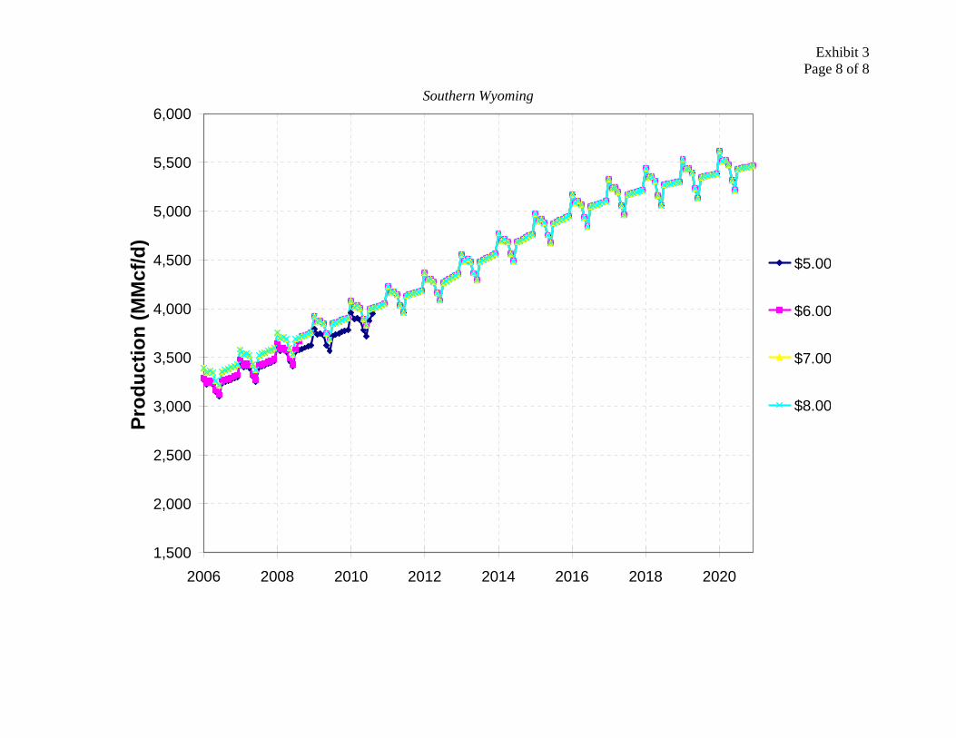
Exhibit 3 Page 8 of 8

Southern Wyoming

1,500

2,000

2,500

3,000

3,500

4,000

4,500

5,000

5,500

6,000

2006 2008 2010 2012 2014 2016 2018 2020

Prod

uctio

n (M

Mcf

/d)

$5.00

$6.00

$7.00

$8.00

Exhibit 4 Page 1 of 1

EXHIBIT 4

CAPITAL COST FOR A NEW PLANT IN NEW YORK CITY OR LONG ISLAND

Simple Cycle Combined Cycle Size 96 MW 519 MW Total Capital Cost $114 million $649 million New York

City Unit cost $1,188/kW $1,250/kW Size 96 MW 519 MW Total Capital Cost $108 million $571 million Long

Island Unit cost $1,125/kW $1,100/kW

Exhibit 5 Page 1 of 3

EXHIBIT 5

RESOURCE ADDITIONS INCLUDED IN ELECTRIC SIMULATION MODEL

In this exhibit, we provide a listing of resource additions by NYISO, PJM and ISO-NE market areas. The expected start-up date for each project is also listed along with the winter MW rating.

NYISO

Recent Plant Additions

Generating Plant In-Service Date MW Jamaica Bay (FPL) July 2003 51

Greenport July 2003 46 Stonybrook (Calpine) 2003 42

Simple Cycle

Freeport 2004 48 Athens Generating May 2004 1,080

Ravenswood (KeySpan) May 2004 250 East River (ConEd) April 2005 360 Bethpage (Calpine) May 2005 79.9

Bethlehem Energy (PSE&G) June 2005 750 Babylon (Pinelawn Power) June 2005 79.9

Poletti Power (NYPA) December 2005 500

Combined Cycle

Astoria (SCS Energy) 2006 500 Total 3,787

Plants in Development

Generating Plant In-Service Date MW Combined

Cycle Caithness Bellport 2009 326

Total 326

Exhibit 5 Page 2 of 3

PJM

Recent Plant Additions

Generating Plant In-Service Date MW Rock Springs (Old Dom & ConEd) Q4 2005 310

Simple Cycle Lakewood Industrial (ConEd) Q4 2005 167

Red Oak (AES) Sept 2002 832 Rock Springs (Old Dom&ConEd) June 2003 620

Lakewood Industrial (ConEd) June 2003 333 Hunterstown Gen (Reliant) July 2003 830

Bethlehem (Conectiv) Dec 2003 1,100Lower Mt Bethel (PPL Global) May 2004 550

Fairless Works (Dominion) July 2004 1,080Marcus Hook (FPL Energy) Q4 2004 725

Combined Cycle

Linden Repowering (PSEG Power) Q2 2006 1,186Coal Seward (Reliant Energy) Oct 2004 520

Total 8,253

PSEG Power LLC is constructing a $590 million, 1,186 MW combined-cycle generating plant at its Linden Generating Station in Linden, New Jersey, at which Units #1-3 (436 MW) will be retired upon project completion.

ISO-NE

Recent Plant Additions

Generating Plant In-Service Date MW Mystic (Banks et al) Jun 2003 1,550

Lake Road (PG&E Energy) Jun 2003 800 Fore River (Banks et al) Jul 2003 832

Combined Cycle

Milford Power Q1/2 2004 544 Total 3,726

Generation Attrition / New Entry in Ontario

Energy prices in New York State are impacted by market dynamics in Ontario. A number of 230 kV and 345 kV AC circuits connect New York and Ontario. The total transfer capability into New York is about 2,500 MW. The total transfer capability into Ontario is about 1,800 MW. Based on the March 2004 IMO “10-Year Outlook,” the table below summarizes the installed generation capacity in Ontario. Over 600 MW of new gas-fired capacity has been added at

Exhibit 5 Page 3 of 3

Brighton Beach and Kirkland Lake. The nuclear group listed does not include the expected return of the Pickering A Unit 1 in 2005, about 515 MW.

Table 1 – Ontario Installed Generation Capacity (10/1/04)

Type Total Capacity (MW)Nuclear 10,850

Coal 7,564 Oil/Gas 4,976 Hydro 7,676 Misc. 66 Total 31,132

Nearly three years ago, the Government of Ontario announced its intention to shut down all coal-fired generation by the end of 2007. While the reactivation of certain Pickering and Bruce units has materially increased provincial generation supply, resource adequacy over the intermediate to long-term is predicated on massive investment in new gas-fired generation and wind turbines as well as the reactivation/re-tubing of the remaining Pickering and Bruce nuclear power plants. A number of smaller scale hydro projects plus high voltage transmission infrastructure improvements are also part of the potential resource additions in Ontario to maintain resource adequacy throughout the province.

In forecasting energy balances in Ontario and transmission exchange between neighboring control areas, LAI has assumed the following:

• Lakeview is shutdown as scheduled by April 30, 2005;

• Coal-fired generation at Nanticoke is retired in 2007, but all coal fired capacity at Lambton, Atikokan and Thunder Bay remains in-service;

• Pickering A Unit 1 returns to service by Q4 2005;

• OPG will refurbish Pickering B Units 5, 6, 7 by 2013, Bruce Power will refurbish Bruce A by 2009, and these units will continue in operation; and

• All generation retirements are compensated by a watt-for-watt mix of gas-fired generation and wind projects in 2006 and 2007.

Exhibit 6 Page 1 of 1

EXHIBIT 6

RPS CAPACITY ADDITIONS AND ANNUAL TARGETS

New York RPS Annual Targets

Year

Total Pre-Program

Renewables (MWh)

Increment Target (MWh)

Total Renewables

(MWh)

Statewide Renewables Percentage

Incremental Statewide

Percentage

Incremental Percentage for LSEs

2005 31,737,254 - 31,737,254 19.2 0.0 0.00 2006 32,015,057 1,360,424 33,375,481 19.9% 0.8% 0.96% 2007 32,281,116 2,821,830 35,102,946 20.7% 1.7% 1.95% 2008 32,547,196 4,306,437 36,853,633 21.4% 2.5% 2.94% 2009 32,813,297 5,787,968 38,601,265 22.1% 3.3% 3.90% 2010 33,079,418 7,301,693 40,381,111 22.8% 4.1% 4.86% 2011 33,295,565 8,867,181 42,162,746 23.6% 5.0% 5.83% 2012 33,511,713 10,403,939 43,915,652 24.3% 5.8% 6.76% 2013 33,727,862 11,988,888 45,716,750 25.0% 6.6% 7.71%

Expected RPS Capacity Additions (2006 – 2013)

NYPSC Expectations / LAI-Adjusted Values Wind Hydro

Imports Biomass Landfill Total

MW 3,029 / 650 1,100 294 123 4,546 / 2,167

MWh 8,318,146 / 1,785,010 4,182,600 1,573,734 1,016,100 15,090,580 /

8,557,444

Capacity Factor 12.5% - 31%1 43% 61% 95% 38%

1 Because the wind resources are not expected to produce at full capacity during system peak, the UCAP adjustment is as low as 10-15%. We used 12.5%. The expected capacity factor for calculating total annual energy production is 31%, consistent with the PSC Order 03-E-0188.

Exhibit 7 Page 1 of 13

EXHIBIT 7

PRICE EFFECTS AT REGIONAL PRICING POINTS

Business-as-Usual Case (Nominal $/MMBtu)

Business-as-Usual Case w/ Broadwater (Nominal $/MMBtu)

Henry Hub Long Island Dawn Henry Hub Long Island Dawn Jan-10 6.48 7.87 6.84 6.21 7.36 6.49 Feb-10 6.55 8.06 6.88 6.24 7.44 6.53 Mar-10 6.55 7.86 6.92 6.26 7.38 6.56 Apr-10 6.29 7.46 6.66 5.99 6.96 6.31 May-10 6.32 7.30 6.71 5.97 6.74 6.36 Jun-10 6.36 7.31 6.74 6.00 6.77 6.39 Jul-10 6.34 7.36 6.56 6.03 6.83 6.25

Aug-10 6.37 7.40 6.59 6.05 6.84 6.28 Sep-10 5.85 6.77 6.36 5.58 6.33 6.11 Oct-10 5.85 6.82 6.25 5.60 6.38 6.01 Nov-10 5.99 7.18 6.38 5.74 6.69 6.06 Dec-10 6.26 7.56 6.62 6.03 7.13 6.37 Jan-11 6.53 14.68 6.86 6.33 7.60 6.60 Feb-11 6.57 12.93 6.90 6.33 7.86 6.64 Mar-11 6.61 8.26 6.94 6.37 7.53 6.67 Apr-11 6.35 7.48 6.67 6.10 7.02 6.42 May-11 6.38 7.32 6.72 6.11 6.85 6.46 Jun-11 6.42 7.36 6.79 6.14 6.82 6.55 Jul-11 6.49 7.41 6.72 6.19 6.91 6.46

Aug-11 6.51 7.46 6.75 6.21 6.95 6.50 Sep-11 6.10 7.03 6.70 5.75 6.46 6.29 Oct-11 6.12 7.09 6.54 5.75 6.54 6.17 Nov-11 6.16 7.26 6.57 5.78 6.73 6.19 Dec-11 6.55 7.81 6.92 6.19 7.22 6.53 Jan-12 6.83 15.12 7.17 6.42 7.82 6.77 Feb-12 6.89 13.17 7.22 6.50 7.88 6.81 Mar-12 6.94 8.26 7.26 6.54 7.64 6.84 Apr-12 6.71 7.89 7.05 6.28 7.26 6.61 May-12 6.70 7.71 7.08 6.33 7.10 6.65

Exhibit 7 Page 2 of 13

Business-as-Usual Case (Nominal $/MMBtu)

Business-as-Usual Case w/ Broadwater (Nominal $/MMBtu)

Henry Hub Long Island Dawn Henry Hub Long Island Dawn Jun-12 6.74 7.75 7.15 6.36 7.07 6.73 Jul-12 6.87 7.81 7.16 6.45 7.13 6.69

Aug-12 6.86 7.85 7.20 6.45 7.17 6.72 Sep-12 6.51 7.53 7.20 6.09 6.86 6.68 Oct-12 6.54 7.59 7.07 6.11 6.94 6.60 Nov-12 6.64 7.82 7.11 6.17 7.17 6.63 Dec-12 7.13 8.46 7.48 6.65 7.82 7.01 Jan-13 7.41 15.57 7.75 6.97 8.27 7.26 Feb-13 7.40 11.37 7.80 6.96 8.29 7.31 Mar-13 7.48 8.89 7.84 6.99 8.17 7.35 Apr-13 7.21 8.47 7.61 6.82 7.79 7.13 May-13 7.30 8.37 7.66 6.85 7.67 7.18 Jun-13 7.36 8.42 7.73 6.89 7.69 7.26 Jul-13 7.42 8.50 7.75 6.98 7.84 7.26

Aug-13 7.43 8.55 7.79 6.98 7.88 7.30 Sep-13 6.79 7.83 7.47 6.34 7.16 6.94 Oct-13 6.78 7.88 7.26 6.36 7.25 6.81 Nov-13 6.83 8.04 7.31 6.41 7.42 6.85 Dec-13 7.30 8.62 7.68 6.85 7.99 7.21 Jan-14 7.56 9.12 7.95 7.17 8.37 7.47 Feb-14 7.61 9.46 8.00 7.22 8.47 7.52 Mar-14 7.66 9.03 8.04 7.24 8.36 7.56 Apr-14 7.41 8.64 7.74 6.99 7.92 7.27 May-14 7.46 8.55 7.80 7.05 7.78 7.32 Jun-14 7.47 8.60 7.87 7.09 7.79 7.43 Jul-14 7.56 8.66 7.79 7.16 7.92 7.35

Aug-14 7.60 8.72 7.83 7.16 8.01 7.39 Sep-14 6.77 7.82 7.36 6.37 7.13 6.89 Oct-14 6.80 7.87 7.23 6.37 7.19 6.76 Nov-14 6.94 8.22 7.34 6.47 7.52 6.86 Dec-14 7.33 8.88 7.65 6.87 8.14 7.16 Jan-15 7.61 16.52 7.92 7.17 8.68 7.41

Exhibit 7 Page 3 of 13

Business-as-Usual Case (Nominal $/MMBtu)

Business-as-Usual Case w/ Broadwater (Nominal $/MMBtu)

Henry Hub Long Island Dawn Henry Hub Long Island Dawn Feb-15 7.67 14.39 7.97 7.24 8.90 7.46 Mar-15 7.71 9.30 8.01 7.26 8.54 7.50 Apr-15 7.44 8.69 7.66 6.97 7.91 7.21 May-15 7.49 8.55 7.71 7.02 7.70 7.24 Jun-15 7.52 8.60 7.75 7.06 7.75 7.29 Jul-15 7.62 8.68 7.73 7.10 7.90 7.25

Aug-15 7.59 8.74 7.77 7.12 7.95 7.29 Sep-15 6.71 7.71 7.04 6.31 6.97 6.65 Oct-15 6.73 7.77 7.06 6.34 7.04 6.65 Nov-15 6.79 7.94 7.10 6.41 7.29 6.70 Dec-15 7.23 8.62 7.53 6.85 7.96 7.10 Jan-16 7.53 17.01 7.80 7.11 8.68 7.36 Feb-16 7.57 14.83 7.84 7.16 8.74 7.40 Mar-16 7.61 9.14 7.89 7.21 8.45 7.44 Apr-16 7.34 8.67 7.59 6.95 7.97 7.18 May-16 7.42 8.54 7.64 6.95 7.71 7.20 Jun-16 7.45 8.59 7.68 7.03 7.75 7.25 Jul-16 7.58 8.67 7.70 7.10 7.92 7.26

Aug-16 7.62 8.72 7.74 7.12 7.97 7.30 Sep-16 7.05 8.05 7.49 6.62 7.35 7.03 Oct-16 7.08 8.20 7.53 6.65 7.43 7.05 Nov-16 7.17 8.42 7.56 6.70 7.70 7.08 Dec-16 7.69 9.29 8.02 7.21 8.50 7.51 Jan-17 8.01 17.52 8.31 7.55 9.01 7.78 Feb-17 8.06 13.47 8.36 7.56 9.02 7.83 Mar-17 8.11 9.66 8.41 7.61 8.89 7.87 Apr-17 7.77 9.15 8.09 7.30 8.33 7.57 May-17 7.84 9.08 8.14 7.33 8.12 7.62 Jun-17 7.88 9.14 8.19 7.36 8.23 7.66 Jul-17 8.03 9.24 8.16 7.52 8.44 7.64

Aug-17 8.08 9.30 8.20 7.55 8.50 7.68 Sep-17 7.57 8.74 8.08 6.98 7.81 7.48

Exhibit 7 Page 4 of 13

Business-as-Usual Case (Nominal $/MMBtu)

Business-as-Usual Case w/ Broadwater (Nominal $/MMBtu)

Henry Hub Long Island Dawn Henry Hub Long Island Dawn Oct-17 7.60 8.80 8.10 7.01 7.89 7.49 Nov-17 7.66 8.98 8.14 7.11 8.14 7.53 Dec-17 8.26 9.81 8.62 7.63 8.94 7.94 Jan-18 8.56 10.39 8.93 7.93 9.41 8.23 Feb-18 8.58 11.91 8.99 7.99 9.50 8.28 Mar-18 8.66 10.27 9.03 8.02 9.36 8.32 Apr-18 8.34 9.83 8.69 7.71 8.85 8.00 May-18 8.39 9.73 8.76 7.76 8.64 8.06 Jun-18 8.46 9.79 8.81 7.74 8.67 8.10 Jul-18 8.60 9.87 8.73 7.89 8.85 8.02

Aug-18 8.64 9.93 8.77 7.96 8.90 8.07 Sep-18 7.71 8.89 8.32 7.16 8.05 7.74 Oct-18 7.71 8.96 8.24 7.20 8.15 7.68 Nov-18 7.84 9.34 8.30 7.35 8.57 7.74 Dec-18 8.33 12.72 8.72 7.80 9.28 8.14 Jan-19 8.63 18.59 9.04 8.08 9.91 8.43 Feb-19 8.68 16.20 9.09 8.13 10.09 8.48 Mar-19 8.73 11.02 9.14 8.17 9.73 8.53 Apr-19 8.33 9.98 8.79 7.77 9.04 8.20 May-19 8.37 9.70 8.85 7.81 8.73 8.26 Jun-19 8.43 9.76 8.91 7.86 8.75 8.30 Jul-19 8.54 9.84 8.68 7.93 8.90 8.06

Aug-19 8.58 9.96 8.71 7.94 8.94 8.08 Sep-19 7.65 8.88 8.33 7.13 8.05 7.73 Oct-19 7.68 8.95 8.30 7.16 8.13 7.75 Nov-19 7.80 9.25 8.34 7.29 8.40 7.78 Dec-19 8.42 10.09 8.84 7.85 9.27 8.22 Jan-20 8.73 19.15 9.16 8.15 10.04 8.51 Feb-20 8.79 16.69 9.22 8.21 10.09 8.56 Mar-20 8.82 10.73 9.27 8.25 9.79 8.61 Apr-20 8.47 10.14 8.92 7.89 9.24 8.28 May-20 8.52 9.96 8.98 7.91 8.87 8.34

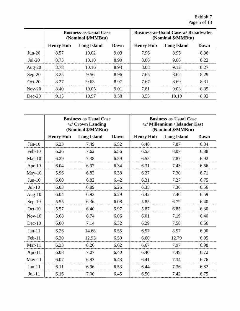
Exhibit 7 Page 5 of 13

Business-as-Usual Case (Nominal $/MMBtu)

Business-as-Usual Case w/ Broadwater (Nominal $/MMBtu)

Henry Hub Long Island Dawn Henry Hub Long Island Dawn Jun-20 8.57 10.02 9.03 7.96 8.95 8.38 Jul-20 8.75 10.10 8.90 8.06 9.08 8.22

Aug-20 8.78 10.16 8.94 8.08 9.12 8.27 Sep-20 8.25 9.56 8.96 7.65 8.62 8.29 Oct-20 8.27 9.63 8.97 7.67 8.69 8.31 Nov-20 8.40 10.05 9.01 7.81 9.03 8.35 Dec-20 9.15 10.97 9.58 8.55 10.10 8.92

Business-as-Usual Case

w/ Crown Landing (Nominal $/MMBtu)

Business-as-Usual Case w/ Millennium / Islander East

(Nominal $/MMBtu) Henry Hub Long Island Dawn Henry Hub Long Island Dawn

Jan-10 6.23 7.49 6.52 6.48 7.87 6.84 Feb-10 6.26 7.62 6.56 6.53 8.07 6.88 Mar-10 6.29 7.38 6.59 6.55 7.87 6.92 Apr-10 6.04 6.97 6.34 6.31 7.43 6.66 May-10 5.96 6.82 6.38 6.27 7.30 6.71 Jun-10 6.00 6.82 6.42 6.31 7.27 6.75 Jul-10 6.03 6.89 6.26 6.35 7.36 6.56

Aug-10 6.04 6.93 6.29 6.42 7.40 6.59 Sep-10 5.55 6.36 6.08 5.85 6.79 6.40 Oct-10 5.57 6.40 5.97 5.87 6.85 6.30 Nov-10 5.68 6.74 6.06 6.01 7.19 6.40 Dec-10 6.00 7.14 6.32 6.29 7.58 6.66 Jan-11 6.26 14.68 6.55 6.57 8.57 6.90 Feb-11 6.30 12.93 6.59 6.60 12.79 6.95 Mar-11 6.33 8.26 6.62 6.67 7.97 6.98 Apr-11 6.08 7.07 6.40 6.40 7.49 6.72 May-11 6.07 6.93 6.43 6.41 7.34 6.76 Jun-11 6.11 6.96 6.53 6.44 7.36 6.82 Jul-11 6.16 7.00 6.45 6.50 7.42 6.75

Exhibit 7 Page 6 of 13

Business-as-Usual Case

w/ Crown Landing (Nominal $/MMBtu)

Business-as-Usual Case w/ Millennium / Islander East

(Nominal $/MMBtu) Henry Hub Long Island Dawn Henry Hub Long Island Dawn

Aug-11 6.18 7.04 6.49 6.53 7.47 6.78 Sep-11 5.71 6.53 6.28 6.12 7.06 6.74 Oct-11 5.71 6.59 6.14 6.15 7.12 6.60 Nov-11 5.74 6.82 6.20 6.21 7.29 6.63 Dec-11 6.15 7.25 6.50 6.58 7.84 6.99 Jan-12 6.43 15.12 6.74 6.88 8.96 7.24 Feb-12 6.47 13.17 6.78 6.92 9.17 7.28 Mar-12 6.50 7.76 6.81 6.97 8.30 7.32 Apr-12 6.24 7.29 6.58 6.69 7.90 7.08 May-12 6.28 7.15 6.63 6.77 7.73 7.11 Jun-12 6.34 7.17 6.69 6.77 7.77 7.17 Jul-12 6.35 7.21 6.70 6.88 7.83 7.19

Aug-12 6.39 7.25 6.74 6.88 7.87 7.23 Sep-12 6.06 6.94 6.67 6.54 7.52 7.21 Oct-12 6.09 7.02 6.59 6.55 7.59 7.07 Nov-12 6.12 7.25 6.62 6.60 7.82 7.11 Dec-12 6.62 7.89 6.97 7.12 8.44 7.50 Jan-13 6.87 15.57 7.22 7.41 8.98 7.77 Feb-13 6.91 11.37 7.27 7.46 9.02 7.82 Mar-13 6.96 8.22 7.31 7.51 8.87 7.86 Apr-13 6.73 7.81 7.10 7.27 8.46 7.61 May-13 6.80 7.74 7.15 7.30 8.38 7.66 Jun-13 6.82 7.78 7.23 7.32 8.42 7.74 Jul-13 6.90 7.85 7.23 7.49 8.51 7.75

Aug-13 6.94 7.89 7.27 7.48 8.56 7.79 Sep-13 6.29 7.24 6.95 6.79 7.83 7.47 Oct-13 6.32 7.30 6.78 6.78 7.88 7.26 Nov-13 6.36 7.50 6.81 6.85 8.03 7.31 Dec-13 6.85 8.01 7.17 7.28 8.62 7.68 Jan-14 7.12 8.58 7.43 7.57 9.11 7.96 Feb-14 7.16 9.46 7.48 7.61 9.19 8.00

Exhibit 7 Page 7 of 13

Business-as-Usual Case

w/ Crown Landing (Nominal $/MMBtu)

Business-as-Usual Case w/ Millennium / Islander East

(Nominal $/MMBtu) Henry Hub Long Island Dawn Henry Hub Long Island Dawn

Mar-14 7.20 8.34 7.52 7.65 9.02 8.05 Apr-14 6.92 8.00 7.23 7.43 8.62 7.74 May-14 7.01 7.90 7.28 7.45 8.47 7.80 Jun-14 7.01 7.92 7.40 7.53 8.50 7.87 Jul-14 7.08 8.01 7.33 7.56 8.65 7.78

Aug-14 7.12 8.06 7.37 7.59 8.70 7.82 Sep-14 6.32 7.19 6.87 6.82 7.87 7.42 Oct-14 6.35 7.23 6.72 6.88 7.94 7.30 Nov-14 6.44 7.59 6.84 6.96 8.25 7.37 Dec-14 6.86 8.64 7.12 7.38 8.86 7.73 Jan-15 7.12 16.52 7.38 7.65 9.96 8.01 Feb-15 7.17 14.39 7.42 7.75 13.88 8.05 Mar-15 7.20 8.40 7.46 7.76 9.28 8.10 Apr-15 6.92 8.01 7.16 7.51 8.73 7.72 May-15 6.98 7.84 7.20 7.51 8.50 7.76 Jun-15 7.03 7.88 7.24 7.60 8.55 7.81 Jul-15 7.06 8.00 7.21 7.68 8.73 7.79

Aug-15 7.08 8.05 7.25 7.65 8.79 7.83 Sep-15 6.24 7.05 6.59 6.74 7.64 7.08 Oct-15 6.26 7.09 6.61 6.77 7.71 7.11 Nov-15 6.35 7.36 6.64 6.82 7.97 7.15 Dec-15 6.77 7.92 7.05 7.26 8.65 7.59 Jan-16 7.03 17.01 7.31 7.57 9.92 7.87 Feb-16 7.08 14.83 7.35 7.61 10.21 7.91 Mar-16 7.14 8.32 7.39 7.68 9.15 7.96 Apr-16 6.88 7.99 7.12 7.38 8.69 7.63 May-16 6.92 7.82 7.15 7.45 8.48 7.68 Jun-16 6.96 7.86 7.19 7.49 8.51 7.73 Jul-16 7.07 8.02 7.20 7.62 8.71 7.74

Aug-16 7.07 8.07 7.24 7.64 8.76 7.78 Sep-16 6.58 7.45 7.03 7.06 8.05 7.51

Exhibit 7 Page 8 of 13

Business-as-Usual Case

w/ Crown Landing (Nominal $/MMBtu)

Business-as-Usual Case w/ Millennium / Islander East

(Nominal $/MMBtu) Henry Hub Long Island Dawn Henry Hub Long Island Dawn

Oct-16 6.61 7.51 7.04 7.09 8.10 7.54 Nov-16 6.66 7.82 7.07 7.19 8.43 7.58 Dec-16 7.21 8.43 7.51 7.70 9.19 8.04 Jan-17 7.49 17.52 7.78 8.01 9.85 8.33 Feb-17 7.54 13.47 7.83 8.07 9.87 8.38 Mar-17 7.58 8.83 7.87 8.12 9.62 8.43 Apr-17 7.24 8.43 7.57 7.79 9.16 8.11 May-17 7.27 8.27 7.62 7.85 8.99 8.16 Jun-17 7.32 8.32 7.66 7.89 9.06 8.21 Jul-17 7.47 8.49 7.60 8.04 9.23 8.17

Aug-17 7.52 8.54 7.64 8.09 9.29 8.21 Sep-17 6.96 7.96 7.51 7.54 8.67 8.08 Oct-17 6.98 8.02 7.49 7.57 8.71 8.10 Nov-17 7.03 8.24 7.52 7.69 8.98 8.14 Dec-17 7.63 8.90 7.95 8.26 9.79 8.62 Jan-18 7.91 9.57 8.23 8.56 10.36 8.94 Feb-18 7.98 11.91 8.28 8.62 10.50 8.99 Mar-18 8.01 9.33 8.32 8.67 10.26 9.04 Apr-18 7.70 8.90 8.01 8.34 9.76 8.70 May-18 7.74 8.77 8.06 8.40 9.65 8.76 Jun-18 7.73 8.82 8.14 8.45 9.72 8.81 Jul-18 7.86 8.95 8.00 8.61 9.86 8.73

Aug-18 7.94 9.00 8.04 8.65 9.92 8.77 Sep-18 7.10 8.18 7.76 7.78 8.92 8.39 Oct-18 7.12 8.22 7.63 7.81 9.00 8.32 Nov-18 7.30 8.60 7.71 7.91 9.38 8.36 Dec-18 7.72 12.72 8.08 8.40 10.18 8.80 Jan-19 8.01 18.59 8.37 8.70 11.43 9.12 Feb-19 8.06 16.20 8.42 8.76 15.93 9.17 Mar-19 8.10 11.02 8.46 8.81 10.67 9.22 Apr-19 7.70 9.03 8.14 8.39 10.01 8.88

Exhibit 7 Page 9 of 13

Business-as-Usual Case

w/ Crown Landing (Nominal $/MMBtu)

Business-as-Usual Case w/ Millennium / Islander East

(Nominal $/MMBtu) Henry Hub Long Island Dawn Henry Hub Long Island Dawn

May-19 7.72 8.79 8.19 8.44 9.68 8.94 Jun-19 7.77 8.84 8.24 8.50 9.79 8.99 Jul-19 7.84 8.93 7.99 8.61 9.90 8.76

Aug-19 7.86 9.58 8.02 8.64 9.96 8.79 Sep-19 7.07 8.17 7.74 7.70 8.90 8.38 Oct-19 7.10 8.22 7.69 7.73 8.99 8.37 Nov-19 7.23 8.50 7.72 7.84 9.30 8.41 Dec-19 7.77 9.19 8.16 8.49 10.17 8.92 Jan-20 8.08 19.15 8.45 8.80 11.58 9.24 Feb-20 8.13 16.69 8.50 8.85 11.99 9.29 Mar-20 8.18 9.63 8.55 8.90 10.75 9.35 Apr-20 7.84 9.22 8.22 8.53 10.20 9.01 May-20 7.85 8.96 8.28 8.58 10.00 9.06 Jun-20 7.90 9.01 8.33 8.63 10.08 9.11 Jul-20 8.01 9.35 8.20 8.81 10.16 8.96

Aug-20 8.04 9.19 8.25 8.83 10.22 9.00 Sep-20 7.58 8.72 8.28 8.25 9.52 8.97 Oct-20 7.60 8.78 8.25 8.28 9.59 8.99 Nov-20 7.76 9.12 8.29 8.42 10.07 9.03 Dec-20 8.45 10.01 8.80 9.16 10.97 9.59

LNG Overbuild Case (Nominal $/MMBtu)

LNG Overbuild Case w/ Broadwater (Nominal $/MMBtu)

Henry Hub Long Island Dawn Henry Hub Long Island Dawn Jan-10 6.40 7.80 6.78 6.15 7.34 6.47 Feb-10 6.43 7.99 6.82 6.19 7.42 6.51 Mar-10 6.47 7.78 6.85 6.23 7.35 6.54 Apr-10 6.20 7.40 6.59 5.94 6.93 6.29 May-10 6.22 7.22 6.64 5.94 6.70 6.34 Jun-10 6.28 7.23 6.68 5.99 6.74 6.37

Exhibit 7 Page 10 of 13

LNG Overbuild Case (Nominal $/MMBtu)

LNG Overbuild Case w/ Broadwater (Nominal $/MMBtu)

Henry Hub Long Island Dawn Henry Hub Long Island Dawn Jul-10 6.34 7.28 6.49 6.04 6.80 6.21

Aug-10 6.30 7.33 6.53 6.06 6.82 6.25 Sep-10 5.37 6.27 5.92 5.20 5.93 5.73 Oct-10 5.42 6.32 5.75 5.19 5.99 5.56 Nov-10 5.63 6.78 5.99 5.39 6.32 5.74 Dec-10 5.75 7.00 6.05 5.53 6.61 5.82 Jan-11 5.93 14.68 6.27 5.74 7.05 6.03 Feb-11 5.97 12.93 6.31 5.77 7.55 6.06 Mar-11 5.99 8.26 6.34 5.78 6.94 6.10 Apr-11 5.67 6.86 6.10 5.47 6.40 5.86 May-11 5.67 6.64 6.14 5.43 6.17 5.90 Jun-11 5.68 6.61 6.17 5.46 6.16 5.93 Jul-11 5.75 6.65 6.04 5.51 6.20 5.74

Aug-11 5.73 6.67 6.08 5.48 6.22 5.77 Sep-11 5.11 6.02 5.73 4.93 5.67 5.51 Oct-11 5.13 6.08 5.58 4.95 5.76 5.35 Nov-11 5.17 6.28 5.65 4.98 5.90 5.40 Dec-11 5.53 6.76 5.91 5.33 6.33 5.67 Jan-12 5.74 15.12 6.13 5.54 6.94 5.88 Feb-12 5.79 13.17 6.16 5.58 7.08 5.91 Mar-12 5.80 7.17 6.20 5.60 6.70 5.95 Apr-12 5.56 6.80 6.02 5.36 6.37 5.73 May-12 5.56 6.59 5.99 5.37 6.16 5.75 Jun-12 5.60 6.56 6.03 5.40 6.14 5.80 Jul-12 5.68 6.60 6.01 5.47 6.21 5.78

Aug-12 5.69 6.65 6.04 5.47 6.24 5.82 Sep-12 5.21 6.19 5.88 5.00 5.77 5.60 Oct-12 5.22 6.26 5.76 5.02 5.86 5.46 Nov-12 5.29 6.52 5.84 5.05 6.06 5.55 Dec-12 5.68 7.04 6.11 5.42 6.57 5.80 Jan-13 5.90 15.57 6.33 5.63 7.08 6.01 Feb-13 5.95 11.37 6.36 5.67 7.06 6.04

Exhibit 7 Page 11 of 13

LNG Overbuild Case (Nominal $/MMBtu)

LNG Overbuild Case w/ Broadwater (Nominal $/MMBtu)

Henry Hub Long Island Dawn Henry Hub Long Island Dawn Mar-13 5.97 7.37 6.40 5.70 6.90 6.07 Apr-13 5.71 6.99 6.21 5.44 6.53 5.89 May-13 5.74 6.83 6.19 5.46 6.33 5.87 Jun-13 5.78 6.87 6.23 5.51 6.38 5.93 Jul-13 5.94 6.94 6.25 5.63 6.54 5.94

Aug-13 5.97 6.99 6.28 5.65 6.51 5.97 Sep-13 5.29 6.36 6.05 5.05 5.86 5.67 Oct-13 5.30 6.42 5.88 5.03 5.95 5.51 Nov-13 5.35 6.62 5.91 5.07 6.12 5.58 Dec-13 5.79 7.15 6.23 5.46 6.65 5.85 Jan-14 6.03 7.62 6.46 5.69 6.98 6.06 Feb-14 6.07 9.46 6.50 5.73 7.11 6.10 Mar-14 6.10 7.49 6.53 5.76 6.94 6.13 Apr-14 5.84 7.13 6.27 5.50 6.58 5.89 May-14 5.87 6.95 6.32 5.53 6.38 5.92 Jun-14 5.92 6.99 6.36 5.58 6.38 6.00 Jul-14 6.05 7.05 6.32 5.67 6.41 5.93

Aug-14 6.06 7.09 6.36 5.68 6.51 5.96 Sep-14 5.13 6.08 5.76 4.97 5.74 5.54 Oct-14 5.11 6.13 5.54 4.98 5.80 5.32 Nov-14 5.21 6.59 5.78 5.04 6.25 5.56 Dec-14 5.48 8.64 5.88 5.31 6.57 5.64 Jan-15 5.68 16.52 6.09 5.51 7.06 5.84 Feb-15 5.71 14.39 6.13 5.55 8.05 5.88 Mar-15 5.77 8.20 6.16 5.60 6.87 5.90 Apr-15 5.44 6.75 5.85 5.27 6.30 5.64 May-15 5.46 6.44 5.87 5.29 5.98 5.68 Jun-15 5.49 6.43 5.90 5.32 6.08 5.71 Jul-15 5.53 6.51 5.64 5.37 6.14 5.48

Aug-15 5.54 6.54 5.67 5.38 6.19 5.51 Sep-15 5.09 6.01 5.59 4.94 5.68 5.38 Oct-15 5.10 6.05 5.58 4.96 5.74 5.38

Exhibit 7 Page 12 of 13

LNG Overbuild Case (Nominal $/MMBtu)

LNG Overbuild Case w/ Broadwater (Nominal $/MMBtu)

Henry Hub Long Island Dawn Henry Hub Long Island Dawn Nov-15 5.13 6.31 5.61 5.00 5.98 5.40 Dec-15 5.49 6.84 5.93 5.34 6.44 5.71 Jan-16 5.71 17.01 6.14 5.56 7.19 5.92 Feb-16 5.74 14.83 6.18 5.59 7.62 5.95 Mar-16 5.77 7.30 6.21 5.62 6.90 5.99 Apr-16 5.54 6.93 5.95 5.39 6.48 5.74 May-16 5.56 6.64 6.00 5.42 6.24 5.78 Jun-16 5.60 6.68 6.03 5.45 6.27 5.81 Jul-16 5.73 6.75 5.89 5.55 6.36 5.71

Aug-16 5.74 6.79 5.93 5.57 6.39 5.74 Sep-16 5.40 6.39 5.95 5.24 5.98 5.76 Oct-16 5.42 6.44 5.98 5.26 6.08 5.76 Nov-16 5.46 6.76 6.01 5.31 6.44 5.79 Dec-16 5.90 7.48 6.40 5.73 7.05 6.12 Jan-17 6.16 17.52 6.64 5.95 7.62 6.34 Feb-17 6.20 13.47 6.68 5.99 7.60 6.38 Mar-17 6.24 7.83 6.71 6.02 7.40 6.41 Apr-17 5.95 7.38 6.44 5.75 6.90 6.15 May-17 5.98 7.22 6.49 5.79 6.65 6.19 Jun-17 6.02 7.26 6.53 5.83 6.75 6.24 Jul-17 6.21 7.36 6.43 5.95 6.88 6.19

Aug-17 6.25 7.41 6.47 5.98 6.94 6.22 Sep-17 5.85 7.01 6.51 5.69 6.60 6.26 Oct-17 5.87 7.06 6.54 5.71 6.64 6.29 Nov-17 5.94 7.35 6.57 5.76 6.92 6.32 Dec-17 6.73 8.40 7.28 6.35 7.70 6.78 Jan-18 7.07 8.98 7.54 6.64 8.21 7.02 Feb-18 7.12 11.91 7.59 6.68 8.31 7.07 Mar-18 7.15 8.80 7.63 6.71 8.16 7.10 Apr-18 6.87 8.40 7.33 6.44 7.71 6.84 May-18 6.91 8.25 7.38 6.48 7.52 6.88 Jun-18 6.96 8.30 7.45 6.53 7.56 7.01

Exhibit 7 Page 13 of 13

LNG Overbuild Case (Nominal $/MMBtu)

LNG Overbuild Case w/ Broadwater (Nominal $/MMBtu)

Henry Hub Long Island Dawn Henry Hub Long Island Dawn Jul-18 7.16 8.40 7.36 6.68 7.69 6.90

Aug-18 7.20 8.45 7.40 6.72 7.73 6.93 Sep-18 6.70 7.94 7.44 6.30 7.24 6.97 Oct-18 6.72 8.00 7.48 6.33 7.29 7.00 Nov-18 6.83 8.51 7.51 6.42 7.75 7.04 Dec-18 7.43 12.72 7.96 7.05 8.56 7.48 Jan-19 7.72 18.59 8.25 7.31 9.22 7.75 Feb-19 7.77 16.20 8.30 7.35 9.40 7.80 Mar-19 7.81 11.02 8.34 7.39 9.03 7.84 Apr-19 7.47 9.15 8.02 7.06 8.38 7.53 May-19 7.52 8.86 8.07 7.10 8.06 7.58 Jun-19 7.57 8.92 8.12 7.15 8.09 7.63 Jul-19 7.71 9.00 7.88 7.26 8.24 7.42

Aug-19 7.74 9.61 7.92 7.28 8.28 7.46 Sep-19 7.15 8.42 7.91 6.68 7.66 7.38 Oct-19 7.19 8.48 7.89 6.71 7.71 7.39 Nov-19 7.27 8.83 7.93 6.81 8.01 7.43 Dec-19 7.88 9.65 8.42 7.44 8.91 7.89 Jan-20 8.21 19.15 8.72 7.74 9.70 8.18 Feb-20 8.26 16.69 8.78 7.78 9.72 8.23 Mar-20 8.30 10.27 8.83 7.82 9.45 8.27 Apr-20 7.96 9.70 8.49 7.51 8.90 7.95 May-20 8.01 9.46 8.55 7.53 8.53 8.00 Jun-20 8.06 9.52 8.60 7.58 8.60 8.05 Jul-20 8.26 9.61 8.45 7.72 8.72 7.90

Aug-20 8.30 9.67 8.50 7.75 8.77 7.94 Sep-20 7.77 9.09 8.52 7.28 8.27 7.96 Oct-20 7.80 9.15 8.55 7.31 8.32 7.95 Nov-20 7.92 9.62 8.60 7.40 8.68 7.98 Dec-20 8.61 10.62 9.12 8.03 9.62 8.45

Exhibit 8 Page 1 of 2

EXHIBIT 8

CALCULATION FRAMEWORK FOR ECONOMIC BENEFITS

The economic benefits can be expressed as the sum over the study period years of the annual benefits for each region, discounted for present value and multiplied by a factor to account for secondary economic effects. The following equation expresses this function:

PVBs,b = PV of Benefit for scenario s relative to baseline scenario, b

= MEF * ∑ regions ∑ years

[ CGSs,b,r,y + EESs,b,r,y ] / (1 + DR) ^ (y – ybase)

MEF = Multiplier effect factor

CGSs,b,r,y = Core gas savings for scenario s relative to baseline scenario b, for region r,1 year y

= ∑ months { (CGLr,y,m – CGLr,2003,m) * ∑ points [ Fp,r * (GPp,y,m,b – GPp,y,m,s) ] + CGLr,2003,m * [0.6 * (GPHH,y,m,b – GPHHy,m,s) + 0.4 * (GPDawn,y,m,b – GPDawn,y,m,s) ] }

EES s,b,r,y = Electric energy savings for scenario s relative to baseline scenario b, for region r, year y

= ∑ months ∑ hours [ ELr,y,m,h * ( EEPr,y,m,h,b – EEPr,y,m,h,s ) ]

DR = Discount Rate

ybase = Base year for present value

CGLr,y,m = Core gas load for region r in year y, month m. CGLr,2003,m is the core gas load for the reference year 2003. This load is assumed to be served under long term firm transportation arrangements, with supply priced 60% at Henry Hub and 40% at Dawn. Incremental loads in later years are supplied from regional trading points.

Fp,r = Weight factor for trading point p, as applied to region r. The fraction of incremental gas load in region r, above the 2003 reference year level, assumed to be supplied from trading point p. Trading points for incremental supplies are TZ6-NY, IGTS-Z1, IGTS-Z2, Niagara, and DTI-SP.

1 Regions include New York City (NYISO Zone J), Long Island (NYISO Zone K), Central (NYISO Zones G, H, and I), North (NYISO Zones E and F), and South (NYISO Zones A, B, C and D.) For presentation purposes, the Central, North, and South regions are combined as “Rest of State”.

Exhibit 8 Page 2 of 2

GPp,y,m,b = Gas Price for trading point p for year y, month m, and scenario b (without Broadwater or scenario s with Broadwater). Trading points are Henry Hub, Dawn, TZ6-NY, IGTS-Z1, IGTS-Z2, Niagara, and DTI-SP.

ELr,y,m,h = Electric Load for region r, year y, month m, hour h

EEPr,y,m,h,b = Electric Energy Price for region r, year y, month m, hour h and scenario b (without Broadwater or scenario s with Broadwater), as determined by MarketSym simulation using appropriate monthly gas prices f

Exhibit 9 Page 1 of 2

EXHIBIT 9

CABRILLO PORT SUMMARY OF FSRU ACCIDENT CONSEQUENCES

Marine Collisionb Intentionalb Escalation Breach size 1300 m2of area 7 m2 & 7 m2 7 m2 & 1300 m2 7 m2 & 2x1300 m2 Number of tanks 50% volume of 1 tank 2 2 3 Release quantity (gal / m3)e 13,000,000 / 50,000 53,000,000 / 200,000 40,000,000 / 150,000 53,000,000 / 200,000 Pool Spread Distance Distance down range (NM / miles / m) 0.40 / 0.45 / 730 0.35 / 0.40 / 650 0.33 / 0.38 / 610 0.43 / 0.50 / 800 Pool Fire Radiative flux distance > 5 kW/m2 (NM / miles / m) 1.60 / 1.85 / 2,970 1.42 / 1.64 / 2,640 1.35 / 1.56 / 2,510 1.74 / 2.01 / 3,230 Radiative flux distance > 12.5kW/m2 (NM / miles / m) 0.99 / 1.14 / 1,830 0.87 / 1.01 / 1,620 0.83 / 0.96 / 1,540 1.07 / 1.24 / 1,990 Radiative flux distance > 37.5kW/m2 (NM / miles / m) 0.49 / 0.57 / 910 0.44 / 0.50 / 810 0.42 / 0.48 / 770 0.54 / 0.62 / 1,000 Vapor Cloud Dispersion (No Ignition) Average flammable height (feet / m) 69.9 / 21 98 / 30 Maximum distance to LFL (NM / miles / m) 2.85 / 3.29 / 5,290 6.03 / 6.95 / 11,175 Time for maximum distance (min)a 50 89 Vapor Cloud (Flash) Fire Radiative flux distance > 5 kW/m2 (NM / miles / m) 3.57 / 4.11 / 6,610 6.31 / 7.27 / 11,700 Radiative flux distance > 12.5kW/m2 (NM / miles / m) 3.29 / 3.79 / 6,100 6.21 / 7.15 / 11,500 Radiative flux distance > 37.5kW/m2 (NM / miles / m) 3.06 / 3.52 / 5,670 6.12 / 7.05 / 11,340

Immediate Ignition No Vapor Cloud Hazard

Source: Risknology 2006, Table 3.8 (see Appendix C1).

Exhibit 9 Page 2 of 2

Notes:

Pool fires and vapor cloud fires are mutually exclusive.

All radiative flux distances given from release location.

LFL = lower flammability limit; NM = nautical miles; m = meters.

Wind speed = 2 meters per second; temperature = 21°C.

a Time includes liquid dispersion and evaporation.

b Mass balance flux rate = 0.282 kg/m2sec.

c Mass balance flux rate = 0.135 kg/m2sec.

d The escalation case was modeled as a pool fire resulting from a breach of secondary containment due to the effects of a fire. Since ignition is guaranteed, no dispersion cloud develops.

e Tank volume of 100,000 m3 is used for ease of calculations; actual tank volume is 90,800 m3.

LIST OF APPENDICES

1. GPCM Model Theory and Structure

2. Basin Production Curves

3. Fuel Price Forecasts

4. Emissions Allowance Price Forecasts

5. Application Review, including Resource Reports

6. Det Norske Veritas: Broadwater Response to USCG Letter

7. Det Norske Veritas Fire Modeling

8. List of FERC Interveners

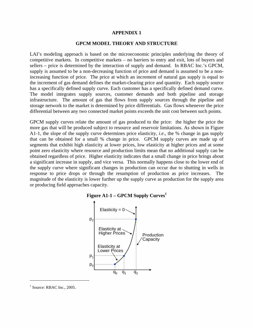
APPENDIX 1

GPCM MODEL THEORY AND STRUCTURE

LAI’s modeling approach is based on the microeconomic principles underlying the theory of competitive markets. In competitive markets – no barriers to entry and exit, lots of buyers and sellers – price is determined by the interaction of supply and demand. In RBAC Inc.’s GPCM, supply is assumed to be a non-decreasing function of price and demand is assumed to be a non-increasing function of price. The price at which an increment of natural gas supply is equal to the increment of gas demand defines the market-clearing price and quantity. Each supply source has a specifically defined supply curve. Each customer has a specifically defined demand curve. The model integrates supply sources, customer demands and both pipeline and storage infrastructure. The amount of gas that flows from supply sources through the pipeline and storage network to the market is determined by price differentials. Gas flows whenever the price differential between any two connected market points exceeds the unit cost between such points.

GPCM supply curves relate the amount of gas produced to the price: the higher the price the more gas that will be produced subject to resource and reservoir limitations. As shown in Figure A1-1, the slope of the supply curve determines price elasticity, i.e., the % change in gas supply that can be obtained for a small % change in price. GPCM supply curves are made up of segments that exhibit high elasticity at lower prices, low elasticity at higher prices and at some point zero elasticity where resource and production limits mean that no additional supply can be obtained regardless of price. Higher elasticity indicates that a small change in price brings about a significant increase in supply, and vice versa. This normally happens close to the lower end of the supply curve where significant changes in production can occur due to shutting in wells in response to price drops or through the resumption of production as price increases. The magnitude of the elasticity is lower further up the supply curve as production for the supply area or producing field approaches capacity.

Figure A1-1 – GPCM Supply Curves1

p0

p1

p2

q0 q1 q2

Elasticity = 0

Elasticity atHigher Prices

Elasticity atLower Prices

ProductionCapacity

1 Source: RBAC Inc., 2005.

A1-2

The demand curve sets the relationship between the price and the amount of gas associated with a customer’s preference. As prices increase, gas demand decreases. As shown in Figure A1-2, GPCM uses a multi-segment demand curve as fuel substitution effects allow certain price elastic customers to switch to an alternate fuel.

Figure A1-2 – GPCM Demand Curves2

Max Price

Low Elasticity

Min Price

Simple Demand Curve

Max Price Non-switchable, highvalue demand

Min Price

Alt FuelPrice

Demand switchable toAlt fuel

Low value demand

Multiple Segment Demand Curve

p

q

p

q

Solutions derived by GPCM require multiple iterations in order to balance supply and demand. Of course, the iterative nature of the solution is not pictured in Figure A1-3, but the calculation of market-clearing prices and quantities, which is equivalent to maximization of the sum of “producer surplus” and “consumer surplus”, requires computation of numerous possible solutions before the optimal solution is found. The model identifies and calculates the flows from supply points to demand points starting with the path with the greatest price differential. Lower cost gas flows are exhausted before higher cost flows between relevant nodes are accepted into the equilibrium solution. Supply and demand are therefore in balance at every node across the continental network. Both price and quantity for a local market equilibrium are influenced by market conditions across the continent. Hence, the level of supply from each supply region and the demand in other consumption regions enter into the determination of the market clearing prices.

2 Ibid.

A1-3

Figure A1-3 – GPCM Market Clearing Price3

ClearingQuantity

ClearingPrice

Market ClearingPrice

Market ClearingQuantity

Market ClearingPrice

Market ClearingQuantity

ConsumerSurplus

ProducerSurplus

Many gas industry market participants use GPCM to estimate the impact of new infrastructure on commodity prices, basis differentials and flows on rival transportation paths linking supply regions with consumption regions. Across North America, GPCM model structure is comprised of 86 supply areas, 164 pipelines, 146 storage areas, and 534 demand centers. Hence, results using the optimization framework in GPCM capture exploration and production, pipeline transportation costs, losses, storage injection and withdrawal profiles, pipeline and LNG import terminal additions, and demand. Model solutions constitute the least cost supply for an exogenous demand that “stacks” the flow of natural gas across rival pipeline paths to market centers from least cost to highest cost. Other key factor inputs to GPCM include: pipeline and storage prices (tariffs), supply curves by production basin, LNG terminal storage and daily vaporization capacities, and demand curves by sector and consumption area.4

As discussed, solutions incorporate price elasticities. Hence, the economic value of the equilibrium solution reflects both supply and demand elasticities in response to changes in price. The objective function that drives the solution constitutes the “greatest value” solution to serve total demand. Therefore the first-best economic solution reflects the least costly supply flowing first before more expensive supply is selected to meet customer demand. Similarly, customers willing to pay more are more likely to be served than those willing to pay less. Various constraints are incorporated in the model reflecting resource limitations, physical constraints on the pipeline network, and pipeline and storage tariffs. After specifying the applicable constraints for the gas system being modeled, a solution can be generated. In order to find an optimal economic solution to this network-flow problem, the model utilizes EMNET, an advanced LP optimizer.5 The model is simulated on a monthly basis, thus enabling the development of long-

3 Source: RBAC, Inc. 4 Gas demand for industrials and electricity generators behind the citygate are rolled-up with direct deliveries off the pipe rather than designated separately. 5 EMNET was developed by Professor Richard McBride at the University of Southern California Graduate School of Business. The EMNET algorithm was designed specifically to solve network flow problems with additional non-

A1-4

term price forecasts as well as the analysis of seasonal supply/demand effects at primary market pricing points.

The LP framework utilizes a “node-arc” network. Nodes represent production regions and supply basins, pipeline zones, interconnects, storage facilities, delivery points, and either specific large customers or groups of smaller customers. Arcs represent gas transactions and flows. Each arc is constrained by capacity limitations. The many compressors, delivery meters, and receipt meters are conveniently rolled up into “pipeline zones.” Arcs connect the pipeline zones to form the North American pipeline network. Each market, storage facility, supply source and pipeline interconnection that is represented by a node is linked to the corresponding pipeline zone(s) by one or more arcs.

Figure A1-4 provides a generalized schematic for the GPCM node-arc structure.

Figure A1-4 – GPCM Node-Arc Structure

At each node

Flow in = Flow out

Time t+1

Storage

DemandLink

StorageLink

TransportZone

TransportLink

InterconnectLink

Interconnect

Supply SupplyLink

TransportZone

Demand

At each node

Flow in = Flow out

At each node

Flow in = Flow out

Time t+1

Storage

DemandLink

StorageLink

TransportZone

TransportLink

InterconnectLink

Interconnect

Supply SupplyLink

TransportZone

Demand

Time t+1

Storage

DemandLink

StorageLink

TransportZone

TransportLink

InterconnectLink

Interconnect

Supply SupplyLink

TransportZone

Time t+1

Storage

DemandLink

StorageLink

TransportZone

TransportLink

InterconnectLink

Interconnect

Supply SupplyLink

TransportZone

Storage

DemandLink

StorageLink

TransportZone

TransportLink

InterconnectLink

Interconnect

Supply SupplyLink

TransportZone

DemandLink

StorageLink

TransportZone

TransportLink

InterconnectLink

Interconnect

Supply SupplyLink

TransportZone

StorageLink

TransportZone

TransportLink

InterconnectLink

Interconnect

Supply SupplyLink

TransportZone

TransportZone

TransportLink

InterconnectLink

Interconnect

Supply SupplyLink

TransportZone

TransportLink

InterconnectLink

Interconnect

Supply SupplyLink

TransportZone

TransportLink

InterconnectLink

Interconnect

Supply SupplyLink

TransportZone

InterconnectLink

Interconnect

Supply SupplyLink

TransportZone

Interconnect

Supply SupplyLink

TransportZone

Interconnect

Supply SupplyLink

TransportZone

Supply SupplyLink

TransportZone

Demand

Each arc is defined by a number of parameters including the capacity or maximum flow that can occur at the arc, any required minimum flow for the arc, the costs for the arc, and an efficiency for the arc, to account for compressor fuel and losses. Each supply, demand or transshipment node is treated as a potential market point where supply and demand must be balanced. The amount of gas that moves from supply nodes to transshipment nodes and then on to demand nodes is driven by price differentials. If the price differential between any connected nodes exceeds the unit cost, including fuel and losses, then the EMNET optimizer ensures the orderly flow of natural gas between these nodes. If the price differential between connected nodes is less than the unit cost, then the optimizer hunts for more price efficient flows realizable elsewhere across the supply chain.

Figure A1-5 reflects the model structure for Long Island and New York City across the New York Facilities System.

network variables and constraints, and has been extended to handle the linearized approximations of non-linear supply, demand and transportation cost functions utilized in GPCM.

A1-5

Figure A1-5 – Model Structure for Long Island and New York City

Long Island / New York Metropolitan Area

New York, LongIsland Industrial

Gas Market

New York City: Industrial

Gas Market

KeySpanEnergy Delivery

Consolidated Edison

Company of New York, Inc.

KeySpan Gas East Corp.

New York, ConEd: Gas-

Fired Gen

New York City Steam

Load

Millennium

Tennessee

Transco

Iroquois

Texas Eastern

New York, LongIsland Gas-Fired

Generation

Long Island / New York Metropolitan Area

New York, LongIsland Industrial

Gas Market

New York City: Industrial

Gas Market

KeySpanEnergy Delivery

Consolidated Edison

Company of New York, Inc.

KeySpan Gas East Corp.

New York, ConEd: Gas-

Fired Gen

New York City Steam

Load

Millennium

Tennessee

Transco

Iroquois

Texas Eastern

New York, LongIsland Gas-Fired

Generation

The supply and demand markets are modeled separately and then connected with a model of the pipeline grid. The gas supply sources modeled in GPCM encompass all of the supply basins and LNG import terminals in North America. Every supply source is constrained by a maximum and minimum daily flow quantity. Hence, every supply source is associated with a supply curve that dictates the amount of gas to be supplied at a given netback price. For each supply source, prices on the supply curve tend to increase over time reflecting higher finding and production costs. However, gas prices have some correlation with crude oil price. Thus assumptions about future oil prices also contribute to the forecast gas price in each production area. Key parameters including the reserves to production ratio and reserves recovery ratio limit supply source production levels. These parameters reflect the relevant depletion trend by producing basin.

All major interstate, intrastate and inter-provincial pipelines are included in the model. Pipeline zones form the basic building block for the model of each pipeline. Long-haul pipelines – even those with postage stamp rates – are differentiated by zones, thus enabling flows between contiguous market areas to be defined, capacity constraints to be identified, and price differentials within relevant boundaries to be captured. Storage injection and withdrawal cycles are incorporated. Each pipeline’s tariff provides the basis for estimating the minimum and maximum transportation prices, as well as relevant fuel retention rates by location, i.e., shrinkage. Price differentials between market points are related to the level of transportation demand between points as well as the overall level of gas prices. This relationship is modeled by assigning a minimum and a maximum price for flow across each zone plus a fractional loss of flow to account for fuel use and losses. Hence, the optimization of flows is achieved with respect to supply and demand based on the cost of transportation between relevant points. A clearinghouse for pipeline transportation is prioritized in accord with character of service: all firm transportation is cleared first before any non-firm transportation is cleared in zonal markets.

A1-6

The clearing or scheduling of non-firm transportation is performed under volumetric rates that range from a high equal to the 100% equivalent load factor rate, including transport commodity plus shrinkage, to a low equal to a pipeline’s firm transport commodity charge.6

Storage is modeled as three distinguishable transaction components: injection, storage and withdrawal.7 Storage facilities are constrained by total storage capacity and daily injection / withdrawal capacity. Storage activity is shaped by a monthly schedule with a constant unit cost per period. The ability to model individual storage facilities on a monthly basis including consideration of inventory balances, withdrawal and injection rates, and facility constraints on injection, withdrawal and inventory allows LAI to introduce demand ratchets at traditional underground storage fields. LAI has incorporated storage ratchets at certain storage hubs of relevance to New York in order to ensure that there is enough working gas storage inventory in February and March. Storage transactions can be modeled where gas is transported to a storage facility on one rate schedule, injected and withdrawn under another and delivered under a third rate. Storage transactions have also been modeled as a bundled structure with all components covered under a single rate.

Major gas customers have been classified as follows: LDCs, industrial, and electric generation. LDC customers therefore represent core demand behind the citygate, including all residential and commercial customers. Non-core includes primarily electric generation and large industrials. Demand curves are delineated for each customer – these represent the amount of gas that would be purchased at a given price. Seasonality is taken into consideration based on the monthly periodicity of the model. Within each market area represented in the model, each demand sector has an individual seasonal profile.

6 The firm transport commodity rate represents the usual minimum rate for non-firm transportation that FERC allows a transporter to charge for interruptible service. 7 Source: RBAC, Inc.

APPENDIX 2

BASIN PRODUCTION CURVES

Permian Basin

The Permian Basin located mostly in west Texas and southeastern New Mexico is a mature basin that has been a major contributor to U.S. production for many years.1 The Permian Basin has historically been the primary source of natural gas for California, Texas and the north Central U.S.2 Recent exploration of deep formations in the Permian Basin may partially offset the production decline. Also, the potential extension of the Barnett Shale may offer new production. LAI expects the Permian Basin to undergo a gradual, but continuing decline in gas production over the forecast period. Permian Basin production has been relatively flat since 1990, with current production at approximately 4 Bcf/d. This basin has traditionally been known for oil production – it still accounts for up to 20% of total U.S. oil production. Associated gas production accounts for 30%-40% of the total production in the basin.3 This has contributed to historical production stability. While the basin is mature, substantial production from enhanced oil recovery projects will continue to provide associated gas. Moreover, continued activity involving horizontal drilling and down-spacing of the gas wells will help support production. Tight gas formation account for about 30% of production, mostly from the Canyon Formation. Production is expected to decline to around 3.3 Bcf/d by 2020.

Following our analysis and review of historical production trends and reserve additions in the basin, we adjusted the average overall annual basin production decline rate upward to 1% from the 0.5% rate originally included in the GPCM database. The overall basin decline rate reflects the projected trend for all production the basin including production from new wells. In recent years, the decline rate from existing wells, assuming no new wells were drilled has averaged about 16%.

1 For this analysis and GPCM modeling, the Permian Basin includes production from eastern New Mexico and Texas Railroad Commission Districts 7B, 7C, 8, and 8A. 2 Gas supplies from the Rocky Mountains and San Juan basins have largely supplanted Permian supplies in California. 3 Associated gas is gas that is produced along with oil production as opposed to non-associated gas that is produced from wells without oil production.

A2-2

Figure A2-1 – Permian Basin Production

0

1,000

2,000

3,000

4,000

2006 2008 2010 2012 2014 2016 2018 2020

Prod

uctio

n (M

Mcf

/d)

Arkla-East Texas Supply Region

The Arkla-East Texas supply region is a mix of older producing fields along with some of the hottest current exploration plays in North America. This supply region includes fields in Arkansas, northern Louisiana and northeastern Texas with current production of 4.9 Bcf/d.4 This supply region includes all or parts of some of the fastest growing new gas supply sources such as the Barnett Shale as well as the Bossier Trend and the Cotton Valley Formation tight sands. Currently, wells in Arkla-East Texas are producing more than 3 Bcf/d from a resource base that is estimated to be 95 Tcf.5 Production from these unconventional gas plays is expected to significantly increase. Growing production from these new fields will more than offset the decline in production from the more mature producing fields with total production in the region reaching 6.7 Bcf/d by 2020.

4 Texas Railroad Commission Districts 5 and 6. 5 Ted McCallister, EIA, “Unconventional Gas: Challenges, Successes, and Future Outlook, Unconventional Gas Production Projections in the Annual Energy Outlook 2005: An Overview.” EIA Midterm Energy Outlook and Modeling Conference, April 12, 2005.

A2-3

Figure A2-2 – Arkla-East Texas Production

0

1,000

2,000

3,000

4,000

5,000

6,000

7,000

8,000

2006 2008 2010 2012 2014 2016 2018 2020

Prod

uctin

(MM

cf/d

)

Gulf of Mexico

The Gulf of Mexico includes two producing regions that are experiencing production and depletion trends in opposite directions. The shallow waters of the Gulf are rapidly depleting. Production in the Deep Gulf constitutes a bright spot for U.S. production. Gas production from the offshore fields in the Gulf of Mexico has historically been focused on the relatively shallow waters (200 meters or less) of the continental shelf at total well depths from the seafloor up to 15,000 feet. Production in the shallow Gulf – currently around 8 Bcf/d – has declined steadily since 1990 when production topped out at 14 Bcf/d. This decline is expected to continue over the forecast period. The decline in production has occurred primarily as the result of depletion. The depletion trend has been accelerated by improved well completion techniques. LAI adjusted the initial offshore shelf production in GPCM upward by approximately 1 Bcf/d based on our analysis of historical production trends. The production decline rate was not significantly changed.

New production in the Gulf of Mexico is likely to be from producing horizons in the deep deposits of the continental shelf (shallow Gulf), often referred to as the Deep Shelf, typically located below the thick tabular salt deposits that cover almost 60% of the northern Gulf of Mexico and in deepwater fields on the Outer Continental Shelf. These areas have been the focus of considerable exploration and development activities in recent years. New exploration targets in ultra deepwater are 18,000 to 30,000 feet below the seafloor in water depths up to 10,000 feet. The deepwater Lower Tertiary formations that stretch from Alaminos Canyon in the western Gulf to Walker Ridge in the eastern Gulf are located in water depths greater than 7.500 feet. This formation has received considerable attention in light of recent new discoveries. Wells being drilled in the shallow waters of the Gulf probing the Deep Shelf deposits have also provided

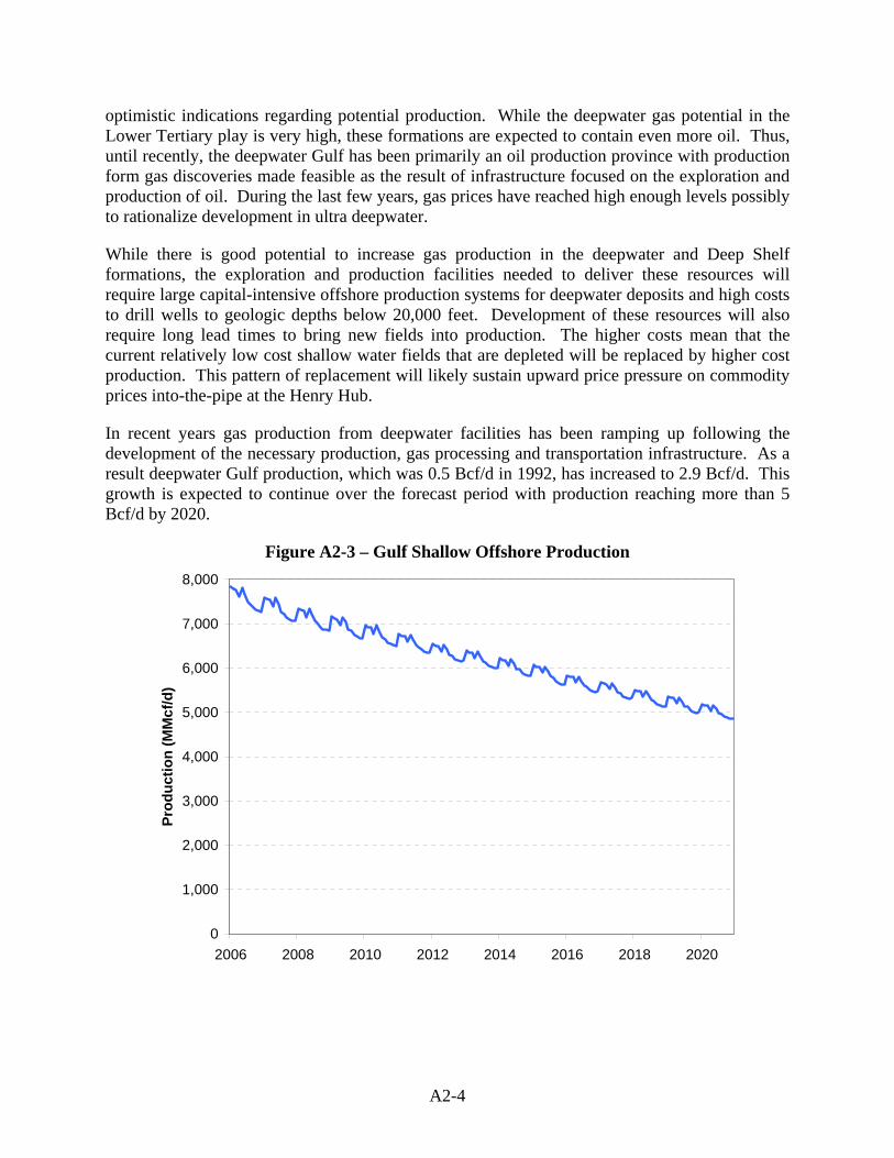
A2-4

optimistic indications regarding potential production. While the deepwater gas potential in the Lower Tertiary play is very high, these formations are expected to contain even more oil. Thus, until recently, the deepwater Gulf has been primarily an oil production province with production form gas discoveries made feasible as the result of infrastructure focused on the exploration and production of oil. During the last few years, gas prices have reached high enough levels possibly to rationalize development in ultra deepwater.

While there is good potential to increase gas production in the deepwater and Deep Shelf formations, the exploration and production facilities needed to deliver these resources will require large capital-intensive offshore production systems for deepwater deposits and high costs to drill wells to geologic depths below 20,000 feet. Development of these resources will also require long lead times to bring new fields into production. The higher costs mean that the current relatively low cost shallow water fields that are depleted will be replaced by higher cost production. This pattern of replacement will likely sustain upward price pressure on commodity prices into-the-pipe at the Henry Hub.

In recent years gas production from deepwater facilities has been ramping up following the development of the necessary production, gas processing and transportation infrastructure. As a result deepwater Gulf production, which was 0.5 Bcf/d in 1992, has increased to 2.9 Bcf/d. This growth is expected to continue over the forecast period with production reaching more than 5 Bcf/d by 2020.

Figure A2-3 – Gulf Shallow Offshore Production

0

1,000

2,000

3,000

4,000

5,000

6,000

7,000

8,000

2006 2008 2010 2012 2014 2016 2018 2020

Prod

uctio

n (M

Mcf

/d)

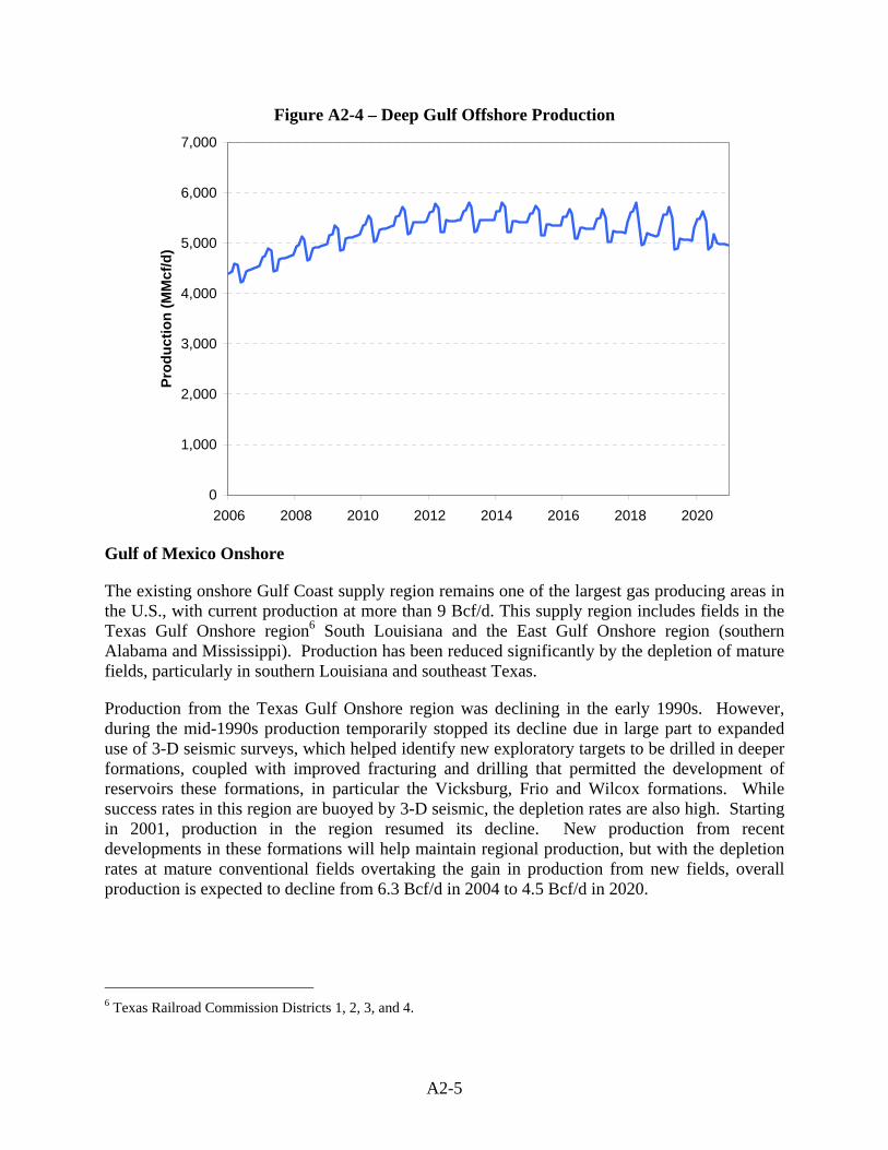
A2-5

Figure A2-4 – Deep Gulf Offshore Production

0

1,000

2,000

3,000

4,000

5,000

6,000

7,000

2006 2008 2010 2012 2014 2016 2018 2020

Prod

uctio

n (M

Mcf

/d)

Gulf of Mexico Onshore

The existing onshore Gulf Coast supply region remains one of the largest gas producing areas in the U.S., with current production at more than 9 Bcf/d. This supply region includes fields in the Texas Gulf Onshore region6 South Louisiana and the East Gulf Onshore region (southern Alabama and Mississippi). Production has been reduced significantly by the depletion of mature fields, particularly in southern Louisiana and southeast Texas.

Production from the Texas Gulf Onshore region was declining in the early 1990s. However, during the mid-1990s production temporarily stopped its decline due in large part to expanded use of 3-D seismic surveys, which helped identify new exploratory targets to be drilled in deeper formations, coupled with improved fracturing and drilling that permitted the development of reservoirs these formations, in particular the Vicksburg, Frio and Wilcox formations. While success rates in this region are buoyed by 3-D seismic, the depletion rates are also high. Starting in 2001, production in the region resumed its decline. New production from recent developments in these formations will help maintain regional production, but with the depletion rates at mature conventional fields overtaking the gain in production from new fields, overall production is expected to decline from 6.3 Bcf/d in 2004 to 4.5 Bcf/d in 2020.

6 Texas Railroad Commission Districts 1, 2, 3, and 4.

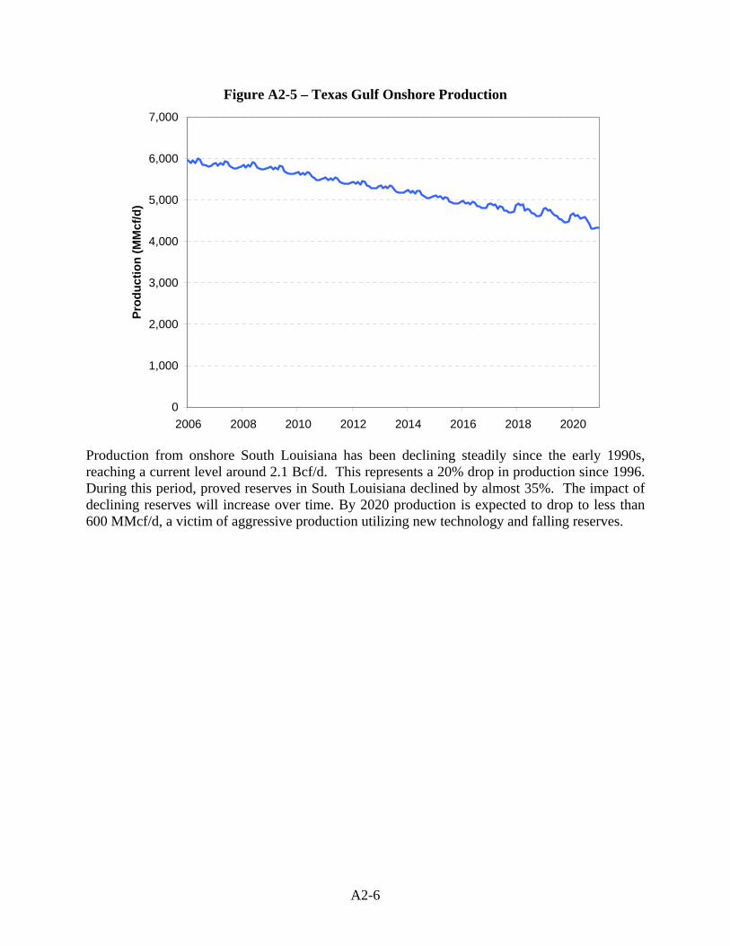
A2-6

Figure A2-5 – Texas Gulf Onshore Production

0

1,000

2,000

3,000

4,000

5,000

6,000

7,000

2006 2008 2010 2012 2014 2016 2018 2020

Prod

uctio

n (M

Mcf

/d)

Production from onshore South Louisiana has been declining steadily since the early 1990s, reaching a current level around 2.1 Bcf/d. This represents a 20% drop in production since 1996. During this period, proved reserves in South Louisiana declined by almost 35%. The impact of declining reserves will increase over time. By 2020 production is expected to drop to less than 600 MMcf/d, a victim of aggressive production utilizing new technology and falling reserves.

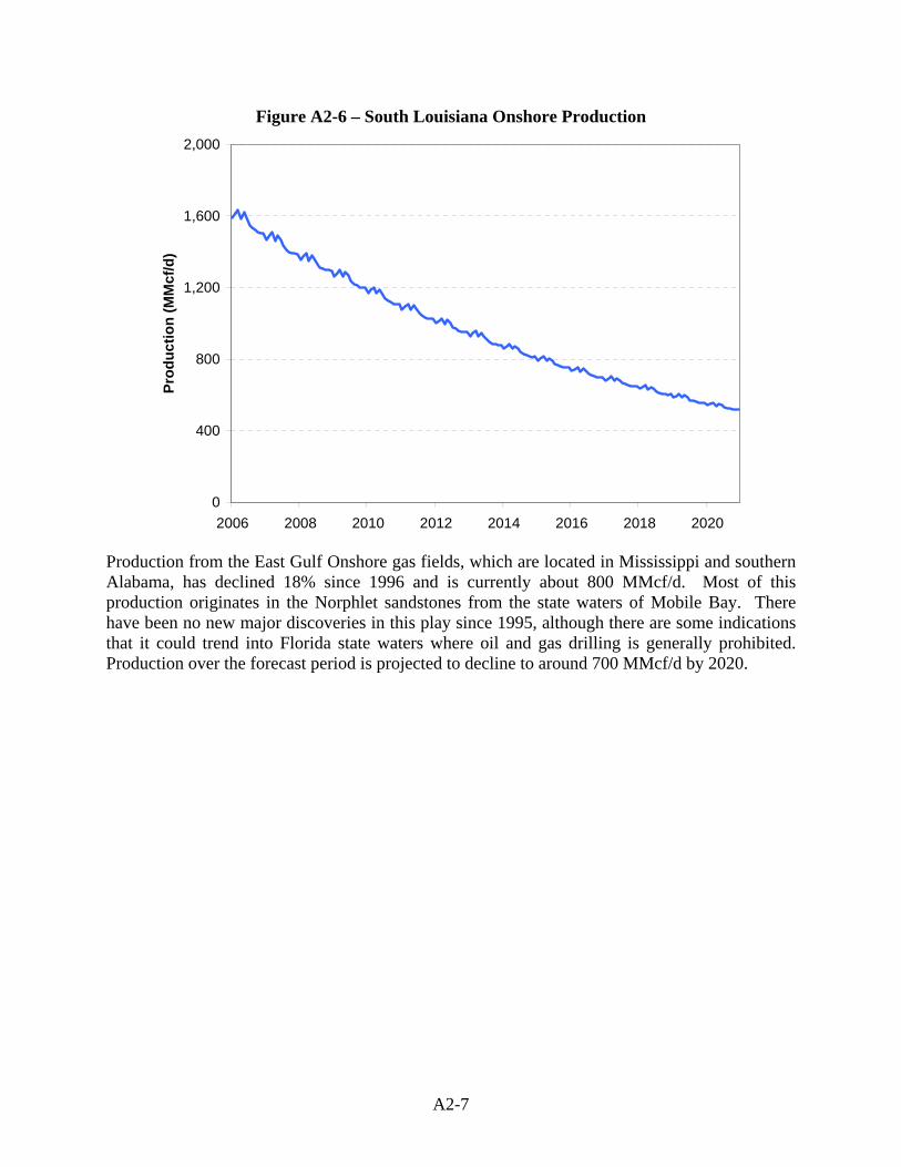
A2-7

Figure A2-6 – South Louisiana Onshore Production

0

400

800

1,200

1,600

2,000

2006 2008 2010 2012 2014 2016 2018 2020

Prod

uctio

n (M

Mcf

/d)

Production from the East Gulf Onshore gas fields, which are located in Mississippi and southern Alabama, has declined 18% since 1996 and is currently about 800 MMcf/d. Most of this production originates in the Norphlet sandstones from the state waters of Mobile Bay. There have been no new major discoveries in this play since 1995, although there are some indications that it could trend into Florida state waters where oil and gas drilling is generally prohibited. Production over the forecast period is projected to decline to around 700 MMcf/d by 2020.

A2-8

Figure A2-7 – East Gulf Onshore Production

0

250

500

750

1,000

2006 2008 2010 2012 2014 2016 2018 2020

Prod

uctio

n (M

Mcf

/d)

Rocky Mountain

The Rocky Mountain producing region encompasses conventional and unconventional producing formations in Wyoming, Montana, Utah, most of Colorado, and the Raton basin in northern New Mexico, but excludes the San Juan basin. Production has grown robustly from 3.5 Bcf/d in 1996 to the current level of about 6.7 Bcf/d. Proved reserves have almost doubled during this period to more than 35 Tcf. E&P in the Rocky Mountain supply region is supported by the relatively large concentration of undeveloped resources in both conventional and unconventional gas formations.7 The growth in Rocky Mountain production is expected to continue over the forecast horizon reflecting increased production of coalbed methane in the Powder River Basin in Wyoming and the Raton Basin, among others. Also making large contributions to growing regional production will be gas from tight sand formations in the Green River, Wind River, Piceance, Uinta, and Denver Basins. By 2020 Rocky Mountain gas production is expected to reach almost 12 Bcf/d.

7 The unconventional resource base in the Rocky Mountain region amounts to 231 Tcf, 46 Tcf in coalbed methane and 185 Tcf in tight sands and shales.

A2-9

Figure A2-8 – Rocky Mountain Production

0

2,000

4,000

6,000

8,000

10,000

12,000

14,000

2006 2008 2010 2012 2014 2016 2018 2020

Prod

uctio

n (M

Mcf

/d)

San Juan Basin

In response to legislative tax incentives adopted by Congress in the 1980’s to promote the production of coalbed methane, the San Juan Basin has been a major producing basin. Located in northwestern New Mexico and southwestern Colorado, production involves traditional sandstones, tight formations and coalbed methane. Conventional formations represent only 3% of the estimated resources of 68 Tcf. Coalbed methane and tight sands represent most of the remaining resources. Coalbed methane production has allowed overall basin production levels to increase from 3.5 Bcf/d in the mid-1990s to about 4 Bcf/d in 2004. Coalbed methane production, primarily from the Fruitland formation, has reached its peak. However, the long decline curves for the coalbed methane wells along with continued development of other unconventional formations will result in steady to slightly declining production going forward. By 2020 production in the San Juan Basin is projected to be about 3.5 Bcf/d.

A2-10

Figure A2-9 – San Juan Production

0

1,000

2,000

3,000

4,000

5,000

2006 2008 2010 2012 2014 2016 2018 2020

Prod

uctio

n (M

Mcf

/d)

Mid-Continent

The Mid-Continent supply region includes producing fields located primarily in Oklahoma, Kansas and parts of northern Texas, including the Texas Panhandle (Texas Railroad Commission Districts 9 and 10). Overall production in the region declined only slightly from 7.8 Bcf/d in 1996 to the current level of production of 7.5 Bcf/d. In Oklahoma, the primary producing basin is the Anadarko Basin, which accounts for more than 80% of production in Oklahoma. The Anadarko Basin is a mature basin, although recent high prices have allowed more drilling and production from deep formations, keeping production about flat in recent years. The largest production declines in the region have occurred in Kansas and in the Texas Panhandle where fields are maturing.8 Production in Kansas has long been dominated by the Hugoton Field, once one of the largest gas producing fields in North America when production peaked in 1970. Hugoton production declined until the mid-1990s when new rules permitting more infill drilling and compression allowed the field to reach a second lower peak in 1996. Since 1996, Hugoton production has declined at an average annual rate of 8%. In the other portion of the Mid-Continent region,9 production has grown significantly from 285 MMcf/d in 1996 to 1 Bcf/d in 2004. This growth has been primarily the result of the Barnett Shale developments.

The current production trends are to continue for the foreseeable future and will be augmented by new coalbed methane production from the Cherokee basin in southeastern Kansas and

8 Texas Railroad Commission District 10. 9 Texas Railroad Commission District 9.

A2-11

northeastern Oklahoma. Mid-continent proved reserves have increased by almost 7% since 1996 with the rapid growth of reserves in the Barnett Shale along with increases in the region’s coalbed methane and deep Anadarko gas reserves offsetting the rapid decline in Hugoton and Texas Panhandle reserves. Mid-continent production is expected to slowly decline from current levels, reaching 6.6 Bcf/d by 2020.

Figure A2-10 – Total Mid-Continent Production

0

1,000

2,000

3,000

4,000

5,000

6,000

7,000

8,000

2006 2008 2010 2012 2014 2016 2018 2020

Prod

uctio

n (M

Mcf

/d)

North Central

The North Central supply region includes gas production from Michigan and North Dakota. Total production in the region has averaged about 700 MMcf/d since the mid-1990s while proved reserves have increased about 50%, primarily as the result of increased exploration and development in the Antrim shale of Michigan. Production in the Williston Basin in North Dakota has remained fairly steady at around 140 MMcf/d since 1996. While this basin is estimated to hold approximately 10 Tcf of tight sand and shale gas resources, the primary focus of recent E&P activity has been oil production from the Bakken shale formation. Overall, North Central gas production is expected to drop slightly and then increase gradually around 2010. At the end of the forecast period we have estimated North Central production to be 600 MMcf/d.

A2-12

Figure A2-11 – North Central Production

0

250

500

750

1,000

2006 2008 2010 2012 2014 2016 2018 2020

Prod

uctio

n (M

Mcf

/d)

Appalachian Basin

The Appalachian Basin has a long history of production from fields in Kentucky, New York, Ohio, Pennsylvania, Virginia, West Virginia and the Black Warrior Basin in Alabama. The primary producing formations have included conventional sandstones and carbonates as well as Devonian shale, coals and tight sands. Improved drilling and production techniques and new seismic technology has led to a renaissance in the region with production, which has grown about 10% since the mid-1990s, currently at just less than 2 Bcf/d. Future production will be dominated by unconventional sources with the estimated resources of 104 Tcf in the region consisting of 9% conventional formations, 61% tight sands, 18% Devonian shales and 12% coalbed methane. Production is projected to increase over the forecast period reaching about 2.3 Bcf/d by 2020.

A2-13

Figure A2-12 – Appalachian Basin Production

0

500

1,000

1,500

2,000

2,500

2006 2008 2010 2012 2014 2016 2018 2020

Prod

uctio

n (M

Mcf

/d)

California

California gas production involves mostly associated production from the oil fields in central and southern parts of the state and production from non-associated fields in the Sacramento Basin. A small amount from offshore fields is projected. Associated production accounts for about 75% of the total. Current production of around 800 MMcf/d represents an 11% increase from the mid-1990s. Proved reserves have declined by 11% over the same period. Associated production, driven primarily by the price of oil and the amount of oil produced through enhanced recovery in the fields around Bakersfield, grew from the mid-1990s through 2001. Since then the decline trend has been well documented. Non-associated production has been in decline since the early 1990s. Total California production is projected to decline to around 600 MMcf/d by 2020.

A2-14

Figure A2-13 – California Production

0

100

200

300

400

500

600

700

800

2006 2008 2010 2012 2014 2016 2018 2020

Prod

uctio

n (M

Mcf

/d)

Alaska

Alaska gas resources and production are split between the southern production around the Cook Inlet and the North Slope. Current marketed gas production is around 1.1 Bcf/d, with about 570 MMcf/d from Cook Inlet and the rest representing net production from the North Slope. Most of the North Slope gas production is used for lease operations at the oil fields for power generation, oil field compression and pipeline pump stations. Approximately 8.7 Bcf/d, which is not included in net production, is produced in association with North Slope oil production and is re-injected into the oil reservoirs to help maintain oil production. Current proved reserves are 8.3 Tcf, with 2 Tcf in the Cook Inlet region and the rest on the North Slope. There is another 30-40 Tcf of discovered gas resources on the North Slope that cannot be considered proved reserves until either a pipeline or a liquefaction terminal is in place.

Production from the reserves on the North Slope will help offset a portion of the overall decline in domestic production. However, commercializing this resource base is dependent on the construction of a new pipeline from the North Slope to existing pipeline infrastructure, probably Alberta. In LAI’s Business-as-Usual Case, we assume that the pipeline will be built by 2013, thereby allowing up to 4.4 Bcf/d to flow by 2015. Alaska gas production will be less than 5 Bcf/d after 2015 as Cook Inlet production is projected to decline significantly over the forecast period. Given the uncertainty associated with predicting the potential decline in Cook Inlet production, as shown in Figure A2-14 we have assumed a relatively level production pattern from 2015-2020.

A2-15

Figure A2-14 – Alaska Production

0

1,000

2,000

3,000

4,000

5,000

6,000

2006 2008 2010 2012 2014 2016 2018 2020

Prod

uctio

n (M

Mcf

/d)

Western Canada Sedimentary Basin

The WCSB covers production from Alberta, Saskatchewan, and British Columbia. The WCSB is one of two primary basins serving New York. The WCSB is a mature producing basin that will likely struggle to maintain current production levels partly as a result of the natural gas intensive process of producing oil from tar sands in Alberta. The WCSB currently accounts for more than 97% of Canada’s gas production --nearly all of the gas exported to U.S. markets. Geological formations containing hydrocarbons show increasing drilling depths and geological complexity moving east to west. Drilling will transition from the shallow reservoirs of western Saskatchewan and eastern Alberta to deeper, more expensive fields in western Alberta and British Columbia. Although coalbed methane production in the WCSB is well behind U.S. coalbed methane production in the San Juan and Rocky Mountains, it is expected to grow rapidly in the WCSB, thus partly offsetting depletion trends in the shallow reservoirs. Whereas U.S. coalbed methane production presently accounts for 4.7 Bcf/d, coalbed methane production in the WCSB is projected to exceed 1.0 Bcf/d by 2010.

Total WCSB production is expected to remain flat at around 16 Bcf/d through 2010. Subsequently, a slight decline is predicted. About 15 Bcf/d is predicted through 2020.10

10Adjustments to the GPCM database are largely consistent with the recent WCSB production forecasts by TransCanada, a 50% owner of Broadwater.

A2-16

Figure A2-15 – WCSB Production

0

4,000

8,000

12,000

16,000

20,000

2006 2008 2010 2012 2014 2016 2018 2020

Prod

uctio

n (M

Mcf

/d)

Atlantic Canada

Production from this supply basin began in late 1999 from the Sable Offshore Energy project, located on the Scotian Shelf off of Nova Scotia, at a rate of approximately 500 MMcf/d. The Maritimes and Northeast Pipeline provides a direct pathway from Nova Scotia to New England enabling physical or financial access to the basin for shippers on Algonquin and Texas Eastern. Until late 2003, producers in Atlantic Canada had high hopes that the Scotian Shelf would become a major supply basin for the Maritimes and New England, with production reaching 2 Bcf/d by 2010. Although initial producer enthusiasm in the Scotian Shelf drew industry comparisons to the potential for another “Gulf of Mexico,” the area is highly unlikely to approach Gulf productivity over the forecast period. Over the last three years, exploration and development efforts on the Scotian Shelf have experienced a number of setbacks as producers encountered expensive dry holes, higher than expected infrastructure costs, and several reserve write-downs. These developments signal reduced expectations regarding the potential for any increase in production from Atlantic Canada for the foreseeable future.

The current outlook assumes that production remains around 400 MMcf/d through about the middle of the next decade. The addition of Deep Panuke along with minor production from onshore Nova Scotia and New Brunswick, and incremental gas production associated with oil field production offshore Newfoundland, result in increased production beginning in 2014. At the end of the forecast period, production is 900 MMcf/d.

A2-17

Figure A2-16 – Atlantic Canada Production

0

250

500

750

1,000

2006 2008 2010 2012 2014 2016 2018 2020

Prod

uctio

n (M

Mcf

/d)

APPENDIX 3

FUEL PRICE FORECASTS

LAI develops fuel price forecasts include based on a range of econometric, statistical and simulation modeling approaches. The forecast for natural gas prices utilize the GPCM modeling system described previously. The forecast for oil includes two components, a near-term forecast and a long-term trend. The near term outlook for light sweet crude oil (equivalent to West Texas Intermediate, WTI) is derived from New York Mercantile Exchange (NYMEX) futures. No. 2 heating oil at New York Harbor (NYH) is derived from the WTI price forecast and then compared for consistency with the NYMEX futures for No. 2 fuel oil. The price of RFO is derived from the crude oil price forecast since RFO prices are also highly correlated to the price of crude oil.

Near term coal and emission allowance prices are based on reported forward prices. Long-term coal price forecasts reflect the production and market conditions that determine free on board (FOB) supply basin prices for the two major coal producing regions of relevance: Northern Appalachia (NAPP) and Central Appalachia (CAPP). These price forecasts, with subsequent adjustments for transportation costs, drive the price of coal delivered to generating plants in New York, PJM and New England. The longer-term forecast for each fuel of relevance over the planning horizon represents LAI’s perspective. Statistical analyses has been performed to account for historical production, consumption and price trends, fuel price parity relationships, technology progress, and resource maturational effects.

Fuel Oil

The price of WTI oil reflects world crude oil prices. WTI prices have experienced booms and busts (Figure A3-1). Most, but not all boom periods have been followed by plateaus or busts. The range between the peaks of the boom periods and the troughs can be substantial. Most recently, oil prices blew through one resistance level after another, reaching $55 bbl in October 2004. We have incorporated monthly volatility into our WTI forecasts for each scenario based on recent historical volatility patterns. The booms have been driven by supply concerns usually accompanied by political turmoil in one or more of the primary producing regions of the Middle East or Africa. High prices during these periods have spurred investment in E&P, subsequently resulting in increased production at about the time the high prices reduced demand. The Organization of the Petroleum Exporting Countries (OPEC)-led cartel restraints on supply have usually wavered, causing acute gyrations in world benchmark prices.

A3-2

Figure A3-1 – WTI Crude Oil Prices

0

10

20

30

40

50

60

1990

1991

1992

1993

1994

1995

1996

1997

1998

1999

2000

2001

2002

2003

2004

Oil

Pric

e ($

/MM

Btu

)

Against the backdrop of the Iraq war and political chaos in a number of producing countries, global market dynamics have caused a paradigm shift. Some have said a “fear premium” ascribable to continued concerns about destabilization in the Middle East is embedded in current world oil prices. Political instability in Venezuela exacerbates the tension. The long-run trend remains materially above the historical bust levels and materially above the average prices seen over the last three decades.1 One factor driving the paradigm shift is based on concerns that world oil production has peaked just as the world demand for refined products for transportation fuels has grown, in particular, in India and China. Some analysts contend that oil reserves and production capacity in Saudi Arabia are overstated and therefore future production increases necessary to meet growing demand, based on abundant Saudi reserves, will not materialize.2 Supporting the expectations for a higher level of prices in the future are recent moves by OPEC to adjust production policies to support prices at levels around $40/bbl.3

1 Over the forecast period upward pressure on oil prices, driven by steady demand for refined products from the industrialized economies and by robust demand in China, India and other developing economies, will be tempered by increased production from non-OPEC fields (Russia and the Caspian Sea). Production in Canada from oil sands will also figure significantly in U.S. imports. Stringent emissions limits on RFO may also have a moderating influence on demand growth. In LAI’s view, production peaks in the Middle East and Africa are likely to sustain significant real upward pressure on prices through 2020. 2 Matthew R. Simmons, Twilight in the Desert: The Fading of Saudi Arabia’s Oil. Presentation to the Hudson Institute, September 19, 2004. 3 Factor inputs for all models were based on market expectations and geopolitical considerations as of July 2005. The run up in oil and gas prices following Hurricanes Katrina and Rita have not been included in this analysis.

A3-3

In consideration of the possibility that oil prices could move higher from current levels, a forecast of higher oil prices is included in our High Price Scenario. The Business-as-Usual Case incorporates a long-term real price escalation of 0.8% per year.

The primary factor affecting the price of residual or distillate fuel oil is the price of crude. Other cost factors relate to refining and emissions limits. Current refinery configurations limit the volume of heavy, high sulfur (sour) crude that can be processed, while environmental restrictions are limiting capacity expansions and additions. The forecasts of residual fuel oil and distillate fuel oil are based on historical relationships with the price of WTI, the NYMEX futures prices for light sweet crude (equivalent to WTI), and the futures prices for No. 2 heating oil. The forecasts for NYH prices for 0.3% and 1% sulfur RFO along with No. 2 fuel oil are derived from the statistical correlations with benchmark crude. The No. 2 oil futures strip is utilized as a check for consistency with the results of the econometric analysis.

For the near term, the Business-as-Usual crude oil forecast utilizes NYMEX futures prices through December 2011.4 We then assume that crude oil prices will escalate at a real rate of 0.8% annually – consistent with the EIA’s forecast of long-term real price escalation in the 2005 Annual Energy Outlook – or about 3.9% per annum in nominal terms. Kerosene prices for gas turbines on Long Island and New York City were forecast based on an analysis of the historical premium for kerosene over No. 2 fuel oil. Delivered fuel oil prices in New York reflect applicable taxes.5

In Table A3-1, we summarize the price adjustments to the NYH price used to obtain the price of RFO and No. 2 fuel oil in New England and PJM.

Table A3-1 – Regional Fuel Oil Price Differentials from NYH Forecasts

Market Residual Fuel Oil No. 2 Fuel Oil

PJM 0.7% NYH + $0.25/MMBtu

NYH + $0.27/MMBtu

New England 0.7% NYH + $0.30/MMBtu

NYH + $0.33/MMBtu

Coal

Coal prices are stated on an FOB basis at the two primary coal supply regions serving New York, PJM and New England. The price of coal is a prime determinant of the price of energy in PJM, in particular. It therefore has a direct effect on LIPA’s cable loading factor on the new high-voltage direct-current cable from New Jersey to Long Island. Individual forecasts have been developed for NAPP and for CAPP (Figure A3-2). The forecast uses econometric models that

4 As of summer 2005. 5 The New York Petroleum Business Tax is $0.39/MMBtu for RFO and $0.56/MMBtu for No. 2 fuel oil). The New York Spill Tax is $0.02/MMBtu for RFO and distillate fuel oil.

A3-4

are based on the historical relationships between the price of coal in these supply regions, underground mining productivity in Appalachia, and inflation.6

Coal market prices are heavily influenced by production costs and mining conditions in the NAPP and CAPP mining regions. Underground mining productivity is a key factor affecting production costs in these mining regions since underground mines account for about 65% of the coal produced in NAPP and CAPP. Underground production in these regions is expected to increase market share over the forecast horizon as Appalachian surface mines are depleted and surface mined production declines in response to the environmental restrictions on mountain top removal mining methods.

Contracts with end-users, primarily electric generators, cover 70% of the coal mined in CAPP and 80% of the coal mined in NAPP.7 The remaining coal purchases are transacted in the spot market. While spot market prices influence contract prices – in some cases serving as the benchmark for the initial price levels in new contracts or for restructured contracts, many large coal users are refusing contracts tied to spot prices. The NAPP and CAPP coal price forecasts were utilized to provide the basis for escalating the cost of coal on a delivered basis to coal-fired plants in New York, New England and PJM. Most of the individual generating plants in each region have a specific mix of spot and contract coal supply arrangements, with specific delivered prices incorporated in MarketSym.8

LAI expects the current run-up in coal prices to recede in both CAPP and NAPP in the near term. After 2008, coal prices are expected to increase in nominal terms at 2.1% for CAPP and 2.0% in NAPP, representing a decrease in real terms. These forecasts reflect the total volume of coal mined in CAPP and NAPP purchased under both contracts and in spot markets. Spot prices are likely to be more volatile, and during periods of tightened supplies may exhibit price run-ups similar to the most recent spot market pricing behavior. This reflects a permanent change from the 1985 to 2001 when coal prices declined steadily in nominal terms. Key factors which have reversed the trend of declining coal prices in Northern and Central Appalachia include: recent industry consolidation due to several producer bankruptcies, depletion and closing of several older mines, and a reduction in the increase in mining productivity.9

For plants located along the east coast that receive shipments by water, coal imported from Colombia and Venezuela will exert some downward pressure on prices. For plants located in the

6 Contract escalators are tied to inflation indices in the United Mine Workers’ contracts with the eastern coal producers. 7 U.S. EIA, U.S. Coal Prices – Northern and Central Appalachian Coal. 8 These data had been in the public domain through FERC Form 423 reports. However, public disclosure of individual plant fuel cost is no longer compulsory under FERC rules. While LAI’s database for regional generating plants runs through 2001, the unavailability of reliable Form 423 data requires a forecast method for consistency. 9 The growth in mining productivity has declined as longwall mining approaches saturation. Our forecast assumes that underground mining productivity in Appalachia will continue to increase, but at an average rate that is lower than history. This rate of growth averaged 5.8% annually from 1980 to 2001. The forecast assumes that the growth in underground mining productivity for the Appalachian producing regions will average about 1% annually over the forecast period.

A3-5

western areas of PJM and New York as well as in the mid-west, Powder River Basin coal can exert some dampening influence on prices.

Figure A3-2 – Historical and Projected Coal Prices

Central Appalachian

North Appalachian

0.00

0.50

1.00

1.50

2.00

2.5019

85

1987

1989

1991

1993

1995

1997

1999

2001

2003

2005

2007

2009

2011

2013

2015

2017

2019

2021

2023

2025

2027

Coa

l Pric

e ($

/MM

Btu

)

Nuclear Fuel

Nuclear fuel prices are forecast to increase at about the rate of inflation through the end of the forecast horizon.10 These costs are driven by U3O8 prices, which represent about 25% of total nuclear fuel costs, along with the costs of enrichment and fabrication. U.S. U3O8 prices declined from around $40/lb in the late 1970s to a range of $10/lb to $20/lb for most of the last 20 years. Recently, spot prices have soared. Spot prices represent about 12% of the market for nuclear fuel. Most of the remainder is purchased under long-term contracts, with 3 to 7 year contracts being the longest typical positions.

Sufficient supplies of uranium and adequate fuel processing capacity should maintain fuel costs at nuclear plants in New York, PJM and New England at the equivalent of $0.40/MMBtu throughout the forecast period.11 This price pattern reflects the impacts of the small number of new plants likely to be built worldwide through 2010. Subsequent increases in demand will depend on the construction of new plants in response to rapidly growing power demand in the developing countries, especially China and India, and, conceivably, potential new plants in the U.S. and Europe to combat global warming. 10 Nuclear fuel supply is comprised of mined and enriched U3O8, utility stockpiles of uranium, and secondary sources such as recycled spent fuel and recycled weapons grade uranium and plutonium. 11 2003 dollars.

APPENDIX 4

EMISSIONS ALLOWANCE PRICE FORECASTS

SO2 Allowance Price Forecast

Until 2003, SO2 allowance prices remained stable in a relatively narrow bandwidth of $100-$200/ton. In 2004, SO2 allowance prices soared to over $700/ton in anticipation of the promulgation of CAIR and the Clean Air Mercury Rule. Uncertainty over the form and stringency of mercury limits affecting existing coal-fired plants coupled with uncertainty concerning the actual impacts of CAIR, caused power generators to delay planned FGD technology retrofits and forced these generators to rely more heavily on allowances to meet compliance requirements. Spot prices briefly exceeded $1,600/ton following promulgation of CAIR in 2005.

The forecast of SO2 allowance prices, presented in Figure A4-1, was based on forward price curves available at the time the forecast was developed. Prices were forecast to remain in the $700/ton vicinity through 2007, then gradually decline to historical values of $200/ton by 2014, as many of the generators implement scrubber retrofits. After 2014, allowance prices were forecast to escalate at a rate comparable to inflation.1

Figure A4-1 – Emissions Allowances Price Forecast

NOx

SO2

0

1,000

2,000

3,000

4,000

5,000

6,000

7,000

8,000

9,000

2003 2005 2007 2009 2011 2013 2015 2017 2019 2021 2023 2025 2027 2029

NO

x Allo

wan

ce P

rice

($/to

n)

0

100

200

300

400

500

600

700

800

900

SO2 A

llow

ance

Pric

e ($

/ton)

1 Market prices for SO2 allowances are based on prices reported by Evolution Markets, as of July 2005.

A4-2

NOx Allowance Price Forecast

The NOx allowance price forecast reflects the costs of meeting increasingly stringent NOx emission limits, coupled with the proliferation of NOx budget programs across the Northeast. Historically, the market price of NOx emissions allowances has been related to the marginal cost of NOx control technology. However, upward excursions from this level have historically preceded reductions in the statewide NOx budgets, as plants have scrambled to retrofit NOx emissions controls technologies, primarily SCR, selective non-catalytic reduction (SNCR), and gas reburning, or have acquired sufficient allowances from the market. For example, in the months preceding program implementation in 1999 and again prior to the May 2003 budget reductions, the cost of NOx allowances exceeded $7,000/ton. NOx allowance prices have since trended downward.

In Figure A4-1, NOx allowance prices reflect the average prices for allowances to be used through 2008, reported for Ozone Transport Commission trades at the time the forecast was developed.2 Allowance prices were forecast to increase from the 2004 level of $2,290/ton to $3,340/ton in 2006. Beyond 2006 allowance prices were forecast to decline through 2012 to reflect the marginal cost of NOx control, about $1,500/ton. After 2012, allowance prices were assumed to escalate with inflation.

Non-ozone season NOx allowances under New York’s ADRP cannot be traded with ozone season allowances. Howeever, generators can manage fuel burns and emissions inter-seasonally to minimize environmental compliance costs. LAI therefore assumed that the non-ozone season NOx allowance prices under ADRP will follow a similar trend as ozone-season NOx allowance prices.

Mercury

Concurrent with CAIR, the EPA issued the Clean Air Mercury Rule, which restricts emissions of mercury from coal-fired generating plants. The proposed implementation plan would establish a cap-and-trade program for mercury. Consideration of mercury emissions restrictions may have a material impact on energy prices and installed capacity values in PJM, and to a lesser extent in NYISO.

The first compliance date under this rule, 2010, is intended to be synchronized with the first CAIR milestone to take advantage of fact that SO2 removal technologies are also effective, to an extent, for mercury emissions control. We expect that coal-fired generators will achieve the first level of mandated reductions in 2010 by installing the same technologies that will be required to meet CAIR limits: SCR and FGD. Mercury removal tests have indicated that the combination of wet FGD and SCR systems, with minor system adjustments and adding small amounts of reagent, can achieve mercury emissions removal efficiencies on the order of 80% to 85%, more than sufficient to meet the Phase I and possibly Phase II mercury limits under the Clean Air Mercury Rule. The key process for achieving mercury removal appears to be the wet FGD system. Early tests using dry FGD systems have not shown similarly high levels of mercury 2 Market prices reported by Cantor Environmental Brokerage, December 2004.

A4-3

removal. In this regard, our attrition analysis of the coal-fired plants in PJM is focused on the added capital and operating costs associated with retrofitting a wet FGD system along with SCR. The existing plants that have not added wet FGD and SCR systems are assumed to incur the costs to retrofit and operate these systems for compliance with mercury emissions limits by 2010.3 Table A4-1 summarizes the capital and operating costs we utilized for the retrofit of wet FGD and SCR systems. Table A4-1 also includes estimated costs for SNCR retrofits. In order to develop these estimated costs, LAI reviewed reported costs for specific plants’ retrofits of SCR, SNCR as well as wet FGD systems.

Table A4-1 – Capital and Operating Costs for FGD, SCR and SNCR Retrofits on Coal-fired Generating Plants

Emissions Control System

Capital Cost ($/kW)

Variable O&M ($/MWh)

Fixed O&M ($/kW-year)

Parasitic Load (%)

Wet FGD (LSFO)4 175 1.10 6.50 2.0 SCR 100 0.605 0.30 N/A

SNCR 20 0.50 0.15 N/A

CO2

The Regional Greenhouse Gas Initiative (RGGI) is a regional cap-and-trade program that will affect approximately 300 power plants in ten northeastern and mid-Atlantic states that have signed the Memorandum of Understanding (all of New England, New York, New Jersey, Maryland, and Delaware) The program establishes annual state-wide caps for CO2 emissions from fossil-fueled plants, 25 MW and larger. The program is designed to commence in January 2009, with a target of stabilizing CO2 emissions at current levels through 2014, and then achieving reductions of 2.5% per year through 2018.

At the time LAI developed the MarketSym model, the RGGI Model Rule had not been framed, it was uncertain whether RGGI would eventually become an enforceable regulatory framework, and the prospect of a federal carbon control policy appeared remote. For purposes of our electric simulation model, in our base scenario we assumed the status quo, i.e., that there are no enforceable state or federal controls on CO2 emissions. We also developed an alternate “CO2 tax” scenario to assess the impact of some type of regulatory controls on CO2 emissions. The combustion of all fossil fuels emits CO2, but coal-fired generation is impacted disproportionately to gas-fired generation under such regulation. In this scenario, $10 per ton of CO2 (escalated)

3 The use of these control technologies will allow the plants to reduce NOx and SO2 emissions allowance costs and more easily meet the more stringent SO2 and NOx emissions limits as well as to comply with the mercury limits. Any plants that cannot meet the cash flow threshold requirements utilized in the attrition analysis as the result of the added costs associated with wet FGD and SCR retrofits are assumed to be retired. 4 Limestone forced oxidation 5 Does not include catalyst replacement costs of $9.75/kW every 5 years.

A4-4

will be assessed on emissions from all fossil generation beginning in 2010.6 This cost can be represented as a tax (if future legislation is structured to be an assessment on output), an emission allowance cost, or the opportunity cost of trading allowances.

6 In 1999, the average CO2 emissions in the U.S. was 2.1 lb/kWh for coal plants, 1.9 lb/kWh for oil-fired plants, and 1.3 lbs/kWh for gas-fired plants. At $10/ton, this equates to $10.50/MWh for coal, $9.50/MWh for oil, and $6.50/MWh for gas. U.S. EIA, Carbon Dioxide Emissions from the Generation of Electric Power in the United States, July 2000.

APPENDIX 5

APPLICATION REVIEW, INCLUDING RESOURCE REPORTS

Broadwater announced the Project in November 2004, and at that time, FERC granted Broadwater’s request to use the National Environmental Policy Act (NEPA) pre-filing review process for the Project. Four FERC and USCG public scoping meetings were held, as well as numerous stakeholder meetings with the public, local, state and federal agencies.

Broadwater filed its application for Certificate of Public Convenience and Necessity with FERC on January 30, 2006. In the application, Broadwater requested that the Commission issue a final order granting it all necessary authorizations by March 31, 2007. Broadwater also requested waivers of “any and all Commission regulations necessary to obtain expeditious approval of Broadwater’s application.” The application consists of sixteen volumes. The application Volume contains the transmittal letter, the application, the Form of Notice and Exhibits A, B, C, G and H. Volumes I – VI contain the Resource Reports for the onshore and offshore facilities. These volumes are public. Volume VII contains the Privileged and Confidential portions of Resource Report 4 and Resource Report 5. Volumes VIII – XIV contain Critical Energy Infrastructure Information of Resource Report 9 and Resource Report 13. Volume XV contains the Sensitive Security Information of Resource Report 8 and Resource Report 11.

The Resource Reports consist of the following documents:

• Resource Report 1 – General Project Description

• Resource Report 2 – Water Use and Quality

• Resource Report 3 – Fish, Vegetation and Wildlife

• Resource Report 4 – Cultural Resources

• Resource Report 5 – Socioeconomics

• Resource Report 6 – Geological Resources

• Resource Report 7 – Soils

• Resource Report 8 – Land Use, Recreation and Aesthetics

• Resource Report 9 – Air and Noise Quality

• Resource Report 10 – Alternatives

• Resource Report 11 – Safety and Reliability

• Resource Report 12 – PCB Contamination (not applicable to Broadwater)

• Resource Report 13 – Engineering and Design Material

• Onshore Facilities Reports

• Environmental Sampling Report

A5-2

LAI reviewed only the publicly available Resource Reports as part of our review of the Project. Due to federal security regulations, Resource Report 13 and some parts of the other reports are subject to restricted distribution and were not available to LAI.

FERC regulations require the applicant to show that the Project is “not inconsistent with the public interest.” Broadwater asserts that:

• The Project will improve access to supplies of natural gas to serve new market demand.

• The Project will not impair the ability of Broadwater to render transportation service at reasonable rates to existing customers.

• The Project will not involve any existing contracts between Broadwater and a foreign government or person concerning the control of operations or rates for the delivery or receipt of natural gas which may restrict or prevent other U.S. companies from extending their activities in the same general area.

The Resource Reports are summarized below, with the exception of Resource Report 11, which is discussed in Section 5.8 of the main report.

Resource Report 1 – General Project Description

Resource Report 1 describes the proposed Project siting, purpose and need, land requirements, construction procedures, operation and maintenance plans, environmental permits and approvals required, decommissioning, removal and abandonment. A list of required permits for the Project can be found at the end of this Appendix.

In this Resource Report, Broadwater examines the volatility in natural gas prices ascribable to capacity constraints in the gas transportation infrastructure into the region, as well as to the increasing reliance on natural gas for electric power generation in New York and Connecticut. Broadwater concludes that without the Project, New York and Connecticut will experience rising price trends and volatility because they are positioned at the end of the continental gas transportation system. Broadwater cites EIA forecast data (especially the 2005 AEO) in its analysis as well as a study by Energy and Environmental Analysis, Inc. (EEA). Resource Report 1 does not provide a forecast of regional gas prices with and without Broadwater.

Some highlights of this report are:

• Flows of up to 600 to 700 MMcf/d could be physically delivered to Long Island and/or New York City from Broadwater based on hydraulic simulations of the Iroquois system, with the balance flowing north into Connecticut.

• Temporary onshore land requirements would be within the existing port communities on the New York shore of Long Island Sound. The need for development of new facilities to support the Project is not expected. Throughout the construction phase, a pipe storage yard and concrete coating facility will be located outside the Long Island Sound area, somewhere on the East Coast.

A5-3

• Permanent onshore facilities will be leased by Broadwater in Greenport and/or Port Jefferson. These facilities will include permanent mooring locations at a port for safe harbor for auxillary and support vessels and for offloading of crews and/or supplies, warehousing facilities and office space.

• The pipeline route will cross two utility cables, both buried six to seven feet below the natural seabed: the AT&T fiber optic telecommunications cable and the Cross Sound Cable. Federal regulations require a minimum of 12 inches of separation between the cables and the pipeline (49 CFR Part 192), therefore Broadwater plans to install a crossing bridge over each of the two cables.

• The FSRU will have a double hull design similar to an LNG carrier. The primary barrier is 1.2-mm stainless steel that would be corrugated to compensate for thermal contraction and mechanical ship deflection. The secondary barrier is a laminated composite material consisting of aluminum foil sandwiched between two glass cloths. The insulation consists of rigid polyurethane foam with reinforcing glass fibers between two plywood sheets, the thickness of which is determined to limit the boil-off rate to 0.15% per day with cargo tanks at 98% full.

• Any LNG spill will be directed overboard, away from critical areas and living quarters, where it will dissipate into the atmosphere and have no impact on water quality.

• At the completion of cargo unloading operations, LNG in the loading arms will be drained by gravity either back into the LNG carrier cargo tanks or to the FSRU drain tank from which it will be pumped into the FSRU storage tanks.

• To maintain the hull integrity of the FSRU and the LNG carrier, a constant curtain of water will be directed overboard during LNG transfer.

• The FSRU will be equipped with a flare for emergencies only. The flare will rise 197 ft (60 m) above the trunk deck and will handle vapors in the event of overpressure in the storage system.

• Normal ballast water intake will be about 900 m3/hr or 5.7 million gallons per day of seawater to offset a daily vaporization and send-out of 2,000 m3/hr. During LNG offloading, the loading rate will be 10,000 m3/hr and discharge rate of ballast water will be about 4,500 m3/hr. For a 145,000 m3 LNG shipment, the FSRU would discharge 50,000 m3 or 13.2 million gallons of water.

• Upon decommissioning, the FSRU will be decoupled from the mooring system and towed to a shipyard to be overhauled for reuse or recycled.

The EEA report entitled “Regional Market Growth and the Need for LNG Imports into the Northeast U.S. and Canada,” is included in Resource Report 1 as Appendix A. This report provides an overview of northeast U.S. and eastern Canadian gas markets, including a breakdown of consumption by market sector in NYC, Long Island, and southern Connecticut. Much of the analysis is focused on national rather than regional trends. In addition to Appendix A, the following are also appendices to Resource Report 1:

• American Bureau of Shipping, Approval in Principle Letter to Broadwater Energy (July 27, 2005)

A5-4

• Stratford Shoal Contingency Plan

Resource Report 2 – Water Use and Quality

Resource Report 2 describes the groundwater and surface water resources that may be affected by the construction and operation of the Project. It also addresses the proposed installation methods for the FSRU and interconnecting subsea pipeline, and the mitigation measures proposed to minimize the associated water quality impacts.

Long Island Sound is designated by NYSDEC as a Class SA water suitable for commercial shellfishing and primary and secondary recreational fishing. These waters are also suitable for fish propagation and survival. NYSDEC has issued applicable guidelines for thermal discharges and mixing zones.

The report states that impacts on Long Island Sound water quality during construction are expected to be minor, localized and short-term. Impacts associated with operation will be minor but long-term and result from routine intake and discharge of Long Island Sound waters by the FSRU. Sediment sampling conducted in the spring of 2005 suggests that no elevated contamination levels (including polycyclic aromatic hydrocarbons, polycarbonate biphenyls, pesticides, volatile organic compounds – VOCs – and dioxin) are present in proximity to the Project area and that pipeline alignment will be routed to avoid areas with elevated contaminant levels. The lack of significant contamination within the Project area restricts construction impacts to localized, short-term increases in TSS in the water column. Using a subsea plow as the primary means of lowering the pipeline below the seabed will decrease the amount of sediment introduced into the water column compared to other installation technologies and will restrict impacts to temporary increases of TSS in the bottom strata. According to the results of the MIKE3 sediment model provided in this Resource Report, the TSS levels would largely be assimilated throughout the Sound within 12 hours following completion of the plowing.

Strong winds associated with hurricanes and other storms may generate significant waves which can limit FSRU operation. Based on historical data, a 100-year storm event would be expected to have a significant wave height of 14.2 ft (4.3 m) and a 1,000-year storm event a height of 18.8 ft (5.7 m). The yoke mooring system is designed to withstand storm scenarios in excess of the 100-year storm event.

Hypoxia, or low levels of DO, is considered to be the most serious water quality issue in Long Island Sound and is most prevalent in the summer. A total of 597 DO readings with an average value of 9.5 mg/L were collected in April and May of 2005 in the area of the proposed pipeline route. DO levels above 4.8 mg/L are considered excellent and supportive of marine life. The proposed marine pipeline would be installed in the winter months when hypoxic conditions are largely absent from the Sound.

Broadwater expects that the installation of the FSRU will not impair water quality. In accordance with international regulations, the FSRU will be required to complete a ballast exchange prior to entering Long Island Sound to ensure that no invasive species or water of reduced quality are introduced.

A5-5

The total average daily water intake to support all FSRU operations will be approximately 5.5 million gallons, assuming an annual average of 118 LNG vessels per year. The FSRU is proposed to have up to seven point-source discharges and some non-point discharges, including ballast water discharge, discharge from the desalinization plant, fire water bypass, treated wastewater from on-board sanitary and other systems, seawater cooling discharge, and stormwater runoff. Of these, ballast water comprises by far the largest component of the FSRU’s water requirements. The LNG revaporization system will be closed-loop and not require intake or discharge of seawater. To control the growth of marine organisms, the FSRU seawater intakes will include the ability to inject a continuous dose of sodium hypochlorite at a concentration of 0.2 ppm which will result in a residual chlorine concentration between 0.01 and 0.05 ppm at the sea chest and at the ballast water discharge. The Project will meet NYSDEC’s SPDES standards for effluent water quality for all discharges.

While the FSRU is discharging ballast water, the LNG carrier will be taking on approximately the same amount of ballast water. The majority of the LNG carriers bringing cargo to the FSRU will be steam-powered vessels and will require approximately 57 million gallons of water for water cooling purposes during a 22 hour offloading process. This discharged cooling water will be approximately 3.6oF (2oC) higher than the ambient water temperature and contain low doses of sodium hypochlorite to prevent the growth of marine organisms. Cumulatively, the LNG carriers will utilize an average of 22.7 million gallons per day, on an annual average, including cooling and ballast water requirements.

Impacts on water quality from operation of the pipeline are expected to be minimal since the pipeline is a closed system. The riser pipe will have contact with the surrounding waters only in the section from the FSRU to the foot of the riser on the seafloor that connects through the mooring tower. Because the temperature of the gas will be 130° F when it exits the FSRU and 120° F at the foot of the riser pipe, there is a potential for heat exchange between the pipeline and the surrounding waters along the exposed riser pipe. However, Broadwater does not expect a thermal plume to develop.

The following are appendices to Resource Report 2:

• Correspondence with NYSDEC for environmental sampling and SPDES permit

• Email approval of the USACE MIKE3 model

• Cadmium clarification memo

• Generic SPCC Plan

• Water quality/sediment quality modeling report

• Grain size analysis May 2005 environmental sampling

• Sediment deposition modeling report

• Natural backfill modeling report

• Thermal modeling report

A5-6

Resource Report 3 – Fish, Vegetation and Wildlife

Resource Report 3 describes the fish, vegetation, and wildlife existing conditions and habitats. It also addresses the construction and operational impacts of the Project on these resources and the proposed mitigation methods.

The Project and the LNG carrier route will be sited to avoid impacts on significant coastal habitats, specifically the Significant Coastal Fish and Wildlife Habitat areas. Long Island Sound has been designated an EFH, i.e. “waters and substrate necessary to fish for spawning, breeding, and feeding or growth to maturity”. Therefore, NOAA’s fisheries unit must be consulted on all proposed activities. The proposed Project would overlap with EFHs for 20 species within or adjacent to the proposed pipeline route.

In April and May 2005, samples were collected at the proposed FSRU location and 27 stations along the proposed pipeline route. A benthic survey and sediment and chemical analyses were conducted at each station. The benthic survey revealed that benthic communities are generally consistent with what would be expected based on depth, substrate, and sedimentary environment.

Ninety five finfish species have been collected between 1984 and 2003 in Long Island Sound as part of the Long Island Sound Trawl Surveys. The proposed FSRU location is at the intersection of four survey squares with mean finfish counts that ranged from 492.3 per tow to 2,879.6 per tow. The mean finfish count along the majority of the proposed pipeline route ranges from 0 per tow to 1,000 per tow. Resource Report 3 provides a detailed discussion of 11 species of finfish and two species of shellfish that have recognized value within the Sound. The Resource Report also describes plankton, reptiles, marine mammals and avian species that frequent the Sound .

According to NOAA Fisheries, there are four species of federally threatened or endangered sea turtles and three whale species in New York waters, most of which are not typically present in Long Island Sound.

Construction and operation of the proposed facilities have the potential to cause both positive and negative effects on the marine environment. Broadwater anticipates that the construction impacts will be short-term and minimized by siting the facility in deep water and installing it during the winter months when use of the Sound by marine species is reduced. Nonetheless, construction will result in the following:

• direct disturbance of bottom sediments,

• direct mortality of most benthic organisms in the path of construction,

• some increase in turbidity levels and suspended solids,

• decreased water quality, and

• acoustic disturbance.

Broadwater points out several positive and operational/long-term impacts resulting from the diversification and expansion of the habitat within the Sound:

• The FSRU would create permanent shaded habitat

A5-7

• The mooring tower and pipeline would create additional structure in the Central portion of the Sound by creating an artificial reef habitat, which would favor a number of species including lobsters.

• The safety / security zone would exclude fishermen.

• Heat dissipation from the pipeline to the water column could establish a microclimate attracting certain species to that area.

Broadwater also notes long-term negative impacts resulting from the operation of the FSRU and pipeline:

• Pipeline maintenance involving periodic inspection and pigging activities will re-disturb the sediments in the pipeline areas.

• Water intake by the FSRU and LNG carriers will entrain organisms smaller than 5 mm and eliminate them by the sodium hypochlorite injection.

• FSRU discharge will contain chlorine at a concentration of 0.01 to 0.05 ppm.

• Spills or other accidents may occur at the facility.

• Maintenance of FSRU sides to reduce biofouling may impact marine resources.

• FSRU and LNG carriers will cause acoustic disturbance.

• Lighting at the facility has the potential to attract avian species.

Broadwater states that any loss of habitat resulting from installation of the FSRU will be offset by the increased habitat that is created. Resource Report 3 concludes that construction of the facilities is unlikely to significantly impact the population or survival of any species within the area.

The following are appendices to Resource Report 3:

• EFH assessment

• Benthic video survey report

• Benthic laboratory analytical results

• Drop camera video

• Ichthyoplankton entrainment estimates

• Correspondence

• Sediment deposition resulting from construction of a natural gas pipeline trench

• Natural backfilling of natural gas pipeline trench

Revised Resource Report 3 – Vegetation and Wildlife

Broadwater revised Resource Report 3 in response to FERC’s request of October 19, 2005. More specific and quantitative information was requested in the following areas:

A5-8

• Threshold values for turbidity and sedimentation and the extent and duration of high values after construction

• Impact of turbidity and sedimentation on the benthic community

• Anti-fouling paint impacts to marine resources

• Hydrostatic impacts to marine resources

• Noise and acoustic shock impacts on marine mammals, fish and birds

• Impact of water intake and discharge, both ballast and cooling, on ichthyoplankton by season

• Ichthyoplankton abundance and diversity by depth distribution or seasonal occurrence by lifestage

• Plans to minimize lighting impacts to birds and marine mammals

• Impacts to marine mammals or birds due to waste streams or toxic substance spills

• Impacts of construction and operation on threatened or endangered species or their habitat.

The revised Resource Report 3 has four additional appendices:

• Appendix D – Drop camera video

• Appendix E – Ichthyoplankton entrainment estimates at the Broadwater FSRU facility based on data collection during the 2002 Poletti ichthyoplankton program

• Appendix G – Sediment deposition resulting from construction of a natural gas pipeline trench

• Appendix H – Natural backfilling of natural gas pipeline trench

Resource Report 4 – Cultural Resources

Resource Report 4 describes the regulatory requirements related to archaeological resources and consultations with Native American Groups. Authorization of the Project by FERC is conditional on Broadwater’s compliance with the 1966 National Historic Preservation Act as amended in 1976, 1980, and 1992. The Area of Potential Effect (APE) is defined based on the potential for effect which may be different for aboveground resources (historic structures and landscapes) and subsurface resources (archaeological sites). The potential for impacting archaeological resources along the proposed 21.7 mile pipeline route is limited to the 300 foot (91 m) wide construction right-of-way for the pipeline trench and the 4,000 foot (1,219 m) right of way for the construction vessel anchors. The vertical APE within the pipeline’s excavated trench is 8 feet (2.4 m). For the YMS tower, the APE is 230 feet (70 m) deep and encompasses approximately 13,180 square feet (1,225 m2).

Broadwater contacted seven Native American Groups in order to give them the opportunity to identify their concerns about properties of religious or cultural importance that may be affected by the Project. None have responded to date.

A5-9

The general area of the Project contains 105 reported shipwrecks/obstructions, 18 of which have known locations. Four of these known locations fall within Broadwater’s APE. In April and May, a remote-sensing geophysical survey was conducted over the APE and produced 13 anomalies which comprise nine discrete targets with moderate to high potential to be archaeological deposits. All nine of the targets are located within the temporary anchor construction right-of-way. Avoidance of these nine targets will be accomplished during construction through the use of midline buoys on anchor cables.

Examination of vibratory core data resulted in no physical evidence for the existence of archaeologically sensitive intact paleosols.

All known cultural resources in the APE will be avoided.

Resource Report 4 contains the following appendices:

• Agency and native American correspondence

• Unanticipated discovery plan

• Overview/survey report

• Proposed pipeline route survey

Resource Report 5 – Socioeconomics

Resource Report 5 provides a socioeconomic overview of the Project area and includes a description of the municipalities, population, income, labor force, housing, local public services and local government revenues and expenditures. It also addresses the socioeconomic impacts during the construction and operation phases of the Project and mitigations to address negative impacts.

The towns and villages proximate to the Project area are in Suffolk County, which encompasses the eastern two-thirds of Long Island and has a population of 1.4 million. All the municipalities profiled are within a 15- to 20-mile (24- to 32-km) radius of the proposed Project and could possibly be impacted during construction or operation of the Project. The list includes four towns (Brookhaven, Huntington, Riverhead and Smithtown) and eleven villages/cities (Asharoken, Belle Terre, Head of Harbor, Huntington Bay, Lloyd Harbor, Nissequogue, Northport, Old Field, PoQuott, Port Jefferson and Shoreham). The socioeconomic assessment considers the following issues:

• influx of temporary workers,

• land-based impacts associated with installation of the infrastructure, and

• fiscal impacts on local governments such as incremental revenues and expenditures.

Total socioeconomic impacts were estimated for both Suffolk County and New York State. Economic impacts were measured by assessing the direct expenditures of the Project’s construction and operational phases on total industry output, employee compensation, and

A5-10

employee levels. Confidential Project construction and operational costs have been omitted from Resource Report 5.

Broadwater expects the construction phase of the Project to take place during late 2009 and 2010. During the construction period, the impact on the regional economy will be short-term, driven by contractual-related spending on goods and services to support construction and installation of the Project. However, due to the highly specialized nature of the energy production equipment and civil works, only a portion of the total construction period capital expenditures will provide a long-term impact on the region’s economy. The majority of the Project’s capital cost components will likely be imported from international manufacturers and fabricators. Transportation impacts on local roads and main arteries are expected to be minimal. The local resources likely to be impacted by the Project construction would include fabricators, storage facilities, support vessels and tugboats, barges, and security support.

The total direct capital expenditures for marine pipeline construction anticipated to impact Suffolk County is $11.1 million. The estimated 139 construction workers coming into the Project area will have a minor impact on the area’s total labor force, employment level, and unemployment rate. Direct expenditures during the construction period will generate an economic impact totaling $20 million for Suffolk County in 2010.1 In addition, these expenditures would result in value added of $8.9 million in 2010, including $5.2 million in total employee compensation.2

The economic impacts during FSRU terminal operations are based on direct expenditures incurred in the Project area necessary to run and maintain the facility, such as personnel wages, facility maintenance, insurance, and bulk chemicals. The annual recurring expenditures will impact the host community over the years 2011 to 2040. The FSRU terminal will employ a total of 60 persons. The direct expenditures to support FSRU operations will generate a total of $39.5 million per year economic impact for Suffolk County. The cumulative economic impact over the entire 30 year life of the Project is estimated to be $475 million. The fiscal analysis in Resource Report 5 does not consider municipal payments in lieu of taxes which are potentially part of the financial structure of the Project and could have a significant positive impact on the host area’s municipal fiscal position.

The estimated environmental benefits are based on fewer air pollutant emissions resulting from a New York State projected economic growth scenario, where relatively more natural gas is used to generate electric power. Public benefits from avoided air pollution damages could average $181 million per year between 2011 and 2020.

Resource Report 5 contains the following appendices:

• Economic impacts of the proposed Broadwater Project

1 The economic impact affects the total value of production by industry for the calendar year that would result from the Project’s construction expenditures. 2 Value added is the sum of employee compensation, proprietor income, other property income, and indirect business tax.

A5-11

• Estimated environmental benefits of the proposed Broadwater Project

Resource Report 6 – Geological Resources

Resource Report 6 describes the physiography and geology of the Project area and the geological hazards, such as the seismicity, of the area.

Both the modified Mercali scale and the Richter scale are used to measure earthquake intensities. Mercali numbers do not correspond directly to Richter numbers so there is no conversion factor. Since 1900, only three earthquakes with magnitudes greater than 4.5 on the Richter scale or VI on the Mercali scale have occurred in the Long Island Sound area. According to the U.S. Geological Survey Earthquake Hazards program, an earthquake with a magnitude greater than 4.75 on the Richter scale has a 3-6% probability of occurring within 50 years in the Project area. This probability decreases significantly with higher Richter scale values. According to Resource Report 6 for the Eastchester Extension Project, pipelines are capable of withstanding earthquakes with an intensity of VII on the Mercali scale which is generally comparable to a range of 5.8-6.1 on the Richter scale. Based on this information, there is a low probability that an earthquake strong enough to damage the pipeline would occur during the life of the Project.

Installation of the mooring tower will require piles to be driven 230 ft beneath the seabed. This is not expected to have any impact on the geologic structure underlying Long Island Sound. A geotechnical investigation revealed that bedrock is not present near the surface and that blasting will not be required for installation of any portions of the pipeline. Broadwater will use concrete mats for pipeline protection wherever adequate burial depth cannot be achieved during construction.

There are no areas of paleontological significance in the Project area.

Resource Report 7 – Soils

Since no land-based facility has been identified, Resource Report 7 describes the soil characteristics of the seafloor, construction impacts and mitigation measures. The seafloor in Long Island Sound consists of silt, clay, sand and gravel. Bedload transport of coarse-grained material, sorting and deposition of fine-grained material, sorting and reworking of sediments, and non-depositional erosion are the four major processes operating in the 850 square mile study area. Trenching operations will be conducted to reduce the amount of sediment introduced into the water column. An estimated total of 354,320 cubic yards and 2,600 acres will be impacted by construction of the proposed marine pipeline. A 4,000 foot trench across the Stratford Shoal may require dredging instead of subsea plowing due to the presence of competent material that could prevent plowing. Also, for safety reasons, subsea plowing will not be used to lower the FSRU and IGTS tie-ins or where the pipeline route traverses the AT&T and Cross Sound Cable. At cable crossings, divers and submersible pumps will be used to place concrete pads, which will be used to separate the pipeline and the other cable by a minimum of one foot.

Appendices included in Resource Report 6 consist of:

• VGS log of vibracores

A5-12

• Cone penetrometer graphs

Resource Report 8 – Land Use, Recreation and Aesthetics

Resource Report 8 describes onshore and offshore land uses including commercial and recreational fishing, recreational and aesthetic resources and the impact of the Project on these resources. It also addresses measures that need to be implemented to avoid and mitigate construction and operational effects.

The Project is located over nine miles from any shoreline. A visual resource assessment was conducted and includes determination of a radius of impact for the Project, an inventory of aesthetic resources within the radius of impact, photo simulations and potential mitigation measures.

During construction, 197 acres of seafloor will be disturbed as a result of the pipeline trench excavations, with an additional 3,174 acres being disturbed by construction barge anchor cable sweep. The yoke mooring system includes a stationary tower structure with a footprint of approximately 13,180 square feet (1,225 m2).

Navigational aids, including lights and foghorns, will be installed on the FSRU to warn other vessels in Long Island Sound, and navigational charts will be updated to show the location of the FSRU. There is no official vessel traffic routing system in the Sound, but the FSRU location is intended to be outside of commonly used East-West routes. Its current location was chosen to minimize impacts on commercial shipping, recreational boating and fishing.

The FSRU would be located in a high-use lobster fishery area. The near-shore shellfish industry will not be affected. During construction, affected areas will be closed to fishing. However, the effects on the fishery would be mitigated by scheduling construction for the winter months. Within the vicinity of the FRSU, up to five lobstermen could lose access to a portion of their historic fishing grounds.

Ferry lines in the area would be temporarily rerouted during pipeline construction. Pipeline construction is expected to proceed at the rate of 1 mile per day. Ferries and recreational vessels would be excluded from the safety zone around the FSRU and LNG carriers, as established by the USCG. The FSRU is not in the path of any existing ferry line.

The results of the Fishermen outreach are included as an appendix to Resource Report 8.

Resource Report 9 – Air and Noise Quality

Resource Report 9 describes the existing air and noise quality and the relevant federal and New York State air regulations. It also addresses construction and operation air quality and noise impacts and mitigation.

Air emissions from the Project will be regulated under the Clean Air Act and state law administered by NYSDEC. The Project would be located within Suffolk County, New York, which is part of the New Jersey-New York-Connecticut Interstate Air Quality Control Region (AQCR). This AQCR is currently designated as an attainment area for CO, lead, NO2, PM10 and

A5-13

SO2. It is designated as a severe non-attainment area for the 1-hour ozone standard and as a moderate non-attainment area for the 8-hour ozone standard. Since most ozone at ground level is formed during reactions between NOx and VOCs, control programs for ozone regulate NOx and VOC emissions. Suffolk County is also designated as a non-attainment area for PM2.5. Non-attainment New Source Review in New York is delegated to NYSDEC and the Prevention of Significant Deterioration (PSD) review is conducted by EPA Region II.

The Broadwater Project will be evaluated against ambient air concentration thresholds for a Class II Area which allows a moderate increase over baseline air quality levels.

Pollutant emission limits and monitoring, reporting, and record-keeping requirements depend on the emission source type and size. The FSRU process heaters (four with one extra as back-up) are subject to Subpart Db of 40 CFR 60. The LNG storage tanks do not appear to be subject to the requirements of Subpart Kb of 40 CFR 60 because LNG would only be directly released to the atmosphere during emergency situations. The FSRU gas turbines (two and one back-up, 22 MW each) will be subject to the requirements of Subpart GG of 40 CFR 60. So far, the EPA has not made an agency-wide determination about whether an FSRU would be subject to a PSD threshold of 250 or 100 tons per year (tpy). The PSD threshold of 100 tpy applies to the gas turbines and process heaters separately. The estimated annual potential emissions for the FSRU as a whole and the Title V Major Source Size Thresholds are shown in Table A5-1.

Table A5-1 – Potential Emissions and Major Source Thresholds

FSRU Annual Emissions(tpy)

Title V Major Source (tpy)

NOx 62 100/25 CO 89 100

VOCs3 18 50/25 PM10 48 100 PM2.5 48 100 SO2 4 100

Ammonia 66 -- Total HAPs 9.4 25

The emission estimates reflect the use of selective catalytic reduction (SCR) for NOx reduction and CO oxidation catalysts on the gas turbines and process heaters. The FSRU is not a major source of hazardous air pollutants (HAPs) and does not fall under National Emission Standards for HAPs regulations.

3 The first value is the threshold for 8-hour moderate ozone non0attainment designation, second value is threshold for 1-hour severe ozone non-attainment designation.

A5-14

Due to the transition from the 1-hour to the 8-hour ozone standard and new non-attainment designation, it is unclear which threshold will apply for NOx and VOC. If the 1-hour severe ozone non-attainment designation applies, the proposed Project will be above the major stationary source size for NOx and will require a Title V permit. Otherwise, the proposed project will be below the major stationary source size under Title V and will need to obtain a State Facility (minor source) permit from New York State.

Construction is anticipated to occur over a two-year period but only during the winter months. The major construction activities consist of pipeline installation, yoke mooring system tower installation, and FSRU towing. Construction-related emissions are not covered by an air permit program and are evaluated under the General Conformity rule. The NOx emissions are above the General Conformity de minimis threshold of 100 tpy for each year of construction and are subject to mitigation. However, with construction scheduled to occur outside the ozone season, Broadwater does not need to mitigate short-term ozone precursor emissions.

Emissions from vessel activities during normal FSRU operation are not covered by an air permit program but are evaluated under the General Conformity rule by comparison to de minimis thresholds.

Table A5-2 – Vessel Emissions (tpy)

LNG Carrier Unloading

Carrier Transit and Support Tugs Total Annual General Conformity

De minimis (8-hour ozone) NOx 23 427 450 100 CO 2 54 56 NA

VOCs 4 18 22 50 PM10/ PM2.5

33 25 58 100

SO2 245 341 586 NA CO2 14,545 37,437 51,982 NA

Vessel activity results in annual NOx emissions above the de minimis threshold, therefore an evaluation of mitigation options will be required.

Atmospheric dispersion models were used to compare estimated air quality impacts from FSRU operations to existing conditions. Modeled air quality concentrations due to the FSRU are below Significant Impact Levels. Locations within an assumed 500 m safety zone around the FSRU were excluded from the Offshore Coastal Dispersion model.

There are no state-wide noise regulations in New York. However, a noise guidance document issued by NYSDEC can be used to evaluate a project’s potential noise impact. Ambient airborne noise levels over ocean areas are in the 50 to 55 dBA range. The predicted noise from the operation of the FSRU is 50 dBA at 0.9 mile (1,500 m) and therefore would not be noticeable 1 mile or more from the FSRU. However, at distances of less than 0.9 mile, the operating noise may become noticeable and at less than 820 ft (250 m), it may begin to interfere with normal conversation volume. At the boundary of a proposed 500 m safety zone, the level would be 59

A5-15

dBA. In addition to normal FSRU operation, foghorns installed on each end of the FSRU will generate warning signals of 146 dBA at 3.3 ft (1 m) as required by USCG regulation which will be audible at 2 miles (3.2 km). This foghorn sound level will be barely audible on shore over background onshore noise levels.

During construction, there will be increased noise level which could impact recreational boaters in sailboats or other non-powered vessels. However, Broadwater states that it will not affect human receptors onshore and can be avoided by recreational boaters.

Appendices included in Resource Report 9 consist of:

• Construction emissions study

• Emissions calculations workbook

• Air quality modeling report

Revised Resource Report 10 – Alternatives

Resource Report 10 describes the alternatives considered in the development of the Broadwater Project. Seven types of alternatives were considered: (i) the no action or postponed action alternatives, (ii) system alternatives to the project, (iii) LNG terminal alternatives, (iv) alternative LNG terminal sites, (v) pipeline route alternatives, (vi) LNG terminal equipment/technology alternatives, and (vii) pipeline construction alternatives.

No action or postponed action alternatives

Absent the Project, Broadwater states that the objectives of the Project would not be met, and a source of reliable, long-term, and competitively priced natural gas would not be available to the region. The impact, both economic and environmental, to the region of delaying the Project by 2-3 years in the hopes that another project might be built would involve higher energy prices, greater emissions, and grater natural gas price volatility.

Use of other fossil fuels would result in a decline in air quality. Traditional, domestic natural gas production levels are expected to continue production decline due to depletion. New sources of nuclear power or hydropower are unlikely to be sited in the region in the foreseeable future. Renewable sources of energy (wind, solar and biomass) and energy conservation are possible clean alternatives but it is unlikely that they will be available in sufficient quantities to meet the region’s growing energy needs. The Long Island Offshore Wind Park and the Roosevelt Island Tidal Energy project are described as providing 140 MW and 10 MW of electric power, respectively.

System alternatives

Other existing or proposed LNG or natural gas facilities would have to meet the stated objectives of the Project: the capability to inject 1 Bcf/d into the greater New York metropolitan area market. Considering the existing pipeline infrastructure, the addition of 1 Bcf/d of incremental gas supply would constitute a significant system expansion for every pipeline except Iroquois. The average operating pressure on the Algonquin, Columbia, Tennessee and Transco pipelines is

A5-16

low, ranging from 650 to 800 psi and could not accommodate the incremental volume requirements of the Project without looping. Even the Texas Eastern system, with a pressure of 1100 psi cannot meet the Project objectives without an expansion with substantial environmental impact. Furthermore, in order to meet Project objectives, all these pipelines would need access to incremental gas supply from interconnections either from the south or the north, which may not be sufficient for the future needs of the New York City / Long Island markets.

Broadwater examined all the approved onshore and offshore U.S. LNG terminals, most of which are located in the Gulf Coast. Although they represent new sources of natural gas supply, they are located far from the New York metropolitan region and would require significant expansion of the pipeline systems from the Gulf Coast. The only LNG terminal approved in the Northeast is the Weaver’s Cove project in Fall River, Massachusetts, with a daily send-out capacity of 0.8 Bcf. If this terminal were built, significant additional pipeline infrastructure would be required to transport this new gas supply to the region via the Algonquin pipeline

Broadwater also examined the four proposed LNG terminals in the Northeast: KeySpan’s LNG facility upgrade (0.5 Bcf/d) in Providence, Rhode Island, BP’s Crown Landing project (1.2 Bcf/d) in New Jersey, and two offshore projects off the coast of Massachusetts, Northeast Gateway (0.8 Bcf/d) and Suez Neptune (0.4 Bcf/d). Broadwater concluded that the three proposed New England facilities are designed to serve the New England market and cannot meet the needs of the New York City / Long Island markets. BP’s Crown Landing (1.2 Bcf/d) in New Jersey would require very costly downstream pipeline enhancements to provide incremental volumes to New York.

LNG terminal alternatives

Shell evaluated both the FSRU and GBS concepts. It was determined early on that the GBS option had more significant environmental and safety challenges because it had to be located in shallower water (up to 60 ft), which in Long Island Sound is closer to populated areas. Three onshore locations (Shoreham, Block Island and Plum Island) were evaluated and found to be environmentally less desirable than the proposed FSRU location.

Broadwater also evaluated shuttle regasification vessels (SRVs) and the number of separate SRV mooring / LNG transfer buoys that would be required to provide 1 bcf/d to the region. Broadwater estimated the maximum sea states during which LNG carrier berthing and LNG transfer / sendout operations could be accomplished and the frequency of these sea states in the Long Island Sound, Block Island Sound and Atlantic Ocean offshore of Long Island.

Alternative LNG terminal sites

Both the Atlantic Ocean and Block Island Sound were evaluated in addition to Long Island Sound for offshore locations. As a result of the comprehensive alternative LNG terminal site analysis, Broadwater identified 24 individual alternative facility concepts and site locations including: nine GBS sites, five, FSRU sites, eight land-based sites and two SRV sites (Figure A5-1). However, the sea conditions were considered too rough for routine and reliable unloading via side-by-side cargo transfer and a much longer gas pipeline would have to be constructed to carry the 1.0 Bcf/d to Iroquois. An offshore pipeline longer than 40 miles would

A5-17

require intermediate pressure boosting located between the FSRU and the interconnection with the Iroquois pipeline. Within Long Island Sound, sites located close to the shoreline were eliminated due to their proximity to higher population densities and to sensitive marine resources and to avoid dredging issues.

Pipeline route alternatives

Broadwater examined several pipeline routes, onshore and offshore, that would reach the target market. One onshore route from an Atlantic Ocean LNG terminal located approximately 20 miles southeast of the Hamptons would make landfall east of Southampton and reach the existing Iroquois meter station at South Commack. Another offshore route from an Atlantic Ocean LNG terminal located approximately 20 miles southeast of Montauk Point would require two offshore platform based compressor stations and would have to be routed around Montauk Point, through Block Island Sound, through the Race and westward along the central axis of Long Island Sound to the Iroquois pipeline. These two Atlantic Ocean alternatives are less desirable than the proposed FSRU site in Long Island Sound because they would require significant new pipeline construction in order to connect to Iroquois.

LNG terminal equipment technology alternatives

Broadwater examined vaporization technology alternatives, mooring system alternatives, nitrogen supply alternatives and a ballast transfer system.

Four vaporization technologies were considered: SCV, STV, seawater-warmed vaporization and air-warmed vaporization. Both of the last two technologies would require standby technology for the colder months of the year when the air and water temperature is too low for the system to be effective on its own so they were eliminated from consideration. Based on evaluations of thermal efficiency, global efficiency, NOx emissions and CO2 emissions, Broadwater selected STV with SCR, which allowed for the lowest achievable emissions rates at comparable thermal efficiencies.

Given the 90-ft water depths in Long Island Sound, there is really only one optimum mooring system, the yoke mooring system which is piled to the seabed. The alternative, an external turret system, is optimum for depths that are greater than 150 ft and requires 6 or more leg anchor systems.

Broadwater proposes to add nitrogen to the gasified LNG in order to meet the gas quality requirements of the Iroquois system. Two nitrogen injection technologies were evaluated: the cryogenic nitrogen plant and the membrane nitrogen plant. Since the cryogenic nitrogen plant is affected by motion, it is less suitable for a marine application than the membrane nitrogen plant.

In order to conserve ballast water, Broadwater assessed a ballast transfer system that would transfer water from the FSRU to the LNG carrier during LNG transfer operations. However, the system was not practical since LNG carriers are currently not configured to accept ballast water from another facility.

A5-18

Figure A5-1 Potential LNG Sites Considered by Broadwater1

1 Broadwater Resource Report 10.

A5-19

Pipeline construction alternatives

Broadwater evaluated both the conventional marine pipeline installation method and the dynamically positioned (DP) vessel marine pipeline installation method. Although using a DP laybarge would minimize bottom disturbance and damage to existing utility cables or pipelines, Broadwater did not consider it the preferred method because of cost, contractual, logistical, legal and labor considerations.

Onshore Resource Reports 1-12

Temporary and permanent onshore facilities would be required during construction and operation. Broadwater proposes to use existing facilities to avoid or minimize additional environmental impact. Only a waterfront facility is required to support construction activities. The permanent leased onshore facilities would be located either in Greenport or Port Jefferson and would include office space and warehouses. The office space would include conference and training facilities as well as the emergency response and communications center. The warehousing with waterfront access would accommodate tugs, personnel transfer and materials transfer.

Resource Reports 5 (Socioeconomics), 10 (Alternatives), 12 (PCB Contamination) and 13 (Engineering Design and Materials) were not required for the onshore facilities.

Permits

Table A5-3 and Table A5-4 list the federal and state permits, respectively, which Broadwater needs to acquire.

A5-20

Table A5-3 – List of Federal Permits, Approvals and Consultations

Agency Act Permit/Approval FERC Natural Gas Act 15 U.S.C. 717 et

seq., 18 CFR Part 153, Subpart B (2002)

Sections 3 and 7 approvals to site, construct and operate the LNG terminal and to construct and operate the subsea connecting pipeline facilities, including the pipeline riser and mooring tower, respectively

The Maritime Transportation Security Act of 2002

Review process – project must be compatible with National and Area Marine Security Plans

USCG

33 CFR § 127 Letter of Recommendation

Advisory Council on Historic Preservation

National Historic Preservation Act, Section 106

Review of project effects on cultural resources

Clean Water Act, Section 401 and 404

Review of Section applications EPA

Clean Air Act Prevention of Significant Deterioration, New Source Review

Marine Mammal Protection Act, 16 U.S.C. 1361 et seq.

Consultation

Magnuson-Stevens Fisheries Conservation and Management Act – Sustainable Fisheries Act

Consultation regarding Essential Fish Habitat

NOAA Fisheries

National Fishing Enhancement Act of 1984

Consultation regarding the National Artificial Reef Plan and commercial/recreational fisheries

Clean Water Act (CWA), 33 U.S.C. § 1344 et seq.

Section 404 – dredge and fill permits USACE

Rivers and Harbors Act of 1899 33 U.S.C. § 403 et seq.

Section 10 permit

USFWS Marine Mammal Protection Act, 16 U.S.C. 1361 et seq.

Consultation

A5-21

Agency Act Permit/Approval Federal agencies NEPA 42 U.S.C. § 4321 et seq.,

particularly 42 U.S.C. § 4332, 40 CFR Part 1500

Procedural statute, not a permitting statute. Requires federal agencies to consider environmental impacts of proposed action

Federal agencies consultation with USFWS and NOAA Fisheries

Section 7, Endangered Species Act, 16 U.S.C. 1531 et seq.

Consultation regarding federally listed threatened or endangered species. If potential adverse impact identified, then a Biological Opinion must be issued by responsible agency. Primarily a procedural statute. No permit required unless an incidental take of protected species is involved (then Section 10 permit required)

FAA 49 CFR Part 77 Review of construction or alteration that might affect navigable airspace

A5-22

Table A5-4 – List of State Permits and Approvals

Agency Act Permit/Approval NYSDEC Clean Water Act 33 U.S.C. §

1342(a) – delegated from EPA State Pollution Discharge Elimination System (SPDES) permit

Clean Water Act 33 U.S.C. § 1341 Section 401 – State certification of water quality Clean Air Act Title V 40CFR 70 –

delegated from EPA; implementing NYS regulations: 6 NYCRR 201

Certificate to operate air contamination sources

6 NYCRR Part 596 Bulk Storage Permit NYSDOS New York State Coastal Zone

Management Act -delegated from the Federal DOC

Coastal Zone Consistency Determination

NYSDPS Natural Gas Pipeline Safety Act, 49 U.S.C. §§ 60101, et seq. (2000) -as agent for USDOT OPS

Requirement to certify that Broadwater will design, install, inspect, test, construct, operate, replace, and maintain a gas pipeline facility under the standards and plans for inspection and maintenance under section 60108 of 49 U.S.C. §60108.

NYSOGS New York Public Lands Law Submerged Lands easement/lease NYSOPRHP Section 106, National Historic

Preservation Act Review of project effects on cultural resources

APPENDIX 6

DET NORSKE VERITAS: BROADWATER RESPONSE TO USCG LETTER (DATED DECEMBER 21, 2005)

DNV prepared Broadwater’s response to the USCG’s letter concerning the four issues related to the applicability of the Sandia Report to the site, the FSRU and future generations of LNG carriers. LAI reviewed DNV’s analysis and highlighted the key points of the analysis.

Issue #1: Breach sizes for FSRU and 250,000 m3 LNG carriers compared to Sandia Report breach sizes

Response: Larger “future generation” vessels like the FSRU and the 250,000 m3 LNG carriers have thicker inner and outer hull plates and a larger horizontal distance between the outer and inner hulls compared to current LNG carriers. Specifically, current LNG vessels have 2.2 m between the inner and outer hull while the FSRU is expected to have 4.8 m between the hulls and a 216,000 m3 vessel has 2.6 m between the hulls. A collision vulnerability analysis calculates the side impact energies that can be absorbed by different sized LNG carriers and the FSRU before tank shell deformation occurs. This analysis revealed that larger carriers absorb about twice the collision energy that smaller carriers are capable of absorbing. Since the more energy a carrier is able to absorb, the smaller the breach size, larger LNG carriers or the FSRU will experience smaller breach sizes given the same impact energies. Therefore, the Sandia Report breach sizes are conservatively applicable to the proposed Broadwater FSRU and larger LNG carriers.

Issue #2: Spill volumes for FSRU and 250,000 m3 LNG carriers compared to Sandia Report spill volumes

Response: If a breach in the FSRU or LNG carrier is assumed to occur just above the water line, it will result in the largest LNG head, release the maximum volume of LNG and therefore produce the most conservative result. Specifically, the FSRU release volume will be 35,560 m3 and the LNG carrier release volume will be 27,300 m3 compared to the Sandia Report release volume of 12,500 m3.

Issue #3: size of hazard zone for FSRU and 250,000 m3 LNG carriers compared to Sandia Report hazard zones

Response: The most serious hazard from an LNG spill is due to thermal radiation from a vapor cloud dispersion with late ignition because it has the potential of extending significantly longer than the thermal hazard zone from a pool fire. The size of the hazard zone is a function of five variables, including:

• hole size,

• LNG head above the breach,

• release rate,

• volume released, and

A6-2

• weather conditions.

The Sandia report uses hole sizes of 1.12-1.60 m for accidental scenarios and a nominal credible hole size of 2.52 m for intentional spills. DNV’s most credible hole sizes for an accidental breach are 0.25 m, 0.75 m and 1.50 m.

The Sandia report models vapor dispersion distances with the CFD software VULCAN while DNV uses PHAST which is considered to give more conservative results. DNV extended the Sandia Report calculations to include the larger release volumes and higher LNG head discussed in Issue #2 while keeping the same hole sizes as the Sandia report. DNV also modeled vapor dispersion distances for three types of weather conditions:

• stability class F with wind speeds of 2 m/s,

• stability class D with wind speeds of 3.5 m/s, and

• stability class D with wind speeds of 7 m/s.

The most frequently occurring weather condition in Long Island Sound is D stability (49%) while F stability only occurs 15% of the time. Since there is limited mixing of the released gases under the stable conditions of the F stability class, they result in a greater hazard distance than any of the other weather conditions and are the most conservative result. DNV found that the Sandia distances to LFL are expanded when the larger spill volumes are used. Specifically, for the largest hole size of 2.52 m, the distance to LFL for a one tank FSRU spill increases to 3.32 km compared to its value of 2.45 km for the Sandia report.

The Sandia report also calculates distance to LFL for a three tank breach but the DNV report does not present the analogous result. The DNV report does not propose a hazard zone size based on the calculated distance to LFL.

Issue #4: use of Long Island Sound atmospheric data instead of Maryland atmospheric data for calculation of vapor dispersion distances.

Response: The Long Island Sound weather is summarized according to stability class and wind speed and it is found that stability class D is predominant. The three most common combinations of wind speed and stability class are shown in Table A6-1.

Table A6-1 – Stability Class Conditions

Stability Class Average Wind Speed Percent of Day F 2 m/s 15% D 3.5 m/s 49% D 7 m/s 21%

These weather conditions were the ones used by DNV to model vapor dispersion distances in Issue #3. The Sandia report used a stability class of F and wind speed of 2.33 m/s.

A6-3

Conclusions

The Broadwater site specific consequence zones are larger than the Sandia hazard zones under the worst case stability F class conditions.

APPENDIX 7

DET NORSKE VERITAS FIRE MODELING

DNV provided site specific thermal hazard zones resulting from pool fires for the hole sizes defined by Sandia using the DNV software PHAST v6.42.

For the modeling, the FSRU tanks are assumed to be 98% full and the LNG carrier tanks 95% full. A breach in both the FSRU and LNG carrier is assumed to occur just above the water line and results in the largest LNG head and release volume. Sandia assumed that 50% of the tank volume would be released whereas DNV calculated the site specific release volumes based on the amount of draft. For the FSRU with a 44,850 m3 tank the release volume is 35,560 m3 whereas for the LNG carrier with a 42,000 m3 tank the release volume is 27,300 m3. The DNV volumes are also larger than the Sandia release volumes because the Broadwater FSRU and LNG vessels are larger than the vessels used in the Sandia report. DNV used 1-2 m2 accidental hole sizes and 5 m2 intentional hole sizes just like the Sandia report. They also used the same discharge coefficient of 0.6 and the same surface emissive power of 220 kW/m2. However, DNV used a burning rate over water of 0.353 kg/m2/s while Sandia used 0.128 kg/m2/s. The burning rate of methane on land is known to be 0.141 kg/m2/s and 2.5 times greater over water. Furthermore, Sandia uses the same pool size for ignited pools and un-ignited pools while DNV calculates larger pool sizes for an un-ignited pool compared to an ignited pool.

The extent of personal injury due to thermal radiation is determined by the radiation exposure level, the duration of exposure and the type of personal protection. The distances to 5 kW/m2 for both the DNV and Sandia results are summarized below.

Table A7-1 – FSRU Pool Fire Modeling Results (Distance in m to 5 kW/m2)

Sandia DNV Hole Size

F 2.33 m/s F 2 m/s D 3.5 m/s D 7 m/s 0.5 m2 470 484 507 1 m2 554 606 629 655 2 m2 784 797 826 858 5 m2 1,305 1,127 1,167 1,211

Table A7-2 – LNG Carrier Pool Fire Modeling Results (Distance in m to 5 kW/m2)

Sandia DNV Hole Size F 2.33 m/s F 2 m/s D 3.5 m/s D 7 m/s

0.5 m2 466 482 504 1 m2 554 602 624 650 2 m2 784 791 820 852 5 m2 1,305 1,120 1,160 1,202

A7-2

DNV does not find the effect of wind speeds and stability class to be significant. The duration of a pool fire depends on hole size, release rate, burning rate and volume released. Hole size is a significant variable; doubling the hole size will double the calculated distance to 5 kW/m2. The duration of the above pool fires are expected to be about 15 min for the 5 m2 hole and 1.5 hours for the 0.5 m2 hole.

DNV repeated their calculations with Sandia’s lower burning rate and found an increase in hazard distances compared to the base case due to the larger steady state pools that will form with a lower burning rate. The FSRU pool fire distances to 5 kW/m2 calculated by DNV range from 689 m to 1,344 m compared to 554 to 1,305 in the Sandia report for the same hole sizes. The LNG carrier pool fire distances to 5 kW/m2 calculated by DNV range from 684 m to 1,335 m compared to 554 to 1,305 in the Sandia report for the same hole sizes.

APPENDIX 8

LIST OF FERC INTERVENERS

Intervener Filing Date

The County of Suffolk, New York 2/17/2006

Supplemented on 3/9/2006

State of Connecticut Department of Environmental Protection 2/27/2006

State of Connecticut Attorney General 3/1/2006 State of Connecticut (Representatives of the Long Island Sound LNG Task Force)

3/2/2006

PSEG Energy Resources & Trade, LLC 3/6/6 BP Energy Company 3/6/6 Shell NA LNG LLC 3/8/2006 Town of Riverhead, New York 3/8/2006 New England LDCs (Including: Bay State Gas Company; Connecticut Natural Gas Corporation; New England Gas Company; Northern Utilities, Inc.; City of Norwich, Department of Public Utilities; NSTAR Gas Company; The Southern Connecticut Gas Company; and Yankee Gas Services Company

3/9/2006

Dominion Cove Point, LNG, LP 3/9/2006 American Gas Association 3/9/2006 KeySpan Delivery Companies (Including: KeySpan Energy NY, KeySpan Energy LI and KeySpan Energy NE)

3/10/2006 Revised on 3/13/2006

Weaver’s Cove Energy, LLC 3/10/2006

Town of Brookhaven, New York 3/10/2006 (electronic) 3/13/2006 (hard copy)

Coral Energy Resources, L.P. 3/10/2006

Town of Southold, New York 3/10/2006 Amended on 3/10/2006

Long Island Power Authority 3/10/2006

Town of Huntington, New York 3/10/2006 (electronic) 3/13/2006 (hard copy)

Consolidated Edison Company of New York, Inc. 3/10/2006

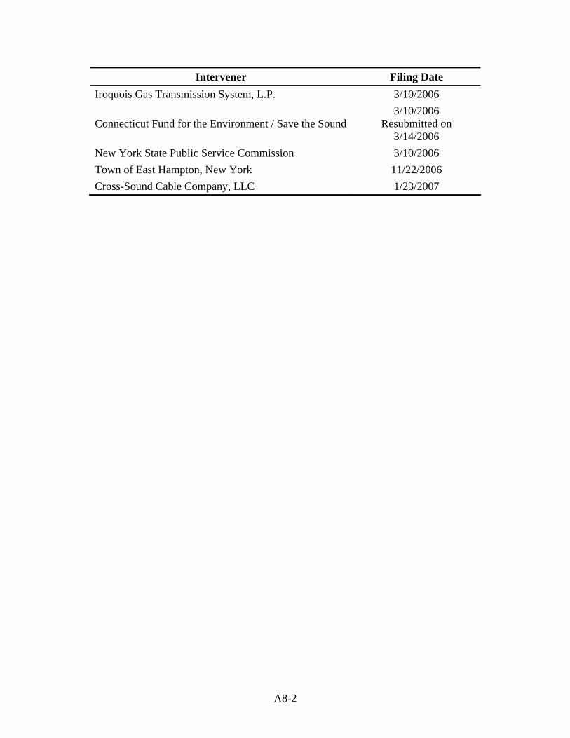
A8-2

Intervener Filing Date Iroquois Gas Transmission System, L.P. 3/10/2006

Connecticut Fund for the Environment / Save the Sound3/10/2006

Resubmitted on 3/14/2006

New York State Public Service Commission 3/10/2006 Town of East Hampton, New York 11/22/2006 Cross-Sound Cable Company, LLC 1/23/2007