SSC-297

EVALUATION OF LIQUIDDYNAMIC LOADS IN SLACK LNG

CARGO TANKSce,

OCT 3 1980

This document has been approvedfor pubic relse and sale; its

LC distribution is unimited.

SHIP STRUCTURE COMMITTEE

C21900

8010 2 063

SHIP STRUCTURE COMMITTEE

The SHIP STRUCTURE C0MWITTEE is constituted to prosecute a researchprogram to improve the hull structures of ships and other marine structuresby an extension of knowledge pertaining to design, materials and methods ofconstruction.

RAIW H. Z. BELL (C7haii~narr N. PITICIChief, Offioe of terohat Marine Aeietant Adini etator for

Safe y CowvolaZ wZop,,ntU. s. Coo t Guard Maritime Adwinitration

. .PALERM W. R. B. X.RAHLDeputy Direotor, Chief. Branch of Marine OltHull 6ro, end Gas OperationsNaval Sea Syjateno Cmwr.~d U. S. Geohogioal Survey

MW. W. N. HANNAN W. C. J. ITFSTCOhEVio. Pr. dent Chief EngineerAmerican Bu au of Shipping Mlitary SeaZift C o mnd

CDR 7. H. ROBINSON,~ U.S. Coast Gu~ard (Seoretaryj)

SHIP STRUCTURE SUBCOMHITTEE

The SHI!' STRUCTURE SUBCOMMITTEE act* for the Ship StructureCouittee on technical matters by provieing technical coordination for thedeteridnation of goals and objectives of the program, and by evaluatingand interpreting the results in terms of structural design, constr:ction andoperation.

U.S. COAST GUMR MILITAKY StALIFT COMMWD

CAP R. L. BNOW MR. 0. A SRCDR J. C. CARD MR. T. V. CHAPMNCDRJ. A. SAZAL JR. MR. A. B. STAVOVY (Chaiman)CDR W. N. SItEPSOk. JR. MR. D. STEIN

NAVAL SEA SYSTEMS COMMAND U. S. GEOLOGICAL SURVLY

Mr. R. CiU MR. R. J. GZAN(ZRLLIWr. R. JOHNSON W. J. MGORY

r. J. B. O'R0 WiMARITIME ADMINISTRATION

AMERICAN BUREAU OF SkMPPINGMR. N. 0. NAWR

DR. D. I, DR. W. M4CLIANMR. I. L. STIN MW. F. SEBOLD

Mr. N. TOULA

N40NAL ACADEfY OF SCIENCES INTURNATIONAL SHIr STRUCTURES CONGRESSSHIP RESEARCH COMMITTEE

Mr. S. G. STIANSER - Liaison*1. 0. H. OA.E . LiaisonW. R. V. RVN Liason AMERICAN IRON 4 STEEL INSTITUTE

THE SOCIETY OF NAVAL ARCHITECTS Mr. R. H. STERM - Liaison& MARINE ENGINEERS

STATE UNIVERSITY OF NEW YORK MARITIME COLLEGEMr. N/. 0. HAIR - LisA'ionDr'. V. R. PORTER- Iaison

WELDING RESEARCH COUNCIL

U. S. COAST GUARD ACADEMYMr. K. H. KOOPYAN - Iatson

CAPT W. C. NOLAN - LiaisonU. S. MERCHANT MARINA ACADEMY

U. S. NAVAL ACA.DEMYDr. C.-B. KIM- Liason

Dr. R. BRATTACHAWRYYA - Liaison

i Member Agencies: Address Correspondence to:

United 2$ars Coast GuardNavl.S,& S stems Command Secretary, Ship Structure CommitteeMilitary Safift Command U.S. Coast Guard Headquarters,(G-M/TP 13)

MlitrySeaIt A mmran, Washington, D.C. 20693Maritme Administration uttUnited Stotes Geological Survey itUiI

Amcdcan Burmvu 3f Shipping C ittAn Interagency Advisory Committee

Dedicated to Improving the Structure of Ships

SR-1251

JULY 1980

The liquid slosh-induced loads which impact on the wallsof partially filled cargo tanks have caused damages and thereforehave been of concern to ship owners and designers for many years.In particular, liquefied natural gas (LNG) csrriers have experiencedrecent problems, Numerous rest programs have been conducted usingscale models of LNG tanks to investigate slosh loadings. HowrvL'r,not all of these studies have covered the complete range of excita-tion amplitudes, frequencies, fill depths and tank geormtries whileobtainint ooth tank wall pressures and force measurements.

The Ship St-ucture Committee undertook a project toreview and make a unJ form presentation of currently available

k model data, and to perform additional model tests to supplementLhese data in order to provide a complete picture of slosh loadsfor both prismatic and spherical tanks.

This report contains the results of that effort.

Rear Admiral, U.S. Coast GuardChairman, Ship Structure Committee

Accession For

liTIS GRA&IWDC TAR fUJiannounced aLJustifiction__ .

By__________

Avail aud/or'

Ds specal

Technical Report Documentation Page

iGoermment Accession N-. 3. Recipient's Catalo No.

fSSC 2 19~~~~fa'/. Til a.. R

' -LACK LNG CARGO TANKS, /- _f_

0 . ea remislsis port No

0 -E .. .SS SWRI Project 02-5033.

9. iermoringO gornization Name end Address 10. Wrk Un No (rRAIS)

SOUTHWEST RESEARCH IN1STITUTEP.O. DRAWER 28510, 62 CULEBRA ROADSAN ANTONIO, TX 78284 -A

12. Sponsoring Agtn-y Name arndAdrs

U. S. COAST GUARDOFFICE OF MERCHANT MARINE SAFETYWASHINGTON, D.C. 20593 ), S o

15. Supelemerstoty Nore,

16. Absirect

This report provides an evaluacion of dynimi,c sloshing loads in slackLNG cargo tanks. A comprehensive review of vcrid4ide scale model sloshingdata is presented. The data are reduced to n conmon format for the pur-poses of defining design load coefficients. LNG tank st?uctural detailsare reviewed with emphasis placed on definlii, unique3 deslJn features whichmust be considered in designing LNG tanks ':o withstind f;,zmic sloshingloads. Additional scale model laboratory experiments are .onducted tc, sup-plement the available model sloshing dat.. Experiments ar- conducted Incombined degrees of freedom to establish the potential to- multi-degrc, .ffreedom excitation for augmenting dynamic slo.hing loads. Experiments vtoealso conducted to establish the slos'' " dyrnimi pressure-icme historieswhich are necessary for structural re vorse bnalysis. 17i.nerments are also,conducted on representative segments of a full-sc;,!e LN, s:nip tank struc-ture which is loaded with a typical full-scale dynumic .-shing pressure aspredicted from the model results. !nalytieal stutli.es are undertaken toprovide techniques for determining wal_ *, ructural reep:rne to dynamic

slosh loads. Finally, design methodoioy i.s preseiited ",)r membrane andsemi-membrane tanks, gravity tanks, 'd p:-snure tanks whereby the designprocedure sequences from comparing resonant olosl.:a.g pbriods to ship peri-ods, defining the design loads, and designing the tnn , tructures affectedby dynamic slosh loads by delineated procedures whicb vary with tank type.

17. Key Words e. Distribution Sateme.nt

liquefied natural gas Document is awlable to the U.S. Publicsloshing structural response through the Natic-nal Technical Informati

model tests load simulator Service, Springfield, VA 22161.dynamic loads Tpressure-time histories

19. Security Clcssf. (of this report) 20. Security Clossf. (of this page) 21. No. of oge, 22. Price

UNCLASSIFIED UNCLASSIFIED 183

Form DOT F 1700.7 (8-72) Reproduction of completed page authorized

Ift

- 0a.-

- C "

"I'rl I Hll11111,T I II III

IC 6

N I

.- , - a.*C .o 1;!A

Civ

a , _ _.: _ .! |

'"

p, a_: *, .. p. I .-. 4 :Ii z

N - -o"

(G0ONZENT S

I. INTRODUCTION 1

II. BACKGROUND 3

II.1 History of Slosh Problem 311.2 Nature of Liquid Sloshing 711.3 Previous Studies 10

III. TASK 1 - DATA REVIEW AND EVALUATION 12

IIl Scale Model Sloshing Data 13111.2 Full Scale Sloshing Data 36111.3 Review of Tank Structural Detail 36

IV. TASK 2 - EXPERIMENTAL STUDIES 47

__ IV.1 Experimental Study Objectives 47IV.2 Experimental Facilities 47

IV.3 Combined Degree of Freedom Model Tests 48IV.4 Dynamic Pressure-Time Histories 65IV.5 Dynamic Load Simulator for Plywood InsulationBox Tests 72

IV.6 Material Properties Tests 89

V. TASK 3 - ANALYTICAL STUDIES 95

V.1 Respones Prediction Method 95V.2 Design Procedures 96

VI. TASK 4 - PRESENTATION OF RESULTS -

DESIGN METHODOLOGY 111

VI.! Current IMCO Requireme,!ts and Proposed Changes i1VI.2 Design Methodology 113

t VI.3 Example Problem Utilizing Tank Design

Methodology 121VI.4 Summary 124

VII. CONCLUSIONS AND RECOMMENDATIONS 125VII.l Summary and Conclusions 125VII.2 Recommendations 126

VIII. REFERENCES 127

V

C 0 N T E N T S (CONT'D)

APPENDIX A SLOSHING FACILITIES FOR

o ANGULAR MOTIONo SIMULTANEOUS HORIZONTAL AND VERTICAL MO'1i1N A-I

APPENDIX B PRESSURE-TIME HISTORY DATA FORTRANSDUCER LOCATIONS 2 - 13 B-i

APPENDIX C ONE-DEGREE-OF-FREEDOM EQUIVALENTSYSTEMS C-i

APPENDIX D EXAMPLE CALCULATIONS FOR MEMBRANEAND PRISMATIC TANKS D-I

APPENDIX E IMCO TANK-TYPE DEFINITIONS E-1

I

vi

LIST OF FIGURES

NO. PAGE NO.

II-1 LNG Carriers: The Current State of the Art ................ 4

11-2 Example LNG Tank Designs ................................... 6

11-3 Typical Pressure Waveforms on Tank Wallswith Sloshing Liquids ...................................... 9

Ill-1 Pressure Definitions ...................................... 21

111-2 Pressure Histograms for 100C-Cycle and 200-CycleResonant Sloshing Tests as Presented in Reference 44 ....... 25

111-3 Highest Average Nondimensionnl Pressure vs NondimensionalTank Filling Level for All Model Tests Run to Date ......... 26

111-4 Maximum Pressure Coefficient vs Tank Filling Levelfor * or (x/j) < 0.30 ..................................... 28

111-5 Pressure Coefficients vs Pitch Amplitude(From Reference 44) -.............. ...... ...... ...... 28

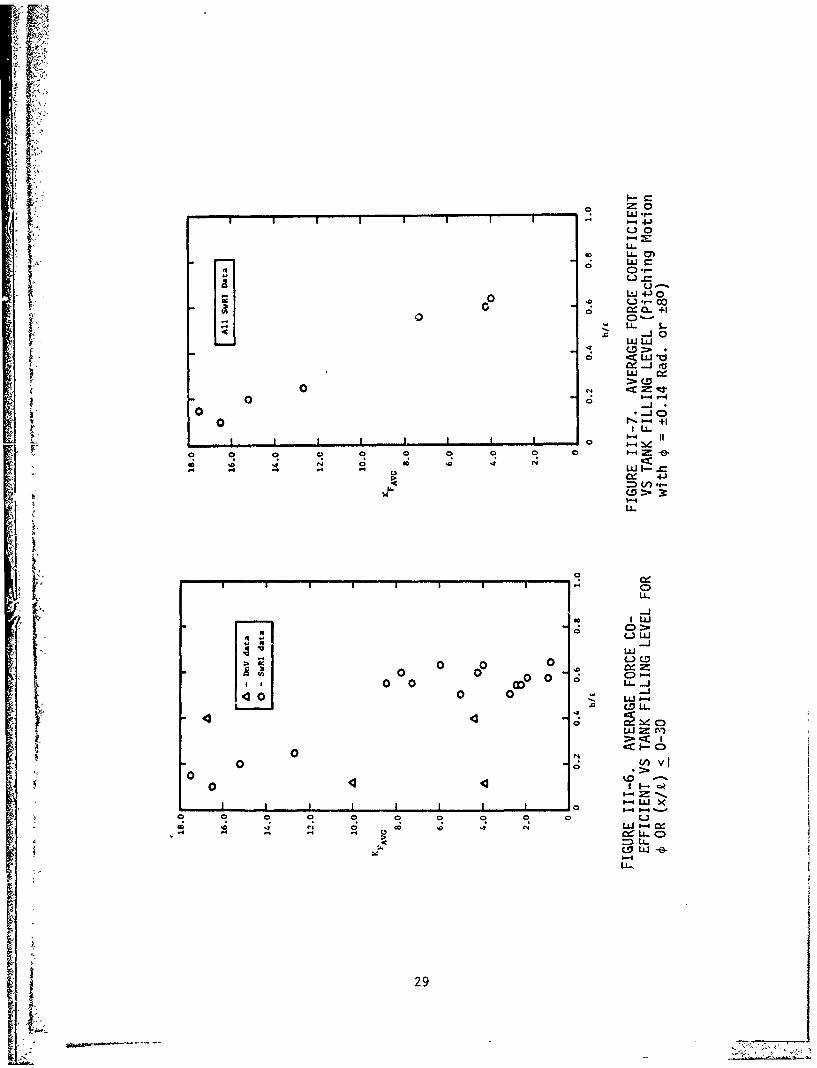
111-6 Average Force Coefficient vs Tank FillingLevel for 0 or (x/£) < 0-30 . -.. . ......................... 29

111-7 Average Force Coefficient vs Tank Filling

Level (Pitching Motion with 0 - + 0.14 Rad. or + 80) ....... 29

111-8 Resonant Liquid Frequency vs Tank Filling

Level for Rectangular or Prismatic Tanks ................... 30

111-9 Slosh Forces on Sphere ...................................... 32

11-10 Resultant Force on Sphere vs Fill Depth (Reference 44) ..... 32

IIl-11 Resultant Force on Sphere vs Excitation Period(Reference 44) ............................................. 33

111-12 Lateral Force on Sphere vs Fill Depth (Reference 44) ....... 33

111-13 Lateral Force on Sphere vs Fxcitation Period(Reference 44) ............................................. 33

111-14 Vertical (Dynamic) Force on Sphere vsFill Depth (Reference 44) .................................. 34

111-15 Vertical Static + Dynamic Force on Sphere vs FillDepth (Reference 44) ....................................... 34

111-16 Vertical (Dynamic) Force on Sphere vs ExcitationPeriod (Reference 44) ..................................... 35

111-17 Vertical (Dynamic) Force on Sphere vs ExcitationAmplitude (Reference 44) ................................... 35

vi.

I

NO. PAGE NO.

111-18 12-Ce1l Primary Insulation Box - Gaz Transport System ....... 38

111-19 Arrangement of Insulation Boxes in Gaz Transport System ..... 39

111-20 Section of Cofferdam Bulkhead for Gaz Transport Tanks ........ 40

111-21 Technigaz Membrane System .................................... 42

111-22 Typical Horizontal Girder - Conch Tank ....................... 43

111-23 Typical Longitudinal Girder .................................. 45

111-24 Typical Transverse Frame ..................................... 46

IV-l Scale Model Tank Dimensions and Pressure TransducerLocations for 1/50 Scale Prismatic Tank from a 125,000m3 Ship ...................................... ...... ........ 49

IV-2 Test Configuration for Combined Pitch and Heave Test ......... 61

IV-3 Experimental and Theoretical Nondimensional ResonantSlosh Period Versus Tank Filling Level ....................... 63

IV-4 Motion Definitions for Surge and Heave ...................... 64

IV-5 Typical Pressure-Time History for Slosh-Induced Impact ....... 66

IV-6 Nondimensional Pressure-Time History Values for 200Resonant Sloshing Cycles at Transducer Location 1for a 25% Full Tank .......................................... 69

IV-7 Integrated Nondimensional Pressure Values for 200Resonant Sloshing Cycles at Transducer Location 1for a 25% Full Tank .......................................... 69

IV-8 Nondimensional Pressure vs Impulse Rise Time for 200Resonant Sloshing Cycles at Transducer Location 1 fora 25% Full Tank .............................................. 70

IV-9 Nondimensional Pressure vs Impulse Duration for 200Resonant Sloshing Cycles at Transducer Location 1for a 25% Full Tank .......................................... 70

IV-10 Nondimensional Impulse Duration vs Impulse Rise Timefor 200 Resonant Sloshing Cycles at Transducer Location1 for a 25% Full Tank ........................................ 70

TV-ll Nondimensional Pressure-Time History Values for 200 ResonantSloshing Cycles at Transducer Location 14 for a 75% FullTank ......................................................... 70

IV 12 Integrated Nondimensional Pressure Values for 200Resonant Sloshing Cycles at Transducer Location 14for a 75% Full Tank .......................................... 71

Sviii

NO. PAGE NO.

IV-13 Nondimensional Pressure vs Impulse Rise Time for 200Resonant Sloshing Cycles at Transducer Location 14for a 75% Full Tank ........................................... 71

IV-14 Nondimensional Pressure vs Impulse Duration for 200Resonant Sloshing Cycles at Transducer Location 14for a 75% Full Tank .......................................... 71

IV-15 Nondimensional Impulse Duration vs Impulse Rise timefor 200 Resonant Sloshing Cycles at Transducer Location14 for a 75% Full Tank ....................................... 71

IV-16 Schematic Diagram of Plywood Insulation Box Dynamic Loader ... 73

IV-17 Typical Pressure-Time Histories for Dynamic LoadingTests on Plywood Insulation Boxes ............................ 75

IV-18 Displacement Transducer Locations for Plywood Box StrengthTests ........................................................ 76

IV-19 Cover Deflection vs Pressure for Dynamic and StaticLoading of a Standard 12-Cell Box ............................ 77

IV-20 Shear Failure of Plywood Insulation Box Cover(Test Box No. 1) ............................................. 78

IV-21 Bending Failure of Plywood Insulation Box Cover(Test Box No. 8) ............................................. 79

IV-22 Support Stiffener Failure in a Plywood Insulation Box(Test Box No. 10) ............................................ 80

IV-23 Plywood Test Specimen Geometry ............................... 91

V-1 Sloshing Pressure with Minimum Rise Time and LongDuration for 36 m (118-ft) Long Tank ......................... 98{ V-2 Dynamic Load Factor for P(T) of Figure V-I ................... 100

V-3 Envelope for Different Rise Times ............................ 100

V-4 Effect of Different Load Decay Times, T3 . . . . . . . . . . . . . . . . . . . . . . 100

A-1 Slosh Test Facility .......................................... A-2

A-2 Slosh Rig Cross-Sectional Dimensions ......................... A-3

A-3 Drive System Block Diagram ................................... A-3

B-1 Nondimensional Pressure-Time History Values for 200Resonant Sloshing Cycles at Transducer Location 4for a 25% Full Tank ....................... ............. B-7

B-2 Integrated Nondimensional Pressure Values for '200Resonant Sloshing Cycles at Transducer Location 4for a 25t Full Tank .......................................... B-7

ix

NO. PAGE NO.

B-3 Nondimensional Pressure vs Impulse Rise Time for 200Resonant Sloshing Cycles at Transducer Location 4 fora 25% Full Tank .............................................. B-8

B-4 Nondimensional Pressure vs Impulse Duration for 200Resonant Sloshing Cycles at Transducer Location 4 fora 25% Full Tank .............................................. B-8

B-5 Nondimensional Impulse Duration vs Impulse Rise Timefor 200 Resonant Sloshing Cycles at Transducer Location 4for a 25% Full Tank ........................................... B-8

B-6 Nondimensional Pressure-Time History Values for 200Resonant Sloshing Cycles at Transducer Location 7 fora 75% Full Tank ............................ .......... B-8

B-7 Integrated Nondimensional Pressure Values for 200 ResonantSloshing Cycles at Transducer Location 7 for a 75% Full Tank.. B-9

B-8 Nond~mensional Pressure vs Impulse Rise Time for 200 ResonantSloshing Cycles at Transducer Location 7 for a 75% Full Tank.. B-9

B-9 Nondimensional Pressure vs Iipulse Duration for 200 ResonantSloshing Cycles at Transducer Lozation 7 for a 75% Full Tank.. B-9

B-10 Nondimensional Impulse Duration vs Impulse Rise Time for 200Resonant Sloshing Cycles at Transducer Location 7 for a

75% Full Tank ................................................ B-9

B-11 Nondimensional Pressure-Time History Values for 200Resonant Sloshing Cycles at Transducer Location 11for a 75% Full Tank .... ..................... B-10

B-12 Integrated Nondimensional Pressure Values for 200 ResonantSloshing Cycles at Transducer Location 11 for a 75% FullTank ..................................................... ... B-10

B-13 Nondimensional Pressure vs Impulse Rise Time for 200Resonant Sloshing Cycles at Transducer Location 11for a 75% Full Tank .......................................... B-10

B-14 Nondimensional Pressure vs Impulse Duration for 200Resonant Sloshing Cycles at Transducer Location 11for a 75% Full Tank .......................................... B-10

B-15 Nondimensional Impulse Duration vs Impulse Rise TimeFor 200 Resonant Sloshing Cycles at Transducer Lo.ation11 for a 75% Full Tank ....................................... B-lb

B-16 Nondimensi Pressure-Time Histoiy Values for 200Resonant g Cycles at Transducer Location 13for a 75' ank........................................... B-lb

B-17 Integrated imensional Pressure Values for 200Resonant Sb shing Cycles at Transducer Location 13for a 75% Fu 1 Tank .......................................... B-l

x

NO. PAGE NO.

B-18 Nondimensional Pressure vs Impulse Rise Time for 200Resonant Sloshing Cycles at Transducer Location 13 fora 75% Full Tank ............................................ B-li

B-19 Nondimensional Pressure vs Impulse Duration for 200Resonant Sloshing Cycles at Transducer Location 13 fora 75% Full Tank ..................... ..... .... B-12

B-20 Nondimensional Impulse Duration vs Impulse Rise Timefor 200 Resonant Sloshing Cycles at Transducer Location13 for a 75% Full Tank .......... ......... . B-12

C-1 Deformation Pattern for Simple Beam ........................ C-1

C-2 Equivalent One-DOF System ..... . ...................... . C-3

C-3 Dynamic Load Factors (DLF) and Time to MaximumResponse (t ) for Different F(t)'s (96) . C-8

C-4 Simply Supported Beam in Equilibrium Under Dynamic Loading.. C-!0

D - 1I. . . . D -3

D-2 .......................................................... D-6

D-3 ...... $...$........ $................ .. . .. .. . .. ......... D-7

D-4 .......... . . ............................... $ .$....... ..... D-10

D-5 ............ .................. ......... .... . .... ..... D-16

xi

LIST OF TABLES

NO. PAGE NO.

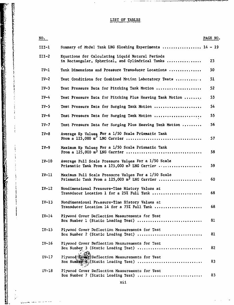
III-i Summary of Model Tank LNG Sloshing Experiments .................. 14 - 19

111-2 Equations for Calculating Liquid Natural Periodsin Rectangular, Spherical, and Cylindrical Tanks ................ 23

IV-i Tank Dimensions and Pressure Transducer Locations .............. 50

IV-2 Test Conditions for Combined Motion Laboratory Tests ............ 51

IV-3 Test Pressure Data for Pitching Tank Motion ..................... 52

IV-4 Test Pressure Data for Pitching Plus Heaving Tank Motion ........ 53

IV-5 Test Pressure Data for Surging Tank Motion .................... 54

IV-6 Test Pressure Data for Surging Tank Motion ...................... 55

IV-7 Test Pressure Data for Surging Plus Heaving Tank Motion ......... 56

IV-8 Average Kp Value5 For a 1/50 Scale Prismatic TankFrom a 125,000 m LNG Carrier ................... ................. 57

IV-9 Maximum Kp Values For a 1/50 Scale Prismatic TankFrom a 125,000 m3 LNG Carrier .................. 0 ....... ..... 58

IV-10 Average Full Scale Pressure Values For a 1/50 ScalePrismatic Tank From a 125,000 m3 LNG Carrier ............. 59

IV-11 Maximum Full Scale Pressure Values For a 1/50 ScalePrismatic Tank From a 125,000 m3 LNG Carrier ................... 60

IV-12 Nondimensional Pressure-Time History Values atTransducer Location 1 for a 25% Full Tank ....................... 68

j IV-13 Nondimensional Pressure-Time History Values atTransducer Location 14 for a 75% Full Tank ...................... 68

IV-14 Plywood Cover Deflection Measurements for TestBox Number 1 (Static Loading Test) .............................. 81

IV-15 Plywood Cover Deflection Measurements for TestBox Number 2 (Static Loading Test) .............................. 81

IV-16 Plywood Cover Deflection Measurements for TestBox Number 3 (Static Loading Test) .............................. 82

IV-17 Plywood ,'"--Deflection Measurements for TestBox Nui !6 (Static Loading Test) .............................. 83

iV-18 Plywood Cover Deflection Measurements for Test

Box Number 7 (Static Loading Test) .............................. 83

xii

NO. PAGE NO.

IV-19 Plywood Cover Deflection Measurements for TestBox Number 8 (Dynamic Loading Test) ......................... 84

IV-2u Plywood Cover Deflection Measurements for TestBox Number 10 (Static Loading Test) ......................... 84

IV-21 Plywood Cover Deflection Measurements for TestBox Number 11 (Static Loading Test) ......................... 84

IV-22 Summary Table of Loading Test Results for thePlywood Insulation Boxes ................................... 85 - 88

IV-23 Results of Tests on Specimens from Old Boxes ................ 90

IV-24 Rasults of Tests on Specimens From New Boxes ................ 92

IV-25 Summary of Plywood Properties (Average Values). . ... .. ,. 93

IV-26 Range of Plywood Properties 94

V-1 Range of Parameters which Describe Sloshing PressuresIn LNG Tanks .. ............................................... 97

V-2 Calculation of Envelope of DLF Using Figure C-2(b) .......... 102

V-3 Frequency Coefficients for the Fundamental ModeS(Equation V-1) ... . ... . .. .. .. . .. . .. . . . .105

V-4 Values of Constants A', B', C' ............................ 106

VI-l Design Methodology Flow Chart ............................... 114 - 116

B-1 Nondimensional Pressure-Time History Values atTransducer Location 2 for a 25% Full Tank ................... B-1

B-2 Nondimensional Pressure-Time History Valuesat Transducer'Iocation 3 for a 25% Full Tank ................ B-2

B-3 Nondimensional Pressure-Time History Valuesat Transducer Location 4 for a 25% Full Tank ................ B-2

B-4 Nondimensional Pressure-Time History Values

at Transducer Location 5 for a 25% Full Tank ................ B-311 B-5 Nondimensional Pressure-Time History Values

at Transducer Location 6 for a 25% Full Tank ........... B-3

B-6 Nondimensional Pressure-Time History Valuesat Transducer Location 7 for a 75% Full Tank ................ B-4

at Transducer Location 7 for a 75% Full Tank..... B-4

B-7 Nondimensional Pressure-Time History Valuesat Transducer Location 8 for a 75% Full Tank ................ B-4

B-8 Nondimensional Pressure-Time HistoryValuesat Transducer Location 9 for a 75% Full Tank ................ B-5

xiii Fl ak...........-

NO. PA , NO.

B-9 Nondimensional Pressure-Time History Valuesat Transducer Location 10 for a 75% Full Tank .............. B-5

B-1O Nondimensional Pressure-Time History Valuesat Transducer Location 11 for a 75% Full Tank .............. B-6

B-11 Nondimensional Pressure-Time History Valuesat Transducer Location 12 for a 75% Full Tank .............. B-6

B-12 Nondimensional Pressure-Time History Values

at Transducer Location 13 for a 75% Full Tank ............. B-7

C-1 Transformation Factors for Beams and One-Way Slabs ......... C-7

D-1 Plywood Material Properties ................................ D-2

D-2 Material Properties for Balsa, Sweet Birch,and Sugar Maple ......................... ........... ...... i

xiv

NOMENCLATURE OF IMPORTANT PARAMETERS

A Cross-sectional area

b Width

CT Cryogenic temperature

D Tank diameter; flexural rigidity of a plate

DLF Dynamic load factor

dof Degree of freedom

:E Elastic modulas of a material

E Flexural rigidity of a plate-stiffener combination

F Dynamic force

f Frequency

G Shear modulus of a material

g Acceleration of gravity

CA Shear rigidity of a material

H Tank height

h liquid filling in a tank; plate thickness

I Second moment of area of stiffener and associated plate; beamsection moment of inertia

K Axial spring constant of a stiffener

KF Nondimensional force coefficientii KL Dynamic load factor

Km Dynamic mass factor

Kp Nondimensional dynamic pressure coefficient

K'p Nondimensional dynamic pressure coefficient corrected for oscilla-Ition amplitude effects

1 KT Nondimensional time coefficient

k Spring constant

KE Kinetic energy

xv

NOMENCLATURE (Cont.)

Tank length; plywood specimen length

VG Liquified Natural Gas (Liquid Methane)

LN2 Liquid nitrogen

LPG Liquified Petroleum Gas

m Mass

N Load applied over a surface

P Dynamic pressure created by liquid sloshing

R Resultant dynamic force created by liquid sloshing in a sphericaltank

RF Reduction factor

RT Room temperature

S Sectional area of stiffener and associated plate

T Time; period

TR Resonant period

tr Rise time

U Internal strain energy

V Spherical tank volume; shear reaction

W Static weight of liquid in a tank; external work

w Deflection of a beam under loading

x Translational (horizontal or surge) excitation amplitude of aprismatic or rectangular ship tank

Y Lateral dynamic force created by liquid sloshing in a spherical tank

y Translational (vertical or heave) excitation amplitude of a prismatic

or rectangular ship tank

Z Vertical dynamic force created by liquid sloshing in a spherical tank

z Distance from a ship tank bottom

Angle (relative to vertical) of the resultant dynamic force (R)

created by liquid sloshing in a ship tank

xvi

NOMENCLATURE (Cont,)

y Specific weight of a liquid

* Pitch or roll angle of a ship tank

p Mass density

f Horizontal excitation amplitude of a spherical ship tank

ISee Equation V-9, Pge. 131.

a Stress

v Poisson's ratio

W Circular frequency

xvii

t I. INTRODUCTION

This report presents all results of Project SR-1251, "Evaluation ofLiquid Dynamic Loads in Slack LNG Cargo Tanks." The study was conductedunder the direction of the Ship Research Committee of the National Academyof Sciences.

The potential for significant loads resulting from sloshing liquidsin slack cargo tanks has been realized by the marine industry for years.In the past decade, with the advent of the supertanker and large LNG ships,sloshing loads have been of even greater concern. In the case of LNGships, certain operational constraints call for the transport of liquidin slack tanks and, in addition, the absence of tank internals results inno damping of the liquid motions. Also, as ship tanks have grown in size,the probability of resonant sloshing has increased since resonant sloshingperiods and ship motions more closely match. In view of this, a signifi-cant activity has been undertaken by various agencies throughout the worldto establish sloshing loads in LNG cargo tanks. Experimental programs havebeen conducted using instrumented scale model tanks. These test programshave covered many different ship tank geometries, excitation amplitudesand frequencies, and liquid fill depths. Experiments were necessary be-cause large amplitude sloshing is not amenable to theoretical analysis.To develop usable liquid dynamic load criteria for sloshing requires the com-bining of current experimental information with new experiments and analysis,

Four project tasks were undertaken to develop dynamic load criteriafor slack tanks. In Task 1, all test reports on LNG slosh loads were as-sembled, and the data reviewed and presented on a uniform basis. The datawere summarized with regard to source, test conditions, and types of mea-surements recorded. To present the data on a uniform basis, nondimensionalcoefficients were utilized where data from the various reports were pre-sented in the same format. Concurrent with this effort, the structuraldetails of typical LNG tank designs were established, and methods and back-ground information necessary to develop LNG slosh load design methodologywere identified.

In Task 2, scale model tanks were utilized to conduct additionalsloshing experiments whereby important loads and test conditions not cur-rently covered in the literature were investigated. Scale model LNG shiptanks were utilized whereby dynamic sloshing pressures were measured atresonant sloshing conditions. Both single and combined degree of freedomexcitation experiments were conducted to evaluate the ability of singledegree of freedom tests to produce maximum impact loads. Significant em-phasis was placed on establishing pressure-time histories for resonantsloshing impact loads for use in dynamic tank wall response analysis.Experimental studies were also conducted to reproduce full-scale impulsive

impact pressures on representative segments of membrane tank structuresand to measure the structural response.

In Task 3, analytical efforts were undertaken to develop methods forpredicting LNG tank wall and support structural response to typical slosh

loads. Analytical methods were used to examine the stresses and deforma-tions in typical LNG tank structures and their supports when subjected todynamic sloshing loads. Design guidelines and design methods were formu-lated utilizing the analytical studies conducted in this task; the experi-mental studies from Task 2; and information on past research and analyses,collected and analyzed in Task 1.

Finally, in Task 4, the composite of information generated in theproject was utilized to generate simplified design procedures to accountfor dynamic loads in slack cargo tanks.

t2

II. BACKGROUND

II.1 History of Slosh Problem

Space Related Activities

The basic problem of determining the dynamic loads which result fromthe motions ("sloshing") of liquids in partially filled moving containers

was studied extensively in the 1950's and 60's in connection with the de-velopment of large rocket vehicles for the space program. Liquid sloshingin spherical and cylindrical nontainers has been studied for space appli-cations, both analytically and experimentally.(l) The nature of sloshloading in these types of tanks and its prediction are probably betterunderstood than for prismatic tanks, but analytical techniques for predict-

*ing large amplitude sloshing are still not fully developed, and such loadsare extremely important in designing the support structure and internalcomponents of ship tanks. In addition, much of the sloshing technologydeveloped for space applications is not applicable because emphasis wasplaced on frequencies and total forces as they related to control systemrequirements, and, therefore, the effects of local peak impact pressure onstructural requirements were not 7tudied to any extent. Further, the ex-citation amplitudes considered in space applications are too small forship motion simulation.

LNG Ship Related Slosh Problems

Current activity in the design of super tankers as well as ships forliquified gas transport has resulted in renewed consideration of the influ-ence of the contained liquids on cargo tank design,(2-7 5 ) especially sincethQ probability of exciting a resonant slosh mode is increased in the lar-ger tanks. In many cases, the transport of liquid cargos in pc.rtiallyfilled tanks is prohibited. However, several factors make partial fillingeither unavoidable or highly attractive. For example, in the case of liq-uid natural gas (LNG) ships, partially filled conditions are needed because(1) chilled-down liquid is required to maintain cold tanks on return trips,(2) higher specific gravity liquids than LNG are transported in tanks de-

signed for LNG, (3) partial unloading is desirable when multi-port stopsare made, and (4) loading or unloading at sea creates significant timeperiods at undesirable fill depths. For all liquid cargo ships, partialfilling in ballast tanks and fuel tanks occurs, and conditions (3) and (4)above for LNG ships also apply. Therefore, the designer of all types ofliquid carriers must be aware of the consequences of liquid sloshing andbe able to predict the resulting loads.

As the - . designs have evolved (Figure II-1), severalimport!:-- ypes of unique ship loads have been considered by the designers..hf slosh-generated loads are one of these and have a considerable influ-ence on the tank and eupport structure design. Several factors make sloshloads more important with regard to LNG ship design. A tank failure in anLNG ship merits special consideration because of (1) the risk of brittle

3

LaoL(3 = La

o q

C\ z 0s I IN CLo

4 ~ ~ g[ EN\ I

tA 14

E) E

co~~ ww

a. z C

44

fracture of the primary structure (low-temperature shock), (2) the expensiverepair cost of the complicated tank designs (3) the high out-of-servicecosts, and (4) the potential for large volume vapor release. Also, the com-plexity of the tank design in LNG carriers is such that at least some LNGtanks are more susceptible to damage from slosh loading than tanks for trans-porting oil or other petroleum p-oducts.

LG Ship Tank Designs

There are presently over tetz designs of LNG tanks that are eithercurrently in use or under major conside7ration. These tanks generally fallinto two categories: namely, freestanding (independent) and non-freestand-ing (membrane) tanks (Figure 11-2). Integral tanks used for LPG tran'portare not acceptable for LNG since their use is restricted to temperaturesgreater than -10*C. The freestanding or independet tank is usually of thaspherical or cylindrical design, and because of its geometry it is amenableto stress analysis and other conventional analytical techniques. Becausethe stresses can be calculated, a secondary barrier system ia not requiredas is the case of the non-freestanding tanks. An exception is the pris-

matic freestanding tank, which does require a secondary barrier. Free-

standing tanks are also easier to fabricate, and the insulation is easierto install than on other systems. One drawback to the freestanding designis the disadvantage of requiring a larger ship per given cargo volume.Since freestanding tank walls can be designed to withstand large impactpressures, the primary problem associated with LNG sloshing in freestand-ing tanks results from the slosh loads on internal components and on thetank support structure.

The second general tank type, the non-freestanding or membrane tank,is essentially built into the ship's hold, making use of the ship's struc-ture for support. The membrane tanks use a thin internal layer of metalto act as a liquid barrier and are directly supported by insulation mater-Jal. The insulation is applied directly to the hull with no access space,which makes this type of tank difficult to repair after material fractureor other damage. Because of the complex structure, membrane tanks are notamenable to analysis. In addition, because of this and the thinness of themembrane, a complete secondary liquid barrier is required. The primaryproblem associated with sloshing in membrane tanks is the potential damageto the tank walls from impulsive slosh pressures. Severe impulsive sloshloads in the membrane tank can occur at small fill depths as a result oflarge-amplitude traveling wave impact, which is not amenable to analysis.Also, severe slosh loads can occur on or near the tank top as a consequenceof standing slosh waves in partially filled tanks. Since this type of tankcannot be analyzed to determine its failure strength, special load testsmust be performed on representative segments (,f ' structure to determine

its load bearing strength. An estimate of the "equivalent" static sloshloads that occur in these types of tanks is then utilized to determine if

the structure has the required strength.

5

otC)C:

414

C L4t4

1'6

7- z 0.

o -to

~ 0).~ WW

WIFM

Recorded LNG Tank Damage from Sloshing

As of 1979, over 80 years of operating experience have been gainedwith numerous ships of various tank designs. During these years, severalstructural problems have been recorded which have resulted from slosh loadson LNG cargo tanks.( 6) Slosh related loads causing tank damage have oc-curred on two ships with membrane tanks, the "Polar Al].ska" and the "ArcticTokyo." On the "Polar Alaska," supports of the electric cables supplyingthe cargo pumps were broken by liquid sloshing loads. This occurred whenthe tank was approximately 15-20% full. The broken cable supports resultedin damage to the bottom of the membrane tank. On the "Arctic Tokyo," aleak in the number 1 tank was caused from liquid sloshing when the tankwas about 20% full. Inspection revealed that the leak was located, alongwith four deformed points in the membranes, in the aft corners of thetransverse and longitudinal bulkheads at about the liquid surface level.Subsequent model tests(15, 4 3 ) performed on scale models of the damaged"Arctic Tokyo" tank revealed that a 15-30% fill depth with respect to tanklength resulted in appreciable impact loads from sloshing. The model testswere not successful, however, in establishing peak impact pressures(7) thatcould have caused the damage. As a result, additional work(10) was under-taken to investigate more thoroughly all aspects of modeling LNG sloshingand to provide a greater understanding of the slosh generated loads andtheir implications to tank and ship design. As a result of these studies,operations with partially filled tanks other than nearly full or nearlyempty have been prohibited.

In the spring of 1978, the first of the 125,000 m3 membrane tank LNGships was put into service. On one of the early cargo-laden voyages, theship experienced heavy seas and the crew heard loud sloshing impact noisesin the cargo tanks. After cargo discharge and subsequent inspection of thetanks, damage to the tank structure was noted. Subsequent studies( 74,75)concluded that the damage was slosh induced, even though the tanks wereapproximately 95% full during the voyage. Thus, the designer must also beconcerned with slosh loads at near full conditions.

11.2 Nature of Liquid Sloshing

General Conditions

In general, sloshing is affected by liquid fill depth, tank geometry,and tank motion (amplitude and frequency). The liquid motion inside a tankhas an infinite number of natural periods, but it is the lowest mode thatis most likely to be excited by the motions of a ship. Most studies have,therefore, concentrated on investigating forced harmonic oscillations in thevicinity of the lowest natural period, which is defined as that predictedby linear theory. Nonlinear effects result in the frequency of maximum re-sponse being slightly different from the natural frequency and dependent onamplitude. The most significant type of ship tank slosh loads occur withlarge excitation amplitudes where nonlinear effects are present.

The sloshing phenomena in cargo tanks that are basically rectangularin shape can usually be described by considering only two-dimensional fluid

7

* rflow. Sloshing in spherical or cylindrical tanks, however, must usuallyconsider three-dimensional flow effects.

jt Two-Dimensional Flow

Tanks with two-dimensional flow are divided into two classes: lowand high liquid fill depths. The low fill depth case is represented by

li/2 < 0.2, where h is the still liquid depth and k is the tank length inthe direction of motion. The low fill depth case is characterized by theformation of hydraulic jumps and traveling waves for excitation periodsaround resonance. At higher fill depths, large standing waves are usuallyformed in the resonant frequency range. When hydraulic jumps or travelingwaves are present, extremely high impact pressures can occur on the tankwalls. Figure II-3a shows typical pressure traces recorded under thissloshing condition. Impact preasures typical of those shown in FigureII-3a can also occur on the tank top when tanks are filled to the higherfill depths. The pressure pulses are similar to those experienced in shipslamming, and the pressure variation is neither harmonic nor periodic sincethe magnitude and duration of the pressure peaks vary from cycle to cycleeven though the tank is experiencing a harmonic oscillation. Figure II-3bshows typical pressure traces that result when small amplitude slophing isoccurring away from resonance at any fill depth.

Three-Dimensional Flow

Three-dimensional flow occurs in spherical tanks, usually in theform of a swirl mode.(l) Similar three-dimensional effects can be presentin cylindrical or rectangular tanks under certain excitation conditions.The prediction of sloshing forces in the neighborhood of resonance withswirling is extremely difficult, and experimental data obtained with scalemodel tanks are usually needed to establish pressures and forces with thistype of sloshing.

Design Implications

The design of a liquid cargo tank to withstand the dynamic slosh-induced loads requires that the designer 1b6 able to predict the resonantslosh periods at different fill depths for the required tank geometry.These periods can then be compared with the expected ship periods to deter-mine the probability of resonant sloshing. An estimate of the maximum dy-namic loads to be expected is then made to determine a proper design. Mosttheoretical analyses are not able to predict slosh pressures and forces inthe neighborhood of resonance, especially for the large amplitude excita-tions typical of a ship cargo tank. However, several theories are avail-able to predict tank loadings at off-resonant, low ampltiude sloshing con-ditions. Depending on the likelihood of resonance and the expected exci-tation amplitudes, the designer can either use theory or turn to experimen-tal model data to provide the required design information.

Available linear and nonlinear theories are discussed in detail in

References 2 and 6. A review of the theoietical efforts reveals that moststudius are limited to linear s-hshing, which is valid only for small

8

iiJ

Impulsive PressurePressureL Peak Magnitude (P)

Ti-e Pressure TailMagnitude (P')

PT

(a) Impact pressure traces with largeamplitude resonant sloshing

Pressure LTime

(b) Pressure trace for non-resonant sloshing

FIGURE 11-3. TYPICAL PRESSURE WAVEFOR4S ON TANK WALLS WITH SLOSHING

LIQUIDS

9

amplitudes and frequencies and predicts an infinite response at resonance.Some nonlinear theories are available for specific tank geometries, andthese theories allow a prediction of slosh-induced dynamic forces andpressures on tank structures at resonance. However, the nonlinear theoriesare also limited to small excitation amplitudes and cannot be used for ageneral tank shape or when certain real sloshing effects are present suchas liquid impacting on the tank top. Therefore, emphasis has been placedon utilizing model test data for predicting full scale tank loads for de-sign purposes.

11.3 Previous Studies

A significant number of scale model studies have been conducted toinvestigate sloshing in LNG cargo tanks. These efforts have been under-taken primarily by three worldwide laboratories:

o Southwest Research Institute (SwRI)

o Det norske Veritas (DnV)

o Bureau Veritas (BV)

These studies are reviewed in detail in Task 1. Nearly all model tests todate have considered the six degrees of ship motion individually and inves-tigated sloshing by varying amplitude and frequency harmonically, usuallyin heave, surge, pitch, or roll. Also, water has been used almost exclu-sively as the model liquid. In most studies, the scaling of impact loaddata to full scale for use in tank design has considered only Froude scal-ing and thus eliminated any possible effects of fluid properties such asviscosity, compressibility, or vapor pressure (cavitation). Under theseassumptions, prescures scale by

p P

where the subscripts m and p are for the model and prototype, respectively.The periods between prototype and model are given by

(T/g/)p = (T glt)m (11-2)

In scaling pressure data, a pressure coefficient is defined as

K = P (11-3)p pg c¢

where 0 is the pitch, roll, or yaw angle. For translation, to is usuallyreplaced by the translational amplitude, x. (See Figures IV-I and IV-4 fordefinitions of and x, respectively.)

10

Scaling Effects

The scaling criteria that should be used in predicting full-scaleslosh loads from model data are discussed in References 2, 10, 44, and 74.Most model studies have utilized Froude scaling to predict full-scale loads,and no allowance for fluid effects was considered. Depending on the cargoto be carried, some of these fluid properties would appear important. Forexample LNG is transported at a tank pressure slightly above its vaporpressure, and, therefore, cavitation and thermodynamic (vapor condensation)effects could be important. Also, LNG has an extremely low viscosity com-pared to water, and therefore model tests using water could produce noncon-servative predictions of full-scale loads if the model tests were over-damped. Also, compressibility of the impacting liquid/vapor could be im-portant in scaling the slosh loads.

SwRI and DnV experimental programs have been conducted to determinethe effects of these fluid properties on scaling sloshing loads. The testresults indicate that fluid properties will have a minor effect on scalingimpact pressures when largc amplitude sloshing, typical of a ship cargotank, is present. To determine the validity of Froude scaling for largeamplitude sloshing, full-scale pressure measurements were recorded in apartially water-filled OBO tank under rolling motion (Reference 2). Subse-quent model tests in 1/30th scale were conducted with the full-scale rollmotions reproduced on the model. Model pressures converted to full-scaleusing Froude scaling showed excellent agreement for both the magnitudes anddistributions of pressures. Since water was used in both model and full-scaletests, the effects of liquid viscosity and vapor condensation were not in-cluded. However, an evaluation of these effects in References 10, 44, and 74indicates they are of small importance to large amplitude slosh scaling.As a result, Froude scaling is appropriate, and Equations 11-2 and 11-3 areused for scaling periods and loads, respectively.

t

'III. TASK 1 - DATA REVIEW AND EVALUATION

The objective of Task 1 of the project was to review and presentcurrently available slosh test data on a uniform basis, to identify datarequired to develop design methods, and to outline required experimentaland analytical studies. The majority of the research work in LNG sloshinghas been done by SwRI, Det norske Veritas, and Bureau Veritas. Numerousmodel tests have been conducted by these groups and others to study slosh-ing loads on LNG ship tanks and the effects of these loads on the tanks and

on the ship structures. A principal part of Task 1 has been to compile allof this information and present it on a uniform basis.

The initial step in Task 1 was to conduct a thorough literaturesearch to find all information that is presently available on LNG sloshingin ship tanks (including pressures, forces, and tank response) and to ob-tain information on tank structural details. This search was broken downinto three segments: (1) a manual search of appropriate journals and peri-odicals, (2) a computer search of the pertinent data bases, and (3) writteninquiries. Written inquiries were sent to

General Dynamics/Quincy Shipbuilding DivisionAvondale Shipyards, Inc.ABS/Research and Development Division

seeking principally tank structural details and the results of tank analy-ses for sloshing loads. In search of sloshing data which might not yetappear in the open literature, inquiries were sent to

Mitsui Shipbuilding and Engineering Co., Ltd.Bureau VeritasDet norske Veritas

In addition to these written inquiries, personnel at Newport News Shipbuild-ing, El Paso Marine, and Kaverner-Moss (U.S. office) were contacted for in-formation.

The manual literature search consisted of a st-!ey of all journalsand periodicals that might contain information on LNG sloshing in shiptanks or on the structural analysis of ship tanks for slosh-induced loads.The following list consists of all the sources that were reviewed in thesearch. The majority of the information was listed in the Marine ResearchInformation Service.

Sources Reviewed by the Manual Literature Search

1. Marine Research Information Service2. Marine Technology3. Shipping World and Shipbuilder4. Royal Institute of Naval Architecture5. The Society of Naval Architects and Marine Engineers

12

6. Tanker and Bulk Carrier7. European Shipbuilding8. Northeast Coast Institute of Engineers and Shipbuilders9. Ship Structure Committee10. International Ship Structures Committee11. United StaZ-s Coast Guard Report12. International Shipbuilding Progress13. Norwegian Maritime Research14. Marine Engineering Log15. Naval Engineers Journal16. The Naval Architect

The computer literature search included searching several data basesto locate articles that contained "key words" that were related to LNGsloshing in ship tanks and structural analysis of ship tanks. Most of thearticles that were located by the computer search were also located by themanual search. This fact gives confidence that the search thoroughly in-vestigated the literature that is currently available on this topic. Thefollowing list consists of all data bases that were searched by computer.

Sources Reviewed by the Computer Literature Search

1. Computerized Engineering Index2. Mechanical Engineering Information Service3. National Technical Information Service4. Oceanic Abstracts5. Energy Line

A reference list of all the literature uncovered during this Task 1activity is included in Section VIII.

III.1 Scale Model Sloshing Data

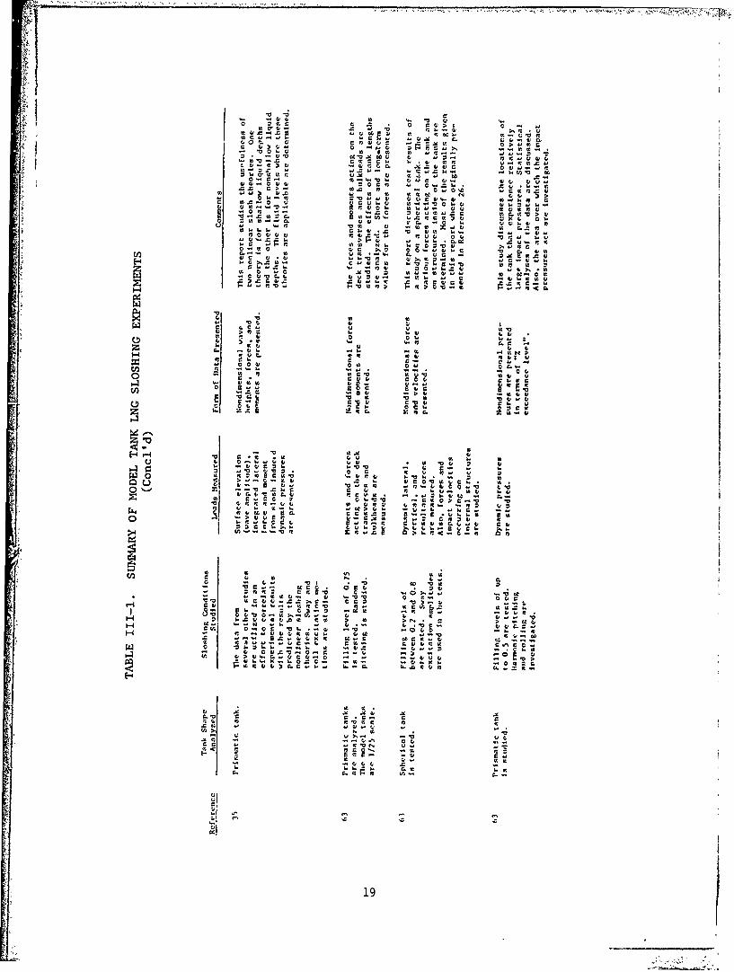
The reports identified by the literature search that contain infor-mation on model tests of LNG sloshing in ship tanks are summarized in TableIII-1. The table includes information on sources nf the reports, tank ge-ometries, test conditions, formats of presented results, and general com-ments and observations. The data contained in these reports were reviL edand analyzed. An attempt was made to reduce all pertinent information fiomthe various reports to a common form for presentation in this report.

A wide range of test conditions is covered by the experimental stud-ies performed to date. Various parameters such as impact pressures, forces,and moments have been measured during these studies. A number of tank ge-ometries, tank motions, and test liquids have also been investigated.

Due to the complexity of the liquid sloshing phenomena and differ-ences in the methods of data acquisition by the various investigators, thedata from the model studies contain a significant amount ok scatter. Forinstance, most of the early model experiments recorded data for relativelyfew sloshing cycles. Later, it was determined (Reference 44) that thesmall sample sizes of the early experiments (N < 200) were not sufficient

13

c 00 101 c)C 44w W00)~l0C r I4C)U0 4L) 4)4 w 0

0 0 I I.1. c " . "a.0 01. m.c id41 c 4))c 4) a' m v. "' C.cC I-

) c be v C 0 0 c f :11-04 0) ) OO C-I 4 )1.0

.I ....C)))4) to) *CC) 0 0 1.4 to z)C4>Ul.4 -0)C toc Cuu - =4)t0v4q.0.g"

0 44))4)eC0 to w r-CC v we4)07v0) 4 .0) V, )0 0 a )4v14m

4) 0 *.61)) 4 x)0 ~ 1. X)0 c ) ma) l 0C~~. v).4 .01 ca Z 4).4 4)))4f-. .0 04 .4r )

cc t: wn4) C L4C01I0 41 C) 4) -4 )04)04)

.0.4))00) cc)U 4 %I.4 <te )) . I~ 11)~1 4) 0 ~ 4) . .0 L,

n))0 c)C 4 4. c) m1. 0 ) W Z vQ4 r. 0 0 0)4.

'A 4) 00 4) 4 4) 14)6

4) 4WC a "C4) 1 )v

f0v u 6 w CL m- &A v)1 . 0

IV IV, W 0 v)). WV0

0j V vV. 40 .u 0- 2: 0 " . IV4

z V6 61) 1 .2 v =.0 0~414)4 >0.4 0.) u c .. 1)4 O14)0 0.

m 0 4).0 ccIIc- 4) v4 C. n1 to In* .1 09

00 4) 0. a) 'A0 ) ) 50.C. c a . .)1 2 w

0 0 Q ) v4 v)~ 1..4 14) 4), K1 4) c)0 6.4 4 4. 40

60 0) ) ) . 4 V) 0 1 0 0-. )4. -!4 V 4 4b. m

4) c ) 4 .0 to.~.4 'A -a 'A

-4 K .4 1. u))1 .4 U .41.00-v)v)4)4c

6- 'C (C. 4)4 41)4 .1 c

41 c.4) .0-4 0,00 0 00 I

*0 .4)4C 0 . q 6o V C

4... l4C '-0 C4 1 -0 c Q-

- I n... CC CC4 lo .41' 0C 1))1

t-4 - C).1. 6- V .. g0 V v 60P.to c P 9 > -0 5 .1 c44 41

4)D N )4 .1 *I) a~ C) 'n z

I ICc Ln ::Cr.I. m

0. 0 0 0 vgoo4o CC C; 4) t)4

r. 1.4)a0

*1.. to 0 .0to

W. 1: 0. Z. 4 co v M -C

14

p I04 no .

04 64 w

C~U z -;0 .0ccVmw )cQ 0 0 r. w- 0. 0v 0 v w .'0 u 044 1 &wx

a140 0040 - m 0 4)4 v Q ; :1 to44>440 p go to 00to4. 04 044L44 14)m

tto11v 0. 04 c wv 4444 410

c 14~ ta 6 -0 m-4 040 044

to040. I4 . 4 0.I. 04 1.4I

04 -0 wc .09 0 4 to4- I "4 040~V vi0 10 m .0 *04. " 1 b04.4 V4w .p

1 u >4314-44 1.00 4I 0 4 00 -044..4

0.01 04404 CL w -.. to 0.4140t4~0 tow C4 v. w4 M 1 0 D 0 0 z 4

u v . 0J .4u4 id0 01 0 0

f. 12 .0 0 00 0 M> .. IVV" . 44 60

0.4004 '...00 v'4 .

0"C 004 c~.

*0 t tor 0

-004

IV a0.p0N ~ 0 0 04

14I 0404

iM u w. .00-

44 nU14 V 044LO

04 b.00 v- 04 =-U4 0 0-4.0u~0 .04 .0 0.4

N ot 0 0 04 04 'Iw t 0r i

W4 a,0 0 00.0to to40.04IC. x E1 044 54 C444 C =0

4100. 0 t 0 u ) 7 1 16

W04 1.!. 44.4 Q ' N0- .o v0 c0 t)110.I a]Q4 0.0 4 - Z44'4 2.0 0 410cc 0 "1 0

040

C4 04 0 Cc~ C3 rx4042 ,O. o 4

150V 0V4

0 0: C

0 r .c, 00w .IM ;S V V w

;.us 0 0.Q Ma9L to0 144 it C ito.4 041 C. jy 0 O

Ch M-0 ~ 9: - 360 .0.3 v.O .0 41 tot 41 U-hatoCa a "u 0) C 0 a ) oo'. > 0 4 y0 M4- W.4 V r 4ra1toOu V UC -0.

.0 ~ ~~ ~ ~ ta. 3 " , .

40,4 "o8 *r a-'Or-aa40 v. wa ma

.a1. -4 41.

001.00pu

I1 v - ac it--g jy.

33; ale 410)1 r

1-4 0 0 h . 0 au 4 bb IAcWOh 0 8-- ~I 414 a3.

hi~~C t41 ah eeraO0 i I 4 .N

o~~f co Ih I

C~- 0041 41 . .

E4 v0.o 0

WW V c C0 t B 4 v a ,0 a t CC Q V

71aV 4 14u.u -00 V i v ~ 1aNOV 06 0% quf.. 0 4.-wC toX C. -a 0 4fl3 l CL 0 V'a . 0 "U C q -!o to V A

r74 40 0w ' 30. '::A fl

*0 0C.

4. 0 N ei w4 .4 14 k 0

u. a - .D o t

0~ ~ * V0 ~~~ 6. v. v011 41 Vai O

cc to .a C 0 .

C; =1 -- a I80 te -- Q 3C C 1.0 ;C.04V1'a 4 0 g -V1 toC g 43..0s a .V.. -a-- c-- C

H ~ ~ ~ ~ ~ ~ t 41C- t . .- ,01 N 0H CVI -0 a tos a No 0 v 4

0 * 4 V C41 . " x -0 x V'M a . a-~ cc0 a 40 .0; &0 g .4u C 4

U*0 Vr-

aV41 >0h 3.4LV~t 0 1; a -

041 c~a 4.00~t aW . iM

16 4

4) 0 33)

1.0 3. t

WO 0. )I

g ' ',.0 to)00 v 14)

0)03 .44430L 0).

1.0 0' 03.) C1

30a 0.0 : .0

to-

11 r v Ob1V) 1Q0 Ov -0 "43 )

c . c4. 3.1)40 .4

to 1 0 Ic

f-in

4)1

1. A.

-3 -c V . 0 4

cn 3 - 3*04 - 04

v09 40. & .0 w

0, 00 , v a C

v. -0 N p0). 4. 21

=6m c. a ... it

66 6 0 0

0~ 0 a~*. 4

6. 0. 94)0

-. g. 3-CC tg

0117

cac

w -u

U~~~- a- N

w 0J

t c

f* ac c a

aa 'A 1)'C

tt a w -

so ~ O P* C L~ -

z 96 C .U 1I U -.. AD *U I

44 I D Z)- a Z '.hC -' Qa 'co c C v o 10

- ICr. ~ D* IAH .0~ ADac; w "ID~, 0 WWD cD le

to c to A 46

vl a a .

a1 *a a;0;

I . !a . 1' l .

izto

0C C to c 0 a

KV; W

Ca 0 v p ou 9.if

H ~ ~ ~ 1 b. U4D~'

C2 c v ~ '.U'0O - - - .~-O ~ o-El

C4 c ~ - a ~ C.4

ID~A.0. DIK .~%~.18 A

rd CC 00 I.

Ce I vC z t ttfc 00 F

C -~~t 0 C- C C

1Q tJ V.- ItC Z1 ctC~ N

C1.CtoWC~ toC003 .' C

IVI I CJ - C C -

C W .'II~ t'A 6C I w0.1 . C U 0 0 0) 0

to t - . C CU O J C L ' >t 'c W C C -0 ti ) I . f ~ t C3 0

ftCIc a c UC Ctta E V00 ~ ~ % UC a~. toU - CfnC2Cl)~~t aC C C 4E1 2 0 CC Ic v caC0 41 u

E-4 'CC0 0

ve ma C CI- 1.4

ft CI C- Cn cI -a 1 1q e00 v0 §a C L

Q a. -. Co1 M C4 v~0 >o v v a .C.r.C. 1 .

.- 2.

41 C. Q-1 U C* S '0C t.C C C ft Ua a t Uf a ' Ct o 2 .s cC V Clo

C4 C- V v a t.it QC C C C.t0-4 Z -- Vl .20 . CW C ft lo-' S0 bCC "C c Zoo.CO

- C..,7 I CC f- c Go ~t Ct C .a0)C Lfff1. W U

o >Co .. l VU .C C.CTI..%0= a

- :: (. V8; 01. 1. C C. -=~r . to

H .. 0UU A v0 to Q... C 6 A

H ~ C -0 ft a'C C - . ~

- .."4 BA. CCKC OC19

for accurately predicting worst case sloshing pressures. Therefore, themore recent studies (containing 200 or more cycles of sloshing data) pip-dict worst case sloshing loads that are considerably higher than earlierestimates.

Because of the inappropriateness of some of the model test results,only a select number of references were chosen for the data presented inthis report. The predicted worst case sloshing loads from the selectedstudies provide a more realistic definition of loads than the early model

test data. The majority of the s-,mmarized data have been extracted fromReferences 9, 10, 44, 64, and 74.

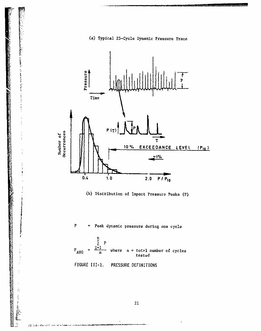
Nondimensional Coefficients

Of principal inportance in many tank analyses is the slosh-induceddynamic impact pressure acting on the tank walls. Figure III-1 shows atypical pressure trace and distribution of pressures taken from labor'torytest data. There are several formats that can be used to present pressureinformation. First, there is the average pressure, PAVG. This value isdefined in Figure III-I as the average pressure for a given number ofsloshing cycles. Next, there is the maximum (worst case) pressure, PMAX,which is the highest pressure occurring during any one of a given numberof sloshing cycles. Finally, there is the "q% exceedance level" pressure,Pq. This is the pressure level which is exceeded by q% of the measuredpressures in a given sample size. For example, the median pressure wouldbe the 50% exceedance level. Much of the data presented by Det norske

Veritas is presented in this form.

For simplicity and uniformity, the pressure results presented in thisreport are in nondimensional form. The nondimensional pressure is denotedas Kp. The pressure value used in Kp is either the average pressure (AVG),maximum pressure (MAX), or thL "q% exceedance level" pressure (q) as indicated.The pressure has been nondimensionalized using Froude and Euler scaling asdiscussed in References 44 and 74. The resulting nondimensional pressureut is defined by the following relation:

K P P

where P = dynamic wall impact pressurep = liquid densityg = acceleration of gravityZ = tank length in the direction of the tank motion

= -glar excitation amplitude (in radians)*x = translational excitation amplitude (in units of length)

*Single amplitude value

Another important parameter to the design analysis of a tar,. is theinertial force created by the sloshing of liquid in the tank. A nondimen-sional force, KF, similar to the nondimensional pressure has been developedfor the presentation of experimental force data. Measured peak sloshing

20

(a) Typical 25-Cycle Dynamic Pressure Trace

Pt -BI 14

Time

Tt I 10 1 EXCEEDANCE LEVEL (Ptp)

0.4 1.0 2.0 PI P10

(b) Distribution of Impact Pressure Peaks (P)

I

P Peak dynamic pressure during one cycle

nI P

P I where n totpl number of cyclestested

FIGURE III-I. PRESSURE DEFINITIONS

21

forces do not exhibit the cyclic variations typical of localized impactpressures. As a result, the average peak force (F) measured over a givennumber of sloshing cycles is representative of the peak force occurring onany given cycle. For a prismatic or rectangular tank geometry, this non-dimensional force is defined as

F FK g or (111-2)F pgkhb pghbx

where F = dynamic force (only inertial forces caused by the liquidare included)

h = liquid filling heightb tank width transverse to the direction of the tank motion

For a spherical tank, dynamic impact pressures are not of criticalimportance to tank design.(2 4,4 4) However, the tank forces created by theinertia of the sloshing liquid are significant to tank design. The nondi-mensional force coefficient used for spherical tanks is defined as:

KF Pg (111-3)

where F = dynamic force (see Figure 111-9 for the definitions of thevarious forces)

V = tank volume

From Froude scaling, the nondimensional time is defined as:

KT T/g7 (111-4)

where T = time.

In addition to resonant sloshing periods, slosh-induced dynamicpressure rise times are normalized by Equation (111-4).

Table 111-2 provides equations for calculating the natural period,TR, of liquid in rectangular, spherical, and cylindrical tanks as a func-tion of fill depth. These equations are derived in Reference 1.

Statistical Analysis of Slosh-Induced Pressures

Because of the random nature of resonant sloshing in an LNG tank, asufficient sample size must be determined that will give a representativedistribution of peak sloshing pressures. References 44 and 64 have both

addressed this problem. These two references used somewhat different ap-proaches to obtain similar results.

22

TABLE 111-2. EQUATIONS FOR CALCULATING LIQUID NATURAL PERIODS

IN RECTANGULAR, SPHERICAL, AND CYLINDRICAL TANKS

Rectangular:

27r

TR

tan1h (Trh)

Spherical Tank:

4hTR = T - for (0.05< 1.0

R g D

with the values of C1 shown on the figure below.

1.0-

IIa. .8 1.2 1.6 ,

hlR

h = liquid filling heightR = tank radiusD = tank diameter

Cylindrical Tank: (Vertical orientation)

T~ 21r

TR = 7.664 <D tanh [7.664 W)]

23

Reference 44 recorded 1000 cycles of resonant sloshing pressures.Then, the largest number of consecutive peak pressures less than 85% of themaximum (worst case) pressure was determined. This number varied from 140to 160 cycles. Based on this information, a sample size of 200 cycles wasconsidered representative. Histograms of the 200-cycle and 1000-cycle testdata are pictured in Figure 111-2. The distributions are quite similar inshape, indicating good repeatability between a 200-cycle sample and a 1000-cycle sample.

In Reference 64, various sample sizes up to 400 cycles were evalu-ated. It was determined that 200 cycles were required to give good repeat-ability of the average pressure for a given sample size. The results ofReferences 44 and 64 show that: (1) 200 cycles are adequate to define theaverage sloshing pressure (PAVG) and (2) that the worst case pressure(PMAx) will be at least 85% (or greater) of PMAX for 1000 cycles of slosh-ing.

Reference 44 developed a theoretical pressure distribution for pre-dicting extreme pressure values. This distribution was based on a three-parameter Weibull curve fit. The resulting equation is:

Q(P) = exp - AO M (111-5)

where Q(P) = the probability that the response variable will begreater than P

P = dynamic pressureAO,A,M = experimentally determined parameters of the distribution

Utilizing this distribution, Reference 44 presents a procedure for estimat-ing long-term distributions of slosh-induced dynamic impact pressures oc-curring during the life of a ship. This procedure is based on the statisti-cal analyses of the slosh pressures and the tank excitation motions.

III.1.1 Prismatic Tanks

Model scale data for slosh-induced dynamic wall pressures vary con-siderably with test conditions. While the general nature of resonantsloshing in prismatic tanks of various geometries is similar, the impactpressures for a given tank can vary significantly with wall location, ex-citation motion and amplitude, liquid density, and fill level. Since itis impossible to measure all possible combinations of these parameters, thecomposite of the sloshing pressure data from all sources is presented sothat the range of load coefficients can be established for design purposes.

Figure 111-3 shows the highest (for any measurement loeation) KPAVG vs fill

level (h/) for a range of excitation motions and amplitudes, tank geome-tries (all are prismatic or rectangular), pressure transducer locations,and test liquids. All points on the graph are for resonant sloshing con-ditions. The KPAVG ranges between 1 and 25. No distinct relation between

KpAVG and the liquid filling level is noted.

f24

.44

ui Ln

D~~ r- u C*-')

0 <,

0 CC)

-J C W n~

U. 0

-- CD

L4 cm

mu.CN 0, -

JC)

0 0

-. r. 0Co 0-

U) w)

z~~C UO0a. )-- a. L.

0- V) 2 0~.fl Ll 1 -

ww

LL

wew

W-JL

__ _ _ _ _ _ _ _ _ _ _ _ _ LL z )Vz 2lUsauaajnz~zOo

go iaqtuin

25

30.0

25.00

20.0

00

0

0 0 0

10.0

0

0 0

00

5.0 0 0 0

0 0

0 0

0 00

00

0 0.2 0.4 0.6 0.8 1.0

h/L9

Kp nondimensional pressure coefficient Caveraged over manyAVG cycles)

h -liquid filling height

9. tank length

NOTE:

Pressures are highest measured values for any test conditloisregardless of tank motion, tank geometry, transducer location,and test liquid.

FIGURE 111-3. HIGHEST AVERAGE NONDIMENSIONAL PRESSURE VSNONDIMENSIONAL TANK FILLING LEVEL FOR ALL MODEL TESTSRUN TO DATE

26

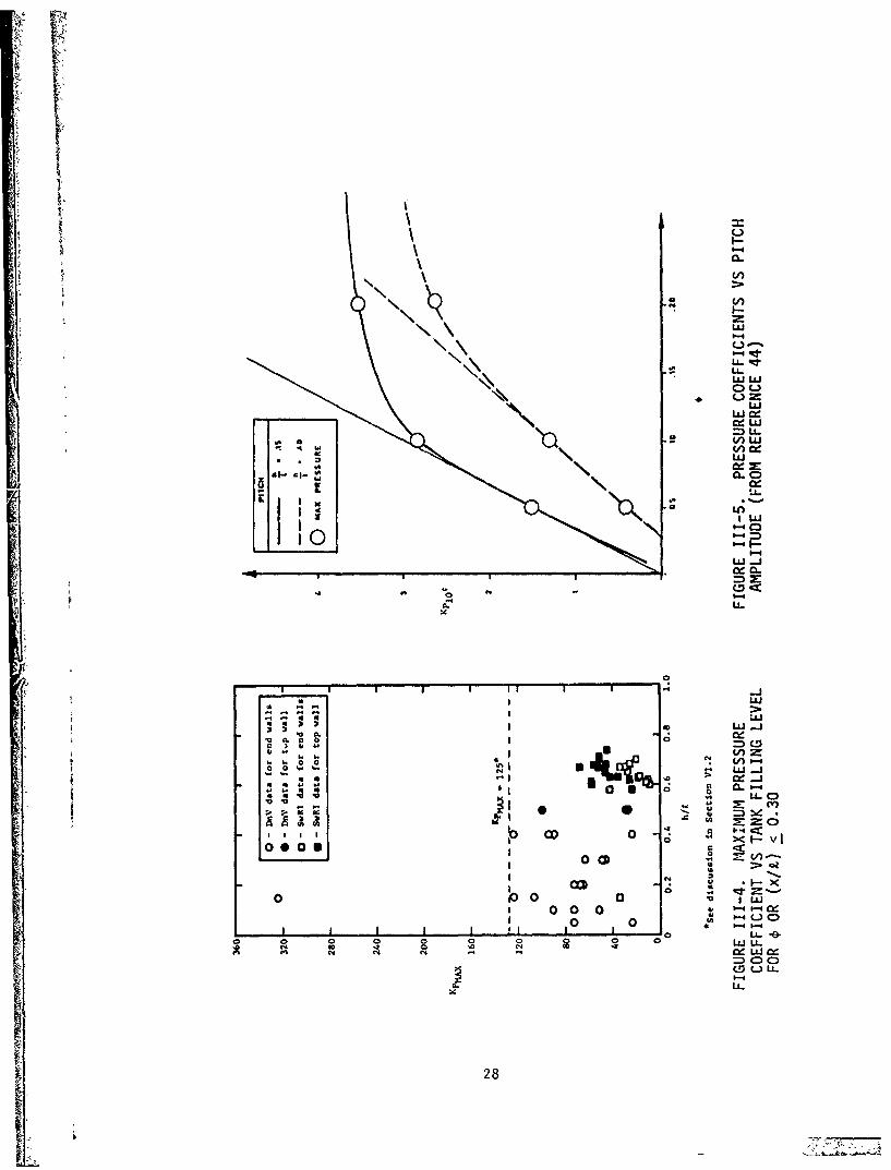
Ranges of KpM X values compiled from the model-scale data are plot-

ted in Figure 111-4. These values are for nondimensional excitation ampli-tudes from 0.05 to 0.30. It should be noted that the data points on thisgraph are worst case values for at least 200 cycles of resonant sloshing.As the filling level increases, the location of the highest pressure movesfrom the vertical walls to the tank top. Otherwise, no clearly definedtrend of KpMAX with h/ is noted. The location of highest pressures on the

vertical walls is usually near the static liquid filling level, while onthe tank top the highest pressure occurs near the corners.

Except for one data point, all KpM~ values on Figure 111-4 range

between 10 and 125. The Kp value of 325 is considered unusual since theother data points represent a wide range of sloshing conditions coveringseveral sources.

The form of nondimensional pressure coefficient equation, EquationllI-1, reveals that the pressure P is assumed to be a linear function ofexcitation amplitude, 4 (i.e., P = Kppgt4). In actuality, pressures areonly a linear function of 4 for amplitudes less than -0.1. Figure 111-5from Reference 44, exhibits pressure vs amplitude data showing this trend.It is evident from Figure 111-5 that as 4 approaches 0.3, the slopes of theKplo vs 4 curves approach horizontal. This means the influence of the ex-

citation amplitude on the impact pressure dimiaishes as the amplitude in-creases. The relation between Kp and 4 exhibited by Figure 111-5 is typi-cal for all areas of the tank that experience slosh-induced impact pres-sures. Thus, if pressure coefficients obtained at experimental amplitudesless than 0.1 are used to predict pressures at larger amplitudes, the re-sults will be conservative.

Figure 111-6 presents sloshing force coefficient data summarizedfrom References 9, 10, and 44 for a range of amplitudes. Figure 111-7 showLthe same data for a given amplitude (±80). The data indicate that the forcecoefficients decrease as the filling level incteases. However, the actualforce will not necessarily decrease with h/k as a result of the definitionof KF (i.e., F = KppgZ 2 (h/k)4)).

Table 111-2 presents an equation that predicts the resonant periodof the liquid in a rectangular (or prismatic) tank. Nondimensionalizing theequation from Table 111-2, it becomes:

(T ' )RESONANCE 47 ftanh y )j (111-6)

A comparison (Figure 111-8) of the resonant periods calculated from thisequation to measured periods from the model tests for a variety of pris-matic tanks indicates that the theoretical values correlate well with theexperimental results.

27

VVIL17.li

LL.

=LL.

w

K 1 0w -j

-J

0w - C

LI.

a

3 *0 . C)

' - e VI

00 0- 0

II . LI LL.OOr! w (Y C

=)C)CCD U zoS I I .

28 0 *

I.L Ul 000

0- +

-j 0

0L

+Iz.LL.

-= V) ---

I w

u -J

-~0 o

0 0 0DLL0 0 00

0 0h4

00 t04

29

00

600

-LJ

0 0 w. L44 4-4

0

Aj a 41VV '-

-Li ex' U'-1 0

'IV:

o 0 U0

E-4

C6- CV 01-4J- -Ij.

CV CV 4.

0. 00

300

The information presented in this section covers the important con-siderations in the design of a rectangular or prismatic tank. Topics suchas scaling criteria for model tests, random excitation motions, statisticalanalysis of cargo sloshing, and several other problems related to cargosloshing in LNG tanks have also been addressed by various investigators.Their works are listed in this report in the Reixrence List of currentlyavailable literature.

111.1.2 Spherical Tanks

As previously stated, forces and not impact pressures are of primaryconcern in the design of a spherical LNG ship tank. References 24 and 44present a thorough set of data on sloshing forces acting on a sphericaltank. The data presented in this section are excerpted from these reports.

The pertinent forces acting on a spherical tank are defined in Fig-ure 111-9. Figures III-10 through 111-17 show typical force magnitudes forvarious tank filling levels and excitation amplitudes. All data compiledwere obtained using a horizontal tank excitation motion. Reaction forcesproduced by pitch and roll motions about the tank centerline were not re-ported. The authors stated that the reaction forces produced by pitch androll are small relative to those produced by horizontal motions.

The following general trends were discovered during the analysis ofthe test data. The maximum lateral force usually occurs under the sameconditions as the maximum resultant force. The direction angle, a, of theresultant force is greatest for h/D less than 0.2. The angle decreases ash/D increases from 0.4 to 0.6 and remains about conscant for h/D valuesabove 0.6.

The lateral force attains its maximum value when h/D is greater than0.8 for large amplitude excitation motion (large amplitude being n/D greaterthan 0.05). The maximum lateral force is about equivalent to the inertialforce of a full sphere. For small amplitude excitations (n/D values near0.01), the maximum lateral force occurs when h/D is about 0.5.

The maximum resultant force is nearly equal to the weLght of liquid4contained in a full sphere. This maximum occurs during the same conditionsthat create the maximum lateral force. These maximum resulting and lateralforces occur at relatively high excitation frequencies.

The maximum dynamic vertical force occurs when the filling level ofthe tank is about 0.4. However, the maximum static plus dynamic verticalforce is created when the tank filling level is greater than 0.8. The maxi-mum static plus dynamic force is about equal in magnitude to the maximumresultant force.

The resonant slosh frequencies for the liquid in a spherical tankvary substantially depending on the filling level. High filling levels

31

- ------

--

0 0 0 w000,

wr- -

4

.lLL

u-hiw

w Gw- 4 3.

cm)

w -j

U S.

l i 0- ha

w Z -D

9 30 2hi~~~~ .3li 3 tt

20U 20

* .c

4L4

UU

UL-

32

1A hI:0 3

T I mO0 hID 0O, hiDsO :

1/01/00 a- shis

1 0 10:0 7 0hio o10 a k

S0 NTURAL SLOSH III1 + $PERIIOD. KF 1 11 -

~ 0 .

5 -. - : ma roo -o -r

-T - ISECIT AI ER O t-bib0 0 l-, O

po ll IFL AGO#t*,1

0 0 11#0 loot

___"__'L /

A-02

FIGURE III-1l. RESULTANT FORCE ON oSPHERE VS EXCITATION PERIOD /,(Reference 44)

0 .10 04 I @4 lo

_______ FIGURE 111-12. LATERAL FORCE ON SPHERE

VS FILL DEPTH (Reference 44)

WI&AL 0 oacE

0.10 - .

,.0 Lo 6.0

jf 1SAIUMAL LOI.. 1100111(1 i

FIGURE 111-13. LATERAL FORCE OlSPHERE VS E.',CITATION PERIOD(Reference 4,') 3 +1

33

0 00 w - *0' 0 u

In0

w

LO0.

0 U

0 0 -r

p~0 U..-

C)

_ _ I0 w

00

0 000L~

rj34

-4;-

0Ito

000 -U 0

a .0

0 0 0~~0 uj

S 3o-.4 0

oY-\,.-Q -

0 , L-

I-aL A -. %- -1 -W

Ir '--

J. V) u

q - 0 P-4

v I WW4

4, "4 , 40

0 0 0 0 C 0 0 I

00 0/

In

0 >-u.

i Cl 0

it35C

have resonant frequencies high enough that the ship motion energy in thisfrequency range is so low that resonant sloshing is unlikely to occur. Forlower filling levels, the liquid response often corresponds with the ship'smotion, causing resonant sloshing to occur in the tank.

The resonant sloshing period-s predicted by the equation for spheri-cal tanks from Table 111-2 are shown in Figures 111-11, 111-13, and 111-16.

111.2 Full-Scale Sloshing Data

Full-scale sloshing data are very scarce. The LNG carrier, the BenFranklin, has been instrumented for recording slosh--related information,-but the ship has yet to go into service. Two El Paso larine Company car-

riers, the Sonatrach and the A have also been instrumented, but nodata are available at this time. Full-scale data on the slosbing of fueloil in a tank with no internal structures are presented in Reference 42;however, this information is only of very limited value to the problem ofLNG sloshing in ship tanks. Full-scale impact pressures measured with ;a-

ter sloshing in an OBO tank are compared to model scale pressures in Refer-ence 2. The model data were obtained in a geometrically similar 1/30 scaletank with the recorded full-scale roll motions reproduced on the model.Pressures in model scale were converted to full scale using Froude scaling.A comparison of predicted to actual pressures showed excellent agreementfor both the magnitudes and distributions of pressures.

111.3 Review of Tank Structural Detail

A general description of LNG tanks was given in Section II. Theimportance of sloshing-induced forces in the design of the tank depends

largely upon the tank type. For this discussion of tank structural de-tails, it is convenient to divide the tanks into two general categories:pressure tanks and nonpressure tanks. Nonpressure tanks include membrane,semi-membrane, and independent prismatic tanks. These tanks are con-structed primarily of plane surfaces and are designed for low vapor pres-

sures. Design for low internal pressures, particularly near the tank topwhere the liquid head is a minimum, makes these tanks susceptible to local-ized sloshing pressure in this region. Also, prismatic tanks with planesurfaces are more likely to experience high liquid impact forces duringLNG sloshing than, for example, pressure tanks with curved boundaries.

In contrast to nonpressure tanks, pressure tanks are designed forhigher internal pressures, approximately 3 to 10 times higher than for non-pressure tanks. In addition, as reported by DnV,(24) impulsive sloshingpressures are unlikely to occur in pressure tanks because of their curvedboundaries, and the limited measurements which have been made indicate that'the pressures are low. Another factor is that pressure tanks which arespherical or cylindrical in geometry will react to the sloshing pressures,even localized ones, primarily with membrane action (as opposed to bendingaction in tanks with plane surfaces), and thus pressure tanks are less sus-ceptible to damage from local sloshing pressure if they do occur.

36

Pressure tanks' structural arrangements are much simpler than tanksconstructed with plane surfaces. The structure consists principally of asmooth wall sphere or cylinder of relatively heavy gauge (1/2 in.). Attach-ments to the tank are made only at its support points and at filling loca-tions. A nonstructural insulation is bonded to the outer surface of thetank wall. The most widely used LNG pressure tank is the Moss-Rosenburgsystem. This system uses an aluminum spherical tank which is attached tothe ship by a cylindrical skirt at the equatorial ring (see Figure II-2b).A discussion of design loads for this tank by Glasfeld(2 3) indicates thatsloshing forces influence only the design of the tank support.

As indicated above, nonpressure tanks are more likely than pressuretanks to experience high sloshing pressures and to be damaged by them.Since the structural details of pressure tanks are not unique, only themore complex and unique aspects of LNG prismatic tank structures will bereviewed. The structures of two types of membrane tanks and one independentprismatic tank are described in the following paragraphs. These tanks arerepresentative of the range of designs of nonpressure type tanks which arebeing built today.

111.3.1 Membrane Tanks

Gaz Transport Design. In the Gaz Transport membrane system, invar

membranes are supported from plywood boxes which are filled with Perliteto provide thermal insulation. Two layers of boxes are used, primary andsecondary. Primary boxes are on the inside of the tank adjacent to the LNGand support the primary membrane. Primary boxes are separated from the sec-ondary boxes by the secondary membrane. Both secondary and primary boxesare directly attached to the ship's hull, but compression forces on the pri-mary boxes are transferred to the hull through the secondary boxes.

The geometry of a 12-cell box is given in Figure 111-18, and thefarrangement of the insulation boxes in the tank is shown in Figure 111-19.

Attachments of the boxes to the hull are not shown. Primary boxes haveboth a 9-cell and 12-cell construction. Twelve-cell boxes are used inareas where maximum overpressures are expected. All secondary boxes havenine cells. Secondary boxes bear directly against the inner hull of theship on the bottom and sides of the tank, against transverse bulkheads(cofferdams) at the tank ends, and against the bottom of the trunk deck atthe tank top. An example of this type of structure is shown in Figure111-20. It is a section of the cofferdam near the top of the tanks. Localstructure between vertical webs is plating stiffened by bulb angles.

Sloshing pressures on the membrane apply loads directly to the coversof the primary boxes. These forces are transferred principally through thelongitudinal (parallel to the box axis) stiffeners in the primary box tothe transverse stiffeners in the secondary boxes at the stiffener crossingpoints. This can be seen from Figure 111-19. Transverse stiffeners in thesecondary boxes transfer the sloshing forces to the ship's hull. As shown inFigure 111-23, each stiffener in the cofferdam bulkhead reacts the loadingfrom approximately two box widths. Because the insulation boxes are verystiff (loads are transferred through bending of the covers in the 12-cell

37

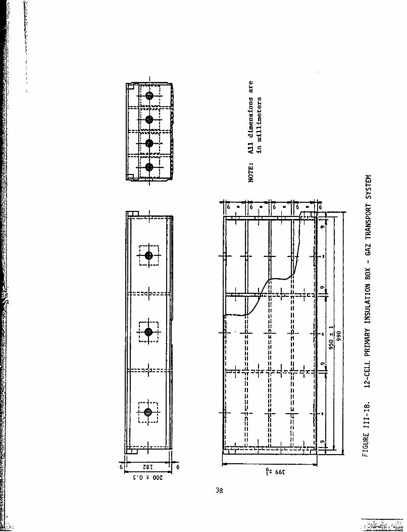
&I r. 0

I

ITC

- -j....0-

6 6

I0 Ia

LMait-

ItI

I~tuu

------ 0.z

I Ci-

Ll C6

n0

4--6--910 ooz-qm 66

38I

rt

-LA I

9-LJ- +.- 2

I~:=CZ >1 I '.-.

39 s- -- U )

1UPPER DECK

AREA OF AI TYPICAL BOX

HP 280 x111I

1 I - 800Onm (31.5")

---------- +- - - -.- --

15mim (0.59")- - I -STL. PLT.

15.5 nmm (0.61")STL. PLT.

(94.5")(TYPICAL)

A -NJ SHIP C

COF COFFERDAM

11 mm (0.43")13 mm (0.51")ST. L.STL. PLT. T.P .

6625 mm(260. 33")

SECTION A-A

FIGURE 111-20. SECTION OF COFFERDAM BULKHEAD FOR GAZ TRANSPORT TANKS

40

box and through compression of the stiffeners), the sloshing forces willbe attenuated very little at the bulkhead. Structures which must be ana-lyzed for sloshing pressures include the primary box covers, stiffenersin the boxes, and local stiffened plates in the hull. Because sloshingpressures are localized, occurring only near the static liquid level, over-all bending of the ship's bulkheads is not a problem.

Technigaz Membrane System. As in the Gaz Transport system, a thinmetal membrane is attached to an insulation system, which in turn is at-tached directly to the inner hull of the ship. In the Technigaz systemthe secondary membrane is a continuous plywood barrier.

A section through the membrane and insulation of the Technigaz Sys-tem is shown in Figure 111-21. The insulation and membrane support in thisdesign consists of:

(1) An end grain balsa pad which is adjacent to the membrane,

(2) A thick sandwich panel built with plywood surfaces and balsacore,

(3) Grounds which are attached to the ship's hull and whichsupport compression from the balsa-plywood panels,

(4) Glass wool which fills the voids between the sandwich paneland the ship's hull and between the grounds.

Structure in the ship's hull which supports the membrane system is similarto that for the Gaz Transport design.

Sloshing pressures on the membrane bear directly on the balsa pad.

These forces are transferred into the balsa-plywood panels, producing bend-

ing in the panels between the grounds and shear reactions at the grounds.The grounds transfer the shear reactions in the panels to the ship's hull.Compression in the balsa pad, bending and shear in the panels, and localdeformation of the ship's hull must be checked for adequate strength toreact to the sloshing pressures.

111.3.2 CONCH Independent Tank

The CONCH LNG tank system is designed to contain the static and dy-namic pressures produced by the LNG independent from the ship's hull. Itis keyed to the hull to prevent translation and rotation relative to theship. Glass wool fills the void space between the tank and the ship innerhull (between the supporting blocks). Tanks are subdivided into approxi-mately four equal volumes by centerline and swash bulkheads. Constructionof the tanks is similar to that of a ship. Bulkheads and tank walls are

constructed of flat plates which are reinforced by stringers and girders.typical horizontal girder (horizontal section through one of the tanks)

is shown in Figure 111-22. The weakest parts of the tank appear to be thelongitudinal and swash bulkheads, the sides of the tank near the top, and

the tank top. These parts of the tank have 0.50-in.-wall thickness and the

41

3.4mm SUGAR MAPLE PLYWOOD

12mm BIRCH PLYWOOD

F 80mm (TYP)j

S. ..j' . . . . ., . .. ... . .. I - _ .-

.......... ... ........./1 wooRY GROUND

-- ' -... . L-I.7. \ . :S" x .. " o .

=~ ~ ~ ~ m (TYPICAL)m inTLPAE HIKES

WOOL SECONDARY GROUND

A42

Level 1 00

~ i.-i;ILevel 4

INNE HULL.a

4 -170.4mm ~ ~ ~ ('A PAE HIKES

SETO 31B B .

FIGUE.11.2. TEH A MEMRAN SYSTE

.................................

-Get I

. '..'-, , 1

r , r ' I s -i pihI bI

434

widest frame spacing. Figures 111-23 and 111-24 show typical vertical sec-

tions taken in the longi:udinal and transverse directions, respectively.

Both the frames and stiffened panels between the frames of the tank

must be checked for damage to sloshing forces. This is true for the tankwalls, bulkheads, and tank top. In addition, tank supports must be analyzedfor the reactions produced by the resultant of the sloshing forces.

44

WcATIDOWAIT1.t.4O Imouk "' .L 001 Ito"~~Mma. \

*~~~~~~LM 2if.t E IR N9?O. 1~P ~ %f

I i'r~~~mi~~.iS -?tE~G OdT ~ R tIo.\ ;

fr~ m'us 1 100 sw- T o V 0 1or5T

(SICA. 4r'P)

00 V's c* L OT '

'I rT~c~ 1, -1 1 1 1 o

FIGURE 111-23. TYPICAL LONGITUDINAL GIRDER

45

lIQUID71471

B UI.KWeAc)

1 10CA7t TWXUUU * T .

AS)WOWN ON PLAN VlleW

PrFAM114t

J ~ ~*1t -- -. v SHME'

FIGURE 111-24. TYPICAL TRANSVERSE FRAME

46

IV. TASK 2 - EXPERIMENTAL STUDIES

IV.l Experimental Study Objectives

As a result of the Task 1 review of previous experimental work, thefollowing experiments were performed.

o Combined degree of freedom excitation (pitch and heave,surge and heave)

o Impulsive pressure-time history measurements

0 Dynamic loads test on full-scale LNG tank structuralsegments

Previous studies provide loads data for a wide range of tank geome-tries, fill depths, and excitation conditions. Previous studies were con-ducted by exciting the model tank in only one degree of freedom (usuallypitch, roll, or surge) and recording loads at resonant sloshing conditions:To determine if combined, simultaneous excitation in more than one degreeof freedom would increase the sloshing pressures, additional two degree offreedom experiments were performed.

The impact pressure-time history is of importance to the prismatictank wall structural design. Previous studies determined peak pressuremagnitudes and distributions, but little data were available on pressure-time histories. Additional experiments were performed to establishP(T) vs T characteristics.

To substantiate the analytical procedures developed in this studyand to evaluate the response of LNG tank wall structures to dynamic sloshpressures, typical full-scale dynamic pressures (predicted from the modeltests) were applied to a representative section of a full-scale LNG mem-brane tank structure in a set of laboratory tests.

IV.2 Experimental Facilities

IV.2.1 Model Tank Sloshing Apparatus

The laboratory work on this project involved sloshing liquid in

scale model ship tanks and measuring slosh-induced dynamic pressures. Thelaboratory facilities at SwRI include two slosh rigs designed for this pur-pose. One machine is capable of producing an angular motion (to simulate

pitching or rolling), and the other can provide independent and simultane-ous horizontal and vertical motions (to simulate surge or sway, and heave).Appendix A provides a detailed description of both these sloshing systems.

IV.2.2 Sloshing Pressure Measurement System

Sloshing dynamic pressures were recorded with Columbia ResearchLabs' Model 100-P piezoelectric pressure transducers in combination with

H47

Model 4101 amplifiers. These transducer/amplifier combinations have a rangeof 0.005 to 4000 pounds per square inch, with a frequency response from 0.1to 10,000 Hz. Transducers were isolated from the walls of the tank by mount-ing them in a plug of silastic material. The silastic eliminated the possi-bility of the transducer casing being loaded by flexing of the walls of themodel tank.

The pressure signals were input to a light-beam galvanometer-typeoscillograph. The oscillograph produced a permanent record of the pressuresignals on oscillograph paper. The oscillograph is a Honeywell Model 1858-0790 G Visicorder oscillograph with a frequency response from 0 to 3000 Hzwith +0% to -5% error. A Hewlett-Packard Model 9864A digitizer in combi-nation with a Hewlett-Packard Model 9830A computer was used to digitize thepressure signals from the oscillograph traces. The digitized pressure val-ues were stored on magnetic disk files for final data reduction.

IV.2.3 Model Ship Tank

The model tank used for all laboratory tests is a 1/50 scale replicaof a prismatic tank from a 125,000 m3 LNG carrier. The tank geometry istypical of most prismatic tanks. The model tank walls are made of plexiglasswith sufficient rigidity such that tank wall response was not a factor in thepressure measurements. Figure IV-l shows the tank and all pressure trans-ducer locations. Table IV-l lists the model scale and corresponding full-scale tank dimensions. The pitch axes for the 25% and 75% tank fillinglevels investigated are denoted in Figure IV-1 as zpl and Zp2, respectively.

For all tests, the model test liquid was water.

IV.3 Combined Degree of Freedom Model Tests

As part of Task 2, the effects of combined tank motions on sloshpressures were investigated. The purpose of this work was to determine ifslosh-induced pressures were augmented by combined motions.

Experimental tank motions included pitching plus heaving and surgingplus heaving. The results for these motions were compared to the resultsfor the individual motions of pitching, surging, and heaving. Low (25%)and high (75%) tank filling levels were used for each case. All laboratorytest motions are summarized in Table IV-2. The detailed test results aregiven in Tables TV-3 through IV-7, with the data summarized in Tables IV-8

through IV-lI. The excitation amplitudes were chosen to represent typicalextreme values that a ship tank might experience while in service. Eachtest was run for 200 cycles at resonant sloshing conditions, while the tankwas undergoing a harmonic excitation motion at resonance.

IV.3.1 Pitching Plus Heaving Test

The angular motion sloshing facility was used to provide the pitch-ing plus heaving motion. The ocale model ship tank was placed approximatelytwo tank lengths out from the pitch axis on a cantilevered beam. This lo-cation represents the typical placement of the fore or aft tank in an LNGcarrier with its pitching axis at the midship. Figure IV-2 shows the loca-tion of the model tank with respect to the sloshing rig axis.

48

Ib15

H

'1411

13 14499Imi1

Pitch6

2 x3

-. 0 -Denotes pressure transducer location

AFIGURE IV-I. SCALE MODEL TANK DIMENSIONS AND PRESSURE TRANSDUCERLOCATIONS FOR 1/50 SCALE PRISMATIC TANK FROM A 125,000 m3 SHIP

{4[ l

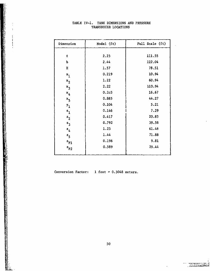
TABLE IV-I. TANK DIMENSIONS AND PRESSURETRANSDUCER LOCATIONS

Dimension Model (ft) Full Scale (ft)

£ 2.23 111.55

b 2.44 122.04

H 1.57 78.51

x 0.219 10.94

x 1.22 60.94

x 2.22 110.94

x 0.333 16.67

x5 0.885 44.27

Yl 0.104 5.21

z 0.146 1 7.29

z2 0.417 20.83

z3 0.792 39.58

z4 1.23 61.46

z5 1.44 71.88

z 0.196 9.81

Z 0.589 29.44

Conversion Factor: 1 foot 0.3048 meters.

50

TABLE IV-2. TEST CONDITIONS FOR COMBINEDMOTION LABORATORY TESTS

Tank NondimensionalTank Motion Tank Amplitude Filling Resonant Slosh Period

Level (T /7)

Pitching +4 25% 5.170

Pitching u+40 75% 3.566

Surging x 0.019 25% 4.869

Surging - 0.019 75% 3.663

Surging x 0.038 25% 4.,69

Surging x U 0.038 75% 3.663

Pitching + Heavig 0 -+4* and 7-- 0.417 25% 4.748-H

Pitching + Heaving +40 and - 0.417 75% 7.235

H (2rd Harmonic)

Surging + Heaving 2E- 0.038 and Y- 0.053 25% 4.869

Surging + Heaving 0.038 and H= 0.053 75% 3.663

See Fiires IV-I and IV-4 for definitions of x, y, 1, H, and *.

51

Lr

cc 0O N N N N N N N N N N N N N N

.. . . . . . . . . . . . .

O(OWi Lo in w' 0 N 1) m CO ) m 0I 0 ' Nd

cc Z0 40U6 N 0 N NO ID V)

0 . 11C

~~0 NDNNUNU N m1

.1 0 0 C) h 0' 0 I 00

U. w.

404

X,~ C- I

w~ ~ ~ ~ ~ ~ Q' w 1 ) .LoN c

* w g t. . 0 0

iLOw

*L ( wQ 040 C) 1 N f- N f.4 .N N N M~~'

CIJ 0: C, CI 0

52

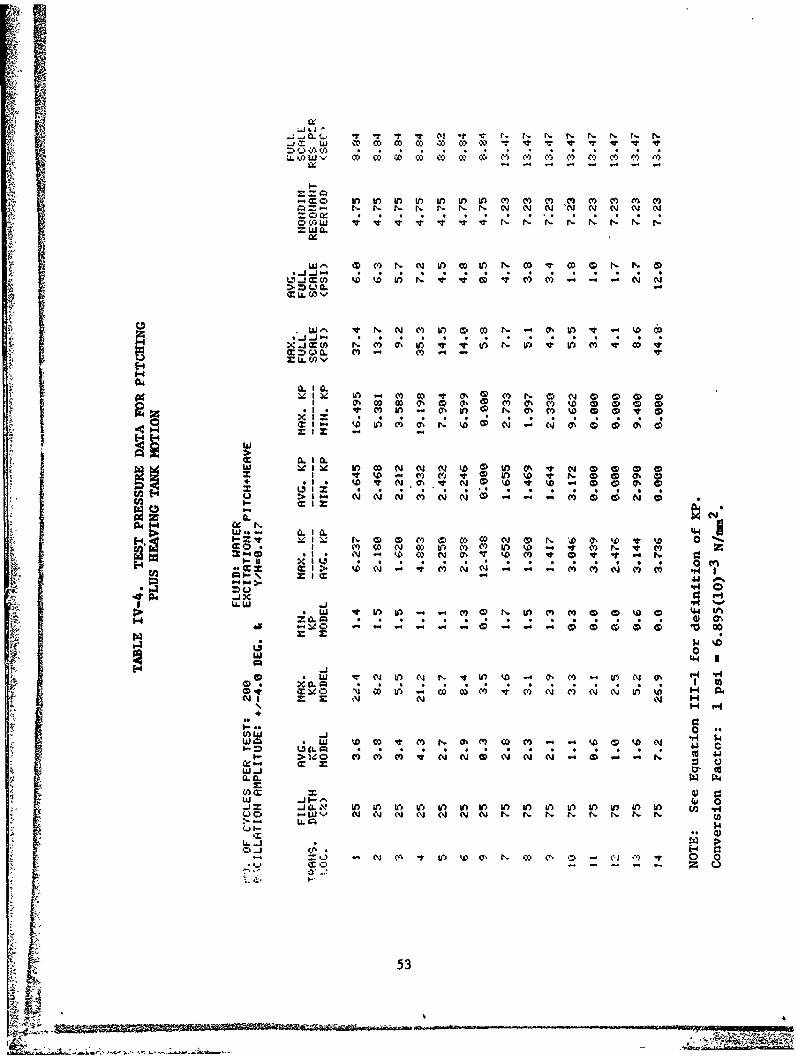
49

-MO' to 0 to If) 1 I i I CV) (V) C') m' CV) CV) m) CV)

= =- N N P. N N N N. Nl kv 0i N~ Nl N C1

OC) Q. C. t, (1 Lo N0 Nn Nl o O N ' N to

L-..JC ) W0 k V) N It IT ' (5) It c ') .4-4. N N

C, ' N N C) U 0 0 N Ch U) v W4 6C'

I-I X.J M 0 N C') 0' )?? U )? U C')' CO~C =0Q . C') - 0 4EU.O'W

'-4

Ch 00 00 C h (S M C') 0 W '0 a'0 CDF1 z (V) ON- W ) ON th M' W' CD CD0t10[I I tp U!. 0000

w wI U '0 U) CN N N w 0 0 v4 N' 0 0 0 0

f4 4D I' 00

W.. I. 1 CL 4 4 4

b-Z'? 111 N 00 CD ') ap ) c N 0O(i ( N wD 0.(V I C) 0 N O 0) () U) ko -4' % N 't 0z(D4 .1. 1 kD MN t'' 0 r' f0' f.N 9I-.II IL ' . * * * * * . * * 0 CO)

(4 .; C;

Q . . . . . . . . . 0 I. 40 .44. - 4 00 0 100O

IQ44

C0 W a ' N U) N N vU 0 kD c" 0'- U) N

CD' MI N 0; C; 140W IM C-4

*441LD CL. in . . . . .0* l Ia ' 0 C) N C-i qCD) 0 CIA *.4 '00 QO

IL CL CL W 4r

I- > C') N ' ' N N N N 4 ~

Z i

k ) I CA) - U) I) W)f U) 0) U t ) In U i i

LIF.

-j CL Q N t. N N N N N N N N N N N N N-im wD o lz i, 0 (p O0O00 0 0 0 0 0 0 C C O

Z 4 . 0 (.( I I 0 I0 I0 Io Io . I0 I * I

0)

Co ' CO co w O co 0 w w) w0 w w w0 w 4D w

o CZILU(.

W' 4 O 0 0 N W) OD v~ oQ% CD It V In N It-1 J I t I . . . . . . . . 4 . .

XM) N (Y N %D 40 m D W N 0; 'ON W C;% 4 Ncc 0 04 M440

ZIZ 4 N N 4

c I ' NOW 0,0% 00 Nn w- 000I r % O 0 0 . 0 4 N 4 0

Ia.. C.91.41.

X 00OD000% V% CD w0 -'N w ) '0 N3-.. N In O~ 0 -40 I N C4% a. 11 0 N0 4 * 4 V; 4 4 V * 0* ; v; II = Q

V.. JX

4L 0%M v 00- 0 N v 0 w 0 0

N% 4C3I 0 m 0 0 IN 0 m0 '. 0 m w N N o m~ NC0x : LQ . .It

>4 0 11. Iw-J

00 C W W ON N0 N. N4 IN N0 N N0 N'N

Q lp kb -'0 -. N -4 Nh M N kn I O

54.

4.J CL Q N N N N fl N CY N NI CY C N W N CY

_J T w 0 m 0 0 0 0 0

=1 .(L) 0o 0o .) Co CLL (1 LL 'Y' C' C * C kio Co Zo C o Co C

i tN 0% W 0 if) W Lo Co CV) 0 COD. o0

W to N V) 0). 0 ) -t It~ N co w0 CD 0) v

V. C0) C; 0% '.z 0 0% 4 b; lz '.0 a: 0; N4 ; Q

M:u~ -- u4 - n 4 N Co (1

to). 1 0 in C C % 0 4 0 C N Q

P4. Co I4 4 o C . 1 . o C '0 C o

1- 1 ON ;:0 '.0 o - '.00 0 -V

C? Co Co in 1 Co in in

U.' C I 4. :b . N N N -'1.0 - N-

W..4 0.0

O3 24*. C 4 4Co 4 Co U; 8. 00 00N 0 n o0

-C 0I N N Co N '0 N N N .4 - Co Co N

A. 4:D M: ?400 ; c ( , H A

W x W W O

o

Z 96 . . . .>X %D N4 C; d 0 4 1; C; N; Iz Nz 1

ILI W- C4 C-4 CW in Coin4 N N N. NW C N 'N -

Q9 z. 0

. f 55

M _ _ _ _ _ _ _ _ _ _ _ _ __ _ _ __ _ _ _ _ _ _ _

Ww.-.. j.. j NL NQ N N N N N j N N N N N N-j~ cc w. 00 O CO CO CO C O C O

I-

r. ND ND ND ND Nq Nb %o '0t 0 ' 0 0 '.0 0 O OD 0" CO C O '0 W0 '0 W0 W0 W0 W0 W

ClwO. ' 7 Y ' O C C; (4 C; C; 4)

W^ 0N CO U, M N Me 0 '0 MOU, N 0% In

-~j (l W '0 N N 0, v 0 4 . O 1 O Y Y U ,C

0-aN WN In WON ' O~ N O' CO CON

I.'-JX. C0 CY 00 to 0 N v O 0; U;' 0 Y 0 OC

U. (a

z tO N N N CU 0 0 CO 0% N 0 NO vi 0

C -4

WO x 00%0m000N 0tx-W' U N N N Nl 0' N N N N ND N% N% I- N N

*.

- J -N COg Y U, v O;m N CN NO 0 N h N W7 40

0Cen

cc 46

LL -j In~~

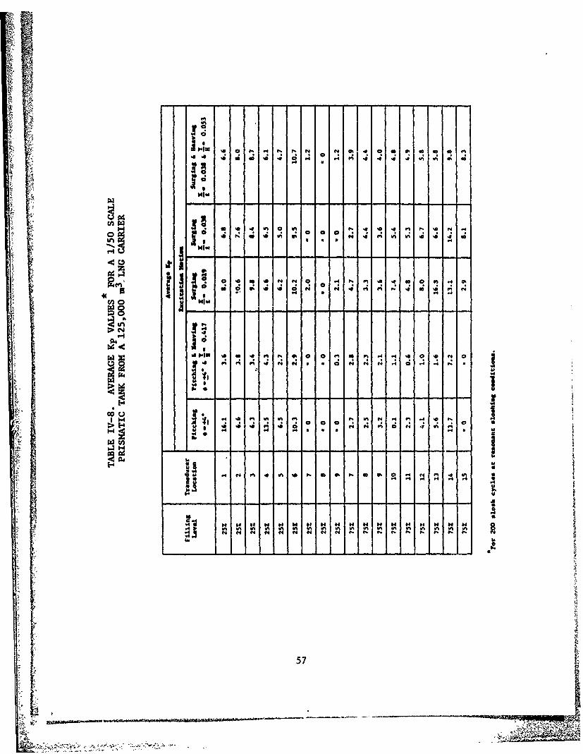
lhj 4.0 0 .4P N N N 40 so 40 m

-~~ --0

0 N N a N -

cn 0 Mimi ~ m 4

44 Ia t. 0 . 0 I 4

E-44

e. f4 1, 4 0 4 N 4 0 of .

~10.

-4Ar

-7-7777

in

en * . N W% C 9

a.0 r4 44 in. - -4 N

f N NI t% .4 .4 UP V9 4 f so 4 N 0CM *4 et . 0" 0 0r

so 4 .4 0. P,~C C i C

H 4 be Ne 64 64 64 * 4 * 4 N 4 e k

wg.0.

4bIU 4 C N N C * .4 @ i 458

rrcMO

14'

C1 4~ ! 9 M .9n *P4 H .4O

P4*

" 11 0 4440~

f4 0

; I

59

tn -m a 4 - -4 a - - -%

cn .' ' Nr 4 4 .4U 4 0.N 14. .4

u~~o 0 UN1Im U ' so P% 4 4 -tVN 4 .

I. C%

'I.9 r4 N % N 4 IA r4 0N 4 * V 4 .0 0 VI V 4I04~

Ln4 mB.. N m

* IA .4 VI N 4 .4 I O

p. ~S N 1 N N U 4 4 0 it te . 4 $4- %A %M N V % N 6 b% %* in A tn in % % 6 n A4

ra

z 4 C4 N N C 0C4 N 4.1 41 t

- - - - - - - - - - - -- - - - - - --0

4-

rw ; I i!: il i40

, i- rl I=4t'

~uI

I.-

61 L

g"

Due to the design of the test rig, the pitching and heaving motionswere simultaneous, but not independent of each other. The two motions wereat the same frequency and in phase for these tests. During testing, it wasnoticed that the fundamental excitation frequency for a 75% full tank under-'going pitching plus heaving did not produce substantial dynamic pressures,so the frequency was increased to the first harmonic. At this frequency,substantial sloshing pressures occurred and were recorded for inclusion inthe test results. The theoretical (Equation 111-6) and experimental exci-tation frequencies are shown in Figure IV-3.

The recorded pressure values for pitching plus heaving and onlypitching are contained in Tables IV-3 and IV-4. No values are found inthe tables for heaving only since the resonant frequency for a heaving mo-tion is twice the natural frequency of the liquid in the tank. The heaveresonant frequency is outside the range of interest for ship motions.Therefore, no attempt was made to excite the tank into resonance in heaveand record pressures.

The pressures presented in Tables IV-3 and IV-4 for pitching andpitching plus heaving indicate there was no augmenting of the pressuresusing the combined motion. In addition, many test pressures were somewhathigher for pitching only motion.

IV.3.2 Surging Plus Heaving Test

The translational motion sloshing facility was utilized for thesurging plus heaving tests. As with the pitching plus heaving test, thesurgirg plus heaving test results are compared to the results of the indi-vidual excitation motion (surging). Figure IV-4 illustrates the survingand heaving motions.

Two surging amplitudes were examined. These are typical extremevalues that P full-scale tank might experience during operation. To deter-mne the worst case combined surging plus heaving condition, the tank wasosci\lated with the surging frequency set at resonance, and the heavingfreq,:=ncl, swept through a range of values from 0 to 5 Hz (model scale) or0 to .,707 Hz (full scale). Next, the tank was oscillated with the heav-ing motion set at its theoretical resonant frequency and the surging exci-tation frequency swept through a range of values [0 to 5 Hz (model scale)or 0 to 0.707 Hz (full scale)]. The worst case was chosen as the one thatcreated the most violent sloshing (by visual observation) and the highestrecorded pressures.

The results of these tests indicate that the worst case sloshingoccurred when the surging and heaving excitation frequencies were equal tothe resonant frequency of the liquid for a surging only motion. The testresults were recorded with both the surging and heaving motions at the samefrequency and in phase. The tank displacements in the surging and heavingdirections were also equal in magnitude (x y = 1 in.= 2.54 cm), with

k(x/) = 0.038 and (y/H) = 0.053.

i] ,62

10

9 Theretcalresonant slosh period calculatedf rom Eq. 111[-6

0 Pitching & Heaving7 (2nd Harmonic)-;

S 60 Surging only

only and

5 ISurging &

Hal " Pitching & Heaving

3 Pitching only

Ia- denotes experimental value given in Table IV-2

00 10 20 30 40 50 60 70 80 90 100

Tank Filling Level(Percent)

I TR - resonant sloshing period

g = acceleration of gravity

9X. = tank length in direction of motionFIGURE IV-3. EXPERIMENTAL AND THEORETICAL NONDIMENSIONAL RESONANTSLOSH PERIOD VERSUS TANK FILLING LEVEL

"If- 63

iy

MoioM I I

S I4 I

I

H Test Tank I Heave

- ' I

£ U0

4) Surge Motion

x *surge motion displacement

y -heave motion displacement

£-tank length

H -tank height

i7IGURE IV-4. MOTION DEFINITIONS FOR SURGE AND HEAVE.

64

The test results for surging plus heaving and surging only are foundin Tables IV-5, IV-6, and IV-7. The results do not indicate any signifi-cant augmenting of the sloshing pressures caused by the combined tank mo-'ions of surging plus heaving, Visual observations also suggested that thesloshing for the surging plus heaving was comparable in magnitude to thatfor only surging.

Based on the results of these laboratory tests, there does not ap-pear to be an increase in the slosh-induced dynamic impact pressures caused

by multi-degree of freedom tank motions. However, it is realized thatthese tests are limited in that simultaneous excitation of all six degreesof freedom could not be investigated. In spite of this limitation, theresults do provide insight into the effects of combined degrees of freedomex.itation and indicate that worst case loads can be obtained by resonantsloshing in single degree of freedom tests. The excellent full-scale/model-scale pressure agreement for the OBO tank (discussed in Section 111-2) wheremodel tests were included in roll only further support this conclusion.

IV.4 Dynamic Pressure-Time Histories

Pressure-time histories were measured in model scale to establishinformation important to the analysis of the tank's structural response todynamic loading caused by cargo sloshing.

A typical pressure-time history (nondimensional) is shown in Fi! _ra

IV-5. Vcr analytical purposes, this pressure trace will be approx1ratedby straight lines connecting points 1, 2, 3, 4, and 5. The most important

&Lements of the pressure trace are (1) the time required to reach the peakpressure (po .nt 2), (2) the magnitude of the peak pressure at point 2, (3)the duration of the pressure spike (point 1 tc point 3), (4) the magnitudeof the tailing pressure between points 3 and 4, (5) the duration of thetailing pressure betweei. points 3 and 4, and (6) the integrated pressurevalue over the entire pressure cycle. By knowing these characteristics ofthe pressure-time history, one can evaluate the structural response of thetank wall to an impact pressure.

Wall impact pres..ure-time histories for both a 25% and a 75% fulltank were recorded. Ths tank excitation motion was harmonic pitching.Two hundred resonant sloshing cycles were recorded for each test. For the25% full test, ptessures were measured at transducer locations 1 through 9(Figure IV-l). Pressures at locations 7 through 15 were recorded for the75% full case.

The test results include two forms of the preesure-tiae history.First, fc " each transducer location, there is a composite worst case pres-sure-time history. This profile includes the shortest pressure riae time(T2), the longest time durat. ..s fcr T3 , T4, and T, and the highest pres-sures for all points (P2 , P3, P4 , and PS) recorded during any of the 200sloshing cycles. This trace represents the worst case values (with rpspectto the loading on a tan', wall structure) Ltlat the particular transducerlocation experienced durlag the 200 cycles of resonant sloshing. In addi-tioi, a pressure-time history showing the average values (for 200 resonant

65

P (T)pgt*

(Noadimensional)\ Pressure

(Nondimensional Time)

The Trapezoidal Rule using the five numbered points is usedto detervine the area under the curve (which is the value ofthe pre",iure integrated over the entire period).

FIGURE IV-5. TYFICAL PRESSURE-TIME HISTORY FOR SLOSH-INDUCED IMPACT

66

sloshing cycles) for the points on the curve are plotted. Also, the inte-I f grated pressure values versus the pressure duration (T) ale presented.

An effort was made to determine if any discernible correlations

exist between the peak pressure (P2), the pressure rise time (T2), and thepressure spike duration (T3). Plots showing peak pressure versus pressurerise time, peak pressure versus pressure spike duration, and pressure spikeduration versus pressure rise time are included in the results.

The nondimensional pressure-time history test results for represen-tative transducer locations 1 and 14 are found in Tables IV-12 and IV-13,

and Figures IV-6 through IV-15. Similar data for the other transducer lo-cations are presented in Appendix B. Maximum, average, and minimum pressureand time values are included in the tables. It should be noted that loca-tions 7, 8, and 9 experienced virtually no pressures when the tank was 25%full. Thus, there are no tables for these locations. The same is true oflocation 15 for the 75% full tank.

The pressure data obtained at transducer locations 1, 4, and 7 arerepresentative results for the test case with the tank 25% full. Dynamicpressures were measured at locations 1 through 6. The pressure-time his-tories at transducer 1 were similar in magnitude and shape to those atlocations 2 and 3. The pressure traces at transducer location 4 were simi-lar to those at locations 5 and 6.

The pressure-time history for location 1 for the 25% full tank isfound in Figure IV-6. The integrated pressure value for this transduceris shown in Figure IV-7. Plots exemplifying the relationships between thepressure rise time (T2), pressure spike duration (T3), and the peak pres-sure (P2) for this location are shown in Figures IV-8 through IV-10. Itshould be noted that several of the plote have data points clustered insmall areas. This was caused by round-off limitations in the computationaethodology that was used for data reduction.

A group of data similar to that just described for the test casewith a 25% full tank was also compiled for the case with the tank 75% full.Data from pressure transducer locations 7, 11, 13, and 14 were chosen asrepresentative for the 75% full tank. The pressure-time histories at lo-cation 7 are similar to those at locations 8 and 9. Likewise, the pressure-time histories at transducer 11 are comparable to those at 10 and 12 (withthe exception that the magnitudes at location 10 are somewhat smaller).

Graphs showing pressure-time histories, integrated pressures, andrelationships between the pressure rise time, the pressure spike duration,and the peak pressure for transducer 14 ate found in Figures IV-11 throughIV-15. Locations 7, 8, and 9 were below the static liquid level, and, asa result, these locations did not experience significant dynamic loadings.The pressure rise times were relatively slow and the peak pressure small.Pressures of a more dynamic nature were measured at locations 10 through 14.

67

0, CJ co .ci 0 i N U') 0 aU) i i i ~) .4 14-ci OL0 D kD 0

E-4 * z' i(1

ww

p= CL C; 8i c iw

ww* ? Co '

_j~ III. knci c-4 Ix

W r. 00 LL. U) .*J0.

4 = = m wo -

I=.J. I- a. D j .

ta. W~ CL1- 0 -

00 0\ o.

CLJ CL b) ci ' 0 otCO0 NN ~ T N

C'J N ' 0 ' C CON. I- tr) cU) 1r) .'

.7 C. . LLJ J

04 0 I- a.C C '

C4 UJ ciiC:

CT. C 7o 67% C

k-)k 0) #I-V o

Co L.- LiU U)?' ON N -

(Z) Ce -. W0 rCL **

> E-4 C ).4 -4 Co U

LL W .4LV

68

Li)

Li)

(n LL

64 ~ILL w

WLAJ0-4

00

f0Z

rnC tn 0

NWn

-~ w'

ce. ))i.

w W V)-va eA fy

m CA V) LL.ti--i-

PI O1TCH ~ ~ I? C ID TI? RE SW l$UY SLOS1INS CN lIT W S

TRIN10LC.ID. I PT~iCH 1..NO. O CYCLES: No T iS.l E. I

FILL DEPTH: U, Or CYCLS : ?N58.0 FILL CL'TP." 2];

iN.,, ,,u

. . . ; .NEa

II.R II : "' "| s ,S

h n 1 , 3 . 3. U3 I .0l .IK : 98 .0 U.4 l." :. :

iIiPUSE RISE TIIITiI IIIUS bUII,TICU'T

(HlllOW.) (11013W1.,)

iFIGURE IV-8. NONDIMENSIONAL FIGURE IV-9. NONDIMENSIONAL PRESSUREPRESSURE VS IMPULSE RISE TIME VS IMPULSE DURATION FOR 200

FOR 200 RESONANT SLOSHING CYCLES RESONANT SLOSHING CYCLES AT TRANS-AT TRANSDUCER LOCATION 1 FOR A DUCER LOCATION 1 FOR A 25%. FULL25% FULL TANK TANK

IESINT SLMSHIIK CNIION

PITCHPITCH TRIWIS.LOC.O. I4STIIRMS.LO(.U. I g. Of CYCLES: 222NO. OF CYCLES :220 FILL DEPTH: ISFILL DLTH: 2S N"

.. 4.

*. . .- . . uu 'I L

• - - : .,I:IIea i. 1 .,

33.11

3.11 i .20 8.38 *.' E1" IIE6I0 . TIE

IlPULSE RISE TIM'.M12(N301lH.) I THE LILTS C ECTIHUS THE DRTR POINTS

ARE ONLY YISURID IlK'S.

FIGURE IV-1O. NONDIMENSIONAL IM- FIGURE IV-11. NONDIMENSIONAL PRESSURE-PULSE DURATION VS IMPULSE RISE TIME HISTORY VALUES FOR 200 RESONANTTIME FOR 200 RESONANT SLOSHING SLOSHING CYCLES AT TRANSDUCER LOCATIONCYCLES AT TRANSDUCER LOCATION 1 14 FOR A 75% FULL TANKFOR A 25% FULL TANK

70

MC4IV.!T LOSHINH CONDITIM6 IESOail 5LDSHIS CW;DITIMIS

PITCH PITCHTOIIIS.,L0031.. I14 TR ;S.LO¢.NO. 14

NO. OF CYCLES: 2M NO. OF CYCLES: L12FILL DEPTH: is FILL DEPTH! 7Sa

.

:o41 . 1a%.4~

I.sl 1.,

,¢ ',1; ., o .n

D].N ..'N..'.13L I:: '.15

9.1 l ' ' 1 £ il z.11 1,14 8111. 12 I . 16 i .l 3l

KaD )URUTION IMSE ISE TIKJT2

(WOII.) (NOII)

FIGURE IV-12. INTEGRATED NON- FIGURE IV-13. NONDIMENSIONALDIMENSIONAL PRESSURE VALUES FOR PRESSURE VS IMPULSE RISE TIME200 RESONANT SLOSHING CYCLES AT FOR 200 RESONANT SLOSHING CYCLESTRANSDUCER LOCATION 14 FOR A 75% AT TRANSDUCER LOCATION 14 FOR AFULL TANK 75% FULL TANK

CIONWIIT SLcSHIH COHDITIONS RI I T 5 U H11.6 C0 15ITN

PITCH PITCHTIW .VCHO. 14 TE15.LDC.tMO. 140O. OF CYCLES: 20 0O. Or CYCLE: M

FILL DEPTH: 7SS

.11E .E

* IM] L*. p . . . .

N.I 'I• ' 8i : 8i. . ..II,.• I ... . .

iR . 3 BA 9.53 I... i1.10 s.12 ISII 0

IIIL..E DIJRETIWM13 IWWPlS OISE TIr.E1T7lOWN.)

FIGURE IV-14. NONDIMENSIONAL FIGURE IV-15. NONDIMENSIONAL IMPULSE, PRESSURE VS IMPULSE DURATION DURATION VS IMPULSE RISE TIME FOR

FOR 200 RESONANT SLOSHING CYCLES 200 RESONANT SLOSHING CYCLES ATAT TRANSDUCER LOCATION 14 FOR A TRANSDUCER LOCATION 14 FOR A 75%75% FULL TANK FULL TANK

71

IV.5 Dynamic Load Simulator for Plywood Insulation Box Tests

A series of strength tests were performed on representative plywoodinsulation boxes (Figure 111-18) from a typical membrane tank insulationsystem. The purpose was to (1) provide structural response data for com-parison to analytical predictions, (2) to evaluate the box response to var-ious projected full scale loading conditions, and (3) to determine pressurelevels a box could withstand without sustaining damage. The loading con-ditions were designed to simulate what a structure might encounter in actualoperation. Tests included both static and dynamic loadings.

Because of the unusual test conditions, a special test fixture wasfabricated. It was necessary to uniformly load the entire cover of thetest box. In addition, a typical full-scale pressure-time history (FigureIV-5) had to be produced on the test structure.

The test system consisted of a chamber of water located on top ofthe box cover with a rubber diaphragm between the two. The box cover wasloaded by pressurizing the water chamber. This created a relatively uni-form load over the cover since the water deformed to the shape of the coveras it deflected under loading. For the dynamic pressure tests, three fast-opening valves located between the pressure source and the water chamberwere used to shape the pressure-time history. A schematic of the testapparatus is presented in Figure IV-16.

The following paragraphs describe the function of each componentshown in Figure IV-16. The pressure supply was a tank filled with nitrogengas. At the exit port to the pressure tank was a hydraulically-operatedcock valve. Between the cock valve and the water chamber was a fast-open-ing, hydraulically operated plunger valve. When this valve and the cockvalve were both opened, the high pressure nitrogen gas pressurized the wa-ter volume. A solenoid valve located between the cock valve and the plungervalve was used as a relief valve. The pressure-time history foi a dynamicpressure test was controlled by the timing of the opening and closing ofthese three valves. The apparatus was capable of creating dynamic pressurerise times as short as 20 milliseconds. Based on the pressure-time historyexperiments, this is a typical rise time that a plywood insulation box mightexperience while in service. Peak dynamic pressures of about 200 psi wereattainable. Static pressures on the order of 250 psi were achieved withthis particular test rig. These pressures represent worst case pressuresthat could be encountered in full scale-resonant sloshing.

The supporting structure for the plywood test box (called the pri-mary box) consisted of ]/2-in.-thick, marine-grade fir plywood boxes (calledsecondary boxes). These boxes simulated the supporting structure of theprimary box in the ship tank. Figure 111-19 shows the supporting configur-ation as it is in the tank. The secondary boxes used in the loading testshad stiffener locations similar to those shown in Figure 111-19. This al-lowed the load transfer through the stiffeners of the primary test box toclosely approximate the actual full-scale conditions. The secondary boxesin the test apparatus rested on a rigid surface.

72

Ugh PressureGas Reservoir

Pressure Gage

Hydraulically Actuated..Cock Valve Solenoid Pressure Relief Valve

T ae eW r Hydraulically Actuated Fast-Opening ValveI" PressureTransducers MaiodPiping

Ru bber Gasket Separa- Ah t- Pressure Gagetins Water Chamber P ressure Transducer

- . tes amberand Test Box e

SPrimary Test Bx-. E Dlsplacemn Transducer

Secondary Support Boxes(Plywood)

'4 FIGURE IV-16. SCHEMATIC DIAGRAM OF PLYWOOD INSULATION BOX DYNAMIC LOADER

73

Instrumentation for the loading tests included pressure measuringdevices to monitor the pressure on the box cover and displacement trans-ducers to measure the deflection of the cover during loading. For the dy-namic loading tests, PCB piezoelectric pressure transducers (Model 102A15)were used uo measure the pressures in the water chamber. These transducershave an operating range of 0.01 to 500 psi with a frequency range of 0.5 to50,000 Hz. Three transducers were used to monitor the uniformity of thepressure in the chamber. Transducers were located at the midpoint of bothend walls of the chamber and at the midpoint of one side wall. All threetransducers were located approximately 1-1/2 in. above the surface of thetest box cover. The general locations of the three pressure transducersand the pressure gage are pictured in Figure IV-16. Figure IV-17 showstypical pressure traces for the three transducers for a dynamic pressuretest. The top photograph shows the pressure-time histories for a test thatdid not experience a box failure. The bottom picture illustrates the pres-sure waveform when a failure occurred. These pressure signals were re-corded on a storage oscilloscope, as were all of the dynamic pressure mea-surements.

One important aspect of these plywood box tests was the determina-tion of the box cover response during loading. The stiffener configuration

divided the boxes into 12 cells. The cover deflections were measured atthe centers of the unsupported cell areas. Figure IV-18 shows the celldivisions for a typical 12-celled box and the locations of the displacementmeasurements. For static loading tests, spring-loaded, linear displacementtransducers were utilized for the measurements. For dynamic loadings, aKaman (Model KD2300-25) inductance-type displacement transducer was used.The performance of the two types of transducers correlated well as evidencedby the results presented in Figure IV-19. "his figure shows that thecover response was similar for static and dynamic loading conditions.

The cover deflection measurements are presented in Tables IV-14through IV-21. In addition to these results, Table IV-22 summarizes thetests and results for all boxes. Some boxes were modified to study the in-fluence of various parameters on box strength.

Three types of failures were observed during the box loading tests.First, some covers experienced shear failures. Usually the shear failurewould occur at a stiffener support. Second, other covers experienced bend-ing failures along the centerline of the unsupported area of an individualcell. The third type of failure was a buckling failure of a stiffener.This was observed in only one test. Figures IV-20, IV-21, and IV-22 showtypical shear, bending, and stiffener failures, respectively.

The test results indicated that the original 12-celled boxes couldwithstand a pressure of about 120 psi without suffering catastrophic fail-ure. The range of failure pressures was 120 to 158.6 psi for both staticand dynamic loading. Also, test results showed no appreciable differencein failure pressures for static or dynamic pressures. A typical dynamicloading is shown in Figure IV-17. The pressure rise time is about 20 ms, theminimum rise time obtainable with the loading device. These observations are

74

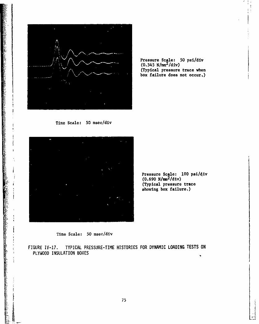
Pressure Scale: 50 psi/div(0.345 N/mm2/div)(Typical pressure trace whenbox failure does not occur,)

Time Scale: 50 msec/div

Pressure Scale: 100 psi/div(0.690 N/mm2/div)(Typical pressure traceshowing box failure.)

Time Scale: 50 msec/div

FIGURE IV-17. TYPICAL PRESSURE-TIME HISTORIES FOR DYNAMIC LOADING TESTS ONPLYWOOD INSULATION BOXES

75

12.32" (312.9 =. 6.03" (1k53.2 t)

3.75" ' -- 1.79" (45.5 a).T ~~ ~~II _ I _ "3. 75 I ! [(95.25.... . -3.84" (97.5 m)

-1 - - - p - - -381(9. nTypicl Displace-

3.75" ment Transducer(95.25 mm) . JL. ..... ...........

-,,r tife-e-- - - - - -r

3.75I Loc tion,(95.25 mm) .. ......... - -- - -

-- - -- - - -----------.. "r----------. r .........,III I,

3.75" Cell Number II(95.25 5 u) 1

12.23" (310.6 mm) 12.23" (310.,) =m) 12.23" (310.6 m)

(j.) Ty.ical D splacement Transducer Locations on12-Cell Plywood Box Cover

12.35" (313.7 mm) 12.35" (313.7 m) 6.0" (152.4 mm)

~ . -7.5" (190.5 mm)

(381.0 mm)

T~~yplcispaclelTransducer Locations

36.69" (931.9 Dim)

(L) Typical Displacement Transducer Locations !or aPlywood Box Cover wirb All Stiffoners Removed

FIGURE IV-18. DISPLACEMENT TRANSDUCER LOCATIONS FOR PLYWOOD

BOX STRENGTH TESTS

k76

7-

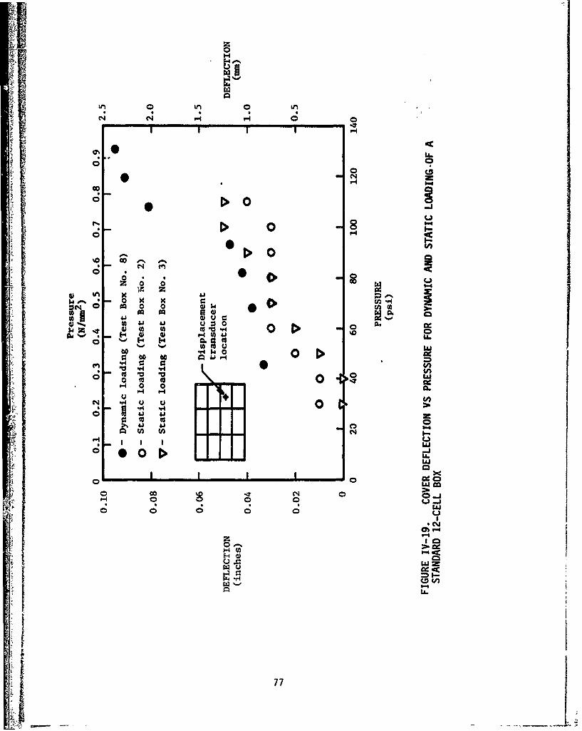
00

M, 0 W~0U

o 0

60 0

0 0

2 '.

0 "4

0 0 -

o cc * *

z o 0

I~d#% OK

41 U,

0 07

(TES BO NO. ~ -1)L

78~

I TE5T Boy "

A At

IM

Ik

I;n

FIGUF(E IV-21. BENDING FAILURE OF PLYWOOD INSULATION BOX COVER* (TEST BOX NO. 8) 7

0

C)

-AJ

I :D

C

80

TABLE IV-14, PLYWOOD COVER DEFLECTION MEASUREMENTS

~ I FOR TEST BOX NUMBER 1 (Static, Loading Test)

Pres~sure Cover Deflection (inches)(psi) Cell No. 1 Cell No. 3 Cell No. 10 Cell No. 12

04.00.00000005 0.00 0.00 0.00 0.00

50 0.00 0.00 0.01 0.00

50 0.04 0.00 0.04 0.01

60 0.04 0.00 0.05 0.03

65 0.04 0.00 0.05 0.03

s0 0.04 0.00 0.06 0.03

90 0.05 0.00 0.06 0.04

100 0.08 0.08 0.09 0.06

110 0.10 0.08 0.13 0.08120 0.20 0.16 0.17 0.18

j~~t Cell number 11 failed in shear at 130 psi (0.896 N/flu2)

Conversion Factors: 1 psi 3i 6.895(10)-3 N/vet2

1 In. 25.4 on

TABLE IV-15, PLYWOOD COVER DEFLECTION MEASUREMENTSFOR TEST I=X NUMBER 2 (Static Loading Test)

J ________Cover Deflection (Inchos)Pressure -

(psi) Cell Cell Cell CCli Cell Cell Cell Call____ No.1I No. 2 No'. 3 No. 6 No. 9 No. 10 No. 11 -No. 12

j0 0.00 0.00 0.00 0.00 0.00 0.00 0.00 0.00

130 0.00 0.00 0.00 0.01 0.01 0.03 0.01 0.03

f 40 0.02 0.00 0.00 0.01 0.01 0.03 0.03 0.05

50 0.04 0.03 0.03 0.02 0.01 0.07 0.04 0.06

160 0.06 0.04 0.05 0.03 0.01 0.08 0.04 0.08

70 0.06 0.05 0.06 0.03 0.01 0.09 0.05 0.08

80 0.07 0.06 0.07 0.03 0.02 0.10 0.08 0.10

90 0.08 0.03 0.08 0.03 0.03 0.10 0.08 0.11

100 0.10 0.05 0.09 0.03 0.03 0.12 0.10 0.16

110 0.11 0.07 0.10 0.04 0.05 0.16 0.10 0.20

ii Cell number 12 failed in shear at 120 psi (0.827 N/mm2).Conversion Factors: 1 psi - 6.895(10)-3 N/mn 2

1 in. - 25.4 mmL 81

TABLE IV-16. PLYWOOD (OVER DEFLECTION MEASUREMENTSFOR TEST BOX NUMBER . (Static Loading Test)

Cover Deflection (inches)Pressure(psi) Cell Cell Cell Cell Cell Cell Cell

No. 1 No. 2 No. 3 :*o. 6 No. 10 No. 11 No. 12

0 0.00 0.00 0.00 0.00 0.00 0.00 0.00

30 0.01 0.02 O.02 0.00 0.03 0.02 0.02

40 0.02 0.03 0.03 0.00 0.05 0.03 0.05

50 0.03 0.04 0.08 0.01 0.08 0.05 0.07

60 0.04 0.05 0.09 0.02 0.09 0.06 0.08

70 0.05 0.06 0.11 0.03 0.10 0.08 0.09

80 0.07 0.08 0.11 0.03 0.10 0.09 0.10

90 0.08 0.09 0.13 0.04 0.12 0.10 0.10

100 0.10 0.10 0.17 0.05 0.15 0.10 0.11

110 0.11 0.11 0.20 0.05 U.i9 0.12 0.11*

110 0.12 0.11 0.22 0.08 0.20 0.14 0.18110 0.13 0.11 0.23 0.07 0.20 0.14 0.18110' 0.13 0.11 0.23 0.08 0.20 0.13 (\!7

i0 0.13 0.11 0.23 0.08 0.20 0.14 0.!7 t90 0.10 0.10 0.20 0.06 0.1, 0-12 , 12

110 0.15 0.10 0.23 0.08 0..O0 0.16 0.730 0.05 0.04 0.10 0.03 C.10 O.G8 "),08

0 0.03 0.00 0.02 0.00 0.04 0.02 *.)3

110 0.18 0.11 0.28 0.07 0.20 0.16 0,17

0 0.03 0.01 0.03 0.01 0.C7 0.03 0.04

120 0.18 0.12 0.30 0.07 L23. I 0. 0.19

Cell number 3 failed in shear at 150 psi (1.03 N/mm 2).

*Pressure was reduced to 90 psi (0.621 N/mwi) and then increased back to110 psi (0.758 N/mm').

Conversion Factors: 1 psi= 6.895(10) 3 N/mm2

1 in. = 25.4 mm

82

= -5- 77

TABLE IV-17. PLYWOOD COVER DEFLECTION MEASURE4ENTSFOR TEST BOX NUMBER 6 (Static Loading Test)

Pressure Cover Deflection (Inches)

(Pat) Cell No. 1 Cell No. 3 Cell No. 10 Cell No. 12

0 0.00 0.00 0.00 0100

30 0.02 0.02 0.01 0,00

40 0.03 0.03 0.02 0.00

50 0.03 0.03 0.03 0.01

60 0.04 0.03 0.04 0.03

70 0.05 0.05 0.04 0.03

so 0.06 0.05 0.05 0.04

90 0.06 0.06 0.06 0.04

100 0.09 0.08 0.07 0.05

110 0.10 0.09 0.14 0.090 0.05 0.00 0.05 0.01

Cell number I failed In shear at 160 psi (1.10 N/ram2).

Conversion Factors: 1 psi - 6.895(10Y)3 N/mm2

I In. - 25.4 m

TABLE IV-18.. PLYWOOD COVER DEFLECTION MEASUREMENTSFOR TEST BOX NUMBER 7 (Static Loading Test)

Pressure Cover Deflection (inches)

(psi) Call No. I Cell No. 3 Cell No. 10 Cell No. 12

0 0.00 0.00 0.00 0.00

6G 0.02 0.02 0.03 0.02

70 0.03 0.03 0.03 0.02

80 0.03 0.03 0.04 0.03

90 0.04 0.04 0.05 0.03

100 0.05 0.05 0.07 0.04

110 0.06 0.07 0.08 0.05

120 0.08 0.08 0.09 0.06

Cell number 1 failed In shear at 240 psi (1.65 N1,,2).

Conversion Factors: 1 psi - 6.895(l0)-3 N/m 2

1 in. =25.4 m

83K L .. ......_ _....__ _ ..

TABLE IV-19. PLYWOOD COVER DEFLECTION MEASUREMENTSFOR TEST BOX NUMBER 8 (Dyneamic Loading Test)

Pressure Cover Deflection,(inches)

.psi) Cell No. 6

0 0.000

45.5 0.03368.1 0,038 TABLE tV-20. PLYWOOD COVER DEFLECTIONMEASUREMENTS FOKRUST BOX NUM&U. 1081.8 0.042 (Static Loading, Test)93.2 0.047

107.8 0.081 Cover Deflection (inches)119.3 0.091 (Cel) c Nu No. Cell o, 3 Ce1 o. 10130.7 0.095

0 0.00 0.00 0.0c I30 0.00 0.00 0.0040 0.00 0.00 0.00

11 numbr 5 failed In banding at 142.1 psi (0.980 N/mm2). 50 0.02 0.00 0.0060 0.02 0.01 0.00

Conversion Faetors: I psi a 6.895(10)-3 N/=n2 70 0.03 0.02 0.01

I In. - 25.4 am so 0.04 0.02 0.01

90 0.05 0.03 0.02100 0.05 0.03 0.03110 0.06 0.03 0.03120 0.06 0.04 0.05

The center longitudinal stiffenar buckled betveen cells4 and 7 and 6 and 9 at a pressure batween 150 *nd 180

TABLE IV-21. PLYWOOD COVER DE LECTION psi (1.03 and 1.24 N/amu).

MEASUREMENTS FOR TEST BOX NUMER 11 Conversion Factors: I psi a 6.89S(0)" Im2(Static Loading Test) I Inh. -25.4 am

Cover Deflection (inches)Pressure(psi) Location Location Location

No. 1 No. 2 No..3

0 0.00 0.00 0.00

5.0 0.10 0.15 0.10

7.5 0.14 0.23 0.13

10.0 0.22 0.32 0.20

12.5 0.28 0.42 0.23

15.0 0.30 -- 0.28

17.5 0.37 -- 0.33

The cover cracked (bending failure) at the 20 psi (0.131 N/MM2)pressure level.

Conversion Factors: 1 psi = 6.895(lo)-3 N/mm2

1 in. 25.4 umw

84

A~6 .40

a 4 a 4 6 -4JW

4 6j W-6

E-4 40 C

J% L44~

*cl N iio-~ ~flfl.4I~( q4vo

-. .4J-4 ~ 'I ~0

85*- a-

11 -

Id C

ja aa ,LI

VI 1.4 A V.4 . .

164 1111 U44

444

ObC4

C -0,

14 5.. % 438

ow 403 41 1"

in v to 1 0 . cco .0

86a

4 .0

4-W A "

*0 "

Id 41w 0

0~gi.-44 1. 1 , " %

Im

ILi

UU

ulI14 'a

" 0~ " .4

"4 oro

44O

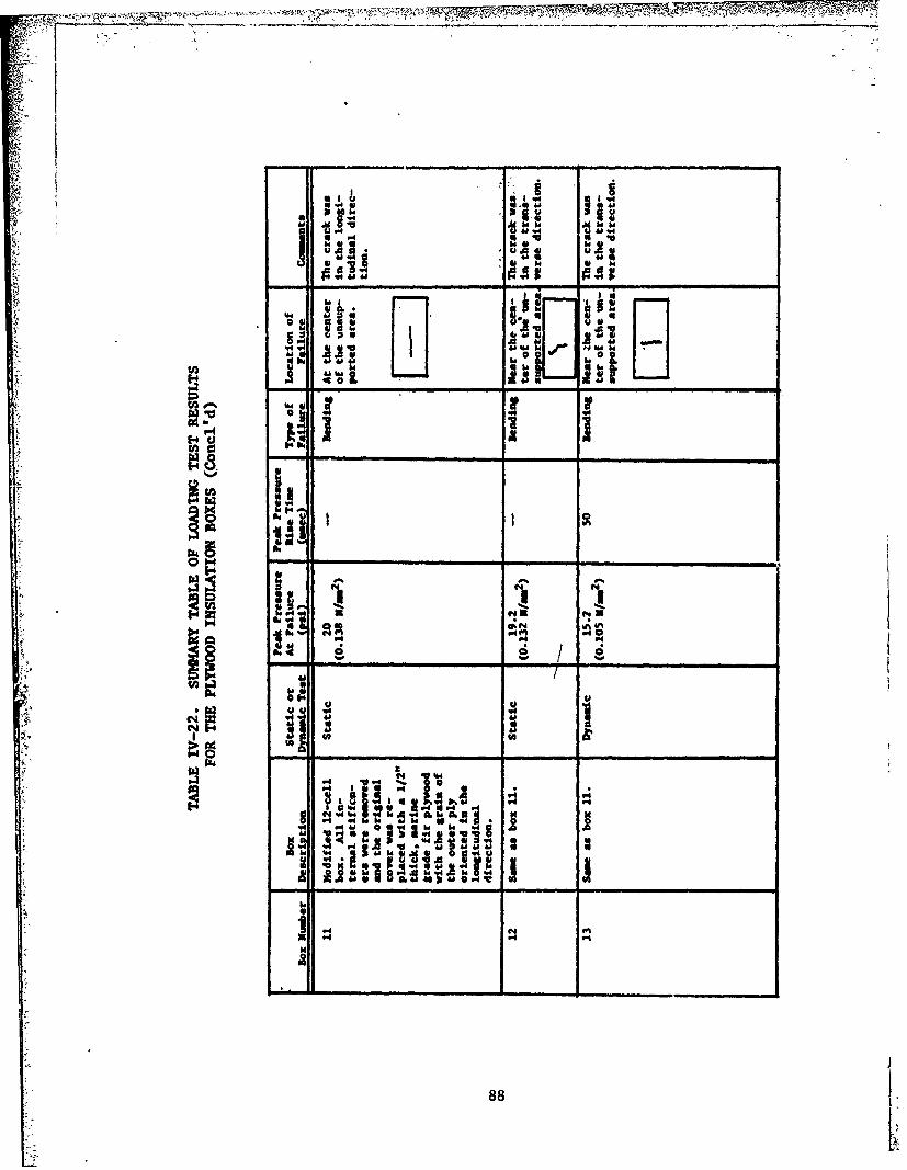
U 4 10 314

4dM

444

a _ _ _

C4C

.4 -

46 m M1 13 N

b.88

consistent with analytical calculations of dynamic response presented in

Section V, which show that rise times must be about 1- 2 ms to produce dynamic

amplification of the loading.

By modifying the test boxes, loading pressures up to 240 psi could be

obtained before box failure occurred. It was observed that the box coverscould withstand approximately 0.2-in. deflections at the centers of the un-

supported cell areas before failure of the cover was observed. Permanent

deformations of the cover (not total failure) were witnessed when pressurelevels reached 80-90 psi; These deformations could be described as

"scalloping" of the unsupported.celi areas with.the'magnitudes of these

deformations in the range of 0.05- to 0.10-in. maximum.IV.6 Material Properties Tests

A series of tests on plywood specimens taken from the Gaz Transportboxes were conducted. The purpose of these tests was to provide materialproperty data for the analysis of the plywood box and to aid in the inter-pretation of tests to measure box strengths. These tests were necessary

F because data from tests by Mitsui(76) and by Gaz Transport( 7 7,78) gave

widely varying results for plywood' srength And eiffneis.

All plywood tests were conducted with simple beams in 3-point bend-ing. As shown in Figure IV-23, the specimens were approximately 50mm wide,

and support spacing was either 121mm, 88mm, or 50mm. Spacings of 121mm and88= match the widths of the cells in the 9-cell and 12-cell boxes, respec-tively. The spacing of 50mm was used to check the effect of very shortspans. All specimens were cut transverse (perpendicular) to the grain.*

This is the weakest direction and also the direction across the narrow di-mension of the cells in the plywood boxes. Principal bending in the actualboxes will occur in the cross-grain direction.

Specimens were cut from the covers of boxes which had been in ser-vice ("old" boxes) and from new boxes which had never been exposed to cryo-genic temperatures. Tests on the specimens from the old boxes were per-

formed at two loading rates. A slow rate of 2.54 mm/mmn represents a statictest, and the fast loading rate of 508 mm/min is the limit of the test ma-chine. Tests with specimens from the new boxes were conducted at both robm

temperature (RT) and at cryogenic temperature (CT). All tests were per-formed at the slow loading rate.

Results for the old plywood are presented in Table IV-23. Consider-

able variation in the stiffness and stress values are evident. Stress values

range from a low of 20.9 N/mm 2 to a high of 65.5 N/mm2, a factor greaterthan 3. Average values of T and E for the two different loading rates andoverall are:

0, N/mm2 (psi E, N/mm2 (psi)

Fast Loading 40.1 (5,816) 2144 (310,987)

Slow Loading 49.4 (7,165) 3797 (550,755)Overall 44.2 (6,411) 2941 (426,592)

*Grain direction of the exterior ply.

89

M .'O U4 N V)~

f O-4 %DN %

X1

0 %D . PI

M@ MIE. N b .0

Z- 1

- ~ 1 N4 N4

00

41 .4

44f %o Nco

~. ~...............

is

Support Points Specimen lengths: 185 mm 121 mm

(Typical) 133 rm 88 mm

Z.. 133 mm 50 M

rT

Grain Direction of Exterior Plies

FIGURE IV-23. PLYWOOD TEST SPECIMEN GEOMETRY

Although a and E for the fast loading rate are lower than for the slow rate,this difference was disregarded for three reasons. First, the maximum anOminimum values for stress occurred at the fast loading rate, which indicatesthat there is no consistent trend. Second, even the fast loading rate usedin the tests* is slow by several orders of magnitude compared to the ex-pected response rate of the plywood covers in the in.lation boxes. Third,drop. tests conducted by Mitsui,(7 6) which give faster loading rates, showelno difference in results from static tests. For these reasons, the averagevalues from all tests were taken as representative of plywood propertiesfrom the old boxes. The spread in the results for different specimens im-plies that there is considerable variation in the plywood even for a singlebox cover.**

Results for the new plywood boxes are given in Table IV-24. Testswere performed at both cryogenic and room temperatures. Plywood .strengthat cryogenic temperatures is consistently higher than at room temperature.Also, scatter is scmcahat less in the strength results for the new boxes.In the room temperature tests, for example, the values differ by a factorof 2.45 as opposed to 3.13 for the old boxes, and this is based on abouttwice as many tests for the new plywood.

Plywood data for all tests, conducted by Mitsui, Gaz Transport andSwRI, are summarized in Table IV-25. These data include one test on thenew box material which is compressive parallel to the grain of the exteriorplies. This test was to give some indication of the basic strength of thevertical stiffeners in the boxes.

*Fast loading rate used in these tests was the highest rate obtainable with

the test device.**All specimens from the old boxes were cut from a single box cover.

91

f4 %CwN gom044 . A .4 0% m 0 LM 0 m %V V% 0~~C

C~44N OO . 4'~t.N I~%Dt~q ..4 w- 4. 4e 0. iV l 9

%D Mf %V N N N 'DV D% 0% 0- 4

r4t 4A ,_ h5 %5I% c %ac omf

go~~~I m1 Le 9%0 %.14 Ts

M M 0 0 00%RRO

14 .4 NN

.2..4,I0 " 41 01 1iQ 4 (1 O V 0 - V% t %% Q c0 ? o 0

1- N a nc

r1 _ _ _ _ _

0 0 N 0 V,

VM LM a Chc O

r. ~U N IT %M 00 m

_ TOW .. Ie-I. I

__b - -A__ _ _ 1.

0n n i 0

0t wi ry 0 -N j

ull

c 0 0 r. 0

ta4 040

0014 d a

-I.1, 'Ii'"W'041

ej 93

As noted, considerable scatter was found in tests on the specimensfrom the old box cover. This cover had sustained localized visible damage,but specimens were cut from areas which appeared to be undamaged. However,the large scatter may indicate that some unnoticed damage was present insome of the specimens tested. Thus, plywood properties for in-serviceboxes were established from tests on both the old and new boxes. Tests onthe new boxes were used to establish th3 minimum, average, and maximumvalues for both cryogenic temperature (CT) and room temperature (RT).These values, taken from Table IV-24, are liated in Table IV-26.

TABLE !V-26. RANGE OF PLYWOOD PROPERTIES

Birch Plyiood, No wei--Prop.rties Perpendicular -I

to Exterior Plywood IT CT RT CT IT CT

o, 2 31.17 59.20 55.96 89.05 77.80 103.70

a. (psi) (4,5,8) (8,587) (8,117) (12,916) (11,285) (15,042)

2 1213 3601 3070 4785 6161 5364(.75,946) (522,325) (445,304) (693,992) (893,653) (778,048),

A reduction factor, RF, for in-service conditions was established bythe ratio of average RT values for the old and new plywood. From TablesIV-23 and TV-24, these average RT values are:

Old plywood: CIAVG - 44.20 N/mm2 (4,411 psi)

EAVG - 2941 N/mm2 (426,592 psi)

New Plywood: aAVG - 55.96 N/am2 (8,117 psi)

EAVG 3070 N/mm2 (445,304 psi)

For "in-service" conditions, the reduction factors become:

44.20For CY: RF =55.96 0.79

i 2941 09For E: RF - 0.96

3070

94I

V. TASK 3 ANALYTICAL STUDIES

V.1 Reaponse Prediction Method

Analytical studies were performed to develop wall-response predictionmethods for prismatic tanks. The methods were developed for and applied tothe two specific tank designs (membrane and prismatic) for which structuraldetails were available. Example calculations for these two tank types aregiven in Appendix D. Also in this appendix, predicted wall response wascompared to the experimental response data presented in Section IV.5, toevaluate the validity of the analytical methodology. Pressure type tankswere not analyzed since impulsive sloshing pressures on the walls of spheri-cal and cylindrical tanks are low and are not significant in the wall design.Sloshing forces are created on cylindrical and spherical tanks, but only theresultant forces are of interest. Methods of predicting these forces arepresented in Section 111.2, and design for these forces is discussed in Sec-tion VI.

The response o.' structures to dynamic loads can be quite complicated;however, simplifying assumptions can be made which make the response calcu-lation tractable and suitable for design purposes. One approach is to as-sume or prescribe a deformation pattern for the structure. When the defor-mation pattern is prescribed, then the displacements at all points in thestructure are known when the displacement at only one point in the structurehas been determined. This is also true of velocity and acceleration; thus,the transient response of the structure can be described by one degree of

Wfreedom (dof). To apply this approach, an equivalent one-dof system mustbe developed. Properties of the equivalent one-dof system are computed fromenergy principles as explained in Appendix C. This explanation is centeredaround the work by Biggs,(79 ) but the basic principles are the same for allsimilar approaches.

This method of calculating the response of structures to dynamic load-ing is used widely for design purposes (see References 80 through 83) be-cause of its simplicity and ease of use. Comparisons between calculatedand measured behavior have been made by Westine and Baker,(8 4) Westine andCox,(8 5) and Westine, Cox and Esparza;( 86) and the one degree of freedomapproximation has been shown to give good results. Although much work ofthis nature has been for elastic-plastic behavior, for the design of shiptanks only elastic behavior is required. Our approach in this work is toassume that the structure will be designed for elastic behavior, even forthe worst case loadings. This is certainly a necessity for structures madeof plywood which exhibit brittle behavior at cryogenic temperatures. Inother materials some plastic behavior could perhaps be tolerated, but it is

not treated here.

As explained in Appendix C, methods for computing equivalent one-dofsystems usually prescribe the static deformed shape as the deformation pat-tern; however, it was also shown that for symmetrical structures with uni-form loading, the fundamental mode shape gives almost identical results.Three other important points are made in Appendix C.

95

(1) Solutions for elastic behavior can be based upon a dynamicload factor (DLF) which is a function of the load-time historyand of the fundamental period of the structure.

(2) The dynamic load factor, when multiplied by the peak forcewhich occurs in F(t), gives an equivalent static force fordesign purposes.

(3) For elastic behavior of structures which are subjected toloads of long duration, relative to the structure's funda-mental period, the equivalent static force gives good eiti-mates of maximum shear reactions in the structures.

Locally, sloshing pressures are uniform, so that the assumption of the fun-damental mode of vibration as the deformation pattern is valid for struc-tural components in the tank. Thus, the approach used for the analysis ofship tanks will be to compute a dynamic load factor (DLF) for structuralelements, which is based upon the fundamental period of the structurc andthe worst case pressure-time history. A static analysis of the structureis then performed using the peak load multiplied by DLF.

To apply this approachone must be able to compute the fundamentalfrequency of the component being analyzed, establish the maximum DLF to beexpected from the sloshing pressures (using the fundamental period), deter-mine the peak value of the sloshing pressure or load, and perform a staticanalysis of the structural component for the design loading, L.e., (Peaksloshing pressure) x DLF. Procedures for computing structural frequenciesand establishing the DLF are given in the next section. Guidelines are alsogiven for the analysis of the structure.

V.2 Desin Procedures

V.2.1 Dynamic Load Factors

Measurements of rise and decay times for sloshing pressure, as re-ported in Section IV.4, showed no consistent relationship between the rise

- ' time, decay time, and peak pressure. Thus, it was not possible to estab-lish correlations which might show that maximum sloshing pressures areassociated with the minimum rise times or that the opposite is true. Like-wise, no relationship could be established between peak pressure and decaytime or between rise time and decay time. Thus, a complete range of valuesmust be considered if the worst case loading for any particular structureis to be obtained.

The wave form for typical sloshing pressures is shown in Figure IV-5,Section IV.4, and the ranges of values for pressure and time are given inTables IV-12 and IV-13 and in Appendix B. These values are in nondimen-sional form. To better understand the range of pressures and times, maxi-mum, minimum, and average values were extracted from Tables IV-12 and IV-13and B-13 through B-24. These values are given in Table V-l, both in non-dimensional form and for an LNG tank which is 36 m (118 ft) long. Thislength is typical of prismatic tanks in today's LNG ships.

96

m

TABLE V-i. RANGE OF PARAMETERS WHICH DESCRIBESLOSHING PRESSURES IN LNG TANKS

Slosh Wave Nondimensional 36 m (118-ft) Ship TankParameters

(See Fig. IV-5) Min. Avg. Max. Min. Avg. Max.

T* 0.0005 0.1677 0.7583 0.0010 0.3213 1.45232P* 0.0297 7.0008 33.7277 0.0700 16.4660 79.32802T3 0.0350 0.3139 0.9489 0.0670 0.6012 1.8173

P3 0.0000 ).5989 2.2346 0 1.4090 5,2560

T 0.0548 0.8491 1.4716 0.1050 1.6262 2.8184

P4 0.0000 0.2719 1.5348 0 0.6400 3.6100T5 0.1642 1.3582 2.0900 0.3145 2.6012 4.0028

P5 0.0000 0.0006 0.3310 0 0.0010 0.7790

Nondimensional times are TV7t ; dimensional times are in seconds,~**

Nondimensional pressures are P/pgt . For the 36 m (118-ft) tank, pres-sures are in psi per 0.1 radian of excitation amplitude *. Multiply by0.006895 to obtain pressure in MPa (N/mm2).

In the discussions which follow, scaled times for the "typical" 36 m (118-ft)

TLNG tank will be used. For different tank sizes, the times will scale byVthe square root of the tank lengtb ratio, increasing for larger tanks and

decreasing for smaller tanks. These discussions lead to a method for deter-mining the dynamic load factors which is applicable to tanks of any size.

Note from Table V-1 that the rise times, T2, vary from a minimum of

Al 0.001 sec to a maximum of 1.4523 sec and that the decay times, T3, for thepressure spike vary from 0.601 to 1.817 sec. Also, the "trailing pressure"(P3 and P4) is usually much lower than the pressure spike and lasts for sev-eral seconds. Typical structures in LNG tanks have fundamental periods ofless than 50 ms; thus, they will be excited by the pressure spike. Thetrailing pressure will act as a static load and, having a much lower magni-tude than the pressure spike, will be a much less severe load. Thus, thetrailing pressure is neglected in the analysis.

Generally, the worst case sloshing load for a structural component isone which has the following properties:

97

(1) highest pressure

(2) shortest rise time

(3) longest duration

For example, if the rise time is zero and the duration is long relative tothe fundamental period of the structure, then the loading will closely ap-proximate a step function which gives a dynamic load factor of 2.0. Thisis seen in Figure C-2 (Appendix C) for the constant load with finite risetime (when the rise time goes to zero) and for the square and triangularforce pulses (with zero rise time) when their duration is long.

A good approximation for the worst case loading is then to combinethe shortest rise time with the longest decay time. Figure V-1 shows suchan approximation for the pressure spike at resonant sloshing. The risetime of 1.0 ms is based on the shortest nondimensional value from labora-tory tests, and the time to decay of 1000 ms is a reasonable worst casevalue. Longer durations were recorded but most were shorter, and, forstructural components with fundamental periods of 50 ms and less, the dif-ferences in structural responses for decay times of 250, 500, or 1000 msare insignificant. This will be demonstrated.

1 ms 1000 ms

TIME

FIGURE V-I. SLOSHING PRESSURE WITH MINIMUM RISE TIME AND LONG DURATIONFOR 36 m (118-ft) LONG TANK

98

For the pressure-time history of Figure V-i, the DLF computed for aone-dof system is given in Figure V-2. This dynamic load factor wos foundby computing the maximum transient response of a one-dof system to a forceproduced by the P(T) in Figure V-i. The maximum transient deformation,divided by the deformation produced by the same force applied statically,gives the DLF. Stiffness of the spring-mass system was varied to vary theperiods. It covers fundamental periods of vibration from 0.5 ms to 28 Ms.Note that the DLF has a maximum value of about 2.0 (1.97) and drops to 1.0(no dynamic effect) at 1.0 ms and 0.50 ms. These periods are whole multi-ples of the rise time, and the structure responds as though the load wereapplied statically.

Because the rise times vary in every sloshing cycle, multiple risetimes must be considered to obtain the worst case for each frequency (eachstructural component); that is, a structure with a fundamental period of

1.0 ms would not be designed for a DLF of 1.0 because a slightly longer orshorter rise time would produce greater response. If the DLF is computedfor several different rise times, the envelope of Figure V-3 is obtained.Curves for two different rise times are showu for illustration. Thestraight lines connecting the tops of the curves for all different risetimes greater than 1.0 ms form the top of the envelope. These intersectthe DLF curve for tr - 1.0 ms because it was the minimum rise time con-sidered.

The effect of shorter decay times is shown in Figure V-4. All curveswere calculated for a rise time of 1 ms. The curve for a decay time of1000 ms is repeated from Figure V-2 and compared with decay times of 250 msand 500 ms. Maximum amplification occurs for the longest rise times as ex-pected, but differences are small. Thus, by using the envelope of FigureV-3 for fundamental periods of less than or equal to 1.2 ms and the curvesof Figure V-2 for periods greater than 1.2 ms, the DLF is found for theworst case combination of rise and decay times. Of course, the peak pres-sure is obtained from data presented in Section III.

The above results are stritly correct only for a tank which is 36 m(118 ft) long. For longer tanks, the values of DLF will be slightly con-Pervative because the rise time will not be as short and decay times greaterthan 1000 ms will ha',e very little effect on the DLF for structural periodsof 50 ms and below. For smaller tanks, the results could be unconservativebecause the rise times will be shorter.

The envelope of the DLF, corresponding to Figures V-2 and V-3, can bereproduced for any tank size using the data in Appendix C if the approxima-tion is made that the decay time of the sloshing pressures is infinite.

Because the maximum decay times are long relative to the structural periodof interest in LNG tankers, this assumption is very reasonable and gives aslightly conservative result.

To establish the envelope of DLF for a tank of a particular size,Figure C-3(b), Appendix C, is used. This graph gives (DLF)max as a functionof the rise time, tr, and the structural period, T. A three-step procedureis required:

99

S.l.

L6 I- L

* 0:10 L-.

If-flu .

Lo Wr-~ I--(414) =VA 4 --wm SLIL.(A)V JOMOW4 .

- I-

aLA

0U

- it w

LLL.

10

(1) Determine the minimum rise time, tr, using the minimumvalue of the nondimensional time T2 /g7F in Table V-1and the tank length.

(2) Establish a range of values of T depending upon the rangeof structural periods of interest, e.g., 0.5 ms < T < 30 ms

as in Figure V-2.

(3) Determine the value of (DLF)max for each value of T by enter-ing Figure C-2(b) for the corresponding values of tr/T andtaking the maximum value of (DLF)max for all tr/T sreaterthan or equal to the value used to enter the figure.

Table V-2 illustrates this procedure for the 36-m (118-ft) tank. Note thatclosely spaced periods, T, are used in some regions to better define thecurve. The values of DLF in Table V-2 are very nearly the same as thosegiven by Figures V-2 and V-3.

It is not necessary to establish the envelope of DLF for each tanktype. For each structural component analyzed, the appropriate value of DLFcan be read directly from Figure C-2(b) for the value of tr calculated forthe tank size and T calculated for the structural component. As for Step 3in the determination of the envelope, the maximum value of DLF is selectedfor all tr/T > the calculated value. The maximum DLF is selected for alltr/T > (the value used to enter the figure) to account for the fact thatrise times can be greater, but not smaller, than the minimum value used toenter the figure.

V.2.2 Frequency Calculations

From the review of LNG tank structural details in Section 111.3, itis clear that several different types of structural elements are subjectedto sloshing pressures. These include:

o beams

plates

isotropic

orthotropic

o stiffened panels

- uniaxial stiffeneing

- biaxial stiffening

o compression members

In addition, the elements are often submerged in liquid on one side, andadded mass effects of the liquid will alter natural frequencies. Also, non-structural material, such as insulation, is often attached to the wall of atank, and this mass must be included in frequency calculations.

101

TABLE V4-2. CALCULATION OF ENVELOPE,OF DLFUSING FIGURE C-2(b)

t /T* T (ms) DLFY from Figure C-2(b)'

0.0625 16.00 1.990

0.1250 8.00 1.970

0.2500 4.00 1.900

0.5000 2.00 1.640

0.7500 1.33 1.300

0.8100 1.23 1.215

1.0000 1.00 1.215

1.2500 0.800 1.215

1.4000 O.710 1.2151.5000 0.670 1.210

1.7500 0.570 1.130

2.0000 0.OO 1.130

2.2500 0.440 1.130

2.4500 0.410 1.130

2.6500 0.380 1.100

2.7000 0.370 1.090

3.0000 0.330 1.090

ii3.2500 0.310 1.090

3.5000 0.290 1.090

*I

Minimum T2 (tr) for 36 m (118-ft) tank is

2 r 0.0005 31? 0.000958 0.001 sec

102

Frequency formulas for uniform beams iv bendihg and' Tor" ax-ial membersare common in textbooks on structural vibrations and will not be includedhere. Formulas for orthotropic plates and stiffened panels 'are less readilyavailable, and methods for computing frequencies of these elements are givenin the following paragraphs. 'The equation for orthotroic plates reduces to

that for isotropic plates when isotropic material properties are used. Inaddition to the plate-panel formulas, a formula for bibiw in whicfi shear issignificant is included. Plates with stiffeners can often be analyzed as abeam which includes one of the stiffeners and 'part of the stiffened plate.

The formulas presented for stiffened panels are for uniform spacing

of uniform stiffeners. For. non-uniforkiupanels and girders , moregeneralnumerical procedures are needed. Finite-element methods are very welladapted to the analysis of complicated geometries. Miy other methods havealso been developed specifically for stiffened panels and grillages. See,for example, the work of Smith,(8 7) Madsen,(8 8) Chang,(8 9) Chang and Michel-son,(90) and Chang and Pilkey.(91)

V.2.2.1 Orthotropic Plates (Reference 92)

Frequency equation:

11 ( 4D B4D 2DH Vl

II

where p - plate material density

a - long dimension of the plate (x-direction)

b * short dimension of the plate (y-direction)

E hD - (V-2a)x 12(l - Vy)x y

E h3

D - (V-2b)y 12(l - vxv)

D D + 6- (V-2,c)

where

103

h = plate thickness

v- Poisson's ratio

E ,E - elastic moduli parallel to x and y axes, respectivelyx y

G - shear modulus

The constants A, B, and C are given in Table V-3 for different boundaryconditions.

V.2.2.2 Panels Stiffened in One Direction (Reference 93)

Frequency equation:

L h- E(B"' +c n p / HZ (V-3)

Panel geometry and definition of terms:

SPLATE STIFFENERS (TYPICAL)

La

Ppp p-.

R - material elastic modulus

p - material density

h - plate thickness

I - second moment of area of stiffener and associated plate

S = sectional area of stiffener and associated plateA +phs

A = sectional area of stiffeners

n = number of stiffenerss

104

TABLE V-3. FREQUENCY C)EFFICIENTS FOR THE FUNDAMENTALMODE (EQDTiTION V-i)

*CASE NO. BOUNDARY CONDITIONS A B C

1 4.730 4.730 151.300

2 4.730 3.927 141.379

3 4.730 T 121.396

AilE

3.927 3.927 132.118

5 3.927 i 113.444

6 I 97.40P?

" ' FIXED BOUNDARY

SIMPLY SUPPORTED BOUNDARY

L 105

The constants A', B', C' are defined in Table V-4.

TABLE V-4. VALUES OF CONSTANTS A', B-, C'

CASE NO. BOUNDARY CONDITIONS 'AA BA C'A

1 I~ 1I1.5764 1.00 0.0833

2 j1.5764 2.25 0.0833

31.5764 1.00 0.1875

4 11111.5764 4.85 0.0833

51.5764 1.00 0.4042

6 3.4642 1.00 0.0833

106

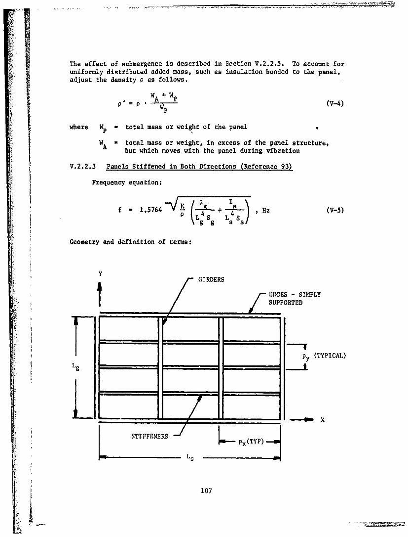
The effect of submergence is described in Section V.2.2.5. To account foruniformly distributed added mass, such as insulation bonded to the panel,adjust the density p as follows.t A +

p = (V-4)

where W total mass or weight of the panel

W total mass or weight, in excess of the panel structure,but which moves with the panel during vibration

V.2.2.3 Panels Stiffened in Both Directions (Reference 93)

Frequency equation:

Ef -1.5764 +(L SHzS 5 (V-5)

Geometry and definition of terms:

GIRDERS

EDGES -SIMPLY

SUPPORTED

Ip (TYPICAL)

Lg /9

10Px(TYP)-I

Ls --

~107

n = number of stiffeners (parallel to the x-direction)

m S= number of girders (parallel to the y-direction)

h = plate thickness

Is lg W second moment of area of stiffeners and girders,respectively, plus the associated plating

AsA S = cross-sectional area of stiffeners and girders,respectively

P" h

Ss As + px h + m (V-6a)

sn

Corrections for added mass effects associated with submersion in a fluidare given in Section V.2.2.5. Account for a uniformly distributed mass,such aL3 insulation which is attached to the pane], by adjusting the panelthickness e in the equation for S. and Sg.

V.2.2.4 Beam Formula for Plate Stiffener (Reference 87)

Frequency formula for the fundamental mode (assumes simple support ofthe stiffener):

f IT- -r HZ (V-7)

2LL + ff

where EI = flexural rigidity of the plate-stiffener combination

GA a shear rigidity of the plate-stiffener combination

L - beam length

ma = mass per unit length of the stiffener and associatedplating

V.2.2.5 Effect of Submergence (Reference 93)

To obtain the frequency, ft, of a plate with one side exposed to airand the other side exposed to a liquid, modify the frequency calculated inair, fa, by the following formula:

108

44f~=f .4' (V-8)

where K + (V-9)

K = 1h a +_- (V-l0)

0t n density of the liquid

Pp M density of the plate

a - plate length

b = plate breadth

h = plate thickness

With both sides of the plate submerged, 4 becomes

= K + 2p /p

V.2.3 Response Calculations

In Section V.2.2, methods are presented for calculating the fundamen-tal frequencies of typical structural components in the walls of LNG tanks.These components include beams, plates, and stiffened panels. Based uponthe fundamental frequency and the minimum rise time of the sloshing forces,a method is given in Section V.2.1 for determining the maximum dyna-ic loadfactor (DLF) of the structural components. The DLF plus the maximum valueof the sloshing fozces (sloshing pressure multiplied by the appropriatearea over which it acts) gives an equivalent static 'load for which thestructural component must be designed to withstand the worst case sloshingforces. These analyses will be performed for structural elements such asbeams, plates, and stiffened panels.

No particular guidance is necessary for the analysis of these compo-nents; however, coupling between structural components can and does occurin complex structures such as the wall of an LNG tank. For these cases, theanalyst must decide whether or not the various components of the tank wallcan be analyzed individually or should be analyzed as a multi-degree offreedom system. If each component in the tank structure is to be analyzedindividually, then it is usually conservative to assume rigid support foreach element (neglecting flexibility in the supporting structure) and thatthe sloshing forces are transferred, undistorted, from one member to thenext. Often the response is attenuated by coupling, but it can be in-creased as well.

109

To resolve such questions which arise when dpplying dOmple analyticalprocedures, a multi-degree of freedom solution is required. These can beobtained by finite-element method or by similar procedures. If a transientresponse calculation is made, then the actual F(t) produced by the slosh-ing pressure is applied to the structure. To be certain that the maximumresponse is obtained, the calculation must be performed with the minimumrise time and with several rise times of longer duration. Such an analysisprocedure can be quite costly to perform, if many dynamic dof's are in-cluded in the calculation.

An alternate approachwhich avoids a dynamic transient solution is toperform an approximate modal analysis using the dynamic load factor deter-mined for a one-dof system (as already described). This method is possiblebecause in a modal superposition analysis, each normal mode responds to theloading independently as a single degree of freedom system. The generalprocedure is as follows:

(1) Calculate the mode shapes and frequencies of the multi-degree of freedom model of the structure.

(2) Calculate the modal displacements and stresses for thepeak sloshing force (statically applied).

(3) Find the dynamic load factors for each mode (each modalfrequen'.y) for the minimum rise time. Figure C-2(b) isused and the values of DLF are read at the correspondingvalues of tr/Ti for i - 1 through N modes. Note that theseare not the envelope values described in Section V.2.1.

(4) Multiply the modal displacement and stresses by theirrespective DLF's.

(5) To find the absolute maximum displacement, sum the modalcontributions. To find the most probable response, takethe square root of the sum of the squares of the modalcontributions.

This procedure should be repeated for several longer rise times to becertain that the worst case loading is used. Alternately, a conservativevalue can be obtained if in Step (3) values of DLF for each mode are readfrom an envelope of DLF established for the tank.

This approximate procedure for calculating the response of a struc-ture to dynamic loading without performing a transien; solution is commonlyused in the nuclear industry(94) for earthquake excitation. A more detailedexplanation of the method is given by Biggs.(

79)

S110

VI. TASK 4 - PRESENTATION OF RESULTS -DESIGN METHODOLOGY

This chapter presents the methodology for designing LNG ship tanks towithstand slosh loads. The procedures are based on the experimental andanalytical studies described in Chapters III - V.

VI.l Current IMCO Requirements and Proposed Changes

VI.l.1 General

Unified Rules for Gas Tankers: Cargo Containment, as published byIMCO, uses the following classification for LNG tanks:

I * Integral

k Membrane (see Figure II-2(a))

Semi-membrane

Independent

Type A

Type B

Type C (pressure tanks) (see Figure II-2(b))

Appendix E includes definitions for all of the above mentioned task class-ifications. With the exception of Type C independent tanks, all tanks must be

analyzed for local sloshing pressures as defined in Section VI.2.2.2. For in-

tegral, membrane and semi-membrane tanks, the local sloshing forces must be ac-

counted for in the design of the insulation, and the ship supporting struc-

ture must be checked for adequate strength. Local sloshing pressures are

produced on the longitudinal bulkheads, transverse bulkheads, and on the

tank top. Areas of the tank which must be checked for sloshing pressures willdepend upon permissible filling depths. In addition to the localized slosh-

ing pressures, the support attachments for all independent tanks must be

d checked for the resultant of the sloshing forces. Dynamic effects of theseforces must be accounted for.

Where tanks or the ship's hull has been designed in accordarce withthe rules and formulas of the classification societies, then the resultingscantlings must be checked for the slosh-induced forces and increased asnecessary. This is true for integral, membrane, semi-membrane, and Type Aindependent tanks. In Type B independent tanks, which are analyzed by re-fined analytical methods, the slosh-induced forces must'be included in these

analyses, as described in Section V.

Inadequate information is available to determine the phasing of theslosh-induced force with other dynamic forces. Thus, stresses produced by

sloshing are assumed to be independent of other dynamic loads and so ae-ecombined with them, taking the square root of the sum of the squares. It

ill

should be noted that stresses produced by sloshing forces add directly tostresses produced by vapor pressure, stationary thermal loads, and otherstatic loads which affect the tank, but they are not combined with them.

VI.l.2 Specific Requirements

Specific requirements for the design of LNG tanks to resist sloshingforces are offered which fit within the framework of the IMCO rules. Thefollowing revisions and/or additions to the rules are suggested.

The IMCO Pars. 4.3.5 Sloshing Loads: Revise Paragraph (a) to read:The risk of significant loads due to sloshing induced by any of the shipmotions mentioned in 2.4.6 must be considered for all filling levels lessthan 100% full.

IMCO Para. 4.4.1 Integral Tanks: Add Paragraph (b): If significantsloshing induced forces are found to occur in the tanks according to 4.3.5,then ship hull scantlings in the transverse and longitudinal bulkheads andin the tank top must be checked for the slosh-induced forces and the scant-lings increased as necessary. Dynamic effects of the sloshing forces areto be considered.

IMCO Pars. 4.4.2 Membrane Tanks: Revise (d) to read; Special atten-tion is to be paid to the possible collapse of the membrane and the insula-tion due to an over-pressure in the interbarrier space, to a possible vacuu:Ain the cargo tank, to the sloshing effects, and to hull vibration effects.

Add Paragraph (f): Special consideration must be given to the effectof sloshing forces on the ship hull as in 4.4.1.

IMCO Pars. 4.4.4 Independent Tanks Type A: Add Paragraph (c): Ifsignificant slosh-induced forces are found to occur in the tank accordingto 4.3.5, then ship hull scantlings in the tank walls, roof, and inter-mediate bulkheads must be checked for the slosh-induced forces and thescantlings increased as necessary. Dynamic effects of the sloshing forcesare to be considered.

IMCO Para. 4.6 Supports: Add Paragraph 4.6.8: Supports for indepen-dent tanks rust be analyzed for the resultant forces produced by sloshingmotions in the tank. Stresses produced by the dynamic sloshing forces shouldbe combined with the wave-induced loads of 4.6.3 according to 4.5.1 for inde-pendent dynamic stresses.

The IMCO paragraphs referenced above arp from the IMCO rules dated1976.

112 JI

VI.2 Design Methodology

A design methodology is presented in flow-chart format in Table VI.l.The design procedure is shown to vary with tank type, i.e., independentpressure tanks (IMCO type C), independent gravity tanks (IMCO types A & B),and membranes and semi-membrane tanks. For all tanks, the design sequenceproceeds from (1) comparing ship periods to predicted resonant slosh periodsto (2) establishing loads based on sloshing pressure and force coefficientsto (3) designing structures by specific delineated methods which vary withtank type.

Each important block in the design sequence is coded on Table VI.l.A description of the procedures for each coded block is given below.

VI.2.1 Loads Prediction Methodology

Resonant Slosh Periods - TR

Resonant sloshing periodswhich are a function of tank geometry andfill depthare determined by the appropriate equation given in Table 111-2.If partial filling is allowed, then Tr should be determined for fill depthsbetween 10% and 98%. Slosh periods considering both the tank length (1)and breadth (b) must be determined for this range of fill depths. If par-tial filling is prohibited, resonan~t periods should be determined for filldepths from 90 to 98%. It is important that tbhse fill depths be consid-ered even when partial filling is prohibited since boil-off results in LNGtypically being carried in this filling range.

Ship Periods - TS

Using standard practices, ship periods in roll, pitch, and surge shouldbe determined for comparison with the resonant sloshing periods. In theevent of overlap between ship periods and resonant sloshing periods, eitherpartial filling (less than about 98% full) must be prohibited or the tankmust be designed to withstand slosh loads.

Design Pressure Coefficients - KP

Several methods exist for establishing design pressure coefficients.Based on the results given in this report, the maximum pressure coefficientis KPHAx - 125. The average pressure coefficient is KPAvG - 25. A conser-

vative approach would be to assume KPMAX and base all subsequent design

analysis on this worst case pressure. An alternate approach would be toadopt the techniques presented in Reference 44. In this reference, a proba-bilistic procedure, involving the response of the liquid in the tank at dif-ferent conditions and the proba3ility of these operating conditions occur-ring, is undertaken. Although there is insufficient detail in Reference 44to include a complete example of how peak sloshing pressures are computedusing the probabilistic procedure, the major steps can be identified,

The procedure utilizes a statistical distribution of pressures ob-tained from scale model experiments and couples this statistical definition

113

R I TSET TANK DIMENSIONS

OFILLING LEVELS

POUD S TOERMINE EXCITATION PEP IODS,D E TTS, FOR ALL POSSIBLE TS

SHIP MOTIONS

REVISE TANK GEOMETRY, NO OVERLAP SLOSHING LOADS DO NOTF! OPERATIONAL FILLING LEVELSR& S IN PERIODS NEED TO BE CONSIDERED

LEAIN CAN PERIODSAPPLODIIED SOVERLAP

DESIG CANNOT

-11

SBE MODIFIED

COMUT TOALREACTION FORCEERIEDSG U]E|PRODUCED BY SLOS"TwP F'OR FR K

DIFFRENTFIV LSS OEFFICIENTS, Kp

FC"UESRSEATTN ETRIEAMPLITUDE OF

SUPPORTS FOR TOTAL REACTION C2 Al EXCITATION, 0, PRODUCEDA PPLIED STATICALLY BY SHIP MOTIONS

(see Page 116) (see Page 115)

TABLE VI-1 DESIGN METHODOLOGY FLOW CHART

114

,~, ,

TPREDICT:PT MAX. SLOSHING PRESS., PMAX

MIN. RISE TIME, T2MAX. DECAY TIME, T3

DETERMINE PRESSUREPD PROFILE ON THE TANK

WALL

TYPE B - OPTION 1ICOMPUTE DYNAMIC RESPONSE OF L| ESTABLISH DYNAMIC LOADTANK STRUCTURE TO TRANSIENT, FACTORS, DLF, FOR

BI DISTRIBUTED PRESSURE SLOSHING PRESSURESP(x or yzt) USINGMULTIPLE-DOF MODEL X

COMUTE EUIVALENT STATICL2 DESIGN LOADS FOR THE

( s e ag 16 ) TANK LL

i'0 (see COMPUT EIIAETSAITYPE B - OPTION 2 , ,

TYPE A MEMBRANE & SEMI-MEMBRANE• °- TANKS

PARESIZE TANK SCANTLINGS AS

NECESSARY BASED UPON CHCK STRENGTH OF INTERNAL2 COMPUTE MODAL STRESSES AND Al CLASSIFI.ATION SOCIET INSULATION BY TESTING

DISPj JCE T O EIUIVALEL TDPLACMENTS FOR EQUIVALENT FORMULAS AND EQUIVALENT OR BY ANALYSIS

iSTATIC LOADS STATIC DESIGN LOADS

COMBINE MODA STRESSES AS /RESIZE SHIP SCANTLINGS AS

B3 INDEPENDENT RESPONSES TO M2J NECESSARY BASED UPONCLASSIFICATION SOCIETY

OBTAINDEIG LOADSOABE IAIMM OSTRE FORMULAS AND EQUIVALENTMAXIMUMH STRESS STATIC DESIGN LOADS

Csee Page 116)

TABLE VT-I DESIGN METHODOLOGY FLOW CHART (CONTD.)

115

'~'4X ,

COMBINE STRESS PRODUCED BYSi SLSHING FORCESWITH OTHER

"INDEPENDENT" DYNAMIC LOADS

S2 ADD STATIC AND DYNAI

STRESSES

TABLE VI-I DESIGN METHODOLOGY FLOW CHART (CONTD.)

116

of pressure distributions with information on ship motion spectral densityin the frequency ranges around the resonant slosh frequencies. Using statis-tical techniques, this procedure then determines the worst case sloshing

V loads that are likely to occur in a 20-year operational period. Pressurecoefficients greater or less than Kp - 125 may be predicted :statisticallydepending on the actual conditions encountered. Based on the results re-ported herein, it is recommended that tank designers use a Kp equal to 125or the statistical approach of Reference 44. A KpMAx - 125 is believed to

be a highly conservative number, and its use would preclude the use of a morecomplicated procedure which is based on probabilistic conditions.

Ship Motion Amplitude - Al

To determine pressure magnitudes, the amplitudes in each of the impor-tant degrees of freedom must be established. Maximum amplitudes will resultin setting maximum anticipated pressures for design purposes. Maximum amp-litudes should be considered for roll, pitch, and surge.

Sloshing Pressures - PT

Sloshing pressures are determined from the pressure coefficient andamplitude information established above. Pressures should be predicted foreach of the appropriate tank walls, whereby the appropriate length dimen-sion, I or b, is utilized. The following values of the pressure coeffic-ients should be used depending on the amplitude.

Kj' K X/k 01 < 0.1 (I1

Kp L, ,0075 + 092) xIL or 0> 0.1 (VI-2)

- < 0..

At low amplitude sloshing, the pressures are shown to be linear withamplitude, while at amplitudes greater than 0.1 the pressures do not in-crease linearly. (Seo Figure III-5,) Equation VI-2 uses currently avail-able data which give the effect of amplitude on pressure coefficients andprovide a more realistic definition of Kp at high amplitudes.

To determine a characteristic range of rise and decay times of thedynamic sloshing pressures, the following coefficients should be utilized.These values are taken from Table V-1.

Minimum pressure rise time: KT2 = 0.0005

Maximum pressure spike duration: KT3 = 0.9489

ri Thus, both maximum and minimum times are established for subsequent struc-tural response calculations. Both length and breadth dimensions of the tankmust be utilized for the characteristic length dimension in these equations.

117" , i1I

Tank Wall Pressure Distribution - PD

The pressure distributions over the tank walls are important in deter-mining the walls' responses to slosh-induced loads. The following idealizedpressure distributions are for (1) vertical tank walls and (2) the tank top.The following pressure distributions have been compiled using the curreItlyavailable data. Because the distributions are affected by a great manyvariables, these idealized distributions should be considered as conserva-tive estimates.

For the vertical tank walls, the pressure may be considered constantin the horizontal direction. In the vertical direction, the pressure vari-ation is described by the following cosine function. The maximum pressureoccurs at the static liquid filling level and decays to zero at levels 20Zabove and below the static liquid level.

Kpz o 151 z- h MV-3)

where Kp U pressure coefficient at level z

KpMAX - maximum pressure coefficient

z m distance from the tank bottom

pot n h liquid filling height

dt TrH ntank height

i and with limits%

SH H: h - < _h + -

- :For localized areas of 4 m2 (2 m x 2 m) or less, the pr"essure can be as-! sumed to act uniformly over the area.

-For the tank top, the pressure may be assumed to be constant (thel, maximum value) on the corner areas. These areas should extend in from the; port and starboard walls one-third of thie width of the tank and from the

fore and aft walls one-third of the length of the tank. The remaining top

areas should be designed to withstand sloshing pressure based on KpAVG.

Total Sloshing Forces - FR

The total forces exerted on the tank bulkheads by the sloshing liquidcan be determined from Figure 111-6 for prismatic tanks and from FiguresIII-10 - 111-17 for spherical tanks. It is noted that for prismatic tanksthese forces represent the inertia forces that occur on the tank wall due

118

to resonant liquid sloshing. They do not include the forces exerted on thestructure by the inertia of tank structural components. For sphericaltanks, both the resultant forces (: gures III-10 and III-11) and the slosh-ing components (Figures 111-12 through 111-17) are given. The resultantforces represent the combination of static aeight and inertial sloshingloads.

VI.2.2 Tank Design Methodology

Tank Support Stresn - C2

The sloshing reaction force is the integral of the sloshing pressuresover the tank wall area. It is produced by the motion of the liquid in thetanks and does not include the inertia of the tank structure or the weightof the liquid. As noted in block FR, some results are given for sphericaltanks which include the weight of the liquid. Rise times and durations arenot given, but it is safe to assume that the reaction is quasi-static forthe response of the tank on its supports, and so the supports should be ana-lyzed for the peak sloshing reaction force, statically applied. This reac-tion produces stress both in the tank and in the supporting structure. Thestructural arrangements for tank support can be very complicated,and com-plex multi-dof analysis procedures are often required to accurately computethe resulting stresses.

Dynamic Tank Structure Response - Bl

Independent tanks, Type B, are analyzed using refined analytical tech-nqiues such as the finite-element method. One approach (Option 1) for cal-culating the stresses in the tank produced by sloshing pressures is to per-

form a dynamic transient solution for the actual pressure-time or force-timehistory. This calculation procedure is discussed in Section V.2.3. Ananalysis of this type should provide the most accurate solution to the be-havior of the tank for sloshing pressures, but it can be very expensive interms of computation time. Multiple analyses, with different loading con-ditions (different rise times for the sloshing pressure) are usually re-quired to determine the worst case loading, making this approach even morecostly. Thus, a more practical approach is the approximate modal analysissuggested as Option 2. (see Section V.2.3).

Dynamic Load Factors - Ll

Once the miniv.em rise time and maximum decay time of the sloshingpressures have been determined, the dynamic load factors for a range of fre-quencies of the tank structure can be established. The dynamic load fac-tors depend only upon the rise and decay times of the loading and the struc-tural vibration periods. They are independent of the pressure magnitude.This procedure is described in detail in Section V.2.1.

Equivalent Static Design Loads - L2

From the dynamic load factors (DLF's) and the peak value of the slosh-ing pressures, equivalent static design loads can be determined for the tank

i L19

1 119N

structure. Design static pressures are simply the peak pressure multipliedby DLF. Design forces are the design static pressures integrated over theappropriate wall area of the tank.

Modal Stress Computation - B2

An alternate approach to a dynamic transient solution for the computa-tion of stresses in the Type B independent tank is to perform an approximatemodal solution. This approach, Option 2, is based upon a multi-dof solutionfor modal frequencies and modal stresses produced by the peak value of thesloshing pressure, applied statically (see Section V.2.3). Frequencies,mode shapes, and static stress are less costly to obtain than a dynamictransient solution described as Option 1 and, once obtained, the solutionsfor stresses under different loading conditions (different rise times) areeasy to obtain.

Combined Modal Stresses - B3

Once modal frequencies have been calculated, the dynamic load factors,DLF's, for each mode can be determined. Static modal stresses multipliedby the modal DLF gives the modal stress for the dynamic loading. The mostprobable maximum stress in the structure is then obtained by combining modalstresses by the "square root" method. This method of combining stressesassumes that modal stresses are independent. An upper limit on stress isobtained by simply adding moe.i values.

Set Tank Scantlings (Type A) - Al

Scantlings for Type A independent tanks are sized according to formu-las of the classification society. Once the equivalent static sloshingpressures have been determined for the tank, these same formulas can beused to size or resize the scantling for the sloshing forces. Alternatemethods, such as those suggested for Type B independent tanks or for themembrane insulation, are also applicable to Type A tanks. Approval to usealternate methods must be granted by the classification society.

Internal Insulation Strength - Ml

Strength of the insulation which supports the membrane must be adequatefor the sloshing pressures. As demonstrated in Appendix D, strength of in-sulation system can be well approximated by fairly simple classical methodsand/or laboratory tests at the equivalent static design pressure. A combi-Ination of testing and analysis is recommended because of uncertainties inthe material properties of some insulation systems. Of course, more refinedanalytical methods can be used, but these are recommended only if materialproperties of construction materials are well defined.

Set Tank Scantlings (Membranes) - M2

As for Type A independent tanks, the scantlings of the ship's innerhull are determined using formulas of the ship classification society. Once

120

the equivalent static sloshing pressures have been determined for the tanks,

these same formulas can be used to size or resize scantlings for the slosh-ing forces. Alternate methods, such as those suggested for Type B indepen-dent tanks or for the membrane insulation are also applicable for Type Atanks. Approval must be granted by the society to use these alternate meth-ods.

Combined Stresses from Sloshing and Other Dynamic Loads - Si

Insufficient information exists to determine the phasing of the sloshloads with other dynamic loads which ac on the tank; thus, the resultingstresses are treated as independent with respect to stresses produced byother dynamic loads. Combination of these independent stresses to producethe most probable maximum dynamic stress is by the square-root method, whichis the square root of the sum of the square of the independent values. Whencombining stress produced by localized sloshing pressure with other dynamicstresses, stress produced by the dynamic liquid head is omitted. Measuredsloshing pressures include the dynamic liquid head. Also, because sloshingpressures occur very near the static liquid level, or above as in the caseof sloshing pressure on the tank top, the liquid head is very small where

sloshing pressures are highest.

Combined Static and Dynamic Stress - S2

Thc resulting dynamic stress is added directly to stresses producedby static loads such as thermal loads, still-water loads, vapor pressureloads, etc., to find the maximum stress for the condition being investigated.

VI.3 Example Problem Utilizing Tank Design Mathodoloj,

The following example problem illustrates the use of the tank designmethodology presented in Table VI-l. The example analyzes a prismatic mem-brane tank with the Gaz Transport membrane system (plywood insulation boxes).Tank dimensions are arbitrarily set at

Z - 36 m (118 ft)

b - 36 m (118 ft)

H = 24.4 m (80 ft)

and tank motion amplitudes (Al) are assumed to be:

fPitchMAX - ±5 ( 0.087 rad.)

ORollMAX - ±100 ( 0.175 rad.)

- =* -0.1S, SurgeMAX

121

Tank filling levels during operation are placed at 90 to 98%. Currentregulations limit most LNG tanks to maximum operational filling levels of97-98%, with partial filling prohibited. From Table VI-1, the initial de-sign steps are to calculate (TR) the resonant periods of the liquid in thetank, to establish (TS) ship motion periods, and to determine if the tankresonant periods coincide with ship motion periods. For purposes of thisexample, the ship motion periods are assumed to be in the range of 6 to 12seconds.

The resonant periods of the liquid in the tank are calculated usingEquation 111-6 for prismatic tanks. For filling levels between 90 and 98%,the resonant pitch and roll sloshing periods are:

6.89 sec < TR < 6.94 sec

0.9 < h/H < 0.98

Thus, the tank excitation periods overlap the resonant periods of the tankliquid so there is the potential for resonant sloshing.

At this point, the designer can decide to modify the tank size orgeometry to change the resonant periods of the liquid in the tank. In thisexample, the tank will remain unchanged, so it must be designed to withstandresonant sloshing conditions.

For design purposes, the maximum nondimensional pressure coefficient(KP) is 125. Equations VI-i and VI-2 are then used to correct this coeffi-cient for tank excitation amplitude effects. As previously mentioned, theamplitudes for this example are assumed values. The corrected coefficientsfor pitching, rolling, and surging motions (PT) are:

for pitching ( - ±5* or 0.087 rad.): K - 125.0

for rolling (0 - ±100 or 0.175 rad.): K4A- 75.4

for surging = ±0.1): K' 125.0

At this point, it is necessary to choose the pressure rise and dura-tion time values (KT2 and KT3) associated with the pressure-time history of

the dynamic impact pressure. Using Table V-i, the minimum nondimensionalrise time (KT2) is 0.0005. The maximum spike duration (KT3) is 0.9489.

Now that the nondimensional design pressures and times have been es-tablished, full scale pressures and times can be calculated. Pressures canbe determined using Equation 111.4. For this example, the liquid density is493.19 kg/m3 (30.79 lbm/ft3). The design pressures are found to be:

2for pitching: P,. 1.892 N/(mm) (274.4 psi)

for rolling: P,.. = 2.295 N/(mm)2 (332.9 psi)

122

for surging: P MAX= 2.175 N/(mm)2 (315.4 psi)

Full-scale times are determined using Equation 11-2. The minimum pressurerise time is 1.0 millisecond, and the maximum pressure spike duration is1.82 seconds.

To compute design loads for structural components of the tank (blockLl of Table VI-I), the dynamic load factors, corresponding to the rise anddecay times of the sloshing pressures, are determined for a range of struc-tural frequencies. This was done for a tank which is 36 m (118 ft) long(or wide) in Section V.2, and the results, expressed as the enveiope of thedynamic load factors (DLF), are plotted in Figures V-2 and V-3.

To determine the equivalent static design load for structural compo-nents of the tank (block L2), the fundamental vibration period of the com-ponent must be calculated. With the fundamental period known, the DLF isread directly from Figures V-2 or V-3. These steps were performed for theGaz Transport insulation boxes and are described in detail in Appendix D,part D.I. Two components of the box were analyzed in the example: the boxcover and the longitudinal stiffener of a primary box. Rasults for thesesteps are:

Fundamental Period,T DLF

Box Cover (12-cell box): 0.93 ms 1.22

Longitudinal Stiffeners: 1.96 ms 1.63

Equivalent static design pressures for the cover and stiffener are obtainedby multiplying the peak sloshing pressures from block PT by the DLF. Usingthe maximum pressure, PMAX, which occurs in roll for this example, the de-

j sign static pressures are:

2Cover: Pdes = 1.22 (2.295) = 2.80 N/mm (406 psi)

Stiffener: P = 1.63 (2.295) = 3.74 N/mm (543 psi)

Strength of the insulation boxes (block Ml) was established in Appen-dix D and expressed in terms of the peak allowable sloshing pressure, Pa-This allowable pressure is the static pressure which the box component willwithstand divided by DLF. The allowable pressure, Pa, would be comparedwith the maximum sloshing pressure, PMAX, rather than the design pressure,Pdes" To obtain a pressure for comparison with Pdes' Pa from Appendix D issimply multiplied by DLF. From Appendix D we have

2Cover: P = 0.853 N/mm (124 psi)a

PS = 1.22 (0.853) = 1.04 N/mm2 (151 psi)des

123

Stiffener: P = 0.778 - 0.937 N/mm2 (113 - 136 psi)a

2P~s 1.63 (0.770 - 0.937) - 1.268 - 1.527 N/mmdes (184 - 222 psi)

where Pdes denotes the design static strength of the component. Comparingthese values to Pdes computed in block L2, we find

Cover: P5ds 1.04 N/m 2 (151 psi)< Pde 2.80 N/m 2 (407 psi)des (11des(47pi

2Stiffener: Pe - 1.268 - 1.527 N/mm (184 - 222 psi)< < des

desde3.74 N/mm2 (543 psi)-

Thus, for this example, the design strength of the insulation is inadequate.In this example, only the primary insulation box was analyzed for the slosh-ing pressures. Of course, in practice the designer would need to check thestrength of the secondary box as well.

The final step (block M2) in evaluating membrane tanks for sloshingpressures is to check the strength of the ship's inner hull which supports themembrane system. Scantlings of the hull are checked using formulas of theclassification societies and the equivalent static design load. In thisexample we did not apply classification society formulas to check hullstrength; however, alternate methods of analysis are applicable, but appro-val of the classification society must be obtained before alternate proced-ures can be applied. As an example of alternate methods, see the analysisof the CONCH independent tank in part D.3 of Appendix D.

VI.4 Summary

The design methodology presented in this chapter is based on a thor-ough review of the literature supplemented by additional experiments andanalytical studies. Since information required for many of the steps inthis procedure is limited, the procedures developed herein have been basedon utilizing conservative approaches. For example, pressure coefAicientsare based on the worst case pressure coefficients determined from a widerange of data available from the literature. Likewise, analytical methodswhich are based rn simplified one degree of freedom analysis have been de-veloped with conservatism imposed. Thus, ut-lizing these techniques, aconservative design could occur. It is believed that the major steps inthe proposed design methodology are appropriate, and it is left to the in-dividual designer to substitute more realistic loads when he believes it isappropriate. As an example, sloshing loads could be more realistically es-tablished from scale model tests on replica models of interest. Scaledship motions could be imposed on the models at fill depths of interest andthe resulting loads and load distributions determined. This would providemore accurate data relative to a specific design. However, if resonantsloshing for all filling levels were investigated, it is likely that aKPMX, nearing the 125 value established herein, would be approached.

124

Li ____

VII CONCLUSIONS AND RECOMMENDATIONS

As a result of the study reported herein the following conclusionsand recommendations are presented.

VII.l Summary and Conclusions

0 A significant amount of scale model sloshing data for bothprismatic and spherical tanks and covering a wide range ofFfill depths, excitation frequencies and amplitudes, tank wailpressure measurement locations and total force measurements isavailable in the literature.

o A compilation of this data and presentation in a common formathas been accomplished to provide design pressure and forcecoefficients.

0 Because the complexity of resonant large amplitude sloshingcauses a wide variation in the impact pressure magnitude oneach successive sloshing cycle, beth worst case and averagepressure coefficients have been d,-Zined for design purposes.These pressures are assumed to potentially occur at any loca-tion on the tank wall if partial filling is allowed.

0 Pressure-time histories have been established for sloshing dy-namic impact pressures. No correlation was foUnd to existbetween impact pressure magnitude and duration. A representa-tive range of impact pressure rise times and durations wereestablished.

0 Dynamic loads test, where predicted full-scale pressure/timehistories were reproduced on representative segments of a LNGmembrane tank structure, established structural response andfailure characteristics. It is noted that failure occurredat simulated loads that could occur during "worst case"resonant sloshing.

o Combined-degree-of-freedom resonant sloshing test (pitch and

heave, surge and heave) produced impact pressures no greaterthan the corresponding pressures measured in single-degree-of-freedom resonant sloshing (at the same amplitudes).

o Materials properties measured on plywood used in some LNGmembrane structures showed considerable variation. This datais valuable in the design of tank wall structures using suchmaterials.

o Analytical methods were developed to predict structural responseto dynamic slosh loads. Localized areas of the tank structureare treated as eq~tivalent one degree-of-freedom systems and a

dynamic load factor (DLF) is established based on the fundamental

125

1

period of the structure and a worst case pressure-time history.Examples for typical structural elements are given and showthit some typical structures are not designed to withstandworst case impact loads.

0 Design methods are presented for independent pressure andgravity tanks and membrane and semi-membrane tanks. The designsequence proceeds from 1) comparing ship periods to predictedresonant slosh periods to 2) establishing loads based on loadscoefficients to 3) designing structures by specific delineatedmethods which vary with tank type.

[ VII.2 Recommendations

0 Additional literature review and experiments are required toevaluate loads on liquid bulk carriers with significant tankinternal structures (i.e., typical crude and chemical carriers).Fnphasis ,,hould be placed on localized loads on web frames,pump columns and swash bulkheads. Total forces should alsobe established.

o Full scale LNG sloshing data currently being obtained shouldbe analyzed in light of the results reported herein. Simulatedfull scale ship motion conditions on scale models should beundertaken with model sloshing loads compared to full scale.

o Additional model experiments should be conducted to furtherestablish effects of excitation amplitude on measured pressurecoefficients. Also end wall pressure distributions for a

complete range of prismatic tank fill levels should be estab-lished.

o Analytical methods and design procedures presented herein

should be further refined after the above recommended work is

accomplished and feedback from industry is obtained.

ACKNOWLEDGEMENTS

Many individuals and organizations assisted in the conduct of thisprogram. Special thanks ere extended to El Paso Marine Company for pro-viding the full-scale LNG membrane tank wall segments and support informa-tion needed for this project. In addition, our sincere appveciation isexpressed to the American Bureau of Shipping, Newport News Shipbuilding andDrydocking Company, General Dynamics-Quincy Division, and Avondale Ship-yards for furnishing information on tank structural details and design pro-cedures. Additional thanks are extended to Det norske Veritas, BureauVeritas, and The Swedish Ship Research Foundation for their comments andLNG sloshing model data which were reviewed in this report.

Special thanks are extended to Mr. A. C. Rogers for his help in thedesign of the dynamic load simulator and to Messrs. C. M. Wood and J. R.Winfield for their work in conducting the experimental studies. Finally,this report could not have been produced withou + the skillful typing andfigure productions of Mrs. Cathy Dean, Mrs. AdeLine Raeke, and Mr. VictorHernancez. Special thanks are extended to these individuals.

126

VIII. REFERENCES

1. Abramson, H. N., The Dynamic Behavior of Liquids in Moving Containers,

NASA SP-106, 1966.

2. Abramson, H. N., Bass, R. L., Faltinsen, 0., and Olsen, H. A., "Liq-uid Slosh in LNG Carriers," 10th Symposium of Naval Hydrodynamics,M.I.T., Boston, Massachusetts, June 25, 1974.

3. Baitis, A. E., et. al., "Prediction of Lifetime Extreme Accelerationsfor Design of LNG Cargo Tanks," Naval Ship Research and DevelopmentCenter, Mar. 1974.

4. Baitis, A. E., "Summary of Development for LNG Tank Design Accelera-tion Rules," David W. Taylor Naval Ship Research and DevelopmentCenter, Bethesda, Maryland, Dec. 1976.

5. Baitis, A. E., Bales, S. L., and Meyers, W. G., "Design Accelerationand Ship Motions for LNG Cargo Tanks," David Taylor Research andDevelopment Center, Bethesda, Maryland.

6. Bass, R. L., "Dynamic Slosh Induced Loads on Liquid Cargo Tank

Bulkheads," Society cf Naval Architects and Marine Engineers,Report R-19, Aug. 1975.

7. Bass, R. L., "Liquid Impact Loads in LNG Carriers," Tech. ReportNo. 1, Aug, 1972, El Paso Natural Gas Co., Southwest ResearchInstitute.

8. Bass, R. L., Hokanson, J. C., and Cox, P. A., "A Study to ObtainVerification of Liquid Natrual Gas (LNG) Tank Loading Criteria,"Final Technical Report SSC-258, Naval Sea Systems Commind ProjectSR-218, May 1976.

9. Bass, R. L., and Oldham, G. A., "Liquid Impact Loads ir, PartiallyFilled Tanks of a 125,000 m3 LNG Carrier," Final Technical Report,Feb. 1975, Methane Tanker Service Co., Southwest Reseacch Institute.

10. Bass, R. L., and Ransleben, G. E., "Scaling Criteria for LargeAmplitude Sloshing in LNG Ship Cargo Tanks," Technical Report No. 2,Oct. 1974, Methane Tanker Service Co., Southwest Research Institute.1 11. Blixell, A., "Calculation of Wall Pressures in a Smooth RectangularTank due Lo Movement of Liquids," Research and Technical AdvisoryServices Report No. 5108, Lloyd's Register of Shipping, March 1972.

12. Brathu, M. C., Huther, M., and Planeix, J. M., "Computer Calculationsof Liquid Motions in Tanks," Flhipping World and Shipbuilder, Dec. 1972.

13. Bureau Veritas, "Etude des Replissages Partiels dans les Cales desNavireB," N.I. 171 BM.l, May 1976.

4 127

! I

14. Bureau Veritas, "Motions of Liquids in a Short LNG Carrier Tank,"BM.1-Ht/nc, Sept. 4, 1972, Gaz Transport Study AT 47, Bureau Veritas.

15. Bureau Veritas, "Motions of Liquid in a LNG Carrier Tank with LowFilling," BM.1-HT/Plx/nc, Gaz Transport Study AT 27, Bureau Veritas(Confidential Report).

16. Campus, P., and DuBois, M., "Mesure sur Modules des Sollicitationsdes Parois et des Plafonds de Citernes de Navires dues au Mouvementdes Cargaisons Liquides," 1974, Bureau Veritas.

17. Chan, A. S. L., and Trbojevic, V. M., "Thin Shell Finite Element bythe Mixed Method Formulation-Part 1."

18. Conners, Thomas G., "Update: Domestic LNG Vessel Construction,"Marine Technology, Vol. 15, No. 1, Jan. 1978, pp 1-13.

19 Drake, Elizabeth and Reid, Robert C., "The Importation of LiquifiedNatural Gas," Scientific American, Vol. 236, No. 4, April 1977.

20. Faltinsen, 0., "A Nonlinear Theory of Sloshing in Rectangular Tanks,"Journal of Ship Research, Vol. 18, No. 4, Dec. 1974.

21. Filstead, C. G., Jr., "The Design and Operation of LNG Ships withRegard to Safety," Shipping World and Shipbuilder, Vol. 165, No. 3866,pp. 259-262, Feb. 1972.

22. Gastech 76, International LNG/LPG Conference New York 1976, "For LNG-A Concrete Answer," Extracts from papers read at this importantassembly.

23. Glasfeld, R. D., "Design of Spherical Shipborne LNG Cargo Tanks,"presented at the Marine Technology Symposium, San Diego, Calif.,1976.

24. Hansen, R., and Rimeid, B. E., "Moss Rosenberg Verft A/S 87, 600 m3LNG-Carrier Prediction of Loads due to Sloshing in Tanks," ReportNo. 72-45-C, May 19, 1972, Moss Rosenberg Verft A/S, Det norskeVeritas.

25. Hansen, Hans R., "Some Aspects concerning the Design of LNG Carriers,"Classification and Registry of Shipping, Information No. 10, Nov. 1972.

26. Hori, Tohru, et. al., "Observations on an Experimental LNG Carrierat Sea (Part 2)," Hitachi Shipbuilding and Engineering Co., Ltd.

27. Howard, J. L., Kvamsdal, R. S., and Naesheim, K., "Building andOperating Experience of Spherical-Tank LNG Carriers," Marine Tech-nology, Vol. 14, No. 2, April 1977, pp. 158-174.

28. Howard, J. L., "LNG Marine Carrier Construction," Marine Technology,Vol. 9, No. 3, pp. 281-291, July 1972

128

29. Huther, M., Dubois, M., and Planeix, J. M., "Model Studies on theMovement of Liquid in Tanks," Marine Engineers Review, Jan. 1973.

30. Huther, M., Olsen, H., and Thomsson, 0., "Liquid Sloshing in Tanks

with Internal Structures," S.S.F. project 5609 Summary Report, April1977.

.31. Hysing, Thor, and Harald Olsen, "A Mini-Study of the Spatial Distri-

bution of Slosh Impact Pressures," Report No. 75-18-S, Det norskeVeritas, Sept. 1, 1975.

32. ino, Nobu, Kenji Sakano, Takeshi Vemura, and Yorimitsu Kobayashi,"Method of Safety Assessment on Structures Under Repeated Loading,"___En__neern__9,_I, 1976,EngneeingReview, Vol. 9,No. 1,Jan.196

33. Jackson, R. G., and Kotcharian, M., "Testing and Technology of Modelsof Integrated Tanks for LNG Carriers," First International Conferenceon LNG, Chicago, Ill., 1968.

34. Johnsen, K. R., and Harald Olsen, "Nonlinear Sloshing in a RectangularContainer," Vol. 2, Report No. 74-72-S, Dot norske Veritas, July 24,1975.

35. Johnsen, K. R., and Harald Olsen, "Nonlinear Sloshing in a Rectangular

Container," User's Manual to the Computer Routine NVSLOSH, ReportNo. 74-72-S, Det norske Veritas, Jan. 22, 1975.

36. Kvamsdal, R., Ramstad Ho, Bognaes, R., and Frank, H. J., "TheDesign of an 88,000 m LNG Carrier with Spherical Cargo Tanks andNo Secondary Barrier," Det norske Veritas and Moss-Rosenberg Verft.

37. Lydersen, N., "Dynamic Liquid Pressure in Tanks," Report No. 69-44-S,Jan. 23, 1970, Det norske Veritas.

38. Marine Media Management, Ltd., "Sener-Crinavia LNG Carrier Pro"iction,"Marine Engineers Review.

39. Mathisen, J., "Sloshing loads due to Ranv.. Pitch Motion," Vol. 4,No. 3, Norwegian Maritire Research, 1976, Det norske Veritas.

40. Mitsui Shipbuilding and 'Ingineering Co., Ltd., "Sloshing Test Programfor Liquid Cargo Tanks,' Ship Research and Development Department,Sept. 12, 1972.

41. Odland, J. R., "A Simplified Calculation of the Interaction ForcesBetween Hull and Tank Sys' tem for a Mss Rosenberg Type LNG Carrier,"No. 1, Vol. 3, Norwegian.Maritime Research, 1975, Det norske Veritas.

42. Olsen, H. A., "Dynamic Si:resses in Bulkhead Plating and Load on Fuel

Tank Bulkhead due to Sloshing," Report No. 70-120-0, Dec. 1970,Akergruppen, Oslo, Det ncrske Veritas.

129

''"

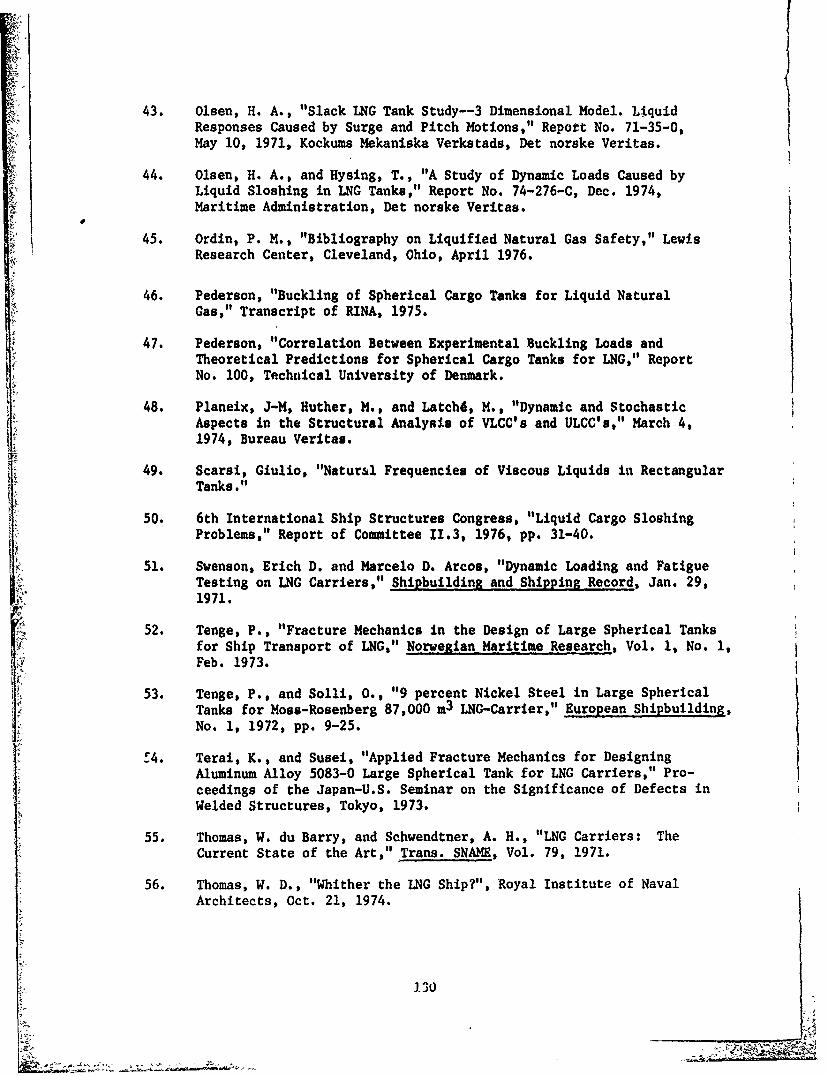
43. Olsen, H. A., "Slack LNG Tank Study--3 Dimensional Model. LiquidResponses Caused by Surge and Pitch Motions," Report No. 71-35-0,May 10, 1971, Kockums Mekaniska Verkstads, Det norske Veritas.

44. Olsen, H. A., and Hysing, T., "A Study of Dynamic Loads Caused byLiquid Sloshing in LNG Tanks," Report No. 74-276-C, Dec. 1974,Maritime Administration, Det norske Veritas.

45. Ordin, P. M., "Bibliography on Liquified Natural Gas Safety," LewisResearch Center, Cleveland, Ohio, April 1976.

46. Pederson, "Buckling of Spherical Cargo Tanks for Liquid NaturalGas," Transcript of RINA, 1975.

47. Pederson, "Correlation Between Experimental Buckling Loads andTheoretical Predictions for Spherical Cargo Tanks for LNG," ReportNo. 100, Technical University of Denmark.

48. Planeix, J-M, Huther, M., and Latchd, M., "Dynamic and Stochasticii " Aspects in the Structural Analysis of VLCC's and ULCC's," March 4,

1974, Bureau Veritas.

49. Scarsi, Giulio, "Natur&l Frequencies of Viscous Liquids in RectangularTanks."

50. 6th International Ship Structures Congress, "Liquid Cargo SloshingProblems," Report of Committee 11.3, 1976, pp. 31-40.

V 51. Swenson, Erich D. and Marcelo D. Arcos, "Dynamic Loading and FatigueTesting on LNG Carriers," Shipbuilding and Shipping Record, Jan. 29,1971.

52. Tenge, P., "Fracture Mechanics in the Design of Large Spherical Tanksfor Ship Transport of LNG," Norwegian Maritime Research, Vol. 1, No. 1,Feb. 1973.

53. Tenge, P., and Solli, 0., "9 percent Nickel Steel in Large Spherical

Tanks for Moss-Rosenberg 87,000 m3 LNG-Carrier," European Shipbuilding,No. 1, 1972, pp. 9-25.

E4. Terai, K., and Susei, "Applied Fracture Mechanics for DesigningAluminum Alloy 5083-0 Large Spherical Tank for LNG Carriers," Pro-ceedings of the Japan-U.S. Seminar on the Significance of Defects inWelded Structures, Tokyo, 1973.

55. Thomas, W. du Barry, and Schwendtner, A. H., "LNG Carriers: TheCurrent State of the Art," Trans. SNAME, Vol. 79, 1971.

56. Thomas, W. D., "Whither the LNG Ship?", Royal Institute of NavalArchitects, Oct. 21, 1974.

130

57. Tonnessen, Arne, "Spherical LNG Tanks on Continuous CylindricalSkirts. A Shipbuilder and Licenser's Experience," Sept. 1977, MossRosenberg Verft. a.s., Moss, Norway.

58. Vilbo, 0. R., "Dynamic Loads Upon Watertight and Swash Bulkhead inPartly Filled Tanks. A Study Made on a Set of Published Data,"Report No. 72-17-S, Feb. 26, 1973, Det norske Veritas.

59. Vinje, Tor, "On Calculation of the Characteristic Frequencies ofFluid-Filled Spherical Shells," Norwegian Maritime Research, Vol. L,No. 1, Feb. 1973.

60. Yajima, H., "On the tttle Fracture Initiatioo Characteristics of9% Ni Steel for Spherical LNG Tank," Proceedings of the Japan-U.S.Seminar on the Significance of Defects in Welded Structures, Tokyo.1973.

61. "Current Developments in Liquified Natural Gas presented at Inter-national Conference," Industrial Heating, Nov. 1977.

62. "Hassi R'Mel'Algerian Owned LNG Ship," Shipping World and Shipbuilder,Vol. 165, No. 3869, pp. 571-574, May 1972.

63. diPapers from the Seminar on Liquid Sloshing," Sponsored by Det norskeVeritas, May 20-21, 1976.

64. Bowles, E. B., Jr. and R. L. Bass, III, "Evaluation of Near FullSloshing Loads in El Paso Marine Company's 125,000 m3 LNG Ship Tanks,"Tech. Report No. 1, June 1978, El Paso Natural Gas Co., SouthwestResearch Institute (Confidential).

4 65. Ochi, Yoshio and Nobuyuki Kobayachi, "Sloshing Experiment of a Cylin-drical Storage Tank," IHI Engineering Review, Vol. 11, No. 2, April1978.

66. Faltinsen, 0. M., "A Numerical Nonlinear Method of Sloshing in Tankswith Two-Dimensional Flow," Report No. 77-014, Jan. 12, 1977, The RoyalNorwegian Council for Scientific and Industrial Research, Det norskeVeritas.

67. Hagiwara, K., "On Secondary Loads on Ship Structure, Part II," June 1976,Mitsubishi Heavy Ind., Ltd., Nagasaki Tech. Inst., Japan.

68. Sawayangi, M., and Matsumoto, Y., "Experimental Study on the SloshingPressure of Rectangular Tanks," Mitsui Eng. and Shipbuilding Co., Ltd.,Chiba Laboratory.

69. Verhagen, J., and van Wijngaarden, "Nonlinear Oscillations of Fluid ina Container," Journal of Fluid Mechanics, Vol. 22, Part 4, pp. 737-751,1965.

131

70. Huther, M., H. Olsen, and 0. Thomsson, "Liquid Sloshing in Tanks withInternal Structures," S.S.F. Project 5609, Main Report, April 1977.

71. Whitman, A. M., and M. C. Pancione, "A Similitude Relarion for FlatPlate Hydrodynamic Tmpact," Journal of Ship Research, Vol. 17, No. 1,1973.

72. Ochi, Yoshio, Osamu Asai, and Kiyoshi Naito, "Coupled Vibration ofLiquid and a Cylindrical Tank," IHI Engineering Review, Vol. 11,No. 3, July 1978.

73. Asan, Seiichi, et al., "Observations on an Experimental LNG Carrier

at Sea (Part 1)," Hitachi Shipbuilding and Engineering Co., Ltd.

74. Bowles, E. B., R. L. Bass, and F. T. Dodge, "Evaluation of Scaling

Criteria for Scale Model Sloshing Simulations of El Paso Marine Com-pany's 125,000 m3 LNG Ship Tanks," Technical Report No. 2, December1978, El Paso Marine Co., Southwest Research Institute (Confidential).

75. Bowles, E. B., R. L. Bass, and P. A. ,ox, "Evaluation of Near FullSloshing Loads and Structural Hespon!-. i in El Paso Marine Company's125,000 m3 LNG Ship Tanks," Technical Report No. 3, in preparation,El Paso Marine Co., Southwest Research Institutp (Confidential).

76. "Dynamic Test on Plywood," Mchiba Laboratory, Technical Division,Mitsui Shipbuilding & Engineering Co., Ltd., 20 Nov. 1972.

77. "Releves de Flexion sur Eprouvettes en Contreplaque de Bouleau(Tranches de Ceissons)," Gaz Transport, Essai NO 70.7, 22 May 1970.

78. "Investigation sur le Comportement au Choc des Contreplaque's a" laTemperature Ambiante et a' la Temperature de Lazote Liquide (-196*C),"Gaz Transport, 17 Fevrier 72, Doc. Int. No 101.

79. Biggs, J. M., Introduction to Structural Dynamics, McGraw-Hill BookCo., New York, 1964.

80. Army Manual TM5-1300, "Structures to Resist the Effects of AccidentalExplosions," June 1969.

81. "The Air Force Manual for Design and Analysis of Hardened Structures,"AFWL-TR-74-102, October 1974.

82. "Shelter Design and Analysis, Volume 4: Protective Construction forShelters," TR-20, Review Draft, dated July 1972.

83. "Suppressive Shields Structural Design and Analysis Handbook," U.S.Army Corps of Engineers, Huntsville Division, Publication HNDM-lll0-1-2, November 1977.

132

84. Westine, P. S., and W. E. Baker, "Energy Solutions for PredictingDeformations in Blast-Loaded Structures," Edgewood Arsenal ContractorReport EM-CR-76027, Report No. 6, November 1975.

85. Westine, P. S., and P. A. Cox, "Additional Energy Solutions for Pre-dicting Structural Deformations," Edgewood Arsenal Contract ReportEM-CR-76031, Report No. 4, Contract DAAAl5-75-C-0083, SwRI, SanAntonio, Texas, 1975.

86. Westine, P. S., P. A. Cox, and E. D. Esparza, "Structural AnalysisEmphasizing Energy Methods: Some Comparisons with Suppressive ShieldExperiments," Minutes of the 17th Explosives Safety Seminar, Denver,

• IColorado, September 1976.87. Smith, C. S., "Bending, Building and Vibration of Orthotropic Plate-

"eam Structures," Journal of Ship Research, December 1968, pp 249-268.

88. Madsen, N. F., "Vibration of Orthogonally Stiffened Panels," Journalof Ship Research, Vol. 22, No. 2, June 1978, pp 100-109.

89. Chang, Pin-Yu, "A Simple Method for Elastic Analysis of Grillages,"Journal of Ship Research, June 1968, pp 153-159.

90. Chang, Pin-Yu, and F. C. Michelsen, "A Vibration Analysis of Grillage

Beams," Journal of Ship Research, March 1969, pp 32-39.

91. Chang, Pin-Yu, and W. 0. Pilkey, "An Efficient, General Method forthe Analysis of Grillages," Journal of Ship Research, June 1971, pp153-171.

92. Leissa, A. W., "Vibration of Plates," NASA SP-160, 1969.

93. Bureau Veritas, "Recommendations Designed to Limit the Effects ofVibrations On-Board Ships," Guidance Note N.I. 138 BM.3.E, May 1971.

94. Nuclear Regulatory Commission, Regulation Guide 1.92.

95. Den Hartog, Mechanical Vibrations, 4th Edition, McGraw-Hill Book Co.,Inc., New York, 1956.

96. U.S. Army Corps of Engineers, "Design of Structures to Resist theEffects of Atomic Weapons," Manual EM 1110-345-415, 1957.

97. Wood Handbook: Wood as an engineering material, by Forest ProductsLaboratory, Forest Service, U.S. Department of Agriculture,Agriculture Handbook No. 72, Revised August 1974, Library ofCongress Catalog Card No. 73-600335.

98. Plywood Design Specification, Published by the American PlywoodAssociation, 1924.

133

99. S. Timoshenko and S. Woinowsky-Krieger, Theory of Plates and 'Shells,McGraw-Hill Book Co., New York, 1959.

100. R.F.S. Hermon, "The Frequency of Flexural Vibration of RectangularOrthotropic Plates with Clamped or Supported Edges," Journal-ofApplied Mechanics, Dec. 1959, pp 537-540.

101. R.J. Roark and W.C. Young, Formulas for Stress and Strain, 5th Ed.,McGraw-Hill Book Company, New York, 1975.

ii

L 134

2

; N1.5 -

APPENDIX A

" SLOSHING FACILITIES FOR ANGULAR MOTION AND SIMULTANEOUS HORIZONTAL AND VERTICAL MOTION

A.1 Angular Motion Slosh Rig

The angular motion slosh test facility (see Figure A.1) consists of atrunnion-mounted "picture frame" weldment made from 8-inch square steel

aetubing. The trunnions are pivoted in pillow blocks mounted on top of struc-ftural steel pedestals attached to a base frame, which is anchored tO a

concrete floor. An adjustable crank attachment is fastened to one of thevertical legs of the "picture frame". A hydraulic actuator piston rodis connected to this crank, while the cylinder is anchored to the pedestal,to provide the excitation.

Dynamometers attached to the upper and lower horizontal members of the"picture frame" carry a vertical support near each side. The model supportframe ii attached to these vertical supports at a height determined bythe desired model vertical location relative to the pitch (roll) axis.Thus, all loads are transmitted into the "picture frame" through the dyna-mometers.

An overall view of the facility is shown in the photograph ofFigure A-1 and clearance dimensions within the support system and pictureframe are shown on Figure A.2. The maximum possible angular travel isabout ±150, provided the actuator force capacity is not exceeded.

The maximum model tank width and height are fixed by the clearances

shown in Figure A.2. Models which do not span the width of the supportframe must be mounted on rails attached to either the top or bottom of thesupport frame. The actual size of the model tank, however, must be suchthat the dynamometers and actuators are not overloaded. The determiningfactors in selection of model size are: (1) The total mass of the tankplus liquid; (2) The combination of excitation frequency, excitation ampli-tude, vertical offset of the model (tank plus liquid), center of gravityfrom the pitch (roll) axis, and the horizontal offset of model from thepitch axis which results in the greatest inertia moment about the pitch axis.These variations determLit the greatest force reactions on the dynamometers.(3) The combination of the above parameters which result in the highestreaction force on the actuator. This iombination may not be the same asthat which results in the greatest dynamometer reactions.

A maximum model size cannot, therefore, be determined until theentirp range of test parameters has been defined. Reactions on the dyna-mometers and actuator must be investigated for every combinacion of testparameters.

Excitation of the system is provided by a linear hydraulic actuatorconnected to a crank on the "picture frame". The actuator has a maximumforce output of about 10,000 pounds at its highest velocity, and up to14,000 pounds at very low velocities (low frequency and low amplitude).A self-contained servo-valve and feedback transducer within the actuator areused in conjunction with an external controller to control the actuator.

The controller has provisions for centering the actuator at any pointwithin its stroke (at the center of the stroke for normal testing), and

A-I

V)-

I A J

0-0

LU,

U- X

Li / _V__

A-02

i ~ ~ ~ ~ 1~ -

Ak

LO> 0

I-

UJU

0: 0~~ (A.

$ $.44 0U

A-"3

6-44

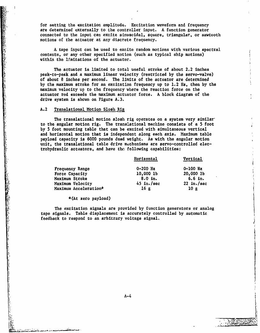
for setting the excitation amplitude. Excitation waveform and frequencyare determined externally to the controller input. A function generatorconnected to the input can excite sinusoidal, square, triangular, or sawtoothmotions of the actuator at any discrete frequency.

A tape input can be used to excite random motions with various spectralcontents, or any other specified motion (such as typical ship motions)within the limitations of the actuator.

The actuator is limited to total useful stroke of about 2.2 inchespeak-to-peak and a maximum linear velocity (restricted by the servo-valve)of about 8 inches per second. The limits of the actuator are determinedby the maximum stroke for an excitation frequency up to 1.2 Hz, then by themaximum velocity up to the frequency where the reaction force on theactuator rod exceeds the maximum actuator force. A block diagram of thedrive system is shown on Figure A'3.

A.2 Translational Motion Slosh Rig

The translational motion slosh rig operates on a system very similar,to the angular motion rig. The translational machine consists of a 5 footby 5 foot mounting table that can be excited with simultaneous verticaland horizontal motion that is independent along each axis. Maximum tablepayload capacity is 6000 pounds dead weight. As with the angular motionunit, the translational table drive mechanisms are servo-controlled elec-trohydraulic actuators, and have the following capabilities:

Horizontal Vertical

Frequency Range 0-200 Hz 0-100 HzForce Capacity 10,000 lb 20,000 lb

Z Maximum Stroke 8.0 in. 6.6 in.Maximum Velocity 45 in./sec 22 in./secMaximum Acceleration* 16 g 10 g

*(At zero payload)

The excitation signals are provided by function generators or analogtape signals. Table displacement is accurately controlled by automaticfeedback to respond to an arbitrary voltage signal.

A-4

APPENDIX B

PRESSURE-TIME HISTORY DATA FOR TRANSDUCER LOCATIONS 2 - 13

TABLE B-1. NONDIMENSIONAL PRESSURE-TIME HISTORY VALUESAT TRANSDUCER LOCATION 2 FOR A 25% FULL TANK

TRANSDUCER LOCATION 2FLUID:WATEREXCITATION:PITCH(AMP.=+/- 4.000 DEG.)NUMBER OF CYCLES PER TEST: 200PERCENT FILLING: 25

PT.2 PT.3 PT.4 PT.5

AVG.KP 6.6493 1.0960 1.0303 0.0435

MRX.KP 15.6515 2.1194 1.8873 0.9474

MIN.KP 3.1777 0.2357 0.3548 0.0027

AVG.TIME 0.1804 0.3225 1.4294 1.9184

MAX.TIME 0.3777 0.5694 1.6614 2.2314

MIN.TIME 0.0398 0.1889 1.1393 1.6617

PT.1 IS ALWAYS ZERO.

A!L VALUES PRINTED IN THE TABLE ARE NONDIMENSIONAL.

NOTE: See Figure IV-5 for definitions.

B-1

Co 0

U, -' N o 0% C44 a; w' , 0 o -

W 0W

-4N CO) kj T t 0% C') 1aN-* - -4 N ' 04

-zx a: tL tO Lo)CT

T W U . V lw0 0

10 1.- 0 U

i- '.wU w -4 :bl C C

PLt.W C. Tr ccCL x

-, -.

CA~ _l kD 0. N._ e4 ~4

z ID N 16T

0. w~U1-4 -ji O 4 t

.O +W LL Cow '

W ckW

9z. U31 CC) D qr ce -&-A

LL 0CO ) U') CO C' C

E- r4 C4 W

0E4 4W- CL * * *L 4

p - 0jw

>t Co4 10:I *0 w

CLi S= C

B-2

CD (0 0 It NM

ND LO 0- a

10 0 (Y CO Co NWN o IM 0 *) 0

0m 0 0 CC

M) U) - -m CO v v t ' ~ C

P4 E- () ) C N r* O C

'0 ti 0.

0 Ck ot * k

_j4 CC t I.X= WC IL 0

JCL>.L 0.C CL

5. 4 C% =.

Ix~~ ~ ~ ~ CJ1 W511> C> CDIPCC 10- 0. WL (L M

0 =~ CD 6.4

Cfl.

LO 0. NIt J) im N C) 0

If4 wo '1 0 O 4 C.

0 0 N Ia 0

04E- 0 o 17 L* v k. L5;t k COv

II- .4WU I! to jiI 0W W 9 * I) 0 4 0 . W W

IL CL CL Mix"03 .-.aO. . . . . . (C

E4 l.Jxmw > cc - > C r -E-l-LW (L MCE E a: X *

B-3

>1 N U) a:.c) CkJ N ) ~ -

W N N -

w

(-4'w 0 o ) Lo0) U)_

. .4 WW co

S00) If) 'T -4 N1 0Ol 0) t0 0o V -4 N X 4( - 4I- . N N w ) .- ' 0 U F\) IC . .4 ) * * *

COhF 4N 0 Z w41

0o 0 t '0 0

4t kD (n. 0 '0 0 N V "W- NO. ND LON 'J 0N ) Q~&cn Q WL 0 00) co I CT'N w Wf -. 04 " - t U 0 .

4% _ N 0) -0IX 0 P Iw - U U. I

IxU.. '0 0 t) N

to CO~ W ) N\ v)0 %q () C'0ir ) o 4 '4

cn 0))

kN*'J k% mt U T. 04 ) '0,

W F- 0 0 0

0 U)

0) v) 0)

t~ 0.; w% 0 0 o~ N,

Nq oi 0

I-Irll L Lkj Fa. . Ia N) I.-'0

U j -. L. LL a: LL-. 4 N4 = = - 0) -

;;(rAl 0-4 C, :m 0 W4 w w0 ) b

IC,: W LL C0.0.~a Cs 4.

B-4

M-0,

If) U) Lo~t Q

0 0 0 --- C .4'Ck4 a :* * 0 0C

vC~ 0 .0 Iii im yCoC ) -.I N 0 Co ) If )

+o w CL) NOmo

CL0 N 0 0 0 I

a.L . . . 0 0 U "

* I-Ct.1 W CL ? ') ."w - Ol- N t CL'7

*~~ ~ *.sW. w If 0 0 U LEA C-4 X..X . CL * ' m

*1 j 4 .4j 14 0go 0

-4 (('lw (0 x4

to 03 47 -

NE 0f W. C N -4 k -Co~C I- ) c

M -. LU

1- Co Nw ft, oo %%) Ci 01) Co PT.

14 D 0z CO

cc .

'm Q u 0 co ChC o rw .-. Co Co N " NNo N'*: y4 "A . CD Cl

U- Co A)I.

VI C4- W

CX Ni '.,C N N 00'. wA Co T f N

.4~~C mL. Co ' C -

B-5a

U0 o 0 Cti 0 N z0*0 0 v 0

In %0 OD c c co

C4 M .~ gCcn 0 a -

:o kD kD OD co co -m

10 v 7' CO U-) P O %044 4.0': , o .

COJ NC6 'CO CO ~0 CD VC Na

IS N 0t kDO W N C) CA: Q

M 1 -4J W L 0 u 0 (1 0 N

2Q iaj -w. 0 - 1=0 CL WO I)

't N - 00 0

D --z (C - O N *V) 0 - a CL=i . . . . m0p.o I-~ w1 wO CJ 0 a-4

413 Q =*. Q ..J

0- lxwx-4 ca

'0 a:

0~~ IC 0 0 0 all(~N) I-) 0. 0 * *

00 0rkN kLu0ic

W-

1--4 a.l ON LoD 0

tWN a ) NIC') a, N %r ' CN 0t.0 Ch t 0

a#~-4 I- * N uC) 4. co It I-j -j 0.i to a. to *o w 9;k!~..-. w' QO - c - to r, Lq w u

It 9z a.0. a. a. U. a- -.

- -0 I-) 1- I- C) J

CA . CL CL.. a- a

a: a- x n- w

B-6

k '-

TABLE B-12. NONDIMENSIONAL PRESSURE-TIME HISTORYVALUES AT TRANSDUCER LOCATION 13 FOR A 75% FULL TANK

TRRWIMSUCEP LOCATI O 13FLLli I: II.TE"EXCITATIOI: PIT'H(AIIP. =+/- 4. 000 IEG. >UMBNUIIER F CYCLES PEP: TEST: 200

PERCENT FILLING: 75

PT.2 P r. PT.4 PT.5

AVG.KP 5.6172 0.0000 0.0000 0.0000

MAX.KP 15.9974 0.0013 0.0000 0.0000

MIN.KP 2.5381 0.0000 0.0000 0.0000

AVG.TIKE 0.1676 0.4066 0.9276 1.4816

llRX. TINE 0.$303 0.6182 1.1879 1.8528

IIN.TWE 0.035$ 0.2842 0.7128 1.1405

PT. I IS tLIAYS ZERO.

ALL VALUES PRINTED IN THE TABLE ARE NONTIIIIENSIONAL.

NOTM: See 'igure V-5 for definitions.

M' R. ,S :.,,W .. ;,

IlPITCH t.2.Er CIFU U'.lz: ;,Fit'I NUM: 2:1 ll

4.U L.'.': '

.9.3

2.4..

I .2 U;2 1.541 2.9 I.~NW~IrdiDa TIKE

TIC LINES (W~ T P Ii R POINTS VRS~ b~II~

FIGURE B-1. NONDIMENSIONAL FRESSURE- FIGURE B-2. INTEGRATED NONDIMENSIONALTIME HISTORY VALUES FOR 200 PRESSURE VALUES FOR 200 RESONANTRESONANT SLOSHING CYCLES AT TRANS- SLOSHING CYCLES AT TRANSDUCERDUCER LOCATION 4 FOR A 25% FULL LOCATION 4 FOR A 25% FULLTANK TANK

B- 7

i-:. ": '

1rITCH TFS.LVC.0 . 4

i...tPRnAM12 4. N6.CF3135: 2

W.. c, j**s U2

1 *FIL UP: 2-o' SOM

"0. ' "4s" " "' .m

11.1m5 .1 U .?As,. ,"...:1 CI . .;. .. .3

.3 Its 5.13 1.12 us1 IIJLLK OLT~RIO1T]I ILSt RISE 1I, T2

(MIR.)

FIGURE B-3. NONDIMENSIONALTM FIGURE B-4. NODMNSOAPRESSURE VS IMPULSE RISE TIME PRESSURE VS IMPULSE DURATIONFOR 200 RESONANT SLOSHING FOR 200 RESONANT SLOSHINGCYCLES AT TRANSDUCER LOCATION 4 CYCLS AT TRANSDUCER LOCATIONFOR A 25%F .ULL.TANK 4 FCP A 25% FULL TANK

PITCH I

Pl..LCl TF S.UC(.I. 7

tI.. Cr cyU.5: if. rILL M'H: MUs FILL .WTI: W ,I.L

S4.18:"" .* .. %- ... ~I~l

,.t R,..--.~ 3

~ IIV

Irt RISE III{ 2

(Nut".) TiC LIICS (tteCTIra TIC Wn POINITS

fa MkY VIMSL5.FIGURE B-S. NONDIMENSIONAL FIGURE B-6. NONDIMENSIONAL

IMPULSE DURATION VS IMPULSE PRESSURE-TIME HISTORY VALUESRISE TIME FOR 200 RESONANT FOR 200 RESONANT SLOSHINGSLOSHING CYCLES AT TRANS- CYCLES AT TRANSDUCER LOCATIONDUCER LOCATION 4 FOR A 25% 7 FOR A 75% FULL TANKFULL TANK

B-8

LV

F PTCN 01IiRS.W~.W. 7 TrR-.* C X.

LL± .otTII; 7-.1 FIL W oT?: n

ZS.0

41. U 4 .N

la . . . AU. .6 1E . .

DIENIOALPRM 3 OUVALUE PRESUR VSISE ISE TIM

FOR 200 RESONAIJ SirSHING FOR 200 RESONANT SLOSHINGCYCLES AT TRANS -'Z LOCATION CYCLES AT TRANSDUCER LOCATION7 FOR A 75% FULL TANK 7 FOR A 75% FULL TANK

s. ~ FL DEF________________ FILL OP70: 7V.

o"I !~ Lln

I.ELLS RISC

FG- Z9. NONDIMENSIONAL FIGURE B-10. NONDIMENSIONALPRESSURE VS IMPULSE DURATION IMPULSE DURATION VS IMPULSEFOR 200 RESONANT SLOSHING RISE TIME FOR 200 RESONANT

CYCLES AT TRANSDUCER LOCATION SLOSHING CYCLES AT TRANSDUCER7 FOR A 75% FULL TANK LOCATION 7 FOR A 75% FULL TANK

BI

PITCH . Rst- SUS4J? .1hi, .K. r CYCE.: 2.11 T PITC3 . €F FTH: ', TF5!.5. C(.t . It

N. Up CYCLE: 24FILL *EP'P:M

a. 'I..

IN

•.5 ...,h

I.WRIA oW .U l: Iu 1.6 211 1F I 0 ROAN S

CYC LIuS AT TI T CRTA COCEs TRNUCE LOCATIO

FIGURE g-ll, NONDIMENSIONAL FIGURE B-12. INTEGRATED NON-LPRESSURE-TIME HISTORY VALUES DIMENSIONAL PRESSURE VALUES

FOR 200 RESONANT SLOSHING FOR 200 RESONANT SLOSHINGi ECYCLES AT TRANSDUCER CYCLES AT TRANSDUCER LOCATIONLOCATION 11 FOR A 75% FULL 11 FOR A 75% FULL TANKTANK

TR?5iM CC.1M. 11C. rfCYCLES: !V, ,.c. cl CYCL.ES ICUFILL DEPTH: "i rMILL ZEFTH: '13;

hII

IWPILSE RISE TIICIZ IMPA5E WAr1fl1I13

FIGURE B-13. NONDIMENSIONAL FIGURE B-14. NONDIMENSIONALPRESSURE VS IMPULSE RISE PRESSURE VS IMPULSE DURATIONT TIE FOR 200 RESONANT FOR 200 RESONANT SLOSIIING1 -SLOSHING CYCLES AT TRANS- CYCLES AT TRANSDUCERDUCER LOCATION 11 FOR A LOCATION 1I FOR A 75% FULL

£ 75% FULL TANK TANK

B-10

U7M..LC.Q. I I rILL D.wTN'u.'. C7 CYCLES: 2Z M

I .62 FIL.L :EFT.K: r iIs1

16.15

________________~ Miia ;i '~ & UM .e m.E .1 . 18

SLHIN CYLE ATTRN- CYCEST RNSlDUCE LOCTIODUCER~~~ LOCTIO 11N FORTI AK 75%T 13FO A7 UL tN

(IN.) MEM ITAHs

FIGURE B-15. NINETNON-L FIGURE.B-l. NONDIMENSIONALDIMPEIONA IO PR SR IMPLE PRESSURETVSEIUSERIS TIMUESRSIEFOR 200 RESONANT OHN FOR 200 RESONANT SLOSHINGSLSGCYCLES AT TRANS- OCTO CYCLES AT TRANSDUCER LOCATION13E LCIN1 FOR A 75%FULTN 13 FOR A 75% FULL TANK

FULL TANK

RESO] ;,R?; 5LDSH i), ? . N; TI i h

P I TCHTRRNS.LIC'.No. 13NO. OF CYCLES: 2FILL DEPTH: 759

FIGURE B-19. NONDIMENSIONALPRESSURE VS IMPULSE

= DURATION FOR 200 RESONANTSLOSHING CYCLES AT TRANS-DUCER LOCATION 13 FOR A75% FULL TANK

LnLi

{,a.SIN

e,. i T!

PITCTRRS.LOC. Q. 13

NO. CF CYCES

FILL DEPTH: 73,"

FIGURE -20. NONDIMENSIONALIMPULSE DURATION VS

C3 IMPULSE RISE TIME FOR 200. S '.RESONANT SLOSHING CYCLES

,~ AT TRANSDUCER LOCATION 13LFOR A 75% FULL TANK

9.30

tal

_.1 a.11 FIUR .220 NONDMENso

z" ~IPUS RIS IMPLS RSETIEOR20{Il

B-1

0.. •E,- €3

,,,,, I g

I I (NOND Il.)

B-12

APPENDIX C

ONV-DEGREE- OF-FREED0M EQUIVALENT SYSTEMS

To derive one-degree-of-freedom (one dof) "equivalent" systems forwhat are normally regarded as multi-dof structural elements requires thatsome assumptions be made about the behavior of the structure. The basicassumption is a deformation pattern which defines displacements of thetotal element in terms of a single displacement at some point in thestructure.

As an example, consider the simply supported beam of .Figure C-i.If the displacement along the beam can be described in terms of a singlevariable, for example, the center displacement, w, then the motions arereduced to a single dof. This is accomplished by assuming a deformationpattern for the beam which is some function of wo. Various choices can~bemade, e.g., the fundamental mode shape, the static deformed shape for theload distribution of the dynamic loading, or simply some approximate shapewhich resembles the fundamental mode or static deformed shape and matchesthe appropriate boundary conditions. For elastic behavior, Biggs(

7 9)

chooses the static deformed shape of the structure. For the simplysupported beam, uniformly loaded by the distributed load N-g(t), (g(t)] isthe time function for the load; the static deformed shape for elasticbehavior is given in Figure C-I.

N-g(t)

L/2

16 w 4 3 3w -h-- (x -L +L x)

5 L

FIGURE C-1. DEFORMATION PATTERN FOR SIMPEE BEAM

Reducing displacements to a single dof does not guarantee similarity

between the computed response of a one-dof system and the structuralelement. One way that similarity can be obtained is to equate the energiesof the distributed and single-dof systems. At any time,the internal strainenergy and the system kinetic energy must equal the external work as shownby Equation C-1.

W fU + KE (C-1)

C-Ii y

W = external work

U - internal strain energy

KE = kinetic energy

If kinematic similarity (equal displacements and velocities in this case)is maintained between the distributed and single-dof systems, then equatingenergies of the two systems will assure similarity of the computed behavior.This is true for elastic or elastic-plastic behavior, but in ship tanksonly elastic behavior will be considered.

As a first example, we chose the fundamental mode of the simplysupported beam as the deformed shape. This choice will permit a check onfrequency with the exact solution to demonstrate kinematic equivalence ofthe distributed and equivalent oystems. The deformed shape for the funda-mental mode is

rx -2w(x) = wo sin (C-2)

L

Evaluating W, U, and RE for this deformation pattern gives

LNNg(t) w(x) dx N-g(t) w L (C-3a)

W - Nf (t) w(x) dx4L

LI 2 I ]2 I rAE o2

KE a f (x) pAdx AL (C-3c)

0

where

E - material modulus

I = beam section moment of inertia

A = beam cross-sectional area

C-2

P material density

w= the beam center displacement and is some function of time.

These same energies, evaluated for the single-dof system of Figure C-2, are

W Fe. g(t) w° (C-4a)

i 2

kw (C-4b)2 e o

1 .2KE T mw ° (C-4c)

SFe'g(t)

e

W0 1 0

k

e

FIGURE C-2. EQUIVALENT ONE-DOF SYSTEM

Equating equations C-3 and C-4 and recognizing that

pAL = m, total beam mass

NL = F, total beam static load

the following relationships are obtained

C-3

FKL eK= 0.6366 (C-5a)

74 Eek - w0.634 k (C-5b)e 32L

K - e = 0.500 (C-5c)m m

where

k = spring constant for the simply supported beam

(N.L divided by static center deflection)

KL - load factor

K - mass factorm

Notice that the equivalent spring constant is very nearly equal to thestatic spring constant multiplied by the load factor.

Because these relationships were developed on the basis of kinematicequivalance of the displacement wo , it is instructive to compare the fre-quency given by the equivalent mass and spring constants with the exactsolution for a simply supported beam. The exact solution for the funda-mental mode is given by Den Hartog(95) as

2 EI? 3 (C-6)

where

m -total beam mass = p AL

For the equivalent system,

_ k 4w e7 Tr EI4EIX -(C-7)

me V 2L (0.3m)

C-4

As expected, the assumption of the fundamental mode for the deformedshape gives a frequency which is exactly equal to the beam's fundamentalfrequency.

Now, K Km, and ke will be determined for the static deformed shapeof the beam for comparison with the results of Biggs(79). The staticdeformed shape is given in Figure C-l, and for this case the energies ofthe distributed system are:

16 woLW N.g(t) 16 (C-8a)

25

3072 EI w

125L 3

KE- 1984 PAL 2 (C-8c)7875 0

Equating to equations (C-4), as before, we obtaiv

FKL 0.64 (C-9a)

F

k 6144 Ele 1 3 0.64 k (C-9b)

me

K - - a 0.5026 - 0.50 (C-9c)m m

These values of stiffness and mass of the equivalent system give a frequency

ofI_

S9.889/_JI (C-10)" mL

which is within 0.2% of the fundamental node of the beam [Equation (C-6)].Because the static deformed shap_ is made up of many normal modes, in addi-tion to the first, some difference in frequency is to be expected. If thebeam truly deforms dynamically with the static deformed shape, then it wouldrespond with the equivalent system frequency.

C-5

Several observations can be made as a result of these calculationsfor elastic behavior:

1. A rational method is available for deriving an equivalentone-dof system for a distributed structure.

2. Kinematic equivalency is maintained if the assumed deformationpattern exactly matches the behavior of the distributed system.

3. The values of K., Km , and ke match those given by Biggs(79)

and others for the static deformed shape. Table C-1 givesthese values for simply supported beams.

4. For the static-deformed shape, the equivalent stiffness, ke,can be computed from the static stiffness of the distributedsystem and the load factor.

5. The fundamental mode shape and the static deformed shape givevery similar results for a uniform loading. Using the staticdeformed shape should give the best results for other thanuniform loading or uniform structures because the deflectedshape will not match the fundamental mode so closely.

Transformation factors as in Table C-1 have been developed by Biggs(79)

and others for many different structural elements and different loadingconditions for each element. For example, Biggs gives values for

0 simply-supported beams

o clamped beams

o propped cantilevers

o one- and two-way slabs with edge supports

0 two-way slabs with interior supports

CA Displacements of the Equivalent Systems

Displacements of these equivalent one-degree-of-freedo4 systems canbe computed using simple numerical methods or closed form solutions. Aconvenient way to present the solution for elastic behavior is in terms ofa dynamic load factor (DLF). The dynamic load factor is simply the maximumdisplacement produced by the dynamic load, divided by the displacementproduced by the peak 'oad applied statically. Thus, the DLF can be eithersmaller or greater than one depending upon the nature of the loading andvibration period of the responding structure.

Plots of dynamic load factors for different types of loading functionsare given in Figure C-3. Note from these figures that the maximum DLF is2.0, whereas the minimum approaches zero for certain types of loads ofvery short duration.

C-6

I- ------

40 0 I

.- '.-, 43

.211

E-4-

- - id I

U 1c-7

h tIk~

I NQ

A'I

0%o o

CV LII c

-4 0 w

C-8

C.2 Shear in the Equivalent System

As Biggs(79) states,

"It is important to recognize that the dynamic reactions ofthe real structural element have no direct counterpart in theequivalent one-degree system, i.e., the spring force, is not thesame as the real reaction. This is true because the simplifiedsystem was deliberately selected so as to have the same dynamicdeflection as the real element, rather than the same force orstress characteristics."

These commeqs are particularly true for elastic-plastic behavior, wherethe maximum resistance is limited by permitting plastic deformation tooccur in the structure. For this case the maximum resistance is not agood indication, of the maximum shear which has occurred in the structuralelement. When only elastic behavior occurs, the maximum resistance of themember, the applied load multiplied by DLF, gives a good indication ofthe peak shear in the member. Here, only elastic behavior will be treatedin keeping with the philosophy that only elastic behavior will be toleratedt in ship tanks.

__ To determine the dynamic reaction, V, of Table C-l, a free-bodydiagram of the element, including inertia effects, must be used. For theuniformly-loaded, simply-supported beam of Figure C-l, such a free-bodyI diagram is given in Figure C-4. Inertia forces are distributed according

A to the assumed deformation pattern and are opposed to the motion. Onlythe period of time up to the maximum response, tn, is considered.

From the free-body diagram of one-half of the beam, an expression forV(t) is obtained by taking moments at x - a, the line of action of theresulting inertia forces.

LV(a) - MX L/2 - F(t) a-z 0 (C-11)

For elastic behavior, locations of the resultant of the inertia forces andthe mid-span moment are determined from the static deformed shape. They are

61a -- L

~* .~, H48EIx-L/2 oC5L2 0

C-

LL F(t)=N'g(t) .L

N-g(t)

K ,,

Mw (x)2

L- a - L/2

Vt) L V-t) fAw(x)dx

(a) (b) 0

FIGURE C-4. SIMPLY SUPPORTED BEAM IN EQUILIBRIUM UNDER DYNAMICLOADING

I

Substituting into Equation (C-I), the dynamic reaction at the beam endfor elastic behavior is

30.216EI

V - 3 o + 0.1066 F(t) (C-12)3 0

where F(t) is the total dynamic load on the beam [N.g(t)*L] and wo isunderstood to be a function of time. Thus, the shear reaction is a function

of the loading as well as the elastic resistance in the member. Noticein Equation C-12 that the maximum reaction may occur when wo is a maximum,when F(t) is a maximum or somewhere in between.

For elastic behavior only, it is worthwhile to compare the shearreactions predicted by Equation C-12 or the equation in Table C-1 with thatobtained from the equivalent static loading. This can be easily done fora simply supported beam, uniformly loaded by a triangular force with zerorise time. This loading most closely approximates the worst case sloshingload because the rise time is only about 1.0 ms and is very short relativeto the decay time.

The shear equation from Table C-1 is

V = .39R + .IlF(t) (C-13)

C-10

For elastic behavior the resistance at the time of maximum response, tm

will equal the dynamic load factor, DLF, multiplied by the peak appliedload Fl. This gives

V - .39.DLF*F1 + .11 F(t) (C-14)

Also, for a triangular pulse of duration td, F(t) can be expressed in termsof the peak load F1 as

F(t) F for o t < t (C-15)t~d

? NowV,. v .39.DLF.F + .11 FI td

1 ltd

- F1 [.39DLF + .ll(td-t)/td] (C-16)

At t - Othe second term in brackets is maximum but the first is zero (thesystem has not displaced). The first term in the brackets corresponds tothe maximum resistance and occurs at t - t . Because sloshing pressuresare of lung duration, the shear will most Tikely peak at t * tm. Thus,

V * .39"DLF 4 l1(t d - t (C-17)

1 m d (-7

This expression is compared to

V 0.5(FI*DLF) (C-18)

which is the maximum shear in a aimply supported beam acted on by a uniform

static load FI.DLF. In non-dimensional form

V9F - 0.5*DLF (C-19)

Equating equation (C-19) to eqtation (C-17) and setting the second term in

equation (C-17) to its maximum value of 0.11 we find

.5DLF - .39'DLF + .11 (C-20)

The sides are only equal when DLF is 1.0 (static loading). When DLF islarger than 1.0, the left side is greater because the term 0.11 is no4-multi-plied by DLF. For DLF < 1.0 the right side can be greater, depending upon

C-II

L,. _ _'

the contribution of the second term for which 0.11 is the maximum valde.Because sloshing pressures have short rise times and long duration (rela-tive to the structural periods of interest), the DLF will always be greaterthan 1.0 for LNG sloshing forces in ship tanks.

C-12

APPENDIX D

EXAMPLE CALCULATIONS FOR MEMBRANE AND PRISMATIC TANKS

Calculations were performed for typical LNG tank structures to illus-trate the methods of computing structural frequencies and the dynamicload factors. In addition, calculations of structural strength have beenmade and are expressed in terms of allowable sloshing pressures which thestructural components can withstand. Allowable sloshing pressures for theGaz Transport insulation boxes are compared with results from laboratorytests conducted on the boxes. Results of the laboratory tests, in whichboth static and dynamic pressure loads were applied to the cover of theboxes, are summarized in Section IV.5. It should be noted that the structuralstrength calculations are only examples of how such analyses may beperformed. Certainly, more rigorous methods are available, as discussedin Section V.2.3, and might be preferred; however, for these cases theone dof analysis is a good approximation to actual structural behavior andshould give conservative results.

D.1 Plywood Insulation Boxes

In this example, the strength of the cover and longitudinal stiffenerin the 12-cell box will be determined. These are the primary load-carryingmembers in the primary boxes and failures were produced in these membersduring laboratory testing. Dynamic load factors for the boxes are based ona tank which is 36m (118 ft) long. Tank length sets the time constantsfor the sloshing pressures and determines the dynamic amplificatian asshown in Section V.2.1.

Material Properties

The insulation boxes are constructed of 7-ply birch plywood. Flexuralstrength and stiffness were measured in 3-point bending tests both at rooman. at LN2 temperatures. Exterior plies were oriented perpendicular (cross-grain)to the direction of the bending stress; this orientation corresponds to theprincipal loading direction of the box covers. Results from these testsare summarized in Section IV.4.

Material properties used in the analysis are given in Table D-1.Values for the elastic modulus and rupture stress in the perpendicular (1)direction are taken from Section IV.6. The elastic modulus parallel (jl)to the grain was calculated using properties for white birch from theWood Handbook(97) and procedures outlined in the Plywood Design Guide(98).Plywood density was measured on box material and Poisson's ratios paralleland perpendicular to the grain of the exterior ply were estimated usingvalues for birch from Reference 97.

Cover Strength

The corner cells are the weakest part of the box covers because, foruniform pressure loadings, the bound'aries over the stiffeners are treatedas clamped and the edges along the side and end of the box are treated assimply supported. All other cells have three clamped edges. Dimensionsaud boundary conditions of the corner cell are:

D-1

TABLE D-1. PLYWOOD MATERIAL PROPERTIES

New Plywood - Average Properties - RT

Direction With Respect to Grain of Exterior Ply

Perpendicular (y) Parallel (x)

ar N/mm2 (ps) 55.96 (8,117) 108.4 (15,727)

Eb NIuu2 (psi) 3070 (445,304) 7149 (1,037,000)

v .206 .268

3 lb sec2 55.36 x I0-8 (5.18 x 10 5 )in.4

Ea N/=i2(psi) 464 (67,260) 618 (89,680)

D-2

i

IYSIMPLY SUPPORTED EDGE

_ _THICKNESS:

h = 9 mm (0.354 in.),"b (3.46 in.)

iX

! :FIXED EDGES DIRECTION

OF EXTERIOR PLY

FIGURE D-1

Static Pressure

Timoshenko and Woinowsky-Krieger (99) give a solution for bendingstresses in a plate with these boundary conditions The maximum momentoccurs near the center of side b and is given by

M - 0.1180 Pb 2 for a/b =2 (D-l)y

For the corner cell

a/b - 3.47,

but the ma&nttude .f the momenc changes very little for b/a > 2 so thevalue given is close to the true value. The stress produced by this momentis

6M3 - -(D-2)h3

Substituting Equation (D-1) for My and the rupture stress or for a, anexpression for the allowable static pressure Pa, can be obtained.

ah2Orh I

Pa 2 (D-3).708b2 ,

For orN/ (8117 psi)h = 9 mm (.354 in.)b = 88 mm (3.46 in.)

Equation (D-3) gives

D-3

P a = 0.827 N/mm 2 (120 psi)

Thus, 0.827 N/mm2 (120 psi) is the allowable static pressure of new boxes atroom temperature based upon average values. This gives a 50% probability offailure if the properties have a normal distribution.

Test results on three new 12-cell boxes produced failures at staticpressures of 120 psi, 130 psi and 150 psi. Table IV-22 in Section IV.5shows the damage and describes the failuze. In three tests failuresoccurred in the corner cells. In one test,the outer cell in the centerof the long cell also failed. This is the second weakest cell in the boxcover. The damage is cited as shear failure because the cover was completelysevered at the stiffener. Shear properties were not measured for the coversand these failures were not predicted. Rough estimates indicate that thecover has about equal shear and bending strength, and the resulting failureis some combination of shear, bending, and local compression. Compressiontends to cut through the inner ply; tension tends to crack the outer ply.These together weaken the plywood in shear.

Dynamic Pressure

To determine the permissible dynamic or sloshing pressure, rise anddecay times of the loading muit be known. These times are a function oftank length and were determind in Section V.2.1 for a tank 36 m (118 ft)long. From these timesthe envelope of the dynamic load factor (DLF) wasalso determined and is given iv Figures V-2 and V-3. Thus, these calculationswill be for a tank which is 36m long so that the DLF already calculatedcan be used.

To read the value of DLF from Figure V-2 and V-3,the fundamental47 Ifrequency of the structural component must be computed. Equations (V-l

and (V-2) of Section V.2.2.1 will be used. Substituting plywood propertiesfrom Table D-1 and the plywood thickness from Figure D-l,we have

Exh3Dx 12(1vxvy)= 458,426 N-mm (4058 lb in.)

E h3

D - 196,837 N-mm (1742 lb in.)y 12(1-v v )x y

D D-v + Gh D /4.8 95,505 N-mm (845 lb in.)xy x y 6 x

The frequency equation is

1 1 (A 4 D B4D 2CDbA4 4

From Table V.1 A = B = 3.927C = 132.118

* Measured by Herman (100) on five-ply maple plywood.D-4

Substituting the known parameters, the fundamental frequency and period ofthe corner cell in the cover are found to be

1f 2058 Hz; T= 0. 4 8 5 ms

These values are for the box cover vibrating in air, whereas in the tank itis exposed to LNG on one side (even though separated by the membrane). Theeffect of the membrane on the added mass of the liquid is uncertain;however, including the effect of the liquid on the frequency will increasethe period and produce a higher DLF (see Figure V-3), a conservativeeffect. Thusothe added mass will be included. Section V.2.2.5 givesapproximate formulas which account for submergence. The frequency in air,fa, is multiplied by a parameter ' to find the frequency, ft, in the liquid.is given by

*IK xPt/Pp

where

a

For LNG

Susttuin~~~ :BbO.::l6 k? (4.63 x 10lO b i: c)p =.48pH2 .48 x 104.3H20M 3 in. 4

Substituting for p4 and the panel dimensions from Figure D-1 we have:

K .3346 fe = Pfa - 1076 Hz

Pf .523 T i/f =0.928 ms

From Figure V-3 the dynamic load factor is found to be

DLF = 1.22

To predict the allowable sloshing pressure for the box cover, the allowablestatic pressure is divided by this factor; however, to be r'presentativeof in-service conditions, the allowable static pressure of .827 N/ m

2

(120 psi), previously calculated, should be adjusted to account for LNG

P D-5,~I

temperatures and in-service effects. The average strength of the plywo;odat LNG temperatures is increased as shown in Table IV-26 from 55.96 N/mm2

(8117 psi) to 89.05 N/mm2 (12,916 psi). Section IV-4 also gives thedegradation of strength for in-service conditions as 79%. Accountingfor the three effects of dynamic loading, LNG temperatures and in-serviceconditions, the allowable sloshing pressure for the cover is

N

827 5(89 5- (0.79) .853 N/mm (124 psi)

Average rather than minimum properties have been used in these calculations,so there is a 50% probability of a bending failure at this pressure for anormal distribution of plywood properties.

Strength of Longitudinal Stiffener

From the analysis of the corner cell in the box cover, it is apparentthat the majority of the pressure loading on the cover is transferred to-the long edges of the cell. These edges are supported by the sides of thebox or by the longitudinal stiffeners. The longitudinal stiffener picks upload from two adjacent cells and so is more highly loaded than the box sides.Figure III- 19 shows the arrangement of the stiffeners in the box and theirsupport points on the transverse stiffeners of the secondary boxes.

Figure D-2 shows the longitudinal stiffener at one end of the primarybox. A uniform loading N is applied to the top of the stiffener from the

(12 in.) SIMPLY SUPPORTEDN A TOP, END AND BOTTOMi OF BOX

o 182 -ma (7.17 in.)

FREE EDGE(SLOT FOR SUPPORT FROM

T S STRANSVERSE STIFFENERTRANSVERSE

STIFFENER) IN SECONDARY BOX

FIGURE D-2

cover and the bottom is assumed to be supported only at the transversestiffener in the secondary box. Simple solutions do not exist for this

D-6

combination of geometry, support conditions and loading. A rather domplexmultidegree-of-freedom analysis, such as with finite elements, would berequired for a good representation of these conditions; however, someapproximations can be made to bound the buckling strength of the stiffenerand this approach will be followed here.

Static Pressure

Two approximations to the actual conditions were checked. They areshown schematically in Figure D-3.

N, N b

a alN N -h

4 (a) UPPER BOUND (b) LOWER BOUND

FIGURE D-3

j Solutions for these cases are given by Roark and Young (101). Notingthat the load N is equal to the pressure applied to the box covermultiplied by the width of a cell (N - 88mm.P) we can express the allowablebuckling load directly in terms of the pressure on the box cover. Materialproperties for the load perpendicular to the grain of the exterior ply(the weakest direction) have been used.

Case (a) N - (88mm)P 4.27 b h (D-4)a .1-V

For the load perpendicular to grain of exterior ply

4.27 (3070) 2 2

9. 8 I-(26) (305 ) 1.22 N/m 2 (177 psi)

E h3

Case (b) N-b = (88mm) Pa =' 3 (lEh) (D-5)(1-v )b

Again for loading perpendicular to the grain of the exterior ply the ID-7

4

allowable pressure is

P = .30 N/mm2 (43 psi)

These two cases should give reasonable bounds for the bucklingstrength of the longitudinal stiffeners, expressed in terms of a uniformstatic pressure applied to the box cover. Of course, average propertiesheve been used and the grain of the stiffener is assumed to be parallelto the box axis and perpendicular to the load direction.

In laboratory tests on the boxes (refer to Table IV-22),bucklingof the longitudinal stiffe er in the end cell was observed at a static

o 103-1.24 (150-180 psi). The exterior grain of the stif-

fener was parallel to the box axis, corresponding to the direction in thepredictions above. Thus, the upper bound estimate, Case (a) appears tooffer a reasonable approximation to the behavior of the stiffener. It isinteresting to note in Table IV-22 that on Test No. 7 the static pressurereerhed 1.65 N/mm2) (240 psi) without stiffener failure. Stiffeners forthe box used in this test were oriented with the exterior grain perpendicularto the box axis (the strong direction). The predicted buckling pressurefor this orientation would increase by the ratio of the elastic modulusin the two directions or would be approximately doubled.

Dynamic Pressure

Under dynamic conditions,the response of the cover was increased by afactor of 1.22. Depending upon the frequency of the stiffener in compressic n,similar amplification may occur. To estimate the frequency of the stiffenerfor compressive loadsuse a spring mass model as in the sketch below. DenHartog (95) gives the frequency equation for this case as

-- ~3)M-M +M

c e

M - mass of cover

Me = added mass of the liquid

m = mass of stiffener

K = axial spring constant of the itiffener

For a unit width of the stiffener and cover the values are:

M (88mm)(1)(9mm)(55.36 x 10-8) = 4.385 x 10-4 kgx 10- 6 lb-sec2

(2.498 in.0in.

D-8

H * 1 ) (1)(49.48 x 10- 1.51 x 10kg£ ~- = bsec2

(8.572 x 106 1bin.

m - (1)(182)(9)(55.36 )r 108) 9.068 x 10 4 kg

(5.17 x 1 -6 lb-sec2(in.

K a AE/L - (9)(1)(464)/182 - 22.94 N/rxn (131 lb/in.)

Substituting into the frequency equation gives

f -509 Hz; T 1/f a 1.96 ms

This period is approuimately twice that of the cover. Generally, fcr thiscondition (a large spread in the stiffnesses of a coupled system) the loadtransferred to the supporting system will be attenuated; however, for thisapproximation it was assumed that the load is unaltered. From Figure V-2the dynamic load factor for this frequency is

DLF 1.63

As for the cover, to predict the allowable buckling load producedby sloshing pressures, the increase in stiffness which occurs at reducedtemperatures and the reduction in strength for in-service conrdiions shouldalso be accounted for. From Section I1.6, Table IV-26, we find

r 4785ERT 3070

and the in-service reduction is 79% as before. Camolning these factors, theallowable sloshing pressure for dynamic buckling (using measured bucklingload from Test 10 in Table IV-22) isI4785

(1.03 - 1.24 N/mm2 ) ( - )(0, 7 9 )a 1.63

2= .778 - .937 N/m 2 (113 - 136 psi)

*Mj is taken as the mass per unit length of a liquid which is containedwithin a half cylinder which lies above one cell of the box cover.

D-9

This allowable sloshing pressure for buckling of the longitudinal stiffeneris based upon one measured value of the static buckling load; however, theexperiment did correlate well with the upper bound on buckling strength com-puted for the stiffener using average material properties. As for the cover,the material is assumed to be oriented in its weakest direction, and thiscondition does exist in the boxes tested.

D.2 Technigaz Membrane Support System

The Technigaz membrane system is described in Section 111.3.1 andshown in Figure III. 3.4. Strudtural support for the membrane is providedby a composite panel formed from plywood sheets with a balsa core. Thepanel is separated from the membrane by an "end grain" balsa pad andsupported from the inner hull by grounds. Sloshing pressures on the membraneproduce bending and shear stresses in the composite panel between thegrounds. The allowable sloshing pressures will be based upon these stresses.

A section of the composite panel between the secondary grounds isshown in Figure D-4.

-SUGAR MAPLE PLYWOOD 3.4 mm (0.134"1)

~BALSA

h __ 155 mm (6.10"1)-- (GRAIN PARALLEL TO FACES) -

BIRCH PLYWOOD12m(042)

! SECONDARY GROUND dl-INNER HULL~~~~(TYPICAL) •. . . . .

L - 487.5 mm(19.20")

FIGURE D-4

Material properties for balsa, sweet birch and sweet sugar maple were takenfrom Reference 97. Pertinent properties are given in Table D-2. Detailscf the plywood construction were unknown so the following assumptions were

xde:

(1) Birch plywood is 7 ply with grain of exterior plies parallelto the grounds (weakest orientation).

(2) Maple plywood is 5 ply with grain of exterior plies parallelto the grounds.

D-10

TABLE D-2. MATERIAL PROPERTIES FOR BALSA,SWEET BIRCH, AND StJGAi'APLE

Sweet SugarBalsa Birch Maple

Specific gravity .17 .65 .63Elautic modulus, 3792 N/mm 2 14,962 N/rm 2 12,618 N/mm 2

longitudinal dir, EL (.55x106 psi) (2.17x106 psi) (1.83 x 106 psi)

Modulus of rupture 117 N/mm2(16,900 psi)

Compression. parallel 54 N/mm2to grain (7,830 psi)Elastic modulus, transverse 015 .050 .050 (est.)(T/EL)

Shear parallel to grain 2.07 T/mm2

(300 psi)

Shear modulus, (GLR/E) .054Longitudinal-radial plane

D-1

Based upon the above assumptions and material properties in Table D-2,thebknding stiffness of the composite panel can be calculated. For a 25.4 mmwide strip between the grounds the axial stiffnesses of the ,lywood faceswere found to be:

birch: (EA)b ' (14962 N/mm2)(12 mm)(25.4 mm)(3/7 + .050.4/7)

- 2.085 X 10 N (.469 x 10 lb)

maple: (EA)m - 12,618 (3.4)(25.4)(2/5 + .050.3/5)

- .4686 x 106 N (.105 x 106 lb)

Neglecting the contribution of the balsa core to the panel stiffness, thelocations of the neutral axis (N.A.) and the bending stiffness (El,) of the

panel are:

YN Y - 35.8 mm(1.41 in.) -

El -EA(y-yNA) -YNA

1.008x I0I0 Nmm2 (3.513 x 106 lb-in.

Mass per unic length of the 25.4 mm (1 in.) strip of panel between thegrounds must include the mass of the "end grain" balsa pad and the membrane.Measured specific gravity of birch plywood is Y - 0.72 and this value wasused in place of the values given in Table D-2 for birch and maple. Fora stainless steel membrane with a thickness of 1.3 mm (.050 in.),the massper unit length is:

Panel: mp 25.4 mm [(.72 x 10-6 3)(12 mm + 3.4 am) +mm

.17x 10- (155 mm)]- 9.509 x -4 &(1.379 x 10741b-sec2/ i.2)

~*- - 3 MM10 b-e n )mm

Pad: m PD - 25.4 mm(55 mm)(.17 x 10-6 & 3)mm

2,375 x 10-4 kl (3.445 x 10-5 Ib-sec2 /in.2)mm

Membrane: m = 25.4 mm(l.3 mm)(7.84 x 10-6

m 3

mmm1(3.755 x 10-5 b-sec2 .2)

! . D-12

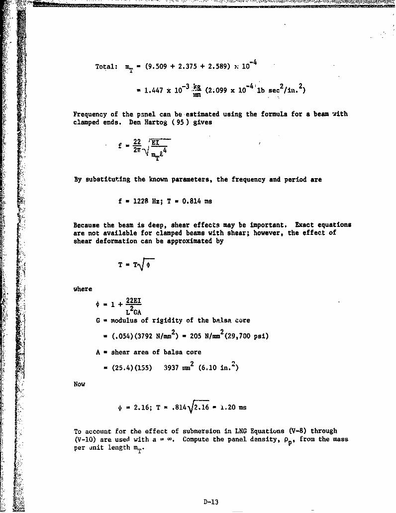
Total: mT-(9.509 + 2.375 + 2.589) ,~10

'I

Frequency of the panel can be estimated using the formula for a beam withclamped ends. Den Hartog (95) gives

22 'El

By substituting the known parameters, the frequency and period are

f 1228 Hz; T 0.814 ma

Because the beam is deep, shear effects may be important. Exact equationsare not available for clamped beams with shear; however, the effect ofshear deformation can be approximated by

T-T\[

where

22EI

LGAG -modulus of rigidity of the bnIlsa core

-(.054)(3792 N/mm 2) 205 N/mm2 (29,700 psi)

A -shear area of balsa core

-(25.4)(155) 393 mm (6.10 in.)

Now

* 2.16; T -.814\/2.16 1 .20 ms

To account for the effect of submersion in LNG Equations (V-8) through(V-) ae ued ith a ~.Compute the panel density, %,frmth msIper anit length MT*

A D-13

Density of the LNG is

p - .335 x 10 8 I

P (25.4) (170)mHm2 M

(3.136 x 10- 7 lb sec2

4in.

pe .48x10 - 8 - (4.49x10- 7 lb sec2

" in4 )

Substituting

K- rh j+ . r(170 mm)

- 1.096

_ . .658K + p- p/p

T - 1.20/.658 - 1.82 ms

For a tank which is 36 m (118 ft) long,the dynamic load factor is readdirectly from Figure V-2 for the fundamental period of 1.82 tas.

DLF Z 1.57

The maximum stress produced by bending will occur in the maple plywoodand is

McI " - "M5

where

C = h-Y A

E r/A (25 4)(34) 5426 N/am2 (78,696 psi)

M = naximum moment for a clamped beam2 (b'*? . DLF)L2

12 12

D-14

b= beam width =25.4 mm (1 in.)

Solving for the allowable sloshing pressure, Pa ,we have

Pa b 12 E(D-6)bDLF.L (h-YA) (EM)

2For a permissible compressive stress of 54 N/mm in the maple plywood,theallowable sloshing pressure is

a 0.957 N/mm (137 psi)i Pa

An allowable sloshing pressure for shear strength of the panelwill be based upon a constant shear stress through the core. The shearreaction at each end of the 25.4 mm (1 in.) wide beam is

V - 1/2.(487.5)(25.4)(Pa )"1.57

Using the allowable stress for shear parallel to the grain (a conservativevalue), the allowable sloshing pressure can be found.

N 2 - V 1/2(487.5)(25.4)P a(1.57)A 155(25.4)

P u 0.84 N/mm2(122 psi)a

Note that the shear and bending strength of the panel are in good balance.The numbers should be somewhat conservative because the shear strengthof the face plywood was neglected, the bending strength of the balsa corewas neglected and the width between the centerline of the grounds wasused for the panel width.

D.3 CONCH Independent Tank

The structural arrangement of the CONCH independent tank is describedin Section 111.3. One of the weakest parts of the tank is the swashbulkhead. In this analysis,we will predict the allowable sloshing pressurefor a section of the bulkhead between Frames 6 and 7 (refer to Figures111-23 and 111-24 ).

A schematic of the section between Frame 6 and 7 is given in FigureD-5. Primary dimensions are in inches as given in the engineering drawings.

D-15

i

FRAME 7 2' 4-7/8"(733 Wm

(344mm 0. 406"

0.0,FRAME 6 9) 7.1/ 2 (10 mm)(13mm) 294 mSTL. PLT. L 23 m) ml

BK. SECTION A-A >11'(229 mm)

.5019

FIGURE D-5

Stiffened Panel

The fundamental frequency of the section of the bulkhead betj%!en theframes and between the brackets will be estiumav'- using Equation % -3).Input parameters for the equation are

h =13 mm (0.50 in.)

2 6E =71,000 N/mm (10.3 x 10 psi)

D-16

p=2.65 x 10 (2.49 x l b se/in. 4)3

I -61.086 x 106 4(146.76 in.4)

2 2S - 10587 min (16.41 in.2)

p - 733 mm (28.875 in.)

LS 3454 mm (136 in.)

Boundary conditions for the panel can be approximated by clamped boundariesat the frame and simply supported along the stiffener to which the bracketsare attached. For these boundary conditions the constants from Table V-2are

I " - 1.5764

W 4.85

C' - .0833

Now substituting into Equation (V-3) we find'- ,,L

h 2

A VE-If 2 (B +C )' 121 HzLs 2 p S n SP

T f 8.25 msf

The dynamic load factor for the bulkhead will be determined using Figure

C-2(b) and the minimum nondimensional rise time T2 [tr in Figure C-2(b)]from Table V-1. For a nondimensional time of 0.0005 and a tank length,L, of 15.608 m (51.208 ft) to the swash bulkhead, the rise time tr is

T2 Vg/L = 0.0005

t = T2 = 0.63 ms

The ratio of che rise time to the fundamental frequency,

t /T = -25 = .076r 8.25

is used to enter Figure C-2(a). The dynamic load factor is

D-17

DLF Z 2.0

Strength of the panel can be approximated by considering the bending ofone stiffener and the associated plating between the two frames for auniform pressure loading acting over the width p (see Section V.2.2.2).The loading per unit length, N, is

N u p.DLF.P

where P is the allowable sloshing pressure. Using the standard equationfor a uniformly loaded beam with clamped ends and taking the allowableyield stress, a , for 5083 aluminum at -196C as 158.6 N/m2 (23,000 psi),the allowable soshing pressure is

1210 2I IP 2 .034 N/mm (5 psi)a pDLF Ls2C

where c, the distance from the neutral axis to the extreme fiber, is I193 m (7.585 in.). This allowable sloshing pressure is quite low andsimply indicates that the tops of LNC tanks are designed for relativelylow static vapor pressure and small liquid loads and not for dynamicsloshing pressures.

D1

SD-18

APPENDIX E

IMCO TANK TYPE DEFINITIONS

CHAPTER IV - CARGO CONTAINMENT

4.1 General

Administrations should take appropriate steps to ensure uniformity in

the implementation and application of the provisions of this chapter.*

4.2 Definitions

In addition to those in 1.4, the following definitions apply through-out the Code.

4.2.1 Integral tanks

(a) Integral tanks form a structural part of the ship's hull andare influenced in the same manner and by the same loads whichstress the adjacent hull structure.

(b) The "design vapour pressure" P0 as defined in 4.2.5 should notnormally exceed 0.25 kp/cm2. If, however, the hull scantlingsare increased accordingly, Po 2may be increased to a highervalue but less than 0.7 kp/cm .

(c) Integral tanks may be used for the products provided that thelowest temperature in any part of the hull structure under nocircumstances will fall below -10C. A lower temperature maybe accepted by the Administration subject to special consider-~ation.

4.2.2 Membrane tanks

(a) Membrane tanks are non-self-supporting tanks which consist of athin layer (membrane) supported through insulation by the adja-cent hull structure. The membrane is designed in such a waythat thermal and other expansion or contraction is compensatedfor without undue stressing of the membrane.

(b) The design vapour pressure P0 should not normally exceed 0.25kp/cm 2 . If, however, the hull scantlings are increased accord-ingly, and consideration is given, where appropriate, to thestrength of the supporting insulation, Po may be increased toa higher value but less than 0.7 kp/cm .

(c) The definition of membrane tanks does not exclude designs suchas those in which non-metallic membranes are used or in which

membranes are included or incorporated in insulation. Suchdesigns require, however, special consideration by the Adminis-tration.

* Reference is made to the published Rules of members and associate members of

the International Association of Classification Societle: and in particularto IACS Unified Requirements Nos. 92 and 93.

E-i

4.2.3 Semi-membrane tanks

(a) Semi-membrane tanks are non-self-supporting tanks in the loadedcondition and consist of a layer, parts of which are supportedthrough insulation by the adjacent hull structure, whereas therounded parts of this layer connecting the above-mentioned sup-ported parts are designed also to accommodate the thermal andother expansion or contraction.

(b) The design vapour pressure Po should not normally exceed 0.25kp/cm2 . If, however, the hull scantlings are increased accord-ingly, and consideration is given, where appropriate, to thestrength of the supporting insulation, Po may be increased toa higher value but less than 0.7 kp/cm2.

4.2.4 Independent tanks

Independent tanks are self-supporting; they do not form part of theship's hull and are not essential to the hull strength. The three categoriesof independent tanks are:

(a) Independent tanks type A which are designed primarily usingRecognized Standards of classical ship-structural analysis

procedures. Where such tanks are primarily constructed ofplane surfaces (gravity tanks , the design vapour pressure Poshould be less than 0.7 kp/cmi.

(b) Independent tanks type B which are designed using model tests,refined analytical tools and analysis methods to determine stresslevels, fatigue life and crack propagation characteristics.Where such tanks are primarily constructed of plane surfaces(gravity tanks2 the design vapour pressure Po should be lessthan 0.7 kp/cm .

(c) Independent tanks type C (also referred to as pressure vessels)are tanks meeting pressure vessel criteria and having a designvapour pressure not less than:

P0 2 + AC(p) kp/cm2]

where 2

A -0.0185 m

with

Orm = design primary membrane stress

AoA = allowable dynamic membrane stress (double amplitudeat probability level Q = 10

-8)

5.5 kp/mm2 for ferritic/martensitic steel2.5 kp/mm2 for aluminum allow (5083-0)

E-2

-- 5

C m a characteristic tank dimension to be taken as the

greatest of the following:

h; 0.75b; or 0.45Z

with

h - height of tank (dimension in ship's verticaldirection) (in)

b - width of tank (dimension in ship's transversedirection) (m)

Z - length of tank (dimension in ship's longitudinaldirection) ()

p " the relative density of the cargo (p 1 1 for fresh water)at the design temperature.

However, the Administration may allocate a tank complying withthe criterion of this sub-paragraph to type A or type B, depen-dent on the configuration of the tank and the arrangement ofits supports and attachments.

*V.S. G0VUME"6 1RTING OFlCE WO 190 3Z6.9?6J

E-

i ;-

SHIP RESEARCH COMNWITTEEMaritime Transportation Research Board

National Academy of Sciences-Natioual Research Council

The Ship Research Comittee has technical cognizance of the

interagency Ship Structure Coummittee' s research program:

Mr. 0. H. Oakley, Chairman, Consultant, McLean, VAProf. A. H.-S. Ang, University of Zllinois, 1ZMr. M. D. Burkhart, Consultant, Clinton, MDDr. J. N. Cordea, Senior StaffiMtalurgist, AJNC?0 INC., MddZetwn, OHl

Mr. D. P. Courtsal, Vice President,, DRAVO Corporati on, Pittsburgh, PA

D.W. R. Porter, Vice Pree. for Academic Affairs,, State Univ. of N.

Prof. H. Z. Sheets, Ditrector of Engineering, Analyais A Teohnologyj, Inc.,

The Ship Design, Response, and Load Criteria Advisory Groupprepared the project prospectus, evaluated the proposals for this project,provided the liaison technical guidance, and reviewed the project reportswith the investigator:

Hr. W. 3. Lane, Chairuman, Consultant, Baltim'ore, AMHr. J. W. Boylston, Manager, Marine operations, El Paso Marine Companyu; I Soloroms, IVProf. J.-N. Yang, Department of Civil,, Mechanical & Environmental Engineering,,

George Washington University, Washington, DCHr. L. R. Glosten, L. Rl. Gloaten Associatee, Inc., Seattle, WAHr. P. H. Kison, EXXON International Comp'any, Florham Park, NVDr. 0. H. Oakley, Jr., Project Engineer, GULF R&DI Comrpany, Houeton, TXMr. J. E. Steele, Naval Architect, Quakertown, PA