REVISION HISTORY

REV DESCRIPTION DCN # DATE APPD

-- Initial Release 891

99-08-17

A Update 55 05-10-21 KBo

B Update 06-06-26 KBo

C Update 07-10-16 KBo

D Update 08-10-16 KBo

E Update 08-11-14 KBo

F Update 2015-02-20 PBa

1.1.1.1G Update 2018-02-21 PBa

H CE conditions implemented 2018-05-28 PBa

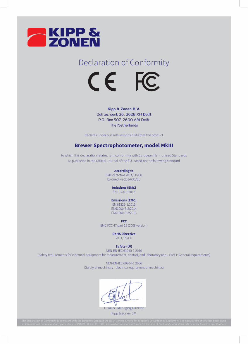
Declaration of Conformity

Kipp & Zonen B.V.

Delftechpark 36, 2628 XH Delft

P.O. Box 507, 2600 AM Delft

The Netherlands

declares under our sole responsibility that the product

Brewer Spectrophotometer, model MkIII

to which this declaration relates, is in conformity with European Harmonised Standards

as published in the Official Journal of the EU, based on the following standard

Del�, March 2019

E. Valks - Managing Director

Kipp & Zonen B.V.

This Declaration of Conformity is compliant with the European Standard EN 45014 General Criteria for supplier’s Declaration of Conformity. The basis for the criteria has been found in international documentation, particularly in ISO/IEC, Guide 22, 1982, Information on manufacturer’s Declaration of Conformity with standards or other technical specifications

According toEMC-directive 2014/30/EU

LV-directive 2014/35/EU

Imissions (EMC)EN61326-1:2013

Emissions (EMC)EN 61326-1:2013

EN61000-3-2:2014EN61000-3-3:2013

FCCEMC FCC 47 part 15 (2008 version)

RoHS Directive2011/65/EU

Safety (LV)NEN-EN-IEC 61010-1:2010

(Safety requirements for electrical equipment for measurement, control, and laboratory use – Part 1: General requirements)

NEN-EN-IEC 60204-1:2006(Safety of machinery - electrical equipment of machines)

3

Contents

1 Important user information ....................................................................................................... 5

Warranty ........................................................................................................................... 5

Recommendations by Environment Canada ....................................................................... 5

2 INTRODUCTION ......................................................................................................................... 6

Safety precautions ............................................................................................................. 6

Waste disposal ................................................................................................................... 7

Customer support .............................................................................................................. 7

Warning and instruction labels ........................................................................................... 7

External controls ................................................................................................................ 8

Tracker external connections ............................................................................................. 9

Brewer Spectrophotometer external connections .............................................................. 9

Short lifting instructions ................................................................................................... 10

3 INTENDED USE......................................................................................................................... 11

4 SYSTEM OVERVIEW ................................................................................................................. 12

5 SYSTEM DESCRIPTION.............................................................................................................. 14

Spectrophotometer ......................................................................................................... 14

MECHANICAL CONSTRUCTION ......................................................................................... 15

6 Solar Tracking .......................................................................................................................... 27

Zenith Positioning System ................................................................................................ 27

Azimuth Positioning System ............................................................................................. 27

7 Computer equipment .............................................................................................................. 28

8 Brewer system setup ............................................................................................................... 29

Spectrophotometer unpacking and setup ........................................................................ 30

Tripod unpacking and setup ............................................................................................. 31

Azimuth tracker unpacking and setup .............................................................................. 33

Mounting the Brewer ....................................................................................................... 33

Brewer operating software .............................................................................................. 34

Computer setup ............................................................................................................... 34

Brewer / computer integration ........................................................................................ 35

Main menu computer ...................................................................................................... 37

Initial tests ....................................................................................................................... 37

Final Installation............................................................................................................... 38

9 Brewer commands .................................................................................................................. 39

Reserved keys: HOME, DEL, CTRL+BREAK, F KEYS ............................................................. 39

Brewer command summary ............................................................................................. 40

10 Routine operations and minor maintenance ............................................................................ 53

4

Daily tasks ........................................................................................................................ 53

Inside Checks ................................................................................................................... 54

Weekly tasks .................................................................................................................... 56

Infrequent tasks ............................................................................................................... 56

Minor maintenance ......................................................................................................... 57

11 UV stability check – QL ............................................................................................................ 60

12 Solar and lunar siting ............................................................................................................... 62

13 Brewer schedules – SE, SKC, SK ................................................................................................ 63

14 Appendix A Brewer Data files .................................................................................................. 65

15 Appendix B Configuration files ................................................................................................. 81

16 Appendix C Factory tests ......................................................................................................... 85

Setup and calibration tests ............................................................................................... 85

SH shutter-motor (slitmask motor) timing test ............................................................................ 85

HV: High Voltage Test ...................................................................................................... 86

RS Slit mask motor run/stop test ...................................................................................... 88

DT: Photomultiplier Deadtime Test .................................................................................. 88

HG: mercury-line wavelength calibration ......................................................................... 90

SL: STANDARD LAMP TEST ............................................................................................... 92

Thermal tests ................................................................................................................... 93

SC: scan test on direct sun ............................................................................................... 95

Instrument inter-comparison calibration .......................................................................... 96

AZ: Zero The Azimuth Tracker ...................................................................................... 96

SR: Azimuth Tracker Steps-Per-Revolution Calibration .................................................. 97

17 APPENDIX D Preliminary Data Reduction ................................................................................ 99

Converting raw counts to light intensity ........................................................................... 99

Converting raw data to count rates .................................................................................. 99

Compensating for deadtime ............................................................................................. 99

Compensating for Rayleigh scattering (DS only) ............................................................. 100

Computing Single and Double Ratios .............................................................................. 101

Determining O3 and SO2 from Direct-Sun Data ............................................................... 101

Determining O3 and SO2 from Zenith-Sky Data ............................................................... 103

18 Appendix E Computer / Brewer Interface (Teletype) ......................................................... 104

19 Appendix F firmware log ........................................................................................................ 118

20 Appendix G BREWCMD.EXE ................................................................................................... 121

21 List of tables and figures ........................................................................................................ 122

5

1 Important user information Dear customer, thank you for purchasing a Kipp & Zonen instrument. It is essential that you read this manual completely for a full understanding of the proper and safe installation, use, maintenance and operation of your new Brewer. We understand that no instruction manual is perfect, so should you have any comments regarding this manual we will be pleased to receive them at: Kipp & Zonen B.V. Delftechpark 36, 2628 XH Delft, - or P.O. Box 507, 2600 AM Delft, The Netherlands Tel. +31 15 2755 210 support@kippzonen.com www.kippzonen.com

Warranty Kipp & Zonen B.V. hereby warrants to its products to be free from defects in material and workmanship for a period of two years from date of purchase. Kipp & Zonen guarantees that the product delivered has been thoroughly tested to ensure that it meets its published specifications. The warranty included in the conditions of delivery is valid only if the product has been installed and used according to the instructions supplied by Kipp & Zonen. Kipp & Zonen shall in no event be liable for incidental or consequential damages, including without limitation, lost profits, loss of income, loss of business opportunities, loss of use and other related exposures, however incurred, arising from the incorrect use of the product. Modifications made by the user can affect the validity of the CE or FCC declaration. An authorization must be obtained from Kipp & Zonen prior to the return of any equipment or parts thereof. Returned material is to be turned to the factory, or other location as may be directed by Kipp & Zonen, freight prepaid and will be returned freight prepaid. Kipp & Zonen is not responsible for any transportation, insurance, demurrage, brokerage, duties, or councilor charges, etc. This warranty is given to the original purchaser and may not be transferred without direct written consent of Kipp & Zonen. Kipp & Zonen reserves the right to make changes to this manual, brochures, specifications and other product documentation without prior notice.

Recommendations by Environment Canada Mark III Brewer Ozone Spectrophotometers are recommended by Environment Canada (EC) as the significantly superior model of Brewer instrument with which to measure ozone in the ultraviolet (UV) region of the spectrum. EC strongly discourages the use of other models of the Brewer instrument for the measurement of ultraviolet radiation or ozone in the UV because of the much poorer stray light performance of the single monochromator versions of the instrument.

6

2 INTRODUCTION Reading this entire manual is recommended for a full understanding of this product.

The triangle with exclamation mark is intended to alert the user to the presence of important operating and maintenance instructions in the literature accompanying the instrument. This electrical equipment should only be serviced by authorized personnel, meaning people who have been trained and designated as “authorized” by their employers.

Safety precautions

Many hazards are associated with installing and maintaining instruments on towers or elevated structures. It is advised to use qualified personnel for installation and maintenance. The client is responsible for following the local safety regulations. The use of appropriate equipment and safety practices is mandatory. Check your company's safety procedure and protective equipment prior to performing any work. ) If the Brewer is mounted at a high position, special care must be taken to secure both the person installing it and the instrument from falling during installation. While every attempt is made to get the highest degree of safety in our products, the client assumes all risk from injuries resulting from improper installation, use or maintenance of the Brewer.

Whenever the Brewer instrument is to be serviced, first disconnect the mains power connector. When the spectrophotometer is to be opened, unplug the grounding cable of the cover, unless instructed to do otherwise. The clamps need to be unlocked.

The Brewer is a very slowly rotating instrument that does not pose any harm to the user. However, it is strongly advised to keep the circular area as indicated to the left free of people at any time. This area should always be free of other equipment and certainly of stationary objects like poles and walls. It is important to have proper grounding of the Brewer tripod, tracker and instrument.

Since the Brewer is composed of heavy substructures (32kg) proper handling and following local procedures for lifting heavy equipment is necessary. The handles on the Brewer cover are intended to lift the cover only, not the entire instrument.

7

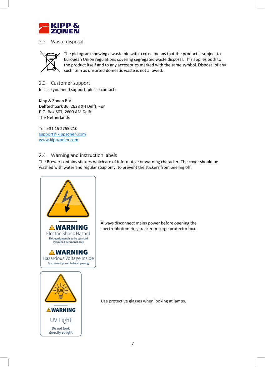
Waste disposal

The pictogram showing a waste bin with a cross means that the product is subject to European Union regulations covering segregated waste disposal. This applies both to the product itself and to any accessories marked with the same symbol. Disposal of any such item as unsorted domestic waste is not allowed.

Customer support In case you need support, please contact: Kipp & Zonen B.V. Delftechpark 36, 2628 XH Delft, - or P.O. Box 507, 2600 AM Delft, The Netherlands Tel. +31 15 2755 210 support@kippzonen.com www.kippzonen.com

Warning and instruction labels The Brewer contains stickers which are of informative or warning character. The cover should be washed with water and regular soap only, to prevent the stickers from peeling off.

Always disconnect mains power before opening the spectrophotometer, tracker or surge protector box.

Use protective glasses when looking at lamps.

8

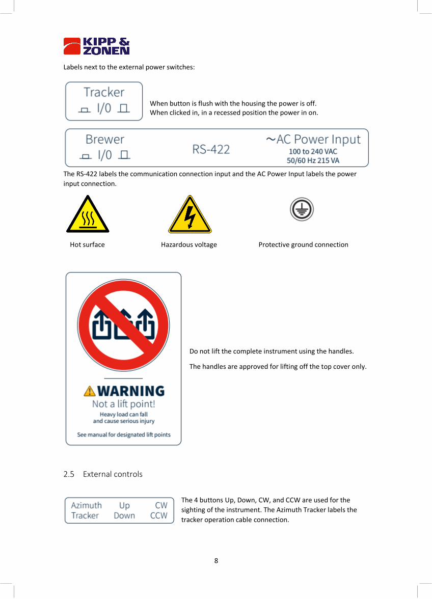
Labels next to the external power switches: When button is flush with the housing the power is off. When clicked in, in a recessed position the power in on.

The RS-422 labels the communication connection input and the AC Power Input labels the power input connection.

Hot surface Hazardous voltage Protective ground connection

Do not lift the complete instrument using the handles.

The handles are approved for lifting off the top cover only.

External controls

The 4 buttons Up, Down, CW, and CCW are used for the sighting of the instrument. The Azimuth Tracker labels the tracker operation cable connection.

9

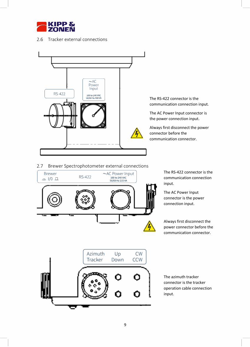
Tracker external connections

The RS-422 connector is the communication connection input.

The AC Power Input connector is the power connection input.

Always first disconnect the power connector before the communication connector.

Brewer Spectrophotometer external connections The RS-422 connector is the communication connection input.

The AC Power Input connector is the power connection input.

Always first disconnect the power connector before the communication connector.

The azimuth tracker connector is the tracker operation cable connection input.

10

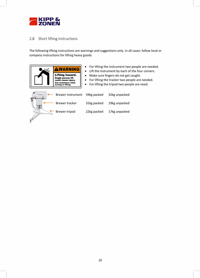
Short lifting instructions

The following lifting instructions are warnings and suggestions only. In all cases: follow local or company instructions for lifting heavy goods.

• For lifting the instrument two people are needed. • Lift the instrument by each of the four corners. • Make sure fingers do not get caught. • For lifting the tracker two people are needed. • For lifting the tripod two people are need.

Brewer instrument 59kg packed 32kg unpacked Brewer tracker 31kg packed 19kg unpacked Brewer tripod 22kg packed 17kg unpacked

11

3 INTENDED USE

The Brewer MkIII Spectrophotometer is primarily intended to be used in outdoor conditions to measure total column ozone and UV radiation. Given its durability and weatherproof design, it can survive extreme climate conditions while working continuously and autonomously. The system is fully programmable, allowing the gathering of data at will. Regular maintenance and calibration needs to be carried out to guarantee proper system functioning.

12

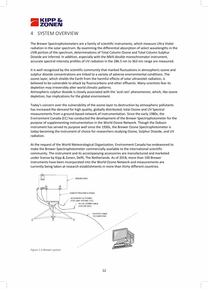
4 SYSTEM OVERVIEW The Brewer Spectrophotometers are a family of scientific instruments, which measure Ultra Violet radiation in the solar spectrum. By examining the differential absorption of select wavelengths in the UVB portion of the spectrum, determinations of Total Column Ozone and Total Column Sulphur Dioxide are inferred. In addition, especially with the MkIII double monochromator instrument, accurate spectral intensity profiles of UV radiation in the 286.5 nm to 363 nm range are measured. It is well recognized by the scientific community that marked fluctuations in atmospheric ozone and sulphur dioxide concentrations are linked to a variety of adverse environmental conditions. The ozone layer, which shields the Earth from the harmful effects of solar ultraviolet radiation, is believed to be vulnerable to attack by fluorocarbons and other effluents. Many scientists fear its depletion may irreversibly alter world climatic patterns. Atmospheric sulphur dioxide is closely associated with the 'acid rain' phenomenon, which, like ozone depletion, has implications for the global environment. Today's concern over the vulnerability of the ozone layer to destruction by atmospheric pollutants has increased the demand for high quality, globally distributed, total Ozone and UV Spectral measurements from a ground-based network of instrumentation. Since the early 1980s, the Environment Canada (EC) has conducted the development of the Brewer Spectrophotometer for the purpose of supplementing instrumentation in the World Ozone Network. Though the Dobson instrument has served its purpose well since the 1930s, the Brewer Ozone Spectrophotometer is today becoming the instrument of choice for researchers studying Ozone, Sulphur Dioxide, and UV radiation. At the request of the World Meteorological Organization, Environment Canada has endeavored to make the Brewer Spectrophotometer commercially available to the international scientific community. The instrument and its accompanying accessories are manufactured and marketed under license by Kipp & Zonen, Delft, The Netherlands. As of 2018, more than 100 Brewer instruments have been incorporated into the World Ozone Network and measurements are currently being taken at research establishments in more than thirty different countries.

Figure 1 A Brewer system

13

The Brewer Spectrophotometer is the core component of a complete Brewer System, which is comprised of the following:

• Brewer Spectrophotometer • Solar Tracking System • Personal Computer operating Brewer Software

All of the above equipment is available from Kipp & Zonen. The Brewer Spectrophotometer is supplied with a complete set of programs, which control all aspects of data collection and some analysis. The Computer is programmed to interact with an operator to control the Brewer in either a manual or fully automated mode of operation. In both the manual and semi-automated modes, the operator initiates a specific observation or instrument test by typing a simple 'command' on the computer keyboard. Raw data is automatically recorded on the computer data drive, and real-time Ozone and UV results can be printed. In the fully automated mode, a ‘schedule’ in the computer controls all operations. The Brewer is automatically set to the proper observation configuration and will then follow a user-defined observation schedule. Data is stored and analyzed in the same manner as in manual or semi-automated mode. The Brewer is designed to recover from a power failure and will resume scheduled operation subject to the computer system recovery, if the Brewer batch file has an automatic launch.

14

5 SYSTEM DESCRIPTION The Brewer MkIII Spectrophotometer is an optical instrument designed to measure ground-level intensities of the attenuated solar ultraviolet (UV) radiation. The Brewer contains two modified Ebert f/6 spectrometers, each utilizing 3600 line / mm holographic diffraction gratings operated in the first order. The Brewer is designed for continuous outdoor operation and is therefore housed in a durable weatherproof shell that protects the finely tuned internal components. The instrument operates reliably and accurately over a wide range of ambient temperature and humidity conditions. Following is a brief description of the major mechanical, optical, and electronic assemblies which make up the basic instrument. A more complete description of the electronic assemblies is provided in the Brewer Service Manual. The Brewer system is comprised of a Spectrophotometer, a Solar Tracker and a computer running the Brewer control and data logging software. Refer to figure 1.

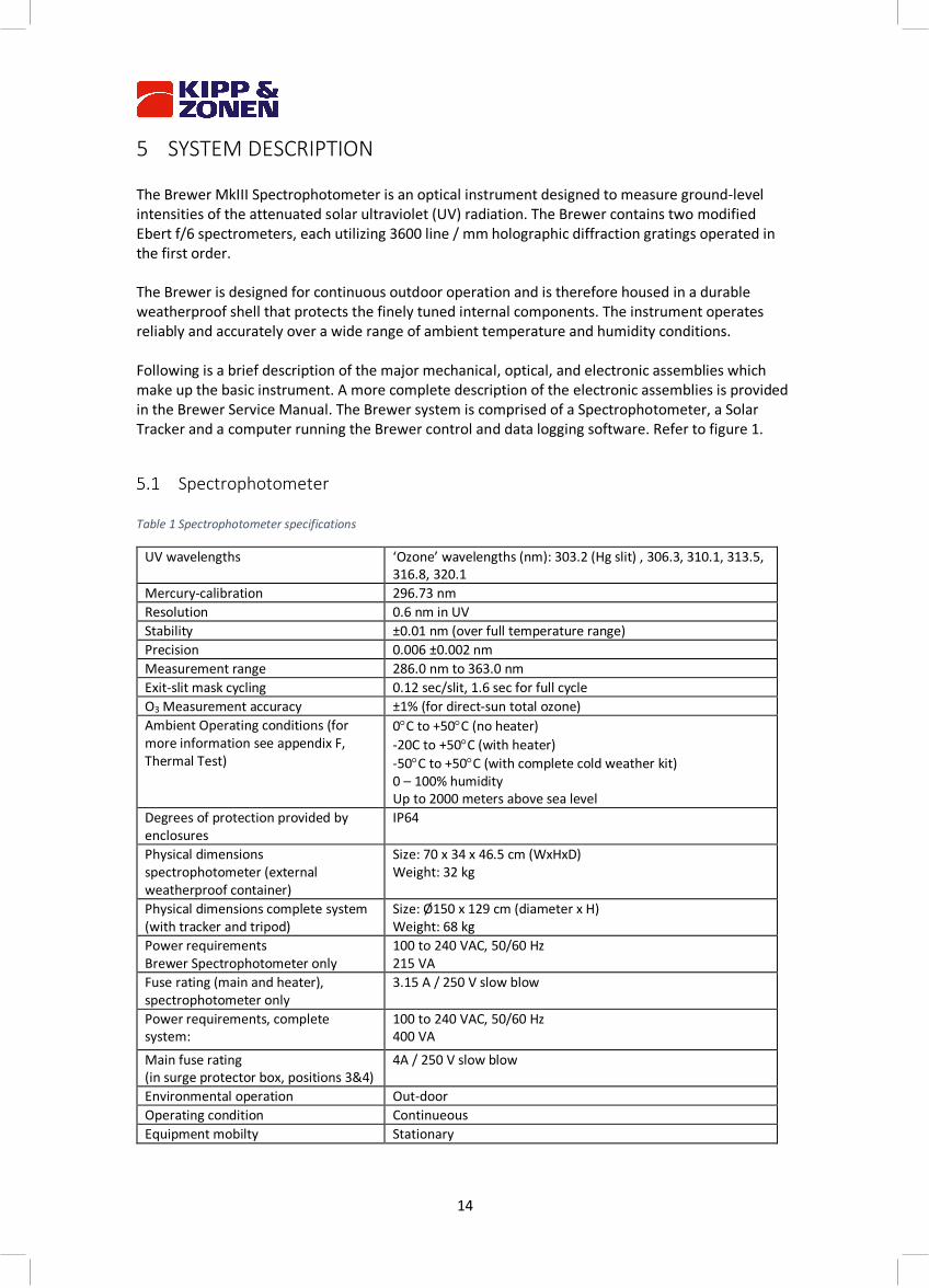
Spectrophotometer Table 1 Spectrophotometer specifications

UV wavelengths ‘Ozone’ wavelengths (nm): 303.2 (Hg slit) , 306.3, 310.1, 313.5, 316.8, 320.1

Mercury-calibration 296.73 nm Resolution 0.6 nm in UV Stability ±0.01 nm (over full temperature range) Precision 0.006 ±0.002 nm Measurement range 286.0 nm to 363.0 nm Exit-slit mask cycling 0.12 sec/slit, 1.6 sec for full cycle O3 Measurement accuracy ±1% (for direct-sun total ozone) Ambient Operating conditions (for more information see appendix F, Thermal Test)

0°C to +50°C (no heater) -20C to +50°C (with heater) -50°C to +50°C (with complete cold weather kit) 0 – 100% humidity Up to 2000 meters above sea level

Degrees of protection provided by enclosures

IP64

Physical dimensions spectrophotometer (external weatherproof container)

Size: 70 x 34 x 46.5 cm (WxHxD) Weight: 32 kg

Physical dimensions complete system (with tracker and tripod)

Size: Ø150 x 129 cm (diameter x H) Weight: 68 kg

Power requirements Brewer Spectrophotometer only

100 to 240 VAC, 50/60 Hz 215 VA

Fuse rating (main and heater), spectrophotometer only

3.15 A / 250 V slow blow

Power requirements, complete system:

100 to 240 VAC, 50/60 Hz 400 VA

Main fuse rating (in surge protector box, positions 3&4)

4A / 250 V slow blow

Environmental operation Out-door Operating condition Continueous Equipment mobilty Stationary

15

MECHANICAL CONSTRUCTION

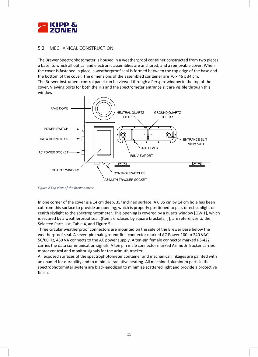
The Brewer Spectrophotometer is housed in a weatherproof container constructed from two pieces: a base, to which all optical and electronic assemblies are anchored, and a removable cover. When the cover is fastened in place, a weatherproof seal is formed between the top edge of the base and the bottom of the cover. The dimensions of the assembled container are 70 x 46 x 34 cm. The Brewer instrument control panel can be viewed through a Perspex window in the top of the cover. Viewing ports for both the iris and the spectrometer entrance slit are visible through this window.

Figure 2 Top view of the Brewer cover

In one corner of the cover is a 14 cm deep, 35° inclined surface. A 6.35 cm by 14 cm hole has been cut from this surface to provide an opening, which is properly positioned to pass direct sunlight or zenith skylight to the spectrophotometer. This opening is covered by a quartz window [QW 1], which is secured by a weatherproof seal. (Items enclosed by square brackets, [ ], are references to the Selected Parts List, Table 4, and Figure 5). Three circular weatherproof connectors are mounted on the side of the Brewer base below the weatherproof seal. A seven-pin male ground-first connector marked AC Power 100 to 240 VAC, 50/60 Hz, 450 VA connects to the AC power supply. A ten-pin female connector marked RS-422 carries the data communication signals. A ten pin male connector marked Azimuth Tracker carries motor control and monitor signals for the azimuth tracker. All exposed surfaces of the spectrophotometer container and mechanical linkages are painted with an enamel for durability and to minimize radiative heating. All machined aluminum parts in the spectrophotometer system are black-anodized to minimize scattered light and provide a protective finish.

16

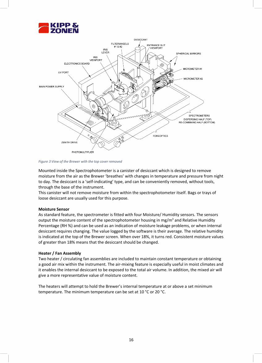
Figure 3 View of the Brewer with the top cover removed

Mounted inside the Spectrophotometer is a canister of desiccant which is designed to remove moisture from the air as the Brewer ‘breathes’ with changes in temperature and pressure from night to day. The desiccant is a ‘self-indicating’ type, and can be conveniently removed, without tools, through the base of the instrument. This canister will not remove moisture from within the spectrophotometer itself. Bags or trays of loose desiccant are usually used for this purpose. Moisture Sensor As standard feature, the spectrometer is fitted with four Moisture/ Humidity sensors. The sensors output the moisture content of the spectrophotometer housing in mg/m3 and Relative Humidity Percentage (RH %) and can be used as an indication of moisture leakage problems, or when internal desiccant requires changing. The value logged by the software is their average. The relative humidity is indicated at the top of the Brewer screen. When over 18%, it turns red. Consistent moisture values of greater than 18% means that the desiccant should be changed. Heater / Fan Assembly Two heater / circulating fan assemblies are included to maintain constant temperature or obtaining a good air mix within the instrument. The air-mixing feature is especially useful in moist climates and it enables the internal desiccant to be exposed to the total air volume. In addition, the mixed air will give a more representative value of moisture content. The heaters will attempt to hold the Brewer’s internal temperature at or above a set minimum temperature. The minimum temperature can be set at 10 °C or 20 °C.

17

The minimum temperature is selected by moving the jumper (J1) on the proportional heater controller (bolted to the Brewer foreoptics supports near the zenith prism): Table 2 Jumper settings J1

Jumper setting Minimum temperature 1-2 20°C 2-3 10°C

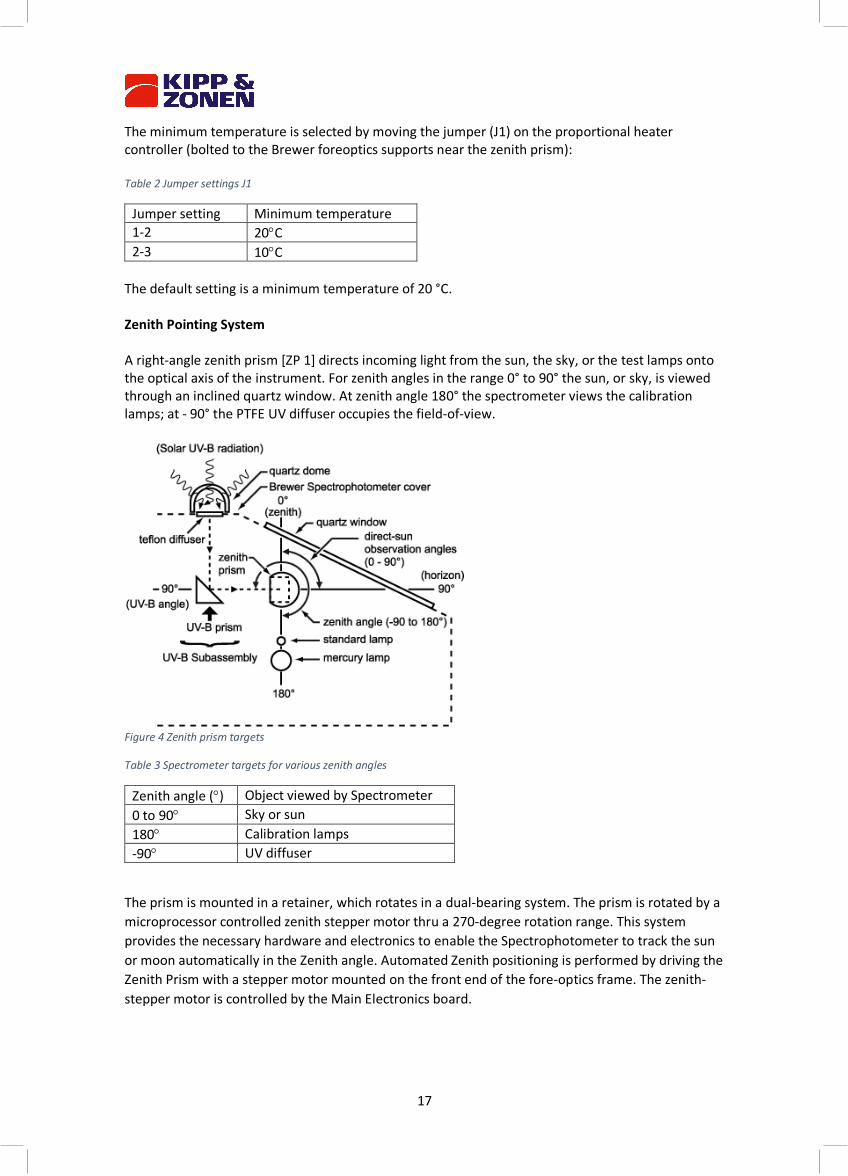
The default setting is a minimum temperature of 20 °C. Zenith Pointing System A right-angle zenith prism [ZP 1] directs incoming light from the sun, the sky, or the test lamps onto the optical axis of the instrument. For zenith angles in the range 0° to 90° the sun, or sky, is viewed through an inclined quartz window. At zenith angle 180° the spectrometer views the calibration lamps; at - 90° the PTFE UV diffuser occupies the field-of-view.

Figure 4 Zenith prism targets

Table 3 Spectrometer targets for various zenith angles

Zenith angle (°) Object viewed by Spectrometer 0 to 90° Sky or sun 180° Calibration lamps -90° UV diffuser

The prism is mounted in a retainer, which rotates in a dual-bearing system. The prism is rotated by a microprocessor controlled zenith stepper motor thru a 270-degree rotation range. This system provides the necessary hardware and electronics to enable the Spectrophotometer to track the sun or moon automatically in the Zenith angle. Automated Zenith positioning is performed by driving the Zenith Prism with a stepper motor mounted on the front end of the fore-optics frame. The zenith-stepper motor is controlled by the Main Electronics board.

18

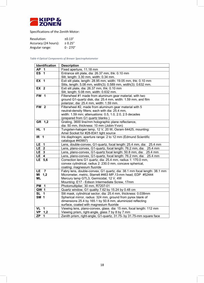
Specifications of the Zenith Motor:

Resolution: ±0.13° Accuracy (24 hours): ± 0.25° Angular range: 0 - 270°

Table 4 Optical Components of Brewer Spectrophotometer

Identification Description AP 1 Fixed aperture, 11.18 mm ES 1 Entrance slit plate, dia: 26.37 mm, thk: 0.10 mm Slit, length: 3.30 mm, width: 0.34 mm. EX 1 Exit slit plate, length: 28.95 mm, width: 19.05 mm, thk: 0.10 mm Slits, length: 5.08 mm, width(3): 0.589 mm, width(3): 0.632 mm. EX 2 Exit slit plate, dia: 26.37 mm, thk: 0.10 mm Slit, length: 5.08 mm, width: 0.632 mm. FW 1 Filterwheel #1 made from aluminum gear material, with two ground G1-quartz disk, dia: 25.4 mm, width: 1.59 mm, and film polarizer, dia: 25.4 mm, width: 1.59 mm. FW 2 Filterwheel #2, made from aluminum gear material with 5 neutral-density filters; each with dia: 25.4 mm, width: 1.59 mm; attenuations: 0.5, 1.0, 2.0, 2.5 decades (prepared from G1 quartz blanks ) GR 1,2 Grating, 3600 line/mm holographic plane reflectance, dia: 50 mm, thickness: 10 mm (Jobin-Yvon) HL 1 Tungsten-halogen lamp, 12 V, 20 W, Osram 64425, mounting: Amel Socket for #28-8341 light source IR 1 Iris diaphragm, aperture range: 2 to 12 mm (Edmund Scientific catalogue #40997) LE 1 Lens, double-convex, G1-quartz, focal length: 25.4 mm, dia: 25.4 mm LE 2 Lens, plano-convex, G1-quartz, focal length: 76.2 mm, dia: 25.4 mm LE 3 Lens, plano-convex, G1-quartz focal length: 50.8 mm, dia: 25.4 mm LE 4 Lens, plano-convex, G1-quartz, focal length: 76.2 mm, dia: 25.4 mm LE 5,6 Correction lens G1 quartz, dia: 25.4 mm, radius 1: 170.0 mm, convex cylindrical, radius 2: 230.0 mm, concave spherical, coating: magnesium fluoride LE 7 Fabry lens, double-convex, G1 quartz, dia: 38.1 mm focal length: 38.1 mm MI 1,2 Micrometer, metric, Starrett #463 MP,13-mm head, EDP #52444 ML Mercury lamp GTL3, Germicidal, 12 V, 4W Mounting: E17 - Edison Intermediate Screw, 17mm PM 1 Photomultiplier, 30 mm, R7207-01 QW 1 Quartz window, G1 quality 7.62 by 15.24 by 0.48 cm SL 1 Slit mask, cylindrical sector, dia: 25.4 mm, thickness: 0.038mm SM 1 Spherical mirror, radius: 324 mm, ground from pyrex blank of dimensions 25.4 by 165.1 by 50.8 mm, aluminized reflecting surface, coated with magnesium fluoride VL 1 Viewing lens, plano-convex, glass. dia: 15 mm, focal length: 112 mm VP 1,2 Viewing prism, right-angle, glass 7 by 8 by 7 mm ZP 1 Zenith prism, right-angle, G1-quartz, 31.75- by 31.75-mm square face

19

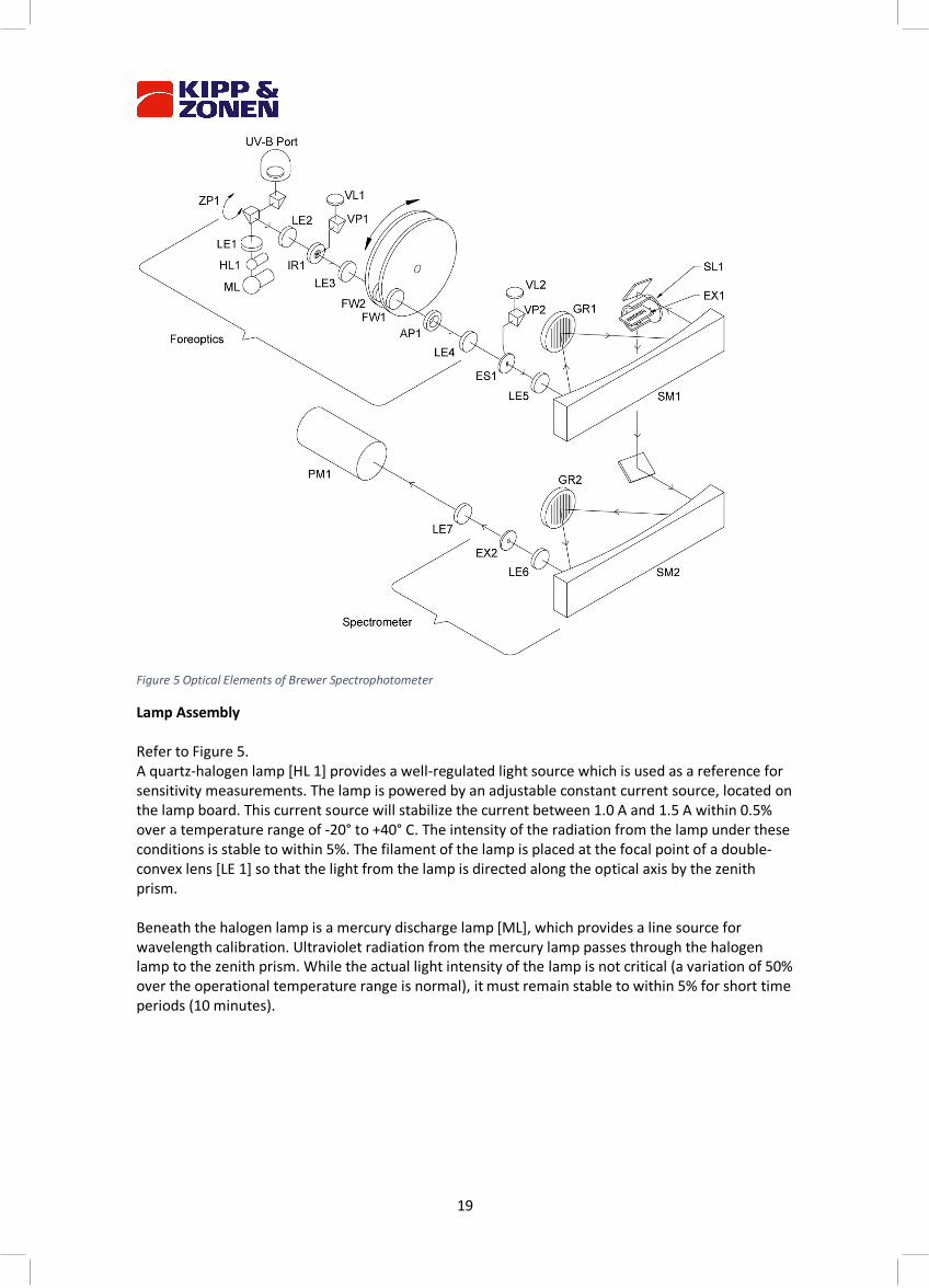
Figure 5 Optical Elements of Brewer Spectrophotometer

Lamp Assembly Refer to Figure 5. A quartz-halogen lamp [HL 1] provides a well-regulated light source which is used as a reference for sensitivity measurements. The lamp is powered by an adjustable constant current source, located on the lamp board. This current source will stabilize the current between 1.0 A and 1.5 A within 0.5% over a temperature range of -20° to +40° C. The intensity of the radiation from the lamp under these conditions is stable to within 5%. The filament of the lamp is placed at the focal point of a double-convex lens [LE 1] so that the light from the lamp is directed along the optical axis by the zenith prism. Beneath the halogen lamp is a mercury discharge lamp [ML], which provides a line source for wavelength calibration. Ultraviolet radiation from the mercury lamp passes through the halogen lamp to the zenith prism. While the actual light intensity of the lamp is not critical (a variation of 50% over the operational temperature range is normal), it must remain stable to within 5% for short time periods (10 minutes).

20

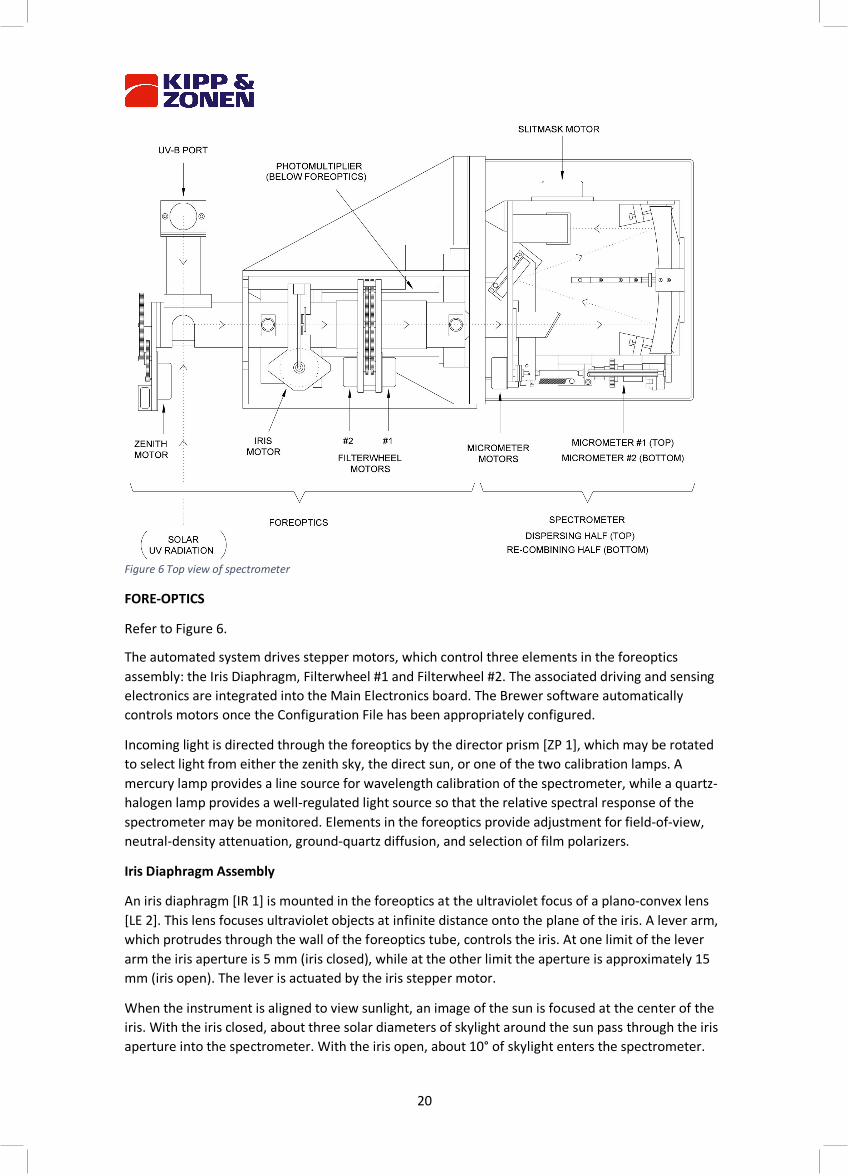
Figure 6 Top view of spectrometer

FORE-OPTICS

Refer to Figure 6.

The automated system drives stepper motors, which control three elements in the foreoptics assembly: the Iris Diaphragm, Filterwheel #1 and Filterwheel #2. The associated driving and sensing electronics are integrated into the Main Electronics board. The Brewer software automatically controls motors once the Configuration File has been appropriately configured.

Incoming light is directed through the foreoptics by the director prism [ZP 1], which may be rotated to select light from either the zenith sky, the direct sun, or one of the two calibration lamps. A mercury lamp provides a line source for wavelength calibration of the spectrometer, while a quartz-halogen lamp provides a well-regulated light source so that the relative spectral response of the spectrometer may be monitored. Elements in the foreoptics provide adjustment for field-of-view, neutral-density attenuation, ground-quartz diffusion, and selection of film polarizers.

Iris Diaphragm Assembly

An iris diaphragm [IR 1] is mounted in the foreoptics at the ultraviolet focus of a plano-convex lens [LE 2]. This lens focuses ultraviolet objects at infinite distance onto the plane of the iris. A lever arm, which protrudes through the wall of the foreoptics tube, controls the iris. At one limit of the lever arm the iris aperture is 5 mm (iris closed), while at the other limit the aperture is approximately 15 mm (iris open). The lever is actuated by the iris stepper motor.

When the instrument is aligned to view sunlight, an image of the sun is focused at the center of the iris. With the iris closed, about three solar diameters of skylight around the sun pass through the iris aperture into the spectrometer. With the iris open, about 10° of skylight enters the spectrometer.

21

On the spectrometer side of the iris there is another plano-convex lens [LE 3]. This lens is positioned such that its focal point is in the plane of the iris. Light passing through the iris aperture is therefore collimated along the optical axis.

Lenses [LE 2, LE 3] in the iris-diaphragm assembly are mounted with their plane side facing the iris.

Filterwheels

Refer to Table 5 and 6 and Figure 7

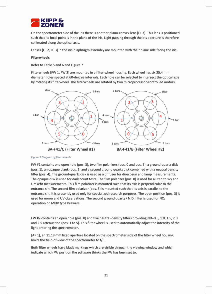
Filterwheels [FW 1, FW 2] are mounted in a filter-wheel housing. Each wheel has six 25.4 mm diameter holes spaced at 60-degree intervals. Each hole can be selected to intersect the optical axis by rotating its filterwheel. The filterwheels are rotated by two microprocessor-controlled motors.

Figure 7 Diagram of filter wheels

FW #1 contains one open hole (pos. 3), two film polarizers (pos. 0 and pos. 5), a ground-quartz disk (pos. 1), an opaque blank (pos. 2) and a second ground quartz disk combined with a neutral density filter (pos. 4). The ground-quartz disk is used as a diffuser for direct-sun and lamp measurements. The opaque disk is used for dark count tests. The film polarizer (pos. 0) is used for all zenith sky and Umkehr measurements. This film polarizer is mounted such that its axis is perpendicular to the entrance slit. The second film polarizer (pos. 5) is mounted such that its axis is parallel to the entrance slit. It is presently used only for specialized research purposes. The open position (pos. 3) is used for moon and UV observations. The second ground quartz / N.D. filter is used for NO2 operation on MkIV type Brewers.

FW #2 contains an open hole (pos. 0) and five neutral-density filters providing ND=0.5, 1.0, 1.5, 2.0 and 2.5 attenuation (pos. 1 to 5). This filter wheel is used to automatically adjust the intensity of the light entering the spectrometer.

[AP 1], an 11.18 mm fixed aperture located on the spectrometer side of the filter wheel housing limits the field-of-view of the spectrometer to f/6.

Both filter wheels have black markings which are visible through the viewing window and which indicate which FW position the software thinks the FW has been set to.

22

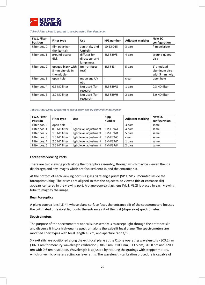
Table 5 Filter wheel #1 (closest to spectrometer) filter description

FW1, Filter Position Filter type Use KPZ number Adjacent marking New EC

configuration Filter pos. 0 film polarizer

(horizontal) zenith sky and Umkehr

10-12-015 3 bars film polarizer

Filter pos. 1 ground-quartz disk

diffuser for direct-sun and lamp meas.

BM-F39/E 4 bars ground-quartz disk

Filter pos. 2 opaque blank with 5 mm pinhole in the middle

(mirror focus test)

BM-F43 5 bars 1’ anodized aluminum disc, with 5 mm hole

Filter pos. 3 open hole moon and UV obs

- clear open hole

Filter pos. 4 0.3 ND filter Not used (for research)

BM-F39/G 1 bars 0.3 ND filter

Filter pos. 5 3.0 ND filter Not used (for research)

BM-F39/H 2 bars 3.0 ND filter

Table 6 Filter wheel #2 (closest to zenith prism and UV dome) filter description

FW2, Filter Position Filter type Use Kipp

number Adjacent marking New EC configuration

Filter pos. 0 open hole - 3 bars same Filter pos. 1 0.5 ND filter light level adjustment BM-F39/A 4 bars same Filter pos. 2 1.0 ND filter light level adjustment BM-F39/B 5 bars same Filter pos. 3 1.5 ND filter light level adjustment BM-F39/C clear same Filter pos. 4 2.0 ND filter light level adjustment BM-F39/D 1 bars same Filter pos. 5 2.5 ND filter light level adjustment BM-F39/F 2 bars same

Foreoptics Viewing Ports

There are two viewing ports along the foreoptics assembly, through which may be viewed the iris diaphragm and any images which are focused onto it, and the entrance slit.

At the bottom of each viewing port is a glass right-angle prism [VP 1, VP 2] mounted inside the foreoptics tubing. The prisms are aligned so that the object to be viewed (iris or entrance slit) appears centered in the viewing port. A plano-convex glass lens [VL 1, VL 2] is placed in each viewing tube to magnify the image.

Rear Foreoptics

A plano convex lens [LE-4], whose plane surface faces the entrance slit of the spectrometers focuses the collimated ultraviolet light onto the entrance slit of the first (dispersion) spectrometer.

Spectrometers

The purpose of the spectrometers optical subassembly is to accept light through the entrance slit and disperse it into a high-quality spectrum along the exit-slit focal plane. The spectrometers are modified Ebert types with focal length 16 cm, and aperture ratio f/6.

Six exit slits are positioned along the exit focal plane at the Ozone operating wavelengths - 303.2 nm (302.1 nm for mercury-wavelength calibration), 306.3 nm, 310.1 nm, 313.5 nm, 316.8 nm and 320.1 nm with 0.6 nm resolution. Wavelength is adjusted by rotating the gratings with stepper motors, which drive micrometers acting on lever arms. The wavelength-calibration procedure is capable of

23

measuring the wavelength setting with a precision of 0.0001 nm, and of controlling the wavelength setting to 0.006 nm.

Between the spectrometers is a cylindrical mask, which exposes only one wavelength slit at a time. The mask is positioned by a stepper motor which cycles through all five operating wavelengths, approximately once per second.

Spectrometers Detailed Description

Light enters the entrance slit and passes through a tilted lens [LE 5] which corrects for the coma and astigmatic aberrations inherent in an Ebert system. In the first spectrometer, the light is collimated by a spherical mirror onto a diffraction grating where it is dispersed. A second mirror reflection focuses the spectrum onto the focal plane of a slotted cylindrical slit mask positioned at the entrance of the second spectrometer. Following wavelength selection by the slit mask, the light passes through the second spectrometer where it is recombined and directed onto the exit slit plane. Six exit slits are located along the focal plane at the appropriate wavelength positions.

Entrance and Exit Slit Plates

The entrance slit and six exit slits [ES 1, EX 1] are laser-etched into 0.1-mm-thick disks of hard shim steel. One of the six exit slits (slit #0) is used for wavelength calibration against the 302-nm group of mercury lines; the other five are for intensity measurements and are nominally set at 306.3, 310.1, 313.5, 316.8, and 320.1 nm. The dimensions for the entrance and exit slits are listed in the Selected Parts List.

Both slit plates are positioned on their respective housings by locating pins, which orient the slit axis to within 0.1°. Both plates are blackened to minimize light reflections.

Correction Lens

The correction lens [LE 5] has a convex-cylindrical surface (radius 170.0 mm) and a concave-spherical surface (radius 230.0 mm).

Both surfaces are coated with a layer of magnesium fluoride to minimize reflectance at 315.0 nm for an incidence angle of 29°. The lens is mounted in the entrance-slit housing at an angle of 29° to the optical axis with the concave-spherical surface facing the entrance slit. The axis of the cylindrical surface is positioned in the horizontal plane to within 1°.

Spherical Mirrors

The spherical mirrors [SM 1 & SM 2] each have a 324 mm radius-of-curvature. The spherical surfaces are ground from rectangular Pyrex blanks. The surfaces are polished, coated with aluminum, and then coated with magnesium fluoride to maximize reflection at 315.0 nm.

Spring-loaded mounts secure the spherical surfaces of the mirrors against three adjustment screws, which are normal to the spherical surfaces in the horizontal plane of the spectrometers. The mirrors are allowed to move on a spherical surface defined by the three adjustment screws, up to a limit of 0.25 mm in the horizontal and vertical. Nylon screws prevent the mirrors from moving beyond this limit.

Diffraction Gratings

The diffraction gratings [GR 1 & GR 2] are 3600 line / mm holographic plane-reflectance types, operated in the first order. The gratings have optimum efficiency over the range 225 to 450 nm in the first order.

24

The gratings are secured with high-quality adhesive to three small blocks, which provide kinematic mounts, as well as fine adjustment for rotation of the gratings about the two axes perpendicular to the grating grooves. The three blocks are thus part of the grating and are the basis of point, slot, and plane mounts, which allows adjustment by three screws fixed in the grating-mount plates. These plates are suspended on a set of cross-springs, which constrain the gratings to rotate in the vertical axis (the axis parallel to the grating grooves). The cross-spring suspension acts as a frictionless bearing. Rotation of the gratings is controlled by two micrometers acting at the end of lever arms such that a 0.03 mm adjustment of the micrometers represents approximately a 0.1 nm wavelength change at the exit-slit plane.

Micrometers

Metric micrometer heads clamped to the spectrometer frame are used to adjust the grating rotation for each half of the spectrometer. Micrometer #1 adjusts the grating in the dispersing half (top) and Micrometer #2 adjusts the grating in the recombining half (bottom). The micrometer shafts are ground to a ball-end head, which inserts into bearings at one end of floating pushrods. A conical depression with a tetrahedral corner at the other end of the pushrods locates a ball-end cone mounted on the end of the grating lever arms. The pushrods are secured between the micrometer shafts and lever arms by tension springs. The material of the pushrods has been selected to minimize differential temperature effects.

The micrometers are rotated by stepper motors. The motors drive two 10-tooth gears, which are kinematically linked, to 60-tooth gears on the micrometer shafts. The drive shafts are coupled to the motor shafts with universal joints

One motor step represents 0.006 nm on the exit-slit plane. Backlash of the micrometers and cross-spring bearing systems have been measured at 0.002 nm. The temperature range of operation for the stepper motors and micrometer adjustment is -16° to +50 °C.

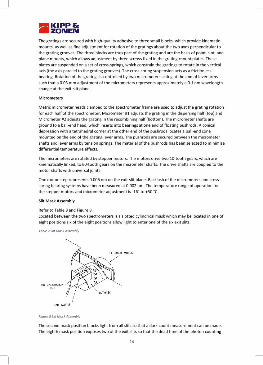
Slit Mask Assembly

Refer to Table 8 and Figure 8 Located between the two spectrometers is a slotted cylindrical mask which may be located in one of eight positions six of the eight positions allow light to enter one of the six exit slits.

Table 7 Slit Mask Assembly

Figure 8 Slit Mask Assembly

The second mask position blocks light from all slits so that a dark count measurement can be made. The eighth mask position exposes two of the exit slits so that the dead time of the photon counting

25

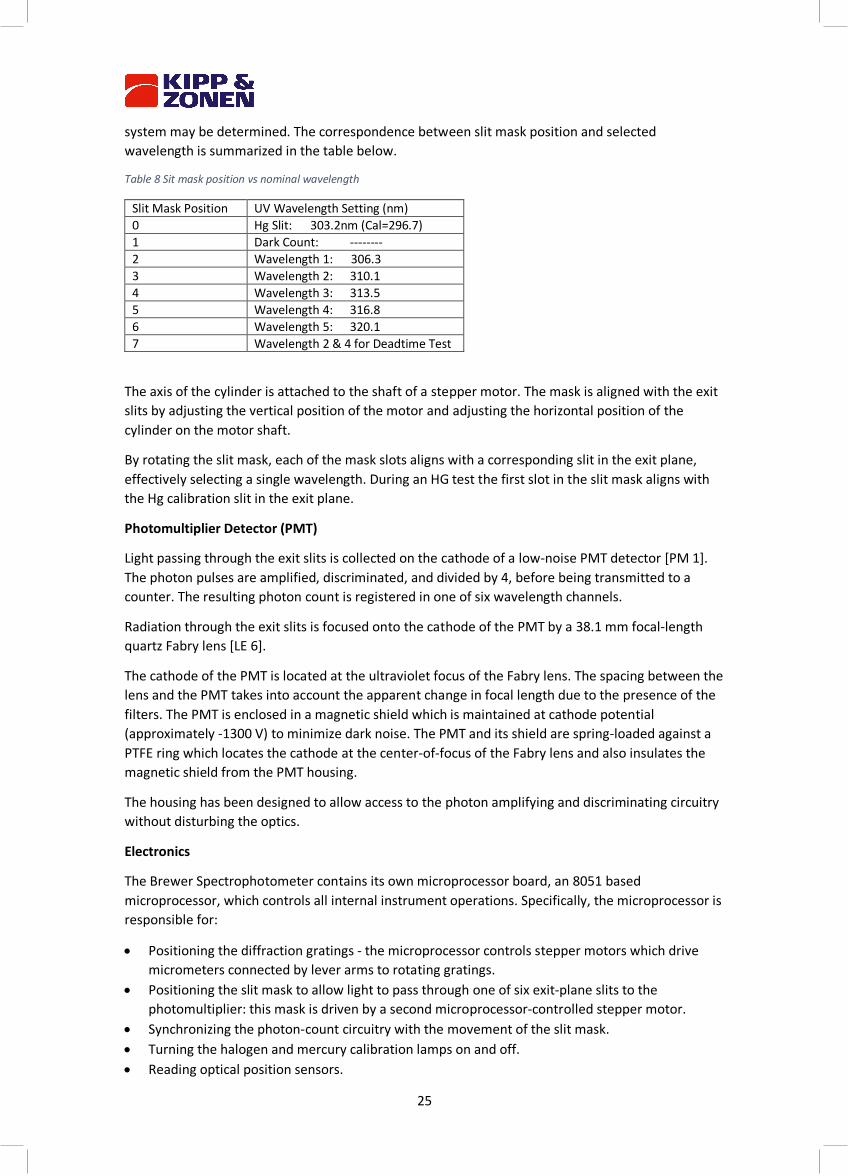
system may be determined. The correspondence between slit mask position and selected wavelength is summarized in the table below.

Table 8 Sit mask position vs nominal wavelength

Slit Mask Position UV Wavelength Setting (nm) 0 Hg Slit: 303.2nm (Cal=296.7) 1 Dark Count: -------- 2 Wavelength 1: 306.3 3 Wavelength 2: 310.1 4 Wavelength 3: 313.5 5 Wavelength 4: 316.8 6 Wavelength 5: 320.1 7 Wavelength 2 & 4 for Deadtime Test

The axis of the cylinder is attached to the shaft of a stepper motor. The mask is aligned with the exit slits by adjusting the vertical position of the motor and adjusting the horizontal position of the cylinder on the motor shaft.

By rotating the slit mask, each of the mask slots aligns with a corresponding slit in the exit plane, effectively selecting a single wavelength. During an HG test the first slot in the slit mask aligns with the Hg calibration slit in the exit plane.

Photomultiplier Detector (PMT)

Light passing through the exit slits is collected on the cathode of a low-noise PMT detector [PM 1]. The photon pulses are amplified, discriminated, and divided by 4, before being transmitted to a counter. The resulting photon count is registered in one of six wavelength channels.

Radiation through the exit slits is focused onto the cathode of the PMT by a 38.1 mm focal-length quartz Fabry lens [LE 6].

The cathode of the PMT is located at the ultraviolet focus of the Fabry lens. The spacing between the lens and the PMT takes into account the apparent change in focal length due to the presence of the filters. The PMT is enclosed in a magnetic shield which is maintained at cathode potential (approximately -1300 V) to minimize dark noise. The PMT and its shield are spring-loaded against a PTFE ring which locates the cathode at the center-of-focus of the Fabry lens and also insulates the magnetic shield from the PMT housing.

The housing has been designed to allow access to the photon amplifying and discriminating circuitry without disturbing the optics.

Electronics

The Brewer Spectrophotometer contains its own microprocessor board, an 8051 based microprocessor, which controls all internal instrument operations. Specifically, the microprocessor is responsible for:

• Positioning the diffraction gratings - the microprocessor controls stepper motors which drive micrometers connected by lever arms to rotating gratings.

• Positioning the slit mask to allow light to pass through one of six exit-plane slits to the photomultiplier: this mask is driven by a second microprocessor-controlled stepper motor.

• Synchronizing the photon-count circuitry with the movement of the slit mask. • Turning the halogen and mercury calibration lamps on and off. • Reading optical position sensors.

26

• Reading analog monitor voltages. • Moving motors to track the sun. • Moving neutral density, diffusing, and polarizing filters into the optical path. • Opening and closing a field-of-view defining iris. • Provides an RS-422C communications link to an external computer.

The microprocessor is programmed to accept commands from the external computer, execute the commands, and return results to the computer. An IBM compatible computer is used as the control console to facilitate programmed command sequencing as well as automatic data logging and processing. Raw data is recorded on hard disk drive, and real-time results may be printed on hard copy or printed to disk for later printing.

The major electronic subsystems of the instrument are:

• Main power supply. • Main Electronics board - carries control program Flash EPROMs, and a serial communications

interface which runs at 1200 baud (bits per second) and provides the following functions: • Input/output Interface - on/off control of the calibration lamps, drives the wavelength-

micrometer stepper motor and slit mask stepper motor. • Photon Counter - accumulates the amplified and scaled photon counts from the Pulse Amplifier

and transfers these counts to the microprocessor. • Clock-Calendar - a real-time clock / calendar which, with the RAM, has battery protection. • Analog-to-Digital (A/D) conversion - 24 single-ended, 10-bit A/D channels for monitoring

instrument voltages, currents, temperatures and moisture. • Pulse Amplifier - mounted in close proximity to the photomultiplier, amplifies and scales the

photon-pulse signal from the photomultiplier, and transmits the conditioned photon signal to the Photon Counter

• Lamp Control board - provides constant current control of the two test lamps in the instrument. It also provides monitor information such as lamp voltage and current which is sent to the A/D converter of the Main Electronics Board.

• High Voltage Control module - contains the high voltage supply and control circuitry as one complete module. It also provides a monitor signal to indicate the level of the high voltage and has an electrically adjustable potentiometer to allow for automated high voltage testing.

Ultra violet dome assembly

Refer to Figure 4

The UV Dome Assembly is an optical assembly which enables the Brewer to measure global UV-B, and portions of UV-A and UV-C, using a thin disc of PTFE as a cosine collector. The disc is mounted on top of the instrument under a 5-cm diameter quartz dome, and is thus exposed to the global UV irradiance. Beneath the disc is a fixed reflecting prism which is located such that the disc is in the spectrometer field-of-view when the zenith prism is set for a zenith angle of –90°.

27

6 Solar Tracking

Within the Brewer software is an Ephemeris algorithm which calculates the azimuth and zenith angles of both the sun and the moon as seen from the current location. Data required for this calculation includes the geographic co-ordinates of the site, the GMT time, and GMT date. These angles are further processed by the software, and positioning commands are sent to the Zenith Drive system and to the Azimuth Tracker.

Zenith Positioning System The Zenith positioning system is attached to the front end of the Fore-optics as described in detail in Section 5.2.

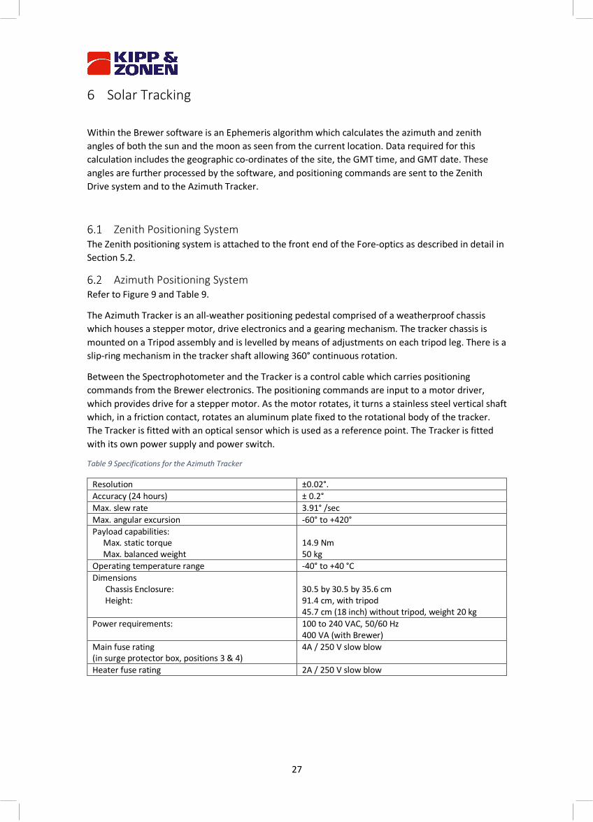
Azimuth Positioning System Refer to Figure 9 and Table 9.

The Azimuth Tracker is an all-weather positioning pedestal comprised of a weatherproof chassis which houses a stepper motor, drive electronics and a gearing mechanism. The tracker chassis is mounted on a Tripod assembly and is levelled by means of adjustments on each tripod leg. There is a slip-ring mechanism in the tracker shaft allowing 360° continuous rotation.

Between the Spectrophotometer and the Tracker is a control cable which carries positioning commands from the Brewer electronics. The positioning commands are input to a motor driver, which provides drive for a stepper motor. As the motor rotates, it turns a stainless steel vertical shaft which, in a friction contact, rotates an aluminum plate fixed to the rotational body of the tracker. The Tracker is fitted with an optical sensor which is used as a reference point. The Tracker is fitted with its own power supply and power switch.

Table 9 Specifications for the Azimuth Tracker

Resolution ±0.02°. Accuracy (24 hours) ± 0.2° Max. slew rate 3.91° /sec Max. angular excursion -60° to +420° Payload capabilities: Max. static torque Max. balanced weight

14.9 Nm 50 kg

Operating temperature range -40° to +40 °C Dimensions Chassis Enclosure: Height:

30.5 by 30.5 by 35.6 cm 91.4 cm, with tripod 45.7 cm (18 inch) without tripod, weight 20 kg

Power requirements: 100 to 240 VAC, 50/60 Hz 400 VA (with Brewer)

Main fuse rating (in surge protector box, positions 3 & 4)

4A / 250 V slow blow

Heater fuse rating 2A / 250 V slow blow

28

7 Computer equipment

The Brewer Spectrophotometer is operated by GWBasic software. This limits the amount of computer platforms suitable for operation.

Reliable PC platforms for Brewer operation are:

• DOS based computers (Windows XP, Windows 7 32-bit) • Windows 7 64-bit using a DosBox environment

It is important for the computer to have at least one USB port.

29

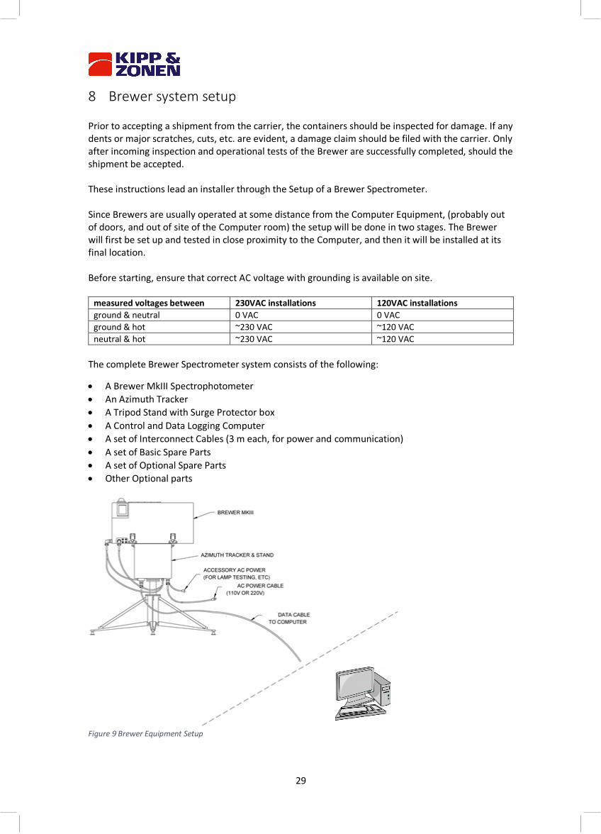
8 Brewer system setup Prior to accepting a shipment from the carrier, the containers should be inspected for damage. If any dents or major scratches, cuts, etc. are evident, a damage claim should be filed with the carrier. Only after incoming inspection and operational tests of the Brewer are successfully completed, should the shipment be accepted. These instructions lead an installer through the Setup of a Brewer Spectrometer. Since Brewers are usually operated at some distance from the Computer Equipment, (probably out of doors, and out of site of the Computer room) the setup will be done in two stages. The Brewer will first be set up and tested in close proximity to the Computer, and then it will be installed at its final location. Before starting, ensure that correct AC voltage with grounding is available on site.

measured voltages between 230VAC installations 120VAC installations ground & neutral 0 VAC 0 VAC ground & hot ~230 VAC ~120 VAC neutral & hot ~230 VAC ~120 VAC

The complete Brewer Spectrometer system consists of the following:

• A Brewer MkIII Spectrophotometer • An Azimuth Tracker • A Tripod Stand with Surge Protector box • A Control and Data Logging Computer • A set of Interconnect Cables (3 m each, for power and communication) • A set of Basic Spare Parts • A set of Optional Spare Parts • Other Optional parts

Figure 9 Brewer Equipment Setup

30

Spectrophotometer unpacking and setup

1. Open the Brewer crate and inspect the contents - at least the following items will be found: a. Brewer Spectrophotometer b. AC Power Cable with surge protector box c. RS-422/USB Converter with Data Communications Cable d. Manuals (Operator’s, Service, Final Test Record) e. Basic Spares Kit, BA-C112 f. Computer and monitor with Brewer operation software

2. Remove the Brewer Cover by unlatching the four latches and lifting the cover off the base. 3. Remove the protective foam on top of the optical assembly and from under the black

spectrometer cover. Inspect the Brewer for loose or broken parts, or disconnected cables. 4. It is recommended to keep the foam for if the instrument is ever to be shipped again. 5. Connect the AC Power Cable to the appropriate connector as per the markings on the Brewer

Cover, plug the other end into a source of AC power, and press the Power Switch. 6. Observe that the Power LED illuminates and that activity occurs as the Brewer Motors initialize. 7. Turn off the Brewer Power Switch and disconnect the power cable. 8. Place a few packages of active desiccant (Silica Gel) inside the Brewer (if not present already)

and install the Brewer Cover. List of tools needed to install and maintain the Brewer:

• Imperial size Allan keys (included) • Wrenches • Screwdrivers • Connector pin removal tool (included)

List of spare parts included (BA-C112B):

• Desiccant Holder Assy • Can of desiccant beads • Desiccant Humidity Indicator • Desiccant, 4 Unit, Type II, TYVEK Bag • Protection Cap PMT • Screw, #10-32 x 5/8"Lg, Skt Hd Cap, SS • Fuse, 2A, 250V, Slow-Blow • Fuse, 4A, 250V, Slow-Blow • Fuse, 3.15A, 250V, SB, 5X20MM • Insertion/Extraction Tool, 'D' Connector • Tool, Hex Key, .035" • Allen Wrench Kit, Ball Point • Lamp, Tungsten, Halogen, 20W, 12V • Lamp, HG Germicidal (GTL3) • Bubble level unit

31

Tripod unpacking and setup 1 Open the Tripod crate and locate the following:

a) Installation instructions floor stand b) Three support legs c) Three support bars d) Upper and lower flange e) Bag with bolts, nuts and allan key f) Bag with Tie-Down kit (this kit will be used in the final assembly, refer to figure 12)

32

Figure 10 Brewer Spectrophotometer Tripod

2. Attach the three legs to eachother with (12 M6 x 16 cap screws, lock washers and flat washers (do NOT tighten the screws).

3. Assemble the upper flange to the three legs with (6) M6 x 16 cap screws, lock washers and flat washers (do NOT tighten the screws).

4. Assemble the lower flange to the three legs with (6) M6 x 16 cap screws, lock washers and flat washers (do NOT tighten the screws).

5. Attach the three cross braces to the three legs with (3) M6 x 120 cap screws, lock washers and flat washers (do NOT tighten the screws).

6. Tighten the 27 cap screws using the provided hex key. 7. Place the stand on a flat mounting surface (recommended surface: concrete pad). 8. Install the Tie-Down kit. Note: the customer has to install an eye bolt (with attachment

‘ring’ or ‘hook’) in the pad. 9. Tighten the M8 nut of the Tie-Down kit with max. 5 Nm (44 in.lbs).

33

Azimuth tracker unpacking and setup Refer to Figure 9.

1. Open the Azimuth Tracker box, remove the Tracker, and inspect it for damage. 2. Mount the Tracker onto the Tripod and secure it with the three bolts provided. Connect the

surge protector box using one of the bolts. 3. Connect the grounding point at the bottom of the tracker spindle to ground. 4. Remove the front and rear covers from the Tracker, and note the spare fuses and mounting

bolts taped to the inside wall of the Tracker. 5. Connect the AC Power Cable from the surge protector box to the voltage mains connector on

the bottom of the Tracker spindle; plug in the other side to the mains grid; the Power Indicator will remain off - if it comes on, push the Power Switch to turn the power indicator lamp off.

6. Rotate the Tracker a few degrees and note that it is relatively easy to turn when power is off. 7. Press the Tracker Power Switch to turn power ON, and observe that the Power Indicator

Illuminates. 8. Attempt to rotate the Tracker again, and note that it is much more difficult to turn with holding

torque on the motor.

Mounting the Brewer

Refer to Figure 9.

1. Place the Brewer on top of the Tracker. The Brewer Power Switch should be at the same side of the Tracker Power Switch. The three bolts protruding from the top of the Tracker mate to the three tapered holes in the bottom of the Brewer - these three bolts form a kinematic mount for the Brewer Optical Assembly.

2. Secure the Brewer to the four Tracker mounting fixings with the bolts provided in the Basic Spares Kit - there are spare bolts taped to the inside wall of the Tracker.

3. When securing the Brewer to the Tracker, start the bolts by hand to ensure that no cross-threading occurs before using the Allen key included in the Basic Spares Kit to do the final tightening. Care must be taken not to overtighten the bolts as the rubber feet may be damaged.

4. Connect the AC Power Cable to the 120/230 V connector and connect the Data Communications Cable to the RS-422 connector at the bottom of the Tracker.

a. Always connect the power cables first before connecting the communication cables. This will ensure an electrical ground is present at all times, so no damage will be done to the electrical communication circuit on the mainboard.

5. Connect the remaining cables from the Tracker to appropriate connectors on the Brewer. Note that each cable / connector combination is unique, which makes it nearly impossible to connect the cables incorrectly.

6. Turn ON the Tracker Power Switch and the Brewer Power Switch. Both Power LED’s will come on. The Brewer will go through an initialization sequence once again and the Tracker will be difficult to turn by hand.

34

Brewer operating software Brewer Operating Software is provided on the computer. It contains files in directories \BDATA, \CALIBRATION CERTIFICATES, \MANUALS + FTR, \SOFTWARE. The \BDATA directory contains the subdirectory \BDATA\NNN (where NNN is the Brewer number). \BDATA directory -- these files contain data collected during the testing of the instrument. \BDATA\NNN -- these files contain firmware and software configuration information specific to the Brewer whose Number (NNN) appears on the Disk identifier, as well as the utility used to load firmware. The \CALIBRATION CERTIFICATES directory contains the Brewer calibration certificate, the UV stability-kit lamps calibration certificate, and the .irr files of the lamps. The \MANUALS + FTR directory contains the subdirectories \FTR and \Manuals. \FTR – contains the FTR in .pdf form. \MANUALS – contains the operators and service manual in .pdf form. The \SOFTWARE directory contains the subdirectories, \BREWCMD, and \BREWER. \BREWCMD contains software for changing the mode of the Brewer and for writing to the flash memory of the Brewer mainboard (see Appendix G). It also contains the configuration file and the firmware. \BREWER directory -- these files contain the MAIN Brewer operating program and all of the routines and data files necessary to control all of the Brewer command functions.

Computer setup This instruction assumes that Kipp & Zonen has NOT supplied the Computer equipment. If Kipp & Zonen has supplied the Computer, then many of the following steps will have already been completed and need only be confirmed at this time. 1. Set up and connect the computer as per the manufacturer’s instructions. Plug the computer

power cord into an AC Power socket and power on the computer. 2. Copy the contents of the USB flash drive that came with the Brewer to the C: drive of the

computer. 3. Use a text editor to display the OP_ST.NNN file in the C:\BDATA\NNN (NNN is the Brewer

Number). The third line of this file will be in the form of ‘ICFJJJYY.nnn’. 4. Using a text editor again, open the ‘ICF’ file as found in step 3.

Line item #24 (following MkIII entry) is the number of the COM port used for communications with the Brewer. The number shown (1 or 2) must match the Computer COM: port number which will be used in this installation, and should be changed if it is not correct. Please note that port number 1 and port number 2 are the only valid entries.

5. Go to the C:\Brewer directory, and with the text editor, open the file OP_ST.FIL and edit this file such that the Brewer number to be installed matches the first entry in the file and that the correct path of the Bdata directory is in the second entry.

6. Configure the AUTOEXEC.BAT file (for DOS), or the Startup Menu (for Windows based systems), if it is desired to have the Brewer restart automatically following a power failure.

7. Test the Software and COM Port: a. Connect the computer side of the communication cable to the RS-422/USB converter box. b. Plug the converter cable into the appropriate port of the Computer c. Launch the Brewer command program by running the BREWCMDW.EXE file through

Windows, or by typing ‘BREWCMD.EXE’ at a DOS prompt - at this point activity will appear

35

on the computer screen, but for this test, only the lights on the converter need to be monitored.

8. Exit the Brewer command program by typing ‘quit’+ Enter. 9. Turn off Computer power.

Brewer / computer integration This section assumes that the Brewer, Tracker, and Computer Equipment have been individually set up and tested for operation.

1. Connect the Brewer side of the Communications Cable to the Azimuth Tracker connector. 2. Plug the AC Power Cable from the Azimuth Tracker into same Power Bar as are plugged the

Computer. Ensure that the other end of the power cable is plugged into the connector under the Tracker, and that the three cables are connected between the Tracker and the Brewer.

3. Turn Brewer and Tracker power ON. - Brewer and Tracker lights will illuminate - Activity will occur inside the Brewer indicating an initialization is in progress.

4. Turn Computer equipment power ON and launch the Brewer.bat program. If the computer is a 64-bit system, the DOSBOX configured batch file needs to be launched.

- The ‘Brewer’ screen will appear, and a number of files will be ‘merged’ - The data converter will indicate communications are occurring by periodic flashes of the

lights. - Following initialization, the Date and Time and Brewer Site information will be read - When the Initialization and reset have completed, the MAIN MENU will appear on the

Computer screen, indicating that the Brewer is ready to accept commands.

5. The Date, the Time, and the Site Information needs to be set. Read about the DA, TI, LF, and LL commands in the Section 4 of this Manual. If accurate information is not available to input at this time, a ‘best guess’ should be used so as not to delay testing. Information required: - GMT Time, accurate to within 20 seconds - GMT Date - Site Name - Site Latitude in degrees, to two decimal accuracy - use + for Northern Hemisphere - Site Longitude in degrees, to two decimal accuracy - use + for Western Hemisphere - Mean Barometric Pressure of the Site, in mbar 6. TIME SET: At the cm-> prompt type TI, and press Enter. The software will prompt for the GMT

time and for verification. 7. DATE SET: At the cm-> prompt type DA, and press Enter. The software will prompt for the date

and for verification 8. LOCATION EDIT: At the cm-> prompt type LF, and press Enter.

- a list of some existing Brewer Locations will scroll on the screen - as a new entry, enter the current Site information, using other entries as a guide, and

follow screen prompts to save and exit the edited file. 9. SELECTING SITE: At the cm-> prompt type LL, and press Enter.

- a list of Site Names will appear. - type the number of the desired Site and press ‘Enter’ twice. - the Tracker position will update according to the information entered in step 8, and the

new site name will appear on the Main Menu screen.

36

10. CONFIRMATION: If the Tripod Stand leg that is adjacent to the ‘ Equator ‘ marking on the lower Tracker flange is pointing to the equator, then the Observation Window of the Brewer will be pointing toward the Sun - assuming Date, Time, and site Co-ordinates are correct.

It is not of major concern if the Brewer is not pointing accurately at this time, as some other parameters may still need adjustment.

Note: the newly entered GMT Date and Time are shown on the Computer display.

37

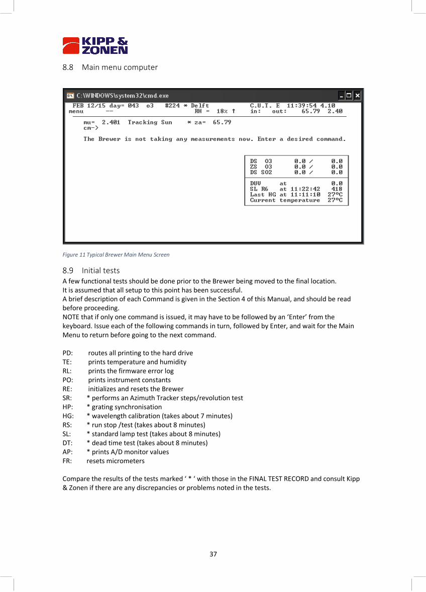
Main menu computer

Figure 11 Typical Brewer Main Menu Screen

Initial tests A few functional tests should be done prior to the Brewer being moved to the final location. It is assumed that all setup to this point has been successful. A brief description of each Command is given in the Section 4 of this Manual, and should be read before proceeding. NOTE that if only one command is issued, it may have to be followed by an ‘Enter’ from the keyboard. Issue each of the following commands in turn, followed by Enter, and wait for the Main Menu to return before going to the next command. PD: routes all printing to the hard drive TE: prints temperature and humidity RL: prints the firmware error log PO: prints instrument constants RE: initializes and resets the Brewer SR: * performs an Azimuth Tracker steps/revolution test HP: * grating synchronisation HG: * wavelength calibration (takes about 7 minutes) RS: * run stop /test (takes about 8 minutes) SL: * standard lamp test (takes about 8 minutes) DT: * dead time test (takes about 8 minutes) AP: * prints A/D monitor values FR: resets micrometers Compare the results of the tests marked ‘ * ‘ with those in the FINAL TEST RECORD and consult Kipp & Zonen if there are any discrepancies or problems noted in the tests.

38

Final Installation

If the results of the initial tests are within acceptable tolerances, then the Brewer can be moved to its final location. 1. At the Brewer Main Menu, issue the command, EX, and the Brewer Operating Program will

terminate. 2. Turn OFF all Brewer and Computer equipment and remove all interconnecting cables. 3. Route the Power and Data Cables from the Computer to the Brewer final location. 4. Disassemble the Brewer-Tracker-Tripod setup, and move them to the final location. 5. At the final location, place the Tripod on a flat surface such that one leg points approximately

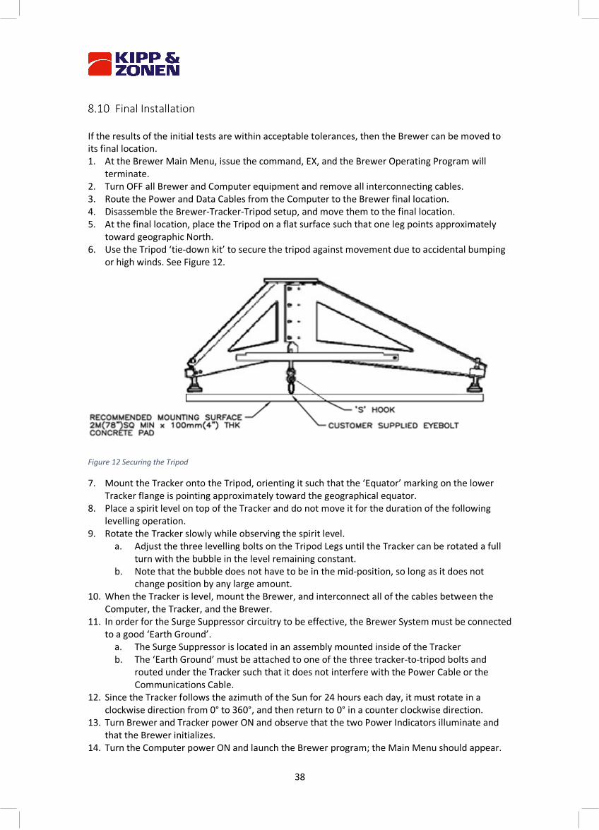
toward geographic North. 6. Use the Tripod ‘tie-down kit’ to secure the tripod against movement due to accidental bumping

or high winds. See Figure 12.

Figure 12 Securing the Tripod

7. Mount the Tracker onto the Tripod, orienting it such that the ‘Equator’ marking on the lower Tracker flange is pointing approximately toward the geographical equator.

8. Place a spirit level on top of the Tracker and do not move it for the duration of the following levelling operation.

9. Rotate the Tracker slowly while observing the spirit level. a. Adjust the three levelling bolts on the Tripod Legs until the Tracker can be rotated a full

turn with the bubble in the level remaining constant. b. Note that the bubble does not have to be in the mid-position, so long as it does not

change position by any large amount. 10. When the Tracker is level, mount the Brewer, and interconnect all of the cables between the

Computer, the Tracker, and the Brewer. 11. In order for the Surge Suppressor circuitry to be effective, the Brewer System must be connected

to a good ‘Earth Ground’. a. The Surge Suppressor is located in an assembly mounted inside of the Tracker b. The ‘Earth Ground’ must be attached to one of the three tracker-to-tripod bolts and

routed under the Tracker such that it does not interfere with the Power Cable or the Communications Cable.

12. Since the Tracker follows the azimuth of the Sun for 24 hours each day, it must rotate in a clockwise direction from 0° to 360°, and then return to 0° in a counter clockwise direction.

13. Turn Brewer and Tracker power ON and observe that the two Power Indicators illuminate and that the Brewer initializes.

14. Turn the Computer power ON and launch the Brewer program; the Main Menu should appear.

39

9 Brewer commands Reserved keys: HOME, DEL, CTRL+BREAK, F KEYS

HOME This key can be pressed to terminate an observation or operation prematurely. It should only be used if the message “press HOME key to abort“ is displayed on the screen. There may be a delay between the time when the DEL key is pressed, and the Main Menu appears, as some aborted activities take longer to terminate.

DEL This key is not normally used for routine work. It can be used in special situations to bypass the five-minute warm-up period of the mercury or standard lamps, or to terminate some operations, such as the zeroing of the Azimuth Tracker if no tracker is present. There may be a delay between the time when the DEL key is presses, and the Main Menu appears as some activity takes longer to abort. Ctrl+Break This combination temporarily halts the Brewer Program so that the GW-BASIC operating system may be accessed. After the CTRL+Break keys have been pressed,

Break in xxxxx OK

will be seen. There will be full access not only to all GW-BASIC commands, but also to the Brewer Program itself. There are a number of ways to restart the Brewer program following a CTRL+Break: • instruct the program to continue by typing ‘CONTINUE’. • Type ‘SYSTEM’ to abort completely from GWBASIC and re-initiate the Brewer operation by one of the traditional methods. The menu displays the MU (air-mass) and ZA (solar zenith-angle) which will be continuously updated during the course of the day, as well as the GMT, date, instrument number, location and data bytes available. Pressing the Return key without a command entry causes the Main Menu to reappear. To issue a command, the appropriate character code is typed, followed by the Enter key. F Keys The F keys are configured to automatically write commonly used commands or sets of commands. The F keys can be used at the Brewer command prompt. The enter key must be pressed to start the command string.

F Key Command Sequence F1 DS F2 ZS F3 ZB F4 HG F5 SL F6 HGSL F7 DSZS2 F8 HGZC2 F9 HGSLDSZSDS F10 DTRSHGSL

40

Brewer command summary Following is the Command Set of the Brewer Spectrophotometer. Commands are entered at the command line, cm->. Note that only two character commands are accepted in a ‘multiple command’ string or in a schedule. Commands may be entered as a series of single commands; each followed by ‘Enter’, or as a command string, consisting of a series of commands, and followed by ‘Enter’ (i.e. pdaphg ‘Enter’). One or more ‘ENTERs’ (when they are prompted for) is generally required for the execution of a single command, whereas on the entry of multiple commands, the subsequent ‘Enters’ are automatically performed by the software. File Name Conventions - JJJ -- indicates a Julian Day. YY --- indicates a year nnn -- indicates a Brewer Instrument Number AP Monitor Voltages Printout This command prints to the line printer, the monitor screen, or to disc, a number of diagnostics that are continuously available in the Brewer. The diagnostics include power supply voltages, test lamp voltages and currents, temperatures, and Brewer moisture content, if the Brewer includes the ‘Moisture’ option. A full list of AP output values can be found in Appendix A AS Azimuth Tracker to the Sun The AS command moves the Azimuth Tracker to the azimuth angle where the Ephemeris has calculated the sun to be for the current location and time. The North Correction from the most recent Siting (see SI command) is applied. AU Automatic Operation The AU command results in the Brewer executing a series of commands, which are, imbedded the AU routine (HP HG DS ZS DS ZS DS ZS B1 UV (or UX)). The sequence continues until interrupted by an operator, or until the sun reaches ZA = 85. At ZA = 85, the system executes the ED command. AZ Azimuth Tracker Zeroing The AZ command causes the Azimuth Tracker to return to its zero reference (North) position, and then move the Brewer to the solar azimuth as calculated by the Ephemeris according to the Location, the Time, and the current North Correction, as determined by the most recent Siting (see SI command). See also Appendix F. B0 Turn off Lamps B0 ensures that the Standard Lamp and Mercury Lamps are both turned off. B1 Mercury Lamp ON B1 turns on the internal Mercury Calibration Lamp, and is useful in a command sequence (i.e. B1DSHG) where a DS measurement is taken while the Mercury lamp is warming up B1. Note that if the HG does not execute for some reason, the lamp may be left on and must be turned off with the B0 command. B2 Standard Lamp ON B2 turns on the internal Standard test Lamp and is useful in a command sequence (i.e. B2ZSSL) where the ZS measurement is taken while the Standard Lamp is warming up.

41

Note that if the SL does not execute for some reason, the Lamp may be left on and should be turned off with the B0 command. CF Instrument Constants File Update CF accesses the Brewer’s Instrument Constants File and allows the operator to make changes. Note that the constants in this file affect the operation and calibration of the instrument, and normally are not changed unless the instrument is undergoing recalibration or has undergone repairs. This command requires operator input, and changes should be made or approved only by qualified personnel. See also Appendix B. CI, CJ Lamp Scan on Slit #1 and Slit #5 CI is used to perform a wavelength scan from 286.5 nm to 366 nm on one of the two internal test lamps. Filter Wheels are set to positions 1 and 0, and the Iris is open. The increment of the scan is user selectable with choices of 1, 2, or 5 Angstrom. Data can be compared with the data contained in the Final Test Record, and is stored in the file CIJJJYY.NNN in the \BDATA directory. A typical command sequence might be B1W1CI, where B1 turns on the HG lamp, W1 produces a 5-minute lamp warm-up delay, and CI executes the wavelength scan. See Appendix A for the format of the CIJJJYY.NNN file. The CI command requires operator input. CJ is the same as CI including the scan backwards. CN Continue Schedule CN initiates the last used schedule. This command is usually put after the sequence of other commands, which are not in the schedule. CO Comments CO allows the operator to enter a comment (up to 75 characters) into the Brewer data file. This command is useful to record information about a measurement, current weather, sky conditions, and so on. This command requires operator input. CS Command Sequence CS is similar to a command line entry at the cm->__ prompt. The operator may enter a sequence of commands to be executed, followed by an integer, which indicates the number of times the sequence is to be repeated. This command requires operator input. CY Slitmask Cycles The default value for slitmask cycling for most observations is 20. The CY command may be used to increase or decrease this number if better statistics, or a faster measurement (with degraded statistics) is desired. This command requires operator input. CZ Custom Scan CZ allows the operator to define a custom scan. Sources may be one of the internal lamps, the UV port, or the quartz window. The scan may be over any wavelength range within the Brewer’s UV scan limits, have any wavelength increment, and use any filterwheel combination. This command requires operator input. Data is stored in a CZJJJYY.nnn file. See also Appendix A. DA Date Set The Brewer ephemeris requires GMT (both date and time) for proper operation. Under normal, uninterrupted operation, the computer, and Brewer, dates will change at 00:00:00 UT, and are displayed on the monitor screen. Under some conditions (power failure at 00:00:00 UT), the date

42

may not update, and may have to be corrected manually. The pointing system updates automatically when a new date is entered. This command requires operator input. DD Print Data Directory DD causes a file listing of the Brewer data directory to be sent to the printer. The printer must have been turned on with the PN command. DDP Print Data Directory DDP causes a file listing of the Brewer program directory to be routed to the printer. The printer must have been turned on with the PN command. DDS Print Data Directory to the screen DDS causes a file listing of the Brewer data directory to be routed to the monitor screen. DI Brewer Health Test The DI command runs a diagnosis of all the motors and lamps. The intensity of the standard lamp is recorded every eight steps of each filterwheel to check filter properties. A decrease in counts for each ND filter in FW#2 should be seen from step 0 to 320. The intensity of the standard lamp is recorded every five steps at one position to check the alignment of the filterwheels. The expected maximum counts are at step 256 and 64 for FW#1 and FW#2 respectively. The intensity of the standard lamp is recorded every 25 steps of the iris motor with a maximum expected at step 250. The intensity of the standard lamp is recorded every step of the zenith motor to check the position of the zenith prism with respect to its reset position. The maximum counts are expected at step 0. The intensity of the standard and mercury lamps is recorded up to 6 minutes after power on. Data is stored in a DIJJJYY.nnn file. DS Direct Sun Ozone Observation DS results in an O3 observation being taken using the direct sun as a radiation source. The Brewer Zenith Prism and Azimuth Tracker are oriented toward the sun, the Iris is closed, FW#1 is rotated to the Ground Quartz Disk (position 1), and FW#2 is adjusted for maximum intensity (starting from position 2) without overdriving the PMT detector. Data is recorded on disk and is printed as previously determined by PN, PD, and PF commands. A DS observation consists of five sets of 20 cycles of the slit mask (a measurement), each cycle taking a reading for 2*0.14 seconds on each wavelength. Intensity data for six wavelengths, and the dark count, is recorded for each of the five measurements. The Azimuth and Zenith positions are updated after each measurement. After each measurement O3 are calculated. After the fifth measurement all data is processed, resulting in a single summary set for the total observation. As a safety feature to prevent damage to the detector, the measurement may terminate if, because of varying cloud conditions, FW#2 has initially been set to a low attenuation value and clouds suddenly move out of the field of view. A DS measurement takes slightly more than three minutes to complete. Details of the data as recorded in the raw data (B) file, and the summary data as recorded in the summary (S) file can be found in Appendix A. DSP Dispersion Test DSP allows for the collection of data for a dispersion test analysis wherein absorption coefficients, wavelength vs. step number and resolution vs. step number equations for each slit is determined. This is a command generally reserved for factory use or for use during an instrument recalibration.

43

DSSUM Direct Sun Data Summary DSSUM reads the daily Data (B) file and printouts out the summary of the day’s DS measurements. An entry is also made to the OZOAVGYY.nnn file. The DSSUM command is usually used as part of the ED command. See also Appendix A. DT Dead Time Measurement Dead Time is a measure of how long a photon counting circuit is ‘dead’ (or cannot count a second photon) after a first photon has been detected. This characteristic of counting circuits can lead to counting errors especially at high photon rates if not compensated for. The DT command initiates a test for the measurement of the dead time of the Photon counting circuits of the Brewer. The DT command is normally executed as part of the ED routine and the test results are recorded in the DTOAVG file. Times differences of greater than 5% should be investigated. The dead time for each instrument is manually record in the Instrument Constants File and can be seen on the PO command printout. For the test the iris is closed, FW#1 is put to position 1. Measurements are made at high intensities (FW#2=0), and at low intensities (FW#2=1). See Appendix F and Appendix. DZ Direct sun with sky radiation measurement Is a Direct Sun measurement but also measures the sky radiation like the Focused Sun (FZ) routine. A later modification also measures slit 7 to perform the DT calculation using the sun as source. ED End of Day At the end of each solar day (solar midnight), it is desirable to summarize, sort, and print out the results of the tests and observations taken the previous day. This may be achieved by using the ED command. The ED routine: • Summarizes data into an ‘S’ file (see SUM). • Sorts and prints data from observations and tests (see OZSUM, FMSUM, FZSUM, HGSUM, SLSUM, UVSUM, and ZSSUM). • Prints constants and monitored values (see PO, AP). • Executes a series of tests (see HG, SL, DT, RS, SR, RE, FR) The first command in ED is a print command, which directs the printout to the printer (see PN) or to a disk file (see PD). If the operator wishes to change the printing path, either the ED-PD.RTN or ED-PN.RTN must be copied to ED.RTN. An operator may run ED at any time. If the Brewer is running in a schedule (see SKC), the ED command is initiated automatically at solar midnight. See also ED-PD and ED-PN. ED-PD End of Day, print to disk ED-PD and ED-PN are the same as the ED command but the operator may easily select the method of printout. In the Brewer program directory, either the ED-PD.RTN or the ED-PN.RTN may be copied to the ED.RTN, resulting in the ED printout being directed to a disk file or to the line printer (see PD and PN commands). See also ED, ED-PN commands. ED-PN End of Day, print to printer See ED, ED-PD commands. END_DAY End of Day (past day) Command Syntax: END_DAY Feb29/98 or END_DAY 06098 END_Day performs an End of Day on a previous day’s data. For the command syntax example: if the raw data file B06098.nnn exists, a Summary file (S06098.nnn) will be created and summary files printed.

44

FI Neutral density attenuation calculation test FF Form Feed FF results in a Form Feed on the printer. FM Focused Moon Observation FM results in an O3 observation to be taken with the moon as the radiation source. The Brewer Zenith Prism and Azimuth Tracker are oriented to the moon, the Iris is opened, FW#1 is rotated to the position 3, and FW#2 is adjusted for maximum intensity, starting at position 2. Data is recorded on disk and is printed as previously determined by PN, PD, and PF commands. An FM observation consists of five sets of 80 cycles of the slit mask (a measurement), each cycle taking a reading for 2*0.14 seconds on each wavelength. Intensity data for six wavelengths, and the dark count, from the five measurements is recorded. The Azimuth and Zenith positions are updated after each measurement. After each measurement, O3 is calculated, and after the final measurement all data is processed, resulting in a single summary set for the total observation. An FM measurement takes approximately 15 minutes to complete. Note that FM observations are not valid for ZA>75° and the message ‘Waiting for the Moon to Rise above ZA=75’ may appear prior to this angle condition being met. See also Appendix A. FMSUM Focus Moon Data Summary FMSUM results in the daily Summary (S) file being read and a printout of the ‘summary’ results of the day’s FM measurements being made. An entry is also made to the FMOAVG.nnn file. The FMSUM command is usually invoked as part of the ED command. FR Micrometer Reset FR performs a reset of the wavelength adjust micrometers. The micrometers are moved to reference points, and then moved to the operating points as dictated by offset values contained in the instruments constants file. The FR command is invoked as part of the RE command, or the operator may manually send the FR command if the positions of the micrometers are suspect. The FR command may be used to determine new micrometer offset values, but these values should only be changed under the supervision of qualified personnel. FR results are recorded in the average file, MIOAVG.nnn, in software versions below 4.10. See also Appendix A. FV Field of view Takes measurements at one wavelength moving the position of brewer in 5 step in azimuth and 10 steps in height. It is very useful to check the sitting of the brewer. During clear conditions, the maximum intensity should occur at the 0 position (original sitting position). There are two version, one only make the measurement of the field of view (fv_orig) , and reports the differences between the maximum intensity found and the current sitting constants. The second also changes the sitting according with the maximum intensity found (fv_chg). This last works well if you have clear sky but could be dangerous if you have clouds, so for routine operation is better to use the first version. FZ Focused Sun Observation As the sun drops lower in the sky, the high Mu values result in an increasing amount of scattered radiation in the field of view of a DS observation. The FZ command allows ozone to be determined at solar angles greater than which could be achieved with a traditional DS. Scattered radiation is measured by offsetting the solar image by 1 degree from the entrance slit, and observing radiation in the vicinity of the solar disk. This scattered radiation is then subtracted from the direct sun result to give a more accurate measure of the direct radiation, before the Ozone determination is made. This method will give reasonably accurate O3 values to ZA of 85° (Air Mass =8.2) as compared to the

45

DS which has cut-off angles of 70 to 80° (Air Mass 3.2 to 5) without corrections. This is a useful command at high latitudes and is normally not used where DS readings are available. For the FZ measurement the iris is closed, FW#1 is set to position 3, and FW#2 is set to position 5. The minimum zenith angle at which an FZ may be taken is 73°. See also DS command. FZSUM Focused Sun Data Summary FZSUM command reads the daily Data (B) file and printouts out the ‘summary’ results of the day’s FZ measurements. The FZSUM command is usually invoked as part of the ED command. GI Global UV ozone measurements Developed by Arne Dahlback. This routine performs ozone measurements using the global UV port, the ozone is then calculated by comparison of the observed ratio to model calculation (7th Brewer Users Group Meeting, Ozone from global irradiance measurements. Methodology, calibration and quality). GS Gratings Data Collection GS initiates a routine that collects data required to calculate Grating Slope and Grating Intercept values, which ensure that the two gratings are synchronized during scanning. The routine performs a scan on slits 1 through 5. Data is written to a GSJJJYY.nnn file. GS is normally run by as part of factory set-up operations or when problems are experienced with the micrometers or gratings. HG Mercury Wavelength Calibration HG is used to accurately locate the 302.15 nm line of the Mercury spectrum, and then adjust the diffraction grating such that the five ozone operational wavelengths fall onto the appropriate exit slits. The zenith prism rotates to the test lamps (position 0), the iris is opened, FW#1 is rotated to the quartz disk (position 1), FW#2 to ND=0 (position 0). Following the initial set-up and lamp warm-up, the grating is scanned in the forward and reverse direction and the resulting combined spectrum is compared to a stored spectrum. Corrections to the micrometer position are made, and if the adjustment required is greater than 2 steps (.012 nm) then the scan is repeated. A test for the presence of Hg lamp radiation is made prior to the beginning of the scan, and if it is not there, an FR test is done to reposition the micrometers to pre-set initialization values and the test is redone. See also Appendix F and Appendix A. HGSUMMercury Lamp Summary HGSUM reads the daily Data (B) file and prints out the ‘summary’ results of the day’s HG calibrations. In addition, an entry is made in the HGOAVG.nnn file. The HGSUM command is usually invoked as part of the ED command. See also Appendix A for an explanation of the HGOAVG.nnn file. HL Mercury lamp scan between 3331 – 3351 Å HL scans the internal mercury lamp spectrum peak centered at 3341.48 Å. The zenith prism rotates to the test lamps (position 0), the iris is opened, FW#1 is rotated to the quartz disk (position 1), FW#2 to ND=0 (position 0). Four scan cycles are taken at a wavelength increment of 0.25 Å. Data is printed to the HLJJJYY.NNN file and to the HLOAVG file. HP Grating Synchronization It is important that the two micrometers remain synchronized such that they are both set to the same wavelength. The HP test tests for this condition and makes an adjustment, if necessary. For this test, the Standard lamp is used as a light source. The Standard Lamp is turned on, the prism is pointed to lamps, the Iris is opened, FW#1 is set to position 1, and FW#2 is set to position 0.

46

Micrometer #2 is then moved relative to Micrometer #1, and is adjusted such that maximum intensity will occur - an adjustment of more than 10 steps results in the test being repeated. HS Mercury lamp scan between 2950 – 2984 Å HS scans the internal mercury lamp spectrum peak centered at 2967.28 Å. The zenith prism rotates to the test lamps (position 0), the iris is opened, FW#1 is rotated to the quartz disk (position 1), FW#2 to ND=0.494 (position 1). Four scan cycles are taken at a wavelength increment of 0.25 Å. Data is printed to the HSJJJYY.NNN file and to the HSOAVG file. HV High Voltage Test The HV command invokes a test used to determine the optimum high voltage setting for the photomultiplier. The HVSET command can then be used to set the High Voltage. This test is normally used in the factory during the final set-up stages of manufacture, or in the field if it is suspected that the setting is not correct. The Standard Lamp is turned on, the iris is opened, FW#1 is put to position 1, and FW#2 is set to position 0. See the HVSET command and Appendix F for more details on the HV test. HVSET High Voltage Set-up The HVSET command can be used to adjust for the optimum High Voltage as determined be the HV test. IC Instrument Configuration File Update The IC command results in a display of the Instrument’s current configuration and allows changes to be made by the operator. See Appendix B for details of the configuration options available. LF Location File Update The LF command displays a list of some of the known locations of Brewer sites throughout the world. The geographical co-ordinates of the current site may be entered and/or modified. LL Location Update The LL command allows an operator to change the co-ordinates of a Brewer location, or for the selection of another site contained in the location file. NI Brewer responsivity check NI calculates the responsivity of the Brewer using the internal standard lamp. This command is useful to check the NISIO4 filter on single Brewers. NO Change Instrument The NO command allows the instrument number of the Brewer to be changed. Each Brewer has a set of files which are stored in the C:\BDATA\NNN subdirectory, and which are necessary for proper operation of Brewer NNN. When the NO command is issued, the software is made aware of which Brewer is connected. NR No Recording This command will turn off recording to the data disk. Data will continue to be printed to the printer, and the ‘bytes free’ message, which normally appears on the screen, will be replaced by a ‘DISK TURNED OFF!’ warning message. See also the DI command. OZSUM Ozone Summary OZSUM reads the daily Date (B) file and prints out the summary results of the day’s O3 observations. In addition, an entry is made in the OZOAVGYY.nnn file.

47

The OZSUM command is usually invoked as part of the ED command. See Appendix A for an example of the OZOAVGYY.nnn file. PB Data Playback Command Syntax: PB BJJJYY. The PB command allows any previous day’s data to be printed using the current temperature coefficients. PD Print to Disk PD directs printing to a ‘D’ file on the data drive rather than to the line printer. See also PN, PF. PF Printer Off PF turns off all printing. Raw data continues to be recorded. See also PN, PD. PN Printer ON PN directs printing to the line printer. See also PD, PF. PO Printout Instrument Constants PO generates a printout of the instrument constants file. An example of PO output values can be found in Appendix A PZ Point to Zenith PZ results in the Zenith Prism being pointed to a Zenith angle of 0° (straight upwards). QS Quick Scan QS is used in conjunction with the UV Stability Check Kit, and gives an indication of the stability of the instrument in the intensity measurement of UV over the range 290 nm to 325 nm. When the equipment has been set up as per the instructions in Section of this manual, and the QS command issued, a report is generated which shows the stability of the instrument at 3.5 nm increments using the first generated set of readings as a reference. For the test, the iris is opened, FW#1 is set to position 3, and FW#2 is set to position 1. See Appendix A for the LAMP_LLL.nnn file and Section 11 for more on QS. QL Lamp Quick Scan QL is a command based on the QS command. The QL command measures at 12 wavelengths for MkII instruments and at 24 wavelengths for MkIII and MkIV. Enhancements compared to the QS routine are that QL measures over the complete UV range for all Brewer types, including on slit 5. The QL output file has corrected (not raw) intensities. For the test, the iris is opened, FW#1 is set to position 3, and FW#2 is set to position 1. See Appendix A for the QL___LLL.nnn file and Section 11 for more on QL. RE Reset RE initializes all of the Brewer motors (similar to the ‘Power On’ initialization), and moves them to positions as defined in the Instruments Constants File. Following a RE, the iris is closed, FW#1 is in position 1 and FW#2 is in position 3. REP Report REP displays (or prints) the SLOAVG, HGOAVG, APOAVG, DTOAVG, MIOAVG, and RSOAVG over a user selected range of days. RS Slit Mask Run/Stop Test A malfunction in the slit mask motor circuit or in the slit mask itself can result in improper counting and consequently incorrect data. The RS test produces a report on the operation of the Slit Mask

48

Motor by taking measurements in the ‘Running’ and ‘Stopped’ modes of the Slit Mask Motor. The RS command is normally executed as part of the ED routine and the test results are recorded in the RSOAVG file. For the RS test, FW#1 is set to position 1, FW#2 is set to position 0 and the iris is open. RS values consistently outside the range of 0.997 to 1.003 for slitmask positions 2 to 6 should be investigated. See Appendix C for an explanation of the RS test, and Appendix A for the RSOAVG.nnn file. SA Solar Angle Printout SA will generate a printout of GMT vs. air mass, solar zenith angle and lunar zenith angle for the day and location currently in use. Printouts for pasts and future dates are possible by simply changing the Brewer system date. SC Direct Sun Scan This test is normally a factory pre-calibration test; the SC determines the optimal operating position of the diffraction grating(s) for taking ozone measurements. Each individual scan is saved to a SCJJJYY.NNN data file, the SC output average values are added to the SCOAVG.NNN file. This command can be used in schedules. A set of good sun scans taken between zenith angles of 48 and 66 degrees will provide useful information preliminary to an ozone re-calibration. SE Schedule Edit SE is used to create or modify Brewer operating schedules, which are stored as ‘.SKD’ files in the Brewer directory. Brewer schedules consist of two columns of data - a solar zenith angle, and a string of commands. The string of commands is executed at the corresponding solar zenith angle. The SA command is useful for converting GMT to solar angle. See Section 8 for more on designing schedules. See also the SK and SKC commands. SH Slit Mask (shutter) Motor Timing Test Normally a factory test, the SH command is used to determine the timing constant used in the control of the slit mask motor. See Appendix F. SI Solar Siting Brewer observations using the solar disc as the radiation source require that the Zenith Prism of the instrument be pointed very accurately toward the sun. The SI command is used in the initial set-up of the instrument and for subsequent checking of pointing accuracy. After the date, time, and station co-ordinates have been set accurately, a set of four controls on the front of the instrument are used to introduce ‘Horizon’ and ‘North’ corrections, which compensate for any offsets that may occur. These corrections are saved and used by the software in future pointing calculations. See also Section 7. SIM Lunar Siting Brewer observations using the lunar disc as the radiation source require that the input window of the instrument be pointed very accurately toward the moon. (Normally the SI command is used if possible, as a siting using the moon is much more difficult task than a siting using the sun.) The SIM command is used in the initial set-up of the instrument and for subsequent checking of pointing accuracy in the event that the SI command cannot be used. After the date, time, and station co-ordinates have been set accurately, a set of four controls on the front of the instrument are used to introduce ‘Horizon’ and ‘North’ corrections, which compensate for any offsets that may occur. These corrections are saved and used by the software in future pointing calculations. See also Section 7.

49

SK Scheduled Operation SK allows an operating schedule, created by the SE command to be run for the current day. At the end of the schedule, the program returns to the main menu and must be restarted the next day. See also Section 8, and SE and SKC. SKC Continuous (scheduled) Operation SKC allows an operating schedule, created by the SE command, to be run continuously - that is, at the end of the local day a set of summary records is produced (see ED), and the schedule waits for the beginning of the next day and the schedule starts again. See also Section 8, and the SE and SK commands. SL Standard Lamp Test SL initiates the most important quality assurance test in the Brewer commend set. This test essentially performs an ozone measurement using an internal quartz-halogen lamp as the source. The test should be run at least at the start and end of the day and should be preceded by an hp and an hg. The values of R5, R6, and F1 should be monitored carefully, and any changes should be noted and investigated. For the SL test, the iris is opened, FW#1 is set to position 1, and FW#2 is set to position 0. See also Appendix F for details on the test. SLSUM Standard Lamp Summary SLSUM reads the daily Data (B) file and prints out the ‘summary’ results of the day’s SL tests In addition entries are made in the SLOAVG.nnn file. The SLSUM command is usually invoked as part of the ED command. See Appendix A for an example of the SL average files. SR Azimuth Tracker Steps per Revolution SR initiates a test that determines the number of motor steps required for one complete revolution (360°) of the Azimuth Tracker. The tracker is first zeroed in the counter clockwise direction, and a discrepancy between where the software thought it was, and where the zero reference was found, is output. The Tracker is then moved a full revolution clockwise and the total number of steps required for this movement is output, and the operator is given an opportunity to save the new value. A progressive change of value over time may suggest that Tracker maintenance is required. See Appendix F. Tracker maintenance is covered in Section 5. SS Direct Sun UV Scan SS results in the Brewer performing a UV scan of the sun through the quartz window. The scan is in 0.5 nm steps over the range 290 nm to 363 nm. Data is stored in an SSJJJYY.nnn file. No response file is available for this mode of UV scanning. See also Appendix A. ST Status and Control ST permits the operator to switch the Brewer’s internal lamps off and on, and to control all Brewer stepper motors except the Slit Mask Motor. SUM Summary Data File SUM reads the daily raw data (BJJJYY.nnn) file and generates a new (SJJJYY.nnn) file, which contains only data summary information. In addition, Umkehr data is processed and put into a separate (UJJJYY.nnn) file. The SUM command and the various summary printout commands are generally performed at local midnight as part of the ED command.

50

TE Temperature Printout TE results in the Brewer temperature (Thermistor #1) in degrees Celsius, along with its equivalent (0 to 5.00 V) voltage, to be printed. If the Brewer has a moisture sensor option, the moisture (in grams/m3) is also printed or displayed. See also Appendix A for the average file. TI Time Set TI allows the operator to set the internal clock of the Brewer, provided the clock option is turned on in the instrument configuration File. Brewer time is GMT or CUT and is entered as a six-digit string (hhmmss). If the internal clock has been turned off in software, there will be an ‘E’ (external) displayed on the computer screen, and the operator will be given the opportunity to turn the internal clock back on. An ‘I’ is displayed on the screen if the system is using the Brewer’s internal clock. TT TeleType Communications TT sets the Brewer program to its teletype mode, whereby the operator may communicate directly with the Brewer via the computer keyboard and a set of low level commands. Exit from teletype mode with the home key. Ctrl-x will allow you to retype a line. See Appendix H for more explanation on the TeleType feature. TU Test UV Port Alignment TU uses an external quartz-halogen lamp mounted over the UV dome to find the zenith motor step position for which the radiation intensity is a maximum through slit #1 of the spectrometer slitmask. This is an alignment test and should be performed if misalignment of the UV optics is suspected. The results of the factory tests are found in the Final Test Record and are nominally 2112+/- 4 steps. UM Umkehr Observations UM results in data being collected which can be processed to produce an Ozone vs. Height profile. Data is normally collected between solar zenith angles of 60 ° and 90° in the morning and in the afternoon. The zenith prism is pointed to a solar zenith angle of 0°, FW#1 is set to the 0 position, FW#2 is set to the 0 position, the iris is opened, and the Tracker is rotated CCW until it is perpendicular to the sun. Intensity measurements are made at two sets of wavelengths - long (320-330 nm) and short (310-320 nm), and continue until they are interrupted by the operator, or by the next zenith angle in a schedule. Raw data is put into the BJJJYY.nnn file, and is processed to an UJJJYY.nnn file by the SUM command. See also Appendix A and Appendix E. UV Related Commands There are a number of Brewer commands that are related to measurements taken through the Ultra Violet (UV) Dome and they are grouped together here for convenience. There are typically two UV scan lengths - ‘short’ UVB scans, which cover the range from 290 nm to 325 nm, and ‘extended’ UV scans which cover the range 286.5 nm to 363 nm. UA Timed UX scan UA performs an Extended UV scan in 0.5 nm increments and stores the data to an UVJJJYY.nnn file. This is a ‘timed’ routine in that it starts on the next half hour after the command is given. On execution of the command, the prism is rotated to the UV dome, FW#2 is moved to the 1 position, FW#1 is moved to the 3 position, the iris is opened, and the tracker is pointed at the sun. See also Appendix A, and the UX command.

51

UB UV Summary for Schedules Raw UV scan data is stored in an UVJJJYY.nnn data file. The UB scan instructs the program to process and print the daily summary for UV measurements taken throughout the day. Damaging Ultra-Violet values are calculated for each scan and written to a DUVJJJYY.nnn. See also Appendix A. UF Fast UVB scan UF results in a UV scan being done in the ascending wavelength direction only. The zenith prism is rotated to the UV dome, FW#2 is set to the 1 position, FW#1 is set to the 3 position, the iris is opened, and the tracker is pointed to the sun. The UV spectrum is scanned in steps of 0.5 nm, with and integration of four shutter cycles for wavelengths less than 300 nm, and an integration of one shutter cycle for wavelengths greater than 300 nm. All data is normalized to a 1-cycle observation and recorded in an UFJJJYY.nnn data file. When scanning is complete, a calculation of the UVB/UVA McKinley - Diffey weighted irradiance is computed and sent to the printer and written to the DUVJJJYY.nnn data file. See also Appendix A. UL UV Lamp Scan UL is a test command that results in a UV scan being performed with a Lamp (rather than the sky) being the source of radiation. The zenith prism is rotated to the UV dome, FW#2 is set to the 1 position, FW#1 is set to the 3 position, the iris is opened, and the tracker is rotated to the sun. The operator is asked for lamp number, and lamp-diffuser separation, and the radiation intensity is measured in 1.5 nm increments over the UVB range. Data is stored in an ULJJJYY.nnn file. See also Appendix A. UV UV(B) Observation UV results in the irradiance over the ‘B’ region of the spectrum to be measured. The zenith prism is rotated to the UV dome, FW#2 is set to the 1 position, FW#1 is set to the 3 position, the iris is opened, and the tracker is pointed toward the sun. The UV spectrum is then scanned in steps of 0.5 nm from 290 nm to 325 nm, and then back to 290 nm. The data is appended to an UVJJJYY.nnn data file. When scanning is complete, a calculation of the UVB/UVA McKinley- Diffey weighted irradiance is computed, sent to the printer and to the monitor screen, and appended to the DUVJJJYY.nnn data file. A correction is made to the Diffey action spectrum to include the effects of the UVA region 325-400 nm). UVSUM UV Data Summary This command initiates activity, which processes and prints the daily summary of all UV measurements made during that day. DUV values are also calculated for each measurement and data is appended to the UVOAVG.nnn file. See also Appendix A. UX Extended UV Wavelength Scan UX causes the irradiance over the 286.5 nm to 363 nm range to be measured in 0.5 nm increments in ascending wavelength. The zenith prism is rotated to the UV dome, FW#2 is set to the 1 position, FW#1 is set to the 0 position, the iris is opened, and the tracker is pointed toward the sun. The UV spectrum is scanned, and the data is appended to a UVJJJYY.nnn data file When scanning is complete, a calculation of the UVB / UVA McKinley- Diffey weighted irradiance is computed, output to the printer and to the monitor screen, and appended to the DUVJJJYY.nnn data file. See also Appendix A.

52

W0-W4 Time delays These five commands result in time delays of 1, 5, 10, 20, and 30 minutes respectively and can be used in command strings or in schedules. XL Extended External Lamp Scan XL is a test command that results in an extended UV scan being performed with a Lamp (rather than the sky) as the source of radiation. The zenith prism is rotated to the UV dome, FW#2 is set to the 1 position, FW#1 is set to the 3 position, the iris is opened, and the Tracker is rotated to the sun. The operator is asked for lamp number and lamp-diffuser separation, and the radiation intensity is measured in 0.5 nm increments over the extended UV range. Data is sampled for 30 cycle time increments through slit #1 for wavelengths less than 300 nm and 20 cycle time increments through slit #5 for higher wavelengths. Data is stored in an XLJJJYY.nnn file and is normalized to 1-cycle observations. See also Appendix A. ZB, ZC, ZS Zenith Sky Observations ZB, ZC, and ZS are variations of the same command, and are used when sky conditions are known and it is desirable to keep the observations separated. ZB is usually used in clear sky conditions (Zenith Blue), ZC is used under cloudy conditions (Zenith Cloud), and ZS is used when conditions are unknown (as is a schedule). The zenith prism is pointed to a Zenith Angle of 0°, the iris is opened, FW#1 is set to position 0, FW#2 is set to position 2, and the azimuth tracker is pointed toward the sun. FW#2 is adjusted according to sky intensity. Data is recorded on disk and is printed as previously determined by PN, PD, and PF commands. A ZS observation consists of seven sets of 20 cycles of the slit mask (a measurement), each cycle taking a reading for 2*0.14 seconds on each wavelength. Intensity data for six wavelengths, and the dark count, from the seven measurements is recorded. The Azimuth and Zenith positions are updated after each measurement. After each measurement O3 is calculated, after the seventh measurement all data is processed, resulting in a single summary set for the total observation. As a safety feature to prevent damage to the detector, the measurement may terminates if, as a result of varying cloud conditions, FW#2 has initially been set to a low attenuation value and clouds suddenly move out of the field of view. ZP initiates a variation of the ZS command in which the Azimuth Tracker is rotated to an angle perpendicular to the sun. A ZS measurement takes slightly more than five minutes to complete. See Appendix A. ZE Zero Zenith Prism ZE positions the zenith prism to its zero-step position, or ZA=180°. The zenith reference is found, and the prism is then moved back a constant number of steps from the zero-step position.

53

10 Routine operations and minor maintenance This section is written for the Brewer Operator, and is meant to be a guide in determining if the Brewer is functioning correctly. It is assumed that the Operator has attended training by Kipp & Zonen personnel at the time of installation. No attempt is made to deal with the science of the instrument, as it is assumed that the appropriate Scientists are interrogating the data and that they have reasonable knowledge of both the Brewer instrument and Atmospheric Science. A properly functioning Brewer requires a relatively small amount of work, but periodic checks and minor maintenance must be done regularly to ensure that high quality data is being recorded. In this manual, the terms Daily, Weekly, and Infrequent are used for frequency of tasks, but local conditions may dictate different intervals.

Daily tasks

Daily tasks are divided into ‘Outside Tasks’, and ‘Inside Tasks’ –i.e. those performed at the Brewer, and those performed at the Computer. These instructions are written assuming that the Brewer is running in ‘Scheduled’ operation.

Outside Tasks

1. Check that the Tracker is pointing toward the Sun, toward the Moon, or perpendicular to the sun, depending on the measurement in progress.

2. Check that the Tracker Power LED is illuminated, and that the Tracker cables are not tangled or pulled tight.

3. Check that the Brewer Power LED is on. 4. Use a soft cloth and mild glass cleaner to clean the UV Dome and the Front Quartz Window

every morning. 5. If the Brewer has a humidity indicator under the viewing window, check its status. 6. If any of the above are abnormal, then make corrections, and make a note in the ‘Brewer Log

Book’

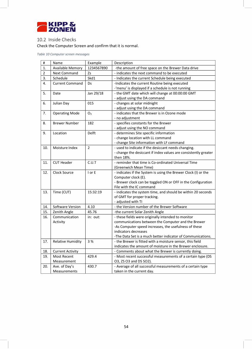
54

Inside Checks Check the Computer Screen and confirm that it is normal.

Table 10 Computer screen messages

# Name Example Description 1. Available Memory 1234567890 -the amount of free space on the Brewer Data drive 2 Next Command Zs - indicates the next command to be executed 3. Schedule Skd1 - Indicates the current Schedule being executed 4. Current Command Ds -Indicates the current Routine being executed

-‘menu’ is displayed if a schedule is not running 5. Date Jan 29/18 - the GMT date which will change at 00:00:00 GMT

- adjust using the DA command 6. Julian Day 015 - changes at solar midnight

- adjust using the DA command 7. Operating Mode O3 - indicates that the Brewer is in Ozone mode

- no adjustment 8. Brewer Number 182 - specifies constants for the Brewer

- adjust using the NO command 9. Location Delft - determines Site specific information

- change location with LL command - change Site information with LF command

10. Moisture Index 2 - used to indicate if the desiccant needs changing. - change the desiccant if index values are consistently greater then 18%.

11. CUT Header C.U.T - reminder that time is Co-ordinated Universal Time (Greenwich Mean Time)

12. Clock Source I or E - indicates if the System is using the Brewer Clock (I) or the Computer clock (E). - Brewer clock can be toggled ON or OFF in the Configuration File with the IC command

13. Time (CUT) 15:32:19 - indicates the system time, and should be within 20 seconds of GMT for proper tracking. - adjusted with TI

14. Software Version 4.10 - the Version number of the Brewer Software 15. Zenith Angle 45.76 -the current Solar Zenith Angle 16. Communication

Activity in: out: - these fields were originally intended to monitor

communications between the Computer and the Brewer -As Computer speed increases, the usefulness of these indicators decreases -The Data Set is a much better indicator of Communications.

17. Relative Humidity 3 % - the Brewer is fitted with a moisture sensor, this field indicates the amount of moisture in the Brewer enclosure.

18. Current Activity - Comments about what the Brewer is currently doing. 19. Most Recent

Measurement 429.4 - Most recent successful measurements of a certain type (DS

O3, ZS O3 and DS SO2). 20. Ave. of Day’s

Measurements 430.7 - Average of all successful measurements of a certain type

taken in the current day.

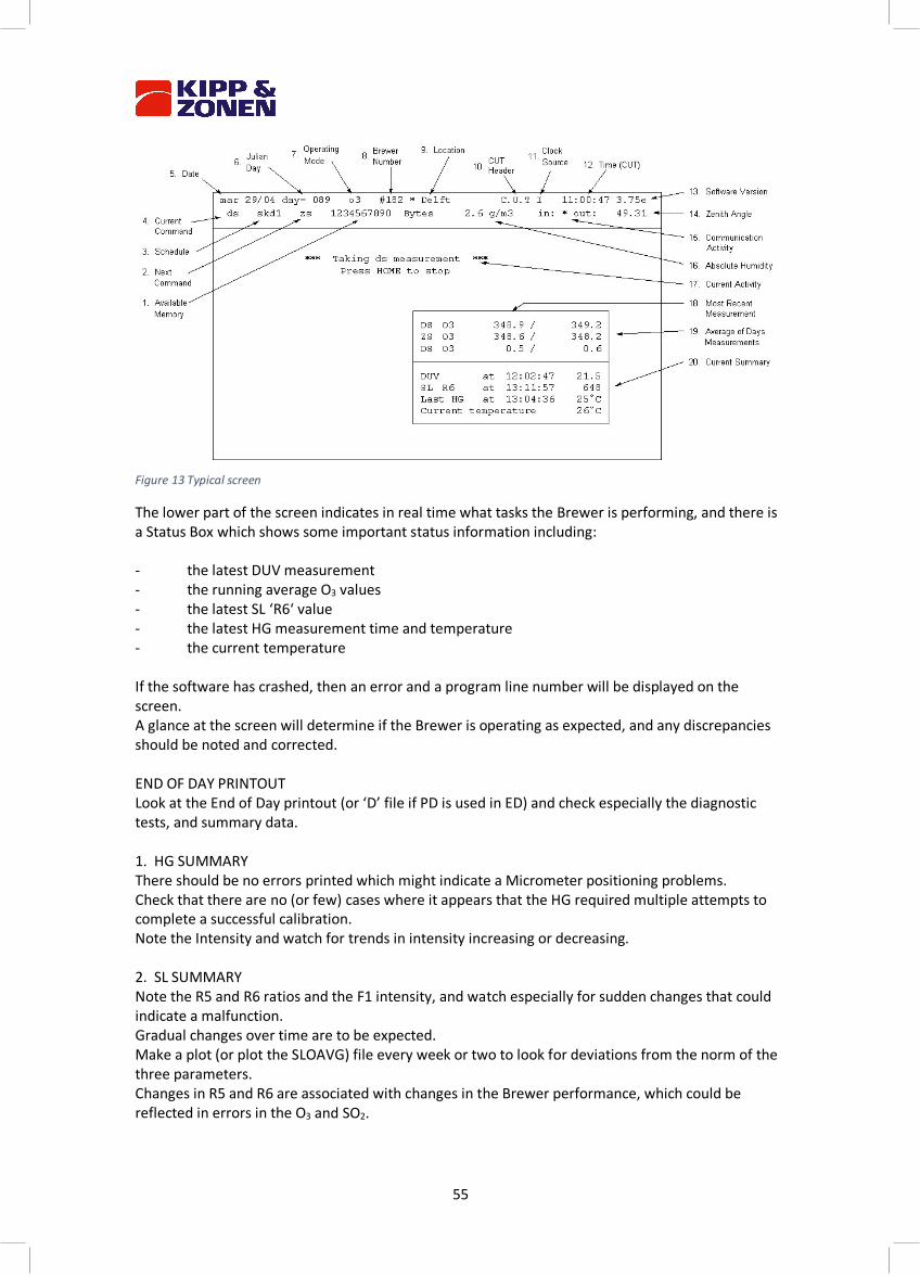
55

Figure 13 Typical screen

The lower part of the screen indicates in real time what tasks the Brewer is performing, and there is a Status Box which shows some important status information including: - the latest DUV measurement - the running average O3 values - the latest SL ‘R6‘ value - the latest HG measurement time and temperature - the current temperature If the software has crashed, then an error and a program line number will be displayed on the screen. A glance at the screen will determine if the Brewer is operating as expected, and any discrepancies should be noted and corrected. END OF DAY PRINTOUT Look at the End of Day printout (or ‘D’ file if PD is used in ED) and check especially the diagnostic tests, and summary data. 1. HG SUMMARY There should be no errors printed which might indicate a Micrometer positioning problems. Check that there are no (or few) cases where it appears that the HG required multiple attempts to complete a successful calibration. Note the Intensity and watch for trends in intensity increasing or decreasing. 2. SL SUMMARY Note the R5 and R6 ratios and the F1 intensity, and watch especially for sudden changes that could indicate a malfunction. Gradual changes over time are to be expected. Make a plot (or plot the SLOAVG) file every week or two to look for deviations from the norm of the three parameters. Changes in R5 and R6 are associated with changes in the Brewer performance, which could be reflected in errors in the O3 and SO2.

56

3. RS TEST: RUN / STOP ratios for wavelength 0 and 2-6 should be 1.000 +/- 0.003 If larger deviations are found, then confirm them to be repeatable before taking any corrective action. 4. DT TEST: The two summary values should be within a few (5) nanoseconds of the values given in the Final Test Record. If larger deviations are found, then confirm them to be repeatable before attempting any corrective action. 5. HP TEST: The test should be successful in one or two attempts. If multiple attempts are required on a regular basis, corrective action may be necessary. 6. RESET The Reset portion of the printout gives values of Azimuth, Zenith and Micrometers zeroing discrepancies. Inspect these discrepancies and confirm that they are repeatable prior to attempting any corrective action. 7. AP PRINTOUT: Inspect the monitor values and look for consistent deviations and trends from the Final Test Record, or from previous values. 8. RL PRINTOUT The Log file printout should be inspected for any errors that the firmware detected, or thought it detected. If the errors persist then Kipp & Zonen should be consulted for advice. 9. OBSERVATION DATA: Data file summaries should be inspected to ensure that they are present, and data should be reviewed as per instructions from the Scientific Authority for the Brewer station.

Weekly tasks There are a number of tasks, which should be performed, and results recorded at least weekly. 1. Steps per Revolution (SR command) 2. Mercury peak wavelengths (HS, HL commands)

Infrequent tasks

This section deals with ‘infrequent’ tasks, as well as those that are more for the integrity of the data than for the operation of the Brewer. The ‘Scientific Authority’ of the observation site usually determines the timing of many of these tasks.

1. UV Stability Check (Section 11) 2. Solar Siting (Section 12) 3. Mechanical Checks 4. UV Calibration 5. Ozone Calibration

57

Minor maintenance Routine maintenance deals with periodic checks and adjustments that the Operator should do to ensure correct operation of the Brewer. These items are not failures, but may lead to failures, or result in poor data if not attended to. Desiccant Changes Moisture is one of the worst enemies of the Brewer and can cause damage to the Optics, which often can be corrected only by returning the Brewer to the factory for parts replacement and recalibration. There are two desiccant systems in the Brewer - the desiccant cartridge ‘breather’ and the loose or bagged desiccant. The desiccant cartridge is intended to remove moisture from the air drawn into the Brewer as temperature changes. This container can be inspected from the underside of the Brewer base by removing two ‘thumbscrews. If the desiccant is no longer orange, then it requires changing. Loose or bagged desiccant is intended to remove moisture from inside the Brewer enclosure. If the Brewer is equipped with a Moisture Sensor, then the Moisture Index is displayed on the Computer Display. The maximum safe level for the Moisture Index is 10. If the Brewer is not equipped with a Moisture Sensor, then Humidity Sensors placed beneath the Brewer Viewing Window should be inspected regularly. If the 40% indicator starts to turn Pink, the moisture is approaching the danger level. If either of the two potentially dangerous conditions of moisture is viewed, then the desiccant in the Brewer enclosure should be changed. The desiccant container mounted in the rear of the Spectrometer should be inspected each time the Brewer cover is removed, and the desiccant replaced whenever it is observed that the indicator is in the 40% region. Tracker Drive Mechanism Refer to Figure 14 If the Steps per Revolution test (SR) returns an erratic result, or a variance that is more than about 20 steps, then the large aluminum drive wheel and the small stainless-steel drive rod should be inspected and cleaned with a dry tissue. If no slippage is observed in the SR, then the cleaning should be done approximately every 3 months. If Tracker slippage is not due to dirty drive gears, then drive gear tensions should be checked. The friction drive arm is set with 9 kg of tension on the lower spring and 4 kg on the upper spring to provide drive friction and gear mesh pressures respectively.

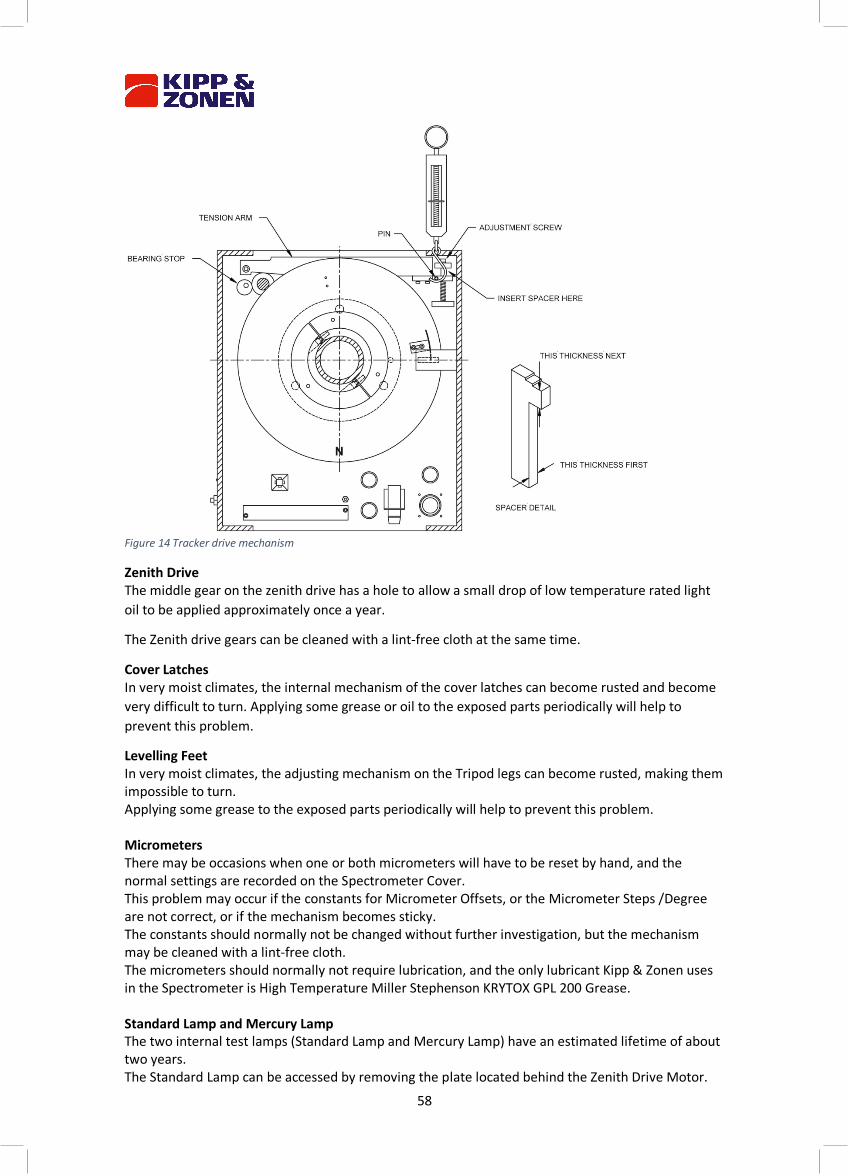
58

Figure 14 Tracker drive mechanism

Zenith Drive The middle gear on the zenith drive has a hole to allow a small drop of low temperature rated light oil to be applied approximately once a year.

The Zenith drive gears can be cleaned with a lint-free cloth at the same time.

Cover Latches In very moist climates, the internal mechanism of the cover latches can become rusted and become very difficult to turn. Applying some grease or oil to the exposed parts periodically will help to prevent this problem.

Levelling Feet In very moist climates, the adjusting mechanism on the Tripod legs can become rusted, making them impossible to turn. Applying some grease to the exposed parts periodically will help to prevent this problem. Micrometers There may be occasions when one or both micrometers will have to be reset by hand, and the normal settings are recorded on the Spectrometer Cover. This problem may occur if the constants for Micrometer Offsets, or the Micrometer Steps /Degree are not correct, or if the mechanism becomes sticky. The constants should normally not be changed without further investigation, but the mechanism may be cleaned with a lint-free cloth. The micrometers should normally not require lubrication, and the only lubricant Kipp & Zonen uses in the Spectrometer is High Temperature Miller Stephenson KRYTOX GPL 200 Grease. Standard Lamp and Mercury Lamp The two internal test lamps (Standard Lamp and Mercury Lamp) have an estimated lifetime of about two years. The Standard Lamp can be accessed by removing the plate located behind the Zenith Drive Motor.

59

Once the two screws are removed, the plate can be detached, bringing with it the lamp socket and the lamp. Great care must be taken not to touch the new lamp with bare hands as oil and/or moisture may change the spectral characteristics of the lamp. The Mercury Lamp may be changed by loosening the two thumbscrews on the lower part of the Lamp Assembly. The Lamp and its socket can then be slid forward (toward the PMT), and the new lamp installed. Great care must be taken not to touch the new lamp. When replacing the lamp and socket, observe that there is a small aligning pin at the top of the assembly. The mercury filament is to be installed in vertical position. Backup Battery The Clock battery on the Main Electronics PCB has an extremely long lifetime under normal operation (power always on) of the Brewer, and it is unlikely that it will have to be changed for many years. In the event that the Battery does require replacement, it can be accessed on the PCB by removing the seven screws securing the rear PCB protective plate, and sliding the plate up. The battery is located on the lower left hand corner of the main circuit board. Prior to removing the battery, the power should be turned off, and the small jumper immediately to the right of the battery should be removed. The battery can then be slid to the left and taken from its holder and replaced with a 3 V Lithium Battery, Kipp & Zonen part no. 75-01-020.

WARNING! Use only the same type of battery. Using a different type could cause damage to the electronics.

Following replacement, the jumper must be replaced, the panel put back on, and the Brewer given a cold start.

60

11 UV stability check – QL Objective: To verify the instrument stability for UV measurements with the optional UV Stability Kit. The stability kit contains three 200 W quartz envelope UV lamps.

Warning! The lamps emit harmful UV radiation, always use protective glasses when the lamps are on and uncovered.

Recommended Frequency of Check: Approximately once every two weeks. Limitation: The UV calibration check procedure assumes Kipp & Zonen’s portable UV lamp assembly, J1017 and KS-J1011, is to be used. This assembly is intended for monitoring instrument stability and NOT to give an absolute responsivity calibration. It is recommended that a NIST traceable 1000 W lamp operated at 50 cm distance from the PTFE diffuser be used for absolute calibration. Lamp Set-up: 1. Ensure the UV Dome is clean. This may be achieved by using a lint free soft cloth or tissue (Kim

Wipes), and clean water, or a mild cleaner. (Windex, isopropyl alcohol, distilled water). 2. When facing the front of the Brewer, position the height extender and Lamp Housing on top of

the UV quartz dome. 3. Select the lamp to be tested. Note the three digit serial number. Insert the lamp into the socket,

ensuring that it is seated completely into the socket. Vertical repeatability is achieved by tightening the two screws holding the lamp. The lamp is 37.5 cm above the diffuser. Connect the two wires. DO NOT touch the lamps with your fingers or allow them to come into contact with any wet or dirty materials. This will reduce the life of the lamp.

4. Place the power supply J1017 on top of the Brewer. Connect the lamp holder cables and fan cable. Plug the AC cord into the power outlet under the Tracker. Turn the lamp power supply on and leave it 10 minutes to warm up. CAUTION! These lamps emit UV radiation which can be harmful to your eyes.

5. Press the ‘#’ button on the power supply. The current of the lamp will be ramped up to 29 A. 6. Allow the lamp to warm up for about 10 minutes.

NOTE: The external tungsten-halogen lamp should be operated at a constant ambient temperature. For this reason, it is recommended to perform the stability check on a dry day when the winds are calm.

Computer Set-up: 1. Press Home to interrupt the Brewer schedule and return control to the Main Menu screen. 2. Issue the hphg commands. The HP will execute, and after a 5 minute lamp warm-up, the HG will

perform a wavelength calibration. 3. Type the command sequence pdqlhphg and press Enter.

a. pd turns on saving data into the D-file b. ql initiates a ‘Quick Lamp Scan’ of the UV lamp c. hp aligns the gratings d. hg does a mercury line wavelength calibration

4. When prompted to do so, enter the following:

a. The lamp number. b. Press Return when prompted to confirm detector distance is 37.5 cm. c. Press delete to bypass lamp warm-up delay.

61

5. The software will then initiate the four commands in sequence and print the results on the screen and in the D-file.

The ‘quick lamp scan’ print-out lists the following:

- Measurement wavelength, in nm. - lamp intensity in counts per second - percent change from initial measurement in the QL_lamp.nnn file

Subsequent Lamps: 1. After the ‘quick scan’ has finished, the UV lamp power supply can be ramped down with the ‘#’

button. After power is off, the fan will continue running for another three minutes. The HOT lamp can be removed from the socket. The lamp should be allowed to cool adequately prior to storing back in the case.

2. Repeat the test for each lamp to be scanned.

CAUTION! These lamps have a limited life expectancy. Do not leave the lamps on for an extended period.

General Instructions: 1. Two lamps should be scanned bi-weekly. If two lamps give approximately the same results, then

the test is complete. If one lamp gives results that are different from the other, then a third lamp should be chosen and the scan run yet another time. The lamp giving the ‘odd’ reading should be noted and used with caution.

2. Once every two months, all three lamps should be scanned to make sure they all give the same results, so availability of spares is assured.

3. The event that the % difference for all lamps is much greater than 5%, it may be necessary to perform other scans with a NIST traceable 1000 W lamp which will be used to create new response files for the instrument. See Appendix C.

4. Perform the TU test prior to changing the response file to make sure that the Zenith Prism is properly aligned. See section 9.2.

62

12 Solar and lunar siting Accurate measurements depend on the instrument being aligned very accurately to the Sun (or Moon). Not only is this important for the direct measurements, but for reasons of polarization and consistency, it applies to all measurements. During installation, care is taken to ensure that the Brewer is oriented properly, but it is not possible to mechanically align the Tripod and the Tracker to the accuracy required. Following installation, the SI (SIM) command can be used to determine both ‘NORTH CORRECTION’ and ‘HORIZON CORRECTION’ information, which are used to compensate for any solar misalignment of the instrument. It is assumed that the date is correct, that the time is accurate to within 20 seconds of GMT, and that the co-ordinates of the site are accurate to two decimal places of latitude and longitude degrees. The following procedure applies to both SI and SIM commands. SI Procedure 1. From the Main Menu, issue the command sequence PDSRSI.

• PD turns on the printer • SR zeros and resets the Tracker • SI puts the software into the Siting Mode • the default mode enables the controls on the Brewer

2. Being careful not to block the sun, look into the ‘Entrance Slit View Tube’. If a bright-diffused image is nowhere to be seen, then go to step 4.

3. Using the UP/DOWN and CW/CCW controls on the front of the Brewer to move the Zenith Prism and/or the Azimuth Tracker such that the diffused image is dissected by the black rectangular image of the entrance slit. Go to step 5.

4. Being careful not to block the Sun, look into the ‘Iris Viewing Tube’. If the Azimuth pointing is accurate to within about 10°, a bright image of the Sun will be seen.

- If no image is seen, and none was seen in step 2, then the Tracker will have to be put into rough alignment by observing shadows cast by various parts on the Brewer, and pushing the CW or CCW buttons until an image appears.

- Once the image is seen in the Viewport, the UP/DOWN and CW/CCW controls are used to move the image into the aperture of the iris.

- When the image disappears into the Iris aperture, then go to step 2. 5. Return to the Computer and follow the instructions for saving the new siting information.

Before saving new values, recheck that the Date and Time are correct. - For accurate tracking to take place the Tracker must be quite level. - Levelling can be checked by alternating the times of day when siting is done - check the

siting in the early morning on one day, and in the late afternoon on another. - If it is found that, the North Correction numbers alternate between higher and lower

numbers consistently from morning to afternoon then this is an indication that the levelling is not accurate.

- If there are very inconsistent North Correction values from one siting to another, this could be an indication of the Tracker drive mechanism slipping.

- If there are inconsistent Horizon Correction values, this could be an indication of Zenith Prism slippage.

- If there is a constant drift in both Horizon and North corrections, then this could be an indication that the site co-ordinates could be incorrect.

63

13 Brewer schedules – SE, SKC, SK A most important feature of the Brewer is its capability to run for longs periods of time in an unattended state. The Brewer system is able to achieve this Automatic operation the use of Schedules Operation. A schedule is simply a file containing a list of instructions, which the Brewer software executes. A series of commands is triggered by the Sun reaching a Solar Zenith Angle (SZA) as prescribed by the Scientific Authority for the observation site. Scheduling Hints and Conventions: - Schedules are created or altered using the SE command. - While in SE, the ^ (shift 6) keys may be used to turn on a flag which causes the Ins and Del keys

to insert or delete full lines. - The SA command is a convenient tool for relating the time (GMT) to the SZA. - In schedule convention, SZA before noon are considered to be negative values, and after noon,

they are positive values. - Schedule names follow DOS rules, and automatically are given the SKD extension. - An ED is invoked automatically at solar midnight by the SKC routine so an additional ED need not

be programmed into the schedule. - Schedules may be ‘linked’ - When running a schedule under SKC, the schedule automatically starts the next day. - When running a schedule under SK, the schedule does not automatically start the next day. - All entries in a schedule are keyed to the SZA, even if they are ‘moon’ measurements. - Only two character commands can be used in a schedule - An integer can be entered at the end of a command line to indicate how many times the

command line is to be repeated i.e. DSZSDS3 will cause the commands DSZSDS to be repeated three times.

- The next SZA will interrupt the current command line when the command in process is finished. - The HPHG sequence is normally inserted such that the internal temperature of the Brewer does

not change more than 2 °C between HG’s. HPHG commands should also be done more frequently in sections of the schedule that have much micrometer movement i.e. UV and UM. Approximate run times for the following measurements are shown below: Table 11 approximate run times

HG 3-5 min. SL (without B2) 9 min DS 3 min ZS 4 min UV 6 min UX 8 min UM Indeterminate must be aborted with

HOME key or new schedule entry FM 11 min

64

Writing Schedules: 1. Determine the Scientific Objectives, and draw up a table of Solar Zenith Angle vs. Commands. 2. Use the SA command to assist in relating to local time. 3. From the Brewer main menu, send the Command SE. 4. A table will appear on the screen with two columns, one for SZA, and one for the commands to

be executed at the SZA. 5. Starting with the first SZA after solar midnight (it will probably be a negative value), enter the

SZA in the left hand column of the table, and enter the commands to be executed at that angle in the right hand column.

6. Carry on through the day, remembering that the SZA changes to +VE after noon (no sign defaults to a positive value).

7. When the schedule is finished, press Ctrl+End and follow the instructions for saving the schedule.

8. The schedule can be tested using the SK or SKC routines.

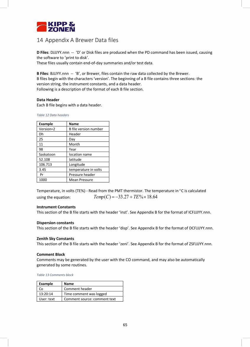
65

14 Appendix A Brewer Data files D Files: DJJJYY.nnn -- ‘D’ or Disk files are produced when the PD command has been issued, causing the software to ‘print to disk’. These files usually contain end-of-day summaries and/or test data. B Files: BJJJYY.nnn -- ‘B’, or Brewer, files contain the raw data collected by the Brewer. B files begin with the characters ‘version’. The beginning of a B file contains three sections: the version string, the instrument constants, and a data header. Following is a description of the format of each B file section. Data Header Each B file begins with a data header. Table 12 Data headers

Example Name Version=2 B file version number Dh Header 25 Day 11 Month 98 Year Saskatoon location name 52.108 latitude 106.713 Longitude 3.45 temperature in volts Pr Pressure header 1000 Mean Pressure

Temperature, in volts (TE%) - Read from the PMT thermistor. The temperature in °C is calculated using the equation:

Instrument Constants This section of the B file starts with the header ‘inst’. See Appendix B for the format of ICFJJJYY.nnn. Dispersion constants This section of the B file starts with the header ‘disp’. See Appendix B for the format of DCFJJJYY.nnn. Zenith Sky Constants This section of the B file starts with the header ‘zeni’. See Appendix B for the format of ZSFJJJYY.nnn. Comment Block Comments may be generated by the user with the CO command, and may also be automatically generated by some routines. Table 13 Comments block

Example Name Co Comment header 13:20:14 Time comment was logged User: text Comment source: comment text

64.18%27.33)( ´+-= TECTemp

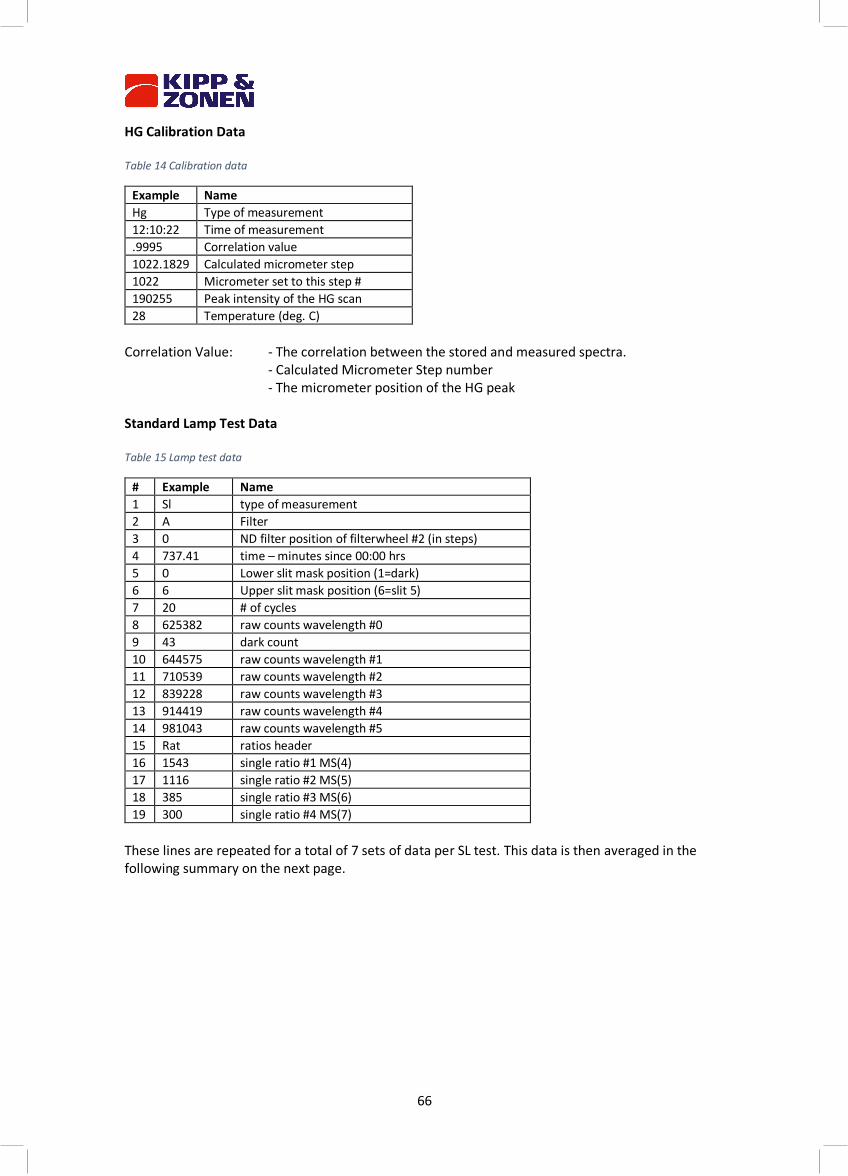
66

HG Calibration Data Table 14 Calibration data

Example Name Hg Type of measurement 12:10:22 Time of measurement .9995 Correlation value 1022.1829 Calculated micrometer step 1022 Micrometer set to this step # 190255 Peak intensity of the HG scan 28 Temperature (deg. C)

Correlation Value: - The correlation between the stored and measured spectra. - Calculated Micrometer Step number - The micrometer position of the HG peak Standard Lamp Test Data Table 15 Lamp test data

# Example Name 1 Sl type of measurement 2 A Filter 3 0 ND filter position of filterwheel #2 (in steps) 4 737.41 time – minutes since 00:00 hrs 5 0 Lower slit mask position (1=dark) 6 6 Upper slit mask position (6=slit 5) 7 20 # of cycles 8 625382 raw counts wavelength #0 9 43 dark count 10 644575 raw counts wavelength #1 11 710539 raw counts wavelength #2 12 839228 raw counts wavelength #3 13 914419 raw counts wavelength #4 14 981043 raw counts wavelength #5 15 Rat ratios header 16 1543 single ratio #1 MS(4) 17 1116 single ratio #2 MS(5) 18 385 single ratio #3 MS(6) 19 300 single ratio #4 MS(7)

These lines are repeated for a total of 7 sets of data per SL test. This data is then averaged in the following summary on the next page.

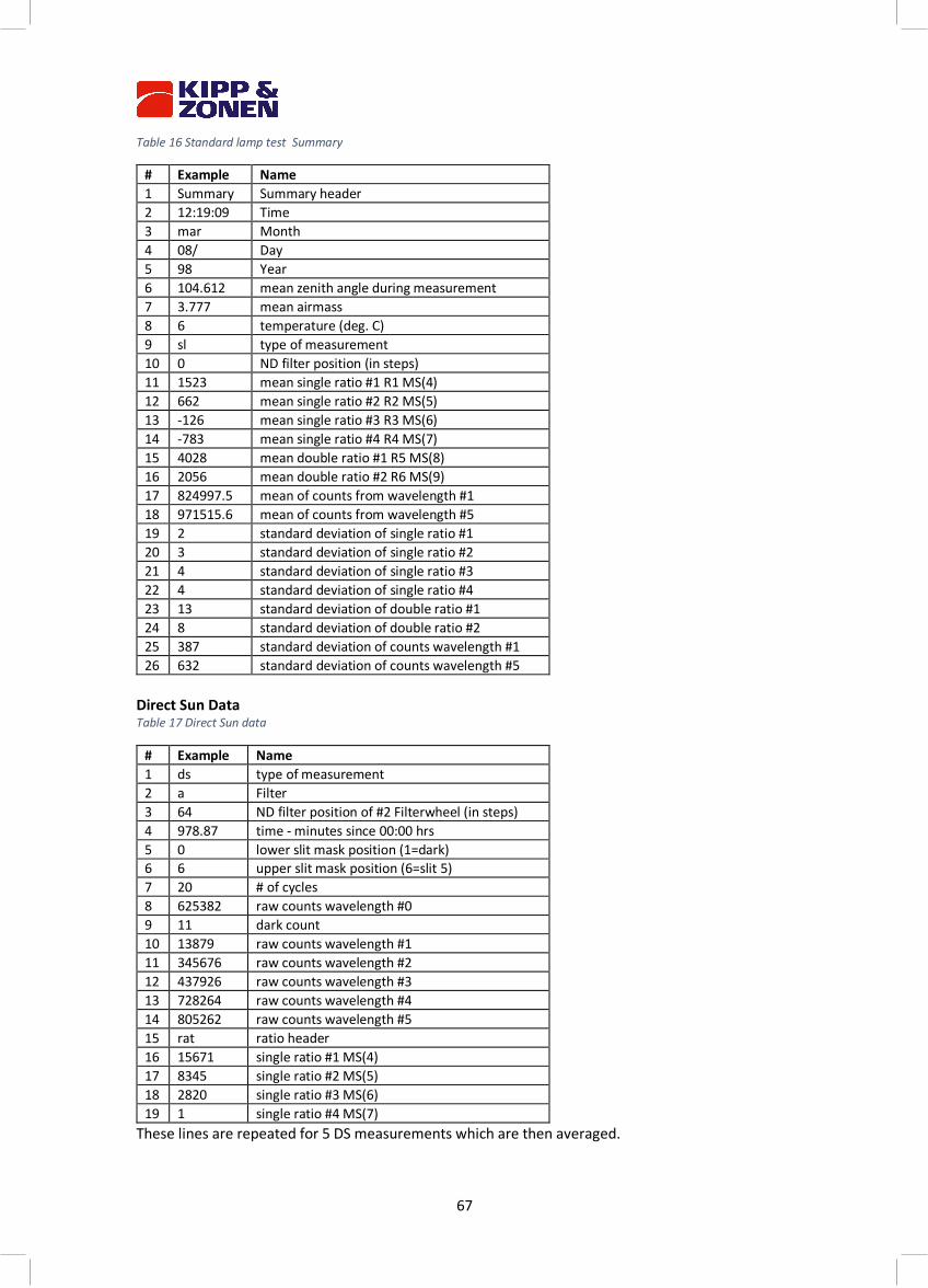
67

Table 16 Standard lamp test Summary

# Example Name 1 Summary Summary header 2 12:19:09 Time 3 mar Month 4 08/ Day 5 98 Year 6 104.612 mean zenith angle during measurement 7 3.777 mean airmass 8 6 temperature (deg. C) 9 sl type of measurement 10 0 ND filter position (in steps) 11 1523 mean single ratio #1 R1 MS(4) 12 662 mean single ratio #2 R2 MS(5) 13 -126 mean single ratio #3 R3 MS(6) 14 -783 mean single ratio #4 R4 MS(7) 15 4028 mean double ratio #1 R5 MS(8) 16 2056 mean double ratio #2 R6 MS(9) 17 824997.5 mean of counts from wavelength #1 18 971515.6 mean of counts from wavelength #5 19 2 standard deviation of single ratio #1 20 3 standard deviation of single ratio #2 21 4 standard deviation of single ratio #3 22 4 standard deviation of single ratio #4 23 13 standard deviation of double ratio #1 24 8 standard deviation of double ratio #2 25 387 standard deviation of counts wavelength #1 26 632 standard deviation of counts wavelength #5

Direct Sun Data Table 17 Direct Sun data

# Example Name 1 ds type of measurement 2 a Filter 3 64 ND filter position of #2 Filterwheel (in steps) 4 978.87 time - minutes since 00:00 hrs 5 0 lower slit mask position (1=dark) 6 6 upper slit mask position (6=slit 5) 7 20 # of cycles 8 625382 raw counts wavelength #0 9 11 dark count 10 13879 raw counts wavelength #1 11 345676 raw counts wavelength #2 12 437926 raw counts wavelength #3 13 728264 raw counts wavelength #4 14 805262 raw counts wavelength #5 15 rat ratio header 16 15671 single ratio #1 MS(4) 17 8345 single ratio #2 MS(5) 18 2820 single ratio #3 MS(6) 19 1 single ratio #4 MS(7)

These lines are repeated for 5 DS measurements which are then averaged.

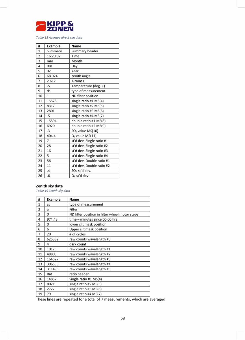
68

Table 18 Average direct sun data

# Example Name 1 Summary Summary header 2 16:20:02 Time 3 mar Month 4 08/ Day 5 92 Year 6 68.024 zenith angle 7 2.617 Airmass 8 -5 Temperature (deg. C) 9 ds type of measurement 10 1 ND filter position 11 15578 single ratio #1 MS(4) 12 8312 single ratio #2 MS(5) 13 2801 single ratio #3 MS(6) 14 -5 single ratio #4 MS(7) 15 15594 double ratio #1 MS(8) 16 6920 double ratio #2 MS(9) 17 .3 SO2 value MS(10) 18 404.4 O3 value MS(11) 19 71 st'd dev. Single ratio #1 20 28 st'd dev. Single ratio #2 21 16 st'd dev. Single ratio #3 22 5 st'd dev. Single ratio #4 23 56 st'd dev. Double ratio #1 24 11 st'd dev. Double ratio #2 25 .4 SO2 st'd dev. 26 .6 O3 st'd dev.

Zenith sky data Table 19 Zenith sky data

# Example Name 1 zs type of measurement 2 a Filter 3 0 ND filter position in filter wheel motor steps 4 974.43 time – minutes since 00:00 hrs 5 0 lower slit mask position 6 6 Upper slit mask position 7 20 # of cycles 8 625382 raw counts wavelength #0 9 4 dark count 10 10125 raw counts wavelength #1 11 48805 raw counts wavelength #2 12 164527 raw counts wavelength #3 13 306533 raw counts wavelength #4 14 311495 raw counts wavelength #5 15 Rat ratio header 16 14857 Single ratio #1 MS(4) 17 8021 single ratio #2 MS(5) 18 2727 single ratio #3 MS(6) 19 79 single ratio #4 MS(7)

These lines are repeated for a total of 7 measurements, which are averaged

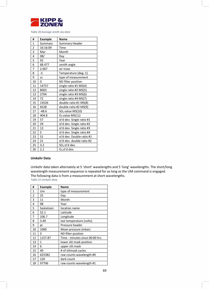
69

Table 20 Average zenith sky data

# Example Name 1 Summary Summary Header 2 16:16:09 Time 3 Mar Month 4 08/ Day 5 92 Year 6 68.477 zenith angle 7 2.667 air mass 8 -5 Temperature (deg. C) 9 zs type of measurement 10 0 ND filter position 11 14757 single ratio #1 MS(4) 12 8003 single ratio #2 MS(5) 13 2704 single ratio #3 MS(6) 14 72 single ratio #4 MS(7) 15 14526 double ratio #1 MS(8) 16 6528 double ratio #2 MS(9) 17 -48.6 SO2 value MS(10) 18 404.8 O3 value MS(11) 19 57 st'd dev. Single ratio #1 20 29 st'd dev. Single ratio #2 21 13 st'd dev. Single ratio #3 22 5 st'd dev. Single ratio #4 23 51 st'd dev. Double ratio #1 24 21 st'd dev. double ratio #2 25 3.2 SO2 st'd dev. 26 2.1 O3 st'd dev.

Umkehr Data Umkehr data taken alternately at 5 ‘short’ wavelengths and 5 ‘long’ wavelengths. The short/long wavelength measurement sequence is repeated for as long as the UM command is engaged. The following data is from a measurement at short wavelengths. Table 21 Umkehr data

# Example Name 1 Um type of measurement 2 25 Day 3 11 Month 4 98 Year 5 Saskatoon location name 6 52.1 Latitude 7 106.7 Longitude 8 3.49 last temperature (volts) 9 pr Pressure header 10 1000 Mean pressure (mbar) 11 0 ND filter position 12 1157.87 Time - minutes since 00:00 hrs. 13 1 lower slit mask position 14 6 upper slit mask 15 40 # of slitmask cycles 16 625382 raw counts wavelength #0 17 120 dark count 18 97706 raw counts wavelength #1

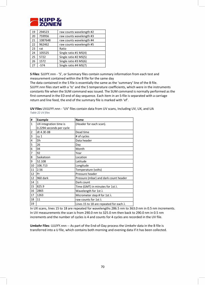
70

19 294523 raw counts wavelength #2 20 759956 raw counts wavelength #3 21 1087648 raw counts wavelength #4 22 962462 raw counts wavelength #5 23 rat Ratio 24 105525 Single ratio #1 MS(4) 25 5722 Single ratio #2 MS(5) 26 1572 Single ratio #3 MS(6) 27 -574 Single ratio #4 MS(7)

S Files: SJJJYY.nnn - ‘S’, or Summary files contain summary information from each test and measurement contained within the B file for the same day The data contained in the S file is essentially the same as the ‘summary’ line of the B file. SJJJYY.nnn files start with a ‘tc’ and the 5 temperature coefficients, which were in the instruments constants file when the SUM command was issued. The SUM command is normally performed as the first command in the ED end of day sequence. Each item in an S-file is separated with a carriage return and line feed, the end of the summary file is marked with ‘ef’. UV Files UVJJJYY.nnn - ‘UV’ files contain data from UV scans, Including UV, UX, and UA Table 22 UV files

# Example Name 1 UX integration time is

0.2294 seconds per cycle (Header for each scan).

2 dt 4.3E-08 Dead time 3 cy 1 # of cycles 4 Dh Data header 5 26 Day 6 04 Month 7 92 Year 8 Saskatoon Location 9 52.108 Latitude 10 106.713 Longitude 11 2.56 Temperature (volts) 12 Pr Pressure header 12 960 dark Pressure (mbar) and dark count header 14 1 Dark count 15 825.9 Time (GMT) in minutes for 1st l 16 2865 Wavelength for 1st l 17 1263 Micrometer step # for 1st l 18 11 raw counts for 1st l 19 Lines 15 to 18 are repeated for each l In UX scans, lines 15 to 18 are repeated for wavelengths 286.5 nm to 363.0 nm in 0.5 nm increments. In UV measurements the scan is from 290.0 nm to 325.0 nm then back to 290.0 nm in 0.5 nm increments and the number of cycles is 4 and counts for 4 cycles are recorded in the UV file. Umkehr Files: UJJJYY.nnn -- As part of the End-of-Day process the Umkehr data in the B file is transferred into a U file, which contains both morning and evening data if it has been collected.

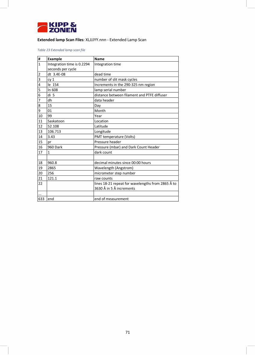
71

Extended lamp Scan Files: XLJJJYY.nnn - Extended Lamp Scan Table 23 Extended lamp scan file

# Example Name 1 Integration time is 0.2294

seconds per cycle Integration time

2 dt 3.4E-08 dead time 3 cy 1 number of slit mask cycles 4 le 154 Increments in the 290-325 nm region 5 ln 608 lamp serial number 6 di 5 distance between filament and PTFE diffuser 7 dh data header 8 15 Day 9 01 Month 10 99 Year 11 Saskatoon Location 12 52.108 Latitude 13 106.713 Longitude 14 3.43 PMT temperature (Volts) 15 pr Pressure header 16 960 Dark Pressure (mbar) and Dark Count Header 17 1 dark count 18 960.8 decimal minutes since 00:00 hours 19 2865 Wavelength (Angstrom) 20 256 micrometer step number 21 121.1 raw counts 22 lines 18-21 repeat for wavelengths from 2865 Å to

3630 Å in 5 Å increments ... 633 end end of measurement

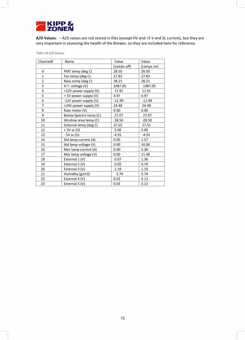
72

A/D Values: -- A/D values are not stored in files (except HV and +5 V and SL current), but they are very important in assessing the health of the Brewer, so they are included here for reference. Table 24 A/D Values

Channel# Name Value Value (Lamps off) (Lamps on) 0 PMT temp (deg C) 28.50 28.50 1 Fan temp (deg C) 27.83 27.83 2 Base temp (deg C) 28.21 28.21 3 H.T. voltage (V) 1487.05 1487.05 4 +12V power supply (V) 11.91 11.91 5 + 5V power supply (V) 4.97 4.97 6 -12V power supply (V) -11.99 -11.99 7 +24V power supply (V) 24.48 24.48 8 Rate meter (V) 0.00 0.00 9 Below Spectro temp (C) 27.07 27.07 10 Window area temp (C) 28.50 28.50 11 External temp (deg C) 27.55 27.55 12 + 5V ss (V) 5.00 5.00 13 - 5V ss (V) -4.91 -4.91 14 Std lamp current (A) 0.00 1.57 15 Std lamp voltage (V) 0.00 10.00 16 Mer lamp current (A) 0.00 0.36 17 Mer lamp voltage (V) 0.00 11.46 18 External 1 (V) 0.07 1.36 19 External 2 (V) 0.05 0.70 20 External 3 (V) 1.19 1.19 21 Humidity (g/m3) 3.74 3.74 22 External 4 (V) 0.02 0.12 23 External 5 (V) 0.03 0.13

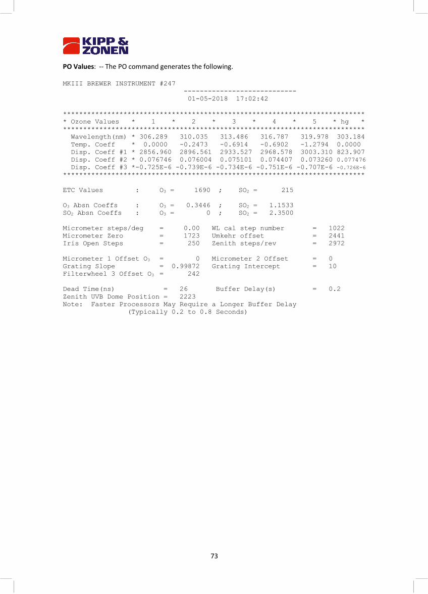
73

PO Values: -- The PO command generates the following. MKIII BREWER INSTRUMENT #247 ---------------------------- 01-05-2018 17:02:42 *************************************************************************** * Ozone Values * 1 * 2 * 3 * 4 * 5 * hg * *************************************************************************** Wavelength(nm) * 306.289 310.035 313.486 316.787 319.978 303.184 Temp. Coeff * 0.0000 -0.2473 -0.6914 -0.6902 -1.2794 0.0000 Disp. Coeff #1 * 2856.960 2896.561 2933.527 2968.578 3003.310 823.907 Disp. Coeff #2 * 0.076746 0.076004 0.075101 0.074407 0.073260 0.077476 Disp. Coeff #3 *-0.725E-6 -0.739E-6 -0.734E-6 -0.751E-6 -0.707E-6 -0.726E-6 *************************************************************************** ETC Values : O3 = 1690 ; SO2 = 215 O3 Absn Coeffs : O3 = 0.3446 ; SO2 = 1.1533 SO2 Absn Coeffs : O3 = 0 ; SO2 = 2.3500 Micrometer steps/deg = 0.00 WL cal step number = 1022 Micrometer Zero = 1723 Umkehr offset = 2441 Iris Open Steps = 250 Zenith steps/rev = 2972 Micrometer 1 Offset O3 = 0 Micrometer 2 Offset = 0 Grating Slope = 0.99872 Grating Intercept = 10 Filterwheel 3 Offset O3 = 242 Dead Time(ns) = 26 Buffer Delay(s) = 0.2 Zenith UVB Dome Position = 2223 Note: Faster Processors May Require a Longer Buffer Delay (Typically 0.2 to 0.8 Seconds)

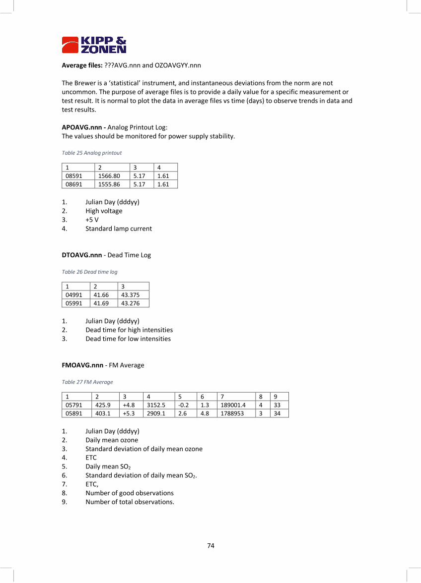
74

Average files: ???AVG.nnn and OZOAVGYY.nnn The Brewer is a ‘statistical’ instrument, and instantaneous deviations from the norm are not uncommon. The purpose of average files is to provide a daily value for a specific measurement or test result. It is normal to plot the data in average files vs time (days) to observe trends in data and test results. APOAVG.nnn - Analog Printout Log: The values should be monitored for power supply stability. Table 25 Analog printout

1 2 3 4 08591 1566.80 5.17 1.61 08691 1555.86 5.17 1.61

1. Julian Day (dddyy) 2. High voltage 3. +5 V 4. Standard lamp current DTOAVG.nnn - Dead Time Log Table 26 Dead time log

1 2 3 04991 41.66 43.375 05991 41.69 43.276

1. Julian Day (dddyy) 2. Dead time for high intensities 3. Dead time for low intensities FMOAVG.nnn - FM Average Table 27 FM Average

1 2 3 4 5 6 7 8 9 05791 425.9 +4.8 3152.5 -0.2 1.3 189001.4 4 33 05891 403.1 +5.3 2909.1 2.6 4.8 1788953 3 34

1. Julian Day (dddyy) 2. Daily mean ozone 3. Standard deviation of daily mean ozone 4. ETC 5. Daily mean SO2 6. Standard deviation of daily mean SO2. 7. ETC, 8. Number of good observations 9. Number of total observations.

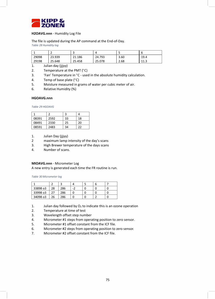
75

H2OAVG.nnn - Humidity Log File

The file is updated during the AP command at the End-of-Day. Table 28 Humidity log

1 2 3 4 5 6 29098 23.939 21.186 24.793 3.60 19.4 29198 25.648 25.458 25.078 2.68 11.3

1. Julian day (jjjyy) 2. Temperature at the PMT (°C) 3. ‘Fan’ Temperature in °C - used in the absolute humidity calculation. 4. Temp of base plate (°C) 5. Moisture measured in grams of water per cubic meter of air. 6. Relative Humidity (%) HGOAVG.nnn Table 29 HGOAVG

1 2 3 4 08391 2592 33 18 08491 2330 25 20 08591 2483 34 22

1. Julian Day (jjjyy) 2 maximum lamp intensity of the day’s scans 3. High Brewer temperature of the days scans 4. Number of scans. MIOAVG.nnn - Micrometer Log A new entry is generated each time the FR routine is run. Table 30 Micrometer log

1 2 3 4 5 6 7 33898 o3 28 286 -2 0 0 0 33998 o3 27 286 0 0 0 0 34098 o3 26 286 0 0 2 0

1. Julian day followed by O3 to indicate this is an ozone operation 2. Temperature at time of test 3. Wavelength offset step number 4. Micrometer #1 steps from operating position to zero sensor. 5. Micrometer #1 offset constant from the ICF file. 6. Micrometer #2 steps from operating position to zero sensor. 7. Micrometer #2 offset constant from the ICF file.

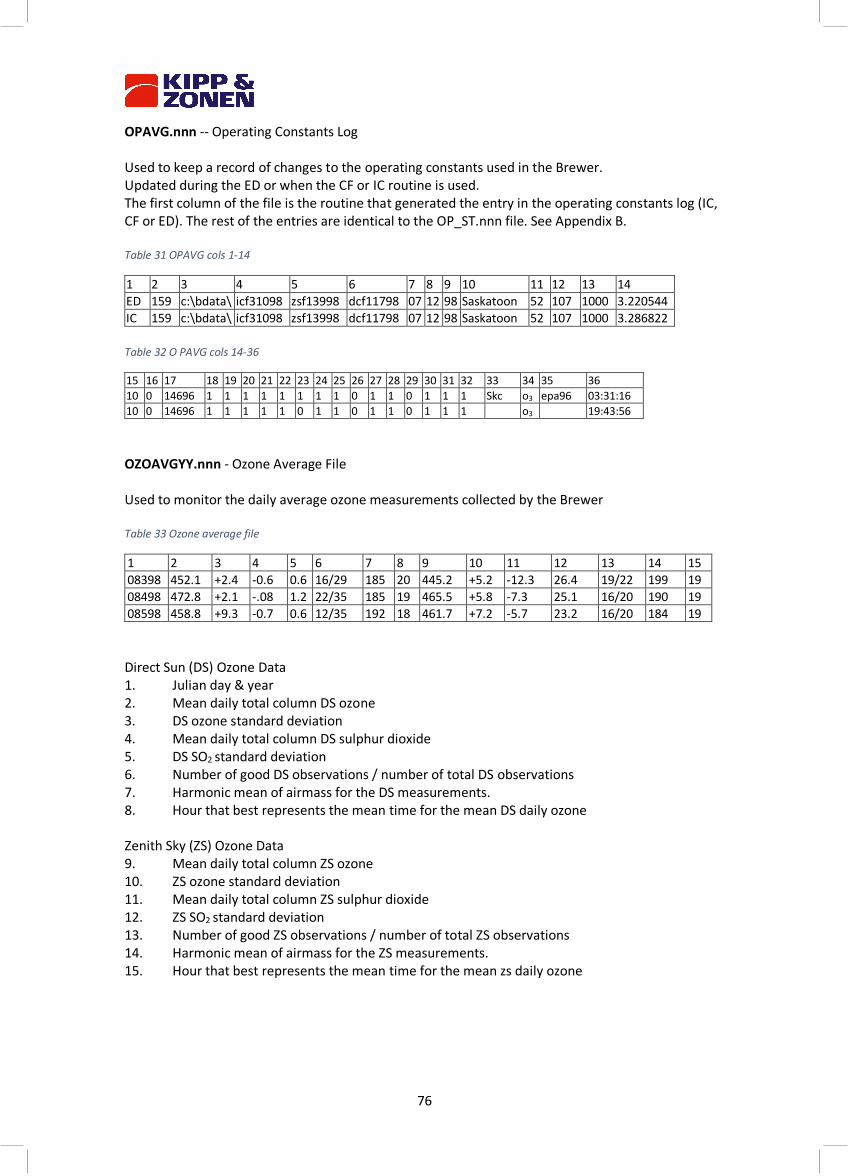
76

OPAVG.nnn -- Operating Constants Log Used to keep a record of changes to the operating constants used in the Brewer. Updated during the ED or when the CF or IC routine is used. The first column of the file is the routine that generated the entry in the operating constants log (IC, CF or ED). The rest of the entries are identical to the OP_ST.nnn file. See Appendix B. Table 31 OPAVG cols 1-14

1 2 3 4 5 6 7 8 9 10 11 12 13 14 ED 159 c:\bdata\ icf31098 zsf13998 dcf11798 07 12 98 Saskatoon 52 107 1000 3.220544 IC 159 c:\bdata\ icf31098 zsf13998 dcf11798 07 12 98 Saskatoon 52 107 1000 3.286822 Table 32 O PAVG cols 14-36

15 16 17 18 19 20 21 22 23 24 25 26 27 28 29 30 31 32 33 34 35 36 10 0 14696 1 1 1 1 1 1 1 1 0 1 1 0 1 1 1 Skc o3 epa96 03:31:16 10 0 14696 1 1 1 1 1 0 1 1 0 1 1 0 1 1 1 o3 19:43:56 OZOAVGYY.nnn - Ozone Average File Used to monitor the daily average ozone measurements collected by the Brewer Table 33 Ozone average file

1 2 3 4 5 6 7 8 9 10 11 12 13 14 15 08398 452.1 +2.4 -0.6 0.6 16/29 185 20 445.2 +5.2 -12.3 26.4 19/22 199 19 08498 472.8 +2.1 -.08 1.2 22/35 185 19 465.5 +5.8 -7.3 25.1 16/20 190 19 08598 458.8 +9.3 -0.7 0.6 12/35 192 18 461.7 +7.2 -5.7 23.2 16/20 184 19 Direct Sun (DS) Ozone Data 1. Julian day & year 2. Mean daily total column DS ozone 3. DS ozone standard deviation 4. Mean daily total column DS sulphur dioxide 5. DS SO2 standard deviation 6. Number of good DS observations / number of total DS observations 7. Harmonic mean of airmass for the DS measurements. 8. Hour that best represents the mean time for the mean DS daily ozone Zenith Sky (ZS) Ozone Data 9. Mean daily total column ZS ozone 10. ZS ozone standard deviation 11. Mean daily total column ZS sulphur dioxide 12. ZS SO2 standard deviation 13. Number of good ZS observations / number of total ZS observations 14. Harmonic mean of airmass for the ZS measurements. 15. Hour that best represents the mean time for the mean zs daily ozone

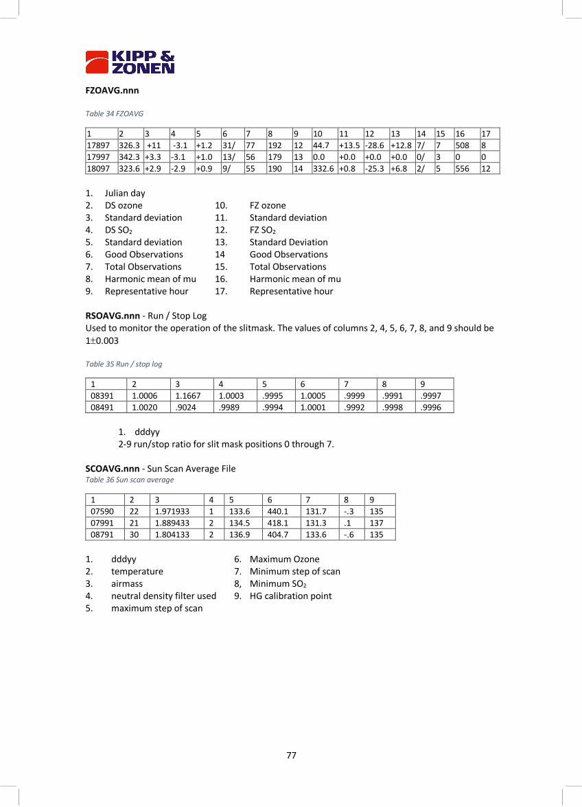
77

FZOAVG.nnn Table 34 FZOAVG

1 2 3 4 5 6 7 8 9 10 11 12 13 14 15 16 17 17897 326.3 +11 -3.1 +1.2 31/ 77 192 12 44.7 +13.5 -28.6 +12.8 7/ 7 508 8 17997 342.3 +3.3 -3.1 +1.0 13/ 56 179 13 0.0 +0.0 +0.0 +0.0 0/ 3 0 0 18097 323.6 +2.9 -2.9 +0.9 9/ 55 190 14 332.6 +0.8 -25.3 +6.8 2/ 5 556 12 1. Julian day 2. DS ozone 10. FZ ozone 3. Standard deviation 11. Standard deviation 4. DS SO2 12. FZ SO2 5. Standard deviation 13. Standard Deviation 6. Good Observations 14 Good Observations 7. Total Observations 15. Total Observations 8. Harmonic mean of mu 16. Harmonic mean of mu 9. Representative hour 17. Representative hour RSOAVG.nnn - Run / Stop Log Used to monitor the operation of the slitmask. The values of columns 2, 4, 5, 6, 7, 8, and 9 should be 1±0.003 Table 35 Run / stop log

1 2 3 4 5 6 7 8 9 08391 1.0006 1.1667 1.0003 .9995 1.0005 .9999 .9991 .9997 08491 1.0020 .9024 .9989 .9994 1.0001 .9992 .9998 .9996

1. dddyy

2-9 run/stop ratio for slit mask positions 0 through 7. SCOAVG.nnn - Sun Scan Average File Table 36 Sun scan average

1 2 3 4 5 6 7 8 9 07590 22 1.971933 1 133.6 440.1 131.7 -.3 135 07991 21 1.889433 2 134.5 418.1 131.3 .1 137 08791 30 1.804133 2 136.9 404.7 133.6 -.6 135

1. dddyy 6. Maximum Ozone 2. temperature 7. Minimum step of scan 3. airmass 8, Minimum SO2 4. neutral density filter used 9. HG calibration point 5. maximum step of scan

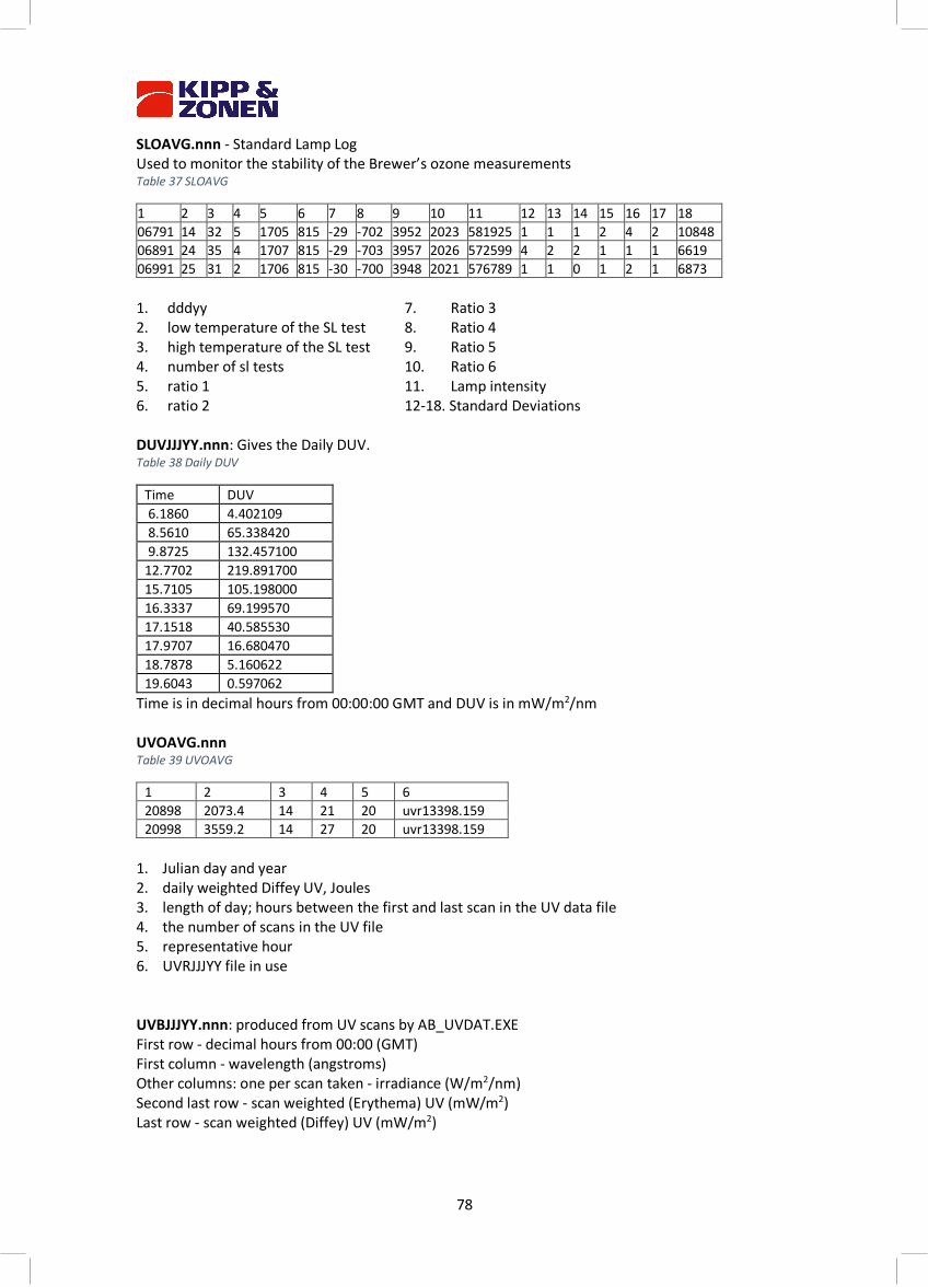
78

SLOAVG.nnn - Standard Lamp Log Used to monitor the stability of the Brewer’s ozone measurements Table 37 SLOAVG

1 2 3 4 5 6 7 8 9 10 11 12 13 14 15 16 17 18 06791 14 32 5 1705 815 -29 -702 3952 2023 581925 1 1 1 2 4 2 10848 06891 24 35 4 1707 815 -29 -703 3957 2026 572599 4 2 2 1 1 1 6619 06991 25 31 2 1706 815 -30 -700 3948 2021 576789 1 1 0 1 2 1 6873 1. dddyy 7. Ratio 3 2. low temperature of the SL test 8. Ratio 4 3. high temperature of the SL test 9. Ratio 5 4. number of sl tests 10. Ratio 6 5. ratio 1 11. Lamp intensity 6. ratio 2 12-18. Standard Deviations DUVJJJYY.nnn: Gives the Daily DUV. Table 38 Daily DUV

Time DUV 6.1860 4.402109 8.5610 65.338420 9.8725 132.457100 12.7702 219.891700 15.7105 105.198000 16.3337 69.199570 17.1518 40.585530 17.9707 16.680470 18.7878 5.160622 19.6043 0.597062

Time is in decimal hours from 00:00:00 GMT and DUV is in mW/m2/nm UVOAVG.nnn Table 39 UVOAVG

1 2 3 4 5 6 20898 2073.4 14 21 20 uvr13398.159 20998 3559.2 14 27 20 uvr13398.159

1. Julian day and year 2. daily weighted Diffey UV, Joules 3. length of day; hours between the first and last scan in the UV data file 4. the number of scans in the UV file 5. representative hour 6. UVRJJJYY file in use UVBJJJYY.nnn: produced from UV scans by AB_UVDAT.EXE First row - decimal hours from 00:00 (GMT) First column - wavelength (angstroms) Other columns: one per scan taken - irradiance (W/m2/nm) Second last row - scan weighted (Erythema) UV (mW/m2) Last row - scan weighted (Diffey) UV (mW/m2)

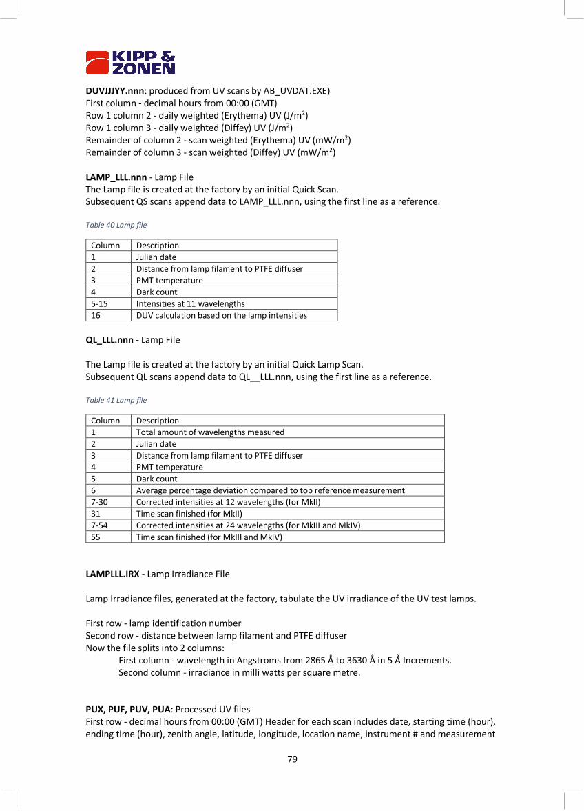
79

DUVJJJYY.nnn: produced from UV scans by AB_UVDAT.EXE) First column - decimal hours from 00:00 (GMT) Row 1 column 2 - daily weighted (Erythema) UV (J/m2) Row 1 column 3 - daily weighted (Diffey) UV (J/m2) Remainder of column 2 - scan weighted (Erythema) UV (mW/m2) Remainder of column 3 - scan weighted (Diffey) UV (mW/m2) LAMP_LLL.nnn - Lamp File The Lamp file is created at the factory by an initial Quick Scan. Subsequent QS scans append data to LAMP_LLL.nnn, using the first line as a reference. Table 40 Lamp file

Column Description 1 Julian date 2 Distance from lamp filament to PTFE diffuser 3 PMT temperature 4 Dark count 5-15 Intensities at 11 wavelengths 16 DUV calculation based on the lamp intensities

QL_LLL.nnn - Lamp File The Lamp file is created at the factory by an initial Quick Lamp Scan. Subsequent QL scans append data to QL__LLL.nnn, using the first line as a reference. Table 41 Lamp file

Column Description 1 Total amount of wavelengths measured 2 Julian date 3 Distance from lamp filament to PTFE diffuser 4 PMT temperature 5 Dark count 6 Average percentage deviation compared to top reference measurement 7-30 Corrected intensities at 12 wavelengths (for MkII) 31 Time scan finished (for MkII) 7-54 Corrected intensities at 24 wavelengths (for MkIII and MkIV) 55 Time scan finished (for MkIII and MkIV)

LAMPLLL.IRX - Lamp Irradiance File Lamp Irradiance files, generated at the factory, tabulate the UV irradiance of the UV test lamps. First row - lamp identification number Second row - distance between lamp filament and PTFE diffuser Now the file splits into 2 columns: First column - wavelength in Angstroms from 2865 Å to 3630 Å in 5 Å Increments. Second column - irradiance in milli watts per square metre. PUX, PUF, PUV, PUA: Processed UV files First row - decimal hours from 00:00 (GMT) Header for each scan includes date, starting time (hour), ending time (hour), zenith angle, latitude, longitude, location name, instrument # and measurement

80

type, Row 2 column 1 - GMT time in minutes, column 2 - Wavelength (Angstroms), column 3 - irradiance (W/m2/nm or mW/m2/nm, depending on selection during processing). PXL: Processed lamp files First row - Lamp Number Row 2 - distance in centimeters Column 1 Row 3 - Wavelength (Angstroms) Row 4 - irradiance (mW/m2/nm)

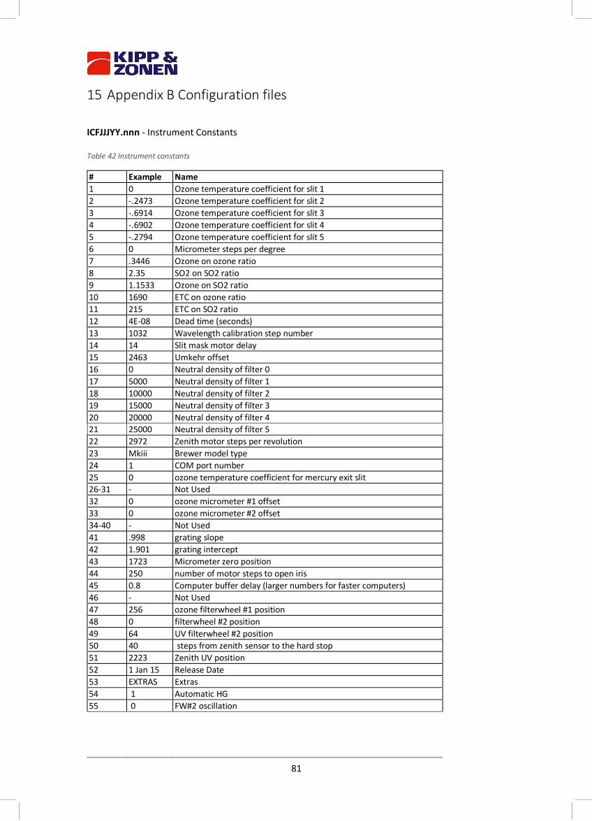
81

15 Appendix B Configuration files

ICFJJJYY.nnn - Instrument Constants Table 42 Instrument constants

# Example Name 1 0 Ozone temperature coefficient for slit 1 2 -.2473 Ozone temperature coefficient for slit 2 3 -.6914 Ozone temperature coefficient for slit 3 4 -.6902 Ozone temperature coefficient for slit 4 5 -.2794 Ozone temperature coefficient for slit 5 6 0 Micrometer steps per degree 7 .3446 Ozone on ozone ratio 8 2.35 SO2 on SO2 ratio 9 1.1533 Ozone on SO2 ratio 10 1690 ETC on ozone ratio 11 215 ETC on SO2 ratio 12 4E-08 Dead time (seconds) 13 1032 Wavelength calibration step number 14 14 Slit mask motor delay 15 2463 Umkehr offset 16 0 Neutral density of filter 0 17 5000 Neutral density of filter 1 18 10000 Neutral density of filter 2 19 15000 Neutral density of filter 3 20 20000 Neutral density of filter 4 21 25000 Neutral density of filter 5 22 2972 Zenith motor steps per revolution 23 Mkiii Brewer model type 24 1 COM port number 25 0 ozone temperature coefficient for mercury exit slit 26-31 - Not Used 32 0 ozone micrometer #1 offset 33 0 ozone micrometer #2 offset 34-40 - Not Used 41 .998 grating slope 42 1.901 grating intercept 43 1723 Micrometer zero position 44 250 number of motor steps to open iris 45 0.8 Computer buffer delay (larger numbers for faster computers) 46 - Not Used 47 256 ozone filterwheel #1 position 48 0 filterwheel #2 position 49 64 UV filterwheel #2 position 50 40 steps from zenith sensor to the hard stop 51 2223 Zenith UV position 52 1 Jan 15 Release Date 53 EXTRAS Extras 54 1 Automatic HG 55 0 FW#2 oscillation

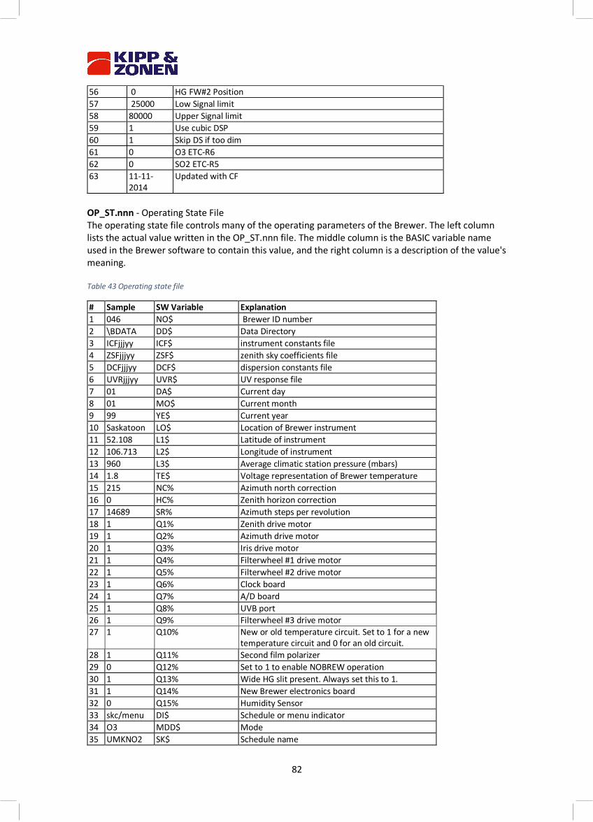
82

56 0 HG FW#2 Position 57 25000 Low Signal limit 58 80000 Upper Signal limit 59 1 Use cubic DSP 60 1 Skip DS if too dim 61 0 O3 ETC-R6 62 0 SO2 ETC-R5 63 11-11-

2014 Updated with CF

OP_ST.nnn - Operating State File The operating state file controls many of the operating parameters of the Brewer. The left column lists the actual value written in the OP_ST.nnn file. The middle column is the BASIC variable name used in the Brewer software to contain this value, and the right column is a description of the value's meaning. Table 43 Operating state file

# Sample SW Variable Explanation 1 046 NO$ Brewer ID number 2 \BDATA DD$ Data Directory 3 ICFjjjyy ICF$ instrument constants file 4 ZSFjjjyy ZSF$ zenith sky coefficients file 5 DCFjjjyy DCF$ dispersion constants file 6 UVRjjjyy UVR$ UV response file 7 01 DA$ Current day 8 01 MO$ Current month 9 99 YE$ Current year 10 Saskatoon LO$ Location of Brewer instrument 11 52.108 L1$ Latitude of instrument 12 106.713 L2$ Longitude of instrument 13 960 L3$ Average climatic station pressure (mbars) 14 1.8 TE$ Voltage representation of Brewer temperature 15 215 NC% Azimuth north correction 16 0 HC% Zenith horizon correction 17 14689 SR% Azimuth steps per revolution 18 1 Q1% Zenith drive motor 19 1 Q2% Azimuth drive motor 20 1 Q3% Iris drive motor 21 1 Q4% Filterwheel #1 drive motor 22 1 Q5% Filterwheel #2 drive motor 23 1 Q6% Clock board 24 1 Q7% A/D board 25 1 Q8% UVB port 26 1 Q9% Filterwheel #3 drive motor 27 1 Q10% New or old temperature circuit. Set to 1 for a new

temperature circuit and 0 for an old circuit. 28 1 Q11% Second film polarizer 29 0 Q12% Set to 1 to enable NOBREW operation 30 1 Q13% Wide HG slit present. Always set this to 1. 31 1 Q14% New Brewer electronics board 32 0 Q15% Humidity Sensor 33 skc/menu DI$ Schedule or menu indicator 34 O3 MDD$ Mode 35 UMKNO2 SK$ Schedule name

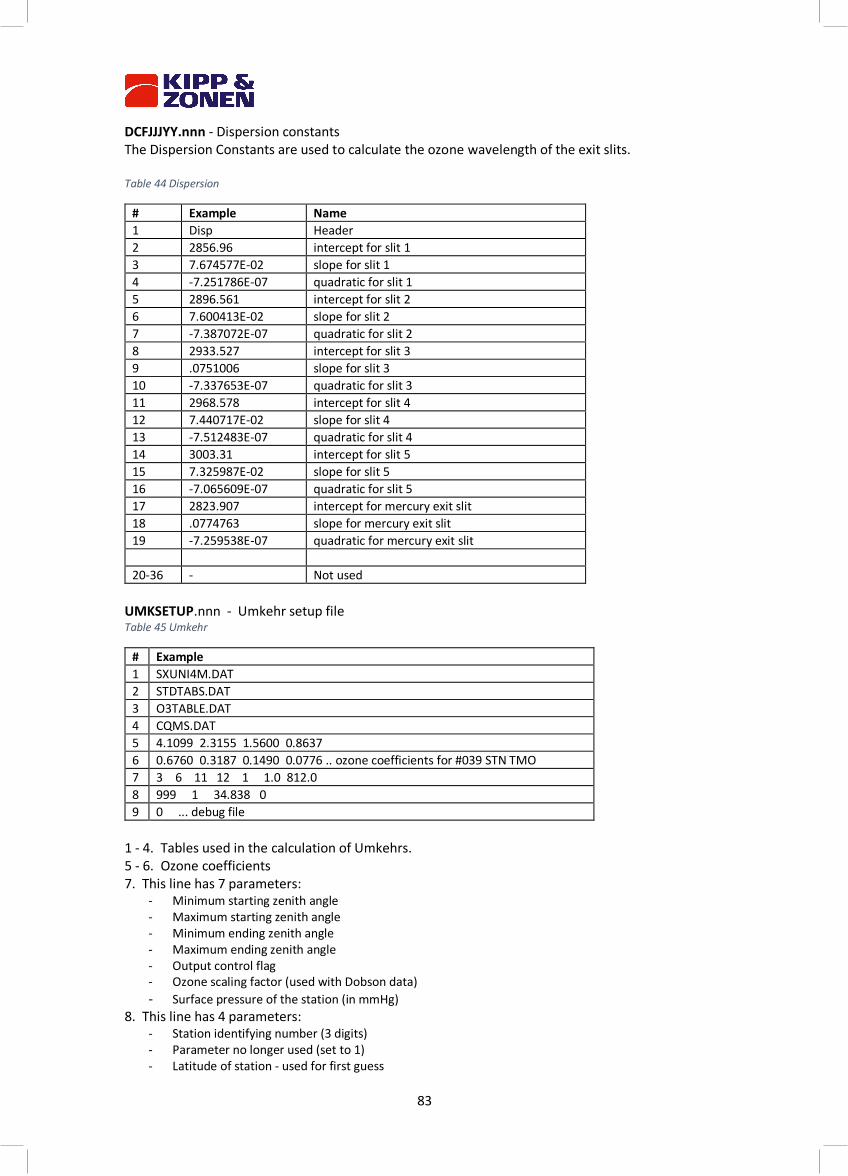
83

DCFJJJYY.nnn - Dispersion constants The Dispersion Constants are used to calculate the ozone wavelength of the exit slits. Table 44 Dispersion

# Example Name 1 Disp Header 2 2856.96 intercept for slit 1 3 7.674577E-02 slope for slit 1 4 -7.251786E-07 quadratic for slit 1 5 2896.561 intercept for slit 2 6 7.600413E-02 slope for slit 2 7 -7.387072E-07 quadratic for slit 2 8 2933.527 intercept for slit 3 9 .0751006 slope for slit 3 10 -7.337653E-07 quadratic for slit 3 11 2968.578 intercept for slit 4 12 7.440717E-02 slope for slit 4 13 -7.512483E-07 quadratic for slit 4 14 3003.31 intercept for slit 5 15 7.325987E-02 slope for slit 5 16 -7.065609E-07 quadratic for slit 5 17 2823.907 intercept for mercury exit slit 18 .0774763 slope for mercury exit slit 19 -7.259538E-07 quadratic for mercury exit slit 20-36 - Not used

UMKSETUP.nnn - Umkehr setup file Table 45 Umkehr

# Example 1 SXUNI4M.DAT 2 STDTABS.DAT 3 O3TABLE.DAT 4 CQMS.DAT 5 4.1099 2.3155 1.5600 0.8637 6 0.6760 0.3187 0.1490 0.0776 .. ozone coefficients for #039 STN TMO 7 3 6 11 12 1 1.0 812.0 8 999 1 34.838 0 9 0 ... debug file

1 - 4. Tables used in the calculation of Umkehrs. 5 - 6. Ozone coefficients 7. This line has 7 parameters:

- Minimum starting zenith angle - Maximum starting zenith angle - Minimum ending zenith angle - Maximum ending zenith angle - Output control flag - Ozone scaling factor (used with Dobson data) - Surface pressure of the station (in mmHg)

8. This line has 4 parameters: - Station identifying number (3 digits) - Parameter no longer used (set to 1) - Latitude of station - used for first guess

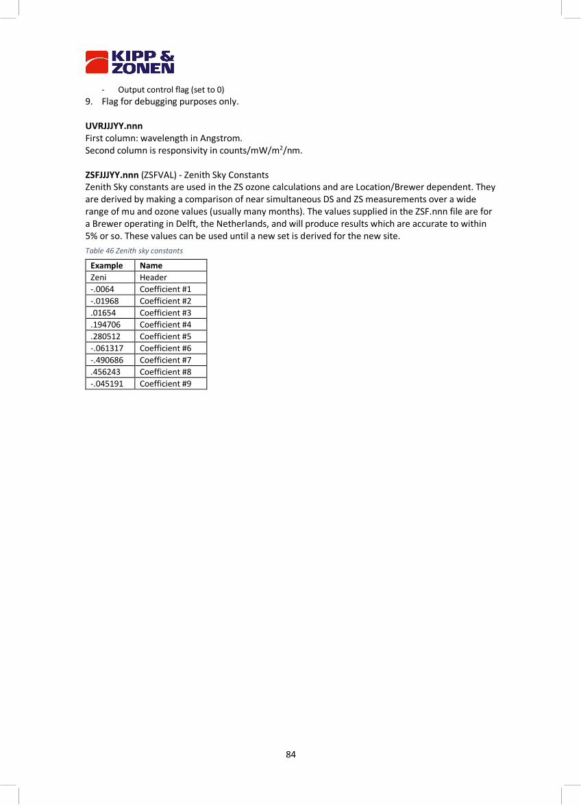
84

- Output control flag (set to 0) 9. Flag for debugging purposes only. UVRJJJYY.nnn First column: wavelength in Angstrom. Second column is responsivity in counts/mW/m2/nm. ZSFJJJYY.nnn (ZSFVAL) - Zenith Sky Constants Zenith Sky constants are used in the ZS ozone calculations and are Location/Brewer dependent. They are derived by making a comparison of near simultaneous DS and ZS measurements over a wide range of mu and ozone values (usually many months). The values supplied in the ZSF.nnn file are for a Brewer operating in Delft, the Netherlands, and will produce results which are accurate to within 5% or so. These values can be used until a new set is derived for the new site. Table 46 Zenith sky constants

Example Name Zeni Header -.0064 Coefficient #1 -.01968 Coefficient #2 .01654 Coefficient #3 .194706 Coefficient #4 .280512 Coefficient #5 -.061317 Coefficient #6 -.490686 Coefficient #7 .456243 Coefficient #8 -.045191 Coefficient #9

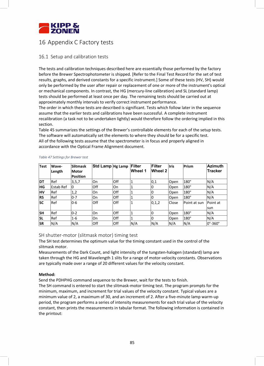
85

16 Appendix C Factory tests

Setup and calibration tests The tests and calibration techniques described here are essentially those performed by the factory before the Brewer Spectrophotometer is shipped. [Refer to the Final Test Record for the set of test results, graphs, and derived constants for a specific instrument.] Some of these tests (HV, SH) would only be performed by the user after repair or replacement of one or more of the instrument's optical or mechanical components. In contrast, the HG (mercury-line calibration) and SL (standard lamp) tests should be performed at least once per day. The remaining tests should be carried out at approximately monthly intervals to verify correct instrument performance. The order in which these tests are described is significant. Tests which follow later in the sequence assume that the earlier tests and calibrations have been successful. A complete instrument recalibration (a task not to be undertaken lightly) would therefore follow the ordering implied in this section. Table 45 summarizes the settings of the Brewer’s controllable elements for each of the setup tests. The software will automatically set the elements to where they should be for a specific test. All of the following tests assume that the spectrometer is in focus and properly aligned in accordance with the Optical Frame Alignment document. Table 47 Settings for Brewer test

Test Wave-Length

Slitmask Motor Position

Std Lamp Hg Lamp Filter Wheel 1

Filter Wheel 2

Iris Prism Azimuth Tracker

DT Ref 3,5,7 On Off 1 0,1 Open 180° N/A HG Estab Ref 0 Off On 1 0 Open 180° N/A HV Ref 1,2 On Off 1 0 Open 180° N/A RS Ref 0-7 On Off 1 0 Open 180° N/A SC Ref 0-6 Off Off 1 0,1,2 Close Point at sun Point at

sun SH Ref 0-2 On Off 1 0 Open 180° N/A SL Ref 1-6 On Off 1 0 Open 180° N/A SR N/A N/A Off Off N/A N/A N/A N/A 0°-360° SH shutter-motor (slitmask motor) timing test The SH test determines the optimum value for the timing constant used in the control of the slitmask motor. Measurements of the Dark Count, and light intensity of the tungsten-halogen (standard) lamp are taken through the HG and Wavelength 1 slits for a range of motor-velocity constants. Observations are typically made over a range of 20 different values for the velocity constant. Method: Send the PDHPHG command sequence to the Brewer, wait for the tests to finish. The SH command is entered to start the slitmask-motor timing test. The program prompts for the minimum, maximum, and increment for trial values of the velocity constant. Typical values are a minimum value of 2, a maximum of 30, and an increment of 2. After a five-minute lamp warm-up period, the program performs a series of intensity measurements for each trial value of the velocity constant, then prints the measurements in tabular format. The following information is contained in the printout:

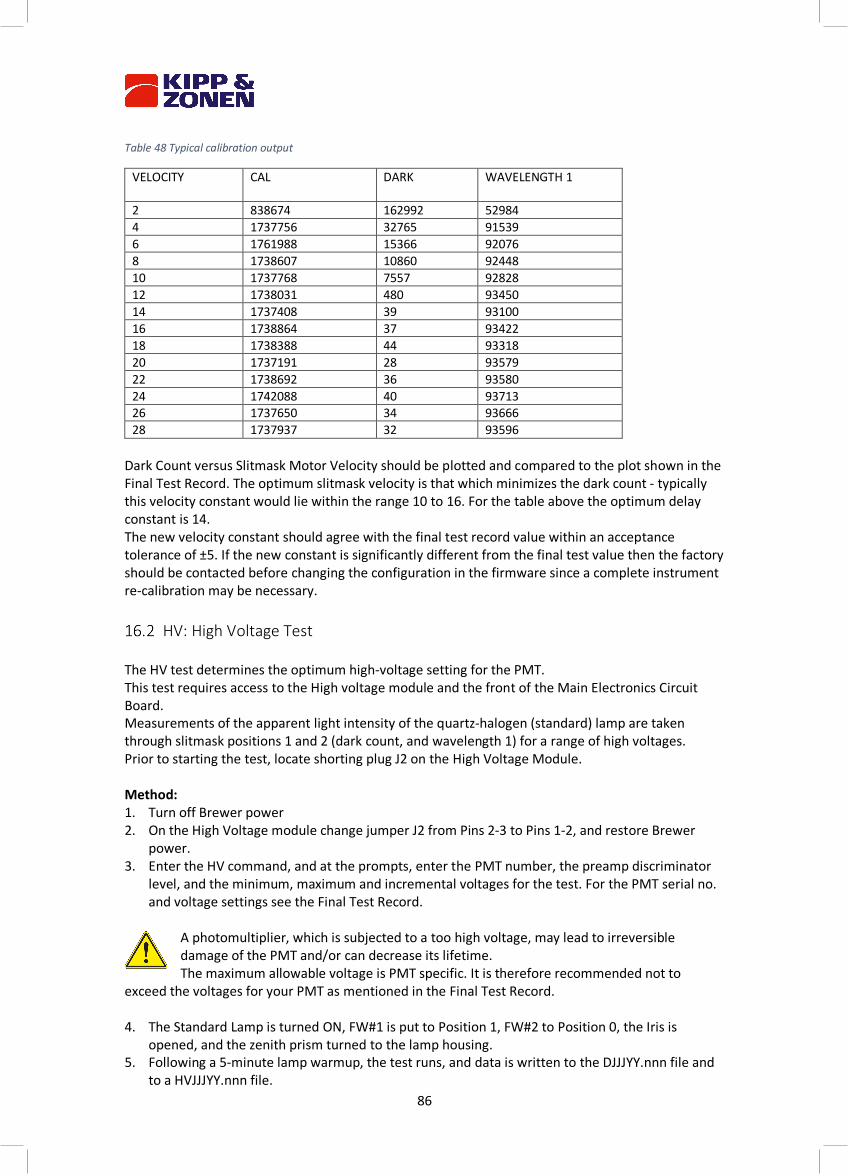
86

Table 48 Typical calibration output

VELOCITY CAL DARK WAVELENGTH 1

2 838674 162992 52984 4 1737756 32765 91539 6 1761988 15366 92076 8 1738607 10860 92448 10 1737768 7557 92828 12 1738031 480 93450 14 1737408 39 93100 16 1738864 37 93422 18 1738388 44 93318 20 1737191 28 93579 22 1738692 36 93580 24 1742088 40 93713 26 1737650 34 93666 28 1737937 32 93596

Dark Count versus Slitmask Motor Velocity should be plotted and compared to the plot shown in the Final Test Record. The optimum slitmask velocity is that which minimizes the dark count - typically this velocity constant would lie within the range 10 to 16. For the table above the optimum delay constant is 14. The new velocity constant should agree with the final test record value within an acceptance tolerance of ±5. If the new constant is significantly different from the final test value then the factory should be contacted before changing the configuration in the firmware since a complete instrument re-calibration may be necessary.

HV: High Voltage Test The HV test determines the optimum high-voltage setting for the PMT. This test requires access to the High voltage module and the front of the Main Electronics Circuit Board. Measurements of the apparent light intensity of the quartz-halogen (standard) lamp are taken through slitmask positions 1 and 2 (dark count, and wavelength 1) for a range of high voltages. Prior to starting the test, locate shorting plug J2 on the High Voltage Module. Method: 1. Turn off Brewer power 2. On the High Voltage module change jumper J2 from Pins 2-3 to Pins 1-2, and restore Brewer

power. 3. Enter the HV command, and at the prompts, enter the PMT number, the preamp discriminator

level, and the minimum, maximum and incremental voltages for the test. For the PMT serial no. and voltage settings see the Final Test Record.

A photomultiplier, which is subjected to a too high voltage, may lead to irreversible damage of the PMT and/or can decrease its lifetime. The maximum allowable voltage is PMT specific. It is therefore recommended not to

exceed the voltages for your PMT as mentioned in the Final Test Record. 4. The Standard Lamp is turned ON, FW#1 is put to Position 1, FW#2 to Position 0, the Iris is

opened, and the zenith prism turned to the lamp housing. 5. Following a 5-minute lamp warmup, the test runs, and data is written to the DJJJYY.nnn file and

to a HVJJJYY.nnn file.

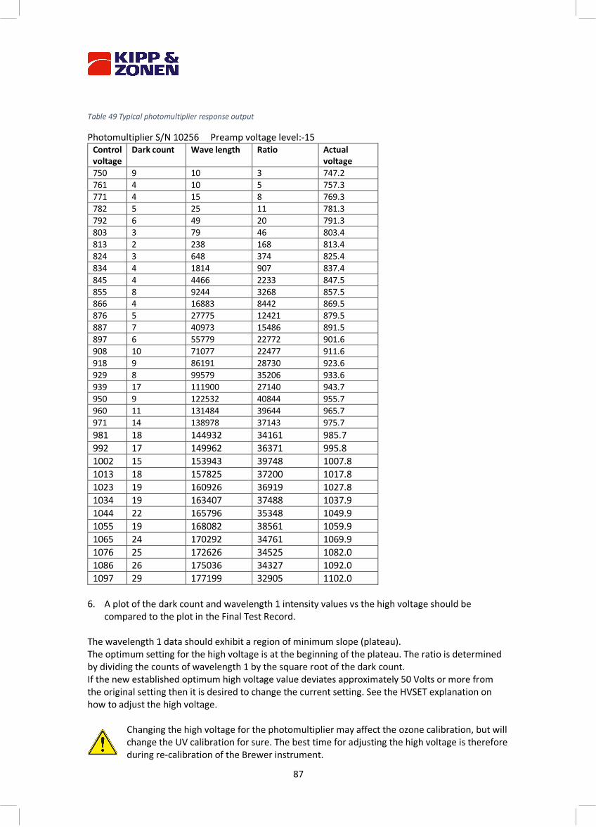
87

Table 49 Typical photomultiplier response output

Photomultiplier S/N 10256 Preamp voltage level:-15 Control voltage

Dark count Wave length Ratio Actual voltage

750 9 10 3 747.2 761 4 10 5 757.3 771 4 15 8 769.3 782 5 25 11 781.3 792 6 49 20 791.3 803 3 79 46 803.4 813 2 238 168 813.4 824 3 648 374 825.4 834 4 1814 907 837.4 845 4 4466 2233 847.5 855 8 9244 3268 857.5 866 4 16883 8442 869.5 876 5 27775 12421 879.5 887 7 40973 15486 891.5 897 6 55779 22772 901.6 908 10 71077 22477 911.6 918 9 86191 28730 923.6 929 8 99579 35206 933.6 939 17 111900 27140 943.7 950 9 122532 40844 955.7 960 11 131484 39644 965.7 971 14 138978 37143 975.7 981 18 144932 34161 985.7 992 17 149962 36371 995.8 1002 15 153943 39748 1007.8 1013 18 157825 37200 1017.8 1023 19 160926 36919 1027.8 1034 19 163407 37488 1037.9 1044 22 165796 35348 1049.9 1055 19 168082 38561 1059.9 1065 24 170292 34761 1069.9 1076 25 172626 34525 1082.0 1086 26 175036 34327 1092.0 1097 29 177199 32905 1102.0

6. A plot of the dark count and wavelength 1 intensity values vs the high voltage should be

compared to the plot in the Final Test Record. The wavelength 1 data should exhibit a region of minimum slope (plateau). The optimum setting for the high voltage is at the beginning of the plateau. The ratio is determined by dividing the counts of wavelength 1 by the square root of the dark count. If the new established optimum high voltage value deviates approximately 50 Volts or more from the original setting then it is desired to change the current setting. See the HVSET explanation on how to adjust the high voltage.

Changing the high voltage for the photomultiplier may affect the ozone calibration, but will change the UV calibration for sure. The best time for adjusting the high voltage is therefore during re-calibration of the Brewer instrument.

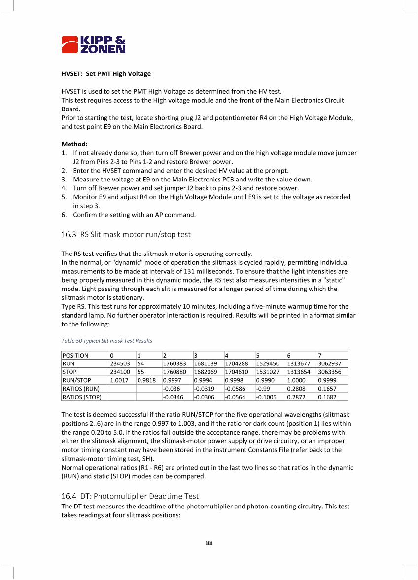
88

HVSET: Set PMT High Voltage HVSET is used to set the PMT High Voltage as determined from the HV test. This test requires access to the High voltage module and the front of the Main Electronics Circuit Board. Prior to starting the test, locate shorting plug J2 and potentiometer R4 on the High Voltage Module, and test point E9 on the Main Electronics Board. Method: 1. If not already done so, then turn off Brewer power and on the high voltage module move jumper

J2 from Pins 2-3 to Pins 1-2 and restore Brewer power. 2. Enter the HVSET command and enter the desired HV value at the prompt. 3. Measure the voltage at E9 on the Main Electronics PCB and write the value down. 4. Turn off Brewer power and set jumper J2 back to pins 2-3 and restore power. 5. Monitor E9 and adjust R4 on the High Voltage Module until E9 is set to the voltage as recorded

in step 3. 6. Confirm the setting with an AP command.

RS Slit mask motor run/stop test The RS test verifies that the slitmask motor is operating correctly. In the normal, or "dynamic" mode of operation the slitmask is cycled rapidly, permitting individual measurements to be made at intervals of 131 milliseconds. To ensure that the light intensities are being properly measured in this dynamic mode, the RS test also measures intensities in a "static" mode. Light passing through each slit is measured for a longer period of time during which the slitmask motor is stationary. Type RS. This test runs for approximately 10 minutes, including a five-minute warmup time for the standard lamp. No further operator interaction is required. Results will be printed in a format similar to the following: Table 50 Typical Slit mask Test Results

POSITION 0 1 2 3 4 5 6 7 RUN 234503 54 1760383 1681139 1704288 1529450 1313677 3062937 STOP 234100 55 1760880 1682069 1704610 1531027 1313654 3063356 RUN/STOP 1.0017 0.9818 0.9997 0.9994 0.9998 0.9990 1.0000 0.9999 RATIOS (RUN) -0.036 -0.0319 -0.0586 -0.99 0.2808 0.1657 RATIOS (STOP) -0.0346 -0.0306 -0.0564 -0.1005 0.2872 0.1682 The test is deemed successful if the ratio RUN/STOP for the five operational wavelengths (slitmask positions 2..6) are in the range 0.997 to 1.003, and if the ratio for dark count (position 1) lies within the range 0.20 to 5.0. If the ratios fall outside the acceptance range, there may be problems with either the slitmask alignment, the slitmask-motor power supply or drive circuitry, or an improper motor timing constant may have been stored in the instrument Constants File (refer back to the slitmask-motor timing test, SH). Normal operational ratios (R1 - R6) are printed out in the last two lines so that ratios in the dynamic (RUN) and static (STOP) modes can be compared.

DT: Photomultiplier Deadtime Test The DT test measures the deadtime of the photomultiplier and photon-counting circuitry. This test takes readings at four slitmask positions:

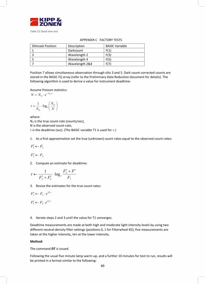
89

Table 51 Dead time test

Slitmask Position Description BASIC Variable 1 Darkcount F(1) 3 Wavelength 2 F(3) 5 Wavelength 4 F(5) 7 Wavelength 2&4 F(7)

Position 7 allows simultaneous observation through slits 3 and 5. Dark count-corrected counts are stored in the BASIC F() array (refer to the Preliminary Data Reduction document for details). The following algorithm is used to derive a value for instrument deadtime: Assume Poisson statistics:

where: No is the true count-rate (counts/sec), N is the observed count-rate, t is the deadtime (sec). (The BASIC variable T1 is used for t.) 1. As a first approximation set the true (unknown) count-rates equal to the observed count-rates:

2. Compute an estimate for deadtime:

3. Revise the estimates for the true count-rates:

4. Iterate steps 2 and 3 until the value for T1 converges.

Deadtime measurements are made at both high and moderate light intensity levels by using two different neutral-density filter settings (positions 0, 1 for Filterwheel #2); five measurements are taken at the higher intensity, ten at the lower intensity.

Method:

The command DT is issued.

Following the usual five minute lamp warm-up, and a further 10 minutes for test to run, results will be printed in a format similar to the following:

t×-×= 00

NeNN

÷ø

öçè

æ×=NN

N e0

0

log1t

33 FF ¢

55 FF ¢

7

3

53

log1FFF

FF e

¢+¢×¢+¢

¬t

tע׬¢ 333

FeFF

tע׬¢ 555

FeFF

APPENDIX C FACTORY TESTS

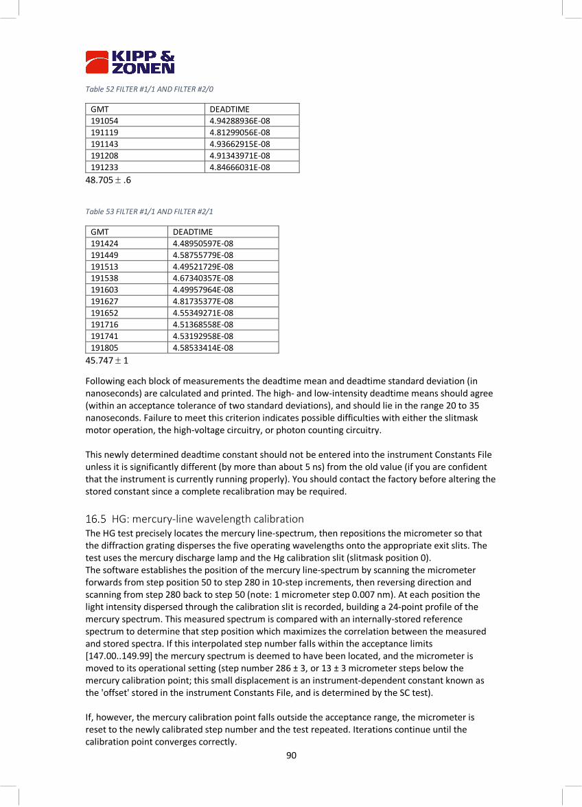
90

Table 52 FILTER #1/1 AND FILTER #2/0

GMT DEADTIME 191054 4.94288936E-08 191119 4.81299056E-08 191143 4.93662915E-08 191208 4.91343971E-08 191233 4.84666031E-08

48.705 ± .6

Table 53 FILTER #1/1 AND FILTER #2/1

GMT DEADTIME 191424 4.48950597E-08 191449 4.58755779E-08 191513 4.49521729E-08 191538 4.67340357E-08 191603 4.49957964E-08 191627 4.81735377E-08 191652 4.55349271E-08 191716 4.51368558E-08 191741 4.53192958E-08 191805 4.58533414E-08

45.747 ± 1

Following each block of measurements the deadtime mean and deadtime standard deviation (in nanoseconds) are calculated and printed. The high- and low-intensity deadtime means should agree (within an acceptance tolerance of two standard deviations), and should lie in the range 20 to 35 nanoseconds. Failure to meet this criterion indicates possible difficulties with either the slitmask motor operation, the high-voltage circuitry, or photon counting circuitry. This newly determined deadtime constant should not be entered into the instrument Constants File unless it is significantly different (by more than about 5 ns) from the old value (if you are confident that the instrument is currently running properly). You should contact the factory before altering the stored constant since a complete recalibration may be required.

HG: mercury-line wavelength calibration The HG test precisely locates the mercury line-spectrum, then repositions the micrometer so that the diffraction grating disperses the five operating wavelengths onto the appropriate exit slits. The test uses the mercury discharge lamp and the Hg calibration slit (slitmask position 0). The software establishes the position of the mercury line-spectrum by scanning the micrometer forwards from step position 50 to step 280 in 10-step increments, then reversing direction and scanning from step 280 back to step 50 (note: 1 micrometer step 0.007 nm). At each position the light intensity dispersed through the calibration slit is recorded, building a 24-point profile of the mercury spectrum. This measured spectrum is compared with an internally-stored reference spectrum to determine that step position which maximizes the correlation between the measured and stored spectra. If this interpolated step number falls within the acceptance limits [147.00..149.99] the mercury spectrum is deemed to have been located, and the micrometer is moved to its operational setting (step number 286 ± 3, or 13 ± 3 micrometer steps below the mercury calibration point; this small displacement is an instrument-dependent constant known as the 'offset' stored in the instrument Constants File, and is determined by the SC test). If, however, the mercury calibration point falls outside the acceptance range, the micrometer is reset to the newly calibrated step number and the test repeated. Iterations continue until the calibration point converges correctly.

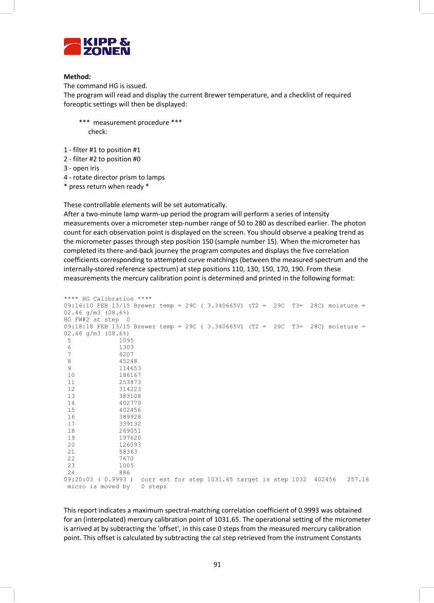
91

Method: The command HG is issued. The program will read and display the current Brewer temperature, and a checklist of required foreoptic settings will then be displayed: *** measurement procedure *** check: 1 - filter #1 to position #1 2 - filter #2 to position #0 3 - open iris 4 - rotate director prism to lamps * press return when ready * These controllable elements will be set automatically. After a two-minute lamp warm-up period the program will perform a series of intensity measurements over a micrometer step-number range of 50 to 280 as described earlier. The photon count for each observation point is displayed on the screen. You should observe a peaking trend as the micrometer passes through step position 150 (sample number 15). When the micrometer has completed its there-and-back journey the program computes and displays the five correlation coefficients corresponding to attempted curve matchings (between the measured spectrum and the internally-stored reference spectrum) at step positions 110, 130, 150, 170, 190. From these measurements the mercury calibration point is determined and printed in the following format:

**** HG Calibration **** 09:16:10 FEB 13/15 Brewer temp = 29C ( 3.340665V) (T2 = 29C T3= 28C) moisture = 02.46 g/m3 (08.6%) HG FW#2 at step 0 09:18:18 FEB 13/15 Brewer temp = 29C ( 3.340665V) (T2 = 29C T3= 28C) moisture = 02.46 g/m3 (08.6%) 5 1095 6 1303 7 4207 8 45248 9 114653 10 186167 11 253873 12 314223 13 383108 14 402770 15 402456 16 389928 17 339132 18 269051 19 197620 20 126093 21 58363 22 7670 23 1005 24 886 09:20:03 ( 0.9993 ) corr est for step 1031.65 target is step 1032 402456 257.16 micro is moved by 0 steps

This report indicates a maximum spectral-matching correlation coefficient of 0.9993 was obtained for an (interpolated) mercury calibration point of 1031.65. The operational setting of the micrometer is arrived at by subtracting the 'offset', in this case 0 steps from the measured mercury calibration point. This offset is calculated by subtracting the cal step retrieved from the instrument Constants

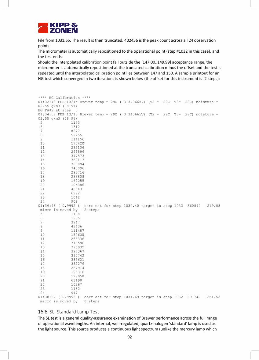
92

File from 1031.65. The result is then truncated. 402456 is the peak count across all 24 observation points. The micrometer is automatically repositioned to the operational point (step #1032 in this case), and the test ends. Should the interpolated calibration point fall outside the [147.00..149.99] acceptance range, the micrometer is automatically repositioned at the truncated calibration minus the offset and the test is repeated until the interpolated calibration point lies between 147 and 150. A sample printout for an HG test which converged in two iterations is shown below (the offset for this instrument is -2 steps):

**** HG Calibration **** 01:32:48 FEB 13/15 Brewer temp = 29C ( 3.340665V) (T2 = 29C T3= 28C) moisture = 02.55 g/m3 (08.9%) HG FW#2 at step 0 01:34:58 FEB 13/15 Brewer temp = 29C ( 3.340665V) (T2 = 29C T3= 28C) moisture = 02.55 g/m3 (08.9%) 5 1153 6 1312 7 8277 8 52255 9 114156 10 175420 11 232106 12 293896 13 347573 14 360113 15 360894 16 345096 17 293716 18 233808 19 169055 20 105386 21 46343 22 6292 23 1042 24 909 01:36:46 ( 0.9992 ) corr est for step 1030.40 target is step 1032 360894 219.08 micro is moved by -2 steps 5 1108 6 1295 7 3947 8 43636 9 111487 10 180635 11 253336 12 316596 13 376939 14 397367 15 397742 16 385621 17 332276 18 267914 19 196316 20 127958 21 63498 22 10267 23 1132 24 917 01:38:37 ( 0.9993 ) corr est for step 1031.69 target is step 1032 397742 251.52 micro is moved by 0 steps

SL: Standard Lamp Test The SL test is a general quality-assurance examination of Brewer performance across the full range of operational wavelengths. An internal, well-regulated, quartz-halogen 'standard' lamp is used as the light source. This source produces a continuous light spectrum (unlike the mercury lamp which

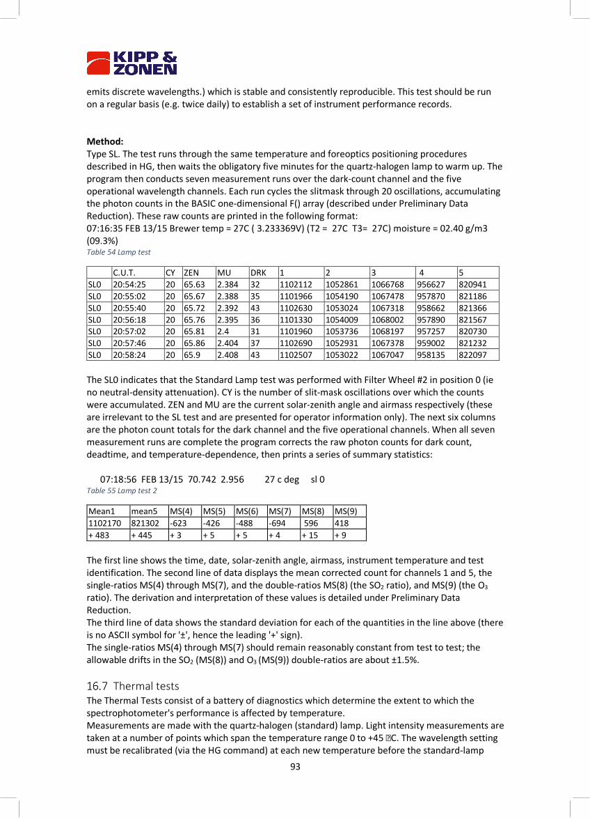
93

emits discrete wavelengths.) which is stable and consistently reproducible. This test should be run on a regular basis (e.g. twice daily) to establish a set of instrument performance records. Method: Type SL. The test runs through the same temperature and foreoptics positioning procedures described in HG, then waits the obligatory five minutes for the quartz-halogen lamp to warm up. The program then conducts seven measurement runs over the dark-count channel and the five operational wavelength channels. Each run cycles the slitmask through 20 oscillations, accumulating the photon counts in the BASIC one-dimensional F() array (described under Preliminary Data Reduction). These raw counts are printed in the following format: 07:16:35 FEB 13/15 Brewer temp = 27C ( 3.233369V) (T2 = 27C T3= 27C) moisture = 02.40 g/m3 (09.3%) Table 54 Lamp test

C.U.T. CY ZEN MU DRK 1 2 3 4 5 SL0 20:54:25 20 65.63 2.384 32 1102112 1052861 1066768 956627 820941 SL0 20:55:02 20 65.67 2.388 35 1101966 1054190 1067478 957870 821186 SL0 20:55:40 20 65.72 2.392 43 1102630 1053024 1067318 958662 821366 SL0 20:56:18 20 65.76 2.395 36 1101330 1054009 1068002 957890 821567 SL0 20:57:02 20 65.81 2.4 31 1101960 1053736 1068197 957257 820730 SL0 20:57:46 20 65.86 2.404 37 1102690 1052931 1067378 959002 821232 SL0 20:58:24 20 65.9 2.408 43 1102507 1053022 1067047 958135 822097 The SL0 indicates that the Standard Lamp test was performed with Filter Wheel #2 in position 0 (ie no neutral-density attenuation). CY is the number of slit-mask oscillations over which the counts were accumulated. ZEN and MU are the current solar-zenith angle and airmass respectively (these are irrelevant to the SL test and are presented for operator information only). The next six columns are the photon count totals for the dark channel and the five operational channels. When all seven measurement runs are complete the program corrects the raw photon counts for dark count, deadtime, and temperature-dependence, then prints a series of summary statistics: 07:18:56 FEB 13/15 70.742 2.956 27 c deg sl 0 Table 55 Lamp test 2

Mean1 mean5 MS(4) MS(5) MS(6) MS(7) MS(8) MS(9) 1102170 821302 -623 -426 -488 -694 596 418 + 483 + 445 + 3 + 5 + 5 + 4 + 15 + 9 The first line shows the time, date, solar-zenith angle, airmass, instrument temperature and test identification. The second line of data displays the mean corrected count for channels 1 and 5, the single-ratios MS(4) through MS(7), and the double-ratios MS(8) (the SO2 ratio), and MS(9) (the O3 ratio). The derivation and interpretation of these values is detailed under Preliminary Data Reduction. The third line of data shows the standard deviation for each of the quantities in the line above (there is no ASCII symbol for '±', hence the leading '+' sign). The single-ratios MS(4) through MS(7) should remain reasonably constant from test to test; the allowable drifts in the SO2 (MS(8)) and O3 (MS(9)) double-ratios are about ±1.5%.

Thermal tests The Thermal Tests consist of a battery of diagnostics which determine the extent to which the spectrophotometer's performance is affected by temperature. Measurements are made with the quartz-halogen (standard) lamp. Light intensity measurements are taken at a number of points which span the temperature range 0 to +45 �C. The wavelength setting must be recalibrated (via the HG command) at each new temperature before the standard-lamp

94

intensities are measured. These intensity data are analyzed to yield the absolute temperature coefficients for each of the five operational wavelengths; the negative of each coefficient is stored in the instrument Constants File for subsequent use during data reduction. During the course of the Thermal Tests all of the Brewer electromechanical subsystems should be thoroughly exercised, and any malfunction corrected. Method: The instrument is placed in a chamber where the ambient temperature is set to values between -5 and +35 °C. (These temperature settings cause the internal Brewer temperature monitor to register between approximately 0 and +45 °C.) The temperature is set at +20 °C and then gradually lowered to -5, raised up to 35, and back to 20, taking approximately 70 hours in total. A typical command sequence send to the Brewer during this test period is PDFR(HP)HGSLSLDTRSAPW2TE100. The HP command is left out for single monochromator brewers. After the Brewer has performed the above test sequence over the whole temperature range, the data is first analysed for operational failures and discrepancies. Special attention is given to the AP voltages, the average (**oavg) files and the HG wavelength calibration position right after the FR. Use the five F() values at all the Brewer temperature settings to determine the five temperature response coefficients in the following five equations:

Where F(i) are the scaled, corrected count rates for slit positions 2 to 6 F0(i) is F(i) at 0 °C TC(i) is the temperature response coeff. for the ith operational wavelength T is the Brewer temperature in °C. The values of F0(i) and TC(i) are determined by linearly regressing F(i) against T. By using the negative of the TC(i) coefficients (as described in Compensating for Temperature under Preliminary Data Reduction document) the wavelength-dependent temperature response of the instrument is compensated. Compare the TC(i) coefficients with those listed in the Final Test Manual. If the freshly determined values do not agree with those obtained at the factory you should consult Kipp & Zonen regarding the advisability of updating the instrument Constants File (CF command). Although the zero-Celsius values, F0(i), are not used by the Brewer software they should be recorded for future reference. Change of Photomultiplier Tube (PMT): Brewers with serial numbers up to #190 have photomultipliers manufactured by ET Enterprises Limited of the UK (previously known as Electron Tubes, Thorn-EMI and EMI). These PMTs are no longer available in a specification that meets the demands of the Brewer. Brewers with serial numbers #191 and higher are fitted with Hamamatsu photomultipliers. These have superior performance to the ET tubes, but there is s restriction on the maximum operating temperature. The Hamamatsu PMT’s have an ambient temperature operating range of 0° to +50° Celsius. When the temperature inside the instrument is higher than 50° Celsius too often, this could adversely affect the characteristics of the PMT. Preventive measures are to be taken when the instrument is located at a site where the temperature inside the Brewer exceeds the limit of 50° Celsius. A simple solution would be to make

6 to2 i T, * TC(i) (i)F F(i) 0 =+¬

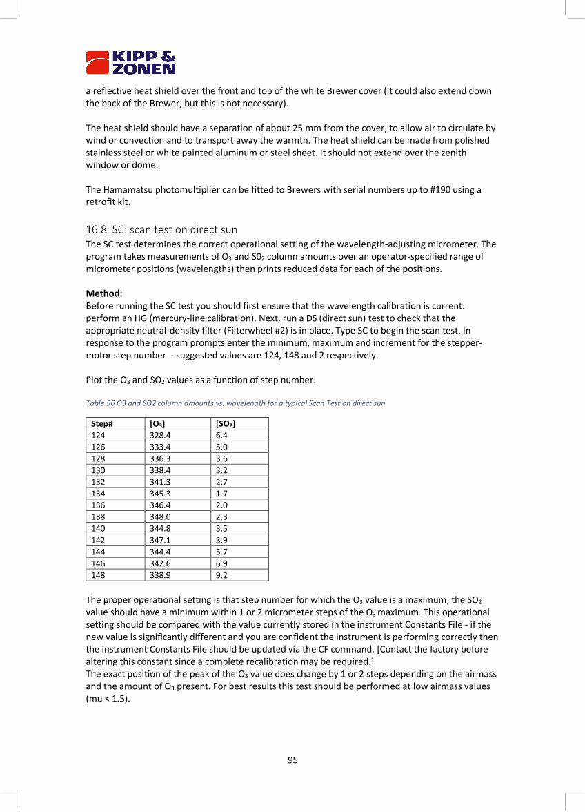
95

a reflective heat shield over the front and top of the white Brewer cover (it could also extend down the back of the Brewer, but this is not necessary). The heat shield should have a separation of about 25 mm from the cover, to allow air to circulate by wind or convection and to transport away the warmth. The heat shield can be made from polished stainless steel or white painted aluminum or steel sheet. It should not extend over the zenith window or dome. The Hamamatsu photomultiplier can be fitted to Brewers with serial numbers up to #190 using a retrofit kit.

SC: scan test on direct sun The SC test determines the correct operational setting of the wavelength-adjusting micrometer. The program takes measurements of O3 and S02 column amounts over an operator-specified range of micrometer positions (wavelengths) then prints reduced data for each of the positions. Method: Before running the SC test you should first ensure that the wavelength calibration is current: perform an HG (mercury-line calibration). Next, run a DS (direct sun) test to check that the appropriate neutral-density filter (Filterwheel #2) is in place. Type SC to begin the scan test. In response to the program prompts enter the minimum, maximum and increment for the stepper-motor step number - suggested values are 124, 148 and 2 respectively. Plot the O3 and SO2 values as a function of step number. Table 56 O3 and SO2 column amounts vs. wavelength for a typical Scan Test on direct sun

Step# [O3] [SO2] 124 328.4 6.4 126 333.4 5.0 128 336.3 3.6 130 338.4 3.2 132 341.3 2.7 134 345.3 1.7 136 346.4 2.0 138 348.0 2.3 140 344.8 3.5 142 347.1 3.9 144 344.4 5.7 146 342.6 6.9 148 338.9 9.2

The proper operational setting is that step number for which the O3 value is a maximum; the SO2 value should have a minimum within 1 or 2 micrometer steps of the O3 maximum. This operational setting should be compared with the value currently stored in the instrument Constants File - if the new value is significantly different and you are confident the instrument is performing correctly then the instrument Constants File should be updated via the CF command. [Contact the factory before altering this constant since a complete recalibration may be required.] The exact position of the peak of the O3 value does change by 1 or 2 steps depending on the airmass and the amount of O3 present. For best results this test should be performed at low airmass values (mu < 1.5).

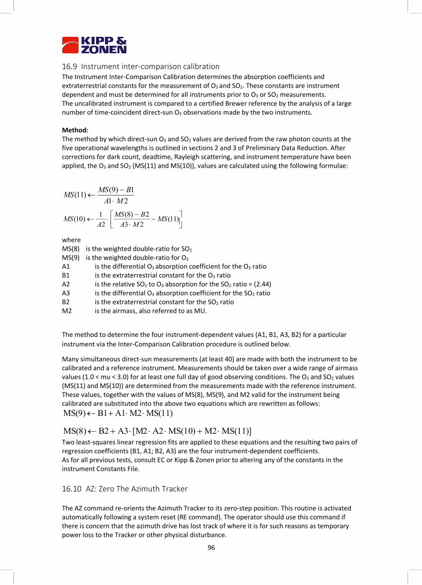
96

Instrument inter-comparison calibration The Instrument Inter-Comparison Calibration determines the absorption coefficients and extraterrestrial constants for the measurement of O3 and SO2. These constants are instrument dependent and must be determined for all instruments prior to O3 or SO2 measurements. The uncalibrated instrument is compared to a certified Brewer reference by the analysis of a large number of time-coincident direct-sun O3 observations made by the two instruments. Method: The method by which direct-sun O3 and SO2 values are derived from the raw photon counts at the five operational wavelengths is outlined in sections 2 and 3 of Preliminary Data Reduction. After corrections for dark count, deadtime, Rayleigh scattering, and instrument temperature have been applied, the O3 and SO2 (MS(11) and MS(10)), values are calculated using the following formulae:

where MS(8) is the weighted double-ratio for SO2 MS(9) is the weighted double-ratio for O3 A1 is the differential O3

absorption coefficient for the O3 ratio B1 is the extraterrestrial constant for the O3 ratio A2 is the relative SO2 to O3 absorption for the SO2 ratio = (2.44) A3 is the differential O3 absorption coefficient for the SO2 ratio B2 is the extraterrestrial constant for the SO2 ratio M2 is the airmass, also referred to as MU.

The method to determine the four instrument-dependent values (A1, B1, A3, B2) for a particular instrument via the Inter-Comparison Calibration procedure is outlined below.

Many simultaneous direct-sun measurements (at least 40) are made with both the instrument to be calibrated and a reference instrument. Measurements should be taken over a wide range of airmass values (1.0 < mu < 3.0) for at least one full day of good observing conditions. The O3 and SO2 values (MS(11) and MS(10)) are determined from the measurements made with the reference instrument. These values, together with the values of MS(8), MS(9), and M2 valid for the instrument being calibrated are substituted into the above two equations which are rewritten as follows:

Two least-squares linear regression fits are applied to these equations and the resulting two pairs of regression coefficients (B1, A1; B2, A3) are the four instrument-dependent coefficients. As for all previous tests, consult EC or Kipp & Zonen prior to altering any of the constants in the instrument Constants File.

AZ: Zero The Azimuth Tracker The AZ command re-orients the Azimuth Tracker to its zero-step position. This routine is activated automatically following a system reset (RE command). The operator should use this command if there is concern that the azimuth drive has lost track of where it is for such reasons as temporary power loss to the Tracker or other physical disturbance.

211)9()11(

MABMSMS

×-

¬

úûù

êëé -

×-

׬ )11(232)8(

21)10( MS

MABMS

AMS

MS(11) M2A1B1 MS(9) ××+¬

MS(11)] M2 MS(10) A2 [M2 A3B2 MS(8) ×+×××+¬

97

Note that the AZ routine can only be accessed if the instrument configuration (IC) is setup to include an Azimuth Tracker System. Method: Type AZ. The following screen display appears while the program steps the azimuth drive towards its internal optically-sensed reference flange: *** zeroing azimuth press Del to abort The operator can abort the operation by pressing the DEL (delete) key; the program will return to the previously displayed menu. When the program has located the reference flange it compares the predicted and actual flange positions, then displays the step discrepancy on the screen for about 5 seconds: *** discrepancy = n AZIMUTH ZEROED AT HH:MM:SS DISCREPANCY = N N will usually be a small integer lying in the range -10 < n < 10. (The Tracker stepper-motor gearing is approximately 15000 steps per revolution, so a discrepancy of 10 steps corresponds to a positional error of 0.2°). N will be much larger if the Brewer has recently been reset or if the Tracker has been physically perturbed (e.g. power interruption). The Azimuth Tracker then returns to the solar azimuth and the previously active menu is displayed.

SR: Azimuth Tracker Steps-Per-Revolution Calibration The SR test determines the number of steps required for the azimuth drive motor to turn the Brewer through 360° in azimuth. This test establishes the steps-per-revolution constant which is used by the Brewer program to orient the Brewer in azimuth to within ±1 minute of arc. An opto-sensor located inside the Azimuth Tracker detects a reference flange on the stationary drive-wheel. The azimuth drive motor is 'zeroed' on this reference, then stepped forward until the flange is again detected on the next revolution. At this point the tracker has rotated exactly 360°, and the steps-per-revolution constant has been determined. The SR routine can only be accessed if the instrument configuration (IC command) has been setup to include an Azimuth Tracker. Method: Type SR to initiate the steps-per-revolution test. The first portion of the calibration proceeds exactly as for AZ. Once the internal optically-sensed reference flange has been detected, the azimuth step-count is set to zero and the drive motor is stepped forward until the flange is again detected after 360° of rotation. During the forward search the following screen message is displayed: *** finding az steps/rev press del to abort

98

It takes approximately 30 seconds to rotate through 360°. (The operator may abort the steps-per-revolution calibration at any time by pressing the DEL key.) Calibration results are displayed as follows: steps/rev measured at 14675 old value = 14678 do you want new value saved? - y/n Enter 'y' if you want to update the calibration value; type 'n' if you feel the test was unsatisfactory for any reason or if the value hasn't changed. A timestamped calibration record will be printed: AZ STEPS/REV = 14675 AT HH:MM:SS The Azimuth Tracker then returns to the solar azimuth and the previously displayed menu will appear.

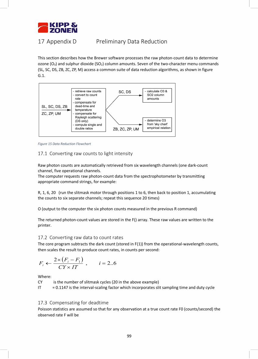
99

17 Appendix D Preliminary Data Reduction

This section describes how the Brewer software processes the raw photon-count data to determine ozone (O3) and sulphur dioxide (SO2) column amounts. Seven of the two-character menu commands (SL, SC, DS, ZB, ZC, ZP, M) access a common suite of data reduction algorithms, as shown in figure G.1.

Figure 15 Data Reduction Flowchart

Converting raw counts to light intensity Raw photon counts are automatically retrieved from six wavelength channels (one dark-count channel, five operational channels. The computer requests raw photon-count data from the spectrophotometer by transmitting appropriate command strings, for example: R, 1, 6, 20 (run the slitmask motor through positions 1 to 6, then back to position 1, accumulating the counts to six separate channels; repeat this sequence 20 times) O (output to the computer the six photon counts measured in the previous R command) The returned photon-count values are stored in the F() array. These raw values are written to the printer.

Converting raw data to count rates The core program subtracts the dark count (stored in F(1)) from the operational-wavelength counts, then scales the result to produce count rates, in counts per second:

Where: CY is the number of slitmask cycles (20 in the above example) IT = 0.1147 is the interval-scaling factor which incorporates slit sampling time and duty cycle

Compensating for deadtime Poisson statistics are assumed so that for any observation at a true count rate F0 (counts/second) the observed rate F will be

( )6..2,

2 1 =´-´

¬ iITCYFF

F ii

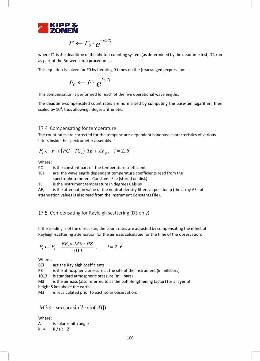
100

where T1 is the deadtime of the photon-counting system (as determined by the deadtime test, DT, run as part of the Brewer setup procedures).

This equation is solved for F0 by iterating 9 times on the (rearranged) expression:

This compensation is performed for each of the five operational wavelengths.

The deadtime-compensated count rates are normalized by computing the base-ten logarithm, then scaled by 104, thus allowing integer arithmetic.

Compensating for temperature The count rates are corrected for the temperature-dependent bandpass characteristics of various filters inside the spectrometer assembly:

Where: PC is the constant part of the temperature coefficient TCi are the wavelength-dependent temperature coefficients read from the spectrophotometer's Constants File (stored on disk) TE is the instrument temperature in degrees Celsius AFp is the attenuation value of the neutral-density filters at position p (the array AF of attenuation values is also read from the instrument Constants File).

Compensating for Rayleigh scattering (DS only)

If the reading is of the direct sun, the count rates are adjusted by compensating the effect of Rayleigh-scattering attenuation for the airmass calculated for the time of the observation:

Where: BEI are the Rayleigh coefficients. PZ is the atmospheric pressure at the site of the instrument (in millibars) 1013 is standard atmospheric pressure (millibars) M3 is the airmass (also referred to as the path-lengthening factor) for a layer of height 5 km above the earth. M3 is recalculated prior to each solar observation:

Where: A is solar zenith angle k = R / (R + Z)

e TFFF 10

0×-׬

e TFFF 10

0×׬

( ) 6..2, =+×++¬ iAFTETCPCFF piii

6..2,10133

=´´

+¬ iPZMBEFF iii

)])sin([sec(arcsin3 AkM ׬

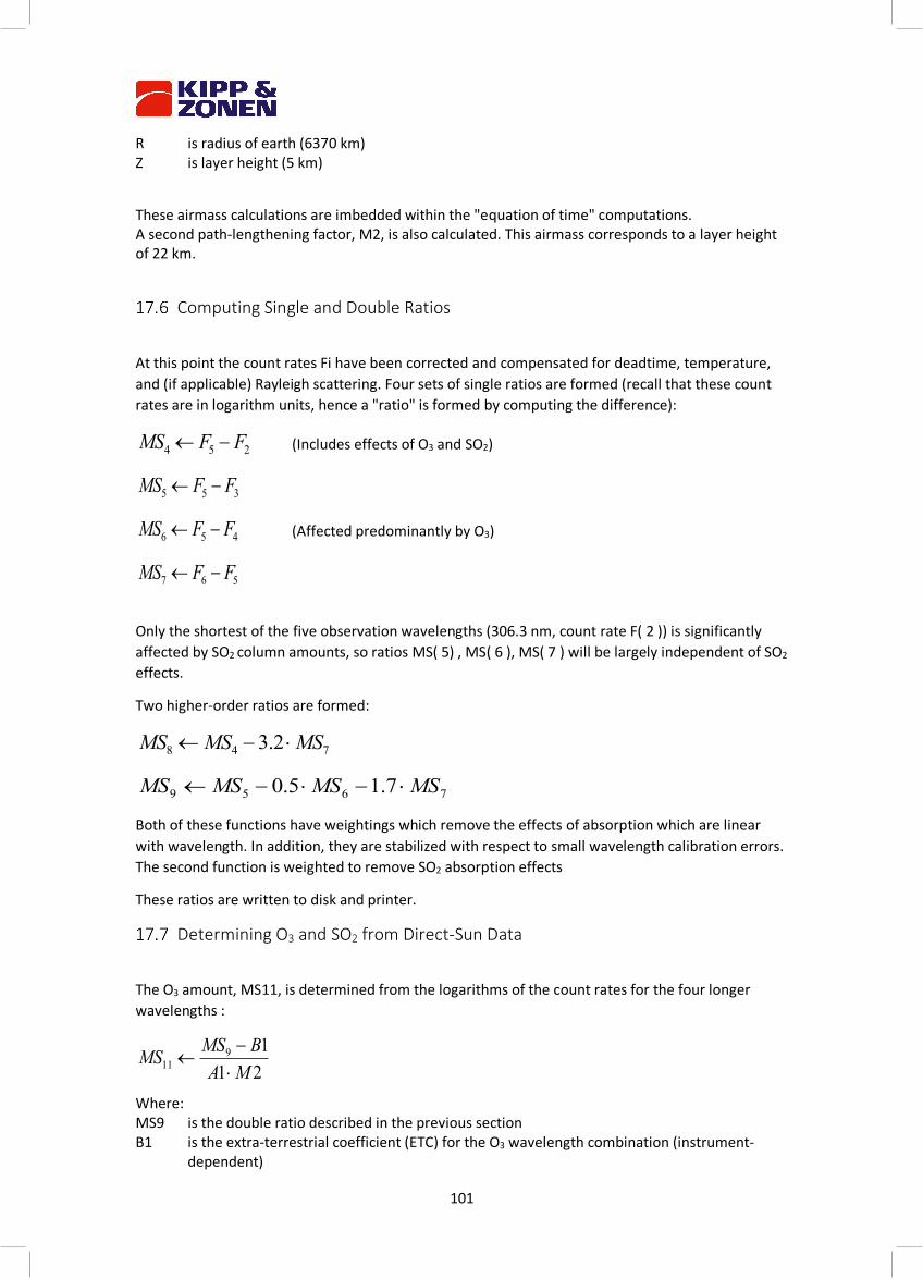
101

R is radius of earth (6370 km) Z is layer height (5 km)

These airmass calculations are imbedded within the "equation of time" computations. A second path-lengthening factor, M2, is also calculated. This airmass corresponds to a layer height of 22 km.

Computing Single and Double Ratios

At this point the count rates Fi have been corrected and compensated for deadtime, temperature, and (if applicable) Rayleigh scattering. Four sets of single ratios are formed (recall that these count rates are in logarithm units, hence a "ratio" is formed by computing the difference):

(Includes effects of O3 and SO2)

(Affected predominantly by O3)

Only the shortest of the five observation wavelengths (306.3 nm, count rate F( 2 )) is significantly affected by SO2 column amounts, so ratios MS( 5) , MS( 6 ), MS( 7 ) will be largely independent of SO2 effects.

Two higher-order ratios are formed:

Both of these functions have weightings which remove the effects of absorption which are linear with wavelength. In addition, they are stabilized with respect to small wavelength calibration errors. The second function is weighted to remove SO2 absorption effects

These ratios are written to disk and printer.

Determining O3 and SO2 from Direct-Sun Data

The O3 amount, MS11, is determined from the logarithms of the count rates for the four longer wavelengths :

Where: MS9 is the double ratio described in the previous section B1 is the extra-terrestrial coefficient (ETC) for the O3 wavelength combination (instrument-

dependent)

254 FFMS -¬

355 FFMS -¬

456 FFMS -¬

567 FFMS -¬

748 2.3 MSMSMS ×-¬

7659 7.15.0 MSMSMSMS ×-×-¬

2119

11 MABMSMS

×-

¬

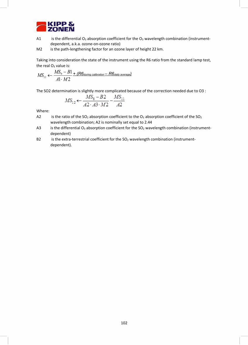
102

A1 is the differential O3 absorption coefficient for the O3 wavelength combination (instrument-dependent, a.k.a. ozone-on-ozone ratio)

M2 is the path-lengthening factor for an ozone layer of height 22 km. Taking into consideration the state of the instrument using the R6 ratio from the standard lamp test, the real O3 value is:

The SO2 determination is slightly more complicated because of the correction needed due to O3 :

Where: A2 is the ratio of the SO2 absorption coefficient to the O3 absorption coefficient of the SO2

wavelength combination; A2 is nominally set equal to 2.44 A3 is the differential O3 absorption coefficient for the SO2 wavelength combination (instrument-

dependent) B2 is the extra-terrestrial coefficient for the SO2 wavelength combination (instrument-

dependent).

2119

11 MABMSMS

×-

¬ + (R6during calibration – R6daily average)

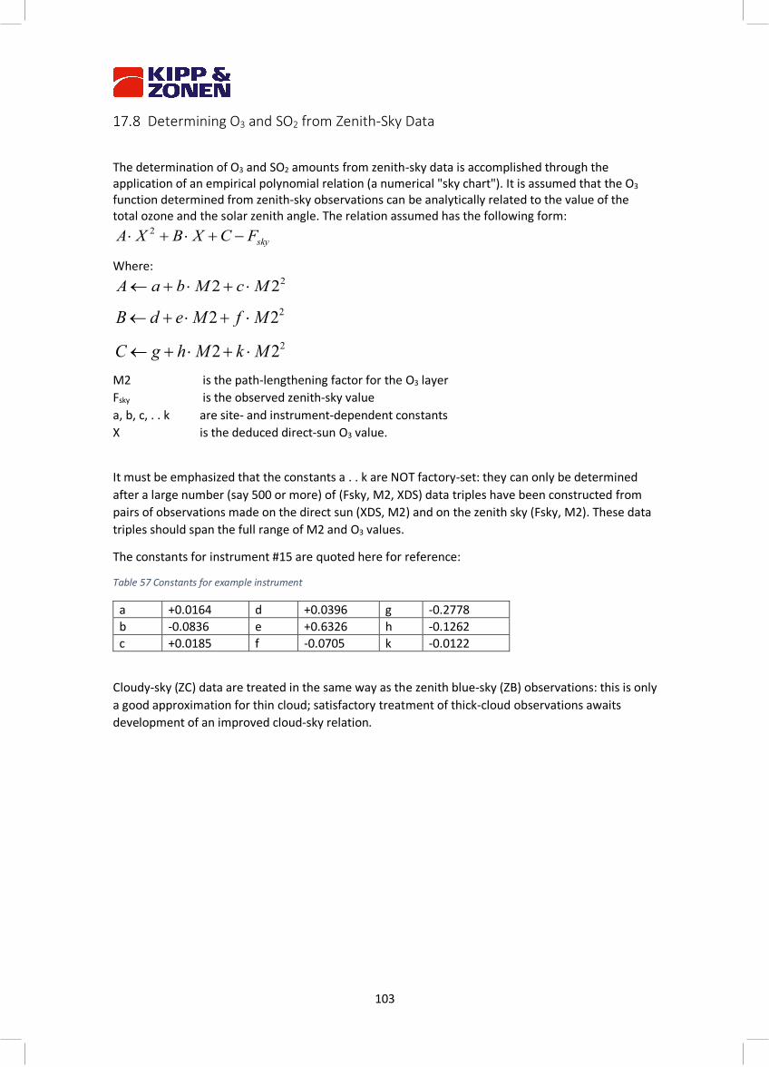
103

Determining O3 and SO2 from Zenith-Sky Data

The determination of O3 and SO2 amounts from zenith-sky data is accomplished through the application of an empirical polynomial relation (a numerical "sky chart"). It is assumed that the O3 function determined from zenith-sky observations can be analytically related to the value of the total ozone and the solar zenith angle. The relation assumed has the following form:

Where:

M2 is the path-lengthening factor for the O3 layer Fsky is the observed zenith-sky value a, b, c, . . k are site- and instrument-dependent constants X is the deduced direct-sun O3 value.

It must be emphasized that the constants a . . k are NOT factory-set: they can only be determined after a large number (say 500 or more) of (Fsky, M2, XDS) data triples have been constructed from pairs of observations made on the direct sun (XDS, M2) and on the zenith sky (Fsky, M2). These data triples should span the full range of M2 and O3 values.

The constants for instrument #15 are quoted here for reference:

Table 57 Constants for example instrument

a +0.0164 d +0.0396 g -0.2778 b -0.0836 e +0.6326 h -0.1262 c +0.0185 f -0.0705 k -0.0122

Cloudy-sky (ZC) data are treated in the same way as the zenith blue-sky (ZB) observations: this is only a good approximation for thin cloud; satisfactory treatment of thick-cloud observations awaits development of an improved cloud-sky relation.

skyFCXBXA -+×+× 2

222 McMbaA ×+×+¬222 MfMedB ×+×+¬222 MkMhgC ×+×+¬

104

18 Appendix E Computer / Brewer Interface (Teletype) The TT command gives an operator direct control of various Brewer functions by allowing low level commands to be sent directly from the Computer keyboard. With this feature, most useful as a troubleshooting tool, all motors can be moved, lamps turned on, and data sampled. This command is useful only when the Brewer and Computer are communicating, and is sent from the Main Menu with the command, TT. A copy of all transactions can be preserved if the print to disk has previously been turned on with the PD command, and a printout is requested after launching TelyType command. Command Level A command string consists of zero or more commands separated by semicolons, optionally followed by the A "command", and sent with ‘Enter’. Examples of TT commands: B,2 - turn on the Quartz Halogen Lamp M,1,0 - move the Zenith Prism to the 0 (Lamps) position R,0,7,10;O;A - run the shutter from position 0 to 7 a total of 10 times, - output the resulting counts, and - repeat until interrupted by ‘HOME’ When executing a command string, the Brewer executes each command set in turn. Commands within a command set are executed concurrently. The command set is assumed to have ended when the first command in the set has ended, even if other commands in the set are still executing. Any commands which generate output transmit that output in accordance to the rules of the low level protocol in effect. Command strings terminating in the A "command" get repeated indefinitely. In the case of the computer interface low level protocol, an ESC command is required to terminate execution; in the case of the TTY low level protocol a break must be sent. The following sections identify the various commands. Commands with single character opcodes constitute the commands supported by the COSMAC based Brewers. They are augmented by a number of commands supported only by later versions of the Brewer. These newer commands have multicharacter opcodes and provide functions specific to newer electronics or provide more natural commands for functions supported by the COSMAC based Brewers. A number of the commands listed below are used only for diagnostics and are not nornally used in day to day operations, but are included for completeness. The commnds in more common use are marked by **. Turn the the mercury lamp and/or the standard lamp on or off. This command requires configuration variables.

1. ** B Syntax B, <mask>

Parameters

The parameter <mask> takes one of four values or an error is logged: <mask> standard lamp

state Mercury lamp state

0 off Off 1 off On 2 on Off 3 on On

105

*Note: if the configuration variable USE.B3.FOR.LAMPS is set to YES then the lamps are both turned on with B,3. If the configuration variable is set to NO then the state of the lamps are not altered and the command is essentially ignored.

Example

B,2 Turn the standard lamp on and the mercury lamp off, update lamp state variables in the background.

2. F

Define the fill characters to be used at the start of every transmission from the Brewer to the controller when using the TTY interface low level protocol.

Syntax F,<count>,<ASCII code> Parameters

parameter range Meaning <ASCII code> 0 to 255 the character to be used as a fill character <count> 0 to 255 the number of fill characters to use for each output

message Example F, 1, 7

Transmit a single BEL character at start of each output message.

3. HVADJUST Adjusts the High Voltage power supply. This command requires configuration variables.

Syntax HVADJUST <delta> Parameters

Parameter / response Format Meaning <delta> -128 to 127 steps to adjust the supply

Use of this command resets the NVRAM variable which keeps track of the latest measurement of the HV supply voltage. The watermarks are also centered around the new HV supply setting; note that this is different in operation from other watermarks.

4. ** I Initializes the specified motor to its 'zero' position and set the corresponding step-count accumulator to 0; moves the motor to its default position. This command requires configuration variables. If the slow and maximum velocities specified for a motor are equal, then the motor reset routine is abbreviated, i.e., the movement does not include moving off the sensor and searching for it at a different speed than the maximum. I commands do not work concurrently (although on reset all motors initialize at once).

Syntax I,<m>

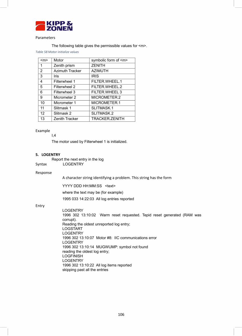
106

Parameters

The following table gives the permissible values for <m>. Table 58 Motor initialize values

<m> Motor symbolic form of <m> 1 Zenith prism ZENITH 2 Azimuth Tracker AZIMUTH 3 Iris IRIS 4 Filterwheel 1 FILTER.WHEEL.1 5 Filterwheel 2 FILTER.WHEEL.2 6 Filterwheel 3 FILTER.WHEEL 3 9 Micrometer 2 MICROMETER.2 10 Micrometer 1 MICROMETER.1 11 Slitmask 1 SLITMASK.1 12 Slitmask 2 SLITMASK.2 13 Zenith Tracker TRACKER.ZENITH

Example I,4 The motor used by Filterwheel 1 is initialized.

5. LOGENTRY Report the next entry in the log

Syntax LOGENTRY

Response A character string identifying a problem. This string has the form

YYYY DDD HH:MM:SS <text> where the text may be (for example) 1995 033 14:22:03 All log entries reported

Entry LOGENTRY 1996 302 13:10:02 Warm reset requested. Tepid reset generated (RAM was corrupt). Reading the oldest unreported log entry; LOGSTART LOGENTRY 1996 302 13:10:07 Motor #8: IIC communications error LOGENTRY 1996 302 13:10:14 MUGWUMP: symbol not found reading the oldest log entry; LOGFINISH LOGENTRY 1996 302 13:10:22 All log items reported skipping past all the entries

107

6. LOGFINISH Resets the log to act as though the newest entry in the log has already been reported.

Syntax LOGFINISH

Example see LOGENTRY

7. LOGSTART Resets the log iterator to the oldest entry in the log.

Syntax LOGSTART Example

see LOGENTRY

8. ** M Move the specified motor to the specified position. If the motor hits a limit sensor during its movement, then the motor is reset to its initial position and the requested motor position is again moved to. This command requires configuration variables. See the 10.31.7 for examples

Syntax M,<m>,<s>

Parameters

The <m> identifies the motor to move. See the section on the I command for possible values. The <s> defines the motion required. If <s> is positive the motor moves to the given position. If <s> is negative, the motor moves |<s>| steps backward and resets the 'zero' position of the motor to be this new position.

Example

M, 4, 256 Moves the translucent ground quartz diffuser on filterwheel 1 into the optical path.

9. ** O Transmit to the controller all photon count data accumulated by the most recent R command, then zero the photon count accumulators. This command requires configuration variables.

Syntax O Response

<c0>,<c1>,<c2>,...,<cn> Each count number returned is in the form of a decimal value using ASCII characters. Each number occupies exactly nine characters and the value is right-justified and padded with spaces. The last value in the list does not have a comma or space but a carriage return as expected.

Parameters

The <ci> are photon counts in the range 0 to 16777215, one for each slitmask position measured in the most recent R command.

Example

See section on the R command.

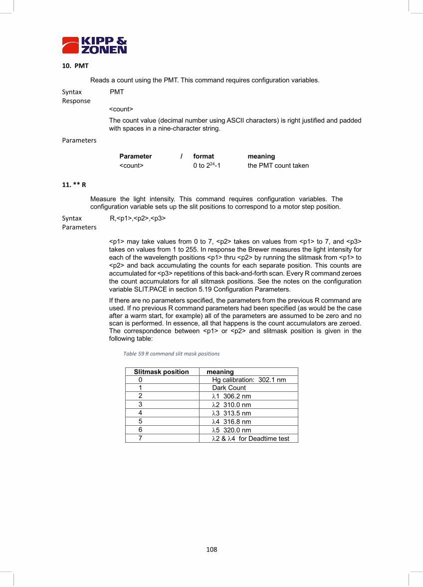
108

10. PMT

Reads a count using the PMT. This command requires configuration variables.

Syntax PMT Response

<count> The count value (decimal number using ASCII characters) is right justified and padded with spaces in a nine-character string.

Parameters

Parameter / response

format meaning <count> 0 to 224-1 the PMT count taken

11. ** R

Measure the light intensity. This command requires configuration variables. The configuration variable sets up the slit positions to correspond to a motor step position.

Syntax R,<p1>,<p2>,<p3> Parameters

<p1> may take values from 0 to 7, <p2> takes on values from <p1> to 7, and <p3> takes on values from 1 to 255. In response the Brewer measures the light intensity for each of the wavelength positions <p1> thru <p2> by running the slitmask from <p1> to <p2> and back accumulating the counts for each separate position. This counts are accumulated for <p3> repetitions of this back-and-forth scan. Every R command zeroes the count accumulators for all slitmask positions. See the notes on the configuration variable SLIT.PACE in section 5.19 Configuration Parameters. If there are no parameters specified, the parameters from the previous R command are used. If no previous R command parameters had been specified (as would be the case after a warm start, for example) all of the parameters are assumed to be zero and no scan is performed. In essence, all that happens is the count accumulators are zeroed. The correspondence between <p1> or <p2> and slitmask position is given in the following table:

Table 59 R command slit mask positions

Slitmask position meaning

0 Hg calibration: 302.1 nm 1 Dark Count 2 l1 306.2 nm 3 l2 310.0 nm 4 l3 313.5 nm 5 l4 316.8 nm 6 l5 320.0 nm 7 l2 & l4 for Deadtime test

109

Example

R; O 0 If the above had been called before any other R command then a single zero is returned indicating that there were no scans taken. R,2,4,4;O[sent to Brewer] 5638, 4996, 54886[returned by Brewer] Sample and accumulate the light intensities for slitmask positions 2, 3,4,4,3 and 2. Repeat this sequence 4 times. In this example the O command is used to display example results. The returned counts correspond to slitmask positions 2, 3 and 4 respectively. R; O[sent to Brewer] 5549, 4989, 54880[returned by Brewer] In the above, the R parameters had already been specified as 2, 4, 4. The new values returned correspond to a new run of the R command as specified.

12. S Report the status of the most recent run command. This command requires configuration variables.

Syntax S Response

<p1>,<p2>,<count>,<p3>,0,<interrupted>, Each number returned in the above string is in the form of a decimal value using ASCII characters. Each number occupies exactly four characters and the value is right-justified and padded with spaces. The last value in the list always has a comma. The number of parameters returned is limited only by the string length.

Parameters

The <pi> are the corresponding parameter from the most recent R command. The remaining parameters are given in the following table.

Response field format Meaning <count> 0..<p3> Number of cycles completed <interrupted> Boolean on if the Run command was interrupted (by a break)

Example S 2, 4, 2, 4, 0, 1, Reports that the R command was R,2,4,4 and was interrupted during the third scan.

13. SAVE Stores the current set of RAM configuration parameters in Flash memory.

Syntax SAVE

110

Response

<retCode>

Parameters. Response format Meaning <retCode> 0 - 127 number of sets of configuration parameters for which there was

room when the operation started. 0 means that no room was left and parameters are not stored

14. STEPS

Determines the number of steps in a complete revolution of the azimuth tracker. This command should always be immediately preceded by an I,2 command and followed by a ?STEPS query. This command requires configuration variables.

Syntax STEPS

Example I.2 Ensures that the motor or tracker position is accurately known. STEPS Moves the motor or tracker exactly one revolution and records the number of steps required. ?STEPS 17979 Reports that the most recent STEPS command discovered 17979 steps in a revolution.

15. T Retransmit the output from the most recent non-null response.

Syntax T

Response

Depends on which of the commands was most recent.

Parameters

The <pi> identify parameters being set, the <vi> give the values to which they are being set. The following table gives the permissible values for <pi> and the corresponding meaning for the <vi>.

Example T[sent to Brewer]

1996 302 13:10:22 All log items reported[returned by Brewer] The previous command string (which in this case was a call to determine the lamp state) was returned.

16. USECONFIG

Restarts software using the configuration in RAM.

Syntax USECONFIG

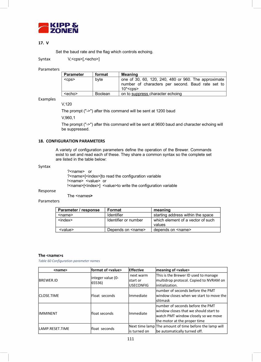
111

17. V

Set the baud rate and the flag which controls echoing.

Syntax V,<cps>[,<echo>] Parameters

Parameter format Meaning <cps> byte one of 30, 60, 120, 240, 480 or 960. The approximate

number of characters per second. Baud rate set to 10*<cps>

<echo> Boolean on to suppress character echoing Examples

V,120 The prompt ("->") after this command will be sent at 1200 baud V,960,1 The prompt ("->") after this command will be sent at 9600 baud and character echoing will be suppressed.

18. CONFIGURATION PARAMETERS

A variety of configuration parameters define the operation of the Brewer. Commands exist to set and read each of these. They share a common syntax so the complete set are listed in the table below:

Syntax ?<name> or ?<name>[<index>]to read the configuration variable !<name> <value> or !<name>[<index>] <value>to write the configuration variable

Response The <names>

Parameters

Parameter / response Format meaning <name> Identifier starting address within the space <index> Identifier or number which element of a vector of such

values <value> Depends on <name> depends on <name>

The <name>s Table 60 Configuration parameter names

<name> format of <value> Effective meaning of <value>

BREWER.ID integer value (0-65536)

next warm start or USECONFIG

This is the Brewer ID used to manage multidrop protocol. Copied to NVRAM on initialization.

CLOSE.TIME Float seconds Immediate number of seconds before the PMT window closes when we start to move the slitmask

IMMINENT float seconds Immediate

number of seconds before the PMT window closes that we should start to watch PMT window closely so we move the motor at the proper time

LAMP.RESET.TIME float seconds Next time lamp is turned on

The amount of time before the lamp will be automatically turned off.

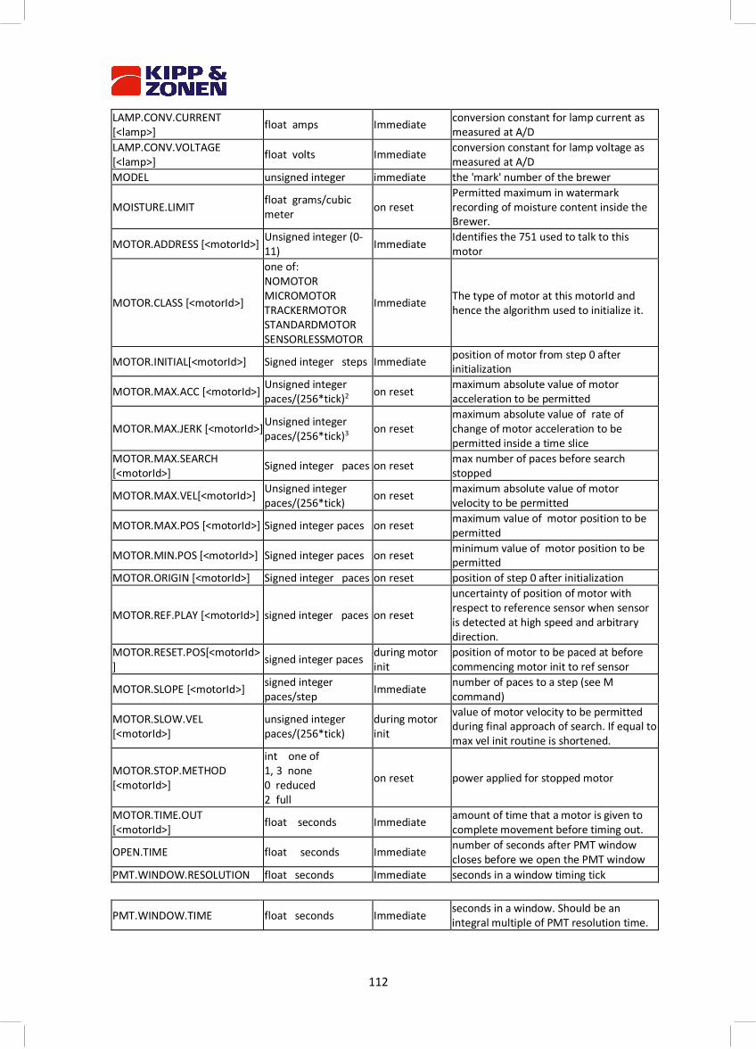
112

LAMP.CONV.CURRENT [<lamp>] float amps Immediate conversion constant for lamp current as

measured at A/D LAMP.CONV.VOLTAGE [<lamp>] float volts Immediate conversion constant for lamp voltage as

measured at A/D MODEL unsigned integer immediate the 'mark' number of the brewer

MOISTURE.LIMIT float grams/cubic meter on reset

Permitted maximum in watermark recording of moisture content inside the Brewer.

MOTOR.ADDRESS [<motorId>] Unsigned integer (0-11) Immediate Identifies the 751 used to talk to this

motor

MOTOR.CLASS [<motorId>]

one of: NOMOTOR MICROMOTOR TRACKERMOTOR STANDARDMOTOR SENSORLESSMOTOR

Immediate The type of motor at this motorId and hence the algorithm used to initialize it.

MOTOR.INITIAL[<motorId>] Signed integer steps Immediate position of motor from step 0 after initialization

MOTOR.MAX.ACC [<motorId>] Unsigned integer paces/(256*tick)2 on reset maximum absolute value of motor

acceleration to be permitted

MOTOR.MAX.JERK [<motorId>] Unsigned integer paces/(256*tick)3 on reset

maximum absolute value of rate of change of motor acceleration to be permitted inside a time slice

MOTOR.MAX.SEARCH [<motorId>] Signed integer paces on reset max number of paces before search

stopped

MOTOR.MAX.VEL[<motorId>] Unsigned integer paces/(256*tick) on reset maximum absolute value of motor

velocity to be permitted

MOTOR.MAX.POS [<motorId>] Signed integer paces on reset maximum value of motor position to be permitted

MOTOR.MIN.POS [<motorId>] Signed integer paces on reset minimum value of motor position to be permitted

MOTOR.ORIGIN [<motorId>] Signed integer paces on reset position of step 0 after initialization

MOTOR.REF.PLAY [<motorId>] signed integer paces on reset

uncertainty of position of motor with respect to reference sensor when sensor is detected at high speed and arbitrary direction.

MOTOR.RESET.POS[<motorId>] signed integer paces during motor

init position of motor to be paced at before commencing motor init to ref sensor

MOTOR.SLOPE [<motorId>] signed integer paces/step Immediate number of paces to a step (see M

command)

MOTOR.SLOW.VEL [<motorId>]

unsigned integer paces/(256*tick)

during motor init

value of motor velocity to be permitted during final approach of search. If equal to max vel init routine is shortened.

MOTOR.STOP.METHOD [<motorId>]

int one of 1, 3 none 0 reduced 2 full

on reset power applied for stopped motor

MOTOR.TIME.OUT [<motorId>] float seconds Immediate amount of time that a motor is given to

complete movement before timing out.

OPEN.TIME float seconds Immediate number of seconds after PMT window closes before we open the PMT window

PMT.WINDOW.RESOLUTION float seconds Immediate seconds in a window timing tick

PMT.WINDOW.TIME float seconds Immediate seconds in a window. Should be an integral multiple of PMT resolution time.

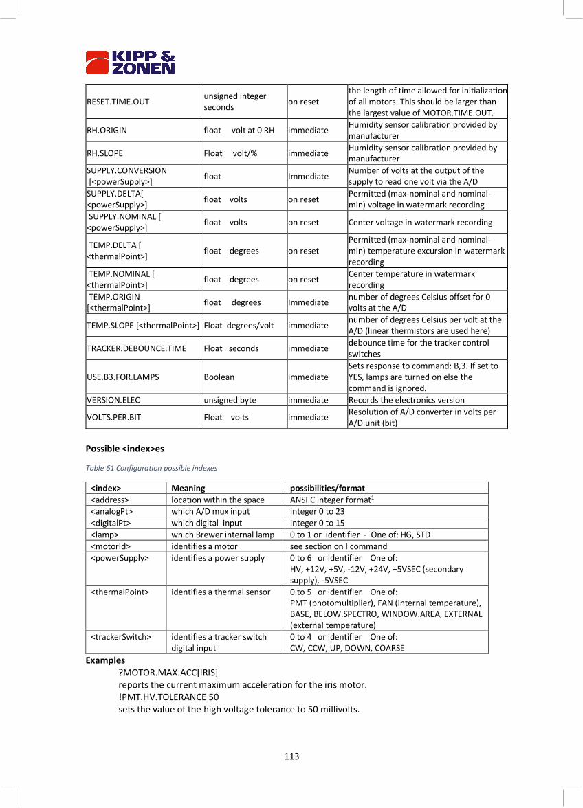
113

RESET.TIME.OUT unsigned integer seconds on reset

the length of time allowed for initialization of all motors. This should be larger than the largest value of MOTOR.TIME.OUT.

RH.ORIGIN float volt at 0 RH immediate Humidity sensor calibration provided by manufacturer

RH.SLOPE Float volt/% immediate Humidity sensor calibration provided by manufacturer

SUPPLY.CONVERSION [<powerSupply>] float Immediate Number of volts at the output of the

supply to read one volt via the A/D SUPPLY.DELTA[ <powerSupply>] float volts on reset Permitted (max-nominal and nominal-

min) voltage in watermark recording SUPPLY.NOMINAL [ <powerSupply>] float volts on reset Center voltage in watermark recording

TEMP.DELTA [ <thermalPoint>] float degrees on reset

Permitted (max-nominal and nominal-min) temperature excursion in watermark recording

TEMP.NOMINAL [ <thermalPoint>] float degrees on reset Center temperature in watermark

recording TEMP.ORIGIN [<thermalPoint>] float degrees Immediate number of degrees Celsius offset for 0

volts at the A/D

TEMP.SLOPE [<thermalPoint>] Float degrees/volt immediate number of degrees Celsius per volt at the A/D (linear thermistors are used here)

TRACKER.DEBOUNCE.TIME Float seconds immediate debounce time for the tracker control switches

USE.B3.FOR.LAMPS Boolean immediate Sets response to command: B,3. If set to YES, lamps are turned on else the command is ignored.

VERSION.ELEC unsigned byte immediate Records the electronics version

VOLTS.PER.BIT Float volts immediate Resolution of A/D converter in volts per A/D unit (bit)

Possible <index>es

Table 61 Configuration possible indexes

<index> Meaning possibilities/format <address> location within the space ANSI C integer format1

<analogPt> which A/D mux input integer 0 to 23 <digitalPt> which digital input integer 0 to 15 <lamp> which Brewer internal lamp 0 to 1 or identifier - One of: HG, STD <motorId> identifies a motor see section on I command <powerSupply> identifies a power supply 0 to 6 or identifier One of:

HV, +12V, +5V, -12V, +24V, +5VSEC (secondary supply), -5VSEC

<thermalPoint> identifies a thermal sensor 0 to 5 or identifier One of: PMT (photomultiplier), FAN (internal temperature), BASE, BELOW.SPECTRO, WINDOW.AREA, EXTERNAL (external temperature)

<trackerSwitch> identifies a tracker switch digital input

0 to 4 or identifier One of: CW, CCW, UP, DOWN, COARSE

Examples ?MOTOR.MAX.ACC[IRIS] reports the current maximum acceleration for the iris motor. !PMT.HV.TOLERANCE 50 sets the value of the high voltage tolerance to 50 millivolts.

114

1 The first character must be a digit. The number interpreted as decimal unless the first digit is a 0 in which case the second character is tested. If it is 'x' or 'X' the remaining digits are interpreted as a hexadecimal number. If the second character is a digit the number is interpreted as octal.

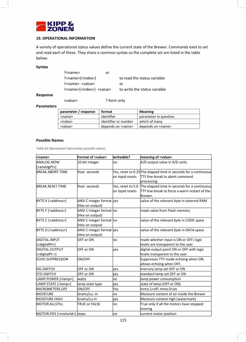
115

19. OPERATIONAL INFORMATION

A variety of operational status values define the current state of the Brewer. Commands exist to set and read each of these. They share a common syntax so the complete set are listed in the table below:

Syntax ?<name> or ?<name>[<index>] to read the status variable !<name> <value> or !<name>[<index>] <value> to write the status variable Response <value> ? form only Parameters

parameter / response format Meaning <name> identifier parameter in question <index> identifier or number which of many <value> depends on <name> depends on <name>

Possible Names

Table 62 Operational information possible names

<name> Format of <value> writeable? meaning of <value> ANALOG.NOW [<analogPt>]

10-bit integer no A/D output value in A/D units

BREAK.ABORT.TIME float seconds Yes, reset to 0.25 on tepid resets

The elapsed time in seconds for a continuous TTY line-break to abort command processing.

BREAK.RESET.TIME float seconds Yes, reset to 5.0 on tepid resets

The elapsed time in seconds for a continuous TTY line-break to force a warm restart of the Brewer.

BYTE.X [<address>] ANSI C integer format (Hex on output)

yes value of the relevant byte in external RAM

BYTE.F [<address>] ANSI C integer format (Hex on output)

no reads value from Flash memory

BYTE.C [<address>] ANSI C integer format (Hex on output)

no value of the relevant byte in CODE space

BYTE.D [<address>] ANSI C integer format (Hex on output)

yes value of the relevant byte in DATA space

DIGITAL.INPUT [<digitalPt>]

OFF or ON no reads whether input is ON or OFF; logic levels are transparent to the user.

DIGITAL.OUTPUT [<digitalPt >]

OFF or ON yes digital output point ON or OFF with logic levels transparent to the user.

ECHO.SUPPRESSION ON/OFF Suppresses TTY mode echoing when ON, allows echoing when OFF.

HG.SWITCH OFF or ON yes mercury lamp set OFF or ON STD.SWITCH OFF or ON yes standard lamp set OFF or ON LAMP.POWER [<lamp>] watts no lamp power consumption LAMP.STATE [<lamp>] lamp state type yes state of lamp (OFF or ON) MICROMETERS.OFF ON/OFF Yes mmo.1=off; mmo.0=on MOISTURE Grams/cu. m no Moisture content of air inside the Brewer MOISTURE.HIGH Grams/cu m yes Moisture content high (watermark) MOTOR.ALLSTILL TRUE or FALSE no True only if all the motors have stopped

moving MOTOR.POS [<motorId>] steps no current motor position

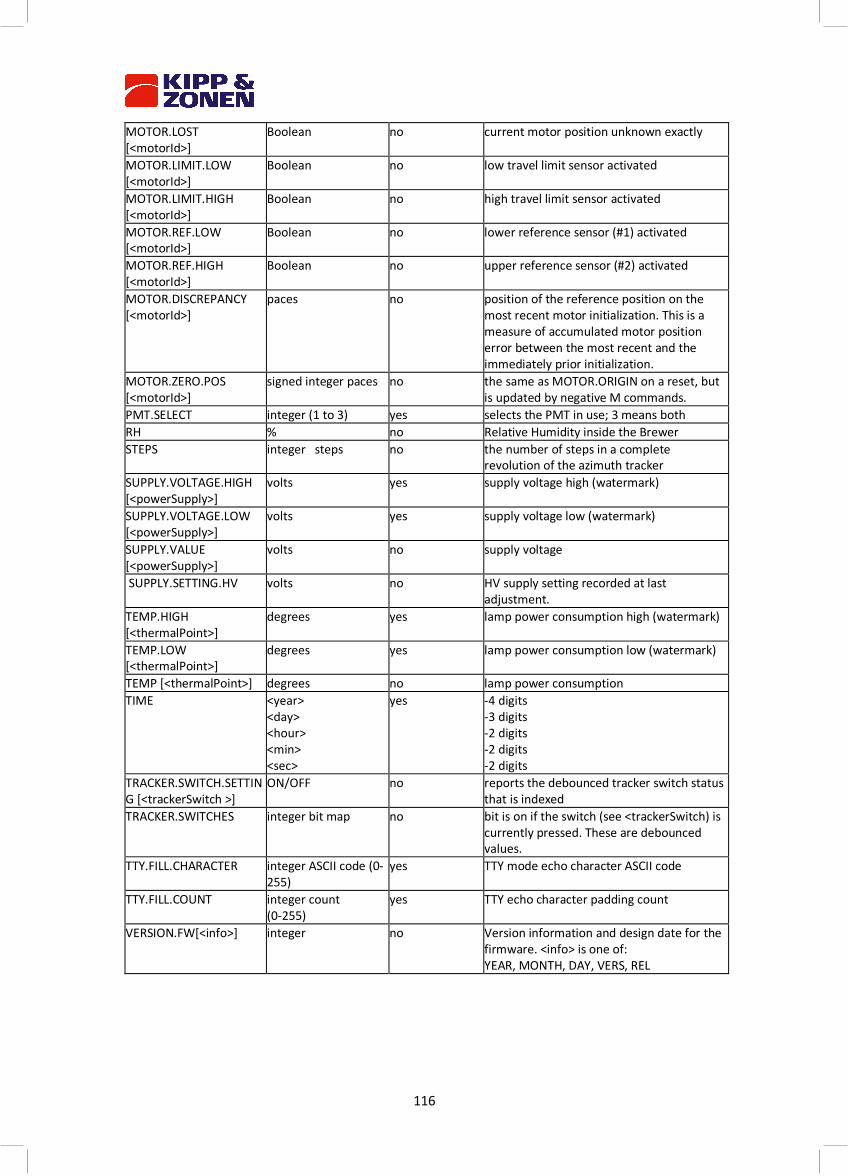
116

MOTOR.LOST [<motorId>]

Boolean no current motor position unknown exactly

MOTOR.LIMIT.LOW [<motorId>]

Boolean no low travel limit sensor activated

MOTOR.LIMIT.HIGH [<motorId>]

Boolean no high travel limit sensor activated

MOTOR.REF.LOW [<motorId>]

Boolean no lower reference sensor (#1) activated

MOTOR.REF.HIGH [<motorId>]

Boolean no upper reference sensor (#2) activated

MOTOR.DISCREPANCY [<motorId>]

paces no position of the reference position on the most recent motor initialization. This is a measure of accumulated motor position error between the most recent and the immediately prior initialization.

MOTOR.ZERO.POS [<motorId>]

signed integer paces no the same as MOTOR.ORIGIN on a reset, but is updated by negative M commands.

PMT.SELECT integer (1 to 3) yes selects the PMT in use; 3 means both RH % no Relative Humidity inside the Brewer STEPS integer steps no the number of steps in a complete

revolution of the azimuth tracker SUPPLY.VOLTAGE.HIGH [<powerSupply>]

volts yes supply voltage high (watermark)

SUPPLY.VOLTAGE.LOW [<powerSupply>]

volts yes supply voltage low (watermark)

SUPPLY.VALUE [<powerSupply>]

volts no supply voltage

SUPPLY.SETTING.HV volts no HV supply setting recorded at last adjustment.

TEMP.HIGH [<thermalPoint>]

degrees yes lamp power consumption high (watermark)

TEMP.LOW [<thermalPoint>]

degrees yes lamp power consumption low (watermark)

TEMP [<thermalPoint>] degrees no lamp power consumption TIME <year>

<day> <hour> <min> <sec>

yes -4 digits -3 digits -2 digits -2 digits -2 digits

TRACKER.SWITCH.SETTING [<trackerSwitch >]

ON/OFF no reports the debounced tracker switch status that is indexed

TRACKER.SWITCHES integer bit map no bit is on if the switch (see <trackerSwitch) is currently pressed. These are debounced values.

TTY.FILL.CHARACTER integer ASCII code (0-255)

yes TTY mode echo character ASCII code

TTY.FILL.COUNT integer count (0-255)

yes TTY echo character padding count

VERSION.FW[<info>] integer no Version information and design date for the firmware. <info> is one of: YEAR, MONTH, DAY, VERS, REL

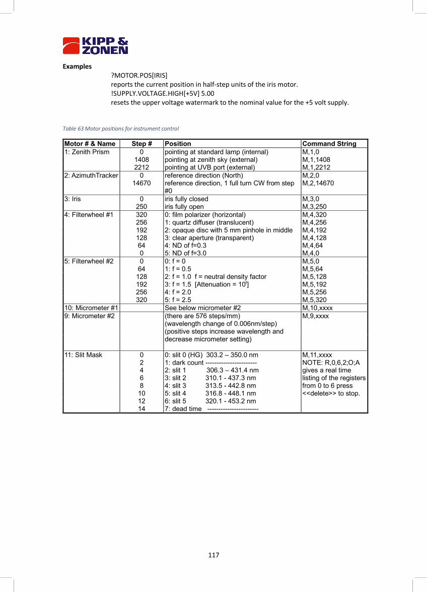
117

Examples ?MOTOR.POS[IRIS] reports the current position in half-step units of the iris motor. !SUPPLY.VOLTAGE.HIGH[+5V] 5.00 resets the upper voltage watermark to the nominal value for the +5 volt supply. Table 63 Motor positions for instrument control

Motor # & Name Step # Position Command String 1: Zenith Prism 0 pointing at standard lamp (internal) M,1,0 1408 pointing at zenith sky (external) M,1,1408 2212 pointing at UVB port (external) M,1,2212 2: AzimuthTracker 0 reference direction (North) M,2,0 14670 reference direction, 1 full turn CW from step

#0 M,2,14670

3: Iris 0 iris fully closed M,3,0 250 iris fully open M,3,250 4: Filterwheel #1 320 0: film polarizer (horizontal) M,4,320 256 1: quartz diffuser (translucent) M,4,256 192 2: opaque disc with 5 mm pinhole in middle M,4,192 128 3: clear aperture (transparent) M,4,128 64 4: ND of f=0.3 M,4,64 0 5: ND of f=3.0 M,4,0 5: Filterwheel #2 0 0: f = 0 M,5,0 64 1: f = 0.5 M,5,64 128 2: f = 1.0 f = neutral density factor M,5,128 192 3: f = 1.5 [Attenuation = 10f] M,5,192 256 4: f = 2.0 M,5,256 320 5: f = 2.5 M,5,320 10: Micrometer #1 See below micrometer #2 M,10,xxxx 9: Micrometer #2 (there are 576 steps/mm) M,9,xxxx (wavelength change of 0.006nm/step) (positive steps increase wavelength and decrease micrometer setting) 11: Slit Mask 0 0: slit 0 (HG) 303.2 – 350.0 nm M,11,xxxx 2 1: dark count ----------------------- NOTE: R,0,6,2;O;A 4 2: slit 1 306.3 – 431.4 nm gives a real time 6 3: slit 2 310.1 - 437.3 nm listing of the registers 8 4: slit 3 313.5 - 442.8 nm from 0 to 6 press 10 5: slit 4 316.8 - 448.1 nm <<delete>> to stop. 12 6: slit 5 320.1 - 453.2 nm 14 7: dead time -----------------------

118

19 Appendix F firmware log Messages appearing in the Instrument Log (accessed using the RL command) have the following format:

yyyy ddd hh mm ss <message part 1> yyyy ddd hh mm ss <message part 2> ... yyyy ddd hh mm ss <message part n>

The 'yyyy ddd hh mm ss ' identifies the time on the instrument clock at the time when the message was recorded. The possible values of <message part 1> are given below. Usually there is only the <message part 1>. <name>: Bad arraySpacing, AddVectors(). Please notify Kipp & Zonen <brewer@kippzonen.com> of the circumstances in which this message was generated. <name>: Can't add preexisting symbol. Please notify Kipp & Zonen <brewer@kippzonen.com> of the circumstances in which this message was generated. <name>: Enum type mismatch. Please notify Kipp & Zonen <brewer@kippzonen.com> of the circumstances in which this message was generated. <name>: Hash table too full. Please notify Kipp & Zonen <brewer@kippzonen.com> of the circumstances in which this message was generated. <name>: Symbol not found. Please notify Kipp & Zonen <brewer@kippzonen.com> of the circumstances in which this message was generated. A command used only by one mode was entered in another mode. Please notify Kipp & Zonen <brewer@kippzonen.com> of the circumstances in which this message was generated. Analog: initialization timed out. During initialization the circuitry used to read analog input channels failed to initialize properly. Attempt to exceed max boundary An M command was issued to a position beyond the highest in the range of the motor. Instead it was moved to the highest legal position. Attempt to exceed min boundary An M command was issued to a position beyond the lowest in the range of the motor. Instead it was moved to the lowest legal position. Bad command, no config variables: A command was issued which required configuration when no configuration was loaded. The subsequent message indicates the command. If the instrument is in Cosmac mode at the time, it also responds immediately with "Sorry, need configuration variables." Bad command string. Command string buffer cleared. An illegal command was (not) processed. The subsequent message indicates the command. Bad digital output setting. Only ON/OFF allowed. (Self-explanitory) Checksum bad in low level command. During initialization, loadmode or opmode a message with a bad checksum was received. This is normal if an initialization starts while a packet is being sent and is of no consequence at that time. At other times it indicates a noisy communication line. Command not accepted while another in progress. Please notify Kipp & Zonen <brewer@kippzonen.com> of the circumstances in which this message was generated. Config signature did not write properly.

119

The configuration was not correctly written to Flash memory. Possibly the Flash memory chip has failed. Flash config checksum error. The data in the configuration is corrupted. Possibly the Flash memory chip has failed. Flash config memory full. Configuration can be saved to Flash memory(see SAVE command) only four times. Reload the firmware. Lamp <number>: told neither ON, OFF.. what?? Only ON and OFF are valid settings for a lamp. MAIN.C : motor initialization timed out. Motor initialization failed to complete in the allotted time (RESET.TIME.OUT). Operation proceeds with the motors which did initialize. Motor <number>: appears stuck with a reference sensor activated. An attempt was made to initialize a motor but the motion which should have removed the blocker from a reference sensor did not do so. Motor <number> became lost during M command. Motor has been reset to its reference position. Warning that a motor encountered an end of travel limit. This indicates that for some time prior to this message the motor was not in position. Motor <number>: configured as nonexisting, cannot be moved/reset. An attempt was made to move a motor which has been configured to a MOTOR.CLASS of NOMOTOR. Motor <number>: IIC communications error Error communicating with the controller for the given motor. If this error persists it indicates a failure in the instrument electronics. Motor <number>: Motor busy. Please notify Kipp & Zonen <brewer@kippzonen.com> of the circumstances in which this message was generated. Motor <number>: Motor lost. The motor controller and the instrument controller are out of step. This error will be corrected next time the moter is moved. If this error persists for the given motor, please notify Kipp & Zonen <brewer@kippzonen.com> of the circumstances in which this message was generated. Motor <number>: Move attempted outside of logical bounds An attempt was made to move the given motor out of bounds. If this error persists, please notify Kipp & Zonen <brewer@kippzonen.com> of the circumstances in which this message was generated. Motor <number>: Movement attempted with too large a jerk Please notify Kipp & Zonen <brewer@kippzonen.com> of the circumstances in which this message was generated. Motor <number>: Movement attempted with too large an acceleration Please notify Kipp & Zonen <brewer@kippzonen.com> of the circumstances in which this message was generated. Motor <number>: Movement attempted with too large a velocity If this error persists for the given motor, please notify Kipp & Zonen <brewer@kippzonen.com> of the circumstances in which this message was generated. Motor <number>: time allotted (<ss> seconds) for motor movement has expired. Motor stopped. The value <ss> comes from the MOTOR.TIME.OUT configuration parameter. New value set for watermark <nameOfWatermark>: <latestMark> <unitsOfWatermark>. The indicated watermark value has been changed to <latestMark>. The possible watermarks are identified in Appendix H. No Flash config segment in Flash to copy into RAM upon initialization Attempt to initialize when no configuration information had been loaded yet. This message is normal as part of the process of loading new firmware.

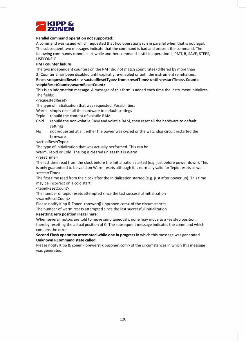
120

Parallel command operation not supported: A command was issued which requested that two operations run in parallel when that is not legal. The subsequent two messages indicate that the command is bad and present the command. The following commands cannot start while another command is still in operation: I, PMT, R, SAVE, STEPS, USECONFIG PMT counter failure The two independent counters on the PMT did not match count rates (differed by more than 2).Counter 2 has been disabled until explicitly re-enabled or until the instrument reinitializes. Reset <requestedReset> -> <actualResetType> from <resetTime> until <restartTime>. Counts: <tepidResetCount>,<warmResetCount> This is an information message. A message of this form is added each time the instrument initializes. The fields: <requestedReset> The type of initialization that was requested. Possibilities: Warm simply reset all the hardware to default settings Tepid rebuild the content of volatile RAM Cold rebuild the non-volatile RAM and volatile RAM, then reset all the hardware to default

settings No not requested at all; either the power was cycled or the watchdog circuit restarted the

firmware <actualResetType> The type of initialization that was actually performed. This can be Warm, Tepid or Cold. The log is cleared unless this is Warm <resetTime> The last time read from the clock before the initialization started (e.g. just before power down). This is only guaranteed to be valid on Warm resets although it is normally valid for Tepid resets as well. <restartTime> The first time read from the clock after the initialization started (e.g. just after power up). This time may be incorrect on a cold start. <tepidResetCount> The number of tepid resets attempted since the last successful initialization <warmResetCount> Please notify Kipp & Zonen <brewer@kippzonen.com> of the circumstances The number of warm resets attempted since the last successful initialization Resetting zero position illegal here: When several motors are told to move simultaneously, none may move to a -ve step position, thereby resetting the actual position of 0. The subsequent message indicates the command which contains the error. Second Flash operation attempted while one in progress in which this message was generated. Unknown RCommand state called. Please notify Kipp & Zonen <brewer@kippzonen.com> of the circumstances in which this message was generated.

121

20 Appendix G BREWCMD.EXE The BrewCMD is a low level utility program to facilitate sending commands to and displaying responses from the Brewer. Hence it can be used for simple operation tasks. There are two versions of BrewCMD available: 1. BrewCMD.exe This version is a DOS based program and works fine with platforms such as W95 and W98. This version of BrewCMD however does not work with WindowsXP and higher. 2. BrewCMDW.exe The ‘W’ extension indicates that this program is a Windows based program. This version works on XP systems and higher. BrewCMDW does not work on MS-DOS, W95 or W98 systems. To run the BrewCMD(W) utility the Brewer must be connected via the serial port of the PC. The BrewCMD utility is intended for the use of the scientist using the Brewer and the technicians installing the Brewer. The BrewCMD utility has three intended functions: • To provide a tool for verifying the validity of connections to the Brewer and for verifying the low level message/response operation of the Brewer. • Uploading firmware and configuration files. • To facilitate sending commands to and displaying responses from the Brewer. Note: The BrewCMD program is a low level utility. Using this utility can modify the calibration and equipment configuration information. For information on how to upload firmware and configuration file please refer to the Service Manual.

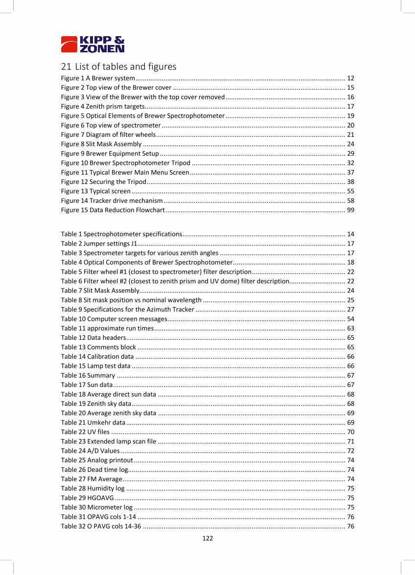
122

21 List of tables and figures Figure 1 A Brewer system ................................................................................................................ 12 Figure 2 Top view of the Brewer cover ............................................................................................ 15 Figure 3 View of the Brewer with the top cover removed ................................................................ 16 Figure 4 Zenith prism targets ........................................................................................................... 17 Figure 5 Optical Elements of Brewer Spectrophotometer ................................................................ 19 Figure 6 Top view of spectrometer .................................................................................................. 20 Figure 7 Diagram of filter wheels ..................................................................................................... 21 Figure 8 Slit Mask Assembly ............................................................................................................ 24 Figure 9 Brewer Equipment Setup ................................................................................................... 29 Figure 10 Brewer Spectrophotometer Tripod .................................................................................. 32 Figure 11 Typical Brewer Main Menu Screen ................................................................................... 37 Figure 12 Securing the Tripod .......................................................................................................... 38 Figure 13 Typical screen .................................................................................................................. 55 Figure 14 Tracker drive mechanism ................................................................................................. 58 Figure 15 Data Reduction Flowchart ................................................................................................ 99

Table 1 Spectrophotometer specifications....................................................................................... 14 Table 2 Jumper settings J1 ............................................................................................................... 17 Table 3 Spectrometer targets for various zenith angles ................................................................... 17 Table 4 Optical Components of Brewer Spectrophotometer ............................................................ 18 Table 5 Filter wheel #1 (closest to spectrometer) filter description .................................................. 22 Table 6 Filter wheel #2 (closest to zenith prism and UV dome) filter description.............................. 22 Table 7 Slit Mask Assembly.............................................................................................................. 24 Table 8 Sit mask position vs nominal wavelength ............................................................................ 25 Table 9 Specifications for the Azimuth Tracker ................................................................................ 27 Table 10 Computer screen messages ............................................................................................... 54 Table 11 approximate run times ...................................................................................................... 63 Table 12 Data headers ..................................................................................................................... 65 Table 13 Comments block ............................................................................................................... 65 Table 14 Calibration data ................................................................................................................ 66 Table 15 Lamp test data .................................................................................................................. 66 Table 16 Summary .......................................................................................................................... 67 Table 17 Sun data ............................................................................................................................ 67 Table 18 Average direct sun data .................................................................................................... 68 Table 19 Zenith sky data .................................................................................................................. 68 Table 20 Average zenith sky data .................................................................................................... 69 Table 21 Umkehr data ..................................................................................................................... 69 Table 22 UV files ............................................................................................................................. 70 Table 23 Extended lamp scan file .................................................................................................... 71 Table 24 A/D Values ........................................................................................................................ 72 Table 25 Analog printout ................................................................................................................. 74 Table 26 Dead time log .................................................................................................................... 74 Table 27 FM Average ....................................................................................................................... 74 Table 28 Humidity log ..................................................................................................................... 75 Table 29 HGOAVG ........................................................................................................................... 75 Table 30 Micrometer log ................................................................................................................. 75 Table 31 OPAVG cols 1-14 ............................................................................................................... 76 Table 32 O PAVG cols 14-36 ............................................................................................................ 76

123

Table 33 Ozone average file ............................................................................................................ 76 Table 34 FZOAVG ............................................................................................................................ 77 Table 35 Run / stop log .................................................................................................................... 77 Table 36 Sun scan average .............................................................................................................. 77 Table 37 SLOAVG............................................................................................................................. 78 Table 38 Daily DUV .......................................................................................................................... 78 Table 39 UVOAVG ........................................................................................................................... 78 Table 40 Lamp file ........................................................................................................................... 79 Table 41 Lamp file ........................................................................................................................... 79 Table 42 Instrument constants ........................................................................................................ 81 Table 43 Operating state file ........................................................................................................... 82 Table 44 Dispersion ......................................................................................................................... 83 Table 45 Umkehr ............................................................................................................................. 83 Table 46 Zenith sky constants .......................................................................................................... 84 Table 47 Settings for Brewer test..................................................................................................... 85 Table 48 Typical calibration output.................................................................................................. 86 Table 49 Typical photomultiplier response output ........................................................................... 87 Table 50 Typical Slitmask Test Results ............................................................................................. 88 Table 51 Dead time test .................................................................................................................. 89 Table 52 FILTER #1/1 AND FILTER #2/0 ............................................................................................ 90 Table 53 FILTER #1/1 AND FILTER #2/1 ............................................................................................ 90 Table 54 Lamp test .......................................................................................................................... 93 Table 55 Lamp test 2 ....................................................................................................................... 93 Table 56 O3 and SO2 column amounts vs. wavelength for a typical Scan Test on direct sun ............ 95 Table 57 Constants for example instrument .................................................................................. 103 Table 58 Motor initialize values ..................................................................................................... 106 Table 59 R command slit mask positions ....................................................................................... 108 Table 60 Configuration parameter names...................................................................................... 111 Table 61 Configuration possible indexes ........................................................................................ 113 Table 62 Operational information possible names ......................................................................... 115 Table 63 Motor positions for instrument control ........................................................................... 117

124