Bounded Mean Oscillation and BandlimitedInterpolation in the Presence of Noise

Gaurav Thakur∗

September 3, 2010

Abstract

We study some problems related to the effect of bounded, additive sample noise in the ban-dlimited interpolation given by the Whittaker-Shannon-Kotelnikov (WSK) sampling formula.We establish a generalized form of the WSK series that allows us to consider the bandlimitedinterpolation of any bounded sequence at the zeros of a sine-type function. The main resultof the paper is that if the samples in this series consist of independent, uniformly distributedrandom variables, then the resulting bandlimited interpolation almost surely has a boundedglobal average. In this context, we also explore the related notion of a bandlimited functionwith bounded mean oscillation. We prove some properties of such functions, and in particular,we show that they are either bounded or have unbounded samples at any positive samplingrate. We also discuss a few concrete examples of functions that demonstrate these properties.

Mathematics Subject Classification (2010): Primary 30E05; Secondary 94A20, 30D15, 30H35Keywords: Sampling theorem, Nonuniform sampling, Paley-Wiener spaces, Entire functions of exponentialtype, BMO, Sine-type functions

1 IntroductionThe classical Whittaker-Shannon-Kotelnikov (WSK) sampling theorem is a central result in signalprocessing and forms the basis of analog-to-digital and digital-to-analog conversion in a varietyof contexts involving signal encoding, transmission and detection. If we normalize the Fouriertransform as f (ω) =

∫∞

−∞f (t)e−2πiωtdt, then the sampling theorem states that a function f ∈ L2(R)

with supp( f )⊂ [−b2 ,

b2 ] can be expressed as a series of the form

f (t) =∞

∑k=−∞

aksin(π(bt− k))

π(bt− k), (1)

where ak = f (k) are its samples. Conversely, for a given collection of data {ak} ∈ l2, the series (1)defines a function in L2(R) with supp( f ) ⊂ [−b

2 ,b2 ] called the bandlimited interpolation of {ak}.

∗Program in Applied and Computational Mathematics, Princeton University, Princeton, NJ 08544, USA, email:gthakur@princeton.edu

1

arX

iv:1

007.

5134

v2 [

mat

h.C

V]

22

Oct

201

0

The calculation or approximation of this series is a standard procedure in many applications. Forexample, in audio processing it is used for resampling signals at a higher rate, typically by applyinga lowpass filter to the piecewise-constant zero order hold function of the samples [6]. In this paper,we consider the situation of bounded noise in the samples ak. Building on recent work by Bocheand Mönich on related problems [3, 4, 5], we study some properties of the effect of the noise onthe bandlimited interpolation f .

Before we discuss our problems, it will be convenient to define the Paley-Wiener spaces for 1 ≤p≤ ∞ by

PW pb =

{f ∈ Lp : supp( f )⊂

[−b

2,b2

]},

where f is interpreted in the sense of tempered distributions. Our notation PW pb essentially fol-

lows Seip [12], and is slightly different from the one used by Boche and Mönich. Without loss ofgenerality, we will set b = 1 in what follows.

Returning to the series (1), we consider corrupted samples of the form ak = Tk +Nk, whereTk are the true samples and Nk is some form of noise, and we correspondingly write f (t) =T (t)+N(t). One obstacle we face is that the noise {Nk}may not naturally decay in time alongsidethe signal, and even if {Tk} ∈ l2, it is often more physically meaningful to consider {Nk} ∈ l∞. TheWSK sampling theorem shows that for any collection of samples {ak} ∈ l2, there exists a uniquefunction f ∈ PW 2

1 with f (k) = ak. However, for bounded samples {ak} ∈ l∞, the series (1) does notnecessarily converge. In fact, a given {ak} ∈ l∞ may correspond to multiple functions f ∈ PW ∞

1 ,or to no such function [3].

A simple example of the former possibility (non-uniqueness) is given by ak ≡ 0, which cor-responds to the functions f (t) ≡ 0 and f (t) = sin(πt). It turns out that adding one extra sampleto the collection {ak} resolves this ambiguity, and allows us to consider the unique bandlimitedinterpolation of any bounded data {ak} ∈ l∞. We discuss the details of this procedure in Section 3.The latter possibility (non-existence) is less obvious, but in [3], Boche and Mönich presented anexplicit example of this phenomenon. They showed that for the samples given by ak = 0, k < 1,and ak = (−1)k/ log(k+1), k ≥ 1, there is no f ∈ PW ∞

1 with f (k) = ak. It is also possible to con-struct other, similar examples using standard special functions, and we describe one such sequenceof {ak} in Section 3 and discuss its properties.

The main observation of this paper is that such examples of {ak} are in a sense “highly oscil-lating.” By assuming that the noise Nk is statistically incoherent and defining N(t) carefully, wecan rule out these examples and obtain sharper statements on the behavior of N(t). More precisely,we show in Section 4 that if Nk is a uniformly distributed, independent white noise process, thensupr>0

12r∫ r−r |N(t)|dt < ∞ almost surely. In other words, the average of |N(t)| is globally bounded.

We find that this result does not generally hold for {Nk} ∈ l∞ that lack such a statistical condition,and we discuss examples that illustrate the differences.

We also study a second topic motivated by further understanding N(t). As discussed in [7],the WSK series (1) can be interpreted as a discrete Hilbert transform operator H, mapping a space

2

of samples into a space of bandlimited functions (see also [1] and [11]). The Plancherel formulashows that H maps l2 into PW 2

1 . In fact, H also maps lp into PW p1 for any 1 < p < ∞, and the series

(1) converges for any {ak} ∈ lp [10]. This can be compared with the continuous Hilbert transform,and more generally any Calderon-Zygmund singular integral operator, which maps Lp into itselffor any 1 < p < ∞. Such operators behave differently for p = ∞, mapping L∞ into the space BMOof functions with bounded mean oscillation [13].

It is thus reasonable to expect that if we consider samples {ak} ∈ l∞, the “right” target space forH may be one of bandlimited functions lying in the space BMO. However, this heuristic reasoningturns out to be incorrect. We consider bandlimited BMO functions in Section 5 and establish someof their properties. In particular, we find that such a function f is either in L∞ or that its samples{ f (k

s )} are unbounded for any sampling rate s > 0. We exhibit a concrete example of such a func-tion, and study it in the context of our other results.

We review some existing theory on bandlimited functions and the space BMO in Section 2,and discuss some preliminary results in Section 3. The main results of the paper are presentedin Sections 4 and 5. We also develop our results for a class of general, nonuniformly spacedinterpolation points, given by zeros of sine-type functions. The above discussion for uniformlyspaced points is a special case.

2 Background MaterialWe will write f1 . f2 if the inequality f1≤C f2 holds for a constant C independent of f1 and f2. Wedefine f1 & f2 similarly, and write f1 h f2 if both f1 . f2 and f1 & f2. For a set of points Y = {yk}and an extra element y, we denote the collection {yk}

⋃{y} by Y , with ||Y ||lp := (||Y ||lp + |y|p)1/p

and ||Y ||l∞ := max(‖Y‖l∞ , |y|). These conventions will be used throughout the paper.

We first review a basic, alternative formulation of PW pb , 1≤ p≤ ∞. An entire function f is said to

be of exponential type b ifb = inf

(β : | f (z)| ≤ eβ |z|,z ∈ C

).

We denote this by writing type( f ) = b, and by type( f ) = ∞ if b = ∞ or f is not entire. By thePaley-Wiener-Schwartz theorem [9], PW p

b can be equivalently described as the space of all entirefunctions with type( f )≤ πb whose restrictions to R are in Lp. It also follows that PW p

b ⊂ PW qb for

p < q. Functions f ∈ PW pb satisfy the classical estimates ‖ f ′‖Lp ≤ πb‖ f‖Lp and ‖ f (·+ ic)‖Lp ≤

eπb|c| ‖ f‖Lp , respectively known as the Bernstein and Plancherel-Polya inequalities [10, 12].

There is a rich and well-developed theory of nonuniform sampling for functions in PW pb . We

only cover a few aspects of it that we will need in this paper, and refer to [12] and [15] for moredetails. We consider a sequence of points X = {xk} ⊂R, indexed so that xk < xk+1. The separationconstant of X is defined by λ (X) = infk |xk+1−xk|, and X is said to be separated if λ (X)> 0. Thegenerating function of X is given by the product

S(z) = zδX limr→∞

∏0<|xk|<r

(1− z

xk

), (2)

3

where δX = 1 if 0 ∈ X and δX = 0 otherwise. For real and separated X , such a function S is said tobe sine-type if the following conditions hold:

(I) The product (2) converges and type(S) = πb < ∞.(II) For any ε > 0, there are positive constants C1(ε) and C2(ε) such that whenever dist(z,X)> ε ,

C1(ε)≤ e−πb|Im(z)||S(z)| ≤C2(ε). (3)

It can be shown that condition (II) is equivalent to requiring that the bounds (3) only hold in somehalf plane {z : |Im(z)| ≥ c}, c > 0. Furthermore, a sine-type function S also satisfies the bounds|S′(xk)|h 1 and forces X to satisfy supk |xk+1− xk|< ∞ [10].

Now suppose the sequence X = {xk} has a sine-type generating function S with type(S) = πb. Let1 < p < ∞. Then any f ∈ PW p

b can be expressed in terms of its samples ak = f (xk),

f (z) =∞

∑k=−∞

akS(z)

S′(xk)(z− xk), (4)

with uniform convergence on compact subsets of C. Conversely, for any {ak} ∈ lp, the series (4)converges uniformly on compact subsets of C and defines a function f ∈PW p

b with ak = f (xk) [10].

The simplest example of a sequence X with a sine-type generating function is the uniformsequence xk =

kb , for which S(z) = sin(πbz)

πb and the expansion (4) reduces to the WSK samplingtheorem. More generally, any finite union of uniform sequences has a sine-type generating func-tion. As a more interesting example, the Bessel function J0 has real, separated zeros, satisfies

J0(z) = J0(−z), and has the asymptotic formula J0(z) =√

2πz cos(z− π

4 )(1+O(1z )) as |z| →∞ and

|argz|< π (see [14]). This implies that for sufficiently small ε > 0, S(z) = zJ0(πz2 )J0(

π(z+ε)2 ) is a

sine-type function with type(S) = π . Sequences X with sine-type generating functions are not themost general class for which f has an expansion of the form (4), but they have several convenientproperties and cover some important cases encountered in applications, such as that of periodicinterpolation points. Such sequences X and various properties of the series (4) have recently beenstudied in [4] in a computational context.

The above results do not directly carry over to bounded functions f ∈ PW ∞b , but in this case we

still have the following theorem [2].

Theorem. (Beurling) For a sequence X = {xk}, let N(X , I) be the number of xk in an interval I.Then ‖ f‖L∞ h ‖ f (X)‖l∞ for all f ∈ PW ∞

b if and only if

D−(X) := limsupr→∞

infa

N(X , [a,a+ r))r

> b.

D−(X) is called the lower uniform density of X . For a uniform sequence xk =ks , D−(X) = s, and

Beurling’s theorem implies that f ∈ PW ∞b is uniquely determined by its samples if we oversample

it beyond its Nyquist rate.

4

We finally review a few properties of the Banach space BMO of functions with bounded meanoscillation, which has been studied extensively in connection with singular integral operators. It isdefined by {

f : ‖ f‖BMO = supI

1|I|

∫I

∣∣∣∣ f (t)− 1|I|

∫I

f (s)ds∣∣∣∣dt < ∞

},

where the supremum runs over all real intervals I. The quantity ‖ f‖BMO is technically a seminorm,since ‖ f‖BMO=‖ f + c‖BMO for any constant c. Now for any g ∈ L1, we denote its Hilbert trans-form by H g(z) :=

∫∞

−∞

g(t)π(t−z)dt and its Riesz projections by P±g := (g± iH g)/2. We can then

consider the “real” Hardy space H1(R), given by{f : ‖ f‖H1(R) = ‖ f‖L1 +‖H f‖L1 < ∞

}.

Finally, it will also be useful to define the subspaces

U1 = { f ∈C∞0 :∫

∞

−∞

f (t)dt = 0}

U2 = { f ∈ H1(R) : (1+ t2)|P+ f (t)| ∈ L∞}

which are both norm dense in H1(R) [8, 13]. These spaces are all closely related, as the followingtheorem shows.

Theorem. (Fefferman) BMO is the dual space of H1(R). More specifically, we have the inequality

‖ f‖BMO h supg∈U

1‖g‖H1(R)

∣∣∣∣∫ ∞

−∞

f (t)g(t)dt∣∣∣∣ ,

where U can be taken as U1 or U2. Conversely, for any bounded linear functional L on H1(R),there is an f ∈ BMO with ‖L‖h ‖ f‖BMO.

We write w = u+ iv for the complex variable w in what follows. Let C± = {w : ±v > 0} be theupper and lower half planes, and let P(w, t) = 1

π

v(u−t)2+v2 be the Poisson kernel on C+. Now define

the square Qa,r = {w : a < u < a+ r,0 < v < r}. A measure µ on C+ is said to be a Carleson

measure if we have N (µ) := sup(

µ(Qa,r)r ,a ∈ R,r > 0

)< ∞. In other words, the measure µ

of any square protruding from the real axis must be comparable to the length of its edge. Thefollowing theorem characterizes BMO in terms of such measures.

Theorem. (Fefferman-Stein) Suppose∫

∞

−∞

| f (t)|t2+1 dt < ∞, so that P(w, ·)? f is well-defined. Then

‖ f‖BMO h[N(

v |∇u,v(P(w, ·)? f )|2 dudv)]1/2

. (5)

A detailed discussion of BMO and the significance of these theorems can be found in [8] or [13].

5

3 Bandlimited Interpolation of Bounded DataIn this section, we establish a preliminary result showing how adding an extra sample allows us totreat the bandlimited interpolation of bounded data, such as the noise model discussed in Section1. We define

PW+b =

{f entire : limsup

r→∞

∫|z|=r

∣∣∣z−2e−πb|Im(z)| f (z)∣∣∣ |dz|< ∞

}. (6)

The Plancherel-Polya inequality shows that PW ∞b ⊂ PW+

b . Functions in PW+b can be expanded in

the following way.

Theorem 1. Suppose X = {xk} ⊂ R is separated and has a sine-type generating function S withtype(S) = πb, and let x 6∈ X . If f ∈ PW+

b and A = f (X), then

f (z) = aS(z)S(x)

+∞

∑k=−∞

ak limz0→z

S(z0)

S′(xk)

(1

z0− xk− 1

x− xk

), (7)

with uniform convergence of compact subsets of C. Conversely, for any A ∈ l∞, the series (7)converges uniformly on compact subsets of C and f ∈ PW+

b .

Proof. We use a standard complex variable argument. Assume z is in a closed ball B with z 6∈ X ,and choose a real sequence {rn} with rn → ∞ and dist({rn},X) > 0. We can then consider theintegral

J(rn) :=1

2πi

∫|w|=rn

f (w)S(z)S(w)

(1

z−w− 1

x−w

)|dw|.

For sufficiently large n, it can be seen by calculating residues that

J(rn) =− f (z)+ aS(z)S(x)

+ ∑|xk|<rn

akS(z)

S′(xk)

(1

z− xk− 1

x− xk

).

The inequalities (3) and (6) imply that as rn→ ∞,

|J(rn)|. maxz∈B|S(z)(z− x)|

∫|w|=rn

| f (w)|e−πb|Im(w)|

|w|2|dw| → 0.

By letting z→ xk for each xk ∈ B, we obtain the formula (7) for all z ∈ B. For the other direction ofTheorem 1, we note that S has simple zeros at exactly X , so for z ∈ R, |S(z)| ≤ 2||S′||L∞dist(z,X).The Bernstein and Plancherel-Polya inequalities then show that for z∈C and d = supk |xk+1−xk|<∞,

|S(z)|. ‖S‖L∞ min(dist(z,X),d)eπb|Im(z)|.

Now define the sets:

Iw1 = (bRe(w)c−min(1/2,λ (X)),bRe(w)c+min(1/2,λ (X)))

I2 = (−∞,b(Re(z)+ x)/2c)\(Iz1

⋃I x1)

I3 = (b(Re(z)+ x)/2c+1,∞)\(Iz1

⋃I x1)

6

Using the separation of X along with basic properties of lower Riemann sums, we have

| f (z)| . |aS(z)|+ eπb|Im(z)| ‖A‖l∞

∞

∑k=−∞

min(dist(z,X),d)|z− x||z− xk||x− xk|

.∥∥A∥∥

l∞ eπb|Im(z)|

(1+ ∑

k∈Z⋂

I2

|xk+1− xk||z− x|λ (X)|z− xk||x− xk|

+ ∑k∈Z

⋂I3

|xk− xk−1||z− x|λ (X)|z− xk||x− xk|

)

.∥∥A∥∥

l∞ eπb|Im(z)|(

1+∫R\(Iz

1⋃

Ix1)

|z− x||z− t||x− t|

dt)

.∥∥A∥∥

l∞ eπb|Im(z)|(1+max(log |z|,0)), (8)

which implies that f ∈ PW+b .

This expansion can be compared with the series (4). It is essentially a nonuniform version of theclassical Valiron interpolation formula considered in [3], in which the derivative of f at a point isused instead of the extra sample a, but the form considered here will be more convenient for ourpurposes. We also mention that the extra point x plays no special role in the collection X , and weisolate it mainly for notational convenience. If we pick any point x j ∈ X and let yk = xk for k 6= j,y j = x and y = x j, then Y = {yk}

⋃y satisfies the conditions of Theorem 1 too.

For any A ∈ l∞, we call the function f given by (7) the bandlimited interpolation of A at X . Notethat for any given a2 and x2 6∈ X , if g is the bandlimited interpolation of A

⋃{a2} at X

⋃{x2}, then

g(z) = f (z)+ cS(z) for some constant c. Moreover, if A ∈ l2, then for any given x 6∈ X we canalways choose a so that f coincides with the series (4), or in the special case of uniformly spacedpoints X = { k

b}, the usual bandlimited interpolation given by the WSK series (1).

We discuss an example of a PW+1 function that illustrates many of the typical properties of the

series (7). We use the uniform samples X = {k} and denote ψ(z) = Γ′(z)Γ(z) , where Γ is the usual

gamma function. The properties of ψ are discussed in depth in [14].

Example. The function G1(z) = sin(πz)ψ(−z) is in PW+1 \PW ∞

1 and satisfies ak = 0 for k < 0 andak = (−1)kπ for k ≥ 0.

The function ψ satisfies the estimate

lim|z|→∞,|argz|<π

ψ(z)logz

= 1, (9)

so G1 is not bounded. With A = {ak} given as above, Theorem 1 shows that for any x and a, the(unique) bandlimited interpolation of A at X is of the form G1(z)+ csin(πz). It follows that thesamples A have no bandlimited interpolation in PW ∞

1 .

It will be instructive to isolate one property of G1 here. A classical formula of Gauss ([14], p. 240)shows that for integer k > 0,

G1(k−12) = G1(−k− 1

2) = (−1)k

(k−1

∑m=1

1m+

2k−1

∑m=k

2m+C

), (10)

7

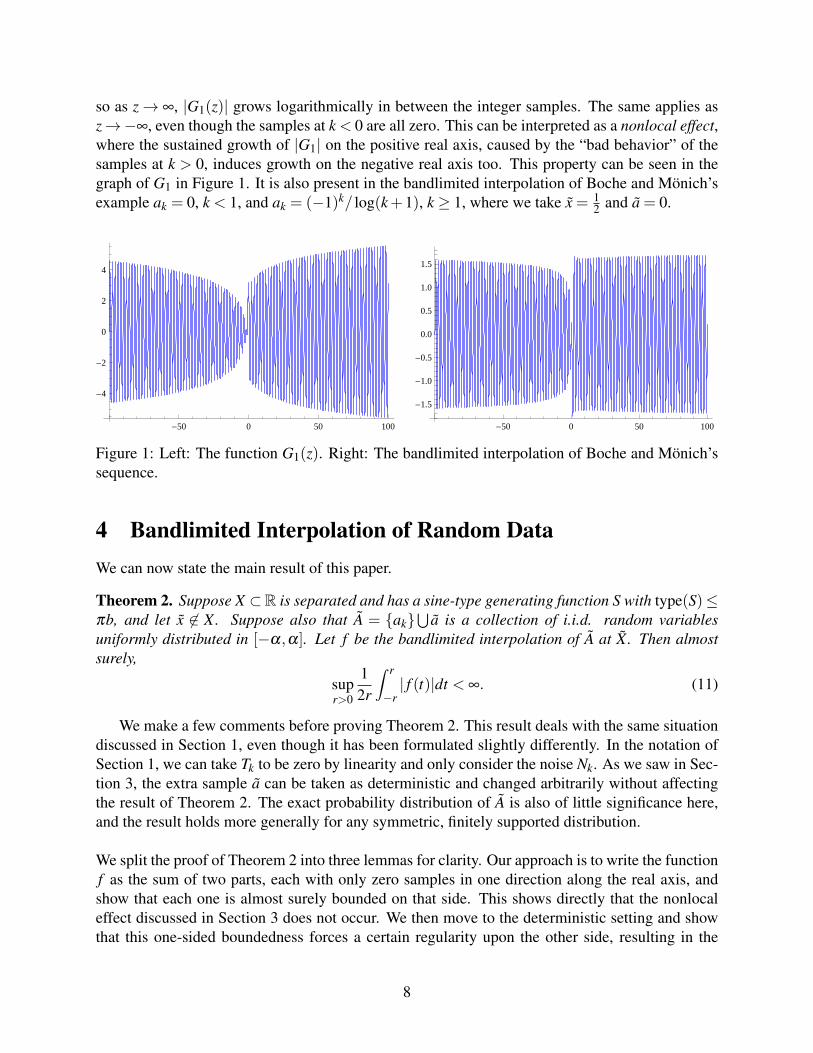
so as z→ ∞, |G1(z)| grows logarithmically in between the integer samples. The same applies asz→−∞, even though the samples at k < 0 are all zero. This can be interpreted as a nonlocal effect,where the sustained growth of |G1| on the positive real axis, caused by the “bad behavior” of thesamples at k > 0, induces growth on the negative real axis too. This property can be seen in thegraph of G1 in Figure 1. It is also present in the bandlimited interpolation of Boche and Mönich’sexample ak = 0, k < 1, and ak = (−1)k/ log(k+1), k ≥ 1, where we take x = 1

2 and a = 0.

-50 0 50 100

-4

-2

0

2

4

-50 0 50 100

-1.5

-1.0

-0.5

0.0

0.5

1.0

1.5

Figure 1: Left: The function G1(z). Right: The bandlimited interpolation of Boche and Mönich’ssequence.

4 Bandlimited Interpolation of Random DataWe can now state the main result of this paper.

Theorem 2. Suppose X ⊂R is separated and has a sine-type generating function S with type(S)≤πb, and let x 6∈ X. Suppose also that A = {ak}

⋃a is a collection of i.i.d. random variables

uniformly distributed in [−α,α]. Let f be the bandlimited interpolation of A at X . Then almostsurely,

supr>0

12r

∫ r

−r| f (t)|dt < ∞. (11)

We make a few comments before proving Theorem 2. This result deals with the same situationdiscussed in Section 1, even though it has been formulated slightly differently. In the notation ofSection 1, we can take Tk to be zero by linearity and only consider the noise Nk. As we saw in Sec-tion 3, the extra sample a can be taken as deterministic and changed arbitrarily without affectingthe result of Theorem 2. The exact probability distribution of A is also of little significance here,and the result holds more generally for any symmetric, finitely supported distribution.

We split the proof of Theorem 2 into three lemmas for clarity. Our approach is to write the functionf as the sum of two parts, each with only zero samples in one direction along the real axis, andshow that each one is almost surely bounded on that side. This shows directly that the nonlocaleffect discussed in Section 3 does not occur. We then move to the deterministic setting and showthat this one-sided boundedness forces a certain regularity upon the other side, resulting in the

8

function having a bounded global average.

For the rest of this section, we assume that X and S are as given in Theorem 2, without repeatingthe conditions on them every time.

Lemma 3. For k such that xk > 0, let {ak} be a collection of i.i.d. random variables uniformlydistributed in [−α,α], let ak = 0 for all other k and let a = 0. Suppose f is the bandlimitedinterpolation of A at X . Then supt<0 | f (t)|< ∞ almost surely.

Proof. We can assume that x0 = min(xk : xk > 0) and x > 0, as the general case follows from theremarks after Theorem 1. Let bk =

akS′(xk)(x−xk)

. Then we have

∞

∑k=0

E (bk) = 0

and the separation property shows that for some constant d,

∞

∑k=0

var(bk) =α2

3

∞

∑k=0

1S′(xk)2(x− xk)2

.α2

3

∞

∑k=0

1(dist(x,X)+λ (X)|k−d|)2

< ∞.

By Kolmogorov’s three-series theorem, ∑∞k=0 bk converges almost surely. Now let

g(t) =f (t)S(t)

=∞

∑k=0

ak

S′(xk)

(1

t− xk− 1

x− xk

).

It is easy to check that if ∑∞k=0 bk converges, then limt→−∞ g(t) = ∑

∞k=0 bk. Since |g(0)|< ∞, it fol-

lows by continuity that supt<0 |g(t)|< ∞ almost surely. We also have supt<0 | f (t)|. supt<0 |g(t)|,which proves the lemma.

Lemma 4. For any A ∈ l∞, let f be the bandlimited interpolation of A at X . Then for each c > 0,∥∥∥∥ f (·+ ic)S(·+ ic)

∥∥∥∥BMO

. ‖A‖l∞ .

Proof. Applying Fefferman’s duality theorem to the series (7) gives∥∥∥∥ f (·+ ic)S(·+ ic)

∥∥∥∥BMO

. suph∈U1

1‖h‖H1(R)

∣∣∣∣∣∫

∞

−∞

∞

∑k=−∞

akh(z)S′(xk)

(1

z+ ic− xk− 1

x− xk

)dz

∣∣∣∣∣ .Since h is finitely supported and the series (7) converges uniformly on compact sets, we can in-terchange the order of summation and integration. P+h and P−h are in L1, so by analyticity we

9

have∥∥∥∥ f (·+ ic)S(·+ ic)

∥∥∥∥BMO

. suph∈U1

1‖h‖H1(R)

∣∣∣∣∣ ∞

∑k=−∞

ak

S′(xk)

∫∞

−∞

(P+h(z)+P−h(z)

z+ ic− xk− h(z)

x− xk

)dz

∣∣∣∣∣= sup

h∈U1

∣∣∣∣∣ 2πi‖h‖H1(R)

∞

∑k=−∞

akP−h(xk− ic)S′(xk)

∣∣∣∣∣. ‖A‖l∞ sup

h∈U1

1‖h‖H1(R)

∞

∑k=−∞

∣∣P−h(xk− ic)∣∣ .

Since X is separated, an elementary property of Hardy spaces ([10], p. 138) is that∞

∑k=−∞

∣∣P−h(xk− ic)∣∣. ∥∥P−h

∥∥L1 ≤ ‖h‖H1(R) ,

which completes the proof.

Lemma 5. For any A ∈ l∞, let f be the bandlimited interpolation of A at X . Suppose thatsupt<0 | f (t)|< ∞ and for some c > 0, f (·+ic)

S(·+ic) ∈ BMO. Then supr>012r∫ r−r | f (t)|dt < ∞.

Proof. We assume c = 1 without loss of generality. Let f±(z) = f (z)e±πbiz, g(z) = f (z+i)S(z+i) , M1 =

supt<0 | f (t)| and M2 = supt<0 |g(t)|. The estimate (8) implies that∫

∞

−∞

| f (t)|t2+1 < ∞, so | f+| has a

harmonic majorant on the upper half plane (see [8]) and the reproducing formula f+(z) = P(z, ·)?f+ holds for Im(z)> 0. We can then estimate

supt<0| f+(t + i)| ≤ sup

t<0

(M1

∫ 0

−∞

P(t + i,s)ds+∫

∞

0| f (s)|P(t + i,s)ds

)≤

(M1

2+

1π

∫∞

0

| f (s)|s2 +1

ds).

This shows that M2 < ∞. Now for any fixed r > 0,

12r

∫ r

−r| f (t + i)|dt .

12r

∫ r

−r|g(t)|dt

≤ 12r

(∫ r

0|g(t)|dt−

∫ 0

−r|g(t)|dt

)+M2

≤ 12r

(∣∣∣∣∫ r

0|g(t)|dt−

∫ r

−r|g(s)|ds

∣∣∣∣+ ∣∣∣∣∫ 0

−r|g(t)|dt−

∫ r

−r|g(s)|ds

∣∣∣∣)+M2

≤ 1r

∫ r

−r

∣∣∣∣g(t)− 12r

∫ r

−rg(s)ds

∣∣∣∣dt +M2

≤ 2‖g‖BMO +M2.

We finally use a Poisson integral again to move back to the real line. For Im(z) < 1, we havef−(z) = P(z− i, ·)? f−(·+ i). This gives

12r

∫ r

−r| f (t)|dt ≤ eπb 1

2r

∫ r

−r

∫∞

−∞

| f (s+ i)|(t− s)2 +1

dsdt

10

= eπb 12πr

∫∞

−∞

| f (s+ i)|(arctan(r+ s)+ arctan(r− s))ds

≤ eπb(

12r

∫ 2r

−2r| f (s+ i)|ds+2

∫R\[−2r,2r]

| f (s+ i)|s2 +1

ds).

Taking the estimate (8) into account again, we conclude that

supr>0

12r

∫ r

−r| f (t)|dt < ∞.

We can now combine these lemmas to complete the proof.

Proof of Theorem 2. For any A ∈ l∞, we can write the bandlimited interpolation f of A at X asf (z) = f1(z) + f2(z) +

aS(z)S(x) , where f1(xk) = 0 for xk < 0 and f2(xk) = 0 for xk ≥ 0. Applying

Lemmas 3-5 on f1(z) and f2(−z) and noting that S ∈ L∞ finishes the proof.

The statistical incoherence in the samples A in Theorem 2 is the reason we have the boundedaverage property (11), and it does not generally hold for bounded samples A. As an illustration ofthis, we return to the example function G1 from Section 3 and show that the average of |G1(t)| isunbounded. It suffices to consider t < 0. Let T be the tent function

T (t) =

2t 0 < t ≤ 1

22−2t 1

2 < t ≤ 10 otherwise

. (12)

It is clear that |sin(πt)| ≥ ∑∞n=−∞ T (t + n), and the formula (9) implies that |ψ(t)| ≥ 1

2 log |t| forsufficiently large t. This shows that

|G1(t)| ≥∞

∑n=2

12

log(n)T (t +n).

It follows that as r→ ∞, 1r∫ 0−r |G1(t)|dt & logr→ ∞.

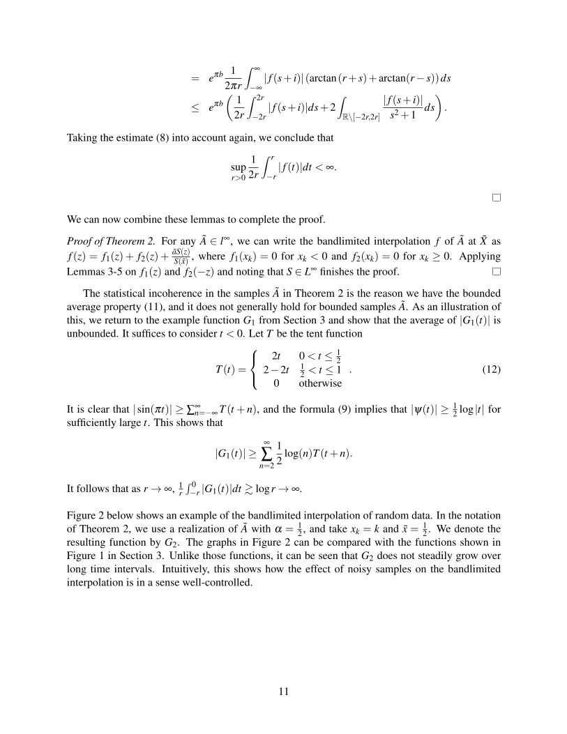
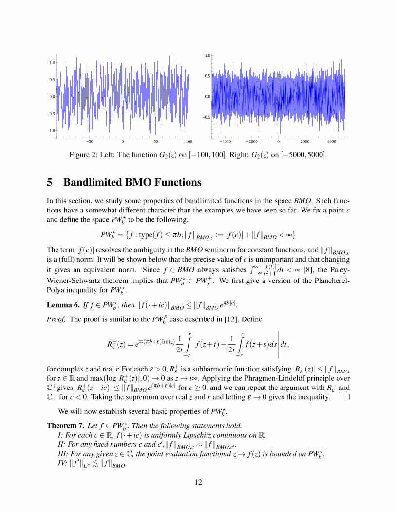
Figure 2 below shows an example of the bandlimited interpolation of random data. In the notationof Theorem 2, we use a realization of A with α = 1

2 , and take xk = k and x = 12 . We denote the

resulting function by G2. The graphs in Figure 2 can be compared with the functions shown inFigure 1 in Section 3. Unlike those functions, it can be seen that G2 does not steadily grow overlong time intervals. Intuitively, this shows how the effect of noisy samples on the bandlimitedinterpolation is in a sense well-controlled.

11

-50 0 50 100

-1.0

-0.5

0.0

0.5

1.0

-4000 -2000 0 2000 4000

-0.5

0.0

0.5

1.0

Figure 2: Left: The function G2(z) on [−100,100]. Right: G2(z) on [−5000,5000].

5 Bandlimited BMO FunctionsIn this section, we study some properties of bandlimited functions in the space BMO. Such func-tions have a somewhat different character than the examples we have seen so far. We fix a point cand define the space PW ?

b to be the following.

PW ?b = { f : type( f )≤ πb,‖ f‖BMO,c := | f (c)|+‖ f‖BMO < ∞}

The term | f (c)| resolves the ambiguity in the BMO seminorm for constant functions, and ‖ f‖BMO,cis a (full) norm. It will be shown below that the precise value of c is unimportant and that changingit gives an equivalent norm. Since f ∈ BMO always satisfies

∫∞

−∞

| f (t)|t2+1 dt < ∞ [8], the Paley-

Wiener-Schwartz theorem implies that PW ?b ⊂ PW+

b . We first give a version of the Plancherel-Polya inequality for PW ?

b .

Lemma 6. If f ∈ PW ?b , then ‖ f (·+ ic)‖BMO ≤ ‖ f‖BMO eπb|c|.

Proof. The proof is similar to the PW pb case described in [12]. Define

R±ε (z) = e∓(πb+ε)Im(z) 12r

r∫−r

∣∣∣∣∣∣ f (z+ t)− 12r

r∫−r

f (z+ s)ds

∣∣∣∣∣∣dt,

for complex z and real r. For each ε > 0, R+ε is a subharmonic function satisfying |R+

ε (z)| ≤ ‖ f‖BMOfor z ∈ R and max(log |R+

ε (z)|,0)→ 0 as z→ i∞. Applying the Phragmen-Lindelöf principle overC+gives |R+

ε (z+ ic)| ≤ ‖ f‖BMO e(πb+ε)|c| for c≥ 0, and we can repeat the argument with R−ε andC− for c < 0. Taking the supremum over real z and r and letting ε → 0 gives the inequality.

We will now establish several basic properties of PW ?b .

Theorem 7. Let f ∈ PW ?b . Then the following statements hold.

I: For each c ∈ R, f (·+ ic) is uniformly Lipschitz continuous on R.II: For any fixed numbers c and c′,‖ f‖BMO,c h ‖ f‖BMO,c′ .III: For any given z ∈ C, the point evaluation functional z→ f (z) is bounded on PW ?

b .IV: ‖ f ′‖L∞ . ‖ f‖BMO.

12

Proof. We set b = 1 without loss of generality. We can prove all of the above statements by usingthe reproducing kernel-like function

K(c, t) =|c|

πt(t− c)sin(

2πNc

t),

where c ∈ R\{0} and N is any integer greater than |c|. As a function of t, K(c, t) is entire andsatisfies 2π ≤ type(K)< ∞. For any f ∈ PW+

1 ,∫∞

−∞

f (t)K(c, t)dt = f (c)− f (0).

This can be seen by observing that for η =±1, the function cz(z−c) exp(2πiηNz/c) f (z) has poles

at c and 0 with respective residues η f (c) and −η f (0). The estimation argument is very similar tothe proof of Theorem 1, and we omit the details.

We now suppose that f ∈ PW ?1 . We want to approximate the H1(R) norm of K(c, t)−K(c′, t),

where c ≥ 1 and c′ ≥ 1. We first integrate the function 1π(z−s)

cz(z−c) exp(2πiηNz/c), where s ∈

R\{0,c}, and perform the same kind of calculation as before to find that

H K(c,s) = − 1πs− 1

π(c− s)+

cexp(2πiNs/c)2πs(c− s)

+cexp(−2πiNs/c)

2πs(c− s)

=c(cos(2πNs/c)−1)

πs(c− s).

Let N = max(dce,dc′e) and define the interval Iw := [w− 12 ,w+ 1

2 ]. We first consider the casewhere 1≤ c≤ 3

2 and |c− c′|> 12 . Recalling that T is the tent function (12), we have∥∥K(c, ·)−K(c′, ·)

∥∥L1

≤∫

∞

−∞

∞

∑n=−∞

(2cT (2Nt/c+n)

π |t(t− c)|+

2c′T (2Nt/c′+n)π |t(t− c′)|

)dt

≤ 16Nπ

+∫R\(I0⋃ Ic)

2cπ |t(t− c)|

dt +∫R\(I0⋃ Ic′)

2c′

π |t(t− c′)|dt

. |c− c′|.

Now suppose that 1≤ c≤ 32 and |c−c′| ≤ 1

2 , so that N = 2. Some elementary estimates show that∥∥K(c, ·)−K(c′, ·)∥∥

L1

.∫ 1/2

−1/2

∣∣∣∣4c − 4c′

∣∣∣∣dt +∫ 5/2

1/2max

(∣∣∣∣4c − sin(4πc/c′)π(c− c′)

∣∣∣∣ , ∣∣∣∣ 4c′− sin(4πc′/c)

π(c′− c)

∣∣∣∣)dt +∫R\(−1/2,5/2)

|c− c′||t|−3/2dt

. |c− c′|.

13

Following the same arguments, we can also obtain the bound ‖H K(c, ·)−H K(c′, ·)‖L1 . |c−c′|for the above choices of c and c′. By Fefferman’s duality theorem and the fact that K(c, ·)−K(c′, ·) ∈ U2, we have

‖ f‖BMO &1

‖K(c, ·)−K(c′, ·)‖H1(R)

∣∣∣∣∫ ∞

−∞

f (t)(K(c, t)−K(c′, t))dt∣∣∣∣& ∣∣∣∣ f (c)− f (c′)

c− c′

∣∣∣∣ , (13)

where the constant in the inequality is independent of c and c′. Since the BMO seminorm istranslation-invariant, the inequality (13) actually holds for all c,c′ ∈ R. Combining this withLemma 6 proves (I) and letting c′ → c gives (IV). If we fix R = |c− c′| > 0, this also showsthat ‖ f‖BMO + | f (c)|& | f (c′)|, where the implied constant depends on R, and we can interchangec and c′ to get (II). Finally, the statement (III) is just (II) phrased in a different way.

Remark. The closure of the set of uniformly continuous BMO functions under the BMO seminormis called V MO, for vanishing mean oscillation. Theorem 7 (I) shows that PW ?

b ⊂V MO. Note thatthere are two non-equivalent definitions of V MO in the literature, and we use the one given in [8].

Remark. Theorem 7 (IV) is a sharper form of the p =∞ case of Bernstein’s inequality. We mentionthat the opposite inequality does not generally hold (even if ‖ f‖BMO is replaced by ‖ f‖BMO,c), andthere are functions f such that f ′ ∈ PW ∞

b but f 6∈ PW ?b .

Corollary 8. Let f ∈ PW ?b . Then either f ∈ PW ∞

b or there is no separated sequence X withD−(X)> 0 such that f (X) ∈ l∞.

Proof. Suppose we have a separated X = {xk} with D−(X) > 0 and f (X) ∈ l∞. This means thatfor some large fixed r, every real interval I of length r contains a point xn ∈ X . Theorem 7 (IV)then shows that for any t ∈ I,

| f (t)|=∣∣∣∣ f (xn)+

∫ t

xn

f ′(u)du∣∣∣∣. | f (xn)|+ r‖ f‖BMO .

Intuitively, Corollary 8 says that an unbounded PW ?b function is large in most places on the

real line. It also shows that the bandlimited interpolation of bounded data A ∈ l∞ can never bein PW ?

b unless it is actually in PW ∞b . This occurs in spite of Lemma 4 and highlights a basic

difference between PW ?b and PW p

b , 1 < p < ∞. In Lemma 4, we generally cannot remove the fac-tor 1

S(·+ic) from the inequality and conclude that f ∈ BMO. In contrast, for A ∈ lp, the series (4)

can be used to find that f (·+ic)S(·+ic) ∈ Lp (see [10]), which clearly implies f (·+ ic)∈ Lp and thus f ∈ Lp.

We finally study an example of an unbounded PW ?b function that illustrates the “largeness”

property described above.

Example. The function G3(z) = ∑∞k=0(−1)k sin

(πz

3·2k

)is in PW ?

1/3\PW ∞

1/3.

14

To see this, we use the identity sinz = 12i

(eiz− e−iz) to write G3 = G3++G3−, where P(w, ·)?

G3± = G3±(w) for w ∈ C±, and then apply the Fefferman-Stein theorem (5) to each part. Letw = u+ iv. We first note that by analyticity,

|∇(P(w, ·)?G3+)|2 = |∇G3+(u+ iv)|2 = 2|G′3+(w)|2.

Since∣∣∣sin πz

3·2k

∣∣∣≤ ∣∣∣ πz3·2k

∣∣∣ for large k, the series defining G3 converges uniformly on compact sets, sowe have

N(

2v∣∣G′3+(w)∣∣2 dudv

)= N

2v

∣∣∣∣∣ ddw

12i

∞

∑k=0

eπi3 2−kw

∣∣∣∣∣2

dudv

≤ N

2ve−2π

3 v

(∞

∑k=0

π

3 ·2k

)2

dudv

≤ 2.

Doing the same calculation with G3−, we find that G3 ∈ PW ?1/3. On the other hand, G3 satisfies the

identity G3(2z) = sin(2πz3 )−G3(z). This implies that for integer n≥ 2,

G3(2n) = (−1)ng3(1)+n−1

∑k=0

(−1)n−k sin(

π2k

3

)= (−1)n

(g3(1)−

√3

2(n−2)

),

so G3 6∈ PW ∞

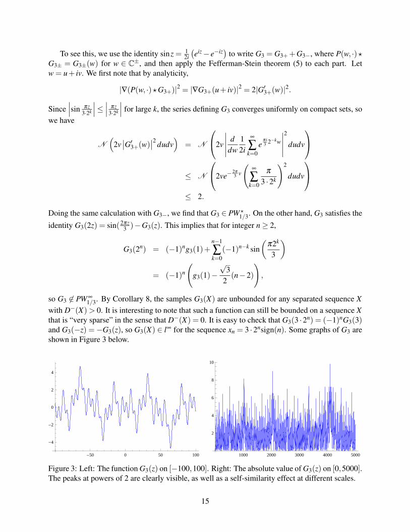
1/3. By Corollary 8, the samples G3(X) are unbounded for any separated sequence Xwith D−(X)> 0. It is interesting to note that such a function can still be bounded on a sequence Xthat is “very sparse” in the sense that D−(X) = 0. It is easy to check that G3(3 ·2n) = (−1)nG3(3)and G3(−z) =−G3(z), so G3(X) ∈ l∞ for the sequence xn = 3 ·2nsign(n). Some graphs of G3 areshown in Figure 3 below.

-50 0 50 100

-4

-2

0

2

4

1000 2000 3000 4000 5000

2

4

6

8

10

Figure 3: Left: The function G3(z) on [−100,100]. Right: The absolute value of G3(z) on [0,5000].The peaks at powers of 2 are clearly visible, as well as a self-similarity effect at different scales.

15

Acknowledgement. The author would like to thank Professor Ingrid Daubechies for many valuablediscussions in the course of this work.

References[1] Y. Belov, T. Y. Mengestie, and K. Seip. Unitary Discrete Hilbert Transforms. J. Analyse

Math., 2009.

[2] A. Beurling. Collected Works of Arne Beurling, Vol. 2: Harmonic Analysis. ContemporaryMathematicians. Birkhauser Boston, Boston, MA, 1989. Edited by L. Carleson, P. Malliavin,J. Neuberger and J. Wermer.

[3] H. Boche and U. J. Mönich. On the behavior of Shannon’s sampling series for boundedsignals with applications. Signal Processing, 88:492–501, 2007.

[4] H. Boche and U. J. Mönich. Convergence behavior of non-equidistant sampling series. SignalProcessing, 90:145–156, 2009.

[5] H. Boche and U. J. Mönich. Global and Local Approximation Behavior of ReconstructionProcesses for Paley-Wiener Functions. Sampling Theory in Signal and Image Proc., 8(1):23–51, 2009.

[6] R. Crochiere and L. R. Rabiner. Multirate Digital Signal Processing. Prentice Hall, Engle-wood Cliffs, NJ, 1983.

[7] C. Eoff. The Discrete Nature of the Paley-Wiener Spaces. Proc. American Math. Society,123(2):505–512, 1995.

[8] J. B. Garnett. Bounded Analytic Functions, Revised First Ed. Grad. Texts in Math. Springer,New York, NY, 2007.

[9] L. Hörmander. The Analysis of Linear Partial Differential Operators, volume I of Classics inMath. Springer, Berlin/Heidelberg, Germany, 2003.

[10] B. Ya. Levin. Lectures on Entire Functions. Number 150 in Transl. Math. Monographs.American Math. Society, Providence, RI, 1996.

[11] Y. Lyubarskii and K. Seip. Complete Interpolating Sequences and Muckenhoupt’s (Ap) Con-dition. Rev. Mat. Iberoamericana, 13(2):361–376, 1997.

[12] K. Seip. Interpolation and Sampling in Spaces of Analytic Functions. Number 33 in U. Lect.Series. American Math. Society, Providence, RI, 2004.

[13] E. M. Stein. Harmonic Analysis: Real-variable Methods, Orthogonality and OscillatoryIntegrals. Number 43 in Princeton Math. Series. Princeton U. Press, Princeton, NJ, 1993.

[14] E. T. Whittaker and G. M. Watson. A Course of Modern Analysis, Fourth Ed. CambridgeMath. Library. Cambridge U. Press, Cambridge, UK, 1927.

16

[15] R. M. Young. An Introduction to Nonharmonic Fourier Series, Revised First Ed. Number 93.Academic Press, San Diego, CA, 2001.

17