arX

iv:0

910.

1581

v2 [

hep-

th]

25 N

ov 2

009

YITP-09-56IPhT-t09/186

Boundary transitions of the O(n) model on a dynamical lattice

Jean-Emile Bourgine∗, Kazuo Hosomichi⋆ and Ivan Kostov∗1

∗ Institut de Physique Theorique, CNRS-URA 2306C.E.A.-Saclay,

F-91191 Gif-sur-Yvette, France

⋆ Yukawa Institute for Theoretical Physics, Kyoto UniversityKyoto 606-8502, Japan

We study the anisotropic boundary conditions for the diluteO(n) loop model with the methods of 2Dquantum gravity. We solve the problem exactly on a dynamicallattice using the correspondence witha largeN matrix model. We formulate the disk two-point functions with ordinary and anisotropicboundary conditions as loop correlators in the matrix model. We derive the loop equations for thesecorrelators and find their explicit solution in the scaling limit. Our solution reproduces the boundaryphase diagram and the boundary critical exponents obtainedrecently by Dubail, Jacobsen and Saleur,except for the cusp at the isotropic special transition point. Moreover, our solution describes the bulkand the boundary deformations away from the anisotropic special transitions. In particular it showshow the anisotropic special boundary conditions are deformed by the bulk thermal flow towards thedense phase.

1Associate member of the Institute for Nuclear Research and Nuclear Energy, Bulgarian Academy of Sciences, 72Tsarigradsko Chaussee, 1784 Sofia, Bulgaria

1 Introduction

The boundary critical phenomena appear in a large spectrum of disciplines of the contemporary the-oretical physics, from solid state physics to string theory. The most interesting situation is whenthe boundary degrees of freedom enjoy a smaller symmetry than those in the bulk. In this case onespeaks of surface anisotropy. The D-branes in string theoryare perhaps the most studied exampleof such anisotropic surface behavior. Another example is provided by the ferromagnets with surfaceexchange anisotropy, which can lead to a critical and multi-critical anisotropic surface transitions. Aninteresting but difficult task is to study the interplay of surface and the bulk transitions and the relatedmulti-scaling regimes.

For uniaxial ferromagnets as the Ising model, there are fourdifferent classes of surface transi-tions: the ordinary, extraordinary, surface, and special transitions [1]. This classification makes sensealso for spin systems with continuousO(n) symmetry. It was predicted by Diehl and Eisenriegler[2], using theε-expansion and renormalization group methods, that the effects of surface anisotropycan be relevant near the special transitions of thed-dimensionalO(n) model. These effects lead to‘anisotropic special transitions’ with different critical exponents.

Recently, an exact solution of the problem for the2-dimensionalO(n) model was presented byDubail, Jacobsen and Saleur [3] using its formulation as a loop model [4, 5]. Using an elaboratemixture of Coulomb gas, algebraic and Thermodynamic Bethe Ansatz techniques, the authors of [3]confirmed for the diluteO(n) model the phase diagram suggested in [2] and determined the exactscaling exponents of the boundary operators. A review of theresults obtained in [3], which is acces-sible for wider audience, can be found in [6]. Their works extended the techniques developped byJacobsen and Saleur [7, 8] for the dense phase of theO(n) loop model.

In this paper we examine the bulk and the boundary deformations away from the anisotropicspecial transitions in the two-dimensionalO(n) model. In particular, we address the question how theanisotropic boundary transitions are influenced by the bulkdeformation which relates the dilute andthe dense phases of theO(n) model. To make the problem solvable, we put the model on a dynamicallattice. This procedure is sometimes called ‘coupling to 2Dgravity’ [9, 10]. The sum over latticeserases the dependence of the correlation functions on the coordinates, so they become ‘correlationnumbers’. Yet the statistical model coupled to gravity contains all the essential information about thecritical behavior of the original model such as the qualitative phase diagram and the conformal weightsof the scaling operators. When the model is coupled to gravity, the bulk and boundary flows, originallydriven by relevant operators, becomes marginal, the Liouville dressing completing the conformalweights to one. This necessitates a different interpretation of the flows. The UV and the IR limitsare explored by taking respectively large and small values of the bulk and boundary cosmologicalconstants. Our method of solution is based on the mapping to the O(n) matrix model [11, 12] andon the techniques developed in [13, 14]. Using the Ward identities of the matrix model, we were ableto evaluate the two-point functions of the boundary changing operators for finite bulk and boundarydeformations away from the anisotropic special transitions.

The paper is structured as follows. In Sect.2 we summarize the known results about the boundarytransitions in theO(n) loop model. In Sect.3 we write down the partition function of the boundaryO(n) model on a dynamical lattice. In particular, we give a microscopic definition of the anisotropicboundary conditions on an arbitrary planar graph. In Sect.4 we reformulate the problem in terms oftheO(n) matrix model. We construct the matrix model loop observables that correspond to the disktwo-point functions with ordinary and anisotropic specialboundary conditions. In Sect.5 we write aset of Ward identities (loop equations) for these loop observables, leaving the derivation to AppendixA. We are eventually interested in the scaling limit, where the volumes of the bulk and the boundary

1

of the planar graph diverge. This limit corresponds to tuning the bulk and the boundary cosmologicalconstants to their critical values. In Sect.6 we write the loop equations in the scaling limit in the formof functional equations. From these functional equations we extract all the information about thebulk and the boundary flows. In particular, we obtain the phase diagram for the boundary transitions,which is qualitatively the same as the one suggested in [3, 6], apart of the fact that we do not observea cusp near the special point. In Sect.7 we derive the conformal weights of the boundary changingoperators. All our results concerning the critical exponents coincide with those of [3, 6]. In Sect.8 wefind the explicit solution of the loop equations in the limit of infinitely large planar graph. The solutionrepresents a scaling function of the coupling for the bulk and boundary perturbations. The endpointsof the bulk and the boundary flows can be found by taking different limits of this general solution.The boundary flows relate the anisotropic special transition with the ordinary or with the extraordinarytransition, depending on the sign of the perturbation. The bulk flow relates an anisotropic boundarycondition in the dilute phase with another anisotropic boundary condition in the dense phase. For therational values of the central charge, the boundary conditions associated with the endpoints of the bulkflow match with those predicted in the recent paper [15] using perturbative RG techniques.

2 The boundary O(n) model on a regular lattice: a summary

TheO(n) model [4] is one of the most studied statistical models. For the definition of the partitionfunction see Sect.3. The model has an equivalent description in terms of a gas of self- and mutuallyavoiding loops with fugacityn. The partition function of the loop gas depends on the temperaturecouplingT which controls the length of the loops:

ZO(n) =∑

loops

n#[loops] (1/T )#[links occupied by loops] . (2.1)

In the loop gas formulation of theO(n) model, the number of flavorsn can be given any real value.The model has a continuum transition if the number of flavors is in the interval[−2, 2]. Dependingon the temperature couplingT the model has two critical phases, the dense and the dilute phases. AtlargeT the loops are small and the model has no long range correlations. The dilute phase is achievedat the critical temperature [16, 17]

Tc =

√

2 +√

2 − n (2.2)

for which the length of the loops diverges. If we adopt for thenumber of flavors the standardparametrization

n = 2cos(πθ), 0 < θ < 1, (2.3)

then at the critical bulk temperature theO(n) model is described by (in general) a non-rational CFTwith central charge

cdilute = 1 − 6θ2

1 + θ. (2.4)

The primary operatorsΦr,s in such a non-rational CFT can be classified according to the generalizedKac table for the conformal weights,

hrs =(rg − s)2 − (g − 1)2

4g, g = 1 + θ. (2.5)

2

Unlike the rational CFTs, here the numbersr ands can take non-integer values.WhenT < Tc, the loops condense and fill almost all space. This critical phase is known as the

dense phase of the loop gas. The dense phase of theO(n) is described by a CFT with lower value ofthe central charge,

cdense = 1 − 6θ2

1 − θ. (2.6)

The generalized Kac table for the dense phase is

hrs =(rg − s)2 − (g − 1)2

4g, g =

1

1 − θ. (2.7)

Most of the exact results for the dense and the dilute phases of the O(n) model were obtained bymapping to Coulomb gas [5, 16].

The boundaryO(n) model was originally studied for the so calledordinary boundary condition,where the loops avoid the boundary as they avoid themselves.The ordinary boundary condition isalso referred asNeumann boundary conditionbecause the measure for the boundary spins is free. Theboundary scaling dimensions of theL-leg operatorsSL, realized as sources ofL open lines, wereconjectured for the ordinary boundary condition in [18] and then derived in [19]:

(Ord|SL|Ord) → ΦB1+L,1 (dilute phase)

(Ord|SL|Ord) → ΦB1,1+L (dense phase). (2.8)

Another obvious boundary condition is thefixed, or Dirichlet, boundary condition, which allows,besides the closed loops, open lines that end at the boundary[20].2 The dimensions of theL-legboundary operators with Dirichlet and Neumann boundary conditions were computed in [21, 22] bycoupling the model to 2D gravity and then using the KPZ scaling relation [23, 24]:

(Ord|SL|Dir) → ΦB1/2+L,0 (dilute phase)

(Ord|SL|Dir) → ΦB0,1/2+L (dense phase). (2.9)

From the perspective of the boundary CFT, these operators are obtained as the result of the fusionof theL-leg operator and a boundary-condition-changing (BCC) operator, introduced in [25], whichtransforms the ordinary into Dirichlet boundary condition.

Recently it was discovered that theO(n) loop model can exhibit unexpectedly rich boundary crit-ical behavior. Jacobsen and Saleur [7, 8] constructed a continuum of conformal boundary conditionsfor the dense phase of theO(n) loop model. TheJacobsen-Saleur boundary condition, which wedenote shortly by JS, prescribes that the loops that touch the boundary at least once are taken withfugacity y 6= n, while the loops that do not touch the boundary are counted with fugacityn. Theboundary parametery can take any real value. The JS boundary conditions contain as particular casesthe ordinary (y = n) and fixed (y = 1) boundary conditions for theO(n) spins. Jacobsen and Saleurconjectured the spectrum and the conformal dimensions of the L-leg boundary operators separatingthe ordinary and the JS boundary conditions. These conformal dimensions were subsequently veri-fied on the model coupled to 2D gravity in [13, 14]. If y is parametrized in the ‘physical’ interval0 ≤ y ≤ n as

y =sin π(r + 1)θ

sin πrθ(1 ≤ r ≤ 1/θ − 1), (2.10)

2 In the papers [20, 21, 22] the loop gas was considered in the context of the SOS model, for which the Dirichlet andNeumann boundary conditions have the opposite meaning.

3

then the BCC operator transforming the ordinary into JS boundary condition is identified as the diag-onal operatorΦr,r. Note thatr here is not necessarily integer or even rational. TheL-leg operatorswith L ≥ 1 fall into two types. The operatorS−

L creates open lines which avoid the JS boundary. TheoperatorS+

L creates open lines that can touch the JS boundary without restriction. The two types ofL-leg boundary operators are identified as

(Ord|S±L |JS) → ΦB

r,r±L (dense phase). (2.11)

The general case of two different JS boundary conditions with boundary parametersy1 andy2 wasconsidered for regular and dynamical lattices respectively in [26] and [27].

The JS boundary condition was subsequently adapted to the dilute phase by Dubail, Jacobsen andSaleur [3]. The authors of [3] considered the loop gas analog of the anisotropic boundaryinteractionstudied previously by Diehl and Eisenriegler [2], which breaks the symmetry as

O(n) → O(n(1)) × O(n(2)), n(1) + n(2) = n. (2.12)

The boundary interaction depends on two coupling constants, λ(1) andλ(2) , associated with the twounbroken subgroups. In terms of the loop gas, the anisotropic boundary interaction is defined byintroducing loops of two colors,(1) and(2), having fugacities respectivelyn(1) andn(2) . Each timewhen a loop of color(α) touches the JS boundary, it acquires an extra factorλ(α) . We will call thisboundary conditiondilute Jacobsen-Saleur boundary condition, or shortly DJS , after the authors of[3].

Let us summarize the qualitative picture of the surface critical behavior proposed in [3]. Considerfirst the isotropic directionλ(1) = λ(2) = λ. In the dilute phase one distinguishes three differentkinds of critical surface behavior: ordinary, extraordinary and special. Whenλ = 0, the loops inthe bulk almost never touch the boundary. This is the ordinary boundary condition. Whenw → ∞,the most probable loop configurations are those with one loopadsorbed along the boundary, whichprevents the other loops in the bulk to touch the boundary. The adsorbed loop plays the role of aboundary with ordinary boundary condition. This is the extraordinary transition. In terms of theO(n)spins, ordinary and the extraordinary boundary conditionsdescribe respectively disordered and or-dered boundary spins.3 The ordinary and the extraordinary boundary conditions describe the samecontinuous theory except for a reshuffling of the boundary operators. TheL-leg operator with or-dinary/extraordinary boundary conditions will look, whenL ≥ 1, as the(L − 1)-leg operator withordinary/ordinary boundary conditions, because its rightmost leg will be adsorbed by the boundary.The0-leg operator with ordinary/extraordinary boundary condition will look like the 1-leg operatorwith ordinary/ordinary boundary condition because one of the vacuum loops will be partially adsorbedby the extraordinary boundary and the part which is not adsorbed will look as an open line connectingthe endpoints of the extraordinary boundary.

The ordinary and the extraordinary boundary conditions areseparated by a special transition,which happens at someλ = λc and describes a conformal boundary condition. For the honeycomblattice the special point is known [28] to be at

λc = (2 − n)−1/2 T 2c (honeycomb lattice). (2.13)

At the special point the loops touch the boundary without being completely adsorbed by it. The specialtransition exists only in the dilute phase, because in the dense phase the loops already almost surely

3The spontaneous ordering on the boundary does not contradict the Mermin-Wagner theorem. In the interval1 < n < 2the target space, the(n − 1)-dimensional sphere, has negative curvature and thus resembles a non-compact space.

4

touch the boundary. The only effect of having small or largeλ is the reshuffling of the spectrum ofL-leg operators, which happens in the same way as in the dilutephase.

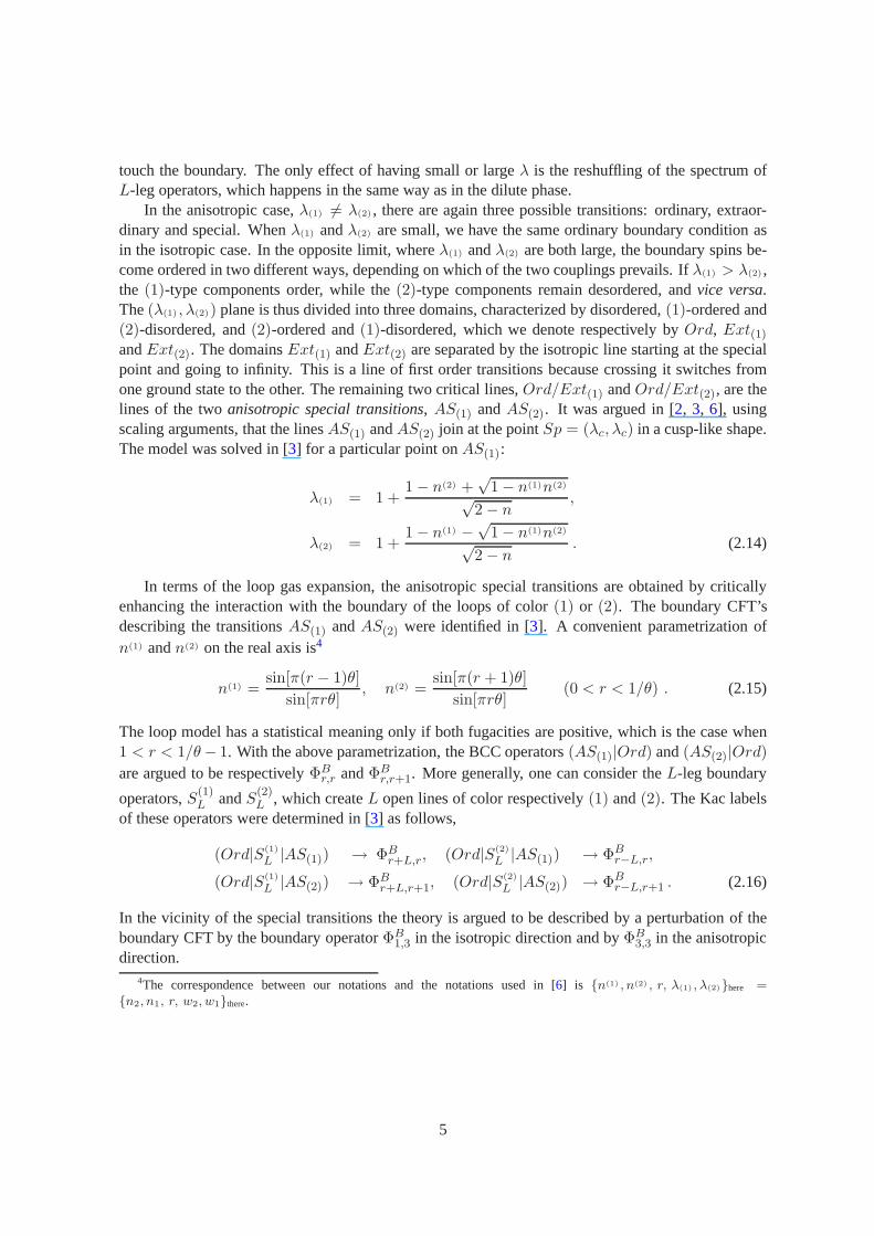
In the anisotropic case,λ(1) 6= λ(2) , there are again three possible transitions: ordinary, extraor-dinary and special. Whenλ(1) andλ(2) are small, we have the same ordinary boundary condition asin the isotropic case. In the opposite limit, whereλ(1) andλ(2) are both large, the boundary spins be-come ordered in two different ways, depending on which of thetwo couplings prevails. Ifλ(1) > λ(2) ,the (1)-type components order, while the(2)-type components remain desordered, andvice versa.The(λ(1) , λ(2)) plane is thus divided into three domains, characterized by disordered,(1)-ordered and(2)-disordered, and(2)-ordered and(1)-disordered, which we denote respectively byOrd, Ext(1)andExt(2). The domainsExt(1) andExt(2) are separated by the isotropic line starting at the specialpoint and going to infinity. This is a line of first order transitions because crossing it switches fromone ground state to the other. The remaining two critical lines,Ord/Ext(1) andOrd/Ext(2), are thelines of the twoanisotropic special transitions, AS(1) andAS(2). It was argued in [2, 3, 6], usingscaling arguments, that the linesAS(1) andAS(2) join at the pointSp = (λc, λc) in a cusp-like shape.The model was solved in [3] for a particular point onAS(1):

λ(1) = 1 +1 − n(2) +

√1 − n(1)n(2)

√2 − n

,

λ(2) = 1 +1 − n(1) −

√1 − n(1)n(2)

√2 − n

. (2.14)

In terms of the loop gas expansion, the anisotropic special transitions are obtained by criticallyenhancing the interaction with the boundary of the loops of color (1) or (2). The boundary CFT’sdescribing the transitionsAS(1) andAS(2) were identified in [3]. A convenient parametrization ofn(1) andn(2) on the real axis is4

n(1) =sin[π(r − 1)θ]

sin[πrθ], n(2) =

sin[π(r + 1)θ]

sin[πrθ](0 < r < 1/θ) . (2.15)

The loop model has a statistical meaning only if both fugacities are positive, which is the case when1 < r < 1/θ − 1. With the above parametrization, the BCC operators(AS(1)|Ord) and(AS(2)|Ord)

are argued to be respectivelyΦBr,r andΦB

r,r+1. More generally, one can consider theL-leg boundary

operators,S(1)L andS

(2)L , which createL open lines of color respectively(1) and(2). The Kac labels

of these operators were determined in [3] as follows,

(Ord|S(1)

L |AS(1)) → ΦBr+L,r, (Ord|S(2)

L |AS(1)) → ΦBr−L,r,

(Ord|S(1)

L |AS(2)) → ΦBr+L,r+1, (Ord|S(2)

L |AS(2)) → ΦBr−L,r+1 . (2.16)

In the vicinity of the special transitions the theory is argued to be described by a perturbation of theboundary CFT by the boundary operatorΦB

1,3 in the isotropic direction and byΦB3,3 in the anisotropic

direction.4The correspondence between our notations and the notationsused in [6] is n(1) , n(2) , r, λ(1) , λ(2)here =

n2, n1, r, w2, w1there.

5

3 The boundary O(n) model on a dynamical lattice

3.1 Anisotropic boundary conditions for the O(n) model on a planar graph

The two-dimensionalO(n) loop model, originally defined on the honeycomb lattice [4], can be alsoconsidered on a honeycomb lattice with defects, such as the one shown in Fig.1a. The lattice repre-sents a trivalent planar graphΓ. We define the boundary∂Γ of the graph by adding a set of extra lines(the single lines in the figure) which turn the original planar graph into a two-dimensional cellularcomplex. The local fluctuating variable is anO(n) classical spin, that is ann-component vector~S(r)with unit norm, associated with each vertexr ∈ Γ, including the vertices on the boundary∂Γ. Thepartition function of theO(n) model on the graphΓ depends on the couplingT , called temperature,and is defined as an integral over all classical spins,

ZO(n)

(T ; Γ) =

∫

∏

r∈Γ

[d~S(r)]∏

〈rr′〉

(

1 +1

T~S(r) · ~S(r′)

)

, (3.1)

where the product runs over the lines〈rr′〉 of the graph, excluding the lines along the boundary. TheO(n)-invariant measure[d~S] is normalized so that

∫

[d~S] SaSb = δa,b. (3.2)

The partition function (3.1) corresponds to theordinary boundary condition, in which there is nointeraction along the boundary.

Expanding the integrand as a sum of monomials, the partitionfunction can be written as a sumover all configurations of self-avoiding, mutually-avoiding loops as the one shown in Fig.1b, eachcounted with a factor ofn:

ZO(n)

(T ; Γ) =∑

loops onΓ

T−length n#loops. (3.3)

The temperature couplingT controls the length of the loops. The advantage of the loop gas represen-tation (3.3) is that it makes sense also for non-integern. In terms of loop gas, the ordinary boundarycondition, which we will denote byOrd, means that the loops in the bulk avoid the boundary as theyavoid the other loops and themselves.

The Dirichlet boundary condition, was originally defined for the dense phase of the loop gas[20, 21, 22] and requires that an open line starts at each point on the boundary. The dilute versionof this boundary condition depends on an adjustable parameter, which controls the number of theopen lines. In terms of theO(n) spins the Dirichlet boundary condition is obtained by switching ona constant magnetic field~B acting on the boundary spins. This modifies the integration measure in(3.1) by a factor

∏

r∈∂Γ

(

1 + ~B · ~S(r))

, (3.4)

where the product goes over all boundary sitesr. The loop expansion with this boundary measurecontains open lines having both ends at the boundary, each weighted with a factor~B2.

Thedilute anisotropic (DJS) boundary conditionis defined as follows. Then components of theO(n) spin are split into two sets,(1) and(2), containing respectivelyn(1) andn(2) components, withn(1) + n(2) = n. This leads to a decomposition of theO(n) spin as

~S = ~S(1) + ~S(2) , ~S(1) · ~S(2) = 0. (3.5)

6

a b

Figure 1: a) A trivalent planar graphΓ with a boundary b) A loop configuration onΓ for the ordinaryboundary condition. The loops avoid the boundary as they avoid themselves

(2)

(1)

Figure 2: A loop configuration for the JS boundary condition. The loopsin the bulk (in red) have fugacityn, while the loops that touch the boundary (in blue and green) have fugacitiesn(1) or n(2) depending on theircolor.

The DJS boundary condition is introduced by an extra factor associated with the boundary links,

∏

〈 rr′〉∈∂Γ

(

1 +∑

α=1,2

λ(α)~S(α)(r) · ~S(α)(r′)

)

. (3.6)

This boundary interaction is invariant under the subgroup of independent rotations of~S(1) and ~S(2).The boundary term changes the loop expansion. The loops are now allowed to pass along the boundarylinks as shown in Fig.2. We have to introduce loops of two colors,(1) and (2), having fugacitiesrespectivelyn(1) andn(2) . A loop of color (α) that visitsN boundary links acquires an additionalweight factorλN

(α) . For the loops that do not touch the boundary, the contributions of the two colorssum up ton(1) + n(2) = n and we obtain the same weight as with the ordinary boundary condition.

3.2 Coupling to 2D discrete gravity

The disk partition function of theO(n) model on a dynamical lattice is defined as the expectation valueof (3.1) in the ensemble of all trivalent planar graphsΓ with the topology of the disk. The measuredepends on two more couplings,µ andµB , called respectively bulk and boundary cosmological con-

7

stants,5 associated with the volume|Γ| = #(cells) and the boundary length|∂Γ| = #(external lines).The partition function of the disk is a function ofµ andµB and is defined by

U(T, µ, µB) =∑

Γ∈Disk

1

|∂Γ|

(

1

µ

)|Γ|( 1

µB

)|∂Γ|

ZO(n)

(T ; Γ). (3.7)

3.3 Two-point functions of the L-leg boundary operators

Our aim is to evaluate the boundary two-point function of twoL-leg operators separating ordinaryand anisotropic boundary conditions. TheL-leg operatorSL is obtained by fusingL spins with flavorindicesa1, . . . , an ∈ 1, . . . , n. In terms of the loop gas, the operatorSL createsL self and mutuallyavoiding open lines. We would like to exclude configurationswhere some of the lines contract amongthemselves. This can be achieved by taking the antisymmetrized product

SL ∼ detL×L

Sai(rj), (3.8)

wherer1, . . . , rL areL consecutive boundary vertices of the planar graphΓ, and we put the labelLinstead of writing its dependence ona1, . . . , aL explicitly. The two-point function of the operatorSL

is evaluated as the partition function of the loop gas in presence ofL open lines connecting the pointsri andr′i. The open lines are self- and mutually avoiding, and are not allowed to intersect thevacuum loops.

Since the DJS boundary condition breaks theO(n) symmetry intoO(n(1)) × O(n(2)), there aretwo inequivalent correlation functions of theL-leg operators withOrd/DJS boundary conditions.Indeed, the insertion ofSa has different effects depending on whethera belongs to theO(n(1)) or theO(n(2)) sectors. In the first case the open line created bySa acquires a factorλ(1) each time it visitesa boundary link. In the second case, the factor isλ(2) . Therefore the boundary spin operators (3.8)with Ord/DJS boundary conditions split into two classes,

S(1)L ∼ det[Sai

(rj)] , a1, . . . , aL ∈ (1),

S(2)L ∼ det[Sai

(rj)] , a1, . . . , aL ∈ (2). (3.9)

We denote the corresponding boundary two-point functions respectively byD(1)L andD

(2)L .

4 Mapping to the O(n) matrix model

The O(n) matrix model [11, 12] generates planar graphs covered by loops in the same way as theone-matrix models considered in the classical paper [29] generate empty planar graphs. The modelinvolves the hermitianN × N matricesM andYa, where the flavor indexa takesn values. Thepartition function is given by anO(n)-invariant matrix integral

ZN (T ) ∼∫

dM dnY e−β tr( 12M

2+ T2

~Y2− 13M

3−M~Y2). (4.1)

This integral can be considered as the partition function ofa zero-dimensional QFT with Feynmanrules given in Fig.3, where we used the ’t Hooft double-line notations. The graphs made of such

5We used bars to distinguish from the bulk and boundary cosmological constants in the continuum limit.

8

aa

i ij

j

k

k

i ij

j

k

k

ij

ij

i i

j j

1/β 1/βT β β

Figure 3:Feynman rules for theO(n) matrix model

i

i

j

j

i

i j

j

j

ji

ik k k k

1/µB λ(1)/µ2B λ(2)/µ2

B

Figure 4: The constituents of the DJS boundary generated byM, ~Y2(1) and ~Y2

(2): a non-occupied site, asequence of two sites visited by a loop of color(1), and a sequence of two sites visited by a loop of color(1)

double-lined propagators are known as fat graphs. The ‘vacuum energy’ of the matrix model repre-sents a sum over connected fat graphs, which can be also considered as discretized two-dimensionalsurfaces of all possible genera. As the action is quadratic in the matricesYa, their propagators arrangein closed loops carrying a flavora. The sum of all Feynman graphs with given connectivity can beviewed as the sum over all configurations of self and mutuallyavoiding loops on a given discretizedsurface. The weight of each loop is given by the product of factors 1/T , one for each link, and thenumber of flavorsn. We are interested in the largeN limit

N → ∞, β/N = µ2 (fixed) , (4.2)

in which only fat graphs of genus zero survive [30].The basic observable in the matrix model is the resolvent

W (µB) =1

β

⟨

tr1

µB − M

⟩

, (4.3)

evaluated in the ensemble (4.1). The resolvent is the one-point function with ordinary boundaryconditions and is related to the disk partition function byW = −∂µB

U .The one-point function with Dirichlet boundary condition is obtained by adding a term~B·~Y which

expresses the coupling with the magnetic field on the boundary. This leads to a more-complicatedresolvent

R(µB, ~B2) =1

β

⟨

tr1

µB − M − ~B · ~Y

⟩

. (4.4)

In order to include the anisotropic boundary conditions in this scheme, we decompose the vector~Y into a sum of ann(1)-component vector~Y(1) and ann(2)-component vector~Y(2) as in (3.5):

~Y = ~Y(1) + ~Y(2) , ~Y(1) · ~Y(2) = 0. (4.5)

9

The one-point function with ordinary and DJS boundary conditions is given by the resolvent

H(µB , λ(1) , λ(2)) =1

β

⟨

tr1

µB − M− 1µB

∑

α=1,2 λ(α)~Y2

(α)

⟩

. (4.6)

The two extra terms are the operators creating boundary links containing segments of lines of type(1)and(2), as shown in Fig.4. Each such operator created two boundary sites, hence the factor 1/µB .

The matrix integral measure becomes singular atM = T/2. We perform a linear change of thevariables

M = T(

12 + X

)

, (4.7)

which sends this singular point toX = 0. After a suitable rescaling of~Y andβ, the matrix modelpartition function takes the canonical form

ZN ∼∫

dX dnYeβtr[−V (X)+X~Y2] , (4.8)

whereV (x) is a cubic potential

V (x) =3∑

j=0

gj

jxj = −T

3

(

x + 12

)3+

1

2

(

x + 12

)2. (4.9)

We introduce the spectral parameterx which is related to the lattice boundary cosmological constantµB by

µB = T(

x + 12

)

. (4.10)

Now the one-point function with ordinary boundary condition is

W (x) =1

β〈trW(x)〉 , (4.11)

where the matrix

W(x)def=

1

x − X. (4.12)

creates a boundary segment with open ends. In the following we will call x boundary cosmologicalconstant. We also redefine the boundary couplingsλ(α) in (4.6) as

λ(α) → λ(α) µB, α = 1, 2 . (4.13)

Then the operator that creates a boundary segment with DJS boundary condition is

H(y)def=

1

y − X− λ(1)~Y2

(1) − λ(2)~Y2

(2)

. (4.14)

The boundaryL-leg operators are represented by the antisymmetrized products

SLdef= Ya1Ya2 · · ·YaL

± permutations. (4.15)

The boundary two-point function of theL-leg operator withOrd/Ord boundary conditions is givenby the expectation value

DL(x1, x2)def=

1

β

⟨

tr[

W(x1)SLW(x2)SL

]⟩

. (4.16)

10

The role of the operatorsW(x1) andW(x2) is to create the two boundary segments with boundarycosmological constants respectivelyx1 andx2. The two insertionsSL generateL open lines at thepoints separating the two segments. It is useful to extend this definition to the caseL = 0, assumingthatS0 is the boundary identity operator. In this simplest case theexpectation value (4.16) is evaluatedinstantly as

D0(x1, x2) =1

β

⟨

tr[

W(x1)W(x2)]⟩

=W (x2) − W (x1)

x1 − x2. (4.17)

The two-point functions (4.16) for L ≥ 1 were computed in [21, 22].In the case of a DJS boundary condition, the matrix model realization of the two types of bound-

aryL-leg operators is given by the antisymmetrized products (4.15), with the restrictions on the com-ponents as in (3.9). The boundary two-point functions withOrd/DJS boundary conditions areevaluated by the expectation values

D0(x, y) =1

β

⟨

tr[

W(x)H(y)]

⟩

(4.18)

and forL ≥ 1,

D(1)L (x, y) =

1

β

⟨

tr[

W(x)S(1)L H(y)S

(1)L

]

⟩

, (4.19)

D(2)L (x, y) =

1

β

⟨

tr[

W(x)S(2)L H(y)S

(2)L

]

⟩

. (4.20)

Apart of the DJS boundary parametern(1) and the boundary couplingsλ(1) , λ(2) for the second seg-ment, they depend on the boundary cosmological constantsx andy associated with the two segmentsof the boundary.

5 Loop equations

Our goal is to evaluate the two-point functions (4.19) in the continuum limit, when the area andthe boundary length of the disk are very large. They will be obtained as solution of a set of Wardidentities, called loop equations, which follow from the translational invariance of the integrationmeasure in (4.1), and in which then(1) enters as a parameter. The solutions of the loop equations areanalytic functions ofn(1) which can take any real value. We will restrict our analysis to the ‘physical’case0 ≤ n(1) ≤ n, when the correlation functions have good statistical limit. Here we summarizethe loop equations which will be extensively studied in following sections. The proofs are given inAppendixA.

5.1 Loop equation for the resolvent

The loop equation for the resolvent is known [31], but we nevertheless recall it here in order to set upa self-contained description of the method. The resolventW (x) splits into a singular partw(x) and apolynomialWreg(x):

W (x)def= Wreg(x) + w(x) . (5.1)

11

The regular part is given by

Wreg(x) =2V ′(x) − nV ′(−x)

4 − n2= −a0 − a1x − a2x

2 ,

a0 = − g1

2 + n=

T − 2

4(2 + n),

a1 = − g2

2 − n=

T − 1

2 − n,

a2 = − g3

2 + n=

T

2 + n. (5.2)

The functionw(x) satisfies a quadratic identity

w2(x) + w2(−x) + nw(x)w(−x) = A + Bx2 + Cx4 . (5.3)

The coefficientsA,B,C as functions ofT , µ andW1 = 〈trX〉 can be evaluated by substituting thelarge-x asymptotics

w(x) = −Wreg(x) +µ−2

x+

〈trX〉βx2

+ O(x−3) (5.4)

in (5.3). The solution of the loop equation (5.3) with the asymptotics (5.4) is given by a meromorphicfunction with a single cut[a, b] on the first sheet, witha < b < 0. This equation can be solved by anelliptic parametrization and the solution is expressed in terms of Jacobi theta functions [32].

5.2 Loop equations for the boundary two-point functions with Ord/DJS boundaryconditions

The two-point correlators (4.16) with ordinary boundary conditions are known to satisfy theintegralrecurrence equations [21, 22]

DL+1 = W ⋆ DL . (5.5)

The “⋆-product” is defined for any pair of meromorphic functions, analytic in the right half planeRe(x) ≥ 0 and vanishing at infinity,

[f ⋆ g](x)def= −

∮

C−

dx′

2πi

f(x) − f(x′)

x − x′g(−x′), (5.6)

with the contourC− encircling the left half plane Rex < 0. These equations actually hold for a moregeneral set of two-point correlators, which have ordinary boundary condition on one segment and anarbitrary boundary condition on the other segment [13]. Thus the boundary two-point functions (4.19)and (4.20) for L ≥ 1 satisfy the same recurrence equations

D(1)L+1 = W ⋆ D

(1)L ,

D(2)L+1 = W ⋆ D

(2)L . (5.7)

Using the recurrence relation, the correlation functions of the L-leg operators can be obtained recur-sively from those of the one-leg operatorsD

(1)1 andD

(2)1 .

12

The correlatorD0, defined by (4.18), and the correlatorsD(1)1 andD

(2)1 , which we normalize as

D(α)1 (x, y) =

1

βn(α)

∑

a

⟨

tr[

W(x)Y(α)a H(y)Y(α)

a

]

⟩

(α = 1, 2), (5.8)

can be determined by the following pair of bilinear functional equations, derived in AppendixA. Inorder to shorten the expressions, here and below we use the shorthand notation

F (x)def= F (−x) . (5.9)

The two equations then read

W − H + D0(x − y) +∑

α=1,2

n(α)λ(α)

(

(λ(α)D0 − 1)D(α)1 + W D0

)

= 0 , (5.10)

P + D0

(

H − V ′ + W + nW)

+∑

α=1,2

n(α) (λ(α)D0 − 1) D(α)1 = 0 . (5.11)

The second equation involves an unknown linear function ofx:

P (x, y)def=

1

β

⟨

trV ′(x) − V ′(X)

x − XH(y)

⟩

= g2H(y) + g3H1(y) + xg3H(y). (5.12)

Equations (5.10) and (5.11) can be solved in favor ofD(1)1 or D

(2)1 . If we define

A(1) def= λ(1)D0 − 1,

B(1) def= (λ(1) − λ(2))n(1)λ(1)D

(1)1 + W − λ(2)

(

W − V ′ + H)

− x − y, (5.13)

C(1) def= λ(1)λ(2)P + (λ(1) + λ(2))H − x + y − (λ(1) − λ(2))

(

W + n(1)W)

− λ(2)V ′ ,

and similarly forA(2),B(2), C(2), with an obvious exchange(1) ↔ (2), then (5.10) and (5.11) takethe following factorized form:

A(α)B(α) = C(α) (α = 1, 2) . (5.14)

Equations (5.14) are the main instrument of our analysis of the DJS boundary conditions.It is convenient to define the functionsD(α)

0 by

D(α)0

def=

D0

1 − λ(α)D0(α = 1, 2) . (5.15)

In AppendixA we show that with this definition the recurrence equations (5.7) hold also forL = 0.The equation forL = 0 is a consequence of (5.14).

5.3 Loop equation for the two-point function with Ord/Dir boundary conditions

On the flat lattice, the DJS boundary condition withn(1) = 1 is equivalent, for a special choice ofthe boundary parameters, to the Dirichlet boundary condition defined by the boundary factor (3.4). Inorder to make the comparison on the dynamical lattice, we will formulate and solve the loop equationfor the two-point function of the BCC operator with ordinary/Dirichlet boundary conditions.

13

Assume that the magnetic field points at the directiona = 1. Then the correlator in question isgiven in the matrix model by the expectation value

Ω(x, y) =1

β〈 trW(x)R(y) 〉 , R(y) =

1

y − X− BY1. (5.16)

To obtain the loop equation we start with the identity

W (x) − R(y) = (y − x)Ω(x, y) − BΩ1(x, y), (5.17)

where we denoted byR(y) the one-point function with Dirichlet boundary condition,

R(x) =1

β〈 trR(y) 〉 , (5.18)

and introduced the auxiliary function

Ω1(x, y) =1

β〈 trY1W(x)R(y) 〉 . (5.19)

The functionΩ1 satisfies the identity

Ω1(x, y) = B

∮

C−

dx1

2πi

Ω(x1, y)Ω(−x1, y)

x − x1, (5.20)

which follows from (A.3). After symmetryzing with respect tox we get

Ω1(x, y) + Ω1(−x, y) = B Ω(x, y)Ω(−x, y). (5.21)

From here we obtain a quadratic functional equation for the correlatorΩ:

(x − y)Ω(x, y) − (x + y)Ω(−x, y) + W (x) + W (−x) + B2 Ω(x, y)Ω(−x, y) = 2R(y). (5.22)

The linear term can be eliminated by a shift

G(x, y) = B Ω(x, y) − x + y

B. (5.23)

The functionG satisfies

G(x, y)G(−x, y) = −W (x) − W (−x) + 2R(y) − x2 − y2

B2. (5.24)

This equation is to be compared with the loop equation (5.14) for Ord/DJS boundary conditions, withn(1) = 1 andλ(2) = 0:

1

λ(1)

A(1)(x, y)B(1)(−x, y) = − W (x) − W (−x) + H(y) − x − y

λ(1)

. (5.25)

These two equations coincide in the limitB,λ(1) → ∞. To see this it is sufficient to notice thatin the limit λ(1) → ∞ we have the relationB(1) = yA(1). The exact relation betweenA(1) (withn(1) = 1, λ(2) = 0) andG in this limit follows from the definitions ofD0 andΩ:

A(1)(x, y′) = BG(x, y) − G(x,−y)

2y, λ(1) = B2, y′ = y2 (B → ∞). (5.26)

14

6 Scaling limit

In this section we will study the continuum limit of the solution, in which the sum over lattices isdominated by those with diverging area and boundary length.The continuum limit is achieved whenthe couplingsx, y andµ are tuned close to their critical values.

Once the bulk coupling constants are set to their critical values, we will look for the critical linein the space of the boundary couplingsy, λ(1) andλ(2) . After the shift (4.7) the bondary cosmologicalconstantx has its critical value atx = 0, while the critical value ofy in general depends on the valuesof λ(1) andλ(2) .

6.1 Scaling limit of the disk one-point function

Here we recall the derivation of the continuum limit of the one-point functionW (x) from the func-tional equation (5.3). Even if the result is well known, we find useful to explain how it is obtained inorder to set up the logic of our approach to the solution of thefunctional equations (5.14).

In the limit x → 0, the boundary length|∂Γ| of the planar graphs in (3.7) becomes critical. Thequadratic functional equation (5.3) becomes singular atx → 0 when the coefficientA on the r.h.s.vanishes. This determines the critical value of the cosmological constantµ, for which the volume|Γ|of a typical planar graph diverges. The condition that the coefficient B of the linear term vanishesdetermines the critical value of the temperature couplingT = Tc for which the length of the loopsdiverges:

Tc = 1 +√

2−n6+n ∈ [1, 2] . (6.1)

Near the critical temperature the coefficientB is proportional toT − Tc.We rescalex → ǫx, whereǫ is a small cutoff parameter with dimension of length, and define the

renormalized coupling constants as

µ − µc ∼ ǫ2µ , T − Tc ∼ ǫ2θt (6.2)

and write (5.1) as

W (x)def= Wreg + ǫ1+θw(x) . (6.3)

The renormalized bulk and boundary cosmological constantsare coupled respectively to the renor-malized areaA and boundary lengthℓ of the graphΓ defined as

A = ǫ2 |Γ|, ℓ = ǫ |∂Γ| . (6.4)

In the following we define the dimensions of the scaling observables by the way they scale withx. Wewill say that the quantityf has dimensiond if the ratiof/xd is invariant with respect to rescalings. Inthis case we write[f ] = d. The continuous quantities introduced until now have scaling dimensions

[x] = 1, [µ] = 2, [t] = 2θ, [w] = 1 + θ . (6.5)

The scaling resolventw(x) is a function with a cut on the negative axis in thex-plane. It canbe obtained from the general solution found in [32] by taking the limit in which the cut extends tothe semi-infinite interval[−∞,−M ]. To determineM as a function ofµ and t one has to solve asystem of difficult transcendental equations. A simpler indirect method was given in [33]. We beginby noticing that the termCx4 in (5.3) drops out because it vanishes faster than the other terms when

15

x → 0, andB = B1 t, whereB1 depends only onn. Introducing a hyperbolic map which resolvesthe branch point atx = −M ,

x = M cosh τ , (6.6)

we obtain a quadratic functional equation for the entire function w(τ) ≡ w[x(τ)]:

w2(τ + iπ) + w2(τ) + n w(τ + iπ)w(τ) = A + B1tM2 cosh2 τ . (6.7)

This equation does not depend on the cutoffǫ, which justifies the definition of the renormalizedthermal coupling in (6.2). Then the unique solution of this equation is, up a factor which depends onthe normalization oft,

w(τ) = M1+θ cosh(1 + θ)τ + tM1−θ cosh(1 − θ)τ . (6.8)

One findsB1 = 4 sin2(πθ) andA = sin2(πθ)(M1+θ − tM1−θ)2 for this solution.The functionM = M(µ, t) can be evaluated using the fact that the derivative∂µW (x) depends

onµ andt only throughM . As a consequence, in the derivative of the solution inµ at fixedx,

∂µw = −M∂µM(

(1 + θ)Mθ − (1 − θ)tM−θ) sinh θτ

sinh τ, (6.9)

the factor in front of the hyperbolic function must be proportional toMθ−1:

∂µM(

(1 + θ)Mθ − (1 − θ)tM−θ)

∼ Mθ−1.

Integrating with respect toµ one finds, for certain normalization ofµ,

µ = (1 + θ)M2 − tM2−2θ. (6.10)

To summarize, the disk bulk and the boundary one-point functions with ordinary boundary condi-tion,−∂µU and−∂xU , are given in the continuum limit in the following parametric form:

− ∂xU |µ = M1+θcosh((1 + θ)τ) + t M1−θcosh(1 − θ)τ , (6.11)

−∂µU |x ∼ Mθ cosh θτ,

x = M cosh τ,

with the functionM(µ, t) determined from the transcendental equation (6.10). The expression for∂µU was obtained by integrating (6.9).

The functionM(t, µ) plays an important role in the solution. Its physical meaning can be revealedby taking the limitx → ∞ of the bulk one-point function−∂µU(x). Sincex is coupled to the lengthof the boundary, in the limit of largex the boundary shrinks and the result is the partition function oftheO(n) field on a sphere with two punctures, the susceptibilityu(µ, t). Expanding atx → ∞ wefind

− ∂µU ∼ xθ − M2θ x−θ + lower powers ofx (6.12)

(the numerical coefficients are omitted). We conclude that the string susceptibility is given, up to anormalization, by

u = M2θ. (6.13)

16

The normalization ofu can be absorbed in the definition of the string coupling constant gs ∼ 1/β.Thus the transcendental equation (6.10) for M gives the equation of state of the loop gas on the sphere,

(1 + θ)u1θ − t u

1−θθ = µ . (6.14)

The equation of state (6.14) has three singular points at which the three-point function of theidentity operator∂µu diverges. The three points correspond to the critical phases of the loop gas onthe sphere. At the critical pointt = 0 the susceptibility scales asu ∼ µθ. This is the dilute phaseof the loop gas, in which the loops are critical, but occupy aninsignificant part of the lattice volume.The dense phase is reached whent/xθ → −∞. In the dense phase the loops remain critical but

occupy almost all the lattice and the susceptibility has different scaling,u ∼ µ1−θ

θ . The scaling of thesusceptibility in the dilute and in the dense phases match with the values (2.4) and (2.6) of the centralcharge of the corresponding matter CFTs. Considered on the interval−∞ < t < 0, the equation ofstate (6.14) describes the massless thermal flow [34] relating the dilute and the dense phases.

At the third critical point∂µM becomes singular butM itself remains finite. It is given by

tc =1 + θ

1 − θM2θ

c > 0, µc = −θ1 + θ

1 − θM2

c < 0. (6.15)

Around this critical pointµ − µc ∼ (M − Mc)2 + · · · , hence the scaling of the susceptibility is that

of pure gravity,u ∼ (µ − µc)1/2.

6.2 The phase diagram for the DJS boundary condition

We found the scaling limit of the one-point function (4.11) as a function of the renormalized bulkcouplings,µ and t, and the couplingx characterizing the ordinary boundary. Now, analyzing theloop equation (5.14) for the two-point functions, we will look for the possible scaling limits for thecouplingsy, λ(1) andλ(2) , characterizing the DJS boundary.

As in the previous subsection, we will write down the conditions that the regular parts of thesource termsC(α) vanish. Let us introduce the isotropic couplingλ and the anisotropic coupling∆ as

λ(1) = λ + 12∆, λ(2) = λ − 1

2∆ (6.16)

and substitute (5.1) in the r.h.s. of (5.14). We obtain

C(1) = c0 + c1x + c2x2 − ∆(w + n(1)w) ,

C(2) = c0 + c1x + c2x2 + ∆(w + n(2)w) , (6.17)

where the coefficientsc0 andc1 are functions ofλ and∆:

c0 = (λ2 − 14∆2)(g2H + g3H1) + 2λH + y − λg1 − ∆

g1(n(1) − n(2))

2(2 + n)(6.18)

c1 = (λ2 − 14∆2)g3H − 1 − λg2 + ∆

g2(n(1) − n(2))

2(2 − n). (6.19)

c2 = −g3

(

λ +n(1) − n(2)

2(2 + n)∆

)

. (6.20)

For generic values of the couplingsy, λ and∆, the coefficientc0 is non-vanishing. The conditionc0 = 0 determines the critical valueyc where the length of the DJS boundary diverges.6 Once the

6 Indeed, the termc0 is the dominant term whenx → 0. Forc0 6= 0 the solution forA(α) andB(α) in (5.14) is given bylinear functions ofx andw. Such a solution describes the situation when the length of the DJS boundary is small and thetwo-point function degenerates to a one-point function.

17

boundary cosmological constant is tuned to its critical value, the conditionc1 = 0 determines thecritical lines in the space of the couplingsλ(1) andλ(2) , where the DJS boundary condition becomesconformal. The two equations

c0(y, λ,∆) = 0, c1(y, λ,∆) = 0 (µ = t = 0) (6.21)

define a one-dimensional critical submanifold in the space of the boundary couplingsy,m,∆:

λ = λ∗(∆) . (6.22)

ObviouslyA(1) andA(2) cannot be simultaneously zero. Therefore the curve (6.22) consists of twobranches, which correspond to different conformal DJS boundary conditions, the lines of anisotropicspecial transitionsAS(1) andAS(2):

AS(1) : A(1) = 0, A(2) 6= 0;

AS(2) : A(2) = 0, A(1) 6= 0. (6.23)

The branchAS(1) corresponds to∆ > 0, while the branchAS(2) corresponds to∆ < 0. Consider

the behavior of correlatorsD(α)0 on the two branches of the critical line. By the definition (5.15), the

two correlatorsD(1)0 andD

(2)0 are related by

D(1)0 =

D(2)0

1 − ∆D(2)0

, D(2)0 =

D(1)0

1 + ∆D(1)0

. (6.24)

On the branchAS(1) the correlatorD(1)0 diverges whileD(2)

0 remines finite, andvice versa. Assume

thatλ(1) andλ(2) are positive. ThenD(α)0 are both positive by construction. If∆ = λ(1) − λ(2) > 0,

then the coefficients of the geometric series

D(1)0 =

∞∑

k=0

∆k(

D(2)0

)k+1(6.25)

are all positive andD(1)0 diverges, whileD(2)

0 → 1/∆. Thus the branchAS(1), whereD(1)0 diverges,

is associated with∆ > 0. On this branch the probability that the loops of color(1) touch the DJS

boundary is critically enhanced. In the correlatorD(1)0 , the ordinary boundary behaves as a loop of

type(1) and can touch the DJS boundary. The geometrical progression(6.25) reflects the possibilityof any number of such events, each contributing a factor∆. Conversely, the ordinary boundary for thecorrelatorD(2)

0 behaves as a loop of type(2), since such loops almost never touch the DJS boundary.On the branchAS(2) the situation is reversed.

It is not possible to solve explicitly the conditions of criticality (6.21) without extra information,because they contain two unknown functions of the three couplings, H andH1. Nevertheless, thequalitative picture can be reconstructed.

First let us notice that the form of the critical curve can be evaluated in the particular casesn(1) = nandn(1) = 0. In the first casen(2) = 0 and the correlation functions do not depend onλ(2) and so thecoefficientsc1 andc2 depend onλ and∆ through the combinationλ(1) = λ + ∆/2. Similarly oneconsiders the casen(1) = 0. The phase diagram in these two cases represents an infinite straight lineseparating the ordinary and the extraordinary transitions:

λ∗(∆) =

λc − ∆/2 if n(1) = n,

λc + ∆/2 if n(1) = 0.(6.26)

18

ExtAS

AS(2)

(2)λ

λ(1)

(1)

∆

Sp λ

Ext

Ord

(1)

(2)

Figure 5: Phase diagram in the rotated(λ(1) , λ(2)) plane forn < 1 andn(1) > n(2) . The ordinary and theextraordinary phases are separated by a line of anisotropicspecial transitions, which consists of two branches,AS(1) andAS(2). The two extraordinary phases,Ext(1) andExt(2), are separated by the isotropic line∆ = 0

The critical line crosses the axis∆ = 0 at the special pointλ = λc. The value ofλc can be evaluatedby solving (6.21) for n(1) = n andλ(2) = 0. The result is

λc =

√

(6 + n)(2 − n)

1 − n. (6.27)

For generaln(1) ∈ [0, n] we can determine three points of the critical curve:

λ(1) , λ(2) = 1 − n

1 − n(1)λc, 0, 0, 1 − n

1 − n(2)λc, λc, λc . (6.28)

In the two limiting cases considered above the critical line, given by equation (6.26), crosses theanisotropic line without forming a cusp. Is this the case in general? Let us consider the vicinity of thespecial point(λ,∆) = (λc, 0). In the vicinity of the special point a new scaling behavior occurs. Inthis regime the termx2 in (6.17) cannot be neglected. The requirement that all terms in (6.17) havethe same dimension determines the scaling of the anisotropic coupling∆:

[∆] = 1 − θ. (6.29)

In order to determine the form of the critical curve near the special point, we return to the equations(6.21) and consider the behavior near the special point of the unknown functionsH(y) = 1

β 〈 trH(y) 〉andH1(y) = 1

β 〈 trXH(y) 〉, which depend implicitly onλ and∆. Fort = µ = 0, these functions canbe decomposed, just as the one-point function with ordinaryboundary condition,W (x), into regularand a singular parts:

H(y) = Hreg(y) + h(y), H1(y) = Hreg1 (y) + cst· h(y) . (6.30)

19

On the critical curveλ = λ∗(∆) the singular part ofH vanishes and the coefficientc1 given by eq.(6.19) can be Taylor expanded inλ − λc and∆:

c1(m,∆) ≡ A1 (λ − λc) + B1 (n(1) − n(2))∆ + A2 (λ − λc)2 + B2 ∆2 + · · · = 0. (6.31)

If A1 6= 0, the critical curve is given by a regular function ofλ and∆, the critical curve is a continuousline which crosses the real axis atλ = λc without forming a cusp. This form of the curve differs fromthe predictions of [2] and [3], where a cusp-like form is predicted by a scaling argument.We will seelater that the fact that the critical curve is analytic at thespecial point does not contradict the scaling(6.29).

6.3 Scaling limit of the functional equation for the disk two-point function

6.3.1 The scaling limit for ∆ 6= 0

Consider first the case when the anisotropic coupling∆ is finite and assume that we are on the branchAS(1) where∆ > 0. Then thex2 term on the r.h.s. can be neglected, because it is subdominantcompared tow ∼ x1+θ. The scaling limit corresponds to the vicinity of the critical submanifoldwhere the two coefficientsc0 andc1 scale respectively asx1+θ andxθ.

We are now going to find the scaling limit of the loop equations(5.14). In the scaling limit we canretain only the singular parts of the correlatorsD

(1),(2)L , which we denote byd(1),(2)

L (L = 0, 1, ...).

We define the functionsd(1)0 andd

(2)0 by

D(1)0 = d

(1)0 , D

(2)0 =

1

∆ − d(2)0

≈ 1

∆+

1

∆2d(2)0 . (6.32)

Then the relation (6.24) implies

d(1)0 d

(2)0 = −1. (6.33)

We define in generald(1),(2)L as the singular part ofD(1),(2)

L , with the normalization chosen so that therecurrence equation (5.7) holds for anyL ≥ 0:

d(1)L+1 = w ⋆ d

(1)L ,

d(2)L+1 = w ⋆ d

(2)L . (6.34)

On the branchAS(1) the first of the two equations (5.14) becomes singular, sinceA(1) vanishes while

A(2) remains finite. We write this equation in terms ofd(2)0 andd

(1)1 using that

A(1) = λ(1) d(2)0 , B(1) =

∆

λ(1)

d(1)1 . (6.35)

We get

d(2)0 d

(1)1 + w + n(1)w = µB − tBx , (∆ > 0) (6.36)

whereµB andtB are defined by

c0

∆= µB ,

c1

∆= −tB . (6.37)

20

Once the solution of (6.37) is known, all two-point functionsd(α)L can be computed by using the

recurrence equations (6.34).The scaling limit near the branchAS(2) (∆ < 0) is obtained by using the symmetryn(1) ↔

n(2) , ∆ ↔ −∆. In this case one obtains another equation

d(1)0 d

(2)1 + w + n(2)w = µB − tBx . (∆ < 0) (6.38)

Note that the relation (6.33) is true on both branches of the critical line.The mapy, λ → µB , tB defined by (6.18), (6.19) and (6.37) represents a coordinate change

in the space of couplings which diagonalizes the scaling transformation. The couplingµB is therenormalized boundary cosmological constant for the DJS boundary.7 The couplingtB is the renor-malized boundary matter coupling, which defines the DJS boundary condition. The dimensions ofthese couplings are

[µB ] = 1 + θ, [tB ] = θ. (6.39)

Once we choosey so thatµB = 0, the conditiontB = 0 gives the critical curve where the anisotropicspecial transitions take place. If the functiontB is regular near the critical lineλ = λ∗(∆), then it canbe replaced by the linear approximation

tB ∼ λ∗(∆) − λ. (6.40)

The deformations in the directionstB and ∆, are driven by some Liouville dressed boundaryoperatorsOB

tBandOB

∆. Knowing the dimensions oftB and∆, we can determine the Kac labels ofthese operators with the help of the KPZ formula. The generalrule for evaluating the Kac labels in2D gravity with matter central charge (2.4) is the following. If a coupling constant has dimensionα,then the corresponding operator has Kac labels(r, s) determined by

α = αr,s = min

(

1 +θ

2± (1 + θ)r − s

2

)

. (6.41)

The details of the identification are given in AppendixB. We find

OBtB

= OB1,3, OB

∆ = OB3,3. (6.42)

Near the special point we have

∆ ∼ t1/φB , φ =

θ

1 − θ=

α1,3

α3,3< 1. (6.43)

SincetB andλ scale differently, there is no contradiction between the scaling (6.43) and the analyticityof the critical curve near the special point.

7More precisely, it is a combination of the boundary couplingconstant and the disk one-point function with DJS bound-ary. What is important for us is that the conditionµB = 0 fixes the critical value of the bare DJS cosmological constant y.At µB = 0, the length of the DJS boundary diverges.

21

6.3.2 The scaling limit in the isotropic direction (∆ = 0)

Along the isotropic line∆ = 0 the two functional equations (5.14) degenerate into a single equationfor the correlatorD0:

A ≡ λD0 − 1 = −y − x + λ(2H + λP − V ′)

y − x + λ (W + H − V ′). (6.44)

In order to evaluateD1 = D(1)1 = D

(2)1 , we can consider the linear order in∆. It is however easier to

use the fact thatD0 andD1 do not depend on the splittingn = n(1) + n(2). Furthermore, if we choosen(1) = n andλ(1) = λ, the observables do not depend onλ(2) , which can be chosen to be zero. Takingn(1) = n, λ(1) = m andn(2) = λ(2) = 0, we obtain from (5.14)

B(1)∣

∣

n(1)=n≡ λ

(

λD1 + nW)

+ x − y =y − x + λ(H − W − nW )

λD0 − 1. (6.45)

From these expressions it is clear how the scaling of the singular parts ofD0 andD1, which wedenote respectively byd0 andd1, change when we go fromλ = 0 to λ = λc. Whenλ = 0 wehaveH(y) = W (y) andD0 is the disk partition function with ordinary boundary conditions and twomarked points on it, eq. (4.17). Whenλ = λc andy = yc,

d0 = g3x2

w∼ x1−θ, d1 =

w(w + nw)

g3 x2∼ x2θ (λ = λc, y = yc). (6.46)

6.3.3 Dirichlet versus DJS

Now we will focus on the special casen(1) = 1 and compare the scaling behavior with that for theDirichlet boundary conditions. The critical behavior of the two-point correlator in both cases is thesame, but the boundary coupling constants correspond to different boundary operators.

Consider the functional equation (5.25) for the correlator with Ord/DJS boundary conditions whenn(1) = 1. The critical value ofλ(1) is infinite in this case, see equation (6.28). The scaling limit of(5.25) is

d(1)0 (x, y)d

(2)1 (−x, y) = − w(x) − w(−x) + µB − x

λ(1)

. (6.47)

The last term remains finite ifλ(1) tends to infinity asx−θ. The scaling boundary coupling can beidentified astB = 1/λ(1) and equation (6.47) takes the general form (6.36). What is remarkable hereis that the boundary temperature constant need not to be tuned. Equation (6.47) holds for any valueof λ(1) . On the other hand, whentB = 1/λ(1) is small, the last term describes the perturbation oftheAS(1) boundary condition by the thermal operatorO1,3 with α1,3 = θ. Whenλ(1) is small, thelast term accounts for the perturbation of the ordinary boundary condition by the two-leg boundaryoperatorO3,1 with α3,1 = −θ, whose matter component is an is irrelevant operator.

Now let us take the scaling limit of the quadratic functionalequation (5.24) for the correlator withOrd/Dir boundary conditions. Atx = 0 the equation (5.24) becomes algebraic. The critical valuey = yc, where the solution develops a square root singularity, is determined by

2W (0) − 2R(yc) + y2c/B

2 = 0.

We can write equation (5.24) as

G(x, y)G(−x, y) = µB − w(x) − w(−x) − x2

B2, (6.48)

22

where

µB = 2w(0) + 2[R(y) − R(yc)] +y2 − y2

c

B2. (6.49)

For any finite value ofB, the scaling limit of this equation is

G(x, y)G(−x, y) = µB − w(x) − w(−x) . (6.50)

Thex2 term survives only ifB vanishes asx1−θ2 :

[B] = (1 − θ)/2 = α2,1. (6.51)

This is the expected answer, becauseOB2,1 is the one-leg boundary operator which creates an open line

starting at the boundary. We conclude that the Dirichlet andthe DJS boundary conditions have thesame scaling limit, but in the first case the boundary coupling λ corresponds to a relevant perturba-tion and it is sufficient give it any finite value, while in the second case the boundary couplingλ(1)

corresponds to an irrelevant perturbation and therefore must be infinitely strong.

7 Spectrum of the boundary operators

Let us denote byα(1)L andα

(2)L the scaling dimensions respectively ofd

(1)L andd

(2)L :

α(α)L = [d

(α)L ] (L ≥ 0, a = 1, 2). (7.1)

The recurrence equations (6.34) tell us that the dimensions grow linearly withL:

α(α)L = L[w] + α

(α)0 . (7.2)

These relations make sense in the dilute phase, where[w] = 1 + θ, as well as in the dense phase,where[w] = 1 − θ. In addition, by (6.33) we have

α(1)0 + α

(2)0 = 0. (7.3)

Thus all scaling dimensions are expressed in terms ofα(1)0 .

Let us evaluateα0 for the branchAS(1) of the critical line. We thus assume that∆ is finite andpositive sufficiently far from the isotropic special point.Takeµ = µB = tB = 0 and write the shiftequations which follow from (6.36),

AS(1) :d(1)0 (eiπx)

d(1)0 (e−iπx)

=w(e−iπx) + n(1)w(x)

w(eiπx) + n(1)w(x). (7.4)

The one-point function (6.8) behaves asw ∼ x1+θ in the dilute phase (t = 0) and asw ∼ x1−θ in thedense phase (t → −∞). In both cases the r.h.s. is just a phase factor. Since all the couplings except for

x have been turned off,d(1)0 (x) should be a simple power function ofx. Substitutingd(1)

L (x) ∼ xα(1)L

in (7.4), we find

n(1) =sin π(α

(1)0 ± θ)

sin πα(1)0

, (+ for dilute, − for dense) . (7.5)

23

This equation determines the exponentα(1)0 up to an integer. In the parametrization (2.15) we have

α(1)0 = −θr + jdil in the dilute phase andα(1)

0 = θr + jden in the dense phase.The integersjdil andjden can be fixed by additional restrictions on the exponents. Letus assume

thatλ(1) andλ(2) are non-negative,n ≥ 0 and the boundary parameterr is in the ‘physical’ interval1 ≤ r ≤ 1/θ − 1, where bothn(1) andn(2) are non-negative. These assumptions guarantee thatthe Boltzmann weights are positive and the loop expansion ofthe observables has good statisticalmeaning. Since all loop configurations that enter in the loopexpansion of the one-point functionW (x) are present in the loop expansions ofA(α) andB(α), the singularity of these observables when

λ → λ∗(∆) must not be weaker than that ofW . In other words, the scaling dimensions ofd(2)0 ∼ A(1)

andd(1)1 ∼ B(1) must not be larger than the scaling dimension of the one-point functionw:

α(2)0 < [w], α

(1)1 < [w]. (7.6)

Sinceα(2)0 + α

(1)1 = [w], this also means thatα(2)

0 andα(1)1 are non-negative. Taking into account that

[w] = 1 ± θ in the dilute/dense phase, we get the bound

− (1 ± θ) ≤ α(1)0 ≤ 0 (+ for dilute, − for dense) . (7.7)

This bound determinesjdil = 0 andjden = −1. As a consequence, on the branchAS(1) of the critical

line the dimensionsα(1)L = [d

(1)L ] in the dilute and in the dense phases are given by

AS(1) :α

(1)L = L(1 + θ) − θr, α

(2)L = L(1 + θ) + θr (dilute phase)

α(1)L = L(1 − θ) + θr − 1, α

(2)L = L(1 − θ) − θr + 1 (dense phase).

(7.8)

Note that the results for the dense phase are valid not only inthe vicinity of the critical lineAS(1), butin the whole half-plane∆ > 0.

By the symmetry(1) ↔ (2), the exponentsα(1)L on the branchAS(1) and the exponentsα(2)

L onthe branchAS(2) should be related byn(1) ↔ n(2) , or equivalentlyr ↔ 1/θ − r:

AS(2) :α

(1)L = L(1 + θ) − θr + 1, α

(2)L = L(1 + θ) + θr − 1, (dilute phase)

α(1)L = L(1 − θ) + θr, α

(2)L = L(1 − θ)− θr (dense phase).

(7.9)

The scaling exponents of the two-point functions of theO(n) model coupled to 2D gravity al-low, through the KPZ formula [23, 24], to determine the conformal weights of the matter boundaryoperators. In the dilute phase, where the Kac parametrization is given by (2.5), the correspondencebetween the scaling dimensionα of a boundary two-point correlator and the conformal weighthr,s ofthe corresponding matter boundary field is given by

α = (1 + θ)r − s → h = hr,s (dilute phase). (7.10)

In the dense phase, where the Kac labels are defined by (2.7), one obtains, taking into account that theidentity boundary operator for the ordinary boundary condition has ‘wrong’ dressing,

α = r − s(1 − θ) → h = hr,s (dense phase). (7.11)

From (7.10) and (7.11) we determine the scaling dimensions of theL-leg boundary operators (3.9):

AS(1) :S

(1)L → OB

r−L,r, S(2)L → OB

r+L,r (dilute phase)

S(1)L → OB

r−1,r−L, S(2)L → OB

r−1,r+L (dense phase).(7.12)

24

AS(2) :S

(1)L → OB

r−L,r+1, S(2)L → OB

r+L,r+1 (dilute phase)

S(1)L → OB

r,r−L, S(2)L → OB

r,r+L (dense phase).(7.13)

These conformal weights are in accord with the results of [7], [13], [14], [3]. We remind that thescaling dimensions are determined up to a symmetry of the Kacparametrization:

hr,s = h−r,−s, hr,s−1 = hr+1/θ,s+1/θ (dilute phase) (7.14)

hr,s = h−r,−s, hr+1,s = hr+1/θ,s+1/θ (dense phase). (7.15)

Comparing the scaling dimensions in the dilute and in the dense phase, we see that the bulk thermalflow tO1,3 transforms the boundary operatorOr,s in the dilute phase into the boundary operatorOs−1,r in the dense phase. For the rational pointsθ = 1/p, our results for the endpoints of the bulkthermal flow driven by the operatortO1,3 match the perturbative calculations performed recently in[15].

In theO(n) model the boundary parameterr is continuous and we can explore the limitr → 1,in which the BCC operatorOr,r carries the same Kac labels as the identity operator. Let us callthis operatorOB

1,1. The bulk thermal flow transforms the operatorsOB1,1 andOB

1,1 into two differentboundary operators in the dense phase. Hence there are at least two distinct boundary operators withKac labels(1, 1): the identity operator and the limitr → 1 of the operatorOB

r,r.

8 Solution of the loop equations in the scaling limit

We are going to study two particular cases where the analyticsolution of the functional equations(6.36) and (6.38) is accessible. First we will evaluate the two-point function on the two branchesAS(1) andAS(2) of the critical line, where theO(n) field is conformal invariant both in the bulk andon the boundary. In this caset = tB = 0 and the boundary two-point function is that of Liouvillegravity. The three couplings are introduced by the world sheet action of Liouville gravity with mattercentral charge (2.4), which we write symbolically as

SLiouv = Sfree +

∫

bulk

µO1,1 +

∫

Ord. boundary

xOB1,1 +

∫

DJS boundary

µB OB1,1. (8.1)

Since the perturbing operators in this case are Liouville primary fields,

O1,1 ∼ e2bφ, OB1,1 ∼ ebφ,

the two-point function is given by the product of matter and Liouville two-point functions. Up to anumerical factor, the solution as a function ofµ andµB must be given by the boundary two-pointfunction in Liouville theory [35]. We will see that indeed the functional equation (6.36) is identicalto a functional equation obtained in [35] using the operator product expansion in boundary Liouvilletheory.

In the second case we are able to solve, we takeµ = µB = 0 and non-zero matter couplingst andtB. This case is more interesting, because it is not described by the standard Liouville gravity. Thecorresponding world sheet action is symbollically writtenas

S = Sfree +

∫

bulk

tO1,3 +

∫

Ord. boundary

xOB1,1 +

∫

DJS boundary

tB OB1,3. (8.2)

25

The worldsheet theory described by this action is more complicated than Liouville gravity, because itdoes not enjoy the factorization properties of the latter. The boundary two-point correlator does notfactorize, for finitet and/ortB , into a product of matter and Liouville correlators, as is the case for theaction (8.1). This is because the perturbing operatorsO1,3 andOB

1,3 have both matter and Liouvillecomponents:

O1,3 ∼ Φ1,3 e2b(1−θ)φ, OB1,3 ∼ ΦB

1,3 eb(1−θ)φ.

Let us mention that the theory of random surfaces described by the action (8.2) has no obvious directmicroscopic realization. Our solution interpolates between the two-point functions for the dilute (t =0) and the dense (t → −∞) phases of the loop gas, on one hand, and between the anisotropic special(tB = 0) and ordinary/extraordinary boundary conditions (tB → ±∞), on the other hand.

8.1 Solution for t = 0, tB = 0

In the dilute phase (t = 0) the solution (6.6) - (6.8) for the boundary one-point function takes the form

x = M cosh τ, w(x) = M1+θ cosh(1 + θ)τ. (8.3)

Then the loop equations (6.36) become a shift equation

d(2)0 (τ) d

(1)1 (τ ± iπ) + w0 cosh [(1 + θ)τ ± iπ(1 − r)θ] = µB − tBM cosh τ , (8.4)

where we introduced the constant

w0 = M1+θ sin πθ

sin πrθ. (8.5)

At the pointtB = 0, where the DJS boundary condition is conformal, this equation can be solvedexplicitly. After a shiftτ → τ ∓ iπ we write it, using (6.33), as

d(1)1 (τ) = [w0 cosh [(1 + θ)τ ± iπrθ] − µB ] d

(1)0 (τ ± iπ). (8.6)

If we parametrizeµB in terms of a new variableσ as

µB = w0 cosh(1 + θ)σ, (8.7)

the loop equation turns out to be identical to the functionalidentity for the boundary Liouville two-point function [35], which we recall in AppendixB. In the Liouville gravity framework,τ andσparametrize the FZZT branes corresponding to the ordinary and anisotropic special boundary condi-tions.

The loop equations for the dense phase (t → −∞), are given by (8.6) with θ sign-flipped. Thisequation describes the only scaling limit in the dense phase. The term withtB is absent in the densephase, because it has dimension1 + θ, while the other terms have dimension1 − θ. In this case, theloop equation gets identical to the functional identity forthe Liouville boundary two-point function ifwe parametrizeµB as

µB = w0 cosh(

1 − θ)σ. (8.8)

26

8.2 Solution for µ = 0, µB = 0

Here we solve the loop equation (6.36) in the scaling limit withµ = µB = 0 but keepingx, t andtBfinite. Let us first find the expression for the one-point function w(x) for µ = 0. The equation (6.10)has in this case two solutions,M = 0 andM = (1 + θ)−1t

12θ . One can see [33] that the first solution

is valid for t < 0, while the second one is valid fort > 0. Therefore whenµ = 0 andt ≤ 0, thesolution (6.6)-(6.8) takes the following simple form:

w(x) = x1+θ + tx1−θ (t ≤ 0). (8.9)

Introduce the following exponential parametrization ofx, t, tB in terms ofτ, γ, γ:

x = eτ , t = −e2γθ, tB = −2w0 eγθ sinh(γθ), w0 =sin(πθ)

sin(πrθ). (8.10)

In terms of the new variables, equation (6.36) with µB = µ = 0 acquires the form

d(1)1 (τ)/d

(1)0 (τ ± iπ) = w0

(

−2eγθ sinh(γθ)eτ + e(1+θ)τ±iπrθ − e2θγe(1+θ)τ±iπrθ)

= 4w0 eτ+γθ coshθ(τ − γ + γ ± iπr)

2sinh

θ(τ − γ − γ ± iπr)

2. (8.11)

Taking the logarithm of both sides we obtain a linear difference equation, which can be solved explic-itly. The solution is given by

AS(1) :d(1)0 (τ) = 1

w0e−

τ2−γ(rθ− 1

2)+ γ

2 V−r(τ − γ + γ)V 1θ−r(τ − γ − γ),

d(1)1 (τ) = −e

τ2+γ( 1

2+θ−rθ)+ γ

2 V1−r(τ − γ + γ)V1+ 1θ−r(τ − γ − γ),

(8.12)

where the functionVr(τ) is defined by

log Vr(τ)def= − 1

2

∫

dω

ω

[

e−iωτ sinh(πrω)

sinh(πω) sinh πωθ

− rθ

πω

]

. (8.13)

The properties of the functionVr(τ) are listed in AppendixC.The solution (8.12) reproduces correctly the scaling exponents (7.8) and it is unique, assuming

that the correlatorsd(1)0 andd

(1)1 have no poles as functions ofx. Near the branchAS(2), the functions

d(2)0 andd

(2)1 are given by the same expressions (8.12), but withr replaced by1/θ − r.

8.3 Analysis of the solution

To explore the scaling regimes of the solution (8.12) we use the expansion (C.2) and return to theoriginal variables,

eτ = x, eγθ = (−t)1θ , e(γ±γ)θ =

(

∓ tB2

+

√

t2B4

− t

)1θ

. (8.14)

Let us define the functionV (x) by Vr(τ) = Vr(eτ ). The largex expansion ofVr goes, according to

(C.5), as

Vr(x) = xrθ/2

(

1 +sin πr

sin π/θx−1 +

sin πrθ

sin πθx−θ + . . .

)

. (8.15)

27

The expansion at smallx follows from the symmetryV (x) = V (1/x). Written in terms of the originalvariables, the scaling solution near the branchAS(1) takes the form

d(1)0 (x) =

1

w0

(−t)−r2√

x

(

−tB/2 +√

t2B/4 − t

)12θ

× V−r

[

x

(

tB/2 +√

t2B/4 − t

)− 1θ

]

V 1θ−r

[

x

(

−tB/2 +√

t2B/4 − t

)− 1θ

]

(8.16)

d(1)1 (x) = −√

x t1−r2

(

−tB/2 +√

t2B/4 − t

)12θ

× V1−r

[

x

(

tB/2 +√

t2B/4 − t

)− 1θ

]

V1+ 1θ−r

[

x

(

−tB/2 +√

t2B/4 − t

)− 1θ

]

.(8.17)

The critical regimes of this solution are associated with the limits t → −0,−∞ andtB → 0,±∞of the bulk and the boundary temperature couplings.

(i) Dilute phase, anisotropic special transitions

This critical regime is achieved when botht andtB are small. Using the asymptotics (8.15), wefind that in the limit(tB → 0, t → −0) the expressions (8.16)-(8.17) reproduce the correct scalingexponents (7.8) in the dilute phase:

AS(1) : d(1)0 ∼ x−rθ, d

(1)1 ∼ x1+θ−θr (tB = 0, t → −0). (8.18)

The regimeAS(2) is obtained by replacing(1) → (2), r → 1θ − r.

(ii) Dilute phase, ordinary transition

At t → −0, the leading behavior ofd(2)0 = 1/d

(1)0 andd

(1)1 for largetB is (we omitted all numerical

coefficients)

d(2)0 ∼ tB

r(

1 + tB− 1

θ x + t−1B xθ + . . .

)

d(1)1 ∼ tB

1−r(

x + tB− 1

θ x2 + t−1B xθ+1 + t−2

B x2θ+1 + . . .) (t → −0, tB → +∞). (8.19)

In the expansion ford(2)0 , the first singular term,xθ, is the singular part ofD0 with ordinary/ordinary

boundary conditions. In the expansion ford(1)1 , the first singular term,x1+θ, is the one-point function

w, while the next term,x2θ+1, is the singular part of the boundary two-point functionD(1)1 with

ordinary/ordinary boundary conditions.

(iii) Dilute phase, extraordinary transition

Now we write the asymptotics of (8.16)-(8.17) in the opposite limit,t → −0, andtB → −∞:

d(2)0 ∼ tB

− 1θ+r(

x + tB− 1

θ x2 + t−1B xθ+1 + t−2

B x2θ+1 + . . .)

d(1)1 ∼ tB

1θ+1−r

(

1 + tB− 1

θ x + t−1B xθ + . . .

) (t = 0, tB → −∞).

(8.20)This asymptotics reflects the symmetry of the solution (8.12) which maps

r → 1 + 1/θ − r, d(2)0 ↔ d

(1)1 (8.21)

28

which is also a symmetry of the loop equations (5.14). In the limit of large and negativetB, thefunctiond

(2)0 behaves as the singular part of the correlatorD

(1)1 with ordinary/ordinary boundary con-

ditions, whiled(1)1 behaves as the singular part of the correlatorD0 with ordinary/ordinary boundary

conditions.The asymptotics of the solution attB → ±∞ confirms the qualitative picture proposed in [3] and

explained in the Introduction. WhentB is large and positive, the loops avoid the boundary and wehave the ordinary boundary condition. In the opposite limit, tB → −∞, the DJS boundary tends to becoated by loop(s). Therefore the typical loop configurations forD(1)

1 in the limit tB → −∞ will look

like those ofD(1)0 in the ordinary phase, because the open line connecting the two boundary-changing

points will be adsorbed by the DJS boundary. Conversely, thetypical loop configurations forD(1)0

will look like those ofD(1)1 in the ordinary phase, because free part of the loop that wraps the DJS

boundary will behave as an open line connecting the two boundary-changing points.We saw that the solution reproduces the qualitative phase diagram for the dilute phase, shown in

Fig. 5. Now let us try to reconstruct the phase diagram in the dense phase.

(iv) Dense phase, anisotropic special transitions

For any finite value oftB , the dense phase is obtained in the limitt → −∞. The asymptotics of(8.16)-(8.17) in this limit does not depend ontB:

d(1)0 ∼ xrθ−1 (−t)

12θ

−r, d(1)1 ∼ x−(1−r)θ (−t)1−r+ 1

2θ (t → −∞). (8.22)

This means that in the dense phase the DJS boundary conditionis automatically conformal for anyvalue of tB. The boundary critical behavior does not change with the isotropic boundary couplingtB, but it can depend on the anisotropic coupling∆. The solution (8.16)-(8.17) holds for any positivevalue of∆. For negative∆ we have another solution, which is obtained by replacing(1) → (2) andr → 1/θ − r. Thus in the dense phase there are two possible critical regimes for the DJS boundary,one for positive∆ and the other for negative∆, which are analogous to the two anisotropic specialtransitions in the dilute phase. The domains of the two regimes are separated by the isotropic line∆ = 0.

The above is true whentB is finite. If tB tends to±∞, we can obtain critical regimes with theproperties of the ordinary and the extraordinary transitions.

(v) Dense phase, ordinary and extraordinary transitions

If we expand the solution (8.16)-(8.17) for −t ≫ x2θ andtB ≫ −tx−θ, the singular parts of thetwo correlators will be the same as the correlators with ordinary boundary condition on both sides.For example, instead of the termt−1

B xθ in the expression ford(2)0 , we will obtaint−1tBx−θ. This is

the singular part of the correlatorD0 with ordinary boundary conditions in the dense phase. Further,the asymptotics of the solution in the limit−t ≫ x2θ andtB ≪ tx−θ is determined by the symmetry(8.21). This critical regime has the properties of the extraordinary transition, in complete analogy withthe dilute case. We conclude that the ordinary and the extraordinary transitions exist also in the densephase, but they are pushed totB → ±∞.

Finally, let us comment on the possible origin of the square-root singularity of the solution (8.16)-(8.17) att2B = 4t. This singularity appears in the disordered phase,t > 0, which is outside the domainof validity of the solution. Nevertheless, one can speculate that this singularity is related to the surfacetransition, which separates the phases with ordered and disordered spins near the DJS boundary. Thesingularity in our solution has two branches,tB = ±2

√t, while in the true solution fort > 0 the

negative branch should disappear.

29

9 Conclusions

In this paper we studied the dilute boundaryO(n) model with a class of anisotropic boundary condi-tions, using the methods of 2D quantum gravity. The loop gas formulation of the anisotropic boundaryconditions, proposed by Dubail, Jacobsen and Saleur (DJS ),involves two kinds of loops having fu-gacitiesn(1) andn(2) = n−n(1). Besides the bulk temperature, which controls the length ofthe loops,the model involves two boundary coupling constants, which define the interaction of the two kinds ofloops with the boundary.

The regime where the DJS boundary condition becomes conformal invariant is named in [3]anisotropic special transition. The enhanced symmetry of the model after coupling to gravity sys-tem allowed us to solve the model analytically away from the anisotropic special transition. We usedthe solution to explore the deformations away from criticality which are generated by the bulk andboundary thermal operators.

Our main results can be summarized as follows.1) We found the phase diagram for the boundary transitions inthe dilute phase of theO(n) model

with anisotropic boundary interaction. The phase diagram is qualitatively the same as the one obtainedin [3] and sketched in the Introduction. The critical line consists of two branches placed above andbelow the isotropic line. Near the special point the critical curve is given by the same equation on bothsides of the isotropic line, which means that the two branches of the critical line meet at the specialpoint without forming a cusp. We also demonstrated that the analytic shape of the critical curve doesnot contradict the scaling of the two boundary coupling constants. This contradicts the picture drawnin [2] on the basis of scaling arguments, which seems to be supported by the numerical analysis of[3]. Of course we do not exclude the possibility that the originof the discrepancy is in the fluctuationsof the metric.

2) From the singular behavior of the boundary two-point functions we obtained the spectrumof conformal dimensions of theL-leg boundary operators between ordinary and anisotropic specialboundary conditions, which is in agreement with [3]. In order to establish the critical exponents weused substantially the assumption thatn(1) andn(2) are both non-negative.

3) We showed that the two-point functions of these operatorscoincide with the two-point func-tions in boundary Liouville theory [35]. The functional equation for the boundary two-point functionobtained from the Ward identities in the matrix model is identical to the functional equation derivedby using the OPE in boundary Liouville theory.

4) The result which we find the most interesting is the expression for the two-point functionsaway from the critical lines. For any finite value of the anisotropic coupling∆, the deviation fromthe critical line is measured by the renormalized bulk and the boundary thermal couplings,t andtB.Our result, given by eqs. (8.16)-(8.17), gives the boundary two-point function in a theory which issimilar to boundary Liouville gravity, except that the bulkand the boundary Liouville interactionsare replaced by the Liouville dressed bulk and boundary thermal operators,tO1,3 andtB OB

1,3. Theboundary flow, generated by the boundary operatorOB

1,3, relates the anisotropic special transitionwith the ordinary and the extraordinary ones. The bulk thermal flow, generated by the operatorO1,3,relates the dilute and the dense phases of theO(n) model coupled to gravity. At the critical value ofthe boundary coupling, the bulk flow induces a boundary flow between one DJS boundary conditionin the dilute phase and another DJS boundary condition in thedense phase. For the rational values ofthe central charge, the boundary conditions associated with the endpoints of the bulk flow match withthose predicted by the recent study using perturbative RG techniques [15].

Here we considered only the boundary two-point functions with ordinary/DJS boundary condi-tions. It is not difficult to write the loop equations for the boundary(n + 1)-point functions with one

30

ordinary andn DJS boundaries. The loop equations forn > 1 will depend not only on the parameterscharacterizing each segment of the boundary, but also on a hierarchy of overlap parameters that definethe fugacities of loops that touch several boundary segments. The loop equations for the casen = 2were studied for the dense phase in [27]. In this case there is one extra parameter, associated withthe loops that touch both DJS boundaries, which determines the spectrum of the boundary operatorscompatible with the two DJS boundary conditions. In the conformal limit, the loop equations for the(1 + n)-point functions should turn to boundary ground ring identities, which, compared to thosederived in [36] for gaussian matter field, will contain a number of extra contact terms with coefficientsdetermined by the overlap parameters. It would be interesting to generalize the calculation of [27] tothe dilute case and compare with the existing results [37, 38] for the 3-point functions in Liouvillegravity with non-trivial matter field.

The method developed in this paper can be generalized in several directions. Our results wereobtained for theO(n) model, but they can be easily extended to other loop models, as the dilute ADEhight models. It is also clear that the method works for more general cases of anisotropic boundaryconditions, with theO(n) invariance broken toO(n1) × · · · × O(nk).

Finally, let us mention that there is an open problem in our approach. The loop equations doesnot allow to evaluate the one-point function with DJS boundary conditions,H(y), except in someparticular cases. There are two possible scaling limits forthis function, which correspond to the twoLiouville dressings of the identity operator with DJS boundary condition, and it can happen that bothdressings are realized depending on the boundary parameters. This ambiguity does not affect theresults reported in this paper.

Acknowledgments

We thank J. Dubail, J. Jacobsen and H. Saleur for useful discussions. This work has been supported inpart by Grant-in-Aid for Creative Scientific Research (project #19GS0219) from MEXT, Japan, Euro-pean Network ENRAGE (contract MRTN-CT-2004-005616) and the ANR program GIMP (contractANR-05-BLAN-0029-01).

A Derivation of the loop equations

Here we give the derivation of the loop equations which are extensively discussed in this work.We first summarize our technique to derive loop equations. The translation invariance of the

matrix measure implies, for any matrixF made out ofX andYa, the identities

1

β〈∂XF〉 + 〈tr

[

(−V ′(X) + ~Y2)F]

〉 = 0, (A.1)

1

β〈∂YaF〉 + 〈tr

[

Ya(XF + FX)]

〉 = 0 , (A.2)

where the derivatives with respect to matrices are defined by∂XF ≡ ∂Fij/∂Xij summed over theindicesi andj, and are generally given by sums of double traces. Written for the observableG =−(XF + FX), the second equation states8

⟨

tr(

YaG)⟩

=1

β

∮

iR

dx

2πi

⟨

∂Ya

[

W(x)GW(−x)]⟩

. (A.3)

8 Here it is assumed that the eigenvalues ofX are all in the left half plane. This is indeed true in the largeN limit of ourmatrix integral.

31

These identities are used along with the largeN factorization

〈trA · trB〉 ≃ 〈trA〉 〈trB〉 (A.4)

to derive various relations among disk correlators.

A.1 Loop equation for the resolvent

An equation for the resolvent (4.11) is obtained if we takeF = W(x). The identity (A.1) then gives

W 2(x) =1

β

⟨

tr[

V ′(X)W(x)]⟩

−n∑

a=1

1

β

⟨

tr[

Y2aW(x)

]⟩

. (A.5)

Then the identity (A.3) applied to the last term gives

⟨

tr[

Y2aW(x)

]⟩

=1

β

∮

iR

dx′

2πi

⟨

∂Ya

[

W(x′)W(x)YaW(−x′)]⟩

=1

β

∮

iR

dx′

2πi

⟨

tr[

W(x′)W(x)]

tr[

W(−x′)]⟩

= −β

∫

iR

dx′

2πi

W (x) − W (x′)

x − x′W (−x′). (A.6)

Using the⋆-product introduced in (5.6), the last line can be written asβ[W ⋆ W ](x). The equation(A.5) can then be written as

W (x)2 − V ′(x)W (x) + n[W ⋆ W ](x) =1

β

⟨

tr(V ′(X) − V ′(x)

x − X

)

⟩

. (A.7)

For a cubic potential the expectation value on the r.h.s. is apolynomial of degree one. Using animportant property of the⋆-product

[f ⋆ g](x) + [g ⋆ f ](−x) = f(x)g(−x) , (A.8)

which can be proved by deforming the contour of integration,one obtains a loop equation [31], whichis a quadratic functional equation forW (x). The term linear inW can be eliminated by a shift

w(x)def= W (x) − 2V ′(x) − nV ′(−x)

4 − n2. (A.9)

The loop equation forw(x) is given by (5.3).

A.2 Loop equations for the boundary two-point functions

The boundary two-point functions ofL-leg operators satisfy the recurrence equations

D(1)L+1 = W ⋆ D

(1)L , D

(2)L+1 = W ⋆ D

(2)L (L ≥ 1)

which can be derived by applying (A.3) with F = WSL+1HSL. By applying (A.3) to F = WYaHandWHYa, we find

D(1)1 = (λ(1)D

(1)1 + W ) ⋆ D0,

1

βn(1)

⟨

tr[

WHY2(1)

]

⟩

= D0 ⋆ (λ(1)D(1)1 + W ), (A.10)

32

and a similar pair of equations forD0 andD(2)1 . The first equation of (A.10) can be rewritten into an

equation for the discontinuity along the branch cut,

DiscD(1)1 (x) = D0(−x)Disc(λ(1)D

(1)1 (x) + W (x)), (A.11)

which implies that the recurrence equation can be extended to L = 0 by defining

D(1)0

def=

D0

λ(1)D0 − 1, D

(2)0

def=

D0

λ(2)D0 − 1.

Also, by applying (A.1) to F = WH one finds

(W + H)D0 = V ′(x)D0 − P (x) − 1

β

⟨

tr[

WH∑

α=1,2

Y2(α)

]

⟩

, (A.12)

whereP (x) is defined in (5.12).By using (A.8) to combine the two equations in (A.10) and noticing that

tr[

WH∑

α=1,2

λ(α)Y2(α)] = tr

[

H + (y − x)WH − W],

one finds a quadratic relation

(y − x)D0(x) + H − W (x) +∑

α=1,2

λ(α)n(α)D(α)1 (−x)

= D0(x)∑

α=1,2

(

λ2(α)n(α)D

(α)1 (−x) + λ(α)n(α)W (−x)

)

. (A.13)

By inserting the second of the equation (A.10) into (A.12) one finds another quadratic equation,

(W (x) + H)D0(x) + P (x) − V ′(x)D0(x) −∑

α=1,2

n(α)D(α)1 (−x)

= −D0(x)

∑

α=1,2

λ(α)n(α)D(α)1 (−x) + nW (−x)

. (A.14)

These two equations are equivalent to (5.10) and (5.11).

B 2D Liouville gravity

In 2D Liouville gravity formalism, thec ≤ 1 matter CFTs are coupled to the Liouville theory withcentral charge26 − c and the reparametrization ghosts. For Liouville theory, wedenote the standardcoupling byb and the background charge byQ = b + 1/b. The central charge is given by26 − c =1 + 6Q2. In our convention,b is always smaller than one. When the matter CFT is(p, q) minimalmodel, we have

b =

√

p

q, c = 1 − 6(p − q)2

pq. (B.1)

In studying theO(n) model we used the parametrizationn = 2cos πθ. If θ = 1/p with p ∈ Z, themodel describes the flow between(p, p+1) and(p−1, p) minimal models corresponding respectivelyto the dilute and dense phase critical points.

33

The primary operators in(p, q) minimal model fit in the Kac table which has(p − 1) rows and(q − 1) columns. The operatorΦr,s has the conformal dimension

hr,s =(rq − sp)2 − (q − p)2

4pq=

(r/b − sb)2 − (1/b − b)2

4, (B.2)

and are subject to the identificationΦr,s = Φp−r,q−s. In 2D Liouville gravity coupled to the(p, q)minimal CFT, the operatorΦr,s is dressed by the Liouville exponentiale2αr,sφ or eαr,sφ dependingon whether it is a bulk or boundary operator, so that the totalconformal weight becomes one. Thisrequires

αr,s(Q − αr,s) + hr,s = 1, 2αr,s = Q ±(

r/b − sb)

. (B.3)

B.1 Conformal weight and scaling exponents of couplings

In making the comparison between the matrix model and Liouville gravity, we start from the fact thatthe resolventw(x) and its argumentx correspond to the two boundary cosmological constantsµB andµB. They couple respectively to the boundary cosmological operatorsebφ andeφ/b, and are therefore

proportional toµ12 andµ

12b2 , whereµ is the Liouville bulk cosmological constant. Sincew(x) ∼ x1±θ

in the dilute and dense phases, we find

(dilute): x = µB, w(x) ∼ x1+θ = µB, b = (1 + θ)−1/2,

(dense): x = µB, w(x) ∼ x1−θ = µB, b = (1 − θ)+1/2.(B.4)

Suppose a boundary condition has a deformation parametrized by a coupling which scales likexρ. Then the corresponding boundary operator should be dressed by the Liouville operator withmomentumα = ρb in the dilute phase andα = ρ/b in the dense phase. Then using (B.3) one candetermine the conformal dimension of the operator responsible for the boundary deformation. Let usapply this idea to the deformations parametrized byµB, tB and∆ in Sect.6.

Deformation by µB. µB scales likex1+θ in the dilute phase andx1−θ in the dense phase. Sothe corresponding operators are dressed bye(1+θ)bφ = eφ/b in the dilute phase ande(1−θ)φ/b = ebφ

in the dense phase. The matter conformal dimension is zero, i.e., the operator responsible for thedeformation is the identityΦ1,1.

Deformation by tB. tB scale likexθ in the dilute phase andx−θ in the dense phase, so the cor-responding operator gets dressings with Liouville momentum bθ = 1

b − b in the dilute phase and−θ/b = b − 1

b in the dense phase. We identify the operator withΦ1,3 (relevant) in the dilute phaseandΦ3,1 (irrelevant) in the dense phase.

Deformation by the anisotropy coupling ∆. The coupling scales likex1−θ in the dilute phase.The corresponding operator is dressed by the Liouville momentumb(1 − θ) = 2b − 1

b and thereforeidentified withΦ3,3.

B.2 Conformal weight and scaling exponents of correlators

After turning on the gravity, correlators no longer depend on the positions of the operators insertedbecause one has to integrate over the positions of those operators. The dimensions of the operatorstherefore should then be read off from the dependence of correlators on the cosmological constantµ.

34

If we restrict to disk worldsheets, the amplitudes withn boundary operatorsOBi dressed by Liouville

operatorseβiφ andλ bulk operatorsOi dressed bye2αjφ scale withµ as

⟨

OB1 · · · OB

n O1 · · · Om

⟩

∝ µ12b

(Q−2P

αj−P

βi). (B.5)

Suppose a disk two-point function of a boundary operatorOB scales likexρ. ThenOB should bedressed with Liouville momentumβ = 1

2(Q − bρ) in the dilute phase andβ = 12 (Q − ρ/b) in the

dense phase. We thus identifyOB with the(r, s) operator in the Kac table if

± ρ = r(1 + θ) − s (dilute phase), ±ρ = r − s(1 − θ) (dense phase). (B.6)

B.3 Boundary two-point function

In Liouville theory with FZZT boundaries, the disk two-point structure constant is

d(β|t, s) =(µπγ(b2)b2−2b2)(Q−2β)/2bG(Q − 2β)G−1(2β − Q)

S(β + it + is)S(β + it − is)S(β − it + is)S(β − it − is). (B.7)

Here the special functionsG andS satisfy

S(x + b) = 2 sin(πbx)S(x), G(x + b) =1√2π

b12−bxΓ(bx)G(x), (B.8)

and similar equations withb replaced by1/b. The boundary parameters is related to the boundarycosmological constant by

µB =( µ

sinπb2

)12cosh(2πbs), µB =

( µ

sin πb−2

)12cosh(2πs/b). (B.9)

whereµ is the bulk cosmological constant andµ is its dual,

(µπγ(b2)b2−2b2)1/b = (µπγ(b−2)b−2+2b−2)b. (B.10)

Our loop equation (5.14) can be compared with

d(β|t, s)d(Q − β − b2 |t ± ib

2 , s) = F (β)

cosh 2πb(t ± iβ) − cosh 2πbs

,

F (β)def=

√

µ

sin πb2

Γ(2bβ − b2 − 1)Γ(1 − 2bβ)

Γ(−b2). (B.11)

or the one withb replaced by1/b. Similarly, the recurrence equation (5.7) among disk correlators ofL-leg operators can be compared with

d(β|t + ib2 , s) − d(β|t − ib

2 , s)

d(β + b2 |t, s)

= G(β)

cos 2πib(t + ib2 ) − cos 2πib(t − ib

2 )

,

G(β)def= −

√

µ

sinπb2

Γ(1 + b2)Γ(1 − 2bβ)

Γ(2 + b2 − 2bβ). (B.12)

35

C Properties of the function Vr(τ )

The functionVr(τ) defined by

log Vr(τ)def= − 1

2

∫ ∞

−∞

dω

ω

[

e−iωτ sinh(πrω)

sinh(πω) sinh πωθ

− rθ

πω

]

(C.1)

satisfies the shift relations

Vr+1(τ) = 2 cosh(θ(τ ± iπr)

2

)

Vr(τ ∓ iπ),

Vr+ 1θ(τ) = 2 cosh

(τ ± iπr

2

)

Vr(τ ∓ iπθ ), (C.2)

which follow from the integration formula

log(2 cosh t) =

∫ ∞

−∞

dω

2ω

[

− e−2iωt

sinh(πω)+

1

πω

]

. (C.3)

By deforming the contour of integration and applying the Cauchy theorem we can write the inte-gral (C.1) as the following formal series which makes sense forRe[τ ] > 0:

ln Vr(τ) =θr

2τ −

∞∑

n=1

(−)n

ne−nτ sin(nπr)

sin(πn/θ)−

∞∑

n=1

(−)n

ne−nθτ sin(nπθr)

sin(nπθ). (C.4)

The expansion forRe[τ ] < 0 follows from the symmetryVr(τ) = Vr(−τ). The expansion of thefunctionVr at infinity is

Vr(τ) = eθr|τ |/2

(

1 +sin(πr)

sin(π/θ)e−|τ | +

sin(πθr)

sin(πθ)e−θ|τ | + . . .

)

, τ → ±∞. (C.5)

References[1] H.W. Diehl, J. Appl. Phys.53, 7914 (1982)

[2] H. W. Diehl and E. Eisenriegler, “Effects of surface exchange anisotropies on magnetic critical and multicritical behav-ior at surfaces”, Phys. Rev. B30 (1984) 300

[3] J. Dubail, J. L. Jacobsen and H. Saleur, “Conformal boundary conditions in the criticalO(n) model and dilute loopmodels”, arXiv:0905.1382v1 [math-ph]

[4] E. Domany, D. Mukamel, B. Nienhuis and A. Schwimmer, “Duality Relations And Equivalences For Models WithO(N) And Cubic Symmetry,” Nucl. Phys. B190 (1981) 279.

[5] B. Nienhuis, “Exact Critical Point And Critical Exponents OfO(N) Models In Two-Dimensions,” Phys. Rev. Lett.49(1982) 1062.

[6] J. Dubail, J. L. Jacobsen and H. Saleur, “Exact solution of the anisotropic special transition in theO(n) model in 2D”,Phys. Rev. Lett.103 (14):145701, 2009 [cond-math,stat-mech 0909.2949]

[7] J. L. Jacobsen and H. Saleur, “Conformal boundary loop models,” Nucl. Phys. B788, 137 (2008) [math-ph/0611078].

[8] J. L. Jacobsen and H. Saleur, , “Combinatorial aspects ofboundary loop models”, arXiv:0709.0812v2 [math-ph]

[9] P. Di Francesco, P. Ginsparg, J. Zinn-Justin, “2D Gravity and Random Matrices”, Phys.Rept. 254 (1995) 1-133, hep-th-9306153

[10] P. Ginsparg and G. Moore, “Lectures on 2D gravity and 2D string theory (TASI 1992)”, hep-th/9304011.

[11] I. K. Kostov, “O(n) vector model on a planar random lattice: spectrum of anomalous dimensions”, Mod. Phys. Lett.A 4 (1989) 217.

36

[12] M. Gaudin and I. Kostov, “O(n) model on a fluctuating planar lattice. Some exact results”Phys. Lett.B 220 (1989)200.

[13] I. Kostov, “Boundary loop models and 2D quantum gravity,” J. Stat. Mech.0708 (2007) P08023 [arXiv:hep-th/0703221].

[14] J. E. Bourgine and K. Hosomichi, “Boundary operators inthe O(n) and RSOS matrix models,” JHEP0901 (2009) 009[arXiv:0811.3252 [hep-th]].

[15] S. Fredenhagen, M. R. Gaberdiel, and C. Schmidt-Colinet. Bulk flows in virasoro minimal models with boundaries.07 2009.

[16] B. Nienhuis, “Critical behavior of two-dimensional spin models and charge asymmetry in the Coulomb gas,” J. Statist.Phys.34, 731 (1984).

[17] B. Nienhuis, “Critical spin-1 vertex models andO(n) models”, Int. J. Mod. Phys. B 4, 929 (1990)

[18] B. Duplantier and H. Saleur, “Exact surface and wedge exponents for polymers in two dimensions,” Phys. Rev. Lett.57 (1986) 3179.

[19] H. Saleur and M. Bauer, “On some relations between localheight probabilities and conformal invariance”,Nucl. Phys.B 320, 591 (1989).

[20] V. A. Kazakov and I. K. Kostov, “Loop gas model for open strings,” Nucl. Phys. B386 (1992) 520 [arXiv:hep-th/9205059].

[21] I. K. Kostov, “Boundary correlators in 2D quantum gravity: Liouville versus discrete approach,” Nucl. Phys. B658,397 (2003) [arXiv:hep-th/0212194].

[22] I. K. Kostov, B. Ponsot and D. Serban, “Boundary Liouville theory and 2D quantum gravity,” Nucl. Phys. B683(2004) 309 [arXiv:hep-th/0307189].

[23] V. Knizhnik, A. Polyakov and A. Zamolodchikov, “Fractal Structure of 2D Quantum Gravity”, Mod. Phys. Lett.A3819 (1988).

[24] F. David,“Conformal field theories coupled to 20D gravity in the conformal gauge”, Mod. Phys. Lett.A3 1651 (1988);J. Distler and H. Kawai, “ Conformal Field Theory and 2-D Quantum Gravity or Who’s Afraid of Joseph Liouville?”,Nucl. Phys.B321 509 (1989).

[25] J. L. Cardy, “Conformal Invariance And Surface Critical Behavior,” Nucl. Phys. B240 (1984) 514.

[26] J. Dubail, J. L. Jacobsen and H. Saleur, “Conformal two-boundary loop model on the annulus”, Nucl. Phys. B813,430 (2009).

[27] J. E. Bourgine, “Boundary changing operators in the O(n) matrix model,” JHEP0909 (2009) 020, arXiv:0904.2297[hep-th].

[28] M. T. Batchelor, C. M. Yung, “Surface critical behaviour of the honeycombO(n) loop model with mixed ordinaryand special boundary conditions”, J.Phys. A28 (1995) L421-L426, arXiv:cond-mat/9507010v2

[29] E. Brezin, C. Itzykson, G. Parisi and J. B. Zuber, “Planar diagrams”, Comm. Math. Phys. 3559 (1978)

[30] G ’t Hooft, “A Planar diagram theory for strong interactions,Nucl. Phys.B 72, 461 (1974).

[31] I. K. Kostov, “Strings with discrete target space,” Nucl. Phys. B376, 539 (1992) [arXiv:hep-th/9112059].

[32] B. Eynard and C. Kristjansen, “Exact solution of theO(n) model on a random lattice”, Nucl. Phys.B455, 577 (1995);Nucl. Phys. B466, 463 (1996).

[33] I. Kostov, “Thermal flow in the gravitationalO(n) model,” arXiv:hep-th/0602075.

[34] P. Fendley, H. Saleur and Al. Zamolodchikov, “MasslessFlows I: the sine-Gordon andO(n) models”, Int.J.Mod.Phys.A8 5751 (1993)

[35] V. Fateev, A. Zamolodchikov, Al. Zamolodchikov, Boundary Liouville Field Theory I. Boundary State and BoundaryTwo-point Function, hep-th/0001012.

[36] I. K. Kostov. Boundary ground ring in 2d string theory.Nucl.Phys., B689:3–36, 2004.

[37] A. Basu and E. J. Martinec, Phys. Rev. D72 (2005) 106007 [arXiv:hep-th/0509142].

[38] P. Furlan, V. B. Petkova and M. Stanishkov, J. Phys. A42 (2009) 304016 [arXiv:0805.0134 [hep-th]].

37

(1)

(2)