1

Boundary Noise Barrier Cost Optimization for Industrial Power Plant

Farrukh Nagi , Jawaid Inayat-Hussain, Abdul Talip Zulkarnain

Mechanical Engineering

Universiti Tenaga Nasional

Malaysia

Abstract: Industrial power plants generate undesirable noise which is a nuisance to not only the

human population, but also to local estuaries and wildlife. These plants were initially located in

suburb areas but over a period of time, rapid expansion in cities have found these plants to be right

in the midst of populated areas. As a consequence, the operators of these plants are required to

comply with stringent regulatory noise levels set by the local authorities. Noise barrier constructed

along the plant boundaries is one of the practical options available for noise control. The barrier’s

height and its expansion along the boundaries determine its cost. In this work, the simulated

annealing method is utilized to optimize the barrier height along the plant boundaries in order to

reduce its cost. A local power plant is used as a case study to demonstrate the effectiveness of these

techniques for the optimization of the barrier cost.

Keywords: Optimization, Plant Boundary, Barrier, Sound Pressure level, Propagation

Introduction

Noise produced by power plants, mainly from gas and steam turbines, pumps and fans,

contribute to noise pollution and psychologically effect the nearby population. Workers inside

the plants can take safety measure but the population residing in the vicinity of the plant is

exposed to noise pollution daily. Similarly noise pollution is also created by the ever increasing

traffic problem that exists in township located near the highways or urban elevated highways.

Other sources of noise pollution are machines or equipment located inside small or medium scale

industries such as generator set, compressor, or sheet metal assembly line. Acoustic louvers and

2

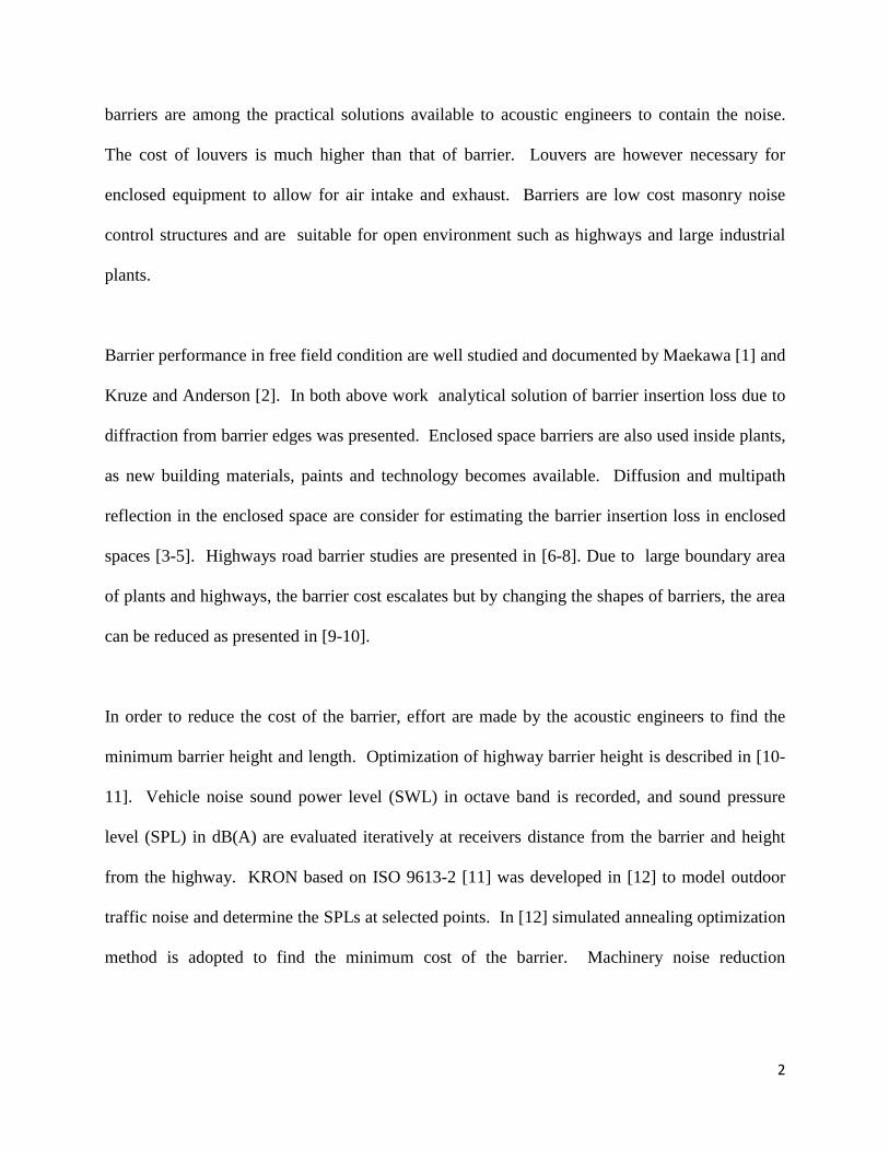
barriers are among the practical solutions available to acoustic engineers to contain the noise.

The cost of louvers is much higher than that of barrier. Louvers are however necessary for

enclosed equipment to allow for air intake and exhaust. Barriers are low cost masonry noise

control structures and are suitable for open environment such as highways and large industrial

plants.

Barrier performance in free field condition are well studied and documented by Maekawa [1] and

Kruze and Anderson [2]. In both above work analytical solution of barrier insertion loss due to

diffraction from barrier edges was presented. Enclosed space barriers are also used inside plants,

as new building materials, paints and technology becomes available. Diffusion and multipath

reflection in the enclosed space are consider for estimating the barrier insertion loss in enclosed

spaces [3-5]. Highways road barrier studies are presented in [6-8]. Due to large boundary area

of plants and highways, the barrier cost escalates but by changing the shapes of barriers, the area

can be reduced as presented in [9-10].

In order to reduce the cost of the barrier, effort are made by the acoustic engineers to find the

minimum barrier height and length. Optimization of highway barrier height is described in [10-

11]. Vehicle noise sound power level (SWL) in octave band is recorded, and sound pressure

level (SPL) in dB(A) are evaluated iteratively at receivers distance from the barrier and height

from the highway. KRON based on ISO 9613-2 [11] was developed in [12] to model outdoor

traffic noise and determine the SPLs at selected points. In [12] simulated annealing optimization

method is adopted to find the minimum cost of the barrier. Machinery noise reduction

3

optimization applications are demonstrated in [13-14], where machines locations on machine

shop floor are optimized to reduce the sound at the boundaries of the machine shop floor.

Barrier cost reductions can be readily done with optimization methods – however most of the

commercial sound propagation packages CadnaA, SoundPlan, Olive Tree Lab-Terrain are not

equipped with optimization algorithms. As a result either processed sound data from these

packages is required to be imported to optimization/mathematical packages or complete source

code of sound propagation plus optimization program has to be written in ‘Visual C’ or ‘Visual

B’. In the work presented herein, MATLAB software package is used to evaluate the sound

propagation and optimize the barrier height at the boundary of a power plant. With the

availability of various optimization methods in MATLAB, different optimization techniques can

be easily evaluated to search for global minimization. Plant noise level evaluated from

MATLAB model is compared with measured data. Which helps to optimized barrier area and

estimate barrier construction cost.

2) Power Plant Sound level

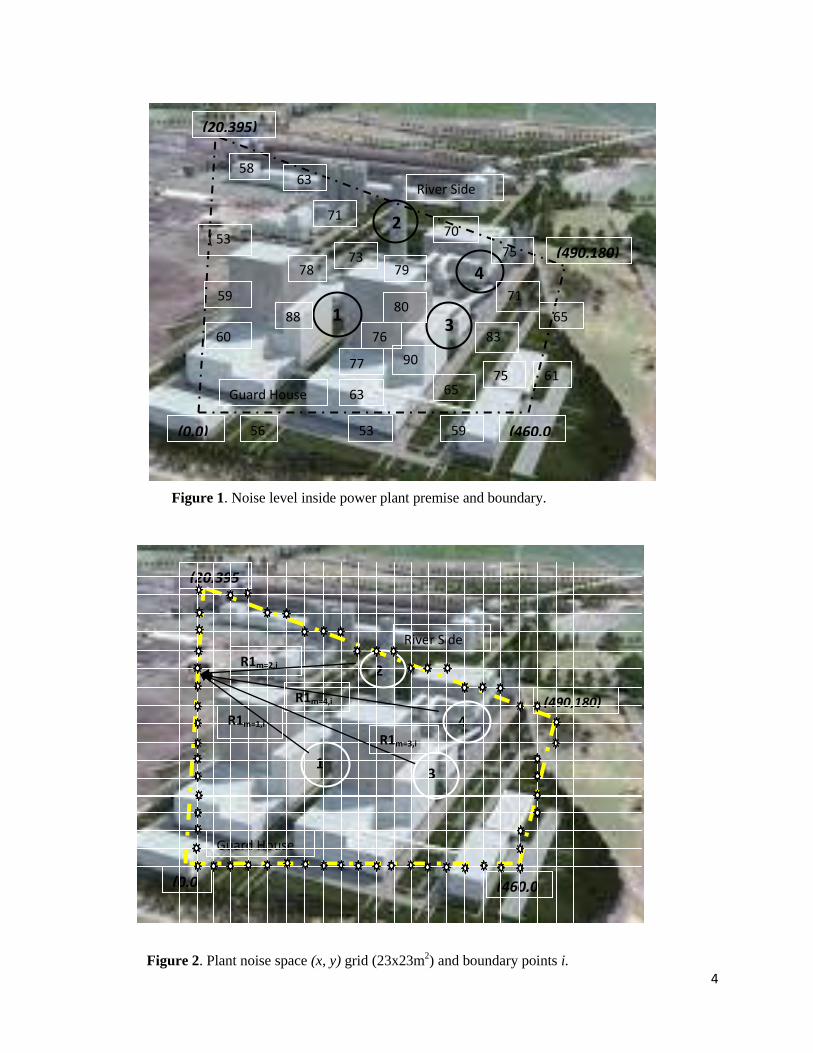
The 1200MW power plant under study is shown in Figure 1. The square boxes show SPL

measured in dB(A) within and on the boundary of the plant. Four dominant sound sources

(SWL) are shown in circles. These sources consist of 1) gas turbine stacks, 2) Air vent skid, 3)

combined cycle steam turbines, and 4) condenser fans. The boundary, which is represented by

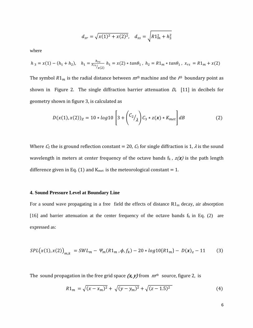
the dashed-dot line, is given in meters. The discretize plant grid (23x23m2) space and boundary

line markers spaced at 23m are shown in Figure 2.

4

Figure 1. Noise level inside power plant premise and boundary.

River Side

Guard House

(0,0) (460,0

)

(490,180)

,0)

(20,395)

3

2

1

4 79

71

58

( 53

59

60

77

78

80

65

53 56

65

61

76

63

83

71

75

75

70

63

59

88

73

90

Figure 2. Plant noise space (x, y) grid (23x23m2) and boundary points i.

River Side

Guard House

(0,0

) (460,0

)

(490,180)

,0)

(20,395

)

3

2

1

4 R1m=1,i

R1m=2,i

R1m=4,i

R1m=3,i

5

The outdoor sound propagation modeling program in MATLAB is based on the algorithm

presented in ISO 9613-2 [11]. The plant equipment SWL is available in third octave band from

the manufacturers.

3. Barrier path length difference [11]

The geometry of the barrier position between source (S) and receiver (R) with optimization

variables, height x(1) and barrier distance from receiver x(2) are shown in Figure 3. The barrier

dimensions are considered from the origin shown in this figure. If x(2) < 0, then barrier is inside

the plant boundary.

Optimization variables x(1) and x(2) in term of path length difference (z) from geometry of

Figure 3 are given as follows:

(1)

Figure 3. Geometric quantities for determining the barrier diffraction and optimization variables x

[11]. The barrier is placed on boundary line where x(1)=0, x(2)=0.

x(1)

x(2)

hrs

R1m

(0,0)

θ1

θ2

h3

h2

h1

6

where

The symbol is the radial distance between mth machine and the ith boundary point as

shown in Figure 2. The single diffraction barrier attenuation Dz [11] in decibels for

geometry shown in figure 3, is calculated as

(2)

Where C2 the is ground reflection constant = 20, C3 for single diffraction is 1, λ is the sound

wavelength in meters at center frequency of the octave bands fk , z(x) is the path length

difference given in Eq. (1) and Kmet is the meteorological constant = 1.

4. Sound Pressure Level at Boundary Line

For a sound wave propagating in a free field the effects of distance R1m decay, air absorption

[16] and barrier attenuation at the center frequency of the octave bands fk in Eq. (2) are

expressed as:

The sound propagation in the free grid space (x, y) from mth source, figure 2, is

(4)

7

The sound propagation at ith boundary points (xi, yi) from mth source is

(5)

where

Index m is for the sound source: M=4 sources

Index k is for octave band center frequency: K=10

is the sound absorption in air (dB)

is the humidity in air = 1

x is vector of optimization variables [x(1) x(2)]

(xm ym) are the location for sources m=1:4

The sound pressure at each ith

boundary point is given in Eq. (4).

where

i is the plant boundary point index and I = 99

The sound pressure level at each ith

boundary point given in Eq (6) is optimized in terms of

variables x(1) and x(2) which enters the SPLi summation through Dz in Eq. (2) and Eq. (3).

5. Barrier Optimization

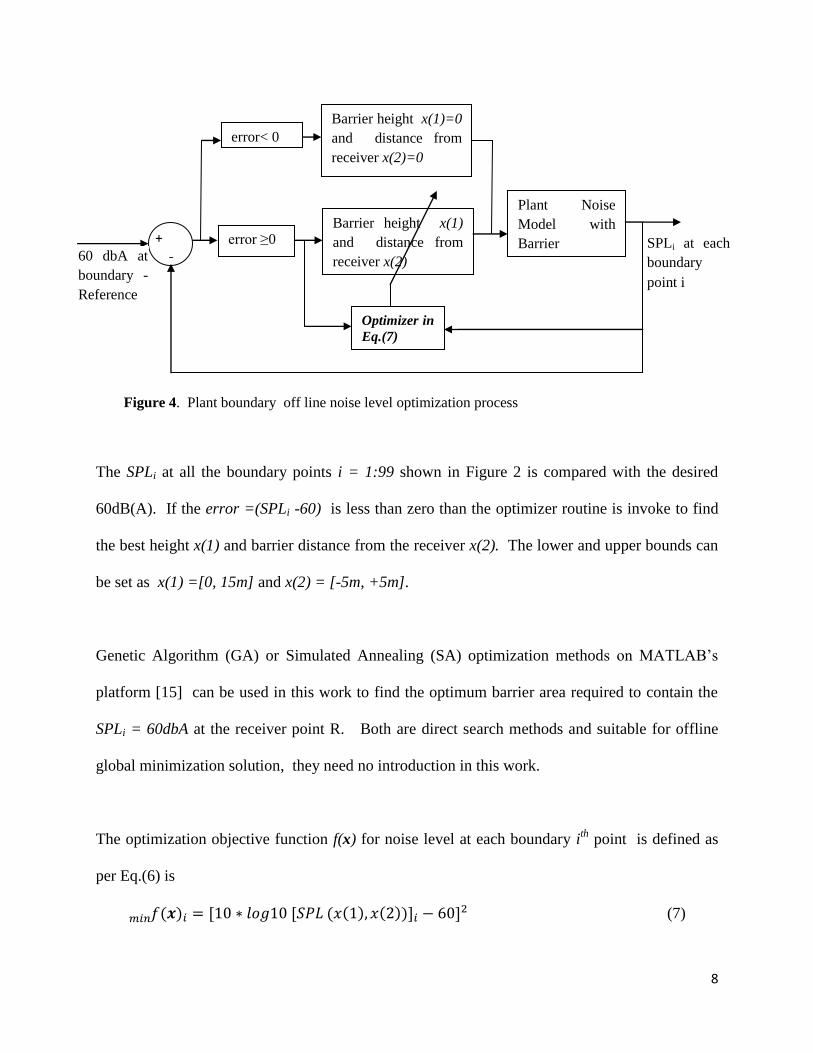
The barrier optimization process is shown in Figure 4. The reference 60 dB(A) sound pressure

level is compared with each plant boundary line point. Barrier height is evaluated at boundary

points where the SPLi is greater than 60 dB(A).

8

The SPLi at all the boundary points i = 1:99 shown in Figure 2 is compared with the desired

60dB(A). If the error =(SPLi -60) is less than zero than the optimizer routine is invoke to find

the best height x(1) and barrier distance from the receiver x(2). The lower and upper bounds can

be set as x(1) =[0, 15m] and x(2) = [-5m, +5m].

Genetic Algorithm (GA) or Simulated Annealing (SA) optimization methods on MATLAB’s

platform [15] can be used in this work to find the optimum barrier area required to contain the

SPLi = 60dbA at the receiver point R. Both are direct search methods and suitable for offline

global minimization solution, they need no introduction in this work.

The optimization objective function f(x) for noise level at each boundary ith

point is defined as

per Eq.(6) is

(7)

+

-

Barrier height x(1)

and distance from

receiver x(2)

Plant Noise

Model with

Barrier error ≥0

Optimizer in

Eq.(7)

In Eq(5)

60 dbA at

boundary -

Reference

SPLi at each

boundary

point i

Figure 4. Plant boundary off line noise level optimization process

Barrier height x(1)=0

and distance from

receiver x(2)=0

error< 0

9

Here the ub and lb bounds are defined as 0 ≤ x(1) ≤ 15m and -5m ≤ x(2) ≤ 5m

6. Results and Analysis

The optimization function in Eq. (7) is carried

out at every ith

plant boundary point and f(x)i

is minimized for x(1) and x(2) . In figure 5

plant sound pressure levels in free space are

evaluated from Eq. (3) and at plant

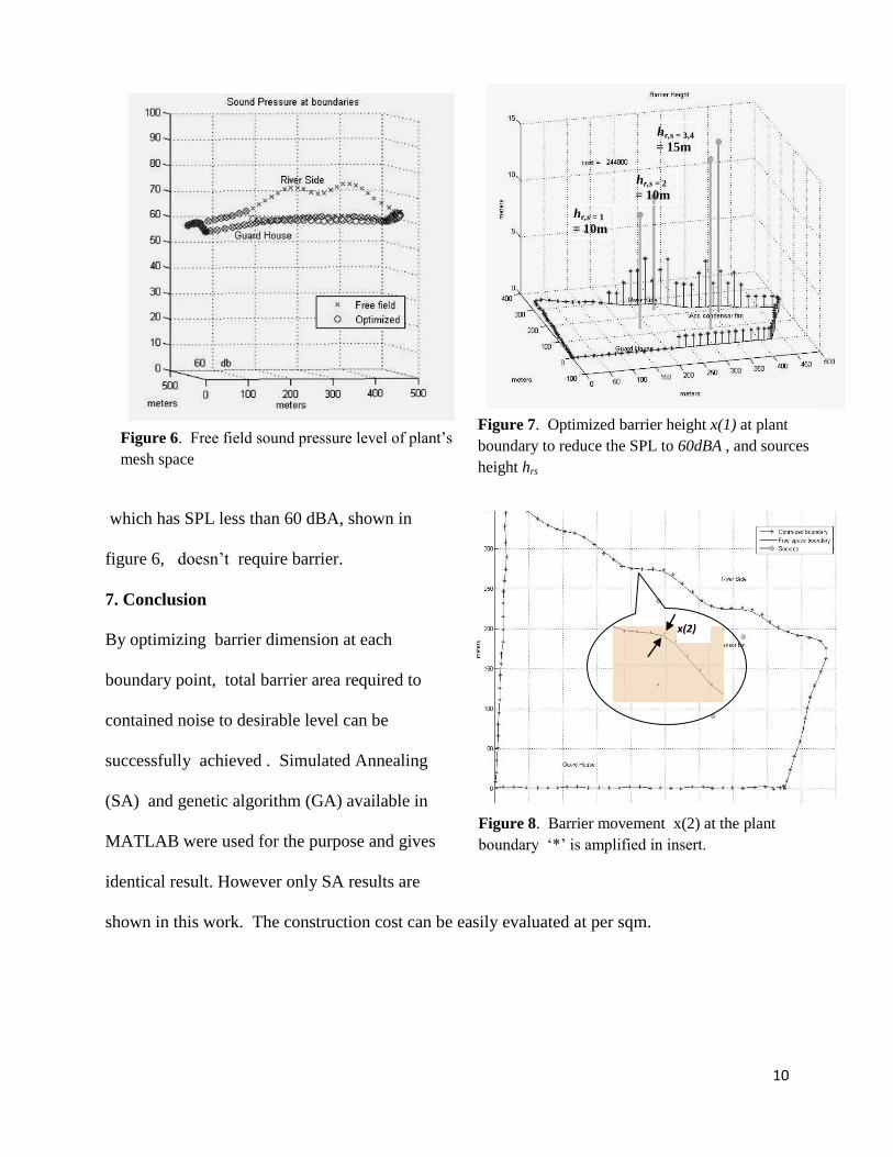
boundary points from Eq. (4). In figure 6,

two SPLi at plant boundary are shown, one

is same as in figure 5 and other one shows the

result after barrier insertion loss to 60dBA by

the optimization process - described in figure

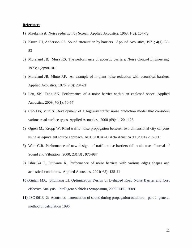
4. In figure 7 the optimize barrier height 0 ≤

x(1) ≤ 15m is shown at the plant’s boundary locations where the SPLi was more the than

required 60dBA level. The height of four sources shown are as [10m 10m 15m 15m] . The

optimizer also adjust the boundary distance from the sources by variable 5m ≤ x(2) ≤ 5m, the

new boundary point x(2) can be seen in insert of figure 8. By moving the barrier away from the

boundary the height x(1) can be reduced. With known barrier’s material and labour cost per

sqm, the total barrier cost is evaluated at the boundary points with barrier. The inter distance

between consecutive points on the boundary is 23m. Left half of the plant’s boundary

Figure 5. Free field sound pressure level of plant’s

mesh space

10

which has SPL less than 60 dBA, shown in

figure 6, doesn’t require barrier.

7. Conclusion

By optimizing barrier dimension at each

boundary point, total barrier area required to

contained noise to desirable level can be

successfully achieved . Simulated Annealing

(SA) and genetic algorithm (GA) available in

MATLAB were used for the purpose and gives

identical result. However only SA results are

shown in this work. The construction cost can be easily evaluated at per sqm.

Figure 6. Free field sound pressure level of plant’s

mesh space

Figure 8. Barrier movement x(2) at the plant

boundary ‘*’ is amplified in insert.

Figure 7. Optimized barrier height x(1) at plant

boundary to reduce the SPL to 60dBA , and sources

height hrs

hr,s = 1

= 10m

hr,s = 2

= 10m

hr,s = 3,4

= 15m

x(2)

11

References

1) Maekawa A. Noise reduction by Screen. Applied Acoustics, 1968; 1(3): 157-73

2) Kruze UJ, Anderson GS. Sound attenuation by barriers. Applied Acoustics, 1971; 4(1): 35-

53

3) Moreland JB, Musa RS. The performance of acoustic barriers. Noise Control Engineering,

1973; 1(2):98-101

4) Moreland JB, Minto RF. An example of in-plant noise reduction with acoustical barriers.

Applied Acoustics, 1976; 9(3): 204-21

5) Lau, SK, Tang SK. Performance of a noise barrier within an enclosed space. Applied

Acoustics, 2009; 70(1): 50-57

6) Cho DS, Mun S. Development of a highway traffic noise prediction model that considers

various road surface types. Applied Acoustics , 2008 (69): 1120-1128.

7) Ogren M., Kropp W. Road traffic noise propagation between two dimensional city canyons

using as equivalent source approach. ACUSTICA –C Acta Acustica 90 (2004) 293-300

8) Watt G.R. Performance of new design of traffic noise barriers full scale tests. Journal of

Sound and Vibration , 2000; 231(3) : 975-987.

9) Ishizuka T, Fujiwara K. Performance of noise barriers with various edges shapes and

acoustical conditions. Applied Acoustics, 2004( 65): 125-41

10) Xintan MA, Shuiliang LI. Optimization Design of L-shaped Road Noise Barrier and Cost

effective Analysis. Intelligent Vehicles Symposium, 2009 IEEE, 2009.

11) ISO 9613 -2: Acoustics – attenuation of sound during propagation outdoors – part 2: general

method of calculation 1996.

12

12) Mun S., Cho Y.H. Noise barrier optimization using a simulated annealing algorithm,.

Applied Acoustic, 2009(70): 1094-1098

13) Lan T.S., Chiu M. C. Identification of noise sources in factory’s sound field by using genetic

algorithm. Applied Acoustics, 2008(69): 733-750

14) Lan T.S., Chiu M. C. Optimal Noise Control on Plant Using Simulated Annealing.

Transaction of the CSME/de la SCGM, 2008; 32(3-4): 423-437

15) Genetic Algorithm and Direct Search Toolbox 2 - MATLAB, User’s Guide, 2008, The

MathWorks, Inc., Natick, Mass. USA.