Copyright by Claire Fontaine Howard 2012 - The University of ...
Upload
khangminh22Category
view
1download
0
Bond Liquidity Premia
Jean-Sebastien FontaineUniversite de Montreal and CIREQ
Rene GarciaEDHEC Business School
First draft: January 7, 2007. This draft: June 27, 2008
Abstract
This paper extends an arbitrage-free term structure model to measure the value of liquid-
ity from observed coupon bonds. Estimation produces a persistent liquidity factor driving
on-the-run premia across all maturities. This factor is priced across interest rate markets
and its impact is pervasive through time, even outside crisis periods. We find that an in-
crease in the value of liquidity predicts not only lower risk premia for both on-the-run and
off-the-run bonds but also higher risk premia on Libor loans, swap contracts and corporate
bonds. Linkages between risk premia in different markets and the valuation of liquidity ob-
tained from on-the-run premia suggest that different securities serve, in part and to varying
degrees, to fulfill investors uncertain future needs for cash. To support this hypothesis, we
study the economic determinants of the liquidity risk factor. We find that liquidity covaries
with changes in aggregate uncertainty, as measured by the volatility implied in S&P500 op-
tions, and with changes in monetary stance, as measured by bank reserves and monetary
aggregates.
JEL Classification: E43, H12.
We thank Greg Bauer, Antonio Diez, Darrell Duffie, Thierry Foucault, Albert Menkveld, Monika Piazzesi,Robert Rasche and Jose Sheinkman for their comments. We also thank participants at the EconometricSociety Summer Meeting (2007), Econometric Society European Meeting (2007), Canadian Economic As-sociation (2007) and the International Symposium on Financial Engineering and Risk Management (2007).The first author gratefully acknowledges support from the IFM2 and the Banque Laurentienne. The sec-ond author is a research fellow at CIRANO and CIREQ. He gratefully acknowledges support from FQRSC,SSHRC, MITACS, Hydro-Quebec, and the Bank of Canada.Correspondence: [email protected].
“... a part of the interest paid, at least on long-term securities, is to be attributed
to uncertainty of the future course of interest rates.”
(p.163)
“... the imperfect ’moneyness’ of those bills which are not money [...] causes the
trouble of investing in them and [causes them] to stand at a discount.”
(p.166)
“... In practice, there is no rate so short that it may not be affected by speculative
elements; there is no rate so long that it may not be affected by the alternative
use of funds in holding cash.”
(p.166)
John R. Hicks, Value and Capital, 2nd edition, 1948.
1 Introduction
Bond traders know very well that liquidity affects asset prices. One prominent case is the
on-the-run premium, whereby the most recently issued (on-the-run) bonds sell at a premium
relative to seasoned (off-the-run) bonds with similar coupons and maturities.Moreover, sys-
tematic variations in liquidity sometimes drive interest rates across several markets. A case
in point occurred around the Federal Open Market Committee [FOMC] decision, on October
15, 1998, to lower the Federal Reserve funds rate by 25 basis points. In the meeting’s opening,
Vice-Chairman McDonough, of the New York district bank, noted increases in the spread
between the on-the-run and the most recent off-the-run 30-year Treasury bonds (0.05% to
0.27%), the spreads between the rate on the fixed leg of swaps and Treasury notes with two
years and ten years to maturity (0.35% to 0.70%, and 0.50% to 0.95% respectively), the
spreads between Treasuries and investment-grade corporate securities (0.75% to 1.24%), and
finally between Treasuries and mortgage-backed securities (1.10% to 1.70%). He concluded
that we were seeing a run to quality and a serious drying up of liquidity1. These events
attest to the sometimes dramatic impact of liquidity seizures2.
1Minutes of the Federal Open Market Committee, October 15, 1998 conference call,http://www.federalreserve.gov/Fomc/transcripts/1998/981015confcall.pdf.
2The liquidity crisis of 2007-2008 provides another example. Facing sharp increases of interest rate spreadsin most markets, the Board approved reduction in discount rate, target Federal Funds rate as well as novelpolicy instruments (e.g. Term Auction Facility, Term Securities Lending Facility) to deal with the ongoingliquidity crisis.
1
The main contribution of this paper is to introduce liquidity as an additional factor in
an otherwise standard term structure model. Indeed, the modern term structure literature
has not recognized the importance of aggregate liquidity for government bonds. We extend
the no-arbitrage dynamic term structure model of Christensen et al. (2007) [CDR, hereafter]
allowing for liquidity3 and we extract a common factor driving on-the-run premia across
maturities. Identification of the liquidity factor is obtained by estimating the model from a
panel of pairs of U.S. Treasury securities where each pair has similar cash flows but different
ages. This sidesteps credit risk issues and delivers direct estimates of the liquidity value: it
isolates price differences that can be attributed to liquidity. Of course, a recent empirical
literature suggests that liquidity is priced on bond markets,4 but these empirical investiga-
tions are limited to a single market and do not measure liquidity value within a no-arbitrage
framework.
Our second contribution is precisely to show that an aggregate liquidity risk component
drives a substantial share of risk premia across different interest rate markets. By construc-
tion, an increase in the liquidity factor is associated with lower expected excess returns for
on-the-run bonds. More interestingly, an increase in the liquidity factor has a large nega-
tive impact on risk premia for off-the-run government bonds. On the other hand, it raises
the risk premium implicit in LIBOR, swap rates and corporate bond yields. Empirically,
the pattern is consistent with accounts of flight-to-quality but the relationship is pervasive
even in normal times. This adds considerably to the existing evidence pointing toward the
importance of marketwide liquidity for risk premia. Commonality between the valuation of
liquidity obtained from on-the-run premia and variations in risk premia across different mar-
kets suggests that different securities serve, in part and to varying degrees, to fulfill investors
uncertain future needs for cash. That is, the aggregate demand for liquidity is a risk factor
relevant for asset prices.
These results raises the all important issue of identifying macroeconomic drivers of the
liquidity factor. Can we characterize the aggregate liquidity premium in terms of economic
state variables? First, we consider principal components extracted by Ludvigson and Ng
(2005) from a data set of 132 macroeconomic variables5. We find that the liquidity factor is
associated with factors measuring monetary conditions in the economy and in the banking
system. In particular, the evidence supports a strong link with measures of bank reserves at
3This model captures parsimoniously the usual level, slope and curvature factors, while delivering goodin-sample fit and forecasting power. Moreover, the smooth shape of Nelson-Siegel curves identifies smalldeviations, relative to an idealized curve, which may be caused by variations in market liquidity.
4See Longstaff (2000) for evidence that liquidity is priced for short-term U.S. Treasury security andLongstaff (2004) for U.S. Treasury bonds of longer maturities. See Collin-Dufresne et al. (2001), Longstaffet al. (2005), Ericsson and Renault (2006), Nashikkar and Subrahmanyam (2006) for corporate bonds.
5We thank Sydney Ludvigson and Serena Ng for making their principal component data available.
2
the Federal Reserve and measures of monetary aggregates. Second, we use implied volatility
from S&P 500 index options as a proxy for aggregate uncertainty and find a significant
positive link with liquidity valuation. Finally, our liquidity factor varies with measures of
transaction costs on the bond market. These findings provide a third important empirical
contribution.
We differ from the modern term structure literature in two significant ways. First, the
latter focuses almost exclusively on bootstrapped zero-coupon yields6. This approach is
convenient because a large family of models delivers zero-coupon yields which are linear in
the state variables (see Dai and Singleton (2000)). However, we argue that pre-processing
the data wipes out the most accessible evidence on liquidity, that is the on-the-run premium.
Therefore, we use coupon bond prices directly. However, the state space is no longer linear
and we handle non-linearities with the Unscented Kalman Filter [UKF], an extension of the
Kalman Filter for non-linear state-space systems (Julier et al. (1995) and Julier and Uhlmann
(1996)). We first estimate a model without liquidity and, notwithstanding the differences in
data and filtering methodology, our results are consistent with CDR. However, pricing errors
in this standard term structure model reveals systematic differences, correlated with ages.
Estimation of the model with liquidity by quasi-maximum likelihood produces a persistent
factor capturing differences between prices of recently issued bonds and prices of older bonds.
The on-the-run premium increases with maturity but decays exponentially with the age of a
bond. These new features complete our contributions to the modeling of the term structure
of interest rates in presence of a liquidity factor.
Our empirical findings can be summarized as follows. Figure 1 shows that the liquidity
factor exhibits large variations through normal and crisis period. Nevertheless, it remains
positive and implies an average premium of $0.38 for a just-issued 10-year bond. Second,
Figure 6a shows that an increase in the value of liquidity predicts lower expected excess
returns and, thus, higher current valuations, for seasoned bonds. For a seasoned bond with
two years to maturity, a one-standard deviation shock to liquidity predicts a decrease in
excess returns of 182 basis points compared to an average excess returns of 214 basis points.
This suggests that off-the-run government bonds are substitutes, albeit imperfect, to on-
the-run issues. Like its more liquid counterpart, a seasoned bond offers low transaction
costs and can be quickly converted into cash via the repo market. Then, all government
bonds share a common, negative, liquidity component that leads to higher bond prices when
the aggregate demand for liquidity increases. These results are robust to including term
structure information among the regressors. Indeed, we confirm the presence in coupon-
6The CRSP data set of zero-coupon yields is the most commonly used. It is based on the bootstrapmethod of Fama and Bliss (1987) [FB].
3

bond data of a forward rate factor summarizing term structure information about the risk
premium (Cochrane and Piazzesi (2005)).
Next, we consider the predictive power of liquidity for the risk premium on short-term
Eurodollar loans. Figure 6b shows that a substantial share of LIBOR spread variability is
linked to variations of the liquidity factor, as much as 28% in univariate regressions. The
relationship is significant, both statistically and economically. Consider a 1-year loan, whose
spread averaged 45 basis points in our sample. Contemporaneously, and controlling for
term structure information, a one-standard deviation shock to liquidity is associated with
a LIBOR spread increase of 7 basis points. We also consider the spread of swap rates over
par bond yields. Figures 6c shows that the information content of liquidity is important.
For the 7-year swap contract, whose spread averaged 53 basis points, a shock to liquidity
is associated with a spread increase of 9 basis points after controlling for term structure
information. In univariate regressions, the R2 ranges from 7 to 12%.
Finally, we consider risk premia on corporate bonds. We find that liquidity is a predictor
for the spread of Moody’s Aaa and Baa indices of corporate bond yields (see Figure 6d). In a
panel of corporate bond spreads, we find that the impact of liquidity follows a flight-to-quality
pattern. Corporate bonds of the highest credit quality appears to be liquid substitutes to
government securities while the risk premia on bonds with lower ratings carry a positive
liquidity component.
Other empirical investigations are related to our work. Jump risk (Tauchen and Zhou
(2006)) or the debt-gdp ratio (Krishnamurthy and Vissing-Jorgensen (2007)) have been
proposed to explain the non-default component of corporate spreads. Also, in a paper
related to ours, Grinblatt (2001) argues that the convenience yields of U.S. Treasury bills
can explain the U.S. Dollar swap spread. Recently, Liu et al. (2006) and Fedlhutter and
Lando (2007) evaluate the relative importance of credit and liquidity risks in swap spreads.
Finally, Pastor and Stambaugh (2003) and Amihud (2002) provide evidence of an aggregate
liquidity risk factor in expected stock returns.
The link between interest rates and aggregate liquidity is supported in the theoreti-
cal literature. Svensson (1985) uses a cash-in-advance constraint in a monetary economy.
Bansal and Coleman (1996) allow government-issued bonds to back checkable accounts and
reduced transaction costs in a monetary economy. Luttmer (1996) investigates asset pricing
in economies with frictions and shows that with transaction costs (bid-ask spreads) there
is in general little evidence against the consumption-based power utility model with low
risk-aversion parameters. Holmstrom and Tirole (1998) introduce a link between the liquid-
ity demand of financially constrained firms and asset prices. Acharya and Pedersen (2004)
4
propose a liquidity-adjusted CAPM model where transaction costs are time-varying. Alter-
natively, Vayanos (2004) takes transactions costs as fixed but introduces the risk of having to
liquidate a portfolio. Lagos (2006) extends the search friction argument to multiple assets:
in a decentralized exchange, agents with uncertain future hedging demand prefer assets with
lower search costs.
The on-the-run liquidity premium was first documented7 by Warga (1992). Amihud
and Mendelson (1991) and, more recently, Goldreich et al. (2005) confirm the link between
the premium and expected transaction costs. Duffie (1996) provides a theoretical channel
between on-the-run premia and lower financing costs on the repo market. Vayanos and
Weill (2006) extend this view and model search frictions in both the repo and the cash
markets explicitly.8 The link between the repo market and the on-the-run premium has been
confirmed empirically. (See Jordan and Jordan (1997), Krishnamurthy (2002), Buraschi and
Menini (2002) and Cheria et al. (2004).)
The rest of the paper is organized as follows. The next section presents the model and
its state-space representation. Section 3 describes the data and Section 4 introduces the
estimation method based on the UKF. We report estimation results for models with and
without liquidity in Section 5. Section 6 evaluates the information content of liquidity for
excess returns and interest rate spreads while Section 7 identifies economic determinants of
liquidity and Section 8 concludes.
2 A Term structure model with liquidity
We base our model on the Arbitrage-Free Extended Nelson-Siegel [AFENS] model introduced
in CDR. This model belongs to the affine family (Duffie and Kan (1996)). The latent
state variables relevant for the evolution of interest rates are grouped within a vector Ft
of dimension k = 3. Its dynamics under the risk-neutral measure Q is described by the
stochastic differential equation
dFQt = KQ(θQ − Ft) + ΣdWQ
t , (1)
7The U.S Treasury recognizes and takes advantages of this price differential: “In addition, although it isnot a primary reason for conducting buy-backs, we may be able to reduce the government’s interest expenseby purchasing older, “off-the-run” debt and replacing it with lower-yield “on-the-run” debt.” [TreasuryAssistant Secretary for financial markets Lewis A. Sachs, Testimony before the House Committee on Waysand Means].
8Kiyotaki and Wright (1989) introduced search frictions in monetary theory and Shi (2005) extends thisframework to include bonds. See Shi (2006) for a review. Search frictions can also rationalize the spreadsbetween bid and ask prices offered by market intermediaries (Duffie et al. (2005)).
5

where dWt is a standard Brownian motion process. Combined with the assumption that the
short rate is affine in all three factors, the model then leads to the usual affine solution for
discount bond yields.
In this context, CDR show that if the short rate is defined as rt = F1,t + F2,t and if the
mean-reversion matrix KQ is restricted to
KQ =
0 0 0
0 λ −λ
0 0 λ
, (2)
then the absence of arbitrage opportunity implies the discount yield function,
y(Ft,m) = a(m) + F1,tb1(m) + F2,tb2(m) + F3,tb3(m), (3)
with loadings given by
b1(m) = 1,
b2(m) =
(1− exp (−mλ)
mλ
),
b3(m) =
(1− exp (−mλ)
mλ− exp (−mλ)
), (4)
where m ≥ 0 is the length of time until maturity (see appendix for the a(m) term).
These loadings are consistent with the static Nelson-Siegel representation of forward rates
(Nelson and Siegel (1987), NS hereafter). Their shapes across maturities lead to the usual
interpretations of factors in terms of level, slope and curvature. Moreover, the NS representa-
tion is parsimonious and imposes a smooth shape to the forward rate curve. Empirically, this
approach is robust to over-fitting and delivers performance in line with, or better than, other
methods for pricing out-of-sample bonds in the cross-section of maturities9. Conversely, its
smooth shape is useful to identify deviations of observed yields from an idealized curve.
A dynamic extension of the NS model, the Extended Nelson-Siegel model [ENS], was
first proposed by Diebold and Li (2006) and Diebold et al. (2006). Diebold and Li (2006)
show large improvements in long-horizon forecasting, argue that the ENS model performs
better than the best essentially affine model of Duffee (2002) and point toward the model’s
parsimony to explain its successes. One concern is that the ENS model does not enforce the
absence of arbitrage. This is precisely the contribution of CDR. They derive the class of
9See Bliss (1997) and Anderson et al. (1996) for an evaluation of yield curve estimation methods.
6

arbitrage-free affine dynamic term structure models with loadings that correspond to the NS
representation. Intuitively, an AFENS model corresponds to a canonical affine model in Dai
and Singleton (2000) where the loading shapes have been restricted through over-identifying
assumptions on the parameters governing the latent factors under the risk-neutral measure.
CDR compare the ENS and AFENS models and show that implementing these restrictions
improves forecasting performances further.
Interestingly, CDR show that we are free to choose the drift and variance term for the
dynamics under the physical measure
dF Pt = KP (θP − Ft) + ΣdW P
t . (5)
Further, we impose that Σ is lower triangular and that KP is diagonal10. We can then cast
the model within a discretized state-space representation. The state equation becomes
(Ft − F ) = Φ(Ft−1 − F ) + Γεt, (6)
where the innovation εt is standard Gaussian, the autoregressive matrix Φ is
Φ = exp
(−K
1
12
)(7)
and the covariance matrix Γ can computed from
Γ =
∫ 112
0
e−KsΣΣT e−Ksds. (8)
Finally, we define a new latent state variable, Lt, that will be driving the liquidity pre-
mium. Its transition equation is
(Lt − L) = φl(Lt−1 − L) + σlεlt, (9)
where the innovation εlt is standard Gaussian and uncorrelated with the innovation in term
structure factors.
Typically, term structure models are not estimated from observed prices. Rather, coupon
bond prices are converted to forward rates using the bootstrap method. This is convenient as
affine term structure models deliver forward rates that are linear in state variables. Is is also
10Formally, the assumption on Σ is required for identification purposes. In practice, the presence of theoff-diagonal elements in the KP matrix does not change our results. Moreover, CDR show that allowing foran unrestricted matrix KP deteriorates out-of-sample performance.
7

thought to be innocuous because bootstrapped forward rates achieve near-exact pricing of
the original sample of bonds. Unfortunately, this extreme fit means that a naive application
of the bootstrap pushes any liquidity effects and other price idiosyncracies into forward rates.
Fama and Bliss (1987) handle this sensitivity to over-fitting by excluding bonds with “large”
price differences relative to their neighbors. This approach is certainly justified for many
of the questions addressed in the literature, but it removes any evidence of large liquidity
effects11. Moreover, the FB data set focuses on discount bond prices at annual maturity
intervals. This smooths away evidence of small liquidity effects being passed through to
forward rates. These effects would be apparent from reversals in the forward rate function
at short maturity interval. Consider three quotes for bonds with successive maturities M1 <
M2 < M3. A relatively expensive quote at maturity M2 induces a relatively small forward
rate from M1 to M2. However, the following normal quote with maturity M3 requires a
relatively large forward rate from M2 to M3. This is needed to compensate the previous low
rate and to achieve exact pricing as required by the bootstrap. However, the reversal cancels
itself as we sum intra-period forward rates to compute annual rates.
Instead of using zero-coupon bond data, we proceed from observed coupon bonds with
say maturity M and intermediate coupon payoffs at maturities m = m1, . . . , M . The price
Dt(m) of a discount bond with maturity m, used to price intermediate payoffs, is given by
Dt(m) = exp(−m(a(m) + b(m)T Ft)
)m ≥ 0,
which follows directly from equation (3) but where we use vector notation for factors Ft and
factor loadings b(m). In a frictionless economy, the absence of arbitrage implies that the
price of a coupon bond equals the sum of discounted coupons and principal. That is, the
frictionless price is
P ∗(Ft, Zt) =M∑
m=m1
Dt(m)× Ct(m), (10)
where Zt includes all characteristics relevant for pricing the bond. In this case, it includes
the maturity M and the schedule of future coupons Ct(m).
11See also the CRSP documentation for a description of this procedure. Briefly, a first filter includes aquote if its yield to maturity falls within a range of 20 basis points from one of the moving averages onthe 3 longer or the 3 shorter maturity instruments or if its yield to maturity falls between the two movingaverages. When computing averages, precedence is given to bills when available and this is explicitly designedto exclude the impact of liquidity on notes and bonds with maturity of less than one year. Amihud andMendelson (1991) document that yield differences between notes and adjacent bills is 43 basis point onaverage, a figure much larger than the 20 basis point cutoff. The second filter excludes observations thatcause reversals of 20 basis points in the bootstrapped discount yield function. The impact of these filtershas not been studied in the literature.
8
With a short-sale constraint on government bonds and a collateral constraint on the
repo market, Luttmer (1996) shows that the set of stochastic discount factors consistent
with the absence of arbitrage satisfies P ≥ P ∗. Moreover, Duffie (1996) and Vayanos and
Weill (2006) show that the combination of these constraints with search frictions on the repo
market induces differences in funding costs that favor recently issued bonds. Intuitively,
the repo market provides the required heterogeneity between assets with identical payoffs.
An investor cannot choose which bond to deliver to unwind a repo position; she must find
and deliver the same security she had originally borrowed. Because of search frictions, then,
investors are better off in the aggregate if they can coordinate around one security and reduce
search costs. In practice, the repo rate is lower for this special issue to provide an incentive
to bond holders to bring their bond to the repo market. Typically, recently issued, on-
the-run, bonds benefit from these lower financing costs, leading to the on-the-run premium.
Alternatively, differences in transaction costs drive a wedge between asset prices (Amihud
and Mendelson (1986)). Empirically, both channels seem to be at work although the effect of
direct transaction costs appears weaker (Amihud and Mendelson (1991) and Goldreich et al.
(2005)) than the effect of repo rates (Jordan and Jordan (1997), Krishnamurthy (2002) and
Cheria et al. (2004) as well as Buraschi and Menini (2002) for the German bonds market).
Then, we model the price, P (Ft, Lt, Zt), of a coupon bond with characteristics Zt as the
sum of discounted coupons to which we add a liquidity term,
P (Ft, Lt, Zn,t) =Mn∑m=1
Dt(m)× Cn,t(m) + ζ(Lt, Zn,t).
Here Zt is a short hand for the maturity, coupon and age of the bond. Grouping observations
together, and adding a pricing error term, we obtain our measurement equation
P (Ft, Lt, Zt) = CtDt + ζ(Lt, Zt) + Ωνt, (11)
where Ct is the (N × Mmax) payoffs matrix obtained from stacking the N row vectors of
individual bond payoffs and Mmax is the longest maturity group in the sample. Shorter payoff
vectors are completed with zeros. Similarly, ζ(Lt, Zt) is a N × 1 vector obtained by staking
the individual liquidity premium. Dt is a (Mmax× 1) vector of discount bond prices and the
measurement error, νt, is a (N × 1) gaussian white noise uncorrelated with innovations in
state variables. The matrix Ω is assumed diagonal and its elements are a linear function of
maturity,
ωn = ω0 + ω1Mn,
9
which reduce substantially the dimension of the estimation problem. However, leaving the
diagonal elements of Ω unrestricted does not affect our results12.
Our specification of the liquidity premium is based on a latent factor common to all bonds
but with loadings that vary with a bond’s maturity and age. Warga (1992) documented the
links of the average on-the-run premium with bond ages and maturities. The on-the-run
premium is given by
ζ(Lt, Zn,t) = Lt × βMn exp
(−1
κagen,t
)(12)
where aget is the age, in years, of the bond at time t. The parameter βM controls the
average of the liquidity premium within maturity group M . Below, we fix βmax = 1 to
identify the level of the liquidity factor. The parameter κ controls the liquidity premium’s
decay as a bond becomes older. The gradual decay of the premium with age has been
documented by Goldreich et al. (2005). For instance, immediately following its issuance
(i.e.: age = 0), the loading on the liquidity factor is βM × 1. Taking κ = 0.5, the loading
decreases by half within any maturity group after a little more than 4 months following
issuance : ζ(Lt, 4) ≈ 12ζ(Lt, 0)).
Equation (11) shows that omitting the liquidity term will push the liquidity effect into
pricing errors, possibly leading to biased estimators and large filtering errors. Alternatively,
adding a liquidity term amounts to filtering a latent factor present in pricing errors. However,
this factor captures that part of pricing errors correlated with bond ages. Our maintained
hypothesis is that any such factor can be interpreted as a liquidity effect. While the specifi-
cation above reflects our priors about the impact of age and maturity, the scale parameters
are left unrestricted at estimation and we allow for a continuum of shapes for the decay of
liquidity.
As discussed above, a positive liquidity term is consistent with the absence of arbitrage
given the frictions observed on the bond market. Our specification delivers a discount rate
function consistent with off-the-run valuations. However, a structural specification of the
liquidity premium raises important challenges. The on-the-run premium is a real arbitrage
opportunity unless we explicitly consider the cost of shorting the more expensive bond or,
alternatively, the benefits accruing to the bondholder from a lower repo rate. These features
are absent from the current crop of term structure models. Moreover, a joint model of the
12This can be explained by noting that the level factor explains most of yields variability. Its impact onbond prices is linear in duration and duration is approximately linear in maturity, at least for maturities upto 10 years. Bid-ask spreads increase with maturity and may also contribute to an increase in measurementerrors with maturity.
10

term structure of repo rates and of government yields is not itself free of arbitrage unless we
simultaneously model the convenience yields of holding short-term government securities.
This follows from the observation that a Treasury bill typically offers a lower yield than
a repo contract with the same maturity. This is beyond the scope of this paper. Our
strategy bypasses these challenging considerations but still allows us to identify the on-the-
run liquidity premia and uncover an aggregate liquidity factor. We now turn to a description
of the data.
3 Data
We use end-of-month prices of U.S. Treasury securities from the CRSP data set. We exclude
callable bonds, flower bonds and other bonds with tax privileges, issues with no publicly
outstanding securities, bonds and bills with less than 2 months to maturity and observations
with either bid or ask prices missing13. We focus on the period from 12/1985 to 12/2007
because the tax premium and the on-the-run premium are hard to untangle in the prior
period. Before 1986, interest income had a favorable tax treatment compared to capital gains
and investors favored high-coupon bonds. In a period of rising interest rates, recently issued
bonds had relatively high coupons and were priced at a premium both for their liquidity
and for their tax benefits. Green and Ødegaard (1997) document that the high-coupon tax
premium mostly disappeared when the asymmetric treatment of interest income and capital
gains was eliminated in the 1986 tax reform.
At each observation date, the CRSP data set14 provides quotes on all outstanding U.S.
Treasury securities. We construct bins around maturities of 3, 6, 9, 12, 18, 24, 36, 48,
60, 84 and 120 months to provide a sufficient coverage of the term structure. Then, for
each date, and within each bin, we choose a pair of securities to identify any on-the-run
premium. First, we want to pick the on-the-run security, if available, and, second, a security
with matching maturity. Unfortunately, on-the-run bonds are not directly identified in the
CRSP database. Instead, we use time since issuance as a proxy and pick the most recently
issued security in each maturity bin. To complete the pair, we pick the off-the-run bond
with time remaining to maturity closest to the center of the maturity bin. By construction,
then, securities within each pair have the same credit quality, similar times to maturity and
similar coupons. Also, we minimize maturity differences between on-the-run bonds and their
13Along the way, we exclude some suspicious quotes. CRSP ID #19920815.107250 on August 31st 1987,#20041031.202120 on November 29th 2002, #20070731.203870 on May 31st 2006 and #20080531.204870 onNovember 30th 2007 were removed because yields to maturity were suspicious. CRSP ID #20040304.400000has a maturity date preceding its issuance date, as dated by the U.S. Treasury.
14See Elton and Green (1998) and Piazzesi (2005) for discussion of the CRSP data set.
11

off-the-run companions throughout the sample. Finally, pinning the off-the-run security in
at the center of its bin ensures a stable coverage of the term structure of interest rates.
The most recent issue at a given bin and date is not always an on-the-run security.
This may be due to the absence of new issuance in some maturity bins throughout the
whole sample (e.g. 18 months to maturity) or within some sub-periods (e.g. 84 months to
maturity). Alternatively, the on-the-run bond may be a few months old, due to the quarterly
issuance pattern observed in some maturity categories. In any case, this introduces variability
in age differences which, in turn, identifies how the liquidity premium varies with age. Still,
the most important aspect of our sample is that whenever an on-the-run security is available,
any large price difference cannot be rationalized from small coupon and maturity differences
under the no-arbitrage restriction. Instead, age differences are magnified in the sample and
any price difference common across maturities and correlated with age will be attributed to
the liquidity effect.
We now investigate some features of our sample of 265×22 = 5830 observations. The first
columns of Table 1 present means and standard deviations of age for each liquidity-maturity
category. The average off-the-run security is always older than the corresponding on-the-run
security. Typically, the off-the-run security has been in circulation for more than a year.
In contrast, the on-the-run security is typically a few months old and, even, a few weeks
old in the 6 and 24-month categories. While a relatively low mean age for the recent issue
indicates a regular issuance pattern, the relatively high standard deviation in the 36 and
84-month categories reflects the decision by the U.S. Treasury to stop the issuance cycles at
these maturities.
The middle columns of Table 1 presents means and standard deviations of duration15.
Note that average duration is almost linear in maturity. Also, as expected, duration is
similar within pairs implying that the averages of cash flow maturities are very close. By
construction, categories with regular issuance patterns exhibit pairs with smaller duration
differences on average. This helps identify price differences due to the on-the-run premium.
Finally, the last columns of Table 1 indicates that the average term structure of coupons is
upward sloping. Standard deviations indicate important variations in coupon rates. This is
in part due to the general decline of interest rates throughout the sample. Notwithstanding
this important variation, coupon differences are typically small. This was another of our
objectives. To summarize our strategy, differences in duration and coupon rates are kept
small within each pair to highlight the effect of age, and thus liquidity, on prices.
15Duration is the relevant measure to compare maturities of bonds with different coupons.
12
4 Estimation Methodology
Equations (6), (9) and (11) can be summarized as a state-space system
(Xt − X) = ΦX(Xt−1 − X) + ΣXεt (13)
Pt = Ψ(Xt, Ct, Zt) + Ωνt, (14)
where Xt ≡ [F Tt Lt]
T and Ψ is the (non-linear) mapping of cash flows Ct, bond characteristics,
Zt, and current states, Xt, into prices.
Estimation of this system is challenging: we do not know the joint density of factors and
prices. Various strategies to deal with non-linear state-space systems have been proposed
in the filtering literature: the Extended Kalman Filter (EKF), the Particle Filter (PF) and
more recently the Unscented Kalman Filter16 (UKF). The UKF is based on a method for
calculating statistics of a random variable which undergoes a nonlinear transformation. It
starts with a well-chosen set of points with given sample mean and covariance. The nonlinear
function is then applied to each point and moments are computed from transformed points.
This approach has a Monte Carlo flavor but the sample is drawn according to a specific
deterministic algorithm. It delivers second-order accuracy but with no increase in computing
cost relative to the EKF. Moreover, analytical derivatives are not required. The UKF has
been introduced in the term structure literature by Leippold and Wu (2003) and in the foreign
exchange literature by Bakshi et al. (2005). Recently, Christoffersen et al. (2007) compared
the EKF and the UKF for the estimation of term structure models. They conclude that the
UKF improves filtering and reduces estimation bias.
To set up notation, we state the standard Kalman filter algorithm as applied to our
model. We then explain how the unscented approximation helps overcome the challenge
posed by a non-linear state-space system. Consider the case where Ψ is linear in X whereas
state variables and bond prices are jointly Gaussian. In this case, the Kalman recursion
provides optimal estimates of current state variables given past and current prices. The
recursion works off estimates of state variables and their associated MSE from the previous
16See Julier et al. (1995), Julier and Uhlmann (1996) and Wan and der Merwe (2001) for a textbooktreatment. Another popular bypasses filtering altogether. It assumes that some prices are observed withouterrors and obtains factors by inverting the pricing equation. In our context, the choice of maturities andliquidity types that are not affected by measurement errors is not innocuous and impacts estimates of theliquidity factor.
13
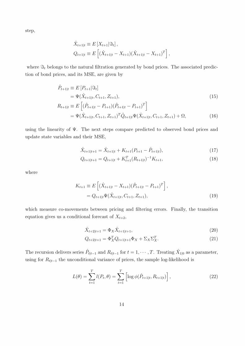
step,
Xt+1|t ≡ E [Xt+1|=t] ,
Qt+1|t ≡ E[(Xt+1|t −Xt+1)(Xt+1|t −Xt+1)
T],
where =t belongs to the natural filtration generated by bond prices. The associated predic-
tion of bond prices, and its MSE, are given by
Pt+1|t ≡ E [Pt+1|=t]
= Ψ(Xt+1|t, Ct+1, Zt+1), (15)
Rt+1|t ≡ E[(Pt+1|t − Pt+1)(Pt+1|t − Pt+1)
T]
= Ψ(Xt+1|t, Ct+1, Zt+1)T Qt+1|tΨ(Xt+1|t, Ct+1, Zt+1) + Ω, (16)
using the linearity of Ψ. The next steps compare predicted to observed bond prices and
update state variables and their MSE,
Xt+1|t+1 = Xt+1|t + Kt+1(Pt+1 − Pt+1|t), (17)
Qt+1|t+1 = Qt+1|t + KTt+1(Rt+1|t)
−1Kt+1, (18)
where
Kt+1 ≡ E[(Xt+1|t −Xt+1)(Pt+1|t − Pt+1)
T],
= Qt+1|tΨ(Xt+1|t, Ct+1, Zt+1), (19)
which measure co-movements between pricing and filtering errors. Finally, the transition
equation gives us a conditional forecast of Xt+2,
Xt+2|t+1 = ΦXXt+1|t+1, (20)
Qt+2|t+1 = ΦTXQt+1|t+1ΦX + ΣXΣT
X . (21)
The recursion delivers series Pt|t−1 and Rt|t−1 for t = 1, · · · , T . Treating X1|0 as a parameter,
using for Rt|t−1 the unconditional variance of prices, the sample log-likelihood is
L(θ) =T∑
t=1
l(Pt, θ) =T∑
t=1
[log φ(Pt+1|t, Rt+1|t)
], (22)
14
where φ(·, ·) is the multivariate Gaussian density.
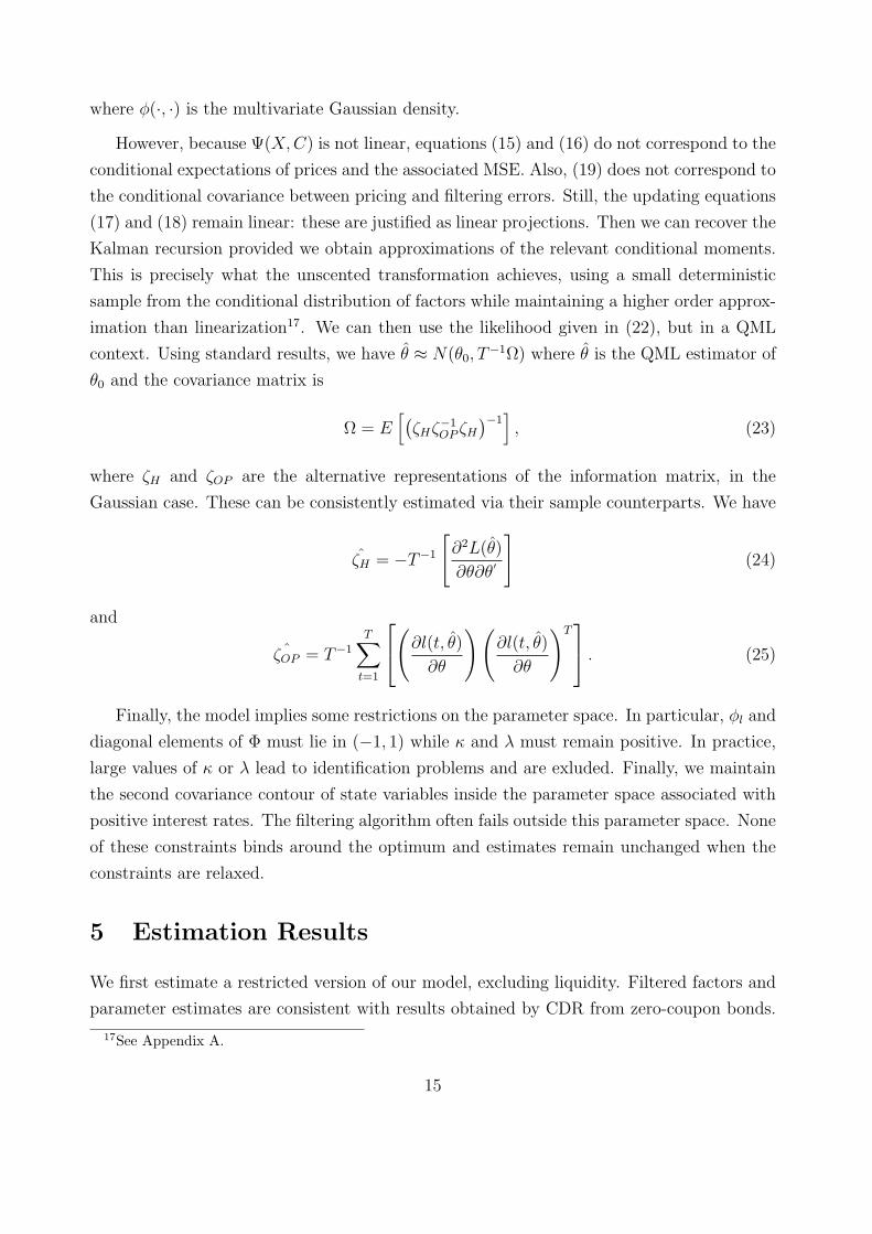
However, because Ψ(X, C) is not linear, equations (15) and (16) do not correspond to the
conditional expectations of prices and the associated MSE. Also, (19) does not correspond to
the conditional covariance between pricing and filtering errors. Still, the updating equations
(17) and (18) remain linear: these are justified as linear projections. Then we can recover the
Kalman recursion provided we obtain approximations of the relevant conditional moments.
This is precisely what the unscented transformation achieves, using a small deterministic
sample from the conditional distribution of factors while maintaining a higher order approx-
imation than linearization17. We can then use the likelihood given in (22), but in a QML
context. Using standard results, we have θ ≈ N(θ0, T−1Ω) where θ is the QML estimator of
θ0 and the covariance matrix is
Ω = E[(
ζHζ−1OP ζH
)−1], (23)
where ζH and ζOP are the alternative representations of the information matrix, in the
Gaussian case. These can be consistently estimated via their sample counterparts. We have
ζH = −T−1
[∂2L(θ)
∂θ∂θ′
](24)
and
ˆζOP = T−1
T∑t=1
(∂l(t, θ)
∂θ
)(∂l(t, θ)
∂θ
)T . (25)
Finally, the model implies some restrictions on the parameter space. In particular, φl and
diagonal elements of Φ must lie in (−1, 1) while κ and λ must remain positive. In practice,
large values of κ or λ lead to identification problems and are exluded. Finally, we maintain
the second covariance contour of state variables inside the parameter space associated with
positive interest rates. The filtering algorithm often fails outside this parameter space. None
of these constraints binds around the optimum and estimates remain unchanged when the
constraints are relaxed.
5 Estimation Results
We first estimate a restricted version of our model, excluding liquidity. Filtered factors and
parameter estimates are consistent with results obtained by CDR from zero-coupon bonds.
17See Appendix A.
15
More interestingly, the on-the-run premium reveals itself in the residuals from the benchmark
model. This provides a direct justification for linking the premium with the age and maturity
of each bond. We then estimate the unrestricted liquidity model. The null of no liquidity is
easily rejected and the liquidity factor captures the systematic differences between on-the-
run and off-the-run bonds. Finally, estimates imply that the on-the-run premium increases
with maturity but decreases with the age of a bond.
5.1 Results for the Benchmark Model Without Liquidity
Estimation18 of the benchmark model put the curvature parameter at λ = 0.6834 when
time periods are measured in years. The standard error is 0.0234 when using the QMLE
covariance matrix and 0.0042 when using the MLE covariance matrix. This estimate lies
between the two values obtained by CDR and pins the maximum curvature loading just
above 31 months to maturity. Estimates for the transition equation are given in Table (2a)
and filtered values of latent term structure factors are presented in Figure 2.
The results imply average short and long term discount rates of 3.74% and 5.45% respec-
tively. Looking at the dynamics, we see that the level factor is very persistent, perhaps a
unit root. This is a standard result: it reflects the gradual decline of interest rates in our
sample. The slope factor is slightly less persistent and exhibits the usual association with
business cycles. It enters positive territory before the recessions of 1990 and 2001. The other
period of inversion starting in 2006 is the so-called “conundrum” episode. The curvature
factor is closely related to the slope factor.
Standard deviations of pricing errors are given by
σ(Mn) = 0.0226 + 0.0284×Mn,
(0.022) (0.019)
implying standard deviations of 0.051 and 0.307 dollars for maturities of 1 and 10 years
respectively. This translates in yield pricing errors of 5.1 and 4.4 basis points using durations
of 1 and 7 years. Table (3a) gives more information on the fit of the benchmark model. Root
Mean Squared Errors (RMSE) increase from $0.045 and $0.048 for 3-month on-the-run and
off-the-run securities respectively, to $0.366 and $0.392 at 10-year maturity. As discussed
above, the monotonous increase of RMSE with maturity may reflect the higher sensitivity of
longer maturity bonds to interest rates. It may also be due to higher uncertainty regarding
18Estimation is implemented in MATLAB via the fmincon routine with the medium-scale (active-set)algorithm. Using different starting values, a maximum was reached at 2492.1. To compute standard errors,we use the final Hessian update (BFGS formula) and each observation gradient is obtained through a centeredfinite difference approximation evaluated at the optimum.
16

the true price, as signaled by wider bid-ask spreads. For the entire sample, the RMSE is
$0.19.
Notwithstanding the differences between estimation approaches, our results are consistent
with CDR. Estimation from coupon bonds or from bootstrapped data seem to provide similar
pictures of the underlying term structure of interest rates and the approximation introduced
when dealing with nonlinearities appears innocuous. However, preliminary estimation of
forward rate curves with the bootstrap smooths away evidence of the on-the-run premia.
In contrast, our sample comprises on-the-run and off-the-run bonds. Any systematic price
differences not due to cash flow differences will be revealed in the pricing errors.
Table 3a confirms that Mean Pricing Errors (MPE) are higher for on-the-run securities
than for off-the-run securities. Residuals of the former are systematically higher than resid-
uals of the latter. For a recent 12-month T-Bill, the average difference is close to $0.08,
controlling for cash flow differences. Similarly, a recently issued 5-year bond is $0.25 more
expensive on average19. To get a clearer picture of the link between age and price differ-
ences, consider Figure 3. The top panels plot residual differences within the 60-month and
84-month category, respectively. The bottom panels plot the ages of each bond in these cate-
gories. Figure 3c shows that there has been regular issuance of 5-year bonds over the sample.
As expected, the difference between residuals is almost always positive. The on-the-run (i.e.
low age) bond appears overpriced compared to the off-the-run (i.e. high age) bond. The
84-month category provides an interesting example. Figure 3d shows that the U.S. Trea-
sury stopped issuing 7-year bonds in 1993. The liquidity premium was positive while the
Treasury proceeded with regular issuance but stopped when issuance ceased. Afterwards,
each pair is made of two old 10-year bonds, aged 2 and 3 years on average, and evidence of
a premium disappears from the residuals. This correspondence between issuance patterns
and systematic pricing errors can be observed in every maturity category. The evidence is
consistent with an on-the-run premium and with our specification: the premium increases
with maturity but decreases with age.
Bonds with 24 months to maturity seem to carry a smaller liquidity premium than what
would be expected given the regular monthly issuance in this category. Note that a formal
test rejects the null hypothesis of zero-mean residual differences. Interestingly, Jordan and
Jordan (1997) could not find evidence of a liquidity or specialness effect at that maturity20.
A smaller price premium for 2-year notes is intriguing and we can only conjecture as to its
19Note that the price impact of liquidity increases with maturity. This is consistent with the results ofAmihud and Mendelson (1991).
20See Jordan and Jordan (1997) p. 2061: “With the exception of the 2-year notes [...], the average pricedifferences in Table II are noticeably larger when the issue examined is on special.”
17
causes. Recall that the magnitude of the premium depends on the benefits of higher liquidity,
both in terms of lower transaction costs and repo rates. However, it also depends on the
expected length of time a bond will offer these benefits. Results in Jordan and Jordan (1997)
suggests that 2-year notes remain “special” for shorter periods of time (see Table I, p.2057).
Similarly, Goldreich et al. (2005) find that the on-the-run premium on 2-year notes goes
to zero faster than other maturities, on average. This is consistent with its short issuance
cycle. Alternatively, holders of long-term bonds may re-allocate funds from their now short
maturity bonds into newly issued longer term securities. If the two-year mark serves as a
focus point for buyers and sellers, this may cause a larger volume of transactions around this
key maturity, increasing the liquidity value of surrounding assets.
5.2 Results for the Liquidity Model
Estimation of the unrestricted model leads to a substantial increase in the log-likelihood.
The benchmark model is nested with 15 parameter restrictions and the improvement in
likelihood is such that comparing the LR test-statistic to its asymptotic distribution leads
to a p-value that is essentially zero21. The estimate for the curvature parameter is now
λ = 0.7138 with QMLE and MLE standard errors of 0.0315 and 0.0035. Results for the
transition equations are given in Table (2b). These imply average short and long term
discount rates of 3.91% and 5.55% respectively. The standard deviations of measurement
errors are given by
σ(Mn) = 0.0309+ 0.0278×Mn,
(0.057) (0.041)
which implies standard deviations of $0.059 and $0.309 for bonds with one and ten years
to maturity respectively. Overall, parameter estimates and latent factors are relatively un-
changed compared to the benchmark model.
Consider now Figure 1 which traces the path of liquidity valuation. First, it exhibits
important variations in the sample. Nonetheless, it remains positive at all dates although it
was left unrestricted at estimation. This is consistent with the prediction that the on-the-run
premium is due to frictions in the cash and the repo markets. The factor’s unconditional
mean implies that a just-issued bond with 10 years to maturity is worth $0.38 more, on
average, than a similar off-the-run bond. This translates into a large negative impact on
21The benchmark model reached a maximum at 2492.1 while the liquidity model reached a maximum at3691.3 leading to an LR test-statistic of 2398. The corresponding critical value for a test with a 0.1% level,taken from the χ2(15) distribution, is 37.7
18

returns as the premium eventually goes to zero. Recall however that this predictable return
differential corresponds to anticipations of lower transaction and funding costs.
We estimate the decay parameter at κ = 0.74 with QMLE and MLE standard errors of
0.33 and 0.06 respectively. This implies a reduction by half of the liquidity premium after a
little more than 6 months. Estimates of β are given in Table 4. Note that the level of the
liquidity premium increases with maturity. The pattern accords with the observations made
from the residuals of the model without liquidity. Table 3b shows RMSE improvements
for almost all maturities while the overall sample RMSE decreases from $0.19 to $0.14.
Moreover, Table 3a shows that the model eliminates most of the systematic differences
between on-the-run and off-the-run bonds. There is still some liquidity effect in the 10-year
category where the average error in this category decreases from $0.295 to $0.183. Part of
the variation in the 10-year on-the-run premium is not common with variations in other
maturity groups.
Finally, Figures 4a and 4b draw the residual differences within the 60-month and 84-
month category, respectively. This is another way to see that the model removes systematic
differences between residuals. Overall, the evidence points toward a single systematic factor
pricing the liquidity benefits of on-the-run U.S. Treasury securities. We interpret this liquid-
ity factor as a measure of the value of liquidity to investors. The results below show that its
variations also explain a substantial share of the variation in the risk premia observed across
interest rate markets.
6 The information content of liquidity
In this section, we document a tight linkage between the liquidity factor and an aggregate
liquidity premium prevalent across interest rate markets. Of course, increases in the liquidity
factor necessarily leads to lower excess returns for on-the-run bonds. We show here that it
also leads to lower risk premia for off-the-run bonds as well as higher risk premia on LIBOR
loans, swap contracts and corporate bonds. Thus, although the payoffs of these other assets
do not appear to be related to the convenience yield of on-the-run securities, a substantial
share of the risk premium they carry is driven by a common liquidity factor. The behavior
of the aggregate liquidity is similar to the often cited “flight-to-liquidity” phenomenon but
remains pervasive in normal market conditions. This commonality across liquidity premia
accords with a substantial theoretical literature supporting the existence of an economy-wide
liquidity risk premium (Svensson (1985), Bansal and Coleman (1996), Holmtrom and Tirole
(1998, 2001), Acharya and Pedersen (2004), Vayanos (2004), Lagos (2006)). The following
section presents our results. For consistency, and unless otherwise stated, we use the AFENS
19

model with liquidity whenever we need to compute zero coupon yields or returns, par yields,
forward rates and the risk-free rate.
6.1 Off-the-run Government Bonds
We first document the negative relationship between liquidity and expected excess returns
on off-the-run bonds. Figure 6a displays the liquidity factor along with excess returns on a
2-year off-the-run bond. Clearly, these variables move in opposite directions throughout the
sample but note also the sharp rises in spreads occurring around the crash of October 1987,
the LTCM crisis in August 1998 and at the end of the millennium. At first, this tight link
between on-the-run premia and returns from government bonds may be surprising. Recall
that on-the-run bonds trade at a premium due to their anticipated transaction costs and
financing advantages on the cash and repo markets. However, although off-the-run bonds
demand higher costs, they can be readily converted into cash via the repo market. This
is especially true relative to other asset classes. Thus, we expect seasoned bonds to be
substitutes to on-the-run bonds. Higher demand for liquidity raises the value of on-the-run
bonds and their substitutes, decreasing the off-the-run bond risk premium. We test this
hypothesis and perform regressions of off-the-run bond excess returns on the liquidity factor.
We also include term structure factors as they span the information content of forward rates
(Fama and Bliss (1987), Campbell and Shiller (1991), Cochrane and Piazzesi (2005)) but do
not suffer from their near-collinearity.
Table 5 presents results from these regressions22. We consider excess returns for off-the-
run bonds with maturities 2, 3, 4, 5, 7 and 10 years and for investment horizons of 6, 12, 18
and 24 months. First, Table 5a presents the estimated average risk premia. These are large,
ranging from 72 to 310 basis points at an horizon of 12 months, and consistent with a period
of declining interest rates. Next, Table 5b presents estimates of the liquidity coefficients.
The results are conclusive. Estimates of the liquidity coefficients are negative at all horizons
and maturities. The predictive content of liquidity peaks at the annual horizon. There,
the evidence of predictability from the liquidity factor is solid with t-statistics ranging from
2.93 up to 3.22 across maturities. Moreover, the impact of liquidity on excess returns is
economically significant: a one-standard deviation shock to liquidity lowers excess returns
by 47 and 350 basis points for maturities of two and ten years respectively. At this horizon,
R2 statistics range from 20% to 36%. Of course, these coefficients of variation pertain to the
22In the following regressions, we standardize each variable by subtracting its mean and dividing by itsstandard deviation. This eases the interpretation of regression coefficients. In particular, for each risk pre-mium regression, the constant corresponds to an estimate of the average risk premium. Also, the coefficientof the liquidity factor measures the impact on expected returns, in basis points, of a one-standard deviationshock to liquidity.
20

joint explanatory power of all regressors. Repeating these regressions but excluding liquidity
leads to a reduction in R2 of 10% or more.
The regressions above use excess returns and term structure factors computed from the
model. One concern is that model misspecification leads to estimates of term structure
factors that do not correctly capture the information content of forward rates. Another
concern is that misspecification induces spurious correlations between excess returns and
liquidity. As a robustness check against both possibilities, we re-examine the predictability
regressions but using different samples of excess returns and forward rates obtained from the
CRSP zero-coupon data set.
We perform regressions of annual excess returns on bonds with maturity from 2 to 5
years. As regressors, we include the liquidity factor along with annual forward rates at
horizon from 1 to 5 years. Excess returns and forward rates are obtained from CRSP FB
data set. Table 6a presents results. Compared to our previous results (Figure 5b) coefficients
of the liquidity factor appear unchanged or, if anything, slightly higher. We conclude that
the predictability power of the liquidity factor is robust to how we compute excess returns
and forward rates.
Moreover, this confirms that the AFENS model captures important aspects of excess
returns. Table 6b provides results for the regressions of CRSP excess returns on CRSP
forward rates, excluding the liquidity factor. This is a replication of the unconstrained
regressions in Cochrane and Piazzesi (2005) but for our shorter sample period and it confirms
that their stylized predictability results hold in this sample. The predictive power of forward
rates is substantial and we recover the tent-shaped pattern of coefficients across maturities.
Table 6c provides results for regression of excess returns from the model on the CRSP
forward rates. Comparing the last two panels, we see that average excess returns, forward
rate coefficients, as well as R2 are similar across data sets. This is striking given that excess
returns were recovered using very different approaches. We conclude that the AFENS model
captures the stylized facts of bond risk premia, which is an important measure of success for
term structure models23. We also conclude that the empirical facts highlighted by Cochrane
and Piazzesi (2005) are not an artefact of the bootstrap method.
Taken as a whole, the results provide evidence that on-the-run premia and bond risk
premia share a common component. Also, off-the-run bonds appear to be liquid substitutes
to their recently issued counterparts. The theoretical and empirical literature point toward
23Fama (1984b) originally identified this modeling challenge but see also Dai and Singleton (2002). Otherstylized facts are documented in Fama (1976), (1984a), and(1984b), as well as Startz (1982) for maturitiesbelow 1 year. See also Shiller (1979), Fama and Bliss (1987), Campbell and Shiller (1991). Our conclusionshold if we use Campbell and Shiller (1991) as a benchmark.
21

short-run fluctuations in transaction costs and financing advantages of new issues as the
source of the on-the-run premium. The implication is that a component of bond risk premia
common with the on-the-run premium is, in fact, linked to variation of liquidity risk. This
leaves as unlikely any role for the traditional explanations of bond risk premia, such as
inflation risk or interest rate risk. Similarly, Longstaff (2004) documents price differences
between off-the-run U.S Treasury bonds and Refcorp bonds24 with similar cash flows. He
argues that discounts on Refcorp bond are due to “...varying preferences for the liquidity of
Treasury bonds, especially in unsettled markets.”.
6.2 LIBOR Spreads
In this section, we provide evidence of a liquidity component in the risk compensation
from money market loans. Specifically, we find that the liquidity factor is related to expected
excess returns on interbank loans, measured from London Inter Bank Offer Rate (LIBOR)
spreads. However, in contrast with the government bond market, the relationship is positive:
higher valuation of liquidity in on-the-run markets predicts higher LIBOR spreads. Figure 6b
highlights the positive correlation between liquidity and the 12-month LIBOR spread. Be-
yond the events discussed in the previous section, note also the sharp rise in LIBOR spread
and liquidity associated with the unraveling of mortgage-backed asset markets toward the
end of 2007. Interbank loans appear to be poor substitutes to U.S. Treasury securities.
Rather, LIBOR spreads in part reflect the opportunity cost, in terms of future liquidity, of
an interbank loan. Indeed, in order to convert a loan back to cash, a bank must enter into a
new bilateral contract to borrow money. The search costs of this transaction depend on the
number of willing counterparties in the market, which in turn may be linked to anticipation
of the bank’s default risk. Thus, it may be difficult at critical times to convert a LIBOR
position back to cash, which may explain why the liquidity factor is positively linked with
LIBOR spreads25.
We obtain LIBOR data from Datastream for the period from 01/1987 up to 12/2007.
We use off-the-run zero-coupon yields26 to compute LIBOR spreads on loans with maturities
of 1, 3, 6, 9 and 12 months. We consider regressions of these spreads on the liquidity and
term structure factors. First note from Table 7a that the average risk premium increases
with maturity, ranging from 34 to 47 basis points. Next, Table 7b presents the liquidity
24Refcorp is an agency of the U.S. government. Its liabilities have their principals backed with U.S.Treasury bonds and coupons explicitly guaranteed by the U.S. Treasury.
25Note that this does not preclude that part of the LIBOR spread is due to the higher default risk of theaverage issuer compared to the U.S. government.
26We use model-implied yields but results are similar using yields from the Svensson, Nelson and Siegelmethod (Gurkaynak et al. (2006)) available at (http://www.federalreserve.gov/pubs/feds/2007).
22

coefficients at horizons of 0, 6, 12, 18 and 24 months. These are significant and negative
at all maturities and horizons. Contemporaneously, a one-standard deviation shock to the
value of liquidity raises the spread of an interbank loan by 7 basis points, after controlling
for term structure information. The impact increases with the forecasting horizon, reaching
13 basis points. Table 7c shows that the explanatory power is substantial across maturities,
ranging from 40% to 54% in these multivariate regressions. Finally, using liquidity only in
the regressions delivers higher coefficients and explanatory power that ranges from 20% to
27%. Again, the information content remains substantial at long horizons.
6.3 Swap Spreads
The impact of liquidity on risk premia extends to the swap market. In this section we
show that swap spreads vary positively with liquidity value. This link can be observed in
Figure 6c. To the extent that swap rates are determined by anticipations of future LIBOR
rates, our results support previous literature (Grinblatt (2001), Duffie and Singleton (1997),
Liu et al. (2006) and Fedlhutter and Lando (2007)) pointing toward LIBOR liquidity as an
important driver of swap spreads. However, a liquidity premium common to U.S. Treasury
securities and swap contracts may be also due to common priced variations of liquidity in
these markets. We do not distinguish between these alternative channels here.
We obtain a sample of swap rates from DataStream, starting in 04/1987 and up to
12/2007. We focus on maturities of 2, 3, 4, 5 and 7 years and compute the spread of swap
rates above the yield to maturity of the corresponding off-the-run par coupon bond. Table 8
shows the results from regressions of swap spreads on the liquidity and term structure factors.
First, note from Table 8a that the average risk premium rises with maturity, ranging from
44 to 53 basis points, extending the pattern of LIBOR risk premia. Next, Table 8b presents
estimates of the liquidity coefficients in forecasting regressions at horizons of 0, 6, 12, 18
and 24 months. The results are conclusive. Contemporaneously, and controlling for term
structure factors, a one-standard deviation shock to the value of liquidity raises swap spreads
from 7 to 9 basis points across maturities. The corresponding t-statistics are 2.06 and 2.91
and the explanatory power is substantial across maturities, ranging from 21% to 24%. Using
only liquidity as a regressor delivers higher coefficients and the explanatory power ranges
from 7% to 12%. Then, expected excess returns on swap contracts also include compensation
for aggregate liquidity. Interestingly, aggregate liquidity affects swap spreads and LIBOR
spreads similarly, even at maturity up to 84 months. This suggests that anticipation of
liquidity compensation in the interbank loan market, rather than liquidity risk, is the main
driver behind the aggregate liquidity component of swap risk premium.
23
6.4 Corporate Spreads
In this section, we show that corporate bond yield spreads also offer a compensation for
aggregate liquidity. Figure 6d traces the liquidity factor along with the Moody’s Baa corpo-
rate index spread. The close link between liquidity value and corporate spread is striking.
Corporate spreads and liquidity were linked in October 1987, August 1998, December 2000
and in the end of 2008. Most interesting is the common variation in normal times throughout
most of the sample. Empirically, we find that the impact of liquidity has a “flight-to-quality”
pattern across credit ratings. Following an increase in the value of liquidity, the largest spread
increases are observed for bonds with lowest credit quality. The impact then decreases as
we consider higher ratings. The sign of the relationship even becomes positive in a different,
shorter, sample of corporate spreads. Our results are consistent with the evidence of an ag-
gregate liquidity effect documented by Collin-Dufresne et al. (2001). They find that most of
the variations of non-default corporate spreads are driven by a single latent factor. In turn,
this factor is related to the 30-year on-the-run premium. The evidence is also consistent with
the differential impact of liquidity across ratings found by Ericsson and Renault (2006).
Our analysis begins with Moody’s Aaa and Baa indices of corporate bond yields. In a
complementary exercise, below, we use a sample of NAIC transaction data27 with a better
coverage of the credit spectrum. We obtain the indices for our entire sample from the
Federal Reserve of New York. Spreads are computed as the differences with the 10-year off-
the-run zero-coupon yield. Table 9a presents results from predictability regressions on the
liquidity and term structure factors. The results are striking. Contemporaneously, a shock
to aggregate liquidity raises Aaa and Baa spreads by 15 and 100 basis points, respectively,
with t-statistics of 7.7 and 12.5. This compares with an average premium of 221 basis
points for bonds with Aaa ratings and an average premium of 331 basis points for bonds
with Baa ratings. Together, term structure and liquidity factors produce R2 of 28% and
44% while liquidity alone produces R2 of 19% and 26%. Moreover, liquidity coefficients are
positive and decay only slowly at longer horizons. The presence of a liquidity component
in corporate spreads, common with on-the-run premia, LIBOR spreads and swap spreads is
strong evidence of a key role for aggregate liquidity in the determination of risk compensation
offered by corporate bonds.
Note that the differential impact of liquidity for these two ratings suggests a flight-to-
liquidity pattern across credit quality. Unfortunately, this sample does not provide a detailed
picture of the credit spectrum. Another approach is to use a sample of NAIC transaction
27We thank Jan Ericsson for providing the NAIC transaction data and control variables. See Ericsson andRenault (2006) for a discussion of their data set.
24

data for the period from 02/1996 to 12/2001. Once restricted to end-of-month observations,
the sample includes 2,171 transactions over 71 months. To preserve parsimony, we group
ratings in five categories. Group 1 includes ratings of lowest credit risk (e.g. Aaa) and group
5 includes ratings of highest credit risk (e.g. C-). We consider regression of NAIC corporate
spreads on the liquidity and term structure factors but we also include the control variables
used by Ericsson and Renault (2006). These are the VIX index, the returns on the S&P500
index, a measure of market-wide default risk premium and an on-the-run dummy signalling
whether that particular bond was on-the-run at the time of the transaction28.
The panel regressions of credit spreads for bond i at date t are given by
sprdi,t+h = α + β1,hLtI(Gi = 1) + · · ·+ β5,hLtI(Gi = 5) + γTh Xt+h + εi,t+h (26)
for horizons h = 0, 6, 12, 18, 24 months. Also, Lt is the liquidity factor and I(Gi = j) is an
indicator function equals to one if the credit rating of bond i belongs in group j = 1, . . . , 5.
Control variables are grouped in the vector Xt+h. Table 9b presents the results. The flight-to-
quality pattern clearly emerges from the results. Consider the contemporaneous (i.e. h = 0)
regression. For the highest rating category, an increase in liquidity value of one standard
deviation decreases spreads by 39 and 25 basis points in groups 1 and 2 respectively. The
effect is smaller and statistically undistinguishable from zero for group 3. Coefficients then
become positive implying increases in spreads of 23 and 30 basis points for groups 4 and 5,
respectively. This is an average effect through time and across ratings within each group.
Looking at predictability results, we see a similar flight-to-liquidity pattern at all horizons.
Finally, explanatory power also rises with the horizon; from 6% up to 9% at an horizon of
24 months29.
The results obtained with spreads computed from Moody’s indices and NAIC transac-
tions differ in one key aspect. Using Moody’s data, estimates of liquidity coefficients imply
that corporate spreads of bonds with Aaa ratings increase when the value of liquidity in-
creases. Then, this sample suggests that corporate bonds of high credit quality are not
considered by investors as liquid substitutes to government bonds. In contrast, estimates of
liquidity coefficients obtained from NAIC data imply that a positive liquidity shock leads
to lower corporate spreads in the highest rating group. Two important differences between
samples may explain the results. First, Moody’s indices cover a much longer time span. The
28We excluded control variables that represent term structure information. Moreover, we do not includeindividual bond fixed-effects as our sample is small relative to the number (998) of securities.
29We do not report other coefficients. Briefly, the coefficients on the level factor are negative and significant,but only contemporaneously. All other coefficients are insignificant but these results are are not directlycomparable with Ericsson and Renault (2006) due to differences of models and sample frequencies.
25
pattern of liquidity premia across the quality spectrum may be time-varying. Second, the
composition of the index is likely to be different from the composition of NAIC transaction
data. The impact of liquidity on corporate spreads may not be homogenous across issues. For
example, the maturity or the age of a bond, the industry of the issuer and security-specific
option features may introduce heterogeneity.
6.5 Discussion
The results above show that aggregate liquidity plays a major role in capital markets.
When on-the-run premia vary, we observe systematic variations of risk premia across inter-
est rate markets. That is, when the liquidity of on-the-run bonds becomes more valuable to
investors, we observe changes of risk premia on the markets for off-the-run U.S. government
bonds, eurodollar loans, swap contracts, and corporate bonds. Note that focusing on the
common component of on-the-run premia helps filtering out local supply or idiosyncratic
effects on prices. Empirically, the impact of aggregate liquidity on asset pricing appears
strongly during crisis and the pattern is suggestive of a flight-to-quality behavior. Never-
theless, its impact is pervasive even in normal times, which points toward an important role
for an aggregate liquidity risk premium. Also, the long-horizon predictive power of liquidity
suggests a low frequency link, possibly due to an underlying general equilibrium relationship.
Jointly, the evidence is hard to reconcile with theories based on variations of credit, inflation
or interest rate risks. Instead, a plausible alternative is that some assets earn an aggregate
liquidity premium if they can be used by investors to meet their uncertain future demand
for cash while other assets offer a compensation for being exposed to variations in the ag-
gregate demand for liquidity. In this context, it is interesting that the aggregate liquidity
risk premium is negative for government bonds but positive in other markets. This confers a
special status to government obligations, although the case of high-quality corporate bonds is
ambiguous. The pattern of compensation for aggregate liquidity risk across markets is likely
a reflection of the pattern of covariations between payoffs and aggregate liquidity states.
The next section identifies candidate determinants of liquidity valuation and to characterize
aggregate liquidity states in terms of known economic indicators.
7 Determinants of Liquidity Value
Given the wide reach of aggregate liquidity risk across markets, it is important to identify the
economic drivers of aggregate liquidity states. However, the liquidity factor aggregates very
diverse economic information. Among other causes, the value of liquidity services depends on
investors’s desire for liquidity. We then consider macroeconomic information summarizing
26
the state of the economy. We find that liquidity valuation varies with measures of change in
monetary aggregates and change in bank reserves at the Federal Reserve. Next, the value
of liquidity may also depend on anticipations of the future path of liquidity demand. Either
through changes in anticipated shocks to aggregate wealth, or through variations in risk
aversion, measures of aggregate uncertainty may be related to the liquidity factor. We find
that liquidity valuation increases with a measure of implied volatility from the stock market.
Liquidity is also related to the amount of liquidity services offered by on-the-run bonds.
We find that liquidity value rises when recently issued bonds offers relatively lower bid-ask
spreads30.
7.1 Macroeconomic Variables
Ludvigson and Ng (2005) [LN hereafter] summarize 132 macroeconomic series into 8
principal components. They can then explore, in a parsimonious way, the predictive content
of a large information set for bond returns. They find that a “real” and an “inflation”
factor31 have substantial predictive power for bond excess returns. They also find that a
“financial” factor is significant but that much of its information content is subsumed in the
Cochrane-Piazzesi measure of bond risk premium. We find that the liquidity factor is also
related to the “inflation” and “financial” factors but not to the “real” factor. Interestingly,
we find, in addition, that the liquidity factor relates to measures of monetary aggregates and
of bank reserves.32. These results are consistent with Longstaff (2004), who establishes a
link between variations of RefCorp spreads and measures of flows into money market mutual
funds, Longstaff et al. (2005), who document a similar link for the non-default component of
corporate spreads and, finally, Chordia et al. (2005), who document that money flows and
monetary surprises affect measures of bond market liquidity.
Table 10 displays results from a regression of liquidity on macroeconomic factors (Re-
gression A). Macroeconomic components with significant coefficients are F2 and F4, the
“financial” and “inflation” factor of LN, as well as F5, F6 and F7. Individual coefficients
have similar magnitude and the R2 is 28%. The “financial” factor relates to different interest
rate spreads, which is consistent with the link between the liquidity factor and risk premia.
Factor F5 is a “housing” factor. It contains substantial information on interest rate levels,
30We also considered the Pastor-Stambaugh measure of aggregate stock market liquidity and found nolink with the liquidity factor.
31Ludvigson and Ng (2005) use univariate regressions of individual series on each principal component tocharacterize its information content. For example, the “real” factor was labeled as such because it has highexplanatory power for real quantities (e.g. Industrial Production).
32A significant link between liquidity and one of the principal components of LN does not necessarilyrequire that this component predicts excess returns. The liquidity factor is endogenous and its loadings onthe underlying macroeconomic variables is unlikely to be constant through time.
27
housing starts and new building permits. Results below show that the significance of the
“inflation” and “housing” factors is not robust.
However, factors F6 and F7 share a similar and extremely interesting interpretation:
these are “monetary conditions” factors. Both have highest explanatory power for the rate of
change in reserves and non-borrowed reserves of depository institutions. Next, factor F6 has
most information for the rate of change of the monetary base and the M1 measure of money
stock. It also contains some information from the PCE indices. Beyond bank reserves, factor
F7 is most informative for the spreads of commercial paper and three-month Treasury bills
above the Federal Reserve funds rate. To a lesser extent, it is linked to the rate of change of
the PCE, housing starts and new building permits. The importance of measures of monetary
aggregates, reserves and short term interest rate spreads points toward a link between the
value of liquidity and financial constraints in the banking system. Monetary policy and the
credit channel appear to be linked with variations in the valuation of marketwide liquidity.
The link between measures of activities in the residential construction sector may be linked
to the availability of loanable funds in the banking system. A decrease of real estate prices
leads to write-offs, increases in loss reserves by banks and reductions of the quantity of funds
available for new loans.
7.2 Aggregate Uncertainty
Higher aggregate liquidity valuation is associated with higher aggregate uncertainty. We
use implied volatility from options on the S&P 500 stock index as proxy for aggregate
uncertainty. The S&P500 index comprises a large share of aggregate wealth and its implied
volatility can be interpreted as a forward looking indicator of wealth volatility. The sample
comprises monthly observations of the CBOE VOX index from 01/1986 to 12/2007. Table 10
presents results from a regression of liquidity on aggregate uncertainty (Regression B). The
coefficients is positive and significant and the R2 is 14%. A one-standard deviation shock to
implied volatility raises the liquidity factor by $0.09.Figure 6b shows that volatility peaks
are often associated with rises in liquidity valuation.
7.3 Transaction Costs Variables
Coupon bond quotes from the CRSP data set include bid and ask prices. At each point
in time, we consider the entire cross-section of bonds and compute the difference between
the median and the minimum bid-ask spreads. This measures the difference in transaction
costs between the most liquid bond and a typical bond. Table 10 presents the results from
a regression of liquidity on this measure of relative transaction costs. The coefficient is
positive and significant. This implies that the liquidity factor increases when the median
28

bid-ask spread moves further away from the minimum spread. That is, on-the-run bonds
become more expensive when they offer relatively lower transaction costs. The explanatory
power of bid-ask information is substantial, as measured by an R2 of 28%. However, there
is a sharp structural break in this relationship. All the statistical evidence is driven by
observations preceding 1990 as made clear by Figure 6a. The first break in this process
coincides with the advent of the GovPX platform while the second, around 1999, matches
the introduction of the eSpeed electronic trading platform. Although transaction costs are
an important determinant of the on-the-run premium, the lack of variability since these
breaks implies a lesser role in the variations of liquidity valuation.
7.4 Combining Regressors
Finally, Table 10 reports the results from a regression combining all the economic infor-
mation considered above (Regression D). We experimented with different specifications and
reached the following conclusions. First, coefficients on the “monetary conditions” factors
remain significant and relatively unchanged. Next, the presence of the bid-ask spread mea-
sure makes the F8 factor significant. This factor contains S&P500 index information (i.e.
index level, dividend yield, price-earning). This may explain why we find that including
the macroeconomic factors makes the implied volatility coefficient insignificant. The infor-
mation content of implied volatility may be subsumed by the information content of the
valuation and valuation ratios on the stock market. On the other hand, information from
Bid-Ask data subsumes the “inflation” and “housing” factors. Given the period of relevance
of bid-ask spread information, this indicates that the relationship between these two factors
and liquidity is not stable over time. Overall, the evidence from macroeconomic variables
supports our interpretation of the liquidity factor as an indicator of the state of aggregate
liquidity.
8 Conclusion
We augment the Arbitrage-Free Extended Nelson-Siegel term structure model of Christensen
et al. (2007) by allowing for a liquidity factor driving the on-the-run premium. Estimation of
the model proceeds directly from coupon bond prices, based on recent advances in non-linear
filtering. We identify from a panel of bonds a common liquidity factor driving on-the-run
premia at different maturities. Its effect increases with maturity and decreases with the age
of a bond.
Our measure of the state of liquidity predicts a substantial share of the risk premium
on off-the-run bonds. It also predicts LIBOR spreads, swap spreads and corporate bond
29

spreads. The pattern across interest rate markets and credit ratings is consistent with
accounts of flight-to-liquidity events. However, the effect is pervasive even in normal times.
The evidence points toward the importance of aggregate liquidity and aggregate liquidity
risk compensation in asset pricing. We find that measures of changes in the stock of money
and measures of the availability of funds in the banking system are important determinants
of our measure of aggregate liquidity. To a lesser extent, the liquidity factor varies positively
with transaction costs and aggregate uncertainty. Our results are robust to changes in data
set and to the inclusion of term structure information.
A large aggregate liquidity risk premium is present across interest rate markets. This
also suggests that financial assets are in part valued for the monetary services they render.
Investors consider the relative ease of converting financial investments back to cash before
deciding upon their portfolio allocation. It remains to be seen if the impact of aggregate
liquidity extends to expected excess returns on stocks. In this context, our results suggest
that on-the-run premia can be used to identify variations in the compensation for aggregate
liquidity risk.
30

A Unscented Kalman Filter
The UKF is based on an approximation to any non-linear transformation of a probabilitydistribution. It has been introduced in Julier et al. (1995) and Julier and Uhlmann (1996)(see Wan and der Merwe (2001) for textbook treatment) and was first imported in financeby Leippold and Wu (2003).
Given Xt+1|t a time-t forecast of state variable for period t + 1, and its associated MSE
Qt+1|t the unscented filter selects a set of Sigma points in the distribution of Xt+1|t such that
x =∑
i
w(i)x(i) = Xt+1|t
Qx =∑
i
w(i)(x(i) − x)(x(i) − x)′ = Qt+1|t.
Julier et al. (1995) proposed the following set of Sigma points,
x(i) =
x i = 0
x +(√
Nx
1−w(0)
∑x
)(i)
i = 1, . . . , K
x−(√
Nx
1−w(0)
∑x
)(i−K)
i = K + 1, . . . , 2K
with weights
w(i) =
w(0) i = 01−w(0)
2Ki = 1, . . . , K
1−w(0)
2Ki = K + 1, . . . , 2K
where(√
Nx
1−w(0)
∑x
)(i)
is the i -th row or column of the matrix square root. Julier and
Uhlmann (1996) use a Taylor expansion to evaluate the approximation’s accuracy. Theexpansion of y = g(x) around x is
y = E [g(x + ∆x)]
= g(x) + E
[D∆x(g) +
D2∆x(g)
2!+
D3∆x(g)
3!+ · · ·
]
where the Di∆x(g) operator evaluates the total differential of g(·) when perturbed by ∆x,
and evaluated at x. A useful representation of this operator in our context is
Di∆x(g)
i!=
1
i!
(n∑
j=1
∆xj∂
∂xj
)i
g(x)
∣∣∣∣∣x=x
Different approximation strategies for y will differ by either the number of terms used inthe expansion or the set of perturbations ∆x. If the distribution of ∆x is symmetric, allodd-ordered terms are zero. Moreover, we can re-write the second terms as a function of the
31
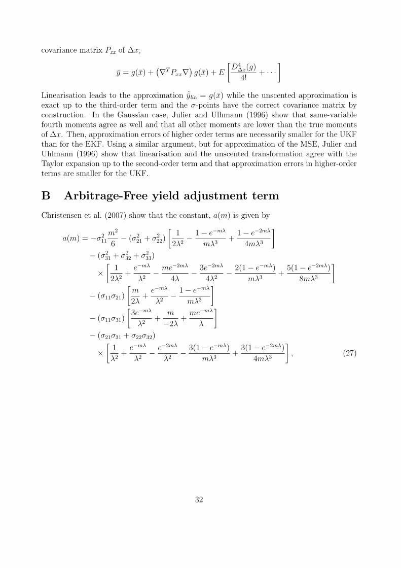
covariance matrix Pxx of ∆x,
y = g(x) +(∇T Pxx∇
)g(x) + E
[D4
∆x(g)
4!+ · · ·
]
Linearisation leads to the approximation ˆylin = g(x) while the unscented approximation isexact up to the third-order term and the σ-points have the correct covariance matrix byconstruction. In the Gaussian case, Julier and Ulhmann (1996) show that same-variablefourth moments agree as well and that all other moments are lower than the true momentsof ∆x. Then, approximation errors of higher order terms are necessarily smaller for the UKFthan for the EKF. Using a similar argument, but for approximation of the MSE, Julier andUhlmann (1996) show that linearisation and the unscented transformation agree with theTaylor expansion up to the second-order term and that approximation errors in higher-orderterms are smaller for the UKF.
B Arbitrage-Free yield adjustment term
Christensen et al. (2007) show that the constant, a(m) is given by
a(m) = −σ211
m2
6− (σ2
21 + σ222)
[1
2λ2− 1− e−mλ
mλ3+
1− e−2mλ
4mλ3
]
− (σ231 + σ2
32 + σ233)
×[
1
2λ2+
e−mλ
λ2− me−2mλ
4λ− 3e−2mλ
4λ2− 2(1− e−mλ)
mλ3+
5(1− e−2mλ)
8mλ3
]
− (σ11σ21)
[m
2λ+
e−mλ
λ2− 1− e−mλ
mλ3
]
− (σ11σ31)
[3e−mλ
λ2+
m
−2λ+
me−mλ
λ
]
− (σ21σ31 + σ22σ32)
×[
1
λ2+
e−mλ
λ2− e−2mλ
λ2− 3(1− e−mλ)
mλ3+
3(1− e−2mλ)
4mλ3
], (27)
32

References
Acharya, V. V. and L. Pedersen (2004). Asset pricing with liquidity risk. NBER (W10814).
Amihud, Y. (2002). Illiquidity and stock returns: cross-section and time-series effects. Jour-
nal of Financial Markets 5, 31–56.
Amihud, Y. and H. Mendelson (1986). Asset pricing and the bid-ask spreads. Journal of
Financial Economics 17, 223–249.
Amihud, Y. and H. Mendelson (1991). Liquidity, maturity and the yields on u.s treasury
securities. The Journal of Finance 46, 1411–1425.
Anderson, N., F. Breedon, M. Deacon, A. Derry, and G. Murphy (1996). Estimating and
interpreting the yield curve. Series in Financial Economics and Quantitative Analysis.
John Wiley & Sons.
Bakshi, G., P. Carr, and L. Wu (2005). Stochastic risk premiums, stochastic skewness in
currency options, and stochastic discount factors in international economies. Journal of
Financial Economics . forthcoming.
Bansal, R. and W. Coleman (1996). A monetary explanation of the term premium, equity
premium and risk-free rate puzzle. The Journal of Political Economy 104, 396–409.
Bliss, R. (1997). Testing term structure estimation methods. Advances in Futures and
Options Research 9, 197–231.
Buraschi, A. and D. Menini (2002). Liquidity risk and specialness. Journal of Financial
Economics 64, 243–284.
Campbell, J. and R. Shiller (1991). Yield spreads and interest rate movements: A bird’s eye
view. Review of Economic Studies 58, 495–514.
Cheria, J., E. Jacquier, and R. Jarrow (2004). A model of the convenience yields in on-the-
run treasuries. Review of Derivatives Research 7, 79–97.
Chordia, T., A. Sarkar, and A. Subrahmanyam (2005). An empirical analysis of stock and
bond market liquidity. Review of Financial Studies 18, 85–129.
Christensen, J., F. Diebold, and G. Rudebusch (2007). The affine arbitrage-free class of
nelson-siegel term structure models. Technical Report 20, FRBSF.
33

Christoffersen, P., K. Jacobs, L. Karoui, and K. Mimouni (2007). Estimating term structure
modesl using swap rates. McGill University.
Cochrane, J. and M. Piazzesi (2005). Bond risk premia. American Economic Review 95,
138–160.
Collin-Dufresne, P., R. Goldstein, and J. Spencer Martin (2001). The determinants of credit
spread changes. The Journal of Finance 56, 2177–2207.
Dai, Q. and K. Singleton (2000). Specification analysis of affine term structure models. The
Journal of Finance 55, 1943–1978.
Dai, Q. and K. Singleton (2002). Expectation puzzles, time-varying risk premia and affine
model of the term structure. Journal of Financial Economics 63, 415–441.
Diebold, F. and C. Li (2006). Forecasting the term structure of government bond yields.
Journal of Econometrics 130, 337–364.
Diebold, F., G. Rudebusch, and S. Aruoba (2006). The macroeconomy and the yield curve :
A dynamic latent factor approach. Journal of Econometrics 131, 309–338.
Duffee, G. (2002). Term premia and interest rate forecast in affine model. The Journal of
Finance 57, 405–443.
Duffie, D. (1996). Special repo rates. The Journal of Finance 51, 493–526.
Duffie, D., N. Garleanu, and L. Pedersen (2005). Over-the-counter markets. Econometrica 73,
1815–1847.
Duffie, D. and R. Kan (1996). A yield-factor model of interest rates. Mathematical Finance 6,
379–406.
Duffie, D. and K. Singleton (1997). An econometric model of the term structure of interest-
rate swap yields. The Journal of Finance 52, 1287–1321.
Elton, E. and T. Green (1998). Tax and liquidity effects in pricing governement bonds. The
Journal of Finance 53, 1533–1562.
Ericsson, J. and O. Renault (2006). Liquidity and credit risk. The Journal of Finance 61,
2219–2250.
Fama, E. (1976). Forward rates as predictors of future spot rates. Journal of Financial
Economics 3, 361–377.
34

Fama, E. (1984a). The information in the term structure. Journal of Financial Economics 13,
509–528.
Fama, E. (1984b). Term premium in bond returns. Journal of Financial Economics 13,
529–546.
Fama, E. and R. Bliss (1987). The information in long-maturity forward rates. American
Economic Review 77, 680–692.
Fedlhutter, P. and D. Lando (2007). Decomposing swap spreads. Copenhagen Business
School.
Goldreich, D., B. Hanke, and P. Nath (2005). The price of future liquidity : Time-varying
liquidity in the u.s. treasury market. Review of Finance 9, 1–32.
Green, R. and B. Ødegaard (1997). Are there tax effects in the relative pricing of the u.s.
government bonds? The Journal of Finance 52, 609–633.
Grinblatt, M. (2001). An analytic solution for interest rate swap spreads. International
Review of Finance 2, 113–149.
Gurkaynak, R., B. Sack, and J. Wright (2006). The u.s. treasury curve: 1961 to present.
Technical Report 2006-28.
Holmstrom, B. and J. Tirole (1998). Private and public supply of liquidity. The Journal of
Political Economy 106, 1–40.
Jordan, B. and S. Jordan (1997). Special repo rates: An empirical analysis. The Journal of
Finance 52, 2051–2072.
Julier, S. and J. Uhlmann (1996). A general method for approximating nonlinear transfor-
mations of probability distributions. Robotics Research Group, University of Oxford.
Julier, S., J. Uhlmann, and H. Durrant-Whyte (1995). A new approach for filtering nonlinear
systems. The Proceedings of the American Control Conference 3, 1628–1632. Seattle.
Kiyotaki, N. and R. Wright (1989). On money as a medium of exchange. The Journal of
Political Economy 97, 927–954.
Krishnamurthy, A. (2002). The bond/old-bond spread. Journal of Financial Economics 66,
463–506.
35
Krishnamurthy, A. and J. Vissing-Jorgensen (2007). The demand for treasury debt. Technical
Report W12881, NBER.
Lagos, R. (2006). Asset prices and liquidity in an exchange economy. Technical Report 373,
Federal Reserve Bank of Minneapolis.
Leippold, M. and L. Wu (2003). Design and estimation of multi-currency quadratic models.
European Finance Review 7, 47–73.
Liu, J., F. Longstaff, and R. Mandell (2006). The market price of risk in interest rate swaps:
The roles of default and liquidity risks. Journal of Business 79, 2337–2359.
Longstaff, F. (2000). The term structure of very short-term rates : New evidence for the
expectation hypothesis. Journal of Financial Economics 58, 397–415.
Longstaff, F. (2004). The flight-to-liquidity premium in U.S. treasury bond prices. The
Journal of Business 77, 511–526.
Longstaff, F., S. Mithal, and E. Neis (2005). Corporate yield spreads: Default risk or
liquidity? new evidence from the credit-default swap market. The Journal of Finance 60,
2213–2253.
Ludvigson, S. and S. Ng (2005). Macro factors in bond risk premia. Technical Report 11703,
NBER.
Luttmer, E. (1996). Asset pricing in economies with frictions. Econometrica 64, 1439–1467.
Nashikkar, A. and M. Subrahmanyam (2006). Latent liquidity and corporate bond yield
spreads. Stern School of Business.
Nelson, C. and A. Siegel (1987). Parsimonious modeling of yield curves. The Journal of
Business 60, 473–489.
Pastor, L. and R. Stambaugh (2003). Liquidity risk and expected stock returns. The Journal
of Political Economy 111, 642–685.
Piazzesi, M. (2005). Affine term structure models. in Handbook of Financial Econometrics.
Elsevier.
Shi, S. (2005). Nominal bonds and interest rates. International Economic Review 46, 579–
612.
36

Shi, S. (2006). Viewpoint: a microfoundation of monetary economics. Canadian Journal of
Economics 39, 643–688.
Shiller, R. (1979). The volatility of long-term interest rates and expectation models of the
term structure. The Journal of Political Economy 87, 1190–1219.
Startz, R. (1982). Do forecast errors of term premia really make a difference between long
and short rates. Journal of Financial Economics 10, 323–329.
Svensson, L. (1985). Money and asset prices in a cash-in-advance economy. The Journal of
Political Economy 93, 919–944.
Tauchen, G. and H. Zhou (2006). Realized jumps on financial markets and predicting credit
spreads. Technical Report 2006-35, Federal Reserve Board.
Vayanos, D. (2004). Flight to quality, flight to liquidity, and the pricing of risk.
NBER (W10327).
Vayanos, D. and P.-O. Weill (2006). A search-based theory of the on-the-run phenomenon.
NBER (W12670).
Wan, E. and R. V. der Merwe (2001). Kalman filtering and neural network, Chapter The
unscented Kalman filter. Wiley and Sons.
Warga, A. (1992). Bond returns, liquidity and missing data. The Journal of Financial and
Quantitative Analysis 27, 605–617.
37
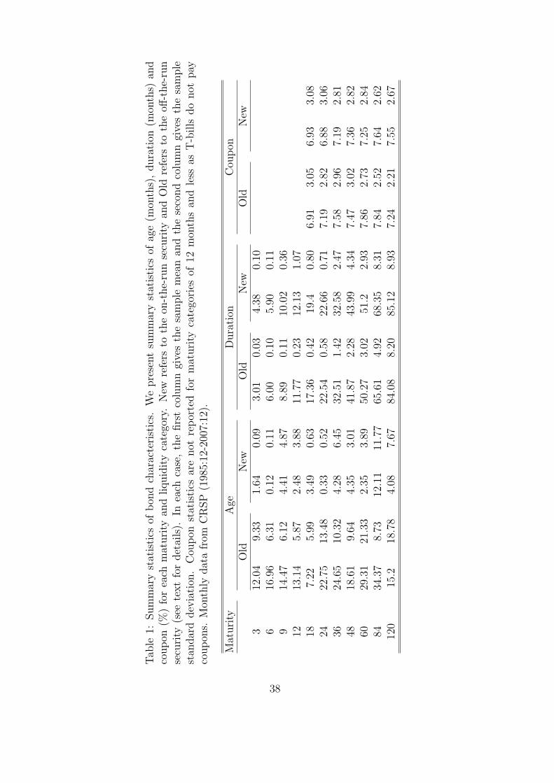
Tab
le1:
Sum
mar
yst
atis
tics
ofbon
dch
arac
teri
stic
s.W
epre
sent
sum
mar
yst
atis
tics
ofag
e(m
onth
s),dura
tion
(mon
ths)
and
coupon
(%)
for
each
mat
uri
tyan
dliquid
ity
cate
gory
.N
ewre
fers
toth
eon
-the-
run
secu
rity
and
Old
refe
rsto
the
off-t
he-
run
secu
rity
(see
text
for
det
ails
).In
each
case
,th
efirs
tco
lum
ngi
ves
the
sam
ple
mea
nan
dth
ese
cond
colu
mn
give
sth
esa
mple
stan
dar
ddev
iati
on.
Cou
pon
stat
isti
csar
enot
repor
ted
for
mat
uri
tyca
tego
ries
of12
mon
ths
and
less
asT
-bills
do
not
pay
coupon
s.M
onth
lydat
afr
omC
RSP
(198
5:12
-200
7:12
).
Mat
uri
tyA
geD
ura
tion
Cou
pon
Old
New
Old
New
Old
New
312
.04
9.33
1.64
0.09
3.01
0.03
4.38
0.10
616
.96
6.31
0.12
0.11
6.00
0.10
5.90
0.11
914
.47
6.12
4.41
4.87
8.89
0.11
10.0
20.
3612
13.1
45.
872.
483.
8811
.77
0.23
12.1
31.
0718
7.22
5.99
3.49
0.63
17.3
60.
4219
.40.
806.
913.
056.
933.
0824
22.7
513
.48
0.33
0.52
22.5
40.
5822
.66
0.71
7.19
2.82
6.88
3.06
3624
.65
10.3
24.
286.
4532
.51
1.42
32.5
82.
477.
582.
967.
192.
8148
18.6
19.
644.
353.
0141
.87
2.28
43.9
94.
347.
473.
027.
362.
8260
29.3
121
.33
2.35
3.89
50.2
73.
0251
.22.
937.
862.
737.
252.
8484
34.3
78.
7312
.11
11.7
765
.61
4.92
68.3
58.
317.
842.
527.
642.
6212
015
.218
.78
4.08
7.67
84.0
88.
2085
.12
8.93
7.24
2.21
7.55
2.67
38

Table 2: Parameter estimates for transition equations. Panel (a) presents estimation resultsfor the AFENS model without liquidity. Panel (b) presents estimation results for AFENSmodel with liquidity. For each parameter, the first standard error (in parenthesis) is com-puted from the QMLE covariance matrix (see Equation 23) while the second is computedfrom the sum of outer products of gradients (see Equation 25). Estimation is based oncoupon bonds data from CRSP 12/1985-12/2007.
(a) Benchmark Model
F K Σ (×102)0.0545 0.171 0.68
Level (0.0152) (0.106) (0.39)(0.0134) (0.072) (0.02)-0.0171 0.182 0.76 0.84
Slope (0.0203) (0.195) (0.74) (0.55)(0.0166) (0.135) (0.05) (0.04)-0.0129 0.885 -0.10 0.39 2.34
Curvature (0.0083) (1.29) (1.88) (1.92) (1.66)(0.0072) (0.288) (0.17) (0.20) (0.13)
(b) Model with liquidity
F K Σ (×102)0.0555 0.181 0.71
Level (0.0239) (0.228) (0.46)(0.0132) (0.079) (0.02)-0.0164 0.186 -0.76 0.84
Slope (0.0177) (0.341) (0.66) (0.48)(0.0186) (0.138) (0.05) (0.04)-0.0163 0.914 0.20 0.30 2.34
Curvature (0.0087) (1.178) (2.10) (1.93) (1.52)(0.0076) (0.301) (0.04) (0.19) (0.11)
L φl σl
0.375 0.965 0.068Liquidity (0.212) (0.044) (0.040)
(0.76) (0.085) (0.016)
39
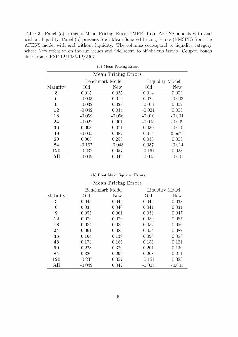
Table 3: Panel (a) presents Mean Pricing Errors (MPE) from AFENS models with andwithout liquidity. Panel (b) presents Root Mean Squared Pricing Errors (RMSPE) from theAFENS model with and without liquidity. The columns correspond to liquidity categorywhere New refers to on-the-run issues and Old refers to off-the-run issues. Coupon bondsdata from CRSP 12/1985-12/2007.
(a) Mean Pricing Errors
Mean Pricing Errors
Benchmark Model Liquidity ModelMaturity Old New Old New
3 0.015 0.025 0.014 0.0026 -0.003 0.019 0.022 -0.0039 -0.032 0.023 -0.011 0.00212 -0.042 0.034 -0.024 0.00318 -0.059 -0.056 -0.010 -0.00424 -0.027 0.001 -0.005 -0.00936 0.008 0.071 0.030 -0.01048 -0.005 0.082 0.014 2.5e−5
60 0.008 0.253 0.038 0.00384 -0.167 -0.043 0.037 -0.014120 -0.237 0.057 -0.161 0.023All -0.049 0.042 -0.005 -0.001
(b) Root Mean Squared Errors
Mean Pricing Errors
Benchmark Model Liquidity ModelMaturity Old New Old New
3 0.048 0.045 0.048 0.0386 0.035 0.040 0.041 0.0349 0.055 0.061 0.038 0.04712 0.073 0.079 0.059 0.05718 0.084 0.085 0.052 0.05624 0.061 0.083 0.054 0.08236 0.104 0.139 0.098 0.08848 0.173 0.185 0.156 0.12160 0.228 0.320 0.201 0.13084 0.326 0.299 0.208 0.211120 -0.237 0.057 -0.161 0.023All -0.049 0.042 -0.005 -0.001
40
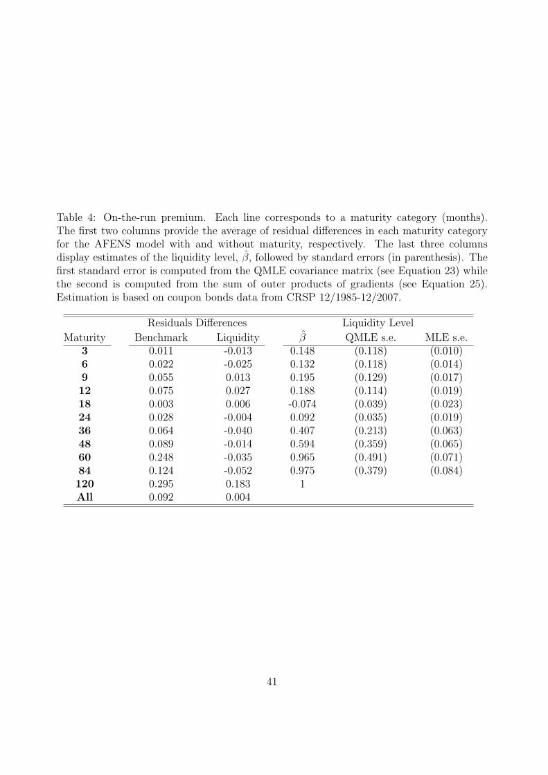
Table 4: On-the-run premium. Each line corresponds to a maturity category (months).The first two columns provide the average of residual differences in each maturity categoryfor the AFENS model with and without maturity, respectively. The last three columnsdisplay estimates of the liquidity level, β, followed by standard errors (in parenthesis). Thefirst standard error is computed from the QMLE covariance matrix (see Equation 23) whilethe second is computed from the sum of outer products of gradients (see Equation 25).Estimation is based on coupon bonds data from CRSP 12/1985-12/2007.
Residuals Differences Liquidity Level
Maturity Benchmark Liquidity β QMLE s.e. MLE s.e.3 0.011 -0.013 0.148 (0.118) (0.010)6 0.022 -0.025 0.132 (0.118) (0.014)9 0.055 0.013 0.195 (0.129) (0.017)12 0.075 0.027 0.188 (0.114) (0.019)18 0.003 0.006 -0.074 (0.039) (0.023)24 0.028 -0.004 0.092 (0.035) (0.019)36 0.064 -0.040 0.407 (0.213) (0.063)48 0.089 -0.014 0.594 (0.359) (0.065)60 0.248 -0.035 0.965 (0.491) (0.071)84 0.124 -0.052 0.975 (0.379) (0.084)120 0.295 0.183 1All 0.092 0.004
41

Tab
le5:
Res
ult
sfr
omre
gres
sion
sof
exce
ssre
turn
sfr
omoff
-the-
run
bon
don
the
liquid
ity
and
term
stru
cture
fact
ors.
Eac
hva
riab
leis
obta
ined
from
the
AFE
NS
model
,dem
eaned
and
div
ided
by
its
stan
dar
ddev
iati
on.
The
spec
ifica
tion
isxr(m
)t+
h=
α(m
)h
+δ(m
)h
Lt+
β(m
)Th
Ft+
ε(m)
(t+
h)w
her
exr(m
)t+
his
the
exce
ssre
turn
sat
hor
izon
h(m
onth
s)on
abon
dof
mat
uri
tym
(mon
ths)
,L
t
isth
eliquid
ity
fact
oran
dF
tis
the
vect
orof
term
stru
cture
fact
or.
Pan
el(a
)co
nta
ins
esti
mat
esof
αan
dPan
el(b
)co
nta
ins
esti
mat
esof
δ.N
ewey
-Wes
tst
andar
der
rors
(h+
3la
gs)
are
incl
uded
inpar
enth
esis
.Pan
el(c
)pre
sents
R2.
24-m
onth
sex
cess
retu
rnon
2-ye
arbon
ds
(low
erle
ftco
rner
ofea
chpan
el)
isal
way
sze
roby
const
ruct
ion.
(a)
Ave
rage
risk
prem
ia
Bon
dM
aturi
tyH
oriz
on2
34
57
106
1.11
(0.3
9)1.
70(0
.62)
2.15
(0.8
1)2.
49(0
.98)
2.98
(1.2
7)3.
50(1
.70)
120.
72(0
.28)
1.34
(0.5
1)1.
80(0
.68)
2.14
(0.8
2)2.
62(1
.05)
3.10
(1.3
7)18
0.37
(0.1
4)1.
02(0
.38)
1.53
(0.5
5)1.
91(0
.67)
2.44
(0.8
4)2.
96(1
.05)
240.
70(0
.24)
1.28
(0.4
1)1.
72(0
.53)
2.33
(0.6
7)2.
94(0
.81)
(b)
Liq
uidi
tyC
oeffi
cien
ts
Bon
dM
aturi
tyH
oriz
on2
34
57
106
-0.5
8(0
.32)
-0.9
9(0
.55)
-1.3
8(0
.75)
-1.7
4(0
.93)
-2.4
2(1
.25)
-3.3
7(1
.70)
12-0
.47
(0.1
6)-0
.96
(0.3
1)-1
.42
(0.4
4)-1
.82
(0.5
7)-2
.54
(0.8
0)-3
.50
(1.1
5)18
-0.1
7(0
.08)
-0.5
0(0
.24)
-0.7
9(0
.38)
-1.0
5(0
.49)
-1.5
2(0
.69)
-2.1
6(0
.96)
24-0
.26
(0.1
9)-0
.48
(0.3
4)-0
.68
(0.4
5)-1
.02
(0.6
2)-1
.49
0.81
)
(c)
R2
Bon
dM
aturi
tyH
oriz
on2
34
57
106
15.1
15.8
16.7
17.5
18.6
19.2
1220
.422
.925
.728
.432
.636
.018
20.7
19.4
20.5
22.5
27.5
33.6
2422
.218
.717
.116
.920
.3
42

Table 6: Results from regressions of excess returns from off-the-run bonds on forward ratesand the liquidity factor. Variables are demeaned and divided by their standard deviations.The specification is xr
(m)t+12 = α(m) +δ(m)Lt +β(m)T ft +ε
(m)(t+12) where xr
(m)t+h is the annual excess
returns on a bond with maturity m (months), Lt is the liquidity factor and ft is the vector of
forward rates f(h)t at horizon h. Panel (a) presents results using excess returns and forward
rates computed from FB data with the liquidity factor from the AFENS model. Panel (b)excludes the liquidity factor. Panel (c) excludes the liquidity factor and uses excess returnscomputed from the model. Newey-West standard errors (in parenthesis) with 15 lags.
(a) Excess returns and forward rates from FB with the liquidity factor
Maturity cst f(1)t f
(2)t f
(3)t f
(4)t f
(5)t Lt R2
2 0.72 0.05 -2.01 2.97 1.07 -1.46 -0.51 0.31(0.23) (0.67) (1.27) (1.49) (0.96) (0.66) (0.18)
3 1.31 -0.29 -3.71 6.51 1.06 -2.50 -1.06 0.32(0.43) (1.27) (2.36) (2.79) (1.73) (1.30) (0.36)
4 1.79 -1.08 -3.86 7.70 1.95 -3.27 -1.56 0.34(0.57) (1.73) (3.20) (3.73) (2.24) (1.79) (0.50)
5 1.98 -2.15 -2.90 8.41 0.88 -2.54 -1.96 0.33(0.69) (2.08) (3.98) (4.50) (2.61) (2.23) (0.63)
(b) Excess returns and forward rates from FB
Maturity cst f(1)t f
(2)t f
(3)t f
(4)t f
(5)t Lt R2
2 0.72 -0.43 -1.34 2.66 0.99 -1.53 0.21(0.24) (0.75) (1.27) (1.77) (1.04) (0.72)
3 1.31 -1.27 -2.33 5.86 0.88 -2.64 0.19(0.45) (1.46) (2.24) (3.30) (1.92) (1.42)
4 1.79 -2.52 -1.83 6.74 1.70 -3.46 0.20(0.61) (2.00) (2.96) (4.45) (2.54) (1.96)
5 1.98 -3.96 -0.35 7.20 0.56 -2.79 0.18(0.73) (2.40) (3.55) (5.32) (3.01) (2.44)
(c) Excess returns from the model and forward rates from FB
Maturity cst f(1)t f
(2)t f
(3)t f
(4)t f
(5)t Lt R2
2 0.70 -0.14 -1.89 2.96 0.92 -1.49 0.22(0.24) (0.75) (1.22) (1.72) (1.00) (0.71)
3 1.31 -1.16 -2.01 4.96 1.18 -2.42 0.19(0.45) (1.44) (2.23) (3.28) (1.88) (1.39)
4 1.77 -2.48 -1.24 6.12 1.16 -2.91 0.18(0.61) (1.99) (3.04) (4.52) (2.56) (1.98)
5 2.12 -3.88 -0.01 6.67 1.04 -3.11 0.17(0.74) (2.40) (3.71) (5.49) (3.08) (2.47)
43

Tab
le7:
Res
ult
sfr
omre
gres
sion
sof
LIB
OR
spre
adson
the
liquid
ity
and
term
stru
cture
fact
orsfr
omth
eA
FE
NS
model
.Spre
ads
are
com
pute
dab
ove
the
AFE
NS
zero
-cou
pon
yie
ldcu
rve.
Eac
hva
riab
les
isdem
eaned
and
div
ided
by
stan
dar
ddev
iati
on.
The
spec
ifica
tion
issp
rd(m
)t+
h=
α(m
)h
+δ(m
)h
Lt+
β(m
)Th
Ft+
ε(m)
(t+
h)
wher
esp
rd(m
)t+
his
the
spre
adat
tim
et+
h(m
onth
s)on
alo
anw
ith
mat
uri
tym
(mon
ths)
,L
tis
the
liquid
ity
fact
oran
dF
tis
the
vect
orof
term
stru
cture
fact
or.
Pan
el(a
)co
nta
ins
esti
mat
esof
α0
and
Pan
el(b
)co
nta
ins
esti
mat
esof
δ(m)
h.
New
ey-W
est
stan
dar
der
rors
(h+
3la
gs)
are
incl
ude
inpar
enth
esis
.Pan
el(c
)pre
sents
R2.
(a)
Ave
rage
Ris
kP
rem
ium
Loa
nM
aturi
tyH
oriz
on1
36
912
00.
34(0
.03)
0.38
(0.0
2)0.
41(0
.02)
0.43
(0.2
)0.
47(0
.02)
(b)
Liq
uidi
tyC
oeffi
cien
ts
Loa
nM
aturi
tyH
oriz
on1
36
912
00.
073
(0.0
2)0.
079
(0.0
2)0.
068
(0.0
1)0.
070
(0.0
1)0.
069
(0.0
1)6
0.04
5(0
.02)
0.06
2(0
.02)
0.06
7(0
.02)
0.07
8(0
.02)
0.08
1(0
.02)
120.
091
(0.0
2)0.
105
(0.0
2)0.
103
(0.0
2)0.
120
(0.0
2)0.
131
(0.0
2)18
0.08
8(0
.02)
0.09
4(0
.02)
0.09
4(0
.02)
0.11
0(0
.02)
0.11
8(0
.02)
240.
109
(0.0
2)0.
112
(0.0
2)0.
113
(0.0
2)0.
124
(0.0
2)0.
130
(0.0
2)
(c)
R2
Loa
nM
aturi
tyH
oriz
on1
36
912
039
.345
.447
.751
.753
.66
42.9
44.5
41.9
41.7
41.1
1249
.046
.637
.936
.636
.418
51.5
43.9
30.8
27.1
25.6
2458
.754
.040
.733
.730
.1
44
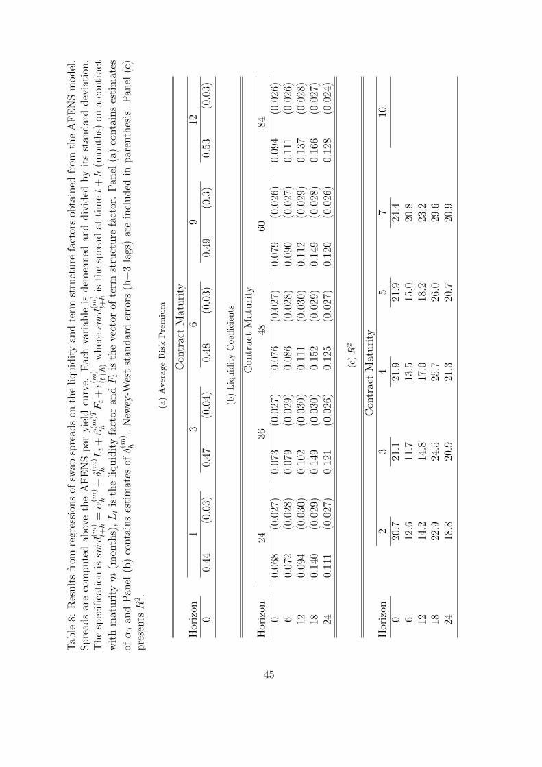
Tab
le8:
Res
ult
sfr
omre
gres
sion
sof
swap
spre
ads
onth
eliquid
ity
and
term
stru
cture
fact
ors
obta
ined
from
the
AFE
NS
model
.Spre
ads
are
com
pute
dab
ove
the
AFE
NS
par
yie
ldcu
rve.
Eac
hva
riab
leis
dem
eaned
and
div
ided
by
its
stan
dar
ddev
iati
on.
The
spec
ifica
tion
issp
rd(m
)t+
h=
α(m
)h
+δ(m
)h
Lt+
β(m
)Th
Ft+
ε(m)
(t+
h)w
her
esp
rd(m
)t+
his
the
spre
adat
tim
et+
h(m
onth
s)on
aco
ntr
act
wit
hm
aturi
tym
(mon
ths)
,L
tis
the
liquid
ity
fact
oran
dF
tis
the
vect
orof
term
stru
cture
fact
or.
Pan
el(a
)co
nta
ins
esti
mat
es
ofα
0an
dPan
el(b
)co
nta
ins
esti
mat
esof
δ(m)
h.
New
ey-W
est
stan
dar
der
rors
(h+
3la
gs)
are
incl
uded
inpar
enth
esis
.Pan
el(c
)pre
sents
R2.
(a)
Ave
rage
Ris
kP
rem
ium
Con
trac
tM
aturi
tyH
oriz
on1
36
912
00.
44(0
.03)
0.47
(0.0
4)0.
48(0
.03)
0.49
(0.3
)0.
53(0
.03)
(b)
Liq
uidi
tyC
oeffi
cien
ts
Con
trac
tM
aturi
tyH
oriz
on24
3648
6084
00.
068
(0.0
27)
0.07
3(0
.027
)0.
076
(0.0
27)
0.07
9(0
.026
)0.
094
(0.0
26)
60.
072
(0.0
28)
0.07
9(0
.029
)0.
086
(0.0
28)
0.09
0(0
.027
)0.
111
(0.0
26)
120.
094
(0.0
30)
0.10
2(0
.030
)0.
111
(0.0
30)
0.11
2(0
.029
)0.
137
(0.0
28)
180.
140
(0.0
29)
0.14
9(0
.030
)0.
152
(0.0
29)
0.14
9(0
.028
)0.
166
(0.0
27)
240.
111
(0.0
27)
0.12
1(0
.026
)0.
125
(0.0
27)
0.12
0(0
.026
)0.
128
(0.0
24)
(c)
R2
Con
trac
tM
aturi
tyH
oriz
on2
34
57
100
20.7
21.1
21.9
21.9
24.4
612
.611
.713
.515
.020
.812
14.2
14.8
17.0
18.2
23.2
1822
.924
.525
.726
.029
.624
18.8
20.9
21.3
20.7
20.9
45
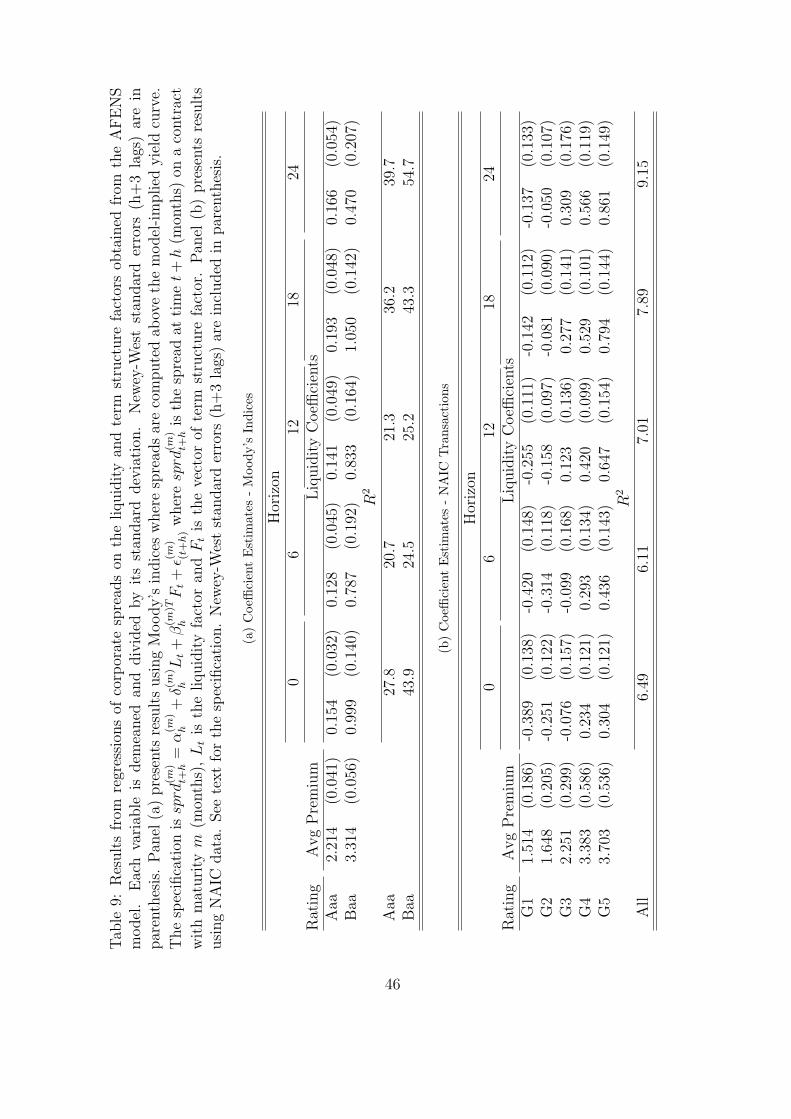
Tab
le9:
Res
ult
sfr
omre
gres
sion
sof
corp
orat
esp
read
son
the
liquid
ity
and
term
stru
cture
fact
ors
obta
ined
from
the
AFE
NS
model
.E
ach
vari
able
isdem
eaned
and
div
ided
by
its
stan
dar
ddev
iati
on.
New
ey-W
est
stan
dar
der
rors
(h+
3la
gs)
are
inpar
enth
esis
.Pan
el(a
)pre
sents
resu
lts
usi
ng
Moody’s
indic
esw
her
esp
read
sar
eco
mpute
dab
ove
the
model
-im
plied
yie
ldcu
rve.
The
spec
ifica
tion
issp
rd(m
)t+
h=
α(m
)h
+δ(m
)h
Lt+
β(m
)Th
Ft+
ε(m)
(t+
h)w
her
esp
rd(m
)t+
his
the
spre
adat
tim
et+
h(m
onth
s)on
aco
ntr
act
wit
hm
aturi
tym
(mon
ths)
,L
tis
the
liquid
ity
fact
oran
dF
tis
the
vect
orof
term
stru
cture
fact
or.
Pan
el(b
)pre
sents
resu
lts
usi
ng
NA
ICdat
a.See
text
for
the
spec
ifica
tion
.N
ewey
-Wes
tst
andar
der
rors
(h+
3la
gs)
are
incl
uded
inpar
enth
esis
.
(a)
Coe
ffici
ent
Est
imat
es-
Moo
dy’s
Indi
ces
Hor
izon
06
1218
24R
atin
gA
vg
Pre
miu
mLiq
uid
ity
Coeffi
cien
tsA
aa2.
214
(0.0
41)
0.15
4(0
.032
)0.
128
(0.0
45)
0.14
1(0
.049
)0.
193
(0.0
48)
0.16
6(0
.054
)B
aa3.
314
(0.0
56)
0.99
9(0
.140
)0.
787
(0.1
92)
0.83
3(0
.164
)1.
050
(0.1
42)
0.47
0(0
.207
)R
2
Aaa
27.8
20.7
21.3
36.2
39.7
Baa
43.9
24.5
25.2
43.3
54.7
(b)
Coe
ffici
ent
Est
imat
es-
NA
ICTra
nsac
tion
s
Hor
izon
06
1218
24R
atin
gA
vg
Pre
miu
mLiq
uid
ity
Coeffi
cien
tsG
11.
514
(0.1
86)
-0.3
89(0
.138
)-0
.420
(0.1
48)
-0.2
55(0
.111
)-0
.142
(0.1
12)
-0.1
37(0
.133
)G
21.
648
(0.2
05)
-0.2
51(0
.122
)-0
.314
(0.1
18)
-0.1
58(0
.097
)-0
.081
(0.0
90)
-0.0
50(0
.107
)G
32.
251
(0.2
99)
-0.0
76(0
.157
)-0
.099
(0.1
68)
0.12
3(0
.136
)0.
277
(0.1
41)
0.30
9(0
.176
)G
43.
383
(0.5
86)
0.23
4(0
.121
)0.
293
(0.1
34)
0.42
0(0
.099
)0.
529
(0.1
01)
0.56
6(0
.119
)G
53.
703
(0.5
36)
0.30
4(0
.121
)0.
436
(0.1
43)
0.64
7(0
.154
)0.
794
(0.1
44)
0.86
1(0
.149
)R
2
All
6.49
6.11
7.01
7.89
9.15
46

Tab
le10
:R
esult
sfr
omre
gres
sion
sof
the
liquid
ity
fact
oron
sele
cted
econ
omic
vari
able
s.B
Ais
the
diff
eren
cebet
wee
nth
em
inim
um
and
the
med
ian
bid
-ask
spre
ads
acro
ssal
lbon
dpri
ceob
serv
atio
non
agi
ven
dat
e.V
XO
isth
eim
plied
vola
tility
from
S&
P50
0ca
llop
tion
s.F
1to
F8
are
pri
nci
pal
com
pon
ents
ofm
acro
econ
omic
seri
esfr
omLudvig
son
and
Ng.
New
ey-W
est
stan
dar
der
rors
(3la
gs)
are
incl
uded
inpar
enth
esis
.
Reg
ress
ors
Model
cst
BA
VX
OF
1F
2F
3F
4F
5F
6F
7F
8R
2
A0.
475
0.03
70.
089
-0.0
080.
055
0.04
3-0
.074
0.08
2-0
.019
30.4
(0.0
33)
(0.0
27)
(0.0
21)
(0.0
20)
(0.0
25)
(0.0
21)
(0.0
25)
(0.0
26)
(0.0
19)
B0.
432
0.14
031
.7(0
.028
)(0
.037
)
C0.
431
0.09
414
.2(0
.033
)(0
.027
)
D0.
474
0.10
20.
031
0.01
30.
060
-0.0
100.
025
0.01
9-0
.056
0.07
0-0
.048
45.2
(0.0
28)
(0.0
35)
(0.0
31)
(0.0
22)
(0.0
21)
(0.0
16)
(0.0
19)
(0.0
19)
(0.0
25)
(0.0
24)
(0.0
16)
47
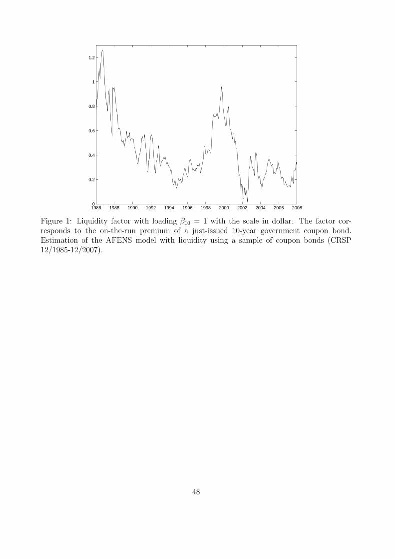
1986 1988 1990 1992 1994 1996 1998 2000 2002 2004 2006 20080
0.2
0.4
0.6
0.8
1
1.2
Figure 1: Liquidity factor with loading β10 = 1 with the scale in dollar. The factor cor-responds to the on-the-run premium of a just-issued 10-year government coupon bond.Estimation of the AFENS model with liquidity using a sample of coupon bonds (CRSP12/1985-12/2007).
48

1986 1988 1990 1992 1994 1996 1998 2000 2002 2004 2006 2008
−0.06
−0.04
−0.02
0
0.02
0.04
0.06
0.08
LevelSlopeCurvature
Figure 2: Term Stucture factors from AFENS model without liquidity. The scale is inpercentage. Coupon bonds data from CRSP 12/1985-12/2007.
.
49
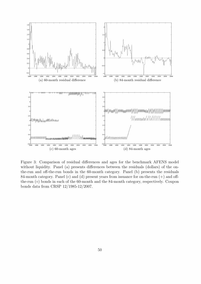
1986 1988 1990 1992 1994 1996 1998 2000 2002 2004 2006 2008
−0.2
0
0.2
0.4
0.6
0.8
1
1.2
1.4
1.6
1.8
(a) 60-month residual difference1986 1988 1990 1992 1994 1996 1998 2000 2002 2004 2006 2008
−1
−0.5
0
0.5
1
1.5
2
(b) 84-month residual difference
1986 1988 1990 1992 1994 1996 1998 2000 2002 2004 2006 2008−0.5
0
0.5
1
1.5
2
2.5
3
3.5
4
4.5
5
(c) 60-month ages1986 1988 1990 1992 1994 1996 1998 2000 2002 2004 2006 2008
−0.5
0
0.5
1
1.5
2
2.5
3
3.5
4
4.5
5
(d) 84-month ages
Figure 3: Comparison of residual differences and ages for the benchmark AFENS modelwithout liquidity. Panel (a) presents differences between the residuals (dollars) of the on-the-run and off-the-run bonds in the 60-month category. Panel (b) presents the residuals84-month category. Panel (c) and (d) present years from issuance for on-the-run (+) and off-the-run () bonds in each of the 60-month and the 84-month category, respectively. Couponbonds data from CRSP 12/1985-12/2007.
50
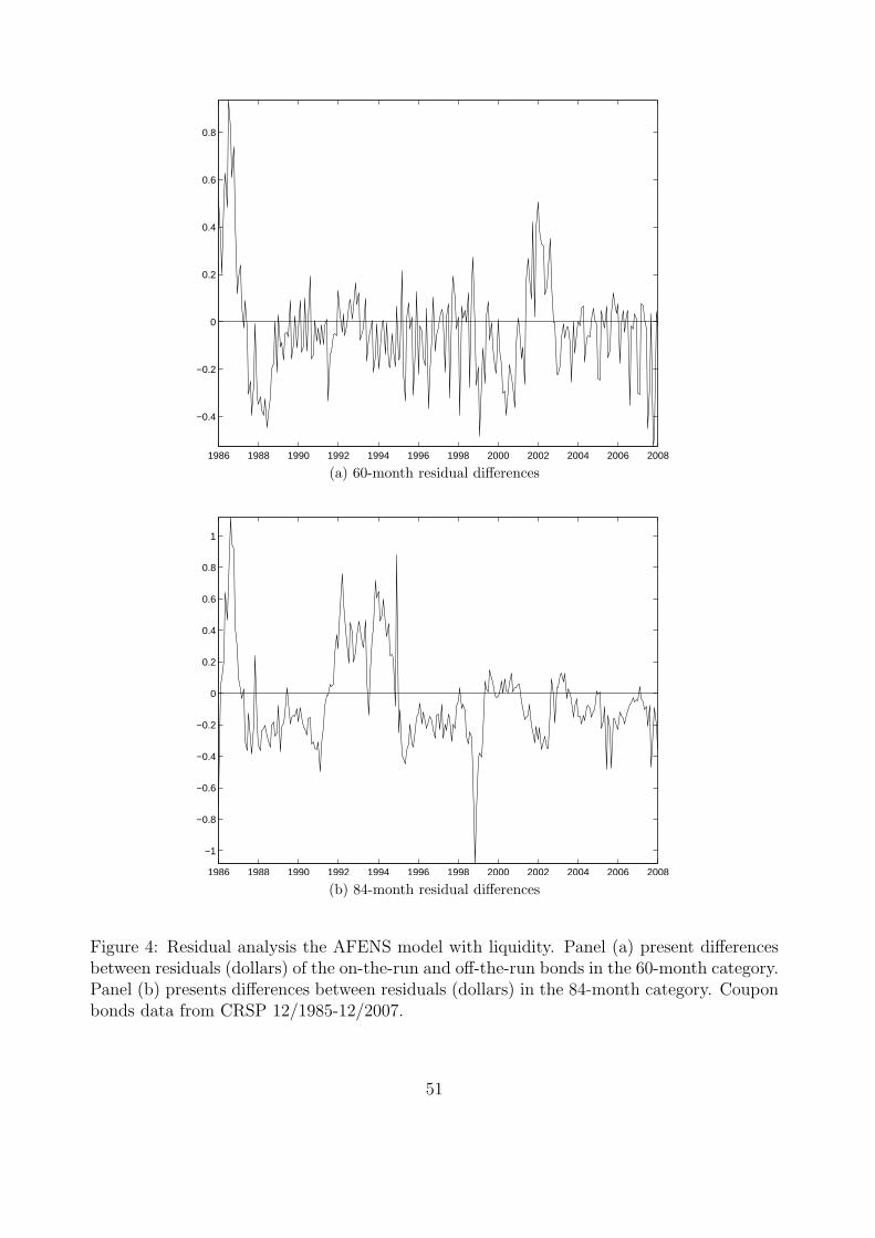
1986 1988 1990 1992 1994 1996 1998 2000 2002 2004 2006 2008
−0.4
−0.2
0
0.2
0.4
0.6
0.8
(a) 60-month residual differences
1986 1988 1990 1992 1994 1996 1998 2000 2002 2004 2006 2008
−1
−0.8
−0.6
−0.4
−0.2
0
0.2
0.4
0.6
0.8
1
(b) 84-month residual differences
Figure 4: Residual analysis the AFENS model with liquidity. Panel (a) present differencesbetween residuals (dollars) of the on-the-run and off-the-run bonds in the 60-month category.Panel (b) presents differences between residuals (dollars) in the 84-month category. Couponbonds data from CRSP 12/1985-12/2007.
51

Figure 5: Comparison of the liquidity factor with expected risk premium in different markets.Panel (a) compares with the risk premium on 2-year off-the-run U.S. Treasury bond. Panel 6bcompares with risk premium on a 12-month LIBOR loan. Panel 6c compares with riskpremium on 7-year swap contract. Panel 6c compares with Moody’s index of risk premiumon Baa corporate bonds.
1986 1988 1990 1992 1994 1996 1998 2000 2002 2004 2006 2008−3
−2
−1
0
1
2
3
4
31−Oct−1987 31−Aug−1998
01−Jan−2000
Liquidity2−year bond
(a) Liquidity and off-the-run excess returns1986 1988 1990 1992 1994 1996 1998 2000 2002 2004 2006 2008
−3
−2
−1
0
1
2
3
4
31−Oct−1987 31−Aug−1998
01−Jan−2000
Liquidity12−month Libor
(b) Liquidity and 12-month LIBOR spread
1986 1988 1990 1992 1994 1996 1998 2000 2002 2004 2006 2008−3
−2
−1
0
1
2
3
4
31−Oct−1987 31−Aug−1998
01−Jan−2000
Liquidity7−Year Swap Spread
(c) Liquidity and 7-year swap spread1986 1988 1990 1992 1994 1996 1998 2000 2002 2004 2006 2008
−3
−2
−1
0
1
2
3
4
31−Oct−1987 31−Aug−1998
01−Jan−2000
LiquidityMoody Baa Index
(d) Liquidity and Moody’s corporate spread index
52
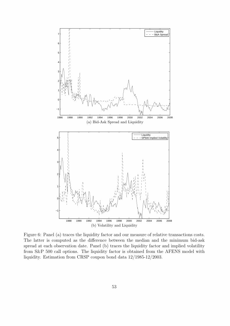
1986 1988 1990 1992 1994 1996 1998 2000 2002 2004 2006 2008
−1
0
1
2
3
4
5
6
7
LiquidityB&A Spread
(a) Bid-Ask Spread and Liquidity
1988 1990 1992 1994 1996 1998 2000 2002 2004 2006 2008
−1
0
1
2
3
4
5
LiquiditySP500 Implied Volatility
(b) Volatility and Liquidity
Figure 6: Panel (a) traces the liquidity factor and our measure of relative transactions costs.The latter is computed as the difference between the median and the minimum bid-askspread at each observation date. Panel (b) traces the liquidity factor and implied volatilityfrom S&P 500 call options. The liquidity factor is obtained from the AFENS model withliquidity. Estimation from CRSP coupon bond data 12/1985-12/2003.
53
Copyright © 2022 FDOKUMEN