Body size and wages in Europe: A semi-parametric analysis

S E D A PA PROGRAM FOR RESEARCH ON

SOCIAL AND ECONOMICDIMENSIONS OF AN AGING

POPULATION

Body size and wages in Europe:A semi-parametric analysis

Vincent A. HildebrandPhilippe Van Kerm

SEDAP Research Paper No. 269

For further information about SEDAP and other papers in this series, see our web site: http://socserv.mcmaster.ca/sedap

Requests for further information may be addressed to:Secretary, SEDAP Research Program

Kenneth Taylor Hall, Room 426McMaster University

Hamilton, Ontario, CanadaL8S 4M4

FAX: 905 521 8232e-mail: [email protected]

June 2010

The Program for Research on Social and Economic Dimensions of an Aging Population (SEDAP) is aninterdisciplinary research program centred at McMaster University with co-investigators at seventeen otheruniversities in Canada and abroad. The SEDAP Research Paper series provides a vehicle for distributingthe results of studies undertaken by those associated with the program. Authors take full responsibility forall expressions of opinion. SEDAP has been supported by the Social Sciences and Humanities ResearchCouncil since 1999, under the terms of its Major Collaborative Research Initiatives Program. Additionalfinancial or other support is provided by the Canadian Institute for Health Information, the CanadianInstitute of Actuaries, Citizenship and Immigration Canada, Indian and Northern Affairs Canada, ICES:Institute for Clinical Evaluative Sciences, IZA: Forschungsinstitut zur Zukunft der Arbeit GmbH (Institutefor the Study of Labour), SFI: The Danish National Institute of Social Research, Social DevelopmentCanada, Statistics Canada, and participating universities in Canada (McMaster, Calgary, Carleton,Memorial, Montréal, New Brunswick, Queen’s, Regina, Toronto, UBC, Victoria, Waterloo, Western, andYork) and abroad (Copenhagen, New South Wales, University College London).

Body size and wages in Europe:A semi-parametric analysis

Vincent A. HildebrandPhilippe Van Kerm

SEDAP Research Paper No. 269

Body size and wages in Europe:A semi-parametric analysis∗

Vincent A. Hildebrand†Department of Economics, Glendon College, York University, Canada

and CEPS/INSTEAD, Luxembourg

Philippe Van Kerm‡CEPS/INSTEAD, Luxembourg

May 2010

Abstract

Evidence of the association between wages and body size –typically measured bythe body mass index– appears to be sensitive to estimation methods and samples,and varies across gender and ethnic groups. One factor that may contribute to thissensitivity is the non-linearity of the relationship. This paper analyzes data from theEuropean Community Household Panel survey and uses semi-parametric techniquesto avoid functional form assumptions and assess the relevance of standard models.If a linear model for women and a quadratic model for men fit the data relativelywell, they are not entirely satisfactory and are statistically rejected in favour of semi-parametric models which identify patterns that none of the parametric specificationscapture. Furthermore, when we use height and weight in the models directly, ratherthan equating body size with the body mass index, the semi-parametric models re-veal a more complex picture with height having additional effects on wages. Weinterpret our results as consistent with the existence of a wage premium for physicalattractiveness rather than a penalty for unhealthy weight.Keywords: Body Mass Index ; obesity ; wages ; partial linear models ; ECHPJEL classification codes: C14 ; J31 ; J71

∗This research is part of the MeDIM project (Advances in the Measurement of Discrimination, Inequalityand Mobility) supported by the Luxembourg ‘Fonds National de la Recherche’ (contract FNR/06/15/08)and by core funding for CEPS/INSTEAD from the Ministry of Culture, Higher Education and Research ofLuxembourg. The authors would like to thank seminar participants at the Australian National Universityand Alessio Fusco, Eric Kam and Don Williams for useful comments.†Vincent Hildebrand, Department of Economics, York Hall 363, Glendon College, York University,

2275 Bayview ave., Toronto, Ontario, M4N 3M6 Canada. E-mail: [email protected].‡Philippe Van Kerm, CEPS/INSTEAD, B.P.48, L-4501 Differdange, Luxembourg. E-mail:

[email protected].

RJsumJ

La corrélation entre les salaires et la taille corporelle ‐ généralement mesurée par l'indice de

masse corporelle ‐ semble être sensible aux méthodes d'estimation, aux échantillons, et varie

selon le sexe et les groupes ethniques. Un facteur pouvant contribuer à cette sensibilité est la non‐

linéarité de cette relation. Ce document analyse les données de l'enquête du Panel

communautaire des ménages et utilise des techniques semi‐paramétriques pour éviter de faire

des hypothèses de formes fonctionnelles et évaluer la pertinence des modèles standards. Bien que

le modèle linéaire pour les femmes et le modèle quadratique pour les hommes ajustent

relativement bien les données, ils ne sont pas entièrement satisfaisants et sont statistiquement

rejetés en faveur des modèles semi‐paramétriques qui identifient des tendances qu'aucune de ces

spécifications paramétriques ne capture. En outre, lorsque nous utilisons la taille et le poids

directement, plutôt que de mesurer la taille corporelle par l'indice de masse corporelle, les

modèles semi‐paramétriques révèlent une situation plus complexe avec l’existence d’effets

supplémentaires de la taille sur les salaires. Nous interprétons nos résultats comme étant

compatible avec l'existence d'une prime salariale pour l'apparence physique plutôt que d'une

pénalité pour les surplus de poids.

1 Introduction

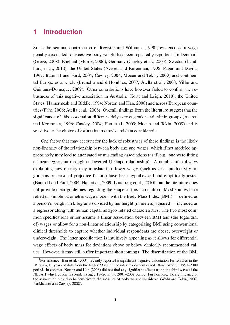
Since the seminal contribution of Register and Williams (1990), evidence of a wagepenalty associated to excessive body weight has been repeatedly reported – in Denmark(Greve, 2008), England (Morris, 2006), Germany (Cawley et al., 2005), Sweden (Lund-borg et al., 2010), the United States (Averett and Korenman, 1996; Pagan and Davila,1997; Baum II and Ford, 2004; Cawley, 2004; Mocan and Tekin, 2009) and continen-tal Europe as a whole (Brunello and d’Hombres, 2007; Atella et al., 2008; Villar andQuintana-Domeque, 2009). Other contributions have however failed to confirm the ro-bustness of this negative association in Australia (Kortt and Leigh, 2010), the UnitedStates (Hamermesh and Biddle, 1994; Norton and Han, 2008) and across European coun-tries (Fahr, 2006; Atella et al., 2008). Overall, findings from the literature suggest that thesignificance of this association differs widely across gender and ethnic groups (Averettand Korenman, 1996; Cawley, 2004; Han et al., 2009; Mocan and Tekin, 2009) and issensitive to the choice of estimation methods and data considered.1

One factor that may account for the lack of robustness of these findings is the likelynon-linearity of the relationship between body size and wages, which if not modeled ap-propriately may lead to attenuated or misleading associations (as if, e.g., one were fittinga linear regression through an inverted U-shape relationship). A number of pathwaysexplaining how obesity may translate into lower wages (such as strict productivity ar-guments or personal prejudice factors) have been hypothesized and empirically tested(Baum II and Ford, 2004; Han et al., 2009; Lundborg et al., 2010), but the literature doesnot provide clear guidelines regarding the shape of this association. Most studies haverelied on simple parametric wage models with the Body Mass Index (BMI) — defined asa person’s weight (in kilograms) divided by her height (in meters) squared — included asa regressor along with human capital and job-related characteristics. The two most com-mon specifications either assume a linear association between BMI and (the logarithmof) wages or allow for a non-linear relationship by categorizing BMI using conventionalclinical thresholds to capture whether individual respondents are obese, overweight orunderweight. The latter specification is intuitively appealing as it allows for differentialwage effects of body mass for deviations above or below clinically recommended val-ues. However, it may still suffer important shortcomings. The discretization of the BMI

1For instance, Han et al. (2009) recently reported a significant negative association for females in theUS using 13 years of data from the NLSY79 which includes respondents aged 18–43 over the 1991–2000period. In contrast, Norton and Han (2008) did not find any significant effects using the third wave of theNLSAH which covers respondents aged 18–26 in the 2001–2002 period. Furthermore, the significance ofthe association may also be sensitive to the measure of body weight considered (Wada and Tekin, 2007;Burkhauser and Cawley, 2008).

1

variable is somewhat arbitrary as there is no a priori guarantee that conventional clini-cal thresholds are adequate to pick up levels where obesity starts affecting wages. Forinstance, it is not unreasonable to believe that moderate deviations of BMI around a cen-tral value or within a socially accepted range (possibly outside clinically recommendedranges) do not trigger an immediate wage penalty. Mis-locating ‘turning points’ in therelationship between BMI and wages will lead to an attenuation of the estimated impactof obesity on wages. In addition, a piecewise constant specification does not identifydifferential wage effects of body size within BMI categories.

This paper addresses these concerns by estimating partial linear regression modelsthat allow us to examine the shape of the BMI-wage relationship without imposing func-tional form assumptions. Two recent studies have adopted this approach to examine thisassociation in China (Shimokawa, 2008) and in the United States (Gregory and Ruhm,2009). Our analysis revisits in a similar fashion the association between BMI and wagesin Europe, and assesses the suitability of standard parametric models. To preview ourresults, we find that a linear model describes the association for women reasonably wellwhile it is better captured by a quadratic model for men. The fit of parametric modelsis however far from fully satisfactory and the semi-parametric models identify patternsthat none of the parametric specifications can capture. In particular, we observe, espe-cially among Northern European men, that body size has no effect on wages over a broad,median BMI range (which does not coincide with classic BMI classifications), but bitesstrongly outside of this range.

The discussion of functional form specifications can be taken further, however. Itoften goes unnoticed that using the BMI as a measure of body size in effect imposes aspecific relationship between height, weight and wages. There has been little concernabout the validity of this approach.2 A further contribution of this paper is to take advan-tage of the semi-parametric approach to examine how height and weight relate to wageswithout using the BMI functional form. By using a bivariate extension of the partial linearmodel adopted in Shimokawa (2008) and Gregory and Ruhm (2009), we are able to testwhether a non-parametric function associating freely weight and height to wages is signif-icantly different from a non-parametric function associating BMI to wages. This allowsus to check whether the BMI functional form reliably captures the relationship betweenbody size and wage. Perhaps unsurprizingly given recent evidence of a height-relatedwage premium –see, inter alia, Case and Paxson (2008)–, we find a significant indepen-dent effect of height after controlling for BMI. This suggests that considering BMI aloneis too restrictive to fully capture the complexity of the association between body size and

2Kan and Lee (2009) is a recent exception. They adopted a similar approach than the one used in thispaper to re-estimate the wage effects of weight among US white females on the sample of Cawley (2004).

2

wages. This, in turn, may also account for the limited robustness of the empirical findingson BMI and wages.

Parametric and semi-parametric models of body size and wages are detailed and dis-cussed in Section 2. Our sample from the European Community Household Panel isdescribed in Section 3 along with a review of existing evidence. Estimation results areshown in Section 4. Section 5 concludes with a discussion of our results.

2 Modeling body size and wage

2.1 Model specifications

Virtually all studies of the wage effects of body size estimate a wage equation which canbe embedded in the following model:

yi = Xiβ + g(hi, wi) + ei (1)

where yit is the logarithm of individual i hourly wage, Xi is a vector of individual at-tributes affecting wage (such as education, work experience), and ei is a residual term.The bivariate function g(hi, wi) captures the effect of body size on wage where body sizeis a function of height (hi) and weight (wi). The vast majority of studies summarize bodysize from height and weight using the body mass index, so the bivariate g(hi, wi) can bereduced to the univariate function f(wi/h

2i ) ≡ f(BMIi), and equation (1) becomes:3

yi = Xiβ + f(BMIi) + ei. (2)

At this point, studies differ in the specification of f . Most of them make further

3See the early contributions of Register and Williams (1990), Averett and Korenman (1996) or Paganand Davila (1997) and more recently Baum II and Ford (2004), Cawley (2004), Cawley et al. (2005),Conley and Glauber (2005), Morris (2006), Brunello and d’Hombres (2007) and Atella et al. (2008) amongmany others. Only some recent studies have considered more complex measures of body mass. Wada andTekin (2007) used alternative measures of body composition from bioelectrical impedance analysis (BIA) tomeasure body fat, and Burkhauser and Cawley (2008) discussed the appropriateness of the BMI as measureof body fat.

3

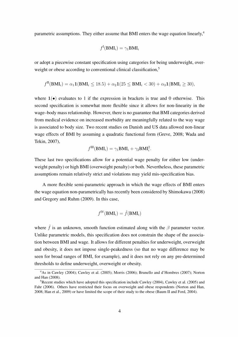
parametric assumptions. They either assume that BMI enters the wage equation linearly,4

f I(BMIi) = γ1BMIi

or adopt a piecewise constant specification using categories for being underweight, over-weight or obese according to conventional clinical classification,5

f II(BMIi) = α11(BMIi ≤ 18.5) + α21(25 ≤ BMIi < 30) + α31(BMIi ≥ 30),

where 1(•) evaluates to 1 if the expression in brackets is true and 0 otherwise. Thissecond specification is somewhat more flexible since it allows for non-linearity in thewage–body mass relationship. However, there is no guarantee that BMI categories derivedfrom medical evidence on increased morbidity are meaningfully related to the way wageis associated to body size. Two recent studies on Danish and US data allowed non-linearwage effects of BMI by assuming a quadratic functional form (Greve, 2008; Wada andTekin, 2007),

f III(BMIi) = γ1BMIi + γ2BMI2i .

These last two specifications allow for a potential wage penalty for either low (under-weight penalty) or high BMI (overweight penalty) or both. Nevertheless, these parametricassumptions remain relatively strict and violations may yield mis-specification bias.

A more flexible semi-parametric approach in which the wage effects of BMI entersthe wage equation non-parametrically has recently been considered by Shimokawa (2008)and Gregory and Ruhm (2009). In this case,

f IV(BMIi) = f(BMIi)

where f is an unknown, smooth function estimated along with the β parameter vector.Unlike parametric models, this specification does not constrain the shape of the associa-tion between BMI and wage. It allows for different penalties for underweight, overweightand obesity, it does not impose single-peakedness (so that no wage difference may beseen for broad ranges of BMI, for example), and it does not rely on any pre-determinedthresholds to define underweight, overweight or obesity.

4As in Cawley (2004); Cawley et al. (2005); Morris (2006); Brunello and d’Hombres (2007); Nortonand Han (2008).

5Recent studies which have adopted this specification include Cawley (2004), Cawley et al. (2005) andFahr (2006). Others have restricted their focus on overweight and obese respondents (Norton and Han,2008; Han et al., 2009) or have limited the scope of their study to the obese (Baum II and Ford, 2004).

4

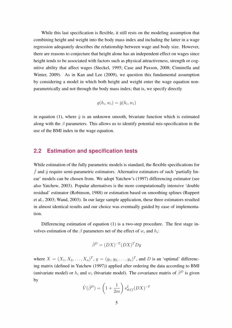
While this last specification is flexible, it still rests on the modeling assumption thatcombining height and weight into the body mass index and including the latter in a wageregression adequately describes the relationship between wage and body size. However,there are reasons to conjecture that height alone has an independent effect on wages sinceheight tends to be associated with factors such as physical attractiveness, strength or cog-nitive ability that affect wages (Steckel, 1995; Case and Paxson, 2008; Cinnirella andWinter, 2009). As in Kan and Lee (2009), we question this fundamental assumptionby considering a model in which both height and weight enter the wage equation non-parametrically and not through the body mass index; that is, we specify directly

g(hi, wi) = g(hi, wi)

in equation (1), where g is an unknown smooth, bivariate function which is estimatedalong with the β parameters. This allows us to identify potential mis-specification in theuse of the BMI index in the wage equation.

2.2 Estimation and specification tests

While estimation of the fully parametric models is standard, the flexible specifications forf and g require semi-parametric estimators. Alternative estimators of such ‘partially lin-ear’ models can be chosen from. We adopt Yatchew’s (1997) differencing estimator (seealso Yatchew, 2003). Popular alternatives is the more computationally intensive ‘doubleresidual’ estimator (Robinson, 1988) or estimation based on smoothing splines (Ruppertet al., 2003; Wand, 2003). In our large sample application, these three estimators resultedin almost identical results and our choice was eventually guided by ease of implementa-tion.

Differencing estimation of equation (1) is a two-step procedure. The first stage in-volves estimation of the β parameters net of the effect of wi and hi:

βD = (DX)−T (DX)TDy

where X = (X1, X2, . . . , Xn)T , y = (y1, y2, . . . , yn)T , and D is an ‘optimal’ differenc-ing matrix (defined in Yatchew (1997)) applied after ordering the data according to BMI(univariate model) or hi and wi (bivariate model). The covariance matrix of βD is givenby

V (βD) =

(1 +

1

2m

)s2

diff (DX)−T

5

where s2diff = n−1v′v is the residual variance of the differenced regression, v = Dy −

DXβD and m is the order of differencing.6 The second stage involves estimation ofthe non-parametric component (f or g) by regressing non-parametrically the first-stageresiduals vi on BMIi or on wi and hi using, e.g., local polynomial regression (or anystandard non-parametric regression). See Yatchew and No (2001) for an application ofthis technique.

The differencing approach offers a straightforward way to test parametric specifi-cations against flexible non-parametric estimates. Let φ(z; θ) be a parametric functionwith parameters θ (such as f I, f II, or f III defined above). Under the null hypothesis thatf(z) = φ(z; θ), the test statistic

(mn)0.5

(s2

res − s2diff

)s2

diff

D→ N(0, 1) (3)

where s2diff is defined above and is obtained using optimalmth order differencing weights,

and s2res = n−1wT w is the residual variance in the parametric model, w = y − Xβ −

φ(z; θ) (Yatchew, 2003, p.63). Note that, because it relies on the differencing principle,computation of the test statistic does not depend on estimation of the unknown f functionbut only of the fully parametric model and of the βD parameters of the linear componentsin the semi-parametric model. This specification test allows us to formally test our variousspecifications against each other.

3 Data

3.1 BMI and wages in the European Community Household

Panel survey

Our study exploits longitudinal data extracted from the European Community House-hold Panel survey (ECHP).7 The ECHP survey is a large-scale, general-purpose panel

6The variance expression is valid provided ‘optimal’ differencing weights are used to construct D. SeeYatchew (1997, 2003) for details. Heteroscedastic-consistent, ‘robust’ standard errors can be estimatedusing the classic ‘sandwich’ formula. See Yatchew (2003, p.72) and StataCorp (2007). Our estimates arebased on optimal differencing weights at the order 100, with robust standard errors.

7The public-use ECHP database was created, maintained and centrally distributed by Eurostat. SeeEUROSTAT (2003) or Lehmann and Wirtz (2003) for more information on the database, and Peracchi(2002) for an independent critical review. All our results are based on the final release (April 2004) of theECHP Users’ Database.

6

survey run in fifteen EU countries over the period 1994–2001. The database contains awide range of household- and individual-level information on income and living condi-tions, employment, education, health, demographic characteristics. In the last four waves(1998–2001), the ECHP included information on respondents’ height and weight.

Several studies have recently used the ECHP to document the wage effects of bodymass in Europe. In a regression model where BMI enters a log-wage equation linearly,Brunello and d’Hombres (2007) found existence of a significant European wide wagepenalty to obesity –of greater magnitude for men. In contrast, relying on a piecewise con-stant specification in BMI capturing whether a respondent is underweight, overweight orobese according to clinical thresholds, Atella et al. (2008) suggested that this Europeanwide wage penalty only affects overweight and obese females. Fahr (2006) further in-vestigated non-linearities in this association with a model which allows to disentangle theindependent wage effects of deviations from both socially accepted body mass and medi-cally recommended thresholds. His results suggest that deviations from medically recom-mended BMI are more hurtful to female earnings than deviations from social norms.8 Theopposite observation seems to hold for men. This is broadly consistent with Atella et al.’s(2008) finding of a more significant negative wage penalty for overweight and obese fe-male respondents since they defined BMI categories according to conventional clinicalthresholds. It is also consistent with the claim that BMI score may capture more accu-rately excessive body fatness in females than in males (Wada and Tekin, 2007; Burkhauserand Cawley, 2008). Fahr (2006) still relied, however, on normative assumptions regardingwhat constitutes socially acceptable BMI scores or more generally, continued to rely onad hoc assumptions regarding the location of potential turning points shaping the BMIwage association.

Differences in methodology and sample selection make it difficult to readily com-pare the results reported in Fahr (2006), Brunello and d’Hombres (2007) and Atella et al.(2008). However, the estimated wage effects of BMI reported in these studies are consis-tent with the view that the association between BMI and wage is likely nonlinear, differacross gender, and that a specification based on clinical thresholds might not optimallycapture important turning points in its true relationship.

8In this context, a socially acceptable BMI is assumed to be determined by the median regional BMIadjusted for gender and broad age groups.

7

3.2 Sample definition

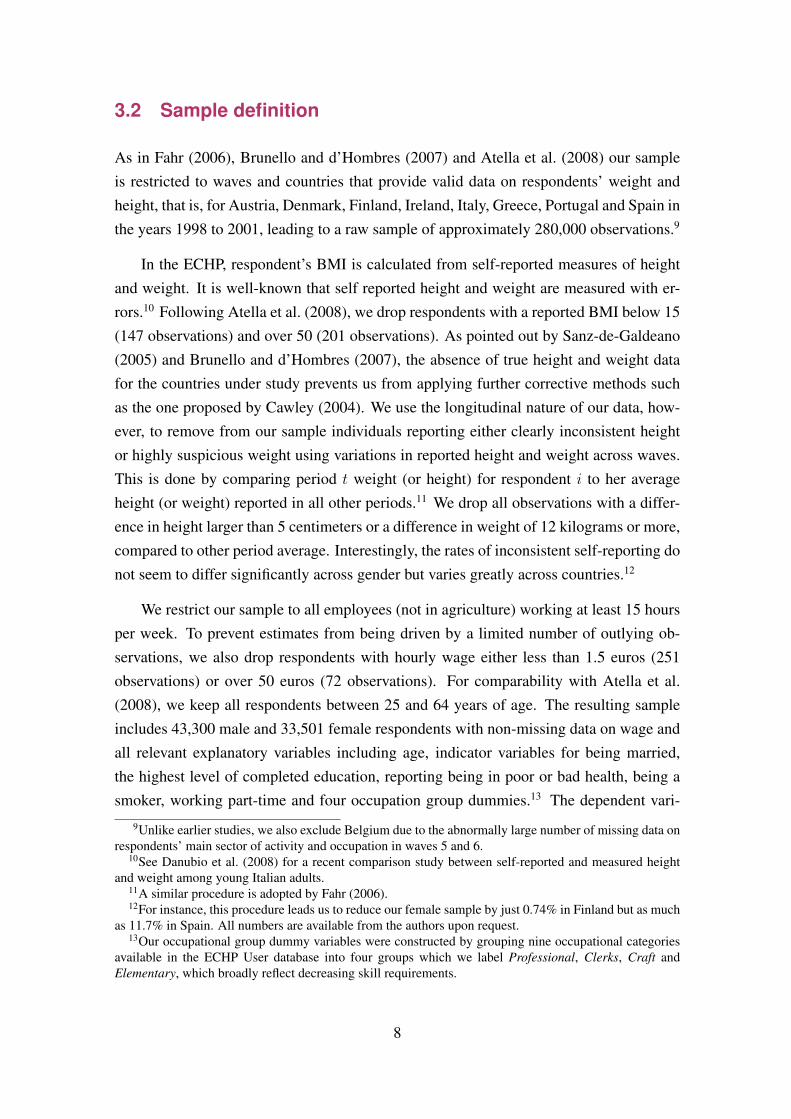
As in Fahr (2006), Brunello and d’Hombres (2007) and Atella et al. (2008) our sampleis restricted to waves and countries that provide valid data on respondents’ weight andheight, that is, for Austria, Denmark, Finland, Ireland, Italy, Greece, Portugal and Spain inthe years 1998 to 2001, leading to a raw sample of approximately 280,000 observations.9

In the ECHP, respondent’s BMI is calculated from self-reported measures of heightand weight. It is well-known that self reported height and weight are measured with er-rors.10 Following Atella et al. (2008), we drop respondents with a reported BMI below 15(147 observations) and over 50 (201 observations). As pointed out by Sanz-de-Galdeano(2005) and Brunello and d’Hombres (2007), the absence of true height and weight datafor the countries under study prevents us from applying further corrective methods suchas the one proposed by Cawley (2004). We use the longitudinal nature of our data, how-ever, to remove from our sample individuals reporting either clearly inconsistent heightor highly suspicious weight using variations in reported height and weight across waves.This is done by comparing period t weight (or height) for respondent i to her averageheight (or weight) reported in all other periods.11 We drop all observations with a differ-ence in height larger than 5 centimeters or a difference in weight of 12 kilograms or more,compared to other period average. Interestingly, the rates of inconsistent self-reporting donot seem to differ significantly across gender but varies greatly across countries.12

We restrict our sample to all employees (not in agriculture) working at least 15 hoursper week. To prevent estimates from being driven by a limited number of outlying ob-servations, we also drop respondents with hourly wage either less than 1.5 euros (251observations) or over 50 euros (72 observations). For comparability with Atella et al.(2008), we keep all respondents between 25 and 64 years of age. The resulting sampleincludes 43,300 male and 33,501 female respondents with non-missing data on wage andall relevant explanatory variables including age, indicator variables for being married,the highest level of completed education, reporting being in poor or bad health, being asmoker, working part-time and four occupation group dummies.13 The dependent vari-

9Unlike earlier studies, we also exclude Belgium due to the abnormally large number of missing data onrespondents’ main sector of activity and occupation in waves 5 and 6.

10See Danubio et al. (2008) for a recent comparison study between self-reported and measured heightand weight among young Italian adults.

11A similar procedure is adopted by Fahr (2006).12For instance, this procedure leads us to reduce our female sample by just 0.74% in Finland but as much

as 11.7% in Spain. All numbers are available from the authors upon request.13Our occupational group dummy variables were constructed by grouping nine occupational categories

available in the ECHP User database into four groups which we label Professional, Clerks, Craft andElementary, which broadly reflect decreasing skill requirements.

8

able of our wage models is the natural logarithm of hourly wage expressed in constant1996 PPP euros.14

3.3 Descriptive statistics

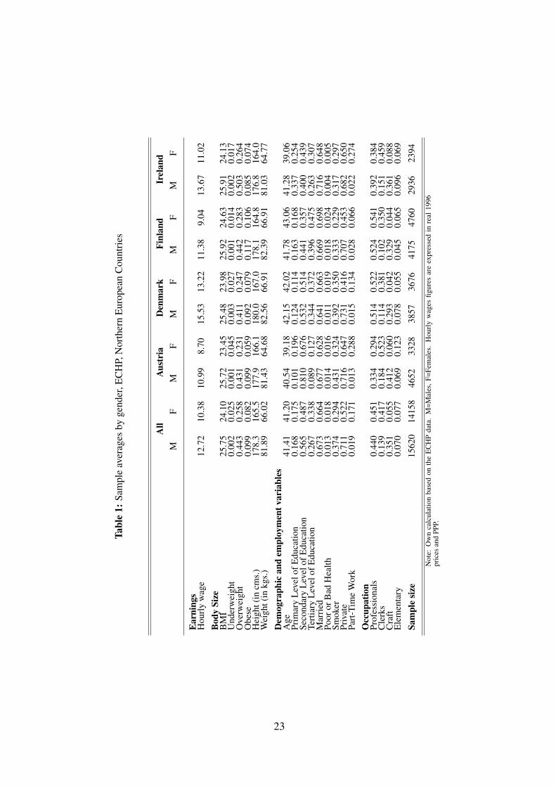
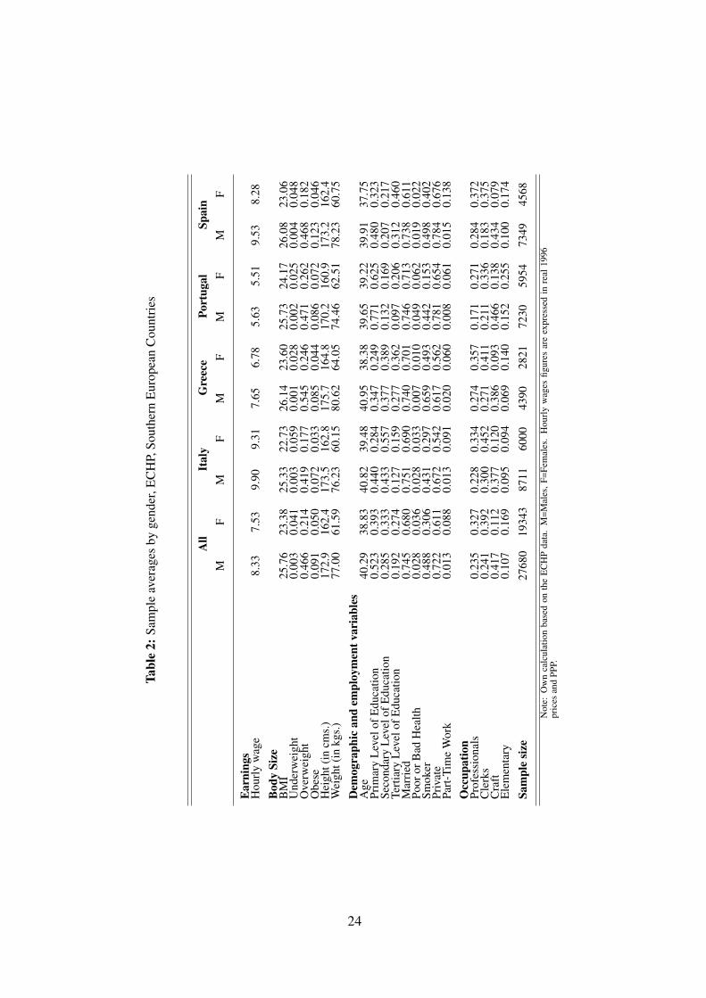
Summary statistics of our sample are reported separately for male and female respondentsliving in Northern European countries (Table 1) and Southern European countries (Table2). According to clinical thresholds, the average European man is overweight with amean BMI just under 26. European women report on average a healthier BMI just over23 in the south and just over 24 in the north. The distribution of the population by BMIcategories reveals that more than half of all male respondents in our sample are overweightor obese. This observation broadly holds across regions and countries. Obesity rates varysignificantly across countries ranging between just under 7% in Italy to over 12% in Spainfor males and between just over 3% in Italy and just over 10% in Finland for females.15

The incidence of underweight among males is extremely low in all countries. Ourpooled sample of Southern European (Northern) countries, only includes 79 (29) under-weight male respondents. This implies that the wage effect of underweight males in eachseparate country would be identified on just a few cases. While the incidence of un-derweight is higher among females at about just over 2.5% in Northern Europe (or 356observations) and just over 4% (or 798 observations) in Southern Europe, the number ofunderweight respondents in each separate country remains small.16 As a result, we limitour analysis to the estimated wage effects of body size for the pooled samples of Southern–Greece, Italy, Portugal and Spain– and Northern European countries –Austria, Denmark,Finland and Ireland– separately. As in Brunello and d’Hombres (2007), the implicit as-sumption behind this pooling is that these Southern and Northern European countriesshare some unobserved regional cultural traits. However, since we dropped Belgium, ourpooled sample of Northern European countries is not strictly comparable to their so calledbeer belt countries.17

Figure 1 compactly presents the distribution of the population and the unconditionalaverage hourly wages by BMI levels, separately by gender, for the pooled samples ofNorthern and Southern European countries. The figure confirms that a large share of male

14We have constructed hourly wage following Arulampalam et al. (2007), that is, as gross monthly earn-ings from main job including overtime divided by 4.5 times weekly hours in main job including overtime.

15Note that the incidence of obesity in our sample is largely consistent with the numbers reported byAtella et al. (2008) using the same age sample restriction than this study.

16With the exception of Italy and Spain due to their larger samples and higher incidence of underweightrespondents.

17Single country results are available from the authors upon request.

9

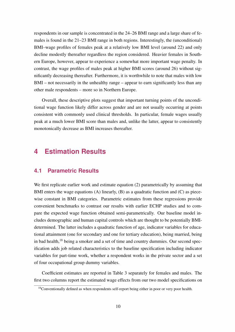
respondents in our sample is concentrated in the 24–26 BMI range and a large share of fe-males is found in the 21–23 BMI range in both regions. Interestingly, the (unconditional)BMI–wage profiles of females peak at a relatively low BMI level (around 22) and onlydecline modestly thereafter regardless the region considered. Heavier females in South-ern Europe, however, appear to experience a somewhat more important wage penalty. Incontrast, the wage profiles of males peak at higher BMI scores (around 26) without sig-nificantly decreasing thereafter. Furthermore, it is worthwhile to note that males with lowBMI – not necessarily in the unhealthy range – appear to earn significantly less than anyother male respondents – more so in Northern Europe.

Overall, these descriptive plots suggest that important turning points of the uncondi-tional wage function likely differ across gender and are not usually occurring at pointsconsistent with commonly used clinical thresholds. In particular, female wages usuallypeak at a much lower BMI score than males and, unlike the latter, appear to consistentlymonotonically decrease as BMI increases thereafter.

4 Estimation Results

4.1 Parametric Results

We first replicate earlier work and estimate equation (2) parametrically by assuming thatBMI enters the wage equations (A) linearly, (B) as a quadratic function and (C) as piece-wise constant in BMI categories. Parametric estimates from these regressions provideconvenient benchmarks to contrast our results with earlier ECHP studies and to com-pare the expected wage function obtained semi-parametrically. Our baseline model in-cludes demographic and human capital controls which are thought to be potentially BMI-determined. The latter includes a quadratic function of age, indicator variables for educa-tional attainment (one for secondary and one for tertiary education), being married, beingin bad health,18 being a smoker and a set of time and country dummies. Our second spec-ification adds job related characteristics to the baseline specification including indicatorvariables for part-time work, whether a respondent works in the private sector and a setof four occupational group dummy variables.

Coefficient estimates are reported in Table 3 separately for females and males. Thefirst two columns report the estimated wage effects from our two model specifications on

18Conventionally defined as when respondents self-report being either in poor or very poor health.

10

the pooled sample of Northern European countries followed by the estimated wage effectsin Southern Europe. Our discussion, primarily focus on the pooled sample estimates fromthe less parsimonious model specification (Model 2).

Estimates from the linear model do not reveal any significant association betweenwage and BMI among males. In contrast, we find a significant wage penalty amongfemales, but an effect relatively small in magnitude. In particular, a 10% increase in theBMI of female respondents is associated with a modest decrease in wages of about 0.48%in Northern Europe and about 0.93% in the South. The insignificant linear wage effectof BMI for males, however, appears to mask a more complex association. As pointedout by Gregory and Ruhm (2009), if individual BMI is negatively associated with bothbeing obese and underweight –as suggested by our unconditional wage profiles– , linearestimates may misleadingly suggest the absence of a significant association. Once wemodel the wage effect of BMI with a quadratic form, we find a statistically significantinverted U-shaped association for males. The peak in the relationship is found at a BMIof about 27 or 28 in both Northern and Southern Europe. We do not find a statisticallysignificant quadratic wage effect for females. Male estimates from the piecewise constantmodel with BMI categories corroborate the existence of an inverted U-shaped associationfor males by indicating the existence of a wage penalty for being underweight or obeseand a premium for being overweight. These estimates, however, are only statisticallysignificant in Northern Europe for underweight and overweight respondents and neversignificant in Southern Europe.19

Taken together, we interpret these results as evidence that the association betweenBMI and wage might be inverted U-shaped for males with a peak at a BMI level in theoverweight range. Clinical thresholds defining BMI categories do not seem to captureaccurately critical turning points in this association; possibly more so, in Southern Eu-rope. These results corroborate recent evidence found in Germany (Cawley et al., 2005)and Denmark (Greve, 2008) and are consistent with previous ECHP-based estimates byFahr (2006) and Atella et al. (2008). In contrast, estimates reveal that overweight or obesefemales earn significantly less than those in the clinically recommended BMI category.These estimates, however, are only significant in Southern Europe indicating that over-weight and obese female earn about 2.7% and 5% less than their ‘healthy ’ counterparts.This regional difference is consistent with Brunello and d’Hombres (2007) finding of astronger association in so called olive belt countries.20 These results provide support for

19Estimates based on single country samples corroborate pooled sample estimates in signs and magnitudebut, not unexpectedly given the small sample sizes, are usually insignificant for both males and females.These results are available upon request.

20As pointed out by Brunello and d’Hombres (2007), this regional difference might just be the result ofthe smaller sample size in Northern Europe. Our more parsimonious specification suggests the existence of a

11

the existence of a monotonically decreasing wage effects in BMI for females as impliedby the linear model.

4.2 Semi-parametric model estimates of the BMI-wage

relationship

As argued in the Introduction, parametric regression results may mask the complexityof the functional relationship between wage and BMI. There is interest in consideringan unconstrained specification to check whether sufficient flexibility is achieved with aquadratic or a classic piecewise constant parametric model.

Our non-parametric estimates of the effect of BMI on log-wage are presented graphi-cally, separately for males and females in Northern (Figures 2 and 3) and Southern Europe(Figures 4 and 5). Each figure presents the BMI-wage profiles implied by our two modelspecifications (the parametric components are estimated as explained in Section 2.1). Foreach level of BMI on the x-axis, the plots show the expected log-wage as given by equa-tion (2), that is, E(log(y)|X,BMI) = Xβ + f(BMI), where X is the vector of means ofother covariates in the sample considered and β and f are the model estimates. We over-lay estimates from the semi-parametric model over predictions implied by the parametricestimates presented in the previous section. Point-wise 90 percent confidence bootstrapvariability bands for the predicted BMI-wage profile from the semi-parametric model arerepresented by the vertical bars around the predictions.21 The red bars at the bottom ofeach graph are kernel density function estimates of the distribution of BMI in the sample.

Our semi-parametric results corroborate our earlier conjecture that the associationbetween BMI and wage reveals an inverted U-shaped for Northern European males (seeFigures 2). However, while the quadratic results suggested a single peak at a BMI of about28, the semi-parametric estimates rather suggest that there is a plateau with maximumwage in the range 24–31 and a penalty above or beyond these. This suggests that thereis a wage penalty for people beyond a ‘normal’ body size. The linear model is clearlymisspecified. The quadratic model underestimates the wage penalty beyond the ‘normal’

statistically significant wage penalty of about 2.2% and 3.9% for overweight and obese females in NorthernEurope. Alternatively, it might also reflect a true North-South differences in norms making clinical BMIthresholds less relevant for Northern European female respondents.

21We implemented the repeated half-sample bootstrap algorithm of Saigo et al. (2001). To take intoaccount the stratification of the survey we resample within stratum identified in the data (for Ireland, Spain,Portugal and Finland) or within NUTS-1 level region if detailed stratum identifier are not provided in thepublic-use dataset (all other countries). The resampling unit is the wave 1 household, so that all dependenceof responses for same household respondents and for repeated responses over time is properly taken intoaccount. All estimates reported are based on 500 replications.

12

range. The piecewise constant model fails to capture the variations within the ‘healthy’(20–24) and ‘obese’ (above 30) ranges.

Figure 4 reveals quite a different expected wage profile for Southern European males.There is no plateau, but the profile is not more quadratic. Surprisingly, we also observean inflection point at BMI around 32 suggesting the existence of a large obesity premiumfor Southern European males (which is not at all apparent in the obesity dummy in thepiecewise constant specification). Extremely few observations are observed with a BMIabove 32 however. Interestingly, single country figures (not reported here but availableupon request from the authors) indicate that this surprising wage increase in SouthernEurope is not confined to a single outlying country but is observed consistently in Italy,Portugal and Spain.

Figures 3 and 5 globally corroborate our earlier parametric estimates indicating ageneral decline in expected wage with BMI for females. But note that the non-parametricestimates show the existence of a peak at a BMI of about 21 (for Northern Europeanwomen) or 22 (for Southern European women). There is therefore also a penalty forunderweight among females, yet a much smaller one than the penalty for overweight orobesity.

In sum, while the overall relationship seem to be relatively well approximated by aquadratic model for men and a linear model for women, the non-parametric estimationreveals fine details that are missed by all other models. Formal tests based on equation (3)of the null hypothesis of equality of the non-parametric curves with any of the parametricmodels considered, all strongly support rejection.22

4.3 Modeling body size without the body mass index

We finally consider the predicted wage effects from body size when the latter is cap-tured by a smooth function of height and weight estimated non-parametrically, ratherthan through the body mass index. Our motivation is to test whether the parametric asso-ciation between weight and height in effect implied by the BMI functional form –weightin kilograms over height squared– adequately relates the combined effects of height andweight on wages. To achieve this, we have estimated directly the bivariate function g ofequation (1) using the same partial linear model as in the previous sub-section. The keydifference is that the non-parametric component is now an unspecified, smooth, bivariate

22Test statistics are not reported here to save space (all p-values are well below 0.001) but are availablefrom the authors upon request.

13

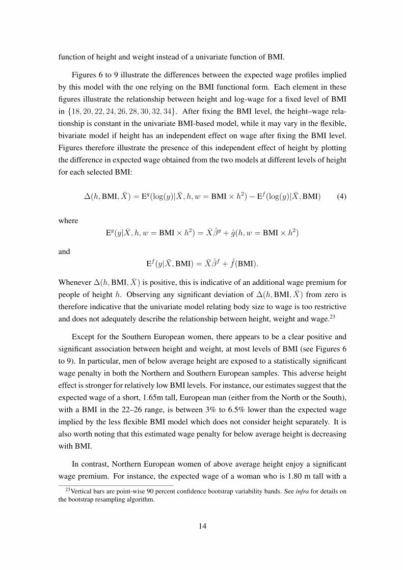
function of height and weight instead of a univariate function of BMI.

Figures 6 to 9 illustrate the differences between the expected wage profiles impliedby this model with the one relying on the BMI functional form. Each element in thesefigures illustrate the relationship between height and log-wage for a fixed level of BMIin {18, 20, 22, 24, 26, 28, 30, 32, 34}. After fixing the BMI level, the height–wage rela-tionship is constant in the univariate BMI-based model, while it may vary in the flexible,bivariate model if height has an independent effect on wage after fixing the BMI level.Figures therefore illustrate the presence of this independent effect of height by plottingthe difference in expected wage obtained from the two models at different levels of heightfor each selected BMI:

∆(h,BMI, X) = Eg(log(y)|X, h, w = BMI× h2)− Ef (log(y)|X,BMI) (4)

whereEg(y|X, h, w = BMI× h2) = Xβg + g(h,w = BMI× h2)

andEf (y|X,BMI) = Xβf + f(BMI).

Whenever ∆(h,BMI, X) is positive, this is indicative of an additional wage premium forpeople of height h. Observing any significant deviation of ∆(h,BMI, X) from zero istherefore indicative that the univariate model relating body size to wage is too restrictiveand does not adequately describe the relationship between height, weight and wage.23

Except for the Southern European women, there appears to be a clear positive andsignificant association between height and weight, at most levels of BMI (see Figures 6to 9). In particular, men of below average height are exposed to a statistically significantwage penalty in both the Northern and Southern European samples. This adverse heighteffect is stronger for relatively low BMI levels. For instance, our estimates suggest that theexpected wage of a short, 1.65m tall, European man (either from the North or the South),with a BMI in the 22–26 range, is between 3% to 6.5% lower than the expected wageimplied by the less flexible BMI model which does not consider height separately. It isalso worth noting that this estimated wage penalty for below average height is decreasingwith BMI.

In contrast, Northern European women of above average height enjoy a significantwage premium. For instance, the expected wage of a woman who is 1.80 m tall with a

23Vertical bars are point-wise 90 percent confidence bootstrap variability bands. See infra for details onthe bootstrap resampling algorithm.

14

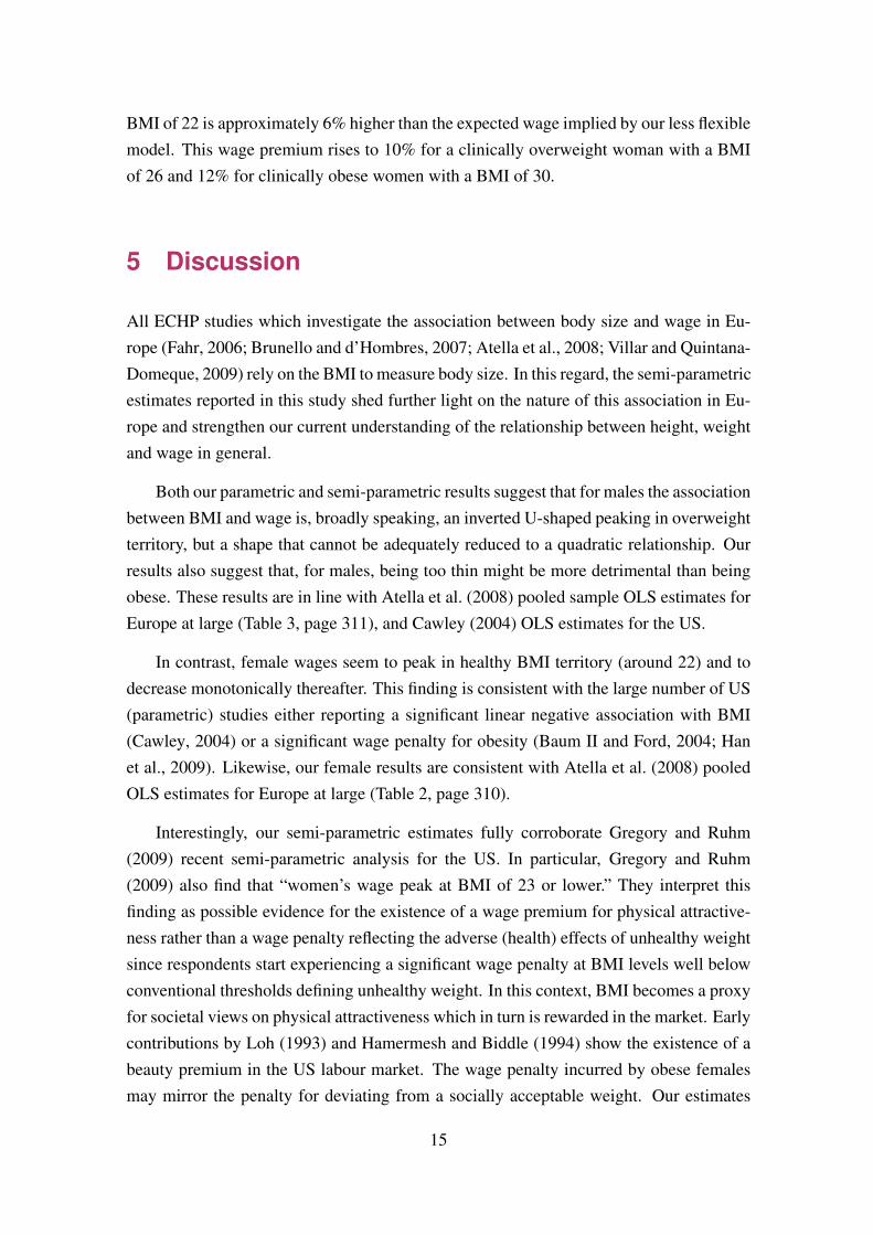
BMI of 22 is approximately 6% higher than the expected wage implied by our less flexiblemodel. This wage premium rises to 10% for a clinically overweight woman with a BMIof 26 and 12% for clinically obese women with a BMI of 30.

5 Discussion

All ECHP studies which investigate the association between body size and wage in Eu-rope (Fahr, 2006; Brunello and d’Hombres, 2007; Atella et al., 2008; Villar and Quintana-Domeque, 2009) rely on the BMI to measure body size. In this regard, the semi-parametricestimates reported in this study shed further light on the nature of this association in Eu-rope and strengthen our current understanding of the relationship between height, weightand wage in general.

Both our parametric and semi-parametric results suggest that for males the associationbetween BMI and wage is, broadly speaking, an inverted U-shaped peaking in overweightterritory, but a shape that cannot be adequately reduced to a quadratic relationship. Ourresults also suggest that, for males, being too thin might be more detrimental than beingobese. These results are in line with Atella et al. (2008) pooled sample OLS estimates forEurope at large (Table 3, page 311), and Cawley (2004) OLS estimates for the US.

In contrast, female wages seem to peak in healthy BMI territory (around 22) and todecrease monotonically thereafter. This finding is consistent with the large number of US(parametric) studies either reporting a significant linear negative association with BMI(Cawley, 2004) or a significant wage penalty for obesity (Baum II and Ford, 2004; Hanet al., 2009). Likewise, our female results are consistent with Atella et al. (2008) pooledOLS estimates for Europe at large (Table 2, page 310).

Interestingly, our semi-parametric estimates fully corroborate Gregory and Ruhm(2009) recent semi-parametric analysis for the US. In particular, Gregory and Ruhm(2009) also find that “women’s wage peak at BMI of 23 or lower.” They interpret thisfinding as possible evidence for the existence of a wage premium for physical attractive-ness rather than a wage penalty reflecting the adverse (health) effects of unhealthy weightsince respondents start experiencing a significant wage penalty at BMI levels well belowconventional thresholds defining unhealthy weight. In this context, BMI becomes a proxyfor societal views on physical attractiveness which in turn is rewarded in the market. Earlycontributions by Loh (1993) and Hamermesh and Biddle (1994) show the existence of abeauty premium in the US labour market. The wage penalty incurred by obese femalesmay mirror the penalty for deviating from a socially acceptable weight. Our estimates

15

could therefore suggest that the socially acceptable bmi of European females is approx-imately 22 - deviations from this ideal physical trait is associated with lower earnings,possibly of larger magnitude in Southern Europe.

Similarly, our analysis shows that males wage peak in the mostly overweight BMIrange 24–31 in Northern Europe. This result is again consistent with the existence ofa wage penalty triggered by deviations from socially acceptable weight which, for thecase of males, would be determined by the average (or median) BMI of the workingpopulation. In this context, it is therefore not surprising that being too thin is associatedwith a significant wage penalty since the European males included in our sample are onaverage slightly overweight. This is consistent with Fahr (2006) who posits that, in someEuropean countries, social norms “set the relevant standard to evaluate men’s physicalappearance.”24 While we find a comparable pattern in Southern Europe, the sudden wagepremium enjoy by men with a BMI over 32 is rather puzzling. It is, however, againconsistent with the view that the association between BMI and wage is not necessarilydriven by the adverse health effects of abnormal weight.

Finally, our fully flexible model reveals that shorter males suffer an additional signif-icant height penalty independent of BMI and that Northern European females of aboveaverage height enjoy a wage premium. The existence of a height-wage premium is nowa well documented empirical regularity. Recent height studies have consistently docu-mented that taller workers earn significantly more than their shorter counterparts in Aus-tralia (Kortt and Leigh, 2010), Germany (Heineck, 2005), the UK (Case et al., 2009) andEurope at large (Cinnirella and Winter, 2009). The existence of differences in cognitiveskills between shorter and taller workers is one possible pathway explaining this height-wage premium (Case and Paxson, 2008). In a recent European study, Cinnirella andWinter (2009) argue that, without being exclusive, a large part of this premium could alsobe due to employer discrimination. While we do not formally explore these issues, webelieve that overall, results from our most flexible specification are also consistent withthe existence of a premium for physical attractiveness.

In sum, our study corroborates the view that the shape of the BMI association dif-fers across gender and suggests that the BMI functional form may be too restrictive toadequately capture the complexities of the association between height, weight and wagesfor men. As Gregory and Ruhm (2009), we posit that this association could be driven byphysical attractiveness rather than unhealthy weight. In this context, gender differencesstem from differences in judgment regarding desirable body types. A good height mightbe more important than an healthy weight for males while an healthy BMI is more desir-

24Fahr (2006) defines social norm as the gender, age group and region specific median BMI.

16

able for females. This conjecture is consistent with Rooth (2010) who finds that obese jobapplicants in Sweden experience lower call back rates and that this differential treatmentis mostly driven by obesity for women and attractiveness for men. However, one needs tokeep in mind that, even if significant, the estimated wage effects of body size reported inthis study are overall fairly small.

Unlike Gregory and Ruhm (2009), our data do not allow us to control for endogene-ity of BMI in the semi-parametric setting. This makes it difficult to give a strictly causalinterpretation to the estimated wage effect of body weight discussed in this study. Re-verse causality and the possibility that body weight could be correlated with unobservedfactors also affecting wages are the two main sources of endogeneity bias identified in theobesity literature. Reverse causality is usually controlled for by instrumenting contem-poraneous BMI with a sufficiently distant BMI measure (Gortmaker et al., 1993; Averettand Korenman, 1996; Cawley, 2004; Gregory and Ruhm, 2009). As in other ECHP stud-ies (Brunello and d’Hombres, 2007; Atella et al., 2008), we are not able to control forthis potential source of bias since our exploitable longitudinal sample only covers threeyears of data. However, most of these studies find that the estimated wage effect of bodyweight using a lagged measure of BMI is virtually identical to that using current BMIscore. The obvious response to the second source of bias is again to use instrumentalvariable estimation techniques. While implementing such strategy is empirically straight-forward, identifying strong instruments turns out to be challenging. A vast majority ofstudies that adopted instrumental variable estimation (Cawley, 2004; Cawley et al., 2005;Brunello and d’Hombres, 2007; Norton and Han, 2008; Gregory and Ruhm, 2009) haveused the BMI of genetically related family members following Cawley (2004). Thesestudies usually find that controlling for potential endogeneity does not affect their resultssubstantially.25 In addition, the reliability of IV estimates using the body weight of agenetically related family member as instrument on ECHP data has been forcefully ques-tioned by Atella et al. (2008). The latter is suspected to yield significant bias on ECHPdata due to severe non-random sample selection (see Atella et al., 2008, for further dis-cussion) from imposed sample restrictions. Given this concern and in the absence of anyconvincing alternative instruments in our data, we deliberately do not address the poten-tial endogeneity of weight (or BMI) in this study. Caution should therefore be exercisedto give a fully causal interpretation to the estimates of wage effects of body size presentedin this paper.

25See Kortt and Leigh (2010) for a comprehensive survey of previous IV studies.

17

References

Arulampalam, W., Booth, A. L. and Bryan, M. L. (2007), ‘Is there a glass ceiling overEurope? Exploring the gender pay gap across the wage distribution’, Industrial and

Labor Relations Review 60(2), 163–186.

Atella, V., Pace, N. and Vuri, D. (2008), ‘Are employers discriminating with respect toweight? European evidence using quantile regression’, Economics and Human Biology

6, 305–329.

Averett, S. A. and Korenman, S. (1996), ‘The economic reality of the beauty myth’, Jour-

nal of Human Resources 31 (2), 304–330.

Baum II, C. L. and Ford, W. F. (2004), ‘The wage effects of obesity: A longitudinalstudy’, Health Economics 13, 885–899.

Brunello, G. and d’Hombres, B. (2007), ‘Does body weight affect wages? Evidence fromEurope’, Economics and Human Biology 5(1), 1–19.

Burkhauser, R. and Cawley, J. (2008), ‘Beyond BMI: The value of more accurate mea-sures of fatness and obesity in social science research’, Journal of Health Economics

27, 519–529.

Case, A. and Paxson, C. (2008), ‘Stature and status: Height, ability, and labor marketoutcomes’, Journal of Political Economy 116(3), 499–532.

Case, A., Paxson, C. and Islam, M. (2009), ‘Making sense of the labor market heightpremium: Evidence from the British Household Panel Survey’, Economics Letters

102, 174–176.

Cawley, J. (2004), ‘The impact of obesity on wages’, Journal of Human Resources

39(2), 451–474.

Cawley, J., Grabka, M. M. and Lillard, D. R. (2005), ‘A comparison of the relation-ship between obesity and earnings in the U.S. and Germany’, Schmollers Jahrbuch

125(1), 119–129.

Cinnirella, F. and Winter, J. (2009), Size matters! Body height and labor market discrim-ination: A cross-european analysis, Technical report, CESifo Working Paper 2733.

Conley, D. and Glauber, R. (2005), Gender, body mass and economic status, TechnicalReport 11343, National Bureau of Economic Research, Cambridge MA.

18

Danubio, M. E., Miranda, G., Vinciguerra, M. G., Vecchi, E. and Rufo, F. (2008), ‘Com-parison of self-reported and measured height and weight: Implications for obesity re-search among young adults’, Economics and Human Biology 6(1), 181–190.

EUROSTAT (2003), DOC.PAN 168/2003-12: ECHP UDB manual, Waves 1 to 8, Euro-stat, European Commission, Luxembourg.

Fahr, R. (2006), The wage effects of social norms: Evidence of deviations from peers’body-mass in Europe, Discussion Paper No. 2323, Institute for the Study of Labor(IZA), Bonn.

Gortmaker, S., Must, A., Perrin, J., Sobol, A. and Dietz, W. (1993), ‘Social and economicconsequences of overweight in adolescence and young adulthood’, New England Jour-

nal of Medicine 329, 1008–1012.

Gregory, C. A. and Ruhm, C. J. (2009), Where does the wage penalty bite?, NBER Work-ing Paper 14984, National Bureau of Economic Research, Cambridge MA.

Greve, J. (2008), ‘Obesity and labor market outcomes in Denmark’, Economics and Hu-

man Biology 6, 350–362.

Hamermesh, D. S. and Biddle, J. E. (1994), ‘Beauty and the labor market’, American

Economic Review 84(5), 1174–1194.

Han, E., Norton, E. C. and Stearns, S. C. (2009), ‘Weight and wage: Fat versus leanpaychecks’, Health Economics 18, 535–548.

Heineck, G. (2005), ‘Up in the skies? The relationship between body height and earningsin Germany’, Labour 19(3), 469–489.

Kan, K. and Lee, M. (2009), Lose weight for money only if over-weight: Marginal inte-gration for semi-linear models, HEDG Working Paper 09/19, University of York.

Kortt, M. and Leigh, A. (2010), ‘Does size matter in Australia?’, Economic Record

86(272), 71–83.

Lehmann, P. and Wirtz, C. (2003), The EC Household Panel Newsletter (01/02), Methodsand Nomenclatures, Theme 3: Population and social conditions, Eurostat, EuropeanCommission, Luxembourg.

Loh, E. S. (1993), ‘The economic effects of physical appearance’, Social Science Quar-

terly 74(2), 420–438.

19

Lundborg, P., Nystedt, P. and Rooth, D.-O. (2010), No country for fat men? Obesity,earnings, skills and health among 450,000 swedish men, IZA Working Paper 4775,IZA.

Mocan, N. H. and Tekin, E. (2009), Obesity, self-esteem and wages, NBER WorkingPaper 15101, National Bureau of Economic Research, Cambridge MA.

Morris, S. (2006), ‘Body mass index and occupational attainment’, Health Economics

25, 347–364.

Norton, E. and Han, E. (2008), ‘Genetic information, obesity, and labor market out-comes’, Health Economics 17, 1089–1104.

Pagan, J. A. and Davila, A. (1997), ‘Obesity, occupational attainment and earnings’, So-

cial Science Quarterly 78(3), 756–770.

Peracchi, F. (2002), ‘The European Community Household Panel: A review’, Empirical

Economics 27, 63–90.

Register, C. A. and Williams, D. R. (1990), ‘Wage effects of obesity among young work-ers’, Social Science Quarterly 71(1), 130–141.

Robinson, P. M. (1988), ‘Root-n-consistent semiparametric regression’, Econometrica

56(4), 931–954.

Rooth, D.-O. (2010), ‘Obesity, attractiveness, and differential treatment in hiring: A fieldexperiment’, Journal of Human Resources 44(3), 710–735.

Ruppert, D., Wand, M. P. and Carroll, R. J. (2003), Semiparametric Regression, Cam-bridge Series in Statistical and Probabilistic Mathematics, Cambridge University Press,New York.

Saigo, H., Shao, J. and Sitter, R. R. (2001), ‘A repeated half-sample bootstrap andbalanced repeated replications for randomly imputed data’, Survey Methodology

27(2), 189–196.

Sanz-de-Galdeano, A. (2005), The obesity epidemic in Europe, Discussion Paper 1814,Institute for the Study of Labor (IZA), Bonn.

Shimokawa, S. (2008), ‘The labour market impact of body weight in China: A semipara-metric analysis’, Applied Economics 40, 949–968.

StataCorp (2007), Stata Statistical Software: Release 10, StataCorp LP, College Station,TX.

20

Steckel, R. H. (1995), ‘Height and the standard of living’, Journal of Economic Literature

33, 1903–1940.

Villar, J. G. and Quintana-Domeque, C. (2009), ‘Income and body mass index in Europe’,Economics and Human Biology 7, 73–83.

Wada, R. and Tekin, E. (2007), Body composition and wages, NBER Working Paper13595, National Bureau of Economic Research, Cambridge MA.

Wand, M. P. (2003), ‘Smoothing and mixed models’, Computational Statistics 18, 223–249.

Yatchew, A. (1997), ‘An elementary estimator of the partial linear model’, Economics

Letters 57, 135–143.

Yatchew, A. (2003), Semiparametric regression for the applied econometrician, Themesin modern econometrics, Cambridge University Press, Cambridge, UK.

Yatchew, A. and No, J. A. (2001), ‘Household gasoline demand in Canada’, Econometrica

69(6), 1697–1709.

21

6 Tables and Figures

22

Tabl

e1:

Sam

ple

aver

ages

byge

nder

,EC

HP,

Nor

ther

nE

urop

ean

Cou

ntri

es

All

Aus

tria

Den

mar

kFi

nlan

dIr

elan

dM

FM

FM

FM

FM

F

Ear

ning

sH

ourl

yw

age

12.7

210

.38

10.9

98.

7015

.53

13.2

211

.38

9.04

13.6

711

.02

Bod

ySi

zeB

MI

25.7

524

.10

25.7

223

.45

25.4

823

.98

25.9

224

.63

25.9

124

.13

Und

erw

eigh

t0.

002

0.02

50.

001

0.04

50.

003

0.02

70.

001

0.01

40.

002

0.01

7O

verw

eigh

t0.

443

0.25

80.

431

0.23

10.

411

0.24

70.

442

0.28

30.

503

0.26

4O

bese

0.09

90.

082

0.09

90.

059

0.09

20.

079

0.11

70.

106

0.08

50.

074

Hei

ght(

incm

s.)

178.

316

5.5

177.

916

6.1

180.

016

7.0

178.

116

4.8

176.

816

4.0

Wei

ght(

inkg

s.)

81.8

966

.02

81.4

364

.68

82.5

666

.91

82.3

966

.91

81.0

364

.77

Dem

ogra

phic

and

empl

oym

entv

aria

bles

Age

41.4

141

.20

40.5

439

.18

42.1

542

.02

41.7

843

.06

41.2

839

.06

Prim

ary

Lev

elof

Edu

catio

n0.

168

0.17

50.

101

0.19

60.

124

0.11

40.

163

0.16

80.

337

0.25

4Se

cond

ary

Lev

elof

Edu

catio

n0.

565

0.48

70.

810

0.67

60.

532

0.51

40.

441

0.35

70.

400

0.43

9Te

rtia

ryL

evel

ofE

duca

tion

0.26

70.

338

0.08

90.

127

0.34

40.

372

0.39

60.

475

0.26

30.

307

Mar

ried

0.67

30.

664

0.67

70.

628

0.64

10.

663

0.66

90.

698

0.71

60.

648

Poor

orB

adH

ealth

0.01

30.

018

0.01

40.

016

0.01

10.

019

0.01

80.

024

0.00

40.

005

Smok

er0.

374

0.29

40.

431

0.32

40.

392

0.35

00.

333

0.22

90.

317

0.29

7Pr

ivat

e0.

711

0.52

20.

716

0.64

70.

731

0.41

60.

707

0.45

30.

682

0.65

0Pa

rt-T

ime

Wor

k0.

019

0.17

10.

013

0.28

80.

015

0.13

40.

028

0.06

60.

022

0.27

4O

ccup

atio

nPr

ofes

sion

als

0.44

00.

451

0.33

40.

294

0.51

40.

522

0.52

40.

541

0.39

20.

384

Cle

rks

0.13

90.

417

0.18

40.

523

0.11

40.

381

0.10

20.

350

0.15

10.

459

Cra

ft0.

351

0.05

50.

412

0.06

00.

293

0.04

20.

329

0.04

40.

361

0.08

8E

lem

enta

ry0.

070

0.07

70.

069

0.12

30.

078

0.05

50.

045

0.06

50.

096

0.06

9Sa

mpl

esi

ze15

620

1415

846

5233

2838

5736

7641

7547

6029

3623

94

Not

e:O

wn

calc

ulat

ion

base

don

the

EC

HP

data

.M

=Mal

es,F

=Fem

ales

.H

ourl

yw

ages

figur

esar

eex

pres

sed

inre

al19

96pr

ices

and

PPP.

23

Tabl

e2:

Sam

ple

aver

ages

byge

nder

,EC

HP,

Sout

hern

Eur

opea

nC

ount

ries

All

Ital

yG

reec

ePo

rtug

alSp

ain

MF

MF

MF

MF

MF

Ear

ning

sH

ourl

yw

age

8.33

7.53

9.90

9.31

7.65

6.78

5.63

5.51

9.53

8.28

Bod

ySi

zeB

MI

25.7

623

.38

25.3

322

.73

26.1

423

.60

25.7

324

.17

26.0

823

.06

Und

erw

eigh

t0.

003

0.04

10.

003

0.05

90.

001

0.02

80.

002

0.02

50.

004

0.04

8O

verw

eigh

t0.

466

0.21

40.

419

0.17

70.

545

0.24

60.

471

0.26

20.

468

0.18

2O

bese

0.09

10.

050

0.07

20.

033

0.08

50.

044

0.08

60.

072

0.12

30.

046

Hei

ght(

incm

s.)

172.

916

2.4

173.

516

2.8

175.

716

4.8

170.

216

0.9

173.

216

2.4

Wei

ght(

inkg

s.)

77.0

061

.59

76.2

360

.15

80.6

264

.05

74.4

662

.51

78.2

360

.75

Dem

ogra

phic

and

empl

oym

entv

aria

bles

Age

40.2

938

.83

40.8

239

.48

40.9

538

.38

39.6

539

.22

39.9

137

.75

Prim

ary

Lev

elof

Edu

catio

n0.

523

0.39

30.

440

0.28

40.

347

0.24

90.

771

0.62

50.

480

0.32

3Se

cond

ary

Lev

elof

Edu

catio

n0.

285

0.33

30.

433

0.55

70.

377

0.38

90.

132

0.16

90.

207

0.21

7Te

rtia

ryL

evel

ofE

duca

tion

0.19

20.

274

0.12

70.

159

0.27

70.

362

0.09

70.

206

0.31

20.

460

Mar

ried

0.74

50.

680

0.75

10.

690

0.74

00.

701

0.74

60.

713

0.73

80.

611

Poor

orB

adH

ealth

0.02

80.

036

0.02

80.

033

0.00

70.

010

0.04

90.

062

0.01

90.

022

Smok

er0.

488

0.30

60.

431

0.29

70.

659

0.49

30.

442

0.15

30.

498

0.40

2Pr

ivat

e0.

722

0.61

10.

672

0.54

20.

617

0.56

20.

781

0.65

40.

784

0.67

6Pa

rt-T

ime

Wor

k0.

013

0.08

80.

013

0.09

10.

020

0.06

00.

008

0.06

10.

015

0.13

8O

ccup

atio

nPr

ofes

sion

als

0.23

50.

327

0.22

80.

334

0.27

40.

357

0.17

10.

271

0.28

40.

372

Cle

rks

0.24

10.

392

0.30

00.

452

0.27

10.

411

0.21

10.

336

0.18

30.

375

Cra

ft0.

417

0.11

20.

377

0.12

00.

386

0.09

30.

466

0.13

80.

434

0.07

9E

lem

enta

ry0.

107

0.16

90.

095

0.09

40.

069

0.14

00.

152

0.25

50.

100

0.17

4Sa

mpl

esi

ze27

680

1934

387

1160

0043

9028

2172

3059

5473

4945

68

Not

e:O

wn

calc

ulat

ion

base

don

the

EC

HP

data

.M

=Mal

es,F

=Fem

ales

.H

ourl

yw

ages

figur

esar

eex

pres

sed

inre

al19

96pr

ices

and

PPP.

24

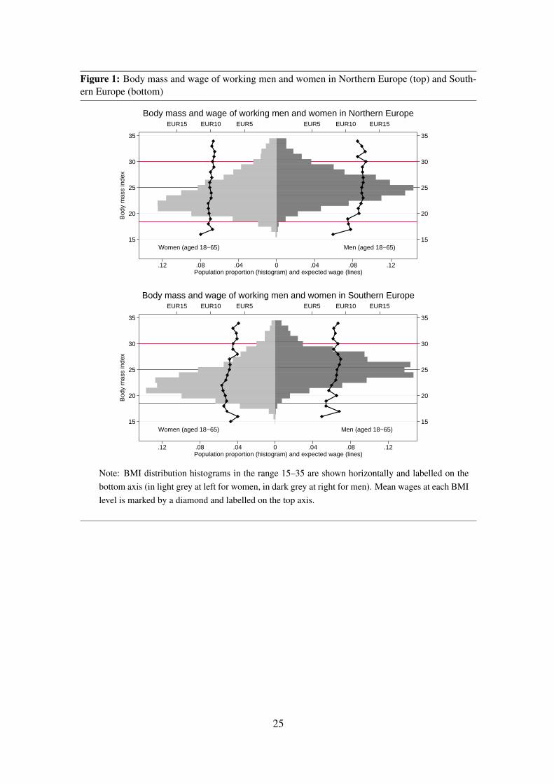
Figure 1: Body mass and wage of working men and women in Northern Europe (top) and South-ern Europe (bottom)

Men (aged 18−65)Women (aged 18−65)15

20

25

30

35

15

20

25

30

35

Bod

y m

ass

inde

xEUR15 EUR10 EUR5 EUR5 EUR10 EUR15

.12 .08 .04 0 .04 .08 .12Population proportion (histogram) and expected wage (lines)

Body mass and wage of working men and women in Northern Europe

Men (aged 18−65)Women (aged 18−65)15

20

25

30

35

15

20

25

30

35

Bod

y m

ass

inde

x

EUR15 EUR10 EUR5 EUR5 EUR10 EUR15

.12 .08 .04 0 .04 .08 .12Population proportion (histogram) and expected wage (lines)

Body mass and wage of working men and women in Southern Europe

Note: BMI distribution histograms in the range 15–35 are shown horizontally and labelled on thebottom axis (in light grey at left for women, in dark grey at right for men). Mean wages at each BMIlevel is marked by a diamond and labelled on the top axis.

25

Table 3: Coefficients on BMI parameters (Northern and Southern European countries)

North South(1) (2) (1) (2)

Men, 18–65Linear specification

BMI 0·001 0·002 0·001 0·001

Quadratic specificationBMI 0·054∗ 0·054∗ 0·040∗ 0·035∗

BMI squared −0·001∗ −0·001∗ −0·001∗ −0·001∗Estimated peak BMI 27·8 28·3 27·4 27·5

Piecewise constant specificationBMI<18.5 (underweight) −0·134† −0·131† −0·080 −0·072

25≤BMI<30 (overweight) 0·012 0·017† 0·009 0·009BMI≥30 (obese) −0·008 0·000 −0·015 −0·012

Women, 18–65Linear specification

BMI −0·004∗ −0·002† −0·004∗ −0·004∗Quadratic specification

BMI −0·016 −0·016 0·006 0·003BMI squared 0·000 0·000 −0·000 −0·000

Estimated peak BMI > 35 30·8 < 15 < 15

Piecewise constant specificationBMI<18.5 (underweight) 0·011 0·011 −0·009 0·008

25≤BMI<30 (overweight) −0·022† −0·015 −0·038∗ −0·027∗BMI≥30 (obese) −0·039∗ −0·016 −0·059∗ −0·050∗

Notes: Model specification (1) includes a quadratic function of age, indicator variables for educa-tional attainment, marital status, bad health, being a smoker and a set of time and country dummies.Model specification (2) is as (1) with additional controls for occupation, sector and part-time em-ployment. ∗ and † indicate significance at 1 and 5 percent levels respectively based on clusterrobust standard error estimates

26

Figure 2: BMI and Expected Wages of Northern European Males

2.2

2.4

2.6

Exp

ecte

d lo

g w

age

15 20 25 30 35BMI

Northern Europe, Men, Model specification (1)

2.2

2.4

2.6

Exp

ecte

d lo

g w

age

15 20 25 30 35BMI

Northern Europe, Men, Model specification (2)

Note: Grey lines show semi-parametrically estimated wage-BMI profiles (with point-wise bootstrapvariability bands). Black lines are the corresponding parametric predictions from a piece-wise con-stant, a linear and a quadratic model. Predictions are computed with all covariates (except BMI) setat their sample means. Density estimates of the distribution of BMI in the sample is reported at thebottom of each plot.

27

Figure 3: BMI and Expected Wages of Northern European Females

2.2

2.4

2.6

Exp

ecte

d lo

g w

age

15 20 25 30 35BMI

Northern Europe, Women, Model specification (1)

2.2

2.4

2.6

Exp

ecte

d lo

g w

age

15 20 25 30 35BMI

Northern Europe, Women, Model specification (2)


28

Figure 4: BMI and Expected Wages of Southern European Males

1.6

1.8

2E

xpec

ted

log

wag

e

15 20 25 30 35BMI

Southern Europe, Men, Model specification (1)

1.6

1.8

2E

xpec

ted

log

wag

e

15 20 25 30 35BMI

Southern Europe, Men, Model specification (2)


29

Figure 5: BMI and Expected Wages of Southern European Females

1.6

1.8

2E

xpec

ted

log

wag

e

15 20 25 30 35BMI

Southern Europe, Women, Model specification (1)

1.6

1.8

2E

xpec

ted

log

wag

e

15 20 25 30 35BMI

Southern Europe, Women, Model specification (2)


30

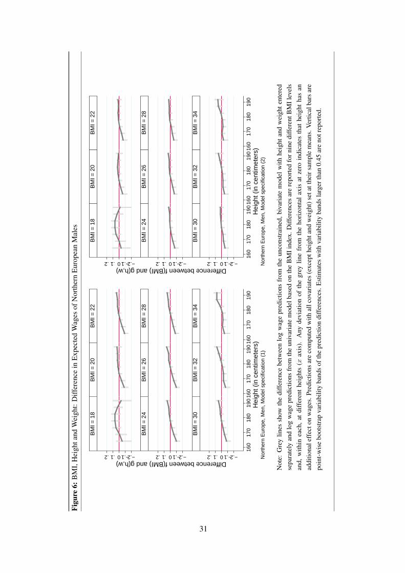
Figu

re6:

BM

I,H

eigh

tand

Wei

ght:

Diff

eren

cein

Exp

ecte

dW

ages

ofN

orth

ern

Eur

opea

nM

ales

−.2−.10.1.2 −.2−.10.1.2 −.2−.10.1.2

160

170

180

190

160

170

180

190

160

170

180

190

BM

I = 1

8B

MI =

20

BM

I = 2

2

BM

I = 2

4B

MI =

26

BM

I = 2

8

BM

I = 3

0B

MI =

32

BM

I = 3

4

Difference between f(BMI) and g(h,w)

Hei

ght (

in c

entim

eter

s)N

orth

ern

Eur

ope,

Men

, Mod

el s

peci

ficat

ion

(1)

−.2−.10.1.2 −.2−.10.1.2 −.2−.10.1.2

160

170

180

190

160

170

180

190

160

170

180

190

BM

I = 1

8B

MI =

20

BM

I = 2

2

BM

I = 2

4B

MI =

26

BM

I = 2

8

BM

I = 3

0B

MI =

32

BM

I = 3

4


Hei

ght (

in c

entim

eter

s)N

orth

ern

Eur

ope,

Men

, Mod

el s

peci

ficat

ion

(2)

Not

e:G

rey

lines

show

the

diff

eren

cebe

twee

nlo

gw

age

pred

ictio

nsfr

omth

eun

cons

trai

ned,

biva

riat

em

odel

with

heig

htan

dw

eigh

tent

ered

sepa

rate

lyan

dlo

gw

age

pred

ictio

nsfr

omth

eun

ivar

iate

mod

elba

sed

onth

eB

MIi

ndex

.Diff

eren

ces

are

repo

rted

forn

ine

diff

eren

tBM

Ilev

els

and,

with

inea

ch,

atdi

ffer

ent

heig

hts

(xax

is).

Any

devi

atio

nof

the

grey

line

from

the

hori

zont

alax

isat

zero

indi

cate

sth

athe

ight

has

anad

ditio

nale

ffec

ton

wag

es.P

redi

ctio

nsar

eco

mpu

ted

with

allc

ovar

iate

s(e

xcep

thei

ghta

ndw

eigh

t)se

tatt

heir

sam

ple

mea

ns.V

ertic

alba

rsar

epo

int-

wis

ebo

otst

rap

vari

abili

tyba

nds

ofth

epr

edic

tion

diff

eren

ces.

Est

imat

esw

ithva

riab

ility

band

sla

rger

than

0.45

are

notr

epor

ted.

31

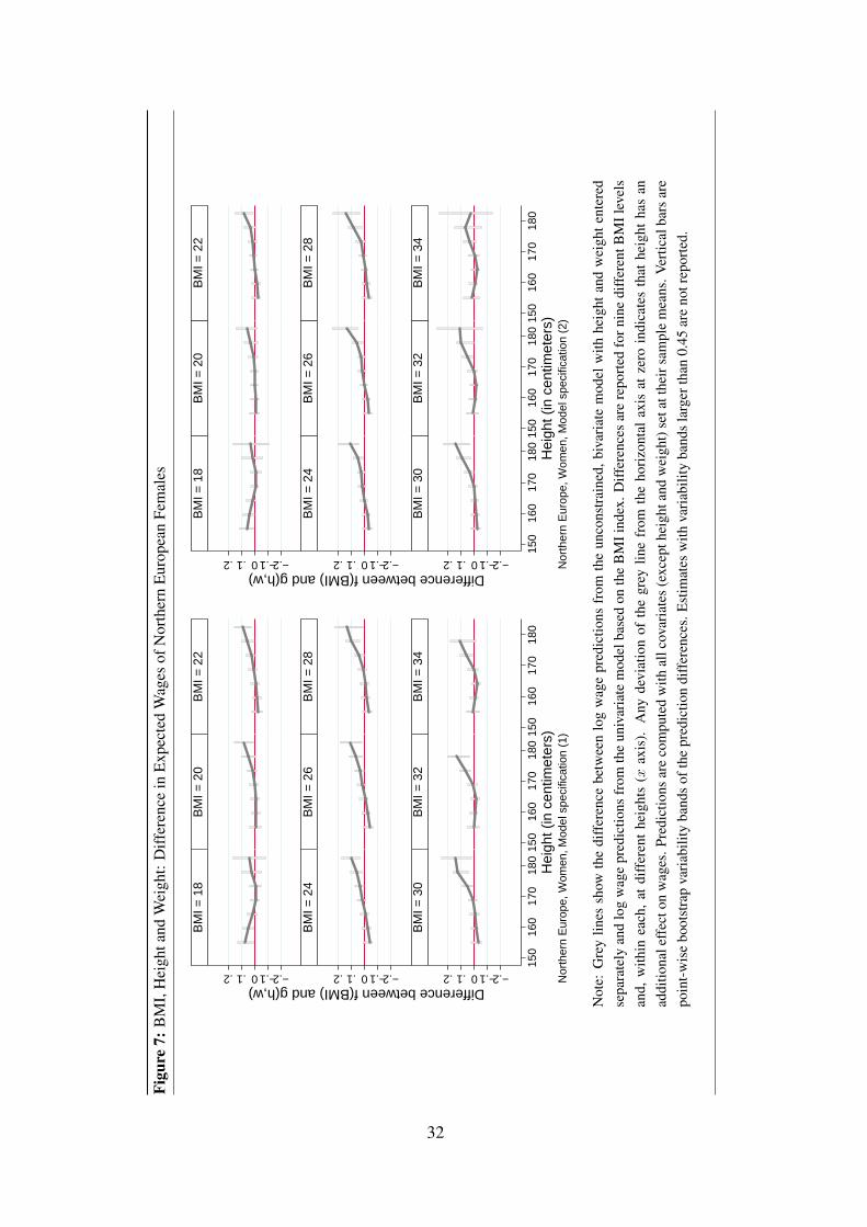
Figu

re7:

BM

I,H

eigh

tand

Wei

ght:

Diff

eren

cein

Exp

ecte

dW

ages

ofN

orth

ern

Eur

opea

nFe

mal

es

−.2−.10.1.2 −.2−.10.1.2 −.2−.10.1.2

150

160

170

180

150

160

170

180

150

160

170

180

BM

I = 1

8B

MI =

20

BM

I = 2

2

BM

I = 2

4B

MI =

26

BM

I = 2

8

BM

I = 3

0B

MI =

32

BM

I = 3

4


Hei

ght (

in c

entim

eter

s)N

orth

ern

Eur

ope,

Wom

en, M

odel

spe

cific

atio

n (1

)

−.2−.10.1.2 −.2−.10.1.2 −.2−.10.1.2

150

160

170

180

150

160

170

180

150

160

170

180

BM

I = 1

8B

MI =

20

BM

I = 2

2

BM

I = 2

4B

MI =

26

BM

I = 2

8

BM

I = 3

0B

MI =

32

BM

I = 3

4


Hei

ght (

in c

entim

eter

s)N

orth

ern

Eur

ope,

Wom

en, M

odel

spe

cific

atio

n (2

)

Not

e:G

rey

lines

show

the

diff

eren

cebe

twee

nlo

gw

age

pred

ictio

nsfr

omth

eun

cons

trai

ned,

biva

riat

em

odel

with

heig

htan

dw

eigh

tent

ered

sepa

rate

lyan

dlo

gw

age

pred

ictio

nsfr

omth

eun

ivar

iate

mod

elba

sed

onth

eB

MIi

ndex

.Diff

eren

ces

are

repo

rted

forn

ine

diff

eren

tBM

Ilev

els

and,

with

inea

ch,

atdi

ffer

ent

heig

hts

(xax

is).

Any

devi

atio

nof

the

grey

line

from

the

hori

zont

alax

isat

zero

indi

cate

sth

athe

ight

has

anad

ditio

nale

ffec

ton

wag

es.P

redi

ctio

nsar

eco

mpu

ted

with

allc

ovar

iate

s(e

xcep

thei

ghta

ndw

eigh

t)se

tatt

heir

sam

ple

mea

ns.V

ertic

alba

rsar

epo

int-

wis

ebo

otst

rap

vari

abili

tyba

nds

ofth

epr

edic

tion

diff

eren

ces.

Est

imat

esw

ithva

riab

ility

band

sla

rger

than

0.45

are

notr

epor

ted.

32

Figu

re8:

BM

I,H

eigh

tand

Wei

ght:

Diff

eren

cein

Exp

ecte

dW

ages

ofSo

uthe

rnE

urop

ean

Mal

es

−.2−.10.1.2 −.2−.10.1.2 −.2−.10.1.2

160

170

180

190

160

170

180

190

160

170

180

190

BM

I = 1

8B

MI =

20

BM

I = 2

2

BM

I = 2

4B

MI =

26

BM

I = 2

8

BM

I = 3

0B

MI =

32

BM

I = 3

4


Hei

ght (

in c

entim

eter

s)S

outh

ern

Eur

ope,

Men

, Mod

el s

peci

ficat

ion

(1)

−.2−.10.1.2 −.2−.10.1.2 −.2−.10.1.2

160

170

180

190

160

170

180

190

160

170

180

190

BM

I = 1

8B

MI =

20

BM

I = 2

2

BM

I = 2

4B

MI =

26

BM

I = 2

8

BM

I = 3

0B

MI =

32

BM

I = 3

4


Hei

ght (

in c

entim

eter

s)S

outh

ern

Eur

ope,

Men

, Mod

el s

peci

ficat

ion

(2)

Not

e:G

rey

lines

show

the

diff

eren

cebe

twee

nlo

gw

age

pred

ictio

nsfr

omth

eun

cons

trai

ned,

biva

riat

em

odel

with

heig

htan

dw

eigh

tent

ered

sepa

rate

lyan

dlo

gw

age

pred

ictio

nsfr

omth

eun

ivar

iate

mod

elba

sed

onth

eB

MIi

ndex

.Diff

eren

ces

are

repo

rted

forn

ine

diff

eren

tBM

Ilev

els

and,

with

inea

ch,

atdi

ffer

ent

heig

hts

(xax

is).

Any

devi

atio

nof

the

grey

line

from

the

hori

zont

alax

isat

zero

indi

cate

sth

athe

ight

has

anad

ditio

nale

ffec

ton

wag

es.P

redi

ctio

nsar

eco

mpu

ted

with

allc

ovar

iate

s(e

xcep

thei

ghta

ndw

eigh

t)se

tatt

heir

sam

ple

mea

ns.V

ertic

alba

rsar

epo

int-

wis

ebo

otst

rap

vari

abili

tyba

nds

ofth

epr

edic

tion

diff

eren

ces.

Est

imat

esw

ithva

riab

ility

band

sla

rger

than

0.45

are

notr

epor

ted.

33

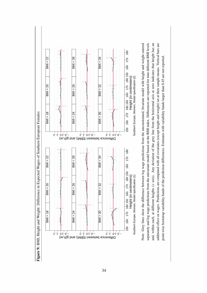
Figu

re9:

BM

I,H

eigh

tand

Wei

ght:

Diff

eren

cein

Exp

ecte

dW

ages

ofSo

uthe

rnE

urop

ean

Fem

ales

−.2−.10.1.2 −.2−.10.1.2 −.2−.10.1.2

150

160

170

180

150

160

170

180

150

160

170

180

BM

I = 1

8B

MI =

20

BM

I = 2

2

BM

I = 2

4B

MI =

26

BM

I = 2

8

BM

I = 3

0B

MI =

32

BM

I = 3

4


Hei

ght (

in c

entim

eter

s)S

outh

ern

Eur

ope,

Wom

en, M

odel

spe

cific

atio

n (1

)

−.2−.10.1.2 −.2−.10.1.2 −.2−.10.1.2

150

160

170

180

150

160

170

180

150

160

170

180

BM

I = 1

8B

MI =

20

BM

I = 2

2

BM

I = 2

4B

MI =

26

BM

I = 2

8

BM

I = 3

0B

MI =

32

BM

I = 3

4


Hei

ght (

in c

entim

eter

s)S

outh

ern

Eur

ope,

Wom

en, M

odel

spe

cific

atio

n (2

)

Not

e:G

rey

lines

show

the

diff

eren

cebe

twee

nlo

gw

age

pred

ictio

nsfr

omth

eun

cons

trai

ned,

biva

riat

em

odel

with

heig

htan

dw

eigh

tent

ered

sepa

rate

lyan

dlo

gw

age

pred

ictio

nsfr

omth

eun

ivar

iate

mod

elba

sed

onth

eB

MIi

ndex

.Diff

eren

ces

are

repo

rted

forn

ine

diff

eren

tBM

Ilev

els

and,

with

inea

ch,

atdi

ffer

ent

heig

hts

(xax

is).

Any

devi

atio

nof

the

grey

line

from

the

hori

zont

alax

isat

zero

indi

cate

sth

athe

ight

has

anad

ditio

nale

ffec

ton

wag

es.P

redi

ctio

nsar

eco

mpu

ted

with

allc

ovar

iate

s(e

xcep

thei

ghta

ndw

eigh

t)se

tatt

heir

sam

ple

mea

ns.V

ertic

alba

rsar

epo

int-

wis

ebo

otst

rap

vari

abili

tyba

nds

ofth

epr

edic

tion

diff

eren

ces.

Est

imat

esw

ithva

riab

ility

band

sla

rger

than

0.45

are

notr

epor

ted.

34

SEDAP RESEARCH PAPERS: Recent Releases

Number Title Author(s)

35

(2008)

No. 227: Using Statistics Canada LifePaths Microsimulation Model toProject the Health Status of Canadian Elderly

J. LégaréY. Décarie

No. 228: An Application of Price and Quantity Indexes in the Analysisof Changes in Expenditures on Physician Services

F.T. DentonC.H. FeaverB.G. Spencer

No. 229: Age-specific Income Inequality and Life Expectancy: NewEvidence

S. PrusR.L. Brown

No. 230: Ethnic Differences in Health: Does Immigration StatusMatter?

K.M. KobayashiS. PrusZ. Lin

No. 231: What is Retirement? A Review and Assessment of AlternativeConcepts and Measures

F.T. DentonB.G. Spencer

No. 232: The Politics of Social Policy Reform in the United States: TheClinton and the W. Bush Presidencies Reconsidered

D. BélandA. Waddan

No. 233: Grand Coalitions for Unpopular Reforms: Building a Cross-Party Consensus to Raise the Retirement Age

M. Hering

No. 234: Visiting and Office Home Care Workers’ OccupationalHealth: An Analysis of Workplace Flexibility and WorkerInsecurity Measures Associated with Emotional and PhysicalHealth

I.U. ZeytinogluM. DentonS. DaviesM.B. SeatonJ. Millen

No. 235: Policy Change in the Canadian Welfare State: Comparing theCanada Pension Plan and Unemployment Insurance

D. BélandJ. Myles

No. 236: Income Security and Stability During Retirement in Canada S. LaRochelle-CôtéJ. MylesG. Picot

No. 237: Pension Benefit Insurance and Pension Plan Portfolio Choice T.F. CrossleyM. Jametti

No. 238: Determinants of Mammography Usage across Rural andUrban Regions of Canada

J.T. McDonaldA. Sherman

(2009)

No. 239: Negative Effects of the Canadian GIS Clawback and PossibleMitigating Alternatives

D. ChisholmR.L. Brown



36

No. 240: Basic Living Expenses for the Canadian Elderly B.-J. MacDonaldD. AndrewsR.L. Brown

No. 241: Financial security of elders in China Y. ChengM.W. Rosenberg

No. 242: The Impact of Skill Mismatch among Migrants on RemittanceBehaviour

J.T. McDonaldM.R. Valenzuela

No. 243: Car Driving and Public Transit Use in Canadian MetropolitanAreas: Focus on Elderly and Role of Health and SocialNetwork Factors

R.G. MercadoK.B. Newbold

No. 244: Where Would You Turn for Help? Older Adults’ Knowledgeand Awareness of Community Support Services

M. DentonJ. PloegJ. TindaleB. HutchisonK. BrazilN. Akhtar-DaneshM. Quinlan

No. 245: New Evidence on Taxes and Portfolio Choice S. AlanK. AtalayT.F. CrossleyS.H. Jeon

No. 246: How should we support pharmaceutical innovation? P. Grootendorst

No. 247: Cohort Working Life Tables for Older Canadians F.T. DentonC.H. FeaverB.G. Spencer

No. 248: Cancer-related health behaviors and health service use amongInuit and other residents of Canada’s north

J.T. McDonaldR. Trenholm

No. 249: Older Aboriginal Peoples in Canada - Demographics, HealthStatus and Access to Health Care

M.W. RosenbergK. WilsonS. AbonyiA. WiebeK. BeachR. Lovelace

No. 250: Patents, Public-Private Partnerships or Prizes: How should wesupport pharmaceutical innovations?

P. Grootendorst

No. 251: Les besoins non comblés de services à domicile chez les aînéscanadiens

M.A. Busque



37

No. 252: La «migration de remplacement» au Québec: à quel pointpeut-on compter sur l’immigration pour contrer les problèmesdémographiques appréhendés?

G. Marois

No. 253: Le vieillissement de la population carcérale sousresponsabilité fédérale au Canada: Vers de «pénitenciers-hospices» ?

A.L. Tesseron

No. 254: International Differences in Longevity and Health and theirEconomic Consequences

P.-C. MichaudD. GoldmanD. LakdawallaA. GaileyY. Zheng

No. 255: Understanding the Economic Consequences of Shifting Trendsin Population Health

P.-C. MichaudD. GoldmanD. LakdawallaY. ZhengA. Gailey

No. 256: Population Aging, Older Workers, and Canada’s Labour Force F.T. DentonB.G. Spencer

No. 257: Patterns of Retirement as Reflected in Income Tax Records forOlder Workers

F.T. DentonRoss FinnieB.G. Spencer

No. 258: Reproductive Contributions of Foreign Wives in Taiwan:Similarities and Differences among Major Source Countries

K.-L. LiawJ.-P. LinC.-C. Liu

No. 259: Chronic Health Conditions: Changing Prevalence in an AgingPopulation and Some Implications for the Delivery of HealthCare Services

F.T. DentonB.G. Spencer

No. 260: Portfolio Allocation in the Face of a Means-Tested PublicPension

D.A. Cobb-ClarkV. Hildebrand

No. 261: Income Replacement in Retirement: Longitudinal Evidencefrom Income Tax Records

F.T. DentonR. FinnieB.G. Spencer

No. 262: A New Bismarckian Regime? Path Dependence and PossibleRegime Shifts in Korea’s Evolving Pension System

M. Hering

(2010)



38

No. 263: Strengthening Fairness and Funding in the Canada PensionPlan: Is Raising the Retirement Age an Option?

M. HeringT.R. Klassen

No. 264: Understanding the Outcomes of Older Job Losers M. BrzozowskiT.F. Crossley

No. 265: Issues in the Issuance of Enhanced Annuities R.L. BrownP. Scahill

No. 266: Criteria for the Optimal Design of a Social SecurityRetirement System

R.L. Brown

No. 267: Retirement 20/20: Innovation in Pension Design R.L. Brown

No. 268: Economic Security in an Aging Canadian Population R.L. Brown

No. 269: Body size and wages in Europe: A semi-parametric analysis V.A. HildebrandP. Van Kerm

Body size and wages in Europe: A semi-parametric analysis

Documents

Transcript of Body size and wages in Europe: A semi-parametric analysis