Body Mass Estimation in Xenarthra: A PredictiveEquation Suitable for All QuadrupedalTerrestrial Placentals?

Soledad De Esteban-Trivigno,1* Manuel Mendoza1 and Miquel De Renzi2

1Institut Catala de Paleontologia (ICP), c/Escola Industrial, 23 Sabadell, Barcelona 08211, Spain2Instituto Cavanilles de Biodiversitat i Biologia Evolutiva, Area de Paleontologıa,Polıgono La Coma s/n 46980 Paterna, Valencia, Spain

ABSTRACT The Magnorder Xenarthra includes strangeextinct groups, like glyptodonts, similar to large armadil-los, and ground sloths, terrestrial relatives of the extanttree sloths. They have created considerable paleobiologi-cal interest in the last decades; however, the ecology ofmost of these species is still controversial or unknown.The body mass estimation of extinct species has great im-portance for paleobiological reconstructions. The common-est way to estimate body mass from fossils is through lin-ear regression. However, if the studied species does nothave similar extant relatives, the allometric patterndescribed by the regression could differ from those shownby the extinct group. That is the case for glyptodonts andground sloths. Thus, stepwise multiple regression weredeveloped including extant xenarthrans (their taxonomicrelatives) and ungulates (their size and ecological rela-tives). Cases were weighted to maximize the taxonomicevenness. Twenty-eight equations were obtained. The dis-tribution of the percent of prediction error (%PE) was ana-lyzed between taxonomic groups (Perissodactyla, Artio-dactyla, and Xenarthra) and size groups (0–20 kg, 20–300kg, and more than 300 kg). To assess the predictive powerof the functions, equations were applied to species notincluded in the regression development [test set crossvalidation, (TSCV)]. Only five equations had a homogene-ous %PE between the aforementioned groups. These wereapplied to five extinct species. A mean body mass of 80 kgwas estimated for Propalaehoplophorus australis (Cingu-lata: Glyptodontidae), 594 kg for Scelidotherium leptoce-phalum (Phyllophaga: Mylodontidae), and 3,550.7 kg forLestodon armatus (Phyllophaga: Mylodontidae). The highscatter of the body mass estimations obtained for Catonyxtarijensis (Phyllophaga: Mylodontidae) and Thalassocnusnatans (Phyllophaga: Megatheriidae), probably due to dif-ferent specializations, prevented us from predicting itsbody mass. Surprisingly, although obtained from ungu-lates and xenarthrans, these five selected equations werealso able to predict the body mass of species from groupsas different as rodents, carnivores, hyracoideans, or tubu-lidentates. This result suggests the presence of a complexcommon allometric pattern for all quadrupedal placen-tals. J. Morphol. 000:000–000, 2008. � 2008 Wiley-Liss, Inc.

KEY WORDS: stepwise multiple regression; groundsloths; glyptodonts; weight

The Magnorder Xenarthra (McKenna and Bell,1997) represents the only placental group with liv-

ing representatives from the initial South Americanmammalian stock (Delsuc et al., 2004). It consistsof two orders, Cingulata (armadillos and glypto-donts) and Pilosa, which have two suborders, Phyl-lophaga (sloths) and Vermilingua (anteaters). Cin-gulata, Phyllophaga, and Vermilingua comprisethree highly specialized lineages, with very dissim-ilar morphologies. However, their monophyly isstrongly supported by many synapomorphies (seee.g., Gaudin and Branham, 1998; Van Dijk et al.,1999; Gaudin, 1999) and molecular analysis(Murphy et al., 2001; Delsuc et al., 2001).

Their fossil record extends back to the middlePalaeocene, about 58 million years ago (Storch,2001). The Magnorder radiated remarkablybetween the Palaeocene and Eocene periods, result-ing in a large diversity of forms (McKenna andBell, 1997, have described 221 genera until now).Most of these genera, however, had become extinct10,000 years ago (Lessa et al., 1997), and only 13genera with 30 species remain nowadays. Theirradiation gave birth to very peculiar extinct formslike glyptodonts, similar to big armadillos, andground sloths, terrestrial relatives of the extanttree sloths (Patterson and Pascual, 1972). Becauseof their strange characteristics, like their simplifiedever-growing teeth, the lack of enamel, or the pres-ence of dermal bones, Xenarthra created consider-able paleobiological interest in the last decades(e.g., Vizcaıno, 1994; Muizon de and McDonald,1995; Farina and Blanco, 1996; Vizcaıno andFarina, 1997; Vizcaıno et al., 1998, 1999, 2003;

Contract grant sponsor: Spanish Ministerio de Educacion y Ciencia;Contract grant numbers: CGL2005-08238-C02-02/BTE, CGL2006-13808-C02-0; Contact grant sponsor: Synthesys; Contract grant num-ber: DE-TAF1779 2.

*Correspondence to: Soledad De Esteban-Trivigno, Institut Catalade Paleontologia (ICP), c/ Escola Industrial, 23 Sabadell, Barcelona08211, Spain. E-mail: soledad.esteban@icp.cat

Published online inWiley InterScience (www.interscience.wiley.com)DOI: 10.1002/jmor.10659

JOURNAL OF MORPHOLOGY 000:000–000 (2008)

� 2008 WILEY-LISS, INC.

Alexander et al., 1999; De Iuliis et al., 2000; Perezet al., 2000; Vizcaıno, 2000; Bargo, 2001; Farinaand Vizcaıno, 2001; Vizcaıno and De Iuliis, 2003;Bargo et al., 2006), although the ecology of most ofthese species is still controversial or unknown.

Body mass is correlated with many ecologicallyrelevant characteristics in mammals (e.g., Damuth,1981; Calder, 1996; Kozlowsky and Weiner, 1997;Polishchuk and Tseitlin, 1999), so its characteriza-tion is of great importance in understanding theecology and adaptations of past species (Damuthand MacFadden, 1990). Because the ecology of glyp-todonts and ground sloths is not well understood,their body mass estimation plays an important rolein reconstructing the ancient ecosystems theyinhabited (Farina, 1996; Croft, 2001; Prevosti andVizcaıno, 2006). However, although some attemptshave been made in the past in order to estimate thebody mass of the larger xenarthrans species, theresults are neither conclusive nor extensive to otherxenarthrans species. Farina et al. (1998) estimatedthe body mass of many Pleistocene ground slothsand glyptodonts as the mean of many simpleregressions predictions. Nevertheless, as the pre-dictive equations were obtained from ungulates(Janis, 1990), the results obtained by Farina et al.(1998) show much dispersion. Indeed, Croft (2001)obtained mass estimates from extant bears, treesloths, and giant anteaters for different species ofground sloths, which he rejected due to clear bodymass overestimation. In other cases, mathematicaland scale models have been used to estimate thebody mass of some Lujanian ground sloths (Bargoet al., 2000; Christiansen and Farina, 2003) andglyptodonts (Farina, 1995). Some problems arisewhen such models are applied because (i) theirapplication is overdependent on the reliability ofsoft-tissue reconstruction, and (ii) the dependencyon the existence of almost complete fossil skeletons.

Body mass of extinct species may be predicted byusing allometric functions (e.g., Scott, 1983; Ander-son et al., 1985; Jungers, 1990; Fortelius, 1993;Noriega, 2001; Gordon, 2003; Mazzetta et al., 2004;Farlow et al., 2005). The search for reliable func-tions to estimate the body mass of glyptodonts andground sloths is indeed hampered by the lack of ec-ological representatives among the living species.Glyptodonts have no extant representatives at thefamily level, and the extant representatives of theextinct sloths, the tree sloths Choloepus and Bra-dypus, are too highly specialized (they have fullysuspensory habits) to allow comparison. Moreover,by simply inspecting the remains of glyptodontsand ground sloths, one can appreciate that mostspecies fall well above of the body size range ofextant xenarthrans. One of the larger extinct spe-cies, Lestodon armatus, could have weighed morethan 3 tons (Bargo et al., 2000), whereas the larg-est living xenarthran, Priodontes maximus, has amaximum weight of only 60 kg.

When body mass is estimated through allometricequations, some authors recommend restrictingthe sample of extant species to those that arebroadly similar in both physical proportions andphylogenetic legacy to the fossilized ones (seeChristiansen, 2004 and references therein).Others, on the contrary, suggest that with phyloge-netically wider data bases, better results areachieved (Calder, 1996; Cuozzo, 2001; Reynolds,2002). In this way, Mendoza et al. (2006) foundthat the highest predictive power is obtained withthose functions derived from the highest taxonomi-cal and ecological diversity, when using multipleregressions. Indeed, these authors show that step-wise multiple regressions can clearly improve thepredictive power of the resultant functions.

Therefore, we do not restrict our recent database to xenarthrans in order to obtain the mostreliable predictive equations for ground sloths andglyptodonts. We add data from Artiodactyla andPerissodactyla because they have a body size spanthat includes most of the body size of extinct xenar-thrans, and their quadrupedal pattern is shared byglyptodonts and most of the ground sloths. Never-theless, regressions fitted with only ungulates arenot the best option, as the scattered results of Fa-rina et al. (1998) point out. Consequently, thesearch for a pattern common to both xenarthransand ungulates requires a reference data base ofextant species consisting of data from both groups;this seems to be a suitable alternative.

Although craniodental measurements and bodymass are correlated to some degree (Legendre andRoth, 1988; Cuozzo, 2001; Gordon, 2003; Egi et al.,2004), there are important differences especiallyamong species with dissimilar diets (see Fortelius,1990). Limb elements, to the contrary, support thebody weight and are, in general, better correlatedwith body mass than craniodental ones (i.e.,Gingerich, 1990; Anyonge, 1993; Martınez andSudre, 1995; Kappelman et al., 1997; Christiansen,1999; Ruff, 2003; Andersson, 2004).

The aim of this work is to obtain reliable equa-tions to apply to any terrestrial Xenarthra, consid-ering especially glyptodonts and ground sloths. Inthis way, we agree with Smith (2002): ‘‘rather thanmany prediction equations, I would have workedtoward developing a few thoroughly evaluatedequations, particularly regarding patterns in thedistribution of residuals.’’

Thus, this will be achieved through stepwise mul-tiple regressions, using postcranial variables, andincluding both xenarthrans and ungulates in thedata base from which the regressions would bedeveloped. Although the reliability of differentfunctions has traditionally been evaluated by com-paring the mean percent prediction error (%PE;Smith, 1981, 1984) obtained from the individual%PE absolute values (Myers, 2001; Ruff, 2003;Wroe et al., 2003), the individual prediction error

2 S. DE ESTEBAN-TRIVIGNO ET AL.

Journal of Morphology

distribution plays an important role, especiallywith such taxonomically wide data bases and bodysizes as those included in this study. Therefore, thehomogeneity of the prediction error will be eval-uated for the obtained functions to verify the equa-tion reliability for different taxonomic groups anddifferent sizes ranges (i.e., prediction error is thesame for all sets of species). Moreover, because pre-diction error in fossils is not possible to check,regression functions will be applied to living speciesthat have never been used to develop equations, inorder to assess how accurately they predict thefunctions of unknown species. Finally, selectedfunctions will be applied to one glyptodont and foursloth species in order to estimate their body mass.

MATERIALS AND METHODS

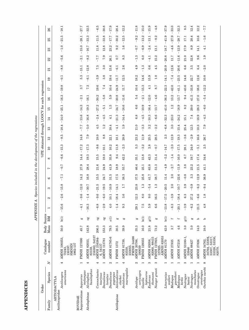
Measurements and regression functions were derived from asample consisting of 279 individuals that were grouped into 94extant species, including 71 Artiodactyla, 11 Perissodactyla(ungulates), 3 Pilosa, and 10 Cingulata (xenarthrans) (AppendixA). All the living families of these orders were represented,except for Bradypodidae, Megalonychidae, and Cyclopedidae(tree sloths and silky anteater), which were left out due to theirarboreal habits. Only adult specimens, as indicated by fusion ofepiphyses, were measured, and captive animals were avoided asfar as possible (Scott, 1985).Twenty-nine species were omitted from the function develop-

ment, because some measurements were unavailable. A part ofthem consists of 18 species of xenarthrans, perissodactyls, andartiodactyls (Appendix B, set test 1). The remaining 11 speciescame from orders different than those used to obtain the func-tions; i.e., hyracoideans, carnivorans, tubulidentates, androdents (Appendix B, set test 2). Recent species names wereupdated following Wilsom and Reeder (2005).Six fossil specimens, belonging to five species of extinct xenar-

thrans, were measured (see Table 2 for their museum cataloguenumber). One Miocene glyptodont species was measured; Prop-alaehoplophorus australis Ameghino 1887 (Cingulata: Glypto-dontidae). In addition, four extinct sloths species were studied:one from the Miocene; Thalassocnus natans Muizon de andMcDonald, 1995 (Phyllophaga: Megatheriidae) and three fromthe Pleistocene. The latter were Lestodon armatus Gervais1855 (Phyllophaga: Mylodontidae), Scelidotherium leptocepha-lum Owen 1839 (Phyllophaga: Mylodontidae) and two individu-als of Catonyx tarijensis Ameghino 1891 (Phyllophaga: Mylo-dontidae). The S. leptocephalum specimen appears in the mu-seum catalogue as Scelidotherium bravardi Lydekker 1886;however, McDonald (1987) considered S. bravardi as a juniorsynonym of S. leptocephalum, so this name is used here. In thisway, both specimens of C. tarijensis are catalogued as Scelido-don tarijensis, but Catonyx is the nearest available name forspecies traditionally placed in Scelidodon, (including C. tarijen-sis; McDonald and Perea, 2002), because the type of Scelidodonis a junior synonym of Scelidotherium.Measurements (both recent individuals and fossil specimens)

were collected by the first author in different museums andinstitutions: Museo de Ciencias Naturales (MCNV; Valencia,Spain) Museo Nacional de Ciencias Naturales (MNCN; Madrid,Spain), Estacion Biologica de Donana (EBD; Sevilla, Spain),Museo de La Plata (MLP; La Plata, Argentine), Museo Argen-tino de Ciencias Naturales Bernardino Rivadavia (MACN; Bue-nos Aires, Argentine), Field Museum of Natural History(FMNH; Chicago), American Museum of Natural History(AMNH; NY), Smithsonian Institution National Museum ofNatural History (SNMNH, Washington, DC), Museum furNaturkunde (ZMB; Berlin, Germany, extant species cataloguenumber corresponds with those from ‘‘Zoologishes Museum

Berlin’’), Museum National d’Histoire Naturelle de Paris(MNHN; Paris, France; extant species catalogue numbers corre-spond with those from ‘‘Collections d’Anatomie Comparee duMuseum d’Histoire Naturelle de Paris’’).

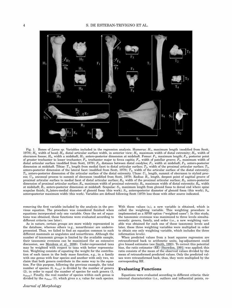
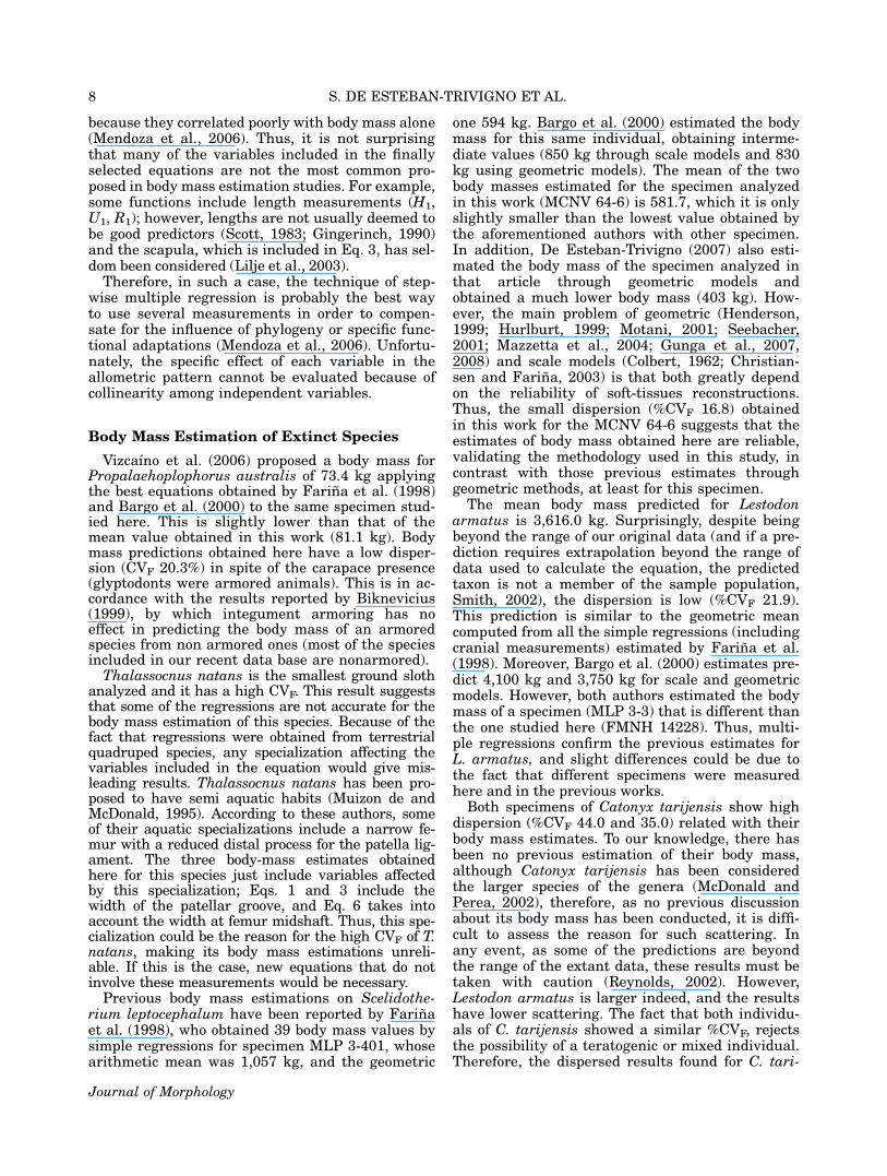
Thirty-three postcranial variables were measured (see Fig. 1).Following Scott (1985), midshafts were located by dividing inhalf the length measurement (as the greatest length of the bonebetween articular surfaces) and measuring this distance fromthe proximal part. When bone processes exist, the measurementwas taken at the nearest point at the end of the process. In thesame way, the anteroposterior diameters were measured fromthe most anterior to the most posterior point as the bone wouldbe positioned in the living animal. Transverse diameters weremeasured at right angles to the anteroposterior diameters. Allthe measurements were taken with electronic calipers, with theexception of bone lengths of some large species (e.g., Ceratothe-rium simun), which were measured with a manual caliper. Botharticular and maximal lengths of humerus and femur were meas-ured. However, in order to avoid collinearity (as both variableswere very similar) only one of them for each bone was includedin the analysis. Because of the fact that maximal lengths weremore correlated with body mass than those articular, the formerwere those included in the regression development.

Data taken in the field for museum specimens rarely includebody weight; therefore, analyses were performed using themean body mass values reported in the literature for each spe-cies as a dependent variable (see Appendix A). When sexualdimorphism existed, and information about sex was available,body mass data of males and females for a given species weredifferentiated, and thereafter the arithmetic mean of individualbody mass data was obtained. Independent variables wereobtained by averaging the measurements of the available set ofindividuals for each species.

Obtaining the Regression Functions

The statistical approach used in this study was linear multipleregression, which was performed with SPSS 12.00, whereas Past(PAlentological STatistics, Hammer et al., 2001) was used to de-velop tests. Variable normality was analyzed with a Shapiro-Wilk test on log-transformed variables. Those variables with anasymmetry or kurtosis value above 1 were discarded and werenot included in the analysis. The regression functions were fittedto the data by means of Ordinary Least Squares (OLS) model (orModel I) on log-transformed variables. Model II of regression issuggested when both predictor and response variables are ran-dom, such as in this case. However, the OLS regression model isrecommended if the main aim of our regression analysis is pre-diction (MacLeod, 2004; Quinn and Keough, 2006).

The stepwise procedure starts with the independent variablethat correlates best with body mass, which is incorporatedwithin the regression function. Once this variable is found, theprogram carries out a search of the remaining variables until avariable is found that accounts for the greatest variance of thedependent variable that is not explained by the first, and thenrepeated successively. At each step, a new variable is includedas characterized by its lowest P value (Pin) or F probability (i.e.,conditional probability of a random relationship between the de-pendent and predictor variables). Inclusion of a new variable inthe regression function modifies the P values of the variablesalready included. If one of these variables exceeds the limitestablished previously (Pout or F probability), it is removed fromthe equation. This process stops when no variable can be addedor removed because none of the variables included in the func-tion exceeds the Pout value, and all the variables that were notincluded exceed the Pin value. Stepwise multiple regressionanalyses were performed using a fixed P-value to both enter(0.001) and be removed (0.002).

A great amount of information contained in the predictor var-iables is redundant; thus, different combinations of these mor-phological variables can characterize the body size of a givengroup of species. Consequently, several stepwise analyses wereperformed in order to obtain different functions, each time

BODY MASS ESTIMATION IN XENARTHRA 3

Journal of Morphology

removing the first variable included by the analysis in the pre-vious equation. The procedure was considered finished whenequations incorporated only one variable. Once the set of equa-tions was obtained, these functions were evaluated according todifferent criteria (see later).As in nature, certain groups are more widely represented in

the database, whereas others (e.g., xenarthrans) are underre-presented. Thus, we failed to find an equation common to suchdifferent mammals as ungulates and xenarthrans. Although thenumber of taxonomic groups is limited by the available sample,their taxonomic evenness can be maximized (for an extensivediscussion, see Mendoza et al., 2006). Under-represented taxamay be weighted with respect to taxa with better representa-tion. Weighting consists of equating the weight for the contribu-tion of each taxon in the body mass function, e.g., in a familywith one genus with four species and another with only two, weclaim that both genera contribute in the same way to the equa-tion. For this purpose, following the previous example, the totalnumber of species (6, nreal) is divided by the number of genera(2), in order to equal the number of species for each genera (3,ntheor). Finally, the real number of species within each genus isdivided by the ntheor (3), which gives a xi value for each species.

With these values (xi), a new variable is obtained, which iscalled the weighting variable. This weighting procedure isimplemented as a SPSS option (‘‘weighted cases’’). In this study,the taxonomic evenness was maximized to three levels simulta-neously: genera, family, and order (i.e., a new weighting vari-able was obtained for each one of these taxonomic levels andlater, these three weighting variables were multiplied in orderto obtain one only weighting variable, which includes the threeinformation levels).

When predicted values from a least squares regression areretransformed back to arithmetic units, log-adjustment couldgive biased estimates (see Smith, 1993). To correct this potentialbias, the ratio estimator (RE) (Snowdon, 1991) was applied; thisratio consists of the mean of the observed values divided by themean of retransformed predicted values. Only the predicted val-ues were retransformed back; thus, they were multiplied by thecorresponding RE.

Evaluating Functions

Equations were evaluated according to different criteria: theirinternal characteristics (i.e., outliers and influential points, re-

Fig. 1. Bones of Lama sp. Variables included in the regression analysis. Humerus: H1, maximum length (modified from Scott,1979); H2, width of head; H3, distal articular surface width, in anterior view; H4, maximum width of distal extremity; H5, width ofolecranon fossae; H6, width a midshaft; H7, antero-posterior dimension at midshaft. Femur: F1, maximum length; F2, posterior pointof greater trochanter to lesser trochanter; F3, trochanter major to fovea capitis; F4, width of patellar groove; F5, maximum width ofdistal articular surface (modified from Scott, 1979); F6, distance between distal condyles; F7, width at midshaft; F8, antero-posteriordimension at midshaft. Tibiae: T1, length from medial facet to distal articular surface; T2, width of the proximal articular surface; T3,antero-posterior dimension of the lateral facet (modified from Scott, 1979); T4, width of the articular surface of the distal extremity;T5, antero-posterior dimension of the articular surface of the distal extremity. Ulnae: U1, length, summit of olecranon to styloid proc-ess; U2, anconeal process to summit of olecranon (modified from Scott, 1979). Radius: R1, length, deepest point of sagittal groove ofproximal articular surface to medial facet of distal articular surface; R2, width of the proximal articular surface; R3, antero-posteriordimension of proximal articular surface; R4, maximum width of proximal extremity; R5, maximum width of distal extremity; R6, widthat midshaft; R7, antero-posterior dimension at midshaft. Scapulae: S1, maximum length from glenoid fossa to dorsal end where spinescapulae finish; S2,latero-medial diameter of glenoid fossa (this work); S3, anteroposterior diameter of glenoid fossa (this work); S4,anteroposterior maximum width (this work). Variables are defined following Scott (1979) less those with other source indicated.

4 S. DE ESTEBAN-TRIVIGNO ET AL.

Journal of Morphology

sidual distribution), and both the mean and distribution of thepredictive error of their estimations.Outliers, influential points, and residuals. Leverage and

Cook’s distance (Di) were used to detect influential points. Influ-ential points were considered to be the observations with a lever-age value higher than twice the ratio of the number of para-meters (including the intercept) to the number of samples (Quinnand Keough, 2006). Observations with Di greater than unitywere considered particularly influential. Those equations show-ing clear outliers or influential points were discarded. Homogene-ity of residuals was controlled by residual vs predicted graphs.Percent prediction error. Although the correlation coeffi-

cient is one of the commonest way to evaluate regressions, itpoorly indicates the independent variable predictive powerbecause it is affected by the range of values of the dependentvariable and, therefore, it could be high even with high resid-uals (Smith, 1981). Thus, function reliability was evaluated bydirectly using the %PE (%PE 5 100 3 [observed 2 predicted]/predicted, Smith, 1981,1984).Because of the nature of the database and the particular

problem under study (a wide range of sizes and species that arequite phlyogenetically distant), the homogeneity of their %PE(from now on called %PEH) was evaluated with respect to sizeand phylogeny. The %PE homogeneity was checked using thosespecies included in the regression development (Appendix A).Obviously, analysis of %PEH with those species not included inthe regressions (Appendix B) may be better; however, thereduced species number in the test sets prevents us fromincluding them in this step of the approach. Therefore, the %PEfor each individual was obtained using the leave-one-out crossvalidation (LOOCV) procedure, which means that the bodymass of each species is estimated with a function adjusted with-out that species.To test the %PEH of phylogeny, the species were classified

into three taxonomic groups: xenarthrans, artiodactyls, andperissodactyls. Normality of %PE for each group was checkedwith a Shapiro-Wilks test. At least one of the groups was non-normal; consequently, a Levene test was applied to check theequality of the variances among the three groups. When varian-ces were not equal, the function was discarded. When equal, aKruskal-Wallis analysis was performed, as it is more robust tonormality departures than an ANOVA analysis. Those equa-tions with dissimilar medians were discarded. As we particu-larly wanted to guard against Type-II error (to accept H0 beingfalse), the Bonferroni correction was not applied, and a P valueof 0.1 was established to reject H0.The procedure described above was also applied to evaluate

the %PEH for size. Economos (1983) suggests that differentscaling relationships may apply to large versus small terrestrialmammals at about 20 kg body mass. In a similar fashion Biew-ener (2000) proposed that posture-related changes in limb me-chanical advantage at sizes above 300 kg body mass appear tobe constrained. Thus, a different allometric pattern could beexhibited by these specified size groups. Therefore, according toboth authors, the data were split in three groups; those specieswith a body mass lower than 20 kg (n 5 27), between 20 and300 kg (n 5 55), and more than 300 kg (n 5 12). When varian-ces or medians were not equal for the three size groups, thefunction was discarded.When a multiple regression equation is calculated for the

purpose of prediction, it will not operate as well on new data asit does in the sample used to determine the equation (Kaufmanand Smith, 2002). Thus, those functions that had homogeneous%PE among taxonomic and body mass groups were analyzedusing the test set cross validation procedure (TSCV). The TSCVassesses the predictive power of the equations with speciesnever used in the regression development.Therefore, the prediction error was evaluated for the set of

placental groups (only considering quadrupedal and terrestrialspecies). We compared the %PE among (i) those species used toobtain the regressions (whose %PE was obtained by LOOCV);(ii) those not used to obtain regressions but from the sameorders as (i) (perisodactyls, artiodactyls, and ungulates, test set

1); (iii) placental species from orders other than those used toobtain the functions (i.e., hyracoideans, carnivorans, tubuliden-tates, and rodents) (test set 2).The variance and median %PEbetween the three groups mentioned in the previous paragraphwas controlled by Levene and Kruskal-Wallis tests, respectively.Only one group of equations was taken into account to applythem to the fossil record, namely the equations with the same%PE distribution for all the placental mammals considered, aswell as low %PE values.

Extinct Species Body Mass Estimation

As a result of the selection process explained before, a smallset of equations was obtained, from which the mean body massfor each extinct species was estimated. Christiansen and Harris(2005) have recently proposed obtaining the mean body massweighting according to the %PE of each function, such thatfunctions with a low %PE contribute more to the mean thanfunctions with a high %PE. Thus, for n estimates of body mass[W1, W2. . .Wn] each one with a mean prediction error [PE1,PE2. . .PEn] the final average (W) will not be a mere average ofthe included mass values, but

W ¼Xni¼1

ðWi=%PEiÞ 3Xni¼1

%PEi

!3 n�2

This procedure was applied to estimate the body mass of eachextinct species with the set of selected functions. To evaluatethe dispersion of the different estimates, the coefficient of varia-tion (CV) was calculated, as the percent of the standard devia-tion divided by the mean, for each extinct species.

RESULTS

Only variable T1 was discarded, and then notincluded in subsequent analyses, because of itshigh values of kurtosis (8.01) and skewed distribu-tion (22.2). The multiple regression stepwise analy-ses provided 28 equations, each one based on dif-ferent combinations of variables (Appendix C). Afterstudying graphical residuals and checking outliersand influential points, nine equations were dis-carded. The remaining equations were checkedfor the phylogenetic and body size influence on the%PE by the Levene and Kruskal-Wallis test; there-fore, a further nine equations were excluded.Ten equations remained at the end of this analyti-cal process. When the homogeneity of %PE betweenthose species used in the equation development andthose never included in the regressions (test sets 1and 2) was compared, only five equations showedthe same %PE for the median and variance. Asexpected, these five functions have low %PE (i.e.,they are among the 10 functions with lowest %PE).Thus, this final set of selected functions (Table 1)was considered suitable to apply to the extinct spe-cies studied. For each species (Table 2), we obtainedits corresponding body mass prediction with eachfunction, together with a weighted mean valueaccording to the %PE of the functions (Christiansenand Harris, 2005).

The body mass estimates obtained from fossilsrange from 72.2 up to 4382.3 kg (Table 2). Sevenestimations are larger than the upper limit of thebody mass included in the regressions (1,879 kg,

BODY MASS ESTIMATION IN XENARTHRA 5

Journal of Morphology

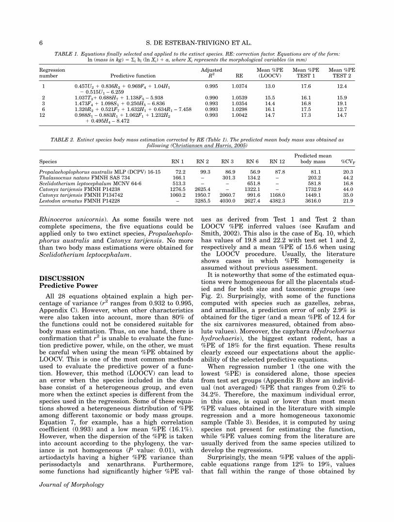
Rhinoceros unicornis). As some fossils were notcomplete specimens, the five equations could beapplied only to two extinct species, Propalaehoplo-phorus australis and Catonyx tarijensis. No morethan two body mass estimations were obtained forScelidotherium leptocephalum.

DISCUSSIONPredictive Power

All 28 equations obtained explain a high per-centage of variance (r2 ranges from 0.932 to 0.995,Appendix C). However, when other characteristicswere also taken into account, more than 80% ofthe functions could not be considered suitable forbody mass estimation. Thus, on one hand, there isconfirmation that r2 is unable to evaluate the func-tion predictive power, while, on the other, we mustbe careful when using the mean %PE obtained byLOOCV. This is one of the most common methodsused to evaluate the predictive power of a func-tion. However, this method (LOOCV) can lead toan error when the species included in the database consist of a heterogeneous group, and evenmore when the extinct species is different from thespecies used in the regression. Some of these equa-tions showed a heterogeneous distribution of %PEamong different taxonomic or body mass groups.Equation 7, for example, has a high correlationcoefficient (0.993) and a low mean %PE (16.1%).However, when the dispersion of the %PE is takeninto account according to the phylogeny, the var-iance is not homogeneous (P value: 0.01), withartiodactyls having a higher %PE variance thanperissodactyls and xenarthrans. Furthermore,some functions had significantly higher %PE val-

ues as derived from Test 1 and Test 2 thanLOOCV %PE inferred values (see Kaufam andSmith, 2002). This also is the case of Eq. 10, whichhas values of 19.8 and 22.2 with test set 1 and 2,respectively and a mean %PE of 15.6 when usingthe LOOCV procedure. Usually, the literatureshows cases in which %PE homogeneity isassumed without previous assessment.

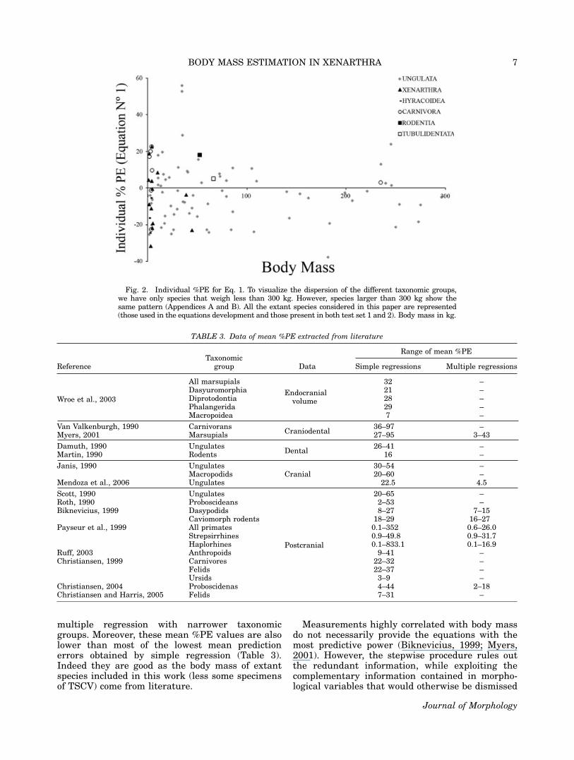
It is noteworthy that some of the estimated equa-tions were homogeneous for all the placentals stud-ied and for both size and taxonomic groups (seeFig. 2). Surprisingly, with some of the functionscomputed with species such as gazelles, zebras,and armadillos, a prediction error of only 2.9% isobtained for the tiger (and a mean %PE of 12.4 forthe six carnivores measured, obtained from abso-lute values). Moreover, the capybara (Hydrochoerushydrochaeris), the biggest extant rodent, has a%PE of 18% for the first equation. These resultsclearly exceed our expectations about the applic-ability of the selected predictive equations.

When regression number 1 (the one with thelowest %PE) is considered alone, those speciesfrom test set groups (Appendix B) show an individ-ual (not averaged) %PE that ranges from 0.2% to34.2%. Therefore, the maximum individual error,in this case, is equal or lower than most mean%PE values obtained in the literature with simpleregression and a more homogeneous taxonomicsample (Table 3). Besides, it is computed by usingspecies not present for estimating the function,while %PE values coming from the literature areusually derived from the same species utilized todevelop the regressions.

Surprisingly, the mean %PE values of the appli-cable equations range from 12% to 19%, valuesthat fall within the range of those obtained by

TABLE 1. Equations finally selected and applied to the extinct species. RE: correction factor. Equations are of the form:ln (mass in kg) 5 Si bi (ln Xi) 1 a, where Xi represents the morphological variables (in mm)

Regressionnumber Predictive function

AdjustedR2 RE

Mean %PE(LOOCV)

Mean %PETEST 1

Mean %PETEST 2

1 0.457U2 1 0.836R2 1 0.969F4 1 1.04H1

2 0.515U1 – 6.2590.995 1.0374 13.0 17.6 12.4

2 1.037T31 0.688H7 1 1.138F5 – 5.938 0.990 1.0539 15.5 16.1 15.93 1.473F4 1 1.098S1 1 0.250H5 – 6.836 0.993 1.0354 14.4 16.8 19.16 1.320R2 1 0.521F7 1 1.632H1 1 0.634R1 – 7.458 0.993 1.0298 16.1 17.5 12.7

12 0.988S1 – 0.883R1 1 1.062F1 1 1.232H2

1 0.495H4 – 8.4720.993 1.0042 14.7 17.3 14.7

TABLE 2. Extinct species body mass estimation corrected by RE (Table 1). The predicted mean body mass was obtained asfollowing (Christiansen and Harris, 2005)

Species RN 1 RN 2 RN 3 RN 6 RN 12Predicted mean

body mass %CVF

Propalaehoplophorus australis MLP (DCPV) 16-15 72.2 99.3 86.9 56.9 87.8 81.1 20.3Thalassocnus natans FMNH SAS 734 166.1 – 301.3 134.2 – 203.2 44.2Scelidotherium leptocephalum MCNV 64-6 513.3 – – 651.8 – 581.8 16.8Catonyx tarijensis FMNH P14238 1276.5 2625.4 – 1322.1 – 1732.9 44.0Catonyx tarijensis FMNH P134742 1060.2 1950.7 2060.7 991.6 1168.0 1449.1 35.0Lestodon armatus FMNH P14228 – 3285.5 4030.0 2627.4 4382.3 3616.0 21.9

6 S. DE ESTEBAN-TRIVIGNO ET AL.

Journal of Morphology

multiple regression with narrower taxonomicgroups. Moreover, these mean %PE values are alsolower than most of the lowest mean predictionerrors obtained by simple regression (Table 3).Indeed they are good as the body mass of extantspecies included in this work (less some specimensof TSCV) come from literature.

Measurements highly correlated with body massdo not necessarily provide the equations with themost predictive power (Biknevicius, 1999; Myers,2001). However, the stepwise procedure rules outthe redundant information, while exploiting thecomplementary information contained in morpho-logical variables that would otherwise be dismissed

Fig. 2. Individual %PE for Eq. 1. To visualize the dispersion of the different taxonomic groups,we have only species that weigh less than 300 kg. However, species larger than 300 kg show thesame pattern (Appendices A and B). All the extant species considered in this paper are represented(those used in the equations development and those present in both test set 1 and 2). Body mass in kg.

TABLE 3. Data of mean %PE extracted from literature

ReferenceTaxonomic

group Data

Range of mean %PE

Simple regressions Multiple regressions

Wroe et al., 2003

All marsupials

Endocranialvolume

32 –Dasyuromorphia 21 –Diprotodontia 28 –Phalangerida 29 –Macropoidea 7 –

Van Valkenburgh, 1990 CarnivoransCraniodental

36–97 –Myers, 2001 Marsupials 27–95 3–43

Damuth, 1990 UngulatesDental

26–41 –Martin, 1990 Rodents 16 –

Janis, 1990 UngulatesCranial

30–54 –Macropodids 20–60 –

Mendoza et al., 2006 Ungulates 22.5 4.5

Scott, 1990 Ungulates

Postcranial

20–65 –Roth, 1990 Proboscideans 2–53 –Biknevicius, 1999 Dasypodids 8–27 7–15

Caviomorph rodents 18–29 16–27Payseur et al., 1999 All primates 0.1–352 0.6–26.0

Strepsirrhines 0.9–49.8 0.9–31.7Haplorhines 0.1–833.1 0.1–16.9

Ruff, 2003 Anthropoids 9–41 –Christiansen, 1999 Carnivores 22–32 –

Felids 22–37 –Ursids 3–9 –

Christiansen, 2004 Proboscidenas 4–44 2–18Christiansen and Harris, 2005 Felids 7–31 –

BODY MASS ESTIMATION IN XENARTHRA 7

Journal of Morphology

because they correlated poorly with body mass alone(Mendoza et al., 2006). Thus, it is not surprisingthat many of the variables included in the finallyselected equations are not the most common pro-posed in body mass estimation studies. For example,some functions include length measurements (H1,U1, R1); however, lengths are not usually deemed tobe good predictors (Scott, 1983; Gingerinch, 1990)and the scapula, which is included in Eq. 3, has sel-dom been considered (Lilje et al., 2003).

Therefore, in such a case, the technique of step-wise multiple regression is probably the best wayto use several measurements in order to compen-sate for the influence of phylogeny or specific func-tional adaptations (Mendoza et al., 2006). Unfortu-nately, the specific effect of each variable in theallometric pattern cannot be evaluated because ofcollinearity among independent variables.

Body Mass Estimation of Extinct Species

Vizcaıno et al. (2006) proposed a body mass forPropalaehoplophorus australis of 73.4 kg applyingthe best equations obtained by Farina et al. (1998)and Bargo et al. (2000) to the same specimen stud-ied here. This is slightly lower than that of themean value obtained in this work (81.1 kg). Bodymass predictions obtained here have a low disper-sion (CVF 20.3%) in spite of the carapace presence(glyptodonts were armored animals). This is in ac-cordance with the results reported by Biknevicius(1999), by which integument armoring has noeffect in predicting the body mass of an armoredspecies from non armored ones (most of the speciesincluded in our recent data base are nonarmored).

Thalassocnus natans is the smallest ground slothanalyzed and it has a high CVF. This result suggeststhat some of the regressions are not accurate for thebody mass estimation of this species. Because of thefact that regressions were obtained from terrestrialquadruped species, any specialization affecting thevariables included in the equation would give mis-leading results. Thalassocnus natans has been pro-posed to have semi aquatic habits (Muizon de andMcDonald, 1995). According to these authors, someof their aquatic specializations include a narrow fe-mur with a reduced distal process for the patella lig-ament. The three body-mass estimates obtainedhere for this species just include variables affectedby this specialization; Eqs. 1 and 3 include thewidth of the patellar groove, and Eq. 6 takes intoaccount the width at femur midshaft. Thus, this spe-cialization could be the reason for the high CVF of T.natans, making its body mass estimations unreli-able. If this is the case, new equations that do notinvolve these measurements would be necessary.

Previous body mass estimations on Scelidothe-rium leptocephalum have been reported by Farinaet al. (1998), who obtained 39 body mass values bysimple regressions for specimen MLP 3-401, whosearithmetic mean was 1,057 kg, and the geometric

one 594 kg. Bargo et al. (2000) estimated the bodymass for this same individual, obtaining interme-diate values (850 kg through scale models and 830kg using geometric models). The mean of the twobody masses estimated for the specimen analyzedin this work (MCNV 64-6) is 581.7, which it is onlyslightly smaller than the lowest value obtained bythe aforementioned authors with other specimen.In addition, De Esteban-Trivigno (2007) also esti-mated the body mass of the specimen analyzed inthat article through geometric models andobtained a much lower body mass (403 kg). How-ever, the main problem of geometric (Henderson,1999; Hurlburt, 1999; Motani, 2001; Seebacher,2001; Mazzetta et al., 2004; Gunga et al., 2007,2008) and scale models (Colbert, 1962; Christian-sen and Farina, 2003) is that both greatly dependon the reliability of soft-tissues reconstructions.Thus, the small dispersion (%CVF 16.8) obtainedin this work for the MCNV 64-6 suggests that theestimates of body mass obtained here are reliable,validating the methodology used in this study, incontrast with those previous estimates throughgeometric methods, at least for this specimen.

The mean body mass predicted for Lestodonarmatus is 3,616.0 kg. Surprisingly, despite beingbeyond the range of our original data (and if a pre-diction requires extrapolation beyond the range ofdata used to calculate the equation, the predictedtaxon is not a member of the sample population,Smith, 2002), the dispersion is low (%CVF 21.9).This prediction is similar to the geometric meancomputed from all the simple regressions (includingcranial measurements) estimated by Farina et al.(1998). Moreover, Bargo et al. (2000) estimates pre-dict 4,100 kg and 3,750 kg for scale and geometricmodels. However, both authors estimated the bodymass of a specimen (MLP 3-3) that is different thanthe one studied here (FMNH 14228). Thus, multi-ple regressions confirm the previous estimates forL. armatus, and slight differences could be due tothe fact that different specimens were measuredhere and in the previous works.

Both specimens of Catonyx tarijensis show highdispersion (%CVF 44.0 and 35.0) related with theirbody mass estimates. To our knowledge, there hasbeen no previous estimation of their body mass,although Catonyx tarijensis has been consideredthe larger species of the genera (McDonald andPerea, 2002), therefore, as no previous discussionabout its body mass has been conducted, it is diffi-cult to assess the reason for such scattering. Inany event, as some of the predictions are beyondthe range of the extant data, these results must betaken with caution (Reynolds, 2002). However,Lestodon armatus is larger indeed, and the resultshave lower scattering. The fact that both individu-als of C. tarijensis showed a similar %CVF, rejectsthe possibility of a teratogenic or mixed individual.Therefore, the dispersed results found for C. tari-

8 S. DE ESTEBAN-TRIVIGNO ET AL.

Journal of Morphology

jensis are more likely to be due to some specific ad-aptation that is not evaluated here, as possiblywas the case of Thalassocnus natans. Anotherlarge ground sloth, Megatherium americanum, hasbeen proposed to have had bipedal habits (Ara-mayo and de Bianco, 1996; Casinos, 1996). Catonyxhas been usually depicted as quadruped, but no in-tensive research on this topic has been done. Theequations obtained in this work are developed forquadrupedal species, which support their weightmost of the time on four limbs. Therefore, the dif-ferences obtained by each equation could be due,e.g., to bipedal habits, as well to other locomotoradaptations (White, 1993).

CONCLUSIONS

Two main sources of problems affect body massestimations: (i) scaling through a wide range ofsizes and phylogenetic groups is not homogeneous(Bertram and Biewener, 1992; Christiansen, 2004)and (ii) generality and precision could probably notbe achieved simultaneously in any case (Gingerich,1990). In the same line of criticism, Smith (2002)holds that multiple regression developed by step-wise procedures cannot generally have a wide-spread application. However, the results presentedin this work, together with those obtained by Men-doza et al. (2006), support that stepwise multipleregressions is the best methodology available, atleast when taxonomically heterogeneous groupsare included. Moreover, test set procedures showthat the degree of generalization (i.e., their abilityto predict the body mass of species other than theone used in the analysis) of the finally selectedequations is probably greater than in any previousstudies. Indeed, the %PE distribution evaluationshows that the selected equations are uniformacross a wide body size range, such as 0.1 kg (Cla-myphorus truncatus) to 1,879 kg (Rhinoceros uni-cornis), and could probably be extended to theentire placental phylogenetic tree if terrestrialquadrupedal species alone are considered. How-ever, the biological or mechanical meaning of theseshared multiple allometric pattern still remainsunexplained. Much work has been done in the lit-erature analyzing the mechanical significance ofsingle postcranial allometric patterns throughtheir regression coefficients and relating them togeometric or elastic similarity. Nevertheless, whenworking with multiple regressions, it could hardlybe achieved evaluating regression coefficients sepa-rately because of collinearity between variables.

Results indicate that using the mean %PE aloneis insufficient to assess regression functions. There-fore, when species incorporated in the recent database are suspected of exhibiting different behaviorin some aspect, assessment of homogeneity of theprediction of error is a useful procedure. The use ofboth TSCV with LOOCV is strongly recommended.

It is usually assumed that it is necessary to selectpreviously the most suitable variables in order todevelop the equations for body mass determination.However, according to Mendoza et al. (2006), a pre-vious sorting of variables in terms of previous func-tional considerations seems not to be the best wayto develop stepwise multiple regressions.

Body mass predictions obtained through thefinally selected equations are adequate only forthree of the five extinct species studied; Propalaeho-plophorus australis, Sscelidotherium leptocepha-lum, and Lestodon armatus. The departure from themultiple allometric pattern for an extinct species, asdescribed by the multiple regressions (e.g., in theThalassocnus natans case), is shown by the scatter-ing (high CV) of the body mass predictions. Thus,when an equation seems homogeneous for extantspecies, an extinct species could be far away fromthe allometric pattern shared by more recent ones.Consequently, it is essential to evaluate the disper-sion of different estimations. Even though makingpredictions beyond the date range is inadvisable,sometimes there is no other alternative (Fortelius,1993). Indeed, when many estimations show littledispersion, like the Lestodon case, estimations onnew specimens can be made with confidence.

ACKNOWLEDGMENTS

We would like to thank to Christian de Muizonfor give SDE access to the Thalassocnus material,and Diego Rasskin-Gutman for his useful sugges-tions. We also would like to express our gratitudeto two anonymous reviewers. We are really gratefulfor the hospitality extended by the staff of themuseums visited: Robert Asher (Museum furNaturkunde, Berlin, Germany), Margarita Belin-chon (Museo de Ciencias Naturales, Valencia,Spain), Josefina Barreiro (Museo Nacional de Cien-cias Naturales, Madrid, Spain), (Estacion Bologicade Donana, Sevilla, Spain), Marcelo Reguero andMariano, Merino (Museo de La Plata, La Plata,Argentina), Alejandro Kramarz (Museo Argentinode Ciencias Naturales Bernardino Rivadavia, Bue-nos Aires, Argentina), Bruce Patterson, WilliamStanley and William Simpson (Field Museum ofNatural History, Chicago, MI), Eileen Westwig(American Museum of Natural History, NY), andJeremy Jacobs (Smithsonian Institution NationalMuseum of Natural History, Washington, DC).

LITERATURE CITED

Alexander RMcN, Farina RA, Vizcaıno SF. 1999. Tail blowenergy and carapace fractures in a large glyptodont (Mam-malia. Xenarthra). Zool J Linn Soc 126:41–49.

Andersson K. 2004. Predicting carnivoran body mass from aweight-bearing joint. J Zool Lond 262:161–172.

Anderson JF, Hall-Martin A, Russell DA. 1985. Long-bone cir-cumference and weight in mammals, birds and dinosaurs.J Zool Lond 207:53–61.

BODY MASS ESTIMATION IN XENARTHRA 9

Journal of Morphology

Aramayo SA, Manera de Bianco,T. 1996. Edad y nuevos hallaz-gos de icnitas de mamıferos y aves en el yacimiento paleoicno-logico de Pehuen-Co (Pleistoceno tardıo), provincia de BuenosAires. Argentina. Primera Reunion Argentina de IcnologıaAmeghiniana N 4:47–57.

Anyonge W. 1993. Body mass in large extant and extinct carni-vores. J Zool Lond 231:339–350.

Bargo MS. 2001. The ground sloth Megatherium americanum:Skull shape, bite forces and diet. Acta Pal Pol 46:173–192.

Bargo MS, Vizcaıno SF, Archuby FM, Blanco RE. 2000. Limbbones proportions, strength and digging in some Lujanian(Late Pleistocene-Early Holocene) Mylodontid ground sloths(Mammalia. Xenarthra). J Vert Paleontol 20:601–610.

Bargo MS, De Iuliis G, Vizcaıno SF. 2006. Hypsodonty in Pleis-tocene ground sloths. Acta Pal Pol 51:53–61.

Bertram JEA, Biewener AA. 1992. Allometry and curvature in thelong bones of quadrupedals mammals. J Zool Lond 226:455–467.

Biewener AA. 2000. Scaling of terrestrial support: differing solutionsto mechanical constrains to size. In: Brown JH, West GB, editors.Scaling in Biology. Cambridge University Press. pp 51–66.

Biknevicius AR. 1999. Body mass estimation in armoured mam-mals: Cautions and encouragements for the use of parametersfrom the appendicular skeleton. J Zool Lond 248:179–187.

Calder WA III. 1996. Size, Function, and Life Story. Dover Pub-lications. New York, USA: Mineola, 431 p.

Casinos A. 1996. Bipedalism and quadrupedalism in Megatherium:An attempt at biomechanical reconstruction. Lethaia 29:87–96.

Christiansen P. 1999. What size were Arctodus simus and Ursusspelaeus (Carnivora: Ursidae)? Ann Zoo Fennici 36:93–102.

Christiansen P. 2004. Body size in proboscideans, with notes onelephant metabolism. Zool J Linn Soc 140:523–549.

Christiansen P, Farina RA. 2003. Mass estimation of two fossilground sloths (Xenarthra; Mylodontidae). Mylodon darwiniOwen 1839 and the gracile morph of Glossotherium robustumOwen 1842. Senckenb Biol 83:95–101.

Christiansen P, Harris JM. 2005. Body size of Smilodon (Mam-malia: Felidae). J Morphol 266:369–384.

Clutton-Brock J, Wilson DE. 2002. Mammals. London, England:Smithsonian Handbooks. 400 p.

Croft DA. 2001. Cenozoic environmental change in South Amer-ica as indicated by mammalian body size distributions (ceno-grams). Diversity Distrib 7:271–287.

Colbert CE. 1962. The weights of dinosaurs. Am Mus Novit2076:1–16.

Cuozzo P. 2001. Craniodental body mass estimators in the dwarfbushbaby (Galagoides). Am J Phys Anthropol 115:187–190.

Damuth J. 1981. Population density and body size in mammals.Nature 290:699–700.

Damuth J, MacFadden BJ. 1990. Introduction: Body size and itsestimation. In: Damuth J, MacFadden BJ, editors. Body Sizein Mammalian Paleobiology: Estimation and Biological Impli-cations. New York: Cambridge University Press. pp 1–10.

De Esteban-Trivigno S. 2007. Digging habits of four species ofground sloths, and locomotion type in Scelidotherium leptoce-phalum (Xenarthra: Phyllophaga). In: Cambra Moo O, Martı-nez Perez C, Chamero Macho B, Escaso Santos F, De EstebanTrivigno, Marugan Lobon J, editors. Cantera Paleontologica.Diputacion provincial de Cuenca: Cuenca. pp 121–132.

De Iuliis G, Bargo MS, Vizcaıno SF. 2000. Variation in skullmorphology and mastication in the fossil giant armadillosPampatherium spp. and allied genera (Mammalia: Xenarthra:Pampatheriidae), with comments on their systematics anddistribution. J Vert Paleontol 20:743–754.

Delsuc F, Catzeflis FM, Stanhope MJ, Douzery EJ. 2001. Theevolution of armadillos, anteaters and sloths depicted by nu-clear and mitochondrial phylogenies: Implications for the sta-tus of the enigmatic fossil Eurotamandua. Proc R Soc LondonSer B Biol Sci 268:1605–1615.

Delsuc F, Vizcaıno SF, Douzery EJP. 2004. Influence of tertiarypaleoenvironmental changes on the diversification of SouthAmerican mammals: A relaxed molecular clock study withinxenarthrans. BMC Evol Biol 4:1–13.

Economous AC. 1983. Elastic and/or geometric similarity inmammalian design? J Theor Biol 103:167–172.

Egi N, Takai M, Shigehara N, Tsubamoto T. 2004. Body massestimates for Eocene eosimiid and amphipithecid primatesusing prosimian and anthropoid scaling methods. Int J Pri-matol 25:211–236.

Farina RA. 1995. Limb bone strength and habits in large glyp-todonts. Lethaia 28:189–196.

Farina RA. 1996. Trophic relationships among Lujanian mam-mals. Evol Theory 11:125–134.

Farina RA, Blanco RE. 1996. Megatherium, the stabber. Pro RSoc Ser B 263:1725–1729.

Farina RA, Vizcaıno SF. 2001. Carved teeth and strength jaws:How glyptodonts masticated. Acta Palaeontol Pol 46:219–234.

Farina RA, Vizcaıno SF, Bargo MS. 1998. Body mass estimationin Lujanian (Late Pleistocene-Early Holocene of South Amer-ica) mammal megafauna. Mastozool Neotropical 51:87–108.

Farlow JO, Hurlburt GR, Elsey RM, Britton ARC, Langston WJr. 2005. Femoral dimensions and body size of Alligator mis-sissipiensis: Estimating the size of extinct mesoeucrocodyli-ans. J Vert Paleontol 25:354–369.

Fortelius M. 1990. Problems with using fossil teeth to estimatebody sizes of extinct mammals. In: Damuth J, MacFaddenBJ, editors. Body size in mammalian paleobiology: Estima-tion and biological implications. New York: Cambridge Uni-versity Press. pp 229–254.

Fortelius M. 1993. The largest land mammal ever imagined.Zool J Linn Soc 107:85–101.

Galindez EJ, Estecondo S, Casanave EB. 2003. The Spleen ofZaedyus pichiy, (Mammalia, Dasypodidae): A light and elec-tron microscopic study. Anat Histol Embryol 32:194–199.

Gaudin TJ. 1999. The morphology of xenarthrous vertebrae(Mammalia: Xenarthra). Fieldiana: Geol New Ser 41:1–38.

GaudinTJ, BranhamDG. 1998. The phylogeny of theMyrmecopha-gidae (Mammalia, Xenarthra, Euteria) and the relationship ofEurotamandua to theVermilingua. JMammal Evol 3:31–78.

Gingerich PD. 1990. Prediction of body mass in mammalianspecies from long bone lengths and diameters. Contrib MusPaleont Univ Michigan 28:79–92.

Gordon CL. 2003. A first look at estimating body size in den-tally conservative marsupials. J Mammal Evol 10:1–21.

Gunga HC, Suthau T, Bellman A, Friedrich A, Schwanebeck T,Stoinski S, Trippel T, KirschK,Hellwich O. 2007. Bodymass esti-mations for Plateosaurus engelhardti using laser scanning and3D reconstructionmethods.Naturwissenschaften 94:623–630.

Gunga HC, Suthau T, Bellman A, Stoinski S, Friedrich A, Trip-pel T, Kirsch K, Hellwich O. 2008. A new body mass estima-tion of Brachiosaurus brancai Janensch, 1914 mounted andexhibited at the Museum of Natural History (Berlin. Ger-many). Fossil Rec 11:33–38.

Hammer Ø, Harper DAT, Ryan PD. 2001. PAST: PaleontologicalStatistics Software Package for Education and Data Analysis.Palaeontologia Electronica 4:9.

Henderson DM. 1999. Estimating the masses and centers ofmass of extinct animals by 3-D mathematical slicing. Paleobi-ology 25:88–106.

Hurlburt G. 1999. Comparison of body mass estimation techni-ques, using recent reptiles and the pelycosaur Edaphosaurusboanerges. J Vert Paleontol 19:338–350.

Janis C. 1990. Correlation of cranial and dental variables withbody size in ungulates and macropodoids. In: Damuth J,MacFadden BJ, editors. Body Size in Mammalian Paleobiol-ogy: Estimation and Biological Implications. New York: Cam-bridge University Press. pp 255–300.

Jungers WL. 1990. Problems and methods in reconstructingbody size in fossil primates. In: Damuth J, MacFadden BJ,editors. Body Size in Mammalian Paleobiology: Estimationand Biological Implications. New York: Cambridge UniversityPress. pp 229–254.

Kappelman J, Plumer T, Bishop L, Duncan A, Appleton S.1997. Bovids as indicators of Plio-Pleistocene paleoenviron-ments in East Africa. J Hum Evol 32:229–256.

10 S. DE ESTEBAN-TRIVIGNO ET AL.

Journal of Morphology

Kaufman JA, Smith RJ. 2002. Statistical issues in the predic-tion of body mass for Pleistocene canids. Lethaia 35:32–34.

Kozlowski J, Weiner J. 1997. Interspecific allometries are by-products of body size optimization. Am Nat 149:352–380.

Legendre S, Roth C. 1988. Correlation of carnasial tooth sizeand body weight in recent carnivores (Mammalia). HistoricalBiol 1:85–98.

Lessa EP, Van Valkenburgh B, Farina RA. 1997. Testinghypotheses of differential mammalian extinctions subsequentto the Great American Biotic Interchange. Palaeogeogr Palae-oclimat Palaeoecol 135:157–162.

Lilje KE, Tardieu C, Fisher MS. 2003. Scaling of long bones inruminants with respect to the scapula. J Zool Syst Evol Res41:118–126.

MacDonald D. 2006. La gran Enciclopedia de los mamıferos.Mexico: Libsa ed. 928 p.

MacLeod N. 2004. Palaeo-math 101: Regression 2. The Palaeon-tological Association. Newsletter 56:60–71.

Martin RA. 1990. Estimating body mass and correlated varia-bles in extinct mammals: Travels in the fourth dimension. In:Damuth J, MacFadden BJ, editors. Body Size in MammalianPaleobiology: Estimation and Biological Implications. NewYork: Cambridge University Press. pp 49–68.

Martınez JN, Sudre J. 1995. The astragalus of Paleogene artio-dactyls: Comparative morphology, variability and predictionof body mass. Lethaia 28:197–209.

Mazzetta GV, Christiansen P., Farina RA. 2004. Giants and bi-zarre: Body size of some southern South American Cretaceousdinosaurs. Historical Biol 16:71–83.

McDonald HG. 1987. A systematic review of the Plio-Pleisto-cene scelidotherine ground sloths (Mammalia: Xenarthra:Mylodontidae). PhD Dissertation, Toronto, Canada: Univer-sity of Toronto.

McDonald HG, Perea D. 2002. The large scelidothere Catonyxtarijensis (Xenarthra, Mylodontidae) from the Pleistocene ofUruguay. J Vert Paleontol 22:677–683.

McKenna MC, Bell SK. 1997. Classification of Mammals above theSpecies Level. New York, USA: Columbia University Press. 631 p.

Mendoza M, Janis CM, Palmqvist P. 2006. Estimating the bodymass of extinct ungulates: A study on the use of multipleregression. J Zool London 270:90–101.

Motani R. 2001. Estimating body mass from silhouettes: Testingthe assumption of elliptical body cross-sections. Paleobiology27:735–750.

Muizon de C, McDonald HG. 1995. An aquatic sloth from thePliocene of Peru. Nature 375:224–227.

Murphy WJ, Elzirik E, Johnson WE, Zhang YP, Ryder OA,O’Brien S. 2001. Molecular phylogenetics and the origins ofplacental mammals. Nature 409:614–618.

Myers TJ. 2001. Prediction of marsupial body mass. Aust J Zool49:99–118.

Noriega JI. 2001. Body mass estimation and locomotion of the Mio-cene pelecaniform bird Macranhinga. Acta Pal Pol 46:247–260.

Parera A. 2002. Los mamıferos de la Argentina y la region aus-tral de Sudamerica. El Ateneo, Buenos Aires: Argentina. 453 p.

Patterson B, Pascual R. 1972. The fossil mammal fauna ofSouth America. In: Keast A, Glass FC, editors. Evolution,Mammals and Southern Continents. Albany, USA: State Uni-versity of New York Press. pp 409–451.

Payseur BA, Covert HH, Vinyard CJ, Dagosto M. 1999. Newbody mass estimates for Omomys carteri, a Middle Eocene pri-mate from North America. Am J Phys Anthropol 110:95–104.

Perez LM, Scillato-Yane GJ, Vizcaıno SF. 2000. Estudio morfo-funcional del aparato hioideo de Glyptodon cf. clavipes Owen(Cingulata: Glyptodontidae). Ameghiniana 37:293–299.

Polishchuk LV, Tseitlin VB. 1999. Scaling of population densityon body mass and a number-size trade off. Oikos 86:544–556.

Prevosti FJ, Vizcaıno,SF. 2006. Paleoecology of the large carni-vore guild from the late Pleistocene of Argentina. Acta PalPol 51:407–422.

Quinn G, Keough M. 2006. Experimental Design and DataAnalysis for Biologists. United Kingdom: Cambridge Univer-sity Press. 537 p.

Reynolds PS. 2002. How big is a giant? The importance ofmethod in estimating body size of extinct mammals. J Mam-mal 83:321–332.

Ruff CB. 2003. Long bone articular and diaphyseal structure inold world monkeys and apes. II: Estimation of body mass. AmJ Phys Anthropol 120:16–37.

Scott KM. 1979. Adaptation and allometry in bovid postcranialproportions, PhD Dissertation, Yale University, CT.

Scott KM. 1983. Prediction of body weight of fossil Artiodactyla.Zool J Linn Soc 27:199–215.

Scott KM. 1985. Allometric trends and locomotor adaptations inthe Bovidae. Bull Am Mus Nat Hist 179:197–288.

Scott KM. 1990. Postcranial dimensions of ungulates as predictorsof body mass. In: Damuth J, MacFadden BJ, editors. Body SizeinMammalian Paleobiology: Estimation and Biological Implica-tions. NewYork: CambridgeUniversity Press. pp 331–335.

Seebacher F. 2001. A new method to calculate allometric length-mass relationships of dinosaurs. J Vert Paleontol 21:51–60.

Silva M, Downing JA. 1995. CRC Handbook of mammalianbody masses. Florida: CRC Press. 359 p.

Smith RJ. 1981. Interpretation of correlations in interspecificallometry. Growth 45:291–297.

Smith RJ. 1984. Allometric scaling in comparative biology: Prob-lems of concept andmethod. Am JPhysiol 246:R152–R160.

Smith RJ. 1993. Logarithmic transformation bias in allometry.Am J Phys Anthropol 90:215–228.

Smith RJ. 2002. Estimation of body mass in paleontology. JHum Evol 43:271–287.

Snowdon,P. 1991. A ratio estimator for bias correction in loga-rithmic regression. Can J For Res 21:720–724.

Storch G. 2001. Fossil records of ‘‘edentates’’ outside SouthAmerica. Lynx 32:355–362.

Van Dijk MAM, Paradis E, Catzeflis F, De Jong WW. 1999. Thevirtues of gaps: Xenarthran (Edentate) monophyly supportedby a unique deletion in alfaA-Crystalin. Syst Biol 48:94–106.

Van Valkenburgh B. 1990. Skeletal and dental predictors ofbody mass in carnivores. In: Damuth J, MacFadden BJ, edi-tors. Body Size in Mammalian Paleobiology: Estimation andBiological Implications. New York: Cambridge UniversityPress. pp 181–205.

Vizcaıno SF. 1994. Mecanica masticatoria de Stegotherium tes-sellatum Ameghino (Mammalia. Xenarthra) del Mioceno deSanta Cruz (Argentina). Algunos aspectos paleoecologicosrelacionados. Ameghiniana 31:283–290.

Vizcaıno S. 2000. Vegetation partitioning among Lujanian (LatePleistocene/Early Holocene) armoured herbivores in the Pam-pean region. Curr Res Pleistocene 17:135–137.

Vizcaıno SF, Farina RA. 1997. Diet and locomotion of the arma-dillo Peltephilus: A new view. Lethaia 30:79–86.

Vizcaıno SF, De Iuliis G. 2003. Evidence for advanced carnivoryin fossil armadillos (Mammalia: Xenarthra: Dasypodidae).Paleobiology 29:123–137.

Vizcaıno SF, De Iuliis G, Bargo MS. 1998. Skull shape, mastica-tory apparatus, and diet of Vassallia and Holmesina (Mam-malia: Xenarthra: Pampatheriidae): When anatomy con-strains destiny. J Mammal Evol 5:291–321.

Vizcaıno SF, Farina RA, Mazzetta GV. 1999. Ulnar dimensionsand fossoriality in armadillos. Acta Theriol 44:309–320.

Vizcaıno SF, Milne N, Bargo MS. 2003. Limb reconstruction ofEutatus seguini (Mammalia: Xenarthra: Dasypodidae). Paleo-biological implications. Ameghiniana 40:1–13.

Vizcaıno SF, Bargo MS, Cassini GH. 2006. Dental occlusal sur-face area in relation to body mass, food habits and other bio-logical features in fossil xenarthrans. Ameghiniana 43:11–26.

White JL. 1993. Indicators of locomotors habits in xenarthrans:Evidence for locomotor heterogeneity among fossil sloths. JVert Paleontol 13:230–242.

Wilsom DE, Reeder DM. 2005. Mammal Species of the World, 3rded. The JohnsHopkinsUniversity Press: Baltimore. 2142 p.

Wroe S, Myers T, Seebacher F, Kear B, Gillespie A, CrowtherM, Salisbury S. 2003. An alternative method for predictingbody mass: The case of the Pleistocene marsupial lion. Paleo-biology 29:403–411.

BODY MASS ESTIMATION IN XENARTHRA 11

Journal of Morphology

APPENDIC

ES

APPENDIX

A.Speciesincluded

inthedevelop

men

tof

theregressions

Ord

er

NCatalogue

number

Bod

yMass

Sou

rce

BM

%PE

obtained

throughLOOCV

forea

chregression

Family

Species

12

36

78

10

12

13

14

15

16

17

19

21

22

23

25

26

ARTIO

DACTYLA

AntilocapridaeAntiloca

pra

americana

4AMNH

100353,

75243,

130197.

SMNHN

1962-137

50.0

b(1)

215.6

22.6

215.8

27.1

20.7

26.6

215.3

28.5

218.4

214.0

225.1

216.3

219.8

20.1

28.0

25.6

21.0

221.5

218.1

BOVID

AE

Aep

ycerotinae

Aep

ycerus

melampus

1FMNH

127890

45.7

g24.1

29.6

212.0

14.2

27.9

14.4

217.2

14.8

27.7

213.6

214.3

22.1

3.7

5.3

215.1

22.1

215.0

228.1

227.7

Alcelaphinae

Alcelaphus

buselaphus

4AMNH

82033,

82159,

216382,54137

142.8

cg216.3

21.4

230.7

16.8

28.4

19.3

217.3

7.9

25.0

216.8

219.3

216.1

7.3

26.1

212.8

28.2

216.7

233.3

232.5

Con

nochaetes

taurinus

4AMNH

216384-

6,54137

206.3

cg26.8

29.6

221.5

15.5

21.6

15.5

29.6

18.0

4.5

22.4

227.2

230.2

19.6

23.9

7.5

27.7

11.8

211

.526.5

Damaliscus

lunatus

1AMNH

113781

153.3

cg22.9

26.0

219.5

24.7

24.9

18.0

210.1

8.8

1.2

24.5

25.1

25.8

7.4

3.8

3.0

7.9

12.8

233.8

230.8

Damaliscus

pyg

argus

2AMNH

81785-6

79.5

c(1)

4.0

10.1

210.9

31.5

41.9

35.8

10.2

22.1

18.4

4.1

1.5

5.9

10.4

19.4

15.6

26.1

23.2

217.7

217.9

Antilopinae

Ammod

orca

sclarkei

1FMNH

1372

30.5

g21.4

218.4

214.1

17.5

18.9

9.4

211

.810.1

24.1

221.3

234.7

230.8

224.9

211

.726.1

0.7

9.2

230.2

228.4

Antidorca

smarsupialis

4AMNH

81739,

83550,

233055.

FMNH

34498

39.9

g9.3

3.6

1.7

38.3

55.7

42.2

22.3

28.9

1.9

214.4

218.6

211

.611

.712.5

2.6

8.3

1.6

212.5

212.2

Antilope

cervicapra

2AMNH

20788,

180039

35.3

g29.1

12.3

23.8

37.5

46.4

35.1

5.3

23.2

11.0

6.8

6.6

5.4

10.4

18.2

4.9

21.3

20.7

29.2

211

.8

Gazella

leptoceros

1FMNH

129355

16.0

h(1)

7.5

8.0

1.3

25.8

25.1

15.8

23.2

11.9

23.3

24.5

210.9

22.1

215.3

14.6

21.3

6.0

26.9

213.2

215.0

Eudorca

sthom

soni

3AMNH

82058,

82060,88415

21.8

g(1)

5.9

9.0

25.4

41.7

63.8

42.3

2.8

25.5

3.2

210.3

216.4

212.0

4.1

15.9

0.6

24.1

22.4

213.1

215.9

Nanger

gra

nti

3FMNH

127923,

127925.

AMNH

82053

73.2

g6.6

16.5

1.3

38.7

51.3

31.4

20.7

28.5

22.2

26.6

213.7

24.6

8.7

1.0

4.5

15.2

13.1

28.2

24.8

Litocra

nius

walleri

1AMNH

811

70

42.0

b(1)

213.8

217.5

220.5

11.4

24.9

25.2

214.7

2.3

26.8

232.3

241.0

236.3

222.3

214.1

220.9

220.8

218.7

241.9

237.9

Madoq

ua

guen

theri

1AMNH

27835

3.7

f28.3

23.9

2.0

2.0

22.7

21.4

22.0

212.9

3.0

223.0

1.2

13.2

242.0

27.4

212.6

11.7

24.6

227.9

233.0

Madoq

ua

kirkii

1AMNH

87218

4.6

f220.1

218.4

210.7

222.6

211

.9216.0

217.5

219.3

215.4

224.2

218.9

213.7

241.1

223.5

220.6

211

.6212.9

228.7

232.3

Neotragus

batesi

3AMNH

53180-1,

53946

3.0

g(1)

23.9

6.3

3.9

20.8

3.8

6.7

28.1

23.6

25.4

15.1

8.2

9.4

243.6

14.6

6.6

21.0

17.9

17.1

8.5

Neotragus

mosch

atus

1AMNH

88427

5.0

g26.2

27.2

20.9

3.3

23.2

19.7

24.0

22.9

12.5

7.4

29.0

41.5

233.8

22.7

3.5

32.8

8.9

20.4

12.4

Oreotra

gus

oreotragus

1AMNH

27826

14.0

b221.5

26.6

26.2

212.9

221.5

217.4

25.1

216.6

210.3

218.9

228.3

227.0

238.0

12.6

6.4

9.6

14.1

10.6

12.2

Ourebia

ourebi

8AMNH

34762,

34764,53304,

53307,53317,

53328,53330,

82070.

18.0

b4.8

1.8

29.4

36.9

41.1

34.6

2.5

26.7

7.9

24.3

26.0

25.4

212.2

10.8

22.0

1.9

4.1

21.6

27.7

APPENDIX

A.(C

ontinued

)

Ord

er

NCatalogue

number

Bod

yMass

Sou

rce

BM

%PE

obtained

throughLOOCV

forea

chregression

Family

Species

12

36

78

10

12

13

14

15

16

17

19

21

22

23

25

26

Proca

pra

gutturosa

2AMNH

46444,

46453

24.0

g225.1

214.5

224.7

215.1

22.8

26.2

212.6

23.5

216.4

219.8

222.6

215.5

23.6

23.0

215.4

210.7

215.7

224.5

225.1

Raphicerus

campestris

1AMNH

34728

10.5

g18.0

24.0

213.7

48.7

51.5

43.5

236.5

26.2

231.5

246.5

27.7

41.2

2.4

244.4

258.7

252.2

262.1

266.2

276.7

Saigatatarica

1AMNH

85305

26.2

cg222.7

29.3

229.6

26.0

5.6

28.5

228.0

216.3

227.9

228.3

232.5

226.5

226.5

25.8

215.8

212.9

217.4

235.4

231.5

Bov

inae

Bos

fron

talis

3AMNH

54469-70,

113746

908.3

c37.1

28.0

30.2

33.5

18.7

17.5

18.9

32.0

22.0

48.9

50.4

49.6

70.1

32.8

17.5

20.4

10.2

53.6

62.5

Bos

javanicus

1AMNH

54551

550.0

g(1)

216.4

25.2

217.1

26.5

210.0

212.3

216.6

210.7

213.7

22.5

9.6

13.0

9.4

2.4

25.1

7.2

28.1

16.7

26.7

Syn

ceru

sca

ffer

3AMNH

34748,

53560,53575

685.0

a28.6

29.4

5.4

25.5

20.1

3.3

9.8

5.9

14.3

15.0

1.0

22.6

35.3

22.0

23.5

10.0

11.7

52.0

66.6

Caprinae

Oreamnos

americanus

4AMNH

35286,

35492,128105,

130223

84.5

cg222.6

1.2

213.4

223.2

221.1

224.8

217.5

228.0

217.7

220.3

222.4

226.1

237.0

25.3

212.1

213.0

29.3

215.2

211

.8

Ovibos

mosch

atus

2AMNH

80095,

100058

253.8

cg28.8

28.2

0.7

23.1

8.1

7.4

6.9

27.0

9.5

213.4

20.9

28.3

16.4

21.3

5.8

2.0

22.7

6.6

2.5

Cep

halophinaeCep

halophus

dorsa

lis

3AMNH

52898,

52924,52928

17.9

g(1)

215.2

1.7

212.0

29.4

25.7

214.9

220.7

218.9

223.0

28.2

215.6

214.3

237.0

27.2

214.4

28.6

210.5

10.3

7.3

Hippotraginae

Hippotra

gus

niger

2AMNH

184663,

216381

240.0

c2.8

12.7

29.0

34.6

33.4

34.1

14.6

33.7

22.9

16.6

24.3

24.2

43.4

13.0

14.1

12.4

14.2

26.2

23.4

Oryxgazella

3AMNH

82042-3,

83495

198.5

g22.5

25.4

213.2

16.0

20.2

17.1

22.3

12.3

8.0

4.3

0.1

22.0

15.1

11.0

5.1

13.7

6.0

26.8

25.5

Red

uncinae

Kob

uskob

4AMNH

36396-7,

53387,82130

105.0

d(1)

10.7

13.8

10.0

25.7

36.4

23.5

13.7

18.4

4.9

4.7

22.0

20.7

3.3

3.8

8.3

18.4

24.9

14.2

15.6

Kob

us

megaceros

1AMNH

82137

86.0

g(1)

10.9

7.3

11.0

14.7

34.1

26.5

17.6

9.3

0.0

27.2

215.0

215.2

22.8

7.2

20.2

6.8

12.5

2.8

3.1

Red

unca

aru

ndinum

1AMNH

80508

60.6

g28.6

213.5

217.3

24.4

42.1

27.6

214.8

9.4

215.6

8.9

9.2

28.4

212.5

215.6

217.5

24.4

22.7

228.5

225.6

Red

unca

fulvorufula

5AMNH

27803,

81680,82064,

82066-67

30.0

g211

.30.7

211

.70.7

15.4

4.9

213.9

23.2

219.3

221.4

224.9

223.1

220.3

28.4

214.4

26.2

23.0

219.7

219.2

Red

unca

redunca

1AMNH

53294

45.0

c(1)

210.8

27.1

213.5

21.3

14.8

20.4

218.7

20.5

219.5

221.4

238.9

235.9

221.2

217.1

213.7

212.1

25.0

221.3

216.1

CERVID

AE

Cervinae

Axisporcinus

2ZMB

6667,14817

40.5

b8.9

51.6

17.0

20.3

14.6

4.1

12.0

23.3

26.2

30.4

9.4

15.9

210.1

9.2

12.9

13.3

30.1

35.2

29.0

Cervus

elaphus

3AMNH

100351-2,

146615

183.1

g219.2

231.7

217.6

221.7

228.6

230.4

230.4

223.3

230.4

223.2

239.5

239.9

228.4

214.8

221.1

224.7

215.3

222.6

217.1

Elaphod

us

cephalophus

4AMNH

84462-3,

114551,11

5638

35.0

b(1)

52.8

69.2

47.1

59.0

70.0

47.1

49.5

47.7

35.0

46.5

45.7

45.2

18.3

7.2

65.2

98.8

113.0

74.3

70.0

Muntiacu

smuntjak

3AMNH

54562,

114550,11

4553

26.6

j214.3

2.0

213.1

25.9

29.2

213.0

28.6

211

.3216.0

212.7

220.2

221.1

234.8

4.0

26.1

20.8

1.0

16.9

21.4

Muntiacu

sreevesi

1AMNH

56993

14.8

g22.1

23.9

12.4

19.0

0.7

24.4

20.9

5.4

5.4

3.7

1.6

5.6

228.1

37.6

19.5

30.5

32.2

41.7

43.5

Rusa

unicolor

2AMNH

5447,

SMNHN

1879/222

162.0

g25.5

25.7

0.3

0.2

25.4

29.0

21.8

28.7

25.0

9.4

218.3

218.4

217.3

24.7

2.3

2.0

20.7

5.8

12.9

Hydropotinae

Hyd

ropotes

inermis

3ZMB

2007,65432.

SMNHN

1948/

87

15.3

g19.8

210.6

6.7

25.0

12.7

9.2

14.1

16.2

7.1

13.0

213.7

27.5

227.3

11.3

17.9

10.2

35.3

25.2

28.3

Capreolinae

Alces americanus

5AMNH

10034829,

122675,125587,

150026

384.0

b0.9

217.1

20.4

211

.1231.4

229.8

217.8

214.7

210.1

24.9

226.5

226.3

233.3

27.6

2.6

3.2

21.1

212.9

22.1

Capreolus

capreolus

5AMNH

54920,

163843-4.

MNCN

18923,

18975

23.4

g29.6

213.2

29.5

29.5

216.8

218.3

214.6

214.5

219.5

220.7

234.0

230.2

236.3

217.4

218.8

214.2

28.0

228.0

225.9

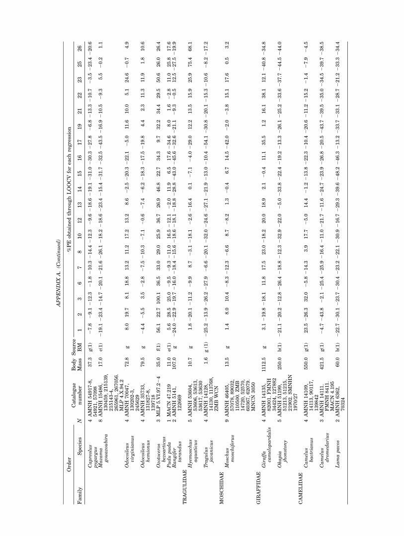
APPENDIX

A.(C

ontinued

)

Ord

er

NCatalogue

number

Bod

yMass

Sou

rce

BM

%PE

obtained

throughLOOCV

forea

chregression

Family

Species

12

36

78

10

12

13

14

15

16

17

19

21

22

23

25

26

Capreolus

pyg

argus

4AMNH

54917-8,

54921,57098

37.3

g(1)

27.8

29.1

212.3

21.8

210.3

214.4

212.3

29.6

218.6

219.1

231.0

230.3

227.8

26.8

213.3

210.7

23.5

223.4

220.6

Maza

ma

gou

azoubira

8AMNH

15486,

130459,215139,

215143-4,

265961,267056.

MLP

4.X.94.2

17.0

c(1)

219.1

223.4

214.7

220.1

221.6

226.1

218.2

218.6

223.4

215.4

231.7

232.5

243.5

216.9

210.5

29.3

5.5

20.2

1.1

Odocoileus

virginianus

4AMNH

70047,

130202-3,

245629

72.8

g8.0

19.7

8.1

18.8

13.2

11.2

17.2

13.2

8.6

22.5

220.3

222.1

25.0

11.6

10.0

5.1

24.6

20.7

4.9

Odocoileus

hem

ionus

4AMNH

35733,

131827-8,

139718

79.5

g24.4

25.5

3.5

22.8

27.5

210.3

27.1

20.6

27.4

26.2

218.3

217.5

219.8

4.4

2.3

11.3

11.9

1.8

10.6

Ozotoceros

bezoa

rticus

3MLP

5.VI.97.224

35.0

f(1)

56.1

22.7

100.1

36.5

33.0

29.0

25.9

36.7

26.9

46.8

22.7

34.3

9.7

32.2

34.4

29.5

50.6

26.0

26.4

Pudupuda

1MACN

47.219

11.0

e(1)

5.6

28.5

25.0

29.5

29.3

211

.016.5

212.1

22.0

11.9

6.5

17.6

234.6

8.0

1.6

22.8

11.0

25.8

17.6

Rangifer

tara

ndus

2AMNH

5141,

122669

107.0

g224.0

222.9

219.7

216.0

218.4

215.6

218.6

218.1

218.8

228.8

243.0

245.6

232.6

221.1

29.3

20.5

12.5

227.5

219.9

TRAGULID

AE

Hyemosch

us

aquaticu

s5

AMNH

53604,

53606,53613,

53617,53630

10.7

g1.8

220.1

211

.229.9

8.7

23.1

218.1

22.6

216.4

0.1

27.1

24.0

229.0

12.2

13.5

15.9

25.9

75.4

68.1

Tra

gulus

javanicus

4AMNH

14128,

14130,11

3768,

ZMB

WCN

1.6

g(1)

225.2

213.9

226.2

227.9

26.6

220.1

232.0

224.6

227.1

221.9

213.0

210.4

254.1

230.8

220.1

215.3

210.6

28.2

217.2

MOSCHID

AE

Mosch

us

mosch

iferus

9AMNH

46405,

57078,89032,

110500.ZMB

14720,52570,

60367,62079.

MNCN

3050

13.5

g1.4

8.0

10.4

28.3

212.3

26.6

8.7

28.2

1.3

20.4

6.7

14.5

242.0

22.0

23.8

15.1

17.6

0.5

3.2

GIR

AFFID

AE

Giraffa

camelop

ard

alis

4AMNH

14135,

82001.FMNH

34424,127882

1112.5

g3.1

219.8

218.1

11.8

17.5

23.0

218.2

20.0

18.9

2.1

20.4

11.1

35.5

1.2

16.1

38.1

12.1

240.8

234.8

Okapia

jhon

ston

y5

AMNH

511

99,

51213,51215,

21902.SMNHN

1970/27

250.0

b(1)

221.1

220.2

212.8

226.4

218.8

212.3

232.9

222.0

25.0

233.8

222.4

219.2

213.3

226.1

225.2

233.6

237.7

244.5

244.0

CAMELID

AE

Camelus

bactrianus

4AMNH

14109,

1411

3,9011

7,

139842

550.0

g(1)

23.5

226.3

32.0

25.8

214.3

3.9

17.7

25.0

14.4

21.2

213.8

222.3

210.4

220.6

211

.2215.2

21.4

27.9

24.5

Camelus

dromed

arius

3AMNH

1411

1.

FMNH

8411

.MACN

4.195

421.5

g(1)

24.7

243.8

22.1

225.4

225.9

216.4

211

.0221.7

211

.6224.7

223.9

226.8

220.5

243.7

239.5

235.0

234.5

239.7

238.5

Lamapacos

2AMNH

6362,

70324

60.0

b(1)

222.7

230.1

223.7

230.4

223.2

222.1

230.9

216.7

229.3

239.6

248.2

246.3

213.2

233.7

233.1

228.7

221.2

233.3

234.4

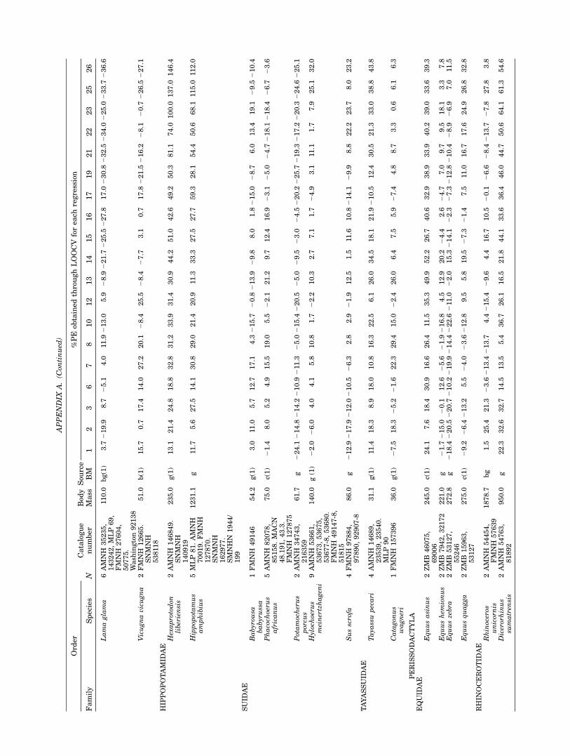
APPENDIX

A.(C

ontinued

)

Ord

er

NCatalogue

number

Bod

yMass

Sou

rce

BM

%PE

obtained

throughLOOCV

forea

chregression

Family

Species

12

36

78

10

12

13

14

15

16

17

19

21

22

23

25

26

Lamaglama

6AMNH

35235,

143242,MLP

69,

FMNH

27604,

50775.

Wash

ington92138

110.0

bg(1)

3.7

219.9

8.7

25.1

4.0

11.9

213.0

5.9

28.9

221.7

225.5

227.8

17.0

230.8

232.5

234.0

225.0

233.7

236.6

Vicugnavicugna

2FMNH

12665.

SNMNH

538118

51.0

b(1)

15.7

0.7

17.4

14.0

27.2

20.1

28.4

25.5

28.4

27.7

3.1

0.7

17.8

221.5

216.2

28.1

20.7

226.5

227.1

HIP

POPOTAMID

AE

Hexaprotodon

liberiensis

2AMNH

146849.

SNMNH

140919

235.0

g(1)

13.1

21.4

24.8

18.8

32.8

31.2

33.9

31.4

30.9

44.2

51.0

42.6

49.2

50.3

81.1

74.0

100.0

137.0

146.4

Hippop

otamus

amphibius

5MLP

81.AMNH

70019.FMNH

127870.

SNMNH

162977.

SMNHN

1944/

199

1231.1

g11

.75.6

27.5

14.1

30.8

29.0

21.4

20.9

11.3

33.3

27.5

27.7

59.3

28.1

54.4

50.6

68.1

115.0

112.0

SUID

AE

Babyrou

sababyrussa

1FMNH

49146

54.2

g(1)

3.0

11.0

5.7

12.7

17.1

4.3

215.7

20.8

213.9

29.8

8.0

1.8

215.0

28.7

6.0

13.4

19.1

29.5

210.4

Phacoch

oeru

safricanus

5AMNH

82078,

85158.MACN

48.191,43.3.

FMNH

127875

75.0

c(1)

21.4

8.0

5.2

4.9

15.5

19.0

5.5

22.1

21.2

9.7

12.4

16.9

23.1

25.0

24.7

218.1

218.4

26.7

23.6

Potamocherus

porcu

s2AMNH

34743,

216359

61.7

g224.1

214.8

214.2

210.9

211

.325.0

215.4

220.5

25.0

29.5

23.0

24.5

220.2

225.7

219.3

217.2

220.3

224.6

225.1

Hylochoeru

smeinertzhagen

i9AMNH

53661,

53673,53675,

53677-8,53680.

FMNH

49147-8,

51815

140.0

g(1)

22.0

26.0

4.0

4.1

5.8

10.8

1.7

22.2

10.3

2.7

7.1

1.7

24.9

3.1

11.1

1.7

7.9

25.1

32.0

Susscrofa

4FMNH

97884,

97890,92907-8

86.0

g212.9

217.9

212.0

210.5

26.3

2.8

2.9

21.9

12.5

1.5

11.6

10.8

214.1

29.9

8.8

22.2

23.7

8.0

23.2

TAYASSUID

AE

Taya

ssupecari

4AMNH

14689,

23539,23540.

MLP

90

31.1

g(1)

11.4

18.3

8.9

18.0

10.8

16.3

22.5

6.1

26.0

34.5

18.1

21.9

210.5

12.4

30.5

21.3

33.0

38.8

43.8

Catagon

us

wagneri

1FMNH

157396

36.0

g(1)

27.5

18.3

25.2

21.6

22.3

29.4

15.0

22.4

26.0

6.4

7.5

5.9

27.4

4.8

8.7

3.3

0.6

6.1

6.3

PERIS

SODACTYLA

EQUID

AE

Equusasinus

2ZMB

46075,

69006

245.0

c(1)

24.1

7.6

18.4

30.9

16.6

26.4

11.5

35.3

49.9

52.2

26.7

40.6

32.9

38.9

33.9

40.2

39.0

33.6

39.3

Equushem

ionus

2ZMB

7942,32172

221.0

g21.7

215.0

20.1

12.6

25.6

21.9

216.8

4.5

12.9

20.2

24.4

2.6

24.7

7.0

9.7

9.5

18.1

3.3

7.8

Equuszebra

2ZMB

53127,

55246

272.8

g218.4

220.5

220.7

210.2

219.9

214.4

222.6

211

.022.0

15.3

214.1

22.3

27.3

212.8

210.4

28.9

26.9

7.0

11.5

Equusquagga

2ZMB

15963,

53127

275.0

c(1)

29.2

26.4

213.2

5.5

24.0

23.6

212.8

9.5

5.8

19.5

27.3

21.4

7.5

11.0

16.7

17.6

24.9

26.8

32.8

RHIN

OCEROTID

AE

Rhinoceros

unicornis

2AMNH

54454,

FMNH

57639

1878.7

bg

1.5

25.4

21.3

23.6

213.4

213.7

4.4

215.4

29.6

4.4

16.7

10.5

20.1

26.6

28.4

213.7

27.8

27.8

3.8

Dicerorhinus

sumatren

sis

2AMNH

54763,

81892

950.0

g22.3

32.6

32.7

14.5

13.5

5.4

36.7

26.1

16.5

21.8

44.1

33.6

36.4

46.0

44.7

50.6

64.1

61.3

54.6

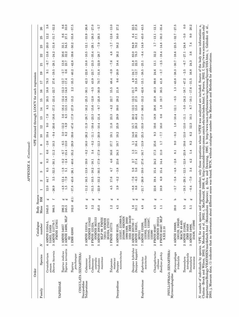
APPENDIX

A.(C

ontinued

)

Ord

er

NCatalogue

number

Bod

yMass

Sou

rce

BM

%PE

obtained

throughLOOCV

forea

chregression

Family

Species

12

36

78

10

12

13

14

15

16

17

19

21

22

23

25

26

Ceratotherium

simum

4AMNH

51854-5,

51855,51859

1845.0

g12.0

44.7

6.5

8.3

6.6

22.6

19.4

9.0

27.8

8.5

20.5

18.8

78.3

9.1

26.7

215.6

220.0

12.2

3.8

Diceros

bicornis

3AMNH

113776-7.

FMNH

127851

986.5

f226.9

3.5

232.3

230.1

211

.2210.3

29.4

220.6

218.6

237.3

223.4

222.7

27.6

219.5

228.1

224.2

231.8

231.7

232.2

TAPIR

IDAE

Tapirusindicus

1AMNH

54657

296.2

g24.8

212.4

21.8

20.2

26.7

26.5

3.0

212.2

3.6

218.4

212.4

212.3

212.7

22.7

13.8

20.6

33.1

8.6

8.6

Tapirusterrestris

2AMNH

14690,MLP

82

245.5

g1.5

27.9

5.1

22.4

215.4

213.0

6.2

28.9

6.5

213.5

214.8

214.0

217.4

0.6

23.7

32.2

54.5

27.1

33.0

Tapirus

pinch

anque

1ZMB

62085

182.0

d(1)

237.8

245.6

226.1

240.6

235.2

229.9

239.6

247.6

217.9

227.9

215.2

2.2

235.3

240.2

242.8

239.6

250.2

255.8

257.5

CIN

GULATA

(XENARTHRA)

Dasypod

idae

Tolypeu

tinae

Cabassou

sunicinctus

2AMNH

133314,

SNMNH

113422

4.0

g211

.2216.5

213.8

219.0

20.2

216.0

226.2

211

.9228.7

216.2

225.3

230.1

42.3

222.8

210.8

210.5

212.1

233.9

226.8

Cabassou

scentralis

2FMNH

121224,

SNMNH

363153

3.2

g231.5

210.5

218.2

218.1

3.4

20.2

211

.1219.4

223.3

215.6

212.8

20.5

43.9

223.7

223.3

235.4

229.1

228.3

227.0

Priod

ontes

maximus

5AMNH

208104.

MLP

89.FMNH

72913.SNMNH

261024,270373

45.0

g222.9

233.2

230.5

217.9

217.9

212.3

220.9

210.4

221.4

29.7

225.8

230.9

70.7

231.8

222.9

228.7

27.9

229.3

25.7

Tolyp

eutes

matacu

s1FMNH

153773

1.2

g4.5

17.6

4.7

4.6

16.6

37.7

19.1

11.8

23.3

24.2

22.7

15.5

48.4

20.9

27.6

4.8

21.7

212.6

213.0

Dasypod

inae

Dasypus

nov

emcinctus

8AMNH

95128,

133357,211

668-9,

255868.SMNHN

1999/1069,2000/

1050.ZMB

24439

4.5

a3.9

20.2

23.8

23.6

24.3

19.7

19.2

25.9

29.9

39.0

29.2

21.8

9.6

220.9

18.4

26.2

58.2

16.0

27.2

Dasypushyb

ridus

2AMNH

20570627

1.6

g28.8

27.6

5.8

2.7

1.3

1.1

14.6

15.7

20.2

212.5

212.5

221.7

4.9

224.7

31.8

83.0

84.9

6.4

22.5

Dasypuskappleri

2AMNH

136251,

267011

10.1

g8.6

26.3

5.6

17.4

3.7

16.4

39.1

28.3

40.4

15.0

27.5

9.9

15.8

212.7

22.3

78.3

78.2

17.1

37.8

Euphractinae

Euphra

ctus

sexcinctus

7AMNH

133288,

133302,133306,

133345,133387,

133390

4.8

g221.7

226.9

219.0

227.6

216.7

213.9

225.3

233.9

217.0

236.0

233.2

242.6

215.1

238.5

225.1

28.4

214.9

245.0

243.5

Chaetop

hra

ctus

villosu

s2FMNH

60467.

SNMNH

391014

4.5

g22.6

19.4

15.4

24.2

17.3

25.6

9.3

19.6

18.9

28.6

25.8

40.3

89.8

24.6

13.1

32.2

1.7

213.1

212.1

Zaed

yuspichiy

2FMNH

60467.MLP

9.XII.2.10

1.1

i18.9

6.9

15.4

14.4

11.0

1.7

27.7

16.0

0.6

1.8

19.7

30.5

41.8

23.7

22.5

218.4

214.8

230.3

235.4

PHYLLOPHAGA

(XENARTHRA)

Myrm

ecop

hagidaeMyrmecop

haga

tridactyla

4AMNH

100068,

100139,136249.

MACN

49.405

39.0

b23.7

25.8

24.8

22.8

8.1

9.0

20.3

1.8

210.4

212.1

20.5

1.3

243.8

238.3

230.7

218.6

223.5

232.7

227.5

Tamandura

tetradactyla

2AMNH

211

662,

ZMB

16458

5.5

g219.3

229.3

212.5

212.8

223.8

219.6

213.0

213.0

211

.125.0

224.2

218.7

247.2

22.5

26.7

227.1

224.8

25.0

0.0

Tamandura

mexicana

3AMNH

14866,

23436,172986

5.1

g20.4

27.0

3.4

4.2

1.4

8.2

6.2

12.3

10.1

8.7

210.1

217.6

231.5

16.8

24.3

3.6

7.4

9.0

20.2

N:number

ofindividuals

bysp

ecies.

%PE:forea

chsp

eciesandregressionnumber,on

lythoseeq

uation

swhose%PEH

wasanalyzedare

included

.Sou

rceof

thebod

ymass

inform

ation

:a,

Clutton

2Brock

andWilson,2002;b,Men

dozaet

al.,2002;c,

MacD

onald,2006;d,http://anim

aldiversity.ummz.umich.edu/site/index

.htm

l;e,

Parera,2002;f,http://w

ww.scien

ce.smith.edu/

dep

artmen

ts/Biology/VHAYSSEN/m

si/default.htm

l(M

ammalian

Species);g,Silva

and

Dow

ning,1995;h:http://w

ww.iucn

.org/them

es/ssc/sgs/nea

asg/layou

t/1024.htm

;i,

Galındez

etal.,

2003;j,Museum

data;(1)indicatesthatnoinform

ation

abou

tdifferentsexes

wasfound;WCN,withou

tcataloguenumber.See

Materials

andMethod

sforabbreviation

s.

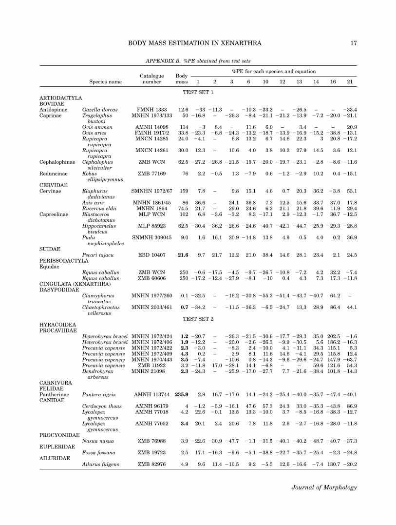
APPENDIX B. %PE obtained from test sets

Species nameCataloguenumber

Bodymass

%PE for each species and equation

1 2 3 6 10 12 13 14 16 21

TEST SET 1ARTIODACTYLABOVIDAEAntilopinae Gazella dorcas FMNH 1333 12.6 233 211.3 – 210.3 233.3 – 226.5 – – 233.4Caprinae Tragelaphus

buxtoniMNHN 1973/133 50 216.8 – 226.3 28.4 221.1 221.2 213.9 27.2 220.0 221.1

Ovis ammon AMNH 14098 114 23 8.4 2 11.6 6.0 – 3.4 – – 20.9Ovis aries FMNH 1917/2 33.8 223.3 26.8 224.3 213.2 218.7 213.9 216.9 215.2 238.8 213.1Rupicapra

rupicapraMNCN 14285 24.0 24.1 – 6.8 13.2 6.7 14.6 22.3 3 20.8 217.2

Rupicaprarupicapra

MNCN 14261 30.0 12.3 – 10.6 4.0 3.8 10.2 27.9 14.5 3.6 12.1

Cephalophinae Cephalophussilvicultor

ZMB WCN 62.5 227.2 226.8 221.5 215.7 220.0 219.7 223.1 22.8 28.6 211.6

Reduncinae Kobusellipsiprymnus

ZMB 77169 76 2.2 20.5 1.3 27.9 0.6 21.2 22.9 10.2 0.4 215.1

CERVIDAECervinae Elaphurus

dadivianusSMNHN 1972/67 159 7.8 – 9.8 15.1 4.6 0.7 20.3 36.2 23.8 53.1

Axis axis MNHN 1861/45 86 36.6 – 24.1 36.8 7.2 12.5 15.6 33.7 37.0 17.8Rucervus eldii MNHN 1864 74.5 21.7 – 29.0 24.6 6.3 21.1 21.8 39.6 11.9 29.4

Capreolinae Blastocerosdichotomus

MLP WCN 102 6.8 23.6 23.2 8.3 217.1 2.9 212.3 21.7 36.7 212.5

Hippocamelusbisulcus

MLP 85923 62.5 230.4 236.2 226.6 224.6 240.7 242.1 244.7 225.9 229.3 228.8

Pudumephistopheles

SNMNH 309045 9.0 1.6 16.1 20.9 214.8 13.8 4.9 0.5 4.0 0.2 36.9

SUIDAEPecari tajacu EBD 10407 21.6 9.7 21.7 12.2 21.0 38.4 14.6 28.1 23.4 2.1 24.5

PERISSODACTYLAEquidae

Equus caballus ZMB WCN 250 20.6 217.5 24.5 29.7 226.7 210.8 27.2 4.2 32.2 27.4Equus caballus ZMB 60606 250 217.2 212.4 227.9 28.1 210 0.4 4.3 7.3 17.3 211.8

CINGULATA (XENARTHRA)DASYPODIDAE

Clamyphorustruncatus

MNHN 1977/260 0.1 232.5 – 216.2 230.8 255.3 251.4 243.7 240.7 64.2 –

Chaetophractusvellerosus

MNHN 2003/461 0.7 234.2 – 211.5 236.3 26.5 224,7 13,3 28.9 86.4 44.1

TEST SET 2HYRACOIDEAPROCAVIIDAE

Heterohyrax brucei MNHN 1972/424 1.2 220.7 – 226.3 221.5 230.6 217.7 229.3 35.0 202.5 21.6Heterohyrax brucei MNHN 1972/406 1.9 212.2 – 220.0 22.6 226.3 29.9 230.5 5.6 186.2 216.3Procavia capensis MNHN 1972/422 2.3 23.0 – 28.3 2.4 210.0 4.1 211.1 34.3 115.1 5.3Procavia capensis MNHN 1972/409 4.3 0.2 – 2.9 8.1 11.6 14.6 24.1 29.5 115.8 12.4Procavia capensis MNHN 1970/443 3.5 27.4 – 210.6 0.8 214.3 29.6 229.6 224.7 147.9 263.7Procavia capensis ZMB 11922 3.2 211.8 17.0 228.1 14.1 26.8 – – 59.6 121.6 54.3Dendrohyrax

arboreusMNHN 21098 2.3 224.3 – 225.9 217.0 227.7 7.7 221.6 238.4 101.8 214.3

CARNIVORAFELIDAEPantherinae Pantera tigris AMNH 113744 235.9 2.9 16.7 217.0 14.1 224.2 225.4 240.0 235.7 247.4 240.1CANIDAE

Cerdocyon thous AMNH 96179 4 21.2 25.9 216.1 47.6 57.3 24.3 33.0 235.3 243.8 86.9Lycalopex

gymnocercusAMNH 77018 4.2 22.6 20.1 13.5 13.3 210.0 3.7 28.5 216.8 238.3 212.7

Lycalopexgymnocercus

AMNH 77052 3.4 20.1 2.4 20.6 7.8 11.8 2.6 22.7 216.8 228.0 211.8

PROCYONIDAENasua nasua ZMB 76988 3.9 222.6 230.9 247.7 21.1 231.5 240.1 240.2 248.7 240.7 237.3

EUPLERIDAEFossa fossana ZMB 19723 2.5 17.1 216.3 29.6 25.1 238.8 222.7 235.7 225.4 22.3 224.8

AILURIDAEAilurus fulgens ZMB 82976 4.9 9.6 11.4 210.5 9.2 25.5 12.6 216.6 27.4 130.7 220.2

BODY MASS ESTIMATION IN XENARTHRA 17

Journal of Morphology

APPENDIX B. (Continued)

Species nameCataloguenumber

Bodymass

%PE for each species and equation

1 2 3 6 10 12 13 14 16 21

RODENTIAHYDROCHOERINAE

Hydrochoerushydrochaeris

ZMB 81299 53 18 222.6 29.5 8.0 26.2 29.0 9.0 22.9 39.1 19.5

TUBULIDENTATAORYCTEROPODIDAE

Orycteropus afer ZMB 84695 66.5 5.1 235.5 219.1 30.2 242.9 216.0 237.8 26.8 213.8 238.8

The body mass values in bold are weight data of the specimen, not from literature. See Materials and Methods for abbreviations.WCN, without catalogue number. When a species was represented by more than one specimen, the mean value for this species wasused in the statistical analysis.

APPENDIX C. Equations obtained through the stepwise procedure. Regressions number 1, 2, 3, 6, and 12 are shown in the results

Regression number Predictive function Adjusted R2 Mean %PE (LOOCV) RE

4 1.986T2 1 0.873H8 – 6.466 0.989 16.5 1.05135 1.910F5 1 0,837R2 2 6.042 0.988 16.5 1.03677 0.621R5 1 0.982F2 1 1.974H1 2 0.59R1 2 9.317 0.993 16.1 0.98618 0.92F1 1 1.724H1 2 0.627R1 1 0.883H2 2 8.842 0.993 16.4 0.97709 1.07H7 1 0.872R3 1 0.742F8 2 4.172 0.987 17.9 1.0803

10 0.857F8 1 0.564H5 1 1.387H2 2 4.993 0.991 15.6 1.036511 0.828R4 1 0.448H51 0.536F3 1 1.487H1 2 0.456R1 27.555 0.992 15.1 1.013813 1.719H2 1 0.521H5 1 1.243F1 20.554R1 27.315 0.992 14.6 1.020314 0.854R3 1 1.02S3 – 0.431H6 1 0.647H5 1 0.753F1 2 6.447 0.989 16.7 1.037115 0.681S2 1 0.836T5 1 1.344S3 20.420H6 1 0.515F6 2 5.331 0.987 18.8 1.040916 1.698S3 1 0.945T5 1 0.736F6 20.344H6 2 5.392 0.986 18.8 1.030117 2.162H1 1 0.932H5 2 9.866 0.958 24.9 1.105718 1.481T5 1 1.341F3 2 5.716 0.977 19.8 1.083919 0.722R7 1 0.844H5 1 1.47F1 2 8.147 0.984 15.7 1.097420 0.993F3 1 1.11H5 1 0.991R6 2 0.379H6 2 4.479 0.986 15.9 0.972921 1.12F1 1 0.721R6 1 1.067H5 2 7.050 0.984 16.6 1.037022 0.582F6 1 1.204R6 1 1.024H5 2 3.707 0.982 19.0 1.016323 1.456R6 1 1.199H5 2 3.545 0.980 21.2 1.002224 1.609T4 1 1.277H3 2 8.667 0.932 19.8 1.056625 1.709U1 1 1.260H5 2 8.667 0.967 25.3 1.092526 1.324R1 1 1.567H5 2 7.028 0.968 25.6 1.056227 2.411S4 1 0.848H5 2 9.840 0.932 34.8 1.307028 1.537H6 1 1.198H5 2 4.223 0.889 50.9 1.2332

18 S. DE ESTEBAN-TRIVIGNO ET AL.

Journal of Morphology