Bituminous Overlay Design
57
Bituminous Overlay Design Dr. M. A. Farooqi Associate Professor, Department of Civil Engineering, AMU
-
Upload
khangminh22 -
Category
Documents
-
view
4 -
download
0
Transcript of Bituminous Overlay Design

Bituminous Overlay Design
Dr. M. A. Farooqi Associate Professor, Department of
Civil Engineering, AMU

Types of Overlays
• Asphalt overlay over asphalt pavements • Asphalt overlays on CC pavements • CC overlays on asphalt pavements • CC overlays on CC pavements

Deflection Approach
• Performance of flexible pavements is related to the elastic deflection of pavement.
• The structural strength of pavement is assessed by measuring surface deflections under a standard axle load.
• Larger pavement deflections imply weaker pavement and subgrade.
• The overlay must be thick enough to reduce the deflection to a tolerable amount.
• Rebound deflections are measured with the help of a Benkelman Beam.

…Deflection Approach
• The structural strength of pavement is assessed by measuring surface deflections under a standard axle load
• Larger pavement deflections imply weaker pavement and subgrade
• The overlay must be thick enough to reduce the deflection to a tolerable amount
• Rebound deflections are measured with the help of a Benkelman Beam

Factors Affecting Elastic Deflection
• Subgrade soil type, • Its moisture content and compaction, • The thickness and quality of the pavement
courses, • Drainage conditions, • Pavement surface temperature etc.

Overview
• Benkelman Beam Works by suitably placing its probe on the pavement between the dual wheels of a loaded truck and measuring deflections to compute: – Rebound, and – Residual deflections of the pavement structure.
• The Rebound deflection is the one related to pavement performance. It is used for the overlay design.
• The Residual deflection may be due to non-recoverable deflection of the pavement or because of the influence of the deflection bowl on the front legs of the beam.

Deflection Survey: Procedure
• The deflection survey essentially consists of two operations: – Condition survey for collecting the basic
information of the road structure, – Grouping of the pavement into sections based on
its condition – Actual measurements of deflection.

Deflection Survey: Procedure
• The condition survey primarily consists of visual observations, pot-holes, cracks, and simple measurements of rut-depth using a 3 meter straight edge.
• Based on the condition, the road lengths shall
be classified in accordance with the criteria:

Criteria for Classification of Pavement Sections
Classification Condition
Good No cracking, rutting less than 10 mm
Fair No cracking or cracking confined to single crack in the wheel track with rutting between 10 mm and 20 mm
Poor Extensive cracking and/or rutting greater than 20 mm. Sections with cracking exceeding 20 percent shall be treated as failed.

Deflection Measurements
• In each road section of uniform performance minimum of ten points should be marked at equal distance in each lane of traffic for making the deflection observations in the outer wheel path.
• The interval between the points should not be more than 50m.
• On roads with more than one lane, the points marked on adjacent lanes should be staggered.
Deflection Measurement Point • In the transverse
direction, the measurement points should be:
• 60cm from the pavement edge if the lane width < 3.5m and
• 90cm when the lane width > 3.5m.
• For divided four lane highway, the measurement points should be 1.5 m from the pavement edge.

Measurements and Corrections

Measurements and Corrections
• For Temperature Variation – Deflection measurements are affected by the
temperature variations (Standard Temperature= 35°C)
• For Moisture Correction for Seasonal Variation (Based on Soil Type and Rainfall) – Pavement deflections are affected by climatic
conditions.

Temperature Measurement
• The pavement temperature should be measured during the deflection survey.
• The measurement should be made at a depth of 40mm using a suitable short-stem mercury or a digital contact thermometer.
• A hole of about 45mm deep and about 10mm diameter should be drilled in the pavement and filled with glycerol and temperature can then be recorded after about 5 minutes.

Temperature Correction • Deflection is affected by pavement temperature. • The Standard Temperature is assumed to be 35°C. • The deflection should be 0.01mm for each degree
centigrade change from the standard temperature of 35°C. • The correction will be
– Positive for pavement temperature < 35°C, and – Negative for pavement temperature > 35°C.
• For example, if the deflection is measured at a pavement temperature of 38°C, the correction factor will be 0.03 mm (=3 x .01) which should be subtracted from the measured deflection to obtain the corrected value corresponding to standard pavement temperature of 35°C.

Temperature Correction
• In colder areas, and areas of altitude greater than 1000m where the average day temperature is less than 20°C for more than 4 months in a year, the standard temperature of 35°C will not apply.
• In the absence of adequate data about deflection performance relationship, it is recommended that: – The deflection measurements be done at
temperatures >20°C – No temp correction is applied.

Seasonal Correction • Pavement deflections also depend on climatic conditions. • It is desirable to take deflection measurements during the
season when the pavement is in its weakest condition (Like, after monsoon).
• When deflections are measured during the dry months, they will require a correction factor which is defined as the ratio of the maximum deflection immediately after monsoon to that of the minimum deflection in the dry months.
• Correction for seasonal variation shall depend on: – Type of subgrade soil, – Its field moisture content (at the time of deflection survey), and – Average annual rainfall in the area.
Seasonal Correction • For this purpose, subgrade soils have been divided into
three broad categories: – Sandy/gravelly, – Clayey with low plasticity (PI < 15) – Clayey with high plasticity (PI > 15)
• Similarly, rainfall has been divided into two categories: – Low rainfall (annual rainfall < 1300 mm), and – High rainfall (annual rainfall >1300 mm).
• Moisture correction factors (or seasonal correction factors) shall be obtained from Figs. 2 to 7 for given field moisture content, type of subgrade soil and annual rainfall.
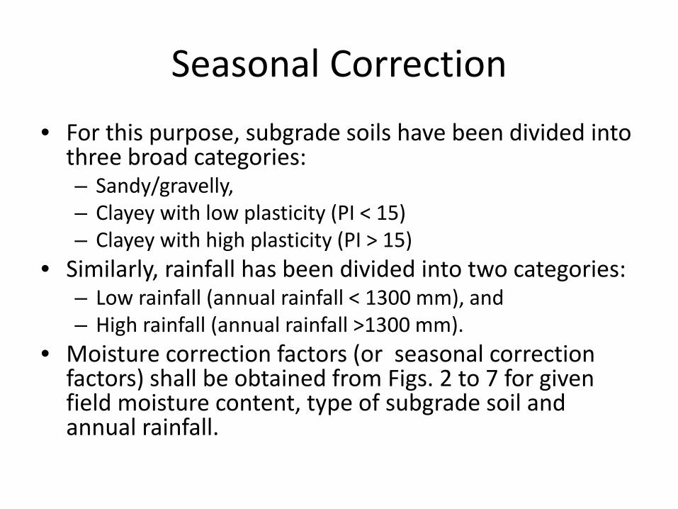
Moisture Content Determination
• The subgrade soil shall be tested for the type of subgrade soil, plasticity index and field moisture content.
• A soil sample weighing about 100g should be collected using an auger from the subgrade underneath the deflection observation points at a depth of 5cm to 10cm below the subgrade level as shown in Figure.
• The soil sample shall be scooped from below the pavement as shown in Figure. • For this purpose a test pit at the shoulder adjacent to pavement edge shall be dug to a
depth up to 15cm below the subgrade level
• The test pit shall repaired immediately after taking soil sample and study of pavement composition.

Moisture Correction Factor for Sandy / Gravelly soil subgrade (For LOW and HIGH rainfall

Moisture Correction Factor for Clayey Subgrade with LOW plasticity (For LOW and HIGH rainfall

Moisture Correction Factor for Clayey Subgrade with HIGH plasticity (For LOW and HIGH rainfall

Benkelman Beam

Benkelman Beam: Introduction
• Benkelman beam is a simple apparatus to conduct structural evaluation of pavement.
• It does so by measuring the deflection of pavement under standard loading conditions
• Following points on the beam are to be understood: Probe point (or Arm Tip), Pivot and dial gauge point.
• From Probe Point to Pivot it is 2.44m and from hinge to dial gauge point it is 1.22m. So the total usable length is 3.66m

Benkelman Beam: Diagram

Benkelman Beam: Diagram

Rebound Deflection

Equipment • In Benkelman beam test, the rebound deflection of pavement is measured
under static load of the rear axle of a standard truck (Axle load : 8170kg). • The equipment shall include: • Benkelman Beam
– (a) Length of probe arm from pivot to probe point: 2.44 m – (b) Length of measurement arm from pivot to dial gauge: 1.22 m
• A 5 tonne truck is recommended as the reaction. The vehicle shall have 8170 kg rear axle load equally distributed over the two wheels, equipped with dual tyres.
• Spacing between the tyre walls should be 30-40 mm. The tyres shall be 10 x 20, 12 ply inflated to a pressure of 5.60 kg/cm. The use of tyres with tubes and rib treads is recommended.
Equipment
• Tyre pressure measuring gauge • Thermometer (0-100°C) with 1° division • A mandrel for making 4.5 cm deep hole in the
pavement for temperature measurement. The diameter of the hole at the surface shall be 1.25 cm and at bottom 1 cm.

Procedure • The point on the pavement to be tested is
selected and marked. – For highways, the point should be located 60 cm
from the pavement edge if the lane width is less than 3.5 m and 90 cm from the pavement edge for wider lanes.
– For divided four lane highway, the measurement points should be 1.5 m from the pavement edge.
• The dual wheels of the truck are centered above the selected point.
• The probe of the Benkelman beam is inserted between the duals tyres (as shown in Figure) to place on the selected point. • The locking pin is removed from the beam and the legs are adjusted so that the plunger of the beam is in contact with the stem of the dial gauge. The beam pivot arms are checked for free movement.

Procedure
• The dial gauge is set at approximately 1 cm. The initial reading is recorded*.
• The truck is slowly driven by 2.70m and an intermediate reading is recorded*.
• The truck is further driven by 9 m (from 2.7m point) to record the final reading*.
*All readings are to be recorded when the rate of recovery of pavement is equal to or less than 0.025 mm per minute

Deflection Readings

Procedure
• Pavement temperature is recorded atleast once every hour inserting thermometer in the standard hole and filling up the hole with glycerol.
• The tyre pressure is checked at two or three hour intervals during the day and adjusted to the standard, if necessary.

Calculations

Computation of Rebound Deflection
The rebound deflection D is computed by one of the two following conditions: 1. If (𝐷𝑖 − 𝐷𝑓) ≤ 2.5 divisions, of the dial gauge or
0.025mm: i. 𝐷 = 2(𝐷𝑜 − 𝐷𝑓) divisions or ii. 𝐷 = 0.02(𝐷𝑜 − 𝐷𝑓)mm
2. If (𝐷𝑖 − 𝐷𝑓) ≥ 2.5 divisions: i. 𝐷 = 2 𝐷𝑜 − 𝐷𝑓 + 2𝐾(𝐷𝑖 − 𝐷𝑓) divisions
The value of K for Benkelman beams available in Indian is calculated to be 2.91, hence:
– 𝐷 = 0.02 𝐷𝑜 − 𝐷𝑓 + 0.0582(𝐷𝑖 − 𝐷𝑓)mm

Overlay Thickness Chart

Equivalency Factor • The thickness deduced from Fig is the overlay thickness in terms of
bituminous macadam construction. • In case other compositions are to be laid for strengthening, the equivalent
overlay thickness to be provided may be determined using appropriate equivalency factors as suggested below: – 1 cm of Bituminous macadam = 1 .5 cm of WBM/WMM/BUSG* – 1 cm of Bituminous macadam = 0.7 cm of DBM/AC/SDC
• From structural considerations, the recommended minimum bituminous overlay thickness is 50 mm Bituminous Macadam(BM) + an additional surfacing course of 50mm DBM or 40 mm Bituminous Concrete (BC). BUSG: Built-up Spray Grout WBM: Water Bound Macadam WMM: Wet Mix Macadam DBM: Dense Bituminous Macadam AC: Asphalt Concrete

Problem 1 • Deflection values:
1.40,1.32,1.25,1.35,1.48,1.60,1.65,1.55,1.45,1.40,1.36,1.46,1.5,1.52,1.45 mm
• Pavement Temperature = 30°C • Subgrade moisture content = 8%, clayey soil, PI>15 • Average annual rainfall = 1500 mm • Design traffic = 15.5 msa
– Two lane single carriageway – ADT of Trucks = 1000 – Annual growth rate = 5% – VDF = 4.5

…Problem 1
• Mean deflection = 1.45 mm • Standard Deviation = 0.107 mm • Characteristic deflection = 1.45 + 2(0.107) = 1.664 mm • Correction for temperature = 0.01(35-30) = 0.05 mm • Characteristic deflection after temp. correction
= 1.664 + 0.05 = 1.714 mm • Seasonal correction factor = 1.4 • Corrected characteristic deflection = 1.4 (1.714)=
2.3996 mm

…Problem 1
• Thickness of overlay in terms of BM from the chart = 190 mm
• Thickness in terms of DBM/AC = 190*0.7 = 133 mm
• Provide 40 mm AC and 95 mm DBM

Problem-2 Design the overlay required for the pavement which is on a National Highway using the following data: Given: • Subgrade: Sandy Soil • Moisture Content: 8% • Pavement Temperature=35° • Annual Rainfall: <1300mm • CVPD: 5000 • Design Period: 10years • Traffic Growth Rate: 7% • VDF: 4.5

Deflection Data S. No D0 Di Df Di-Df Do-Df D
1 100 52 50 2 50 1.00
2 100 55 53 2 47 0.94
3 100 53 52 1 48 0.96
4 100 52 52 0 48 0.96
5 100 53 51 2 49 0.98
6 100 55 53 2 47 0.94
7 100 55 53 2 47 0.94
8 100 57 56 1 44 0.88
9 100 59 58 1 42 0.84
10 100 49 47 2 53 1.06
11 100 54 52 2 48 0.96
Mean StDev De Moisture Corr Temp Corr
0.95 0.056 1.06 1.03 0

…Problem-2
𝑁 =365 × 1 + 0.07 10 − 1 × 5000 × 0.75 × 4.5
0.07
𝑁 = 85.1 msa

Calculations • Characteristic Deflection, 𝐷𝑎 = 0.95mm • Standard Deviation, 𝜎 = 0.056mm • Characteristic Deflection,𝐷𝑐 = 0.95 + 2 × 0.056 = 1.06mm • Correction Factor for Temp = 0.01mm/°C rise
– +ve for temp higher than 35 – -ve for temp. lower than 35
• Since Temp=35°C, so no correction. • Referring to Chart for Sandy Soil, Low Rainfall, correction factor is:
1.03 • Corrected Deflection =1.06 x 1.03 = 1.09mm • So For 85.1msa and Characteristic Deflection of 1.09, the overlay
thickness from the Chart is: 160mm BM • So, We can provide: 100mm BM + 45mm BC

Pavement Condition Survey
• Visual inspection of the road stretch and grouping into sub-stretches • Assessment of pavement cracking – type & percentage cracked area • Rut depth measurements • Observations on other types of pavement • deterioration

Loading and other standards
• Axle load of 8170 kg / load of 4085 kg on dual wheels
• Tire pressure, p = 5.6 kg / sqcm • Standard pavement temperature = 35°C • Highest subgrade moisture content soon after
monsoon • Some precautions during rebound deflection
observations – very low or zero values – variation of individual values, not more than one
third of mean value

Benkelman Beam Probe

Overlay Design Steps: IRC
• Design curves relating characteristic pavement deflection to the cumulative number of standard axles are to be used.
• The Deflection of the pavement after the corrections i.e., Characteristic Deflection is to be used for the design purposes.
• The design traffic in terms of cumulative standard number of axles is to be used.

Overlay Design Steps: IRC
• The thickness obtained from the curves is in terms of Bituminous Macadam construction.
• If other compositions are to be laid then 1 cm of Bituminous Macadam = 1.5 cm of WBM/Wet Mix Macadam/BUSG
• 1 cm of Bituminous Macadam = 0.7 cm of DBM/AC/SDBC

Material For Overlay • The type of material for overlay depends on factors
such as – Importance of the road – Design Traffic – Thickness and condition of the existing pavement
• Construction convenience • Economics • Before implementing the overlay, the existing surface is
to be corrected and brought to proper profile by filling pot holes, ruts and undulations
• No part of the overlay thickness shall be used for the correction of surface irregularities.

Traffic Volume
• Traffic in terms of million standard axle shall be considered for the design of overlay.
• Cumulative standard axles may be worked out, if sufficient data of the following parameters is available: – Wheel load – Distribution of commercial vehicles – Vehicle damage factor and their transverse
placement, • otherwise design traffic may be calculated as per
the procedure given in IRC-37.

Type of Traffic Considered
• For the purpose of design, only the number of commercial vehicles of laden weight of 3 tons or more and their axle loads are considered.
• The traffic is considered in both directions in the case of two lane road, and in the direction of heavier traffic in the case of multi lane divided highways.
• To obtain a realistic estimate of design traffic existing traffic, possible changes in road network and land use of the area, the probable growth of traffic and design life should be considered.

Traffic Census
• Estimate of the initial daily average traffic flow for any road should normally be based on 7-day 24-hours classified traffic counts.
• However, in exceptional cases where this information is not available, 3-day count could be used (IRC:81-1997).

Traffic Design Traffic growth rate • An estimate of likely growth rate can be obtained as follows:
– By studying the past trend in traffic growth. – Elasticity of transport demand. – If adequate data is not available, it is recommended that an average
value of 7.5 per cent may be adopted for roads in rural routes.
Design life • It is recommended that the design life for strengthening of major
roads should be atleast 10 years. • Less important roads may, however, be designed for a shorter
design period but not less than 5 years in any case.

Traffic Design Computation of design traffic • The design traffic is considered in terms of the
cumulative number of standard axles to be carried during the design life of the road.
• Its computation involves estimates of the initial volume of commercial vehicles per day, lateral distribution of traffic, the growth rate, the design life in years and the vehicle damage factor (number of standard axle per commercial vehicle)
• To convert commercial vehicles to standard axles, the following equation may be used to make the required calculation

Traffic Design Distribution of commercial traffic over the carriageway • A realistic assessment of distribution of commercial traffic by direction and by lane is necessary as it directly
affects the total equivalent standard axle load applications used in the design. • It is recommended that for the time being the following distribution may be assumed for design until more
reliable data on placement of commercial vehicles on the carriageway lanes are available. • If in a particular situation a better estimate of the distribution of traffic between the carriageway lanes is available
from traffic survey, the same should be adopted and the design is based on the traffic in the most heavily trafficked lane. The design will normally be applied over the whole carriageway width.
– (i) Single-lane roads (3.75 m width) The traffic tends to be more channelized on single lane roads than on two lane roads and to allow for this concentration of wheel load repetitions, the design should be based on the total number of commercial vehicles per day in both directions multiplied by two.
– (ii) Two-lane single carriageway roads: The design should be based on 75 per cent of the total number of commercial vehicles in both directions.
– (iii) Four-lane single carriageway roads: The design should be based on 40 per cent of the total number of commercial vehicles in both directions.
– (iv) Dual carriageway roads: The design of dual two lane carriageway roads should be based on 75 per cent of the number of commercial vehicles in each direction. The distribution factor shall be reduced by 20 percent for each additional lane.
– Ex: For dual three-lane carriageway distribution factor- 60 per cent • The traffic in each direction may be assumed to be half the sum in both directions when the latter only is known.
Where significant difference between the two streams can occur, the condition in the more heavily trafficked lane should be considered for design.
• However, if on a particular situation a better estimate of the distribution of traffic between the carriageway lanes is available from traffic survey, the same should be adopted and the design is based on the traffic in the most heavily traffic lane. The design will normally be applied over the whole carriageway width.
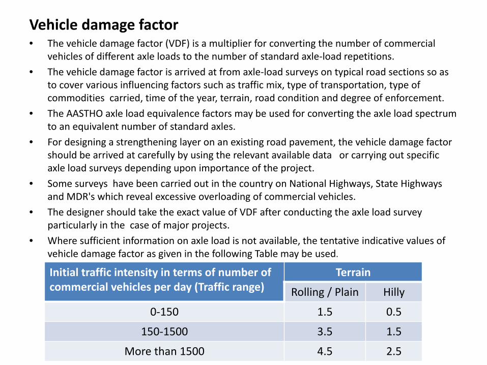
Vehicle damage factor • The vehicle damage factor (VDF) is a multiplier for converting the number of commercial
vehicles of different axle loads to the number of standard axle-load repetitions. • The vehicle damage factor is arrived at from axle-load surveys on typical road sections so as
to cover various influencing factors such as traffic mix, type of transportation, type of commodities carried, time of the year, terrain, road condition and degree of enforcement.
• The AASTHO axle load equivalence factors may be used for converting the axle load spectrum to an equivalent number of standard axles.
• For designing a strengthening layer on an existing road pavement, the vehicle damage factor should be arrived at carefully by using the relevant available data or carrying out specific axle load surveys depending upon importance of the project.
• Some surveys have been carried out in the country on National Highways, State Highways and MDR's which reveal excessive overloading of commercial vehicles.
• The designer should take the exact value of VDF after conducting the axle load survey particularly in the case of major projects.
• Where sufficient information on axle load is not available, the tentative indicative values of vehicle damage factor as given in the following Table may be used.
Initial traffic intensity in terms of number of commercial vehicles per day (Traffic range)
Terrain
Rolling / Plain Hilly
0-150 1.5 0.5
150-1500 3.5 1.5
More than 1500 4.5 2.5