Bistability in the Chemical Master Equation for Dual Phosphorylation Cycles

Armando Bazzani, Gastone C. Castellani,∗ Enrico Giampieri, and Daniel RemondiniPhysics Dept. of Bologna University and INFN Bologna

Leon N CooperInstitute for Brain and Neural Systems,Department of Physics, Brown University, Providence, RI 02912

(Dated: October 21, 2011)

Dual phospho/dephosphorylation cycles, as well as covalent enzymatic-catalyzed modificationsof substrates are widely diffused within cellular systems and are crucial for the control of complexresponses such as learning, memory and cellular fate determination. Despite the large body of deter-ministic studies and the increasing work aimed at elucidating the effect of noise in such systems, someaspects remain unclear. Here we study the stationary distribution provided by the two-dimensionalChemical Master Equation for a well-known model of a two step phospho/dephosphorylation cycleusing the quasi-steady state approximation of enzymatic kinetics. Our aim is to analyze the role offluctuations and the molecules distribution properties in the transition to a bistable regime. Whendetailed balance conditions are satisfied it is possible to compute equilibrium distributions in a closedand explicit form. When detailed balance is not satisfied, the stationary non-equilibrium state isstrongly influenced by the chemical fluxes. In the last case, we show how the external field derivedfrom the generation and recombination transition rates, can be decomposed by the Helmholtz theo-rem, into a conservative and a rotational (irreversible) part. Moreover, this decomposition, allows tocompute the stationary distribution via a perturbative approach. For a finite number of moleculesthere exists diffusion dynamics in a macroscopic region of the state space where a relevant transitionrate between the two critical points is observed. Further, the stationary distribution function canbe approximated by the solution of a Fokker-Planck equation. We illustrate the theoretical resultsusing several numerical simulations.

I. INTRODUCTION

One of the most important aspects of biological sys-tems is their capacity to learn and memorize patternsand to adapt themselves to exogenous and endogenousstimuli by tuning signal transduction pathways activ-ity. The mechanistic description of this behavior is typ-ically depicted as a “switch” that can drive the cell fateto different stable states characterized by some observ-ables such as levels of proteins, messengers, organellesor phenotypes [21]. The biochemical machinery of signaltransduction pathways is largely based on enzymatic re-actions, whose average kinetic can be described withinthe framework of chemical kinetics and enzyme reac-tions as pioneered by Michaelis and Menten [9, 17]. Thesteady state velocity equation accounts for the majorityof known enzymatic reactions, and can be adjusted tothe description of regulatory properties such as cooper-ativity, allostericity and activation/inhibition[10]. Theo-retical interest in enzymatic reactions has never stoppedsince Michaelis-Menten’s work and has lead to new dis-coveries such as zero-order ultrasensitivity [1, 4]. Amongvarious enzymatic processes, a wide and important classcomprises the reversible addition and removal of phos-phoric groups via phosphorylation and dephosphoryla-tion reactions catalyzed by kinases and phosphatases.The phospho/dephosphorylation cycle (PdPC) is a re-versible post-translational substrate modification that is

∗ Gastone.Castellani@unibo.it

central to cellular signalling regulation and can play akey role in the switch phenomenon for several biolog-ical processes ([7, 15]). Dual PdPC’s are classified ashomogeneous and heterogeneous based on the numberof different kinases and phosphatases ([6]); the homo-geneous has one kinase and one phosphatase, while theheterogeneous has two kinases and two phosphatases.Variants of homogeneous and heterogeneous dual PdPC’smay only have a non-specific phosphatase and two spe-cific kinases [3] or, symmetrically, a non-specific kinaseand two specific phosphatases. The PdPC with the non-specific phosphatase controls the phosphorylation state ofAMPA receptors that mediates induction of Long TermPotentiation (LTP) and Long Term Depression (LTD)in vitro and in vivo[2, 3, 20]. Recently, several au-thors have reported bistability in homogeneus pPdPC[6, 12]) as well as those with a non-specific phosphataseand two different kinases [2]. The bistable behaviourof the homogeneous system is explained on the basis ofa competition between the substrates for the enzymes.The majority of studies on biophysical analysis of phos-pho/dephosphorylation cycle have been performed in aaveraged, deterministic framework based on Michaelis-Menten (MM) approach, using the steady state approxi-mation. However, recently some authors [8] have pointedto the role of fluctuations in the dynamics of biochemicalreactions. Indeed, in a single cell, the concentration ofmolecules (substrates and enzymes) can be low, and thusit is necessary to study the PdPC cycle within a stochas-tic framework. A “natural” way to cope with this prob-lem is the so-called Chemical Master Equation (CME)approach [18], that realizes in an exact way the proba-

arX

iv:1

106.

4445

v2 [

phys

ics.

bio-

ph]

20

Oct

201

1

2

bilistic dynamics of a finite number of molecules, and re-covers the chemical kinetics of the Law of Mass Action,which yields the continuous Michaelis-Menten equationin the thermodynamic limit (N → ∞,) using the meanfield approximation. In this paper we study a stochasticformulation of enzymatic cycles that has been extensivelyconsidered by several authors ([6, 12]). The determinis-tic descriptions of these models characterize the stabilityof fixed points and give a geometrical interpretation ofthe observed steady states, as the intersection of coniccurves([12]). The stochastic description can in fact pro-vide further information on the relative stability of thedifferent steady states in terms of a stationary distribu-tion. We propose a perturbative approach for computingthe stationary solution out of the thermodynamics equi-librium. We also point out the role of currents in thetransition from a mono-modal distribution to a bimodaldistribution; this corresponds to bifurcation in the deter-ministic approach. The possibility that chemical fluxescontrol the distribution shape suggests a generic mecha-nism used by biochemical systems out of thermodynamicequilibrium to obtain a plastic behavior. Moreover, weshow that at the bimodal transition there exists a dif-fusion region in the configuration space where a Fokker-Planck equation can be introduced to approximate thestationary solution. Analogous models have been previ-ously studied [1, 13, 14] for single-step PdPC.

II. DUALPHOSPORYLATION/DEPHOSPHORYLATION

ENZYMATIC CYCLES

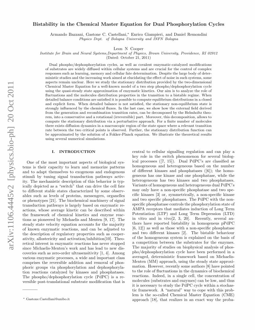
The process shown in Fig. (1) is a two-step chain ofaddition/removal reactions of chemical groups and may,in general, model important biological processes suchas phenotype switching (ultrasensitivity) and chroma-tine modification by histone acetylation/deacetylation aswell as phospho/dephosphorylation reactions. Withoutloss of generality, we perform a detailed study of the ho-mogeneous phospho/dephosphorylation two-step cycles(PdPC cycles) where two enzymes drive phosphoryla-tion and dephosphorylation respectively. Thus, there is acompetition between the two cycles for the advancementof the respective reactions.

The deterministic Michaelis-Menten (MM) equationsof the scheme (1) with the quasi-steady-state hypothesisreads:

FIG. 1. Scheme of the double enzymatic cycle of ad-dition/removal reactions of chemical groups via Michelis-Menten kinetic equations as shown in eq (1) in the case ofphosphoric groups.

dA

dt=

kM4vM2

(1−A−APP )

kM2kM4

+ kM4(1−A−AP

P ) + kM2AP

P

− kM3vM1A

kM1kM3 + kM1(1−A−APP ) + kM3A

dAPP

dt=

kM1vM3

(1−A−APP )

kM1kM3

+ kM1(1−A−AP

P ) + kM3A

− kM2vM4

APP

kM2kM4 + kM4(1−A−APP ) + kM2

APP

(1)

where A and APP are the concentrations of the non-

phosphorylated and double phosphorylated substrates,kMi

denote the MM constants and vMiare the maxi-

mal reaction velocities (i = 1, · · · 4). Let n1 and n2 de-note the molecules number of the substrates A and AP

Prespectively, the corresponding CME for the probabilitydistribution ρ(n1, n2, t) is written

∂ρ

∂t= g1(n1 − 1, n2)ρ(n1 − 1, n2, t)− g1(n1, n2)ρ(n1, n2, t)

+ r1(n1 + 1, n2)ρ(n1 + 1, n2, t)− r1(n1, n2)ρ(n1, n2, t)

+ g2(n1, n2 − 1)ρ(n1, n2 − 1, t)− g2(n1, n2)ρ(n1, n2, t)

+ r2(n1, n2 + 1)ρ(n1, n2 + 1, t)− r2(n1, n2)ρ(n1, n2, t)

(2)

where gj(n1, n2) and rj(n1, n2) are the generation andrecombination terms respectively, defined as :

r1(n1, n2) =KM3

vM1n1

KM1KM3 +KM1(NT − n1 − n2) +KM3n1

g1(n1, n2) =KM4

vM2(NT − n1 − n2)

KM2KM4

+KM4(NT − n1 − n2) +KM2

n2

r2(n1, n2) =KM2vM4n2

KM2KM4

+KM4(NT − n1 − n2) +KM2

n2

g2(n1, n2) =KM1

vM3(NT − n1 − n2)

KM1KM3 +KM1(NT − n1 − n2) +KM3n1

(3)

NT is the total number of molecules, and we have intro-duced scaled constants KM = NT kM . The biochemical

3

meaning is that the enzyme quantities should scale as thetotal number of molecule NT , to have a finite thermody-namic limit NT → ∞, in the transition rates (3). As itis known from the theory of one-step Markov processes,the CME (2) has a unique stationary solution ρs(n1, n2)that describes the statistical properties of the system ona long time scale. The CME recovers the Mass Action-based MM equation (1) in the thermodynamic limit whenthe average field theory approach applies. Indeed it canbe shown that the critical points of the stationary distri-bution for the CME can be approximately computed bythe conditions (cfr. eq. (15))

g1(n1, n2) = r1(n1 + 1, n2) g2(n1, n2) = r2(n1, n2 + 1)(4)

whose solutions tend to the equilibrium points of the MMequation when the fluctuation effects are reduced in thethermodynamic limit as O(1/

√N). As a consequence,

one would expect that the probability distribution be-comes singular, being concentrated at the fixed stablepoints of the equations (1), and that the transition rateamong the stability regions of attractive points is negli-gible. However, when a phase transition occurs due tothe bifurcation of the stable solution, fluctuations arerelevant even for large NT and the CME approach isnecessary. In the next section we discuss the stationarydistribution properties for the CME (2).

III. THE STATIONARY DISTRIBUTION

The stationary solution ρs(n1, n2) of the CME (2) canbe characterized by a discrete version of the zero diver-

gence condition for the current vector ~J components(seeAppendix)

Js1 = g1(n1 − 1, n2)ρs(n1 − 1, n2)− r1(n1, n2)ρs(n1, n2)

Js2 = g2(n1, n2 − 1)ρs(n1, n2 − 1)− r2(n1, n2)ρs(n1, n2)

(5)

and the CME r.h.s. reads

D1Js1 (n1, n2) +D2J

s2 (n1, n2) = 0 (6)

where we have introduced the difference operators

D1f(n1, n2) = f(n1 + 1, n2)− f(n1, n2)

D2f(n1, n2) = f(n1, n2 + 1)− f(n1, n2) (7)

Due to the commutative properties of the difference op-erators, the zero-divergence condition for the currentis equivalent to the existence of a current potentialA(n1, n2) such that

Js1 (n1, n2) = D2A(n1, n2) n1 ≥ 1

Js2 (n1, n2) = −D1A(n1, n2) n2 ≥ 1

(8)

We remark that the r.h.s. of eq. (8) is a discrete versionof the curl operator. The potential difference A(n′1, n

′2)−

A(n1, n2) defines the chemical transport across any lineconnecting the states (n1, n2) and (n′1, n

′2). At the sta-

tionary state the net transport across any closed path iszero and we have no current source in the network. Asdiscussed in [16, 18] we distinguish two cases: when thepotential A(n1, n2) is constant (the so called “detailedbalance condition”) and the converse case correspondingto a non-equilibrium stationary state. In this case thestationary solution ρs is characterized by the conditionJ1 = J2 = 0 over all the states, whereas in the othercase we have macroscopic chemical fluxes in the system.When detailed balance holds, simple algebraic manipu-lations (see Appendix) result in the following conditionsfor the stationary solutions

D1 ln ρs(n1, n2) = ln a1(n1, n2) (9)

D2 ln ρs(n1, n2) = ln a2(n1, n2) n1 + n2 < NT

(10)

where the discrete drift vector field components ai aredefined by:

a1(n1, n2) =g1(n1, n2)

r1(n1 + 1, n2)a2(n1, n2) =

g2(n1, n2)

r2(n1, n2 + 1).

(11)Equations (9) and (10) imply the existence of a potentialV (n1, n2) such that

ln a1(n1, n2) = −D1V (n1, n2)

ln a2(n1, n2) = −D2V (n1, n2) (12)

Using definition (3) it is possible to explicitly computea set of parameter values for the PdPC cycle, that sat-isfy the detailed balance condition (12) according to therelations

2KM1= KM2

= KM3= 2KM4

(13)

where the reaction velocities VM are arbitrary. The sta-tionary distribution is given by the Maxwell-Boltzmanndistribution

ρs(n1, n2) = exp(−V (n1, n2)) (14)

where the potential V (n1, n2) is computed by integrat-ing equation (12) and choosing the initial value V (0, 0)to normalize the distribution (14). Using a thermody-namical analogy, we can interpret the potential differ-ence V (n1, n2) − V (0, 0) as the chemical energy neededto reach the state (n1, n2) from the initial state (0, 0). Asa consequence, the vector field (11) represents the workfor one-step transition along the n1 or n2 direction. Def-inition (14) also implies that the critical points of thestationary distribution are characterized by the condi-tions

g1(n1, n2)

r1(n1 + 1, n2)=

g2(n1, n2)

r2(n1, n2 + 1)= 1 (15)

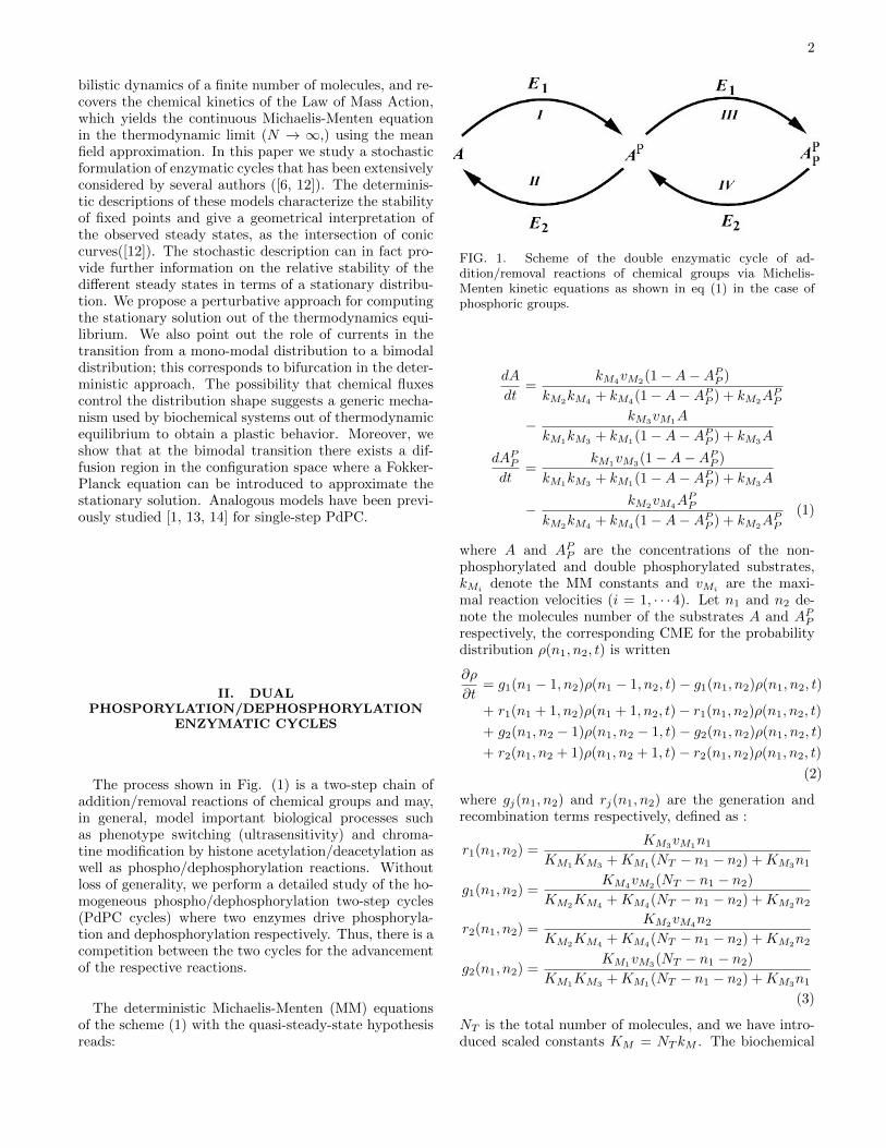
and coincides with the critical points of the MM equa-tions. In figure 2 we plot the stationary distributions

4

FIG. 2. Stationary distributions for the A and APP states in the double phosphorylation cycle when detailed balance (13)

holds with KM1 = KM4 = 1 and KM2 = KM3 = 2. In the top figure we set the reaction velocities vM1 = vM2 = 1 andvM2 = vM3 = 1.05 (symmetric case), whereas in the bottom figure we increase the vM2 and vM3 value to 1.15. The number ofmolecules is NT = 40. The transition from a unimodal distribution to a bimodal distribution is clearly visible.

(14) in the case NT = 40 with KM1= KM4

= 1and KM2

= KM3= 2; we consider two symmetric

cases: vM1= vM2

= 1 with vM2= vM3

= 1.05 orvM2

= vM3= 1.15 (all the units are arbitrary). In

the first case, the probability distribution is unimodal,whereas in the second case the transition to a bimodaldistribution is observed. Indeed, the system has a phasetransition at vM2

= vM3' 1.1 that corresponds to a bi-

furcation of the critical point defined by the condition(15).

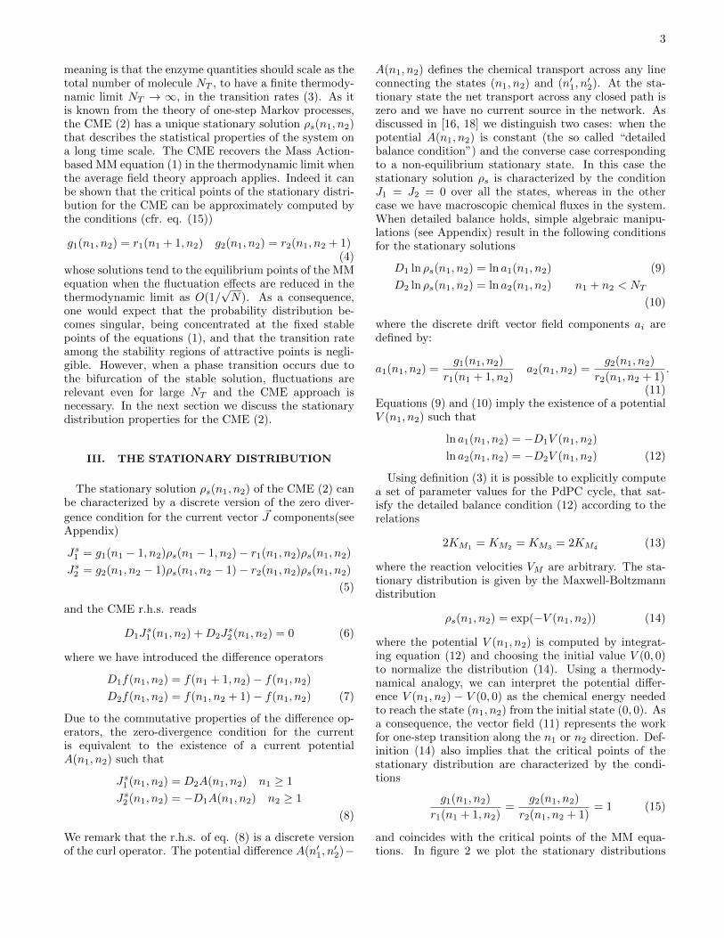
In figure 2 we distinguish two regions: a drift domi-nated region and a diffusion dominated region. In thefirst region the chemical reactions mainly follow the gra-dient of the potential V (n1, n2) and tend to concentratearound the stable critical points, so that the dynamic iswell described by a Liouville equation[5]. In the secondregion the drift field (11) is small and the fluctuations dueto the finite size introduce a diffusive behaviour. Thenthe distribution can be approximated by the solution ofa Fokker-Planck equation[18]. As discussed in the Ap-pendix, the diffusion region is approximately determinedby the conditions

g1(n1, n2)− r1(n1 + 1, n2) ' g2(n1, n2)− r2(n1, n2 + 1)

' O(1/NT ) (16)

To illustrate this phenomenon, we outline in fig. 3 theregion where condition (16) is satisfied (i.e. the gradientof the potential V (n1, n2) is close to 0 (12)). This is theregion where the fixed points of the MM equation arelocated, and comparison with fig. 2 shows that it definesthe support of the stationary distribution.

In the diffusion dominated region a molecule can un-dergo a transition from the dephosphorylated equilib-rium to the double phosphorylated one. At the station-ary state the transition probability from one equilibriumto the other can be estimated by the Fokker-Planck ap-

FIG. 3. In grey we show the region where components ofthe vector field (11) are ' 1 using the parameter values offig. 2 (bottom). The blue lines enclose the region where thefirst component is nearby 1, whereas the red ones enclose thecorresponding region for the second component.

proximation; but this does not imply that the Fokker-Planck equation allows us to describe the transient re-laxation process toward the stationary state. Indeed,due to the singularity of the thermodynamics limit, thedynamics of transient states may depend critically on fi-nite size effects not described by using the Fokker-Planckapproximation[19]. To cope with these problems in thePdPC model further studies are necessary.

When the current (8) is not zero the CME (2) relaxestoward a Non-Equilibrium Stationary State (NESS) andthe field (11) is not conservative. We shall perform aperturbative approach to point out the effects of currentson the NESS nearby the transition region to the bimodalregime. We consider the following decomposition for the

5

vector field

ln a1(n1, n2) = −D1V0(n1, n2) +D2H(n1, n2)

ln a2(n1, n2) = −D2V0(n1, n2)−D1H(n1, n2)

n1 + n2 ≤ NT − 1 (17)

where the rotor potential H(n1, n2) takes into accountthe irreversible rotational part. The potential H(n1, n2)can be recursively computed using the discrete Laplaceequation

(D1D1+D2D2)H = D2 ln (a1(n1, n2))−D1 ln (a2(n1, n2))(18)

where n1 + n2 ≤ NT − 2, with the boundary condi-tions H(n,N − n) = H(n,N − 1 − n) = 0 (see Ap-pendix). Assuming that the potential H is small withrespect to V , we can approximate the NESS by usingthe Maxwell-Boltzmann distribution (14) with V = V0.However, as we shall show in the next section, at thephase transition even the effect of small currents be-comes critical, and the study of higher perturbative or-ders is necessary. To point out the relation amongthe rotor potential H, the NESS ρs and the chemicalflux J , we compute the first perturbative order lettingρs(n1, n2) = exp(−V0(n1, n2)− V1(n1, n2)). From defini-tion (5) the condition (8) reads:

exp (−V0(n1, n2)− V1(n1, n2)) r1(n1, n2)

· (exp (D2H(n1 − 1, n2))− exp (−D1V1(n1 − 1, n2)))

= D2a(n1, n2))

exp (−V0(n1, n2)− V1(n1, n2)) r2(n1, n2)

· (exp (−D1H(n1, n2 − 1))− exp (−D2V1(n1, n2 − 1)))

= −D1a(n1, n2)

(19)

V1(n1, n2) turns out to be an effective potential thatsimulates the current’s effect on the unperturbed station-ary distribution by using a conservative force. We notethat if the rotor potential H is zero, then both the cur-rent potential A and the potential correction V1 are zero,so that all these quantities are of the same perturbativeorder, and the first perturbative order of eqs. (19) reads

exp (−V0(n1, n2)) r1(n1, n2) ·(D1V1(n1 − 1, n2) +D2H(n1 − 1, n2)) = D2A(n1, n2)

exp (−V0(n1, n2)) r2(n1, n2) ·(D2V1(n1, n2 − 1)−D1H(n1, n2 − 1)) = −D1A(n1, n2)

(20)

From the previous equations we see that the currentsdepend both on the rotor potential H and the potentialcorrection V1, which is unknown; thus they cannot bedirectly computed from (20). We obtain an equation for

V1 by eliminating the potential A from (20)

D1 (exp (−V0(n1, n2)) r1(n1, n2)D1V1(n1 − 1, n2))

+D2 (exp (−V0(n1, n2)) r2(n1, n2)D2V1(n1, n2 − 1)) =

D2 (exp (−V0(n1, n2)) r2(n1, n2)D1H(n1, n2 − 1))

−D1 (exp (−V0(n1, n2)) r1(n1, n2)D2H(n1 − 1, n2))

(21)

Eq. (21) is defined for n1 ≥ 1, n2 ≥ 1 and n1 + n2 ≤NT − 1, and we can solve the system by introducing theboundary conditions V1(n, 0) = V1(0, n) = V1(n,NT −n) = 0. It is interesting to analyze equation (21) in thephase transition regime. When the recombination termsr1,r2 are almost equal and their variation is small (for ourparameter choice this is true for n1 ' n2 and n1+n2 � 1)the r.h.s. can be approximated by

exp(−V0(n1, n2) [D2V0(n1, n2)D1H(n1, n2 − 1)

−D1V0(n1, n2)D2H(n1 − 1, n2)]

(22)

As a consequence, in the transition regime this term isnegligible since both D1V0(n1, n2) and D2V0(n1, n2) tendtoward zero in the diffusion region where the bifurcationoccurs; thus the first perturbative order is not enoughto compute the stationary distribution correction, buthigher orders should be considered.

IV. NUMERICAL SIMULATIONS

In order to study the non equilibrium stationary con-ditions in the double phosphorylation cycle (1) we haveperturbed the detailed balance conditions considered infigure (2) by changing the value of the MM constantsKM2 and KM3 . In figure (4) we show the rotor field ofthe potential H in the cases KM2 = KM3 = 2.2 andKM2 = KM3 = 1.8 when the detailed balance condition(13) does not hold. We see that in the first case (leftpicture) the rotor field tends to move the particles fromthe borders toward the central region n1 = n2, so thatwe expect an increase of the probability distribution inthe center, whereas in the second case the rotor field isdirected from the central region to the borders and weexpect a decrease of the probability distribution in thisregion. To illustrate the effect of the potential H, wecompare the zero-order approximation of the probabil-ity distribution (14), where the potential V0(n1, n2) iscomputed using decomposition (17) with the stationarysolution of the CME (2). The main parameter values arereported in table IV

Case KM2 KM3 vM2 vM3

I 1.8 1.8 1.05 1.05II 1.8 1.8 1.15 1.15III 2.2 2.2 1.05 1.05IV 2.2 2.2 1.15 1.15

6

FIG. 4. Plot of the rotor field for the potential H using the following parameter values: vM1 = vM2 = 1, vM2 = vM3 = 1.15KM1 = KM4 = 1, NT = 40 and KM2 = KM3 = 1.8 (left picture) or KM2 = KM3 = 2.2 (right picture).

FIG. 5. (Left picture): plot of the zero-order approximation for the probability distribution using the decomposition (17) forthe vector field associated to the CME. (Right picture): plot of the stationary distribution computed by directly solving theCME (2). We use the parameter values of the case I in the table IV.

whereas the other parameters values are: vM1= vM2

=1,KM1

= KM4= 1 and NT = 40. For the first parameter

set, the zero-order approximation is a bimodal distribu-tion, but the effect of the currents induced by the rotorpotential H (see fig. 4) left) are able to destroy the bi-modal behaviour by depressing the two maximal at theborder (see fig. 5).

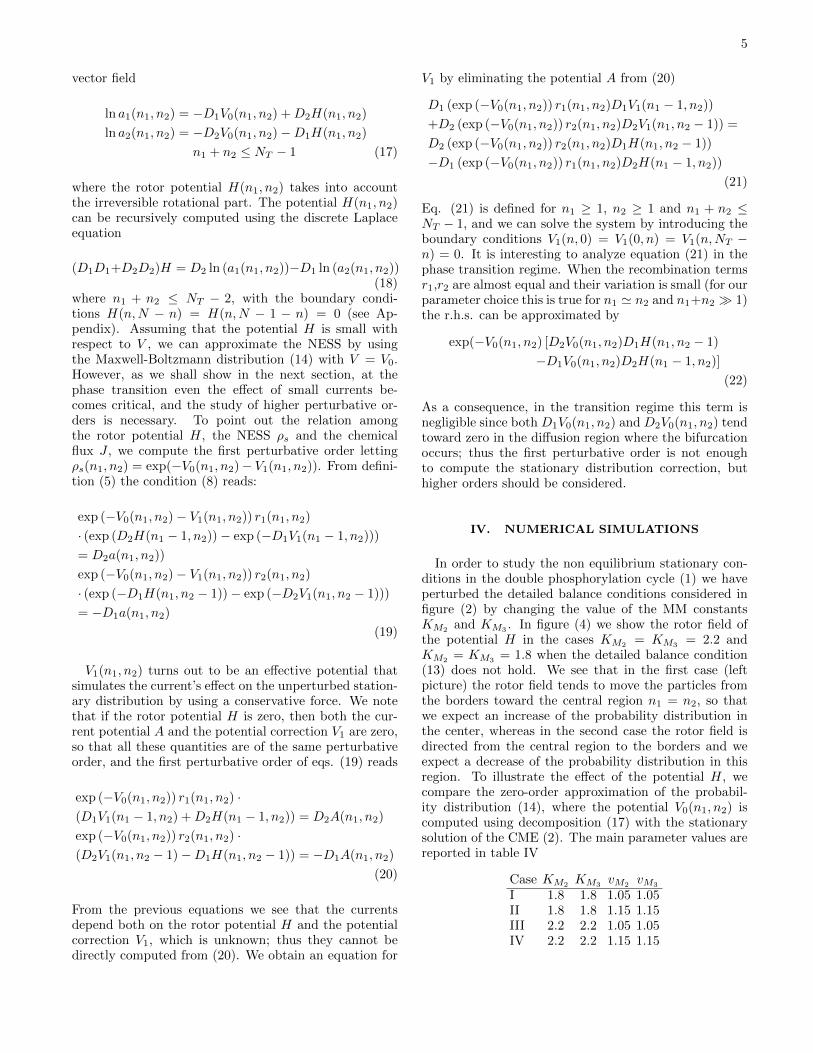
If we increase the value of the K2M and K3M (case II),the exact stationary distribution becomes bimodal andthe effect of currents is to introduce a strong transitionprobability between the two distribution maxima (fig. 6).

Therefore, when the MM constants KM2 and KM3 are< 2 (we note that for KM2

= KM3= 2, the detailed

balance holds), the non-conservative nature of the field(17) introduces a delay in the phase transition from a

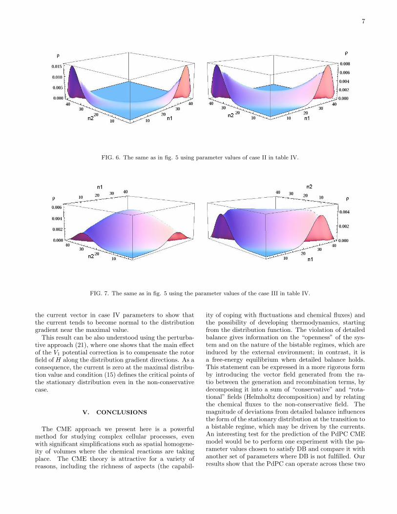
mono-modal to a bimodal distribution. However, whenwe consider KM2 = KM3 > 2 (cases III and IV) the rotorpotential H moves the particle towards the borders andthe central part of the distribution is depressed. This isshown in the figure 7 where we compare the zero-orderapproximation of the stationary distribution and the so-lution of the CME using the case III parameters of thetable IV.

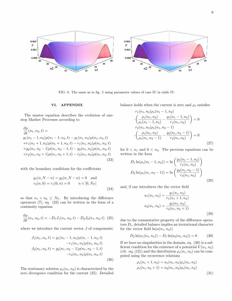
Finally, in case IV of table IV, the CME stationarysolution undergoes a transition to a bimodal distribu-tion, whereas the zero-order approximation is still mono-modal ( fig. 9), so that the effect of currents is to antici-pate the phase transition.

Using the stationary solution one can also compute thecurrents according to definition (5). In figure (9) we plot

7

FIG. 6. The same as in fig. 5 using parameter values of case II in table IV.

FIG. 7. The same as in fig. 5 using the parameter values of the case III in table IV.

the current vector in case IV parameters to show thatthe current tends to become normal to the distributiongradient near the maximal value.

This result can be also understood using the perturba-tive approach (21), where one shows that the main effectof the V1 potential correction is to compensate the rotorfield of H along the distribution gradient directions. As aconsequence, the current is zero at the maximal distribu-tion value and condition (15) defines the critical points ofthe stationary distribution even in the non-conservativecase.

V. CONCLUSIONS

The CME approach we present here is a powerfulmethod for studying complex cellular processes, evenwith significant simplifications such as spatial homogene-ity of volumes where the chemical reactions are takingplace. The CME theory is attractive for a variety ofreasons, including the richness of aspects (the capabil-

ity of coping with fluctuations and chemical fluxes) andthe possibility of developing thermodynamics, startingfrom the distribution function. The violation of detailedbalance gives information on the “openness” of the sys-tem and on the nature of the bistable regimes, which areinduced by the external environment; in contrast, it isa free-energy equilibrium when detailed balance holds.This statement can be expressed in a more rigorous formby introducing the vector field generated from the ra-tio between the generation and recombination terms, bydecomposing it into a sum of “conservative” and “rota-tional” fields (Helmholtz decomposition) and by relatingthe chemical fluxes to the non-conservative field. Themagnitude of deviations from detailed balance influencesthe form of the stationary distribution at the transition toa bistable regime, which may be driven by the currents.An interesting test for the prediction of the PdPC CMEmodel would be to perform one experiment with the pa-rameter values chosen to satisfy DB and compare it withanother set of parameters where DB is not fulfilled. Ourresults show that the PdPC can operate across these two

8

FIG. 8. Current vector field computed by using definiton(5) and the stationary solution of the CME with case IV pa-rameters. The distribution is bimodal (cfr. figure 8) and thecurrent lines tend to be orthogonal to the distribution gradi-ent near the maximal value.

regions, and that the transition regime can be explainedby the role of the currents, that, within a thermody-namic framework, can be interpreted as the effect of anexternal energy source. A full thermodynamic analysisof this cycle is beyond the scope of this paper, but we cansurmise that this approach might be extended to othercycles in order to quantify if, and how much energy, isrequired to maintain or create bistability. Another wayto extend this analysis would be the generalization ton-step phospho/dephosphorylation cycles, where the sta-tionary distribution will be the product of n independentone-dimensional distributions. In conclusion, our resultscould be important for a deeper characterization of bio-chemical signaling cycles that are the molecular basis forcomplex cellular behaviors implemented as a “switch”between states.

[1] Berg, O., Paulsson, J., and Ehrenberg, M. (2000). Fluc-tuations and quality of control in biological cells: zero-order ultrasensitivity reinvestigated. Biophysical Jour-nal, 79(3):1228–1236.

[2] Castellani, G., Bazzani, A., and LN, C. (2009). To-ward a microscopic model of bidirectional synaptic plas-ticity. Proceedings of the National Academy of Sciences,106(33):14091.

[3] Castellani GC, Q. E. C. L. S. H. (2001). A biophysicalmodel of bidirectional synaptic plasticity: dependence onAMPA and NMDA receptors. Proceedings of the NationalAcademy of Sciences, 98(22):12772–7.

[4] Goldbeter, A. and Koshland, D. (1981). An amplifiedsensitivity arising from covalent modification in biologicalsystems. Proceedings of the National Academy of Sciencesof the United States of America, 78(11):6840.

[5] Huang, K. (1987). Statistical Mechanics. Wiley.[6] Huang, Q. and Qian, H. (2009). Ultrasensitive dual phos-

phorylation dephosphorylation cycle kinetics exhibitscanonical competition behavior. Chaos: An Interdisci-plinary Journal of Nonlinear Science, 19:033109.

[7] Krebs, E. G., KENT, A. B., and FISCHER, E. H. (1958).The muscle phosphorylase b kinase reaction. J BiolChem, 231(1):73–83.

[8] Mettetal, J. and van Oudenaarden, A. (2007). Necessarynoise. Science, 317:463.

[9] Michaelis, L. and Menten, M. (1913). Kinetics of inver-tase action. Biochem. Z, 49:333–369.

[10] Min, W., Gopich, I. V., English, B. P., Kou, S. C., Xie,X. S., and Szabo, A. (2006). When does the Michaelis-Menten equation hold for fluctuating enzymes? J PhysChem B, 110(41):20093–7.

[11] Onsager, L. (1931). Reciprocal Relations in IrreversibleProcesses. Phys. Rev., 37:405.

[12] Ortega, F., Garces, J., Mas, F., Kholodenko, B., andCascante, M. (2006). Bistability from double phos-phorylation in signal transduction. FEBS JOURNAL,273(17):3915.

[13] Qian, H. (2003). Thermodynamic and kinetic analysis ofsensitivity amplification in biological signal transduction.Biophysical chemistry, 105(2-3):585–593.

[14] Qian, H., Cooper, J., et al. (2008). Temporal Coopera-tivity and Sensitivity Amplification in Biological SignalTransductiona . Biochemistry, 47(7):2211–2220.

[15] Samoilov, M., Plyasunov, S., and Arkin, A. P. (2005).Stochastic amplification and signaling in enzymatic futilecycles through noise-induced bistability with oscillations.Proc Natl Acad Sci U S A, 102(7):2310–5.

[16] Schnakenberg, J. (1976). Network theory of microscopicand macroscopic behavior of master equation systems.Rev. Mod. Phys., 48(4):571–585.

[17] Segel, L. (1984). Modeling dynamic phenomena in molec-ular and cellular biology. Cambridge Univ Pr.

[18] van Kampen, N. G. (2007). Stochastic Processes inPhysics and Chemistry. North Holland, third edition.

[19] Vellela, M. and Qian, H. (2007). A quasistationary anal-ysis of a stochastic chemical reaction: Keizer’s paradox.Bull. Math. Biol., 69:1727–1746.

[20] Whitlock JR, H. A. S. M. B. M. (2006). Learning in-duces long-term potentiation in the hippocampus. Sci-ence, 313:1093–1097.

[21] Xiong, W. and Ferrell, J. (2003). A positive-feedback-based bistable memory module that governs a cell fatedecision. Nature, 426(6965):460–465.

9

FIG. 9. The same as in fig. 5 using parameter values of case IV in table IV.

VI. APPENDIX

The master equation describes the evolution of one-step Markov Processes according to

∂ρ

∂t(n1, n2, t) =

g1(n1 − 1, n2)ρ(n1 − 1, n2, t)− g1(n1, n2)ρ(n1, n2, t)

+r1(n1 + 1, n2)ρ(n1 + 1, n2, t)− r1(n1, n2)ρ(n1, n2, t)

+g2(n1, n2 − 1)ρ(n1, n2 − 1, t)− g2(n1, n2)ρ(n1, n2, t)

+r2(n1, n2 + 1)ρ(n1, n2 + 1, t)− r2(n1, n2)ρ(n1, n2, t)

(23)

with the boundary conditions for the coefficients

g1(n,N − n) = g2(n,N − n) = 0 and

r2(n, 0) = r1(0, n) = 0 n ∈ [0, NT ]

(24)

so that n1 + n2 ≤ NT . By introducing the differenceoperators (7), eq. (23) can be written in the form of acontinuity equation

∂ρ

∂t(n1, n2, t) = −D1J1(n1, n2, t)−D2J2(n1, n2, t) (25)

where we introduce the current vector J of components:

J1(n1, n2, t) = g1(n1 − 1, n2)ρ(n1 − 1, n2, t)

−r1(n1, n2)ρ(n1, n2, t)

J2(n1, n2, t) = g2(n1, n2 − 1)ρ(n1, n2 − 1, t)

−r2(n1, n2)ρ(n1, n2, t)

(26)

The stationary solution ρs(n1, n2) is characterized by thezero divergence condition for the current (25). Detailed

balance holds when the current is zero and ρs satisfies

r1(n1, n2)ρs(n1 − 1, n2)

·(

ρs(n1, n2)

ρs(n1 − 1, n2)− g1(n1 − 1, n2)

r1(n1, n2)

)= 0

r2(n1, n2)ρs(n1, n2 − 1)

·(

ρs(n1, n2)

ρs(n1, n2 − 1)− g2(n1, n2 − 1)

r2(n1, n2)

)= 0

(27)

for 0 < n1 and 0 < n2. The previous equations can bewritten in the form

D1 ln(ρs(n1 − 1, n2)) = ln

(g1(n1 − 1, n2)

r1(n1, n2)

)D2 ln(ρs(n1, n2 − 1)) = ln

(g2(n1, n2 − 1)

r2(n1, n2)

)(28)

and, if one introduces the the vector field

a1(n1, n2) =g1(n1, n2)

r1(n1 + 1, n2)

a2(n1, n2) =g2(n1, n2)

r2(n1, n2 + 1)

(29)

due to the commutative property of the difference opera-tors Di, detailed balance implies an irrotational characterfor the vector field ln(a(n1, n2))

D2 ln(a1(n1, n2))−D1 ln(a2(n1, n2)) = 0 (30)

If we have no singularities in the domain, eq. (30) is a suf-ficient condition for the existence of a potential V (n1, n2)(cfr. eq, (12)) and the distribution ρs(n1, n2) can be com-puted using the recurrence relations

ρs(n1 + 1, n2) = a1(n1, n2)ρs(n1, n2)

ρs(n1, n2 + 1) = a2(n1, n2)ρs(n1, n2)

(31)

10

Therefore, the components a1(n1, n2) and a2(n1, n2) canalso be interpreted as creation operators according torelations (31) and detailed balance condition (30) isequivalent to the commutativity property for these op-erators. The stationary distribution can be writtenin the Maxwell-Boltzmann form (14) and the potentialV (n1, n2) is associated with an “energy function”. Wefinally observe that the critical points of the stationarydistribution ρs are defined by the condition

a1(n1, n2) = a2(n1, n2) = 1 (32)

For the double phosphorylation cycle (1) it is possible toderive explicit expressions for the stationary distribution

ρs(n1, n2) by applying recursively the relations (31) ina specific order: for example, first moving along the n2direction and then along n1, we obtain an expression forρs(n1, n2) as a function of ρs(0, 0)

ρs(n1, n2) =

n1∏i=1

g1(i− 1, n2)

r1(i, n2)

n2∏l=1

g2(0, l − 1)

r2(0, l)ρs(0, 0)

(33)A direct substitution of the coefficients (3) in the relation(33) gives

ρs(n1, n2) =

n1∏i=1

KM4VM2(NT − i− n2 + 1)

KM2KM4 +KM4(NT − i− n2 + 1) +KM2n2· KM1KM3 +KM1(NT − i− n2) +KM3i

KM3VM1i

·n2∏l=1

KM1VM3(NT − l + 1)

KM1KM3 +KM1(NT − l + 1)

KM2KM4 +KM4(NT − l) +KM2l

KM2VM4lρs(00)

We can further simplify this expression by using thedefinition of multinomial coefficients and the rising andfalling factorial symbols, defined as x(n) = x(x + 1)(x +

2) · · · (x + n − 1) = (x+n−1)!(x−1)! and x(n) = x(x − 1)(x −

2) · · · (x− n+ 1) = x!(x−n)! ) respectively.

ρs(n1, n2) =

(VM2

VM1

)n1(VM3

VM4

)n2(NT − n2

n1

)(NT

n2

)(KM3 −KM1

KM3

)n1(KM2 −KM4

KM2

)n2

·

(KM1(1 + n2 −KM3 −NT )−KM3)(n1)

(KM1 −KM3)(n1)(KM2(1 + n2

KM4) +NT − n2)(n1)

·

(KM2(1 +KM4) +KM4(NT − 1))(n2)

(KM2 −KM4)(n2)(KM3 +NT )(n2)

ρs(0, 0)

Finally, it is interesting to go to a continuous limitthat is equivalent to NT → ∞. First we introduce thepopulation densities A = n1/NT and AP

P = n2/NT anduse the fact that the generation and recombination ratesare invariant by substituting n1 and n2 with A and AP

P .

Then we approximate

D1V (A,APP ) = V (A+ 1/NT , A

PP )− V (A,AP

P )

=1

NT

∂V

∂A(A+

1

2NT, AP

P ) +O(1/N3T )

and a similar expression holds for D2V (A,APP ). Accord-

ing to eq. (12), the partial derivatives of V (A,APP ) are

bounded when NT → ∞ only in the domain where thefollowing approximation holds (diffusion dominated re-gion)

gi(A,APP )

ri(A,APP )

= 1 +O(1/NT ) i = 1, 2 (34)

and we can estimate

ln

(g1(A,AP

P )

r1(A+ 1/NT , APP )

)' −2

r1(A+ 1/NT , APP )− g1(A,AP

P )

r1(A+ 1/NT , APP ) + g1(A,AP

P )+O(1/N3

T )

ln

(g2(A,AP

P )

r2(A,APP + 1/NT )

)' −2

r2(A,APP + 1/NT )− g2(A,AP

P )

r2(A,APP + 1/NT ) + g2(A,AP

P )+O(1/N3

T )

(35)

Then we may approximate (we use the convention of leav-ing out the dependence on AP

P )

11

r1(A+ 1/NT )− g1(A)

r1(A+ 1/NT ) + g1(A)=r1(A+ 1/2NT )− g1(A+ 1/2NT ) + 1/2NT (∂r1/∂A(A+ 1/2NT ) + ∂g1/∂A(A+ 1/2NT ))

r1(A+ 1/NT ) + g1(A)

(36)

up to an error of order O(1/N2T ) (a similar expression is

obtained for the second equation). Therefore, detailedbalance in the continuous limit reads

r1(A,APP )− g1(A,AP

P ) + 1/2NT

(∂r1/∂A(A,AP

P ) + ∂g1/∂A(A,APP ))

r1(A+ 1/2NT , APP ) + g1(A− 1/2NT , AP

P )= − 1

2NT

∂V

∂A(A,AP

P )

r2(A,APP )− g2(A,AP

P ) + 1/2NT

(∂r2/∂A

PP (A,AP

P ) + ∂g2/∂APP (A,AP

P ))

r2(A,APP + 1/2NT ) + g2(A,AP

P − 1/2NT )= − 1

2NT

∂V

∂APP

(A,APP )

(37)

The limit NT →∞ turns out to be singular since

− ∂V

∂A(A,AP

P ) =2NT (r1(A,AP

P )− g1(A,APP )) + ∂r1/∂A(A,AP

P ) + ∂g1/∂A(A,APP )

r1(A,APP ) + g1(A,AP

P )

− ∂V

∂APP

(A,APP ) =

2NT (r2(A,APP )− g2(A,AP

P )) + ∂r2/∂APP (A,AP

P ) + ∂g2/∂APP (A,AP

P )

r2(A,APP ) + g2(A,AP

P )

(38)

Hence in the diffusion domain defined by condition (34),we recover detailed balance for a Fokker-Planck equationwith drift and diffusion coefficients defined as:

ci(A,APP ) = 2NT

(ri(A,A

PP )− gi(A,AP

P ))

i = 1, 2

and

bi(A,APP ) = ri(A,A

PP ) + gi(A,A

PP ) i = 1, 2

In the diffusion region the drift and the diffusion coef-ficients are of the same order, otherwise ci(A,A

PP ) �

bi(A,APP ) when NT � 1. As a consequence, the sta-

tionary solution of F.P. equation is an approximation ofthe stationary distribution of the CME in the diffusionregion, but the approximation of the transient state dy-namics using the F.P. equation requires further studiesdue to the singularity of the thermodynamic limit.In the generic case of eq. (23), we represent the r.h.s. ofeq. (28) as a sum of a rotational and a gradient vector

fields

ln a1(n1, n2) = D1V (n1, n2) +D2H(n1, n2)

ln a2(n1, n2) = D2V (n1, n2)−D1H(n1, n2)

(39)Taking into account the condition n1+n2 ≤ NT−1, fromthe eqs. (39) we get the discrete Poisson equations

(D1D1 +D2D2)V (n1, n2) =

D1 ln (a1(n1, n2)) +D2 ln (a2(n1, n2))

(D1D1 +D2D2)H(n1, n2) =

D2 ln (a1(n1, n2))−D1 ln (a2(n1, n2))

(40)

We remark that the r.h.s. of eqs. (40) is defined only ifn1 + n2 ≤ N − 2 and corresponds to N(N − 1)/2 inde-pendent equations, whereas we have (N + 2)(N + 1)/2unknown values H(n1, n2). As a consequence from theexplicit form of the discrete Poisson operator

(D21 +D2

2)H(n1, n2) = H(n1 + 2, n2)− 2H(n1 + 1, n2) +H(n1, n2) +H(n1, n2 + 2)− 2H(n1, n2 + 1) +H(n1, n2)

we can set the boundary conditions H(n,N − n) =H(n,N − 1 − n) = 0 and recursively solve the system

setting

2H(n,N − 2− n) =

ln

(a1(n,N − 1− n)a2(n,N − 2− n)

a1(n,N − 2− n)a2(n+ 1, N − 2− n)

))

(41)

12

and successively using the equations

2H(n,N − j − n) = −H(n+ 2, n− j − n)−H(n,N − j − n− 2) + 2H(n+ 1, N − j − n) + 2H(n,N − j − n− 1)

+ lna1(n,N − j − n+ 1)a2(n,N − j − n)

a1(n,N − j − n)a2(n+ 1, N − j − n)

(42)

for N ≥ j > 2. Once H(n1, n2) is computed, we definethe “potential” V (n1, n2) by using eq. (39). The recur-sion relations (42) can be written in an exponential formby defining

R(n1, n2) = exp(H(n1, n2))

R(n,N − j − n)) =√a1(n,N − j − n+ 1)a2(n,N − j − n)

a1(n,N − j − n)a2(n+ 1, N − j − n)

· R(n+ 1, N − j − n)R(n,N − j − n− 1)√R(n+ 2, n− j − n)R(n,N − j − n− 2)

(43)

As a consequence, the recurrence (31) reads

ρs(n1 + 1, n2) = a1(n1, n2)R(n1, n2)

R(n1, n2 + 1)ρs(n1, n2)

ρs(n1, n2 + 1) = a2(n1, n2)R(n1 + 1, n2)

R(n1, n2)ρs(n1, n2)

(44)

for all n1 + n2 ≤ N − 1.

The current componentss (25) turn out to be propor-tional to the rotational part of the field (39) (i.e. toH(n1, n2))[11], so that the current vanishes at the pointswhere condition (32) is satisfied. One can prove thatthe critical points of the stationary distribution are stilldefined by eq. (32). Indeed, if one computes the for-mal expansion of the generation and recombination rates

around a solution of eqs. (31)

g(n) = 1 +∂g

∂n(n∗) ·∆n+ ....

r(n) = 1 +∂r

∂n(n∗) ·∆n+ ....

(45)

(for the sake of simplicity we have normalized the value ofthe generation and recombination rate to 1 at the criticalpoint) the current components can be approximated bythe expressions

Js1 (n1, n2) ' ρs(n1 − 1, n2)− ρs(n1, n2)

+∂g1∂n

(n∗) ·∆nρs(n1 − 1, n2)− ∂r1∂n

(n∗) ·∆nρs(n1, n2)

Js2 (n1, n2) ' ρs(n1, n2 − 1)− ρs(n1, n2)

+∂g2∂n

(n∗) ·∆nρs(n1, n2 − 1)− ∂r2∂n

(n∗) ·∆nρs(n1, n2)

(46)

At the critical point n∗ we get

ρs(n∗1 − 1, n∗2) = ρs(n

∗1, n∗2 − 1) = ρs(n

∗1, n∗2) (47)

since Js(n∗1, n∗2) = 0. The condition (47) means the n∗ is

a critical point for the stationary distribution ρs.When H(n1, n2) is small, the detailed balance solution(14) is a good approximation of the stationary solutionρs(n1, n2) and a perturbative approach can be applied.Let us write the stationary condition (6) in the form

D1r1(n1, n2)ρs(n1, n2)

(1− a1(n1 − 1, n2)

ρs(n1 − 1, n2)

ρs(n1, n2)

)+

D2r2(n1, n2)ρs(n1, n2)

(1− a2(n1, n2 − 1)

ρs(n1, n2 − 1)

ρs(n1, n2)

)= 0

(48)

By using the definitions (39), we assume that the rota-tional field is associated with a potential εH(n1, n2), withε� 1 perturbation parameter and we write the station-ary solution in the form

ρs(n1, n2) = C exp(V (n1, n2) + εV1(n1, n2)) (49)

From a direct calculation we get

13

D1r1(n1, n2)eV (n1,n2) (1− exp(ε(D2H(n1 − 1, n2)−D1V1(n1 − 1, n2))))

+D2r2(n1, n2)eV (n1,n2) (1− exp(−(εD1H(n1, n2 − 1) +D2V1(n1, n2 − 1))) 'εD1r1(n1, n2)eV (n1,n2) (D1V1(n1 − 1, n2)−D2H(n1 − 1, n2))

+εD2r2(n1, n2)eV (n1,n2) (D2V1(n1, n2 − 1) +D1H(n1, n2 − 1)) = 0

(50)

for all the values n1 + n2 ≤ N − 1 and ni ≥ 1. Thecorrection potential V1(n1, n2) has to be computed from

the previous equation, and it enters in the definition ofthe stationary currents.