Bioquímica e Biofísica Computacionais: - Teses USP

Guilherme Menegon Arantes

Bioquímica e Biofísica Computacionais:Simulações da Reatividade e da Estrutura de Biomoléculas

2016

Guilherme Menegon Arantes

Bioquímica e Biofísica Computacionais:Simulações da Reatividade e da Estrutura de Biomoléculas

Texto apresentado como requisito para obten-ção de título de Livre-Docente junto ao De-partamento de Bioquímica da Universidadede São Paulo

Departamento de BioquímicaInstituto de Química

Universidade de São Paulo

2016

Dedico este trabalho a toda minha família, em especiala minha filha, Julia, e a minha irmã, Fernanda.Porque a família é como a raiz de uma árvore.

Sem ela, seríamos facilmente derrubados.

Agradecimentos

Agradeço primeiramente a toda comunidade do Instituto de Química pelo convívio.Mesmo após 20 anos frequentando este Instituto, ainda me empolgo como se fosse aprimeira vez que ando pelos seus longos corredores.

Aos colegas do Departamento de Bioquímica, personificados nas chefias da MariaJúlia Manso e do Chuck Farah, pela ajuda em estabelecer meu grupo de pesquisa física etecnicamente. Ao Sandro Marana pelas conversas, constante apoio, colaborações e por tersempre aberto as portas do seu laboratório. Ao Roberto Salinas e novamente ao Chuckpelas recentes colaborações que espero que floresçam.

Ao meu grupo de pesquisa, alunos e estagiários, em particular Ariane Alves, MuriloTeixeira, Raphael Sayegh e Vanesa Galassi. Com eles descobri que também é divertidoacompanhar o crescimento de um aluno.

Ao Martin J. Field, meu principal colaborador e também amigo. Não seria exagero eleter dividido o Nobel de Química em 2013.

Ao Luís Gustavo Dias, grande amigo e antigo mentor, pelas discussões científicas (ounem tanto!).

Às agências de fomento: Pró-Reitoria de Pesquisa-USP pelo auxílio, CAPES e CNPqpelas bolsas, e FAPESP pelas bolsas e auxílios, principalmente o Jovem Pesquisador e osRegulares que permitiram a instalação do meu grupo de pesquisa e a montagem da nossainfraestrutura de pesquisa, usada em todos trabalhos apresentados aqui. Espero que estaFundação volte a ser generosa com projetos individuais e independentes.

Sumário

1 Introdução . . . . . . . . . . . . . . . . . . . . . . . . . . . . . . . . . . . . . 91.1 Organização do texto . . . . . . . . . . . . . . . . . . . . . . . . . . . . . . 10

2 Modelos e metodologias computacionais . . . . . . . . . . . . . . . . . . . . 112.1 Química quântica . . . . . . . . . . . . . . . . . . . . . . . . . . . . . . . . 112.2 Mecânica molecular . . . . . . . . . . . . . . . . . . . . . . . . . . . . . . . 132.3 Potenciais híbridos QC/MM . . . . . . . . . . . . . . . . . . . . . . . . . . 152.4 Dinâmica molecular . . . . . . . . . . . . . . . . . . . . . . . . . . . . . . . 162.5 Estimativa de energia livre . . . . . . . . . . . . . . . . . . . . . . . . . . . 17

3 Enzimologia Computacional . . . . . . . . . . . . . . . . . . . . . . . . . . . 194 Metaloproteínas de Ferro-enxofre . . . . . . . . . . . . . . . . . . . . . . . . 235 Flexibilidade conformacional e complexação . . . . . . . . . . . . . . . . . . 286 Conclusões e Perspectivas . . . . . . . . . . . . . . . . . . . . . . . . . . . . 32

Referências . . . . . . . . . . . . . . . . . . . . . . . . . . . . . . . . . . . . . . 34ANEXO A A computational perspective on enzymatic catalysis . . . . . . . . 40ANEXO B The catalytic acid in the dephosphorylation of the Cdk2-pTpY/CycA

protein complex by Cdc25B phosphatase . . . . . . . . . . . . . . 48ANEXO C Approximate Multiconfigurational Treatment of Spin-Coupled Me-

tal Complexes . . . . . . . . . . . . . . . . . . . . . . . . . . . . . 53ANEXO D Ferric-Thiolate Bond Dissociation Studied with Electronic Struc-

ture Calculations . . . . . . . . . . . . . . . . . . . . . . . . . . . . 63ANEXO E Homolytic cleavage of Fe-S bonds in Rubredoxin under mechani-

cal stress . . . . . . . . . . . . . . . . . . . . . . . . . . . . . . . . 71ANEXO F Force induced chemical reactions on the metal center in a single

metalloprotein molecule . . . . . . . . . . . . . . . . . . . . . . . . 75ANEXO G Flexibility and inhibitor binding in Cdc25 phosphatases . . . . . . 85ANEXO H Conformational Flexibility of the Complete Catalytic Domain of

Cdc25B Phosphatases . . . . . . . . . . . . . . . . . . . . . . . . . 102ANEXO I Ligand-receptor affinities computed by an adapted linear interac-

tion model for continuum electrostatics and by protein conforma-tional averaging . . . . . . . . . . . . . . . . . . . . . . . . . . . . 111

ANEXO J Partition, orientation and mobility of ubiquinones in a lipid bilayer 123

Lista de abreviaturas e siglas

∆∆Gcat Diminuição da barreira para uma reação catalisada, página 19

∆G‡enz Energia de ativação no ambiente enzimático, página 19

h Constante de Planck, página 17

kB Constante de Boltzmann, página 17

T Temperatura, página 17

LJ Lennard-Jones, página 15

MM Mecânica molecular, página 13

PMF Potencial de força média, página 17

PTP Proteínas-fosfatase de tirosina, página 20

QC Química quântica, página 12

QC/MM Híbrido de química quântica e mecânica molecular, página 15

TS Estado de transição, página 17

9

1 Introdução

Enzimas são catalisadores de extraordinária eficiência, capazes de acelerar reaçõesquímicas até vinte ordens de magnitude[1]! Também possuem grande seletividade pelosseus substratos e sua atividade é microscopicamente controlável. São essenciais paracatalisar reações bioquímicas e regular processos celulares. Do ponto de vista molecular, avida como nós a conhecemos é orquestrada por enzimas.

Mas, como proteínas aceleram reações químicas? Um dos maiores desafios da ciênciamoderna é desvendar os mecanismos que propiciam tamanho poder e controle catalítico.Proponho neste texto contribuir com respostas para esta pergunta. Significa, a grossomodo, estudar o que os “elétrons estão fazendo” no sítio ativo das biomoléculas. Ou seja, ainvestigação das interações moleculares que podem influenciar uma reação química requeruma descrição da estrutura eletrônica da biomolécula, pelo menos da sua região reativa.

A melhor teoria que conhecemos para determinar a estrutura eletrônica de uma moléculaé a mecânica quântica[2]. Para sistemas simples, digamos uma molécula de água isolada,as equações da mecânica quântica permitem o cálculo de propriedades como geometria,energia da ligação covalente, espectro de absorção de luz, entre outras, com maior exatidãoe precisão do que qualquer método experimental existente.

No entanto, as equações da mecânica quântica são muito complexas. Sua aplicação paraestudar reações químicas de sistemas com mais do que uma dúzia de átomos apenas tornou-se viável nos últimos 40 anos, graças ao espetacular desenvolvimento das metodologias decálculo e simulação, e da capacidade de processamento dos computadores.

Atualmente, a pesquisa científica em diversas áreas moleculares é permeada por cálculoe simulação computacional, com crescente impacto e importância[3, 4, 5, 6]. Diversos prêmiosNobel em Química já foram concedidos para pesquisadores na área (Fukui & Hoffmann em1981, Marcus em 1991, Kohn & Pople em 1998). O prêmio Nobel concedido em 2013 paraKarplus, Levitt e Warshel pelo desenvolvimento de potenciais híbridos para simulaçãomolecular é um claro reconhecimento de que métodos computacionais podem ser usadoscom grande sucesso para estudar biomoléculas e para responder perguntas, por exemplo,sobre os mecanismos microscópicos de catálise enzimática.

O texto apresentado aqui esta apoiado nestas tradições teóricas. Descreveremosdesenvolvimentos metodológicos e aplicações de cálculo e simulação computacionais deenzimas como proteínas-fosfatases e metaloproteínas de ferro-enxofre a fim de compreenderseus mecanismos de catálise.

Seja na reatividade química ou em processos biofísicos que não envolvem a quebra ouformação de ligações covalentes, como na complexação e no reconhecimento intermole-cular, é fundamental que aconteça um encaixe ou ajuste estrutural mediados por forçasde interação entre as moléculas participantes. De fato, pode-se afirmar que todas as

10 Capítulo 1. Introdução

funções e mecanismos biomoleculares são determinados pela estrutura tridimensional dosparticipantes e suas interações.

Uma propriedade fundamental de soluções aquosas em condições normais, como nointerior celular, é que proteínas e outras biomoléculas solvatadas assumem um imensoconjunto de configurações, graças às flutuações térmicas e à fricção induzida por moléculasde solvente. Tamanha flexibilidade estrutural sugere que proteínas podem ser consideradasnanomáquinas que funcionam graças a sua movimentação[7].

Assim, outro objetivo deste texto é responder as perguntas: Qual é o papel daflexibilidade estrutural na formação de complexos e no reconhecimento entre biomoléculas?Como determinar o conjunto de configurações que melhor descreve a estrutura de umabiomolécula em solução? Nestas investigações também apresentaremos desenvolvimentosmetodológicos e aplicações de simulação computacional baseadas em aproximações damecânica quântica como a teoria de forças intermoleculares[8, 9], e em metodologias damecânica estatística[10] que permitem conectar propriedades microscópicas com observáveismacroscópicas, principalmente a energia livre.

1.1 Organização do textoEste documento compila nove artigos de minha autoria já publicados em revistas

indexadas e de prestígio em suas áreas do conhecimento e um manuscrito em fase finalde preparação. O primeiro critério que usei para escolha dos artigos foi a coerência dostemas pesquisados. Foi uma escolha natural visto que meu interesse e curiosidade emcompreender a estrutura e a reatividade de biomoléculas utilizando modelagem molecularmantém-se constantes desde meu doutoramento.

O segundo critério foi usado para demonstrar minha independência científica. Assim,estão incluídos apenas artigos que sou autor para correspondência. Sou o único autor departe destes trabalhos, o que reforça tal independência, mas também apresento artigoscujos resultados foram obtidos ou em colaboração com colegas do Departamento e doexterior, ou por alunos e pesquisadores membros de meu grupo de pesquisa e sob minhaorientação direta.

Nos próximos capítulos estes artigos serão analisados criticamente para sistematizarminhas contribuições científicas. Reconhecendo a profundidade e a interdisciplinaridadedos temas, incluí um capítulo inicial que brevemente introduz as metodologias de cálculoe simulação computacionais empregadas. Em seguida, três capítulos são usados paraapresentar as linhas de pesquisa. Todas são intimamente relacionadas pelo uso de métodosde simulação molecular como ferramenta de investigação. Além disso, a segunda linha(Capítulo 4) pode ser considerada uma extensão ou continuação da primeira (Capítulo 3),mas aplicada a metaloproteínas.

11

2 Modelos e metodologias computacionais

A atividade científica constituiu-se desde seus primórdios num diálogo entre experimentoe teoria. Observações empíricas apenas não trazem qualquer explicação sobre a natureza.A interpretação destas observações, sim. Uma boa teoria traz explicações sobre umconjunto de fenômenos, deve ser experimentalmente testável e capaz de fazer previsõessobre fenômenos similares. Teorias são compostas por conjuntos de modelos e abstraçõesinternamente consistentes que permitem a interpretação dos fenômenos[11].

Modelos são idealizações ou simplificações de um objeto ou processo. Por constru-ção, nenhum modelo é real. As aproximações e idealizações usadas para construir ummodelo muitas vezes permitem sua descrição matemática, com grande abstração e, logo,generalidade. Por exemplo, uma série de fenômenos (bio)físicos é modelada por equaçõesdiferenciais[12, 13].

A descrição matemática de um modelo é útil se as propriedades calculadas foremcompatíveis às observáveis experimentais, proporcionando, assim, credibilidade ou umavalidação para o modelo. Como muitas vezes um modelo depende de parâmetros, quepodem ou devem ser ajustados, é necessária uma calibração inicial dos parâmetros antesda aplicação do modelo. Finalmente, modelos cada vez mais complexos são usados atu-almente para idealizar ou simular a natureza. Daí vem o imenso impacto que métodoscomputacionais tem na ciência contemporânea já que computadores permitem que as des-crições matemáticas subjacentes a tais modelos complexos sejam numericamente testadase analisadas[6].

O enfoque deste texto e da pesquisa científica apresentada aqui é em modelos defenômenos bioquímicos e biofísicos moleculares. Não procuro estudar apenas um únicosistema, como uma proteína, ou uma via metabólica ou de sinalização. Mas, através doestudo detalhado de vários sistemas, procuro por mecanismos gerais de funcionamento,que podem explicar o comportamento molecular de uma gama de processos ou sistemasbiológicos.

Energia talvez seja o conceito abstrato mais importante neste texto. Parto do princípioque energias de interação e as forças interatômicas derivadas controlam todo comporta-mento microscópico. No restante deste capítulo serão apresentados os modelos teórico-computacionais usados na pesquisa descrita. Estes são usualmente classificados quanto aonível teórico ou forma funcional que a energia é descrita.

2.1 Química quânticaPermita-me iniciar com uma famosa citação de Paul Dirac, um dos pais da mecânica

quântica, em um artigo em 1929[14]:

12 Capítulo 2. Modelos e metodologias computacionais

The general theory of quantum mechanics is now almost complete...The underlying physical laws necessary for a large part of physics andthe whole of chemistry are thus completely known, and the difficulty isonly that the exact application of these laws leads to equations much toocomplicated to be soluble. It therefore becomes desirable that approximatepractical methods of applying quantum mechanics should be developed.

De fato, as leis físicas necessárias para descrição de toda química e, portanto, todabioquímica já são conhecidas. O problema é que sua aplicação exata é impossível namaioria dos casos de interesse. Assim, nas últimas décadas, parte significativa da pesquisarealizada buscou aproximações e tratamentos simplificados das equações da mecânicaquântica. Sua aplicação para determinação da estrutura eletrônica de átomos e moléculasé usualmente chamada de química quântica (QC).

Se considerarmos uma única geometria estática de uma molécula, a energia cinéticados elétrons e as interações entre os elétrons e os núcleos que compõem a molécula podeser dada pela função hamiltoniana[2, 15]:

HQC = −N∑i

12∇

2i −

M∑A

N∑i

ZA

rAi

+N∑

i>j

1rij

+M∑

A>B

ZAZB

RAB

(2.1)

onde a equação é dada em unidades atômicas, ∇2 é o operador laplaciano, ZA é o númeroatômico do átomo no centro A, rAi é a distância entre o centro A e o elétron i, rij é adistância entre os elétrons i e j, e RAB é a distâncias entre os centros atômicos A e B. Assomatórias são efetuadas sobre os M núcleos atômicos e os N elétrons da molécula.

A estrutura eletrônica é, então, descrita por uma função de onda Ψ, que é determinadapela solução da equação de Schrödinger não-relativística e independente do tempo:

HQCΨ = EΨ (2.2)

onde E é a energia do sistema molecular referente ao estado eletrônico descrito por Ψ queé função de 3N coordenadas eletrônicas.

A função de onda Ψ depende parametricamente das coordenadas nucleares ({RA}),ou seja, para cada geometria dos núcleos, teremos uma Ψ e E diferentes. A soluçãoda equação 2.2 sob diferentes geometrias e acoplada a uma equação de propagação demovimento (seção 2.4) permite a descrição da evolução temporal do sistema molecular.

Pelo princípio da superposição[2], a estrutura eletrônica ou a função de onda de umamolécula é uma simples combinação (somatória) de diferentes configurações eletrônicas.Por exemplo, a molécula de hidrogênio tem sua estrutura eletrônica descrita por umacombinação de configurações iônicas, onde os dois elétrons estão conjuntamente maispróximos de um dos núcleos (como em um par H+H−), e de configurações covalentes,onde cada elétron esta mais próximo de um dos núcleos, tipicamente ao longo do eixo queconecta os dois núcleos (i.e., a ligação química, como indicado pela fórmula plana H–H).

Cada uma destas configurações eletrônicas é usualmente construída como um produto(antissimetrizado) de orbitais moleculares que descrevem a localização de pares de elétrons

2.2. Mecânica molecular 13

com spins opostos. Teorias envolvendo orbitais moleculares estão no cerne dos estudosmodernos sobre reatividade já que uma reação química nada mais é que um rearranjo dosorbitais moleculares e das configurações eletrônicas entre reagentes e produtos[16, 17].

A medida que ampliamos ambas expansões, em configurações e em orbitais moleculares,nos aproximamos de uma solução exata da equação 2.2. Métodos QC que ampliamas expansões sistematicamente e não utilizam parâmetros empíricos são chamados demétodos ab initio ou de alto nível[15]. Os métodos ab initio de maior exatidão sãocomputacionalmente custosos, o que dificulta sua aplicação para sistemas complexos.

Uma maneira encontrada para melhorar a eficiência computacional foi truncar asexpansões de configurações eletrônicas e dos orbitais para o menor número possível determos. Os termos ausentes ou de difícil computação podem ser substituídos por parâmetrosderivados de medidas experimentais ou de cálculos QC de alto nível. Neste caso, temosos chamados métodos QC semiempíricos, que são os mais eficientes empregados paramodelagem de reatividade molecular[18]. No entanto, paga-se um preço pela eficiência coma diminuição da acuracidade e da generalidade de aplicação.

A metodologia mais comum em QC atualmente é baseada na teoria do funcional dadensidade (DFT)[19]. Aqui, a descrição da estrutura eletrônica é feita pela densidadeeletrônica que depende de apenas três coordenadas espaciais, ao contrário da função deonda que depende de 3N coordenadas espaciais. Esta redução na dimensionalidade implicaque um potencial de troca-correlação descrevendo as interações entre elétrons seja usadona equação 2.1. No entanto, a forma exata deste potencial não é conhecida e diversasaproximações são usadas. A eficiência computacional e a exatidão dos cálculos de DFT éintermediária entre aquelas dos métodos ab initio de alto nível e dos métodos semiempíricos.Embora esta seja uma metodologia com boa acuracidade para moléculas orgânicas, adescrição de reações envolvendo centros metálicos por DFT pode ser problemática, porquea natureza multiconfiguracional da estrutura eletrônica destes centros não é descritacorretamente[19, 20].

2.2 Mecânica molecular

A descrição da energia de interação entre biomoléculas solvatadas por métodos QC écustosa e, muitas vezes, desnecessária. Uma maneira muito mais eficiente é a descrição dasinterações por campos de força aditivos chamados de mecânica molecular (MM). Estasfunções de energia são derivadas da teoria de forças intermoleculares[8, 9] e da interpretaçãode espectroscopia vibracional[21]. Mecânica molecular é largamente empregada paraamostrar geometrias próximas ao equilíbrio. Em conjunto com a técnica de dinâmicamolecular (seção 2.4), MM pode descrever a estrutura e as mudanças conformacionaisde biomoléculas em processos e condições que simulam o comportamento no ambientecelular[21, 22].


A energia de interação em uma descrição de MM, VMM , é tipicamente dividida empartes ligantes (ou covalentes), Vcov, responsáveis pela manutenção da conectividade entreos átomos e da estrutura interna de cada molécula, e partes não ligantes, Vnon, responsáveispela descrição das interações entre os átomos de diferentes moléculas ou entre regiõescovalentemente distantes da mesma molécula:

VMM = Vcov + Vnon (2.3)Vcov = Vlig + Vang + Vdied (2.4)Vnon = Velet + VLJ (2.5)

onde cada um dos termos são descritos por funções específicas, explicadas abaixo.As energias de estiramento de ligação e de ângulos entre ligações assumem uma forma

harmônica:Vlig/ang =

∑lig/ang

12kb(b− b0)2 (2.6)

onde kb é uma constante de força, b é o comprimento da ligação entre dois átomos ouo ângulo de ligação entre três átomos conectados sequencialmente e b0 é a distância deligação de equilíbrio ou o ângulo de equilíbrio. A somatória corre sobre todas as ligaçõesou os ângulos entre ligações definidos no sistema. Graças a sua forma harmônica, a energiaaumentará indefinidamente a medida que a distância ou o ângulo de ligação se distorceremdos valores de equilíbrio.

A energia de torção em torno de uma ligação, ou seja, a energia de rotação de umângulo diedral %, é descrita tipicamente por uma função periódica contínua como:

Vdied =∑

diedrais

∑n

12Kn[1 + cos(n%− δ)] (2.7)

onde n é a periodicidade do ângulo, que varia normalmente de 0 a 4, δ é a fase, usualmentetomada como 0◦, e Kn é uma constante de força. A primeira somatória corre sobre todosdiedrais definidos no sistema e a segunda corre sobre as n funções cosseno usadas paracada diedral.

Cargas parciais (qi), puntiformes e constantes são atribuídas aos centros atômicos decada molécula para mimetizar sua distribuição de carga. Por exemplo, uma molécula deágua teria uma carga qO = −0.8 (unidades de carga eletrônica) sobre o oxigênio, maiseletronegativo, e qH = 0.4 colocada sobre cada hidrogênio, de forma a reproduzir seudipolo molecular e sua carga total neutra (qO + 2qH = 0). Assim, a interação eletrostáticaentre as moléculas do sistema é dada pela forma coulômbica clássica:

Velet =∑i<j

qiqj

rij

(2.8)

onde a soma corre sobre todos os pares de centros atômicos i e j, e rij é a distância entreestes centros atômicos.

2.3. Potenciais híbridos QC/MM 15

A repulsão entre as nuvens eletrônicas de cada molécula, que impede a sobreposiçãoda matéria, e o efeito atrativo dispersivo de van der Waals, produzido pela correlação dasflutuações da densidade eletrônica de dois grupos, são usualmente dados por um potencialde Lennard-Jones (LJ): :

VLJ =∑i<j

εij

(σij

rij

)12

− 2(σij

rij

)6 (2.9)

onde εij é a profundidade (mínimo de energia) do potencial de LJ e σij é a posição dofundo do poço de potencial.

Nota-se que um campo de força MM depende de diversos parâmetros como distânciasde equilíbrio b0, constantes de força kb e Kn, cargas parciais qi, etc., que são definidospara cada tipo atômico que compõe o sistema. Por exemplo, a carga parcial do hidrogêniona água é diferente da carga do hidrogênio ligado a um carbono alifático, assim como asdistâncias de equilíbrio ou as constantes de força das ligações H–O e H–C são diferentes,etc. Assim, quando especificamos um campo de força como AMBER[23] ou CHARMM[24],tipicamente empregados para biomoléculas, definimos as formas funcionais (como asmostradas acima) e o conjunto de parâmetros associados que descrevem as energias deinteração. Também nota-se que estas descrições aproximadas da energia de interaçãodescartam diversas contribuições, como polarização ou transferência de carga, que sãonaturalmente incluídas em tratamentos mais rigorosos baseados em QC.

2.3 Potenciais híbridos QC/MMChegamos, então, em um breve dilema: Embora métodos QC sejam nossa melhor

teoria para descrever o comportamento molecular, incluindo reatividade, são métodoscomputacionalmente custosos e impraticáveis para sistemas biológicos contendo muitosmilhares de átomos. Por outro lado, métodos mais eficientes computacionalmente comoMM não descrevem explicitamente a estrutura eletrônica das moléculas, impedindo asimulação da quebra e formação de ligações químicas, espectroscopia eletrônica, entre outrosefeitos quânticos. Assim, como podemos estudar fenômenos eletrônicos em biomoléculas,por exemplo, o mecanismo de uma reação enzimática?

A solução óbvia é combinar ambas metodologias no que ficou conhecido como potenciaishíbridos de química quântica e mecânica molecular (QC/MM, também chamado deQM/MM, onde QM vem de mecânica quântica). Embora inicialmente sugerida porWarshel e Levitt[25], a implementação mais difundida e utilizada de potenciais híbridosfoi proposta por Field e Karplus[26]. O prêmio Nobel em Química foi concedido em 2013justamente por estes desenvolvimentos metodológicos. Cabe notar aqui que o Prof. MartinField (IBS, França) colabora regularmente com nosso grupo de pesquisa e parte dos estudosdescritos aqui foi realizado em conjunto com seu grupo de pesquisa[27, 28, 29, 30].


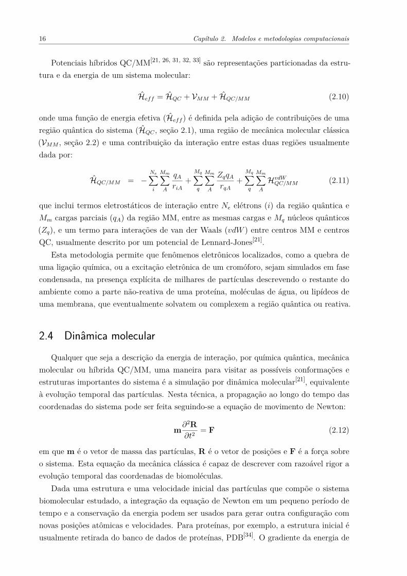
Potenciais híbridos QC/MM[21, 26, 31, 32, 33] são representações particionadas da estru-tura e da energia de um sistema molecular:

Heff = HQC + VMM + HQC/MM (2.10)

onde uma função de energia efetiva (Heff ) é definida pela adição de contribuições de umaregião quântica do sistema (HQC , seção 2.1), uma região de mecânica molecular clássica(VMM , seção 2.2) e uma contribuição da interação entre estas duas regiões usualmentedada por:

HQC/MM = −Ne∑i

Mm∑A

qA

riA

+Mq∑q

Mm∑A

ZqqA

rqA

+Mq∑q

Mm∑A

HvdWQC/MM (2.11)

que inclui termos eletrostáticos de interação entre Ne elétrons (i) da região quântica eMm cargas parciais (qA) da região MM, entre as mesmas cargas e Mq núcleos quânticos(Zq), e um termo para interações de van der Waals (vdW ) entre centros MM e centrosQC, usualmente descrito por um potencial de Lennard-Jones[21].

Esta metodologia permite que fenômenos eletrônicos localizados, como a quebra deuma ligação química, ou a excitação eletrônica de um cromóforo, sejam simulados em fasecondensada, na presença explícita de milhares de partículas descrevendo o restante doambiente como a parte não-reativa de uma proteína, moléculas de água, ou lipídeos deuma membrana, que eventualmente solvatem ou complexem a região quântica ou reativa.

2.4 Dinâmica molecularQualquer que seja a descrição da energia de interação, por química quântica, mecânica

molecular ou híbrida QC/MM, uma maneira para visitar as possíveis conformações eestruturas importantes do sistema é a simulação por dinâmica molecular[21], equivalenteà evolução temporal das partículas. Nesta técnica, a propagação ao longo do tempo dascoordenadas do sistema pode ser feita seguindo-se a equação de movimento de Newton:

m∂2R∂t2

= F (2.12)

em que m é o vetor de massa das partículas, R é o vetor de posições e F é a força sobreo sistema. Esta equação da mecânica clássica é capaz de descrever com razoável rigor aevolução temporal das coordenadas de biomoléculas.

Dada uma estrutura e uma velocidade inicial das partículas que compõe o sistemabiomolecular estudado, a integração da equação de Newton em um pequeno período detempo e a conservação da energia podem ser usados para gerar outra configuração comnovas posições atômicas e velocidades. Para proteínas, por exemplo, a estrutura inicial éusualmente retirada do banco de dados de proteínas, PDB[34]. O gradiente da energia de

2.5. Estimativa de energia livre 17

interação, ou seja, a derivada em relação às posições das funções de energia mostradasacima, determina as forças usadas na equação de movimento.

No limite de um longo tempo de simulação, podemos amostrar os estados conformacio-nais importantes visitados por um sistema molecular. São estes estados importantes quecontribuirão significativamente para a energia livre e, logo, para as observáveis médias quepretendemos obter da simulação e comparar com as medidas experimentais.

2.5 Estimativa de energia livreEnergia livre é uma quantidade fundamental em sistemas termalizados pois determina a

estabilidade e a cinética de processos e reações. Se considerarmos um equilíbrio hipotéticoentre dois estados, A ⇀↽ B, a constante de equilíbrio é:

Keq = exp[−(GB −GA

RT

)](2.13)

onde R é a constante universal dos gases, T é a temperatura, e GB é a energia livre doestado B. Pela teoria do estado de transição[35], a constante cinética é:

kvel =(kBT

h

)exp

[−(G‡ −GA

RT

)](2.14)

onde kB é a constante de Boltzmann, h é a constante de Planck e G‡ é a energia livre doestado de transição (TS) que conecta o reagente A ao produto B.

Processos ativados como reações químicas ou mudanças conformacionais de biomoléculaspodem ser convenientemente expressados em termos de uma coordenada de reação ξ quedescreve o processo (por exemplo, uma distância de ligação que será quebrada) e umpotencial de força média (PMF), que nada mais é do que a energia livre do processo aolongo da coordenada de reação. O PMF é definido a partir da função de distribuição〈ρ(ξ)〉[36]:

PMF (ξ) = kBT ln[〈ρ(ξ)〉] (2.15)

onde 〈· · ·〉 significa uma média com peso de Boltzmann:

〈ρ(ξ)〉 =∫dR δ[ξ′(R)− ξ]exp[−V(R)/kBT ]∫

dR exp[−V(R)/kBT ] (2.16)

onde V(R) é a energia potencial ou de interação do sistema em função das coordenadas Re δ[x] é a função δ de Dirac que “filtra” as coordenadas R diferentes de ξ. Na prática, afunção de distribuição ρ(ξ) é calculada a partir de um simples histograma normalizado daocorrência da coordenada de reação ξ ao longo da simulação.

Uma vez que a presença de barreiras energéticas maiores que kBT ao longo da coorde-nada de reação dificulta a visitação de conformações importantes durante uma simulação,métodos de aumento de amostragem, como a amostragem por guarda-chuva (umbrella)[36],


devem ser usados. Esta e outras metodologias similares foram empregadas em parte dosartigos compilados aqui[37, 38, 39, 40].

Assim, estimativas computacionais de energia livre para processos de interesse podemser diretamente comparadas com observações experimentais como constantes de equilíbrio(Keq) e constantes cinéticas (kvel) para validar os modelos de simulação empregados.

19

3 Enzimologia Computacional

Neste capítulo serão discutidos mecanismos catalíticos propostos para explicar ocomportamento enzimático microscopicamente, conforme detalhado no Anexo A[41]. Partedestes mecanismos, incluindo a importante contribuição eletrostática, é bem ilustradapelas reações catalisadas por proteínas-fosfatase. A simulação dos mecanismos de reaçãoda fosfatase Cdc25B é apresentada no Anexo B[38].

Neste ponto acho pertinente introduzir duas definições. O termo “mecanismo catalítico”é usado para descrever as forças ou interações microscópicas usadas por enzimas paraamplificar a velocidade de reações. Já “mecanismo de reação” é a sequência de transfor-mações químicas (quebra e formação de ligações) e mudanças de estrutura observadas aolongo da reação.

Embora existam diversas sugestões de mecanismos catalíticos, foi novamente AriehWarshel[16, 42, 43] quem escrutinizou as propostas em comparações com resultados ex-perimentais quantitativos e simulações computacionais. Sua primeira observação é queprecisamos definir uma reação de referência em solução aquosa na ausência de catalisador eum ciclo termodinâmico que permitam a comparação com a reação enzimática. Catálise quí-mica somente ocorrerá quando a barreira para reação no sítio ativo da enzima (∆G‡enz) formenor do que a barreira em solução aquosa para a mesma reação de referência (∆G‡sol), ouseja, se a diminuição da barreira para uma reação catalisada ∆∆Gcat ≡ ∆G‡enz−∆G‡sol < 0.

Para uma série de enzimas analisadas, a principal espécie estabilizada é o estado detransição no sítio ativo da enzima, como proposto por Pauling[44]. Outras sugestões como adesestabilização do estado reagente[45], o modelo do sítio dividido proposto por Menger[46] ea hipótese das conformações próximas ao ataque proposta por Bruice[47] tem contribuiçõespequenas ou inexistentes para ∆∆Gcat (Anexo A)[41].

Mas quais interações e forças moleculares promovem a estabilização do TS no sítio ativo?Novamente para uma série de enzimas, as contribuições para diminuição da energia deativação foram quantificadas para diferentes mecanismos catalíticos[48]. Catálise covalente,ou seja, a formação de um intermediário covalente ligado à enzima, contribui cerca de5 kcal/mol em média para ∆∆Gcat. Catálise ácido-base geral, quando ocorre a doaçãoou acepção de um H+ diretamente pela enzima ou intermediada por moléculas de águaativada, também contribui cerca de 5 kcal/mol em média (Anexo A)[41].

A principal força intermolecular otimizada pela evolução de enzimas tão eficientes éa interação eletrostática[49]. Classifico como eletrostáticas todas interações do substratoativado com cargas e dipolos da proteína, ligações de hidrogênio com as cadeias proteicasprincipais e laterais, assim como a coordenação não-covalente com metais ou gruposprostéticos carregados, já que estas interações podem ser razoavelmente bem descritas por

20 Capítulo 3. Enzimologia Computacional

Figura 1 – Representação pictórica da distribuição dos dipolos (setas) que solvatam rea-gentes (RS e ES, círculos) com carga localizada e estado de transição com cargadeslocalizada numa reação em solução aquosa (esquerda) ou no sítio ativo deuma enzima (direita).

forças eletrostáticas dadas pelas equações 2.8 ou 2.11.Em média a interação eletrostática contribui 17 kcal/mol para ∆∆Gcat

[48, 41], graçasprincipalmente a pre-orientação dos dipolos (e cargas parciais em geral) da proteína paraestabilizar o TS. A Figura 1 indica que embora os dipolos do solvente sejam capazes deestabilizar o TS da reação em fase aquosa, estes dipolos devem se reorganizar, com umalto custo de energia livre. Por outro lado, a enzima uma vez enovelada tem os dipolos nosítio ativo pré-organizados para complementar a distribuição de carga do TS.

As contribuições para ∆∆Gcat de efeitos entrópicos, em que a flexibilidade do substratoestaria restringida no sítio ativo, e de impedimento estérico, em que a enzima poderia“forçar” estericamente o substrato numa determinada conformação reativa, são cerca de2-3 kcal/mol, significativamente menores. Efeitos dinâmicos e quânticos como tunelamentotambém tem contribuição limitada para diminuição da energia de ativação enzimática[48, 41].

Portanto, enzimas funcionam principalmente como um “super-solvente” eletrostáticocom baixa energia de reorganização. Mas cada enzima tem sua própria receita, dependenteda reação química catalisada, em que uma combinação dos mecanismos catalíticos descritosacima pode ser utilizada (Anexo A)[41].

Os mecanismos catalíticos apresentados podem ser ilustrados pelas reações catalisadaspor proteínas-fosfatase de tirosina (PTP)[50]. Estas enzimas atuam na sinalização celularao contrabalancear a atividade de quinases e desfosforilar fosfotirosina, além de fosfoserinae fosfotreonina no caso das fosfatases duais. Perturbações neste balanço estão envolvidasem diferentes tipos de câncer[51], diabetes[52], entre outras doenças. Assim, a compreensãodo mecanismo de reação de diferentes fosfatases pode ser útil para o desenho de inibidoresmais potentes e seletivos destas enzimas.

Investiguei as reações catalisadas por duas fosfatases: VHR[37] e Cdc25B[38]. Em ambasenzimas, a principal dúvida sobre o mecanismo da primeira etapa de reação era o estado deprotonação do grupo fosfato no substrato: ou um diânion, conforme mostrado na equaçãoquímica 3.1 abaixo, ou um monoânion monoprotonado:

PTP–Cys–S− · · ·ROPO2−3 · · ·HOOC–PTP→

PTP–Cys–S–PO2−3 + ROH + −OOC–PTP (3.1)

21

PTP–Cys–S–PO2−3 + H2O + −OOC–PTP→

PTP–Cys–S− + HOPO2−3 + HOOC–PTP (3.2)

As equações acima mostram as duas etapas de reação catalisadas por proteínas-fosfatase:tiólise de éster de fosfato que leva à desfosforilação do substrato; e hidrólise do intermediáriotio-fosforilado que regenera a enzima livre. Em ambas reações temos um ácido-base geralHOOC–PTP e R representa o substrato.

Através de simulações híbridas QC/MM (seção 2.3) com uma descrição quânticasemiempírica (seção 2.1) especialmente parametrizada para reações de transferência defosfato[53], levantei perfis de energia livre (seção 2.5) para diferentes propostas de mecanismoda primeira etapa de reação (Equação 3.1). Na VHR[37], determinei que o substrato reagecomo um diânion já que a barreira calculada com este estado de protonação difere emapenas 1 kcal/mol da barreira obtida de experimentos cinéticos. A barreira calculadapara as reações com o substrato monoprotonado é cerca de 15 a 25 kcal/mol mais alta,indicando que o substrato não reage quando protonado. Na VHR, também investiguei areatividade do mutante sem o ácido-geral (D92A). A elevação da barreira calculada nestemutante foi de 5 kcal/mol, de acordo com a contribuição média indicada acima para omecanismo de catálise ácido-base geral.

Para a fosfatase Cdc25B, utilizei um modelo contendo o substrato natural, a quinasedependente de ciclina 2 bisfosforilada, Cdk2-pTpY/CycA. Ou seja, o complexo de Michaelissimulado é um complexo ternário entre Cdc25B/Cdk2-pTpY/CycA[54]. O sistema eracomposto por cerca de 130.000 átomos e, provavelmente, tratou-se da maior simulaçãohíbrida QC/MM realizada até a época que o estudo foi conduzido (Anexo B)[38].

A estrutura do sítio ativo no complexo pode ser visualizada no painel A da Figura 2.Estão mostrados apenas os átomos pesados do motivo catalítico conservado nas PTPs,o P-loop CX5R. A estrutura deste sítio é similar àquela observada para os complexosde Michaelis da VHR com substratos artificiais[37]. Nota-se aqui um preciso encaixe dasinterações eletrostáticas, principal mecanismo catalítico empregado por enzimas[41]: osgrupos NH da cadeia principal tem seus dipolos apontando e, portanto, estabilizando ogrupo fosfato dianiônico do substrato. A cadeia lateral da arginina conservada (Arg479 naCdc25B) tem carga positiva e também coordena o grupo fosfato. Contudo, a interaçãoeletrostática ótima é atingida na região do TS ao longo do progresso da reação detransferência de fosfato quando as distâncias dos contatos NH· · ·OPO2−

3 são minimizadas.As superfícies de energia livre obtidas estão mostradas na Figura 2. Duas coordenadas

de reação (seção 2.5) foram avaliadas explicitamente: ξP =d(PO)-d(PS), a diferença entrea distância da ligação quebrada e da ligação formada ao longo da transferência de fosfato;e ξH = d(OH), a distância entre o H+ doado e o oxigênio da cadeia lateral da treoninadesfosforilada. A primeira observação relevante é que as reações do substrato mono- oudianiônico se processam por mecanismos simultâneos de transferência de fosfato e de H+.Barreiras de mais de 45 kcal/mol teriam de ser transpostas para transferência por etapas,

22 Capítulo 3. Enzimologia Computacional

A

0

10

20

30

40

50

60

-2.5 -2

-1.5 -1

-0.5 0

0.5 1

1.5 2

1

1.5

2

2.5

3

3.5

4

d(PO) - d(PS)

d(OH)

C

B−3

d(O

H)

d(PO)−d(PS)

−3

d(O

H)

d(PO)−d(PS)

5

10

30

40

50

20

−2−2 −1−1 0 0 1 1 2 2

1 1

1.5 1.5

2 2

2.5 2.5

3 3

3.5 3.5

4 4

−2 −1.5

−1 −0.5

0 0.5

1 1.5

2 2

1

1.5

2

2.5

3

3.5

4

d(PO) − d(PS)

d(OH)

D

Figura 2 – Estrutura do sítio ativo da Cdc25B complexada ao seu substrato natural,fosfotreonina de Cdk2/CycA (painel A). Superfícies de energia livre em funçãode duas coordenadas de reação para desfosforilação catalisada pela Cdc25Bdo seu substrato natural na forma monoprotonada monoaniônica (painel B) edianiônica (painel C e D). O painel D representa os mesmos dados do painel Cna forma de curvas de nível com valores de energia livre indicados pela cor.

digamos, primeiro H+ e depois fosfato, ou vice-versa.A barreira calculada para a reação do substrato dianiônico com a transferência de

H+ a partir do ácido-geral E474 é de 17 kcal/mol, idêntica ao valor experimental[38].Por outro lado, a barreira calculada para a reação do substrato monoprotonado é de38 kcal/mol, o que torna esta proposta mecanística energeticamente inviável. Portanto,o ótimo acordo entre as barreiras calculadas e experimentais valida as estimativas deenergia livre com potenciais híbridos QC/MM e, logo, a determinação do mecanismo dereação catalisado pela Cdc25B frente ao seu substrato natural. Os mecanismos catalíticossubjacentes também estão de acordo com as teorias propostas para explicar a catáliseenzimática[43, 48, 41].

23

4 Metaloproteínas de Ferro-enxofre

Como mostrado no capítulo anterior, a simulação de reações de moléculas orgânicasna presença de milhares de átomos e interações em fase condensada pode ser muito bemsucedida. No entanto, o panorama é diferente para simular reações envolvendo átomos oucentros metálicos, principalmente metais de transição de camada aberta. A limitação aquiapresenta-se na descrição da estrutura eletrônica visto que as aproximações e os métodosexistentes não são tão robustos ou exatos para o tratamento de metais quanto são paramoléculas orgânicas[15, 55, 28]. O problema é o imenso número de diferentes configuraçõeseletrônicas com energia similar que estão acessíveis nos sistemas metálicos (seção 2.1).

De fato, o desenvolvimento de métodos para o tratamento de sistemas com estruturaeletrônica multiconfiguracional é a principal fronteira em aberto no cálculo de estru-tura eletrônica[15, 20, 56, 57, 30]. Investiguei uma possível solução deste problema para ocaso de agregados polinucleares de metais de transição acoplados por interações de spin(Anexo C)[20]. Desenvolvi uma série de aproximações fisicamente motivadas que resultana seleção de configurações eletrônicas e na drástica diminuição do tamanho da expansãousada na função de onda destes agregados metálicos. Consequentemente, mostrei que ocálculo da estrutura eletrônica do complexo [2Fe-2S] torna-se factível e mais robusto, semperda significativa na acuracidade (Anexo C)[20].

Mas qual a relação entre a estrutura eletrônica de centros metálicos e a química debiomoléculas? Cerca de 30% das enzimas conhecidas contém metais essenciais para suaestrutura e atividade. Átomos metálicos possuem uma plástica e complexa estruturaeletrônica que permite às metaloenzimas estabelecer estruturas únicas assim como catalisarreações eficientemente, ou mesmo reações inacessíveis sem o acoplamento com o metal.Em particular, metaloproteínas de ferro-enxofre equipadas com agregados polinuclearescomo [2Fe-2S] e [4Fe-4S] são responsáveis pela reatividade e pelas transferências eletrônicasem diversos processos biológicos essenciais como a fotossíntese e a fosforilação oxidativa[58].Um dos meus objetivos de pesquisa a longo prazo é investigar a estrutura eletrônica esimular os mecanismos de reação destas metaloproteínas (Capítulo 6).

Rubredoxina é uma proteína carregadora de elétrons envolvida em processos de oxi-dorredução em bactérias[59]. Seu centro redox possui apenas um átomo de ferro ligado aquatro cadeias laterais de cisteína ionizadas numa geometria tetraédrica (Figura 3A). É amais simples proteína de ferro-enxofre conhecida e, portanto, foi escolhida como um alvoapropriado para estudos iniciais da estrutura eletrônica destas metaloproteínas.

Recentemente, fascinantes experimentos de microscopia de força atômica (AFM) “single-molecule” descreveram o desenovelamento da rubredoxina sob tensão mecânica. Comoindicado na Figura 3B, polímeros lineares de rubredoxina são esticados e perfis de forçapor distância de tensionamento são medidos. O completo desenovelamento da rubredoxina

24 Capítulo 4. Metaloproteínas de Ferro-enxofre

só ocorrerá se pelo menos duas ligações Fe–S forem rompidas. Dada a precisão e o graude controle destes experimentos, diversas propriedades das ligações químicas Fe–S foramavaliadas[60, 61, 62, 63].

Figura 3 – A) No topo, a estrutura cristalográfica da rubredoxina cuja cadeia principalesta representada por um tubo cinza. O centro de ferro (laranja) e as cisteínasassociadas estão representados por bolas e bastões. Embaixo, um esquema docentro de ferro e sua coordenação tetraédrica, com a numeração dos resíduosde cisteína indicados. B) Esquema do experimento de AFM “single-molecule”com poli-rubredoxina representada por um cartoon, ligada numa extremidadeà ponta do microscópio e a uma base de sustentação na outra extremidade[63].

Com o objetivo de simular os experimentos de AFM, iniciei o estudo da estabilidadeda ligação Fe–S a partir de cálculos QC para a reação modelo (Anexo D)[30]

Fe(SCH3)−4 ⇀↽ Fe(SCH3)3 + CH3S− (4.1)

que mimetiza a quebra de ligação observada na rubredoxina. Comparamos uma referênciade estrutura eletrônica ab initio multiconfiguracional com diferentes funcionais de DFTe métodos semiempíricos (seção 2.1). O propósito foi encontrar um método de cálculocom acuracidade e eficiência computacional balanceadas. Determinamos que as eficientesfuncionais OLYP e OPBE apresentam os melhores resultados em comparação com areferência ab initio, e que a funcional B3LYP é satisfatória, principalmente para descriçõesda geometria dos complexos (Anexo D)[30]. Assim, obtivemos uma calibração de umametodologia QC para ser aplicada nas simulações da proteína completa.

De volta à rubredoxina, uma das principais dúvidas que emergiram dos estudos porAFM foi o mecanismo de rompimento da ligação Fe–S[60]. Poderia se tratar de uma quebrahomolítica, em que o par de elétrons da ligação quebrada é dividido igualitariamente,resultando nos produtos radical tiolato (S−I) e complexo ferroso (formalmente Fe2+, comd6 elétrons na camada de valência); ou um mecanismo heterolítico, em que o par de elétrons

25

ficaria somente com um dos produtos, resultando em ânion tiolato (S−II) e complexoférrico (formalmente Fe3+, com d5 elétrons na camada de valência).

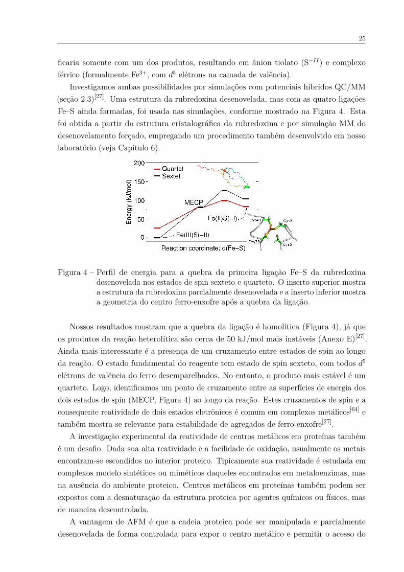
Investigamos ambas possibilidades por simulações com potenciais híbridos QC/MM(seção 2.3)[27]. Uma estrutura da rubredoxina desenovelada, mas com as quatro ligaçõesFe–S ainda formadas, foi usada nas simulações, conforme mostrado na Figura 4. Estafoi obtida a partir da estrutura cristalográfica da rubredoxina e por simulação MM dodesenovelamento forçado, empregando um procedimento também desenvolvido em nossolaboratório (veja Capítulo 6).

Figura 4 – Perfil de energia para a quebra da primeira ligação Fe–S da rubredoxinadesenovelada nos estados de spin sexteto e quarteto. O inserto superior mostraa estrutura da rubredoxina parcialmente desenovelada e a inserto inferior mostraa geometria do centro ferro-enxofre após a quebra da ligação.

Nossos resultados mostram que a quebra da ligação é homolítica (Figura 4), já queos produtos da reação heterolítica são cerca de 50 kJ/mol mais instáveis (Anexo E)[27].Ainda mais interessante é a presença de um cruzamento entre estados de spin ao longoda reação. O estado fundamental do reagente tem estado de spin sexteto, com todos d5

elétrons de valência do ferro desemparelhados. No entanto, o produto mais estável é umquarteto. Logo, identificamos um ponto de cruzamento entre as superfícies de energia dosdois estados de spin (MECP, Figura 4) ao longo da reação. Estes cruzamentos de spin e aconsequente reatividade de dois estados eletrônicos é comum em complexos metálicos[64] etambém mostra-se relevante para estabilidade de agregados de ferro-enxofre[27].

A investigação experimental da reatividade de centros metálicos em proteínas tambémé um desafio. Dada sua alta reatividade e a facilidade de oxidação, usualmente os metaisencontram-se escondidos no interior proteico. Tipicamente sua reatividade é estudada emcomplexos modelo sintéticos ou miméticos daqueles encontrados em metaloenzimas, masna ausência do ambiente proteico. Centros metálicos em proteínas também podem serexpostos com a desnaturação da estrutura proteica por agentes químicos ou físicos, masde maneira descontrolada.

A vantagem de AFM é que a cadeia proteica pode ser manipulada e parcialmentedesenovelada de forma controlada para expor o centro metálico e permitir o acesso do

26 Capítulo 4. Metaloproteínas de Ferro-enxofre

solvente e de reagentes externos, mantendo parte dos contatos proteicos nativos. Assim,em colaboração com o grupo do Prof. Hongbin Li da University of British Columbia,Canadá, que conduziu os experimentos de AFM citados acima, investigamos as alteraçõescausadas na estabilidade da ligação Fe–S na rubredoxina tensionada pela presença dereagentes como SCN−, que compete pelo centro de ferro, e H+, que compete pelo grupotiol das cisteínas.

Os resultados experimentais indicam que a presença destes reagentes diminui a forçanecessária para romper as ligações Fe–S[29]. A Figura 5 mostra os resultados computacionaispara as possíveis reações de substituição e rompimento de duas ligações Fe–S com o grupotiol sequencialmente protonado, necessárias para desenovelar a rubredoxina completamente(veja acima). Além do rompimento puramente dissociativo[27], também simulamos asreações de substituição por água. O caminho de reação mais provável é aquele com asmenores barreiras, ou seja, a sequência de protonação e substituição por água (barreirasde 27 e 34 kJ/mol) das duas ligações Fe–S (Anexo F)[29].

Figura 5 – Substituição e quebra das ligações Fe–S na rubredoxina. Painel da esquerdasuperior mostra as possíveis reações de duas ligações Fe–S sequencialmenteprotonadas. O painel da esquerda inferior mostra o perfil de energia calculadopara as mesmas reações, com as barreiras indicadas e o painel da direita mostraos perfis de energia e de força calculados para etapa limitante.

Para discernir as diferentes propostas mecanísticas, calculamos a força necessáriapara rompimento da ligação Fe–S em cada etapa dos mecanismos propostos. Na etapadeterminante da velocidade da reação com protonação (barreira de 34 kJ/mol, Figura 5),calculamos a força em cerca de 350 pN, em razoável acordo com a força medida por AFM,cerca de 160±60 pN. As forças calculadas para outras propostas são ainda maiores e,portanto, em desacordo com os dados experimentais. Observamos também que todasreações de protonação e de substituição do centro de ferro-enxofre ocorrem por mecanismoheterolítico e no spin sexteto, sem o cruzamento entre estados eletrônicos[29].

Assim, por uma combinação de experimentos de AFM com simulações computacionais,quantificamos e determinamos os possíveis mecanismos para desestabilização das ligações

27

Fe–S na rubredoxina quando o centro de ferro-enxofre é protonado ou tem seus ligantessubstituídos (Anexo F)[29].

5 Flexibilidade conformacional e complexa-ção

Conforme levantado no Capítulo 1, a estrutura de biomoléculas é bastante flexível emcondições normais. Em parte considerável do proteoma, segmentos contínuos com dezenasde aminoácidos possuem alta flexibilidade ou são intrinsecamente desordenados[65, 66]. Asconformações destes segmentos são alteradas quando interagem com outras proteínas ouaté com pequenas moléculas[67]. Então, como a distribuição estrutural destas proteínase de outras biomoléculas flexíveis pode ser descrita? Qual o papel desta flexibilidade naformação de complexos?

De volta à fosfatase Cdc25B[38], observei que a porção C-terminal do seu domíniocatalítico apresentava consideráveis flutuações de posição durante uma simulação dedinâmica molecular[68]. Estas flutuações e a possível desordem estrutural associada sãocompatíveis com observações experimentais, como a indefinição da densidade eletrônicacorrespondente à região C-terminal das fosfatases Cdc25B[69] e sua isoforma Cdc25A[70] apartir dos padrões de difração de raios-X obtidos de seus cristais.

Esta não é uma mera curiosidade estrutural. A porção C-terminal das Cdc25 tem umpapel importante no reconhecimento do substrato natural[54] e na atividade enzimática[71].Além disso, a porção C-terminal esta em contato direto com o sítio ativo e, portanto,também deve influenciar a complexação de pequenas moléculas que possivelmente atuemcomo inibidores competitivos da enzima. Assim, elegi a Cdc25B como um possível alvopara estudar as duas perguntas colocadas acima.

Para investigar o processo de complexação, utilizei três tipos de representações daestrutura da Cdc25B, com progressivo aumento de flexibilidade da região C-terminal: aestrutura cristalográfica[69]; um conjunto de estruturas obtidos por simulação de dinâmicamolecular[68]; e um conjunto de estruturas obtidas de biblioteca de rotâmeros[72]. Esteúltimo conjunto apresentava grandes flutuações e desordem na região C-terminal. Cadadescrição foi usada para gerar complexos proteína-inibidor com duas moléculas orgânicasque são potentes inibidores da atividade enzimática (Anexo G)[68].

Os resultados indicaram que o aumento da flexibilidade na cadeia principal da Cdc25Bleva a uma maior diversidade de sítios e modos de ligação dos inibidores, principalmentepelo aparecimento de sítios crípticos ou cavidades transientes na superfície da regiãoenovelada da proteína, que estão ocluídos nas representações estruturais menos flexíveis.Por exemplo, a Figura 6 mostra três modos de ligação obtidos para a representaçãoestrutural de dinâmica molecular. Para o mesmo ligante, apenas um modo foi obtidopara a estrutura cristalográfica, e oito modos foram observados para as estruturas obtidasde biblioteca de rotâmeros. A região C-terminal com maior flexibilidade, possivelmente

29

Figura 6 – Estrutura da Cdc25B obtida por simulação de dinâmica molecular. Painel Amostra três diferentes modos de ligação e uma variedade de contatos entrea Cdc25B e o ligante derivado de benzoquinona. Painel B mostra vinteestruturas sobrepostas do domínio catalítico completo da Cdc25B validadaspor experimentos de RMN. A porção C-terminal desordenada esta mostradaem vermelho.

desordenada[72], não forma sítios ou contatos estáveis com os inibidores. Assim, essa regiãonão deve contribuir significativamente para sua estabilidade, embora possa influenciar acinética de entrada ou saída de inibidores competitivos (Anexo G)[68].

No entanto, este trabalho computacional teve um caráter especulativo porque nãopossuía maiores evidências para discriminar qual seria a representação estrutural da Cdc25Bmais apropriada[68]. A etapa seguinte foi, então, buscar por validações experimentais quepermitissem determinar a correta distribuição conformacional da proteína em solução.

Expressão, purificação e medidas de espectroscopia de ressonância magnética nuclear(RMN) do domínio catalítico completo da Cdc25B selvagem foram conduzidas pelo RaphaelSayegh sob minha orientação, e coorientado pelos colegas Profs. Sandro Marana eRoberto Salinas (Anexo H). RMN provém resolução atômica da estrutura e da dinâmicaconformacional de biomoléculas em solução e, portanto, é ideal para comparações evalidações das simulações moleculares.

Depois de superar problemas com a baixa estabilidade da proteína em solução con-centrada, obtivemos diversos espectros de RMN que permitiram o assinalamento dosdeslocamentos químicos de cerca de 85% dos átomos da cadeia principal, além de medidasde acoplamento residual dipolar e de parâmetros de relaxação dos grupos NH da cadeiaprincipal. Estes dados indicaram claramente que a α-hélice presente na porção C-terminalda Cdc25B é estável e enovelada, contrariando os resultados de simulação anteriores[68, 72].Por outro lado, confirmaram que os últimos 16 aminoácidos da Cdc25B encontram-sedesordenados[68], conforme mostrado na Figura 6, e formam contatos metaestáveis com orestante da proteína (Anexo H)[71, 54].

Assim como nos estudos de reatividade em que podemos calcular observáveis experi-mentais para validar quantitativamente as simulações (Capítulo 3), nos estudos estruturaispodemos calcular todos parâmetros de RMN citados no parágrafo anterior a partir dastrajetórias de simulação de dinâmica molecular. A comparação entre os valores pode serusada para escolher um conjunto de configurações que esta de acordo com as observações

30 Capítulo 5. Flexibilidade conformacional e complexação

experimentais e descreve estatisticamente a estrutura em solução da Cdc25B (Capítulo 6).Procedimentos similares podem ser usados para qualquer outra biomolécula cujos dadosestejam disponíveis[73, 74].

Como podemos utilizar um conjunto de estruturas de uma proteína flexível paraestimar sua afinidade por pequenas moléculas? Sugeri uma possível solução eficienteque foi executada pela Ariane Alves sob minha orientação (Anexo I)[39]. A metodologiapode ser dividida em três etapas: dado conjunto de estruturas da proteína receptora,geramos complexos entre cada estrutura e a pequena molécula ligante utilizando ancoragemmolecular[75]; em seguida ranqueamos os complexos usando a aproximação de energia deinteração linear[76, 77]; finalmente agrupamos os complexos de acordo com seu ranqueamentonuma única estimativa da energia livre de complexação (i.e., a afinidade) do par receptor-ligante utilizando a teoria do ligante implícito[78].

Para testar a metodologia, escolhemos três proteínas modelo: lisozima de fago T4,transcriptase reversa de HIV-1 e proteína ligante FK506 humana. Uma grande quantidadede complexos entre estas proteínas e diferentes ligantes tem estrutura cristalográfica eafinidade experimental conhecidas[39]. Os resultados obtidos mostram que o método temboa capacidade para prever afinidades para estes três receptores. É importante que oranqueamento energético seja capaz de discriminar modos de ligação de falsos positivos seuma grande quantidade (∼ 103) de geometrias de complexos receptor-ligante for usadapara estimar a afinidade. Conforme mostrado na Figura 7A, os complexos com maiorafinidade correspondem ao sítio de ligação cristalográfico (Anexo I). Também notamosque o número e a diversidade de modos de ligação encontrados aumenta para as proteínasmais flexíveis, de acordo com meu estudo anterior[68].

Figura 7 – A) Superposição de poses da lisozima T4 (cinza) complexada a 2-propilfenol,colorido de acordo com sua energia de ligação. O sítio de ligação cristalográ-fico esta populado com ligantes em vermelho e laranja. B) Conformação daubiquinona (UQ10, em licorice) complexada à membrana de POPC (em linhas,cadeias acila em ciano, oxigênios em vermelho e nitrogênio da colina em azul).

31

Flexibilidade e dinâmica conformacional também são fundamentais para função deoutras biomoléculas. Ubiquinona ou coenzima-Q é a molécula universal carregadorade carga em processos celulares de transferência eletrônica. Sua localização e partiçãomembranar tem sido debatidas há décadas[79, 80, 81, 82] e sua difusão entre os complexosrespiratórios até já foi proposta como a etapa limitante da velocidade de toda fosforilaçãooxidativa[83].

Com objetivo de resolver este longo debate e permitir futuros estudos da reatividadeda ubiquinona nos complexos respiratórios (Capítulo 6), a Dra. Vanesa Galassi realizousob minha supervisão a parametrização de um campo de força para ubiquinona e diversassimulações de sua complexação com membranas modelo (Anexo J)[40].

A calibração do modelo molecular foi realizada meticulosamente pela parametrizaçãoda função de energia MM (seção 2.2) da ubiquinona em comparação com dados obtidos porcálculos QC de alto nível (seção 2.1) para complexos isolados, e pela estimativa de perfisde energia livre (seção 2.5) de complexação de ubiquinonas com diferentes comprimentosda cadeia isoprênica a membranas modelo de 1-palmitoil-2-oleoil-sn-glicero-3-fosfocolina(POPC). As energias livres de ligação ubiquinona-membrana calculadas estão em ótimoacordo com as constantes de partição medidas experimentalmente para uma série homólogade ubiquinonas. O mesmo acordo foi observado entre as constantes de difusão calculadas eexperimentais[40].

As simulações também indicam claramente a localização da ubiquinona inserida namembrana. A cabeça quinona esta na região interfacial da membrana, próxima aosgrupos glicerol do lipídeo, altamente hidratada e com orientação normal ao plano damembrana. As primeiras unidades isoprênicas da cadeia estão estendidas e a caudaatravessa e interdigita a membrana nas ubiquinonas com seis ou mais unidades isopreno(Figura 7). Esta localização é notável porque coincide com a localização dos sítios ativosredox na citocromo bc1 (Qi e Qo) e com a entrada do sítio de ligação do substrato naNADH:ubiquinona redutase. Logo, a evolução parece ter otimizado a localização destessítios proteicos de acordo com as propriedades fisioquímicas da ubiquinona para facilitar a(des)complexação deste substrato (Anexo J)[40].

6 Conclusões e Perspectivas

Apresentei acima uma sistematização das minhas contribuições científicas recentes.Estes trabalhos foram realizados sob minha coordenação, como único autor ou em colabo-ração com colegas e estudantes sob minha orientação. Acredito que o texto demonstra aindependência e a coesão da pesquisa realizada.

Sem dúvida, a importância de cálculo e simulação computacional em bioquímica ebiofísica é crescente. Nestas áreas de pesquisa, simulações são tipicamente empregadaspara ajudar ou aprofundar a interpretação de resultados experimentais. Antevejo que numfuturo próximo, simulações terão ainda maior importância e capacidade preditiva, e serãousadas crescentemente para dirigir a pesquisa e propor experimentos validatórios. Isto jáocorre em diversas áreas da física, por exemplo. Nosso estudo da estrutura da Cdc25Be diversas outras linhas de pesquisa, notadamente o desenho de enzimas e estruturasproteicas[84, 85], caminham por esta via.

Métodos computacionais, em particular híbridos QC/MM, contribuíram decisivamentepara determinação das forças intermoleculares e dos mecanismos catalíticos que operamem diferentes enzimas. A estabilização eletrostática do estado de transição proporcionadapelo ambiente enzimático pré-organizado foi identificada como a principal contribuiçãopara catálise. Em particular, determinei o mecanismo de reação para fosfatase Cdc25B,em ótimo acordo com observáveis experimentais (Capítulo 3).

A simulação molecular de metaloenzimas apresenta diversos desafios. Propomosaproximações para o estudo de agregados metálicos polinucleares, como os centros [2Fe-2S]encontrados na cadeia de transporte de elétrons da fosforilação oxidativa. Avaliamosquais metodologias aproximadas de cálculo de estrutura eletrônica seriam indicadas paraestudar a reatividade das ligações Fe–S encontradas nesses agregados e investigamos aestabilidade desta ligação numa metaloproteína simples, a rubredoxina, em comparaçãocom experimentos de AFM (Capítulo 4). Estes estudos formam uma sólida base parafuturas investigações de metaloproteínas de ferro-enxofre mais complexas.

Investigamos o papel da flexibilidade estrutural no reconhecimento entre biomoléculas.Para a fosfatase Cdc25B, simulei a formação de complexos com pequenas moléculas paradiferentes conjuntos de estruturas tridimensionais e conduzimos experimentos de RMN paravalidar qual o modelo estrutural mais apropriado. Propomos uma metodologia para prevera afinidade de complexos entre pequenas moléculas e proteínas flexíveis, representadas porconjuntos de estruturas. Determinamos a partição, localização e a difusão de ubiquinonacomplexada à membrana fosfolipídica, novamente em ótimo acordo com experimentos(Capítulo 5).

A construção de um ensemble conformacional que represente a estrutura da Cdc25Bserá realizada no futuro próximo pela combinação das medidas de RMN com observáveis

33

calculadas e pela seleção de geometrias estatisticamente bem distribuídas[13, 73] obtidas desimulação de dinâmica molecular. Este ensemble conformacional será usado para previsãode modos de ligação da Cdc25B por inibidores e fosfato inorgânico, e de contatos transientesentre o núcleo proteico enovelado e a região C-terminal desordenada. Experimentos deRMN de pertubação do deslocamento químico serão usados na validação destas previsões.

Nossos futuros estudos de reatividade enzimática estarão focados nos mecanismos de re-ação de proteínas de ferro-enxofre. Em particular, estudaremos os três primeiros complexosrespiratórios mitocondriais equipados com agregados de ferro-enxofre: NADH:ubiquinonaredutase, succinato desidrogenase e citocromo bc1. Modelos tridimensionais destas proteí-nas embebidas em membranas lipídicas já foram construídos. Dentro desta linha, chamadade Bioenergética Molecular Computacional, investigaremos o mecanismo de acoplamentoentre a redução de quinona e o bombeamento de H+ no complexo I[86] e as transferênciaseletrônicas observadas na etapa determinante de velocidade no ciclo-Q do complexo III[87].

Finalmente, continuaremos a simulação e a interpretação de experimentos de AFM.No momento, terminamos o desenvolvimento e a calibração de um método de mecânicamolecular capaz de descrever o rompimento de ligações covalentes mecanicamente induzidas.

Referências

1 LAD, C.; WILLIAMS, N. H.; WOLFENDEN, R. The rate of hydrolysis ofphosphomonoester dianions and the exceptional catalytic proficiencies of protein andinositol phosphatases. Proc. Natl. Acad. Sci. USA, v. 100, p. 5607–5610, 2003.

2 SLATER, J. C. Quantum Theory of Atomic Structure. 1st. ed. New York: McGraw-Hill,1960.

3 FIELD, M. J. Simulating enzyme reactions: Challenges and perspectives. J. Comp.Chem., v. 23, p. 48–58, 2002.

4 JORGENSEN, W. L. The many roles of computation in drug discovery. Science, v. 303,p. 1813–1818, 2004.

5 SHAW, D. E. et al. Atomic-level characterization of the structural dynamics of proteins.Science, v. 330, p. 341–346, 2010.

6 WINSBERG, E. Science in the Age of Computer Simulation. 1st. ed. Chicago, EUA:The University of Chicago Press, 2010.

7 WEBER, J. K.; SHUKLA, D.; PANDE, V. S. Heat dissipation guides activation insignaling proteins. Proc. Natl. Acad. Sci. USA, v. 112, p. 10377–10382, 2015.

8 HIRSCHFELDER, J. O.; MEATH, W. J. The nature of intermolecular forces. Adv.Chem. Phys., v. 12, p. 3–106, 1967.

9 JEZIORSKI, B.; MOSZYNSKI, R.; SZALEWICZ, K. Perturbation theory approach tointermolecular potential energy surfaces of van der Waals complexes. Chem. Rev., v. 94, p.1887–1930, 1994.

10 MCQUARRIE, D. A. Statistical Mechanics. 1st. ed. New York: Harper and Row,1976.

11 GODFREY-SMITH, P. Theory and Reality: An introduction to the philosophy ofscience. 1st. ed. Chicago, EUA: The University of Chicago Press, 2003.

12 HIRSCH, M. W.; SMALE, S.; DEVANEY, R. L. Differential Equations, DynamicalSystems, and an Introduction to Chaos. 2nd. ed. Oxford, UK: Academic Press, 2004.

13 ZUCKERMAN, D. M. Statistical Physics of Biomolecules: An Introduction. 1st. ed.[S.l.]: CRC Press, 2010.

14 DIRAC, P. Quantum mechanics of many-electron systems. Proc. R. Soc. London Ser.A, v. 123, p. 714–733, 1929.

15 HELGAKER, T.; JØRGENSEN, P.; OLSEN, J. Molecular Electronic-StructureTheory. 1st. ed. New York: Wiley, 2000.

16 WARSHEL, A. Computer Modeling of Chemical Reactions in Enzymes and Solutions.1st. ed. New York: Wiley, 1991.

Referências 35

17 SHAIK, S. S.; SCHLEGEL, H. B.; WOLFE, S. Theoretical Aspects of PhysicalOrganic Chemistry: The SN2 Mechanism. 1st. ed. New York: Wiley, 1992.

18 THIEL, W. Semiempirical methods. In: GROTENDORST, J. (Ed.). ModernMethods and Algorithms of Quantum Chemistry. Jülich: John von Neumann Institute forComputing, 2001. v. 3, p. 261–283.

19 PARR, R. G.; YANG, W. Density-Functional Theory of Atoms and Molecules. 1st. ed.Oxford: Oxford University Press, 1996.

20 ARANTES, G. M.; TAYLOR, P. R. Approximate multiconfigurational treatment ofspin-coupled metal complexes. J. Chem. Theory Comput., v. 6, p. 1981–1989, 2010.

21 FIELD, M. J. A Pratical Introduction to the Simulation of Molecular Systems. 1st. ed.Cambridge: Cambridge University Press, 1999.

22 JORGENSEN, W. L.; TIRADO-RIVES, J. Monte Carlo vs molecular dynamics forconformational sampling. J. Phys. Chem., v. 100, p. 14508–14513, 1996.

23 CORNELL, W. D. et al. A second generation force field for the simulation of proteins,nucleic acids, and organic molecules. J. Am. Chem. Soc., v. 117, p. 5179–5197, 1995.

24 MACKERELL JR., A. D. et al. All-atom empirical potential for molecular modelingand dynamics studies of proteins. J. Phys. Chem. B, v. 102, p. 3586–3616, 1998.

25 WARSHEL, A.; LEVITT, M. Theoretical studies of enzymic reactions: Dielectric,electrostatic and steric stabilization of the carbonium ion in the reaction of lysozyme. J.Mol. Biol., v. 103, p. 227–249, 1976.

26 FIELD, M. J.; BASH, P. A.; KARPLUS, M. A combined quantum mechanical andmolecular mechanical poteintial for molecular dynamics simulations. J. Comput. Chem.,v. 11, p. 700–733, 1990.

27 ARANTES, G. M.; BHATTACHARJEE, A.; FIELD, M. J. Homolytic cleavage ofFe–S bonds in rubredoxin under mechanical stress. Angew. Chem. Int. Ed., v. 52, p.8144–8146, 2013.

28 BHATTACHARJEE, A. et al. Theoretical modeling of low energy electronictransitions in reduced cobaloximes. ChemPhysChem, v. 15, p. 2951–2958, 2014.

29 ZHENG, P. et al. Force induced chemical reactions on the metal center in a singlemetalloprotein molecule. Nature Comm., v. 6, p. 7569, 2015.

30 ARANTES, G. M.; FIELD, M. J. Ferric-thiolate bond dissociation studied withelectronic structure calculations. J. Phys. Chem. A, v. 119, p. 10084–10090, 2015.

31 FIELD, M. J. The pDynamo program for molecular simulations using hybridquantum chemical and molecular mechanical potentials. J. Chem. Theory Comput., v. 4,p. 1151–1161, 2008.

32 FIELD, M. J. et al. The DYNAMO library for molecular simulations using hybridquantum mechanical and molecular mechanical potentials. J. Comput. Chem., v. 21, p.1088–1100, 2000.

36 Referências

33 ARANTES, G. M.; RIBEIRO, M. C. C. A microscopic view of substitution reactionssolvated by ionic liquids. J. Chem. Phys., v. 128, p. 114503, 2008.

34 The Protein Data Bank. 2002. Royal Society Protein Data Bank. http://www.pdb.org.

35 TRUHLAR, D. G.; GARRETT, B. C.; KLIPPENSTEIN, S. J. Current status oftransition-state theory. J. Phys. Chem., v. 100, p. 12771–12800, 1996.

36 ROUX, B. The calculation of the potential of mean force using computer simulations.Comp. Phys. Comm., v. 91, p. 275–282, 1995.

37 ARANTES, G. M. Free energy profiles for catalysis by dual-specificity phosphatases.Biochem. J., v. 399, n. 2, p. 343–350, 2006.

38 ARANTES, G. M. The catalytic acid in the dephosphorylation of the Cdk2-pTpY/CycA protein complex by Cdc25B phosphatase. J. Phys. Chem. B, v. 112, p.15244–15247, 2008.

39 NUNES-ALVES, A.; ARANTES, G. M. Ligand-receptor affinities computed byan adapted linear interaction model for continuum electrostatics and by proteinconformational averaging. J. Chem. Inf. Model., v. 54, p. 2309–2319, 2014.

40 GALASSI, V. V.; ARANTES, G. M. Partition, orientation and mobility ofubiquinones in a lipid bilayer. Biochim. Biophys. Acta, v. 1847, p. 1345, 2015.

41 ARANTES, G. M. A computational perspective on enzymatic catalysis. Quim. Nova,v. 31, p. 377–383, 2008.

42 ÅQVIST, J.; WARSHEL, A. Simulation of enzyme-reactions using valence-bondforce-fields and other hybrid quantum-classical approaches. Chem. Rev., v. 93, p.2523–2544, 1993.

43 WARSHEL, A. et al. Electrostatic basis for enzyme catalysis. Chem. Rev., v. 106, p.3210–3235, 2006.

44 PAULING, L. Nature of forces between large molecules of biological interest. Nature,v. 161, p. 707–709, 1948.

45 JENCKS, W. P. Catalysis in Chemistry and Enzymology. 1st. ed. New York: Dover,1987.

46 MENGER, F. M. Analysis of ground-state and transition-state effects in enzymecatalysis. Biochemistry, v. 31, p. 5368–5373, 1992.

47 BRUICE, T. C.; LIGHTSTONE, F. C. Ground state and transition state contributionsto the rates of intramolecular and enzymatic reactions. Acc. Chem. Res., v. 32, p. 127–136,1999.

48 GARCIA-VILOCA, M. et al. How enzymes work: Analysis by modern rate theoryand computer simulations. Science, v. 303, p. 186–195, 2004.

49 WARSHEL, A.; FLORIáN, J. Computer simulation of enzyme catalysis: Finding outwhat has been optimized by evolution. Proc. Natl. Acad. Sci. USA, v. 95, p. 5950–5955,1998.

Referências 37

50 GOLDSTEIN, B. J. Tyrosine Phospoprotein Phosphatases. 2nd. ed. Oxford: OxfordUniversity Press, 1998.

51 OSTMAN, A.; HELLBERG, C.; BOHMER, F. Protein-tyrosine phosphatases andcancer. Nat. Rev. Cancer, v. 6, p. 307–320, 2006.

52 JOHNSON, T.; ERMOLIEFF, J.; MR, M. J. Protein tyrosine phosphatase 1binhibitors for diabetes. Nat. Rev. Drug Discovery, v. 1, p. 696–709, 2002.

53 ARANTES, G. M.; LOOS, M. Specific parametrisation of a hybrid potential tosimulate reactions in phosphatases. Phys. Chem. Chem. Phys., v. 8, p. 347–353, 2006.

54 SOHN, J. et al. Experimental validation of the docking orientation of Cdc25 with itsCdk2-CycA protein substrate. Biochemistry, v. 44, p. 16563–16573, 2005.

55 CRAMER, C. J.; TRUHLAR, D. G. Density functional theory for transition metalsand transition metal chemistry. Phys. Chem. Chem. Phys., v. 11, p. 10757–10816, 2009.

56 CHAN, G. K.-L. Low entanglement wavefunctions. WIREs Comput. Mol. Sci., v. 2, p.907–920, 2012.

57 OLIVARES-AMAYA, R. et al. The ab-initio density matrix renormalization group inpractice. J. Chem. Phys., v. 142, p. 034102, 2015.

58 BEINERT, H.; HOLM, R. H.; MUNCK, E. Iron-sulfur clusters: Nature’s modular,multipurpose structures. Science, v. 277, p. 653–659, 1997.

59 VOET, D.; VOET, J. Biochemistry. 2nd. ed. New York: Wiley, 1995.

60 ZHENG, P.; LI, H. Highly covalent ferric-thiolate bonds exhibit surprisingly lowmechanical stability. J. Am. Chem. Soc., v. 133, p. 6791–6798, 2011.

61 ZHENG, P. et al. Hydrogen bond strength modulates the mechanical strength offerric-thiolate bonds in rubredoxin. J. Am. Chem. Soc., v. 134, p. 4124–4131, 2012.

62 ZHENG, P. et al. Single molecule force spectroscopy reveals that iron is released fromthe active site of rubredoxin by a stochastic mechanism. J. Am. Chem. Soc., v. 135, p.7992–8000, 2013.

63 ZHENG, P. et al. Single molecule force spectroscopy reveals the molecular mechanicalanisotropy of the fes4 metal center in rubredoxin. J. Am. Chem. Soc., v. 135, p.17783–17792, 2013.

64 SCHRODER, D.; SHAIK, S.; SCHWARZ, H. Two-state reactivity as a new conceptin organometallic chemistry. Acc. Chem. Res., v. 33, p. 139–145, 2000.

65 DUNKER, A. K. et al. The roles of intrinsic disorder in protein interaction networks.FEBS Lett., v. 272, p. 5129–5148, 2005.

66 RADIVOJAC, P. et al. Intrinsic disorder and functional proteomics. Biophys. J.,v. 92, p. 1439–1456, 2007.

67 WRIGHT, P. E.; DYSON, H. J. Linking folding and binding. Curr. Op. Struct. Biol.,v. 19, p. 31–38, 2009.

38 Referências

68 ARANTES, G. M. Flexibility and inhibitor binding in Cdc25 phosphatases. Proteins:Struct. Funct. Genet., v. 78, p. 3017–3032, 2010.

69 REYNOLDS, R. A. et al. Crystal structure of the catalytic subunit of Cdc25brequired for G(2)/M phase transition of the cell cycle. J. Mol. Biol., v. 293, p. 559–568,1999.

70 FAUMAN, E. B. et al. Crystal structure of the catalytic domain of the human cellcycle control phosphatase, Cdc25A. Cell, v. 93, p. 617–625, 1998.

71 WILBORN, M. et al. The c-terminal tail of the dual-specificity Cdc25B phosphatasemediates modular substrate recognition. Biochemistry, v. 40, p. 14200–14206, 2001.

72 MAMONOV, A. B. et al. General library-based monte carlo technique enablesequilibrium sampling of semi-atomistic protein models. J. Phys. Chem. B, v. 113, p.10891–10904, 2009.

73 LEUNG, H. T. A. et al. A rigorous and efficient method to reweight very largeconformational ensembles using average experimental data and to determine their relativeinformation content. J. Chem. Theory Comput., v. 12, p. 383–394, 2016.

74 NODET, G. et al. Quantitative description of backbone conformational sampling ofunfolded proteins at amino acid resolution from NMR residual dipolar couplings. J. Am.Chem. Soc., v. 131, p. 17908–17918, 2009.

75 SOUSA, S. F.; FERNANDES, P. A.; RAMOS, M. J. Protein–ligand docking: currentstatus and future challenges. Proteins, v. 65, p. 15–26, 2006.

76 GALLICCHIO, E.; KUBO, M. M.; LEVY, R. M. Enthalpy–entropy and cavitydecomposition of alkane hydration free energies: numerical results and implications fortheories of hydrophobic solvation. J. Phys. Chem. B, v. 104, p. 6271–6285, 2000.

77 ÅQVIST, J.; LUZHKOV, V. B.; BRANDSDAL, B. O. Ligand binding affinities frommd simulations. Acc. Chem. Res., v. 35, p. 358–365, 2002.

78 MINH, D. D. L. Implicit ligand theory: rigorous binding free energies andthermodynamic expectations from molecular docking. J. Chem. Phys., v. 137, p. 104106,2012.

79 KATSIKAS, H.; QUINN, P. The polyisoprenoid chain length influences the interactionof ubiquinones with phospholipid bilayers. Biochim. Biophys. Acta, v. 689, p. 363–369,1982.

80 LENAZ, G. et al. Localization and preferred orientations of ubiquinone homologs inmodel bilayers. Biochem. Cell. Biol., v. 70, p. 504–514, 1992.

81 METZ, G. et al. Nmr studies of ubiquinone location in oriented model membranes:Evidence for a single motionally-averaged population. J. Am. Chem. Soc., v. 117, p.564–565, 1995.

82 HAUSS, T. et al. Localization of coenzyme q10 in the center of a deuterated lipidmembrane by neutron diffraction. Biochim. Biophys. Acta, v. 1710, p. 57–62, 2005.

Referências 39

83 LENAZ, G.; FATO, R. Is ubiquinone diffusion rate-limiting for electron transfer? J.Bioener. and Biomem., v. 18, p. 369–401, 1986.

84 DAS, R.; BAKER, D. Macromolecular modeling with rosetta. Annu. Rev. Biochem.,v. 77, p. 363–382, 2008.

85 FLEISHMAN, S.; BAKER, D. Role of the biomolecular energy gap in protein design,structure, and evolution. Cell, v. 149, p. 262–273, 2012.

86 SAZANOV, L. A. A giant molecular proton pump: structure and mechanism ofrespiratory complex i. Nature Rev Mol Cell Biol, v. 16, p. 375–388, 2015.

87 CROFTS, A. R. et al. The Q-cycle reviewed: How well does a monomeric mechanismof the bc1 complex account for the function of a dimeric complex? Biochim. Biophys.Acta, v. 1777, p. 1001–1019, 2008.

40

ANEXO A – A computational perspectiveon enzymatic catalysis

Quim. Nova, Vol. 31, No. 2, 377-383, 2008

Rev

isão

*e-mail: [email protected]

UMA PERSPECTIVA COMPUTACIONAL SOBRE CATÁLISE ENZIMÁTICA

Guilherme M. Arantes*Instituto de Química, Universidade de São Paulo, Av. Lineu Prestes 748, 05508-900 São Paulo - SP, Brasil

Recebido em 24/11/06; aceito em 18/5/07; publicado na web em 19/12/07

A COMPUTATIONAL PERSPECTIVE ON ENZYMATIC CATALYSIS. Enzymes are extremely efficient catalysts. Here, part ofthe mechanisms proposed to explain this catalytic power will be compared to quantitative experimental results and computersimulations. Influence of the enzymatic environment over species along the reaction coordinate will be analysed. Concepts oftransition state stabilisation and reactant destabilisation will be confronted. Divided site model and near-attack conformationhypotheses will also be discussed. Molecular interactions such as covalent catalysis, general acid-base catalysis, electrostatics, entropiceffects, steric hindrance, quantum and dynamical effects will also be analysed as sources of catalysis. Reaction mechanisms, inparticular that catalysed by protein tyrosine phosphatases, illustrate the concepts.

Keywords: enzymatic catalysis; computer simulation; reaction mechanism.

INTRODUÇÃO

Enzimas são catalisadores de extraordinária eficiência. Os au-mentos de velocidade de reações alcançados por enzimas podemchegar a vinte ordens de magnitude1 ! Por outro lado, enzimas pos-suem uma grande especificidade pelos substratos, sua atividade écontrolável e totalmente seletiva.

Sob uma perspectiva teórica, a sugestão de Fischer2, conhecidacomo a hipótese da “chave e fechadura”, foi a primeira propostapara explicar o poder catalítico das enzimas. Com o advento dateoria do estado de transição3 nos anos 1930, Pauling4 propôs queesta espécie seria preferencialmente ligada pelo sítio ativo enzi-mático. Já em 1969, Jencks5 escreveu que “o estudo dos mecanis-mos moleculares de catálise enzimática é necessariamente empíricoe qualitativo”. No entanto, nos últimos 30 anos, simulaçõescomputacionais que permitem determinações quantitativas de pro-priedades termodinâmicas têm alterado este panorama, apon-tando e quantificando os mecanismos catalíticos empregados porenzimas.

Cabem aqui duas definições. O termo “mecanismo catalítico”é usado para descrever as forças ou interações microscópicas utili-zadas pelas enzimas para amplificar a velocidade de reações. Já“mecanismo de reação” é a seqüência de transformações (quebra eformação de ligações químicas) e mudanças de estrutura do com-plexo enzimático observadas ao longo do progresso da reação.

Diversos mecanismos catalíticos já foram propostos para ex-plicar as acelerações enzimáticas em nível microscópico. Por exem-plo, Menger contabilizou 21 teorias sobre catálise enzimática6. Estenúmero é elevado em conseqüência de diferentes interpretaçõessemânticas e imprecisas definições de quantidades termodinâmicasnas teorias propostas, e também porque a maior parte destas teori-as não foi (ou não pode ser) testada quantitativamente. Portanto,há muita controvérsia sobre a importância de cada um dos diferen-tes mecanismos e teorias propostos para explicar o poder catalíticodas enzimas7-9.

Sem dúvida, cada enzima possui sua própria “receita”6 paracatálise, em que uma combinação das interações propostas podeestar atuando. O principal objetivo deste texto é analisar e

quantificar a contribuição de cada uma destas interações para oaumento da velocidade de reações no ambiente enzimático. Inici-almente apresentaremos o modelo básico e suas equaçõesmacroscópicas para a atividade enzimática, e a definição de reaçãode referência em solução aquosa, que deve ser usada na compara-ção com a reação enzimática. Em seguida, discutiremos qual espé-cie ao longo da coordenada de reação sofre influência determinantedo ambiente enzimático. A hipótese de desestabilização do estadoreagente (complexo enzima-substrato ou complexo de Michaelis)será confrontada com a hipótese de estabilização do estado de tran-sição (TS)3. Propostas relacionadas como as conformações próxi-mas ao ataque10 e do sítio dividido6 também serão analisadas.

As interações moleculares usadas para explicar os mecanismoscatalíticos, incluindo catálise covalente, catálise ácido-base geral,interação eletrostática, efeitos entrópicos, impedimento estérico e,efeitos quânticos e dinâmicos serão discutidas. Esta lista deinterações pode ser incompleta, dada a limitação de tamanho paraeste texto, e parcial, pois reflete as propostas que foram testadas equantificadas por simulações computacionais. Mecanismos de re-ação de algumas enzimas, em particular as proteínas tirosina-fosfatases, serão usados para ilustrar os conceitos discutidos11.

DESCRIÇÃO MACROSCÓPICA

As Equações de Michaelis-Mentem12,13 são o modelo básico usadopara descrever cinética enzimática para um único substrato, S:

(1)

(2)

(3)

onde E denota enzima, P é o produto, KS é a constante de equilíbrio

para dissociação do complexo E.S, kcat

é a constante de velocidadede reação observada e K

M é a constante de Michaelis. Na maioria

dos casos, k-1 >> k

cat, portanto, K

S ≈ K

M. Neste modelo, a velocida-

378 Quim. NovaArantes

de inicial de formação do produto, v = kcat

[E.S], também pode serescrita como:

(4)

onde definimos a concentração total de enzima, [E]T = [E] + [E.S].

Equações semelhantes também são válidas para sistemas mais com-plexos como, por exemplo, na presença de dois ou mais substratosdiferentes. Nestes casos, a definição da constante K

S é alterada.

Considerando este modelo, existem três maneiras da evoluçãomaximizar a constante de velocidade de catálise aparente, definidacomo k

cat / K

M. Alteração somente de K

S para um determinado substrato

pode amplificar a velocidade de catálise aparente pelo aumento da[E.S], além de modificar a seletividade por este substrato. Um dospossíveis mecanismos empregados neste caso é o encaminhamento,em que o volume livre para difusão do substrato é reduzido ou pormudanças estruturais na enzima (como em complexos enzimáticosmulti-unidades) ou por interações eletrostáticas que guiam o substratopara o sítio ativo14. A velocidade de catálise também pode seramplificada pelo aumento da k

cat sem alteração da seletividade pelo

substrato, ou seja, apenas aumentando a velocidade da etapa de trans-formação química na enzima. Finalmente, a velocidade de catálisepode ser aumentada pela modificação simultânea de k

cat e K

S. Não

discutiremos aqui processos que alterem apenas a associação entreenzima e substrato (K

S). Este texto focaliza os processos que aumen-

tam a velocidade de catálise principalmente pelo aumento de kcat

.

REAÇÃO DE REFERÊNCIA

Para identificação das fontes de aceleração enzimática, a rea-ção catalisada deve ser comparada com uma reação de referênciaem solução aquosa sem catálise. Caso a reação enzimática e a rea-ção observada em solução ocorrem segundo o mesmo mecanismo,ou seja, possuam um estado de transição semelhante, o seguinteciclo termodinâmico pode ser usado para comparação:

(5)

A velocidade de reação na enzima será maior que a reação nãocatalisada em solução se k

cat / K

S > k

non. Neste caso, a afinidade da

enzima pelo TS ou complexo ativado, S‡, é KTS

= (kcat

/ KS)/k

non > 0,

ou seja, o complexo ativado é mais estável quando ligado à enzimaque quando em solução.

No entanto, o mecanismo de reação atuante no sítio enzimáticopode ser diferente do mecanismo de reação observado em soluçãoaquosa na ausência do catalisador. Por exemplo, a hidrólise deésteres de fosfato em solução aquosa ocorre diretamente num ata-que nucleofílico por uma molécula de água. Porém, a mesma rea-ção catalisada pelas proteínas tirosina-fosfatases (PTPs) ocorre emduas etapas: uma tiólise do éster de fosfato, seguida de uma hidrólisedo intermediário tiofosforilado (Figura 1)15,16.

Nestes casos, o mecanismo de reação na enzima não deve ser

diretamente comparado com o mecanismo observado em soluçãovia um ciclo termodinâmico como o da Equação 5. A análise doefeito enzimático deve ser feita em comparação com uma reaçãode referência em solução aquosa (caracterizada por k

non), constituí-

da pelos mesmos grupos reativos (R e S na Figura 2) e o mesmomecanismo de reação na enzima, mas solvatados por água. (Figura2)9,17. Simulações computacionais podem ser usadas para calcularo perfil energético das reações de referência que são inacessíveisexperimentalmente18-20.

ESPÉCIE CATALISADA

Estabilização do TS ou desestabilização do reagente?

A hipótese da “chave e fechadura” proposta inicialmente porFischer para racionalizar o poder catalítico das enzimas foi esten-dida pela proposta de Haldane2, em que o substrato não “encaixa”exatamente na enzima, mas sofre uma distorção após a formaçãodo complexo E.S, e pela proposta de Pauling4, em que a enzima seliga mais fortemente ao TS que ao substrato.

A hipótese de Pauling apóia-se no conceito de estado de transi-ção3 e diz que este é mais estabilizado no sítio ativo da enzima emrelação a mesma espécie numa reação de referência em soluçãoaquosa. Esta hipótese é amplamente aceita como principal fontede catálise e parece válida em todas enzimas já analisadas quanti-tativamente2,10,18,19,21,22.

Centenas de estruturas tridimensionais determinadas paraenzimas complexadas a análogos de TS apóiam a noção decomplementaridade entre as estruturas do sítio ativo e do TS. Estescomplexos são de grande utilidade prática no desenho de drogasque funcionam como inibidores enzimáticos competitivos13. Noentanto, comprovar a hipótese de Pauling por experimentos não édiretamente possível, já que um TS é um objeto transiente. Simu-lações computacionais de reações enzimáticas mostram repetida-mente8,21-24 que a interação eletrostática entre o ambiente enzimáticoe o TS é a maior responsável pela diminuição de ΔG‡

enz em relação

a ΔG‡sol

(Figura 2), demonstrando que o TS é a principal espécieque sofre catálise ao longo da coordenada de reação na enzima.

A afirmação de “maior ligação ou afinidade da enzima peloTS” é por vezes interpretada literalmente, como se o TS fosse atin-

Figura 1. Esquema da reação de hidrólise catalisada pelas proteínas tirosina-fosfatases (PTP). Ph indica um grupo fenil e CYS, o resíduo de cisteina

Figura 2. Esquema do perfil energético de uma reação enzimática e suareferência em solução. ΔG

B , ΔG

comp , ΔG‡

enz e ΔG‡

sol são, respectivamente, a

energia livre de formação do complexo entre a enzima E-R e o substrato S,

de complexação entre os reagentes R e S em solução, de ativação da reaçãono ambiente enzimático e de ativação da reação no complexo de encontro

R.S dos reagentes em solução. A região com linhas diagonais indica o solvente

aquoso

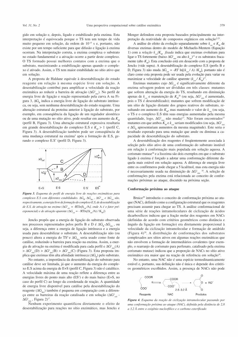
379Uma perspectiva computacional sobre catálise enzimáticaVol. 31, No. 2

gido em solução e, depois, ligado e estabilizado pela enzima. Estainterpretação é equivocada porque o TS tem um tempo de vidamuito pequeno em solução, da ordem de 10-15 s e, portanto, nãoexiste por um tempo suficiente para que difusão e ligação à enzimaocorram. Na interpretação correta, a enzima complexa o substratono estado fundamental e a ativação ocorre a partir deste complexo.O TS formado possui melhores contatos com a enzima que osubstrato, maximizando a estabilização apenas quando o comple-xo é ativado. Assim, o TS tem maior estabilidade no sítio ativo queem solução.

A proposta de Haldane equivale à desestabilização do estadoreagente em relação à mesma espécie livre em solução. Adesestabilização contribui para amplificar a velocidade da reaçãoenzimática ao reduzir a barreira de ativação (ΔG‡

enz). No perfil de

energia livre de ligação e reação representado pela curva A na Fi-gura 3, ΔG

B indica a energia livre de ligação do substrato intrínse-

ca, ou seja, sem nenhuma desestabilização do estado reagente. Umaalteração estrutural da proteína anterior à ligação do substrato, porexemplo, em conseqüência da ligação de um regulador alostéricoou de uma mutação no sítio ativo, pode resultar em aumento da K

M

(perfil B, Figura 3). Uma alteração estrutural expressiva resultariaem grande desestabilização do complexo E.S e K

M > 1 (perfil C,

Figura 3). A desestabilização também pode ser conseqüência deuma mudança estrutural na enzima5 após a formação de E.S, ge-rando o complexo E.S’ (perfil D, Figura 3).

Jencks propôs que a energia de ligação do substrato observadanos processos representados pelos perfis B e D é ΔG

B-ΔG

des , ou

seja, a diferença entre a energia de ligação intrínseca e a energiausada para desestabilizar o substrato. A desestabilização não (oupouco) altera a energia do TS5 e ΔG

des seria usado como fonte de

catálise, reduzindo a barreira para reação na enzima. Assim, a ener-gia de ativação na enzima é modificada para cada perfil e ΔG‡

enz(A)

> ΔG‡enz

(D) > ΔG‡enz

(B) > ΔG‡enz

(C) (Figura 3). Esta proposta im-plica que enzimas têm alta afinidade intrínseca (ΔG

B) pelo substrato.

No entanto, a importância da desestabilização do substrato paracatálise deve ser limitada, já que o aumento da energia do comple-xo E.S acima da energia de E+S (perfil C, Figura 3) não é catalítico.A velocidade máxima de uma reação reflete a diferença entre asenergias livres do ponto mais alto (ES‡) e do mais baixo (E+S, nocaso do perfil C) ao longo da coordenada de reação. A quantidadede energia livre disponível para catálise pela desestabilização doreagente (ΔG

des) também é pequena em comparação com a diferen-

ça entre as barreiras da reação catalisada e em solução (ΔG‡sol

-ΔG‡

enz , Figura 2)17.

Nenhum experimento quantificou diretamente o efeito dedesestabilização para reações no sítio enzimático, mas Jencks e

Menger defendem esta proposta baseados principalmente na inter-pretação da reatividade de compostos orgânicos em solução5,25.

A análise do efeito da evolução separadamente sobre kcat

e KM de

diversas enzimas dentro do modelo de Michaelis-Mentem (Equação1) com a relação k

cat/K

M fixada indica que enzimas evoluíram para

ligar o TS fortemente (baixo ΔG‡enz

ou alto kcat

)12 e os substratos fraca-mente (alto K

M). Esta conclusão está em desacordo com a proposta de

Jencks (vide supra). A desestabilização do complexo E.S (perfis B eD, Figura 3) não muda ΔG

cat = -RT ln[(k

cat / A) /K

M], portanto não é

claro como esta proposta pode ser usada pela evolução para variar oumaximizar a velocidade de catálise aparente (k

cat / K

M)17.

Enzimas mutantes cujo ΔGcat

é significativamente diferente daenzima selvagem podem ser divididas em três classes: mutantesque sofrem alteração da energia do TS, resultando em diminuiçãoapenas de k

cat e manutenção de K

M26 (ou seja, ΔG‡

enz é aumentado,

pois o TS é desestabilizado); mutantes que sofrem modificação deum sítio de ligação distante dos grupos reativos do substrato, re-sultando em aumento do K

M, mas mantendo o valor de k

cat (ou seja,

o TS e o complexo E.S têm suas energias aumentadas pela mesmaquantidade, logo, ΔG‡

enz não muda)17. Não foram encontrados27

mutantes em que ambos KM e k

cat seriam modificados (ou seja, ΔG‡

enz

e ΔGB apresentariam aumentos da mesma magnitude). Este seria o

resultado esperado para uma mutação que anule ou diminua a ca-pacidade de desestabilização do substrato.

A desestabilização dos reagentes é freqüentemente associada àseleção pelo sítio ativo de uma conformação do substrato instávelem relação à conformação mais populada em solução aquosa. Acorismato mutase28 e a lisozima são dois exemplos em que o substratoligado à enzima é forçado a adotar uma conformação diferente da-quela mais estável em solução aquosa. A diferença de energia livreentre os confôrmeros pode chegar a 5 kcal/mol, mas esta energia nãoé necessariamente usada na diminuição de ΔG‡

enz 18. A seleção de

conformações pela enzima está relacionada ao conceito de confor-mações próximas ao ataque, discutido na próxima seção.

Conformação próxima ao ataque

Bruice29 introduziu o conceito de conformação próxima ao ata-que (NAC), definido como a configuração estrutural que os reagentesprecisam assumir para chegar ao TS. A análise conformacional deuma série de reações intramoleculares de ciclização de ácidosdicarboxílicos indicou que a fração molar dos reagentes em NACs(definidas de acordo com critérios geométricos como distância eângulo da ligação em formação) era diretamente proporcional àvelocidade da ciclização intramolecular e formação de anidrido(Figura 4)29. A distribuição de conformações dos substratoscomplexados aos sítios ativos em algumas reações enzimáticas quenão envolvem a formação de intermediários covalentes (por exem-plo, o rearranjo de corismato para perfenato, catalisado pela enzimacorismato mutase) indicou que a proporção de NACs no sítio ativoenzimático era maior que na reação de referência em solução10.

No entanto, uma NAC não é uma espécie termodinamicamenteestável e, portanto, sua definição não é única e depende dos critéri-os geométricos escolhidos. Assim, a presença de NACs não pode

Figura 3. Esquema do perfil de energia livre de reações enzimáticas para

complexos E.S com diferentes estabilidades. ΔGB, ΔG

des , ΔG‡

enz e ΔG

cat são,

respectivamente, a energia livre de formação do complexo E.S, de desestabilizaçãode E.S, de ativação na enzima (ΔG‡

enz = -RTln[k

cat /A], onde A é o fator pré-

exponencial) e de ativação aparente (ΔGcat

= - RTln[(kcat

/A) / KM

])

Figura 4. Esquema da reação de ciclização intramolecular passando por

uma conformação próxima ao ataque (NAC), definida pela distância de 2,8a 3,2 Å entre o oxigênio nucleofílico e o carbono esterificado


ser medida experimentalmente e sua contribuição energética paracatálise é difícil de ser avaliada com precisão. Estimativas compu-tacionais sugerem que contribuições entre 1 a 3 kcal/mol estãodisponíveis para catálise através da estabilização ou seleção deNACs por enzimas, em relação à população normal de NACs ob-servada em solução aquosa7,30.

Também inspirado pela idéia de controle estéreo-populacionalem reações intramoleculares, Menger propôs sua hipótese espaço-temporal, postulando que a “velocidade da reação entre os gruposX e Y é proporcional ao tempo que X e Y residem a uma distânciacrítica”25. Esta hipótese é equivalente ao aumento da fração molarde NACs.

Modelo do sítio dividido

Menger também propôs uma função catalítica para o complexoE.S6. No seu modelo de sítio dividido, a interação entre o substrato e aenzima pode ser dividida em sítios ou regiões de ligação (lig) e sítiosou regiões de reação (reac). A energia livre de cada espécie é descritapela soma das energias de cada região, ΔG=ΔG(lig)+ΔG(reac). Asseguintes hipóteses estão no cerne do modelo:

1. a energia de formação do complexo E.S proveniente da re-gião ligante, ΔG

B(lig), é conservada quando o TS é alcançado, já o

ΔGB(reac) não é conservado no TS, porque a estrutura molecular

nesta região é modificada;2. as forças atuantes são sempre estabilizantes (atrativas) na

região de ligação, e desestabilizantes na região reativa.Nesta proposta, a desestabilização da parte reativa é compensa-

da pela estabilização na região ligante. Assim, a energia de ligaçãototal (ΔG

B) é maior que num complexo E.S com apenas uma região

(reativa) desestabilizada (como os exemplos da Figura 3), e a barrei-ra de ativação para reação é reduzida. Este modelo é semelhante àproposta de ligação uniforme feita por Alberty e Knowles31.

No entanto, o ganho em energia livre neste modelo é limitadopela diferença entre a estabilização da região ligante e a desesta-bilização da região reativa. Estimativas computacionais17 e medi-das cinéticas para catálise de substratos com diferentes regiõesligantes mas com a mesma região reativa12 sugerem que aumentosde velocidade de apenas três ordens de magnitude podem ser obti-dos pelo modelo de sítio dividido.

Por exemplo, este modelo pode explicar porque enzimas CDC25da família das PTPs desfosforilam o substrato natural (a proteínaCDK2) 103 vezes mais rápido que substratos artificiais que possu-em apenas uma região reativa e nenhuma região de ligação32.

Interações e mecanismos catalíticos microscópicos

Nesta seção, revisaremos possíveis forças e interações micros-cópicas que podem explicar como enzimas estabilizam o TS e au-mentam a velocidade das reações catalisadas. Existe uma dificul-dade intrínseca em particionar estas contribuições energéticas, por-que muitas delas não são aditivas e independentes33. Por exemplo,experimentos de mutação sítio-dirigida podem avaliar a contribui-ção de um determinado resíduo para abaixamento da energia deativação. No entanto, estes experimentos são sempre cooperativos,pois alteram uma série de interações, como eletrostática, impedi-mento estérico, dinâmica, liberdade configuracional, entre outras.Simulações computacionais são bastante poderosas para lidar comesta limitação, pois permitem que as contribuições sejam separa-das e avaliadas independentemente.

Cabe aqui uma explicação sobre as contribuições discutidas aseguir e sua relação com os resultados obtidos em uma simulação.A maioria das simulações computacionais de reações enzimáticas

discutidas aqui são obtidas por potenciais híbridos de mecânicaquântica e mecânica molecular24,28.

Nestas simulações, a parte de mecânica quântica descreve aquebra e a formação de ligações químicas dos grupos reativos (áto-mos do substrato e do sítio ativo que participam da reação quími-ca) e, portanto, descreve as contribuições discutidas nas seções“Catálise covalente” e “Catálise ácido-base geral”.

A parte de mecânica molecular é responsável pela descriçãodas forças intermoleculares, como as forças eletrostáticas e de vander Waals, e das interações ligantes, como estiramento de ligaçõese torções de ângulos diedrais. As contribuições da “Interaçãoeletrostática” estão diretamente ligadas à força eletrostática pre-sente nesta parte do potencial. Da mesma forma, “Tensão e impe-dimento estérico” são descritos pelas interações ligantes e de vander Waals (ver abaixo). Contribuições termodinâmicas para catálise,como descrito na seção “Efeitos entrópicos”, são obtidas atravésda amostragem do espaço configuracional disponível ao sistemaenzimático durante a simulação18,22. Finalmente, “Efeitos quânticose dinâmicos” são observados numa simulação ou através de corre-ções à dinâmica clássica, ou explicitamente se a dinâmica da partereativa for tratada quanto-mecanicamente8.

Catálise covalente

Catálise covalente pode ser descrita como uma modificaçãoquímica transiente na enzima que ativa o substrato ou transfere umgrupo reativo do substrato para outro aceptor. Para a catálisecovalente ser efetiva, as seguintes condições devem ser atingidas5:o catalisador deve ter uma maior reatividade frente ao substratoque o aceptor final; o intermediário formado entre o catalisador e osubstrato deve ser mais reativo que o substrato; o intermediáriodeve ser termodinamicamente instável (maior energia livre) emrelação ao produto final, de maneira que o intermediário não acu-mule.

Catalisadores como proteases, estearases, descarboxilases,fosfatases (incluindo as PTPs), entre outras enzimas, formam in-termediários covalentes e parecem seguir as condições acima. Porexemplo, fosfatases que utilizam um resíduo de cisteína para ata-que nucleofílico sobre fósforo formam um intermediário tiofos-forilado15 (Figura 1). A energia de ativação para alcoólise34 ouhidrólise35 de tioésteres de fosfato (quebra da ligação P-S) é 6 e 10kcal/mol mais baixa que a respectiva reação de oxiésteres de fosfato(quebra da ligação P-O). Assim, a vantagem energética obtida pelacatálise covalente é desta magnitude (5-10 kcal/mol).

Houk propôs recentemente36 que a catálise covalente é ummecanismo fundamental para todas enzimas de alta capacidadecatalítica [com (k

cat /K

M)/k

non > 1011]. Contudo, este argumento pode

ser refutado já que algumas das enzimas de maior capacidadecatalítica não apresentam intermediários covalentes7.

A formação de intermediários resulta na divisão do processototal em diversas etapas ou reações37, portanto, o mecanismo dereação na enzima pode ser diferente do mecanismo de reação ob-servado em solução. A análise do mecanismo catalítico deve serfeita entre cada etapa e a respectiva reação de referência nãocatalisada em solução (ver seção Reação de referência).

Catálise ácido-base geral

A catálise ácido-base geral, ou seja, doação (ou acepção) de H+

por um grupo enzimático que funciona como um ácido (ou umabase), é uma das etapas envolvidas em diversas reações bioquími-cas. A transferência pode ocorrer de três formas: um pré-equilíbriorápido e anterior à etapa limitante da velocidade de reação; simul-


taneamente à reação ou, constituir a etapa limitante (por exemplo,na transferência de H+ de carbonos alifáticos)5. No primeiro caso,as barreiras intrínsecas de transferência de H+ são pequenas. Po-rém, a transferência pode formar intermediários de maior energialivre e, conseqüentemente, elevar a barreira total da reação. Estesintermediários são evitados nas reações enzimáticas5.

A transferência também pode neutralizar ou alterar a carga dosgrupos reagentes, facilitando outras etapas do mecanismo de rea-ção. Por exemplo, o ataque nucleofílico das PTPs sobre o substratoé facilitado pela doação de H+ ao grupo de saída. Caso esta transfe-rência de H+ não aconteça (após uma mutação do resíduo que fun-ciona como ácido geral), outras etapas do mecanismo de reaçãosão energeticamente desestabilizadas ou até impedidas15,38.

Avaliar a contribuição da catálise ácido-base geral para a dimi-nuição da barreira de reação não é trivial, porque a transferência deH+ pode influenciar diferentes etapas ou ocorrer em etapas nãolimitantes. Em solução aquosa, a catálise ácido-base geral propi-cia aumentos na constante de velocidade de cerca de 102-103 ve-zes5. Para as PTPs, cerca de 5 kcal/mol de estabilização do TS sãoatribuídos à catálise ácido-base geral, tanto por simulações com-putacionais15 como por mutações do resíduo envolvido na transfe-rência de H+ 39.

Interação eletrostática

A importância das interações eletrostáticas foi rapidamenteidentificada para a ligação de substratos e para estabilidade eenovelamento de proteínas, através da formação de pares iônicosou pontes salinas5. Porém, sua importância como mecanismocatalítico não foi comprovada até o advento de experimentos demutação sítio-dirigida e de simulações computacionais26,40.

Mutações em resíduos que estabilizam cargas formais ou parciaisdo TS resultam em diminuição de k

cat 41. Alterações no microambiente

dielétrico de uma reação podem diminuir a altura da barreira em maisde 20 kcal/mol42. Assim, enzimas fornecem um microambiente alta-mente polar cujo potencial eletrostático complementa as mudanças decargas observadas ao longo de uma reação18 (Figura 5).

A coordenação (não covalente) com íons metálicos e ligações dehidrogênio são normalmente consideradas interações eletrostáticas,pois são modeladas com razoável sucesso por esta força18,23.

Simulações computacionais mostram repetidamente8,21,23,24 que ainteração eletrostática entre o ambiente enzimático e o TS das reaçõescatalisadas é a maior responsável pela diminuição de ΔG‡

enz em rela-

ção a ΔG‡sol

(Figura 2). Mesmo nos casos onde o TS é menos polar queo estado reagente, a estabilização eletrostática do TS na enzima é maiorque em solução20. O aumento médio de velocidade atribuído à interaçãoeletrostática é calculado em 1011 vezes (equivalente a um abaixamen-to de 17 kcal/mol na energia de ativação)8.

Solventes polares, como a água, podem reorientar seus dipolospara estabilizar a distribuição de carga atingida no TS. Em umaenzima, no entanto, os dipolos que estabilizam o TS já estão pré-orientados no complexo E.S para estabilizar as cargas do TS. Emsolução, a energia para reorientar os dipolos do solventecomplementariamente às cargas do TS é elevada. Na enzima, aenergia de orientação dos dipolos no sítio ativo já foi gasta duranteo enovelamento e a formação da estrutura nativa. Portanto, enzimassão “supersolventes”, que funcionam por substituição de solvataçãodo TS, com pequena energia de reorganização18.

Uma proposta relacionada, em que enzimas propiciariammicroambientes apolares que desestabilizam os reagentes pordessolvatação5,28 (vide supra), é baseada na observação que algumasreações em fase gasosa ou em solventes apolares ocorrem mais rapi-damente que as mesmas reações em soluções polares42. Energias de

solvatação do reagente por água e pelo sítio enzimático (solvataçãoassume um sentido generalizado aqui) podem ser calculadas em com-paração com a reação em fase gasosa, ou seja, na ausência de qual-quer solvente. Por exemplo, a energia de solvatação calculada para oestado reagente na enzima haloalcano desalogenase é cerca de 30kcal/mol menor que em solução aquosa e, portanto, supôs-se que aenzima desestabilizaria o substrato ao diminuir sua solvatação28.Entretanto, a energia de pré-organização do sítio ativo é incorreta-mente descartada neste cálculo (ao contrário da reorganização dosolvente aquoso)9. A hipótese de dessolvatação também é refutadase um ciclo termodinâmico (como a Equação 5) inclui a transferên-cia dos fragmentos reativos polares do solvente aquoso (referência)para o possível microambiente apolar. Esta transferência envolve umaalta energia, que não está disponível no processo de catálise18. Sítiosativos são ambientes altamente polares e heterogêneos, bastante di-ferentes de solventes apolares ou da fase gasosa.

Efeitos entrópicos

O aumento da velocidade de reações por efeitos entrópicos éfreqüentemente considerado um importante mecanismo cata-lítico5,24,43. Esta proposta já foi enunciada de diversas maneiras, masem essência implica que o espaço configuracional disponível paraos reagentes em solução é restringido no sítio ativo enzimático, re-sultando em significativas diferenças entrópicas entre as energiaslivres de ativação na enzima e na reação de referência em solução.

A definição do estado de referência em solução é crucial paracorreta estimativa dos efeitos entrópicos. O efeito de concentraçãoem solução aquosa, referente à aproximação dos reagentes, é dadopor ≈-RTln55 para cada par de reagentes. Assim para uma reaçãobimolecular R+S em solução (Figura 2), esta contribuição (ΔG

comp)

é 2.4 kcal/mol a 300 K. Descontado o efeito de concentração, adiferença entre as barreiras entrópicas (ΔS) para ativação da reaçãoem solução e na enzima pode ser escrita por:

(ΔΔS‡)sol → enz

=[ ΔS‡enz

- ΔS‡sol

]=[(STS

enz - SE.S

enz) - (STS

sol - SR.S

sol)]

=[(STSenz

- STSsol

) - ΔSB] (6)

onde ΔSB = SE.S

enz - SR.S

sol é a entropia de ligação do substrato, con-

siderando os estados E.S e R.S (Figura 2).

Figura 5. Exemplo de estabilização eletrostática do TS: estrutura do sítio ativo

coordenado ao TS da primeira etapa de reação catalisada pelas PTPs (Figura1). Interações eletrostáticas entre o grupo fosfato (PO

3-) e a carga positiva da

arginina (ARG) e as ligações de hidrogênio estão indicadas por linhas

tracejadas. A estrutura foi obtida a partir de uma simulação de dinâmicamolecular15 e parte dos átomos foram apagados para facilitar a visualização.

Legenda para os tipos atômicos: H(branco), C(cinza), Cα(linhas diagonais

cruzadas), N(preto), O(linhas diagonais), P(ondulado) e S(linhas cruzadas)


As propostas que sustentam o efeito entrópico como mecanismocatalítico assumem implicitamente que os graus de liberdade do TSem solução e na enzima estão congelados, ou seja STS

enz = STS

sol ≈ 0 e,

portanto, superestimam (ΔΔS‡)sol → enz

= -ΔSB

19,24,41. Esta suposição ébaseada num raciocínio para reações bimoleculares utilizandoreagentes esféricos5 em que até -35 unidades entrópicas (cerca de 10kcal/mol a 300 K) seriam obtidas pela restrição translacional no sí-tio ativo. Porém, este raciocínio não é válido para estruturas mole-culares, porque parte da movimentação livre nos complexos R.S eE.S também está livre no TS (parte dos graus de liberdadetranslacionais e rotacionais tidos como “congelados” são, na verda-de, transformados em vibrações de baixa freqüência dos TS, cujacontribuição entrópica é bastante apreciável)18,41,44.

Simulações computacionais das contribuições entrópicas ain-da sofrem de problemas de convergência e, portanto, as estimati-vas não são totalmente seguras45, mas simulações semiquantita-tivas18,45 indicam que (ΔΔS‡)

sol → enz < 1 kcal/mol.

Nenhum experimento demonstrou diretamente que a catáliseenzimática estivesse associada à (ΔΔS‡)

sol → enz . A análise das contri-

buições para energia livre de reações enzimáticas e de sua referênciaem solução determinadas por gráficos de Arrhenius10,45 indica que acontribuição entrópica é equivalente nos dois ambientes. Dados ex-perimentais obtidos em solução46 sugerem que a água já impõe res-trições à movimentação translacional e rotacional de solutos polarese, portanto, o ganho em termos destas contribuições pela transferên-cia dos reagentes para o sítio ativo enzimático seria pequeno.

Os aumentos de velocidade observados em reações intra-moleculares (ver seção Espécie catalisada), em que os reagentesestão covalentemente ligados e parcialmente imobilizados, são ci-tados como evidência de catálise por efeitos entrópicos. Porém, ainformação obtida destes modelos não é diretamente transferívelpara reações enzimáticas, porque a restrição das configurações dis-poníveis na reação intramolecular não está necessariamente ligadaàs possíveis restrições observadas no sítio ativo, em comparaçãocom a reação intermolecular de referência em solução18. Simula-ções computacionais também indicam que o aumento da velocida-de de reações intramoleculares não está necessariamente associa-do a contribuições entrópicas29.

Portanto, embora efeitos entrópicos para catálise não possamser totalmente ignorados, a magnitude destas contribuições é me-nor que o tradicionalmente proposto5.

Tensão e impedimento estérico

A tensão ou impedimento estérico resultante da aproximaçãoespacial entre moléculas ou partes da mesma molécula foram su-geridos como um possível mecanismo catalítico ligado àdesestabilização do substrato (ver seção Espécie catalisada)5.

Existem dois casos limites nessa hipótese. Se o sítio ativo forrelativamente rígido e sua estrutura complementar ao TS, o reagentesofreria uma distorção geométrica para se acomodar no sítio ati-vo5, diminuindo a energia de ativação como mostrado no perfil B,Figura 3. Caso o sítio ativo seja flexível e o substrato rígido, aformação do complexo E.S seria acompanhada por uma mudançaconformacional na enzima que tensionaria e desestabilizaria a geo-metria do substrato, aumentando a energia livre do sistema (perfilD, Figura 3)5.

Nenhuma observação experimental suporta diretamente ambasas propostas5 e as evidências existentes são consideradas ambíguas12.A catálise na lisozima é tradicionalmente citada como evidência datensão que pode ser exercida sobre o substrato, pois a estrutura dosítio ativo parece complementar à conformação “barco” do substrato(um sacarídeo, cuja conformação “cadeira” é cerca de 5 kcal/mol

mais estável em solução aquosa). No entanto, a diferença de energialivre associada à mudança da conformação cadeira para conforma-ção sofá entre a solução aquosa e o ambiente enzimático é menorque 1 kcal/mol18. Portanto, esta diferença não é suficiente para ex-plicar o abaixamento da energia de ativação no ambiente enzimático.

Medidas de RMN e simulações computacionais mostram queenzimas são moléculas bastante flexíveis, que podem acomodarmudanças na estrutura do substrato sem aumento significativo daenergia livre8,37. Mudanças geométricas do reagente associadas àformação do TS são menores que 1 Å, e deformações desta magni-tude são facilmente acomodadas pelos modos vibracionais de bai-xa energia da proteína (que, pictoricamente, pode ser comparada aum conjunto de molas com baixa constante de força)18 .

Numa simulação computacional, o impedimento estérico podeser definido como o potencial repulsivo das interações de van derWaals e as contribuições da distorção de ligações, ângulos e diedrais.A contribuição total destas interações para diminuição de ΔG‡

enz foi

calculada em menos que 2 kcal/mol para diferentes enzimas18,30.A proposta de “ajuste induzido”5 é semelhante mas não está

relacionada à catálise, porque a energia de ligação é utilizada namodificação da estrutura enzimática para regular a especificidadepelo substrato, ao invés de diminuir ΔG‡

enz .

Efeitos quânticos e dinâmicos

A dinâmica enzimática também foi proposta recentemente comoum possível mecanismo catalítico2,8.

Movimentações de larga escala na estrutura enzimática comotorção de sub-unidades, modos vibracionais de baixa freqüência ereposicionamento de grupos protéicos causados, por exemplo, pelaligação do substrato ou de um regulador alostérico, são alteraçõesconformacionais na enzima responsáveis pelo correto posicio-namento dos grupos catalíticos. Se a amostragem conformacionalé feita corretamente durante as simulações computacionais, estesefeitos, chamados de reorganização da estrutura enzimática23, sãoincorporados normalmente18,21,24 e não representam um mecanis-mo catalítico em particular8,41.

A liberdade conformacional não deve ser confundida com asflutuações dinâmicas da estrutura protéica, principalmente as vi-brações que amplificam efeitos quânticos como tunelamento47,48.A teoria generalizada do estado de transição3,49 pode ser usada pararacionalizar estes efeitos. Segundo a Equação:

k(T) = τ(T) (kBT/h) exp [-ΔG‡/RT] (7)

onde R, h e kB são constantes, e T é a temperatura, a constante de

velocidade da reação, k(T), pode ser elevada pelo aumento do coe-ficiente de transmissão, τ(T), ou pela diminuição da barreira dereação, ΔG‡ .

As mudanças conformacionais descritas acima alteram apenasΔG‡. Já o fator de transmissão pode ser alterado pela dinâmica dosistema reativo, onde τ(T)≤1, ou seja, uma trajetória de reação podeultrapassar o TS, mas ser improdutiva e retornar aos reagentes.

Além de um recruzamento não-reativo clássico, τ(T) pode seralterado por efeitos de solvatação de não-equilíbrio (por exemplo,proveniente de uma distribuição configuracional dos reagentes forado equilíbrio) e por efeitos quânticos como tunelamento2,8,41,43,50.Os efeitos de recruzamento e de não-equilíbrio podem apenas tor-nar τ(T) menor que um e, usualmente, já são pequenos em soluçãoaquosa. Neste meio, τ(T) é quase unitário2. Assim, pouca ou ne-nhuma vantagem catalítica pode ser explorada por enzimas bus-cando minimizar estes efeitos, de acordo com resultados observa-dos em simulações computacionais2,8.


Já o tunelamento pode fenomenologicamente resultar emτ(T)>1, ou seja, pode amplificar a constante de velocidade semalterar o termo exponencial na Equação 7. Contribuições de até 3ordens de magnitude para o aumento da velocidade de reaçõesenzimáticas foram atribuídas à dinâmica da proteína, ou seja, àsvibrações que amplificam o tunelamento em comparação com areação em solução, nos sistemas em que uma transferência de hi-drogênio (tanto nas formas H+, H neutro e H-) é determinante davelocidade de reação8,43,50. As desidrogenases de álcool47 e delactato48 são exemplos de sistemas em que este mecanismo catalíticoé observado.

CONCLUSÃO

Diversas teorias e hipóteses já foram propostas para explicarporque enzimas são catalisadores de extrema eficiência. Neste tex-to apresentamos uma perspectiva computacional destas propostas,principalmente daquelas que foram testadas quantitativamente ecomparadas com experimentos.

A utilização de ciclos termodinâmicos e de corretas reações dereferência é essencial para racionalização das interações e dosmecanismos catalíticos. Sem dúvida, cada enzima utiliza uma com-binação das forças e interações revisadas aqui, dependendo da rea-ção química catalisada. Contudo, a espécie que sofre influênciadeterminante do ambiente enzimático é o estado de transição. Esteé estabilizado principalmente por interações eletrostáticas geradaspelo sítio ativo e pela estrutura enzimática pré-organizados. Emmédia, reduções de cerca de 17 kcal/mol na energia de ativaçãopodem ser obtidas por este mecanismo catalítico.

O aumento da fração molar de conformações próxima ao ata-que (NACs) e a desestabilização do substrato contribuem em esca-la bem menor (no máximo 5 kcal/mol) para reduções na energia deativação enzimática. A desestabilização é viável principalmentepelo modelo do sítio dividido. A catálise covalente, a catálise áci-do-base geral e efeitos quânticos e dinâmicos também podem con-tribuir na mesma magnitude (5 kcal/mol cada) para o aumento davelocidade das reações enzimáticas em que intermediários são for-mados ou hidrogênio seja transferido, respectivamente.

Já efeitos entrópicos e impedimento estérico, antes postuladoscomo importantes mecanismos catalíticos, contribuem, na verda-de, com menos que 3 kcal/mol para reduções na energia de ativa-ção enzimática e têm pouca influência sobre os aumentos de velo-cidade observados.

Simulações computacionais são, portanto, ferramentas bastan-te poderosas na investigação da atividade enzimática e na elucidaçãodo poder catalítico destas macromoléculas biológicas.

AGRADECIMENTOS

O autor gostaria de agradecer as bolsas financiadas pela FAPESP(Fundação de Amparo à Pesquisa do Estado de São Paulo), nosprojetos 99/07688-9 e 2005/03995-7.

REFERÊNCIAS

1. Lad, C.; Williams, N. H.; Wolfenden, R.; Proc. Natl. Acad. Sci. U.S.A. 2003,100, 5607.

2. Benkovic, S. J.; Hammes-Schiffer, S.; Science 2003, 301, 1196.3. Billing, G. D.; Mikkelsen, V.; Introduction to Molecular Dynamics and

Chemical Kinetics, Wiley: New York, 1st ed., 1996.4. Pauling, L.; Nature 1948, 161, 707.5. Jencks, W. P.; Catalysis in Chemistry and Enzymology, Dover: New York,

1st ed., 1987.6. Menger, F. M.; Biochemistry 1992, 31, 5368.7. Bruice, T. C.; Chem. Rev. 2006, 106, 3119.8. Garcia-Viloca, M.; Gao, J.; Karplus, M.; Truhlar, D. G.; Science 2004, 303,

186.9. Warshel, A.; Sharma, P. K.; Kato, M.; Xiang, Y.; Liu, H.; Olsson, M. H.

M.; Chem. Rev. 2006, 106, 3210.10. Bruice, T. C.; Acc. Chem. Res. 2002, 35, 139.11. Arantes, G. M.; Tese de Doutorado, Unversidade de São Paulo, Brasil,

2004.12. Fersht, A.; Structure and Mechanism in Protein Science: A Guide to Enzyme

Catalysis and Protein Folding, W. H. Freeman: New York, 1st ed., 1999.13. Voet, D.; Voet, J.; Biochemistry, Wiley: New York, 2nd ed., 1995.14. Raushel, F. M.; Thoden, J. B.; Holden, H. M.; Acc. Chem. Res. 2003, 36,

539.15. Arantes, G. M.; Biochem. J. 2006, 399, 343.16. Arantes, G. M.; Chaimovich, H.; J. Phys. Chem. A 2005, 109, 5625.17. Warshel, A.; Florián, J.; Proc. Natl. Acad. Sci. U.S.A. 1998, 95, 5950.18. Warshel, A.; Computer Modeling of Chemical Reactions in Enzymes and

Solutions, Wiley: New York, 1st ed., 1991.19. Kollman, P. A.; Kuhn, B.; Donini, O.; Perakyla, M.; Stanton, R.; Bakowies,

D.; Acc. Chem. Res. 2001, 34, 72.20. Roca, M.; Martí, S.; Andrés, J.; Moliner, V.; Tunón, I.; Bertrán, J.; Williams,

I. H.; J. Am. Chem. Soc. 2003, 125, 7726.21. Field, M. J.; J. Comp. Chem. 2002, 23, 48.22. Dwyer, M. A.; Looger, L. L.; Hellinga, H. W.; Science 2004, 304, 1967.23. Kollman, P. A.; Kuhn, B.; Perakyla, M.; J. Phys. Chem. B 2002, 106, 1537.24. Åqvist, J.; Warshel, A.; Chem. Rev. 1993, 93, 2523.25. Menger, F. M.; Acc. Chem. Res. 1985, 18, 128.26. Leatherbarrow, R. J.; Fersht, A. R.; Winter, G.; Proc. Natl. Acad. Sci. U.S.A.

1985, 82, 7840.27. Warshel, A.; J. Biol. Chem. 1998, 273, 27035.28. Gao, J.; Ma, S.; Major, D. T.; Nam, K.; Pu, J.; Truhlar, D. G.; Chem. Rev.

2006, 106, 3188.29. Bruice, T. C.; Lightstone, F. C.; Acc. Chem. Res. 1999, 32, 127.30. Shurki, A.; Strajbl, M.; Villá, J.; Warshel, A.; J. Am. Chem. Soc 2002, 124,

4097.31. Albery, W. J.; Knowles, J. R.; Biochemistry 1976, 15, 5631.32. Rudolph, J.; Biochemistry 2002, 41, 14613.33. Kraut, D. A.; Carroll, K. S.; Herschlag, D.; Annu. Rev. Biochem. 2003, 72,

517.34. Gregersen, B. A.; Lopez, X.; York, D. M.; J. Am. Chem. Soc. 2003, 125,

7178.35. Thain, E. M.; J. Chem. Soc. 1957, 4694.36. Zhang, X.; Houk, K. N.; Acc. Chem. Res. 2005, 38, 379.37. Hammes, G. G.; Biochemistry 2002, 41, 8221.38. Arantes, G. M.; Loos, M.; Phys. Chem. Chem. Phys. 2006, 8, 347.39. Jackson, M. D.; Denu, J. M.; Chem. Rev 2001, 101, 2313.40. Gilson, M. K.; Honig, B. H.; Nature 1987, 330, 84.41. Villà, J.; Warshel, A.; J. Phys. Chem. B 2001, 105, 7887.42. Menegon, G.; Loos, M.; Chaimovich, H.; J. Phys. Chem. A 2002, 106,

9078.43. Kohen, A.; Klinman, J. P.; Acc. Chem. Res. 1998, 31, 397.44. Ayala, P.; Schlegel, H. B.; J. Chem. Phys. 1998, 108, 2314.45. Villá, J.; Strajbl, M.; Glennon, T. M.; Sham, Y. Y.; Chu, Z. T.; Warshel, A.;

Proc. Natl. Acad. Sci. U.S.A. 2000, 97, 11899.46. Yu, Y. B.; J. Phys. Chem. B 2003, 107, 1721.47. Nagel, Z. D.; Klinman, J. P.; Chem. Rev. 2006, 106, 3095.48. Antoniou, D.; Basner, J.; Nunez, S.; Schwartz, S. D.; Chem. Rev. 2006,

106, 3170.49. Truhlar, D. G.; Garrett, B. C.; Klippenstein, S. J.; J. Phys. Chem. 1996,

100, 12771.50. Bala, P.; Grochowski, P.; Nowinski, K.; Lesyng, B.; McCammon, J. A.;

Biophys. J. 2000, 79, 1253.

48

ANEXO B – The catalytic acid in thedephosphorylation of the Cdk2-pTpY/CycAprotein complex by Cdc25B phosphatase

The Catalytic Acid in the Dephosphorylation of the Cdk2-pTpY/CycA Protein Complex byCdc25B Phosphatase

Guilherme Menegon Arantes*Departamento de Bioquimica, Instituto de Quımica, UniVersidade de Sao Paulo, AV. Lineu Prestes 748,05508-900 Sao Paulo, SP, Brasil

ReceiVed: August 5, 2008; ReVised Manuscript ReceiVed: September 16, 2008

The development of anticancer therapeutics that target Cdc25 phosphatases is now an active area of research.A complete understanding of the Cdc25 catalytic mechanism would certainly allow a more rational inhibitordesign. However, the identity of the catalytic acid used by Cdc25 has been debated and not establishedunambiguously. Results of molecular dynamics simulations with a calibrated hybrid potential for the firstreaction step catalyzed by Cdc25B in complex with its natural substrate, the Cdk2-pTpY/CycA protein complex,are presented here. The calculated reaction free-energy profiles are in very good agreement with experimentalmeasurements and are used to discern between different proposals for the general acid. In addition, thesimulations give useful insight on interactions that can be explored for the design of inhibitors specific toCdc25.

1. Introduction

Cdc25 phosphatases are crucial regulators of the eukaryoticcell cycle because they activate cyclin-dependent kinases (Cdk)responsible for cycle check points. Overexpression of Cdc25phosphatases has been linked to diverse cancers.1 Hence, theseenzymes are now attractive targets for antineoplastic agents.2-4

Because most drugs that target enzymes are competitive orirreversible inhibitors of active sites,5 it is important that drugdesigners know the catalytic residues and understand thecatalytic mechanism of the target enzyme.

Cdc25 phosphatases are protein tyrosine phosphatases (PTPs)of dual specificity.6 They hydrolyze phosphotyrosine, phospho-serine, and phosphothreonine in two consecutive reactions. Thefirst step is the nucleophilic attack from a PTP cysteine sidechain toward the phosphate ester substrate, with a possible H+

transfer from a general acid to the leaving group. A thiophos-phorylated PTP intermediate is formed, and the substrate isdephosphorylated (eq 1). The PTP intermediate is hydrolyzed,and free enzyme is regenerated in the second step (eq 2).6-8

Almost all PTPs use as a general acid, an Asp residue locatedin a mobile loop (the WPD loop) at a distance from the activesite.7 Cdc25s are an exception to this observation. Structuralstudies have demonstrated that Cdc25s lack an Asp residue nearthe active site or in a flexible loop comparable to the WPD

loop in the other PTPs that could donate a H+ to the leavinggroup.9,10 Hence, the identity of the general acid on Cdc25sremains elusive. It has been suggested that the catalytic acid isa Glu residue (Glu474 on Cdc25B) located in the active sitejust after the catalytic cysteine (Cys473 on Cdc25B).9,11 ThisGlu residue is conserved among all known Cdc25 isoforms.7

Another proposal suggested that the substrate could bind as aphosphate monoanion and transfer the proton itself to the leavinggroup.12 If well characterized, the difference in the catalytic acidbetween Cdc25 phosphatases and other PTPs could be exploredin the design of inhibitors specific to Cdc25s.

In the following work, both proposals for the catalytic acidwere tested via molecular dynamics simulations for the firstreaction step (eq 1) of Cdc25B docked with its natural substrate,the protein complex Cdk2-pTpY/CycA, cyclin-dependent kinase2 bis-phosphorylated and complexed with cyclin A.13 Thisreaction corresponds to dephosphorylation of pThr14 on Cdk2via a nucleophilic attack by Cys473 on Cdc25B. The nextsection gives details about the modeled structures and potentialsused in the simulations. Calculated free-energy profiles shownin the Results and Discussion section are compared to theexperimental rate constant and used to discern which proposalfor the general acid is energetically feasible. In addition,interactions containing Glu474 are suggested as a new targetfor the design of inhibitors specific to Cdc25s.

2. Materials and Methods

Initial coordinates of a Cdc25B/Cdk2-pTpY/CycA modelcomplex were kindly provided by J. Rudolph (Duke University).This model has been extensively validated via kinetic, mu-tagenic, X-ray crystallographic, and calorimetric studies.13 Theprotein complex was solvated in a cubic water box of side 108.8Å. The resulting system has a total of 129793 atoms, including39263 water molecules, 4 Na+ to neutralize the total charge,and 735 amino acids from the three proteins. This is a verylarge model structure as well as the first computer simulationof a phosphatase reaction with its natural substrate. Theprotonation state of each residue was the same as that adopted* E-mail: [email protected].

PTP-Cys-· · ·ROPO32-98

+H+

PTP-Cys-PO32- + ROH (1)

PTP-Cys-PO32- + H2O98

-H+

PTP-Cys- + HOPO32- (2)

J. Phys. Chem. B 2008, 112, 15244–1524715244

10.1021/jp8070019 CCC: $40.75 2008 American Chemical SocietyPublished on Web 11/04/2008

by Rudolph et al.,13 but the side chain of Glu474 was protonated,Ser473 was changed to Cys, and its side chain was ionized.This system was equilibrated for 1 ns of molecular dynamicssimulation14 at 300K and 1 atm using the Berendsen temperatureand pressure couplings.15 The protein complex and the solventwere represented with the OPLS-AA16 and TIP-3P17 force fields,respectively. The LINCS algorithm was used to constrainhydrogen bonds, and a time step of 2 fs was used. Long-rangeelectrostatics were truncated with the force-switching methodstarting at ron ) 10 Å until roff ) 13 Å.15

During this initial equilibration phase, the distance betweenthe pThr14 Oγ on the Cdk2 leaving group and the acidichydrogen from Glu474 on Cdc25B, d(OH), was noted to betoo large for H+ transfer, d(OH) ≈ 7 Å. The free energyassociated with decreasing such a distance was determined. Anumbrella potential was used to guide the d(OH) coordinatetoward lower values in a series of short simulations. The effectof such a potential was removed, and the short simulations werepieced together using the weighted histogram analysis method(WHAM).18 Reference values �i were equally spaced at 0.10Å, and a constant kumb ) 1500 kJ mol-1 Å-2 was used.Molecular dynamics runs with at least 5 ps of equilibration and20 ps of data collection were used for each reference window�i. Further details are the same as those previously reported.8,19

Another 5 ns of molecular dynamics were run for equilibra-tion of the solvated Michaelis complex. Harmonic potentialswere used to tether the pThr14 phosphorus to the Cys473 sulfurand the pThr14 Oγ oxygen to the Glu474 acidic hydrogen. Bothharmonic potentials had minima set to 4.0 Å with kf ) 50 kcalmol-1 Å-2. The final configuration has a root-mean-squareddeviation (rmsd) of 0.8 Å for all protein CR atoms in comparisonwith the initial structure provided by Rudolph.13 This finalequilibrated structure (Figure 1) represents a better model tostudy the possible phosphate and H+ transfers catalyzed byCdc25B in complex with Cdk2-pTpY/CycA.

Free-energy profiles for the chemical reactions were obtainedwith a hybrid potential of quantum mechanics and molecularmechanics (QM/MM)20 specifically parametrized for phos-phatases.21 This potential has already been tested extensivelyand shown to provide excellent agreement with experiment foranother dual-specificity phosphatase, VHR, in wild-type andmutated forms, reacting either with aryl or alkyl small-moleculesubstrates.8,22 In the hybrid potential simulations, the side chainsof Cys473, Glu474, and pThr14 were represented in the QMregion with the parametrized QM/MM potential.21 The reminderof the protein complex and the solvent were represented withthe OPLS-AA and TIP-3P force fields, respectively. A combina-tion of an umbrella potential and the WHAM method was used

to obtain the reaction free-energy profiles as described above.A velocity Verlet-Langevin scheme was used to integrate theequations of motion23 during the simulation of reaction profiles.A time step of 1 fs and a friction coefficient of γ ) 10 ps-1

were used. Additional details are the same as those used inprevious phosphatase simulations.8,21

Equilibration molecular dynamics were carried out with theGROMACS program (version 3.3.2).15 Computations of free-energy profiles were done with the DYNAMO library.24

3. Results and Discussion

In the simulated Michaelis complex shown in Figure 1, thedianionic phosphate group of pThr14 is coordinated to theCdc25B P-loop. The ionized phosphate equatorial oxygens arehydrogen bonded with the P-loop backbone and with the Arg479side chain on Cdc25B. Such an arrangement is equivalent tothe one observed for reaction of VHR phosphatase with small-molecule substrates.8 The pThr14 Oγ forms a hydrogen bondto the side chain of Arg36 on Cdk2. This last side chain togetherwith the side chain in Phe475 on Cdc25B creates a pathwayfor proton transfer from Glu474. The average distance betweenArg36 and Phe475 side chains observed during the last 1 ns ofmolecular dynamics in the equilibration phase is 4.6 Å. It isenough space for the transferred H+ to travel from Glu474 topThr14. Glu474 Oε also forms a hydrogen bond to the Arg36

Figure 1. Snapshot of the simulated Michaelis complex. Only part ofthe P-loop heavy atoms are shown. Some side chains and parts of thebackbone were erased to ease visualization.

Figure 2. Two-dimensional free-energy profile (color coded in kcal/mol) for dephosphorylation of the Cdk2-pTpY/CycA complex byCdc25B. The phosphate in pThr14 was modeled as a dianion. H+

transfer is represented by d(OH), the distance between the pThr14 Oγ

and the acidic hydrogen from Glu474. Phosphate transfer is describedby d(PO) - d(PS), the difference between forming P-S and breakingP-O bonds to phosphorus. In the Michaelis complex, d(PO) - d(PS)< -1.5. In the product, d(PO) - d(PS) > +1.0. The upper panel is a3D projection. The lower panel is a contour plot for the same datawith discrete energy levels of 2, 7, 17, 27, 37, 47, and 57 kcal/mol,following the color code given in the upper panel.

Dephosphorylation of the Cdk2-pTpY/CycA Protein Complex J. Phys. Chem. B, Vol. 112, No. 47, 2008 15245

side chain. Hence, the Arg36 side chain on Cdk2 is buried inthe Cdc25B active site. Site-directed mutagenesis of this residuehas not decreased phosphatase activity nor changed the kcat/KM

versus pH profiles.13 Thus, Arg36 on Cdk2 might not beimportant for the transition-state stabilization, but it seemsrelevant for complexation between Cdk2 and Cdc25B.

Figure 2 describes the energetics of two reaction coordinatesrepresenting H+ transfer and phosphate transfer. In the Michaeliscomplex, d(OH) < 3.0 Å and d(PO) - d(PS) < -1.5. In thisregion, the free-energy surface is flat, indicating that thereis some conformational freedom for Glu474 and pThr14 sidechains. Phosphate transfer from pThr14 would not occur withoutproton transfer to the leaving group. Figure 2 shows that barriersas high as 60 kcal/mol would have to be traversed if d(OH) >2 Å. On the other hand, proton transfer to pThr14 Oγ wouldnot occur if the P-O bond in pThr14 was preserved, againbecause barriers are as high as 60 kcal/mol. Hence, bothreactions are concerted. In the transition-state region, d(OH) ≈1.5 Å and d(PO) - d(PS) ≈ -0.3 Å. In the product region, thephosphate group is transferred to Cys473, Cdc25B is thiophos-phorylated, and Cdk2 is dephosphorylated. The calculated free-energy barrier is 17 kcal/mol. This value is identical to thebarrier determined experimentally.25 In fact, H+ transfer is well-advanced, but not complete, in comparison to phosphate transferin the transition state. This is in line with the interpretation ofkinetic isotope effects measured for the dephosphorylation ofan alkyl phosphate substrate by Cdc25A.26

The second proposal for general acid catalysis, namely, thatpThr14 could bind as a phosphate monoanion and transfer theproton itself to the leaving group was tested on Figure 3. In thereactant state corresponding to the Michaelis complex, one ofthe equatorial phosphate oxygens in pThr14 is protonated, andthe extra proton is coordinated by the Cys473 thiolate. The otherinteractions in the active site are similar to those described abovefor the dianion reaction. Phosphate and H+ transfer areconcerted, with the transition state located in the region withd(PO) - d(PS) ≈ -0.2 Å and d(OH) ≈ 1.7 Å. The calculatedfree-energy barrier is 38 kcal/mol, indicating that this proposalis energetically unfeasible and that no reaction would beexperimentally observed if the pThr14 phosphate group wasprotonated. Reaction barriers of similar magnitudes were alsocalculated for reaction of small-molecule substrates in monoan-ionic (monoprotonated) form with the VHR phosphatase.8

The simulation method used and the reaction barrierscalculated here have a precision of (5 kcal/mol or better, asshown for another PTP.8,21 Therefore and also because of the

agreement between the calculated barrier for reaction of pThr14in dianionic form with experimental measurements (see above),it can be concluded that Glu474 on Cdc25B may well functionas the catalytic general acid in dephosphorylation of its naturalsubstrate, pThr14 on the Cdk2-pTpY/CycA complex.

As mentioned in the Materials and Methods section, thedistance between pThr14 Oγ and the acidic hydrogen fromGlu474 observed in the initial structure13 was too large for H+

transfer (see Table 1). It is shown in Figure 4 that theconformational transition associated with this distance reductionis accessible. Simulations show that this transition correspondsto torsions of the Glu474 side chain dihedrals, with the reminderof the protein complex showing no appreciable structuraldeviations. Relevant geometrical parameters are given in Table1. The Glu474 side chain switches from an extended transconformation at d(OH) ≈ 7 Å to a gauche conformation atd(OH) ≈ 4 Å. The calculated free-energy profile shown inFigure 4 has a free-energy barrier of 12 kcal/mol for reactionfrom right to left. Thus, the Glu474 side chain is flexible, andthe transition that approximates the acidic hydrogen to theleaving group is thermally accessible at room temperature. Ithas been proposed that a related conformational transition couldbe rate-limiting in the Cdc25-catalyzed dephosphorylation ofsmall-molecule substrates containing leaving groups with highpKa’s.11 However, the simulations presented here indicate thatthe chemical step is slower than the Glu474 conformationaltransition. Nevertheless, the free-energy difference between theright and left minima, 7 kcal/mol, should be added to the

Figure 3. Two-dimensional free-energy contour plot (color coded inkcal/mol) for dephosphorylation of the Cdk2-pTpY/CycA complexcatalyzed by Cdc25B with the phosphate group in pThr14 modeled asa monoanion. The d(PO) - d(PS) is defined in Figure 2, and d(OH) isthe distance between the pThr14 Oγ and the phosphate hydrogen.

TABLE 1: Calculated Geometrical Parameters forCdk2-pTpY/CycA Complexed with Cdc25Ba

initialstructure13

Michaeliscomplex

Glu474 DihedralsHO-Cδ-Cγ-C� 173 50Cδ-Cγ-C�-CR -167 53Cγ-C�-CR-N -178 43

initialstructure13

Michaeliscomplex

Distance BetweenHO (Glu474)b Oγ (pThr14)c 7.2 4.1Oγ (pThr14)c Hω (Arg36)c 2.4 2.5Oε (Glu474)b H{ω′} (Arg36)c 2.6 3.0Oε (Glu474)b Hω (Arg427)b 4.4 6.0Oε (Glu474)b H4 (Tyr528)b 1.6 3.4Oε (Glu474)b C4 (Phe475)b 4.2 3.2Cδ (Glu474)b C4 (Phe475)b 4.5 4.2

a Distances given in Å, and angles given in degrees. b OnCdc25B. c On Cdk2.

Figure 4. Free-energy profile (kcal/mol) for the conformationaltransition that decreases the distance between the Cdk2 pThr14 Oγ andthe acidic hydrogen from Glu474 on Cdc25B, d(OH).

15246 J. Phys. Chem. B, Vol. 112, No. 47, 2008 Arantes

reaction barrier calculated for the dianion reaction (Figure 2).Measured reaction rates are related to the lowest accessible free-energy minima and the top of the barrier.

Table 1 also shows interactions of Glu474 that may beexplored in the rational design of inhibitors to Cdc25s. Forinstance, a possible inhibitor could push the Glu474 side chainaway from the Cdc25B active site in the direction of Arg427.Then, Glu474 Oε could hydrogen bond to the side chains ofeither Arg427 and Tyr528. In fact, a hydrogen bond is alreadyformed between Glu474 and Tyr528 side chains in the initialstructure. A putative inhibitor could prevent disruption of thislast hydrogen bond, preserving a favorable energetic contactand, hence, block the conformational transition that decreasesd(OH) and allows general acid catalysis. Such an inhibitor couldalso benefit from π-stacking interactions with Phe475.

The present study gives compelling evidence that Glu474 onCdc25B, or the equivalent amino acid in other Cdc25 isoforms,performs as the general acid for dephosphorylation of its naturalsubstrate. The different identity and location of this general acidon Cdc25 from other PTPs can be explored in the design ofspecific inhibitors. Actually, we believe this is a new andimportant strategy to design specific inhibitors for Cdc25phosphatases. This inhibitory mechanism would involve ob-struction of Glu474 side chain flexibility, avoiding the generalacid to get close enough to the substrate leaving group for H+

transfer. In fact, a related possibility has already been exploredwith success for phosphatase Ptp1B. A conformational transitionof the WPD loop in Ptp1B that correctly places the catalyticgeneral acid was blocked by small molecules.27 We are nowexploring similar inhibitory strategies in our laboratory.

Acknowledgment. The author would like to acknowledgefunding from FAPESP (Fundacao de Amparo a Pesquisa doEstado de Sao Paulo, Projects 07/52772-6 and 07/59345-6).

References and Notes

(1) Lyon, M. A.; Ducruet, A. P.; Wipf, P.; Lazo, J. S. Nat. ReV. DrugDiscoVery 2002, 1, 961–976.

(2) Ducruet, A. P.; Vogt, A.; Wipf, P.; Lazo, J. S. Annu. ReV.Pharmacol. Toxicol. 2005, 45, 725.

(3) Jiang, Z.-X.; Zhang, Z.-Y. Cancer Metastasis ReV. 2008, 27, 263–272.

(4) Contour-Galcera, M.-O.; Sidhu, A.; Prvost, G.; Bigg, D.; Ducom-mun, B. Pharmacol. Ther. 2007, 115, 1–12.

(5) Robertson, J. G. Biochemistry 2005, 33, 5561–5571.(6) Rudolph, J. Biochemistry 2007, 46, 3595–3604.(7) Jackson, M. D.; Denu, J. M. Chem. ReV 2001, 101, 2313–2340.(8) Arantes, G. M. Biochem. J. 2006, 399, 343–350.(9) Fauman, E. B.; Cogswell, J. P.; Lovejoy, B.; Rocque, W. J.; Holmes,

W.; Montana, V. G.; Piwnica-Worms, H.; Rink, M. J.; Saper, M. A. Cell1998, 93, 617–625.

(10) Reynolds, R. A.; Yem, A. W.; Wolfe, C. L.; Deibel, M. R.;Chidester, C. G.; Watenpaugh, K. D. J. Mol. Biol. 1999, 293, 559–568.

(11) McCain, D. F.; Catrina, I. E.; Hengge, A. C.; Zhang, Z.-Y. J. Biol.Chem. 2002, 277, 11190–11200.

(12) Rudolph, J. Biochemistry 2002, 41, 14613–14623.(13) Sohn, J.; Parks, J. M.; Buhrman, G.; Brown, P.; Kristjansdottir,

K.; Safi, A.; Edelsbrunner, H.; Yang, W.; Rudolph, J. Biochemistry 2005,44, 16563–16573.

(14) Field, M. J. A Pratical Introduction to the Simulation of MolecularSystems, 1st ed.; Cambridge University Press: Cambridge, U.K., 1999.

(15) Lindahl, E.; Hess, B.; van der Spoel, D. J. Mol. Model. 2001, 7,306–317.

(16) Jorgensen, W. L.; Maxwell, D. S.; Tirado-Rives, J. J. Am. Chem.Soc. 1996, 118, 11225–11236.

(17) Jorgensen, W. L.; Chandrasekhar, J.; Madura, J. D.; Impey, R. W.;Klein, M. L. J. Chem. Phys. 1983, 79, 926–935.

(18) Roux, B. Comput. Phys. Commun. 1995, 91, 275–282.(19) Thomas, A.; Jourand, D.; Bret, C.; Amara, P.; Field, M. J. J. Am.

Chem. Soc. 1999, 121, 9693–9702.(20) Field, M. J.; Bash, P. A.; Karplus, M. J. Comput. Chem. 1990, 11,

700–733.(21) Arantes, G. M.; Loos, M. Phys. Chem. Chem. Phys. 2006, 8, 347–

353.(22) Arantes, G. M. On the Protein Tyrosine Phosphatases. Phosphate

Esters Intrinsic Reactivity and Computer Simulation of the Mechanisms ofEnzymatic Reaction. Thesis, Institute of Chemistry, University of Sao Paulo,2004.

(23) Allen, M.; Tildesley, D. Computer Simulation of Liquids, 1st ed.;Oxford University Press: New York, 1987.

(24) Field, M. J.; Albe, M.; Bret, C.; Martin, F. P.-D.; Thomas, A.J. Comput. Chem. 2000, 21, 1088–1100.

(25) Sohn, J.; Rudolph, J. Biophys. Chem. 2007, 125, 549–555.(26) McCain, D. F.; Grzyska, P. K.; Wu, L.; Hengge, A. C.; Zhang,

Z.-Y. Biochemistry 2004, 43, 8256–8264.(27) Wiesmann, C.; Barr, K. J.; Kung, J.; Zhu, J.; Erlanson, D. A.; Shen,

W.; Fahr, B. J.; Zhong, M.; Taylor, L.; Randal, M.; McDowell, R. S.;Hansen, S. K. Nat. Struct. Mol. Biol. 2004, 11, 730–737.

JP8070019

Dephosphorylation of the Cdk2-pTpY/CycA Protein Complex J. Phys. Chem. B, Vol. 112, No. 47, 2008 15247

53

ANEXO C – ApproximateMulticonfigurational Treatment ofSpin-Coupled Metal Complexes

Approximate Multiconfigurational Treatment ofSpin-Coupled Metal Complexes

Guilherme Menegon Arantes*,† and Peter R. Taylor‡

Instituto de Quımica, UniVersidade de Sao Paulo, AV. Lineu Prestes 748,05508-900, Sao Paulo, SP, Brazil and Department of Chemistry, UniVersity of

Warwick, CoVentry, CV4 7AL, United Kingdom

Received March 8, 2010

Abstract: The weak interaction between unpaired electrons in polynuclear transition-metalcomplexes is often described by exchange and spin polarization mechanisms. The resultingintrinsic multiconfigurational electronic structure for such complexes may be calculated with wavefunction-based methods (e.g., complete active space configuration interaction and completeactive space self-consistent field), but computations become extremely demanding and evenunfeasible for polynuclear complexes with a large number of open-shells. Here, several levelsof selection of configurations and symmetry considerations that still capture the essential physicsof exchange and spin polarization mechanisms are presented. The proposed approximationsresult in significantly smaller configuration interaction expansions and are equally valid for abinitio and semiempirical methods. Tests are performed in simple molecular systems and in smalltransition-metal complexes that cover a range of valence and charge states. In particular,superexchange contributions can be calculated to good accuracy using only single ionicexcitations. Further reduction in the size of the configuration expansions is possible but restrictsthe description to low-lying spin ladders. The proposed configuration interaction schemes maybe used to resolve space and spin symmetries in the calculation of electronic structures,exchange coupling constants, and other properties pertinent to polynuclear transition-metalcomplexes.

1. Introduction

Polynuclear transition-metal (TM) compounds with weaklycoupled open-shell electrons have interesting magneticproperties as a consequence of the population at thermalenergies of low-lying excited states with different total spins.The underlying interactions are traditionally mapped to aspin-spin coupling between momenta S localized in neigh-boring magnetic sites and are often described by theHeisenberg-Dirac-van Vleck spin Hamiltonian:1

where JAB is the isotropic Heisenberg coupling constantbetween spins on sites A and B. Since [HHDvV, S2] ) 0, thetwo operators share a common set of eigenstates. Theeigenvalues correspond to a spin ladder, and the energy gapsbetween low-lying spin states depend linearly on the Jcoupling constant. For the simplest case of a pair of magneticsites with spins SA and SB, the coupling is ferromagnetic,and J > 0 in the signal convention assumed on eq 1, if theground state is high-spin S ) SA + SB. The coupling isantiferromagnetic, and J < 0, if the ground state is low-spinS ) |SA - SB|. The spin-spin interaction modeled by eq 1is in fact an effective one. As proposed by Heisenberg2 andDirac,3 the interactions arise due to spin-independent Cou-lomb electron-electron repulsion and exchange symmetry.

First-principles calculations with the spin-free electronicHamiltonian should then be able to predict spin eigenstatesand J constants for TM compounds. Anderson4,5 was seminal

* Corresponding author. Email: [email protected].† Universidade de Sao Paulo.‡ University of Warwick.

HHDvV ) - ∑A<B

JABSA · SB (1)

J. Chem. Theory Comput. 2010, 6, 1981–1989 1981

10.1021/ct1001279 2010 American Chemical SocietyPublished on Web 06/10/2010

in realizing how to extract the main contributions to theeffective spin coupling from the electronic structure. Hismodel can be understood by considering the following simplevalence-bond (VB) scheme: A pair of magnetic sites A andB contain two weakly interacting electrons occupying twoorthogonal orbitals (constructed by a suitable rotation of themolecular orbitals) labeled a and b localized on centers Aand B, respectively. By weakly interacting it should meanthat the two electrons do not form a covalent bond. Thissituation corresponds to a dihydrogen molecule at stretchedbond distance or a spin-coupled Cu(II, d9) dimer. Four Slaterdeterminants with MS ) 0 can be constructed: |abj|, |ajb|, |aaj|,and |bbj|. The first two are “neutral” configurations, and thelast two are charge-transfer “ionic” configurations. Theircombination results in the following configuration statefunctions:

The energy difference between the triplet |3Ψneu⟩ and thesinglet |1Ψneu⟩ will be proportional to Kab, the exchangeintegral between orbitals a and b.6 This direct exchangeinteraction is ferromagnetic because the high-spin state(triplet) is favored. Configuration mixing between neutraland ionic states will lower the singlet energy and lead to theground state:6

where |1Ψion⟩ is a superposition of the two ionic configurationstate functions shown above and R gives the degree of mixingbetween the neutral and ionic states. This mixing is equiva-lent to a virtual hopping of the electron from one magneticsite to the other (the charge-transfer ionic configurations),and it gives an antiferromagnetic contribution to spin-coupling because the low spin (singlet) is favored. In general,for weakly coupled open-shell compounds with severalunpaired electrons, neutral configurations will appear in thewave function expansion for all spin states. Their contributionto spin coupling is ferromagnetic, i.e., stabilize the high-spin state, and is known as the direct exchange effect ormechanism. Ionic configurations will appear in expansionsof all but the highest spin state and give antiferromagneticcontributions known as the through-space superexchangemechanism.

This simple VB model can be expanded to explicitlyinclude an occupied valence closed shell of diamagneticligand bridges that coordinate metal ions in TM complexes.Ligand-to-metal charge-transfer (LMCT) excitations built outof a set of neutral and ionic configurations, equivalent tothose on eq 3, will have either anti- or ferromagneticcontributions to spin coupling. This issue is discussed in moredetail below. To make a connection with the jargon ofprevious perturbative treatments,7–9 it should be noted thatsingle LMCT excitations out of neutral configurations areusually called ligand spin polarization (LSP) because an

effective spin density appears on the bridge.8 Double LMCTexcitations are termed dynamic or double spin polarization(DSP). Excitations from core orbitals or to unoccupiedorbitals have been suggested to account for dynamic cor-relation and orbital relaxation effects9,10 and, hence, do notcomprise additional spin-coupling mechanisms.

Another modification of the two electrons in two localizedorbitals scheme presented above is the addition of a thirdelectron resulting in a mixed valence compound such as thestretched H2

- molecule. Delocalization or “resonance” of theexcess electron between the magnetic sites A and B stabilizesthe system and occurs favorably when the local spins SA

and SB are aligned in parallel. This double exchange effectmay then give effective ferromagnetic contributions to thespin coupling in mixed valence TM complexes.11,12

The method most widely used today to predict J couplingconstants for polynuclear complexes is the broken-symmetryapproach proposed by Noodleman.13,12 In this single con-figuration description, the solution for the low-spin state (theBS state, corresponding to MS ) |SA - SB| in the aboveexample with two magnetic centers) has space and spinsymmetries broken. Such state is not a spin eigenstate but asuperposition of spin states weighted by Clebsh-Gordancoefficients. A value for J can be estimated14 by using spin-projection techniques and by also computing the highest spin(HS) state, which usually is well described by a singleconfiguration:

where E is the state energy and ⟨S2⟩ is the expectation valueof the total spin operator. The success of the broken-symmetry approach can be traced to appropriate descriptionsof direct exchange, superexchange, and LSP mechanismsdiscussed above.8 However, its accuracy obviously dependson the electronic structure method employed for the singleconfiguration calculations, which is often spin-polarizeddensity functional theory. Because eigenfunctions for thelower spin states are not obtained explicitly, the broken-symmetry approach is not suited to study state specificproperties. Nevertheless, mapping and spin-projection tech-niques may also be applied to estimate g tensors andhyperfine coupling constants15 and to optimize geometries16

approximately. Along the same line, an extended broken-symmetry approach has been introduced recently that allowsthe calculation of energy derivatives for homovalent bi-nuclear complexes.17

From the VB discussion in the previous paragraphs, itseems evident to employ configuration interaction (CI) ofSlater determinants to compute wave functions for low-spineigenstates. All spin-coupling mechanisms and electroniceffects cited above can be naturally accounted for if anappropriate configuration space is used. However, theexponential scaling of the size of the CI space puts seriouslimitations on the range of TM complexes and propertiesthat can be calculated with CI. For instance, the configura-tional space generated in full excitation level for about 18unpaired electrons already exceeds the capacity of modern

|1Ψneu⟩ ) 2-1/2[|abj |- |ajb|]|1Ψion

A ⟩ ) |aaj |

|1ΨionB ⟩ ) |bbj |

|3Ψneu⟩ ) 2-1/2[|abj |+ |ajb|]

(2)

|1ΨCI⟩ ) (1 - R)1/2|1Ψneu⟩ + R1/2|1Ψion⟩ (3)

J ) -EHS - EBS

⟨S2⟩HS - ⟨S2⟩BS

(4)

1982 J. Chem. Theory Comput., Vol. 6, No. 7, 2010 Arantes and Taylor

CI code implementations and computer hardware. At thispoint, some heroic CI computations on low-spin states ofbinuclear TM complexes by Malrieu and collaborators shouldbe mentioned.18,9 Their dedicated difference CI method hasbeen used to compute energy differences between spinmultiplets in very good agreement with experimental data.Together with perturbative analysis, this CI method has alsobeen used to identify contributions to spin coupling.9,10 Evenso, the dedicated difference CI also suffers from an expo-nential scaling of the CI space and thus is limited to binuclearcomplexes with a small number of unpaired electrons.

In this paper approximate levels of CI selection areproposed in trying to find short CI expansions that stillcapture the essential physics of spin coupling for the low-spin eigenstates. Determinants are built with localizedmolecular orbitals. But instead of specifying a given levelof excitation from a single reference as in canonical CI, theconfigurational space is built by completing the spin manifoldfor neutral (or covalent), ionic, and ligand-to-metal charge-transfer VB-like structures. It is important to note that allapproximations proposed here concern only the selection ofconfigurations that enter in the CI. Thus, all the conclusionsobtained should be equally valid irrespective of the method,semiempirical or ab initio, used to calculate the molecularintegrals and configuration energies. A semiempirical Hamil-tonian was employed here because future applications of theproposed approximations will use a hybrid quantum/classicalpotential based on semiempirical methods. Tests are per-formed in several simple systems so that full CI calculationscan be carried out as references. Details of the computationalmethods are given in the next section. The results show thatsingle ionic excitations between magnetic sites are enoughto obtain an accurate superexchange contribution. Furtherreduction in the size of the CI space is possible but restrictsthe description to ground spin ladders. For iron-sulfurclusters, spin coupling can be correctly described by rathersmall CI expansions, paving the way for simulation studiesof magnetic and electronic properties of these prostheticgroups in the condensed phase.

2. Computational Methods

Test calculations were performed on simple spin-coupledmolecular systems. Two homonuclear diatomics, N2 and Cr2,two bridged triatomics, N2F- and Fe2S4+, and the ring clusterFe2S2

2+, were studied. Dinitrogen bond distance was set to4.5 bohr (∼2.86 Å), and the dichromium bond distance wasset to 4.4 bohr (∼2.33 Å). At such separations, covalentbonding is not significant, and energy splittings between thetotal spin eigenstates have magnitudes similar to thoseobserved in polynuclear TM complexes. The equilibriumbond lengths for dinitrogen and dichromium are ∼1.11 and∼1.68 Å, respectively. Each atom in the stretched diatomicmolecule plays the role of an open-shell metal center ormagnetic site. The unpaired electrons are weakly interacting,in a suitable model to the direct exchange and through-spacesuperexchange mechanisms. Yet, dinitrogen is simple enoughto allow complete expansions of the electronic wave functionas well as several levels of CI selection. Neutral, dipositive,and mononegative total molecular charges were assigned for

dinitrogen as models of magnetic compounds with half-fullopen shell, less than half-full, and mixed valence, respec-tively. Triatomic molecules composed of two magneticcenters separated by a diamagnetic ligand are the simplestsystems to probe the effect of the proposed approximationson interactions via the ligand spin polarization mechanism.Since bridge ligands found in TM complexes are usuallydiamagnetic anions, stretched dinitrogen was bridged withfluoride in an angular geometry with C2V symmetry, ∠ )75°, d(N-F) ) 1.80 Å, and d(N-N) ) 2.19 Å. In the TMcompound Fe2S4+, two Fe(III) are bridged by a sulfideligand. A symmetric linear geometry was adopted withd(Fe-S) ) 1.271 Å. The binuclear iron-sulfur cluster Fe2

S2+1/+2 is the prosthetic group found in many electron-transfer

proteins, such as ferredoxin. Each iron is also attached tothe protein by two cysteine sulfur atoms, with a totaltetrahedral coordination. By contrast, the bare Fe2S2

2+ clusterstudied here, a D2h geometry was used,19 with d(Fe-Fe) )2.543 and d(Fe-S) ) 2.251 Å. The z axis contains the twomagnetic sites in all molecules studied.

Calculations were carried out with a semiempirical neglectof diatomic differential overlap (NDDO) Hamiltonian.20,21

A slightly modified version of the MOPAC200022,23 codethat allowed CI calculations using localized molecularorbitals was employed. Standard AM1 parameters were usedfor nitrogen and fluoride24 and modified neglect of dif-ferential overlap (MNDO)-d parameters were used forsulfur.25 MNDO-d parameters were not available for chro-mium and iron, so a quick parametrization had to be done.See details and the parameter values in the SupportingInformation. Molecular orbitals (MOs) were obtained fromhigh-spin restricted open-shell Hartree-Fock (ROHF) cal-culations and were localized using an equivalent Pipek-Mezeyprocedure.26 Although MOPAC does not work with sym-metry-adapted basis, all resulting wave functions werechecked for the correct space and spin symmetries. Activespaces defined for the CASCI (full CI on the given activespace)27 calculations contained all open-shell MOs as wellas outer valence unoccupied and double-occupied MOs inN2+2 and N2

-, respectively. All unpaired electrons wereincluded in the active spaces. Full details of the active spacesused are given for each tested molecule in the Results andDiscussion Section. Approximate CI expansions were basedon the VB arguments presented in the Introduction. Hence,instead of specifying a given level of excitation from theROHF solution, the selected CI expansions included alldeterminants needed to complete the spin manifold for agiven level of approximation for the mechanisms of effectivespin-coupling discussed. Only MS ) 0 (or MS ) 0.5, forN2-) determinants were used in the selected CI expansions.

For the larger active spaces, CASCI calculations were notfeasible for the low-spin states (singlet and triplet). MOPACgenerates and diagonalizes the CI matrix (or secular deter-minant) explicitly, and the code could not be compiled touse more than 2 GB of memory. Thus, the size of the CIexpansions were limited to about 9000 configurations, whichis less than the number of configurations necessary to expandthe singlet and triplet states for the molecules formed by Crand Fe. All the CASCI calculations were done with the

Spin-Coupled Metal Complexes J. Chem. Theory Comput., Vol. 6, No. 7, 2010 1983

semiempirical NDDO Hamiltonian. The CASSCF method27

within the MOLCAS 6.2 program system28 was used tocompute a reference value for the Fe2S2

+2 cluster. Thiscalculation was conducted with basis symmetry adapted tothe D2h point group, using the ANO-RCC29 set withquadruple-� contraction (e.g., 7s6p4d3f2g for iron).

3. Results and Discussion

Results of several approximate levels of CI selection on theelectronic structure of simple molecules are presented in thissection. For the diatomic systems and the linear Fe2S4+, allspin ladders shown are Σ states. For NFN-, the lowest energyspin states are alternating A1 and B2 states, and for the ringFe2S2, the spin ladder shown has alternating Ag and B1u states.For example, the correct energy ordering for the total spineigenstates of neutral N2 is 1Σ < 3Σ < 5Σ < 7Σ.

3.1. Neutral N2. For neutral N2, the following configu-ration is obtained after localizing the high-spin ROHF MOs:|[core]2sA2sjA2sB2sjB2pz

A2pzB2px

A2pxB2py

A2pyB|, where the over

bar assigns spin down and the superscripts A and B are usedto label each nitrogen atom. Localized MOs have largecontributions by only one atomic function which is then usedas a label. The six unpaired electrons in the six 2p MOs areresponsible for the spin coupling and form the active spacefor generation of configurations used in the wave functionexpansion. Because of localization, the MOs will have a C∞V

symmetry, which is lower than the nuclear point group.The relative energies obtained for the lowest energy spin

eigenstates are shown in Table 1. The CASCI has a total of400 configurations with MS ) 0. There are 20 unpairedneutral configurations, i.e., with 1 electron in each of the 6

active MO. The septet wave function is composed only bythese 20 configurations, with equal CI weights. The largestCI weights (∼0.24 in the singlet state) in the expansionsfor all other spin states come from two configurations,|pz

ApjzBpx

ApjxBpy

ApjyB| (only the active space is represented on this

and the following determinant configurations) and therespective A to B spin inversion. These two configurationscorrespond to a 4S high-spin state on each N atom. Thesecond largest contributions come from the other 18 unpairedneutral configurations, such as |pjz

ApjzBpx

ApxBpy

ApjyB|, which cor-

responds to combinations of atomic excited states or non-Hund states.30 Ionic configurations have rather smallercontributions (CI weight e 0.03 in the singlet). The next-lying excited state above the septet shown in Table 1 is atleast 2 eV higher in energy.

Judgement from the weights in the CASCI expansionwould suggest that only the 20 unpaired neutral configura-tions could be used in the wave function expansion for allspin eigenstates. However, this approximation results in aflat spin ladder, with the same energy for all states. Asdescribed in the Introduction Section, neutral configurationsare not able to account for the effective antiferromagneticinteractions between the open shells. The ladder is flatbecause MOs are strictly localized so that the direct exchange(Kab) ferromagnetic contribution is very small, actually nullin the precision used. The first reasonable level of ap-proximation, named neu + single ion in Table 1, is anexpansion containing 20 neutral configurations plus all the60 symmetry-allowed “metal-to-metal” (or nitrogen-to-nitrogen) ionic single excitations that can be constructed fromthe set of neutral configurations, e.g., |pz

BpjzBpx

ApjxBpy

ApjyB|. The

energy values obtained with this expansion are within 0.001eV of the CASCI reference, and the number of configurationsused is five-fold smaller. Since localized MOs are used,excitations between MOs that belong to the same irrep ofC∞V are symmetry allowed. A second approximation can bemade by including neutral and single ionic excitations onlybetween localized MOs composed by the same atomicfunctions (neu + px, py, pz ion, Table 1). This results inidentical energies showing that symmetry-allowed “crossed”ionic excitations (e.g., px

BfpyA) do not interact with the wave

function for the low-lying states of neutral N2. An expansionincluding neutral and the 12 single ionic excitations betweenthe 2pz MOs (neu + pz ion) results in energies within 0.01eV of the CASCI reference. This suggests a third level ofapproximation in which the only ionic excitations includedare those between MOs composed of atomic functions withlarge overlap (the z axis is the intermolecular axis). As acounter example, an expansion including neutral and ionicexcitations between MOs composed of atomic functions withsmall overlap (neu + px, py ion) results in almost noantiferromagnetic contributions and a spin ladder in largedisagreement with the CASCI reference. It should be notedthat, by progressively removing from the CI space theexcitations between 2px and 2py MOs (as in neu + px, py, pz

ion and in neu + pz ion), spin ladders of higher energy anddifferent space symmetry will not be correctly described. Thisis not a problem for neutral N2 because the next-lying stateabove the 7Σ state is much higher in energy, but it might

Table 1. Relative Energies (eV) and Number ofConfigurations (size) Included in the WavefunctionExpansions for Electronic Eigenstates of Dinitrogen inNeutral, Dipositive, and Negative Total Molecular Charge

N20

CI expansion size 1Σg3Σu

5Σg7Σu

CASCI 400 0.0000 0.0281 0.0876 0.1872neu + single ion 80 0.0000 0.0278 0.0868 0.1864neu + px, py, pz ion 56 0.0000 0.0278 0.0868 0.1864neu + pz ion 32 0.0000 0.0262 0.0822 0.1778neu + px, py ion 44 0.0000 0.0014 0.0043 0.0087

N22+

CI expansion size 1Σu3Σg

5Σu

CASCI 225 0.0000 0.0515 0.1953neu + single ion 162 0.0000 0.0514 0.1939neu + unpair, pz ion 114 0.0000 0.0514 0.1939neu pz + unpair, pz ion 72 0.0000 0.0514 0.1939neu + pz ion 78 0.0000 0.0567 0.2028neu + unpair ion 90 0.0000 -0.0029 -0.0087

N2-

CI expansion size 2Σu4Σg

6Σu

CASCI 300 0.3125 0.1458 0.0000neu + single ion 240 0.3126 0.1458 0.0000neu pz + pz ion 44 0.3130 0.1460 0.0000neu 60 0.3298 0.1568 0.0000neu pz 20 0.3298 0.1568 0.0000


introduce errors when the ground spin ladder is neardegenerate to other ladders.

Double ionic (N2--N2+), triple ionic (N3--N3+), andinternal paired neutral configurations, e.g. |pz

ApjzBpx

ApjxApx

BpjxB|,

which also corresponds to non-Hund atomic states, have verysmall contributions and can be safely neglected. Removingthe two neutral configurations corresponding to the 4S high-spin state on each N atom from the expansion neu + singleion or using only these two neutral configurations plus allsingle ionic ones results in an incomplete spin manifold and,consequently, bogus spin ladders.

Linear spin ladders, i.e., ladders that follow a regular Landesplitting, are obtained within the CASCI, and the levels ofapproximation suggested above are shown in Figure 1. TheCASCI ladder and the expansion named neu + single ionhave both correlation coefficients to a straight line of 0.9994and a F variance quality of 1662. The expansion neu + pz

ion has a correlation of 0.9992 and a F variance quality of1187. In conclusion, the CI expansion neu + single ioncaptures the essential physics of exchange interactions forthe ground spin ladder (Table 1) as well as for higher energyladders (not shown) of the stretched dinitrogen molecule.

To test the limits of the proposed configuration selection,the singlet-triplet energy gap was calculated with varyingbond distances. Figure 2 shows that the expansion neu +single ion results in energy gaps in very good agreementwith the CASCI wave function down to bond distances of∼2.0 Å. Below this distance, the interaction between theunpaired electrons is strong, and covalent bonding becomesappreciable. The system is not only spin coupled, and theproposed approximate CI selections do not apply.

3.2. N22+. For N2

2+, the configuration obtained afterlocalizing the high-spin ROHF MOs is equivalent to theneutral N2 configuration (see above) but with two previous

highest occupied molecular orbitals (HOMOs) now unoc-cupied. The relative energies obtained for the lowest energyspin eigenstates are shown in Table 1. The expansion neu+ single ion results in energy values in excellent agreement(within 0.002 eV) with the CASCI reference. For less thanhalf-filled open shells, there are ionic configurations whichstill have all electrons unpaired. There are 36 of suchunpaired ionic configurations for N2

2+. An expansion includ-ing all neutral configurations, unpaired ionic and single ionicexcitations between the 2pz MOs (neu + unpair, pz ion) resultin energies identical to the neu + single ion expansion. Singleionic excitations between MOs composed by atomic func-tions with small overlap (e.g., py

BfpyA) and crossed single

excitations do not interact with the wave function for thelow-lying states of N2

2+. A selection of the neutral configura-tions included in the expansions is possible for the open-shell systems without exactly half-full shells, i.e., more orless than half-filled and mixed valence. An expansionincluding only neutral configurations with one electron ineach 2pz MOs, unpaired ionic and single ionic excitationsbetween the 2pz MOs (neu pz + unpair, pz ion) also result inenergies identical to the neu + single ion expansion. Anexpansion including all neutral configurations and the 24single ionic excitations between the 2pz MOs (neu + pz ion)results in energies within 0.01 eV of the CASCI reference.But, contrary to the equivalent neu + pz ion expansion forthe neutral N2, an excess antiferromagnetic character isobserved. This is a consequence of neglecting the ferromag-netic contribution of unpaired ionic configurations, easilyseen in the results for the neu + unpair ion expansion inTable 1. Thus, not all metal-to-metal ionic excitations givean antiferromagnetic contribution to spin coupling, but onlythose that alter the number of unpaired electrons.

Considering a particle-hole symmetry, an equivalentbehavior would be observed for the more than half-filledcase. For example, in N2

2-, ionic configurations without anempty MO give ferromagnetic contributions, equivalent tothe ionic unpaired configurations in the less than half-filledcase.

3.3. N2-. For N2

-, the localized high-spin ROHF MOs usedin the CI expansions were obtained for the neutral dinitrogento avoid an artificial polarization of the occupied MOs andthereof biased CI results. Similar results were obtained if afractional occupation of the MOs was allowed in the ROHFsolution. The relative energies obtained for the lowest energyspin eigenstates are shown in Table 1. Delocalization of theexcess electron stabilizes the “neutral” configurations result-ing in a ferromagnetic CASCI spin ladder. This is the double-exchange effect.11 Antiferromagnetic contributions by thesuperexchange mechanism are an order of magnitude smaller.Thus, an expansion including only neutral configurations(neu, Table 1) accounts for the double-exchange effect andresults in energies within 0.02 eV of the CASCI reference.In fact, an expansion (neu pz) in which the excess electronoccupies only the 2pz orbitals has identical results. However,by removing from the CI space configurations in which theexcess electron occupies the 2px and 2py MOs, spin ladders

Figure 1. Spin ladders for the lowest energy total spin eigen-states of N2

0 calculated with different wave function expansions.See text for details.

Figure 2. Triplet-singlet energy gap for varying N20 bond

distances.


with higher energy and different space symmetry will notbe correctly described, as observed for similar CI selectionsin N2

0/+2.The antiferromagnetic contribution can be retrieved in an

expansion including all symmetry-allowed single ionicexcitations (neu + single ion) resulting in energies within0.0001 eV of the CASCI reference. The expansion includingthe interacting neutral and the 24 single ionic excitationsbetween the 2pz MOs (neu pz + pz ion) contains five-foldless configurations than the CASCI and results in energieswithin 0.001 eV of this reference.

3.4. Cr2. For the stretched dichromium molecule, covalentbonding between the 3d orbitals is not significant. However,there is still a σ bond formed mostly between the diffuse 4schromium orbitals.31 The correct energy ordering for the totalspin states should have the antiferromagnetic singlet as theground state and the ferromagnetic undecaplet as the highestenergy state of the ground spin ladder.

The canonical high-spin ROHF solution has 10 singlyoccupied MOs formed by antisymmetric and symmetriccombinations of the atomic 3d functions. The HOMO-1 andHOMO are formed, respectively, by antisymmetric andsymmetric combinations of the 4s functions. After full orbitallocalization, each Cr atom contains six electrons and aconfiguration corresponding to a 7S atomic state. The activespace was composed of the 12 electrons in 10 MOs formedby 3d functions and the 2 MOs formed by 4s functions. Allthe configurations used in the expansions were formed outof the two possible combinations of the localized 4s orbitalsconsistent with a σ bonding MO. The CASCI solution wasonly computed down to the quintet state. The seculardeterminants necessary to obtain states with S < 2 were toolarge and could not be built due to memory limitations (seeComputational Methods Section).

Figure 3 shows spin ladders calculated for Cr2 underdifferent CI selections. The undecaplet state was chosen aszero of energy. An expansion including only unpaired neu-tral configurations (252 configurations in total), e.g.,|[core]dz2

Adjz2Bdx2-y2

A djx2-y2B dxy

A djxyBdxz

AdjxzBdyz

AdjyzB|, yields an incorrect

spin ladder with a high-spin ground state, as expected fromthe direct-exchange contribution to spin coupling. Theexpansion neu + single ion, including all 252 unpairedneutral configurations plus 1260 ionic configurations, resultsin fair agreement with the CASCI result (within 0.1 eV).Ionic configurations were built from the set of unpaired

neutral configurations by metal-to-metal single excitationsbetween MOs belonging to the same irreps of the C∞V group.It should be noted that the neu + single ion CI expansioncontains only 1512 configurations, instead of the 63 504configurations that would be necessary to expand the singletstate in the CASCI wave function. Energies within 0.01 eVof the neu + single ion expansion are obtained by a smallerexpansion with 952 configurations that does not contain thecrossed ionic excitations between MOs belonging to the sameC∞V irrep but formed by different atomic functions, e.g.,dxz

AfdyzB.

The spin ladders obtained with CASCI and neu + singleion approximation have, respectively, correlation coefficientsto a straight line of 0.9998 and 0.996 and a F variance qualityof 4032 and 465. The approximations proposed for the modelstretched dinitrogen are equally valid for the stretcheddichromium and result in a reduction of at least two ordersof magnitude in the size of the CI space.

3.5. NFN- in C2W Symmetry. On the following sections,the proposed approximations are tested on compoundscontaining diamagnetic bridges. Localized MOs were ob-tained for angular NFN- from a high-spin ROHF solution.Each nitrogen has a double-occupied 2s-like shell and 3unpaired electrons in orbitals composed by the 2p functions.Fluoride has 4 double-occupied orbitals composed by 2s and2p functions. All 9 MOs formed by p functions and 12electrons are included in the active space.

Figure 4 shows spin ladders calculated under different CIselections. The singlet was chosen as zero of energy. Anexpansion including only unpaired neutral and ionic singleexcitations between the magnetic (nitrogen) centers with thebridge (fluoride) MOs left double occupied (neu + singleion, 80 configurations in total) yields a largely antiferro-magnetic ladder, in large disagreement with the CASCIreference. The ligand spin polarization has to be includedfor a qualitatively correct description of the NFN- wavefunction.

LSP configurations are obtained by LMCT single excita-tions built from the set of neutral and ionic determinants.An expansion including the neu + single ion set and allconfigurations generated from the (20) neutral determinantsby LMCT single excitations (+ lsp neu, 280 configurationsin total) results in an overestimation of the ferromagneticinteractions. On the other hand, a similar expansion (+ lspion, 406 configurations in total) but with LSP configurations

Figure 3. Spin ladders for the lowest energy total spin eigen-states of Cr2 at 4.4 bohr separation calculated with different wavefunction expansions.

Figure 4. Spin ladders for the lowest energy total spin eigen-states of NFN- in angular geometry calculated with differentwave function expansions.


generated by single excitation from the (60) ionic determi-nants results in an overestimation of the antiferromagneticcontributions. A proper balance is obtained by an expansionincluding the neu + single ion set plus both neutral and ionicligand spin polarization (+ lsp ion + lsp neu), resulting inenergies within 0.03 eV of the CASCI reference. DoubleLMCT excitations can also be constructed from the neutraland ionic configurations set by either exciting the same bridgeorbital or two different ones. The resulting contributions areanti- and ferromagnetic but with much smaller magnitude(∼0.01 eV), as found for other TM bridged systems.8,7

In other words, the set of unpaired neutral and single ionicconfigurations might be considered a zero-order referenceset. LSP excitations built out of this multireference set resultin anti- and ferromagnetic contributions to spin coupling ifthe excitation originates from an ionic or a neutral config-uration, respectively. For NFN-, the LSP contributions arelarger than the through-space superexchange contributionsand have to be included for a qualitatively correct descriptionof the spin coupling. This is not generally true, as shownbelow for the TM compounds. DSP contributions arerelatively small and can be removed from the CI spacewithout affecting the results significantly.

3.6. Linear Fe2S4+. Localized MOs were obtained forlinear Fe2S4+ from a high-spin ROHF solution. Each metalcenter has a half-filled valence shell with 5 unpaired electronsin 5 orbitals composed by 3d functions, corresponding to anatomic 6S state. The sulfur bridge has four double-occupied2s- and 2p-like orbitals. The 3 outer-valence bridge MOsand the 10 MOs formed by iron 3d functions were includedin the active space, with the respective 16 electrons.

A CASCI solution with such a large active space is notfeasible within the memory limitations found here (seeComputational Methods Section). Instead, Figure 5 shows aCASCI result obtained with only 10 electrons in the 10 MOsformed by iron 3d functions. The undecaplet state was chosenas zero of energy. The neu expansion includes only unpairedneutral configurations with double-occupied ligand MOs (252configurations in total, Figure 5) and results in smallferromagnetic coupling, as observed above for the chromiumdimer. The neu + single ion expansion includes the ionicconfigurations (1512 configurations in total) and results invery good agreement with the 10 electron in 10 orbitalsCASCI. The effect of neutral LSP configurations (neu + ion+ lsp neu) is ferromagnetic, and the ionic LSP (neu + ion

+ lsp ion) is antiferromagnetic. Neutral and ionic LSPconfigurations are obtained by LMCT single excitations builtfrom the set of neutral (neu) and ionic (ion) determinants,respectively. However, contrary to the NFN- example above,through-space superexchange dominates, and the ligand spinpolarization is relatively smaller in Fe2S4+. For example, theladder obtained with the expansion neu + ion + lsp neu isantiferromagnetic. In fact, inclusion of both neutral and ionicLSP configurations practically cancels out the polarizationeffect and results in a spin ladder very close to the neu +single ion expansion. Even if LMCT excitations are notexplicitly included in the CI space, the effect of bridges andligands is at least partially included when MOs are generatedand when energies of the zero-order multireference configu-rations are calculated. Results similar to those shown inFigure 5 for the neu + single ion expansion are obtained byremoving the crossed ionic excitations, as observed abovefor stretched N2 and Cr2, leading an expansion with only952 configurations.

3.7. Fe2S22+ Ring. The final example is the iron-sulfur

cluster Fe2S22+. Localized MOs obtained from a high-spin

ROHF solution show a half-filled valence 3d shell with 5unpaired electrons in each iron center. Each sulfur bridgehas 3 outer-valence double-occupied localized MOs com-posed by 2p functions. An active space containing all 16valence MOs and the respective 22 electrons is only feasibleusing modern direct CI procedures. An ab initio CASSCFcomputation using such large active space is taken asreference in Table 2. The CASSCF singlet wave function isexpanded in almost two million determinants in comparisonto the approximate and much shorter expansion neu + singleion that includes only 1512 determinants corresponding tothe unpaired neutral and ionic single excited states. Theagreement between the CASSCF and the selected neu +single ion expansion is very good (within 0.05 eV) andsuggests that this level of approximation captures theessential physics of spin coupling in transition-metal com-plexes. In fact, energies within 0.003 eV of the neu + singleion expansion were obtained with an even smaller expansioncontaining 952 configurations, by removing the crossed ionicexcitations.

4. Conclusions

Approximate configuration interaction expansions wereintroduced for the calculation of wave functions with correctspin and space symmetries of weakly coupled transition-metal compounds with many open shells. The selection ofconfigurations included in the CI space was based on physical

Figure 5. Spin ladders for the lowest energy total spin eigen-states of linear Fe2S4+ calculated with different wave functionexpansions.

Table 2. Relative Energies (eV) for Fe2S22+ Lowest Energy

Spin Eigenstates Calculated with Two Different CIExpansions

⟨S2⟩ neu + single ion CASSCF

0 0.000 0.0002 0.041 0.0466 0.135 0.136

12 0.283 0.26720 0.475 0.42730 0.717 0.679


arguments for the mechanisms of spin coupling, namelydirect exchange, superexchange, double exchange, and ligandspin polarization. In the spirit of valence-bond calculations,localized (molecular) orbitals were used in the constructionof Slater determinants. But, instead of specifying a level ofexcitation as in the normal CI terminology, the expansionsincluded all determinants needed to complete the spinmanifold compatible with the exchange mechanisms depictedin the Introduction Section.

A zero-order multireference set was identified as the setof neutral and single ionic configurations. The neutral setaccounts for the direct-exchange ferromagnetic mechanismand corresponds to configurations with an equivalent numberof unpaired electrons in each magnetic site (excluding theexcess electron in mixed valence systems). The ionic set isbuilt by symmetry-allowed metal-to-metal single excitationsfrom the neutral set that alter the total number of unpairedelectrons. For all the spin-coupled compounds tested hereand, we believe, for any spin-coupled system, single ionicexcitations are enough to account for the through-spacesuperexchange antiferromagnetic mechanism.

Symmetry-allowed excitations involve molecular orbit-als that belong to the same irrep of the localized MOspoint group. The contribution of symmetry-allowed crossedionic excitations, i.e., excitations between MOs formedmainly by different atomic functions, was very small ornull for the ground spin ladder in all molecules studied.For other systems, this result will depend on the localiza-tion method employed and on whether the localized MOsresemble pure atomic orbitals or combinations thereof.Even smaller expansions are possible by selectivelyremoving from the CI space other ionic configurations orneutral configurations for the more or less than half-filledand mixed valence systems that have very small or nullCI weights in the expansions of the low-lying spin states.For instance, removing excitations between MOs formedby atomic functions with a small overlap in N2 resultedin energies close to those obtained with the full zero-orderset for the ground spin ladder. However, spin ladders ofhigher energy and different space symmetry might not becorrectly described by CI spaces smaller than the zero-order multireference set.

Ligand-to-metal charge-transfer configurations con-structed from the zero-order reference set account forligand spin polarization and double spin polarization.Single LMCT out of the neutral set always give aferromagnetic contribution. On the other hand, singleLMCT out of the ionic set always give an antiferromag-netic contribution, sometimes called “through-bond” su-perexchange. The LSP configurations should be includedin the CI space whenever this contribution is comparablein magnitude to through-space direct and superexchange.For the iron-sulfur compounds studied here, the LSPcontribution is small and approximately cancels out whenboth ionic and neutral single LMCT excitations areincluded. This is not a general result,9,10,30 but it is avaluable one in reducing the size of the CI expansions. Arelated argument is valid for the mixed valence systemtested. The double-exchange effect in N2

- is much larger

than the superexchange so that ionic configurations canbe excluded from the CI space without affecting the energysplittings significantly.

Comparisons with experimental J coupling constants arenot given here. Such comparisons would not be fair at thisstage because the calculations presented do not include theeffect of dynamic correlation, which is essential for quantita-tive results.27,9 Dynamic correlation can be added on top ofthe zero-order set by either multireference CI or perturbativecorrections.27 If a semiempirical method is employed, thencorrelation can be implicitly included in the parametrizationof electron-repulsion integrals.

The proposed approximations result in much shorter CIexpansions. For example, the CASSCF result obtainedwith 2 × 106 configurations for Fe2S2

2+ is reproduced withabout 103 configurations. However, the exponential scalingof the CI space size is not entirely ameliorated. Poly-nuclear compounds with a larger number of magneticcenters and unpaired electrons will still require largeconfigurational spaces that may exceed the availablecomputational resources even if including only neutral andsingle ionic excitations between neighboring sites. Nev-ertheless, identifying the spin-coupling mechanisms withvalence-bond structures and including controlled ap-proximations in the CI expansion may open the way totreat these more challenging systems.

Acknowledgment. Jeppe Olsen (University of Århus)is acknowledged for helpful discussions. G.M.A. acknowl-edges funding from FAPESP, projects 07/52772-6 and 07/59345-6.

Supporting Information Available: Semiempiricalparameters and the procedure used for their calibration. Thismaterial is available free of charge via the Internet at http://pubs.acs.org.

References

(1) Blondin, G.; Girerd, J.-J. Chem. ReV. 1990, 90, 1359–1376.

(2) Heisenberg, W. Z. Phys. 1928, 49, 619–636.

(3) Dirac, P. Proc. R. Soc. London, Ser. A 1929, 123, 714–733.

(4) Anderson, P. W. Phys. ReV. 1950, 79, 350–356.

(5) Anderson, P. W. Phys. ReV. 1959, 115, 2–13.

(6) Hay, P. J.; Thibeault, J. C.; Hoffmann, R. J. Am. Chem. Soc.1975, 97, 4884–4899.

(7) de Loth, P.; Cassoux, P.; Daudey, J. P.; Malrieu, J. P. J. Am.Chem. Soc. 1981, 103, 4007–4016.

(8) Noodleman, L.; Davidson, E. R. Chem. Phys. 1986, 109, 131–143.

(9) Calzado, C. J.; Cabrero, J.; Malrieu, J. P.; Caballol, R.J. Chem. Phys. 2002, 116, 2728–2747.

(10) Calzado, C. J.; Angeli, C.; Taratiel, D.; Caballol, R.; Malrieu,J.-P. J. Chem. Phys. 2009, 131, 044327.

(11) Zener, C. Phys. ReV. 1951, 82, 403–405.

(12) Noodleman, L.; Han, W.-G. J. Biol. Inorg. Chem. 2006, 11,674–694.

(13) Noodleman, L. J. Chem. Phys. 1981, 74, 5737–5743.


(14) Soda, T.; Kitagawa, Y.; Onishi, T.; Takano, Y.; Shigeta, Y.;Nagao, H.; Yoshioka, Y.; Yamaguchi, K. Chem. Phys. Lett.2000, 319, 223–230.

(15) Sinnecker, S.; Neese, F.; Noodleman, L.; Lubitz, W. J. Am.Chem. Soc. 2004, 126, 2613–2622.

(16) Li, J.; Noodleman, L. In Spectroscopic Methods in Bioi-norganic Chemistry; Solomon, E. I., Hodgson, K. O., Eds.;ACS Symposium Series: Washington, DC, 1998; Vol. 692.

(17) Nair, N. N.; Schreiner, E.; Pollet, R.; Staemmler, V.; Marx,D. J. Chem. Theory Comput. 2008, 4, 1174–1188.

(18) Cabrero, J.; Amor, N. B.; de Graaf, C.; Illas, F.; Caballol, R.J. Phys. Chem. A 2000, 104, 9983–9989.

(19) Hubner, O.; Sauer, J. J. Chem. Phys. 2002, 116, 617–628.

(20) Dewar, M. J.; Thiel, W. J. Am. Chem. Soc. 1977, 99, 4899–4907.

(21) Thiel, W. Semiempirical Methods. In Modern Methods andAlgorithms of Quantum Chemistry; Grotendorst, J., Ed.; Johnvon Neumann Institute for Computing: Julich, Germany, 2001;Vol. 3, pp 1-24.

(22) Stewart, J. J. P. J. Comput.-Aided Mol. Des. 1990, 4, 1–45.

(23) Stewart, J. J. P. MOPAC 2000; Fujitsu Limited, Tokyo, Japan,1999.

(24) Dewar, M. J.; Zoebisch, E. G.; Healy, H. F.; Stewart, J. P. P.J. Am. Chem. Soc. 1985, 107, 3902–3909.

(25) Thiel, W.; Voityuk, A. A. J. Phys. Chem. 1996, 100, 616–626.

(26) Pipek, J.; Mezey, P. J. Chem. Phys. 1989, 90, 4916–4926.

(27) Helgaker, T.; Jørgensen, P.; Olsen, J. Molecular Electronic-Structure Theory, 1st ed.; Wiley: New York, 2000; pp 523-645.

(28) Karlstrom, G.; Lindh, R.; Malmqvist, P.-Å.; Roos, B. O.; Ryde,U.; Veryazov, V.; Widmark, P.-O.; Cossi, M.; Schimmelpfen-nig, B.; Neogrady, P.; Seijo, L. Comput. Mater. Sci. 2003,28, 222.

(29) Roos, B. O.; Lindh, R.; Malmqvist, P.-A.; Veryazov, V.;Widmark, P.-O. J. Phys. Chem. A 2005, 109, 6575–6579.

(30) Bastardis, R.; Guihery, N.; de Graaf, C. J. Chem. Phys. 2008,129, 104102.

(31) Goodgame, M. M.; Goddard, W. A., III Phys. ReV. Lett. 1985,54, 661–664.

CT1001279


63

ANEXO D – Ferric-Thiolate BondDissociation Studied with Electronic Structure

Calculations

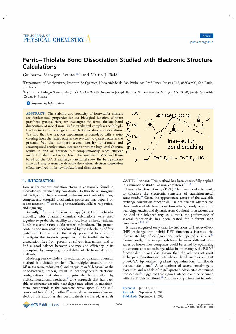
Ferric−Thiolate Bond Dissociation Studied with Electronic StructureCalculationsGuilherme Menegon Arantes*,† and Martin J. Field‡

†Department of Biochemistry, Instituto de Química, Universidade de Sao Paulo, Av. Prof. Lineu Prestes 748, 05508-900, Sao Paulo,SP Brazil‡Institut de Biologie Structurale (IBS), CEA/CNRS/Universite Joseph Fourier, 71 Avenue des Martyrs, CS 10090, 38044 GrenobleCedex 9, France

*S Supporting Information

ABSTRACT: The stability and reactivity of iron−sulfur clustersare fundamental properties for the biological function of theseprosthetic groups. Here, we investigate the ferric−thiolate bonddissociation of model iron−sulfur tetrahedral complexes with high-level ab initio multiconfigurational electronic structure calculations.We find that the reaction mechanism is homolytic with a spin-crossing from the sextet state in the reactant to quartet state in theproduct. We also compare several density functionals andsemiempirical configuration interaction with the high-level ab initioresults to find an accurate but computationally more efficientmethod to describe the reaction. The functionals M06 and thosebased on the OPTX exchange functional show the best perform-ance and may reasonably describe the various electron correlationeffects involved in ferric−thiolate bond dissociation.

1. INTRODUCTION

Iron under various oxidation states is commonly found inbiomolecules tetrahedrally coordinated to thiolate or inorganicsulfide ligands. These iron−sulfur clusters are involved in manycomplex and essential biochemical processes that depend onredox reactions,1−3 such as photosynthesis, cellular respiration,and signaling.Recently,4−6 atomic force microscopy (AFM) and molecular

modeling with quantum chemical calculations were usedtogether to probe the stability and reactivity of ferric−thiolatebonds in a simple iron−sulfur protein, rubredoxin. This proteincontains one iron center coordinated by the side-chains of fourcysteines.7 Our aims in the study presented here are toinvestigate the intrinsic properties of ferric−thiolate bonddissociation, free from protein or solvent interactions, and tofind a good balance between accuracy and efficiency in itsdescription by comparing several different electronic structuremethods.Modeling ferric−thiolate dissociation by quantum chemical

methods is a difficult problem. The multiplet structure of iron(d5 in the ferric redox state) and its spin manifold, as well as thebond-breaking process, result in near-degenerate electronicconfigurations that should, in principle, be described bymulticonfigurational methods.8 One approach that has beenable to correctly describe near-degenerate effects in transition-metal compounds is the complete active space (CAS) self-consistent field (SCF) method,9 especially when some dynamicelectron correlation is also perturbatively recovered, as in its

CASPT210 variant. This method has been successfully appliedin a number of studies of iron complexes.11−14

Density functional theory (DFT)15 has been used extensivelyto calculate the electronic structure of transition-metalcompounds.16 Given the approximate nature of the availableexchange-correlation functionals it is not evident whether theaforementioned electron correlation effects, nondynamic fromnear-degeneracies and dynamic from Coulomb interactions, areincluded in a balanced way. As a result, the performance ofseveral functionals has been tested for different ironcomplexes.14,16−27

It was recognized early that the inclusion of Hartree−Fock(HF) exchange into hybrid DFT functionals increases therelative stability of configurations with unpaired electrons.17

Consequently, the energy splittings between different spinstates of iron−sulfur complexes could be tuned by optimizingthe amount of exact exchange added in, for example, the B3LYPfunctional.17 It was also shown that the addition of exactexchange underestimates metal−ligand bond energies and thatpure-GGA (generalized gradient approximation) functionalsoverestimate them.19 A comparison of several metal−liganddiatomics and models of metalloprotein active-sites containingiron centers20 suggested that a good balance could be obtainedwith the TPSSh functional.28 Another comparison that included

Received: June 13, 2015Revised: September 8, 2015Published: September 9, 2015

Article

pubs.acs.org/JPCA

© 2015 American Chemical Society 10084 DOI: 10.1021/acs.jpca.5b05658J. Phys. Chem. A 2015, 119, 10084−10090

ferrous and ferric complexes with tetrahedral coordination14,18

suggested that functionals such as OLYP and OPBE, based onHandy and Cohen’s OPTX pure-GGA exchange functional,29

are the most computationally cost-effective in describing ironcompounds.Here we investigate ferric−thiolate bond dissociation in the

following two isolated model reactions

⇌ +− −Fe(SH) Fe(SH) HS4 3 (1)

⇌ +− −Fe(SCH ) Fe(SCH ) H CS3 4 3 3 3 (2)

using several DFT functionals and multiconfigurational ab initio(CASPT2) and semiempirical30 methods. Details of thereaction mechanisms, spin states and densities, electronicconfigurations, and relative energetics are given in the followingsections. These results are used to help identify an accurate andefficient treatment of the dissociation reaction.

2. COMPUTATIONAL METHODS

Molecular geometries for species along reactions 1 and 2 wereoptimized at the DFT level with the B3LYP functional31,32 andthe 6-31+G(2df,p)33 basis set for all possible electronic spinstates (S = 0.5, 1.5, and 2.5). Spin-polarized orbitals wereadopted. Optimizations conducted with the TZVP basis set34

resulted in equivalent structures. Ferric−thiolate bond dis-sociation was obtained by optimizing the geometry with thedissociative Fe−S distance fixed at a given value. TheGAUSSIAN 09 program (rev. A1)35 was used for geometryoptimizations. It should be noted that the calculated Fe−Sbond length for the reactant ground state (2.32 Å) is in goodagreement with the experimental bond lengths observed incrystallographic structures of proteins that contain tetrahedralFe−S centers. As an example, in rubredoxin (PDB ID 8RXN),the bond lengths are in the range of 2.27−2.30 Å.A minimum-energy crossing point (MECP) between sextet

and quartet electronic states was optimized with the pDynamolibrary36 as described previously5 with the B3LYP functionaland the TZVP basis set.Single-point DFT energies for geometries corresponding to

the CASPT2 low-energy pathway described below wereobtained with the ORCA program version 3.0.137 and thefollowing functionals: OLYP, O3LYP,29,32 OPBE,29,38 PBE0,39

BLYP,32,40 B3LYP, B3LYP-D3, BP86,40,41 TPSS, TPSSh,28

M06,42 and B2PLYP.43 Spin-polarized orbitals and standardintegration grids were adopted. The Def2-TZVP basis set44 andresolution of identity with the TZV/J45 auxiliary basis were

used. A second-order SCF optimization had to be activated toobtain convergence in several cases.Although the Fe(SH)4

− ground state (reactant in sextetelectronic spin) belongs to the S4 molecular point group, thetetrahedral symmetry around the iron center is broken in allother geometries studied here. Thus, all calculations werecarried out in the C1 point-group symmetry.Single-point multiconfigurational calculations were carried

out with the geometries optimized by DFT along the ferric−thiolate bond dissociation. The active space was not built usingan analysis of the corresponding irreducible representations(irreps) and symmetry adapted linear combinations of ligandmolecular orbitals. Instead, it was chosen with five molecularorbitals for the metal 3d open-shell, as these are necessary todescribe the near-degenerate configurations arising from theferric ion multiplet structure, and two extra pairs of correlatingmolecular orbitals (MOs) describing the bond dissociationprocess. This active space contained nine electrons in nineorbitals. Similar choices, such as seven electrons in seven MOs,were also tried and yielded equivalent results. The double-shelleffect11 was tested for the ferric ion complexes studied herewith an active space of nine electrons in fourteen orbitals andfound to be negligible (Table S3).All multiconfigurational CASSCF and CASPT28,10 calcu-

lations were performed with the MOLCAS program, version7.4.46 The ANO-RCC basis-set47 with contractions Fe-[7s6p5d2f1g], S[6s5p3d2f], and H[3s2p1d] was employed asthis was shown to be appropriate in previous benchmarkcalculations for iron compounds.12 CASSCF orbitals wereoptimized for the average of the first three roots with equalweights. Scalar relativistic effects were included using aDouglas−Kroll−Hess Hamiltonian. In all CASPT2 calculationsthe core electrons were frozen (26 frozen MOs), and only thevalence space was correlated. The standard IPEA shift of 0.25au and an extra denominator shift of 0.3 au were used to avoidintruder states.10,48

To test if semiempirical potentials could be used to modelferric−thiolate bond dissociation, the performance of themodern PM6 parametrization30 that contains d-orbitals in itsminimal basis set was investigated with complete active spaceconfiguration interaction (CASCI) calculations.8 Several activespaces were tested for these semiempirical calculations, and thebest results were obtained with seven electrons in seven MOsspace. Orbitals were determined from restricted-open shell(ROHF) calculations with fractional occupation.49,50

The performance of the original PM6 parametrization wasvery poor (see Results and Discussion); therefore, a specific

Figure 1. Relative energy profiles for ferric−thiolate bond dissociation obtained at the DFT level. Calculations were carried out at the B3LYP/6-31+G(2df,p) level in the quartet (dashed line) and sextet (solid line) spin states for Fe(SH)4

− (left panel) and Fe(SCH3)4− (right panel). The inset

shows the spin density over the dissociating sulfur atom (S1) for the sextet state.

The Journal of Physical Chemistry A Article

DOI: 10.1021/acs.jpca.5b05658J. Phys. Chem. A 2015, 119, 10084−10090

10085

reparametrization for iron was carried out. CASPT2 energiesreported here for Fe−S bond dissociation, iron atomicmultiplet and ionization energies taken from spectroscopicaldata,51 and DFT energies for different Fe(SH)4

− andFe(SCH3)4

− geometries (not shown) were used as target orreference properties. Optimized parameters are given in theSupporting Information (Table S1). Full details of thereparametrization procedure are not relevant for the con-clusions drawn here and will be given in a future publication.All semiempirical calculations were done with the pDynamolibrary.36

3. RESULTS AND DISCUSSION3.1. Energy Profiles for Bond Dissociation. Our

calculation results for reaction 1 show the ground-state reactantis a sextet spin state and has a tetrahedral geometry belongingto the S4 point group. The quartet and doublet reactants havedistorted tetrahedral coordination around the iron center withoverall C2 symmetry. All other geometries along the Fe−Sdissociation belong to the C1 point group.The DFT energy profiles shown in Figure 1 for both

Fe(SH)4− and Fe(SCH3)4

− dissociation have several note-worthy features. First, the quartet reactant lies 20 kJ/mol higherin energy than the sextet reactant. However, the lowest-energyproduct of bond dissociation is a quartet. Thus, there is a spincrossing along the reaction. A minimum-energy crossing pointwas optimized at a ferric−thiolate bond distance d(Fe−S) ≈ 3.7Å. Products in all spin states are ion−molecule complexes withsmall (<4 kJ/mol) recombination barriers. Also, the quartettransition-state region is reached before the MECP, whereas thesextet transition-state region is reached after the MECP. Thedoublet state energy profile is not shown nor discussed in detailhere as all doublet stationary geometries along ferric−thiolatebond dissociation lie at least 90 kJ/mol higher than the otherspin states.The ferric−thiolate bond dissociation mechanism can be

deduced from the DFT profiles. Although the reactants have aformally ferric center, both sextet and quartet products have aferrous center with a dissociated thiolate radical. To illustratethis, the inset in Figure 1 shows that the spin density in thedissociative sulfur atom (S1) changes rather smoothly from 0 to1 during Fe−S bond dissociation. As a result, Fe−S bonddissociation in both sextet and quartet spin states is homolytic.5

The energetics, iron coordination, and Fe−S bond distancesof stationary points are very similar between the Fe(SH)4

− andFe(SCH3)4

− dissociation profiles. Thus, the conclusions drawnbelow for Fe(SH)4

− should be equally valid for Fe(SCH3)4−

when comparing the different CASPT2, DFT, and semi-empirical methods. The only caveat concerns the productregion as different d(Fe−S) distances are observed because ofthe bulkier methyl groups in Fe(SCH3)4

− (Figure 1). A relatedobservation should also be made for the products of ferric−thiolate bond cleavage in Fe(SH)4

− optimized with the OPBEand TPSSh functionals (data not shown). For these twofunctionals, the products resulted in H2S instead of HS

−, as thisleaving group removes a proton from another thiol group atd(Fe−S) > 4 Å.The multiconfigurational CASPT2 energy profile for Fe-

(SH)4− dissociation is shown in Figure 2. The energies and

structures reported in this figure correspond to the CASPT2minimum-energy pathway for ferric−thiolate bond dissociationwith DFT optimized geometries. These six structures, alongwith the doublet product and reactant structures (not shown in

the figure), will be termed in what follows as reactants (R),transition state (TS), MECP, and products (P), together withtheir respective total spin electronic state, which can havedoublet (2), quartet (4), and sextet (6) multiplicities.The reaction coordinates of the low-energy species along the

CASPT2 minimum-energy pathway are similar to those foundwith DFT. However, we were unable to identify a 6TS with theCASPT2 single-point calculations because of the rather flattransition region observed in the DFT profile [d(Fe−S) > 4 Åin the left panel of Figure 1]. The relative energies for thequartet and sextet profiles found with CASPT2 differ at mostby 20 kJ/mol from those obtained with B3LYP for all speciesexcept the MECP (Table S2). This is the accuracy (∼20 kJ/mol) often expected of hybrid functionals in isodesmicprocesses involving metals, such as heterolytic bond dissocia-tions.19 However, at the crossing point, the difference in relativeenergy between the B3LYP and CASPT2 energy profiles ishigher (50 kJ/mol), which can be partially attributed to astructural relaxation energy not included in our CASPT2 single-point calculations. Although the 6MECP and 4MECP CASPT2energies differ by less than 4 kJ/mol, indicating that they mightbe near a surface crossing, the structure still could be far fromthe true minimum-energy crossing of the CASPT2 energysurfaces. Further comparisons between the multiconfigurationalresults and several DFT functionals will be given in the nextsection.A homolytic reaction mechanism with a spin crossing along

the dissociation is also observed in the CASPT2 results. Thereactant is in a sextet state, and the most stable product is in thequartet state containing a partial thiolate radical and a ferrouscenter. However, instead of changing smoothly as in themonoconfigurational DFT calculations (inset in Figure 1),CASSCF spin-densities change abruptly during dissociation as aconsequence of hopping between surfaces with differentelectronic configurations. As shown in Table 1 for the reactantstates, almost no spin density is seen on sulfur atoms and thespin density on the iron atom equates to the expected numberof unpaired electrons in the spin state. For the MECP, spindensities correspond to different electronic configurations, andspin unpairing is already evident on the dissociating sulfur atom(S1). In fact, the crossing between the sextet and quartet spinstates is equivalent to a spin flipping over this sulfur atom.Electronic configurations and, consequently, spin densities aresimilar between the MECP and product states for both sextetand quartet spin states.

Figure 2. Relative energy profiles for Fe(SH)4− ferric−thiolate bond

dissociation obtained at the CASPT2 level. Calculations were carriedout with the ANO-RCC basis set for the quartet (dashed line) andsextet (solid line) spin states. Structures are shown in ball−stickrepresentation with iron in crossed lines and sulfur in diagonal lines.



10086

In the calculations for 6R employing spatially restrictedorbitals (ROHF and CASSCF), we observe a typical molecularorbital ordering equivalent to what is usually expected from d5

metal centers with tetrahedral coordination.52 The valenceorbitals of the sulfur ligand combine into nonbonding MOsbelonging approximately to the T1 irrep in the Td localsymmetry around the iron center and into bonding MOsbelonging to irreps A1, E, and T2. The five unpaired electrons ofthe metal are distributed in e2 t2

3-like orbitals, with contributionsof about 5−10% weight from ligand orbitals from irreps E andT2. For the other geometries along the reaction pathway, thelocal symmetry around the iron center is distorted and it ismore difficult to label the symmetry of the MOs. The ferric−thiolate bond that is broken upon dissociation has a σcharacter.3 All the occupied bonding and nonbonding ligandorbitals lie lower in energy than the metal d-shell. This is incontrast to the orbital ordering observed in our DFTunrestricted calculations in which an inverted level-scheme isfound due to strong spin polarization of the MOs. The MOordering in the inverted-level scheme shows the metal d-shellbelow the ligand bonding and nonbonding MOs. This has alsobeen observed in similar iron−sulfur compounds andextensively discussed by Noodleman et al.,53−55 Solomon etal.,56 and more recently by Ichiye and co-workers.22,57

Wave functions for all species in the sextet state show a singleconfiguration with more than 98% of the weight in the CIexpansion. The other two reactant states, 4R and 2R, aredominated by a single configuration with ≈80% weight in theCI expansion, and the remaining configurations account fordifferent occupations of the metal d-shell. All other quartet anddoublet species have large mixtures of configurations withoutany surpassing 20% weight. These results suggest thatmonoconfigurational electronic structure methods may beable to describe the bond-breaking process properly in onlythe sextet state.3.2. Comparison with DFT Functionals and Semi-

empirical Methods. To test the performance of moreapproximate electronic structure methods in the descriptionof ferric−thiolate bond dissociation, we compared the CASPT2relative energies with a series of DFT functionals andsemiempirical methods. Table 2 shows the deviations andmaximum errors obtained, and Table S2 in the SupportingInformation gives the relative energy values. We note that theestimated accuracy of CASPT2 to describe spin-splittings is∼12 kJ/mol.12,14

An analysis of the data shows that the best performingfunctional is the M06 hybrid meta-GGA, followed by thesimpler OLYP pure-GGA functional, although with a muchlarger maximum error. The doublet states have the highestrelative energies and give the maximum errors for all functionalsexcept B2PLYP and M06. The OLYP functional is followedclosely by OPBE and O3LYP, suggesting that Handy andCohen’s OPTX exchange functional29 is the most appropriateto describe Fe−S bond dissociation. This exchange functionalincludes some nondynamic electron correlation effects (named“left−right correlation”)29 that contribute to the correctdescription of homolytic bond dissociation. On the otherhand, Becke’s one-parameter exchange functional,40 used inBLYP and BP86, performs significantly worse. This is because itstays closer to the uniform electron gas assumption (the Diraccoefficient is not scaled)29 and does not include such left−rightnondynamic correlation effects.Apart from the highly parametrized M06, meta-GGA

functionals, such as TPSS, do not perform particularly well.Inclusion of Hartree−Fock exchange does not markedlyimprove the results for TPSSh in comparison to TPSS. Bycontrast, hybrid functionals, such as B3LYP and PBE0, do showlower errors, especially for energy splittings between differentspin states. It should be noted that the pure GGA functionalsnot based on the OPTX exchange functional, such as BLYP,BP86, and TPSS, give a qualitatively wrong description of thespin splitting, as 4R is more stable than 6R (Table S2). Mixingsome exact exchange with the OPTX functional as in O3LYPdoes not improve the spin splittings in comparison to the pure-GGA OLYP. The double-hybrid functional B2PLYP does notperform significantly better, suggesting that the inclusion ofdynamic correlation effects via an MP2 contribution is notimportant for the description of ferric−thiolate bonddissociation. Finally, inclusion of dispersion corrections as inthe B3LYP-D3 functional does not change the relative energies,in comparison to the B3LYP functional.

Table 1. Mulliken Spin Populations Calculated from theCASSCF Wavefunction for Fe and S Atoms in Structuresfrom Reaction 1a

Fe S1 S2 S3 S42R 1.00 −0.03 0.02 −0.02 0.022P 1.34 −0.29 −0.01 −0.00 −0.044R 3.11 −0.02 −0.03 −0.03 −0.024TS 3.50 −0.50 −0.07 0.03 0.034MECP 3.52 −0.52 0.03 0.03 −0.054P 3.50 −0.53 0.03 0.03 −0.056R 4.75 0.06 0.06 0.06 0.066MECP 3.91 0.86 0.03 0.03 0.146P 3.91 0.84 0.03 0.18 0.02

aThe spin density moduli were less than 0.02 for all hydrogen atoms inall structures.

Table 2. Comparison of Several DFT Functionals andSemiempirical Methods with the CASPT2 Referencea

method STDEV MAE

B2PLYP 38.4 108.6B3LYP 39.9 113.7B3LYP-D3 38.4 105.2BLYP 54.2 143.5BP86 49.2 134.7M06 17.8 31.8O3LYP 25.4 83.1OLYP 19.5 75.0OPBE 26.9 83.8PBE0 32.6 92.8PM6b 79.7 319.7PM6Rb 25.2 67.5TPSS 52.8 143.6TPSSh 46.4 122.5

aStandard deviations (STDEV) and maximum absolute errors (MAE)of relative energies (in kilojoules per mole) for structures from theFe(SH)4 ferric−thiolate bond dissociation pathways. Values obtainedfrom the relative energies (Table S2) of nine single-point calculations,corresponding to the six structures shown in Figure 2 (both quartetand sextet states were calculated for the MECP), 2R and 2P. bPM6 isthe original semiempirical parametrization and PM6R is theparametrization obtained in this work (Table S1).



10087

We conclude that the hybrid M06 functional and thefunctionals based on Handy and Cohen’s OPTX exchange givethe best results for iron−sulfur bond dissociation. If computa-tional efficiency is important, then the pure-GGA functionalsOLYP and OPBE are to be preferred.Given that we are particularly interested in the simulation of

iron−sulfur clusters in complex systems, we wanted to evaluatemethods that are computationally more efficient than CASPT2and DFT. As an initial choice, we tried the recent semiempiricalHamiltonian PM630 that contains d-orbitals in its minimalbasis-set and was parametrized for molecules containing iron.These tests, using unrestricted HF (UHF) and ROHF +CASCI calculations and the original PM6 Hamiltonian, resultedin a very poor description of ferric−thiolate bond dissociationenergetics (Table 2 and Table S2, which show the ROHF +CASCI results only). This poor performance is due to anincorrect MO ordering, as the orbital formed mainly by the Fe4s-shell was occupied and lower in energy than the MOscomposed by the Fe 3d open-shell, suggesting an imbalancebetween the semiempirical ζs and ζd orbital coefficients. Ourprevious experience58 indicates that this imbalance can becorrected by a specific reparametrization of the iron PM6parameters. This we did successfully, leading to a para-metrization that we denote PM6R (Table S1).ROHF + CASCI calculations with the new PM6R

Hamiltonian perform rather well, with deviations similar tofunctionals based on OPTX exchange, but with smallermaximum errors (Table 2). However, this is not a faircomparison because the CASPT2 reference energies wereactually used to fit the PM6R parameters. The observed MOorbital ordering is indeed similar to that obtained for the abinitio CASSCF wave functions with, in increasing order ofenergy, doubly occupied ligand MOs, singly occupied MOscorresponding to the Fe 3d shell, and an unoccupied Fe 4sshell. The resulting spin densities are consequently moreaccurate and close to those shown in Table 1. However, itshould be noted that UHF calculations with the newparameters yielded poor results. Thus, although our specificallyparametrized semiempirical Hamiltonian, in conjunction withCI calculations, can describe the energetics and electronicconfiguration of ferric−thiolate bond dissociation rather well,the transferability and applicability of these new parameters inother circumstances needs to be further validated.

4. CONCLUSIONS

We have studied ferric−thiolate bond dissociation in theisolated model iron−sulfur tetrahedral compounds, Fe(SH)4

−

and Fe(SCH3)4−, using the multiconfigurational wave function

methods, ab initio CASPT2 and semiempirical CASCI, andseveral DFT functionals. The reaction proceeds via a homolyticmechanism with a spin crossing between the sextet and quartetstates. This two-state reactivity is often seen in transition-metalcompounds,59 and so studies of the stability, reactivity, andbiosynthesis of iron−sulfur clusters in proteins need to carefullyaccount for the different accessible spin states.The high-level CASPT2 method was used as a reference,

against which the various other electronic structure approacheswere compared. We find that the M06 functional is the best fordescribing Fe−S bond dissociation when all possible spin statesare to be considered. Our DFT comparisons are also inagreement with previous studies14 that highlight the reliabilityof the OLYP and OPBE functionals for describing iron

complexes. The B3LYP functional gives satisfactory results, andit should be fairly dependable for geometry optimizations.Ferric−thiolate bond dissociation is a difficult problem to

model as it involves different kinds of electron correlationeffects that change unevenly as the reaction progresses. Near-degenerate nondynamic correlation is important for describingthe multiplet structure of the ferric center and, consequently,the energy splittings between the various spin states. Bycontrast, left−right nondynamic correlation is critical for thedescription of homolytic bond dissociation, whereas angularcorrelation in the transition metal also needs to be consideredappropriately, given the change in metal coordination fromtetrahedral reactants to trigonal products. As a result, thisreaction constitutes a tough test for electronic structuremethods, in particular for the single-determinant, principallyDFT, approaches tried here.We conclude by noting that specifically parametrized

semiempirical methods employing d-orbitals and CI calcu-lations can be used to model the Fe−S dissociation reaction,but further studies are necessary to evaluate the generalapplicability of this approach.

■ ASSOCIATED CONTENT*S Supporting InformationThe Supporting Information is available free of charge on theACS Publications website at DOI: 10.1021/acs.jpca.5b05658.

Tables containing the reoptimized PM6 iron semi-empirical parameters and the relative energies calculatedwith all the electronic structure methods used here(PDF)

■ AUTHOR INFORMATIONCorresponding Author*E-mail: [email protected] authors declare no competing financial interest.

■ ACKNOWLEDGMENTSFunding from FAPESP (12/02501-4 and 14/21900-2) and ajoint FAPESP-CNRS project (23277) are gratefully acknowl-edged.

■ REFERENCES(1) Beinert, H.; Holm, R. H.; Munck, E. Iron-Sulfur Clusters:Nature’s Modular, Multipurpose Structures. Science 1997, 277, 653−659.(2) Holm, R. H.; Kennepohl, P.; Solomon, E. I. Structural andFunctional Aspects of Metal Sites in Biology. Chem. Rev. 1996, 96,2239−2314.(3) Solomon, E. I.; Gorelsky, S. I.; Dey, A. Metal-Thiolate Bonds inBioinorganic Chemistry. J. Comput. Chem. 2006, 27, 1415−1428.(4) Zheng, P.; Li, H. Highly Covalent Ferric-Thiolate Bonds ExhibitSurprisingly Low Mechanical Stability. J. Am. Chem. Soc. 2011, 133,6791−6798.(5) Arantes, G. M.; Bhattacharjee, A.; Field, M. J. HomolyticCleavage of Fe-S Bonds in Rubredoxin Under Mechanical Stress.Angew. Chem., Int. Ed. 2013, 52, 8144−8146.(6) Zheng, P.; Arantes, G. M.; Field, M. J.; Li, H. Force InducedChemical Reactions on the Metal Center in a Single MetalloproteinMolecule. Nat. Commun. 2015, 6, 7569.(7) Beinert, H. Iron-Sulfur Proteins: Ancient Structures, Still Full ofSurprises. JBIC, J. Biol. Inorg. Chem. 2000, 5, 2−15.(8) Helgaker, T.; Jørgensen, P.; Olsen, J. Molecular Electronic-Structure Theory, 1st ed.; Wiley: New York, 2000.



10088

(9) Roos, B. O.; Taylor, P. R.; Siegbahn, P. E. M. A Complete ActiveSpace SCF Method (CASSCF) Using a Density Matrix FormulatedSuper-CI Approach. Chem. Phys. 1980, 48, 157−173.(10) Andersson, K.; Malmqvist, P. A.; Roos, B. O. Second-OrderPerturbation Theory with a Complete Active Space Self-ConsistentField Reference Function. J. Chem. Phys. 1992, 96, 1218.(11) Pierloot, K. Nondynamic Correlation Effects in Transition MetalCoordination Compounds, 1st ed.; Marcel Dekker: New York, 2001; pp123−158.(12) Pierloot, K.; Vancoillie, S. Relative Energy of the High-(5T2g)and Low-(1A1g) Spin States of [Fe(H2O)6]

2+, [Fe(NH3)6]2+, and

[Fe(bpy)3]2+: CASPT2 Versus Density Functional Theory. J. Chem.

Phys. 2006, 125, 124303.(13) Arantes, G. M.; Taylor, P. R. Approximate MulticonfigurationalTreatment of Spin-Coupled Metal Complexes. J. Chem. TheoryComput. 2010, 6, 1981−1989.(14) Swart, M. Accurate Spin-State Energies for Iron Complexes. J.Chem. Theory Comput. 2008, 4, 2057−2066.(15) Parr, R. G.; Yang, W. Density-Functional Theory of Atoms andMolecules, 1st ed.; Oxford University Press: Oxford, 1996.(16) Cramer, C. J.; Truhlar, D. G. Density Functional Theory forTransition Metals and Transition Metal Chemistry. Phys. Chem. Chem.Phys. 2009, 11, 10757−10816.(17) Reiher, M.; Salomon, O.; Hess, B. A. Reparameterization ofHybrid Functionals Based on Energy Differences of States of DifferentMultiplicity. Theor. Chem. Acc. 2001, 107, 48−55.(18) Swart, M.; Groenhof, A. R.; Ehlers, A. W.; Lammertsma, K.Validation of Exchange-Correlation Functionals for Spin States of IronComplexes. J. Phys. Chem. A 2004, 108, 5479−5483.(19) Jensen, K. P.; Roos, B. O.; Ryde, U. Performance of DensityFunctionals for First Row Transition Metal Systems. J. Chem. Phys.2007, 126, 014103.(20) Jensen, K. P. Bioinorganic Chemistry Modeled with the TPSShDensity Functional. Inorg. Chem. 2008, 47, 10357−10365.(21) Sorkin, A.; Iron, M. A.; Truhlar, D. G. Density FunctionalTheory in Transition-Metal Chemistry: Relative Energies of Low-Lying States of Iron Compounds and the Effect of Spatial SymmetryBreaking. J. Chem. Theory Comput. 2008, 4, 307−315.(22) Niu, S.; Nichols, J. A.; Ichiye, T. Optimization of Spin-Unrestricted Density Functional Theory for Redox Properties ofRubredoxin Redox Site Analogues. J. Chem. Theory Comput. 2009, 5,1361−1368.(23) Bergeler, M.; Stiebritz, M. T.; Reiher, M. Structure-PropertyRelationships of Fe4S4 Clusters. ChemPlusChem 2013, 78, 1082−1098.(24) Bruska, M. K.; Stiebritz, M. T.; Reiher, M. Analysis ofDifferences in Oxygen Sensitivity of Fe-S Clusters. Dalton Trans. 2013,42, 8729−8735.(25) Ye, S.; Neese, F. Accurate Modeling of Spin-State Energetics inSpin-Crossover Systems with Modern Density Functional Theory.Inorg. Chem. 2010, 49, 772−774.(26) Isley, W. C., III; Zarra, S.; Carlson, R. K.; Bilbeisi, R. A.; Ronson,T. K.; Nitschke, J. R.; Gagliardi, L.; Cramer, C. J. PredictingParamagnetic 1H NMR Chemical Shifts and State-Energy Separationsin Spin-Crossover Host-Guest Systems. Phys. Chem. Chem. Phys. 2014,16, 10620−10628.(27) Ferre, N.; Guihery, N.; Malrieu, J.-P. Spin Decontamination ofBroken-Symmetry Density Functional Theory Calculations: DeeperInsight and New Formulations. Phys. Chem. Chem. Phys. 2015, 17,14375−14382.(28) Tao, J. M.; Perdew, J. P.; Staroverov, V. N.; Scuseria, G. E.Climbing the Density Functional Ladder: Nonempirical Meta-Generalized Gradient Approximation Designed for Molecules andSolids. Phys. Rev. Lett. 2003, 91, 146401.(29) Handy, N. C.; Cohen, A. J. Left-Right Correlation Energy. Mol.Phys. 2001, 99, 403−412.(30) Stewart, J. J. P. Optimization of Parameters for SemiempiricalMethods V: Modification of NDDO Approximations and Applicationto 70 Elements. J. Mol. Model. 2007, 13, 1173−1213.

(31) Becke, A. D. Density Functional Thermochemistry. III. TheRole of Exact Exchange. J. Chem. Phys. 1993, 98, 5648.(32) Lee, C.; Yang, W.; Parr, R. Development of the Colle-SalvettiCorrelation-Energy Formula into a Functional of the Electron Density.Phys. Rev. B: Condens. Matter Mater. Phys. 1988, 37, 785−789.(33) Ditchfield, R.; Hehre, W.; Pople, J. A. Self-ConsistentMolecular-Orbital Methods. IX. An Extended Gaussian-Type Basisfor Molecular-Orbital Studies of Organic Molecules. J. Chem. Phys.1971, 54, 724−728.(34) Schafer, A.; Horn, H.; Ahlrichs, R. Fully Optimized ContractedGaussian Basis Sets for Atoms Li to K. J. Chem. Phys. 1992, 97, 2571−2577.(35) Frisch, M. J.; Trucks, G. W.; Schlegel, H. B.; Scuseria, G. E.;Robb, M. A.; Cheeseman, J. R.; Scalmani, G.; Barone, V.; Mennucci,B.; Petersson, G. A. et al. Gaussian 09, revision A.1; Gaussian, Inc.:Wallingford, CT, 2009.(36) Field, M. J. The pDynamo Program for Molecular Simulationsusing Hybrid Quantum Chemical and Molecular MechanicalPotentials. J. Chem. Theory Comput. 2008, 4, 1151−1161.(37) Neese, F. The ORCA Program System. Wiley Interdiscip. Rev.:Comput. Mol. Sci. 2012, 2, 73−78.(38) Perdew, J. P.; Burke, K.; Ernzerhof, M. Generalized GradientApproximation Made Simple. Phys. Rev. Lett. 1996, 77, 3865−3868.(39) Adamo, C.; Barone, V. Toward Reliable Density FunctionalMethods Without Adjustable Parameters: The PBE0 model. J. Chem.Phys. 1999, 110, 6158−6170.(40) Becke, A. D. Density-Functional Exchange-Energy Approx-imation with Correct Asymptotic Behavior. Phys. Rev. A: At., Mol., Opt.Phys. 1988, 38, 3098−3100.(41) Perdew, J. P. Density-Functional Approximation for theCorrelation Energy of the Inhomogeneous Electron Gas. Phys. Rev.B: Condens. Matter Mater. Phys. 1986, 33, 8822−8824.(42) Zhao, Y.; Truhlar, D. G. The M06 Suite of Density Functionalsfor Main Group Thermochemistry, Thermochemical Kinetics, Non-covalent Interactions, Excited States, and Transition Elements: TwoNew Functionals and Systematic Testing of Four M06-ClassFunctionals and 12 Other Functionals. Theor. Chem. Acc. 2008, 120,215−241.(43) Schwabe, T.; Grimme, S. Double-Hybrid Density Functionalswith Long-Range Dispersion Corrections: Higher Accuracy andExtended Applicability. Phys. Chem. Chem. Phys. 2007, 9, 3397.(44) Weigend, F.; Ahlrichs, R. Balanced Basis Sets of Split Valence,Triple Zeta Valence and Quadruple Zeta Valence Quality for H to Rn:Design and Assessment of Accuracy. Phys. Chem. Chem. Phys. 2005, 7,3297−3305.(45) Weigend, F. Accurate Coulomb-Fitting Basis Sets for H to Rn.Phys. Chem. Chem. Phys. 2006, 8, 1057−1065.(46) Aquilante, F.; De Vico, L.; Ferre, N.; Ghigo, G.; Malmqvist, P.-A.; Neogrady, P.; Pedersen, T. B.; Pitonak, M.; Reiher, M.; Roos, B.O.; et al. MOLCAS 7: The Next Generation. J. Comput. Chem. 2010,31, 224−247.(47) Roos, B. O.; Lindh, R.; Malmqvist, P.-A.; Veryazov, V.;Widmark, P.-O. New Relativistic ANO Basis Sets for Transition MetalAtoms. J. Phys. Chem. A 2005, 109, 6575−6579.(48) Roos, B. O.; Andersson, K.; Fulscher, M. P.; Serrano-Andres, L.;Pierloot, K.; Merchan, M.; Molina, V. Applications of Level ShiftCorrected Perturbation Theory in Electronic Spectroscopy. J. Mol.Struct.: THEOCHEM 1996, 388, 257−276.(49) Granucci, G.; Toniolo, A. Molecular Gradients for Semi-empirical CI Wavefunctions with Floating Occupation MolecularOrbitals. Chem. Phys. Lett. 2000, 325, 79−85.(50) Slavícek, P.; Martínez, T. J. Ab Initio Floating OccupationMolecular Orbital-Complete Active Space Configuration Interaction:An Efficient Approximation to CASSCF. J. Chem. Phys. 2010, 132,234102.(51) Ralchenko, Y.; Kramida, A. E.; Reader, J. NIST ASD Team,NIST Atomic Spectra Database (version 3.1.5). National Institute ofStandards and Technology, Gaithersburg, MD, http://physics.nist.gov/asd3 (accessed March 7, 2012).



10089

(52) Butcher, K. D.; Didziulis, S. V.; Briat, B.; Solomon, E. I. VariablePhoton Energy Photoelectron Spectroscopy on FeCl4

−: An UnusualElectronic Structure for High-Spin d5 Complexes. J. Am. Chem. Soc.1990, 112, 2231−2242.(53) Noodleman, L.; Norman, J. G., Jr; Osborne, J. H.; Aizman, A.;Case, D. A. Models for Ferredoxins: Electronic Structures of Iron-Sulfur Clusters with One, Two, and Four Iron Atoms. J. Am. Chem.Soc. 1985, 107, 3418−3426.(54) Noodleman, L.; Peng, C.; Case, D.; Mouesca, J.-M. OrbitalInteractions, Electron Delocalization and Spin Coupling in Iron-SulfurClusters. Coord. Chem. Rev. 1995, 144, 199−244.(55) Noodleman, L.; Han, W.-G. Structure, Redox, pKa, Spin. AGolden Tetrad for Understanding Metalloenzyme Energetics andReaction Pathways. JBIC, J. Biol. Inorg. Chem. 2006, 11, 674−694.(56) Solomon, E. I.; Randall, D. W.; Glaser, T. Electronic Structuresof Active Sites in Electron Transfer Metalloproteins: Contributions toReactivity. Coord. Chem. Rev. 2000, 200, 595−632.(57) Niu, S.; Wang, X.-B.; Yang, X.; Wang, L.-S.; Ichiye, T.Mechanistic Insight into the Symmetric Fission of [4Fe-4S] AnalogueComplexes and Implications for Cluster Conversions in Iron-SulfurProteins. J. Phys. Chem. A 2004, 108, 6750−6757.(58) Arantes, G. M.; Loos, M. Specific Parametrisation of a HybridPotential to Simulate Reactions in Phosphatases. Phys. Chem. Chem.Phys. 2006, 8, 347−353.(59) Schroder, D.; Shaik, S.; Schwarz, H. Two-State Reactivity as aNew Concept in Organometallic Chemistry. Acc. Chem. Res. 2000, 33,139−145.



10090

71

ANEXO E – Homolytic cleavage of Fe-Sbonds in Rubredoxin under mechanical stress

Bioinorganic ModelingDOI: 10.1002/anie.201303462

Homolytic Cleavage of Fe�S Bonds in Rubredoxin under MechanicalStress**Guilherme M. Arantes,* Anirban Bhattacharjee, and Martin J. Field

The biosynthesis, stability, and folding pathways of the iron–sulfur proteins[1,2] can be probed by analyzing proteinunfolding and Fe�S bond dissociation. Some of the simplestiron–sulfur proteins belong to the rubredoxin family, whichparticipate in electron transfer processes in bacteria andarchea. Rubredoxins lack inorganic sulfide and have only oneFe center coordinated by the side-chains of four cysteineresidues[2] (Figure 1a and b). Recent rubredoxin unfoldingexperiments, performed by protein engineering and single-molecule atomic-force microscopy,[3,4] indicated that their Fe�S bonds had an unexpectedly low stability under mechanicalstress. It was suggested that the activation process for bond

dissociation[3] could occur by heterolytic fission, as observedfor disulfide bridges,[5] or homolytic cleavage, as hypothesizedfor the rupture of C�Si bonds.[6] Given that Fe complexes canhave near-degenerate levels with different total spin,[7] anunderstanding of the reactivity of iron–sulfur clusters requiresthat their spin states and spin crossovers be characterizedduring the reaction.

Herein we have adopted a multiscale modeling approachemploying quantum chemical (QC), molecular mechanical(MM), and hybrid QC/MM potentials, to address thesequestions. Full details of the models and programs used aregiven in the Supporting Information. We started by studyingthe mechanical unfolding of rubredoxin using an MMpotential with an implicit model of solvent. A standardbiomolecular force field was employed, except for the Fe�Sbonds of the iron–sulfur complex which were represented byspecially parameterized Morse potentials that permitted bonddissociation. The starting structures for all simulations werederived from those of the oxidized rubredoxin from Pyro-coccus furiosus (protein databank (PDB) codes 1BRF and1CAA[9,10]). Unfolding was emulated by performing molec-ular dynamics (MD) simulations of the protein with an addedharmonic potential that pulled apart the N- and C-termini ata constant speed.

Although we imposed no bias on the order of dissociationof the Fe�S bonds, we observed that the Fe�S(Cys5) bondruptured first in most of our simulations. Results of one ofthese simulations carried out with a pulling speed of10 nm ns�1 are shown in Figure 2. It is clear from the Ca

RMSDs that rubredoxin unfolds during the trajectory. Thefirst contacts disrupted are interchain hydrogen bonds in theanti-parallel b-strand formed between the N- and C-termini.Other local polar contacts that stabilize the secondarystructure are approximately maintained throughout thesimulation, but fluctuations of the hydrophobic contacts andhydrogen bonds in the protein�s core result in progressivedisorganization of the globular fold. In the last part of thetrajectory, the hydrogen bonds that hold together the N-terminal anti-parallel b-strand are broken. Large fluctuationsare observed for both the Fe–Sg bond distances (� 0.5 �) andSg-Fe-Sg valence angles (� 208) along the trajectory, until theFe�Sg(Cys5) bond breaks after about 1 ns of simulation(Supporting Information Figure S1).[8]

A snapshot of one of the unfolded rubredoxin structuresobtained just before Fe�Sg bond disruption is shown inFigure 1c. The local symmetry around the iron–sulfur centeris broken upon mechanical unfolding with the iron tetrahe-dral coordination (pseudo-Td) changing to C2. This step ischaracterized by changes in the Sg-Fe-Sg valence angles fromapproximately 1098 in folded rubredoxin to 90–1258 in the

Figure 1. Rubredoxin structures: a) schematic representation of thefolded protein; b) close-up of the iron–sulfur cluster from the foldedprotein; c) schematic representation of the protein from one of thepulling simulations just before Fe�S bond rupture: and d) close-up ofthe iron–sulfur cluster from the structure shown in (c). In (b) and (d)important hydrogen bonds are indicated by dashed lines and Fe or-ange, S yellow, C green, N blue.

[*] Dr. G. M. ArantesDepartamento de Bioqu�mica, Instituto de Qu�micaUniversidade de S¼o PauloAv. Lineu Prestes 748, 05508-900, S¼o Paulo, SP (Brazil)E-mail: [email protected]

Dr. A. Bhattacharjee, Dr. M. J. FieldInstitut de Biologie Structurale (IBS) Jean-Pierre EbelCEA/CNRS/Universite Joseph Fourier41, rue Jules Horowitz, 38027 Grenoble, Cedex 1 (France)

[**] We acknowledge funding from FAPESP (projects 07/52772-6 and12/02501-4) and a joint FAPESP-CNRS project (23277).

Supporting information for this article is available on the WWWunder http://dx.doi.org/10.1002/anie.201303462.

.AngewandteCommunications

8144 � 2013 Wiley-VCH Verlag GmbH & Co. KGaA, Weinheim Angew. Chem. Int. Ed. 2013, 52, 8144 –8146

unfolded protein (Tables S3 and S4).[8] Hydrogen bonds in thevicinity of the iron–sulfur center are also significantlyperturbed upon unfolding. The four backbone hydrogenbonds (O···HN) involving Cys5 and Cys38 in the foldedrubredoxin are disrupted as are three of the six hydrogenbonds between the protein backbone and the four Sgs, withonly the Sg(Cys5)···NH(Cys8), Sg(Cys5)···NH(Ile7), and Sg-(Cys38)···NH(Ile40) interactions maintained in the stretchedprotein (Figure 1 d and Tables S3 and S4[8]).

To assess the effect of the rubredoxin environment on Fe�S stretching, we probed the intrinsic stability of FeIII�thiolatebonds using density functional theory (DFT) calculations ofthe gas-phase model reaction [Eq. (1)].

FeðSCH3Þ4� Ð FeðSCH3Þ3 þ CH3S� ð1Þ

Figure 3a shows the energy profile for this reaction andTable S1[8] some relevant geometrical parameters. From theseit can be seen that the reactant, Fe(SCH3)4

� , has a sextetground state and S4 symmetry with local tetrahedral ironcoordination, whereas the product, in which one Fe�S bond isbroken, has a quartet ground state and C2 symmetry. Doubletstates were also considered but they were at least 50 kJmol�1

higher in energy. The sextet profile has a late transition state(TS) whereas the quartet has an early TS. A minimum energycrossing point (MECP)[11] between the energy surfaces of thetwo spin states was found just after the quartet TS along thereaction coordinate. This is the highest energy point along thepathway that connects sextet reactants to quartet products.The energetics of this MECP as well as the efficiency of spincrossover (given mostly by the magnitude of the spin-orbitcoupling) are largely responsible for determining the kineticsof the intrinsic Fe�S dissociation reaction.

Spin populations for stationary points along the path areshown in Table S2[8] which indicates that both quartet andsextet reactants may be described as formal FeIII···SII� orferric–thiolate complexes given that the spin populations on

the sulfur atoms are small. In contrast, the products haveapproximately one unpaired electron on the dissociated sulfuratom, suggesting a formal FeII�SIC� or a ferrous–thiolateradical pair. The spin populations of the intermediate pointswith increasingly higher Fe�S distance interpolate nicelybetween the FeIII�SII� and FeII···SIC� formal descriptions,indicating that Fe�S dissociation in Fe(SCH3)4

� proceedsthrough a homolytic bond fission mechanism.

To examine Fe�S bond rupture in the protein, QC/MMcalculations of the protein in explicit solvent were performedusing structures obtained from the MM/MD simulations. Inthese models, the Fe center and Cys side-chains were in theQC region and were treated with a DFT potential. Only Fe�S(Cys5) rupture was studied in detail because there isexperimental evidence that this and the Fe�S(Cys38) bondare the most labile of the four Cys bonds.[3, 4] Our simplemechanical model under stress also produced Fe�S(Cys5)dissociation in most of the pulling simulations that weconducted, and tests of Fe�S rupture calculated with thehybrid potential gave higher barriers for the other three Cysresidues.

Figure 3b and c show that both folded and unfoldedrubredoxin are similar to the gas-phase model with ground-state sextet reactants and quartet products. In contrast, theTSs on both surfaces are late, with the MECPs between the

Figure 2. Structural changes during a rubredoxin pulling simulation.Top: the protein Ca root mean squared deviation (RMSD) from theinitial folded structure; middle: the Fe–S distances for theCys5 (black), Cys8 (red), Cys38 (green), and Cys41 (blue) side chains;bottom: the Sg(Cys5)-Fe-Sg valence angles for the Cys8 (black),Cys41 (red), and Cys38 (green) side chains.

Figure 3. Relative energy profiles for iron–sulfur bond dissociation inthe quartet (red) and sextet (black) spin states. Fe�S dissociationproceeds from left to right in all panels with the reaction coordinatetaken as the Fe�S distance, d(Fe-S). a) the DFT profile for the gas-phase model Equation (1); b) and c) DFT/MM profiles for folded andunfolded rubredoxin (Rd), respectively.

AngewandteChemie

8145Angew. Chem. Int. Ed. 2013, 52, 8144 –8146 � 2013 Wiley-VCH Verlag GmbH & Co. KGaA, Weinheim www.angewandte.org

surfaces coming before the TSs and 20–30 kJ mol�1 lower inenergy. This situation indicates that the Fe�S dissociationkinetics in rubredoxin will be mainly determined by the 4TS–6R energy difference. Spin crossover is still part of thereaction mechanism but should play a less-important kineticrole for dissociation in the protein compared to the intrinsicgas-phase reaction. The mechanism of bond fission ishomolytic in both rubredoxin models. Spin populations (notshown) are similar to the gas-phase values, with both quartetand sextet products having approximately one unpairedelectron on sulfur, indicating a FeII–thiolate radical dissoci-ation product.

The protein environment imposes significant geometricalconstraints on the cluster. The quartet–sextet gap increases byapproximately 5 kJmol�1 in folded rubredoxin and decreasesby about the same amount in unfolded rubredoxin comparedto the gas-phase gap. The folded protein restricts Fecoordination to a rather symmetrical tetrahedral coordination(Tables S3,S4),[8] which destabilizes the quartet state. On theother hand, unfolded rubredoxin is more flexible and allowsthe coordination around iron to relax. Consequently, reactionbarriers and energies for both spin-states are significantlyhigher (ca. 50 kJmol�1, Figure 3b and c) in folded rubredoxinas a result of constraints in Fe�S bond elongation imposed bythe folded protein matrix.

These constraining effects are partially mitigated byhydrogen bonds between the Sg atoms of the cluster and theprotein backbone, especially Sg(Cys5)···NH(Ile7) which ismaintained throughout the reaction and stabilizes Fe–Srupture (Table S4).[8] This type of hydrogen-bonding stabili-zation has been confirmed by experiments which show thatmutation of Ile7 to Pro in rubredoxin results in greater Fe�Sbond mechanical stability.[4] The simulated reaction energyand barrier for the flexible unfolded rubredoxin are 20–30 kJ mol�1 lower than the gas-phase reaction. Both hydro-gen-bonding and protein constraints are responsible forshifting 4TS to a late TS in unfolded rubredoxin.

The barrier to Fe�S dissociation in unfolded rubredoxin is99 kJ mol�1 corresponding to the relative energy of 4TS(Figure 3c). This compares reasonably well with the barrierof 78 kJmol�1 derived from the experimental dissociation rate(0.15 s�1).[3] The low barrier obtained for the reverse reaction,in which the Fe�S bond reforms (right to left on Figure 3c), isalso corroborated experimentally as the rubredoxin recoversmechanical stability upon relaxation of the stressed chain.[3]

This qualitative agreement provides support for the simula-tion methodology that we employ.

A high degree of covalency has been assigned to the Fe�Sbond from the interpretation of X-ray absorption spectros-copy on iron–sulfur complexes,[12] although it does nottranslate into a high stability for Fe�S bonds in rubredoxin

under mechanical stress.[3] In the analysis proposed bySolomon et al.,[12] the stability of a Fe�S bond depends onits covalency as well as on the electrostatic interaction energybetween the dissociated fragments. For the homolytic reac-tion detected in our work, the radical products[FeIICys3···S

�ICys] will have neutral formal charges andconsequently a much smaller electrostatic interaction thancharge separated heterolytic products. Thus, the mechanicalstability of Fe�S bonds in stretched rubredoxin is principallydetermined by their intrinsic bond covalency and interactionswith the protein matrix, with the ionic character of the bondsplaying only a minor role.

Herein we have shown that iron–sulfur tetrahedral com-plexes have sextet ground states at their equilibrium geo-metries but pass through a spin crossing and change to quartetstates upon Fe–S dissociation. This two-state reactivity hasbeen extensively characterized in metal complexes[7] and isrelevant for the stability of Fe�S bonds in rubredoxin. Forboth folded and mechanically unfolded rubredoxin, and forthe intrinsic reaction, Fe�S cleavage follows a homolyticmechanism. Such a mechanism, and the insights provided byour calculations, should be pertinent for studies of dissocia-tion of metal–ligand bonds in other bioinorganic complexesand metalloenzymes.

Received: April 23, 2013Published online: June 18, 2013

.Keywords: density functional theory · iron–sulfur clusters ·molecular dynamics · single-molecule studies · spin crossover

[1] H. Beinert, R. H. Holm, E. Munck, Science 1997, 277, 653 – 659.[2] H. Beinert, J. Biol. Inorg. Chem. 2000, 5, 2 – 15.[3] P. Zheng, H. Li, J. Am. Chem. Soc. 2011, 133, 6791 – 6798.[4] P. Zheng, S. J. Takayama, A. G. Mauk, H. Li, J. Am. Chem. Soc.

2012, 134, 4124 – 4131.[5] S. Garcia-Manyes, J. Liang, R. Szoszkiewicz, T.-L. Kuo, J. M.

Fernandez, Nat. Chem. 2009, 1, 236 – 242.[6] M. Grandbois, M. Beyer, M. Rief, H. Clausen-Schaumann, H. E.

Gaub, Science 1999, 283, 1727 – 1730.[7] D. Schrçder, S. Shaik, H. Schwarz, Acc. Chem. Res. 2000, 33,

139 – 145.[8] Full details can be found in the Supporting Information.[9] R. Bau, D. C. Rees, D. M. Kurtz, R. A. Scott, H. Huang,

M. W. W. Adams, M. K. Eidsness, J. Biol. Inorg. Chem. 1998, 3,484 – 493.

[10] M. W. Day, B. T. Hsu, L. Joshua-Tor, J. B. Park, Z. H. Zhou,M. W. Adams, D. C. Rees, Protein Sci. 1992, 1, 1494 – 1507.

[11] S. Madsen, F. Jensen, Theor. Chem. Acc. 2009, 123, 477 – 485.[12] E. I. Solomon, S. I. Gorelsky, A. Dey, J. Comput. Chem. 2006, 27,

1415 – 1428.

.AngewandteCommunications

8146 www.angewandte.org � 2013 Wiley-VCH Verlag GmbH & Co. KGaA, Weinheim Angew. Chem. Int. Ed. 2013, 52, 8144 –8146

75

ANEXO F – Force induced chemicalreactions on the metal center in a single

metalloprotein molecule

ARTICLE

Received 16 Jan 2015 | Accepted 19 May 2015 | Published 25 Jun 2015

Force-induced chemical reactions on the metalcentre in a single metalloprotein moleculePeng Zheng1,2, Guilherme M. Arantes3, Martin J. Field4 & Hongbin Li1

Metalloproteins play indispensable roles in biology owing to the versatile chemical reactivity

of metal centres. However, studying their reactivity in many metalloproteins is challenging, as

protein three-dimensional structure encloses labile metal centres, thus limiting their access to

reactants and impeding direct measurements. Here we demonstrate the use of single-

molecule atomic force microscopy to induce partial unfolding to expose metal centres in

metalloproteins to aqueous solution, thus allowing for studying their chemical reactivity in

aqueous solution for the first time. As a proof-of-principle, we demonstrate two chemical

reactions for the FeS4 centre in rubredoxin: electrophilic protonation and nucleophilic ligand

substitution. Our results show that protonation and ligand substitution result in mechanical

destabilization of the FeS4 centre. Quantum chemical calculations corroborated experimental

results and revealed detailed reaction mechanisms. We anticipate that this novel approach

will provide insights into chemical reactivity of metal centres in metalloproteins under

biologically more relevant conditions.

DOI: 10.1038/ncomms8569 OPEN

1 Department of Chemistry, University of British Columbia, Vancouver, British Columbia, Canada V6T 1Z1. 2 School of Chemistry and Chemical Engineering,Nanjing University, Nanjing 210063, P. R. China. 3 Departamento de Bioquımica, Instituto de Quımica, Universidade de Sao Paulo, Avenue Lineu Prestes 748,Sao Paulo SP 05508-900, Brazil. 4 Institut de Biologie Structurale (IBS) Jean-Pierre Ebel, CEA/CNRS/Universite Joseph Fourier, 71 Avenue des Martyrs,CS 10090, Grenoble 9 38044, France. Correspondence and requests for materials should be addressed to G.M.A. (email: [email protected]) or to H.L.(email: [email protected]).

NATURE COMMUNICATIONS | 6:7569 | DOI: 10.1038/ncomms8569 | www.nature.com/naturecommunications 1

& 2015 Macmillan Publishers Limited. All rights reserved.

Metalloproteins are ubiquitous in nature and playindispensable roles in a wide range of cellularprocesses1,2. Owing to their versatile chemical

reactivity, incorporated metal ions add functionality to proteinsand help to catalyse some of the most difficult reactions in nature3.Because of this, the investigation of metal centre reactivity is ofgreat importance for understanding metalloprotein function andmechanism of action. In many metalloproteins, labile metalcentres are often enclosed and protected by the three-dimensional(3D) structure of the polypeptide chain, limiting access toreactants and making it difficult to study their chemicalreactivity in aqueous environment.

To overcome the challenges arising from protein structures,synthetic analogue strategies have been developed. Thesestrategies involve the synthesis of metal complexes that mimicthe natural metal centres in proteins, but lack a 3D proteinscaffold. For example, FeS clusters from iron–sulfur proteins weresome of the earliest types of metal centres that were synthesized,and the study of such metal centres has provided much valuablestructural and functional information4,5. The first kinetic studyof a ligand substitution reaction on a synthetic clusterFe4S4(SR)4

2� ,which serves as the analogue for the active site offerredoxin, was accomplished in the early 1970s (refs 6,7). Inaddition, protonation chemistry on the cluster has also beenwidely demonstrated8. These studies revealed the versatilereactivity of the FeS cluster in iron–sulfur proteins, suggestingthat such reactivity may be important for the catalytic functionsof some metalloproteins in vivo9, such as the nitrogenases andhydrogenases.

By contrast, direct demonstration of the reactivity ofmetalloprotein FeS centres in aqueous solution has beenchallenging, in part because of the fact that metal centres areoften buried and inaccessible to the aqueous environment. Theaddition of chemical denaturants, which disrupts the proteinstructure and exposes metal centres to the solution, is often usedto investigate the reactivity of FeS centres in metalloproteins inaqueous solution10,11. However, there is growing evidence thatthe protein structure close to the metal centre can significantlyinfluence and regulate the reactivity of the metal centre, makingthe use of chemical denaturants potentially problematic3,12. As aresult, it is necessary to develop alternative and complementarymethods to study the properties of such metal centres byaccessing the metal centre while maintaining protein nativestructure as much as possible.

Single-molecule force spectroscopy has evolved into a powerfultechnique for investigating force-induced conformationalchanges in macromolecules and chemical reactions through theapplication of a stretching force with picoNewton precision toindividual molecules13–20. In particular, single-molecule forcespectroscopy has enabled the investigation of protein unfolding/folding reactions under a stretching force in great detail. Theexperimental conditions offered by force spectroscopy closelymimic the physiological environment of a wide range of proteinsthat are subjected to a stretching force in a variety of biologicalprocesses, including muscle contraction21, protein translocation22

and protein proteasomal degradation23. Such environments arealso relevant for some metalloproteins. For example, metallo-protein superoxide dismutase 1 is known to follow a proteasomaldegradation pathway and its forced unfolding is an importantstep in its degradation and the disassembly of its metal centres24.

Our previous studies have shown that single-molecule atomicforce microscopy (AFM) can be used to investigate the unfolding/folding mechanism of metalloproteins and the disassembly ofmetal centres25–29. In a force spectroscopy experiment, a proteinis stretched from two specific residues and can undergo force-induced unfolding. Weak interactions/bonds can be ruptured

along the unfolding pathway13,16,17,20. Rubredoxin is the firstmetalloprotein that has been studied in detail using single-molecule AFM. Our results showed that the FeS4 centre isruptured as the small iron–sulfur protein rubredoxin isunfolded26,27. Subsequent molecular simulations and quantumchemical (QC) calculations provided a detailed description ofrubredoxin unfolding and the rupture mechanism of ferric–thiolate bonds30. Our results showed that specific residues (1–5and 41–53) outside of the metal centre can be first unfolded andextended before rupture of the FeS4 centre. As a result, the FeS4

centre can be exposed to the aqueous environment, while theprotein structure between residues 5 and 41 remains largelyintact25,28. We reasoned that the FeS4 centre exposed in this waycould readily access chemical reactants in solution and participatedirectly in chemical reactions within the bulk solution, while therest of the protein structure remains folded.

Here we use the well-characterized rubredoxin as a modelsystem to demonstrate the utility of AFM to probe the chemicalreactivity of metal centre in metalloproteins in aqueous environ-ments. We investigate two different chemical reactions at theiron–sulfur centre in rubredoxin: electrophilic protonationchemistry and nucleophilic ligand substitution. We demonstratethat protonation of the FeS4 centre occurs when the metal centreis exposed as a result of the force-induced partial unfolding ofrubredoxin. We observed that the rupture force and bond lifetimeof ferric–thiolate bonds in the FeS4 centre is significantlydecreased in acidic solutions as a result of protonation of theFeS4 centre. In addition, we found that substitution withthiocyanate (SCN� ), a weaker nucleophile compared withthiolate for ferric ion, is facilitated by the application of amechanical stretching force. The mechanical rupture rate offerric–thiolate bonds in the presence of SCN� is linearlydependent on SCN� concentration. Further details into themolecular mechanisms and distinctive features of these reactionsin the FeS4 centre in rubredoxin were elucidated using QCcalculations. By combining single-molecule force spectroscopywith QC calculations, our work represents a new approachtowards studying the chemical reactivity of metal centres inmetalloproteins, one that we anticipate will provide insights intothe chemical reactivity of metal centres in aqueous solution underbiologically relevant conditions.

ResultsProtonation chemistry on the FeS4 centre of rubredoxin.Rubredoxin is the simplest iron–sulfur protein found in nature,with only 53 residues enclosing the FeS4 centre active site31,32,and its mechanical unfolding and the disassembly of the FeS4

centre have been characterized in detail using single-moleculeAFM techniques and QC calculations25–30. In the FeS4 centre,ferric–thiolate bonds between the sulfur atoms of four cysteineresidues coordinate the ferric ion. As shown in Fig. 1a, the metalion is buried inside the protein, making it difficult to access byexogenous reactants in solution. Although many iron–sulfurclusters participate in protonation chemistry8, such reactionscannot be detected by simply putting the protein in mildly acidicsolutions. For example, the FeS4 centre in rubredoxin is stableeven at pH 2 (10 mM Hþ ) at room temperature33. However,force-induced partial unfolding of the protein should lead to theexposure of the FeS4 to aqueous environment (Fig. 1b), making itfeasible to study the chemical reactivity of the FeS4 centre inaqueous environments.

To directly investigate the chemical reactivity of the FeS4 centrein rubredoxin, we constructed a polyprotein chimera (RD-GB1)n

to use in single-molecule AFM experiments, where RD representsrubredoxin. It incorporates the well-studied GB1 domain as a

ARTICLE NATURE COMMUNICATIONS | DOI: 10.1038/ncomms8569

2 NATURE COMMUNICATIONS | 6:7569 | DOI: 10.1038/ncomms8569 | www.nature.com/naturecommunications


fingerprint to help identify single-molecule stretching events34. Inaddition, the GB1 domain is a non-metalloprotein whosemechanical stability is largely unaffected by pH and ligandsubstitution, and is thus a perfect control and internal forcecaliper for investigating the effect of pH on the rupture of FeS4

centre in rubredoxin in our AFM experiments35. Stretching thepolyprotein (RD-GB1)n results in force-extension curves with acharacteristic sawtooth pattern, in which each individualsawtooth corresponds to the mechanical unfolding of anindividual domain. Unfolding events with a contour lengthincrement DLc of 18 nm correspond to GB1 unfolding events,while those with a DLc of 13 nm correspond to the completeunfolding of rubredoxin and the rupture of its FeS4 centre(Fig. 1c). The unfolding force for rubredoxin corresponds mainlyto the force required to rupture its FeS4 centre, as apo-rubredoxinunfolds at forces that are below the detection limit (B20 pN) ofour AFM26.

Many residues in rubredoxin, including the sulfur atomsinvolved in the ferric–thiolate bonds, can easily becomeprotonated. Since apo-rubredoxin unfolds at forces below 20 pNunder acidic conditions (data not shown), which is similar to thatunder neutral conditions, changes of unfolding force of holo-rubredoxin under acidic conditions will reflect the effect ofprotonation of residues that directly affect the mechanicalstrength of the FeS4 centre. In fact, protonation of sulfur atomswill result in Fe–S bond weakening and an acceleration of thiolatebond rupture. Thus, monitoring the force at which the FeS4

centre ruptures under acidic conditions should provide valuableinformation about the protonation state of the FeS4 centre.

Stretching the polyprotein (RD-GB1)n in the presence of0.01 mM Hþ (pH 5) resulted in typical force-extension curveswith a sawtooth pattern appearance (Fig. 1c, curve 1). Fitting theexperimental data to the worm-like chain model of polymerelasticity36 revealed that the unfolding force peaks show twodistinct contour length increments. This is similar to the resultsof previous experiments performed at neutral pH (Fig. 1c,curve 2)26. The DLc histogram clearly shows these twodistributions (Fig. 1d). In addition, the average unfolding forceof the GB1 domain is similar under the two conditions,specifically 194±48 pN (average±s.d., n¼ 284, pH 7.4) and190±49pN (n¼ 441, pH 5). This clearly shows that protonationdoes not affect the unfolding of GB1. In contrast to this, therupture of the FeS4 centre was significantly affected by a decreasein pH. The rupture force of the ferric–thiolate bonds at pH 5 wasconsiderably lower (160±60 pN (n¼ 500)) than that measured atneutral pH (211±86 pN, n¼ 1421; Fig. 1c). A clear shifttowards lower force is also observed within the rupture forcehistogram (Fig. 1e). Figure 1f shows the rupture force offerric–thiolate bonds as a function of pH, from which it isevident that the mechanical bond strength of the ferric–thiolatebond is significantly weakened at an acidic pH when comparedwith a neutral pH. This change in the ferric–thiolate bondrupture force is likely caused by protonation of the metal site atacidic pH.

300

250

200

150

100

50

0

98765432

100

80

60

40

20

0

25201510520015010050

5004003002001000

pH 5.0

pH 7.4

Extension (nm)

For

ce

ΔLc ∼18 nm ΔLc ∼13 nm

Curve 2

Fre

quen

cy

Force (pN) pH

For

ce (

pN)

ΔLc (nm)

Num

ber

of e

vent

s

* * *

* ****

a

b

c d

e f

Curve 1

F

Figure 1 | Partial unfolding of rubredoxin by force exposes the FeS4 centre and allows for protonation of the metal site. (a) The structure of rubredoxin,

depicted in both cartoon and surface models, shows that the FeS4 centre is buried within the protein structure. (b) A schematic showing how rubredoxin

can partially unfold during stretching in the AFM experiments, leading to the exposure of the FeS4 centre to the aqueous environment. (c) Typical force-

extension curves of stretching polyprotein (RD-GB1)n at a pH of 5.0 (curve 1) and a pH of 7.4 (curve 2). Both curves show force peaks corresponding to the

rupture of the FeS4 centre, which are characterized by DLc of 13 nm and is indicated by *, and unfolding of the fingerprint domain GB1 (DLc of 18 nm). Scale

bar for the y axis, 100 pN. (d) A histogram of DLc of (RD-GB1)n at pH 5 shows two distributions: one is centred at B13 nm, and the other one is at B18 nm.

Gaussian fits (solid lines) to the experimental data measure a DLc of 13.2±0.5 nm for rubredoxin and 18.1±0.6 nm for GB1. (e) Rupture force histograms

of rubredoxin at pH 7.4 (in black) and pH 5 (in red). These histograms clearly show that the rupture force of the FeS4 centre decreases at lower pH.

(f) The rupture force of ferric–thiolate bonds decreases as the pH decreases from 7.4 to 3. The error corresponds to the s.d.

NATURE COMMUNICATIONS | DOI: 10.1038/ncomms8569 ARTICLE



To obtain further insights about how protonation affects theferric–thiolate bond rupture, we performed stretching experi-ments at different pulling speeds (Supplementary Fig. 1) andmeasured the pulling-speed dependence of these rupture forces.Using a well-established Monte Carlo procedure37, we estimatedthe ferric–thiolate bond dissociation rate constant under zeroforce, and the distance between the bound state and the transitionstate, Dxu. An acidic pH significantly increased the Dxu whencompared with the bond rupture of ferric–thiolate bonds atneutral pH (from 0.11 nm at neutral pH to 0.17 nm at acidic pH).This result corroborates our assertion that protonation likelyoccurs on the thiolate ligand and changes the rupture mechanismof the FeS4 centre at acidic pH. In addition, the spontaneousdissociation rate, a0, increases with a decrease in pH (an increasein [Hþ ]), indicating how protonation affects the ferric–thiolatebond rupture process. This result indicates that the sulfur atom ofthe ferric–thiolate bond is indeed protonated during therubredoxin unfolding process, demonstrating the chemicalreactivity of sulfur atoms in the FeS4 centre (SupplementaryFig. 2).

Ligand substitution on the rubredoxin FeS4 centre. Force canbe used not only to probe the consequence of protonation of theferric–thiolate bonds, which is a common reaction for iron–sulfurclusters, but may also be exploited to mechanically activate themetal–ligand bond, thus making a suite of otherwise difficultreactions possible. To examine this possibility, we carried out aligand substitution reaction on the FeS4 centre in rubredoxinusing SCN� , which is a weaker nucleophilic ligand than thiolateand so does not normally substitute for thiolate at the FeS4 centre.We carried out force-extension measurements of rubredoxin inthe presence of SCN� (Fig 2). As shown in Figs 2a,b, the ferric–thiolate bond rupture force decreases in the presence of SCN� ,suggesting that SCN� weakens the ferric–thiolate bond.

Moreover, this weakening effect is dependent on the concentra-tion of SCN� , where increasing concentrations of SCN� resultin a decrease in bond strength (Fig. 2d). These results clearlyindicate that, although SCN� is a weaker nucleophilic ligand, itstill affects the mechanical rupture of the FeS4 centre. Thisseeming paradox can be explained if we suppose that stretchingforces weaken the FeS4 centre to such an extent that SCN� canstart to compete with thiolate for the ferric ion. It is worth notingthat rubredoxin is much less sensitive to the effect of SCN� thanit is to protonation, as a minimum concentration of 5 mM thio-cyanate is necessary for an observable effect (compared with aminimum proton concentration of 0.01 mM).

We then carried out force clamp experiments38,39 to obtainquantitative information about how SCN� affects rupturekinetics. Figure 3a shows a typical extension-time trace of(RD-GB1)n in the presence of 50 mM KSCN under a constantstretching force of 90 pN. Normalized ensemble averages oflength versus time from 51 molecules (Fig. 3b) can be fit using asingle exponential relationship; this was used to measure theferric–thiolate bond rupture rate in the presence of 50 mN SCN�

at a force of 90 pN. By carrying out force clamp experiments atdifferent forces, we found that the logarithm of the rupture rate offerric–thiolate bonds depends linearly on the pulling force,thereby following force-rupture behaviour predicted by the classicBell–Evans model (Fig. 3c). Fitting the experimental data to theBell–Evans model40 allowed us to estimate the spontaneousrupture rate of ferric–thiolate bonds at zero force in the presenceof a given SCN� concentration. Substitution rates were obtainedfrom a linear fit of the semi-logarithm plot, specifically 0.15, 0.21,0.33 and 0.46 s� 1 at KSCN concentrations of 5, 50, 500 and800 mM, respectively (Fig. 3c). The distance between bound stateand mechanical transition state is B0.14 nm under eachconcentration. We found that the rupture rate of ferric–thiolatebonds is linearly dependent on [SCN� ], suggesting that the

150100500 4002000

a

Extension (nm)

Fre

qeun

cy

For

ce (

pN)

**

*

** **

b

ΔLc ∼13 nmΔLc ∼18 nm

Force (pN)

252015105

Fre

qeun

cy

ΔLc (nm)

300

250

200

150

100

50

8006004002000

For

ce (

pN)

(SCN–) (mM)

c d

Curve 2

Curve 1

No KSCNIn 100 mM KSCN

Figure 2 | Mechanical unfolding of rubredoxin at various KSCN concentrations. (a) Typical force-extension curves of stretching polyprotein (RD-GB1)n in

100 mM KSCN (curve 1) and in the absence of KSCN (curve 2). Both curves show force peaks corresponding to the rupture of the FeS4 centre, which are

characterized by DLc of 13 nm and indicated by *, and unfolding of the fingerprotein domain GB1 (DLc of 18 nm). Scale bar for the y axis is 100 pN.

(b) Rupture force histograms of rubredoxin in the presence of 100 mM KSCN (in black) and in Tris (in red). These histograms clearly show that the rupture

force of the FeS4 centre decreases in the presence of 100 mM KSCN. (c) The histogram of DLc of (RD-GB1)n in the presence of 100 mM KSCN shows two

distributions: one is centred at B13 nm and the other one is at B18 nm. Gaussian fits (solid lines) to the experimental data measure a DLc of 12.9±0.5 nm

for rubredoxin and 18.0±0.5 nm for GB1. (d) The rupture force of ferric–thiolate bonds decreases as the KSCN concentration increases.




rupture of ferric–thiolate bonds in the presence of SCN� is firstorder with respect to [SCN� ]. This linear relationship can bedescribed as r¼ k� [SCN� ]þ 0.15, where r is the ferric–thiolatebond dissociation rate in the presence of SCN� , k (the rateconstant) is equal to 0.36 M� 1 s� 1 (Fig. 3d) and the intercept of0.15 indicates the spontaneous bond dissociation rate of Fe–Sbond in the absence of SCN� . Ligand substitution reactions arecommon reactions in synthetic analogues of Fe–S clusters fromiron–sulfur proteins, and are often second-order reactions, beingfirst order with respect to both the metal cluster and thecompeting agent9. For example, several ligand substitutionreactions on the alkylthiolate tetramer dianion Fe4S4(SR)4

2� ,which is an analogue of the active site of ferredoxin, exhibit ratesthat are linearly dependent on the concentration of the competingagent R’SH (refs 7,41–43). Our results that the SCN�

substitution reaction on the ferric–thiolate bond in rubredoxinis first order with respect to SCN� when the pH is kept at 7.4 arein good agreement with studies of similar reactions usinginorganic analogues of the FeS cluster from iron–sulfur proteins.

QC calculations outline the FeS bond cleavage mechanism. Ourexperimental results on protonation and ligand substitutionreactions on the FeS4 centre in rubredoxin demonstrate thatchemical reactions can be directly monitored in iron–sulfurproteins in aqueous solution in the absence of chemicaldenaturants, where the protein is only partially unfolded by astretching force and the protein structure surrounding the metalcentre is still largely present.

Although our AFM experiments allow the observation offerric–thiolate bond rupture in rubredoxin, they cannot giveindications as to the mechanism by which rupture occurs withinthe protein. This rupture could occur in a heterolytic manner,leading to thiolate anion; it can also be homolytic, resulting in athiol radical44,45. In our previous QC studies, we found that therupture of ferric–thiolate bonds without ligand substitution orprotonation follows a homolytic mechanism30. To gain insightsinto the mechanism by which FeS4 rupture occurs within theprotein in the presence of exogeneous ligands, we used QCcalculations based on density functional theory (DFT) to modelFe–S bond cleavage reactions. The Fe(SCH3)4

� compound waschosen to model the ferric–thiolate centre in rubredoxin exposedunder mechanical tension. In order to unfold rubredoxincompletely, two ferric–thiolate bonds have to be broken. Thesereactions were investigated under three conditions: pure water,acidic conditions and in the presence of SCN� , as shown inFig. 4a–d. Reactions in Fig. 4a–d are referred to as Reaction A–D,respectively. Calculations were performed in an implicit aqueoussolvent to account for the aqueous environment in which AFMexperiments were conducted. Further details on the calculationprocedures are given in the Methods section.

In pure water and in the presence of SCN� , we observed thatsubstitution reactions have significantly lowered activationbarriers compared with bare FeS bond dissociation withoutligand exchange. Under acidic conditions, both ligand substitu-tion and bare dissociation are competitive. In contrast to ourprevious study in which the rupture of ferric–thiolate bondsfollows a homolytic mechanism30, we found that the rupture of

1.0

0.8

0.6

0.4

0.2

0.0

1.00.80.60.40.20.0

Time (s)

Pu

(t)

a b

0.1

2

468

1

2

468

10

100806040200

800 mM 500 mM 50 mM 5 mM

0.6

0.5

0.4

0.3

0.2

0.1

0.0

1,0008006004002000

α (s

–1M

–1)

KSCN concentration (mM)Force (pN)

k (s

–1)

c d

0.1 s

90 pN

15 n

m

Figure 3 | Force clamp experiments characterize the rupture rate of ferric–thiolate bond in the presence of KSCN. (a) Representative length-time curves

of (rubredoxin-GB1)n under a constant force of 90 pN in the presence of 50 mM SCN� . Steps coloured in black correspond to the unfolding events of GB1,

while those in red correspond to the unfolding event of rubredoxin. (b) Average time course of unfolding of rubredoxin obtained by summation and

normalization of the rubredoxin portion of 51 curves such as the one in a. The unfolding time course of rubredoxin in the presence of 50 mM SCN� can be

described by a single exponential (blue dotted line) with a rate constant of 5.39 s� 1. (c) Semi-logarithmic plot of FeS4 centre rupture rate as a function of

force under different concentrations of KSCN. The solid lines are fits based on the Bell–Evans model, giving the spontaneous rupture rate of FeS4 in the

presence of KSCN. (d) Rupture rate constant of FeS4 as a function of KSCN concentration. The solid line is a linear fit to the data. This linear dependence on

[KSCN] demonstrates that the SCN� ligand substitution reaction is first order with respect to SCN� .




ferric–thiolate bonds proceeds via a heterolytic mechanism in thereactions with ligand substitution and leaving-group protonation;no electronic spin crossing is observed, as all products stay intheir initial reactant high-spin (sextet) configuration.

Sequential FeS bond cleavage from Fe(SCH3)4� without ligand

exchange will proceed by a simple dissociation mechanism, inwhich products have a three- and a two-coordinated ferric ioncentre (Dn only mechanism, Fig. 4d). On the other hand, ligandsubstitution reactions may proceed through three possiblemechanisms: (A) initial thiol(ate) dissociation, which results ina stable intermediate with three-coordinated iron, followed by thenew ligand addition (DnþAn mechanism); (B) ligand additionforming a stable penta-coordinated intermediate, followed bythiol(ate) dissociation (AnþDn mechanism); (C) simultaneousligand addition and thiol(ate) elimination without a stableintermediate (AnDn mechanism).

For reactions occurring in pure water (Fig. 4a), the two ligandsubstitution reactions proceed via an AnDn mechanism with aconcerted proton transfer from the attacking water to thethiolate-leaving group. Two-dimensional potential energy scanswere conducted to determine the concerted proton and ferric iontransfer reaction barrier. Figure 5a shows that the secondsubstitution reaction is rate-limiting, with a barrier of89 kJ mol� 1.

For the reaction in the presence of SCN� , we investigated thesequential substitution of two SCN� towards iron and thesubstitution of one SCN� and one water molecule (Fig. 4b).Figure 5b shows that the reaction profile with the lowest barriercorresponds to an initial reaction with water (barrier of65 kJ mol� 1) followed by the rate-limiting substitution withSCN� , with a barrier of 70 kJ mol� 1, corroborating the first-

order character of the SCN� reaction. The mechanism forSCN� substitution towards the ferric ion centre in eitherFe(SCH3)4

� or Fe(SCH3)3OH� is AnþDn, with a shallow andtransient penta-coordinated intermediate. The reaction barriersare much higher for two sequential SCN� reactions, and also forthe dissociative mechanisms (DnþAn and Dn only, data notshown).

For the reactions under acidic conditions, protonation of thethiolate ligand leads to considerably lower barriers for FeS bondrupture. Figure 5c shows that the second substitution reaction israte-limiting, with a barrier of 34 kJ mol� 1, corresponding to thewater addition step in a DnþAn mechanism. A competitivechannel with a barrier of 40 kJ mol� 1 was found for watersubstitution without acid catalysis in the second FeS bondcleavage, corresponding to thiol dissociation via an AnþDnmechanism. A purely dissociative mechanism without ligandsubstitution at iron (Dn only, Fig. 4d) also becomes competitive,with a barrier of 39 kJ mol� 1 (Fig. 5d), corresponding to thesecond FeS bond dissociation. It should be noted that for thepurely dissociative mechanism (Dn only) shown in Figs 4d and5d, no transition state was identified, and barriers correspond tothe dissociated product energies. Thus, based only on thecalculated energy profiles, we are unable to discriminate betweenreaction C and D or between the associative and dissociativemechanisms under acidic conditions.

In order to resolve this uncertainty and directly probe the effectof mechanical force on the ferric–thiolate bond dissociation, weemployed the constrained geometries simulate external force(COGEF) method and determined the rupture or maximum forcealong the dissociation profiles (Supplementary Fig. 3). Table 1shows results for the reactions in pure water and acidic

OH

Fe(SCH3)3 Fe(SCH3)4CH3SH

H2O

CH3SH

H2O (OH)2−Fe(SCH3)2

−Fe(SCH3)4

OH−

Fe(SCH3)3

H2O

Fe(SCH3)2 −

OH

NCS

SCN−SCN−

H2O

SCN−

CH3S− CH3S−

CH3S−

(NCS)2

−Fe(SCH3)2

OH−

Fe(SCH3)3

H+

CH3SH

H2O

H+

OH2

Fe(SCH3)3 H+

Fe(SCH3)2 +

HSCH3

OH2

CH3SH

H2O H2O

CH3SH

−Fe(SCH3)4

Fe(SCH3)2

OH2

OH

CH3SH

H2O

(OH (OH2)2

−Fe(SCH3)4

HSCH3

Fe(SCH3)3

CH3SHFe(SCH3)3

H++Fe(SCH3)2

HSCH3 CH3SHFe(SCH3)2 +

H+

CH3SHCH3SH

−

NCS

Fe(SCH3)3

Fe(SCH3)3

HSCH3 Fe(SCH3)2 +

a

b

c

d

−−

Figure 4 | Scheme of the Fe(SCH3)4� model reactions studied. (a) Pure water substitution (reaction A); (b) substitution in the presence of SCN�

(reaction B); (c) water substitution under acid catalysis (reaction C); (d) bond dissociation under acid catalysis (reaction D).




conditions. The calculated forces are consistently about twice ashigh as the average of the measured AFM rupture forces. Thisshift between calculated COGEF and measured forces has beenobserved for other mechanochemical activated reactions36.

Most importantly, we observe a clear decrease in the calculatedmaximum force when going from the pure water (Fmax¼ 651 pN)to the acid-catalysed reaction (Fmax¼ 350 pN), in agreement withthe AFM data. Comparison of the calculated rupture forces helpsto clarify the mechanochemical mechanism of ferric–thiolatebond dissociation under acidic conditions. The mechanism withthe lowest rupture forces corresponds to reaction C with aconcerted AnDn mechanism in the first FeS bond cleavage(Fmax¼ 298 pN and barrier of 27 kJ mol� 1) and a protonatedintermediate that dissociates via a DnþAn mechanism in thesecond FeS bond cleavage (Fmax¼ 350 pN and barrier of34 kJ mol� 1). Reaction D and the two deprotonated steps in

reaction C have significantly higher calculated rupture forces(Table 1).

On going from the pure water to the acid-catalysed reaction,the change in reaction coordinate between bound and transitionstates estimated from the AFM experiments (Dxu) increases by0.6 Å. This is comparable to the 0.3 Å increase obtained from thecalculated differences of ferric–thiolate bond distance betweenreactant and transition state structures (Dd(FeS) in Table 1) forthe reactions with the lowest rupture force. Differences betweenthe experimental and calculated values for Dxu and rupture force(Fmax) may be attributed to approximations in the QC level oftheory (DFT) and to a lack of description of the full proteinstructure in the calculated model.

DiscussionThe chemical reactivity of metal centres in metalloproteinsplays critical roles in the functioning of metalloproteins inbiology. In physiological environments, metal centres of manymetalloproteins are often enclosed by the 3D structure ofproteins, making it difficult to investigate the reactivity ofmetal centres in aqueous environments. Synthetic inorganicanalogues provide excellent model compounds for probing thestructure and function of metal centres in metalloproteins.However, most inorganic analogues, including iron–sulfurclusters, are labile towards water and/or oxygen, in the absenceof the protective 3D structure of proteins. As a result, manyexperiments using inorganic analogues have been conducted innon-aqueous organic solvent, with only a few recent studiesperformed with partially protic solvents43. Because of this, itremains challenging to investigate the chemical reactivity ofmetal centres in metalloproteins in aqueous environments in thepresence of proteins’ 3D structure.

Reaction progressReaction progress

8965

c

b

d

a

(OH (OH2)2

Fe(SCH3)4

Fe(SCH3)2 +

+HSCH3

OH2

Fe(SCH3)2

Fe(SCH3)3

Fe(SCH3)2

OH2

OH

OH2Fe(SCH

3)3

HSCH3

Fe(SCH3)3

OH−

34

65

4027

Fe(SCH3)4 −

Fe(SCH3)3

HSCH3

Fe(SCH3)3

Fe(SCH3)4

−

Fe(SCH3)2 +

HSCH3

+Fe(SCH

3)2

−

(OH)2

OH−

−

Fe(SCH3)3

Fe(SCH3)4

Fe(SCH3)2

Fe(SCH3)3

OH

Fe(SCH3)3

NCS Fe(SCH3)2

−

OH

NCS

−

(NCS)2

Fe(SCH3)2

−

−

0

26

39

50

0

100

150

20

200

40

250

60

0

Ene

rgy

(kJ

mol

−1 )

E

nerg

y (k

J m

ol−

1 )

80

73

7065

100

50

100

150

0

100

200

300−

Figure 5 | Relative energy profiles indicate possible mechanisms for the ferric–thiolate bond cleavage. Calculations were performed at the DFT level of

theory in implicit aqueous solvent for the Fe(SCH3)4� model reactions in their sextet electronic spin states. (a) Pure water substitution; (b) substitution in

the presence of SCN� ; (c) water substitution under acid catalysis; (d) bond dissociation under acid catalysis.

Table 1 | Rupture force and difference in bond distancebetween reactant and transition state.

Reaction Mechanism Fmax (pN) Dd(FeS) (Å)

A, step 1 AnDn 548 0.2A, step 2 AnDn 651 0.3C, step 1 protonated AnDn 298 0.2C, step 2 neutral AnþDn 963 0.2C, step 2 protonated DnþAn 350 0.6D, step 1 Dn 579 1.1

Rupture force (Fmax in pN) and difference in bond distance (Dd(FeS) in Å) are calculated withthe COGEF method. Steps 1 and 2 correspond to the first and second FeS bond cleavage,respectively (Fig. 4).




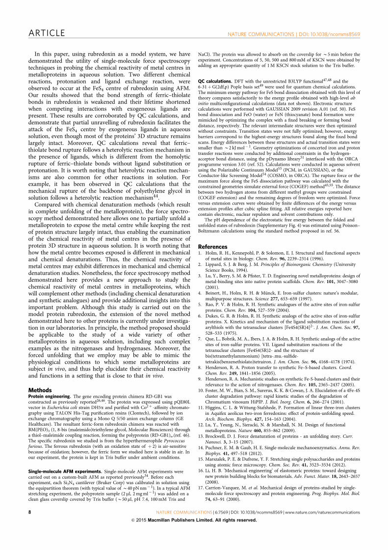
In this paper, using rubredoxin as a model system, we havedemonstrated the utility of single-molecule force spectroscopytechniques in probing the chemical reactivity of metal centres inmetalloproteins in aqueous solution. Two different chemicalreactions, protonation and ligand exchange reaction, wereobserved to occur at the FeS4 centre of rubredoxin using AFM.Our results showed that the bond strength of ferric–thiolatebonds in rubredoxin is weakened and their lifetime shortenedwhen competing interactions with exogeneous ligands arepresent. These results are corroborated by QC calculations, anddemonstrate that partial unravelling of rubredoxin facilitates theattack of the FeS4 centre by exogeneous ligands in aqueoussolution, even though most of the proteins’ 3D structure remainslargely intact. Moreover, QC calculations reveal that ferric–thiolate bond rupture follows a heterolytic reaction mechanism inthe presence of ligands, which is different from the homolyticrupture of ferric–thiolate bonds without ligand substitution orprotonation. It is worth noting that heterolytic reaction mechan-isms are also common for other reactions in solution. Forexample, it has been observed in QC calculations that themechanical rupture of the backbone of polyethylene glycol insolution follows a heterolytic reaction mechanism44.

Compared with chemical denaturation methods (which resultin complete unfolding of the metalloprotein), the force spectro-scopy method demonstrated here allows one to partially unfold ametalloprotein to expose the metal centre while keeping the restof protein structure largely intact, thus enabling the examinationof the chemical reactivity of metal centres in the presence ofprotein 3D structure in aqueous solution. It is worth noting thathow the metal centre becomes exposed is different in mechanicaland chemical denaturations. Thus, the chemical reactivity ofmetal centres may exhibit differences in mechanical and chemicaldenaturation studies. Nonetheless, the force spectroscopy methoddemonstrated here provides a new approach to study thechemical reactivity of metal centres in metalloproteins, whichwill complement other methods (including chemical denaturationand synthetic analogues) and provide additional insights into thisimportant problem. Although this study is carried out on themodel protein rubredoxin, the extension of the novel methoddemonstrated here to other proteins is currently under investiga-tion in our laboratories. In principle, the method proposed shouldbe applicable to the study of a wide variety of othermetalloproteins in aqueous solution, including such complexexamples as the nitrogenases and hydrogenases. Moreover, theforced unfolding that we employ may be able to mimic thephysiological conditions to which some metalloproteins aresubject in vivo, and thus help elucidate their chemical reactivityand functions in a setting that is close to that in vivo.

MethodsProtein engineering. The gene encoding protein chimera RD-GB1 wasconstructed as previously reported26,46. The protein was expressed using pQE80Lvector in Escherichia coli strain DH5a and purified with Co2þ -affinity chromato-graphy using TALON His-Tag purification resins (Clontech), followed by ionexchange chromatography using a Mono Q 5/50 anion exchange column (GEHealthcare). The resultant ferric-form rubredoxin chimera was reacted withBM(PEO)3 (1, 8-bis (maleimido)triethylene glycol, Molecular Biosciences) througha thiol–maleimide coupling reaction, forming the polyprotein (RD-GB1)n.(ref. 46).The specific rubredoxin we studied is from the hyperthermerophile Pyrococcusfurious. The ferrous rubredoxin (with an oxidation state of þ 2) is air-sensitivebecause of oxidation; however, the ferric form we studied here is stable in air. Inour experiment, the protein is kept in Tris buffer under ambient conditions.

Single-molecule AFM experiments. Single-molecule AFM experiments werecarried out on a custom-built AFM as reported previously34. Before eachexperiment, each Si3N4 cantilever (Bruker Corp) was calibrated in solution usingthe equipartition theorem (with typical value of B40 pN nm� 1). In a typical AFMstretching experiment, the polyprotein sample (2 ml, 2 mg ml� 1) was added on aclean glass coverslip covered by Tris buffer (B50ml, pH 7.4, 100 mM Tris and

NaCl). The protein was allowed to absorb on the coverslip for B5 min before theexperiment. Concentrations of 5, 50, 500 and 800 mM of KSCN were obtained byadding an appropriate quantity of 1 M KSCN stock solution to the Tris buffer.

QC calculations. DFT with the unrestricted B3LYP functional47,48 and the6-31þG(2df,p) Pople basis set49 were used for quantum chemical calculations.The minimum energy pathway for FeS bond dissociation obtained with this level oftheory compares satisfactorily to the energy profile obtained with high-level abinitio multiconfigurational calculations (data not shown). Electronic structurecalculations were performed with GAUSSIAN 2009 revision A.01 (ref. 50). FeSbond dissociation and FeO (water) or FeN (thiocyanate) bond formation weremimicked by optimizing the complex with a fixed breaking or forming bonddistance, respectively. The relevant intermediate structures were then optimizedwithout constraints. Transition states were not fully optimized; however, energybarriers correspond to the highest-energy structures found along the fixed bondscans. Energy differences between these structures and actual transition states weresmaller than B2 kJ mol� 1. Geometry optimizations of concerted iron and protontransfer reactions were conducted by additional constraints in the hydrogen-acceptor bond distance, using the pDynamo library51 interfaced with the ORCAprogramme version 3.01 (ref. 52). Calculations were conducted in aqueous solventusing the Polarizable Continuum Model53 (PCM, in GAUSSIAN), or theConductor-like Screening Model54 (COSMO, in ORCA). The rupture force or themaximum force along the FeS dissociation pathway was calculated with theconstrained geometries simulate external force (COGEF) method45,55. The distancebetween two hydrogen atoms from different methyl groups were constrained(COGEF extension) and the remaining degrees of freedom were optimized. Forceversus extension curves were obtained by finite differences of the energy versusextension profiles after cubic spline fitting. All relative energies reported herecontain electronic, nuclear repulsion and solvent contributions only.

The pH dependence of the electrostatic free energy between the folded andunfolded states of rubredoxin (Supplementary Fig. 4) was estimated using Poisson–Boltzmann calculations using the standard method proposed in ref. 56.

References1. Holm, R. H., Kennepohl, P. & Solomon, E. I. Structural and functional aspects

of metal sites in biology. Chem. Rev. 96, 2239–2314 (1996).2. Lippard, S. J. & Berg, J. M. Principles of Bioinorganic Chemistry (University

Science Books, 1994).3. Lu, Y., Berry, S. M. & Pfister, T. D. Engineering novel metalloproteins: design of

metal-binding sites into native protein scaffolds. Chem. Rev. 101, 3047–3080(2001).

4. Beinert, H., Holm, R. H. & Munck, E. Iron-sulfur clusters: nature’s modular,multipurpose structures. Science 277, 653–659 (1997).

5. Rao, P. V. & Holm, R. H. Synthetic analogues of the active sites of iron-sulfurproteins. Chem. Rev. 104, 527–559 (2004).

6. Dukes, G. R. & Holm, R. H. Synthetic analogs of the active sites of iron-sulfurproteins. X. Kinetics and mechanism of the ligand substitution reactions ofarylthiols with the tetranuclear clusters [Fe4S4(SR)4]2-. J. Am. Chem. Soc. 97,528–533 (1975).

7. Que, L., Bobrik, M. A., Ibers, J. A. & Holm, R. H. Synthetic analogs of the activesites of iron-sulfur proteins. VII. Ligand substitution reactions of thetetranuclear clusters [Fe4S4(SR)2- and the structure ofbis(tetramethylammonium) [tetra-.mu.-sulfide-tetrakis(benzenethiolato)tetrairon. J. Am. Chem. Soc. 96, 4168–4178 (1974).

8. Henderson, R. A. Proton transfer to synthetic Fe–S-based clusters. Coord.Chem. Rev. 249, 1841–1856 (2005).

9. Henderson, R. A. Mechanistic studies on synthetic Fe-S-based clusters and theirrelevance to the action of nitrogenases. Chem. Rev. 105, 2365–2437 (2005).

10. Foster, M. W., Bian, S. M., Surerus, K. K. & Cowan, J. A. Elucidation of a 4Fe-4Scluster degradation pathway: rapid kinetic studies of the degradation ofChromatium vinosum HiPIP. J. Biol. Inorg. Chem. 6, 266–274 (2001).

11. Higgins, C. L. & Wittung-Stafshede, P. Formation of linear three-iron clustersin Aquifex aeolicus two-iron ferredoxins: effect of protein-unfolding speed.Arch. Biochem. Biophys. 427, 154–163 (2004).

12. Lu, Y., Yeung, N., Sieracki, N. & Marshall, N. M. Design of functionalmetalloproteins. Nature 460, 855–862 (2009).

13. Brockwell, D. J. Force denaturation of proteins - an unfolding story. Curr.Nanosci. 3, 3–15 (2007).

14. Puchner, E. M. & Gaub, H. E. Single-molecule mechanoenzymatics. Annu. Rev.Biophys. 41, 497–518 (2012).

15. Marszalek, P. E. & Dufrene, Y. F. Stretching single polysaccharides and proteinsusing atomic force microscopy. Chem. Soc. Rev. 41, 3523–3534 (2012).

16. Li, H. B. ’Mechanical engineering’ of elastomeric proteins: toward designingnew protein building blocks for biomaterials. Adv. Funct. Mater. 18, 2643–2657(2008).

17. Carrion-Vazquez, M. et al. Mechanical design of proteins-studied by single-molecule force spectroscopy and protein engineering. Prog. Biophys. Mol. Biol.74, 63–91 (2000).




18. Janshoff, A., Neitzert, M., Oberdorfer, Y. & Fuchs, H. Force spectroscopy ofmolecular systems - single molecule spectroscopy of polymers andbiomolecules. Angew. Chem. Int. Ed. 39, 3213–3237 (2000).

19. Beyer, M. K. & Clausen-Schaumann, H. Mechanochemistry: the mechanicalactivation of covalent bonds. Chem. Rev. 105, 2921–2948 (2005).

20. Zoldak, G. & Rief, M. Force as a single molecule probe of multidimensionalprotein energy landscapes. Curr. Opin. Struct. Biol. 23, 48–57 (2013).

21. Li, H. et al. Reverse engineering of the giant muscle protein titin. Nature 418,998–1002 (2002).

22. Prakash, S. & Matouschek, A. Protein unfolding in the cell. Trends Biochem. Sci.29, 593–600 (2004).

23. Sauer, R. T. & Baker, T. A. AAAþ proteases: ATP-fueled machines of proteindestruction. Annu. Rev. Biochem. 80, 587–612 (2011).

24. Kabuta, T., Suzuki, Y. & Wada, K. Degradation of amyotrophic lateral sclerosis-linked mutant Cu,Zn-superoxide dismutase proteins by macroautophagy andthe proteasome. J. Biol. Chem. 281, 30524–30533 (2006).

25. Zheng, P., Chou, C. C., Guo, Y., Wang, Y. & Li, H. Single molecule forcespectroscopy reveals the molecular mechanical anisotropy of the FeS4 metalcenter in rubredoxin. J. Am. Chem. Soc. 135, 17783–17792 (2013).

26. Zheng, P. & Li, H. Highly covalent ferric� thiolate bonds exhibit surprisinglylow mechanical stability. J. Am. Chem. Soc. 133, 6791–6798 (2011).

27. Zheng, P., Takayama, S.-i. J., Mauk, A. G. & Li, H. Hydrogen bond strengthmodulates the mechanical strength of ferric-thiolate bonds in rubredoxin.J. Am. Chem. Soc. 134, 4124–4131 (2012).

28. Zheng, P., Takayama, S. J., Mauk, A. G. & Li, H. Single molecule forcespectroscopy reveals that iron is released from the active site of rubredoxin by astochastic mechanism. J. Am. Chem. Soc. 135, 7992–8000 (2013).

29. Zheng, P., Wang, Y. & Li, H. Reversible unfolding-refolding of rubredoxin: asingle-molecule force spectroscopy study. Angew. Chem. Int. Ed. Engl. 53,14060–14063 (2014).

30. Arantes, G. M., Bhattacharjee, A. & Field, M. J. Homolytic cleavage of Fe-Sbonds in rubredoxin under mechanical stress. Angew. Chem. Int. Ed. Engl. 52,8144–8146 (2013).

31. Blake, P. R. et al. Determinants of protein hyperthermostability: purificationand amino acid sequence of rubredoxin from the hyperthermophilicarchaebacterium Pyrococcus furiosus and secondary structure of the zinc adductby NMR. Biochemistry 30, 10885–10895 (1991).

32. Lovenber., W. & Sobel, B. E. Rubredoxin - a new electron transfer protein fromclostridium Pasteurianum. Proc. Natl Acad. Sci. USA 54, 193–199 (1965).

33. Cavagnero, S., Zhou, Z. H., Adams, M. W. & Chan, S. I. Response of rubredoxinfrom Pyrococcus furiosus to environmental changes: implications for the originof hyperthermostability. Biochemistry 34, 9865–9873 (1995).

34. Cao, Y., Lam, C., Wang, M. & Li, H. Nonmechanical protein can have signi-ficant mechanical stability. Angew. Chem. Int. Ed. Engl. 45, 642–645 (2006).

35. Zheng, P. et al. Single molecule force spectroscopy reveals that electrostaticinteractions affect the mechanical stability of proteins. Biophys. J. 100,1534–1541 (2011).

36. Marko, J. F. & Siggia, E. D. Stretching DNA. Macromolecules 28, 8759–8770(1995).

37. Rief, M., Fernandez, J. M. & Gaub, H. E. Elastically coupled two-level systems asa model for biopolymer extensibility. Phys. Rev. Lett. 81, 4764–4767 (1998).

38. Fernandez, J. M. & Li, H. Force-clamp spectroscopy monitors the foldingtrajectory of a single protein. Science 303, 1674–1678 (2004).

39. Garcia-Manyes, S., Liang, J., Szoszkiewicz, R., Kuo, T. L. & Fernandez, J. M.Force-activated reactivity switch in a bimolecular chemical reaction. Nat. Chem.1, 236–242 (2009).

40. Evans, E. Probing the relation between force--lifetime--and chemistry in singlemolecular bonds. Annu. Rev. Biophys. Biomol. Struct. 30, 105–128 (2001).

41. Bobrik, M. A., Que, Jr. L. & Holm, R. H. Synthetic analogs of the active sites ofiron-sulfur proteins. IV. Ligand substitution reactions of the tetranuclearclusters (Fe4S4(SR)4)2-. J. Am. Chem. Soc. 96, 285–287 (1974).

42. Job, R. C. & Bruice, T. C. Iron-sulfur clusters II: Kinetics of ligand exchangestudied on a water-soluble Fe4S4(SR)4n- cluster. Proc. Natl Acad. Sci. USA 72,2478–2482 (1975).

43. Lo, W., Scott, T. A., Zhang, P., Ling, C. C. & Holm, R. H. Stabilities of cubanetype [Fe(4)S(4)(SR)(4)](2-) clusters in partially aqueous media. J. Inorg.Biochem. 105, 497–508 (2011).

44. Aktah, D. & Frank, I. Breaking bonds by mechanical stress: when do electronsdecide for the other side? J. Am. Chem. Soc. 124, 3402–3406 (2002).

45. Ribas-Arino, J. & Marx, D. Covalent mechanochemistry: theoretical conceptsand computational tools with applications to molecular nanomechanics. Chem.Rev. 112, 5412–5487 (2012).

46. Zheng, P., Cao, Y. & Li, H. Facile method of constructing polyproteins forsingle-molecule force spectroscopy studies. Langmuir 27, 5713–5718 (2011).

47. Becke, A. D.Density-Functional Thermochemistry.3. The role of exactexchange. J. Chem. Phys. 98, 5648–5652 (1993).

48. Lee, C., Yang, W. & Parr, R. G. Development of the Colle-Salvetti correlation-energy formula into a functional of the electron density. Phys. Rev. B Condens.Matter 37, 785–789 (1988).

49. Ditchfie, R., Hehre, W. J. & Pople, J. A. Self-consistent molecular-orbitalmethods.9. Extended Gaussian-type basis for molecular-orbital studies oforganic molecules. J. Chem. Phys. 54, 724 (1971).

50. Frisch, M. J. T. et al. Gaussian 09, Revision A.01 (Gaussian Inc., 2009).51. Field, M. J. The pDynamo program for molecular simulations using hybrid

quantum chemical and molecular mechanical potentials. J. Chem. TheoryComput. 4, 1151–1161 (2008).

52. Neese, F. The ORCA program system. Wires Comput. Mol. Sci. 2, 73–78 (2012).53. Tomasi, J., Mennucci, B. & Cammi, R. Quantum mechanical continuum

solvation models. Chem. Rev. 105, 2999–3093 (2005).54. Klamt, A. Conductor-Like Screening model for real solvents - a new approach

to the quantitative calculation of solvation phenomena. J. Phys. Chem. 99,2224–2235 (1995).

55. Beyer, M. K. The mechanical strength of a covalent bond calculated by densityfunctional theory. J. Chem. Phys. 112, 7307–7312 (2000).

56. Yang, A. S. & Honig, B. On the pH dependence of protein stability. J. Mol. Biol.231, 459–474 (1993).

AcknowledgementsThis work is supported by the Natural Sciences and Engineering Research Councilof Canada, the Canada Foundation for Innovation, the Canada Research Chairsprogramme. G.M.A. acknowledges funding from FAPESP (projects 12/02501-4 and14/21900-2).

Author contributionsP.Z. and H.L. conceived the project, P.Z., G.M.A., M.J.F. and H.L. designed the research,P.Z., G.M.A. and M.J.F. performed the experiments/calculations and analysed the data,P.Z., G.M.A., M.J.F. and H.L. wrote the manuscript.

Additional informationSupplementary Information accompanies this paper at http://www.nature.com/naturecommunications

Competing financial interests: The authors declare no competing financial interests.

Reprints and permission information is available online at http://npg.nature.com/reprintsandpermissions/

How to cite this article: Zheng, P. et al. Force-induced chemical reactions onthe metal centre in a single metalloprotein molecule. Nat. Commun. 6:7569doi: 10.1038/ncomms8569 (2015).

This work is licensed under a Creative Commons Attribution 4.0International License. The images or other third party material in this

article are included in the article’s Creative Commons license, unless indicated otherwisein the credit line; if the material is not included under the Creative Commons license,users will need to obtain permission from the license holder to reproduce the material.To view a copy of this license, visit http://creativecommons.org/licenses/by/4.0/




85

ANEXO G – Flexibility and inhibitor bindingin Cdc25 phosphatases

proteinsSTRUCTURE O FUNCTION O BIOINFORMATICS

Flexibility and inhibitor binding in Cdc25phosphatasesGuilherme Menegon Arantes*

Instituto de Quımica, Universidade de Sao Paulo, Av. Lineu Prestes 748, 05508-900, Sao Paulo, SP, Brasil

INTRODUCTION

Cell division cycle Cdc25 phosphatases have turned into active tar-

gets for the development of antineoplastic agents as their overexpres-

sion has been detected in several human cancers.1–7 Although differ-

ent classes of Cdc25s inhibitors have been identified so far, the num-

ber of potent inhibitors that are active in vivo is still limited and

restricted to quinoid-based compounds.1,2 Thus, rational drug design

toward Cdc25 would certainly benefit from a detailed knowledge of

this enzyme catalytic mechanism and tertiary structure.

Cdc25s are dual-specificity protein tyrosine phosphatases (PTP) that

dephosphorylate pTyr and pThr residues on cyclin-dependent kinases

(Cdk) responsible for cell cycle checkpoints.8,9 Known as the P-loop,

the active site is characterized by the sequence Cys-(Xxx)5-Arg con-

served among all known PTPs (Fig. 1). The conserved Cys is the nucleo-

phile that attacks the substrate phosphate group, which is in turn stabi-

lized by the conserved Arg side chain. Poor selectivity has been observed

in vitro for the most potent PTP inhibitors because these compounds

bind to the conserved P-loop.4,5 One important difference between

Cdc25 and the other PTPs that could be explored in the design of selec-

tive inhibitors is the catalytic general acid. In Cdc25, this residue was

identified by the Glu following the nucleophilic Cys in the P-loop

sequence.9,10 But, in all other PTPs, the general acid is an Asp located

in a flexible loop distant from the active site.8,11

The three Cdc25 isoforms found in humans share 70% identity in

the primary sequence of their catalytic C-terminal domain, but pres-

ent larger variance in their N-terminal regulatory domain where sev-

eral splice variants are possible.1 All the structural information avail-

able for Cdc25s was obtained from X-ray crystallographic data for

Cdc25A12 and Cdc25B13 catalytic domains in either apo forms (PDB

code 1c25)12 or with sulfate bound to the P-loop (codes 1qb0, 1cwr,

2a2k, 2ifd).13,14 NMR structures and order parameters15 for Cdc25

in solution, structures for inhibitor-Cdc25 complexes, or for the diver-

gent N-terminal domain have not been described to our knowledge.

The most notable difference between the crystal structures of isoforms

Cdc25A and B is observed in the backbone of the last 20 aminoacids

in the C-terminus. This region contains an a-helix for Cdc25B but it

is unstructured for Cdc25A (Fig. 1). Additional 28 (Cdc25A) and 16

Additional Supporting Information may be found in the online version of this article.

Grant sponsor: FAPESP; Grant numbers: 07/52772-6, 07/59345-6

*Correspondence to: Guilherme Menegon Arantes, Instituto de Quımica, Universidade de Sao Paulo,

Av. Lineu Prestes 748, 05508-900, Sao Paulo, SP, Brasil. E-mail: [email protected]

Received 4 April 2010; Revised 7 June 2010; Accepted 23 June 2010

Published online 23 July 2010 in Wiley Online Library (wileyonlinelibrary.com).

DOI: 10.1002/prot.22826

ABSTRACT

Cdc25 phosphatases involved in cell cycle

checkpoints are now active targets for the de-

velopment of anti-cancer therapies. Rational

drug design would certainly benefit from

detailed structural information for Cdc25s.

However, only apo- or sulfate-bound crystal

structures of the Cdc25 catalytic domain have

been described so far. Together with previously

available crystalographic data, results from mo-

lecular dynamics simulations, bioinformatic

analysis, and computer-generated conforma-

tional ensembles shown here indicate that the

last 30–40 residues in the C-terminus of

Cdc25B are partially unfolded or disordered in

solution. The effect of C-terminal flexibility

upon binding of two potent small molecule

inhibitors to Cdc25B is then analyzed by using

three structural models with variable levels of

flexibility, including an equilibrium distributed

ensemble of Cdc25B backbone conformations.

The three Cdc25B structural models are used

in combination with flexible docking, cluster-

ing, and calculation of binding free energies by

the linear interaction energy approximation to

construct and validate Cdc25B-inhibitor com-

plexes. Two binding sites are identified on top

and beside the Cdc25B active site. The diversity

of interaction modes found increases with re-

ceptor flexibility. Backbone flexibility allows

the formation of transient cavities or compact

hydrophobic units on the surface of the stable,

folded protein core that are unexposed or

unavailable for ligand binding in rigid and

densely packed crystal structures. The present

results may help to speculate on the mecha-

nisms of small molecule complexation to par-

tially unfolded or locally disordered proteins.

Proteins 2010; 78:3017–3032.VVC 2010 Wiley-Liss, Inc.

Key words: molecular dynamics; conforma-

tional ensemble; docking; intrinsic disorder;

protein tyrosine phosphatases; transient cav-

ities; computer simulation; receptor flexibility.

VVC 2010 WILEY-LISS, INC. PROTEINS 3017

(Cdc25B) residues in the protein C-terminal were present

in the constructs used for crystallization, but had no

observable electron densities suggesting further intrinsic

flexibility or disorder in the C-terminus.12,13 Interest-

ingly, it has been shown that this C-terminal tail medi-

ates substrate recognition by up to 100-fold in the phos-

phatase activity of Cdc25B and Cdc25C toward the bis-

phosphorylated Cdk2-pTpY/CycA natural substrate.16

Structural disorder plays a role in the molecular recog-

nition between proteins involved in cell signaling.17 In

particular, the interaction between Cdk and several of its

partner proteins including p21,18 but not yet Cdc25, has

been shown to proceed through disorder-to-order transi-

tions.19 Thus, it is possible that the recognition between

Cdc25 and Cdk/Cyc complexes is driven by a similar

mechanism involving the last 30–40 residues in the

Cdc25 C-terminal. Even if a disorder-to-order transition

is not involved, C-terminal flexibility will be relevant

because this tail occupies the protein-protein contact sur-

face between the Cdc25 catalytic domain and the Cdk2

main body.14 The Cdc25 C-terminus is also in contact

with its own main body and near the active site P-loop

(Fig. 1), such that its flexibility will also influence bind-

ing of competitive inhibitors. What is then, the effect of

this putative C-terminal disorder on the complexation of

small molecules to Cdc25? It appears that this question

has received little attention for partially unfolded proteins

in general, even though it has been suggested that a large

fraction of eukariotic proteins (�30%) contains intrinsi-

cally disordered regions.17

Modelling protein–inhibitor complexation, in particu-

lar, docking of small molecules to rigid receptor struc-

tures, is an established area with several parameterized

and tested methods.20,21 Including protein flexibility

into such docking protocols is, however, less devel-

oped.22,23 Most of the approaches currently in use were

designed to account for side chain or limited backbone

flexibility, for instance, by introducing soft or average

grid models of receptor ligand interaction.24,25 This is

clearly inappropriate for large-scale fluctuations present

in partially disordered proteins because average positions

will not represent the relevant conformational states.23,26

Receptor flexibility may also be included by docking to

several different structures from a configurational ensem-

ble.27–29 The problem here is how to obtain representa-

tive structures for flexible or disordered protein domains.

A set of geometries obtained from X-ray crystallography

might be perturbed by crystal packing30,31 and disor-

dered segments will not have visible electron densities.

Ensembles obtained from NMR might be more appropri-

ate models for solution configurations but the fitting

procedure traditionally used for structural determination

by reproducing distance restrains becomes less reliable

for proteins with intrinsic disorder and does not result in

an equilibrium distribution of configurations.15,30

Receptor structures may be generated computationally,

but large-scale fluctuations and protein disorder are more

difficult to simulate accurately. Molecular dynamics (MD)

simulations up to the nanosecond timescale under normal

temperature probe local fluctuations around the starting

geometry.32 High temperature MD may unveil cryptic

binding sites or induced fit changes if the protein region

that undergoes conformational exchange is known in

advance.33 Otherwise, several MD acceleration34,35 and

generalized ensemble36,37 methods may be used to

increase configurational sampling. Computer generation

of protein conformational ensembles may be based on geo-

metrical information of reference configurations,38–40

on backbone dihedral angle propensities extracted from

existing libraries,41,42 or on combinations of both

approaches.43 Statistical libraries built from geometries of

coiled protein fragments are reasonable models for the

unfolded or disordered regions.41,44 For protein–inhibitor

complexation a further challenge is the selection of an

ensemble subset that is relevant for binding.22 Although a

criteria based on structural variance is often used,22,32 a

more formal filtering should rely on the Boltzmann distri-

bution of the ensemble.45

In this work, Cdc25B C-terminal flexibility is analyzed,

and its effect on the complexation of quinone-based

small molecules is investigated using computer simula-

tions. Details about the computational methods used are

given in the next section. Results for molecular dynamics

simulations of Cdc25B strongly support that the C-termi-

nus is flexible and partially unfolded in solution. Three

Cdc25B structural models with variable levels of flexibil-

ity are compared: A rigid model corresponding to the

crystal structure, a semiflexible model corresponding to a

set of MD snapshots and a fully flexible model built with

Figure 1Superposition of the Cdc25A (in blue, PDB code 1c25) and Cdc25B (in

magenta, PDB code 1qb0) catalytic domain crystal structures.

G. M. Arantes

3018 PROTEINS

statistical rigor for backbone configurations. Then,

Cdc25B-inhibitor complexes using the three structural

models are presented and validated by the calculation of

binding free energies. Given the lack of experimental data

to benchmark the structural models and the generated

ligand–receptor complexes, the focus here is on discus-

sing the binding sites and less detail is reported on spe-

cific ligand–receptor molecular interactions. Finally, the

effect of C-terminal flexibility on the small molecule

complexation is described.

METHODS

Molecular dynamics and system set-up

Coordinates of a sulfate-bound Cdc25B crystal struc-

ture deposited in the PDB code 1qb0 were used to start

the molecular dynamics simulation. This protein chain

contains 177 residues from Asp374 to Trp550 of the

Cdc25B primary sequence. The initial simulation model

was built by removing all crystallographic waters, ions,

and b-mercaptoethanol. Missing hydrogen atoms were

added, considering all Asp, Glu, Arg, Lys, and His side

chains charged. This protonation state is slightly different

from the one accepted as the catalytic competent state in

which Cys473 is deprotonated and Glu474 protonated.9

Such difference should not influence the flexibility in the

P-loop active site backbone, which, is rather rigid, but it

might play a role for the detailed interactions in small

molecule complexation in the active site. The protein

chain was solvated by superimposing it to a replicated

water box, leaving at least 12 A between the protein and

the box edge. Six chloride anions were added to neutral-

ize the total system charge. Initial coordinates for one of

the chloride anions were extracted from the crystal struc-

ture (PDB code 1qb0). Although it was suggested that

this chloride anion may have a structural role,13 it dif-

fuses out of the interaction site within 5 ns of simula-

tion. Periodic boundary conditions were used with a

cubic box length of �78 A. Long-range electrostatics

were treated with the particle-mesh Ewald summation

with a 1.2 A Fourier grid spacing and fourth-order inter-

polation. A switch function with roff 5 10.0 A was used

to truncate long-range van der Waals interactions with-

out dispersion corrections.

All model building, molecular dynamics simulations

and trajectory analysis were carried out with the GRO-

MACS 4.0.2 suite of programs.46 The OPLS-AA47 force

field was used for the protein and ions, and the rigid

TIP3P48 potential was used for water. The LINCS algo-

rithm was used to constrain all covalent bonds and a

time step of 2 fs was used in MD integration.

The solvated protein heavy atoms were restrained to

their initial coordinates. The system was first energy-

minimized to relax unfavorable contacts, and kinetic

energy was gradually injected in the system by running

short (40 ps) MD simulations at 50, 100, 200, and 300

K. Restrains in the protein heavy atoms were gradually

removed by reducing the harmonic constant from the

initial 1000 kj mol21 A22 to 200, 20, and 2 kj mol21

A22 along another set of short (40 ps) MD simulations

at 300 K. This careful heating and pre-equilibration

phase was used to avoid artifactual flexibility in the apo

Cdc25B simulation as well as artifactual decomplexation

of inhibitors in the evaluation of interaction energies (see

Linear Interaction Energy section below). An equilibra-

tion 2 ns MD run was obtained without any position

restrains at 300 K and 1 atm. The Berendsen temperature

and pressure couplings were used up to this point.

Finally, a production 60 ns MD trajectory was obtained

at the same temperature and pressure conditions but in a

canonical ensemble using the Nose-Hoover extended

temperature scheme (time constant sT 5 0.1 ps) and the

Parrinello–Rahman pressure coupling (time constant sP5 0.5 ps). No group separation was used.

Bioinformatic analysis of disorderedsequences

Four different bioinformatic methods were used to

predict the disordered regions of Cdc25 isoforms A and

B. Primary sequences were submitted to web servers

queries and default algorithm options were used. FoldIn-

dex49 builds a score based on residue charge and hydro-

phobicity for a sliding window of 51 residues. Dis-

opred250 uses a linear support vector machine to analyze

the sequence profiles. VL3H51 and VLXT52 both search

using neural networks, and the latter is based on residue

physicochemical properties. Default server and algorith-

mic values were used in all queries. Only VL3H gives a

continuous N-terminal disordered segment. All other

predictors give N-terminal segments containing ordered

gaps of up to 30 amino acids, but with a total of more

than 75% of disordered residues in the N-terminal do-

main. The score given for the discontinuous segments is

the average of disordered scores (FoldIndex and VLXT)

or the range of scores (Disopred2). In FoldIndex, nega-

tive scores mean a segment will more likely be disor-

dered. Scores on the other methods give the probability

of disordered structure in the segment.

Ensemble generation

Two conformational ensembles based on the Cdc25B

catalytic domain crystal structure (code 1qb0) were used

here. The MD ensemble was composed of 150 snapshots

spaced by 400 ps each from the 60 ns MD trajectory

described above. Another Cdc25B conformational ensem-

ble built with a library-based Monte Carlo approach was

kindly provided by D. Zuckerman and co-workers.43 The

177 Cdc25B residues deposited on the PDB code 1qb0

are present in this model. The protein is divided into

Flexibility in Cdc25 Phosphatases

PROTEINS 3019

fragments identified with residue types for which statisti-

cal libraries of backbone conformations were built in

advance. Fragment libraries have Boltzmann distributions

pifrag, which account for correlations internal to each frag-

ment. The distribution of protein configurations built

with a simple product of fragments

plibi ðri; . . . ; rM Þ ¼YM

i

pfragi ðrÞ ð1Þ

will be biased toward the isolated fragment distributions.

Thus, Metropolis Monte Carlo is used to resample and

obtain protein configurations in equilibrium distribu-

tion.53 The protein internal energy is written as:

U protðri; . . . ; rM Þ ¼XM

i

Ufragi ðriÞ þ U restðri; . . . ; rM Þ ð2Þ

where Uifrag is the energy internal to each fragment

obtained from the library and Urest accounts for the

interactions between the M fragments. The interaction

term is described by a structure-based (or Go type)

potential, which stabilizes the native Cdc25B fold13 but

allows fluctuations around it in reasonable agreement

with experimental data.43 It should be noted that Boltz-

mann distributed protein backbone configurations are

generated with this formal procedure. However, residue

side chain conformations are built for each backbone

geometry separately, using the backbone-dependent

rotamer library SCWRL.54 Thus, side chains will not fol-

low the equilibrium distribution. Further details for the

generation of the Zuckerman Cdc25B ensemble are given

in the original paper.43

Small molecule docking and clustering

The studied ligands were 6-chloro-7-(2-morpholin-4-

ylethylamino)quinoline-5,8-dione (NSC 663284), 1 in

Figure 2, and 2,5-dihydroxy-3-(7–(2-methyl-benzyl)-1H-

indol-3-yl)[1,4]benzoquinone, 2 in Figure 2. For each re-

ceptor structure, 200 AutoDock 4.0 runs were performed

for each ligand.55 Interaction maps were generated in a

cubic grid with 60 points and 0.375 A spacing, centered

in the Cys473 Sg, the catalytic nucleophile. This medium

sized grid allowed docking to sites up to 11 A away from

the Cdc25B active site. A distance-dependent dielectric

constant was used for electrostatic interactions.55 Four

torsions for 1 and five torsions for 2 were active. The

genetic algorithm used for conformational search was set

with 150 individuals in the population for a maximum

of 27,000 generations or 2.5 3 106 energy evaluations.

Two clustering steps were used to analyze the docking

poses (more than 30.000 per ligand per ensemble).

Within each receptor structure, poses were initially clus-

tered for ligand heavy atom root mean-squared deviation

(RMSD) with a 2.0 A cutoff. The pose with lowest free

energy score in each initial cluster was considered a valid

one if it belonged to a cluster with at least 20 members

and if its AutoDock 4.0 free energy score was at most 2.0

kcal/mol higher than the lowest free energy score found

within dockings for the same receptor structure. This is

the definition for valid pose or valid complex used

throughout this work. Then, the set of valid poses for all

receptor structures in each ensemble was clustered for

ligand heavy-atom RMSD tolerance of 4.0 A after least-

square fitting of Cas for the stable residues in the recep-

tor (residues 377–530). This procedure gave the best

compromise between the size of clustering problem, the

amount of clusters finally obtained, and the expected ac-

curacy of the docking function.55 The eight clusters with

the largest population of valid poses for each ligand and

ensemble were analyzed in detail below.

Several criteria in the above procedure were relaxed to

test for cluster robustness. For instance, decreasing the

number of members (20) or increasing the cutoff energy

(2 kcal/mol) in 50% for the first clustering step, enlarged

the set of valid poses, but yielded qualitatively the same

eight most populated clusters, that is, the same binding

sites and cluster centroids. Throughout this work, the

centroid geometry represents the clusters obtained in the

second clustering step. A cluster centroid is defined as

the valid complex with the smallest average distance to

the other valid complexes within the same cluster. Again,

the same binding sites were obtained if the RMSD toler-

ance was changed to 3.5 or 4.5 A in the second clustering

step (the population of each cluster was smaller or larger,

respectively). Several clustering algorithms (single-linkage,

Daura et al.,56 and self-organizing maps57) were tested

yielding similar results.

Linear interaction energy

The stability of the binding modes found in the dock-

ing and clustering procedure was estimated using the fol-

Figure 2Structure of the quinolinequinone 1 and the indolyldihydroxyquinone 2.

G. M. Arantes

3020 PROTEINS

lowing linear interaction energy (LIE) approximation to

the binding free energy58:

DGbind ’aðhV vdWcompi�hV vdW

sol iÞþbðhV eletcompi�hV elet

sol iÞ ð3Þ

where h��i represents an ensemble average (obtained here

from a MD trajectory) of nonbonded van der Waals

(vdw) and electrostatic (elec) interaction energies (V)

between the ligand and its surrounding environment.

Direct calculation of absolute free energies is possible,59

but extremely demanding for computational resources

and, hence, unfeasible for such large set of complexes as

found here. The LIE is computationally more efficient

because it only requires two end states MD simulations,

one for the free ligand in solvent (sol) and another for

the ligand–protein complex (comp). The parameters

adopted were a 5 0.18, b 5 0.37 for 1, and b 5 0.33

for 2.60 MD simulations starting from the ligand–protein

complex poses obtained with AutoDock and for the free

ligand in water were carried out following the same

model building, heating, and pre-equilibration proce-

dures adopted for the apo Cdc25B (Molecular dynamics

and system set-up section). The equilibration and data

acquisition MD trajectories were run for 0.5 and 1.0 ns,

respectively, and both simulations were obtained at 300

K and 1 atm in a canonical ensemble using the Nose-

Hoover and the Parrinello–Rahman coupling schemes.

Long-range electrostatics were treated with a switch func-

tion with ron 5 8 A and roff 5 12 A. The force field for

both ligands was derived from the OPLS-AA force field

with appropriate partial charges derived from the charges

assigned to similar OPLS groups.

RESULTS AND DISCUSSION

Cdc25B is partially unfolded in solution

To explore the intrinsic flexibility of apo Cdc25B in

aqueous solvent, a long molecular dynamics simulation

was conducted at normal conditions. The observed tra-

jectory begins with a rapid relaxation of the protein

structure from the initial crystallographic coordinates in

response to the solvated environment. The protein core

(residues 374–531) has a constant deviation from the ini-

tial coordinates measured by a Ca RMSD �2 A up to the

end of the simulation as shown in Figure 3(A). However,

at about 40 ns, a steep increase in the Ca RMSD from

4 A to more than 8 A is observed for the last 19 residues

in the Cdc25B C-terminus [Fig. 3(A)]. The protein

radius of gyration, which is stable at �16.7 A from 5 to

40 ns also increases to �17.0 A from 40 ns to the end of

the simulation.

Figure 3(B) shows fluctuations of the protein Cas

about their mean position obtained from the Cdc25B

MD run and from the temperature factors of Cdc25A

and Cdc25B crystallographic structures. The Cdc25B

RMSF obtained from the X-ray structure is rather flat

and featureless, which maybe a consequence of the

refinement procedure on the diffraction data.31 There is

some fair agreement between the RMSF obtained from

the Cdc25A structure and from the Cdc25B simulation.

The catalytic domains of the two isoforms share more

than 70% identity in their primary sequences and have

almost identical folds (Fig. 1), so they should also have

equivalent backbone fluctuations. For instance, both

RMSFs are larger than 1 A from residues 443–466, and

drop steadily in residues 469–471. This is the active site

region, which is prearranged to bind phosphate

esters.9,11,13 The main differences between fluctuations

calculated from the experimental and simulated data are

observed for the protein terminals. The simulated RMSF

is >3 A for the first three residues (374–376) in the N-

Figure 3Molecular dynamics of apo Cdc25B in solution. Top panel A shows the

Ca root mean-squared deviation from the crystalographic structure for

the Cdc25B protein core (residues 374–531) and the 19 residues in the

C-terminus (residues 532–550). Lower panel B gives the Ca root mean-

squared fluctuation obtained from the 60ns MD and calculated from

temperature factors for the Cdc25A (PDB code 1c25) and Cdc25B

(PDB code 1qb0) structures. [Color figure can be viewed in the online

issue, which is available at wileyonlinelibrary.com.]


PROTEINS 3021

terminus and for residues 531–548 in the C-terminus

[Fig. 3(B)]. The large and localized flexibility in the N-

terminus should be expected as the protein is truncated

in this position. In fact, the Cdc25B construct expressed

and used for X-ray crystallography has in addition 18

residues (356–373) along the N-terminus and 16 residues

(551–566) along the C-terminus, which are not observed

in the electron density maps.13 The simulated protein

contains only residues 374–550, as given in the PDB file,

including an a-helix present along residues 533–546.13

The large RMSD and RMSF observed for the C-termi-

nus during the MD trajectory correspond to a local

unfolding and detaching of the terminal a-helix from the

protein main-body. It may be possible that the last 16

residues (551–566) along the C-terminus, which were

present in the Cdc25B construct used for crystallization,

but absent from the MD simulation, are necessary to sta-

bilize the terminal a-helix. However, no terminal helix is

observed in the crystal structure for isoform Cdc25A

(Fig. 1) even though the complete C-terminus, residues

336–523 in the Cdc25A numbering, was present in the

crystallized construct. In fact, electron densities for the

last 28 residues (496–523) in Cdc25A were not observed

and this region was considered disordered in the crystal

form.12

These observations suggest that the terminal Cdc25

regions, especially the last 30–40 residues in the C-termi-

nus, are intrinsically disordered or at least partially

unfolded in solution. The terminal a-helix present in the

Cdc25B structure may be a crystal packing artifact or

may be stabilized because favorable interactions between

symmetrically related molecules (the terminal Trp550

side chains are in contact in the 1qb0 model13,43).

To support the partial unfolding hypothesis, the pri-

mary sequences of Cdc25A and Cdc25B were submitted

to bioinformatic analysis for prediction of disordered

protein sequences.52 Table I shows the results obtained

with four different methods. The whole N-terminal do-

main is predicted as disordered, with up to 320 unfolded

residues for Cdc25A and 370 residues for Cdc25B. To

our knowledge, the structure of the N-terminal region of

Cdc25s has never been solved, which might be explained

by the difficulty in obtaining crystals and a diffraction

pattern from partially disordered materials. The ordered

segment found by all bioinformatic methods roughly

coincides with the catalytic domains of Cdc25A and B

observed by X-ray crystallography12,13 and with the core

region of Cdc25B stable during the MD simulations

described above. The disordered segments found for the

C-terminus are all continuous, but with variable size.

They range from the last 75 residues (FoldIndex) down

to the last 40 (VL3H) or 30–20 residues (Disopred2 and

VLXT) for both Cdc25A and B. But, clearly, the bioinfor-

matic search confirms the suggestion from MD simula-

tions that the Cdc25 terminals are disordered or partially

unfolded in solution.

Modeling Cdc25B with conformationalensembles

The effects of protein flexibility upon binding and mo-

lecular recognition may be accounted for by modeling

the receptor geometry with a conformational ensemble

or a collection of structures.22,29 Statistically significant

sampling of such conformations following a Boltzmann

distribution45 is not feasible with the computer power

available nowadays if proteins the size of Cdc25 catalytic

domain (�200 residues) are modelled by detailed all-

atom force fields, such as the one used here for MD. Dif-

ferent methods exist to generate conformational ensem-

bles.38–42,61,62 Here two computational models were

adopted: An ensemble selected from the present MD tra-

jectory and an ensemble generated for the Cdc25B cata-

lytic domain by Zuckerman and co-workers.43 See the

Methods section for details about ensemble construction.

The Zuckerman ensemble contained 250 structures with

Ca RMSD from the X-ray structure varying from 3 to

10 A. The core of the Cdc25B catalytic domain (residues

377–530) remains stable and folded. But, large fluctua-

tions are again observed in the C-terminus. In fact, the

C-terminal helix is unfolded in all configurations in the

Zuckerman ensemble. This is another independent com-

putational evidence of the intrinsic disorder suggested

above for the Cdc25 C-terminal region. Figures shown

below for ligand–protein complexes with the Zuckerman

ensemble are illustrative examples of configurations com-

posing this ensemble. The average radius of gyration for

protein conformations in the ensemble is 17.8 � 0.7 A,

�1 A larger than the radius of gyration observed in the

MD simulation. Even though the C-terminus unfolds,

the main distance from residues to the protein center-of-

mass does not change significantly, because the protein

core remains stable and folded. In agreement with experi-

mental evaluation of the Cdc25B crystal structure, part

of the Zuckerman ensemble had a disulfide bridge

formed between C426 and C473 (corresponding to the

PDB model 1cwr).13 Only the 176 structures without

such bridge were used here.

Table IDisordered Regions on the Cdc25A and B Complete Primary Sequences

Predicted by Various Bioinformatic Methodsa

Method

Cdc25A Cdc25B

Segment Score Segment Score

Disopred250 1–323 0.2–1.0 1–368 0.2–1.0504–523 0.5 546–566 �0.5

FoldIndex49 61–325 20.20 � 0.09 160–375 20.22 � 0.08450–523 20.19 � 0.08 494–566 20.14 � 0.06

VL3H51 1–323 0.8 1–368 0.8480–523 0.8 528–566 0.7

VLXT52 1–329 0.7 1–365 0.8493–523 0.8 541–562 0.9

aResidue numbering covers the entire protein sequence: 1–523 for Cdc25A and 1–

566 for Cdc25B.13

G. M. Arantes

3022 PROTEINS

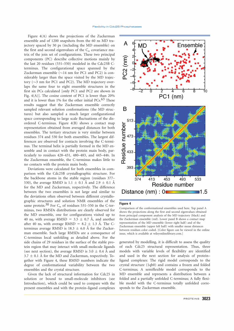
Figure 4(A) shows the projections of the Zuckerman

ensemble and of 1200 snapshots from the 60 ns MD tra-

jectory spaced by 50 ps (including the MD ensemble) on

the first and second eigenvalues of the Ca covariance ma-

trix of the join set of configurations. These two principal

components (PC) describe collective motions mainly by

the last 20 residues (531–550) modeled in the Cdc25B C-

terminus. The configurational space spanned by the

Zuckerman ensemble (�14 nm for PC1 and PC2) is con-

siderably larger than the space visited by the MD trajec-

tory (�3 nm for PC1 and PC2). The MD trajectory over-

laps the same four to eight ensemble structures in the

first six PCs calculated [only PC1 and PC2 are shown in

Fig. 4(A)]. The cosine content of PC1 is lower than 20%

and it is lower than 1% for the other initial PCs.63 These

results suggest that the Zuckerman ensemble correctly

sampled relevant solution conformations (the MD struc-

tures) but also sampled a much larger configurational

space corresponding to large scale fluctuations of the dis-

ordered C-terminus. Figure 4(B) shows a contact map

representation obtained from averaged distances for both

ensembles. The tertiary structure is very similar between

residues 374 and 530 for both ensembles. The largest dif-

ferences are observed for contacts involving the C-termi-

nus. The terminal helix is partially formed in the MD en-

semble and in contact with the protein main body, par-

ticularly to residues 428–431, 480–483, and 445–446. In

the Zuckerman ensemble, the C-terminus makes little to

no contacts with the protein main body.

Deviations were calculated for both ensembles in com-

parison with the Cdc25B crystallographic structure. For

the backbone atoms in the stable region (residues 377–

530), the average RMSD is 1.1 � 0.1 A and 2.9 � 0.1 A

for the MD and Zuckerman, respectively. The difference

between the two ensembles is not large and similar to

the deviations often observed between different crystallo-

graphic structures and solution NMR ensembles of the

same protein.30 For Ca of residues 531–550 in the C-ter-

minus, two RMSDs distributions are clearly observed for

the MD ensemble, one for configurations visited up to

40 ns, with average RMSD 5 3.5 � 0.7 A, and another

after 40 ns, with average RMSD 5 8.2 � 1.3 A. The C-

terminus average RMSD is 18.3 � 6.0 A for the Zucker-

man ensemble. Such large RMSDs are a consequence of

C-terminus local unfolding as detailed above. For the

side chains of 29 residues in the surface of the stable pro-

tein region that may interact with small-molecule ligands

(see next section), the average RMSD is 3.0 � 0.4 A and

3.7 � 0.1 A for the MD and Zuckerman, respectively. To-

gether with Figure 4, these RMSD numbers indicate the

degree of conformational variability between the two

ensembles and the crystal structure.

Given the lack of structural information for Cdc25 in

solution or bound to small-molecule inhibitors (see

Introduction), which could be used to compare with the

present ensembles and with the protein–ligand complexes

generated by modelling, it is difficult to assess the quality

of each Cdc25 structural representation. Thus, three

models with variable levels of flexibility are identified

and used in the next section for analysis of protein–

ligand complexes: The rigid model corresponds to the

crystal structure (1qb0) and contains a frozen and folded

C-terminus; A semiflexible model corresponds to the

MD ensemble and represents a distribution between a

folded and a partially unfolded C-terminus; A fully flexi-

ble model with the C-terminus totally unfolded corre-

sponds to the Zuckerman ensemble.

Figure 4Comparison of the conformational ensembles used here. Top panel A

shows the projections along the first and second eigenvalues obtained

from principal component analysis of the MD trajectory (black) and

the Zuckerman ensemble (red). Lower panel B shows a contact map

representation of the MD ensemble (lower right half) and of the

Zuckerman ensemble (upper left half) with smaller mean distances

between residues color coded. [Color figure can be viewed in the online

issue, which is available at wileyonlinelibrary.com.]


PROTEINS 3023

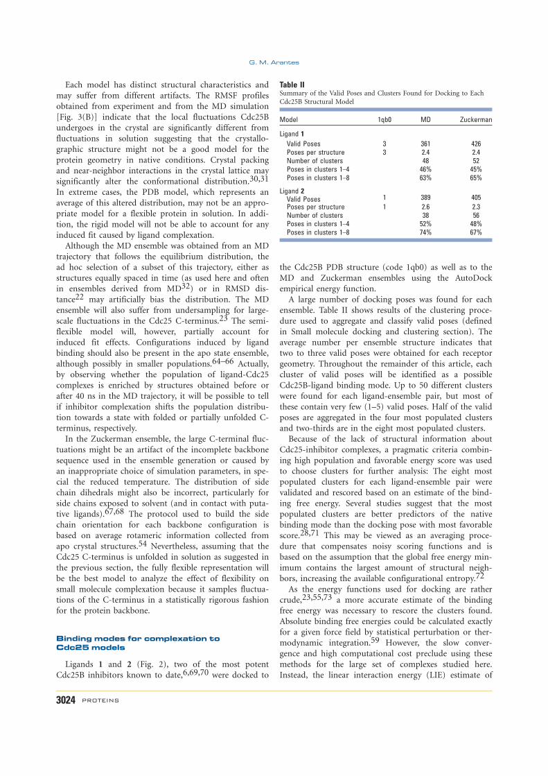
Each model has distinct structural characteristics and

may suffer from different artifacts. The RMSF profiles

obtained from experiment and from the MD simulation

[Fig. 3(B)] indicate that the local fluctuations Cdc25B

undergoes in the crystal are significantly different from

fluctuations in solution suggesting that the crystallo-

graphic structure might not be a good model for the

protein geometry in native conditions. Crystal packing

and near-neighbor interactions in the crystal lattice may

significantly alter the conformational distribution.30,31

In extreme cases, the PDB model, which represents an

average of this altered distribution, may not be an appro-

priate model for a flexible protein in solution. In addi-

tion, the rigid model will not be able to account for any

induced fit caused by ligand complexation.

Although the MD ensemble was obtained from an MD

trajectory that follows the equilibrium distribution, the

ad hoc selection of a subset of this trajectory, either as

structures equally spaced in time (as used here and often

in ensembles derived from MD32) or in RMSD dis-

tance22 may artificially bias the distribution. The MD

ensemble will also suffer from undersampling for large-

scale fluctuations in the Cdc25 C-terminus.23 The semi-

flexible model will, however, partially account for

induced fit effects. Configurations induced by ligand

binding should also be present in the apo state ensemble,

although possibly in smaller populations.64–66 Actually,

by observing whether the population of ligand-Cdc25

complexes is enriched by structures obtained before or

after 40 ns in the MD trajectory, it will be possible to tell

if inhibitor complexation shifts the population distribu-

tion towards a state with folded or partially unfolded C-

terminus, respectively.

In the Zuckerman ensemble, the large C-terminal fluc-

tuations might be an artifact of the incomplete backbone

sequence used in the ensemble generation or caused by

an inappropriate choice of simulation parameters, in spe-

cial the reduced temperature. The distribution of side

chain dihedrals might also be incorrect, particularly for

side chains exposed to solvent (and in contact with puta-

tive ligands).67,68 The protocol used to build the side

chain orientation for each backbone configuration is

based on average rotameric information collected from

apo crystal structures.54 Nevertheless, assuming that the

Cdc25 C-terminus is unfolded in solution as suggested in

the previous section, the fully flexible representation will

be the best model to analyze the effect of flexibility on

small molecule complexation because it samples fluctua-

tions of the C-terminus in a statistically rigorous fashion

for the protein backbone.

Binding modes for complexation toCdc25 models

Ligands 1 and 2 (Fig. 2), two of the most potent

Cdc25B inhibitors known to date,6,69,70 were docked to

the Cdc25B PDB structure (code 1qb0) as well as to the

MD and Zuckerman ensembles using the AutoDock

empirical energy function.

A large number of docking poses was found for each

ensemble. Table II shows results of the clustering proce-

dure used to aggregate and classify valid poses (defined

in Small molecule docking and clustering section). The

average number per ensemble structure indicates that

two to three valid poses were obtained for each receptor

geometry. Throughout the remainder of this article, each

cluster of valid poses will be identified as a possible

Cdc25B-ligand binding mode. Up to 50 different clusters

were found for each ligand-ensemble pair, but most of

these contain very few (1–5) valid poses. Half of the valid

poses are aggregated in the four most populated clusters

and two-thirds are in the eight most populated clusters.

Because of the lack of structural information about

Cdc25-inhibitor complexes, a pragmatic criteria combin-

ing high population and favorable energy score was used

to choose clusters for further analysis: The eight most

populated clusters for each ligand-ensemble pair were

validated and rescored based on an estimate of the bind-

ing free energy. Several studies suggest that the most

populated clusters are better predictors of the native

binding mode than the docking pose with most favorable

score.28,71 This may be viewed as an averaging proce-

dure that compensates noisy scoring functions and is

based on the assumption that the global free energy min-

imum contains the largest amount of structural neigh-

bors, increasing the available configurational entropy.72

As the energy functions used for docking are rather

crude,23,55,73 a more accurate estimate of the binding

free energy was necessary to rescore the clusters found.

Absolute binding free energies could be calculated exactly

for a given force field by statistical perturbation or ther-

modynamic integration.59 However, the slow conver-

gence and high computational cost preclude using these

methods for the large set of complexes studied here.

Instead, the linear interaction energy (LIE) estimate of

Table IISummary of the Valid Poses and Clusters Found for Docking to Each

Cdc25B Structural Model

Model 1qb0 MD Zuckerman

Ligand 1Valid Poses 3 361 426Poses per structure 3 2.4 2.4Number of clusters 48 52Poses in clusters 1–4 46% 45%Poses in clusters 1–8 63% 65%

Ligand 2Valid Poses 1 389 405Poses per structure 1 2.6 2.3Number of clusters 38 56Poses in clusters 1–4 52% 48%Poses in clusters 1–8 74% 67%

G. M. Arantes

3024 PROTEINS

the binding free energy was used because it is a more

economic but still reliable free energy model.58,74 LIE

approximations have their roots on physical theories of

solvation linear response and, in principle, can yield

absolute free energies.58 However, the formulations used

in practice, such as eq. 3, resemble linear structure-activ-

ity relationships which are empirically trained by adjust-

ing coefficients [(a and b in Eq. (3)]. Thus, parameter-

ized LIE relationships are often used to rank a series of

related ligands and its accuracy therefore depends on the

similarity between ligands. Because 1 and 2 are structur-

ally different and the LIE relationship used here was not

trained for these specific ligands, we do not expect to

discriminate the most potent between the two inhibitors,

neither to obtain LIE estimates in close agreement with

experimental binding free energies. However, the LIE val-

ues are well-suited to rank the various clusters or binding

modes found within each ligand-structural model pair

because errors will largely cancel between complexes with

the same ligand.58 Because the LIE includes both recep-

tor and ligand local flexibility, a detailed all-atom force

field description for the energy function and explicit sol-

vent contributions, its ranking accuracy is expected to be

superior to the AutoDock energy function.58

The number of valid poses used in the LIE evaluation

for each cluster was composed by the maximum between

15% of the cluster size and 4 poses. The cluster centroid

was included in the set, and the remaining poses were

randomly chosen within each cluster.73 For the rigid

model, LIE scores represent averages � standard devia-

tions obtained for four geometries in the same valid

pose. Complexes were considered relevant binding modes

in the discussion below only if their average LIE score

less one standard deviation was smaller (or more stable)

than the lowest average LIE plus one standard deviation

within the same ligand-structural model pair. Only bind-

ing modes with the lowest intrinsic binding free energies

(or highest partial association constant) will contribute

significantly to the measured inhibition constants.64,75

Figure 5 shows the three valid poses found for 1, and

one valid pose found for 2 by docking to the rigid crys-

tallographic model. LIE scores for complexes 1Ap, 1Bp,

and 1Cp are 212.4 � 1.0, 26.3 � 1.8 and 212.6 � 2.2

kcal/mol, respectively. Complex 1Bp will not be relevant

because its intrinsic binding free energy is 6.0 kcal/mol

lower. In complex 1Ap, the ligand is placed in a shallow

pocket formed beside the P-loop, with the quinoline-

dione moiety in contact with residues D392-K394, Y400

and K509, and the morpholine group in contact to

K513-E514. In 1Cp, the inhibitor is docked to the P-

loop, with the quinolinedione also in contact to residues

Y428, M531, and R544. Complex 2Ap LIE score equals

to 27.9 � 1.4 kcal/mol and shows the dihydroxyquinone

group complexed with the P-loop and M531, the indole

ring in contact with Y428 and R482, and the 2-methyl-

benzyl group coordinated to the C-terminus.

AutoDock and LIE results for binding free energies dif-

fer qualitatively. For instance, AutoDock gives similar

ranking for complexes 1Ap, 1Bp, and 1Cp, but the LIE

value for 1Bp is much higher than for the other two

complexes. Similar qualitative differences are observed

between AutoDock and LIE scores for the ensemble com-

plexes. Tables III and IV give average LIE and standard

deviation, as well as the number of valid poses found for

the eight most populated clusters in each ligand-ensemble

pair. Standard deviations from the average LIE energy are

appreciable. RMSDs for the ligand atom positions between

initial and final geometries out of the LIE MD trajectories

vary from 0.5 to 1.7 A, without any correlation to LIE

deviations. The LIE deviations may be due to a lack of

convergence in the average potential energies used in Eq.

(3) and obtained from the relatively short (1.5 ns) MD

trajectories.58,60 For complexes with the ensemble, LIE

deviations are also caused by inherent variability in initial

geometries among valid poses within each cluster.

Normalized histograms depicting contacts between

ligand and protein were built for complexes with both

ensembles (four figures in the Supporting Information).

A contact was defined if at least one residue atom lays at

a distance �4.5 A from any ligand atom. A list of con-

tacts was generated for each valid pose and the fraction

of each contact found within a cluster was calculated.

Figure 5Complexes between the Cdc25B crystal structure and 1 (three structures on the left) and 2 (structure on the right). Residues in contact with the

ligand (distance <4.5 A) are shown in yellow and printed accordingly. P-loop residue numbering was not printed. [Color figure can be viewed inthe online issue, which is available at wileyonlinelibrary.com.]


PROTEINS 3025

The histograms identify the main contacts formed and

their dispersion within each cluster.

From the eight most populated clusters found for

binding between 1 and the MD ensemble, only 1Dm and

1Gm are identified as relevant modes by LIE scoring.

Geometries for the cluster centroids representing these

complexes are shown in Figure 6. Although its LIE score

is rather low, 1Am is also shown because it corresponds

to the most populated cluster found (Tables III and IV).

In 1Am, the ligand is complexed to the P-loop and with

the C-terminus. In 1Dm, the quinolinedione is buried in

the same shallow pocket as in 1Ap. In 1Gm, the quinoli-

nedione is complexed in front of the P-loop and the

morpholine is buried inside the P-loop. Notably, all com-

plexes, but 1Dm and 1Em, show contacts between 1 and

W550 (See Supporting Information).

Figure 7 shows the centroid geometry for 4 out of the

5 clusters identified as relevant binding modes for com-

plexes between 1 and the Zuckerman ensemble. The 8

most populated clusters found can be roughly divided in

two groups. In 1Az and 1Dz, the ligand assumes different

orientations but binds to the shallow pocket formed

beside the P-loop and also observed in complexes 1Ap

and 1Dm. In fact, 1Az and 1Ap correspond to almost

identical binding modes with equivalent ligand-residue

contacts. The other group is formed by 1Bz, 1Fz, and

1Gz and shows the ligand bound into the P-loop. In 1Gz

(geometry not shown), the ligand occupies the same site

as in 1Bz and 1Fz, but with morpholine coordinated to

the P-loop and the quinolinedione in contact with resi-

dues M531-H533.

Thus, the same two binding sites are observed for 1

complexed with Cdc25B in the three structural models

analyzed. In complexes 1Ap, 1Dm, 1Az, and 1Dz, the

shallow pocket formed beside the P-loop together with

residues D392-H395, Y400, K509-G510, and K513-E514

is occupied. It may accommodate two orientations of the

quinolinedione group: complexed with the P-loop (com-

plex 1Dz) or with residues D392-H395 (1Ap, 1Dm, and

1Az). The morpholine group may be exposed to solvent

(1Dm) or in contact with K513-E514 (1Ap and 1Az).

Backbone flexibility in the C-terminus and the protein

main-body has little influence on binding to the shallow

pocket since all structural models can account for bind-

ing. This is an obvious conclusion given the site distance

from the C-terminus and the stability of the protein core

(see Cdc25B is partially unfolded in solution section).

However, the precise orientation and the contacts formed

by 1 depend on the flexibility of P-loop and shallow

pocket side chains.

The second binding site observed in 1Cp, 1Am, 1Gm,

1Bz, and 1Fz shows the quinolinedione coordinated to

the P-loop in several orientations. The contacts formed

and the ligand orientation are largely influenced by the

C-terminus backbone flexibility. In the rigid model,

dense packing by the C-terminus complexed with the

protein main-body and side chains of Y428, M531, and

R544 leaves little room for 1 so that the morpholine

group points to the shallow pocket beside the P-loop and

coordinates K513 (complex 1Cp). The increased receptor

flexibility modeled by the MD ensemble corresponds to a

partial detachment of the C-terminus from the protein

main-body and allows ligand reorientation. Therefore,

the morpholine group may coordinate deeper in the

direction of residues E431 (1Gm) or Y528 (1Am).

Although the C-terminus fluctuates widely in the fully-

flexible model, the region composed of residues M531-

N532 moves on average to configurations closer to the

P-loop and makes favorable contacts with 1 (1Bz and

1Fz). Such fluctuations also allow placing the morpholine

group in the space occupied by the C-terminus in the

more rigid models. Backbone flexibility thus yields ligand

complexation with regions of the stable protein core that

were unavailable and unexposed in the rigid model.

Table IIIProperties of the Eight Most Populated Clusters Found for 1

Complexed to Cdc25B Ensembles

MD ensemble

Complex 1Am 1Bm 1Cm 1Dm 1Em 1Fm 1Gm 1Hm

Valid poses 91 31 24 19 17 15 15 14Poses used for LIE 14 5 4 4 4 4 4 4Average LIEa 25.4 22.8 20.6 29.3 27.7 24.8 211.0 25.0LIE Std. Deviationa 2.7 2.6 1.2 1.9 0.6 2.5 1.8 1.2

Zuckerman ensemble

Complex 1Az 1Bz 1Cz 1Dz 1Ez 1Fz 1Gz 1Hz


aAverage binding free-energy and standard deviation from LIE calculation given in

kcal/mol.

Table IVProperties of the Eight Most Populated Clusters Found for 2

Complexed to Cdc25B Ensembles

MD ensemble

Complex 2Am 2Bm 2Cm 2Dm 2Em 2Fm 2Gm 2Hm


Zuckerman ensemble

Complex 2Az 2Bz 2Cz 2Dz 2Ez 2Fz 2Gz 2Hz


aAverage binding free-energy and standard deviation from LIE calculation given in

kcal/mol.

G. M. Arantes

3026 PROTEINS

Noteworthy, the LIE scores suggest that 1Cp, 1Gm, and

1Bz/1Fz are more stable than 1Ap, 1Dm, and 1Az/1Dz,

respectively in each structural model. Thus, binding 1 to

the P-loop should be more stable than binding to the

shallow pocket.

Complexes between 2 and the MD ensemble that rep-

resent relevant binding modes are shown in Figure 8. In

2Am, the dihydroxyquinone is coordinated above the P-

loop with the 2-methyl-benzyl moiety in contact with the

C-terminus. In both 2Cm and 2Em, the ligand is com-

plexed outside the P-loop, with the 2-methyl-benzyl

group coordinated to the shallow pocket. Complex 2Em

is the most stable and the only binding mode that does

not coordinate to W550. In 2Dm, the dihydroxyquinone

group coordinates both the P-loop and N532.

Complexes between 2 and the Zuckerman ensemble

are shown in Figure 9. All of them have LIE scores

within one standard deviation from the cluster with low-

est average LIE. Therefore, the eight complexes may rep-

resent relevant binding modes. In both 2Az and 2Bz, 2 is

complexed to the shallow pocket formed beside the P-

loop. Complex 2Gz shows 2 coordinated with the C-ter-

minus and only R479 in the P-loop. In the remaining

complexes, the ligand binds to the P-loop. Similar con-

tacts, excluding those with the C-terminus, are observed

in 2Fz and 2Ap.

Because 2 is a bulkier ligand, it does not fit entirely

in the shallow pocket identified above for 1. Docking

to the rigid crystal model results in only one binding

mode where 2 is complexed to the P-loop and the C-

terminus (2Ap). Increasing receptor flexibility leads to

complexes in which (part of) 2 coordinates the shallow

pocket (2Cm, 2Em, 2Az, and 2Bz). In fact, 2 fits com-

pletely in the shallow pocket only in the fully flexible

model (2Az and 2Bz). Thus, backbone flexibility in the

C-terminus grants access of bulkier groups to cavities

transiently formed on the surface of the stable folded

protein core.66 Complexes coordinating the shallow pocket

are less stable than complexes bound to the P-loop, as

observed for 1. Increased flexibility also results in a larger

diversity of modes for 2 complexed with the P-loop.

For the semiflexible model, the fraction of receptor

structures in each cluster obtained after 40 ns in the MD

trajectory suggests whether complexation shifts the popu-

Figure 6Relevant complexes found between 1 and the MD Cdc25B ensemble. Residues in contact with the ligand (distance <4.5 A) and with a normalized count

higher than 5% (see Fig. 11 and explanation on text) are shown in yellow and printed accordingly. P-loop residue numbering were not printed. [Color

figure can be viewed in the online issue, which is available at wileyonlinelibrary.com.]

Figure 7Relevant complexes found between 1 and the Zuckerman Cdc25B ensemble. [Color figure can be viewed in the online issue, which is available at

wileyonlinelibrary.com.]


PROTEINS 3027

lation distribution toward a state with a partially

unfolded C-terminus.65,66 Because one-third of the MD

ensemble corresponds to structures obtained after 40 ns,

a similar fraction would be expected in a cluster without

a shifted receptor population. Modes 1Dm and 1Gm

have fractions of 0.26 and 0.67, respectively. As expected

from the complex geometries (Fig. 6), 1Dm does not

have a clear dependence on the C-terminal flexibility.

But, 1Gm shows significant enrichment for receptor

structures corresponding to larger fluctuations of the C-

terminus. Ligand coordination in 1Gm requires a recep-

tor with less dense packing between the C-terminus and

the protein main-body. For 2, 2Dm is the only relevant

complex with a fraction (0.59) significantly different

from one-third, also in agreement with observation that

the ligand requires more orientation freedom than avail-

able in the rigid model.

Comparison with previously available data

A series of quinolinediones were tested experimentally

for Cdc25 inhibition.69 The most potent inhibitor found

was 1 (IC50 5 0.21 lM), 15-fold more potent than the

unsubstituted quinolinedione. Several substitutions of the

Figure 8Relevant complexes found between 2 and the MD Cdc25B ensemble. [Color figure can be viewed in the online issue, which is available at


Figure 9Relevant complexes found between 2 and the Zuckerman Cdc25B ensemble. [Color figure can be viewed in the online issue, which is available at


G. M. Arantes

3028 PROTEINS

morpholine-ethylamino group for other similar sized

amino derivatives, removal or substitution of chloride by

methoxide as well as different quinones (isoquinoline,

quinazoline, etc.) resulted in 2- to 10-fold decrease in in-

hibition potency. The regioisomer of 1 with chloride and

morpholine-ethylamino group positions exchanged was

four-fold less potent. Thus, the quinolinedione is the

main function responsible for inhibitory activity and the

specific contacts of substituents have relatively less im-

portance. Kinetic data for inhibition by 1 fit to a partial

mixed competitive model69 and displays a time-depend-

ent inhibition.70 As it was shown that 1 irreversibly oxi-

dizes the catalytic C473 of Cdc25B,76 it is plausible that

1 occupies two different binding sites in Cdc25: one for

reversible, competitive binding and another for irreversi-

ble oxidation. Average edge-to-edge distances between

the catalytic C473 and 1 are 3.3 � 0.6 A and 7 � 1 A for

the binding mode on top of the P-loop (complexes 1Cp,

1Gm, 1Bz, and 1Fz) and in the shallow pocket beside the

active site (1Ap, 1Dm, 1Az, and 1Dz), respectively. Thus,

both sites may allow fast electron transfer for irreversible

oxidation of C473.77 On the other hand, only the com-

plexes with 1 on top of the P-loop would display kinetics

consistent with competitive inhibition.

Several indolyldihydroxyquinones related to 2 were

screened for Cdc25 inhibition.70 Modifications in the 2-

and 4-position of the indole ring (position 1 corresponds

to the nitrogen atom and 3 corresponds to the bond

with quinone) lead to loss of inhibitory potency by hin-

dering the torsion around the quinone bond. Modifica-

tions at 5- and 6-position have little effect, indicating

that these positions do not make specific contacts with

the receptor. Substitutions at 7-position with hydropho-

bic groups bulkier than propyl increase potency suggest-

ing that the 2-methyl-benzyl group in 2 occupies a

hydrophobic pocket. Two related inhibitors were screened

against various Cdc25B point mutants: Molecule 2A (in

the nomenclature used in the original article70) lacks the

2-methyl-benzyl group at 7-position and this position is

substituted by the less bulky prenyl group in molecule

6B. In comparison with wild-type inhibition, mutants

E474Q, F475A, and R482L have 5- to 10-fold less inhibi-

tion potency by both 2A and 6B indicating that these

residues make specific contacts with the indole and qui-

none groups. A Cdc25B construct lacking the last 18 C-

terminal residues (549–566) is five-fold less inhibited by

6B, but has no significant change when inhibited by 2A,

suggesting that specific contacts are not established with

the C-terminus by the indole and quinone groups.

Mutants E478Q, Y528F, M531A, N532A, and R544L do

not show significant changes when inhibited by 6B, sug-

gesting that these residues do not make specific contacts

with ligands similar to 2. Kinetic data for indolyldihy-

droxyquinones indicate that these are reversible and com-

petitive ligands with time-independent inhibition.70

The above discussion may help to narrow down the

possible binding modes found for 2. Complex 2Ap is not

a good model because specific contacts are established

between the indole ring and the protein C-terminal.

Complex 2Am seems unlikely because it makes no con-

tact with R482 (or the neighbor P481), and coordinates

residues which deletion or mutation does not affect bind-

ing considerably (W550, N532, and M531). Complex

2Dm is also unlike because it shows specific contacts

with N532 and the 2-methyl-benzyl group is exposed to

solvent. Similar reasoning suggests that 2Cz, 2Dz, 2Gz,

and 2Hz are also unlikely.

The rigid Cdc25B crystal structure was used as a recep-

tor model in another docking study.78 For 1, the binding

mode found resembles complex 1Cp with the ligand

slightly dislocated and forming a bidentate hydrogen bond

with R482. Two modes were found for 2 corresponding to

the same binding site as 2Ap, but with either 2-methyl-

benzyl or dihydroxyquinone buried in the P-loop. The

main difference in comparison with the results presented

here were contacts observed between R544 and both 1 and

2.78 Given the same receptor structure was used, this var-

iance is due to the different docking algorithms used.

CONCLUSIONS

Results from molecular dynamics simulations and bioin-

formatic searches presented here and of computer-generated

conformational ensembles43 indicate that the C-terminus is

either unfolded or in equilibrium between a partially folded

and a disordered state in Cdc25B under normal conditions

in aqueous solution. Because of the growing interest in tar-

geting Cdc25 phosphatases for development of anti-cancer

therapeutics,1–7 these results should warn those using the

available Cdc25 crystal structures in structure-based drug

design that such receptor configurations may be flawed or

incomplete.

Complexes were obtained between three Cdc25 struc-

tural models and two quinone-based small molecules,

which are potent Cdc25 inhibitors. The structural models

had variable levels of flexibility so that the effect of

Cdc25 C-terminal unfolding on small-molecule complex-

ation could be evaluated. The same two binding sites

were observed for 1 complexed with Cdc25B in the three

structural models analyzed in agreement with experimen-

tally measured mixed kinetics.69 Binding to the shallow

pocket formed beside the P-loop may account for irre-

versible oxidation of the catalytic C473.76 Backbone flex-

ibility has little influence on this binding site, but the

contacts formed by 1 depend on the flexibility of P-loop

and shallow pocket side-chains. Binding to the P-loop

my occur in several orientations, which are clearly influ-

enced by C-terminus backbone flexibility, and by the

appearance of cavities unexposed in the rigid model.

Complexation to the P-loop has a more favorable free


PROTEINS 3029

energy and may account for both irreversible oxidation

and competitive inhibition.

In contrast to 1, there should be only one mechanism

of inhibition by 2 binding competitively to the active

site.70 This study and previously available data do not

allow an unambiguous identification of this binding

mode. The most likely possibilities are either described

by complexes 2Cm and 2Em or 2Az and 2Bz or 2Fz.

However, it is unlike that binding of 2 is a multimodal

process.64,75 Direct interactions with the C-terminus

should be negligible for all complexes, but 2Fz. Neverthe-

less, inclusion of flexibility is essential to uncover the

hydrophobic regions for binding the bulky 2-methyl-ben-

zyl group and to obtain complexes in agreement with ex-

perimental data. It is expected that site-directed muta-

genesis of Cdc25B residues D392-H395, Y400, Y428,

P444-L445, K509-G510, and K513-E514 should help to

resolve the occupation of the shallow pocket beside the

P-loop and similar hydrophobic cavities.

As noted, backbone fluctuations alter the available

binding sites in Cdc25B. The MD ensemble only hints at

the Cdc25B transient cavities because of insufficient

backbone sampling. A major advantage of using an en-

semble following an equilibrium distribution, such as the

Zuckerman ensemble as a structural model for receptor

docking is the appropriate sampling of large scale fluctu-

ations,43 which help to disclosure the transient binding

sites. The distribution of side chain rotamers, specially

for side chain exposed to the solvent and inside binding

pockets is also fundamental for ligand-receptor interac-

tions.23,26 But, because the side chain distribution in the

Zuckerman ensemble does not follow an equilibrium dis-

tribution and given the lack of experimental structural

information for comparison, we have refrained from dis-

cussing detailed interactions. It may be anticipated that

ligands bound to Cdc25 will shift the population of side

chain rotamers, as observed in the Cdc25A active site

between apo12 and substrate-bound structures.79

Contacts observed between ligands and putative disor-

dered regions (here the Cdc25B C-terminal) in rigid recep-

tor models will not be maintained when backbone flexibil-

ity is introduced because such disordered regions fluctuate

wildly and do not assume a unique or stable set of configu-

rations. New or cryptic binding sites involving the disor-

dered region are not observed for the same reason. The

main effect of modeling backbone flexibility is the forma-

tion of transient cavities or compact hydrophobic units66

on the surface of the stable, folded protein core that are

unexposed or unavailable for ligand binding in rigid and

densely packed structures. These cavities are particularly

important for binding to bulkier ligands with hydrophobic

moieties. Repositioning of flexible but still ordered regions

(e.g., residues M531-N532 in Cdc25B) also creates addi-

tional sites for contacts with ligands in comparison to a

rigid model. Thus, the increased flexibility results in a

larger diversity of simulated binding modes, in particular

to bulkier ligands. Further, an approximate and economic

receptor model for Cdc25B and other partially disordered

proteins could be built by removing or truncating the par-

tially unfolded or disordered regions (residues 531–550 for

Cdc25B) from the available crystallographic or solution

structure. Corroboration of the present conclusions and

simulation results by structural and binding studies for dif-

ferent Cdc25B constructs is now underway in collabora-

tion with experimental groups.

ACKNOWLEDGMENTS

Comments on the manuscript by Shaker Chuck Farah

(Universidade de Sao Paulo) are acknowledged.

REFERENCES

1. Boutros R, Lobjois V, Ducommun B. Cdc25 phosphatases in cancer

cells: key players? Good targets? Nat Rev Cancer 2007;7:495–507.

2. Brezak MC, Kasprzyk P, Galcera MO, Lavergne O, Prevost GP.

Cdc25 inhibitors as anticancer agents are moving forward. Anti-

Cancer Agents in Med Chem 2008;8:857–862.

3. Lazo JS, Wipf P. Is Cdc25 a druggable target? Anti-Cancer Agents

in Med Chem 2008;8:837–842.

4. Bakan A, Lazo JS, Wipf P, Brummond KM, Bahar I. Toward a mo-

lecular understanding of the interaction of dual specificity phospha-

tases with substrates: insights from structure-based modeling and

high throughput screening. Curr Med Chem 2008;19:2536–2544.

5. Vintonyak VV, Antonchick AP, Rauh D, Waldmann H. The thera-

peutic potential of phosphatase inhibitors. Curr Opin Chem Biol

2009;13:272–283.

6. Lavecchia A, Giovanni CD, Novellino E. Cdc25A and B dual-speci-

ficity phosphatase inhibitors: potential agents for cancer therapy.

Curr Med Chem 2009;16:1831–1849.

7. Park H, Bahn YJ, Ryu SE. Structure-based de novo design and bio-

chemical evaluation of novel Cdc25 phosphatase inhibitors. Bioorg

Med Chem Lett 2009;19:4330–4334.

8. Rudolph J. Cdc25 phosphatases: structure, specificity, and mecha-

nism. Biochemistry 2007;46:3595–3604.

9. Arantes GM. The catalytic acid in the dephosphorylation of the

Cdk2-pTpY/CycA protein complex by Cdc25B phosphatase. J Phys

Chem B 2008;112:15244–15247.

10. McCain DF, Catrina IE, Hengge AC, Zhang ZY. The catalytic mech-

anism of Cdc25A phosphatase. J Biol Chem 2002;277:11190–11200.

11. Arantes GM. Free energy profiles for catalysis by dual-specificity

phosphatases. Biochem J 2006;399:343–350.

12. Fauman EB, Cogswell JP, Lovejoy B, Rocque WJ, Holmes W, Mon-

tana VG, Piwnica-Worms H, Rink MJ, Saper MA. Crystal structure

of the catalytic domain of the human cell cycle control phospha-

tase, Cdc25A. Cell 1998;93:617–625.

13. Reynolds RA, Yem AW, Wolfe CL, Deibel MR, Chidester CG,

Watenpaugh KD. Crystal structure of the catalytic subunit of

Cdc25b required for G(2)/M phase transition of the cell cycle. J

Mol Biol 1999;293:559–568.

14. Sohn J, Parks JM, Buhrman G, Brown P, Kristjansdottir K, Safi A,

Edelsbrunner H, Yang W, Rudolph J. Experimental validation of the

docking orientation of Cdc25 with its Cdk2-CycA protein substrate.

Biochemistry 2005;44:16563–16573.

15. Cavanagh J, Fairbrother WJ, Palmer AG, III, Skelton NJ. Protein

NMR Spectroscopy: principles and Practice. 2nd edn. New York:

Academic Press; 2007.

16. Wilborn M, Free S, Ban A, Rudolph J. The c-terminal tail of the

dual-specificity Cdc25B phosphatase mediates modular substrate

recognition. Biochemistry 2001;40:14200–14206.

G. M. Arantes

3030 PROTEINS

17. Dunker AK, Cortese MS, Romero P, Iakoucheva LM, Uversky VN.

The roles of intrinsic disorder in protein interaction networks.

FEBS Lett 2005;272:5129–5148.

18. Kriwacki RW, Hengst L, Tennant L, Reed SI, Wright PE. Structural

studies of p21Waf1/CiP1/Sdi1 in the free and Cdk2-bound state: con-

formational disorder mediates binding diversity. Proc Natl Acad Sci

USA 1996;93:11504–11509.

19. Wright PE, Dyson HJ. Linking folding and binding. Curr Op Struct

Biol 2009;19:31–38.

20. Jorgensen WL. The many roles of computation in drug discovery.

Science 2004;303:1813–1818.

21. Sotriffer CA, Flader W, Winger RH, Rode BM, Leidl KR, Vargas

JM. Automated docking of ligands to antibodies: methods and

applications. Methods 2000;20:280–291.

22. Totrov M, Abagyan R. Flexible ligand docking to multiple receptor

conformations: a practical alternative. Curr Opin Struct Biol 2008;

18:178–184.

23. Cozzini P, Kellogg GE, Spyrakis F, Abraham DJ, Costantino G, Emer-

son A, Fanelli F, Gohlke H, Kuhn LA, Morris GM, Orozco M, Pertin-

hez TA, Rizzi M, Sotriffer CA. Target flexibility: an emerging consider-

ation in drug discovery and design. J Med Chem 2008;51:6237–6255.

24. Kallblad1 P, Dean PM. Efficient conformational sampling of local

side-chain flexibility. J Mol Biol 2003;326:1651–1665.

25. Osterberg F, Morris GM, Sanner MF, Olson AJ, Goodsell DS. Auto-

mated docking to multiple target structures: incorporation of pro-

tein mobility and structural water heterogeneity in autodock. Pro-

teins: Struct Funct Genet 2002;46:34–40.

26. Erickson JA, Jalaie M, Robertson DH, Lewis RA, Vieth M. Lessons in

molecular recognition: the effects of ligand and protein flexibility on

molecular docking accuracy. J Med Chem 2004;47:45–55.

27. Knegtel RMA, Kuntz ID, Oshiro CM. Molecular docking to ensem-

bles of protein structures. J Mol Biol 1997;266:424–440.

28. Prasad JC, Goldstone JV, Camacho CJ, Vajda S, Stegeman JJ. En-

semble modeling of substrate binding to cytochromes p450: analysis

of catalytic differences between cyp1a orthologs. Biochemistry

2007;46:2640–2654.

29. Burra PV, Zhang Y, Godzik A, Stec B. Global distribution of confor-

mational states derived from redundant models in the pdb points

to non-uniqueness of the protein structure. Proc Natl Acad Sci

USA 2009;106:10505–10510.

30. Damm KL, Carlson HA. Exploring experimental sources of multiple

protein conformations in structure-based drug design. J Am Chem

Soc 2007;129:8225–8235.

31. Davis AM, Teague SJ, Kleywegt GJ. Application and limitations of

x-ray crystallographic data in structure-based ligand and drug

design. Angew Chem Int Ed 2003;42:2718–2736.

32. Wong CF, Kua J, Zhang Y, Straatsma T, McCammon JA. Molecular

docking of balanol to dynamics snapshots of protein kinase A. Pro-

teins: Struct Funct Genet 2005;61:850–858.

33. Frembgen-Kesner T, Elcock AH. Computational sampling of a cryp-

tic drug binding site in a protein receptor: explicit solvent molecu-

lar dynamics and inhibitor docking to p38 map kinase. J Mol Biol

2006;359:202–214.

34. Ensing B, Vivo MD, Liu Z, Moore P, Klein ML. Metadynamics as a

tool for exploring free energy landscapes of chemical reactions. Acc

Chem Res 2006;39:73–81.

35. van Aalten D, de Groot B, Berendsen H, Findlay J, Amadei A. A

comparison of techniques for calculating protein essential dynamics.

J Comput Chem 1997;18:169–181.

36. Zuckerman DM, Lyman E. A second look at canonical sampling of

biomolecules using replica exchange simulation. J Chem Theory

Comput 2006;3:1200–1202.

37. Nagasima T, Sugita Y, Mitsutake A, Okamoto Y. Generalized-ensem-

ble simulations of spin systems and protein systems. Comp Phys

Comm 2002;146:69–76.

38. de Groot B, van Aalten D, Scheek R, Amadei A, Vriend G,

Berendsen H. Prediction of protein conformational freedom

from distance constraints. Proteins: Struct Funct Genet 1997;29:

240–251.

39. Lange OF, Lakomek NA, Fars C, Schrder GF, Walter KFA, Becker S,

Meiler J, Grubmller H, Griesinger C, de Groot BL. Recognition dy-

namics up to microseconds revealed from an rdc-derived ubiquitin

ensemble in solution. Science 2008;320:1471–1475.

40. Shehu A, Kavraki LE, Clementi C. Multiscale characterization of

protein conformationl ensembles. Proteins 2009;76:837–851.

41. Bernado P, Blanchard L, Timmins P, Marion D, Ruigrok RWH,

Blackledge M. A structural model for unfolded proteins from resid-

ual dipolar couplings and small-angle x-ray scattering. Proc Natl

Acad Sci USA 2005;102:17002–17007.

42. Das R, Baker D. Macromolecular modeling with rosetta. Annu Rev

Biochem 2008;77:363–382.

43. Mamonov AB, Bhatt D, Cashman DJ, Ding Y, Zuckerman DM.

General library-based monte carlo technique enables equilibrium

sampling of semi-atomistic protein models. J Phys Chem B 2009;

113:10891–10904.

44. Nodet G, Salmon L, Ozenne V, Meier S, Jensen MR, Blackledge M.

Quantitative description of backbone conformational sampling of

unfolded proteins at amino acid resolution from nmr residual dipo-

lar couplings. J Am Chem Soc 2009;131:17908–17918.

45. McQuarrie DA. Statistical Mechanics. 1st edn. New York: Harper

and Row; 1976.

46. Hess B, Kutzner C, van der Spoel D, Lindahl E. Gromacs 4: algo-

rithms for highly efficient, load-balanced, and scalable molecular

simulation. J Chem Theory Comput 2008;4:435–447.

47. Jorgensen WL, Maxwell DS, Tirado-Rives J. Development and testing

of the OPLS all-atom force field on conformational energetics and

properties of organic liquids. J Am Chem Soc 1996;118:11225–11236.

48. Jorgensen WL, Chandrasekhar J, Madura JD, Impey RW, Klein ML.

Comparison of simple potential functions for simulating liquid

water. J Chem Phys 1983;79:926–935.

49. Prilusky J, Felder CE, Zeev-Ben-Mordehai T, Rydberg E, Man O,

Beckmann JS, Silman I, Sussman JL. A simple tool to predict

whether a given protein sequence is intrinsically unfolded. Bioinfor-

matics 2005;21:3435–3438.

50. Ward JJ, Sodhi JS, McGuffin LJ, Buxton BF, Jones DT. Prediction

and functional analysis of native disorder in proteins from the three

kingdoms of life. J Mol Biol 2004;337:635–645.

51. Peng K, Vucetic S, Radivojac P, Brown CJ, Dunker AK, Obradovic

Z. Optimizing intrinsic disorder predictors with protein evolution-

ary information. J Bioinf Comput Biol 2005;3:35–60.

52. Radivojac P, Iakoucheva LM, Oldfield CJ, Obradovic Z, Uversky

VN, Dunker AK. Intrinsic disorder and functional proteomics. Bio-

phys J 2007;92:1439–1456.

53. Liu JS. Monte Carlo strategies in scientific computing. 1st ed. New

York: Springer; 2001.

54. Canutescu AA, Shelenkov AA, Dunbrack RL. A graph-theory algorithm

for rapid protein side-chain prediction. Protein Sci 2001;12:2001–2014.

55. Huey R, Morris GM, Olson AJ, Goodsell DS. A semiempirical free

energy force field with charge-based desolvation. J Comput Chem

2007;28:1145–1152.

56. Daura X, Gademann K, Jaun B, Seebach D, van Gunsteren WF,

Mark AE. Peptide folding: when simulation meets experiment.

Angew Chem Int Ed 1999;38:236–240.

57. Haykin SS. Neural networks — A comprehensive foundation. 2nd

ed. Upper Saddle River, NJ: Prentice-Hall; 1999.

58. Aqvist J, Luzhkov VB, Brandsdal BO. Ligand binding affinities from

MD simulations. Acc Chem Res 2002;35:358–365.

59. Pearlman DA, Rao G. Free energy calculations: methods and appli-

cations. In: Schleyer PvR, Allinger NL, Clark T, Gasteiger J, Kollman

PA, Schaefer IHF, Schreiner PR, editors Encyclopedia of Computa-

tional Chemistry, Vol. 2, 1st ed. Chichester: Wiley; 1998. pp. 1036–1061.

60. Hansson T, Marelius J, qvist J. Ligand binding affinity prediction by

linear interaction energy methods. J Comput Aid Mol Des 1998;12:

27–35.


PROTEINS 3031

61. Benedix A, Becker CM, de Groot BL, Caflisch A, Bckmann RA.

Predicting free energy changes using structural ensembles. Nat

Methods 2009;6:3–4.

62. Krzeminski M, Fuentes G, Boelens R, Bonvin AM. Minoes: a new

approach to select a representative ensemble of structures in nmr

studies of (partially) unfolded states. Application to d 25-PYP. Pro-

teins 2009;74:895–904.

63. Lange OF, Grubmuller H. Generalized correlation for biomolecular

dynamics. Proteins: Struct Funct Genet 2006;62:1053–1061.

64. Eftink MR, Anusiem AC, Biltonen RL. Enthalpy-entropy compensa-

tion and heat capacity changes for protein-ligand interactions: gen-

eral thermodynamic models and data for the binding of nucleotides

to ribonuclease A. Biochemistry 1983;22:3884–3896.

65. Bakan A, Bahar I. The intrinsic dynamics of enzymes plays a domi-

nant role in determining the structural changes induced upon in-

hibitor binding. Proc Natl Acad Sci USA 2009;105:14349–14354.

66. Teague SJ. Implications of protein flexibility for drug discovery. Nat

Rev Drug Discov 2003;2:527–541.

67. Heringa J, Argos P. Strain in protein structures as viewed through

nonrotameric side chains: II. Effects upon ligand binding. Proteins:

Struct Funct Genet 1999;37:44–55.

68. Gunasekaran K, Nussinov R. How different are structurally flexible

and rigid binding sites? Sequence and structural features discrimi-

nating proteins that do and do not undergo conformational change

upon ligand binding. J Mol Biol 2007;365:257–273.

69. Lazo JS, Aslan DC, Southwick EC, Cooley KA, Ducruet AP, Joo B,

Vogt A, Wipf P. Discovery and biological evaluation of a new family

of potent inhibitors of the dual specificity protein phosphatase

Cdc25. J Med Chem 2001;44:4042–4049.

70. Sohn J, Kiburz B, Li Z, Deng L, Safi A, Pirrung MC, Rudolph J.

Inhibition of Cdc25 phosphatases by indolyldihydroxyquinones. J

Med Chem 2003;46:2580–2588.

71. Kallblad P, Mancera RL, Todorov NP. Assessment of multiple bind-

ing modes in ligand-protein docking. J Med Chem 2004;47:3334–

3337.

72. Shortle D, Simons KT, Baker D. Clustering of low-energy conforma-

tions near the native structures of small proteins. Proc Natl Acad

Sci USA 1998;95:11158–11162.

73. Krol M, Tournier AL, Bates PA. Flexible relaxation of rigid-body

docking solutions. Proteins: Struct Funct Genet 2007;68:159169.

74. Rizzo RC, Tirado-Rives J, Jorgensen WL. Estimation of binding affin-

ities for hept and nevirapine analogues with HIV-1 reverse transcrip-

tase via Monte Carlo simulations. J Med Chem 2001;44:145–154.

75. Khandelwal A, Lukacova V, Kroll DM, Raha S, Comez D, Balaz S.

Processing multimode binding situations in simulation-based pre-

diction of ligand-macromolecule affinities. J Phys Chem A 2005;

109:6387–6391.

76. Brisson M, Nguyen T, Wipf P, Joo B, Day BW, Skoko JS, Schreiber

EM, Foster C, Bansal P, Lazo JS. Redox regulation of Cdc25B by

cell-active quinolinediones. Mol Pharmacol 2005;68:1810–1820.

77. Moser CC, Keske JM, Warncke K, Farid RS, Dutton PL. Nature of

biological electron transfer. Nature 1992;355:796–802.

78. Lavecchia A, Cosconati S, Limongelli V, Novellino E. Modeling of

Cdc25B dual specifity protein phosphatase inhibitors: docking of ligands

and enzymatic inhibition mechanism. ChemMed Chem 2006;1:540–550.

79. Kolmodin K, Aqvist J. Prediction of a ligand-induced conforma-

tional change in the catalytic core of Cdc25A. FEBS Lett 2000;

465:8–11.

G. M. Arantes

3032 PROTEINS

102

ANEXO H – Conformational Flexibility ofthe Complete Catalytic Domain of Cdc25B

Phosphatases

Conformational Flexibility of the Complete CatalyticDomain of Cdc25B Phosphatases

Raphael S. R. Sayegh, Fabio K. Tamaki, Sandro R. Marana, Roberto K. Salinas, andGuilherme M. Arantes∗

Department of Biochemistry, Instituto de Química, Universidade de São Paulo, Av. Prof.Lineu Prestes 748, São Paulo, Brazil

March 28, 2016

Abstract

Cdc25B phosphatases are involved in cell cyclecheckpoints and have become possible targets forthe development of new anticancer drugs. A morerational design of Cdc25B ligands would benefitfrom detailed knowledge of its tertiary structure.The conformational flexibility of the C-terminalregion of the Cdc25B catalytic domain has beendebated recently and suggested to play an im-portant role in the complexation of competitiveinhibitors. Here, a combination of experimentalNMR measurements and molecular dynamics sim-ulations is presented for the complete catalytic do-main of the Cdc25B phosphatase. The stabilityof the C-terminal α-helix is confirmed, but thelast 20 residues in the complete catalytic domainare very flexible, establish different contacts withthe protein core and occlude the active site. Thecombination of experimental and computationalmethods may provide detailed atomic resolutionfor flexible or disordered protein regions in solu-tion.

1 Introduction

Progression in the cell cycle is controlled by molec-ular checkpoints where the deactivation of cyclin-dependent kinases (Cdk) complexes by Cdc25phosphatases is an essential step[1]. Three Cdc25homologous forms (A, B and C) are encoded inthe human genome. For instance, Cdc25A hasbeen linked to the G1/S transition of the cell cy-cle, while Cdc25B acts in the G2/M transition[2].Not surprisingly, the three forms have been foundto be over-expressed in several types of human tu-

∗Corresponding author; Email: [email protected]

mors [3], and Cdc25 phosphatases have becomeactive targets for the development of new anti-cancer drugs [4, 5]

Cdc25 is considered a member of the protein ty-rosine phosphatase (PTP) family[6], but it shareslow sequence and structural similarity with otherPTPs besides the conserved active site motif Cys–(Xxx)5–Arg, known as the phosphate binding loop(P-loop). This low similarity may be useful forthe design of selective inhibitors. Cdc25s alsoshow substrate promiscuity as they dephosphory-late both pThr and pTyr residues found in Cdkvia a cysteine side-chain nucleophile[1, 7, 8].

The similarity between the amino-acid sequencesof the three human Cdc25 homologous forms ishigher than 70% for their complete catalytic do-mains but drops to less than 30% in the C-terminus. Crystal structures are available forCdc25A and Cdc25B catalytic domains[9, 10].The only notable structural difference betweenthe two forms is a C-terminal α-helix found onlyfor Cdc25B, whereas a coiled coil is found in thesame region for Cdc25A. Additional segments of22 (Cdc25A) and 16 (Cdc25B) amino-acids werepresent in the C-terminus of both protein con-structions used for crystallography, but structuresfor these regions were not provided in the finalmodel probably due to an undefined electronicdensity map.

Previous computer simulations suggested that theC-terminal α-helix observed in Cdc25B could be(partially) unfolded in solution[11, 12]. But, re-cent nuclear magnetic resonance (NMR) exper-iments have refuted the simulation results andshown that the C-terminal helix has little flexibil-ity and is well folded in the ps–ms time scale[13].Unfortunately, the protein construction used forthis NMR study lacked the last 16 residues present

1

in the C-terminus of wild-type Cdc25B.

Notably, the C-terminus is involved in therecognition and discrimination between Cdk/Cyccomplexes[14]. For instance, residues 556R and562R found in the Cdc25B C-terminus have beenfound to modulate up to 10× each the stability ofthe complex with the bis-phosphorylated Cdk2-pYpT/Cyclin-A natural substrate[14]. Given thespatial proximity of the C-terminus to the P-loopin the Cdc25B structure[10], the terminal regionmight also play important roles in complexationprocesses such as: release and egress of the prod-uct inorganic phosphate[7, 8], binding and stabil-ity of bulky artificial phosphatase substrates suchas O-methyl fluorescein phosphate[5], and com-plexation of competitive inhibitors[11].

Here, the conformational flexibility of the com-plete catalytic domain of Cdc25B was probed withexperimental NMR and molecular dynamics sim-ulations. The last 20 residues in the Cdc25B C-terminus were found to be highly flexible, partiallyocclude the active site and make frequent contactswith the protein core. This full-scale represen-tation of the structure will be valuable to ratio-nally design competitive inhibitors of Cdc25 phos-phatases.

2 Methods

2.1 Cloning, expression and purifica-tion of Cdc25B

The complete Cdc25B catalytic domain (residues373S–566Q) was amplified from a plasmid pur-chased from Origene (code: NM_021873) with thecDNA sequence of human Cdc25B and cloned intopET-28a vector using NdeI/BamHI restriction en-zyme cloning sites.

Expression of Cdc25B fused to a His6-tag followedby thrombin cleavage site at the N-terminal endwas done in Escherichia coli BL21 (DE3-Gold).Cells were grown in M9 medium labeled with15NH4Cl and 13C–glucose at 37 ℃ until they reachlog phase of growth (OD600nm = 0.6-0.8). Then,the temperature was set to 20 ℃ and the proteinexpression was induced with 0.8 mM IPTG for 18 hbefore collection of cells by centrifugation. NMRsamples used for backbone assignment were ex-pressed in M9 medium prepared with 2H2O to al-low aleatory and partial deuteration of the pro-tein.

Cells were lysed by sonication in buffer contain-ing 20 mM Tris pH 7.4, 500 mM NaCl, 10% glyc-erol, 5 mM β-mercaptoethanol and 1 mM PMSF.After centrifugation, the supernatant was incu-bated with Ni2+ resin and washed with phosphatebuffer (20 mM NaPi pH 6.7, 500 mM NaCl, 5 mMβ-mercaptoethanol and 20 mM imidazole) beforeelution of the protein with phosphate buffer con-taining 500 mM imidazole.

The His6-tag was cleaved with incubation of theprotein in thrombin-agarose resin (Sigma) undergentle shaking for 2 h at room temperature be-fore submitting to size exclusion chromatographywith a Hiload 26/600 Superdex 75 (GE Health-care) column equilibrated with buffer containing20 mM NaPi (pH 6.7), 50 mM NaCl, 2 mM β-mercaptoethanol and 2 mM DTT. Fractions wereeluted by SDS polyacrylamide gel electrophoresis,pooled and concentrated for NMR spectroscopyexperiments.

2.2 NMR experiments and assignmentof the complete catalytic domain

Samples of ∼ 0.2 mM 13C/15N-labeled and par-tially deuterated Cdc25B in buffer containing20 mM NaPi (pH 6.7), 50 mM NaCl, 5% 2H2O,2 mM β-mercaptoethanol and 2 mM DTT wereused in NMR experiments.

Triple-resonance experiments (HNCA,HN(CO)CA, HN(CA)CB, HN(COCA)CB,HNCO, HN(CO)CA) using traditional pulse se-quences [15] and 1H−15N HSQC experiments [16]were used. All spectra were acquired at 298 Kon a 800 MHz Bruker Avance™III spectrometerequipped with a cryogenic probe and processedwith NMRPipe package [17]. Spectra visual-ization and assignment were done in CCPNMRAnalysis 2.4 software [18].

2.3 Relaxation rates, heteronuclearNOE and model-free analysis

Spin-lattice relaxation (R1) and rotating framerelaxation (R1ρ) rates of backbone amide reso-nances from uniformly labeled 15N Cdc25B weremeasured by inverse detected 2D NMR experi-ments [19]. R1 and R1ρ relaxation rates were cal-culated using 12 different relaxation delays in theacquisition of 2D spectra. Delay times used for R1were: 0.1, 0.2, 0.35, 0.5, 0.6, 0.75, 0.9, 1.2, 1.4, 1.6,

2

1.8 and 2.0 s. Delay times used for R1ρ were: 0.01,0.024, 0.04, 0.054 (2×), 0.08, 0.096, 0.112, 0.124,0.14, 0.16 and 0.18 s. Exponential decay of peakintensities were fitted in MATLAB®R2009b soft-ware. Spectra were acquired with 16 scans with arecycle delay of 3 s.

Spin-spin relaxation rates (R2) were calculatedfrom R1ρ rates with pulse sequences optimized forweak spin-lock fields (up to 1 kHz) [20]:

R1ρ = R2 cos2 θ + R1 sin2 θ

where θ = tan−1(2π∆ν/γNB1), ∆ν is the reso-nance offset and γNB1 is the strength of the spin-lock field.

Heteronuclear NOE of 15N spins was obtainedby the relation between peak intensity from 2D1H−15N spectra in the presence or in the absenceof proton saturation.

Order parameters of 15N spins were calculatedwith ModelFree [21] and FAST-Modelfree [22]programs. The central structure of the mostpopulated cluster from a MD simulation of theCdc25B complete catalytic domain was used toobtain the initial parameters of an axially sym-metric diffusion tensor using PDBinertia [23] andR2R1_diffusion program [24]: τc = 12.6 ns,D‖/⊥ = 1.26, θ = 0 ° and φ = 0 °.

Parameters were adjusted with 600 Monte Carlosimulations and 15N chemical shift anisotropy andNH bond length values of -160 ppm and 1.02 Å,respectively. Global parameters converged after 5iterations.

2.4 Residual dipolar couplings

Partial alignment of proteins was achieved inliquid crystalline media prepared with PEG/n-hexanol as described previously [25]. Scalar cou-plings of backbone amides (1JNH) were measuredin isotropic media using anti-phase in-phase exper-iments [26]. Residual dipolar couplings of back-bone amides (DNH) were calculated by subtracting1JNH from NH splittings measured in anisotropicmedia.

A comparison between calculated and measuredDNH was performed with the DC program in-cluded in NMRPipe package [17]. The crys-tal structure of the Cdc25B catalytic domain(PDB: 1QB0)[10] was used to calculate DNH. Hy-drogens were added to the PDB structure with

pdb2gmx tool, available in GROMACS suite ofprograms [27], followed by an energy minimizationprocedure with heavy atoms restrained to theirinitial coordinates.

2.5 Molecular dynamics simulation

A simulation of Cdc25B catalytic domain wasstarted with coordinates from the crystal struc-ture deposited in PDB (code 1QB0). AdditionalN-terminal residues (GSHMEFQ) resulting fromthe adapter sequence used for cloning and the C-terminal residues (552G-566Q) absent in the crys-tal structure were manually added in an extendedconformation. Crystallographic waters, ions andβ-mercaptoethanol were removed and hydrogenswere added to the structure. A MD simulation inimplicit solvent with coordinate restrains for allatoms present in the crystal structure was initiallycarried out for 12 ns. The final structure was sol-vated in a dodecahedron water box and NaCl ionswere added to neutralize the system up to a 100mM salt concentration.

The Amber99SB-ILDN force field [28] was used forprotein and solvent ions and the TIP3P model [29]was used for water molecules. A 2 µs-long MD sim-ulation was performed at 300 K and 1 bar pressurewith a 2 fs integration steps in the NPT ensem-ble. The PME method [30] with 0.9 nm real spacecutoff was used to treat long-range electrostatics,the Berendsen barostat [31] was used with period0.5 ps and the Bussi thermostat was used with pe-riod 0.5 ps [32]. Construction of the models, MDsimulations and analysis of results were performedwith the GROMACS 4.6.1 suite of programs[27].

3 Results and discussion

3.1 Assignment of the Cdc25B com-plete catalytic domain

Backbone atoms of the complete catalytic domainof wild-type (WT) Cdc25B (segment 373S–566Q)were assigned by conventional NMR triple reso-nance experiments. The 1H−15N HSQC spectrum(Figure 1A) showed relatively good peak disper-sion, except for the region around δ1H = 8.2 ppmand δ15N = 120 ppm which suggests the pres-ence of conformational disorder in the polypeptidechain [33]. Out of 187 expected backbone amide

3

Figure 1: Assignment of backbone amide reso-nances in the 1H−15N HSQC spectrumof the Cdc25B complete catalytic domain.Residues of the C-terminal segment (552G–566Q) are marked with red dots. Panel Bis a magnification of the central region inthe spectrum.

resonances in the HSQC spectrum, 173 were ob-served and 143 were assigned (∼ 82 %). All back-bone amide resonances of the C-terminal segment552G–566Q absent in the crystal structure andin the Cdc25B construction used by Lund andCierpicki [13] were located in regions of the HSQCspectrum expected for residues in random coil con-formation (red dots in Figure 1)[33].

Assignments were in close agreement with thechemical shifts provided by Lund and Cierpicki,except for δ15N of 434G, 511G, 509K and 529R.These differences are probably due to a shorterspectral window used by Lund and Cierpicki forthe acquisition of NMR spectra in the 15N dimen-sion [13]. Our results should present the correctδ15N for these residues.

Most of the unassigned or unobserved resonancescorrespond to segments of the protein located inexposed loop regions (378L–388L, 458I–467V and499S–502Y) where amide protons are probablyin fast exchange with water. The active site P-loop (474E–480G) was not assigned due to signal

broadening probably caused by intermediate rateexchange of HOPO2−

3 ions with the buffer, as alsoobserved in a low molecular weight protein tyro-sine phosphatase [34]. Part of this P-loop (475F–480G) was assigned by Lund and Cierpicki [13],but using a protein construction truncated andwith a point mutation at the catalytic cysteine(C473S) that could alter the binding and dynamicproprieties of the active site.

Residues 373S–377E, 394K, 396Q, 416N, 439T,446E, 495N–497Y, 510G and 547T–550W were as-signed here but not by Lund and Cierpicki. Onthe other hand, they assigned 387L, 388L, 420K–422V, 433E, 438K, 459A, 468I, 488R, 505M, 506Yand 535A, which was not done here. These dif-ferences may be attributed to the partial deutera-tion of the protein conducted here and to differentbuffers used in protein preparations for acquisitionof NMR spectra.

3.2 Fast dynamics in the Cdc25B ter-minals

Values of R1 and R2 15N relaxation rates andheteronuclear {1H}−15N NOE of the C-terminal547T–566Q and N-terminal 373S–377E segmentsshown in Figure 2 are clearly different from therest of the protein. Higher R1 and lower R2 andNOE values found in the Cdc25B terminals incomparison to the rest of the protein chain arerelated to fast tumbling (lower τc)[35], indicatingthe presence of considerable motion in the ps–nstimescale in these terminal regions.

0

0.5

1

NO

E {

1 H}-

15N

0

10

20

30

40

R2 (

s-1)

380 400 420 440 460 480 500 520 540 560Residue

0.5

0.75

1

1.25

R1 (

s-1)

Figure 2: R1 and R2 relaxation rates and {1H}−15NNOE of backbone 15N spins measured forthe Cdc25B complete catalytic domain.

4

0

0,2

0,4

0,6

0,8

1

S2

380 400 420 440 460 480 500 520 540 560Residue

0

5

10

15

20

Rex

(s-1

)

A

B

413

534

Figure 3: Order parameters (S2, panel A) and ratesof conformational exchange (Rex, panel B)obtained after the adjustment of relaxationmeasurements with Lipari-Szabo formal-ism.

The amplitude of motions in this timescale wasquantified with order parameters (S2) adjustedfrom the 15N relaxation and NOE measurements.Lower S2 values also pointed to increased con-formational flexibility of the terminal regions andS2 values close to unity indicate a relative rigid-ity of the protein core (Figure 3A). A significantcontribution of conformational exchange (Rex) forresidues 413K and 534E was determined here, in-dicating motion in the µs–ms timescale for thesetwo residues (Figure 3B). Lund and Cierpicki havenot observed a large Rex contribution for 534E,but their R2 value for the same residue in the WTCdc25B is considerably higher than in the C473Smutant, suggesting that this point mutation hasaltered the conformational flexibility around theactive site.

3.3 The last 20 residues in Cdc25B C-terminus are disordered

Experimental residual dipolar couplings (DNH) ofthe Cdc25B complete catalytic domain measuredin neutral PEG/hexanol alignment media agreewell with DNH calculated for the residues presentin the crystal structure with a Q=0.26 quality fac-tor (Figure 4A). Thus, the protein core and theC-terminal α-helix are well folded and populateconformations in solution similar to the crystalstructure.

The observed DobsNH for residues in the C-terminus

(549S–566Q) decay to values closer to 0 Hz whencompared to the rest of polypeptide chain (Fig-ure 4B), suggesting again conformational disorderin this region. The same is also observed for the

N-terminus. Given that the Cdc25B C-terminusis enriched with charged residues, DNH measure-ments in a neutral alignment media should per-turb relatively less and more consistently reportthe conformational distribution of the C-terminusin solution.

-40 -30 -20 -10 0 10 20 30

Dcalc

NH (Hz)

-40

-30

-20

-10

0

10

20

30

Dob

s

NH

(H

z)

380 400 420 440 460 480 500 520 540 560Residue

Q = 0.26

A B

Figure 4: Residual dipolar couplings of backboneamides of the Cdc25B complete catalyticdomain. Panel A shows a comparison be-tween DNH calculated from crystal struc-ture (PDB: 1QB0) and measured in neutralPEG/n-hexanol alignment media. Panel Bshows the measured DNH for each residue.

The global flexibility of the Cdc25B has been de-bated in the literature[13]. Previous simulationsemploying either molecular dynamics[11] with theOPLS-AA force field[36] or a library of rotamerssampled by Monte Carlo[12] suggested that theCdc25B C-terminal α-helix may (partially) unfoldin solution. NMR experiments presented previ-ously for a truncated construction of the Cdc25Bcatalytic domain[13] and obtained here for thecomplete catalytic domain show this C-terminalα-helix is folded and has little flexibility. Thus,the force field description used in the previoussimulations[11, 12] artificially destabilized helicalconformations. This supports the notion thatforce fields should be carefully tested and furtherdeveloped, and simulations should be comparedand validated with experimental data when avail-able.

In order to probe the conformations visited bythe C-terminus and its possible contacts withthe protein core, a long MD simulation was car-ried out with the Amber99SB-ILDN force fieldwhich has a balanced helix-coil description andhas been successfully used to simulate disorderedregions[37, 38].

Figure 5 (insert) shows that the protein core(residues 373–546) and the C-terminal helix (534–546) remained well folded during the whole sim-ulation trajectory, in agreement with the NMRmeasurements. The root mean-square fluctuation(RMSF) profile shown for the Cdc25B Cα is verysimilar to the fluctuations derived from random

5

coil index (RCI) analysis of backbone chemicalshifts [39]. This is particularly true for the C-terminus and suggests that the simulation cor-rectly samples the amplitude of movements forthis protein region.

The lower panel in Figure 5 shows structures ob-tained from the MD trajectory. The C-terminusfluctuates widely and occupies a large volumeclose to the active site. Thus, it may directly inter-act with possible competitive inhibitors that bindto Cdc25B[11]. The C-terminus also makes fre-quent contacts with the solvent-exposed surface ofsegments 443–449 and 482–487 in helical regionson the protein core. In particular, the indole groupof residue 550W forms a cation-π stacking inter-action with the guanidinum group of 482R.

Figure 5: Conformational flexibility of the Cdc25Bcomplete catalytic domain probed by a 2 µsmolecular dynamics simulation. The up-per panel shows Cdc25B Cα root mean-square fluctuation (RMSF) profiles fromMD simulation (black) and derived fromRCI analysis (red). The inset shows devia-tions (RMSD) of Cdc25B Cα coordinates ofthe protein core (orange), C-terminal helix(green) and C-terminal segment (magenta)during the MD trajectory. The lower panelshows a superposition of 10 structures ob-tained from the MD simulation.

4 Conclusions

The conformational flexibility of the Cdc25B com-plete catalytic domain was evaluated with experi-mental NMR measurements and MD simulations.The protein construction used here contains allresidues at the C-terminus that were not presentin studies previously published[13, 11, 12].

Our results show that the last 20 C-terminalresidues (547T–566G) show large fluctuationswhen compared to the rest of the chain. Confor-mational disorder for the C-terminus is supportedby a range of observations such as assignment ofthe 1H−15N HSQC spectra compatible with ran-dom coil conformation, 15N relaxation rates in ac-cord with fast tumbling and derived order param-eters, residual dipolar couplings close to zero, andlarge mean fluctuations found in the long time MDsimulations.

The C-terminal helix is well folded during thewhole MD trajectory presented here (Figure5), in disagreement with previous molecularsimulations[11, 12]. This is due to the use of theOPLS-AA force field in the previous MD simu-lation which has been shown to give an unbal-anced description of helix-coil conformations[37,38]. Also, the inclusion of the last 15 residues inthe C-terminus might also stabilize the terminalhelix in the simulations.

The large fluctuations in position observed here inthe MD simulations are validated by the RCI in-dexes derived from the NMR chemical-shifts. Thevolume occupied by the terminal residues occludesthe entrance of the shallow Cdc25B active site.Frequent contacts between the C-terminus andthe protein core were also observed. Thus, thecombination of experimental NMR spectroscopyand computer simulation is a powerful method tostudy with atomic resolution the conformationalflexibility of proteins in solution.

References[1] Boutros, R.; Dozier, C.; Ducommun, B. Curr.

Opin. Cell Biol. 2006, 18, 185–191.

[2] Rudolph, J. Biochemistry 2007, 46, 3595–3604.

[3] Boutros, R.; Lobjois, V.; Ducommun, B. Nat.Rev. Cancer 2007, 7, 495–507.

6

[4] Lavecchia, A.; Di Giovanni, C.; Novellino, E.Curr. Med. Chem. 2009, 16, 1831–1849.

[5] Lazo, J. S.; Wipf, P. Anti-Cancer Agents inMed. Chem. 2008, 8, 837–842.

[6] Zhang, Z. Y. Crit. Rev. Biochem. Mol. Biol.1998, 33, 1–52.

[7] Arantes, G. M. Biochem. J. 2006, 399, 343–350.

[8] Arantes, G. M. 2008, 112, 15244–15247.

[9] Fauman, E. B.; Cogswell, J. P.; Love-joy, B.; Rocque, W. J.; Holmes, W.; Mon-tana, V. G.; Piwnica-Worms, H.; Rink, M. J.;Saper, M. A. Cell 1998, 93, 617–625.

[10] Reynolds, R. A.; Yem, A. W.; Wolfe, C. L.;Deibel, M. R.; Chidester, C. G.; Waten-paugh, K. D. J. Mol. Biol. 1999, 293, 559–68.

[11] Arantes, G. M. Proteins 2010, 78, 3017–3032.

[12] Mamonov, A. B.; Bhatt, D.; Cashman, D. J.;Ding, Y.; Zuckerman, D. M. J. Phys. Chem.B 2009, 113, 10891–10904.

[13] Lund, G.; Cierpicki, T. Proteins 2014, 82,2889–95.

[14] Wilborn, M.; Free, S.; Ban, A.; Rudolph, J.Biochemistry 2001, 40, 14200–14206.

[15] Sattler, M. Prog. Nucl. Magn. Reson. Spec-trosc. 1999, 34, 93–158.

[16] Mori, S.; Abeygunawardana, C.; John-son, M.; Vanzijl, P. J. Magn. Reson. Ser. B1995, 108, 94–98.

[17] Delaglio, F.; Grzesiek, S.; Vuister, G. W.;Zhu, G.; Pfeifer, J.; Bax, A. J. Biomol. NMR1995, 6, 277–293.

[18] Vranken, W. F.; Boucher, W.; Stevens, T. J.;Fogh, R. H.; Pajon, A.; Llinas, M.; Ul-rich, E. L.; Markley, J. L.; Ionides, J.;Laue, E. D. Proteins 2005, 59, 687–96.

[19] Kay, L. E.; Torchia, D. A.; Bax, A. Biochem-istry 1989, 28, 8972–8979.

[20] Massi, F.; Johnson, E.; Wang, C.; Rance, M.;Palmer, A. G. J. Am. Chem. Soc. 2004, 126,2247–56.

[21] Palmer, A. G. ModelFree 4.2. http://www.palmer.hs.columbia.edu/software/modelfree.html, 2014.

[22] Cole, R.; Loria, J. P. J. Biomol. NMR 2003,26, 203–213.

[23] Palmer, A. G. PDBinertia 1.11.http://www.palmer.hs.columbia.edu/software/pdbinertia.html, 2014.

[24] Palmer, A. G. R2R1_diffusion 1.11.http://www.palmer.hs.columbia.edu/software/r2r1\_diffusion.html, 2014.

[25] Rückert, M.; Otting, G. J. Am. Chem. Soc.2000, 122, 7793–7797.

[26] Cordier, F.; Dingley, A. J.; Grzesiek, S. J.Biomol. NMR 1999, 13, 175–180.

[27] Hess, B.; Kutzner, C.; Van Der Spoel, D.;Lindahl, E. J. Chem. Theory Comput. 2008,4, 435–447.

[28] Lindorff-Larsen, K.; Piana, S.; Palmo, K.;Maragakis, P.; Klepeis, J. L.; Dror, R. O.;Shaw, D. E. Proteins 2010, 78, 1950–8.

[29] Jorgensen, W. L.; Chandrasekhar, J.;Madura, J. D.; Impey, R. W.; Klein, M. L.J. Chem. Phys. 1983, 79, 926.

[30] Darden, T.; York, D.; Pedersen, L. J. Chem.Phys. 1993, 98, 10089.

[31] Berendsen, H. J. C.; Postma, J. P. M.; vanGunsteren, W. F.; DiNola, a.; Haak, J. R. J.Chem. Phys. 1984, 81, 3684–3690.

[32] Bussi, G.; Donadio, D.; Parrinello, M. J.Chem. Phys. 2007, 126 .

[33] Wishart, D. S.; Bigam, C. G.; Holm, A.;Hodges, R. S.; Sykes, B. D. J. Biomol. NMR1995, 5, 67–81.

[34] Stehle, T.; Sreeramulu, S.; Löhr, F.;Richter, C.; Saxena, K.; Jonker, H. R. A.;Schwalbe, H. J. Biol. Chem. 2012, 287,34569–34582.

[35] Hore, P. J. Nuclear Magnetic Resonance; Ox-ford University Press: New York, NY, EUA,1995; p 87.

[36] Jorgensen, W. L.; Maxwell, D. S.; Tirado-Rives, J. J. Am. Chem. Soc. 1996, 118,11225–11236.

[37] Rauscher, S.; Gapsys, V.; Gajda, M. J.;Zweckstetter, M.; de Groot, B. L.; Grub-muller, H. 2015, 11, 5513–5524.

7

[38] Palazzesi, F.; Prakash, M. K.; Bonomi, M.;Barducci, A. 2015, 11, 2–7.

[39] Berjanskii, M. V.; Wishart, D. S. J. Am.Chem. Soc. 2005, 127, 14970–14971.

8

111

ANEXO I – Ligand-receptor affinitiescomputed by an adapted linear interactionmodel for continuum electrostatics and by

protein conformational averaging

Ligand−Receptor Affinities Computed by an Adapted LinearInteraction Model for Continuum Electrostatics and by ProteinConformational AveragingAriane Nunes-Alves and Guilherme Menegon Arantes*

Department of Biochemistry, Instituto de Química, Universidade de Sao Paulo, Av. Prof. Lineu Prestes 748, 05508-900, Sao Paulo,SP, Brazil

*S Supporting Information

ABSTRACT: Accurate calculations of free energies involved insmall-molecule binding to a receptor are challenging. Interactionsbetween ligand, receptor, and solvent molecules have to bedescribed precisely, and a large number of conformationalmicrostates has to be sampled, particularly for ligand binding to aflexible protein. Linear interaction energy models are computation-ally efficient methods that have found considerable success in theprediction of binding free energies. Here, we parametrize a linearinteraction model for implicit solvation with coefficients adapted byligand and binding site relative polarities in order to predict ligand binding free energies. Results obtained for a diverse series ofligands suggest that the model has good predictive power and transferability. We also apply implicit ligand theory and proposeapproximations to average contributions of multiple ligand−receptor poses built from a protein conformational ensemble andfind that exponential averages require proper energy discrimination between plausible binding poses and false-positives (i.e.,decoys). The linear interaction model and the averaging procedures presented can be applied independently of each other and ofthe method used to obtain the receptor structural representation.

1. INTRODUCTIONPrediction of binding affinities between small-molecule ligandsand protein receptors has both fundamental and appliedimportance.1 In practice, this is a very challenging task2 becausethe ligand functional or bound configurations have a smallenergy difference from the huge amount of alternative ligandunbound configurations.3 The number and strength ofcontributions in the ligand bound and unbound states aresimilar. Consequently, intermolecular interactions have to beevaluated with accuracies much better than 1 kcal mol−1 todiscriminate the small energy gap between the two states.3,4 Inaddition, a huge number of configurations has to be generatedand their energy calculated to sample the important conforma-tional microstates of the molecular system.3,5,6 The number ofconfigurations to be sampled will increase if the protein or theligand has a more flexible structure and if their binding pose isunknown or not unique.2,7

Despite the challenges, there has been enormous progress inthe prediction of binding free energies, and several methodshave been proposed to tackle the problem.1,8,9 In one hand, theapplication of detailed all-atom force fields, molecular dynamics(MD) simulations (or related approaches), and rigorous freeenergy estimators10−13 have found impressive agreement withexperimental affinities;14−17 but, given the high computationalcosts associated, these methods have been successfully appliedmainly to less flexible proteins and ligands for which bindingsites are known or easy to determine.18 The high computationalcosts still prohibit these rigorous methods from being applied

in screenings of large ligand sets. On the other hand, moleculardocking19−21 employs approximate descriptions of intermolec-ular interactions usually parametrized against empirical data andefficient conformational search methods to generate bindingposes,22,23 rank or enrich ligand sets,24,25 and determine ligandaffinities.2,26 However, docking has many documented fail-ures27,23,28 which may be due to severe approximations in thecalculation of interactions and lack of transferability for ligandsor receptors not included in the method parametrization as wellas to insufficient conformational sampling.Another family of methods shows accuracy and computa-

tional ease in between the two approaches just mentioned.They are called linear interaction energy (LIE) models29−32

because a linear response of the intermolecular interactions33 isassumed in the estimation of binding free energies by theequation

α β γΔ = Δ⟨ ⟩ + Δ⟨ ⟩ +− −G V VLIE vdWl e

eletl e

(1)

where a force field description of intermolecular van der Waals(vdW) and electrostatic (elet) interactions between ligand andits environment (Vl−e) is employed. The difference (Δ) ofensemble averaged (⟨···⟩) interactions between the ligand freestate (when environment is the solvent only) and bound state(when environment is the solvated protein complex) is

Received: May 19, 2014Published: July 30, 2014

Article

pubs.acs.org/jcim

© 2014 American Chemical Society 2309 dx.doi.org/10.1021/ci500301s | J. Chem. Inf. Model. 2014, 54, 2309−2319

multiplied by coefficients derived from the linear responseassumption (β) or fit to empirical data (α and γ).32,34

LIE models have been applied successfully to predictaffinities for a range of ligand−receptor complexes.32,35−38

However, in many of these applications, the LIE models werespecifically parametrized to the system studied. In order toincrease the model transferability, Hansson et al. proposed theadaptation of coefficients to ligand properties (e.g., the numberof possible hydrogen bonds).39 Recently, Linder et al. suggestedan adaptative LIE model where coefficients in eq 1 are adjustedby the relative polarities of the ligand and of the binding cavityachieving accuracy and model transferability.40

To increase computational efficiency and to avoid thesometimes slow convergence of explicit solvent contribu-tions41,42 in eq 1, continuum electrostatics descriptions ofsolvation43−46 have been used in LIE models.36,41,47−49 Here,we propose and describe the necessary parametrization of LIEmodels that combine an implicit solvent description withadaptative coefficients40 to predict binding affinities. Localconfigurational sampling of ligand−receptor complexes usuallydone by molecular dynamics simulations is substituted by moreeconomic molecular docking and geometry optimiza-tions.21,36,47

The methods mentioned so far rely their predictions on oneinitial receptor structure, typically obtained from X-raycrystallography. During conformational search in moleculardocking, the receptor structure is maintained rigid, maybeallowing for side-chain rotations or smoothened interac-tions.50−52 In methods applying ensemble averages, proteinconfigurations near the initial structure are visited in relativelyshort MD simulations; but, for flexible receptors, sufficientsampling of protein motions will be difficult to achieve in bothapproaches. A possible solution in those cases is to start thesearch or averaging from a conformational ensemble, i.e., frommultiple representations of the receptor structure.6,7,53,54

Several approaches, mostly related to docking, are now usedto predict binding poses and affinities from receptor conforma-tional ensembles.22,55−59 Usually a dominant pose anddominant state approximation is applied.57−59 This meansthat the binding free energy or the related docking score for agiven ligand−receptor pair is estimated from the most favorablepose (only one) found after evaluating several complexesobtained from the different receptor structures in the ensemble.This approximation should be appropriate for the level ofaccuracy expected in docking, but it dismisses importantcontributions such as multiple binding poses, receptorreorganization energy and thermal fluctuations, and the relatedentropic effects. Thus, it may be useful to average contributionsobtained from an ensemble of ligand−receptor poses.60,61Based on the implicit ligand theory recently developed,61 two

ensemble averages can be defined for the calculation of bindingfree energy between a ligand and a receptor represented by aconformational ensemble embedded in an implicit solvent. Thefirst average concerns with the ligand configurationaldistribution that may be obtained for interaction with onegiven rigid receptor structure. It has been called the bindingpotential of mean-force, B, and may be estimated by anexponential mean

∑= − −Ψ

=

⎛⎝⎜

⎞⎠⎟B k T

P k Tln

1exp

i

Pi

B1 B (2)

where kB is the Boltzmann constant, T is the temperature, P isthe number of ligand configurations sampled, and Ψi is theimplicit solvent-mediated interaction energy for the ith ligandpose.61

The second ensemble average accounts for the receptorconfigurational distribution. Similarly, it may be estimated by anexponential mean, leading to an expression for the binding freeenergy

∑Δ = − − + Δ ξ=

⎛⎝⎜

⎞⎠⎟⎟G k T

NB

k TGln

1expave

n

Nn

B1 B (3)

where Bn is the binding potential of mean-force (eq 2) for thenth receptor configuration out of a total of N configurationssampled.61 ΔGξ represents a correction to standard concen-tration due to restriction of the volume sampled by the ligand.Here, we propose approximations to these two exponential

averages in order to account for multiple binding poses and forprotein conformation flexibility. In the next section, we providedetails of the training and test sets and the methodology usedto calibrate adapted LIE models for continuum solvation.System setup, generation of receptor−ligand poses, anddefinition of the force fields employed are also described.Both Results and Discussion are divided in two parts. First, wereport the construction and performance of the adapted LIEmodels and the procedures for averaging contributions from anensemble of ligand−receptor poses. Then, we analyze theaccuracy and shortcomings of the proposed LIE model as wellas the applicability of the ligand−receptor conformationalaveraging.

2. COMPUTATIONAL METHODSCalibration and tests of the proposed approximations wereconducted using bacteriophage T4 lysozyme mutants L99A62

and L99A/M102Q,17,63 HIV-1 reverse transcriptase (HIVRT),and human FK506 binding protein 12 (FKBP) as modelsystems (Table 1). These proteins were chosen based on the

availability of experimental structures and binding affinities.The ligand set varies in size from fragment-like small moleculeswhich bind T4 lysozyme to lead-like molecules which bindFKBP. Only neutral ligands were considered (Table S3 andFigure S1 in the Supporting Information, SI).

2.1. Parametrization of the Model. Following Linder etal.,40 system-derived descriptors are used here to scalecoefficients in the linear interaction models. Ligand (π) andcavity or binding site (η) relative polarities were given by theratio PSA/SA, where SA represents the ligand or cavity totalsurface area and PSA represents the area of its subset of polaratoms (Table S3 and Table S4). Ligand surface area wasobtained from the “3V” server,64 and ligand polar surface area

Table 1. Proteins Included in the Training and Test Sets andRanges of Binding Affinities of Associated Ligands (in kcalmol−1)

proteina PDB code ligands −ΔGexp

L99A 3DMV benzene derivatives 4.5−6.7M102Q 1LI3 benzene derivatives 4.3−5.8HIVRT 1RT1 HIV1−HIV6 4.9−11.8FKBP 1FKG FKB1−FKB5 7.8−11.2

aT4 lysozyme mutants L99A and M102Q, HIV-1 reverse transcriptase(HIVRT), and human FK506 binding protein 12 (FKBP).

Journal of Chemical Information and Modeling Article

dx.doi.org/10.1021/ci500301s | J. Chem. Inf. Model. 2014, 54, 2309−23192310

was calculated using the approach of Ertl et al.65 Cavity areawas obtained from the SA of residues in contact with (or lessthan 4 Å from) the ligand. Thus, each binding pose has acharacteristic η. Protein carbonyl C, O, N, and H bound to Oand N were assigned as polar atoms.66

Coefficients in the LIE equations were obtained by anoptimization procedure that minimized deviations betweencalculated and experimental affinities for a training set of 10 T4lysozyme ligands, 3 HIVRT ligands, and 10 T4 lysozyme false-positive poses, as indicated in Table S5. The test set used tocheck the performance of the parametrized equations wascomposed of a different set of 15 T4 lysozyme binders, 10 T4lysozyme false-positive poses, 9 T4 lysozyme nonbinders, 3HIVRT ligands, and 5 FKBP ligands, as indicated in Table 2.Optimization was carried out with a combination of genetic(GA)67 and simplex68 algorithms as previously described.69 Apopulation of 10 individuals with each coefficient representedby 12 bits was used in the GA. Coefficients in eq 6 could varybetween [0,10] for k5, [−20,20] for k6, and [−10,10] for theothers ki (eqs 6 and S1−S3). Populations evolved for 106

generations. Simplex optimization was carried from the best GAindividuals until the difference in deviations between successivegenerations was smaller than 10−6 kcal mol−1.2.2. Construction of Receptor−Ligand Structures.

Protein structures retrieved from the Protein Databank(PDB) were used after removal of water and othercrystallization molecules. Incomplete side chains were builtwith the WHATIF server.70 Hydrogens were constructed usingthe GROMACS PDB parser71 for proteins and Babel 2.272 forligands. Ligand geometry was optimized using Gaussian73 withthe AM174 potential if holo crystal structures were unavailable.To train and test the LIE models, holo structures were taken

from the PDB when available. Otherwise, the most favorablebinding pose obtained from docking the ligand to an apostructure was used (Table S3). These poses were compared toknown crystal structures of congeneric ligands bound to thesame protein to confirm the docked ligand was complexed in aplausible binding mode.Unstable or artificial poses of known binders may be

generated in docking due to inaccuracies in the scoringfunctions.27,28,75 Such artificial poses, here called false-positives,were used as a decoy set to assist in the parametrization of theLIE equations. Assuming the ligand will occupy a site differentfrom the known crystallographic site, false-positive poses wereobtained by docking ligands to apo crystal structures using agrid excluding the known binding site. Selected poses weresubmitted to energy minimization, careful heating up ramps,and 10−20 ns explicit solvent molecular dynamics simulationsas described below. False-positive poses were retained only ifthe ligand spent more than 20% of the trajectory dissociatedfrom the protein. Ligand-protein dissociation was monitored bythe ligand solvent accessible surface area (SASA).Tentative configurational ensembles were generated for apo

T4 lysozyme L99A and M102Q mutants, HIVRT bound toligand HIV1 and FKBP bound to ligand FKB1 (Table 1).Ensembles generated from apo HIVRT and FKBP could not beused for docking due to large conformational changes whichoccluded the binding sites (see Discussion for further details).Receptor structures were submitted to energy minimization,and implicit solvent molecular dynamics simulations were runfor 160−235 ns. For each protein, an ensemble was constructedby 50 configurations (excluding the ligand in the case ofHIVRT and FKBP) collected along trajectories at regular time

intervals (3−4 ns) after stabilization of Cα root mean-squareddeviation (RMSD). For each configuration in an ensemble, 20docking poses were generated resulting in a total of 1000ligand-bound structures for each protein−ligand pair.Dockings to crystal structures were performed with

AutoDock 4.050 with its genetic algorithm search run with150 individuals for 27,000 generations maximum. Dockings to

Table 2. Binding Free Energies (in kcal mol−1)Experimentally Measured and Estimated by Eq 6 for theLigand Test Set

ligand ΔGexpa ΔGALICE

L99An-butylbenzeneb −6.7 −6.3propylbenzene −6.5 −5.7ethylbenzeneb −5.7 −5.1toluene −5.5 −3.7benzeneb −5.2 −3.03-ethyltoluene −5.1 −5.5meta-xylene −4.7 −4.52-ethyltoluene −4.5 −4.8propylbenzene >−2.0 −1.4ortho-xylene (A) >−2.0 0.7toluene >−2.0 −1.74-ethyltoluene >−2.0 −2.1benzene >−2.0 −0.83-methylpyrrole >−2.0 −2.6phenol >−2.0 −3.11,3,5-trimethylbenzene >−2.0 −4.4cyclohexane >−2.0 −2.62-fluoroaniline >−2.0 −2.8

M102Q(phenylamino)acetonitrileb −5.8 −4.8toluene −5.2 −4.13-methylpyrrole −5.2 −2.9thieno[3,2-b]thiopheneb −4.9 −3.52-ethylphenolb −4.8 −5.0catecholb −4.4 −2.52-ethoxyphenolb −4.3 −4.9thieno[3,2-b]thiophene >−2.0 −0.3(phenylamino)acetonitrile >−2.0 −0.4catechol >−2.0 −2.42-propylphenol (A) >−2.0 −1.72-ethoxyphenol >−2.0 −0.7phenylhydrazine >−2.0 −3.02-methoxyphenolb >−2.0 −4.54-vinylpyridine >−2.0 −4.2N-(o-tolyl)cyanoformamide >−2.0 −5.0

HIVRTHIV3 −8.1 −10.5HIV4 −10.6 −9.5HIV5 −6.4 −7.4

FKBPFKB1b −11.0 −10.9FKB2b −11.2 −11.4FKB3 −7.8 −7.2FKB4 −8.5 −7.8FKB5 −9.6 −9.9

aRepeated from Table S3. bHolo structure taken from the PDB. False-positive poses of binder molecules are underlined. These poses andnonbinders were assumed to have ΔGexp > −2.0 kcal mol−1. The label(A) represents different false-positive poses of the same ligand.



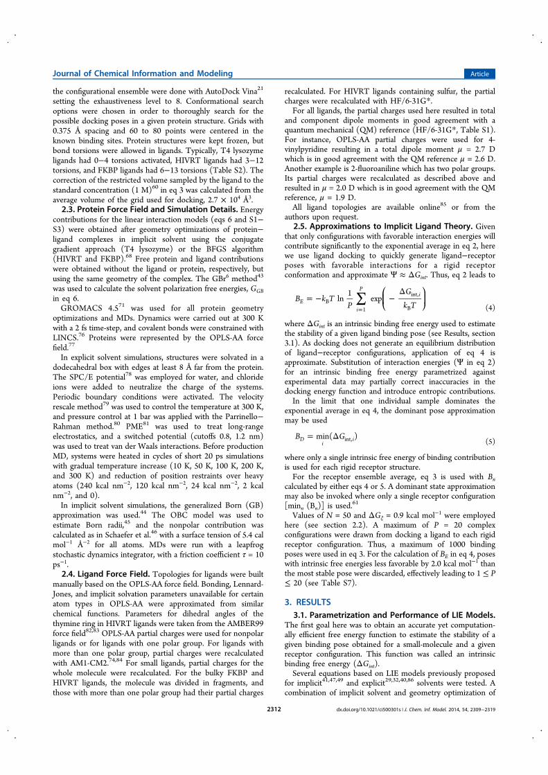
the configurational ensemble were done with AutoDock Vina21

setting the exhaustiveness level to 8. Conformational searchoptions were chosen in order to thoroughly search for thepossible docking poses in a given protein structure. Grids with0.375 Å spacing and 60 to 80 points were centered in theknown binding sites. Protein structures were kept frozen, butbond torsions were allowed in ligands. Typically, T4 lysozymeligands had 0−4 torsions activated, HIVRT ligands had 3−12torsions, and FKBP ligands had 6−13 torsions (Table S2). Thecorrection of the restricted volume sampled by the ligand to thestandard concentration (1 M)60 in eq 3 was calculated from theaverage volume of the grid used for docking, 2.7 × 104 Å3.2.3. Protein Force Field and Simulation Details. Energy

contributions for the linear interaction models (eqs 6 and S1−S3) were obtained after geometry optimizations of protein−ligand complexes in implicit solvent using the conjugategradient approach (T4 lysozyme) or the BFGS algorithm(HIVRT and FKBP).68 Free protein and ligand contributionswere obtained without the ligand or protein, respectively, butusing the same geometry of the complex. The GBr6 method43

was used to calculate the solvent polarization free energies, GGBin eq 6.GROMACS 4.571 was used for all protein geometry

optimizations and MDs. Dynamics were carried out at 300 Kwith a 2 fs time-step, and covalent bonds were constrained withLINCS.76 Proteins were represented by the OPLS-AA forcefield.77

In explicit solvent simulations, structures were solvated in adodecahedral box with edges at least 8 Å far from the protein.The SPC/E potential78 was employed for water, and chlorideions were added to neutralize the charge of the systems.Periodic boundary conditions were activated. The velocityrescale method79 was used to control the temperature at 300 K,and pressure control at 1 bar was applied with the Parrinello−Rahman method.80 PME81 was used to treat long-rangeelectrostatics, and a switched potential (cutoffs 0.8, 1.2 nm)was used to treat van der Waals interactions. Before productionMD, systems were heated in cycles of short 20 ps simulationswith gradual temperature increase (10 K, 50 K, 100 K, 200 K,and 300 K) and reduction of position restraints over heavyatoms (240 kcal nm−2, 120 kcal nm−2, 24 kcal nm−2, 2 kcalnm−2, and 0).In implicit solvent simulations, the generalized Born (GB)

approximation was used.44 The OBC model was used toestimate Born radii,45 and the nonpolar contribution wascalculated as in Schaefer et al.46 with a surface tension of 5.4 calmol−1 Å−2 for all atoms. MDs were run with a leapfrogstochastic dynamics integrator, with a friction coefficient τ = 10ps−1.2.4. Ligand Force Field. Topologies for ligands were built

manually based on the OPLS-AA force field. Bonding, Lennard-Jones, and implicit solvation parameters unavailable for certainatom types in OPLS-AA were approximated from similarchemical functions. Parameters for dihedral angles of thethymine ring in HIVRT ligands were taken from the AMBER99force field82,83 OPLS-AA partial charges were used for nonpolarligands or for ligands with one polar group. For ligands withmore than one polar group, partial charges were recalculatedwith AM1-CM2.74,84 For small ligands, partial charges for thewhole molecule were recalculated. For the bulky FKBP andHIVRT ligands, the molecule was divided in fragments, andthose with more than one polar group had their partial charges

recalculated. For HIVRT ligands containing sulfur, the partialcharges were recalculated with HF/6-31G*.For all ligands, the partial charges used here resulted in total

and component dipole moments in good agreement with aquantum mechanical (QM) reference (HF/6-31G*, Table S1).For instance, OPLS-AA partial charges were used for 4-vinylpyridine resulting in a total dipole moment μ = 2.7 Dwhich is in good agreement with the QM reference μ = 2.6 D.Another example is 2-fluoroaniline which has two polar groups.Its partial charges were recalculated as described above andresulted in μ = 2.0 D which is in good agreement with the QMreference, μ = 1.9 D.All ligand topologies are available online85 or from the

authors upon request.2.5. Approximations to Implicit Ligand Theory. Given

that only configurations with favorable interaction energies willcontribute significantly to the exponential average in eq 2, herewe use ligand docking to quickly generate ligand−receptorposes with favorable interactions for a rigid receptorconformation and approximate Ψ ≈ ΔGint. Thus, eq 2 leads to

∑= − −Δ

=

⎛⎝⎜

⎞⎠⎟B k T

P

G

k Tln

1expE

i

Pi

B1

int,

B (4)

where ΔGint is an intrinsic binding free energy used to estimatethe stability of a given ligand binding pose (see Results, section3.1). As docking does not generate an equilibrium distributionof ligand−receptor configurations, application of eq 4 isapproximate. Substitution of interaction energies (Ψ in eq 2)for an intrinsic binding free energy parametrized againstexperimental data may partially correct inaccuracies in thedocking energy function and introduce entropic contributions.In the limit that one individual sample dominates the

exponential average in eq 4, the dominant pose approximationmay be used

= ΔB Gmin( )Di

iint, (5)

where only a single intrinsic free energy of binding contributionis used for each rigid receptor structure.For the receptor ensemble average, eq 3 is used with Bn

calculated by either eqs 4 or 5. A dominant state approximationmay also be invoked where only a single receptor configuration[minn (Bn)] is used.

61

Values of N = 50 and ΔGξ = 0.9 kcal mol−1 were employedhere (see section 2.2). A maximum of P = 20 complexconfigurations were drawn from docking a ligand to each rigidreceptor configuration. Thus, a maximum of 1000 bindingposes were used in eq 3. For the calculation of BE in eq 4, poseswith intrinsic free energies less favorable by 2.0 kcal mol−1 thanthe most stable pose were discarded, effectively leading to 1 ≤ P≤ 20 (see Table S7).

3. RESULTS3.1. Parametrization and Performance of LIE Models.

The first goal here was to obtain an accurate yet computation-ally efficient free energy function to estimate the stability of agiven binding pose obtained for a small-molecule and a givenreceptor configuration. This function was called an intrinsicbinding free energy (ΔGint).Several equations based on LIE models previously proposed

for implicit41,47,49 and explicit29,32,40,86 solvents were tested. Acombination of implicit solvent and geometry optimization of



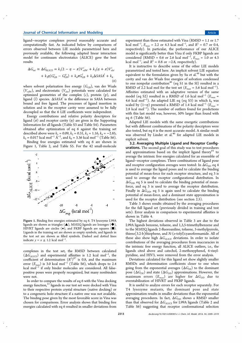
ligand−receptor complexes proved reasonably accurate andcomputationally fast. As indicated below by comparisons oferrors observed between LIE models parametrized here andpreviously available, the following adapted linear interactionmodel for continuum electrostatics (ALICE) gave the bestresults

η π η π

η π

Δ ≈ Δ = − − + +

+ − + + Δ +

G G k V k V

k G G k G k SASA k

(2 ) ( )

( )int ALICE vdW

celetc

GBc

GBp

GBl l

1 2

3 4 5 6(6)

where solvent polarization free energy (GGB), van der Waals(VvdW), and electrostatic (Velet) potentials were calculated foroptimized geometries of the complex (c), protein (p), andligand (l) species. ΔSASAl is the difference in SASA betweenbound and free ligand. The processes of ligand insertion insolution and in the receptor cavity were assumed to be fullydecoupled so that the 6 LIE coefficients were independent.Energy contributions and relative polarity descriptors for

ligand (π) and receptor cavity (η) are given in the SupportingInformation for all ligands (Table S3 and Table S4). Parametersobtained after optimization of eq 6 against the training setdescribed above were k1 = 0.09, k2 = 0.31, k3 = 1.16, k4 = −2.85,k5 = 0.017 kcal mol−1 Å−2, and k6 = 3.36 kcal mol−1 (Table S6).Binding free energies estimated with eq 6 are shown in

Figure 1, Table 2, and Table S5. For the 42 small-molecule

complexes in the test set, the RMSD between calculated(ΔGALICE) and experimental affinities is 1.2 kcal mol−1, thecoefficient of determination (R2)87 is 0.8, and the maximumerror (Emax) is 3.0 kcal mol−1 (Table S6), which drops to 2.4kcal mol−1 if only binder molecules are considered. All false-positive poses were properly recognized, but many nonbinderswere not.In order to compare the results of eq 6 with the Vina docking

energy function,21 ligands in our test set were docked with Vinato their respective protein crystal structure (native docking) orto a congeneric holo structure if a native one was not available.The binding pose given by the most favorable score in Vina waschosen for comparisons. Error analysis shows that binding freeenergies calculated with eq 6 resulted in smaller deviations from

experiment than those estimated with Vina (RMSD = 1.1 or 1.7kcal mol−1, Emax = 2.2 or 4.3 kcal mol−1, and R2 = 0.7 or 0.4,respectively). In particular, the performance of our ALICEmodel is significantly better than Vina if only FKBP ligands areconsidered (RMSD = 0.6 or 2.6 kcal mol−1, Emax = 1.0 or 4.3kcal mol−1, and R2 = 0.8 or −2.8, respectively).It is instructive to describe some of the other LIE models

parametrized and tested here. An implicit solvent LIE equationequivalent to the formulation given by Su et al.49 but with thecavity and van der Waals free energies of solvation condensedto one nonpolar contribution46 (eq S1 in the SI) resulted in aRMSD of 2.2 kcal mol for the test set (Emax = 5.6 kcal mol−1).Affinities estimated with an adaptative version of the samemodel (eq S2) resulted in a RMSD of 1.6 kcal mol−1 (Emax =4.6 kcal mol−1). An adapted LIE eq (eq S3) in which k6 wasscaled by (1−η) presented a RMSD of 1.4 kcal mol−1 (Emax =2.8 kcal mol−1). The number of outliers found for predictionswith this last model was, however, 50% larger than found witheq 6 (Table S6).Adapted LIE models with the same energetic contributions

but with different combinations of the polarity descriptors werealso tested, but eq 6 is the most accurate model. A similar resultwas observed by Linder et al.40 for adapted LIE models inexplicit solvent.

3.2. Averaging Multiple Ligand and Receptor Config-urations. The second goal of this study was to test proceduresand approximations based on the implicit ligand theory61 toaverage the intrinsic free energies calculated for an ensemble ofligand−receptor complexes. Three combinations of ligand poseand receptor configuration averages were tested: In ΔGEE, eq 4is used to average the ligand poses and to calculate the bindingpotential of mean-force for each receptor structure, and eq 3 isused to average the receptor configurational distribution. InΔGDE, eq 5 is used to calculate the binding potential of mean-force, and eq 3 is used to average the receptor distribution.Finally in ΔGDD, eq 5 is again used to calculate the bindingpotential of mean-force, and a dominant state approximation isused for the receptor distribution (see section 2.5).Table 3 shows results obtained by the averaging procedures

for the full ligand set (previously divided in training and testsets). Error analysis in comparison to experimental affinities isshown in Table 4.The highest deviations observed in Table 3 are due to the

L99A ligands benzene, toluene, and 1,3,5-trimethylbenzene andto the M102Q ligands 2-fluoroaniline, toluene, 3-methylpyrrole,thieno[3.2-b]thiophene, and N-(o-tolyl)cyanoformamide. All ofthese also show high ΔGALICE deviations. In order to isolatecontributions of the averaging procedures from inaccuracies inthe intrinsic free energy function, all ALICE outliers, i.e., theligands cited above and catechol, 2-methoxyphenol, 4-vinyl-pyridine, and HIV3, were removed from the error analysis.Deviations calculated for this ligand set show slightly smaller

RMSDs and determination coefficients closer to one whengoing from the exponential averages (ΔGEE) to the dominantpose (ΔGDE) and state (ΔGDD) approximations. However, themaximum errors (Emax) are higher for ΔGDD due tooverstabilization of HIVRT and FKBP ligands.It is useful to analyze errors for each receptor separately. For

T4 lysozyme mutants, the dominant pose and stateapproximation results in smaller deviations than the exponentialaveraging procedures. In fact, ΔGDD shows a RMSD smallerthan that observed for ΔGALICE for L99A ligands (Table 2 andTable S6) suggesting that receptor conformational selection

Figure 1. Binding free energies estimated by eq 6. T4 lysozyme L99Aligands are shown as triangles (▲), M102Q ligands are lozenges (◆),HIVRT ligands are circles (•), and FKBP ligands are squares (■).Ligands in the training set are shown as empty symbols, and ligands inthe test set are shown as filled symbols. Dashed and dotted linesindicate y = x ± 1.2 kcal mol−1.



contributes to the calculation of binding free energies even forthe small and hydrophobic L99A ligands and for the relativelyrigid T4 lysozyme engineered cavity. Results for the M102Qmutant show higher deviations which in part may be due to thehigher inaccuracies in the ALICE model for this receptor(Table 2).

For HIVRT and specially for FKBP ligands, the oppositetrend is observed. The best predictions were obtained forexponential averaging of both pose and receptor configurations(ΔGEE). The dominant approximations overstabilize thebinding free energies because some binding poses are asmuch as 3.5 kcal mol−1 more stable than the experimental freeenergy.The relative rankings of binding affinities among the HIVRT

and the FKBP ligands are recovered with all averagingprocedures, except for the two ligands with the most favorableaffinities in each receptor. However, experimental andcalculated differences between these two ligands are smallerthan 0.3 kcal mol−1.If the Vina docking energy function is used to approximate Ψ

in eq 2, the free energies predicted show significativedisagreement with experiment for all ligand sets. For example,ΔGEE

Vina calculated for the FKBP ligands give RMSD = 3.8 kcalmol−1, Emax = 4.6 kcal mol−1, and R2 = −7.0 suggesting that thedocking energy function will give meaningless results if used toapproximate the solvent-mediated interaction energy in eq 2.This result can be traced to the Vina inability to discriminatefalse-positive poses. Almost all poses generated from dockingwere on average used to calculate BE

Vina. On the other hand, lessthan half of the generated poses were on average used tocalculate BE

ALICE for the same set of ligand−receptor poses(Figure S2 and Table S7).

4. DISCUSSION4.1. ALICE Model Contributions, Performance, and

Limitations. Several LIE equations with different definitions ofthe nonpolar solvation contribution and with differentcombinations of polarity descriptors were described and testedhere. The best predictions for a test set composed of 42 small-

Table 3. Binding Free Energies (in kcal mol−1)Experimentally Measured and Estimated by the AveragingProcedures Described in the Text for the Full Ligand Set

ligand ΔGexpa ΔGEE ΔGDE ΔGDD

L99Aisobutylbenzene −6.4 −4.1 −4.4 −5.64-ethyltoluene −5.4 −3.7 −4.1 −4.7para-xylene −4.6 −3.1 −3.5 −4.1indole −4.9 −2.7 −3.2 −3.8ortho-xylene −4.6 −3.1 −3.6 −4.2n-butylbenzene −6.7 −4.4 −4.7 −5.7propylbenzene −6.5 −3.8 −4.2 −5.1ethylbenzene −5.7 −3.1 −3.7 −4.1toluene −5.5 −2.5 −3.1 −3.5benzene −5.2 −1.7 −2.3 −3.03-ethyltoluene −5.1 −3.7 −4.1 −4.8meta-xylene −4.7 −3.1 −3.6 −4.02-ethyltoluene −4.5 −3.7 −4.1 −4.83-methylpyrrole >−2.0 −1.3 −2.0 −2.3phenol >−2.0 −1.5 −2.1 −2.61,3,5-trimethylbenzene >−2.0 −3.6 −3.9 −4.9cyclohexane >−2.0 −1.9 −2.4 −2.72-fluoroaniline >−2.0 −1.7 −2.3 −2.8

M102Q2-fluoroaniline −5.5 −1.5 −2.1 −2.85-chloro-2-methylphenol −5.3 −2.6 −3.2 −4.0benzyl acetate −4.7 −4.4 −4.5 −5.6ortho-cresol −4.7 −2.1 −2.6 −3.22-propylphenol −5.6 −3.5 −3.8 −4.7(phenylamino)acetonitrile −5.8 −3.2 −3.4 −4.4toluene −5.2 −2.3 −2.6 −3.13-methylpyrrole −5.2 −0.9 −1.6 −2.0thieno[3.2-b]thiophene −4.9 −1.7 −1.9 −2.72-ethylphenol −4.8 −2.7 −3.2 −3.9catechol −4.4 −2.8 −3.0 −4.52-ethoxyphenol −4.3 −2.6 −3.1 −3.9phenylhydrazine >−2.0 −1.6 −2.3 −3.22-methoxyphenol >−2.0 −2.1 −2.7 −3.34-vinylpyridine >−2.0 −2.3 −2.7 −3.2N-(o-tolyl)cyanoformamide >−2.0 −1.8 −2.4 −3.6

HIVRTHIV1 −11.5 −10.4 −11.1 −12.2HIV2 −4.9 −4.6 −5.2 −6.3HIV3 −8.1 −8.6 −9.2 −10.0HIV4 −10.6 −8.7 −9.2 −10.6HIV5 −6.4 −7.5 −8.2 −9.8HIV6 −11.8 −10.3 −10.5 −12.0

FKBPFKB1 −11.0 −11.9 −12.6 −13.8FKB2 −11.2 −11.7 −12.2 −13.3FKB3 −7.8 −7.4 −8.2 −9.3FKB4 −8.5 −7.6 −8.2 −9.4FKB5 −9.6 −10.7 −11.2 −12.8

aRepeated from Table S3. Nonbinders were assumed to have ΔGexp >−2.0 kcal mol−1.

Table 4. Error Analysis of the Binding Free EnergiesCalculated by the Averaging Procedures Proposed forDifferent Ligand Sets

ΔGEE ΔGDE ΔGDD

Full Ligand Set (Table 3)a

RMSD 1.7 1.5 1.3Emax 2.9 2.6 3.4R2 0.6 0.7 0.8

L99A Ligandsa

RMSD 1.7 1.4 0.7Emax 2.7 2.3 1.5R2 0.0 0.3 0.8

M102Q Ligandsa

RMSD 2.2 1.8 1.3Emax 2.9 2.6 2.1R2 −3.0 −1.8 −0.4

HIVRT LigandsRMSD 1.2 1.2 1.7Emax 1.9 1.8 3.4R2 0.8 0.8 0.6

FKBP LigandsRMSD 0.8 1.1 2.3Emax 1.1 1.7 3.2R2 0.6 0.3 −1.9

aLigands with a ΔGALICE deviation from the experimental affinityhigher than one RMSD (1.2 kcal mol−1, Table 2) were removed fromthe error analysis. Deviations (in kcal mol−1, except for R2) werecalculated for each set in comparison to experimental affinities.



molecule complexes of 4 different receptors were obtained witheq 6 with 6 adjustable parameters. None of the ligands in thetest set were used in the parametrization training set.Deviations observed with this ALICE model and withpreviously proposed LIE models are similar. For instance, theimplicit solvent LIE model proposed by Su et al. has 4adjustable parameters and resulted in a RMSD of 1.3 kcal mol−1

with R2 = 0.62 for a set of 57 HIVRT ligands (including the 6HIVRT ligands used here).49 The implicit solvent LIE modelwith 2 adjustable parameters proposed by Kolb et al. showed aRMSD of 1.6 kcal mol−1 with a correlation coefficient of 0.52for a set of 128 EGFR kinase ligands.36 The LIE modelproposed by Wall et al. has 3 adjustable parameters and showeda RMSD of 1.6 kcal mol−1 and a correlation coefficient of 0.62for a set of 15 neuraminidase inhibitiors.35 Finally, the adaptedLIE model for explicit solvent proposed by Linder et al. has 3adjustable parameters and resulted in a mean absolute deviation(similar to a RMSD) of 1.6 kcal mol−1, Emax = 3.4 kcal mol−1,and R2 = 0.72 for a diverse set of 38 ligands and their respective16 receptors.40 Deviations reported for these four LIE modelswere obtained with the same ligands (or with a congeneric setof ligands) used for training the models. Still, the ALICE modelproposed has the smallest RMSD and the determinationcoefficient closest to 1.In order to analyze the energy contributions included in the

ALICE model, it should be noted that implicit solvation is notpairwise decomposable in general. Consequently, the splittingof solute−solvent interactions necessary for LIE calculations isnot unique. The solvent polarization energy in the boundligand state is given by (GGB

c − GGBc′ ) where the initial state, c′,

indicates a complex with ligand charges turned off. As discussedby Su et al.,49 the initial state is approximated here to the freeprotein (p). With the GBr6 method,43 the electrostaticpolarization energy calculated for the training set changes by0.2−0.7 kcal mol−1 between these two initial state definitions.This polarization response is scaled by the cavity polaritydescriptor in eq 6. A combination with the ligand polarity didnot result in better predictions.Nonpolar solvent contributions from the free ligand and the

receptor complex were replaced by a simple ΔSASA termwithout loss of accuracy. Previous work suggested that theconstant term in a LIE equation, γ in eq 1 or k6 in eq 6, may berelated to binding site hydrophobicity32,34 or nonpolar surfacearea.88 An ALICE model (eq S3 in the SI) in which theconstant term is scaled by the nonpolar cavity surface (1−η)was tested, but this modification also did not result in betterperformance.The comparable accuracy obtained here for different LIE

models (eq 6 and eqs S1−S3) suggests the exact form of a LIEequation is less important given a proper parametrization isconducted. Significant departure from theoretical values isobserved for the parameters obtained here. For instance,k2(η+π), equivalent to the parameter β in previous LIE models(eq 1), ranged from 0.03 to 0.27. This is below the theoreticalvalue of β = 0.5.29,49 It is expected that parameter values willmutually compensate model assumptions and inaccuracies inthe solvent model, molecular mechanical potentials, etc. Thus,the parametrized LIE equations presented here may be cast aslinear free energy relationships which coefficients are onlybounded by the linear response theory.30

Applications of these LIE models depend, however, on theirtransferability for receptors and ligands not included in thetraining set used to parametrize the equations. Here coefficients

were scaled by ligand and cavity polarities in order to increasemodel transferability.40 Eq 6 correctly predicts affinities forligands which receptors were either included (T4 lysozyme andHIVRT) or not (FKBP) in the training set. The sensitivity ofΔGALICE on the η and π descriptor values is small. Variations of∼0.2 kcal mol−1 were observed when descriptor values werescaled by ±20%. Predictions for other receptors and ligandsshould have similar accuracy, but an extensive test oftransferability is left for future studies.The computational efficiency observed for eq 6 suggests it

can be used to predict affinities for large ligand sets. Forinstance, our ALICE model could be used instead of the scoringor energy functions currently employed in molecular docking.To this end, ligand−receptor poses would have to be generatedby the conformational search procedures found in docking21,50

or by another method such as mining-minima.89 Ligand andprotein topologies containing connectivity, force field param-eters, and polarity descriptors would have to be available orbuilt. Although cumbersome when manually done, this processcan be made fairly automatic.64,66,90

In order to improve the ALICE model proposed, it may beuseful to analyze the highest deviations found. The followingligands are described as eq 6 outliers since they show deviationslarger than one RMSD: benzene, toluene, 1,3,5-trimethylben-zene (L99A), 2-fluoroaniline, catechol, 3-methylpyrrole, thieno-[3,2-b]thiophene, 4-vinylpiridine, 2-methoxyphenol, N-(o-tolyl)cyanoformamide (M102Q), and HIV3. All but 2-fluoroaniline belong to the test set, and all T4 lysozymeoutliers have underestimated free energies. Most of theseligands are also outliers for eqs S1−S3 (see Table S6).The binding affinity increases for L99A ligands upon addition

of linear methylene units, as seen for benzene to toluene and upto n-butylbenzene. The experimental free energy differenceupon methylene addition in this series is 0.2−0.3 kcal mol−1 butbetween ethylbenzene and propylbenzene, which is 0.8 kcalmol−1. Although eq 6 incorrectly predicts a small stability tobenzene and toluene, appropriate affinities are predicted uponincreasing the number of methylene units. This observationsuggests a slightly unbalanced description of the nonpolarcontributions involving aliphatic and aromatic carbons. Anatom-type dependent surface tension, k5 in eq 6, could amendthis problem.The hydrophobic ligand 1,3,5-trimethylbenzene should

interact more favorably with the L99A nonpolar engineeredbinding site than with water, as suggested by the free energycalculated with the ALICE model. Docking suggests that thereis enough room to accommodate this relatively bulky ligand inthe L99A cavity (Table S7). However, the experimental freeenergy shows that 1,3,5-trimethylbenzene is a L99A nonbinder.As T4 lysozyme must show some breathing or openingmovement to allow the entrance or exit of ligands from theengineered cavity,91 we speculate that 1,3,5-trimethylbenzene isa kinetic nonbinder and that there may not be a low energypathway allowing its entrance into the L99A cavity.The highest number of outliers were found for M102Q

ligands. Possibly electrostatic interactions were not described orsampled correctly in the LIE models tested. Yet no correlationwas found between outliers and significant flaws in thedescription of their dipole moments (Table S1) or theavailability of experimental ligand−receptor structures. Thelack of holo crystal structures for some ligands and thepossibility that receptor structures used for the calculation ofΔGALICE are not representative of complexes observed in



aqueous solution may contribute for inaccuracies in theprediction of intrinsic binding free energies. This appears tobe the case for catechol as discussed in the next section.4.2. Analysis of the Proposed Conformational

Averaging Schemes. Ensembles for all target receptorswere initially built with apo protein representations. For the T4lysozyme mutants, 3 structures out of 50 in the L99A ensembleand 11 structures out of 50 for the M102Q ensemble had theirbinding cavity fully blocked by side-chains rotations. Dockingto these receptor structures did not yield complexes with ligandinside the engineered binding site even for small ligands such astoluene. This problem was more pronounced for the HIVRTand FKBP bulky ligands as none of the receptor structuresobtained from apo molecular dynamics after equilibration wereable to accommodate ligands in its crystallographic binding site.Thus, molecular dynamics obtained from holo structures wereused to generate the HIVRT and FKBP ensembles.Affinities were consistently underestimated for T4 lysozyme

mutants by all three combinations of ensemble averages tested.Although ΔGDD shows a small RMSD and a favorable erroranalysis for L99A ligands, the dominant approximation thatcounts only the most favorable pose underestimates affinitiesfor almost all T4 lysozyme ligands but catechol (see below).This tendency suggests that the tentative apo M102Q ensembleused here systematically degrades the structural representationin comparison to the crystal structures. As noted, side-chainsrotations block the binding cavity even for the relatively rigidengineered site in T4 lysozyme. Apo protein ensembles have tobe used carefully and possibly enlarged or modified92 toaccommodate ligand binding.The only notable exception is catechol binding to M102Q.

Although the ALICE free energy function predicts unstablebinding for catechol to the crystal (holo) configuration,favorable binding is predicted by ΔGDD. Thus, receptorconfigurational sampling is important for the prediction ofcatechol binding, and the M102Q crystal configuration mayhave a low contribution to the binding affinity. In fact, it hasbeen shown that catechol has at least two binding modes93 andthat enhanced sampling is required to compute its binding freeenergy correctly.18

Increasing the number of poses that contribute toexponential averaging results in less favorable binding freeenergies for all ligands tested. This “dilution” effect has twopossible causes. One is artificially related to the discriminationof poses that should contribute to the ensemble averages. Itdepends on the discriminatory quality of the intrinsic freeenergy function. The second cause has a physical origin as themacroscopically measured affinity may be an average of severalbinding poses, some of which will have higher intrinsic freeenergies of binding.Free energies calculated for the T4 lysozyme mutants

decrease up to 50% on going from ΔGDD to ΔGEE. Thedilution effect is more pronounced for T4 lysozyme because theintrinsic free energy differences between ligand poses inside oroutside the engineered binding site is small (<2.0 kcal mol−1).Consequently, it is harder to discriminate poses that shouldcontribute to the ensemble averages from decoy poses. In fact,for all T4 lysozyme ligands, the average number of posesincluded in the calculation of the binding potential of mean-force (eq 4) is higher than the average number of poses insidethe receptor binding site (Table S7).The importance of pose discrimination on ensemble averages

is also illustrated when the Vina energy function is used as an

approximation instead of ΔGALICE (eq 6). The exponentiallyaveraged free energies obtained in this case are significantly lessfavorable than the corresponding dominant approximation(ΔGDD

Vina) for the same set of ligand−receptor poses.For HIVRT and FKBP ligands, pose discrimination with the

ALICE model is rather accurate. Although the absolute valuesof binding free energies are higher, the predictions with theALICE intrinsic free energy function show smaller deviationsfor both receptors (Table 2). The better discrimination isreflected by the average number of poses used to calculate BEwhich is closer to the average number of poses found inside thereceptor binding site (Table S7).Thus, for HIVRT and FKBP ligands, the decrease of

calculated free energies on going from ΔGDD to ΔGEE doesnot appear artifactual but a physical effect due to averaging adistribution of ligand−receptor conformations. Induced fit isexpected to change the receptor conformational distributionupon ligand complexation. Indeed, some of the configurationsfound for the complexes with the receptor ensemble show morefavorable intrinsic free energies of binding. This also explainsthe overstabilization observed for ΔGDD predictions.Receptor reorganization free energy will be accounted for if

the ensemble is canonically distributed and wide enough torepresent the relevant receptor motions. If ligand binding has alarge reorganization free energy, the associated receptormotions will have high free energy costs, and the number orfraction of binding-competent configurations in the ensemblewill be small. Consequently, a ligand complex formed with suchrare receptor configurations will only contribute significativelyto the final exponential average if it has a highly favorableintrinsic binding free energy. On the other hand, if thereorganization free energy for ligand binding is small, thefraction of binding-competent configurations in the ensemblewill be large, and a reasonable number of ligand complexes withthese popular receptor configurations will contribute to theaverage even if their intrinsic binding free energies are nothighly favorable.We do not investigate here what is the appropriate size of the

ensemble to account for the reorganization energy correctly,but 50 configurations appear to be insufficient, specially if anapo structure is used to generate the ensemble.92 When a holostructure is used to generate a tentative ensemble, the fullreceptor reorganization energy may not be accounted for, butthe relative contribution upon a series of congeneric ligands canbe retrieved.Finally, which of the three averaging procedures should be

applied? The answer depends on the receptor ensemble and theintrinsic free energy function. For receptor ensembles withunknown or biased distributions, with insufficient sampling andfor free energy functions that cannot discriminate correctbinding poses from decoys, the dominant pose and stateapproximation (ΔGDD) should be applied. For more flexiblereceptors and upon increasing the quality of the conformationalensemble, the state exponential average (ΔGDE) might beincluded. The exponential average for multiple ligandconfigurations (ΔGEE) should be employed only when acalibrated and discriminatory intrinsic free energy function isavailable. This is probably the case for the ALICE modelproposed (eq 6) with lead-like ligands.

5. CONCLUSIONSWe have parametrized an adapted linear interaction energymodel that employs a simple combination of energy



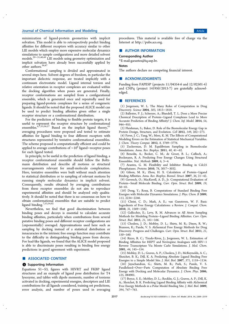
minimization of ligand-protein geometries with implicitsolvation. This model is able to retrospectively predict bindingaffinities for different receptors with accuracy similar to otherLIE models which employ more expensive molecular dynamicssimulations to sample configurations and more detailed solventmodels.29−31,40,49 LIE models using geometry optimization andimplicit solvation have already been successfully applied byother authors.36,47

Conformational sampling is divided and approximated inseveral steps here. Solvent degrees of freedom, in particular theimportant dielectric response, are treated implicitly with acontinuum electrostatic model. Ligand internal torsion andrelative orientation in receptor complexes are evaluated withinthe docking algorithm when poses are generated. Finally,receptor conformations are sampled from a configurationalensemble, which is generated once and repeatedly used forpreparing ligand-protein complexes for a series of congenericligands. It should be noted that the proposed ALICE model canbe used to predict binding affinities given either a singlereceptor structure or a conformational distribution.For the prediction of binding to flexible protein targets, it is

useful to represent the receptor structure by conformationalensembles.6,7,53,56,57 Based on the implicit ligand theory,61

averaging procedures were proposed and tested to estimateaffinities for ligand binding to four different receptors withstructures represented by tentative conformational ensembles.The scheme proposed is computationally efficient and could beapplied to average contributions of ∼106 ligand−receptor posesfor each ligand tested.In principle, to be useful in the prediction of ligand binding, a

receptor conformational ensemble should follow the Boltz-mann distribution and describe all motions or structuralrearrangements relevant for small-molecule complexation.Here, tentative ensembles were built without much attentionto statistical distribution or to sampling of relevant motions byrunning simple molecular dynamics in implicit solvent.Consequently, results obtained by averaging contributionsfrom these receptor ensembles do not aim to reproduceexperimental affinities and should be analyzed only qualita-tively. It should be noted that there is no consensus on how toobtain conformational ensembles that are suitable to predictligand binding.7,53,54,92

Nevertheless, we find that good discrimination betweenbinding poses and decoys is essential to calculate accuratebinding affinities, particularly when contributions from severalputative binding poses and different receptor configurations are(exponentially) averaged. Approximations used here such assampling by docking instead of a statistical distribution orinnacuracies in the intrinsic free energy function may contributeto the difficulty in distinguishing binding poses from decoys.For lead-like ligands, we found that the ALICE model proposedis able to discriminate poses resulting in binding free energypredictions in good agreement with experiment.

■ ASSOCIATED CONTENT

*S Supporting InformationEquations S1−S3, figures with HIVRT and FKBP ligandstructures and an example of ligand pose distribution for T4lysozyme, and tables with dipole moments, number of torsionsactivated in docking, experimental energies, descriptors and LIEcontributions for all ligands considered, training set predictions,error analysis, and number of poses used in averaging

procedures. This material is available free of charge via theInternet at http://pubs.acs.org.

■ AUTHOR INFORMATION

Corresponding Author*E-mail:[email protected].

NotesThe authors declare no competing financial interest.

■ ACKNOWLEDGMENTS

Funding from FAPESP (projects 11/04354-6 and 12/02501-4)and CNPq (project 141950/2013-7) are gratefully acknowl-edged.

■ REFERENCES(1) Jorgensen, W. L. The Many Roles of Computation in DrugDiscovery. Science 2004, 303, 1813−1818.(2) Ballester, P. J.; Schreyer, A.; Blundell, T. L. Does a More PreciseChemical Description of Protein−Ligand Complexes Lead to MoreAccurate Prediction of Binding Affinity? J. Chem. Inf. Model. 2014, 54,944−955.(3) Fleishman, S.; Baker, D. Role of the Biomolecular Energy Gap inProtein Design, Structure, and Evolution. Cell 2012, 149, 262−273.(4) Faver, J. C.; Yang, W.; Merz, K. M. The Effects of ComputationalModeling Errors on the Estimation of Statistical Mechanical Variables.J. Chem. Theory Comput. 2012, 8, 3769−3776.(5) Zuckerman, D. M. Equilibrium Sampling in BiomolecularSimulations. Annu. Rev. Biophys. 2011, 40, 41−62.(6) Benedix, A.; Becker, C. M.; de Groot, B. L.; Caflisch, A.;Bockmann, R. A. Predicting Free Energy Changes Using StructuralEnsembles. Nat. Methods 2009, 6, 3−4.(7) Arantes, G. M. Flexibility and Inhibitor Binding in Cdc25Phosphatases. Proteins 2010, 78, 3017−3032.(8) Gilson, M. K.; Zhou, H. X. Calculation of Protein−LigandBinding Affinities. Annu. Rev. Biophys. Biomol. Struct. 2007, 36, 21−42.(9) Guvench, O.; MacKerell, A. D., Jr. Computational Evaluation ofProtein−Small Molecule Binding. Curr. Opin. Struct. Biol. 2009, 19,56−61.(10) Deng, Y.; Roux, B. Computations of Standard Binding FreeEnergies with Molecular Dynamics Simulations. J. Phys. Chem. B 2009,113, 2234−2246.(11) Christ, C. D.; Mark, A. E.; van Gunsteren, W. F. BasicIngredients of Free Energy Calculations: a Review. J. Comput. Chem.2010, 31, 1569−1582.(12) Gallicchio, E.; Levy, R. M. Advances in All Atom SamplingMethods for Modeling Protein−Ligand Binding Affinities. Curr. Opin.Struct. Biol. 2011, 21, 161−166.(13) Chodera, J. D.; Mobley, D. L.; Shirts, M. R.; Dixon, R. W.;Branson, K.; Pande, V. S. Alchemical Free Energy Methods for DrugDiscovery: Progress and Challenges. Curr. Opin. Struct. Biol. 2011, 21,150−160.(14) Rizzo, R. C.; Tirado-Rives, J.; Jorgensen, W. L. Estimation ofBinding Affinities for HEPT and Nevirapine Analogues with HIV−1Reverse Transcriptase Via Monte Carlo Simulations. J. Med. Chem.2001, 44, 145−154.(15) Mobley, D. L.; Graves, A. P.; Chodera, J. D.; McReynolds, A. C.;Shoichet, B. K.; Dill, K. A. Predicting Absolute Ligand Binding FreeEnergies to a Simple Model Site. J. Mol. Biol. 2007, 371, 1118−1134.(16) Jayachandran, G.; Shirts, M. R.; Park, S.; Pande, V. S.Parallelized−Over−Parts Computation of Absolute Binding FreeEnergy with Docking and Molecular Dynamics. J. Chem. Phys. 2006,125, 084901.(17) Boyce, S. E.; Mobley, D. L.; Rocklin, G. J.; Graves, A. P.; Dill, K.A.; Shoichet, B. K. Predicting Ligand Binding Affinity with AlchemicalFree Energy Methods in a Polar Model Binding Site. J. Mol. Biol. 2009,394, 747−763.



(18) Mobley, D. L.; Chodera, J. D.; Dill, K. A. On the Use ofOrientational Restraints and Symmetry Corrections in AlchemicalFree Energy Calculations. J. Chem. Phys. 2006, 125, 084902.(19) Kuntz, I. D.; Blaney, J. M.; Oatley, S. J.; Langridge, R.; Ferrin, T.E. A Geometric Approach to Macromolecule−Ligand Interactions. J.Mol. Biol. 1982, 161, 269−288.(20) Sousa, S. F.; Fernandes, P. A.; Ramos, M. J. Protein−LigandDocking: Current Status and Future Challenges. Proteins 2006, 65,15−26.(21) Trott, O.; Olson, A. J. AutoDock Vina: Improving the Speedand Accuracy of Docking with a New Scoring Function, EfficientOptimization, and Multithreading. J. Comput. Chem. 2010, 31, 455−461.(22) Bowman, A. L.; Nikolovska-Coleska, Z.; Zhong, H.; Wang, S.;Carlson, H. A. Small Molecule Inhibitors of the MDM2−P53Interaction Discovered by Ensemble−Based Receptor Models. J. Am.Chem. Soc. 2007, 129, 12809−12814.(23) Plewczynski, D.; Lazniewski, M.; Augustyniak, R.; Ginalski, K.Can We Trust Docking Results? Evaluation of Seven Commonly UsedPrograms on PDBbind Database. J. Comput. Chem. 2011, 32, 742−755.(24) Keenan, S. M.; Geyer, J. A.; Welsh, W. J.; Prigge, S. T.; Waters,N. C. Rational Inhibitor Design and Iterative Screening in theIdentification of Selective Plasmodial Cyclin Dependent KinaseInhibitors. Comb. Chem. High Throughput Screening 2005, 8, 27−38.(25) Bisson, W. H.; Cheltsov, A. V.; Bruey-Sedano, N.; Lin, B.; Chen,J.; Goldberger, N.; May, L. T.; Christopoulos, A.; Dalton, J. T.; Sexton,P. M.; Zhang, X.-K.; Abagyan, R. Discovery of Antiandrogen Activityof Nonsteroidal Scaffolds of Marketed Drugs. Proc. Natl. Acad. Sci. U.S. A. 2007, 104, 11927−11932.(26) Frimurer, T. M.; Peters, G. H.; Iversen, L. F.; Andersen, H. S.;Møller, N. P. H.; Olsen, O. H. Ligand−Induced ConformationalChanges: Improved Predictions of Ligand Binding Conformations andAffinities. Biophys. J. 2003, 84, 2273−2281.(27) Kitchen, D. B.; Decornez, H.; Furr, J. R.; Bajorath, J. Dockingand Scoring in Virtual Screening for Drug Discovery: Methods andApplications. Nat. Rev. Drug Discovery 2004, 3, 935−949.(28) Kim, R.; Skolnick, J. Assessment of Programs for Ligand BindingAffinity Prediction. J. Comput. Chem. 2008, 29, 1316−1331.(29) Åqvist, J.; Medina, C.; Sammuelsson, J.-E. A New Method forPredicting Binding Affinity in Computer−Aided Drug Design. ProteinEng. 1994, 7, 385−391.(30) Carlson, H. A.; Jorgensen, W. L. An Extended Linear ResponseMethod for Determining Free Energies of Hydration. J. Phys. Chem.1995, 99, 10667−10673.(31) Gallicchio, E.; Kubo, M. M.; Levy, R. M. Enthalpy−Entropy andCavity Decomposition of Alkane Hydration Free Energies: NumericalResults and Implications for Theories of Hydrophobic Solvation. J.Phys. Chem. B 2000, 104, 6271−6285.(32) Åqvist, J.; Luzhkov, V. B.; Brandsdal, B. O. Ligand BindingAffinities from MD Simulations. Acc. Chem. Res. 2002, 35, 358−365.(33) King, G.; Warshel, A. Investigation of the Free Energy Functionsfor Electron Transfer Reactions. J. Chem. Phys. 1990, 93, 8682−8692.(34) Almlof, M.; Brandsdal, B. O.; Åqvist, J. Binding AffinityPrediction with Different Force Fields: Examination of the LinearInteraction Energy Method. J. Comput. Chem. 2004, 25, 1242−1254.(35) Wall, I. D.; Leach, A. R.; Salt, D. W.; Ford, M. G.; Essex, J. W.Binding Constants of Neuraminidase Inhibitors: an Investigation ofthe Linear Interaction Energy Method. J. Med. Chem. 1999, 42, 5142−5152.(36) Kolb, P.; Huang, D.; Dey, F.; Caflisch, A. Discovery of KinaseInhibitors by High−Throughput Docking and Scoring Based on aTransferable Linear Interaction Energy Model. J. Med. Chem. 2008, 51,1179−1188.(37) Stjernschantz, E.; Marelius, J.; Medina, C.; Jacobsson, M.;Vermeulen, N. P. E.; Oostenbrink, C. Are Automated MolecularDynamics Simulations and Binding Free Energy Calculations RealisticTools in Lead Optimization? An Evaluation of the Linear InteractionEnergy (LIE) Method. J. Chem. Inf. Model. 2006, 46, 1972−1983.

(38) de Amorim, H. L. N.; Caceres, R. A.; Netz, P. A. LinearInteraction Energy (LIE) Method in Lead Discovery and Optimiza-tion. Curr. Drug Targets 2008, 9, 1100−1105.(39) Hansson, T.; Marelius, J.; Åqvist, J. Ligand Binding AffinityPrediction by Linear Interaction Energy Methods. J. Comput.-AidedMol. Des. 1998, 12, 27−35.(40) Linder, M.; Ranganathan, A.; Brinck, T. Adapted LinearInteraction Energy”: a Structure−Based LIE Parametrization for FastPrediction of Protein−Ligand Affinities. J. Chem. Theory Comput.2013, 9, 1230−1239.(41) Zhou, R. H.; Friesner, R. A.; Ghosh, A.; Rizzo, R. C.; Jorgensen,W. L.; Levy, R. M. New Linear Interaction Method for BindingAffinity Calculations Using a Continuum Solvent Model. J. Phys. Chem.B 2001, 105, 10388−10397.(42) Alves, A. F. N. M.Sc. thesis, Instituto de Quimica, Universidadede Sao Paulo, Sao Paulo, 2013. Available at http://www.teses.usp.br/teses/disponiveis/46/46131/tde-08052013-144801/ (accessed June20, 2014).(43) Tjong, H.; Zhou, H.-X. GBr6: A Parameterization−Free,Accurate, Analytical Generalized Born Method. J. Phys. Chem. B2007, 111, 3055−3061.(44) Still, W. C.; Tempczyk, A.; Hawley, R. C.; Hendrickson, T.Semianalytical Treatment of Solvation for Molecular Mechanics andDynamics. J. Am. Chem. Soc. 1990, 112, 6127−6129.(45) Onufriev, A.; Bashford, D.; Case, D. A. Exploring Protein NativeStates and Large−Scale Conformational Changes with a ModifiedGeneralized Born Model. Proteins 2004, 55, 383−394.(46) Schaefer, M.; Bartels, C.; Karplus, M. Solution Conformationsand Thermodynamics of Structured Peptides: Molecular DynamicsSimulation with an Implicit Solvation Model. J. Mol. Biol. 1998, 284,835−848.(47) Huang, D.; Caflisch, A. Efficient Evaluation of Binding FreeEnergy Using Continuum Electrostatic Solvation. J. Med. Chem. 2004,47, 5791−5797.(48) Carlsson, J.; Ander, M.; Nervall, M.; Åqvist, J. ContinuumSolvation Models in the Linear Interaction Energy Method. J. Phys.Chem. B 2006, 110, 12034−12041.(49) Su, Y.; Gallicchio, E.; Das, K.; Arnold, E.; Levy, R. M. LinearInteraction Energy (LIE) Models for Ligand Binding in ImplicitSolvent: Theory and Application to the Binding of NNRTIs to HIV−1Reverse Transcriptase. J. Chem. Theory Comput. 2007, 3, 256−277.(50) Huey, R.; Morris, G. M.; Olson, A. J.; Goodsell, D. S. ASemiempirical Free Energy Force Field with Charge−Based Desolva-tion. J. Comput. Chem. 2007, 28, 1145−1152.(51) Cavasotto, C. N.; Abagyan, R. A. Protein Flexibility in LigandDocking and Virtual Screening to Protein Kinases. J. Mol. Biol. 2004,337, 209−225.(52) Erickson, J. A.; Jalaie, M.; Robertson, D. H.; Lewis, R. A.; Vieth,M. Lessons in Molecular Recognition: the Effects of Ligand andProtein Flexibility on Molecular Docking Accuracy. J. Med. Chem.2004, 47, 45−55.(53) Wong, C. F.; Kua, J.; Zhang, Y.; Straatsma, T.; McCammon, J.A. Molecular Docking of Balanol to Dynamics Snapshots of ProteinKinase A. Proteins 2005, 61, 850−858.(54) Mamonov, A. B.; Bhatt, D.; Cashman, D. J.; Ding, Y.;Zuckerman, D. M. General Library−Based Monte Carlo TechniqueEnables Equilibrium Sampling of Semi−Atomistic Protein Models. J.Phys. Chem. B 2009, 113, 10891−10904.(55) Kallblad, P.; Mancera, R. L.; Todorov, N. P. Assessment ofMultiple Binding Modes in Ligand−Protein Docking. J. Med. Chem.2004, 47, 3334−3337.(56) Novoa, E. M.; de Pouplana, L. R.; Barril, X.; Orozco, M.Ensemble Docking from Homology Models. J. Chem. Theory Comput.2010, 6, 2547−2557.(57) Totrov, M.; Abagyan, R. Flexible Ligand Docking to MultipleReceptor Conformations: A Practical Alternative. Curr. Opin. Struct.Biol. 2008, 18, 178−184.



(58) B-Rao, C.; Subramanian, J.; Sharma, S. D. Managing ProteinFlexibility in Docking and Its Applications. Drug Discovery Today 2009,14, 394−400.(59) Cozzini, P.; Kellogg, G. E.; Spyrakis, F.; Abraham, D. J.;Costantino, G.; Emerson, A.; Fanelli, F.; Gohlke, H.; Kuhn, L. A.;Morris, G. M.; Orozco, M.; Pertinhez, T. A.; Rizzi, M.; Sotriffer, C. A.Target Flexibility: an Emerging Consideration in Drug Discovery andDesign. J. Med. Chem. 2008, 51, 6237−6255.(60) Gallicchio, E.; Lapelosa, M.; Levy, R. M. Binding EnergyDistribution Analysis Method (BEDAM) for Estimation of Protein−Ligand Binding Affinities. J. Chem. Theory Comput. 2010, 6, 2961−2977.(61) Minh, D. D. L. Implicit Ligand Theory: Rigorous Binding FreeEnergies and Thermodynamic Expectations from Molecular Docking.J. Chem. Phys. 2012, 137, 104106.(62) Eriksson, A. E.; Baase, W. A.; Wozniak, J. A.; Matthews, B. W. ACavity−Containing Mutant of T4 Lysozyme Is Stabilized by BuriedBenzene. Nature 1992, 355, 371−373.(63) Wei, B. Q.; Baase, W. A.; Weaver, L. H.; Matthews, B. W.;Shoichet, B. K. A Model Binding Site for Testing Scoring Functions inMolecular Docking. J. Mol. Biol. 2002, 322, 339−355.(64) Voss, N. R.; Gerstein, M.; Steitz, T. A.; Moore, P. B. TheGeometry of the Ribosomal Polypeptide Exit Tunnel. J. Mol. Biol.2006, 360, 893−906.(65) Ertl, P.; Rohde, B.; Selzer, P. Fast Calculation of Molecular PolarSurface Area As a Sum of Fragment−Based Contributions and ItsApplication to the Prediction of Drug Transport Properties. J. Med.Chem. 2000, 43, 3714−3717.(66) Hendlich, M.; Bergner, A.; Gunther, J.; Klebe, G. Relibase:Design and Development of a Database for Comprehensive Analysis ofProtein−Ligand Interactions. J. Mol. Biol. 2003, 326, 607−620.(67) Carroll, D. L. Genetic Algorithm Driver, Version 1.7; 1998.(68) Press, W. H.; Teukolsky, S. A.; Vetterling, W. T.; Flannery, B. P.Numerical Recipes in FORTRAN 77: the Art of Scientific Computing, 2nded.; Cambridge University Press: Cambridge, 1992.(69) Arantes, G. M.; Loos, M. Specific Parametrisation of a HybridPotential to Simulate Reactions in Phosphatases. Phys. Chem. Chem.Phys. 2006, 8, 347−353.(70) Chinea, G.; Padron, G.; Hooft, R. W. W.; Sander, C.; Vriend, G.The Use of Position−Specific Rotamers in Model−Building byHomology. Proteins 1995, 23, 415−421.(71) Pronk, S.; Pall, S.; Schulz, R.; Larsson, P.; Bjelkmar, P.;Apostolov, R.; Shirts, M. R.; Smith, J. C.; Kasson, P. M.; van der Spoel,D.; Hess, B.; Lindahl, E. GROMACS 4.5: a High−Throughput andHighly Parallel Open Source Molecular Simulation Toolkit. Bio-informatics 2013, 29, 845−854.(72) O’Boyle, N. M.; Banck, M.; James, C. A.; Morley, C.;Vandermeersch, T.; Hutchison, G. R. Open Babel: an Open ChemicalToolbox. J. Cheminf. 2011, DOI: doi:10.1186/1758-2946-3-33.(73) Frisch, M. J. et al. Gaussian 09, Revision A.1; Gaussian, Inc.:Wallingford, CT, 2009.(74) Dewar, M. J. S.; Zoebisch, E. G.; Healy, E. F.; Stewart, J. J. P.Development and Use of Quantum Mechanical Molecular Models. 76.AM1: A New General Purpose Quantum Mechanical MolecularModel. J. Am. Chem. Soc. 1985, 107, 3902−3909.(75) Moitessier, N.; Englebienne, P.; Lee, D.; Lawandi, J.; Corbeil, C.R. Towards the Development of Universal, Fast and Highly AccurateDocking/scoring Methods: a Long Way to Go. Br. J. Pharmacol. 2008,153, S7−S26.(76) Hess, B.; Bekker, H.; Berendsen, H. J. C.; Fraaije, J. G. E. M.LINCS: a Linear Constraint Solver for Molecular Simulations. J.Comput. Chem. 1997, 18, 1463−1472.(77) Jorgensen, W. L.; Maxwell, D. S.; Tirado-Rives, J. Developmentand Testing of the OPLS All−Atom Force Field on ConformationalEnergetics and Properties of Organic Liquids. J. Am. Chem. Soc. 1996,118, 11225−11236.(78) Berendsen, H. J. C.; Grigera, J. R.; Straatsma, T. P. The MissingTerm in Effective Pair Potentials. J. Phys. Chem. 1987, 91, 6269−6271.

(79) Bussi, G.; Donadio, D.; Parrinello, M. Canonical SamplingThrough Velocity Rescaling. J. Chem. Phys. 2007, 126, 014101.(80) Parrinello, M.; Rahman, A. Polymorphic Transitions in SingleCrystals: a New Molecular Dynamics Method. J. Appl. Phys. 1981, 52,7182−7190.(81) Darden, T.; York, D.; Pedersen, L. Particle Mesh Ewald: anN×log(N) Method for Ewald Sums in Large Systems. J. Chem. Phys.1993, 98, 10089−10092.(82) Wang, J.; Cieplak, P.; Kollman, P. A. How Well Does aRestrained Electrostatic Potential (RESP) Model Perform inCalculating Conformational Energies of Organic and BiologicalMolecules? J. Comput. Chem. 2000, 21, 1049−1074.(83) Cornell, W. D.; Cieplak, P.; Bayly, C. I.; Gould, I. R.; Merz, K.M.; Ferguson, D. M.; Spellmeyer, D. C.; Fox, T.; Caldwell, J. W.;Kollman, P. A. A Second Generation Force Field for the Simulation ofProteins, Nucleic Acids, and Organic Molecules. J. Am. Chem. Soc.1995, 117, 5179−5197.(84) Li, J.; Xing, J.; Cramer, C. J.; Truhlar, D. G. Accurate DipoleMoments from Hartree−Fock Calculations by Means of Class IVCharges. J. Chem. Phys. 1999, 111, 885−892.(85) Ligand Topologies. http://gaznevada.iq.usp.br/wp-content/uploads/opls_site.tar.gz (accessed May 2014).(86) Jones-Hertzog, D. K.; Jorgensen, W. L. Binding Affinities forSulfonamide Inhibitors with Human Thrombin Using Monte CarloSimulations with a Linear Response Method. J. Med. Chem. 1997, 40,1539−1549.(87) Zar, J. H. Biostatistical Analysis, 4th ed.; Prentice Hall: NJ, 1999.(88) Reynolds, J. A.; Gilbert, D. B.; Tanford, C. EmpiricalCorrelation Between Hydrophobic Free Energy and Aqueous CavitySurface Area. Proc. Natl. Acad. Sci. U. S. A. 1974, 71, 2925−2927.(89) Chen, W.; Gilson, M. K.; Webb, S. P.; Potter, M. J. ModelingProtein−Ligand Binding by Mining Minima. J. Chem. Theory Comput.2010, 6, 3540−3557.(90) Vanommeslaeghe, K.; Hatcher, E.; Acharya, C.; Kundu, S.;Zhong, S.; Shim, J.; Darian, E.; Guvench, O.; Lopes, P.; Vorobyov, I.;Mackerell, A. D., Jr. CHARMM General Force Field: a Force Field forDrug−like Molecules Compatible with the CHARMM All−AtomAdditive Biological Force Fields. J. Comput. Chem. 2010, 31, 671−690.(91) Mulder, F. A. A.; Hon, B.; Muhandiram, D. R.; Dahlquist, F. W.;Kay, L. E. Flexibility and Ligand Exchange in a Buried Cavity Mutantof T4 Lysozyme Studied by Multinuclear NMR. Biochemistry 2000, 39,12614−12622.(92) Seeliger, D.; de Groot, B. L. Conformational Transitions uponLigand Binding: Holo−Structure Prediction from Apo Conformations.PLoS Comput. Biol. 2010, 6, e1000634.(93) Graves, A. P.; Brenk, R.; Shoichet, B. K. Decoys for Docking. J.Med. Chem. 2005, 48, 3714−3728.



123

ANEXO J – Partition, orientation andmobility of ubiquinones in a lipid bilayer

Partition, orientation and mobility of ubiquinones in a lipid bilayer

Vanesa Viviana Galassi, Guilherme Menegon Arantes ⁎Department of Biochemistry, Instituto de Química, Universidade de São Paulo, Av. Prof. Lineu Prestes 748, 05508-900, São Paulo, SP, Brazil

a b s t r a c ta r t i c l e i n f o

Article history:Received 19 May 2015Received in revised form 2 July 2015Accepted 4 August 2015Available online 6 August 2015

Keywords:Membrane localizationMembrane insertionComputer simulationFree-energy profileMolecular dynamicsForce-field parametrization

Ubiquinone is the universal mobile charge carrier involved in biological electron transfer processes. Its redoxproperties and biological function depend on the molecular partition and lateral diffusion over biological mem-branes. However, ubiquinone localization and dynamicswithin lipid bilayers are long debated and still uncertain.Here we present molecular dynamics simulations of several ubiquinone homologs with variable isoprenoid taillengths complexed to phosphatidylcholine bilayers. Initially, a new force-field parametrization for ubiquinoneis derived from and compared to high level quantum chemical data. Free energy profiles for ubiquinone insertionin the lipid bilayer are obtained with the new force-field. The profiles allow for the determination of the equilib-rium location of ubiquinone in themembrane aswell as for the validation of the simulationmodel by direct com-parison with experimental partition coefficients. A detailed analysis of structural properties and interactionsshows that the ubiquinone polar head group is localized at the water–bilayer interface at the same depthof the lipid glycerol groups and oriented normal to the membrane plane. Both the localization and orienta-tion of ubiquinone head groups do not change significantly when increasing the number of isoprenoid units.The isoprenoid tail is extended and packed with the lipid acyl chains. For ubiquinones with long tails, theterminal isoprenoid units have high flexibility. Calculated ubiquinone diffusion coefficients are similar tothat found for the phosphatidylcholine lipid. These results may have further implications for themechanisms of ubiquinone transport and binding to respiratory and photosynthetic protein complexes.

© 2015 Elsevier B.V. All rights reserved.

1. Introduction

Ubiquinone or coenzyme-Q was described over five decades agoas a central molecule in cellular respiration and photosynthesis [1,2]. It is the ubiquitous mobile charge carrier linking distant redoxcenters in biological electron transfer chains. Ubiquinone receiveselectrons from NADH:ubiquinone reductase (respiratory complexI), succinate:ubiquinone reductase (complex II) in bacteria ormitochondria and reaction centers in purple and cyanobacteria.Cytochrome bc1 (complex III) and the related cytochrome bf6 thenoxidize ubiquinol, the reduced counterpart of ubiquinone, to contin-ue the electron transfer chain. Biological membranes harboring theproteins involved in bio-energetical processes contain a pool ofubiquinone and ubiquinol molecules which is responsible for 95%of the energy transduction in aerobic organisms [3–5].

Ubiquinone is an amphipathic molecule formed by a modifiedbenzoquinone polar head and a lipid tail composed of 6 to 10 iso-prenoid units in biologically relevant homologs [6,3]. The quinonehead may be reduced by up to two electrons and receive two pro-tons, passing through a semi-quinone intermediate up to the quinol

form. Ubiquinone redox properties and biological function ascharge carriers will depend on its partition and diffusion over bio-logical membranes. But, despite much experimental progress ob-tained during the last decades, the localization and orientation ofubiquinones in biological membranes are still under heavy debate[6–15].

It has been proposed that the polar head of ubiquinones with morethan 3 isoprenoid units are fully embedded in the membrane core andoriented parallel to the interfacial plane, lying in the bilayer midplanespace [6–10]. Other authors have suggested that the quinone head islocated close to the phospholipid polar groups and oriented parallel toits hydrocarbon tails, with the isoprenoid chain spanning the membrane[11–15]. Other proposals include the formation of ubiquinone aggregatesor the partition between separate pools inside the lipid bilayer [14,16].

There is also a lack of consensus on the dynamical properties ofubiquinone embedded in lipid bilayers [17–21] as diffusion constantsexperimentally determined range from 10−9 up to 10−6 cm2 s−1. Thishigh variation is due to the application of various measurement tech-niques [22,19] and to the usage of probes (fluorescent, spin labels,etc.) attached to ubiquinone which will alter its intrinsic diffusionproperties. Nevertheless, it has been suggested that ubiquinone diffu-sion between respiratory complexes is the rate limiting step in thewhole mitochondrial electron transfer chain [17].

Biochimica et Biophysica Acta 1847 (2015) 1560–1573

⁎ Corresponding author.E-mail address: [email protected] (G.M. Arantes).

http://dx.doi.org/10.1016/j.bbabio.2015.08.0010005-2728/© 2015 Elsevier B.V. All rights reserved.

Contents lists available at ScienceDirect

Biochimica et Biophysica Acta

j ourna l homepage: www.e lsev ie r .com/ locate /bbab io

Computer simulations can give detailed information on the parti-tion, orientation and mobility of solutes embedded in lipid bilayers[23–25]. The accuracy and precision of the results obtained in a simula-tion will depend both on the energy description – the molecularmechanics (MM) force-field – and on appropriate sampling of the rele-vant degrees of freedom. Although there are a few simulation studiesfocusing on ubiquinone properties when bound to proteins [26–29], toour knowledge there is only one simulation study of ubiquinonecomplexed to a lipid bilayer [22,30]. Unfortunately, this study reportsa very short simulation time (less than 20 ns in aggregate) which isnot enough to reach equilibration and proper sampling.

Here we apply long molecular dynamics (MD) simulations andfree energy calculations to investigate the properties of several ubi-quinone homologs bound to model lipid bilayers. Although ubiqui-none force-fields were previously available [26,28], we have testedtheir performance both in comparison to quantum chemical refer-ence properties and to experimental data and judged necessary tobuild a new parametrization for ubiquinone compatible with theCHARMM force-field [31,32]. This energy function has been carefullyvalidated for a series of lipids [33], including 1-palmitoyl-2-oleoyl-sn-glycero-3-phosphocholine (POPC) which was used here to buildamodel bilayer.We find that the polarity and flexibility of isoprenoidunits should be carefully calibrated in order to obtain an accuratedescription for ubiquinone partition in membranes. The insertionprocess is simulated with enhanced sampling of several degrees offreedom that may be relevant to the interaction of ubiquinone withthe bilayer. After validation of the simulations by comparison toavailable experimental measurements, we present a detailed analy-sis of the simulation results providing interesting points for the ubi-quinone localization, interactions and lateral mobility whenembedded in a POPC bilayer.

2. Materials & methods

2.1. Reference set and force-field parameterization strategy

A detailed parametrization for ubiquinone was performed here inaccordance with the CHARMM force-field [31,32]. Details are givenbelow for the ab initio electronic structure calculations used to buildthe training and test sets, and for the fitting strategy used to adjust theparameters. Ubiquinone-1 (UQ1 or UQn, for n isoprenoid units),ubiquinol-1 (UQ1H2) and 3-methyl-3-hexene (isoprene or ISP) wereused here as molecular fragments for the force-field parametrization.Please refer to Fig. 1 for atom naming used throughout the text. Anequivalent naming scheme is used for ketonic ubiquinone. Isoprenewas used to adjust parameters for the isoprenoid tail, whereas UQ1and UQ1H2 were used for the quinone head.

A reference set of ubiquinone interaction energies, bond torsion po-tentials and molecular dipoles was built from quantum chemical (QC)calculations and used as targets for the force-field parametrization. QCcalculations were conducted with GAUSSIAN 09 (Rev. A01) [34] formolecules and complexes in the gas phase. All geometry optimizationswere performed with the B3LYP functional [35] and the 6–31+G**basis set [36]. All single-point energies and quantummechanical dipolemoments used in the reference set were calculated at the MP2/6-311+G(2df,2p) level [37].

Hydrogen-bonded ubiquinone–water complexes were used tomodel solvent interactions. Three different orientations were used forubiquinone with oxygens O4, O1 and O3 (equivalent to O2) acceptingthe water hydrogen and two orientations were used with oxygen inubiquinol (O4 and O1) donating a hydrogen to water. Hydrophobiccontacts were modeled by complexes between UQ1 and methane anda ISP dimer. Interaction energies (Ei in Eq. (1)) were computed with acounterpoise scheme to correct for the basis-set superposition error[38]. The distance and orientation of all complexes were optimizedwhereas internal coordinates of each molecule were kept frozen at

their isolated geometry. Water internal coordinates were kept frozenat the TIP3P [39] equilibrium geometry. Please refer to the Results(Fig. 2) and Supporting Information (SI, Fig. S1) for the relative orienta-tion of the dimer complexes.

Torsions around bonds O2–C2, C6–C7 in UQ1, O1–C1, O2–C2, O4–C4inUQ1H2, and C7–C8 andC9–C11 in ISPwere evaluated (Figs. 3 and S2).Torsion potentials (Et in Eq. (1)) were scanned in 15° or 30° angle incre-ments by partial geometry optimizations with fixed bond lengths butflexible angle and dihedrals to avoid clashes and obtain torsional pro-files representative of configurations visited at normal thermal energies.Torsions were further divided into polar (tp) and non-polar (tnp). Tor-sion rotamers were selected for the calculation of molecular dipoles(D in Eq. (1)).

The following error function was minimized by adjusting the force-field parameters:

P ¼ ∑Ninti wi∑

Nintsp

j

EMMi; j −EQC

i; j

EQCi; j

��þ∑Ntp

t wtp∑Ntp

sp

j

EMMt; j −EQC

t; j

EQCt; j

��þ

∑Ntnpt wtnp∑

Ntnpsp

j

EMMt; j −EQC

t; j

EQCt; j

��þwD∑

NDsp

j ∑α¼x;y;z

DMMj;α −DQC

j;α

DQCj;α

��

ð1Þ

wherew are theweights assigned to each property,Nint=5 is the num-ber of interaction pair complexes (3 hydrogen-bonded and 2 hydropho-bic), and Ntp = 3 and Ntnp = 4 are the number of polar and non-polarbond torsions included in the training set. Nsp geometries were usedfor each property: Nsp

int = 3, including the minima and two adjacentpoints along the interaction profile;Nsp

tp andNsptnpwere either 6 or 12, de-

pending on the angle increments, and NspD = 2, 4 and 4 conformations

respectively for UQ1, UQ1H2 and ISP. Superscripts MM and QC indicatethe calculation method.

In order to obtain parameters for ubiquinone compatible with theCHARMM force-field, atom types were assigned by chemical analogywith previously parametrized molecules (Table S1). Bond and valenceangle parameters were kept from the standard CHARMM values. Im-proper dihedrals were not included in aromatic rings or unsaturatedbonds as they were not necessary to maintain planarity. Root meansquare deviations of Cartesian coordinates are smaller than 0.01 nmfor UQ1 geometries optimized with the force-field parametrized herein comparison to geometries optimized with the reference QC method.

Fig. 1. Structure and atom naming of isoprene (ISP) and ubiquinol-1 (UQ1H2).

1561V.V. Galassi, G.M. Arantes / Biochimica et Biophysica Acta 1847 (2015) 1560–1573

Partial charges were adjusted for atoms C2/C3, O2/O3, CM2/CM3,CM5, C6, ketonic groups of UQ1 (C1/C4 and O1/O4) or phenolic groupsof UQ1H2 (C1/C4, O1/O4 and H1/H4), and for isoprene C9, C10 and C11(Fig. 1). Groups with neutral total charge were defined among thefollowing bound atom sets: (C2, O2, CM2, HM2) and the equivalentCM3 methoxide group, (C6, C5, CM5, HM5), (C9, C10, H10, C11, H11),(C1, O1) and (C4, O4) in quinones and (C1, O1, H1) and (C4, O4, H4)in quinols. Charges for atoms in the aromatic ring and its substituentswere made symmetric. Charges for isoprenoid tails longer than foundin UQ1 were adapted accordingly. Partial charges for all other atomtypes such as aliphatic hydrogens were kept in their standardCHARMM values.

Bond torsionswere fitted by altering the number of expansion termsof order n, their phase δ and force constant Kϕ (Table S3) in the corre-sponding Fourier dihedral terms [31]. For ISP, torsions around bondsC7–C8 and C9–C11 were adjusted. For UQ1, polar torsion C2–O2 (andthe equivalent C3–O3)and non-polar torsions C6–C7 and C7–C8 andfor UQ1H2 polar torsions C1–O1 and C4–O4 were optimized.

Partial chargeswere optimized first by settingwi=1,wD=1,wtp=0.04 and wtnp = 0 and minimizing Eq. (1). Then, dihedral parameterswere optimized by setting wi = 1, wD = 0, wtp = 0.01–1.0 andwtnp = 1. After these two optimization cycles, torsions around bondsC6–C7 and C2–O2 (and the equivalent C3–O3) were still not describedsatisfactorily. Then, the Rmin Lennard-Jones parameter for atoms C8,CM5, O2, O3, CM2 and CM3 were slightly changed by evaluating onlythe error of these three torsions. A final optimization cycle was per-formed by including the full training set and varying all partial chargesand dihedral parameters at the same time.

All MM energies and properties used in the force-field parametriza-tion were obtained using GROMACS package version 4.6.1 [40]. For theparameter optimization, a combination of genetic algorithm andsimplex was used as described before [41]. See Tables S1, S2 and S3for the final optimized parameter values. GROMACS compatible topolo-gies are available upon request from the authors.

2.2. System setup and molecular dynamics simulations

The force-field obtained was tested by molecular dynamics simula-tions and free energy calculations. All MD simulations reported herewere carried out with GROMACS package version 4.6.7 [40]. Lipidparameters were taken from the CHARMM36 force-field [33] andwater was described by TIP3P [39]. The NPT ensemble was used andtemperature kept at 310Kwith theBussi thermostat [42] and a couplingconstant of 0.1 ps with two separate coupling groups (water andeverything else). Pressure was kept at 1.0 bar with the Berendsenbarostat [43] with a coupling constant of 1 ps and a compressibilityof 1.0 · 10−5 bar−1 for the unrestrained simulations and of0.5 · 10−5 bar−1 for the restrained free energy simulations. Semi-isotropic coupling in the direction normal to the bilayer was applied inthe lipid simulations. Electrostatic interactions were handled by theparticle mesh Ewald method [44] with a real space cutoff of 1.0 nm,grid spacing of 0.13 nm and quartic interpolation. All bonds wereconstrained using the LINCS algorithm [45] and van der Waals interac-tions were truncated at 1.0 nm. No dispersion corrections were appliedin order to avoid artifacts in mean area per lipid and bilayer thickness[46]. The integration time step was set to 2 fs and the nonbonded listwas updated every 20 fs.

Symmetric lipid bilayers containing different numbers of POPC andwater molecules were built: 128 lipids and ~7900 water molecules(large system, LS), 72 lipids and ~6100 water molecules (medium sys-tem, MS) and 50 lipids and ~3300 water molecules (small system, SS).NaCl was added up to a final concentration of 0.150 M. After energyminimization using the conjugate gradient algorithm, an equilibrationMD was run for 30 ns for the SS and up to 200 ns for the LS, resultingin a mean area per molecule of 0.63, 0.61 and 0.62 nm2 respectivelyfor the small, medium and large systems. This is in reasonable

agreement with the experimental value of 0.68 nm2[47]. The calculatedbilayer thickness was 3.9 nm in all systems which is near the experi-mental value of 3.7 nm [47]. Mean area was computed as the ratio be-tween the area of the membrane plane and the number of lipids perleaflet. Membrane thickness was calculated as the distance betweenthe peaks of the lipid headgroup electron density.

Ubiquinone was inserted in the membranes using two differentprotocols: For the insertion of UQ1 in the LS bilayer, a pulling from thewater phase towards the membrane center of mass (COM) wasconducted in the membrane normal direction with the pull code inGROMACS and a rate of 4.10−5 nm ps−1. For all other insertions, theprotocol described by Javanainen was used [48]. In short, ubiquinonewas placed at themembrane edge using a visualization tool, the box di-mensions were increased accordingly, water and lipids were restrainedin themembrane normal direction to avoid escaping to the empty spacegenerated, and a 5 ns MD simulation was run with an anisotropicbarostat and a reference pressure of 1000 bar in the direction whichubiquinone was placed. After ubiquinone was immersed into themembrane, the system was relaxed by removing all restrains and thepressure reversed back to semi-isotropic and 1.0 bar in another 30 nsMD run. The mean area and bilayer thickness were monitored tocheck for equilibration.

Ubiquinone concentration in percentage per mole was 0.8% in LS,1.4% inMS and 2.0% in SSmembranes. This is similar to previous ubiqui-none simulations [22] and to the physiological concentration range of1–3% [8].

Unconstrained MD simulations were performed for the embeddedubiquinones using the last frame from the umbrella sampling windowwith minimum free energy (see below). Trajectories with 200 ns werecollected for UQ1, UQ1H2 and UQ2 and trajectories with 400 ns werecollected for UQ6 and UQ10. Two simulations starting from differentisoprenoid tail conformations (folded and fully extended) were per-formed for UQ10 with the quinone head positioned near the minimumfree energy configuration found for the other ubiquinones. All proper-ties calculated from these two simulations are equivalent and, hence, in-dependent of the tail starting conformation.

Diffusion coefficients were calculated from the linear phase of themean squared displacements with dimensionality set to 2, as onlylateral diffusion along the membrane plane was processed [49]. Theorientation of the ubiquinone head was calculated from the angleformed between the quinone ring plane (defined by atoms C1, C3and C5) and the bilayer midplane. Flexibility and extension of theisoprenoid tail were evaluated from the distance between the lastcarbon of the tail (CT) and both the quinone head COM and the bilay-er midplane. Contacts between ubiquinone atoms and differentgroups in POPC were definedwith a 0.3 nm cut-off. Order parametersSCD for lipid methylene units were calculated using the programLOOS [50].

2.3. Free energy calculations

Umbrella sampling (US) [51] and bias-exchange metadynamics(BEMD) [52] were used to compute the free energy profile for ubiqui-none insertion into the model bilayers. The distance between the ubi-quinone head COM and the membrane COM along its normal z-axiswas used as the insertion reaction coordinate.

Initial configurations for each US window were extracted from anon-equilibrium trajectory generated with an extra pulling force actingover ubiquinone along the z-axis in the range [0,5] nm for the POPC bi-layer (Section 2.2). The pulling spring constant was 300 kJmol−1 nm−1

and the pulling rate was 4.10−5 nm ps−1. US windows were chosenequally spaced by 0.125 nm in the range z = [0.00,2.75] nm while ubi-quinone is inside the membrane or in the interface and by 0.250 nm inthe range z = [3.0,5.0] nm while ubiquinone is in water. The umbrellapotential was set with kumb = 1000 kJ mol−1 nm−1 in the membranerange and with kumb = 500 kJ mol−1 nm−1 in the water range.

1562 V.V. Galassi, G.M. Arantes / Biochimica et Biophysica Acta 1847 (2015) 1560–1573

Simulations run for 60 ns in eachUSwindowwith a total aggregate timeof 5.5 μs for all US simulations. The reaction coordinate was recordedeach 200 fs. Potentials of mean-force (PMF) were calculated from thereaction coordinate occurrence using the weighted histogram analysismethod [53]. The PMFs shown were obtained from 30 ns of equilibra-tion and 30 ns of accumulation in each window. PMF uncertaintieswere estimated by bootstrap analysis using the Bayesian method [54].It should be noted that ubiquinone insertion in the US simulationswas carried out over only one bilayer leaflet (z-axis N 0).

The bias-exchange metadynamics method [52] was applied toenhance sampling along degrees of freedom orthogonal to the insertionreaction coordinate. BEMD is an extension of metadynamics [55]for replica exchange in a collective variable (CV) space. The PLUMEDplug-in version 2.1 [56] was used for these simulations.

The following CVswere chosen besides the z-axis coordinate: C6–C7bond torsion whichwas identified with a high torsional barrier (Fig. 3);the angle formed between ubiquinone atoms C1and C4 and the COM ofthe membrane (θUQ). Following a recent publication that studied theinsertion of ethanol in a model bilayer with BEMD simulations [24],coordination numbers N between ubiquinone and membrane lipidtails or water molecules were also included as CVs. These contactswere calculated with the soft function:

Ng1−g2 ¼Xi∈g1

Xj∈g2

1− ri jr0

� �n

1− ri jr0

� �m ð2Þ

where rij is the distance between atoms i and j and the sums run overtwo sets of atoms (g1 and g2). Values of r0 = 0.3 nm, m = 12, andn = 6 were adopted. Four contact number CVs (Ng1–g2) were definedby the combination of g1 = {H,I} and g2 = {A,W}, where H indicatesthe set of ubiquinone head atoms, I is the set of isoprenoid tail atoms,A is the set of lipid acyl chain carbon atoms and W is the set of wateroxygen atoms.

For UQ1, UQ1H2 and UQ2, BEMD simulations were performed for120 ns with the 7 CVs defined in the previous paragraph and an extrareplica without metadynamics boost. For UQ0, two BEMD simulationswere performed with a different combination of CVs. One simulationwas performed for 160 ns with 4 CVs: z-axis, θUQ, NH–A and NH–W, andanother was done for 120 ns with 4 CVs: z-axis, z-axis with a slowergaussian function deposition, and torsions around C2–O2 and C3–O3bonds. All BEMD simulations were performed in SS bilayers(Section 2.2). For UQ1, a BEMD simulationwas repeatedwith theMSbi-layer. The gaussian height for all CVs was set to 0.5 kJ mol−1 and gauss-ian widths were set to 4 nm for the coordination number CVs and to0.2 nm for all other CVs. The frequency of gaussian deposition was setto 4 ps for the z-axis CV, 10 ps for the coordination number CVs and20 ps for all other CVs (including the z-axis with slower deposition).Exchanges were attempted randomly among replicas every 20 ps.

PMFs were obtained from the BEMD simulations by averaging NBE

profiles generated at different accumulation times from the historydependent potential of the sum of gaussian functions deposited fora given CV [57,58]. Typically, 10 to 12 profiles were generated, thefirst 2 or 3 with the shortest accumulation times were discardedand NBE ~ 8–10 profiles were averaged. For total simulation timeslonger than about 80 ns, the system could freely diffuse along the en-hanced CV. Uncertainties were estimated from the standard devia-tion of the mean [57].

Standard binding free energies between ubiquinone and the lipidmembrane, ΔGb

∘ , were determined by trapezoidal integration of thePMF profiles according to [59]:

e−βΔG∘b ¼

Zbound

e−β PMF zð Þ½ �dzZ

unbounde−β PMF zð Þ½ �dz

: ð3Þ

A separate ΔGb∘ was calculated for each leaflet in the BEMD profiles

with bound regions set to z∈ [0.0,2.5] nmor z∈ [−2.5,0.0] and unboundregion set to z ∈ [2.5,5.0] nm or z ∈ [−5.0,−2.5] nm, respectively. Re-sults shown are an average of the two separate ΔGb

∘ . For the PMFs ob-tained from US, the bound region was set to z b 2.6 nm, 2.9 nm and4.0 nm for UQ1, UQ2 and UQ6, respectively. These boundaries corre-spond to the z value where the PMF(z) reached a plateau. The unboundregion was set such that the same integration volume was used,resulting in the calculation of a standard free energy. Uncertaintieswere propagated from the PMFs following standard formulas [60].

3. Results & discussion

3.1. Performance of the new CHARMM compatible parametrization

As described in Section (2.1), partial charges, Lennard-Jones param-eters (Rmin) and dihedral force constants of a CHARMM compatibleforce-field were adjusted in order to reproduce high-level QC data forbond torsion potentials, molecular dipoles and interaction energies offragment molecules ubiquinone-1, ubiquinol-1 and isoprene isolatedand in complex with water or apolar molecules.

The description of molecular and energetic properties was greatlyimproved with the force-field parametrized here, both qualitativelyfor the shape of bond torsion potentials or the description ofhydrogen-bonded complexes, as well as quantitatively for the relativestability between rotamers or complexation energies. In particular, itwas noted that the molecular dipole of the apolar isoprene molecule(ISP) was incorrectly described by up to 2 Debye using the previouslyavailable CHARMM compatible force-fields (Table S4) [26,28]. Thiswas corrected in the current parametrization which leads to significantimprovements on the bilayer partition free energy of ubiquinones.

A few examples are noted below to illustrate the performance of theavailable force-fields in comparison to high-level QC calculations. Pleaserefer to SI (Figs. S1 and S2) for a complete set of results for interactionand torsion profiles used for training and testing the force-fields. Thisanalysis may help to identify flaws in the potential energy descriptionand suggest internal degrees of freedom which should be sampledcarefully in condensed-phase simulations.

For the interaction energy profiles used in the parametrization train-ing set (Figs. 2A and S1), deviations of the ubiquinone force-field obtain-ed here from the QC reference are always smaller than 5 kJ/mol nearminima and over longer separation distances. Differences are at most10 kJ/mol for interaction energy profiles used only for testing such asthe one in Fig. 2B. Other force-field parametrizations [28,26] showmuch higher deviations and even qualitatively wrong descriptionssuch as in a hydrogen bond between water and the quinol hydrogen(Fig. 2B).

The shapes of the potential energy profile and relative energies be-tween minima are well described by the force-field obtained here forubiquinone bond torsions either included or not in the parametrization(Figs. 3 and S2). Deviations smaller than 10 kJ/mol are observed nearenergy barriers. On the other hand, previously availableMMparametri-zations result in torsions with incorrect shapes (e.g., in Fig. 3A) and inhigh deviations near energy barriers (Fig. 3B and C).

Torsions in the isoprenoid tail around bond C(4 + 5i)–C(6 + 5i)in the i-th isoprenoid unit were also improved (Fig. 3A) leading toa more accurate description of ubiquinone homologs with long iso-prenoid tails. The torsion around the C6–C7 bond was particularly chal-lenging to be described with the available force-fields (Fig. 3B). Duringthe parametrization of the dihedral force constants, it was noted thatthe barriers along this bond torsion could not be adjusted due to toohigh repulsion interactions between atoms C8 and CM5 and their re-spective hydrogens. Thus, Lennard-Jones parameters for both carbonatoms were changed and a significant improvement (~20 kJ/mol) wasobtained. Nevertheless, the force-field parametrized here is still unableto describe the barrier near dihedral angle ~270° with an accuracy


better than 15 kJ/mol. In fact, this is the highest deviation observed overall potential energy comparisons done here. Because the C6–C7 bondtorsion contributes significantly for the ubiquinone flexibility as it con-nects the quinoneheadwith the isoprenoid tail, sampling along this tor-sion was carefully monitored in the insertion free energy calculations.

Methoxide group torsion around bond C2–O2 (or C3–O3) alsoshows high barriers when described with previous parametrizations(see Fig. 3C for UQ1H2 and Fig. S2 for UQ1). The barrier deviationswere also due to too high repulsion interaction between CM2 (orCM3) and O1 (or O4) and were again corrected with changes in theLennard-Jones Rmin parameter. The deviations were greatly improvedwith the force-field parametrization presented here.

3.2. Free energy profiles for partition into the membrane

Potentials of mean-force (PMFs) for the insertion of various ubiqui-none homologs into model POPC bilayers were calculated in order tocheck the accuracy of the parametrized force-fields and to determinethe equilibrium ubiquinone localization along the membrane normal.Umbrella sampling and bias-exchange metadynamics were used toenhance sampling over the membrane insertion coordinate (z-axis de-fined above) and along orthogonal collective coordinates in the case ofBEMD. In this section, we describe the PMFs and derived free energyquantities (ΔGb

∘ ). Details of the ubiquinone localization and contactswithin the bilayer are left to Section 3.3 below.

Fig. 4 shows that the general shape andminima of the PMF obtainedby US change little for the three ubiquinones tested. One isoprenoid unitis enough to partition ubiquinone UQ1 into the bilayer and, as expected,increasing thenumber of isoprenoid units enhances hydrophobicity andconsequently membrane affinity. But, the z-axis position of the PMFminima is rather constant (1.68 nm for UQ1 to 1.55 nm for UQ6).These minima correspond to the preferential localization of the ubiqui-none head in themembrane and have been observed in the same z-axisrange for the insertion of other amphiphile molecules [23]. Thus, previ-ous proposals of the ubiquinone head localization in the middle of thebilayer are not plausible [6–10,22].

The translocation of ubiquinone from one bilayer leaflet to theother will depend on the free energy barrier separating the

Fig. 2. Interaction energies for ubiquinone–water hydrogen-bonded complexes. QC refer-ence energies were obtained at theMP2/6-311+G(2df,2p) level (black circles). The othercurves are different ubiquinoneMMparametrizations proposed by Kaszuba et al. [28] (redup triangles), Autenrieth et al. [26] (green left triangles) and here (blue down triangles).Complex orientation is shown as insets. Data in panel A was included in the force-fieldparametrization while panel B was used only for testing purposes.

Fig. 3. Bond torsion potentials for ubiquinoneobtained at QC andMM levels as indicated inthe legend for Fig. 2. Data from panels A and Bwere included in the force-field parametri-zation while panel C was used only for testing.


membrane center and the minima in the PMF. The barrier decreasesfrom 62 ± 2 kJ mol−1 for UQ1, to 47 ± 2 kJ mol−1 for UQ2 and to40 ± 2 kJ mol−1 for UQ6. This is again in line with the higher hydro-phobicity of ubiquinones with longer tails and suggests that anapproximate barrier of ~40 kJ mol−1 should be observed for the“flip-flop” of natural ubiquinones with long isoprenoid tails (UQ6–UQ10). Thus, the translocation of ubiquinone is a rare event and willnot be observed faster than the micro- to milli-second time scale. Thisis in agreement with the flip-flop rate estimated from NMR measure-ments [11]. There is no significant barrier in the PMFs for the water-membrane insertion process, as also observed for the insertion ofsmall polar and charged molecules [61,62,24] or large amphiphiles[23], suggesting that ubiquinone insertion will be diffusion-controlled.It should be noted that the lack of an insertion barrier may also be dueto incomplete sampling for the ubiquinoneswith longer isoprenoid tails.

Although we expect to have obtained converged PMFs for UQ1 andUQ2 (see discussion below), the same cannot be said for UQ6 whichhas a longer tail and would require longer simulation times for conver-gence. It has been recently noted that the calculation of PMFs in themembrane–water interface region for the insertion of amphiphileswith long hydrophobic tails can be problematic [23]. Although errors

in this region of the PMFs result in incorrect calculated binding freeenergies, they do not effect significantly the z-axis location of PMFminima nor the translocation barrier which should be well describedby the PMFs shown in Fig. 4 even for UQ6. Thus, our discussion in theprevious paragraph is accurate, but the value estimated below forthe free energy of binding of UQ6 (Table 1) should only be consideredqualitatively.

It has been noted [63,61,62,23] that the solvation substitution oc-curring in membrane–water interfaces is often the process with theslowest relaxation to be described during the simulation of solute in-sertion into lipid bilayers. In accordance, we have noticed a suddenchange in the hydration number of the ubiquinone tail for homologswith two or more isoprenoid units in US windows located at the mem-brane–water interface. For UQ2, it was observed at z ~ 2.8 nm (Fig. S3),corresponding to simulation windows where the isoprenoid tail doesnot transition between water and bilayer and stays in only one ofthese phases during all accumulation time. This sudden change mayalso be causing the small flat region observed at similar z coordinateon the calculated PMF for UQ2 (Fig. 4) [23].

To enhance sampling along slow degrees of freedom such as thenumber of contacts of ubiquinone with water and with the lipid we

Fig. 4. PMFs for ubiquinone insertion in large (LS) POPC bilayer obtainedby umbrella sampling forUQ1 (panel A), UQ2 (B), andUQ6 (C). The insets show the calculated binding free energyΔGb

∘ as a function of equilibration time for fixed 30 ns of accumulation time in each US window.

Fig. 5. PMFs for ubiquinone insertion in small (SS) POPC bilayer obtained by bias-exchange metadynamics for UQ0 (panel A), UQ1 (B), UQ1H2 (C), and UQ2 (D). The insets show thecalculated binding free energy ΔGb

∘ as a function of total simulation time.


have employed BEMD simulations. Internal bond torsions of theinserted molecule can also difficult sampling [25]. Thus, we have en-hanced sampling over ubiquinone tail C6−C7 which was identifiedwith large energy barrier (Fig. 3).

PMFs shown in Fig. 5 were obtained from the BEMD simulationsfor insertion over the two bilayer leaflets. The PMF shape is morerugged than the US PMFs as a result of the gaussian depositionscheme that enhances sampling along the membrane normal z-axis[24]. Nevertheless, for UQ1 and UQ2 the position of the PMF minima(~1.65 nm in modulo) and the translocation energy barrier (55 ±10 kJ mol−1 for UQ1 and 47 ± 10 kJ mol−1 for UQ2) are equivalentto those observed in the US PMFs. It should be noted that uncer-tainties reported for free energies obtained by BEMD are higherthan those reported for US due to higher standard deviations obtain-ed in the averaging procedure used to calculate the PMFs from BEMD(see Materials & methods). This scheme is formally different andmore likely to accumulate statistical errors than the bootstrap analy-sis used to estimate the uncertainties of PMFs from US.

The minima observed in the PMF for UQ0 insertion were not pro-nounced in either the simulation shown in Fig. 5 or in a simulationwith enhanced sampling for C2–O2 and C3–O3 bond torsions (datanot shown) suggesting that our UQ0 model gives a very low affinityfor the membrane. Ubiquinol UQ1H2 insertion PMF and localization inthe membrane are similar to the other quinone homologs. This is inagreement with their comparable experimental reactivity [64] andfree energy of binding (Table 1).

The accuracy of the PMFs simulated here for ubiquinone insertioninto a POPC bilayer can be accessed by comparisons of the calculatedfree energy of binding (ΔGb

∘ , Eq. (2)) with free energies derived from ex-perimental partition coefficients as shown in Table 1. It should be notedthat the available experimental data were obtained in conditions andsystem composition which are different from those simulated here.For instance, the partition coefficient reported for UQ0 was obtainedin awater–octanolmixture [65]. For the other ubiquinones, partition co-efficients were obtained in bovine heart submitochondrial particleswith a mixed lipid composition [66], or in sonicated asolectin vesiclesmainly composed by phosphatidylcholine [67]. Thus, part of the diver-gence between experimental and simulated values may be attributedto differences in the model composition.

The highest differences from experiment in the binding free energycalculations are observed for UQ1 and UQ1H2 in Table 1. For thequinone, the calculated ΔGb

∘ suggests an affinity of 6–12 kJ mol−1

lower than the experimental values. For the quinol, an affinity of8 kJ mol−1 higher than experiment is found. These differences may bedue to unbalanced interactions of the quinone (or quinol) head withthe lipid polar group. Values calculated for UQ0 and UQ2 are almostequivalent to the experimental measurements. No experimental valuefor UQ6 partition coefficient is available, but the binding free energyfor biological ubiquinones was estimated to be more negative than−60 kJ mol−1[66]. As noted above, we do not expect to have a quanti-tative value for UQ6 binding free energy. Thus, given the statisticaluncertainty in the simulations, the composition differences between

Table 1Experimental and calculated standard binding free energies (ΔGb

∘ , in kJ mol−1) betweenubiquinone homologs and model bilayers.a

Experimental US BEMD

UQ0 −2[65] 2 ± 2UQ1 −17[66], −20[18] −8 ± 1 −11 ± 3UQ1H2 −18[67] −26 ± 3UQ2 −21[18], −24[66] −21 ± 1 −22 ± 3UQ6 −81 ± 1

a Experimental free energies were obtained from partition coefficients measured for bo-vine heart submitochondrial particles [66], asolectin vesicles [18,67] andwater–octanol [65]mixtures assuming a temperature of 310 K. Values calculated in POPC bilayers were obtain-ed from US and BEMD simulations employing the force-field parametrized here. Uncer-tainties were propagated from the corresponding PMFs.

Fig. 6.Membrane protrusion uponubiquinone insertion. Snapshotswere obtained from the last frames of UQ2 simulation inUSwindows centered at z=0.2 nm(panel A), z=0.4 nm(B),z = 0.6 nm (C) and z = 0.9 nm (D). Ubiquinone is represented in green sticks. Membrane is represented in lines with lipid glycerol oxygen atoms in violet balls and interfacial wateroxygens in red balls.


the simulated models and experimental setups, and the variations ofmeasured values, we conclude that our force-field yields PMFs and de-rived free energy quantities in good agreement with experimentalobservations.

The agreement of ΔGb∘ calculated for UQ1 and UQ2 between US and

BEMD methods also suggests a good accuracy for the calculated PMFs.These two methods estimate free energies using different assumptionsand the simulations were carried out independently in different bilayerpreparations (LS for US and SS for BEMD). The influence of the bilayersize on the binding free energy calculated here from the BEMD simula-tion should be negligible. For instance, ΔGb

∘ = −10 ± 3 kJ mol−1 forUQ1 insertion in the MS bilayer is equivalent to the value calculatedfor the SS bilayer (Table 1).

On the other hand, the force-field description changes the calculatedbiding free energy considerably. For the insertion of UQ1 in the LSmem-brane using US and the force-field proposed by Kaszuba et al. [28], thecalculated ΔGb

∘ =1± 1 kJ mol−1 is 18 kJ mol−1 higher than the exper-imental value. Such high hydrophilicity of the Kaszuba et al. potentialcan be attributed to the incorrect high polarity of the isoprenoid tail ob-servedwith their charge parametrization (Table S4). This artifactwill bemore pronounced for ubiquinones with longer isoprenoid tails as thetotal dipole for the longer tails will be a vector sum of the contributionsof each isoprenoid unit.

Convergence of the calculated PMFs can be accessed from the de-rived free energies of binding obtained over different equilibration(US) or total simulation (BEMD) times as shown in the insets of Figs. 4and 5. For the US simulations, the calculated ΔGb

∘ shows variationssmaller than ~3 kJ mol−1 after 15 ns of equilibration time in each win-dow. For the BEMD simulations, ΔGb

∘ shows variations smaller than~6 kJ mol−1 after 80 ns of total simulation time. Both variations arecomparable to the uncertainties estimated from the PMFs. Higher preci-sion would require much longer simulation times [61]. However, we donot judge a higher precision necessary as the variations of referencepartition coefficients measured for same ubiquinone in different exper-imental preparations are similar to the present calculated statisticaluncertainties (~3 kJ mol−1).

Besides essential sampling over the bilayer insertion coordinate (z-axis), we identify that enhanced sampling over the coordination num-bers between water or lipid molecules and the ubiquinone head andtail (Ng1–g2 in Eq. (1)) are the most important ones in order to describethe slow relaxation of the solvation substitution process in the mem-brane interface. Thus, convergence of calculated PMFs in BEMD simula-tions can be significantly accelerated for ubiquinones with longerisoprenoid tails by enhanced sampling of the coordination betweenwater and tail. Enhanced sampling of ubiquinone orientation and inter-nal degrees of freedom are less important. For instance, a BEMD simula-tion with enhanced sampling of methoxide bonds (C2–O2 and C3–O3)resulted in a ΔGb

∘ = 1 ± 1 kJ mol−1 for UQ0 which is equivalent to thebinding free energy calculated for UQ0 without such enhancement(Table 1). Rotations through thesemethoxide bonds aswell as in quinolhydroxide bonds (H1–O1 and H4–O4) are observed over the simulationtime of the US and BEMD simulations (Fig. S5). It should be noted thatrotations over C6–C7 bondswere not observed during the accumulationtime of the US windows, but were observed on the longer free MDsimulations (see Section 3.3 and the discussion of Fig. 8). However,increasing the sampling of this C6–C7 bond as done in the BEMD simu-lations does not lead to significant differences in the calculated PMF andderived quantities.

3.3. Ubiquinone-membrane structure and interactions

Ubiquinone insertion induced a structural perturbation in the bilay-erwhen the ubiquinone polar head group is located near themembranemidplane (ubiquinone head COM with z b 0.6 nm) as shown in Fig. 6.This protrusion has a “funnel”-like shape and corresponds to bothlipid head groups andwater molecules dragged towards themembrane

center. The number of contacts with water also reports the significanthydration of the ubiquinone head when partitioned inside the mem-brane (Fig. S3). The opposite effect when ubiquinone desorbs from thebilayerwas not observed [61], suggesting that the solvation substitutionin the bilayer interface is more favorable than membrane deformation.

Results presented over the remaining of this and the next sections(Figs. 7–12) were obtained from unconstrained MDs started from thelast frame of the 60 ns US window with lowest free energy value inthe respective PMF. This should correspond to the equilibrium configu-ration of ubiquinone embedded in the bilayer. Isoprenoid tails should bewell equilibrated as restrictions in US were included only in the ubiqui-none head. The last 180 ns for UQ1–UQ2 and the last 360 ns for UQ6 andUQ10 of the unconstrained MD trajectories are used for analysis.

Fig. 7. Ubiquinone localization in the bilayer obtained from unconstrained MD simula-tions. The distance between ring COM and the last carbon (CT) of ubiquinone isoprenoidtail (panel A), the distance between CT and the membrane COM (B) and the angle be-tween ubiquinone head plane and the membrane midplane (C) for UQ1 (red), UQ2(green) and UQ6 (blue) are shown. UQ2 curve is not shown in panel C as it is equivalentto UQ1 and would difficult its visualization.


Considerable effort has been made towards describing ubiquinonelocalization in lipid bilayers. The two main proposals in the literaturesuggest that ubiquinone head lies in the bilayer midplane, orientedparallel to membrane plane [6–10] or that the head group is localizednear the water–bilayer interface close to the glycerol average position[12–15]. Our results strongly support the second model as the minimaobserved in all PMFs calculated here corresponds to z ≈ 1.6 nm. The zinsertion coordinate is equivalent to the distance between the mem-brane midplane and the COM of the ubiquinone head. Thus, contraryto previous suggestions [16], the localization of the ubiquinone headdoes not change significantly with the length of the isoprenoid tail.

It is remarkable that the average positions of ubiquinone ring incytochrome bc1 (complex III) for both the Qo and Qi redox sites are ob-served around the same z-axis values (±1.6 nm) [68,69]. The entranceof the narrow ubiquinone chamber in NADH:ubiquinone reductase(complex I) is also located near the membrane interface at an approxi-mately similar z-axis value [70]. Thus, the equilibrium location of ubi-quinones in a bilayer matches the position of protein binding sites inrespiratory complexes, probably facilitating the binding mechanismand increasing the rate of protein binding and unbinding.

The sharp monotonic distribution of the distance between the lastisoprenoid carbon (CT) and the COM of the ubiquinone head shown inFig. 7A for UQ1 and UQ2 suggests a reduced internal flexibility for thetails of ubiquinones with few isoprenoid units. The UQ6 tail, however,has high internal conformational flexibility and a broad distributioncentered at 2 nm. A similar broad distribution is observed for the

UQ10 terminal isoprenoid carbon (data not shown). The UQ6 tail distri-bution is altered when ubiquinone is moved inside the membrane(Fig. S4) suggesting that a tail rearrangement is observed during theubiquinone flip-flop pathway.

Fig. 7B shows the localization of CT regarding membrane normal.The isoprenoid tail is mostly extended and in contact with lipid acylchains up to about the sixth isoprenoid unit. Given the polar head local-ization discussed above, ubiquinones span the membrane similar to aPOPC molecule. For UQ6 and longer ubiquinones, the tail length islonger than the POPC acyl chain. CT interdigitates over the two bilayerleaflets and it is preferentially localized in the leaflet opposed to itshead. For UQ10, the four terminal isoprenoid units have increasinglyhigher flexibility. In fact, the terminal CT in UQ10 equally samples thewhole apolar region of both membrane leaflets (Fig. S4).

This is contrary to previous suggestions that the isoprenoid tailwould fold over itself [22,19] and suggests that no aggregation or clus-tering of ubiquinones inside the lipid bilayer should be observed inthe concentration range studied here (~2% per mol) [66]. It should benoted that the distribution of z-axis position of the terminal carbon inPOPC (both chains, data not shown) is about an order of magnitudeless broad than observed here for ubiquinone CT. The higher flexibilityin the ubiquinone tail might be related to its higher diffusion rates(Section 3.4) [19] and may also facilitate binding into the narrowNADH:ubiquinone reductase ubiquinone chamber.

The equilibrium ubiquinone head orientation is indicated in Fig. 7C.For all ubiquinones studied (UQ1 up to UQ10), the quinone head is

Fig. 8. Selected interactions of ubiquinonewith themembrane environment. Ubiquinone is represented in sticks and the lipid bilayer is represented in lines and balls with phosphate P inochre and choline N in blue.Watermolecules and atoms of lipid that interact with UQ1 and UQ1H2 are depicted in balls and sticks, and hydrogen bonds are indicated in black dashed line.Carbon atoms are colored cyan, H inwhite and O in red. Panels A and B show bidentatewater–ubiquinone oxygenhydrogen bonds. Hydrogen bonds of ubiquinol hydrogenwithwater areshow in panel C and with POPC phosphate is shown in panel D.


oriented normal to the membrane, forming an angle of ~90° with themidplane. The angle distribution is rather sharp, with fluctuationssmaller than 30° in the time scale of the unconstrainedMD simulations.Atoms C5 andC6of theubiquinone ringpoint to the center of the bilayerand atomsC1–C4 point towards the solution phase as expected from themore hydrophilic groups attached to the last centers (Fig. 8). Thus, theubiquinone orientation when bound to the membrane does not changewith increased isoprenoid tail length. When the quinone head isinserted into the low-packing bilayer center (z ~ 0 nm) as well aswhen it is free in solution (z N 4.0 nm) during the US simulations thewhole orientation space is sampled and ubiquinone head tumbles al-most freely (Fig. S4).

Since ubiquinones have been suggested to order lipid membranes[9], we have computed carbon–hydrogen order parameters SCD forsn− 1 and sn−2 chains of POPC for simulations of ubiquinone-free bi-layers and for bilayers containing ubiquinones of different isoprenoidchain length. While average SCD order parameters show small shiftsfor ubiquinone containing bilayers, there was a significant change inorder parameters of POPC molecules approximately in the first ubiqui-none lipid shell (within 0.7–0.8 nm) as shown in Fig. 9. Acyl chain order-ing upon ubiquinone addition observed in fluorescence anisotropymeasurements [9] was more pronounced for short tail homologs. Thisis again in agreement with our simulation results.

Ubiquinone and ubiquinol oxygens were highly hydrated whenpartitioned into themembrane as shown in Fig. 10. This is due to the in-terfacial localization of the quinone head and to the bilayer protrusion(Fig. 6). Ubiquinone oxygens, both ketonic and methoxyl (Figs. 10Aand S6A) have a first solvation layer formed by water and lipid cholinegroups. Glycerols have also significant contribution to the first

interaction layer, while phosphate groups were farther away. This isagain in agreement with previous suggestions from experimental stud-ies [12–15].

Ubiquinol showed a very similar interaction pattern for methoxyloxygens (Fig. S6B), while hydroxyl oxygens show a perturbed patternin comparison to the quinone oxygens (Fig. 10B). These hydroxyl oxy-gens have sharper interactions with the water solvent and with thelipid phosphate group because of the donation of hydrogen bonds. H1and H4 establish bonds with lipid phosphate groups (Fig. 8D) andwater molecules (Fig. 8C) for half of the simulation time. In approxi-mately the other half of the simulation, intramolecular bonds areformed between H1 (H4) and O2 (O3).When located inside the bilayer,the intramolecular hydrogen bonds are prevailing. However, it shouldbe noted that all these hydrogen bonds break and form quickly withan average life time of 1 ns.

The intramolecular hydrogen bonds in UQ1H2 can also be analyzedfrom the respective C1–O1 (or C4–O4) bond torsions (Fig. 11). The en-ergy minimum of the force-field calculated in vacuum found at ~0° isnormally populated in solution as it corresponds to the intramolecularhydrogen bond H1–O2 and H4–O3. The second energy minimum at±180° is not populated in solution or in the membrane, as water orany H-bond acceptor (such as the lipid phosphate, Fig. 8) is hinderedby HM5 or H7 and no hydrogen bond can be established for thisconfiguration. The intermolecular acceptors bind to UQ1H2 hydrogenswhen this torsion is ±60°, resulting in a broad distribution for C1–O1(or C4–O4) bond torsions in the [−90°,90°] range.

Rotamers of themethoxide groupswith angles of±70° for torsion ofbonds C2–O2 and C3–O3 are more populated in condensed phase thanexpected from their force-field energy profiles (Fig. 11B). As described

Fig. 9. Calculated carbon-hydrogen bond vector order parameters for POPC sn− 1 (panelA) and for sn-2 (B) acyl chains. Order parameters were calculated for a pure POPC bilayer(black lines) and in the presence of ubiquinone separately for lipid molecules within orfurther away than 0.8 nm of UQ1 or UQ6 as colored in the legend.

Fig. 10.Minimum distance distribution. Calculations were performed over unconstrainedMD simulations between different lipid or solvent groups as shown in the legend and O1in UQ1 (panel A) and O1 in UQ1H2 (B). SOL is the water solvent.


above, O2 and O3 are available as H-bond acceptors preferentially forthese dihedral angles (Fig. 8A and B) [29]. The region around 0° is lesspopulated as these configurations partially block hydrogen bonding toO1/O4. In the bilayer interior, where no H-bond donors are available,bond torsion distributions are closer to what is expected from theforce-field profile (Fig. S5A).

Distributions of non-polar bond torsions are not changed from thecorresponding torsion potentials, as shown in Fig. 11C and D for theC6–C7 and C9–C11 bonds in the isoprenoid tail. It should be notedthat transitions over the high energy barriers around bond C6–C7were observed during the unconstrained MD simulation time scale(200 ns).

3.4. Ubiquinone mobility and diffusion over the membrane

The dynamics of ubiquinone embedded in the bilayer was investi-gated by the self part of van Hove correlation function, Gs(r, Δt) [71,72]. This function gives the probability for a particle to show positiondisplacements (r) in Δt time intervals. The van Hove distributions forPOPC at 0.01 ns and longer times are gaussian-shaped as shown inFig. 12. This is expected for a simple diffusion mechanism and is inagreement with a fast characteristic relaxation time (b10 ps) for lipids

Fig. 11.Dihedral angle distributions of bond torsions. Bond C1–O1 shown in UQ1H2 (panel A), bonds C3–O3 (B) and C6–C7 (C) in UQ1, and bond C9–C11 in UQ2 (D)were calculated overunconstrained MD simulations (full lines). The force-field energy in vacuum is also show in dashed lines.

Fig. 12. Self-part of the van Hove correlation function (Gs). Calculationswere performed inunconstrained 200 ns MD trajectories for POPC (panel A) and UQ6 (B) at times t = 0.01,0.1, 1, and 10 ns.

Table 2Experimental and simulated (MD) lateral diffusion coefficients (in 10−7 cm2 s−1) forvarious ubiquinones complexed to lipid bilayers.a

Experiment MD

UQ1 6[19], 9[14] 4.2UQ1H2 12.0UQ2 12[19], 25[14] 4.0UQ6 4.7UQ10 13[19], 2.6[20], 5[14] 5.3POPC 1.5[76] 6.0

a Experimental coefficients were measured by fluorescence quenching in asolectin ves-icles [19,14,20] and by NMR relaxation in pure POPC oriented bilayers [76] in temperaturesof ~310 K. Simulated values were obtained from the angular coefficient of the linear regionof Eq. (3) calculated from unconstrained MD simulations.


in liquid crystalline phase [73,74]. In this regime, the mean square dis-placement has a linear dependence with respect to time (x2(t) ∝ t).The same behavior is observed for ubiquinone and ubiquinol, but relax-ation times are shorter and higher displacements are observed in thesame timescale.

In contrast to what is observed for the pure POPC lipid, linearity ofsquared-displacement x2(t) with time is lost for ubiquinones at timeslonger than 25 ns, already observed from the non-gaussian shape ofthe t=10 ns curve for UQ6 (Fig. 12B). It may be attributed to a slow re-laxation process of the lipid polar group andwater solvating ubiquinoneat the bilayer interface.

Table 2 shows lateral diffusion coefficients D calculated from theEinstein relation:

D ¼ limt→∞

x2 tð Þ� �4t

: ð4Þ

Similar values (not shown) were calculated from fitting the self partof van Hove correlation function to a gaussian function (whereasGs(r, Δt) = (r/2DΔt)exp[−r2/4DΔt]) [75].

Calculated lateral diffusion constants are about the same for all ubi-quinones (UQ1–UQ10). But, diffusion is three times faster for ubiquinol(UQ1H2). The value calculated for POPC diffusion is in between. This re-sult suggests that the polar region in amphipathic molecules is themajor determinant of their diffusion dynamics. The calculated resultsshould be compared to diffusion coefficients obtained from experi-ments that probe similar molecular scales. Thus, given the simulatedtime (ns) and length (nm) scales, methods such as fluorescence colli-sional quenching andNMR relaxation are themost appropriate for com-parisons [22,19]. As shown in Table 2, thesemethods give experimentaldiffusion constants that vary up to one order of magnitude (2.6–2510−7 cm2 s−1) for different ubiquinones and membrane preparations.Results from other methods such as fluorescence recovery afterphoto-bleaching probe rather different length scales (μm) and yieldslower diffusion constants in the order of 10−8 to 10−9 cm2 s−1[17,21]. Thus, we conclude that results for the calculated diffusion constantsare in the same order of magnitude to experimental measurements forboth POPC pure lipid bilayers [76] and for ubiquinone embedded in thebilayer [18].

4. Conclusions

An accurate energy model of ubiquinone is crucial to describe itsconformational flexibility and interfacial behavior. Here, we haveparametrized a CHARMM compatible force-field for ubiquinone withspecial attention to group polarity and torsional barriers involving theisoprenoid tail. The description of water interactions with the ubiqui-none polar head was also significantly improved. The proposed force-field and simulation model were validated against experimental dataand important insight on the ubiquinone interfacial behavior was ob-tained by computing free energies for a series of homologs. The conver-gence of PMFs for long amphiphiles such as ubiquinones interactingwith lipid bilayers was tackled by two enhanced sampling methods,umbrella sampling and bias-exchange metadynamics.

We performed a detailed analysis of ubiquinone interaction withinthe lipid bilayer by addressing structural and dynamical properties. Re-sults are in linewith previous experimental studies [11–15] and supportthe proposal that ubiquinone head is localized in the interfacial regionnear the lipid glycerol groups and is highly hydrated due to membraneprotrusion. The headplane displays a normal orientationwith respect tothe membrane midplane direction. Isoprenyl tails are extended andpacked with the lipid acyl chains. In long tail homologs such as UQ6and UQ10, the isoprenoid chain interdigitates across the bilayer andits terminal isoprenoid units have high flexibility. The internal torsionsof ubiquinone are modulated by the condensed phase. In particular,ubiquinol hydrogen bonds to the lipid phosphate group, to water and

intermolecularly to its methoxide oxygens. It was also found that thediffusion rate of various ubiquinones embedded in a bilayer is similarto that of POPC lipids.

Notably the equilibriumposition of ubiquinonehead along thebilay-er normal z-axis is coincident with the modulus of the average positionof ubiquinone redox sites in cytochrome bc1 and with the entrance ofthe binding site in NADH:ubiquinone reductase. Given the rathersmall changes observed here for polar head localization and orientation,and dynamics for ubiquinones with different isoprenoid tail lengths,we can also speculate that, in the complex lipid mixtures observed inbacterial or mitochondrial membranes — which lack cholesterol intheir content, changes in bilayer acyl lipid composition will result insmall perturbations to the ubiquinone partition and dynamics observedhere.

The energy model and molecular dynamics simulations presentedhere for several ubiquinone homologs provide important insights ontheir behavior when embedded in a lipid bilayer. These results consti-tute a benchmark to studies of the transport and complexation mecha-nisms of this universal charge carrier with proteins involved in cellularrespiration and photosynthesis.

Transparency document

The Transparency document associated with this article can befound, in the online version.

Acknowledgments

Funding from FAPESP (projects 12/02501-4, 12/17833-2 and14/21900-2) is acknowledged.

Appendix A. Supplementary data

Supplementary data to this article can be found online at http://dx.doi.org/10.1016/j.bbabio.2015.08.001.

References

[1] P. Mitchell, Coupling of phosphorylation to electron and hydrogen transfer by achemi-osmotic type of mechanism, Nature 191 (4784) (1961) 144–148.

[2] D. Green, The mitochondrial electron transfer system, Comp. Biochem. 14 (1966)309–326.

[3] A. Kröger, M. Klingenberg, S. Schweidler, Further evidence for the pool function ofubiquinone as derived from the inhibition of the electron transport by antimycin,Eur. J. Biochem. 39 (2) (1973) 313–323.

[4] C. Heron, C. Ragan, B. Trumpower, The interaction between mitochondrial NADH-ubiquinone oxidoreductase and ubiquinol-cytochrome c oxidoreductase. restora-tion of ubiquinone-pool behaviour, Biochem. J. 174 (1978) 791–800.

[5] L. Ernster, G. Dallner, Biochemical, physiological and medical aspects of ubiquinonefunction, Biochim. Biophys. Acta (BBA) - Mol. Basis Dis. 1271 (1) (1995) 195–204.

[6] H. Katsikas, P. Quinn, The polyisoprenoid chain length influences the interaction ofubiquinoneswith phospholipid bilayers, Biochim. Biophys. Acta 689 (1982) 363–369.

[7] H. Katsikas, P.J. Quinn, Fluorescence probe studies of the distribution of ubiquinonehomologues in bilayers of dipalmitoylglycerophosphocholine, Eur. J. Biochem. 131(1983) 607–612.

[8] G. Metz, K. Howard, W. van Liemt, J. Prestegard, J. Lugtenburg, S. Smith, NMR studiesof ubiquinone location in oriented model membranes: evidence for a singlemotionally-averaged population, J. Am. Chem. Soc. 117 (1995) 564–565.

[9] M. Jemiola-Rzeminska, J. Kruk, M. Skowronek, K. Strzalka, Location of ubiquinonehomologues in liposome membranes studied by fluorescence anisotropy ofdiphenyl-hexatriene and trimethylammonium-diphenyl-hexatriene, Chem. Phys.Lipids 79 (1996) 55–63.

[10] T. Hauß, S. Dante, T.H. Haines, N.A. Dencher, Localization of coenzyme Q10 in thecenter of a deuterated lipid membrane by neutron diffraction, Biochim. Biophys.Acta 1710 (2005) 57–62.

[11] P.B. Kingsley, G.W. Feigenson, 1 H-NMR study of the location and motion of ubiqui-nones in perdeuterated phosphatidylcholine bilayers, Biochim. Biophys. ActaBioenerg. 635 (3) (1981) 602–618.

[12] M.A. Stidham, T. McIntosh, J.N. Siedow, On the localization of ubiquinone inphosphatidylcholine bilayers, Biochim. Biophys. Acta 767 (1984) 423–431.

[13] B.A. Cornell, M.A. Keniry, A. Post, R.N. Robertson, L.E. Weir, P.W. Westerman,Location and activity of ubiquinone 10 and ubiquinone analogues in model andbiological membranes, Biochemistry 26 (24) (1987) 7702–7707.


[14] G. Lenaz, B. Samori, R. Fato, M. Battino, G.P. Castelli, I. Domini, Localization and pre-ferred orientations of ubiquinone homologs inmodel bilayers, Biochem. Cell Biol. 70(1992) 504–514.

[15] M. Afri, B. Ehrenberg, Y. Talmon, J. Schmidt, Y. Cohena, A.A. Frimer, Location andmo-bility of ubiquinones of different chain lengths in artificial membrane vesicles,Chem. Phys. Lipids 131 (2004) 107–121.

[16] G. Lenaz, Quinone specificity of complex I, Biochim. Biophys. Acta 1364 (1998)207–221.

[17] S. Gupte, E.-S. Wu, L. Hoechli, M. Hoechli, K. Jacobson, A.E. Sowers, C.R. Hackenbrock,Relationship between lateral diffusion, collision frequency, and electron transfer ofmitochondrial inner membrane oxidation–reduction components, Proc. Natl. Acad.Sci. U. S. A. 81 (1984) 2606–2610.

[18] R. Fato, M. Battino, M.D. Esposti, G.P. Castelli, G. Lenaz, Determination of partitionand lateral diffusion coefficients of ubiquinones by fluorescence quenching of n-(9-Anthroy1oxy)stearic acids in phospholipid vesicles and mitochondrial mem-branes, Biochemistry 25 (1986) 3378–3390.

[19] S.D. Bernardo, R. Fato, R. Casadio, P. Fariselli, G. Lenaz, A high diffusion coeffi-cient for coenzyme Q10 might be related to a folded structure, FEBS Lett. 426(1998) 77–80.

[20] R. Fato, E. Estornell, S.D. Bernardo, F. Pallotti, G.P. Castelli, G. Lenaz, A method for es-timating lateral diffusion coefficients in membranes from steady-state fluorescencequenching studies, Biophys. J. 51 (1987) 735–744.

[21] I. Llorente-Garcia, T. Lennc, H. Erhardt, O.L. Harriman, L.-N. Liu, A. Robson, S.-W.Chiu, S. Matthews, N.J. Willis, C.D. Bray, S.-H. Lee, J.Y. Shin, C. Bustamante, J.Liphardt, T. Friedriche, C.W. Mullineaux, M.C. Leak, Single-molecule in vivo imagingof bacterial respiratory complexes indicates delocalized oxidative phosphorylation,Biochim. Biophys. Acta 1837 (2014) 811–824.

[22] J.A. Söderhäll, A. Laaksonen, Molecular dynamics simulations of ubiquinone inside alipid bilayer, J. Phys. Chem. B 105 (2001) 9308–9315.

[23] H.A. Filipe, M.J. Moreno, T. Róg, I. Vattulainen, L.M. Loura, How to tackle the issuesin free energy simulations of long amphiphiles interacting with lipid membranes:convergence and local membrane deformations, J. Phys. Chem. B 118 (2014)3572–3581.

[24] Z. Ghaemi, M. Minozzi, P. Carloni, A. Laio, A novel approach to the investigation ofpassive molecular permeation through lipid bilayers from atomistic simulations, J.Phys. Chem. B 116 (2012) 8714–8721.

[25] J.P. Jambeck, A.P. Lyubartsev, Exploring the free energy landscape of solutes embed-ded in lipid bilayers, J. Phys. Chem. Lett. 4 (2013) 1781–1787.

[26] F. Autenrieth, E. Tajkhorshid, J. Baudry, Z. Luthey-Schulten, Classical force fieldparameters for the heme prosthetic group of cytochrome c, J. Comput. Chem. 25(13) (2004) 1613–1622.

[27] A. Aird, J.Wrachtrup, K. Schulten, C. Tietz, Possible pathway for ubiquinone shuttlingin Rhodospirillum rubrum revealed by molecular dynamics simulations, Biophys. J.92 (1) (2007) 23–33.

[28] K. Kaszuba, P.A. Postila, O. Cramariuc, M. Sarewicz, A. Osyczka, I. Vattulainen, T. Róg,Parametrization of the prostetic redox centers of the bacterial cytochrome Bc1 com-plex for atomistic molecular dynamics simulations, Theor. Chem. Accounts 132(1370) (2013) 1–11.

[29] J.V. Vermaas, A.T. Taguchi, S.A. Dikanov, C.A. Wraight, E. Tajkhorshid, Redox poten-tial tuning through differential quinone binding in the photosynthetic reactioncenter of Rhodobacter sphaeroides, Biochemistry 54 (2015) 2104–2116.

[30] J.A. Nilsson, A. Lyubartsev, L.A. Eriksson, A. Laaksonen, Molecular dynamics simula-tions of ubiquinone; a survey over torsional potentials and hydrogen bonds, Mol.Phys. 99 (21) (2001) 1795–1804.

[31] A.D.MacKerell Jr., D. Bashford, M. Bellott, R.L. Dunbrack Jr., J.D. Evanseck, M.J. Field, S.Fischer, J. Gao, H. Guo, S. Ha, D. Joseph-McCarthy, L. Kuchnir, K. Kuczera, F.T.K. Lau, C.Mattos, S. Michnick, T. Ngo, D.T. Nguyen, B. Prodhom, W. E. R. III, B. Roux, M.Schlenkrich, J.C. Smith, R. Stote, J. Straub, M. Watanabe, J. Wirkiewicz-Kuczera, D.Yin, M. Karplus, All-atom empirical potential for molecular modeling and dynamicsstudies of proteins, J. Phys. Chem. B 102 (1998) 3586–3616.

[32] K. Vanommeslaeghe, E. Hatcher, C. Acharya, S. Kundu, S. Zhong, J. Shim, E. Darian, O.Guvench, P. Lopes, I. Vorobyov, A. D. M. Jr., CHARMM General Force Field: a forcefield for drug-like molecules compatible with the CHARMM all-atom additivebiological force fields, J. Comput. Chem. 31 (4) (2010) 671–690.

[33] J.B. Klauda, R.M. Venable, J.A. Freites, J.W. O'Connor, D.J. Tobias, C. Mondragon-Ramirez, I. Vorobyov, A. D. M. Jr., R.W. Pastor, Update of the CHARMM all-atomadditive force field for lipids: validation on six lipid types, J. Phys. Chem. B 114(23) (2010) 7830–7843.

[34] P. Hratchian, A.F. Izmaylov, J. Bloino, G. Zheng, J.L. Sonnenberg, M. Hada, M. Ehara, K.Toyota, R. Fukuda, J. Hasegawa, M. Ishida, T. Nakajima, Y. Honda, O. Kitao, H. Nakai,T. Vreven, J.A. Montgomery Jr., J.E. Peralta, F. Ogliaro, M. Bearpark, J.J. Heyd, E.Brothers, K.N. Kudin, V.N. Staroverov, R. Kobayashi, J. Normand, K. Raghavachari,A. Rendell, J.C. Burant, S.S. Iyengar, J. Tomasi, M. Cossi, N. Rega, J.M. Millam, M.Klene, J.E. Knox, J.B. Cross, V. Bakken, C. Adamo, J. Jaramillo, R. Gomperts, R.E.Stratmann, O. Yazyev, A.J. Austin, R. Cammi, C. Pomelli, J.W. Ochterski, R.L. Martin,K. Morokuma, V.G. Zakrzewski, G.A. Voth, P. Salvador, J.J. Dannenberg, S. Dapprich,A.D. Daniels, Farkas, J.B. Foresman, J.V. Ortiz, J. Cioslowski, D.J. Fox, Gaussian 09,Revision A.1, Gaussian, Inc., Wallingford CT, 2009.

[35] A.D. Becke, A new mixing of Hartree–Fock and local density-functional theories, J.Chem. Phys. 98 (2) (1993) 1372–1377.

[36] W.J. Hehre, R. Ditchfield, J.A. Pople, Selfconsistent molecular orbital methods. XII.Further extensions of GaussianType basis sets for use in molecular orbital studiesof organic molecules, J. Chem. Phys. 56 (5) (1972) 2257–2261.

[37] A. Szabo, N. Ostlund, Modern Quantum Chemistry, 1st edn Dover, New York, 1989.[38] F.B. Van Duijneveldt, J.G.C.M. Van de Rijdt, J.H. Van Lenthe, State of the art in coun-

terpoise theory, Chem. Rev. 94 (1994) 1873–1885.

[39] W.L. Jorgensen, J. Chandrasekhar, J.D.Madura, R.W. Impey,M.L. Klein, Comparison ofsimple potential functions for simulating liquid water, J. Chem. Phys. 79 (1983)926–935.

[40] S. Pronk, S. Pall, R. Schulz, P. Larsson, P. Bjelkmar, R. Apostolov, M.R. Shirts, J.C. Smith,P.M. Kasson, D. van der Spoel, B. Hess, E. Lindahl, GROMACS 4.5: a high-throughputand highly parallel open source molecular simulation toolkit, Bioinformatics 29(2013) 845–854, http://dx.doi.org/10.1093/bioinformatics/btt055.

[41] G.M. Arantes, M. Loos, Specific parametrisation of a hybrid potential to simulatereactions in Phosphatases, Phys. Chem. Chem. Phys. 8 (2006) 347–353.

[42] G. Bussi, D. Donadio, M. Parrinello, Canonical sampling through velocity rescaling, J.Chem. Phys. 126 (014101) (2007) 1–7.

[43] H. Berendsen, J. Postma, W. vanGunsteren, A. DiNola, J. Haak, Molecular dynamicswith coupling to an external bath, J. Chem. Phys. 81 (8) (1984) 3684–3690.

[44] T. Darden, D. York, L. Pedersen, Particle Mesh Ewald: an N-log(N) method for Ewaldsums in large systems, J. Chem. Phys. 98 (12) (1993) 10089–10092.

[45] B. Hess, H. Bekker, H.J. Berendsen, J.G. Fraaije, LINCS: a linear constraint solver formolecular simulations, J. Comput. Chem. 18 (12) (1997) 1463–1472.

[46] C. Anézo, A.H. de Vries, H.-D. Höltje, D.P. Tieleman, S.-J. Marrink, Methodologicalissues in lipid bilayer simulations, J. Phys. Chem. B 107 (2003) 9424–9433.

[47] N. Kucerka, S. Tristram-Nagle, J.F. Nagle, Structure of fully hydrated fluid phase lipidbilayers with monounsaturated chains, J. Mol. Biol. 208 (3) (2005) 193–202.

[48] M. Javanainen, Universal method for embedding proteins into complex lipid bi-layers for molecular dynamics simulations, J. Chem. Theory Comput. 10 (2014)2577–2582.

[49] A. Einstein, Investigations on the Theory of the BrownianMovement, Courier Corpo-ration, 1956.

[50] T.D. Romo, N. Leioatts, A. Grossfield, Lightweight object oriented structure analysis:tools for building tools to analyzemolecular dynamics simulations, J. Comput. Chem.35 (32) (2014) 2305–2318.

[51] G. Torrie, J. Valleau, Nonphysical sampling distributions in Monte Carlo free-energyestimation: umbrella sampling, J. Comp. Physiol. 23 (2) (1977) 187–199.

[52] S. Piana, A. Laio, A bias-exchange approach to protein folding, J. Phys. Chem. B 111(17) (2007) 4553–4559.

[53] S. Kumar, J.M. Rosenberg, D.B.R.H. Swendsen, P.A. Kollman, The weighted histogramanalysis method for free-energy calculations on biomolecules. I. The method, J.Comput. Chem. 13 (8) (1992) 1011–1021.

[54] J.S. Hub, B.L. de Groot, D. van der Spoel, g_wham—A free weighted histogram anal-ysis implementation including robust error and autocorrelation estimates, J. Chem.Theory Comput. 6 (12) (2010) 3713–3720.

[55] A. Laio, M. Parrinello, Escaping free-energy minima, Proc. Natl. Acad. Sci. U. S. A. 99(20) (2002) 12562–12566.

[56] M. Bonomi, D. Branduardi, G. Bussi, C. Camilloni, D. Provasi, P. Raiteri, D. Donadio, F.Marinelli, F. Pietrucci, R.A. Broglia, M. Parrinello, PLUMED: a portable plugin for free-energy calculations with molecular dynamics, Comput. Phys. Commun. 180 (2009)1961–1972.

[57] A. Laio, F.L. Gervasio, Metadynamics: a method to simulate rare events and recon-struct the free energy in biophysics, chemistry and material science, Rep. Prog.Phys. 71 (126601) (2008) 1–22.

[58] Y. Crespo, A. Laio, G.E. Santoro, E. Tosatti, Calculating thermodynamics properties ofquantum systems by a non-Markovian Monte Carlo procedure, Phys. Rev. E 80(015702) (2009) 1–4.

[59] I.J. General, A note on the standard states binding free energy, J. Chem. TheoryComput. 6 (8) (2010) 2520–2524.

[60] H. Ku, Notes on the use of propagation of error formulas, J. Res. Natl. Bur. Stand. 70(4) (1966) 263–273.

[61] C. Neale, W.D. Bennett, D.P. Tieleman, R. Pomès, Statistical convergence of equilibri-um properties in simulations of molecular solutes embedded in lipid bilayers, J.Chem. Theory Comput. 7 (2011) 4175–4188.

[62] C. Neale, C. Madill, S. Rauscher, R. Pomès, Accelerating convergence in moleculardynamics simulations of solutes in lipid membranes by conducting a randomwalk along the bilayer normal, J. Chem. Theory Comput. 9 (8) (2013) 3686–3703.

[63] M.J. Hinner, S.-J. Marrink, Alex H. de Vries, Location, tilt, and binding: a moleculardynamics study of voltage-sensitive dyes in biomembranes, J. Phys. Chem. B 113(48) (2009) 15807–15819.

[64] V.E. Kagan, E.A. Serbinova, G.M. Koynova, S.A. Kitanova, V.A. Tyurin, T.S.Stoytchev, P.J. Quinn, L. Packer, Antioxidant action of ubiquinol homologueswith different isoprenoid chain length in biomembranes, Free Radic. Biol. Med.9 (1990) 117–126.

[65] J.A. Platts, M.H. Abraham, D. Butina, A. Hersey, Estimation of molecular linear freeenergy relationship descriptors by a group contribution approach. 2. Prediction ofpartition coefficients, J. Chem. Inf. Comput. Sci. 40 (1) (2000) 71–80.

[66] R. Fato, E. Estornell, S.D. Bernardo, F. Pallotti, G.P. Castelli, G. Lenaz, Steady-statekinetics of the reduction of coenzyme Q analogs by complex I (NADH:ubiquinoneoxidoreductase) in bovine heart mitochondria and submitochondrial particles,Biochemistry 35 (1996) 2705–2716.

[67] R. Fato, C. Castelluccio, G. Palmer, G. Lenaz, A simple method for the determinationof the kinetic constants of membrane enzymes utilizing hydrophobic substrates:ubiquinol cytochrome c reductase, Biochim. Biophys. Acta 932 (1988) 216–222.

[68] S. Iwata, J.W. Lee, K. Okada, J.K. Lee, M. Iwata, B. Rasmussen, T.A. Link, S.Ramaswamy, B. Jap, Complete structure of the 11-subunit bovine mitochondrialcytochrome bc1 complex, Science 281 (1998) 64–71.

[69] C. Lange, J.H. Nett, B.L. Trumpower, C. Hunte, Specific roles of protein–phospholipidinteractions in the yeast cytochrome bc1 complex structure, EMBO J. 20 (2001)6591–6600.

[70] R. Baradaran, J.M. Berrisford, G.S. Minhas, L.A. Sazanov, Crystal structure of the entirerespiratory complex I, Nature 494 (2013) 443–448.


[71] L. van Hove, Correlations in space and time and born approximation scattering insystems of interacting particles, Phys. Rev. 95 (1) (1954) 249–3720.

[72] M.P. Allen, D.J. Tildesley, J.R. Banavar, Computer Simulation of Liquids, vol. 42,American Institute of Physics, 2008.

[73] P. Khalatur, N. Balabaev, A. Pavlov, Molecular dynamics study of a lipid bilayer and apolymer liquid, Mol. Phys. 59 (4) (1986) 753–773.

[74] F.W. Starr, B. Hartmanna, J.F. Douglas, Dynamical clustering and a mechanism forraft-like structures in a model lipid membrane, Soft Matter 10 (2014) 3036–3047.

[75] P.S. Niemela, M.S. Miettinen, L. Monticelli, H. Hammaren, P. Bjelkmar, T. Murtola, E.Lindahl, I. Vattulainen, Membrane proteins diffuse as dynamic complexes withlipids, J. Am. Chem. Soc. 132 (22) (2010) 7574–7575.

[76] A. Filippov, G. Orodd, G. Lindblom, Influence of cholesterol and water content onphospholipid lateral diffusion in bilayers, Langmuir 19 (2003) 6397–6400.


Bioquímica e Biofísica Computacionais: - Teses USP

Documents

Transcript of Bioquímica e Biofísica Computacionais: - Teses USP