Binary Neural Network Training Algorithms Based on Linear Sequential Learning
19
International Journal of Neural Systems, Vol. 13, No. 5 (2003) 333–351 c World Scientific Publishing Company BINARY NEURAL NETWORK TRAINING ALGORITHMS BASED ON LINEAR SEQUENTIAL LEARNING DI WANG * and NARENDRA S. CHAUDHARI † School of Computing Engineering, Block N4-2a-32, 50 Nanyang Avenue, Nanyang Technological University (NTU), Singapore 639798 * [email protected] † [email protected] Received 22 April 2003 Revised 31 July 2003 Accepted 3 September 2003 A key problem in Binary Neural Network learning is to decide bigger linear separable subsets. In this paper we prove some lemmas about linear separability. Based on these lemmas, we propose Multi-Core Learning (MCL) and Multi-Core Expand-and-Truncate Learning (MCETL) algorithms to construct Binary Neural Networks. We conclude that MCL and MCETL simplify the equations to compute weights and thresholds, and they result in the construction of simpler hidden layer. Examples are given to demonstrate these conclusions. Keywords : Binary Neural Networks (BNN); linear sequential learning; Expand and Truncate Learning (ETL); Multi-Layer Perception (MLP); linearly separable functions; Boolean functions. 1. Introduction Binary Neural Networks (BNN) have widely been used in many fields such as data mining, 1–3 classification 4 and recognition. 5 For example, BNN has been applied to identify the distorted UV-visible spectra by T. Windeatt, R. Tebbs 3 in 1997. Construction of innovative methods for BNN learning has been a hot topic of research in the last decade. 6–10 These developments have resulted in new approaches for VLSI 3 implementations, as well as learning theory 11–13 and artificial intelligence. 11 The applications of BNNs in these areas have now re- sulted in well-developed methods. Non-ordinal variables can easily be modeled in the framework of BNNs. Vinay Deolalikar 14 mapped a Boolean Function to BNNs with zero threshold and binary {1, -1} weights. He substituted a pair of input and output, say X and Y, as a new sin- gle normalized variable, say Z XY , which can con- vert multiple classification problem to two classifica- tion problem. Forcada and Carrasco 11 investigated the relationship and conversion algorithm between finite-state computation and neural network learn- ing. Stenphan Mertens and Andreas Engel 12 inves- tigated the Vapnik-Chervonenkis (VC) dimension of neural networks with binary weights and obtained the lower bounds for large systems through theo- retical argument. Kim and Roche 13 discussed and answered two mathematical questions for BNNs: (i) there exists a ρ(0 <ρ< 1), such that for all sufficiently large n there is a BNN of n hidden neurons which can separate ρn (unbiased) ran- dom patterns with probability close to 1; (ii) it is impossible for a BNN of n hidden neurons to separate (1 - o(1))n random patterns with probability greater than some positive constant. These theoretical results have also led to the development of simple and efficient BNN training algorithms. 333 Int. J. Neur. Syst. 2003.13:333-351. Downloaded from www.worldscientific.com by Dr. Narendra Chaudhari on 10/14/14. For personal use only.
Transcript of Binary Neural Network Training Algorithms Based on Linear Sequential Learning
International Journal of Neural Systems, Vol. 13, No. 5 (2003) 333–351c©World Scientific Publishing Company
BINARY NEURAL NETWORK TRAINING ALGORITHMS
BASED ON LINEAR SEQUENTIAL LEARNING
DI WANG∗ and NARENDRA S. CHAUDHARI†
School of Computing Engineering,
Block N4-2a-32, 50 Nanyang Avenue,
Nanyang Technological University (NTU), Singapore 639798∗[email protected]†[email protected]
Received 22 April 2003Revised 31 July 2003
Accepted 3 September 2003
A key problem in Binary Neural Network learning is to decide bigger linear separable subsets. In this paperwe prove some lemmas about linear separability. Based on these lemmas, we propose Multi-Core Learning(MCL) and Multi-Core Expand-and-Truncate Learning (MCETL) algorithms to construct Binary NeuralNetworks. We conclude that MCL and MCETL simplify the equations to compute weights and thresholds,and they result in the construction of simpler hidden layer. Examples are given to demonstrate theseconclusions.
Keywords: Binary Neural Networks (BNN); linear sequential learning; Expand and Truncate Learning(ETL); Multi-Layer Perception (MLP); linearly separable functions; Boolean functions.
1. Introduction
Binary Neural Networks (BNN) have widely been
used in many fields such as data mining,1–3
classification4 and recognition.5 For example, BNN
has been applied to identify the distorted UV-visible
spectra by T. Windeatt, R. Tebbs3 in 1997.
Construction of innovative methods for BNN
learning has been a hot topic of research in the last
decade.6–10 These developments have resulted in new
approaches for VLSI3 implementations, as well as
learning theory11–13 and artificial intelligence.11 The
applications of BNNs in these areas have now re-
sulted in well-developed methods.
Non-ordinal variables can easily be modeled in
the framework of BNNs. Vinay Deolalikar14 mapped
a Boolean Function to BNNs with zero threshold
and binary {1, −1} weights. He substituted a pair
of input and output, say X and Y, as a new sin-
gle normalized variable, say ZXY, which can con-
vert multiple classification problem to two classifica-
tion problem. Forcada and Carrasco11 investigated
the relationship and conversion algorithm between
finite-state computation and neural network learn-
ing. Stenphan Mertens and Andreas Engel12 inves-
tigated the Vapnik-Chervonenkis (VC) dimension of
neural networks with binary weights and obtained
the lower bounds for large systems through theo-
retical argument. Kim and Roche13 discussed and
answered two mathematical questions for BNNs:
(i) there exists a ρ(0 < ρ < 1), such that for all
sufficiently large n there is a BNN of n hidden
neurons which can separate ρn (unbiased) ran-
dom patterns with probability close to 1;
(ii) it is impossible for a BNN of n hidden neurons
to separate (1 − o(1))n random patterns with
probability greater than some positive constant.
These theoretical results have also led to the
development of simple and efficient BNN training
algorithms.
333
Int.
J. N
eur.
Sys
t. 20
03.1
3:33
3-35
1. D
ownl
oade
d fr
om w
ww
.wor
ldsc
ient
ific
.com
by D
r. N
aren
dra
Cha
udha
ri o
n 10
/14/
14. F
or p
erso
nal u
se o
nly.
334 D. Wang & N. S. Chaudhari
Many training algorithms for neural networks
have been proposed since 1960’s. These train-
ing algorithms can be classified into two categories
based on their training process. One category fixes
the network structure (the number of hidden layers
and the number of neurons in each hidden layer);
then connection weights and thresholds in param-
eter space are adjusted by decreasing errors be-
tween model outputs and desired outputs. Examples
of such methods are backpropagation (BP) and
Radial Basis Function (RBF). These algorithms
cannot guarantee fast convergence and need more
training time. The other category, called sequen-
tial training algorithms, adds hidden layers and hid-
den neurons in the training process. Examples of
such methods are Expand-and-Truncate Learning
(ETL) algorithm,6 and Constructive Set Covering
Learning Algorithm (CSCLA).7 Sequential training
algorithms are promising because they guarantee
faster convergence and need less training time. In
this paper we deal with only sequential training
algorithms.
Donald L. Gray and Anthony N. Michel8 devised
Boolean-Like Training Algorithm (BLTA) for con-
struction of BNNs in 1992. BLTA does well in mem-
orization and generalization, but many hidden neu-
rons are needed. Jung Kim and Sung Kwon Park6
proposed Expand-and-Truncate Learning (ETL) al-
gorithm in 1995. They defined set of included true
vertices (SITV) as a set of true vertices, which can
be separated from the remaining vertices by a hy-
perplane. The status of “true” and “false” vertices
is converted, if SITV cannot be expanded further.
Atsushi Yamamoto and Toshimichi Saito9 improved
ETL (called IETL) by modifying some vertices in
SITV as “don’t care”. Fewer neurons are needed in
IETL. ETL and IETL begin with selecting a true
vertex as the core vertex for SITV. In both of these
methods, the number of hidden neurons depend on
the choice of the core vertex and an order to ex-
amine the status of vertex. Different choice of core
vertex and different examining order cause different
structure of neural nets. In addition, ETL and IETL
need to search a lot of training pairs for determining
each neuron in the hidden layer. If h hidden neurons
are needed for n-dimensional inputs, the number of
operations needed are: O(h2n).
Ma Xiaomin introduced the idea of weighted
Hamming distance hypersphere in 1999,15 which
improved the representation ability of each hidden
neuron, hence improved the learning ability of BNNs.
In his later research in 2001,7 based on the idea
of weighted Hamming distance hypersphere he pro-
posed Constructive Set Covering Learning Algorithm
(CSCLA). CSCLA needs an ancillary Neural Net-
work. Hence it results in double work for training
space. In his paper, he only considered including
vertices with Hamming distance one from the core,
not including vertices with Hamming distance more
than one in a hidden neuron. So Xiaomin’s neural
networks have more hidden neurons.
A key problem in BNN learning algorithms stated
above is to find maximal linearly separable subsets.
Bernd Sternbach and Roman Kohut16 discussed how
to transfer linearly inseparable mapping to linearly
separable mapping by expanding the input dimen-
sion. Otherwise a linearly inseparable function can
only be represented by a nonlinear hidden neuron.
A nonlinear hidden neuron has greater representa-
tion ability than a linear hidden neuron, but the
computation is more complex. Janusz Starzyk and
Jing Pang4 proposed evolvable BNNs for data classi-
fication. They introduced evolutionary idea to BNN
training algorithm by generating new features (com-
bination of the input bits), and then selecting some
features which make more contribution (activation
or inhibition) to linear separability. Chaudhari and
Tiwari17 proposed combination of BLTA and ETL
for adapting BNNs to handle multiple classes, as
needed for many classification problems. An alterna-
tive method to train BNNs is to begin with several
core vertices which we call as Multi-Core Learning
(MCL).10
In this paper we first introduce some basic
lemmas about linear separability of n-dimensional
Boolean (having values 0 or 1) vertices and give proof
of their validity. Based on these lemmas, we present
Multi-Core Learning (MCL) algorithm and Multi-
Core Expand-and-Truncate Learning (MCETL) al-
gorithm to construct BNNs. A performance compar-
ison between MCL, MCETL algorithms and ETL,
IETL algorithms is given. We conclude that MCL
and MCETL need fewer hidden neurons in most
cases. Also MCL and MCETL algorithms give sim-
pler equations to compute the values of weights and
thresholds than ETL. The number of operations
needed for MCL and MCETL is lower than that for
ETL and IETL.
Int.
J. N
eur.
Sys
t. 20
03.1
3:33
3-35
1. D
ownl
oade
d fr
om w
ww
.wor
ldsc
ient
ific
.com
by D
r. N
aren
dra
Cha
udha
ri o
n 10
/14/
14. F
or p
erso
nal u
se o
nly.
Binary Neural Network Training Algorithms Based on Linear Sequential Learning 335
This paper is organized as follows. Section 2 in-
troduces some preliminaries. Section 3 presents our
lemmas of linear separability. Section 4 explains
MCL algorithm and presents some examples. Sec-
tion 5 explains MCETL algorithm, and illustrates it
using an example. Section 6 gives the concluding
remarks.
2. Preliminaries
A Boolean function f(X) = f(x1, x2, . . . , xn) is a
mapping from (0, 1)n to (0, 1). A set of 2n binary
patterns, each with n bits, can be considered as
an n-dimensional hypercube (in the variable space).
Each pattern is located on one vertex of the hyper-
cube. We consider a minimal hypersphere enclos-
ing all vertices of this hypercube, and define it as
“exhyperspere”. All patterns lie on the surface of
this exhyperspere. We want to separate a true set,
{X |f(X) = 1}, and a false set, {X |f(X) = 0}, using
linearly separable (one or more) Boolean functions.
Assume that, we want to separate true set from
false set by k (n− 1)-dimensional hyperplanes. Kim
and Park’s ETL algorithm5 to achieve this separa-
tion proceeds as follows. Vertices between two con-
secutive hyperplanes have the same desired outputs.
The two consecutive groups separated by a hyper-
plane have different desired outputs. So these k
(n−1)-dimensional hyperplanes partition all vertices
into k + 1 groups. Vertices in each group have the
same desired outputs (either 0 or 1).
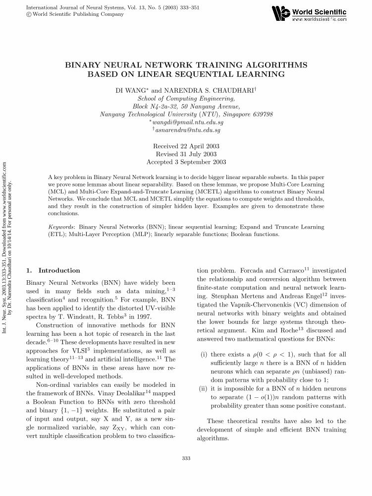
We illustrate the training process of ETL using
analogy shown in Fig. 1. White regions stand for true
subsets and black regions stand for false subsets. The
number in each region stands for the order of gen-
erating hyperplanes (hidden neurons). Based on the
selected true core vertex (in region 1), ETL begins
to extend its set of included true vertices (SITV) to
cover as many true vertices as possible. When SITV
covers region 1 (reaches the boundary of region 1
and region 2), it meets a false vertex, which prevents
SITV from further expansion. Then false vertices
out of region 1 are converted to true vertices and
true vertices out of region 1 are converted to false
vertices. Hence the false vertex which blocks the ex-
pansion will not block it now. SITV then expands
to include false vertices in region 2 until it reaches
region 3. This process goes on until it covers all true
vertices or all false vertices.
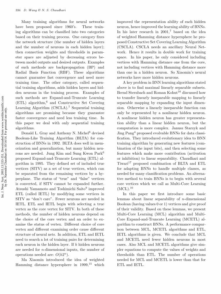
IETL improves ETL by considering some of the
vertices having in SITV as “don’t care”. The vertices
in SITV are overlooked when determining whether a
vertex can be added to SITV. In ETL algorithm, af-
ter expanding, the new hyperplane must include all
vertices in SITV. But in IETL this condition is not
necessary. IETL improves ETL by using less num-
ber of hidden neurons to solve the same problem.
However, IETL does not give guidelines about which
part should be considered as “don’t care”. In addi-
tion, in IETL vertices are considered in groups, not
one by one. This makes programming of IETL dif-
ficult. Figure 2 shows the training process of IETL.
IETL undergoes a training process similar to ETL,
however, the difference is: the vertices in SITV are
considered as “don’t care”. Hence one region can
overlap another region. In Fig. 2, region 2 overlaps
region 1, 3, 4 and 5. The decision made by the region
labeled by lower number.
Because each vertex lies on the surface of the ex-
hypersphere (represented by a circle in Fig. 1 and
Fig. 2), ETL and IETL guarantee convergence.
Fig. 1. Training process of ETL
Fig. 2. Training process of IETL
Fig. 3. Training process of MCL
Fig. 4. Training process of MCETL
Fig. 1. Training process of ETL. Fig. 1. Training process of ETL
Fig. 2. Training process of IETL
Fig. 3. Training process of MCL
Fig. 4. Training process of MCETL
Fig. 2. Training process of IETL.
Int.
J. N
eur.
Sys
t. 20
03.1
3:33
3-35
1. D
ownl
oade
d fr
om w
ww
.wor
ldsc
ient
ific
.com
by D
r. N
aren
dra
Cha
udha
ri o
n 10
/14/
14. F
or p
erso
nal u
se o
nly.
336 D. Wang & N. S. Chaudhari
If only one (n − 1)-dimensional hyperplane (one
hidden neuron) is needed, this function is linearly
separable. Otherwise, the inseparable function
should be decomposed into multiple linearly separa-
ble functions. ETL algorithm begins with selecting
one core vertex; the vertices which are not included
in SITV are examined one by one; then SITV will in-
clude as many vertices as it can; if no more vertices
can be added to SITV, the first separating hyper-
plane is found. However, if we have not separated
all true vertices from false vertices using this hyper-
plane, a second separating hyperplane is to be found.
To obtain the second hyperplane, false vertices are
converted to true vertices, and true vertices which
are not in SITV are converted to false vertices, and
the second separating hyperplane is obtained. This
process goes on until all true vertices are separated
from all false vertices. ETL is based on the result
that any binary-to-binary mapping can be decom-
posed into a series of linearly separable functions:
y(x1, x2, . . . , xn) = x1θ(x2θ(· · · (xn−1θxn)) · · · ) ,
(1)
where operator θ is either logical AND or logical OR.
The number of hidden neurons needed equals to the
number of separating hyperplanes.
IETL improves ETL by modifying some vertices
in SITV as “don’t care”, and hence needs less hidden
neurons. ETL and IETL guarantee convergence.
The neural net constructed by ETL and IETL al-
gorithms depend on the selected core vertex and the
order to examine whether a true vertex which can
be added to SITV. An inclusion of “inappropriate”
true vertex to SITV prevents the subsequent addi-
tion of many “true” vertices to SITV. We refer this
phenomenon as a “blocking problem”. Due to the
blocking problem, more hidden neurons are needed.
Considering these problems, we propose al-
ternative methods: Multi-Core Leaning (MCL)
algorithm and Multi-Core Expand-and-Truncate
Leaning (MCETL) algorithm.
Binary-to-binary mapping (1) can be reduced to
y(x1, x2, . . . , xn) =
k⋃
j=1
Aj (2)
where Aj is a set of vertices that can be linearly
separated from the rest vertices. We need k hid-
den neurons altogether. MCL and MCETL begin
Fig. 1. Training process of ETL
Fig. 2. Training process of IETL
Fig. 3. Training process of MCL
Fig. 4. Training process of MCETL
Fig. 3. Training process of MCL.
Fig. 1. Training process of ETL
Fig. 2. Training process of IETL
Fig. 3. Training process of MCL
Fig. 4. Training process of MCETL Fig. 4. Training process of MCETL.
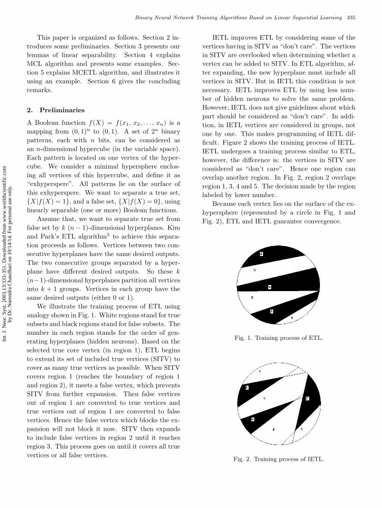
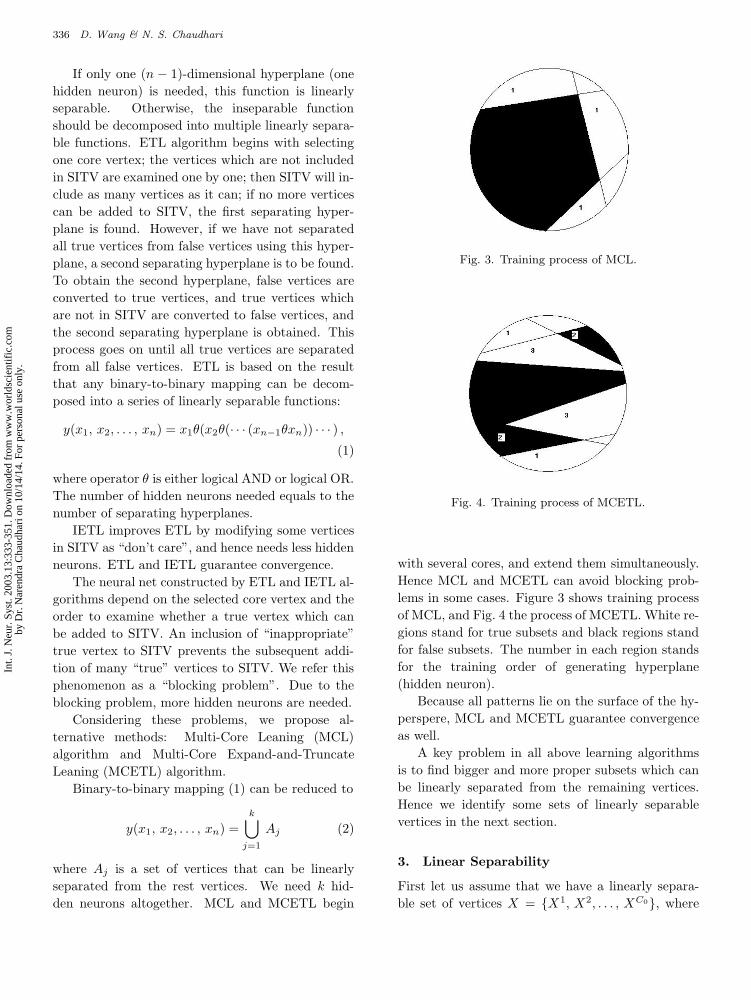
with several cores, and extend them simultaneously.
Hence MCL and MCETL can avoid blocking prob-
lems in some cases. Figure 3 shows training process
of MCL, and Fig. 4 the process of MCETL. White re-
gions stand for true subsets and black regions stand
for false subsets. The number in each region stands
for the training order of generating hyperplane
(hidden neuron).
Because all patterns lie on the surface of the hy-
perspere, MCL and MCETL guarantee convergence
as well.
A key problem in all above learning algorithms
is to find bigger and more proper subsets which can
be linearly separated from the remaining vertices.
Hence we identify some sets of linearly separable
vertices in the next section.
3. Linear Separability
First let us assume that we have a linearly separa-
ble set of vertices X = {X1, X2, . . . , XC0}, where
Int.
J. N
eur.
Sys
t. 20
03.1
3:33
3-35
1. D
ownl
oade
d fr
om w
ww
.wor
ldsc
ient
ific
.com
by D
r. N
aren
dra
Cha
udha
ri o
n 10
/14/
14. F
or p
erso
nal u
se o
nly.
Binary Neural Network Training Algorithms Based on Linear Sequential Learning 337
each Xk (k = 1, 2, . . . , C0) has n components, say
xki , (i = 1, 2, . . . , n). We now give a constructive
algorithm for obtaining linear separable hyperplane.
We also illustrate it with an example.
Example 1
Consider a Boolean function, f(x1, x2, x3) with
three variables, having (0, 0, 1) and (0, 1, 1) as true
vertices.
In the following, we give a method to obtain a
linearly separable hyperplane to separate these two
vertices {001, 011} from the remaining.
Let:
C0 = number of true vertices to be
separated from the remaining. (3)
To obtain the separating hyperplane for each in-
put bit (variable) xi in f we define:
Ci =
C0∑
k=1
xki (4)
For our example with {001, 011} vertices, we
have C1 = 0, C2 = 1, C3 = 2. After having obtain
these Ci’s, we obtain wi’s according to the following:
wi = 2Ci − C0 (5)
Thus, for our example with {001, 011}, we have,
w1 = −2, w2 = 0, w3 = 2.
Next, for the set of true vertices, X we define the
threshold:
T = minX∈SITV
(
n∑
i=1
wixi
)
(6)
Thus, for our example with X = {001, 011}, we
have: T = min{2, 2} = 2.
Now in term of above parameters, we use the fol-
lowing theorems to obtain the separating hyperplane.
Theorem 1
Let X be a linearly separable set of vertices. Then
the following hyperplane is a separating hyperplane
n∑
i=1
wixi = T (7)
where the parameters wi’s are obtained as in (5) and
T is obtained as in (6) above.
Proof
Our proof is based on Kim and Park’s approach.6
Let us consider a reference hypersphere (RHP):
(
x1 −1
2
)2
+
(
x2 −1
2
)2
+ · · · +
(
xn −1
2
)2
=n
4
(8)
All 2n vertices lie on this reference hypersphere.
Let us now consider a subset of these 2n vertices,
which are linearly separable. They lie on some hy-
persphere with (c1, c2, . . . , cn,) as a center and r as
a radius. Let:
n∑
i=1
(xi − ci)2 = r2 (9)
be this hypersphere (HP). In this hypersphere, let
us obtain the parameters ci and r are as follow. We
now give the proof of the above.
ci =
C0∑
k=1
xki /C0 . (10)
We obtain the intersection of HP and RHP from
(8) and (9) as follows:
n∑
i=1
(1 − 2ci)xi = r2 −
n∑
i=1
c2i . (11)
All vertices in HP lie on one side of or on hyper-
plane (11):
n∑
i=1
(1 − 2ci)xi ≤ r2 −n∑
i=1
c2i . (12)
All the remaining vertices (i.e., vertices not in
HP, but in RHP) lie on the other side of hyperplane
(11):n∑
i=1
(1 − 2ci)xi > r2 −
n∑
i=1
c2i . (13)
So the intersection (11) of HP and RHP is the
separating hyperplane, which separates true set from
the remaining.
Rewriting (11), we have:
n∑
i=1
(2ci − 1)xi =
n∑
i=1
c2i − r2 . (14)
Int.
J. N
eur.
Sys
t. 20
03.1
3:33
3-35
1. D
ownl
oade
d fr
om w
ww
.wor
ldsc
ient
ific
.com
by D
r. N
aren
dra
Cha
udha
ri o
n 10
/14/
14. F
or p
erso
nal u
se o
nly.
338 D. Wang & N. S. Chaudhari
In Eq. (14) r is defined as the minimal value that
meets the condition that all of the C0 vertices are
exactly in or on the hypersphere. So it is reasonable
to define r as the largest Euclidean distance between
the center of the hypersphere and all C0 vertices in
that linearly separable set:
r2 = max
n∑
k=1
(xki − ci)
2 (15)
Multiply (14) by C0, we obtain:
n∑
i=1
C0(2ci − 1)xi = C0
(
n∑
i=1
c2i − r2
)
(16)
In Eq. (16), we take C0(2ci−1) as the connection
weight, and C0(∑n
i=1 c2i − r2) as the threshold:
wi = C0(2ci − 1) . (17)
T = C0
(
n∑
i=1
c2i − r2
)
. (18)
Substitute (4), (10) and (15) into (17) and (18),
we obtain (5), and (6) in the following step:
wi = C0(2ci − 1) = 2
C0∑
k=1
xki − C0
= 2Ci − C0 . (19)
T = C0
(
n∑
i=1
c2i − r2
)
= C0
n∑
i=1
c2i − C0 max
n∑
k=1
(xki − ci)
2
= min
n∑
k=1
(2C0cixki − C0(x
ki )2) (20)
xki = (0, 1), so (xk
i )2 = xki . Hence:
T = min
n∑
k=1
C0(2ci − 1)xki
= minX∈SITV
(
n∑
i=1
wixi
)
(21)
�
Kim and Park proposed some hypotheses
about linear separatility of n-dimensional Boolean
vertices.18 They are stated in the following theorem.
Theorem 2
The following set of vertices can linearly be separated
from the rest:
1. A vertex,
2. Vertices with a vertex from which all the other
vertices are separated by distance one,
3. All four vertices on a face,
4. All the vertices on any number of connected
faces,
5. Each set of all the remaining vertices exclud-
ing each set of the vertices listed.
Since Kim and Park’s work18 does not include
the proof, we proceed to prove the above theorem.
Proof (of 1)
Given one vertex X to be separated, according to
Eqs. (3)–(6) we can construct the hidden neuron as:
wi =
{
1 if xi = 1;
−1 if xi = 0 .(22)
Suppose there are n1 true bits (bits having value
one) in X . Then:
T = n1 ; (23)
For X :
n∑
i=1
wixi ≥ T
(
n∑
i=1
wixi = n1
)
. (24)
We obtain any other vertex with Hamming dis-
tance k from X by converting k bits. Whenever true
bit is converted, one is reduced from∑n
i=1 wixi.
So, for any vertex with Hamming distance k from
X :n∑
i=1
wixi = T − k ≤ T . (25)
�
Proof (of 2)
Suppose we begin with one core vertex in SITV, say
Xc = {xc1, xc
2, . . . , xcn}. Let {Xj1 , Xj2 , . . . , Xjr}
be a set of vertices having Hamming distance equal
to one from the core, where Xjl is the vertex
whose jlth bit is different from the core, while other
bits are equal to the core. We now show that
Int.
J. N
eur.
Sys
t. 20
03.1
3:33
3-35
1. D
ownl
oade
d fr
om w
ww
.wor
ldsc
ient
ific
.com
by D
r. N
aren
dra
Cha
udha
ri o
n 10
/14/
14. F
or p
erso
nal u
se o
nly.
Binary Neural Network Training Algorithms Based on Linear Sequential Learning 339
{Xj1 , Xj2 , . . . , Xjr} and Xc can be linearly sepa-
rated from the remaining vertices. Totally (r+1) ver-
tices are included in SITV including the core. These
(r+1) vertices can be linearly separated from the rest
vertices hyperplane (7). From (3)–(6), we obtain:
C0 = (r + 1) . (26)
wi = 2Ci − (r + 1) . (27)
Ci =
r+1∑
l=1
xli , (28)
where xli is the ith bit of Xjl .
If r = 1, only one vertex X and the core vertex
Xc are to be linearly separated from the remaining
vertices. We assume X and Xc are different at the
ith bit, and do not differ for other bits. From Eqs. (4)
and (5), we have:
For the ith bit, wi = 0.
Let there be n1 one (true) bits in X . Let j denote
an index where the jth bit of X (which is same the
jth bit of Xc) is one. Then wj = 2.
Let there be n2 zero (false) bits in X . Let the kth
bit of X (which is same the kth bit of Xc) be zero.
Then wj = −2. From Eqs. (3)–(6), the separating
hyperplane is:
n∑
i=1
wixi = T = 2n1 . (29)
We note that, for X (and Xc),
n∑
i=1
wixi ≥ 2n1 . (30)
For other vertices Y , we can verify that
n∑
i=1
wixi < 2n1 . (31)
Now suppose 1 < r ≤ n. Consider (r + 1) ver-
tices S = {Xc, Xj1 , Xj2 , . . . , Xjr}. We show that
hyperplane (7) separates S.
From (5) we have:
wi =
r − 1, if xci = 1, and ∃jl jl = i,
r + 1, if xci = 1, and ∀jl jl 6= i ,
−(r − 1), if xci = 0, and ∃jl jl = i,
−(r + 1), if xci = 0, and ∀jl jl 6= i .
(32)
Let
N1 = X in SITV |xi = 0, xci = 1}, |N1| = n1 .
N2 = {Y not in SITV |yi = 0, xci = 1}, |N2| = n2 .
N3 = {X in SITV |xi = 1, xci = 0}, |N3| = n3 .
N4 = {Y not in SITV |yi = 1, xci = 0}, |N4| = n4 .
We can verify that:
n1 + n3 = r . (33)
n2 + n4 = n − r . (34)
For core vertex Xc, using above, we have
n∑
i=1
wixci = (r−1)×1×n1+(r+1)×1×n2 . (35)
A vertex in N1 (N1 is included in SITV) is a re-
sult of converting one bit of the core vertex from one
to zero; then, (r−1) is reduced from∑n
i=1 wixci . So,
we have:
n∑
i=1
wixi = (r−1)×n1+(r+1)×n2−(r−1) . (36)
Similarly, for a vertex in N2:
n∑
i=1
wixi = (r−1)×n1+(r+1)×n2−(r+1) . (37)
For a vertex in N3:
n∑
i=1
wixi = (r−1)×n1+(r+1)×n2−(r−1) . (38)
For a vertex in N4:
n∑
i=1
wixi = (r−1)×n1+(r+1)×n2−(r+1) . (39)
We have covered all vertices whose Hamming
distance is one from the core. The vertices whose
Hamming distance is more than one are obtained by
converting the bits different from the core one by
one. Each time we convert a bit,∑n
i=1 wixci will be
reduced by (r + 1) if xci = 1, and reduced by (r − 1)
if xci = 0.
Thus we have:
n∑
i=1
wixci >
n∑
i=1
wixN1
i
=n∑
i=1
wixN3
i >n∑
i=1
wixN2
i
=
n∑
i=1
wixN4
i . (40)
Int.
J. N
eur.
Sys
t. 20
03.1
3:33
3-35
1. D
ownl
oade
d fr
om w
ww
.wor
ldsc
ient
ific
.com
by D
r. N
aren
dra
Cha
udha
ri o
n 10
/14/
14. F
or p
erso
nal u
se o
nly.
340 D. Wang & N. S. Chaudhari
and,
n∑
i=1
wixHD=1i >
n∑
i=1
wixHD>1i , (41)
where HD stands for the Hamming distance from the
core. So we can separate SITV from the rest vertices
by the hyperplane (7).
For all the vertices in SITV:
n∑
i=1
wixi ≥ T = minX∈SITV
(
n∑
i=1
wixi
)
. (42)
For all the vertices not in SITV:
n∑
i=1
wixi < T (43)
�
Proof (of 3)
Suppose we want to separate four vertices: differ-
ent at the ith bit and the jth bit {00, 01, 10, 11},
and with the same value at other bits. According to
Eqs. (3)–(6) we can construct the hidden neuron as
the following:
wi = wj = 0 . (44)
For other bits:
wl =
{
4 if xl = 1;−4 if xl = 0 .
(45)
Suppose that, except for the ith bit and the jth
bit, there exists n1 one (true) bits in these four ver-
tices, then we have:
T = 4n1 . (46)
For the four vertices to be separated:
n∑
i=1
wixi ≥ T
(
in factn∑
i=1
wixi = 4n1
)
. (47)
Not considering ith bit and the jth bit into ac-
count, we obtain other vertex with Hamming dis-
tance k by converting k bits. Whenever one bit is
converted, 4 is reduced from∑n
i=1 wixi.
So, for any vertex with Hamming distance k from
X :n∑
i=1
wixi = T − 4k ≤ T . (48)
�
We can simplify the values of connection weights
and threshold as follows.
wi = wj = 0 ; (49)
For other bits:
wl =
{
1 if xl = 1;
−1 if xl = 0 .(50)
T = n1 . (51)
After simplification all values are also integral
numbers.
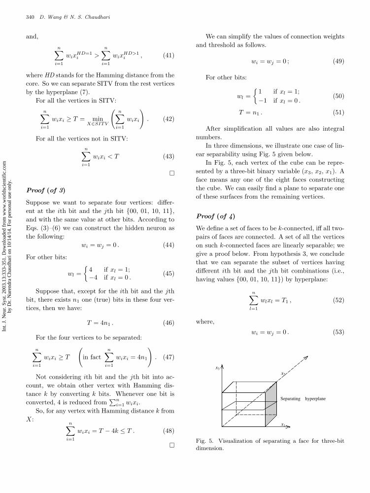
In three dimensions, we illustrate one case of lin-
ear separability using Fig. 5 given below.
In Fig. 5, each vertex of the cube can be repre-
sented by a three-bit binary variable (x3, x2, x1). A
face means any one of the eight faces constructing
the cube. We can easily find a plane to separate one
of these surfaces from the remaining vertices.
Proof (of 4)
We define a set of faces to be k-connected, iff all two-
pairs of faces are connected. A set of all the vertices
on such k-connected faces are linearly separable; we
give a proof below. From hypothesis 3, we conclude
that we can separate the subset of vertices having
different ith bit and the jth bit combinations (i.e.,
having values {00, 01, 10, 11}) by hyperplane:
n∑
l=1
wlxl = T1 , (52)
where,
wi = wj = 0 . (53)
Fig. 5. Visualization of separating a face for three-bit dimension.
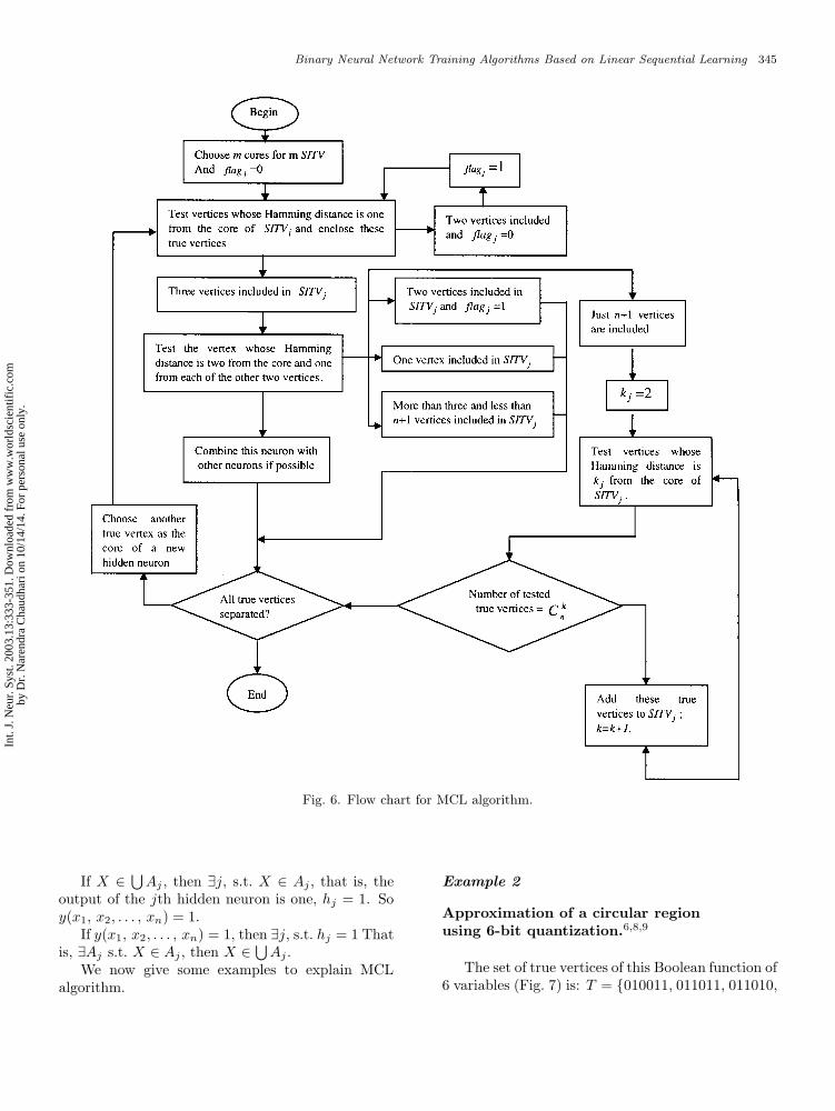
Fig 6. Flow Chart for MCL Algorithm.
x3 x2
x1
Separating hyperplane
Begin
Choose m cores for m SITV And jflag =0
Test vertices whose Hamming distance is onefrom the core of jSITV and enclose thesetrue vertices
Two vertices included and jflag =0
More than three and less than n+1 vertices included in jSITV
Two vertices included in jSITV and jflag =1
One vertex included in jSITV
Three vertices included in jSITV
Test the vertex whose Hammingdistance is two from the core and onefrom each of the other two vertices.
Choose anothertrue vertex as thecore of a newhidden neuron
All true verticesseparated?
End
Just n+1 verticesare included
jk =2
Number of tested true vertices =
jflag =1
Add these true vertices to jSITV ; k=k+1.
Combine this neuron with other neurons if possible
Test vertices whoseHamming distance is
jk from the core of
jSITV .
knC
Fig. 5. Visualization of separating a face for three-bitdimension.
Int.
J. N
eur.
Sys
t. 20
03.1
3:33
3-35
1. D
ownl
oade
d fr
om w
ww
.wor
ldsc
ient
ific
.com
by D
r. N
aren
dra
Cha
udha
ri o
n 10
/14/
14. F
or p
erso
nal u
se o
nly.
Binary Neural Network Training Algorithms Based on Linear Sequential Learning 341
For other bits:
wl =
{
1 if xl = 1;
−1 if xl = 0 .(54)
T1 = n1 . (55)
The k connected faces can be separated by the
Boolean function of the following nature:
f(x1, x2, . . . , xn) = (x1 ∧ x2 · · · ∧ xj)
∧ (xi1 ∨ xi2 ∨ · · · ∨ xik) (56)
where ∧ is Boolean “AND” and ∨ is Boolean “OR”
operations.
According to Eqs. (3)–(6) we can construct the
hidden neuron as:
wi = 0 . (57)
wij =
{
n/k if xij = 1 ,
−n/k if xij = −1 .(58)
For other bits:
wi =
{
n if xi = 1;
−n if xi = 0 .(59)
T = minX∈f−1(1)
(
n∑
i=1
wixi
)
. (60)
For vertices on the connected surfaces:
n∑
i=1
wixi ≥ T . (61)
For other vertices:
n∑
i=1
wixi < T . (62)
�
Part 5 of Theorem 2 follows from the above four
parts directly.
Following the arguments above, we propose two
additional lemmas to obtain linearly separable set of
vertices.
Lemma 1
Given a core vertex, all vertices whose Hamming dis-
tance is one from the core, along with the core can
be linearly separated from the remaining vertices by
a hyperplane.
Proof
Suppose X is an n-dimensional input. According to
Eqs. (3)–(6), we can construct the hidden neuron as
follows.
Let there be n1 one (true) bits in the core Xc.
Let j denote an index where the jth bit of Xc is one.
Let there be n2 zero (false) bits in the core Xc.
Let k denote an index where the kth bit of Xc is
zero.
According to formula (3)–(6), we get:
C0 = n + 1 . (63)
For the kth bit where xck = 0,
Ck = 1 , (64)
wk = −(n − 1) . (65)
For the jth bit where xcj = 1,
Cj = n (66)
wj = (n − 1) . (67)
So for the core
n∑
i=1
wixi = n1(n − 1) . (68)
We can get vertices whose Hamming distance is
one from the core by converting one bit of the core.
Whenever we convert a bit of the core from one to
zero or from zero to one,∑n
i=1 wixi will be reduced
by (n − 1).
For any vertex X whose Hamming distance is one
from the core:
n∑
i=1
wixi = (n1 − 1)(n − 1) . (69)
In the same way we obtain∑n
i=1 wixi for the ver-
tices X whose Hamming distance is m (m > 1) from
the core by converting m bits of the core, either from
zero to one, or from one to zero. Also whenever one
bit is converted, (n − 1) is reduced from∑n
i=1 wixi.
So we get for all vertices whose Hamming distance is
m from the core:
n∑
i=1
wixi = (n1 − m)(n − 1) . (70)
Int.
J. N
eur.
Sys
t. 20
03.1
3:33
3-35
1. D
ownl
oade
d fr
om w
ww
.wor
ldsc
ient
ific
.com
by D
r. N
aren
dra
Cha
udha
ri o
n 10
/14/
14. F
or p
erso
nal u
se o
nly.
342 D. Wang & N. S. Chaudhari
So we obtain,
T = minHD<2
n∑
i=1
wixi = (n1 − 1)(n − 1) . (71)
For all vertices whose Hamming distance is equal
to or less than one:
n∑
i=1
wixi ≥ T , (72)
while for all vertices whose Hamming distance is
larger than one:
n∑
i=1
wixi < T . (73)
�
Lemma 2
Given a core vertex, all vertices whose Hamming dis-
tance is equal to or less than k from the core, along
with the core can be linearly separated from the re-
maining vertices by a hyperplane.
Proof
Using Eqs. (3)–(6), we get:
C0 =
k∑
j=0
Cjn . (74)
For the ith bit where xci = 0, we have:
Ci =k∑
j=1
(Cjn − Cj
n−1) . (75)
wi = 2Ci − C0 = −Ckn−1 . (76)
For the ith bit where xci = 1, we have:
Ci = 1 +
k∑
j=1
Cjn−1 . (77)
wi = 2Ci − C0 = Ckn−1 . (78)
For any vertex X we suppose:
m1 bits are the same with the core and xci = 0 .
m2 bits are different from the core and xci = 0 .
m3 bits are different from the core and xci = 1 .
m4 bits are the same with the core and xci = 1 .
So we have,
n∑
i=1
wixi = (m4 − m2)Ckn−1 . (79)
Assume there are n1 one (true) bits and n2 zero
(false) bits in the core Xc. Using Eqs. (3)–(6), we
obtain:
for the core:
n∑
i=1
wixi = n1Ckn−1 . (80)
We get vertices whose Hamming distance is one
from the core by converting one bit of the core.
Whenever we convert one bit of the core from one to
zero or from zero to one,∑n
i=1 wixi will be reduced
by Ckn−1. So for any vertex X whose Hamming dis-
tance is one from the core:
n∑
i=1
wixi = (n1 − 1)Ckn−1 . (81)
In the same way we get∑n
i=1 wixi for the ver-
tices X whose Hamming distance is l (1 < l < k)
from the core by converting l bits of the core, either
from zero to one, or from one to zero. Also whenever
one bit is converted, Ckn−1 is reduced from
n∑
i=1
wixi.
So we get for vertices whose Hamming distance is l
from the core:
n∑
i=1
wixi = (n1 − l)Ckn−1 . (82)
So we set
T = minHD≤k
n∑
i=1
wixi = (n1 − k)Ckn−1 . (83)
For all vertices whose Hamming distance is equal
to or less than k:
n∑
i=1
wixi ≥ T , (84)
while for all vertices whose Hamming distance is
larger than k, we have:
n∑
i=1
wixi < T . (85)
�
Int.
J. N
eur.
Sys
t. 20
03.1
3:33
3-35
1. D
ownl
oade
d fr
om w
ww
.wor
ldsc
ient
ific
.com
by D
r. N
aren
dra
Cha
udha
ri o
n 10
/14/
14. F
or p
erso
nal u
se o
nly.
Binary Neural Network Training Algorithms Based on Linear Sequential Learning 343
Suppose that we wish to separate all vertices hav-
ing Hamming distance less than or equal to k to-
gether with some vertices at Hamming distance k+1,
from the core vertex. The above separating hyper-
plane construction does not work in this case. As an
example, suppose we want to separate subset {0101,
0100, 1101, 0001, 0111, 1001, 0110} (true subset)
centered at 0101 from the remaining subset {0000,
0010, 0011, 1000, 1010, 1011, 1100, 1110, 1111} (false
subset). Thus k = 1, and for k + 1 = 2, only vertices
1001 and 0110 are to be separated.
According to Eqs. (3)–(6), we obtain W =
{−3, 3, −3, 3}, T = 0. The values of∑4
i=1 wixi for
true subset are {6, 3, 3, 3, 3, 0, 0}, and for false
subset are {0, −3, 0, −3, −6, −3, 0, −3, 0}. So we
cannot separate these two subsets by a hyperplane
obtained from Eqs. (3)–(6).
Based on these lemmas, we present MCL and
MCETL in the following sections.
4. Multi-Core Learning
4.1. Multi-core architecture
Multi-Core Learning constructs a three-layer neural
network with one hidden layer.
The hard-limiter activation function for the jth
hidden neuron is:
hj =
1 ifd∑
i=1
wijxi ≥ Tj
0 otherwise
. (86)
where wij is the connection weight between the ith
bit of the input and the jth hidden neuron; xi is the
ith bit of the input; d is the dimension of input; Tj
is the threshold of the jth hidden neuron; and hj is
the output of the hard limiter activation function of
the jth neuron.
The hard-limiter activation function for the out-
put layer is:
y =
1 ifm∑
j=1
woj hj ≥ T o
0 otherwise
, (87)
where woj is the weight connection between the jth
hidden neuron and the output neuron; T o is the
threshold of the output neuron; and y is the final
output.
4.2. Neurons in hidden layer
As stated in Eqs. (1) and (2), a binary-to-binary
mapping can be described as a Boolean function.7
y(x1, x2, . . . , xn) = x1θ(x2θ(· · · (xn−1θxn)) · · · ) ,
y(x1, x2, . . . , xn) =
k⋃
j=1
Aj ,
where Aj is a set of vertices that can be linearly
separated from the rest vertices. Totally we have k
linearly separable subsets. Hence k hidden neurons
are needed in our neural network.
We select m true vertices as core for each SITV,
where m ≤ 2bn3c, n is the dimension of input.
We give the following steps for Multi-Core Learning
(MCL).
Algorithm 1
MCL algorithm
(a) Select a true vertex randomly. Convert 3 con-
tinuous bits (in groups) of this true vertex. If
the result vertex is true, consider it as a SITV
core. For example, we convert the 1st, 2nd
3rd bit to get X1, convert the 4th 5th, 6th
bit to get X2, and convert all the 1st, 2nd
3rd, 4th 5th, 6th bit to get X3. Continu-
ing with this example, suppose that we begin
with an arbitrary true vertex {001001}, and
m = 4. Then if {001110, 110001, 110110} are
true vertices, they are taken as cores. So the
Hamming distance between any two cores is
more than two initially.
(b) Set flagj = 0 and kj = 0 for each SITV.
(c) Test vertices whose Hamming distance is one
from SITV cores.
(d) When three vertices are included in SITVj ,
test the vertex whose hamming distance is
two from SITVj core and one from each of
the other two vertices.
(e) If the tested vertex is false, go to step
f to examine other vertices whose Ham-
ming distance is one from the core; else
if true, include this vertex in SITVj , and
combine this hidden neuron with other hid-
den neurons if possible. We scan the
connection weights of each hidden neuron,
and select two hidden neurons with all the
Int.
J. N
eur.
Sys
t. 20
03.1
3:33
3-35
1. D
ownl
oade
d fr
om w
ww
.wor
ldsc
ient
ific
.com
by D
r. N
aren
dra
Cha
udha
ri o
n 10
/14/
14. F
or p
erso
nal u
se o
nly.
344 D. Wang & N. S. Chaudhari
corresponding bits of connection weights the
same except for one contrary bit. We com-
bine the two hidden neurons by setting the
weight of the contrary bit as zero, and coping
those of other bits (for example, we can com-
bine wj1 = {4, 2, 3, −3} and wj2 = {4, 2,
3, 3} as wj12 = {4, 2, 3, 0}).
(f) If more than three and less than n + 1 ver-
tices are enclosed in SITVj , go to step l for
SITVj .
(g) If only two vertices are included and flagj =
0, the core is moved to the other vertex. Set
flagj = 1, and go to step c. Else if only two
vertices are included and flagj = 1, go to
step l for SITVj .
(h) If no other vertex except for the core is in-
cluded, this corresponding hidden neuron can
only separate one vertex from the rest ver-
tices. Go to step l for SITVj .
(i) If n + 1 vertices are true (all vertices with
Hamming distance one are true), set kj = 2
and, go to step k.
(j) Include all the vertices at Hamming distance
kj − 1. Test vertices at Hamming distance
kj from the SITVj core. If all Ckn vertices at
Hamming distance kj are true, go to step k.
Else go to step l for SITVj .
(k) Increment kj (by one), and go to step j.
(l) If all the true vertices have been included in⋃k
j=1 SITVj , stop the training process. Else
select a true vertex which is not included in⋃k
j=1 SITVj as the new core, and go to step c.
End of MCL algorithm.
All hidden neurons are trained simultaneously.
When each individual hidden neuron is trained, other
vertices are considered as “don’t care”. The details
are shown in the flow chart in Fig. 6.
To get an efficient neural network structure, we
need to generate maximum linearly separable sub-
sets. We need to combine two connected hid-
den neurons if possible. In step 4, a method is
given to combine two continuous neurons. Some-
times, we do not expect a 100% precision; an ap-
proximate result is acceptable. A neuron with
weights {w1, w2, . . . , wl, . . . , wk ± ε, . . . , wn} can
be combined with a neuron with weights {w1,
w2, . . . , −wl, . . . , wk ∓ ε, . . . , wn}; the result neu-
ron’s weights are {w1, w2, . . . , 0, . . . , wk, . . . , wn}.
ε/C0 is a small value, where C0 is the number of ver-
tices represented by this hidden neuron. The value
of ε/C0 is up to the expected precision.
Formulas to train hidden neurons (neuron j in
our method) are as follows:
wij = 2Cij − C0j , (88)
Cij =
C0j∑
l=1
xil , (89)
where C0j is the number of vertices in SITVj , xil is
the ith bit of the lth vertex in SITVj .
Tj = minX∈SITVj
(
n∑
i=1
wijxi
)
, (90)
where xi is the ith bit of X . We compute all the
results of∑n
i=1 wijxi for each vertex X in SITVj ,
and let Tj equal to the minimum of {∑n
i=1 wijxi}.
SITVj can be separated from the rest vertices by a
hyperplane.
For all vertices in SITVj
n∑
i=1
wijxi ≥ minX∈SITVj
(
n∑
i=1
wijxi
)
. (91)
For the rest vertices,
n∑
i=1
wijxi < minX∈SITVj
(
n∑
i=1
wijxi
)
. (92)
Thus, for all vertices in SITVj , hj = 1; for
the rest of the vertices (not included in SITVj),
hj = 0. When we compute Tj , we need not com-
pute∑n
i=1 wijxi for any vertex outside SITVj , which
simplifies the training process. The number of oper-
ations needed for are O(2nh), where h is the number
of hidden neurons, and n is the input dimension.
4.3. Construction of output neuron
for MCL
The weights between hidden neurons and the output
neuron, and threshold of the output neuron can be
determined by the following formulas:
T o = 1 , (93)
woj = 1 , (94)
where T o is the threshold of the output neuron; woj is
the weight connection between the jth hidden neu-
ron and the output neuron.
Int.
J. N
eur.
Sys
t. 20
03.1
3:33
3-35
1. D
ownl
oade
d fr
om w
ww
.wor
ldsc
ient
ific
.com
by D
r. N
aren
dra
Cha
udha
ri o
n 10
/14/
14. F
or p
erso
nal u
se o
nly.
Binary Neural Network Training Algorithms Based on Linear Sequential Learning 345
Fig. 6. Flow chart for MCL algorithm.
If X ∈⋃
Aj , then ∃j, s.t. X ∈ Aj , that is, theoutput of the jth hidden neuron is one, hj = 1. Soy(x1, x2, . . . , xn) = 1.
If y(x1, x2, . . . , xn) = 1, then ∃j, s.t. hj = 1 Thatis, ∃Aj s.t. X ∈ Aj , then X ∈
⋃
Aj .We now give some examples to explain MCL
algorithm.
Example 2
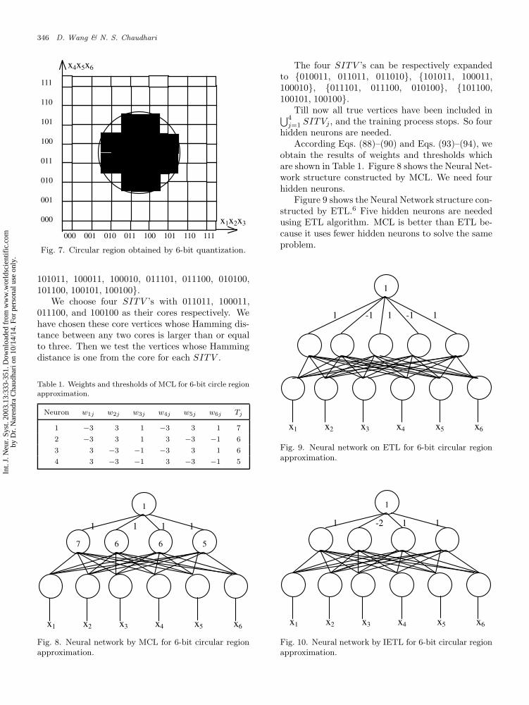
Approximation of a circular regionusing 6-bit quantization.6,8,9
The set of true vertices of this Boolean function of6 variables (Fig. 7) is: T = {010011, 011011, 011010,
Int.
J. N
eur.
Sys
t. 20
03.1
3:33
3-35
1. D
ownl
oade
d fr
om w
ww
.wor
ldsc
ient
ific
.com
by D
r. N
aren
dra
Cha
udha
ri o
n 10
/14/
14. F
or p
erso
nal u
se o
nly.
346 D. Wang & N. S. Chaudhari
111
110
101
100
011
010
001
000
000 001 010 011 100 101 110 111
x1x2x3
x4x5x6
Fig. 7. Circular region obtained by 6-bit quantization.
101011, 100011, 100010, 011101, 011100, 010100,101100, 100101, 100100}.
We choose four SITV ’s with 011011, 100011,011100, and 100100 as their cores respectively. Wehave chosen these core vertices whose Hamming dis-tance between any two cores is larger than or equalto three. Then we test the vertices whose Hammingdistance is one from the core for each SITV .
Table 1. Weights and thresholds of MCL for 6-bit circle regionapproximation.
Neuron w1j w2j w3j w4j w5j w6j Tj
1 −3 3 1 −3 3 1 7
2 −3 3 1 3 −3 −1 6
3 3 −3 −1 −3 3 1 6
4 3 −3 −1 3 −3 −1 5
Fig 7. Circular Region obtained by 6-bit quantization.
Fig 8. Neural Network by MCL for 6-bit circular region approximation.
Fig. 9. Neural Network on ETL for 6-bit circlular region approximation.
Fig 10. Neural Network by IETL for 6-bit circlular region approximation.
000 001 010 011 100 101 110 111
111
110
101
100
011
010
001
000 x1x2x3
x4x5x6
1
7 6 6 5
x1 x2 x3 x4 x5 x6
1 1 1 1
1
1 -1 1 -1 1
x1 x2 x3 x4 x5 x6
1
x1 x2 x3 x4 x5 x6
1 -2 1 1
Fig. 8. Neural network by MCL for 6-bit circular regionapproximation.
The four SITV ’s can be respectively expandedto {010011, 011011, 011010}, {101011, 100011,100010}, {011101, 011100, 010100}, {101100,100101, 100100}.
Till now all true vertices have been included in⋃4
j=1 SITVj , and the training process stops. So fourhidden neurons are needed.
According Eqs. (88)–(90) and Eqs. (93)–(94), weobtain the results of weights and thresholds whichare shown in Table 1. Figure 8 shows the Neural Net-work structure constructed by MCL. We need fourhidden neurons.
Figure 9 shows the Neural Network structure con-structed by ETL.6 Five hidden neurons are neededusing ETL algorithm. MCL is better than ETL be-cause it uses fewer hidden neurons to solve the sameproblem.
Fig 7. Circular Region obtained by 6-bit quantization.
Fig 8. Neural Network by MCL for 6-bit circular region approximation.
Fig. 9. Neural Network on ETL for 6-bit circlular region approximation.
Fig 10. Neural Network by IETL for 6-bit circlular region approximation.
000 001 010 011 100 101 110 111
111
110
101
100
011
010
001
000 x1x2x3
x4x5x6
1
7 6 6 5
x1 x2 x3 x4 x5 x6
1 1 1 1
1
1 -1 1 -1 1
x1 x2 x3 x4 x5 x6
1
x1 x2 x3 x4 x5 x6
1 -2 1 1
Fig. 9. Neural network on ETL for 6-bit circular regionapproximation.
Fig 7. Circular Region obtained by 6-bit quantization.
Fig 8. Neural Network by MCL for 6-bit circular region approximation.
Fig. 9. Neural Network on ETL for 6-bit circlular region approximation.
Fig 10. Neural Network by IETL for 6-bit circlular region approximation.
000 001 010 011 100 101 110 111
111
110
101
100
011
010
001
000 x1x2x3
x4x5x6
1
7 6 6 5
x1 x2 x3 x4 x5 x6
1 1 1 1
1
1 -1 1 -1 1
x1 x2 x3 x4 x5 x6
1
x1 x2 x3 x4 x5 x6
1 -2 1 1
Fig. 10. Neural network by IETL for 6-bit circular regionapproximation.
Int.
J. N
eur.
Sys
t. 20
03.1
3:33
3-35
1. D
ownl
oade
d fr
om w
ww
.wor
ldsc
ient
ific
.com
by D
r. N
aren
dra
Cha
udha
ri o
n 10
/14/
14. F
or p
erso
nal u
se o
nly.
Binary Neural Network Training Algorithms Based on Linear Sequential Learning 347
Table 2. Weights and thresholds of IETL for 6-bit circle regionapproximation.
Neuron w1j w2j w3j w4j w5j w6j Tj
1 −6 6 2 −6 6 2 13
2 −58 −6 −2 −6 6 2 −11
3 −58 −6 −2 −6 6 2 −58
4 6 −6 −2 6 −6 −2 9
Using IETL of Yamamoto and Saito,9 also fourhidden neurons are needed. Figure 10 shows the Neu-ral Network structure constructed by IETL.9 The re-sults of weights and thresholds by IETL are shownin Table 2.9 Comparing Table 1 with Table 2, we cansee the values of weights and thresholds in MCL aremuch smaller than those in IETL. The smaller nu-merical values are preferred for hardware realization.
We now consider a few more examples.
Example 3
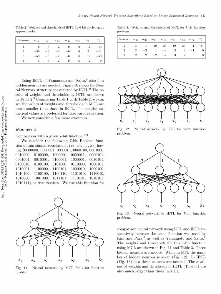
Comparison with a given 7-bit function.6,9
We consider the following 7-bit Boolean func-tion obtain similar conclusion f(x1, x2, . . . , x7) hav-ing {0000000, 0000001, 0000010, 0000100, 0001000,0010000, 0100000, 1000000, 0000011, 0000101,0001001, 0010001, 0100001, 1000001, 0010101,0100010, 0100100, 0101000, 0110000, 1000101,1010001, 1100000, 1100101, 1000010, 1000100,1010100, 1100100, 1100110, 1101010, 1110010,1010000, 1001000, 1011101, 1110101, 1010101,1010111} as true vertices. We use this function for
Fig. 11. Neural Network by MCL for 7-bit function problem. Fig 12. Neural Network by ETL for 7-bit function problem.
Fig 13. Neural Network by IETL for 7-bit function problem.
x1 x2 x3 x4 x5 x6 x7
1 1 1
x1 x2 x3 x4 x5 x6 x7
1
x1 x2 x3 x4 x5 x6 x7
-2 1 1
1
Fig. 11. Neural network by MCL for 7-bit functionproblem.
Table 3. Weights and thresholds of MCL for 7-bit functionproblem.
Neuron w1j w2j w3j w4j w5j w6j w7j Tj
1 3 −1 −19 −29 −19 −29 1 −37
2 3 −3 1 −3 3 3 −1 9
3 2 2 −2 −2 3 2 0 8
Fig. 11. Neural Network by MCL for 7-bit function problem. Fig 12. Neural Network by ETL for 7-bit function problem.
Fig 13. Neural Network by IETL for 7-bit function problem.
x1 x2 x3 x4 x5 x6 x7
1 1 1
x1 x2 x3 x4 x5 x6 x7
1
x1 x2 x3 x4 x5 x6 x7
-2 1 1
1
Fig. 12. Neural network by ETL for 7-bit functionproblem.
Fig. 11. Neural Network by MCL for 7-bit function problem. Fig 12. Neural Network by ETL for 7-bit function problem.
Fig 13. Neural Network by IETL for 7-bit function problem.
x1 x2 x3 x4 x5 x6 x7
1 1 1
x1 x2 x3 x4 x5 x6 x7
1
x1 x2 x3 x4 x5 x6 x7
-2 1 1
1
Fig. 13. Neural network by IETL for 7-bit functionproblem.
comparison neural network using ETL and IETL re-spectively because the same function was used byKim and Park,6 as well as Yamamoto and Saito.9
The weights and thresholds for this 7-bit functionusing MCL are shown in Fig. 11 and Table 3. Threehidden neurons are needed. While in ETL the num-ber of hidden neurons is seven (Fig. 12). In IETL(Fig. 13) also three neurons are needed. These val-ues of weights and thresholds in IETL (Table 4) arealso much larger than those in MCL.
Int.
J. N
eur.
Sys
t. 20
03.1
3:33
3-35
1. D
ownl
oade
d fr
om w
ww
.wor
ldsc
ient
ific
.com
by D
r. N
aren
dra
Cha
udha
ri o
n 10
/14/
14. F
or p
erso
nal u
se o
nly.
348 D. Wang & N. S. Chaudhari
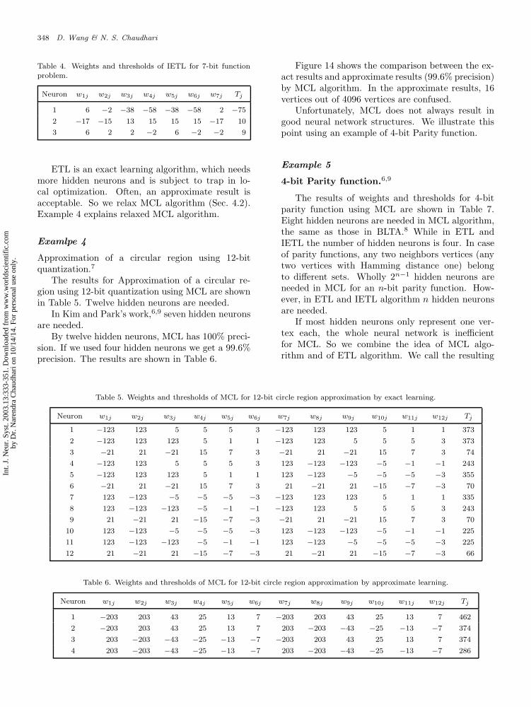
Table 4. Weights and thresholds of IETL for 7-bit functionproblem.
Neuron w1j w2j w3j w4j w5j w6j w7j Tj
1 6 −2 −38 −58 −38 −58 2 −75
2 −17 −15 13 15 15 15 −17 10
3 6 2 2 −2 6 −2 −2 9
ETL is an exact learning algorithm, which needsmore hidden neurons and is subject to trap in lo-cal optimization. Often, an approximate result isacceptable. So we relax MCL algorithm (Sec. 4.2).Example 4 explains relaxed MCL algorithm.
Examlpe 4
Approximation of a circular region using 12-bitquantization.7
The results for Approximation of a circular re-gion using 12-bit quantization using MCL are shownin Table 5. Twelve hidden neurons are needed.
In Kim and Park’s work,6,9 seven hidden neuronsare needed.
By twelve hidden neurons, MCL has 100% preci-sion. If we used four hidden neurons we get a 99.6%precision. The results are shown in Table 6.
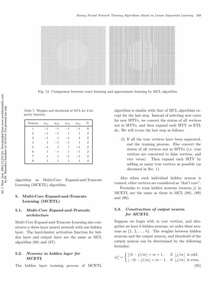
Figure 14 shows the comparison between the ex-act results and approximate results (99.6% precision)by MCL algorithm. In the approximate results, 16vertices out of 4096 vertices are confused.
Unfortunately, MCL does not always result ingood neural network structures. We illustrate thispoint using an example of 4-bit Parity function.
Example 5
4-bit Parity function.6,9
The results of weights and thresholds for 4-bitparity function using MCL are shown in Table 7.Eight hidden neurons are needed in MCL algorithm,the same as those in BLTA.8 While in ETL andIETL the number of hidden neurons is four. In caseof parity functions, any two neighbors vertices (anytwo vertices with Hamming distance one) belongto different sets. Wholly 2n−1 hidden neurons areneeded in MCL for an n-bit parity function. How-ever, in ETL and IETL algorithm n hidden neuronsare needed.
If most hidden neurons only represent one ver-tex each, the whole neural network is inefficientfor MCL. So we combine the idea of MCL algo-rithm and of ETL algorithm. We call the resulting
Table 5. Weights and thresholds of MCL for 12-bit circle region approximation by exact learning.
Neuron w1j w2j w3j w4j w5j w6j w7j w8j w9j w10j w11j w12j Tj
1 −123 123 5 5 5 3 −123 123 123 5 1 1 373
2 −123 123 123 5 1 1 −123 123 5 5 5 3 373
3 −21 21 −21 15 7 3 −21 21 −21 15 7 3 74
4 −123 123 5 5 5 3 123 −123 −123 −5 −1 −1 243
5 −123 123 123 5 1 1 123 −123 −5 −5 −5 −3 355
6 −21 21 −21 15 7 3 21 −21 21 −15 −7 −3 70
7 123 −123 −5 −5 −5 −3 −123 123 123 5 1 1 335
8 123 −123 −123 −5 −1 −1 −123 123 5 5 5 3 243
9 21 −21 21 −15 −7 −3 −21 21 −21 15 7 3 70
10 123 −123 −5 −5 −5 −3 123 −123 −123 −5 −1 −1 225
11 123 −123 −123 −5 −1 −1 123 −123 −5 −5 −5 −3 225
12 21 −21 21 −15 −7 −3 21 −21 21 −15 −7 −3 66
Table 6. Weights and thresholds of MCL for 12-bit circle region approximation by approximate learning.
Neuron w1j w2j w3j w4j w5j w6j w7j w8j w9j w10j w11j w12j Tj
1 −203 203 43 25 13 7 −203 203 43 25 13 7 462
2 −203 203 43 25 13 7 203 −203 −43 −25 −13 −7 374
3 203 −203 −43 −25 −13 −7 −203 203 43 25 13 7 374
4 203 −203 −43 −25 −13 −7 203 −203 −43 −25 −13 −7 286
Int.
J. N
eur.
Sys
t. 20
03.1
3:33
3-35
1. D
ownl
oade
d fr
om w
ww
.wor
ldsc
ient
ific
.com
by D
r. N
aren
dra
Cha
udha
ri o
n 10
/14/
14. F
or p
erso
nal u
se o
nly.
Binary Neural Network Training Algorithms Based on Linear Sequential Learning 349
Fig. 14. Comparison between exact learning and approximate learning by MCL algorithm.
Fig. 15. Neural Network by MCETL for 4-bit parity function.
0
0 4
x1 x2 x3 x4
1 1 -3 -3
-2 6
Fig. 14. Comparison between exact learning and approximate learning by MCL algorithm.
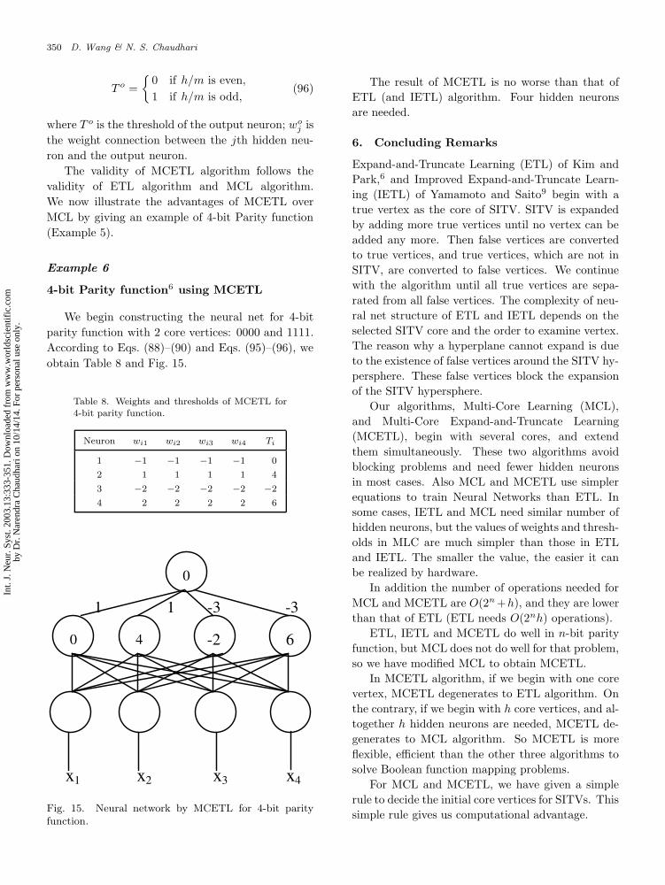
Table 7. Weights and thresholds of MCL for 4-bitparity function.
Neuron wi1 wi2 wi3 wi4 Ti
1 −1 −1 −1 −1 0
2 −1 −1 1 1 2
3 −1 1 −1 1 2
4 1 −1 −1 1 2
5 −1 1 1 −1 2
6 1 −1 1 −1 2
7 1 1 −1 −1 2
8 1 1 1 1 4
algorithm as Multi-Core Expand-and-Truncate
Learning (MCETL) algorithm.
5. Multi-Core Expand-and-Truncate
Learning (MCETL)
5.1. Multi-Core Expand-and-Truncate
architecture
Multi-Core Expand-and-Truncate Learning also con-
structs a three-layer neural network with one hidden
layer. The hard-limiter activation function for hid-
den layer and output layer are the same as MCL
algorithm (86) and (87).
5.2. Neurons in hidden layer for
MCETL
The hidden layer training process of MCETL
algorithm is similar with that of MCL algorithm ex-
cept for the last step. Instead of selecting new cores
for new SITVs, we convert the status of all vertices
not in SITVs, and then expand each SITV as ETL
do. We will revise the last step as follows:
(l) If all the true vertices have been separated,
end the training process. Else convert the
status of all vertices not in SITVs (i.e. true
vertices are converted to false vertices, and
vice versa). Then expand each SITV by
adding as many true vertices as possible (as
discussed in Sec. 1).
Also when each individual hidden neuron is
trained, other vertices are considered as “don’t care”.
Formulas to train hidden neurons (neuron j) in
MCETL are the same as those in MCL (88), (89)
and (90).
5.3. Construction of output neuron
for MCETL
Suppose we begin with m core vertices, and alto-
gether we have h hidden neurons, we order these neu-
rons as {1, 2, . . . , h}. The weights between hidden
neurons and the output neuron, and threshold of the
output neuron can be determined by the following
formulas:
woj =
{
b(h − j)/mc × m + 1, if bj/mc is odd,
b−(h − j)/mc × m − 1, if bj/mc is even,
(95)
Int.
J. N
eur.
Sys
t. 20
03.1
3:33
3-35
1. D
ownl
oade
d fr
om w
ww
.wor
ldsc
ient
ific
.com
by D
r. N
aren
dra
Cha
udha
ri o
n 10
/14/
14. F
or p
erso
nal u
se o
nly.
350 D. Wang & N. S. Chaudhari
T o =
{
0 if h/m is even,
1 if h/m is odd,(96)
where T o is the threshold of the output neuron; woj is
the weight connection between the jth hidden neu-
ron and the output neuron.
The validity of MCETL algorithm follows the
validity of ETL algorithm and MCL algorithm.
We now illustrate the advantages of MCETL over
MCL by giving an example of 4-bit Parity function
(Example 5).
Example 6
4-bit Parity function6 using MCETL
We begin constructing the neural net for 4-bit
parity function with 2 core vertices: 0000 and 1111.
According to Eqs. (88)–(90) and Eqs. (95)–(96), we
obtain Table 8 and Fig. 15.
Table 8. Weights and thresholds of MCETL for4-bit parity function.
Neuron wi1 wi2 wi3 wi4 Ti
1 −1 −1 −1 −1 0
2 1 1 1 1 4
3 −2 −2 −2 −2 −2
4 2 2 2 2 6
Fig. 14. Comparison between exact learning and approximate learning by MCL algorithm.
Fig. 15. Neural Network by MCETL for 4-bit parity function.
0
0 4
x1 x2 x3 x4
1 1 -3 -3
-2 6
Fig. 15. Neural network by MCETL for 4-bit parityfunction.
The result of MCETL is no worse than that of
ETL (and IETL) algorithm. Four hidden neurons
are needed.
6. Concluding Remarks
Expand-and-Truncate Learning (ETL) of Kim and
Park,6 and Improved Expand-and-Truncate Learn-
ing (IETL) of Yamamoto and Saito9 begin with a
true vertex as the core of SITV. SITV is expanded
by adding more true vertices until no vertex can be
added any more. Then false vertices are converted
to true vertices, and true vertices, which are not in
SITV, are converted to false vertices. We continue
with the algorithm until all true vertices are sepa-
rated from all false vertices. The complexity of neu-
ral net structure of ETL and IETL depends on the
selected SITV core and the order to examine vertex.
The reason why a hyperplane cannot expand is due
to the existence of false vertices around the SITV hy-
persphere. These false vertices block the expansion
of the SITV hypersphere.
Our algorithms, Multi-Core Learning (MCL),
and Multi-Core Expand-and-Truncate Learning
(MCETL), begin with several cores, and extend
them simultaneously. These two algorithms avoid
blocking problems and need fewer hidden neurons
in most cases. Also MCL and MCETL use simpler
equations to train Neural Networks than ETL. In
some cases, IETL and MCL need similar number of
hidden neurons, but the values of weights and thresh-
olds in MLC are much simpler than those in ETL
and IETL. The smaller the value, the easier it can
be realized by hardware.
In addition the number of operations needed for
MCL and MCETL are O(2n +h), and they are lower
than that of ETL (ETL needs O(2nh) operations).
ETL, IETL and MCETL do well in n-bit parity
function, but MCL does not do well for that problem,
so we have modified MCL to obtain MCETL.
In MCETL algorithm, if we begin with one core
vertex, MCETL degenerates to ETL algorithm. On
the contrary, if we begin with h core vertices, and al-
together h hidden neurons are needed, MCETL de-
generates to MCL algorithm. So MCETL is more
flexible, efficient than the other three algorithms to
solve Boolean function mapping problems.
For MCL and MCETL, we have given a simple
rule to decide the initial core vertices for SITVs. This
simple rule gives us computational advantage.
Int.
J. N
eur.
Sys
t. 20
03.1
3:33
3-35
1. D
ownl
oade
d fr
om w
ww
.wor
ldsc
ient
ific
.com
by D
r. N
aren
dra
Cha
udha
ri o
n 10
/14/
14. F
or p
erso
nal u
se o
nly.
Binary Neural Network Training Algorithms Based on Linear Sequential Learning 351
References
1. D. Hand, H. Mannila and P. Smyth 2001, Principles
of Data Mining (MIT Press).2. T. Windeatt and R. Ghaderi 2001, “Binary label-
ing and decision-level fusion,” Information Fusion 2,103–112.
3. T. Windeatt and R. Tebbs 1997, “Spectral techniquefor hiddenlayer neural network training,” Pattern
Recognition Letters 18(8), 723–731.4. J. A. Starzyk and J. Pang 2000, “Evolvable bi-
nary artificial neural network for data classification,”Proc. of Int. Conf. on Parallel and Distributed Pro-
cessing Techniques and Applications (PDPTA), LasVegas, Nevada, USA.
5. J. H. Kim, B. Ham and S.-K. Park 1993, “Thelearning of multi-output binary neural networks forhandwriting digit recognition,” Proc. of 1993 In-
ternational Joint Conference on Neural Networks
(IJCNN), 1, 605–508.6. J. H. Kim, S.-K. Park 1995, “The geometrical learn-
ing of binary neural networks,” IEEE Tran. Neural
Networks 6(1), 237–247.7. X. Ma, Y. Yang and Z. Zhang 2001, “Constructive
learning of binary neural networks and its applica-tion to nonlinear register synthesis,” Proc. of Inter-
national Conference on Neural Information Process-
ing (ICONIP)’01 1, 90–95.8. D. L. Gray and A. N. Michel 1992, “A training al-
gorithm for binary feed forward neural networks,”IEEE Tran. on Neural Networks 3(2), 176–194.
9. A. Yamamoto and T. Saito 1997, “An improvedExpand-and-Truncate Learning,” Proc. of IEEE In-
ternational Conference on Neural Networks (ICNN)2, 1111–1116.
10. D. Wang and N. S. Chaudhari 2003, “A multi-corelearning algorithm for binary neural networks,” inProceedings of the International Joint Conference on
Neural Networks (IJCNN ’03) (Portland, USA) 1,450–455.
11. M. Forcada and R. C. Carrasco 2001, “Finite-state computation in analog neural networks: stepstowards biologically plausible models?” Emergent
Neural Computational Architectures Based on Neu-
roscience, Lecture Notes in Computer Science,Springer 2036, 487–501.
12. S. Mertens and A. Engel 1997, “Vapnic-Chervonenkis dimension of neural networks withbinary weights,” Physical Review E 55(4), 4478–4491.
13. J. H. Kim and J. R. Roche 1998, “Covering cubesby random half cubes, with applications to binaryneural networks,” Journal of Computer and System
Science 56(2), 223–252.14. V. Deolalikar 2001, “Mapping Boolean functions
with neural networks having binary weights and zerothresholds,” IEEE Tran. on Neural Networks 12(4),1–8.
15. X. Ma, Y. Yang and Z. Zhang 1999, “Research onthe learning algorithm of binary neural networks,”Chinese Journal of Computers 22(9), 931–935.
16. B. Steinbach and R. Kohut 2002, “Neural Networks— A model of Boolean functions,” Proceedings of
the 5th Interational Workshop on Boolean Problems
(Freiberg, Germany), 223–240.17. N. S. Chaudhari and A. Tiwari 2002, “Extend-
ing ETL for multi-class output,” International Con-
ference on Neural Information Processing, 2002
(ICONIP’02). In, Proc.: Computational Intelligence
for E-Age, Asia Pacific Neural Network Asscoication
(APNNA), Singapore, 1777–1780.18. S.-K. Park and J. H. Kim 1991, “A liberalization
technique for linearly inseparable pattern,” Proc. of
Twenty-Third Southeastern Symposium, 207–211.19. S.-K. Park and J. H. Kim 1993, “Geometrical learn-
ing algorithm for multilayer neural network in a bi-nary field,” IEEE Trans. Computers 42(8), 988–992.
20. S.-K. Park, A. Marston and J. H. Kim 1992, “Onthe structural requirements of multilayer perceptionsin binary field,” 24th Southeastern Symp. on System
Theory & 3rd Annual Symp. on, and Comm., Signal
Proc. and ASIC VLSI Design, Proc. SSST/CSA 92,203–207.
21. S.-K. Park, J. H. Kim and H.-S. Chung 1991, “Atraining algorithm for discrete multilayer percep-tions,” Proc. of IEEE International Symposium on
Circuits and Systems, (ISCAS)’91, Singapore, 2140–2143.
Int.
J. N
eur.
Sys
t. 20
03.1
3:33
3-35
1. D
ownl
oade
d fr
om w
ww
.wor
ldsc
ient
ific
.com
by D
r. N
aren
dra
Cha
udha
ri o
n 10
/14/
14. F
or p
erso
nal u
se o
nly.