
Binary Decomposition and Coding Schemes for the ...
78
Binary Decomposition and Coding Schemes for the Nonnegative and Peak-constrained Additive White Gaussian Noise Channel by Sarah Ahmed Bahanshal B.Sc. Hons., Effat University, 2019 A THESIS SUBMITTED IN PARTIAL FULFILLMENT OF THE REQUIREMENTS FOR THE DEGREE OF MASTER OF APPLIED SCIENCE in THE COLLEGE OF GRADUATE STUDIES (Electrical Engineering) THE UNIVERSITY OF BRITISH COLUMBIA (Okanagan) April 2021 © Sarah Ahmed Bahanshal, 2021
-
Upload
khangminh22 -
Category
Documents
-
view
0 -
download
0
Transcript of Binary Decomposition and Coding Schemes for the ...

Binary Decomposition and CodingSchemes for the Nonnegative andPeak-constrained Additive White
Gaussian Noise Channelby
Sarah Ahmed Bahanshal
B.Sc. Hons., Effat University, 2019
A THESIS SUBMITTED IN PARTIAL FULFILLMENT OFTHE REQUIREMENTS FOR THE DEGREE OF
MASTER OF APPLIED SCIENCE
in
THE COLLEGE OF GRADUATE STUDIES
(Electrical Engineering)
THE UNIVERSITY OF BRITISH COLUMBIA
(Okanagan)
April 2021
© Sarah Ahmed Bahanshal, 2021
The following individuals certify that they have read, and recommendto the College of Graduate Studies for acceptance, a thesis/dissertation en-titled:
Binary Decomposition and Coding Schemes for the
Nonnegative and Peak-constrained Additive White
Gaussian Noise Channel
submitted by Sarah Ahmed Bahanshal in partial fulfilment of the re-quirements of the degree of Master of Applied Science
Prof. Anas Chaaban, School of EngineeringSupervisor
Prof. Md. Jahangir Hossain, School of EngineeringSupervisory Committee Member
Prof. Chen Feng, School of EngineeringSupervisory Committee Member
Prof. Shahria Alam, School of EngineeringUniversity Examiner
ii
Abstract
We consider the design of practical capacity-approaching coding schemesfor the peak-constrained intensity modulation with direct detection (IM/DD)channel. This channel is used to model point-to-point optical wireless com-munication. We first introduce the vector binary channel (VBC), which de-composes the peak-constrained continuous IM/DD channel into a set ofN bit-pipes. The decomposition is almost capacity-preserving, i.e., loss-less, when the model’s parameters are tuned well. This holds since thedecomposition represents binary addition with carryover properly; eliminat-ing information loss. Furthermore, a method for converting the Gaussiannoise random variable into N Bernoulli random variables is proposed to beused in the VBC. Additionally, we propose five practical coding schemesfor the VBC model. Among the five proposed schemes, the best cod-ing scheme in terms of achievable rates is the State-Aware Coding, whichapproaches the peak-constrained IM/DD channel capacity at moderate tohigh signal-to-noise ratio (SNR). This scheme uses coding for a channel withstate, and makes use of the previously decoded bit-pipes as a state for thecurrent decoding operation. Moreover, the Independent Coding scheme,which encodes over each bit-pipe independently and decodes independentlyand sequentially while subtracting the carryover, is found to be 0.2 natsaway from capacity. All five proposed schemes are shown to have a maxi-mum of 1 nats gap to capacity, and could be easily realized in practice by abinary-input channel capacity-achieving code, such as a polar code.
iii

Lay Summary
Imagine two people trying to communicate over a noisy channel. Assumethat they have an agreed upon set of words, labelled by a unique sequenceof bits (1’s and 0’s). Communicating over the noisy channel creates errorsin the received word as it flips some bits, and the receiver does not knowthe error locations. Since they do not have control over the noisy channel,sometimes it gets too noisy and the receiver cannot understand what hasbeen sent. To combat this issue, both parties agree to repeat the transmis-sion three times, this way if the channel flips one bit then they have twoextra bits to guess the sent message, they try this method and are satisfiedwith the accuracy but the transmission time is unbearable. In this thesis, weconsider this problem of making fast yet accurate transmission for opticalcommunications, where sending and receiving information is through light.1
1Inspired from [Cru14].
iv

Preface
The research work of this thesis is conducted under the supervision andguidance of Prof. Anas Chaaban. The thesis has been reviewed by Dr.Chaaban. Part of the thesis is submitted as a conference paper to the ISIT2021 conference [BC21].
v
Table of Contents
Abstract . . . . . . . . . . . . . . . . . . . . . . . . . . . . . . . . iii
Lay Summary . . . . . . . . . . . . . . . . . . . . . . . . . . . . . iv
Preface . . . . . . . . . . . . . . . . . . . . . . . . . . . . . . . . . v
Table of Contents . . . . . . . . . . . . . . . . . . . . . . . . . . . vi
List of Tables . . . . . . . . . . . . . . . . . . . . . . . . . . . . . ix
List of Figures . . . . . . . . . . . . . . . . . . . . . . . . . . . . . x
List of Acronyms . . . . . . . . . . . . . . . . . . . . . . . . . . . xi
Glossary of Notation . . . . . . . . . . . . . . . . . . . . . . . . . xii
Acknowledgements . . . . . . . . . . . . . . . . . . . . . . . . . . xiii
Dedication . . . . . . . . . . . . . . . . . . . . . . . . . . . . . . . xiv
Chapter 1: Introduction . . . . . . . . . . . . . . . . . . . . . . . 11.1 Background and Motivation . . . . . . . . . . . . . . . . . . . 11.2 Literature Review . . . . . . . . . . . . . . . . . . . . . . . . 41.3 Problem Statement . . . . . . . . . . . . . . . . . . . . . . . . 51.4 Thesis Organization . . . . . . . . . . . . . . . . . . . . . . . 5
Chapter 2: Foundations and Preliminaries . . . . . . . . . . . . 62.1 Channel Coding and Capacity . . . . . . . . . . . . . . . . . . 6
2.1.1 Binary Symmetric Channel . . . . . . . . . . . . . . . 92.1.2 Binary Erasure Channel . . . . . . . . . . . . . . . . . 10
2.2 Useful Theorems and Lemmas . . . . . . . . . . . . . . . . . . 122.2.1 Data Processing Inequality . . . . . . . . . . . . . . . 12
vi

TABLE OF CONTENTS
2.2.2 Information Lost in Erasures . . . . . . . . . . . . . . 122.2.3 Capacity of a Channel with State . . . . . . . . . . . . 13
2.3 Polar Codes . . . . . . . . . . . . . . . . . . . . . . . . . . . . 142.3.1 Polarization . . . . . . . . . . . . . . . . . . . . . . . . 152.3.2 Code Construction . . . . . . . . . . . . . . . . . . . . 192.3.3 Encoding . . . . . . . . . . . . . . . . . . . . . . . . . 202.3.4 Decoding . . . . . . . . . . . . . . . . . . . . . . . . . 20
2.4 Peak-Constrained IM/DD Channel . . . . . . . . . . . . . . . 212.5 Chapter Summary . . . . . . . . . . . . . . . . . . . . . . . . 22
Chapter 3: Binary Decomposition: Vector Binary Channel . 243.1 Mathematical Formulation . . . . . . . . . . . . . . . . . . . . 25
3.1.1 Modelling Unerased Outputs . . . . . . . . . . . . . . 263.1.2 Modelling Output with Erasures . . . . . . . . . . . . 28
3.2 The Vector Binary Channel (VBC) . . . . . . . . . . . . . . . 293.3 Characterizing the Binary Noise Distribution . . . . . . . . . 313.4 Showing that VBC is (almost) Capacity-Preserving . . . . . . 333.5 Chapter Summary . . . . . . . . . . . . . . . . . . . . . . . . 34
Chapter 4: Coding Schemes for the VBC . . . . . . . . . . . . 364.1 An Encoding Scheme for the VBC . . . . . . . . . . . . . . . 374.2 Coding schemes for the VBC . . . . . . . . . . . . . . . . . . 38
4.2.1 Independent Coding . . . . . . . . . . . . . . . . . . . 384.2.2 State-Aware Coding . . . . . . . . . . . . . . . . . . . 404.2.3 Independent Coding: Binary Input Quaternary-Output 414.2.4 Partial-State-Aware Coding . . . . . . . . . . . . . . . 444.2.5 Descending Independent Coding . . . . . . . . . . . . 45
4.3 Chapter Summary . . . . . . . . . . . . . . . . . . . . . . . . 47
Chapter 5: Independent Polar Coding over the VBC . . . . . 495.1 Bit Error Rate . . . . . . . . . . . . . . . . . . . . . . . . . . 505.2 Frame Error Rate . . . . . . . . . . . . . . . . . . . . . . . . . 505.3 Numerical Evaluations . . . . . . . . . . . . . . . . . . . . . . 515.4 Chapter Summary . . . . . . . . . . . . . . . . . . . . . . . . 53
Chapter 6: Results and Discussion . . . . . . . . . . . . . . . . 54
Chapter 7: Conclusion . . . . . . . . . . . . . . . . . . . . . . . . 587.1 Conclusion . . . . . . . . . . . . . . . . . . . . . . . . . . . . 587.2 Limitations . . . . . . . . . . . . . . . . . . . . . . . . . . . . 58
vii

TABLE OF CONTENTS
7.3 Future Work and Extensions . . . . . . . . . . . . . . . . . . 59
Bibliography . . . . . . . . . . . . . . . . . . . . . . . . . . . . . . 60
Appendix . . . . . . . . . . . . . . . . . . . . . . . . . . . . . . . . 63Appendix A: An Algorithm for Polar Codes Construction . . . . . 64
viii

List of Tables
Table 3.1 Conditional noise probabilities example. . . . . . . . . 33
Table 5.1 Polar coding for the Independent Coding scheme. . . . 53
ix

List of Figures
Figure 1.1 Communication system model. . . . . . . . . . . . . . 2
Figure 2.1 Channel coding block diagram. . . . . . . . . . . . . . 7Figure 2.2 Binary symmetric channel. . . . . . . . . . . . . . . . 9Figure 2.3 Binary erasure channel. . . . . . . . . . . . . . . . . . 10Figure 2.4 Capacity of concatenating a noisy channel with an
erasure channel. . . . . . . . . . . . . . . . . . . . . . 13Figure 2.5 The synthesised vector channel. . . . . . . . . . . . . 18Figure 2.6 Vector channel, W2 . . . . . . . . . . . . . . . . . . . 19
Figure 3.1 The vector binary channel. . . . . . . . . . . . . . . . 30Figure 3.2 Quantizing the Gaussian noise. . . . . . . . . . . . . . 32Figure 3.3 Binary noise probabilities example. . . . . . . . . . . 33
Figure 4.1 Coding for the IM/DD channel using the VBC witherasures. . . . . . . . . . . . . . . . . . . . . . . . . . 37
Figure 4.2 Achievable rates for independent (RIC) and state-aware coding schemes (RSC), as compared to capacityand bounds. . . . . . . . . . . . . . . . . . . . . . . . 39
Figure 4.3 Binary-input quaternary-output channel. . . . . . . . 42
Figure 5.1 Achievable rates with polar codes . . . . . . . . . . . 52
Figure 6.1 Achievable rates for the five proposed coding schemesas compared to the capacity and bounds. . . . . . . . 55
x
List of Acronyms
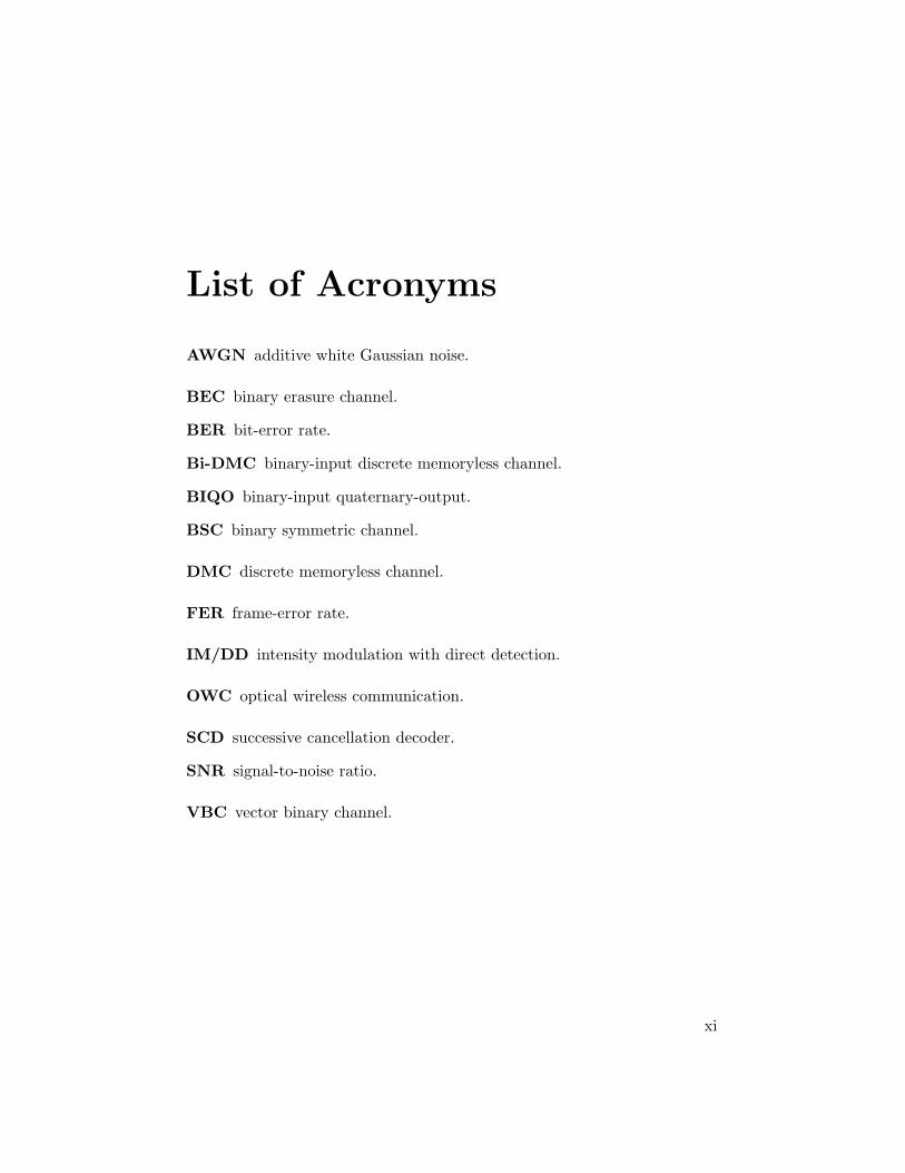
AWGN additive white Gaussian noise.
BEC binary erasure channel.
BER bit-error rate.
Bi-DMC binary-input discrete memoryless channel.
BIQO binary-input quaternary-output.
BSC binary symmetric channel.
DMC discrete memoryless channel.
FER frame-error rate.
IM/DD intensity modulation with direct detection.
OWC optical wireless communication.
SCD successive cancellation decoder.
SNR signal-to-noise ratio.
VBC vector binary channel.
xi
Glossary of Notation
H(X) entropy of random variable X.H(Y |X) conditional entropy of random variable Y
given X.I(X;Y ) mutual information of two random variables
X and Y .N number of bit-pipes.PX the probability distribution of random vari-
able X.PY |X conditional probability distribution of Y
given X.Q(.) tail distribution function for standard Gaus-
sian.β the DC shift factor.ǫ probability of erasure.⌊.⌋ floor operation.γ scaling factor.EX expected value with respect to the distribu-
tion of the random variable X.P{E} the probability of event E.P{Y = y,X = x} joint probability mass function of Y given X.P{Y = y|X = x} conditional probability mass function of Y
given X.X ,Y input and output alphabets, respectively.IE indicator function for event E which is equal
to one if and only if E is true.h(.) binary entropy function.ξ erasure symbol.k message length.min(a, b) the minimum of a and b.n codeword length.|.| cardinality of a set.
xii

Acknowledgements
The completion and success of this thesis could not have been realizedwithout the phenomenal supervision of Prof. Anas Chaaban. I am sincerelythankful to Prof. Anas for teaching me from the start how to be a diligentresearcher. I am deeply indebted to him for his constant follow-up andexpert guidance at every step of the way, for his patience, and for teachingme many things, especially Information Theory, which I am un-entropicallyvery fortunate to study.
My heartfelt appreciation goes to my parents for their unwavering beliefin me and my abilities, for motivating me whenever I was feeling very blue,and for encouraging me to run after the stars. My sincere thanks go to myfamily and friends for their love and support. I am especially grateful toHibatallah Alwazani, my best friend, for her bountiful, limitless support,and for listening to me talk about my research at any time of the day. Imust acknowledge Kelowna ducks for being a wonderful company wheneverneeded.
xiii

Dedication
To my parents, for infinitely many things.
xiv
Chapter 1
Introduction
1.1 Background and Motivation
Communication systems are becoming more important for our daily lives,especially with the advent of technology and the ever-increasing numberof users which encourages the design of systems to satisfy the demandsfor faster data rates. According to a recent report by Cisco [Cis20], therewill be 5.3 billion internet users by 2023, which is about 66% of globalpopulation. This increased demand is making the radio frequency spectrumscarce as well as expensive, since most sub-bands are exclusively licensed[KU14]. This motivates the search for other feasible alternatives. One suchalternative is to utilize other bands of the electromagnetic spectrum for datatransmission, particularly the infrared, visible and ultraviolet spectra, thisis known as optical wireless communication (OWC) [CRA20, HHI20].
OWC uses unlicensed bands of the spectrum and operates at frequencieswhich are higher than radio frequencies, enabling it to have faster data rates[KU14]. Furthermore, the joint infrared and visible light spectra is 2600times larger than the radio frequency spectrum [HHI20]. There are manyforms of OWC, one way is for point-to-point indoor communications, whichis a common form of free-space optical (FSO) communications, by usingLASERS or LEDs as both a source of light and information. The advantageof FSO over fibre optical links is the reduced infrastructure costs [CRA20].In addition, Li-Fi (light-fidelity) indicates a complete bi-directional multi-user communication networking ability, in other words an access point. Li-Fiaccess points are anticipated to act as a supplement to the exiting hetero-geneous wireless network, which would benefit from their fast data rates[HSMF20].
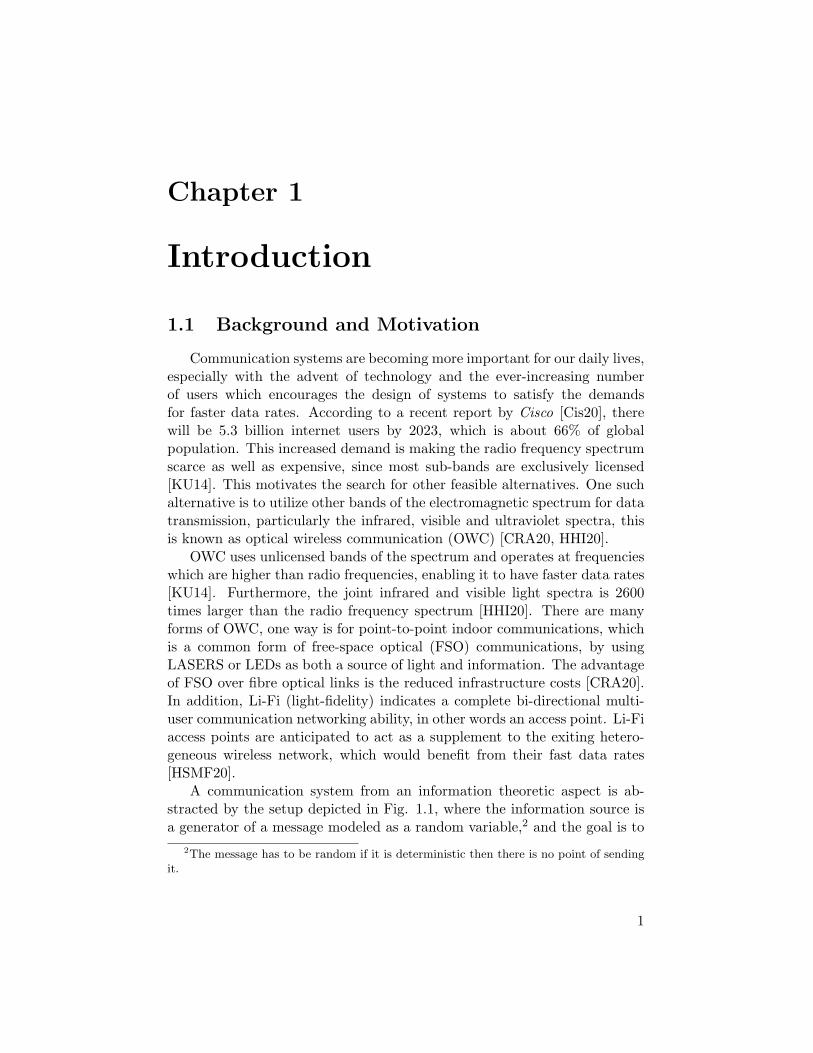
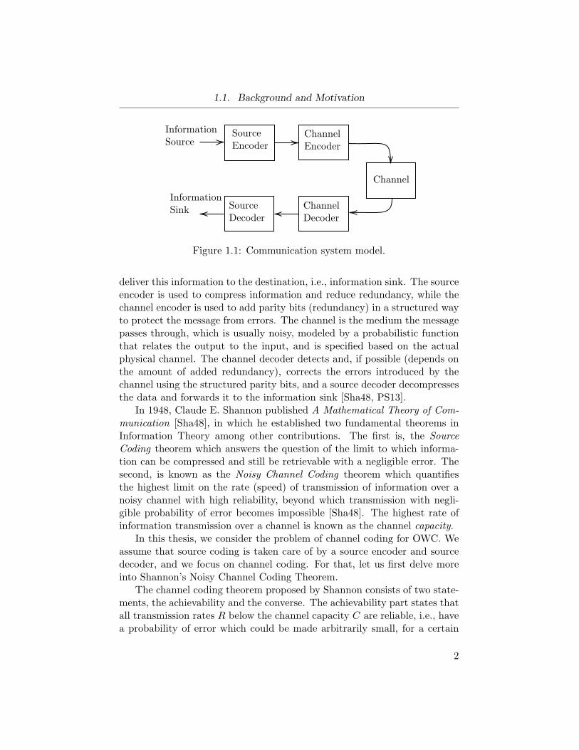
A communication system from an information theoretic aspect is ab-stracted by the setup depicted in Fig. 1.1, where the information source isa generator of a message modeled as a random variable,2 and the goal is to
2The message has to be random if it is deterministic then there is no point of sendingit.
1
1.1. Background and Motivation
SourceEncoder
ChannelEncoder
Channel
ChannelDecoder
SourceDecoder
InformationSource
InformationSink
Figure 1.1: Communication system model.
deliver this information to the destination, i.e., information sink. The sourceencoder is used to compress information and reduce redundancy, while thechannel encoder is used to add parity bits (redundancy) in a structured wayto protect the message from errors. The channel is the medium the messagepasses through, which is usually noisy, modeled by a probabilistic functionthat relates the output to the input, and is specified based on the actualphysical channel. The channel decoder detects and, if possible (depends onthe amount of added redundancy), corrects the errors introduced by thechannel using the structured parity bits, and a source decoder decompressesthe data and forwards it to the information sink [Sha48, PS13].
In 1948, Claude E. Shannon published A Mathematical Theory of Com-munication [Sha48], in which he established two fundamental theorems inInformation Theory among other contributions. The first is, the SourceCoding theorem which answers the question of the limit to which informa-tion can be compressed and still be retrievable with a negligible error. Thesecond, is known as the Noisy Channel Coding theorem which quantifiesthe highest limit on the rate (speed) of transmission of information over anoisy channel with high reliability, beyond which transmission with negli-gible probability of error becomes impossible [Sha48]. The highest rate ofinformation transmission over a channel is known as the channel capacity.
In this thesis, we consider the problem of channel coding for OWC. Weassume that source coding is taken care of by a source encoder and sourcedecoder, and we focus on channel coding. For that, let us first delve moreinto Shannon’s Noisy Channel Coding Theorem.
The channel coding theorem proposed by Shannon consists of two state-ments, the achievability and the converse. The achievability part states thatall transmission rates R below the channel capacity C are reliable, i.e., havea probability of error which could be made arbitrarily small, for a certain
2
1.1. Background and Motivation
channel characterized by PY |X , whereX and Y denote the channel input andoutput respectively. This is proved with a random coding argument whichis not necessarily practically feasible. In other words, Shannon proved theexistence of channel codes which achieve the channel capacity C, but didnot state the explicit construction of those codes. The converse part statesthat whenever R > C, the probability of error is bounded away from zeroregardless of the encoder and decoder design. This is to say, for reliablecommunication, the transmission rate R should be tuned to be less thancapacity [GK11, Mac02]. Now the question arises: How to design encodersand decoders with rates as close as possible to capacity while adhering tolow complexity constraints for practicality’s sake?
We consider the channel coding problem for an optical communicationchannel due to the increased interest in OWCs over the past decade. Thisinterest is fueled by several reasons. First of all, the ever-growing demandfor wireless data transfer, coupled with the scarcity of the radio frequencyspectrum forces us to consider the optical spectrum as an alternative or sup-plement for radio-frequency wireless communication. Additionally, OWCprovides economical gains and fast data rates [HHI20, CH20, ABK+12]. InOWC, the transmitter is a light source, which could be a LASER diodeor an LED, and the receiver is a photodetector. LEDs and LASERs areboth activated by the flow of positive current, which has an almost linearrelationship to the emitted light intensity. In particular, assume that theflow of current in the diode is denoted by I, and the resulting emitted lightintensity to be denoted by X, then X = ηI, where η is the electrical-to-optical conversion efficiency of the light source [CH20], for the rest of thisthesis we assume η = 1, without loss of generality. The data transmission isdone by modulating the light source’s emitted light intensity (by tuning theinput current), meaning that the input to the channel is proportional to thelight intensity. Therefore, the channel input is non-negative (as the currentis non-negative). Furthermore, the emitted light intensity has a maximumpeak power, which is a result of physical limits and safety measures. Addi-tionally, for eye-safety measures, an average power constraint is imposed onthe optical intensity. In the receiving end, the photodetector receives theincident light which could be corrupted by environmental factors such as fad-ing and ambient light. This channel is known as IM/DD channel, which isan additive white Gaussian noise (AWGN) channel with average, peak andnonnegative power constraints on the input signal [HWNC98, KU14].
In the next section, we discuss similar contributions in this field, forchannel coding for OWC. Additionally, we extend the discussion on contri-butions which motivate this research.
3
1.2. Literature Review
1.2 Literature Review
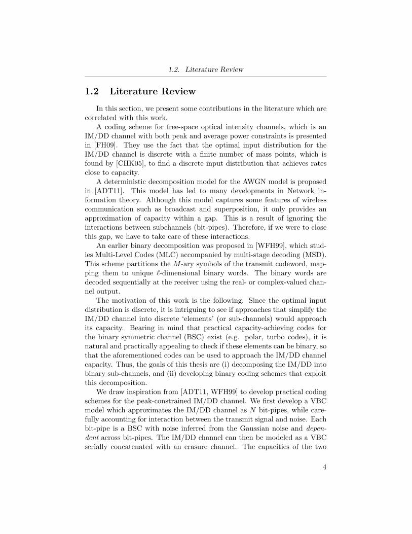
In this section, we present some contributions in the literature which arecorrelated with this work.
A coding scheme for free-space optical intensity channels, which is anIM/DD channel with both peak and average power constraints is presentedin [FH09]. They use the fact that the optimal input distribution for theIM/DD channel is discrete with a finite number of mass points, which isfound by [CHK05], to find a discrete input distribution that achieves ratesclose to capacity.
A deterministic decomposition model for the AWGN model is proposedin [ADT11]. This model has led to many developments in Network in-formation theory. Although this model captures some features of wirelesscommunication such as broadcast and superposition, it only provides anapproximation of capacity within a gap. This is a result of ignoring theinteractions between subchannels (bit-pipes). Therefore, if we were to closethis gap, we have to take care of these interactions.
An earlier binary decomposition was proposed in [WFH99], which stud-ies Multi-Level Codes (MLC) accompanied by multi-stage decoding (MSD).This scheme partitions the M -ary symbols of the transmit codeword, map-ping them to unique ℓ-dimensional binary words. The binary words aredecoded sequentially at the receiver using the real- or complex-valued chan-nel output.
The motivation of this work is the following. Since the optimal inputdistribution is discrete, it is intriguing to see if approaches that simplify theIM/DD channel into discrete ‘elements’ (or sub-channels) would approachits capacity. Bearing in mind that practical capacity-achieving codes forthe binary symmetric channel (BSC) exist (e.g. polar, turbo codes), it isnatural and practically appealing to check if these elements can be binary, sothat the aforementioned codes can be used to approach the IM/DD channelcapacity. Thus, the goals of this thesis are (i) decomposing the IM/DD intobinary sub-channels, and (ii) developing binary coding schemes that exploitthis decomposition.
We draw inspiration from [ADT11, WFH99] to develop practical codingschemes for the peak-constrained IM/DD channel. We first develop a VBCmodel which approximates the IM/DD channel as N bit-pipes, while care-fully accounting for interaction between the transmit signal and noise. Eachbit-pipe is a BSC with noise inferred from the Gaussian noise and depen-dent across bit-pipes. The IM/DD channel can then be modeled as a VBCserially concatenated with an erasure channel. The capacities of the two
4
1.3. Problem Statement
channels differ due to quantization effects and erasures, but this differencecan be eliminated by appropriately choosing the parameters of the model.Thus, the generated (VBC) model is nearly capacity-preserving.
1.3 Problem Statement
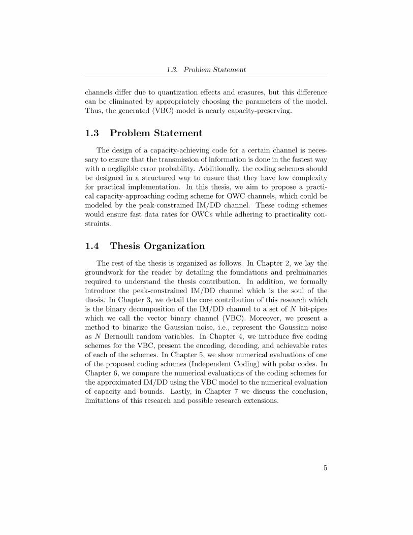
The design of a capacity-achieving code for a certain channel is neces-sary to ensure that the transmission of information is done in the fastest waywith a negligible error probability. Additionally, the coding schemes shouldbe designed in a structured way to ensure that they have low complexityfor practical implementation. In this thesis, we aim to propose a practi-cal capacity-approaching coding scheme for OWC channels, which could bemodeled by the peak-constrained IM/DD channel. These coding schemeswould ensure fast data rates for OWCs while adhering to practicality con-straints.
1.4 Thesis Organization
The rest of the thesis is organized as follows. In Chapter 2, we lay thegroundwork for the reader by detailing the foundations and preliminariesrequired to understand the thesis contribution. In addition, we formallyintroduce the peak-constrained IM/DD channel which is the soul of thethesis. In Chapter 3, we detail the core contribution of this research whichis the binary decomposition of the IM/DD channel to a set of N bit-pipeswhich we call the vector binary channel (VBC). Moreover, we present amethod to binarize the Gaussian noise, i.e., represent the Gaussian noiseas N Bernoulli random variables. In Chapter 4, we introduce five codingschemes for the VBC, present the encoding, decoding, and achievable ratesof each of the schemes. In Chapter 5, we show numerical evaluations of oneof the proposed coding schemes (Independent Coding) with polar codes. InChapter 6, we compare the numerical evaluations of the coding schemes forthe approximated IM/DD using the VBC model to the numerical evaluationof capacity and bounds. Lastly, in Chapter 7 we discuss the conclusion,limitations of this research and possible research extensions.
5
Chapter 2
Foundations andPreliminaries
In the previous chapter, we discussed the motivation which drives thework of this thesis, as well as some useful contributions. We also describedthe information theoretic abstraction of a communication system. In thischapter, we discuss some of the necessary background needed for the rest ofthis thesis, we start by detailing the channel coding problem then we providethe channel capacity.
2.1 Channel Coding and Capacity
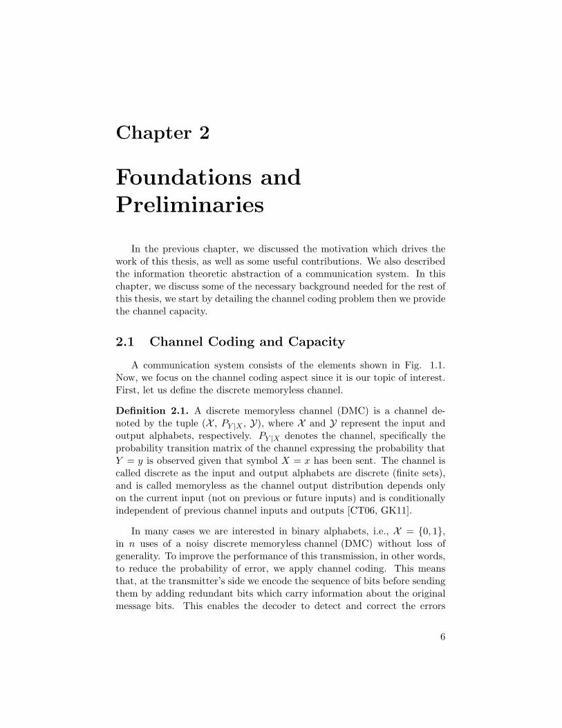
A communication system consists of the elements shown in Fig. 1.1.Now, we focus on the channel coding aspect since it is our topic of interest.First, let us define the discrete memoryless channel.
Definition 2.1. A discrete memoryless channel (DMC) is a channel de-noted by the tuple (X , PY |X , Y), where X and Y represent the input andoutput alphabets, respectively. PY |X denotes the channel, specifically theprobability transition matrix of the channel expressing the probability thatY = y is observed given that symbol X = x has been sent. The channel iscalled discrete as the input and output alphabets are discrete (finite sets),and is called memoryless as the channel output distribution depends onlyon the current input (not on previous or future inputs) and is conditionallyindependent of previous channel inputs and outputs [CT06, GK11].
In many cases we are interested in binary alphabets, i.e., X = {0, 1},in n uses of a noisy discrete memoryless channel (DMC) without loss ofgenerality. To improve the performance of this transmission, in other words,to reduce the probability of error, we apply channel coding. This meansthat, at the transmitter’s side we encode the sequence of bits before sendingthem by adding redundant bits which carry information about the originalmessage bits. This enables the decoder to detect and correct the errors
6
2.1. Channel Coding and Capacity
EncoderChannel
Decoder
Xm
PY |X
U1, . . . , Uk X1, . . . , Xn U1, . . . , UkY1, . . . , Yn
Y m
Figure 2.1: Channel coding block diagram.
on the message bits using the extra parity bits. We provide the formaldiscussion next [GK11, CT06].
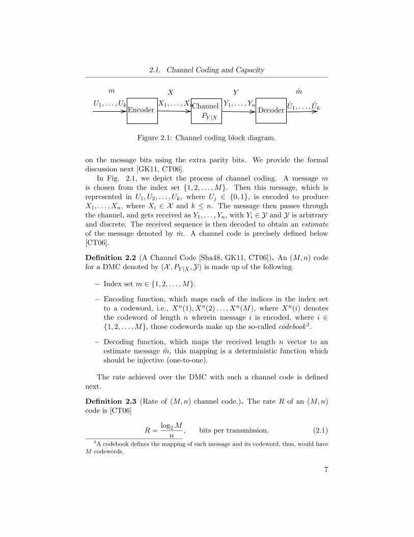
In Fig. 2.1, we depict the process of channel coding. A message mis chosen from the index set {1, 2, . . . ,M}. Then this message, which isrepresented in U1, U2, . . . , Uk, where Uj ∈ {0, 1}, is encoded to produceX1, . . . , Xn, where Xi ∈ X and k ≤ n. The message then passes throughthe channel, and gets received as Y1, . . . , Yn, with Yi ∈ Y and Y is arbitraryand discrete. The received sequence is then decoded to obtain an estimateof the message denoted by m. A channel code is precisely defined below[CT06].
Definition 2.2 (A Channel Code [Sha48, GK11, CT06]). An (M,n) codefor a DMC denoted by (X , PY |X ,Y) is made up of the following.
− Index set m ∈ {1, 2, . . . ,M}.
− Encoding function, which maps each of the indices in the index setto a codeword, i.e., Xn(1), Xn(2) . . . , Xn(M), where Xn(i) denotesthe codeword of length n wherein message i is encoded, where i ∈{1, 2, . . . ,M}, those codewords make up the so-called codebook3.
− Decoding function, which maps the received length n vector to anestimate message m, this mapping is a deterministic function whichshould be injective (one-to-one).
The rate achieved over the DMC with such a channel code is definednext.
Definition 2.3 (Rate of (M,n) channel code.). The rate R of an (M,n)code is [CT06]
R =log2M
n, bits per transmission. (2.1)
3A codebook defines the mapping of each message and its codeword, thus, would haveM codewords.
7
2.1. Channel Coding and Capacity
A rate R is said to be achievable if there exits a (M =⌈
2nR⌉
, n) codewith a vanishing probability of error as n → ∞, where the probability oferror is P{m 6= m} [CT06].
Next, we provide the highest limit on achievable rates which is knownas the capacity of a certain channel, after we define the following necessaryterms: entropy, conditional entropy and mutual information [Sha48, CT06].
Definition 2.4 (Entropy [Sha48, GK11]). The entropy of a random variableX is its minimum descriptive complexity. In other words, entropy is ameasure of the average uncertainty in the random variable. It measuresthe number of bits required to represent the random variable on average 4.Entropy of a discrete random variable X is usually denoted by H(X) andis defined as
H(X) = −∑
x∈XP{X = x} log2 P{X = x}, (2.2)
where P{X = x} is the probability mass function ofX and X is its alphabet.
Next, we define the conditional entropy.
Definition 2.5 (Conditional Entropy [Sha48, CT06]). Let X and Y be tworandom variables. The conditional entropy of Y givenX, i.e., H(Y |X), mea-sures the remaining uncertainty about the outcome of Y given the knowledgeof X. It is defined as
H(Y |X) =∑
x∈X ,y∈YP{X = x, Y = y} log2 P{Y = y|X = x}, (2.3)
where P{X = x, Y = y} is the joint probability mass function of X and Y ,P{Y = y|X = x} represents the conditional probability of Y given X, andX and Y represent X and Y alphabets, respectively.
Now, we are ready to define the mutual information.
Definition 2.6 (Mutual Information [Sha48, CT06]). The mutual informa-tion of two random variables X and Y is denoted by I(X;Y ), and measuresthe amount of information of X conveyed by the observation of Y . In otherwords, it defines the reduction in uncertainty of X when Y is observed, givenby
I(X;Y ) = H(Y )−H(Y |X). (2.4)
The mutual information is a symmetric function, i.e., I(X,Y ) = I(Y ;X).Now we are ready to state the channel coding theorem.
4This is in case the logarithm is of base 2.
8
2.1. Channel Coding and Capacity
Theorem 2.7 (Channel Coding Theorem [Sha48]). The capacity C of adiscrete memoryless channel PY |X is
C = maxPX
I(X;Y ), (2.5)
where X is the input to the channel, Y is its output, and PX denotes theinput distribution.
The channel coding theorem characterizes the maximum achievable rateof transmission of information over a noisy channel with a negligible prob-ability of error. Next, we present two channels that we need in the decom-position model in the following chapters.
2.1.1 Binary Symmetric Channel
The BSC is one of the simplest noisy channel models with a binaryinput and output. This channel is interesting to study as it could modeltransmissions of bits over a noisy channel, which could cause errors that flipthe message bits randomly. We formally define this channel next.
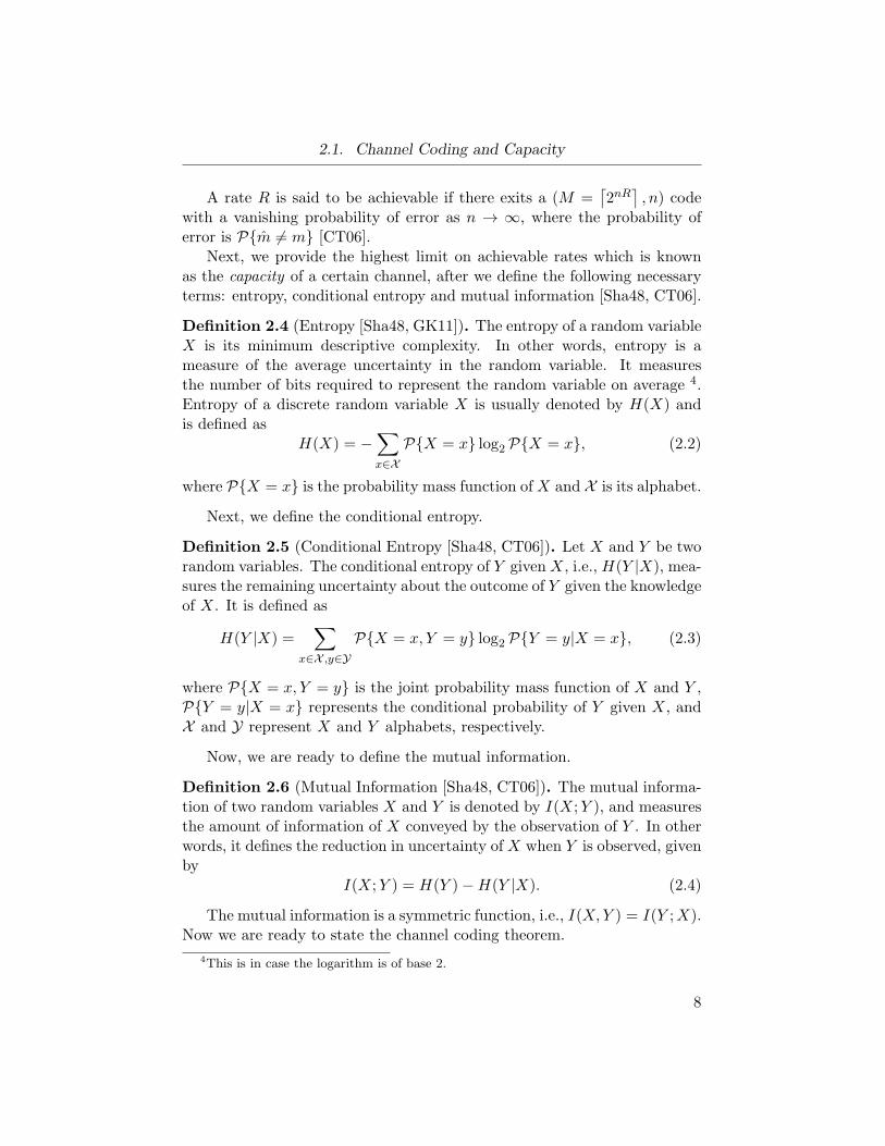
Definition 2.8 (Binary Symmetric Channel). The binary symmetric chan-nel has the input-output relation Y = X with probability 1−α and Y 6= Xwith probability α, where X is the input Bernoulli random variable, Y is theoutput Bernoulli random variable. The sets X and Y represents the inputand output alphabets, respectively, where X = Y = {0, 1}. The crossoverprobability is represented by α, where α = P{Y 6= X}. We denote thischannel as BSC(α).
0
1
0
1
X Y1− α
1− α
α
α
Figure 2.2: Binary symmetric channel.
The BSC is shown in Fig. 2.2. If a bit is sent, the flipped version is re-ceived with probability α, and the unchanged bit is received with probability1 − α. Note that, the output of a BSC could be modeled by Y = X + Z,
9
2.1. Channel Coding and Capacity
X Y0
1
0
1
ξǫ
ǫ
1− ǫ
1− ǫ
Figure 2.3: Binary erasure channel.
where Z is a Bernoulli random variable with probability α, and the additionis an XOR operation (modulo 2).
In the following chapters, we propose a decomposition model of theIM/DD channel into N -bit-pipes. We also, introduce some coding schemeswhich treat each bit-pipe as a BSC, thus it is important to characterizethe capacity of such a channel. The capacity of a BSC(α) is found usingTheorem 2.7 as
CBSC = maxPX
I(X,Y ), (2.6)
= maxPX
H(Y )−H(Y |X), (2.7)
≤ 1− h(α), (2.8)
where h(α) is the binary entropy function and is equal to h(α) = −α log2 α−(1 − α) log2(1 − α), and PX is the input distribution which is a Bernoullidistribution. The capacity is attained by using a Bern(0.5) distribution forthe input as it maximizes the mutual information by maximizing the outputentropy, i.e., H(Y ).
In the next section, we discuss another important channel called binaryerasure channel.
2.1.2 Binary Erasure Channel
The binary erasure channel (BEC) is also another popular channel modelthat we utilize in the following chapters, since we consider the possibilityof symbol erasure. For example, in cases where the receiver gets symbolswith soft information indicating low reliability, the receiver can then declarethem as erasures. This helps as the receiver does not have to locate errors,but only correct the erasures. The BEC is formally defined below.
10

2.1. Channel Coding and Capacity
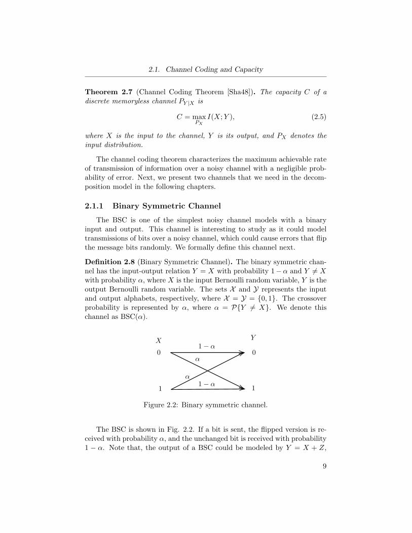
Definition 2.9 (Binary Erasure Channel). The binary erasure channel hasthe input-output relation Y = X with probability 1 − ǫ and Y = ξ withprobability ǫ, with ξ being the erasure symbol, X is the input Bernoullirandom variable, Y is the output random variable, the input alphabet isX = {0, 1}, the output alphabet is Y = {0, 1, ξ}, and ǫ represents theerasure probability, i.e., ǫ = P{Y = ξ}. We denote this channel by BEC(ǫ).
The capacity of a binary erasure channel is obtained using Theorem 2.7as [CT06]
CBEC = maxPX
I(X,Y ), (2.9)
= maxPX
H(Y )−H(Y |X), (2.10)
= maxPX
H(Y )− h(ǫ), (2.11)
where H(Y |X) = h(ǫ) because Y is uncertain if and only if it is erased. Tofind H(Y ), suppose we have a random variable E = 1 if Y = ξ, and E = 0otherwise. Then using the chain rule of joint entropy,
H(Y ) = H(Y,E) = H(E) +H(Y |E). (2.12)
The first equality above holds asH(Y ) = H(Y,E)−H(E|Y ), andH(E|Y ) =0 because E is a function of Y , if Y is known then there is no uncertaintyin determining E. Now, we need to find H(E) and H(Y |E). Supposethat p = P{X = 0}, then using the definition of entropy (Definition 2.4),H(E) = P{E = 1} log2 P{E = 1} + P{E = 0} log2 P{E = 0}, whereP{E = 1} = pǫ+ (1− p)ǫ = ǫ, and P{E = 0} = 1− ǫ. Thus, H(E) = h(ǫ).To find H(Y |E), we use Definition 2.5 and obtain H(Y |E) = (1 − ǫ)h(p).Therefore, the capacity of a BEC could be expressed as
CBEC = maxp
h(ǫ) + (1− ǫ)h(p)− h(ǫ) (2.13)
= maxp
(1− ǫ)h(p) (2.14)
= (1− ǫ), (2.15)
where the maximum is attained with a Bern(0.5) input distribution, i.e.,p = 0.5.
In the following section, we state useful lemmas, we also discuss thecapacity of a BEC from another insightful perspective.
11
2.2. Useful Theorems and Lemmas
2.2 Useful Theorems and Lemmas
In this section, we present some important lemmas which are needed forlater chapters.
2.2.1 Data Processing Inequality
The data processing inequality shows that no matter how you processinformation, you cannot increase information. In other words, processingcan only destroy information [GK11, Mac02]. The statement of the theoremis given next, and will be used in Chapter 3 to prove the achievable rate ofthe binary decomposition model. The data processing inequality makes useof Markov chains, which we define next.
Definition 2.10 (Markov Chain). A Markov chain represents a stochasticmodel which describes a sequence of possible states, in which the probabilityof a certain state only depends on the previous state.
Now, we are ready to state the inequality.
Theorem 2.11 (Data Processing Inequality [CT06]). If random variablesX, Y , and Z form a Markov chain, X → Y → Z
I(X;Z) ≤ I(X;Y ). (2.16)
We say that, X → Y → Z, forms a Markov chain if and only if Z isconditionally independent of X given Y .
2.2.2 Information Lost in Erasures
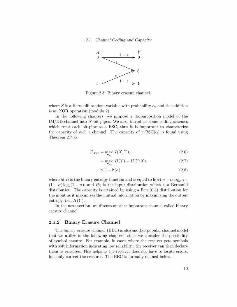
The capacity of the overall channel resulting from the serial concate-nation of a noisy channel with an erasure channel is quantified in [VW08]and is suitable in different scenarios. Consider a transmission of bits takingplace over a channel which outputs signal amplitudes in the interval [0, 1].Suppose that a detector is used to decide that the output bit is 0 if the am-plitude is in [0, 0.45], 1 if the amplitude is in [0.55, 1], and declares an erasureotherwise due to the low quality and high uncertainty of the received signal.This scenario can be modeled as a channel which flips bits with probabilityp, but replaces bits by an erasure with probability ǫ. This model can be alsorepresented as a concatenation of a BSC(p) and a BEC(ǫ) (cf. Fig. 2.4). Weshall see that a similar concatenation appears in the channel decompositiondiscussed in Chapter 3.
12
2.2. Useful Theorems and Lemmas
DMCErasureChannel
X1 Y1 Y2
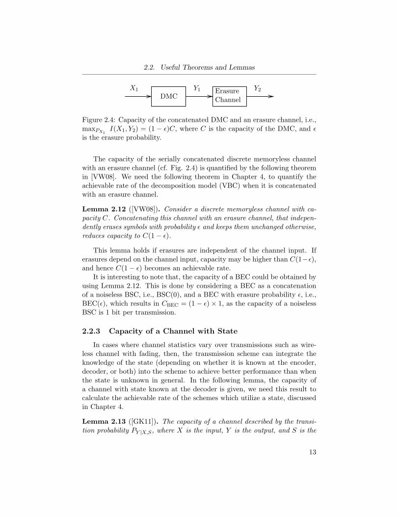
Figure 2.4: Capacity of the concatenated DMC and an erasure channel, i.e.,maxPX1
I(X1, Y2) = (1 − ǫ)C, where C is the capacity of the DMC, and ǫis the erasure probability.
The capacity of the serially concatenated discrete memoryless channelwith an erasure channel (cf. Fig. 2.4) is quantified by the following theoremin [VW08]. We need the following theorem in Chapter 4, to quantify theachievable rate of the decomposition model (VBC) when it is concatenatedwith an erasure channel.
Lemma 2.12 ([VW08]). Consider a discrete memoryless channel with ca-pacity C. Concatenating this channel with an erasure channel, that indepen-dently erases symbols with probability ǫ and keeps them unchanged otherwise,reduces capacity to C(1− ǫ).
This lemma holds if erasures are independent of the channel input. Iferasures depend on the channel input, capacity may be higher than C(1−ǫ),and hence C(1− ǫ) becomes an achievable rate.
It is interesting to note that, the capacity of a BEC could be obtained byusing Lemma 2.12. This is done by considering a BEC as a concatenationof a noiseless BSC, i.e., BSC(0), and a BEC with erasure probability ǫ, i.e.,BEC(ǫ), which results in CBEC = (1− ǫ)× 1, as the capacity of a noiselessBSC is 1 bit per transmission.
2.2.3 Capacity of a Channel with State
In cases where channel statistics vary over transmissions such as wire-less channel with fading, then, the transmission scheme can integrate theknowledge of the state (depending on whether it is known at the encoder,decoder, or both) into the scheme to achieve better performance than whenthe state is unknown in general. In the following lemma, the capacity ofa channel with state known at the decoder is given, we need this result tocalculate the achievable rate of the schemes which utilize a state, discussedin Chapter 4.
Lemma 2.13 ([GK11]). The capacity of a channel described by the transi-tion probability PY |X,S, where X is the input, Y is the output, and S is the
13
2.3. Polar Codes
state known only at the decoder, is given by
C = maxPX
I(X;Y |S). (2.17)
This capacity can be achieved by treating (Y, S) as the channel output.Next, we describe Polar Coding, which can be used over the BSC, BEC,
in addition of other types of channels to achieve capacity.
2.3 Polar Codes
Now, we focus on binary input channels and the goal is to design channelcoding schemes for such a channel, i.e., a scheme which would recover thesent bits from the received noisy version.
If we consider an uncoded transmission over a noisy channel, the per-formance of this scheme is fixed and we cannot improve it. For instance,consider a BSC(0.3), if we use this channel to transmit information bits, onebit per channel use, then the probability of error, i.e., P{Y 6= X} = 0.3,which is not practical. Integrating channel coding to this BSC(0.3) promisesto reduce this probability of error to approach zero with a transmission rateapproaching the capacity of this channel (cf. Sec. 2.1.1), with a long enoughcodeword. In other words, coding makes the transmission over a noisy chan-nel practical by adding redundant bits which helps us do the estimation in abetter way, thus reducing the probability of error. Now the coding problemis the design of codes with rates close to channel capacity, while having adefined structure.
There has been many efforts to achieve or approach the Shannon limit,for instance, using Turbo and low density parity check codes (LDPC). Thesecodes could achieve the capacity of binary channels. Yet, polar codes are thefirst codes which provably achieve the capacity of binary input memorylesschannels [Arı15, VVH15].
Polar codes are invented by Erdal Arikan in 2008 and are the first evercodes which are proved to achieve Shannon capacity. In this section we intro-duce polar codes from a practical prospective and we include the following:(i) polarization, (ii) code construction, (iii) encoding, and (iv) decoding. Westart by giving the general overview on polarization and what enables it andwe state the channel polarization theorem.
First, let us introduce the notation and the binary input discrete mem-oryless channel which we denote by (Bi-DMC).
Definition 2.14. (Bi-DMC) Let W : X → Y denote the channel which isa binary-input discrete memoryless channel (Bi-DMC), with X, Y denoting
14
2.3. Polar Codes
the input and output random variables. Binary-input means that the inputalphabet X = {0, 1}, and the output alphabet is Y is arbitrary, we consider itto be discrete5. The channel denotes the transition probabilities as PY=y|X=x
where x ∈ X and y ∈ Y. We also assume that the channel is a symmetricchannel6.
For symmetric Bi-DMC the capacity is achieved by a discrete uniforminput distribution, i.e., P{X = 1} = P{X = 0} = 0.5. Let CW denotethe capacity of this channel W , then CW = I(X;Y ) with X ∼ Bern(0.5).Additionally, the capacity is bounded by 0 ≤ CW ≤ 1 (assuming the usedlogarithms are to the base 2), this is because the input is binary (a bit) andthe maximum capacity is 1 bit per channel use, capacity is always positive,and capacity is zero for channels which are very noisy.
2.3.1 Polarization
The main idea underlying polar codes is the following. It is known thatthe coding problem is trivial for two types of channels (i) noiseless channel(perfect channel), (ii) very noisy channel (useless channel)7. Based on this,the idea is to start with an ordinary (noisy) channel W and instead of codingfor this noisy channel directly, we take n copies8 of W , and decompose itinto n new (polarized if n is large enough) channels, each could be either auseful or a useless channel, thus, the coding problem vanishes.
The method followed to realize polarization includes combining and split-ting. First, we take n independent copies of W and combine them to createa vector channel. This concludes the combination aspect, after that we de-compose the vector channel into n new channels which are denoted by Wt,for t = 1, . . . , n. Those new channels are polarized, i.e., either perfect oruseless. This is known as splitting. To summarize, instead of coding for
5In fact, it can be continuous, but for the sake of unified notations we assume that it isdiscrete. Additionally, in this thesis, we consider polar coding for bit-pipes with discreteoutput set so this assumption is valid.
6A symmetric channel is defined by a channel transition matrix with rows that arepermutations of each other and so are the columns [CT06], examples are BSC(p) andBEC(ǫ), cf. Sec. 2.1.1 and Sec. 2.1.2. A symmetry assumption allows us to directly usethe uniform distribution over the input set as it maximizes the mutual information.
7For a noiseless channel there is no need to do channel coding as the received symbolswould be received error-free. For a very noisy channel, the received symbols becomeindependent of the sent symbols, and no matter how long you construct the codewordsthe message would not be retrievable.
8Note that taking n independent copies of a channel is equivalent to n independentuses of that channel.
15
2.3. Polar Codes
n copies of a noisy channel W , we represent it as n binary input polarizedchannels, and code over the polarized channel [Ari09].
Combining
More formally, the combing operation could be denoted by a one-to-onemapping through a matrix multiplication, which is to be defined.
Un = XnFn, (2.18)
where Xn denotes the vector input to the n copies of channel W , i.e., Xn =(X1, . . . , Xn). Fn : {0, 1}n → {0, 1}n is the mapping matrix of size n × n,leading to the vector Un = (U1, . . . , Un). Now, we define the vector channelWn : Un → Yn, as a channel with vector input Un and vector outputYn = (Y1, . . . , Yn), where Yi represents the output of the ith copy of channelW .
It is necessary to note that the combining operation is lossless, in otherwords, is capacity preserving. This could be shown as
CWn = I(Un;Yn),
= I(Xn;Yn),
= nI(X;Y ) = nCW ,
(2.19)
where CWn indicates the capacity of the vector channel. The first equality(mutual information between Un and Yn is equal to the mutual informationbetween Xn and Yn), holds since the mapping between Un and Xn is one-to-one. The second holds as we start with n independent and identical copiesof W , meaning that I(Xt;Yt) are equal ∀t and the total capacity is n timesCW .
Splitting
Before stating the splitting operation we first define the chain rule ofmutual information
Definition 2.15. The chain rule of mutual information for vectors Xn andYn is [CT06]
I(Xn;Yn) =n∑
t=1
I(Xt;Yn|Xt−1), (2.20)
where Xt−1 = (X1, . . . , Xt−1).
16
2.3. Polar Codes
Using the chain rule on the combined synthesised vector channel withvector input Un and output Yn, the splitting operation could be formulatedas
CWn = I(Un;Yn)
=n∑
t=1
I(Ut;Yn|Ut−1).
(2.21)
Therefore, interpreting the result of (2.21), we have n subchannels each witha binary input Ut, vector output Yn, and side information Ut−1 given byUt−1 = (U1, . . . , Ut−1).
Based on this, we define the resulting subchannels Wt, for t = 1, . . . , nwhich are binary input channels and are polarized if n is large enough andthe mapping matrix Fn is a good polarizer. Each channel Wt is polarizedin the sense that its capacity I(Ut;Y
n|Ut − 1) is either close to one or closeto zero (this is explained in more detail in the polarization theorem). Wediscuss good polarizing matrices next.
Good Polarizing Mapping Matrix
Now we should discuss the mapping matrix which would ensure that thethe newly constructed channels (Wt for t = 1, . . . , n) are polarized9. For
that, we first define the following matrix F =
(
1 01 1
)
and we define the
mapping matrix Fn in (2.18) as
Fn = F⊗j = F⊗j−1F, (2.22)
where n = 2j , j ≥ 1, with the convention F⊗0 , (1), F⊗j is of size n × nand ⊗ denotes the Kronecker product and is defined as follows.
Definition 2.16 (Kronecker product). The Kronecker product is denotedby ⊗ and is defined for two matrices A and B as
A⊗B =
A11B . . . A1hB...
. . ....
Am1B . . . AmhB
, (2.23)
where Aij indicates the element in the ith row and jth column of matrix Aof size m× h.
9It is interesting to note that if matrix Fn was constructed randomly consisting of zerosand ones, then, Fn is a good polarizer with high probability. This approach is similar toShannon’s random coding argument. Yet, the disadvantage would be the high complexityand the lack of structure.
17
2.3. Polar Codes
W
W
...FN...
X1
Xn
Y1
Yn
U1
Un
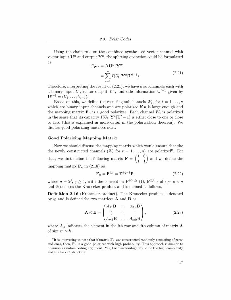
Wn
Figure 2.5: The synthesised vector channel Wn, with input vector Un gen-erated by a one-to-one mapping of the vector Xn, and output vector Yn,the channel W is the original noisy channel we wish to do coding for.
Figure 2.5 represents (2.18), the mapping of Xn and Un through themapping matrix Fn, resulting in the vector channel Wn. To make (2.22)clear, we give an example for n = 4, j = 2 the mapping matrix F4 would be
F⊗2 = F⊗1 ⊗ F =
1 0 0 01 1 0 01 0 1 01 1 1 0
, (2.24)
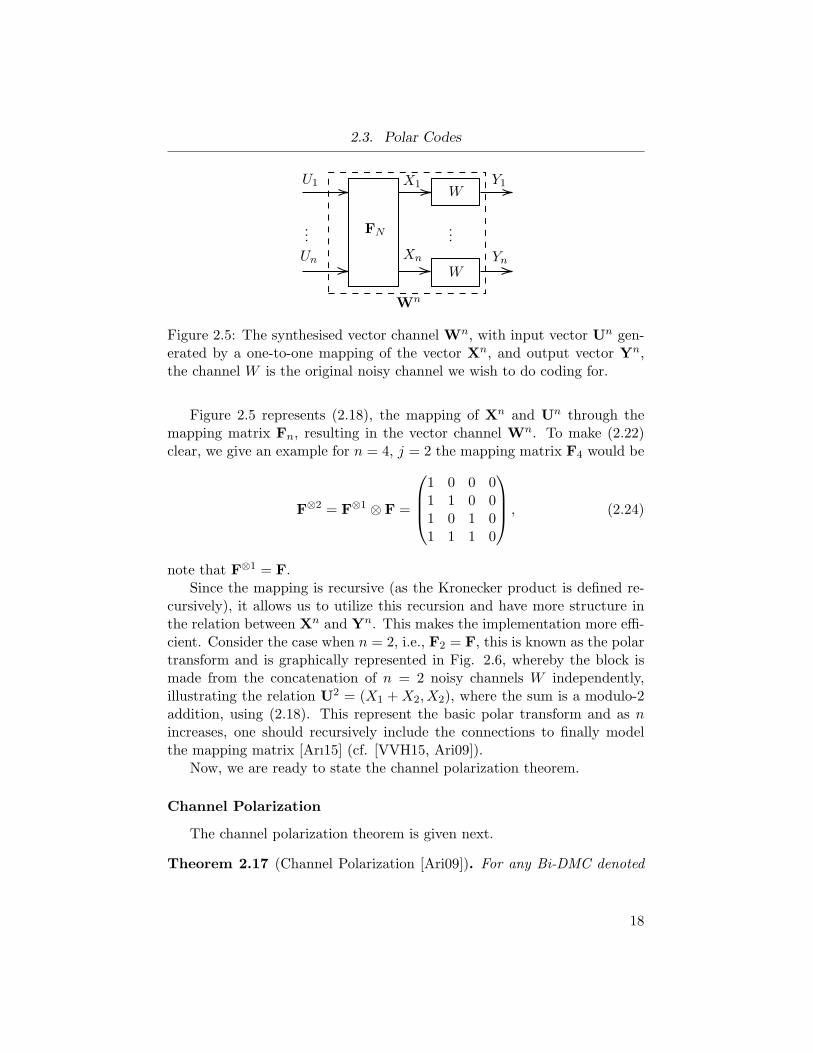
note that F⊗1 = F.Since the mapping is recursive (as the Kronecker product is defined re-
cursively), it allows us to utilize this recursion and have more structure inthe relation between Xn and Yn. This makes the implementation more effi-cient. Consider the case when n = 2, i.e., F2 = F, this is known as the polartransform and is graphically represented in Fig. 2.6, whereby the block ismade from the concatenation of n = 2 noisy channels W independently,illustrating the relation U2 = (X1 +X2, X2), where the sum is a modulo-2addition, using (2.18). This represent the basic polar transform and as nincreases, one should recursively include the connections to finally modelthe mapping matrix [Arı15] (cf. [VVH15, Ari09]).
Now, we are ready to state the channel polarization theorem.
Channel Polarization
The channel polarization theorem is given next.
Theorem 2.17 (Channel Polarization [Ari09]). For any Bi-DMC denoted
18
2.3. Polar Codes
W
W
U1
U2
X2
X1
Y1
Y2
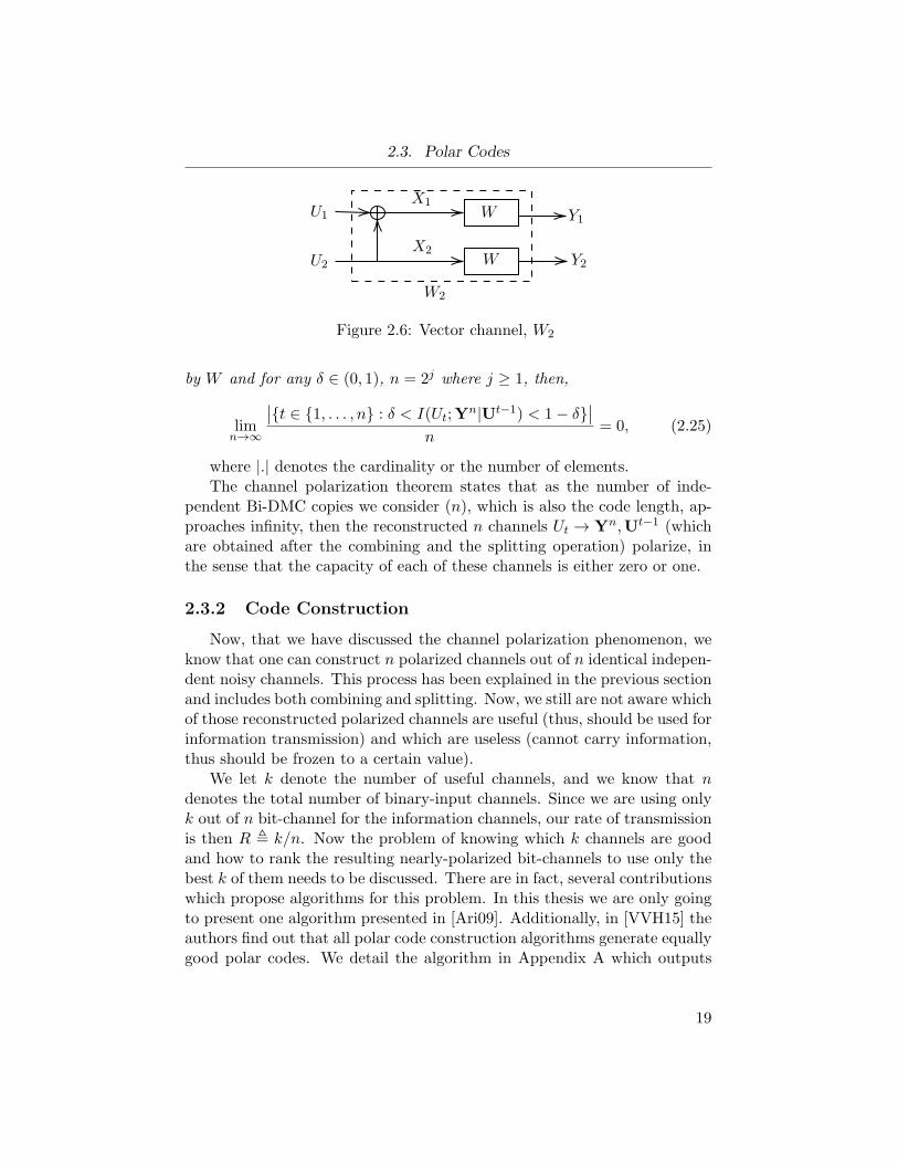
W2
Figure 2.6: Vector channel, W2
by W and for any δ ∈ (0, 1), n = 2j where j ≥ 1, then,
limn→∞
∣
∣{t ∈ {1, . . . , n} : δ < I(Ut;Yn|Ut−1) < 1− δ}
∣
∣
n= 0, (2.25)
where |.| denotes the cardinality or the number of elements.The channel polarization theorem states that as the number of inde-
pendent Bi-DMC copies we consider (n), which is also the code length, ap-proaches infinity, then the reconstructed n channels Ut → Yn,Ut−1 (whichare obtained after the combining and the splitting operation) polarize, inthe sense that the capacity of each of these channels is either zero or one.
2.3.2 Code Construction
Now, that we have discussed the channel polarization phenomenon, weknow that one can construct n polarized channels out of n identical indepen-dent noisy channels. This process has been explained in the previous sectionand includes both combining and splitting. Now, we still are not aware whichof those reconstructed polarized channels are useful (thus, should be used forinformation transmission) and which are useless (cannot carry information,thus should be frozen to a certain value).
We let k denote the number of useful channels, and we know that ndenotes the total number of binary-input channels. Since we are using onlyk out of n bit-channel for the information channels, our rate of transmissionis then R , k/n. Now the problem of knowing which k channels are goodand how to rank the resulting nearly-polarized bit-channels to use only thebest k of them needs to be discussed. There are in fact, several contributionswhich propose algorithms for this problem. In this thesis we are only goingto present one algorithm presented in [Ari09]. Additionally, in [VVH15] theauthors find out that all polar code construction algorithms generate equallygood polar codes. We detail the algorithm in Appendix A which outputs
19
2.3. Polar Codes
the information set I that specifies the indices of the k best channels withcapacities approaching one (for large enough n).
2.3.3 Encoding
Encoding for polar codes includes the following. Now that we have nbinary-input channels which are polarized (if n is large enough), it is intuitiveto use the channels with capacities approaching one for data transmissionand disregard the remaining channels with a negligible channel capacity.The encoding process is formally described below.
Given n = 2j , the code length, with j ≥ 1, and k the length of theinformation word. Then the binary word Un = (U1, . . . , Un) contains kinformation bits and n − k frozen bits. The indices of the information bitsand the frozen bit depends on the outcome of the code construction step.So, we place the information bits based on10 I. Hence, the codeword Xn
has a code rate R = k/n and can be obtained as
Xn = UnFn, (2.26)
where Fn, as defined in the polarization section, is the generator matrix ofsize n× n.
It is important to note that, (2.18) is structured in an opposite way of(2.26), as earlier the goal was to find a well-structured polarizing matrix Fn.However, in the encoding stage we assume that Fn is already designed, andwith the code construction step, we know which channels should be used,i.e., in which indices of Un the information bits should be located (and therest should be frozen).
In the next, section we discuss the decoding for polar codes.
2.3.4 Decoding
Recall that from the code construction step, we have the set I whichincludes the k information bits’ indices, which are considered in the encod-ing step where the vector Un = (U1, . . . , Un) is constructed to include kinformation bits in their respective indices, and n − k frozen bits (a frozenbit is known to both the encoder and decoder and is usually set to 0).
Consider a successive cancellation decoder (SCD) for polar code of lengthn, which is a power of two, i.e., n = 2j with j = 1, 2, . . .. The SCD ob-serves the channel output Yn and generates an estimate Un = (U1, . . . , Un)
10I is the set which contains the k out of n indices of good channels which should beused for information transmission, , cf. previous Sec. 2.3.2 and Appendix A
20
2.4. Peak-Constrained IM/DD Channel
of the input vector Un = (U1, . . . , Un). This is done as the name states,successively. Specifically, the decoder will decode one bit Ut by observ-ing Yn, and the previously estimated bit sequence given by the vectorUt−1 = (U1, . . . , Ut−1). Note that Un includes both information and frozenbits, and the decoder knows the locations of those frozen bits, so if for in-stance, Ut is a frozen bit then the decoder sets the estimate Ut to the agreedupon frozen value. There are several estimation metrics to be used, here,we discuss the log-likelihood ratio, which is given by
Lt = ln
(
PYn,Ut−1|Ut=0
PYn,Ut−1|Ut=1
)
, (2.27)
using (2.27), we can express the previous discussion into the following cases,for all t = 1, . . . , n:
Ut =
Ut (frozen bit) , if t ∈ Ic,
0, if t ∈ I and Lt ≥ 1,
1, if t ∈ I and Lt < 1,
(2.28)
note that, Ic is the set of indices for the frozen bits.Successive cancellation decoder is one of the most popular decoders, and
is usually used as a fundamental block in other decoders. It is necessaryto note that, the above discussion was general and we did not utilize therecursive nature of polar codes, which if used reduce the decoding complex-ity. The SCD then becomes a greedy binary tree search algorithm, with thegoal of finding the leaf node that maximizes the likelihood. We neglect thediscussion on the updated SCD, since it is outside the scope of this work,and we refer the reader to [Ari09, NCLZ14, Dos14, VHV16].
2.4 Peak-Constrained IM/DD Channel
In this section, we introduce the peak-constrained IM/DD channel, whichcould be used to model optical wireless communication. Consider a peak-constrained IM/DD channel, which is an AWGN with a nonnegative inputand a peak constraint. This channel is defined next.
Definition 2.18 (IM/DD Channel). The IM/DD channel with a peak con-straint A is characterized by the input-output relation
Y = X + Z, (2.29)
21
2.5. Chapter Summary
where X is the input random variable representing the transmitted intensityand is constrained by
0 ≤ X ≤ A, (2.30)
where A is the peak amplitude constraint, Y is the output random variable,and Z ∼ N (0, σ2) is independent and identically distributed (i.i.d.) Gaus-sian with zero mean and variance σ2 = 1, without loss of generality.11, andY is the output random variable.
In OWC, the noise is usually modelled as a Gaussian random variabledue to the several factors which can cause the distortion in the receivedsignal. These factors include thermal noise and ambient light. A Gaussiannoise model does reflect on those factors (following from the central limittheorem), especially the thermal noise factor which results from the electricalcomponents (e.g., LEDs and photodiodes).
Another possible model for OWC is the additive Poisson channel model.In which the input to the channel represents the number of emitted photons(light particles), the output of the channel is the received number of photons,and the noise is amount of noisy photons imposed on the transmitted signalwhich follows a Poisson distribution. It is necessary to recall that a Gaussiandistribution is the limit of a Poisson distribution (as the mean of the Poissondistribution goes large). Therefore, in some practical applications where theunderlying Poisson channel model has large mean, the IM/DD channel canbe modeled as an additive channel with Gaussian noise.
2.5 Chapter Summary
Now that we have discussed the necessary background and previewedthe channel model. Let us restate the problem statement and objective ofthe thesis.
We want to send a message m ∈ {1, ..., 2nR} with rate R over n uses ofthe channel. Encoding, decoding, achievable rate, and capacity are definedin the standard Shannon sense [CT06] (cf. Sec. 2.1). The capacity of anIM/DD channel is given by
CIM/DD = maxPX
I(X;Y ) (2.31)
11Note that the results of this thesis can be easily extended to the peak constrainedAWGN channel where |X| < A, and with some additional effort to the IM/DD channelwith an average constraint E[X] ≤ E
22
2.5. Chapter Summary
where PX is the input distribution. The closed form expression for the ca-pacity of the IM/DD channel is unknown, yet the capacity is computable byrunning a numerical optimization over the input distribution [CHK05]. Theobjective of this research is to design a simple binary coding scheme whichachieves or approaches capacity. To this end, we propose a decompositionof the IM/DD channel into binary channels as explained in the followingchapter.
23
Chapter 3
Binary Decomposition:Vector Binary Channel
In the previous chapters, we introduced the IM/DD channel as a modelfor point-to-point OWC, and the motivations for considering OWC includingits fast data rates and to satisfy the increased demands. In addition, we alsodescribed the channel coding problem and why it is needed.
Coding for the IM/DD is a hard task, since the optimal input distri-bution is not known. There is an insight, though, that the optimal inputdistribution is discrete with a finite number of mass points [CHK05] but find-ing those mass points remains a hard problem. Moreover, suppose that weare constrained to using a binary code because of its simplicity for a channelwith a continuous input (e.g. peak-constrained IM/DD channel), generallyspeaking, the achievable rates would be away from capacity (except at lowSNR in which the optimal input distribution is two mass points with equalprobabilities). In particular, for every channel use we can only recover amaximum of 1 bit, which is away from the capacity of the peak-constrainedIM/DD channel at moderate to high SNR.
This sparks the need for designing a coding scheme for the IM/DD chan-nel which is both practical and with a rate close to capacity. It is importantto recall that multi-level codes accompanied by multi-stage decoding servesthe same purpose of achieving rates close to capacity for the IM/DD chan-nel, but has a different structure with a considerable complexity [WFH99].Given that the optimal input distribution is discrete and polar codes whichachieve the capacity of binary-input channels (Bi-DMC) exist, we propose anearly lossless decomposition model that approximates the IM/DD channelinto an equivalent set of N bit-pipes. Each of these bit-pipes has a binaryinput, output and noise, and we can use a binary code (e.g., polar code)over each of the subchannels and achieve higher rates by summing over therates of the N bit-pipes.
The core contribution of this thesis is the decomposition model for thethe continuous IM/DD channel (2.31). Firstly, we develop a vector binarychannel (VBC) model which approximates (within quantization error) the
24

3.1. Mathematical Formulation
IM/DD channel as a collection of N bit-pipes. Each of the N bit-pipes hasa binary input, output, and noise. Hence, each bit-pipe could be modelledas a BSC with a certain crossover probability. Since the goal is to utilize theVBC to approximate the IM/DD channel, the crossover probabilities of thebit-pipes are inferred from the Gaussian noise. To fully characterize the VBCwe present a method to obtain the distribution of the crossover probabilities,more specifically, we develop a method to convert the continuous Gaussiannoise to N Bernoulli random variables. In the next section, we present themathematical formulation towards the VBC model.
3.1 Mathematical Formulation
Consider the nonnegative, peak-constrained IM/DD channel model (def-inition 2.18). The goal is to decompose this channel model into a setof bit-pipes. First, we use a nonnegative N -bit representation to repre-sent the channel input and output. This can only represent numbers in{0, 1, . . . , 2N − 1}. Since Y is unbounded, we first introduce a region ofwidth β > 0 around [0, A] and neglect all output value outside this regionby considering them as erasures. More specifically, we first apply a bias witha large enough value of β to obtain Y defined as
Y = X + Z + β. (3.1)
Then, we treat the events Y < 0 or Y > A+2β as erasure events, and definethe resulting signal as 12
Y ′ =
{
Y , for Y ∈ [0, A+ 2β],
erasure (ξ), otherwise.(3.2)
The erasure probability is given by ǫ = P{Y < 0} + P{Y > A + 2β}where P{E} denotes the probability of event E. Since this depends on theinput distribution PX which is yet to be specified, we bound ǫ by the worst-case scenario given by P{Y < 0|X = 0} + P{Y > A + 2β|X = A} leadingto
ǫ ≤ ǫ , 2Q(β), (3.3)
12A typical value is β ≥ 3. This is due to the fact that the added noise is standardGaussian and for β = 3 the probability that a certain noise instance lies in range [−β, β]is ≈ 0.99.
25
3.1. Mathematical Formulation
where Q(x) is the tail distribution function for a standard Gaussian dis-
tribution, i.e., Q(x) = 1√2π
∫∞x
exp(
−u2
2
)
du. It is necessary to note that
β is a positive scalar so the upper bound in (3.3) is always meaningful, as0 ≤ Q(β) ≤ 0.5 , ∀β ≥ 0.
3.1.1 Modelling Unerased Outputs
We now focus on the case where the output is not erased (throughout(3.4)-(3.16)), i.e., Y ′ 6= ξ (we consider the erasures later). Starting withY ′ 6= ξ in (3.2), we scale the received shifted signal by a positive scalingfactor γ, which grants the model one more degree of freedom, leading to
Y = γY ′. (3.4)
Then, we choose the number of bits N into which we quantize the channeloutput as N = ⌈log2 γ(A+ 2β)⌉. The received signal is then represented asa weighted sum of N bits as
Y ≈N−1∑
i=0
Y bi 2
i, (3.5)
with the difference being merely the quantization distortion, where Y bi de-
notes the binary representation of the output Y which is shifted by β andscaled by γ, i.e.,
Y bi =
⌊
Y
2i
⌋
mod 2, i = 0, 1, ...N − 1. (3.6)
Substituting (3.1) and (3.4) in (3.6) and using the relation ⌊a+ b⌋ = ⌊a⌋+⌊b⌋+ ⌊a− ⌊a⌋+ b+ ⌊b⌋⌋, we obtain
Y bi =
⌊
γ(X + Z + β)
2i
⌋
mod 2
=
(⌊
γX
2i
⌋
+
⌊
γ(Z + β)
2i
⌋
+ ⌊δi⌋
)
mod 2,
(3.7)
where δi is the sum of the fractional part of γX2i
and γ(Z+β)2i
, given by
δi =γX
2i−
⌊
γX
2i
⌋
+γ(Z + β)
2i−
⌊
γ(Z + β)
2i
⌋
, i = 0, 1 . . . , N − 1. (3.8)
Next, we distinguish between two cases: γ(Z+β) ≥ 0 and γ(Z+β) < 0.We start by considering the first case.
26

3.1. Mathematical Formulation
Nonnegative Shifted and Scaled Noise
Assume that γ(Z + β) ≥ 0 (the complementary case will be treatedafterwards). In this case, we can write
Y bi =
(⌊
X
2i
⌋
mod 2 +
⌊
Z
2i
⌋
mod 2 + ⌊δi⌋ mod 2
)
mod 2, (3.9)
which follows from the modular arithmetic relation (a + b) mod 2 = (amod 2 + b mod 2) mod 2, where X and Z are defined as13
X = γX and Z = γ (Z + β) . (3.10)
Next, the goal is to rewrite (3.9) in a form which shows its explicitdependence on the binarized versions of X and Z, therefore we define thefollowing
Xbi =
⌊
X
2i
⌋
mod 2, i = 0, 1, ...N − 1, (3.11)
Zbi =
⌊
Z
2i
⌋
mod 2, i = 0, 1, ...N − 1. (3.12)
Thus, X ≈∑N−1
i=0 2iXbi and Z ≈
∑N−1i=0 2iZb
i , within quantization error. Itremains to binarize δi, let W
bi be given by
W bi = ⌊δi⌋ mod 2, i = 0, 1, . . . , N − 1. (3.13)
Consequently, using (3.11), (3.12), and (3.13) in (3.9), we obtain
Y bi = (Xb
i + Zbi +W b
i ) mod 2, i = 0, . . . , N − 1. (3.14)
This representation connects the binary representation of Y , which is de-noted by Y b
i , with the binary representation of X and Z, which are denotedby Xb
i and Zbi , respectively, in addition to a bit W b
i which one can show tobe equal to
W bi = (Xb
i−1Zbi−1 +Xb
i−1Wbi−1 + Zb
i−1Wbi−1) mod 2, (3.15)
for i = 0, . . . , N − 1. Thus, W bi is the carryover bit resulting from the
‘lower significance’ bits Xbi−1, Z
bi−1, and W b
i−1. To fully characterize W b0 , we
can freeze all Xb−1, X
b−2, . . . to zero by ensuring X is an integer leading to
W b0 = 0.
13The assumption γ(Z + β) ≥ 0 is needed as in (3.9) we have the term ⌊ Z
2i⌋, this term
would binarize a negative number (Z), and (3.9) would not hold. Note that we providean example that shows this and how we remedy this later.
27
3.1. Mathematical Formulation
Negative Scaled Shifted Noise
In the other case where Y is not erased and γ(Z + β) < 0, the binaryrepresentation of Z = γ(Z + β) (i.e., Zb
i in (3.12)) results in a discrep-ancy between Y b
i in (3.7) and (3.14). This is a result of the relation (−|a|)mod 2 = (|a|) mod 2, where |.| denotes the absolute value. For example,let X = A = 2, γ = β = 1, and Z = −2, then X = 2 and Z = −1 us-ing (3.10). The binary representations of X and Z are (Xb
0, Xb1) = (0, 1)
and (Zb0, Z
b1) = (1, 0) using (3.11) and (3.12), respectively. The carry-
over bits are (W b0 ,W
b1 ) = (0, 0) from (3.15). Adding those bits results in
(Y b0 , Y
b1 ) = (1, 1) (cf. (3.14)), meaning that Y = 3 which is incorrect since
Y = Y = γ(X + Z + β) = 1. To remedy this, we integrate the two’scomplement of γ(Z+β) into the expression of Z in (3.10) and redefine it as
Z = 2N Iγ(Z+β)<0 + γ(Z + β), (3.16)
where IE is an indicator function for event E defined as
IE =
{
0, E is false,
1, otherwise.(3.17)
Referring to the example above, as γ(Z + β) < 0 it would be altered toZ = 3 using (3.16) and (Zb
0, Zb1) = (1, 1). Thus, (Y b
0 , Yb1 ) = (1, 0), meaning
that Y = 1, which is desired. Therefore, embedding the two’s complementrepresentation of γ(Z + β) and redefining Z if it is negative resolves theproblem.
Next, we reconsider the erasure and redefine the channel output.
3.1.2 Modelling Output with Erasures
Note that we ignored erasures in the previous analysis. To model theIM/DD channel, we re-integrate erasures, and define the output Y c
i for i =0, . . . , N − 1 as 14
Y ci =
{
Y bi , with probability 1− ǫ,
ξ, with probability ǫ.(3.18)
Recall the following definitions
Y bi = (Xb
i + Zbi +W b
i ) mod 2, i = 0, . . . , N − 1, (3.19)
14Note that we need to model erasures as the received Y could be erased if Y /∈ [0, A+2β].
28
3.2. The Vector Binary Channel (VBC)
with the input bit Xbi defined as
Xbi =
⌊
X
2i
⌋
mod 2, i = 0, 1, ...N − 1, (3.20)
where X = γX. The noise bit Zbi is defined as
Zbi =
⌊
Z
2i
⌋
mod 2, i = 0, 1, ...N − 1, (3.21)
where Z is
Z = 2N Iγ(Z+β) + γ(Z + β). (3.22)
The carryover bit W bi is given by
W bi = (Xb
i−1Zbi−1 +Xb
i−1Wbi−1 + Zb
i−1Wbi−1) mod 2, (3.23)
for i = 0, . . . , N − 1.Now we are ready to define the vector binary channel.
3.2 The Vector Binary Channel (VBC)
In this section, we formally define the vector binary channel (VBC) byusing the mathematical formulation introduced in the previous section. Inaddition, we show how the VBC is used to model the IM/DD by consideringthe output with erasures. We start by defining the VBC.
Definition 3.1 (Vector Binary Channel). The VBC is characterized by acollection of the input-output relation Y b
i = (Xbi +Zb
i +W bi ) mod 2, for each
of the N bit-pipes. For which, Y bi represents the ith bit-pipe’s output bit as
defined in (3.19), Xbi is the input bit whose distribution is to be optimized,
Zbi (as defined in (3.21)) is binary noise obtained from the N -bit of the
binary representation of the Gaussian noise (biased and scaled), and W bi is
a carryover bit as defined in (3.13) and (3.23).
The VBC is depicted in Fig. 3.1. To model the IM/DD channel, were-integrate erasures, and define the resulting channel next.
Definition 3.2 (VBC with erasures: VBCǫ). VBCǫ is a channel with inputXb
i and output Y ci as defined in (3.18) for i = 0, . . . , N − 1.
29

3.2. The Vector Binary Channel (VBC)
Xb0
W b0 + Zb
0
Y b0
Xb1
W b1 + Zb
1
Y b1
XbN−1
W bN−1 + Zb
N−1
Y bN−1
...
Figure 3.1: The Vector Binary Channel, which represents a collection Nbit-pipes, for which the input is Xb
i the noise is the modulo two addition ofZbi and W b
i . In general, Zbi is binary noise Bernoulli random variable and
W bi is the carryover bit from the lower bit-pipe.
The VBC with erasures channel defined above is used to approximate theIM/DD channel in (2.29), as a channel with a vector binary input, output(which could be erased), and noise. Now let X
b and Yc represent vectors
(Xb0, . . . , X
bN−1)
T and (Y c0 , . . . , Y
cN−1)
T , representing the binary vector input
and output, respectively. Also, let Xbi be Bernoulli pi, and let us denote
by Vp the set of active bit-pipes, i.e., those with 0 < pi < 1.15 Thus,Vp = {i ∈ {0, . . . , N − 1} : 0 < pi < 1}. Then we can state the followinglemma.
Lemma 3.3. The capacity of VBCǫ in Definition 3.2 satisfies
CVBCǫ = maxp0,p1,...,pN−1
I(Xb;Y c) ≤ CIM/DD, (3.24)
where pi satisfies∑
i∈Vp2i ≤ γA (peak power constraint).
Proof. This follows from the data processing inequality (cf. Theorem 2.11).
Note that, given the output is not erased then the shifted, scaled, andtruncated (due to erasures) Gaussian noise γ(Z + β) is dependent on the
15Note that if pi = 0 or pi = 1 then Xbi is deterministic (frozen bit) and cannot carry
information).
30
3.3. Characterizing the Binary Noise Distribution
input X. For instance, if X = A, then noise values Z must be in [−(A +β), β], but if X = 0, then Z is in [−β,A + β]. In the following section, weprovide an approximation which makes the Gaussian noise independent ofthe input, and we show that is approximation is a good approximation if theDC shift applied, i.e., β is large enough. To fully characterize this model, itremains to express the distribution of noise Zb
i , which is discussed next.
3.3 Characterizing the Binary Noise Distribution
To find the binary noise Zbi distribution, we use the following approxi-
mation. We forge the noise Z (given Y 6= ξ) to be independent of X, byconsidering the interval [−(A+ β), A+ β] to be a unified support for Z re-gardless of X. If β is large enough (i.e., β ≥ 3), this approximation resultsin a negligible difference, as Q(3) ≈ 0.001. Specifically, if X = 0, the noiseZ should satisfy Z ≥ −β, while we use the approximation Z ≥ −(A + β)instead. This would not significantly change the distribution of Z if β islarge enough, since the ‘added noise density’ between −(A + β) and −β isnearly zero.
Obtaining the noise probabilities is essential for calculating the achiev-able rates for each of the coding schemes in Chapter 4. The distribution ofZbi is a function of the applied bias β, the scaling factor γ, and the peak con-
straint A. One can express the probability αi = P{Zbi = 1} as the integral
of the probability density function of γ(Z + β) over all intervals [k, k + 1)such that k ∈ {−L, . . . , 2N − 1}, 16 where L = ⌊γA⌋, and the i-th bit in thebinary representation of k, denoted bki , is equal to 1. This can be written as
αi , P{Zbi = 1} =
1
T
2N−1∑
k=−Lbki =1
Q
(
k − γβ
γσ
)
−Q
(
k + 1− γβ
γσ
)
. (3.25)
where T = Q(−L) − Q(2N ) is a normalization quantity needed to ensure∫ 2N−1−L
Pγ(Z+β)dZ = 1, cf. Fig. 3.2. A graphical depiction of this probabilityis given in Fig. 3.3, for A = 10, β = 5, and γ = 10.23. The plot shows thatthe higher bit-pipes (larger i) are more useful as a they are less noisy. Since,
16Note that if the subject was Z and not γ(Z + β), then, this would be redefined toexpress the unified support expressed earlier of Z which is [−⌊A+ β⌋ , A+ β]. Also, notethat both cases are equivalent. For example, considering the noise Z, the support startsfrom −⌊A+ β⌋, but if we add β and multiply by γ we obtain the minimum starting pointfor γ(Z + β) which is −L.
31
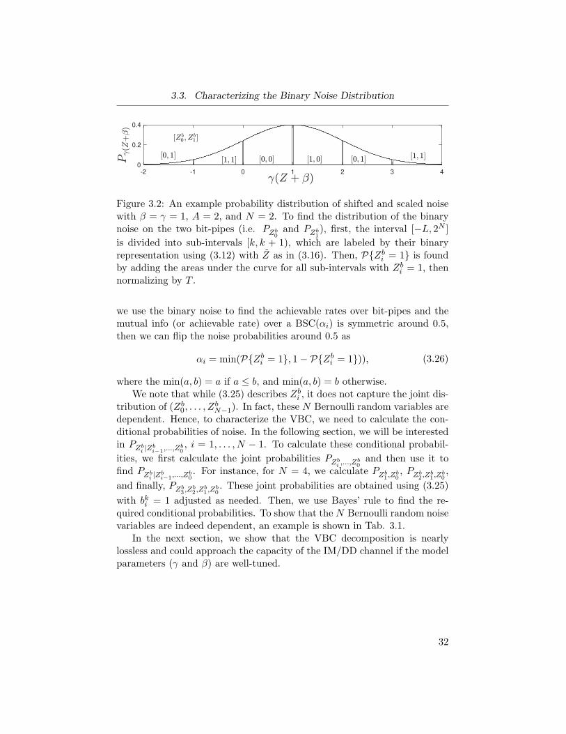
3.3. Characterizing the Binary Noise Distribution
-2 -1 0 1 2 3 4
0
0.2
0.4
Figure 3.2: An example probability distribution of shifted and scaled noisewith β = γ = 1, A = 2, and N = 2. To find the distribution of the binarynoise on the two bit-pipes (i.e. PZb
0and PZb
1), first, the interval [−L, 2N ]
is divided into sub-intervals [k, k + 1), which are labeled by their binaryrepresentation using (3.12) with Z as in (3.16). Then, P{Zb
i = 1} is foundby adding the areas under the curve for all sub-intervals with Zb
i = 1, thennormalizing by T .
we use the binary noise to find the achievable rates over bit-pipes and themutual info (or achievable rate) over a BSC(αi) is symmetric around 0.5,then we can flip the noise probabilities around 0.5 as
αi = min(P{Zbi = 1}, 1− P{Zb
i = 1})), (3.26)
where the min(a, b) = a if a ≤ b, and min(a, b) = b otherwise.We note that while (3.25) describes Zb
i , it does not capture the joint dis-tribution of (Zb
0, . . . , ZbN−1). In fact, these N Bernoulli random variables are
dependent. Hence, to characterize the VBC, we need to calculate the con-ditional probabilities of noise. In the following section, we will be interestedin PZb
i |Zbi−1
,...,Zb0, i = 1, . . . , N − 1. To calculate these conditional probabil-
ities, we first calculate the joint probabilities PZbi ,...,Z
b0and then use it to
find PZbi |Zb
i−1,...,Zb
0. For instance, for N = 4, we calculate PZb
1,Zb
0, PZb
2,Zb
1,Zb
0,
and finally, PZb3,Zb
2,Zb
1,Zb
0. These joint probabilities are obtained using (3.25)
with bki = 1 adjusted as needed. Then, we use Bayes’ rule to find the re-quired conditional probabilities. To show that the N Bernoulli random noisevariables are indeed dependent, an example is shown in Tab. 3.1.
In the next section, we show that the VBC decomposition is nearlylossless and could approach the capacity of the IM/DD channel if the modelparameters (γ and β) are well-tuned.
32

3.4. Showing that VBC is (almost) Capacity-Preserving
0
0.1
0.2
0.3
0.4
0.5
0.6
0.7
0.8
0.9
0 1 2 3 4 5 6 7
Figure 3.3: Binary noise probability for the VBC with A = 10, β = 5, andγ = 10.23
Table 3.1: Conditional noise probabilities for A = 1, γ = 0.75, β = 3. Inthis example, the marginal distribution of Zb
2 is given by P{Zb2 = 0} =
1−P{Zb2 = 1} = 1−α2 = 0.9888. Note that the marginal P{Zb
2 = 0} is notequal to the conditionals P{Zb
2 = 0|Zb1, Z
b0}, which shows that the variables
are dependent.
P{Zb2 = 0 | Zb
1, Zb0}
Zb1 = 0, Zb
0 = 0 0.827
Zb1 = 0, Zb
0 = 1 0.999
Zb1 = 1, Zb
0 = 0 0.999
Zb1 = 1, Zb
0 = 1 0.991
3.4 Showing that VBC is (almost)Capacity-Preserving
In this section, we show that the VBC is (almost) capacity-preserving.In other words, we show that decoding all input bits (Xb
N−1, . . . , Xb0) from
all output bits (Y bN−1, . . . , Y
b0 ) jointly achieves nearly the same rate as when
decoding using the continuous input and output, i.e., X and Y , respectively.Referring back to the mathematical formulation of the VBC, the first
process is to shift the output by a factor β. The shift does not change themutual information, i.e., I(X;Y ) = I(X;Y + β). The second step is toconsider an erasure symbol, in case the shifted output is outside the range
33
3.5. Chapter Summary
[0, A + 2β]. To ensure that this process does not lead to a significant lossin information, then, we should decrease the chance that an output outsidethis range is received, i.e., we need to reduce the erasure probability. Thisis easily satisfied by choosing a large enough β (cf. (3.3)). The third stepis to scale the shifted truncated output by γ. One can show that scaling anoutput does not change the mutual information, i.e., I(X;Y ′) = I(X; γY ′).Consequently, we introduce the VBC model which has binarized inputs,output, and noise. This can affect the achievable rate slightly due to theflooring operations, nevertheless, it does not not affect the achievable ratesignificantly when γ and β are tuned well.
Consider an example whenA = 100, γ = 10.23, and β = 5, the achievablerates at each processing discussed earlier for the unchanged IM/DD channel(I(X;Y ) = 3.1795 nats), the shifted and truncated output (I(X;Y ′) =3.1795 nats), the scaled, shifted, and truncated output (I(X; Y ) = 3.1795nats), and the binarized output (I(Xb
i ;Ybi ) = 3.1792 nats) for all i jointly,
showing the the VBC is (almost) lossless.Another interesting way to justify the (nearly) capacity-preserving prop-
erty of the VBC is the following. As β → ∞ and γ → ∞, then the numberof bits we quantize the IM/DD channel into also increases, i.e., N → ∞. AsN → ∞, the VBC then approaches the continuous IM/DD channel (as yougenerally need infinitely many bits to approximate a positive real number).This is because as β → ∞, it implies that all the noise distribution is con-sidered (Z > −∞) so the loss due to the introduction of erasures vanishes.In addition, as γ → ∞ then the precision of conversion to binary increasesand the decimal values are dealt with effectively, in other words the loss ofinformation due to the flooring operation is reduced. This way, we can saythat the VBC is asymptotically capacity-preserving.
To sum it up, the VBC has capacity that is almost equal to the capacityof the IM/DD channel for well-tuned free parameters (γ and β). Neverthe-less, encoding and decoding over all bit-pipes jointly may not be practical.Therefore, we develop simpler schemes for the VBC with the goal of ap-proaching the channel capacity of the IM/DD channel. In the next chapter,we explain how codes for the VBC can be used in the IM/DD channel, andwe present some practical coding schemes.
3.5 Chapter Summary
In this chapter, we presented the mathematical formulation towards thevector binary channel (VBC). The procedure followed was to shift the re-
34
3.5. Chapter Summary
ceived value by a nonnegative factor β, then introduce an erasure symbolif and only if the received value is too small/large, then scale non-erasedoutputs, and finally represent the output into N bits. We also showed howto represent those received N bits as a function of input, carryover, andnoise bits.
In addition, we developed a method to convert the Gaussian randomvariable into N Bernoulli random variables. This enables the approximationof the peak-constrained IM/DD channel by the VBC with the generated NBernoulli noise random variables. Furthermore, we show that the VBC isnearly capacity-preserving.
35
Chapter 4
Coding Schemes for the VBC
In the previous chapter, we showed the mathematical formulation to-wards the decomposition model, which we call the vector binary channel(VBC). The VBC consists of N bit-pipes, and approximates the IM/DDchannel.
In this chapter, we propose five coding schemes to be used with the VBCwith erasures model (VBCǫ), to code for the approximated IM/DD channel(cf. Definition 3.2). The complexity of each coding scheme depends on (i)whether the decoding is with or without state, where the state is the noiseover the previously decoded bit-pipes, and (ii) the number of output bitsused for each decoding operation. The schemes we present have sequentialdecoding, which could either be done starting with the lowermost i = 0 bit-pipe. with the least power level, then proceeding to upper bit-pipes, untildecoding all N bit-pipes, or starting from the uppermost bit-pipe, wherei = N − 1, and decoding sequentially until bit-pipe i = 0’s input Xb
0 isdecoded. The achievable rate of each coding scheme is derived and thetransmission scheme is presented.
Coding for the IM/DD channel can be realized by coding for VBCǫ,since this channel (cf. Definition 3.2) approximates the IM/DD channel(cf. Definition 2.18). This is done by using the operations shown in Fig.4.1. The message m with rate R is first split into multiple messages mi,i = 0, . . . , N − 1, with rate Ri so that R =
∑
iRi. Messages mi are encodedinto a binary codeword of length n, given by (Xb
i (1), . . . , Xbi (n)) for bit-pipe
i. At each time instant, the encoded bits are converted to decimal using∑
iXbi (t)2
i, for t = 1, . . . , n, then divided by γ to produce X, which is thensent over the channel. The corrupted symbol Y is then biased by β, scaledby γ, and then erased if γ(Y + β) falls outside [0, γ(A+2β)], and convertedto binary otherwise. This leads to received signals (Y c
i (1), . . . , Yci (n)), i =
0, . . . , N − 1, whose symbols are 0, 1, or ξ. These signals are then decodedinto mi.
Next, we present the coding schemes, by specifying the encoding, de-coding, and achievable rate of each scheme. First, we detail the encodingwhich all the coding scheme follow. The encoding considers bit-pipes to be
36
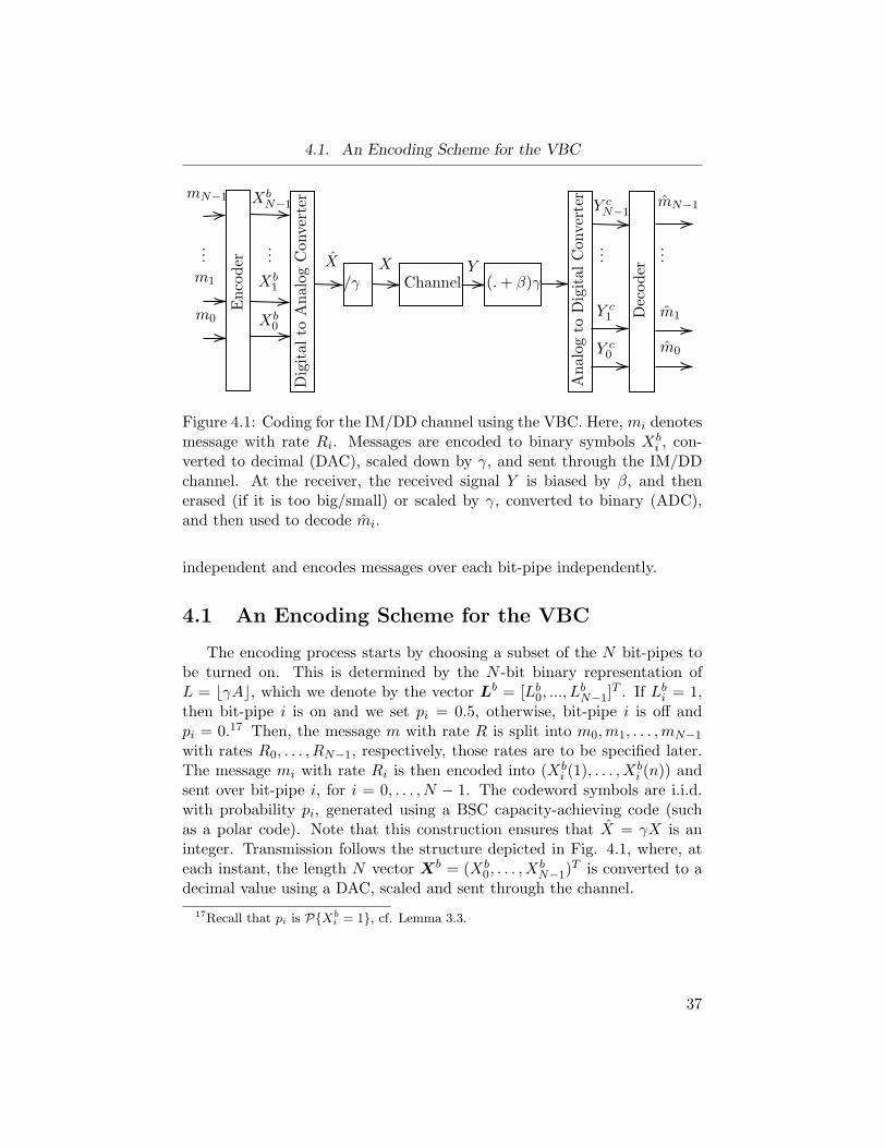
4.1. An Encoding Scheme for the VBC
Encoder
mN−1
...
m1
m0 Xb0
Xb1
XbN−1
Digital
toAnalog
Con
verter
X
/γX
ChannelY
(.+ β)γ
Analog
toDigital
Con
verter
Decoder
Y c0
Y c1
Y cN−1
m0
m1
mN−1
......
...
Figure 4.1: Coding for the IM/DD channel using the VBC. Here, mi denotesmessage with rate Ri. Messages are encoded to binary symbols Xb
i , con-verted to decimal (DAC), scaled down by γ, and sent through the IM/DDchannel. At the receiver, the received signal Y is biased by β, and thenerased (if it is too big/small) or scaled by γ, converted to binary (ADC),and then used to decode mi.
independent and encodes messages over each bit-pipe independently.
4.1 An Encoding Scheme for the VBC
The encoding process starts by choosing a subset of the N bit-pipes tobe turned on. This is determined by the N -bit binary representation ofL = ⌊γA⌋, which we denote by the vector L
b = [Lb0, ..., L
bN−1]
T . If Lbi = 1,
then bit-pipe i is on and we set pi = 0.5, otherwise, bit-pipe i is off andpi = 0.17 Then, the message m with rate R is split into m0,m1, . . . ,mN−1
with rates R0, . . . , RN−1, respectively, those rates are to be specified later.The message mi with rate Ri is then encoded into (Xb
i (1), . . . , Xbi (n)) and
sent over bit-pipe i, for i = 0, . . . , N − 1. The codeword symbols are i.i.d.with probability pi, generated using a BSC capacity-achieving code (suchas a polar code). Note that this construction ensures that X = γX is aninteger. Transmission follows the structure depicted in Fig. 4.1, where, ateach instant, the length N vector Xb = (Xb
0, . . . , XbN−1)
T is converted to adecimal value using a DAC, scaled and sent through the channel.
17Recall that pi is P{Xbi = 1}, cf. Lemma 3.3.
37
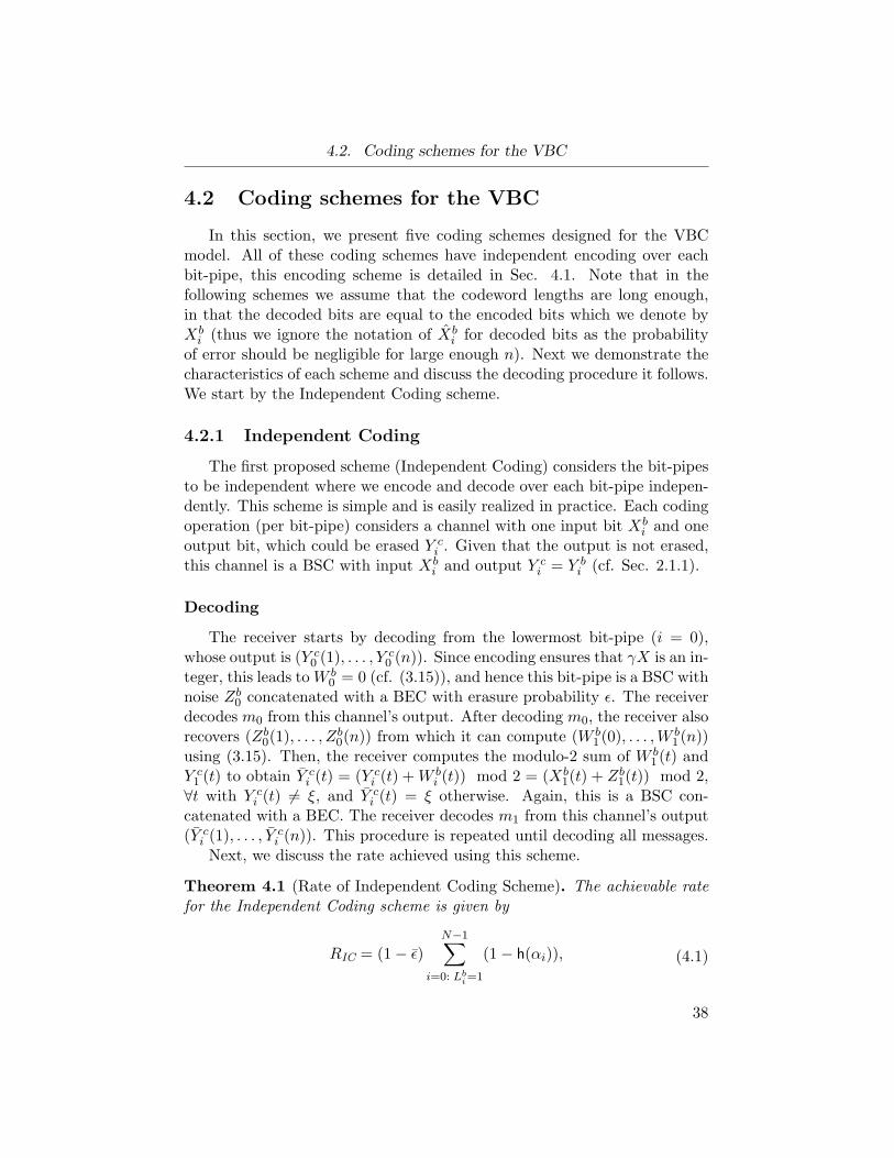
4.2. Coding schemes for the VBC
4.2 Coding schemes for the VBC
In this section, we present five coding schemes designed for the VBCmodel. All of these coding schemes have independent encoding over eachbit-pipe, this encoding scheme is detailed in Sec. 4.1. Note that in thefollowing schemes we assume that the codeword lengths are long enough,in that the decoded bits are equal to the encoded bits which we denote byXb
i (thus we ignore the notation of Xbi for decoded bits as the probability
of error should be negligible for large enough n). Next we demonstrate thecharacteristics of each scheme and discuss the decoding procedure it follows.We start by the Independent Coding scheme.
4.2.1 Independent Coding
The first proposed scheme (Independent Coding) considers the bit-pipesto be independent where we encode and decode over each bit-pipe indepen-dently. This scheme is simple and is easily realized in practice. Each codingoperation (per bit-pipe) considers a channel with one input bit Xb
i and oneoutput bit, which could be erased Y c
i . Given that the output is not erased,this channel is a BSC with input Xb
i and output Y ci = Y b
i (cf. Sec. 2.1.1).
Decoding
The receiver starts by decoding from the lowermost bit-pipe (i = 0),whose output is (Y c
0 (1), . . . , Yc0 (n)). Since encoding ensures that γX is an in-
teger, this leads toW b0 = 0 (cf. (3.15)), and hence this bit-pipe is a BSC with
noise Zb0 concatenated with a BEC with erasure probability ǫ. The receiver
decodes m0 from this channel’s output. After decoding m0, the receiver alsorecovers (Zb
0(1), . . . , Zb0(n)) from which it can compute (W b
1 (0), . . . ,Wb1 (n))
using (3.15). Then, the receiver computes the modulo-2 sum of W b1 (t) and
Y c1 (t) to obtain Y c
i (t) = (Y ci (t) +W b
i (t)) mod 2 = (Xb1(t) + Zb
1(t)) mod 2,∀t with Y c
i (t) 6= ξ, and Y ci (t) = ξ otherwise. Again, this is a BSC con-
catenated with a BEC. The receiver decodes m1 from this channel’s output(Y c
i (1), . . . , Yci (n)). This procedure is repeated until decoding all messages.
Next, we discuss the rate achieved using this scheme.
Theorem 4.1 (Rate of Independent Coding Scheme). The achievable ratefor the Independent Coding scheme is given by
RIC = (1− ǫ)N−1∑
i=0: Lbi=1
(1− h(αi)), (4.1)
38
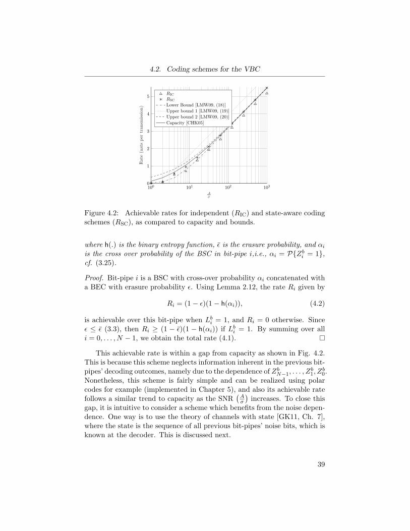
4.2. Coding schemes for the VBC
100 101 102 1030
1
2
3
4
5
Aσ
Rate(natsper
tran
smission
)
RIC
RSC
Lower Bound [LMW09, (18)]
Upper bound 1 [LMW09, (19)]
Upper bound 2 [LMW09, (20)]
Capacity [CHK05]
Figure 4.2: Achievable rates for independent (RIC) and state-aware codingschemes (RSC), as compared to capacity and bounds.
where h(.) is the binary entropy function, ǫ is the erasure probability, and αi
is the cross over probability of the BSC in bit-pipe i,i.e., αi = P{Zbi = 1},
cf. (3.25).
Proof. Bit-pipe i is a BSC with cross-over probability αi concatenated witha BEC with erasure probability ǫ. Using Lemma 2.12, the rate Ri given by
Ri = (1− ǫ)(1− h(αi)), (4.2)
is achievable over this bit-pipe when Lbi = 1, and Ri = 0 otherwise. Since
ǫ ≤ ǫ (3.3), then Ri ≥ (1 − ǫ)(1 − h(αi)) if Lbi = 1. By summing over all
i = 0, . . . , N − 1, we obtain the total rate (4.1).
This achievable rate is within a gap from capacity as shown in Fig. 4.2.This is because this scheme neglects information inherent in the previous bit-pipes’ decoding outcomes, namely due to the dependence of Zb
N−1, . . . , Zb1, Z
b0.
Nonetheless, this scheme is fairly simple and can be realized using polarcodes for example (implemented in Chapter 5), and also its achievable ratefollows a similar trend to capacity as the SNR
(
Aσ
)
increases. To close thisgap, it is intuitive to consider a scheme which benefits from the noise depen-dence. One way is to use the theory of channels with state [GK11, Ch. 7],where the state is the sequence of all previous bit-pipes’ noise bits, which isknown at the decoder. This is discussed next.
39
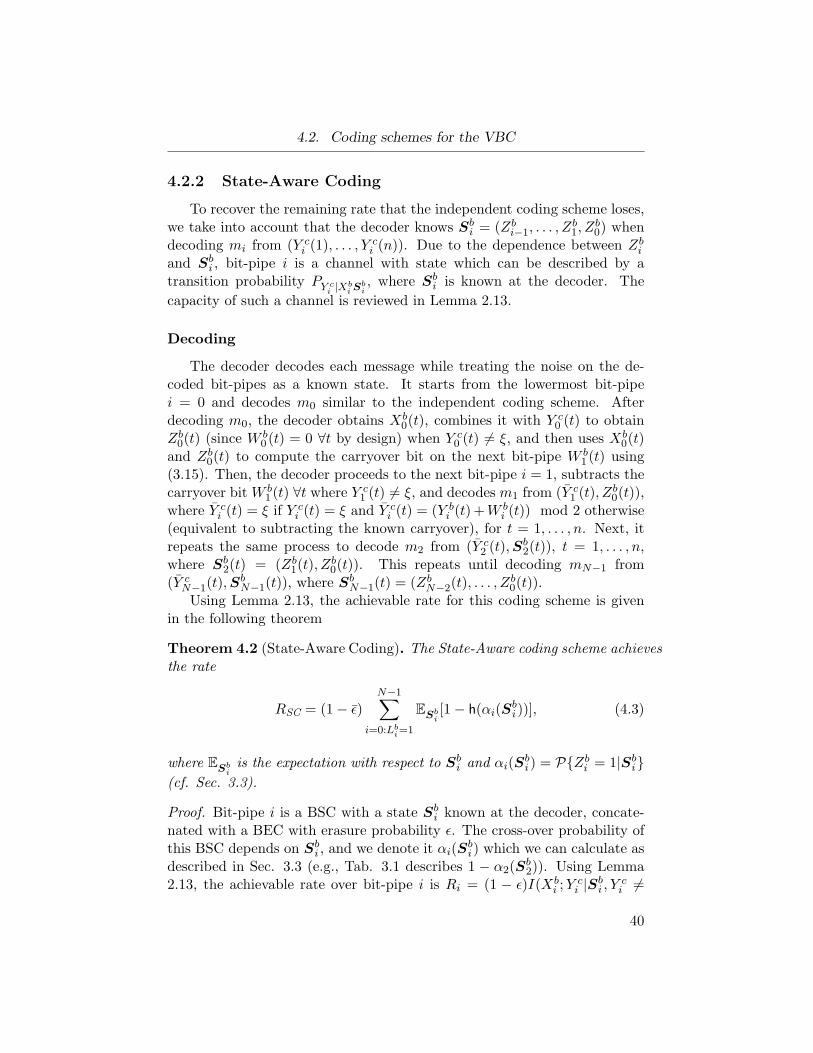
4.2. Coding schemes for the VBC
4.2.2 State-Aware Coding
To recover the remaining rate that the independent coding scheme loses,we take into account that the decoder knows Sb
i = (Zbi−1, . . . , Z
b1, Z
b0) when
decoding mi from (Y ci (1), . . . , Y
ci (n)). Due to the dependence between Zb
i
and Sbi , bit-pipe i is a channel with state which can be described by a
transition probability PY ci |Xb
iSbi, where S
bi is known at the decoder. The
capacity of such a channel is reviewed in Lemma 2.13.
Decoding
The decoder decodes each message while treating the noise on the de-coded bit-pipes as a known state. It starts from the lowermost bit-pipei = 0 and decodes m0 similar to the independent coding scheme. Afterdecoding m0, the decoder obtains Xb
0(t), combines it with Y c0 (t) to obtain
Zb0(t) (since W b
0 (t) = 0 ∀t by design) when Y c0 (t) 6= ξ, and then uses Xb
0(t)and Zb
0(t) to compute the carryover bit on the next bit-pipe W b1 (t) using
(3.15). Then, the decoder proceeds to the next bit-pipe i = 1, subtracts thecarryover bit W b
1 (t) ∀t where Yc1 (t) 6= ξ, and decodes m1 from (Y c
1 (t), Zb0(t)),
where Y ci (t) = ξ if Y c
i (t) = ξ and Y ci (t) = (Y b
i (t)+W bi (t)) mod 2 otherwise
(equivalent to subtracting the known carryover), for t = 1, . . . , n. Next, itrepeats the same process to decode m2 from (Y c
2 (t),Sb2(t)), t = 1, . . . , n,
where Sb2(t) = (Zb
1(t), Zb0(t)). This repeats until decoding mN−1 from
(Y cN−1(t),S
bN−1(t)), where S
bN−1(t) = (Zb
N−2(t), . . . , Zb0(t)).
Using Lemma 2.13, the achievable rate for this coding scheme is givenin the following theorem
Theorem 4.2 (State-Aware Coding). The State-Aware coding scheme achievesthe rate
RSC = (1− ǫ)N−1∑
i=0:Lbi=1
ES
bi[1− h(αi(S
bi))], (4.3)
where ES
biis the expectation with respect to S
bi and αi(S
bi) = P{Zb
i = 1|Sbi}
(cf. Sec. 3.3).
Proof. Bit-pipe i is a BSC with a state Sbi known at the decoder, concate-
nated with a BEC with erasure probability ǫ. The cross-over probability ofthis BSC depends on S
bi , and we denote it αi(S
bi) which we can calculate as
described in Sec. 3.3 (e.g., Tab. 3.1 describes 1 − α2(Sb2)). Using Lemma
2.13, the achievable rate over bit-pipe i is Ri = (1 − ǫ)I(Xbi ;Y
ci |S
bi , Y
ci 6=
40
4.2. Coding schemes for the VBC
ξ) = (1 − ǫ)ES
bi[1 − h(αi(S
bi))] ≥ (1 − ǫ)E
Sbi[1 − h(αi(S
bi))] if L
bi = 1, and
zero otherwise. Summing over all bit-pipes proves the theorem.
Let Si denote the set of all the possible realizations of Sbi . The cardinality
of the state set depends on i, for instance, S1 = {0, 1} is the set of possiblevalues of Zb
0, S2 = {00, 01, 10, 11} is the set of possible values of Zb1Z
b0, etc..
In general18, |Si| = 2i.It is necessary to note that the decoders in this scheme have a state as
an additional input, and that the construction of the decoder depends onthe level of the bit-pipe i, for i = 0, .., N − 1. Thus, State-Aware codinghas different decoders design and the complexity of each decoder increasesas we go up the bit-pipe levels, which is due to the exponential increase ofthe number of possible states as you go up the levels of the bit-pipes. Thisscheme approaches capacity at moderate and high SNR as we see next.
The achievable rate for both of the above schemes (the IndependentCoding and State-Aware coding) have a gap to capacity at low SNR. This isbecause at low SNR the noise is large and important information is pushedto an extra carryover bit which is fed to the next bit-pipe. To reduce thisgap and achieve higher rates we introduce schemes which decode from twobit-pipes at a time and recover this information from the extra carryover bit(bit-pipe i+ 1).
Next, we present a scheme which starts decoding from lower significantbit-pipes which are noisy, then proceeds to less noisy ones without utilizingthe knowledge of state, yet decoding from two output bits utilizing thecarryover inherent in the second output bit as we see next.
4.2.3 Independent Coding: Binary InputQuaternary-Output
To retrieve the rate that the Independent Coding scheme and the State-Aware coding scheme lose at low SNR, (detailed in Sec. 4.2.1 and Sec.4.2.2,respectively), we introduce a scheme which benefits from the carryover bitthat both aforementioned schemes neglect.19 In this scheme, each inputbit is decoded using two consecutive output bits, where the second outputpossesses the carryover bit we are interested in. The receiver starts decoding
18Note that for i = 0, the first bit-pipe, there is no state and this bit-pipe is a BSC withno state with crossover probability α0 = P{Zb
0 = 1}, and |S0| = 1, thus (4.3) still holds.19They neglect it as they decode each input bit from one output bit, since each input
is superimposed with a binary noise, and adding two binary numbers could result in twobits with the second bit being the carryover bit.
41
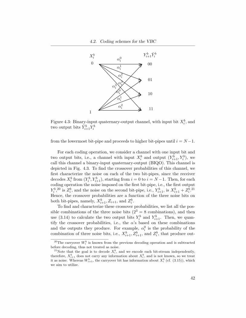
4.2. Coding schemes for the VBC
00
01
10
11
0
1
Xbi
Y bi+1Y
bi
α0i
α1i
α2i
α3i
α2i
α1i
α0i
α3i
Figure 4.3: Binary-input quaternary-output channel, with input bit Xbi , and
two output bits Y bi+1Y
bi
from the lowermost bit-pipe and proceeds to higher bit-pipes until i = N−1.
For each coding operation, we consider a channel with one input bit andtwo output bits, i.e., a channel with input Xb
i and output (Y bi+1, Y
bi ), we
call this channel a binary-input quaternary-output (BIQO). This channel isdepicted in Fig. 4.3. To find the crossover probabilities of this channel, wefirst characterize the noise on each of the two bit-pipes, since the receiverdecodes Xb
i from (Y bi , Y
bi+1), starting from i = 0 to i = N−1. Then, for each
coding operation the noise imposed on the first bit-pipe, i.e., the first outputY bi ,
20 is Zbi , and the noise on the second bit-pipe, i.e., Y b
i+1, is Xbi+1 + Zb
i .21
Hence, the crossover probabilities are a function of the three noise bits onboth bit-pipes, namely, Xb
i+1, Zi+1, and Zbi .
To find and characterize these crossover probabilities, we list all the pos-sible combinations of the three noise bits (23 = 8 combinations), and thenuse (3.14) to calculate the two output bits Y b
i and Y bi+1. Then, we quan-
tify the crossover probabilities, i.e., the α’s based on these combinationsand the outputs they produce. For example, α0
i is the probability of thecombination of three noise bits, i.e., Xb
i+1, Zbi+1, and Zb
i , that produce out-
20The carryover W bi is known from the previous decoding operation and is subtracted
before decoding, thus not treated as noise.21Note that the goal is to decode Xb
i , and we encode each bit-stream independently,therefore, Xb
i+1 does not carry any information about Xbi , and is not known, so we treat
it as noise. Whereas W bi+1, the carryover bit has information about Xb
i (cf. (3.15)), whichwe aim to utilize.
42
4.2. Coding schemes for the VBC
put bits (Y bi+1, Y
bi ) = (0, 0), when Xb
i = 0 is sent, these combinations are(Xb
i+1, Zbi+1, Z
bi ) = (0, 0, 0) and (Xb
i+1, Zbi+1, Z
bi ) = (1, 1, 0). These combina-
tions are the same which lead to (Y bi+1, Y
bi ) = (0, 1), when Xb
i = 1, thusthe transition is with the same probability α0
i . One can verify these com-binations by using Y b
i = (Xbi + Zb
i +W bi ) mod 2 with the steps illustrated
above.Next, we detail the decoding of this scheme.
Decoding
The receiver starts by decoding from the lowermost BIQO channel withi = 0, the output of this channel is (Y b
0 (1), . . . , Yb0 (n)), and (Y b
1 (1), . . . , Yb1 (n)).
Since, the encoder constructs γX to be an integer, meaning that the decoderknows that W b
0 = 0, as there is no carryover from the fractional parts of γXand γ(Z + β) (cf. (3.15)). Hence, this channel is a 1-input 2-output chan-nel (or as we call it BIQO) as depicted in Fig. 4.3, with noise Zb
0, andXb
i+1 + Zbi+1. This BIQO channel is concatenated with a BEC 22 with era-
sure probability ǫ, the output of this channel is then (Y c0 (1), . . . , Y
c0 (n)), and
(Y c1 (1), . . . , Y
c1 (n)). Therefore, the receiver decodes m0 from this channel’s
output. Moreover, after decodingm0, the receiver also recovers (Zb0(1), . . . , Z
b0(n)),
which it uses to deduce the carryover bit on bit-pipe i = 1, i.e.,W b1 (0), . . .W
b1 (n)
using (3.15). With the knowledge of W b1 (0), . . .W
b1 (n), the receiver then
computes the modulo-2 sum of W1(t) and Y c1 (t) 6= ξ to subtract this known
carryover noise for the next decoding operation, this is denoted by Y ci (t) =
(Y ci (t) +W b
i (t)) mod 2. Thus, we obtain Y c1 (t) = (Xb
1(t) + Zb1(t)) mod 2,
∀t with non-erased outputs, i.e., Y ci (t) 6= ξ, and Y c
i (t) = ξ otherwise. Next,the receiver decodes m1 from (Y c
1 (0), . . . , Yc1 (n)) (with the subtracted car-
ryover W b1 (t)) and (Y c
2 (0), . . . , Yc2 (n)) (which embeds the carryover we aim
to use). Again, this is a BIQO, concatenated with an erasure channel. Thisprocedure is repeated until decoding the last subchannel with i = N − 1.Next, we quantify the achievable rate of this scheme.
Theorem 4.3 (Independent Coding: BIQO). The Independent Coding with
22Recall that we introduce a concatenation with an erasure channel to better approxi-mate the IM/DD channel by using the VBC with erasures.
43
4.2. Coding schemes for the VBC
BIQO channels coding scheme achieves the rate
RBIQO = (1− ǫ)N−1∑
i=0:Lbi=1
I(Xbi ; Y
bi , Y
bi+1),
= (1− ǫ)N−1∑
i=0:Lbi=1
H(Y bi , Y
bi+1)−H(Y b
i , Ybi+1 | X
bi ).
(4.4)
where we assume that for the last sub-channel N−1 the mutual informa-tion is I(Xb
N−1; YbN−1, Y
bN ) = I(Xb
N−1; YbN−1). The alphas are the transition
probabilities (cf. Fig. 4.3) and are equal to
α0i = P{(Xb
i+1, Zbi+1, Z
bi ) = (0, 0, 0)}+P{(Xb
i+1, Zbi+1, Z
bi ) = (1, 1, 0)} (4.5)
α1i = P{(Xb
i+1, Zbi+1, Z
bi ) = (0, 0, 1)}+P{(Xb
i+1, Zbi+1, Z
bi ) = (1, 1, 1)} (4.6)
α2i = P{(Xb
i+1, Zbi+1, Z
bi ) = (0, 1, 0)}+P{(Xb
i+1, Zbi+1, Z
bi ) = (1, 0, 0)} (4.7)
α3i = P{(Xb
i+1, Zbi+1, Z
bi ) = (0, 1, 1)}+P{(Xb
i+1, Zbi+1, Z
bi ) = (1, 0, 1)} (4.8)
Proof. Each bit-pipe i, i = 0, . . . , N − 1 is a BIQO with transition prob-abilities αj
i , where j ∈ {0, 1, 2, 3}, concatenated with a BEC with erasureprobability ǫ. Using Lemma 2.12, the rate Ri = (1 − ǫ)I(Xb
i ; Ybi , Y
bi+1) is
achievable over this bit-pipe when Lbi = 1, and Ri = 0 otherwise. Since
ǫ ≤ ǫ (3.3), therefore, Ri ≥ (1− ǫ)I(Xbi ; Y
bi , Y
bi+1) if L
bi = 1. Summing over
all i, the total rate (4.4) is obtained.
Next, we explain a coding which uses the concept of channel with stateas the State-Aware coding scheme in Sec. 4.2.2. However, this scheme hasa lower complexity as the state set is only dependent on the noise of theprevious bit-pipe’s noise, thus, the decoder is the same for all bit-pipes.This is discoursed next.
4.2.4 Partial-State-Aware Coding
This coding scheme is similar to a previously presented scheme (State-Aware coding), as it uses the concept of a channel with state. The differenceis that the state in this scheme is only the previous noise bit. In particular,we take into account only part of what the decoder knows and the statefor bit-pipe i is Zb
i−1, when decoding mi from (Y ci (1), . . . , Y
ci (n)), where
Y ci (t) = (Y c
i (t)+W ci (t)) mod 2 for Y c
i 6= ξ and is erasure otherwise. In thiscontext, each bit-pipe is a channel (BSC) with a state known at the decoder,
44
4.2. Coding schemes for the VBC
this channel can be described by the transition probability PY ci |Xb
i Zbi−1
. The
capacity of a channel with state known at the decoder is given in Lemma2.12.
Next, we discuss the decoding of this scheme in more details.
Decoding
The decoder decodes each message while treating the noise bit on thepreviously decoded bit-pipe as a state. This is done starting from the low-ermost bit-pipe with i = 0. The decoder then decodes the message m0
from (Y c0 (1), . . . , Y
c0 (n)). It is known that the carryover on the first bit-pipe
is zero, i.e., W b0 (t) = 0, since the encoder ensures that γX is an integer.
Therefore, this bit-pipe is a BSC with crossover probability P{Zb0(t) = 1},
this BSC is concatenated with a BEC(ǫ), and the receiver decodes m0 fromthis bit-pipe’s output. 23 After m0 is decoded, the receiver recovers Xb
0(t),then combines it with Y c
0 (t) to obtain Zb0(t), for t = 1, . . . , n, when Y c
0 6= ξ.The receiver then uses the knowledge of Xb
0(t) and Zb0(t) to calculate the
carryover bit on the next bit-pipe, i.e., W b1 (t) using (3.15). Consequently,
the receiver proceeds to the next bit-pipe with i = 1, subtracts the carryoverit knows W b
1 (t) from Y c1 (t) using an XOR operation, ∀t where Y c
1 (t) 6= ξ toobtain Y c
i (t) and Y ci (t) = ξ otherwise. Then, the receiver decodes m1 from
(Y c1 (t), Z
b0(t)), for i = 0, . . . , N − 1 and t = 1, . . . , n. The receiver repeats
the same steps until decoding mN−1 from (Y cN−1(t), Z
bN−2(t)).
The achievable rate of this scheme follows the same expression for theState-Aware coding given in Theorem 4.2 with the adjustment of the stateexpression (which in turn affects αi(S
bi). In this scheme Sb
i = (Zbi−1) and
αi(Sbi) = P{Zb
i |Zbi−1}. Additionally, the state set is uniform for all bit-pipes
and |Sbi | = 2, where Sb
i = {0, 1} for all i.
4.2.5 Descending Independent Coding
In all the schemes above, the receiver decodes from the lowermost bit-pipe to the uppermost one. The reason was to be able to subtract thecarryover as the decoder proceeds through the bit-pipes. One may arguethat decoding the bit-pipes starting from the top to the bottom is a viableidea, as higher bit-pipes are less noisy and so any propagation of error willbe avoided. Here, we implement this idea, where we consider the bit-pipesto be independent, yet the decoding operation starts from bit-pipe i = N−1
23Note that, in this decoding operation there is no state as this is the first bit-pipe tobe decoded.
45
4.2. Coding schemes for the VBC
and continues to lower bit-pipes until decoding the lowermost bit-pipe withi = 0.
We explain this decoding procedure formally below.
Decoding
The decoding process starts by decoding from the uppermost bit-pipe(i = N − 1), whose output is (Y c
N−1(1), . . . , YcN−1(n)). Since the carryover
imposed on this bit-pipes is not known, it is considered as noise. Hence, thebit-pipe is a BSC with crossover probability P{(Zb
N−1+W bN−1) mod 2 = 1}
concatenated with a BEC(ǫ). The receiver decodes mN−1 from this chan-nel’s output. After decoding mN−1, the receiver proceeds to the next de-coding operation, to decode mN−2 from (Y c
N−2(1), . . . , YcN−2(n)), which is
again a BSC with crossover probability P{(ZbN−2 + W b
N−2) mod 2 = 1}concatenated with a BEC(ǫ). This procedure is repeated until decoding thelowermost message m0.
We discuss the rate achieved using this scheme next.The rate achieved by this scheme is the same as the Independent Coding
scheme in Sec. 4.2.1, which is presented in Theorem 4.1. The difference isthe crossover probability of each BSC which becomes αi = P{(Zb
i + W bi )
mod 2 = 1}. This crossover probability needs to characterized to evaluatethe achievable rates. We discuss the derivation next.
The crossover probability could be expressed as
P{(Zbi +W b
i ) mod 2} = P{Zbi = 1,W b
i = 0}+ P{Zbi = 0,W b
i = 1}. (4.9)
Now, we need to characterize the joint probabilities of Zbi and W b
i . Asan illustration, we consider P{Zb
i = 0,W bi = 1} and detail the deriva-
tion next. To do that, we denote by Sbi = (Zb
i−1, . . . , Zb0), define a real-
ization of this vector as si = (zi−1, . . . , z0), where Sbi = si is equivalent to
Zbi−1 = zi−1, . . . , Z
b0 = z0 and zi ∈ {0, 1}. Therefore, using the total law of
probability we can express the joint probability P{Zbi = 0,W b
i = 1} as
P{Zbi = 0,W b
i = 1} =∑
si
P{W bi = 1|Sb
i = si}P{Zbi = 0|Sb
i = si}P{Sbi = si}.
(4.10)The above equality uses the law of total probability and follows as W b
i andZbi are conditionally independent given Sb
i . To calculate (4.10), we onlyneed to characterize P{W b
i |Sbi = si} as the expressions of P{Zb
i |Sbi = si}
and P{Sbi = si} are already characterized, cf. Sec. 3.3. Now we focus on
finding P{W bi |S
bi = si}.
46
4.3. Chapter Summary
Recall that the carryover at bit-pipe i, i.e., W bi , is defined as W b
i =(W b
i−1 +Xbi−1 + Zb
i−1) mod 2. Then, we can characterize the probability ofthe carryover as
P{W bi = 1} = P{(W b
i−1 +Xbi−1 + Zb
i−1) mod 2 = 1},
= P{W bi−1 = 1, Xb
i−1 = 1, Zbi−1 = 1}
+ P{W bi−1 = 1, Xb
i−1 = 1, Zbi−1 = 0}
+ P{W bi−1 = 1, Xb
i−1 = 0, Zbi−1 = 1}
+ P{W bi−1 = 0, Xb
i−1 = 1, Zbi−1 = 1}.
(4.11)
Now to find P{W bi |S
bi = si}, we use (4.11) and obtain
P{W bi = 1|Sb
i} = P{W bi−1 = 1|Sb
i−1}P{Xbi−1 = 1}zi−1P{Zb
i−1 = 1|Sbi−1}},
+ P{W bi−1 = 1|Sb
i−1}P{Xbi−1 = 1}(1− zi−1)P{Zb
i−1 = 0|Sbi−1}}
+ P{W bi−1 = 1|Sb
i−1}P{Xbi−1 = 0}zi−1P{Zb
i−1 = 1|Sbi−1}}
+ P{W bi−1 = 0|Sb
i−1}P{Xbi−1 = 1}zi−1P{Zb
i−1 = 1|Sbi−1}},
(4.12)where Sb
i−1 = (Zbi−2, . . . , Z
b0) this follows as Xb
i−1 is independent of Zbi−1,
W bi−1, and the input Xb
i−1 is also independent of the previous noise Sib. Ad-ditionally, W b
i−1 is independent of Zbi−1 given Sb
i−1 = Zbi−2, . . . , Z
b0.Moreover,
P{Zbi−1 = 1|Sb
i} = zi−1P{Zbi−1 = 1|Sb
i−1}.We can see that due the recursive nature of the carryover, calculating a
carryover at bit-pipe i depends on all previous carryovers. Then, so does itsprobability. Therefore, to calculate the crossover probability αi, we use theabove equations starting from i = 0, calculate the joint probability of Zb
i
and W bi , then continue until i = N − 1, and evaluate the achievable rates.
4.3 Chapter Summary
In this chapter we presented five coding schemes for the VBC to codefor the IM/DD channel. All the presented coding schemes use the sameencoding procedure. Encoding is done by dividing the message m intom0, . . . ,mN−1 with rates R0, . . . , RN−1 for bit-pipes i = 0, . . . , N − 1, re-spectively. First, we choose a subset of the bit-pipes to be on or which weset pi = P{Xb
i = 1} = 0.5 and freeze the transmission over the remainingsubset by setting pi = 0.
Then we present five coding schemes each with a different decodingmethod. The simplest is the Independent Coding scheme which decodes
47
4.3. Chapter Summary
sequentially starting from the least significant bit while subtracting carry-over bits. We also presented the State-Aware Coding scheme which decodessequentially starting from the lowermost bit-pipe while subtracting carry-over bits and using the knowledge of previously decoded noise bits as a statefor the current decoding operation. Furthermore, the Independent Codingwith BIQO subchannels decodes each bit-pipe’s input from two consecutivebit-pipes’ outputs, sequentially from bit-pipe i = 0 to i = N − 1. The pre-sented coding schemes are realizable in practice by the use of polar codes,and are of an acceptable complexity. The Independent Coding scheme hasa lower complexity as compared to the State-Aware Coding complexity asthe decoders design are uniform for all bit-pipes. The Independent Codingwith BIQO is more complex than the Independent Coding scheme as foreach decoding operation we consider a channel with one input bit and twooutput bits (BIQO) instead of a BSC.
48
Chapter 5
Independent Polar Codingover the VBC
Previously, in Sec. 2.3, polar codes were presented as a capacity-achievingchannel code for any binary input discrete memoryless channel. Addition-ally, we have established a binary decomposition of the IM/DD channelleading to the VBC model in Chapter 3. Furthermore, we presented somecoding schemes for the VBC, the simplest scheme is the Independent Codingscheme (cf. Sec. 4.2.1). In this scheme, we have N bit-pipes, each of whichis made up of a BSC concatenated with a BEC, and we encode indepen-dently over each bit-pipe, and decode independently and sequentially whilesubtracting the carryover bit.
In this chapter, we provide the practical implementation and the re-sulting achievable rates, bit-error rate (BER), and frame-error rate (FER)for polar codes with the Independent Coding scheme to code for the VBC.Specifically, the goal is to use a polar encoder and decoder in the IM/DDapproximation, cf. Fig. 4.1. This is done as follows. Suppose we aregiven message mi, to be sent over bit-pipe i. We construct the codeword(Xb
i (1), . . . , Xbi (n)) using polar coding. In decoding, we are given the re-
ceived vector (Y ci (1), . . . , Y
ci (n)) through which we desire to estimate the
message mi, we use a polar decoder to decode the message and we denotethe estimated message by mi.
To apply polar coding for a certain Bi-DMC, one has to first do code con-struction. The code construction algorithm we use, is presented by Arikanin the same paper [Ari09], we detail the algorithm in Appendix A. 24
The process to implement polar codes is the following: for each SNRvalue we decompose the IM/DD channel into N bit-pipes to create the VBC.For the Independent Coding scheme, each bit-pipe is a BSC concatenatedwith a BEC(ǫ), and the decoding over each bit-pipe is done sequentiallywhile subtracting the carryover bit. Note that, in the following simulations
24Recall that code construction is choosing k out of n channels to be used for trans-mission of data (channels which have capacities close to one), and send frozen bits on theother channels (those which have capacities approaching zero).
49
5.1. Bit Error Rate
we assume that the carryover bit is decoded correctly by ensuring that thecodeword length (blocklength) specified for each bit-pipe is large enough,this way there will be no propagation of error and each bit-pipe acts asan independent BSC(αi) concatenated with BEC(ǫ).25 For simplicity, weonly consider polar coding for the BSC while assuming that the erasureprobability is negligible, and obtain the BER and FER and achievable rate.26
The crossover probability of each bit-pipe is inferred form the Gaussiannoise, i.e., the crossover probability is obtained from the quantized Gaussiandistribution as αi = P{Zb
i = 1}, using (3.25). We choose k and n of eachbit-pipe so that k/n is less than or equal to the capacity of the bit-pipe.27
5.1 Bit Error Rate
The BER for each bit-pipe is the ratio of the number of bit errors andthe total number of sent bits, which could be expressed as
BERi =
∑Tj=1
∑nt=1 IUb
i,j(t) 6=Ubi,j(t)
nT, (5.1)
where U bi,j(t) and U b
i,j(t) represent the tth bit in the jth frame sent and re-
ceived (respectively) over bit-pipe i, T is the number of sent blocks (frames),n is the codeword length (blocklength). Using (5.1), the total BER for thetransmission over the approximated IM/DD using the N bit-pipes is ob-tained by taking the average over all BERi for i = 0, . . . , N − 1.
5.2 Frame Error Rate
To calculate the FER, we calculate the ratio of the count of the numberof erroneous frames and the total number of sent frames, where each frameis of length n. To obtain the FER for each bit-pipe we use the following
25In general there would be propagation of error for finite blocklength but for largeenough blocklength this propagation could be made negligible, also but transmitting atrates lower than the capacity of the bit-pipe we can ensure lower probability of propagationof error.
26Considering the BEC would affect the achievable rate negligibly as the erasure prob-ability is almost zero for large enough β, cf. (3.3) and Lemma 2.12. A full simulationwould be provided in future work.
27Recall that k is the message length, n is the codeword length and the rate is R = k/n.
50
5.3. Numerical Evaluations
formula
FERi =
∑Tj=1 I
∑nt=1
Ubi,j(t) 6=Ub
i,j(t)>0
T. (5.2)
Now, we need to find the overall FER for the approximated IM/DDchannel or the N bit-pipes. If any of the bit-pipes i = 0, . . . , N − 1 have aframe error, then, there is a frame error in the IM/DD, and the only casewe consider that there is no frame error if all the N bit-pipes have error-freeframes. This could be written as
FER = 1−N∏
i=1
(1− FERi) , (5.3)
this quantifies the total frame error for the approximated IM/DD channel.
5.3 Numerical Evaluations
As an example, consider the case when A = 501.19, γ = 1.0188, β = 5.Table 5.3 shows the process of implementing polar codes for the IndependentCoding scheme. The polar code is implemented separately for each bit-pipe(BSC), then the BER and FER analysis per bit-pipe are analyzed, this isdone by a large enough number of iterations T . For the numerical evalu-ations, we use the packages provided by [VHV16] with slight adjustments.Using the data in Table 5.3, we obtain the overall BER for the N bit-pipes,by taking the average of all BERi values, we obtain BER = 0.00016. Using(5.3), we obtain the overall FER as FER = 0.049, which is not necessarilysmall enough for some practical applications. Yet, the FER values of eachbit-pipe, i.e., FERi is very low, thus is satisfactory. To further decrease theoverall FER, one can always ignore weak bit-pipes, i.e., bit-pipes with lowcapacities and high FERs. Such bit-pipes require much longer blocklengths.Nevertheless, we know that polar codes theoretically achieve the capacityof a Bi-DMC with a negligible error probability as blocklength n → ∞.Thus,the FER can be decreased further increasing n.
Next, we plot the achievable rates in comparison to the achievable rateof the Independent coding.
The rates achieved for a range of SNRs by considering polar encoders anddecoders concatenated with the Independent Coding scheme is demonstratedin Fig. 5.1. It can be seen that there is a rate gap to the IndependentCoding scheme RIC , although polar codes are capacity-achieving. This isdue to computation constraints.
51
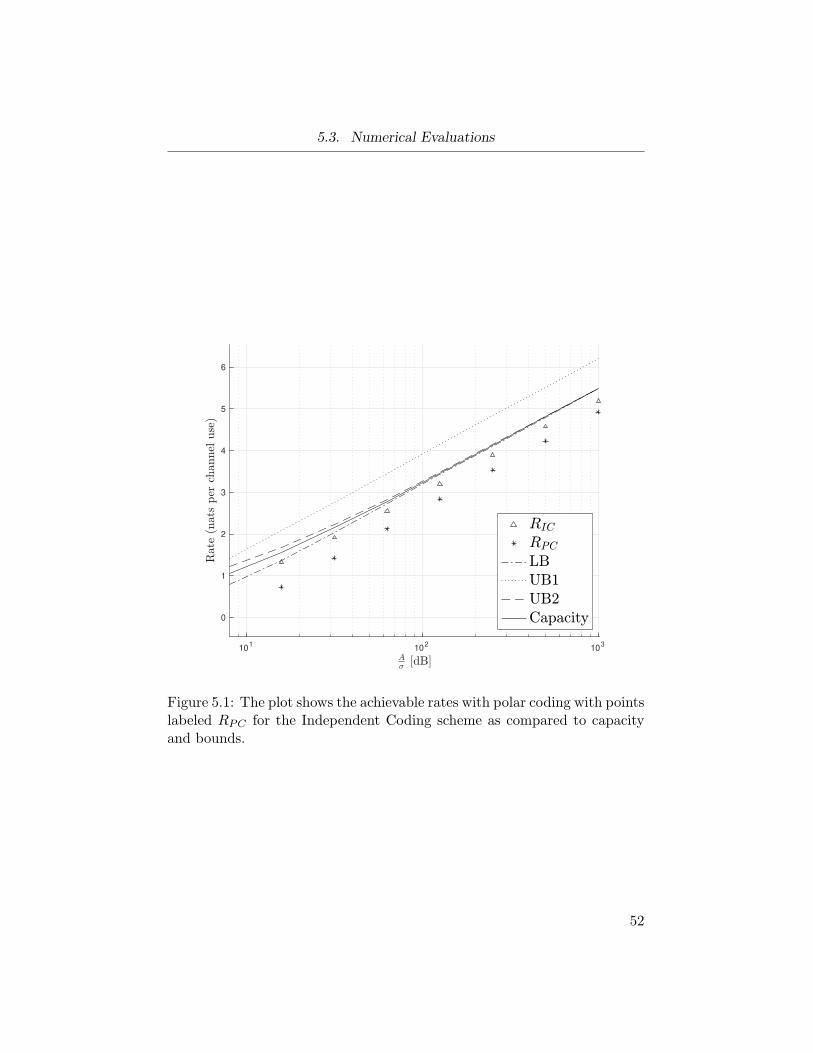
5.3. Numerical Evaluations
101
102
103
0
1
2
3
4
5
6
Figure 5.1: The plot shows the achievable rates with polar coding with pointslabeled RPC for the Independent Coding scheme as compared to capacityand bounds.
52
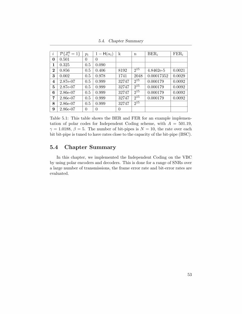
5.4. Chapter Summary
i P{Zbi = 1} pi 1− H(αi) k n BERi FERi
0 0.501 0 0
1 0.325 0.5 0.090
2 0.856 0.5 0.406 8192 215 4.8462e-5 0.0021
3 0.002 0.5 0.978 1741 2048 0.00017352 0.0029
4 2.87e-07 0.5 0.999 32747 215 0.000179 0.0092
5 2.87e-07 0.5 0.999 32747 215 0.000179 0.0092
6 2.86e-07 0.5 0.999 32747 215 0.000179 0.0092
7 2.86e-07 0.5 0.999 32747 215 0.000179 0.0092
8 2.86e-07 0.5 0.999 32747 215
9 2.86e-07 0 0 0
Table 5.1: This table shows the BER and FER for an example implemen-tation of polar codes for Independent Coding scheme, with A = 501.19,γ = 1.0188, β = 5. The number of bit-pipes is N = 10, the rate over eachbit bit-pipe is tuned to have rates close to the capacity of the bit-pipe (BSC).
5.4 Chapter Summary
In this chapter, we implemented the Independent Coding on the VBCby using polar encoders and decoders. This is done for a range of SNRs overa large number of transmissions, the frame error rate and bit-error rates areevaluated.
53
Chapter 6
Results and Discussion
In this chapter we provide and discuss the research results.The numerical evaluations for the proposed schemes for the VBC model
(which approximates the IM/DD channel) are demonstrated and evaluated.The achievable rates of the different schemes are compared to the capac-ity and bounds of the peak-constrained IM/DD channel. Since there isno closed-form expression for the capacity of the peak-constrained IM/DDchannel, the capacity is numerically evaluated using a numerical optimiza-tion for the continuous IM/DD channel [CHK05]. Additionally, the depictedbounds are from [LMW09], where UB1, UB2, and LB represent the two up-per bounds and the lower bound, respectively.
The results in Fig. 6.1 show that (note that we discuss and justify theseresults later)
1. At moderate to high SNR, the achievable rates of the State-Awarecoding scheme RSC approaches capacity.
2. At low SNR, the State-Aware coding and the Independent codingscheme both have a considerable gap to capacity (schemes which de-code one input bit from one output bit).
3. At low SNR, the Independent Coding with BIQO achieves the highestrates among all the other schemes.
4. The Independent Coding scheme RIC and the Independent Codingwith BIQO follow a similar trend to capacity, but have a gap to ca-pacity with the BIQO scheme performing slightly better as it decodesfrom two outputs.
5. The State-Aware scheme performs either better than (or equivalentto) the Partial-State-Aware Coding and Independent Coding Schemes.Additionally the Partial-State-Aware Coding scheme achieves rateswhich are more than or equal to the Independent Coding Scheme.Moreover, at moderate to high SNR, the Partial-State-Aware RPSC
54
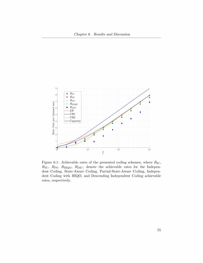
Chapter 6. Results and Discussion
100
101
102
103
0
1
2
3
4
5
6
7
8
9
Figure 6.1: Achievable rates of the presented coding schemes, where RIC,RSC, RPS, RBIQO, RDIC, denote the achievable rates for the Indepen-dent Coding, State-Aware Coding, Partial-State-Aware Coding, Indepen-dent Coding with BIQO, and Descending Independent Coding achievablerates, respectively.
55
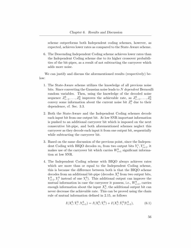
Chapter 6. Results and Discussion
scheme outperforms both Independent coding schemes, however, asexpected, achieves lower rates as compared to the State-Aware scheme.
6. The Descending Independent Coding scheme achieves lower rates thanthe Independent Coding scheme due to its higher crossover probabili-ties of the bit-pipes, as a result of not subtracting the carryover whichadds more noise.
We can justify and discuss the aforementioned results (respectively) be-low:
1. The State-Aware scheme utilizes the knowledge of all previous noisebits. Since converting the Gaussian noise leads toN dependent Bernoullirandom variables. Then, using the knowledge of the decoded noisesequence Zb
i−1, . . . , Zb0 improves the achievable rate, as Zb
i−1, . . . , Zb0
convey some information about the current noise bit Zbi due to their
dependence, cf. Sec. 3.3.
2. Both the State-Aware and the Independent Coding schemes decodeeach input bit from one output bit. At low SNR important informationis pushed to an additional carryover bit which is imposed on the nextconsecutive bit-pipe, and both aforementioned schemes neglect thiscarryover as they decode each input it from one output bit, sequentiallywhile subtracting the carryover bit.
3. Based on the same discussion of the previous point, since the Indepen-dent Coding with BIQO decodes mi from two output bits Y c
i , Yci+1, it
makes use of the carryover bit which carries W bi+1 significant informa-
tion at low SNR.
4. The Independent Coding scheme with BIQO always achieves rateswhich are more than or equal to the Independent Coding scheme,this is because the difference between both is that the BIQO schemedecodes from an additional bit-pipe (decodes Xb
i from two output bits,Y bi+1, Y
bi instead of one Y b
i ). This additional output can improve themutual information in case the carryover it possess, i.e., W b
i+1, carriesenough information about the input Xb
i , the additional output bit cannever decrease the achievable rate. This can be proved using the chainrule of mutual information defined in 2.15, as follows
I(Xbi ; Y
bi , Y
bi+1) = I(Xb
i ; Ybi ) + I(Xb
i ; Ybi |Y
bi+1), (6.1)
56
Chapter 6. Results and Discussion
where I(Xbi ; Y
bi , Y
bi+1) is the achievable rate for the independent cod-
ing with BIQO, and = I(Xbi ; Y
bi ) is the rate for the Independent
Coding scheme. By the non-negativity property of mutual informa-tion we know that I(Xb
i ; Ybi |Y
bi+1) ≥ 0. Therefore, I(Xb
i ; Ybi , Y
bi+1) ≥
I(Xbi ; Y
bi ).
5. Both of the State-Aware schemes achieve rates more than the indepen-dent coding schemes. Without loss of generality consider the State-Aware coding scheme in Sec. 4.2.2 with a state Sb
i = (Zbi−1, . . . , Z
b0)
when decoding message mi, then the achievable rate over this bit-pipegiven by I(Xb
i ; Yci |S
bi) satisfies the following relation
I(Xbi ; Y
ci |S
bi) ≥ I(Xb
i ; Yci ), (6.2)
where I(Xbi ; Y
ci ) is the achievable rate over the Independent Coding
scheme for bit-pipe i. The above relation (which does not gener-ally hold) is true in this case because I(Xb
i ;Zbi−1, . . . , Z
b0) = 0, the
noise bits and the input bit are independent by construction (recallthat we consider a uniform support of the Gaussian noise regard-less of the input, which ensures their independence, cf. Sec. 3.3).More precisely, by the chain rule of mutual information we can writeI(Xb
i ; Yci ,S
bi) = I(Xb
i ;Sbi) + I(Xb
i ; Yci |S
bi) = I(Xb
i ; Yci ) + I(Xb
i ;Sbi |Y
ci ).
Using I(Xbi ;S
bi) = 0, then, I(Xb
i ; Yci |S
bi) = I(Xb
i ; Yci ) + I(Xb
i ;Sbi |Y
bi ),
since the mutual information is non-negative, i.e., I(Xbi ;S
bi |Y
bi ) ≥ 0.
We finally obtain I(Xbi ; Y
ci |S
bi) ≥ I(Xb
i ; Yci ). The same discussion can
be used to prove that the State-Aware coding scheme achieves ratesthat are more than or equal to the Partial-State-Aware coding scheme,i.e., I(Xb
i ; Yci |S
bi) ≥ I(Xb
i ; Yci |Z
bi−1).
6. Decoding from lower more noisy bit-pipes achieves higher rates thandecoding from upper less noisy bit-pipes. This is true as when wedecode each message sequentially from the lower bit-pipe we also re-cover the carryover bit which is imposed on the next bit-pipe, and wesubtract this carryover bit before decoding. This way there is usuallylesser noise on each bit-pipe, i.e., the crossover probability on eachbit-pipe is less when subtracting the carryover bit leading to higherachievable rate per each bit-pipe.
57
Chapter 7
Conclusion
In this chapter we provide the conclusion of this thesis. We also discussthe limitations of this research. In addition we provide some future researchdirections.
7.1 Conclusion
In conclusion, we propose the VBC as an approximation for the IM/DDchannel, with a peak constraint (which is an AWGN with a positive inputand a peak-constraint). The VBC is a collection of N bit-pipes, representinga channel with a binary vector input, noise, and output. This decompositionis nearly lossless as it considers the carryovers. Furthermore, we present amethod to represent the continuous Gaussian noise as N Bernoulli randomvariables to be compatible with the VBC model. In addition, we presentfive coding schemes for the VBC model with the goal of designing a prac-tical coding scheme for the IM/DD channel. The achievable rates for theschemes are evaluated and compared to a numerical evaluation of capacityand bounds. The achievable rate of the State-Aware coding is nearly equalto capacity at moderate and high SNR as shown in 6.1 discussed in Sec. ??.The Independent Coding scheme secures good achievable rates which areabout 0.2 nats away from capacity at moderate and high SNR, while beinga practical coding scheme for the VBC that is realizable using polar codes.At low SNR, the Independent Coding with BIQO has the best performancein terms of achievable rates, and achieves rates which are about 0.06 natsaway from capacity at low SNR.
In the following section, we discuss the research limitations.
7.2 Limitations
Some of the limitations of this thesis are the following:
− The general form of an IM/DD channel has peak and average powerconstraints. This thesis only considers the peak constraint.
58
7.3. Future Work and Extensions
− Optimal choices of the free parameter β and γ is not governed yet. Wecurrently choose them by an exhaustive search.
− We assume that the noise bits are independent of the input bits byconsidering a uniform region of possible noise values for any input.
− In Chapter 5, we ignore the propagation of error in the sequentialdecoding by assuming that the used codelength are long enough.
7.3 Future Work and Extensions
There are several ways one can extend the work of this thesis. One way isto consider this system model in a multi-user scenario, i.e., extend the designof the coding schemes to work for multiple access channels and broadcastchannels, and compare the achievable rates to capacity. This would be agreat contribution in coding for multi-user IM/DD channel (optical com-munications) if the coding schemes are practical and the rates are close tocapacity.
Another possible extension is to include an average constraint, as theIM/DD has both an average and a peak constraint in general. Thus, inte-grating the average constraint would be a necessary extension. This couldpossibly be realized by using the algorithm we present in 28
Additionally, with some additional effort, this work could be extendedfor power-constrained AWGN channels. Or perhaps for other non-Gaussiannoise channels, with a constrained input distribution. For non-Gaussian(say Poisson distribution) noise channels, the noise could be binarized in asimilar concept to the equation we use to convert the Gaussian noise into NBernoulli random variables in (3.25).
Apart from these, one can find approximations to characterize good val-ues of the free parameters for the VBC as a function of the SNR, specifically,the scaling (γ) and the DC shift (β), instead of running an exhaustive search.
28We consider this extension in a journal paper.
59
Bibliography
[ABK+12] Shlomi Arnon, John Barry, George Karagiannidis, RobertSchober, and Murat Uysal, editors. Advanced Optical WirelessCommunication Systems. Cambridge University Press, 2012. →pages 3
[ADT11] A. S. Avestimehr, S. N. Diggavi, and D. N. C. Tse. Wire-less network information flow: A deterministic approach. IEEETransactions on Information Theory, 57(4):1872–1905, 2011. →pages 4
[Ari09] E. Arikan. Channel polarization: A method for construct-ing capacity-achieving codes for symmetric binary-input mem-oryless channels. IEEE Transactions on Information Theory,55(7):3051–3073, 2009. → pages 16, 18, 19, 21, 49, 64
[Arı15] Erdal Arıkan. On the origin of polar coding. IEEE journalon Selected Areas in Communications, 34(2):209–223, 2015. →pages 14, 18
[BC21] Sarah Bahanshal and Anas Chaaban. A binary decompositionand transmission schemes for the peak-constrained im/dd chan-nel. 2021. → pages v
[CH20] Anas Chaaban and Steve Hranilovic. Capacity of opticalwireless communication channels. Philosophical transactions.Series A, Mathematical, physical, and engineering sciences,378:20190184, 04 2020. → pages 3
[CHK05] T. H. Chan, S. Hranilovic, and F. R. Kschischang. Capacity-achieving probability measure for conditionally gaussian chan-nels with bounded inputs. IEEE Transactions on InformationTheory, 51(6):2073–2088, 2005. → pages 4, 23, 24, 39, 54
[Cis20] Cisco. Cisco annual internet report (2018–2023) white paper.Technical report, March 2020. → pages 1
60
Bibliography
[CRA20] Anas Chaaban, Zouheir Rezki, and Mohamed-Slim Alouini. Onthe capacity of intensity-modulation direct-detection gaussianoptical wireless communication channels: A tutorial. arXivPreprint, 2020. → pages 1
[Cru14] Brit Cruise. Error correction (video), 2014. → pages iv
[CT06] Thomas M Cover and Joy A Thomas. Elements of InformationTheory. Wiley, New York, 2 edition, 2006. → pages 6, 7, 8, 11,12, 15, 16, 22
[Dos14] Davide Dosio. Polar codes for error correction: analysis anddecoding algorithms. 2014. → pages 21
[FH09] A. A. Farid and S. Hranilovic. Channel capacity andnon-uniform signalling for free-space optical intensity chan-nels. IEEE Journal on Selected Areas in Communications,27(9):1553–1563, 2009. → pages 4
[GK11] A. El Gamal and Young-Han Kim. Network Information The-ory. Cambridge University Press, 2011. → pages 3, 6, 7, 8, 12,13, 39
[HHI20] Elmirghani Jaafar Haas Harald and White Ian. Optical wirelesscommunication. Philosophical transactions. Series A, Mathe-matical, physical, and engineering sciences, 2020. → pages 1,3
[HSMF20] Harald Haas, Elham Sarbazi, HanaaMarshoud, and John Fakidis.Chapter 11 - visible-light communications and light fidelity. InAlan E. Willner, editor, Optical Fiber Telecommunications VII,pages 443–493. Academic Press, 2020. → pages 1
[HWNC98] D. J. T. Heatley, D. R. Wisely, I. Neild, and P. Cochrane. Opti-cal wireless: the story so far. IEEE Communications Magazine,36(12):72–74, 1998. → pages 3
[KU14] Mohammad-Ali Khalighi and Murat Uysal. Survey on freespace optical communication: A communication theory perspec-tive. IEEE Communications Surveys Tutorials, 16:2231–2258,11 2014. → pages 1, 3
61
Bibliography
[LMW09] A. Lapidoth, S. M. Moser, and M. A. Wigger. On the capacityof free-space optical intensity channels. IEEE Transactions onInformation Theory, 55(10):4449–4461, 2009. → pages 39, 54
[Mac02] David J. C. MacKay. Information Theory, Inference & LearningAlgorithms. Cambridge University Press, USA, 2002. → pages3, 12
[NCLZ14] K. Niu, K. Chen, J. Lin, and Q. T. Zhang. Polar codes: Primaryconcepts and practical decoding algorithms. IEEE Communi-cations Magazine, 52(7):192–203, 2014. → pages 21
[PS13] J.G. Proakis and M. Salehi.Fundamentals of Communication Systems. Pearson Edu-cation, 2013. → pages 2
[Sha48] Claude E. Shannon. A mathematical theory of communication.Bell Syst. Tech. J., 27(3):379–423, 1948. → pages 2, 7, 8, 9
[VHV16] Harish Vangala, Yi Hong, and Emanuele Viterbo. A practicalintroduction to polar codes. 2016. → pages 21, 51
[VVH15] Harish Vangala, Emanuele Viterbo, and Yi Hong. A compar-ative study of polar code constructions for the awgn channel.arXiv preprint arXiv:1501.02473, 2015. → pages 14, 18, 19, 64
[VW08] S. Verdu and T. Weissman. The information lost in erasures.IEEE Transactions on Information Theory, 54(11):5030–5058,2008. → pages 12, 13
[WFH99] U. Wachsmann, R. F. H. Fischer, and J. B. Huber. Multilevelcodes: theoretical concepts and practical design rules. IEEETransactions on Information Theory, 45(5):1361–1391, 1999. →pages 4, 24
62

Appendix
63
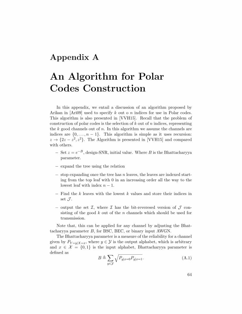
Appendix A
An Algorithm for PolarCodes Construction
In this appendix, we entail a discussion of an algorithm proposed byArikan in [Ari09] used to specify k out o n indices for use in Polar codes.This algorithm is also presented in [VVH15]. Recall that the problem ofconstruction of polar codes is the selection of k out of n indices, representingthe k good channels out of n. In this algorithm we assume the channels areindices are {0, . . . , n − 1}. This algorithm is simple as it uses recursion:z → {2z − z2, z2}. The Algorithm is presented in [VVH15] and comparedwith others.
− Set z = e−B, design-SNR, initial value. Where B is the Bhattacharyyaparameter.
− expand the tree using the relation
− stop expanding once the tree has n leaves, the leaves are indexed start-ing from the top leaf with 0 in an increasing order all the way to thelowest leaf with index n− 1.
− Find the k leaves with the lowest k values and store their indices inset J .
− output the set I, where I has the bit-reveresed version of J con-sisting of the good k out of the n channels which should be used fortransmission.
Note that, this can be applied for any channel by adjusting the Bhat-tacharyya parameter B, for BSC, BEC, or binary input AWGN.
The Bhattacharyya parameter is a measure of the reliability for a channelgiven by PY=y|X=x, where y ∈ Y is the output alphabet, which is arbitraryand x ∈ X = {0, 1} is the input alphabet, Bhattacharyya parameter isdefined as
B ,∑
y∈Y
√
Py|x=0Py|x=1. (A.1)
64