Aantekeningen bij ooit, deel 2: de opkomst van niet-polair ooit
Upload
khangminh22Category
view
1download
0
Memorandum To (SodM), (RWS), (Kustwacht), (Min EZK) Copy From ONE-Dyas Date 23 september 2020 Subject Verslag overleg vergunningsaanvraag pijpleiding, kabel N05-A
ONE-Dyas is bezig met de vergunningsaanvragen voor een ontwikkeling van het N05-A veld in blok N05. Hiervoor zal ook een pijpleiding naar de NGT en een kabel naar het Duitse windpark Riffgat aangelegd worden. Ter voorbereiding van de vergunningsaanvraag houdt ONE-dyas een presentatie om het tracé en de wijze van installatie van de leiding en de kabel te verduidelijken. Introductie ONE-Dyas presenteert een overzicht van de ontwikkeling van N05-A. Slide 2 en 3. Hij gaat in op de pijpleidingroute en de route voor de kabel naar het Windpark Riffgat, slide 4 en 5. Het jacket en platform ontwerp van N05-A worden getoond, slide 6-8
Opmerking SodM: Omdat die niet tussen mijnbouwinstallaties loopt, wordt de kabel niet automatisch aangewezen als pijpleiding onder het Mbb. Het dient bevestigd te worden of de minister de kabel aanwijst als pijpleiding onder de Mbb, waarbij mogelijk meespeelt dat het verbonden is met een buitenlands windpark. Indien de kabel niet aangewezen wordt als pijpleiding onder het Mbb, is mogelijk een Watervergunning nodig voor de kabel. ONE-Dyas overlegt met EZK over soort vergunning voor de kabel. RWS zal dit ook overleggen met EZK. Reactie ONE-Dyas: art 92 Mbb: met een pijpleiding wordt bedoeld een andere leiding dan bedoeld onder 1°, aan te wijzen door Onze Minister, die een mijnbouwwerk verbindt met een ander werk ten behoeve van het vervoer van stoffen te rekenen vanaf de eerste isolatieafsluiter van het mijnbouwwerk; (Mijnbouwwet art 1, sub ag onder 2). De kabel kan dus aangewezen worden als pijpleiding, omdat:
1. Een windpark een ’ander werk’ is. 2. De locatie van dit ‘andere werk’ is geen criteria voor de aanwijzing als pijpleiding.
Presentatie onderzoeken ONE-Dyas presenteert de onderzoeken die gedaan zijn om een tracé voor de pijpleiding en de kabel vast te stellen. Slide 9-13. Opmerking over Environmental Survey Results: Geen habitat H1170 gevonden, Borkumse Stenen wordt mogelijk beschermd obv KRM.

Memorandum Vraag RWS Worden UXO’s vermeden? Reactie ONE-Dyas: Dit is het uitgangspunt voor de pijplijn route, Magnetische contacten worden met een vaste afstand gemeden. In Duitsland zal nog extra UXO onderzoek nodig zijn, hierbij wordt de kabel in Nederland meegenomen. Opmerking Kustwacht UXO campagnes graag melden aan de Kustwacht, zodat Defensie zich kan voorbereiden op eventuele ontmanteling.
Presentatie pijpleiding en kabel Frits toont de fysische eigenschappen van de pijpleiding, slide 14
Vraag van SodM: welke operationele druk heeft de leiding, aangezien de leiding aansluit op de NGT Reactie ONE-Dyas: de leiding is ontworpen voor een druk van 85 en 90 bar, omdat NGT overweegt de druk te verlagen. Voorlopig zal de operationele druk 90 bar zijn. Vraag van SodM: Is het mogelijk de leiding te piggen? Het is een harde eis, ook voor spur leiding, dat de integriteit van de leiding op ieder moment kan worden aangetoond. Reactie ONE-Dyas: het wordt mogelijk om de pijpleiding te piggen via een tijdelijke sidetap vanaf de NGT naar N05-A. Deze tijdelijke pig launcher wordt verwijderd na aanleg. ONE-Dyas komt met een alternatieve methode om de integriteit van de leiding te kunnen aantonen.
ONE-Dyas toont de fysische eigenschappen van de kabel, slide 15. De kabel moet nog ontworpen worden; inclusief fiber optic voor data communicatie.
Opmerking SodM: In het verleden zijn er bepaalde stakeholders die de wenselijkheid van het gebruik van duurzaam opgewekte energie voor fossiele energie ter discussie hebben gesteld. Het is goed hier rekening mee te houden.
Slide 16: installatie methode pijpleiding, kabel. Door waterdiepte is een DP schip niet mogelijk voor de aanleg van de pijpleiding: mogelijk zullen mass excavation pumps gebruikt worden. Eerst pijpleiding leggen dan met mass excavation in de bodem laten zakken.
Opmerking RWS: Er zijn veel stenen in dat gebied. De pijpleiding door het eigen gewicht in de bodem laten zakken kan een probleem zijn bij een stenige ondergrond. Reactie ONE-Dyas: Route is op 25 m van grotere stenen gekozen. Er zijn met name stenen bij eerste km vanaf het platform. Opmerking SodM: Minimale begraafdiepte opnemen in aanvraag en ook de onderzochte aspecten die hebben geleid tot de minimale begraafdiepte beschrijven. Reactie ONE-Dyas: voor leidingen groter dan 20” geldt in principe geen begraafdiepte, dit was alleen nodig voor de stabiliteit. Er wordt nog gekeken of de leiding (top op pipe) gelijk met het zeebed kan worden gelegd. Minimale begraafdieptes incl. onderbouwing zullen in de vergunningsaanvraag worden meegenomen. Opmerking SodM, RWS Voor een kabel geldt een minimale diepte van 1 m beneden zeebed op open zee, gerelateerd aan ligging van het zeebed.

Memorandum Reactie ONE-Dyas: begraafdiepte is inderdaad 1 m. de streefdiepte is dieper. Vraag Kustwacht: Hoe zit het met de overvisbaarheid van de pijpleiding? Reactie ONE-Dyas: Bij een 20" leiding is dit geen probleem: vistuig blijft er niet achter hangen, leiding wordt niet beschadigd door vistuig.
ONE-Dyas presenteert de voorgestelde methode voor de tie-in op de NGT. Slide 17 en 18 locatie van de tie-in NGT: aansluiting op bestaande tie-in scheelt kosten, maar ligt net buiten de gesurveyde corridor. Ontbrekende informatie is opgevraagd bij NGT en getracht te intrapoleren met bestaande onderzoeken. Slide 19- 25 Bestaande tie-in aanpassing
Vraag SodM: Welke waterdiepte moet gehanteerd worden bij de NGT? Reactie Kustwacht: In principe 10 meter
Reactie ONE-Dyas: Waterdiepte bij NGT is nu 6 m, dome steekt 2 m boven NGT uit. Voor de installatie zal eerst de bestaande rockdump verwijderd worden. Reactie SodM: belangrijk om dit goed op te nemen in vergunningsaanvraag. Ook moet de subsea dome overvisbaar zijn. Opmerking SodM: Het eigendom van de pijpleiding moet helder zijn: waar begint de eigendom, aansprakelijkheid van de NGT, waar begint eigendom. Reactie ONE-Dyas: het meest logisch lijkt de eerste klep op de sidetap. Voor vergunningsaanvraag dient duidelijk te zijn welke afspraken er gemaakt zijn met de NGT, alternatief is dat dit als mogelijk voorwaarde opgenomen wordt in de vergunning. Opmerking SodM: Goede oplossing voor gebruik van bestaande sidetap. Goed om piglauncer aan te kunnen sluiten: extra aansluiting. Reactie ONE-Dyas: aansluiting via een hottap is de fall back optie.
Vragen Jaap van den Hoed:
1. Is er overleg met TenneT over de kabel van de windparken ‘Boven de eilanden’ Reactie ONE-Dyas: Er is overleg, de kabels van het windpark liggen westelijker dan de N05-A leiding, er zijn geen kruisingen met onze leiding.
2. Coordinaten in lat lon: ETRS89 3. Westereems: leiding loopt door Westereems: moet betrokken worden bij de aanvraag. VTS
loopt tot ongeveer boorlokatie. Kusteacht geeft naw . (deze zijn ontvangen): Reactie ONE-Dyas: de pijpleiding ligt buiten de eigenlijk vaarroute en passeert de boei aan de westkant.
4. Oesterherstelproject ten noorden van N05-A: bekend? Reactie ONE-Dyas: Ja, er is overleg met WNF.
5. Verdachte bewegingen van Greenpeace etc. doorgeven aan Kustwacht. 6. Wanneer gaat ONE-Dyas het jacket installeren? Reactie ONE-Dyas: over 2 a 3 jaar 7. UXO campagne: melden aan kustwacht/defensie.

Memorandum Vragen RWS Grens NL-Dtl: Westereemsverdrag: check grensoverschrijdende situatie Vragen aan EZK: Kan de kabel als pijpleiding aangewezen worden. EZK gaat het onderzoeken. Als het niet het geval is dan is een Waterwetvergunning nodig en co-ordinatie tussen Waterwet en Wabo. Voorbeelden worden genoemd van Q13 en Ameland-Westgat van de NAM. Hier is de kabel vergund onder het mijnbouwbesluit. SodM checkt het voorbeeld van Q13.

N05A Development
SODM September 2020

Drilling and completion of gas wells in the N05A block. Installation of a gas processing platform. Installation of a gas export pipeline from the N05A platform to a tie-in point at the NGT pipeline. Tie-in of the pipeline to the platform and NGT pipeline. Installation of a power cable from the Riffgat windfarm to the N05A platform. Tie-in of the power cable to the platform and windfarm transformer station. Burial of the pipeline and power cable.
24/09/2020 <Presentation title> 2
N5A Development Project Overview

24/09/2020 <Presentation title> 3
N05A Field Location

24/09/2020 <Presentation title> 4
N05A Field Layout

24/09/2020 5
N05A Platform Approaches
Status update MT_N05A development - Basic Engineering
24/09/2020 6
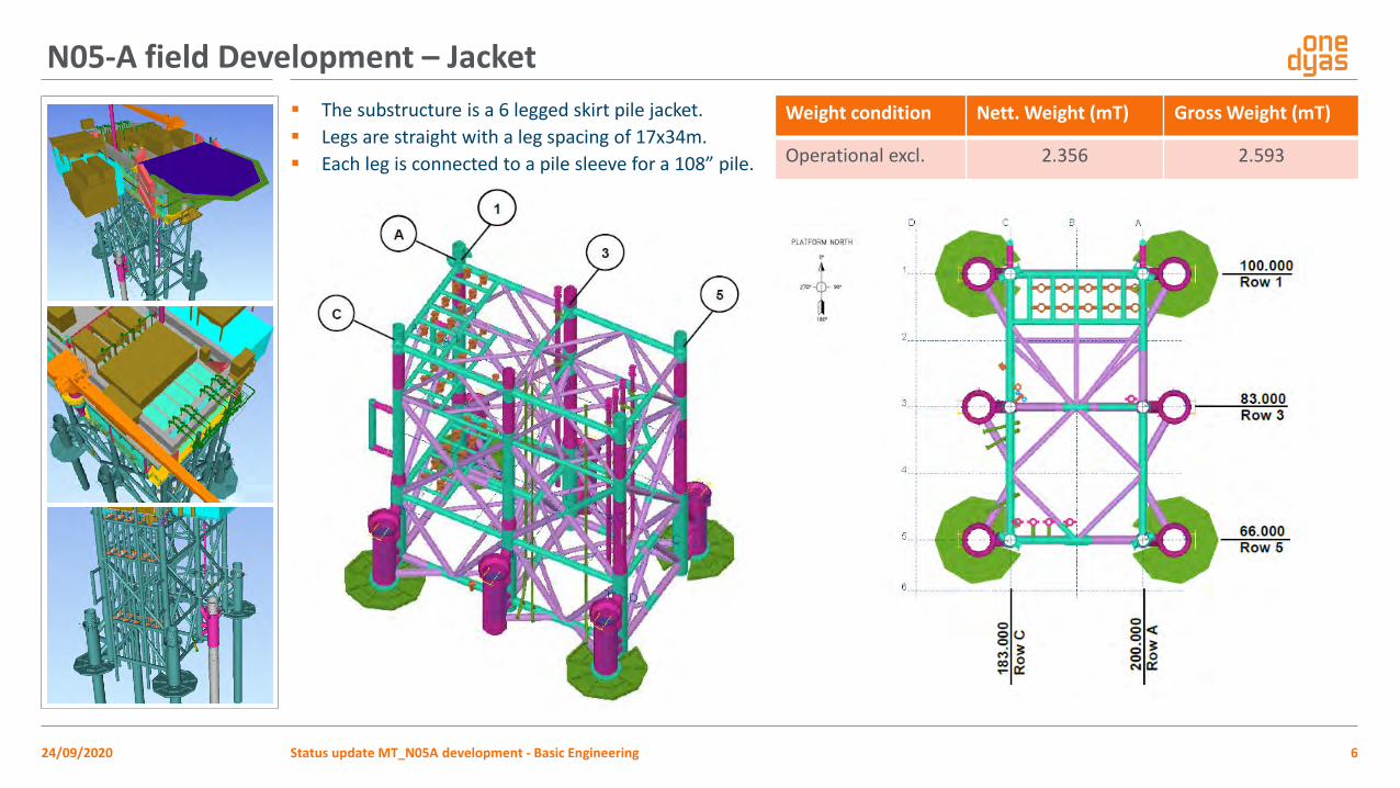
N05-A field Development – Jacket The substructure is a 6 legged skirt pile jacket. Legs are straight with a leg spacing of 17x34m. Each leg is connected to a pile sleeve for a 108” pile.
Weight condition Nett. Weight (mT) Gross Weight (mT)
Operational excl. 2.356 2.593
Status update MT_N05A development - Basic Engineering

24/09/2020 Status update MT_N05A development - Basic Engineering 7
N05-A field Development – Topside
Topside structure consists of 2 main levels and an aluminium helicopter structure.
On the topside there is space for equipment, living quarters and walkways, three staircases enable personnel to reach the different levels.
Ventboom 33m.
Weight condition Nett Weight (mT) Gross Weight (mT)
Operational 2.265 2.640
Operational incl. future module 2.887 3.265
Weight categories
Gross Weight (mT)
Architectural 57,0
Electrical 148,2
Instrumentation 52,6
Mechanical 571,0
Piping 409,3
Structural 1.426,3
Future 600,0

24/09/2020 8
Results Basic Engineering – 3D Model including future module
Status update MT_N05A development - Basic Engineering

The following surveys have been performed for the N05A platform location and pipeline and cable routes:
- Geophysical survey- Geotechnical survey- Environmental survey
The selected survey corridor is 1000m wide,
Using the survey data the following studies have been done:
- Archaeological study- Concrete weight coated pipeline or buried pipeline- Plume modelling for pipeline and cable installation- Environmental temperature influencing by power cable.
24/09/2020 title<Presentation > 9
Performed Surveys and Studies

24/09/2020 title<Presentation > 10
Geophysical Survey Results
Water depths within route corridor Maximum: 26.7m LAT; Minimum: 9.4m LAT. The seabed shoals gently towards the south of the survey area, the end of the proposed route.
Seabed sediments within corridor Seabed sediments along the proposed pipeline route corridor are expected to comprise fine to coarse SAND, with occasional areas of coarse SAND and CLAY with gravel and shell fragments.
Debris/obstructions within corridor Numerous objects interpreted as boulders and items of debris are observed within the proposed pipeline route corridor. Most of the objects interpreted as boulders occur towards the north of the survey corridor area and coincide with areas of clay exposure. The most significant objects identified on the sonar records are interpreted as shipwrecks. The largest occurs at approximately KP2.462, the other at KP 2.373, both lay East of the selected pipeline route. Numerous magnetic contacts have been detected within the corridor survey area.

The soils in the study area of the pipeline and cable routes mostly consist of fine to medium SAND. Along the VC_C locations the percentage of clayey SILT (which can include a variable percentage of clay) increase. It should be noted that gravelly Sand was found in VC_C_5, VC_C_6, VC_C_8 VC_P, VC_P_3 between -22 and -25 m LAT approximately.
24/09/2020 title<Presentation > 11
Geotechnical Survey Results

24/09/2020 title<Presentation > 12
Environmental Survey Results

Het gecombineerde bureauonderzoek en de analyse van de meetgegevens van geofysisch onderzoek heeft uitgewezen dat in het onderzoeksgebied op twee locaties resten van mogelijk archeologische waarde voorkomen. Het gaat om de wraklocatie van de Iris/Sperrbrecher (NCN1404), die in 1942 gezonken is, en een locatie (NCN661) waar (vermoedelijk) resten van een onbekend wrak voorkomen.
De beoogde pijpleidingroute ligt op 133 tot 168 meter afstand van de twee locaties met wrakresten met mogelijke archeologische waarde. Als deze route wordt aangehouden zal de aanleg van de pijpleiding de wrakresten op deze locaties niet aantasten.
Op basis van de gegevens van dit bureauonderzoek wordt de kans dat archeologische resten worden aangetast door de geplande installatie van het platform en de aanleg van de pijpleiding en de kabel klein geacht. Dit geldt zowel voor het Nederlandse als het Duitse deel van het onderzochte gebied. Daarom wordt geadviseerd om het gebied vrij te geven voor de geplande ontwikkeling, op voorwaarde dat de routes en platformlocaties niet worden gewijzigd.
24/09/2020 title<Presentation > 13
Archaeological Study Results

24/09/2020 <Presentation title> 14
Gas Export Pipeline Data
Target burial depth minimum 1m measured from top of pipeline to mean natural seabed

The power cable is currently being designed. Design input data:
- 33kV rated 20MW - cable dimension 3x1x300 sqmm- length approx. 9km - From OWF Riffgat transformer station to N05A platform
Target burial depth minimum 1m measured from top of cable to mean natural seabed
24/09/2020 <Presentation title> 15
Power Cable Data

The power cable will be installed by a dedicated cable installation vessel, by S-lay reeling. The power cable shall be buried by jetting using a specific cable trencher. Power cable tie-ins executed from the installation vessel by pulling through J-tubes.
Pipeline installation options:- S-lay from an anchored shallow water pipelay barge.- Pull-in by S-lay from a static DP vessel at sufficient waterdepth towards NGT, followed by normal S-lay.
Pipeline burial may be executed by mechanical trenching or jetting. Pipeline tie-in at the N05A platform performed by air-diving from a DP DSV. Pipeline tie-in to the NGT pipeline executed by air diving from a static jack-up platform.
Pipeline and cable crossings with existing cables will be made by separation mattresses on either side of existing cables. Thereafter crossings will be rock-dumped.
Pipeline and cable tie-ins will also be rock-dumped.
Estimated durations:- Pipeline installation and trenching 30 days- Power cable installation and trenching 10 days- Pipeline tie-ins 20 days- Rock-dumping 7 days
24/09/2020 <Presentation title> 16
Pipeline and Power Cable Installation

24/09/2020 <Presentation title> 17
Pipeline tie-in at existing NGT sidetap

24/09/2020 <Presentation title> 18
Alternative tie-in by hot-tapping into NGT pipeline

24/09/2020 <Presentation title> 19
Side Tap Tie-in – Exchange bolts for Long bolts

24/09/2020 <Presentation title> 20
Side Tap Tie-in – Milling RTJ groove

24/09/2020 <Presentation title> 21
Side Tap Tie-in – Install DBB Ball Valve
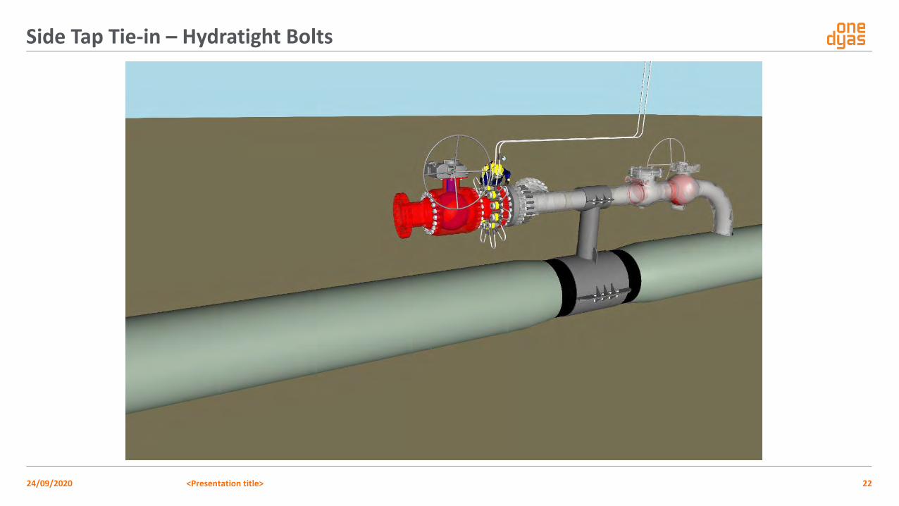
24/09/2020 <Presentation title> 22
Side Tap Tie-in – Hydratight Bolts

24/09/2020 <Presentation title> 23
Side Tap Tie-in – Hottap Through Valve and Blind flange
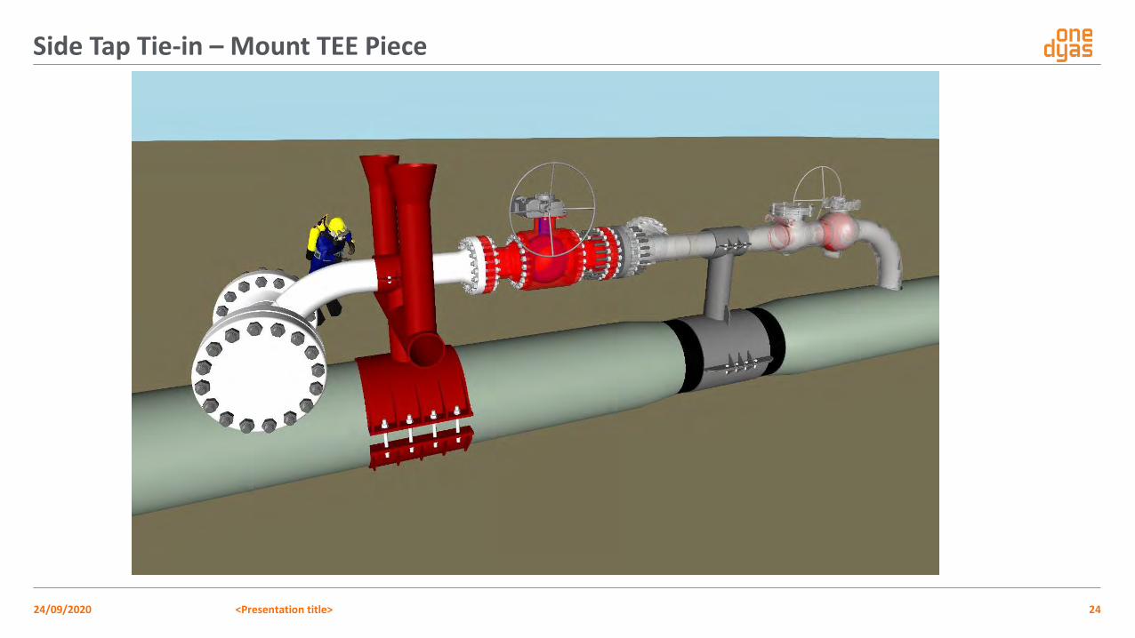
24/09/2020 <Presentation title> 24
Side Tap Tie-in – Mount TEE Piece

24/09/2020 <Presentation title> 25
Side Tap Tie-in – Install Protection Dome

N05-A Pipeline design
Route Selection Report
DOCUMENT NUMBER:
N05A-7-10-0-70031-01
Rev. Date Description Originator Checker Approver
01 15-01-2020 For Comments SvdV JvdB PF 02 17-03-2020 For Approval PF SvdV PF

Client
ONE-Dyas B.V.
Project N05-A Pipeline Design
Document Route Selection Report
Project number 19018 Document number N05A-7-10-0-70031-01 Revision 02 Date 17-03-2020
Route Selection Report N05A-7-10-0-70031-01, Rev. 02, 17-03-2020
i
Revision History
Revision Description
01 For Client Comments
02 Client comments incorporated
Revision Status
Revision Description Issue date Prepared Checked Enersea approval
Client approval
01 For Client Comments 15-01-2020 SvdV JvdB PF
02 For Approval 17-03-2020 PF SvdV PF
All rights reserved. This document contains confidential material and is the property of enersea. No part of this document may be reproduced, stored in a retrieval system, or transmitted in any form or by any means electronic, mechanical, chemical, photocopy, recording, or otherwise, without prio r written permission from the author.
Route Selection Report N05A-7-10-0-70031-01, Rev. 02, 17-03-2020
ii
Table of content 1. Introduction ......................................................................................................... 1 1.1. Project Introduction ..................................................................................................... 1 1.2. Purpose and Scope Document ...................................................................................... 2 1.3. System of Units ............................................................................................................ 2 1.4. Abbreviations ............................................................................................................... 2 1.5. References ................................................................................................................... 3 1.5.1. Regulations, Codes, Standards and Guidelines ...............................................................3 1.5.2. Company Engineering Standards and Specifications ......................................................3 1.5.3. Project Reference Documents .......................................................................................3 1.6. Holds ............................................................................................................................ 3
2. Summary .............................................................................................................. 4
3. Pipeline & Power Cable Route Data Options ........................................................... 5 3.1. General ........................................................................................................................ 5 3.2. Coordinate System ....................................................................................................... 5 3.3. Routing Options ............................................................................................................ 6 3.4. Crossings ...................................................................................................................... 7 3.5. Selected Routes ............................................................................................................ 7 3.6. Coordinates of Pipeline & Cable Routes and Key Facilities ............................................ 8 3.7. Bathymetry.................................................................................................................. 10 3.7.1. Pipeline Route ............................................................................................................. 10 3.7.2. Power Cable Route ...................................................................................................... 11 3.8. Survey Route ............................................................................................................... 12 3.8.1. Magnetometer Contacts .............................................................................................. 12 3.8.2. Geophysical Data ......................................................................................................... 14 3.8.3. Geotechnical Data ....................................................................................................... 14
A. Selected Pipeline & Power Cable Route ................................................................ 15
B. Pipeline & Power Cable Route Options ................................................................. 16
C. Environmental Data GEOxyz ................................................................................ 17

Route Selection Report N05A-7-10-0-70031-01, Rev. 02, 17-03-2020
1
Figure 1, N05A Field layout
1. Introduction
1.1. Project Introduction
One-Dyas plans to develop a successfully drilled well in block N05-A of the North Sea Dutch Continental Shelf. More wells will be drilled at this location through the same jacket. It is planned to develop the wells by installing a platform and a gas export pipeline with a connection to the NGT pipeline @KP142.1. The approximate length of the pipeline is 14.7 km. In addition, a power cable will be installed from the Riffgat Windpark to the N05-A platform.

Route Selection Report N05A-7-10-0-70031-01, Rev. 02, 17-03-2020
2
1.2. Purpose and Scope Document
The objective of this route selection study is to present the optimum pipeline route from the N05-A platform to the NGT tie-in and the power cable route from the N05-A platform to the Riffgat Offshore Substation. The major aspects that are involved in the selection of pipeline route are orientation, seabed features, future developments and constructability of the pipeline. The following aspects have been considered in the pipeline route selection study:
• Identification of seabed features such as sand dunes, mega ripples, anomalies, magnetic contacts and risk of their impact towards the selected pipeline & cable route,
• Avoid possible archaeological values
• Avoid possible environmentally sensitive areas • Selection of the shortest pipeline & cable route, • Minimizing pipeline and cable crossings, • Optimizing the extent of pre-sweeping, if required,
• Constructability aspects such as platform approach, start-up and lay down, spool installation, tie-ins, pre-sweep and trenching limitations such as lateral slopes,
• Fulfilling pipeline & cable route requirements in accordance with COMPANY Specifications, codes and standards,
• Minimum radius of curvature calculations for pipeline & cable route bends, based on installation conditions.
Note1: the installation contractor will perform a route survey immediately prior to pipelay. Subject to actual findings (sand waves, ripples, mega ripples, anomalies, magnetic contacts) a rerouting may be required
1.3. System of Units
All dimensions and calculations applied are based on the International System of Units (SI) unless noted otherwise.
1.4. Abbreviations
LAT = Lowest Astronomical Tide
MSL = Mean Sea Water Level
KP= Kilometer Post
N = North
OSS = Offshore Substation
TP = Tangent Point
IP = Intersection Point
NGT= Noord Gas Transport

Route Selection Report N05A-7-10-0-70031-01, Rev. 02, 17-03-2020
3
1.5. References
1.5.1. Regulations, Codes, Standards and Guidelines
[i] NEN3656. “Eisen voor stalen buisleidingsystemen op zee.” December 2015.
1.5.2. Company Engineering Standards and Specifications
[A] Hold [1]
1.5.3. Project Reference Documents
[1] LU0022H-553-RR-02 “5A to NGT hot tap Pipeline Route Report”
[2] LU0022H-553-RR-03-2.0 “N5a Lab Test Results Report”
[3] LU0022H-553-RR-04-2.1 N5a “Habitat Assessment Survey Report”
[4] LU0022H-553-RR-05-1.1 N5a “Environmental Baseline Survey Report”
[5] 181892-1-R2 “Metocean Criteria for the N05A Platform”
[6] 191146-1-R2 “Metocean Criteria for the N05A Platform – Side Tap”
[7] P904921/02 “N5A Development Site – Engineering Advice – Geotechnics”
[8] N05A-7-10-0-70026-01 “Basis of Design Pipeline & Tie-in Spools”
[9] N05A-7-10-0-70030-01 “Risk assessment & dropped object analysis”
[10] N05A-7-51-0-72510-01-04 “Overall field layout drawing”
[11] Geo XYZ, Surveys, 2019 LU0022H-553-RR-04-2.1, LU0022H-553-RR-05-1.1, LU0022H-553-RR-02
1.6. Holds
[1] -

Route Selection Report N05A-7-10-0-70031-01, Rev. 02, 17-03-2020
4
2. Summary
The 14.7 km pipeline originates at the N05-A Platform and terminates at the NGT tie-in location (NGT KP 142.1). The 8.7 km power cable is located between the N05-A platform and the Riffgat Offshore Substation.
The pipeline and power cable route is selected on the basis of the following criteria:
1. Shortest route possible within the given constraints; 2. Immunizing seabed intervention requirements; 3. Avoidance of restricted areas; 4. Adept a route radius curvature greater or equal to the radius requirements (2000 m resp. 100m for
pipeline and cable) 5. Minimum clearance distance of 25m from sonar contacts, 100m from magnetic contacts points and 150m
at wrecks, 6. Minimizing pipeline and cable crossings 7. Location of Start-up and lay-down target boxes such that pipeline expansion can be absorbed and
installability is feasible.
The route layout for both the pipeline and cable is shown in Figure 2-1. Reference is made to route drawing “N05A-7-51-0-72510-01-04 Overall field layout drawing”.
Figure 2-1 – Pipeline Route (see also appendix A)
Pipeline
Cable

Route Selection Report N05A-7-10-0-70031-01, Rev. 02, 17-03-2020
5
3. Pipeline & Power Cable Route Data Options
3.1. General
As per the requirements of ref. [i], the pipeline is to be buried along its entire length with a minimum burial depth TOP of 0.2m outside shipping lanes and 0.6m TOP inside shipping lanes. However, a target burial depth of 1.0m TOP is chosen covering the results of the risk assessment study and bottom roughness analysis.
ITEM VALUE
Original location N05-A Platform Tie-in location NGT tie-in Approx. pipeline length 14.7 KM Water depth -10.0 to -25.9m LAT Route bend radius pipeline 2000m
Table 3-1 General Pipeline Overview
ITEM VALUE
Original location N05-A Platform Tie-in location Riffgat OSS
Approx. cable length 8.7 KM Water depth -19.5 to -25.9m LAT Route bend radius cable 100m
Table 3-2 General Cable Overview
3.2. Coordinate System
The parameters of the geodetic system to be used for horizontal positions are taken from ref. [4] and listed in Table 4-2.
ITEM VALUE
Datum European Datum 1950 (ED50) Projection ED50 / UTM zone 31 N Ellipsoid name International 1924 Semi major axis 6 378 388 m Inverse flattening 297.000 Central Meridian 03o00”00’ E Latitude of Origin 00o00”00’ N False Northing 0 mN False Easting 500 000 mE Scale Factor 0.9996
Table 3-3 Geodetic parameters
The vertical position is given relative to the Lowest Astronomical Tide (LAT).

Route Selection Report N05A-7-10-0-70031-01, Rev. 02, 17-03-2020
6
3.3. Routing Options
For both the pipeline and the power cable several routing options have been reviewed bearing in mind the selection criteria as mentioned in section 1.2 and 2.
For the pipeline as well as for the power cable 3 different routes have been determined:
- Pipeline: The pipeline starts at the south side of the platform and leaves the platform in a south-westly direction. In the first area there are a lot of boulders which make it more difficult to route the pipeline without having any removals. The pipeline is running along most of the boulders with respect to the minimum clearance of 25m accept for two. The minimum distance at these locations is 14m. From this point there are three different pipeline routes determined.
o Magenta route
The pipeline is routed with a minimum bending radius of 2000m, where the first bend starts at least 1.0 km from the target box. The pipeline is routed at the west side of the ship wreck found, where the distance is at least 150m. From here the pipeline is routed between the magnetic contacts with respect to the distances as given in chapter 2.
o Blue route
The pipeline is routed with a minimum bending radius of 1500m, where the first bend starts at least 1.0 km from the target box. The pipeline is routed at the east side of the ship wreck found, where the distance is at least 150m. From here the pipeline is routed between the magnetic contacts with respect to the distances as given in chapter 2.
o Green route
The pipeline is routed with a minimum bending radius of 2000m, where the first bend starts at 0.8 km from the target box. The pipeline is routed at the east side of the ship wreck found, where the distance is at least 150m. From here the pipeline is routed at the east side of the first magnetic contact because the bending radius of 2000m is not allowing it to pas the magnetic contact at the west side. The next section of the pipeline is routed between the magnetic contacts with respect to the distances as given in chapter 2.
- Power cable: The power cable starts at the east side of the platform and has three different cable routes.
o Option 1a
The cable is routed to the north side of the corridor with minimum distances as given in chapter 2. At KP 0.8 the cable is routed to the centre of the corridor and goes through the magnetic contacts. At KP 2.5 the cable is routed between two magnetic contacts where the minimum distance to the closed magnetic contact is 60m. From here the cable is going North to avoid the SSS-contacts in this area.
o Option 1b
The cable is routed at the north side of the corridor with minimum distances as given in chapter 2. At KP 2.5 the cable is routed close to the North edge of the corridor with a minimum distance of 150m with the upper North magnetic contact.
o Option 2
The cable is routed at the south side of the corridor with minimum distances as given in chapter 2. At KP 3.0 the cable is routed between two magnetic contacts where the minimum distance to the closest magnetic contact is 38m. From here the cable is going North to avoid the SSS-contacts in this area.
Route Selection Report N05A-7-10-0-70031-01, Rev. 02, 17-03-2020
7
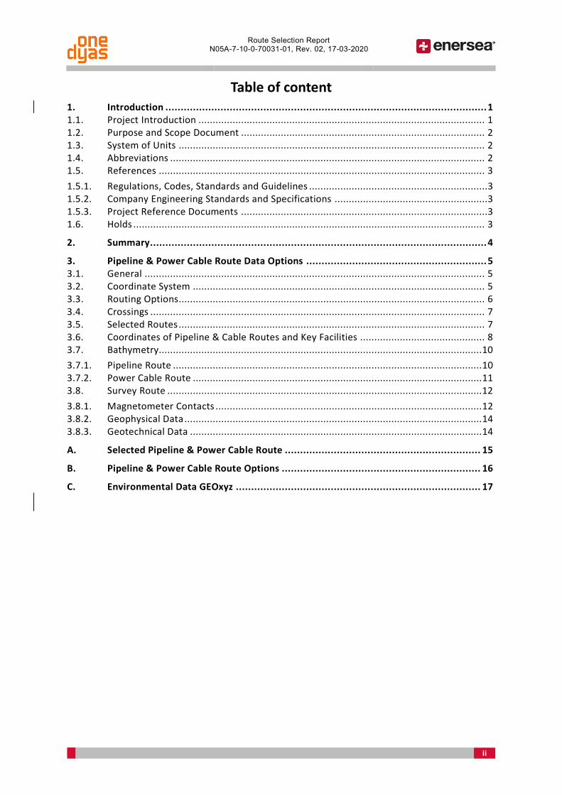
Reference is made to figure 3-1 indicating the different pipeline and cable route options.
Figure 3-1 – Pipeline Route Options (see also appendix B)
3.4. Crossings
Along the route options several in/out of use cable crossings/features are anticipated based on the surveys [1], [3] and [4]:
Pipeline: Cable:
- Unclassified linear feature @KP 2.6 - Power cable NorNed @KP 2.3
- Power cable crossing Gemini OWP (2x) @KP 6.4
- Telecom cable Tycom Telecom @KP 8.2
3.5. Selected Routes
Pipeline:
The selected pipeline is the magenta route option. By passing the wreck at the west side the magnetic contacts of the unknown linear feature are avoided. This pipeline route has also the minimum amount of bends, only 2 and has the longest straight part between the first bend and the platform.
Cable:
The selected cable route is cable route option 01b. By routing the cable at the north side of the corridor all the magnetic contacts are avoided with a minimum clearance of 100m.
Pipeline routes
Cable routes

Route Selection Report N05A-7-10-0-70031-01, Rev. 02, 17-03-2020
8
3.6. Coordinates of Pipeline & Cable Routes and Key Facilities
For the selected routes, table 3-4 provides an overview of the positions of the pipeline, cable, tie-in locations and crossings.
Location Point Easting
(mE) Northing
(mN) Bearing
(°) Radius
(m) KP
(km)
PIP
ELIN
E
N05-A PLATFORM 721.607 5.954.650
N05-A PLATFORM TARGET BOX 721.622 5.954.608 0,000 219
TP-1 720.725 5.953.484 1,428
IP-1 720.454 5.953.144 2000
TP-2 720.348 5.952.723 2,293 194
TP-3 718.799 5.946.549 8,659
IP-2 718.738 5.946.309 2000
TP-4 718.738 5.946.062 9,151
180
NGT TARGET BOX 718.738 5.940.549 14,664
NGT TIE-IN POINT 718.766 5.940.532
CROSSINGS PIPELINE
POWER CABLE BUITENGAATS 719.346 5.948.729 6,412
POWER CABLE ZEEENERGIE 719.327 5.948.655 6,487
TELECOM CABLE TYCOM TELECOMS 718.915 5.947.014 8,180
PO
WER
CA
BLE
N05-A PLATFORM 721.607 5.954.650
N05-A PLATFORM TARGET BOX 721.636 5.954.637 0,000 90
TP-1C 721.664 5.954.637 0,028
IP-1C (platform pull in) 721.668 5.954.637 15*
TP-2C 721.671 5.954.639 0,035 63
TP-3C 721.876 5.954.745 0,266
IP-2C 721.892 5.954.753 100
TP-4C 721.910 5.954.755 0,302
84
TP-5C 723.428 5.954.926 1,829
IP-3C 723.440 5.954.628 100
TP-6C 723.452 5.954.626 1,853
97
* The pull-in radius is smaller than the normal bending radius of the cable.

Route Selection Report N05A-7-10-0-70031-01, Rev. 02, 17-03-2020
9
Location Point Easting
(mE) Northing
(mN) Bearing
(°) Radius
(m) KP
(km)
TP-7C 724.774 5.954.766 3,185
IP-4C 724.784 5.954.765 100
TP-8C 724.794 5.954.762 3,206
109
TP-9C 726.933 5.954.026 5,468
IP-5C 726.965 5.955.015 100
TP-10C 726.997 5.954.025 5,533
72
OSS RIFFGAT TARGET BOX 729.998 5.955.018 8,694
CROSSINGS CABLE
POWER CABLE NORNED 723.853 5.954.878 2,257
Table 3-4 Coordinates of Selected Pipeline & Cable Route and Key Facilities

Route Selection Report N05A-7-10-0-70031-01, Rev. 02, 17-03-2020
10
3.7. Bathymetry
The water depth ranges between -10.0m and -25.9m LAT along the pipeline route, whereas the water depth variation along the cable route is between -19.5m and -25.9m LAT, with the seabed gently dipping to the north.
3.7.1. Pipeline Route
The water depths along the pipeline route at the platform, tie-in and at crossing locations are listed in the Table below; data has been taken from Reference [10].
Location Water Depth (m)
[LAT]
N05-A Platform – target box -25.9
NGT tie-in – target box -10.0
Power cable Buitengaats -19.2
Power cable Zeeenergie -19.0
Telecom cable Tycom Telecom -17.6
Table 3-5 Pipeline Water Depths at Platform, tie -in and Crossings
Figure 3-2 – Seabed Profile along Proposed Pipeline Route

Route Selection Report N05A-7-10-0-70031-01, Rev. 02, 17-03-2020
11
3.7.2. Power Cable Route
The water depths along the cable route at the platforms and at crossing locations are listed in the Table below; data has been taken from Reference [10].
Location Water Depth (m)
[LAT]
N05-A Platform – target box -25.9
Riffgat OSS – target box -20.0
Power cable NorNed -23.6
Table 3-6 Power Cable Water Depths at Platforms and Crossings
Figure 3-3 – Seabed Profile along Proposed Power Cable Route
Route Selection Report N05A-7-10-0-70031-01, Rev. 02, 17-03-2020
12
3.8. Survey Route
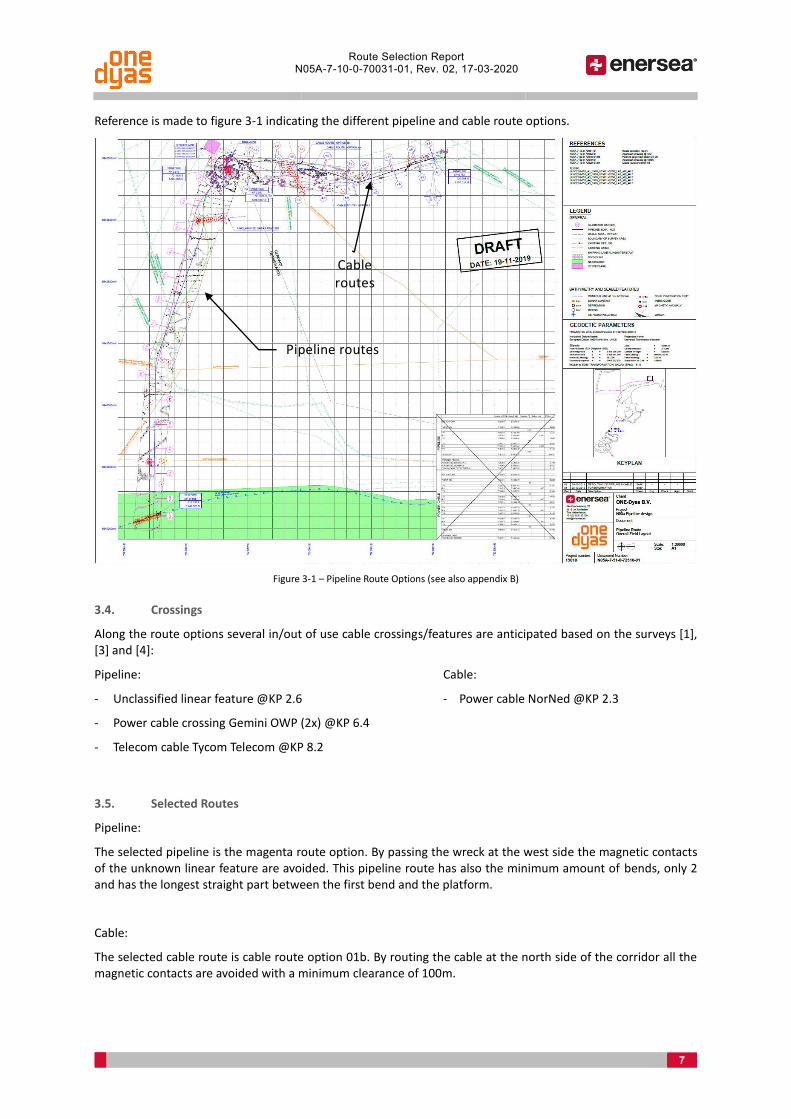
3.8.1. Magnetometer Contacts
A total of 241 magnetic anomalies (appendix C) were picked within the surveyed N05-A platform to the 36” NGT Tie-in and N05-A platform to Riffgat Tie-in route corridor. Most of these anomalies can be attributed to unknown identified seabed features. The following seabed infrastructures are known, one (1) pipeline and four (4) cables. However, there is one (1) unknown linear feature.
The following existing pipelines and cable are detected:
• 36” Pipeline from L10-AR to Uithuizen • Tycom Telecom cable • Buitengaats Power cable • Zeeenergie Power cable • Norned Power cable
Figure 3-4 – Magnetometer Contacts showing route crossing with cables
Route Selection Report N05A-7-10-0-70031-01, Rev. 02, 17-03-2020
13
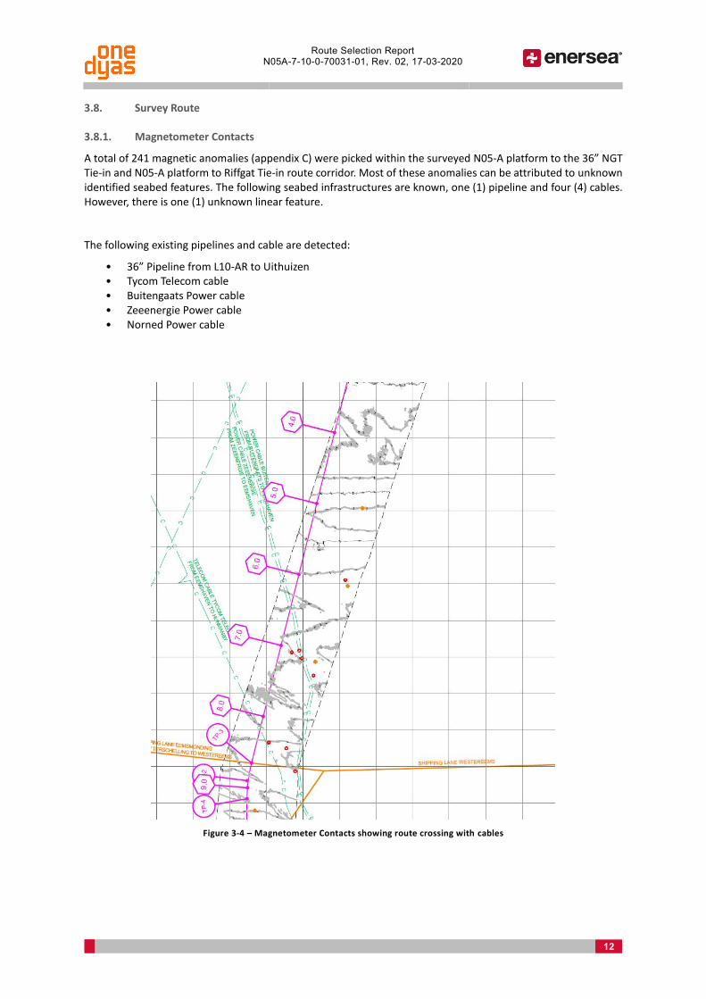
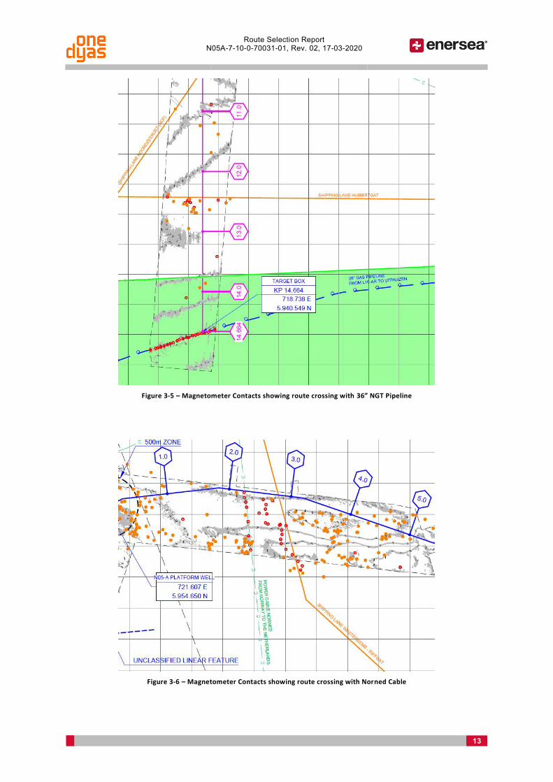
Figure 3-5 – Magnetometer Contacts showing route crossing with 36” NGT Pipeline
Figure 3-6 – Magnetometer Contacts showing route crossing with Norned Cable

Route Selection Report N05A-7-10-0-70031-01, Rev. 02, 17-03-2020
14
3.8.2. Geophysical Data
Eight-Hundred-Thirty (830) side scan sonar contacts were observed within the route survey. Most of the contacts are boulders located around the N05-A platform and stretching to the east side to Riffgat. Besides the boulders the following contacts are found: twenty-six (26) debris items, two (2) wrecks. Side scan sonar data can be found in Appendix C
3.8.3. Geotechnical Data
The majority of the surface sediments is interpreted as fine to medium grained sand and generally thickening to the south. Sand was absent (or less than 0.5m thick) from KP 0.430 to KP 0.450, KP 0.757 to KP 1.045 and near KP 5.0 (channel), where the subsoil consists of sand with layers of clay. The soil properties are based on assumptions with reference to the geo-surveys reports, ref [11]. The 0.5 m top layer consists of mobile and loose sand properties. The clay outcrops are regarded as hard soil and to the South the subsoil sands are assumed to be medium.
Route Selection Report N05A-7-10-0-70031-01, Rev. 02, 17-03-2020
15
A. Selected Pipeline & Power Cable Route
(1 page: ref. N05A-7-51-0-72510-01-05 Overall field layout drawing)

N05
-A
ONE D
YAS
22
22
229,3 t
Westereemsvaktype D
SHIPPING LANE WESTEREEMS
SHIP
PING
LAN
E NO
ORDZE
EKUS
T (N
CP)
SHIPPING LANE EEMSMONDINGFROM TERSCHELLING TO WESTEREEMS
SHIPPING LANE HUIBERTGAT
SHIPPING LANE WESTEREEMS - RIFFGAT
OO
OO
OO
OO
OO
OO O O O O O O O O O O O O
O OO
OO
OO
O O O O O O O O O O O O O O O O O
POW
ER C
ABLE BUITEN
GAATS
FRO
M BU
ITENG
AATS TO EEM
SHAVEN
POW
ER C
ABLE ZEEENER
GIE
FRO
M ZEEEN
ERG
IE TO EEM
SHAVEN
TELECOM
CABLE TYCOM
TELECOM
FROM
EEMSHAVEN TO
HUNMANBY
Riffgat
POW
ER C
ABLE NO
RN
ED
FRO
M N
OR
WAY TO
THE N
ETHER
LAND
S
-13.
0 -13.0-13.0
-13.0
-13.
0
-13.0
-13.
0
-13.0
-13.0
-13.0
-13.0
-13.0
-13.0
-13.0-13.0
-13.
0-13.0
-13.0
-13.0
-13.0-13.0
-13.0
-13.
0
-13.0-13.0
-13.0
-13.0
-13.
0-13.0
-13.0
-13.0
-13.
0-13.0-1
3.0
-13.0
-13.0
-13.0
-13.0
-13.0
-12.0
-12.0
-12.
0
-12.0
-12.
0
-12.0
-12.0 -12.0
-12.0
-11.
0 -11.
0 -11.
0
-11.0
-11.0-11.0-11.0
-11.0
-11.0
-11.0
-10.0
-10.0
-10.0-10.
0
-10.0
-10.
0
-10.
0
-10.
0
-10.
0
-10.0
-10.0
-10.0
-10.0
-10.0
-10.0
-9.0
-9.0
-9.0-9.0
-9.0-9.0
-14.0
-14.0
-14.
0-1
4.0
-14.
0
-14.0
-14.0 -14.
0
-14.0
-14.0-14.0 -14.0
-14.0
-14.
0-14.0
-14.0
-14.0-14.0
-14.0
-14.
0 -14.0
-14.0
-14.
0-1
4.0
-14.
0
-14.0
-14.0
-14.0 -14.0
-14.0-14.0
-15.
0
-15.0
-15.0-15.0
-15.0-15.0-15.0
-15.0
-16.0
-16.0-16.0
-16.0
-16.
0
-16.0
-16.0
-16.0
-16.
0
-16.0 -16.0
-16.0
-16.0
-16.
0
-16.0
-16.0
-16.0
-16.0
-16.0
-17.0
-17.0
-17.0
-17.0
-17.0
-17.
0
-17.0
-17.0
-17.0
-17.0 -17.0
-17.0-17.0-17.0 -1
7.0
-17.0-1
7.0 -17.0
-18.
0
-18.0
-18.0
-18.0
-18.0
-18.0 -18.
0 -18.0
-18.0 -18.0
-18.0
-18.0
-18.0
-18.0
-18.0
-18.
0 -18.
0-1
8.0
-18.0
-18.0
-18.0
-18.0
-18.0
-18.0
-18.0
-18.0
-18.
0
-17.0
-17.0
-18.0
-18.0-18.0
-18.0
-19.0
-19.0
-19.0
-19.0
-19.0-19.0
-19.0
-19.0-19.0-19.0-19.0
-19.
0
-20.0
-20.0
-20.
0-2
0.0
-20.0
-20.
0
-20.
0
-20.
0
-21.0-21
.0-21.0
-21.
0
-21.0
-21.
0-2
1.0 -21.0
-21.0 -21.
0
-21.
0 -21.
0
-20.0-20.0
-20.
0
-20.0
-20.0
-20.0
-20.0-20.
0
-19.
0 -19.0
-19.
0-19.0
-19.0
-19.0-19.0
-19.
0
-18.0
-18.0
-18.
0
-18.0
-18.
0
-18.0
-18.0
-18.0
-19.0
-19.0
-19.
0-19.0
-19.
0-19.0
-19.0
-19.0
-19.0-1
9.0
-19.0
-19.0
-19.0-1
9.0
-19.0
-19.0
-19.0
-19.0
-19.
0
-19.0
-19.
0-20.0
-20.
0
-20.
0-20.0
-20.0
-20.
0
-20.0
-20.
0-20.0
-20.0
-21.0
-21.
0
-22.0
-22.0
-21.0-21.0
-21.
0
-21.0
-21.0
-21.0
-21.0
-21.0 -21.0
-21.0
-21.
0
-22.0-22.
0
-22.0-22.0
-22.
0
-22.0 -22.0
-23.0
-23.0
-23.0
-23.0
-23.0-23.0
-24.0
-24.0
-24.0
-24.0-24.0
-24.0
-24.
0
-24.
0
-24.0
-24.0
-24.0
-24.0
-24.0-24.0
-24.0
-25.0
-25.0
-25.0
-25.0 -25.0-25.0
-25.
0
-25.0
-25.0 -25.0
-25.0
-25.
0
-25.0
-25.0
-26.0
-26.0
-26.
0
-26.0
-26.0 -26.
0
-26.0
-26.0
-26.0
-26.0
-26.0 -26.0
-26.0
-26.0
-26.0
-26.
0-26.0
-26.0-26.0
-26.
0-26.0-26.
0
-26.0
-25.0
-25.
0
-25.0
-25.0-25.0
-25.0
-25.
0
-25.0
-25.0
-25.0
-25.0
-25.0
-25.0
-25.
0-25.0
-25.0
-25.0
-25.0
-24.0
-24.0
-24.0
-24.0
-24.
0
-24.0
-24.0
-24.0
-24.0
-24.
0-2
4.0
-24.0
-24.0 -24.
0
-24.0
-24.
0
-24.0
-24.0
-23.0
-23.0
-23.
0 -23.
0 -23.0
-23.0
-23.
0
-23.
0
-23.
0
-23.0
-23.
0
-23.0-23.0 -23.0
-23.0
-23.
0-2
3.0
-23.
0-23
.0
-23.
0 -23.0
-23.0-23.0-23.0-23.0
-23.0-23.0
-24.0 -24.0
-24.0
-24.0
-24.0
-24.0
-24.0
-24.
0 -24.
0
-24.0
-24.0
-24.0-24.0-2
4.0
-24.0-24.0
-24.0
-25.0
-25.
0
-25.
0
-25.0
-25.
0-25.0
-25.0
-25.0
-25.
0 -25.0
-25.0
-25.0 -25.0
-25.0
-25.0
-25.0
-25.
0-25
.0
-25.
0
-25.0 -25.0 -25.0
-25.
0
-25.0
-22.0
-22.0
-22.0
-22.0
-22.0
-22.0
-22.0-22.0
-22.
0
-22.
0-2
2.0
-22.
0
-21.0
-21.0
-21.0
-21.0
-21.0
-21.
0-21.
0-2
1.0
-21.0
-21.0
-21.0
-21.0
-21.
0
-21.0
-21.
0
-21.
0
-21.0
-21.0
-21.0
-21.
0
-22.0
-22.
0
-23.
0
-23.0
-23.0
-20.
0
-20.0
-20.
0
-20.
0-2
0.0
-20.0
-20.0
-20.0
-19.
0
-19.
0
-19.
0
-20.
0
-20.0
-20.0
-19.0
-19.0
-20.0
-20.
0
-21.0
-21.0
-21.0
-24.0 -24.
0
-24.0
-24.0
-24.0-24.0
-24.0-24.
0
-24.
0-24.0
-24.0-24.0-24.0
-24.
0-2
4.0-24.0
-24.0
-24.0
-24.0
-24.
0
-24.0
KP 14.664718.738 E
5.940.549 N
TARGET BOX
KP 0.000721.622 E
5.954.608 N
TARGET BOX
TELECOM CABLE UK-GERMANY 3
FROM WINTERTON(GB) TO BORKUM(G)
TELECOM CABLE WINTERTON - BORKUM 1
FROM WINTERTON(GB) TO BORKUM(G)
36" GAS PIPELINE
FROM L10-AR TO UITHUIZEN
GERM
ANY
NETHERLANDS
-23.0
-23.0
-23.
0
0.0
1.02.0
3.0
4.0
5.0 6.0
7.0
8.0
8.7
TP-1
N05-A PLATFORM WELL
721.607 E5.954.650 N
IP-1
TP-2
TP-3
TP-4
IP-2
14.7
0.0
1.0
2.0
3.0
4.0
5.0
6.0
7.0
8.0
9.0
10.0
11.0
12.0
13.0
14.0
14.6
64
All rights reserved. This document contains confidential material and is the property of Enersea. No part of this document may be reproduced, stored in a retrieval system, or transmitted in any form or by any means electronically, mechanically, chemically, by photocopy, by recording, or otherwise, without Enersea's prior written permission.
REFERENCESN05A-7-50-0-72018-01/06
N05A-7-50-0-72019-01N05A-7-10-0-70032-01
GEOxyzLU0022H-553_A1_1905_UTM31-ED50_LAT_MB_#0.5LU0022H-553_A2_1905_UTM31-ED50_LAT_MB_#0.5 + EXTRA POLYGONLU0022H-553_A3_1905_UTM31-ED50_LAT_MB_#0.5 + EXTRA POLYGONLU0022H-553_A4_1905_UTM31-ED50_LAT_MB_#0.5LU0022H-553_A5_1905_UTM31-ED50_LAT_MB_#0.5
Pipeline alignment sheet - Buried / Unburied option - sheet01-06Approach drawing @ N05AApproach drawing @ NGT
Horizontal Datum Name:European Datum 1950 North Sea -UKCS
Ellipsoid:International 1924 (Hayford 1909)Semi major axis a = 6 378 388.000Semi minor axis b = 6 356 911.946Inverse ELattening 1/f = 297.000Excentricity squared e = 0.006 722 670
Projection Name:Universal Transverse Mercator
Zone : = North 31Central meridian : = 3° EastLatitude of origin : = EquatorFalse Easting : = 500 000.00 mFalse Northing : = 0.00 mScale factor on C.M.: = 0.999 6
PROJECTED CRS: ED50/UTM zone 31N (EPSG: 23031)
WGS84 to ED50 TRANSFORMATION: UKOAA (EPSG: 1311)
GEODETIC PARAMETERS
KEYPLAN
LEGENDGENERAL
KILOMETER MARKER
PIPELINE: N05A - NGT
CABLE: N05A - RIFFGAT
BOUNDARY OF SURVEY AREA
EXISTING PIPELINE
EXISTING CABLE
SHIPPING LANE RIJKSWATERSTAAT
ROCKDUMP
NATURA2000
OYSTERBANK
O
Client
Project
Document
Scale:
Jan Evertsenweg 123115 JA SchiedamThe Netherlands+31(0) [email protected]
Size:
Document NumberProject number:
ONEDyas B.V.
N05-A TO NGT PIPELINE
Pipeline RouteOverall Field Layout
1:30000A1
N05A-7-51-0-72510-0119018
01Rev Date CheckEng. Appr. ClientDrawnDescription
-- -SvdV23-10-2019 FOR INFORMATION
7200
00m
E
5942500mN
5940000mN
BATHYMETRY AND SEABED FEATURES
CONTOUR LINE AT 1m INTERVAL
SONAR CONTACT
DEPRESSION
MOUND
AS-FOUND WELLHEAD
CONE PENETRATION TEST
VIBRE CORE
MAGNETIC ANOMALY
WRECK
7250
00m
E
7300
00m
E
7175
00m
E
7225
00m
E
7275
00m
E
5942500mN
5942500mN
5942500mN
5942500mN
5942500mN
7325
00m
E
OYSTER BANK1. 720951.850 E, 5955840.077 N
2. 721381.786 E, 5955584.877 N
3. 721126.478 E, 5955154.840 N
4. 720695.873 E, 5955410,485 N
UNCLASSIFIED LINEAR FEATURE
02 -- -SvdV20-11-2019 REROUTING OF PIPELINE & CABLE
500m ZONE
03 PF- PFSvdV06-12-2019 FOR COMMENTS04 PF- PFSvdV18-12-2019 CLIENT COMMENTS INCORPORATED05 PF- PFSvdV04-02-2020 CLIENT COMMENTS INCORPORATED

Route Selection Report N05A-7-10-0-70031-01, Rev. 02, 17-03-2020
16
B. Pipeline & Power Cable Route Options
(1 page: ref. N05A-7-51-0-72510-01-02b Overall field layout drawing)

Westereemsvaktype D
SHIPPING LANE WESTEREEMS
SHIP
PING
LAN
E NO
ORDZE
EKUS
T (N
CP)
SHIPPING LANE EEMSMONDINGFROM TERSCHELLING TO WESTEREEMS
SHIPPING LANE HUIBERTGAT
SHIPPING LANE WESTEREEMS - RIFFGAT
OO
OO
OO
OO
OO
OO O O O O O O O O O O O O
O OO
OO
OO
O O O O O O O O O O O O O O O O O
POW
ER C
ABLE BUITEN
GAATS
FRO
M BU
ITENG
AATS TO EEM
SHAVEN
POW
ER C
ABLE ZEEENER
GIE
FRO
M ZEEEN
ERG
IE TO EEM
SHAVEN
TELECOM
CABLE TYCOM
TELECOM
FROM
EEMSHAVEN TO
HUNMANBY
Riffgat
POW
ER C
ABLE NO
RN
ED
FRO
M N
OR
WAY TO
THE N
ETHER
LAND
S
-13.
0 -13.0
-13.0
-13.0
-13.
0
-13.0
-13.
0
-13.0
-13.0
-13.0
-13.0
-13.0
-13.0
-13.0-13.0
-13.
0-13.0
-13.0
-13.0
-13.0-13.0
-13.0
-13.
0
-13.0-13.0
-13.0
-13.0
-13.
0-13.0
-13.0
-13.0
-13.
0-13.0-1
3.0
-13.0
-13.0
-13.0
-13.0
-13.0
-12.0
-12.0
-12.
0
-12.0
-12.
0
-12.0
-12.0 -12.0
-12.0
-11.
0 -11.
0 -11.
0
-11.0
-11.0-11.0-11.0
-11.0
-11.0
-11.0
-10.0
-10.0
-10.0-10.
0
-10.0
-10.
0
-10.
0
-10.
0
-10.
0
-10.0
-10.0
-10.0
-10.0
-10.0
-10.0
-9.0
-9.0
-9.0-9.0
-9.0-9.0
-14.0
-14.0
-14.
0-1
4.0
-14.
0
-14.0
-14.0-14.
0
-14.0
-14.0-14.0 -14.0
-14.0
-14.
0-14.0
-14.0
-14.0-14.0
-14.0
-14.
0 -14.0
-14.0
-14.
0-1
4.0
-14.
0
-14.0
-14.0
-14.0 -14.0
-14.0-14.0
-15.
0
-15.0
-15.0-15.0
-15.0-15.0-15.0
-15.0
-16.0
-16.0-16.0
-16.0
-16.
0
-16.0
-16.0
-16.0
-16.
0
-16.0 -16.0
-16.0
-16.0
-16.
0
-16.0
-16.0
-16.0
-16.0
-16.0
-17.0
-17.0
-17.0
-17.0
-17.0
-17.
0
-17.0
-17.0
-17.0
-17.0 -17.0
-17.0-17.0-17.0 -1
7.0
-17.0-1
7.0 -17.0
-18.
0
-18.0
-18.0
-18.0
-18.0
-18.0 -18.
0 -18.0
-18.0 -18.0
-18.0
-18.0
-18.0
-18.0
-18.0
-18.
0 -18.
0-1
8.0
-18.0
-18.0
-18.0
-18.0
-18.0
-18.0-18.0
-18.0
-18.0
-18.
0
-17.0
-17.0
-18.0
-18.0-18.0
-18.0
-19.0
-19.0
-19.0
-19.0
-19.0-19.0
-19.0
-19.0
-19.0-19.0-19.0-19.0
-19.
0
-20.0
-20.0
-20.
0-2
0.0
-20.0
-20.
0
-20.
0
-20.
0
-21.0
-21.0
-21.0
-21.
0
-21.0
-21.
0-2
1.0 -21.0
-21.0 -21.
0
-21.
0 -21.
0
-20.0-20.0
-20.
0
-20.0-20.0
-20.0-20.0-2
0.0
-19.
0 -19.0
-19.
0-19.0
-19.0
-19.0
-19.0
-19.
0
-18.0
-18.0
-18.
0
-18.0
-18.
0
-18.0
-18.0
-18.0
-19.0
-19.0
-19.
0-19.0
-19.
0-19.0
-19.0
-19.0
-19.0-1
9.0
-19.0
-19.0
-19.0-1
9.0
-19.0
-19.0
-19.0
-19.0
-19.
0
-19.0
-19.
0-20.0
-20.
0
-20.
0-20.0
-20.0
-20.
0
-20.0
-20.
0-20.0
-20.0
-21.0
-21.
0
-22.0
-22.0
-21.0-21.0
-21.
0
-21.0
-21.0
-21.0
-21.0
-21.0 -21.0
-21.0
-21.
0
-22.0-22.
0
-22.0-22.0
-22.
0
-22.0 -22.0
-23.0
-23.0
-23.0
-23.0
-23.0-23.0
-24.0
-24.0
-24.0
-24.0-24.0
-24.0
-24.
0
-24.
0
-24.0
-24.0
-24.0
-24.0
-24.0-24.0
-24.0
-25.0
-25.0
-25.0
-25.0 -25.0-25.0
-25.
0
-25.0
-25.0 -25.0
-25.0
-25.
0
-25.0
-25.0
-26.0
-26.0
-26.
0
-26.0
-26.0 -26.
0
-26.0
-26.0
-26.0
-26.0
-26.0 -26.0
-26.0
-26.0
-26.0
-26.
0-26.0
-26.0-26.0
-26.
0-26.0-26.
0
-26.0
-25.0
-25.
0
-25.0
-25.0-25.0
-25.0
-25.
0
-25.0
-25.0
-25.0
-25.0
-25.0
-25.0
-25.
0-25.0
-25.0
-25.0
-25.0
-24.0
-24.0
-24.0
-24.0
-24.
0
-24.0
-24.0
-24.0
-24.0
-24.
0-2
4.0
-24.0
-24.0 -24.
0
-24.0
-24.
0
-24.0
-24.0
-23.0
-23.0
-23.
0 -23.
0 -23.0
-23.0
-23.
0
-23.
0
-23.
0
-23.0
-23.
0
-23.0-23.0 -23.0
-23.0-2
3.0
-23.
0
-23.
0-23
.0
-23.
0 -23.0
-23.0-23.0-23.0-23.0
-23.0-23.0
-24.0 -24.0
-24.0
-24.0
-24.0
-24.0
-24.0
-24.
0 -24.
0
-24.0
-24.0
-24.0-24.0
-24.
0
-24.0 -24.0-24.0
-25.0
-25.
0
-25.
0
-25.0
-25.
0-25.0
-25.0
-25.0
-25.
0 -25.0
-25.0
-25.0 -25.0
-25.0
-25.0
-25.0
-25.
0-25
.0
-25.
0
-25.0 -25.0 -25.0
-25.
0
-25.0
-22.0
-22.0-22.0
-22.0
-22.0-22.0
-22.0-22.0
-22.
0
-22.
0-2
2.0
-22.
0
-21.0
-21.0
-21.0
-21.0
-21.0
-21.
0-21.
0-2
1.0
-21.0
-21.0
-21.0
-21.0
-21.
0
-21.0
-21.
0
-21.
0
-21.0
-21.0
-21.0
-21.
0
-22.0
-22.
0
-23.
0
-23.0
-23.0
-20.
0
-20.0
-20.
0
-20.
0-2
0.0
-20.0
-20.0
-20.0
-19.
0
-19.
0
-19.
0
-20.
0
-20.0
-20.0
-19.0
-19.0
-20.0
-20.
0
-21.0
-21.0
-21.0
-24.0 -24.
0
-24.0-24.0
-24.0-24.0
-24.0-24.
0
-24.
0-24.0
-24.0
-24.0-24.0
-24.
0-2
4.0-24.0
-24.0
-24.0
-24.0
-24.
0
-24.0
KP 14.698718.738 E
5.940.525 N
TIE-IN POINT
KP 0.019721.605 E
5.954.609 N
TARGET BOX
KP 8.752729.998 E
5.955.018 N
TARGET BOX
8.752
TELECOM CABLE UK-GERMANY 3
FROM WINTERTON(GB) TO BORKUM(G)
TELECOM CABLE WINTERTON - BORKUM 1
FROM WINTERTON(GB) TO BORKUM(G)
36" GAS PIPELINE
FROM L10-AR TO UITHUIZEN
KP 0.000721.636 E
5.954.637 N
TARGET BOX
GERM
ANY
NETHERLANDS
14.6
9814
.7
0.0
1.0
2.0
3.0
4.0
5.0
6.0
7.0
8.0
9.0
10.0
11.0
12.0
13.0
14.0
-23.0
-23.0
-23.
0
N05-
A
ONE D
YAS 22
22
229,3 t
0.0
1.02.0
3.0
4.0
5.0 6.0
7.0
8.0
8.7
0.0
1.0
2.0
3.04.0 5.0
6.0
7.0
8.0
8.7
0.01.0
2.0 3.0 4.0
5.0 6.0
7.0
8.0
8.8
All rights reserved. This document contains confidential material and is the property of Enersea. No part of this document may be reproduced, stored in a retrieval system, or transmitted in any form or by any means electronically, mechanically, chemically, by photocopy, by recording, or otherwise, without Enersea's prior written permission.
REFERENCESN05A-7-10-0-70031-01N05A-7-10-0-70032-01N05A-7-50-0-72018-01/06N05A-7-50-0-72019-01N05A-7-10-0-72020-01/04
FUGROLU0022H-553_A1_1905_UTM31-ED50_LAT_MB_#0.5LU0022H-553_A2_1905_UTM31-ED50_LAT_MB_#0.5LU0022H-553_A3_1905_UTM31-ED50_LAT_MB_#0.5LU0022H-553_A4_1905_UTM31-ED50_LAT_MB_#0.5LU0022H-553_A5_1905_UTM31-ED50_LAT_MB_#0.5
Route selection reportApproach drawing @ NGTPipeline alignment sheet 01-06Approach drawing @ N05ACable route sheet 01-04
DRAFTDATE: 19-11-2019
Horizontal Datum Name:European Datum 1950 North Sea -UKCS
Ellipsoid:International 1924 (Hayford 1909)Semi major axis a = 6 378 388.000Semi minor axis b = 6 356 911.946Inverse ELattening 1/f = 297.000Excentricity squared e = 0.006 722 670
Projection Name:Universal Transverse Mercator
Zone : = North 31Central meridian : = 3° EastLatitude of origin : = EquatorFalse Easting : = 500 000.00 mFalse Northing : = 0.00 mScale factor on C.M.: = 0.999 6
PROJECTED CRS: ED50/UTM zone 31N (EPSG: 23031)
WGS84 to ED50 TRANSFORMATION: UKOAA (EPSG: 1311)
GEODETIC PARAMETERS
KEYPLAN
LEGENDGENERAL
KILOMETER MARKER
PIPELINE: N05A - NGT
CABLE: N05A - RIFFGAT
BOUNDARY OF SURVEY AREA
EXISTING PIPELINE
EXISTING CABLE
SHIPPING LANE RIJKSWATERSTAAT
ROCKDUMP
NATURA2000
OYSTERBANK
O
Client
Project
Document
Scale:
Jan Evertsenweg 123115 JA SchiedamThe Netherlands+31(0) [email protected]
Size:
Document NumberProject number:
ONE-Dyas B.V.
N05a Pipeline design
Pipeline RouteOverall Field Layout
1:30000A1
N05A-7-51-0-72510-0119018
01Rev Date CheckEng. Appr. ClientDrawnDescription
-- -SvdV23-10-2019 FOR INFORMATION
7200
00m
E
5942500mN
5940000mN
BATHYMETRY AND SEABED FEATURES
CONTOUR LINE AT 1m INTERVAL
SONAR CONTACT
DEPRESSION
MOUND
AS-FOUND WELLHEAD
CONE PENETRATION TEST
VIBRE CORE
MAGNETIC ANOMALY
WRECK
7250
00m
E
7300
00m
E
7175
00m
E
7225
00m
E
7275
00m
E
5942500mN
5942500mN
5942500mN
5942500mN
5942500mN
7325
00m
E
OYSTER BANK1. 720951.850 E, 5955840.077 N
2. 721381.786 E, 5955584.877 N
3. 721126.478 E, 5955154.840 N
4. 720695.873 E, 5955410,485 N
CABLE ROUTE - OPTION 2
CABLE ROUTE - OPTION 1aCABLE ROUTE - OPTION 1b
UNCLASSIFIED LINEAR FEATURE
02 -- -SvdV19-11-2019 REROUTING OF PIPELINE & CABLE
500m ZONE

Magnetic Contacts N05A-7-10-0-70031-01, Rev. 02, 17-03-2020
17
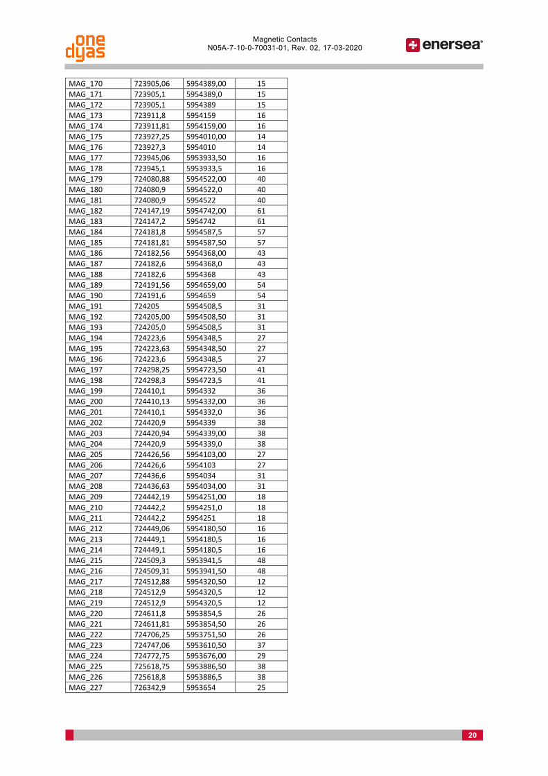
C. Environmental Data GEOxyz Magnetic Contacts
MAG ID Easting Northing Size nT
MAG_001 717953,7 5940271,5 1846 MAG_002 717991,0 5940276,5 2449 MAG_003 718039,9 5940290,0 1412 MAG_004 718041,2 5940299,0 88 MAG_005 718096,4 5940310,5 5750 MAG_006 718148,3 5942788,5 35 MAG_007 718149,5 5940331,0 2207 MAG_008 718198,9 5940350,5 4606 MAG_009 718247,8 5940365,0 878 MAG_010 718312,4 5940395,0 4218 MAG_011 718346,7 5940412,0 1847 MAG_012 718409,7 5940429,5 1254 MAG_013 718424,0 5944905,0 44 MAG_014 718444,3 5942692,5 828 MAG_015 718462,9 5941110,5 163 MAG_016 718472,4 5940453,5 1966 MAG_017 718484,8 5942724,5 4590 MAG_018 718491,8 5940449,0 962 MAG_019 718506,9 5942723,0 1900 MAG_020 718508,2 5942754,0 9330 MAG_021 718509,3 5940455,5 558 MAG_022 718516,3 5942748,5 5361 MAG_023 718534,0 5942694,0 1157 MAG_024 718548,1 5945123,5 32 MAG_025 718565,1 5940481,0 3279 MAG_026 718595,9 5942616,0 52 MAG_027 718617,5 5940493,0 5243 MAG_028 718662,3 5940506,0 613 MAG_029 718720,1 5940516,0 2386 MAG_030 718766,9 5940523,0 2963 MAG_031 718829,4 5940541,0 706 MAG_032 718856,6 5940558,0 9291 MAG_033 718875,8 5944329,5 23 MAG_034 718975,9 5941798,0 86 MAG_035 718995,8 5942736,5 67 MAG_036 719033,8 5946829,5 22 MAG_037 719274,9 5946749,5 136 MAG_038 719349,1 5948063,0 51 MAG_039 719395,2 5946438,0 14 MAG_040 719449,5 5948089,0 11 MAG_041 719489,0 5947981,0 40 MAG_042 719645,7 5947744,5 73 MAG_043 720080,7 5949053,0 11 MAG_044 720398,8 5952407,0 22 MAG_045 720432,3 5952500,5 428 MAG_046 720451,3 5952357,0 15 MAG_047 720452,1 5952553,0 197 MAG_048 720492,5 5952478,5 6757 MAG_049 720507,6 5952530,5 846 MAG_050 720589,2 5952492,5 539 MAG_051 720687,5 5951846,0 11 MAG_052 720733,6 5952469,5 17 MAG_053 720796,44 5954306,50 11

Magnetic Contacts N05A-7-10-0-70031-01, Rev. 02, 17-03-2020
18
MAG_054 720823,9 5952486,5 38 MAG_055 720895,0 5952512,5 195 MAG_056 720896,6 5952528,5 258 MAG_057 720966,9 5952512,5 155 MAG_058 720972,6 5952521,0 30 MAG_059 720981,25 5955029,50 15 MAG_060 721006,69 5954892,50 18 MAG_061 721006,69 5954892,5 18 MAG_062 721043,6 5954396,5 50 MAG_063 721043,63 5954396,50 50 MAG_064 721043,6 5954396,5 50 MAG_065 721050,88 5954393,50 66 MAG_066 721050,9 5954393,5 66 MAG_067 721050,9 5954393,5 66 MAG_068 721097,9 5953584,0 8 MAG_069 721144,6 5952537,5 59 MAG_070 721224,2 5952542,0 88 MAG_071 721272 5954784,5 23 MAG_072 721272,00 5954784,50 23 MAG_073 721272,0 5954784,5 23 MAG_074 721395,3 5952547,0 97 MAG_075 721424,3 5952569,5 110 MAG_076 721424,88 5954616,50 285 MAG_077 721424,9 5954616,5 285 MAG_078 721424,88 5954616,5 285 MAG_079 721424,9 5954616,5 285 MAG_080 721430,5 5952680,5 22 MAG_081 721567,25 5954416,50 12 MAG_082 721567,3 5954416,5 12 MAG_083 721567,25 5954416,5 12 MAG_084 721567,3 5954416,5 12 MAG_085 721568,5 5954404,5 22 MAG_086 721568,50 5954404,50 22 MAG_087 721571,7 5954762,5 18 MAG_088 721571,69 5954762,50 18 MAG_089 721571,69 5954762,5 18 MAG_090 721571,7 5954762,5 18 MAG_091 721615,3 5954915,0 27 MAG_092 721615,25 5954915,00 27 MAG_093 721615,25 5954915 27 MAG_094 721615,3 5954915 27 MAG_095 721625,25 5954596,50 53 MAG_096 721625,3 5954596,5 53 MAG_097 721625,25 5954596,5 53 MAG_098 721625,3 5954596,5 53 MAG_099 721625,4 5954919,0 28 MAG_100 721625,38 5954919,00 28 MAG_101 721625,38 5954919 28 MAG_102 721625,4 5954919 28 MAG_103 721645,7 5954971,5 66 MAG_104 721645,69 5954971,50 66 MAG_105 721645,69 5954971,5 66 MAG_106 721645,7 5954971,5 66 MAG_107 721650,5 5954550 376 MAG_108 721650,50 5954550,00 376 MAG_109 721650,5 5954550,0 376 MAG_110 721657,8 5954589 358 MAG_111 721657,8 5954589,0 358

Magnetic Contacts N05A-7-10-0-70031-01, Rev. 02, 17-03-2020
19
MAG_112 721657,81 5954589,00 358 MAG_113 721657,81 5954589 358 MAG_114 721658,0 5954624,0 45 MAG_115 721658,00 5954624,00 45 MAG_116 721658 5954624 45 MAG_117 721666,7 5954576,0 1100 MAG_118 721666,69 5954576,00 1100 MAG_119 721666,69 5954576 1100 MAG_120 721666,7 5954576 1100 MAG_121 721670,5 5954647,5 27 MAG_122 721670,50 5954647,50 27 MAG_123 721672,2 5954562,0 2733 MAG_124 721672,19 5954562,00 2733 MAG_125 721672,19 5954562 2733 MAG_126 721672,2 5954562 2733 MAG_127 721683,56 5954529,00 252 MAG_128 721683,6 5954529,0 252 MAG_129 721683,56 5954529 252 MAG_130 721683,6 5954529 252 MAG_131 721685,69 5954453,00 110 MAG_132 721685,7 5954453,0 110 MAG_133 721685,69 5954453 110 MAG_134 721685,7 5954453 110 MAG_135 721691,2 5954590,0 360 MAG_136 721691,19 5954590,00 360 MAG_137 721691,19 5954590 360 MAG_138 721691,2 5954590 360 MAG_139 721695,69 5954426,00 35 MAG_140 721695,7 5954426,0 35 MAG_141 721695,69 5954426 35 MAG_142 721695,7 5954426 35 MAG_143 721702,2 5954504,0 58 MAG_144 721702,19 5954504,00 58 MAG_145 721702,19 5954504 58 MAG_146 721702,2 5954504 58 MAG_147 721708,19 5954468,00 119 MAG_148 721708,2 5954468,0 119 MAG_149 721708,19 5954468 119 MAG_150 721708,2 5954468 119 MAG_151 721709,3 5954964,0 21 MAG_152 721709,25 5954964,00 21 MAG_153 721709,25 5954964 21 MAG_154 721709,3 5954964 21 MAG_155 721806,3 5954401,5 10 MAG_156 721806,3 5954401,5 10 MAG_157 721806,31 5954401,50 10 MAG_158 721806,31 5954401,5 10 MAG_159 722858,06 5954425,00 43 MAG_160 722858,1 5954425,0 43 MAG_161 722858,1 5954425 43 MAG_162 723840,1 5954855,5 31 MAG_163 723840,13 5954855,50 31 MAG_164 723843,06 5954772,50 17 MAG_165 723843,1 5954772,5 17 MAG_166 723868,19 5954698,50 23 MAG_167 723868,2 5954698,5 23 MAG_168 723879,8 5954617 25 MAG_169 723879,81 5954617,00 25
Magnetic Contacts N05A-7-10-0-70031-01, Rev. 02, 17-03-2020
20
MAG_170 723905,06 5954389,00 15 MAG_171 723905,1 5954389,0 15 MAG_172 723905,1 5954389 15 MAG_173 723911,8 5954159 16 MAG_174 723911,81 5954159,00 16 MAG_175 723927,25 5954010,00 14 MAG_176 723927,3 5954010 14 MAG_177 723945,06 5953933,50 16 MAG_178 723945,1 5953933,5 16 MAG_179 724080,88 5954522,00 40 MAG_180 724080,9 5954522,0 40 MAG_181 724080,9 5954522 40 MAG_182 724147,19 5954742,00 61 MAG_183 724147,2 5954742 61 MAG_184 724181,8 5954587,5 57 MAG_185 724181,81 5954587,50 57 MAG_186 724182,56 5954368,00 43 MAG_187 724182,6 5954368,0 43 MAG_188 724182,6 5954368 43 MAG_189 724191,56 5954659,00 54 MAG_190 724191,6 5954659 54 MAG_191 724205 5954508,5 31 MAG_192 724205,00 5954508,50 31 MAG_193 724205,0 5954508,5 31 MAG_194 724223,6 5954348,5 27 MAG_195 724223,63 5954348,50 27 MAG_196 724223,6 5954348,5 27 MAG_197 724298,25 5954723,50 41 MAG_198 724298,3 5954723,5 41 MAG_199 724410,1 5954332 36 MAG_200 724410,13 5954332,00 36 MAG_201 724410,1 5954332,0 36 MAG_202 724420,9 5954339 38 MAG_203 724420,94 5954339,00 38 MAG_204 724420,9 5954339,0 38 MAG_205 724426,56 5954103,00 27 MAG_206 724426,6 5954103 27 MAG_207 724436,6 5954034 31 MAG_208 724436,63 5954034,00 31 MAG_209 724442,19 5954251,00 18 MAG_210 724442,2 5954251,0 18 MAG_211 724442,2 5954251 18 MAG_212 724449,06 5954180,50 16 MAG_213 724449,1 5954180,5 16 MAG_214 724449,1 5954180,5 16 MAG_215 724509,3 5953941,5 48 MAG_216 724509,31 5953941,50 48 MAG_217 724512,88 5954320,50 12 MAG_218 724512,9 5954320,5 12 MAG_219 724512,9 5954320,5 12 MAG_220 724611,8 5953854,5 26 MAG_221 724611,81 5953854,50 26 MAG_222 724706,25 5953751,50 26 MAG_223 724747,06 5953610,50 37 MAG_224 724772,75 5953676,00 29 MAG_225 725618,75 5953886,50 38 MAG_226 725618,8 5953886,5 38 MAG_227 726342,9 5953654 25

Side Sonar Scan Contacts N05A-7-10-0-70031-01, Rev. 02, 17-03-2020
21
MAG_228 726342,94 5953654,00 25 MAG_229 727182,38 5954201,00 25 MAG_230 727182,4 5954201,0 25 MAG_231 727182,4 5954201 25 MAG_232 727518,9 5953952 5 MAG_233 727518,94 5953952,00 5 MAG_234 728994,88 5954791,50 14 MAG_235 728994,9 5954791,5 14 MAG_236 728994,9 5954791,5 14 MAG_237 729047,19 5955011,50 14 MAG_238 729047,2 5955011,5 14 MAG_239 729615,69 5955031,50 26 MAG_240 729615,7 5955031,5 26 MAG_241 729615,7 5955031,5 26
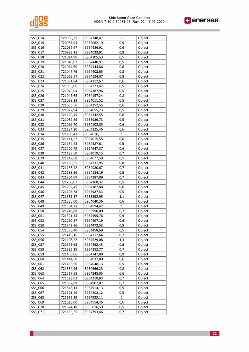
Side Sonar Scan Contacts
Contact ID Easting Northing Height Contact Type
DEB_001 718843,3 5945900,7 5.9x1.5x0.1 Debris DEB_002 718696,2 5943976,4 3.0x0.3x0.1 Debris DEB_003 718510,6 5942751,2 1.5x1.7xnmh Debris DEB_004 718689,5 5942724,0 3.0x0.5x0.3 Debris DEB_005 718419,5 5942669,9 0.8x0.3x0.1 Debris DEB_006 718479,3 5942653,2 2.5x1.2x0.1 Debris DEB_007 718581,4 5942595,0 5.0x1.3x0.3 Debris DEB_008 718582,9 5942591,3 4.1x1.0x0.6 Debris DEB_009 718580,4 5942585,2 1.8x0.5x0.2 Debris DEB_010 718589,2 5942584,2 5.1x2.4x0.3 Debris DEB_011 718584,4 5942581,4 4.1x3.3x0.5 Debris DEB_012 718550,1 5942539,3 1.4x0.8x0.2 Debris DEB_013 718606,0 5942526,9 2.9x1.0x0.6 Debris DEB_014 718630,6 5942524,1 2.0x0.5x0.1 Debris DEB_015 720403,1 5952036,9 1.9x0.7x0.2 Wreck DEB_016 718395,4 5945567,7 1.0x0.7x0.1 Wreck DEB_017 718387,7 5945566,4 3.9x0.5x0.1 Debris DEB_018 718282,9 5944250,1 1.6x0.7x0.3 Debris DEB_019 718930,1 5944019,3 6.2x1.8x0.4 Debris DEB_020 718995,4 5943832,0 2.0x0.6x0.2 Debris DEB_021 718878,1 5943526,3 2.1x0.7x0.2 Debris DEB_022 718167,1 5942830,6 2.2x0.8x0.2 Debris DEB_023 718254,5 5942712,2 2.9x1.1x0.1 Debris DEB_024 718142,1 5942390,0 3.4x1.6x0.8 Debris DEB_025 718784,2 5941352,3 3.3x1.5xnmh Debris DEB_026 718687,6 5941281,5 1.4x0.6x0.1 Debris SSS_001 720764,04 5955368,29 0,9 Debris SSS_002 720829,13 5954453,20 0,6 Debris SSS_003 720820,73 5954342,72 0,6 Object SSS_004 720821,77 5954270,88 0,5 Object SSS_005 720880,99 5954431,59 0,6 Object SSS_006 720892,17 5954300,94 0,8 Object SSS_007 720893,26 5954290,00 0,7 Object SSS_008 720905,80 5954298,46 0,9 Object SSS_009 720945,81 5954410,62 0,6 Object SSS_010 720952,19 5954327,47 0,6 Object SSS_011 720959,37 5954364,43 0,6 Object SSS_012 720960,29 5954352,58 0,7 Object SSS_013 720968,48 5954364,83 0,6 Object
Side Sonar Scan Contacts N05A-7-10-0-70031-01, Rev. 02, 17-03-2020
22
SSS_014 720988,35 5954348,47 1 Object SSS_015 720987,94 5954062,19 0,9 Object SSS_016 721039,97 5954486,91 0,6 Object SSS_017 720995,11 5954033,91 0,8 Object SSS_018 721014,90 5954205,53 0,5 Object SSS_019 721048,07 5954440,97 0,5 Object SSS_020 721014,60 5954144,86 0,6 Object SSS_021 721047,79 5954403,65 0,8 Object SSS_022 721023,57 5954124,07 0,8 Object SSS_023 721031,84 5954112,67 0,6 Object SSS_024 721055,06 5954273,47 0,5 Object SSS_025 721070,04 5954387,96 0,5 Object SSS_026 721047,65 5954157,24 0,8 Object SSS_027 721039,23 5954011,52 0,5 Object SSS_028 721083,56 5954252,55 0,6 Object SSS_029 721077,94 5954055,23 0,5 Object SSS_030 721120,45 5954342,55 0,6 Object SSS_031 721082,86 5953986,73 0,5 Object SSS_032 721096,70 5954103,85 0,6 Object SSS_033 721124,20 5954225,46 0,6 Object SSS_034 721108,47 5954016,11 1 Object SSS_035 721111,52 5954015,55 0,6 Object SSS_036 721154,23 5954387,61 0,5 Object SSS_037 721200,49 5954647,37 0,6 Object SSS_038 721129,50 5954019,15 0,7 Object SSS_039 721147,68 5954077,59 0,5 Object SSS_040 721189,65 5954331,95 0,8 Object SSS_041 721166,42 5954080,67 0,7 Object SSS_042 721183,36 5954184,19 0,5 Object SSS_043 721204,09 5954287,89 0,7 Object SSS_044 721200,07 5954168,32 0,5 Object SSS_045 721202,45 5954182,88 0,6 Object SSS_046 721195,78 5953987,53 0,5 Object SSS_047 721381,17 5955392,95 1,1 Object SSS_048 721235,00 5954040,36 0,6 Object SSS_049 721304,21 5954594,42 1 Object SSS_050 721246,88 5953990,00 0,7 Object SSS_051 721321,53 5954595,76 0,9 Object SSS_052 721290,57 5954297,19 0,6 Object SSS_053 721343,86 5954472,53 0,5 Object SSS_054 721373,40 5954458,69 0,5 Object SSS_055 721419,15 5954712,64 0,7 Object SSS_056 721408,52 5954529,08 1,3 Object SSS_057 721395,63 5954262,43 0,6 Object SSS_058 721395,15 5954252,77 0,7 Object SSS_059 721458,06 5954747,89 0,9 Object SSS_060 721444,60 5954037,80 0,6 Object SSS_061 721455,66 5954048,13 0,5 Object SSS_062 721554,96 5954666,23 0,8 Object SSS_063 721517,58 5954248,05 0,6 Object SSS_064 721523,03 5954218,83 0,7 Object SSS_065 721637,89 5954907,07 0,7 Object SSS_066 721648,13 5954914,13 0,5 Object SSS_067 721571,49 5954203,12 0,5 Object SSS_068 721656,39 5954932,11 1 Object SSS_069 721616,00 5954554,46 0,6 Object SSS_070 721674,18 5955016,59 0,5 Object SSS_071 721655,25 5954793,46 0,7 Object

Side Sonar Scan Contacts N05A-7-10-0-70031-01, Rev. 02, 17-03-2020
23
SSS_072 721625,01 5954519,17 0,7 Object SSS_073 721680,77 5955011,05 0,7 Object SSS_074 721652,06 5954564,38 0,6 Object SSS_075 721604,57 5954084,46 0,7 Object SSS_076 721626,38 5954092,91 0,5 Object SSS_077 721625,38 5954063,72 0,7 Object SSS_078 721717,09 5954862,86 0,6 Object SSS_079 721718,05 5954870,34 0,7 Object SSS_080 721738,42 5955038,28 0,7 Object SSS_081 721723,22 5954856,19 0,6 Object SSS_082 721624,62 5953973,00 0,7 Object SSS_083 721767,69 5955126,00 0,6 Object SSS_084 721775,98 5955044,12 0,7 Object SSS_085 721796,01 5955132,17 0,8 Object SSS_086 721801,77 5955134,43 0,7 Object SSS_087 721710,89 5954302,92 0,5 Object SSS_088 721800,27 5955078,78 0,5 Object SSS_089 721746,76 5954595,75 0,6 Object SSS_090 721788,65 5954958,66 0,6 Object SSS_091 721808,34 5955123,30 0,6 Object SSS_092 721684,49 5953956,43 1,6 Object SSS_093 721798,86 5954964,39 0,6 Object SSS_094 721766,62 5954616,90 0,8 Object SSS_095 721819,68 5955039,44 0,8 Object SSS_096 721759,40 5954496,67 0,6 Object SSS_097 721704,59 5954008,27 0,5 Object SSS_098 721712,63 5954066,90 1 Object SSS_099 721703,78 5953951,67 0,9 Object SSS_100 721791,38 5954654,79 0,5 Object SSS_101 721764,51 5954382,53 0,5 Object SSS_102 721772,48 5954430,59 0,6 Object SSS_103 721847,33 5954926,04 0,6 Object SSS_104 721815,38 5954641,85 0,6 Object SSS_105 721788,50 5954369,26 0,6 Object SSS_106 721854,68 5954924,85 0,5 Object SSS_107 721825,40 5954588,20 0,5 Object SSS_108 721829,40 5954595,07 0,6 Object SSS_109 721851,99 5954594,19 0,6 Object SSS_110 721858,18 5954627,12 0,6 Object SSS_111 721880,66 5954700,94 0,6 Object SSS_112 721850,61 5954434,71 0,6 Object SSS_113 721810,07 5953955,71 0,7 Object SSS_114 721968,21 5955303,95 0,5 Object SSS_115 721896,80 5954569,62 0,7 Object SSS_116 721926,97 5954712,77 0,5 Object SSS_117 721940,17 5954537,16 0,7 Object SSS_118 721949,13 5954256,82 0,7 Object SSS_119 722061,99 5954903,71 0,5 Object SSS_120 722026,14 5954527,01 0,7 Object SSS_121 721976,86 5953947,97 0,6 Object SSS_122 722031,16 5954397,32 0,7 Object SSS_123 722007,93 5954191,32 0,6 Object SSS_124 722037,39 5954431,37 0,9 Object SSS_125 722065,60 5954532,75 0,5 Object SSS_126 722072,28 5954539,20 0,5 Object SSS_127 722049,53 5954224,70 0,8 Object SSS_128 722128,63 5954814,33 0,6 Object SSS_129 722131,17 5954814,97 0,5 Object

Side Sonar Scan Contacts N05A-7-10-0-70031-01, Rev. 02, 17-03-2020
24
SSS_130 722141,98 5954862,02 0,5 Object SSS_131 722091,64 5954408,44 0,8 Object SSS_132 722066,30 5954157,96 0,6 Object SSS_133 722079,71 5954193,94 0,6 Object SSS_134 722127,92 5954494,60 0,5 Object SSS_135 722094,41 5954197,41 0,5 Object SSS_136 722100,07 5954244,99 0,7 Object SSS_137 722112,91 5954349,57 1 Object SSS_138 722112,75 5954276,00 0,7 Object SSS_139 722119,71 5954332,11 0,6 Object SSS_140 722168,47 5954646,15 0,5 Object SSS_141 722175,02 5954701,14 0,7 Object SSS_142 722117,03 5954180,65 0,5 Object SSS_143 722162,02 5954289,85 0,6 Object SSS_144 722256,41 5954766,99 0,8 Object SSS_145 722258,54 5954554,99 0,6 Object SSS_146 722266,05 5954620,89 0,5 Object SSS_147 722266,66 5954547,24 0,6 Object SSS_148 722348,34 5955174,34 1 Object SSS_149 722271,90 5954311,52 0,5 Object SSS_150 722326,41 5954704,99 1,1 Object SSS_151 722299,30 5954139,59 1 Object SSS_152 722362,88 5954613,53 0,6 Object SSS_153 722407,24 5954745,37 0,6 Object SSS_154 722397,54 5954086,30 0,6 Object SSS_155 722524,39 5954965,64 0,7 Object SSS_156 722504,06 5954768,70 0,5 Object SSS_157 722557,20 5954951,23 0,6 Object SSS_158 722475,09 5954215,99 0,6 Object SSS_159 722536,86 5954258,29 0,7 Object SSS_160 722583,42 5954193,39 0,5 Object SSS_161 722664,75 5954088,19 0,5 Object SSS_162 722698,08 5954168,32 0,7 Object SSS_163 722990,18 5955000,42 0,6 Object SSS_164 723059,38 5954145,40 0,6 Object SSS_165 723228,22 5954951,32 0,8 Object SSS_166 723230,39 5954954,08 0,6 Object SSS_167 723246,39 5954499,21 0,8 Object SSS_168 723264,94 5954042,88 0,6 Object SSS_169 723277,68 5953991,55 0,8 Object SSS_170 723288,81 5953947,23 0,5 Object SSS_171 723312,59 5954027,25 0,5 Object SSS_172 723325,45 5954026,92 0,6 Object SSS_173 723346,77 5954092,76 0,5 Object SSS_174 723383,38 5954065,30 0,7 Object SSS_175 723532,73 5954134,02 0,6 Object SSS_176 723718,13 5954854,97 0,5 Object SSS_177 723711,89 5954061,63 0,8 Object SSS_178 723715,87 5954080,48 0,7 Object SSS_179 723716,67 5954083,25 0,9 Object SSS_180 723754,52 5953968,95 1,1 Object SSS_181 723862,13 5954493,02 1 Object SSS_182 723808,64 5953913,20 0,8 Object SSS_183 723809,10 5953901,40 0,7 Object SSS_184 723849,19 5954109,37 0,6 Object SSS_185 723845,06 5953991,78 0,6 Object SSS_186 723854,66 5954067,59 0,5 Object SSS_187 723853,79 5954050,54 0,5 Object

Side Sonar Scan Contacts N05A-7-10-0-70031-01, Rev. 02, 17-03-2020
25
SSS_188 723862,24 5954111,86 0,5 Object SSS_189 723857,63 5954050,68 0,6 Object SSS_190 723852,05 5953876,48 0,6 Object SSS_191 723881,22 5953902,89 0,7 Object SSS_192 723905,57 5954059,20 0,6 Object SSS_193 723903,64 5953887,23 0,6 Object SSS_194 723926,72 5954041,65 0,5 Object SSS_195 723960,42 5954035,26 0,5 Object SSS_196 723975,07 5954068,32 0,5 Object SSS_197 724277,58 5954747,16 0,6 Object SSS_198 724476,72 5953817,57 0,5 Object SSS_199 724644,94 5954411,18 0,5 Object SSS_200 724661,78 5954539,65 0,6 Object SSS_201 724579,57 5953602,83 0,7 Object SSS_202 724731,05 5954433,07 0,7 Object SSS_203 724642,24 5953636,41 0,6 Object SSS_204 724766,83 5954450,51 0,6 Object SSS_205 724783,12 5954517,10 0,6 Object SSS_206 724778,58 5954449,53 0,6 Object SSS_207 724778,70 5954349,32 0,6 Object SSS_208 724780,26 5953558,96 0,5 Object SSS_209 724942,39 5954328,74 0,7 Object SSS_210 724989,45 5954393,95 0,6 Object SSS_211 725009,84 5954374,67 0,7 Object SSS_212 725048,36 5954528,27 0,6 Object SSS_213 724985,69 5953718,56 1,2 Object SSS_214 725096,72 5954515,79 0,5 Object SSS_215 725124,32 5954241,75 0,6 Object SSS_216 725134,42 5954237,50 0,6 Object SSS_217 725144,69 5954278,59 0,6 Object SSS_218 725092,50 5953770,38 0,5 Object SSS_219 725150,03 5954266,54 0,5 Object SSS_220 725152,17 5954277,48 0,5 Object SSS_221 725178,56 5954225,18 0,5 Object SSS_222 725124,87 5953745,24 0,6 Object SSS_223 725115,87 5953501,85 0,5 Object SSS_224 725172,54 5953894,35 0,5 Object SSS_225 725246,91 5954420,97 0,7 Object SSS_226 725261,74 5954467,16 0,7 Object SSS_227 725212,52 5953937,96 0,6 Object SSS_228 725244,46 5954123,17 0,5 Object SSS_229 725262,43 5954046,93 0,6 Object SSS_230 725276,31 5954136,17 0,5 Object SSS_231 725288,51 5954240,26 0,6 Object SSS_232 725285,49 5954061,94 0,9 Object SSS_233 725327,30 5954221,86 0,7 Object SSS_234 725336,55 5954215,62 0,8 Object SSS_235 725341,32 5954252,77 0,6 Object SSS_236 725346,39 5954204,15 0,5 Object SSS_237 725390,80 5954497,76 0,6 Object SSS_238 725361,58 5954030,67 0,7 Object SSS_239 725387,33 5954238,49 0,5 Object SSS_240 725361,50 5953844,71 0,8 Object SSS_241 725428,26 5954348,17 0,6 Object SSS_242 725473,83 5954428,28 0,7 Object SSS_243 725407,58 5953805,92 0,7 Object SSS_244 725447,98 5953818,37 0,8 Object SSS_245 725500,73 5954077,67 0,6 Object

Side Sonar Scan Contacts N05A-7-10-0-70031-01, Rev. 02, 17-03-2020
26
SSS_246 725469,00 5953705,87 0,7 Object SSS_247 725502,53 5953777,01 0,6 Object SSS_248 725503,43 5953676,67 0,5 Object SSS_249 725549,47 5953801,34 0,7 Object SSS_250 725568,76 5953790,04 1,1 Object SSS_251 725654,15 5954532,82 0,5 Object SSS_252 725650,48 5954214,47 0,5 Object SSS_253 725671,55 5954313,50 0,6 Object SSS_254 725663,15 5954214,40 0,6 Object SSS_255 725649,37 5953785,79 0,6 Object SSS_256 725831,42 5954364,25 0,5 Object SSS_257 725785,29 5953766,44 0,6 Object SSS_258 725827,13 5953653,81 0,6 Object SSS_259 725928,37 5954476,41 0,6 Object SSS_260 725965,90 5954322,62 0,7 Object SSS_261 725997,41 5953887,92 0,5 Object SSS_262 726052,22 5954102,79 0,5 Object SSS_263 726057,41 5954141,89 0,6 Object SSS_264 726125,63 5954417,63 0,7 Object SSS_265 726114,48 5954190,77 0,6 Object SSS_266 726107,63 5954125,64 0,7 Object SSS_267 726119,61 5954110,39 0,6 Object SSS_268 726091,62 5953851,33 0,7 Object SSS_269 726190,19 5954548,21 0,6 Object SSS_270 726173,34 5954150,49 0,5 Object SSS_271 726253,07 5954394,21 0,9 Object SSS_272 726319,83 5954354,42 0,5 Object SSS_273 726386,30 5954389,49 0,7 Object SSS_274 726412,12 5954380,81 0,6 Object SSS_275 726385,89 5954146,61 0,9 Object SSS_276 726544,54 5954494,79 0,5 Object SSS_277 726502,03 5954104,70 0,8 Object SSS_278 726506,85 5954107,53 0,7 Object SSS_279 726592,04 5954486,38 0,7 Object SSS_280 726742,62 5954423,38 0,7 Object SSS_281 726870,97 5954279,25 0,6 Object SSS_282 726958,22 5954177,60 0,6 Object SSS_283 726989,51 5954175,50 0,7 Object SSS_284 727046,94 5954189,82 0,5 Object SSS_285 727104,19 5954382,52 1,1 Object SSS_286 729697,53 5955104,13 0,6 Object SSS_287 729774,83 5955004,78 0,7 Object SSS_288 729767,36 5955100,95 0,5 Object SSS_289 729791,72 5955056,65 0,9 Object SSS_290 729990,54 5955191,79 0,6 Object SSS_291 730162,26 5955230,58 0,5 Object SSS_292 730317,76 5955207,78 0,6 Object SSS_293 730309,61 5955222,10 1,2 Object SSS_294 730297,63 5955291,03 0,5 Object SSS_295 730324,81 5955286,64 0,5 Object SSS_296 730359,44 5955287,63 0,7 Object SSS_297 730418,89 5955242,55 0,5 Object SSS_298 730417,60 5955276,24 0,6 Object SSS_299 730463,81 5955245,45 0,5 Object SSS_300 730506,71 5955235,50 0,5 Object SSS_301 730516,10 5955237,56 0,5 Object SSS_302 730541,92 5955229,90 0,9 Object SSS_303 730556,17 5955284,38 0,6 Object

Side Sonar Scan Contacts N05A-7-10-0-70031-01, Rev. 02, 17-03-2020
27
SSS_304 730578,58 5955257,66 0,9 Object SSS_305 730574,39 5955355,60 0,5 Object SSS_306 721419,2 5954712,6 0,7 Object SSS_307 721408,5 5954529,1 1,3 Object SSS_308 721458,1 5954747,9 0,9 Object SSS_309 721555,0 5954666,2 0,8 Object SSS_310 721616,0 5954554,5 0,6 Object SSS_311 721655,2 5954793,5 0,7 Object SSS_312 721625,0 5954519,2 0,7 Object SSS_313 721652,1 5954564,4 0,6 Object SSS_314 721746,8 5954595,7 0,6 Object SSS_315 721766,6 5954616,9 0,8 Object SSS_316 721759,4 5954496,7 0,6 Object SSS_317 721791,4 5954654,8 0,5 Object SSS_318 721772,5 5954430,6 0,6 Object SSS_319 721815,4 5954641,9 0,6 Object SSS_320 721825,4 5954588,2 0,5 Object SSS_321 721829,4 5954595,1 0,6 Object SSS_322 721852,0 5954594,2 0,6 Object SSS_323 721858,2 5954627,1 0,6 Object SSS_324 721880,7 5954700,9 0,6 Object SSS_325 721850,6 5954434,7 0,6 Object SSS_326 721896,8 5954569,6 0,7 Object SSS_327 721927,0 5954712,8 0,5 Object SSS_328 721940,2 5954537,2 0,7 Object SSS_329 722026,1 5954527,0 0,7 Object SSS_330 722037,4 5954431,4 0,9 Object SSS_331 722065,6 5954532,7 0,5 Object SSS_332 722072,3 5954539,2 0,5 Object SSS_333 722091,6 5954408,4 0,8 Object SSS_334 722127,9 5954494,6 0,5 Object SSS_335 722168,5 5954646,2 0,5 Object SSS_336 722175,0 5954701,1 0,7 Object SSS_337 722256,4 5954767,0 0,8 Object SSS_338 722258,5 5954555,0 0,6 Object SSS_339 722266,1 5954620,9 0,5 Object SSS_340 722266,7 5954547,2 0,6 Object SSS_341 722326,4 5954705,0 1,1 Object SSS_342 722362,9 5954613,5 0,6 Object SSS_343 722407,2 5954745,4 0,6 Object SSS_344 723246,4 5954499,2 0,8 Object SSS_345 723862,1 5954493,0 1 Object SSS_346 724644,9 5954411,2 0,5 Object SSS_347 724731,1 5954433,1 0,7 Object SSS_348 724766,8 5954450,5 0,6 Object SSS_349 724778,6 5954449,5 0,6 Object SSS_350 724778,7 5954349,3 0,6 Object SSS_351 724942,4 5954328,7 0,7 Object SSS_352 724989,4 5954394,0 0,6 Object SSS_353 725009,8 5954374,7 0,7 Object SSS_354 725124,3 5954241,8 0,6 Object SSS_355 725134,4 5954237,5 0,6 Object SSS_356 725144,7 5954278,6 0,6 Object SSS_357 725150,0 5954266,5 0,5 Object SSS_358 725152,2 5954277,5 0,5 Object SSS_359 725178,6 5954225,2 0,5 Object SSS_360 725246,9 5954421,0 0,7 Object SSS_361 725244,5 5954123,2 0,5 Object

Side Sonar Scan Contacts N05A-7-10-0-70031-01, Rev. 02, 17-03-2020
28
SSS_362 725262,4 5954046,9 0,6 Object SSS_363 725276,3 5954136,2 0,5 Object SSS_364 725288,5 5954240,3 0,6 Object SSS_365 725285,5 5954061,9 0,9 Object SSS_366 725327,3 5954221,9 0,7 Object SSS_367 725336,5 5954215,6 0,8 Object SSS_368 725341,3 5954252,8 0,6 Object SSS_369 725346,4 5954204,1 0,5 Object SSS_370 725361,6 5954030,7 0,7 Object SSS_371 725387,3 5954238,5 0,5 Object SSS_372 725428,3 5954348,2 0,6 Object SSS_373 725500,7 5954077,7 0,6 Object SSS_374 725650,5 5954214,5 0,5 Object SSS_375 725671,5 5954313,5 0,6 Object SSS_376 725663,1 5954214,4 0,6 Object SSS_377 725831,4 5954364,2 0,5 Object SSS_378 725965,9 5954322,6 0,7 Object SSS_379 726052,2 5954102,8 0,5 Object SSS_380 726057,4 5954141,9 0,6 Object SSS_381 726114,5 5954190,8 0,6 Object SSS_382 726107,6 5954125,6 0,7 Object SSS_383 726119,6 5954110,4 0,6 Object SSS_384 726173,3 5954150,5 0,5 Object SSS_385 726385,9 5954146,6 0,9 Object SSS_386 726502,0 5954104,7 0,8 Object SSS_387 726506,9 5954107,5 0,7 Object SSS_388 726871,0 5954279,2 0,6 Object SSS_389 726958,2 5954177,6 0,6 Object SSS_390 726989,5 5954175,5 0,7 Object SSS_391 727046,9 5954189,8 0,5 Object SSS_392 727104,2 5954382,5 1,1 Object SSS_393 729697,5 5955104,1 0,6 Object SSS_394 729774,8 5955004,8 0,7 Object SSS_395 729767,4 5955101,0 0,5 Object SSS_396 729791,7 5955056,7 0,9 Object SSS_397 729990,5 5955191,8 0,6 Object SSS_398 721343,9 5954472,5 0,5 Object SSS_399 721373,4 5954458,7 0,5 Object SSS_400 721517,6 5954248,1 0,6 Object SSS_401 721290,6 5954297,2 0,6 Object SSS_402 721395,6 5954262,4 0,6 Object SSS_403 721571,5 5954203,1 0,5 Object SSS_404 721523,0 5954218,8 0,7 Object SSS_405 721395,2 5954252,8 0,7 Object SSS_406 721626,4 5954092,9 0,5 Object SSS_407 721604,6 5954084,5 0,7 Object SSS_408 721455,7 5954048,1 0,5 Object SSS_409 721444,6 5954037,8 0,6 Object SSS_410 721235,0 5954040,4 0,6 Object SSS_411 721246,9 5953990,0 0,7 Object SSS_412 721195,8 5953987,5 0,5 Object SSS_413 721388,2 5953864,3 0,6 Object SSS_414 721246,8 5953887,4 0,6 Object SSS_415 721227,5 5953868,5 0,7 Object SSS_416 721343,0 5953829,2 0,5 Object SSS_417 721224,7 5953846,8 0,6 Object SSS_418 721379,4 5953792,7 0,6 Object SSS_419 721392,0 5953769,8 0,7 Object

Side Sonar Scan Contacts N05A-7-10-0-70031-01, Rev. 02, 17-03-2020
29
SSS_420 721261,2 5953798,9 0,8 Object SSS_421 721418,9 5953687,4 0,6 Object SSS_422 721338,8 5953691,8 0,8 Object SSS_423 721339,8 5953688,0 0,8 Object SSS_424 721351,0 5953668,2 0,8 Object SSS_425 721357,9 5953583,8 0,5 Object SSS_426 721410,7 5953535,3 0,6 Object SSS_427 718503,9 5942263,9 0,8 Object SSS_428 720988,4 5954348,5 1 Object SSS_429 721040 5954486,9 0,6 Object SSS_430 721048,1 5954441 0,5 Object SSS_431 721047,8 5954403,6 0,8 Object SSS_432 721055,1 5954273,5 0,5 Object SSS_433 721070 5954388 0,5 Object SSS_434 721083,6 5954252,5 0,6 Object SSS_435 721120,5 5954342,5 0,6 Object SSS_436 721124,2 5954225,5 0,6 Object SSS_437 721154,2 5954387,6 0,5 Object SSS_438 721200,5 5954647,4 0,6 Object SSS_439 721189,7 5954332 0,8 Object SSS_440 721204,1 5954287,9 0,7 Object SSS_441 721304,2 5954594,4 1 Object SSS_442 721321,5 5954595,8 0,9 Object SSS_443 721290,6 5954297,2 0,6 Object SSS_444 721343,9 5954472,5 0,5 Object SSS_445 721373,4 5954458,7 0,5 Object SSS_446 721419,2 5954712,6 0,7 Object SSS_447 721408,5 5954529,1 1,3 Object SSS_448 721395,6 5954262,4 0,6 Object SSS_449 721395,2 5954252,8 0,7 Object SSS_450 721458,1 5954747,9 0,9 Object SSS_451 721555 5954666,2 0,8 Object SSS_452 721517,6 5954248,1 0,6 Object SSS_453 721523 5954218,8 0,7 Object SSS_454 721637,9 5954907,1 0,7 Object SSS_455 721648,1 5954914,1 0,5 Object SSS_456 721571,5 5954203,1 0,5 Object SSS_457 721656,4 5954932,1 1 Object SSS_458 721616 5954554,5 0,6 Object SSS_459 721674,2 5955016,6 0,5 Object SSS_460 721655,2 5954793,5 0,7 Object SSS_461 721625 5954519,2 0,7 Object SSS_462 721680,8 5955011 0,7 Object SSS_463 721652,1 5954564,4 0,6 Object SSS_464 721717,1 5954862,9 0,6 Object SSS_465 721718,1 5954870,3 0,7 Object SSS_466 721738,4 5955038,3 0,7 Object SSS_467 721723,2 5954856,2 0,6 Object SSS_468 721767,7 5955126 0,6 Object SSS_469 721776 5955044,1 0,7 Object SSS_470 721710,9 5954302,9 0,5 Object SSS_471 721800,3 5955078,8 0,5 Object SSS_472 721746,8 5954595,7 0,6 Object SSS_473 721788,7 5954958,7 0,6 Object SSS_474 721808,3 5955123,3 0,6 Object SSS_475 721798,9 5954964,4 0,6 Object SSS_476 721766,6 5954616,9 0,8 Object SSS_477 721819,7 5955039,4 0,8 Object

Side Sonar Scan Contacts N05A-7-10-0-70031-01, Rev. 02, 17-03-2020
30
SSS_478 721759,4 5954496,7 0,6 Object SSS_479 721791,4 5954654,8 0,5 Object SSS_480 721764,5 5954382,5 0,5 Object SSS_481 721772,5 5954430,6 0,6 Object SSS_482 721847,3 5954926 0,6 Object SSS_483 721815,4 5954641,9 0,6 Object SSS_484 721788,5 5954369,3 0,6 Object SSS_485 721854,7 5954924,8 0,5 Object SSS_486 721825,4 5954588,2 0,5 Object SSS_487 721829,4 5954595,1 0,6 Object SSS_488 721852 5954594,2 0,6 Object SSS_489 721858,2 5954627,1 0,6 Object SSS_490 721880,7 5954700,9 0,6 Object SSS_491 721850,6 5954434,7 0,6 Object SSS_492 721896,8 5954569,6 0,7 Object SSS_493 721927 5954712,8 0,5 Object SSS_494 721940,2 5954537,2 0,7 Object SSS_495 721949,1 5954256,8 0,7 Object SSS_496 722062 5954903,7 0,5 Object SSS_497 722026,1 5954527 0,7 Object SSS_498 722031,2 5954397,3 0,7 Object SSS_499 722007,9 5954191,3 0,6 Object SSS_500 722037,4 5954431,4 0,9 Object SSS_501 722065,6 5954532,7 0,5 Object SSS_502 722072,3 5954539,2 0,5 Object SSS_503 722049,5 5954224,7 0,8 Object SSS_504 722128,6 5954814,3 0,6 Object SSS_505 722131,2 5954815 0,5 Object SSS_506 722142 5954862 0,5 Object SSS_507 722091,6 5954408,4 0,8 Object SSS_508 722066,3 5954158 0,6 Object SSS_509 722079,7 5954193,9 0,6 Object SSS_510 722127,9 5954494,6 0,5 Object SSS_511 722094,4 5954197,4 0,5 Object SSS_512 722100,1 5954245 0,7 Object SSS_513 722112,9 5954349,6 1 Object SSS_514 722112,7 5954276 0,7 Object SSS_515 722119,7 5954332,1 0,6 Object SSS_516 722168,5 5954646,2 0,5 Object SSS_517 722175 5954701,1 0,7 Object SSS_518 722117 5954180,7 0,5 Object SSS_519 722162 5954289,9 0,6 Object SSS_520 722256,4 5954767 0,8 Object SSS_521 722258,5 5954555 0,6 Object SSS_522 722266,1 5954620,9 0,5 Object SSS_523 722266,7 5954547,2 0,6 Object SSS_524 722271,9 5954311,5 0,5 Object SSS_525 722326,4 5954705 1,1 Object SSS_526 722299,3 5954139,6 1 Object SSS_527 722362,9 5954613,5 0,6 Object SSS_528 722407,2 5954745,4 0,6 Object SSS_529 722397,5 5954086,3 0,6 Object SSS_530 722524,4 5954965,6 0,7 Object SSS_531 722504,1 5954768,7 0,5 Object SSS_532 722557,2 5954951,2 0,6 Object SSS_533 722475,1 5954216 0,6 Object SSS_534 722536,9 5954258,3 0,7 Object SSS_535 722583,4 5954193,4 0,5 Object

Side Sonar Scan Contacts N05A-7-10-0-70031-01, Rev. 02, 17-03-2020
31
SSS_536 722664,8 5954088,2 0,5 Object SSS_537 722698,1 5954168,3 0,7 Object SSS_538 723059,4 5954145,4 0,6 Object SSS_539 723228,2 5954951,3 0,8 Object SSS_540 723230,4 5954954,1 0,6 Object SSS_541 723246,4 5954499,2 0,8 Object SSS_542 723264,9 5954042,9 0,6 Object SSS_543 723277,7 5953991,5 0,8 Object SSS_544 723312,6 5954027,2 0,5 Object SSS_545 723325,5 5954026,9 0,6 Object SSS_546 723346,8 5954092,8 0,5 Object SSS_547 723383,4 5954065,3 0,7 Object SSS_548 723532,7 5954134 0,6 Object SSS_549 723718,1 5954855 0,5 Object SSS_550 723711,9 5954061,6 0,8 Object SSS_551 723715,9 5954080,5 0,7 Object SSS_552 723716,7 5954083,2 0,9 Object SSS_553 723754,5 5953969 1,1 Object SSS_554 723862,1 5954493 1 Object SSS_555 723808,6 5953913,2 0,8 Object SSS_556 723809,1 5953901,4 0,7 Object SSS_557 723849,2 5954109,4 0,6 Object SSS_558 723845,1 5953991,8 0,6 Object SSS_559 723854,7 5954067,6 0,5 Object SSS_560 723853,8 5954050,5 0,5 Object SSS_561 723862,2 5954111,9 0,5 Object SSS_562 723857,6 5954050,7 0,6 Object SSS_563 723881,2 5953902,9 0,7 Object SSS_564 723905,6 5954059,2 0,6 Object SSS_565 723903,6 5953887,2 0,6 Object SSS_566 723926,7 5954041,6 0,5 Object SSS_567 723960,4 5954035,3 0,5 Object SSS_568 723975,1 5954068,3 0,5 Object SSS_569 724277,6 5954747,2 0,6 Object SSS_570 724644,9 5954411,2 0,5 Object SSS_571 724661,8 5954539,6 0,6 Object SSS_572 724731,1 5954433,1 0,7 Object SSS_573 724766,8 5954450,5 0,6 Object SSS_574 724783,1 5954517,1 0,6 Object SSS_575 724778,6 5954449,5 0,6 Object SSS_576 724778,7 5954349,3 0,6 Object SSS_577 724942,4 5954328,7 0,7 Object SSS_578 724989,4 5954394 0,6 Object SSS_579 725009,8 5954374,7 0,7 Object SSS_580 725048,4 5954528,3 0,6 Object SSS_581 725096,7 5954515,8 0,5 Object SSS_582 725124,3 5954241,8 0,6 Object SSS_583 725134,4 5954237,5 0,6 Object SSS_584 725144,7 5954278,6 0,6 Object SSS_585 725092,5 5953770,4 0,5 Object SSS_586 725150 5954266,5 0,5 Object SSS_587 725152,2 5954277,5 0,5 Object SSS_588 725178,6 5954225,2 0,5 Object SSS_589 725172,5 5953894,4 0,5 Object SSS_590 725246,9 5954421 0,7 Object SSS_591 725261,7 5954467,2 0,7 Object SSS_592 725212,5 5953938 0,6 Object SSS_593 725244,5 5954123,2 0,5 Object
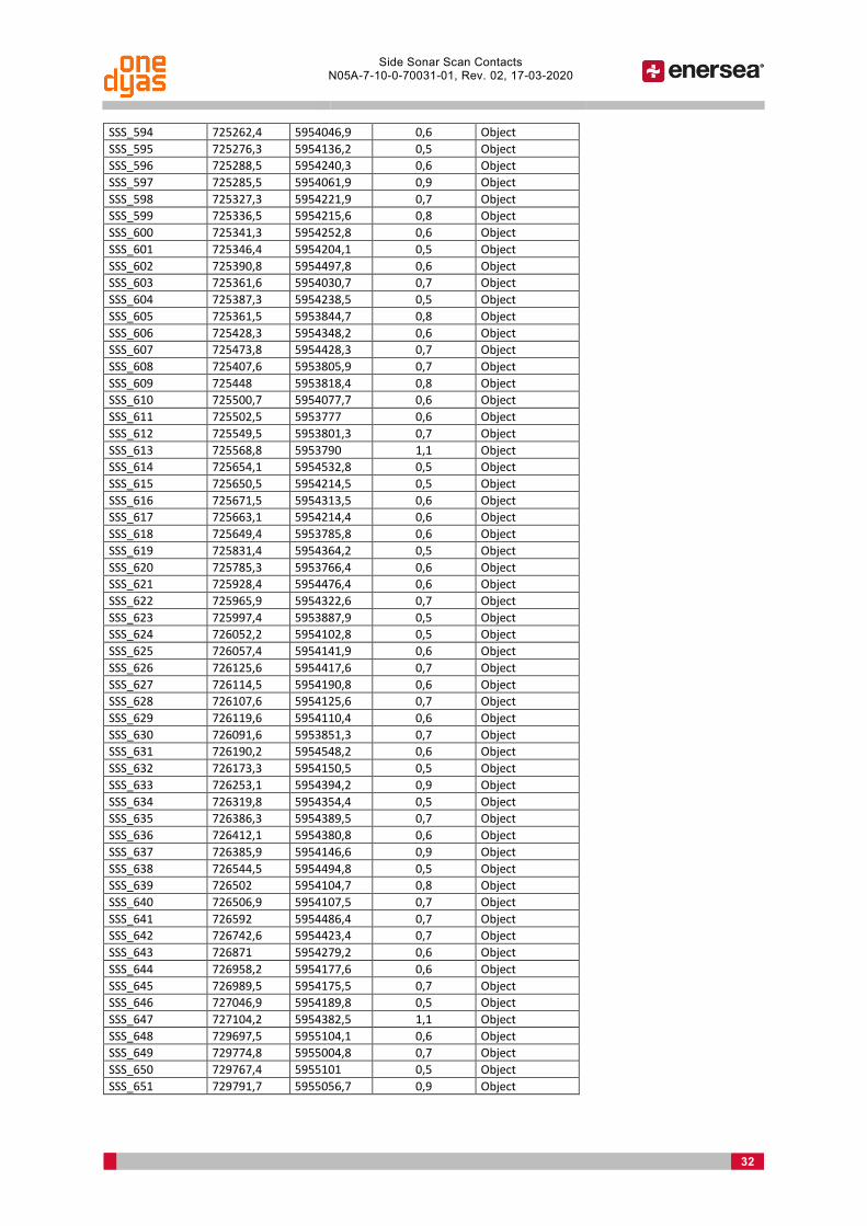
Side Sonar Scan Contacts N05A-7-10-0-70031-01, Rev. 02, 17-03-2020
32
SSS_594 725262,4 5954046,9 0,6 Object SSS_595 725276,3 5954136,2 0,5 Object SSS_596 725288,5 5954240,3 0,6 Object SSS_597 725285,5 5954061,9 0,9 Object SSS_598 725327,3 5954221,9 0,7 Object SSS_599 725336,5 5954215,6 0,8 Object SSS_600 725341,3 5954252,8 0,6 Object SSS_601 725346,4 5954204,1 0,5 Object SSS_602 725390,8 5954497,8 0,6 Object SSS_603 725361,6 5954030,7 0,7 Object SSS_604 725387,3 5954238,5 0,5 Object SSS_605 725361,5 5953844,7 0,8 Object SSS_606 725428,3 5954348,2 0,6 Object SSS_607 725473,8 5954428,3 0,7 Object SSS_608 725407,6 5953805,9 0,7 Object SSS_609 725448 5953818,4 0,8 Object SSS_610 725500,7 5954077,7 0,6 Object SSS_611 725502,5 5953777 0,6 Object SSS_612 725549,5 5953801,3 0,7 Object SSS_613 725568,8 5953790 1,1 Object SSS_614 725654,1 5954532,8 0,5 Object SSS_615 725650,5 5954214,5 0,5 Object SSS_616 725671,5 5954313,5 0,6 Object SSS_617 725663,1 5954214,4 0,6 Object SSS_618 725649,4 5953785,8 0,6 Object SSS_619 725831,4 5954364,2 0,5 Object SSS_620 725785,3 5953766,4 0,6 Object SSS_621 725928,4 5954476,4 0,6 Object SSS_622 725965,9 5954322,6 0,7 Object SSS_623 725997,4 5953887,9 0,5 Object SSS_624 726052,2 5954102,8 0,5 Object SSS_625 726057,4 5954141,9 0,6 Object SSS_626 726125,6 5954417,6 0,7 Object SSS_627 726114,5 5954190,8 0,6 Object SSS_628 726107,6 5954125,6 0,7 Object SSS_629 726119,6 5954110,4 0,6 Object SSS_630 726091,6 5953851,3 0,7 Object SSS_631 726190,2 5954548,2 0,6 Object SSS_632 726173,3 5954150,5 0,5 Object SSS_633 726253,1 5954394,2 0,9 Object SSS_634 726319,8 5954354,4 0,5 Object SSS_635 726386,3 5954389,5 0,7 Object SSS_636 726412,1 5954380,8 0,6 Object SSS_637 726385,9 5954146,6 0,9 Object SSS_638 726544,5 5954494,8 0,5 Object SSS_639 726502 5954104,7 0,8 Object SSS_640 726506,9 5954107,5 0,7 Object SSS_641 726592 5954486,4 0,7 Object SSS_642 726742,6 5954423,4 0,7 Object SSS_643 726871 5954279,2 0,6 Object SSS_644 726958,2 5954177,6 0,6 Object SSS_645 726989,5 5954175,5 0,7 Object SSS_646 727046,9 5954189,8 0,5 Object SSS_647 727104,2 5954382,5 1,1 Object SSS_648 729697,5 5955104,1 0,6 Object SSS_649 729774,8 5955004,8 0,7 Object SSS_650 729767,4 5955101 0,5 Object SSS_651 729791,7 5955056,7 0,9 Object

Side Sonar Scan Contacts N05A-7-10-0-70031-01, Rev. 02, 17-03-2020
33
SSS_652 729990,5 5955191,8 0,6 Object SSS_653 730162,3 5955230,6 0,5 Object SSS_654 730317,8 5955207,8 0,6 Object SSS_655 730309,6 5955222,1 1,2 Object SSS_656 730297,6 5955291 0,5 Object SSS_657 730324,8 5955286,6 0,5 Object SSS_658 730359,4 5955287,6 0,7 Object SSS_659 730418,9 5955242,5 0,5 Object SSS_660 730417,6 5955276,2 0,6 Object SSS_661 730463,8 5955245,5 0,5 Object SSS_662 730506,7 5955235,5 0,5 Object SSS_663 730516,1 5955237,6 0,5 Object SSS_664 721968,2 5955304,0 0,5 Object SSS_665 721381,2 5955392,9 1,1 Object SSS_666 721801,8 5955134,4 0,7 Object SSS_667 721796,0 5955132,2 0,8 Object SSS_668 721808,3 5955123,3 0,6 Object SSS_669 721767,7 5955126,0 0,6 Object SSS_670 721800,3 5955078,8 0,5 Object SSS_671 721819,7 5955039,4 0,8 Object SSS_672 721776,0 5955044,1 0,7 Object SSS_673 721738,4 5955038,3 0,7 Object SSS_674 722062,0 5954903,7 0,5 Object SSS_675 721674,2 5955016,6 0,5 Object SSS_676 722142,0 5954862,0 0,5 Object SSS_677 721680,8 5955011,0 0,7 Object SSS_678 721798,9 5954964,4 0,6 Object SSS_679 721788,7 5954958,7 0,6 Object SSS_680 721854,7 5954924,8 0,5 Object SSS_681 721847,3 5954926,0 0,6 Object SSS_682 722131,2 5954815,0 0,5 Object SSS_683 722128,6 5954814,3 0,6 Object SSS_684 721656,4 5954932,1 1 Object SSS_685 721648,1 5954914,1 0,5 Object SSS_686 721637,9 5954907,1 0,7 Object SSS_687 721718,1 5954870,3 0,7 Object SSS_688 721717,1 5954862,9 0,6 Object SSS_689 721723,2 5954856,2 0,6 Object SSS_690 722031,2 5954397,3 0,7 Object SSS_691 721200,5 5954647,4 0,6 Object SSS_692 721321,5 5954595,8 0,9 Object SSS_693 721304,2 5954594,4 1 Object SSS_694 721764,5 5954382,5 0,5 Object SSS_695 721788,5 5954369,3 0,6 Object SSS_696 721949,1 5954256,8 0,7 Object SSS_697 721710,9 5954302,9 0,5 Object SSS_698 721040,0 5954486,9 0,6 Object SSS_699 721048,1 5954441,0 0,5 Object SSS_700 721154,2 5954387,6 0,5 Object SSS_701 721047,8 5954403,6 0,8 Object SSS_702 721070,0 5954388,0 0,5 Object SSS_703 721189,7 5954332,0 0,8 Object SSS_704 721120,5 5954342,5 0,6 Object SSS_705 721204,1 5954287,9 0,7 Object SSS_706 720988,4 5954348,5 1 Object SSS_707 721712,6 5954066,9 1 Object SSS_708 721055,1 5954273,5 0,5 Object SSS_709 721083,6 5954252,5 0,6 Object

Side Sonar Scan Contacts N05A-7-10-0-70031-01, Rev. 02, 17-03-2020
34
SSS_710 721625,4 5954063,7 0,7 Object SSS_711 721124,2 5954225,5 0,6 Object SSS_712 721202,4 5954182,9 0,6 Object SSS_713 721183,4 5954184,2 0,5 Object SSS_714 721704,6 5954008,3 0,5 Object SSS_715 721200,1 5954168,3 0,5 Object SSS_716 721810,1 5953955,7 0,7 Object SSS_717 721014,9 5954205,5 0,5 Object SSS_718 721703,8 5953951,7 0,9 Object SSS_719 721684,5 5953956,4 1,6 Object SSS_720 721624,6 5953973,0 0,7 Object SSS_721 721047,7 5954157,2 0,8 Object SSS_722 721014,6 5954144,9 0,6 Object SSS_723 721096,7 5954103,8 0,6 Object SSS_724 721166,4 5954080,7 0,7 Object SSS_725 721023,6 5954124,1 0,8 Object SSS_726 721147,7 5954077,6 0,5 Object SSS_727 721031,8 5954112,7 0,6 Object SSS_728 721077,9 5954055,2 0,5 Object SSS_729 721129,5 5954019,2 0,7 Object SSS_730 720987,9 5954062,2 0,9 Object SSS_731 721567,9 5953867,9 0,6 Object SSS_732 721111,5 5954015,6 0,6 Object SSS_733 721108,5 5954016,1 1 Object SSS_734 720995,1 5954033,9 0,8 Object SSS_735 721039,2 5954011,5 0,5 Object SSS_736 721082,9 5953986,7 0,5 Object SSS_737 721072,1 5953895,1 0,6 Object SSS_738 720316,0 5950031,5 0,9 Object SSS_739 720114,5 5948971,1 0,8 Object SSS_740 719671,1 5947933,0 0,6 Object SSS_741 718851,9 5942574,8 0,5 Object SSS_742 722065,602 5954532,748 0,5 Object SSS_743 721847,333 5954926,036 0,6 Object SSS_744 721718,052 5954870,335 0,7 Object SSS_745 721723,219 5954856,189 0,6 Object SSS_746 721523,033 5954218,829 0,7 Object SSS_747 721517,576 5954248,052 0,6 Object SSS_748 721717,093 5954862,856 0,6 Object SSS_749 721395,154 5954252,774 0,7 Object SSS_750 721395,633 5954262,425 0,6 Object SSS_751 721321,532 5954595,757 0,9 Object SSS_752 721738,417 5955038,276 0,7 Object SSS_753 721767,685 5955125,998 0,6 Object SSS_754 721800,267 5955078,779 0,5 Object SSS_755 721200,485 5954647,373 0,6 Object SSS_756 721710,894 5954302,916 0,5 Object SSS_757 721759,398 5954496,665 0,6 Object SSS_758 721815,378 5954641,854 0,6 Object SSS_759 721940,171 5954537,155 0,7 Object SSS_760 722072,284 5954539,197 0,5 Object SSS_761 721571,489 5954203,118 0,5 Object SSS_762 722031,163 5954397,323 0,7 Object SSS_763 721764,507 5954382,525 0,5 Object SSS_764 721788,498 5954369,264 0,6 Object SSS_765 722112,914 5954349,566 1 Object SSS_766 721656,392 5954932,107 1 Object SSS_767 721788,653 5954958,655 0,6 Object

Side Sonar Scan Contacts N05A-7-10-0-70031-01, Rev. 02, 17-03-2020
35
SSS_768 721896,799 5954569,624 0,7 Object SSS_769 721819,678 5955039,442 0,8 Object SSS_770 721775,982 5955044,12 0,7 Object SSS_771 721808,335 5955123,298 0,6 Object SSS_772 721458,055 5954747,893 0,9 Object SSS_773 721880,655 5954700,943 0,6 Object SSS_774 721554,962 5954666,225 0,8 Object SSS_775 722119,708 5954332,113 0,6 Object SSS_776 721637,887 5954907,072 0,7 Object SSS_777 721625,005 5954519,167 0,7 Object SSS_778 721419,153 5954712,644 0,7 Object SSS_779 721746,755 5954595,746 0,6 Object SSS_780 721766,615 5954616,901 0,8 Object SSS_781 721825,401 5954588,196 0,5 Object SSS_782 721851,994 5954594,191 0,6 Object SSS_783 721854,677 5954924,845 0,5 Object SSS_784 722037,385 5954431,371 0,9 Object SSS_785 722026,142 5954527,01 0,7 Object SSS_786 721290,573 5954297,188 0,6 Object SSS_787 721343,864 5954472,532 0,5 Object SSS_788 721373,402 5954458,692 0,5 Object SSS_789 721408,521 5954529,082 1,3 Object SSS_790 721829,398 5954595,074 0,6 Object SSS_791 721652,063 5954564,38 0,6 Object SSS_792 721791,384 5954654,785 0,5 Object SSS_793 721798,859 5954964,393 0,6 Object SSS_794 721648,134 5954914,129 0,5 Object SSS_795 721796,007 5955132,171 0,8 Object SSS_796 721655,249 5954793,462 0,7 Object SSS_797 721304,212 5954594,415 1 Object SSS_798 721674,177 5955016,59 0,5 Object SSS_799 721949,132 5954256,82 0,7 Object SSS_800 721850,605 5954434,709 0,6 Object SSS_801 721680,772 5955011,048 0,7 Object SSS_802 721858,183 5954627,117 0,6 Object WRECK_001 720537,7 5952510,7 19.1x12.9x0.2 Wreck WRECK_002 720467,1 5952450,6 40.1x12.8x1.1 Wreck

N5a Development LU0022H-553-RR-05
Environmental Baseline Survey Report Revision 1.1
www.geoxyzoffshore.com Page 1 of 235
N5a Development
Title Environmental Baseline Survey Report
GEOxyz Report No. LU0022H-553-RR-05
ONE Report No. N05A-7-10-0-70020-01
Revision 1.1
1.1 30/10/2019 Review copy PC PC
1.0 11/09/2019 First draft IE PC
Revision Date Description of Revision Author Checked Approved Approved by Client
N5a Development LU0022H-553-RR-05
Environmental Baseline Survey Report Revision 1.1
www.geoxyzoffshore.com Page 2 of 235
REVISION HISTORY
The screen version of this document is always the CONTROLLED COPY. When printed it is considered a FOR INFORMATION ONLY copy, and it is the holder’s responsibility that they hold the latest valid version.
On the front page the ‘Description of Revision’ box should always contain only one of three possible descriptions; First draft, Review copy, or approved. The table on this page can be used to explain the reason for the revision and what has changed since the previous revision. If number of changes are significant, the document ID of the comment sheet can be referenced in the ‘Changes’ column instead.
Rev. Reason for revision Changes from previous version
1.0 First Issue N/A
1.1 Review copy Application of client comments

N5a Development LU0022H-553-RR-05
Environmental Baseline Survey Report Revision 1.1
www.geoxyzoffshore.com Page 3 of 235
TABLE OF CONTENTS
Revision History ................................................................................................................................................. 2 Definitions and Abbreviations ........................................................................................................................... 7
Executive Summary ................................................................................................................................ 9
1 Introduction ................................................................................................................................. 10
1.1 Project Overview ............................................................................................................................... 10 1.2 Scope of Work ................................................................................................................................... 11
Objectives .................................................................................................................................. 12
1.3 Geodetic Parameters ........................................................................................................................ 13
Horizontal Reference ................................................................................................................. 13 Vertical Reference ..................................................................................................................... 13
2 Survey Operations and Data Review .............................................................................................. 14
Summary of Survey Operations ........................................................................................................ 14 Geophysical Data .............................................................................................................................. 15 Envrionmental Ground-truthing and Sampling................................................................................. 16 Habitat Investigation ......................................................................................................................... 19
Habitat Classification ................................................................................................................. 19 Assessment of Sensitive Habitats .............................................................................................. 19
Sample Analyses ................................................................................................................................ 21
3 Results and interpretation ............................................................................................................ 22
Bathymetry........................................................................................................................................ 22
N5A to NGT Hot Tap Pipeline Route .......................................................................................... 22 N5A to Riffgat Cable Route ........................................................................................................ 22
Seabed Features ................................................................................................................................ 23
N5A Site ..................................................................................................................................... 23 N5A to NGT Hot Tap Pipeline Route .......................................................................................... 23 N5A to Riffgat Cable Route ........................................................................................................ 23
Shallow Soils ...................................................................................................................................... 24
N5A Site ..................................................................................................................................... 24 N5A to NGT Hot Tap Pipeline Route .......................................................................................... 24 N5A to Riffgat Cable Route ........................................................................................................ 24 N5A Site ..................................................................................................................................... 25
Particle Size Distribution ................................................................................................................... 29
Multivariate Analysis ................................................................................................................. 36
Total Organic Matter, Total Organic Carbon, and Moisture Content ............................................... 41 Sediment Hydrocarbons ................................................................................................................... 44
N5a Development LU0022H-553-RR-05
Environmental Baseline Survey Report Revision 1.1
www.geoxyzoffshore.com Page 4 of 235
Total Hydrocarbon Content ....................................................................................................... 44 Saturate/Aliphatic Hydrocarbons .............................................................................................. 47 Polycyclic Aromatic Hydrocarbons (PAHs) ................................................................................. 54 Normalisation of Total PAH ....................................................................................................... 57
Heavy and Trace Metal Concentrations ............................................................................................ 59
Normalisation of Heavy Metals ................................................................................................. 63
Macrofaunal Analyses ....................................................................................................................... 71
Infaunal Trends .......................................................................................................................... 75 Univariate Parameters ............................................................................................................... 80 Multivariate Analyses ................................................................................................................ 88 Environmental Variables ............................................................................................................ 93 Epifaunal and other Biological Groups ...................................................................................... 94
Environmental Habitats .................................................................................................................... 95
‘Infralittoral Fine Sand’ (A5.23) .................................................................................................. 97 ‘Infralittoral Coarse Sediment’ (A5.13) ...................................................................................... 98 ‘Infralittoral Mixed Sediment’ (A5.43) ....................................................................................... 99 ‘Dense Lanice conchilega and Other Polychaetes in Tide-swept Infralittoral Sand and Mixed
Gravelly Sand’ (A5.137) ......................................................................................................................... 101 Potential Sensitive Habitats and Species ................................................................................. 103
4 Conclusion .................................................................................................................................. 106
5 Bibliography ............................................................................................................................... 108
Appendix A - Geo Ocean III ............................................................................................................................ 112 Appendix B - BSL Sampling Equipment .......................................................................................................... 114 Appendix C - Log Sheets ................................................................................................................................. 119 Appendix D - Field Operations and Survey Methods ..................................................................................... 124 Appendix E - Sample and Seabed Photographs ............................................................................................. 126 Appendix F - Data presentation, Laboratory and Statistical Analyses .......................................................... 159 Appendix G - Particle Size Distibutions .......................................................................................................... 172 Appendix H - Total Aliphatic Concentrations (µg.kg-1) .................................................................................. 189 Appendix I - GC FID Traces (Saturates) .......................................................................................................... 192 Appendix J - Polycyclic Aromatic Hydrocarbon Concentration (µg.kg-1) ........................................................ 197 Appendix K - Polycyclic Aromatic Hydrocarbon Concentration: EPA (µg.kg-1) .............................................. 201 Appendix L - Polycyclic Aromatic Hydrocarbon: Parents Compounds and Alkyl Derivatives ......................... 204 Appendix M - Macrofaunal Species List ......................................................................................................... 209 Appendix N - Spearman’s Correlation............................................................................................................ 230 Appendix O - AQA Certification of Laboratories ............................................................................................ 231 Appendix P - Service Warranty ...................................................................................................................... 235
TABLE OF FIGURES
Figure 1: Project location overview ................................................................................................................. 11
N5a Development LU0022H-553-RR-05
Environmental Baseline Survey Report Revision 1.1
www.geoxyzoffshore.com Page 5 of 235
Figure 2: Survey strategy overview ................................................................................................................. 18 Figure 3: N5A Site and Route Survey Bathymetry ........................................................................................... 26 Figure 4: Interpreted N5A Site and Route Seabed Features ........................................................................... 27 Figure 5: Interpreted N5A site and route seabed features ............................................................................. 28 Figure 6: Mean particle size (mm) ................................................................................................................... 32 Figure 7: Proportion of fines (%) ..................................................................................................................... 33 Figure 8: Proportion of sands (%) .................................................................................................................... 34 Figure 9: Proportion of gravels (%) .................................................................................................................. 35 Figure 10: Particle size distribution similarity dendrogram ............................................................................ 36 Figure 11: Principal components analysis of particle size data ....................................................................... 37 Figure 12: Particle size distribution for all stations in clusters a, b & c ........................................................... 38 Figure 13: Multivariate cluster distribution over bathymetry ........................................................................ 39 Figure 14: Multivariate cluster distribution over interpreted seabed features .............................................. 40 Figure 15:Total organic carbon (TOC; % w/w C) .............................................................................................. 43 Figure 16: Total hydrocarbon concentrations (mg.kg¯¹) ................................................................................. 46 Figure 17: Total saturate alkanes (mg.kg¯¹ ...................................................................................................... 48 Figure 18: Example gas chromatogram for saturate hydrocarbon analysis (GRAB_C_2) ............................... 49 Figure 19: Example gas chromatogram for saturate hydrocarbon analysis (GRAB_P_1) ............................... 49 Figure 20: Carbon preference index ................................................................................................................ 52 Figure 21: Petrogenic/biogenic ratio ............................................................................................................... 53 Figure 22: Polycyclic aromatic hydrocarbons (2-6 Ring) ................................................................................. 55 Figure 23: Example parent/alkyl PAH plots ..................................................................................................... 56 Figure 24: Heavy metal concentration for barium (Ba; mg.kg-1) ..................................................................... 64 Figure 25: Heavy metal concentration for nickel (Ni; mg.kg-1) ........................................................................ 65 Figure 26: Heavy metal concentration for copper (Cu; mg.kg-1) ..................................................................... 66 Figure 27: Heavy metal concentration for iron (Fe; mg.kg-1) .......................................................................... 67 Figure 28: Heavy metal concentration for arsenic (As; mg.kg-1) ..................................................................... 68 Figure 29: Heavy metal concentration for aluminium (Al; mg.kg-1) ................................................................ 69 Figure 30: Heavy metal concentration for zinc (Zn; mg.kg-1) .......................................................................... 70 Figure 31: Proportion of individual abundance by main taxonomic group for each replicate (part 1) .......... 72 Figure 32: Proportion of individual abundance by main taxonomic group for each replicate (part 2) .......... 72 Figure 33: Proportion of individual richness by main taxonomic group for each replicate (part 3) ............... 73 Figure 34: Proportion of individual richness by main taxonomic group for each replicate (part 4) ............... 73 Figure 35: Proportion of individual abundance by main taxonomic group for each station .......................... 74 Figure 36: Proportion of individual richness by main taxonomic group for each station ............................... 74 Figure 37: Example photographs of macrofauna species within survey area ................................................. 79 Figure 38: Macrofauna species abundance (per 0.2m2).................................................................................. 83 Figure 39: Macrofauna species richness (per 0.2m2) ...................................................................................... 84 Figure 40: Species abundance and richness by station (0.2m2) ...................................................................... 85 Figure 41: Species accumulation curve of the N5A survey area ..................................................................... 86 Figure 42: Macrofauna – Shannon-Wiener diversity (H per 0.1m2) ................................................................ 87 Figure 43: Dendrogram of macrofaunal replicates ......................................................................................... 89 Figure 44: Dendrogram of macrofaunal stations ............................................................................................ 89 Figure 45: MDS ordination of macrofauna by replicates ................................................................................ 90 Figure 46: MDS ordination of macrofauna by station ..................................................................................... 91
N5a Development LU0022H-553-RR-05
Environmental Baseline Survey Report Revision 1.1
www.geoxyzoffshore.com Page 6 of 235
Figure 47: Principal component analysis of particle size data ........................................................................ 93 Figure 48: Epifaunal versus infaunal richness ................................................................................................. 94 Figure 49: N5A site and route habitat distribution ......................................................................................... 96 Figure 50: Example images of ‘Infralittoral fine sand’ (A5.23) ........................................................................ 98 Figure 51: Example images of ‘Infralittoral coarse sediment’ (A5.13) ............................................................ 99 Figure 52: Example images of ‘Infralittoral mixed sediment’ (A5.43) ........................................................... 101 Figure 53: Example images of Dense Lanice conchilega and other polychaetes in tide-swept infralittoral sand and mixed gravelly sand’ (A5.137) ........................................................................................................ 102
TABLE OF TABLES
Table 1: Abbreviations used in this Document .................................................................................................. 7 Table 2: Proposed N5A Platform, N5A to Riffgat Cable Route and N5A to NGT Hot Tap Route Locations .... 10 Table 3: Detailed scope of work for each area ................................................................................................ 12 Table 4: Geodetic parameters ......................................................................................................................... 13 Table 5: Overview of survey operations .......................................................................................................... 14 Table 6: Summary of drop-down camera and grab sampling locations for survey area ................................ 16 Table 7: Summary of camera transect locations for the survey area ............................................................. 17 Table 8: Summary of resemblance to a stony reef, as summarised in Irving (2009) ...................................... 20 Table 9: Stony reef structure matrix (after Irving, 2009) ................................................................................ 20 Table 10: Overall stony reefiness matrix (structure vs extent) ....................................................................... 20 Table 11: Summary of surface particle size distribution ................................................................................. 30 Table 12: Summary of total organic carbon and moisture content ................................................................ 42 Table 13: Summary of hydrocarbon concentrations ....................................................................................... 45 Table 14: Normalised PAH concentrations (μg.kg-1)........................................................................................ 58 Table 15: Total heavy and trace metal concentrations (mg.kg-1) .................................................................... 62 Table 16: Overall Species Ranking (Top 15 Species) ........................................................................................ 76 Table 17: Univariate faunal parameters (0.1m2 replicates) ............................................................................ 80 Table 18: Univariate faunal parameters (0.2m2 pooled station replicates) .................................................... 82 Table 19: Summary of SIMPROF groupings ..................................................................................................... 88 Table 20: Similarity percentage (SIMPER) for clusters A-D ............................................................................. 92 Table 21: Summary of stony reef structure assessment ............................................................................... 104 Table 22: Species characteristic of permanently flooded sandbank – Netherlands habitat subtype H1110_C ....................................................................................................................................................................... 105
N5a Development LU0022H-553-RR-05
Environmental Baseline Survey Report Revision 1.1
www.geoxyzoffshore.com Page 7 of 235
DEFINITIONS AND ABBREVIATIONS
Throughout this document the following terminology is used:
ONE-Dyas Oranje Nassau Energie B.V. (Client)
GEOxyz GEOxyz Offshore (Contractor)
TTS T.T. Surveys Ltd (Supplier)
Igeotest Igeotest Geoscience Group (Supplier)
BSL Benthic Solutions Ltd (Supplier)
Peak Peak Processing (Supplier)
Where abbreviations used in this document are not included in this list, it may be assumed that they are either equipment brand names or company names.
Table 1: Abbreviations used in this Document
Acronym Description Acronym Description
Al Aluminium (element) MP Megapixel ANOSIM Analysis of Similarity NGT Noordgastransport
AQC Analytical Quality Control Ni Nickel (element)
AR Aqua Regia NMBAQC National Marine Biological Association Quality Control
As Arsenic (element) n-MDS Non-Metric Multidimensional Scaling
Ba Barium (element) NOAA National Oceanic and Atmospheric Administration
BAC Background Assessment Concentration NPD Naphthalene, Anthracene and Dibenzothiophene
BSL Benthic Solutions Limited N/S No Sample Cd Cadmium (element) OGUK Oil & Gas United Kingdom
CEFAS Centre for Environment, Fisheries and Aquaculture
OSPAR Convention for the protection of the Marine Environment of the North East Atlantic
CEMP Coordinated Background Monitoring Programme
OWF Offshore Wind Farm
CPI Carbon Preference Index PAH Polyaromatic Hydrocarbons Cr Chromium (element) Pb Lead (element) Cu Copper (element) P/B Ratio Petrogenic Biogenic Ratio CV Coefficient of Variation PC Physico-chemical grab sample
DBT Dibenzothiophene PCA Principal Components Analysis DCM Dichloromethane Ph Phytane DVV Double Van Veen Pr Pristane
EBS Environmental Baseline Survey PRIMER Plymouth Routines In Multivariate Ecological Research
ED50 European Datum 1950 PSA Particle Size Analysis EOL End Of Line PWL Proposed Well Location EPA Environmental Protection Agency SAC Special Area of Conservation ERL Effective Range Low Sb Tin (element) ERM Effective Range Median SBP Sub-bottom profiler EU European Union SCI Sites of Community Importance
EUNIS European Nature Information System SD Standard Deviation F1,2 & 3 Fauna grab sample 1, 2 & 3 SIC Single Ion Current
Fe Iron (element) SIMPROF Similarity Profile Analysis GC Gas Chromatography SNS Southern North Sea
GC-FID Gas Chromatography with Flame Ionisation Detection
SOL Start Of Line

N5a Development LU0022H-553-RR-05
Environmental Baseline Survey Report Revision 1.1
www.geoxyzoffshore.com Page 8 of 235
Acronym Description Acronym Description
GC-MS Gas Chromatography Mass Spectrometry SOP Standard Operating Procedure HAP Habitat Action Plan SPA Special Protection Area HAS Habitat Assessment Survey SSS Side-scan Sonar HD High Definition THC Total Hydrocarbon Content HF Hydrofluoric acid TOC Total Organic Carbon Hg Mercury (element) TOM Total Organic Matter HM Heavy and Trace Metals TRV Toxicity Reference Value
ICP-MS Inductively Coupled Plasma Mass Spectrometry
UCM Unresolved Complex Mixture
ICP-OES Inductively Coupled Plasma - Optical Emission Spectrometry
UK United Kingdom
IMS Industrial Methylated Spirit UKAS United Kingdom Accreditation Service IUCN International Union for Conservation of Nature UK BAP United Kingdom Biodiversity Action Plan JNCC Joint Nature Conservation Committee UKCS United Kingdom Continental Shelf
LAT Lowest Astronomical Tide UKOOA United Kingdom Offshore Operators Association
LED Light-emitting Diode UTC Universal Time Coordinated LOI Loss on Ignition UTM 31 Universal Transverse Mercator – Zone 31
MAG Magnetometer V Vanadium (element) MBES Multi Beam Echo Sounder VC Vibrocore MDL Mean Detection Limit WGS84 World Global Spheroid 1984 MDS Multi-Dimensional Scaling Zn Zinc (element)
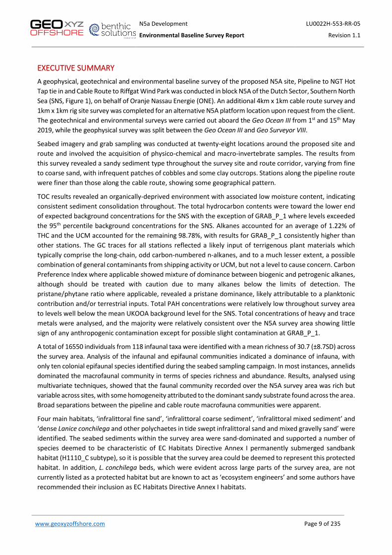
N5a Development LU0022H-553-RR-05
Environmental Baseline Survey Report Revision 1.1
www.geoxyzoffshore.com Page 9 of 235
EXECUTIVE SUMMARY
A geophysical, geotechnical and environmental baseline survey of the proposed N5A site, Pipeline to NGT Hot Tap tie in and Cable Route to Riffgat Wind Park was conducted in block N5A of the Dutch Sector, Southern North Sea (SNS, Figure 1), on behalf of Oranje Nassau Energie (ONE). An additional 4km x 1km cable route survey and 1km x 1km rig site survey was completed for an alternative N5A platform location upon request from the client. The geotechnical and environmental surveys were carried out aboard the Geo Ocean III from 1st and 15th May 2019, while the geophysical survey was split between the Geo Ocean III and Geo Surveyor VIII.
Seabed imagery and grab sampling was conducted at twenty-eight locations around the proposed site and route and involved the acquisition of physico-chemical and macro-invertebrate samples. The results from this survey revealed a sandy sediment type throughout the survey site and route corridor, varying from fine to coarse sand, with infrequent patches of cobbles and some clay outcrops. Stations along the pipeline route were finer than those along the cable route, showing some geographical pattern.
TOC results revealed an organically-deprived environment with associated low moisture content, indicating consistent sediment consolidation throughout. The total hydrocarbon contents were toward the lower end of expected background concentrations for the SNS with the exception of GRAB_P_1 where levels exceeded the 95th percentile background concentrations for the SNS. Alkanes accounted for an average of 1.22% of THC and the UCM accounted for the remaining 98.78%, with results for GRAB_P_1 consistently higher than other stations. The GC traces for all stations reflected a likely input of terrigenous plant materials which typically comprise the long-chain, odd carbon-numbered n-alkanes, and to a much lesser extent, a possible combination of general contaminants from shipping activity or UCM, but not a level to cause concern. Carbon Preference Index where applicable showed mixture of dominance between biogenic and petrogenic alkanes, although should be treated with caution due to many alkanes below the limits of detection. The pristane/phytane ratio where applicable, revealed a pristane dominance, likely attributable to a planktonic contribution and/or terrestrial inputs. Total PAH concentrations were relatively low throughout survey area to levels well below the mean UKOOA background level for the SNS. Total concentrations of heavy and trace metals were analysed, and the majority were relatively consistent over the N5A survey area showing little sign of any anthropogenic contamination except for possible slight contamination at GRAB_P_1.
A total of 16550 individuals from 118 infaunal taxa were identified with a mean richness of 30.7 (±8.7SD) across the survey area. Analysis of the infaunal and epifaunal communities indicated a dominance of infauna, with only ten colonial epifaunal species identified during the seabed sampling campaign. In most instances, annelids dominated the macrofaunal community in terms of species richness and abundance. Results, analysed using multivariate techniques, showed that the faunal community recorded over the N5A survey area was rich but variable across sites, with some homogeneity attributed to the dominant sandy substrate found across the area. Broad separations between the pipeline and cable route macrofauna communities were apparent.
Four main habitats, ‘infralittoral fine sand’, ‘infralittoral coarse sediment’, ‘infralittoral mixed sediment’ and ‘dense Lanice conchilega and other polychaetes in tide swept infralittoral sand and mixed gravelly sand’ were identified. The seabed sediments within the survey area were sand-dominated and supported a number of species deemed to be characteristic of EC Habitats Directive Annex I permanently submerged sandbank habitat (H1110_C subtype), so it is possible that the survey area could be deemed to represent this protected habitat. In addition, L. conchilega beds, which were evident across large parts of the survey area, are not currently listed as a protected habitat but are known to act as ‘ecosystem engineers’ and some authors have recommended their inclusion as EC Habitats Directive Annex I habitats.
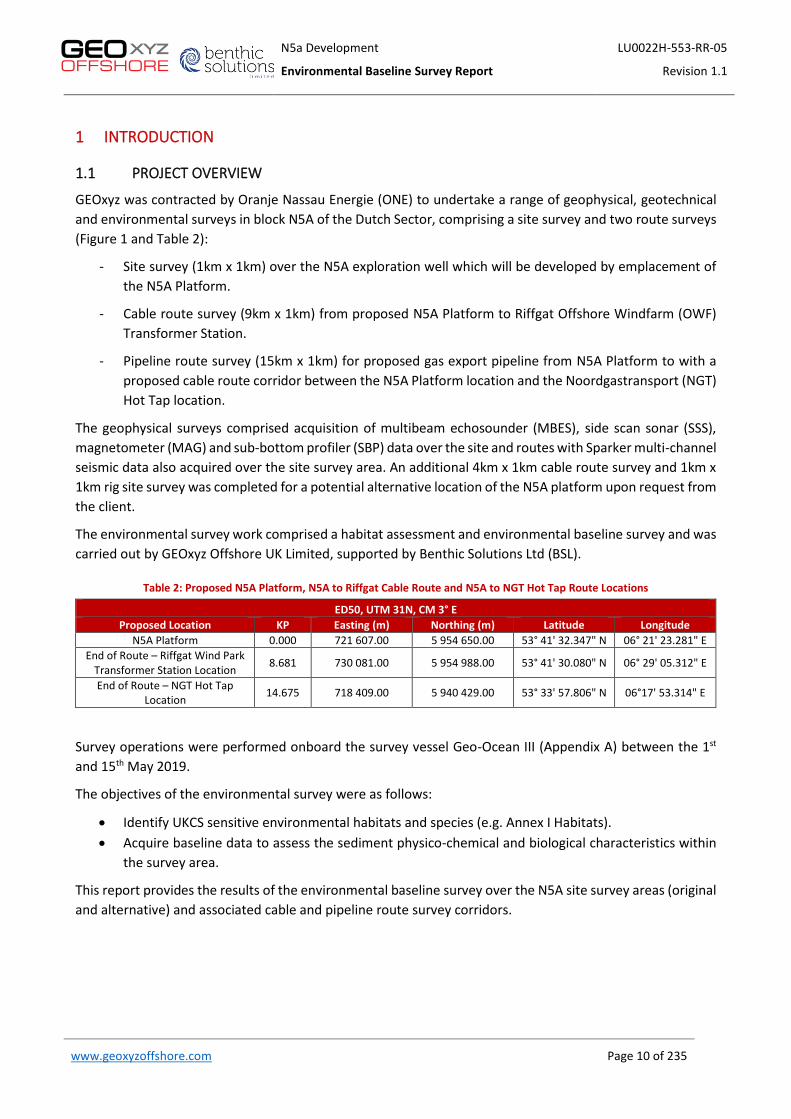
N5a Development LU0022H-553-RR-05
Environmental Baseline Survey Report Revision 1.1
www.geoxyzoffshore.com Page 10 of 235
1 INTRODUCTION
1.1 PROJECT OVERVIEW
GEOxyz was contracted by Oranje Nassau Energie (ONE) to undertake a range of geophysical, geotechnical and environmental surveys in block N5A of the Dutch Sector, comprising a site survey and two route surveys (Figure 1 and Table 2):
- Site survey (1km x 1km) over the N5A exploration well which will be developed by emplacement of the N5A Platform.
- Cable route survey (9km x 1km) from proposed N5A Platform to Riffgat Offshore Windfarm (OWF) Transformer Station.
- Pipeline route survey (15km x 1km) for proposed gas export pipeline from N5A Platform to with a proposed cable route corridor between the N5A Platform location and the Noordgastransport (NGT) Hot Tap location.
The geophysical surveys comprised acquisition of multibeam echosounder (MBES), side scan sonar (SSS), magnetometer (MAG) and sub-bottom profiler (SBP) data over the site and routes with Sparker multi-channel seismic data also acquired over the site survey area. An additional 4km x 1km cable route survey and 1km x 1km rig site survey was completed for a potential alternative location of the N5A platform upon request from the client.
The environmental survey work comprised a habitat assessment and environmental baseline survey and was carried out by GEOxyz Offshore UK Limited, supported by Benthic Solutions Ltd (BSL).
Table 2: Proposed N5A Platform, N5A to Riffgat Cable Route and N5A to NGT Hot Tap Route Locations
ED50, UTM 31N, CM 3° E Proposed Location KP Easting (m) Northing (m) Latitude Longitude
N5A Platform 0.000 721 607.00 5 954 650.00 53° 41' 32.347" N 06° 21' 23.281" E End of Route – Riffgat Wind Park
Transformer Station Location 8.681 730 081.00 5 954 988.00 53° 41' 30.080" N 06° 29' 05.312" E
End of Route – NGT Hot Tap Location 14.675 718 409.00 5 940 429.00 53° 33' 57.806" N 06°17' 53.314" E
Survey operations were performed onboard the survey vessel Geo-Ocean III (Appendix A) between the 1st and 15th May 2019.
The objectives of the environmental survey were as follows:
• Identify UKCS sensitive environmental habitats and species (e.g. Annex I Habitats). • Acquire baseline data to assess the sediment physico-chemical and biological characteristics within
the survey area.
This report provides the results of the environmental baseline survey over the N5A site survey areas (original and alternative) and associated cable and pipeline route survey corridors.

N5a Development LU0022H-553-RR-05
Environmental Baseline Survey Report Revision 1.1
www.geoxyzoffshore.com Page 11 of 235
Figure 1: Project location overview
1.2 SCOPE OF WORK
There were three main work areas for geophysical, geotechnical and environmental surveys as described in N5A-7-10-0-70000-01-05 - Pipeline Route and Platform Area Survey Scope. These were:
• Platform Survey Future N5A location; • Pipeline Route Survey from the future N5A platform location to a subsea hot-tap tie-in at the
NGT pipeline near KP 142.1(orange line in Figure 1 above); • Cable Route Survey from the future N5A platform location to the Riffgat transformer station
(blue line in Figure 1 above).
The following surveys were required by ONE and are described in more detail in Table 3:
• Geophysical Pipeline and Power Cable Route Surveys; • Geotechnical Pipeline and Power Cable Route Surveys; • Environmental Pipeline and Power Cable Route surveys including the Platform Area; • Geophysical Platform Area Survey.
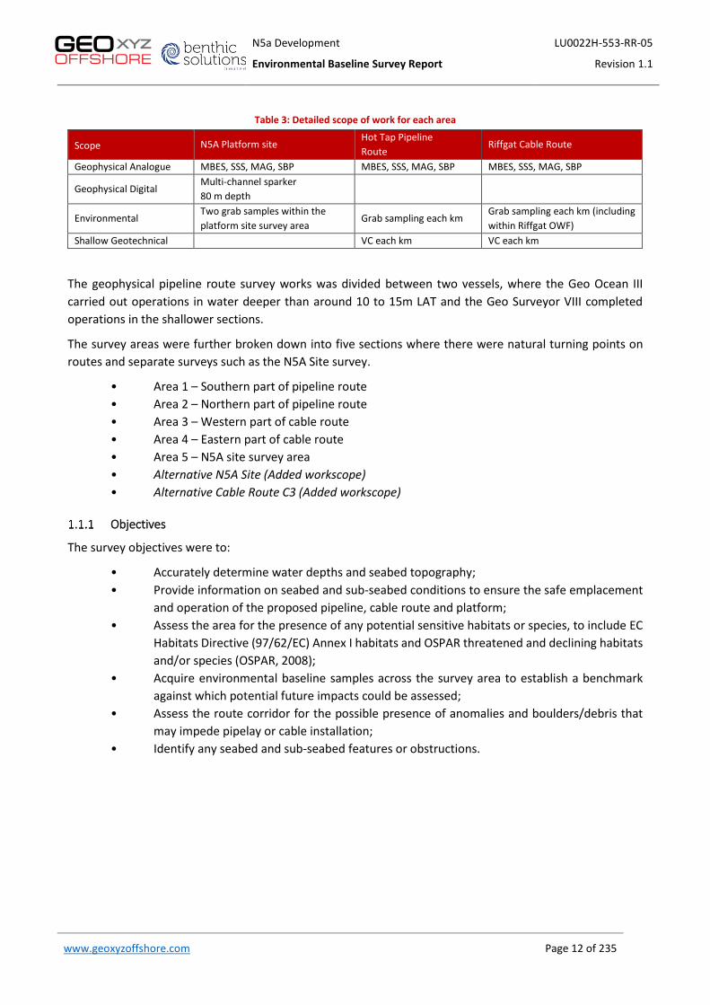
N5a Development LU0022H-553-RR-05
Environmental Baseline Survey Report Revision 1.1
www.geoxyzoffshore.com Page 12 of 235
Table 3: Detailed scope of work for each area
Scope N5A Platform site Hot Tap Pipeline Route
Riffgat Cable Route
Geophysical Analogue MBES, SSS, MAG, SBP MBES, SSS, MAG, SBP MBES, SSS, MAG, SBP
Geophysical Digital Multi-channel sparker 80 m depth
Environmental Two grab samples within the platform site survey area
Grab sampling each km Grab sampling each km (including within Riffgat OWF)
Shallow Geotechnical VC each km VC each km
The geophysical pipeline route survey works was divided between two vessels, where the Geo Ocean III carried out operations in water deeper than around 10 to 15m LAT and the Geo Surveyor VIII completed operations in the shallower sections.
The survey areas were further broken down into five sections where there were natural turning points on routes and separate surveys such as the N5A Site survey.
• Area 1 – Southern part of pipeline route • Area 2 – Northern part of pipeline route • Area 3 – Western part of cable route • Area 4 – Eastern part of cable route • Area 5 – N5A site survey area • Alternative N5A Site (Added workscope)
• Alternative Cable Route C3 (Added workscope)
Objectives
The survey objectives were to:
• Accurately determine water depths and seabed topography; • Provide information on seabed and sub-seabed conditions to ensure the safe emplacement
and operation of the proposed pipeline, cable route and platform; • Assess the area for the presence of any potential sensitive habitats or species, to include EC
Habitats Directive (97/62/EC) Annex I habitats and OSPAR threatened and declining habitats and/or species (OSPAR, 2008);
• Acquire environmental baseline samples across the survey area to establish a benchmark against which potential future impacts could be assessed;
• Assess the route corridor for the possible presence of anomalies and boulders/debris that may impede pipelay or cable installation;
• Identify any seabed and sub-seabed features or obstructions.

N5a Development LU0022H-553-RR-05
Environmental Baseline Survey Report Revision 1.1
www.geoxyzoffshore.com Page 13 of 235
1.3 GEODETIC PARAMETERS
Horizontal Reference
Table 4: Geodetic parameters
Geodetic Parameters
Spheroid International 1924 Semi-major axis 6378388.297 Semi-minor axis 6356911.946 Datum European Datum 1950 (ED50) Projection Universal Transverse Mercator (UTM) False Easting 500000.00 False Northing 0.00 Central Meridian 3° East Central Scale Factor 0.9996 Latitude of Origin 0° Grid Zone 31 North
Datum Transformation WGS84 – ED50
dx + 89.5m dy +93.8m dz +123.1m Rx 0.0 Ry 0.0 Rz -0.156
Scale -1.2ppm
Vertical Reference
All water depths have been reduced to LAT using the UKHO VORF model. MSL is 1.6m above LAT within the survey area.

N5a Development LU0022H-553-RR-05
Environmental Baseline Survey Report Revision 1.1
www.geoxyzoffshore.com Page 14 of 235
2 SURVEY OPERATIONS AND DATA REVIEW
SUMMARY OF SURVEY OPERATIONS
Between the 01st April and 15th May 2019, a geophysical, seismic, geotechnical and environmental survey was completed for the N5A Development Project – Pipeline Route and Platform Area Survey aboard the Geo Ocean III. An overview of the survey operations is given in Table 5.
Table 5: Overview of survey operations
Survey Operations Geo Ocean III– N5A Site, Cable Route and Pipeline Route Survey
1 29/04/2019 Alongside Eemshaven Completed demobilisation from previous project commenced mobilisation for ONE project. Completed Survey Positioning, MRU and SVP Comparisons
2 30/04/2019
Completed mobilisation of personnel to vessel Completed all vessel crew inductions Completed kick-off meeting and mobilisation HIRA review Completed transit to work location Completed Vessel DP trials
3 01/05/2019
Completed Recce line through pipeline route and location. MBES calibration location identified Completed MBES calibration SSS verification completed Muster Drill completed Started analogue survey acquisition on northern section of pipeline route (Area 2)
4 02/05/2019
Continued analogue survey acquisition on northern section of pipeline route (Area 2) Started Vibro-coring operations on northern section of pipeline route (Area 2) Continued analogue survey acquisition cross lines only on northern section of pipeline route (Area 2) Carried out three Environmental Camera observations on environmental sample locations on northern section of pipeline route (Area 2) Continued analogue survey acquisition cross lines only on northern section of pipeline route and western section of cable route. (Area 2 and Area 3)
5 03/05/2019
Continued analogue survey acquisition cross lines only on western section of cable route. (Area 3) Stopped operations due to increasing weather affecting data. Carried out five Environmental Camera observations on environmental sample locations on northern section of pipeline route (Area 2) Stopped due to weather rising out of safe working limits for operations Standing by on weather
6 04/05/2019 Standing by on weather 7 05/05/2019 Standing by on weather
8 06/05/2019
Standing by on weather Completed Drop Camera locations on northern section of pipeline route (Area 2) Commenced Grab Sample locations on northern section of pipeline route (Area 2) Stopped Grab Sampling due to rigging issue
9 07/05/2019
Resumed analogue survey acquisition on northern section of pipeline route (Area 2) Stopped analogue survey acquisition on northern section of pipeline route (Area 2) Thruster Technician onboard to fix thruster issue and returned to shore Completed Vibro-core operations on northern section of pipeline route (Area 2)
10 08/05/2019 Completed Environmental Grab Sampling operations on northern section of pipeline route (Area 2) Completed analogue survey acquisition on northern section of pipeline route (Area 2) Commenced N5A UHR Site Survey (Area 5)
11 09/05/2019
Completed N5A UHR Site Survey (Area 5) Acquired one-line analogue survey acquisition on western section of cable route (Area 3) Completed analogue survey acquisition on eastern section of cable route (Area 4) Completed Geotechnical Vibro-cores on eastern section of cable route (Area 4) Completed Environmental Video Photography and Grab Sampling operations on eastern section of cable route (Area 4) Re-commenced analogue survey acquisition on western section of cable route (Area 3)

N5a Development LU0022H-553-RR-05
Environmental Baseline Survey Report Revision 1.1
www.geoxyzoffshore.com Page 15 of 235
Survey Operations Geo Ocean III– N5A Site, Cable Route and Pipeline Route Survey
12 10/05/2019 Completed analogue survey acquisition on western section of cable route (Area 3) Completed Geotechnical Vibro-cores on western section of cable route (Area 3) Completed N5A UHR Site Survey reshoots (Area 5)
13 11/05/2019
Completed additional environmental video and photography transects on N5A Site Survey location. Completed Environmental Video Photography and Grab Sampling operations on western section of cable route (Area 3) Commenced Geotechnical Vibro-cores on southern section of pipeline route (Area 1) Commenced Environmental Video Photography on southern section of pipeline route (Area 1)
14 12/05/2019
Completed Environmental Video Photography and Grab Sampling operations on southern section of pipeline route (Area 1) Completed Geotechnical Vibro-cores on southern section of pipeline route (Area 1) Commenced analogue survey acquisition on southern section of pipeline route (Area 1) and infill on northern pipeline route (area 2)
15 13/05/2019 Completed analogue survey acquisition on southern section of pipeline route (Area 1) and infill on northern pipeline route (area 2) Completed analogue survey acquisition on alternative cable route (C3)
16 14/05/2019
Completed Alternative N5A UHR Site Survey Completed Geotechnical Vibro-cores on alternative N5A site and cable route (C3) Completed Environmental Video Photography and Grab Sampling operations on alternative N5A site and cable route (C3)
17 15/05/2019 Arrived in Eemshaven Demobilisation Completed
GEOPHYSICAL DATA
Analogue geophysical data acquired by GEOxyz during the survey were used for site selection as no previous geophysical data were available for the survey area. This data was reviewed onboard by BSL and camera transects were selected to target any habitats and boundaries across the survey area, with particular attention paid to the investigation of potential Annex I habitats protected under the EU Habitats Directive. Where features of interest occurred in close proximity to one of the environmental sampling stations, based on the rationale outlined in the scope of work, this station was to be moved slightly to provide additional ground-truthing data for the feature of interest.
The following datasets were available for review during the preparation of this report:
• Bathymetry, reduced and processed offshore to provide a digital terrain model where major bathymetric features and minor bathymetric changes could be identified and highlighted. This included the identification of large features (e.g. linear ridges of cobbles and boulders) and seabed infrastructure (e.g. existing pipelines).
• Side scan sonar (SSS) with data run at both high (400kHz) and low (100kHz) frequencies at variable ranges for different sections of the survey; 50m/150m/200m/250m for the N5A to NGT Hot Tap Pipeline, 150m/200m on the Riffgat Cable Route and 75m/125m in the Platform Area with digital rendering onto a seabed mosaic of the area (100KHz) for review. Changes in sediment type and hardness, along with features observed through low level relief and discrete objects could also be delineated.

N5a Development LU0022H-553-RR-05
Environmental Baseline Survey Report Revision 1.1
www.geoxyzoffshore.com Page 16 of 235
ENVRIONMENTAL GROUND-TRUTHING AND SAMPLING
The environmental sampling strategy was defined by the client prior to the commencement of the survey. Sampling locations along the pipeline and cable routes were positioned every kilometre from the proposed N5A well locations to the shore and to the Riffgat offshore wind farm (Figure 2). Two stations (Grab_P_0 and Grab_P_7) along the pipeline route were repositioned to cover areas of interest identified from the sidescan sonar record (Table 6). At each of these sampling locations a drop-down video assessment was conducted before grab sampling, with video footage acquired at all stations apart from Grab_P_14 where the visibility severely reduced. Additional camera transects were conducted over the proposed N5A well locations and additional areas of interest identified following review of the sidescan sonar record (Table 7).
Seabed video footage was acquired along eight camera transects using a Seabug camera system mounted within a BSL camera sled frame equipped with a separate strobe, and LED lamps. The camera unit itself is capable of acquiring images at 14.7MP resolution but was set to a resolution of 5MP (2592 x 1944 pixels) to optimise image upload times during camera operation.
A BSL Double grab (double Van Veen) was used for seabed sampling, requiring two successful deployments at each location. A maximum of three ‘no sample’ deployments was allowed at each station before abandoning. A 0.1m2 Day Grab was used on the first deployment, before switching to the BSL Double grab for all remaining deployments at the client’s request.
Table 6: Summary of drop-down camera and grab sampling locations for survey area
ED50, UTM 31N, CM 3° E
Station Rationale Type Easting (m)
Northing (m) PC F1 F2 F3
Grab_P_0 Pipeline Route - Positioned at 1km intervals EBS/HAS 721619 5954453 Y Y Y Y
Grab_P_1 Moved from KP in order to investigate area of high reflectivity sediment EBS/HAS 721325 5953791 Y Y Y Y
Grab_P_2 Pipeline Route - Positioned at 1km intervals EBS/HAS 720981 5952752 Y Y Y Y
Grab_P_3 Pipeline Route - Positioned at 1km intervals EBS/HAS 720669 5951801 Y Y Y Y
Grab_P_4 Pipeline Route - Positioned at 1km intervals EBS/HAS 720355 5950850 Y Y Y Y
Grab_P_5 Pipeline Route - Positioned at 1km intervals EBS/HAS 720041 5949900 Y Y Y Y
Grab_P_6 Pipeline Route - Positioned at 1km intervals EBS/HAS 719729 5948950 Y Y Y Y
Grab_P_7 Moved from KP to investigate mixed reflectivity sediment EBS/HAS 719347 5948023 Y Y Y Y
Grab_P_8 Pipeline Route - Positioned at 1km intervals EBS/HAS 719105 5947052 Y Y Y Y
Grab_P_9 Pipeline Route - Positioned at 1km intervals EBS/HAS 718861 5945912 Y Y Y Y
Grab_P_10 Pipeline Route - Positioned at 1km intervals EBS/HAS 718779 5944917 Y Y Y Y
Grab_P_11 Pipeline Route - Positioned at 1km intervals EBS/HAS 718695 5943920 Y Y Y Y
Grab_P_12 Pipeline Route - Positioned at 1km intervals EBS/HAS 718614 5942923 Y Y Y Y
Grab_P_13 Pipeline Route - Positioned at 1km intervals EBS/HAS 718532 5941927 Y Y Y Y
Grab_P_14 Pipeline Route - Positioned at 1km intervals EBS/HAS 718450 5940930 Y Y Y Y
Grab_P_15 Pipeline Route - Positioned at 1km intervals EBS/HAS 718366 5939933 Y Y Y Y
Grab_C_0 Original Cable Route and N5A well centre location EBS/HAS 721610 5954652 Y Y Y Y
Grab_C_1 Original Cable Route – Positioned at 1km intervals EBS/HAS 722604 5954538 Y Y Y Y
Grab_C_2 Original Cable Route – Positioned at 1km intervals EBS/HAS 723596 5954425 Y Y Y Y
Grab_C_3 Original Cable Route – Positioned at 1km intervals EBS/HAS 724588 5954315 Y Y Y Y

N5a Development LU0022H-553-RR-05
Environmental Baseline Survey Report Revision 1.1
www.geoxyzoffshore.com Page 17 of 235
ED50, UTM 31N, CM 3° E
Grab_C_4 Original Cable Route – Positioned at 1km intervals EBS/HAS 725579 5954203 Y Y Y Y
Grab_C_5 Original Cable Route – Positioned at 1km intervals EBS/HAS 726575 5954089 Y Y Y Y
Grab_C_6 Original Cable Route – Positioned at 1km intervals EBS/HAS 727355 5954245 Y Y Y Y
Grab_C_7 Original Cable Route – Positioned at 1km intervals EBS/HAS 728149 5954477 Y Y Y Y
Grab_C_8 Original Cable Route – Positioned at 1km intervals EBS/HAS 729107 5954756 Y Y Y Y
Grab_C3_0 Secondary Cable Route and N5A second potential well centre location EBS/HAS 722288 5953018 Y Y Y Y
Grab_C3_1 Secondary Cable Route – Positioned to investigate mixed reflectivity sediment EBS/HAS 723809 5953378 Y Y Y Y
Grab_C3_2 Secondary Cable Route – Positioned to investigate high reflectivity sediment EBS/HAS 725337 5953741 Y Y Y Y
Table 7: Summary of camera transect locations for the survey area
ED50, UTM 31N, CM 3° E
Transect Rationale SOL/EOL Date and time Depth
(m) Easting
(m) Northing
(m) No.
Stills
Video footage (mm:ss)
Grab P_0 Investigating area of mixed reflectivity sediment
SOL 02/05/2019 17:15:11 30 721647 5954430 27 07:13
EOL 02/05/2019 17:22:21 31 721591 5954476
North Transect 1
Investigating transition from mixed to high reflectivity sediment
SOL 11/05/2019 00:49:10 29 721486 5954680 30 10:11
EOL 11/05/2019 00:59:10 29 721363 5954634
North Transect 2
Investigating transition from low to mixed reflectivity sediment
SOL 11/05/2019 00:06:17 30 721609 5954992 41 12:49
EOL 11/05/2019 00:18:59 28 721631 5955152
North Transect 3
Investigating transition from mixed to high reflectivity sediment
SOL 11/05.2019 02:04:48 29 721902 5954407 50 12:29
EOL 11/05/2019 02:17:13 29 721802 5954550
N5A Transect 1
Transect across original N5A well location
SOL 11/05/2019 01:38:05 29 721585 5954588 35 08:37
EOL 11/05/2019 01:46:38 29 721626 5954708
N5A Transect 2
Transect across original N5A well location
SOL 11/05/2019 01:16:28 28 721668 5954631 39 09:13
EOL 11/05/2019 01:25:35 29 721544 5954667
Grab_C3_0 Transect across second proposed N5A well location
SOL 14/05/2019 21:51:02 24 722231 5952983 36 09:15
EOL 14/05/2019 22:00:14 25 722335 5953047
Grab_C3_2 Investigating area of high reflectivity sediment
SOL 14/05/2019 20:46:00 25 725366 5953610 37 12:36
EOL 14/05/2019 20:58:53 25 725326 5953785

N5a Development LU0022H-553-RR-05
Environmental Baseline Survey Report Revision 1.1
www.geoxyzoffshore.com Page 18 of 235
Figure 2: Survey strategy overview

N5a Development LU0022H-553-RR-05
Environmental Baseline Survey Report Revision 1.1
www.geoxyzoffshore.com Page 19 of 235
HABITAT INVESTIGATION
Habitat Classification
A marine biotope classification system for British waters was developed by Connor et al. (2004) from data acquired during the JNCC Marine Nature Conservation Review (MNCR) and subsequently revised by Parry et
al. (2015) to provide improved classification of deep-sea habitats. The resultant combined JNCC (2015) classification system is analogous with the European Nature Information Service Habitat Classification (EUNIS, 2013), which has compiled habitat information from across Europe into a single database. The two classification systems are both based around the same hierarchical analysis. Initially abiotic habitats are defined at four levels. Biological communities are then linked to these (at two lower levels) to produce a biotope classification. (Connor et al., 2004; EUNIS, 2013).
Habitat descriptions have been interpreted from the side scan sonar and bathymetric data acquired during the current survey, in conjunction with additional information on seabed sediment types and faunal communities from seabed photography and grab sampling. Global Mapper V20 GIS software was used to review side scan sonar mosaic (Geotiff) and multibeam bathymetry data (Geotiff and xyz) and to delineate areas of different seabed habitats.
Assessment of Sensitive Habitats
The Netherlands is a signatory of the Convention on the Conservation of European Wildlife and Natural Habitats (Bern Convention, 1979). To meet their obligations under the convention, the European Community Habitats Directive was adopted in 1992. The provisions of the Directive require Member States to introduce a range of measures including the protection of species listed in the Annexes; to undertake surveillance of habitats and species and produce a report every six years on the implementation of the Directive. The 189 habitats listed in Annex I of the Directive and the 788 species listed in Annex II, are to be protected by means of a network of sites. Each Member State is required to prepare and propose a national list of sites, which will be evaluated in order to form a European network of Sites of Community Importance (SCIs). These will eventually be designated by Member States as Special Areas of Conservation (SACs), and along with Special Protection Areas (SPAs) classified under the EC Birds Directive (2009), form a network of protected areas known as Natura 2000. The Directive was amended in 1997 by a technical adaptation Directive and latterly by the Environment Chapter of the Treaty of Accession 2003.
Based on the above, the OSPAR list of threatened and/or declining species and habitats and Annex I habitats of particular relevance to this region of Dutch waters are:
• Biogenic reefs formed by Sabellaria spinulosa (the Ross Worm); and, • Sandbanks which are slightly covered by sea water all the time
Stony reefs are an Annex I habitat and are protected under the EU habitats directive. Sampling location Grab_C3_2 showed a high proportion of cobbles and boulders, and consequently a stony reef assessment was conducted. The seabed camera ground-truthing data were assessed for potential stony reefs using the criteria proposed by Irving (2009). While the Irving (2009) criteria have been approved by the UK regulators for application in UK waters, they have not been explicitly approved by the Netherlands authorities but are used here as they provide a useful basis for semi-quantitative assessment of potential Annex I stony reef habitat. The Irving (2009) method breaks down the assessment criteria into measures of reef ‘quality’ or ‘reefiness’ as outlined in Table 8. This is based on a minimum cobble size of 64mm being present and indicating relief above the natural seabed where >10% of the matrix are cobble related and a minimum surface area of around 25m2 is recorded.

N5a Development LU0022H-553-RR-05
Environmental Baseline Survey Report Revision 1.1
www.geoxyzoffshore.com Page 20 of 235
The stony reef assessment was based on HD video and stills taken during the camera transects. Stills were acquired when the camera frame landed on the seabed for one or more seconds in order to obtain the best possible image quality, while the changes in coverage and density of cobbles/boulders were estimated during the video data analysis.
Table 8: Summary of resemblance to a stony reef, as summarised in Irving (2009)
Measure of ‘reefiness’ NOT a reef Low(c) Medium High Composition(a) <10% 10-40% 40-95% >95% Elevation(b) Flat seabed <64mm 64mm-5m >5m Extent (m2) <25m2 >25m2 >25m2 >25m2
Biota Dominated by infauna
>80% of species are epifauna
(a) Diameter of cobbles / boulders being greater than 64mm. Percentage cover relates to a minimum area
of 25m2. This ‘composition’ characteristic also includes ‘patchiness’.
(b) Minimum height (64mm) relates to minimum size of constituent cobbles. This characteristic could also
include ‘distinctness’ from the surrounding seabed.
(c) When determining if the seabed is considered as Annex I stony reef, a ‘low’ scored (in any category),
would require a strong justification for this area to be considered as contributing to the Marine Natura site
network of qualifying reefs in terms of the EU Habitats Directive.
The Irving (2009) stony reef protocol was split into separate assessments of reef ‘structure’ and ‘overall reefiness’ using a method developed by BSL staff (Table 9 and Table 10). This provided a reef structure value that could be then assessed against extent, where applicable, to provide a measure of overall ‘reefiness’ as illustrated in Table 10. As separate thresholds for ‘Low’, ‘Medium’ and ‘High’ stony reef extent were not given in Irving (2009), the overall ‘reefiness’ is determined by reef structure provided that the extent of the stony reef covers a minimum of 25m2.
Table 9: Stony reef structure matrix (after Irving, 2009)
Reef Structure Matrix
Elevation
Flat <64mm 64mm-5m >5m
Not a Reef Low Medium High
Composition
<10% Not a reef NOT A REEF NOT A REEF NOT A REEF NOT A REEF 10-40% Low NOT A REEF LOW LOW LOW 40-95% Medium NOT A REEF LOW MEDIUM MEDIUM >95% High NOT A REEF LOW MEDIUM HIGH
Table 10: Overall stony reefiness matrix (structure vs extent)
Overall Reefiness Matrix Reef Structure (incl. Composition and Elevation)
Not a Reef Low Medium High
Extent (m2) <25 Not a Reef NOT A REEF NOT A REEF NOT A REEF NOT A REEF >25 Low - High NOT A REEF LOW MEDIUM HIGH
In evaluating the ground-truthing of stony patches, Irving (2009) also recommended that the associated biota was considered, indicating that areas dominated by infauna should be considered ‘Not a Reef’ whereas areas where greater than 80% of species were epifaunal should be considered to show ‘High’ reefiness, but no recommendations were given as to the proportion of infauna and epifauna warranting classification of ‘Low’ or ‘Medium’ reefiness. In practise, it is not practical to assess the proportion of infaunal and epifaunal species in a quantitative manner. This cannot be undertaken from seabed camera data (i.e. video footage or still
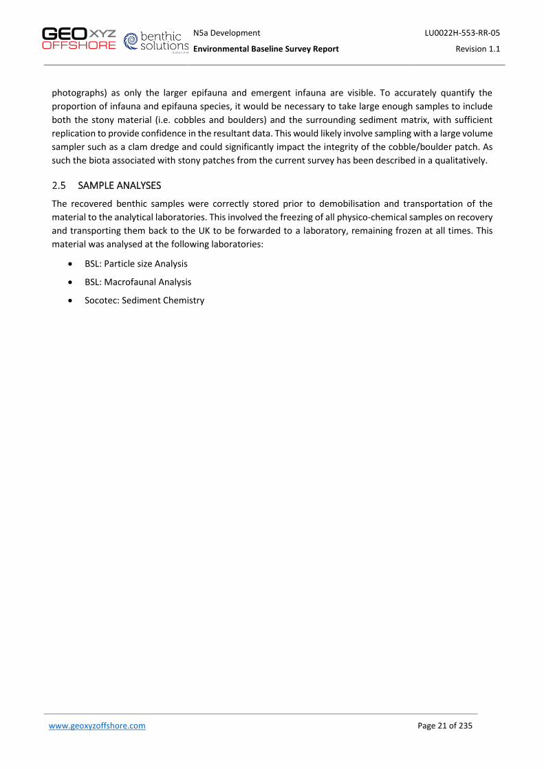
N5a Development LU0022H-553-RR-05
Environmental Baseline Survey Report Revision 1.1
www.geoxyzoffshore.com Page 21 of 235
photographs) as only the larger epifauna and emergent infauna are visible. To accurately quantify the proportion of infauna and epifauna species, it would be necessary to take large enough samples to include both the stony material (i.e. cobbles and boulders) and the surrounding sediment matrix, with sufficient replication to provide confidence in the resultant data. This would likely involve sampling with a large volume sampler such as a clam dredge and could significantly impact the integrity of the cobble/boulder patch. As such the biota associated with stony patches from the current survey has been described in a qualitatively.
SAMPLE ANALYSES
The recovered benthic samples were correctly stored prior to demobilisation and transportation of the material to the analytical laboratories. This involved the freezing of all physico-chemical samples on recovery and transporting them back to the UK to be forwarded to a laboratory, remaining frozen at all times. This material was analysed at the following laboratories:
• BSL: Particle size Analysis
• BSL: Macrofaunal Analysis
• Socotec: Sediment Chemistry

N5a Development LU0022H-553-RR-05
Environmental Baseline Survey Report Revision 1.1
www.geoxyzoffshore.com Page 22 of 235
3 RESULTS AND INTERPRETATION
BATHYMETRY
The following text was adapted from the survey reports for the N5A site (LU-0022H-553-RR-01), N5A to NGT Hot Tap pipeline route (LU-0022H-553-RR-02) and N5A to Riffgat cable route (LU-0022H-553-RR-07) to provide an overview of the bathymetry across the survey site and route corridors.
Bathymetry data were acquired using an R2 Sonics 2022 multi-beam echo sounder for the site and an R2Sonic 2024 multi-beam echo sounder for the two route surveys. All bathymetry data have been reduced to LAT, which was 1.6m below MSL within the survey area and are presented at a 0.5m x 0.5m bin size.
N5A to NGT Hot Tap Pipeline Route
Water depths along the proposed N5A to NGT Hot Tap pipeline route ranged between 9.8m LAT at KP0.000 and 26.4m LAT at KP14.675, with the seabed shoaling gently towards the southern end of the proposed pipeline route. A series of natural troughs trending west-north-west to east-south-east occurred within the survey corridor, crossing the proposed pipeline route, the largest of which was approximately 250m wide.
A variety of anthropogenic debris/wreck and areas of disturbed seabed were evident on the bathymetry data:
• Two prominent features interpreted as shipwrecks surrounded by seabed scouring; the largest (40.1m x 12.8m x 1.1m) occurred at approximately KP2.462, 369m west-north-west of the proposed route and the other (19.1m x 12.9m x 0.2m) occurred at approximately KP2.373, 339m west-north-west of the proposed route.
• Three semi-circular features with 1m of positive relief, interpreted as being related to previous drilling activity, were observed on bathymetry data. These were observed at the start of the proposed route between KP0.009 and KP0.089, offset by 90m to the east-south-east at their closest approach. These features lay within a 30m radius of each other and exhibited average dimensions of 30m x 30m.
• Three existing cables and one pipeline were expected to cross the proposed pipeline route but were not observed on the bathymetry data.
N5A to Riffgat Cable Route
The seabed shoaled gently towards the east-north-east end of the proposed N5A to Riffgat cable route with water depths ranging between 26.0m at KP0.280 and 19.6m KP7.941. A series of natural troughs, predominantly trending north-west to south-east, crossed the proposed cable route from approximately KP5.158 to KP8.681 and were interpreted to be related to tidal/current processes.
Three semi-circular features with 1m of positive relief, interpreted as being related to previous drilling activity, were imaged in the bathymetry data. These were positioned at the start of the proposed route between KP0.085 and KP0.168; at their minimum offset from the route they were approximately 27m south-south-west. They were positioned within a 30m radius and had average dimensions of 30m x 30m.
The Norned cable was observed crossing the proposed cable route at KP2.313 trending north-north-west to south-south-east.

N5a Development LU0022H-553-RR-05
Environmental Baseline Survey Report Revision 1.1
www.geoxyzoffshore.com Page 23 of 235
SEABED FEATURES
The following text was adapted from the survey reports for the N5A site (LU-0022H-553-RR-01), N5A to NGT Hot Tap pipeline route (LU-0022H-553-RR-02) and N5A to Riffgat cable route (LU-0022H-553-RR-07) to provide an overview of the seabed features across the survey area, focussing on features of particular relevance to the environmental baseline and habitat assessment of the survey area.
Side scan sonar data were acquired with an Edgetech 4200 system operating at 100kHz/400kHz with between 75m and 200m per channel range. This was supplemented by swathe bathymetry data gridded to 0.5m bin size.
N5A Site
Seabed sediments across the N5A survey area were expected to comprise ‘fine sand with shell fragments’. An area of ‘coarse sand and shell with a high density of sand mason worms and razor clams’ was evident in the north of the survey area, while an area of ‘coarse sand with pebbles and cobbles’ was present in the south. The uppermost sand unit was merely a veneer and the boundary between the sand and the underlying clay outcrops was arbitrary with the potential for some clay to outcrop in the areas interpreted as sand.
Outcrops of clay were interpreted within the survey area, showing a positive relief of up to 0.5m above background seabed levels. Elsewhere accumulations of coarse sand and gravel were also observed on the bathymetry as having positive relief above the ambient seabed, with some accumulations likely to be caused by the stabilising effect of high densities of sand mason worms and razor clams on the seabed.
Within the survey area there was no existing infrastructure other than the previously drilled N5 Well (~140m from the proposed platform and ~1.6km from the alternative platform location). Seabed scars up to 1.1m high from the rig whilst over the N5-Ruby wellsite were observed on the bathymetry and side scan sonar data. Numerous magnetometer anomalies were observed within this area; however no wellhead or other evidence of the drilling location could be observed at seabed.
N5A to NGT Hot Tap Pipeline Route
Seabed sediments along the proposed pipeline route corridor were expected to comprise ‘fine sand and shell fragments’, with occasional areas of ‘coarse sand and shell fragments’.
Bedforms were not imaged in the sonar or bathymetry records. However, photographs taken along the route as part of the environmental survey showed clear seabed rippling over much of the survey corridor.
Numerous objects interpreted as boulders and items of debris were observed within the proposed pipeline route corridor. Most of the objects interpreted as boulders occurred towards the north of the survey corridor area and coincided with areas of clay exposure.
The most significant objects identified on the sonar records were two interpreted shipwrecks, the largest (40.1m x 12.8m x 1.1m) occurring at approximately KP2.462, 369m west-north-west of the proposed route and the other (19.1m x 12.9m x 0.2m) at approximately KP2.373, 339m west-north-west of the proposed route.
Three existing cables and one pipeline were expected to cross the proposed pipeline route but were not observed on the bathymetry data.
N5A to Riffgat Cable Route
Seabed sediments along the proposed pipeline route corridor were expected to comprise fine to coarse SAND, with occasional areas of ‘coarse sand and clay with pebbles and cobbles’ and ‘coarse sand with pebbles
N5a Development LU0022H-553-RR-05
Environmental Baseline Survey Report Revision 1.1
www.geoxyzoffshore.com Page 24 of 235
and cobbles’. Approaching the Riffgat Wind Park, the seabed sediments were dominated by ‘coarse sand and shell fragments’ with occasional patches of ‘coarse sand with pebbles and cobbles’.
Bedforms were not imaged in the sonar or bathymetry records. However, photographs taken along the proposed route corridor as part of the environmental survey clearly showed ripples covering the majority of the seabed within the survey corridor area.
There were numerous objects interpreted as boulders within the proposed pipeline route corridor. Most of the objects, interpreted as boulders occur towards the north of the survey corridor in an area coinciding with areas of clay exposure.
SHALLOW SOILS
The following text was adapted from the survey reports for the N5A site (LU-0022H-553-RR-01), N5A to NGT Hot Tap pipeline route (LU-0022H-553-RR-02) and N5A to Riffgat cable route (LU-0022H-553-RR-07) to provide an overview of the shallow soils across the survey area, focussing on the upper layers of relevance to interpretation of the seabed sediment distribution and bathymetric features.
Interpretation of shallow soils across the survey area was based upon pinger and sparker data. Additional information was gained from vibrocore logs and borehole N5-1, 90m south of the proposed Platform Location acquired by Fugro in November 2016. Vibrocore VC_P_0 is at the proposed Platform Location.
N5A Site
The uppermost mappable unit was confirmed as SAND in the vibrocore logs. Where mapped in the western parts of the survey area this unit was under 1.5m thick. This surficial SAND unit was only mappable when thicker than 0.5m and was likely to be present outside the mapped area but at thicknesses below 0.5m.
Three sub units within the Quaternary sequence were interpreted within the area based on the acoustic nature of the sparker data. The uppermost unit, (besides surficial sand mapped from the Pinger data), interpreted within the survey area is a chaotic unit, interpreted to comprise dense to very dense medium to coarse SAND with traces of shell fragments (as sampled within the borehole). Within the survey area, the reflector which correlates with the base of this unit undulates between 1.2m and 18.0m below seabed.
N5A to NGT Hot Tap Pipeline Route
This unit of fine to medium grained SAND generally thicken to the south. It was absent (or less than 0.5m thick) from KP 0.430 to KP 0.450 and KP 0.757 to KP 1.045. South of KP 5.951 the base of the mapped unit becomes indistinct to the point of being unmappable, at this point the unit was approximately 9m thick.
The mapped unit was sub-cropped by a sequence of variable composition. Vibrocore logs show that this sub-crop predominantly comprises silty fine SAND except for the area north of KP 1.246 where the sub crop was more clay prone and was interpreted to be the infill of a broad channel.
N5A to Riffgat Cable Route
This unit of fine to medium grained SAND generally thickened to the east. West of the route AC at KP 5.156 the unit was approximately 0.5 to 1m thick or absent/unmappably thin, east of this point the unit locally exceeds a thickness of 2m.

N5a Development LU0022H-553-RR-05
Environmental Baseline Survey Report Revision 1.1
www.geoxyzoffshore.com Page 25 of 235
Vibrocore logs showed that the mapped unit was sub-cropped by clay prone deposits from KP0 to KP 3.357, interpreted to be the infill of a broad channel. From KP 3.357 to the end of the route the mapped unit was sub cropped by fine SAND.
N5A Site
The seabed within the N5A site survey area sloped gently to the west. The minimum water depth was 23.7m LAT in the NNE of the survey area, while the maximum depth was 26.6m LAT in the WSW. Small areas with relief of up to 0.4m were observed on the bathymetry data with measured gradients of up to 6° on their flanks, which were interpreted to be largely due to outcropping clays.
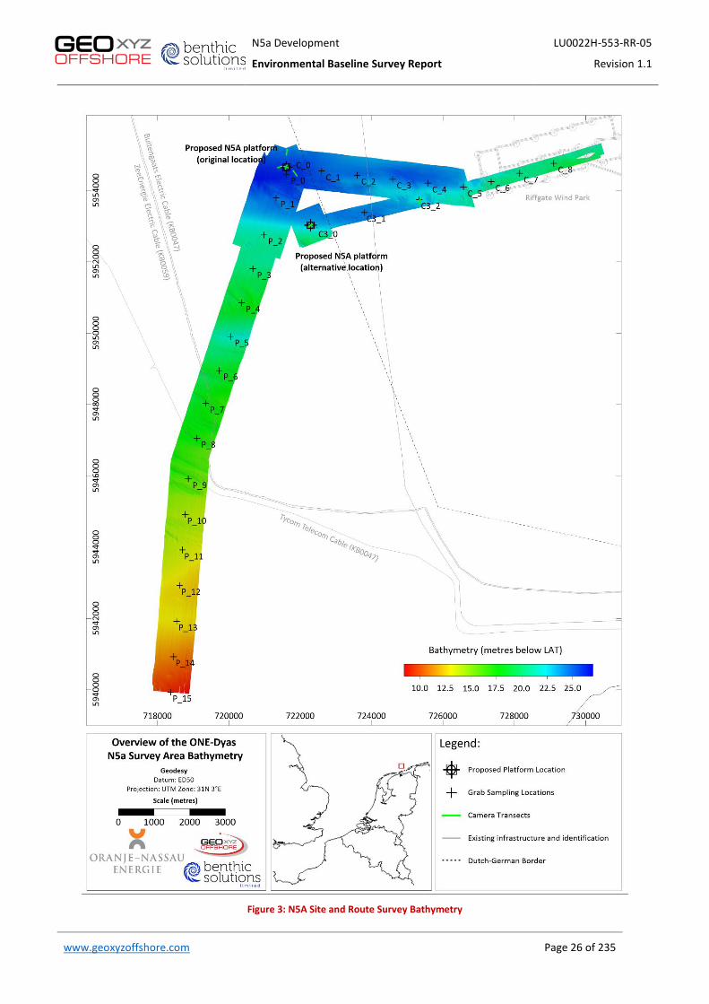
N5a Development LU0022H-553-RR-05
Environmental Baseline Survey Report Revision 1.1
www.geoxyzoffshore.com Page 26 of 235
Figure 3: N5A Site and Route Survey Bathymetry

N5a Development LU0022H-553-RR-05
Environmental Baseline Survey Report Revision 1.1
www.geoxyzoffshore.com Page 27 of 235
Figure 4: Interpreted N5A Site and Route Seabed Features
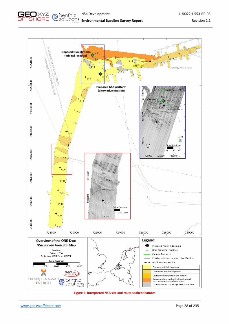
N5a Development LU0022H-553-RR-05
Environmental Baseline Survey Report Revision 1.1
www.geoxyzoffshore.com Page 28 of 235
Figure 5: Interpreted N5A site and route seabed features
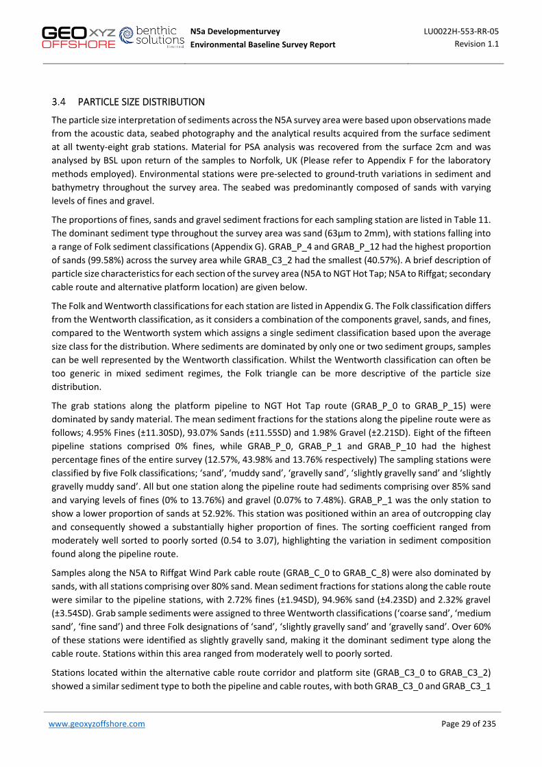
N5a Developmenturvey LU0022H-553-RR-05 Environmental Baseline Survey Report Revision 1.1
www.geoxyzoffshore.com Page 29 of 235 Page 29 of 235
PARTICLE SIZE DISTRIBUTION
The particle size interpretation of sediments across the N5A survey area were based upon observations made from the acoustic data, seabed photography and the analytical results acquired from the surface sediment at all twenty-eight grab stations. Material for PSA analysis was recovered from the surface 2cm and was analysed by BSL upon return of the samples to Norfolk, UK (Please refer to Appendix F for the laboratory methods employed). Environmental stations were pre-selected to ground-truth variations in sediment and bathymetry throughout the survey area. The seabed was predominantly composed of sands with varying levels of fines and gravel.
The proportions of fines, sands and gravel sediment fractions for each sampling station are listed in Table 11. The dominant sediment type throughout the survey area was sand (63µm to 2mm), with stations falling into a range of Folk sediment classifications (Appendix G). GRAB_P_4 and GRAB_P_12 had the highest proportion of sands (99.58%) across the survey area while GRAB_C3_2 had the smallest (40.57%). A brief description of particle size characteristics for each section of the survey area (N5A to NGT Hot Tap; N5A to Riffgat; secondary cable route and alternative platform location) are given below.
The Folk and Wentworth classifications for each station are listed in Appendix G. The Folk classification differs from the Wentworth classification, as it considers a combination of the components gravel, sands, and fines, compared to the Wentworth system which assigns a single sediment classification based upon the average size class for the distribution. Where sediments are dominated by only one or two sediment groups, samples can be well represented by the Wentworth classification. Whilst the Wentworth classification can often be too generic in mixed sediment regimes, the Folk triangle can be more descriptive of the particle size distribution.
The grab stations along the platform pipeline to NGT Hot Tap route (GRAB_P_0 to GRAB_P_15) were dominated by sandy material. The mean sediment fractions for the stations along the pipeline route were as follows; 4.95% Fines (±11.30SD), 93.07% Sands (±11.55SD) and 1.98% Gravel (±2.21SD). Eight of the fifteen pipeline stations comprised 0% fines, while GRAB_P_0, GRAB_P_1 and GRAB_P_10 had the highest percentage fines of the entire survey (12.57%, 43.98% and 13.76% respectively) The sampling stations were classified by five Folk classifications; ‘sand’, ‘muddy sand’, ‘gravelly sand’, ‘slightly gravelly sand’ and ‘slightly gravelly muddy sand’. All but one station along the pipeline route had sediments comprising over 85% sand and varying levels of fines (0% to 13.76%) and gravel (0.07% to 7.48%). GRAB_P_1 was the only station to show a lower proportion of sands at 52.92%. This station was positioned within an area of outcropping clay and consequently showed a substantially higher proportion of fines. The sorting coefficient ranged from moderately well sorted to poorly sorted (0.54 to 3.07), highlighting the variation in sediment composition found along the pipeline route.
Samples along the N5A to Riffgat Wind Park cable route (GRAB_C_0 to GRAB_C_8) were also dominated by sands, with all stations comprising over 80% sand. Mean sediment fractions for stations along the cable route were similar to the pipeline stations, with 2.72% fines (±1.94SD), 94.96% sand (±4.23SD) and 2.32% gravel (±3.54SD). Grab sample sediments were assigned to three Wentworth classifications (‘coarse sand’, ‘medium sand’, ‘fine sand’) and three Folk designations of ‘sand’, ‘slightly gravelly sand’ and ‘gravelly sand’. Over 60% of these stations were identified as slightly gravelly sand, making it the dominant sediment type along the cable route. Stations within this area ranged from moderately well to poorly sorted.
Stations located within the alternative cable route corridor and platform site (GRAB_C3_0 to GRAB_C3_2) showed a similar sediment type to both the pipeline and cable routes, with both GRAB_C3_0 and GRAB_C3_1

N5a Developmenturvey LU0022H-553-RR-05 Environmental Baseline Survey Report Revision 1.1
www.geoxyzoffshore.com Page 30 of 235 Page 30 of 235
constituting over 90% sands. These were moderately sorted and represented the Wentworth classification of ‘fine sand’ and the folk classification of ‘sand’.
Station GRAB_C3_2 was the only station dominated by gravel (54.91%) as opposed to sand (40.57%). This station was classified as ‘granule’ on the Wentworth scale, ‘muddy sandy gravel’ on the Folk scale and was very poorly sorted. Note: four grab attempts were made at this station due to cobbles trapped in the jaws of the sampler, and video footage of this station showed an area of coarse sand and cobbles, which was explored further in the habitat assessment for its potential as an EC Habitats Directive Annex I stony reef.
Table 11: Summary of surface particle size distribution
Station Depth
(m) Mean Sediment Size
Sorting Skewness Kurtosis Fines (%)
Sands (%)
Gravel (%) mm Phi()
GRAB_P_0 29 0.301 1.73 1.80 0.49 1.29 12.47 87.13 0.40 GRAB_P_1 27 0.050 4.33 3.07 0.46 0.82 43.98 52.92 3.11 GRAB_P_2 24 0.227 2.14 0.59 0.05 1.10 3.88 95.37 0.75 GRAB_P_3 24 0.226 2.14 0.52 0.03 1.02 3.64 96.23 0.13 GRAB_P_4 22 0.278 1.85 0.54 0.02 0.99 0.00 99.58 0.42 GRAB_P_5 20 0.316 1.66 0.75 0.05 0.94 0.78 98.21 1.01 GRAB_P_6 21 0.258 1.95 0.56 -0.01 0.97 0.00 99.53 0.47 GRAB_P_7 21 0.224 2.16 0.56 -0.04 0.94 0.00 99.38 0.62 GRAB_P_8 21 0.439 1.19 0.83 0.03 1.19 0.11 96.14 3.74 GRAB_P_9 19 0.223 2.17 1.05 -0.32 1.93 0.00 94.33 5.67
GRAB_P_10 17 0.199 2.33 1.32 0.41 2.45 13.76 85.02 1.22 GRAB_P_11 17 0.285 1.81 1.14 -0.34 2.17 0.00 92.52 7.48 GRAB_P_12 16 0.223 2.16 0.56 -0.04 0.94 0.00 99.58 0.42 GRAB_P_13 16 0.200 2.32 0.54 0.02 0.99 0.52 99.42 0.07 GRAB_P_14 14 0.210 2.25 0.64 -0.07 1.02 0.00 97.52 2.49 GRAB_P_15 13 0.208 2.27 0.62 -0.10 1.11 0.00 96.29 3.71 GRAB_C_0 24 0.604 0.73 0.67 0.00 1.14 0.11 98.55 1.35 GRAB_C_1 27 0.589 0.76 1.59 -0.05 1.97 3.70 84.80 11.50 GRAB_C_2 28 0.446 1.16 0.89 0.29 1.16 2.65 96.87 0.48 GRAB_C_3 28 0.259 1.95 0.91 0.30 2.00 5.97 94.00 0.03 GRAB_C_4 25 0.223 2.16 0.70 0.06 1.05 4.36 95.10 0.54 GRAB_C_5 24 0.458 1.13 1.20 0.09 1.13 3.07 94.11 2.82 GRAB_C_6 24 0.405 1.30 0.75 0.05 0.98 1.56 97.26 1.18 GRAB_C_7 24 0.449 1.16 1.17 0.15 1.05 3.08 94.99 1.94 GRAB_C_8 28 0.361 1.47 0.64 -0.06 0.99 0.00 98.97 1.03
GRAB_C3_0 25 0.214 2.23 0.77 0.31 1.91 5.44 94.09 0.47 GRAB_C3_1 25 0.208 2.27 0.90 0.34 2.27 7.41 91.98 0.62 GRAB_C3_2 25 2.154 -1.11 2.41 0.27 0.64 4.52 40.57 54.91
Mean 0.37 1.77 0.99 0.09 1.29 4.32 91.80 3.88 SD 0.37 0.89 0.60 0.21 0.50 8.58 13.46 10.33
CV (%) 101.9 50.0 60.5 242.3 38.6 198.5% 14.7% 266.3%
A comparison of the full particle size distribution dataset by Phi classification is presented in Figure 12. The majority of samples peaked in the sand fraction (-1 to 4), with grabs along the cable route peaking more generally in the finer fraction (0.73 – 2.16). GRAB_C3_2 was the only station in the survey area to show a differing peak at -1.11 in the granule pebbles fraction, but also showed a smaller peak similar to other stations for the medium sands fraction (1.5). Some stations showed higher fines (GRAB_P_0, GRAB_P_1,

N5a Developmenturvey LU0022H-553-RR-05 Environmental Baseline Survey Report Revision 1.1
www.geoxyzoffshore.com Page 31 of 235 Page 31 of 235
GRAB_P_10), while the distribution of sediment at stations along the cable route survey area (GRAB_C stations) were generally more sandy.
The mean particle sizes for sampling stations are displayed in Figure 6 and Table 11, which ranged from 0.050mm at GRAB_P_1 to 2.154mm at GRAB_C3_2 (mean 0.37mm±0.37SD). Overall, sands proportions across the survey area were described as the major component of the sediment, which is illustrated by a negative correlation between sands and fines (ƍ(5)=-0.723, p<0.001). At 81% of the stations sampled in the N5A survey area, the sands fraction contributed >90% of the sediment type. This is likely attributed to the proximity to shore creating a strong hydrodynamic regime where the settlement of fines materials is restricted.
The proportion of gravels fraction (>63µm, <200µm) was generally very low across the N5A survey area (Figure 9) and only contributed as a major component to GRAB_C3_2 (54.91% Gravel). These results ranged from 0.00% (GRAB_P_4, P_6, P_7, P_9, P_11, P_12, P_14, P_15 and GRAB_C_8) to 54.91% (GRAB_C3_2) with a mean of 3.88% (±10.33SD).
The geographical distribution of sediment fines (i.e. silts and clays <63µm) is presented in Figure 7. Percentages of fine sediments were moderately low throughout the survey area with a mean of 4.32% (±8.58SD). There was no discernible pattern of fines across the N5A area, and as a result the proportion of fines varied from station to station. However, relatively high fines were found near the proposed platform location (GRAB_P_1, GRAB_P_0), and at GRAB_P_10 along the pipeline route. Furthermore, instances of high fines corresponded with the presence of clay materials at GRAB_P_1 and GRAB_C3_1.
It should be noted that where mixed sediment occurs (including shell debris), the sub-sampling process itself can introduce additional variation, where only a relatively small sub-sample is recovered for analysis. For example, the seabed photography at GRAB_C3_1 showed significant clay and fines materials, yet within the PSA sample this only represented 7.41% of the material recovered. As such, the results of particle size analysis should be treated with caution as grab data may not necessarily provide an accurate representation of the sediment type.

N5a Developmenturvey LU0022H-553-RR-05 Environmental Baseline Survey Report Revision 1.1
www.geoxyzoffshore.com Page 32 of 235 Page 32 of 235
Figure 6: Mean particle size (mm)

N5a Developmenturvey LU0022H-553-RR-05 Environmental Baseline Survey Report Revision 1.1
www.geoxyzoffshore.com Page 33 of 235 Page 33 of 235
Figure 7: Proportion of fines (%)

N5a Developmenturvey LU0022H-553-RR-05 Environmental Baseline Survey Report Revision 1.1
www.geoxyzoffshore.com Page 34 of 235 Page 34 of 235
Figure 8: Proportion of sands (%)

N5a Developmenturvey LU0022H-553-RR-05 Environmental Baseline Survey Report Revision 1.1
www.geoxyzoffshore.com Page 35 of 235 Page 35 of 235
Figure 9: Proportion of gravels (%)

N5a Development LU0022H-553-RR-05 Environmental Baseline Survey Report Revision 1.1
www.geoxyzoffshore.com Page 36 of 235 Page 36 of 235
Multivariate Analysis
To provide a detailed examination of the particle size distribution within the survey area, a multivariate analysis was performed using Plymouth Routines in Multivariate Ecological Research software (PRIMER; Clarke and Warwick, 1994) to illustrate data trends.
A similarity dendrogram was generated by hierarchical agglomerative clustering (CLUSTER) with the aim to segregate stations by their similarities/dissimilarities with the results presented in Figure 10 below. A ‘slice’ was added at a Euclidean distance of 6.0 to reduce the number of clusters presented, for ease of interpretation.
Figure 10: Particle size distribution similarity dendrogram
The results of CLUSTER analysis presented in Figure 10 indicated that the stations could be separated into three statistically distinct clusters, as follows:
• Cluster a: Samples in cluster a were dominated by coarse sand, had a mean phi value of 0.95 (±0.59SD) and were found mostly towards the northeast of the survey area. This group included a large portion of the N5A platform location to Riffgat Wind Park cable route stations (78% of GRAB_C stations) and including the particularly coarse station on the alternative cable route (GRAB_C3_2). A review of the sediment types from seabed photography and video confirmed the prevalence of coarse sand over the areas where these grabs occurred, with all stations grouped into cluster a having been previously categorised as either ‘infralittoral coarse sediment’, ‘infralittoral mixed sediment’ or ‘Dense Lanice conchilega and other polychaetes in tide-swept infralittoral sand and mixed gravelly sand’ habitats (Figure 14).
• Cluster b: Only GRAB_P_1 was grouped into cluster b. This station was characterised by a dominant fines fraction (52.92%), which was significantly higher than all other stations in the N5A survey area. The habitat assessment previously identified this area as being composed of ‘infralittoral mixed sediment’ with clay. GRAB_P_1 had some sediment within the coarser phi fraction (small percentage
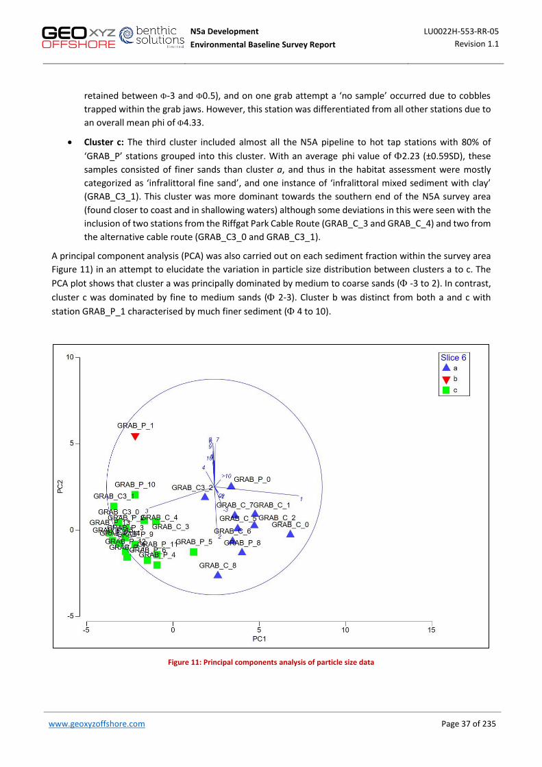
N5a Development LU0022H-553-RR-05 Environmental Baseline Survey Report Revision 1.1
www.geoxyzoffshore.com Page 37 of 235 Page 37 of 235
retained between -3 and 0.5), and on one grab attempt a ‘no sample’ occurred due to cobbles trapped within the grab jaws. However, this station was differentiated from all other stations due to an overall mean phi of 4.33.
• Cluster c: The third cluster included almost all the N5A pipeline to hot tap stations with 80% of ‘GRAB_P’ stations grouped into this cluster. With an average phi value of 2.23 (±0.59SD), these samples consisted of finer sands than cluster a, and thus in the habitat assessment were mostly categorized as ‘infralittoral fine sand’, and one instance of ‘infralittoral mixed sediment with clay’ (GRAB_C3_1). This cluster was more dominant towards the southern end of the N5A survey area (found closer to coast and in shallowing waters) although some deviations in this were seen with the inclusion of two stations from the Riffgat Park Cable Route (GRAB_C_3 and GRAB_C_4) and two from the alternative cable route (GRAB_C3_0 and GRAB_C3_1).
A principal component analysis (PCA) was also carried out on each sediment fraction within the survey area Figure 11) in an attempt to elucidate the variation in particle size distribution between clusters a to c. The PCA plot shows that cluster a was principally dominated by medium to coarse sands ( -3 to 2). In contrast, cluster c was dominated by fine to medium sands ( 2-3). Cluster b was distinct from both a and c with station GRAB_P_1 characterised by much finer sediment ( 4 to 10).
Figure 11: Principal components analysis of particle size data

N5a Development LU0022H-553-RR-05 Environmental Baseline Survey Report Revision 1.1
www.geoxyzoffshore.com Page 38 of 235 Page 38 of 235
A comparison of the full particle size distribution dataset for each of the clusters, is shown in Figure 12 along with example seabed and grab sample photographs for typical samples from each cluster. Cluster a displayed a relatively unimodal distribution for all stations within the cluster, peaking in the coarse sand fraction with the exception of GRAB_C3_2. This station shows a bimodal distribution peaking in the very coarse sands fraction. Cluster b displayed a slightly trimodal distribution with small peaks for the fines, sands and gravel fractions. Lastly, cluster c presented a unimodal distribution with sands slightly finer than cluster a. The geographical distribution of clusters is displayed over bathymetry data in Figure 13 and over the interpreted seabed features in Figure 14.
Figure 12: Particle size distribution for all stations in clusters a, b & c

N5a Development LU0022H-553-RR-05 Environmental Baseline Survey Report Revision 1.1
www.geoxyzoffshore.com Page 39 of 235 Page 39 of 235
Figure 13: Multivariate cluster distribution over bathymetry

N5a Development LU0022H-553-RR-05 Environmental Baseline Survey Report Revision 1.1
www.geoxyzoffshore.com Page 40 of 235 Page 40 of 235
Figure 14: Multivariate cluster distribution over interpreted seabed features

N5a Development LU0022H-553-RR-05 Environmental Baseline Survey Report Revision 1.1
www.geoxyzoffshore.com Page 41 of 235 Page 41 of 235
TOTAL ORGANIC MATTER, TOTAL ORGANIC CARBON, AND MOISTURE CONTENT
Sediment samples were analysed for total organic matter (TOM), total organic carbon (TOC) and moisture content; the results of which are presented in Table 12, with spatial variation in TOC levels illustrated in Figure 15. TOC represents the proportion of biological material and organic detritus within the substrate. This method is less susceptible to the interference sometimes seen using crude combustion techniques, such as analysing TOM by LOI.
TOM results were low throughout the survey area with all but two stations showing less than 1% TOM. Although UKOOA (United Kingdom Offshore Operations Association) threshold levels are based on contamination and natural background levels within the UK Sector of the North Sea, they provide a useful reference for areas of similar sediment types and are used in this report to establish any areas of interest. All stations excluding GRAB_P_1 had values below the mean UKOOA (2001) background levels for the Southern North Sea of 2.3%. TOM was highest at GRAB_P_1 (5.1%), followed by 1.2% at GRAB_C3_1. These were stations where fines were higher and consequently retention of TOM is more likely to occur.
While measuring TOM is useful, it can be biased and TOC is often used as a more accurate measure of carbon. TOC represents the proportion of biological material and organic detritus within the substrate. This method is less susceptible to the interference sometimes seen using more crude combustion techniques, such as analysing TOM by loss on ignition (LOI). TOC results were consistently low throughout the N5A survey area (mean 0.40% w/w±0.08SD), ranging from 0.04% (GRAB_P_4, P_5,P_6 and P_9) to 1.03% (GRAB_P_1). These low results highlight an organically deprived environment of the N5A area with an absence of anthropogenic influences. TOC presence in surface sediments are an important source of food for benthic fauna (Snelgrove and Butman, 1994), although an overabundance may lead to reductions in species richness and number of individuals due to oxygen depletion. Increases in TOC may also reflect increases in both, physical factors (i.e. fines) and common co-varying environmental factors through elevated adsorption on increased sediment surface areas (Thompson and Lowe, 2004). This was apparent at GRAB_P_1 and is backed up by a positive statistical correlation between TOC and fines (ƍ(28)=0.583, p = 0.01), and a negative correlation between sands and TOC (ƍ(28)=-0.581, p = 0.01).
Terrestrially derived carbon from runoff and fluvial systems, combined with primary production from sources such as phytoplankton blooms, contribute to the TOC levels recorded in sediments. While both allochthonous and autochthonous sources will be present throughout the N5A survey area, a general lack of fine material at most stations and, therefore, reduced surface area for adsorption means that overall, TOC levels within the sediment are low. This may in turn affect the richness and abundance of deposit-feeding organisms within the sediment.
Moisture content was similar throughout the N5A survey area (mean 20.07%±2.9), results ranging from 15.4% at GRAB_C_7 to 26.2% at GRAB_P_1. The only statistical trends with moisture content (other than with TOC and TOM) were a negative correlation between moisture and mean size (ƍ(28)=-0.510, p = 0.01), and a positive correlation with THC (ƍ(28)=0.445, p = 0.05).

N5a Development LU0022H-553-RR-05 Environmental Baseline Survey Report Revision 1.1
www.geoxyzoffshore.com Page 42 of 235 Page 42 of 235
Table 12: Summary of total organic carbon and moisture content
Station Total Organic Matter
(% w/w) Total Organic Carbon
(% w/w) Moisture Content
(%) GRAB_P_0 0.7 0.11 22.8 GRAB_P_1 5.1 1.03 26.2
GRAB_P_2 0.9 0.12 18.2 GRAB_P_3 0.6 0.06 20.0 GRAB_P_4 0.4 0.04 17.8
GRAB_P_5 0.6 0.04 20.2 GRAB_P_6 0.4 0.04 23.8 GRAB_P_7 0.5 0.05 16.4
GRAB_P_8 0.5 0.04 17.6 GRAB_P_9 0.7 0.09 24.5
GRAB_P_10 0.7 0.07 21.6
GRAB_P_11 0.5 0.06 22.1 GRAB_P_12 0.6 0.05 24.0 GRAB_P_13 0.6 0.07 20.5
GRAB_P_14 0.8 0.08 20.6 GRAB_P_15 0.6 0.05 18.7 GRAB_C_0 0.5 0.06 20.4
GRAB_C_1 0.6 0.05 19.6 GRAB_C_2 0.5 0.05 23.4 GRAB_C_3 0.6 0.06 20.0
GRAB_C_4 0.7 0.09 24.2 GRAB_C_5 0.4 0.05 17.2 GRAB_C_6 0.5 0.06 18.4
GRAB_C_7 0.5 0.06 15.4 GRAB_C_8 0.4 0.05 20.8
GRAB_C3_0 0.9 0.12 25.9
GRAB_C3_1 1.2 0.19 23.2 GRAB_C3_2 0.9 0.11 17.4
Mean 0.8 0.11 20.7 SD 0.9 0.18 2.9
CV (%) 110.8 174.9 174.9
14.1

N5a Development LU0022H-553-RR-05 Environmental Baseline Survey Report Revision 1.1
www.geoxyzoffshore.com Page 43 of 235 Page 43 of 235
Figure 15:Total organic carbon (TOC; % w/w C)

N5a Development LU0022H-553-RR-05 Environmental Baseline Survey Report Revision 1.1
www.geoxyzoffshore.com Page 44 of 235 Page 44 of 235
SEDIMENT HYDROCARBONS
Results from hydrocarbon analyses are summarised and tabulated as THC, total PAH, total n-alkanes and homologue ratios in Table 13 with individual alkanes (nC10-nC37) listed in Appendix H. Example gas chromatography (GC) traces can be seen in Section 3.6.2 (with the remainder in Appendix I), showing the aliphatic HC traces for the N5A grab locations labelled with every fourth n-alkane, the isoprenoid HC pristane (Pr) and phytane (Ph), and the internal standards hepta-methylnonane (A), deuterated hexadecane (B) and 1-chlorooctadecane (C).
Total Hydrocarbon Content
The total hydrocarbon content within the sediments, measured by integration of all non-polarised components within the GC trace, showed variable concentrations, ranging from 13.65 mg.kg-1 at GRAB_P_1 to 0.87mg.kg-1 at GRAB_C_6 (Table 13; Figure 16; mean 3.15mg.kg-1± 2.69SD). Finer sediments are generally expected to show higher retention of water and contaminants, particularly due to the lower levels of hydrodynamic reworking of the substrate. Where fines are dominant, contaminants such as THC are more likely to be retained in the substrate (i.e. a sink) than in areas where coarser sediments are dominant due to the increased potential for sorption onto the grains (Thompson and Lowe, 2004). Thus, there was a correlation between fines and THC (ƍ(28)=0.557, p=<0.01) with GRAB_P_1 having the highest fines and hence the highest THC. GRAB_C3_1 had the second highest concentration of THC; this station was also characterised as an area with fines (and situated in an outcrop of clay) materials which could have resulted in the higher than normal concentrations.
The United Kingdom Offshore Operators Association (UKOOA) conducted an analysis from UK Oil & Gas Environmental Surveys From 1975-95, separating the results into regions of the North Sea (southern, central and northern). The results included the mean and 95th percentile of a range of potential contaminants found near and far from installations, providing a reference for marine environmental studies. Although the N5A survey area is not located in the UK sector, the percentiles for the Southern North Sea have been applied on the assumption that they present a similar sediment type to the N5A survey area.
The mean background THC levels for surface sediments recorded for stations located over 5km from oil and gas platforms from the SNS were estimated by UKOOA (2001) to be 4.34mg.kg-1, with an upper 95th percentile concentration of 11.39mg.kg-1. The mean THC level for eight of the sampling locations fell above the mean percentile value (highlighted in Table 13), while only GRAB_P_1 exceeded the 95th Percentile. All other stations fell below this threshold indicated little to no external hydrocarbon enrichment. Geographically, in general stations surrounding the proposed platform location were characterized by slightly higher THC values, perhaps an indication of the oil deposits known to be below this vicinity.
The mean proportion of unresolved complex mixtures (UCM) of hydrocarbons was 98.78% (±1.22SD) with no discernible spatial pattern of distribution evident across the survey area. UCM is composed of a complex mixture of hydrocarbons which remain after substantial weathering and biodegradation (McDougall, 2000).
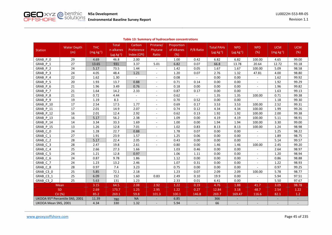
N5a Development LU0022H-553-RR-05 Environmental Baseline Survey Report Revision 1.1
www.geoxyzoffshore.com Page 45 of 235 Page 45 of 235
Table 13: Summary of hydrocarbon concentrations
Station Water Depth
(m) THC
(mg.kg-1)
Total n-alkanes (μg.kg-1)
Carbon Preference Index (CPI)
Pristane/ Phytane
Ratio
Proportion of Alkanes
(%) P/B Ratio
Total PAHs (μg.kg-1)
NPD (μg.kg-1)
NPD (%)
UCM (mg.kg-1)
UCM (%)
GRAB_P_0 29 4.69 46.8 2.00 - 1.00 0.42 6.82 6.82 100.00 4.65 99.00 GRAB_P_1 27 13.65 931 3.37 5.01 6.82 0.07 66.8 13.78 20.64 12.72 93.18 GRAB_P_2 24 5.17 73.5 1.44 - 1.42 0.05 1.67 1.67 100.00 5.09 98.58 GRAB_P_3 24 4.05 48.4 1.21 - 1.20 0.07 2.76 1.32 47.81 4.00 98.80 GRAB_P_4 22 1.62 1.30 - - 0.08 - 0.00 0.00 - 1.62 99.92 GRAB_P_5 20 1.93 13.7 0.88 - 0.71 0.14 0.00 0.00 - 1.92 99.29 GRAB_P_6 21 1.96 3.49 0.76 - 0.18 0.00 0.00 0.00 - 1.96 99.82 GRAB_P_7 21 1.64 14.2 2.33 - 0.87 0.17 0.00 0.00 - 1.63 99.13 GRAB_P_8 21 0.72 4.44 - - 0.62 - 1.35 1.35 100.00 0.71 99.38 GRAB_P_9 19 1.19 8.3 - - 0.70 0.52 0.00 0.00 - 1.18 99.30 GRAB_P_10 17 2.54 17.5 1.77 - 0.69 0.17 3.53 3.53 100.00 2.52 99.31 GRAB_P_11 17 2.01 14.9 2.07 - 0.74 0.12 4.34 4.34 100.00 1.99 99.26 GRAB_P_12 16 2.01 12.4 2.92 - 0.62 0.13 1.92 1.92 100.00 2.00 99.38 GRAB_P_13 16 5.17 56.2 2.38 - 1.09 0.00 4.19 4.19 100.00 5.11 98.91 GRAB_P_14 14 3.34 33.3 1.69 - 1.00 0.00 1.94 1.94 100.00 3.30 99.00 GRAB_P_15 13 1.26 12.8 7.01 - 1.02 0.83 8.13 8.13 100.00 1.24 98.98 GRAB_C_0 24 1.28 22.7 0.88 1.78 0.07 0.00 0.00 - 1.25 98.22 GRAB_C_1 27 1.91 23.9 1.57 - 1.25 0.06 0.00 0.00 - 1.89 98.75 GRAB_C_2 28 5.17 22.4 2.05 - 0.43 0.00 0.00 0.00 - 5.14 99.57 GRAB_C_3 28 2.47 19.8 2.61 - 0.80 0.00 1.46 1.46 100.00 2.45 99.20 GRAB_C_4 25 2.66 27.3 1.66 1.03 0.46 0.00 0.00 - 2.64 98.97 GRAB_C_5 24 1.21 12.8 0.97 1.06 1.11 0.00 0.00 - 1.20 98.94 GRAB_C_6 24 0.87 9.78 1.86 1.12 0.00 0.00 0.00 - 0.86 98.88 GRAB_C_7 24 1.23 13.2 2.46 1.07 0.31 0.00 0.00 - 1.22 98.93 GRAB_C_8 28 0.97 7.4 3.23 0.75 0.00 0.00 0.00 - 0.97 99.25 GRAB_C3_0 25 5.85 72.1 2.18 1.23 0.07 2.09 2.09 100.00 5.78 98.77 GRAB_C3_1 25 6.09 152 1.60 0.83 2.49 0.10 19.9 0.00 - 5.94 97.51 GRAB_C3_2 25 5.63 131 1.23 2.33 0.01 6.41 0.00 - 5.50 97.67
Mean 3.15 64.5 2.08 2.92 1.22 0.19 4.76 1.88 41.7 3.09 98.78 SD 2.69 173.7 1.25 2.95 1.22 0.27 12.84 3.18 48.7 2.54 1.22
CV (%) 85.2 269.1 59.8 101.3 100.1 146.8 269.7 169.47 116.6 82.1 1.2 UKOOA 95th Percentile SNS, 2001 11.39 780 NA - 6.85 - 366 - - - - UKOOA Mean SNS, 2001 4.34 330 1.32 - 5.94 - 66 - - - -

N5a Development LU0022H-553-RR-05 Environmental Baseline Survey Report Revision 1.1
www.geoxyzoffshore.com Page 46 of 235 Page 46 of 235
Figure 16: Total hydrocarbon concentrations (mg.kg¯¹)

N5a Development LU0022H-553-RR-05 Environmental Baseline Survey Report Revision 1.1
www.geoxyzoffshore.com Page 47 of 235 Page 47 of 235
Saturate/Aliphatic Hydrocarbons
All samples were analysed for n-alkanes using gas chromatography flame ionisation detection (GC-FID). The results are summarised in Table 13 and individually listed in Appendix H, which gives a breakdown of consecutive n-alkane content from nC10 through to nC37, together with the isoprenoid hydrocarbons pristane (Pr) and phytane (Ph).
Example gas chromatograms are given in Figure 18 and Figure 19. Total n alkane concentrations were variable but relatively low, with results ranging from 3.49μg.kg-1 to 931 μg.kg-1 (mean 64.53μg.kg-1±174SD, Figure 17). N-alkanes are widely distributed in the environment and can be naturally sourced from a range of materials including phytoplankton and bacteria (Yu, 2016).
The mean background n-alkanes levels for surface sediments recorded for stations located over 5km from oil and gas platforms from the SNS were estimated by UKOOA (2001) to be 330μg.kg-1, with an upper 95th percentile concentration of 780 μg.kg-1. Most stations within the N5A survey area fell significantly below the mean background level for n-alkanes, where the second closest station to the mean was GRAB_C3_1, which had a concentration of 152μg.kg-1. On the other hand, GRAB_P_1 exceeded both the mean and 95th percentile ranges with a value of 931μg.kg-1.
Alkanes contributed on average 1.22% (±1.22SD) to the THC levels recovered, which is comparatively low and would be expected for uncontaminated marine sediments where background hydrocarbons are continuously replenished by a low but consistent source of alkanes. In this case, it likely reflects the sandy nature of the seabed sediments, and the local hydrodynamic regime resulting in a continual replenishment and loss of alkanes to the environment. At station GRAB_P_1, n-alkanes comprised 6.82% of THC, more than five times the mean for the survey area. This was most likely a function of the higher fines at this station and is supported by the statistically positive correlation between fines and proportion of n-alkanes (ƍ(28)=0.559, p=<0.01).
Inspection of the individual gas chromatograms revealed a UCM envelope of between nC20 and nC37 at some stations (Figure 19 and Appendix H). This may reflect a combination of general contaminants from shipping activity (e.g. heavy greases and fuel oils, lubricants or waxes). The alkanes associated with this heavier UCM may also correspond to an input of terrigenous plant materials which typically comprise the long-chain, odd carbon-numbered n-alkanes (nC25-nC33; Eglinton et al., 1962; McDougall, 2000; Bouloubassi et al., 2001).

N5a Development LU0022H-553-RR-05 Environmental Baseline Survey Report Revision 1.1
www.geoxyzoffshore.com Page 48 of 235 Page 48 of 235
Figure 17: Total saturate alkanes (mg.kg¯¹

N5a Development LU0022H-553-RR-05 Environmental Baseline Survey Report Revision 1.1
www.geoxyzoffshore.com Page 49 of 235 Page 49 of 235
Figure 18: Example gas chromatogram for saturate hydrocarbon analysis (GRAB_C_2)
Figure 19: Example gas chromatogram for saturate hydrocarbon analysis (GRAB_P_1)
Internal standards
A – hepta-methylnonane
B - d34 hexadecane
C – 1-chlorooctadecane
C20 – 20 carbon
homologue
Internal standards
A – hepta-methylnonane
B - d34 hexadecane
C – 1-chlorooctadecane
C20 – 20 carbon
homologue

N5a Development LU0022H-553-RR-05 Environmental Baseline Survey Report Revision 1.1
www.geoxyzoffshore.com Page 50 of 235 Page 50 of 235
A closer review of the different proportions of n-alkanes recorded can sometimes identify trends within the data or the source from which the different organic components derive. Whilst this is particularly useful for stations that contain a moderate to high level of saturates, low concentrations can often skew such indices so they appear unrepresentative. The following ratios were further reviewed in the sections below.
Carbon Preference Index (CPI)
The CPI is associated with the preference of biogenic n-alkanes (i.e. that of a preference for odd-carbon numbered homologues, particularly around nC27-33; Sleeter et al., 1980), derived from fatty acids, alcohols, esters and land plant waxes. The CPI was calculated for all stations and the results were relatively consistent, ranging from 0.76 to 7.01 (Figure 20, mean 2.08± 1.25SD) for the full saturate range (nC10-nC37; Table 13). CPI could not be calculated for stations where alkane levels were consistently below the detectable limits (GRAB_P_4, GRAB_P_8 and GRAB_P_9).
The highest value was recorded at GRAB_P_15 (7.01), the shallowest station at 13m (and the closest to shore) which likely receives more terrestrial plant wax input than deeper stations, although there was no statistical correlation to corroborate this hypothesis. Previous studies have shown that a CPI between 5-10 is attributed to the influence of these plant materials and therefore it can be assumed that plant materials dominate GRAB_P_15 (Emerson and Hedges, 2008). CPI was also relatively high at GRAB_P_1 (3.37) suggesting a dominance of the more biogenic odd-carbon numbered alkanes. Conversely, 46.43% of stations had CPI values below 2.0; these were split between the pipeline to NGT Hot Tap and the cable route stations with no apparent geographical pattern of distribution, with no obvious correlation related to the sediment type. Stations with the lowest CPI included GRAB_P_6 (0.88), GRAB_P_7 (0.76) and GRAB_C_0 (0.88) and suggest a dominance of petrogenic compounds.
Review of individual n-alkane concentrations indicated that variation in CPI values at N5A was primarily due to many n-alkanes falling below the limits of detection, with minor variations in concentrations of n-alkanes at low levels resulting in a disproportionately large effect on the CPI. Furthermore, the opposite trend of CPI should therefore be interpreted with caution for the N5A survey area.
P/B Ratio
The P/B ratio compares the lighter, more petrogenic aliphatics with the heavier, and more biogenic aliphatics (Figure 21). For two stations (GRAB_P_4 and GRAB_P_8) this ratio was not calculated due to the majority of alkanes being recorded below the limits of detection. Where applicable, the results showed consistently low ratios, with values of 0.00 at several stations to 1.11 at GRAB_C_5 (mean 0.19±0.27) and no apparent pattern of distribution, although a significant correlation with fines was observed (ƍ(28)=0.387, p=<0.05), as well as a negative trend with mean size (ƍ(28)=-0.396, p=<0.05). All stations, excluding GRAB_C_5, had a P/B ratio of less than one. These low levels highlight the dominant biogenic influence within the survey area, indicative of aliphatics from natural biogenic origins and limited influence from petrogenic aliphatics.
The Pr/Ph Ratio
Pristane (Pr) and phytane (Ph) are both isoprenoidal alkanes commonly found as constituents within crude oils (Berthou and Friocourt, 1981). However, in biogenic environments, only Pr is commonly found in the marine environment as it is naturally biosynthesised as a product of the phytol moiety of chlorophyll. Ph is generally absent or only present at low levels in uncontaminated natural systems (Blumer and Snyder, 1965). A presence of both isoprenoids at similar levels is typically taken as an indication of petroleum contamination. It should be noted that the Pr/Ph ratio can often be difficult to interpret due to its erratic nature and should

N5a Development LU0022H-553-RR-05 Environmental Baseline Survey Report Revision 1.1
www.geoxyzoffshore.com Page 51 of 235 Page 51 of 235
be used mainly to corroborate other results. Use of the ratio in interpretative discourse is open to criticism, mainly owing to the natural occurrence of Ph in some older sediments and the confusing variation of sedimentary Pr, induced by the variability of phytoplankton numbers (Blumer and Snyder, 1965).
Phytane was below limits of detection (<1) for all but three of the stations sampled, with one of these having undetectable levels of pristane. As a result, only two Pr/Ph ratios could be calculated for the survey area at the two stations with the highest concentrations of THC and total n-alkanes (GRAB_P_1 and GRAB_C3_1). GRAB_P_1 had a value of 5.01 suggesting pristane dominance and biogenic origin of isoprenoids while GRAB_C3_1 had a value of 0.83 indicating the dominance of phytane in this area. However, concentrations for both phytane and pristane were low at both stations which often produces inconsistent Pr/Ph ratios.

N5a Development LU0022H-553-RR-05 Environmental Baseline Survey Report Revision 1.1
www.geoxyzoffshore.com Page 52 of 235 Page 52 of 235
Figure 20: Carbon preference index
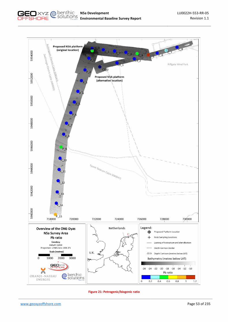
N5a Development LU0022H-553-RR-05 Environmental Baseline Survey Report Revision 1.1
www.geoxyzoffshore.com Page 53 of 235 Page 53 of 235
Figure 21: Petrogenic/biogenic ratio
N5a Development LU0022H-553-RR-05 Environmental Baseline Survey Report Revision 1.1
www.geoxyzoffshore.com Page 54 of 235 Page 54 of 235
Polycyclic Aromatic Hydrocarbons (PAHs)
Polycyclic aromatic hydrocarbons were analysed at each station using gas chromatography mass spectrometry (GC-MS). Results of the single ion current (SIC) analyses are summarised in Table 13, and detailed in Appendix J, showing concentrations for both parent compounds and their alkyl derivatives. The concentrations of 18 PAH priority pollutants listed by US Environmental Protection Agency (EPA) are listed in Appendix K. The EPA list of PAHs is used globally in assessment of contamination relating to both environmental and human health studies.
Polycyclic aromatic hydrocarbons and their alkyl derivatives have been recorded in a wide range of marine sediments (Laflamme and Hites, 1978) with the majority of compounds produced from what is thought to be pyrolytic sources. These include the combustion of organic material such as forest fires (Youngblood and Blumer, 1975), the burning of fossil fuels and, in the case of offshore oil fields, flare stacks. The resulting PAHs, rich in the heavier weight 4-6 ring aromatics, are normally transported to the sediments via atmospheric fallout or river runoff. Another PAH source is petroleum hydrocarbon, often associated with localised drilling activities. These are rich in the lighter, more volatile 2 and 3 ring PAHs (NPD; naphthalene (128), phenanthrene, anthracene (178) and dibenzothiophene (DBT)) with their alkyl derivatives.
Total PAH concentrations (2-6 compounds) over the N5A survey area were relatively low and highly variable, with concentrations ranging from 0μg.kg-1to 66.8μg.kg-1 (mean 4.76μg.kg-1±12.84.72SD; Table 13). Many stations had levels of PAH that were below the limit of detection, including all stations along the N5A platform to Riffgat Wind Park cable route (Figure 22), reflecting the presence of mobile sandy sediments. The highest total PAH concentration of 66.8μg.kg-1 was recorded at station GRAB_P_1. As mentioned previously, this station also recorded the highest concentrations for THC and total n-alkanes (13,647μg.kg-1 and 931μg.kg-1, respectively).
Total PAH concentrations correlated with total n-alkanes (ƍ(28)=0.596, p<0.01), but both parameters were low throughout the majority of the survey area and were deemed to be consistent with uncontaminated marine sediments. All stations showed 2-6 ring PAH concentrations below the mean level for background sediments in the SNS (292μg.kg-1, UKOOA, 2001).Only station GRAB_P_1 showed total PAH and total n-alkane concentrations above the UKOOA (2001) 95th percentile for background sediments in the southern North Sea.
All total PAH concentrations recorded during the survey fell significantly below the US EPA toxicity reference value (TRV) of 870μg.kg-1 (US EPA, 1999; Macdonald et al., 1996). All stations were also found to sit at the lower end of the Centre for Environment, Fisheries and Aquaculture Science (CEFAS) PAH concentrations for sediments surrounding North Sea oil and gas installations which ranged from 20μg.kg-1 to 74700μg.kg-1 (Sheahan et al., 2001).
The lighter, more volatile NPD fraction (2 and 3 ring aromatics) was consistently low with almost negligible concentrations observed, ranging from 0.00 μg.kg-1 to 13.78 μg.kg-1 (mean 1.90μg.kg-1±3.2SD). This follows a similar pattern to the total PAHs. NPD concentrations were again highest for station GRAB_P_1 (13.78μg.kg-1), followed by GRAB_P_15 (8.13 μg.kg-1) The NPD PAH accounted for a varying proportion of the total PAH at stations, ranging from 0% to 100%, with some percentages unable to be calculated as PAH levels were below the limit of detection. At some stations the NPD PAH accounted for 100% of the total PAHs but this reflected the overall low levels of total PAH and not elevated levels of NPD PAH. At stations where higher PAH concentrations occurred (e.g. GRAB_P_1 and GRAB_C3_1), the percentage NPD was low (20.64% and 0% respectively), indicating a dominance of pyrolytic-derived PAH at these stations. Consequently, the ratio of NPD to 4-6 ring PAHs was considered to be low (0-0.92) at every station.
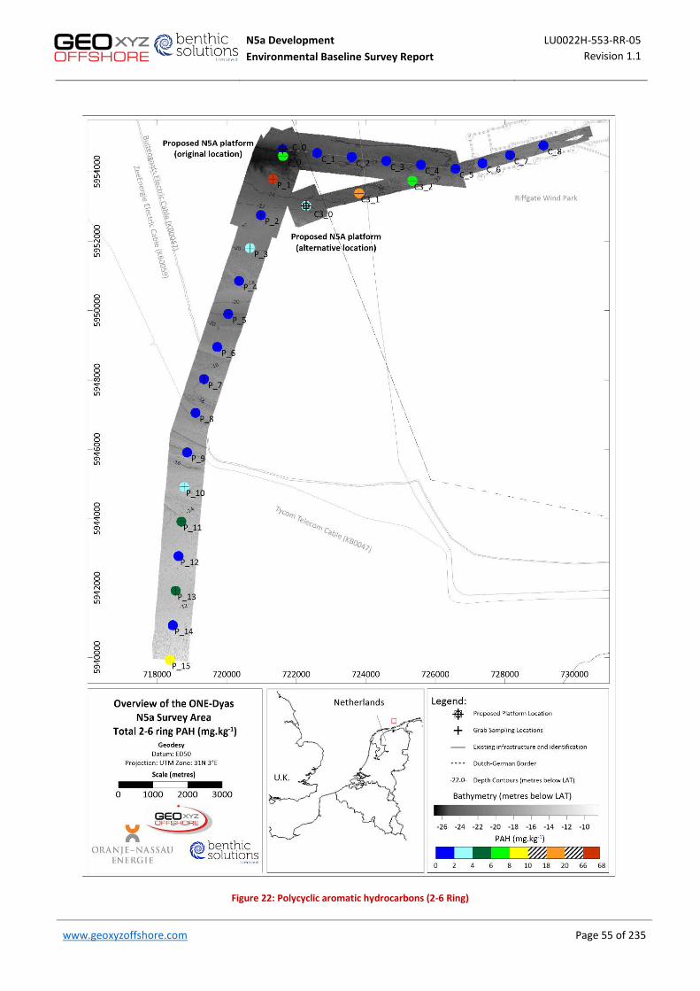
N5a Development LU0022H-553-RR-05 Environmental Baseline Survey Report Revision 1.1
www.geoxyzoffshore.com Page 55 of 235 Page 55 of 235
Figure 22: Polycyclic aromatic hydrocarbons (2-6 Ring)

N5a Development LU0022H-553-RR-05 Environmental Baseline Survey Report Revision 1.1
www.geoxyzoffshore.com Page 56 of 235 Page 56 of 235
Further information on the source(s) of PAH in the sediment may be obtained from a study of their alkyl homologue distributions (i.e. the degree of methyl, ethyl, substitution of the parent compounds). Pyrolytically derived PAHs are predominantly unalkylated compounds, whereas petrogenically derived PAHs are formed at relatively low temperatures (<150°C) and contain mainly alkylated species. The distribution of parent 2-6 ring PAH compounds also reflects whether the source is petrogenic or pyrolytic. This trend is represented graphically in Appendix L, and four example plots in Figure 23, which show three-dimensional plots of the parent compound distribution and the alkyl homologue distribution of the aromatic material in each of the sediments analysed.
Stations across the N5A survey area presented a mixed range of alkyl distributions, with some stations having little or no PAH content, as seen in Figure 23c and d (GRAB_P_9, GRAB_C_3). GRAB_P_1 and GRAB_C3_1 showed more obvious pyrolytic PAH content, dominated by 4-6 ring compounds, however the PAH concentrations at all stations were low (<12μg.kg-1) and considered to represent natural variations across the N5A development survey area.
Figure 23: Example parent/alkyl PAH plots
The results indicate that PAHs could be classified as having derived from mixed sources consistent with ambient seabed conditions in the southern North Sea.
a b
c d

N5a Development LU0022H-553-RR-05 Environmental Baseline Survey Report Revision 1.1
www.geoxyzoffshore.com Page 57 of 235 Page 57 of 235
Normalisation of Total PAH
Normalised total PAH data were calculated to allow comparison to OSPAR background assessment concentrations (BACs; OSPAR, 2014). BACs are threshold concentrations below which contaminants can be considered at background levels (OSPAR, 2008b). Natural and anthropogenic contaminants tend to show a higher affinity to fine particulate matter compared to coarse (OSPAR, 2009) due to the increased adsorption capacity of organic matter and clay minerals. For sites where there is variability in grain size between stations, impact footprints from point sources of contamination may at least partly be obscured by differences in sediment granulometry. Normalisation was undertaken using a simple ratio approximation, where PAH concentrations (based on the 11 PAH components outlined in OSPAR, 2014) were normalised to 2.5% TOC content at each station (Table 14).
All normalised PAHs were below their respective BACs (OSPAR, 2014), indicating little or no anthropogenic impact on the PAH composition of the sediments within the survey area. This is supported by many of the PAH measurements falling below the limit of detection (Appendix K). Furthermore, PAH concentrations at station GRAB_P_1, where the highest levels of PAH occurred, levels were substantially below the various BC, BAC, ERL and ERM levels.

N5a Development LU0022H-553-RR-05 Environmental Baseline Survey Report Revision 1.1
www.geoxyzoffshore.com Page 58 of 235 Page 58 of 235
Table 14: Normalised PAH concentrations (μg.kg-1)
Blue cell = above BC Green cell = above BAC Orange cell = above ERL Yellow cell = above ERM
Note: where levels were below the detection limit, a value of half the detection limit was applied in the calculations.
*Concentration of that produces a harmful affect 10% of the time (Long et.al., 1995)
**Concentration of that produces a harmful affect 50% of the time (Long et.al., 1995
Station N
apht
hale
ne
Acen
apht
hyle
ne
Acen
apht
hene
Fluo
rene
Phen
anth
rene
Dibe
nzot
hiop
hene
Anth
race
ne
Fluo
rant
hene
Pyre
ne
Benz
o[a]
anth
race
ne
Chry
sene
Benz
o[b]
fluor
anth
ene
Benz
o[k]
fluor
anth
ene
Benz
o[e]
pyre
ne
Benz
o[a]
pyre
ne
Pery
lene
Inde
no[1
23,c
d]py
rene
Dibe
nzo[
a,h]
anth
race
ne
Benz
o[gh
i]per
ylen
e
GRAB_P_0 <0.5 <0.5 <0.5 <0.5 <0.5 <0.5 <0.5 <0.5 <0.5 <0.5 <0.5 <0.5 <0.5 <0.5 <0.5 40 <0.5 <0.5 <0.5 GRAB_P_1 <0.5 <0.5 <0.5 <0.5 <0.5 <0.5 <0.5 <0.5 <0.5 <0.5 <0.5 4.93 <0.5 4.30 3.79 118.93 4.22 0.00 7.60 GRAB_P_2 <0.5 <0.5 <0.5 <0.5 <0.5 <0.5 <0.5 <0.5 <0.5 <0.5 <0.5 <0.5 <0.5 <0.5 <0.5 <0.5 <0.5 <0.5 <0.5 GRAB_P_3 <0.5 <0.5 <0.5 <0.5 <0.5 <0.5 <0.5 <0.5 <0.5 <0.5 <0.5 <0.5 <0.5 <0.5 <0.5 <0.5 <0.5 <0.5 <0.5 GRAB_P_4 <0.5 <0.5 <0.5 <0.5 <0.5 <0.5 <0.5 <0.5 <0.5 <0.5 <0.5 <0.5 <0.5 <0.5 <0.5 <0.5 <0.5 <0.5 <0.5 GRAB_P_5 <0.5 <0.5 <0.5 <0.5 <0.5 <0.5 <0.5 <0.5 <0.5 <0.5 <0.5 <0.5 <0.5 <0.5 <0.5 <0.5 <0.5 <0.5 <0.5 GRAB_P_6 <0.5 <0.5 <0.5 <0.5 <0.5 <0.5 <0.5 <0.5 <0.5 <0.5 <0.5 <0.5 <0.5 <0.5 <0.5 <0.5 <0.5 <0.5 <0.5 GRAB_P_7 <0.5 <0.5 <0.5 <0.5 <0.5 <0.5 <0.5 <0.5 <0.5 <0.5 <0.5 <0.5 <0.5 <0.5 <0.5 <0.5 <0.5 <0.5 <0.5 GRAB_P_8 <0.5 <0.5 <0.5 <0.5 <0.5 <0.5 <0.5 <0.5 <0.5 <0.5 <0.5 <0.5 <0.5 <0.5 <0.5 <0.5 <0.5 <0.5 <0.5 GRAB_P_9 <0.5 <0.5 <0.5 <0.5 <0.5 <0.5 <0.5 <0.5 <0.5 <0.5 <0.5 <0.5 <0.5 <0.5 <0.5 <0.5 <0.5 <0.5 <0.5 GRAB_P_10 <0.5 <0.5 <0.5 <0.5 <0.5 <0.5 <0.5 <0.5 <0.5 <0.5 <0.5 <0.5 <0.5 <0.5 <0.5 <0.5 <0.5 <0.5 <0.5 GRAB_P_11 <0.5 <0.5 <0.5 <0.5 <0.5 <0.5 <0.5 <0.5 <0.5 <0.5 <0.5 <0.5 <0.5 <0.5 <0.5 <0.5 <0.5 <0.5 <0.5 GRAB_P_12 <0.5 <0.5 <0.5 <0.5 <0.5 <0.5 <0.5 <0.5 <0.5 <0.5 <0.5 <0.5 <0.5 <0.5 <0.5 <0.5 <0.5 <0.5 <0.5 GRAB_P_13 <0.5 <0.5 <0.5 <0.5 <0.5 <0.5 <0.5 <0.5 <0.5 <0.5 <0.5 <0.5 <0.5 <0.5 <0.5 <0.5 <0.5 <0.5 <0.5 GRAB_P_14 <0.5 <0.5 <0.5 <0.5 <0.5 <0.5 <0.5 <0.5 <0.5 <0.5 <0.5 <0.5 <0.5 <0.5 <0.5 <0.5 <0.5 <0.5 <0.5 GRAB_P_15 <0.5 <0.5 <0.5 <0.5 <0.5 <0.5 <0.5 <0.5 <0.5 <0.5 <0.5 <0.5 <0.5 <0.5 <0.5 <0.5 <0.5 <0.5 <0.5 GRAB_C_0 <0.5 <0.5 <0.5 <0.5 <0.5 <0.5 <0.5 <0.5 <0.5 <0.5 <0.5 <0.5 <0.5 <0.5 <0.5 <0.5 <0.5 <0.5 <0.5 GRAB_C_1 <0.5 <0.5 <0.5 <0.5 <0.5 <0.5 <0.5 <0.5 <0.5 <0.5 <0.5 <0.5 <0.5 <0.5 <0.5 <0.5 <0.5 <0.5 <0.5 GRAB_C_2 <0.5 <0.5 <0.5 <0.5 <0.5 <0.5 <0.5 <0.5 <0.5 <0.5 <0.5 <0.5 <0.5 <0.5 <0.5 <0.5 <0.5 <0.5 <0.5 GRAB_C_3 <0.5 <0.5 <0.5 <0.5 <0.5 <0.5 <0.5 <0.5 <0.5 <0.5 <0.5 <0.5 <0.5 <0.5 <0.5 <0.5 <0.5 <0.5 <0.5 GRAB_C_4 <0.5 <0.5 <0.5 <0.5 <0.5 <0.5 <0.5 <0.5 <0.5 <0.5 <0.5 <0.5 <0.5 <0.5 <0.5 <0.5 <0.5 <0.5 <0.5 GRAB_C_5 <0.5 <0.5 <0.5 <0.5 <0.5 <0.5 <0.5 <0.5 <0.5 <0.5 <0.5 <0.5 <0.5 <0.5 <0.5 <0.5 <0.5 <0.5 <0.5 GRAB_C_6 <0.5 <0.5 <0.5 <0.5 <0.5 <0.5 <0.5 <0.5 <0.5 <0.5 <0.5 <0.5 <0.5 <0.5 <0.5 <0.5 <0.5 <0.5 <0.5 GRAB_C_7 <0.5 <0.5 <0.5 <0.5 <0.5 <0.5 <0.5 <0.5 <0.5 <0.5 <0.5 <0.5 <0.5 <0.5 <0.5 <0.5 <0.5 <0.5 <0.5 GRAB_C_8 <0.5 <0.5 <0.5 <0.5 <0.5 <0.5 <0.5 <0.5 <0.5 <0.5 <0.5 <0.5 <0.5 <0.5 <0.5 <0.5 <0.5 <0.5 <0.5 GRAB_C3_0 <0.5 <0.5 <0.5 <0.5 <0.5 <0.5 <0.5 <0.5 <0.5 <0.5 <0.5 <0.5 <0.5 <0.5 <0.5 <0.5 <0.5 <0.5 <0.5 GRAB_C3_1 <0.5 <0.5 <0.5 <0.5 <0.5 <0.5 <0.5 <0.5 <0.5 <0.5 <0.5 <0.5 <0.5 <0.5 <0.5 810.53 <0.5 <0.5 17.50 GRAB_C3_2 <0.5 <0.5 <0.5 <0.5 <0.5 <0.5 <0.5 <0.5 <0.5 <0.5 <0.5 <0.5 <0.5 <0.5 <0.5 479.55 <0.5 <0.5 <0.5
Mean 0 0 0 0 0 0 0 0 0 0 0 0.18 0.00 0.15 0.14 51.75 0.15 0.00 0.90
SD 0 0 0 0 0 0 0 0 0 0 0 0.93 0.00 0.81 0.72 175.08 0.80 0.00 3.56
CV (%) - - - - - - - - - - - - - - - 338.3 - - 396.8 BC (OSPAR 2014) 5 - - - 17 - 3 20 13 9 11 - - - 15 - 50 - 45 BAC (OSPAR 2014) 8 - - - 32 - 5 39 24 16 20 - - - 30 - 103 - 80 NOAA ERL* 160 44 16 19 240 - 85 600 665 261 384 - 240 - 430 - 2000 63 170 NOAA ERM** 210 640 500 540 1500 - 1100 5100 2600 1600 2800 1800 1340000 - 1600 - 320000 260 320000
N5a Development LU0022H-553-RR-05 Environmental Baseline Survey Report Revision 1.1
www.geoxyzoffshore.com Page 59 of 235 Page 59 of 235
HEAVY AND TRACE METAL CONCENTRATIONS
Results for Heavy and trace metal analysis are given in Table 15. All of the metals analysed (aluminium (Al), arsenic (As), barium (Ba), cadmium (Cd), chromium (Cr), copper (Cu), iron (Fe), mercury (Hg), nickel (Ni), lead (Pb), tin (Sn), vanadium (V) and zinc (Zn)), underwent an Aqua Regia (AR) acid extraction followed by ICP analysis.
The question of bioavailability of metals to marine organisms is a complex one, as sediment granulometry and the interface between water and sediment all affect the bioavailability and subsequent toxicity. Therefore, even if a metal is found in higher concentrations it does not necessarily follow that this will have a detrimental effect on the environment, if present in an insoluble state. Historically, several extraction techniques have been applied to metal analysis, with the most common applying to an HF/perchloric extraction for total metals, and a weaker nitric or aqua regia extraction. The latter techniques have shown close correlation to metal burdens in the tissues of benthic organisms (Luoma and Davies, 1983; Bryan and Langston, 1992). However, the way bioavailability is reflected by the extent to which a particular metal digests is not well understood, and research is ongoing. A fusion analysis for Ba is preferred due to the likely presence of insoluble Ba, which is typically recorded in areas where previous drilling activities have occurred. No barium by fusion was conducted in these analyses but is recommended for any post-drilling analyses.
Metals occur naturally in the marine environment and are widely distributed in both dissolved and sedimentary forms. Some are essential to marine life while others may be toxic to numerous organisms (Paez-Osuna and Ruiz-Fernandez, 1995). Rivers, coastal discharges, and the atmosphere are the principal modes of entry for most metals into the marine environment (Schaule and Patterson, 1983), with anthropogenic inputs occurring primarily as components of industrial and municipal wastes. Historically, several HM are found in elevated concentrations where drilling fluids or produced waters have been discharged by oil and gas installations. These include intentional additives (such as metal based salts and organo-metallic compounds in the fluids) as well as impurities within the drilling mud systems such as clays (e.g. bentonites; a gelling and viscosifying agent) and metal lignosulphates (a viscosity controller; McCourt et
al., 1991). The metals most characteristic for offshore contamination of marine sediments from oil and gas activities are Ba, Cr, Pb and Zn (Neff, 2005), although these may vary greatly depending on the constituents used.
Trace metal contaminants in the marine environment tend to form associations with the non-residual phases of mineral matter, such as Fe and Mn oxides and hydroxides, metal sulphides, organics, and carbonates. Metals associated with these non-residual phases are prone to various environmental interactions and transformations (physical, chemical and biological), potentially increasing their biological availability (Tessier
et al., 1979). Residual trace metals are defined as those which are part of the silicate matrix of the sediment and that are located mainly in the lattice structures of the component minerals. Non-residual trace metals are not part of the silicate matrix and have been incorporated into the sediment from aqueous solution by processes such as adsorption and organic complexes and may include trace metals originating from sources of pollution. Therefore, in monitoring trace metal contamination of the marine environment, it is important to distinguish these more mobile metals from the residual metals held tightly in the sediment lattice (Chester and Voutsinou, 1981), which are of comparatively little environmental significance.
Metals are generally not harmful to organisms at concentrations normally found in marine sediments and some, like zinc, may be essential for normal metabolism although can become toxic above a critical threshold. In order to assign a level of context for toxicity, an approach used by Long et al. (1995) to characterize
N5a Development LU0022H-553-RR-05 Environmental Baseline Survey Report Revision 1.1
www.geoxyzoffshore.com Page 60 of 235 Page 60 of 235
contamination in sediments will be used here. These researchers reviewed field and laboratory studies and identified nine metals that were observed to have ecological or biological effects on organisms. They defined “effect range low” (ERL) values as the lowest concentration of a metal that produced adverse effects in 10% of the data reviewed, whilst “effect range median” (ERM) values designate the level at which half of the studies reported harmful effects. Consequently, metal concentrations recorded below the ERL value are not expected to elicit adverse effects, while levels above the ERM value are likely to be toxic to some marine life.
Of particular relevance to the offshore oil and gas industry are metals associated with drilling related discharges. These can contain substantial amounts of barium sulphate (barites) as a weighting agent (National Research Council, 1983) and barium is frequently used to detect the deposition of drilling fluids around offshore installations (Chow and Snyder, 1981; Gettleson and Laird, 1980; Tricine and Trefry, 1983; Muniz et al., 2004). Solid barites are often discharged during the drilling process and often contain measurable concentrations of heavy metals as impurities, including cadmium, chromium, copper, lead, mercury, and zinc (National Research Council, 1983; McLeese et al., 1987). Heavy metals, either as impurities or additives are also present in other mud components. For this survey, natural barium (Ba) levels were consistent and ranged from 8.1mg.kg-1 to 48.3mg.kg-1 (mean 13.01mg.kg-1±8.38SD) when analysed by aqua regia-extraction (Figure 24), falling well below the UKOOA 95th percentile for the SNS (272mg.kg-1). Barium levels were highest at station GRAB_P_1 (48.3mg.kg-1) and were considered to be low and consistent with uncontaminated sediments, with contaminated stations frequently showing concentrations in thousands or tens of thousands of mg.kg-1 (ppm).
Mean levels of metals for the entire survey area fell below their respective UKOOA (2001) and Long et al. (1995) reference thresholds for anthropogenic contamination and potential toxicological impacts. In addition, concentrations of cadmium, mercury and tin were all often found to be under the limit of detection for the majority of stations. Tin (Sn) concentrations were below the limit of detection (0.5mg.kg-1) at 92% of stations, with only station GRAB_P_1 recording detectable concentrations.
Heavy and trace metal concentrations showed minimal variation across the survey area. Station GRAB_P_1 recorded the highest concentrations of all analysed metals with the exception of mercury. Metals concentrations at station GRAB_P_1 were consistently more than double the mean for the N5A development survey area (excluding mercury). These included all metals associated with drilling related barite discharges (arsenic, chromium, nickel, vanadium, zinc and iron). Although highest at this station, only levels of zinc (40.4mg.kg-1) and copper (14.7mg.kg-1) exceeded the UKOOA 95th percentile limits for the SNS, and both fell below their respective ERL and ERM thresholds. The high concentrations at station GRAB_P_1 were considered to reflect natural variation within the survey area with the high percentage fines at this station acting to retain metals more easily.
Cadmium, mercury and zinc were consistently low across all stations with respective mean values of 0.03 mg.kg-1±0.03SD, 0.02 mg.kg-1±0.02SD and 0.27 mg.kg-1±0.09SD. Nickel and copper levels across the N5A area were also consistently low with respective means of 3.19mg.kg-1±3.46SD (Figure 25) and 6.17mg.kg-1±1.82SD (Figure 26). Only copper at GRAB_P_1 exceeded the UKOOA 95th percentile (Ni, 21.45mg.kg-1, UKOOA 2001; Cu, 13.86mg.kg-1, UKOOA 2001). The concentrations of nickel and copper also did not surpass the effect range low values of 20.9mg.kg-1and 34.0mg.kg-1.
Iron (Fe) is an important metal as it is often associated with other elements, such as arsenic (As). Iron concentrations ranged from 2440mg.kg-1 at GRAB_P_11 to 16800mg.kg-1 at GRAB_P_1 (Figure 27) and was significantly correlated to 61.53% of the metals (Appendix N), including arsenic ƍ(28)=0.826, p<0.001. Arsenic levels were relatively consistent at most stations (mean 3.37.kg-1±1.84SD; Figure 28), however, there were

N5a Development LU0022H-553-RR-05 Environmental Baseline Survey Report Revision 1.1
www.geoxyzoffshore.com Page 61 of 235 Page 61 of 235
slightly elevated concentrations nearer at stations to the N5A platform, and at GRAB_P_1 the value recorded (10.5mg.kg-1) exceeded the effect range low (8.2mg.kg-1).
Similarly, aluminium levels were also higher at GRAB_P_1 at 12700mg.kg-1, well above the survey area mean of 1359mg.kg-1 (±2267SD). Aluminium is often associated with higher levels of silicates which also frequently correlate with higher concentrations of other metals (Figure 29). This is corroborated by the findings of the Spearman’s correlation table which resulted in significant Spearman’s correlations between aluminium and 69.2% of the other heavy and trace metals (Appendix N).
The physical nature of the sediment had a clear effect on the concentrations of some heavy and trace metals found in N5A. This was supported by significant correlations between the proportions of fines, sand and gravel and the heavy and trace metals (Appendix N). Significant positive Spearman’s rank correlations were seen between fines and aluminium, arsenic, barium, iron, lead, nickel and vanadium in addition to negative correlations between sand and aluminium, arsenic, iron, nickel and vanadium. As such, it is unsurprising to that the sand-dominated stations grouped within PSA multivariate cluster a also exhibited some of the lowest metals concentrations. In particular stations GRAB_P_8 and GRAB_C_6, which showed the lowest concentrations of several metals (five and eight metals respectively) as well as the lowest THC and UMC.
There was a positive correlation between distance to shore and arsenic, vanadium, barium and iron concentrations, with higher levels recorded at stations farthest from shore. This is interesting as it would be expected that terrestrial influences would provide more metals effluents to stations closest to shore. However, the positive correlation between fines and distance to shore may account for this variation with higher fines generally found further offshore and associated with higher metals concentrations.

N5a Development LU0022H-553-RR-05 Environmental Baseline Survey Report Revision 1.1
www.geoxyzoffshore.com Page 62 of 235
Table 15: Total heavy and trace metal concentrations (mg.kg-1)
Orange cell = above ERL Yellow cell = above ERM*
Note: where levels were below the detection limit, a value of half the detection limit was applied in the calculations.
**Lowest concentration of metal that can produce a harmful affect (Long et.al., 1995)
Station Arsenic (AR-ICP)
Cadmium (AR-ICP)
Chromium (AR-ICP)
Copper (AR-ICP)
Lead (AR-ICP)
Mercury (AR-ICP)
Nickel (AR-ICP)
Tin (AR-ICP)
Vanadium (AR-ICP)
Zinc (AR-ICP)
Aluminium (AR-ICP)
Barium (AR-ICP)
Iron (AR-ICP)
GRAB_P_0 5.3 <0.04* 4.1 6.2 3.6 0.02 2.8 <0.5 8.0 13.6 1060 16.5 4030 GRAB_P_1 10.5 0.17 23.3 14.7 9.5 0.03 20.5 1 31.5 40.4 12700 48.3 16800 GRAB_P_2 3.7 <0.04* 5.7 6.0 3.2 <0.015* 3.4 <0.5* 8.3 15.0 1760 12.5 4280 GRAB_P_3 2.8 <0.04* 3.7 4.7 2.4 <0.015* 2.1 <0.5* 5.2 11.8 832 10.0 3510 GRAB_P_4 3.0 <0.04* 3.2 5.8 1.8 <0.015* 1.8 <0.5* 4.4 19.8 633 9.1 3200 GRAB_P_5 2.7 <0.04* 3.3 5.3 1.8 <0.015* 2.0 <0.5* 4.2 10.8 647 9.5 3120 GRAB_P_6 2.8 <0.04* 4.3 5.4 2.4 0.07 2.3 <0.5* 4.1 15.8 709 9.1 3000 GRAB_P_7 2.7 0.04 4.4 5.5 2.2 0.03 2.4 <0.5* 4.4 14.8 899 10.4 3090 GRAB_P_8 2.2 <0.04* 2.5 6.1 1.6 0.02 1.9 <0.5* 3.0 8.8 467 8.4 2640 GRAB_P_9 2.5 <0.04* 3.5 4.5 1.7 <0.015* 2.1 <0.5* 3.8 14.0 873 9.9 2610 GRAB_P_10 2.9 <0.04* 4.5 5.5 2.3 <0.015* 2.4 <0.5* 5.8 10.4 797 9.1 2920 GRAB_P_11 2.3 0.05 3.4 4.6 1.7 <0.015* 1.8 <0.5* 3.7 12.3 732 8.1 2440 GRAB_P_12 2.5 0.04 4.4 5.4 2.0 <0.015* 2.3 <0.5* 4.3 16.2 960 9.9 3060 GRAB_P_13 2.6 <0.04* 4.8 5.4 2.6 0.06 2.5 <0.5* 4.9 15.7 1210 11.6 3510 GRAB_P_14 2.7 0.05 4.9 5.9 2.7 0.02 2.8 <0.5* 5.0 19.7 997 9.7 2860 GRAB_P_15 2.5 0.04 5.5 6.8 1.9 <0.015* 2.5 <0.5* 14.3 17.2 967 10.1 2860 GRAB_C_0 4.7 <0.04* 2.9 6.2 2.1 <0.015* 2.4 <0.5* 6.3 7.7 600 9.5 3420 GRAB_C_1 7.3 <0.04* 2.8 5.5 2.1 <0.015* 2.5 <0.5* 8.9 11.6 847 10.8 4370 GRAB_C_2 4.3 <0.04* 2.9 6.0 2.0 <0.015* 2.2 <0.5* 6.4 9.9 542 9.0 3440 GRAB_C_3 2.8 <0.04* 3.8 6.0 2.1 <0.015* 2.4 <0.5* 5.5 14.6 748 11.3 3450 GRAB_C_4 3.1 <0.04* 5.3 7.7 2.9 0.02 3.4 <0.5* 6.7 14.4 1140 22.9 3870 GRAB_C_5 2.5 <0.04* 2.9 5.8 1.8 <0.015* 2.3 <0.5* 4.1 7.4 721 11.1 3180 GRAB_C_6 1.3 <0.04* 2.6 6.4 1.5 <0.015* 1.9 <0.5* 2.6 7.2 508 9.3 2520 GRAB_C_7 2.2 <0.04* 3.5 7.3 1.8 <0.015* 2.8 <0.5* 4.1 9.5 733 10.2 3120 GRAB_C_8 1.8 0.04 2.6 6.2 1.5 0.02 1.9 <0.5* 3.1 6.5 448 9.3 2630 GRAB_C3_0 3.4 <0.04* 6.2 5.8 3.8 0.1 3.2 <0.5* 8.2 17.4 1270 11.6 4400 GRAB_C3_1 2.9 <0.04* 5.6 6.7 3.0 0.04 3.9 <0.5* 7.7 12.6 1740 29.8 4040 GRAB_C3_2 4.7 0.05 5.5 5.3 3.6 0.03 4.7 <0.5* 11.4 14.3 2520 17.5 6590 Mean 3.38 0.03 4.7 6.2 2.6 0.02 3.2 0.27 6.8 13.9 1359 13.0 3891 SD 1.84 0.03 3.8 1.8 1.5 0.02 3.5 0.09 5.5 6.3 2267 8.4 2664 CV (%) 54.5 95.4 80.6 29.6 59.0 108.7 108.6 32.0 81.3 45.6 166.8 64.4 68.5 UKOOA 95th Percentile SNS, 2001 - 0.72 44.8 13.9 21.0 0.05 21.5 - 35.8 35.8 - - 18555 NOAA ERL** 8.20 1.20 81.0 34.0 46.7 0.15 20.9 - 150 - - NOAA ERM 70.0 9.60 370 270 218 0.71 51.6 - 410 - -
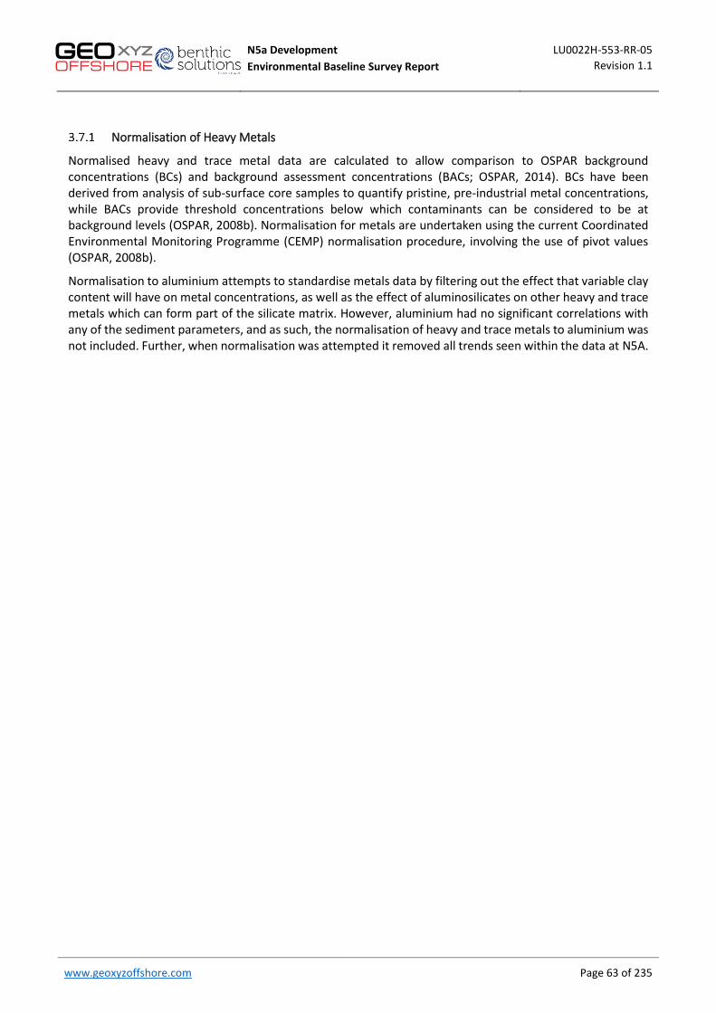
N5a Development LU0022H-553-RR-05 Environmental Baseline Survey Report Revision 1.1
www.geoxyzoffshore.com Page 63 of 235
Normalisation of Heavy Metals
Normalised heavy and trace metal data are calculated to allow comparison to OSPAR background concentrations (BCs) and background assessment concentrations (BACs; OSPAR, 2014). BCs have been derived from analysis of sub-surface core samples to quantify pristine, pre-industrial metal concentrations, while BACs provide threshold concentrations below which contaminants can be considered to be at background levels (OSPAR, 2008b). Normalisation for metals are undertaken using the current Coordinated Environmental Monitoring Programme (CEMP) normalisation procedure, involving the use of pivot values (OSPAR, 2008b).
Normalisation to aluminium attempts to standardise metals data by filtering out the effect that variable clay content will have on metal concentrations, as well as the effect of aluminosilicates on other heavy and trace metals which can form part of the silicate matrix. However, aluminium had no significant correlations with any of the sediment parameters, and as such, the normalisation of heavy and trace metals to aluminium was not included. Further, when normalisation was attempted it removed all trends seen within the data at N5A.
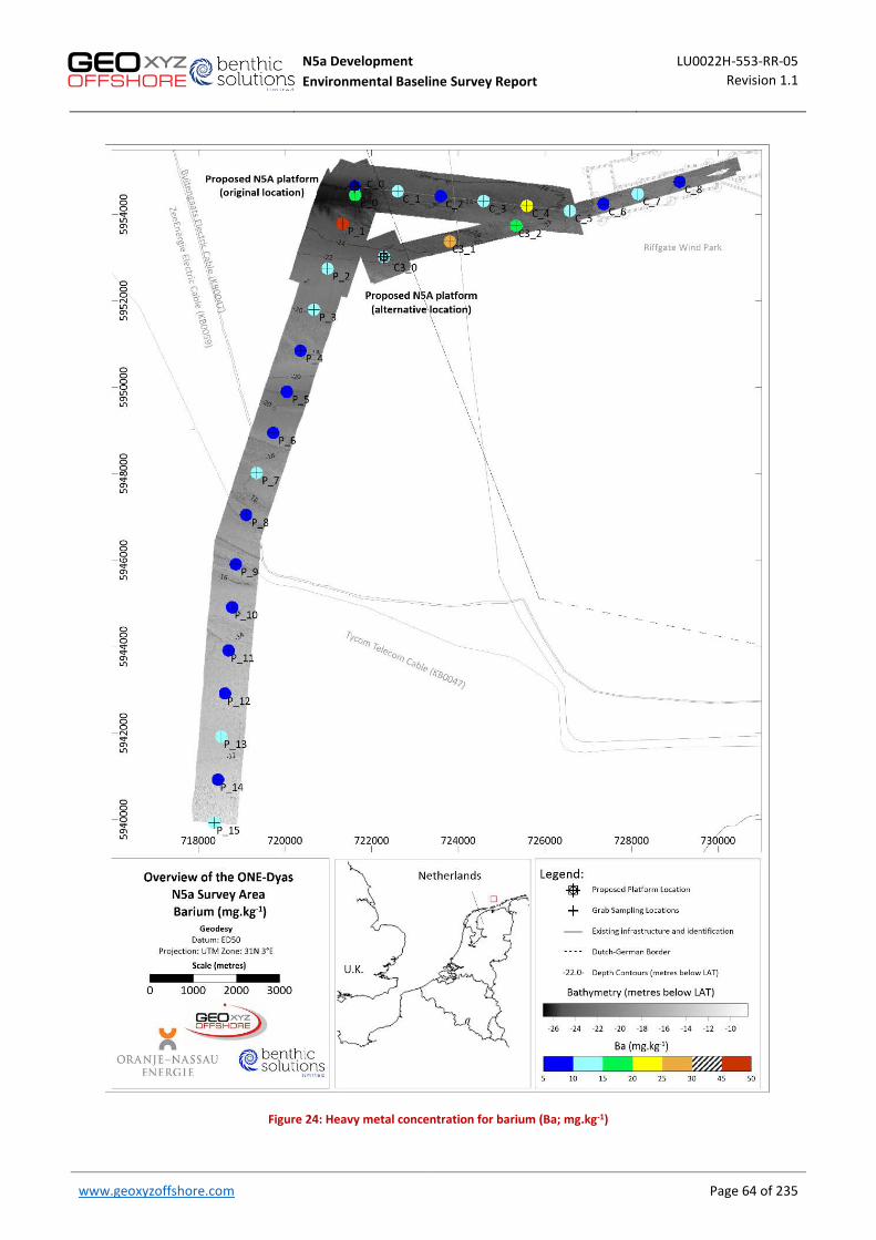
N5a Development LU0022H-553-RR-05 Environmental Baseline Survey Report Revision 1.1
www.geoxyzoffshore.com Page 64 of 235
Figure 24: Heavy metal concentration for barium (Ba; mg.kg-1)

N5a Development LU0022H-553-RR-05 Environmental Baseline Survey Report Revision 1.1
www.geoxyzoffshore.com Page 65 of 235
Figure 25: Heavy metal concentration for nickel (Ni; mg.kg-1)

N5a Development LU0022H-553-RR-05 Environmental Baseline Survey Report Revision 1.1
www.geoxyzoffshore.com Page 66 of 235
Figure 26: Heavy metal concentration for copper (Cu; mg.kg-1)

N5a Development LU0022H-553-RR-05 Environmental Baseline Survey Report Revision 1.1
www.geoxyzoffshore.com Page 67 of 235
Figure 27: Heavy metal concentration for iron (Fe; mg.kg-1)

N5a Development LU0022H-553-RR-05 Environmental Baseline Survey Report Revision 1.1
www.geoxyzoffshore.com Page 68 of 235
Figure 28: Heavy metal concentration for arsenic (As; mg.kg-1)
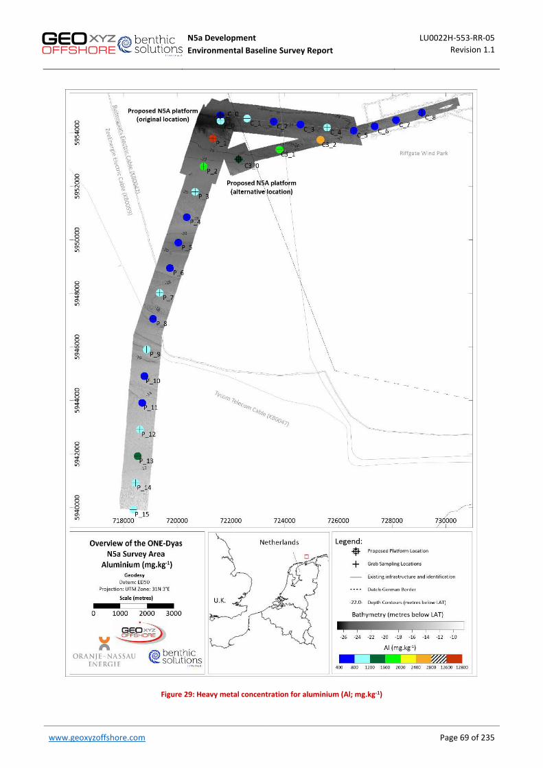
N5a Development LU0022H-553-RR-05 Environmental Baseline Survey Report Revision 1.1
www.geoxyzoffshore.com Page 69 of 235
Figure 29: Heavy metal concentration for aluminium (Al; mg.kg-1)

N5a Development LU0022H-553-RR-05 Environmental Baseline Survey Report Revision 1.1
www.geoxyzoffshore.com Page 70 of 235
Figure 30: Heavy metal concentration for zinc (Zn; mg.kg-1)

N5a Development LU0022H-553-RR-05 Environmental Baseline Survey Report Revision 1.1
www.geoxyzoffshore.com Page 71 of 235 Page 71 of 235
MACROFAUNAL ANALYSES
Macrofaunal analysis was carried out on 56 grab sample replicates from 28 stations sampled within the N5A survey area. Macrofaunal samples were processed in the field over a 500μm mesh sieve. The sediment over the N5A survey area was found to consist of fine and coarse sand with varying densities of cobbles and some areas of exposed clay.
True solitary epifaunal species were counted while encrusting epifaunal species were recorded separately, as colonial epifauna, from the main phyla groupings (e.g. Annelida, Arthropoda, Mollusca and Echinodermata). Solitary epifauna include specimens that, although epifaunal in nature, are recorded in low counts. Colonial epifauna consist of encrusting epifauna which are generally recorded in high counts or as presence/absence. For this survey colonial epifauna included Cnidaria and Bryozoa. Colonial epifauna were omitted from statistical analyses as a true abundance cannot be determined. Within the present analyses solitary epifauna have been included with infaunal species, however, due to the importance that colonial epifauna can have at locations containing coarse sediments; the richness of these macrobenthos is presented and discussed separately in Section 3.8.5.
Subsequent macrofaunal taxonomy of all recovered fauna identified a total of 16,550 individuals (infauna) from the 56 samples analysed. Faunal data for each sample are listed in Appendix M, whilst univariate analyses are summarised by replicate in Table 17and station in Table 18. Of the 150 taxa recorded, 118 were infaunal, consisting of 52 annelids accounting for 58.9% of the total individuals. The molluscs were represented by 21 taxa (9.3% of total individuals), the crustaceans by 35 taxa (7.9% of total individuals), echinoderms by three taxa (0.2% of total individuals) and others (Nematoda, Nemertea, Platyhelminthes, Branchiostoma) were accounted by four taxa (22.6% of total individuals). Solitary epifauna consisted of four taxa and accounted for 1.2% of total abundance. Colonial epifauna were represented by ten taxa, however abundance data for these species are not available as they are recorded as presence/absence. The proportional composition of the different faunal groups is presented in Figure 31 and Figure 32 (abundance) and Figure 33 and Figure 34 (richness) by replicate, and Figure 35 (abundance) and Figure 36 (richness) by station.
With the exception of species that have been intentionally grouped at higher taxonomic levels (i.e. Nematoda and Nemertea), all adult specimens were identified to species level (~85% of samples). Five fragmented species were noted during the survey and were excluded from analyses. Juveniles (if present) are often excluded from community analyses due to their high mortality prior to reaching maturity and difficulties in distinguishing species of the same genus. Consequently, they tend to induce a recruitment spike at certain times of the year due to rapid settlement and colonisation but are essentially an ephemeral part of the population masking the underlying trends within the mature adults. A total of 1,032 juvenile individuals spanning 15 taxa were recorded during the current survey. Highest numbers of juveniles were found within the class Asteroidea, with a total number of 585 across the survey area (>300 individuals at GRAB_P_0). These numbers are considered to be low as juvenile numbers are expected to be in the thousands during recruitment periods. Nonetheless, juveniles have been excluded from further analysis as their inclusion was likely to significantly impact the results.
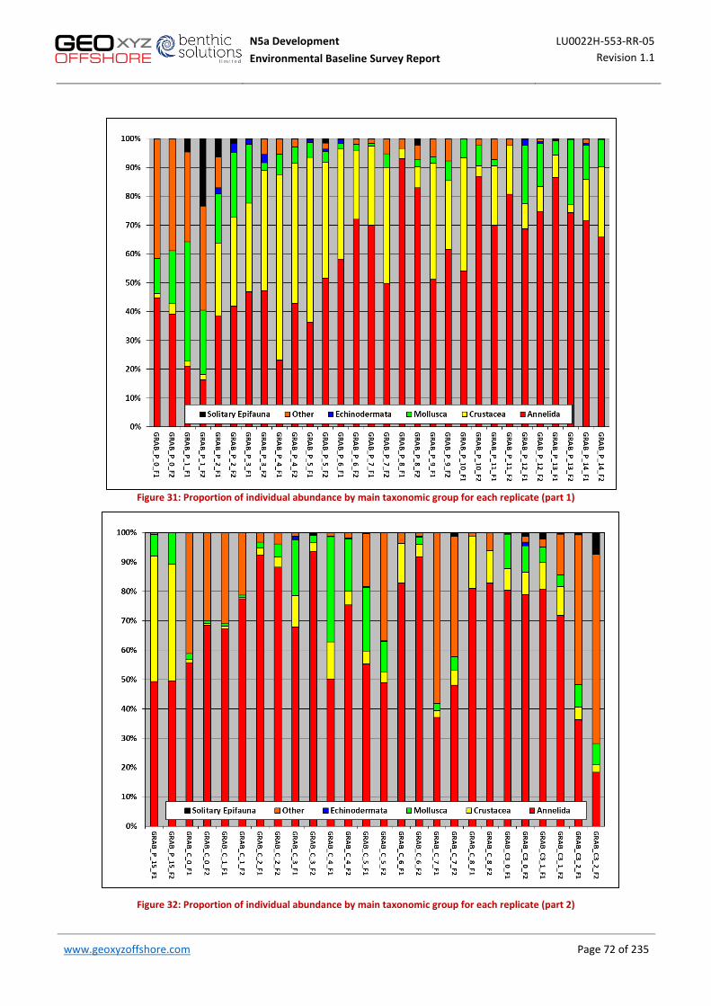
N5a Development LU0022H-553-RR-05 Environmental Baseline Survey Report Revision 1.1
www.geoxyzoffshore.com Page 72 of 235 Page 72 of 235
Figure 31: Proportion of individual abundance by main taxonomic group for each replicate (part 1)
Figure 32: Proportion of individual abundance by main taxonomic group for each replicate (part 2)
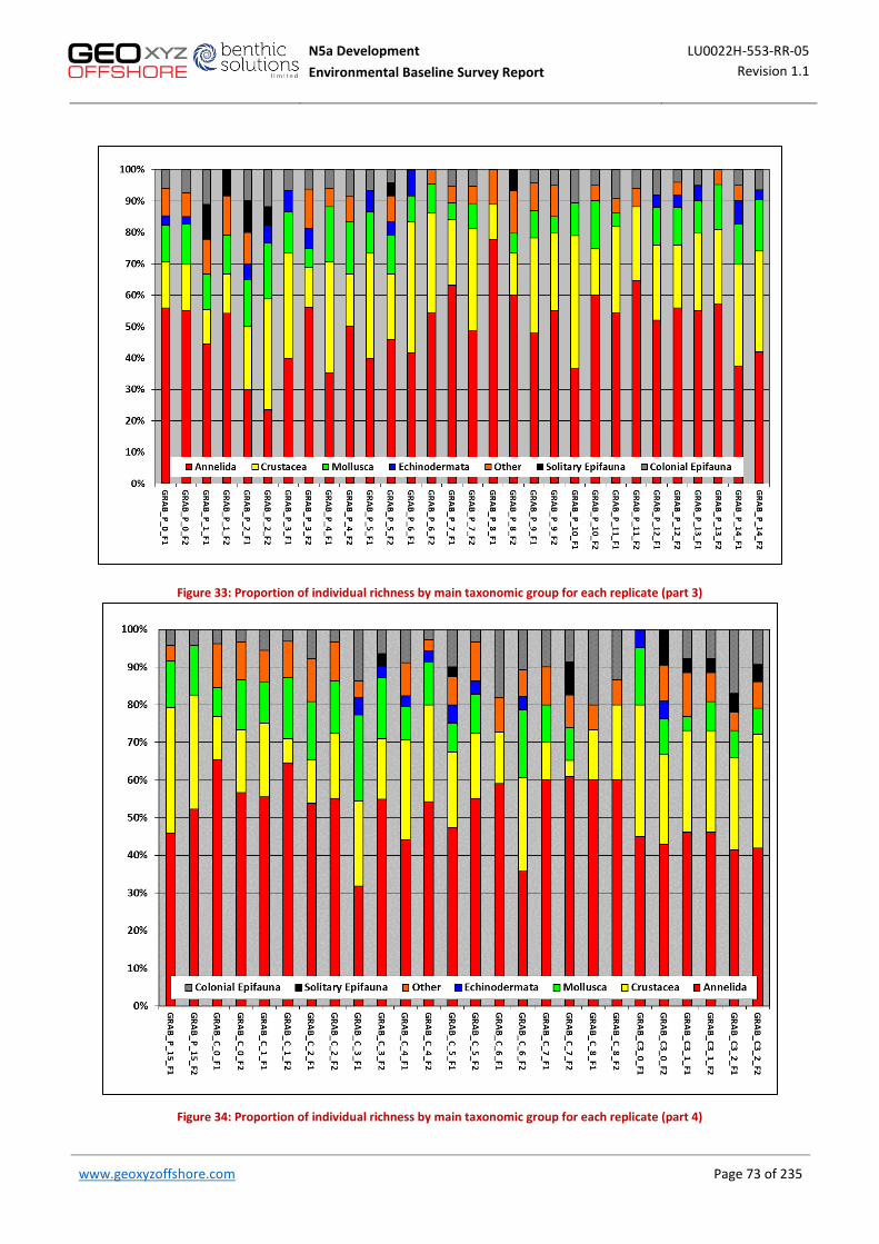
N5a Development LU0022H-553-RR-05 Environmental Baseline Survey Report Revision 1.1
www.geoxyzoffshore.com Page 73 of 235 Page 73 of 235
Figure 33: Proportion of individual richness by main taxonomic group for each replicate (part 3)
Figure 34: Proportion of individual richness by main taxonomic group for each replicate (part 4)

N5a Development LU0022H-553-RR-05 Environmental Baseline Survey Report Revision 1.1
www.geoxyzoffshore.com Page 74 of 235 Page 74 of 235
Figure 35: Proportion of individual abundance by main taxonomic group for each station
Figure 36: Proportion of individual richness by main taxonomic group for each station
N5a Development LU0022H-553-RR-05 Environmental Baseline Survey Report Revision 1.1
www.geoxyzoffshore.com Page 75 of 235 Page 75 of 235
Infaunal Trends
The macrofauna throughout the N5A survey area showed moderate species richness and high abundance, with some variation evident between stations. The infaunal community was in most instances dominated by annelids, followed by molluscs and crustaceans in terms of species richness, and in terms of abundance annelids were commonly dominant. Exceptions to this included GRAB_P_1, GRAB_P_4, GRAB_P_5, GRAB_C_7 and GRAB_C3_2, where annelids were not the most dominant phylum.
A measure of the overall dominance pattern in the sampling area was achieved by ranking the top 15 species per station according to abundance, giving a rank score of ten to the most abundant species, decreasing to one for the tenth most abundant species, and summing these scores for all 56 samples to provide an overall dominance score (Eleftheriou and Basford, 1989) for each species. The rank dominance calculation indicated a fairly homogeneous spread of macrofaunal species across the N5A survey area, resulting in seven of the highest numerically ranked species being listed in the top ten overall dominance ranks (Table 16). Notable variation in abundance and dominance rank was shown by the polychaete Nephtys cirrosa which was ranked 24th for abundance (103 individuals) and 13th for dominance, suggesting a patchy distribution of this species. The rank dominance was shown in both abundance and richness, with six annelids recorded in the top ten ranked species. In overall rank order, the annelid Spiophanes bombyx was top and relatively dominant in terms of abundance with 1993 individuals across the 56 stations (Table 16). This was followed by the two annelids, Lanice conchilega (2213 individuals, and commonly known as sand mason worm) and Scoloplos
armiger (543 individuals), other Nematoda (3443 individuals) and annelid Ophelia borealis. Ranks six to ten were dominated by the bivalve mollusc, Abra alba, two crustaceans, Tanaissus lilljeborgi and Bathyporeia
elegans and two annelids, Magelona johnstoni and Grania.
No single taxa was recorded in every replicate sample, however the bristle worm Spiophanes bombyx occurred in 52 of the 56 replicates (93% of replicates). Out of the total 16,550 individuals recorded, 38 taxa across five phyla were recorded in only one replicate across the survey area, while 17 of these taxa (3 phyla) were recorded just once. The highest number of individuals was recorded at station GRAB_P_0 and GRAB_C3_2, recording a total of 2,372 and 1,938 individuals respectively, which was a result of the high numbers of Nematoda counted, with over 58% of all Nematoda individuals found at these two stations alone (Table 18).

N5a Development LU0022H-553-RR-05 Environmental Baseline Survey Report Revision 1.1
www.geoxyzoffshore.com Page 76 of 235 Page 76 of 235
Table 16: Overall Species Ranking (Top 15 Species)
Overall Top
15 Rank Species/Taxon
Total rank
score
(out of 560)
Phylum
Numerical
Abundance
(56 replicates)
Numerical Top
15 rank
1 Spiophanes bombyx 367 Annelida 1993 3 2 Lanice conchilega 329 Annelida 2213 2 3 Scoloplos armiger 263 Annelida 543 9
4 Nematoda 221 Others 3443 1 5 Ophelia borealis 176 Annelida 573 8 6 Abra alba 147 Mollusca 1087 4
7 Tanaissus lilljeborgi 143 Crustacea 237 11 8 Bathyporeia elegans 115 Crustacea 181 16 9 Magelona johnstoni 112 Annelida 724 7
10 Grania 112 Annelida 790 6 11 Monopseudocuma gilsoni 107 Crustacea 222 13
12 Nephtys cirrosa 96 Annelida 106 24
13 Lagis koreni 96 Annelida 353 10
14 Eteone longa 80 Annelida 196 14
15 Aonides paucibranchiata 80 Annelida 1024 5
Further comments relating to the macrobenthic infaunal population and their separate phyletic groups are presented below, with comments on epifaunal species shown in Section 3.7.5. Example photographs of some macro-invertebrate specimens recorded during the survey are shown in Figure 37.
Annelida The Annelida group encompassed 45 taxa, with 43 belonging to Polychaeta and four belonging to Oligochaeta. The most abundant polychaete by a large margin was Lanice conchilega, otherwise known as the sand mason worm. This species forms tubes that project from the seabed with a characteristic fringe. It was recorded in 52 out of the 56 samples, however its abundance varied across the survey area. In some stations the species was recorded with only a few individuals whereas in the sample P_00_F1 it reached 261 individuals. The species is known to display different feeding strategies depending on its densities, adopting deposit feeding in low densities and suspension feeding when the polychaete is found in higher densities as coping mechanism due to competition (several thousand individuals per m2) (Buhr & Winter, 1977).
The Pectinariidae Lagis koreni was also one of the most common species recorded. These worms form a tube with a mucus extension and often co-occurs with high densities of Abra
alba (Eagle, 1975), which was also present in high numbers in the survey area.
The errant polychaeta included a mix of omnivorous and carnivorous species. Spionidae showed the highest diversity with ten taxa recorded, including three species of the genus Spio
sp. The Spionidae worms Spiophanes bombyx and Aonides paucibranchiata were recorded in high numbers, with S. bombyx occurring with upwards of 550 individuals at one station and A. paucibranchiata reaching 425 individuals in one sample.

N5a Development LU0022H-553-RR-05 Environmental Baseline Survey Report Revision 1.1
www.geoxyzoffshore.com Page 77 of 235 Page 77 of 235
Arthropoda The Arthropoda group was well represented with 38 taxa being identified, including Cirripedia, Copepoda, Amphipoda, Isopoda, Tanaidacea, Cumacea and Decapoda. Amongst the Crustacea, the tanaid Tanaissus lilljeborgi was the most abundant and it is the only tanaid commonly found in sublittoral sands in UK waters (Jones & Holdich, 1983).
Amphipods were varied and distributed sporadically throughout the samples, with 19 taxa identified. Two species of the amphipod genus Bathyporeia were recorded including B. elegans and B. guilliamsoniana, with the former being the most abundant. All species within the genus Bathyporeia are burrowing amphipods that are confined to sandy bottoms (d'Udekem d'Acoz, 2004). Urothoe poseidonis was recorded in moderate abundance and was present in 26 out of the 56 stations. Another species of Urothoe, U. brevicornis, was also present but in much lower abundance with only three individuals recorded.
Several species of Decapods were recorded including several brachyuran crabs, the hermit crab Pagurus bernhardus, the mud shrimp Upogebia deltaura and the caridean shrimps Processa modica and Crangon crangon. Brachyuran crabs recorded included the spider crab Macropodia rostrata, the thumbnail crab Thia scutellata and the pea crab Pinnotheres pisum, which is a parasitic crab that lives in bivalve shells such as Mytilus and Spisula sp. (Ingle, 1997).
Mollusca The mollusc group was well represented with 29 taxa identified including Gastropoda and Bivalvia. Bivalves were common throughout the survey with Abra alba occurring in 36 out of 56 samples, and in the highest abundance, with up to 243 individuals recorded at station P_00_F2. The largest bivalve observed in the samples was the non-native razor shell Ensis leei which occurred in moderate numbers. The species is native to the North American Atlantic coast, from Canada to South Carolina and was first reported in Europe from the Netherlands in 1984 and from the UK in 1989 and is now spreading quickly across the southeast coast of England (Oliver et al., 2016). It can burrow itself quickly into the sediment and is able to swim three to five metres at a time by flicking its foot and propelling a jet of water out of the pedal opening (Fraser et al., 2018).
Gastropods were represented by eight different taxa but were infrequently recorded across the survey area with the most abundant being the micromollusc Caecum glabrum.
Minor Phyla Minor phyla included Echinoderms, Chordates and Ascidians. The number of Echinodermata was small with only seven taxa however high numbers of juvenile Asteroidea were present in high numbers throughout the survey area. The sea potato Echinocardium cordatum occurred in low numbers at 21 stations. The species lives in a permanent burrow buried about 8 cm deep.
Amongst Chordata, juvenile Ascidians were recorded at 21 stations. The lancelet Branchiostoma lanceolatum was recorded at 14 stations. This animal is considered an invertebrate as it has a notochord but no backbone. B. lanceolatum is covered with fins and manages to cover small distances by swimming; however, it stays buried in coarse sediment most of the time (Degraer et al., 2006). Only one species of fish was found in the survey area, the sand goby Pomatoschistus minutus. This species is abundant in inshore waters on sandy and muddy bottoms. It is caught in abundance by shrimp fishermen using beam trawls and in push nets over sandy shores. Although it enters estuaries, it always stays in moderately deep waters (Wheeler, 1969).

N5a Development LU0022H-553-RR-05 Environmental Baseline Survey Report Revision 1.1
www.geoxyzoffshore.com Page 78 of 235 Page 78 of 235
As previously discussed in Section 3.4, coarse material was a minimal component of the sediment at most of the grab sample stations, where the main component was sand. As a result, there was little substrate available for colonisation by sessile epifaunal species, which was reflected in the results with a much greater abundance of infaunal species in comparison to colonial epifaunal species. Across all stations there were 118 infaunal species and only ten colonial epifaunal species.

N5a Development LU0022H-553-RR-05 Environmental Baseline Survey Report Revision 1.1
www.geoxyzoffshore.com Page 79 of 235 Page 79 of 235
Figure 37: Example photographs of macrofauna species within survey area

N5a Development LU0022H-553-RR-05 Environmental Baseline Survey Report Revision 1.1
www.geoxyzoffshore.com Page 80 of 235 Page 80 of 235
Univariate Parameters
The primary and univariate parameters for all stations are listed in Table 17 by replicate and in Table 18 by station. The number of species per 0.1m2 sample was considered moderately diverse, ranging from nine species for replicate GRAB_P_8 F1 to a maximum of 38 species for replicate GRAB_P_14 F1 (mean 22.8±7.5SD). The species richness throughout the N5A survey area is illustrated in Figure 38 and Figure 39.
Species abundance was considerably more variable than richness throughout the survey area, ranging from a minimum of 29 individuals for replicate GRAB_P_8 F1 to a maximum of 1,368 for replicate GRAB_P_0 F2, giving a mean of 295 ±319SD. By station, the mean number of individuals increased to 591±615SD with the highest number of 2,372 individuals recorded at station GRAB_P_0. The high variability in the mean number of individuals by replicate and station was the consequence of the patchy distribution of Nematoda and the annelids Spiophanes bombyx and Lanice conchilega, which showed particularly high abundances at some stations. For example, 915 Nematoda were recorded at GRAB_P_0 but no specimens were recorded at GRAB_C3_0. The individual abundance by station throughout the survey area is illustrated in Figure 40.
The sediment characteristics had a significant impact on the fauna observed at each station, with significant Spearman’s rank correlations seen between several primary and univariate macrofauna variables and fines (Appendix N). Negative correlations were found between the percentage of fines and evenness (ƍ(28)=-0.537, p<0.01), percentage fines and Shannon-Wiener Diversity (ƍ(28)=-0.534, p<0.01) and percentage fines and Simpson’s Diversity (ƍ(28)=-0.478, p<0.05). Conversely, the percentage of sands and evenness were positively correlated (ƍ(28)=0.400, p<0.05). Faunal abundance was positively correlated with water depth (ƍ(28)=0.383, p<0.05) and negative correlations were seen between both Shannon-Wiener diversity and Evenness and with distance to shore and water depth. The relationship between richness and abundance is presented in Figure 40.
Table 17: Univariate faunal parameters (0.1m2 replicates)
Station
Number of Species per 0.1m2
(S)
Number of Individuals per
0.1m2 (N)
Richness (Margalef)
Evenness (Pielou's
Evenness)
Shannon-Wiener
Diversity
Simpsons Diversity
(1-Lambda')
GRAB_P_00_F1 32 1004 4.49 0.54 2.69 0.75 GRAB_P_00_F2 37 1368 4.99 0.57 2.96 0.79 GRAB_P_01_F1 16 109 3.20 0.66 2.63 0.75 GRAB_P_01_F2 24 324 3.98 0.60 2.76 0.78 GRAB_P_02_F1 18 47 4.42 0.89 3.72 0.92 GRAB_P_02_F2 15 62 3.39 0.83 3.25 0.86 GRAB_P_03_F1 14 49 3.34 0.90 3.43 0.91 GRAB_P_03_F2 15 36 3.91 0.87 3.39 0.90 GRAB_P_04_F1 16 56 3.73 0.76 3.04 0.81 GRAB_P_04_F2 11 35 2.81 0.76 2.64 0.78 GRAB_P_05_F1 14 77 2.99 0.81 3.07 0.85 GRAB_P_05_F2 23 136 4.48 0.80 3.61 0.88 GRAB_P_06_F1 12 55 2.75 0.76 2.74 0.80 GRAB_P_06_F2 22 100 4.56 0.80 3.57 0.89 GRAB_P_07_F1 18 120 3.55 0.70 2.90 0.80 GRAB_P_07_F2 35 191 6.47 0.81 4.16 0.91 GRAB_P_08_F1 9 29 2.38 0.92 2.90 0.88 GRAB_P_08_F2 15 41 3.77 0.87 3.39 0.89 GRAB_P_09_F1 22 129 4.32 0.84 3.75 0.90 GRAB_P_09_F2 19 117 3.78 0.85 3.61 0.89
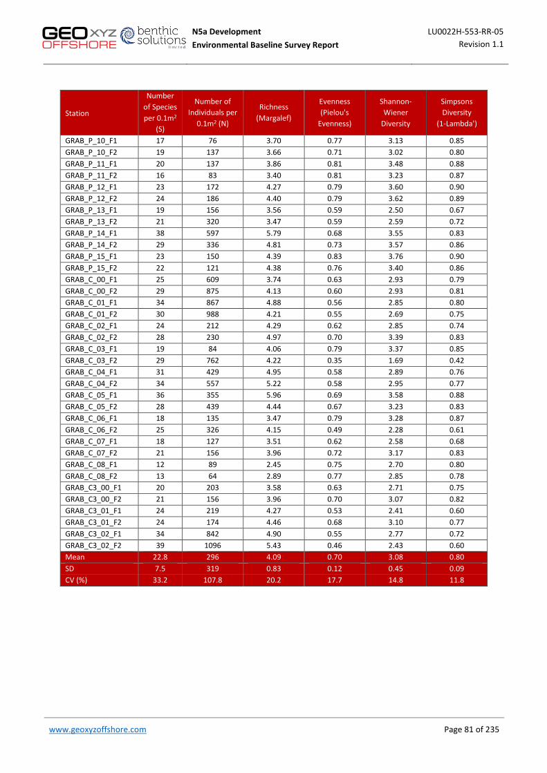
N5a Development LU0022H-553-RR-05 Environmental Baseline Survey Report Revision 1.1
www.geoxyzoffshore.com Page 81 of 235 Page 81 of 235
Station
Number of Species per 0.1m2
(S)
Number of Individuals per
0.1m2 (N)
Richness (Margalef)
Evenness (Pielou's
Evenness)
Shannon-Wiener
Diversity
Simpsons Diversity
(1-Lambda')
GRAB_P_10_F1 17 76 3.70 0.77 3.13 0.85 GRAB_P_10_F2 19 137 3.66 0.71 3.02 0.80 GRAB_P_11_F1 20 137 3.86 0.81 3.48 0.88 GRAB_P_11_F2 16 83 3.40 0.81 3.23 0.87 GRAB_P_12_F1 23 172 4.27 0.79 3.60 0.90 GRAB_P_12_F2 24 186 4.40 0.79 3.62 0.89 GRAB_P_13_F1 19 156 3.56 0.59 2.50 0.67 GRAB_P_13_F2 21 320 3.47 0.59 2.59 0.72 GRAB_P_14_F1 38 597 5.79 0.68 3.55 0.83 GRAB_P_14_F2 29 336 4.81 0.73 3.57 0.86 GRAB_P_15_F1 23 150 4.39 0.83 3.76 0.90 GRAB_P_15_F2 22 121 4.38 0.76 3.40 0.86 GRAB_C_00_F1 25 609 3.74 0.63 2.93 0.79 GRAB_C_00_F2 29 875 4.13 0.60 2.93 0.81 GRAB_C_01_F1 34 867 4.88 0.56 2.85 0.80 GRAB_C_01_F2 30 988 4.21 0.55 2.69 0.75 GRAB_C_02_F1 24 212 4.29 0.62 2.85 0.74 GRAB_C_02_F2 28 230 4.97 0.70 3.39 0.83 GRAB_C_03_F1 19 84 4.06 0.79 3.37 0.85 GRAB_C_03_F2 29 762 4.22 0.35 1.69 0.42 GRAB_C_04_F1 31 429 4.95 0.58 2.89 0.76 GRAB_C_04_F2 34 557 5.22 0.58 2.95 0.77 GRAB_C_05_F1 36 355 5.96 0.69 3.58 0.88 GRAB_C_05_F2 28 439 4.44 0.67 3.23 0.83 GRAB_C_06_F1 18 135 3.47 0.79 3.28 0.87 GRAB_C_06_F2 25 326 4.15 0.49 2.28 0.61 GRAB_C_07_F1 18 127 3.51 0.62 2.58 0.68 GRAB_C_07_F2 21 156 3.96 0.72 3.17 0.83 GRAB_C_08_F1 12 89 2.45 0.75 2.70 0.80 GRAB_C_08_F2 13 64 2.89 0.77 2.85 0.78 GRAB_C3_00_F1 20 203 3.58 0.63 2.71 0.75 GRAB_C3_00_F2 21 156 3.96 0.70 3.07 0.82 GRAB_C3_01_F1 24 219 4.27 0.53 2.41 0.60 GRAB_C3_01_F2 24 174 4.46 0.68 3.10 0.77 GRAB_C3_02_F1 34 842 4.90 0.55 2.77 0.72 GRAB_C3_02_F2 39 1096 5.43 0.46 2.43 0.60 Mean 22.8 296 4.09 0.70 3.08 0.80 SD 7.5 319 0.83 0.12 0.45 0.09 CV (%) 33.2 107.8 20.2 17.7 14.8 11.8

N5a Development LU0022H-553-RR-05 Environmental Baseline Survey Report Revision 1.1
www.geoxyzoffshore.com Page 82 of 235 Page 82 of 235
Table 18: Univariate faunal parameters (0.2m2 pooled station replicates)
Station Number of Species per
0.2m2 (S)
Number of Individuals per
0.2m2 (N)
Richness (Margalef)
Evenness (Pielou's
Evenness)
Shannon-Wiener
Diversity
Simpsons Diversity
(1-Lambda') GRAB_P_00 40 2372 5.02 0.54 2.89 0.78 GRAB_P_01 26 433 4.12 0.60 2.83 0.79 GRAB_P_02 24 109 4.90 0.85 3.90 0.91 GRAB_P_03 20 85 4.28 0.87 3.75 0.92 GRAB_P_04 21 91 4.43 0.74 3.24 0.80 GRAB_P_05 24 213 4.29 0.79 3.64 0.90 GRAB_P_06 25 155 4.76 0.76 3.55 0.88 GRAB_P_07 38 311 6.45 0.73 3.86 0.88 GRAB_P_08 16 70 3.53 0.86 3.43 0.89 GRAB_P_09 26 246 4.54 0.82 3.87 0.91 GRAB_P_10 27 213 4.85 0.71 3.38 0.85 GRAB_P_11 23 220 4.08 0.77 3.50 0.88 GRAB_P_12 31 358 5.10 0.76 3.79 0.90 GRAB_P_13 25 476 3.89 0.57 2.67 0.71 GRAB_P_14 41 933 5.85 0.69 3.67 0.84 GRAB_P_15 30 271 5.18 0.77 3.80 0.89 GRAB_C_00 38 1484 5.07 0.58 3.02 0.81 GRAB_C_01 42 1855 5.45 0.52 2.82 0.78 GRAB_C_02 35 442 5.58 0.64 3.28 0.79 GRAB_C_03 36 846 5.19 0.40 2.05 0.51 GRAB_C_04 40 986 5.66 0.60 3.18 0.82 GRAB_C_05 45 794 6.59 0.64 3.53 0.86 GRAB_C_06 32 461 5.05 0.55 2.77 0.71 GRAB_C_07 27 283 4.61 0.65 3.10 0.78 GRAB_C_08 16 153 2.98 0.74 2.94 0.80 GRAB_C3_00 30 359 4.93 0.61 3.00 0.79 GRAB_C3_01 33 393 5.36 0.57 2.87 0.68 GRAB_C3_02 49 1938 6.34 0.48 2.70 0.66 GRAB_P_00 40 2372 5.02 0.54 2.89 0.78 Mean 30.7 591 4.93 0.67 3.25 0.81 SD 8.7 614 0.84 0.12 0.46 0.09 CV (%) 28.3 104.0 17.1 18.2 14.3 11.4

N5a Development LU0022H-553-RR-05 Environmental Baseline Survey Report Revision 1.1
www.geoxyzoffshore.com Page 83 of 235 Page 83 of 235
Figure 38: Macrofauna species abundance (per 0.2m2)

N5a Development LU0022H-553-RR-05 Environmental Baseline Survey Report Revision 1.1
www.geoxyzoffshore.com Page 84 of 235 Page 84 of 235
Figure 39: Macrofauna species richness (per 0.2m2)
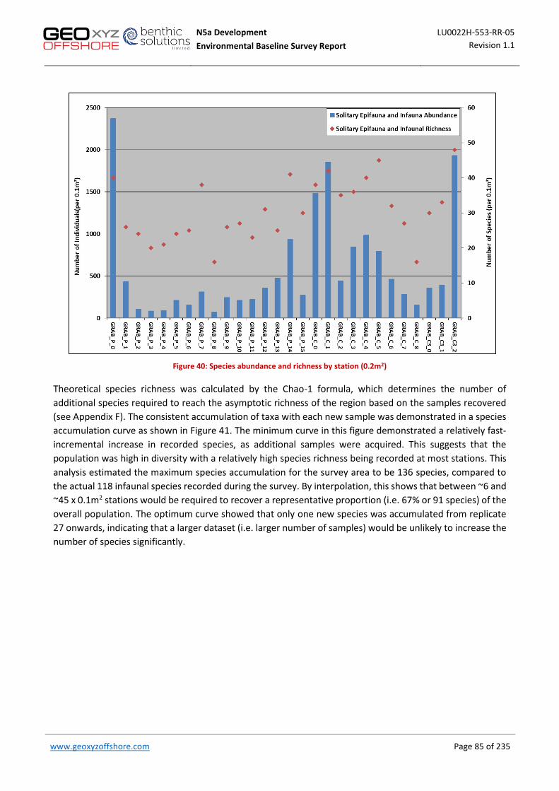
N5a Development LU0022H-553-RR-05 Environmental Baseline Survey Report Revision 1.1
www.geoxyzoffshore.com Page 85 of 235 Page 85 of 235
Figure 40: Species abundance and richness by station (0.2m2)
Theoretical species richness was calculated by the Chao-1 formula, which determines the number of additional species required to reach the asymptotic richness of the region based on the samples recovered (see Appendix F). The consistent accumulation of taxa with each new sample was demonstrated in a species accumulation curve as shown in Figure 41. The minimum curve in this figure demonstrated a relatively fast-incremental increase in recorded species, as additional samples were acquired. This suggests that the population was high in diversity with a relatively high species richness being recorded at most stations. This analysis estimated the maximum species accumulation for the survey area to be 136 species, compared to the actual 118 infaunal species recorded during the survey. By interpolation, this shows that between ~6 and ~45 x 0.1m2 stations would be required to recover a representative proportion (i.e. 67% or 91 species) of the overall population. The optimum curve showed that only one new species was accumulated from replicate 27 onwards, indicating that a larger dataset (i.e. larger number of samples) would be unlikely to increase the number of species significantly.

N5a Development LU0022H-553-RR-05 Environmental Baseline Survey Report Revision 1.1
www.geoxyzoffshore.com Page 86 of 235 Page 86 of 235
Figure 41: Species accumulation curve of the N5A survey area
The Shannon-Wiener diversity was variable throughout survey area, ranging from a minimum of 1.69 GRAB_C_3 F2 to a maximum of 4.16 at GRAB_P_7 F2 (mean 3.08±0.45SD), by replicate. The difference between the two samples is likely attributable to the high abundance of S. bombyx at GRAB_C3_2 F2 (576 individuals) and low abundance at GRAB_P_7 F2 (39 individuals). This trend was not repeated at station level with a minimum of 2.05 at station GRAB_C_3 to a maximum of 3.90 at station GRAB_P_2 (mean 3.25±0.46SD). The spatial variation in Shannon-Wiener diversity is presented by station in Figure 42, with stations along the pipeline route generally having a higher H’ diversity value.
Pielou’s equitability showed similar variation to the Shannon-Wiener index, with replicate GRAB_C_3 F2 showing the lowest evenness of 0.35, compared to a maximum equitability score of 0.92 for replicate GRAB_P_8 F1 (mean 0.70±0.12). By station, a similar pattern was observed once again as equitability was lowest for GRAB_C_3 (0.40) and highest for GRAB_P_8 (0.86) with a slightly lower mean equitability of 0.67±0.12SD. This indicates that species were relatively evenly represented within samples, although there was variation from station to station. Margalef’s Index (Species Richness) showed moderate variation with maximum and minimum values recorded for GRAB_P_7 F2 and GRAB_P_8 F1 respectively by replicate (mean 4.09±0.83SD). By station, the maximum level was recorded for GRAB_C_5 (6.59) with a minimum of 2.98 for GRAB_C_8 (mean 4.93±0.84SD). Although species diversity was not highest for GRAB_C_5 (45 instead of the maximum 49 recorded elsewhere), this station showed low abundance relative to the species count. Simpson’s diversity ranged from 0.51 at station GRAB_C_1 to 0.92 at station GRAB_P_3 (mean 0.81±0.09SD).
The overall picture indicated by the univariate parameters is one of a variable macrofauna diversity with no particular trend in spatial distribution.

N5a Development LU0022H-553-RR-05 Environmental Baseline Survey Report Revision 1.1
www.geoxyzoffshore.com Page 87 of 235 Page 87 of 235
Figure 42: Macrofauna – Shannon-Wiener diversity (H per 0.1m2)
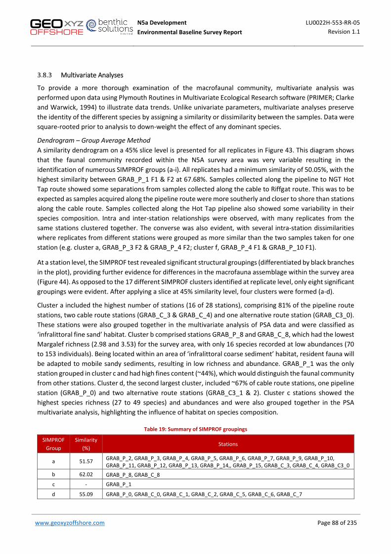
N5a Development LU0022H-553-RR-05 Environmental Baseline Survey Report Revision 1.1
www.geoxyzoffshore.com Page 88 of 235 Page 88 of 235
Multivariate Analyses
To provide a more thorough examination of the macrofaunal community, multivariate analysis was performed upon data using Plymouth Routines in Multivariate Ecological Research software (PRIMER; Clarke and Warwick, 1994) to illustrate data trends. Unlike univariate parameters, multivariate analyses preserve the identity of the different species by assigning a similarity or dissimilarity between the samples. Data were square-rooted prior to analysis to down-weight the effect of any dominant species.
Dendrogram – Group Average Method
A similarity dendrogram on a 45% slice level is presented for all replicates in Figure 43. This diagram shows that the faunal community recorded within the N5A survey area was very variable resulting in the identification of numerous SIMPROF groups (a-i). All replicates had a minimum similarity of 50.05%, with the highest similarity between GRAB_P_1 F1 & F2 at 67.68%. Samples collected along the pipeline to NGT Hot Tap route showed some separations from samples collected along the cable to Riffgat route. This was to be expected as samples acquired along the pipeline route were more southerly and closer to shore than stations along the cable route. Samples collected along the Hot Tap pipeline also showed some variability in their species composition. Intra and inter-station relationships were observed, with many replicates from the same stations clustered together. The converse was also evident, with several intra-station dissimilarities where replicates from different stations were grouped as more similar than the two samples taken for one station (e.g. cluster a, GRAB_P_3 F2 & GRAB_P_4 F2; cluster f, GRAB_P_4 F1 & GRAB_P_10 F1).
At a station level, the SIMPROF test revealed significant structural groupings (differentiated by black branches in the plot), providing further evidence for differences in the macrofauna assemblage within the survey area (Figure 44). As opposed to the 17 different SIMPROF clusters identified at replicate level, only eight significant groupings were evident. After applying a slice at 45% similarity level, four clusters were formed (a-d).
Cluster a included the highest number of stations (16 of 28 stations), comprising 81% of the pipeline route stations, two cable route stations (GRAB_C_3 & GRAB_C_4) and one alternative route station (GRAB_C3_0). These stations were also grouped together in the multivariate analysis of PSA data and were classified as ‘infralittoral fine sand’ habitat. Cluster b comprised stations GRAB_P_8 and GRAB_C_8, which had the lowest Margalef richness (2.98 and 3.53) for the survey area, with only 16 species recorded at low abundances (70 to 153 individuals). Being located within an area of ‘infralittoral coarse sediment’ habitat, resident fauna will be adapted to mobile sandy sediments, resulting in low richness and abundance. GRAB_P_1 was the only station grouped in cluster c and had high fines content (~44%), which would distinguish the faunal community from other stations. Cluster d, the second largest cluster, included ~67% of cable route stations, one pipeline station (GRAB_P_0) and two alternative route stations (GRAB_C3_1 & 2). Cluster c stations showed the highest species richness (27 to 49 species) and abundances and were also grouped together in the PSA multivariate analysis, highlighting the influence of habitat on species composition.
Table 19: Summary of SIMPROF groupings
SIMPROF Group
Similarity (%)
Stations
a 51.57 GRAB_P_2, GRAB_P_3, GRAB_P_4, GRAB_P_5, GRAB_P_6, GRAB_P_7, GRAB_P_9, GRAB_P_10, GRAB_P_11, GRAB_P_12, GRAB_P_13, GRAB_P_14,, GRAB_P_15, GRAB_C_3, GRAB_C_4, GRAB_C3_0
b 62.02 GRAB_P_8, GRAB_C_8
c - GRAB_P_1
d 55.09 GRAB_P_0, GRAB_C_0, GRAB_C_1, GRAB_C_2, GRAB_C_5, GRAB_C_6, GRAB_C_7

N5a Development LU0022H-553-RR-05 Environmental Baseline Survey Report Revision 1.1
www.geoxyzoffshore.com Page 89 of 235 Page 89 of 235
Figure 43: Dendrogram of macrofaunal replicates
Figure 44: Dendrogram of macrofaunal stations
GR
AB_P
_3_F
2G
RAB
_P_4
_F2
GR
AB_C
_3_F
2G
RAB
_C_4
_F1
GR
AB_C
_4_F
2G
RAB
_P_2
_F1
GR
AB_C
_3_F
1G
RAB
_P_6
_F1
GR
AB_P
_6_F
2G
RAB
_C3_
0_F1
GR
AB_C
3_0_
F2G
RAB
_P_2
_F2
GR
AB_P
_3_F
1G
RAB
_P_7
_F1
GR
AB_P
_5_F
1G
RAB
_P_5
_F2
GR
AB_P
_7_F
2G
RAB
_P_1
4_F1
GR
AB_P
_14_
F2G
RAB
_P_1
3_F1
GR
AB_P
_13_
F2G
RAB
_P_1
2_F1
GR
AB_P
_12_
F2G
RAB
_P_1
5_F1
GR
AB_P
_15_
F2G
RAB
_P_1
0_F2
GR
AB_P
_9_F
1G
RAB
_P_9
_F2
GR
AB_P
_11_
F1G
RAB
_P_1
1_F2
GR
AB_P
_4_F
1G
RAB
_P_1
0_F1
GR
AB_P
_8_F
1G
RAB
_P_8
_F2
GR
AB_C
_6_F
2G
RAB
_C_6
_F1
GR
AB_C
_8_F
1G
RAB
_C_8
_F2
GR
AB_P
_1_F
1G
RAB
_P_1
_F2
GR
AB_C
3_1_
F1G
RAB
_C3_
1_F2
GR
AB_C
_2_F
2G
RAB
_C_2
_F1
GR
AB_C
_5_F
2G
RAB
_C_7
_F1
GR
AB_C
_7_F
2G
RAB
_P_0
_F1
GR
AB_P
_0_F
2G
RAB
_C_0
_F1
GR
AB_C
_1_F
1G
RAB
_C_0
_F2
GR
AB_C
_1_F
2G
RAB
_C_5
_F1
GR
AB_C
3_2_
F1G
RAB
_C3_
2_F2
Samples
100
80
60
40
20
Sim
ilarit
y
Slice 45%abcdefghi
GR
AB_P
_2G
RAB
_P_3
GR
AB_P
_4G
RAB
_P_6
GR
AB_P
_5G
RAB
_P_7
GR
AB_P
_9G
RAB
_P_1
1G
RAB
_P_1
0G
RAB
_P_1
2G
RAB
_P_1
3G
RAB
_P_1
4G
RAB
_P_1
5G
RAB
_C3_
0G
RAB
_C_3
GR
AB_C
_4G
RAB
_P_8
GR
AB_C
_8G
RAB
_P_1
GR
AB_P
_0G
RAB
_C_0
GR
AB_C
_1G
RAB
_C_7
GR
AB_C
_2G
RAB
_C_6
GR
AB_C
3_1
GR
AB_C
_5G
RAB
_C3_
2
Samples
100
80
60
40
20
Sim
ilarit
y
Slice 45%abcd

N5a Development LU0022H-553-RR-05 Environmental Baseline Survey Report Revision 1.1
www.geoxyzoffshore.com Page 90 of 235 Page 90 of 235
Multi-dimensional Scaling (MDS) Ordination Plot
Similarities in the macrofaunal communities recorded across the survey area are presented as 2-dimensional multi-dimensional scaling (MDS) ordinations in Figure 45 by replicate and in Figure 46 by station. Figure 45 shows a 2-D MDS plot that presents all 56 replicates from the survey area, revealing a potentially useful 2-D plot ordination due to a stress level of 0.175 recorded. At a replicate level, some clear separations are seen between the nine SIMPROF groups, particularly for group i and g. However, some of groups are less obvious and similarities can be seen with replicates from other groups, such as those within groups d and e. At a station level, separation of clusters is clearer and visibly show the distinct separations between the groupings, with a stress level of 0.165.
Figure 45: MDS ordination of macrofauna by replicates

N5a Development LU0022H-553-RR-05 Environmental Baseline Survey Report Revision 1.1
www.geoxyzoffshore.com Page 91 of 235 Page 91 of 235
Figure 46: MDS ordination of macrofauna by station
In order to determine the magnitude of the differences between the SIMPROF groups in all dimensions, an ANOSIM (analysis of similarity) test was performed. This recorded a similarity R value of 0.813 (p=0.001) and 0.87 (p=0.001) on a replicate and station level, respectively. The combination of dendrograms, SIMPROF tests, MDSs and ANOSIM tests indicate that there is a significant difference between the macrofaunal communities recorded around the N5A survey area. A combination of factors are likely to have influenced the macrofaunal communities recorded with sediment characteristics being one of the major contributing factors.
Table 20 shows the top five species responsible for the differences between the clusters and their average contributory percentages. Differences here ranged from 57.54% to almost 69.21% dissimilarity. The results revealed variable species were responsible for changes seen within the clusters. Within cluster c, relatively high abundance of Phoronida (79) were responsible for the largest dissimilarity between this cluster and clusters a and b (5.71% and 6.87%), while the very high abundances of sand mason worm, Lanice conchilega
and unidentified Grania in cluster d resulted in a significant dissimilarity of 5.95% and 4.51%. Differences between Cluster a and b were largely driven by the high abundances of Spiophanes bombyx and Magelona
johnstoni in cluster a, while separations between a and d were driven by large numbers of Nematoda and Grania within cluster d and their absence from a. Lastly, clusters d and b differed again due to high abundances of Nematoda, Abra alba, Spio symphyta, Spiophanes bombyx and Lanice conchilega within d and their relative absence in stations within cluster b.

N5a Development LU0022H-553-RR-05 Environmental Baseline Survey Report Revision 1.1
www.geoxyzoffshore.com Page 92 of 235 Page 92 of 235
Table 20: Similarity percentage (SIMPER) for clusters A-D
Cluster a Cluster b Cluster d
Cluster c
Average dissimilarity 61.31% Average dissimilarity 69.21% Average dissimilarity 57.54%
Phoronida 5.71% Phoronida 6.87% Lanice conchilega 5.95%
Nematoda 4.96% Abra alba 6.31% Grania 4.51%
Abra alba 4.34% Nematoda 4.90% Phoronida 4.04%
Lanice conchilega 3.99% Lagis koreni 4.37% Spio symphyta 2.86%
Bathyporeia elegans 3.09% Lanice conchilega 4.14% Tubificoides benedii 2.64%
Cluster a
Average dissimilarity 67.30% Average dissimilarity 64.52%
Spiophanes bombyx 4.06% Grania 3.96% Magelona johnstoni 3.88% Nematoda 3.84% Bathyporeia elegans 3.60% Aonides
paucibranchiata 3.40% Grania 3.58% Magelona johnstoni 2.59% Monopseudocuma gilsoni
3.49% Bathyporeia elegans 2.38%
Cluster b
Average dissimilarity 62.50%
Nematoda 4.11%
Abra alba 3.29%
Spio symphyta 3.19%
Spiophanes bombyx 3.12%
Lanice conchilega 3.08%
The stations grouped within cluster a showed moderate abundances with the highest contribution from the bristleworm Spiophanes bombyx, typically found in sandy areas. The stations within cluster b showed the lowest richness and some of the lowest abundances of all stations, and were dominated by Ophelia borealis,
followed by an unidentified Grania and the annelid Scoloplos armiger, accounting for over 34% similarity. Amongst those stations belonging to cluster d (which included stations with the highest abundances and richness), the sand mason worm Lanice conchilega and unidentified Nematoda were dominant and responsible for over 16% similarity. Notably high abundances of Nematoda were found at stations GRAB_P_0 and GRAB_C3_2 within this cluster (915 and 1104 respectively).
Principal Component Analysis (PCA)
A PCA was carried out on the raw particle size and macrofaunal data for each station (Figure 47) to determine whether sediment composition can explain the differences between clusters. This PCA chart shows the distribution of each station along the axes based on their particle size distribution, overlaid with macrofauna clusters (as symbols). The plot shows a general separation between stations along the N5A platform to NGT Hot Tap pipeline dominated by a finer sands fraction (cluster a, mean ɸ2.10 ±0.20SD, 0.24mm ±0.03SD) and those along that cable route to Riffgat Wind Park with a coarser sediment (cluster d, mean ɸ1.01 ±0.93SD, 0.62mm ±0.59SD). The groupings follow a very similar pattern to those found through the particle size analysis, with only macrofauna at GRAB_C3_1 departing from this overall trend.
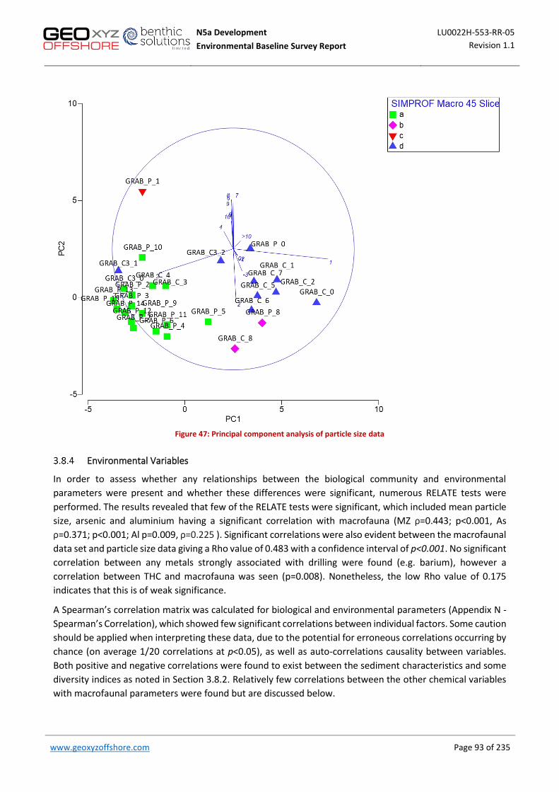
N5a Development LU0022H-553-RR-05 Environmental Baseline Survey Report Revision 1.1
www.geoxyzoffshore.com Page 93 of 235 Page 93 of 235
Figure 47: Principal component analysis of particle size data
Environmental Variables
In order to assess whether any relationships between the biological community and environmental parameters were present and whether these differences were significant, numerous RELATE tests were performed. The results revealed that few of the RELATE tests were significant, which included mean particle size, arsenic and aluminium having a significant correlation with macrofauna (MZ ρ=0.443; p<0.001, As ρ=0.371; p<0.001; Al p=0.009, ρ=0.225 ). Significant correlations were also evident between the macrofaunal data set and particle size data giving a Rho value of 0.483 with a confidence interval of p<0.001. No significant correlation between any metals strongly associated with drilling were found (e.g. barium), however a correlation between THC and macrofauna was seen (p=0.008). Nonetheless, the low Rho value of 0.175 indicates that this is of weak significance.
A Spearman’s correlation matrix was calculated for biological and environmental parameters (Appendix N - Spearman’s Correlation), which showed few significant correlations between individual factors. Some caution should be applied when interpreting these data, due to the potential for erroneous correlations occurring by chance (on average 1/20 correlations at p<0.05), as well as auto-correlations causality between variables. Both positive and negative correlations were found to exist between the sediment characteristics and some diversity indices as noted in Section 3.8.2. Relatively few correlations between the other chemical variables with macrofaunal parameters were found but are discussed below.
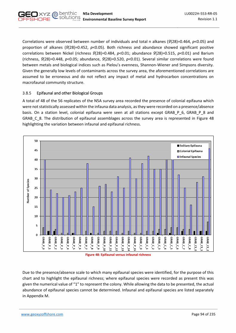
N5a Development LU0022H-553-RR-05 Environmental Baseline Survey Report Revision 1.1
www.geoxyzoffshore.com Page 94 of 235 Page 94 of 235
Correlations were observed between number of individuals and total n alkanes (ƍ(28)=0.464, p<0.05) and proportion of alkanes (ƍ(28)=0.452, p<0.05). Both richness and abundance showed significant positive correlations between Nickel (richness ƍ(28)=0.484, p<0.01; abundance ƍ(28)=0.515, p<0.01) and Barium (richness, ƍ(28)=0.448, p<0.05; abundance, ƍ(28)=0.520, p<0.01). Several similar correlations were found between metals and biological indices such as Pielou’s evenness, Shannon-Wiener and Simpsons diversity. Given the generally low levels of contaminants across the survey area, the aforementioned correlations are assumed to be erroneous and do not reflect any impact of metal and hydrocarbon concentrations on macrofaunal community structure.
Epifaunal and other Biological Groups
A total of 48 of the 56 replicates of the N5A survey area recorded the presence of colonial epifauna which were not statistically assessed within the infauna data analysis, as they were recorded on a presence/absence basis. On a station level, colonial epifauna were seen at all stations except GRAB_P_6, GRAB_P_8 and GRAB_C_8. The distribution of epifaunal assemblages across the survey area is represented in Figure 48 highlighting the variation between infaunal and epifaunal richness.
Figure 48: Epifaunal versus infaunal richness
Due to the presence/absence scale to which many epifaunal species were identified, for the purpose of this chart and to highlight the epifaunal richness; where epifaunal species were recorded as present this was given the numerical value of “1” to represent the colony. While allowing the data to be presented, the actual abundance of epifaunal species cannot be determined. Infaunal and epifaunal species are listed separately in Appendix M.

N5a Development LU0022H-553-RR-05 Environmental Baseline Survey Report Revision 1.1
www.geoxyzoffshore.com Page 95 of 235 Page 95 of 235
Analysis of the infaunal and epifaunal communities indicated the dominance of infauna, and varying levels of epifaunal species at each station. Ten taxa considered to be colonial epifaunal were recorded during the current survey, belonging to 2 phyla, the Cnidaria (6 taxa) and the Bryozoa (4 taxa). Some stations recorded no colonial epifauna species, while station GRAB_C3_2 recorded the highest richness of epifaunal species comprising seven different taxa; this also coincided with the highest proportion of gravels within the survey area recorded (54.91%) at this station. The general low dominance of epifauna in this survey is due to the lack of coarse sediment providing a suitable habitat in the form of hard substrate.
Grab sampling often fails to recover coarse material, especially the larger pebbles and cobbles colonised by epilithic fauna, therefore, it is important to not only assess epifauna through physical samples, but also through analysis of video and still photographs. In this case, coarse material was variable, with pebbles and cobbles present in large quantities at GRAB_C3_2 only. The higher epifaunal abundances recorded at this station may suggest a relatively true representation of macrofauna for this area, however, due to three no samples (a cause of cobbles stuck within the jaws of the grab), it should be highlighted that some macrofaunal species may have been missed due to no acquisition of the larger pebble/cobble components that epifaunal species may have colonised onto. Additionally, this station was assessed for ‘stony reefiness’, further justification for the possible low representation of the macrofaunal community within the grab sample.
The epifauna was not considered to be very diverse due to the low number of taxa present within the samples. However, species of interest are discussed in the following text.
The epifauna within the samples was very sparse with only four species of Bryozoa identified across the survey area. The most common was Electra pilosa which displays a wide variety of both encrusting and erect growing forms depending on the surfaces available (Hayward & Ryland, 1998). The only representative of the Ctenostome Bryozoa was Alcyonidium parasiticum which produces thick cylinders around hydroids or erect bryozoans and forming a coated surface of silt and fine sand which obscures details of the zooids and gives a distinct earthy appearance (Hayward, 1985). Hydrozoa were moderately well represented across the survey area with six distinct taxa recorded, with the Campanulariid Clytia hemisphaerica being the most common occurring in 15 out of 56 stations.
The solitary epifauna was represented by the occurrence of sea anemones namely Actiniaria amongst which Sagartia troglodytes was the most common throughout the survey area. This species displays extremely variable colouration patterns. It is a widespread species likely to be encountered in mud, sand or gravel, usually attached to stones or shell fragments (Manuel, 1988).
ENVIRONMENTAL HABITATS
Video and still photography ground-truthing from twenty-eight drop-down camera deployments and eight camera transects confirmed the presence of a predominantly sandy seabed with spatial variability in the proportions of shell fragments, coarse substrate (gravel, pebbles and cobbles) and outcropping clay. In addition, areas of coarse substrate along the northern edge of the survey area supported high densities of sand mason worms (Lanice conchilega) and razor clams (suspected Ensis leei).
Habitats were identified using a combination of field observations, detailed review of video footage and still images. Based on the ground-truthing data obtained from the N5A development site and route survey area, four EUNIS habitat classifications were assigned: ‘Infralittoral fine sand’ (A5.23), ‘Infralittoral coarse sediment’ (A5.13), ‘Infralittoral Mixed Sediment’ (A5.43) and ‘Dense Lanice conchilega and other polychaetes in tide-swept infralittoral sand and mixed gravelly sand’ (A5.137). The habitat classifications for the N5A development survey area are illustrated in Figure 49.
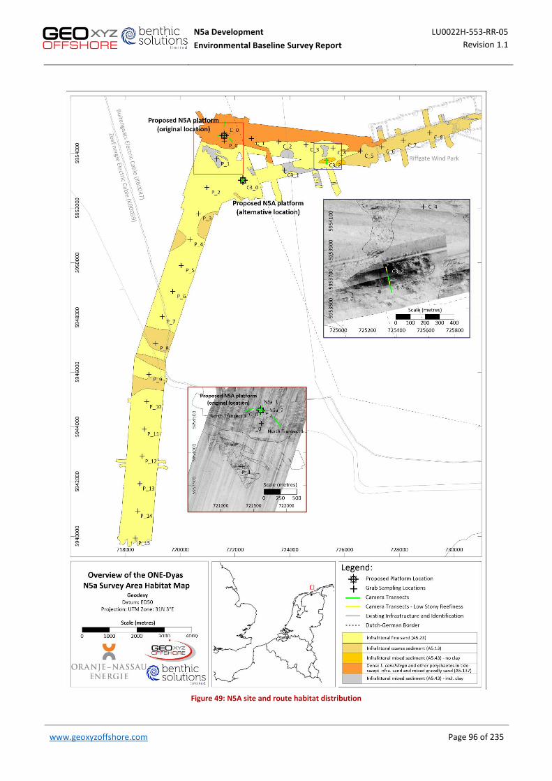
N5a Development LU0022H-553-RR-05 Environmental Baseline Survey Report Revision 1.1
www.geoxyzoffshore.com Page 96 of 235 Page 96 of 235
Figure 49: N5A site and route habitat distribution
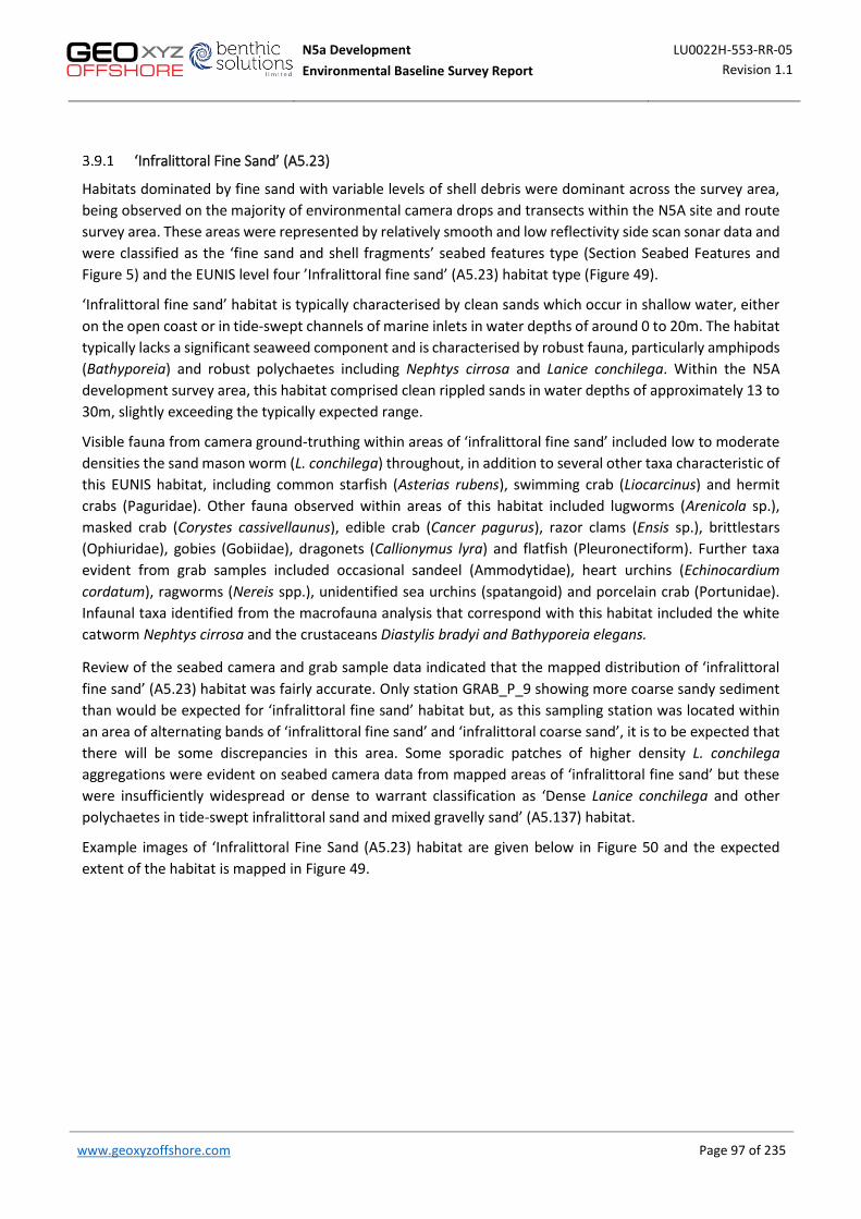
N5a Development LU0022H-553-RR-05 Environmental Baseline Survey Report Revision 1.1
www.geoxyzoffshore.com Page 97 of 235 Page 97 of 235
‘Infralittoral Fine Sand’ (A5.23)
Habitats dominated by fine sand with variable levels of shell debris were dominant across the survey area, being observed on the majority of environmental camera drops and transects within the N5A site and route survey area. These areas were represented by relatively smooth and low reflectivity side scan sonar data and were classified as the ‘fine sand and shell fragments’ seabed features type (Section Seabed Features and Figure 5) and the EUNIS level four ’Infralittoral fine sand’ (A5.23) habitat type (Figure 49).
‘Infralittoral fine sand’ habitat is typically characterised by clean sands which occur in shallow water, either on the open coast or in tide-swept channels of marine inlets in water depths of around 0 to 20m. The habitat typically lacks a significant seaweed component and is characterised by robust fauna, particularly amphipods (Bathyporeia) and robust polychaetes including Nephtys cirrosa and Lanice conchilega. Within the N5A development survey area, this habitat comprised clean rippled sands in water depths of approximately 13 to 30m, slightly exceeding the typically expected range.
Visible fauna from camera ground-truthing within areas of ‘infralittoral fine sand’ included low to moderate densities the sand mason worm (L. conchilega) throughout, in addition to several other taxa characteristic of this EUNIS habitat, including common starfish (Asterias rubens), swimming crab (Liocarcinus) and hermit crabs (Paguridae). Other fauna observed within areas of this habitat included lugworms (Arenicola sp.), masked crab (Corystes cassivellaunus), edible crab (Cancer pagurus), razor clams (Ensis sp.), brittlestars (Ophiuridae), gobies (Gobiidae), dragonets (Callionymus lyra) and flatfish (Pleuronectiform). Further taxa evident from grab samples included occasional sandeel (Ammodytidae), heart urchins (Echinocardium
cordatum), ragworms (Nereis spp.), unidentified sea urchins (spatangoid) and porcelain crab (Portunidae). Infaunal taxa identified from the macrofauna analysis that correspond with this habitat included the white catworm Nephtys cirrosa and the crustaceans Diastylis bradyi and Bathyporeia elegans.
Review of the seabed camera and grab sample data indicated that the mapped distribution of ‘infralittoral fine sand’ (A5.23) habitat was fairly accurate. Only station GRAB_P_9 showing more coarse sandy sediment than would be expected for ‘infralittoral fine sand’ habitat but, as this sampling station was located within an area of alternating bands of ‘infralittoral fine sand’ and ‘infralittoral coarse sand’, it is to be expected that there will be some discrepancies in this area. Some sporadic patches of higher density L. conchilega aggregations were evident on seabed camera data from mapped areas of ‘infralittoral fine sand’ but these were insufficiently widespread or dense to warrant classification as ‘Dense Lanice conchilega and other polychaetes in tide-swept infralittoral sand and mixed gravelly sand’ (A5.137) habitat.
Example images of ‘Infralittoral Fine Sand (A5.23) habitat are given below in Figure 50 and the expected extent of the habitat is mapped in Figure 49.
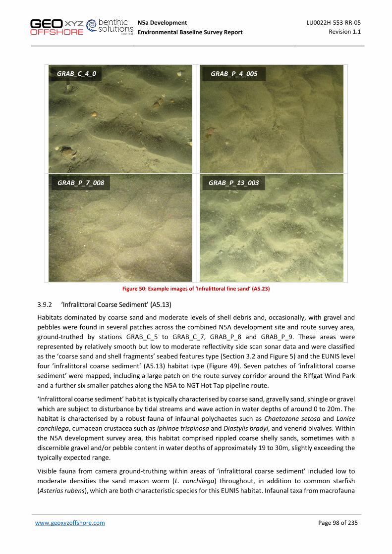
N5a Development LU0022H-553-RR-05 Environmental Baseline Survey Report Revision 1.1
www.geoxyzoffshore.com Page 98 of 235 Page 98 of 235
Figure 50: Example images of ‘Infralittoral fine sand’ (A5.23)
‘Infralittoral Coarse Sediment’ (A5.13)
Habitats dominated by coarse sand and moderate levels of shell debris and, occasionally, with gravel and pebbles were found in several patches across the combined N5A development site and route survey area, ground-truthed by stations GRAB_C_5 to GRAB_C_7, GRAB_P_8 and GRAB_P_9. These areas were represented by relatively smooth but low to moderate reflectivity side scan sonar data and were classified as the ‘coarse sand and shell fragments’ seabed features type (Section 3.2 and Figure 5) and the EUNIS level four ’infralittoral coarse sediment’ (A5.13) habitat type (Figure 49). Seven patches of ‘infralittoral coarse sediment’ were mapped, including a large patch on the route survey corridor around the Riffgat Wind Park and a further six smaller patches along the N5A to NGT Hot Tap pipeline route.
‘Infralittoral coarse sediment’ habitat is typically characterised by coarse sand, gravelly sand, shingle or gravel which are subject to disturbance by tidal streams and wave action in water depths of around 0 to 20m. The habitat is characterised by a robust fauna of infaunal polychaetes such as Chaetozone setosa and Lanice
conchilega, cumacean crustacea such as Iphinoe trispinosa and Diastylis bradyi, and venerid bivalves. Within the N5A development survey area, this habitat comprised rippled coarse shelly sands, sometimes with a discernible gravel and/or pebble content in water depths of approximately 19 to 30m, slightly exceeding the typically expected range.
Visible fauna from camera ground-truthing within areas of ‘infralittoral coarse sediment’ included low to moderate densities the sand mason worm (L. conchilega) throughout, in addition to common starfish (Asterias rubens), which are both characteristic species for this EUNIS habitat. Infaunal taxa from macrofauna
GRAB_P_7_008 GRAB_P_13_003
GRAB_C_4_0
02
GRAB_P_4_005

N5a Development LU0022H-553-RR-05 Environmental Baseline Survey Report Revision 1.1
www.geoxyzoffshore.com Page 99 of 235 Page 99 of 235
ground-truthing for this classification included the presence of Scoloplos armiger, Eteone longa, Lanice
conchilega, Nematoda and Nemertea.
Review of the seabed camera and grab sample data indicated that the mapped distribution of ‘infralittoral coarse sediment’ (A5.13) habitat was fairly accurate, but with two exceptions. Station GRAB_C_0 was classified as ‘infralittoral coarse sediment’ habitat but was located within an area of ‘Dense Lanice conchilega and other polychaetes in tide-swept infralittoral sand and mixed gravelly sand’ (A5.137) habitat, while station GRAB_C_8 was classified as ‘infralittoral fine sand’ habitat but was located within an area of ‘infralittoral coarse sediment’. Both of these exceptions reflect the heterogenous nature of the seabed habitats within the survey area.
Example images of ‘infralittoral coarse sediment (A5.13) habitat are given below in Figure 51, the expected extent of the habitat is mapped in Figure 49.
Figure 51: Example images of ‘Infralittoral coarse sediment’ (A5.13)
‘Infralittoral Mixed Sediment’ (A5.43)
Habitats dominated by coarse gravelly sand with pebbles, cobbles and, in some areas exposed clay clasts, were found delineated in ten patches across the combined N5A development site and N5A to Riffgat route survey area. These areas were classified as the ‘coarse sand with pebbles and cobbles’ seabed features type (Section 3.2 and Figure 5) and the EUNIS level four ’infralittoral mixed sediment’ (A5.43) habitat type (Figure 49). Two patches located midway along the N5A to Riffgat cable route showed moderate to high reflectivity side scan sonar signatures but showed no evidence of clay on ground-truthing data from station GRAB_C3_2. A further ten patches along the N5A to Riffgat route showed similar mottled side scan sonar signatures and
GRAB_P_8_002 GRAB_P_9_003
GRAB_C_5_005 GRAB_C_7_006

N5a Development LU0022H-553-RR-05 Environmental Baseline Survey Report Revision 1.1
www.geoxyzoffshore.com Page 100 of 235 Page 100 of 235
may include exposed clay, as evident from ground-truthing at stations GRAB_P_1 and GRAB_C3_1 over two of the patches.
‘Infralittoral mixed sediment’ habitat is typically characterised by mixed muddy gravelly sands or very poorly sorted mosaics of shell, cobbles and pebbles embedded in mud, sand or gravel in water depths of around 0 to 30m. Due to the variable nature of the sediment type, a wide array of communities are reported to be found in areas of mixed sediment, including those characterised by bivalves, polychaetes and file shells. Within the N5A development survey area, this habitat comprised coarse gravelly sand with pebbles, cobbles and sometimes with the addition of exposed clay clasts, in water depths of approximately 24 to 27m, slightly exceeding the typically expected range.
Visible fauna from camera ground-truthing within areas of ‘infralittoral mixed sediment’ included common starfish (Asterias rubens) and burrowing anemones (Cerianthidae) which are both characteristic species for this EUNIS habitat. Seabed and grab sample photographs from station GRAB_C3_1 show numerous holes within the exposed clay clasts which may indicate the presence of boring piddock bivalves (typically Pholas
dactylus or Barnea candida), although no live individuals could be discerned from the seabed or grab sample photographs. While piddocks are not protected by legislation, they are not widespread in the marine environment and would therefore be worthy of note if found. However, macrofaunal analysis of these stations did not reveal the presence of piddocks at any stations within the survey area, and thus this habitat remains assigned to the ‘infralittoral mixed sediment’ (A5.43) classification. Macrofauna found at the stations classified as mixed sediment include high abundances of Nematoda, Mediomastus fragilis, and Nemertea, which are all characterizing species for this habitat.
Example images of ‘infralittoral coarse sediment (A5.13) habitat are given below in Figure 52 and the expected extent of the habitat is mapped in Figure 49.

N5a Development LU0022H-553-RR-05 Environmental Baseline Survey Report Revision 1.1
www.geoxyzoffshore.com Page 101 of 235 Page 101 of 235
Figure 52: Example images of ‘Infralittoral mixed sediment’ (A5.43)
‘Dense Lanice conchilega and Other Polychaetes in Tide-swept Infralittoral Sand and Mixed Gravelly Sand’ (A5.137)
Habitats dominated by gravelly, shelly coarse sand with moderate to high densities of Lanice conchilega were evident at several ground-truthing locations (stations GRAB_C_1, GRAB_C_2 and GRAB_P_0, and transects N5A_1, N5A_2, NT_1, NT_2 and NT_3) within the N5A site and to the east along the N5A to Riffgat Wind Park route. These areas were represented by mottled low to high reflectivity side scan sonar data and were classified as the ‘coarse sand and shell with a high density of sand mason worms and razor clams’ seabed features type (Section 3.2 and Figure 5) and the EUNIS level four ‘Dense Lanice conchilega and other polychaetes in tide-swept infralittoral sand and mixed gravelly sand’ (A5.137) habitat type (Figure 49). This habitat was delineated in a single large area along the northern edge of the combined N5A survey area.
‘Dense Lanice conchilega and other polychaetes in tide-swept infralittoral sand and mixed gravelly sand’ habitat is typically characterised by coarse sand, gravelly sand, shingle or gravel which are subject to disturbance by tidal streams and wave action in water depths of around 0 to 20m. The habitat is characterised by high densities of L. conchilega, which are thought to stabilise the seabed and allow the development of a more diverse associated faunal community. Within the N5A development survey area, this habitat comprised gravelly, shelly coarse sands in water depths of approximately 28 to 29m, slightly exceeding the typically expected range.
Visible fauna from camera ground-truthing within areas of ‘dense Lanice conchilega and other polychaetes in tide-swept infralittoral sand and mixed gravelly sand’ included moderate to high densities the sand mason
GRAB_C3_2_019 GRAB_C3_2_023
GRAB_C3_1_002 GRAB_C3_1_008
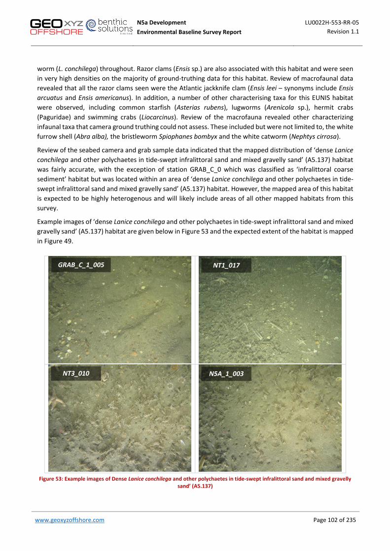
N5a Development LU0022H-553-RR-05 Environmental Baseline Survey Report Revision 1.1
www.geoxyzoffshore.com Page 102 of 235 Page 102 of 235
worm (L. conchilega) throughout. Razor clams (Ensis sp.) are also associated with this habitat and were seen in very high densities on the majority of ground-truthing data for this habitat. Review of macrofaunal data revealed that all the razor clams seen were the Atlantic jackknife clam (Ensis leei – synonyms include Ensis
arcuatus and Ensis americanus). In addition, a number of other characterising taxa for this EUNIS habitat were observed, including common starfish (Asterias rubens), lugworms (Arenicola sp.), hermit crabs (Paguridae) and swimming crabs (Liocarcinus). Review of the macrofauna revealed other characterizing infaunal taxa that camera ground truthing could not assess. These included but were not limited to, the white furrow shell (Abra alba), the bristleworm Spiophanes bombyx and the white catworm (Nephtys cirrosa).
Review of the seabed camera and grab sample data indicated that the mapped distribution of ‘dense Lanice
conchilega and other polychaetes in tide-swept infralittoral sand and mixed gravelly sand’ (A5.137) habitat was fairly accurate, with the exception of station GRAB_C_0 which was classified as ‘infralittoral coarse sediment’ habitat but was located within an area of ‘dense Lanice conchilega and other polychaetes in tide-swept infralittoral sand and mixed gravelly sand’ (A5.137) habitat. However, the mapped area of this habitat is expected to be highly heterogenous and will likely include areas of all other mapped habitats from this survey.
Example images of ‘dense Lanice conchilega and other polychaetes in tide-swept infralittoral sand and mixed gravelly sand’ (A5.137) habitat are given below in Figure 53 and the expected extent of the habitat is mapped in Figure 49.
Figure 53: Example images of Dense Lanice conchilega and other polychaetes in tide-swept infralittoral sand and mixed gravelly
sand’ (A5.137)
NT3_010 N5A_1_003
GRAB_C_1_005 NT1_017
N5a Development LU0022H-553-RR-05 Environmental Baseline Survey Report Revision 1.1
www.geoxyzoffshore.com Page 103 of 235 Page 103 of 235
Potential Sensitive Habitats and Species
There are a number of potential sensitive habitats and species which are listed by one or more International Conventions, European Directives or UK Legislation (Appendix G) and are known to occur in the wider region (southern North Sea), including:
• Biogenic reefs formed by the ross worm Sabellaria spinulosa (EC Habitats Directive Annex I and OSPAR threatened and declining habitat);
• Stony reefs formed by aggregations of cobbles and/or boulders (EC Habitats Directive Annex I); • ‘Sandbanks which are slightly covered by sea water all the time’ (EC Habitats Directive Annex I).
Biogenic Reef Habitat
The most likely biogenic reef habitats to occur in sandy habitats in the southern North Sea are biogenic reefs formed by the polychaete worm Sabellaria spinulosa, also known as the ross worm. Ross worms build tubes from sand and shell fragments and where large numbers can form reefs. Sabellaria spinulosa form reef-like or agglomerations of sand tubes that act to stabilise cobble, pebble and gravel habitats, providing a consolidated habitat for epibenthic species. The aggregations of the tube-building polychaete worm are solid (albeit fragile), and can form large structures at least several centimetres thick, raised above the surrounding seabed, and persist for many years. A such they provide a biogenic habitat that allows many other associated species to become established (Holt et al., 1998 Foster-Smith and White, 2001, Gubbay, 2007).
These reefs are ecologically important as they provide a habitat for a wide range of other seabed dwelling organisms and as such can support a greater biodiversity than the surrounding area. Due to their conservation importance they are listed as an EC Habitats Directive Annex I habitat (Habitats Directive 1992 & 1997) and an OSPAR (2008) threatened and declining habitat. However, no evidence of S. spinulosa aggregations was seen on any of the video transect data from the survey area, including transects over areas of high or variable reflectivity coarse or mixed sediments. Further, no specimens of S. spinulosa were recorded within the macrofauna analyses.
While Lanice conchilega beds are not listed by either the EC Habitats Directive (EC, 2013) or OSPAR (2008) as protected habitats, Rabaut et al. (2007) highlighted the role of L. conchilega as ‘ecosystem engineers’ which act to stabilise otherwise mobile seabed substrates and facilitate the development of more diverse macrofaunal communities (Rabaut et al, 2007). Furthermore, it has been suggested that Lanice conchilega beds meet the qualifying criteria for inclusion as EC Habitats Directive Annex I habitats (Rabaut et al, 2009).
Stony Reef Habitat
Stony reefs are defined by the Habitats Directive as comprising ‘areas of boulders (>256mm diameter) or cobbles (64mm – 256mm diameter) which arise from the seafloor and provide suitable substratum for the attachment of algae and/or animal species’ (EC, 2013).
The seabed video footage was analysed to assess broad habitat changes across the survey area, and to identify any areas with potential for stony reef habitats (See Appendix E). Only one seabed camera transect (Station GRAB_C3_2) within the N5A development survey area exhibited any potential for consideration as a potential stony reef (EC, 2013). As such, the video footage from station GRAB_C3_2 was assessed further using the BSL-modified stony reef assessment method (after Irving, 2009). While the Irving (2009) criteria have been approved by the UK regulators for application in UK waters, they have not been explicitly approved

N5a Development LU0022H-553-RR-05 Environmental Baseline Survey Report Revision 1.1
www.geoxyzoffshore.com Page 104 of 235 Page 104 of 235
by the Netherlands authorities. However, this method has been used here as a useful basis for semi-quantitative assessment of potential Annex I stony reef habitat.
As detailed in Section 2.4.2, there were three criteria that were assessed to estimate the quality of potential stony reef, including composition (%), elevation (mm) and the extent. Video footage and still photographs were first reviewed to assess the ‘stony reef structure’ using a combination of the composition and elevation measures (Table 21). The results of reef structure analysis are summarised in Table 21, and highlighted the limited potential for the area to be classified as a stony reef due to the low percentage cover and elevation of cobbles (>64mm diameter) in this area. As such, this area is not considered to be sufficiently noteworthy to be classified as an EC Habitats Directive Annex I stony reef.
Table 21: Summary of stony reef structure assessment
Station Easting Northing Length (m) Sediment type
Stony Reefiness (After Irving 2009)
Composition (% cover cobbles/
boulders)
Elevation (of cobbles/ boulders in
cm)
Stony Reef Structure
Classification
C3_2
725 366 5 953 610 61.3
Coarse sand ripples with small shell fragments that have accumulated between ripples
Not a Reef Not a Reef Not a Reef
725 352 5 953 670 725 352 5 953 670
17.7 Cobbles overlying coarse sand with occasional boulders 25 10 Low 725 347 5 953 687
725 347 5 953 688 24.7 Coarse sand with cobbles 10 5 Not a Reef
725 343 5 953 712 725 343 5 953 712
44.2 Occasional cobble overlying coarse sand and infrequent boulders 10 5 Not a Reef 725 333 5 953 755
725 333 5 953 755 30.3
Cobbles overlying coarse sand with occasional boulders 30 20 Low
725 326 5 953 785
Shallow Sandbanks Habitat
Areas of protected shallow sandbank habitat are loosely defined by depths contours of less than 20 metres below chart datum (approximately equivalent to LAT). However, areas of seabed on the flanks of shallow sandbanks but in depths exceeding 20m LAT may also be considered to be shallow sandbank habitat as any anthropogenic impacts on these areas could potentially affect the integrity of the feature as a whole.
Sandbanks which are slightly covered by sea water all the time are sandy sediments that are permanently covered by seawater and typically at depths less than 20m (LAT) and are of conservation value as they can host maerl beds as well as being typically colonised by a range of burrowing fauna, epifauna and sand eels, which are an important food source for many birds. Although much of the survey area is shallower than 20m LAT, there were no defined sandbank features in this area (Figure 1).
Due to the variety of H1110 habitat in the Netherlands, the Dutch government decided to subdivide this into three subtypes; H1110_A Wadden Sea, H1110_B North Sea and H1110_C Offshore (Noordzeeloket, 2019). Habitat H1110_C is of most relevance to the current survey area representing permanently flooded sandbanks in water depths of up to 40m, with the Dogger Bank being the main area currently protected under this habitat subtype offshore of the Netherlands. At present, no habitat profile document has been finalised for habitat subtype H1110_C. However, some key characteristics for compiling this profile document are available in Jak et al., (2009), with requirements including the presence of sandy seabed and species characteristic of H1110_C habitat (Table 22).

N5a Development LU0022H-553-RR-05 Environmental Baseline Survey Report Revision 1.1
www.geoxyzoffshore.com Page 105 of 235 Page 105 of 235
With the sediments within the survey area being classified within one of three Folk designations of ‘sand’, ‘slightly gravelly sand’ and ‘gravelly sand’, the N5A Development survey sediments can be considered to be sufficiently sandy to meet the requirements of the H1110_C habitat subtype. Review of the macrofauna species dataset together with the grab sample and seabed video logs for the current survey, showed that several of the species characteristic of the H1110_C habitat subtype were present within the survey area. In particular, sandmason worms (Lanice conchilega) and bathyporeid amphipods (Bathyporeia guilliamsoniana, B. elegans and Bathyporeia spp.) were recorded in almost all grab samples from the survey area. Other characterising species for the permanently flooded sandbank H1110_C habitat subtype present within the survey area included the polychaete Sigalion mathildae and sandeels (Ammodytes marinus).
With both the sediment type and associated fauna present within the survey area meeting the requirements outlined by Jak et al., (2009), it is possible that the survey area will be considered to represent EC Habitats Directive Annex I habitat subtype H1110_C (permanently flooded sandbank) throughout N5A Development site and route survey areas. However, there is currently insufficient information in the public domain to pre-empt this decision.
Table 22: Species characteristic of permanently flooded sandbank – Netherlands habitat subtype H1110_C
Species Group Common Name Species Name Description
Polychaete Sandmason Lanice conchilega Species occurring on sand substrate
Polychaete na Sigalion mathildae Mainly occurring in clean sandy substrates, Dogger
Bank one of the areas where the species occurs.
Crustacea Sand digger shrimp Bathyporeia guilliamsoniana Epiphytes in clean sand and on Dogger Bank
Crustacea Sand digger shrimp Bathyporeia elegans Occurring in coarse, clean, low-fines sediments
Crustacea Cumacean Iphinoe trispinosa Specific for sand from Dogger Bank
Echinodermata Brittlestar Acrocnida brachiata Occurring in high densities in clean sand up to a depth of 40 m
Echinodermata Pea urchin Echinocyamus pusillus Found in coarse sand and fine gravel enriched with detritus
Mollusca Ocean quahog Arctica islandica Occurs on edges of the Dogger Bank - long-lived species
Mollusca Common whelk Buccinum undatum Occurs on mixed substrate – long-lived species
Mollusca Bivalve Mactra coralina Long-lived species that feeds on particles from the water column. Found in fine to coarse sand
Fish Lesser sandeel Ammodytes marinus Occurring in fine sand. An important food source
for birds, fish and marine mammals
Fish Lesser weaver Trachinus vipera Specific to sand, where they lie buried subsurface
Ray Thornback ray Raja clavata Residual population. Long-lived species
Fish Plaice Pleuronectes platessa Generally found on sandy substrate. Common species
Note: species occurring within the N5a Development survey area are shown in bold font type.

N5a Development LU0022H-553-RR-05 Environmental Baseline Survey Report Revision 1.1
www.geoxyzoffshore.com Page 106 of 235 Page 106 of 235
4 CONCLUSION
In May 2019, Oranje Nassau Energie (ONE) contracted GEOxyz Offshore, supported by Benthic Solutions Ltd (BSL) to undertake a range of geophysical, geotechnical and environmental surveys in block N5A of the Dutch Sector of the Southern North Sea, comprising a site survey for the N5A proposed platform and two route surveys; one along a planned pipeline to NGT Hot Tap, and the other a cable route to Riffgat Offshore Wind Park. Environmental baseline sampling within the N5A survey area involved the acquisition of camera footage, physico-chemical and macro-invertebrate samples.
Grab sampling was carried out across 28 locations (with two replicates) within the survey area, of which both physico-chemical and fauna samples were taken for each location. To aid habitat ground-truthing, drop down video footage was taken at all grab locations (28 stations) and a further eight camera transects of approximately 100m in length were conducted within the survey area.
Review of the seabed photography, acoustic survey data, video and seabed sample analysis of the survey area revealed a uniform seabed which ranged from a minimum of approximately 9.8m LAT at KP0.000 on the N5A to NGT Hot Tap pipeline route to a maximum of 26.4m LAT at KP14.675. Both the N5A to NGT Hot Tap pipeline route and N5A to Riffgat Cable Route were crossed by a series of natural troughs trending west-north-west to east-south-east. Two potential wrecks were discovered, and scars thought to be attributed to previous exploratory drilling activity were observed near to the proposed platform location (~140m away).
Particle size analysis showed a sand-dominated environment with ~93% of samples comprising over 80% sands, largely due to the proximity to shore resulting in a strong hydrodynamic regime, restricting the settling of fine sediment. Variable proportions of gravel and fines were seen in grab sample data, reflecting the presence of areas of more mixed sediment and outcropping clay.
The results showed low levels of total hydrocarbon content (THC) within the survey area, with levels ranging from 0.72mg.kg-1 to 13.65mg.kg-1 (mean 3.15mg.kg-1±2.69SD). Eight stations recorded levels above mean background levels for the southern North Sea (UKOOA, 2001) and one station (GRAB_P_1) had levels exceeding the 95th percentile for uncontaminated background sediments, reflecting the high percentage fines at this station. Alkanes contributed on average 1.22% to the THC levels recorded across the survey area indicating the seabed consisted of uncontaminated marine sediments where background hydrocarbons are continually replenished. Polyaromatic hydrocarbon levels were low but variable ranging from 0.00μg.g-1 to 66.8μg.g-1. Once again, only GRAB_P_1 exceeded the 95th percentile value for background PAH levels in the southern North Sea. Gas chromatography traces for all stations, including station GRAB_P_1 showed signatures consistent with background uncontaminated sediments.
Concentrations of heavy metals were within the typical ranges expected for uncontaminated background sediments, with only zinc and copper at GRAB_P_1 exceeding the 95th percentile for the southern North Sea. Barium was recorded at low levels and showed no evidence of the elevated concentrations associated with drilling impact.
The macrofauna throughout the N5A survey area showed some variability in terms of abundance, richness and species composition which was shown to be influenced by the sediment composition. Overall the survey area was highly species abundant with a total of 16,550 individuals (infaunal species) identified. Of the 150 species recorded, 118 were infaunal and were dominated by annelids, accounting for 58.90% of total individuals recorded. Molluscs, followed by crustaceans, were the next major phyla represented in N5A (9.3% and 7.9% of individuals, respectively). The samples were not considered to be epifaunal rich, with a combined grouping of colonial and solitary epifauna accounting for thirteen species, of which Cnidaria was the most

N5a Development LU0022H-553-RR-05 Environmental Baseline Survey Report Revision 1.1
www.geoxyzoffshore.com Page 107 of 235 Page 107 of 235
well represented with six taxa observed. This is due to the sand dominated area lacking suitable substrate for these species to attach to and colonise. The Shannon-Wiener Diversity was variable ranging from a minimum of 2.05 at GRAB_C_3 to a maximum of 3.90 at station GRAB_P_2. Further analysis using multivariate statistics identified four groupings, very similar to the clusters identified in the particle size analysis signifying links between particle size and the community of macrofauna, which was verified through statistical tests highlighting a correlation between macrofauna communities and particle size data.
In total, four habitats were assigned within the survey area: ‘infralittoral fine sand’, ‘infralittoral coarse sediment’, ‘infralittoral mixed sediment’ (split into categories ‘no clay’ and ‘incl. clay’) and ‘dense Lanice
conchilega and other polychaetes in tide swept infralittoral sand and mixed gravelly sand’. The infralittoral fine sand was the dominant sediment type and was typically assigned to the habitats along the more southerly pipeline to NGT Hot Tap route. Stations along the Riffgat cable route consisted of a combination of habitat types, with a large patch infralittoral coarse sediment further North. Clay outcrops at GRAB_P_1 and GRAB_C3_1 resulted in higher fines proportions in the PSA data for these stations, which was interpreted to be present in eight other small patches within the survey area. The last habitat type, ‘dense Lanice conchilega and other polychaetes in tide-swept infralittoral sand and mixed gravelly sand’ was seen in a single large area along the northern edge of the N5A site and the N5A to Riffgat Wind park Cable Route.
A single patch of cobbles and boulders was identified at GRAB_C3_2, and as a result a stony reef assessment was performed. Due to insufficient cover or elevation of cobbles, it was found that there was a low chance of this being a true stony reef and thus did not warrant consideration as a potential EC Habitats Directive Annex I stony reef habitat (after Irving, 2009).
The seabed sediments within the survey area were characterised by sand-dominated and supported several species listed by Jak et al., (2009) as being characteristic of the EC Habitats Directive Annex I permanently submerged sandbank habitat (subtype H1110_C). At present there is insufficient publicly available information to confirm classification of the survey area as the H1110_C habitat subtype, but it is possible that the survey area will be classified as such.
No other protected habitats or species were observed within the survey area, based on review of the acquired geophysical data and environmental ground-truthing by grab sampling and seabed photography.

N5a Development LU0022H-553-RR-05 Environmental Baseline Survey Report Revision 1.1
www.geoxyzoffshore.com Page 108 of 235 Page 108 of 235
5 BIBLIOGRAPHY
Berthou, F., and Friocourt, M.P. 1981. Gas Chromatographic Separation of Diastereometric Isoprenoids as Molecular Markers of Oil Pollution. J Chromatog 219: 393-402.
Blumer, M. and Snyder, W.D. 1965. Isoprenoid hydrocarbons in recent sediments: presence of pristane and probably absence of phytane, Science 150: 1588.
Bouloubassi, I., Fillaux, J. and Saliot, A. 2001. Hydrocarbons in surface sediments from the Changjiang (Yangtze river) estuary, East China Sea. Mar Pollut Bull 42: 1335-1346.
Bryan, G.W., and Langston, W.J. 1992. Bioavailability, accumulation and effects of heavy metals in sediments with special reference to United Kingdom estuaries: A review. Environ Pollut, 76: 89-131.
Buhr K.-J. & Winter J.E, 1977. Distribution and maintenance of a Lanice conchilega association in the Weser estuary (FRG), with special reference to the suspension-feeding behaviour of Lanice conchilega. In Proceedings of the Eleventh European Symposium of Marine Biology, University College, Galway, 5-11 October 1976. Biology of Benthic Organisms (ed. B.F. Keegan, P.O. Ceidigh & P.J.S. Boaden), pp. 101-113. Oxford: Pergamon Press.
Chester, R. and Voutsinou, F.G. 1981. The Initial Assessment of Trace Metal Pollution in Coastal Sediments. Mar Pol Bull 12: 84-91.
Chow, T.J. and Snyder, C.G. 1980. Barium in the Marine Environment: A Potential Indicator of Drilling Contamination. In Symposium Proceedings: Research on environmental fate and effects of drilling fluids and cuttings. Lake Buena Vista, Florida, 2: 723-736.
Clarke, K.R. and Warwick, R.M. 1994. Similarity-based testing for community pattern: the 2-way layout with no replication. Mar Biol 118: 167-17.
Connor, D. W, Allen, J. H., Golding, N., Howell, K. L., Lieberknecht, L. M., Northern, K. O. and Reker, J. B. 2004. The Marine Habitat Classification for Britain and Ireland. Version 04.05. Introduction.
Degraer, S.; Wittoeck, J.; Appeltans, W.; Cooreman, K.; Deprez, T.; Hillewaert, H.; Hostens, K.; Mees, J.; Vanden Berghe, E.; Vincx, M. 2006. The macrobenthos atlas of the Belgian part of the North Sea. Belgian Science Policy. D/2005/1191/3. ISBN 90-810081-6-1. 164 pp.
Eagle, R.A., 1975. Natural fluctuations in a soft bottom benthic community. Journal of the Marine Biological Association of the United Kingdom, 55, 865-878.
Eglinton, G., Gonzalez, A.G., Hamilton, R.J. and Raphael, R.A. 1962. Hydrocarbon constituents of the wax coatings of plant leaves: a taxonomic survey. Phytochemistry 1: 89-102.
Eleftheriou, A., Basford, D. J., 1989. The macrobenthic infauna of the offshore northern North Sea. J Mar Biol Assoc UK 69: 123-143.
Emerson, S., Hedges, J., 2008. Chemical Oceanography and the Marine Carbon Cycle. Cambridge University Press. 286pp
EUNIS, 2013. The European Nature Information Service. Accessed from http://eunis.eea.europa.eu/habitats.jsp
Folk, R.L., 1954.The distinction between grain size and mineral composition in sedimentary rock nomenclature. J Geol 62: 344-349.
Foster-Smith, R.L. & White, W.H. 2001. Sabellaria spinulosa reef in The Wash and North Norfolk Coast cSAC and its approaches: Part I, mapping techniques and ecological assessment. English Nature Research Reports, Number 545. 53pp.

N5a Development LU0022H-553-RR-05 Environmental Baseline Survey Report Revision 1.1
www.geoxyzoffshore.com Page 109 of 235 Page 109 of 235
Fraser, S., Shelmerdine, R.L., and Mouat, B. (2018). Razor clam biology, ecology, stock assessment, and exploitation: a review of Ensis spp. in Wales. NAFC Marine Centre report for the Welsh Government. Contract number C243/2012/2013. pp 52.
Gettleson, D.A., and Laird, C.E. 1980. Benthic Barium Levels in the Vicinity of Six Drill Sites on the Gulf of Mexico. In Symposium Proceedings: Research on Environmental Fate and Effects of Drilling Fluids and Cuttings. Lake Buena Vista, Florida, 2: 739-785.
Gubbay, S., (2007). Defining and managing Sabellaria spinulosa reefs: Report of an inter-agency workshop 1-2 May, JNCC Report No 405.
Hayward P.J., 1985 Ctenostome Bryozoans, Synopses of the British Fauna (New Series) No. 33, London: Brill, 169 pp.
Hayward P.J. & Ryland J.S., 1998. Cheilostomatous Bryozoa Part 1: Aeteoidea – Cribilinoidea. Synopses of the British Fauna (New Series), No. 10. (Second Edition) Published for the Linnean Society of London and The Estuarine and Coastal Sciences Association by Field Studies Council, Shrewsbury, 366pp.
Holt, T.J., Rees, E.I., Hawkins, S.J. & Seed, R. (1998). Biogenic Reefs (volume IX). An overview of dynamic and sensitivity characteristics for conservation management of marine SACs. Scottish Association of Marine Science (UK Marine SACs Project). 170pp.Habitats Directive (European Community), 1992, 1997. Council Directive 92/43/EEC on the Conservation of natural habitats and of wild fauna and flora.
Ingle R. W. (1997). Crayfishes, Lobsters, and Crabs of Europe: An Illustrated Guide to Common and Traded Species. London: Chapman & Hall.
Irving, R. 2009. The identification of the main characteristics of stony reef habitats under the Habitats Directive. JNCC Report No. 432. pp. 42.
Jak, R.G., Bos, O.G., Witbaard, R. & Lindeboom, H.J. 2009. Conservation objectives for Natura 2000 sites (SACs and SPAs) in the Dutch sector of the North Sea. IMARES – Institute for Marine Resources & Ecosystem Studies. Report number C065/09.
JNCC. 2015. The Marine Habitat Classification for Britain and Ireland Version 15.03 [Online]. [Date accessed]. Available from: jncc.defra.gov.uk/MarineHabitatClassification.
Jones, J., & Holdich, D. (1983). A New Species of the Tanaid Genus Tanaissus Norman & Scott from British Waters. Crustaceana, 45(2), 214-219.
Laflamme, R.E. and Hites, R.A. 1978. The global distribution of polycyclic aromatic hydrocarbons in recent sediments. Geochim Cosmochim Acta. 42: 289-303.
Long, E.R., MacDonald, D.D., Smith, S.L. and Calder, F.D. 1995. Incidence of adverse biological effects within ranges of chemical concentrations in marine and estuary sediments. Environ Manage 19: 81-97.
Luoma, S.N., and Davies J.A. 1983. Requirements for modelling trace metal portioning in oxidised estuarine sediments. Mar Chem, 12: 159-181.
Macdonald, D.D., Carr, R.S., Calder, F.D., Long, E.R., and Ingersoll, C.G. 1996.Development and evaluation of sediment quality guidelines for Florida coastal waters. Ecotoxicology. 5: 253-278.
Manuel R.L., 1988. British Anthozoa. Keys and notes for the identification of the species. Synopses of the British Fauna (New Series), No. 18. Published for The Linnaean Society of London and The Estuarine and Brackish-Water Sciences Association by Academic Press, London, New York, Toronto, Sydney, San Francisco, 241 pp.

N5a Development LU0022H-553-RR-05 Environmental Baseline Survey Report Revision 1.1
www.geoxyzoffshore.com Page 110 of 235 Page 110 of 235
McCourt, C.B., Price, R.J., John, S.D., Penny, D.M. and Clarke, L.J. 1991. Environmental Applications of Plasma Spectrometries within the Oil Industry. SPE, Proceedings First International Conference on Health, Safety and Environment, The Hague, The Netherlands 10 - 14 November 1991, SPE 23349, 301-309.
McDougall, J. 2000. Section 5.1. The significance of hydrocarbons in surficial sediments from the Atlantic Margin regions. In: Hydrocarbons in environmental surveys of the seafloor of the UK Atlantic Margin. Atlantic Frontier Environmental Network [CD-Rom]. Available from Geotek Ltd, Daventry, Northants, NN11 5EA, UK.ISBN 09538399-0-7
McLeese, D.W., Sprague, J.B., and Ray, S. 1987. Effects of cadmium on marine biota. p. 171-198. In: Nriagu, J.O. and J.B. Sprague (eds.). Cadmium in the Aquatic Environment. Advances in Environmental Science and Technology, Volume 19. John Wiley & Sons, New York. pp. 272.
Muniz, P., Danulat, E., Yannicelli, B., Garcia-Alonso, J., and Bicego, M.C. 2004. Assessment of contamination by heavy metals and petroleum hydrocarbons in sediments of Montevideo harbour (Uruguay). Environmental International. 29: 1019-1028.
Neff, J.M. 2005. Bioaccumulation in marine organisms. Effects of contaminants from oil well produced water. Elsevier, Oxford, UK.
National Research Council (NRC), 1983. Drilling Discharges in the Marine Environment. National Academy Press, Washington DC. pp. 180
Noordzeeloket, 2019. Habitat type H1110C on the Dogger Bank[Online]. [Date accessed]. Available from: https://www.noordzeeloket.nl/en/policy/noordzee-natura-2000/gebieden/doggersbank/dogger-bank/habitattype/.
Oliver, P. G., Holmes, A. M., Killeen, I. J. & Turner, J. A. 2016. Marine Bivalve Shells of the British Isles. Amgueddfa Cymru - National Museum Wales. Available from: http://naturalhistory.museumwales.ac.uk/britishbivalves.
OSPAR Commission, 2004. OSPAR guidelines for monitoring the environmental impact of offshore oil and gas activities. Meeting of the OSPAR Offshore Industries Committee (OIC), 15 – 19 March, 2004.
OSPAR, 2008. Descriptions of habitats on the OSPAR list of threatened and/or declining species and habitats. OSPAR Convention for the Protection of the Marine Environment of the North-east Atlantic. Reference Number: 2008-07. 8pp.
OSPAR, 2009. Agreement on CEMP Assessment Criteria for the QSR 2010. Agreement 2009-2
OSPAR 8, 2009 – Update of JAMP guidance on normalisation of contaminant concentrations in sediment.
Paez-Osuna, F., and Ruiz-Fernandez, C. 1995. Comparative Bioaccumulation of Trace Metals in Penaneus stylirostris in Estuarine and Coastal Environments. Estuar Coastal Shelf S 40: 35-44.
Parry, M.E.V., K.L. Howell, B.E. Narayanaswamy, B.J. Bett, D.O.B. Jones, D.J. Hughes, N. Piechaud, H. Ellwood, N. Askew, C. Jenkins And E. Manca. 2015. A Deep-sea Section for the Marine Habitat Classification of Britain and Ireland. JNCC report 530. In: JNCC. 2015. The Marine Habitat Classification for Britain and Ireland Version 15.03 [Online].
Rabaut, M., Guilini, K., Van Hoey, G., Vincx, M., Degraer, S. 2007. A bioengineered soft-bottom environment: the impact of Lanice conchilega on the benthic species-species densities and community structure. Estuar. Coastal Shelf Sci. doi:10.1016/j.ecss.2007.05.041.
Rabaut, M., Vincx. M. and Degraer, S. 2009. Do Lanice conchilega (sandmason) aggregations classify as reefs? Quantifying habitat modifying effects. Helgol Mar Res (2009) 63:37–46. DOI 10.1007/s10152-008-0137-4.

N5a Development LU0022H-553-RR-05 Environmental Baseline Survey Report Revision 1.1
www.geoxyzoffshore.com Page 111 of 235 Page 111 of 235
Schaule, B.K. and Patterson, C.C. 1983. Perturbations of the Natural Lead Depth Profile in the Sargasso Sea by Industrial Lead. In: Trace Metals in Seawater. Plenum Press, New York.
Sheahan, D., Rycroft, R., Allen, Y., Kenny, A., Mason, C. & Irish, R. 2001. Contaminant Status of the North Sea. Technical report produced for SEA2. Report no. TR_004. Report to the Department of Trade and Industry. Centre for Environment, Fisheries and Aquaculture Science. pp. 66
Snelgrove, P.V.R., and Butman, C.A. 1994. Animal–sediment relationships revisited: cause versus effect. Oceanogr Mar Biol Annu Rev 32: 111–177.
Sleeter, T.D., Butler, J.N. and Barbash, J.E. 1980. Hydrocarbons in the Sediment of the Bermuda Region: Lagoonal to Abyssal Depths. Pp 267-288 In: Petrakis, L. and Weiss, F.T. (Eds.). Petroleum in the Marine Environment. Chem. Soc., Washington, D.C
Tessier, A., Campbell, P.G.C., and Bisson, M. 1979. Sequel Extraction Procedure for the Speciation of Particulate Trace Metals. Anal Chem 51: 844 - 851.
Thompson, B., and Lowe, S. 2004. Assessment of macrobenthos response to sediment contamination in the San Francisco estuary, California, USA. Environ Toxicol Chem 23: 2178–2187.
Tricine, R.P., and Trefry, J.H. 1983. Particulate Metal Tracers of Petroleum Drilling Mud Dispersion in the Marine Environment. Environ Sci Technol 17: 507 - 512.
UKOOA, 2001. An analysis of U.K Offshore Oil & gas Environmental Surveys 1975-95, pp. 141.
US EPA, 1999. Toxicity Reference Values – Screening Level Ecological Risk Assessment Protocol. Center for Combustion Science and Engineering. pp. 98.
Wheeler A., 1969. The fishes of the British Isles and North West Europe. MacMillan. London UK, 630pp., plates 1-16.
Youngblood, W.W. and Blumer, M., 1975. Polycyclic aromatic hydrocarbons in the environment: homologues series in soils and recent marine sediments. Geochim Cosmochim Acta, 39: 1303-1314.
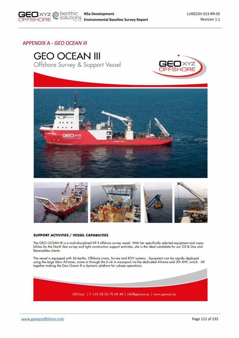
N5a Development LU0022H-553-RR-05 Environmental Baseline Survey Report Revision 1.1
www.geoxyzoffshore.com Page 112 of 235 Page 112 of 235
APPENDIX A - GEO OCEAN III

N5a Development LU0022H-553-RR-05 Environmental Baseline Survey Report Revision 1.1
www.geoxyzoffshore.com Page 113 of 235 Page 113 of 235
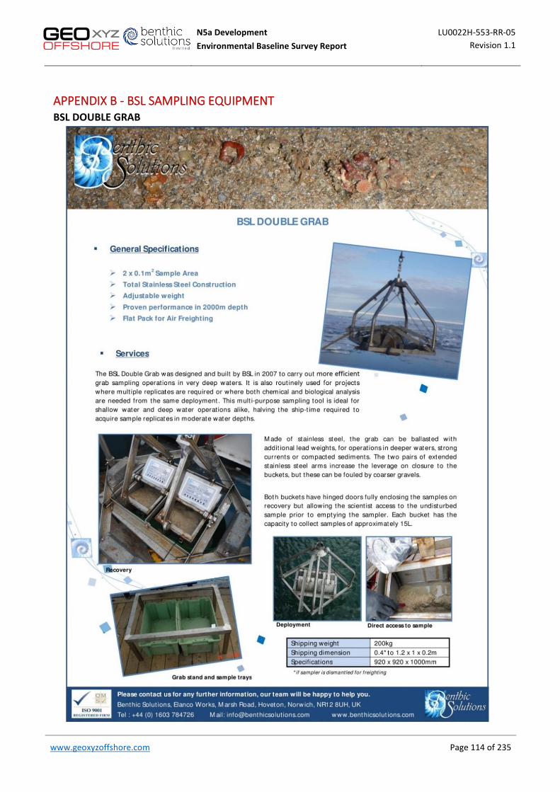
N5a Development LU0022H-553-RR-05 Environmental Baseline Survey Report Revision 1.1
www.geoxyzoffshore.com Page 114 of 235 Page 114 of 235
APPENDIX B - BSL SAMPLING EQUIPMENT BSL DOUBLE GRAB

N5a Development LU0022H-553-RR-05 Environmental Baseline Survey Report Revision 1.1
www.geoxyzoffshore.com Page 115 of 235 Page 115 of 235
BSL DAY GRAB

N5a Development LU0022H-553-RR-05 Environmental Baseline Survey Report Revision 1.1
www.geoxyzoffshore.com Page 116 of 235 Page 116 of 235
BSL WILSON AUTO-SIEVER
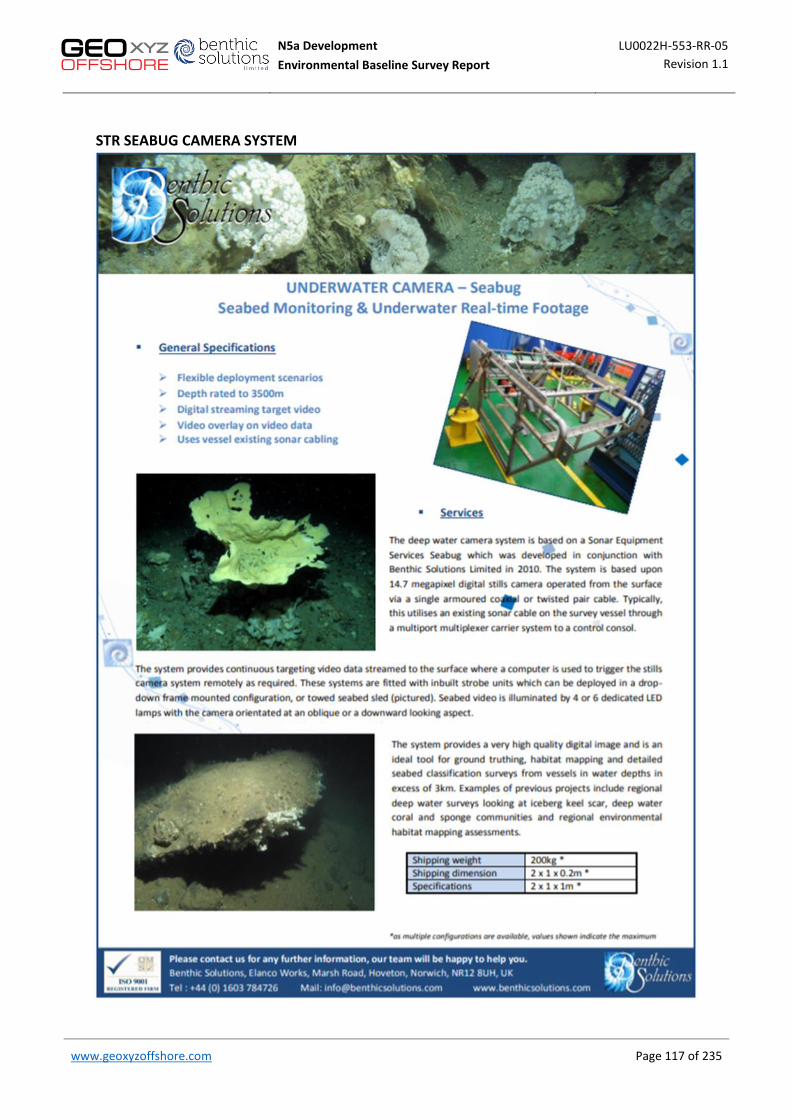
N5a Development LU0022H-553-RR-05 Environmental Baseline Survey Report Revision 1.1
www.geoxyzoffshore.com Page 117 of 235 Page 117 of 235
STR SEABUG CAMERA SYSTEM

N5a Development LU0022H-553-RR-05 Environmental Baseline Survey Report Revision 1.1
www.geoxyzoffshore.com Page 118 of 235 Page 118 of 235
BSL MOD4 UNDERWATER CAMERA SYSTEM
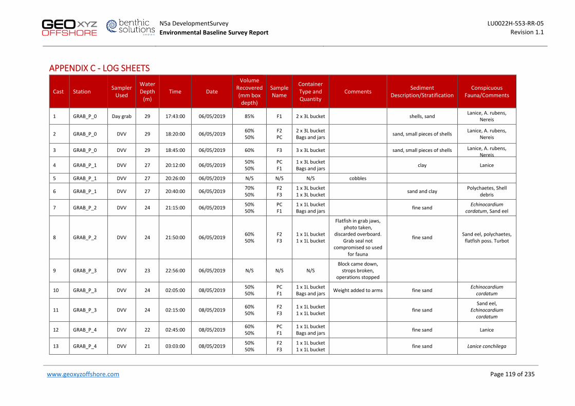
N5a DevelopmentSurvey LU0022H-553-RR-05 Environmental Baseline Survey Report Revision 1.1
www.geoxyzoffshore.com Page 119 of 235 Page 119 of 235 119 o
APPENDIX C - LOG SHEETS
Cast Station Sampler Used
Water Depth
(m) Time Date
Volume Recovered (mm box
depth)
Sample Name
Container Type and Quantity
Comments Sediment Description/Stratification
Conspicuous Fauna/Comments
1 GRAB_P_0 Day grab 29 17:43:00 06/05/2019 85% F1 2 x 3L bucket shells, sand Lanice, A. rubens, Nereis
2 GRAB_P_0 DVV 29 18:20:00 06/05/2019 60% 50%
F2 PC
2 x 3L bucket Bags and jars sand, small pieces of shells Lanice, A. rubens,
Nereis
3 GRAB_P_0 DVV 29 18:45:00 06/05/2019 60% F3 3 x 3L bucket sand, small pieces of shells Lanice, A. rubens, Nereis
4 GRAB_P_1 DVV 27 20:12:00 06/05/2019 50% 50%
PC F1
1 x 3L bucket Bags and jars clay Lanice
5 GRAB_P_1 DVV 27 20:26:00 06/05/2019 N/S N/S N/S cobbles
6 GRAB_P_1 DVV 27 20:40:00 06/05/2019 70% 50%
F2 F3
1 x 3L bucket 1 x 3L bucket sand and clay Polychaetes, Shell
debris
7 GRAB_P_2 DVV 24 21:15:00 06/05/2019 50% 50%
PC F1
1 x 1L bucket Bags and jars fine sand Echinocardium
cordatum, Sand eel
8 GRAB_P_2 DVV 24 21:50:00 06/05/2019 60% 50%
F2 F3
1 x 1L bucket 1 x 1L bucket
Flatfish in grab jaws, photo taken,
discarded overboard. Grab seal not
compromised so used for fauna
fine sand Sand eel, polychaetes, flatfish poss. Turbot
9 GRAB_P_3 DVV 23 22:56:00 06/05/2019 N/S N/S N/S Block came down,
strops broken, operations stopped
10 GRAB_P_3 DVV 24 02:05:00 08/05/2019 50% 50%
PC F1
1 x 1L bucket Bags and jars Weight added to arms fine sand Echinocardium
cordatum
11 GRAB_P_3 DVV 24 02:15:00 08/05/2019 60% 50%
F2 F3
1 x 1L bucket 1 x 1L bucket fine sand
Sand eel, Echinocardium
cordatum
12 GRAB_P_4 DVV 22 02:45:00 08/05/2019 60% 50%
PC F1
1 x 1L bucket Bags and jars fine sand Lanice
13 GRAB_P_4 DVV 21 03:03:00 08/05/2019 50% 50%
F2 F3
1 x 1L bucket 1 x 1L bucket fine sand Lanice conchilega

N5a DevelopmentSurvey LU0022H-553-RR-05 Environmental Baseline Survey Report Revision 1.1
www.geoxyzoffshore.com Page 120 of 235 Page 120 of 235 120 o
Cast Station Sampler Used
Water Depth
(m) Time Date
Volume Recovered (mm box
depth)
Sample Name
Container Type and Quantity
Comments Sediment Description/Stratification
Conspicuous Fauna/Comments
14 GRAB_P_5 DVV 20 03:31:00 08/05/2019 50% 50%
PC F1
1 x 1L bucket Bags and jars Sand and shell Echinocardium
cordatum, razor clam
15 GRAB_P_5 DVV 20 03:42:00 08/05/2019 50% 50%
F2 F3
1 x 1L bucket 1 x 1L bucket Sand and shell Lanice conchilega
16 GRAB_P_6 DVV 21 04:29:00 08/05/2019 50% 50%
PC F1
1 x 1L bucket Bags and jars Fine sand Echinocardium
cordatum (damaged)
17 GRAB_P_6 DVV 22 04:41:00 08/05/2019 50% 50%
F2 F3
1 x 1L bucket 1 x 1L bucket Fine sand with minor shell
fragments
polychaetes, Nereis, Lanice conchilega, fish
(damaged)
18 GRAB_P_7 DVV 22 05:09:00 08/05/2019 N/S N/S N/S No sample, triggered but empty
19 GRAB_P_7 DVV 22 05:22:00 08/05/2019 N/S N/S N/S No sample, did not trigger
20 GRAB_P_7 DVV 21 05:25:00 08/05/2019 N/S N/S N/S No sample, did not trigger
21 GRAB_P_7 DVV 21 05:27:00 08/05/2019 50% 50%
PC F1
1 x 1L bucket Bags and jars Fine sand with minor shell
debris Lanice conchilega,
polychaetes
22 GRAB_P_7 DVV 21 05:37:00 08/05/2019 50% 50%
F2 F3
1 x 1L bucket 1 x 1L bucket
Fine sand with minor shell debris, small amounts of
mud/clay
Abundant Lanice conchilega, polychaetes
23 GRAB_P_8 DVV 21 06:01:00 08/05/2019 N/S N/S N/S
24 GRAB_P_8 DVV 21 06:03:00 08/05/2019 N/S N/S N/S
25 GRAB_P_8 DVV 20 06:04:00 08/05/2019 70% 70%
PC F1
1 x 5L bucket Bags and jars Coarse sand with shell
fragments Polychaetes
26 GRAB_P_8 DVV 21 06:12:00 08/05/2019 70% 60%
F2 F3
1 x 5L bucket 1 x 5L bucket Coarse sand with shell
fragments Lanice conchilega
27 GRAB_C_8 DVV 24 19:00:00 09/05/2019 80% 80%
PC F1
1 x 1L bucket Bags and jars Coarse sand with shell
fragments Lanice conchilega
28 GRAB_C_8 DVV 24 19:15:00 09/05/2019 80% 80%
F2 F3
1 x 1L bucket 1 x 1L bucket Coarse sand with shell
fragments Lanice conchilega

N5a DevelopmentSurvey LU0022H-553-RR-05 Environmental Baseline Survey Report Revision 1.1
www.geoxyzoffshore.com Page 121 of 235 Page 121 of 235 121 o
Cast Station Sampler Used
Water Depth
(m) Time Date
Volume Recovered (mm box
depth)
Sample Name
Container Type and Quantity
Comments Sediment Description/Stratification
Conspicuous Fauna/Comments
29 GRAB_C_7 DVV 24 19:30:00 09/05/2019 70%, 70% PC F1
3 x 3L bucket Bags and jars Coarse sand with shell
fragments No conspicuous Fauna
30 GRAB_C_7 DVV 24 19:45:00 09/05/2019 N/S N/S N/S Deployed but no sample, not triggering
31 GRAB_C_7 DVV 24 20:05:00 09/05/2019 70% 80% F2 F3
2 x 5L bucket 2 x 5L bucket Coarse sand with shell
fragments No conspicuous Fauna
32 GRAB_C_6 DVV 24 20:27:00 09/05/2019 60% 80% PC F1
1 x 3L bucket Bags and jars Coarse sand with shell
fragments No conspicuous Fauna
33 GRAB_C_6 DVV 24 21:05:00 09/05/2019 80%, 80% F2 F3
1 x 3L bucket 1 x 3L bucket Coarse sand with shell
fragments Urchin
34 GRAB_C_5 DVV 25 05:37:00 11/05/2019 40% 70%
PC F1
1 x 3L + 1x5L bucket
Bags and jars Coarse sand with shell
fragments
Gobidae, Asterias, Lancelet. Lanice
conchilega
35 GRAB_C_5 DVV 25 05:42:00 11/05/2019 70% 70%
F2 F3
2 x 5L bucket 1 x 5L + 1x 3L
bucket Coarse sand with shell
fragments
Lanice conchilega, polychaetes, spatangoid
36 GRAB_C_4 DVV 28 06:40:00 11/05/2019 60% 60%
PC F1
1 x 1L bucket Bags and jars Fine sand with shell debris
Lanice conchilega, polychaetes, spatangoid
37 GRAB_C_4 DVV 28 07:01:00 11/05/2019 70% 70%
F2 F3
1 x 1L bucket 1 x 1L bucket Fine sand with shell debris
Lanice conchilega, polychaetes, spatangoid
38 GRAB_C_3 DVV 28 07:29:00 11/05/2019 N/S N/S N/S Did not trigger
39 GRAB_C_3 DVV 28 07:36:00 11/05/2019 70% 70%
PC F1
1 x 1L bucket Bags and jars Very fine sand with minor
shell debris Lanice conchilega,
polychaetes
40 GRAB_C_3 DVV 28 07:47:00 11/05/2019 N/S N/S N/S Triggered but no sample
41 GRAB_C_3 DVV 28 07:49:00 11/05/2019 70% 70%
F2 F3
1 x 1L bucket 1 x 1L bucket Very fine sand with minor
shell debris and soft clay
Anemones, Lanice conchilega,
polychaetes, Asterias, spatangoid

N5a DevelopmentSurvey LU0022H-553-RR-05 Environmental Baseline Survey Report Revision 1.1
www.geoxyzoffshore.com Page 122 of 235 Page 122 of 235 122 o
Cast Station Sampler Used
Water Depth
(m) Time Date
Volume Recovered (mm box
depth)
Sample Name
Container Type and Quantity
Comments Sediment Description/Stratification
Conspicuous Fauna/Comments
42 GRAB_C_2 DVV 27 08:15:00 11/05/2019 70% 70%
PC F1
1 x 5L bucket Bags and jars Coarse sand and clay Lanice conchilega and
polychaetes
43 GRAB_C_2 DVV 28 08:27:00 11/05/2019 70% 40%
F2 F3
1 x 5L bucket 1 x 3L bucket
Razor clams in jaws (F3) Coarse sand
Razor clams, Lanice conchilega,
polychaetes. Lancelet
44 GRAB_C_1 DVV 28 08:55:00 11/05/2019 60% 60%
PC F1
1 x 3L + 1x5L bucket
Bags and jars Coarse sand and abundant
shell debris Lancelet and polychaetes
45 GRAB_C_1 DVV 28 09:04:00 11/05/2019 60% 40%
F2 F3
1 x 5L bucket 1 x 5L bucket
Razor clams in jaws (F3)
Coarse sand and abundant shell debris
Lanice conchilega, lancelet, polychaetes,
porcelain crab
46 GRAB_C_0 DVV 29 09:32:00 11/05/2019 90% 90%
PC F1
2 x 5L bucket Bags and jars
Label for F2 in F1 bucket (2 of 2) Coarse sand
Lanice conchilega, razor clams and
polychaetes
47 GRAB_C_0 DVV 29 09:41:00 11/05/2019 90% 90%
F2 F3
2 x 5L bucket 2 x 5L bucket
Label for F3 in F2 bucket (1 of 2) Coarse sand
Lanice conchilega, razor clams and
polychaetes
48 GRAB_P_15 DVV 13 02:15:00 12/05/2019 60% 60%
PC F1
1 x 1L bucket Bags and jars Fine sand with shell Polychaetes
49 GRAB_P_15 DVV 13 02:20:00 12/05/2019 60% 60%
F2 F3
1 x 1L bucket 1 x 1L bucket Fine sand with shell Polychaetes, Sand eel
50 GRAB_P_14 DVV 14 03:05:00 12/05/2019 60% 60%
PC F1
1 x 3L bucket Bags and jars Fine sand with shell Asterias, Spatangoid,
Ophiuroid
51 GRAB_P_14 DVV 14 03:10:00 12/05/2019 60% 60%
F2 F3
1 x 3L bucket 1 x 3L bucket Fine sand with shell Spatangoid, Ophiuroid
52 GRAB_P_13 DVV 16 03:30:00 12/05/2019 60% 60%
PC F1
1 x 1L bucket Bags and jars Fine sand with minor shell
debris Polychaetes
53 GRAB_P_13 DVV 16 03:45:00 12/05/2019 60% 60%
F2 F3
1 x 1L bucket 1 x 1L bucket Fine sand with minor shell
debris
Nereis, Lanice conchilega, Ophiuroid,
Spatangoids
54 GRAB_P_12 DVV 16 04:32:00 12/05/2019 60% 60%
PC F1
1 x 3L bucket Bags and jars Fine sand with shell debris
Nereis, Lanice conchilega, Spatangoids

N5a DevelopmentSurvey LU0022H-553-RR-05 Environmental Baseline Survey Report Revision 1.1
www.geoxyzoffshore.com Page 123 of 235 Page 123 of 235 123 o
Cast Station Sampler Used
Water Depth
(m) Time Date
Volume Recovered (mm box
depth)
Sample Name
Container Type and Quantity
Comments Sediment Description/Stratification
Conspicuous Fauna/Comments
55 GRAB_P_12 DVV 16 04:42:00 12/05/2019 60% 60%
F2 F3
1 x 3L bucket 1 x 3L bucket Fine sand with shell debris
Nereis, Lanice conchilega, Spatangoids
56 GRAB_P_11 DVV 17 05:03:00 12/05/2019 70% 70%
PC F1
1 x 3L bucket Bags and jars Fine sand with significant
shell debris Lanice conchilega
57 GRAB_P_11 DVV 17 05:13:00 12/05/2019 70% 70%
F2 F3
1 x 3L bucket 1 x 3L bucket Fine sand with significant
shell debris Lanice conchilega
58 GRAB_P_10 DVV 17 05:35:00 12/05/2019 60% 60%
PC F1
1 x 1L bucket Bags and jars Fine sand with shell debris Polychaetes, Lanice
conchilega, Nerie’s
59 GRAB_P_10 DVV 17 05:44:00 12/05/2019 60% 60%
F2 F3
1 x 1L bucket 1 x 1L bucket Fine sand with shell debris Polychaetes, Lanice
conchilega
60 GRAB_P_9 DVV 19 06:05:00 12/05/2019 60% 60%
PC F1
1 x 3L bucket Bags and jars Fine sand with shell debris Nereis
61 GRAB_P_9 DVV 19 06:13:00 12/05/2019 60% 60%
F2 F3
1 x 3L bucket 1 x 3L bucket Fine sand with shell debris Polychaetes
62 GRAB_C3_0 DVV 24 22:43:00 14/05/2019 60% 60%
PC F1 1x1L bucket Fine sand with shell debris Echinocardium
cordatum
63 GRAB_C3_0 DVV 24 22:59 14/05/2019 50% 50%
F2 F3
1 x 1L bucket 1 x 1L bucket Fine sand with shell debris Echinocardium
cordatum
64 GRAB_C3_1 DVV 25 23:36:00 14/05/2019 50% 50%
PC F1
1 x 3L bucket Bags and jars Fine sand with clay beneath Polychaetes
65 GRAB_C3_1 DVV 25 23:45:00 14/05/2019 50% 50%
F2 F3
1 x 3L bucket 1 x 3L bucket Fine sand with clay beneath Polychaetes
66 GRAB_C3_2 DVV 25 00:13:00 15/05/2019 NS NS cobbles in jaws
67 GRAB_C3_2 DVV 25 00:20:00 15/05/2019 50% 50%
PC F1
1 x 3L bucket Bags and jars sandy gravel polychaetes hydroids
68 GRAB_C3_2 DVV 25 00:29:00 15/05/2019 50% NS F2 1x5L bucket cobble in jaws of one
bucket sandy gravel polychaetes hydroids
69 GRAB_C3_2 DVV 25 00:36:00 15/05/2019 45% F3 1x1L bucket cobble in jaws of one bucket sandy gravel polychaetes hydroids

N5a Development LU0022H-553-RR-05 Environmental Baseline Survey Report Revision 1.1
www.geoxyzoffshore.com Page 124 of 235 Page 124 of 235
APPENDIX D - FIELD OPERATIONS AND SURVEY METHODS
SEABED PHOTOGRAPHY AND VIDEO
Seabed video footage was acquired at eight transects using a STR Seabug Underwater camera system mounted within a BSL camera sled equipped with a separate strobe, and LED lamps. The camera unit itself is capable of acquiring images at 24MP resolution but was set to a resolution of 5MP (2592 x 1944 pixels) to optimize image upload times during camera operation. Drop down video acquiring an average of five stills and one minute of video was also conducted at each grab location (28 locations).
Once at the seabed, the camera would be moved along the length of the transect at no more than 0.5 knots. Stills Photographs were captured remotely using a surface control unit via a sonar cable to the camera system. Still images were uploaded in real time and saved to the laptop via specialist software. Live video footage, overlaid with the date, time, position and site details was viewed in real-time, and recorded directly onto a media storage device and to the laptop via specialist software. The live video stream was used to assist with targeting of the stills camera. HD footage was saved internally by the video camera; data was downloaded at the end of each day of camera operations and backed-up onto a hard drive.
Full camera specifications can be found in the table below.
STR Seabug Underwater Camera Specifications
Standard Features Comment
Image Resolution 5 to 14.7 megapixel (up to 4,416 x 3,312 pixels)
Light Sensitivity Setting ISO 60-1600 Auto/Manual Selected
Sensor Type 1 / 1.8” format high density CCD sensor
Light source 4 x 1000 lumen controllable LED lamps
Stills strobe TTL controller
Typical settings Aperture priority at F8, Shutter speed typically 1/125th second, Auto flash mode (TTL)
Framing Video Used 320 Line / 50 Hz PAL
Control System SES Multiport DTS
Manufacturer STR
Other sensors Depth sensor and compass
A MOD4 underwater camera system was also supplied as a backup. This camera was not used during operations.
GRAB SAMPLING
The BSL double grab was designed and built by BSL for operations in soft sediments, compacted sands and shallow stiff clays. This device consists of two 0.1m2 samplers set into a ballasted frame, reducing the time required to obtain multiple replicates at a single station.
A BSL Double grab was used for seabed sampling for the ONE Pipeline survey. Two successful deployments were required at each location. Three consecutive ‘no sample’ deployments were agreed to be the maximum number of attempts at any location before abandoning it. The inner stainless grab buckets were cleaned before deployment at any new station to avoid contamination.

N5a Development LU0022H-553-RR-05 Environmental Baseline Survey Report Revision 1.1
www.geoxyzoffshore.com Page 125 of 235 Page 125 of 235
Samples were subject to quality control on recovery and were retained in the following circumstances:
• Water above sample was undisturbed; • Bucket closure complete (no sediment washout); • Sampler was retrieved perfectly upright; • Inspection/access doors had closed properly; • No disruption of sample; • Sample was taken inside the acceptable target range (<15m); • Sample size was greater than six litres (ca. 40% of the sampler’s
capacity); • No hagfish (Myxine glutinosa) and/or mucus coagulants.
Key observations from samples included colour, sediment classification, layering (including redox discontinuity layers), smell (including the presence of H2S), obvious fauna, evidence of bioturbation and anthropogenic debris.
A 0.1m2 Day Grab was also supplied as the original primary sampler but was not used due to the clients request to use the BSL Double Grab instead.
BSL Double Grab
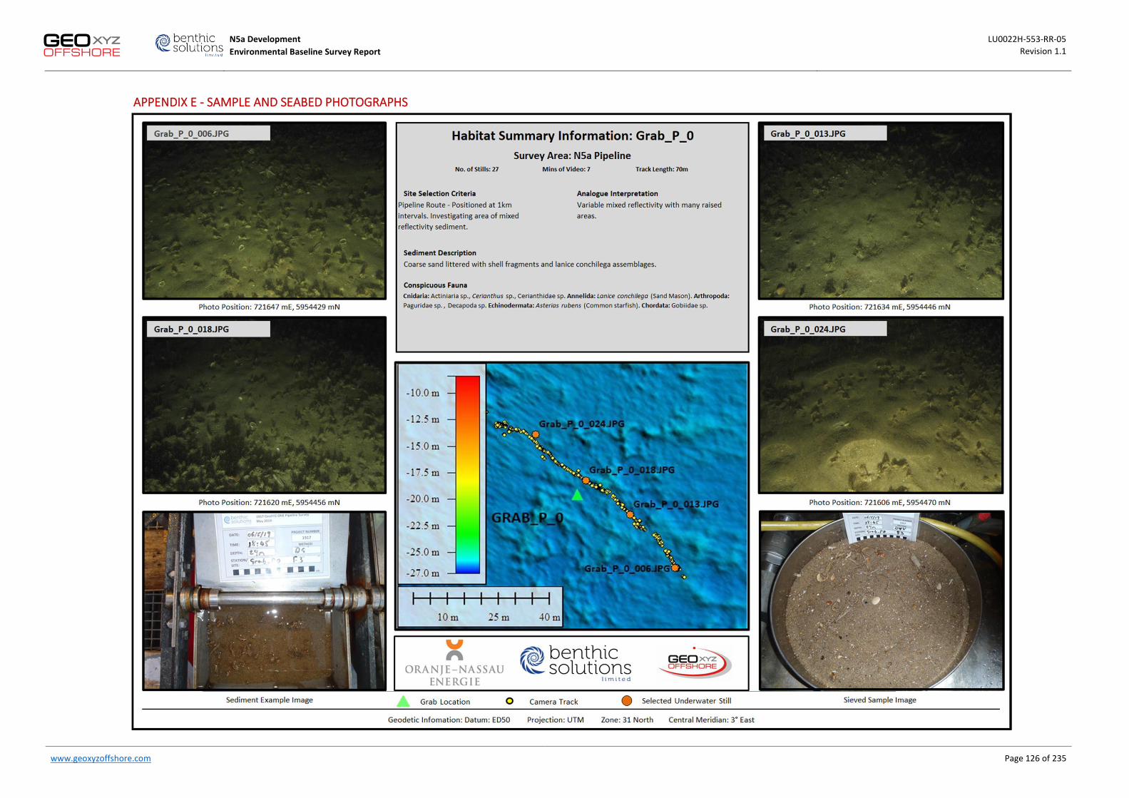
N5a Development LU0022H-553-RR-05 Environmental Baseline Survey Report Revision 1.1
www.geoxyzoffshore.com Page 126 of 235
APPENDIX E - SAMPLE AND SEABED PHOTOGRAPHS
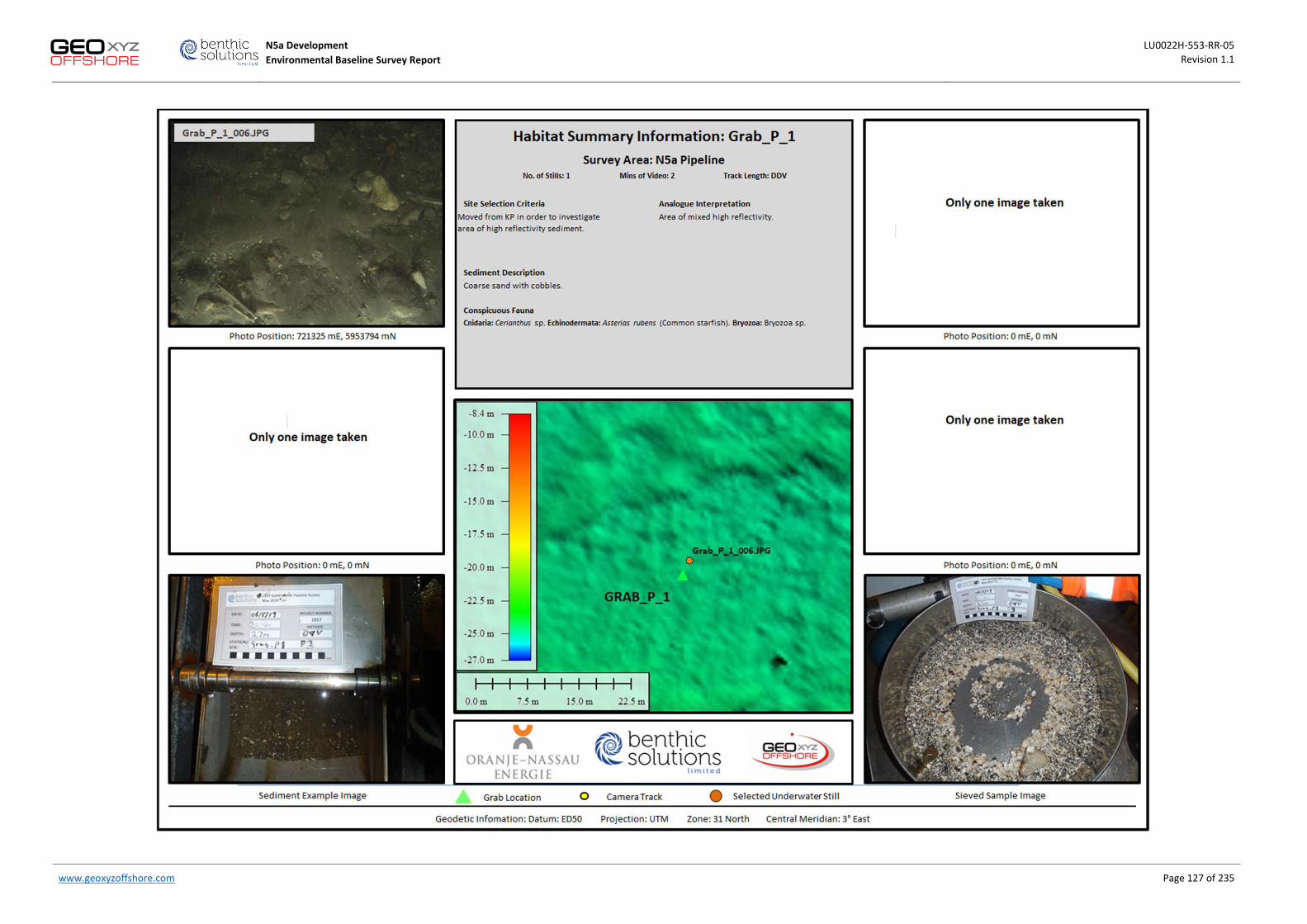
N5a Development LU0022H-553-RR-05 Environmental Baseline Survey Report Revision 1.1
www.geoxyzoffshore.com Page 127 of 235
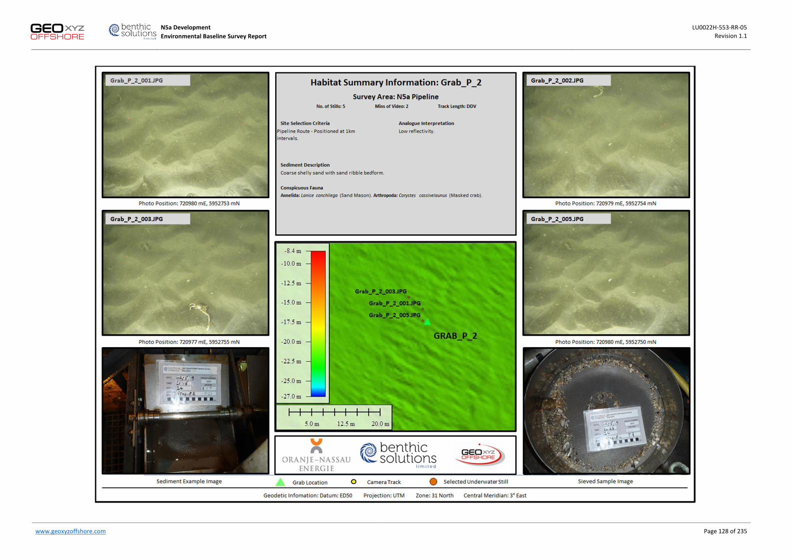
N5a Development LU0022H-553-RR-05 Environmental Baseline Survey Report Revision 1.1
www.geoxyzoffshore.com Page 128 of 235

N5a Development LU0022H-553-RR-05 Environmental Baseline Survey Report Revision 1.1
www.geoxyzoffshore.com Page 129 of 235

N5a Development LU0022H-553-RR-05 Environmental Baseline Survey Report Revision 1.1
www.geoxyzoffshore.com Page 130 of 235

N5a Development LU0022H-553-RR-05 Environmental Baseline Survey Report Revision 1.1
www.geoxyzoffshore.com Page 131 of 235

N5a Development LU0022H-553-RR-05 Environmental Baseline Survey Report Revision 1.1
www.geoxyzoffshore.com Page 132 of 235

N5a Development LU0022H-553-RR-05 Environmental Baseline Survey Report Revision 1.1
www.geoxyzoffshore.com Page 133 of 235
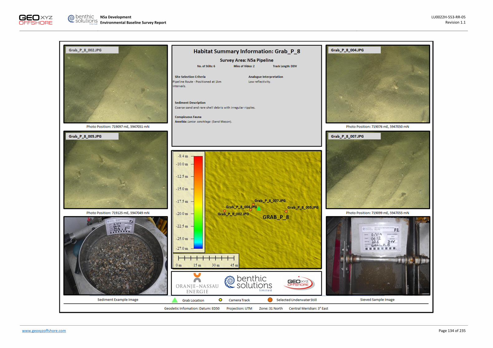
N5a Development LU0022H-553-RR-05 Environmental Baseline Survey Report Revision 1.1
www.geoxyzoffshore.com Page 134 of 235

N5a Development LU0022H-553-RR-05 Environmental Baseline Survey Report Revision 1.1
www.geoxyzoffshore.com Page 135 of 235

N5a Development LU0022H-553-RR-05 Environmental Baseline Survey Report Revision 1.1
www.geoxyzoffshore.com Page 136 of 235

N5a Development LU0022H-553-RR-05 Environmental Baseline Survey Report Revision 1.1
www.geoxyzoffshore.com Page 137 of 235

N5a Development LU0022H-553-RR-05 Environmental Baseline Survey Report Revision 1.1
www.geoxyzoffshore.com Page 138 of 235

N5a Development LU0022H-553-RR-05 Environmental Baseline Survey Report Revision 1.1
www.geoxyzoffshore.com Page 139 of 235
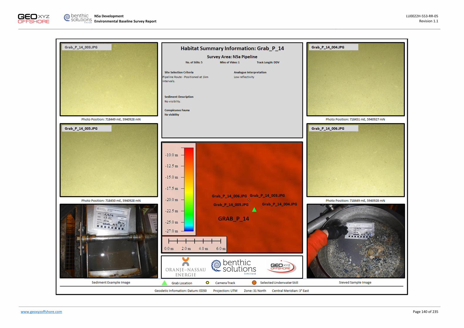
N5a Development LU0022H-553-RR-05 Environmental Baseline Survey Report Revision 1.1
www.geoxyzoffshore.com Page 140 of 235

N5a Development LU0022H-553-RR-05 Environmental Baseline Survey Report Revision 1.1
www.geoxyzoffshore.com Page 141 of 235

N5a Development LU0022H-553-RR-05 Environmental Baseline Survey Report Revision 1.1
www.geoxyzoffshore.com Page 142 of 235

N5a Development LU0022H-553-RR-05 Environmental Baseline Survey Report Revision 1.1
www.geoxyzoffshore.com Page 143 of 235

N5a Development LU0022H-553-RR-05 Environmental Baseline Survey Report Revision 1.1
www.geoxyzoffshore.com Page 144 of 235

N5a Development LU0022H-553-RR-05 Environmental Baseline Survey Report Revision 1.1
www.geoxyzoffshore.com Page 145 of 235
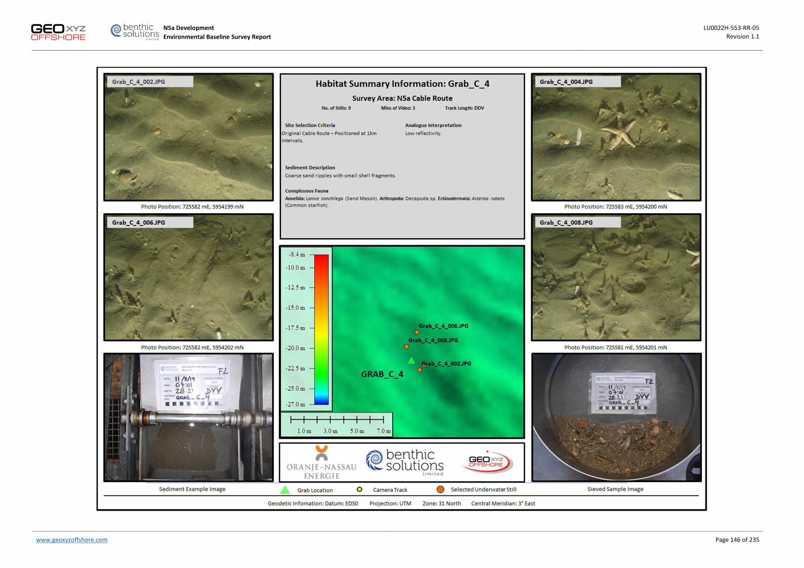
N5a Development LU0022H-553-RR-05 Environmental Baseline Survey Report Revision 1.1
www.geoxyzoffshore.com Page 146 of 235
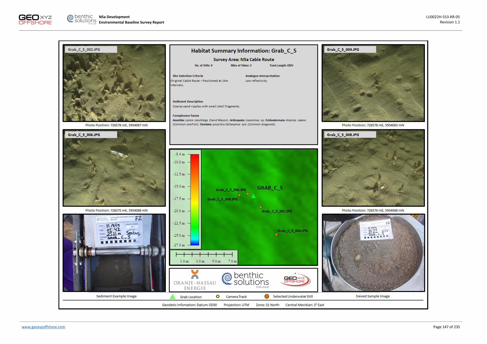
N5a Development LU0022H-553-RR-05 Environmental Baseline Survey Report Revision 1.1
www.geoxyzoffshore.com Page 147 of 235

N5a Development LU0022H-553-RR-05 Environmental Baseline Survey Report Revision 1.1
www.geoxyzoffshore.com Page 148 of 235

N5a Development LU0022H-553-RR-05 Environmental Baseline Survey Report Revision 1.1
www.geoxyzoffshore.com Page 149 of 235

N5a Development LU0022H-553-RR-05 Environmental Baseline Survey Report Revision 1.1
www.geoxyzoffshore.com Page 150 of 235

N5a Development LU0022H-553-RR-05 Environmental Baseline Survey Report Revision 1.1
www.geoxyzoffshore.com Page 151 of 235
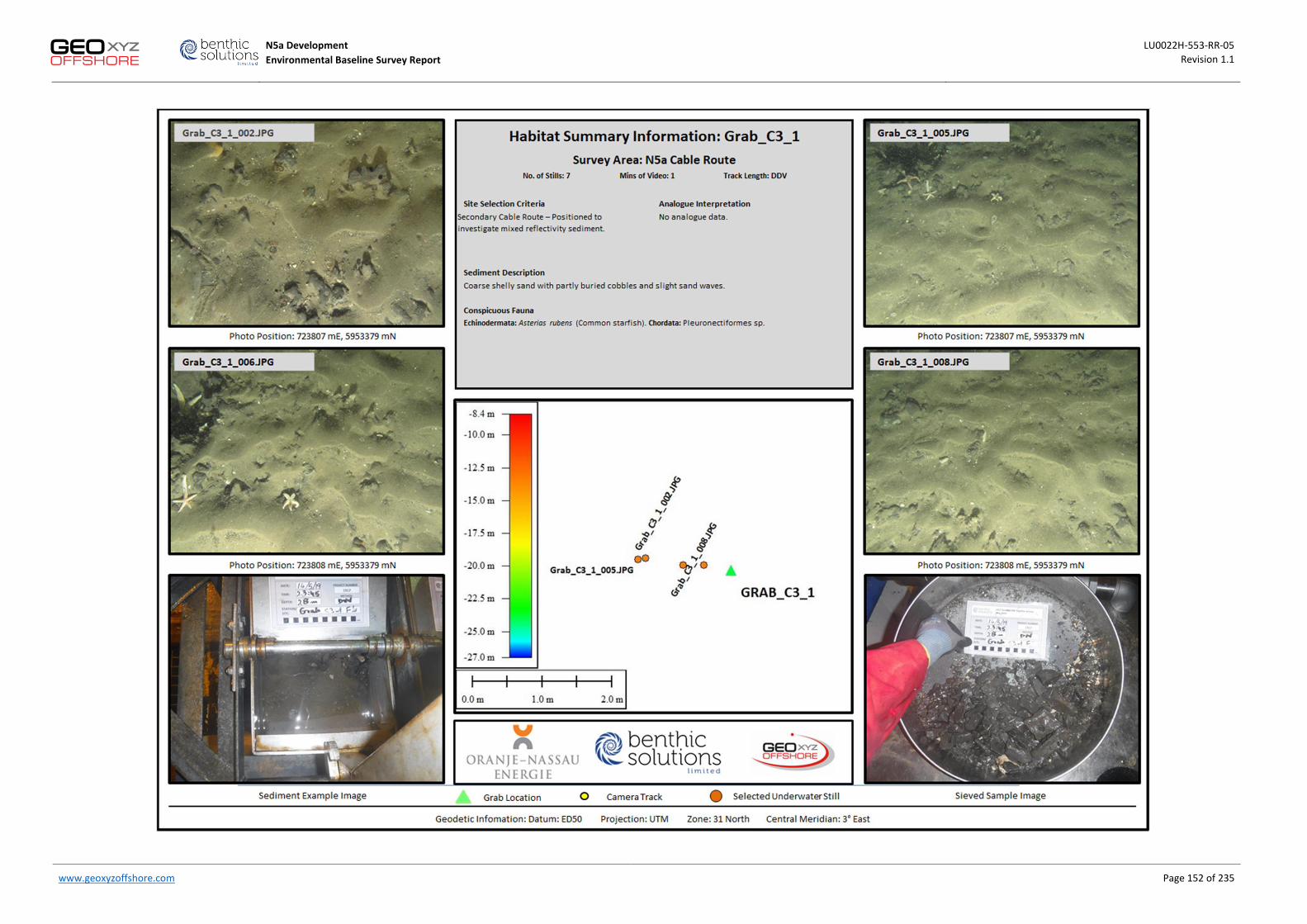
N5a Development LU0022H-553-RR-05 Environmental Baseline Survey Report Revision 1.1
www.geoxyzoffshore.com Page 152 of 235
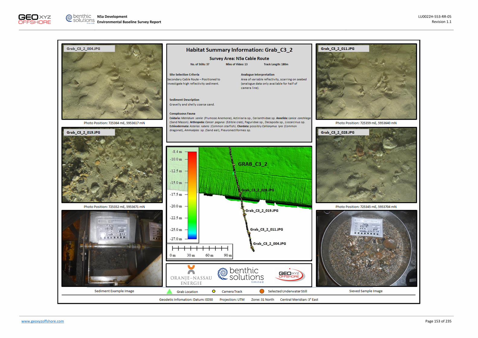
N5a Development LU0022H-553-RR-05 Environmental Baseline Survey Report Revision 1.1
www.geoxyzoffshore.com Page 153 of 235

N5a Development LU0022H-553-RR-05 Environmental Baseline Survey Report Revision 1.1
www.geoxyzoffshore.com Page 154 of 235
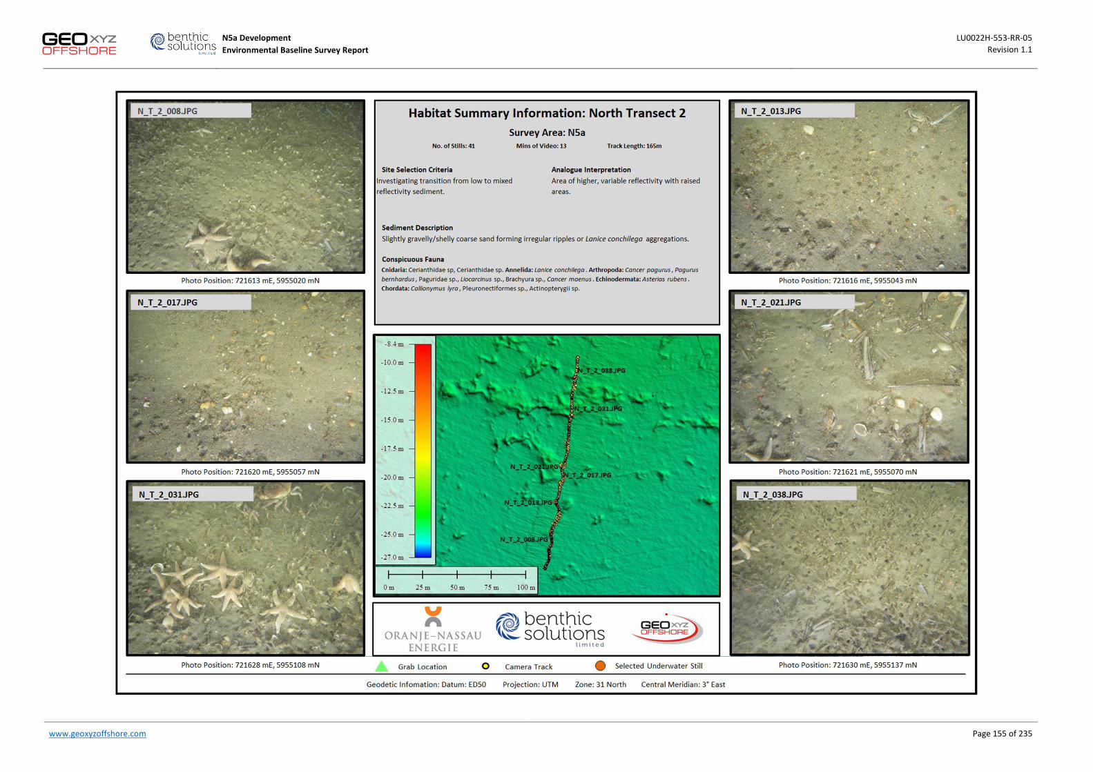
N5a Development LU0022H-553-RR-05 Environmental Baseline Survey Report Revision 1.1
www.geoxyzoffshore.com Page 155 of 235

N5a Development LU0022H-553-RR-05 Environmental Baseline Survey Report Revision 1.1
www.geoxyzoffshore.com Page 156 of 235
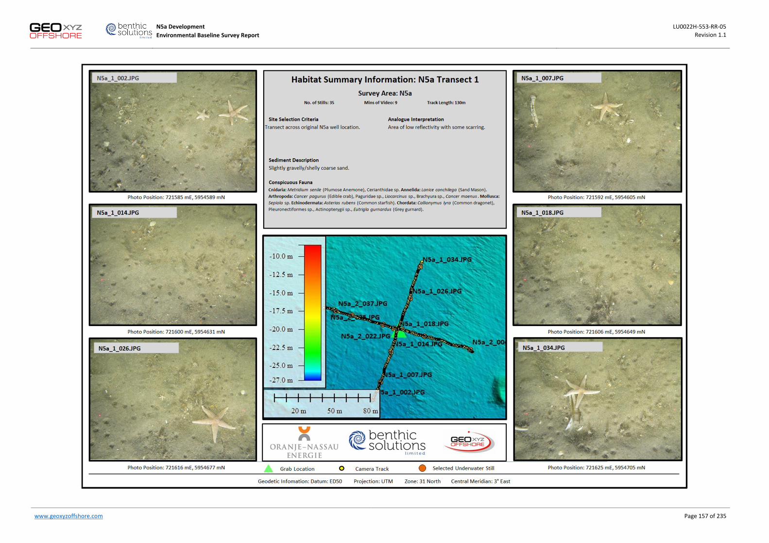
N5a Development LU0022H-553-RR-05 Environmental Baseline Survey Report Revision 1.1
www.geoxyzoffshore.com Page 157 of 235

N5a Development LU0022H-553-RR-05 Environmental Baseline Survey Report Revision 1.1
www.geoxyzoffshore.com Page 158 of 235
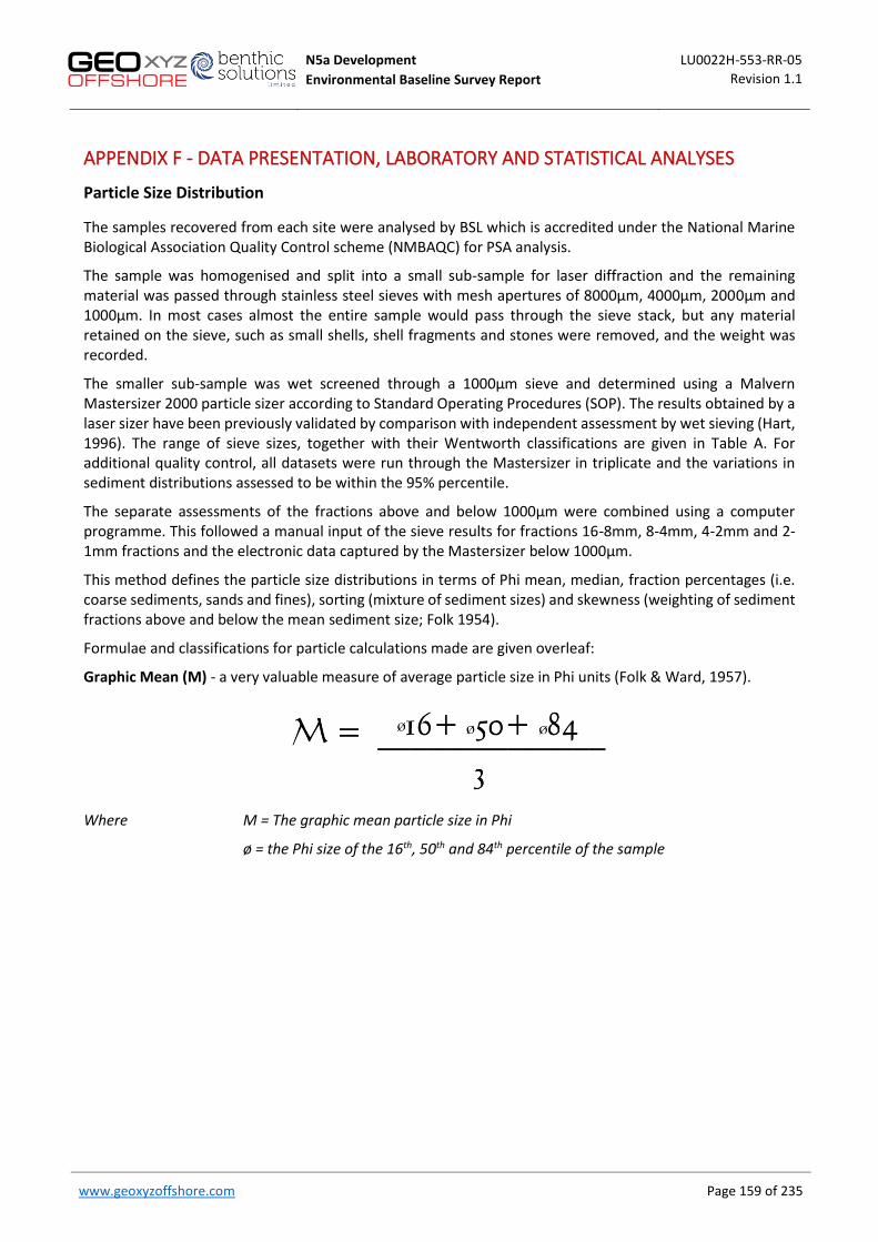
N5a Development LU0022H-553-RR-05 Environmental Baseline Survey Report Revision 1.1
www.geoxyzoffshore.com
Page 159 of 235
APPENDIX F - DATA PRESENTATION, LABORATORY AND STATISTICAL ANALYSES
Particle Size Distribution
The samples recovered from each site were analysed by BSL which is accredited under the National Marine Biological Association Quality Control scheme (NMBAQC) for PSA analysis.
The sample was homogenised and split into a small sub-sample for laser diffraction and the remaining material was passed through stainless steel sieves with mesh apertures of 8000µm, 4000µm, 2000µm and 1000µm. In most cases almost the entire sample would pass through the sieve stack, but any material retained on the sieve, such as small shells, shell fragments and stones were removed, and the weight was recorded.
The smaller sub-sample was wet screened through a 1000µm sieve and determined using a Malvern Mastersizer 2000 particle sizer according to Standard Operating Procedures (SOP). The results obtained by a laser sizer have been previously validated by comparison with independent assessment by wet sieving (Hart, 1996). The range of sieve sizes, together with their Wentworth classifications are given in Table A. For additional quality control, all datasets were run through the Mastersizer in triplicate and the variations in sediment distributions assessed to be within the 95% percentile.
The separate assessments of the fractions above and below 1000µm were combined using a computer programme. This followed a manual input of the sieve results for fractions 16-8mm, 8-4mm, 4-2mm and 2-1mm fractions and the electronic data captured by the Mastersizer below 1000µm.
This method defines the particle size distributions in terms of Phi mean, median, fraction percentages (i.e. coarse sediments, sands and fines), sorting (mixture of sediment sizes) and skewness (weighting of sediment fractions above and below the mean sediment size; Folk 1954).
Formulae and classifications for particle calculations made are given overleaf:
Graphic Mean (M) - a very valuable measure of average particle size in Phi units (Folk & Ward, 1957).
Where M = The graphic mean particle size in Phi
ø = the Phi size of the 16th, 50th and 84th percentile of the sample

N5a Development LU0022H-553-RR-05 Environmental Baseline Survey Report Revision 1.1
www.geoxyzoffshore.com
Page 160 of 235
Table A: Phi and Sieve Apertures with Wentworth and Folk Classifications
Aperture in Microns Aperture in Phi Unit Sediment Description
Wentworth (1922) Folk (1954) 8000 -3
Pebble Gravel 4000 -2
2000 -1 Granule 1400 -0.5
Very Coarse Sand
Sands
1000 0 710 0.5
Coarse Sand 500 1 355 1.5
Medium Sand 250 2 180 2.5
Fine Sand 125 3 90 3.5
Very Fine Sand 63 4 44 4.5
Coarse Silt
Mud
31.5 5 22 5.5
Medium Silt 15.6 6 11 6.5
Fine Silt 7.8 7 5.5 7.5
Very Fine Silt 3.9 8 2 9
Clay 1 10
Sorting (D) – the inclusive graphic standard deviation of the sample is a measure of the degree of sorting (Table B).
where D = the inclusive graphic standard deviation
ø = the Phi size of the 84th, 16th, 95th and 5th percentile of the sample

N5a Development LU0022H-553-RR-05 Environmental Baseline Survey Report Revision 1.1
www.geoxyzoffshore.com
Page 161 of 235
Table B: Sorting Classifications
Sorting Coefficient (Graphical Standard Deviation) Sorting Classifications
0.00 < 0.35 Very well sorted
0.35 < 0.50 Well sorted
0.50 < 0.71 Moderately well sorted
0.71 < 1.00 Moderately sorted
1.00 < 2.00 Poorly sorted
2.00 < 4.00 Very poorly sorted
4.00 + Extremely poorly sorted
• Skewness (S) – the degree of asymmetry of a frequency or cumulative curve (Table C).
where S = the skewness of the sample
ø = the Phi size of the 84th, 16th, 50th, 95th and 5th percentile of the sample
Table C: Skewness Classifications
Skewness Coefficient Mathematical Skewness Graphical Skewness
+1.00 > +0.30 Strongly positive Strongly coarse skewed
+0.30 > +0.10 Positive Coarse skewed
+0.10 > -0.10 Near symmetrical Symmetrical
-0.10 > -0.30 Negative Fine skewed
-0.30 > -1.00 Strongly negative Strongly fine skewed
Skewness Coefficient Mathematical Skewness Graphical Skewness
+1.00 > +0.30 Strongly positive Strongly coarse skewed
• Graphic Kurtosis (K) – The degree of peakedness or departure from the ‘normal’
frequency or cumulative curve (Table D).
Where K = Kurtosis
ø = the Phi size of the 95th, 5th, 75th and 25th percentile of the sample
Table D: Kurtosis Classifications
Kurtosis Coefficient Kurtosis Classification Graphical Meaning
0.41 < 0.67 Very Platykurtic Flat-peaked; the ends are better sorted than the centre 0.67 < 0.90 Platykurtic

N5a Development LU0022H-553-RR-05 Environmental Baseline Survey Report Revision 1.1
www.geoxyzoffshore.com
Page 162 of 235
Kurtosis Coefficient Kurtosis Classification Graphical Meaning
0.90 < 1.10 Mesokurtic Normal; bell shaped curve
1.11 < 1.50 Leptokurtic Curves are excessively peaked; the centre is better sorted than the ends.
Graphical Meaning 1.50 < 3.00 Very Leptokurtic
3.00 + Extremely Leptokurtic
Kurtosis Coefficient Kurtosis Classification
Sediment Total Organic Carbon (TOC) and Total Organic Matter (TOM)
Organic matter and carbon contents sediments were analysed using a combination of tests. These include Total Carbon (TC), analysed using a known weight of dried soil and combusted at 1300°C and the amount of Carbon determined by Infra-Red detection, Total Organic Matter by loss on ignition (TOM; see below) and Total Organic Carbon (TOC; see below). In addition to the standard accreditation as outlined below, additional analytical quality control (AQC), is carried out with every batch where a soil of known value is determined (every batch of 15 samples or part thereof). Blank determinations are also carried out routinely where required.
Total Organic Carbon was analysed using an Eltra combustion method. This method is used for total carbon analysis of dried, crushed rock powder and environmental soil samples. The samples are previously treated with 10% HCl to remove inorganic carbon (Carbonates) before washing to remove residual acids and further dried. The Carbon Analyser heats the sample in a flow of oxygen and any carbon present is converted to carbon dioxide which is measured by infra-red absorption. The percentage carbon is then calculated with respect to the original sample weight. The range for the method is 0.01% - 100%. The method is currently being evaluated under the United Kingdom Accreditation Service (UKAS) accreditation scheme.
TOM was analysed using 1g of air dried and ground sample (<200µm) placed in a crucible and dried in an oven at 50±2.5°C until constant weight was achieved. The final sample weight was recorded to the nearest 0.01% and the sample was allowed to cool in a desiccator. The sample was then placed in a muffle furnace and heated to 440±25°C for four hours. The crucible was removed from the furnace and allowed to cool to room temperature in a desiccator. Thereafter, the crucible was reweighed and the percentage loss on ignition calculated. This test is reported to 0.01% and is accredited under the UKAS scheme.
N5a Development LU0022H-553-RR-05 Environmental Baseline Survey Report Revision 1.1
www.geoxyzoffshore.com
Page 163 of 235
Hydrocarbon Concentrations (Total Hydrocarbon Concentrations and Aliphatics)
General Precautions
High purity solvents were used throughout the analyses. Solvent purity was assessed by evaporating an appropriate volume to 1ml and analysing the concentrate by GC for general hydrocarbons, target n-alkanes and aromatics. All glassware and extraction sundries were cleaned prior to use by thorough rinsing with hydrocarbon-free deionised water followed by two rinses with dichloromethane. All glassware was heated in a high temperature oven at 450oC for six hours.
Extraction Procedure for Hydrocarbons
Each analytical sample (15±0.1g) was spiked with an internal standard solution containing the following components: aliphatics - heptamethylnonane, 1-chlorooctadecane and squalane. The sample was then wet vortex extracted using three successive aliquots of dichloromethane (DCM)/methanol. The extracts were combined and water partitioned to remove the methanol and any excess water from the sample.
Solvent extracts were chemically dried and then reduced to approximately 1ml using a Kuderna Danish evaporator with micro Snyder.
Column Fractionation for Aliphatic and Aromatic Fractions
The concentrated extract was transferred to a pre-conditioned flash chromatography column containing approximately 1g of activated Silica gel. The compounds were eluted with 3ml of Pentane/DCM (2:1). An aliquot of the extract was then taken and analysed for THC content and individual n-alkanes by large volume injection GC-FID.
Quality Control Samples
The following quality control samples were prepared with the batches of sediment samples:
• A method blank comprising 15±0.1g of baked anhydrous sodium sulphate (organic free) treated as a sample.
• A matrix matched standard sample consisting of 15±0.1g baked sand spiked with Florida mix and treated as sample.
• A sample duplicate - any one sample from the batch, dependent upon available sample mass, analysed in duplicate.
Hydrocarbon Analysis
Analysis of total hydrocarbons and aliphatics was performed by using an Agilent 6890 with an FID detector. Appropriate column and GC conditions were used to provide sufficient chromatographic separation of all analytes and the required sensitivity.
Carbon Preference Index The carbon preference index is calculated as follows:
N5a Development LU0022H-553-RR-05 Environmental Baseline Survey Report Revision 1.1
www.geoxyzoffshore.com
Page 164 of 235
Petrogenic/Biogenic (or P/B) Ratio The Petrogenic/Biogenic Ratio is calculated as follows:
Calibration and Calculation
GC techniques require the use of internal standards in order to obtain quantitative results. The technique requires addition of non-naturally occurring compounds to the sample, allowing correction for varying recovery.
Target analytes concentrations were calculated by comparison with the nearest eluting internal standards. A relative response factor was applied to correct the data for the differing responses of target analytes and internal standards. Response factors were established prior to running samples, from solutions containing USEPA(16) PAHs + Dibenzothiophene for the GC-MS, Florida mix (even n-Alkanes nC10-nC40) for individual GC-FID targets and a Diesel/Mineral Oil mix for total oil determination.
Heavy and Trace Metal Concentrations
Sample Digestion Procedure
Easily Leachable (Aqua Regia) Extraction – Ba, Al, Cr, Cu, Ni, Zn, As, Pb, Sn, V, Se, Co & Cd) Approximately 1g of the sediment was accurately weighed out and transferred to a beaker and wet with approximately 20ml of distilled water. Hydrochloric acid (6ml) and Nitric acids (2ml) were added, and the covered sample left to digest for four hours in a steam bath. After digestion, the sample was filtered through a Whatman 542 filter paper into a 100ml standard flask. The watch-glass and beaker were rinsed thoroughly, transferring the washings to the filter paper. The filter paper was rinsed until the volume was approximately 90ml. The filter funnel was rinsed into the flask and then the flask was made up to volume and mixed well. The filtrate was then analysed by ICP-OES and/or ICP-MS. Microwave Assisted Digestion Procedure
The air-dried and ground sediment sample is digested with concentrated hydrofluoric/nitric acids and hydrogen peroxide in a Teflon digestion vessel. The microwave digestion process involves a two-stage extraction process. The digest is made up to 100ml in a Gradplex flask. The mean detection limits are given in Table E for microwave assisted hydrofluoric acid (HF) digestions.

N5a Development LU0022H-553-RR-05 Environmental Baseline Survey Report Revision 1.1
www.geoxyzoffshore.com
Page 165 of 235
Table E: Heavy Metals - Mean Detection Limits (MDL)
Analyte Unit MDL Al µg.g-1 10 As µg.g-1 0.5 Ba µg.g-1 1 Cd µg.g-1 0.2 Cr µg.g-1 2 Cu µg.g-1 2 Fe µg.g-1 45 Hg µg.g-1 0.01 Li µg.g-1 2 Ni µg.g-1 2 Pb µg.g-1 1.5 Sn µg.g-1 1 Sr µg.g-1 5 V µg.g-1 1 Zn µg.g-1 3
ICPMS ICPOES TMMS
Mercury Digestion Procedure
Approximately 1g of the sediment was accurately weighed and transferred to a beaker. Hydrogen peroxide (10ml of 30 volumes) was added, and the covered sample left to digest for 0.5 hour in the fume cupboard. 10ml of nitric acid was added and the sample placed on the hotplate for one hour.
After digestion, the sample was filtered through a Whatman 542 filter paper into a 100ml standard flask. The watch-glass and beaker were rinsed thoroughly, transferring the washings to the filter paper. The filter paper was rinsed until the volume was approximately 90ml. Subsequently, the filter funnel was rinsed into the flask and then the flask was made up to 100ml volume and mixed well. The filtrate was then analysed by ICP-MS.
Macro-invertebrate Analysis
Methodology
All macrofaunal determination was carried by BSL or BSL contracted specialist taxonomist with vast experience in the identification of macrofaunal samples undertaken in shallow and deep-water environments (such as Southern North Sea, Channel Island, Ireland, Scotland, Faroes and sub-Antarctic waters) and the survey region.
Benthic sediment samples were thoroughly washed with freshwater on a 500µm sieve to remove traces of formalin, placed in gridded, white trays and then hand sorted by eye followed by binocular microscope, to remove all fauna. Sorted organisms were preserved in 70% industrial methylated spirit (IMS) and 5% glycerol. Where possible, all organisms were identified to species level according to appropriate keys for the region. Colonial and encrusting organisms were recorded by presence alone and, where colonies could be identified as a single example, these were also recorded, although these datasets have not been considered in the overall analysis of the material. The presence of anthropogenic components was also recorded where relevant.
All taxa were distinguished by species but identified to at least family level where possible. Nomenclature for species names were allocated either when identity was confirmed, allocated as “cf.” when apparently identifying to a known species but confirmation was not possible (for example, incomplete specimens or
N5a Development LU0022H-553-RR-05 Environmental Baseline Survey Report Revision 1.1
www.geoxyzoffshore.com
Page 166 of 235
descriptions), or allocated as “aff.” when close to but distinct from a described species. The terms “indet.” refers to being unable to identify to a lower taxon and “juv” as a juvenile to that species, genus or family.
Quality Assurance
Benthic Solutions is committed to total quality control from the start of a project to its completion and demonstrates this through its ISO 9001:2004 accredited Quality Management System. All samples taken or received by the company were given a unique identification number. All analytical methods were carried out according to recognised standards for marine analyses. All taxonomic staff are fully qualified to post-doctorate level. Documentation is maintained that indicates the stage of analysis that each sample has reached. A full reference collection of all specimens has been retained for further clarification of putative species groups where/if required. BSL is a participant in the NMBAQC quality assurance scheme.
Digital datasets are kept for all sites in the form of excel spreadsheets (by sample and by station) on BSL’s archive computer. This system is duplicated onto a second archive drive in case of electronic failure. These datasets will be stored in this way for a minimum of three years, or transferred to storage disk (data CD or DVD).
Data Standardisation and Analyses
In accordance to OSPAR Commission (2004) guidelines, all species falling into juvenile, colonial, planktonic of meiofaunal taxa are excluded from the full analyses within the dataset. This helps to reduce the variability of data undertaken during different periods within the year, or where minor changes may occur or where some groups may only be included in a non-quantitative fashion, such as presence/absence. Certain taxa, such as the Nematoda, normally associated with meiofauna, were included where individuals greater than 10mm were recorded. The following primary and univariate parameters were calculated for each all data by stations and sample (Table F).

N5a Development LU0022H-553-RR-05 Environmental Baseline Survey Report Revision 1.1
www.geoxyzoffshore.com
Page 167 of 235
Table F: Primary and Univariate Parameter Calculations
In addition to univariate methods of analysis, data for both sample replicates and stations were analysed using multivariate techniques. These serve to reduce complex species-site data to a form that is visually interpretable. A multivariate analysis was based on transformed data (double square root) to detect any improved relationships when effects of dominance were reduced. The basis for multivariate analyses was based upon the software PRIMER.
Similarity Matrices and Hierarchical Agglomerative Clustering: A similarity matrix is used to compare every individual sample replicate and/or stations with each other. The coefficient used in this process is based upon Bray Curtis (Bray & Curtis, 1957), considered to be the most suitable for community data. These are subsequently assigned into groups of replicates and/or stations according to their level of similarity and clustered together based upon a Group Average Method into a dendrogram of similarity.
Non-Metric Multidimensional Scaling (n-MDS): n-MDS is currently widely used in the analysis of spatial and temporal change in benthic communities (e.g. Warwick & Clarke, 1991). The recorded observations from
Variable Parameter Formula Description Total Species
S Number of species recorded Species richness
Total Individuals
N Number of individuals recorded Sample abundance
Shannon-Wiener Index
H(s)
where s = number of species & Pi = proportion of total sample belonging to ith species.
Diversity: using both richness and equitability, recorded in log 2.
Simpsons Diversity
1-Lambda
where ni = number of individuals in the ith species & N = total number of individuals
Evenness, related to dominance of most common species (Simpson, 1949)
Pielou’s Equitability
J where s = number of species & H(s) = Shannon-Wiener diversity index.
Evenness or distribution between species (Pielou, 1969)
Margalef's Richness
DMg where s = number of species & N = number of individuals.
Richness derived from number of species and total number of individuals (Clifford & Stevenson, 1975)

N5a Development LU0022H-553-RR-05 Environmental Baseline Survey Report Revision 1.1
www.geoxyzoffshore.com
Page 168 of 235
data were exposed to computation of triangular matrices of similarities between all pairs of samples. The similarity of every pair of sites was computed using the Bray-Curtis index on transformed data. Clustering was by a hierarchical agglomerative method using group average sorting, and the results are presented as a dendrogram and as a two-dimensional ordination plot. The degree of distortion involved in producing an ordination gives an indication of the adequacy of the n-MDS representation and is recorded as a stress value as outline in Table G.
Table G: Inference from n-MDS Stress Values
n-MDS Stress Adequacy of Representation for Two-Dimensional Plot
≤0.05 Excellent representation with no prospect of misinterpretation.
>0.05 to 0.1 Good ordination with no real prospect of a misleading interpretation.
>0.1 to 0.2 Potentially useful 2-d plot, though for values at the upper end of this range too much reliance should not be placed on plot detail; superimposition of clusters should be undertaken to verify conclusions.
>0.2 to 0.3 Ordination should be treated with scepticism. Clusters may be superimposed to verify conclusions, but ordinations with stress values >2.5 should be discarded. A 3-d ordination may be more appropriate.
>0.3 Ordination is unreliable with points close to being arbitrarily placed in the 2-d plot. A 3-d ordination should be examined.
SIMPER: the n-MDS clustering program is used to analyse differences between sites. SIMPER enables those species responsible for differences to be identified by examining the contribution of individual species to the similarity measure. As all sites grouped within a single cluster, this program was subsequently not used.
Bioaccumulation Curve Estimates are undertaken using Chao-1 (S*1). This is a formula that estimates how many additional species would be needed to sample all of the asymptotic species richness of a region, based on the samples acquired. It calculates this by comparing the number of species that occur in one sample with those that occur in two samples where;
S*1 = Sobs + (a2/2b)
Sobs is the number of species observed
a is the number of species observed just once
b is the number of species observed just twice
RELATE – Is non-parametric Mantel test that looks at the relationship between two matrices (often biotic and environmental). This shows the degree of seriation, an alternative to cluster analysis, which looks for a sequential pattern in community change. The test computes Spearman’s rank correlation coefficient ( ) between the corresponding elements of each pair of matrices to produce a correlation statistic present between the two datasets, the significance of the correlation determined by a permutation procedure (Clarke & Gorley, 2006).
SIMPROF (similarity profile) test - analyses data for significant clusters that show evidence of a multivariate pattern in data that are a priori unstructured, i.e. single samples from each site. The test works by comparing samples which have been ranked and ordered by resemblance against an expected profile which is obtained by permuting random species (variables) across the set of samples, a mean of 1000 permutations is taken to produce an expected result for null structure with rare and common species displaying the same pattern. If the actual data deviates outside the 95% limits of the expected profile then there is evidence for significant structure and vice versa. The ‘significant structure’ is well represented on a dendrogram which will also show the clusters containing that lack significant differentiation (null structure), (Clarke & Gorley, 2006).

N5a Development LU0022H-553-RR-05 Environmental Baseline Survey Report Revision 1.1
www.geoxyzoffshore.com
Page 169 of 235
Normalisation
Normalisation is a procedure used here to correct concentrations for the influence of the natural variability in sediment composition (i.e. grain size, organic matter and mineralogy). Natural and anthropogenic contaminants tend to show a much higher affinity to fine particulate matter compared to coarse (OSPAR, 2009) due to the increased adsorption capacity of organic matter and clay minerals. In sites where there is variability in grain size between stations, effects of sources of contamination will at least partly be obscured by grain size differences.
Normalisation can be performed through linear regression or by simple contaminant/normaliser ratios
Linear regression normalisation takes into account the possible presence of contaminants and co-factors. The binding capacity of the sediments can be related to the content of fines (primary co-factor) in the sediments. The level of fines can be represented by the contents of major elements of the clay fraction such as aluminium (secondary co-factor). Figure A represents the general model for normalisation of the contaminants
Figure A: Relation Between the Contaminant C and the Cofactor N
N5a Development LU0022H-553-RR-05 Environmental Baseline Survey Report Revision 1.1
www.geoxyzoffshore.com
Page 170 of 235
Cx and Nx represent the contaminant and the co-factor contents, respectively, in pure sand. The regression line will always originate from this point and pivot depending on the sampled contaminant concentrations (Cs and Ns). These ‘pivot values’ are derived from statistical analysis of contaminant concentrations in pure sand.
The linear relationship between the pivot point and the sampled concentrations allows determination of the contaminant content for any preselected co-factor content (Nss) by interpolation and extrapolation. When comparing to the OSPAR BCs and BACs the secondary cofactors for normalisation are 50ppm of Li for metals and 2.5% TOC when normalising organics. The slope of the regression line (PL) can be represented by Equation 1, which can then be re-arranged to give the contaminant content Css that is normalised to Nss in Equation 2.
Equation 1: Slope of the Regression Line Expressed in Terms of Nss
Equation 2: Rewritten Equation Giving the Contaminant Content Css normalised to Nss Normalisation of Metals
This method is limited by the sampled concentration of the contaminant. If a measured concentration falls below the Cx ‘pivot value’ for that metal or if the concentration of Li falls below the Nx ‘pivot value’, the method will give a skewed result (often a negative concentration). The pivot values for the contaminants are given in Table H.
Table H: Pivot Values for Metals with OSPAR Background Concentrations (CSEMP, 2013)
Metal Al As Cd Cr Cu Hg Ni Pb Z Nx or Cx (µg.g-1) 14,000 5 0.03 13 3 0 4 9 13
If a metal is found to be below these values the alternative method of a simple ratio between contaminant/normaliser can be used (Equation 3).
Equation 3: Ratio Method for the Normalisation of a Contaminant
Cx and Nx represent the contaminant and the co-factor contents, respectively, in pure sand. The regression line will always originate from this point and pivot depending on the sampled contaminant concentrations (Cs and Ns). These ‘pivot values’ are derived from the statistical analysis of contaminant concentrations in pure sand The linear relationship between the pivot point and the sampled concentrations allows determination of the contaminant content for any preselected co-factor content (Nss) by interpolation and extrapolation. When comparing to the OSPAR BCs and BACs the secondary cofactors for normalisation are 50 000 µgg-1 of Al for metals and 2.5% TOC when normalising organics. The slope of the regression line (PL) can be represented by Equation 1, which can then be re-arranged to give the contaminant content Css that is normalised to Nss in Equation 2.
𝑃𝐿 =𝑑𝐶
𝑑𝑁=
𝐶𝑠 − 𝐶𝑥
𝑁𝑠 − 𝑁𝑥=
𝐶𝑠𝑠 − 𝐶𝑥
𝑁𝑠𝑠 − 𝑁𝑥
Equation 1: Slope of the regression line expressed in terms of Nss
𝐶𝑠𝑠 = 𝐶𝑠 − 𝐶𝑥 𝑁𝑠𝑠 − 𝑁𝑥
𝑁𝑠 − 𝑁𝑥+ 𝐶𝑥
Equation 2: Rewritten equation giving the contaminant content Css normalised to Nss Normalisation of Metals This method is limited by the sampled concentration of the contaminant. If a measured concentration falls below the Cx ‘pivot value’ for that metal or if the concentration of Al falls below the Nx ‘pivot value’, the method will give a skewed result (often a negative concentration). The pivot values for the contaminants are given in Table C.4. Table C.4: Pivot Values for Metals with OSPAR Background Concentrations (CSEMP, 2013)
Metal Al As Cd Cr Cu Hg Ni Pb Zn
Nx or Cx (µgg-1) 14 000 5 0.03 13 3 0 4 9 13
If a metal is found to be below these values the alternative method of a simple ratio between contaminant/normaliser can be used (Error! Reference source not found.).
𝐶𝑠𝑠 =𝑁𝑠𝑠
𝑁𝑠𝐶𝑠
Equation 3: Ratio method for the normalisation of a contaminant.
N5a Development LU0022H-553-RR-05 Environmental Baseline Survey Report Revision 1.1
www.geoxyzoffshore.com
Page 171 of 235
Bibliography
Bray, J.R. and Curtis, J.T., 1957. An ordination of the upland forest communities of Southern Wisconsin. Ecol. Monogr. 27: 325-349. Clarke, K.R. and Gorley, R.N., 2001 and 2006. PRIMER v5 (& v6): User manual/tutorial, PRIMER-E, Plymouth UK, 91pp & 192pp. Folk, R.L., 1954.The distinction between grain size and mineral composition in sedimentary rock nomenclature. Journal of Geology 62: 344-349. Folk, R.L. and Ward, W.C., 1957. Brazos River Bar: A Study in the Significance of Grain Size Parameters. Journal of Sedimentary Research 27: 3-26. Hart, B., 1996. Ecological Monitoring Unit - Confirmation of the reproducibility of the Malvern Mastersizer Microplus Laser Sizer and comparison of its output with the Malvern 3600E sizer. Brixham Environmental Laboratory report BL2806/B. OSPAR Commission, 2004. OSPAR guidelines for monitoring the environmental impact of offshore oil and gas activities. Meeting of the OSPAR Offshore Industries Committee (OIC), 15 – 19 March, 2004. Pielou, E.C., 1969. An introduction to mathematical ecology. Wiley, New York. Simpson, E.H., 1949. Measurement of diversity. Nature, 163, 688. Warwick, R.M. and Clarke, K.R., 1991. A comparison of some methods for analysing changes in benthic community structure. J. Mar. Biol. Ass. U.K. 71: 225-244.
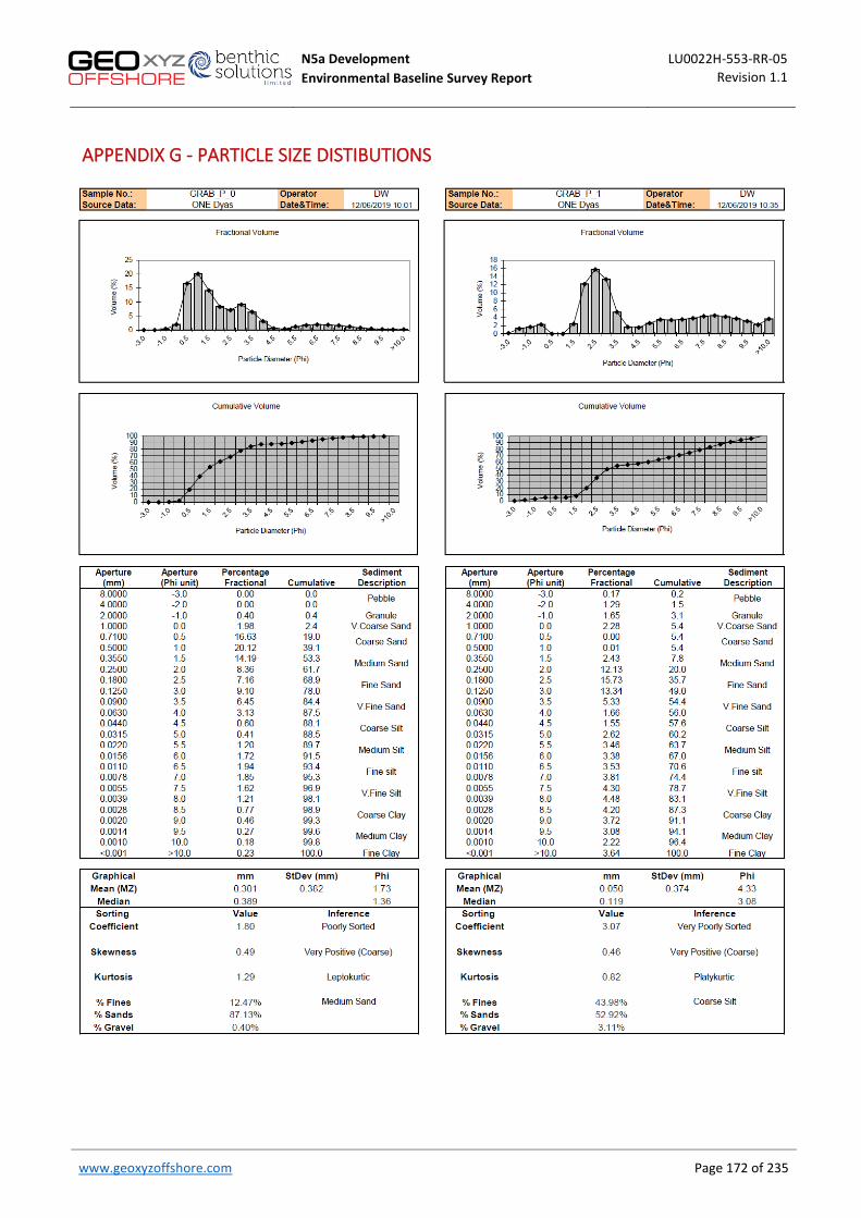
N5a Development LU0022H-553-RR-05 Environmental Baseline Survey Report Revision 1.1
www.geoxyzoffshore.com
Page 172 of 235
APPENDIX G - PARTICLE SIZE DISTIBUTIONS

N5a Development LU0022H-553-RR-05 Environmental Baseline Survey Report Revision 1.1
www.geoxyzoffshore.com
Page 173 of 235

N5a Development LU0022H-553-RR-05 Environmental Baseline Survey Report Revision 1.1
www.geoxyzoffshore.com
Page 174 of 235

N5a Development LU0022H-553-RR-05 Environmental Baseline Survey Report Revision 1.1
www.geoxyzoffshore.com
Page 175 of 235
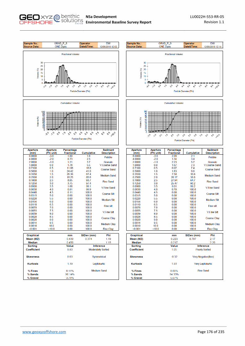
N5a Development LU0022H-553-RR-05 Environmental Baseline Survey Report Revision 1.1
www.geoxyzoffshore.com
Page 176 of 235

N5a Development LU0022H-553-RR-05 Environmental Baseline Survey Report Revision 1.1
www.geoxyzoffshore.com
Page 177 of 235

N5a Development LU0022H-553-RR-05 Environmental Baseline Survey Report Revision 1.1
www.geoxyzoffshore.com
Page 178 of 235

N5a Development LU0022H-553-RR-05 Environmental Baseline Survey Report Revision 1.1
www.geoxyzoffshore.com
Page 179 of 235

N5a Development LU0022H-553-RR-05 Environmental Baseline Survey Report Revision 1.1
www.geoxyzoffshore.com
Page 180 of 235
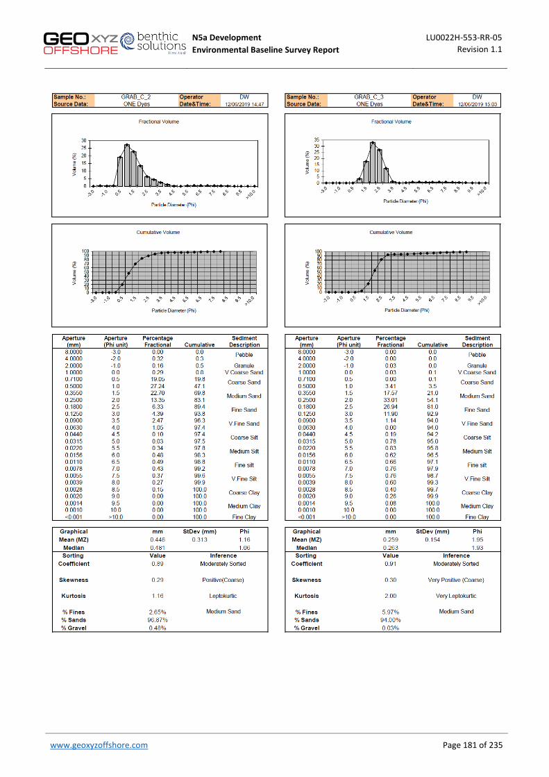
N5a Development LU0022H-553-RR-05 Environmental Baseline Survey Report Revision 1.1
www.geoxyzoffshore.com
Page 181 of 235
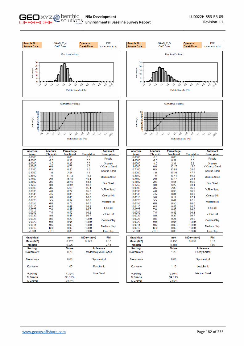
N5a Development LU0022H-553-RR-05 Environmental Baseline Survey Report Revision 1.1
www.geoxyzoffshore.com
Page 182 of 235

N5a Development LU0022H-553-RR-05 Environmental Baseline Survey Report Revision 1.1
www.geoxyzoffshore.com
Page 183 of 235

N5a Development LU0022H-553-RR-05 Environmental Baseline Survey Report Revision 1.1
www.geoxyzoffshore.com
Page 184 of 235

N5a Development LU0022H-553-RR-05 Environmental Baseline Survey Report Revision 1.1
www.geoxyzoffshore.com
Page 185 of 235

N5a Development LU0022H-553-RR-05 Environmental Baseline Survey Report Revision 1.1
www.geoxyzoffshore.com
Page 186 of 235

N5a Development LU0022H-553-RR-05 Environmental Baseline Survey Report Revision 1.1
www.geoxyzoffshore.com
Page 187 of 235
Modified Folk Classification

N5a Development LU0022H-553-RR-05 Environmental Baseline Survey Report Revision 1.1
www.geoxyzoffshore.com
Page 188 of 235
Folk and Wentworth Classifications
Station Folk Classification Wentworth Classification
Grab_P_0 Medium Sand Muddy sand
Grab_P_1 Coarse Silt Slightly gravelly muddy sand
Grab_P_2 Fine Sand Sand
Grab_P_3 Fine Sand Sand
Grab_P_4 Medium Sand Sand
Grab_P_5 Medium Sand Slightly gravelly sand
Grab_P_6 Medium Sand Sand
Grab_P_7 Fine Sand Sand
Grab_P_8 Medium Sand Slightly gravelly sand
Grab_P_9 Fine Sand Slightly gravelly sand
Grab_P_10 Fine Sand Slightly gravelly muddy sand
Grab_P_11 Medium Sand Gravelly sand
Grab_P_12 Fine Sand Sand
Grab_P_13 Fine Sand Sand
Grab_P_14 Fine Sand Slightly gravelly sand
Grab_P_15 Fine Sand Slightly gravelly sand
Grab_C_0 Coarse Sand Slightly gravelly sand
Grab_C_1 Medium Sand Gravelly sand
Grab_C_2 Medium Sand Sand
Grab_C_3 Fine Sand Sand
Grab_C_4 Medium Sand Sand
Grab_C_5 Medium Sand Slightly gravelly sand
Grab_C_6 Medium Sand Slightly gravelly sand
Grab_C_7 Medium Sand Slightly gravelly sand
Grab_C_8 Coarse Sand Slightly gravelly sand
Grab_C3_0 Fine Sand Sand
Grab_C3_1 Fine Sand Sand
Grab_C3_2 Granule Muddy sandy gravel
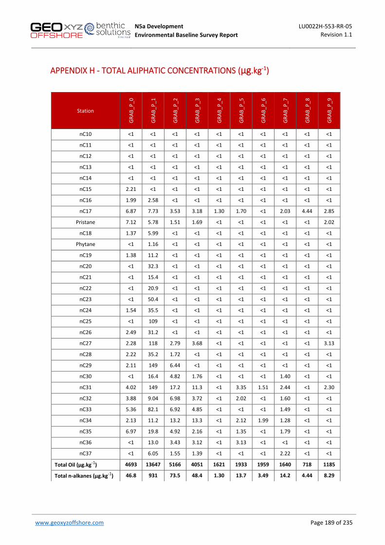
N5a Development LU0022H-553-RR-05 Environmental Baseline Survey Report Revision 1.1
www.geoxyzoffshore.com
Page 189 of 235
APPENDIX H - TOTAL ALIPHATIC CONCENTRATIONS (µg.kg-1)
Station
GRAB
_P_0
GRAB
_P_1
GRAB
_P_2
GRAB
_P_3
GRAB
_P_4
GRAB
_P_5
GRAB
_P_6
GRAB
_P_7
GRAB
_P_8
GRAB
_P_9
nC10 <1 <1 <1 <1 <1 <1 <1 <1 <1 <1
nC11 <1 <1 <1 <1 <1 <1 <1 <1 <1 <1
nC12 <1 <1 <1 <1 <1 <1 <1 <1 <1 <1
nC13 <1 <1 <1 <1 <1 <1 <1 <1 <1 <1
nC14 <1 <1 <1 <1 <1 <1 <1 <1 <1 <1
nC15 2.21 <1 <1 <1 <1 <1 <1 <1 <1 <1
nC16 1.99 2.58 <1 <1 <1 <1 <1 <1 <1 <1
nC17 6.87 7.73 3.53 3.18 1.30 1.70 <1 2.03 4.44 2.85
Pristane 7.12 5.78 1.51 1.69 <1 <1 <1 <1 <1 2.02
nC18 1.37 5.99 <1 <1 <1 <1 <1 <1 <1 <1
Phytane <1 1.16 <1 <1 <1 <1 <1 <1 <1 <1
nC19 1.38 11.2 <1 <1 <1 <1 <1 <1 <1 <1
nC20 <1 32.3 <1 <1 <1 <1 <1 <1 <1 <1
nC21 <1 15.4 <1 <1 <1 <1 <1 <1 <1 <1
nC22 <1 20.9 <1 <1 <1 <1 <1 <1 <1 <1
nC23 <1 50.4 <1 <1 <1 <1 <1 <1 <1 <1
nC24 1.54 35.5 <1 <1 <1 <1 <1 <1 <1 <1
nC25 <1 109 <1 <1 <1 <1 <1 <1 <1 <1
nC26 2.49 31.2 <1 <1 <1 <1 <1 <1 <1 <1
nC27 2.28 118 2.79 3.68 <1 <1 <1 <1 <1 3.13
nC28 2.22 35.2 1.72 <1 <1 <1 <1 <1 <1 <1
nC29 2.11 149 6.44 <1 <1 <1 <1 <1 <1 <1
nC30 <1 16.4 4.82 1.76 <1 <1 <1 1.40 <1 <1
nC31 4.02 149 17.2 11.3 <1 3.35 1.51 2.44 <1 2.30
nC32 3.88 9.04 6.98 3.72 <1 2.02 <1 1.60 <1 <1
nC33 5.36 82.1 6.92 4.85 <1 <1 <1 1.49 <1 <1
nC34 2.13 11.2 13.2 13.3 <1 2.12 1.99 1.28 <1 <1
nC35 6.97 19.8 4.92 2.16 <1 1.35 <1 1.79 <1 <1
nC36 <1 13.0 3.43 3.12 <1 3.13 <1 <1 <1 <1
nC37 <1 6.05 1.55 1.39 <1 <1 <1 2.22 <1 <1
Total Oil (µg.kg-1) 4693 13647 5166 4051 1621 1933 1959 1640 718 1185
Total n-alkanes (µg.kg-1) 46.8 931 73.5 48.4 1.30 13.7 3.49 14.2 4.44 8.29
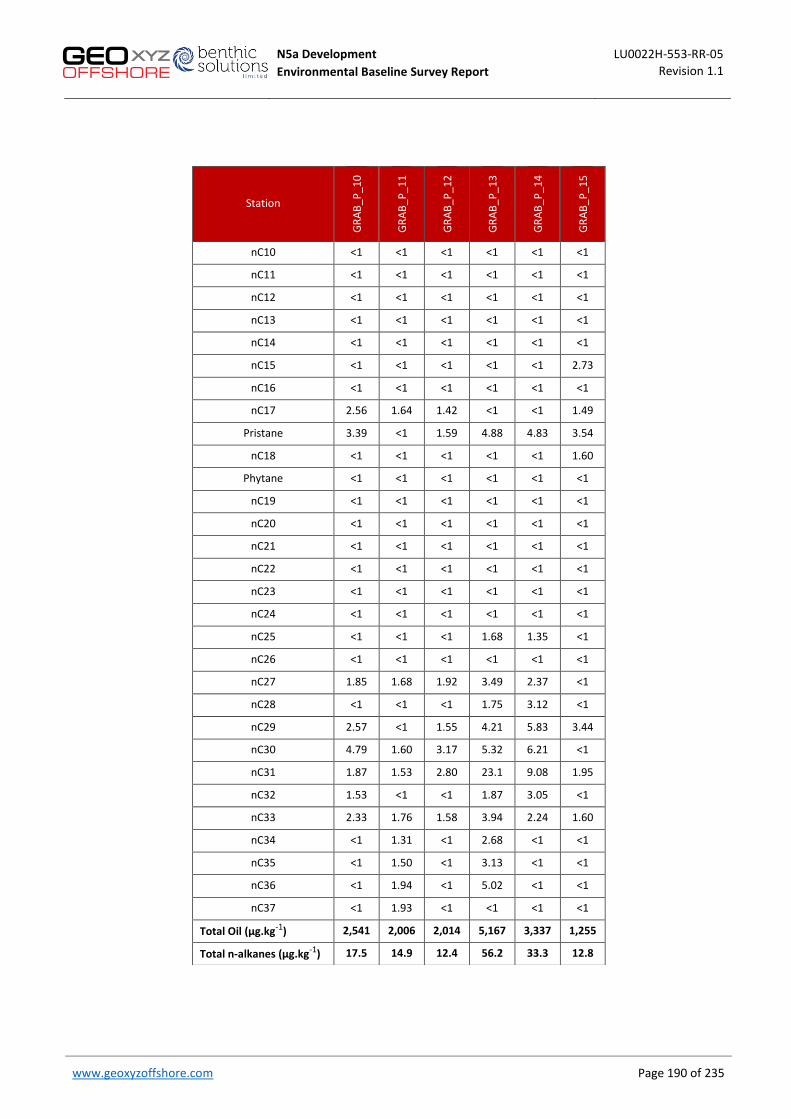
N5a Development LU0022H-553-RR-05 Environmental Baseline Survey Report Revision 1.1
www.geoxyzoffshore.com
Page 190 of 235
Station
GRAB
_P_1
0
GRAB
_P_1
1
GRAB
_P_1
2
GRAB
_P_1
3
GRAB
_P_1
4
GRAB
_P_1
5
nC10 <1 <1 <1 <1 <1 <1
nC11 <1 <1 <1 <1 <1 <1
nC12 <1 <1 <1 <1 <1 <1
nC13 <1 <1 <1 <1 <1 <1
nC14 <1 <1 <1 <1 <1 <1
nC15 <1 <1 <1 <1 <1 2.73
nC16 <1 <1 <1 <1 <1 <1
nC17 2.56 1.64 1.42 <1 <1 1.49
Pristane 3.39 <1 1.59 4.88 4.83 3.54
nC18 <1 <1 <1 <1 <1 1.60
Phytane <1 <1 <1 <1 <1 <1
nC19 <1 <1 <1 <1 <1 <1
nC20 <1 <1 <1 <1 <1 <1
nC21 <1 <1 <1 <1 <1 <1
nC22 <1 <1 <1 <1 <1 <1
nC23 <1 <1 <1 <1 <1 <1
nC24 <1 <1 <1 <1 <1 <1
nC25 <1 <1 <1 1.68 1.35 <1
nC26 <1 <1 <1 <1 <1 <1
nC27 1.85 1.68 1.92 3.49 2.37 <1
nC28 <1 <1 <1 1.75 3.12 <1
nC29 2.57 <1 1.55 4.21 5.83 3.44
nC30 4.79 1.60 3.17 5.32 6.21 <1
nC31 1.87 1.53 2.80 23.1 9.08 1.95
nC32 1.53 <1 <1 1.87 3.05 <1
nC33 2.33 1.76 1.58 3.94 2.24 1.60
nC34 <1 1.31 <1 2.68 <1 <1
nC35 <1 1.50 <1 3.13 <1 <1
nC36 <1 1.94 <1 5.02 <1 <1
nC37 <1 1.93 <1 <1 <1 <1
Total Oil (µg.kg-1) 2,541 2,006 2,014 5,167 3,337 1,255
Total n-alkanes (µg.kg-1) 17.5 14.9 12.4 56.2 33.3 12.8

N5a Development LU0022H-553-RR-05 Environmental Baseline Survey Report Revision 1.1
www.geoxyzoffshore.com
Page 191 of 235
Station
GRAB
_C_0
GRAB
_C_1
GRAB
_C_2
GRAB
_C_3
GRAB
_C_4
GRAB
_C_5
GRAB
_C_6
GRAB
_C_7
GRAB
_C_8
GRAB
_C3_
0
GRAB
_C3_
1
GRAB
_C3_
2
nC10 <1 <1 <1 <1 <1 <1 <1 <1 <1 <1 <1 <1
nC11 <1 <1 <1 <1 <1 <1 <1 <1 <1 <1 <1 <1
nC12 <1 <1 <1 <1 <1 <1 <1 <1 <1 <1 <1 <1
nC13 <1 <1 <1 <1 <1 <1 <1 <1 <1 <1 <1 <1
nC14 <1 <1 <1 <1 <1 <1 <1 <1 <1 <1 <1 <1
nC15 <1 <1 <1 <1 <1 <1 <1 <1 <1 <1 <1 <1
nC16 <1 <1 <1 <1 2.10 1.59 <1 <1 <1 1.98 1.20 <1
nC17 <1 <1 <1 <1 2.87 2.51 <1 1.41 <1 1.61 <1 <1
Pristane 2.31 <1 <1 1.45 3.82 1.09 <1 1.19 <1 3.62 1.13 4.69
nC18 1.39 1.46 <1 <1 1.37 2.64 <1 1.72 <1 <1 1.14 <1
Phytane <1 1.34 <1 <1 <1 <1 <1 <1 <1 <1 1.37 <1
nC19 <1 <1 <1 <1 2.25 <1 <1 <1 <1 1.31 3.40 1.72
nC20 <1 <1 <1 <1 <1 <1 <1 <1 <1 <1 8.31 <1
nC21 <1 <1 <1 <1 <1 <1 <1 <1 <1 <1 2.91 <1
nC22 <1 <1 <1 <1 <1 <1 <1 <1 <1 <1 3.11 1.39
nC23 <1 <1 <1 <1 <1 <1 <1 <1 <1 <1 1.52 <1
nC24 <1 <1 <1 <1 <1 <1 <1 <1 <1 <1 9.07 4.52
nC25 2.02 <1 <1 1.22 <1 <1 <1 <1 <1 <1 1.13 2.03
nC26 1.27 <1 <1 <1 <1 <1 <1 <1 1.74 <1 8.21 6.35
nC27 <1 <1 2.46 2.92 3.08 <1 1.84 1.82 2.56 6.00 6.40 4.12
nC28 1.50 <1 1.39 2.17 1.04 <1 <1 <1 <1 <1 11.3 7.46
nC29 4.96 2.91 3.73 5.19 5.50 2.39 3.46 3.03 3.05 11.7 38.3 37.6
nC30 4.61 7.86 5.94 3.32 5.76 1.26 1.80 2.09 <1 3.84 7.89 13.5
nC31 1.55 2.77 2.14 3.40 3.32 <1 <1 1.52 <1 19.1 25.8 7.53
nC32 1.27 <1 <1 <1 <1 <1 <1 <1 <1 1.39 1.15 22.1
nC33 2.13 5.92 5.05 1.60 <1 1.39 1.06 1.58 <1 7.03 8.17 8.54
nC34 2.03 <1 <1 <1 <1 1.01 1.62 <1 <1 9.51 4.92 1.02
nC35 <1 3.02 1.64 <1 <1 <1 <1 <1 <1 1.51 4.47 8.68
nC36 <1 <1 <1 <1 <1 <1 <1 <1 <1 5.97 2.23 2.70
nC37 <1 <1 <1 <1 <1 <1 <1 <1 <1 1.16 1.37 2.25
Total Oil (µg.kg-1) 1277 1914 5167 2472 2664 1210 873 1230 974 5855 6092 5634
Total n-alkanes (µg.kg-1) 22.7 23.9 22.4 19.8 27.3 12.8 9.78 13.2 7.35 72.1 152 131

N5a Development LU0022H-553-RR-05 Environmental Baseline Survey Report Revision 1.1
www.geoxyzoffshore.com
Page 192 of 235
APPENDIX I - GC FID TRACES (SATURATES)
GRAB_P_0
GRAB_P_1
GRAB_P_2 GRAB_P_3
GRAB_P_4 GRAB_P_5

N5a Development LU0022H-553-RR-05 Environmental Baseline Survey Report Revision 1.1
www.geoxyzoffshore.com
Page 193 of 235
GRAB_P_6
GRAB_P_7
GRAB_P_8 GRAB_P_9
GRAB_P_10 GRAB_P_11

N5a Development LU0022H-553-RR-05 Environmental Baseline Survey Report Revision 1.1
www.geoxyzoffshore.com
Page 194 of 235
GRAB_P_12
GRAB_P_13
GRAB_P_14 GRAB_P_15
GRAB_C_0 GRAB_C_1
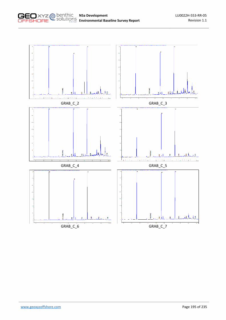
N5a Development LU0022H-553-RR-05 Environmental Baseline Survey Report Revision 1.1
www.geoxyzoffshore.com
Page 195 of 235
GRAB_C_2
GRAB_C_3
GRAB_C_4 GRAB_C_5
GRAB_C_6 GRAB_C_7

N5a Development LU0022H-553-RR-05 Environmental Baseline Survey Report Revision 1.1
www.geoxyzoffshore.com
Page 196 of 235
GRAB_C_8
GRAB_C3_0
GRAB_C3_1 GRAB_C3_2

N5a Development LU0022H-553-RR-05 Environmental Baseline Survey Report Revision 1.1
www.geoxyzoffshore.com
Page 197 of 235
APPENDIX J - POLYCYCLIC AROMATIC HYDROCARBON CONCENTRATION (µg.kg-1)
Station
GRAB
_P_0
GRAB
_P_1
GRAB
_P_2
GRAB
_P_3
GRAB
_P_4
GRAB
_P_5
GRAB
_P_6
GRAB
_P_7
GRAB
_P_8
GRAB
_P_9
Naphthalene <1 <1 <1 <1 <1 <1 <1 <1 <1 <1
C1 Naphthalenes 1.39 <1 <1 <1 <1 <1 <1 <1 <1 <1
C2 Naphthalenes 2.42 1.95 1.67 1.32 <1 <1 <1 <1 1.35 <1
C3 Naphthalenes 1.42 1.66 <1 <1 <1 <1 <1 <1 <1 <1
C4 Naphthalenes <1 2.26 <1 <1 <1 <1 <1 <1 <1 <1
Sum Naphthalenes 5.23 5.87 1.67 1.32 0.00 0.00 0.00 0.00 1.35 0.00
Phenanthrene / Anthracene 0.00 0.00 0.00 0.00 0.00 0.00 0.00 0.00 0.00 0.00
C1 178 1.59 2.46 <1 <1 <1 <1 <1 <1 <1 <1
C2 178 <1 2.53 <1 <1 <1 <1 <1 <1 <1 <1
C3 178 <1 1.40 <1 <1 <1 <1 <1 <1 <1 <1
Sum 178 1.59 6.39 0.00 0.00 0.00 0.00 0.00 0.00 0.00 0.00
Dibenzothiophene <1 <1 <1 <1 <1 <1 <1 <1 <1 <1
C1 Dibenzothiophenes <1 1.52 <1 <1 <1 <1 <1 <1 <1 <1
C2 Dibenzothiophenes <1 <1 <1 <1 <1 <1 <1 <1 <1 <1
C3 Dibenzothiophenes <1 <1 <1 <1 <1 <1 <1 <1 <1 <1
Sum Dibenzothiophenes 0.00 1.52 0.00 0.00 0.00 0.00 0.00 0.00 0.00 0.00
Fluoranthene / Pyrene 0.00 0.00 0.00 0.00 0.00 0.00 0.00 0.00 0.00 0.00
C1 202 <1 2.93 <1 <1 <1 <1 <1 <1 <1 <1
C2 202 <1 5.15 <1 <1 <1 <1 <1 <1 <1 <1
C3 202 <1 4.51 <1 <1 <1 <1 <1 <1 <1 <1
Sum 202 0.00 12.6 0.00 0.00 0.00 0.00 0.00 0.00 0.00 0.00
Benzoanthracene / Chrysene 0.00 0.00 0.00 0.00 0.00 0.00 0.00 0.00 0.00 0.00
C1 228 <1 4.65 <1 <1 <1 <1 <1 <1 <1 <1
C2 228 <1 5.50 <1 <1 <1 <1 <1 <1 <1 <1
Sum 228 0.00 10.1 0.00 0.00 0.00 0.00 0.00 0.00 0.00 0.00
Benzofluoranthenes / Benzopyrenes 0.00 5.36 0.00 0.00 0.00 0.00 0.00 0.00 0.00 0.00
C1 252 <1 3.92 <1 1.44 <1 <1 <1 <1 <1 <1
C2 252 <1 11.9 <1 <1 <1 <1 <1 <1 <1 <1
Sum 252 0.00 21.2 0.00 1.44 0.00 0.00 0.00 0.00 0.00 0.00 Dibenzoanthracene / Indenopyrene / Benzoperylene
0.00 4.88 0.00 0.00 0.00 0.00 0.00 0.00 0.00 0.00
C1 276 <1 2.39 <1 <1 <1 <1 <1 <1 <1 <1
C2 276 <1 1.84 <1 <1 <1 <1 <1 <1 <1 <1
Sum 276 0.00 9.10 0.00 0.00 0.00 0.00 0.00 0.00 0.00 0.00
Sum of all PAHs 6.82 66.8 1.67 2.76 0.00 0.00 0.00 0.00 1.35 0.00
Sum of NPD fraction 6.82 13.78 1.67 1.32 0.00 0.00 0.00 0.00 1.35 0.00
NPD/4-6 Ring PAH Ratio - 0.26 - 0.92 - - - - - -

N5a Development LU0022H-553-RR-05 Environmental Baseline Survey Report Revision 1.1
www.geoxyzoffshore.com
Page 198 of 235
Station
GR
AB
_P_1
0
GR
AB
_P_1
1
GR
AB
_P_1
2
GR
AB
_P_1
3
GR
AB
_P_1
4
GR
AB
_P_1
5
Naphthalene <1 <1 <1 <1 <1 <1
C1 Naphthalenes 1.46 <1 <1 <1 <1 1.51
C2 Naphthalenes 2.07 4.34 1.92 2.77 1.94 2.31
C3 Naphthalenes <1 <1 <1 <1 <1 2.27
C4 Naphthalenes <1 <1 <1 <1 <1 2.04
Sum Naphthalenes 3.53 4.34 1.92 2.77 1.94 8.13
Phenanthrene / Anthracene 0.00 0.00 0.00 0.00 0.00 0.00
C1 178 <1 <1 <1 1.42 <1 <1
C2 178 <1 <1 <1 <1 <1 <1
C3 178 <1 <1 <1 <1 <1 <1
Sum 178 0.00 0.00 0.00 1.42 0.00 0.00
Dibenzothiophene <1 <1 <1 <1 <1 <1
C1 Dibenzothiophenes <1 <1 <1 <1 <1 <1
C2 Dibenzothiophenes <1 <1 <1 <1 <1 <1
C3 Dibenzothiophenes <1 <1 <1 <1 <1 <1
Sum Dibenzothiophenes 0.00 0.00 0.00 0.00 0.00 0.00
Fluoranthene / Pyrene 0.00 0.00 0.00 0.00 0.00 0.00
C1 202 <1 <1 <1 <1 <1 <1
C2 202 <1 <1 <1 <1 <1 <1
C3 202 <1 <1 <1 <1 <1 <1
Sum 202 0.00 0.00 0.00 0.00 0.00 0.00
Benzoanthracene / Chrysene 0.00 0.00 0.00 0.00 0.00 0.00
C1 228 <1 <1 <1 <1 <1 <1
C2 228 <1 <1 <1 <1 <1 <1
Sum 228 0.00 0.00 0.00 0.00 0.00 0.00
Benzofluoranthenes / Benzopyrenes 0.00 0.00 0.00 0.00 0.00 0.00
C1 252 <1 <1 <1 <1 <1 <1
C2 252 <1 <1 <1 <1 <1 <1
Sum 252 0.00 0.00 0.00 0.00 0.00 0.00 Dibenzoanthracene / Indenopyrene / Benzoperylene
0.00 0.00 0.00 0.00 0.00 0.00
C1 276 <1 <1 <1 <1 <1 <1
C2 276 <1 <1 <1 <1 <1 <1
Sum 276 0.00 0.00 0.00 0.00 0.00 0.00
Sum of all PAHs 3.53 4.34 1.92 4.19 1.94 8.13
Sum of NPD fraction 3.53 4.34 1.92 4.19 1.94 8.13
NPD/4-6 Ring PAH Ratio - - - - - -

N5a Development LU0022H-553-RR-05 Environmental Baseline Survey Report Revision 1.1
www.geoxyzoffshore.com
Page 199 of 235
Station
GRAB
_C_0
GRAB
_C_1
GRAB
_C_2
GRAB
_C_3
GRAB
_C_4
GRAB
_C_5
GRAB
_C_6
GRAB
_C_7
GRAB
_C_8
Naphthalene <1 <1 <1 <1 <1 <1 <1 <1 <1
C1 Naphthalenes <1 <1 <1 <1 <1 <1 <1 <1 <1
C2 Naphthalenes <1 <1 <1 1.46 <1 <1 <1 <1 <1
C3 Naphthalenes <1 <1 <1 <1 <1 <1 <1 <1 <1
C4 Naphthalenes <1 <1 <1 <1 <1 <1 <1 <1 <1
Sum Naphthalenes 0.00 0.00 0.00 1.46 0.00 0.00 0.00 0.00 0.00
Phenanthrene / Anthracene 0.00 0.00 0.00 0.00 0.00 0.00 0.00 0.00 0.00
C1 178 <1 <1 <1 <1 <1 <1 <1 <1 <1
C2 178 <1 <1 <1 <1 <1 <1 <1 <1 <1
C3 178 <1 <1 <1 <1 <1 <1 <1 <1 <1
Sum 178 0.00 0.00 0.00 0.00 0.00 0.00 0.00 0.00 0.00
Dibenzothiophene <1 <1 <1 <1 <1 <1 <1 <1 <1
C1 Dibenzothiophenes <1 <1 <1 <1 <1 <1 <1 <1 <1
C2 Dibenzothiophenes <1 <1 <1 <1 <1 <1 <1 <1 <1
C3 Dibenzothiophenes <1 <1 <1 <1 <1 <1 <1 <1 <1
Sum Dibenzothiophenes 0.00 0.00 0.00 0.00 0.00 0.00 0.00 0.00 0.00
Fluoranthene / Pyrene 0.00 0.00 0.00 0.00 0.00 0.00 0.00 0.00 0.00
C1 202 <1 <1 <1 <1 <1 <1 <1 <1 <1
C2 202 <1 <1 <1 <1 <1 <1 <1 <1 <1
C3 202 <1 <1 <1 <1 <1 <1 <1 <1 <1
Sum 202 0.00 0.00 0.00 0.00 0.00 0.00 0.00 0.00 0.00
Benzoanthracene / Chrysene 0.00 0.00 0.00 0.00 0.00 0.00 0.00 0.00 0.00
C1 228 <1 <1 <1 <1 <1 <1 <1 <1 <1
C2 228 <1 <1 <1 <1 <1 <1 <1 <1 <1
Sum 228 0.00 0.00 0.00 0.00 0.00 0.00 0.00 0.00 0.00
Benzofluoranthenes / Benzopyrenes 0.00 0.00 0.00 0.00 0.00 0.00 0.00 0.00 0.00
C1 252 <1 <1 <1 <1 <1 <1 <1 <1 <1
C2 252 <1 <1 <1 <1 <1 <1 <1 <1 <1
Sum 252 0.00 0.00 0.00 0.00 0.00 0.00 0.00 0.00 0.00 Dibenzoanthracene / Indenopyrene / Benzoperylene
0.00 0.00 0.00 0.00 0.00 0.00 0.00 0.00 0.00
C1 276 <1 <1 <1 <1 <1 <1 <1 <1 <1
C2 276 <1 <1 <1 <1 <1 <1 <1 <1 <1
Sum 276 0.00 0.00 0.00 0.00 0.00 0.00 0.00 0.00 0.00
Sum of all PAHs 0.00 0.00 0.00 1.46 0.00 0.00 0.00 0.00 0.00
Sum of NPD fraction 0.00 0.00 0.00 1.46 0.00 0.00 0.00 0.00 0.00
NPD/4-6 Ring PAH Ratio - - - - - - - - -

N5a Development LU0022H-553-RR-05 Environmental Baseline Survey Report Revision 1.1
www.geoxyzoffshore.com
Page 200 of 235
Station
GRAB
_C3_
0
GRAB
_C3_
1
GRAB
_C3_
2
Naphthalene <1 <1 <1
C1 Naphthalenes <1 <1 <1
C2 Naphthalenes 2.09 <1 <1
C3 Naphthalenes <1 <1 <1
C4 Naphthalenes <1 <1 <1
Sum Naphthalenes 2.09 0.00 0.00
Phenanthrene / Anthracene 0.00 0.00 0.00
C1 178 <1 <1 <1
C2 178 <1 <1 <1
C3 178 <1 <1 <1
Sum 178 0.00 0.00 0.00
Dibenzothiophene <1 <1 <1
C1 Dibenzothiophenes <1 <1 <1
C2 Dibenzothiophenes <1 <1 <1
C3 Dibenzothiophenes <1 <1 <1
Sum Dibenzothiophenes 0.00 0.00 0.00
Fluoranthene / Pyrene 0.00 0.00 0.00
C1 202 <1 1.76 <1
C2 202 <1 2.59 1.52
C3 202 <1 1.56 <1
Sum 202 0.00 5.91 1.52
Benzoanthracene / Chrysene 0.00 0.00 0.00
C1 228 <1 3.53 1.51
C2 228 <1 2.76 <1
Sum 228 0.00 6.29 1.51
Benzofluoranthenes / Benzopyrenes 0.00 0.00 0.00
C1 252 <1 1.57 <1
C2 252 <1 3.42 3.37
Sum 252 0.00 4.99 3.37 Dibenzoanthracene / Indenopyrene / Benzoperylene
0.00 1.33 0.00
C1 276 <1 1.33 <1
C2 276 <1 <1 <1
Sum 276 0.00 2.66 0.00
Sum of all PAHs 2.09 19.9 6.41
Sum of NPD fraction 2.09 0.00 0.00
NPD/4-6 Ring PAH Ratio - - -

N5a Development LU0022H-553-RR-05 Environmental Baseline Survey Report Revision 1.1
www.geoxyzoffshore.com
Page 201 of 235
APPENDIX K - POLYCYCLIC AROMATIC HYDROCARBON CONCENTRATION: EPA (µg.kg-1)
Station
GRAB
_P_0
GRAB
_P_1
GRAB
_P_2
GRAB
_P_3
GRAB
_P_4
GRAB
_P_5
GRAB
_P_6
GRAB
_P_7
GRAB
_P_8
GRAB
_P_9
Naphthalene <1 <1 <1 <1 <1 <1 <1 <1 <1 <1
Acenaphthylene <1 <1 <1 <1 <1 <1 <1 <1 <1 <1
Acenaphthene <1 <1 <1 <1 <1 <1 <1 <1 <1 <1
Fluorene <1 <1 <1 <1 <1 <1 <1 <1 <1 <1
Phenanthrene <1 <1 <1 <1 <1 <1 <1 <1 <1 <1
Dibenzothiophene <1 <1 <1 <1 <1 <1 <1 <1 <1 <1
Anthracene <1 <1 <1 <1 <1 <1 <1 <1 <1 <1
Fluoranthene <1 <1 <1 <1 <1 <1 <1 <1 <1 <1
Pyrene <1 <1 <1 <1 <1 <1 <1 <1 <1 <1
Benzo[a]anthracene <1 <1 <1 <1 <1 <1 <1 <1 <1 <1
Chrysene <1 <1 <1 <1 <1 <1 <1 <1 <1 <1
Benzo[b]fluoranthene <1 2.03 <1 <1 <1 <1 <1 <1 <1 <1
Benzo[k]fluoranthene <1 <1 <1 <1 <1 <1 <1 <1 <1 <1
Benzo[e]pyrene <1 1.77 <1 <1 <1 <1 <1 <1 <1 <1
Benzo[a]pyrene <1 1.56 <1 <1 <1 <1 <1 <1 <1 <1
Perylene 1.76 49.0 <1 <1 <1 <1 <1 <1 <1 <1
Indeno[123,cd]pyrene <1 1.74 <1 <1 <1 <1 <1 <1 <1 <1
Dibenzo[a,h]anthracene <1 <1 <1 <1 <1 <1 <1 <1 <1 <1
Benzo[ghi]perylene <1 3.13 <1 <1 <1 <1 <1 <1 <1 <1
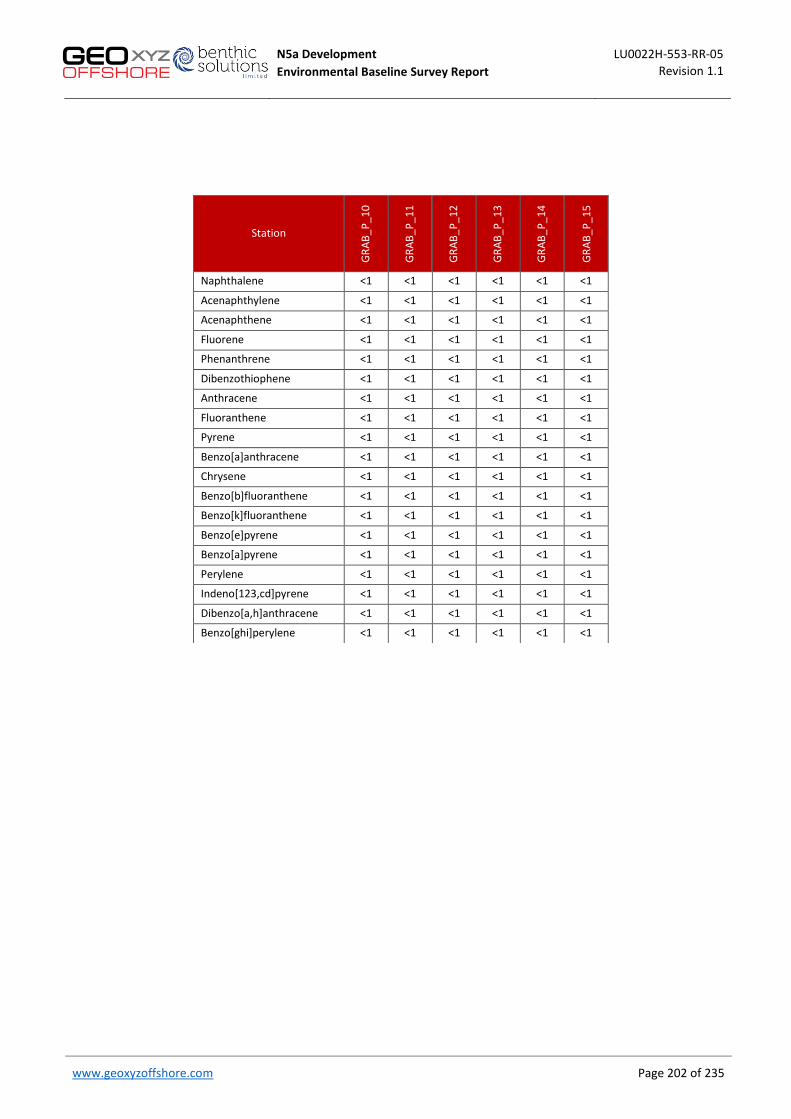
N5a Development LU0022H-553-RR-05 Environmental Baseline Survey Report Revision 1.1
www.geoxyzoffshore.com
Page 202 of 235
Station
GRAB
_P_1
0
GRAB
_P_1
1
GRAB
_P_1
2
GRAB
_P_1
3
GRAB
_P_1
4
GRAB
_P_1
5
Naphthalene <1 <1 <1 <1 <1 <1
Acenaphthylene <1 <1 <1 <1 <1 <1
Acenaphthene <1 <1 <1 <1 <1 <1
Fluorene <1 <1 <1 <1 <1 <1
Phenanthrene <1 <1 <1 <1 <1 <1
Dibenzothiophene <1 <1 <1 <1 <1 <1
Anthracene <1 <1 <1 <1 <1 <1
Fluoranthene <1 <1 <1 <1 <1 <1
Pyrene <1 <1 <1 <1 <1 <1
Benzo[a]anthracene <1 <1 <1 <1 <1 <1
Chrysene <1 <1 <1 <1 <1 <1
Benzo[b]fluoranthene <1 <1 <1 <1 <1 <1
Benzo[k]fluoranthene <1 <1 <1 <1 <1 <1
Benzo[e]pyrene <1 <1 <1 <1 <1 <1
Benzo[a]pyrene <1 <1 <1 <1 <1 <1
Perylene <1 <1 <1 <1 <1 <1
Indeno[123,cd]pyrene <1 <1 <1 <1 <1 <1
Dibenzo[a,h]anthracene <1 <1 <1 <1 <1 <1
Benzo[ghi]perylene <1 <1 <1 <1 <1 <1
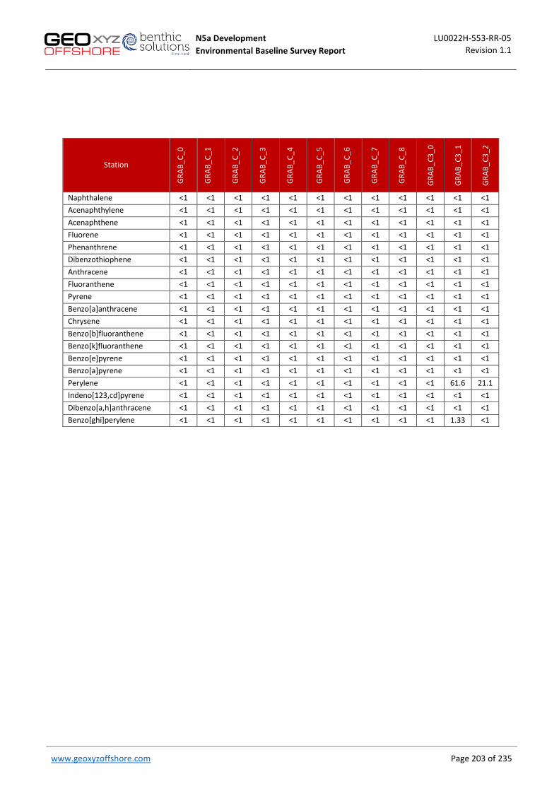
N5a Development LU0022H-553-RR-05 Environmental Baseline Survey Report Revision 1.1
www.geoxyzoffshore.com
Page 203 of 235
Station
GRAB
_C_0
GRAB
_C_1
GRAB
_C_2
GRAB
_C_3
GRAB
_C_4
GRAB
_C_5
GRAB
_C_6
GRAB
_C_7
GRAB
_C_8
GRAB
_C3_
0
GRAB
_C3_
1
GRAB
_C3_
2
Naphthalene <1 <1 <1 <1 <1 <1 <1 <1 <1 <1 <1 <1 Acenaphthylene <1 <1 <1 <1 <1 <1 <1 <1 <1 <1 <1 <1 Acenaphthene <1 <1 <1 <1 <1 <1 <1 <1 <1 <1 <1 <1 Fluorene <1 <1 <1 <1 <1 <1 <1 <1 <1 <1 <1 <1 Phenanthrene <1 <1 <1 <1 <1 <1 <1 <1 <1 <1 <1 <1 Dibenzothiophene <1 <1 <1 <1 <1 <1 <1 <1 <1 <1 <1 <1 Anthracene <1 <1 <1 <1 <1 <1 <1 <1 <1 <1 <1 <1 Fluoranthene <1 <1 <1 <1 <1 <1 <1 <1 <1 <1 <1 <1 Pyrene <1 <1 <1 <1 <1 <1 <1 <1 <1 <1 <1 <1 Benzo[a]anthracene <1 <1 <1 <1 <1 <1 <1 <1 <1 <1 <1 <1 Chrysene <1 <1 <1 <1 <1 <1 <1 <1 <1 <1 <1 <1 Benzo[b]fluoranthene <1 <1 <1 <1 <1 <1 <1 <1 <1 <1 <1 <1 Benzo[k]fluoranthene <1 <1 <1 <1 <1 <1 <1 <1 <1 <1 <1 <1 Benzo[e]pyrene <1 <1 <1 <1 <1 <1 <1 <1 <1 <1 <1 <1 Benzo[a]pyrene <1 <1 <1 <1 <1 <1 <1 <1 <1 <1 <1 <1 Perylene <1 <1 <1 <1 <1 <1 <1 <1 <1 <1 61.6 21.1 Indeno[123,cd]pyrene <1 <1 <1 <1 <1 <1 <1 <1 <1 <1 <1 <1 Dibenzo[a,h]anthracene <1 <1 <1 <1 <1 <1 <1 <1 <1 <1 <1 <1 Benzo[ghi]perylene <1 <1 <1 <1 <1 <1 <1 <1 <1 <1 1.33 <1
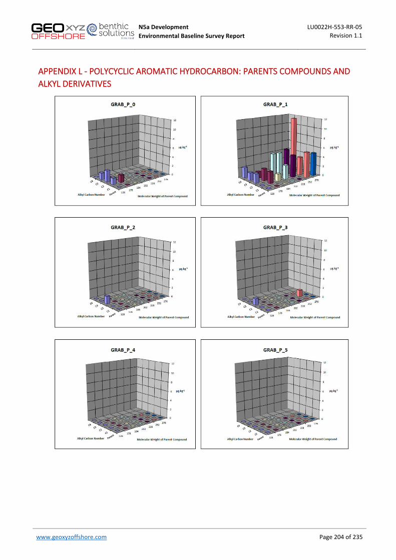
N5a Development LU0022H-553-RR-05 Environmental Baseline Survey Report Revision 1.1
www.geoxyzoffshore.com
Page 204 of 235
APPENDIX L - POLYCYCLIC AROMATIC HYDROCARBON: PARENTS COMPOUNDS AND
ALKYL DERIVATIVES

N5a Development LU0022H-553-RR-05 Environmental Baseline Survey Report Revision 1.1
www.geoxyzoffshore.com
Page 205 of 235

N5a Development LU0022H-553-RR-05 Environmental Baseline Survey Report Revision 1.1
www.geoxyzoffshore.com
Page 206 of 235

N5a Development LU0022H-553-RR-05 Environmental Baseline Survey Report Revision 1.1
www.geoxyzoffshore.com
Page 207 of 235

N5a Development LU0022H-553-RR-05 Environmental Baseline Survey Report Revision 1.1
www.geoxyzoffshore.com
Page 208 of 235

N5a Development LU0022H-553-RR-05 Environmental Baseline Survey Report Revision 1.1
www.geoxyzoffshore.com
Page 209 of 235
APPENDIX M - MACROFAUNAL SPECIES LIST
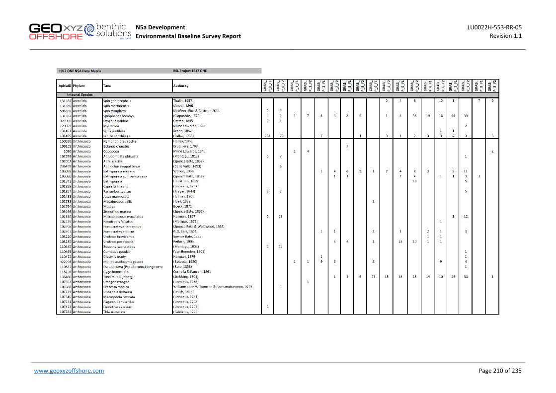
N5a Development LU0022H-553-RR-05 Environmental Baseline Survey Report Revision 1.1
www.geoxyzoffshore.com
Page 210 of 235
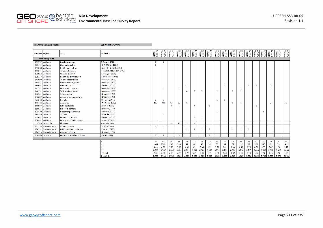
N5a Development LU0022H-553-RR-05 Environmental Baseline Survey Report Revision 1.1
www.geoxyzoffshore.com
Page 211 of 235
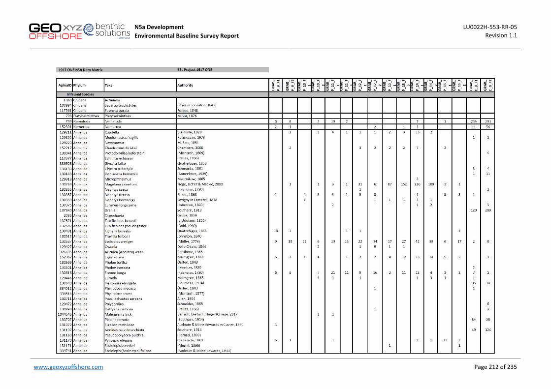
N5a Development LU0022H-553-RR-05 Environmental Baseline Survey Report Revision 1.1
www.geoxyzoffshore.com
Page 212 of 235

N5a Development LU0022H-553-RR-05 Environmental Baseline Survey Report Revision 1.1
www.geoxyzoffshore.com
Page 213 of 235

N5a Development LU0022H-553-RR-05 Environmental Baseline Survey Report Revision 1.1
www.geoxyzoffshore.com
Page 214 of 235

N5a Development LU0022H-553-RR-05 Environmental Baseline Survey Report Revision 1.1
www.geoxyzoffshore.com
Page 215 of 235

N5a Development LU0022H-553-RR-05 Environmental Baseline Survey Report Revision 1.1
www.geoxyzoffshore.com
Page 216 of 235

N5a Development LU0022H-553-RR-05 Environmental Baseline Survey Report Revision 1.1
www.geoxyzoffshore.com
Page 217 of 235

N5a Development LU0022H-553-RR-05 Environmental Baseline Survey Report Revision 1.1
www.geoxyzoffshore.com
Page 218 of 235
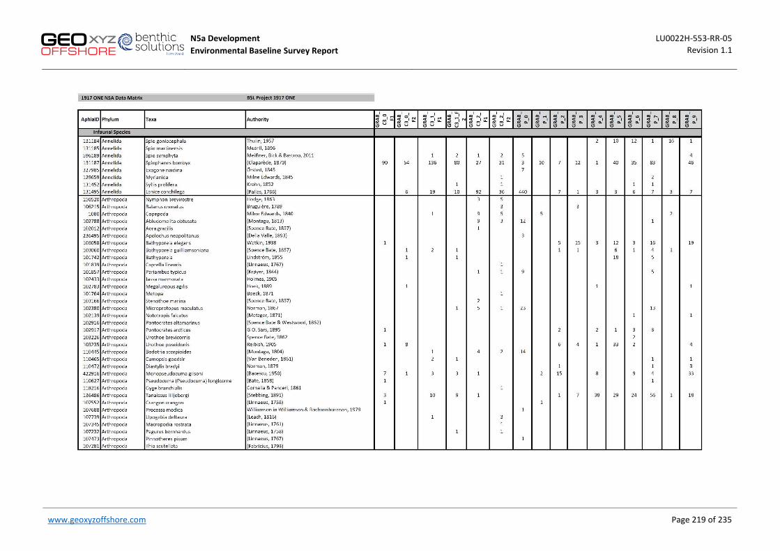
N5a Development LU0022H-553-RR-05 Environmental Baseline Survey Report Revision 1.1
www.geoxyzoffshore.com
Page 219 of 235

N5a Development LU0022H-553-RR-05 Environmental Baseline Survey Report Revision 1.1
www.geoxyzoffshore.com
Page 220 of 235

N5a Development LU0022H-553-RR-05 Environmental Baseline Survey Report Revision 1.1
www.geoxyzoffshore.com
Page 221 of 235

N5a Development LU0022H-553-RR-05 Environmental Baseline Survey Report Revision 1.1
www.geoxyzoffshore.com
Page 222 of 235

N5a Development LU0022H-553-RR-05 Environmental Baseline Survey Report Revision 1.1
www.geoxyzoffshore.com
Page 223 of 235

N5a Development LU0022H-553-RR-05 Environmental Baseline Survey Report Revision 1.1
www.geoxyzoffshore.com
Page 224 of 235

N5a Development LU0022H-553-RR-05 Environmental Baseline Survey Report Revision 1.1
www.geoxyzoffshore.com
Page 225 of 235

N5a Development LU0022H-553-RR-05 Environmental Baseline Survey Report Revision 1.1
www.geoxyzoffshore.com
Page 226 of 235

N5a Development LU0022H-553-RR-05 Environmental Baseline Survey Report Revision 1.1
www.geoxyzoffshore.com
Page 227 of 235

N5a Development LU0022H-553-RR-05 Environmental Baseline Survey Report Revision 1.1
www.geoxyzoffshore.com
Page 228 of 235

N5a Development LU0022H-553-RR-05 Environmental Baseline Survey Report Revision 1.1
www.geoxyzoffshore.com
Page 229 of 235

N5a Development LU0022H-553-RR-05 Environmental Baseline Survey Report Revision 1.1
www.geoxyzoffshore.com
Page 230 of 235
APPENDIX N - SPEARMAN’S CORRELATION

N5a Development LU0022H-553-RR-05 Environmental Baseline Survey Report Revision 1.1
www.geoxyzoffshore.com Page 231 of 235 Page 231 of 235
APPENDIX O - AQA CERTIFICATION OF LABORATORIES
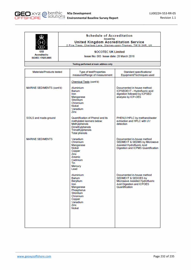
N5a Development LU0022H-553-RR-05 Environmental Baseline Survey Report Revision 1.1
www.geoxyzoffshore.com Page 232 of 235 Page 232 of 235

N5a Development LU0022H-553-RR-05 Environmental Baseline Survey Report Revision 1.1
www.geoxyzoffshore.com Page 233 of 235 Page 233 of 235

N5a Development LU0022H-553-RR-05 Environmental Baseline Survey Report Revision 1.1
www.geoxyzoffshore.com Page 234 of 235 Page 234 of 235

N5a Development LU0022H-553-RR-05 Environmental Baseline Survey Report Revision 1.1
www.geoxyzoffshore.com Page 235 of 235 Page 235 of 235
APPENDIX P - SERVICE WARRANTY
This report, with its associated works and services, has been designed solely to meet the requirements of the contract agreed with you, our client. If used in other circumstances, some or all of the results may not be valid and we can accept no liability for such use. Such circumstances include different or changed objectives, use by third parties, or changes to, for example, station conditions or legislation occurring after completion of the work. In case of doubt, please consult Benthic Solutions Limited. Please note that all charts, where applicable should not be used for navigational purposes.

N5a Development
Title Habitat Assessment Survey Report
GEOxyz Report No. LU0022H-553-RR-04
ONE Report No. N05A-7-10-0-70019-01
Revision 2.1
2.1 30/10/2019 Final Issue PC PC SD
2.0 20/09/2019 Final Issue HB PC SD
1.0 19/07/2019 First Issue HB PC
Revision Date Description of Revision Author Checked Approved Approved Client

N5a Development LU0022H-553-RR-04
Habitat Assessment Survey Report Revision 2.1
www.geoxyzoffshore.com Page 1 of 96
REVISION HISTORY
The screen version of this document is always the CONTROLLED COPY. When printed it is considered a FOR INFORMATION ONLY copy, and it is the holder’s responsibility that they hold the latest valid version.
The table on this page can be used to explain the reason for the revision and what has changed since the previous revision.
Rev. Reason for revision Changes from previous version
1.0 First Issue N/A
2.0 Approved by Client None
2.1 Approved by Client
Comments on EBS report required small adaptions to this report as there is overlapping content. Changes from previous version: • Modifcation of text describing H1110 habitat type in order to
correlate the observed faunal communities with the characterising species for the H1110_C habitat subtype.
• Reference to Zostera marina beds has been removed from the relevant text.

N5a Development LU0022H-553-RR-04
Habitat Assessment Survey Report Revision 2.1
www.geoxyzoffshore.com Page 2 of 96
TABLE OF CONTENTS
Revision History .................................................................................................................................................. 1 Abbreviations ...................................................................................................................................................... 4
1 Introduction ................................................................................................................................... 5
1.1 Project Overview .................................................................................................................................. 5 1.2 Scope of Work ...................................................................................................................................... 6
1.2.1 Objectives ..................................................................................................................................... 7
1.3 Geodetic Parameters ........................................................................................................................... 8
1.3.1 Horizontal Reference .................................................................................................................... 8 1.3.2 Vertical Reference ........................................................................................................................ 8
2 Survey Operations And Data Review ............................................................................................... 9
2.1 Summary of Survey Operations ........................................................................................................... 9 2.2 Geophysical Data ............................................................................................................................... 10 2.3 Environmental Ground-truthing and Sampling.................................................................................. 11 2.4 Habitat Investigation .......................................................................................................................... 14
2.4.1 Habitat Classification .................................................................................................................. 14 2.4.2 Assessment of Sensitive Habitats ............................................................................................... 14
3 Results and Interpretation ............................................................................................................ 17
3.1 Bathymetry......................................................................................................................................... 17
3.1.1 N5A to NGT Hot Tap Pipeline Route ........................................................................................... 17 3.1.2 N5A to Riffgat Cable Route ......................................................................................................... 17
3.2 Seabed Features ................................................................................................................................. 18
3.2.1 N5A Site ...................................................................................................................................... 18 3.2.2 N5A to NGT Hot Tap Pipeline Route ........................................................................................... 18 3.2.3 N5A to Riffgat Cable Route ......................................................................................................... 18
3.3 Shallow Soils ....................................................................................................................................... 19
3.3.1 N5A Site ...................................................................................................................................... 19 3.3.2 N5A to NGT Hot Tap Pipeline Route ........................................................................................... 19 3.3.3 N5A to Riffgat Cable Route ......................................................................................................... 19 3.3.4 N5A Site ...................................................................................................................................... 23
3.4 Habitat Assessment............................................................................................................................ 23
3.4.1 Video/Photographic Survey ........................................................................................................ 23 3.4.2 General Habitats ......................................................................................................................... 24 3.4.3 Potential Sensitive Habitats and Species .................................................................................... 30
4 Conclusion .................................................................................................................................... 34 5 References ................................................................................................................................... 35

N5a Development LU0022H-553-RR-04
Habitat Assessment Survey Report Revision 2.1
www.geoxyzoffshore.com Page 3 of 96
Appendix A – GEO OCEAN III ............................................................................................................................. 36 Appendix B – BSL SAMPLING EQUIPMENT ....................................................................................................... 38 Appendix C – LOG SHEETS ................................................................................................................................. 43 Appendix D – FIELD OPERATIONS AND SURVEY METHODS .............................................................................. 48 Appendix E – HABITAT ASSESSMENT ................................................................................................................ 50 Appendix F – CONSPICUOUS SPECIES EXAMPLES FROM SEABED PHOTOGRAPHY........................................... 58 Appendix G – REGIONAL STANDARDS AND BACKGROUND INFORMATION ..................................................... 59 Appendix H – SAMPLE AND SEABED PHOTOGRAPHS ....................................................................................... 61 Appendix I – SERVICE WARRANTY .................................................................................................................... 95
TABLE OF TABLES Table 1 Abbreviations used in this document .................................................................................................... 4 Table 2: Proposed N5A Platform, N5A to Riffgat Cable Route and N5A to NGT Hot Tap Route Locations ....... 5 Table 3: Detailed scope of work for each area ................................................................................................... 7 Table 4: Geodetic parameters ............................................................................................................................ 8 Table 5: Overview of survey operations ............................................................................................................. 9 Table 6: Summary of drop-down camera and grab sampling locations for survey area ................................. 11 Table 7: Summary of camera transect locations for the survey area .............................................................. 12 Table 8: Summary of resemblance to a stony reef, as summarised in Irving (2009) ....................................... 15 Table 9: Stony Reef Structure Matrix (after Irving, 2009) ................................................................................ 15 Table 10: Overall Stony Reefiness matrix (structure vs extent) ....................................................................... 15 Table 11: Summary of stony reef structure assessment .................................................................................. 31 Table 12: Species characteristic of permanently flooded sandbank – Netherlands habitat subtype H1110_C .......................................................................................................................................................................... 32
TABLE OF FIGURES Figure 1: Project location overview .................................................................................................................... 6 Figure 2: Survey strategy overview .................................................................................................................. 13 Figure 3: N5A Site and Route Survey Bathymetry ............................................................................................ 21 Figure 4: Interpreted N5A Site and Route Seabed Features ............................................................................ 22 Figure 5: Example images of ‘Infralittoral fine sand’ (A5.23) ........................................................................... 25 Figure 6: Example images of ‘Infralittoral coarse sediment’ (A5.13) ............................................................... 26 Figure 7: Example images of ‘Infralittoral mixed sediment’ (A5.43) ................................................................ 28 Figure 8: Example images of Dense Lanice conchilega and other polychaetes in tide-swept infralittoral sand and mixed gravelly sand’ (A5.137) ................................................................................................................... 29 Figure 9: N5A Site and Route Habitat Distribution ........................................................................................... 33

N5a Development LU0022H-553-RR-04
Habitat Assessment Survey Report Revision 2.1
www.geoxyzoffshore.com Page 4 of 96
ABBREVIATIONS
The abbreviations listed in Table 1 are used within this report. Where abbreviations used in this document are not included in Table 1, it may be assumed that they are either equipment brand names or company names.
Table 1 Abbreviations used in this document
Description Description
2DHR 2-Dimensional High Resolution OSPAR Oslo/Paris Convention (for the Protection of the Marine Environment of the North-East Atlantic)
BSL Benthic Solutions Limited OWF Offshore Windfarm
CNS Central North Sea PC Physico-chemical grab sample
CPT Cone Penetrometer Test PPP Precise Point Positioning
EBS Environmental Baseline Survey PPS Pulse per second
ED50 European Datum 1950 ROV Remotely Operated Vehicle
F1/F2/F3 Fauna grab samples 1, 2 and 3 SBP Sub-Bottom Profiler
GNSS Global Navigation Satellite System SSS Side Scan Sonar
HAS Habitat Assessment Survey UHR Ultra-High Resolution
KP Kilometre Post UKCS United Kingdom Continental Shelf
LAT Lowest Astronomical Tide USBL Ultra-short Baseline
LED Light Emitting Diode UTC Universal Time Coordinated
MAG Magnetometer UTM Universal Transverse Mercator
MBES Multibeam Echosounder VC Vibro-core
NGT Noordgastransport VORF Vertical Offshore Reference Frames
MSL Mean Sea Level WGS84 World Geodetic System 1984
ONE Oranje-Nassau Energie

N5a Development LU0022H-553-RR-04
Habitat Assessment Survey Report Revision 2.1
www.geoxyzoffshore.com Page 5 of 96
1 INTRODUCTION
1.1 PROJECT OVERVIEW
GEOxyz was contracted by Oranje Nassau Energie (ONE) to undertake a range of geophysical, geotechnical and environmental surveys in block N5A of the Dutch Sector, comprising a site survey and two route surveys (Figure 1 and Table 2):
- Site survey (1km x 1km) over the N5A exploration well which will be developed by emplacement of the N5A Platform.
- Cable route survey (9km x 1km) from proposed N5A Platform to Riffgat Offshore Windfarm (OWF) Transformer Station.
- Pipeline route survey (15km x 1km) for proposed gas export pipeline from N5A Platform to with a proposed cable route corridor between the N5A Platform location and the Noordgastransport (NGT) hot tap location.
The geophysical surveys comprised acquisition of multibeam echosounder (MBES), side scan sonar (SSS), magnetometer (MAG) and sub-bottom profiler (SBP) data over the site and routes with Sparker multi-channel seismic data also acquired over the site survey area. An additional 4km x 1km cable route survey and 1km x 1km rig site survey was completed for a potential alternative location of the N5a platform upon request from the client.
The environmental survey work comprised a habitat assessment and environmental baseline survey and was carried out by GeoXYZ Offshore UK Limited, supported by Benthic Solutions Ltd (BSL).
Table 2: Proposed N5A Platform, N5A to Riffgat Cable Route and N5A to NGT Hot Tap Route Locations
ED50, UTM 31N, CM 3° E
Proposed Location KP Easting (m) Northing (m) Latitude Longitude
N5A Platform 0.000 721 607.00 5 954 650.00 53° 41' 32.347" N 06° 21' 23.281" E
End of Route – Riffgat Windpark Transformer Station Location
8.681 730 081.00 5 954 988.00 53° 41' 30.080" N 06° 29' 05.312" E
End of Route – NGT hot tap Location
14.675 718 409.00 5 940 429.00 53° 33' 57.806" N 06°17' 53.314" E
Survey operations were performed onboard the survey vessel Geo-Ocean III (Appendix A) between the 1st and 15th May 2019.
The objectives of the environmental survey were as follows:
• Identify UKCS sensitive environmental habitats and species (e.g. Annex I Habitats). • Acquire baseline data to assess the sediment physico-chemical and biological characteristics within
the survey area.
This report provides the results of the environmental habitat assessment over the N5a site survey areas (original and alternative) and associated cable and pipeline route survey corridors.

N5a Development LU0022H-553-RR-04
Habitat Assessment Survey Report Revision 2.1
www.geoxyzoffshore.com Page 6 of 96
Figure 1: Project location overview
1.2 SCOPE OF WORK
There were three main work areas for geophysical, geotechnical and environmental surveys as described in N5A-7-10-0-70000-01-05 - Pipeline Route and Platform Area Survey Scope. These were:
• Platform Survey Future N5A location; • Pipeline Route Survey from the future N5A platform location to a subsea hot-tap tie-in at the
NGT pipeline near KP 142.1(orange line in Figure 1 above); • Cable Route Survey from the future N5A platform location to the Riffgat transformer station
(blue line in Figure 1 above).
The following surveys were required by ONE and are described in more detail in Table 3:
• Geophysical Pipeline and Power Cable Route Surveys; • Geotechnical Pipeline and Power Cable Route Surveys; • Environmental Pipeline and Power Cable Route surveys including the Platform Area; • Geophysical Platform Area Survey.

N5a Development LU0022H-553-RR-04
Habitat Assessment Survey Report Revision 2.1
www.geoxyzoffshore.com Page 7 of 96
Table 3: Detailed scope of work for each area
Scope N5A Platform site Hot Tap Pipeline Route
Riffgat Cable Route
Geophysical Analogue MBES, SSS, MAG, SBP MBES, SSS, MAG, SBP MBES, SSS, MAG, SBP
Geophysical Digital Multi-channel sparker 80 m depth
Environmental Two grab samples within the platform site survey area
Grab sampling each km Grab sampling each km (including within Riffgat OWF)
Shallow Geotechnical VC each km VC each km
The geophysical survey works were divided between two vessels, with the Geo Ocean III carrying out operations in water deeper than around 10 to 15m LAT and the Geo Surveyor VIII completing operations in the shallower sections.
The survey areas were further broken down into 5 section where there were natural turning points on routes and separate surveys such as the N5A Site survey.
• Area 1 – Southern part of pipeline route • Area 2 – Northern part of pipeline route • Area 3 – Western part of cable route • Area 4 – Eastern part of cable route • Area 5 – N5A site survey area • Alternative N5A Site (Added workscope)
• Alternative Cable Route C3 (Added workscope)
1.2.1 Objectives
The survey objectives were to:
• Accurately determine water depths and seabed topography; • Provide information on seabed and sub-seabed conditions to ensure the safe emplacement
and operation of the proposed pipeline, cable route and platform; • Assess the area for the presence of any potential sensitive habitats or species, to include EC
Habitats Directive (97/62/EC) Annex I habitats and OSPAR threatened and declining habitats and/or species (OSPAR, 2008);
• Acquire environmental baseline samples across the survey area to establish a benchmark against which potential future impacts could be assessed;
• Assess the route corridor for the possible presence of anomalies and boulders/debris that may impede pipelay or cable installation;
• Identify any seabed and sub-seabed features or obstructions.

N5a Development LU0022H-553-RR-04
Habitat Assessment Survey Report Revision 2.1
www.geoxyzoffshore.com Page 8 of 96
1.3 GEODETIC PARAMETERS
1.3.1 Horizontal Reference
Table 4: Geodetic parameters
Geodetic Parameters
Spheroid International 1924 Semi-major axis 6378388.297 Semi-minor axis 6356911.946 Datum European Datum 1950 (ED50) Projection Universal Transverse Mercator (UTM) False Easting 500000.00 False Northing 0.00 Central Meridian 3° East Central Scale Factor 0.9996 Latitude of Origin 0° Grid Zone 31 North
Datum Transformation WGS84 – ED50
dx + 89.5m dy +93.8m dz +123.1m Rx 0.0 Ry 0.0 Rz -0.156
Scale -1.2ppm
1.3.2 Vertical Reference
All water depths have been reduced to LAT using the UKHO VORF model. MSL is 1.6m above LAT within the survey area.

N5a Development LU0022H-553-RR-04
Habitat Assessment Survey Report Revision 2.1
www.geoxyzoffshore.com Page 9 of 96
2 SURVEY OPERATIONS AND DATA REVIEW
2.1 SUMMARY OF SURVEY OPERATIONS
Between the 01st April and 15th May 2019, a geophysical, geotechnical and environmental survey was completed for the N5a Development Project – Pipeline Route and Platform Area Survey aboard the Geo Ocean III. An overview of the survey operations is given in Table 5.
Table 5: Overview of survey operations
Survey Operations Geo Ocean III– N5A Site, Cable Route and Pipeline Route Survey
1 29/04/2019 Alongside Eemshaven Completed demobilisation from previous project commenced mobilisation for One-Dyas project. Completed Survey Positioning, MRU and SVP Comparisons
2 30/04/2019
Completed mobilisation of personnel to vessel Completed all vessel crew inductions Completed kick-off meeting and mobilisation HIRA review Completed transit to work location Completed Vessel DP trials
3 01/05/2019
Completed Recce line through pipeline route and location. MBES calibration location identified Completed MBES calibration SSS verification completed Muster Drill completed Started analogue survey acquisition on northern section of pipeline route (Area 2)
4 02/05/2019
Continued analogue survey acquisition on northern section of pipeline route (Area 2) Started Vibro-coring operations on northern section of pipeline route (Area 2) Continued analogue survey acquisition cross lines only on northern section of pipeline route (Area 2) Carried out 3 Environmental Camera observations on environmental sample locations on northern section of pipeline route (Area 2) Continued analogue survey acquisition cross lines only on northern section of pipeline route and western section of cable route. (Area 2 and Area 3)
5 03/05/2019
Continued analogue survey acquisition cross lines only on western section of cable route. (Area 3) Stopped operations due to increasing weather affecting data. Carried out 5 Environmental Camera observations on environmental sample locations on northern section of pipeline route (Area 2) Stopped due to weather rising out of safe working limits for operations Standing by on weather
6 04/05/2019 Standing by on weather
7 05/05/2019 Standing by on weather
8 06/05/2019
Standing by on weather Completed Drop Camera locations on northern section of pipeline route (Area 2) Commenced Grab Sample locations on northern section of pipeline route (Area 2) Stopped Grab Sampling due to rigging issue
9 07/05/2019
Resumed analogue survey acquisition on northern section of pipeline route (Area 2) Stopped analogue survey acquisition on northern section of pipeline route (Area 2) Thruster Technician onboard to fix thruster issue and returned to shore Completed Vibro-core operations on northern section of pipeline route (Area 2)
10 08/05/2019 Completed Environmental Grab Sampling operations on northern section of pipeline route (Area 2) Completed analogue survey acquisition on northern section of pipeline route (Area 2) Commenced N5A UHR Site Survey (Area 5)
11 09/05/2019 Completed N5A UHR Site Survey (Area 5) Acquired one-line analogue survey acquisition on western section of cable route (Area 3)

N5a Development LU0022H-553-RR-04
Habitat Assessment Survey Report Revision 2.1
www.geoxyzoffshore.com Page 10 of 96
Survey Operations Geo Ocean III– N5A Site, Cable Route and Pipeline Route Survey Completed analogue survey acquisition on eastern section of cable route (Area 4) Completed Geotechnical Vibro-cores on eastern section of cable route (Area 4) Completed Environmental Video Photography and Grab Sampling operations on eastern section of cable route (Area 4) Re-commenced analogue survey acquisition on western section of cable route (Area 3)
12 10/05/2019 Completed analogue survey acquisition on western section of cable route (Area 3) Completed Geotechnical Vibro-cores on western section of cable route (Area 3) Completed N5A UHR Site Survey reshoots (Area 5)
13 11/05/2019
Completed additional environmental video and photography transects on N5A Site Survey location. Completed Environmental Video Photography and Grab Sampling operations on western section of cable route (Area 3) Commenced Geotechnical Vibro-cores on southern section of pipeline route (Area 1) Commenced Environmental Video Photography on southern section of pipeline route (Area 1)
14 12/05/2019
Completed Environmental Video Photography and Grab Sampling operations on southern section of pipeline route (Area 1) Completed Geotechnical Vibro-cores on southern section of pipeline route (Area 1) Commenced analogue survey acquisition on southern section of pipeline route (Area 1) and infill on northern pipeline route (area 2)
15 13/05/2019 Completed analogue survey acquisition on southern section of pipeline route (Area 1) and infill on northern pipeline route (area 2) Completed analogue survey acquisition on alternative cable route (C3)
16 14/05/2019
Completed Alternative N5A UHR Site Survey Completed Geotechnical Vibro-cores on alternative N5A site and cable route (C3) Completed Environmental Video Photography and Grab Sampling operations on alternative N5A site and cable route (C3)
17 15/05/2019 Arrived in Eemshaven Demobilisation Completed
2.2 GEOPHYSICAL DATA
Analogue geophysical data acquired by GEOxyz during the survey were used for site selection as no previous geophysical data were available for the survey area. This data was reviewed onboard by BSL and camera transects were selected to target any habitats and boundaries across the survey area, with particular attention paid to the investigation of potential Annex I habitats protected under the EU Habitats Directive. Where features of interest occurred in close proximity to one of the environmental sampling stations, based on the rationale outlined in the scope of work, this station was to be moved slightly to provide additional ground-truthing data for the feature of interest.
The following datasets were available for review during the preparation of this report:
• Bathymetry, reduced and processed offshore to provide a digital terrain model where major bathymetric features and minor bathymetric changes could be identified and highlighted. This included the identification of large features (e.g. linear ridges of cobbles and boulders) and seabed infrastructure (e.g. existing pipelines).
• Side scan sonar (SSS) with data run at both high (400kHz) and low (100kHz) frequencies at ranges varying from 75m to 125m with digital rendering onto a seabed mosaic of the area (100KHz) for review. Changes in sediment type and hardness, along with features observed through low level relief and discrete objects could also be delineated.
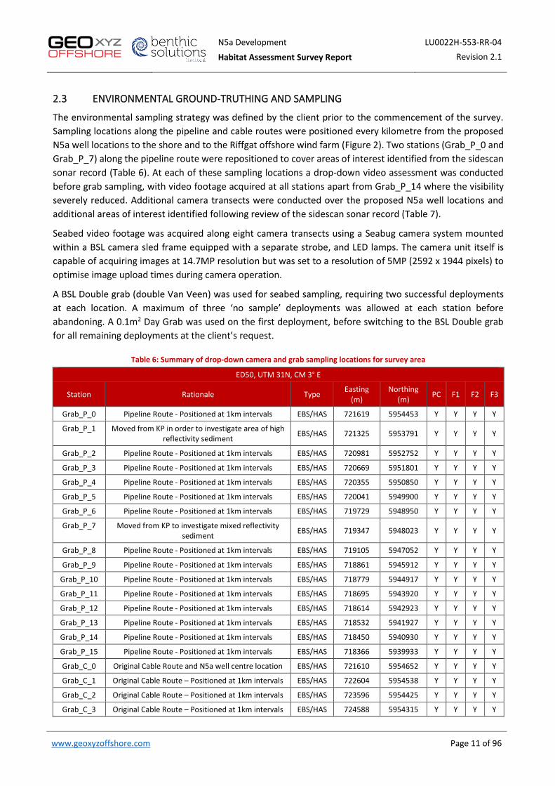
N5a Development LU0022H-553-RR-04
Habitat Assessment Survey Report Revision 2.1
www.geoxyzoffshore.com Page 11 of 96
2.3 ENVIRONMENTAL GROUND-TRUTHING AND SAMPLING
The environmental sampling strategy was defined by the client prior to the commencement of the survey. Sampling locations along the pipeline and cable routes were positioned every kilometre from the proposed N5a well locations to the shore and to the Riffgat offshore wind farm (Figure 2). Two stations (Grab_P_0 and Grab_P_7) along the pipeline route were repositioned to cover areas of interest identified from the sidescan sonar record (Table 6). At each of these sampling locations a drop-down video assessment was conducted before grab sampling, with video footage acquired at all stations apart from Grab_P_14 where the visibility severely reduced. Additional camera transects were conducted over the proposed N5a well locations and additional areas of interest identified following review of the sidescan sonar record (Table 7).
Seabed video footage was acquired along eight camera transects using a Seabug camera system mounted within a BSL camera sled frame equipped with a separate strobe, and LED lamps. The camera unit itself is capable of acquiring images at 14.7MP resolution but was set to a resolution of 5MP (2592 x 1944 pixels) to optimise image upload times during camera operation.
A BSL Double grab (double Van Veen) was used for seabed sampling, requiring two successful deployments at each location. A maximum of three ‘no sample’ deployments was allowed at each station before abandoning. A 0.1m2 Day Grab was used on the first deployment, before switching to the BSL Double grab for all remaining deployments at the client’s request.
Table 6: Summary of drop-down camera and grab sampling locations for survey area
ED50, UTM 31N, CM 3° E
Station Rationale Type Easting (m)
Northing (m) PC F1 F2 F3
Grab_P_0 Pipeline Route - Positioned at 1km intervals EBS/HAS 721619 5954453 Y Y Y Y
Grab_P_1 Moved from KP in order to investigate area of high reflectivity sediment EBS/HAS 721325 5953791 Y Y Y Y
Grab_P_2 Pipeline Route - Positioned at 1km intervals EBS/HAS 720981 5952752 Y Y Y Y
Grab_P_3 Pipeline Route - Positioned at 1km intervals EBS/HAS 720669 5951801 Y Y Y Y
Grab_P_4 Pipeline Route - Positioned at 1km intervals EBS/HAS 720355 5950850 Y Y Y Y
Grab_P_5 Pipeline Route - Positioned at 1km intervals EBS/HAS 720041 5949900 Y Y Y Y
Grab_P_6 Pipeline Route - Positioned at 1km intervals EBS/HAS 719729 5948950 Y Y Y Y
Grab_P_7 Moved from KP to investigate mixed reflectivity sediment EBS/HAS 719347 5948023 Y Y Y Y
Grab_P_8 Pipeline Route - Positioned at 1km intervals EBS/HAS 719105 5947052 Y Y Y Y
Grab_P_9 Pipeline Route - Positioned at 1km intervals EBS/HAS 718861 5945912 Y Y Y Y
Grab_P_10 Pipeline Route - Positioned at 1km intervals EBS/HAS 718779 5944917 Y Y Y Y
Grab_P_11 Pipeline Route - Positioned at 1km intervals EBS/HAS 718695 5943920 Y Y Y Y
Grab_P_12 Pipeline Route - Positioned at 1km intervals EBS/HAS 718614 5942923 Y Y Y Y
Grab_P_13 Pipeline Route - Positioned at 1km intervals EBS/HAS 718532 5941927 Y Y Y Y
Grab_P_14 Pipeline Route - Positioned at 1km intervals EBS/HAS 718450 5940930 Y Y Y Y
Grab_P_15 Pipeline Route - Positioned at 1km intervals EBS/HAS 718366 5939933 Y Y Y Y
Grab_C_0 Original Cable Route and N5a well centre location EBS/HAS 721610 5954652 Y Y Y Y
Grab_C_1 Original Cable Route – Positioned at 1km intervals EBS/HAS 722604 5954538 Y Y Y Y
Grab_C_2 Original Cable Route – Positioned at 1km intervals EBS/HAS 723596 5954425 Y Y Y Y
Grab_C_3 Original Cable Route – Positioned at 1km intervals EBS/HAS 724588 5954315 Y Y Y Y
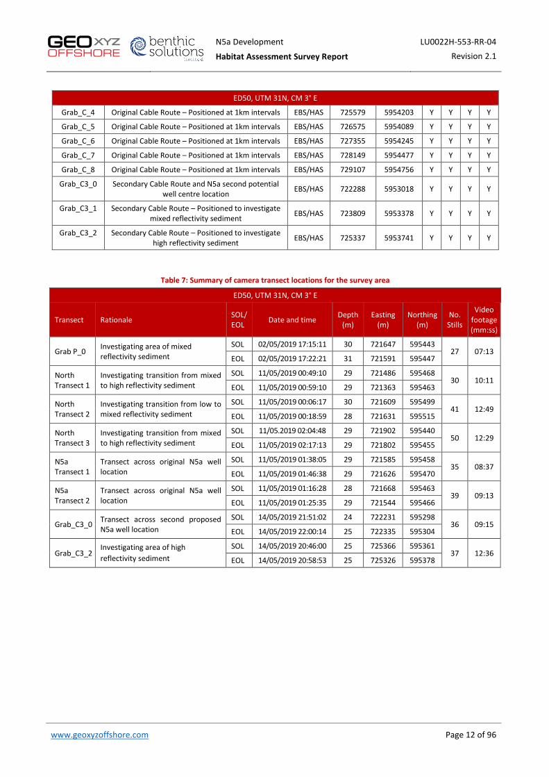
N5a Development LU0022H-553-RR-04
Habitat Assessment Survey Report Revision 2.1
www.geoxyzoffshore.com Page 12 of 96
ED50, UTM 31N, CM 3° E
Grab_C_4 Original Cable Route – Positioned at 1km intervals EBS/HAS 725579 5954203 Y Y Y Y
Grab_C_5 Original Cable Route – Positioned at 1km intervals EBS/HAS 726575 5954089 Y Y Y Y
Grab_C_6 Original Cable Route – Positioned at 1km intervals EBS/HAS 727355 5954245 Y Y Y Y
Grab_C_7 Original Cable Route – Positioned at 1km intervals EBS/HAS 728149 5954477 Y Y Y Y
Grab_C_8 Original Cable Route – Positioned at 1km intervals EBS/HAS 729107 5954756 Y Y Y Y
Grab_C3_0 Secondary Cable Route and N5a second potential well centre location EBS/HAS 722288 5953018 Y Y Y Y
Grab_C3_1 Secondary Cable Route – Positioned to investigate mixed reflectivity sediment EBS/HAS 723809 5953378 Y Y Y Y
Grab_C3_2 Secondary Cable Route – Positioned to investigate high reflectivity sediment EBS/HAS 725337 5953741 Y Y Y Y
Table 7: Summary of camera transect locations for the survey area
ED50, UTM 31N, CM 3° E
Transect Rationale SOL/EOL Date and time Depth
(m) Easting
(m) Northing
(m) No.
Stills
Video footage (mm:ss)
Grab P_0 Investigating area of mixed reflectivity sediment
SOL 02/05/2019 17:15:11 30 721647 5954430 27 07:13
EOL 02/05/2019 17:22:21 31 721591 5954476
North Transect 1
Investigating transition from mixed to high reflectivity sediment
SOL 11/05/2019 00:49:10 29 721486 5954680 30 10:11
EOL 11/05/2019 00:59:10 29 721363 5954634
North Transect 2
Investigating transition from low to mixed reflectivity sediment
SOL 11/05/2019 00:06:17 30 721609 5954992 41 12:49
EOL 11/05/2019 00:18:59 28 721631 5955152
North Transect 3
Investigating transition from mixed to high reflectivity sediment
SOL 11/05.2019 02:04:48 29 721902 5954407 50 12:29
EOL 11/05/2019 02:17:13 29 721802 5954550
N5a Transect 1
Transect across original N5a well location
SOL 11/05/2019 01:38:05 29 721585 5954588 35 08:37
EOL 11/05/2019 01:46:38 29 721626 5954708
N5a Transect 2
Transect across original N5a well location
SOL 11/05/2019 01:16:28 28 721668 5954631 39 09:13
EOL 11/05/2019 01:25:35 29 721544 5954667
Grab_C3_0 Transect across second proposed N5a well location
SOL 14/05/2019 21:51:02 24 722231 5952983 36 09:15
EOL 14/05/2019 22:00:14 25 722335 5953047
Grab_C3_2 Investigating area of high reflectivity sediment
SOL 14/05/2019 20:46:00 25 725366 5953610 37 12:36
EOL 14/05/2019 20:58:53 25 725326 5953785

N5a Development LU0022H-553-RR-04
Habitat Assessment Survey Report Revision 2.1
www.geoxyzoffshore.com Page 13 of 96
Figure 2: Survey strategy overview

N5a Development LU0022H-553-RR-04
Habitat Assessment Survey Report Revision 2.1
www.geoxyzoffshore.com Page 14 of 96
2.4 HABITAT INVESTIGATION
2.4.1 Habitat Classification
A marine biotope classification system for British waters was developed by Connor et al. (2004) from data acquired during the JNCC Marine Nature Conservation Review (MNCR) and subsequently revised by Parry et
al. (2015) to provide improved classification of deep-sea habitats. The resultant combined JNCC (2015) classification system forms the basis of the European Nature Information Service Habitat Classification (EUNIS, 2013), albeit with differing habitat coding nomenclature, which has compiled habitat information from across Europe into a single database. The two classification systems are both based around the same hierarchical analysis. Initially abiotic habitats are defined at four levels. Biological communities are then linked to these (at two lower levels) to produce a biotope classification. (Connor et al., 2004; EUNIS, 2013).
Habitat descriptions have been interpreted from the side scan sonar and bathymetric data acquired during the current survey, in conjunction with additional information on seabed sediment types and faunal communities from seabed photography and grab sampling. Global Mapper V20 GIS software was used to review side scan sonar mosaic (Geotiff) and multibeam bathymetry data (Geotiff and xyz) and to delineate areas of different seabed habitats.
2.4.2 Assessment of Sensitive Habitats
The Netherlands is a signatory of the Convention on the Conservation of European Wildlife and Natural Habitats (Bern Convention, 1979). To meet their obligations under the convention, the European Community Habitats Directive was adopted in 1992. The provisions of the Directive require Member States to introduce a range of measures including the protection of species listed in the Annexes; to undertake surveillance of habitats and species and produce a report every six years on the implementation of the Directive. The 189 habitats listed in Annex I of the Directive and the 788 species listed in Annex II, are to be protected by means of a network of sites. Each Member State is required to prepare and propose a national list of sites, which will be evaluated in order to form a European network of Sites of Community Importance (SCIs). These will eventually be designated by Member States as Special Areas of Conservation (SACs), and along with Special Protection Areas (SPAs) classified under the EC Birds Directive (2009), form a network of protected areas known as Natura 2000. The Directive was amended in 1997 by a technical adaptation Directive and latterly by the Environment Chapter of the Treaty of Accession 2003.
Based on the above, the OSPAR list of threatened and/or declining species and habitats and Annex I habitats of particular relevance to this region of UK waters are:
• Biogenic reefs formed by Sabellaria spinulosa (the Ross Worm); and, • Sandbanks which are slightly covered by sea water all the time
Stony reefs are an Annex I habitat and are protected under the EU habitats directive. Sampling location Grab_C3_2 showed a high proportion of cobbles and boulders, and consequently a stony reef assessment was conducted. The seabed camera ground-truthing data were assessed for potential stony reefs using the criteria proposed by Irving (2009). While the Irving (2009) criteria have been approved by the UK regulators for application in UK waters, they have not been explicitly approved by the Netherlands authorities but are used here as they provide a useful basis for semi-quantitative assessment of potential Annex I stony reef habitat. The Irving (2009) method breaks down the assessment criteria into measures of reef ‘quality’ or ‘reefiness’ as outlined in Table 8. This is based on a minimum cobble size of 64mm being present and
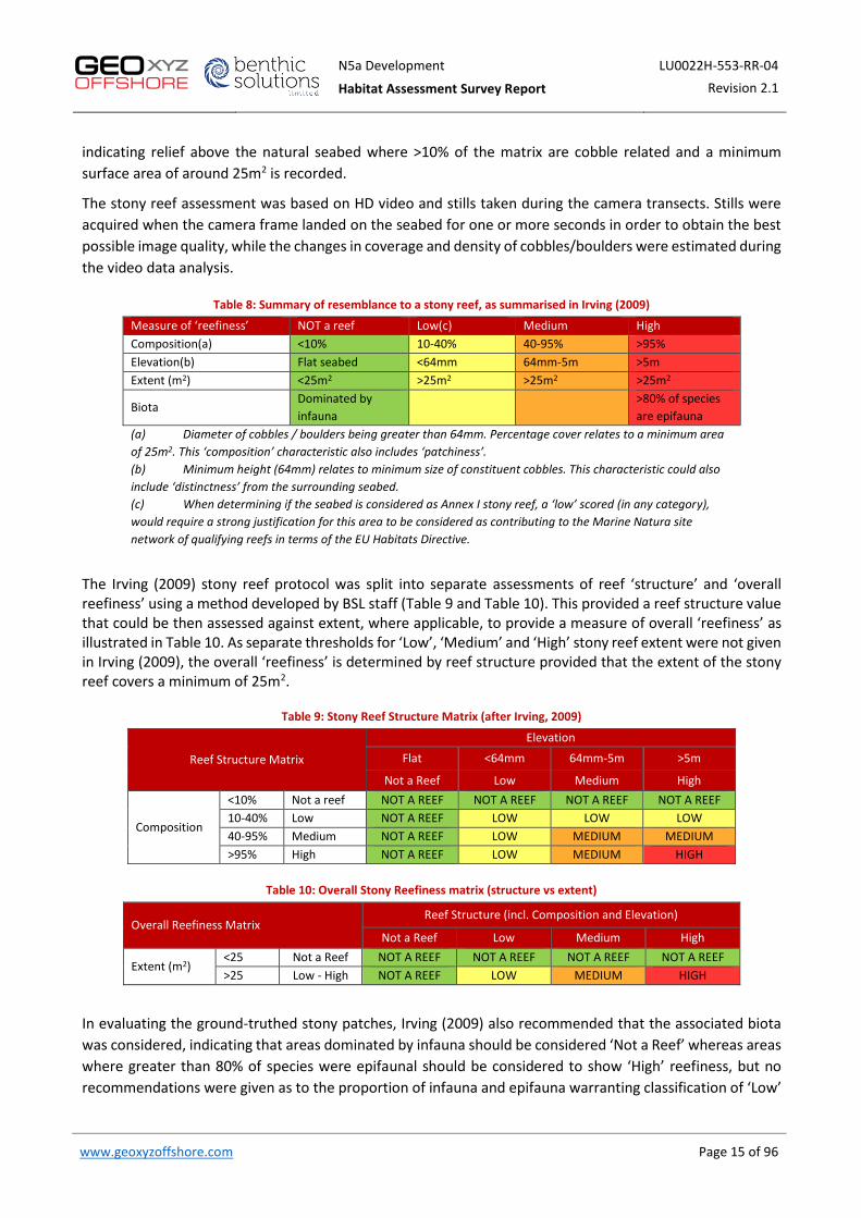
N5a Development LU0022H-553-RR-04
Habitat Assessment Survey Report Revision 2.1
www.geoxyzoffshore.com Page 15 of 96
indicating relief above the natural seabed where >10% of the matrix are cobble related and a minimum surface area of around 25m2 is recorded.
The stony reef assessment was based on HD video and stills taken during the camera transects. Stills were acquired when the camera frame landed on the seabed for one or more seconds in order to obtain the best possible image quality, while the changes in coverage and density of cobbles/boulders were estimated during the video data analysis.
Table 8: Summary of resemblance to a stony reef, as summarised in Irving (2009)
Measure of ‘reefiness’ NOT a reef Low(c) Medium High Composition(a) <10% 10-40% 40-95% >95% Elevation(b) Flat seabed <64mm 64mm-5m >5m Extent (m2) <25m2 >25m2 >25m2 >25m2
Biota Dominated by infauna
>80% of species are epifauna
(a) Diameter of cobbles / boulders being greater than 64mm. Percentage cover relates to a minimum area
of 25m2. This ‘composition’ characteristic also includes ‘patchiness’.
(b) Minimum height (64mm) relates to minimum size of constituent cobbles. This characteristic could also
include ‘distinctness’ from the surrounding seabed.
(c) When determining if the seabed is considered as Annex I stony reef, a ‘low’ scored (in any category),
would require a strong justification for this area to be considered as contributing to the Marine Natura site
network of qualifying reefs in terms of the EU Habitats Directive.
The Irving (2009) stony reef protocol was split into separate assessments of reef ‘structure’ and ‘overall reefiness’ using a method developed by BSL staff (Table 9 and Table 10). This provided a reef structure value that could be then assessed against extent, where applicable, to provide a measure of overall ‘reefiness’ as illustrated in Table 10. As separate thresholds for ‘Low’, ‘Medium’ and ‘High’ stony reef extent were not given in Irving (2009), the overall ‘reefiness’ is determined by reef structure provided that the extent of the stony reef covers a minimum of 25m2.
Table 9: Stony Reef Structure Matrix (after Irving, 2009)
Reef Structure Matrix
Elevation
Flat <64mm 64mm-5m >5m
Not a Reef Low Medium High
Composition
<10% Not a reef NOT A REEF NOT A REEF NOT A REEF NOT A REEF 10-40% Low NOT A REEF LOW LOW LOW 40-95% Medium NOT A REEF LOW MEDIUM MEDIUM >95% High NOT A REEF LOW MEDIUM HIGH
Table 10: Overall Stony Reefiness matrix (structure vs extent)
Overall Reefiness Matrix Reef Structure (incl. Composition and Elevation)
Not a Reef Low Medium High
Extent (m2) <25 Not a Reef NOT A REEF NOT A REEF NOT A REEF NOT A REEF >25 Low - High NOT A REEF LOW MEDIUM HIGH
In evaluating the ground-truthed stony patches, Irving (2009) also recommended that the associated biota was considered, indicating that areas dominated by infauna should be considered ‘Not a Reef’ whereas areas where greater than 80% of species were epifaunal should be considered to show ‘High’ reefiness, but no recommendations were given as to the proportion of infauna and epifauna warranting classification of ‘Low’

N5a Development LU0022H-553-RR-04
Habitat Assessment Survey Report Revision 2.1
www.geoxyzoffshore.com Page 16 of 96
or ‘Medium’ reefiness. In practise, it is not practical to assess the proportion of infaunal and epifaunal species in a quantitative manner. This cannot be undertaken from seabed camera data (i.e. video footage or still photographs) as only the larger epifauna and emergent infauna are visible. To accurately quantify the proportion of infauna and epifauna species, it would be necessary to take large enough samples to include both the stony material (i.e. cobbles and boulders) and the surrounding sediment matrix, with sufficient replication to provide confidence in the resultant data. This would likely involve sampling with a large volume sampler such as a clam dredge and could significantly impact the integrity of the cobble/boulder patch. As such the biota associated with stony patches from the current survey has been described in a qualitatively.
N5a Development LU0022H-553-RR-04
Habitat Assessment Survey Report Revision 2.1
www.geoxyzoffshore.com Page 17 of 96
3 RESULTS AND INTERPRETATION
3.1 BATHYMETRY
The following text was adapted from the survey reports for the N5A site (LU-0022H-553-RR-01), N5A to NGT Hot Tap pipeline route (LU-0022H-553-RR-02) and N5A to Riffgat cable route (LU-0022H-553-RR-07) to provide an overview of the bathymetry across the survey site and route corridors.
Bathymetry data were acquired using an R2 Sonics 2022 multi-beam echo sounder for the site and an R2Sonic 2024 multi-beam echo sounder for the two route surveys. All bathymetry data have been reduced to LAT, which was 1.6m below MSL within the survey area, and are presented at a 0.5m x 0.5m bin size.
3.1.1 N5A to NGT Hot Tap Pipeline Route
Water depths along the proposed N5A to NGT Hot Tap pipeline route ranged between 9.8m LAT at KP0.000 and 26.4m LAT at KP14.675, with the seabed shoaling gently towards the southern end of the proposed pipeline route. A series of natural troughs trending west-north-west to east-south-east occurred within the survey corridor, crossing the proposed pipeline route, the largest of which was approximately 250m wide.
A variety of anthropogenic debris/wreck and areas of disturbed seabed were evident on the bathymetry data:
• Two prominent features interpreted as shipwrecks surrounded by seabed scouring; the largest (40.1m x 12.8m x 1.1m) occurred at approximately KP2.462, 369m west-north-west of the proposed route and the other (19.1m x 12.9m x 0.2m) occurred at approximately KP2.373, 339m west-north-west of the proposed route.
• Three semi-circular features with 1m of positive relief, interpreted as being related to previous drilling activity, were observed on bathymetry data. These were observed at the start of the proposed route between KP0.009 and KP0.089, offset by 90m to the east-south-east at their closest approach. These features lay within a 30m radius of each other and exhibited average dimensions of 30m x 30m.
• Three existing cables and one pipeline were expected to cross the proposed pipeline route but were not observed on the bathymetry data.
3.1.2 N5A to Riffgat Cable Route
The seabed shoaled gently towards the east-north-east end of the proposed N5A to Riffgat cable route with water depths ranging between 26.0m at KP0.280 and 19.6m KP7.941. A series of natural troughs, predominantly trending north-west to south-east, crossed the proposed cable route from approximately KP5.158 to KP8.681 and were interpreted to be related to tidal/current processes.
Three semi-circular features with 1m of positive relief, interpreted as being related to previous drilling activity, were imaged in the bathymetry data. These were positioned at the start of the proposed route between KP0.085 and KP0.168; at their minimum offset from the route they were approximately 27m south-south-west. They were positioned within a 30m radius and had average dimensions of 30m x 30m.
The Norned cable was observed crossing the proposed cable route at KP 2.313 trending north-north-west to south-south-east.

N5a Development LU0022H-553-RR-04
Habitat Assessment Survey Report Revision 2.1
www.geoxyzoffshore.com Page 18 of 96
3.2 SEABED FEATURES
The following text was adapted from the survey reports for the N5A site (LU-0022H-553-RR-01), N5A to NGT Hot Tap pipeline route (LU-0022H-553-RR-02) and N5A to Riffgat cable route (LU-0022H-553-RR-07) to provide an overview of the seabed features across the survey area, focussing on features of particular relevance to the environmental baseline and habitat assessment of the survey area.
Side scan sonar data were acquired with an Edgetech 4200 system operating at 100kHz/400kHz with between 75m and 200m per channel range. This was supplemented by swathe bathymetry data gridded to 0.5m bin size.
3.2.1 N5A Site
Seabed sediments across the N5A survey area were expected to comprise ‘fine sand with shell fragments’. An area of ‘coarse sand and shell with a high density of sand mason worms and razor clams’ was evident in the north of the survey area, while an area of ‘coarse sand with pebbles and cobbles’ was present in the south. The uppermost sand unit was merely a veneer and the boundary between the sand and the underlying clay outcrops was arbitrary with the potential for some clay to outcrop in the areas interpreted as sand.
Outcrops of clay were interpreted within the survey area, showing a positive relief of up to 0.5m above background seabed levels. Elsewhere accumulations of coarse sand and gravel were also observed on the bathymetry as having positive relief above the ambient seabed, with some accumulations likely to be caused by the stabilising effect of high densities of sand mason worms and razor clams on the seabed.
Within the survey area there was no existing infrastructure other than the previously drilled N5 Well. Seabed scars up to 1.1m high from the rig whilst over the N5-Ruby wellsite were observed on the bathymetry and side scan sonar data. Numerous magnetometer anomalies were observed within this area, however no wellhead or other evidence of the drilling location could be observed at seabed.
3.2.2 N5A to NGT Hot Tap Pipeline Route
Seabed sediments along the proposed pipeline route corridor were expected to comprise ‘fine sand and shell fragments’, with occasional areas of ‘coarse sand and shell fragments’.
Bedforms were not imaged in the sonar or bathymetry records. However, photographs taken along the route as part of the environmental survey showed clear seabed rippling over the majority of the survey corridor.
Numerous objects interpreted as boulders and items of debris were observed within the proposed pipeline route corridor. Most of the objects interpreted as boulders occurred towards the north of the survey corridor area and coincided with areas of clay exposure.
The most significant objects identified on the sonar records were two interpreted shipwrecks, the largest (40.1m x 12.8m x 1.1m) occurring at approximately KP2.462, 369m west-north-west of the proposed route and the other (19.1m x 12.9m x 0.2m) at approximately KP2.373, 339m west-north-west of the proposed route.
Three existing cables and one pipeline were expected to cross the proposed pipeline route but were not observed on the bathymetry data.
3.2.3 N5A to Riffgat Cable Route
Seabed sediments along the proposed pipeline route corridor were expected to comprise fine to coarse SAND, with occasional areas of ‘coarse sand and clay with pebbles and cobbles’ and ‘coarse sand with pebbles
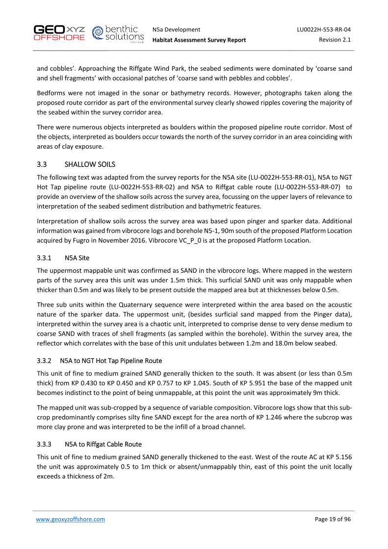
N5a Development LU0022H-553-RR-04
Habitat Assessment Survey Report Revision 2.1
www.geoxyzoffshore.com Page 19 of 96
and cobbles’. Approaching the Riffgate Wind Park, the seabed sediments were dominated by ‘coarse sand and shell fragments’ with occasional patches of ‘coarse sand with pebbles and cobbles’.
Bedforms were not imaged in the sonar or bathymetry records. However, photographs taken along the proposed route corridor as part of the environmental survey clearly showed ripples covering the majority of the seabed within the survey corridor area.
There were numerous objects interpreted as boulders within the proposed pipeline route corridor. Most of the objects, interpreted as boulders occur towards the north of the survey corridor in an area coinciding with areas of clay exposure.
3.3 SHALLOW SOILS
The following text was adapted from the survey reports for the N5A site (LU-0022H-553-RR-01), N5A to NGT Hot Tap pipeline route (LU-0022H-553-RR-02) and N5A to Riffgat cable route (LU-0022H-553-RR-07) to provide an overview of the shallow soils across the survey area, focussing on the upper layers of relevance to interpretation of the seabed sediment distribution and bathymetric features.
Interpretation of shallow soils across the survey area was based upon pinger and sparker data. Additional information was gained from vibrocore logs and borehole N5-1, 90m south of the proposed Platform Location acquired by Fugro in November 2016. Vibrocore VC_P_0 is at the proposed Platform Location.
3.3.1 N5A Site
The uppermost mappable unit was confirmed as SAND in the vibrocore logs. Where mapped in the western parts of the survey area this unit was under 1.5m thick. This surficial SAND unit was only mappable when thicker than 0.5m and was likely to be present outside the mapped area but at thicknesses below 0.5m.
Three sub units within the Quaternary sequence were interpreted within the area based on the acoustic nature of the sparker data. The uppermost unit, (besides surficial sand mapped from the Pinger data), interpreted within the survey area is a chaotic unit, interpreted to comprise dense to very dense medium to coarse SAND with traces of shell fragments (as sampled within the borehole). Within the survey area, the reflector which correlates with the base of this unit undulates between 1.2m and 18.0m below seabed.
3.3.2 N5A to NGT Hot Tap Pipeline Route
This unit of fine to medium grained SAND generally thicken to the south. It was absent (or less than 0.5m thick) from KP 0.430 to KP 0.450 and KP 0.757 to KP 1.045. South of KP 5.951 the base of the mapped unit becomes indistinct to the point of being unmappable, at this point the unit was approximately 9m thick.
The mapped unit was sub-cropped by a sequence of variable composition. Vibrocore logs show that this sub-crop predominantly comprises silty fine SAND except for the area north of KP 1.246 where the subcrop was more clay prone and was interpreted to be the infill of a broad channel.
3.3.3 N5A to Riffgat Cable Route
This unit of fine to medium grained SAND generally thickened to the east. West of the route AC at KP 5.156 the unit was approximately 0.5 to 1m thick or absent/unmappably thin, east of this point the unit locally exceeds a thickness of 2m.

N5a Development LU0022H-553-RR-04
Habitat Assessment Survey Report Revision 2.1
www.geoxyzoffshore.com Page 20 of 96
Vibrocore logs showed that the mapped unit was sub-cropped by clay prone deposits from KP0 to KP 3.357, interpreted to be the infill of a broad channel. From KP 3.357 to the end of the route the mapped unit was subcropped by fine SAND.

N5a Development LU0022H-553-RR-04
Habitat Assessment Survey Report Revision 2.1
www.geoxyzoffshore.com Page 21 of 96
Figure 3: N5A Site and Route Survey Bathymetry

N5a Development LU0022H-553-RR-04
Habitat Assessment Survey Report Revision 2.1
www.geoxyzoffshore.com Page 22 of 96
Figure 4: Interpreted N5A Site and Route Seabed Features

N5a Development LU0022H-553-RR-04
Habitat Assessment Survey Report Revision 2.1
www.geoxyzoffshore.com Page 23 of 96
3.3.4 N5A Site
The seabed within the N5A site survey area sloped gently to the west. The minimum water depth was 23.7m LAT in the NNE of the survey area, while the maximum depth was 26.6m LAT in the WSW. Small areas with relief of up to 0.4m were observed on the bathymetry data with measured gradients of up 6° on their flanks, which were interpreted to be largely due to outcropping clays.
3.4 HABITAT ASSESSMENT
3.4.1 Video/Photographic Survey
A total of twenty-eight drop-down camera deployments and eight camera transects were conducted within the combined N5A development site and route survey area. The camera ground-truthing was undertaken to investigate the distribution of different seabed habitats and associated fauna, while additionally assessing the presence or absence of potential sensitive habitats and species. Drop-down camera deployments were undertaken to provide additional data on the composition of the seabed sediment and associated visible fauna. In contrast, the camera transects were selected to investigate areas of different acoustic facies on the side scan sonar record and/or bathymetric features evident on the MBES data. The ground-truthing stations and transects are listed in Table 6 and Table 7, respectively, and their locations are shown in Figure 2 to Figure 4, with summary photopages included in Appendix H.
Seabed video and photographic data were acquired using a Seabug camera system mounted within a BSL camera sled frame equipped with a separate strobe, and LED lamps. The Seabug is capable of acquiring images at 14.7MP resolution but was set to a resolution of 5MP (2592 x 1944 pixels) to optimise image upload times during camera operation. (see Appendix B and D).
Video and camera ground-truthing along all of the transects confirmed the presence of sand-dominated substrate throughout the site and route survey areas. While the dominant sediment type was ‘fine sand and shell fragments’, several patches of coarser sediment were present across the survey area. The N5A site and route survey corridor to the Riffgate Wind Park showed increasingly coarse sediment, including areas of gravel (>2mm), pebble (>4mm) and cobble (>64mm) in addition to sporadic clay outcrops. The area of coarser substrate along the northern edge of the N5A site and the route survey corridor to the Riffgate Wind Park also supported significant densities of sand mason worms (Lanice conchilega) and razor clams (Ensis sp., possibly E. leei). Although both L. conchilega and E. leei were observed elsewhere within the N5A site and along the route to the wind park, they were less numerous and more patchily distributed outside the area of the delineated area of ‘coarse sand and shell with a high density of sand mason worms and razor clams’. Habitat assessment logs for each of the nineteen camera transects locations are included in Appendix E.
Conspicuous epifauna showed moderate diversity and density for a predominantly mobile sandy seabed. Camera ground-truthing stations and transects across all mapped seabed habitats showed a similar species assemblage including frequent observations of sand mason worms (Lanice conchilega) and common starfish (Asterias rubens). Other species observed more sporadically throughout the combined N5A site and route survey area included razor clams (Ensis sp. possibly E. leei), burrowing anemones (Cerianthidae), swimming crabs (Liocarcinus sp.), masked crabs (Corystes cassivelaunus), hermit crabs (Paguridae sp.), edible crabs (Cancer pagurus), brittlestars (Ophiuridae), gobies (Gobiidae), dragonets (Callionymus lyra), flatfish (Pleuronectiformes) and sandeels (Ammodytes sp.).
Areas of coarser substrate, including the delineated area of ‘coarse sand and shell with a high density of sand mason worms (L. conchilega) and razor clams (suspected E. leei)’, were characterized by higher abundances

N5a Development LU0022H-553-RR-04
Habitat Assessment Survey Report Revision 2.1
www.geoxyzoffshore.com Page 24 of 96
of all of the aforementioned fauna with additional observations of plumose anemones (Metridium senile), unidentified anemones (Actiniaria), cuttlefish (Sepiidae), European squid (Loligo vulgaris), common dab (Limanda limanda) and grey gurnard (Eutriglia gurnardus).
Example photographs of the common and/or conspicuous faunal groups encountered during the N5A development survey are provided in Appendix F.
3.4.2 General Habitats
Video and still photography ground-truthing from twenty-eight drop-down camera deployments and eight camera transects confirmed the presence of a predominantly sandy seabed with spatial variability in the proportions of shell fragments, coarse substrate (gravel, pebbles and cobbles) and outcropping clay. In addition, an areas of coarse substrate along the northern edge of the survey area supported high densities of sand mason worms (Lanice conchilega) and razor clams (suspected Ensis leei).
Habitats were identified using a combination of field observations, detailed review of video footage and still images. Based on the ground-truthing data obtained from the N5A development site and route survey area, four EUNIS habitat classifications were assigned: ‘Infralittoral fine sand’ (A5.23), ‘Infralittoral coarse sediment’ (A5.13), ‘Infralittoral Mixed Sediment’ (A5.43) and ‘Dense Lanice conchilega and other polychaetes in tide-swept infralittoral sand and mixed gravelly sand’ (A5.137). The habitat classifications for the N5A development survey area are illustrated in Figure 9.
‘Infralittoral Fine Sand’ (A5.23)
Habitats dominated by fine sand with variable levels of shell debris were dominant across the survey area, being observed on the majority of environmental camera drops and transects within the N5A site and route survey area. These areas were represented by relatively smooth and low reflectivity side scan sonar data and were classified as the ‘fine sand and shell fragments’ seabed features type (Section 3.2 and Figure 4) and the EUNIS level 4 ’Infralittoral fine sand’ (A5.23) habitat type (Figure 9).
‘Infralittoral fine sand’ habitat is typically characterised by clean sands which occur in shallow water, either on the open coast or in tide-swept channels of marine inlets in water depths of around 0 to 20m. The habitat typically lacks a significant seaweed component and is characterised by robust fauna, particularly amphipods (Bathyporeia) and robust polychaetes including Nephtys cirrosa and Lanice conchilega. Within the N5A development survey area, this habitat comprised clean rippled sands in water depths of approximately 13 to 30m, slightly exceeding the typically expected range.
Visible fauna from camera ground-truthing within areas of ‘infralittoral fine sand’ included low to moderate densities the sand mason worm (L. conchilega) throughout, in addition to several other taxa characteristic of this EUNIS habitat, including common starfish (Asterias rubens), swimming crab (Liocarcinus) and hermit crabs (Paguridae). Other fauna observed within areas of this habitat included lugworms (Arenicola sp.), masked crab (Corystes cassivellaunus), edible crab (Cancer pagurus), razor clams (Ensis sp.), brittlestars (Ophiuridae), gobies (Gobiidae), dragonets (Callionymus lyra), flatfish (Pleuronectiform). Further taxa evident from grab samples included occasional sandeel (Ammodytidae), heart urchins (Echinocardium cordatum), ragworms (Nereis spp.), unidentified sea urchins (spatangoid) and porcelain crab (Portunidae).
Review of the seabed camera and grab sample data indicated that the mapped distribution of ‘infralittoral fine sand’ (A5.23) habitat was fairly accurate. Only station P_9 showing more coarse sandy sediment than would be expected for ‘infralittoral fine sand’ habitat but, as this sampling station was located within an area of alternating bands of ‘infralittoral fine sand’ and ‘infralittoral coarse sand’, it is to be expected that there
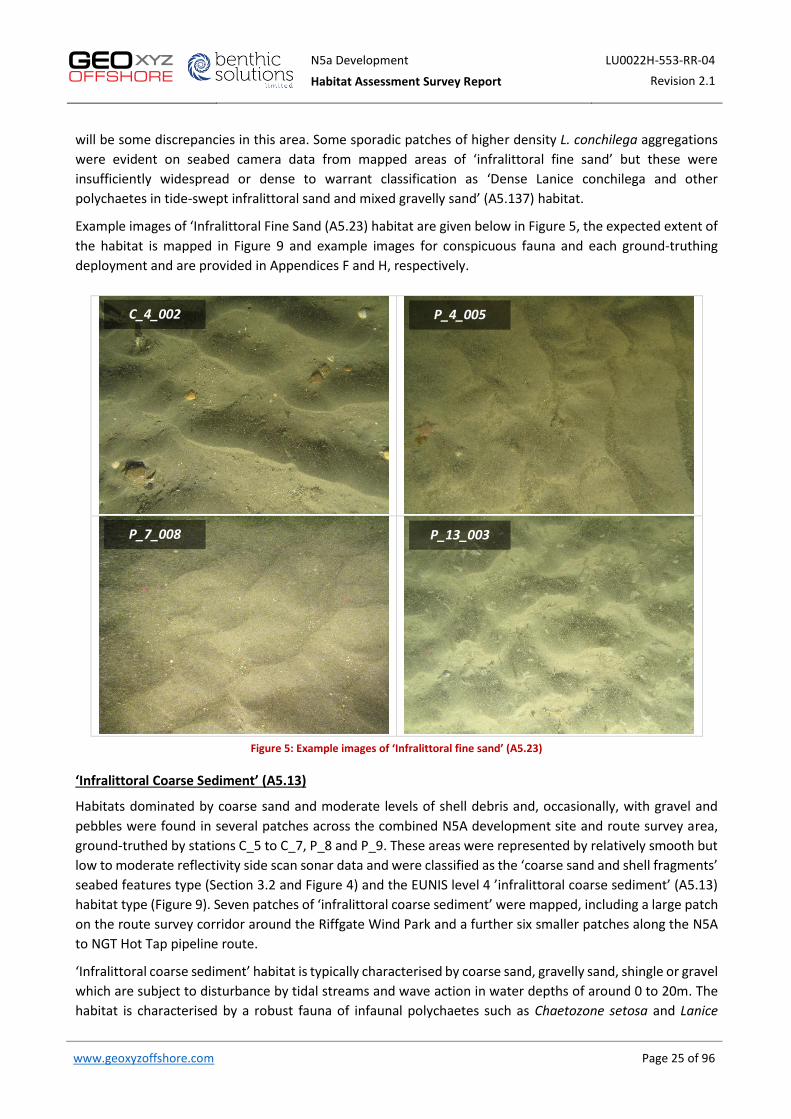
N5a Development LU0022H-553-RR-04
Habitat Assessment Survey Report Revision 2.1
www.geoxyzoffshore.com Page 25 of 96
will be some discrepancies in this area. Some sporadic patches of higher density L. conchilega aggregations were evident on seabed camera data from mapped areas of ‘infralittoral fine sand’ but these were insufficiently widespread or dense to warrant classification as ‘Dense Lanice conchilega and other polychaetes in tide-swept infralittoral sand and mixed gravelly sand’ (A5.137) habitat.
Example images of ‘Infralittoral Fine Sand (A5.23) habitat are given below in Figure 5, the expected extent of the habitat is mapped in Figure 9 and example images for conspicuous fauna and each ground-truthing deployment and are provided in Appendices F and H, respectively.
Figure 5: Example images of ‘Infralittoral fine sand’ (A5.23)
‘Infralittoral Coarse Sediment’ (A5.13)
Habitats dominated by coarse sand and moderate levels of shell debris and, occasionally, with gravel and pebbles were found in several patches across the combined N5A development site and route survey area, ground-truthed by stations C_5 to C_7, P_8 and P_9. These areas were represented by relatively smooth but low to moderate reflectivity side scan sonar data and were classified as the ‘coarse sand and shell fragments’ seabed features type (Section 3.2 and Figure 4) and the EUNIS level 4 ’infralittoral coarse sediment’ (A5.13) habitat type (Figure 9). Seven patches of ‘infralittoral coarse sediment’ were mapped, including a large patch on the route survey corridor around the Riffgate Wind Park and a further six smaller patches along the N5A to NGT Hot Tap pipeline route.
‘Infralittoral coarse sediment’ habitat is typically characterised by coarse sand, gravelly sand, shingle or gravel which are subject to disturbance by tidal streams and wave action in water depths of around 0 to 20m. The habitat is characterised by a robust fauna of infaunal polychaetes such as Chaetozone setosa and Lanice
P_7_008 P_13_003
C_4_002 P_4_005

N5a Development LU0022H-553-RR-04
Habitat Assessment Survey Report Revision 2.1
www.geoxyzoffshore.com Page 26 of 96
conchilega, cumacean crustacea such as Iphinoe trispinosa and Diastylis bradyi, and venerid bivalves. Within the N5A development survey area, this habitat comprised rippled coarse shelly sands, sometimes with a discernible gravel and/or pebble content in water depths of approximately 19 to 30m, slightly exceeding the typically expected range.
Visible fauna from camera ground-truthing within areas of ‘infralittoral fine sand’ included low to moderate densities the sand mason worm (L. conchilega) throughout, in addition to common starfish (Asterias rubens), which are both characteristic species for this EUNIS habitat. The majority of other characterising taxa for this habitat are infaunal species are not effectively assessed from seabed camera ground-truthing.
Review of the seabed camera and grab sample data indicated that the mapped distribution of ‘infralittoral coarse sediment’ (A5.13) habitat was fairly accurate, but with two exceptions. Station C_0 was classified as ‘infralittoral coarse sediment’ habitat but was located within an area of ‘Dense Lanice conchilega and other polychaetes in tide-swept infralittoral sand and mixed gravelly sand’ (A5.137) habitat, while station C_8 was classified as ‘infralittoral fine sand’ habitat but was located within an area of ‘infralittoral coarse sediment’. Both of these exceptions reflect the heterogenous nature of the seabed habitats within the survey area.
Example images of ‘infralittoral coarse sediment (A5.13) habitat are given below in Figure 6, the expected extent of the habitat is mapped in Figure 9 and example images for conspicuous fauna and each ground-truthing deployment and are provided in Appendices F and H, respectively.
Figure 6: Example images of ‘Infralittoral coarse sediment’ (A5.13)
P_8_002 P_9_003
C_5_005 C_7_006

N5a Development LU0022H-553-RR-04
Habitat Assessment Survey Report Revision 2.1
www.geoxyzoffshore.com Page 27 of 96
‘Infralittoral Mixed Sediment’ (A5.43)
Habitats dominated by coarse gravelly sand with pebbles, cobbles and, in some areas exposed clay clasts, were found delineated in ten patches across the combined N5A development site and N5A to Riffgate route survey area. These areas were classified as the ‘coarse sand with pebbles and cobbles’ seabed features type (Section 3.2 and Figure 4) and the EUNIS level 4 ’infralittoral mixed sediment’ (A5.43) habitat type (Figure 9). Two patches located midway along the N5A to Riffgate cable route showed moderate to high reflectivity side scan sonar signatures but showed no evidence of clay on ground-truthing data from station C3_2. A further ten patches along the N5A to Riffgate route showed similar mottled side scan sonar signatures and may include exposed clay, as evident from ground-truthing at stations P_1 and C3_1 over two of the patches.
‘Infralittoral mixed sediment’ habitat is typically characterised by mixed muddy gravelly sands or very poorly sorted mosaics of shell, cobbles and pebbles embedded in mud, sand or gravel in water depths of around 0 to 30m. Due to the variable nature of the sediment type, a wide array of communities are reported to be found in areas of mixed sediment, including those characterised by bivalves, polychaetes and file shells. Within the N5A development survey area, this habitat comprised coarse gravelly sand with pebbles, cobbles and sometimes with the addition of exposed clay clasts, in water depths of approximately 24 to 27m, slightly exceeding the typically expected range.
Visible fauna from camera ground-truthing within areas of ‘infralittoral fine sand’ included common starfish (Asterias rubens) and burrowing anemones (Cerianthidae) which are both characteristic species for this EUNIS habitat. Seabed ad grab sample photographs from station C3_1 show numerous holes within the exposed clay clasts which may indicate the presence of boring piddock bivalves (typically Pholas dactylus or Barnea
candida), although no live individuals could be discerned from the seabed or grab sample photographs. While piddocks are not protected by legislation, they are not widespread in the marine environment and would therefore be worthy of note if recorded within the macrofaunal analysis dataset at these stations. In the absence of confirmed piddock presence at these stations, the ‘infralittoral mixed sediment’ (A5.43) habitat has been assigned, however, this should be amended to ‘piddocks with a sparse associated fauna in sublittoral very soft chalk or clay’ (A4,231) habitat if piddocks are identified in the grab samples.
Example images of ‘infralittoral coarse sediment (A5.13) habitat are given below in Figure 7, the expected extent of the habitat is mapped in Figure 9 and example images for conspicuous fauna and each ground-truthing deployment and are provided in Appendices F and H, respectively.

N5a Development LU0022H-553-RR-04
Habitat Assessment Survey Report Revision 2.1
www.geoxyzoffshore.com Page 28 of 96
Figure 7: Example images of ‘Infralittoral mixed sediment’ (A5.43)
‘Dense Lanice conchilega and other polychaetes in tide-swept infralittoral sand and mixed gravelly sand’ (A5.137)
Habitats dominated by gravelly, shelly coarse sand with moderate to high densities of Lanice conchilega were evident at several ground-truthing locations (stations C_1, C_2 and P_0, and transects N5A_1, N5A_2, NT_1, NT_2 and NT_3) within the N5A site and to the east along the N5A to Riffgate Wind Park route. These areas were represented by mottled low to high reflectivity side scan sonar data and were classified as the ‘coarse sand and shell with a high density of sand mason worms and razor clams’ seabed features type (Section 3.2 and Figure 4) and the EUNIS level 4 ‘Dense Lanice conchilega and other polychaetes in tide-swept infralittoral sand and mixed gravelly sand’ (A5.137) habitat type (Figure 9). This habitat was delineated in a single large area along the northern edge of the combined N5A survey area.
‘Dense Lanice conchilega and other polychaetes in tide-swept infralittoral sand and mixed gravelly sand’ habitat is typically characterised by coarse sand, gravelly sand, shingle or gravel which are subject to disturbance by tidal streams and wave action in water depths of around 0 to 20m. The habitat is characterised by high densities of L. conchilega, which are thought to stabilise the seabed and allow the development of a more diverse associated faunal community. Within the N5A development survey area, this habitat comprised gravelly, shelly coarse sands in water depths of approximately 28 to 29m, slightly exceeding the typically expected range.
Visible fauna from camera ground-truthing within areas of ‘dense Lanice conchilega and other polychaetes in tide-swept infralittoral sand and mixed gravelly sand’ included moderate to high densities the sand mason worm (L. conchilega) throughout. Razor clams (Ensis sp.) are also associated with this habitat and were seen
C3_2_019 C3_2_023
C3_1_002 C3_1_008

N5a Development LU0022H-553-RR-04
Habitat Assessment Survey Report Revision 2.1
www.geoxyzoffshore.com Page 29 of 96
in very high densities on the majority of ground-truthing data for this habitat. Preliminary review of macrofaunal sample data indicated that the majority of, if not all, the razor clams are the Atlantic jackknife clam (Ensis leei – synonyms include Ensis arcuatus and Ensis americanus). In addition, a number of other characterising taxa for this EUNIS habitat were observed, including common starfish (Asterias rubens), lugworms (Arenicola sp.), hermit crabs (Paguridae) and swimming crabs (Liocarcinus). The majority of other characterising taxa for this habitat are infaunal species are not effectively assessed from seabed camera ground-truthing.
Review of the seabed camera and grab sample data indicated that the mapped distribution of ‘dense Lanice
conchilega and other polychaetes in tide-swept infralittoral sand and mixed gravelly sand’ (A5.137) habitat was fairly accurate, with the exception of station C_0 which was classified as ‘infralittoral coarse sediment’ habitat but was located within an area of ‘dense Lanice conchilega and other polychaetes in tide-swept infralittoral sand and mixed gravelly sand’ (A5.137) habitat. However, the mapped area of this habitat is expected to be highly heterogenous and will likely include areas of all other mapped habitats from this survey.
Example images of ‘dense Lanice conchilega and other polychaetes in tide-swept infralittoral sand and mixed gravelly sand’ (A5.137) habitat are given below in Figure 8, the expected extent of the habitat is mapped in Figure 9 and example images for conspicuous fauna and each ground-truthing deployment and are provided in Appendices F and H, respectively.
Figure 8: Example images of Dense Lanice conchilega and other polychaetes in tide-swept infralittoral sand and mixed gravelly
sand’ (A5.137)
NT3_010 N5a_1_003
C_1_005 NT1_017

N5a Development LU0022H-553-RR-04
Habitat Assessment Survey Report Revision 2.1
www.geoxyzoffshore.com Page 30 of 96
3.4.3 Potential Sensitive Habitats and Species
There are a number of potential sensitive habitats and species which are listed by one or more International Conventions, European Directives or UK Legislation (Appendix G) and are known to occur in the wider region (southern North Sea), including:
• Biogenic reefs formed by the ross worm Sabellaria spinulosa (EC Habitats Directive Annex I and OSPAR threatened and declining habitat);
• Stony reefs formed by aggregations of cobbles and/or boulders (EC Habitats Directive Annex I); • ‘Sandbanks which are slightly covered by sea water all the time’ (EC Habitats Directive Annex I).
Biogenic Reef Habitat
The most likely biogenic reef habitats to occur in sandy habitats in the southern North Sea are biogenic reefs formed by the polychaete worm Sabellaria spinulosa, also known as the ross worm. Ross worms build tubes from sand and shell fragments and where large numbers can form reefs. Sabellaria spinulosa form reef-like or agglomerations of sand tubes that act to stabilise cobble, pebble and gravel habitats, providing a consolidated habitat for epibenthic species. The aggregations of the tube-building polychaete worm are solid (albeit fragile), and can form large structures at least several centimetres thick, raised above the surrounding seabed, and persist for many years. A such they provide a biogenic habitat that allows many other associated species to become established (Holt et al., 1998 Foster-Smith and White, 2001, Gubbay, 2007).
These reefs are ecologically important as they provide a habitat for a wide range of other seabed dwelling organisms and as such can support a greater biodiversity than the surrounding area. Due to their conservation importance they are listed as an EC Habitats Directive Annex I habitat (Habitats Directive 1992 & 1997) and an OSPAR (2008) threatened and declining habitat. However, no evidence of S. spinulosa aggregations was seen on any of the video transect data from the survey area, including transects over areas of high or variable reflectivity coarse or mixed sediments.
While Lanice conchilega beds are not listed by either the EC Habitats Directive (EC, 2013) or OSPAR (2008) as protected habitats, Rabaut et al. (2007) highlighted the role of L. conchilega as ‘ecosystem engineers’ which act to stabilise otherwise mobile seabed substrates and facilitate the development of more diverse macrofaunal communities (Rabaut et al, 2007). Furthermore, it has been suggested that Lanice conchilega beds meet the qualifying criteria for inclusion as EC Habitats Directive Annex I habitats (Rabaut et al, 2009).
Stony Reef Habitat
Stony reefs are defined by the Habitats Directive as comprising ‘areas of boulders (>256mm diameter) or cobbles (64mm – 256mm diameter) which arise from the seafloor and provide suitable substratum for the attachment of algae and/or animal species’ (EC, 2013).
The seabed video footage was analysed to assess broad habitat changes across the survey area, and to identify areas any with potential for stony reef habitats (See Appendix E). Only one seabed camera transect (Station C3_2) within the N5A development survey area exhibited any potential for consideration as a potential stony reef (EC, 2013). As such, the video footage from station C3_2 was assessed further using the BSL-modified stony reef assessment method (after Irving, 2009). While the Irving (2009) criteria have been approved by the UK regulators for application in UK waters, they have not been explicitly approved by the Netherlands authorities. However, this method has been used here as a useful basis for semi-quantitative assessment of potential Annex I stony reef habitat.

N5a Development LU0022H-553-RR-04
Habitat Assessment Survey Report Revision 2.1
www.geoxyzoffshore.com Page 31 of 96
As detailed in Section 2.4.2, there were three criteria that were assessed to estimate the quality of potential stony reef, including composition (%), elevation (mm) and the extent. Video footage and still photographs were first reviewed to assess the ‘stony reef structure’ using a combination of the composition and elevation measures (Table 11). The results of reef structure analysis are summarised in Table 11, and highlighted the limited potential for the area to be classified as a stony reef due to the low percentage cover and elevation of cobbles (>64mm diameter) in this area. As such, this area is not considered to be sufficiently noteworthy to be classified as an EC Habitats Directive Annex I stony reef.
Table 11: Summary of stony reef structure assessment
Station Easting Northing Length (m) Sediment type
Stony Reefiness (After Irving 2009)
Composition (% cover cobbles/ boulders)
Elevation (of cobbles/ boulders in
cm)
Stony Reef Structure
Classification
C3_2
725 366 5 953 610 61.3
Coarse sand ripples with small shell fragments that have accumulated between ripples
Not a Reef Not a Reef Not Reef
725 352 5 953 670
725 352 5 953 670 17.7
Cobbles overlying coarse sand with occasional boulders 25 10 Low
725 347 5 953 687 725 347 5 953 688
24.7 Coarse sand with cobbles 10 5 Not a Reef 725 343 5 953 712 725 343 5 953 712
44.2 Occasional cobble overlying coarse sand and infrequent boulders 10 5 Not a Reef
725 333 5 953 755 725 333 5 953 755
30.3 Cobbles overlying coarse sand with occasional boulders 30 20 Low
725 326 5 953 785
Shallow Sandbanks Habitat
Sandbanks which are slightly covered by sea water all the time are sandy sediments that are permanently covered by seawater and typically at depths less than 20m (LAT) and are of conservation value as they can host maerl beds as well as being typically colonised by a range of burrowing fauna, epifauna and sand eels, which are an important food source for many birds. Although much of the survey area is shallower than 20m LAT, there were no defined sandbank features in this area (Figure 1).
Due to the variety of H1110 habitat in the Netherlands, the Dutch government decided to subdivide this into three subtypes; H1110_A Wadden Sea, H1110_B North Sea and H1110_C Offshore (Noordzeeloket, 2019). Habitat H1110_C is of most relevance to the current survey area representing permanently flooded sandbanks in water depths of up to 40m, with the Dogger Bank being the main area currently protected under this habitat subtype offshore of the Netherlands. At present, no habitat profile document has been finalised for habitat subtype H1110_C. However, some key characteristics for compiling this profile document are available in Jak et al., (2009), with requirements including the presence of sandy seabed and species characteristic of H1110_C habitat (Table 12).
With the sediments within the survey area being classified within one of three Folk designations of ‘sand’, ‘slightly gravelly sand’ and ‘gravelly sand’, the N5A Development survey sediments can be considered to be sufficiently sandy to meet the requirements of the H1110_C habitat subtype. Review of the macrofauna species dataset together with the grab sample and seabed video logs for the current survey, showed that several of the species characteristic of the H1110_C habitat subtype were present within the survey area. In particular, sandmason worms (Lanice conchilega) and bathyporeid amphipods (Bathyporeia guilliamsoniana,

N5a Development LU0022H-553-RR-04
Habitat Assessment Survey Report Revision 2.1
www.geoxyzoffshore.com Page 32 of 96
B. elegans and Bathyporeia spp.) were recorded in almost all grab samples from the survey area. Other characterising species for the permanently flooded sandbank H1110_C habitat subtype present within the survey area included the polychaete Sigalion mathildae and sandeels (Ammodytes marinus).
With both the sediment type and associated fauna present within the survey area meeting the requirements outlined by Jak et al., (2009), it is possible that the survey area will be considered to represent EC Habitats Directive Annex I habitat subtype H1110_C (permanently flooded sandbank) throughout N5A Development site and route survey areas. However, there is currently insufficient information in the public domain to pre-empt this decision.
Table 12: Species characteristic of permanently flooded sandbank – Netherlands habitat subtype H1110_C
Species Group Common Name Species Name Description
Polychaete Sandmason Lanice conchilega Species occurring on sand substrate
Polychaete na Sigalion mathildae Mainly occurring in clean sandy substrates, Dogger
Bank one of the areas where the species occurs.
Crustacea Sand digger shrimp Bathyporeia guilliamsoniana Epiphytes in clean sand and on Dogger Bank
Crustacea Sand digger shrimp Bathyporeia elegans Occurring in coarse, clean, low-fines sediments
Crustacea Cumacean Iphinoe trispinosa Specific for sand from Dogger Bank
Echinodermata Brittlestar Acrocnida brachiata Occurring in high densities in clean sand up to a depth of 40 m
Echinodermata Pea urchin Echinocyamus pusillus Found in coarse sand and fine gravel enriched with detritus
Mollusca Ocean quahog Arctica islandica Occurs on edges of the Dogger Bank - long-lived species
Mollusca Common whelk Buccinum undatum Occurs on mixed substrate – long-lived species
Mollusca Bivalve Mactra coralina Long-lived species that feeds on particles from the water column. Found in fine to coarse sand
Fish Lesser sandeel Ammodytes marinus Occurring in fine sand. An important food source
for birds, fish and marine mammals
Fish Lesser weaver Trachinus vipera Specific to sand, where they lie buried subsurface
Ray Thornback ray Raja clavata Residual population. Long-lived species
Fish Plaice Pleuronectes platessa Generally found on sandy substrate. Common species
Note: species occurring within the N5a Development survey area are shown in bold font type.

N5a Development LU0022H-553-RR-04
Habitat Assessment Survey Report Revision 2.1
www.geoxyzoffshore.com Page 33 of 96
Figure 9: N5A Site and Route Habitat Distribution

N5a Development LU0022H-553-RR-04
Habitat Assessment Survey Report Revision 2.1
www.geoxyzoffshore.com Page 34 of 96
4 CONCLUSION
The seabed sediment within the combined N5A site and route survey area ranged from a minimum of approximately 9.8m LAT at KP0.000 on the N5A to NGT Hot Tap pipeline route to a maximum of 26.4m LAT at KP14.675. Both the N5A to NGT Hot Tap pipeline route and N5A to Riffgat cable route were crossed by a series of natural troughs trending west-north-west to east-south-east.
The seabed features within the combined site and route survey area were interpreted from a combination of geophysical and environmental ground-truthing data to comprise five main seabed feature types:
• ‘Fine sand and shell fragments’ was the dominant sediment type across the combined survey area; • ‘Coarse sand and shell fragments’ was delineated in a large area around the Riffgate Wind Park and
in six smaller patches along the routes; • ‘Coarse sand with pebbles and cobbles’ was present in two small patches midway along the N5A to
Riffgate Wind Park cable route; • ‘Coarse sand and shell with a high density of sand mason worms and razor clams’ was seen in a single
large area along the northern edge of the N5A site and the N5A to Riffgate Wind Park cable route; • ‘Coarse sand and clay with pebbles and cobbles’ was interpreted to be present in ten small patches
within the N5A site and along the N5A to Riffgate Wind Park cable route.
Based on review of the seabed camera and grab sampling data obtained during the N5A development site and route survey area, four EUNIS habitat classifications were assigned: ‘Infralittoral fine sand’ (A5.23), ‘Infralittoral coarse sediment’ (A5.13), ‘Infralittoral Mixed Sediment’ (A5.43) and ‘Dense Lanice conchilega and other polychaetes in tide-swept infralittoral sand and mixed gravelly sand’ (A5.137). Each of the assigned EUNIS habitat types corresponded to one of the interpreted seabed features types, with the exception of the ‘infralittoral mixed sediment’ (A5.43) EUNIS habitat, which was assigned to two seabed features types – ‘Coarse sand with pebbles and cobbles’ and ‘Coarse sand and clay with pebbles and cobbles’.
Although a single patch of cobbles was observed within the survey area, there was deemed to be insufficient cover or elevation of cobbles to warrant consideration as a potential EC Habitats Directive Annex I stony reef habitat (after Irving, 2009).
The seabed sediments within the survey area were characterised by sand-dominated and supported several species listed by Jak et al., (2009) as being characteristic of the EC Habitats Directive Annex I permanently submerged sandbank habitat (subtype H1110_C). At present there is insufficient publicly available information to confirm classification of the survey area as the H1110_C habitat subtype, but it is possible that the survey area will be classified as such.
While Lanice conchilega beds are not currently listed as protected habitats, they are known to act as ‘ecosystem engineers’ (Rabaut et al., 2007) and have been suggested for inclusion as EC Habitats Directive Annex I habitats (Rabaut et al, 2009).
No other protected habitats or species were observed within the survey area, based on review of the acquired geophysical data and environmental ground-truthing by grab sampling and seabed photography.
N5a Development LU0022H-553-RR-04
Habitat Assessment Survey Report Revision 2.1
www.geoxyzoffshore.com Page 35 of 96
5 REFERENCES
Connor, D. W., Allen, J. H., Golding, N., Howell, K. L., Lieberknecht, L. M., Northen, K. O. and Reker, J. B. 2004. The Marine Habitat Classification for Britain and Ireland. Version 04.05. Peterborough, JNCC.
EC, 2013. Interpretation Manual of European Union Habitats. EUR 28. April 2013 [Online]. ]. Available from: http://ec.europa.eu/environment/nature/legislation/habitatsdirective/docs/Int_Manual_EU28.pdf.
EUNIS, 2013. The European Nature Information Service. Available from: http://eunis.eea.europa.eu/habitats.jsp.
Foster-Smith, R.L. & White, W.H. 2001. Sabellaria spinulosa reef in The Wash and North Norfolk Coast cSAC and its approaches: Part I, mapping techniques and ecological assessment. English Nature Research Reports, Number 545. 53pp.
Gubbay, S., 2007. Defining and managing Sabellaria spinulosa reefs: Report of an inter-agency workshop 1-2 May, JNCC Report No 405.
Holt, T.J., Rees, E.I., Hawkins, S.J. & Seed, R. 1998. Biogenic Reefs (volume IX). An overview of dynamic and sensitivity characteristics for conservation management of marine SACs. Scottish Association of Marine Science (UK Marine SACs Project). 170pp.Habitats Directive (European Community), 1992, 1997. Council Directive 92/43/EEC on the Conservation of natural habitats and of wild fauna and flora.
Irving, R. 2009. The identification of the main characteristics of stony reef habitats under the Habitats Directive. JNCC Report No. 432. 42pp.
Jak, R.G., Bos, O.G., Witbaard, R. & Lindeboom, H.J. 2009. Conservation objectives for Natura 2000 sites (SACs and SPAs) in the Dutch sector of the North Sea. IMARES – Institute for Marine Resources & Ecosystem Studies. Report number C065/09.
JNCC. 2015. The Marine Habitat Classification for Britain and Ireland Version 15.03 [Online]. [Date accessed]. Available from: jncc.defra.gov.uk/MarineHabitatClassification.
Noordzeeloket, 2019. Habitat type H1110C on the Dogger Bank[Online]. [Date accessed]. Available from: https://www.noordzeeloket.nl/en/policy/noordzee-natura-2000/gebieden/doggersbank/dogger-bank/habitattype/.
OSPAR, 2008. Descriptions of habitats on the OSPAR list of threatened and/or declining species and habitats. OSPAR Convention for the Protection of the Marine Environment of the North-east Atlantic. Reference Number: 2008-07. 8pp.
Parry, M.E.V., K.L. Howell, B.E. Narayanaswamy, B.J. Bett, D.O.B. Jones, D.J. Hughes, N. Piechaud, H. Ellwood, N. Askew, C. Jenkins And E. Manca. 2015. A Deep-sea Section for the Marine Habitat Classification of Britain and Ireland. JNCC report 530. In: JNCC. 2015. The Marine Habitat Classification for Britain and Ireland Version 15.03 [Online].
Rabaut, M., Guilini, K., Van Hoey, G., Vincx, M., Degraer, S. 2007. A bioengineered soft-bottom environment: the impact of Lanice conchilega on the benthic species-species densities and community structure. Estuar. Coastal Shelf Sci. doi:10.1016/j.ecss.2007.05.041.
Rabaut, M., Vincx. M. and Degraer, S. 2009. Do Lanice conchilega (sandmason) aggregations classify as reefs? Quantifying habitat modifying effects. Helgol Mar Res (2009) 63:37–46. DOI 10.1007/s10152-008-0137-4.
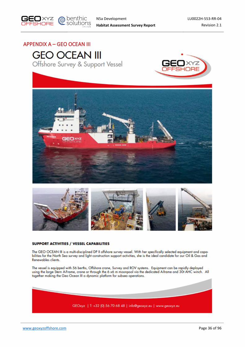
N5a Development LU0022H-553-RR-04
Habitat Assessment Survey Report Revision 2.1
www.geoxyzoffshore.com Page 36 of 96
APPENDIX A – GEO OCEAN III
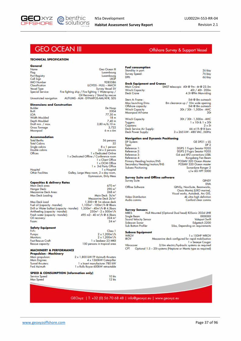
N5a Development LU0022H-553-RR-04
Habitat Assessment Survey Report Revision 2.1
www.geoxyzoffshore.com Page 37 of 96

N5a Development LU0022H-553-RR-04
Habitat Assessment Survey Report Revision 2.1
www.geoxyzoffshore.com Page 38 of 96
APPENDIX B – BSL SAMPLING EQUIPMENT
BSL DOUBLE GRAB
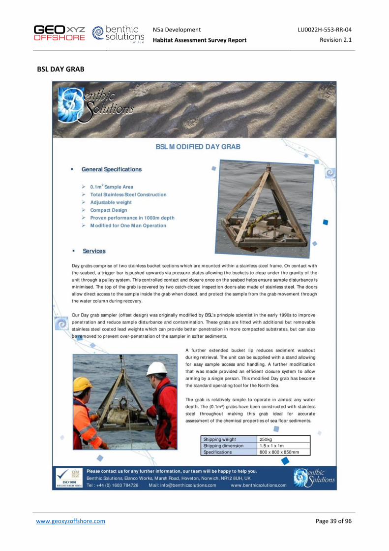
N5a Development LU0022H-553-RR-04
Habitat Assessment Survey Report Revision 2.1
www.geoxyzoffshore.com Page 39 of 96
BSL DAY GRAB

N5a Development LU0022H-553-RR-04
Habitat Assessment Survey Report Revision 2.1
www.geoxyzoffshore.com Page 40 of 96
BSL WILSON AUTO-SIEVER

N5a Development LU0022H-553-RR-04
Habitat Assessment Survey Report Revision 2.1
www.geoxyzoffshore.com Page 41 of 96
STR SEABUG CAMERA SYSTEM

N5a Development LU0022H-553-RR-04
Habitat Assessment Survey Report Revision 2.1
www.geoxyzoffshore.com Page 42 of 96
BSL MOD4 UNDERWATER CAMERA SYSTEM

N5a Development LU0022H-553-RR-04
Habitat Assessment Survey Report Revision 2.1
www.geoxyzoffshore.com Page 43 of 96
APPENDIX C – LOG SHEETS
Cast Station Sampler Used
Water Depth
(m) Time Date
Volume Recovered (mm box
depth)
Sample Name
Container Type and Quantity
Comments Sediment Description/Stratification
Conspicuous Fauna/Comments
1 GRAB_P_0 Day grab 29 17:43:00 06/05/2019 85% F1 2 x 3L bucket shells, sand Lanice. conchilega, Asterias rubens, Nereis
2 GRAB_P_0 DVV 29 18:20:00 06/05/2019 60% 50%
F2 PC
2 x 3L bucket Bags and jars sand, small pieces of shells L. conchilega, A.
rubens, Nereis
3 GRAB_P_0 DVV 29 18:45:00 06/05/2019 60% F3 3 x 3L bucket sand, small pieces of shells L. conchilega, A. rubens, Nereis
4 GRAB_P_1 DVV 27 20:12:00 06/05/2019 50% 50%
PC F1
1 x 3L bucket Bags and jars clay L. conchilega
5 GRAB_P_1 DVV 27 20:26:00 06/05/2019 N/S N/S N/S Cobbles
6 GRAB_P_1 DVV 27 20:40:00 06/05/2019 70% 50%
F2 F3
1 x 3L bucket 1 x 3L bucket sand and clay Polychaetes, Shell
debris
7 GRAB_P_2 DVV 24 21:15:00 06/05/2019 50% 50%
PC F1
1 x 1L bucket Bags and jars fine sand Echinocardium
cordatum, sandeel
8 GRAB_P_2 DVV 24 21:50:00 06/05/2019 60% 50%
F2 F3
1 x 1L bucket 1 x 1L bucket
Flatfish in grab jaws, photo taken,
discarded overboard. Grab seal not
compromised so used for fauna
fine sand Sandeel, polychaetes, flatfish poss. turbot
9 GRAB_P_3 DVV 23 22:56:00 06/05/2019 N/S N/S N/S Block came down,
strops broken, operations stopped
10 GRAB_P_3 DVV 24 02:05:00 08/05/2019 50% 50%
PC F1
1 x 1L bucket Bags and jars Weight added to arms fine sand E. cordatum
11 GRAB_P_3 DVV 24 02:15:00 08/05/2019 60% 50%
F2 F3
1 x 1L bucket 1 x 1L bucket fine sand Sandeel, E. cordatum
12 GRAB_P_4 DVV 22 02:45:00 08/05/2019 60% 50%
PC F1
1 x 1L bucket Bags and jars fine sand L. conchilega
13 GRAB_P_4 DVV 21 03:03:00 08/05/2019 50% 50%
F2 F3
1 x 1L bucket 1 x 1L bucket fine sand L. conchilega

N5a Development LU0022H-553-RR-04
Habitat Assessment Survey Report Revision 2.1
www.geoxyzoffshore.com Page 44 of 96
Cast Station Sampler Used
Water Depth
(m) Time Date
Volume Recovered (mm box
depth)
Sample Name
Container Type and Quantity
Comments Sediment Description/Stratification
Conspicuous Fauna/Comments
14 GRAB_P_5 DVV 20 03:31:00 08/05/2019 50% 50%
PC F1
1 x 1L bucket Bags and jars Sand and shell E. cordatum, razor
clam
15 GRAB_P_5 DVV 20 03:42:00 08/05/2019 50% 50%
F2 F3
1 x 1L bucket 1 x 1L bucket Sand and shell L. conchilega
16 GRAB_P_6 DVV 21 04:29:00 08/05/2019 50% 50%
PC F1
1 x 1L bucket Bags and jars Fine sand E. cordatum
(damaged)
17 GRAB_P_6 DVV 22 04:41:00 08/05/2019 50% 50%
F2 F3
1 x 1L bucket 1 x 1L bucket Fine sand with minor shell
fragments
Polychaetes, Nereis, L. conchilega, fish
(damaged)
18 GRAB_P_7 DVV 22 05:09:00 08/05/2019 N/S N/S N/S No sample, triggered but empty
19 GRAB_P_7 DVV 22 05:22:00 08/05/2019 N/S N/S N/S No sample, did not trigger
20 GRAB_P_7 DVV 21 05:25:00 08/05/2019 N/S N/S N/S No sample, did not trigger
21 GRAB_P_7 DVV 21 05:27:00 08/05/2019 50% 50%
PC F1
1 x 1L bucket Bags and jars Fine sand with minor shell
debris L. conchilega, polychaetes
22 GRAB_P_7 DVV 21 05:37:00 08/05/2019 50% 50%
F2 F3
1 x 1L bucket 1 x 1L bucket
Fine sand with minor shell debris, small amounts of
mud/clay
Abundant L. conchilega, polychaetes
23 GRAB_P_8 DVV 21 06:01:00 08/05/2019 N/S N/S N/S
24 GRAB_P_8 DVV 21 06:03:00 08/05/2019 N/S N/S N/S
25 GRAB_P_8 DVV 20 06:04:00 08/05/2019 70% 70%
PC F1
1 x 5L bucket Bags and jars Coarse sand with shell
fragments Polychaetes
26 GRAB_P_8 DVV 21 06:12:00 08/05/2019 70% 60%
F2 F3
1 x 5L bucket 1 x 5L bucket Coarse sand with shell
fragments L. conchilega
27 GRAB_C_8 DVV 24 19:00:00 09/05/2019 80% 80%
PC F1
1 x 1L bucket Bags and jars Coarse sand with shell
fragments L. conchilega
28 GRAB_C_8 DVV 24 19:15:00 09/05/2019 80% 80%
F2 F3
1 x 1L bucket 1 x 1L bucket Coarse sand with shell
fragments L. conchilega
29 GRAB_C_7 DVV 24 19:30:00 09/05/2019 70%, 70% PC F1
3 x 3L bucket Bags and jars Coarse sand with shell
fragments No conspicuous fauna

N5a Development LU0022H-553-RR-04
Habitat Assessment Survey Report Revision 2.1
www.geoxyzoffshore.com Page 45 of 96
Cast Station Sampler Used
Water Depth
(m) Time Date
Volume Recovered (mm box
depth)
Sample Name
Container Type and Quantity
Comments Sediment Description/Stratification
Conspicuous Fauna/Comments
30 GRAB_C_7 DVV 24 19:45:00 09/05/2019 N/S N/S N/S Deployed but no sample, not triggering
31 GRAB_C_7 DVV 24 20:05:00 09/05/2019 70% 80% F2 F3
2 x 5L bucket 2 x 5L bucket Coarse sand with shell
fragments No conspicuous fauna
32 GRAB_C_6 DVV 24 20:27:00 09/05/2019 60% 80% PC F1
1 x 3L bucket Bags and jars Coarse sand with shell
fragments No conspicuous fauna
33 GRAB_C_6 DVV 24 21:05:00 09/05/2019 80%, 80% F2 F3
1 x 3L bucket 1 x 3L bucket Coarse sand with shell
fragments Urchin
34 GRAB_C_5 DVV 25 05:37:00 11/05/2019 40% 70%
PC F1
1 x 3L + 1x5L bucket
Bags and jars Coarse sand with shell
fragments Gobidae, Asterias,
Lancelet. L. conchilega
35 GRAB_C_5 DVV 25 05:42:00 11/05/2019 70% 70%
F2 F3
2 x 5L bucket 1 x 5L + 1x 3L
bucket Coarse sand with shell
fragments
L. conchilega, polychaetes, spatangoid
36 GRAB_C_4 DVV 28 06:40:00 11/05/2019 60% 60%
PC F1
1 x 1L bucket Bags and jars Fine sand with shell debris
L. conchilega, polychaetes, spatangoid
37 GRAB_C_4 DVV 28 07:01:00 11/05/2019 70% 70%
F2 F3
1 x 1L bucket 1 x 1L bucket Fine sand with shell debris
L. conchilega, polychaetes, spatangoid
38 GRAB_C_3 DVV 28 07:29:00 11/05/2019 N/S N/S N/S Did not trigger
39 GRAB_C_3 DVV 28 07:36:00 11/05/2019 70% 70%
PC F1
1 x 1L bucket Bags and jars Very fine sand with minor
shell debris L. conchilega, polychaetes
40 GRAB_C_3 DVV 28 07:47:00 11/05/2019 N/S N/S N/S Triggered but no sample
41 GRAB_C_3 DVV 28 07:49:00 11/05/2019 70% 70%
F2 F3
1 x 1L bucket 1 x 1L bucket Very fine sand with minor
shell debris and soft clay
Anemones, L. conchilega,
polychaetes, A rubens, spatangoid
42 GRAB_C_2 DVV 27 08:15:00 11/05/2019 70% 70%
PC F1
1 x 5L bucket Bags and jars Coarse sand and clay L conchilega and
polychaetes
43 GRAB_C_2 DVV 28 08:27:00 11/05/2019 70% 40%
F2 F3
1 x 5L bucket 1 x 3L bucket
Razor clams in jaws (F3) Coarse sand
Razor clams, L. conchilega,
polychaetes. Lancelet

N5a Development LU0022H-553-RR-04
Habitat Assessment Survey Report Revision 2.1
www.geoxyzoffshore.com Page 46 of 96
Cast Station Sampler Used
Water Depth
(m) Time Date
Volume Recovered (mm box
depth)
Sample Name
Container Type and Quantity
Comments Sediment Description/Stratification
Conspicuous Fauna/Comments
44 GRAB_C_1 DVV 28 08:55:00 11/05/2019 60% 60%
PC F1
1 x 3L + 1x5L bucket
Bags and jars Coarse sand and abundant
shell debris Lancelet and polychaetes
45 GRAB_C_1 DVV 28 09:04:00 11/05/2019 60% 40%
F2 F3
1 x 5L bucket 1 x 5L bucket
Razor clams in jaws (F3)
Coarse sand and abundant shell debris
L. conchilega, lancelet, polychaetes, porcelain
crab
46 GRAB_C_0 DVV 29 09:32:00 11/05/2019 90% 90%
PC F1
2 x 5L bucket Bags and jars
Label for F2 in F1 bucket (2 of 2) Coarse sand L. conchilega, razor
clams and polychaetes
47 GRAB_C_0 DVV 29 09:41:00 11/05/2019 90% 90%
F2 F3
2 x 5L bucket 2 x 5L bucket
Label for F3 in F2 bucket (1 of 2) Coarse sand L. conchilega, razor
clams and polychaetes
48 GRAB_P_15 DVV 13 02:15:00 12/05/2019 60% 60%
PC F1
1 x 1L bucket Bags and jars Fine sand with shell Polychaetes
49 GRAB_P_15 DVV 13 02:20:00 12/05/2019 60% 60%
F2 F3
1 x 1L bucket 1 x 1L bucket Fine sand with shell Polychaetes, sandeel
50 GRAB_P_14 DVV 14 03:05:00 12/05/2019 60% 60%
PC F1
1 x 3L bucket Bags and jars Fine sand with shell Asterias, Spatangoid,
Ophiura
51 GRAB_P_14 DVV 14 03:10:00 12/05/2019 60% 60%
F2 F3
1 x 3L bucket 1 x 3L bucket Fine sand with shell Spatangoid, Ophiura
52 GRAB_P_13 DVV 16 03:30:00 12/05/2019 60% 60%
PC F1
1 x 1L bucket Bags and jars Fine sand with minor shell
debris Polychaetes
53 GRAB_P_13 DVV 16 03:45:00 12/05/2019 60% 60%
F2 F3
1 x 1L bucket 1 x 1L bucket Fine sand with minor shell
debris Nereis, L. conchilega, Ophiura, Spatangoids
54 GRAB_P_12 DVV 16 04:32:00 12/05/2019 60% 60%
PC F1
1 x 3L bucket Bags and jars Fine sand with shell debris Nereis, L. conchilega,
Spatangoids
55 GRAB_P_12 DVV 16 04:42:00 12/05/2019 60% 60%
F2 F3
1 x 3L bucket 1 x 3L bucket Fine sand with shell debris Nereis, L. conchilega,
Spatangoids
56 GRAB_P_11 DVV 17 05:03:00 12/05/2019 70% 70%
PC F1
1 x 3L bucket Bags and jars Fine sand with significant
shell debris L. conchilega
57 GRAB_P_11 DVV 17 05:13:00 12/05/2019 70% 70%
F2 F3
1 x 3L bucket 1 x 3L bucket Fine sand with significant
shell debris L. conchilega
58 GRAB_P_10 DVV 17 05:35:00 12/05/2019 60% 60%
PC F1
1 x 1L bucket Bags and jars Fine sand with shell debris Polychaetes, L.
conchilega, Nereis
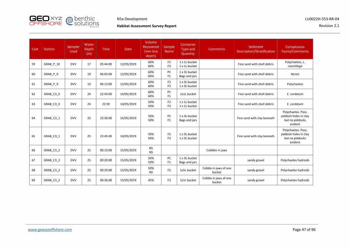
N5a Development LU0022H-553-RR-04
Habitat Assessment Survey Report Revision 2.1
www.geoxyzoffshore.com Page 47 of 96
Cast Station Sampler Used
Water Depth
(m) Time Date
Volume Recovered (mm box
depth)
Sample Name
Container Type and Quantity
Comments Sediment Description/Stratification
Conspicuous Fauna/Comments
59 GRAB_P_10 DVV 17 05:44:00 12/05/2019 60% 60%
F2 F3
1 x 1L bucket 1 x 1L bucket Fine sand with shell debris Polychaetes, L.
conchilega
60 GRAB_P_9 DVV 19 06:05:00 12/05/2019 60% 60%
PC F1
1 x 3L bucket Bags and jars Fine sand with shell debris Nereis
61 GRAB_P_9 DVV 19 06:13:00 12/05/2019 60% 60%
F2 F3
1 x 3L bucket 1 x 3L bucket Fine sand with shell debris Polychaetes
62 GRAB_C3_0 DVV 24 22:43:00 14/05/2019 60% 60%
PC F1 1x1L bucket Fine sand with shell debris E. cordatum
63 GRAB_C3_0 DVV 24 22:59 14/05/2019 50% 50%
F2 F3
1 x 1L bucket 1 x 1L bucket Fine sand with shell debris E. cordatum
64 GRAB_C3_1 DVV 25 23:36:00 14/05/2019 50% 50%
PC F1
1 x 3L bucket Bags and jars Fine sand with clay beneath
Polychaetes. Poss. piddock holes in clay
but no piddocks evident
65 GRAB_C3_1 DVV 25 23:45:00 14/05/2019 50% 50%
F2 F3
1 x 3L bucket 1 x 3L bucket Fine sand with clay beneath
Polychaetes. Poss. piddock holes in clay
but no piddocks evident
66 GRAB_C3_2 DVV 25 00:13:00 15/05/2019 NS NS Cobbles in jaws
67 GRAB_C3_2 DVV 25 00:20:00 15/05/2019 50% 50%
PC F1
1 x 3L bucket Bags and jars sandy gravel Polychaetes hydroids
68 GRAB_C3_2 DVV 25 00:29:00 15/05/2019 50% NS F2 1x5L bucket Cobble in jaws of one
bucket sandy gravel Polychaetes hydroids
69 GRAB_C3_2 DVV 25 00:36:00 15/05/2019 45% F3 1x1L bucket Cobble in jaws of one bucket sandy gravel Polychaetes hydroids
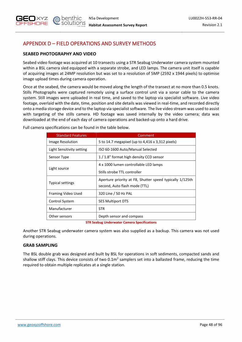
N5a Development LU0022H-553-RR-04
Habitat Assessment Survey Report Revision 2.1
www.geoxyzoffshore.com Page 48 of 96
APPENDIX D – FIELD OPERATIONS AND SURVEY METHODS
SEABED PHOTOGRAPHY AND VIDEO
Seabed video footage was acquired at 10 transects using a STR Seabug Underwater camera system mounted within a BSL camera sled equipped with a separate strobe, and LED lamps. The camera unit itself is capable of acquiring images at 24MP resolution but was set to a resolution of 5MP (2592 x 1944 pixels) to optimise image upload times during camera operation.
Once at the seabed, the camera would be moved along the length of the transect at no more than 0.5 knots. Stills Photographs were captured remotely using a surface control unit via a sonar cable to the camera system. Still images were uploaded in real time, and saved to the laptop via specialist software. Live video footage, overlaid with the date, time, position and site details was viewed in real-time, and recorded directly onto a media storage device and to the laptop via specialist software. The live video stream was used to assist with targeting of the stills camera. HD footage was saved internally by the video camera; data was downloaded at the end of each day of camera operations and backed-up onto a hard drive.
Full camera specifications can be found in the table below.
Standard Features Comment
Image Resolution 5 to 14.7 megapixel (up to 4,416 x 3,312 pixels)
Light Sensitivity setting ISO 60-1600 Auto/Manual Selected
Sensor Type 1 / 1.8” format high density CCD sensor
Light source 4 x 1000 lumen controllable LED lamps
Stills strobe TTL controller
Typical settings Aperture priority at F8, Shutter speed typically 1/125th second, Auto flash mode (TTL)
Framing Video Used 320 Line / 50 Hz PAL
Control System SES Multiport DTS
Manufacturer STR
Other sensors Depth sensor and compass STR Seabug Underwater Camera Specifications
Another STR Seabug underwater camera system was also supplied as a backup. This camera was not used during operations.
GRAB SAMPLING
The BSL double grab was designed and built by BSL for operations in soft sediments, compacted sands and shallow stiff clays. This device consists of two 0.1m2 samplers set into a ballasted frame, reducing the time required to obtain multiple replicates at a single station.

N5a Development LU0022H-553-RR-04
Habitat Assessment Survey Report Revision 2.1
www.geoxyzoffshore.com Page 49 of 96
A BSL Double grab was used for seabed sampling Seagull site and route survey. Two successful deployments were required at each location. Three consecutive ‘no sample’ deployments were agreed to be the maximum number of attempts at any location before abandoning it. The inner stainless grab buckets were cleaned before deployment at any new station to avoid contamination.
Samples were subject to quality control on recovery and were retained in the following circumstances:
• Water above sample was undisturbed; • Bucket closure complete (no sediment washout); • Sampler was retrieved perfectly upright; • Inspection/access doors had closed properly; • No disruption of sample; • Sample was taken inside the acceptable target range (<15m); • Sample size was greater than 6 litres (ca. 40% of the sampler’s capacity); • No hagfish (Myxine glutinosa) and/or mucus coagulants.
Key observations from samples included colour, sediment classification, layering (including redox discontinuity layers), smell (including the presence of H2S), obvious fauna, evidence of bioturbation and anthropogenic debris.
BSL Double Grab

N5a Development LU0022H-553-RR-04
Habitat Assessment Survey Report Revision 2.1
www.geoxyzoffshore.com Page 50 of 96
APPENDIX E – HABITAT ASSESSMENT
ED50, UTM 31N, CM 3° E
Station Easting (m)
Northing (m)
Date & Time
Example Photograph (file name) Sediment type Conspicuous fauna Depth
(m)
Stony Reefiness (After Irving 2009)
Overall Reef Structure
EUNIS Habitat Classification with SBF/Habitat Map
Colour Code
Composition (% cover of
cobbles/ boulders)
Elevation (of cobbles/
boulders in cm)
Reef Structure
Matrix
Grab_C_0
N5a_1_018.jpg, N5a_1_019.jpg, N5a_2_021.jpg, N5a_1_022.jpg
Coarse sand and shell fragments
Asterias rubens, Lanice conchilega 30 n/a n/a n/a n/a Infralittoral coarse Sediment
(A5.13)
Grab_C_1
722598 5954539 11/05/19 02:56:48
Grab_C_1_005.jpg Coarse sand and shell fragments with Lanice
conchilega assemblages
Asterias rubens, Liocarcinus sp., Lanice conchilega, Decapoda
28 n/a n/a n/a n/a
Dense Lanice conchilega and other polychaetes in tide-
swept infralittoral sand and mixed gravelly sand
(A5.137) 722599 5954538 11/05/19
02:57:27
Grab_C_2
723694 5954422 11/05/19 03:28:13
Grab_C_2_002.jpg Coarse sand and shell fragments with Lanice
conchilega assemblages
Asterias rubens, Liocarcinus sp., Lanice
conchilega, Loligo vulgaris
28 n/a n/a n/a n/a
Dense Lanice conchilega and other polychaetes in tide-
swept infralittoral sand and mixed gravelly sand
(A5.137) 723596 5954422 11/05/19
03:29:04
Grab_C_3 724589 5954311 11/05/19
04:08:03 Grab_C_3_003.jpg
Fine to medium sand ripples with shell
fragments accumulated between ripples
Asterias rubens, Liocarcinus sp., Lanice
conchilega 28 n/a n/a n/a n/a Infralittoral fine sand
(A5.23) 724590 5954310 11/05/19
04:10:35
Grab_C_4 725582 5954199 11/05/19
04:34:40 Grab_C_4_002.jpg
Fine to medium sand ripples with shell
fragments accumulated between ripples
Asterias rubens, Lanice conchilega, Arenicola
sp., Decapoda 28 n/a n/a n/a n/a Infralittoral fine sand
(A5.23) 725581 5954200 11/05/19
04:37:18
Grab_C_5
726576 5954086 11/05/19 05:01:59
Grab_C_5_002.jpg
Coarse sand ripples with small shell fragments
accumulated between ripples
Asterias rubens, Liocarcinus sp., Lanice
conchilega, poss. Callionymus lyra
25 n/a n/a
n/a
n/a Infralittoral coarse Sediment (A5.13)
726573 5954088 11/05/19 05:05:12
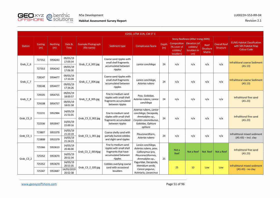
N5a Development LU0022H-553-RR-04
Habitat Assessment Survey Report Revision 2.1
www.geoxyzoffshore.com Page 51 of 96
ED50, UTM 31N, CM 3° E
Station Easting (m)
Northing (m)
Date & Time
Example Photograph (file name) Sediment type Conspicuous fauna Depth
(m)
Stony Reefiness (After Irving 2009)
Overall Reef Structure
EUNIS Habitat Classification with SBF/Habitat Map
Colour Code
Composition (% cover of
cobbles/ boulders)
Elevation (of cobbles/
boulders in cm)
Reef Structure
Matrix
Grab_C_6 727352 5954243 09/05/19
17:05:54 Grab_C_6_002.jpg
Coarse sand ripples with small shell fragments
accumulated between ripples
Lanice conchilega 24 n/a n/a n/a n/a Infralittoral coarse Sediment (A5.13)
727353 5954242 09/05/19 17:06:30
Grab_C_7 728147 5954477 09/05/19
17:33:39 Grab_C_7_004.jpg
Coarse sand ripples with small shell fragments
accumulated between ripples
Lanice conchilega, Asterias rubens 24 n/a n/a n/a n/a Infralittoral coarse Sediment
(A5.13) 728148 5954477 09/05/19
17:34:26
Grab_C_8 729105 5954755 09/05/19
18:00:57 Grab_C_8_005.jpg
Fine to medium sand ripples with small shell fragments accumulated
between ripples
Poss. Gobiidae, Asterias rubens, Lanice
conchilega 24 n/a n/a n/a n/a Infralittoral fine sand
(A5.23) 729108 5954757 09/05/19
18:01:58
Grab_C3_0
722231 5952984 14/05/19 21:51:01
Grab_C3_0_002.jpg
Fine to medium sand ripples with small shell fragments accumulated
between ripples
Asterias rubens, Lanice conchilega, Decapoda,
Ammodytes sp., Corystes cassivelaunus,
Gobiidae, Ophiura ophiura
24 n/a n/a n/a n/a Infralittoral fine sand (A5.23)
722336 5953047 14/05/19 22:00:16
Grab_C3_1 723807 5953379 14/05/19
21:23:19 Grab_C3_1_001.jpg
Coarse shelly sand with partially buried cobbles and slight sand ripples
Pleuronectiform, Asterias rubens 24 n/a n/a n/a n/a Infralittoral mixed sediment
(A5.43) – incl. clay 723808 5953379 14/05/19
21:24:23
Grab_C3_2
725366 5953610 14/05/19 20:46:00
Grab_C3_2_0014jpg
Fine to medium sand ripples with small shell fragments that have
accumulated between ripples
Lanice conchilega, Asterias rubens, poss.
Callionymus lyra, Pleuronectiformes,
Ammodytes sp., Paguridae, Decapoda,
Metridium senile, Cancer pagurus,
Actiniaria, Liocarcinus
25
Not a Reef Not a Reef Not Reef Not a Reef Infralittoral fine sand
(A5.23) 725352 5953670 14/05/19
20:51:34
725352 5953670 14/05/19 20:51:35
Grab_C3_2_020.jpg Cobbles overlying coarse
sand with occasional boulders
25 10 Low Low Infralittoral mixed sediment (A5.43) - no clay
725347 5953687 14/05/2019 20:52:38
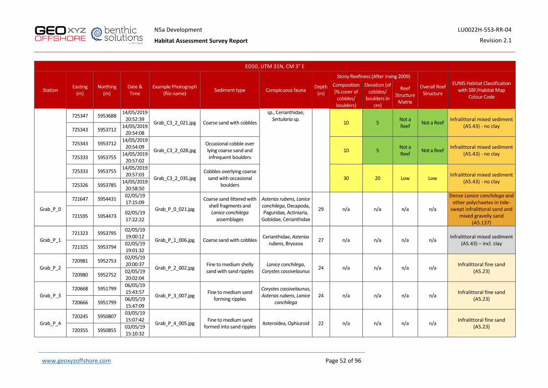
N5a Development LU0022H-553-RR-04
Habitat Assessment Survey Report Revision 2.1
www.geoxyzoffshore.com Page 52 of 96
ED50, UTM 31N, CM 3° E
Station Easting (m)
Northing (m)
Date & Time
Example Photograph (file name) Sediment type Conspicuous fauna Depth
(m)
Stony Reefiness (After Irving 2009)
Overall Reef Structure
EUNIS Habitat Classification with SBF/Habitat Map
Colour Code
Composition (% cover of
cobbles/ boulders)
Elevation (of cobbles/
boulders in cm)
Reef Structure
Matrix
725347 5953688 14/05/2019 20:52:39
Grab_C3_2_021.jpg Coarse sand with cobbles
sp., Cerianthidae, Sertularia sp.
10 5 Not a Reef Not a Reef Infralittoral mixed sediment
(A5.43) - no clay 725343 5953712 14/05/2019
20:54:08
725343 5953712 14/05/2019 20:54:09
Grab_C3_2_028.jpg Occasional cobble over lying coarse sand and infrequent boulders
10 5 Not a Reef Not a Reef Infralittoral mixed sediment
(A5.43) - no clay 725333 5953755 14/05/2019
20:57:02
725333 5953755 14/05/2019 20:57:03
Grab_C3_2_035.jpg Cobbles overlying coarse
sand with occasional boulders
30 20 Low Low Infralittoral mixed sediment (A5.43) - no clay
725326 5953785 14/05/2019 20:58:50
Grab_P_0
721647 5954431 02/05/19 17:15:09
Grab_P_0_021.jpg
Coarse sand littered with shell fragments and Lanice conchilega
assemblages
Asterias rubens, Lanice conchilega, Decapoda, Paguridae, Actiniaria,
Gobiidae, Cerianthidae
29 n/a n/a n/a n/a
Dense Lanice conchilega and other polychaetes in tide-
swept infralittoral sand and mixed gravelly sand
(A5.137) 721595 5954473 02/05/19
17:22:22
Grab_P_1 721323 5953795 02/05/19
19:00:12 Grab_P_1_006.jpg Coarse sand with cobbles Cerianthidae, Asterias
rubens, Bryozoa 27 n/a n/a n/a n/a Infralittoral mixed sediment (A5.43) – incl. clay
721325 5953794 02/05/19 19:01:32
Grab_P_2 720981 5952753 02/05/19
20:00:37 Grab_P_2_002.jpg Fine to medium shelly
sand with sand ripples Lanice conchilega,
Corystes cassivelaunus 24 n/a n/a n/a n/a Infralittoral fine sand (A5.23)
720980 5952752 02/05/19 20:02:04
Grab_P_3 720668 5951799 06/05/19
15:43:57 Grab_P_3_007.jpg Fine to medium sand
forming ripples
Corystes cassivelaunus, Asterias rubens, Lanice
conchilega 24 n/a n/a n/a n/a Infralittoral fine sand
(A5.23) 720666 5951799 06/05/19
15:47:09
Grab_P_4 720245 5950807 03/05/19
15:07:42 Grab_P_4_005.jpg Fine to medium sand
formed into sand ripples Asteroidea, Ophiuroid 22 n/a n/a n/a n/a Infralittoral fine sand (A5.23)
720355 5950855 03/05/19 15:10:32

N5a Development LU0022H-553-RR-04
Habitat Assessment Survey Report Revision 2.1
www.geoxyzoffshore.com Page 53 of 96
ED50, UTM 31N, CM 3° E
Station Easting (m)
Northing (m)
Date & Time
Example Photograph (file name) Sediment type Conspicuous fauna Depth
(m)
Stony Reefiness (After Irving 2009)
Overall Reef Structure
EUNIS Habitat Classification with SBF/Habitat Map
Colour Code
Composition (% cover of
cobbles/ boulders)
Elevation (of cobbles/
boulders in cm)
Reef Structure
Matrix
Grab_P_5 720036 5949903 03/05/19
13:36:49 Grab_P_5_004.jpg Fine to medium shelly
sand with rare cobbles
Paguridae, Lanice conchilega, Asterias
rubens 20 n/a n/a n/a n/a Infralittoral fine sand
(A5.23) 720036 5949903 03/05/19
13:38:12
Grab_P_6 719725 5948952 03/05/19
13:04:18 Grab_P_6_004.jpg Fine to medium sand with
irregular ripples Lanice conchilega, Pleuronectiform
22 n/a n/a n/a n/a Infralittoral fine sand (A5.23)
719729 5948948 03/05/19 13:08:36
Grab_P_7 719412 5948000 03/05/19
11:18:23 Grab_P_7_005.jpg Fine to medium sand with
irregular ripples
Lanice conchilega, Callionymus lyra,
Ophiuroid 21 n/a n/a n/a n/a Infralittoral fine sand
(A5.23) 719411 5948003 03/05/19
11:22:22
Grab_P_8 719099 5947048 03/05/19
12:05:32 Grab_P_8_005.jpg
Coarse sand and shell debris with irregular
ripples Lanice conchilega 21 n/a n/a n/a n/a Infralittoral coarse Sediment
(A5.13) 719094 5947051 03/05/19
12:07:34
Grab_P_9 718861 5945913 11/05/19
22:31:48 Grab_P_9_002.jpg
Coarse sand and shell debris with irregular
ripples
Asterias rubens, Lanice conchilega, Corystes
cassivelaunus, Actinopterygii
19 n/a n/a n/a n/a Infralittoral coarse Sediment (A5.13)
718862 5945911 11/05/19 22:33:08
Grab_P_10 718778 5944917 11/05/19
23:01:57 Grab_P_10_003.jpg Fine to medium sand Asterias rubens, Lanice
conchilega 17 n/a n/a n/a n/a Infralittoral fine sand
(A5.23) 718778 5944917 11/05/19
23:04:14
Grab_P_11 718697 5943920 11/05/19
23:30:17 Grab_P_11_009.jpg
Fine to medium sand and shell debris with irregular
ripples
Brachyura, Lanice conchilega 17 n/a n/a n/a n/a Infralittoral fine sand
(A5.23) 718697 5943920 11/05/19
23:32:11
Grab_P_12
718614 5942925 11/05/19 23:58:12
Grab_P_12_002.jpg Fine to medium sand and shell debris with irregular
ripples
Asterias rubens, Lanice conchilega,
Callionymus lyra, Gobiidae, Actiniaria, Brachyura, Cancer
pagurus, Liocarcinus sp.
16 n/a n/a n/a n/a Infralittoral fine sand (A5.23)
718615 5942922 12/05/19 00:00:03

N5a Development LU0022H-553-RR-04
Habitat Assessment Survey Report Revision 2.1
www.geoxyzoffshore.com Page 54 of 96
ED50, UTM 31N, CM 3° E
Station Easting (m)
Northing (m)
Date & Time
Example Photograph (file name) Sediment type Conspicuous fauna Depth
(m)
Stony Reefiness (After Irving 2009)
Overall Reef Structure
EUNIS Habitat Classification with SBF/Habitat Map
Colour Code
Composition (% cover of
cobbles/ boulders)
Elevation (of cobbles/
boulders in cm)
Reef Structure
Matrix
Grab_P_13 718531 5941926 12/05/19
00:30:02 Grab_P_13_005.jpg Fine to medium sand with
irregular ripples
Asterias rubens, Ophiuroids, Lanice
conchilega 16 n/a n/a n/a n/a Infralittoral fine sand
(A5.23) 718533 5941928 12/05/19
00:31:30
Grab_P_14
No visibility
Grab_P_15 718366 5939934 12/05/19
01:53:30 Grab_P_15_005.jpg Fine to medium sand
with irregular ripples Lanice conchilega,
Actinopterygii 13 n/a n/a n/a n/a Infralittoral fine sand (A5.23)
718366 5939933 12/05/19 01:55:09
N5a_1
721585 5954589 11/05/19 01:38:04
N5a_1_014.jpg
Slightly gravelly/shelly coarse sand. 'Burrows'
formed by Ensis retracting below surface
when the camera sled comes into contact with
the seabed
Lanice conchilega, Ensis 'burrows', Leptothecata,
Actiniaria, Cancer pagurus, Callionymus
lyra, Paguridae, Actinopterygii, Sepiida,
Pleuronectiform, Brachyura, Sepiola
spp., Cancer pagurus, Metridium senile, Ensis
sp., Liocarcinus sp., Cerianthidae
29 n/a n/a n/a n/a
Dense Lanice conchilega and other polychaetes in tide-
swept infralittoral sand and mixed gravelly sand
(A5.137) 721626 5954710 11/05/19
01:46:42
N5a_2
721669 5954631 11/05/19 01:16:25
N5a_2_002.jpg
Slightly gravelly/shelly coarse sand. 'Burrows'
formed by Ensis retracting below surface
when the camera sled comes into contact with
the seabed
Asterias rubens, Lanice conchilega, Cancer pagurus, Actiniaria, Paguridae, Ensis sp.,
Cancer pagurus, Pagurus bernhardus,
Brachyura, Callionymus lyra, Metridium senile,
29
n/a n/a n/a n/a
Dense Lanice conchilega and other polychaetes in tide-
swept infralittoral sand and mixed gravelly sand
(A5.137) 721555 5954667 11/05/19 01:24:59
721554 5954667 11/05/19 01:25:00 N5a_2_038.jpg n/a n/a n/a n/a Dense Lanice conchilega and
other polychaetes in tide-

N5a Development LU0022H-553-RR-04
Habitat Assessment Survey Report Revision 2.1
www.geoxyzoffshore.com Page 55 of 96
ED50, UTM 31N, CM 3° E
Station Easting (m)
Northing (m)
Date & Time
Example Photograph (file name) Sediment type Conspicuous fauna Depth
(m)
Stony Reefiness (After Irving 2009)
Overall Reef Structure
EUNIS Habitat Classification with SBF/Habitat Map
Colour Code
Composition (% cover of
cobbles/ boulders)
Elevation (of cobbles/
boulders in cm)
Reef Structure
Matrix
721552 5954668 11/05/19 01:25:15
Large boulder surrounded by Ensis
shells
Liocarcinus sp., Cerianthidae
swept infralittoral sand and mixed gravelly sand
(A5.137)
721551 5954668 11/05/19 01:25:16
N5a_2_039.jpg Coarse sand ripples n/a n/a n/a n/a Infralittoral coarse Sediment (A5.13)
721544 5954669 11/05/19 01:25:39
North Transect 1
721487 5954681 11/05/19 00:49:09
N_T_1_002.jpg
Slightly gravelly/shelly coarse sand forming
irregular ripples. 'Burrows' formed by
Ensis retracting below surface when the
camera sled comes into contact with the seabed Asterias rubens, Lanice
conchilega, Cancer pagurus, Pagurus
bernhardus, Actiniaria, Paguridae, Ensis sp.,
Brachyura, Actinopterygii, Cancer
pagurus, Pleuronectiform, Limanda limanda,
Liocarcinus sp., Cerianthidae
29
n/a n/a n/a n/a
Dense Lanice conchilega and other polychaetes in tide-
swept infralittoral sand and mixed gravelly sand
(A5.137) 721425 5954656 11/05/19 00:55:02
721425 5954656 11/05/19 00:55:03
N_T_1_021.jpg
Dense aggregations of Lanice conchilega,
Asterias rubens and Ensis shells on gravelly coarse sand. 'Burrows'
formed by Ensis retracting below surface
when the camera sled comes into contact with
the seabed.
n/a n/a n/a n/a
Dense Lanice conchilega and other polychaetes in tide-
swept infralittoral sand and mixed gravelly sand
(A5.137) 721392 5954643 11/05/19
00:57:24
721391 5954643 11/05/19 00:57:25
N_T_1_028.jpg
Slightly gravelly/shelly coarse sand. 'Burrows'
formed by Ensis retracting below surface
when the camera sled comes into contact with
the seabed
n/a n/a n/a n/a
Dense Lanice conchilega and other polychaetes in tide-
swept infralittoral sand and mixed gravelly sand
(A5.137) 721363 5954633 11/05/19 00:59:20

N5a Development LU0022H-553-RR-04
Habitat Assessment Survey Report Revision 2.1
www.geoxyzoffshore.com Page 56 of 96
ED50, UTM 31N, CM 3° E
Station Easting (m)
Northing (m)
Date & Time
Example Photograph (file name) Sediment type Conspicuous fauna Depth
(m)
Stony Reefiness (After Irving 2009)
Overall Reef Structure
EUNIS Habitat Classification with SBF/Habitat Map
Colour Code
Composition (% cover of
cobbles/ boulders)
Elevation (of cobbles/
boulders in cm)
Reef Structure
Matrix
North Transect 2
721609 5954992 11/05/19 00:06:16
N_T_2_003.jpg
Slightly gravelly/shelly coarse sand forming
irregular ripples. 'Burrows' formed by
Ensis retracting below surface when the
camera sled comes into contact with the seabed
Asterias rubens, Lanice conchilega, Cancer pagurus, Pagurus
bernhardus, Cancer pagurus,
Pleuronectiform, Callionymus lyra,
Bachyura, Actiniaria, Sepiidae, Liocarcinus
sp., Cerianthidae
29
n/a n/a n/a n/a
Dense Lanice conchilega and other polychaetes in tide-
swept infralittoral sand and mixed gravelly sand
(A5.137) 721618 5955031 11/05/19 00:10:55
721617 5955032 11/05/19 00:10:56
N_T_2_014.jpg
Gravelly/shelly coarse sand forming irregular
ripples. 'Burrows' formed by Ensis
retracting below surface when the camera sled
comes into contact with the seabed
n/a n/a n/a n/a
Dense Lanice conchilega and other polychaetes in tide-
swept infralittoral sand and mixed gravelly sand
(A5.137) 721625 5955086 11/05/19 00:14:33
721625 5955086 11/05/19 00:14:34
N_T_2_038.jpg
Dense aggregations of Lanice conchilega,
Asterias rubens and Ensis shells on gravelly coarse sand. 'Burrows'
formed by Ensis retracting below surface
when the camera sled comes into contact with
the seabed.
n/a n/a n/a n/a
Dense Lanice conchilega and other polychaetes in tide-
swept infralittoral sand and mixed gravelly sand
(A5.137) 721631 5955141 11/05/19
00:18:28
721631 5955142 11/05/19 00:18:29
N_T_2_041.jpg
Slightly gravelly/shelly coarse sand. 'Burrows'
formed by Ensis retracting below surface
when the camera sled comes into contact with
the seabed
n/a n/a n/a n/a
Dense Lanice conchilega and other polychaetes in tide-
swept infralittoral sand and mixed gravelly sand
(A5.137) 721632 5955153 11/05/19 00:19:05

N5a Development LU0022H-553-RR-04
Habitat Assessment Survey Report Revision 2.1
www.geoxyzoffshore.com Page 57 of 96
ED50, UTM 31N, CM 3° E
Station Easting (m)
Northing (m)
Date & Time
Example Photograph (file name) Sediment type Conspicuous fauna Depth
(m)
Stony Reefiness (After Irving 2009)
Overall Reef Structure
EUNIS Habitat Classification with SBF/Habitat Map
Colour Code
Composition (% cover of
cobbles/ boulders)
Elevation (of cobbles/
boulders in cm)
Reef Structure
Matrix
North Transect 3
721902 5954408 11/05/19 02:04:47
N_T_3_010.jpg
Dense aggregations of Lanice conchilega,
Asterias rubens and Ensis shells on gravelly coarse sand. 'Burrows'
formed by Ensis retracting below surface
when the camera sled comes into contact with
the seabed.
Asterias rubens, Lanice conchilega, Cancer pagurus, Pagurus
bernhardus, Cancer pagurus,
Pleuronectiform, Actiniaria, Gobiidae, Paguridea, Ensis sp., Limanda, Metridium
senile, Liocarcinus sp., Eutrigla gurnardus,
Cerianthidae
29
n/a n/a n/a n/a
Dense Lanice conchilega and other polychaetes in tide-
swept infralittoral sand and mixed gravelly sand
(A5.137) 721888 5954432 11/05/19
02:07:32
721887 5954432 11/05/19 02:07:33
N_T_3_018.jpg
Slightly gravelly/shelly coarse sand. 'Burrows'
formed by Ensis retracting below surface
when the camera sled comes into contact with
the seabed
n/a n/a n/a n/a
Dense Lanice conchilega and other polychaetes in tide-
swept infralittoral sand and mixed gravelly sand
(A5.137) 721865 5954461 11/05/19 02:09:55
721865 5954461 11/05/19 02:09:56
N_T_3_039.jpg
Dense aggregations of Lanice conchilega,
Asterias rubens and Ensis shells on gravelly coarse sand. 'Burrows'
formed by Ensis retracting below surface
when the camera sled comes into contact with
the seabed.
n/a n/a n/a n/a
Dense Lanice conchilega and other polychaetes in tide-
swept infralittoral sand and mixed gravelly sand
(A5.137) 721824 5954518 11/05/19 02:14:38
721823 5954519 11/05/19 02:14:39
N_T_3_050.jpg
Slightly gravelly/shelly coarse sand. 'Burrows'
formed by Ensis retracting below surface
when the camera sled comes into contact with the seabed. Infrequent
boulders.
n/a n/a n/a n/a
Dense Lanice conchilega and other polychaetes in tide-
swept infralittoral sand and mixed gravelly sand
(A5.137) 721801 5954551 11/05/19 02:17:16

N5a Development LU0022H-553-RR-04
Habitat Assessment Survey Report Revision 2.1
www.geoxyzoffshore.com Page 58 of 96
APPENDIX F – CONSPICUOUS SPECIES EXAMPLES FROM SEABED PHOTOGRAPHY Examples of Conspicuous Fauna
Common Starfish (Asterias rubens)
Atlantic Jackknife Clam
(Ensis leei)
Swimming Crab (Liocarcinus sp.)
The Edible Crab
(Cancer pagurus)
Sand mason worm (Lanice conchilega)
Burrowing anemones
(Cerianthidae)
Hermit Crab (Paguridae)
Hydroids (Sertularia)
Barnacles on an Edible Crab
(Cirripedia and Cancer pagurus)
Sand Eel
(Ammodytes sp.)
Burrowing Brittlestar
(Ophiuroid)
Common Dragonet (Callionymus lyra)

N5a Development LU0022H-553-RR-04
Habitat Assessment Survey Report Revision 2.1
www.geoxyzoffshore.com Page 59 of 96
APPENDIX G – REGIONAL STANDARDS AND BACKGROUND INFORMATION
UK BIODIVERSITY ACTION PLAN
In 1994, the UK published its Biodiversity Action Plan (UKBAP) for the protection and sustainable use of biodiversity. This plan combined new and existing conservation initiatives on objectives for conserving and enhancing species and habitats as well as promoting public awareness and contributing to international conservation efforts. Following the initial strategy publication, 391 Species Action Plans (SAPs) and 45 Habitat Action Plans (HAPs) were later published for the UK's most threatened (i.e. "priority") species and habitats. These plans describe the status of each habitat and species, outlines the threats they face, set targets and objectives for their management, and propose actions necessary to achieve recovery.
Key UKBAP Habitats that may occur in an open water marine environment are as follows:
• Deep-sea Sponge Communities
• Fragile Sponge and Anthozoan Communities on Subtidal Rocky Habitats
• Blue and Horse Mussel Beds
• Mud Habitats in Deep Water
• Sabellaria spinulosa Reefs
The UKBAP habitat most likely to occur in the wider region around the current survey area is deep sea sponge communities. Although sponge communities are usually found in water depths greater than 250 m there have been significant sponge aggregations recorded in depths below 30 m (UKBAP, 2008).
OSPAR COMMISSION
At its Biodiversity Committee (BDC) meeting in 2003, OSPAR agreed to proceed with a programme to collate existing data on the distribution of fourteen key habitats, as part of a wider programme to develop measures for their protection and conservation. The UK agreed to compile the relevant data for its own marine waters and submit these for collation into composite maps on the distribution of each habitat type across the whole OSPAR area. The work is being coordinated by the Joint Nature Conservation Committee (JNCC).
EUROPEAN HABITATS DIRECTIVE
The United Kingdom is a signatory of the Convention on the Conservation of European Wildlife and Natural Habitats (Bern Convention). To meet their obligations under the convention, the European Community Habitats Directive was adopted in 1992. The provisions of the Directive require Member States to introduce a range of measures including the protection of species listed in the Annexes; to undertake surveillance of habitats and species and produce a report every six years on the implementation of the Directive. The 189 habitats listed in Annex I of the Directive and the 788 species listed in Annex II, are to be protected by means of a network of sites.
Each Member State is required to prepare and propose a national list of sites, which will be evaluated in order to form a European network of Sites of Community Importance (SCIs). These will eventually be designated by Member States as Special Areas of Conservation (SACs), and along with Special Protection Areas (SPAs) classified under the EC Birds Directive, form a network of protected areas known as Natura 2000. The Directive was amended in 1997 by a technical adaptation Directive and latterly by the Environment Chapter of the Treaty of Accession 2003.

N5a Development LU0022H-553-RR-04
Habitat Assessment Survey Report Revision 2.1
www.geoxyzoffshore.com Page 60 of 96
The implementation of the Habitats Directive (EHD; 92/43/EEC) in offshore waters commenced in 2000 and highlighted a number of potential habitats for which SACs may be selected in UK offshore waters. The Annex I habitats which are particularly prevalent in this region of UK waters are submarine structures formed by leaking gases.
The Habitats Directive introduces a precautionary principle for protected areas whereby projects can only be permitted where no adverse effect on the integrity of the site can be shown.
The Emerald Network was developed in 1989 within the framework of the Bern Convention (1979), and is an ecological network which comprises areas of special conservation interest (ASCIs; Council of Europe, 2015). The objective of this network is to achieve ensure survival of the species and habitats which require site-specific protection. The EUNIS habitat of “sublittoral sediment” has been designated a resolution 4 habitat type which is used for the designation of Emerald sites throughout Europe where relevant to sensitive habitats or species.
IUCN RED LIST SPECIES
The IUCN Red List classifies species into categories based on their assessed risk of extinction for a particular region. This would assign species to any of the following categories classified as a Red List species; extinct (EX), extinct in the wild (EW), regionally extinct (RE), critically endangered (CR), endangered (EN), vulnerable (VU), near threatened (NT) or data deficient (DD). Species categorised as CR, EN or VU are additionally described as threatened (IUCN, 2014; Keith et al., 2013).

N5a Development LU0022H-553-RR-04
Habitat Assessment Survey Report Revision 2.1
www.geoxyzoffshore.com Page 61 of 96
APPENDIX H – SAMPLE AND SEABED PHOTOGRAPHS
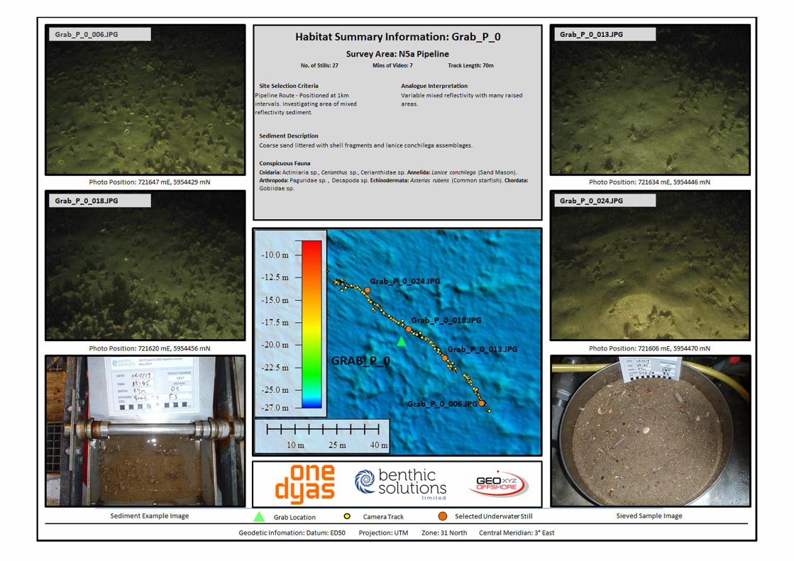
N5a Development LU0022H-553-RR-04
Habitat Assessment Survey Report Revision 2.1
www.geoxyzoffshore.com Page 62 of 96
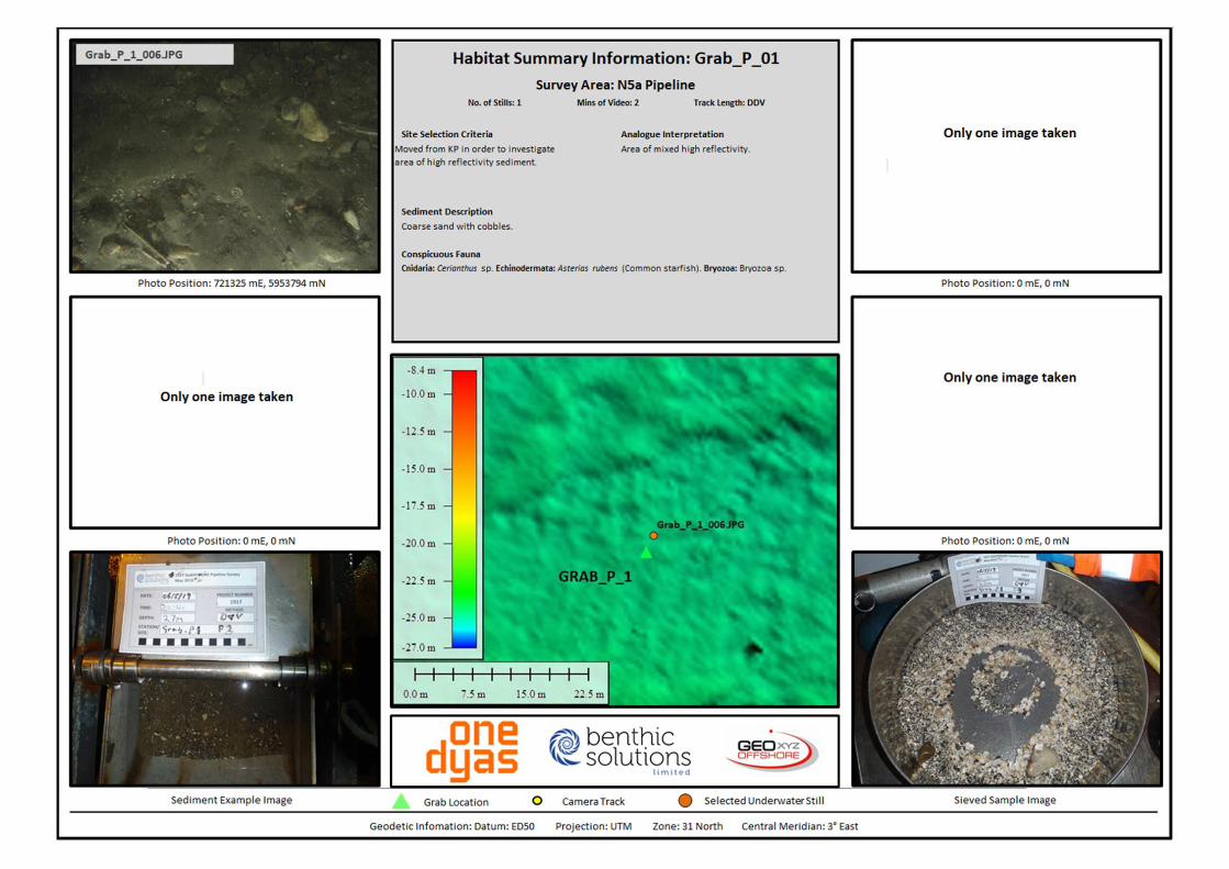
N5a Development LU0022H-553-RR-04
Habitat Assessment Survey Report Revision 2.1
www.geoxyzoffshore.com Page 63 of 96

N5a Development LU0022H-553-RR-04
Habitat Assessment Survey Report Revision 2.1
www.geoxyzoffshore.com Page 64 of 96

N5a Development LU0022H-553-RR-04
Habitat Assessment Survey Report Revision 2.1
www.geoxyzoffshore.com Page 65 of 96
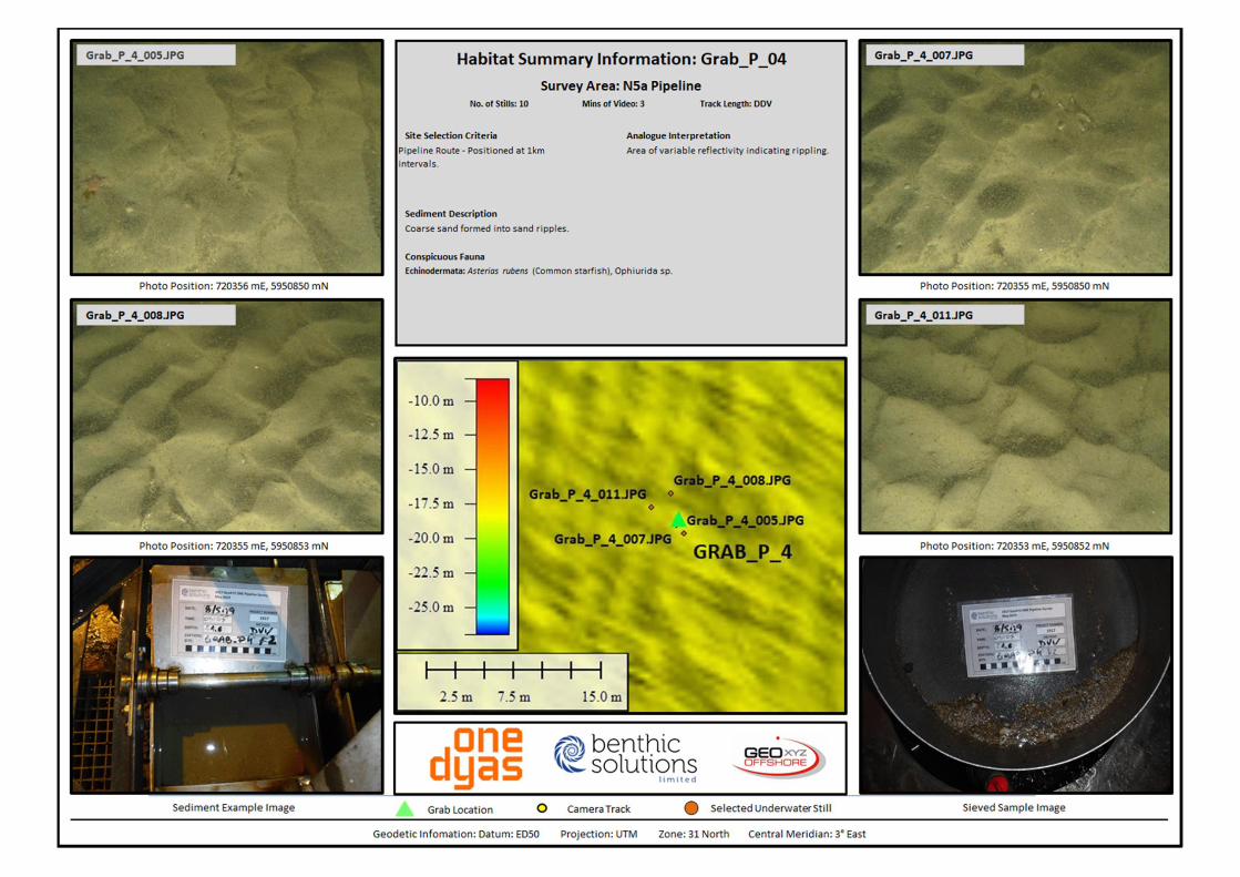
N5a Development LU0022H-553-RR-04
Habitat Assessment Survey Report Revision 2.1
www.geoxyzoffshore.com Page 66 of 96

N5a Development LU0022H-553-RR-04
Habitat Assessment Survey Report Revision 2.1
www.geoxyzoffshore.com Page 67 of 96
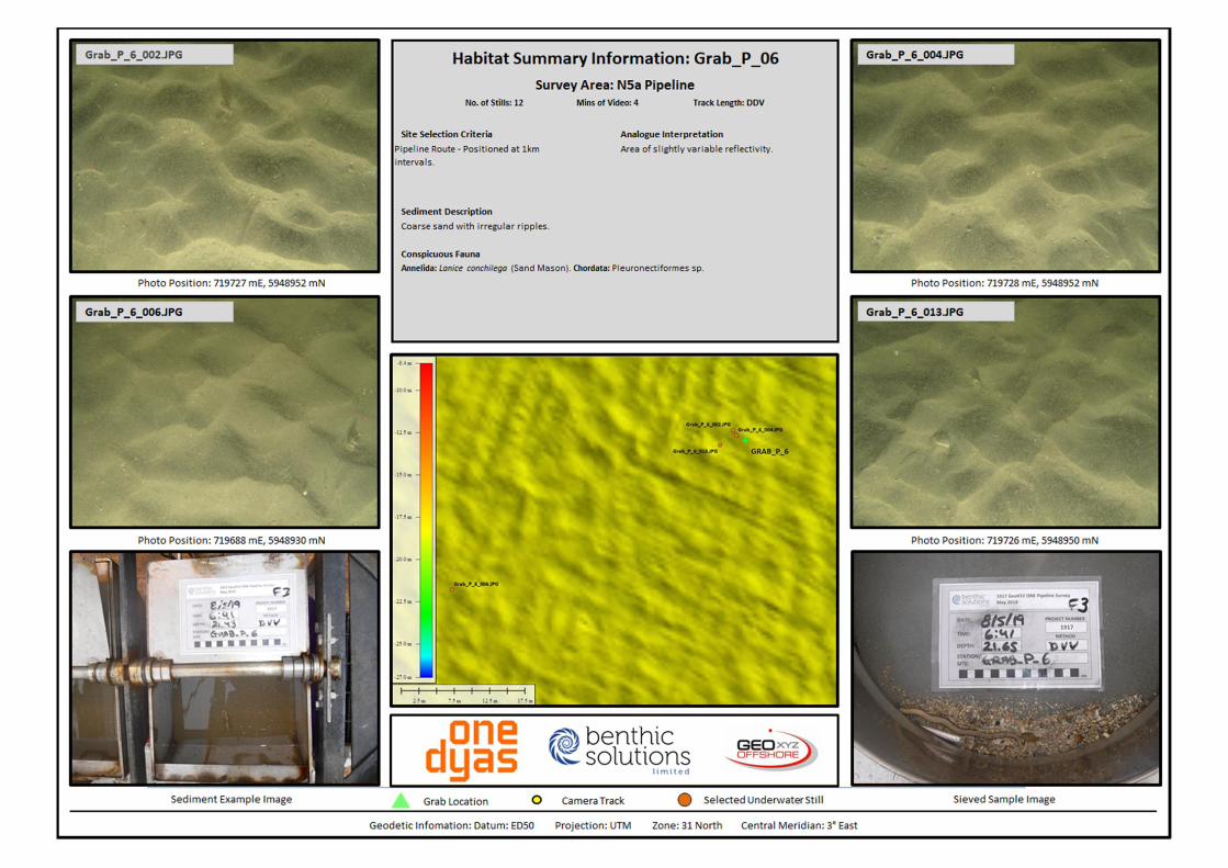
N5a Development LU0022H-553-RR-04
Habitat Assessment Survey Report Revision 2.1
www.geoxyzoffshore.com Page 68 of 96

N5a Development LU0022H-553-RR-04
Habitat Assessment Survey Report Revision 2.1
www.geoxyzoffshore.com Page 69 of 96

N5a Development LU0022H-553-RR-04
Habitat Assessment Survey Report Revision 2.1
www.geoxyzoffshore.com Page 70 of 96

N5a Development LU0022H-553-RR-04
Habitat Assessment Survey Report Revision 2.1
www.geoxyzoffshore.com Page 71 of 96

N5a Development LU0022H-553-RR-04
Habitat Assessment Survey Report Revision 2.1
www.geoxyzoffshore.com Page 72 of 96

N5a Development LU0022H-553-RR-04
Habitat Assessment Survey Report Revision 2.1
www.geoxyzoffshore.com Page 73 of 96

N5a Development LU0022H-553-RR-04
Habitat Assessment Survey Report Revision 2.1
www.geoxyzoffshore.com Page 74 of 96

N5a Development LU0022H-553-RR-04
Habitat Assessment Survey Report Revision 2.1
www.geoxyzoffshore.com Page 75 of 96

N5a Development LU0022H-553-RR-04
Habitat Assessment Survey Report Revision 2.1
www.geoxyzoffshore.com Page 76 of 96
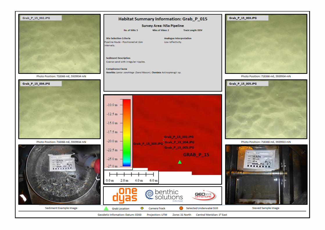
N5a Development LU0022H-553-RR-04
Habitat Assessment Survey Report Revision 2.1
www.geoxyzoffshore.com Page 77 of 96

N5a Development LU0022H-553-RR-04
Habitat Assessment Survey Report Revision 2.1
www.geoxyzoffshore.com Page 78 of 96

N5a Development LU0022H-553-RR-04
Habitat Assessment Survey Report Revision 2.1
www.geoxyzoffshore.com Page 79 of 96
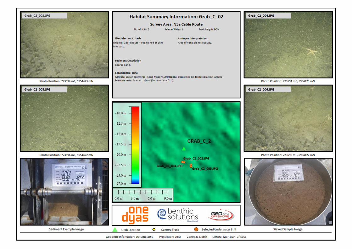
N5a Development LU0022H-553-RR-04
Habitat Assessment Survey Report Revision 2.1
www.geoxyzoffshore.com Page 80 of 96

N5a Development LU0022H-553-RR-04
Habitat Assessment Survey Report Revision 2.1
www.geoxyzoffshore.com Page 81 of 96

N5a Development LU0022H-553-RR-04
Habitat Assessment Survey Report Revision 2.1
www.geoxyzoffshore.com Page 82 of 96

N5a Development LU0022H-553-RR-04
Habitat Assessment Survey Report Revision 2.1
www.geoxyzoffshore.com Page 83 of 96
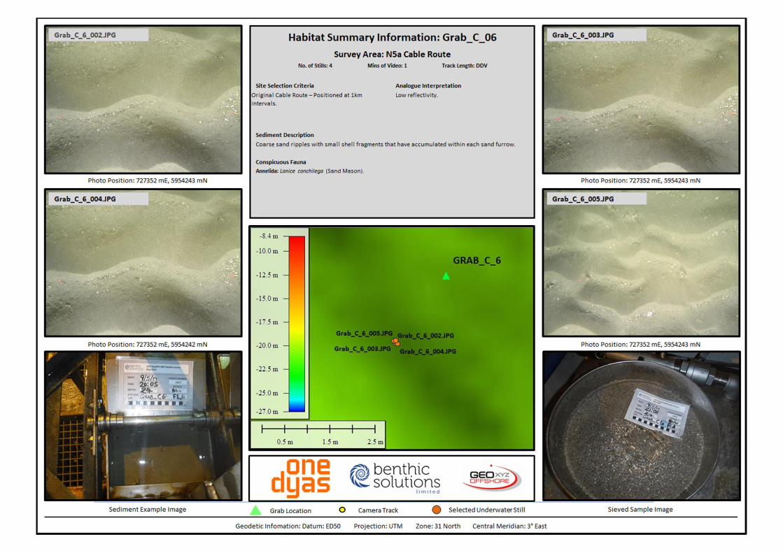
N5a Development LU0022H-553-RR-04
Habitat Assessment Survey Report Revision 2.1
www.geoxyzoffshore.com Page 84 of 96
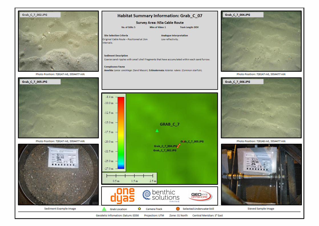
N5a Development LU0022H-553-RR-04
Habitat Assessment Survey Report Revision 2.1
www.geoxyzoffshore.com Page 85 of 96

N5a Development LU0022H-553-RR-04
Habitat Assessment Survey Report Revision 2.1
www.geoxyzoffshore.com Page 86 of 96

N5a Development LU0022H-553-RR-04
Habitat Assessment Survey Report Revision 2.1
www.geoxyzoffshore.com Page 87 of 96

N5a Development LU0022H-553-RR-04
Habitat Assessment Survey Report Revision 2.1
www.geoxyzoffshore.com Page 88 of 96
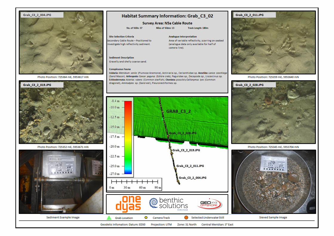
N5a Development LU0022H-553-RR-04
Habitat Assessment Survey Report Revision 2.1
www.geoxyzoffshore.com Page 89 of 96

N5a Development LU0022H-553-RR-04
Habitat Assessment Survey Report Revision 2.1
www.geoxyzoffshore.com Page 90 of 96
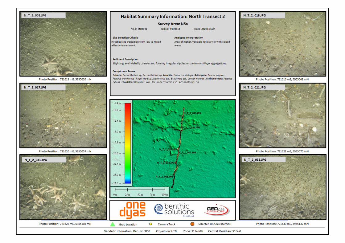
N5a Development LU0022H-553-RR-04
Habitat Assessment Survey Report Revision 2.1
www.geoxyzoffshore.com Page 91 of 96

N5a Development LU0022H-553-RR-04
Habitat Assessment Survey Report Revision 2.1
www.geoxyzoffshore.com Page 92 of 96
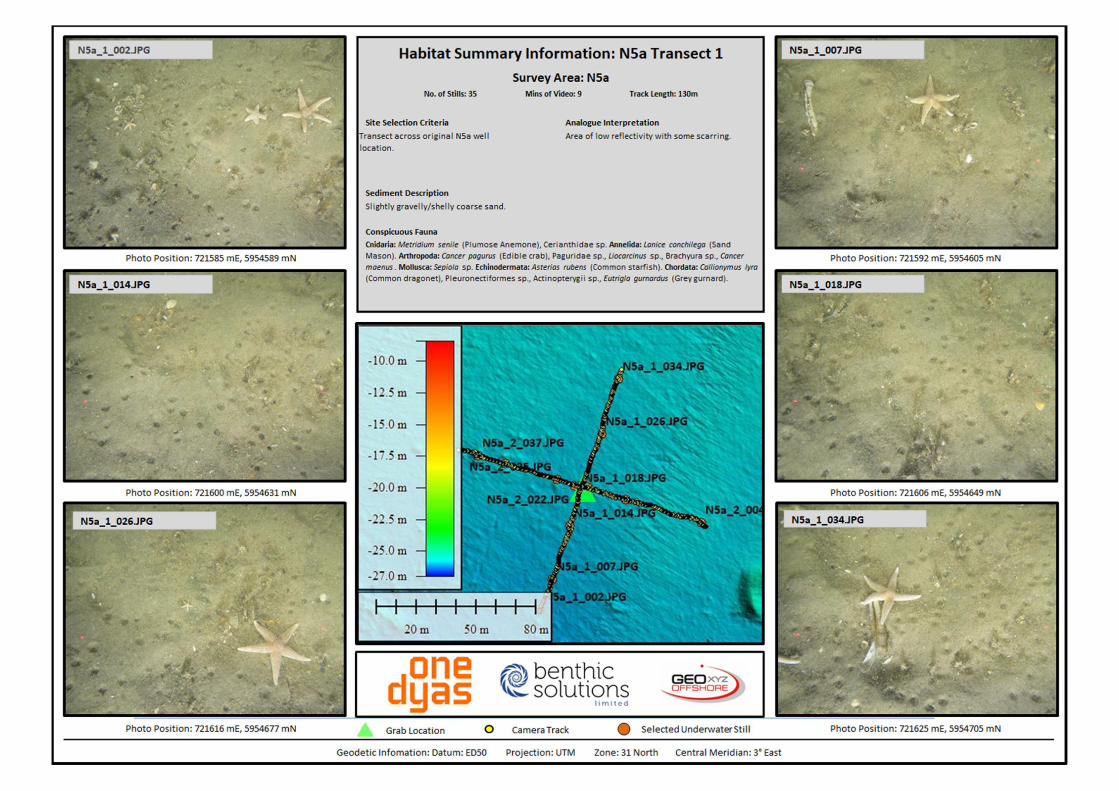
N5a Development LU0022H-553-RR-04
Habitat Assessment Survey Report Revision 2.1
www.geoxyzoffshore.com Page 93 of 96

N5a Development LU0022H-553-RR-04
Habitat Assessment Survey Report Revision 2.1
www.geoxyzoffshore.com Page 94 of 96

N5a Development LU0022H-553-RR-04
Habitat Assessment Survey Report Revision 2.1
www.geoxyzoffshore.com Page 95 of 96
APPENDIX I – SERVICE WARRANTY
This report, with its associated works and services, has been designed solely to meet the requirements of the contract agreed with you, our client. If used in other circumstances, some or all of the results may not be valid and we can accept no liability for such use. Such circumstances include different or changed objectives, use by third parties, or changes to, for example, site conditions or legislation occurring after completion of the work. In case of doubt, please consult Benthic Solutions Limited. Please note that all charts, where applicable should not be used for navigational purposes.
Copyright © 2022 FDOKUMEN