Canadian Science Advisory Secretariat (CSAS)

Research Document 2015/070 Pacific Region

November 2015

Big Skate (Raja binoculata) and Longnose Skate (R. rhina) stock assessments for British Columbia

J.R. King1, A.M. Surry1, S. Garcia2,and P.J. Starr3

1 Fisheries & Oceans Canada, Pacific Biological Station

3190 Hammond Bay Road Nanaimo, British Columbia V9T 6N7

2 1536 G Street Anchorage, Alaska 99501

3 Canadian Groundfish Research and Conservation Society 1406 Rose Ann Drive

Nanaimo, British Columbia V9T 4K8

Foreword This series documents the scientific basis for the evaluation of aquatic resources and ecosystems in Canada. As such, it addresses the issues of the day in the time frames required and the documents it contains are not intended as definitive statements on the subjects addressed but rather as progress reports on ongoing investigations.

Research documents are produced in the official language in which they are provided to the Secretariat.

Published by: Fisheries and Oceans Canada

Canadian Science Advisory Secretariat 200 Kent Street

Ottawa ON K1A 0E6

http://www.dfo-mpo.gc.ca/csas-sccs/ csas-sccs@dfo-mpo.gc.ca

© Her Majesty the Queen in Right of Canada, 2015 ISSN 1919-5044

Correct citation for this publication: King, J.R., Surry, A.M., Garcia, S., and Starr, P.J. 2015. Big Skate (Raja binoculata) and

Longnose Skate (R. rhina) stock assessments for British Columbia. DFO Can. Sci. Advis. Sec. Res. Doc. 2015/070. ix + 329 p.

iii

TABLE OF CONTENTS ABSTRACT .............................................................................................................................. viii

RESUME ................................................................................................................................... ix

1 INTRODUCTION ................................................................................................................. 1

1.1 Request for advice.......................................................................................................... 1 1.2 Distribution and Biology .................................................................................................. 1 1.3 Skate Management in the Groundfish Fisheries ............................................................. 2

1.3.1 Trawl Fishery ........................................................................................................... 2 1.3.2 Line Fisheries .......................................................................................................... 3 1.3.3 Fishery and Market Dynamics ................................................................................. 4

1.4 Previous Assessments ................................................................................................... 4 1.5 Current Assessment ....................................................................................................... 5

1.5.1 Skate Management Areas ....................................................................................... 5 1.5.2 Assessment Approaches ......................................................................................... 6

2 METHODS .......................................................................................................................... 8

2.1 Data Inputs ..................................................................................................................... 8 2.1.1 Catch Data .............................................................................................................. 8 2.1.2 Historical Catch Data Reconstruction ...................................................................... 8 2.1.3 Abundance Indices .................................................................................................. 9

2.2 Approaches for provision of advice ................................................................................11 2.2.1 Bayesian Surplus Production Model .......................................................................11 2.2.2 Depletion-Corrected Average Catch Analysis .........................................................11 2.2.3 Catch-MSY Approach .............................................................................................11 2.2.4 Mean Catch ............................................................................................................12 2.2.5 Advice for 4B (Minor Areas 14 – 18, 28 – 29) .........................................................12

3 RESULTS .......................................................................................................................... 13

3.1 Data Inputs ....................................................................................................................13 3.1.1 Catch ......................................................................................................................13 3.1.2 Abundance Indices .................................................................................................13

3.2 Historic Catch Reconstruction .......................................................................................14 3.3 Bayesian Surplus Production Model ..............................................................................15 3.4 Depletion-Corrected Average Catch Analysis ................................................................15 3.5 Catch-MSY Approach ....................................................................................................16 3.6 Mean Catch ...................................................................................................................16 3.7 Catch and distribution in 4B (Minor areas 13 – 18, 28 – 29) ..........................................16

4 DISCUSSION .................................................................................................................... 16

5 CONCLUSIONS AND RECOMMENDATIONS .................................................................. 17

6 ACKNOWLEDGEMENTS .................................................................................................. 18

7 REFERENCES .................................................................................................................. 18

8 TABLES ............................................................................................................................ 22

9 FIGURES .......................................................................................................................... 29

MINUTES AND RECOMMENDATIONS FROM MEETINGS AND WORKSHOPSAPPENDIX A. .................................................................................................................................................41

iv

DISTRIBUTION AND BIOLOGY ........................................................................63 APPENDIX B.

HISTORICAL COMMERCIAL FISHERIES: 1870S TO 1995 ..............................69 APPENDIX C.

MODERN COMMERCIAL FISHERIES: 1996 – 2011 ........................................75 APPENDIX D.

DEVELOPMENT OF A GLM TO PREDICT SKATE CATCH ..............................90 APPENDIX E.

HISTORIC TRAWL CATCH RECONSTRUCTION ........................................... 105 APPENDIX F.

STANDARDIZATION OF COMMERCIAL TRAWL CPUE ................................ 145 APPENDIX G.

RESEARCH SURVEYS ................................................................................... 164 APPENDIX H.

SURPLUS PRODUCTION MODEL ................................................................... 223 APPENDIX I.

DEPLETION-CORRECTED AVERAGE CATCH ANALYSIS ............................ 234 APPENDIX J.

CATCH-MSY APPROACH ............................................................................... 240 APPENDIX K.

R CODE ........................................................................................................... 273 APPENDIX L.

DATABASE QUERIES .................................................................................... 300 APPENDIX M.

v

LIST OF TABLES Table 1. List of available trawl and longline research surveys investigated to provide relative

abundance indices for Big Skate and Longnose Skate. .....................................................22

Table 2. Biomass estimates for Big Skate from the Hecate Strait Multispecies Assemblage Survey and the Hecate Strait Synoptic Survey in Skate Management Area 5CDE. Bootstrap bias corrected confidence intervals and CVs are based on 1000 random draws with replacement. ..............................................................................................................23

Table 3. Catch rate (CPUE; pieces per 100 hooks) for Big Skate from longline surveys by Skate Management Area. Bootstrap bias corrected confidence intervals and CVs are based on 1000 random draws with replacement. ..............................................................................24

Table 4. Results of trend analyses for surveys with CVs estimates <0.2 target precision level (for trawl biomass or longline catch rates) for Big Skate and Longnsoe skate. The trend analyses provided estimates of slope (b), mean annual rate of change (r) and accumulated rate of change (R). Bootstrapping (1,000 random with replacement) distributions for b and r provided 2.5 and 97.5% quantiles. Bootstrapped distributions with zero outside of these quantiles are noted with astericks. .....................................................................................25

Table 5. Biomass estimates for Longnose Skate from the WCVI Shrimp Survey and Synoptic Survey in Skate Management Area 3CD; the Queen Charlotte Sound Shrimp Survey and Synoptic Survey in Skate Management Area 5AB; the Hecate Strait Synoptic Survey and the West Coast Haida Gwaii Synoptic Survey in Skate Management Area 5CDE. Bootstrap bias corrected confidence intervals and CVs are based on 1000 random draws with replacement. ..............................................................................................................26

Table 6. Catch rate (CPUE; pieces per 100 hooks) for Longnose Skate from longline surveys by Skate Management Area. Bootstrap bias corrected confidence intervals and CVs are based on 1000 random draws with replacement................................................................27

Table 7. Mean commercial trawl and line catch (landings and discards*discard mortality [tonnes]) for Big Skate and Longnose Skate by Skate Management Area (and coastwide for Longnose Skate only) for long-term (1996 – 2011), 10-year (2002 – 2011) and 5-year (2007 – 2011) periods. The range of mean MSY estimates (tonnes) produced across all scenarios from the Catch-MSY approach is presented for each Skate Management Area. ..........................................................................................................................................28

vi

LIST OF FIGURES Figure 1. Mean catch per unit of effort (CPUE) for Big Skate over a 0.1° x 0.1° grid for (A) the

commercial trawl fishery and research trawl surveys from 1996 – 2011 (kg/hour) and (B) the commercial longline fishery and research longline surveys from from 2006 – 2011 (pieces / 100 hooks). A mean CPUE value of zero represents fishing effort with zero catch of Big Skate. ......................................................................................................................29

Figure 2. Mean catch per unit of effort (CPUE) for Longnose Skate over a 0.1° x 0.1° grid for (A) the commercial trawl fishery and research trawl surveys from 1996 – 2011 (kg/hour) and (B) the commercial longline fishery and research longline surveys from from 2006 – 2011 (pieces / 100 hooks). A mean CPUE value of zero represents fishing effort with zero catch of Longnose Skate. ..................................................................................................30

Figure 3. Proposed Skate Management Areas. Area 3CD includes minor areas 19 and 20. Area 5AB includes minor area 12. Area 4B is minor areas 13 – 18, 28 and 29 only. ........31

Figure 4. Big Skate catch (landings and discard mortality in tonnes) by trawl (thin line) and line (dashed line) gear by Skate Management Area. Thick line is total catch (tonnes). ...........32

Figure 5. Longnose Skate catch (landings and discard mortality in tonnes) by trawl (thin line) and line (dashed line) gear by Skate Management Area. Thick line is total catch (tonnes). ..........................................................................................................................................33

Figure 6. Big Skate indices from trawl and longline research surveys. Annual mean biomass (squares) is estimated by stratified swept-area calculation (Appendix H). Annual mean catch per unit effort (CPUE, squares) is calculated as pieces per 100 hooks. Boostrapped replicates (1,000 random with replacement) were used to estimate 95% confidence intervals (vertical lines), 25th and 75th quantiles (boxes) and median (horizontal lines). Trend analyses and bootstrapped estimates of slope and annual rate of change did not detect any trends significantly (p<0.05) different than zero. ...............................................34

Figure 7. Longnose Skate abundance indices from trawl research surveys. Annual mean biomass (squares) is estimated by stratified swept-area calculation (Appendix H). Boostrapped replicates (1,000 random with replacement) were used to estimate 95% confidence intervals (vertical lines), 25th and 75th quantiles (boxes) and median (horizontal lines). Only those trends (red line) significantly different (p<0.05) than zero are plotted. ..35

Figure 8. Longnose Skate catch rates (pieces per 100 hooks, squares) from longline research surveys. Boostrapped replicates (1,000 random with replacement) were used to estimate 95% confidence intervals (vertical lines), 25th and 75th quantiles (boxes) and median (horizontal lines). Trend analyses and bootstrapped estimates of slope and annual rate of change did not detect any trends significantly different (p<0.05) than zero. .......................36

Figure 9. Observed and predicted annual mean Big Skate catch (kg) based on: A) lognormal GLM, using all data points; B) lognormal GLM, with high-leverage data points removed; C) lognormal GLM using positive tows only (zeros excluded); D) two-step GLM using all data points. Data are rolled up trawl tows from Skate Management Area 5CDE in 2001 – 20011. Errors bars are the 95% confidence intervals. Note that using positive tows only as in (C) results in higher annual mean catch than when all data points are used. .................37

Figure 10. Bayesian Surplus Production Model results for Big Skate in 5CDE. Probability distributions for the: A) intrinsic population growth rate (r) and, B) carrying capacity (K); prior (solid line) and posterior (dashed line). Posterior probability distributions for: C) MSY, D) BMSY , and E) FMSY . F) The log predicted Big Skate population abundance in area 5CDE from 1984 – 2011. The light grey is the 90% quantile, medium grey is the 80%

vii

quantile, dark grey is the 50% quantile and the solid black line is the median log predicted population biomass. ..........................................................................................................38

Figure 11. Results from Catch-MSY approach for Big Skate in 5CDE using catch data from 1996 – 2011 (case 1 is default scenario). Posterior density distributions for: A) carrying capacity, k (thousand of tonnes) and B) intrinsic rate of increase, r . The thick solid lines are geometric means, dashed lines are 5%, 50% (median) and 95% quantiles, red lines are prior distributions. ..............................................................................................................39

Figure 12. Mean catch per unit effort (CPUE) by 0.05° by 0.05° grid in Skate Management Area 4B for Big Skate captured in A) trawl commercial fisheries, B) line commercial fisheries, C) line research surveys and for Longnose Skate captured in D) trawl commercial fisheries, E) line commercial fisheries, F) line research surveys. ...........................................................40

viii

ABSTRACT Big Skate (Raja binoculata) and Longnose Skate (R. rhina) are captured and landed by the commercial groundfish trawl and hook-and-line fisheries. Harvest advice was requested to assess whether current harvest levels are sustainable and compliant with the Fishery Decision-making Framework Incorporating the Precautionary Approach. This is the first detailed stock assessment undertaken for these Pacific stocks. Several methods were explored for assessing the stock status of Big Skate and Longnose Skate in order to provide harvest advice. A Bayesian surplus production model was investigated for a Big Skate case study, but produced unsatisfactory results for providing fisheries management advice and was not considered further. As such, reliable estimates of biomass could not be produced, and evaluation of current and future stock status relative to fishery and biological reference points was not possible.

As an alternative to formal stock assessment models, two data-limited approaches were investigated for a Big Skate case study. The first, Depletion-Corrected Average Catch Analysis, produced a range of potential yield estimates that were above the long-term average catch, with an upper bound that was three orders of magnitude larger than the long-term average catch. Based on these results, this approach was not investigated further. The second data-limited approach, Catch-MSY (maximum sustainable yield) Approach, produced plausible results for a Big Skate case study and was applied to Big Skate and Longnose Skate in all areas. However, results were extremely sensitive to assumptions, without consistent responses across areas or assumption combinations, and are not recommended as the sole basis of advice to managers.

In lieu of the development of decision tables, and based on life history traits (namely extremely low fecundity and low intrinsic rate of increase for these species), it is recommened that Big Skate and Longnose Skate be managed by catch limits in all areas of British Columbia. Establishing harvest yields based on mean historic catch, with consideration given to results of trend analyses of research survey abundance indices and to the ranges of maximum sustainable yield estimates identified by the Catch-MSY Approach is recommended. For Big Skate, there were no significant trends in abundance indices from surveys for all areas, and mean historical catches were below the maximum MSY estimate from the catch-MSY results. For Longnose Skate, trawl survey data indicated statistically significant declines in abundance in all areas; however, no significant trends were detected for the longline survey data. For all areas, mean historical catches exceeded the upper maximum sustainable yield estimate from the Catch-MSY Approach results.

ix

Évaluations des stocks de raie biocellée (Raja binoculata) et de pocheteau long-nez (R. rhina) en Colombie-Britannique

RESUME La raie biocellée (Raja binoculata) et le pocheteau long-nez (R. rhina) sont pêchés et débarqués dans le cadre des pêches commerciales au poisson de fond au chalut et à la ligne. Des avis sur les prélèvements ont été demandés en vue de déterminer si les niveaux de récolte actuels sont durables et conformes au cadre décisionnel pour les pêches intégrant l'approche de précaution du MPO. Il s'agit de la première évaluation détaillée entreprise pour ces stocks dans le Pacifique. Plusieurs méthodes ont été étudiées pour évaluer l'état du stock de raie biocellée et de pocheteau long-nez dans le but de fournir un avis sur les prélèvements. Un modèle bayésien de production excédentaire a été envisagé pour réaliser une étude de cas sur la raie biocellée, mais a produit des résultats insatisfaisants qui ne permettaient pas de formuler des conseils en matière de gestion des pêches et n'a donc pas été retenu. Par conséquent, nous n'avons pas pu produire d'estimations fiables de la biomasse ni évaluer l'état actuel et futur des stocks en fonction de la pêche et des points de référence biologiques.

Comme solution de rechange aux modèles officiels d'évaluation des stocks, deux approches utilisant des données limitées ont été envisagées pour l'étude de cas sur la raie biocellée. La première, la méthode « Depletion-Corrected Average Catch Analysis », a produit une gamme d'estimations du rendement potentiel qui étaient supérieures aux prises moyennes à long terme et qui présentaient une limite supérieure qui dépasse de trois ordres de grandeur les prises moyennes à long terme. Étant donné ces résultats, cette approche n'a pas été examinée davantage. La deuxième approche utilisant des données limitées, la méthode fondée sur le RMS (rendement maximal soutenu), a produit des résultats plausibles pour une étude de cas sur la raie biocellée et a été appliquée aux stocks de raie biocellée et de pocheteau long-nez dans toutes les régions. Toutefois, les résultats reposaient essentiellement sur des hypothèses et donnaient des réponses variables selon les régions et les combinaisons d'hypothèses. Il n'est donc pas recommandé de fonder les avis aux gestionnaires uniquement sur ces résultats.

Au lieu de produire des tableaux de décision, et étant donné les caractéristiques du cycle biologique de ces espèces (soit leur taux de fécondité extrêmement faible et leur faible taux de croissance intrinsèque), il est recommandé de gérer la raie biocellée et le pocheteau long-nez au moyen de limites de prises dans toutes les zones de la Colombie-Britannique. Il est également recommandé d'établir des taux de prélèvement en fonction des prises historiques moyennes, compte tenu des résultats des analyses de tendances provenant des indices d'abondance des relevés de recherche, et compte tenu de la gamme des estimations du rendement maximal soutenu découlant de la méthode fondée sur le RMS et les prises. En ce qui concerne la raie biocellée, les indices d'abondance provenant des relevés dans toutes les zones n'ont révélé aucune tendance importante, et les prises historiques moyennes étaient inférieures au RMS estimé à partir des résultats de la méthode fondée sur le RMS et les prises. Quant au pocheteau long-nez, les données des relevés au chalut ont révélé des baisses d'abondance statistiquement significatives dans toutes les zones. Toutefois, aucune tendance importante n'est ressortie des données des relevés à la palangre. Dans toutes les zones, les prises historiques moyennes dépassaient le rendement maximal soutenu estimé à l'aide des résultats de la méthode fondée sur le RMS et les prises.

1

1 INTRODUCTION

1.1 REQUEST FOR ADVICE In 2009, the Canadian Pacific halibut fishery received Marine Stewardship Council certification subject to conditions, one of which is directly related to skate bycatch in the halibut fishery:

• Condition 2.1.4.1: Develop a strategic plan to understand and mitigate risks to non-target species affected by the BC Halibut Fishery. Specifically, assessments to be completed on the consequences [risks] of current levels of removal to non-target species.

In 2010, the catch (landings and discards) of Big Skate and Longnose Skate was approximately 5% of the annual halibut catch.

In response to the condition placed on the halibut fishery, the Groundfish Management Unit (GMU) in the Pacific Region has submitted a “2012 Request for a Working Paper for British Columbia Big Skate and Longnose Skate” to the Centre for Science Advice - Pacific (CSAP). The GMU is requesting: (i) advice on the current status of Big Skate and Longnose Skate populations relative to the reference points within DFO's Fishery Decision-making Framework Incorporating the Precautionary Approach (DFO 2009); and (ii) provision of decision tables that forecast the impact of varying levels of harvest on future population trends.

1.2 DISTRIBUTION AND BIOLOGY Big Skate, Raja binoculata, and Longnose Skate, R. rhina, belong to the family Rajidae within Chondrichthyes: Elamsobranchii. Recent evidence has recommended that Big Skate be placed in a newly erected genus, Beringraja, based on egg case and clasper morphology, and the number of embryos per egg case (Ishihara et al. 2012) The catalogue of fishes updated by the California Academy of Sciences (Eschmeyer, 2013) lists Big Skate to be currently valid as Beringraja binoculata, suggesting that in the near future the new scientific name of this species will be universally accepted and adopted. Longnose Skate will continue to be classified under the genus Raja.

Big Skate and Longnose Skate are coastal species found along the continental shelf of the eastern Pacific from central Baja California to the eastern Bering Sea (Ebert 2003; Mecklenburg et al. 2002). Big Skate are found on sandy and muddy bottoms at depths ranging from the low intertidal zone to 800 m, but are usually found at less than 200m (Mecklenburg et al. 2002). Longnose Skate are found on mud-cobble bottom, often near boulders and rock ledges (Ebert 2003) at depths from 20 – 1000 m, but are usually found at less than 350 m (Ebert 2003; Mecklenberg et al. 2002). Participants in groundfish commercial fisheries in British Columbia report that Big Skate are encountered most frequently at 55 – 110 m, while Longnose Skate are encountered at approximately 110 – 605 m (Appendix A).

A tagging program for Big Skate in British Columbia conducted from 2003 – 2006 indicated that little movement occurs between geographic regions, suggesting the existence of reasonably discrete Big Skate stocks (King and McFarlane 2010). Approximately 75% of the recaptured Big Skate were recaptured within 21 km of the original tagging location, and there was no evidence of seasonal migrations. A small number of Big Skate (about 1.5% of recaptures), mostly females that were maturing or just matured at the time of tagging, were recaptured in waters throughout the Gulf of Alaska and the Bering Sea, as well as off the Washington and Oregon coasts (King and McFarlane 2010). These long-range movements of up to 2340 km indicate the potential for exchange of Big Skate throughout its extensive distribution range (King and McFarlane 2010).

2

Skate sexes are dimorphic, with females often growing larger than males, especially in larger species such as Big Skate (Ebert et al. 2008). Males are identifiable by the presence of paired claspers on the pelvic fins which are used for fertilization. Fertilization is internal, and females are oviparous, depositing eggs in purse-like egg cases on the bottom. Big Skate egg cases are the largest of any skate species in the eastern North Pacific, and contain up to 8 eggs, with 3–4 being most common (DeLacy and Chapman 1935, Hitz 1964; Ford 1971). Longnose Skate egg cases contain one egg (DeLacy and Chapman 1935).

Big Skate are considered the largest skate species in the eastern North Pacific, reaching a maximum total length of 184 cm for males and 214 cm for females (McFarlane and King 2006). Growth and maturity estimates are available for Big Skate from northern British Columbia collected during research trawl surveys conducted by DFO in 2001 – 2003 (McFarlane and King 2006). Age at 50% maturity was estimated to be 6 years (72 cm) for males and 8 years (90 cm) for females. Growth in male Big Skates is most rapid in the first 5 years and by age 11 growth is greatly reduced. Similarly in female Big Skates, growth is very rapid in the first 6 years followed by a marked reduction by age 12 (McFarlane and King 2006). The maximum age estimated for Big Skate in British Columbia waters is 26 years (McFarlane and King 2006).

The maximum recorded total length for Longnose Skate is 136 cm for males and 145 cm for females (Ebert et al. 2008); however, the maximum length observed to date in British Columbia is 140 cm for males and 146 cm for females (Jackie. King, Fisheries and Oceans Canada, Pacific Biological Station, Nanaimo, unpub. data). Growth and maturity estimates are available for Longnose Skate from northern British Columbia collected during research trawl surveys conducted by DFO in 2001 – 2004 (McFarlane and King 2006). Age at 50% maturity was estimated to be 7 years (65 cm) for males and 10 years (83 cm) for females. Growth is similar in male and female Longnose Skates and appears to slow after approximately age 7; after age 14 there is very little subsequent growth. The maximum age estimated for Longnose Skate in British Columbia waters is 26 years (McFarlane and King 2006).

See Appendix B for a more comprehensive outline of skate biology, including reproductive biology, diet and predators.

1.3 SKATE MANAGEMENT IN THE GROUNDFISH FISHERIES Groundfish catches, including skates, are managed according to established groundfish management areas, called Major Areas or Pacific Fishery Management Council (PFMC) Areas (DFO 2011). In general, Major Areas 3C and 3D correspond to the West Coast of Vancouver Island, Major Area 4B corresponds to the Strait of Georgia, Major Areas 5A and 5B correspond to Queen Charlotte Sound, Major Areas 5C and 5D correspond to Hecate Strait, and Major Area 5E corresponds to the west coast of Haida Gwaii. Major areas are subdivided into Minor Areas, which are roughly equivalent to Pacific Fishery Management Subareas, described in the Pacific Fishery Management Area Regulations, 2007 (SOR/2007-77).

Skates have been encountered in commercial fisheries in British Columbia since at least the early 1900s (Appendix D). However, the first management measures specifically restricting skate catch in British Columbia were not implemented until 2002, and these measures only affected certain fisheries in specific areas. To date, there are no annual limits on trawl catches of skates except for Big Skate and Longnose Skate in Hecate Strait (Major Areas 5C and 5D), while line catch of skate is restricted only by coastwide trip limits.

1.3.1 Trawl Fishery Currently, the largest fishery in British Columbia that encounters skate is the groundfish trawl fishery which operates by midwater trawl coastwide, and by bottom trawl in all areas outside the

3

Strait of Georgia (4B) under the provisions of an "Option A" trawl (T) license (DFO 2011). Skate are predominately captured in the Option A fishery by bottom trawl in the Hecate Strait area (5C and 5D). Starting in 1996, all Option A trawlers were subject to 100% at-sea observer coverage, along with 100% dockside validation. Therefore, from 1996 onwards, skates have been identified to species, and along with other groundfish species, reliable estimates of discards and landings have been collected. In 1997, DFO and Industry agreed to implement Individual Vessel Quotas (IVQs) for the Option A fishery, although skates were not quota species (DFO 1998a). Since 2002, following the recommendations of Benson et al. (2001), trawl harvests of Big and Longnose Skate by the Option A fishery in 5C and 5D combined have been subject to a total allowable catch (TAC) of 567 tonnes and 47 tonnes, respectively, and vessels have been subject to IVQs for these species (DFO 2002a). Currently Option A vessels catching skate in other outside areas (3C, 3D, 5A, 5B or 5E) are not subject to any TAC (DFO 2011).

A small bottom trawl fishery operates within the Strait of Georgia (4B) under the provisions of an "Option B" trawl (T) license (DFO 2011). This fleet consists of small 1-2 man vessels that predominantly day fish out of the Metro Vancouver and Sydney areas. The Option B fishery occurs primarily in the southern portion of the Strait of Georgia and is subject to 100% dockside validation. Starting in 2002, the Option B fishery was subject to limited on-board observer coverage to verify fishing locations and amounts of retained and discarded catch (DFO 2002a). This was increased to mandatory 10% covereage in 2003, and to 100% in 2007 (DFO 2003; DFO 2007). Since 1997, Option B vessels have been restricted to 15 landings per month and a total monthly catch of 6.8 tonnes of all Groundfish species combined. Within that monthly cap there is no restriction on the amount that could be skate species.

1.3.2 Line Fisheries Hook and line fisheries that encounter skate in British Columbia operate under the authority of vessel-based or party-based licences and include longline, handline, jig, troll, and trap fisheries for Halibut (L) , Sablefish(K), Rockfish (ZN), and Salmon Troll (AT) (DFO 2011). These licences include what is commonly referred to as "Schedule II – Other Species" provisions, which authorize fishing for dogfish, lingcod, sole and flounder, Pacific cod, and other non-groundfish species by hook and line gear. Prior to 2006, skate was also included in Schedule II provisions (e.g. DFO 2001).

From 1996, dockside validation has been required, and vessels are restricted to designated landing locations (DFO 1998b). Species-specific identification of skates in the dockside monitoring program started in 1997. Starting in 2001, the hook and line fleet was subject to limited coverage (50 sea days) by at-sea observers (DFO 2001). At-sea monitoring increased from 2002 – 2006, and included both on-board observers and electronic monitoring. By 2006, the hook and line fleet was subject to mandatory 100% at-sea coverage by either observer or electronic monitoring (DFO 2002b; DFO 2006).

A large groundfish hook and line fishery operates in all areas outside the Strait of Georgia (4B) and encounters skates predominantly off the West Coast of Vancouver Island (3C and 3D) (DFO 2011). In addition, a hook and line fishery occurs within the inside waters of the Strait of Georgia (4B), primarily in the western Strait of Georgia, Queen Charlotte Strait, and eastern Juan de Fuca Strait (DFO 2011). Prior to 2004, there were no limits on skate catch by hook and line fisheries anywhere in British Columbia. In 2004, in response to a three-fold increase in skate landings from the hook and line fishery between 2002 and 2003, as well as recommendations from Benson et al. (2001), Schedule II licenced vessels were restricted to a maximum of 5.7 tonnes of skate landed (all species combined) per calendar month (DFO 2004). In 2006, with the implementation of the Commercial Groundfish Integration Pilot Program (CGIPP), skate was removed from the Schedule II provisions and made solely a trip limit for the

4

directed hook and line fisheries (DFO 2006). The monthly 5.7 tonnes limit was modified in to a maximum trip limit of 2.7 tonnes of skate (all species combined) taken during a directed fishery trip (e.g. halibut, sablefish, rockfish, Schedule II dogfish or lingcod), excluding inside rockfish vessels which are subject to a skate trip limit of 20 kg, and inside halibut vessels which have non-retention of skate (DFO 2006).

1.3.3 Fishery and Market Dynamics Participants in the groundfish commercial fisheries provided input on factors influencing the skate fishery and market dynamics (Appendix A). The catches (landings and discards) of both skate species are affected by market demand, market price, fuel costs, management actions and the opportunities or restrictions on catch of other species. In 1996 interest in skate led to the development of a targeted skate fishery in Hecate Strait (5C and 5D). However in that same year, the implementation of mandatory at-sea observer coverage for the commercial trawl fleet and Individual Vessel Quotas for most major trawl species influenced fishing behaviour, and consequently 1996 was not a ‘typical’ year. In subsequent years, although there was uncertainty surrounding how to operate in this new management regime, the groundfish fleet was free to respond to market demand by developing new opportunities to fish skate species, because these species were not constrained by quotas. As a result, increased landings of Big Skate and Longnose Skate occurred. Coincident with this development, special large mesh trawl codends (12 – 16 inches) were being used to target skate while reducing the bycatch of other species. The use of these large mesh codends has been intermittent, with no more than approximately 12 vessels participating, mainly in 5CD and to a lesser extent in 5AB.

Landings in 5CD increased as market demand and prices for skate increased, until 2002 when caps for Big Skate and Longnose Skate catch were implemented. Levels of catch for both species in 5CD have remained relatively steady since 2002, but have increased in 5AB since the market prices were still high and there were no catch limits in place in that area. In addition, there were no quota or lease fees charged against skate catches in 5AB which provided economic incentives to harvest skate in that area. The market price for skate was highest in 2003. Rising fuel prices, along with a dropping Canadian dollar and a diminishing market for skate contributed to a decrease in skate landings from 2007.

Opportunities and restrictions for other species also impact skate catch. For example, in 2001 portions of Hecate Strait were closed due to Pacific cod restrictions which limited fishable areas and also influenced the ability to select other species to target, such as skate. In 2005 there was an arrowtooth flounder fishery in 5CD and skates were caught incidentally. In 2006, a quota for arrowtooth flounder was put in place which would have likely lowered the incidental catch of skate. The fishing behaviour of the line fleet has been influenced by opportunities for halibut and sablefish. Since the 2006 integration of the line and trawl fisheries, more vessels in the line fleet have increased effort on halibut and sablefish with less effort on dogfish. Halibut and sablefish typically occupy the same depth range as Longnose Skate, and because of increased effort in these depths for these species, line landings of Longnose Skate have increased. However, a decreasing halibut quota since 2008 has complicated this impact for line landings of Big Skate in 3CD. Reduced halibut quota, coupled with increased fuel prices, has resulted in shorter trips which tend to fish in shallower depths which are the preferred deths for Big Skate, and consequently lead to increased interceptions and landings of Big Skate.

1.4 PREVIOUS ASSESSMENTS In 2001, a review of the biology, fisheries, stock assessments, and management of 14 shark species and 5 skate species (including Big Skate, Raja binoculata, and Longnose Skate, R. rhina) was presented to the Pacific Science Advice Review Committee (PSARC) (Benson et al.

5

2001). The intent of the document was to address questions raised by managers and to form the basis for subsequent management actions. The specific questions were:

1. What is known about the biology and productivity of skates and sharks that are caught in BC waters and/or other jurisdictions?

2. What is known about the biomass and stock size structure of BC skates and sharks and how does this relate to historical stock conditions?

3. What are the appropriate harvest levels, given the biology and status of skates and sharks?

4. What information is available on the bycatch and associated mortalities of skates and sharks in other fisheries?

Benson et al. (2001) highlighted the increased landings of Big Skate and Longnose Skate since 1996 resulting from the development of directed trawl and longline fisheries for both species. In 2001, the largest amount of skate landings were by trawl gear and the largest catches were reported in 5D (northern Hecate Strait). Based on the life history of Big Skate and Longnose Skate, concerns regarding the potential low resilience of these species, and increases in these species’ catch since 1996, Benson et al. (2001) recommended catch limits be put in place for these two species. The document cited a concern that a coastwide limit would result in increased effort in Major Area 5D (northern Hecate Strait). Therefore area-specific catch limits for 5D were recommended for Big Skate (700 tonnes) and Longnose Skate (200 tonnes) based on the 1996 – 2000 median catches for each species. Prior to this time there were no specific restrictions on the catch of skate in BC Groundfish fisheries. In 2002, a trawl catch limit was implemented for Big Skate (567 tonnes) and Longnose Skate (47 tonnes) for the combined area 5CD. A lower limit over a wider area was selected to address concerns of possible limitations that skate quotas would have on other target fisheries. In 2004, line vessels were restricted to a monthly limit of 5.7 tonnes of skate landed (all species combined). This limit was modified in 2006 to a maximum trip limit of 2.7 tonnes of skate (all species combined), excluding inside rockfish vessels which are subject to a trip limit of 20 kg of skate (all species combined).

1.5 CURRENT ASSESSMENT The work undertaken for this assessment was directed and reviewed by a skate Technical Science Working Group (TSWG), which met four times between July and November 2012 (Appendix A). The TSWG provided input on data sources and interpretation including suitable surveys, standardization of fishery and survey indices of abundance, reconstruction of historic (1954 – 1995) fishery data, assessment methodologies, suitable management units and provision of advice to managers. In a December 2012 workshop, representatives of the trawl fleet and the Schedule II line fleet provided input on the interpretation of skate catch data in relation to management changes, fishery dynamics, market fluctuations, and abundance or distributional changes (Appendix A).

1.5.1 Skate Management Areas A comprehensive tagging study of Big Skate in British Columbia found that 75% of the recovered tagged fish were recaptured within 21 km of the tagging location (King and McFarlane, 2010). Tagging studies on other skate species (R. radiata, R. clavata, R. montagui) conducted in the Atlantic confirm limited movements of skates and rays, typically less than 130 km, even up to 20 years after tagging (Templeman 1984; Walker et al. 1997; Sutcliffe et al. 2002). These results suggest that a coastwide unit of management is not biologically appropriate for skates. Additionally, there are localized spatial patterns evident in the trawl catch of Big Skate and Longnose Skate, with centres of the catch occurring in Major Areas 5D

6

and 5B for Big Skate (Figure 1A) and in 3C for Longnose Skate (Figure 2A). The line catch for Big Skate does not have as definitive a spatial pattern as for trawl catch (Figure 1B). The spatial pattern of line catch for Longnose Skate is similar to the trawl catch for that species (Figure 2B).

Stock status information specific to Major Area 4B was identified in the Request for Advice, because there are trip limits for the longline fishery that apply to skates in this area. However, annual Big Skate and Longnose Skate catches in 4B are very low (typically less than 30 tonnes/year) with limited survey data available and most of the catch occurring at the northern and southern limits of the Strait of Georgia (Minor Area 12, Queen Charlotte Strait and Minor Areas 19 and 20: Juan de Fuca Strait). The spatial pattern in the commercial catches for Minor Area 12 appears continuous with the adjacent Major Area 5A, while the spatial pattern for Minor Areas 19 and 20 appears continuous with the adjacent Major Area 3C. Ecologically, these demarcations roughly overlap the physical oceanographic boundaries of the Strait of Georgia (Thomson 1994).

Considering tagging results and fishery spatial patterns, the TSWG selected four Skate Management Areas (Figure 3) for assessment and provision of advice:

1. 3CD (including minor areas 19 and 20 of 4B)

2. 5AB (including minor area 12 of 4B),

3. 5CDE,

4. 4B (minor areas 13 – 18, 28, 29 only).

These aggregates were seen as a compromise to selecting smaller (e.g. 3C, 3D etc) units. Smaller units might limit opportunities in other fisheries if Big Skate and Longnose Skate restrictions were implemented.

Area 5E (West Coast Haida Gwaii) represents a large geographic area with limited grounds suitable for the skate fishery, and is geographically distinct from Areas 5C and 5D (Hecate Strait). However, the spatial extent of commercial fishing off north Haida Gwaii ranges across the 5D and 5E boundary. The narrow continental shelf off the west coast of Haida Gwaii would likely limit targeted skate fishing in Area 5E. Based on these considerations, 5E was included with 5CD and not retained as a separate management area. In this document, these Skate Management Areas will be referred to as 3CD, 5AB, 5CDE and 4B.

At the December 2012 meeting with groundfish industry representatives (Appendix A), it was noted that catch limits for skate within these four aggregated management units might constrain the opportunity to capture other groundfish species. This may be true, particularly for Longnose Skate because they tend to be passively intercepted while fishing for other species (Appendix A). Industry representatives suggested that since Big Skate appear to be more aggregated, a coastwide catch limit might impose more of a risk for area depletion (Appendix A). However, a coastwide catch limit might be more appropriate for Longnose Skate because they do exhibit the aggregataing behaviour, and a coastwide limit would allow more flexibility for the integrated groundfish fisheries and would be less likely to result in area depletions (Appendix A). Based on this feedback, coastwide harvest advice is provided for Longnose Skate in addition to the four proposed Skate Management Areas.

1.5.2 Assessment Approaches Several methods were explored for assessing the stock status of Big Skate and Longnose Skate in order to provide harvest advice. Initially, a Bayesian surplus production model (SPM) was developed for Big Skate in 5CDE (Schaefer 1954; Hilborn and Walters 1992) because this

7

was the one area with some data available for performing a skate stock assessment, although the lack of any catch-age data precluded the development of an age-structured model. A SPM was selected because of its reduced data requirements and it is a well known, frequently employed, stock assessment model (e.g. Brodziak and Ishimura 2011; Jiao et al. 2011). Such a model is capable of estimating current stock status relative to reference points FMSY (the fishing mortality rate that produces MSY) and BMSY (the biomass that supports MSY removals). However, when this model was applied in this instance, it was determined that the available indices of abundance (fishery and survey catch per unit effort) were not informative, providing results that were unsatisfactory for providing fisheries management advice and therefore not considered further. The model was not applied to other Skate Management Areas or to Longnose Skate because these options had even fewer available data. Consequently, this assessment cannot provide estimates of biomass or abundance. Without current biomass estimates, the status of skate stocks can not be assessed relative to the reference points within DFO's Fishery Decision-making Framework Incorporating the Precautionary Approach (DFO 2009). Forecasts of the impacts of varying harvest levels on future population trends also cannot be produced without a suitable population model.

As an alternative to formal stock assessment models, two data-limited approaches were investigated. A Depletion-Corrected Average Catch (DCAC) analysis (MacCall 2009) was explored for Big Skate in 5CDE. As used here, DCAC required a time series of catch, an estimate of natural mortality (M), an estimate of FMSY, and an estimate of the depletion of the stock from the first to last year of the catch time series (MacCall 2009). DCAC can incorporate uncertainty by using assumed probability distributions over a range of plausible parameter values in lieu of point estimates (Berkson et al. 2011). The results obtained for Big Skate in 5CDE produced a range of potential yield estimates that were above the long-term average catch, with an upper bound that was three orders of magnitude larger than the longterm average catch. Based on these results, DCAC was not applied to other Skate Management Areas or to Longnose Skate.

The second data-limited approach investigated was the “Catch-MSY” approach (Martell and Froese, 2012). It is an approach which estimates maximum sustainable yield (MSY) based on time series of removals (catch) along with estimates of the maximum rate of population increase (r) and carrying capacity (K) for a given stock. As well, the method requires prior estimates on the initial level of depletion at the point in time when catches begin. Catch-MSY was applied to Big Skate in 5CDE, and based on the initial results, the approach was applied to other Skate Management Areas and to Longnose Skate. Results were extremely sensitive to assumptions, without consistent responses across areas or assumption combinations. The resultant ranges of MSY estimates have been provided in this assessment document as guidance for setting harvest levels. Specific harvest advice (i.e. recommended levels of catch relative to achieving target reference points) from this approach is not intended.

In lieu of specific harvest advice, this assessment summarizes average historic catches relative to the ranges of MSY estimated from the Catch-MSY approach to provide guidance for setting harvest levels. The use of average catches to set potential yields is consistent with the “Fishery Decision-making Framework Incorporating the Precautionary Approach” (DFO 2009). For stocks that appear to have stable abundance indices, but lack estimates of stock status based on model results, historical fishing mortality can be used as yields limits (DFO 2009). Relative abundance indices from research surveys are provided here to assess relative stock stability.

8

2 METHODS

2.1 DATA INPUTS Two types of data inputs were required for the provision of advice: 1) historic records of total catch for all approaches, 2) indices of relative population abundance for assessing relative stability of the stocks and for input in stock assessment models.

2.1.1 Catch Data Commercial groundfish catch and effort data are available from the Groundfish Data Unit (Fisheries and Oceans Canada, Pacific Region) from 1954 to the present. In general, the species resolution, completeness, and accuracy of the data has improved over time.

The GFCatch database contains commercial groundfish catch data from 1954 – 1995: species resolution for less important species is poor, few discards were recorded, and only a limited amount of non-trawl data were recorded (Fisheries and Oceans Canada, Pacific Region, Groundfish Data Unit; Rutherford 1999; Appendix D). These data are based on fisher logbooks, landing records (sales slips or validation records), and anecdotal information (Rutherford 1999) and do not reliably record the catch of skates, even as a mixed-species category.

The PacHarvTrawl, PacHarvHL, PacHarvSable, and GFFOS databases contain commercial groundfish catch data from 1996 to the present (Fisheries and Oceans Canada, Pacific Region, Groundfish Data Unit; Appendix D). These data identify skate to species, include estimated discards for some fisheries, and are based on obsever and/or fisher logbooks which are verified by dockside monitoring programs.

Data presented here are for the period with species identification (1996 – 2011) for skate catches taken with commercial trawl and line gear. Catch is defined as the sum of landings plus the dead discards. When discarded skate are returned to the water, it is assumed that a proportion of those skates will die as a result of the capture and handling process, defined as the discard mortality rate (Alverson et al 1994). Dead discards were estimated by applying a constant discard mortality rate to the estimated total discards. A number of studies have looked at discard mortality rates for skates caught in trawl fisheries. Gertseva (2009), Enever et al. (2009), Laptikhovsky (2004) and Stobutzki et al. (2002), reported discard mortality rates for skates of 50%, 55%, 59.1%, and 40%, respectively. A discard mortality rate of 50% was assumed for the skate trawl fishery (since 1996) in British Columbia, based on an approximate average of these reported rates. Feedback from participants in the skate trawl fishery suggests that 50% is a reasonable estimate (Appendix A). Therefore, trawl Catch was calculated as the sum of landings and 50%*discards. A discard mortality rate of 10% was assumed for the skate line fishery. There are no research studies to date for line gear discard mortality rates for skates or rays, but feedback from participants in the commercial line fishery (Appendix A) suggests that 10% is a reasonable estimate. Therefore, line Catch was calculated as the sum of landings and 10%*discards. Catch was calculated separatelyfor each of the four Skate Management Areas.

2.1.2 Historical Catch Data Reconstruction As skates were unlikely to be a target species prior to 1996, it can be assumed that most skate catch prior to 1996 was discarded, and consequently most of the total skate catch in 1954 – 1995 was not recorded. In order to use catch records from this period, some method of estimating unrecorded catches of skate by species is required. As an exploratory exercise, Generalized Linear Models (GLMs), based on explanatory factors available for the Big Skate 5CDE fishery, were developed. The GLMs regressed log(catch) against explanatory factors such as month, depth fished, fishing duration and fishing locality to predict the observed non-targeted landings and discards of Big Skate in 5CDE during the period with available targeting

9

information and acceptable observer coverage (2001 – 2011; Appendix D). The resulting estimated coefficients were then applied to the same factors as measured during the pre-1996 fishery in order to predict the skate landings by species during that period.. Two GLM approaches were taken: 1 – a lognormal GLM applied three ways (using all tows, removing influential tows, using only positive skate catch tows): 2 – a two step approach using a “delta-lognormal” distribution (see Vignaux 1994), with a binomial component to predict positive skate catch tows, followed by a lognormal GLM to predict catch using only the predicted positive tows. Methods and results for these exploratory GLM procedures are provided in Appendix E.

Based on the exploratory results, the two-step approach was applied to both Big Skate and Longnose Skate data in Skate Management Areas 3CD, 5AB, and 5CDE to predict historical (pre-1996) catch. As done for the exploratory analysis, non-targeted trawl tows were used to predict observed catch for the period 2001 – 2011 to assess the ability of each GLM to predict observed catch (Appendix F). The available explanatory variables included month, depth fished, fishing duration, and locality. The top fish species landed was added as an additional fifth variable. One major limitation to this analysis was that the variables used had to be consistent over the long time period over which the analysis was conducted. Consequently the vessel ID could not be used because the assumption of stationarity was unlikely to be correct. Once the appropriate variable coefficients (by species and large area) had been calculated, each model was applied to the historic commercial trawl data (1954 – 1995) to reconstruct historic skate catch. Note that historic fishing events where skates had been the Top Species landed were excluded from the GLM analysis, but were added to the reconstructed discards to calculate total historic catch. The resolution of the model was unable to predict skate catch by species; therefore, the average proportions of Big and Longnose Skate from non-targeted tows in each Skate Management Area in the modern data (2001 – 2011) were used to partition the historic landed skate catches by species.. Methods and results for the four-variable and five-variable two-step GLM approach and historic catch reconstructions are provided in Appendix F.

2.1.3 Abundance Indices Fishery-dependent Abundance Indices The SPM required indices of abundance for the case study of Big Skate in 5CDE. A fishery-dependent abundance index was derived from commercial trawl fishery catch rates in 5CDE (catch-per-unit effort; CPUE – Appendix G). The commercial trawl CPUE index was standardized using a stepwise GLM procedure (Appendix G) for the period 1996 – 2011 . Methods and results for the stepwise GLM procedure are provided in Appendix G, which followed a procedure similar to that described for the estimation of historical catch (See Section 2.1.2 above). Two stepwise regression models were estimated using the same data set, one which used log(catch) as the dependent variable and assumed a lognormal distribution and the other using a binary (‘0/1’) variable and assumed a binomial distribution. These dependent variables were regressed against a range of explanatory variables, one of which is a categorical “year” effect, with the expectation that the “year” effect will reflect the underlying abundance after the other measurable effects have been removed. As for the procedure which estimated historical catch, the “year” effects for the two regression models were combined into a single series assuming a delta-lognormal distribution. Commercial catch rates were not standardized in other Skate Management Areas because advice received from fishers (Appendix A) indicated that it was not certain that the standardization procedure was able to remove all the fishery-dependent effects (Section 1.3.3, Appendix A). In addition, strong time constraints precluded full investigation of commercial catch rates.

10

Fishery-independent Abundance Indices Fishery-independent abundance indices were available from a number of research survey series conducted along the British Columbia coast between 1980 and 2011, although the coverage of these survey series has been patchy through time (Appendix H). All research survey data, with the exception of the the NMFS Triennial Survey, were obtained from the GFBio Database (Fisheries and Oceans Canada, Pacific Region, Groundfish Data Unit) and detailed descriptions of the data and methods used to analyse these data are provided in Appendix H.

There are a number of research trawl survey series in British Columbia waters with potential for providing information about Big Skate and Longnose Skate (Table 1). The United States National Marine Fisheries Service (NMFS) operated a series of triennial surveys that included waters off the west coast of Vancouver Island (approximating Major Area 3C) in 1980, 1983, 1989, 1992, 1995, 1998, and 2001. Fisheries and Oceans Canada conducted a series of Multispecies Assemblage Surveys in Hecate Strait from 1984 – 2003; Shrimp Surveys were conducted off the west coast of Vancouver Island and in Queen Charlotte Sound from 2003 – 2011, and groundfish Synoptic Surveys covering the West Coast of Vancouver Island, Queen Charlotte Sound, Hecate Strait, and West Coast Haida Gwaii were conducted on a biennial schedule from 2003 – 2011. Additional survey series, including historic surveys in Queen Charlotte Sound, and shrimp surveys prior to 2003, were not used because skates captured during these surveys were not identified to species. A short series of Pacific Cod monitoring surveys which operated from 2002 – 2004 in Hecate Strait was not included because the time series was too short, very few skates were captured, and the area surveyed represented only a fraction of Hecate Strait.

For all research trawl surveys, a biomass index was constructed from the annual swept area biomass estimates for each survey, following the methods developed for the Groundfish Trawl Synoptic Surveys (Stanley et al. 2004). These methods can be applied to other trawl surveys (e.g. King et al. 2012) which either follow a stratified random design or which can be post-stratified, to obtain biomass indices which may be informative for a species of interest. Annual swept area biomass estimates were determined as the catch rate per swept area, expanded by the total area in each stratum. Bootstrapped estimates of coefficient of variance (CV) on mean annual biomass estimates were used to assess the relative error for each biomass estimate. Stanley et al. (2004) suggested that the relative error, or CV, could be used as a measure of precision for biomass estimates and could be be used to assess the usability of a survey for estimating abundance of a species. They classified the utility of a survey for indexing a species’ abundance as excellent (<0.2), good (0.2-0.3), adequate (0.3-0.4), poor (0.4-0.6) and very poor (>0.6). We used a mean CV criterion of <0.4 (adequate) as a selection threshold for surveys that adequately indexed either Big Skate or Longnose Skate biomass. Methods used to develop all research survey indices (including a bootstrap analysis of annual variance) and the resulting values for each species by Skate Management Area are available in Appendix H.

Several longline research survey series are conducted in British Columbia waters which are designed to monitor Pacific halibut and rockfish, but which encounter both skate species (Table 1). The International Pacific Halibut Commission (IPHC) conducts an annual standardized stock assessment survey using longline gear. Since 2003, an observer has been deployed on this survey to enumerate the non-halibut catch from each hook. The Pacific Halibut Management Association of British Columbia (PHMA) in cooperation with Fisheries and Oceans Canada initiated a depth stratified, random design research longline survey in 2006 to provide catch rates of all species and biological samples of inshore rockfish off the coastal waters of B.C. for stock assessment. Fisheries and Oceans Canada has conducted longline surveys for inshore rockfish in the northern and southern portions of the Strait of Georgia (4B) since 2003. For

11

longline surveys, catch rates were calculated as pieces per 100 hooks. Bootstrapped estimates of coefficient of variance (CV) on mean annual catch rate estimates were used to assess the relative error. As with the trawl surveys, only longline surveys which have mean CV of 0.4 or less were used as abundance indices. Methods used to develop all research survey indices (including a bootstrap analysis of annual variance) and the resulting values for each species by Skate Management Area are available in Appendix H.

Average Historical Catch The use of average historical catch levels as harvest yield advice requires that stocks appear stable. The survey indices were used to provide an indication of overall population trend or stability in each Skate Management Area. Only survey series where all or most years surveyed in the series yielded index values that met precision criteria were considered. Trend analyses (on either annual mean trawl biomass or annual mean longline catch rates) were conducted using the trend function in the PBStools package (v1.24.20) of R (http://code.google.com/p/pbs-software/). The function uses the methods of Schnute et al. (2004) to fit a trend line through the annual mean values, and produces estimates of the annual rate of change (r) and the total change (R) over the time series. Bootstrapped estimates of r and slope of the trend line (b) were assessed to determine if either were significantly different than zero, where different from zero indicates a trend.

2.2 APPROACHES FOR PROVISION OF ADVICE 2.2.1 Bayesian Surplus Production Model To investigate whether a surplus production model (SPM) would be useful for estimating stock status for Big Skate and Longnose Skate in British Columbia, a Graham-Schaefer SPM (Schaefer 1954; Hilborn and Walters 1992) was applied to Big Skate in Skate Management Area 5CDE, using life history data, commercial catch from the trawl and longline sectors of the commercial fishery from 1996 – 2011 (Appendix D), standardized trawl catch-per-unit effort data for 1996 – 2011 (Appendix G), and the Hecate Strait Multispecies trawl research survey as an additional index of abundance (1984 – 2003; Appendix H). The SPM was applied in a Bayesian context informed by life history data. Methods for the Bayesian SPM are provided in Appendix I. The R-code for the SPM as applied to Big Skate in 5CDE is provided in Appendix L.

2.2.2 Depletion-Corrected Average Catch Analysis As an extension of the Bayesian SPM exploratory analysis, a Depletion-Corrected Average Catch (DCAC) analysis (MacCall 2009) was conducted for Big Skate in 5CDE. DCAC provides estimates of potential yield (Ypot) and sustainable yield (Ysust). Ypot is a conservative estimate of MSY based on unfished biomass and natural mortality, and Ysust is the total removals that will likely maintain a stock at its current abundance given its depletion over the catch time series. The approach used for DCAC required commercial catch from the trawl and longline sectors of the commercial fishery from 1996 – 2011 (Appendix D), an estimate of FMSY and carrying capacity (K). The posterior probability distributions of FMSY and K from the SPM (Section 2.2.1; Appendix I) were used to capture uncertainty surrounding the true values of K and FMSY. Methods for the DCAC are provided in Appendix J. The R-code for DCAC as applied to Big Skate in 5CDE is provided in Appendix L.

2.2.3 Catch-MSY Approach The Catch-MSY approach (Martell and Froese, 2012) is based on a simple Schaefer production model and requires inputs of catch, range of plausible intrinsic rate of increase (r), range of plausible carrying capacity (k), and initial and final depletion levels (λ and μ respectively). A narrow range of r-K combinations are able to maintain a population without collapse or without

12

exceeding an assumed carrying capacity in order to produced the observed removals under the assumption that there is only observation error and no process error. This is the equivalent of assuming in an age-structured model that recruitment is constant. Random r-K pairs are drawn from prior probability distributions and a Bernoulli distribution is used as a likelihood function for accepting each pair. In order to be accepted the r-K pairs must result in a final relative biomass estimate that falls within an assumed range of final depletion; not crash the stock (i.e. the stock size does not go to zero); and not exceed the upper bound of K. The set of resultant viable r-K combinations are used to approximate MSY using the equation r*K/4. Maximum sustainable yield (MSY), the 5% and 95% quantiles, median, and geometric mean were taken from this distribution.

The prior distribution for r was estimated using the method developed by McAllister et al. (2001) which requires prior distributions for litter size, age-at-maturity, maximum age, and natural mortality (Appendix B), where natural mortality is based on Hoenig (1983). A uniform distribution for K was bounded by the maximum catch in the time series (lower bound) and 100 times the maximum catch in the time series (upper bound). Random draws (100,000) of r-K pairs from the prior distributions were used in the production model to calculate annual biomasses. Two depletion levels were specified as a prior on the proportion of K: initial depletion (λ) and final depletion (μ). The initial depletion level is used to estimate the starting biomass value, and has a range from lower λ to upper λ. The final depletion level represents the current state of biomass, and ranges from lower μ and upper μ. The lower μ and upper μ are used to accept or reject the r-K pairs used in calculating MSY. The lower μ level limits the lower bound of the MSY distribution, and the upper μ level, along with the range of k values, limits the upper bound of the MSY distribution. Starting biomass estimates, expressed as a fraction of K, were sequentially selected by increments of 50 tonnes within the bounds of the initial depletion levels. Separate analyses were done for each Skate Management Area (excluding 4B) for each species, as well as coastwide (excluding 4B) analyses for Longnose Skate. For each species-area combination, a baseline case was formulated with default values for K, λ and μ; sensitivity analyses were conducted by varying K, and the ranges of λ or μ. Methods for the Catch-MSY approach are provided in Appendix K. The R-code for Catch-MSY is provided in Appendix L.

2.2.4 Mean Catch The commercial catch data reported in Appendix D were summarized as long-term (1996 – 2011), 10 year (2002 – 2011) and 5 year (2007 – 2011) means for each species by Skate Management Area. The intent is to provide an indication of historical levels of catch as guidance for setting harvest levels. These historical levels of removal are considered to be appropriate if there are no indications of strong declines in abundance (DFO, 2009). Commercial trawl and line data were combined; catch data included landings and the estimated discard mortalities (discards scaled by fishery-specific discard mortality rate).

2.2.5 Advice for 4B (Minor Areas 14 – 18, 28 – 29) Big Skate and Longnose Skate catches in 4B (Minor areas 14 – 18, 28 – 29) are exceptionally small and preclude provision of advice using the above approaches. There is not enough information available to provide advice on trip limits or Total Allowable Catches in this area. However, as a broad overview, mean catches for each species have been summarized for the long-term (1996 – 2011), 10 year (2002 – 2011) and 5 year (2007 – 2011) periods. In addition, spatial distributions of commercial trawl and survey catches were provided to show where fishing occurs, where skates are encountered, and their relative spatial overlap.

13

3 RESULTS

3.1 DATA INPUTS 3.1.1 Catch Big Skate catch – The largest annual catch (tonnes) of Big Skate occurs in 5CDE (Figure 4), with a maximum total catch of 1178 tonnes in 1997. Combined areas 5CDE had the highest annual Big Skate catch in all years except 2002 – 2006 when the annual catch in 5AB was higher than in 5CDE with a maximum catch of 1175 tonnes in 2003 (Figure 4). In both of these areas, trawl catch exceeded line catch of Big Skate. Conversely the line catch always exceeded the trawl catch in 3CD, but the total catch of Big Skate is low, with a maximum catch of 84 tonnes in 2010 (Figure 4). The lowest catches of Big Skate occur in 4B, with a maximum catch of only 27 tonnes in 2004 (Figure 4). From 1996 – 2005, line catch in 4B exceeded trawl catch, but in 2006 line catch dropped dramatically and remained close to 0 tonnes through 2011 (Figure 4).

Longnose Skate catch – The largest annual catch (tonnes) of Longnose Skate occurs in 3CD (Figure 5), with a maximum total catch of 284 tonnes in 2011. In 3CD, annual trawl catch exceeds annual line catch of Longnose Skate. This is not the case in the other three areas. Line catch has exceeded trawl catch of Longnose Skate since 2006 in 5AB and since 2003 in 5CDE (Figure 5). Line catch accounts for almost all of the Longnose Skate catch in 4B (Figure 5). In 5AB and 5CDE, maximum catches of 177 tonnes/year have been attained in 2006 and 1996 respectively (Figure 5). The lowest catches of Longnose Skate occurred in 4B, with a maximum catch of only 28 tonnes in 2000 (Figure 5).

3.1.2 Abundance Indices Big Skate abundance indices – The Hecate Strait Multispecies Assemblage Trawl Survey series and the Hecate Strait Synoptic Trawl Survey series for Big Skate in 5CDE had CVs ≤ 0.4 for bootstrapped biomass estimates (Table 2). In addition, the IPHC and PHMA Longline Survey Series for Big Skate in 3CD, 5AB, and 5CDE had mean CVs ≤ 0.4 for the abundance ndices (Table 3). Trend analyses for these surveys estimated slopes (b) and annual rates of change (r) close to zero (Figure 6; Table 4). The bootstrapped distributions for b and r had 2.5 and 97.5% quantiles that bounded zero, indicating that the b and r estimates are not significantly (p>0.05) different from zero (Table 4). The two trawl surveys indicate no trend in Big Skate biomass, and the longline surveys indicate no trend in Big Skate catch rates.

Longnose Skate abundance indices - There are useable surveys for Longnose Skate abundance indices in each Skate Management Area, except for 4B. The Shrimp Trawl Surveys, Synoptic Trawl Surveys, IPHC Standardized Stock Assessment Longline Survey, the PHMA Southern and Northern Longline Surveys, and the Inshore Rockfish Northern Longline Surveys all had mean CVs ≤ 0.4 for bootstrapped biomass (trawl, tonnes) or catch rate (longline, pieces per 100 hooks) estimates (Table 5 and Table 6). The trawl surveys provide conflicting trend estimates to those provided by the longline surveys.

In 3CD, trend analyses for the WCVI Shrimp Trawl Survey and the WCVI Synoptic Trawl Survey both estimate negative b and r values (Figure 7 and Table 4), and the bootstrapped distributions indicate that these declines are significantly (p<0.05) different from zero (Table 4). The PHMA Southern Longline Survey in 3CD also exhibited negative b and r values (Figure 8 and Table 4) that were similar to the WCVI Shrimp Trawl Survey, but the bootstrapped distributions for b and r had 2.5 and 97.5% quantiles that bounded zero, indicating that the b and r estimates are not significantly (p>0.05) different from zero (Table 4). The IPHC Standardized Stock Assessment Longline Survey had an estimated slope (b) and annual rate of change (r) close to zero (Figure

14

8 and Table 4). Overall, the trawl surveys indicate a decline in Longnose Skate biomass, while the longline surveys indicate no trend in Longnose Skate catch rates in 3CD.

In 5AB, both the QCS Shrimp Trawl Survey and the QCS Synoptic Trawl Survey trend analyses for estimated negative b and r values (Figure 7 and Table 4), and the bootstrapped distributions indicate that these declines are significantly (p<0.05) different from zero (Table 4). The PHMA Southern Longline Survey in 3CD also exhibited negative b and r values that were similar to the Shrimp Trawl Survey (Figure 8 and Table 4), but the bootstrapped distributions for b and r had 2.5 and 97.5% quantiles that bounded zero, indicating that the b and r estimates are not significantly (p>0.05) different from zero (Table 4). The IPHC Standardized Stock Assessment Longline Survey and the Inshore Rockfish Northern Longline Survey both had an estimated slope (b) and annual rate of change (r) close to zero (Figure 8 and Table 4). Similar to 3CD, the trawl surveys indicate a decline in Longnose Skate biomass, while the longline surveys indicate no trend in Longnose Skate catch rates in 5AB.

The trend analyses for the HS Synoptic Trawl Survey in 5CDE estimated b and r values close to zero (Figure 7 and Table 4). Conversely, the WCHG Synoptic Trawl Survey in 5CDE trend analysis estimated negative b and r values (Figure 7 and Table 4), and the bootstrapped distributions indicate that the decline is significantly (p<0.05) different from zero (Table 4). The IPHC Standardized Stock Assessment Longline Survey and the PHMA Northern Longline Survey in 5CDE had estimated slopes (b) and annual rates of change (r) close to zero (Figure 8 and Table 4). The bootstrapped distributions for b and r had 2.5 and 97.5% quantiles that bounded zero, indicating that these b and r estimates are not significantly (p>0.05) different from zero (Table 4). Overall, the trawl and longline surveys indicate no trend in Longnose Skate biomass or catch rates in Hecate Strait, but a decline in biomass off the west coast of Haida Gwaii.

3.2 HISTORIC CATCH RECONSTRUCTION The lognormal GLM model fit applied to the available data for Big Skate in 5CDE and selected month, locality, depth and duration to predict Big Skate landings and discards. The total Big Skate catch over the 2001 – 2011 time series was approximately 3,800 tonnes and the GLM predicted a total catch over the same time series of only 1,467 tonnes (Figure 9A).. A shortcoming of this method appears to be a substantial negative bias in the estimation procedure, probably due to the lack of skate abundance information in the model, which is predicting catches on the basis of depth, location and season. However, given the prediction nature of this model, it would be unwise to incorporate such information in it.

The same method was repeated after the removal of three data points that exerted high leverage on the model. The GLM fit to the reduced data set also chose the model with the same four explanatory variables. The mean predicted Big Skate catch still underestimated the observed Big Skate catch (Figure 9B). A third lognormal GLM was fit to all of the available tows that had positive Big Skate catch only. This best model used the same four explanatory variables as did the previous models, although the variable order of acceptance into the model differed from the previous models, and mean predicted Big Skate catch continued to be underestimated (Figure 9C). This final lognormal GLM model using positive catch only was combined with a binomial model in the two-step approach below to create the final delta-lognormal model.

The binomial component of this two-step approach was used to predict positive tows by selecting three explanatory variables out of the four possible variables: locality, depth and duration. Although month did not meet the selection criteria, it was forced into the model to be consistent with the lognormal GLMs. The binomial model overestimated the number of positive

15

tows (predicted = 8,364 tows; observed=7,163 tows). Although the final model continued to underestimate the observed catch, it came closest to the observed catches among all the models (Figure 9D).

When the two-step approach was applied to both Big Skate and Longnose Skate in Skate Management Areas 3CD, 5AB, and 5CDE for non-targeted tows (2001 – 2011), all of the predicted results underestimated the observed data by at least 40%. Explanatory variables included month, depth fished, fishing duration, locality (four-variable GLM) and also top species landed (five-variable GLM). When reconstructing historic data, the four-variable GLM predicted higher catch than the five-variable GLM. Because this approach is known to provide negatively biased estimates of catch, the estimates should be interpreted accordingly. Detailed results are provided in Appendix F.

3.3 BAYESIAN SURPLUS PRODUCTION MODEL Posterior distributions for r, K and depletion were dependent on the informative prior probability distribution used for r. Due to the lack of contrast in the CPUE and survey data, there is little information in the data to inform the prior probability distribution for r, resulting in a posterior distribution for r that is nearly identical to the prior distribution. The r prior and posterior probability distributions almost completely overlapped, signifying that the observed data (i.e., total catch, standardized commercial CPUE, and research survey CPUE) contained little additional information regarding the true value of r (Figure 9A). The posterior distribution of the carrying capacity, K, was highly skewed towards higher abundances, as a result of the inverse relationship between r and K (Figure 9B). Posterior distributions of MSY and BMSY exhibited high uncertainty and wold resemble the distribution of K, whereas FMSY was highly informative (Figure 10C – E). The long tails present in the MSY and BMSY posterior distributions are due to the highly skewed posterior for K. The posterior distribution for FMSY in 5CDE is directly related to the posterior distribution for r and as a result also exhibits a tight distribution about its mode. The standardized CPUE time series and the Hecate Strait Multispecies Assemblage Survey for 5CDE were variable with little trend; consequently, the model fit these data with a horizontal line through the later part of the time series (Figure 10F). It is unknown if the lack of trends observed in the data are representative of the true population abundance; however this was the assumption made when these series were used in this model. Detailed results are provided in Appendix I.

3.4 DEPLETION-CORRECTED AVERAGE CATCH ANALYSIS The posterior distribution of potential yield (Ypot ) estimated by DCAC exhibited high uncertainty, with a long tail due to the highly skewed prior for K (taken from the SPM) (Figure 10B). While Ypot is a conservative estimate of MSY, the shape of the posterior distribution was similar to the one for MSY produced by the SPM (Figure 10C). The range of potential yield estimates were all higher than the long-term mean catch for Big Skate in 5CDE, with an upper bound that was higher by three orders of magnitude (i.e. 387,000 tonnes). The posterior distribution of sustainable yield (Ysust ) was not as wide as the distribution for Ypot, and the median estimate (526 tonnes) was similar to the long-term mean catch (587 tonnes) for Big Skate in 5CDE (Figure 4). This is not surprising given that Ysust is the estimated yield that should maintain levels of abundance experienced during the historical period from which the catches were derived, while accounting for stock depletion. If stock abudance did not change over the length of the time series, Ysust is equal to the average catches. The posterior distribution of Ysust had 2.5 and 97.5% quantiles of 353 and 2,118 tonnes respectively. Detailed results are provided in Appendix J.

16

3.5 CATCH-MSY APPROACH The results obtained were sensitive to the assumptions, particularly to the priors used to describe the initial and final depletion levels. The impact of selecting wider bounds for depletion levels (either initial or final) tended to result in higher numbers of plausible r-K pairs and higher mean MSY estimates. All posterior carrying capacity (K) distributions were updated from the uniform prior K distributions used for both species (Figure 11A), implying that there is information about stock size in the catch history, when coupled with the informed priors used for the r parameter. However, there were mixed updates on the r-productivity parameter priors, indicating that there was much less information in the catch history with respect to this parameter for either species. For Big Skate, the default scenario (Case 1), and the scenarios which assumed low K (Case 2) or moderate K (Case 3), produced posterior r distributions that were updated from the prior distributions (Figure 11B), for all management areas. The other scenarios were not as consistent across management areas, with only some case-area combinations producing updated posterior r distributions. For Longnose Skate, only the scenarios with assumed low K (Case 2 and Case 7) produced posterior r distributions that were updated from the prior distributions. However, both of these scenarios produced very few plausible r-K pairs (<8% of 100,000 random draws). For Big Skate, in each Skate Management Area the ranges of mean MSY across scenarios included the historic mean catch levels (Table 7). The upper ranges of mean MSY across scenarios for Longnose Skate where lower than historic mean catch levels (Table 7). Detailed results are provided in Appendix K.

3.6 MEAN CATCH The long-term (1996 – 2011), 10-year (2002 – 2011) and 5-year (2007 – 2011) mean catches (tonnes) for Big Skate and Longnose Skate are summarized in Table 7. There is no pattern between historic periods across Skate Management Areas. For example, for Big Skate in 3CD the 5-year mean catch is highest, while in 5CDE the long-term catch is highest and in 5AB the 10-year catch is highest.

3.7 CATCH AND DISTRIBUTION IN 4B (MINOR AREAS 13 – 18, 28 – 29) Annual commercial trawl and line catch (landings and discards*discard mortality rate [tonnes]) for both species is less than 28 tonnes in 4B for the length of the time series (Figure 4 and Figure 5). Mean catch (1996 – 2011) for Big Skate is 13 tonnes and for Longnose Skate is 9 tonnes (Table 7). The catch of Big Skate was mainly by line gear prior to 2003, after which landings by trawl gear began to appear. After commercial groundfish integration and restrictions on inshore rockfish in 4B, line vessels (particularly those targeting spiny dogfish) reduced effort in the Strait of Georgia. Accordingly, line catch of both Big Skate and Longnose Skate dropped dramatically in 2006. Currently the catch of Longnose Skate is about 1 tonne, while that of Big Skate is only 8 tonnes (Table 7). Big Skate are encountered throughout the Strait of Georgia, while Longnose Skate are encountered mainly in the northern portion and in the southern Gulf Islands (Figure 12).

4 DISCUSSION Despite having reliable estimates of commercial catch and life history variables, attempts to provide yield advice based on assessment modeling (Bayesian Surplus Production Model) and data-limited assessment approaches (Depletion-Corrected Average Catch Analysis and Catch-MSY Approach) produced unreliable results since the catch and abundance time series were not informative, i.e lacked contrast. Of the three approaches attempted, the Catch-MSY approach provided the most encouraging results and was applied to all Skate Management

17

Areas for both Big Skate and Longnose Skate. However, given the sensitivity to assumptions and the relatively uninformative catch data, the mean MSY estimates produced from this approach should only be used for consideration when selecting harvest levels from mean historic catches. The mean MSY estimates represent a suite of plausible scenarios based on a defensible life history of the species and using observed recent mortality levels, including discards.

Reliable indices of abundance are available for Big Skate in each of the Skate Management Areasfrom either trawl surveys (5CDE) or longline surveys (3CD and 5AB). Trend analyses did not detect a slope or annual change significantly different from zero for any time series. These results suggest that historic levels of removal have not resulted in a significant decline in abundance of Big Skate in 5CDE. The mean historic catch levels do not exceed the range of MSY estimates resultant from the Catch-MSY approach (Table 7).

For Longnose Skate, several trawl and longline surveys provided indices of abundance in each Skate Management Area. Trend analyses for trawl surveys suggested that in all areas, the historic levels of removal have paralleled declines in Longnose Skate abundance that are significantly different from zero. No trends were detected in any of the longline surveys, although it is important to note that the PHMA surveys only have 3 years of observations. The IPHC longline surveys have 9 years of observations, but no trends were detected. In all Skate Management Areas the mean historic catch levels of Longnose Skate exceed the range of MSY estimates produced by the Catch-MSY approach (Table 7).

5 CONCLUSIONS AND RECOMMENDATIONS Despite having reliable estimates of commercial catch and life history variables, attempts to provide yield advice based on assessment modeling (Bayesian Surplus Production Model) and data-limited assessment approaches (Depletion-Corrected Average Catch Analysis and Catch-MSY Approach) produced unreliable results since the catch and abundance time series were not informative, i.e lacked contrast. Assessment methods could not provide reliable estimates of biomass, preventing evaluation of current and future stock status relative to reference points.

The Catch-MSY approach is has been newly developed for data-limited species and this is its first known application to an operating fishery with the intent of providing harvest advice. The assumptions are simple and transparent, i.e. they do not represent difficult biological concepts, and are relatively easy to interpret. The Catch-MSY approach was developed for data-limited species, and most elasmobranch fisheries fall within this category. This approach requires information on the productivity of the species (i.e. the intrinsic rate of increase, r). Elasmobranchs are relatively easy to categorize in this context, because they tend to be low productivity species, with relatively narrow productivity limits driven by low fecundity, late maturation, and long life spans. Such characteristics translate into relatively well specified priors, defining levels of productivity that are generally low and rarely high. This approach may work well for elasmobranchs and should be investigated in the future for other species with similar life history constraints. Future work could include using Catch-MSY methods in a Management Strategy Evaluation style approach to see how it performs in harvest strategy selection compared to other approaches. The problem of discrete sequential increments noted in these analyses could potentially be solved by modifying the method to use instantaneous fishing mortality instead of discrete catch removals from biomass estimates.

As noted, assessment methods did not provide reliable estimates of biomass, preventing evaluation of stock status relative to references points, and precluding the development of decision tables to forecast the impact of varying levels of harvest on future population trends. In lieu of the development of decision tables, and based on life history traits (namely extremely low

18

fecundity and low intrinsic rate of increase for these species), we recommend that Big Skate and Longnose Skate be managed by catch limits in all areas of British Columbia. Given the results of tagging studies, we recommend that Big Skate and Longnose Skate be managed based on the Skate Management Areas identified in this document. We suggest that the total annual harvest yields be selected based on mean historic catch with consideration given to the results of trend analyses applied to research survey indices and to the range of MSY estimtes identified by the sensitivity analyses of the Catch-MSY approach (Table 7).

Another avenue for future investigation is standardization of commercial catch per unit effort time series to use as an additional index of relative abundance. Several external forces, such as market demand, fuel prices, or dynamics of other fisheries, may have an impact on catch rates for Big Skate and Longnose Skate and would need to be included in a standardization analysis. In addition, the incidence of changed gear capture methods (such as intermittent use of large mesh codends to target Big Skate in Hecate Strait) would need to be included in a standardization analysis.

6 ACKNOWLEDGEMENTS The Technical Skate Working Group members provided insightful review and direction for this stock assessment. Andrew Edwards and Robyn Forrest provided advice in interpretation of Catch-MSY results. Chantelle Caron provided the history of Skate management in British Columbia. Several industry members attended a meeting and provided invaluable insight into the fisheries and market dynamics. Rowan Haigh provided assistance with PBStools. Rob Flemming provided help with the longline survey data, and its extraction.

7 REFERENCES Alverson, D.L., Freeberg, M.H., Murawski, S.A., and Pope, J.G. 1994. A global assessment of

fisheries bycatch and discards. Food and Agriculture Organization Technical Paper,339.

Brodziak, J. and Ishimura,G. 2011. Development of Bayesian production models for assessing the North Pacific swordfish population. Fish. Sci. 77: 23-34.

Benson, A.J., McFarlane, G.A., and King, J.R. 2001. A phase “0” review of Elasmobranch biology, fisheries, assessment and management. DFO Can. Sci. Advis. Sec. Res. Doc. 2001/129. 69p.

Berkson, J., L. Barbieri, S. Cadrin, S. L. Cass-Calay, P. Crone, M. Dorn, C. Friess, D., Kobayashi, T. J. Miller, W. S. Patrick, S. Pautzke, S. Ralston, M. Trianni. 2011. Calculating acceptable biological catch for stocks that have reliable catch data only (Only Reliable Catch Stocks – ORCS). NOAA Technical Memorandum NMFS-SEFSC-616, 56 P.

DeLacy, A.C. and Chapman, W.M. 1935. Notes on some elasmobranchs of Puget Sound, with descriptions of their egg cases. Copeia. 1935(2): 63-67.

DFO. 1998a. Pacific Region 1998 Management Plan. Groundfish Trawl. 35 p.

DFO. 1998b. Pacific Region 1998 Management Plan. Groundfish by Hook and Line. 36 p.

DFO. 2001. Pacific Region Integrated Fisheries Management Plan. Lingcod, Dogfish, Tuna, Skate, Sole, Flounder and Pacific cod by Hook and Line. April 1, 2001 – March 31, 2002. 44 p.

19

DFO. 2002a. Pacific Region Integrated Fisheries Management Plan. Groundfish Trawl. April 1, 2002 – March 31, 2003. 89 p.

DFO. 2002b. Pacific Region Integrated Fisheries Management Plan. Lingcod, Dogfish, Skate, Sole, Flounder and Pacific cod by Hook and Line. May 15, 2002 – March 31, 2003. 49 p.

DFO. 2003. Pacific Region Integrated Fisheries Management Plan. Groundfish Trawl. April 1, 2003 – March 31, 2004. 114 p.

DFO. 2004. Pacific Region Integrated Fisheries Management Plan. Lingcod, Dogfish, Skate, Sole, Flounder and Pacific cod by Hook and Line. April 1, 2004 – March 31, 2005. 140 p.

DFO. 2006. Pacific Region Integrated Fisheries Management Plan. Groundfish. April 1, 2006 – March 31, 2007. 137 p.

DFO. 2007. Pacific Region Integrated Fisheries Management Plan. Groundfish. March 10, 2007 – March 31, 2008. 134 p.

DFO. 2009. A fishery decision-making framework incorporating the Precautionary Approach. (Accessed November 6, 2012).

DFO. 2011. Pacific Region Integrated Fisheries Management Plan. Groundfish. February 21, 2011 – February 20, 2013. 224 p.

Ebert, D.A. 2003. Sharks, Rays and Chimaeras of California. University of California Press, Berkeley, California, 284 p.

Ebert D.A. , Smith, W.A., and Cailliet, G.M. 2008. Reproductive biology of two commercially exploited skates, Raja binoculata and R. rhina, in the western Gulf of Alaska. Fisheries Research 94: 48 – 57.

Enever, R., Catchpole, T.L., Ellis, J.R. and Grant, A. 2009. The survival of skates (Rajidae) caught by demersal trawlers fishing in UK waters. Fisheries Research. 97: 72 – 76.

Eschmeyer, W. N. (ed). 2013. Catalog of Fishes. California Academy of. Electronic version accessed January 23, 2013.

Ford, P., 1971. Differential growth rate in the tail of the Pacific Big skate, Raja binoculata. J. Fish. Res. Bd. Canada 28, 95–98.

Gertseva, V. 2009. The population dynamics of the Longnose skate, Raja rhina, in the northeast Pacific Ocean. Fisheries Research. 95: 146 – 153.

Hilborn, R., and Walters, C.J. 1992. Quantitative Fisheries Stock Assessment: Choice, Dynamics and Uncertainty. Chapman & Hall, New York. 592 pp.

Hitz, G.R., 1964. Observations on egg cases of the Big skate (Raja binoculata Girard) found in Oregon coastal waters. J. Fish. Res. Bd. Can. 21 (4), 851–854.

Hoenig, J.M. 1983. Empirical use of longevity data to estimate mortality rates. Fishery Bulletin, 82: 898–903.

Ishihara, H., Treloar, M., Bor, P., Senou, H. and Jeong, C. 2012. The comparaive morphology of skate egg capsules (Chondrichthyes: Elasmobranchii: Rajiformes). Bull. Kanagawa Prefect Mus. (Nat. Sci.) 41: 9 – 25.

Jiao, Y., Cortés, E., Andrews, K, and Guo, F. 2011. Poor-data and data-poor species stock assessment using a Bayesian hierarchical approach. Ecological Applications 21(7): 2691 – 2708.

20

King, J.R., McAllister, M., Holt, K.R., and Starr, P.J. 2012. Lingcod (Ophiodon elongatus) stock assessment and yield advice for outside stocks in British Columbia. DFO Can. Sci. Advis. Sec. Sci. Advis. Rep. 2011/051.

King, J.R. and McFarlane, G.A. 2010. Movement patterns and growth estimates of Big skate (Raja binoculata) based on tag-recapture data. Fisheries Research. 101: 50–59.

Laptikhovsky, V. 2004. Survival rates for rays discarded by the bottom trawl squid fishery off the Falkland Islands. Fish. Bull. 102: 757 – 759.

MacCall, A. D. 2009. Depletion-corrected average catch: a simple formula for estimating sustainable yields in data-poor situations. International Council for the Exploration of the Seas Journal of Marine Science, 66: 2267–2271.

Martell, S., and R. Froese. 2012. A simple method for estimating MSY from catch and resilience. Fish and Fisheries.14: 504-514. DOI: 10.11/j.467 – 2979.2012.00485.x

McAllister, M.K., Pikitch, E.K., and Babcock, E.A. 2001.Using demographic methods to construct Bayesian priors for the intrinsic rate of increase in the Schaefer model and implications for stock rebuilding. Canadian Journal of Fisheries and Aquatic Science, 58:1871 – 1890.

McFarlane, G.A. and King, J.R. 2006. Age and growth of Big skate (Raja binoculata) and Longnose skate (Raja rhina) in British Columbia waters. Fisheries Research. 78: 169–178.

Mecklenburg, C.W., Mecklenburg, T.A., Thorsteinson, L.K., 2002. Fishes of Alaska. American Fisheries Society, Bethesda, Maryland, p. 1037.

Rutherford, K. L. 1999. A Brief History of GFCATCH (1954 – 1995), the Groundfish Catch and Effort Database at the Pacific Biological Station. Can. Tech. Rep. Fish. Aquat. Sci. 2299: 66 p.

Schaefer, M. B. 1954. Some aspects of the dynamics of populations important to the management of the commercial marine fisheries. Bulletin of the Inter-American Tropical Tuna Commission, 1:27–56.

Schnute J.T., Haigh R., Krishka B.A., Sinclair A., Starr P.J. 2004. The British Columbia Longspine Thornyhead fishery: analysis of survey and commercial data (1996 – 2003). DFO Can. Sci. Advis. Sec. Res. Doc. 2004/059. iii + 75.

Stanley, R.D., Starr, P., Olsen, N., Haigh, R. 2004. Summary of results of the 2003 Queen Charlotte Sound Bottom trawl survey. DFO Can. Sci. Advis. Sec. Res. Doc. 2004/028. iv + 50p.

Stobutzki, I.C., Miller, M.J., Heales, D.S., and Brewer, D.T. 2002. Sustainability of elasmobranchs caught as bycatch in a tropical prawn (shrimp) trawl fishery. Fish. Bull. 100: 800 – 821.

Sutcliffe, R., Little, B., Holt, D., 2002. Common skate tagging in Scotland. Shark Focus 13, 12–13.

Templeman, W., 1984. Migrations of thorny skate (Raja radiata) tagged in the Newfoundland area. J. Northw. Atl. Fish. Sci. 5, 55–63.

Thomson, R.E. 1994. Physical oceanography of the Strait of Georgia-Puget Sound-Juan de Fuca Strait system. pp. 36-100. In Review of the Marine Environment and Biota of Strait of Georgia, Puget Sound and Juan de Fuca: Proceedings of the BC/Washington Symposium on the Marine Environment, January 13-14, 1994. R.C.H. Wilson, R.J. Beamish, F. Aitkens and J. Bell [eds.]. Can. Tech. Rep. Fish. Aquat. Sci.: 1948: 390 p.

21

Vignaux, M. 1994. Catch per unit effort (CPUE) analysis of west coast South Island and Cook Strait spawning hoki fisheries, 1987–93. N.Z. Fish. Assess. Res. Doc. 94/11.

Walker, P.A., Howlett, G., Millner, R., 1997. Distribution, movement and stock structure of three ray species in the North Sea and eastern English Channel. J. Mar. Sci. 54: 797–808.

22

8 TABLES Table 1. List of available trawl and longline research surveys investigated to provide relative abundance indices for Big Skate and Longnose Skate.

Skate Management Area Survey Applicable Years

Trawl surveys

3CD

NFMS Triennial Trawl Survey 1980, 1983, 1989, 1992, 1995, 1998, 2001

West Coast Vancouver Island Shrimp Trawl Survey 2003 – 2011

West Coast Vancouver Island Synoptic Trawl Survey 2004, 2006, 2008, 2010

5AB

Queen Charlotte Sound Shrimp Trawl Survey 2003 – 2011

Queen Charlotte Sound Synoptic Trawl Survey 2003 – 2005, 2007, 2009, 2011

5CDE

Hecate Strait Multispecies Assemblage Trawl Survey

1984, 1987, 1989, 1991, 1993, 1995, 1996, 1998, 2000, 2002, 2003

Hecate Strait Synoptic Trawl Survey 2005, 2007, 2009, 2011

West Coast Haida Gwaii Synoptic Trawl Survey 2006 – 2008, 2010

Longline Surveys

3CD

IPHC Standardized Assessment Longline Survey 2003 – 2011

PHMA Southern Longline Survey 2007, 2009, 2011

5AB

IPHC Standardized Assessment Longline Survey 2003 – 2011

PHMA Southern Longline Survey 2007, 2009, 2011

ISRF Northern Longline Survey 2003, 2004, 2007, 2008, 2010

5CDE

IPHC Standardized Assessment Longline Survey 2003 – 2011

PHMA Northern Longline Survey 2006, 2008, 2010

4B ISRF Northern Longline Survey 2003, 2004, 2007, 2008, 2010 ISRF Southern Longline Survey 2005, 2009, 2011

23

Table 2. Biomass estimates for Big Skate from the Hecate Strait Multispecies Assemblage Survey and the Hecate Strait Synoptic Survey in Skate Management Area 5CDE. Bootstrap bias corrected confidence intervals and CVs are based on 1000 random draws with replacement.

Survey Year

Total number of

tows

Number of tows with Big Skate

Biomass (t)

Mean bootstrap

biomass (t)

Lower bound

biomass (t)

Upper bound

biomass (t)

Bootstrap CV

Hecate Strait Multispecies Assemblage Survey 1984 146 34 776 774 514 1064 0.189 1987 85 17 837 832 412 1326 0.272 1989 90 32 3681 3623 2137 5541 0.244 1991 97 24 1110 1104 495 1958 0.352 1993 94 40 1634 1645 1130 2225 0.166 1995 101 39 1098 1098 747 1515 0.179 1996 105 42 1174 1174 778 1614 0.188 1998 86 28 1102 1085 654 1579 0.221 2000 105 31 1343 1317 720 2096 0.260 2002 91 33 792 797 495 1103 0.193 2003 95 45 2900 2890 1780 4350 0.236

Hecate Strait Synoptic Survey 2005 203 43 786 782 466 1161 0.235 2007 134 30 814 811 437 1256 0.263 2009 156 19 389 390 189 644 0.301 2011 186 48 1301 1299 826 1836 0.200

24

Table 3. Catch rate (CPUE; pieces per 100 hooks) for Big Skate from longline surveys by Skate Management Area. Bootstrap bias corrected confidence intervals and CVs are based on 1000 random draws with replacement.

Survey Year

Total number of sets

Number of sets with Big Skate

Mean CPUE

Mean bootstrap

CPUE

Lower bound CPUE

Upper bound CPUE

Bootstrap CV

3CD IPHC Standardized Stock Assessment Survey 2003 34 12 0.16 0.16 0.04 0.34 0.508 2004 34 9 0.07 0.07 0.03 0.13 0.361 2005 35 16 0.44 0.44 0.21 0.70 0.287 2006 34 12 0.16 0.16 0.07 0.26 0.302 2007 35 9 0.12 0.12 0.04 0.22 0.373 2008 35 8 0.10 0.10 0.03 0.18 0.377 2009 35 10 0.12 0.12 0.04 0.23 0.422 2010 34 11 0.21 0.21 0.08 0.39 0.364 2011 47 17 0.18 0.18 0.09 0.30 0.310

PHMA Southern Longline Survey 2007 82 22 0.17 0.16 0.08 0.27 0.292 2009 72 21 0.25 0.25 0.11 0.45 0.342 2011 90 25 0.17 0.17 0.09 0.27 0.253

5AB IPHC Standardized Stock Assessment Survey 2003 65 18 0.16 0.16 0.06 0.31 0.397 2004 69 25 0.15 0.15 0.07 0.26 0.325 2005 62 15 0.06 0.06 0.03 0.09 0.265 2006 68 15 0.06 0.06 0.03 0.10 0.311 2007 66 13 0.13 0.13 0.05 0.24 0.397 2008 62 10 0.05 0.05 0.02 0.08 0.333 2009 69 17 0.10 0.10 0.04 0.19 0.356 2010 67 24 0.13 0.12 0.07 0.20 0.261 2011 69 20 0.13 0.13 0.05 0.25 0.382

PHMA Southern Longline Survey 2007 100 16 0.07 0.07 0.03 0.12 0.303 2009 98 13 0.12 0.12 0.04 0.24 0.445 2011 107 31 0.10 0.10 0.06 0.16 0.259

5CDE IPHC Standardized Stock Assessment Survey 2003 71 35 0.17 0.17 0.11 0.24 0.195 2004 68 29 0.30 0.30 0.13 0.57 0.370 2005 73 25 0.20 0.20 0.11 0.30 0.240 2006 68 20 0.25 0.26 0.12 0.44 0.314 2007 69 9 0.11 0.11 0.04 0.21 0.369 2008 72 17 0.18 0.18 0.09 0.30 0.305 2009 66 19 0.08 0.08 0.04 0.14 0.289 2010 69 19 0.18 0.18 0.08 0.30 0.323 2011 70 22 0.26 0.26 0.09 0.56 0.509

PHMA Northern Longline Survey 2006 176 72 0.18 0.18 0.14 0.23 0.132 2008 176 37 0.10 0.10 0.06 0.16 0.240 2010 182 39 0.09 0.09 0.06 0.14 0.208

25

Table 4. Results of trend analyses for surveys with CVs estimates <0.2 target precision level (for trawl biomass or longline catch rates) for Big Skate and Longnsoe skate. The trend analyses provided estimates of slope (b), mean annual rate of change (r) and accumulated rate of change (R). Bootstrapping (1,000 random with replacement) distributions for b and r provided 2.5 and 97.5% quantiles. Bootstrapped distributions with zero outside of these quantiles are noted with astericks.

Area Survey Trend Analyses Estimates Bootstrapped 2.5 and 97.5% quantiles

b r R b r Big Skate

3CD

IPHC Longline Survey 0.003 -0.997 -0.974 -0.154, 0.121 -1.154, -0.879

PHMA Southern Longline Survey -0.002 -1.002 -1.010 -0.579, 0.555 -1.579, -0.445

5AB

IPHC Longline Survey -0.006 -1.006 -1.047 -0.188, 0.090 -1.188, -0.910

PHMA Southern Longline Survey -0.023 -1.023 -1.094 -0.335, 0.113 -1.335, -0.887

5CDE

Hecate Strait Multispecies Assemblage Trawl Survey 0.021 0.015 0.033 -0.012, 0.057 -0.009, 0.040

Hecate Strait Synoptic Trawl Survey 0.056 0.040 0.263 -0.084, 0.199 -0.057, 0.148

PHMA Northern Longline Survey -0.005 -0.004 -0.001 -0.667, 0.798 -0.369, 0.740

Longnose Skate

3CD

WCVI Shrimp Trawl Survey -0.188 -0.122 -0.691 -0.251, -0.124* -0.160, -0.082*

WCVI Synoptic Trawl Survey -0.112 -0.075 -0.464 -0.188, -0.031* -0.122, -0.021*

IPHC Longline Survey 0.081 0.058 0.567 -0.253, 0.410 -0.161, 0.328

PHMA Southern Longline Survey -0.186 -0.121 -0.403 -1.084, 0.796 -0.528, 0.736

5AB

QCS Shrimp Trawl Survey -0.126 -0.083 -0.543 -0.191, -0.060* -0.124, -0.041*

QCS Synoptic Trawl Survey -0.099 -0.066 -0.422 -0.168, -0.032* -0.110, -0.022*

IPHC Longline Survey 0.047 0.033 0.295 -0.293, 0.385 -0.184, 0.306

PHMA Southern Longline Survey -0.203 -0.131 -0.430 -1.218, 0.761 -0.570, 0.695

ISRF Northern Longline Survey 0.024 -0.978 -0.830 -0.177, 0.434 -1.177, -0.566

5CDE

Hecate Strait Synoptic Trawl Survey 0.016 -.0110 -.0680 -0.183, 0.290 -0.119, 0.223

West Coast Haida Gwaii Synoptic Trawl Survey -0.177 -0.116 -0.522 -0.301, -0.058* -0.188, -0.040*

IPHC Longline Survey 0.032 0.022 0.193 -0.284, 0.361 -0.179, 0.284

PHMA Northern Longline Survey 0.012 0.001 0.034 -0.831, 0.850 -0.438, 0.802

26

Table 5. Biomass estimates for Longnose Skate from the WCVI Shrimp Survey and Synoptic Survey in Skate Management Area 3CD; the Queen Charlotte Sound Shrimp Survey and Synoptic Survey in Skate Management Area 5AB; the Hecate Strait Synoptic Survey and the West Coast Haida Gwaii Synoptic Survey in Skate Management Area 5CDE. Bootstrap bias corrected confidence intervals and CVs are based on 1000 random draws with replacement.

Survey Year

Total number with

LN Skate

Number of tows with LN

Skate

Biomass (t)

Mean bootstrap

biomass (t)

Lower bound

biomass (t)

Upper bound

biomass (t)

Bootstrap CV

3CD WCVI Shrimp Survey

2003 65 36 171 171 118 238 0.167 2004 71 33 306 311 168 502 0.272 2005 70 49 460 455 271 733 0.269 2006 70 46 182 182 126 247 0.173 2007 70 22 79 80 40 124 0.266 2008 74 45 104 103 68 140 0.174 2009 62 47 157 157 113 210 0.160 2010 73 48 104 103 75 135 0.148 2011 73 24 63 63 38 90 0.221

WCVI Synoptic Survey 2004 89 51 716 712 534 907 0.138 2006 164 80 540 535 405 678 0.131 2008 159 96 610 609 466 771 0.130 2010 136 74 489 493 378 617 0.121

5AB Queen Charlotte Sound Shrimp Survey

2003 63 45 282 282 194 375 0.172 2004 65 43 340 343 191 560 0.265 2005 47 43 707 703 462 995 0.192 2006 67 45 157 158 111 211 0.158 2007 65 28 97 97 58 143 0.235 2008 69 40 221 222 135 346 0.243 2009 64 50 349 352 245 469 0.164 2010 70 43 231 230 144 328 0.206 2011 67 22 65 65 34 98 0.244

Queen Charlotte Sound Synoptic Survey 2003 233 80 494 498 329 729 0.206 2004 230 78 551 552 402 734 0.151 2005 224 90 573 577 449 711 0.116 2007 257 52 283 284 183 401 0.197 2009 233 55 297 295 195 422 0.195 2011 252 68 382 384 280 489 0.136

5CDE Hecate Strait Synoptic Survey

2005 203 40 412 409 125 809 0.443 2007 134 29 213 212 131 302 0.207 2009 156 31 217 218 137 312 0.201 2011 186 47 396 395 265 539 0.183

West Coast Haida Gwaii Synoptic Survey 2006 97 33 87 88 58 123 0.185 2007 111 33 87 87 57 121 0.194 2008 110 42 77 78 49 111 0.206 2010 123 34 47 47 32 64 0.176

27

Table 6. Catch rate (CPUE; pieces per 100 hooks) for Longnose Skate from longline surveys by Skate Management Area. Bootstrap bias corrected confidence intervals and CVs are based on 1000 random draws with replacement.

Survey Year

Total number of sets

Number of sets with Longnose Skate

Mean CPUE

Mean bootstrap

CPUE

Lower bound CPUE

Upper bound CPUE

Bootstrap CV

3CD IPHC Standardized Stock Assessment Survey 2003 34 24 0.52 0.52 0.32 0.76 0.217 2004 34 25 0.74 0.75 0.44 1.11 0.238 2005 35 33 1.06 1.06 0.72 1.49 0.178 2006 34 27 0.44 0.44 0.28 0.61 0.206 2007 35 27 0.82 0.83 0.58 1.15 0.177 2008 35 28 1.24 1.23 0.67 1.93 0.261 2009 35 32 1.75 1.74 1.25 2.26 0.156 2010 34 32 1.04 1.05 0.74 1.38 0.161 2011 47 43 0.80 0.80 0.58 1.06 0.152

PHMA Southern Longline Survey 2007 82 62 1.75 1.76 1.27 2.30 0.149 2009 72 49 0.78 0.78 0.56 1.04 0.159 2011 90 64 0.95 0.95 0.69 1.28 0.158

5AB IPHC Standardized Stock Assessment Survey 2003 65 46 0.73 0.74 0.53 0.96 0.144 2004 69 49 0.75 0.75 0.53 1.00 0.159 2005 62 48 0.70 0.70 0.51 0.92 0.148 2006 68 43 0.83 0.83 0.52 1.25 0.231 2007 66 40 0.70 0.70 0.44 1.03 0.216 2008 62 40 0.86 0.86 0.56 1.17 0.179 2009 69 55 1.03 1.02 0.77 1.29 0.128 2010 67 52 1.04 1.04 0.78 1.30 0.131 2011 69 52 0.85 0.85 0.61 1.10 0.147

PHMA Southern Longline Survey 2007 100 74 1.47 1.47 1.09 1.92 0.150 2009 98 65 0.72 0.72 0.53 0.91 0.138 2011 107 70 0.65 0.66 0.47 0.89 0.170

Inshore Rockfish Northern Longline Survey 2003 56 25 0.44 0.45 0.28 0.61 0.185 2004 47 16 0.27 0.27 0.14 0.41 0.261 2007 43 16 0.34 0.34 0.17 0.57 0.298 2010 35 9 0.28 0.28 0.09 0.55 0.444

5CDE IPHC Standardized Stock Assessment Survey 2003 71 67 0.73 0.73 0.60 0.86 0.092 2004 68 63 1.01 1.01 0.76 1.30 0.133 2005 73 63 0.89 0.90 0.69 1.14 0.127 2006 68 54 0.94 0.94 0.66 1.27 0.170 2007 69 51 0.81 0.82 0.54 1.16 0.195 2008 72 55 0.87 0.87 0.64 1.10 0.139 2009 66 57 0.74 0.74 0.57 0.96 0.134 2010 69 56 1.01 1.02 0.74 1.30 0.136 2011 70 60 0.92 0.92 0.69 1.16 0.127

PHMA Northern Longline Survey 2006 176 140 0.85 0.85 0.70 1.01 0.091 2008 176 135 0.94 0.94 0.77 1.13 0.098 2010 182 123 0.70 0.71 0.57 0.85 0.099

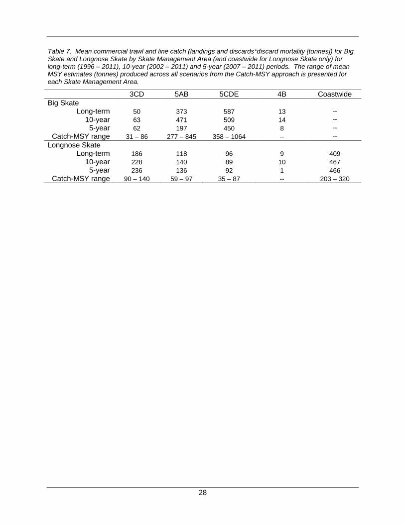
28

Table 7. Mean commercial trawl and line catch (landings and discards*discard mortality [tonnes]) for Big Skate and Longnose Skate by Skate Management Area (and coastwide for Longnose Skate only) for long-term (1996 – 2011), 10-year (2002 – 2011) and 5-year (2007 – 2011) periods. The range of mean MSY estimates (tonnes) produced across all scenarios from the Catch-MSY approach is presented for each Skate Management Area.

3CD 5AB 5CDE 4B Coastwide Big Skate

Long-term 50 373 587 13 -- 10-year 63 471 509 14 -- 5-year 62 197 450 8 --

Catch-MSY range 31 – 86 277 – 845 358 – 1064 -- -- Longnose Skate

Long-term 186 118 96 9 409 10-year 228 140 89 10 467 5-year 236 136 92 1 466

Catch-MSY range 90 – 140 59 – 97 35 – 87 -- 203 – 320

29

9 FIGURES

Figure 1. Mean catch per unit of effort (CPUE) for Big Skate over a 0.1° x 0.1° grid for (A) the commercial trawl fishery and research trawl surveys from 1996 – 2011 (kg/hour) and (B) the commercial longline fishery and research longline surveys from from 2006 – 2011 (pieces / 100 hooks). A mean CPUE value of zero represents fishing effort with zero catch of Big Skate.

30

Figure 2. Mean catch per unit of effort (CPUE) for Longnose Skate over a 0.1° x 0.1° grid for (A) the commercial trawl fishery and research trawl surveys from 1996 – 2011 (kg/hour) and (B) the commercial longline fishery and research longline surveys from from 2006 – 2011 (pieces / 100 hooks). A mean CPUE value of zero represents fishing effort with zero catch of Longnose Skate.

31

Figure 3. Proposed Skate Management Areas. Area 3CD includes minor areas 19 and 20. Area 5AB includes minor area 12. Area 4B is minor areas 13 – 18, 28 and 29 only.

32

Figure 4. Big Skate catch (landings and discard mortality in tonnes) by trawl (thin line) and line (dashed line) gear by Skate Management Area. Thick line is total catch (tonnes).

33

Figure 5. Longnose Skate catch (landings and discard mortality in tonnes) by trawl (thin line) and line (dashed line) gear by Skate Management Area. Thick line is total catch (tonnes).

34

Figure 6. Big Skate indices from trawl and longline research surveys. Annual mean biomass (squares) is estimated by stratified swept-area calculation (Appendix H). Annual mean catch per unit effort (CPUE, squares) is calculated as pieces per 100 hooks. Boostrapped replicates (1,000 random with replacement) were used to estimate 95% confidence intervals (vertical lines), 25th and 75th quantiles (boxes) and median (horizontal lines). Trend analyses and bootstrapped estimates of slope and annual rate of change did not detect any trends significantly (p<0.05) different than zero.

2006 2007 2008 2009 2010

0.0

0.5

1.0

1.5

2.0

2.5

3.0

PHMA Survey in 5CDE

Year

CPU

E (p

iece

s pe

r 100

hoo

ks)

2007 2008 2009 2010 2011

0

2

4

6

8

10

PHMA Survey in 5AB

Year

CP

UE

(pie

ces

per 1

00 h

ooks

)

2007 2008 2009 2010 2011

0

2

4

6

8

10

12

PHMA Survey in 3CD

Year

CP

UE

(pie

ces

per 1

00 h

ooks

)

2005 2006 2007 2008 2009 2010 2011

7

8

9

10

11

Hecate Strait Synoptic Surve

Year

Bio

mas

s (to

nnes

)

2003 2004 2005 2006 2007 2008 2009 2010 2011

0

2

4

6

8

IPHC Survey 5CDE

Year

CPU

E (p

iece

s pe

r 100

hoo

ks)

2003 2004 2005 2006 2007 2008 2009 2010 2011

0

1

2

3

4

IPHC Survey 5AB

Year

CP

UE

(pie

ces

per 1

00 h

ooks

)

2003 2004 2005 2006 2007 2008 2009 2010 2011

0.0

0.5

1.0

1.5

2.0

2.5

IPHC Survey 3CD

YearC

PUE

(pie

ces

per 1

00 h

ooks

)

1984 1986 1988 1990 1992 1994 1996 1998 2000 2002

8

9

10

11

12

HS Multispecies Assemblage

Year

Bio

mas

s (to

nnes

)

35

Figure 7. Longnose Skate abundance indices from trawl research surveys. Annual mean biomass (squares) is estimated by stratified swept-area calculation (Appendix H). Boostrapped replicates (1,000 random with replacement) were used to estimate 95% confidence intervals (vertical lines), 25th and 75th quantiles (boxes) and median (horizontal lines). Only those trends (red line) significantly different (p<0.05) than zero are plotted.

2003 2004 2005 2006 2007 2008 2009 2010 2011 2012

0

200

400

600

800

1000

1200

QCS Shrimp Survey

Year

Bio

mas

s (to

nnes

)

( b= -22.2829, r= -23.2829, R= -201.5461)

2005 2006 2007 2008 2009 2010 20110

200

400

600

800

1000

HS Synoptic Survey

Year

Bio

mas

s (to

nnes

)

2003 2004 2005 2006 2007 2008 2009 2010 2011

200

400

600

800

QCS Synoptic Survey

Year

Biom

ass

(tonn

es)

( b= -29.1608, r= -30.1608, R= -234.2868)

2004 2005 2006 2007 2008 2009 2010 2011 2012

200

400

600

800

1000

WCVI Synoptic Survey

Year

Bio

mas

s (to

nnes

)

( b= -39.0264, r= -40.0264, R= -313.2115)

2006 2007 2008 2009 2010 2011 2012

20

40

60

80

100

120

140

160

WCHG Synoptic Survey

Year

Bio

mas

s (to

nnes

)

( b= -7.9189, r= -8.9189, R= -48.5136)

2003 2004 2005 2006 2007 2008 2009 2010 2011 2012

5

6

7

8

9

10

WCVI Shrimp Survey

Year

Bio

mas

s (to

nnes

)( b= -0.1884, r= -0.1224, R= -0.6912)

36

Figure 8. Longnose Skate catch rates (pieces per 100 hooks, squares) from longline research surveys. Boostrapped replicates (1,000 random with replacement) were used to estimate 95% confidence intervals (vertical lines), 25th and 75th quantiles (boxes) and median (horizontal lines). Trend analyses and bootstrapped estimates of slope and annual rate of change did not detect any trends significantly different (p<0.05) than zero.

2003 2004 2005 2006 2007 2008 2009 2010 2011

0

2

4

6

8

IPHC Survey in 3CD

Year

CP

UE

(pie

ces

per 1

00 h

ooks

)

2003 2004 2005 2006 2007 2008 2009 2010 2011

-3

-2

-1

0

1

2

3

IPHC Survey in 5AB

YearC

PU

E (p

iece

s pe

r 100

hoo

ks)

2003 2004 2005 2006 2007 2008 2009 2010

1

2

3

4

Inshore Rockfish Survey 5AB

Year

CP

UE

(pie

ces

per 1

00 h

ooks

)

2003 2004 2005 2006 2007 2008 2009 2010 2011

0

2

4

6

8

IPHC Survey in 5CDE

Year

CP

UE

(pie

ces

per 1

00 h

ooks

)

2006 2007 2008 2009 2010

0

1

2

3

4

5

6

7

PHMA Survey in 5CDE

Year

CP

UE

(pie

ces

per 1

00 h

ooks

)

2007 2008 2009 2010 2011

0

2

4

6

8

10

PHMA Survey in 5AB

Year

CP

UE

(pie

ces

per 1

00 h

ooks

)

2007 2008 2009 2010 2011

0

2

4

6

8

10

12

PHMA Survey in 3CD

Year

CP

UE

(pie

ces

per 1

00 h

ooks

)

37

Figure 9. Observed and predicted annual mean Big Skate catch (kg) based on: A) lognormal GLM, using all data points; B) lognormal GLM, with high-leverage data points removed; C) lognormal GLM using positive tows only (zeros excluded); D) two-step GLM using all data points. Data are rolled up trawl tows from Skate Management Area 5CDE in 2001 – 20011. Errors bars are the 95% confidence intervals. Note that using positive tows only as in (C) results in higher annual mean catch than when all data points are used.

38

Figure 10. Bayesian Surplus Production Model results for Big Skate in 5CDE. Probability distributions for the: A) intrinsic population growth rate (r) and, B) carrying capacity (K); prior (solid line) and posterior (dashed line). Posterior probability distributions for: C) MSY, D) BMSY , and E) FMSY . F) The log predicted Big Skate population abundance in area 5CDE from 1984 – 2011. The light grey is the 90% quantile, medium grey is the 80% quantile, dark grey is the 50% quantile and the solid black line is the median log predicted population biomass.

39

Figure 11. Results from Catch-MSY approach for Big Skate in 5CDE using catch data from 1996 – 2011 (case 1 is default scenario). Posterior density distributions for: A) carrying capacity, k (thousand of tonnes) and B) intrinsic rate of increase, r . The thick solid lines are geometric means, dashed lines are 5%, 50% (median) and 95% quantiles, red lines are prior distributions.

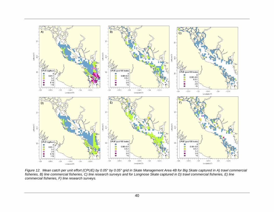
40

Figure 12. Mean catch per unit effort (CPUE) by 0.05° by 0.05° grid in Skate Management Area 4B for Big Skate captured in A) trawl commercial fisheries, B) line commercial fisheries, C) line research surveys and for Longnose Skate captured in D) trawl commercial fisheries, E) line commercial fisheries, F) line research surveys.

41

MINUTES AND RECOMMENDATIONS FROM MEETINGS AND APPENDIX A.WORKSHOPS

A.1 JUNE 6, 2012 TECHNICAL SCIENCE WORKING GROUP Team Members Present: Jackie King – DFO Science Sabrina Garcia – SFU Robyn Forrest – DFO Science Gordon McFarlane – DFO Science, Emeritus Maria Surry – DFO Science Greg Workman – DFO Science Chantelle Caron – DFO EFM Paul Starr – CGRCS Andrew Edwards – DFO Science

Objective of Meeting:

• Review the background on Big Skate and Longnose Skate fishery management, biology, available data, results of surplus production modeling efforts in Hecate Strait

• Review and finalize Project Charter • Provide action items and recommendations for data compilation and modeling

approaches

Agenda 9:00 Background (Jackie King)

• Review of Request for Working Paper • Phase 0 Recommendations • Current Fisheries Management of skates • input from industry on management units • Fishery hot spots – by sector • Big Skate and Longnose Skate biology

9:30 Fishery and research data (Maria Surry)

• Fishery landings and discards • Fishery CPUE • Available research survey CPUE

10:00 Surplus Production Model for Big Skate in Hecate Strait and Queen Charlotte Sound (Sabrina Garcia)

• Model structure • Input data • Depletion Corrected Average Catch methods • Bayesian analyses for parameters • Model outputs

11:00 Working Group Recommendations

• Input data • Model selection • Management units for model runs and provision of advice

42

• Review and approval of Project Charter • Assignment of tasks • Deadlines

Discussion on presentations: All presentations were made available to the Team Members as pdf files.

1. Background

• A cap of 567 tonnes for Big Skate and 200 tonnes for Longnose Skate has been in place in Areas 5CD combined since 2002. It is unclear if there are vessel limits for skates applied to other management areas

• ACTION ITEM: Chantelle will clarify trawl skate management in other areas for the Team Members

2. Available Data

• The catch rate observed in the PHMA longline survey could be used to validate longline fishery catch rate data that are derived from logbook records which may be incorrect

• The line data (longline, handline, trap) begin at different years depending on fishery sector

o The approach applied to the Boccacio assessment may be applicable here in using effort time series to extrapolate prior to the start year

o Kate Rutherford and Lynne Yamanaka are currently working on a catch reconstruction project for line data

o ACTION ITEM: Jackie will liaise with Kate and Lynne to see if results of their reconstruction are applicable to skates and available in a timely manner for this assessment

• Skate trawl catch prior to 1996 will require assumed proportion of big and Longnose Skates to apply to the generic category “skate”

o Also need to reconstruct based on catch rate applied to effort o Trawl reconstruction back to 1954 has been undertaken by Rowan Haigh, and

his efforts may be applicable to skate o ACTION ITEM: Maria will liaise with Rowan regarding trawl catch reconstruction

to 1954. • The high 5B trawl catches post-2002 is likely a fishing up effect in anticipation of a

possible cap implementation o This indicates that the catch might not reflect the abundance and that CPUE may

not be useful o This would be a good point of clarification to raise with industry at a skate data

workshop o ACTION ITEM: Chantelle will identify suitable industry representatives to invite to

such a workshop • It would also be useful to ask industry about the high spike in line catch in 2004 • It is not clear if line fisheries off the west coast of Vancouver Island are targeting skates,

particularly Longnose Skate, and the high catch by that sector may be due to an increase in spiny dogfish fishing

o Another question for industry that would be good for a skate data workshop • Another survey to investigate is the Pacific Ocean Perch Goose Island Gully survey • For the length data, it would be useful to also see number of samples (i.e. fishing events)

that the length data come from

43

o ACTION ITEM: Maria will include this information in future presentations on size data

• The catch (landings and discards) in Area 4B is mainly from statistical areas 12 (Queen Charlotte Strait) and 19 – 20 (Victoria to Port Renfrew)

o Ecologically these areas are related to 5A and 3C respectively o It would make sense to roll up these into those larger Areas and to not formally

assess 13 – 18 (paucity of data) but rather advise that trip limits remain in place • There is spatial patterns to the trawl catch for Big Skate with the center of the catch in

5D, 5B o Longnose Skate trawl is less spatially distinct, and has more catch off the west

coast Vancouver Island o Taken together, it would suitable to assess 5CDE, 5AB(12), 3CD(19,20) as units.

Coastwide is not considered, given the tagging data which illustrates little movement >25km

• Commercial CPUE data requires standardization and a look at differences between non-directed and directed events

• ACTION ITEM: Paul agreed to lead this analysis with data support from Maria

3. Surplus Production Model-Hecate Strait 5CD

• k (growth coefficient) had an upper bound of 0.1for prior distribution o The posterior distribution fit was poor o Rebound the prior distribution very close to zero and with a higher max (i.e. 0.2

or higher) • to and Linf also didn’t have good posterior fits, so the prior boundaries for those need to

be broader • Pauly’s equation to calculate M is not a good choice, it would be best to use an equation

that relied on actual observed data i.e. Hoenig’s equation using maximum age o The results that M is 0.046 given the maximum age is 25 is not at all reasonable;

a M that low would related to a fish that was about 65 years old o The distribution around Hoenig estimation could be approximated using a normal

distribution 0.075 – 0.225 • Using age at first selectivity (=1) is questionable

o Assuming age 1 is incorrect o More appropriate to use knife edge selectivity at 50% selectivity; derived from

actual data from directed fisheries • Rather than use breeding interval, use a distribution of annual number of clutches

o It would still be okay to include the unreasonable two week breeding interval observed for skates in an aquarium if the distribution placed less probability on it

• Commercial landed CPUE (i.e. directed) trawl data was used to tune o This has the issue of hyperstability o Tiscard CPUE should also be included o Standardized CPUE was already discussed above

• Survey indices, Norm Olsen’s swept area extraction procedure should be used for all trawl surveys

• The posterior distribution on K (carrying capacity) is skewed to the lowest possible value indicating that the prior distribution is too constraining

• Set lowest boundary to 1 not 10,000 • The depletion estimates were not fitted because of the tight rmax prior and ill-bounded

K; the MSY has too tight a distribution o It would be possibly be improved by looking to McAllister’s approach to r

44

4. Elasmobranch Optimal Harvest Rate Estimation

• It would be possible to use the life history parameters of this species to estimate thresholds and used as a precautionary reference point

• It also could be used to develop priors for age structured assessment

o Given the growth curve for these species does not appear to asymptote, it might be possible to use lengths to estimate ages for age structured assessment

o The length data by area by year are not robust enough to be able to do this

Recommendations:

• Assessment units: 3CD (including 19 and 20 from 4B); 5AB (including 12 from 4B); 5CDE; Statistical Areas 13 – 18 in 4B have very little catch and data and will not be formally assessed, trip limits already in place appear to be currently sufficient.

o Catch data will be reconstructed to 1954 for trawl data; and for as far back as possible for line data.

o Trawl catch rates from non-directed tow could be applied to historic effort to estimate pre-1996 discards by area.

o Observed survey proportions of Big Skate and Longnose Skate in relation to all skate could be applied to pre-1996 commercial data with only a ‘skate’ category.

o The trawl proportions of Big Skate and Longnose Skate in relation to all skate in non-directed and directed fishing could be applied to pre-1996 commercial data with only a ‘skate’ category.

o The approach of line catch reconstruction used in Boccaccio should be investigated.

• The standardized swept area estimates for trawl surveys that are used in other groundfish assessments should be used here as an index of abundance.

• Other surveys to investigate include the Pacific Ocean Perch Goose Island Gully survey; the PHMA survey; the IPHC setline survey; the NMFS triennial survey

• The surplus production model should be re-parameterized with the following changes o The prior boundaries on k should be broadened to extend from close to zero to

0.2 (or higher) o The prior boundaries on to and Linf should be much wider o Calculate M based on maximum age as per Hoenig’s equation; a simulated

normal distribution from 0.075 – 0.225 could be used o Use knife edge at 50% selectivity from commercial size data from the directed

fisheries, and the growth curve to estimate age at 50% selectivity o Use a lognormal distribution of annual number of clutches (not breeding interval)

from 1 – 24 with mean around 5 o The lower boundary for the prior distribution of K (carrying capacity) should be 1

not 10,000 o Use the McAllister approach to estimate rmax

• A data workshop will be held with Industry sometime in August 2012 to review the data. Items to discuss should include:

o The spike in line catch in 2004 o Reasons for the decline in trawl catch o Utility of CPUE as an index of abundance o The increase in catch post-2002 in 5B o Size preference in the market for skates

45

o Targeting of skates by line off the west coast of Vancouver Island, particularly Longnose Skate

• The Project Charter was accepted, with revisions to the Timetable to reflect ongoing data analyses.

Next steps The scheduled next meeting for the Technical Science Working Group is July 5, 2012 (9 – 4) in the PBS Conference Room. Agenda items will include:

• Review results of re-parameterization outlined in Recommendation 5 (Sabrina) • Review results of commercial CPUE standardization (Paul) • Review progress made on catch reconstruction outlined in Recommendation 2

(Maria) • Plan data workshop with industry • Recommend appropriate assessment methodology

A.2 JULY 5, 2012 TECHNICAL SCIENCE WORKING GROUP Team Members Present: Jackie King – DFO Science Sabrina Garcia – SFU Robyn Forrest – DFO Science Gordon McFarlane – DFO Science, Emeritus Maria Surry – DFO Science Greg Workman – DFO Science Chantelle Caron – DFO EFM via Web Paul Starr – CGRCS Andrew Edwards – DFO Science Kate Rutherford – DFO Science

Objective of Meeting:

• Update on historic management • Review results from exploratory analyses of the impacts on bycatch • Composition and size due to voluntary change in mesh size in 2004/05 • Review preliminary trawl catch reconstruction using associated species • Landings • Review issues with line data relevant to data reconstruction • Review preliminary results of commercial cpue standardization • Review results of surplus production re-parameterization based on june 6 • TSWG recommendations • Provide action items and recommendations for data reconstruction

Agenda 9:00 Historic skate management clarification (Chantelle)

• Action item from previous meeting

9:15 Impact of the change in mesh size (Jackie)

• Clarification on 2004 – 2005 change from 4.5 inch to 10 inch mesh size • And impacts on catch composition

46

9:30 Fishery data reconstruction (Maria)

• Cleaning up ‘skate’ category catches (landings or discards) prior to • 1996 • Estimating trawl discards 1954 – 1995

o Catch ratios based on associated species landed o Analyses by depth

• Estimating line discards prior to 2002

10:00 Fishery CPUE GLM analyses (Paul)

10:30 Big Skate in 5CDE - new parameterizations and model runs (Sabrina)

• Available research CPUE (and other areas) • New parameterization results • Model runs based on the preliminary reconstructed trawl data

11:00 Working Group Recommendations

• Reconstructed fishery data – how far back; what approaches • Model selection • Parameterization approaches • Data Workshop with Industry – planning and issues to raise

Discussion on presentations: All presentations were made available to the Team Members as pdf files

1. Historic Management

• The history of the targeted skate fisheries and management changes were provided as a text file, which will be included in the stock Assessment working paper as a table with areas, and years of management changes

• As an action item from June 6, it was clarified that trawl management measures were in place in 5CD only

o In 2002 a trawl tac of 567 tonnes for Big Skate and a trawl TAC o Of 47 tonnes for Longnose Skate were implemented in 5CD o These TACs have been managed by individual vessel quotas for option a trawl

vessels o There are no TAC, IVQ or species trip limits for trawl fisheries in any other areas

2. Impacts of change in mesh size

• It was suggested at the previous meeting that trawlers targeting skate had voluntarily switched from small mesh size (5.5 inch) to larger mesh size (10.5 inch) around 2004 – 2005 in order to reduce bycatch of small skates and of other species

o This would have an impact on data reconstruction efforts and possibly on commercial catch rates as abundance indices

• Exploratory analyses on bycatch composition and size composition focused on areas 5B and 5D where skates are primarily targeted

o There was no discernible increase in the proportion of Big Skate or Longnose Skate in the catch compositions post-2005

o Size data is sparse, but most robust for Big Skate in 5B: however, there was no apparent increase in the size of Big Skate with the larger mesh size

There was some indication of smaller Big Skate being retained

47

• Around 2005 a korean market for smaller skates developed, so the proposed change in mesh size was likely not universal across all vessels or used by only a few vessels in a couple of years

• Overall this issue does not require immediate attention and industry should be asked at the data workshop if it actually occurred or how prevalent it was

• Future analyses should used geometric means instead and consider a glm to see if depth is influential for annual mean estimates

• ACTION ITEM: Chantelle will clarify historic minimum mesh size requirements by area, indicating any changes; this information will be included in the historic management section

3. Preliminary results of data reconstruction

• At the June 6 meeting it was recommended that the a similar approach to rockfish reconstruction efforts be investigated, using catch ratio to target species

• All data reconstruction exploratory analyses focused on Big Skate in Areas 5C, D and E • TRAWL

o Used 2001 – 2011 non-directed tows o In 5D, Pacific cod was the most frequently captured species (by o Number of tows) along with Big Skate

This is not a reasonable species to use as an associated species since its abundance has fluctuated dramatically, and 2001 – 2011 is a period of very low abundance

o Could test the data reconstruction on observed discards 1996 – 2000 o A better approach to investigate would be to use GLM to investigate influential

factors such as month, locality and depth (see mccarthy, 2006) Industry should still comment on any results of a GLM Requires current data to be rolled-up in a similar manner to the Historic data prior to GLM analyses This approach would need to be reviewed by the TSWG to Assess its utility Use 2001 – 2011 non-directed data Could focus on Big Skate in Areas 5C, D and E (separately) first

• LINE o Preliminary look at catch ratio of Big Skate to halibut in the halibut fishery

illustrate an number of difficult issues with reconstructing line data for skates back to 1954 Current discards are in pieces, with no size data available to convert to

weight It might be possible to use AMR video data to estimate sizes Historic logbook effort data are inconsistent Historic logbook depth data are inconsistent and usually not available Within the line fisheries, discard mortality is not uniform over time: prior to

the mid-1980s, crucifiers would have been used, resulting in high initial discard mortality

o Overall, given the low skate discards and landings in the current data which are considered to be reliable, coupled with the issues in historic data, the line data will not be reconstructed

o Future assessments could investigate the sensitivity of the inclusion of line data • ACTION ITEM: Maria to provide catch table summaries with the best estimates of

landings and discards to date

48

4. GLM of commercial catch per unit effort

• Analyses were conducted on events from core vessels (with at least 3 tows per year for at least 3 years) within depth range 40 to 215 m and less than 24 hours in duration

• In 2010 there is an overwhelming drop in the number of tows included in the analyses due to a large number excluded since the duration >24hrs

• A quick check in FOS during the meeting showed that the maximum duration in 2010 was 19 hrs

• ACTION ITEM: Paul will investigate the error and report at the next meeting (perhaps with cinnamon rolls)

• R2 was used as a stopping rule for explanatory variables, however AIC should be used to assess most suitable model the 2007 standardized data are deflated due to many tows in Feb and March in the Butterworth locality (the locality with the highest influence across years

• The number of trips included in 2007 is a large drop down from 2006 • ACTION ITEM: Jackie since 2007 is the switch from PacHarvTrawl to FOS, need to

verify with Rowan that data from both sources are included • Overall the GLM analyses are adequate, but uncertain if the resultant time series reflects

abundance ie. a drop since 2006 in CPUE coincides with a large drop in the number of tows included in core vessel data

5. Surplus production model reparameterization

• Survey data o do not include PHMA survey since it is hard-bottom survey focused on rockfish o do include IPHC setline survey, multi-species survey, and synoptic survey

(synoptic surveys are to based on biomass estimates that are standardized by depth stratum)

• Instead of estimating a depletion, could assume 1954 starts at K • The fit to CPUE is a straight line, ie. no fit

o There is no information in the indices • Could put informed q priors on the surveys, essentially making them biomass estimates

and model with a delay difference model • The surplus production model is inflating the biomass estimates to get any • fits; so not currently reliable biomass estimates • An alternate approach might be to get estimates of MSY based on catch (Martell and

Froese, 2012) • Focus should be on providing the best estimates of catch possible

Recommendations:

• Conduct GLM analyses on trawl data for historic (1954 – 1995) data discard estimation o Focus on Big Skate in Areas 5C, D and E o Use 2001 – 2011 non-directed, rolled up by locality and depth o Explanatory variables to include month, locality and depth

Next steps

• The scheduled next meeting for the Technical Science Working Group is August 9 (9 – 4) in the PBS Conference Room. Agenda items will include:

o Report on 2010 outliers in commercial CPUE standardization (Paul) o Review results trawl data reconstruction (1954 – 1995) based on GLM with 2001

– 2011 non-directed data for 5C, D and E (Sabrina)

49

A.3 AUGUST 9, 2012 TECHNICAL SCIENCE WORKING GROUP Team Members Present: Jackie King – DFO Science Sabrina Garcia – SFU Robyn Forrest – DFO Science Gordon McFarlane – DFO Science, Emeritus Maria Surry – DFO Science Chantelle Caron – DFO EFM Paul Starr – CGRCS Andrew Edwards – DFO Science

Objective of Meeting:

• Review GLM analyses on non-directed fishing events for application in reconstructing historic discards

• Discuss and recommend methods of providing advice to management

Agenda 9:00 Any follow up from previous meeting:

• Questions for Paul on CPUE GLM analyses corrections? • Questions for Maria on official catch tables? • Chantelle to clarify historic minimum mesh size requirements by area, indicating any

changes

9:15 GLM analyses applied to historic data reconstruction (Sabrina)

• 2001 – 2011 trawl data with non-directed effort, rolled up akin to historic data • Influencing factors: locality, depth, month, duration • Application to 1954 – 1995 trawl data to estimate Big Skate discards

10:00 Discussion

• Utility of latest GLM analyses as method of data reconstruction • How will we provide assessment advice to GMU?

o Surplus production model? o Martell and Froese approach? o Something akin to US approach for data deficient species (eg. Gulf of Alaska

skates)? F is some proportion of M and applied to trawl survey biomass estimates

to select TAC • Data Workshop with Industry – are we at a stage where we can set a date and begin to

plan our discussion with them?

Discussion on presentations: 1. GLM analyses for historic catch reconstruction

• The methods and results were provided as a text file, which will be included in the stock assessment Working Paper as an appendix

• Alternatives for depth would be to include it as a continuous variable, however the historic data will be rolled up into bins, and not truly continuous

o Could also use fewer than 8 bins to reduce the variance, • Could also look at top species landed as a factor

50

o Do not use actual landed amount, since it would be impacted by change in abundance, rather code it only as a factor (which would be akin to presence/absence)

o It might be useful to group species in aggregates eg. Flatfish, rockfish, gadid o It is unlikely that top species will produce a better fit, since they are a surrogate

for habitat, which is already captured by locality and depth • Interaction between depth and locality was looked at but not presented and did not add

much to the model • The best approach will be the two-step with first predicting positive tows, then applying

the log GLM to predict catch o Underestimates catch by about 60% o It is still worthwhile to reconstruct discards and know that the historic catch

estimates are minimum estimates o The implications of underestimating catch, is underestimating yield o Conversely the impact on the stock, and any depletion, will also be

underestimated

2. Methods for providing advice

• The tier 5 and tier 6 approach used in nmfs would be easy to do and include in an assessment

o Gulf of alaska skates are assessed as tier 5, and the application of the hoenig estimation of m (0.15) to the hecate strait synoptic survey biomass estimates (of about 1,000 tonnes) would result in a recommended yield of 150 tonnes, which would only cover the trawl discards

o If we were to apply tier 6 approach and use average catches to set yield, then it should be selected for a time period for which the survey biomass indices are available and stable (i.e. that amount of catch was associated with a stable abundance index)

o This tier 6 would not be easy for the other areas since the synoptic surveys do not exhibit stable biomass trends

• DCAC was already done for 5CDE Big Skate and produced a yield of only 207 tonnes o There is no need to investigate this approach further, but the analyses should be

included in the stock assessment so that reviewers will know the method was investigated

• Catch-msy (martell and froese, 2012) has produced reasonable msy estimates for pacific hake and for sablefish, and should be looked at for Big Skate in 5cde as a case study

o Two catch histories could be investigated (1996 – 2011; and historic) o The r values for low resilience species seem reasonable for Big Skate based on

bayesian analyses using macallister’s approach so 0.05 – 0.5 are okay o Looking at a number of different depletion ranges would be preferable

• GMU will be interested in receiving yield advice, even if only based on average catches, if all other methods prove to be unreliable

o It will still be of interest to set Big Skate and Longnose Skate quotas in all management areas

Recommendations:

• Update the two-step GLM analyses with top landed species included as a factor and reconstruct management area specific historic catch estimates for both Big Skate and Longnose Skate

51

• Apply the R-code provided by Martell and Froese (2012) to Big Skate in 5CDE for two catch histories: o 1996 – 2011 o Historic – 2011 (to be determined based on catch reconstruction and an estimate of

a reliable start year eg. 1980)

Next steps

• The TSWG will reconvene (data TBA) to review: o The GLM analyses with top species, and the historic catch reconstruction. o The results of the catch-MSY approach for Big Skate in 5CDE for the two catch

histories. • Post-review of the catch reconstruction by the TSWG, a workshop with industry will be

set up to review all available catch data, and the approach taken to estimate historic discards

A.4 NOVEMER 22, 2012 TECHNICAL SCIENCE WORKING GROUP Team Members Present: Jackie King – DFO Science Sabrina Garcia – SFU (via the web) Robyn Forrest – DFO Science Gordon McFarlane – DFO Science, Emeritus Maria Surry – DFO Science Chantelle Caron – DFO EFM (via the web) Paul Starr – CGRCS Kate Rutherford – DFO Science

Objective of Meeting:

• Review GLM analyses on non-directed fishing events for application in reconstructing historic discards for both species in 3CD, 5AB and 5CDE using four variables (depth, month, locality, duration) and five variables (addition of top species landed)

• Review results of Catch-MSY approach for Big Skate in 5CDE based on two catch histories

• Review Strait of Georgia data

Agenda 9:00 GLM analyses applied to historic data reconstruction

• Inclusion of top spp. Landed to previous 4 factor GLM • Compare 4 factor (depth, locality, month, duration) to 5 factor (+ top spp.) GLM results • Review results for both species in 3CD, 5AB and 5CDE • Decide on validity of approach

9:45 Catch-MSY Approach

• Review the results of case study (Big Skate in 5CDE) using: o Catch history 1: 1996 – 2011 o Catch history 2: 1954 – 2011 (4 factor GLM only)

• Decide on validity of approach, suitable scenarios and catch histories

10:30 Area 4B

• Review catch data for remaining areas of 4B (Minor 13 – 18, 28, 29)

52

• Fishery distribution in 4B • Review available survey data

11:00 Plan the Way Forward

• Review Request for Advice o What can we do, what can’t we do

• Approach for provision of management advice • Industry Workshop meeting mid-December

o Confirm the topics for discussion and feedbacks • Current line limits are for skates (all species)

o Data on ‘other’ skates

Discussion on presentations: 1. GLM analyses for historic catch reconstruction

• The updated methods and results were provided as a text file, which will be included in the stock assessment Working Paper as an appendix

• Many of the stocks had a poor fit of predicted (catches based on positive, non-directed tows) to the observed (same tows) e.g. Big Skate in 5AB

o Presented are mean catches, but it was clarified that the fit does not improve with summed catches

o Likely because the variables just don’t have enough explanatory power to explain the data;

Missing is a factor that relates to abundance/distribution such as year, but year can not

o It may also be a function of allowing all four variables to be retained (vs. a stepwise approach); however it was noted that there is little improvement to deviance when factor coefficients are examined sequentially

• The best fit could only predict 60 – 70% of the observed data • Maybe an improvement could be to use negative binomial (allowing zeros) instead of

lognormal • Another improvement could be to consider another an alternate cut-off (currently 0.5) in

selecting what is consider positive tows; currently not capturing enough of the positive tows

• Overall, seems to miss larger discard events; again this might be captured with an alternate distribution to the lognormal

• There is just not enough variability in factors in the data; i.e. they are always fishing in the same place, at same depths, capturing the same thing

• This approach has been explored sufficiently, and there is no need to further investigate a means of improvement, since it is unlikely to be improved much more

• Overall, this approach underestimates historic discards but it is a useful first step in exploring the estimation of discards for these two species

2. Discard mortality rate

• It was noted that trawl discards in the surplus production, and the Catch-MSY approach below applied a 50% discard mortality rate to discards (1996 – 2011) then added the amount to landings in estimating total ‘catch’

o The group had reviewed the relevant literature in June 2012 and agreed to this • However, 50% was also applied to the longline discards (1996 – 2011)

53

o This discard mortality rate is too high for skates; however surplus production analyses do not need to be redone since the longline discards are so small in comparison to the trawl data

o There are no current literature studies available for longline captured skates o Currently the DFO IFMP uses 6% discard mortality rate for spiny dogfish, which

did not come from science advice or the literature; in the spiny dogfish assessment, it was felt that this rate was likely too low

o There is research on blue sharks captured by line gear based on satellite tags and that estimate is 20%, which is too high and likely influenced by tagging mortality from a tag more invasive than standard spaghetti tags

o 10% seems to be a reasonable estimate o Yes it would be possible to look at sensitivity analyses for 5, 10 or 15% discard

mortality rate in the surplus production model, but the fact is that the longline discards are relatively small compared to trawl catch that it would make very little difference so there is no need to revisit this

3. Catch-MSY approach

• For the MSY posterior densities, please plot the 5 and 95 percentiles instead of the assumed distribution (i.e. 2 standard deviations)

• Plot the posterior MSY with the prior MSY distribution (uniform bounded by lower r-k and upper r-k calculations) to assess the improvement of the posterior to the prior

• Instead of using the r ranges outlined in Martell and Froese (2012) based on low resiliency, use the distribution based on McAllister’s approach for estimating r; namely the lower and upper bounds resulting from that estimation and the shape of the distribution (i.e. not uniform)

• It would be best to go with the wide ranges (0.1 – 0.9) of both initial and final depletion levels

• Yes, while Catch History 2 (based on GLM reconstruction) is way out, still do these analyses

o For each stock select the reconstruction that provides higher estimates since we know they are biased low

• Even though varying k did not impact the MSY estimates, keep these as scenarios and varying them in concert with wider depletion levels to see if there is an interaction effect

4. Strait of Georgia skates

• These are the minor areas 13 – 18, 28 and 29 • Line landings (both species) drop after 2006

o Is this because the dogfish fleet went to the outside to fish after 2006? This is a question for industry

• Trawl landings for Big Skate increase after 2004 o Did Option B start to operate more to account for this increase? was there an

increase in market demand, say in Vancouver? These are also questions for industry

o It seems to be an unexpected signal, given that the surveys encounter more Longnose Skates than Big Skate suggesting that Big Skate are not as abundant

• 4B was identified in the Request for Advice since there are some trip limits for skates, and if GMU need to change they them they would like to know; it is also consistent with the general movement towards having catch limits of species coastwide

o It is acceptable to say that there is not enough information to provide advice on trip limits or TACs

54

o A broad overview which provides a look at the catches and the distribution is still useful

o The distribution needs to include the negative tows to get a sense of where trawling occurs, the positive tows to see where the industry encounters them, and a similar plot for surveys

5. Next steps

• Request for Advice o Stock status, alternate reference points and decision tables with projections and

uncertainties can not be produced as per requested; The simplest modeling approach (surplus production) that could

accommodate this request was not reliable: the posteriors came up against the bounds, there were no reliable indices of abundance and the results were implausible

This highlights the need for a regional approach to data-limited species and guidance on approaches for provision of advice

• Approach for provision of advice o Can provide MSY estimates (from Catch-MSY approach) that provides an idea of

a long-term sustainable yield o Could also include average catches (long-term average; last 10 years and last 5

years) for consideration o Could also present trawl survey estimates of current biomass

• Appendices to include in the Research Document o Biology o Management History (completed) o Catch data (completed) o Commercial CPUE standardization (completed) o Survey data, indices and trawl estimates of biomass o Historic trawl discard reconstruction (completed) o Surplus production model for Big Skate 5CDE (completed) o DCAC for Big Skate 5CDE (completed) o Catch-MSY approach for both species in all areas (revisions as below) o Catch data on other skates captured in BC trawl and line fisheries (simple table

of coastwide landings and discards-could be included in catch data Appendix

Recommendations: Revise the Catch-MSY approach and conduct for both species in all management units with

• Two catch histories: 1-1996 – 2011; 2-reconstructed 1954 – 2011 from either 4 variable or 5 variable approach (which ever is higher); catch reconstruction can not be done for remaining areas of 4B

• Instead of uniform r priors based on resiliency, use mcallister approach to estimate the lower and upper bounds and the general shape of the distribution from which to randomly draw from

• Keep the three k scenarios (100*max catch; 50*max catch; 10*max catch) • In addition to the default range initial and final depletion levels, investigate the wide

ranges (0.1 to 0.9) scenarios separately and together • Investigate the potential interaction between k and depletion levels by using wide ranges

on initial and final depletions, in concert with the three k scenarios

55

Case r priors k priors initial depletion range

final depletion range

Case 1 as per McAllister

100*max catch 0.5k – 0.9k 0.3k – 0.7k

Case 2 as per McAllister

50*max catch 0.5k – 0.9k 0.3k – 0.7k

Case 3 as per McAllister

10*max catch 0.5k – 0.9k 0.3k – 0.7k

Case 4 as per McAllister

100*max catch 0.1k – 0.9k 0.3k – 0.7k

Case 5 as per McAllister

100*max catch 0.5k – 0.9k 0.1k – 0.9k

Case 6 as per McAllister

100*max catch 0.1k – 0.9k 0.1k – 0.9k

Case 7 as per McAllister

50*max catch 0.1k – 0.9k 0.1k – 0.9k

Case 8 as per McAllister

10*max catch 0.1k – 0.9k 0.1k – 0.9k

Next steps

• Revise the Catch-MSY approach and produced Appendix for distribution to the group; review and feedback to be conducted via email

• Industry workshop will be held in mid-December • Draft Research Document to be provided to the TSWG by February 2013

A.5 DECEMBER 13, 2012 SKATE DATA WORKSHOP Present: Jackie King – DFO Science Maria Surry – DFO Science Kate Rutherford – DFO Science Chantelle Caron – DFO EFM (teleconference) Brian Mose – Groundfish Industry Dan Edwards – Groundfish Industry Gary Kraus – Groundfish Industry

Objective of Meeting:

• Receive advice from the groundfish commercial fishing industry on interpretation of Big Skate and Longnose Skate catch data (trawl and line) in relation to management changes, fishery dynamics, market fluctuations or abundance/distributional changes.

Background Provided Prior to Meeting: Groundfish Science has received a Request for Advice for harvest yields of Big Skate and Longnose Skate in BC waters. In June 2012, Science began compiling commercial and research data and investigating approaches to assessing these stocks and providing management advice. A stock assessment document will be presented and reviewed through the Centre for Scientific Advice Pacific process. Species specific yield advice will be recommended to managers for three management units: 3CD (including minor areas 19 and 20 from 4B), 5AB (including minor area 12 from) and 5CDE. There are not enough data to be able to provide yield

56

advice for 4B (minor areas 13 – 18, 28 and 29), however catch, effort and distribution data will be summarized for this Area.

Catch data for Big Skate and Longnose Skate from commercial trawl and line fisheries in British Columbia are available from 1996 – 2011 (line data begin in 1997). These data identify skate to species, include discards for some fisheries, and are based on observer and/or fisher logbooks verified by dockside monitoring programs. Although both bottom and midwater trawl catches are represented in the data, less than 1% of the trawl trips that caught skate used midwater gear. Line fisheries encompass the halibut fishery (“halibut”), ZN rockfish fisheries (“ZN”), directed lingcod and dogfish fisheries (“Schedule II”), as well as the sablefish and combined sablefish-halibut fisheries. In the line fisheries, skate are predominantly caught on longline gear.

Appendix Table A-1 (Big Skate) and Appendix Table A-2 (Longnose Skate) contain the best estimates of landings, discards and catch (landing + discards) in tonnes (1,000 kg) for trawl and line gear. There are a number of yearly differences in relative catch, or differences between species and areas that require input from industry for the best interpretation.

General Discussion: 1. Relative Abundance

• These are two different species found in different amounts depending on area and at different depths

• Big Skate are clumped or abundant, not so with Longnose Skate o Longnose Skate are caught in small amounts incidentally

• Big Skate dominate 5CDE and 5AB, and are very less abundant in 3CD o There are few Longnose Skate up north; likely a depth issue o Longnose Skate are more abundant in 3CD

• In January and February, Big Skate juveniles (about 12 inches in body length) are found up on the flats in Northern Hecate Strait

• Big Skate are found from 20 – 80 fathoms, rarely past 100 fathoms • Longnose Skate are found from 60 – 330 fathoms

2. Management Units

• The proposed management units (3CD, 5AB, 5CDE and 4B) were recommended by the Technical Science Working Group based on Big Skate tagging research and global skate tagging research

o For Big Skate in BC, 75% of recovered tagged fish were recaptured within 23 km of the tagging location

o These aggregated units were seen as a compromise to using smaller (e.g. 3C, 3D etc) units

• This recommendation was communicated by DFO – EFM to Groundfish Industry for feedback in June

o That communication was not widely distributed and industry would like an opportunity to discuss it within their advisory panels (GTAC and CIC)

• TACs by these management units might be constraining for the integrated fisheries o An alternate more amenable to industry might be coastwide TACs for Longnose

Skate o A coastwide TAC for Big Skate might have more of a risk of area depletion o Industry representatives noted that since Longnose Skate are intercepted

incidentally, a coastwide TAC would not be as constraining and, since Longnose Skate are not as aggregated, would not likely result in area depletions

57

• Managers can still take the input of industry when considering science advice and select alternate management units

o The stock assessment document should include coastwide advice for Longnose Skate to allow for discussion at the CSAP meeting

• Managers do not necessarily need to use the science advice to set TACs, but rather could set soft caps by management units

3. Overview of External Forces Influencing Skate Catch

• Market demand, market price, fuel costs, management actions, and restrictions/opportunities of other species are all factors that influence the amount of skate caught

• In 1996 accountability in the trawl fleet due to mandatory at sea observer and IVQs makes it a ‘misfit’ year in fishing behaviour

• In 1997 there was much uncertainty in how to fish given the new management arena, but skate were not on the list of quota species

o Large mesh codends (12 – 16 inch) were used to target skate and reduce other species bycatch

o This practice began in the mid 90’s with increase Skate market demand and smaller trip limits for other traditional groundfish species moved harvesters to explore new opportunities

o So while you still need to be accountable for skate catch and releases, it was safe to bring them in and land them

• When market was there and the prices increased, so did the landings until a TAC was put in place in 5CD

o Since the TAC in 2002 the levels have really kept steady o In 2007/2008 some vessels used a large mesh codend to target skate

• Following the TAC in 5CD, the landings in 5AB ramped up because the market prices was still high and there was no limit in 5AB

• In addition, there are no DFO quota fees and no lease fees charged against skate catches from 5AB which provided harvesters an economic incentive

• The line landings in 3CD for Big Skate increased 2008 – 2010 from halibut fishing and changes in fishing behaviour (e.g. depths fished) due to dropping halibut quota

• Where possible, use notations with catch tables to indicate known external forces (e.g. management changes)

• In 2005 there was an arrowtooth flounder fishery in 5CD with skates caught incidentally with arrowtooth

o In 2006 a TAC for arrowtooth was put in place which would have lowered the skate incidental catch

• In 2001, portions of Hecate Strait were closed due to Pacific cod restrictions, and in 2012 a small area was opened up

• The fishing behaviour in the line fleet has changed since 2006 with lower halibut and sablefish TACs

o Now those fishers are heading to their favourite spot, getting halibut and then heading back in

o Halibut and sablefish are in the depths of Longnose; dogfish are in the depth of Big Skate and Longnose Skate

o Since 2006 integration, line landings of Longnose Skate have increased as vessels are switching to halibut and sablefish with less effort on dogfish

58

4. Discards

• Catch tables show line discards at 0 or close to 0 but discards were occurring o Line discards were not included in the tables because they are only available in

pieces and we don't have a weight-per-piece to use o Research data on weight-per-piece is very limited and likely not applicable to the

commercial fishery o Line landings and discards from halibut fishery in 1999 – 2003 have both total

weight and piece counts so this time period could provide an estimated average piece weight, but there are few data points

• Grading doesn't occur in the line fisheries for either species, so size composition in discards was likely the same as for landings, especially for Longnose Skate, so landed weight per piece could be applied to discard pieces.

Specific Questions 1. Overall, in the areas that you fish, are you seeing less, more or the same number of skates

now than you did before 1996?

• Prior to 1996 there was less market interest in skates, and they were primarily discarded which means that it is difficult to recall what the relative abundance was like 16 years ago when little attention was paid to them so its difficult to comment

• Its easiest to recall what has happened in the last 5 years or so o From Masset to Bonilla, Big Skate seem to be increasing beginning 3 – 4 years

ago with a levelling off in the last two years (this increase is across all sizes) o In 2012 there were more Longnose Skate at the very north and off Bonilla, mixed

with Dover sole o Off WCVI see more Longnose Skate now than in 2000

• Since 2000 the abundance of Big Skate in 5CDE has been increasing • In 5AB, after 1997 there was a slight fishing down period, and the market fell out

coincident to when it was fished down o From 1997 – 2007 the amount of Big Skate decreased, but in 2012 the level has

improved and there are more now than there were six years ago

2. Given what you know about skate fishery and market dynamics, do you think that a commercial catch per unit effort (CPUE) would be useful as an index of abundance?

• Given the external forces already discussed, this would not be a good index of abundance for Big Skate

• Since they aren’t targeted it might be useful for Longnose Skate o But a slight change in targeting would change the utility, for example an

arrowtooth fishery would have more Longnose Skate so the impact of that external factor would not make it a useful index of abundance

o So reluctant to say yes even for Longnose Skate o It could be an index worth watching if you are aware of the external forces

3. Is there a market preference for a certain size of skate?

• For line sector there is no preference • The trawl has periodically had some grading based on market preference • During the period of peak market demand, there was some size grading for a small

market for mid-size fisheries • There is never a difference in price for different sizes, only a difference in demand

59

• About 4 – 5 years ago one of the processor did have a minimum size limit (around 30 or 40 cm body length)

4. Did some boats switch to a larger mesh size to reduce catch of smaller sized big and Longnose Skates in targeted tows around 2004 or 2005? If so, how many boats did this and how many years did they do this?

• Yes a large mesh (12 – 13 inch) codend is used to target skate • The intent is to limit other species bycatch not to limit the catch of smaller sized skates • In 1997 some vessels fished all winter with the big codend to target skate • The use of the codend is mainly in Hecate Strait, there are a few for 5AB • In total about 12 vessels have them • The use of these codends depends on market conditions and quota holdings, and is not

consistent from year to year • After 2002 and the limit in 5CD, they were not used as frequently • During 2004 and 2005 the use of these codends in 5AB increased with the increase in

market demands

5. Do you think that misidentification of Big Skate or Longnose Skate by at sea observers or by industry is an issue? Do you think the identification of the other skates encountered (for example, sandpaper skate) is reliable?

• These two species are easy to identify • Since 2008/2009 requirement to account for everything released, these identifications

have likely gotten better • Sandpaper Skate and Broad Skate are likely identified correctly, but the other species

are likely not • Species other than Big Skate and Longnose Skate are released at sea since the others

are small and rare • With the loss of DFO licensing offices, the DFO skate ID guides could maybe be

distributed through AMR

6. When Science assesses the skate stocks, mortality rates to the discards will need to be applied to estimate total removals (i.e. dead fish) from the population. There are a few research studies on trawl discard mortality rate for skates or rays. The estimate based on those studies that will be applied to trawl discards is 50%. There are no research studies on line gear discard mortality rate for skates or rays. In lieu of published estimates, a 10% discard mortality rate will be applied to line discards. Please provide feedback on these discard mortality rates.

• On line gear, skates can sit on a hook and still be quite lively when hauled up • By trawl, the deeper water Longnose Skate are not as hardy as the shallow water Big

Skate o Overall skates are quite hardy, but it depends on catch depth, size of haul, tow

time, time on deck, and handling practices by the vessel • These two mortality rates seem reasonable • Prior to 1996 a higher trawl discard rate would be more likely (say around 75%)

o Fishing behaviour was very different, and skates would not have been returned to the water as quickly, and tows would have been longer in duration

7. In 2003, Big Skate line landings spike dramatically in Areas 5AB and 5CDE. Trawl landings in 5AB also spiked dramatically that same year. Can you provide any reasons for this limited increase?

60

• In 2003, the market prices was the highest so they would have targeted them o There were no trip limits in place for line yet o There was no TAC in 5AB to limit trawl o No TAC meant no DFO quota fees and no quota lease fees associated with the

catch

8. The Big Skate trawl catch data in 5AB has a period of approximately doubled catches (2002 – 2006) and a couple of years with extremely low catches (2008 – 2009). Are there fishery dynamics that can explain this?

• The high catches were because of the market demand and the lack of TAC in 5AB to be able to bring in skates to meet the demand

• In 2007/2008 fuel prices increased, the dollar increased in value and the market was gone

o 2008 was a difficult year for a number of the external forces discussed - it was the perfect storm.

9. Why did Big Skate trawl catch in 5CDE decline from 2004 – 2010? This also applies to trawl catch for Longnose.

• That decline really is a big drop in 2008 onwards, due to the same factors listed above and of course the TAC limits the total catch including releases at sea

10. Although the Big Skate landings in 4B are very small, the landings by trawl are high for 2004 – 2011? Did a local market open up? Did some fishers begin targeting Big Skate? We see more Longnose Skate than Big Skate in research bottom trawls in the Strait of Georgia (4B), but it appears as if the Option B trawlers encounter Big Skate more than Longnose. Is this a reflection of targeting Big Skate, or are Big Skate relatively more abundant than Longnose Skate in 4B?

• The Option B trawlers fish shallow, so they would encounter Big Skate more often than Longnose Skate

• But there may be a local market for skate • Option B trawler would be able to answer better

11. Longnose Skate catch by both trawl and line are higher than Big Skate in 3CD. Are Longnose Skate more abundant in that area, or are Longnose Skate being targeted off the west coast of Vancouver Island?

• Longnose Skate are more abundant than Big Skate in 3CD • In addition, Longnose Skate are also distributed over a larger depth stratum; therefore,

interceptions would be greater based on the overall activity for other groundfish species

12. The line catch of Longnose Skate in 5AB is higher than that of Big Skate by line. Are Longnose Skate being targeted by the line sector?

• Likely a reflection of the depth that they are fishing, with Longnose Skate found at depths greater than 60 fathoms

• Halibut fishermen are staying outside of the 60 fathom mark to avoid high encounters with Big Skate

13. In 4B, the line landings of Longnose Skate are negligible. This also applies to Big Skate. Is this a reflection of the spiny dogfish fishery focusing less effort in the Strait of Georgia? A comparable increase in line landings is not observed in 3CD in 2006 to account for this.

61

• It was likely that only about 4 boats were fishing prior to 2006 and that these boats stopped fishing in 4B in 2006

• Yes it connected to the diminished dogfish effort • The boats left in 4B now are fishing on the western side near Entrance Island, before

2006 they were fishing on the eastern side where there is better skate habitat

Recommendations:

• Discuss management units suggested by the Technical Science Working Group with the Groundfish Industry at GTAC and CIC meetings.

• Provide coastwide options for Longnose Skate in the science advice to managers for discussion through the CSAP process.

62

Appendix Table A-1. Table supplied for December 13, 2012 Skate Data Workshop: Big Skate landings, discards and catch (landings + discards) in tonnes for trawl and line gear by management area.

Year Trawl (t) Line (t) Total Catch Year Trawl (t) Line (t) Total

Catch Landings Discards Catch Landings Discards Catch Landings Discards Catch Landings Discards Catch 3CD 5CDE

1996 2.95 11.80 14.75 -- -- -- 14.75 1996 268.31 105.62 373.94 -- -- -- 373.94 1997 5.06 10.52 15.58 12.67 0 12.67 28.25 1997 1033.15 267.88 1301.03 11.47 0 11.47 1312.51 1998 2.27 28.43 30.70 9.09 0 9.09 39.79 1998 394.77 218.14 612.91 11.57 0 11.57 624.48 1999 3.15 17.72 20.87 12.93 0.11 12.98 33.85 1999 664.08 110.37 774.45 7.43 2.40 8.63 783.08 2000 4.64 12.93 17.57 46.37 0.33 46.53 64.10 2000 600.15 104.95 705.10 17.38 5.35 20.05 725.16 2001 8.70 13.16 21.86 24.85 0.40 25.05 46.92 2001 820.01 108.41 928.42 13.52 6.55 16.79 945.22 2002 11.99 23.05 35.04 51.08 3.32 52.74 87.78 2002 477.46 153.22 630.69 16.71 26.79 30.11 660.79 2003 19.15 13.64 32.79 45.80 2.00 46.80 79.58 2003 414.68 170.23 584.91 265.63 14.49 272.88 857.79 2004 26.88 14.71 41.59 36.70 0.65 37.03 78.61 2004 490.29 168.87 659.16 46.68 9.41 51.38 710.54 2005 21.99 9.32 31.31 27.15 0.06 27.18 58.49 2005 356.50 135.16 491.66 33.19 0.28 33.33 524.99 2006 16.50 4.04 20.54 24.75 0.02 24.76 45.30 2006 348.82 67.66 416.48 22.65 0.05 22.68 439.16 2007 11.83 3.88 15.71 35.86 0 35.86 51.57 2007 362.86 64.84 427.69 24.51 2.78 25.90 453.60 2008 6.22 2.78 9.00 52.35 0 52.35 61.35 2008 320.07 51.75 371.82 32.50 0.02 32.51 404.33 2009 6.66 1.77 8.44 64.41 0 64.41 72.85 2009 322.16 40.15 362.31 18.10 0 18.10 380.40 2010 6.64 1.53 8.17 75.68 0 75.68 83.84 2010 385.42 81.22 466.64 26.04 0 26.04 492.68 2011 13.41 0.52 13.94 22.97 0 22.97 36.90 2011 541.49 64.60 606.09 21.59 0 21.59 627.68

5AB

4B

1996 103.85 23.70 127.55 -- -- -- 127.55 1996 0.02 0 0.02 -- -- -- 0.02 1997 136.26 71.35 207.60 16.06 0 16.06 223.66 1997 0.03 0 0.03 2.53 0 2.53 2.56 1998 74.62 82.48 157.10 12.32 0 12.32 169.42 1998 0 0 0.00 3.86 0 3.86 3.86 1999 192.87 79.45 272.32 5.62 0.76 6.00 278.32 1999 0.04 0 0.04 6.65 0.03 6.67 6.71 2000 246.19 36.24 282.43 20.71 0.66 21.03 303.46 2000 0.01 0 0.01 25.44 0 25.44 25.45 2001 273.27 44.94 318.21 3.00 5.38 5.69 323.90 2001 0.66 0.17 0.83 22.48 0.39 22.67 23.50 2002 558.36 86.09 644.45 9.84 5.16 12.42 656.88 2002 0.92 0.63 1.55 24.86 0.54 25.13 26.68 2003 1077.56 73.41 1150.97 60.11 5.52 62.86 1213.83 2003 1.34 0.59 1.93 9.94 2.22 11.05 12.98 2004 582.48 53.06 635.54 31.19 2.43 32.41 667.95 2004 7.63 0.36 7.99 19.16 0.26 19.30 27.29 2005 648.99 28.78 677.76 20.00 0.00 20.00 697.77 2005 7.70 0.42 8.12 17.14 0.01 17.15 25.27 2006 593.09 16.52 609.61 9.76 0.02 9.77 619.39 2006 6.12 1.01 7.14 0.72 0.00 0.72 7.85 2007 358.67 6.32 364.99 18.78 0.57 19.07 384.06 2007 7.93 0.91 8.84 2.17 0 2.17 11.01 2008 32.91 1.17 34.08 18.11 0.00 18.11 52.19 2008 6.17 1.75 7.93 0.63 0 0.63 8.56 2009 36.59 3.92 40.51 18.49 1.21 19.09 59.61 2009 4.35 1.41 5.75 0.27 0 0.27 6.02 2010 148.95 10.61 159.56 22.22 0 22.22 181.78 2010 8.19 1.82 10.01 0.57 0 0.57 10.58 2011 275.09 3.08 278.18 20.86 0 20.86 299.04 2011 6.84 2.36 9.21 0.60 0 0.60 9.81

Appendix Table A-2. Table supplied for December 13, 2012 Skate Data Workshop: Longnose Skate landings, discards and catch (landings + discards) in tonnes for trawl and line gear by management area

Year Trawl (t) Line (t) Total Catch Year Trawl (t) Line (t) Total

Catch Landings Discards Catch Landings Discards Catch Landings Discards Catch Landings Discards Catch 3CD 5CDE

1996 11.08 54.12 65.20 -- -- -- 65.20 1996 51.16 93.79 144.95 -- -- -- 144.95 1997 49.36 54.71 104.07 20.10 0 20.10 124.17 1997 127.42 83.66 211.08 8.44 0 8.44 219.51 1998 54.85 80.71 135.57 3.88 0 3.88 139.44 1998 12.36 115.26 127.62 5.90 0 5.90 133.53 1999 55.26 96.08 151.34 28.21 0.77 28.59 179.93 1999 49.47 39.12 88.60 11.43 1.61 12.24 100.83 2000 71.61 74.29 145.90 49.57 1.45 50.29 196.19 2000 88.12 27.51 115.63 21.48 2.49 22.72 138.35 2001 61.52 57.10 118.61 72.42 3.68 74.26 192.87 2001 57.67 40.25 97.92 15.22 14.13 22.29 120.21 2002 73.24 81.80 155.04 46.72 17.79 55.61 210.65 2002 23.64 31.19 54.83 15.47 28.82 29.88 84.70 2003 118.03 76.92 194.95 40.07 32.43 56.29 251.24 2003 26.85 29.32 56.16 56.99 31.30 72.64 128.81 2004 154.50 80.75 235.26 62.42 14.83 69.84 305.09 2004 14.70 34.96 49.66 57.69 9.23 62.30 111.96 2005 183.26 63.84 247.09 49.01 4.24 51.13 298.22 2005 18.47 25.00 43.48 44.57 0.25 44.70 88.17 2006 123.91 43.64 167.55 53.42 0.35 53.59 221.15 2006 17.65 16.37 34.02 61.12 0.30 61.27 95.30 2007 115.03 44.34 159.37 53.74 0 53.74 213.11 2007 14.76 18.00 32.76 58.73 0.63 59.05 91.81 2008 139.92 24.99 164.91 86.39 0 86.39 251.30 2008 9.06 10.82 19.88 76.92 0.16 77.00 96.87 2009 130.49 38.65 169.14 96.73 0 96.73 265.87 2009 9.66 8.73 18.39 82.25 0 82.25 100.64 2010 83.01 21.17 104.18 99.47 0 99.47 203.65 2010 6.28 14.63 20.91 60.20 0 60.20 81.11 2011 169.53 13.25 182.78 102.92 0 102.92 285.70 2011 9.98 10.07 20.05 52.95 0 52.95 73.00

5AB

4B

1996 102.91 54.73 157.63 -- -- -- 157.63 1996 0.09 0 0.09 0.09 1997 34.36 43.10 77.46 7.88 0 7.88 85.35 1997 0.05 0 0.05 3.57 0 3.57 3.62 1998 12.54 37.71 50.25 4.38 0 4.38 54.63 1998 0 0 0.00 2.56 0 2.56 2.56 1999 35.00 64.74 99.75 9.44 0.37 9.62 109.37 1999 0.00 0 0.00 6.45 0.47 6.69 6.69 2000 48.45 21.16 69.61 36.01 2.94 37.48 107.09 2000 0.02 0 0.02 27.79 0 27.79 27.81 2001 39.63 35.82 75.46 23.79 11.36 29.47 104.93 2001 0.17 0.10 0.26 5.94 0.28 6.08 6.35 2002 71.17 33.57 104.74 21.40 27.14 34.97 139.71 2002 0.12 0.35 0.47 26.76 0.42 26.97 27.44 2003 77.14 18.93 96.07 51.41 24.91 63.86 159.93 2003 0.06 0.39 0.45 23.00 0.73 23.37 23.82 2004 72.11 17.17 89.28 85.37 7.65 89.19 178.48 2004 0.07 0.22 0.28 18.14 0.23 18.26 18.54 2005 59.79 12.59 72.38 60.17 1.38 60.86 133.24 2005 0.04 0.25 0.29 15.99 0.42 16.20 16.49 2006 73.91 8.84 82.75 83.56 0.09 83.60 166.35 2006 0.04 0.54 0.58 3.98 0.01 3.98 4.56 2007 52.59 10.37 62.96 68.77 3.00 70.27 133.23 2007 0.01 1.35 1.35 0.91 0 0.91 2.26 2008 19.94 3.89 23.83 117.42 3.84 119.34 143.17 2008 0.17 0.69 0.86 1.16 0 1.16 2.02 2009 27.21 4.82 32.03 86.22 4.40 88.42 120.45 2009 0.05 0.33 0.39 0.66 0 0.66 1.05 2010 36.80 7.55 44.35 95.50 0 95.50 139.85 2010 0.17 0.44 0.61 0.71 0 0.71 1.32 2011 49.58 7.11 56.69 58.18 0 58.18 114.87 2011 0.03 1.11 1.14 0.36 0 0.36 1.50

63

DISTRIBUTION AND BIOLOGY APPENDIX B.

B.1 SYSTEMATICS AND DIVERSITY Skates and rays, sometimes called batoids, belong to the order Rajiformes of the class Chondrichthyes. Among the batoids, skates (families Arhychobatidae and Ragidae) are the most diverse group, representing at least 245 species, over 22% of all known chondrichthyan species and about 43% of all batoids (Ebert and Compagno 2007). Skates inhabit benthic marine waters nearly worldwide, at depths from the intertidal down to more than 3,000 m, but are most diverse at higher latitudes and in deeper waters (Ebert and Compagno 2007; Mecklenberg et al. 2002).

Big Skate, Raja binoculata, and Longnose Skate, R. rhina, belong to the family Ragidae, and are two of approximately 11 species of skate in British Columbia (DFO 2012; Coad 2012; Love et al 2005; Gillespie 1993). Big Skate and Longnose Skate account for more than 95% of the skate taken commercially in British Columbia fisheries. Other species of skate identified in commercial fisheries in British Columbia include the Aleutian Skate, Bathyraja aleutica, Abyssal Skate, B. abyssicola, Broad Skate, Amblyraja badia, Roughtail Skate (B. trachura) and Sandpaper Skate, B. kincaidii . Of these, only the Sandpaper Skate is taken regularly in commercial fisheries.

Recent evidence has recommended that Big Skate be placed in a newly erected genus, Beringraja, based on egg case and clasper morphology, and the number of embryos per egg case (Ishihara et al. 2012) The catalogue of fishes updated by the California Academy of Sciences (Eschmeyer, 2013) lists Big Skate to be currently valid as Beringraja binoculata, suggesting that in the near future the new scientific name of this species will be universally accepted and adopted. Longnose Skate will continue to be classified under the genus Raja.

B.2 DISTRIBUTION Big Skate and Longnose Skate are coastal species found along the continental shelf of the eastern Pacific from central Baja California to the eastern Bering Sea (Ebert 2003; Mecklenburg et al. 2002). The distribution of Big Skate extends further north into eastern Bering Sea and west through the Aleutian Islands than that of Longnose Skate (Mecklenburg et al. 2002), while the distribution of Longnose Skate includes the Gulf of California.

Big Skate are found on sandy and muddy bottoms at depths ranging from the low intertidal zone to 800m, but are usually found at less than 200m (Mecklenburg et al. 2002). Longnose Skate are found on mud-cobble bottom, often near boulders and rock ledges (Ebert 2003) at depths from 20 – 1000m, but are usually found at less than 350m (Ebert 2003; Mecklenberg et al. 2002). Participants in groundfish commercial fisheries in British Columbia report that Big Skate are encountered most frequently at 55 – 110 m, while Longnose Skate are encountered at approximately 110 – 605 m (Appendix A).

A tagging program for Big Skate in British Columbia conducted from 2003 – 2006 indicated that little movement occurs between geographic regions, suggesting the existence of reasonably discrete Big Skate stocks (King and McFarlane 2010). Approximately 75% of the recaptured Big Skate were recaptured within 21 km of the original tagging location, and there was no evidence of seasonal migrations. A small number of Big Skate (about 1.5% of recaptures), mostly females that were maturing or just matured at the time of tagging, were recaptured in waters throughout the Gulf of Alaska and the Bering Sea, as well as off Washington and Oregon (King and McFarlane 2010). These long-range movements of up to 2340 km indicate the

64

potential for exchange of Big Skate throughout its extensive distribution range (King and McFarlane 2010).

B.3 DESCRIPTION Skates are characterized by flattened, kite-shaped bodies, long-based pectoral fins attached to the sides of the head and continuous with the body, and slender tails tapering posteriorly, usually with one or more rows of thorns or spines (Ebert 2003; Mecklenberg et al. 2002). Skates have their mouth opening and five paired gill slits on the underside of the head, two small dorsal fins set well behind the pelvic fins, no anal fin, and a small or absent caudal fin (Ebert 2003; Mecklenberg et al. 2002).

Big Skate are brown to reddish brown or gray on the dorsal surface, with white spots and dark mottling, and prominent, dark-centred eyespots; the ventral surface is white to muddy white, sometimes with dark blotches (Ebert 2003; Mecklenberg et al. 2002). The snout is stiff, long, and moderately pointed. There is one nuchal (mid-back) thorn, and a continuous row of dorsal thorns from the pelvic region to the first dorsal fin. The pelvic fin is shallowly notched.

Longnose Skate are dark brown or gray on the dorsal surface, with faint dark and light blotches, sometimes with pale-centered eye-spots; the ventral surface is mottled and grey, brown, or black (Ebert 2003; Mecklenberg et al. 2002). The snout is stiff, extremely long, and tapers to an acute point. There are one or two nuchal (mid-back) thorns, and a continuous row of thorns on the tail only, with lateral rows of thorns on very large individuals. The pelvic fin is deeply notched.

B.4 REPRODUCTION Skate sexes are dimorphic, with females often growing larger than males, especially in larger species such as Big Skate (Ebert et al. 2008). Males are identifiable by the presence of paired claspers on the pelvic fins which are used for fertilization. Fertilization is internal, and females are oviparous, depositing eggs in purse-like egg cases on the bottom. Egg cases are thought to be deposited in pairs, with one mature egg released from each ovary for each deposition event (Clark 1922) and have been observed in distinct "beds" or nursery grounds for a variety of skate species in the eastern Pacific (e.g. Hoff 2010; Love et al 2008; Hitz 1964). Big Skate egg cases have been observed off Oregon in defined beds where the embryos can be found at various stages of development (Hitz 1964). Love et al. (2008) observed a Longnose Skate nursery ground near the edge of a submarine canyon in California, consisting of a large aggregation of egg cases at various stages of development.

Big Skate exhibit no defined breeding season, as egg cases are deposited year round (Ebert 2003). Longnose Skate have an extended reproductive season lasting at least six months and possibly extending to year round (Ebert et al. 2008). The interval between egg laying events for Big Skate and Longnose Skate is unknown. The incubation period is unknown for both species, although DeLacy and Chapman (1935) suggested that incubation was likely at least a year for Big Skate. Incubation periods of 2 – 4 years or longer have been suggested for other northern skate species (Berestovskii 1994; Hoff 2008). Hoff (2008) suggests that embryonic developmental rates of skate are most likely coupled with environmental temperatures, and are therefore likely lengthy for most northern species.

Big Skate egg cases are the largest of any skate species in the eastern North Pacific, ranging in size between 23 and 31cm (Ebert 2003), and contain up to 8 eggs, with 3–4 being most common (DeLacy and Chapman 1935, Hitz 1964; Ford 1971). They are one of only two skate species known to have more than one embryo per egg case (Ishihura et al. 2012). At birth the young range in size from 18 to 23cm (Ebert 2003).

65

Longnose Skate egg cases range in size between 8 and 13 cm and contain one egg (DeLacy and Chapman 1935; Hart 1973). At birth the young range in size from 12 – 17 cm (Ebert 2003).

B.5 AGE AND GROWTH Big Skate are considered the largest skate species in the eastern North Pacific, reaching a maximum total length of 184 cm for males and 214 cm for females (McFarlane and King 2006). Growth and maturity estimates are available for Big Skate from northern British Columbia collected during research trawl surveys conducted by DFO in 2001 – 2003 (McFarlane and King 2006). Age at 50% maturity was estimated to be 6 years (72 cm) for males and 8 years (90 cm) for females. Growth in male Big Skate is most rapid in the first 5 years and by age 11 growth is greatly reduced. Similarly in female Big Skate, growth is very rapid in the first 6 years followed by a marked reduction by age 12 (McFarlane and King 2006). The maximum age estimated for Big Skate in British Columbia waters is 26 years (McFarlane and King 2006).

The maximum recorded total length for Longnose Skate is 136 cm for males and 145 cm for females (Ebert et al. 2008); however, the maximum length observed to date in British Columbia is 140 cm for males and 146 cm for females (Jackie. King, Fisheries and Oceans Canada, Pacific Biological Station, Nanaimo, unpub. data). Growth and maturity estimates are available for Longnose Skate from northern British Columbia collected during research trawl surveys conducted by DFO in 2001 – 2004 (McFarlane and King 2006). Age at 50% maturity was estimated to be 7 years (65 cm) for males and 10 years (83 cm) for females. Growth is similar in male and female Longnose Skate and appears to slow after approximately age 7; after age 14 there is very little subsequent growth. The maximum age estimated for Longnose Skate in British Columbia waters is 26 years (McFarlane and King 2006).

B.6 DIET Like other cartilaginous fishes, skates are carnivorous predators, and in general, skates as a group occupy a fairly high trophic level (Ebert 2003; Ormseth 2012). Some species are piscivorous while others specialize in benthic invertebrates; some species are benthophagic during the juvenile stage but become piscivorous as they grow larger (Ebert 2003; Robinson 2007). Although there is only limited information on diets of Big Skate and Longnose Skate in British Columbia, information from the northern (Gulf of Alaska) and southern (California) limits of both species' ranges likely applies to British Columbia skates.

In British Columbia, Big Skate and Longnose Skate diet information was collected on two research surveys in Hecate Strait in 2002 – 2003 (Choromanski et al. 2005; Choromanski et al. 2004). Approximately 500 Big Skate and 50 Longnose Skate samples were examined from the two surveys. For Big Skate, Pacific sand lance (Ammodytes hexapterus), was the most common prey type, followed by crustaceans (crabs, shimps, euphausiids and others), flatfish and other fish, and molluscs (bivalves, gastropods, squids) (Unpublished data query. DFO Pacific Region, Groundfish Data Unit, Nanaimo, BC). For Longnose Skate, the most common prey types were fishes (Pacific sand lance, flatfish and other fish) and crustaceans (shrimps and euphausiids) (Unpublished data query. DFO Pacific Region, Groundfish Data Unit, Nanaimo, BC).

In the Gulf of Alaska the diet of Big Skate consists of invertebrates (Crangon shrimps and other invertebrates including tanner crab), Pacific sand lance, flatfish (Arrowtooth flounder and halibut), and other fish (Yang 2007; Ormseth 2011). Ebert (2003) reports that the diet of Big Skate in California consists of polychaete worms, molluscs, crustaceans, and small benthic fishes, with juveniles consuming higher proportions of polychaetes and molluscs than adults.

66

In the Gulf of Alaska the diet of Longnose Skate is mainly flatfish, Pollock, capelin, and Pacific sand lance (Ormseth 2011). Robinson et al. (2007) classify Longnose Skate in California as a generalist feeder, consuming a large number of prey items and a great diversity of species of fishes and invertebrates. They found significant dietary shifts with increasing skate total length and with increasing depths: smaller skates ate small crustaceans and larger skates ate larger fishes and cephalopods, while with increasing depths, diet included bentho-pelagic teleosts and more cephalopods and euphausiids.

B.7 PREDATORS Information on predation of Big Skate and Longnose Skate in British Columbia must largely be inferred from reports from other jurisdictions in the range of these species, and is often based on reports for other skate species in the same range. The exception is predation by Sperm whales, Physeter macrocephalus, for which there are reports of skate in stomachs examined at the Coal Harbour whaling station in the 1940s and 1960s (Pike 1950; Flinn et al. 2002); in particular, Pike (1950) identified three instances of Longnose Skate ranging in length from 33 to 41 inches. In addition, there have been recent reports of skates depredated by Sperm whales from longline gear in Queen Charlotte Sound, British Columbia (J. Ford, Fisheries and Oceans Canada, 3190 Hammond Bay Road, Nanaimo, BC V9T 6N7, personal communication). The depredated skate were likely Big Skate or Longnose Skate due to the prevalence of these species in the British Columbia longline fishery compared to other species of skate.

Predators on skate in general in Alaska (including Big Skate and Longnose Skate) are thought to contribute less than 2% of total skate mortality and include sperm whales, Steller sea lions, Eumetopias jubatus, and sharks; in addition Pacific cod, Gadus macrocephalus and Pacific halibut, Hippoglossus stenolepis prey on young skates (Ormseth 2012). Skate have also been identified in the diet of Steller sea lions and harbour seals, Phoca vitulina, in the San Juan Islands, Washington (Lance et al. 2012; Lance and Jeffries 2007). Ebert (2003) reports that predators of Big Skate in California include Sevengill sharks and northern elephant seals, while predators of Longnose Skate include sharks and Sperm whales.

Predation on egg cases is likely a significant source of mortality for Big Skate and Longnose Skate, although no information exists specifically for these species. Gastropods are well known to prey on skate egg cases (e.g. Hoff 2009; Cox et al 1999). A review by Bor and Santos (2003) found that in addition to gastropods, Green sea urchin, Strongylocentrotus droebachiensis, bony fish, elasmobranchs, Northern elephant seal, Mirounga angustirostris, and Steller sea lion may occasionally prey on skate egg cases. Recently, sea otters, Enhydra lutris kenyoni, have also been found to prey on egg cases (Wolt et al. 2012). Skate egg cases have been found in the stomachs of Sperm whales, but are most likely the result of accidental ingestion (Bor and Santos 2003; Cox and Koob 1993). Hoff (2009) suggested that the high density of egg cases found in nursery sites may convey a survival advantage due to reduced predation.

B.8 REFERENCES Berestovskii, E. G. 1994. Reproductive biology of the family Rajidae in the seas of the far north.

J. Ichthyol. 34(6):26−37.

Bor, P. H. F. & Santos, M. B. 2003. Findings of elasmobranch eggs in the stomach of sperm whales and other marine organisms. Journal of Marine Biology 83: 1351–1353.

Choromanski E.M., Workman, G.D., and Fargo, J. 2005. Hecate Strait multispecies bottom trawl survey, GGGS W.E. Ricker, May 19 to June 7,2003. Can. Data Rep. Fish. Aquat. Sci. 1169: viii + 85 p.

67

Choromanski, E.M., J. Fargo, G.D. Workman, and K. Mathias. 2004. Multispecies trawl survey of Hecate Strait, F/V Viking Storm, June 10 – 28, 2002. Can. Data Rep. Fish. Aquat. Sci. 1124: 81p.

Clark, R.S. 1922. Rays and Skates ( Raiœ) No. 1.—Egg-Capsules and Young. Journal of the Marine Biological Association of the United Kingdom (New Series). 12: 578 – 643.

Coad, B.W. 2012. Fishes of Canada: An annotated Checklist. Electronic version accessed January 23, 2013.

Cox, D.L. and Koob, T.J., 1993. Predation on elasmobranch eggs. Environmental Biology of Fishes, 38, 117 – 125.

Cox, D. L., Walker, P. and Koob, T. J. 1999. Predation on eggs of the thorny skate. Transactions of the American Fisheries Society 128, 380–384.

DFO. 2012. Skates of British Columbia. DFO/2011 – 1797. Electronic version accessed January 23, 2013.

DeLacy, A.C. and Chapman, W.M. 1935. Notes on some elasmobranchs of Puget Sound, with descriptions of their egg cases. Copeia. 1935(2): 63 – 67.

Ebert, D.A. 2003. Sharks, Rays and Chimaeras of California. University of California Press, Berkeley, California, p. 284.

Ebert, D.A. and Compagno, L.J.V. 2007. Biodiversity and systematics of skates (Chondrichthyes: Rajiformes: Rajoidei). Environ. Biol. Fish. 80:111 – 124.

Ebert D.A. , Smith, W.A., and Cailliet, G.M. 2008. Reproductive biology of two commercially exploited skates, Raja binoculata and R. rhina, in the western Gulf of Alaska. Fisheries Research 94: 48 – 57.

Eschmeyer, W. N. (ed). 2013. Catalog of Fishes. California Academy of Sciences. Electronic version accessed January 23, 2013.

Flinn, R.D., Trites, A.W., and Gregr, E.J. 2002. Diet of Fin, Sei, and Sperm whales in British Columbia: an analysis of commercial whaling records, 1963 – 1967. Marine Mammal Science, 18(3): 663 – 379.

Ford, P., 1971. Differential growth rate in the tail of the Pacific Big skate, Raja binoculata. J. Fish. Res. Bd. Canada 28, 95–98.

Gillespie, G. E. 1993. An updated list of the fishes of British Columbia, and those of interest in adjacent waters, with numeric code designations. Can. Tech. Rep. Fish. Aquat. Sci. 1918: 116 p.

Hart, J.L. 1973. Pacific fishes of Canada. Fish. Res. Board Can. Bull. 180. 740 p.

Hitz, G.R., 1964. Observations on egg cases of the Big skate (Raja binoculata Girard) found in Oregon coastal waters. J. Fish. Res. Bd. Can. 21 (4), 851–854.

Hoff, G.R. 2008. A nursery site of the Alaska skate (Bathyraja parmifera) in the eastern Bering Sea. Fish. Bull. 106:233–244.

Hoff, G.R. 2009. Skate Bathyraja spp. egg predation in the eastern Bering Sea. J. Fish Biology. 74: 250 – 269.

Hoff, G.R. 2010. Identification of skate nursery habitat in the eastern Bering Sea. Mar. Ecol. Prog. Ser. 403: 243 – 254.

68

Ishihara, H., Treloar, M., Bor, P., Senou, H. and Jeong, C. 2012. The comparaive morphology of skate egg capsules (Chondrichthyes: Elasmobranchii: Rajiformes). Bull. Kanagawa Prefect Mus. (Nat. Sci.) 41: 9 – 25.

King, J.R. and McFarlane, G.A. 2010. Movement patterns and growth estimates of Big skate (Raja binoculata) based on tag-recapture data. Fisheries Research. 101: 50 – 59.

Lance, M.M. and Jeffries, S.J. 2007. Temporal and spatial variability of harbor seal diet in the San Juan Island archipelago. Final Report to UC Davis Wildlife Health Center, SeaDoc Society, Washington Department of Fish and Wildlife, Lakewood, WA. 21 p.

Lance, M.M., Chang, W-Y, Jeffries, S.J., Pearson, S.F., Acevedo-Gutiérrez, A. 2012. Harbor seal diet in northern Puget Sound: implications for the recovery of depressed fish stocks. Mar. Ecol. Prog. Ser. 464: 257–271.

Love, M.S., Mecklenburg, C.W., Mecklenburg, T.A., and Thorsteinson, L.K. 2005. Resource Inventory of Marine and Estuarine Fishes of the West Coast and Alaska: A Checklist of North Pacific and Arctic Ocean Species from Baja California to the Alaska–Yukon Border. U. S. Department of the Interior, U. S. Geological Survey, Biological Resources Division, Seattle, Washington, 98104, OCS Study MMS 2005-030 and USGS/NBII 2005-001.

Love, M.S., Schroeder, D.M., Snook, L., York, A., and Cochrane, G. 2008. All their eggs in one basket: a rocky reef nursery for the Longnose skate (Raja rhina Jordan & Gilbert, 1880) in the southern California Bight. Fish. Bull. 106(4): 471 – 475.

McFarlane, G.A. and King, J.R. 2006. Age and growth of Big skate (Raja binoculata) and Longnose skate (Raja rhina) in British Columbia waters. Fisheries Research. 78: 169 – 178.

Mecklenburg, C.W., Mecklenburg, T.A., Thorsteinson, L.K., 2002. Fishes of Alaska. American Fisheries Society, Bethesda, Maryland, p. 1037.

Ormseth, O. 2011. 18. Gulf of Alaska skates. NPFMC Gulf of Alaska Stock Assessment and Fishery Evaluation, 1315 – 1376.

Ormseth, O. 2012. 18. Assessment of the skate stock complex in the Bering Sea and Aleutian Islands. NPFMC Bering Sea and Aleutian Islands Stock Assessment and Fishery Evaluation, 1647 – 1734.

Pike, G.C. 1950. Stomach contents of whales caught off the coast of British Columbia. Fisheries Research Board of Canada, Progress Reports of the Pacific Coast Stations. 83: 27 – 28.

Robinson, H.J., Cailliet, G.M., and Ebert, D.A. 2007. Food habits of the Longnose skate, Raja rhina (Jordan and Gilbert, 1880), in central California waters. Environ. Biol. Fish. 80:165 – 179.

Wolt, R.C., Gelwick, F.P., Weltz, F., and Davis, R.W. 2012. Foraging behavior and prey of sea otters in a soft- and mixed-sediment benthos in Alaska. Mammalian Biology. 77: 271 – 280.

Yang, M-S. 2007. Food habits and diet overlap of seven skate species in the Aleutian Islands. U.S. Dep. Commer., NOAA Tech. Memo. NMFS-AFSC-177, 46 p.

69

HISTORICAL COMMERCIAL FISHERIES: 1870S TO 1995 APPENDIX C.

C.1 EARLY FISHERY: 1870S – 1944 Commercial groundfish fisheries have operated in British Columbia since the 1870s, and incidental catches of skates have likely been ongoing since this time. As early as 1876, British Columbia commercial hook and line fisheries were capturing groundfish such as halibut, dogfish, "cod" (lingcod and others), and rockfishes (Forrester et al. 1978; Anderson 1877).

The first recorded landings of "skate" in British Columbia occurred in 1911 (Cunningham 1913). The trawl fishery in the Strait of Georgia began around the same year, close to the port of Vancouver in relatively shallow water and likely focussed on English sole, Pacific cod, and dogfish (Forrester et al. 1978; Ketchen et al. 1983). Throughout the early years of the fishery, the trawl fleet consisted of small boats which operated in protected waters close to the ports of delivery; markets were limited due to the relatively small population in coastal towns and the difficulties inherent in transporting fish east of the mountains (Forrester et al. 1978).

By the 1930s, the trawl fishery had spread within the Strait of Georgia to grounds off the Fraser River Estuary, to the Gulf Islands, and to most of the fishing areas along the east coast of Vancouver Island from Sidney to Comox at depths of 25 – 110 m (Ketchen et al. 1983). In addition, fishing was also occurring around Prince Rupert and other locations on the north coast. Skate landings are reported in Annual Reports of the Department of Marine and Fisheries from 1911 to 1916 (Cunningham 1913 – 1918) and subsequently in Dominion Bureau of Statistics (DBS) reports to the 1950s (DBS 1917 – 1955) (Appendix Table C-1 and Appendix Figure C-1). From 1911 to 1944 coastwide skate landings remained fairly constant, at around 40 tonnes per year, with most landings reported from the Strait of Georgia.

Ketchen et al. (1983) note that prior to around 1938 – 1940, fisheries were fairly localized, and the area of capture could therefore be inferred relatively reliably from the area of landing. In the early 1940s, fishing grounds were expanded to include offshore grounds to northern British Columbia, with new species of interest being exploited due to wartime demands (Forrester et al. 1978). As vessels started fishing over a wider area in the same trip, and landings became more centralized in Vancouver, port-of-landing records were no longer indicative of area of catch (Ketchen et al. 1983). Catch records from this time period do not include estimates of skate discarded at sea, and it can only be assumed that some quantity of skate was encountered and discarded in most fisheries operating at the time. Furthermore, Ketchen et al. (1983) note that as it is impossible to verify the accuracy of these early catch records, they should be treated with caution and regarded as only approximations of historical events.

C.2 HISTORIC TRAWL FISHERY STATISTICS: 1945 – 1995 Starting in 1945, the Fisheries Research Board of Canada distributed logbooks to the groundfish trawl fishery, and began maintaining representatives at important ports of landing (Ketchen et al. 1983). Catch and effort statistics by capture location for the trawl fishery were based on daily vessel logbooks, landing records (sales slips and port validation records), interviews with vessel skippers, and observations at the waterfront and were summarized annually in a number of departmental publications (e.g. Thomson and Yates 1960; Thomson and Yates 1961; Rutherford 1999). Over time, the amount and quality of data collected has increased, and from 1954 – 1995, groundfish commercial trawl statistics are archived in the GFCatch database (Rutherford 1999; Fisheries and Oceans Canada, Pacific Region, Groundfish Data Unit).

70

Landings of "skate" were recorded from 1945 – 1995; skate are not identified to species (Appendix Table C-1 and Appendix Figure C-1). Rutherford (1999) notes that throughout 1954 – 1995, species resolution for non-commercial and less important species was poor and few discards were recorded. As skates were not a targeted species during this time period, it is assumed that most skate catch was discarded, and therefore not recorded. Coastwide, trawl landings increased gradually from 1945 – 1974 from around 40 tonnes per year to around 70 tonnes per year, possibly as a result of the expanding groundfish trawl fishery for other species. In 1975, landings increased dramatically, and from 1975 – 1995 landings averaged around 180 tonnes per year; this increase is coincident with the general expansion of the groundfish trawl fishery and increase in groundfish trawl landings which occurred around the time of Extended Jurisdiction in 1977.

For assessment purposes and reconstruction of historic catches, the time series of groundfish commercial catch and effort data is generally assumed to start in 1954. Reconstruction of historic trawl catches is discussed in detail Appendices F and G.

C.3 HISTORIC LINE FISHERY STATISTICS: 1951 – 1995 In 1951, a "sales slip" system was introduced to record landings, sales, and area of catch information by gear type for all the British Columbia fisheries. Information was summarized annually from 1951 – 1995 in departmental publications (Department of Fisheries of Canada [DFC] 1951 – 1968; Department of Fisheries and Forestry of Canada [DFFC] 1969 – 1970; Department of Environment [DE] 1971 – 1977; Fisheries and Oceans Canada [DFO] 1978 – 1995). From 1983 – 1995, sales slip data are archived in the PacHarv3 database (Fisheries and Oceans Canada, Pacific Region, Regional Data Services Unit). Landings of "skate" by longline and "other" gears (where "other" is sometimes identified as troll, handline, trap, or gillnet) are available from 1951 – 1995, and are not identified to species (Appendix Table C-1 and Appendix Figure C-1). For convenience, all non-trawl fisheries that encountered skate are referred to as line fisheries.

Line landings of skate were minimal to 1985, never exceeding 10 tonnes per year and averaging around 2 tonnes per year. Line landings increased in 1986, and in 1986 – 1995, landings averaged around 25 tonnes per year. This increase may have been due in part to a change in hook type which occurred in the halibut longline fishery in 1982 – 1984 which doubled catchability in the halibut fishery (Quinn et al. 1985).

There is no information on discards in the line fishery in 1951 – 1995. As landings of skate from the line fishery are very low relative to landings in the trawl fishery, with no verification through port monitoring or logbooks, line landings in this time period were not considered for assessment purposes.

C.4 REFERENCES Anderson, A.C. 1877. Appendix No. 21. Report of the inspector of Fisheries for British

Columbia for the year of 1876. p. 339 – 347 in Ninth Annual Report of the Department of Marine and Fisheries being for the fiscal year ended 30th June 1876. Maclean, Roger & co.

Cunningham, F.H. 1913. Appendix No. 12. British Columbia. p. 291 – 317 in Forty-fifth Annual Report of the Department of Marine and Fisheries. 1911 – 12. Fisheries. Ottawa, King's Printer.

71

Cunningham, F.H. 1914. Appendix No. 11. British Columbia. p. 266 – 315 in Forty-sixth Annual Report of the Department of Marine and Fisheries. 1912 – 13. Fisheries. Ottawa, King's Printer.

Cunningham, F.H. 1915. Appendix No. 9. British Columbia. p. 251 – 283 in Forty-seventh Annual Report of the Department of Marine and Fisheries. 1913 – 14. Fisheries. Ottawa, King's Printer.

Cunningham, F.H. 1916. Appendix No. 8. British Columbia. p. 247 – 295 in Forty-eighth Annual Report of the Fisheries Branch, Department of the Naval Service. 1914 – 15. Ottawa, King's Printer.

Cunningham, F.H. 1917. Appendix 9. British Columbia. p. 249 – 299 in Forty-ninth Annual Report of the Fisheries Branch, Department of the Naval Service. 1915 – 16. Ottawa, King's Printer.

Cunningham, F.H. 1918. Appendix 9. British Columbia. p. 230 – 273 in Fiftieth Annual Report of the Fisheries Branch, Department of the Naval Service. 1915 – 16. Ottawa, King's Printer.

Department of Fisheries of Canada (DFC). 1951 – 1968. British Columbia catch statistics, by area and type of gear (as reported on sales slips received by the Department). [1951 – 1965]. 13 v.

Department of Fisheries and Forestry of Canada (DFFC). 1969 – 1970. British Columbia catch statistics, by area and type of gear (as reported on sales slips received by the Department). [1969 – 1970]. 2 v.

Department of the Environment (DE). 1971 – 1977. British Columbia catch statistics, by area and type of gear (as reported on sales slips received by the Department) [1971 – 1977]. 7 v.

Department of Fisheries and Oceans (DFO). 1978 – 1995. British Columbia catch statistics, by area and type of gear (as reported on sales slips received by the Department). [1978 – 1982]. Fisheries and Oceans, Fisheries Management, Pacific Region, 5 v.

Dominion Bureau of Statistics, Fisheries Division (DBS). 1917 – 1944. Fisheries Statistics of Canada. [1917 – 1944]. Ottawa, King's Printer, 28 v.

Forrester, C. R., Beardsley, A. J., & Takahashi, Y. 1978. Groundfish, shrimp, and herring fisheries in the Bering Sea and Northeast Pacific – historical catch statistics through 1970. International North Pacific Fisheries Commission Bulletin 37. 147 p.

Ketchen, K.S., Bourne, N. and Butler, T.H. 1983. History and present status of fisheries for marine fishes and invertebrates in the Strait of Georgia, British Columbia. Can. J. Fish. Aquat. Sci. 40: 1095 – 1119.

Quinn, T.J., II, Deriso, R.B, and Hoag, S.H. 1985. Methods of population assessment of Pacific Halibut. International Pacific Halibut Commission Scientific Report No. 72. 52. p.

Rutherford, K. L. 1999. A Brief History of GFCATCH (1954 – 1995), the Groundfish Catch and Effort Database at the Pacific Biological Station. Can. Tech. Rep. Fish. Aquat. Sci. 2299: 66 p.

Thomson, J. A., and Yates, A. N. 1960. British Columbian landings of trawl-caught groundfish by month, by major statistical area. Vol. 1, 1945 – 1949. Fish. Res. Bd. Can. Stat. Circ. Ser. No. CNS 1. Biological Station, Nanaimo, B.C.

72

Thomson, J. A., and Yates, A. N. 1961. British Columbian landings of trawl-caught groundfish by month, by major statistical area. Vol. 2, 1950 – 1954. Fish. Res. Bd. Can. Stat. Circ. Ser. No. CNS 2. Biological Station, Nanaimo, B.C.

73

Appendix Table C-1. Historical coastwide skate catch in British Columbia, 1911 – 1995. Data sources are indicated below.

Year Trawl Line 1 Total Year Trawl Line 1 Total 1911 -- -- 21.68 2 1954 87.49 6 0.68 5 88.17 1912 -- -- 40.73 1955 56.47 0.68 57.15 1913 -- -- 0.00 1956 53.60 0.34 53.94 1914 -- -- 34.61 1957 61.21 2.38 63.60 1915 -- -- 24.00 1958 52.32 2.38 54.70 1916 -- -- 35.65 1959 60.22 1.02 61.24 1917 -- -- 74.07 3 1960 79.58 2.15 81.74 1918 -- -- 111.04 1961 68.23 0.79 69.02 1919 -- -- 46.13 1962 68.38 1.02 69.40 1920 -- -- 21.50 1963 58.30 0.91 59.20 1921 -- -- 76.75 1964 62.10 1.02 63.12 1922 -- -- 25.08 1965 64.19 0.91 65.10 1923 -- -- 42.18 1966 44.15 1.93 46.08 1924 -- -- 30.12 1967 49.90 0.68 50.58 1925 -- -- 44.36 1968 50.55 0.34 50.89 1926 -- -- 43.32 1969 84.65 0.68 85.33 1927 -- -- 50.03 1970 84.27 0.45 84.72 1928 -- -- 51.44 1971 65.58 0.00 65.58 1929 -- -- 52.57 1972 82.48 1.81 84.29 1930 -- -- 43.91 1973 80.80 1.13 81.94 1931 -- -- 55.88 1974 67.98 6.80 74.78 1932 -- -- 39.78 1975 159.34 2.27 161.60 1933 -- -- 32.70 1976 184.44 2.72 187.16 1934 -- -- 35.24 1977 236.22 2.72 238.94 1935 -- -- 40.28 1978 145.48 2.00 147.48 1936 -- -- 39.19 1979 170.71 5.00 175.71 1937 -- -- 30.30 1980 255.07 8.00 263.07 1938 -- -- 31.48 1981 240.18 0.70 240.88 1939 -- -- 38.19 1982 128.86 0.50 129.36 1940 -- -- 38.83 1983 137.14 1.11 7 138.25 1941 -- -- 31.93 1984 154.78 9.75 164.53 1942 -- -- 39.55 1985 144.57 7.51 152.08 1943 -- -- 52.57 1986 198.75 21.11 219.86 1944 -- -- 37.10 1987 291.25 26.00 317.25 1945 30.88 4 -- 30.88 1988 227.89 23.85 251.74 1946 19.22 -- 19.22 1989 136.41 15.06 151.47 1947 22.79 -- 22.79 1990 67.16 21.11 88.27 1948 20.84 -- 20.84 1991 93.94 16.64 110.58 1949 26.58 -- 26.58 1992 114.04 21.91 135.94 1950 32.50 -- 32.50 1993 106.91 5.90 112.81 1951 51.17 2.38 5 53.55 1994 200.28 19.42 219.70 1952 47.15 3.86 51.00 1995 386.77 76.86 463.63 1953 38.58 2.04 40.63

1 "Line" is predominantly Longline catch but includes a small amount from "other" gears (troll, handline, trap, etc.) 2 1911 – 1916: Cunningham 1913 – 1918: Annual Report of the Department of Marine and Fisheries 3 1917 – 1944: Dominion Bureau of Statistics, Fisheries Division (DBS): Fisheries Statistics of Canada 4 1945 – 1953: Thompson and Yates 1960 & 1961: British Columbian landings of trawl-caught groundfish 5 1951 – 1982: Department of Fisheries and Oceans (under various names): British Columbia catch statistics, by area and type of gear (as reported on sales slips received by the Department). 6 1954 – 1995: GFCatch Database, Fisheries and Oceans Canada, Pacific Region, Groundfish Data Unit 7 1983 – 1995: PacHarv3 database, Fisheries and Oceans Canada, Pacific Region, Regional Data Services Unit

74

Appendix Figure C-1. Historical coastwide skate catch in British Columbia in 1911 – 1995, with trawl and line catch shown as stacked values. Prior to 1945, gear type was not indicated but was likely predominantly trawl (Forrester et al. 1978; Ketchen et al. 1983). Data sources are indicated in Appendix Table C-1.

Coastwide Skate Catch (1911 - 1995)

0

50

100

150

200

250

300

350

400

450

500

1910 1920 1930 1940 1950 1960 1970 1980 1990Year

Land

ings

(ton

nes)

Trawl

LineTotal

75

MODERN COMMERCIAL FISHERIES: 1996 – 2011 APPENDIX D.

D.1 INTRODUCTION Currently, there are four commercial fisheries which encounter skates in British Columbia. The largest fisheries operate in coastal and offshore waters outside the Strait of Georgia and include the groundfish trawl fleet, which captures skates predominately in the Hecate Strait area (Major Areas 5C and 5D), and the hook and line fleet, which captures skates predominantly off the West Coast of Vancouver Island (Major Areas 3C and 3D). Two smaller fisheries operate within the Strait of Georgia including a hook and line fleet that targets dogfish, rockfish, and halibut, primarily in the western Strait of Georgia, Queen Charlotte Strait, and eastern Juan de Fuca Strait, and a small bottom trawl fleet (around 10 vessels in any given year) that consists of small 1 – 2 man vessels that predominately day-fish out of the Metro Vancouver and Sydney areas.

Catch data for Big Skate and Longnose Skate from commercial trawl and line fisheries in British Columbia is available from 1996 – 2011 (Fisheries and Oceans Canada, Pacific Region, Groundfish Data Unit). These data identify skate to species, include estimated discards for some fisheries, and are based on obsever and/or fisher logbooks which are verified by dockside monitoring programs.

Biological data is available from the commercial trawl fishery in British Columbia from 2001 – 2011 (Fisheries and Oceans Canada, Pacific Region, Groundfish Data Unit). These data were collected by fishery observers and consist of measurements of total length, usually not separated by sex.

D.1.1 Background D.1.1.1 Trawl Big Skate and Longnose Skate commercial trawl catch data are available from 1996 – 2011. Although both bottom and midwater trawl catches are represented in the data, less than 1% of the trawl trips that caught skates used midwater gear, and only about 1% of the total catch of Big Skate and Longnose Skate was captured by midwater trawl. Midwater trawl catch is not included any analyses in this assessment.

Trawl data from 1996 is based on 100% observer coverage of the fishery, includes estimates of landed and discarded weight with georeferenced tow locations, and is generally considered reliable.

On average, about 4% of trawl trips each year land Big Skate or Longnose Skate catch that is not recorded in the observer log. This is a result of species being missed or misidentified at sea. These landings do not have any gear details, area, or effort information associated with them.

There have been targeted skate tows in the trawl fishery throughout this time period, but information on target species by tow is only available from 2001 onwards.

From 2003 onwards, most skate catch (> 99%) was identified to species. Prior to 2003, observers may have been less proficient at identifying skates with, on average, less than 85% identified to species.

D.1.1.2 Line Big Skate and Longnose Skate commercial Line catch data are available from 1997 – 2011. Line fisheries encompass the halibut fishery (“halibut”), ZN rockfish fisheries (“ZN”), directed lingcod and dogfish fisheries (“Schedule II”), as well as the sablefish, combined sablefish-

76

halibut, and combined halibut-ZN fisheries. When gear is specified, skate are predominantly caught on longline gear.

Line data from 1997 is based on validation records from the dockside monitoring program (DMP), as well as fisher logbooks when available. In general, accurate landing estimates come from validation records (catch is weighed at the dock), but area information is sparse or missing. Logbooks provide tow-by-tow information including georeferenced capture location, retained catch, and discarded catch, but retained and discarded catch may be visual estimates, and are often only available as piece counts. In the ideal situation, validation records are linked to the logbook records for the corresponding trip, with the logbook retained catch proportions by area applied to the landed catch for a “best” estimate of landed catch.

Between 1997 and 2006, catch records from more than 60% of trips are based on validation records only, leaving a large proportion of catch unassigned to area. For 2007 onwards, the situation is much improved, with about 10% of trip catch estimates based on validation records only, and a correspondingly lower proportion of catch is therefore unassigned to area. Throughout the time series, most discards are recorded as piece counts.

From 2001 onwards, most skate catch (> 95%) was identified to species. Prior to 2001, fishers and dockside monitors may have been less proficient at identifying skates with, on average, less than 65% identified to species.

D.1.1.3 Skate Management Areas Skate management areas were defined as in Section 1.5.1:

• Skate Management Area 3CD: West Coast Vancouver Island, including Juan de Fuca Strait (Major Areas 3C, 3D, and Minor Areas 19 and 20 of 4B);

• Skate Management Area 5AB: Queen Charlotte Sound, including Queen Charlotte Strait (Major Areas 5A, 5B, and Minor Area 12 of 4B);

• Skate Management Area 5CDE: Hecate Strait and West Coast Haida Gwaii (Major Areas 5C, 5D, and 5E.)

• Skate Management Area 4B: (Minor Areas 13 – 18, 28 and 29 of Major Area 4B)

D.2 METHODS

D.2.1 Overview For the trawl fishery, commercial catch data were obtained for each species from the PacHarvTrawl database for 1996 – 2006 and the GFFOS database for 2007 – 2011 (Fisheries and Oceans Canada, Pacific Region, Groundfish Data Unit). Information on whether tows targeted Big Skate or Longnose Skate was obtained from both databases for 2001 – 2011.

For the line fisheries, landings and discards were obtained, where possible, as both catch counts and catch weights for each species by fishery from the PacHarvHL database (1997 – 2005), PacHarvSable database (2000 – 2005) and the GFFOS database for 2006 – 2011 (Fisheries and Oceans Canada, Pacific Region, Groundfish Data Unit).

Queries used to extract the catch data from the databases are described in Appendix M. Following extraction, data was further manipulated in Microsoft Excel.

Biological data was obtained for each species by Skate Management Area from the GFBio database for 2001 – 2011 (Fisheries and Oceans Canada, Pacific Region, Groundfish Data Unit).

77

D.2.2 Catch Summaries Landings and discards were summed by Major Area for each fishery. In addition, landings and discards were obtained and summed for Minor Areas 12, 19, and 20 in Major Area 4B. Landings and discards which did not have a major area assigned were given the area code “UNK” for unknown area.

For the trawl fishery, landings and discards with area code UNK were assigned to major areas based on the annual proportions of catch by area for each fishery.

For the line fishery, landings and discards with area code UNK were assigned to major areas based on the annual proportions of catch by area for each fishery, in years where area proportions were available. For 2000, landings in the PacHarvHL database are not reported by area, so the 2001 – 2011 long term area proportions were used instead.

For the line fisheries in 1997 – 2006, few discards were reported, but all discard records were available as both piece counts and weights. For the line fisheries in 2007 – 2011, many discards were reported, but most records were available as piece counts only. The validated average landed catch weights per trip have already been utilized to generate retained catch weights from the recorded retained piece counts for each trip in the GFFOS database (Wyeth 2010). Anecdotal information from participants in the skate line fishery (Appendix A) indicate that grading (size-specific retention or releasing) does not occur in the skate line fisheries, and therefore the average landed catch weight per trip was applied to the discarded pieces in order to obtain estimates of discarded weight for each trip in 2007 – 2011. Where average weight per piece was not available for a trip, the average weight per piece by Skate Management Area for the year was applied.

Landings and discards for the individual line fisheries were summed to obtain total landings and total discards for all line fisheries. When discarded skate are returned to the water, it is assumed that a proportion of those skates will die as a result of the capture and handling process, defined as the discard mortality rate (Alverson et al 1994). Dead discards were estimated by applying a discard mortality rate to the total discards. Catch is defined as the sum of landings plus the dead discards.

Since 2002, the Integrated Fisheries Management Plan (IFMP) for Groundfish Trawl has included a "set mortality rate" for skates of 5% for the first two hours fished or portion thereof and 5% for each additional hour (DFO 2002). However, the IFMP states that this rate does "not necessarily reflect true mortality rates of fish released at-sea, but [is] intended to provide incentives for vessel operators to reduce towing time and avoid by-catch wherever possible" (DFO 2002). A number of studies have looked at discard mortality rates for skates caught in trawl fisheries. Gertseva (2009), Enever et al. (2009), Laptikhovsky (2004) and Stobutzki et al. (2002), reported discard mortality rates for skates of 50%, 55%, 59.1%, and 40%, respectively. Therefore, a discard mortality rate of 50% was assumed for the skate trawl fishery in British Columbia, based on the average of these reported rates. Anecdotal information from participants in the skate trawl fishery suggests that 50% is a reasonable estimate (Appendix A). Therefore, trawl Catch was calculated as the sum of landings and 50%*discards.

A discard mortality rate of 10% was assumed for the skate line fishery. There are no research studies to date on line gear discard mortality rates for skates or rays, but anecdotal information from participants in the skate line fishery (Appendix A) suggests that 10% is a reasonable estimate. Therefore, line Catch was calculated as the sum of landings and 10%*discards.

Catch was determined for the three Skate Management Areas and the Strait of Georgia as follows:

78

• Skate Management Area 3CD: West Coast Vancouver Island, including Juan de Fuca Strait

o Catch is the sum of landings and dead discards in Major Areas 3C, 3D, and in Minor Areas 19 and 20 of 4B.

• Skate Management Area 5AB: Queen Charlotte Sound, including Queen Charlotte Strait

o Catch is the sum of landings and dead discards in Major Areas 5A, 5B, and in Minor Area 12 of 4B.

• Skate Management Area 5CDE: Hecate Strait and West Coast Haida Gwaii

o Catch is the sum of landings and dead discards in Major Areas 5C, 5D, and 5E.

• Skate Management Area 4B: Strait of Georgia

o Catch is the sum of landings and dead discards in Minor Areas 13 – 18, 28 and 29 of Major Area 4B.

To aid in the interpretation of Catch, the management measures and fishery/market dynamics which may have influenced the skate fisheries and which are discussed in Section 1.3 and Appendix A have been summarized in Appendix Table D-1.

D.2.3 Results D.2.3.1 Catch Big Skate and Longnose Skate commercial trawl and line Catch is presented for each Skate Management Area, the Strait of Georgia, and Coastwide (Appendix Table D-2 to Appendix Table D-9 and Appendix Figure D-1). Where applicable, trawl Catch is shown for targeted and non-targeted fishing events.

It should be noted that trawl Catch prior to 2003, and line Catch prior to 2001 may be underestimates due to uncertainty in species identification. In addition, line Catch in 1997 – 2006 is likely underestimated, as generally few discards are reported.

Consult Appendix Table D-1 for additional information which may be useful in interpreting trends in Catch.

D.2.3.2 Biological Data Biological data (total lengths) for Big Skate and Longnose Skate captured in the commercial trawl fishery from 2001 – 2011 are summarized in Appendix Table D-10 and Appendix Table D-11. Most Big Skate and all Longnose Skate were not identified by sex.

D.3 REFERENCES Alverson, D.L., Freeberg, M.H., Murawski, S.A., and Pope, J.G. 1994. A global assessment of

fisheries bycatch and discards. Food and Agriculture Organization Technical Paper,339.

DFO. 2002. Pacific Region Integrated Fisheries Management Plan. Groundfish Trawl. April 1, 2002 – March 31, 2003. 89 p.

Enever, R., Catchpole, T.L., Ellis, J.R. and Grant, A. 2009. The survival of skates (Rajidae) caught by demersal trawlers fishing in UK waters. Fisheries Research. 97: 72 – 76.

Gertseva, V. 2009. The population dynamics of the Longnose skate, Raja rhina, in the northeast Pacific Ocean. Fisheries Research. 95: 146 – 153.

79

Laptikhovsky, V. 2004. Survival rates for rays discarded by the bottom trawl squid fishery off the Falkland Islands. Fish. Bull. 102: 757 – 759.

Stobutzki, I.C., Miller, M.J., Heales, D.S., and Brewer, D.T. 2002. Sustainability of elasmobranchs caught as bycatch in a tropical prawn (shrimp) trawl fishery. Fish. Bull. 100: 800 – 821.

Wyeth, M. 2010. FOS for Groundfish: GFFOS Manual, Version 2.1. September 16, 2010. Unpublished report. DFO Pacific Region, Nanaimo, BC.

80

Appendix Table D-1. Management measures and fishery/market dynamics which may have influenced skate catch. Information was obtained from (i) Integrated Fisheries Management Plans (IFMPs) and (ii) anecdotal information from participants in the skate line fishery (Appendix A). For more information, including citations for specific events, consult Section 1.3.

Note Year Trawl Line

1 1996 • Mandatory at-sea observers Option A only (i) no change

2 1997

• Introduction of IVQ (no limit on skate) (i)

• Option B restricted to 15 landings per month and total monthly catch of 15,000 lbs all groundfish other than dogfish, lingcod & rockfish (no restriction on % that could be skate) (i)

no change

3 1998

• Option B subject to DMP (i) • Option B – no onboard observers (i)

• no limit on amount of skate that can be landed (i)

• Validation required with designated landing locations (i)

4 2001

• Annual Pacific cod seasonal closure in Hecate Strait expanded in area and duration for greater protection of Pacific cod – expands from just a portion of HS to include a bigger area in HS as well as part of Dixon Entrance and goes to April 30 instead of April 15 (i)

• Pacific cod restrictions impacted skate catch (ii)

• Option B – onboard observer at Department's discretion (i)

• Limited at-sea observer coverage (i)

5 2002

• Start of BS tagging study in HS (i) • TAC for BS and LNS in 5C & 5D

based on average annual trawl catch for 1997 – 2000 (567t and 47t respectively) (i)

• Skates now under IVQ with species caps of 7.5% (species cap = max % of coastwide IVQ allowed to be held by any indiv. license) (i)

• Intention to change species cap to 5% when coastwide TAC implemented (i)

• No fishing for or retention of skate in Hecate Strait April 1 – 30 (i)

• Option B 100 % DMP (i) • Due to concerns over Option B –

limited onboard observer coverage (i) • Mortality rate applied: 5% for first 2

hours fished or portion thereof and 5% for each additional hour (i)

• Implementation of max trip limit of 50 lbs skate for inside rockfish fishery (i)

• At-sea observer coverage for sched II species (incl. skate) increasing from 50 days to 250 days (mainly focussed on lingcod and dogfish) (i)

6 2003

• Market price high; landings increase in 5A & 5B because no TAC, no quota fees, no lease fees compared to 5C & 5D (ii)

• 3-fold increase in Line landings because market price was the highest ever (i)

• At-sea observer coverage continues

81

Note Year Trawl Line • Marketable size listed as 26 inches (66

cm) and larger but noted that it's legal to retain fish smaller than this (i)

• First year of Option B 10% onboard observer coverage (i)

with target of 250 sea days (i)

7 2004 no change

• Implementation of monthly vessel limit of 12,500 lb skate (all species) in response to Benson et al (2000) and 3-fold increase in H&L skate landings from 2002 to 2003 (i)

• At-sea observer coverage of Sched II fishery: 13% of sea days monitored (8% by observer and 5% by EM) (i)

8 2005 no change

• 20% of H&L at-sea days monitored by EM (i)

• 12,500 lb monthly limit for skate continues (i)

9 2006

• Integration (i) • Implementation of arrowtooth flounder

TAC – likely lowered incidental skate catch (ii)

• Integration (i) • Directed H&L fishing for skates not

permitted (i) • Vessels fishing lingcod and dogfish

required to aquire quota for non-directed species (i)

• Implementation of max trip limit of 6,000 lb skate (all species), excluding inside rockfish fishery (i)

• Max trip limit of 50 lbs skate for inside rockfish fishery (i)

• Mandatory 100% at-sea monitoring (observer or EM) (i)

• Vessels switching to halibut and sablefish with less effort on dogfish; therefore, Longnose Skate landings have increased (ii)

10 2007 • Option B 100% observer coverage (on board or EM) (i) no change

11 2007

to 2008

• Fuel prices increased, dollar increased in value, skate market gone: not economical to fish in 5AB (ii)

no change

12 2008

to 2010

• Increase in 3CD – changes in fishing behaviour (e.g. depths fished) due to dropping halibut quota (ii)

no change

13 2011

to 2013

• Decrease in area of Pacific cod seasonal closure (i, ii) no change

82

Appendix Table D-2. Big Skate trawl and line catch for Skate Management Area 3CD: West Coast Vancouver Island (Major Areas 3C, 3D, 4B - Minor Areas 19 and 20), where Trawl catch = Landings + 50% Discards and Line catch = Landings + 10% Discards.

Year Trawl catch (tonnes) Line catch (tonnes) All

Gears Catch

Targeted Fishing Events Non-targeted Fishing Events All Fishing Events All Fishing Events Landings Discards Catch Landings Discards Catch Landings Discards Catch Landings Discards Catch

1996 -- -- -- 2.95 11.80 8.85 2.95 11.80 8.85 -- -- -- 8.85 1997 -- -- -- 5.06 10.52 10.32 5.06 10.52 10.32 12.67 0.00 12.67 22.99 1998 -- -- -- 2.27 28.43 16.49 2.27 28.43 16.49 9.09 0.00 9.09 25.57 1999 -- -- -- 3.15 17.72 12.01 3.15 17.72 12.01 12.93 0.11 12.94 24.95 2000 -- -- -- 4.64 12.93 11.11 4.64 12.93 11.11 46.37 0.33 46.40 57.50 2001 0.00 0.00 0.00 8.70 13.16 15.28 8.70 13.16 15.28 24.83 0.40 24.89 40.17 2002 0.00 0.00 0.00 11.99 23.05 23.51 11.99 23.05 23.51 51.08 3.32 51.42 74.93 2003 0.00 0.00 0.00 19.15 13.64 25.97 19.15 13.64 25.97 45.80 2.00 46.00 71.97 2004 0.49 0.00 0.49 26.39 14.70 33.74 26.88 14.71 34.23 36.70 0.65 36.77 71.00 2005 0.05 0.00 0.05 21.94 9.31 26.60 21.99 9.32 26.65 27.15 0.06 27.15 53.80 2006 0.00 0.00 0.00 16.50 4.04 18.52 16.50 4.04 18.52 24.75 30.46 27.79 46.31 2007 0.00 0.00 0.00 11.83 3.88 13.77 11.83 3.88 13.77 35.86 20.75 37.93 51.71 2008 0.00 0.00 0.00 6.22 2.78 7.61 6.22 2.78 7.61 52.35 18.37 54.19 61.80 2009 0.00 0.00 0.00 6.66 1.77 7.55 6.66 1.77 7.55 64.41 18.75 66.29 73.84 2010 0.00 0.00 0.00 6.64 1.53 7.40 6.64 1.53 7.40 75.68 12.23 76.90 84.30 2011 0.00 0.00 0.00 13.41 0.52 13.67 13.41 0.52 13.67 22.97 8.87 23.85 37.53

Appendix Table D-3. Longnose Skate trawl and line catch for Skate Management Area 3CD: West Coast Vancouver Island (Major Areas 3C, 3D, 4B - Minor Areas 19 and 20), where Trawl catch = Landings + 50% Discards and Line catch = Landings + 10% Discards.

Year Trawl catch (tonnes) Line catch (tonnes) All

Gears Catch

Targeted Fishing Events Non-targeted Fishing Events All Fishing Events All Fishing Events Landings Discards Catch Landings Discards Catch Landings Discards Catch Landings Discards Catch

1996 -- -- -- 11.08 54.12 38.14 11.08 54.12 38.14 -- -- -- 38.14 1997 -- -- -- 49.36 54.71 76.71 49.36 54.71 76.71 20.10 0.00 20.10 96.81 1998 -- -- -- 54.85 80.71 95.21 54.85 80.71 95.21 3.88 0.00 3.88 99.08 1999 -- -- -- 55.26 96.08 103.30 55.26 96.08 103.30 28.21 0.77 28.28 131.58 2000 -- -- -- 71.61 74.29 108.75 71.61 74.29 108.75 49.57 1.45 49.71 158.46 2001 0.00 0.00 0.00 61.52 57.10 90.06 61.52 57.10 90.06 72.41 3.68 72.79 162.85 2002 0.00 0.00 0.00 73.24 81.80 114.14 73.24 81.80 114.14 46.72 17.79 48.50 162.63 2003 2.68 0.28 2.82 115.36 76.64 153.68 118.03 76.92 156.49 40.07 32.43 43.32 199.81 2004 1.11 0.00 1.11 153.39 80.75 193.77 154.50 80.75 194.88 62.42 14.83 63.90 258.78 2005 0.13 0.00 0.13 183.13 63.84 215.04 183.26 63.84 215.18 49.01 4.24 49.43 264.61 2006 0.21 0.03 0.23 123.70 43.61 145.51 123.91 43.64 145.73 53.42 156.95 69.11 214.85 2007 0.00 0.00 0.00 115.03 44.34 137.20 115.03 44.34 137.20 53.74 103.12 64.05 201.25 2008 0.02 0.00 0.02 139.90 24.99 152.39 139.92 24.99 152.41 86.39 79.38 94.33 246.74 2009 0.50 0.09 0.54 129.99 38.56 149.27 130.49 38.65 149.82 96.73 49.61 101.69 251.51 2010 0.08 0.00 0.08 82.93 21.17 93.52 83.01 21.17 93.59 99.47 49.52 104.43 198.02 2011 1.96 0.18 2.05 167.57 13.07 174.11 169.53 13.25 176.16 102.92 50.14 107.93 284.09

83

Appendix Table D-4. Big Skate trawl and line catch for Skate Management Area 5AB: Queen Charlotte Sound (Major Areas 5A, 5B, 4B - Minor Area 12), where Trawl catch = Landings + 50% Discards and Line catch = Landings + 10% Discards.

Year Trawl catch (tonnes) Line catch (tonnes) All

Gears Catch

Targeted Fishing Events Non-targeted Fishing Events All Fishing Events All Fishing Events Landings Discards Catch Landings Discards Catch Landings Discards Catch Landings Discards Catch

1996 -- -- -- 103.85 23.70 115.70 103.85 23.70 115.70 -- -- -- 115.70 1997 -- -- -- 136.26 71.35 171.93 136.26 71.35 171.93 16.06 0.00 16.06 187.99 1998 -- -- -- 74.62 82.48 115.86 74.62 82.48 115.86 12.32 0.00 12.32 128.18 1999 -- -- -- 192.87 79.45 232.59 192.87 79.45 232.59 5.62 0.76 5.69 238.29 2000 -- -- -- 246.19 36.24 264.31 246.19 36.24 264.31 20.71 0.66 20.77 285.08 2001 63.66 2.87 65.10 209.61 42.07 230.64 273.27 44.94 295.74 3.00 5.38 3.54 299.27 2002 146.59 2.34 147.76 411.77 83.76 453.65 558.36 86.09 601.41 9.81 5.16 10.36 611.77 2003 636.35 26.07 649.38 441.21 47.35 464.88 1077.56 73.41 1114.26 59.94 5.52 60.66 1174.92 2004 291.80 6.88 295.24 290.68 46.18 313.77 582.48 53.06 609.01 30.73 2.43 31.43 640.45 2005 436.71 9.94 441.67 212.28 18.84 221.70 648.99 28.78 663.38 19.89 0.00 20.00 683.38 2006 305.92 3.14 307.49 287.17 13.38 293.86 593.09 16.52 601.35 9.76 54.81 15.25 616.60 2007 257.29 1.72 258.15 101.38 4.60 103.68 358.67 6.32 361.83 18.78 72.67 26.05 387.88 2008 4.95 0.01 4.96 27.96 1.16 28.54 32.91 1.17 33.50 18.11 47.91 22.90 56.40 2009 0.46 0.00 0.46 36.13 3.92 38.09 36.59 3.92 38.55 18.49 33.15 21.80 60.35 2010 30.87 0.61 31.17 118.08 10.00 123.08 148.95 10.61 154.25 22.22 28.07 25.03 179.28 2011 89.77 0.28 89.91 185.32 2.80 186.72 275.09 3.08 276.64 20.86 25.51 23.41 300.05

Appendix Table D-5. Longnose Skate trawl and line catch for Skate Management Area 5AB: Queen Charlotte Sound (Major Areas 5A, 5B, 4B - Minor Area 12), where Trawl catch = Landings + 50% Discards and Line catch = Landings + 10% Discards.

Year Trawl catch (tonnes) Line catch (tonnes) All

Gears Catch

Targeted Fishing Events Non-targeted Fishing Events All Fishing Events All Fishing Events Landings Discards Catch Landings Discards Catch Landings Discards Catch Landings Discards Catch

1996 -- -- -- 102.91 54.73 130.27 102.91 54.73 130.27 -- -- -- 130.27 1997 -- -- -- 34.36 43.10 55.91 34.36 43.10 55.91 7.88 0.00 7.88 63.79 1998 -- -- -- 12.54 37.71 31.39 12.54 37.71 31.39 4.38 0.00 4.38 35.77 1999 -- -- -- 35.00 64.74 67.37 35.00 64.74 67.37 9.44 0.37 9.47 76.85 2000 -- -- -- 48.45 21.16 59.03 48.45 21.16 59.03 36.01 2.94 36.30 95.34 2001 0.64 0.01 0.64 39.00 35.81 56.91 39.63 35.82 57.55 23.79 11.36 24.93 82.47 2002 2.26 0.00 2.26 68.90 33.57 85.69 71.17 33.57 87.95 21.32 27.14 24.12 112.07 2003 3.60 0.28 3.74 73.54 18.65 82.87 77.14 18.93 86.61 51.27 24.91 53.90 140.51 2004 3.45 0.27 3.58 68.67 16.90 77.12 72.11 17.17 80.70 84.99 7.65 86.13 166.83 2005 1.43 0.17 1.52 58.35 12.42 64.56 59.79 12.59 66.08 60.03 1.38 60.31 126.39 2006 12.31 0.00 12.32 61.59 8.84 66.01 73.91 8.84 78.33 83.56 154.81 99.04 177.37 2007 1.22 0.02 1.23 51.37 10.35 56.55 52.59 10.37 57.77 68.77 126.79 81.45 139.22 2008 0.00 0.00 0.00 19.94 3.89 21.88 19.94 3.89 21.88 117.42 133.69 130.79 152.67 2009 0.00 0.00 0.00 27.21 4.82 29.62 27.21 4.82 29.62 86.22 109.15 97.13 126.75 2010 0.00 0.00 0.00 36.80 7.55 40.58 36.80 7.55 40.58 95.50 75.10 103.01 143.59 2011 0.76 0.56 1.05 48.82 6.55 52.09 49.58 7.11 53.14 58.18 82.32 66.41 119.55

84

Appendix Table D-6. Big Skate trawl and line catch for Skate Management Area 5CDE: Hecate Strait and West Coast Haida Gwaii (Major Areas 5C, 5D, 5E), where Trawl catch = Landings + 50% Discards and Line catch = Landings + 10% Discards.

Year Trawl catch (tonnes) Line catch (tonnes) All

Gears Catch

Targeted Fishing Events Non-targeted Fishing Events All Fishing Events All Fishing Events Landings Discards Catch Landings Discards Catch Landings Discards Catch Landings Discards Catch

1996 -- -- -- 268.31 105.62 321.12 268.31 105.62 321.12 -- -- -- 321.12 1997 -- -- -- 1033.15 267.88 1167.09 1033.15 267.88 1167.09 11.47 0.00 11.47 1178.57 1998 -- -- -- 394.77 218.14 503.84 394.77 218.14 503.84 11.57 0.00 11.57 515.41 1999 -- -- -- 664.08 110.37 719.27 664.08 110.37 719.27 7.43 2.40 7.67 726.93 2000 -- -- -- 600.15 104.95 652.63 600.15 104.95 652.63 17.38 5.35 17.92 670.54 2001 331.27 3.79 333.16 488.74 104.63 541.05 820.01 108.41 874.22 13.52 6.55 14.17 888.39 2002 7.64 0.45 7.87 469.82 152.77 546.21 477.46 153.22 554.07 16.71 26.79 19.39 573.46 2003 138.94 7.99 142.94 275.74 162.24 356.86 414.68 170.23 499.79 265.63 14.49 267.08 766.88 2004 110.20 20.18 120.29 380.08 148.69 454.43 490.29 168.87 574.72 46.68 9.41 47.62 622.34 2005 56.50 11.75 62.37 300.00 123.41 361.71 356.50 135.16 424.08 33.19 0.28 33.22 457.30 2006 46.29 4.21 48.39 302.53 63.46 334.26 348.82 67.66 382.65 22.65 173.99 40.05 422.70 2007 102.91 8.45 107.14 259.94 56.38 288.13 362.86 64.84 395.27 24.51 141.78 38.69 433.97 2008 133.29 12.61 139.60 186.78 39.14 206.35 320.07 51.75 345.95 32.50 96.38 42.14 388.08 2009 130.97 14.29 138.12 191.18 25.86 204.11 322.16 40.15 342.23 18.10 66.17 24.72 366.95 2010 208.23 40.84 228.65 177.20 40.37 197.38 385.42 81.22 426.03 26.04 60.91 32.13 458.16 2011 315.45 41.40 336.15 226.05 23.20 237.65 541.49 64.60 573.79 21.59 59.42 27.54 601.33

Appendix Table D-7. Longnose Skate trawl and line catch for Skate Management Area 5CDE: Hecate Strait and West Coast Haida Gwaii (Major Areas 5C, 5D, 5E), where Trawl catch = Landings + 50% Discards and Line catch = Landings + 10% Discards.

Year Trawl catch (tonnes) Line catch (tonnes) All

Gears Catch

Targeted Fishing Events Non-targeted Fishing Events All Fishing Events All Fishing Events Landings Discards Catch Landings Discards Catch Landings Discards Catch Landings Discards Catch

1996 -- -- -- 51.16 93.79 98.06 51.16 93.79 98.06 -- -- -- 98.06 1997 -- -- -- 127.42 83.66 169.25 127.42 83.66 169.25 8.44 0.00 8.44 177.68 1998 -- -- -- 12.36 115.26 69.99 12.36 115.26 69.99 5.90 0.00 5.90 75.90 1999 -- -- -- 49.47 39.12 69.03 49.47 39.12 69.03 11.43 1.61 11.60 80.63 2000 -- -- -- 88.12 27.51 101.87 88.12 27.51 101.87 21.48 2.49 21.72 123.60 2001 1.94 2.31 3.10 55.73 37.94 74.70 57.67 40.25 77.80 15.22 14.13 16.64 94.43 2002 0.00 0.00 0.00 23.64 31.19 39.23 23.64 31.19 39.23 15.47 28.82 18.35 57.58 2003 0.01 0.00 0.01 26.84 29.32 41.50 26.85 29.32 41.51 56.99 31.30 60.12 101.63 2004 0.04 0.01 0.04 14.66 34.96 32.14 14.70 34.96 32.18 57.69 9.23 58.61 90.79 2005 0.04 0.00 0.04 18.43 25.00 30.93 18.47 25.00 30.97 44.57 0.25 44.60 75.57 2006 0.05 0.13 0.12 17.60 16.24 25.72 17.65 16.37 25.84 61.12 115.25 72.65 98.49 2007 0.63 0.18 0.72 14.12 17.82 23.03 14.76 18.00 23.76 58.73 137.60 72.49 96.25 2008 0.00 0.00 0.00 9.06 10.82 14.47 9.06 10.82 14.47 76.92 121.78 89.10 103.56 2009 0.00 0.00 0.00 9.66 8.73 14.02 9.66 8.73 14.02 82.25 93.06 91.56 105.58 2010 0.00 0.00 0.00 6.28 14.63 13.59 6.28 14.63 13.59 60.20 80.98 68.30 81.89 2011 0.00 0.01 0.01 9.98 10.05 15.01 9.98 10.07 15.01 52.95 59.37 58.88 73.90

85

Appendix Table D-8. Big Skate trawl and line catch for the Strait of Georgia (Major Area 4B: Minor Areas 13-18, 28, 29), where Trawl catch = Landings + 50% Discards and Line catch = Landings + 10% Discards.

Year Trawl catch (tonnes) Line catch (tonnes) All

Gears Catch

Targeted Fishing Events Non-targeted Fishing Events All Fishing Events All Fishing Events Landings Discards Catch Landings Discards Catch Landings Discards Catch Landings Discards Catch

1996 -- -- -- 0.02 0.00 0.02 0.02 0.00 0.02 -- -- -- 0.02 1997 -- -- -- 0.03 0.00 0.03 0.03 0.00 0.03 2.53 0.00 2.53 2.56 1998 -- -- -- 0.00 0.00 0.00 0.00 0.00 0.00 3.86 0.00 3.86 3.86 1999 -- -- -- 0.04 0.00 0.04 0.04 0.00 0.04 6.65 0.03 6.66 6.70 2000 -- -- -- 0.01 0.00 0.01 0.01 0.00 0.01 25.44 0.00 25.44 25.45 2001 0.00 0.00 0.00 0.66 0.17 0.75 0.66 0.17 0.75 22.50 0.39 22.51 23.26 2002 0.00 0.00 0.00 0.92 0.63 1.23 0.92 0.63 1.23 24.89 0.54 24.91 26.14 2003 0.10 0.07 0.13 1.24 0.52 1.50 1.34 0.59 1.63 10.10 2.22 10.16 11.80 2004 0.00 0.00 0.00 7.63 0.36 7.81 7.63 0.36 7.81 19.62 0.26 19.19 27.00 2005 0.15 0.03 0.17 7.55 0.39 7.74 7.70 0.42 7.91 17.26 0.01 17.15 25.05 2006 0.04 0.02 0.05 6.08 1.00 6.58 6.12 1.01 6.63 0.72 0.11 0.73 7.36 2007 0.00 0.00 0.00 7.93 0.91 8.39 7.93 0.91 8.39 2.17 0.07 2.17 10.56 2008 0.00 0.00 0.00 6.17 1.75 7.05 6.17 1.75 7.05 0.63 0.09 0.64 7.69 2009 0.00 0.00 0.00 4.35 1.41 5.05 4.35 1.41 5.05 0.27 0.01 0.27 5.32 2010 0.00 0.00 0.00 8.19 1.82 9.10 8.19 1.82 9.10 0.57 0.07 0.58 9.68 2011 0.00 0.00 0.00 6.84 2.36 8.02 6.84 2.36 8.02 0.60 0.01 0.60 8.63

Appendix Table D-9. Longnose Skate trawl and line catch for the Strait of Georgia (Major Area 4B: Minor Areas 13-18, 28, 29), where Trawl catch = Landings + 50% Discards and Line catch = Landings + 10% Discards.

Year Trawl catch (tonnes) Line catch (tonnes) All

Gears Catch

Targeted Fishing Events Non-targeted Fishing Events All Fishing Events All Fishing Events Landings Discards Catch Landings Discards Catch Landings Discards Catch Landings Discards Catch

1996 -- -- -- 0.09 0.00 0.09 0.09 0.00 0.09 -- -- -- 0.09 1997 -- -- -- 0.05 0.00 0.05 0.05 0.00 0.05 3.57 0.00 3.57 3.62 1998 -- -- -- 0.00 0.00 0.00 0.00 0.00 0.00 2.56 0.00 2.56 2.56 1999 -- -- -- 0.00 0.00 0.00 0.00 0.00 0.00 6.45 0.47 6.50 6.50 2000 -- -- -- 0.02 0.00 0.02 0.02 0.00 0.02 27.79 0.00 27.79 27.81 2001 0.00 0.00 0.00 0.17 0.10 0.22 0.17 0.10 0.22 5.96 0.28 5.97 6.19 2002 0.00 0.00 0.00 0.12 0.35 0.29 0.12 0.35 0.29 26.84 0.42 26.80 27.09 2003 0.00 0.00 0.00 0.06 0.39 0.25 0.06 0.39 0.25 23.15 0.73 23.08 23.33 2004 0.00 0.00 0.00 0.07 0.22 0.17 0.07 0.22 0.17 18.52 0.23 18.16 18.34 2005 0.00 0.01 0.00 0.04 0.24 0.16 0.04 0.25 0.17 16.13 0.42 16.03 16.20 2006 0.00 0.00 0.00 0.04 0.54 0.31 0.04 0.54 0.31 3.98 0.82 4.06 4.36 2007 0.00 0.00 0.00 0.01 1.35 0.68 0.01 1.35 0.68 0.91 1.26 1.03 1.71 2008 0.00 0.00 0.00 0.17 0.69 0.51 0.17 0.69 0.51 1.16 1.46 1.31 1.82 2009 0.00 0.00 0.00 0.05 0.33 0.22 0.05 0.33 0.22 0.66 0.63 0.72 0.94 2010 0.00 0.00 0.00 0.17 0.44 0.39 0.17 0.44 0.39 0.71 0.88 0.80 1.19 2011 0.00 0.00 0.00 0.03 1.11 0.59 0.03 1.11 0.59 0.36 0.26 0.39 0.97

86

Appendix Table D-10. Number of samples examined, summary of total length (cm) by sex, and summary of round weight (kg) for Big Skate captured in the commercial trawl fishery in 2001 - 2011. Number of fish examined (No.), mean, standard deviation (SD), and the range of values is provided. A "sample" consists of fish from the same trawl tow, or in some cases multiple tows from the same trip.

Area Year No. Samples

Total Length (cm) Round Weight (kg)

Males Females Unknown Sex All Sexes

No. Mean (SD) Range No. Mean (SD) Range No. Mean (SD) Range No. Mean (SD) Range

5AB

2001 1 0 -- -- 0 -- -- 31 98.7 (23.13) 67.0 - 152.0 0 -- -- 2002 3 0 -- -- 0 -- -- 178 92.2 (24.79) 46.0 - 171.0 0 -- -- 2003 18 0 -- -- 0 -- -- 1281 78.7 (24.42) 35.0 - 175.0 0 -- -- 2004 10 0 -- -- 0 -- -- 593 94.2 (23.81) 51.0 - 184.0 0 -- -- 2005 17 174 86.0 (20.63) 43.0 - 137.0 149 75.9 (20.07) 17.0 - 146.0 1000 90.8 (22.20) 40.0 - 175.0 0 -- -- 2006 2 0 -- -- 0 -- -- 277 92.9 (28.99) 31.0 - 143.0 0 -- -- 2007 10 0 -- -- 0 -- -- 571 102.8 (25.79) 36.0 - 199.0 0 -- -- 2010 3 0 -- -- 0 -- -- 213 82.5 (21.42) 43.0 - 147.0 0 -- -- 2011 5 0 -- -- 0 -- -- 415 98.2 (19.40) 30.0 - 147.0 0 -- --

Total 69 174 86.0 (20.63) 43.0 - 137.0 149 75.9 (20.07) 17.0 - 146.0 4559 89.9 (25.20) 30.0 - 199.0 0 -- --

5CDE

2001 6 0 -- -- 0 -- -- 276 110.6 (28.07) 36.0 - 189.0 0 -- -- 2002 4 22 62.1 (13.60) 33.8 - 79.8 36 65.2 (12.61) 39.0 - 82.3 277 96.9 (22.25) 58.0 - 152.0 0 -- -- 2003 6 0 -- -- 0 -- -- 501 90.2 (20.20) 26.0 - 163.0 0 -- -- 2004 4 0 -- -- 0 -- -- 278 82.7 (37.91) 28.0 - 195.0 0 -- -- 2005 2 0 -- -- 0 -- -- 91 83.3 (23.75) 42.0 - 170.0 0 -- -- 2007 1 0 -- -- 0 -- -- 101 82.9 (18.38) 49.0 - 138.0 0 -- -- 2008 2 0 -- -- 0 -- -- 190 85.4 (19.31) 55.0 - 184.0 0 -- -- 2009 2 0 -- -- 0 -- -- 178 70.8 (18.76) 33.0 - 152.0 0 -- -- 2010 5 0 -- -- 0 -- -- 360 79.2 (23.68) 39.0 - 143.0 0 -- -- 2011 5 0 -- -- 0 -- -- 236 96.0 (22.84) 45.0 - 157.0 0 -- --

Total 37 22 62.1 (13.60) 33.8 - 79.8 36 65.2 (12.61) 39.0 - 82.3 2488 89.0 (26.67) 26.0 - 195.0 0 -- --

87

Appendix Table D-11. Number of samples examined, summary of total length (cm) by sex, and summary of round weight (kg) for Longnose Skate captured in the commercial trawl fishery in 2003 - 2011. Number of fish examined (No.), mean, standard deviation (SD), and the range of values is provided. A "sample" consists of fish from the same trawl tow.

Area Year No. Samples

Total Length (cm) Round Weight (kg)

Males Females Unknown Sex All Sexes

No. Mean (SD) Range No. Mean (SD) Range No. Mean (SD) Range No. Mean (SD) Range

3CD

2003 1 0 -- -- 0 -- -- 42 73.9 (12.78) 46.0 - 97.0 0 -- -- 2004 1 0 -- -- 0 -- -- 64 78.2 (11.61) 59.0 - 106.0 0 -- -- 2007 1 0 -- -- 0 -- -- 47 81.2 (16.51) 45.0 - 113.0 0 -- -- 2008 1 0 -- -- 0 -- -- 54 90.9 (12.99) 62.0 - 132.0 0 -- -- 2011 1 0 -- -- 0 -- -- 32 90.0 (17.42) 52.0 - 121.0 0 -- --

Total 5 0 -- -- 0 -- -- 239 82.5 (15.35) 45.0 - 132.0 0 -- --

5AB 2003 1 0 -- -- 0 -- -- 38 107.9 (16.45) 79.0 - 143.0 0 -- --

5CDE 2004 1 0 -- -- 0 -- -- 36 61.2 (14.38) 42.0 - 92.0 0 -- --

88

Appendix Figure D-1. Trawl and line catch by Species and Skate Management Area shown as stacked values, where Trawl catch = Landings + 50% Discards and Line catch = Landings + 10% Discards.

89

Appendix Figure D-2. Trawl and line catch by Species and Skate Management Area shown as stacked values, where Trawl catch = Landings + 50% Discards and Line catch = Landings + 10% Discards.

90

DEVELOPMENT OF A GLM TO PREDICT SKATE CATCH APPENDIX E.(Case Study: Big Skate in 5CDE)

E.1 INTRODUCTION Commercial groundfish catch and effort data are available in the GFCatch database from 1954 – 1995 (Fisheries and Oceans Canada, Pacific Region, Groundfish Data Unit). Species resolution for non-commercial and less important species is poor and few discards were recorded (Rutherford 1999). As skates were not a targeted species prior to 1996, it is assumed that most skate catch was discarded, and therefore not recorded. In order to utilize catch records from this period for the big and Longnose Skate assessments, reconstruction of total skate catch by species and management area is necessary.

In order to investigate whether reconstruction of “historic” (1954 – 1995) Big Skate total catch is possible, we investigated the relationship between Big Skate total catch (landings plus discards) and a variety of explanatory variables in modern data (2001 – 2011). Tow-by-tow catch and effort data for Big Skate from the BC bottom trawl fishery were gathered from 2001 to 2011 for Skate Management Area 5CDE, the areas of Hecate Strait, Dixon Entrance and the west coast of Haida Gwaii, using data from the DFO PacHarvTrawl and GFFOS databases (Fisheries and Oceans Canada, Pacific Region, Groundfish Data Unit). A generalized linear model (GLM) was constructed by sequentially adding explanatory variables to the model, using the log of Big Skate total catch as the response variable. The predictive power of the resultant models was explored by comparing the predicted Big Skate catch in 2001 – 2011 with that observed in the dataset.

E.2 METHODS

E.2.1 Selection of data E.2.1.1 Area Codes and Localities DFO commercial catch data includes location information for fishing events. From 1994, this information has included detailed geographic coordinates (LORAN and/or latitude and longitude) (Rutherford 1999). Prior to 1994, fishing events were recorded by fishing ground only, using a system of area codes, with Major Areas corresponding to large areas of the coast, Minor Areas referring to subdivisions within a Major Area, and Locality referring to a specific fishing ground within a Minor Area. When comparing modern catch locations with historic locations, Locality is the finest level of detail possible.

To permit the inclusion of fishing ground as an explanatory variable in the GLM, each unique combination of Major Area, Minor Area, and Locality was recoded as a unique integer. The unique code assigned and the corresponding fishing ground names are shown in Appendix Table E-1. Hereafter, "DFO locality" refers to the recoded combination of Major, Minor, and Locality codes. Any DFO localities with less than 50 rolled-up observations were binned into Locality code 312. The unique codes for DFO locality are more extensive than those used in Appendix G for the CPUE Standardization, but are numbered consistently.

E.2.1.2 Targeting As tows prior to 1996 did not target skate, comparable tows in 1996 onwards are the non-targeted Big Skate tows only. However, although targeting on skates began in 1996, data on the target species for each tow were not recorded until 2001. Therefore, only the non-targeted tows for 2001 – 2011 were selected for the GLM analysis. Data were obtained from the

91

PacHarvTrawl database for 2001 – 2006 and the GFFOS database for 2007 – 2011 (Fisheries and Oceans Canada, Pacific Region, Groundfish Data Unit).

E.2.1.3 Rolling up Tows Another important consideration for comparability of 2001 – 2011 data with historic data is the practice of “rolling up” the historic tows. Until the 1970s, fishers tended to group tows in their logbook, summarizing all the tows made at the same fishing location into one “rolled up” entry (Rutherford 1999). The rolled up entry by definition includes “zeros” because tows are included in the rollup regardless of whether they have catch for a particular species of interest. In the 1970’s, logbooks were changed so that information was recorded on a tow-by-tow basis; however, DFO staff continued to roll tows up during data processing to maintain compatibility with earlier data (Rutherford 1999). Tows for 1954 – 1995 were rolled up within a trip based on fishing location (using the groundfish management Locality code as described above) and depth; however, depth criteria were applied on a case by case basis, either by fishers recording data in their logbooks or during data processing by DFO staff – i.e. there were no consistent depth “bins” into which tows were grouped.

To improve comparability of the 2001 – 2011 data with historic data, the 2001 – 2011 bottom trawl tows were rolled up by trip, targeting (targeted on Big Skate or not), DFO location, and depth bin. Only the non-targeted rollup events were included for further analysis. Effort was summed for each rollup event. Total catch of Big Skate (landings + discards), total landings by fish species, and total landings of all fish species were summed for each rollup. Tows were assigned to depth bins based on, in preferential order, the average of the start and end depths, the provided “mid” depth, the start depth, or the end depth, depending on what data were available. Note that assigning consistent depth bins is different from the practice of ad hoc rolling up by similar depths as practiced for the historic data. In addition, Year, Month, Major Area, Minor Area and a proxy for Vessel Code were provided.

Examples of queries used to extract the rolled up catch data from the databases are described in Appendix M.

E.2.1.4 Depth Bins Depth bins were equivalent to those used for the CPUE standardization (Appendix G), and ranged from 15 m to 215 m in 25 m increments. Coast-wide depths ranged from 12 – 963 m, with 92% of tows occurring between 15 and 215 m, corresponding to 99% of the total landings per year (Appendix Figure E-1).

E.2.1.5 Other Variables Although year and vessel information were provided for each rolled-up event, they were not used as predictor variables in the GLM. In order for the GLM based on the modern data set (2001 – 2011) to be applicable to the historic data (1954 – 1995), the coefficients created for each level of the factors in the modern data set must be applicable to the same levels in the historic data set. A factor "Year" used in the modern data set for 2001 – 2011 could by definition have no corresponding coefficients in the historic data set for 1954 – 1995. The vessels fshing in the modern data set were usually not the same vessels as those fishing in the historic data set, so usuing "Vessel" as a factor would have resulted in a large number of unmatched coefficients.

E.2.2 Lognormal GLM A lognormal GLM analysis was performed on all catch records by offering four possible explanatory variables to the model; three variables were used as factors (Depth Bin, DFO

92

locality, and Month) and one (Duration in minutes) was supplied as a continuous variable. After examination of the trend in Big Skate catch versus the continuous variable, a third-order polynomial was used to describe the effect of Duration on Big Skate catch. The response variable was the log of Big Skate total catch. Because Big Skate catch is often zero, and the log of zero is undefined, 0.50 kg was added to all tows that caught zero Big Skate.

Following the methods used in McCarthy (2006), factors were added sequentially to the base GLM until the improvement in model deviance (R2) was less than 1%. Data points that exerted high leverage on the first lognormal GLM were removed, and a second lognormal GLM was fit to the remaining data.

As one alternative to adding the constant 0.50 kg to the tows that caught zero Big Skate, a third lognormal GLM was fit to the positive tows only.

E.2.3 Two-step Approach An additional alternative to adding a constant to the zero records, or to fitting a model to the positive records only, is to use a model that allows zeros. A two-step approach was used, first using a binomial model to predict positive tows, and then a lognormal model to predict the catch for those positive tows.

Using the same explanatory variables as the lognormal GLM, a binomial GLM with a logit link was used to predict Big Skate catch, where 0 indicated zero Big Skate catch and 1 indicated positive Big Skate catch. The model produces a probability which can be interpreted as the probability that a given tow caught Big Skate. A probability of 50% was arbitrarily selected as the threshold: if the predicted probability was larger than 50%, it was assumed to result in a positive tow. The lognormal GLM was then used to predict catch for those positive tows.

E.2.4 R code All models were run in R 2.10.1 (R Development Core Team 2009). R code is provided in Appendix L.

E.3 RESULTS

E.3.1 Data summary for Area 5CDE Big Skate trawl total catch is shown plotted by Year, Month, Depth Bin, DFO locality, and Duration (minutes) in Appendix Figure E-2. Appendix Figure E-3 shows the mean and 95% confidence interval for Big Skate catch for the three categorical explanatory variables (Month, Depth bin, and DFO locality) used in the GLM.

Trawl catch data for Big Skate are relatively uniform across year and month (Appendix Figure E-2 and Appendix Figure E-3). Big Skate catches are largest in the 65 – 90 m depth range, corresponding to Depth Bin 3. Big Skate catch showed some variability with DFO locality (Appendix Table E-1; Appendix Figure E-2 and Appendix Figure E-3). Two Peaks (Locality 251) had the largest total Big Skate catch over the time series, followed by Butterworth (250) and East Horseshoe (229). The smallest total Big Skate catches were from South Hogback (284) and East Moresby (234). Most Big Skate catch occurred at tow durations between 0 – 1500 minutes (Appendix Figure E-2). Eight rolled-up events exist which trawled for more than 48 hours, while the largest rolled up trawl tow duration was 4,389 minutes (equal to approximately 73 hours).

93

E.3.2 Lognormal GLM The first GLM model fit to all the available data minus one event where trawl duration (minutes) was not recorded (10,820 total rolled-up events). The best model uses all four variables to predict Big Skate catch (Appendix Table E-2). Diagnostic plots for this GLM showed that three data points were exerting high leverage on the model (Appendix Figure E-4). The predictive capability of the first GLM is shown in Appendix Figure E-5 and Appendix Figure E-6. Appendix Figure E-6 shows that the mean predicted catches of Big Skate per year differ significantly over the available time series. The total Big Skate catch over the 2001 – 2011 time series is approximately 3,800 tonnes and the GLM only predicts a total catch over the same time series of approximately 1,467 tonnes.

The same method was repeated after the removal of the three data points that exerted high leverage on the model (10,817 total rolled-up events). The second GLM fit to the reduced data set also chose the model with all four explanatory variables, although the order of acceptance into the model was different from the original model including all data points (Appendix Table E-3). However, after those three points were removed, Depth Bin explained a higher proportion of the variance as opposed to DFO locality when all data points were included. When mean observed and mean predicted Big Skate catch are plotted against year (Appendix Figure E-7), the overall trend is similar to those found using all available data points.

A third lognormal GLM was fit to all of the available tows that had positive Big Skate catch only (n=7,163 data points). The best model used the same four explanatory variables as the previous models, although the variable order of acceptance into the model differed from the previous models (Appendix Table E-4). However, mean predicted Big Skate catch was still underestimated (Appendix Figure E-8).

E.3.3 Two Step Approach A fourth GLM was developed which used a two step approach: a binomial component predicted positive tows (tows which caught Big Skate) and a lognormal component predicted the catch from those positive tows.

The binomial component of the two-step approach was used to predict positive tows. The best model used three explanatory variables: DFO locality, Duration, and Depth Bin; however, although month did not improve the deviance by more than 1%, it was still used as a predictor variable in the model to be consistent with the lognormal GLMs (Appendix Table E-5). The binomial model predicted 8,364 positive tows, whereas the actual data set contained 7,163 positive tows.

The lognormal component of the two-step approach predicted Big Skate catch from the positive tows predicted by the binomial model.. The mean Big Skate per year using the two step approach is shown in Appendix Figure E-9. The trend is identical to that produced by the log-normal GLM fit to positive data; however, it predicts an overall Big Skate catch of 2,197 tonnes. The estimated overall Big Skate catch is closer to the observed overall catch seen in the data series; however, the model overestimates the number of positive tows in the data.

E.4 REFERENCES McCarthy, K. 2006. Calculated red grouper discards by vessels with federal permits in the Gulf

of Mexico. SEDAR 12-DW-17. Sustainable Fisheries Division Contribution SFD-2006-030.

R Development Core Team. 2009. R: A language and environment for statistical computing. R 16 Foundation for Statistical Computing. Vienna, Austria. URL http://www.R-project.org.

94

Rutherford, K. L. 1999. A Brief History of GFCATCH (1954 – 1995), the Groundfish Catch and Effort Database at the Pacific Biological Station. Can. Tech. Rep. Fish. Aquat. Sci. 2299: 66 p.

95

Appendix Table E-1. Unique DFO locality code for groundfish fishing grounds (based on combined Major Area, Minor Area, and Locality codes), fishing ground name, and associated Big Skate catch (kg) based on rolled up trawl data from 2001 – 2011.

Major Area

Minor Area Locality Unique

DFO locality Fishing Ground Name Big Skate Catch (kg)

5C

2

1 209 West Horseshoe 129,341.66 2 210 Ole Spot 287,995.05 4 212 South Moresby 839.05 6 214 Cushewa/Reef Island Flats 2,351.35

10 218 NW Middle Bank 128.45

6 1 220 North Moresby 4,492.22 2 221 South Bonilla 27,631.84

10 229 East Horsehoe 310,054.91

7 0 230 Unknown 241.02 1 231 Central Moresby 160.47 4 234 East Moresby 25.40

5D

1 0 236 Unknown 40,723.88 5 241 West Two Peaks 67,501.41

3 1 243 Mcintyre Bay 109,422.91 2 244 West Masset 97,184.02 3 245 NE Langara 1,512.99

4

1 250 Butterworth 785,584.47 2 251 Two Peaks 1,589,608.19 5 254 Dundas 105,596.84

11 260 S of Barren Island 77,764.81

5

1 263 White Rocks 56,908.47 2 264 Bonilla 4,723.44 3 265 Shell Ground 97,444.64 4 266 Venus 4,010.66

5E 31 14 284 South Hogback 11.34 5C/5D/5E NA NA 312 NA 21,632.85

96

Appendix Table E-2. Order of acceptance of variables into the lognormal model of total Big Skate catch using all available data from tows in 2001 – 2011 in 5CDE, with the amount of explained deviance (R2) for each variable.

Variable 1 2 3 4 DFO locality 0.3315 Duration fished (minutes) 0.1519 0.4290 Depth Bin 0.2745 0.3901 0.4747 Month 0.0152 0.3509 0.4425 0.4867 Improvement in model deviance 0 0.0975 0.0457 0.012

Appendix Table E-3. Order of acceptance of variables into the lognormal model of total Big Skate catch, using tows in 2001 – 2011 in 5CDE where data points with high leverage were removed, with the amount of explained deviance (R2) for each variable.

Variable 1 2 3 4 Depth Bin 0.2744 DFO locality 0.0123 0.3900 Duration fished (minutes) 0.1521 0.3794 0.4747 Month 0.0152 0.2927 0.4068 0.4867 Improvement in model deviance 0 0.1156 0.0847 0.012

Appendix Table E-4. Order of acceptance of variables into the lognormal model of total Big Skate catch using positive tows only for 2001 – 2011 in 5CDE, with the amount of explained deviance (R2) for each variable.

Variable 1 2 3 4 Duration fished (minutes) 0.1740 DFO locality 0.1194 0.3057 Depth Bin 0.1114 0.2766 0.3515 Month 0.0568 0.2269 0.3359 0.3761 Improvement in model deviance 0 0.1317 0.0458 0.0246

Appendix Table E-5. Order of acceptance of variables into the binomial model of presence/absence of Big Skate catch using all available data from tows in 2001 – 2011 in 5CDE, with the amount of explained deviance (R2) for each variable..

Variable 1 2 3 4 DFO locality 0.2694 Duration fished (minutes) 0.0628 0.3100 Depth Bin 0.1999 0.3043 0.3405 Month 0.0057 0.2790 0.3184 0.3499 Improvement in model deviance 0 0.0406 0.0305 0.0094

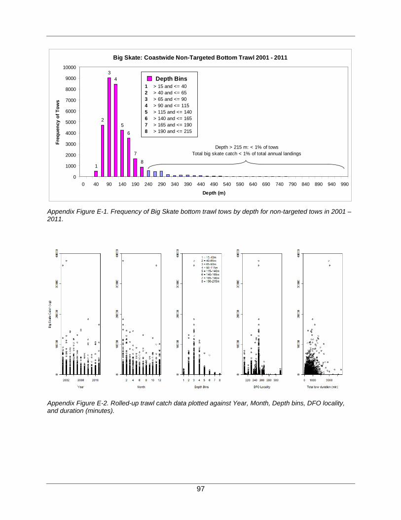
97

Appendix Figure E-1. Frequency of Big Skate bottom trawl tows by depth for non-targeted tows in 2001 – 2011.

Appendix Figure E-2. Rolled-up trawl catch data plotted against Year, Month, Depth bins, DFO locality, and duration (minutes).

Big Skate: Coastwide Non-Targeted Bottom Trawl 2001 - 2011

7

65

4

2

18

3

0

1000

2000

3000

4000

5000

6000

7000

8000

9000

10000

0 40 90 140 190 240 290 340 390 440 490 540 590 640 690 740 790 840 890 940 990

Depth (m)

Freq

uenc

y of

Tow

s

Depth > 215 m: < 1% of towsTotal big skate catch < 1% of total annual landings

Depth Bins12345678

> 15 and <= 40> 40 and <= 65> 65 and <= 90> 90 and <= 115> 115 and <= 140> 140 and <= 165> 165 and <= 190> 190 and <= 215

98

Appendix Figure E-3. Mean non-targeted Big Skate catch (kg) from rolled up trawl tows in 5CDE in 2001 – 2011 plotted against three categorical explanatory variables. Error bars are the 95% confidence intervals. The top left panel shows mean Big Skate catch by month (1-January, 2-February, 3-March, 4-April, 5-May, 6-June, 7-July, 8-August, 9-September, 10-October, 11-November, 12-December). The top right panel shows mean Big Skate catch by depth bin. The bottom panel shows mean Big Skate catch by DFO locality (DFO Localities are defined in Appendix Table E-1).

99

Appendix Figure E-4. Diagnostic plot for GLM that includes all four predictor variables (n=10820). The bottom figure shows three data points that are exerting high leverage on the model output.

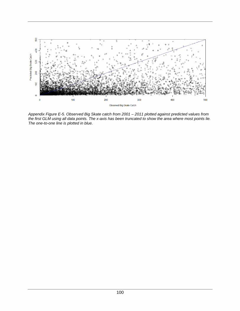
100

Appendix Figure E-5. Observed Big Skate catch from 2001 – 2011 plotted against predicted values from the first GLM using all data points. The x-axis has been truncated to show the area where most points lie. The one-to-one line is plotted in blue.

101

Appendix Figure E-6. Oserved mean Big Skate catch (kg) per year and predicted mean Big Skate catch (kg) per year based on the first lognormal GLM, using all data points. Data is rolled up trawl tows from Skate Management Area 5CDE in 2001 – 20011. Errors bars are the 95% confidence intervals

102

Appendix Figure E-7. Oserved mean Big Skate catch (kg) per year and predicted mean Big Skate catch (kg) per year based on the second lognormal GLM, with high-leverage data points removed. Data is rolled up trawl tows from Skate Management Area 5CDE in 2001 – 20011. Errors bars are the 95% confidence intervals

103

Appendix Figure E-8. Observed mean Big Skate catch (kg) in 2001 – 2011 and predicted mean Big Skate catch per year based on the third lognormal GLM using positive tows only (zeros excluded). Data is rolled up trawl tows from Skate Management Area 5CDE in 2001 – 2011. Note that using positive tows only results in higher annual mean catch than when all data points are used as in Appendix Figure E-6, Appendix Figure E-7, and Appendix Figure E-9.

104

Appendix Figure E-9. Observed mean Big Skate catch (kg) in 2001 – 2011 predicted mean Big Skate catch (kg) per year based on the two-step GLM. Data is rolled up trawl tows from Skate Management Area 5CDE in 2001 – 2011

105

HISTORIC TRAWL CATCH RECONSTRUCTION APPENDIX F.

F.1 INTRODUCTION Commercial groundfish catch and effort data are available in the GFCatch database from 1954 – 1995 (Fisheries and Oceans Canada, Pacific Region, Groundfish Data Unit). Species resolution for non-commercial and less important species is poor and few discards were recorded (Rutherford 1999). As skates were not a targeted species prior to 1996, it is assumed that most skate catch was discarded, and therefore not recorded. In order to utilize catch records from this period for the big and Longnose Skate assessments, reconstruction of total skate catch, consisting of recorded landings and reconstructed discards, is necessary.

Using the two-step GLM method described in Appendix E, two reconstructions of historical skate discards were performed using commercial non-targeted Big Skate and Longnose Skate trawl catch data from 2001 – 2011. Skate were not targeted in 1954 – 1995, and therefore it was assumed that most skate catch was discarded (and not recorded) during this time period. Therefore, the reconstructions used non-targeted trawl tows and total (landed plus discarded) Big Skate and Longnose Skate catch from the modern data set for which we have targeting information (2001 – 2011). The first reconstruction used four variables to predict skate catch: Depth Bin, Month, DFO locality, and Duration in minutes. The second reconstruction used an additional variable, Top Species (top fish species landed), to predict skate catch. Separate reconstructions were performed for Big Skate and Longnose Skate in Skate Management Area 3CD (west coast of Vancouver Island, including Juan de Fuca Strait), 5AB (Queen Charlotte Sound, including Queen Charlotte Strait and Johnstone Strait), and 5CDE (Hecate Strait, Dixon Entrance and the west coast of Haida Gwaii).

F.2 METHODS

F.2.1 Selection of Data F.2.1.1 Skate Management Areas Data was subsetted into the three Skate Management Areas as defined in Section 1.5.1:

• Skate Management Area 3CD: West Coast Vancouver Island, including Juan de Fuca Strait (Major Areas 3C, 3D, and Minor Areas 19 and 20 of 4B);

• Skate Management Area 5AB: Queen Charlotte Sound, including Queen Charlotte Strait (Major Areas 5A, 5B, and Minor Area 12 of 4B);

• Skate Management Area 5CDE: Hecate Strait and West Coast Haida Gwaii (Major Areas 5C, 5D, and 5E.)

F.2.1.2 Targeting As in Appendix E, only the non-targeted tows for 2001 – 2011 were selected for analysis. Data were obtained from the PacHarvTrawl database for 2001 – 2006 and the GFFOS database for 2007 – 2011 (Fisheries and Oceans Canada, Pacific Region, Groundfish Data Unit).

F.2.1.3 Rolling up Tows As in Appendix E, the 2001 – 2011 bottom trawl tows were rolled up by trip, targeting (targeted on Big Skate or not), DFO location, and depth bin. Only the non-targeted rollup events were included for further analysis. Tow duration in minutes was summed for each rollup event. Total catch of Big Skate (landings + discards), total landings by fish species, and total landings of all fish species were summed for each rollup.

106

F.2.1.4 DFO Locality DFO locality is defined as in Appendix E. In order for DFO locality to be useful as an explanatory variable to reconstruct historic catches, localities present in the modern data set had to also be present in the historical data set: i.e. modern fishing locations for which catch could be reconstructed had to be consistent with historical fishing locations.

As in Appendices F and H, if a modern locality had less than fifty observations it was binned into alternate bin “312”. Localities that were binned into 312 in the modern data set were also binned in the historic data set regardless of the number of historic observations. The GLMs use the modern data to predict Big Skate catches; therefore, the assumption is that if a locality is not important in the modern data then it is unlikely to be important historically.

Within each Skate Mangement Area, fishing events may have been recorded for which detailed fishing ground information was missing, with location only available at the level of Major area or Minor area, and Locality coded as "unknown" ("9", "0", or "99"). These localities were binned into Locality 312.

It is not unreasonable that changes in fisher preference and species targeting would have occurred over the decades covered by the reconstruction, and a number of localities could not be matched between the historic and modern data set. Localities not present in the modern data set because fishing occurred deeper than 215 m were excluded from the historic data set. A few historic localities were adjacent to modern localities which caught skate, so the localities were combined. Historic localities that did not fish close to modern localities were binned into “312”. Although fishing does not occur near modern localities, one cannot assume that these localities did not catch any skate. Binning the mismatched localities into “312” assumes that they are equivalent to localities with less than 50 observations since the coefficient produced from the GLM is applied to all records within the “312” bin.

F.2.1.5 Duration Duration was used as a factor with 11 discrete levels, rather than a continuous variable as in Appendix E, with durations from 0 to 1200 minutes binned in 120 minute increments, and durations greater than 1200 minutes assigned to the final bin (Appendix Table F-1). As in Appendix E, all records missing duration were excluded from the analysis.

F.2.1.6 Top Species Top Species was defined as the species group with the largest landed value by weight for each rolled up fishing event. The individual species with the largest landed value by weight for each rolled up fishing event were binned into ten groups (Appendix Table F-2). For some rolled up events, there was no single top species (ie., there were ties between two or more species); these records were excluded from the analysis.

Fishing events with Big Skate or Longnose Skate as the species with the largest landed value by weight were excluded from the GLM analysis; however the catch from these fishing events in the historic data set was added to the reconstructed catch.

F.2.1.7 Other Variables The categorical variables Depth Bin and Month are defined as in Appendix E.

F.2.1.8 Historic landed skate catch Although most skate catch in 1954 – 1995 is thought to have been discarded and thus not recorded, some fishing events did record landed skate catch, and in some cases skates were the top landed speces. Fishing events with skates as the Top Species were excluded from the GLM analysis, but were added to the reconstructed discards to calculate total historic catch.

107

Skates in the historic data were not identified to species; therefore, the average proportions of big and Longnose Skate from non-targeted tows in each Skate Management Area in the modern data set were used to partition the historic landed skate catch into Big Skate and Longnose Skate (Appendix Table F-3).

F.2.2 Discard Mortality For the reconstructed catch history from 1954 – 995, a 75% mortality rate was assumed for discarded skates based on anecdotal information obtained from participants in the modern skate fishery (Appendix A). Skate fishers suggested that prior to 1996, fishing behaviour was very different, with skates not returned to the water as quickly as in the modern fishery, and tows of longer duration, resulting in higher mortality rates than what is assumed for the modern data set. Therefore, trawl Catch was calculated as the sum of landings and 75%*discards.

F.2.3 R code All models were run in R 2.10.1 (R Development Core Team 2009). R code is provided in Appendix L.

F.3 RESULTS

F.3.1 Modern Data Exploratory Analysis Median non-targeted Big Skate total catch is shown plotted by Year, Month, Depth Bin, DFO locality, Duration and Top Species in Appendix Figure F-1. Appendix Figure F-2 to Appendix Figure F-4 show the mean and 95% confidence interval for Big Skate catch by each variable.

Median non-targeted Longnose Skate total catch is shown plotted by Year, Month, Depth Bin, DFO locality, Duration and Top Species in Appendix Figure F-5. Appendix Figure F-6 to Appendix Figure F-8 show the mean and 95% confidence interval for Longnose Skate catch by each variable.

F.3.1.1 Big Skate 3CD 16,975 records of non-targeted Big Skate catch exist for Skate Management Area 3CD. Twenty observations were not included in the GLM analysis because total duration (minutes) was not recorded. From the 16,955 remaining records 228 were not included in the GLM analysis because big or Longnose Skate were the top species landed.

Non-targeted Big Skate catch does not appear to change yearly or monthly. Median Big Skate catches in depth bins 1, 2, and 3 are higher than median catches in the remaining bins. However, the highest non-targeted Big Skate catch occurred in depth bin 5. Non-targeted Big Skate median catches appeared similar across all localities. The highest single catch occurred in locality 106. Duration bins 4, 5, 6, and 11 yielded the highest single non-targeted Big Skate catches. Duration bins 1 and 2 had many zeroes and thus their medians are at or near zero. Top species bins 1, 2, 3, 4, and 9 were the most closely associated with large non-targeted Big Skate catches. Top species bin 5 (other rockfish) did not have any associated non-targeted Big Skate catch while top species bin 10 only had two positive records of Big Skate catch (Appendix Figure F-1).

Mean non-targeted Big Skate catches increased from 2001 – 2004, decreased to 2008, and have since slowly increased to 2011. No trend is evident in mean Big Skate catch per month; however, the highest mean non-targeted Big Skate catch occurred in June. Depth bins 2 and 3 have the highest non-targeted mean Big Skate catch with mean catches decreasing with deeper depths (Appendix Figure F-2). The highest mean non-targeted Big Skate catch occurred in

108

locality 113 followed by 106 and 128. Generally, mean non-targeted Big Skate catch increased with increasing tow duration. The highest mean Big Skate catch is associated with top species group 3 (dogfish) followed by group 9 (lingcod) (Appendix Figure F-2).

F.3.1.2 Big Skate 5AB Although major area 4B minor area 12 is grouped with 5AB, no records in 4B minor 12 exist from 2001 – 2011. 16, 863 records of non-targeted Big Skate catch exist for area 5AB. Five observations were not included in the GLM analysis because total duration (min) was not recorded. From the 16, 858 remaining records 574 were not included in the GLM analysis because big or Longnose Skate were the top species landed. One record was not included in the analysis because top species landed data was not recorded.

Non-targeted Big Skate catch does not appear to be affected by year except for low catches evident in 2008 and 2009 relative to other years. Unlike Big Skate catches in 3CD, a trend in non-targeted Big Skate catches by month occurs in 5AB. Starting at the lowest catches in January non-targeted Big Skate catches increase to their peak in July and then continuously decrease as the year progresses. No Big Skate catch occurs in depth bin 1. Median Big Skate catches in depth bins 2, 3, and 4 are higher than median catches in the remaining bins. The highest non-targeted Big Skate catch occurred in depth bin 3. Non-targeted Big Skate median catches appeared to be similar across all localities except for 195 which has a higher median and contained the largest catch events (followed by localities 193 and 192). Non-targeted Big Skate catch generally increased with increasing tow duration. Top species bins 1, 2, 4, and 9 were the most closely associated with large non-targeted Big Skate catches in this management area. Top species bin 7 and 8 (bathypelagics and sablefish, respectively) only had eight and one positive non-targeted Big Skate catch events, respectively (Appendix Figure F-1).

Mean non-targeted Big Skate catches in 5AB did not show an evident decreasing, increasing, or stable trend. The highest mean catch occurred in 2002 and 2003 while the lowest occurred in 2008. Mean non-targeted Big Skate catch in 5AB starts near zero in January and increases to its maximum in July with consistent decreases until December. Depth bins 2, 3, and 4 have the highest non-targeted mean Big Skate catch with mean catches decreasing with deeper depths (Appendix Figure F-3). The highest mean non-targeted Big Skate catch occurred in locality 195 followed by 193 then 194. Generally, mean non-targeted Big Skate catch increased with increasing tow duration as was seen in area 3CD. The highest mean Big Skate catch is associated with top species group 9 (lingcod), 5 (other rockfish), followed by group 3 (dogfish) (Appendix Figure F-3).

F.3.1.3 Big Skate 5CDE 10,821 records of non-targeted Big Skate catch exist for area 5CDE. One observation was not included in the GLM analysis because total duration (min) was not recorded. From the 10,820 remaining records 645 were not included in the GLM analysis because big or Longnose Skate were the top species landed.

Non-targeted Big Skate catch does not appear to be affected by year except for two large catch events that occurred in 2001 and 2002 (36,057 and 37,606 kg, respectively). Non-targeted Big Skate catch is relatively similar across months. The two largest catch events occur in January and November, respectively. Median Big Skate catches increase from depth bin 1 to their peak in depth bin 3 and subsequently decrease to almost zero in depth bin 8. The two largest non-targeted Big Skate catches occurred in depth bin 3. Non-targeted Big Skate median catches vary greatly depending on locality, however, localities 250 and 251 appear to be the most important in regards to Big Skate catch. Non-targeted Big Skate catch increased with increasing tow duration. Top species bins 1, 2, and 9 were the most closely associated with non-targeted

109

Big Skate catches in this area. The two largest non-targeted Big Skate catches are not shown in the top species plot because the top species landed with those catches was skate. Except for top species group 9, the other top species groups did not seem to be closely associated with non-targeted Big Skate catch (Appendix Figure F-1).

Mean non-targeted Big Skate catches in 5CDE showed a general decreasing trend from 2001 – 2009 with slight increases seen in 2010 and 2011. Mean non-targeted Big Skate catch in 5CDE starts at its peak in January and decreases to its minimums in summer and early autumn months and starts increasing again in November and December. Mean non-targeted Big Skate catch peaks in depth bin 3 and decreases at both shallower and deeper depths (Appendix Figure F-4). The highest mean non-targeted Big Skate catch occurs in localities 251 and 250 followed by 210. A number of localities (e.g., 284, 231, and 212) had means close to zero even though more than 50 observations occurred in those localities. Generally, mean non-targeted Big Skate catch increased with increasing tow duration as was seen in area 3CD and 5AB. The highest mean Big Skate catch is associated with top species group 1 (Pacific cod and tomcod) and closely followed by 2 (flatfish complex) and 9 (lingcod) (Appendix Figure F-4).

F.3.1.4 Longnose Skate 3CD 16, 945 records of non-targeted Longnose Skate catch exist for area 3CD including 4B minor 19 and 20 after deleting records for which total duration (min) was not recorded. From the 16, 945 remaining records 224 were not included in the GLM analysis because big or Longnose Skate were the top species landed.

Non-targeted Longnose Skate catch does not appear to be affected by year or month, however, this may be attributed to the scale used for the plots. Median Longnose Skate catches in depth bins 6, 7, and 8 are higher than median catches in the shallower bins. Higher Longnose Skate catches in deeper depths are expected as Longnose Skates are known to inhabit deeper waters than Big Skate. The highest non-targeted Longnose Skate catch occurred in depth bin 6. Non-targeted Longnose Skate median catches appeared to be similar across all localities although some localities (e.g., 82, 154, and 155) exhibited much lower catches relative to others. The highest single catch occurred in locality 128. Median non-targeted Longnose Skate catches generally increased with increasing tow duration. Duration bins 3 and 7 contained the highest non-targeted Longnose Skate catches. Top species 2 and 9 were the most closely associated with large non-targeted Longnose Skate catches. Top species bin 5 (other rockfish) was associated with one positive non-targeted Longnose Skate catch event (Appendix Figure F-5).

Mean non-targeted Longnose Skate catch did not seem to be associated with a yearly trend. The highest mean catches occurred in 2003 and 2005. The highest mean non-targeted Longnose Skate catch occurred in November and December with the lowest in October. Mean non-targeted Longnose Skate catch generally increased with increasing depths, the highest mean occurred in depth bin 8 (Appendix Figure F-6). The highest mean non-targeted Big Skate catch occurred in locality 127 followed by 138 and 125. Generally, mean non-targeted Longnose Skate catch increased with increasing tow duration. The highest mean Longnose Skate catch is associated with top species group 8 (sablefish) followed by group 9 (lingcod) (Appendix Figure F-6).

F.3.1.5 Longnose Skate 5AB Although major area 4B minor area 12 is grouped with 5AB, no records from 4B minor 12 exist from 2001 – 2011 for Longnose Skate. 17,280 records of non-targeted Longnose Skate catch exist for area 5AB. Six observations were not included in the GLM analysis because total duration (min) was not recorded. From the 17,280 remaining records 869 were not included in

110

the GLM analysis because big or Longnose Skate were the top species landed. One record was not included in the analysis because the top species landed was not recorded.

Non-targeted Longnose Skate catches appear to be similar across years. The highest non-targeted Longnose Skate catches occurred in 2001, 2002, and 2004. Non-targeted Longnose Skate catches were highest in June, July, and August. Medians of Longnose Skate catch appear similar across all months. Longnose Skate catch did not occur in depth bin 1. The highest Longnose Skate catches occurred in depth bins 6 and 8 with the lowest occurring in depth bin 2. The highest non-targeted Longnose Skate catch occurred in depth bin 6. Non-targeted Longnose Skate catch occurred predominantly in localities 195, 193, 193, 204, and 179. Median non-targeted Longnose Skate catches generally increased with increasing tow duration. Duration bin 2 contained the two highest non-targeted Longnose Skate catches. Top species 2 and 9 were the most closely associated with large non-targeted Longnose Skate catches followed closely by 4 and 6 (Appendix Figure F-5).

Mean non-targeted Longnose Skate catch was relatively stable from 2001 – 2006 followed by a decrease to 2008 and subsequent increase until 2011. The highest mean non-targeted Longnose Skate catches occurred in the summer months of June, July, and August with the lowest mean catches occurring in March and April. The highest mean non-targeted Longnose Skate catch occurred in depth bin 3 (Appendix Figure F-7). The highest mean non-targeted Big Skate catch occurred in locality 195 followed by 204 and 192. Mean Longnose Skate catches were lowest in localities 187, 191, and the binned locality 312. Generally, mean non-targeted Longnose Skate catch increased with increasing tow duration. The highest mean Longnose Skate catch occurred with top species group 9 (lingcod), however, the remaining top species groups (except for group 7) were similarly associated with Longnose Skate catch (Appendix Figure F-7).

F.3.1.6 Longnose Skate 5CDE 11,304 records of non-targeted Longnose Skate catch exists for area 5CDE after one observation was deleted because total duration (min) was not recorded. From the 11,304 remaining records 852 were not included in the GLM analysis because big or Longnose Skate were the top species landed.

Non-targeted Longnose Skate catches were relatively similar across years with high Longnose Skate catch events occurring in 2001 and 2004. Medians of Longnose Skate catch appear similar across all months and depth bins. The highest Longnose Skate catches occurred in depth bins 4 and 6. Non-targeted Longnose Skate catch occurred predominantly in localities 254 and 260. Median non-targeted Longnose Skate catches generally increased with increasing tow duration. However, duration bin 1 contained the highest non-targeted Longnose Skate catch. Top species 2, 1, and 9, respectively, were most closely associated with large non-targeted Longnose Skate catches followed closely by 4 and 6 (Appendix Figure F-5). Mean non-targeted Longnose Skate catch showed a general decrease from 2001 – 2009 followed by a small increase in 2010 and 2011. The highest mean non-targeted Longnose Skate catches occurred in November and the lowest mean catches occurred in March and April. Mean Longnose Skate catch increases with depth up until depth bin 6.

Mean Longnose Skate catch drastically decreases in depth bins 7 and 8 (Appendix Figure F-8). The highest mean non-targeted Longnose Skate catch occurred in locality 254 followed by 260. The mean Longnose Skate catches found in 254 and 260 are almost double those found in localities with the next largest mean catch (250 and 251). A number of localities exist with mean Longnose Skate catches close to zero even with more than 50 observations in that locality (e.g., 284, 231, and 234). Generally, mean non-targeted Longnose Skate catch increased with increasing tow duration until duration bin 7, decreased and stabilized until duration bin 10, and

111

increased again in duration bin 11. The highest mean Longnose Skate catch occurred with top species group 2 (flatfish complex) followed closely by group (lingcod) (Appendix Figure F-8).

F.3.2 Four-Variable two-step glm The order of acceptance of variables into the four-variable lognormal GLM of positive tows and the four-variable binomial GLM are presented for each Skate Management Area in Appendix Table F-4 to Appendix Table F-6 for Big Skate and in Appendix Table F-7 to Appendix Table F-9 for Longnose Skate. For consistency, all four variables are included in each model, even when the improvement in deviance from adding further variables is less than 1%. All four variables were found to be statistically significant in all models.

F.3.2.1 Big Skate The modern Big Skate data set for 3CD contained 3,076 positive tows. The binomial GLM underestimated the number of positive tows and predicted 972 positive tows. The mean Big Skate catch predicted using the two-step GLM on average captures mean catch trends (panel A of Appendix Figure F-9).

From the 23, 121 available records from the historic data set for Big Skate in 3CD, the binomial GLM predicted 7,277 positive tows. Using those 7,277 positive tows, the lognormal GLM predicted mean catches by year as shown in panel B of Appendix Figure F-9.

The modern Big Skate data set for 5AB contained 6,144 positive tows. The binomial GLM underestimated the number of positive tows and predicted 5,422 positive tows. The mean Big Skate catch predicted using the two-step GLM do not capture mean catch trends (panel A of Appendix Figure F-10).

From the 20,771 available records from the historic data set for Big Skate in 5AB, the binomial GLM predicted 10,863 positive tows. Using those 10,863 positive tows, the lognormal GLM predicted mean catches by year as shown in panel B of Appendix Figure F-10.

The modern Big Skate data set for 5CDE contains 7,163 positive tows. The binomial GLM overestimates the number of positive tows and predicts 8,343 positive. The mean Big Skate catch predicted using the two-step GLM consistently underestimates mean catch (panel A of Appendix Figure F-11).

From the 32,113 available records from the historic data set for Big Skate in 5CDE, the binomial GLM predicted 28,727 positive tows. Using those 28,727 positive tows, the lognormal GLM predicted mean catches by year as shown in panel B of Appendix Figure F-11.

F.3.2.2 Longnose Skate The modern Longnose Skate data set for 3CD contained 8,660 positive tows. The binomial GLM overestimated the number of positive tows and predicted 9,046 positive tows. The mean Longnose Skate catch predicted using the two-step GLM method consistently underestimates mean catches and does not capture trends seen in the observed data set (panel A of Appendix Figure F-12).

Out of the 23,121 available records from the historic data set for Longnose Skate in 3CD, the binomial GLM predicted 14,617 positive tows. Using those 14,617 positive tows, the lognormal GLM predicted mean catches by year as shown in panel B of Appendix Figure F-12.

The modern Longnose Skate data set for 5AB contained 6,946 positive tows. The binomial GLM underestimated the number of positive tows and predicted 4,296 positive tows. The mean Longnose Skate catch predicted using the two-step GLM is underestimated (panel A of Appendix Figure F-13).

112

Out of the 20,745 available records from the historic data set for Longnose Skate in 5AB, the binomial GLM predicted 9,868 positive tows. Using those 9,868 positive tows, the lognormal GLM predicted mean catches by year as shown in panel B of Appendix Figure F-13.

The modern Longnose Skate data set for 5CDE contained 4,297 positive tows. The binomial GLM underestimated the number of positive tows and predicted 3,096 positive tows. The mean Longnose Skate catch predicted using the two-step GLM is underestimated from 2001 – 2008 and then slightly overestimated from 2009 – 2011 (panel A of Appendix Figure F-14).

Out of the 32,093 available records from the historic data set for Longnose Skate in 5CDE, the binomial GLM predicted 13,372 positive tows. Using those 13,372 positive tows, the lognormal GLM predicted mean catches by year as shown in panel B of Appendix Figure F-14.

F.3.3 Five-variable two-step glm The order of acceptance of variables into the five-variable lognormal GLM of positive tows and the five-variable binomial GLM are presented for each Skate Management Area in Appendix Table F-10 to Appendix Table F-12 for Big Skate and in Appendix Table F-13 to Appendix Table F-15 for Longnose Skate. For consistency, all five variables are included in each model, even when the improvement in deviance from adding further variables is less than 1%. All five variables were found to be statistically significant in all models.

F.3.3.1 Big Skate The modern Big Skate data set for 3CD contained 2,993 positive tows. The binomial GLM underestimated the numbr of positive tows and predicted 1,014 positive tows. The mean Big Skate catch predicted using the two-step GLM in general captures mean catch trends seen in the modern data set (panel A of Appendix Figure F-15).

Out of the 22,889 available records from the historic data set for Big Skate in 3CD, the binomial GLM predicted 8,393 positive tows. Using those 8,393 positive tows, the lognormal GLM predicted mean catches by year as shown in panel B of Appendix Figure F-15.

The modern Big Skate data set for 5AB contained 5,997 positive tows. The binomial GLM underestimated the number of positive tows, and predicted 4,786 positive tows. The mean Big Skate catch predicted using the two-step GLM does not capture mean catch trends seen in the modern data set (panel A of Appendix Figure F-16).

Out of the 20,484 available records from the historic data set for Big Skate in 5AB, the binomial GLM predicted 11,058 positive tows. Using those 11,058 positive tows, the lognormal GLM predicted mean catches by year as shown in panel B of Appendix Figure F-16.

The modern Big Skate data set for 5CDE contained 6,529 positive tows. The binomial GLM overestimated the number of positive tows and predicted 7,635 positive tows. The mean Big Skate catch predicted using the two-step GLM does not capture mean catch trends seen in the modern data set (panel A of Appendix Figure F-17).

Out of the 31,681 available records from the historic data set for Big Skate in 5CDE, the binomial GLM predicted 27,714 positive tows. Using those 27,714 positive tows, the log-normal GLM predicted mean catches by year as shown in panel B of Appendix Figure F-17.

F.3.3.2 Longnose Skate The modern Longnose Skate data set for 3CD contained 8,453 positive tows. The binomial GLM overestimated the number of positive tows and predicted 9,461. The mean Longnose Skate catch predicted using the two-step GLM is underestimated (panel A of Appendix Figure F-18).

113

Out of the 22, 889 available records from the historic data set for Longnose Skate in 3CD, the binomial GLM predicted 17,121 positive tows. Using those 17,121 postive tows, the lognormal GLM predicted mean catches by year as shown in panel B of Appendix Figure F-18.

The modern Longnose Skate data set for 5AB contained 6,450 positive tows. The binomial GLM underestimated the number of positive tows and predicted 4,417 positive tows. The mean Longnose Skate catch predicted using the two-step GLM is underestimated (panel A of Appendix Figure F-19).

Out of the 20,484 available records from the historic data set for Longnose Skate in 5AB, the binomial GLM predicted 10,570 positive Longnose Skate catch records. Using those 10,570 positive tows, the lognormal GLM predicted mean catches by year as shown in panel B of Appendix Figure F-19.

The modern Longnose Skate data set for 5CDE contained 3,965 postive tows. The binomial GLM underestimated the number of positive tows and predicted 2,953 positive tows. The mean Longnose Skate catch predicted using the two-step GLM does not capture mean catch trends (panel A of Appendix Figure F-20).

Out of the 31,681 available records from the historic Longnose Skate data set in 5CDE, the binomial GLM predicted 11,652 positive tows. Using those 11,652 positive tows, the lognormal GLM predicted mean catches by year as shown in panel B of Appendix Figure F-20.

F.3.4 Reconstructed Catches Reconstructed catches based on the four-variable two-step method are presented in Appendix Table F-16 for Big Skates and Appendix Table F-17 for Longnose Skate. Reconstructed catches based on the five-variable two-step method are presented in Appendix Table F-18 for Big Skates and Appendix Table F-19 for Longnose Skate. For each catch history, reconstructed catch consists of the sum of total landed skate from tows where skates were the top species landed, with the appropriate species proportion applied (Appendix Table F-3), and reconstructed discards from the two-step GLM with a 75% discard mortality rate applied. Catch histories are shown in Appendix Figure F-21 and Appendix Figure F-22 for Big Skate and Longnose Skate, respectively.

F.4 REFERENCES R Development Core Team. 2009. R: A language and environment for statistical computing. R

16 Foundation for Statistical Computing. Vienna, Austria. URL http://www.R-project.org.

Rutherford, K. L. 1999. A Brief History of GFCATCH (1954 – 1995), the Groundfish Catch and Effort Database at the Pacific Biological Station. Can. Tech. Rep. Fish. Aquat. Sci. 2299: 66 p.

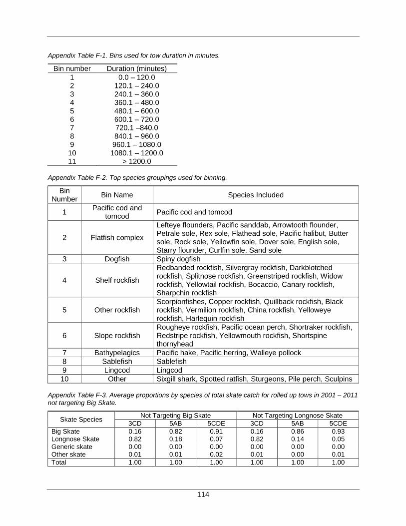
114

Appendix Table F-1. Bins used for tow duration in minutes.

Bin number Duration (minutes) 1 0.0 – 120.0 2 120.1 – 240.0 3 240.1 – 360.0 4 360.1 – 480.0 5 480.1 – 600.0 6 600.1 – 720.0 7 720.1 –840.0 8 840.1 – 960.0 9 960.1 – 1080.0 10 1080.1 – 1200.0 11 > 1200.0

Appendix Table F-2. Top species groupings used for binning.

Bin Number Bin Name Species Included

1 Pacific cod and tomcod Pacific cod and tomcod

2 Flatfish complex

Lefteye flounders, Pacific sanddab, Arrowtooth flounder, Petrale sole, Rex sole, Flathead sole, Pacific halibut, Butter sole, Rock sole, Yellowfin sole, Dover sole, English sole, Starry flounder, Curlfin sole, Sand sole

3 Dogfish Spiny dogfish

4 Shelf rockfish

Redbanded rockfish, Silvergray rockfish, Darkblotched rockfish, Splitnose rockfish, Greenstriped rockfish, Widow rockfish, Yellowtail rockfish, Bocaccio, Canary rockfish, Sharpchin rockfish

5 Other rockfish Scorpionfishes, Copper rockfish, Quillback rockfish, Black rockfish, Vermilion rockfish, China rockfish, Yelloweye rockfish, Harlequin rockfish

6 Slope rockfish Rougheye rockfish, Pacific ocean perch, Shortraker rockfish, Redstripe rockfish, Yellowmouth rockfish, Shortspine thornyhead

7 Bathypelagics Pacific hake, Pacific herring, Walleye pollock 8 Sablefish Sablefish 9 Lingcod Lingcod 10 Other Sixgill shark, Spotted ratfish, Sturgeons, Pile perch, Sculpins

Appendix Table F-3. Average proportions by species of total skate catch for rolled up tows in 2001 – 2011 not targeting Big Skate.

Skate Species Not Targeting Big Skate Not Targeting Longnose Skate 3CD 5AB 5CDE 3CD 5AB 5CDE

Big Skate 0.16 0.82 0.91 0.16 0.86 0.93 Longnose Skate 0.82 0.18 0.07 0.82 0.14 0.05 Generic skate 0.00 0.00 0.00 0.00 0.00 0.00 Other skate 0.01 0.01 0.02 0.01 0.00 0.01 Total 1.00 1.00 1.00 1.00 1.00 1.00

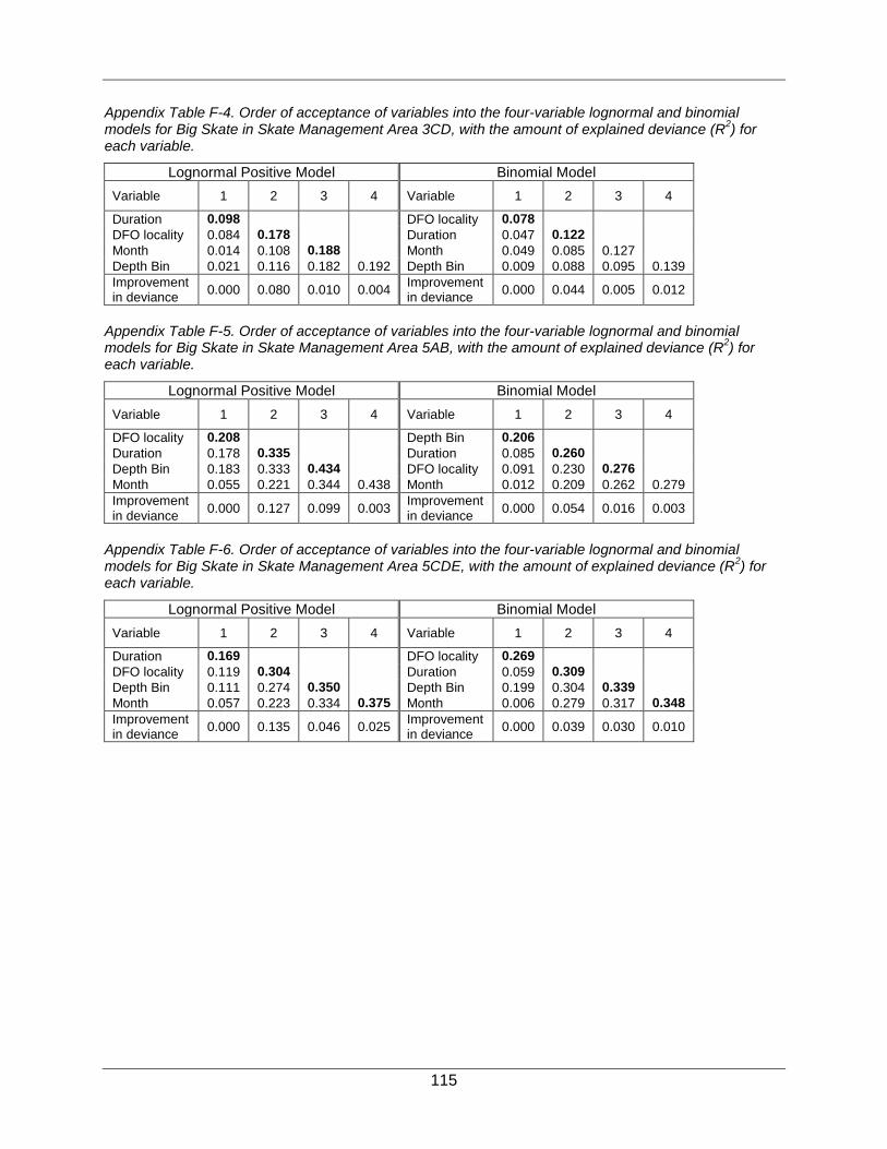
115

Appendix Table F-4. Order of acceptance of variables into the four-variable lognormal and binomial models for Big Skate in Skate Management Area 3CD, with the amount of explained deviance (R2) for each variable.

Lognormal Positive Model Binomial Model Variable 1 2 3 4 Variable 1 2 3 4

Duration 0.098 DFO locality 0.078 DFO locality 0.084 0.178 Duration 0.047 0.122 Month 0.014 0.108 0.188 Month 0.049 0.085 0.127 Depth Bin 0.021 0.116 0.182 0.192 Depth Bin 0.009 0.088 0.095 0.139 Improvement in deviance 0.000 0.080 0.010 0.004 Improvement

in deviance 0.000 0.044 0.005 0.012

Appendix Table F-5. Order of acceptance of variables into the four-variable lognormal and binomial models for Big Skate in Skate Management Area 5AB, with the amount of explained deviance (R2) for each variable.

Lognormal Positive Model Binomial Model Variable 1 2 3 4 Variable 1 2 3 4

DFO locality 0.208 Depth Bin 0.206 Duration 0.178 0.335 Duration 0.085 0.260 Depth Bin 0.183 0.333 0.434 DFO locality 0.091 0.230 0.276 Month 0.055 0.221 0.344 0.438 Month 0.012 0.209 0.262 0.279 Improvement in deviance 0.000 0.127 0.099 0.003 Improvement

in deviance 0.000 0.054 0.016 0.003

Appendix Table F-6. Order of acceptance of variables into the four-variable lognormal and binomial models for Big Skate in Skate Management Area 5CDE, with the amount of explained deviance (R2) for each variable.

Lognormal Positive Model Binomial Model Variable 1 2 3 4 Variable 1 2 3 4

Duration 0.169 DFO locality 0.269 DFO locality 0.119 0.304 Duration 0.059 0.309 Depth Bin 0.111 0.274 0.350 Depth Bin 0.199 0.304 0.339 Month 0.057 0.223 0.334 0.375 Month 0.006 0.279 0.317 0.348 Improvement in deviance 0.000 0.135 0.046 0.025 Improvement

in deviance 0.000 0.039 0.030 0.010

116

Appendix Table F-7. Order of acceptance of variables into the four-variable lognormal and binomial models for Longnose Skate in Skate Management Area 3CD, with the amount of explained deviance (R2) for each variable.

Lognormal Positive Model Binomial Model Variable 1 2 3 4 Variable 1 2 3 4

Duration 0.174 DFO locality 0.056 DFO locality 0.062 0.229 Duration 0.045 0.093 Depth Bin 0.015 0.192 0.259 Month 0.022 0.072 0.110 Month 0.021 0.198 0.248 0.275 Depth Bin 0.008 0.063 0.099 0.115 Improvement in deviance 0.000 0.055 0.030 0.016 Improvement

in deviance 0.000 0.037 0.017 0.005

Appendix Table F-8. Order of acceptance of variables into the four-variable lognormal and binomial models for Longnose Skate in Skate Management Area 5AB, with the amount of explained deviance (R2) for each variable.

Lognormal Positive Model Binomial Model Variable 1 2 3 4 Variable 1 2 3 4

Duration 0.147 Duration 0.063 DFO locality 0.070 0.192 DFO locality 0.027 0.081 Month 0.022 0.158 0.201 Depth Bin 0.009 0.067 0.084 Depth Bin 0.237 0.154 0.197 0.205 Month 0.005 0.065 0.083 0.085 Improvement in deviance 0.000 0.045 0.009 0.004 Improvement

in deviance 0.000 0.018 0.003 0.001

Appendix Table F-9. Order of acceptance of variables into the four-variable lognormal and binomial models for Longnose Skate in Skate Management Area 5CDE, with the amount of explained deviance (R2) for each variable.

Lognormal Positive Model Binomial Model Variable 1 2 3 4 Variable 1 2 3 4

DFO locality 0.149 DFO locality 0.064 Duration 0.078 0.225 Duration 0.050 0.104 Month 0.024 0.170 0.249 Depth Bin 0.036 0.079 0.124 Depth Bin 0.076 0.158 0.240 0.261 Month 0.011 0.071 0.113 0.131 Improvement in deviance 0.000 0.076 0.024 0.012 Improvement

in deviance 0.000 0.040 0.020 0.007

117

Appendix Table F-10. Order of acceptance of variables into the five-variable lognormal and binomial models for Big Skate in Skate Management Area 3CD, with the amount of explained deviance (R2) for each variable.

Lognormal Positive Model Binomial Model Variable 1 2 3 4 5 Variable 1 2 3 4 5

Duration 0.110 Top Species 0.102 DFO locality 0.086 0.188 DFO locality 0.079 0.140 Top Species 0.054 0.151 0.197 Duration 0.049 0.139 0.179 Month 0.013 0.119 0.197 0.208 Month 0.009 0.107 0.144 0.184 Depth Bin 0.020 0.127 0.193 0.202 0.212 Depth Bin 0.048 0.116 0.141 0.180 0.186 Improvement in deviance 0.00 0.078 0.009 0.011 0.004 Improvement

in deviance 0.000 0.091 0.039 0.005 0.002

Appendix Table F-11. Order of acceptance of variables into the five-variable lognormal and binomial models for Big Skate in Skate Management Area 5AB, with the amount of explained deviance (R2) for each variable.

Lognormal Positive Model Binomial Model Variable 1 2 3 4 5 Variable 1 2 3 4 5

Duration 0.197 Depth Bin 0.189 DFO locality 0.174 0.324 Duration 0.086 0.247 Depth Bin 0.164 0.315 0.413 Top Species 0.138 0.208 0.265 Top Species 0.072 0.252 0.378 0.420 DFO locality 0.083 0.210 0.260 0.276 Month 0.042 0.223 0.331 0.417 0.424 Month 0.010 0.192 0.249 0.267 0.279 Improvement in deviance 0.000 0.127 0.089 0.007 0.004 Improvement

in deviance 0.000 0.058 0.018 0.011 0.003

Appendix Table F-12. Order of acceptance of variables into the five-variable lognormal and binomial models for Big Skate in Skate Management Area 5CDE, with the amount of explained deviance (R2) for each variable.

Lognormal Positive Model Binomial Model Variable 1 2 3 4 5 Variable 1 2 3 4 5

Duration 0.179 DFO locality 0.265 DFO locality 0.110 0.303 Duration 0.063 0.307 Depth Bin 0.095 0.269 0.334 Depth Bin 0.190 0.297 0.334 Month 0.030 0.210 0.320 0.358 Top Species 0.226 0.288 0.327 0.341 Top Species 0.030 0.204 0.309 0.346 0.361 Month 0.007 0.272 0.313 0.341 0.350 Improvement in deviance 0.000 0.124 0.041 0.014 0.003 Improvement

in deviance 0.000 0.042 0.027 0.007 0.009

118

Appendix Table F-13. Order of acceptance of variables into the five-variable lognormal and binomial models for Longnose Skate in Skate Management Area 3CD, with the amount of explained deviance (R2) for each variable.

Lognormal Positive Model Binomial Model Variable 1 2 3 4 5 Variable 1 2 3 4 5

Duration 0.186 Top Species 0.158 DFO locality 0.061 0.239 Duration 0.048 0.201 Depth Bin 0.013 0.203 0.267 DFO locality 0.057 0.177 0.215 Month 0.019 0.208 0.256 0.281 Depth Bin 0.008 0.161 0.204 0.220 Top Species 0.032 0.204 0.249 0.276 0.292 Month 0.021 0.159 0.203 0.216 0.221 Improvement in deviance 0.000 0.053 0.028 0.009 0.011 Improvement

in deviance 0.000 0.043 0.014 0.005 0.001

Appendix Table F-14. Order of acceptance of variables into the five-variable lognormal and binomial models for Longnose Skate in Skate Management Area 5AB, with the amount of explained deviance (R2) for each variable.

Lognormal Positive Model Binomial Model Variable 1 2 3 4 5 Variable 1 2 3 4 5

Duration 0.126 Duration 0.059 DFO locality 0.059 0.172 Top Species 0.043 0.098 Month 0.021 0.139 0.184 DFO locality 0.025 0.078 0.113 Depth Bin 0.027 0.138 0.179 0.189 Depth Bin 0.008 0.062 0.102 0.117 Top Species 0.011 0.128 0.177 0.188 0.202 Month 0.004 0.061 0.101 0.116 0.120 Improvement in deviance 0.000 0.046 0.012 0.005 0.013 Improvement

in deviance 0.000 0.039 0.015 0.004 0.003

Appendix Table F-15. Order of acceptance of variables into the five-variable lognormal and binomial models for Longnose Skate in Skate Management Area 5CDE, with the amount of explained deviance (R2) for each variable.

Lognormal Positive Model Binomial Model Variable 1 2 3 4 5 Variable 1 2 3 4 5

DFO locality 0.159 DFO locality 0.069 Duration 0.079 0.235 Duration 0.052 0.111 Month 0.025 0.176 0.256 Depth Bin 0.037 0.084 0.129 Depth Bin 0.082 0.169 0.250 0.269 Top Species 0.024 0.076 0.116 0.137 Top Species 0.056 0.171 0.244 0.263 0.277 Month 0.012 0.076 0.119 0.137 0.144 Improvement in deviance 0.000 0.076 0.021 0.013 0.008 Improvement

in deviance 0.000 0.042 0.018 0.008 0.007

119

Appendix Table F-16. Recorded landings and reconstructed discards (tonnes) for Big Skate in 1954 – 1995. Discards were reconstructed using the four-variable two-step GLM method. "Catch" is the sum of landings and 75%*discards.

Year 3CD 5AB 5CDE Landings Discards Catch Landings Discards Catch Landings Discards Catch

1954 0.01 16.75 12.57 0.62 6.19 5.26 -- 143.79 107.84 1955 -- 13.64 10.23 -- 6.71 5.03 -- 201.92 151.44 1956 -- 12.57 9.43 -- 32.22 24.17 4.32 246.89 189.49 1957 -- 9.86 7.40 0.12 29.23 22.04 -- 210.93 158.20 1958 -- 7.23 5.42 0.25 44.00 33.25 -- 245.53 184.15 1959 0.00 7.23 5.43 -- 34.18 25.64 -- 240.04 180.03 1960 -- 7.72 5.79 0.26 47.87 36.16 0.02 277.77 208.35 1961 0.02 9.07 6.83 -- 39.51 29.64 -- 252.43 189.32 1962 0.12 6.74 5.17 0.20 40.82 30.81 -- 253.80 190.35 1963 0.01 6.14 4.61 0.04 30.91 23.22 0.10 241.98 181.58 1964 0.03 8.36 6.30 -- 29.17 21.88 -- 280.56 210.42 1965 0.06 10.43 7.88 0.36 24.08 18.42 -- 382.07 286.55 1966 -- 14.70 11.02 0.30 61.12 46.14 -- 429.24 321.93 1967 0.05 13.67 10.30 -- 47.40 35.55 -- 362.92 272.19 1968 0.11 11.64 8.84 1.23 59.61 45.94 -- 494.53 370.90 1969 0.31 11.44 8.89 0.71 68.85 52.35 2.64 481.72 363.93 1970 0.24 13.16 10.11 3.64 35.05 29.93 1.06 423.32 318.55 1971 0.08 18.44 13.91 0.53 42.79 32.62 1.12 379.95 286.08 1972 0.00 22.53 16.91 -- 48.27 36.20 2.37 268.95 204.08 1973 0.13 13.32 10.11 0.36 27.77 21.19 -- 228.23 171.17 1974 -- 13.51 10.13 1.00 24.08 19.06 4.65 194.29 150.37 1975 -- 20.27 15.20 -- 48.98 36.74 4.95 314.56 240.86 1976 0.03 15.00 11.28 0.20 64.28 48.42 17.38 358.54 286.29 1977 0.09 12.37 9.36 0.29 62.83 47.41 7.84 414.81 318.95 1978 -- 11.50 8.62 2.35 68.69 53.86 4.56 339.46 259.15 1979 0.09 10.80 8.19 -- 74.33 55.75 4.16 502.59 381.10 1980 0.13 10.78 8.22 0.44 81.37 61.47 16.69 496.66 389.19 1981 -- 9.54 7.15 1.91 64.21 50.07 7.51 369.80 284.86 1982 -- 13.10 9.83 1.86 67.98 52.84 1.20 248.73 187.75 1983 -- 6.12 4.59 -- 61.63 46.22 2.72 248.07 188.77 1984 -- 7.41 5.56 -- 35.12 26.34 6.39 268.69 207.91 1985 -- 9.94 7.45 -- 42.13 31.59 12.16 278.57 221.09 1986 -- 6.49 4.86 -- 54.61 40.96 8.90 186.73 148.94 1987 -- 5.80 4.35 0.21 66.11 49.79 1.06 338.51 254.94 1988 -- 11.55 8.66 3.60 61.90 50.03 4.16 346.25 263.84 1989 0.03 12.15 9.15 1.27 57.12 44.11 18.09 362.27 289.79 1990 -- 12.05 9.04 0.78 70.25 53.47 0.63 386.42 290.45 1991 -- 11.00 8.25 0.23 100.68 75.74 0.86 484.49 364.23 1992 0.00 19.32 14.50 1.56 115.21 87.97 4.12 577.48 437.23 1993 0.04 21.19 15.93 5.28 131.05 103.56 10.04 829.79 632.38 1994 0.03 20.50 15.40 44.41 126.10 138.98 3.21 520.19 393.36 1995 -- 18.67 14.00 19.55 133.75 119.86 24.21 544.04 432.24

120

Appendix Table F-17. Recorded landings and reconstructed discards (tonnes) for Longnose Skate in 1954 – 1995. Discards were reconstructed using the four-variable two-step GLM method. "Catch" is the sum of landings and 75%*discards.

Year 3CD 5AB 5CDE Landings Discards Catch Landings Discards Catch Landings Discards Catch

1954 -- 31.47 23.60 0.11 0.79 0.70 -- 3.26 2.45 1955 -- 25.34 19.00 -- 1.11 0.83 -- 6.06 4.54 1956 0.24 28.19 21.38 -- 3.72 2.79 0.24 7.25 5.67 1957 -- 19.60 14.70 0.02 4.83 3.65 -- 6.94 5.20 1958 -- 13.86 10.40 0.04 3.61 2.75 -- 8.30 6.23 1959 -- 15.06 11.29 -- 2.44 1.83 -- 10.71 8.03 1960 0.00 15.67 11.76 0.04 3.01 2.30 0.00 13.08 9.81 1961 -- 19.79 14.84 -- 2.88 2.16 -- 9.90 7.42 1962 -- 15.47 11.60 0.03 3.09 2.35 -- 10.37 7.78 1963 0.01 11.99 9.00 0.01 2.96 2.23 0.01 8.08 6.06 1964 -- 16.56 12.42 -- 4.30 3.22 -- 10.22 7.66 1965 -- 24.37 18.28 0.06 4.72 3.60 -- 14.23 10.67 1966 -- 26.58 19.93 0.05 11.73 8.85 -- 13.86 10.39 1967 -- 23.81 17.86 -- 9.86 7.40 -- 14.08 10.56 1968 -- 20.88 15.66 0.21 10.70 8.24 -- 12.01 9.01 1969 0.15 23.37 17.67 0.12 17.74 13.43 0.15 13.93 10.59 1970 0.06 27.10 20.38 0.62 10.94 8.82 0.06 17.78 13.39 1971 0.06 36.46 27.41 0.09 10.70 8.12 0.06 19.30 14.54 1972 0.13 42.05 31.67 -- 12.58 9.44 0.13 18.51 14.01 1973 -- 21.73 16.30 0.06 7.28 5.52 -- 17.09 12.82 1974 0.26 22.85 17.39 0.17 7.54 5.82 0.26 15.71 12.04 1975 0.27 39.24 29.70 -- 10.55 7.92 0.27 18.85 14.41 1976 0.96 31.16 24.33 0.03 15.41 11.59 0.96 26.39 20.75 1977 0.43 39.27 29.88 0.05 14.98 11.28 0.43 26.78 20.51 1978 0.25 33.30 25.22 0.40 19.52 15.04 0.25 23.14 17.60 1979 0.23 30.10 22.80 -- 19.10 14.33 0.23 37.13 28.08 1980 0.92 28.56 22.33 0.08 19.26 14.52 0.92 30.71 23.95 1981 0.41 26.00 19.92 0.33 14.35 11.09 0.41 24.00 18.41 1982 0.07 30.54 22.97 0.32 15.61 12.03 0.07 17.35 13.08 1983 0.15 20.76 15.72 -- 12.62 9.47 0.15 13.27 10.10 1984 0.35 24.45 18.68 -- 10.50 7.88 0.35 20.66 15.84 1985 0.67 32.59 25.11 -- 11.36 8.52 0.67 17.36 13.68 1986 0.49 32.38 24.77 -- 14.62 10.97 0.49 13.34 10.49 1987 0.06 27.86 20.95 0.04 21.78 16.37 0.06 20.04 15.09 1988 0.23 42.53 32.13 0.61 19.31 15.10 0.23 18.24 13.91 1989 0.99 48.96 37.71 0.22 18.76 14.29 0.99 17.59 14.19 1990 0.03 40.45 30.37 0.13 20.64 15.61 0.03 20.61 15.50 1991 0.05 42.94 32.25 0.04 26.16 19.66 0.05 20.37 15.32 1992 0.23 99.10 74.55 0.27 35.27 26.72 0.23 32.62 24.69 1993 0.55 114.53 86.45 0.90 36.67 28.41 0.55 56.88 43.21 1994 0.18 96.71 72.71 7.58 34.83 33.70 0.18 32.41 24.48 1995 1.33 85.74 65.64 3.34 34.78 29.43 1.33 35.19 27.72

121

Appendix Table F-18. Recorded landings and reconstructed discards (tonnes) for Big Skate in 1954 – 1995. Discards were reconstructed using the five-variable two-step GLM method. "Catch" is the sum of landings and 75%*discards.

Year 3CD 5AB 5CDE Landings Discards Catch Landings Discards Catch Landings Discards Catch

1954 0.01 15.91 11.94 0.62 6.36 5.40 -- 122.44 91.83 1955 -- 13.66 10.24 -- 6.58 4.93 -- 174.26 130.69 1956 -- 12.12 9.09 -- 29.22 21.91 4.32 214.26 165.01 1957 -- 9.19 6.89 0.12 31.08 23.43 -- 175.17 131.38 1958 -- 6.66 4.99 0.25 42.19 31.90 -- 202.14 151.61 1959 0.00 7.30 5.48 -- 37.35 28.02 -- 190.30 142.72 1960 -- 8.40 6.30 0.26 47.16 35.63 0.02 223.12 167.36 1961 0.02 9.48 7.14 -- 40.12 30.09 -- 210.16 157.62 1962 0.12 6.59 5.07 0.20 42.03 31.72 -- 204.83 153.62 1963 0.01 5.80 4.36 0.04 31.47 23.64 0.10 188.88 141.76 1964 0.03 8.11 6.11 -- 31.64 23.73 -- 223.83 167.87 1965 0.06 11.67 8.81 0.36 24.60 18.80 -- 298.27 223.70 1966 -- 12.84 9.63 0.30 48.14 36.41 -- 338.60 253.95 1967 0.05 12.67 9.56 -- 39.90 29.93 -- 288.15 216.11 1968 0.11 10.69 8.13 1.23 50.15 38.85 -- 395.83 296.87 1969 0.31 10.67 8.32 0.71 55.66 42.46 2.64 397.93 301.09 1970 0.24 11.83 9.11 3.64 28.37 24.92 1.06 359.40 270.61 1971 0.08 16.41 12.39 0.53 32.77 25.11 1.12 320.03 241.14 1972 0.00 19.10 14.33 -- 36.60 27.45 2.37 217.42 165.44 1973 0.13 12.06 9.17 0.36 23.17 17.74 -- 187.08 140.31 1974 -- 12.32 9.24 1.00 19.58 15.68 4.65 157.80 122.99 1975 -- 18.48 13.86 -- 38.13 28.59 4.95 263.62 202.66 1976 0.03 13.87 10.44 0.20 48.61 36.66 17.38 294.85 238.52 1977 0.09 12.68 9.59 0.29 48.63 36.76 7.84 345.71 267.12 1978 -- 11.16 8.37 2.35 54.10 42.92 4.56 284.50 217.93 1979 0.09 11.17 8.47 -- 56.48 42.36 4.16 410.69 312.18 1980 0.13 11.30 8.61 0.44 66.83 50.57 16.69 397.11 314.52 1981 -- 10.00 7.50 1.91 54.68 42.92 7.51 310.03 240.03 1982 -- 12.79 9.59 1.86 58.08 45.41 1.20 201.85 152.59 1983 -- 6.62 4.96 -- 53.86 40.39 2.72 200.77 153.29 1984 -- 6.87 5.15 -- 31.30 23.47 6.39 220.21 171.54 1985 -- 10.26 7.70 -- 34.50 25.87 12.16 221.12 178.00 1986 -- 7.04 5.28 -- 46.96 35.22 8.90 153.68 124.15 1987 -- 6.23 4.67 0.21 57.12 43.05 1.06 274.74 207.11 1988 -- 12.04 9.03 3.60 53.48 43.71 4.16 287.39 219.70 1989 0.03 12.80 9.63 1.27 49.94 38.73 18.09 301.84 244.47 1990 -- 12.29 9.22 0.78 60.27 45.98 0.63 327.83 246.50 1991 -- 11.40 8.55 0.23 84.74 63.79 0.86 407.24 306.30 1992 0.00 21.86 16.40 1.56 98.02 75.07 4.12 492.95 373.84 1993 0.04 19.71 14.82 5.28 110.05 87.82 10.04 692.42 529.35 1994 0.03 19.81 14.88 44.41 107.29 124.87 3.21 438.04 331.75 1995 -- 19.12 14.34 19.55 107.97 100.53 24.21 467.32 374.70

122

Appendix Table F-19. Recorded landings and reconstructed discards (tonnes) for Longnose Skate in 1954 – 1995. Discards were reconstructed using the five-variable two-step GLM method. "Catch" is the sum of landings and 75%*discards.

Year 3CD 5AB 5CDE Landings Discards Catch Landings Discards Catch Landings Discards Catch

1954 0.04 29.73 22.34 0.11 1.30 1.08 -- 2.71 2.03 1955 -- 25.57 19.18 -- 1.52 1.14 -- 5.36 4.02 1956 -- 27.92 20.94 -- 4.96 3.72 0.24 6.47 5.09 1957 -- 19.17 14.37 0.02 6.13 4.62 -- 5.78 4.34 1958 -- 13.30 9.97 0.04 5.95 4.50 -- 5.97 4.48 1959 0.01 14.13 10.61 -- 5.49 4.12 -- 7.06 5.30 1960 -- 17.16 12.87 0.04 6.18 4.68 0.00 9.04 6.78 1961 0.13 21.04 15.91 -- 5.66 4.24 -- 7.95 5.96 1962 0.63 15.50 12.26 0.03 6.50 4.91 -- 8.73 6.55 1963 0.04 11.29 8.50 0.01 5.27 3.96 0.01 5.81 4.36 1964 0.13 16.34 12.38 -- 5.67 4.25 -- 7.30 5.47 1965 0.30 24.58 18.74 0.06 5.99 4.55 -- 8.62 6.47 1966 -- 23.99 17.99 0.05 9.90 7.47 -- 8.83 6.62 1967 0.26 22.00 16.76 -- 8.91 6.68 -- 10.67 8.00 1968 0.57 18.98 14.81 0.21 8.89 6.88 -- 8.96 6.72 1969 1.60 20.97 17.32 0.12 15.18 11.51 0.15 11.67 8.90 1970 1.24 23.63 18.96 0.62 8.94 7.32 0.06 16.72 12.60 1971 0.39 32.95 25.10 0.09 8.77 6.67 0.06 17.41 13.12 1972 0.02 38.20 28.67 -- 9.88 7.41 0.13 15.30 11.60 1973 0.65 19.27 15.10 0.06 6.03 4.59 -- 13.86 10.40 1974 -- 20.44 15.33 0.17 6.40 4.97 0.26 12.79 9.85 1975 -- 34.88 26.16 -- 8.74 6.55 0.27 16.20 12.42 1976 0.18 28.37 21.46 0.03 12.04 9.07 0.96 21.72 17.25 1977 0.44 37.36 28.46 0.05 11.75 8.86 0.43 21.77 16.76 1978 -- 31.18 23.39 0.40 16.00 12.40 0.25 17.27 13.20 1979 0.47 29.60 22.67 -- 14.58 10.94 0.23 28.30 21.45 1980 0.68 29.77 23.01 0.08 16.21 12.23 0.92 22.59 17.86 1981 -- 25.74 19.31 0.33 12.81 9.93 0.41 19.66 15.15 1982 -- 28.19 21.15 0.32 13.44 10.40 0.07 13.25 10.00 1983 -- 18.86 14.15 -- 11.21 8.41 0.15 9.93 7.60 1984 -- 22.39 16.79 -- 8.82 6.61 0.35 17.49 13.47 1985 -- 28.99 21.74 -- 8.84 6.63 0.67 15.12 12.01 1986 -- 30.56 22.92 -- 12.64 9.48 0.49 10.98 8.72 1987 -- 25.95 19.46 0.04 18.91 14.22 0.06 13.73 10.35 1988 -- 43.47 32.60 0.61 16.77 13.19 0.23 13.70 10.50 1989 0.16 47.72 35.95 0.22 16.56 12.64 0.99 14.21 11.65 1990 -- 37.03 27.77 0.13 18.50 14.01 0.03 16.53 12.43 1991 -- 41.40 31.05 0.04 23.24 17.47 0.05 15.55 11.71 1992 0.02 111.08 83.33 0.27 33.38 25.30 0.23 25.03 19.00 1993 0.19 117.24 88.11 0.90 34.96 27.12 0.55 40.38 30.84 1994 0.13 101.60 76.33 7.58 33.19 32.47 0.18 27.87 21.08 1995 -- 89.34 67.00 3.34 33.39 28.38 1.33 31.27 24.78

123

Appendix Figure F-1. Plots of median non-targeted Big Skate total catch by year, month, depth, locality, duration, and top species in Skate Management Areas 3CD, 5AB, and 5CDE.

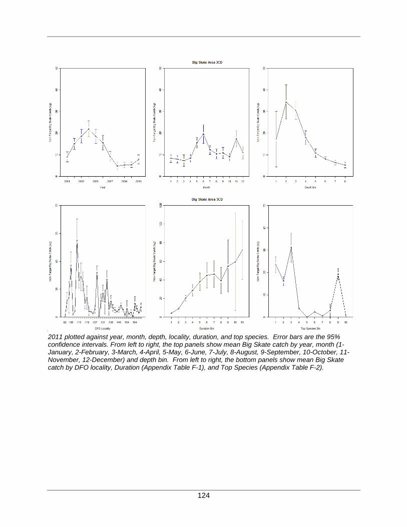
124

Appendix Figure F-2. Mean non-targeted Big Skate catch (kg) from rolled up trawl tows in 3CD in 2001 – 2011 plotted against year, month, depth, locality, duration, and top species. Error bars are the 95% confidence intervals. From left to right, the top panels show mean Big Skate catch by year, month (1-January, 2-February, 3-March, 4-April, 5-May, 6-June, 7-July, 8-August, 9-September, 10-October, 11-November, 12-December) and depth bin. From left to right, the bottom panels show mean Big Skate catch by DFO locality, Duration (Appendix Table F-1), and Top Species (Appendix Table F-2).

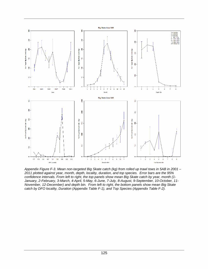
125

Appendix Figure F-3. Mean non-targeted Big Skate catch (kg) from rolled up trawl tows in 5AB in 2001 – 2011 plotted against year, month, depth, locality, duration, and top species. Error bars are the 95% confidence intervals. From left to right, the top panels show mean Big Skate catch by year, month (1-January, 2-February, 3-March, 4-April, 5-May, 6-June, 7-July, 8-August, 9-September, 10-October, 11-November, 12-December) and depth bin. From left to right, the bottom panels show mean Big Skate catch by DFO locality, Duration (Appendix Table F-1), and Top Species (Appendix Table F-2).

126

Appendix Figure F-4. Mean non-targeted Big Skate catch (kg) from rolled up trawl tows in 5CDE in 2001 – 2011 plotted against year, month, depth, locality, duration, and top species. Error bars are the 95% confidence intervals. From left to right, the top panels show mean Big Skate catch by year, month (1-January, 2-February, 3-March, 4-April, 5-May, 6-June, 7-July, 8-August, 9-September, 10-October, 11-November, 12-December) and depth bin. From left to right, the bottom panels show mean Big Skate catch by DFO locality, Duration (Appendix Table F-1), and Top Species (Appendix Table F-2).

127

Appendix Figure F-5. Plots of median non-targeted Longnose Skate total catch by year, month, depth, locality, duration, and top species in Skate Management Areas 3CD, 5AB, and 5CDE.

128

Appendix Figure F-6. Mean non-targeted Longnose Skate catch (kg) from rolled up trawl tows in 3CD in 2001 – 2011 plotted against year, month, depth, locality, duration, and top species. Error bars are the 95% confidence intervals. From left to right, the top panels show mean Big Skate catch by year, month (1-January, 2-February, 3-March, 4-April, 5-May, 6-June, 7-July, 8-August, 9-September, 10-October, 11-November, 12-December) and depth bin. From left to right, the bottom panels show mean Big Skate catch by DFO locality, Duration (Appendix Table F-1), and Top Species (Appendix Table F-2).

129

Appendix Figure F-7. Mean non-targeted Longnose Skate catch (kg) from rolled up trawl tows in 5AB in 2001 – 2011 plotted against year, month, depth, locality, duration, and top species. Error bars are the 95% confidence intervals. From left to right, the top panels show mean Big Skate catch by year, month (1-January, 2-February, 3-March, 4-April, 5-May, 6-June, 7-July, 8-August, 9-September, 10-October, 11-November, 12-December) and depth bin. From left to right, the bottom panels show mean Big Skate catch by DFO locality, Duration (Appendix Table F-1), and Top Species (Appendix Table F-2).

130

Appendix Figure F-8. Mean non-targeted Longnose Skate catch (kg) from rolled up trawl tows in 5CDE in 2001 – 2011 plotted against year, month, depth, locality, duration, and top species. Error bars are the 95% confidence intervals. From left to right, the top panels show mean Big Skate catch by year, month (1-January, 2-February, 3-March, 4-April, 5-May, 6-June, 7-July, 8-August, 9-September, 10-October, 11-November, 12-December) and depth bin. From left to right, the bottom panels show mean Big Skate catch by DFO locality, Duration (Appendix Table F-1), and Top Species (Appendix Table F-2).

131

Appendix Figure F-9. (A) Observed mean catch in 2001 – 2011 and predicted mean catch using the four-variable two-step GLM method and (B) mean reconstructed catch for 1954 – 1995 for Big Skate in 3CD.

132

Appendix Figure F-10. (A) Observed mean catch in 2001 – 2011 and predicted mean catch using the four-variable two-step GLM method and (B) mean reconstructed catch for 1954 – 1995 for Big Skate in 5AB.

133

Appendix Figure F-11. (A) Observed mean catch in 2001 – 2011 and predicted mean catch using the four-variable two-step GLM method and (B) mean reconstructed catch for 1954 – 1995 for Big Skate in 5CDE.

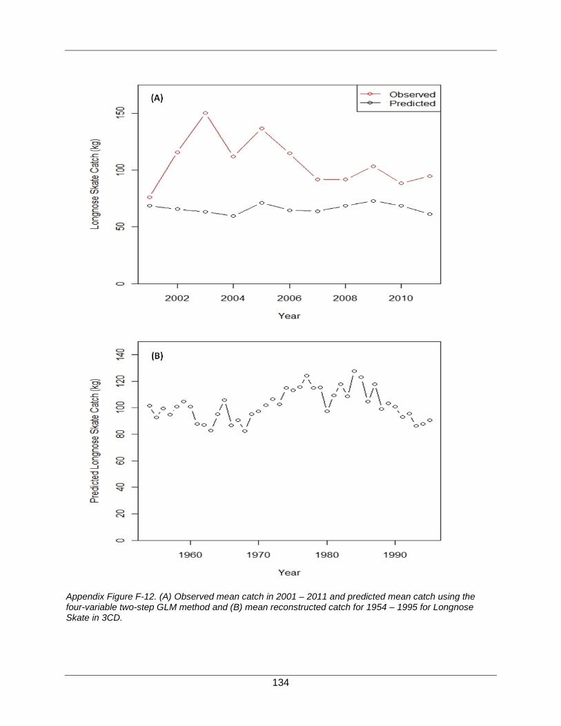
134

Appendix Figure F-12. (A) Observed mean catch in 2001 – 2011 and predicted mean catch using the four-variable two-step GLM method and (B) mean reconstructed catch for 1954 – 1995 for Longnose Skate in 3CD.

135

Appendix Figure F-13. (A) Observed mean catch in 2001 – 2011 and predicted mean catch using the four-variable two-step GLM method and (B) mean reconstructed catch for 1954 – 1995 for Longnose Skate in 5AB.

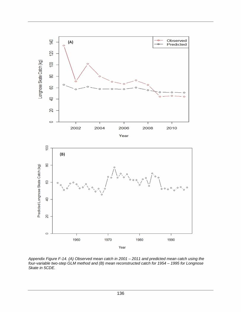
136

Appendix Figure F-14. (A) Observed mean catch in 2001 – 2011 and predicted mean catch using the four-variable two-step GLM method and (B) mean reconstructed catch for 1954 – 1995 for Longnose Skate in 5CDE.

137

Appendix Figure F-15. (A) Observed mean catch in 2001 – 2011 and predicted mean catch using the five-variable two-step GLM method and (B) mean reconstructed catch for 1954 – 1995 for Big Skate in 3CD.

138

Appendix Figure F-16. (A) Observed mean catch in 2001 – 2011 and predicted mean catch using the five-variable two-step GLM method and (B) mean reconstructed catch for 1954 – 1995 for Big Skate in 5AB.

139

Appendix Figure F-17. (A) Observed mean catch in 2001 – 2011 and predicted mean catch using the five-variable two-step GLM method and (B) mean reconstructed catch for 1954 – 1995 for Big Skate in 5CDE.

140

Appendix Figure F-18. (A) Observed mean catch in 2001 – 2011 and predicted mean catch using the five-variable two-step GLM method and (B) mean reconstructed catch for 1954 – 1995 for Longnose Skate in 3CD.

141

Appendix Figure F-19. (A) Observed mean catch in 2001 – 2011 and predicted mean catch using the five-variable two-step GLM method and (B) mean reconstructed catch for 1954 – 1995 for Longnose Skate in 5AB.

142

Appendix Figure F-20. (A) Observed mean catch in 2001 – 2011 and predicted mean catch using the five-variable two-step GLM method and (B) mean reconstructed catch for 1954 – 1995 for Longnose Skate in 5CDE.

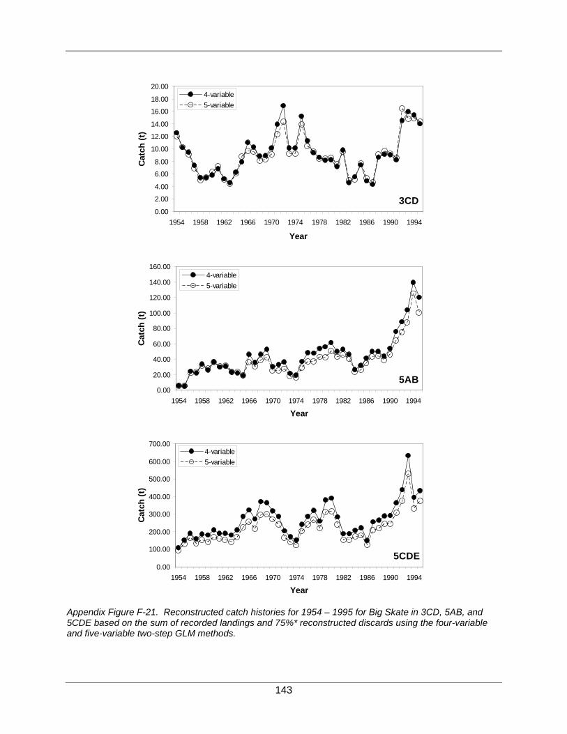
143

Appendix Figure F-21. Reconstructed catch histories for 1954 – 1995 for Big Skate in 3CD, 5AB, and 5CDE based on the sum of recorded landings and 75%* reconstructed discards using the four-variable and five-variable two-step GLM methods.

3CD0.00

2.00

4.00

6.00

8.00

10.00

12.00

14.00

16.00

18.00

20.00

1954 1958 1962 1966 1970 1974 1978 1982 1986 1990 1994

Year

Cat

ch (t

)

4-variable5-variable

5AB0.00

20.00

40.00

60.00

80.00

100.00

120.00

140.00

160.00

1954 1958 1962 1966 1970 1974 1978 1982 1986 1990 1994

Year

Cat

ch (t

)

4-variable5-variable

5CDE0.00

100.00

200.00

300.00

400.00

500.00

600.00

700.00

1954 1958 1962 1966 1970 1974 1978 1982 1986 1990 1994

Year

Cat

ch (t

)

4-variable5-variable

144

Appendix Figure F-22. Reconstructed catch histories for 1954 – 1995 for Longnose Skate in 3CD, 5AB, and 5CDE based on the sum of recorded landings and 75%* reconstructed discards using the four-variable and five-variable two-step GLM methods.

3CD0.00

10.00

20.00

30.00

40.00

50.00

60.00

70.00

80.00

90.00

100.00

1954 1958 1962 1966 1970 1974 1978 1982 1986 1990 1994

Year

Cat

ch (t

)

4-variable5-variable

5AB0.00

5.00

10.00

15.00

20.00

25.00

30.00

35.00

40.00

1954 1958 1962 1966 1970 1974 1978 1982 1986 1990 1994

Year

Cat

ch (t

)

4-variable5-variable

5CDE0.00

5.00

10.00

15.00

20.00

25.00

30.00

35.00

40.00

45.00

50.00

1954 1958 1962 1966 1970 1974 1978 1982 1986 1990 1994

Year

Cat

ch (t

)

4-variable5-variable

145

STANDARDIZATION OF COMMERCIAL TRAWL CPUE APPENDIX G.(Case Study: Big Skate in 5CDE)

G.1 INTRODUCTION Commercial catch and effort data can be used to generate indices of annual abundance in several ways. Such indices can be derived from the arithmetic mean or geometric mean of catch divided by appropriate effort (Catch Per Unit Effort or CPUE), but these indices assume that changes in annual CPUE reflect changes in the underlying fish stock, rather than changes in the fishery over the assessed period. Such an assumption frequently fails because changes in fisheries over time can have a considerable effect on the resulting CPUE. Consequently, methods to standardize for changes to vessel configuration, the timing or location of catch and other possible effects have been developed to remove potential biases to CPUE that result from such changes. In these models, abundance is represented as a “year effect” and the dependent variable is either an explicitly calculated CPUE represented as catch divided by effort, or an implicit CPUE represented as catch per tow or catch per record. In the latter case, an effort term is usually offered as an explanatory variable, allowing the model to select the effort term with the greatest explanatory power. It is always preferable to standardize for as many factors as possible when using CPUE as a proxy for abundance.

G.2 METHODS

G.2.1 Arithmetic and Unstandardized CPUE Arithmetic and unstandardized CPUE indices provide measures of how much the standardization procedure has modified the series from these two sets of indices, but do not take into account any changes in the fishery.

Arithmetic CPUE in year y was calculated as the total catch for the year divided by the total effort in the year using Eq. 1:

(1)

where Ci,y is the [catch], Ei,y= Ti,y ([tows]) or Ei,y= Hi,y ([hours_fished]) for record i in year y, and ny is the number of records in year y.

Unstandardized (geometric) CPUE assumes a log-normal error distribution. An unstandardised index of CPUE in year y was calculated as the geometric mean of the ratio of catch to effort for each record i in year y using Eq. 2:

(2)

where , and are as defined for Eq. 1

( )ˆyA

,1

,1

ˆ

y

y

n

i yi

y n

i yi

CA

E

=

=

=∑

∑

( )ˆyG

,

,1

lnˆ exp

yni y

i yiy

y

CE

Gn

=

=

∑

iC ,i yE yn

146

G.2.2 Standardized CPUE These models are preferred over the unstandardized models described above because they account for changes in fishing behaviour and other factors which may affect the estimated abundance trend. In the models described below, catch per record is used as the dependent variable and the associated effort is treated as an explanatory variable.

G.2.2.1 Lognormal Model Standardized CPUE assumes the same lognormal error distribution as the unstandarized (geometric) CPUE index, but uses explanatory variables to represent changes in the fishery. A standardized CPUE index (Eq. 3) is calculated from a generalised linear model (GLM) (Quinn and Deriso 1999) using a range of explanatory variables including [year], [month], [depth], [vessel] and other available factors:

(3)

where = (where [tow]) for the ith record is the intercept; is the year

coefficient for the year corresponding to the ith record; and are the coefficients for

factorial variables a and b corresponding to the ith record; and are polynomial functions (to the 3rd order) of the continuous variables and corresponding to the ith record; and is an error term.

The actual number of factorial and continuous explanatory variables in each model depends on the model selection criteria. Because each record represents a single tow, and always equal 1.

Note that calculating standardized CPUE with Eq. 3 without additional explanatory variables is equivalent to using Eq. 2, provided the same definition for is used.

Canonical coefficients and standard errors were calculated for each categorical variable (Francis 1999). Standardized analyses typically set one of the coefficients to 1.0 without an error term and estimate the remaining coefficients and the associated error relative to the fixed coefficient. This is required because of parameter confounding. The Francis (1999) procedure rescales all coefficients so that the geometric mean of the coefficients is equal to 1.0 and calculates a standard error for each coefficient, including the fixed coefficient.

Coefficient-distribution-influence plots (CDI plots) are visual tools to facilitate understanding of patterns which may exist in the combination of coefficient values, distributional changes, and annual influence (Bentley et al. 2012). CDI plots were used to illustrate each explanatory variable added to the model.

G.2.2.2 Binomial Logit Model The procedure described by Eq. 3 is necessarily confined to the positive catch observations in the data set because the logarithm of zero is undefined. Observations with zero catch were modelled by fitting a linear regression model based on a binomial distribution and using the presence/absence of skate as the dependent variable (where 1 is substituted for in Eq. 3 if it is a successful catch record and 0 if it is not successful), using the same data set. Explanatory factors are estimated in the model in the same manner as described in Eq. 3. Such a model provides an alternative series of standardized coefficients of relative annual changes that is analogous to the equivalent series estimated from the lognormal regression.

( ) ( )ln( ) + ..... ....i i ii y a b i i iI B Y f fα β χ δ ε= + + + + + +

iI i iC E i iE T= BiyY

iaα ibβ

( )if χ ( )if δ

iχ iδ

iε

iT iE

,i yE

ln( )iI

147

G.2.2.3 Combined Model A combined model, integrating the two sets of relative annual changes estimated by the lognormal and binomial models, can be estimated using the delta distribution, which allows zero and positive observations (Vignaux 1994). Such a model provides a single index of abundance which integrates the signals from the positive (lognormal) and binomial series. This approach uses the following equation to calculate an index based on the two contributing indices:

(4)

where = combined index for year y, = lognormal index for year I, = binomial index

for year I = proportion zero for base year 0.

Francis (2001) suggests that a bootstrap procedure is the appropriate way to estimate the variability of the combined index. Therefore, confidence bounds for the combined model were estimated using a bootstrap procedure based on 1000 replicates, drawn with replacement.

G.3 PRELIMINARY INSPECTION OF THE DATA Tow-by-tow catch and effort data for Big Skate from the BC bottom trawl fishery were gathered from 1996 to 2011 for Skate Management Area 5CDE, the areas of Hecate Strait, Dixon Entrance and the west coast of Haida Gwaii, using data from the DFO PacHarvTrawl and GFFOS databases (Fisheries and Oceans Canada, Pacific Region, Groundfish Data Unit) (Appendix Table G-1). Each record represents a single tow, which results in equivalency between the number of records and number of tows. Catch per record can therefore be used to represent CPUE, because each record (tow) has an implicit effort component.

The depth distribution of the majority of successful catch records data ranged from about 40 m to 215 m, with a long right-hand tail of sporadic observations at deeper depths up to over 900 m (Appendix Figure G-1). It is possible that the deeper recorded depths are in error or document tows that passed through a wide range of depths. Valid tows were binned by depth in 25 m increments, between 15 and 215 m,.

There were a total of 82 trawl vessels in the 5CDE data set which recorded a catch of Big Skate at least once. Vessel qualification criteria based on number of trips per year, number of years fishing, and number of positive Big Skate catch tows were developed to avoid including vessels which only occaisionally fished in 5CDE, or which did not actively fish Big Skate (Appendix Figure G-2). Qualified vessels were those which had fished at least three trips for a minimum of three years, with at least 50 positive Big Skate catch tows. Once a vessel was selected, all data for the qualifying vessel were included, regardless of the number of trips in a year.

The analysis was based on a core fleet of 28 qualified vessels, responsible for 84% of the total catch. The vessel overlap across years was good, with a considerable number of vessels operating across most of the available 16 years of data (Appendix Figure G-3). Only tows which were less than 6 hours long were used in the analysis. This did not drop much data because over 99% of the tows were less than 5 hour in length.

011 1

LyC

y

By

YY

P Y

= − −

C

yY LyY B

yY

0P

148

G.4 RESULTS

G.4.1 Arithmetic and Unstandardized CPUE Arithmetic and unstandardized CPUE indices were calculated using Eqs. 1 and 2. Number of positive tows (records) was used as the effort component in Eq. 1 and each record is a single tow when using Eq. 2. The resultant indices were scaled such that the geometric mean of each series was 1.0 (Appendix Table G-2, Appendix Figure G-4).

G.4.2 Lognormal Positive Model A standardized lognormal General Linnear Model (GLM) analysis was performed on positive catch records by offering eight explanatory variables to the model and using ln(catch) as the dependent variable, where catch is the total by weight of landed plus discarded skate in each record (tow) (Eq. 3). The resulting CPUE index is presented in Appendix Table G-2 and Appendix Figure G-4.

Variables were offered sequentially, beginning with the year categorical variable, until the improvement in the model R2 was less than 1% (Appendix Table G-3). Hours fished was offered as continuous variable modelled as a 3rd order polynomial. This model selected 6 of the 8 available explanatory variables, including DFO locality (21 categories), Hours fished (continuous), Depth band (8 categories), Month (12 categories), and Vessel (28 categories) as explanatory variables, in addition to Year, in the final lognormal model, accounting for 26% of the total model variation (Appendix Table G-3). The year variable explained 1.4% of the total model deviance.

Model residuals appeared to be consistent with the underlying lognormal distributional assumption, with some deviation near the peak of the distribution and at the two tails (Appendix Figure G-5).

A stepwise plot of the year indices as each explanatory variable was introduced into the model shows relatively little impact from the standardization procedure (Appendix Figure G-6).

CDI plots of the five explanatory variables introduced to the model in addition to Year show some overall trends (

Appendix Figure G-7 to Appendix Figure G-9). For instance, there appears to have been a shift toward the “Two Peaks” locality in recent years, the DFO locality with the highest catch rate (

Appendix Figure G-7). Similarly, there has been some recent seasonal shifts to months with lower catch rates (Appendix Figure G-8) and a surprising withdrawal of the vessels with the highest catch rates since the mid-2000s (Appendix Figure G-9).

The plot of the year indices shows a gradual decreasing trend to 2009, but the most recent two years have recovered to near the mean of the series (about 300 kg/h; Appendix Table G-2, Appendix Figure G-4).

G.4.3 Binomial Logit Model The same variables used in the lognormal model were offered sequentially to this model, beginning with the year categorical variable, until the improvement in the model R2 was less than 1%. The model produced a variable set of year indices with a dissimilar trend to the trend estimated by the lognormal model (Appendix Figure G-10). The index might affected by the very high proportion of zero tows in 1996 and there is a slight declining trend in the proportion of zero tows in the years following 1996 (Appendix Table G-1, Appendix Figure G-10).

149

G.4.4 Combined Model Appendix Figure G-11 shows that the effect of adding the binomial series to the lognormal series to produce a combined series is relatively small because the resulting series more closely resembles the lognormal series. An exception is 1996, where the combined index resembles the binomial index due to the very high proportion of zero tows in that year. All three sets of indices appear to converge after 1999.

G.4.5 Comparison with Survey Index A comparison of two GLM indices (combined and lognormal) with the scaled biomass indices from the Hecate Strait synoptic survey (Olsen et al. 2009; Unpublished data queries. DFO Pacific Region, Groundfish Data Unit, Nanaimo, BC) shows reasonable agreement between all three series over the four overlapping years (Appendix Figure G-12). The strong drop by all indices in 2009 may be due to some change in the availability of Big Skate in that year, given the strong and rapid recovery seen in the following two years.

G.5 REFERENCES Bentley, N., Kendrick, T. H., Starr, P. J., and Breen, P. A. 2012. Influence plots and metrics:

tools for better understanding fisheries catch-per-unit-effort standardizations. ICES Journal of Marine Science, 69: 84–88.

Francis, R.I.C.C. 1999. The impact of correlations on standardised CPUE indices. New Zealand Fishery Assessment Research Document 1999/42. 30 p. (Unpublished report held in NIWA library, Wellington, New Zealand)

Francis, R.I.C.C. 2001. Orange roughy CPUE on the South and East Chatham Rise. New Zealand Fishery Assessment Report 2001/26. 30 p.

Olsen, N., Rutherford, K.L., Stanley, R.D., and Wyeth, M.R. 2009. Hecate Strait groundfish bottom trawl survey, May 26th to June 21st, 2009. Can. Manuscr. Rep. Fish. Aquat. Sci. 2901: vi + 49 p.

Quinn, T.R. and R.B. Deriso. 1999. Quantitative Fish Dynamics. Oxford University Press. 542 p.

Vignaux, M. 1994. Catch per unit effort (CPUE) analysis of west coast South Island and Cook Strait spawning hoki fisheries, 1987–93. N.Z. Fish. Assess. Res. Doc. 94/11.

150

Appendix Table G-1. Summary data for the Big Skate fishery in 5CDE by year for the core data set (after selection of core vessels and applying all filters).

Year Number vessels

Number trips

Number tows

% zero tows

Total catch (t)

Total hours

CPUE (kg/h) (Eq. 1)

1996 23 171 1,921 73.1 179.3 3,879 46.2 1997 24 225 2,753 45.4 821.2 5,682 144.5 1998 22 248 3,586 45.7 479.7 7,758 61.8 1999 24 294 3,884 39.3 666.4 8,375 79.6 2000 23 290 3,850 37.7 633.9 7,954 79.7 2001 25 248 2,613 38.6 468.8 5,263 89.1 2002 24 251 2,947 34.5 454.0 5,349 84.9 2003 22 212 2,377 31.8 557.5 4,258 130.9 2004 20 226 2,605 33.9 624.4 4,676 133.5 2005 19 284 2,804 37.8 476.1 4,743 100.4 2006 16 186 2,080 31.7 386.3 3,904 98.9 2007 16 163 1,827 29.8 406.7 3,449 117.9 2008 14 168 1,674 35.9 309.9 3,207 96.6 2009 16 183 1,988 39.2 245.4 3,878 63.3 2010 14 170 1,782 31.4 428.1 3,411 125.5 2011 14 198 2,169 25.6 582.0 3,979 146.3

151

Appendix Table G-2. Relative indices of annual CPUE from the arithmetic, unstandardized, lognormal, binomial, and combined models of non-zero catches of Big Skate in 5CDE . All indices are scaled so that their geometric means equal 1.0. Upper and lower 95% confidence bounds and associated standard error (SE) are presented for the lognormal model, while bootstrapped upper and lower 95% confidence bounds are presented for the combined model.

Year Arithmetic Index

Unstandardized Index

Lognormal Binomial Index

Combined Index Lower bound Upper bound SE Index Lower bound Upper bound

1996 1.142 1.133 1.426 1.285 1.583 0.053 0.195 0.604 0.527 0.691 1997 1.801 1.237 1.377 1.289 1.471 0.034 0.672 1.213 1.120 1.306 1998 0.811 0.915 0.963 0.909 1.021 0.030 0.670 0.848 0.798 0.912 1999 0.931 0.851 0.868 0.824 0.915 0.027 0.953 0.880 0.826 0.937 2000 0.870 0.945 0.978 0.930 1.029 0.026 0.985 1.003 0.948 1.061 2001 0.963 1.092 0.978 0.921 1.038 0.031 0.969 0.996 0.929 1.063 2002 0.774 0.871 0.843 0.798 0.890 0.028 1.100 0.896 0.845 0.950 2003 1.133 1.075 1.220 1.149 1.295 0.030 1.407 1.396 1.301 1.490 2004 1.195 1.325 1.257 1.186 1.332 0.030 1.325 1.415 1.329 1.498 2005 0.899 0.964 1.023 0.965 1.085 0.030 1.071 1.079 1.009 1.147 2006 0.896 1.155 1.207 1.133 1.286 0.032 1.531 1.413 1.321 1.511 2007 1.044 1.156 1.109 1.038 1.184 0.034 1.818 1.353 1.263 1.446 2008 0.951 0.767 0.718 0.668 0.772 0.037 1.199 0.785 0.729 0.849 2009 0.669 0.658 0.554 0.518 0.593 0.035 0.855 0.539 0.499 0.582 2010 1.154 1.083 0.975 0.911 1.044 0.035 1.355 1.105 1.019 1.186 2011 1.188 1.017 0.927 0.873 0.984 0.031 1.476 1.075 1.010 1.140

152

Appendix Table G-3. Order of acceptance of variables into the lognormal model of positive total mortalities (verified landings plus discards) of Big Skate by core vessels in 5CDE (based on the vessel selection criteria of at least three trips in three or more years plus 50 positive catch records for Big Skate) with the amount of explained deviance (R2) for each variable. Variables accepted into the model are marked with an *. Year was forced as the first variable.

Variable 1 2 3 4 5 6 7 Year* 0.014 - - - - - - DFO locality* 0.106 0.124 - - - - - Hours fished* 0.012 0.027 0.175 - - - - Depth bands* 0.092 0.109 0.163 0.212 - - - Month* 0.069 0.086 0.174 0.208 0.241 - Vessel* 0.040 0.053 0.162 0.199 0.237 0.258 - 0.1° Latitude bands 0.094 0.111 0.137 0.189 0.221 0.248 0.265 Major PMFC area 0.010 0.025 0.127 0.176 0.214 0.242 0.259 Improvement in deviance 0.000 0.110 0.051 0.038 0.028 0.018 0.007

Appendix Table G-4. DFO localities with associated estimated standardized index of relative catch rate (see upper left graph,Appendix Figure G-9). Remaining localities were put into a “plus” group (not reported here) because there were too few positive records to reliably estimate the relative catch rate. The mean Big Skate catch rate of this series, including the “Plus” group, is 1.0

Major Area

Minor Area Minor Area Name Locality

Code Locality Name Index

5C

2 2B-East 209 West Horseshoe 1.439 210 Ole Spot 1.184 214 Cumshewa/Reef Is. Flats 0.777

6 5-Lower-SE Hecate Strait 220 North Moresby 0.651 221 South Bonilla 0.718 229 East Horseshoe 1.339

5D

1 2A-East- Skidegate 236 Unknown 1.145 241 West Two Peaks 1.444

3 1 East-Dixon Entrance 243 Mcintyre Bay 0.771 244 West Masset 0.962 245 NE Langara 0.457

4 4-Two Peaks-Dundas Is. 250 Butterworth 2.616

5 White Rocks

251 Two Peaks 1.927 254 Dundas 1.297 260 S Of Barren Island 1.616 263 White Rocks 0.838 264 Bonilla 0.871 265 Shell Ground 1.038 266 Venus 0.540

153

Appendix Figure G-1. Depth distribution of Big Skate for tows with landed plus discarded catch in Areas 5CDE from 1996 to 2011 in 25 m intervals. Each bin interval is labelled with the upper bound of the interval. Vertical lines indicate the following quantiles: 1%=29 m; 99%=560 m. Mean depth=104 m; median depth=85 m.

154

Appendix Figure G-2. Plots showing the relationship of number of trawl vessels [left panel] or percentage of total Big Skate catch [right panel] with the number of trips per year and the number of years in the fishery for Areas 5CDE from 1996 to 2011. Each plotted point relates the number of years vessels participated in the fishery having recorded at least the indicated minimum number of trips per year.

155

Appendix Figure G-3. Bubble plot showing vessel participation (number tows) by the core fleet by year.

156

Appendix Figure G-4. Three CPUE series for Big Skate from 1996 to 2011 in 5CDE. The solid line is the standardized CPUE series from the lognormal model (Eq. 3). The arithmetic series (Eq. 1) is the sum of the annual non-zero catch (landings plus discards) and the unstandardized series (Eq. 2) is the geometric mean of all positive catch observations. All three series have a geometric mean equal to 1.0.

157

Appendix Figure G-5. Residual diagnostic plots for the GLM lognormal analysis for Big Skate in 5CDE. Upper left: histogram of the standardized residuals with overlaid lognormal distribution (SDNR = standard deviation of normalised residuals. MASR = median of absolute standardized residuals). Lower left: Q-Q plot of the standardized residuals with the outside horizontal and vertical lines representing the 5th and 95th percentiles of the theoretical and observed distributions. Upper right: standardized residuals plotted against the predicted CPUE. Lower right: observed CPUE plotted against the predicted CPUE.

158

Appendix Figure G-6. Plot showing the year coefficients after adding each successive term of the standardized lognormal regression analysis for Big Skate in 5CDE. The final model is shown with a thick solid black line. Each line has been scaled so that the geometric mean equals 1.0.

159

Appendix Figure G-7. CDI plots showing the effect of introducing the categorical variables DFO locality and Hours fishing to the lognormal regression model for Big Skate in 5CDE. Each plot consists of subplots showing the effect by level of variable (top left), the distribution of variable records by year (bottom left), and the cumulative effect of variable by year (bottom right).

160

Appendix Figure G-8. CDI plots showing the effect of introducing the categorical variables Depth bands and Month to the lognormal regression model for Big Skate in 5CDE. Each plot consists of subplots showing the effect by level of variable (top left), the distribution of variable records by year (bottom left), and the cumulative effect of variable by year (bottom right).

161

Appendix Figure G-9. CDI plot showing the effect of introducting the categorical variable Vessel to the lognormal regression model for Big Skate in 5CDE. Each plot consists of subplots showing the effect by level of variable (top left), the distribution of variable records by year (bottom left), and the cumulative effect of variable by year (bottom right).

162

Appendix Figure G-10. Year effects from a standardized binomial logit model fit to the presence/absence of Big Skate in the 5CDE trawl fishery, using the same dataset that provided the lognormal regression model. Also shown is the relative proportion of tows with zero Big Skate by year (mean=0.62). Each series has been normalized so that the geometric mean=1.0.

163

Appendix Figure G-11. Combined, lognormal and binomial models for Big Skate in 5CDE, based on commercial trawl catch and effort data. The error bars for the combined model were estimated by a bootstrap procedure replicated 1000 times with replacement.

Appendix Figure G-12. Comparison of the combined and lognormal GLM models for Big Skate in 5CDE with scaled biomass indices for Big Skate from the Hecate Strait synoptic survey (Olsen et al. 2009; Unpublished data queries. DFO Pacific Region, Groundfish Data Unit, Nanaimo, BC). The error bars for the survey data points were estimated by a bootstrap procedure replicated 1000 times with replacement.

164

RESEARCH SURVEYS APPENDIX H.

H.1 AVAILABLE DATA

H.1.1 Trawl Surveys There are a number of research trawl surveys in British Columbia waters with potential for providing information about trends in relative abundance of Big Skate and Longnose Skate (Appendix Table H-1). Survey data was analysed for Skate Management Area 3CD from 1980 to 2011, for Skate Management Area 5AB from 2003 – 2011, and for Skate Management Area 5CDE from 1985 – 2011 (Appendix Table H-1). The United States National Marine Fisheries Service (NMFS) operated a triennial survey that included waters off the west coast of Vancouver Island (approximating Major Area 3C) in 1980, 1983, 1989, 1992, 1995, 1998, and 2001. Fisheries and Oceans Canada conducted a Multipspecies Assemblage Survey in Hecate Strait in 1984 – 2003, shrimp surveys off the west coast of Vancouver Island and in Queen Charlotte Sound in 2003 – 2011, and synoptic surveys covering the West Coast of Vancouver Island, Queen Charlotte Sound, Hecate Strait, and West Coast Haida Gwaii in 2003 – 2011. Historic surveys in Queen Charlotte Sound and shrimp surveys prior to 2003 were not included in the analysis, because skates which were captured during these surveys were not identified to species. The skate tagging surveys which occurred in 2004 – 2006 in Hecate Strait and Queen Charlotte Sound and off the west coast of Vancouver Island in 2008 were not included because those surveys were designed to optimize the amount of big skate encountered for tagging and as such do not provide relative indices of abundance. A Pacific Cod monitoring survey which operated in 2002 – 2004 in Hecate Strait was not included because the time series was short, few skate were captured, and the area surveyed represented only a small portion of Hecate Strait. Additional surveys which represented very short time series, stand-alone surveys, and/or surveys which captured few skate were also not used.

Data for Fisheries and Oceans Canada surveys is available in the GFBio Database (Fisheries and Oceans Canada, Pacific Region, Groundfish Data Unit). Tow-by-tow data from the United States National Marine Fisheries Service (NMFS) Triennial Survey were provided by Mark Wilkins (NMFS) for the seven years that the survey worked in BC waters.

H.1.2 Line Surveys There are three research longline surveys in British Columbia waters with potential for providing information about Big Skate and Longnose Skate (Appendix Table H-1). Surveys included the British Columbia portion of the International Pacific Halibut Commission (IPHC) Standardized Assessment Survey in 2003 – 2011 which operated annually in 2003 – 2011 in Skate Management Areas 3CD, 5AB, and 5CDE; the Pacific Halibut Management Association of British Columbia (PHMA) survey which operated in annually in 2006 – 2011, with even years in Skate Management Area 5CDE and odd years in Skate Management Areas 3CD and 5AB; and the Fisheries and Oceans Canada Inshore Rockfish Longline Survey which operated in Skate Management Areas 3CD (Major Area 4B, Minor Areas 19 and 20) and 4B (Major Area 4B, Minor Areas 14 – 18, 28 – 29) in 2005, 2009, and 2011, and in Skate Management Areas 5AB (Major Area 5A, Minor Area 11 and Major Area 4B, Minor Area 12) and 4B (Major Area 4B, Minor Area 13) in 2003, 2004, 2007, 2008, and 2010 (Appendix Table H-1). IPHC surveys prior to 2003 were not utilized, because species other than halibut were not enumerated for all hooks.

Data for all three surveys are available in the GFBio Database (Fisheries and Oceans Canada, Pacific Region, Groundfish Data Unit).

165

H.1.3 Biological Data Biological data (total length, sex, round weight) has been collected from Big Skate and Longnose Skate captured during many Fisheries and Oceans Canada research surveys in British Columbia. These data are are available in the GFBio Database (Fisheries and Oceans Canada, Pacific Region, Groundfish Data Unit).

H.2 METHODS

H.2.1 Analytical Methods H.2.1.1 Trawl Biomass Index Calculations For all research trawl surveys described below, a biomass index was constructed from the annual swept area biomass estimates for each survey, following the methods developed for the Groundfish Trawl Synoptic Surveys (Stanley et al. 2004). These methods can been applied to other trawl surveys (e.g. King et al. 2012) which either follow a stratified random design, or which can be post-stratified, to obtain biomass indices which may be informative for a species of interest. To compute the biomass estimates, R-source code was adapted from code provided by Norm Olsen (Fisheries and Oceans Canada, 3190 Hammond Bay Road, Nanaimo, BC V9T 6N7; Appendix L).

Annual swept area biomass estimates were determined as the catch rate per swept area, expanded by the total area in each stratum.

CPUE Density Catch and effort data for stratum i in year y yield catch per unit of effort (CPUE) values, Uyi. Given a set of data {Cyij, Eyij} for tows j = 1, …., nyi,

(1) ∑=

=yin

j yij

yij

yiyi E

Cn

U1

1,

where Cyij is the catch (kg) in tow j, stratum i, year y; Eyij is the effort (hours) in tow j, stratum i, year y; and nyi is the number of tows in stratum i, year y.

CPUE values (Uyi) convert to CPUE densities yiδ (kg/m2) using

(2) yiyi Uvw1

=δ ,

where v is the average vessel speed (km/hour) and w is the average door spread (km).

Alternatively, if vessel information exists for every tow, CPUE density can be expressed directly as

(3) ∑=

=yin

j yijyij

yij

yiyi wD

Cn 1

1δ

where Cyij is the catch (kg) in tow j, stratum i, year y; Dyij is the distance travelled (km) for tow j, stratum i, year y; wyij is the net width or door spread (km) for tow j, stratum i, year y; and nyi is the number of tows in stratum i, year y. Dyij wyij is the swept area for tow j, stratum i, year y.

The biomass estimation procedure used equation 3. When the distance travelled (Dyij) was not available, the code estimated the distance travelled as the product of the difference between

166

start and end of bottom contact time (tow duration) and the tow speed. When bottom contact times were not available, end of gear deployment and beginning of gear retrieval were used. When net width or door spread (wyij) was not available, the mean doorspread for the survey was used.

Annual Biomass Estimate The annual biomass estimate (By) is the sum of the product of CPUE densities and the area of each stratum across m strata:

(4) ∑ ∑= =

==m

i

m

iyiiyiy BAB

1 1

δ ,

where yiδ is the mean CPUE density (kg/m2) for stratum i, year y; Ai is the area (m2) of stratum i; Byi is the biomass (kg) for stratum i, year y; and m is the number of strata.

Error Distribution The variance of the survey biomass estimate (Vy) is given by

(5) ∑ ∑= =

==m

i

m

iyin

Ay VV

yi

iyi

1 1

22σ ,

where 2

yiσ is the variance of CPUE density (k2/km4) for stratum i, year y; and Vyi is the variance of the biomass estimate (kg2) for for stratum i, year y.

The coefficient of variation (CVy) of the annual biomass estimates (By) is given by

(6) y

yy B

VCV = .

Bootstrapping was used to estimate the uncertainty of the biomass estimates. One thousand bootstrap replicates with replacement were made on the survey data to provide bias corrected (Efron 1982) estimates of CV and 95% confidence regions.

Survey Precision The CV of the biomass estimates incorporates the variation in catch rate and provides a measure of relative error for each biomass estimate. Stanley et al. (2004) suggested that the relative error, or CV, could be used as a measure of precision for biomass estimates, and classified the utility of a survey for indexing a species’ abundance as excellent (<0.2), good (0.2-0.3), adequate (0.3-0.4), poor (0.4-0.6) and very poor (>0.6). We used a mean CV criterion of <0.4 (adequate) as a selection threshold for surveys that adequately indexed either Big skate or Longnose skate biomass.

H.2.1.2 Line CPUE Index Calculations Catch Rate For the longline surveys described below, relative abundance indices were calculated for Big Skate and Longnose Skate using the annual mean catch per unit of effort (CPUE) in each Skate Management Area for each survey. CPUE was calculated as pieces per 100 hooks and sets with zero skate catch were included. This differs from Flemming et al. (2012) who used median positive CPUE as a relative abundance index for IPHC surveys. The unit of effort was hooks rather than "skates" (strings of longline gear) to remove the effect of differences in string length between years and surveys (Flemming et al. 2012).

167

For each Skate Management Area and survey, CPUE (Uy) was calculated similarly to Equation 1 as follows:

(7) 10011

×= ∑=

yin

i yi

yi

yiy H

Cn

U ,

where Cyi is the catch (pieces) in tow i, year y; Hyi is the number of normal condition hooks in tow i, year y; and ny is the number of tows in year y.

One thousand bootstrap replicates with replacement were made on the annual CPUE data to provide bias corrected (Efron 1982) estimates of CV and 95% confidence regions.

Survey Precision The CV of the mean catch rate provides a measure of relative error for each estimate. As with the trawl surveys, a target precision of 0.2 was used to assess the usability of a survey to provide relative catch rate estimates for that species.

H.2.2 Trend Analyses Only surveys with a mean CV less than 0.4 were considered adequate for indexing either Big skate or Longnose skate abundance. For these selected surveys, trend analyses (on either mean trawl biomass or mean longline catch rates) were conducted using the trend function in the PBStools package (v1.24.20) of R. The function uses the methods of Schnute et al. (2004) to fit a trend line through the annual mean values, and produces estimates of the annual rate of change (r) and the total change (R) over the time series.

The annual mean values are transformed to a logarithmic scale as follows:

(8) ii XY 2log= ,

where Xi is the annual mean value (relative index), for year i, and Yi is the transformed value. Schnute et al. (2004) note that using the binary log transforms relative change to a convenient linear scale. A linear regression through the transformed data points gives a slope estimate b that provides a summary statistic for the entire series of I observations that represents the annual logarithmic growth rate (Schnute et al. 2004). The parameter b also defines the annual relative growth rate, r, and the accumulated relative change for the series, RI (Schnute et al. 2004):

(9) i

iib

XXXr −

=−= +112 and

(10) I

IIbI X

XXR 1)1( 12 −=−= − ,

during a time series of I observations.

The PBStools package provided bootstrapped estimates of r and slope of the trend line (b) which were assessed to determine if either were significantly different than zero, where different from zero indicates a trend.

168

H.2.3 Survey Methods H.2.3.1 NMFS Triennial Trawl Survey (3C) Tow-by-tow data from the United States National Marine Fisheries Service (NMFS) Triennial Survey were provided by Mark Wilkins (NMFS) for the seven years (1980, 1983, 1989, 1992, 1995, 1998, and 2001) that the survey worked in BC waters. The Canadian portion of the NMFS Triennial Survey covered the International Pacific Fisheries Commission (INPFC) area "Vancouver" which is approximately equivalent to Major Area 3C, and covered a number of area and depth strata. Strata that were not surveyed consistently in all seven years of the survey were dropped from the analysis. Depth strata retained for the analysis included 55 – 183 m, 184 – 219 m, and 220 – 366 m. In addition, strata used in the 1980 and 1983 surveys covered a smaller area than in subsequent surveys, so the 1980 and 1983 indices were scaled upwards by the ratio of total stratum areas relative to the area covered in 1989 and later surveys. A detailed description of the geographic area, stratum definitions, and tow locations for each year of the survey, as well as the methods by which tows were designated as usable for these analyses is provided in King et al. (2012). Tow locations for each year of the survey are illustrated in Appendix Figure H-1 and Appendix Figure H-2.

When calculating the variance for this survey, it was assumed that the variance and CPUE within any stratum was equal, even for strata that were split by the presence of the US/Canada border. The total biomass (Byi) within a stratum which straddled the border was split between the two countries by the ratio of the relative area within each country. The variance for that part of stratum i within each country was calculated as being in proportion to the ratio of the square of the area within each country relative to the total area of stratum i. The partial variance the Canadian portion of a stratum was used instead of the total variance in the stratum when calculating the variance for the total biomass in Canadian waters.

H.2.3.2 WCVI Shrimp Trawl Survey (3CD) The west coast of Vancouver Island (WCVI) shrimp survey has occurred approximately annually from 1973 (Boutillier et al. 1999); however, skates were not identified to species until 2003. The survey area covered a portion of the west coast of Vancouver Island, extending from off Ucluelet at approximately 48.7 ° N to Nootka Island at approximately 49.6° N (Appendix Figure H-3). Biomass estimates are based on a post-stratification of this survey into two areal strata following the methodology of Starr et al. (2002) and King et al. (2012) in their reanalyses of the data from the same survey for Pacific cod and Lingcod. Surveyed depths in the two strata ranged from 93 – 170 m. Data analyses assumed that tow locations were selected randomly within a stratum relative to the biomass of Big Skate and Longnose Skate; this was not part of the original survey design. The original survey design used latitudinal transects and selected the stations randomly along the transect.

H.2.3.3 WCVI Synoptic Trawl Survey (3CD) The west coast Vancouver Island (WCVI) synoptic survey is part of a coastwide Groundfish synoptic trawl survey series, and has been conducted every even year from 2004 (e.g. Olsen et al. 2009a). The survey area covered the west coast of Vancouver Island from the mouth of Juan de Fuca Strait at approximately 48.2° N to north of Quatsino Sound at approximately 50.6° N (Appendix Figure H-4). The design includes a single areal stratum and four depth strata (50 – 125 m, 125 – 200 m, 200 – 330 m, 330 – 500 m). Tows are randomly distributed over the trawlable portion of each stratum with a sampling frequency proportional to the area of the stratum.

169

H.2.3.4 QCS Shrimp Trawl Survey (5AB) The Queen Charlotte Sound (QCS) shrimp survey has occurred annually from 1998 (Boutillier et al. 1999); however, skates were not identified to species until 2003. The survey area covered the eastern portion of Queen Charlotte Sound west of Calvert Island and Hunter Island, from approximately 51.3° to 52.1° N and 127.9° to 129.0° W (Appendix Figure H-5). Similar to the WCVI shrimp survey, biomass estimates are based on a post-stratification of this survey into two areal strata following the methodology of Starr et al. (2002) and King et al. (2012) in their reanalyses of the data from the same survey for Pacific cod and Lingcod. Surveyed depths in the two strata ranged from 111 – 230 m. Data analyses assumed that tow locations were selected randomly within a stratum relative to the biomass of Big Skate and Longnose Skate; this was not part of the original survey design. The original survey design used latitudinal transects and selected the stations randomly along the transect.

H.2.3.5 QCS Synoptic Trawl Survey (5AB) The Queen Charlotte Sound (QCS) synoptic survey is part of a coastwide Groundfish synoptic trawl survey series, and was conducted in 2003 and 2004, and every odd year from 2005 – 2011 (e.g. Olsen et al. 2009b). The survey area covered all of Queen Charlotte Sound and southern portion of Hecate Strait, from approximately 50.9° to 52.7° N and 127.9° to 131.5° W (Appendix Figure H-22). The design includes a two areal strata, each of which is divided into four depth strata (50 – 120 m, 120 – 250 m, 250 – 370 m, 370 – 500 m). Tows are randomly distributed over the trawlable portion of each stratum with a sampling frequency proportional to the area of the stratum.

H.2.3.6 Hecate Strait Multispecies Assemblage Trawl Survey (5CDE) The Hecate Strait (HS) Multispecies Assemblage survey was a series of multi-species grounfish surveys designed originally to map species assemblages in Hecate Strait. The survey was conducted in 1984, 1987, 1991, 1993, 1995, 1996, 1998, 2000, 2002, and 2003 (e.g. Choromanski et al. 2005). The survey area covered Hecate Strait from approximately 52.5° to 54.5° N, extending westerly into Dixon Entrance off Masset at approximately 132.2° W (Appendix Figure H-7). Biomass estimates are based on a post-stratification of this survey by depth stratum (10 fathom intervals from 10 – 130 fm), and assume that tow locatations were selected randomly within each stratum. However, the original survey design was depth stratified within a spatial grid, with each grid cell and depth interval representing a single stratum which contained one tow. Tow locations were not chosen randomly within the spatial grid; rather they were selected based on suitable bottom conditions.

H.2.3.7 Hecate Strait Synoptic Trawl Survey (5CDE) The Hecate Strait (HS) synoptic survey is part of a coastwide Groundfish synoptic trawl survey series, and was conducted every odd year from 2005 (e.g. Olsen et al. 2009c). The survey area covers Hecate Strait and Dixon Entrance from approximately 52.7° to 54.7° N (Appendix Figure H-8). The design includes a single areal stratum, divided into four depth strata (10 – 70 m, 70 – 130 m, 130 – 220 m, 220 – 500 m). Tows are randomly distributed over the trawlable portion of each stratum with a sampling frequency proportional to the area of the stratum.

H.2.3.8 West Coast Haida Gwaii Synoptic Trawl Survey (5CDE) The West Coast Haida Gwaii (WCHG) synoptic survey is part of a coastwide Groundfish synoptic trawl survey series, and was conducted in 2006 and 2007, and every even year from 2008 (e.g. Olsen et al. 2008). The survey area covers the west coast of Graham Island from approximately 53.0° to 54.5° N (Appendix Figure H-8). The design includes a single areal stratum, divided into four depth strata (180 – 330 m, 330 – 500 m, 500 – 800 m, and 800 – 1300

170

m). The deepest stratum has not been consistently monitored over the series, and is thus omitted from analyses. Tows are randomly distributed over the trawlable portion of each stratum with a sampling frequency proportional to the area of the stratum.

H.2.3.9 IPHC Standardized Assessment Longline Survey (3CD, 5AB, 5CDE) The International Pacific Halibut Commission (IPHC) Standardized Assessment Survey is a fixed-station longline survey to index Pacific Halibut (Hippoglossus stenolepis) which has occurred annually in waters from southern Oregon to the Bering Sea from 1963; however, prior to 2003, species other than halibut were not identified and enumerated for all hooks deployed. Since 2003, the IPHC has provided the opportunity to deploy an additional technician during the British Columbia portion of the survey to identify catch to a species level on a hook-by-hook basis and to collect biological samples from rockfish (e.g. Flemming et al. 2012); from 2007, Fisheries and Oceans Canada has contracted the IPHC to provide the additional technician. Although the additional data collection was to provide biological information on rockfish, many other groundfish species including Big Skate and Longnose Skate are routinely identified and enumerated during the survey.

The British Columbia portion of the IPHC survey consists of 170 fixed (non-random) survey stations, positioned equidistant from one another on a 10 nautical mile square grid at depths ranging from 19 – 461 m. The survey area covered the west coast of Vancouver Island (Skate Management Area 3CD, Appendix Figure H-9), Queen Charlotte Sound (Skate Management Area 5AB, Appendix Figure H-10), and Hecate Strait, Dixon Entrance, and a portion of the west coast of Haida Gwaii (Skate Management Area 5CDE, Appendix Figure H-11).

H.2.3.10 PHMA Longline Survey (3CD, 5AB, 5CDE) The Pacific Halibut Management Association (PHMA) Survey is a depth stratified, random design research longline survey that has been conducted annually in British Columbia from 2006 (L. Yamanaka, Fisheries and Oceans Canada, 3190 Hammond Bay Road, Nanaimo, BC V9T 6N7, personal communication). The survey is designed to provide catch rates of all species and biological samples of inshore rockfish for stock assessment. The "southern" survey occurs in odd years, and covers the west coast of Vancouver Island (Skate Management Area 3CD, Appendix Figure H-12) and a portion of Queen Charlotte Sound (Skate Management Area 5AB, Appendix Figure H-13). The "northern" survey occurs in even years, and covers portions of Hecate Strait, Dixon Entrance, and the west coast of Haida Gwaii (Skate Management Area 5CDE, Appendix Figure H-14). Sets are allocated over three depth strata ranging from 20 – 260 m.

H.2.3.11 Inshore Rockfish Longline Survey (5AB, 4B) Fisheries and Oceans Canada has operated an Inshore Rockfish (ISRF) longline survey in the Strait of Georgia from 2003 (e.g. Lochead and Yamanaka 2007). The survey is designed to provide an index of relative abundance for inshore rockfish, but also identifies and enumerates all other species captured during the survey. The survey occurred in the northern Strait of Georgia in Minor areas 12 and 13 (Skate Management Areas 5AB, Appendix Figure H-15 and Skate Management Area 4B, Appendix Figure H-16) in 2003, 2004, 2007, 2008, and 2010. The survey occurred in the southern Strait of Georgia in Minor areas 14 – 18, 28 and 29 (Skate Management Area 4B, Appendix Figure H-17) in 2005, 2009, and 2011. Sets are allocated over two depth strata ranging from 41 – 100 m and exclude areas with flat, muddy, and sandy bottom substrates.

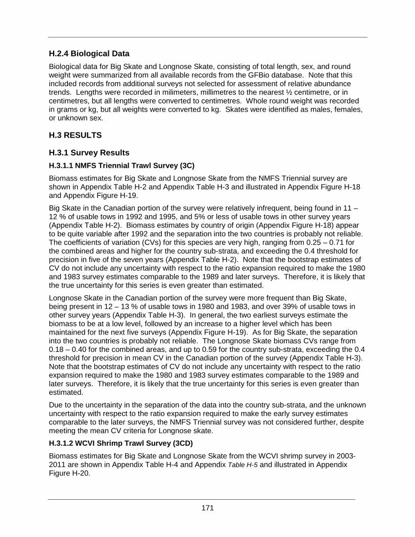
171

H.2.4 Biological Data Biological data for Big Skate and Longnose Skate, consisting of total length, sex, and round weight were summarized from all available records from the GFBio database. Note that this included records from additional surveys not selected for assessment of relative abundance trends. Lengths were recorded in milimeters, millimetres to the nearest ½ centimetre, or in centimetres, but all lengths were converted to centimetres. Whole round weight was recorded in grams or kg, but all weights were converted to kg. Skates were identified as males, females, or unknown sex.

H.3 RESULTS

H.3.1 Survey Results H.3.1.1 NMFS Triennial Trawl Survey (3C) Biomass estimates for Big Skate and Longnose Skate from the NMFS Triennial survey are shown in Appendix Table H-2 and Appendix Table H-3 and illustrated in Appendix Figure H-18 and Appendix Figure H-19.

Big Skate in the Canadian portion of the survey were relatively infrequent, being found in 11 – 12 % of usable tows in 1992 and 1995, and 5% or less of usable tows in other survey years (Appendix Table H-2). Biomass estimates by country of origin (Appendix Figure H-18) appear to be quite variable after 1992 and the separation into the two countries is probably not reliable. The coefficients of variation (CVs) for this species are very high, ranging from 0.25 – 0.71 for the combined areas and higher for the country sub-strata, and exceeding the 0.4 threshold for precision in five of the seven years (Appendix Table H-2). Note that the bootstrap estimates of CV do not include any uncertainty with respect to the ratio expansion required to make the 1980 and 1983 survey estimates comparable to the 1989 and later surveys. Therefore, it is likely that the true uncertainty for this series is even greater than estimated.

Longnose Skate in the Canadian portion of the survey were more frequent than Big Skate, being present in 12 – 13 % of usable tows in 1980 and 1983, and over 39% of usable tows in other survey years (Appendix Table H-3). In general, the two earliest surveys estimate the biomass to be at a low level, followed by an increase to a higher level which has been maintained for the next five surveys (Appendix Figure H-19). As for Big Skate, the separation into the two countries is probably not reliable. The Longnose Skate biomass CVs range from 0.18 – 0.40 for the combined areas, and up to 0.59 for the country sub-strata, exceeding the 0.4 threshold for precision in mean CV in the Canadian portion of the survey (Appendix Table H-3). Note that the bootstrap estimates of CV do not include any uncertainty with respect to the ratio expansion required to make the 1980 and 1983 survey estimates comparable to the 1989 and later surveys. Therefore, it is likely that the true uncertainty for this series is even greater than estimated.

Due to the uncertainty in the separation of the data into the country sub-strata, and the unknown uncertainty with respect to the ratio expansion required to make the early survey estimates comparable to the later surveys, the NMFS Triennial survey was not considered further, despite meeting the mean CV criteria for Longnose skate.

H.3.1.2 WCVI Shrimp Trawl Survey (3CD) Biomass estimates for Big Skate and Longnose Skate from the WCVI shrimp survey in 2003-2011 are shown in Appendix Table H-4 and Appendix Table H-5 and illustrated in Appendix Figure H-20.

172

Big Skate were not abundant in the WCVI shrimp survey (Appendix Figure H-3). They were encountered in only a small number of tows, with no Big Skate captured in 2004, 2007, or 2010, and Big Skate captured in 14% of tows in 2003 and less than 3% of tows in the remaining years (Appendix Table H-4). Biomass estimates range from a high of 122 t in 2003 to just 3 – 36 tonnes in 2005 – 2011 with a mean CV exceeding the 0.4 threshold for precision and ranging from 0.48 – 0.98 (Appendix Table H-4, Appendix Figure H-20).

Longnose Skate were more abundant than Big Skate in the survey and were encountered in more than 50% of the tows in most years (Appendix Table H-5 and Appendix Figure H-3). Biomass estimates increased from 171 t in 2003 to 460 t in 2005, the highest biomass estimate of the series; biomass estimates from 2006 – 2011 fluctuated between 63 t and 182 t (Appendix Table H-5 and Appendix Figure H-20). The CV for the series was within the 0.4 threshold for precision and ranged from 0.15 – 0.27 (Appendix Table H-5).

H.3.1.3 WCVI Synoptic Trawl Survey (3CD) Biomass estimates for Big Skate and Longnose Skate from the WCVI synoptic survey in 2004 – 2010 are shown in Appendix Table H-6 and Appendix Table H-7 and illustrated in Appendix Figure H-20.

Big Skate were not abundant in the WCVI synoptic survey (Appendix Figure H-4). They were encountered in only a small number of tows (Appendix Table H-6), with Big Skate captured in less than 10% of the tows in most years. Biomass estimates declined from 224 t in 2004 to 84 t in 2010 (Appendix Table H-6 and Appendix Figure H-20). The CV for the series ranged from 0.33 – 0.60, with the mean CV exceeding the 0.4 threshold for precision.

Longnose Skate were more abundant than Big Skate in the survey and were encountered in 40 – 60 % of the tows each year (Appendix Table H-7). Biomass estimates declined from 716 t in 2004 to 489 t in 2010, with a CV ranging from 0.12 – 0.14, within the 0.4 threshold for precision (Appendix Table H-7 and Appendix Figure H-20).

H.3.1.4 QCS Shrimp Trawl Survey (5AB) Biomass estimates for Big Skate and Longnose Skate from the QCS Shrimp survey in 2003 – 2010 are shown in Appendix Table H-8 and Appendix Table H-9 and illustrated in Appendix Figure H-21.

Big Skate were not abundant in the QCS shrimp survey (Appendix Figure H-5). In most years, they were encountered in only a small number of tows, with no Big Skate captured in 2009 or 2011, and Big Skate captured in 21% of tows in 2010, but less than 15% of tows per year in the remaining years (Appendix Table H-8). Biomass estimates fluctuated between 5 t and 83 t over the series, with CVs ranging from 0.28 – 0.99, and the mean CV exceeded the 0.4 threshold for precision (Appendix Table H-8, Appendix Figure H-21).

Longnose Skate were more abundant than Big Skate in the survey and were encountered more than 50% of the tows in most years (Appendix Table H-9 and Appendix Figure H-5). Biomass estimates were quite variable, rising from 282 t to 707 t in 2003 – 2005, declining in 2006 and 2007 to 97 t in 2007, increasing in 2008 and 2009 to 349 t in 2009, and declining again in 2010 and 2011 to 65 t in 2011 (Appendix Figure H-21). The CV for the series ranged from 0.16 – 0.27, and the mean CV was below the 0.4 threshold for precision.

H.3.1.5 QCS Synoptic Trawl Survey (5AB) Biomass estimates for Big Skate and Longnose Skate from the QCS Synoptic survey in 2003 – 2011 are shown in Appendix Table H-10 and Appendix Table H-11 and illustrated in Appendix Figure H-21.

173

Big Skate were not abundant in the QCS Synoptic Survey (Appendix Figure H-6). They were encountered in only 2 – 6% of tows each year (Appendix Table H-10). Biomass estimates decreased from 663 t in 2003 to 18 t in 2011 (Appendix Figure H-21). CVs for the series range from 0.33 – 0.68, and the mean CV exceeded the 0.4 threshold for precision.

Longnose Skate were more abundant than Big Skate in the survey and were encountered in 20 – 40% of the tows (Appendix Table H-11 and Appendix Figure H-6). Biomass estimates showed a slight increase in 2003 – 2005 from 494 – 573 t, dropped to 283 t in 2007, and increased in 2009 and 2011 to 382 t in 2011 (Appendix Table H-11 and Appendix Figure H-21). The CV for the series ranged from 12 – 21 %, and the mean CV was below the 0.4 threshold for precision (Appendix Table H-11).

H.3.1.6 Hecate Strait Multispecies Assemblage Trawl Survey (5CDE) Biomass estimates for Big Skate and Longnose Skate from the Hecate Strait Multispecies Assemblage (HSMA) survey in 1984 – 2003 are shown in Appendix Table H-12 and Appendix Table H-13 and illustrated in Appendix Figure H-22.

Big Skate were abundant in the HSMA Survey (Appendix Figure H-7). They were encountered in 23 – 47% of tows each year (Appendix Figure H-22). Biomass increased slightly from 776 – 837 t from 1984 to 1987, increased to the series maximum of 3681 t in 1989, and decreased to 1110 t in 1991; from 1991 to 1998, biomass fluctuated between approximately 1100 t and 1600, increasing to 2900 t in 2003 (Appendix Table H-12 and Appendix Figure H-22). The CV for the series ranged from 0.17 – 0.35, and the mean CV was within the 0.4 threshold for precision (Appendix Table H-12).

Longnose Skate were less abundant than Big Skate in the survey and were encountered in 1 – 24% of the tows (Appendix Table H-13 and Appendix Figure H-7). Biomass was highest in 1984 at 301 t, and fluctuated between 4 t and 191 t in 1987 – 2003 (Appendix Table H-13 and Appendix Figure H-22). The CV for the series ranged from 0.28 – 0.71, and the mean CV exceed the 0.4 threshold for precision precision (Appendix Table H-13).

H.3.1.7 Hecate Strait Synoptic Trawl Survey (5CDE) Biomass estimates for Big Skate and Longnose Skate from the Hecate Strait Synoptic survey in 2005 – 2011 are shown in Appendix Table H-14 and Appendix Table H-15 and illustrated in Appendix Figure H-22.

Big Skate were abundant in the Hecate Strait Synoptic survey (Appendix Figure H-8). They were encountered in 12 – 26 % of tows each year (Appendix Table H-14). Biomass estimates were similar in 2005 and 2007 at 786 t and 814 t, respectively, dropped to 389 t in 2009, and increased to 1301 t in 2011 (Appendix Table H-14 and Appendix Figure H-22). The CV for the series ranged from 0.20 – 0.30, and the mean was within the 0.4 threshold (Appendix Table H-14).

Longnose Skate were less abundant than Big Skate in the survey but were present in a similar proportion of tows each year (Appendix Table H-15 and Appendix Figure H-8). Biomass was highest in 2005 at 412 t, dropped to 213 and 217 t in 2007 and 2009 respectively, and increased to 396 t in 2011 (Appendix Table H-15 and Appendix Figure H-22). The CV for the series ranged from 0.18 – 0.44, and the mean CV was within the 0.4 threshold for precision (Appendix Table H-15).

H.3.1.8 West Coast Haida Gwaii Synoptic Trawl Survey (5CDE) Biomass estimates for Big Skate and Longnose Skate from the West Coast Haida Gwaii Synoptic survey in 2006 – 2010 are shown in Appendix Table H-16 and Appendix Table H-17 and illustrated in Appendix Figure H-22.

174

Big Skate were virtually absent from the West Coast Haida Gwaii Synoptic survey and were encounted in only a single tow in 2006 (Appendix Table H-16 and Appendix Figure H-8). The biomass estimate for 2006 is 1 t, with a CV of 0.95 (Appendix Table H-16 and Appendix Figure H-22).

Longnose Skate were at low abundance in the survey but were present in 27 – 38% of tows each year (Appendix Table H-17 and Appendix Figure H-8). Biomass estimates were 87 t in 2006 and 2007, 77 t in 2008, and dropped to 47 t in 2010 (Appendix Table H-17 and Appendix Figure H-22). The CV for the series ranged from 0.18 – 0.20, and the mean CV was within the 0.4 threshold for precision (Appendix Table H-17).

H.3.1.9 IPHC Standardized Assessment Longline Survey (3CD) Mean catch per unit of effort (CPUE) for Big Skate and Longnose Skate from the IPHC Standardized Assessment Longline Survey in 2003 – 2011 in Skate Management Area 3CD is shown in Appendix Table H-18 and Appendix Table H-19 and illustrated in Appendix Figure H-23.

Big Skate were encountered in 23 – 46 % of the longline sets each year (Appendix Table H-18 and Appendix Figure H-9). Mean CPUE was highest in 2005 at 0.44 pieces / 100 hooks and ranged from 0.07 – 0.21 pieces / 100 hooks in the other years of the survey (Appendix Table H-18 and Appendix Figure H-23). The CV for the series ranged from 0.29 – 0.57 and the mean was within the 0.4 threshold for precision (Appendix Table H-18).

Longnose Skate were more abundant than Big Skate in the survey and were encounterd in over 70 % of the longline sets each year (Appendix Table H-19 and Appendix Figure H-9). Mean CPUE increased from 0.52 – 1.06 pieces / 100 hooks in 2003 – 2005, decreased to 0.44 pieces / 100 hooks in 2006, increased to 1.75 pieces / 100 hooks in 2007 – 2009, and decreased to 0.80 pieces / 100 hooks in 2010 – 2011 (Appendix Table H-19 and Appendix Figure H-23). The CV for the series ranged from 0.15 – 0.26 and the mean CV was within the 0.4 threshold for precision (Appendix Table H-19).

H.3.1.10 PHMA Longline Survey (3CD) Mean catch per unit of effort (CPUE) for Big Skate and Longnose Skate from the PHMA Southern Longline Survey in 2007, 2009 and 2011 in Skate Management Area 3CD is shown in Appendix Table H-20 and Appendix Table H-21 and illustrated in Appendix Figure H-23.

Big Skate were encountered in 27 – 29 % of the longline sets each year (Appendix Table H-20 and Appendix Figure H-12). Mean CPUE was 0.17 pieces / 100 hooks in 2007 and 2011, and 0.25 pieces / 100 hooks in 2009 (Appendix Table H-20 and Appendix Figure H-23). The CV for the series ranged from 0.25 – 0.34 and the mean CV exceeded the 0.4 threshold for precision (Appendix Table H-20).

Longnose Skate were more abundant than Big Skate in the survey and were encounterd in over 70 % of the longline sets each year (Appendix Table H-21 and Appendix Figure H-9). Mean CPUE was highest in 2007 at 1.75 pieces / 100 hooks and lower in 2009 and 2011 at 0.78 and 0.95 pieces / 100 hooks, respectively (Appendix Table H-21 and Appendix Figure H-23). The CV for the series ranged from 0.15 – 0.16 and the mean CV was within the 0.4 threshold for precision (Appendix Table H-21).

H.3.1.11 IPHC Standardized Assessment Longline Survey (5AB) Mean catch per unit of effort (CPUE) for Big Skate and Longnose Skate from the IPHC Standardized Assessment Longline Survey in 2003 – 2011 in Skate Management Area 5AB is shown in Appendix Table H-22 and Appendix Table H-23 and illustrated in Appendix Figure H-24.

175

Big Skate were encountered in 16 – 36 % of the longline sets each year (Appendix Table H-22 and Appendix Figure H-10). Mean CPUE fluctuated from 0.16 – 0.05 pieces / 100 hooks over the time series (Appendix Table H-22 and Appendix Figure H-24). The CV for the series ranged from 0.26 – 0.40 and the mean CV was within the 0.4 threshold for precision (Appendix Table H-22).

Longnose Skate were more abundant than Big Skate in the survey and were encounterd in over 60 % of the longline sets each year (Appendix Table H-23 and Appendix Figure H-10). Mean CPUE ranged from 0.70 – 1.04 pieces / 100 hooks over the series (Appendix Table H-23 and Appendix Figure H-24). The CV for the series ranged from 0.13 – 0.23 and the mean CV was within the 0.4 threshold for precision (Appendix Table H-23).

H.3.1.12 PHMA Longline Survey (5AB) Mean catch per unit of effort (CPUE) for Big Skate and Longnose Skate from the PHMA Southern Longline Survey in 2007, 2009 and 2011 in Skate Management Area 5AB is shown in Appendix Table H-24 and Appendix Table H-25 and illustrated in Appendix Figure H-24.

Big Skate were encountered in 13 – 29 % of the longline sets each year (Appendix Table H-24 and Appendix Figure H-13). Mean CPUE was between 0.07 and 0.12 pieces / 100 hooks and (Appendix Table H-24 and Appendix Figure H-24). . The CV for the series ranged from 0.26 – 0.45 and the mean CV was within the 0.4 threshold for precision (Appendix Table H-24).

Longnose Skate were more abundant than Big Skate in the survey and were encounterd in over 65 % of the longline sets each year (Appendix Table H-25 and Appendix Figure H-13). Mean CPUE was highest in 2007 at 1.47 pieces / 100 hooks and lower in 2009 and 2011 at 0.72 and 0.65 pieces / 100 hooks, respectively (Appendix Table H-25 and Appendix Figure H-24). The CV for the series ranged from 0.14 – 0.17 and the mean CV was within the 0.4 threshold for precision (Appendix Table H-25).

H.3.1.13 Inshore Rockfish Longline Survey (5AB) Mean catch per unit of effort (CPUE) for Big Skate and Longnose Skate from the Inshore Rockfish Longline Survey in 2003 – 2010 in Skate Management Area 5AB is shown in Appendix Table H-26 and Appendix Table H-27 and illustrated in Appendix Figure H-24.

Big Skate were encountered in less than 9% of the longline sets each year; in 2008 only 7 sets were completed and no skates were encountered (Appendix Table H-26 and Appendix Figure H-15). Mean CPUE was between 0.01 and 0.08 pieces / 100 hooks (Appendix Table H-26 and Appendix Figure H-24). The CV for the series ranged from 0.47 – 0.94 and the mean CV exceeded the 0.4 threshold for precision (Appendix Table H-26).

Longnose Skate were more abundant than Big Skate in the survey and were encounterd in 26 – 45% of the longline sets each year, except in 2008 where only 7 sets were completed and no skates were encountered (Appendix Table H-27 and Appendix Figure H-15). Mean CPUE fluctuated over the series and ranged from 0.27 – 0.44 pieces / 100 hooks (Appendix Table H-27 and Appendix Figure H-24). The CV for the series ranged from 0.18 – 0.44 and the mean CV was within the 0.4 threshold for precision (Appendix Table H-27).

H.3.1.14 IPHC Standardized Assessment Longline Survey (5CDE) Mean catch per unit of effort (CPUE) for Big Skate and Longnose Skate from the IPHC Standardized Assessment Longline Survey in 2003 – 2011 in Skate Management Area 5CDE is shown in Appendix Table H-28 and Appendix Table H-29 and illustrated in Appendix Figure H-25.

176

Big Skate were encountered in 11 – 26 % of the longline sets each year (Appendix Table H-28 and Appendix Figure H-11). Mean CPUE fluctuated between 0.08 – 0.26 pieces / 100 hooks over the time series (Appendix Table H-28 and Appendix Figure H-25). The CV for the series ranged from 0.20 – 0.51 and the mean CV was within the 0.4 threshold for precision (Appendix Table H-28).

Longnose Skate were more abundant than Big Skate in the survey and were encounterd in over 70 % of the longline sets each year (Appendix Table H-29 and Appendix Figure H-11). Mean CPUE ranged from 0.73 – 1.01 pieces / 100 hooks over the series (Appendix Table H-29 and Appendix Figure H-25). The CV for the series ranged from 0.09 – 0.19 and the mean CV was within the 0.4 threshold for precision (Appendix Table H-29).

H.3.1.15 PHMA Longline Survey (5CDE) Mean catch per unit of effort (CPUE) for Big Skate and Longnose Skate from the PHMA Northern Longline Survey in 2006, 2008 and 2010 in Skate Management Area 5CDE is shown in Appendix Table H-30 and Appendix Table H-31 and illustrated in Appendix Figure H-25.

Big Skate were encountered in 20 – 40 % of the longline sets each year (Appendix Table H-30 and Appendix Figure H-14). Mean CPUE was highest in 2006 at 0.18 pieces / 100 hooks, and lower in 2008 and 2010 at 0.10 and 0.09 pieces / 100 hooks, respectively (Appendix Table H-30 and Appendix Figure H-25). The CV for the series ranged from 0.13 – 0.24 and the mean CV was within the 0.4 threshold for precision (Appendix Table H-30).

Longnose Skate were more abundant than Big Skate in the survey and were encounterd in over 65 % of the longline sets each year (Appendix Table H-31 and Appendix Figure H-14). Mean CPUE was 0.70 – 0.94 pieces / 100 hooks respectively (Appendix Table H-31 and Appendix Figure H-25). The CV for the series ranged from 0.09 – 0.10 and the mean CV was within the 0.4 threshold for precision (Appendix Table H-31).

H.3.1.16 Inshore Rockfish Longline Surveys (4B) Mean catch per unit of effort (CPUE) for Big Skate and Longnose Skate from the Inshore Rockfish Longline Surveys in the northern Strait of Georgia in 2003 – 2010 is shown in Appendix Table H-32 and Appendix Table H-33 and illustrated in Appendix Figure H-26.

Big Skate were not abundant in the northern Inshore Rockfish Longline Survey; they were encountered in only 1 – 2 sets per year in most years, and no skates were encountered in 2004 (Appendix Table H-32 and Appendix Figure H-16). Mean CPUE was between 0.01 and 0.03 pieces / 100 hooks (Appendix Table H-32 and Appendix Figure H-26). The CV for the series ranged from 0.67 – 1.0 and the mean CV exceeded the 0.4 threshold for (Appendix Table H-32).

Longnose Skate were more abundant than Big Skate in the northern Inshore Rockfish Longline Survey and were encounterd in 6 – 24% of the longline sets each year (Appendix Table H-33 and Appendix Figure H-16). Mean CPUE was 0.03 – 0.05 pieces / 100 hooks in 2003 – 2004 and was 0.13 – 0.19 pieces / 100 hooks in 2007 – 2010 (Appendix Table H-33 and Appendix Figure H-26). The CV for the series ranged from 0.32 – 0.94 and the mean CV exceeded the 0.4 threshold for precision (Appendix Table H-33).

Mean catch per unit of effort (CPUE) for Big Skate and Longnose Skate from the Inshore Rockfish Longline Surveys in the southern Strait of Georgia in 2005, 2009 and 2011 is shown in Appendix Table H-34 and Appendix Table H-35 and illustrated in Appendix Figure H-26.

Big Skate were not abundant in the southern Inshore Rockfish Longline survey and were encountered in only two sets in 2005 (Appendix Table H-34 and Appendix Figure H-17). Mean

177

CPUE was 0.01 pieces / 100 hooks (Appendix Table H-34 and Appendix Figure H-26). The CV was 0.69 and the mean CV exceeded the 0.4 threshold for precision (Appendix Table H-34).

Longnose Skate were more abundant than Big Skate in the southern Inshore Rockfish Longline Survey and were encounterd in 7 – 14% of the longline sets each year (Appendix Table H-35 and Appendix Figure H-17). Mean CPUE was 0.03 – 0.11 pieces / 100 hooks (Appendix Table H-35 and Appendix Figure H-26). The CV for the series ranged from 0.37 – 68 and the mean CV exceeded the 0.4 threshold for precision (Appendix Table H-35).

H.3.2 Trend Analyses H.3.2.1 Big Skate survey indices The Hecate Strait Multispecies Assemblage Trawl Survey series and the Hecate Strait Synoptic Trawl Survey series for Big Skate in 5CDE had mean CVs ≤ 0.4 for bootstrapped biomass estimates . In addition, the IPHC and PHMA Longline Survey Series for Big Skate in 3CD, 5AB, and 5CDE had mean CVs ≤ 0.4 for the catch rate indices. Trend analyses for these surveys estimated slopes (b) and annual rates of change (r) close to zero (Appendix Table H-36). The bootstrapped distributions for b and r had 2.5 and 97.5% quantiles that bounded zero, indicating that the b and r estimates are not significantly (p>0.05) different from zero (Appendix Table H-36). The two trawl surveys indicate no trend in Big Skate biomass, and the longline surveys indicate no trend in Big Skate catch rates.

H.3.2.2 Longnose Skate survey indices There are useable survey series for Longnose Skate abundance indices in each Skate Management Area, except for 4B. The Shrimp Trawl Surveys, Synoptic Trawl Surveys, IPHC Standardized Stock Assessment Longline Surveys, the PHMA Southern and Northern Longline Surveys, and the Inshore Rockfish Northern Longline Surveys all had mean CVs ≤ 0.4 for bootstrapped biomass (trawl) or catch rate (longline) estimates. The trawl surveys provide conflicting trend estimates to the longline surveys.

In 3CD, trend analyses for the WCVI Shrimp Trawl Survey and the WCVI Synoptic Trawl Survey both estimate negative b and r values, and the bootstrapped distributions indicate that these declines are significantly (p<0.05) different from zero (Appendix Table H-36). The PHMA Southern Longline Survey in 3CD also exhibited negative b and r values that were similar to the WCVI Shrimp Trawl Survey, but the bootstrapped distributions for b and r had 2.5 and 97.5% quantiles that bounded zero, indicating that the b and r estimates are not significantly (p>0.05) different from zero (Appendix Table H-36). The IPHC Standardized Stock Assessment Longline Survey had an estimated slope (b) and annual rate of change (r) close to zero (Appendix Table H-36). Overall, the trawl surveys indicate a decline in Longnose Skate biomass, while the longline surveys indicate no trend in Longnose Skate catch rates in 3CD.

In 5AB, the QCS Shrimp Trawl Survey and the QCS Synoptic Trawl Survey trend analyses for both estimate negative b and r values, and the bootstrapped distributions indicate that these declines are significantly (p<0.05) different from zero (Appendix Table H-36). The PHMA Southern Longline Survey in 3CD also exhibited negative b and r values that were similar to the Shrimp Trawl Survey, but the bootstrapped distributions for b and r had 2.5 and 97.5% quantiles that bounded zero, indicating that the b and r estimates are not significantly (p>0.05) different from zero (Appendix Table H-36). The IPHC Standardized Stock Assessment Longline Survey and the Inshore Rockfish Northern Longline Survey both had an estimated slope (b) and annual rate of change (r) close to zero (Appendix Table H-36). Overall, the trawl surveys indicate a decline in Longnose Skate biomass, while the longline surveys indicate no trend in Longnose Skate catch rates in 5AB.

178

The trend analyses for the HS Synoptic Trawl Survey in 5CDE estimated b and r values close to zero; both estimates had zeros bounded by the bootstrapped distribution (Appendix Table H-36). Conversely, the WCHG Synoptic Trawl Survey in 5CDE trend analysis estimated negative b and r values, and the bootstrapped distributions indicate that the decline is significantly (p<0.05) different from zero (Appendix Table H-36). The IPHC Standardized Stock Assessment Longline Survey and the PHMA Northern Longline Survey in 5CDE had estimated slopes (b) and annual rates of change (r) close to zero (Appendix Table H-36). The bootstrapped distributions for b and r had 2.5 and 97.5% quantiles that bounded zero, indicating that these b and r estimates are not significantly (p>0.05) different from zero (Appendix Table H-36). Overall, the trawl and longline surveys indicate no trend in Longnose Skate biomass or catch rates in Hecate Strait, but a decline in biomass off the west coast of Haida Gwaii.

H.3.3 Biological Data Biological data (total length by sex and whole round weight) for Big Skate captured in research trawl and longline surveys from 1984 – 2011 are summarized in Appendix Table H-37 and Appendix Table H-38. Biological data (total length by sex and whole round weight) for Longnose Skate captured in research trawl and longline surveys from 1984 – 2011 are summarized in Appendix Table H-39 and Appendix Table H-40. Note that in 1984 – 1993 skates are not identified to sex.

H.4 REFERENCES Boutillier, J.A., Bond, J.A., and Nguyen, H. 1999. Evaluation of a new assessment and

management framework for shrimp stocks in British Columbia. DFO Can. Sci. Advis. Sec. Res. Doc. 1999/124. 28p.

Choromanski E.M., Workman, G.D., and Fargo, J. 2005. Hecate Strait multispecies bottom trawl survey, CCGS W.E. Ricker, May 19 to june 7, 2003. Can. Data Rep. Fish. Aquat. Sci. 1169: viii + 85 p.

Efron, B. 1982. The jackknife, the bootstrap, and other resampling plans. Society of Industrial and Applied Mathematics CBMS-NSF Monographs, 38.

Flemming, R.G., Yamanaka, K.L., Cooke, K., and Dykstra C., 2012. Summary of non-halibut catch from the Standardized Stock Assessment Survey conducted by the International Pacific Halibut Commission in British Columbia from June 3 to August 27, 2010. Can. Tech. Rep. Fish. Aquat. Sci. 2989: viii + 99 p.

King, J.R., M. McAllister, K.R. Holt and P.J. Starr. 2012. Lingcod (Ophiodon elongatus) stock assessement and yield advice for outside stocks in British Columbia. DFO Can. Sci. Advis. Sec.Res. Doc. 2011/124. viii + 177p.

Lochead, J.K., and Yamanaka, K.L. 2007. Summary report for the inshore rockfish (Sebastes spp.) longline survey conducted in Statistical Areas 14 to 20, 28 and 29, from August 11 to September 6, 2005. Can. Tech. Rep. Fish. Aquat. Sci. 2690: viii + 53 p.

Olsen, N., Rutherford, K.L., Stanley, R.D., and Wyeth, M.R. 2009a. West coast Vancouver Island groundfish bottom trawl survey, May 26th to June 22nd, 2008. Can. Manuscr. Rep. Fish. Aquat. Sci. 2902: vi + 50 p.

Olsen, N., Rutherford, K.L., Stanley, R.D., and Wyeth, M.R. 2009b. Queen Charlotte Sound groundfish bottom trawl survey, July 7th to August 8th, 2009. Can. Manuscr. Rep. Fish. Aquat. Sci. 2899: vi + 61 p.

179

Olsen, N., Rutherford, K.L., Stanley, R.D., and Wyeth, M.R. 2009c. Hecate Strait groundfish bottom trawl survey, May 26th to June 21st, 2009. Can. Manuscr. Rep. Fish. Aquat. Sci. 2901: vi + 49 p.

Olsen, N., Rutherford, K.L., and Stanley, R.D. 2008. West Coast Queen Charlotte Islands groundfish bottom trawl survey, August 25th to September 21st, 2008. Can. Manuscr. Rep. Fish. Aquat. Sci. 2858: vii + 50 p.

Schnute J.T., Haigh R., Krishka B.A., Sinclair A., Starr P.J. 2004. The British Columbia Longspine Thornyhead fishery: analysis of survey and commercial data (1996 – 2003). DFO Can. Sci. Advis. Sec. Res. Doc. 2004/059. iii + 75.

Stanley, R.D., Starr, P., Olsen, N., Haigh, R. 2004. Summary of results of the 2003 Queen Charlotte Sound Bottom trawl survey. DFO Can. Sci. Advis. Sec. Res. Doc. 2004/028. iv + 50p.

Starr, P.J., A.S. Sinclair, and J. Boutillier. 2002. West coast Vancouver Island Pacific cod assessment: 2002. DFO Can. Sci. Advis. Sec. Res. Doc. 2002/113. 28p.

180

Appendix Table H-1. List of available research surveys which may provide relative biomass indices for Big Skate and Longnose Skate

Skate Management Area Survey Applicable Years

3CD (West Coast Vancouver Island including Juan de Fuca Strait)

NFMS Triennial Trawl Survey 1980, 1983, 1989, 1992, 1995, 1998, 2001

West Coast Vancouver Island Shrimp Trawl Survey 2003 – 2011

West Coast Vancouver Island Synoptic Trawl Survey 2004, 2006, 2008, 2010

IPHC Standardized Assessment Longline Survey 2003 – 2011

PHMA Southern Longline Survey 2007, 2009, 2011

5AB (Queen Charlotte Sound, including Queen Charlotte Strait)

Queen Charlotte Sound Shrimp Trawl Survey 2003 – 2011

Queen Charlotte Sound Synoptic Trawl Survey

2003 – 2005, 2007, 2009, 2011

IPHC Standardized Assessment Longline Survey 2003 – 2011

PHMA Southern Longline Survey 2007, 2009, 2011

ISRF Northern Longline Survey

2003, 2004, 2007, 2008, 2010

5CDE (Hecate Strait and West Coast Haida Gwaii)

Hecate Strait Multispecies Assemblage Trawl Survey

1984, 1987, 1989, 1991, 1993, 1995, 1996, 1998, 2000, 2002, 2003

Hecate Strait Synoptic Trawl Survey 2005, 2007, 2009, 2011

West Coast Haida Gwaii Synoptic Trawl Survey 2006 – 2008, 2010

IPHC Standardized Assessment Longline Survey 2003 – 2011

PHMA Northern Longline Survey 2006, 2008, 2010

4B (Strait of Georgia, excluding Juan de Fuca Strait and Johnstone Strait)

ISRF Northern Longline Survey

2003, 2004, 2007, 2008, 2010

ISRF Southern Longline Survey 2005, 2009, 2011

181

Appendix Table H-2. Biomass estimates for Big Skate from the NMFS Triennial Survey in 1980 – 2011 in the Vancouver INPFC region (Total region, Canadian waters only and US waters only). Bootstrap bias corrected confidence intervals and CVs are based on 1000 random draws with replacement.

Estimate Type

Survey Year

Total number of tows

Number of tows with Big Skate

Biomass (t)

Mean bootstrap

biomass (t)

Lower bound

biomass (t)

Upper bound

biomass (t)

Bootstrap CV

Total Vancouver

1980 85 2 183 182 0 580 0.71 1983 117 8 365 367 108 705 0.42 1989 120 9 364 366 118 725 0.42 1992 109 19 885 888 495 1,334 0.25 1995 97 8 369 369 84 722 0.46 1998 96 6 427 429 92 852 0.44 2001 73 3 274 278 48 725 0.59

Canada Vancouver (Major Area

3C)

1980 59 1 81 76 0 488 1.02 1983 47 2 162 163 0 503 0.69 1989 65 3 116 115 31 316 0.60 1992 59 7 342 340 119 666 0.40 1995 62 7 353 354 80 693 0.46 1998 54 2 87 87 0 345 0.95 2001 36 0 -- -- -- -- --

US Vancouver

1980 26 1 94 98 0 471 0.97 1983 70 6 189 190 29 441 0.53 1989 55 6 248 252 48 602 0.55 1992 50 12 543 548 256 892 0.31 1995 35 1 16 15 0 32 0.52 1998 42 4 340 342 69 731 0.49 2001 37 3 274 278 48 725 0.59

182

Appendix Table H-3. Biomass estimates for Longnose (LN) Skate from the NMFS Triennial Survey in 1980 – 2011 in the Vancouver INPFC region (Total region, Canadian waters only and US waters only). Bootstrap bias corrected confidence intervals and CVs are based on 1000 random draws with replacement.

Estimate Type

Survey Year

Total number of tows

Number of tows with LN Skate

Biomass (t)

Mean bootstrap

biomass (t)

Lower bound

biomass (t)

Upper bound

biomass (t)

Bootstrap CV

Total Vancouver

1980 85 14 725 723 331 1,267 0.33 1983 117 13 318 287 147 658 0.40 1989 120 41 2,304 2,291 1,533 3,188 0.19 1992 109 37 1,863 1,878 1,004 3,087 0.28 1995 97 44 1,576 1,582 1,049 2,220 0.18 1998 96 58 2,364 2,356 1,591 3,831 0.23 2001 73 40 1,936 1,896 1,315 2,779 0.19

Canada Vancouver (Major Area

3C)

1980 59 7 324 322 87 752 0.54 1983 47 6 130 134 12 315 0.59 1989 65 28 1,506 1,503 886 2,161 0.21 1992 59 23 1,470 1,487 680 2,584 0.32 1995 62 30 1,268 1,280 785 1,856 0.21 1998 54 36 1,382 1,391 931 1,860 0.16 2001 36 20 1,544 1,508 1,001 2,243 0.21

US Vancouver

1980 26 7 373 373 112 757 0.43 1983 70 7 173 142 71 413 0.53 1989 55 13 798 789 418 1,393 0.30 1992 50 14 393 391 190 736 0.35 1995 35 14 308 302 189 498 0.25 1998 42 22 982 965 370 2,244 0.50 2001 37 20 392 388 215 646 0.28

183

Appendix Table H-4. Biomass estimates for Big Skate from the WCVI Shrimp Survey in Skate Management Area 3CD. Bootstrap bias corrected confidence intervals and CVs are based on 1000 random draws with replacement.

Survey Year

Total number of

tows

Number of tows with Big Skate

Biomass (t)

Mean bootstrap

biomass (t)

Lower bound

biomass (t)

Upper bound

biomass (t)

Bootstrap CV

2003 65 9 122 120 30 250 0.484 2004 71 0 0 0 0 0 -- 2005 70 1 15 14 0 44 0.985 2006 70 2 5 5 0 13 0.674 2007 70 0 0 0 0 0 -- 2008 74 1 3 3 0 9 0.938 2009 62 1 10 10 0 29 0.957 2010 73 0 0 0 0 0 -- 2011 73 2 36 36 0 98 0.742

Appendix Table H-5. Biomass estimates for Longnose (LN) Skate from the WCVI Shrimp Survey in Skate Management Area 3CD. Bootstrap bias corrected confidence intervals and CVs are based on 1000 random draws with replacement.

Survey Year

Total number of

tows

Number of tows with LN Skate

Biomass (t)

Mean bootstrap

biomass (t)

Lower bound

biomass (t)

Upper bound

biomass (t)

Bootstrap CV

2003 65 36 171 171 118 238 0.167 2004 71 33 306 311 168 502 0.272 2005 70 49 460 455 271 733 0.269 2006 70 46 182 182 126 247 0.173 2007 70 22 79 80 40 124 0.266 2008 74 45 104 103 68 140 0.174 2009 62 47 157 157 113 210 0.160 2010 73 48 104 103 75 135 0.148 2011 73 24 63 63 38 90 0.221

Appendix Table H-6. Biomass estimates for Big Skate from the WCVI Synoptic Survey in Skate Management Area 3CD. Bootstrap bias corrected confidence intervals and CVs are based on 1000 random draws with replacement.

Survey Year

Total number of

tows

Number of tows with Big Skate

Biomass (t)

Mean bootstrap

biomass (t)

Lower bound

biomass (t)

Upper bound

biomass (t)

Bootstrap CV

2004 89 11 224 224 96 391 0.327 2006 164 12 177 178 66 321 0.373 2008 159 5 118 118 10 280 0.598 2010 136 10 84 83 20 177 0.484

Appendix Table H-7. Biomass estimates for Longnose (LN) Skate from the WCVI Synoptic Survey in Skate Management Area 3CD. Bootstrap bias corrected confidence intervals and CVs are based on 1000 random draws with replacement.

Survey Year

Total number of

tows

Number of tows with LN Skate

Biomass (t)

Mean bootstrap

biomass (t)

Lower bound

biomass (t)

Upper bound

biomass (t)

Bootstrap CV

2004 89 51 716 712 534 907 0.138 2006 164 80 540 535 405 678 0.131 2008 159 96 610 609 466 771 0.130 2010 136 74 489 493 378 617 0.121

184

Appendix Table H-8. Biomass estimates for Big Skate from the Queen Charlotte Sound Shrimp Survey in Skate Management Area 5AB. Bootstrap bias corrected confidence intervals and CVs are based on 1000 random draws with replacement.

Survey Year

Total number of

tows

Number of tows with Big Skate

Biomass (t)

Mean bootstrap

biomass (t)

Lower bound

biomass (t)

Upper bound

biomass (t)

Bootstrap CV

2003 63 8 48 47 13 96 0.448 2004 65 2 10 10 0 26 0.715 2005 47 5 28 28 0 70 0.660 2006 67 6 73 72 14 154 0.491 2007 65 2 18 18 0 46 0.718 2008 69 1 5 5 0 16 0.987 2009 64 0 -- -- -- -- -- 2010 70 15 83 82 42 132 0.282 2011 67 0 -- -- -- -- --

Appendix Table H-9. Biomass estimates for Longnose (LN) Skate from Queen Charlotte Sound Shrimp Survey in Skate Management Area 5AB. Bootstrap bias corrected confidence intervals and CVs are based on 1000 random draws with replacement.

Survey Year

Total number of

tows

Number of tows with LN skate

Biomass (t)

Mean bootstrap

biomass (t)

Lower bound

biomass (t)

Upper bound

biomass (t)

Bootstrap CV

2003 63 45 282 282 194 375 0.172 2004 65 43 340 343 191 560 0.265 2005 47 43 707 703 462 995 0.192 2006 67 45 157 158 111 211 0.158 2007 65 28 97 97 58 143 0.235 2008 69 40 221 222 135 346 0.243 2009 64 50 349 352 245 469 0.164 2010 70 43 231 230 144 328 0.206 2011 67 22 65 65 34 98 0.244

Appendix Table H-10. Biomass estimates for Big Skate from the Queen Charlotte Sound Synoptic Survey in Skate Management Area 5AB. Bootstrap bias corrected confidence intervals and CVs are based on 1000 random draws with replacement.

Survey Year

Total number of

tows

Number of tows with Big Skate

Biomass (t)

Mean bootstrap

biomass (t)

Lower bound

biomass (t)

Upper bound

biomass (t)

Bootstrap CV

2003 233 12 663 690 96 1711 0.681 2004 230 14 203 204 92 340 0.325 2005 224 11 608 624 76 1312 0.507 2007 257 8 445 460 66 1276 0.686 2009 233 7 71 71 14 162 0.522 2011 252 5 18 18 2 42 0.630

Appendix Table H-11. Biomass estimates for Longnose (LN) Skate from Queen Charlotte Sound Synoptic Survey in Skate Management Area 5AB. Bootstrap bias corrected confidence intervals and CVs are based on 1000 random draws with replacement.

Survey Year

Total number of

tows

Number of tows with LN skate

Biomass (t)

Mean bootstrap

biomass (t)

Lower bound

biomass (t)

Upper bound

biomass (t)

Bootstrap CV

2003 233 80 494 498 329 729 0.206 2004 230 78 551 552 402 734 0.151 2005 224 90 573 577 449 711 0.116

185

Survey Year

Total number of

tows

Number of tows with LN skate

Biomass (t)

Mean bootstrap

biomass (t)

Lower bound

biomass (t)

Upper bound

biomass (t)

Bootstrap CV

2007 257 52 283 284 183 401 0.197 2009 233 55 297 295 195 422 0.195 2011 252 68 382 384 280 489 0.136

Appendix Table H-12. Biomass estimates for Big Skate from the Hecate Strait Multispecies Assemblage Survey in Skate Management Area 5CDE. Bootstrap bias corrected confidence intervals and CVs are based on 1000 random draws with replacement.

Survey Year

Total number of

tows

Number of tows with Big Skate

Biomass (t)

Mean bootstrap

biomass (t)

Lower bound

biomass (t)

Upper bound

biomass (t)

Bootstrap CV

1984 146 34 776 774 514 1064 0.189 1987 85 17 837 832 412 1326 0.272 1989 90 32 3681 3623 2137 5541 0.244 1991 97 24 1110 1104 495 1958 0.352 1993 94 40 1634 1645 1130 2225 0.166 1995 101 39 1098 1098 747 1515 0.179 1996 105 42 1174 1174 778 1614 0.188 1998 86 28 1102 1085 654 1579 0.221 2000 105 31 1343 1317 720 2096 0.260 2002 91 33 792 797 495 1103 0.193 2003 95 45 2900 2890 1780 4350 0.236

Appendix Table H-13. Biomass estimates for Longnose (LN) Skate from Queen Charlotte Sound Synoptic Survey in Skate Management Area 5AB. Bootstrap bias corrected confidence intervals and CVs are based on 1000 random draws with replacement.

Survey Year

Total number of

tows

Number of tows with LN skate

Biomass (t)

Mean bootstrap

biomass (t)

Lower bound

biomass (t)

Upper bound

biomass (t)

Bootstrap CV

1984 146 22 301 296 128 518 0.336 1987 85 3 4 4 0 10 0.616 1989 90 10 191 192 40 381 0.479 1991 97 17 60 60 30 98 0.281 1993 94 16 113 113 50 189 0.312 1995 101 2 10 10 0 23 0.708 1996 105 10 28 28 11 50 0.354 1998 86 5 34 33 6 72 0.532 2000 105 17 125 124 58 198 0.292 2002 91 11 61 61 22 107 0.363 2003 95 23 133 132 63 223 0.325

Appendix Table H-14. Biomass estimates for Big Skate from the Hecate Strait Synoptic Survey in Skate Management Area 5CDE. Bootstrap bias corrected confidence intervals and CVs are based on 1000 random draws with replacement.

Survey Year

Total number of

tows

Number of tows with Big Skate

Biomass (t)

Mean bootstrap

biomass (t)

Lower bound

biomass (t)

Upper bound

biomass (t)

Bootstrap CV

2005 203 43 786 782 466 1161 0.235 2007 134 30 814 811 437 1256 0.263 2009 156 19 389 390 189 644 0.301 2011 186 48 1301 1299 826 1836 0.200

186

Appendix Table H-15. Biomass estimates for Longnose (LN) Skate from Hecate Strait Synoptic Survey in Skate Management Area 5CDE. Bootstrap bias corrected confidence intervals and CVs are based on 1000 random draws with replacement.

Survey Year

Total number of

tows

Number of tows with LN skate

Biomass (t)

Mean bootstrap

biomass (t)

Lower bound

biomass (t)

Upper bound

biomass (t)

Bootstrap CV

2005 203 40 412 409 125 809 0.443 2007 134 29 213 212 131 302 0.207 2009 156 31 217 218 137 312 0.201 2011 186 47 396 395 265 539 0.183

Appendix Table H-16. Biomass estimates for Big Skate from the West Coast Haida Gwaii Synoptic Survey in Skate Management Area 5CDE. Bootstrap bias corrected confidence intervals and CVs are based on 1000 random draws with replacement.

Survey Year

Total number of

tows

Number of tows with Big Skate

Biomass (t)

Mean bootstrap

biomass (t)

Lower bound

biomass (t)

Upper bound

biomass (t)

Bootstrap CV

2006 97 1 1 1 0 4 0.946 2007 111 0 -- -- -- -- -- 2008 110 0 -- -- -- -- -- 2010 123 0 -- -- -- -- --

Appendix Table H-17. Biomass estimates for Longnose (LN) Skate from West Coast Haida Gwaii Synoptic Survey in Skate Management Area 5CDE. Bootstrap bias corrected confidence intervals and CVs are based on 1000 random draws with replacement.

Survey Year

Total number of

tows

Number of tows with LN skate

Biomass (t)

Mean bootstrap

biomass (t)

Lower bound

biomass (t)

Upper bound

biomass (t)

Bootstrap CV

2006 97 33 87 88 58 123 0.185 2007 111 33 87 87 57 121 0.194 2008 110 42 77 78 49 111 0.206 2010 123 34 47 47 32 64 0.176

Appendix Table H-18. Catch per unit of effort (CPUE, pieces per 100 hooks) for Big Skate from the IPHC Longline Survey in Skate Management Area 3CD in 2003 – 2011. Bootstrap bias corrected confidence intervals and CVs are based on 1000 random draws with replacement.

Survey Year

Total Number of Sets

Number of Sets with Big Skate

Mean CPUE

Mean Bootstrap

CPUE

Lower Bound CPUE

Upper Bound CPUE

Bootstrap CV

2003 34 12 0.16 0.16 0.04 0.34 0.508 2004 34 9 0.07 0.07 0.03 0.13 0.361 2005 35 16 0.44 0.44 0.21 0.70 0.287 2006 34 12 0.16 0.16 0.07 0.26 0.302 2007 35 9 0.12 0.12 0.04 0.22 0.373 2008 35 8 0.10 0.10 0.03 0.18 0.377 2009 35 10 0.12 0.12 0.04 0.23 0.422 2010 34 11 0.21 0.21 0.08 0.39 0.364 2011 47 17 0.18 0.18 0.09 0.30 0.310

Appendix Table H-19. Catch per unit of effort (CPUE, pieces per 100 hooks) for Longnose Skate from the IPHC Longline Survey in Skate Management Area 3CD in 2003 – 2011. Bootstrap bias corrected confidence intervals and CVs are based on 1000 random draws with replacement.

187

Survey Year

Total Number of Sets

Number of Sets with

Longnose Skate

Mean CPUE

Mean Bootstrap

CPUE

Lower Bound CPUE

Upper Bound CPUE

Bootstrap CV

2003 34 24 0.52 0.52 0.32 0.76 0.217 2004 34 25 0.74 0.75 0.44 1.11 0.238 2005 35 33 1.06 1.06 0.72 1.49 0.178 2006 34 27 0.44 0.44 0.28 0.61 0.206 2007 35 27 0.82 0.83 0.58 1.15 0.177 2008 35 28 1.24 1.23 0.67 1.93 0.261 2009 35 32 1.75 1.74 1.25 2.26 0.156 2010 34 32 1.04 1.05 0.74 1.38 0.161 2011 47 43 0.80 0.80 0.58 1.06 0.152

Appendix Table H-20. Catch per unit of effort (CPUE, pieces per 100 hooks) for Big Skate from the PHMA Southern Longline Survey in Skate Management Area 3CD in 2007 – 2011. Bootstrap bias corrected confidence intervals and CVs are based on 1000 random draws with replacement.

Survey Year

Total Number of Sets

Number of Sets with Big Skate

Mean CPUE

Mean Bootstrap

CPUE

Lower Bound CPUE

Upper Bound CPUE

Bootstrap CV

2007 82 22 0.17 0.16 0.08 0.27 0.292 2009 72 21 0.25 0.25 0.11 0.45 0.342 2011 90 25 0.17 0.17 0.09 0.27 0.253

Appendix Table H-21. Catch per unit of effort (CPUE, pieces per 100 hooks) for Longnose Skate from the PHMA Southern Longline Survey in Skate Management Area 3CD in 2007 – 2011. Bootstrap bias corrected confidence intervals and CVs are based on 1000 random draws with replacement.

Survey Year

Total Number of Sets

Number of Sets with

Longnose Skate

Mean CPUE

Mean Bootstrap

CPUE

Lower Bound CPUE

Upper Bound CPUE

Bootstrap CV

2007 82 62 1.75 1.76 1.27 2.30 0.149 2009 72 49 0.78 0.78 0.56 1.04 0.159 2011 90 64 0.95 0.95 0.69 1.28 0.158

Appendix Table H-22. Catch per unit of effort (CPUE, pieces per 100 hooks) for Big Skate from the IPHC Longline Survey in Skate Management Area 5AB in 2003 – 2011. Bootstrap bias corrected confidence intervals and CVs are based on 1000 random draws with replacement.

Survey Year

Total Number of Sets

Number of Sets with Big Skate

Mean CPUE

Mean Bootstrap

CPUE

Lower Bound CPUE

Upper Bound CPUE

Bootstrap CV

2003 65 18 0.16 0.16 0.06 0.31 0.397 2004 69 25 0.15 0.15 0.07 0.26 0.325 2005 62 15 0.06 0.06 0.03 0.09 0.265 2006 68 15 0.06 0.06 0.03 0.10 0.311 2007 66 13 0.13 0.13 0.05 0.24 0.397 2008 62 10 0.05 0.05 0.02 0.08 0.333 2009 69 17 0.10 0.10 0.04 0.19 0.356 2010 67 24 0.13 0.12 0.07 0.20 0.261 2011 69 20 0.13 0.13 0.05 0.25 0.382

188

Appendix Table H-23. Catch per unit of effort (CPUE, pieces per 100 hooks) for Longnose Skate from the IPHC Longline Survey in Skate Management Area 5AB in 2003 – 2011. Bootstrap bias corrected confidence intervals and CVs are based on 1000 random draws with replacement.

Survey Year

Total Number of Sets

Number of Sets with

Longnose Skate

Mean CPUE

Mean Bootstrap

CPUE

Lower Bound CPUE

Upper Bound CPUE

Bootstrap CV

2003 65 46 0.73 0.74 0.53 0.96 0.144 2004 69 49 0.75 0.75 0.53 1.00 0.159 2005 62 48 0.70 0.70 0.51 0.92 0.148 2006 68 43 0.83 0.83 0.52 1.25 0.231 2007 66 40 0.70 0.70 0.44 1.03 0.216 2008 62 40 0.86 0.86 0.56 1.17 0.179 2009 69 55 1.03 1.02 0.77 1.29 0.128 2010 67 52 1.04 1.04 0.78 1.30 0.131 2011 69 52 0.85 0.85 0.61 1.10 0.147

Appendix Table H-24. Catch per unit of effort (CPUE, pieces per 100 hooks) for Big Skate from the PHMA Southern Longline Survey in Skate Management Area 5AB in 2007 – 2011. Bootstrap bias corrected confidence intervals and CVs are based on 1000 random draws with replacement.

Survey Year

Total Number of Sets

Number of Sets with Big Skate

Mean CPUE

Mean Bootstrap

CPUE

Lower Bound CPUE

Upper Bound CPUE

Bootstrap CV

2007 100 16 0.07 0.07 0.03 0.12 0.303 2009 98 13 0.12 0.12 0.04 0.24 0.445 2011 107 31 0.10 0.10 0.06 0.16 0.259

Appendix Table H-25. Catch per unit of effort (CPUE, pieces per 100 hooks) for Longnose Skate from the PHMA Southern Longline Survey in Skate Management Area 5AB in 2007 – 2011. Bootstrap bias corrected confidence intervals and CVs are based on 1000 random draws with replacement.

Survey Year

Total Number of Sets

Number of Sets with

Longnose Skate

Mean CPUE

Mean Bootstrap

CPUE

Lower Bound CPUE

Upper Bound CPUE

Bootstrap CV

2007 100 74 1.47 1.47 1.09 1.92 0.150 2009 98 65 0.72 0.72 0.53 0.91 0.138 2011 107 70 0.65 0.66 0.47 0.89 0.170

Appendix Table H-26. Catch per unit of effort (CPUE, pieces per 100 hooks) for Big Skate from the Inshore Rockfish Northern Longline Survey in Skate Management Area 5AB in 2003 – 2010. Bootstrap bias corrected confidence intervals and CVs are based on 1000 random draws with replacement.

Survey Year

Total Number of Sets

Number of Sets with Big Skate

Mean CPUE

Mean Bootstrap

CPUE

Lower Bound CPUE

Upper Bound CPUE

Bootstrap CV

2003 56 5 0.08 0.08 0.02 0.17 0.472 2004 47 4 0.07 0.06 0.01 0.14 0.528 2007 43 2 0.02 0.02 0.00 0.05 0.719 2008 7 0 -- -- -- -- -- 2010 35 1 0.01 0.01 0.00 0.04 0.939

189

Appendix Table H-27. Catch per unit of effort (CPUE, pieces per 100 hooks) for Longnose Skate from the Inshore Rockfish Northern Longline Survey in Skate Management Area 5AB in 2003 – 2010. Bootstrap bias corrected confidence intervals and CVs are based on 1000 random draws with replacement.

Survey Year

Total Number of Sets

Number of Sets with

Longnose Skate

Mean CPUE

Mean Bootstrap

CPUE

Lower Bound CPUE

Upper Bound CPUE

Bootstrap CV

2003 56 25 0.44 0.45 0.28 0.61 0.185 2004 47 16 0.27 0.27 0.14 0.41 0.261 2007 43 16 0.34 0.34 0.17 0.57 0.298 2008 7 0 -- -- -- -- -- 2010 35 9 0.28 0.28 0.09 0.55 0.444

Appendix Table H-28. Catch per unit of effort (CPUE, pieces per 100 hooks) for Big Skate from the IPHC Longline Survey in Skate Management Area 5CDE in 2003 – 2011. Bootstrap bias corrected confidence intervals and CVs are based on 1000 random draws with replacement.

Survey Year

Total Number of Sets

Number of Sets with Big Skate

Mean CPUE

Mean Bootstrap

CPUE

Lower Bound CPUE

Upper Bound CPUE

Bootstrap CV

2003 71 35 0.17 0.17 0.11 0.24 0.195 2004 68 29 0.30 0.30 0.13 0.57 0.370 2005 73 25 0.20 0.20 0.11 0.30 0.240 2006 68 20 0.25 0.26 0.12 0.44 0.314 2007 69 9 0.11 0.11 0.04 0.21 0.369 2008 72 17 0.18 0.18 0.09 0.30 0.305 2009 66 19 0.08 0.08 0.04 0.14 0.289 2010 69 19 0.18 0.18 0.08 0.30 0.323 2011 70 22 0.26 0.26 0.09 0.56 0.509

Appendix Table H-29. Catch per unit of effort (CPUE, pieces per 100 hooks) for Longnose Skate from the IPHC Longline Survey in Skate Management Area 5CDE in 2003 – 2011. Bootstrap bias corrected confidence intervals and CVs are based on 1000 random draws with replacement.

Survey Year

Total Number of Sets

Number of Sets with

Longnose Skate

Mean CPUE

Mean Bootstrap

CPUE

Lower Bound CPUE

Upper Bound CPUE

Bootstrap CV

2003 71 67 0.73 0.73 0.60 0.86 0.092 2004 68 63 1.01 1.01 0.76 1.30 0.133 2005 73 63 0.89 0.90 0.69 1.14 0.127 2006 68 54 0.94 0.94 0.66 1.27 0.170 2007 69 51 0.81 0.82 0.54 1.16 0.195 2008 72 55 0.87 0.87 0.64 1.10 0.139 2009 66 57 0.74 0.74 0.57 0.96 0.134 2010 69 56 1.01 1.02 0.74 1.30 0.136 2011 70 60 0.92 0.92 0.69 1.16 0.127

Appendix Table H-30. Catch per unit of effort (CPUE, pieces per 100 hooks) for Big Skate from the PHMA Northern Longline Survey in Skate Management Area 5CDE in 2007 – 2011. Bootstrap bias corrected confidence intervals and CVs are based on 1000 random draws with replacement.

Survey Year

Total Number of Sets

Number of Sets with Big Skate

Mean CPUE

Mean Bootstrap

CPUE

Lower Bound CPUE

Upper Bound CPUE

Bootstrap CV

2006 176 72 0.18 0.18 0.14 0.23 0.132 2008 176 37 0.10 0.10 0.06 0.16 0.240 2010 182 39 0.09 0.09 0.06 0.14 0.208

190

Appendix Table H-31. Catch per unit of effort (CPUE, pieces per 100 hooks) for Longnose Skate from the PHMA Northern Longline Survey in Skate Management Area 5CDE in 2007 – 2011. Bootstrap bias corrected confidence intervals and CVs are based on 1000 random draws with replacement.

Survey Year

Total Number of Sets

Number of Sets with

Longnose Skate

Mean CPUE

Mean Bootstrap

CPUE

Lower Bound CPUE

Upper Bound CPUE

Bootstrap CV

2006 176 140 0.85 0.85 0.70 1.01 0.091 2008 176 135 0.94 0.94 0.77 1.13 0.098 2010 182 123 0.70 0.71 0.57 0.85 0.099

Appendix Table H-32. Catch per unit of effort (CPUE, pieces per 100 hooks) for Big Skate from the Inshore Rockfish Northern Longline Survey in Skate Management Area 4B in 2003 – 2010. Bootstrap bias corrected confidence intervals and CVs are based on 1000 random draws with replacement.

Survey Year

Total Number of Sets

Number of Sets with Big Skate

Mean CPUE

Mean Bootstrap

CPUE

Lower Bound CPUE

Upper Bound CPUE

Bootstrap CV

2003 31 1 0.01 0.01 0.00 0.04 0.962 2004 17 0 -- -- -- -- -- 2007 21 1 0.02 0.02 0.00 0.07 1.010 2008 50 1 0.01 0.01 0.00 0.03 0.954 2010 29 2 0.03 0.03 0.00 0.08 0.678

Appendix Table H-33. Catch per unit of effort (CPUE, pieces per 100 hooks) for Longnose Skate from the Inshore Rockfish Northern Longline Survey in Skate Management Area 4B in 2003 – 2010. Bootstrap bias corrected confidence intervals and CVs are based on 1000 random draws with replacement.

Survey Year

Total Number of Sets

Number of Sets with

Longnose Skate

Mean CPUE

Mean Bootstrap

CPUE

Lower Bound CPUE

Upper Bound CPUE

Bootstrap CV

2003 31 2 0.03 0.03 0.00 0.07 0.686 2004 17 1 0.05 0.05 0.00 0.16 0.942 2007 21 5 0.19 0.20 0.04 0.41 0.493 2008 50 10 0.13 0.13 0.05 0.22 0.316 2010 29 7 0.17 0.17 0.06 0.31 0.364

Appendix Table H-34. Catch per unit of effort (CPUE, pieces per 100 hooks) for Big Skate from the Inshore Rockfish Southern Longline Survey in Skate Management Area 4B in 2005 – 2011. Bootstrap bias corrected confidence intervals and CVs are based on 1000 random draws with replacement.

Survey Year

Total Number of Sets

Number of Sets with Big Skate

Mean CPUE

Mean Bootstrap

CPUE

Lower Bound CPUE

Upper Bound CPUE

Bootstrap CV

2005 77 2 0.01 0.01 0.00 0.03 0.688 2009 27 0 -- -- -- -- -- 2011 69 0 -- -- -- -- --

Appendix Table H-35. Catch per unit of effort (CPUE, pieces per 100 hooks) for Longnose Skate from the Inshore Rockfish Southern Longline Survey in Skate Management Area 4B in 2005 – 2011. Bootstrap bias corrected confidence intervals and CVs are based on 1000 random draws with replacement.

Survey Year

Total Number of Sets

Number of Sets with

Longnose Skate

Mean CPUE

Mean Bootstrap

CPUE

Lower Bound CPUE

Upper Bound CPUE

Bootstrap CV

2005 77 7 0.06 0.06 0.02 0.11 0.421 2009 27 2 0.03 0.03 0.00 0.08 0.678 2011 69 10 0.11 0.11 0.04 0.20 0.365

191

Appendix Table H-36. Results of trend analyses for surveys with CVs estimates <0.4 target precision level (for trawl biomass or longline catch rates) for Big Skate and Longnsoe skate. The trend analyses provided estimates of slope (b), mean annual rate of change (r) and accumulated rate of change (R). Bootstrapping (1,000 random with replacement) distributions for b and r provided 2.5 and 97.5% quantiles. Bootstrapped distributions with zero outside of these quantiles are noted with asterisks.

Area Survey Trend Analyses Estimates

Bootstrapped 2.5 and 97.5% quantiles

b r R b r Big Skate

3CD

IPHC Longline Survey 0.003 -0.997 -0.974 -0.154, 0.121 -1.154, -0.879

PHMA Southern Longline Survey -0.002 -1.002 -1.010 -0.579, 0.555 -1.579, -0.445

5AB

IPHC Longline Survey -0.006 -1.006 -1.047 -0.188, 0.090 -1.188, -0.910

PHMA Southern Longline Survey -0.023 -1.023 -1.094 -0.335, 0.113 -1.335, -0.887

5CDE

Hecate Strait Multispecies Assemblage Trawl Survey 0.021 0.015 0.033 -0.012, 0.057 -0.009, 0.040

Hecate Strait Synoptic Trawl Survey 0.056 0.040 0.263 -0.084, 0.199 -0.057, 0.148

PHMA Northern Longline Survey -0.005 -0.004 -0.001 -0.667, 0.798 -0.369, 0.740

Longnose Skate

3CD

WCVI Shrimp Trawl Survey -0.188 -0.122 -0.691 -0.251, -0.124* -0.160, -0.082*

WCVI Synoptic Trawl Survey -0.112 -0.075 -0.464 -0.188, -0.031* -0.122, -0.021*

IPHC Longline Survey 0.081 0.058 0.567 -0.253, 0.410 -0.161, 0.328

PHMA Southern Longline Survey -0.186 -0.121 -0.403 -1.084, 0.796 -0.528, 0.736

5AB

QCS Shrimp Trawl Survey -0.126 -0.083 -0.543 -0.191, -0.060* -0.124, -0.041*

QCS Synoptic Trawl Survey -0.099 -0.066 -0.422 -0.168, -0.032* -0.110, -0.022*

IPHC Longline Survey 0.047 0.033 0.295 -0.293, 0.385 -0.184, 0.306

PHMA Southern Longline Survey -0.203 -0.131 -0.430 -1.218, 0.761 -0.570, 0.695

ISRF Northern Longline Survey 0.024 -0.978 -0.830 -0.177, 0.434 -1.177, -0.566

5CDE

Hecate Strait Synoptic Trawl Survey 0.016 -.0110 -.0680 -0.183, 0.290 -0.119, 0.223

West Coast Haida Gwaii Synoptic Trawl Survey -0.177 -0.116 -0.522 -0.301, -0.058* -0.188, -0.040*

IPHC Longline Survey 0.032 0.022 0.193 -0.284, 0.361 -0.179, 0.284

PHMA Northern Longline Survey 0.012 0.001 0.034 -0.831, 0.850 -0.438, 0.802

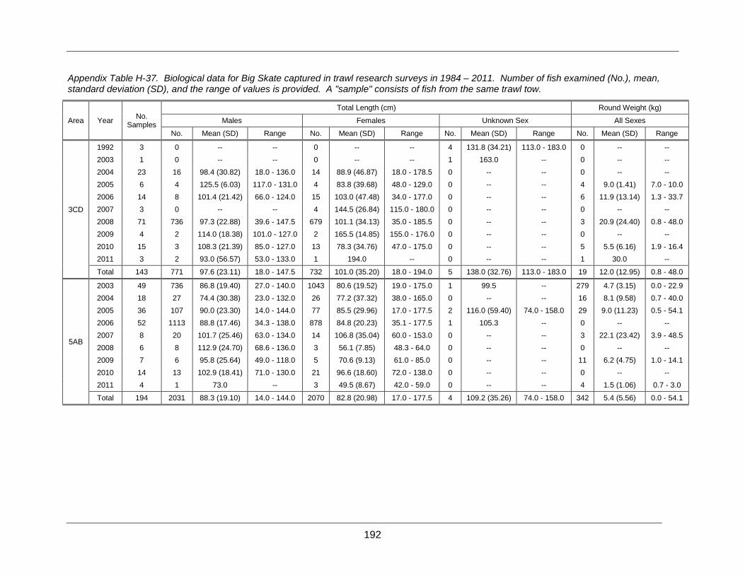
192

Appendix Table H-37. Biological data for Big Skate captured in trawl research surveys in 1984 – 2011. Number of fish examined (No.), mean, standard deviation (SD), and the range of values is provided. A "sample" consists of fish from the same trawl tow.

Area Year No. Samples

Total Length (cm) Round Weight (kg)

Males Females Unknown Sex All Sexes

No. Mean (SD) Range No. Mean (SD) Range No. Mean (SD) Range No. Mean (SD) Range

3CD

1992 3 0 -- -- 0 -- -- 4 131.8 (34.21) 113.0 - 183.0 0 -- -- 2003 1 0 -- -- 0 -- -- 1 163.0 -- 0 -- -- 2004 23 16 98.4 (30.82) 18.0 - 136.0 14 88.9 (46.87) 18.0 - 178.5 0 -- -- 0 -- -- 2005 6 4 125.5 (6.03) 117.0 - 131.0 4 83.8 (39.68) 48.0 - 129.0 0 -- -- 4 9.0 (1.41) 7.0 - 10.0 2006 14 8 101.4 (21.42) 66.0 - 124.0 15 103.0 (47.48) 34.0 - 177.0 0 -- -- 6 11.9 (13.14) 1.3 - 33.7 2007 3 0 -- -- 4 144.5 (26.84) 115.0 - 180.0 0 -- -- 0 -- -- 2008 71 736 97.3 (22.88) 39.6 - 147.5 679 101.1 (34.13) 35.0 - 185.5 0 -- -- 3 20.9 (24.40) 0.8 - 48.0 2009 4 2 114.0 (18.38) 101.0 - 127.0 2 165.5 (14.85) 155.0 - 176.0 0 -- -- 0 -- -- 2010 15 3 108.3 (21.39) 85.0 - 127.0 13 78.3 (34.76) 47.0 - 175.0 0 -- -- 5 5.5 (6.16) 1.9 - 16.4 2011 3 2 93.0 (56.57) 53.0 - 133.0 1 194.0 -- 0 -- -- 1 30.0 --

Total 143 771 97.6 (23.11) 18.0 - 147.5 732 101.0 (35.20) 18.0 - 194.0 5 138.0 (32.76) 113.0 - 183.0 19 12.0 (12.95) 0.8 - 48.0

5AB

2003 49 736 86.8 (19.40) 27.0 - 140.0 1043 80.6 (19.52) 19.0 - 175.0 1 99.5 -- 279 4.7 (3.15) 0.0 - 22.9 2004 18 27 74.4 (30.38) 23.0 - 132.0 26 77.2 (37.32) 38.0 - 165.0 0 -- -- 16 8.1 (9.58) 0.7 - 40.0 2005 36 107 90.0 (23.30) 14.0 - 144.0 77 85.5 (29.96) 17.0 - 177.5 2 116.0 (59.40) 74.0 - 158.0 29 9.0 (11.23) 0.5 - 54.1 2006 52 1113 88.8 (17.46) 34.3 - 138.0 878 84.8 (20.23) 35.1 - 177.5 1 105.3 -- 0 -- -- 2007 8 20 101.7 (25.46) 63.0 - 134.0 14 106.8 (35.04) 60.0 - 153.0 0 -- -- 3 22.1 (23.42) 3.9 - 48.5 2008 6 8 112.9 (24.70) 68.6 - 136.0 3 56.1 (7.85) 48.3 - 64.0 0 -- -- 0 -- -- 2009 7 6 95.8 (25.64) 49.0 - 118.0 5 70.6 (9.13) 61.0 - 85.0 0 -- -- 11 6.2 (4.75) 1.0 - 14.1 2010 14 13 102.9 (18.41) 71.0 - 130.0 21 96.6 (18.60) 72.0 - 138.0 0 -- -- 0 -- -- 2011 4 1 73.0 -- 3 49.5 (8.67) 42.0 - 59.0 0 -- -- 4 1.5 (1.06) 0.7 - 3.0

Total 194 2031 88.3 (19.10) 14.0 - 144.0 2070 82.8 (20.98) 17.0 - 177.5 4 109.2 (35.26) 74.0 - 158.0 342 5.4 (5.56) 0.0 - 54.1

193

Appendix Table H-37. (Continued)

Area Year No. Samples

Total Length (cm) Round Weight (kg)

Males Females Unknown Sex All Sexes

No. Mean (SD) Range No. Mean (SD) Range No. Mean (SD) Range No. Mean (SD) Range

5CDE

1984 32 0 -- -- 0 -- -- 70 98.6 (23.83) 52.0 - 152.0 0 -- -- 1986 62 0 -- -- 0 -- -- 396 98.8 (20.34) 44.0 - 172.0 0 -- -- 1987 16 0 -- -- 0 -- -- 32 114.7 (25.38) 59.0 - 170.0 0 -- -- 1989 34 0 -- -- 0 -- -- 177 99.5 (36.45) 19.0 - 187.0 0 -- -- 1991 27 0 -- -- 0 -- -- 112 91.5 (27.92) 21.0 - 171.0 0 -- -- 1993 41 0 -- -- 0 -- -- 178 88.5 (27.19) 19.0 - 140.0 0 -- -- 1998 24 39 100.5 (22.69) 58.0 - 134.0 25 94.7 (45.41) 48.0 - 188.0 7 71.0 (23.41) 40.0 - 114.0 0 -- -- 2000 22 26 86.8 (28.07) 40.0 - 129.0 33 97.2 (49.28) 40.0 - 182.0 1 174.0 -- 0 -- -- 2002 1 1 20.8 -- 0 -- -- 0 -- -- 1 0.0 -- 2003 80 1182 87.3 (21.10) 44.5 - 144.8 1053 98.7 (40.18) 21.0 - 198.0 1 75.4 -- 941 8.2 (10.27) 0.1 - 55.0 2004 40 2662 94.4 (21.85) 41.2 - 159.0 1133 92.0 (28.41) 33.9 - 182.0 3 128.1 (34.30) 97.2 - 165.0 0 -- -- 2005 87 2777 80.1 (19.51) 35.0 - 140.2 1551 75.7 (23.71) 35.0 - 195.0 1 116.0 -- 17 9.8 (10.94) 0.6 - 40.0 2006 62 2253 82.2 (21.56) 31.9 - 179.1 1112 76.9 (25.03) 32.3 - 195.5 0 -- -- 1 7.8 -- 2007 30 47 85.6 (25.61) 39.0 - 132.0 29 93.3 (49.80) 39.0 - 188.0 0 -- -- 19 12.1 (15.21) 0.7 - 53.9 2009 18 25 91.9 (27.41) 41.0 - 138.0 21 85.8 (33.72) 47.0 - 170.0 0 -- -- 35 7.8 (6.01) 1.3 - 23.2 2011 45 91 95.1 (26.65) 49.0 - 140.0 57 102.7 (41.04) 46.0 - 182.0 0 -- -- 19 10.3 (4.94) 3.7 - 24.6

Total 621 9103 86.0 (21.97) 20.8 - 179.1 5014 85.2 (31.51) 21.0 - 198.0 978 96.7 (27.19) 19.0 - 187.0 1033 8.3 (10.20) 0.0 - 55.0

4B

2003 13 4 48.6 (14.09) 34.0 - 67.5 3 82.1 (16.34) 63.7 - 95.0 11 44.5 (20.68) 19.3 - 86.0 0 -- -- 2005 2 1 22.2 -- 1 30.5 -- 1 48.0 -- 3 0.4 (0.51) 0.1 - 1.0 2008 1 1 73.0 -- 0 -- -- 0 -- -- 1 2.9 --

Total 16 6 48.3 (19.43) 22.2 - 73.0 4 69.2 (29.03) 30.5 - 95.0 12 44.8 (19.74) 19.3 - 86.0 4 1.0 (1.31) 0.1 - 2.9

194

Appendix Table H-38. Biological data for Big Skate captured in longline research surveys in 2003 – 2011. Number of fish examined (No.), mean, standard deviation (SD), and the range of values is provided. A "sample" consists of fish from the same longline set.

Area Year No. Samples

Total Length (cm) Round Weight (kg)

Males Females Unknown Sex All Sexes

No. Mean (SD) Range No. Mean (SD) Range No. Mean (SD) Range No. Mean (SD) Range

3CD

2005 7 12 117.0 (18.71) 75.0 - 139.0 8 108.1 (35.30) 58.0 - 154.0 0 -- -- 0 -- -- 2009 3 3 92.7 (19.40) 80.0 - 115.0 2 94.0 (46.67) 61.0 - 127.0 0 -- -- 5 7.6 (5.80) 1.9 - 15.2 2011 1 1 90.0 -- 0 -- -- 0 -- -- 1 5.1 --

Total 11 16 110.8 (20.79) 75.0 - 139.0 10 105.3 (35.31) 58.0 - 154.0 0 -- -- 6 7.2 (5.29) 1.9 - 15.2

5AB

2003 5 9 105.1 (25.14) 61.3 - 137.0 1 104.0 -- 0 -- -- 9 8.8 (5.62) 1.1 - 18.7 2004 3 2 102.5 (6.36) 98.0 - 107.0 4 101.5 (19.67) 78.0 - 126.0 0 -- -- 0 -- -- 2006 1 0 -- -- 1 107.0 -- 0 -- -- 0 -- -- 2007 2 1 122.0 -- 1 189.0 -- 0 -- -- 0 -- -- 2010 1 1 93.0 -- 0 -- -- 0 -- -- 1 11.8 --

Total 12 13 105.1 (21.49) 61.3 - 137.0 7 115.1 (35.48) 78.0 - 189.0 0 -- -- 10 9.1 (5.38) 1.1 - 18.7

5CDE 2000 2 4 126.5 (4.12) 122.0 - 132.0 2 139.5 (16.26) 128.0 - 151.0 0 -- -- 0 -- --

4B

2003 1 1 81.0 -- 0 -- -- 0 -- -- 0 -- -- 2005 2 2 94.0 (18.38) 81.0 - 107.0 0 -- -- 0 -- -- 0 -- -- 2010 2 0 -- -- 2 127.5 (13.44) 118.0 - 137.0 0 -- -- 2 14.1 (1.32) 13.1 - 15.0

Total 5 3 89.7 (15.01) 81.0 - 107.0 2 127.5 (13.44) 118.0 - 137.0 0 -- -- 2 14.1 (1.32) 13.1 - 15.0

195

Appendix Table H-39. Number of samples examined, summary of total length (cm) by sex, and summary of round weight (kg) for Longnose Skate captured in trawl research surveys in 1984 – 2011. Number of fish examined (No.), mean, standard deviation (SD), and the range of values is provided. A "sample" consists of fish from the same trawl tow.

Area Year No. Samples

Total Length (cm) Round Weight (kg)

Males Females Unknown Sex All Sexes No. Mean (SD) Range No. Mean (SD) Range No. Mean (SD) Range No. Mean (SD) Range

3CD

1992 6 0 -- -- 0 -- -- 6 88.3 (9.77) 77.0 - 105.0 0 -- -- 2001 21 16 87.7 (19.97) 45.6 - 129.3 31 99.1 (20.92) 65.6 - 144.2 0 -- -- 40 6.3 (3.96) 0.5 - 15.9 2002 16 4 98.1 (12.87) 85.2 - 112.5 31 100.6 (16.28) 57.6 - 127.3 0 -- -- 0 -- -- 2004 112 215 73.9 (21.92) 19.0 - 117.0 236 70.8 (26.13) 20.0 - 140.0 0 -- -- 0 -- -- 2005 80 173 64.6 (24.20) 18.0 - 132.0 232 64.3 (22.97) 14.0 - 129.0 0 -- -- 0 -- -- 2006 149 217 69.8 (27.19) 18.0 - 124.0 231 71.8 (28.30) 16.0 - 145.0 0 -- -- 46 5.4 (4.36) 0.4 - 20.6 2007 51 63 58.5 (21.61) 20.0 - 105.0 70 65.7 (25.59) 20.0 - 136.0 0 -- -- 0 -- -- 2008 183 315 68.5 (24.52) 19.0 - 134.0 343 70.3 (27.96) 18.0 - 142.0 1 61.0 -- 14 1.3 (1.36) 0.0 - 4.5 2009 85 296 58.8 (20.98) 17.0 - 120.0 310 59.3 (19.78) 17.0 - 119.0 1 27.0 -- 0 -- -- 2010 155 244 73.1 (21.74) 19.0 - 130.0 205 68.1 (23.93) 16.0 - 129.0 1 70.0 -- 49 4.5 (3.32) 0.6 - 14.2 2011 43 39 65.9 (22.93) 17.0 - 110.0 29 66.3 (26.00) 23.5 - 111.0 0 -- -- 55 1.8 (1.83) 0.1 - 7.2

Total 901 1582 67.7 (23.98) 17.0 - 134.0 1718 68.3 (25.92) 14.0 - 145.0 9 76.4 (22.50) 27.0 - 105.0 204 4.1 (3.76) 0.0 - 20.6

5AB

2003 51 32 85.8 (18.24) 52.0 - 120.0 36 86.4 (13.92) 60.0 - 126.0 2 73.5 (37.48) 47.0 - 100.0 45 4.8 (2.83) 1.2 - 14.5 2004 97 111 78.0 (22.26) 24.0 - 117.0 125 77.1 (23.39) 31.0 - 124.0 1 100.0 -- 39 3.6 (2.50) 0.3 - 10.2 2005 107 187 75.8 (23.37) 23.0 - 124.0 165 72.3 (26.35) 17.0 - 126.0 1 94.0 -- 50 5.7 (3.71) 0.4 - 16.1 2006 50 47 65.9 (28.15) 19.0 - 110.0 76 61.1 (24.19) 19.0 - 117.0 1 86.0 -- 0 -- -- 2007 67 57 81.5 (26.12) 19.0 - 123.0 37 84.5 (27.69) 29.0 - 137.0 1 70.0 -- 33 5.4 (3.20) 0.6 - 12.0 2008 43 44 66.3 (22.75) 24.0 - 116.0 69 69.1 (27.30) 25.0 - 130.5 1 90.6 -- 4 1.9 (2.19) 0.8 - 5.2 2009 89 128 70.3 (26.35) 21.0 - 127.0 134 75.3 (26.48) 21.0 - 124.0 1 74.0 -- 56 5.0 (3.34) 0.7 - 12.2 2010 45 115 76.9 (26.35) 10.0 - 128.0 119 72.1 (22.88) 21.0 - 125.0 0 -- -- 0 -- -- 2011 73 55 77.8 (28.11) 20.5 - 128.5 60 80.0 (22.55) 40.0 - 127.3 2 102.0 (19.80) 88.0 - 116.0 94 3.6 (3.27) 0.0 - 14.7

Total 622 776 75.2 (25.18) 10.0 - 128.5 821 73.9 (25.28) 17.0 - 137.0 10 86.6 (19.15) 47.0 - 116.0 321 4.5 (3.29) 0.0 - 16.1

196

Appendix Table H-39. (Continued)

Area Year No.

Samples

Total Length (cm) Round Weight (kg)

Males Females Unknown Sex All Sexes

No. Mean (SD) Range No. Mean (SD) Range No. Mean (SD) Range No. Mean (SD) Range

5CDE

1984 21 0 -- -- 0 -- -- 40 95.2 (26.16) 29.0 - 141.0 0 -- -- 1986 4 0 -- -- 0 -- -- 8 81.6 (29.83) 41.0 - 124.0 0 -- -- 1987 4 0 -- -- 0 -- -- 5 69.2 (13.72) 58.0 - 93.0 0 -- -- 1989 11 0 -- -- 0 -- -- 25 74.1 (24.93) 29.0 - 132.0 0 -- -- 1991 24 0 -- -- 0 -- -- 30 73.3 (25.68) 23.0 - 117.0 0 -- -- 1993 16 0 -- -- 0 -- -- 31 70.6 (24.57) 22.0 - 105.0 0 -- -- 1998 5 3 102.7 (9.07) 93.0 - 111.0 1 80.0 -- 1 97.0 -- 0 -- -- 2000 14 10 70.7 (18.91) 43.0 - 105.0 3 58.0 (30.51) 27.0 - 88.0 1 96.0 -- 0 -- -- 2003 45 43 82.1 (17.58) 54.8 - 122.0 51 77.4 (20.72) 36.0 - 135.0 0 -- -- 70 3.8 (3.42) 0.2 - 17.7 2004 23 22 97.4 (17.86) 45.0 - 125.0 18 88.0 (20.88) 48.5 - 129.0 0 -- -- 15 6.3 (4.21) 1.0 - 15.1 2005 76 58 86.3 (21.85) 46.0 - 123.0 72 87.7 (22.98) 33.0 - 138.0 0 -- -- 56 4.7 (3.30) 0.6 - 14.8

2006 33 19 100.6 (21.70) 55.0 - 132.0 25 109.7 (22.51) 68.0 - 139.0 3 104.0 (15.72) 86.0 - 115.0 27 9.5 (5.58) 1.1 - 20.0

2007 80 64 90.7 (20.48) 44.0 - 140.0 50 93.0 (22.66) 28.0 - 138.0 2 69.5 (16.26) 58.0 - 81.0 91 5.8 (4.01) 0.4 - 17.0

2008 43 20 105.2 (14.61) 76.0 - 128.0 52 96.0 (20.44) 52.0 - 139.0 0 -- -- 70 6.5 (3.87) 0.8 - 18.2

2009 44 34 94.0 (22.64) 48.0 - 128.0 40 88.5 (20.65) 52.5 - 138.0 0 -- -- 39 5.0 (3.57) 0.8 - 13.5

2010 34 22 101.9 (17.85) 73.0 - 131.0 29 96.4 (16.45) 57.0 - 129.0 0 -- -- 2 4.8 (1.56) 3.7 - 5.9

2011 67 90 81.7 (21.02) 41.5 - 130.0 67 79.8 (22.82) 19.0 - 138.0 1 92.5 -- 21 2.5 (1.89) 0.0 - 7.3

Total 544 385 89.1 (21.49) 41.5 - 140.0 408 88.7 (23.07) 19.0 - 139.0 147 80.2 (26.69) 22.0 - 141.0 391 5.4 (4.07) 0.0 - 20.0

4B 2003 28 47 44.7 (16.92) 19.1 - 78.0 18 48.3 (19.09) 17.0 - 82.0 7 47.2 (21.49) 17.8 - 74.0 0 -- -- 2005 6 2 48.0 (18.38) 35.0 - 61.0 0 -- -- 6 50.0 (16.19) 33.0 - 71.0 7 0.9 (0.81) 0.2 - 2.0

Total 34 49 44.9 (16.78) 19.1 - 78.0 18 48.3 (19.09) 17.0 - 82.0 13 48.5 (18.50) 17.8 - 74.0 7 0.9 (0.81) 0.2 - 2.0

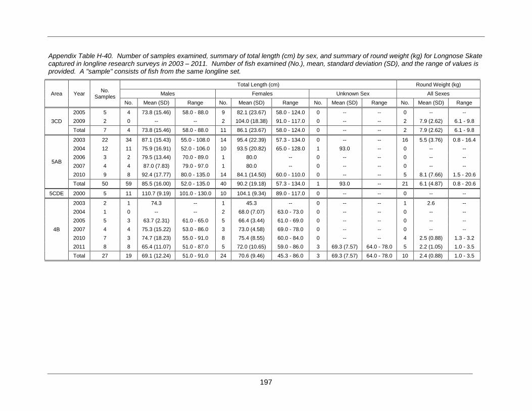
197

Appendix Table H-40. Number of samples examined, summary of total length (cm) by sex, and summary of round weight (kg) for Longnose Skate captured in longline research surveys in 2003 – 2011. Number of fish examined (No.), mean, standard deviation (SD), and the range of values is provided. A "sample" consists of fish from the same longline set.

Area Year No. Samples

Total Length (cm) Round Weight (kg)

Males Females Unknown Sex All Sexes

No. Mean (SD) Range No. Mean (SD) Range No. Mean (SD) Range No. Mean (SD) Range

3CD 2005 5 4 73.8 (15.46) 58.0 - 88.0 9 82.1 (23.67) 58.0 - 124.0 0 -- -- 0 -- -- 2009 2 0 -- -- 2 104.0 (18.38) 91.0 - 117.0 0 -- -- 2 7.9 (2.62) 6.1 - 9.8

Total 7 4 73.8 (15.46) 58.0 - 88.0 11 86.1 (23.67) 58.0 - 124.0 0 -- -- 2 7.9 (2.62) 6.1 - 9.8

5AB

2003 22 34 87.1 (15.43) 55.0 - 108.0 14 95.4 (22.39) 57.3 - 134.0 0 -- -- 16 5.5 (3.76) 0.8 - 16.4 2004 12 11 75.9 (16.91) 52.0 - 106.0 10 93.5 (20.82) 65.0 - 128.0 1 93.0 -- 0 -- -- 2006 3 2 79.5 (13.44) 70.0 - 89.0 1 80.0 -- 0 -- -- 0 -- -- 2007 4 4 87.0 (7.83) 79.0 - 97.0 1 80.0 -- 0 -- -- 0 -- -- 2010 9 8 92.4 (17.77) 80.0 - 135.0 14 84.1 (14.50) 60.0 - 110.0 0 -- -- 5 8.1 (7.66) 1.5 - 20.6

Total 50 59 85.5 (16.00) 52.0 - 135.0 40 90.2 (19.18) 57.3 - 134.0 1 93.0 -- 21 6.1 (4.87) 0.8 - 20.6

5CDE 2000 5 11 110.7 (9.19) 101.0 - 130.0 10 104.1 (9.34) 89.0 - 117.0 0 -- -- 0 -- --

4B

2003 2 1 74.3 -- 1 45.3 -- 0 -- -- 1 2.6 -- 2004 1 0 -- -- 2 68.0 (7.07) 63.0 - 73.0 0 -- -- 0 -- -- 2005 5 3 63.7 (2.31) 61.0 - 65.0 5 66.4 (3.44) 61.0 - 69.0 0 -- -- 0 -- -- 2007 4 4 75.3 (15.22) 53.0 - 86.0 3 73.0 (4.58) 69.0 - 78.0 0 -- -- 0 -- -- 2010 7 3 74.7 (18.23) 55.0 - 91.0 8 75.4 (8.55) 60.0 - 84.0 0 -- -- 4 2.5 (0.88) 1.3 - 3.2 2011 8 8 65.4 (11.07) 51.0 - 87.0 5 72.0 (10.65) 59.0 - 86.0 3 69.3 (7.57) 64.0 - 78.0 5 2.2 (1.05) 1.0 - 3.5

Total 27 19 69.1 (12.24) 51.0 - 91.0 24 70.6 (9.46) 45.3 - 86.0 3 69.3 (7.57) 64.0 - 78.0 10 2.4 (0.88) 1.0 - 3.5

198

Appendix Figure H-1. Plot of tow locations (green dots) in the Vancouver INPFC region for the 1980, 1983, 1989 and 1992 triennial surveys in Canadian waters. Dashed line shows approximate position of the Canada/USA marine boundary. Horizontal lines are the stratum boundaries: 47°30′, 47°50′, 48°20′ and 49°50′. Tows south of the 47°30′ line were not included in the analysis. Isobaths act as stratum boundaries at 55, 183, 220, 366, and 500 m.

199

Appendix Figure H-2. Plot of tow locations (green dots) in the Vancouver INPFC region for the 1995, 1998 and 2001 triennial surveys in Canadian waters. Dashed line shows approximate position of the Canada/USA marine boundary. Horizontal lines are the stratum boundaries: 47°30′, 47°50′, 48°20′ and 49°50′. Tows south of the 47°30′ line were not included in the analysis. Isobaths act as stratum boundaries at 55, 183, 220, 366, and 500 m.

200

Appendix Figure H-3. Distribution of mean catch per unit of effort by 0.1° x 0.1° grid (upper panels) and capture locations (lower panels) for Big Skate and Longnose Skate from the West Coast Vancouver Island shrimp survey in Skate Management Area 3CD in 2003 – 2011.

201

Appendix Figure H-4. Distribution of mean catch per unit of effort by 0.1° x 0.1° grid (upper panels) and capture locations (lower panels) for Big Skate and Longnose Skate from the West Coast Vancouver Island Synoptic survey in Skate Management Area 3CD in 2003 – 2010.

202

Appendix Figure H-5. Distribution of mean catch per unit of effort by 0.1° x 0.1° grid (upper panels) and capture locations (lower panels) for Big Skate and Longnose Skate from the Queen Charlotte Sound shrimp survey in Skate Management Area 5AB in 2003 – 2011.

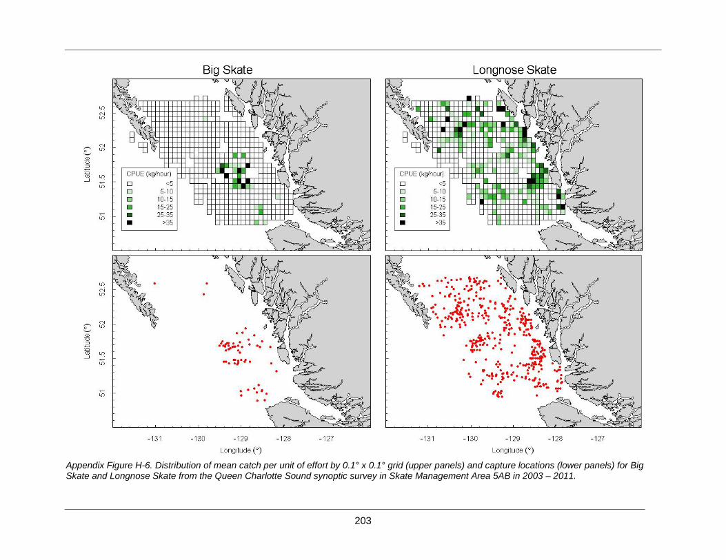
203

Appendix Figure H-6. Distribution of mean catch per unit of effort by 0.1° x 0.1° grid (upper panels) and capture locations (lower panels) for Big Skate and Longnose Skate from the Queen Charlotte Sound synoptic survey in Skate Management Area 5AB in 2003 – 2011.

204

Appendix Figure H-7. Distribution of mean catch per unit of effort by 0.1° x 0.1° grid (upper panels) and capture locations (lower panels) for Big Skate and Longnose Skate from the Hecate Strait Multispecies Assemblage survey in Skate Management Area 5CDE in 1985 – 2003.

205

Appendix Figure H-8. Distribution of mean catch per unit of effort by 0.1° x 0.1° grid (upper panels) and capture locations (lower panels) for Big Skate and Longnose Skate from the Hecate Strait (2005 – 2011) and West Coast Haida Gwaii (2006 – 2010) synoptic surveys in Skate Management Area 5CDE.

206

Appendix Figure H-9. Distribution of mean catch per unit of effort by 0.1° x 0.1° grid (upper panels) and capture locations (lower panels) for Big Skate and Longnose Skate from the IPHC Longline Survey (2003 – 2011) in Skate Management Area 3CD.

207

Appendix Figure H-10. Distribution of mean catch per unit of effort by 0.1° x 0.1° grid (upper panels) and capture locations (lower panels) for Big Skate and Longnose Skate from the IPHC Longline Survey (2003 – 2011) in Skate Management Area 5AB.

208

Appendix Figure H-11. Distribution of mean catch per unit of effort by 0.1° x 0.1° grid (upper panels) and capture locations (lower panels) for Big Skate and Longnose Skate from the IPHC Longline Survey (2003 – 2011) in Skate Management Area 5CDE.

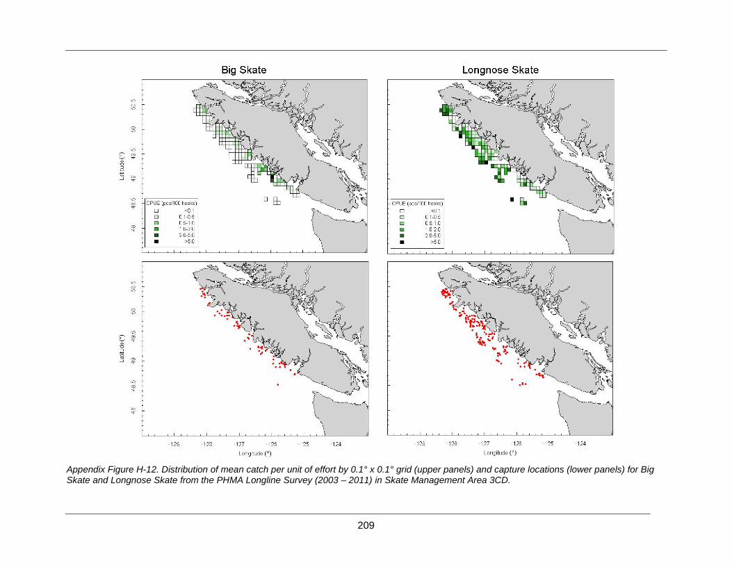
209

Appendix Figure H-12. Distribution of mean catch per unit of effort by 0.1° x 0.1° grid (upper panels) and capture locations (lower panels) for Big Skate and Longnose Skate from the PHMA Longline Survey (2003 – 2011) in Skate Management Area 3CD.

210

Appendix Figure H-13. Distribution of mean catch per unit of effort by 0.1° x 0.1° grid (upper panels) and capture locations (lower panels) for Big Skate and Longnose Skate from the PHMA Longline Survey (2003 – 2011) in Skate Management Area 5AB.

211

Appendix Figure H-14. Distribution of mean catch per unit of effort by 0.1° x 0.1° grid (upper panels) and capture locations (lower panels) for Big Skate and Longnose Skate from the PHMA Longline Survey (2003 – 2011) in Skate Management Area 5CDE.

212

Appendix Figure H-15. Distribution of mean catch per unit of effort by 0.1° x 0.1° grid (upper panels) and capture locations (lower panels) for Big Skate and Longnose Skate from the northern ISRF Longline Survey (2003 – 2011) in Skate Management Area 5AB.

213

Appendix Figure H-16. Distribution of mean catch per unit of effort by 0.1° x 0.1° grid (upper panels) and capture locations (lower panels) for Big Skate and Longnose Skate from the northern ISRF Longline Survey (2003 – 2011) in Skate Management Area 4B.

214

Appendix Figure H-17. Distribution of mean catch per unit of effort by 0.1° x 0.1° grid (upper panels) and capture locations (lower panels) for Big Skate and Longnose Skate from the southern ISRF Longline Survey (2003 – 2011) in Skate Management Area 4B.

215

Appendix Figure H-18. Biomass estimates for Big Skate based on the NMFS Triennial Survey in the INPFC Vancouver region (total region, Canadian waters only and US waters only) in 1980 – 2001. Error bars are the bias corrected 95% confidence intervals based on 1000 bootstrap replicates. The Canadian portion of the Vancouver region is approximately equivalent to Major Area 3C.

Appendix Figure H-19. Biomass estimates for Longnose Skate based on the NMFS Triennial Survey in the INPFC Vancouver region (total region, Canadian waters only and US waters only) in 1980 – 2001. Error bars are the bias corrected 95% confidence intervals based on 1000 bootstrap replicates. The Canadian portion of the Vancouver region is approximately equivalent to Major Area 3C.

0

500

1,000

1,500

0

500

1,000

1,500

1980 1984 1988 1992 1996 2000 1980 1984 1988 1992 1996 2000

1980 1984 1988 1992 1996 2000

Total Vancouver Canada Vancouver

US Vancouver

Bio

mas

s (t)

Year

0

1,000

2,000

3,000

4,000

0

1,000

2,000

3,000

4,000

1980 1984 1988 1992 1996 2000 1980 1984 1988 1992 1996 2000

1980 1984 1988 1992 1996 2000

Total Vancouver Canada Vancouver

US Vancouver

Bio

mas

s (t)

Year

216

Appendix Figure H-20. Biomass estimates for Big Skate and Longnose Skate based on research trawl surveys in Skate Management Area 3CD from 2003 – 2011. Error bars are the bias corrected 95% confidence intervals based on 1000 bootstrap replicates. The NMFS Triennial Survey covered Area 3C only. Note the different scales on the y-axes.

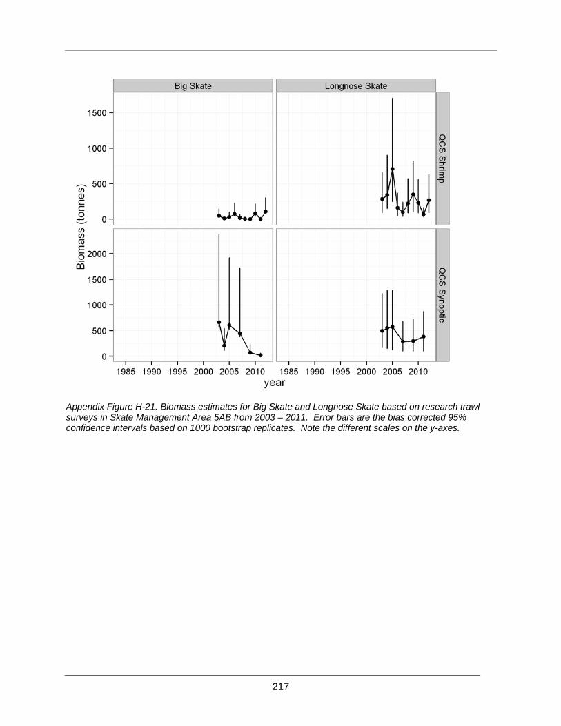
217

Appendix Figure H-21. Biomass estimates for Big Skate and Longnose Skate based on research trawl surveys in Skate Management Area 5AB from 2003 – 2011. Error bars are the bias corrected 95% confidence intervals based on 1000 bootstrap replicates. Note the different scales on the y-axes.

218

Appendix Figure H-22. Biomass estimates for Big Skate and Longnose Skate based on research trawl surveys in Skate Management Area 5CDE from 1985 – 2011. Error bars are the bias corrected 95% confidence intervals based on 1000 bootstrap replicates. Note the different scales on the y-axes.

219

Appendix Figure H-23. Biomass estimates for Big Skate and Longnose Skate based on research longline surveys in Skate Management Area 3CD from 2003 – 2011. Error bars are the bias corrected 95% confidence intervals based on 1000 bootstrap replicates.

220

Appendix Figure H-24. Biomass estimates for Big Skate and Longnose Skate based on research longline surveys in Skate Management Area 5AB from 2003 – 2011. Error bars are the bias corrected 95% confidence intervals based on 1000 bootstrap replicates.

221

Appendix Figure H-25. Biomass estimates for Big Skate and Longnose Skate based on research longline surveys in Skate Management Area 5CDE from 2003 – 2011. Error bars are the bias corrected 95% confidence intervals based on 1000 bootstrap replicates.

222

Appendix Figure H-26. Biomass estimates for Big Skate and Longnose Skate based on research longline surveys in Skate Management Area 4B from 2003 – 2011. Error bars are the bias corrected 95% confidence intervals based on 1000 bootstrap replicates

223

SURPLUS PRODUCTION MODEL APPENDIX I.(Case Study: Big Skate in 5CDE)

I.1 INTRODUCTION A surplus production model (SPM) is one possible method of estimating current stock status in the context of maximum sustainable yield (MSY) and associated parameters such as FMSY (the fishing mortality rate that produces MSY) and BMSY (the biomass that supports MSY removals). To investigate whether a SPM would be useful for estimating stock status for Big Skate and Longnose Skate in British Columbia, a SPM was applied to a subset of the available data. The model was applied to Big Skate in Skate Management Area 5CDE, which corresponds to Hecate Strait, Dixon Entrance, and the west coast of Haida Gwaii, and used life history data, commercial catch from the trawl and longline sectors of the commercial fishery in 1996 – 2011 (Appendix D), standardized trawl catch-per-unit effort data for 1996 – 2011 (Appendix G), and a fishery-independent research survey as an additional index of abundance (1984 – 2003; Choromanski et al. 2005; Appendix H). The SPM was applied in a Bayesian context informed by life history data.

I.2 METHODS

I.2.1 Model Description A Graham-Schaefer surplus production model (SPM) was selected (Schaefer 1954; Hilborn and Walters 1992). The Graham-Schaefer model estimates stock status as follows:

(1)

Biomass dynamic modelswhere Bt is the biomass of the stock at time t, r (year-1) is the intrinsic growth rate of the population in the absence of density-dependence, K is the carrying capacity (tonnes), and Ct is catch in tonnes at time t.

The Graham-Schaefer model allows for the direct estimation of MSY, BMSY, and FMSY, as follows:

(2)

(3)

(4)

The surplus production model and Leslie Matrices were run in R 2.10.1 (R Development Core Team 2009). R code is provided in Appendix L.

I.2.2 Model Inputs I.2.2.1 Fishery dependent catch data Catch data for Big Skate from the commercial trawl and line fisheries in Skate Management Area 5CDE were gathered from 1996 to 2011 from the DFO PacHarvTrawl, PacHarvHL, and

tt

ttt CKBrBBB −

−+=+ 11

=

4KrMSY

2KBMSY =

2rFMSY =

224

GFFOS databases (Fisheries and Oceans Canada, Pacific Region, Groundfish Data Unit). Details of the commercial catch data as well as summary tables are provided in Appendix D.

In order to fit the stock assessment model, a time series of annual catch and fishery-dependent standardized catch-per-unit-effort (CPUE) was generated for 1996 – 2011. Annual landings (tonnes) were calculated by summing the landings from each trawl tow (targeted and non-targeted) and line trip in a given year. Appropriate discard mortality rates as described in Appendix D were applied to calculate dead discards, and total catch was therefore the sum of landings plus dead discards (Appendix Figure I-1). The CPUE standarization is described in detail in Appendix G (Appendix Figure I-1).

I.2.2.2 Fishery independent data The Hecate Strait Multispecies trawl survey was a fishery-independent research trawl survey conducted 11 times between 1984 and 2003 (Choromanski et al. 2005). The survey recorded tow duration (minutes), trawl door spread (meters), vessel speed (meters per minute), Big Skate weight (kg), and Big Skate density (kg/m2). Survey data was obtained from the DFO GFBio database (Fisheries and Oceans Canada, Pacific Region, Groundfish Data Unit). Annual CPUE from the Hecate Strait Multispecies trawl survey was used as an additional, fishery-independent, index of abundance for Big Skate. Annual CPUE (tonnes/hr) was calculated as the total catch of Big Skate for each survey in tonnes divided by the total hours spent trawling for the survey (Appendix Figure I-1). All tows were included even if they did not encounter Big Skate.

I.2.3 Estimating Priors I.2.3.1 Intrinsic Rate of Growth (r) The Graham-Schaefer model requires an estimate of the intrinsic rate of increase of the population, r (Eq. 1). Following the methodology of McAllister et al. (2001), a demographic method was used to construct a prior probability for r, using life history data for Big Skate.

McAllister et al. (2001) use a Leslie matrix to calculate rm , the innate capacity for increase, or the maximum per capita rate of increase in the absence of density-dependence. Leslie matrices project a population matrix over some set time period until the population age structure has stabilized. The estimate of rm is calculated by taking the ratio of abundance between a time step and the one previous (McAllister et al. 2001). The population was set to have 1,000 individuals and was projected for 300 years following the methods of McAllister et al. (2001).

The initial number of individuals at age x is given by

(5)

Where lx is the expected survivorship from age 0 to age x.

The number of individuals in the next time step is calculated by

(6)

where A is the maximum age of the population, mx is the percent mature at age x, and Nx,t are the numbers of individuals of age x at time t.

The matrix was projected for 300 years to ensure that the population stabilized. In order to determine when stabilization occurs, the average percent change in the proportion at age between each time is calculated. Once the proportion is lower than 0.0001%, the population is assumed to have reached a stable distribution, and rm is calculated by

xx lN ⋅= 000,10,

∑=

+ =A

xtxxt NmN

0,1,0

225

(7)

where Pt is the sum of individuals in each age class (McAllister et al. 2001).

Four life history parameters are needed to calculate rm using Leslie matrices: natural mortality, maximum age, age at maturity, and fecundity. For each parameter, a uniform distribution was created to account for uncertainty.

Maximum age for Big Skates in British Columbia was reported as 26 years (McFarlane and King 2006). The uniform distribtution included ages ranging from 23 to 29 years (+/- 3 years).

Maximum age was used to estimate natural mortality through Hoenig’s (1983) equation:

(8)

where M is natural mortality and tmax is maximum age.

Assuming a maximum age of 26 years (McFarlane and King 2006), Equation 8 predicts an M of 0.172 year-1 for Big Skate. A uniform distribution was used to include values +/- 0.05 of the predicted M, resulting in a range of M from 0.122 to 0.222 year-1.

Age at maturity for females is believed to be 8 yrs; however, the youngest mature female found was 5 years and the oldest immature female found was 9 years (McFarlane and King 2006). Therefore, the uniform distribution for age at maturity ranged between 5 and 10 years.

Fecundity was defined as mean litter size per breeding event. The mean litter size for Big Skate assumes that Big Skate release 2 egg cases, each containing 4 pups, for every breeding event. The model assumes a 1:1 sex ratio and therefore 4 daughters per breeding event. The uniform distribution for fecundity ranged between 0 and 8 daughters per breeding event which is plausible for Big Skate given that individual egg cases may contain between 1 and 7 pups (Ebert 2003).

One thousand Monte Carlo simulations were run to develop a distribution of rm . Simulations that did not converge on a value of rm were not included in the final distribution. However, negative rm values and those lower than 0.01 year-1 were included.

The final distribution of rm was used to inform a prior for r, the intrinsic growth rate of the population, for the Graham-Schaefer model (Appendix Figure I-2). The prior for r was best represented by a log-normal distribution bounded between 0.036 – 0.961 year-1:

(9)

I.2.3.2 Carrying Capacity (K) The 5CDE Big Skate stock may have been at some fraction of K in 1996 because the groundfish fishery began around 1954, and although not targeted, Big Skate landings and discards may have occurred. The prior for K was a rescaled beta (α = 1.15, β = 1.15) distributed between 1 and 10 million tonnes (Eq. 10). The wide, slightly informative distribution for K attempted to give the model flexibility to find the most probable value given the data.

(10)

)log( 1+

=t

tm P

Pr

( ) ( )maxlog982.044.1log tM ⋅−=

( ) ( )33.0sd,16.0meanloglnorm~p ==r

( )15.1,15.1beta~110

1p 7 ==

−− βαK

226

I.2.3.3 Depletion Depletion estimates biomass at the start of the fishery as a proportion of K (Punt 1990). Depletion was uniformly distributed between 0.05 and 1 (Eq. 11). A uniform distribution was used because a beta distribution would allow the depletion to equal zero which would cause the model to crash.

(11)

I.2.4 Estimating Stock Status The Graham-Schaefer model predicted the index of abundance using the following equation:

(12)

where Ij,t is the abundance for index j at time t, and q is the catchability coefficient which scales the population size to the index j. In order to calculate the likelihood for each index of abundance, we assumed a sigma of 0.30 for each index of abundance.

The relative fit of the Graham-Schaefer model to the catch, CPUE, and survey data was determined using the log-likelihood. The negative log-likelihood for each index of abundance was calculated using the following:

(13)

where Ij,t and q are defined as above, r is the intrinsic rate of growth, K is the carrying capacity, depl is the depletion, is the variance of each index j where = 0.30, and j is each respective index at time t. The total negative log-likelihood was equal to the sum of the negative log-likelihood of each available index (Eq. 13) multiplied by the prior probability distributions of the three model parameters, r, K, and depletion (Eqs. 9 – 11). Markov chain Monte Carlo (MCMC) methods were used to sample from the posterior probability distributions of the three model parameters, r, K, and depletion, using 4 million iterations, a burn-in of 2,000, and thin of 1,000 for a total chain length of 3,998. MCMC diagnostics were checked to determine if the chains had converged on the posterior distribution of the model parameters. Posterior probability distributions of r and K were used to calculate probability distributions of MSY, BMSY, and FMSY. Each iteration of the MCMC chain was used to calculate the predicted Big Skate population for the entire length of the time series along with 50, 80 and 90% quantiles. Additionally, the median of the posterior distribution for the three model parameters was used to predict an index of abundance for the stock.

I.3 RESULTS

I.3.1 Parameter Estimates and Stock Status The highly informative prior probability distribution for the intrinsic population growth rate, r, influenced the posterior probability distributions for all three parameters of the Graham-Schaefer surplus production model. The prior and posterior probability distribution almost completely overlapped, signifying that the observed data (i.e., total catch, standardized CPUE, and research survey CPUE) contained little information regarding the true value of r (Appendix Figure I-2). The mode of the posterior of r equalled 0.176 year-1. The posterior distribution of the carrying capacity, K, was highly skewed towards higher abundances, likely as a result of the

( ) ( )00.1max,05.0minuniform~depletionp ==

tjtj BqI =,

( ) ( ) ( )( )2,,22,

,ˆloglog

21

21log,,,,|logL tjtj

jjtj

jjtj III

deplKrqI −+

−=−

σπσσ

2jσ jσ

227

inverse relationship between r and K (Appendix Figure I-2). The mode of the posterior probability distribution of K occurred at approximately 266,000 tonnes. The mode of the depletion posterior distribution for 5CDE signified that at the start of the targeted fishery in 1996 the stock was at 51% of K (Appendix Figure I-2). The depletion result suggests that non-targeted Big Skate mortality induced through other fisheries prior to 1996 is a possibility. The median estimates of r, K, and depletion occurred at 0.189 year-1, 880,000 tonnes, and 56% for 5CDE. Quantiles, means, and standard deviations for the posterior distributions of the three model parameters for 5CDE are shown in Appendix Table I-1.

Posterior distributions of MSY and BMSY exhibited high uncertainty, whereas FMSY was highly informative. The mode of the posterior for MSY for 5CDE equalled 11,000 tonnes (Appendix Figure I-3). BMSY is directly related to K; therefore, the posterior distributions and modes of BMSY exactly match that of K, except the values are halved (Appendix Figure I-3). The long tails present in the MSY and BMSY posterior distributions are due to the highly skewed posterior for K. The posterior distribution for FMSY in 5CDE is directly related to the posterior distribution for r and as a result also exhibits a tight distribution about its mode, equal to 0.087 year-1 (Appendix Figure I-3). Quantiles, means, and standard deviations for MSY, BMSY, and FMSY for 5CDE Big Skate are shown in Appendix Table I-1.

Using the median estimates of the posterior probability distributions, the surplus production model predicted 5CDE Big Skate abundance to be at carrying capacity. For 5CDE the predicted population biomass was 490,000 tonnes in 1984 and stabilized at its final predicted biomass of 875,000 tonnes (Appendix Figure I-4). The standardized CPUE time series and the Hecate Strait Multispecies survey for the 5CDE was highly variable and showed little trend; hence, the model fit a horizontal line through the later part of the time series (Appendix Figure I-5).

I.3.2 Uncertainty in Parameter Estimates and stock status Posterior distributions for r, K and depletion for 5CDE were highly dependent on the informative prior probability distribution used for r. Due to the lack of variation in the CPUE and survey data, the prior probability distribution of r outweighs the likelihood of the data which results in a posterior distribution for r that almost identically matches its prior distribution. The informative prior for r influences the posterior distribution for K since these two parameters are inversely correlated (Hilborn and Walters 1992). In order to get reliable estimates of K, fishery data needs to have contrast. Ideally, data will be collected from when the population is near K (i.e., pre-exploitation), when it has been fished to low abundances, and then when it is allowed to recover. Furthermore, the informative prior for r also indirectly affects the posterior distribution of depletion since it is calculated jointly with r and K.

The extent of uncertainty in estimates of MSY, BMSY and FMSY are directly related to the uncertainty in the estimates of r and K. The high uncertainty in the estimates of MSY is due in part to the high uncertainty in K while estimates of BMSY are entirely dependent on the uncertainty of the K posterior. The tight distribution of the FMSY posterior is a function of the informative prior and tight posterior distribution for r. For elasmobranchs, MSY generally ranges between 4.5 and 7.5% of the unexploited biomass (Anderson 1990). The MSY was estimated between 6.5 and 7.6% of the unexploited biomass in a multispecies ray fishery in the South Atlantic (Agnew et al. 2000). The mode of the MSY posterior was approximately 4% of the mode of the K posterior in 5CDE (11,000/266,000 tonnes). It is likely that creating an informative prior for K, possibly by using density estimates for Big Skate and area swept data from research surveys, would narrow the range of possible MSY and BMSY values.

228

The median predicted population size and predicted indices of abundance of Big Skate in 5CDE were stable during the later part of the time series. The wide range of predicted population sizes results from the skewed K posterior distribution. As previously mentioned, creating an informative prior for K could generate a narrower range of predicted population abundances. The model output suggests that the catch taken from 1984 – 2011 did not have a significant effect on the population dynamics of Big Skate in either stock. These findings are based on the assumption that there was zero Big Skate catch from 1984 – 1995 which may be unrealistic. The best fit to the multiple indices of abundance used in this model was a relatively horizontal line through the later data points and was likely due to the variability and lack of contrast in the data. It is unknown if the lack of trends observed in the data are representative of the true population abundance.

I.4 REFERENCES Agnew, D.J., Nolan, C.P., Beddington, J.R., and Baranowski, R. 2000. Approaches to the

assessment and management of multispecies skate and ray fisheries using the Falkland Islands fishery as an example. Canadian Journal of Fisheries and Aquatic Science, 57: 429 – 440.

Anderson, E. D. 1990. Fishery models as applied to elasmobranch fisheries. Elasmobranchs as living resources: advances in the biology, ecology, systematics and the status of the fisheries. NOAA Technical Report NMFS, 90: 479 – 490.

Choromanski E.M., Workman, G.D., and Fargo, J. 2005. Hecate Strait multispecies bottom trawl survey, CCGS W.E. Ricker, May 19 to june 7, 2003. Can. Data Rep. Fish. Aquat. Sci. 1169: viii + 85 p.

Ebert, D.A. 2003. Sharks, rays, and chimaeras of California. University of California Press, Berkeley, California. 297 pp.

Hilborn, R., and Walters, C.J. 1992. Quantitative Fisheries Stock Assessment: Choice, Dynamics and Uncertainty. Chapman & Hall, New York. 592 pp.

Hoenig, J.M. 1983. Empirical use of longevity data to estimate mortality rates. Fishery Bulletin, 82: 898–902.

McFarlane, G.A., and King, J.R., 2006. Age and growth of Big skate (Raja binoculata) and Longnose skate (Raja rhina) in British Columbia waters. Fisheries Research, 78: 169–178.

McAllister, M.K., Pikitch, E.K., and Babcock, E.A. 2001.Using demographic methods to construct Bayesian priors for the intrinsic rate of increase in the Schaefer model and implications for stock rebuilding. Canadian Journal of Fisheries and Aquatic Science, 58:1871 – 1890.

Punt, A. E. 1990. Is B1= K an appropriate assumption when applying an observation error production model estimator to catch–effort data? South African Journal of Marine Science, 9:249–259.

R Development Core Team. 2009. R: A language and environment for statistical computing. R 16 Foundation for Statistical Computing. Vienna, Austria. URL http://www.R-project.org.

Schaefer, M. B. 1954. Some aspects of the dynamics of populations important to the management of the commercial marine fisheries. Bulletin of the Inter-American Tropical Tuna Commission, 1:25–56.

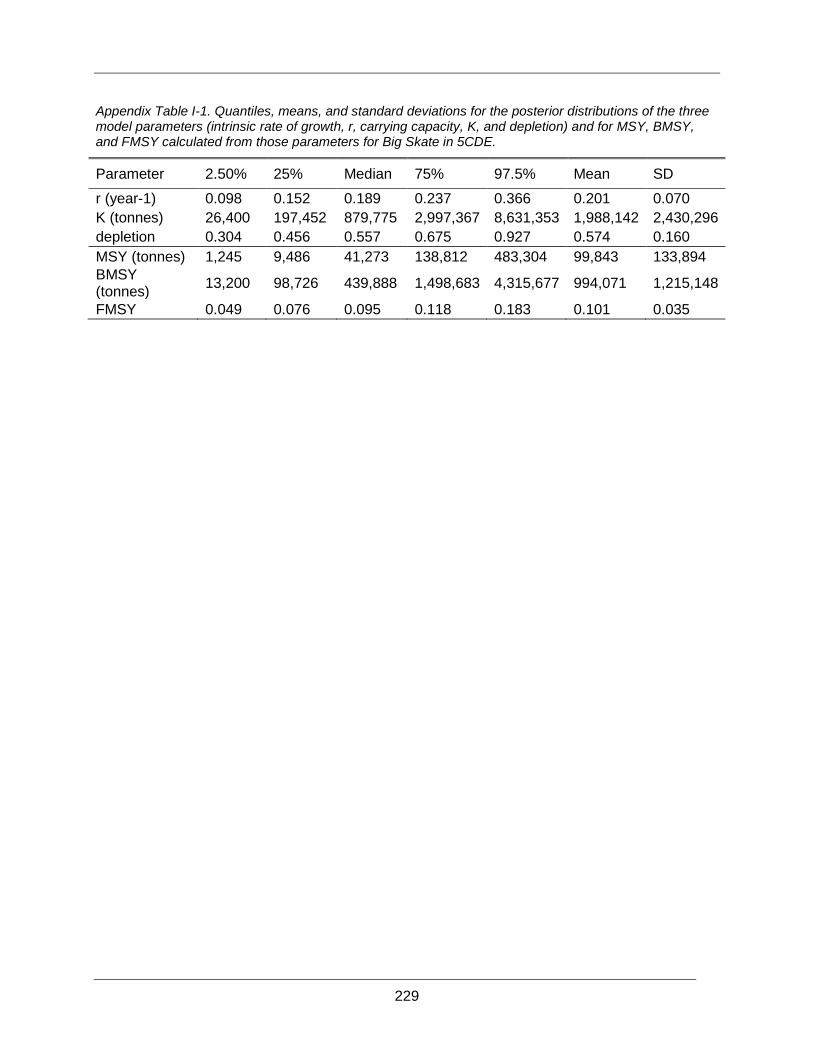
229

Appendix Table I-1. Quantiles, means, and standard deviations for the posterior distributions of the three model parameters (intrinsic rate of growth, r, carrying capacity, K, and depletion) and for MSY, BMSY, and FMSY calculated from those parameters for Big Skate in 5CDE.

Parameter 2.50% 25% Median 75% 97.5% Mean SD

r (year-1) 0.098 0.152 0.189 0.237 0.366 0.201 0.070 K (tonnes) 26,400 197,452 879,775 2,997,367 8,631,353 1,988,142 2,430,296 depletion 0.304 0.456 0.557 0.675 0.927 0.574 0.160 MSY (tonnes) 1,245 9,486 41,273 138,812 483,304 99,843 133,894 BMSY (tonnes) 13,200 98,726 439,888 1,498,683 4,315,677 994,071 1,215,148

FMSY 0.049 0.076 0.095 0.118 0.183 0.101 0.035

230

Appendix Figure I-1. Abundance indices for Big Skate from 5CDE: (A) Catch (landings plus dead discards, tonnes) from the commercial trawl and longline fisheries; (B) Standardized commercial trawl catch per unit of effort (CPUE); and (C) Total annual CPUE (tonnes per hour) from the Hecate Strait Multispecies Survey (1984 – 2003).

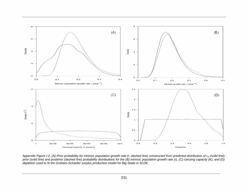
231

Appendix Figure I-2. (A) Prior probability for intrinsic population growth rate (r, dashed line) constructed from predicted distribution of rm (solid line); prior (solid line) and posterior (dashed line) probability distributions for the (B) intrinsic population growth rate (r), (C) carrying capacity (K), and (D) depletion used to fit the Graham-Schaefer surplus production model for Big Skate in 5CDE.

232

Appendix Figure I-3. Posterior probability distributions for MSY, BMSY , and FMSY, for Big Skate in 5CDE.

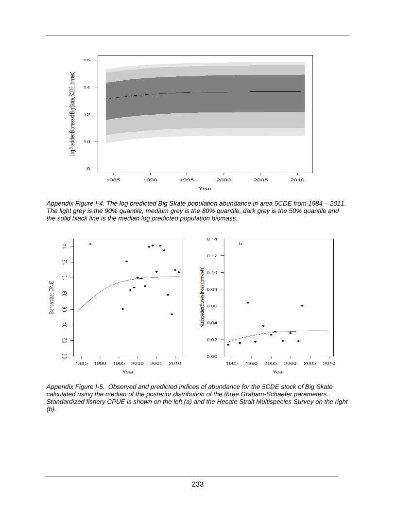
233

Appendix Figure I-4. The log predicted Big Skate population abundance in area 5CDE from 1984 – 2011. The light grey is the 90% quantile, medium grey is the 80% quantile, dark grey is the 50% quantile and the solid black line is the median log predicted population biomass.

Appendix Figure I-5. Observed and predicted indices of abundance for the 5CDE stock of Big Skate calculated using the median of the posterior distribution of the three Graham-Schaefer parameters. Standardized fishery CPUE is shown on the left (a) and the Hecate Strait Multispecies Survey on the right (b).

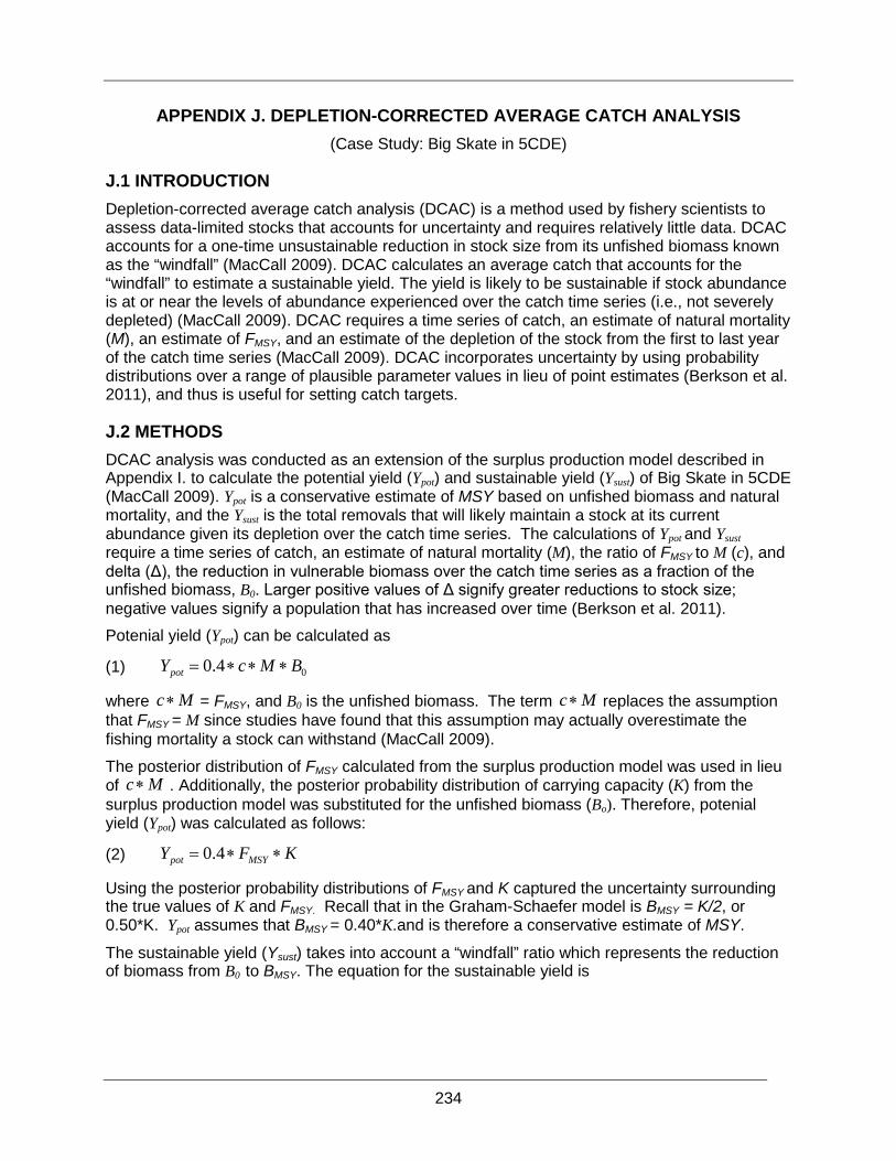
234

DEPLETION-CORRECTED AVERAGE CATCH ANALYSIS APPENDIX J.(Case Study: Big Skate in 5CDE)

J.1 INTRODUCTION Depletion-corrected average catch analysis (DCAC) is a method used by fishery scientists to assess data-limited stocks that accounts for uncertainty and requires relatively little data. DCAC accounts for a one-time unsustainable reduction in stock size from its unfished biomass known as the “windfall” (MacCall 2009). DCAC calculates an average catch that accounts for the “windfall” to estimate a sustainable yield. The yield is likely to be sustainable if stock abundance is at or near the levels of abundance experienced over the catch time series (i.e., not severely depleted) (MacCall 2009). DCAC requires a time series of catch, an estimate of natural mortality (M), an estimate of FMSY, and an estimate of the depletion of the stock from the first to last year of the catch time series (MacCall 2009). DCAC incorporates uncertainty by using probability distributions over a range of plausible parameter values in lieu of point estimates (Berkson et al. 2011), and thus is useful for setting catch targets.

J.2 METHODS DCAC analysis was conducted as an extension of the surplus production model described in Appendix I. to calculate the potential yield (Ypot) and sustainable yield (Ysust) of Big Skate in 5CDE (MacCall 2009). Ypot is a conservative estimate of MSY based on unfished biomass and natural mortality, and the Ysust is the total removals that will likely maintain a stock at its current abundance given its depletion over the catch time series. The calculations of Ypot and Ysust require a time series of catch, an estimate of natural mortality (M), the ratio of FMSY to M (c), and delta (Δ), the reduction in vulnerable biomass over the catch time series as a fraction of the unfished biomass, B0. Larger positive values of Δ signify greater reductions to stock size; negative values signify a population that has increased over time (Berkson et al. 2011). Potenial yield (Ypot) can be calculated as

(1)

where = FMSY, and B0 is the unfished biomass. The term replaces the assumption that FMSY = M since studies have found that this assumption may actually overestimate the fishing mortality a stock can withstand (MacCall 2009).

The posterior distribution of FMSY calculated from the surplus production model was used in lieu of . Additionally, the posterior probability distribution of carrying capacity (K) from the surplus production model was substituted for the unfished biomass (Bo). Therefore, potenial yield (Ypot) was calculated as follows:

(2)

Using the posterior probability distributions of FMSY and K captured the uncertainty surrounding the true values of K and FMSY. Recall that in the Graham-Schaefer model is BMSY = K/2, or 0.50*K. Ypot assumes that BMSY = 0.40*K.and is therefore a conservative estimate of MSY.

The sustainable yield (Ysust) takes into account a “windfall” ratio which represents the reduction of biomass from B0 to BMSY. The equation for the sustainable yield is

04.0 BMcYpot ∗∗∗=

Mc ∗ Mc ∗

Mc ∗

KFY MSYpot ∗∗= 4.0

235

(3)

where C are all the catches in the time series, n is the number of years in the catch time series, and the ratio of W/Ypot (= Δ/0.4*FMSY) expresses the windfall relative to a single year of potential yield. If no change in abundance occurred (i.e., Δ=0), the equation for Ysust equals the average catch. If stock abundance increased, Δ and the ratio W /Ypot are negative and the resulting Ysust is larger than the average of historic catches (McCall, 2009).

Delta (Δ) is the reduction in vulnerable biomass over the catch time series as a fraction of the unfished biomass, B0. Δ is calculated using the equation

(4)

where BFYR is the biomass in the first year of the time series, BLYR is the biomass in the last year of the time series, and B0 is the unfished biomass (MacCall 2009).

The first and last year biomass predicted from the surplus production model were used to calculate the difference in biomass over the time series. As for Ypot, the posterior probability distribution of K from the surplus production model was substituted for the unfished biomass (B0) to calculate a posterior distribution of Δ. According to the surplus production model predictions of first and last year biomass and K, the 95% quantile of Δ for 5CDE was -0.66 to – 0.06 for the time period 1984 to 2011 (Appendix Figure J-1). Random values of Δ were drawn directly from the posterior estimates of Δ. The 95% quantiles of Δ are negative thereby predicting that the 5CDE biomass of Big Skate has increased over its respective catch time series. However, the range of Δ does include zero (i.e., same biomass at first and last year) and positive estimates (i.e., decreasing biomass over the time series). The estimates of Ysust predicted by the posterior Δ estimate accounts for the uncertainty contained in the SPM outputs. Estimated Ysust values were intertpreted in the context of the stock abundance estimated by the SPM.

All analyses were run in R 2.10.1 (R Development Core Team 2009). R code is provided in Appendix L.

J.3 RESULTS Estimates of potential yield (Ypot) for Big Skate in 5CDE were lower than the estimates of MSY obtained using the surplus production model because DCAC assumes that BMSY occurs at 40% of B0 (or K) rather than 50% of B0 (or K). Resulting estimates of sustainable yield (Ysust) were significantly lower than both the Ypot and MSY because the 5CDE stock is estimated to be well above BMSY. If the stock was at BMSY then it would be able to sustain removals equivalent to approximately 9,000 tonnes, the mode of the Ypot posterior distribution (Appendix Figure J-2). Based on the mode the of Ysust posterior distribution, the 5CDE stock of Big Skate can sustain removals equal to 530 tonnes without changing the current estimated stock size. The density distribution of Ysust starts at approximately 300 tonnes, equivalent to the average Big Skate catch from 1984 to 2011, increases to its mode of 530 tonnes, and then decreases to nearly zero at 2,000 tonnes (Appendix Figure J-3).

As a result of the low estimates of FMSY predicted by the surplus production model a number of the “windfall” ratios calculated were highly negative numbers. Consequently, the Ysust values predicted from these “windfall” ratios were also negative and are thus considered inplausible. Therefore, Appendix Figure J-3 only shows plausible Ysust values. Given the assumed range of

pot

sust

YWn

CY

+= ∑

0BBB LYR

FYR −=∆

236

Δ values, the range of predicted plausible Ysust for 5CDE Big Skate is approximately 300 – 166,000 tonnes. The unlikely upper bounds of the Ysust distribution occur when the denominator the Ysust equation approaches zero (i.e., the “windfall” ratio approaches -28). The relatively low plausible Ysust values occur because the current predicted abundance in 5CDE is near or at carrying capacity and experiencing strong effects of density-dependence. Appendix Table J-1 shows the 2.5, 25, 50, 75, and 97.5% quantiles, mean, and standard deviation for Ypot and Ysust, respectively.. A stock at carrying capacity is not as productive as a stock below carrying capacity due to the strong effects of density-dependence resulting in low birth rates relative to death rates.

The surplus production model predicted an increase in the stock’s biomass since the beginning of the time series; hence, most of the assumed depletion (Δ) values were negative and the resulting predicted modal sustainable yield (approximately 530 tonnes) is larger than the average of historic catches (approximately 330 tonnes). However, our assumption of zero catch from 1984 – 1995 has a large effect on the sustainable yield. If we assumed a non-zero catch from 1984 – 1995, the predicted sustainable yield would likely be larger than those presented here.

J.4 REFERENCES Berkson, J., L. Barbieri,L., Cadrin,S., Cass-Calay, S.L., Crone, P., Dorn, M., Friess, C.,

Kobayashi, D., Miller,T.J., Patrick, W.S., Pautzke, S., Ralston, S., and Trianni, M. 2011. Calculating acceptable biological catch for stocks that have reliable catch data only (Only Reliable Catch Stocks – ORCS). NOAA Technical Memorandum NMFS-SEFSC-616, 56 pp.

MacCall, A. D. 2009. Depletion-corrected average catch: a simple formula for estimating sustainable yields in data-poor situations. International Council for the Exploration of the Seas Journal of Marine Science, 66: 2267–2271.

R Development Core Team. 2009. R: A language and environment for statistical computing. R 16 Foundation for Statistical Computing. Vienna, Austria. URL http://www.R-project.org.

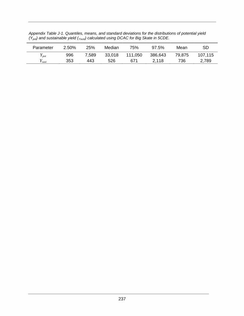
237

Appendix Table J-1. Quantiles, means, and standard deviations for the distributions of potential yield (Ypot) and sustainable yield (Ysust) calculated using DCAC for Big Skate in 5CDE.

Parameter 2.50% 25% Median 75% 97.5% Mean SD Ypot 996 7,589 33,018 111,050 386,643 79,875 107,115 Ysust 353 443 526 671 2,118 736 2,789

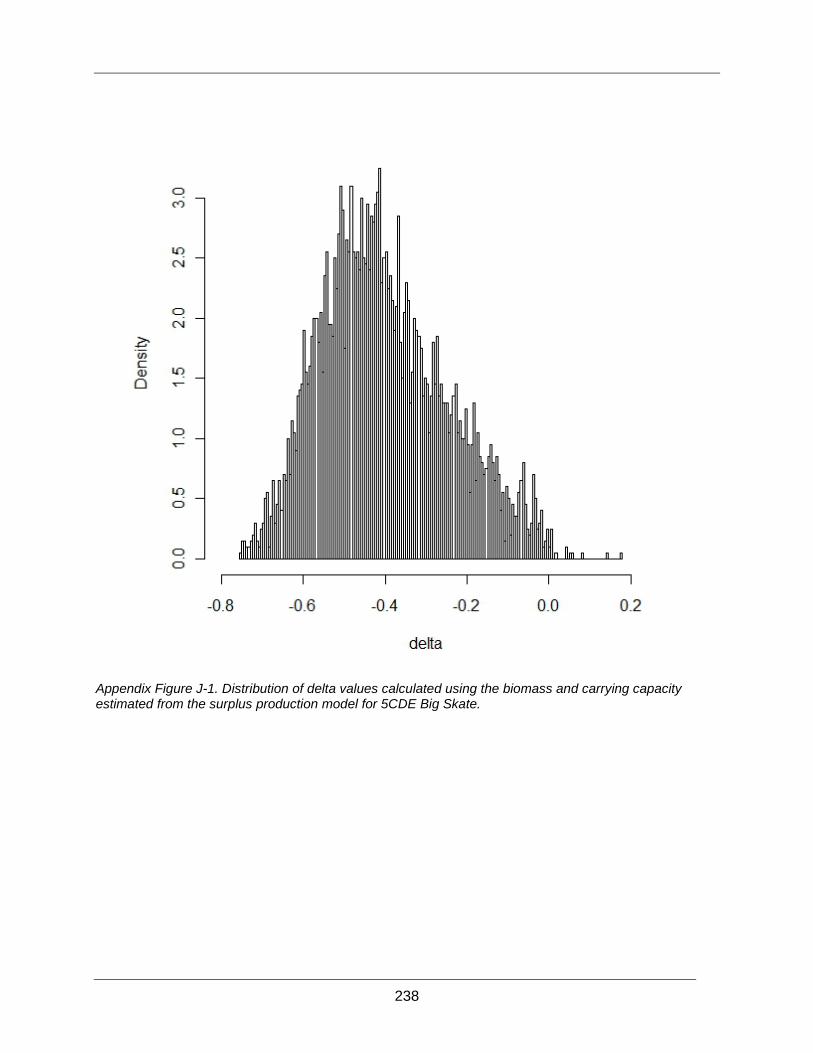
238

Appendix Figure J-1. Distribution of delta values calculated using the biomass and carrying capacity estimated from the surplus production model for 5CDE Big Skate.

239

Appendix Figure J-2. Potential yield (Ypot) (solid line) estimated using DCAC compared to MSY (dashed line) estimated from the Graham-Schaefer surplus production model Big Skate from 5CDE.

Appendix Figure J-3. Distribution of sustainable yield (Ysust) estimated using DCAC for the Big Skate from 5CDE.

240

CATCH-MSY APPROACH APPENDIX K.

K.1 CATCH-MSY APPROACH Martell and Froese (2012) introduced a simple approach of estimating maximum sustainable yield (MSY) using time series of removals along with estimates of the maximum rate of population increase (r) and carrying capacity (k) for a given stock. The approach uses the Schaefer production model to estimate annual biomasses for a given set of r and k parameters. A narrow range of r-k combinations are able to maintain a population without collapse or without exceeding an assumed carrying capacity in order to produced the observed removals. Random r-k pairs are drawn from a uniform prior distribution and a Bernoulli distribution is used as a likelihood function for accepting each pair. In order to be accepted the r-k pairs must 1) result in in a final relative biomass estimate that falls within an assumed range of depletion, 2) does not crash the stock, and 3) does not exceed the upper bound of k. The set of resultant viable r-k combinations are used to approximate MSY.

K.2 METHODS All analyses were conducted in R (hacks package, R-Project 2.15.1) with basic code (CatchMSY_2.r) available from http://www.fish-base.de/rfroese (downloaded 28/08/2012). Revised R code used in these analyses is provided in Appendix L. The Catch-MSY approach is based on a simple Schaefer production model (Appendix Table K-1) and requires inputs of catch (ct), range of intrinsic rate of increase (r), range of carrying capacity (k), and initial and final depletion levels (λ and μ respectively). Random draws (100,000) of r-k pairs from prior distributions are used in the production model to calculate annual biomasses. Starting biomass estimates, expressed as a fraction of k, are sequentially selected by increments of 50 tonnes within the bounds of the initial depletion levels. Baseline analysis used default values for r, k λ and μ (Appendix Table K-2) recommended by Martell and Froese (2012). Separate analyses were done for each Skate Management Area (excluding 4B) for each species, as well as coastwide (excluding 4B) analyses for Longnose Skate based on input from industry (Appendix A).

K.2.1 Catch estimates Two catch histories were used as inputs for separate analyses: Catch History 1-total catch (landings and dead discards with appropriate mortality rates in tonnes) from 1996 – 2011 (Appendix D: Appendix Table D-2 to Appendix Table D-7); and Catch History 2-the total catch as above plus reconstructed historic catch (tonnes) based on GLM analyses for 1954 – 1995 (Appendix F: Appendix Table F-16 to Appendix Table F-19). For each species and Skate Management Area, the GLM reconstruction that produced the highest discard estimates was used since all are likely underestimates. For Catch History 1 compilations, discards were estimated as 50% (discard mortality) for discarded (kg) skates by trawl and 10% (discard mortality) for discarded (kg) skates by line gear as per Appendix D. For Catch History 2, trawl discards were estimated by 75% (discard mortality) based on input from industry (Appendix A). For each catch history, several alternate cases were analyzed by varying estimates of k and depletion levels (Appendix Table K-2).

K.2.2 Estimates of r The r prior distribution was estimated using the Leslie matrix method outlined by McAllister et al. (2001) which requires litter size, age-at-maturity, maximum age and natural mortality (Appendix B), where natural mortality is based on Hoenig (1983). Density distributions for possible r

241

values were based on 10,000 Monte Carlo simulations, with r constrained to be >0.01 as suggested by McAllister et al. (2001).

For Big Skate the resultant possible r values from thed McAllister et al. (2001) approach were bounded by 0.014 and 0.320 and approximated by a normal distribution with a mean of 0.146 and standard deviation of 0.06 (Appendix Figure K-1). The possible r values for Longnose Skate were bounded by 0.012 and 0.171 and approximated by a beta distribution with shape parameter values of 2.79 and 36.27 (Appendix Figure K-1). In all cases used in the Catch-MSY approach, r values were randomly drawn from the approximate distribution identified for that species. Both of these resultant r distributions were used as the prior distributions, from which random draws were made for the Catch MSY approach.

K.2.3 Estimates of k and depletion levels A uniform distribution bounded by the maximum catch (lower) and 100 times the maximum catch (upper) in the time series was used to draw random samples of k. Sensitivity analyses were conducted using alternate upper bounds for k of 10 times (low) and 50 times (mid) the maximum catch (Appendix Table K-2).

Two depletion levels were estimated as a proportion of k: initial depletion (λ) and final depletion (μ). The initial depletion level is used to estimate starting biomass values. The final depletion level represents the current state of biomass, and the lower and upper bounds are used to accept or reject the r-k pairs used in calculating MSY. The lower depletion level limits the lower bound of the MSY distribution, and the upper depletion level, along with the range of k values, limits the upper bound of the MSY distribution. When depletion levels are unknown, Martell and Froese (2012) provide default boundary values based on the catch in the first and final years relative to maximum catch in the time series. For both catch histories, these default bounds were 10% – 50% of k for initial depletion and 30% – 70% of k for final depletion (Appendix Table K-2). Sensitivity analyses were conducted using wider ranges (10% – 90% of k) for both sets of depletions (Appendix Table K-2).

K.2.4 MSY estimation The geometric mean of the resultant density distribution calculated from possible r-k pairs was used for MSY estimation. Martell and Froese (2012) suggested using the geometric mean rather than arithmetic mean, median or mode since it was the estimate of MSY that was similar to the one derived by using the respective central values of r and k.

K.3 RESULTS

K.3.1 Big Skate Similar resultant distribution shapes for plausible r-k pair plots, and r posterior and k posterior densities were obtained across Skate Management Areas in each case analysis. Exceptions are noted below. To limit the number of figures, distributions are plotted for Skate Management Area 5CDE since this is the area with the highest Big Skate catches. However, MSY distributions are plotted for each Skate Management Area since these are results from calculations on the plausible r and k values and may be of interest to fisheries managers.

K.3.1.1 Catch History 1: 1996 – 2011 Case 1 (baseline) The Case 1 (baseline) analyses for all three Skate Management Areas resulted in only 27% of the 100,000 draws with plausible r-k pairs (Appendix Table K-3). The r-k pairs distribution

242

exhibit a decline in k range (and viable r-k pairs) with increasing r (Appendix Figure K-2). The r posterior distribution was slightly skewed left from the normal distribution of priors (Appendix Figure K-2). For all Skate Management Areas, the k posterior distribution was highly skewed to the left and much different from the uniform prior distribution shape (Appendix Figure K-2). The MSY estimates ranged from 47.8 tonnes for 3CD to 536 tonnes for 5CDE (Appendix Table K-4), with similar skewed left distributions for all Skate Management Areas (Appendix Figure K-2).

Varying k – Cases 2 and 3 A lower k upper bound on the prior distribution (Case 2) resulted in fewer plausible r-k pairs than the baseline for 3CD (5% of the 100,000 draws) and 5CDE (14%), but about the same number for 5AB (27%) (Appendix Table K-3). The plausible r-k pairs occupied the upper right space constrained by both prior bounds (Appendix Figure K-3). Most posterior r and k densities were accordingly skewed right, different from the normal (r) or uniform (k) prior distributions (Appendix Figure K-3). The exception to this was r posterior distribution for 5AB which was only slightly skewed right, yet still similar to a normal distribution. The MSY estimates were all lower than those estimated for the Case 1 (baseline), and ranged from 37.2 tonnes for 3CD to 409 tonnes for 5CDE (Appendix Table K-4; Appendix Figure K-3).

A mid k upper bound on the prior distribution (Case 3) resulted in 28 – 30% plausible r-k pairs from 100,000 draws, slightly more than baseline (Appendix Table K-3). The plausible r-k pairs distribution were similar to the shape of the baseline distribution (Appendix Figure K-4). Most posterior r and k densities for Case 3 were similar in shape to the Case 1 distributions, varying from the normal (r) or uniform (k) prior distributions (Appendix Figure K-4). The exception to this was r posterior distribution for 5AB which was similar to a normal distribution. The MSY estimates were all lower than those estimated for the Case 1 (baseline), and ranged from 45 tonnes for 3CD to 508 tonnes for 5CDE (Appendix Table K-4; Appendix Figure K-4).

Varying initial and final depletion – Cases 4, 5 and 6 Selecting a wider range of initial depletion (λ) levels (Case 4), final depletion (μ) level (Case 5), or both (Case 6), resulted in approximately twice as many plausible r-k pairs (50 – 68%) than Case 1 (baseline) (Appendix Table K-3). The r-k pairs occupied a wider space in pair plot region for each case, although the overall shape of decreasing k values with increasing r values was retained for Case 4 (wider initial depletion bounds) and Case 5 (wider final depletion bounds) only (Appendix Figure K-5 and Appendix Figure K-6). In Case 4 and Case 5 a wider range of k values were possible over a wider range of r values than in the baseline (Case 1). When both depletions are given wider bounds (Case 6), no shape or pattern is evident, and all values of k are plausible for higher values of r (Appendix Figure K-7). Unlike the baseline (Case 1), Cases 4 – 6 all r posterior densities were similar to the prior density, i.e. normal distribution shape (Appendix Figure K-5 to Appendix Figure K-7). Similar to the baseline (Case 1), the k posterior densities were different from uniform, and were all skewed right (Appendix Figure K-5 to Appendix Figure K-7). Selecting wider depletion bounds resulted in higher geometric mean MSY, from 1.5 to 2.3 times higher (Appendix Table K-3); the shape of these distributions were wider and skewed right compared to those resultant from the baseline (Case 1) analyses (Appendix Figure K-5 to Appendix Figure K-7). When initial depletion bounds are wider (Case 4), MSY estimates ranged from 85.5 (3CD) to 1064 tonnes (5CDE). Wider final depletion bounds (Case 5) resulted in MSY estimates ranging from 72.3 (3CD) to 856 tonnes (5CDE). Varying both (Case 6) resulted in MSY estimates ranging from 81.3 (3CD) to 1029 tonnes (5CDE).

243

Varying k, wide initial and final depletion bound – Cases 7 and 8 A lower k upper bound (with wider depletion bounds) on the prior distribution (Case 7) resulted in fewer plausible r-k pairs for Skate Management Areas 3CD (11%) and 5CDE (19%), but more pairs for 5AB (36%) compared to the baseline (Appendix Table K-3). The shape of the r-k pair plots was similar to Case 2 (low k, default depletion bounds) with the upper right hand space occupied, albeit a wider space (Appendix Figure K-8). Most posterior r and k densities were accordingly skewed right, different from the normal (r) or uniform (k) prior distributions (Appendix Figure K-8). As with Case 2, the exception to this was the r posterior distribution for 5AB which was only slightly skewed right, still similar to a normal distribution. The estimates of MSY were all lower than those estimated for the Case 1 (baseline), for 3CD (10.59 tonnes) and 5CDE (19.44 tonnes), and higher for 5AB (35.53 tonnes) (Appendix Table K-4; Appendix Figure K-8).

A mid k upper bound on the prior distribution (Case 8) resulted in more plausible r-k pairs than Case 1 (baseline) (Appendix Table K-3). The plausible r-k pairs distribution had no shape or pattern evident and all values of k are plausible for higher values of r (Appendix Figure K-9) Unlike the baseline (Case 1), all r posterior densities were similar to the prior density, i.e. normal distribution shape (Appendix Figure K-9). Similar to the baseline (Case 1), the k posterior densities were different from uniform, and were all skewed right (Appendix Figure K-9). The estimates of MSY were all higher than those estimated for the Case 1 (baseline), and ranged from 57.6 tonnes for 3CD to 728 tonnes for 5CDE (Appendix Table K-4; Appendix Figure K-9).

K.3.1.2 Catch History 2: 1954 – 2011 All cases resulted in less than 35% of the 100,000 draws with plausible r-k pairs for Skate Management Areas; most cases were less than 15% (Appendix Table K-3). These proportions were much lower than most cases in Catch History 1. The patterns for the r-k pair plots exhibited evidence of bifurcation, the most pronounced produced for 3CD (Appendix Figure K-10), suggesting a problem with discrete increments. Only Case 1 and Case 5 did not exhibit such patterns. Since the surplus production model produces annual estimates for the time series with a starting biomass that sequentially increases in increments of 50 tonnes between the bounds defined for the initial starting depletion, alternate increments of 10 tonnes and 1 tonnes were investigated for Case 6 in 3CD as an example since it had a distinct pattern. Increments smaller than 1 tonnes were not investigated, since the computing time for 1 tonnes increments for a single case was approximately 11 hours. The proportion of 100,000 draws with plausible r-k pairs increased by about 5% with each smaller increment (Appendix Table K-5). There was limited improvement in removing the bifurcation pattern in the r-k plot for increments of 10 tonnes (Appendix Figure K-11). However the bifurcation pattern was not evident in the r-k plot for increments of 1 tonnes (Appendix Figure K-11) suggesting that this small increment begins to approximate a continuous (vs. discrete) sequence. Estimates of r increased with smaller increments, and the estimates of k decreased (Appendix Table K-5). There was only a 5 tonnes increase in geometric mean MSY estimated with 1 tonnes increments compared to 50 tonnes increments (Appendix Table K-5).

The total computing time required to run all cases for Catch History 2 in all three Management units with 1 tonnes increments would be approximately 11 days. Given no appreciable difference in the MSY estimated by 50 tonnes and 1 tonnes for Big Skate in 3CD (Appendix Table K-5), these computations were not undertaken.

Overall, Catch History 2 for Big Skate resulted in most cases with less than 15% of the 100,000 draws with plausible r-k pairs (Appendix Table K-3). The general shape of the r-k pair plots were similar to those produced for Catch History 1 (declining k values with increasing r values), albeit all with much narrower range. The exceptions were Cases 4 and 6 (wider initial depletion

244

bounds; wider initial and final depletion bounds) which exhibited a pattern similar to other cases in Catch History 2, but exhibited no pattern in Catch History 1. This was also reflected in the r posterior densities for Catch History 2 (Appendix Figure K-12): for Catch History 2 they were skewed left, not approximating the normal distribution of the r prior densities, while for Catch History 1 they were normally distributed. All MSY estimates for Catch History 2 were lower (approximately 50%) than those produced for Catch History 1 (Appendix Table K-4). Since k and MSY distributions were similar to Catch History 1, no figures were provided.

K.3.2 Longnose Skate As with Big Skate, similar resultant distribution shapes for plausible r-k pair plots and r posterior and k posterior densities were obtained across Skate Management Areas and coastwide for each case analysis conducted for Longnose Skate. Exceptions are noted below. To limit the number of figures, distributions are plotted for Skate Management Area 3CD since this is the Skate Management Area with the highest Longnose Skate catches. All MSY distributions are plotted since these are results from calculations on the plausible r and k values and may be of interest to fisheries managers on a Skate Management Area scale.

K.3.2.1 Catch History 1: 1996 – 2011 Case 1 (baseline) The Case 1 (baseline) analyses for all three Skate Management Areas resulted in 37 – 43%% of the 100,000 draws with plausible r-k pairs (Appendix Table K-6). The r-k pairs distribution exhibited a decline in k range (and viable r-k pairs) with increasing r values after about 0.07 (Appendix Figure K-13). For all r values less than 0.07, all values within the bounded k range were possible. The r posterior distribution was not different from the beta distribution of priors (Appendix Figure K-13). For all Skate Management Areas, the k posterior distribution was highly skewed to the left and much different from the uniform prior distribution shape (Figure 13). The estimated geometric mean MSY ranged from 70.4 tonnes for 5CDE to 133 tonnes for 3CD and 275 tonnes coastwide (Appendix Table K-7), with similar skewed left distributions for all areas (Appendix Figure K-13).

Varying k – Cases 2 and 3 A lower k upper bound on the prior distribution (Case 2) resulted in less than 1% of plausible r-k pairs from 100,000 draws compatible with the time series of catch available for any Skate Management Areas or Coastwide (Appendix Table K-6). Outcomes of this case were not considered further, beyond noting that the geometric mean MSY did not vary drastically from those produced for Case 1 (Appendix Table K-7) and no figure is provided.

A mid k upper bound on the prior distribution (Case 3) resulted in slightly fewer (30 – 38%) plausible r-k pairs from 100,000 compared to Case 1 (Appendix Table K-6). The plausible r-k pairs distribution were similar to the baseline (Case 1) shape (Appendix Figure K-14). The posterior k densities were skewed right, with no values in the left-hand portion of the uniform prior distribution (Appendix Figure K-14). The estimated geometric mean MSY were all lower than those estimated for the Case 1 (baseline), and ranged from 57 tonnes for 5CDE to 106 tonnes for 3CD and 221 tonnes coastwide (Appendix Table K-7; Appendix Figure K-14).

Varying initial and final depletion – Cases 4, 5 and 6 Selecting a wider range of initial depletion (λ) levels (Case 4) final depletion (μ) level (Case 5) or both (Case 6) resulted in only a 10% increase in plausible r-k pairs than Case 1 (baseline) (Appendix Table K-6). For each case, the r-k pairs occupied the whole space in pair plot region, with no pattern evident (Appendix Figure K-15 to Appendix Figure K-17). As with the baseline

245

(Case 1), all r posterior densities were similar to the prior density (Appendix Figure K-15 to Appendix Figure K-17). Similar to the baseline (Case 1), the k posterior densities were different from uniform, and were all skewed left (Appendix Figure K-15 to Appendix Figure K-17). Selecting wider depletion bounds resulted in higher geometric mean MSY than those produced for baseline (Case 1; Appendix Table K-6). The shape of these distributions were narrower but also skewed right compared to those resultant from the baseline (Case 1) analyses (Appendix Figure K-15 to Appendix Figure K-17). When initial depletion bounds are wider (Case 4) MSY estimates ranged from 87 tonnes for 5CDE to 157 tonnes for 3CD and 320 tonnes coastwide (Appendix Table K-7). Wider final depletion bounds (Case 5) resulted in geometric mean MSY estimates ranging from 77.6 tonnes for 5CDE to 139 tonnes for 3CD and 283 tonnes coastwide (Appendix Table K-7). Varying both (Case 6) resulted in geometric mean MSY estimates ranging from 78.4 tonnes for 5CDE to 140 tonnes for 3CD and 285 tonnes coastwide (Appendix Table K-7).

Varying k, wide initial and final depletion bound – Cases 7 and 8 A lower k upper bound (with wider depletion bounds) on the prior distribution (Case 7) resulted in less than 8% of plausible r-k pairs from 100,000 draws compatible with the time series of catch available for any Skate Management Areas or coastwide (Appendix Table K-6). Outcomes of this case were not considered further, beyond noting that the geometric mean MSY estimates were lower than those produced for Case 1 (Appendix Table K-7) and no figure is provided.

A mid k upper bound on the prior distribution (Case 8) resulted similar proportion of plausible r-k pairs than Case 1 (baseline) (Appendix Table K-6). The plausible r-k pairs distribution had no shape or pattern evident and all values of k are plausible for higher values of r (Appendix Figure K-18) As with the baseline (Case 1), all r posterior densities were similar to the prior density distribution shape (Appendix Figure K-18). Similar to the baseline (Case 1), the k posterior densities were different from uniform, and were all skewed right (Appendix Figure K-18). The estimated geometric mean MSY were all lower than those estimated for the Case 1 (baseline), and ranged from 56.1 tonnes for 5CDE to 100 tonnes for 3CD and 203 tonnes coastwide (Appendix Table K-7).

K.3.2.2 Catch History 2: 1954 – 2011 Most of the cases resulted in less than 35% of the 100,000 draws with plausible r-k pairs compatible with the time series of catch available for Skate Management Areas or coastwide (Appendix Table K-6). Cases 2 and 7 had less than 2% and are not considered further (Appendix Table K-6). Generally, the proportions were much lower than those produced for the same Skate Management Area and case in Catch History 1. As with Big Skate, the patterns for the r-k pair plots exhibited evidence of bifurcation by Skate Management Area, for example those plotted for 3CD (Appendix Figure K-19). Only Case 1 and Case 5 did not exhibit such patterns. This bifurcation pattern was not evident in any of the cases of the coastwide stock (Appendix Figure K-20).

Cases 1 and 3 resulted in r-k pair plots were similar to those produced for Catch History 1 (declining k values with increasing r values), albeit all much narrower range (Appendix Figure K-10). Cases 4, 5, 6 and 8 for Catch History 2 had different r-k pair plots than for Catch History 1 where no pattern was evident, with patterns of decreasing k with increasing r (Appendix Figure K-19). All r posterior densities produced for Catch History 2 had similar shapes and range to those in Catch History 1 but were more peaked around the mean, extending beyond the r prior distribution (Appendix Figure K-21).

246

All MSY estimates for Catch History 2 were lower (approximately 50%) than those produced for Catch History 1 (Appendix Table K-7). Since distributions were similar to Catch History 1, no figures were provided.

K.4 DISCUSSION The Catch-MSY approach is an approach newly developed for data-limited species and this is the first known application to an operating fishery with the intent of providing harvest advice. The assumptions are simple and transparent, i.e. they do not represent difficult biological concepts, and are relatively easy to interpret. However, the results obtained were sensitive to the assumptions, particularly to the initial and final depletion levels. The impact of selecting wider bounds for depletion levels (either initial or final) tended to result in more plausible r-k pairs and higher mean MSY estimates but, because these scenarios encompass the extreme extent of possible depletions levels relative to k, they are less helpful in specifying an appropriate MSY level.

For both species, the plausible r-k pairs obtained using the reconstructed Catch History 2 (1954 – 2011) had a distinct bifurcation pattern in the r-k space. This was the result of the discrete sequential increase in starting biomass (from lower initial depletion level to upper initial depletion level). Since catch is subtracted from biomass estimates in this implementation, there were ranges where negative biomass estimates resulted in rejected r-k pairs. The pattern could be eliminated with an increment of 1 tonnes. This increment however was not logistically possible to implement due to a long computing time, and the resultant mean MSY estimate was only 5 tonnes different from the results of the default increment (50 tonnes). Given these results, coupled with the underestimation of the GLM models to reproduce observed skate discards (Appendix F), the application of this method using Catch History 2 is not recommended.

All posterior k distributions were updated from the uniform prior k distributions used for both species, implying that there is information about stock size in the catch history, when coupled with the informed priors on the r parameter. However, there were mixed updates on the r-productivity parameter priors, indicating that there was much less information in the catch history with respect to this parameter for either species. For Big Skate, the default scenario (Case 1) or the scenario with assumed moderate k (Case 2) produced posterior r distributions that were updated from the prior distributions, irrespective of management area. The other scenarios were not as consistent across management areas, with only some case-area combinations producing updated posterior r distributions. For Longnose Skate, only the scenario with assumed moderate k (Case 2) produced posterior r distributions that were updated from the prior distributions. The informed r prior distributions were developed from published life history parameters using the method of MacAllister (1999) and are the best estimates that can be made with the information available. Our implementation represents an improvement over the methodology suggested by Martell & Froese (2012), who suggested using uniform (uninformed) priors for this parameter. The lack of updated r posteriors is not surprising, given that catch histories can theoretically be generated by small or large stocks, depending on the level of productivity.

Given the sensitivity to assumptions, the relatively uniformative catch data, the mean MSY estimates produced from this approach should not be used as a stand alone methodology to set harvest levels. Rather, the mean MSY estimates produced from Catch History 1 (1996 – 2011) can be used to set a range for potential harvest levels for specific areas and species. The mean MSY estimates represent a suite of plausible scenarios, based on a defensible life history of the species and using observed recent mortality levels, including discards.

247

The Catch-MSY approach was developed for data limited species, and most elasmobranch fisheries fall within this category. This approach requires information on the productivity of the species (i.e. the intrinsic rate of increase, r). Elasmobranchs are relatively easy to categorize in this context, because they tend to be low productivity species, with relatively narrow productivity limits driven by low fecundity, late maturation, and long life spans. Such characteristics translate into relatively well specified priors, defining levels of productivity that are generally low and rarely high. This approach may work well for elasmobranchs and should be investigated in the future for other species with similar life history constraints.

Future work could include using Catch-MSY methods in a Management Strategy Evaluation style approach to see how it performs in harvest strategy selection compared to other approaches. The problem of discrete sequential increments noted in these analyses could potentially be solved by modifying the method to use instantaneous fishing mortality instead of discrete catch removals from biomass estimates.

However, there are some important limitations to this approach that should be noted. MSY is an equilibrium characteristic for a stock and represents an estimate of the long-term yield of the population at average recruitment levels. The Catch-MSY approach does not include information about recruitment, selectivity or any age-structured effects and consequently setting catch limits based on this approach may result in fishing mortality rates that may be inappropriate in any particular year. The Catch-MSY approach is also dependent on the catch history to set the level of the MSY and will fail to the extent that the catch history is not representative, either because of poorly defined stock boundaries or, as in the case of Catch History 2, a substantial underestimate of the true levels of removals.

K.5 REFERENCES Hoenig, J.M. 1983. Empirical use of longevity data to estimate moratality rates. Fish. Bull. U.S.

81: 898 – 903.

Martell, S., and Froese, R. 2012. A simple method for estimating MSY from catch and resilience. Fish and Fisheries. DOI: 10.1111/j.467 – 2979.2012.00485.x

McAllister, M.K., Pikitch, E.K., and Babcock, E.A. 2001.Using demographic methods to construct Bayesian priors for the intrinsic rate of increase in the Schaefer model and implications for stock rebuilding. Canadian Journal of Fisheries and Aquatic Science, 58:1871 – 1890.

248

Appendix Table K-1. The Schaefer-production model and parameters used in the Catch-MSY approach (from Martell and Froese 2012).

Data and model inputs ct ; observed catch from t=1 to t=n years (1) λ1, λ2 ; lower and upper bounds for relative biomass in year 1 (2) μ 1, μ2 ; lower and upper bounds for depletion level in year n (3)

Parameters Θ = {k, r}; carrying capacity and intrinsic rate of increase (4)

Initial states (t=1) Bt = λ1 k exp(v t); biomass at t (5)

Dynamic states (t > 1) Bt+1 = [Bt + rBt(1 – B/k) – ct]exp(v t); biomass at t+1 (6)

Likelihood

l(Θ|ct) = 1 μ1≤ Bn /k ≤ μ 2 (7) = 0 μ1>Bn/k Or Bn/k > μ 2

Prior densities

ρ(log(k)) ~ uniform(log(lower k), log(upper k)) (8) ρ(r) ~ normal(0.146, 0.06) ; for Big Skate (9) ρ(r) ~ beta(2.79,26.67) ; for Longnose Skate (10) ρ(v t) ~ normal(0, σv) (11)

Management quantiles

MSY = ¼ r k ; maximum sustainable yield (12) BMSY = ½ k ; biomass at maximum sustainable yield FMSY = ½ r ; fishing mortality at maximum sustainable yield

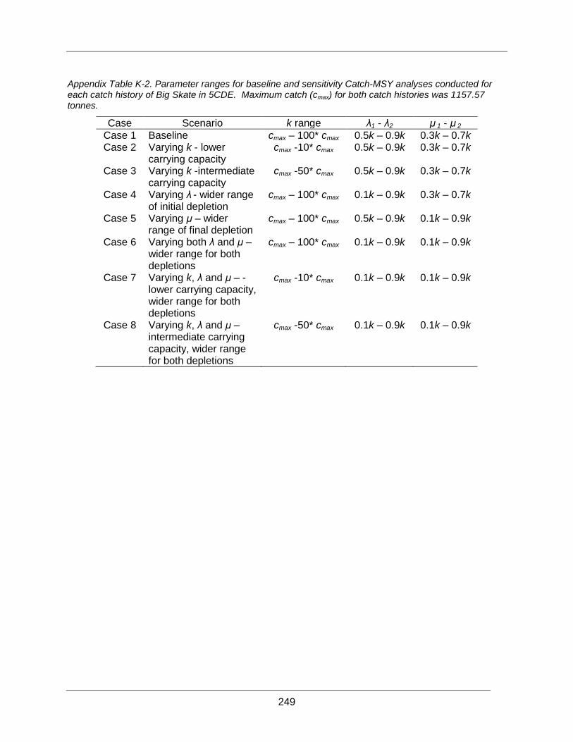
249

Appendix Table K-2. Parameter ranges for baseline and sensitivity Catch-MSY analyses conducted for each catch history of Big Skate in 5CDE. Maximum catch (cmax) for both catch histories was 1157.57 tonnes.

Case Scenario k range λ1 - λ2 μ 1 - μ 2 Case 1 Baseline cmax – 100* cmax 0.5k – 0.9k 0.3k – 0.7k Case 2 Varying k - lower

carrying capacity cmax -10* cmax 0.5k – 0.9k 0.3k – 0.7k

Case 3 Varying k -intermediate carrying capacity

cmax -50* cmax 0.5k – 0.9k 0.3k – 0.7k

Case 4 Varying λ - wider range of initial depletion

cmax – 100* cmax 0.1k – 0.9k 0.3k – 0.7k

Case 5 Varying μ – wider range of final depletion

cmax – 100* cmax 0.5k – 0.9k 0.1k – 0.9k

Case 6 Varying both λ and μ – wider range for both depletions

cmax – 100* cmax 0.1k – 0.9k 0.1k – 0.9k

Case 7 Varying k, λ and μ – - lower carrying capacity, wider range for both depletions

cmax -10* cmax 0.1k – 0.9k 0.1k – 0.9k

Case 8 Varying k, λ and μ – intermediate carrying capacity, wider range for both depletions

cmax -50* cmax 0.1k – 0.9k 0.1k – 0.9k

250

Appendix Table K-3. Proportion of plausible r – k pairs (from 100,000 draws) for each Case analysis and both catch histories for Big Skate by Skate Management Area.

Baseline Varying k Wider depletion Varying k with wider depletion (λ and μ)

Catch History Case 1 Case 2 (low k)

Case 3 (mid k)

Case 4 (λ only)

Case 5 (μ only)

Case 6 (λ and μ)

Case 7 (low k)

Case 8 (mid k)

3CD 1 (1996-2011) 26.99 4.87 28.49 50.11 51.02 55.09 10.59 41.20 2 (1954-2011) 5.45 2.75 5.91 11.80 13.79 24.27 8.75 24.85 5AB 1 (1996-2011) 27.08 27.35 29.68 61.91 56.43 68.00 35.63 62.10 2 (1954-2011) 4.43 7.05 5.14 11.73 11.65 23.87 20.82 25.18 5CDE 1 (1996-2011) 27.43 13.75 29.39 55.47 52.63 59.60 19.44 52.51 2 (1954-2011) 9.25 9.02 10.68 17.24 27.99 34.77 15.03 36.42

Appendix Table K-4. MSY estimates (as geometric mean in tonnes) from the posterior density distributions for each Case analysis and both catch histories for Big Skate by Skate Management Area.

Baseline Varying k Wider depletion Varying k with wider depletion (λ and μ)

Catch History Case 1 Case 2 (low k)

Case 3 (mid k)

Case 4 (λ only)

Case 5 (μ only)

Case 6 (λ and μ)

Case 7 (low k)

Case 8 (mid k)

3CD 1 (1996-2011) 47.8 37.2 45 85.5 72.3 81.3 30.7 57.6 2 (1954-2011) 22.7 24.9 22.4 37.5 30.2 44.4 30.1 38.8 5AB 1 (1996-2011) 367 289 350 845 645 837 277 596 2 (1954-2011) 154 153 151 302 211 365 209 317 5CDE 1 (1996-2011) 536 409 508 1064 856 1029 358 728 2 (1954-2011) 351 359 347 508 537 657 407 591

Appendix Table K-5. Proportion of plausible r-k pairs (from 100,000 draws), geometric mean r, k (tonnes), and MSY (tonnes) produced for Catch History 2 (1954 – 2011) of Big Skate in 3CD for Case 6 with starting biomass sequentially increasing in increments of 50, 10 and 1 tonnes.

Increment Proportion Geometric mean r k MSY

50 24.27 0.103 1,723 44.4 10 29.61 0.110 1,720 47.2 1 33.94 0.118 1,688 49.7

251

Appendix Table K-6. Proportion of plausible r-k pairs (from 100,000 draws) for each Case analysis and both catch histories for Longnose Skate by Skate Management Area.

Baseline Varying k Wider depletion Varying k with wider depletion (λ and μ)

Catch History Case 1 Case 2 (low k)

Case 3 (mid k)

Case 4 (λ only)

Case 5 (μ only)

Case 6 (λ and μ)

Case 7 (low k)

Case 8 (mid k)

3CD 1 (1996-2011) 39.07 0.15 32.71 44.34 48.67 49.23 1.31 40.15 2 (1954-2011) 17.02 0.94 17.70 34.37 30.85 43.13 1.58 36.19 5AB 1 (1996-2011) 38.84 0.15 32.43 43.71 48.31 48.49 0.97 39.40 2 (1954-2011) 16.61 0.73 17.40 34.19 29.28 42.86 1.45 35.96 5CDE 1 (1996-2011) 42.52 0.25 37.90 49.42 53.70 53.93 8.03 45.61 2 (1954-2011) 17.90 4.44 19.09 36.93 32.49 46.61 6.98 40.31 Coastwide 1 (1996-2011) 37.41 0.03 29.93 41.36 46.29 46.17 0.25 36.76 2 (1954-2011) 20.59 0.02 20.52 29.41 41.09 41.99 0.15 33.76

Appendix Table K-7. MSY estimates (as geometric mean in tonnes) from the posterior density distributions for each Case analysis and both catch histories for Longnose Skate by Skate Management Area.

Baseline Varying k Wider depletion Varying k with wider depletion (λ and μ)

Catch History Case 1 Case 2 (low k)

Case 3 (mid k)

Case 4 (λ only)

Case 5 (μ only)

Case 6 (λ and μ)

Case 7 (low k)

Case 8 (mid k)

3CD 1 (1996-2011) 133 129 106 157 139 140 90.4 100 2 (1954-2011) 65.7 79.5 62.6 113 90.2 126 88 96.2 5AB 1 (1996-2011) 82.3 80.2 66.2 96.5 86 85.6 59.2 61.9 2 (1954-2011) 37.6 46 35.9 67 51.3 73.8 50.2 56.1 5CDE 1 (1996-2011) 70.4 51.8 57.1 87.1 77.6 78.4 34.6 56.1 2 (1954-2011) 33.9 35.1 32.3 62.3 47.8 69.2 37.3 52.6 Coastwide 1 (1996-2011) 275 297 221 320 283 285 228 203 2 (1954-2011) 184 304 182 242 268 278 236 212

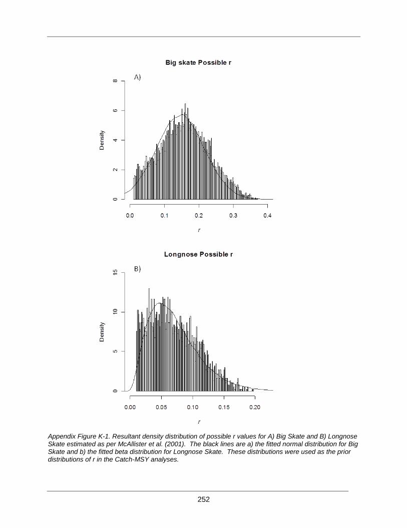
252

Appendix Figure K-1. Resultant density distribution of possible r values for A) Big Skate and B) Longnose Skate estimated as per McAllister et al. (2001). The black lines are a) the fitted normal distribution for Big Skate and b) the fitted beta distribution for Longnose Skate. These distributions were used as the prior distributions of r in the Catch-MSY analyses.

253

Appendix Figure K-2. Results for Big Skate Catch History 1 (1996 – 2011) Case 1 (baseline). a) the resultant r-k pair distribution b) r posterior density distribution; c) k (thousand of tonnes) posterior density distribution for Skate Management Area 5CDE only since distributions from the other Skate Management Areas were similar in shape. The resultant MSY (thousand of tonnes) posterior density distributions for d) 3CD; e) 5AB and f) 5CDE. The thick solid lines are geometric means, dashed lines are 5%, 50% (median) and 95% quantiles, red lines are prior distributions.

254

Appendix Figure K-3. Results for Big Skate Catch History 1 (1996 – 2011) Case 2 (low k). a) the resultant r-k pair distribution b) r posterior density distribution; c) k (thousand of tonnes) posterior density distribution for Skate Management Area 5CDE only since distributions from the other Skate Management Areas were similar in shape. The resultant MSY (thousand of tonnes) posterior density distributions for d) 3CD; e) 5AB and f) 5CDE. The thick solid lines are geometric means, dashed lines are 5%, 50% (median) and 95% quantiles, red lines are prior distributions.

255

Appendix Figure K-4. Results for Big Skate Catch History 1 (1996 – 2011) Case 3 (mid k). a) the resultant r-k pair distribution b) r posterior density distribution; c) k (thousand of tonnes) posterior density distribution for Skate Management Area 5CDE only since distributions from the other Skate Management Areas were similar in shape. The resultant MSY (thousand of tonnes) posterior density distributions for d) 3CD; e) 5AB and f) 5CDE. The thick solid lines are geometric means, dashed lines are 5%, 50% (median) and 95% quantiles, red lines are prior distributions.

256

Appendix Figure K-5. Results for Big Skate Catch History 1 (1996 – 2011) Case 4 (wider λ bounds). a) the resultant r-k pair distribution b) r posterior density distribution; c) k (thousand of tonnes) posterior density distribution for Skate Management Area 5CDE only since distributions from the other Skate Management Areas were similar in shape. The resultant MSY (thousand of tonnes) posterior density distributions for d) 3CD; e) 5AB and f) 5CDE. The thick solid lines are geometric means, dashed lines are 5%, 50% (median) and 95% quantiles, red lines are prior distributions.

257

Appendix Figure K-6. Results for Big Skate Catch History 1 (1996 – 2011) Case 5 (wider μ bounds). a) the resultant r-k pair distribution b) r posterior density distribution; c) k (thousand of tonnes) posterior density distribution for Skate Management Area 5CDE only since distributions from the other Skate Management Areas were similar in shape. The resultant MSY (thousand of tonnes) posterior density distributions for d) 3CD; e) 5AB and f) 5CDE. The thick solid lines are geometric means, dashed lines are 5%, 50% (median) and 95% quantiles, red lines are prior distributions.

258

Appendix Figure K-7. Results for Big Skate Catch History 1 (1996 – 2011) Case 6 (wider λ and μ bounds). a) the resultant r-k pair distribution b) r posterior density distribution; c) k (thousand of tonnes) posterior density distribution for Skate Management Area 5CDE only since distributions from the other Skate Management Areas were similar in shape. The resultant MSY (thousand of tonnes) posterior density distributions for d) 3CD; e) 5AB and f) 5CDE. The thick solid lines are geometric means, dashed lines are 5%, 50% (median) and 95% quantiles, red lines are prior distributions.

259

Appendix Figure K-8. Results for Big Skate Catch History 1 (1996 – 2011) Case 7 (wider λ and μ bounds, low k). a) the resultant r-k pair distribution b) r posterior density distribution; c) k (thousand of tonnes) posterior density distribution for Skate Management Area 5CDE only since distributions from the other Skate Management Areas were similar in shape. The resultant MSY (thousand of tonnes) posterior density distributions for d) 3CD; e) 5AB and f) 5CDE. The thick solid lines are geometric means, dashed lines are 5%, 50% (median) and 95% quantiles, red lines are prior distributions.

260

Appendix Figure K-9. Results for Big Skate Catch History 1 (1996 – 2011) Case 8 (wider λ and μ bounds, mid k). a) the resultant r-k pair distribution b) r posterior density distribution; c) k (thousand of tonnes) posterior density distribution for Skate Management Area 5CDE only since distributions from the other Skate Management Areas were similar in shape. The resultant MSY (thousand of tonnes) posterior density distributions for d) 3CD; e) 5AB and f) 5CDE. The thick solid lines are geometric means, dashed lines are 5%, 50% (median) and 95% quantiles, red lines are prior distributions.

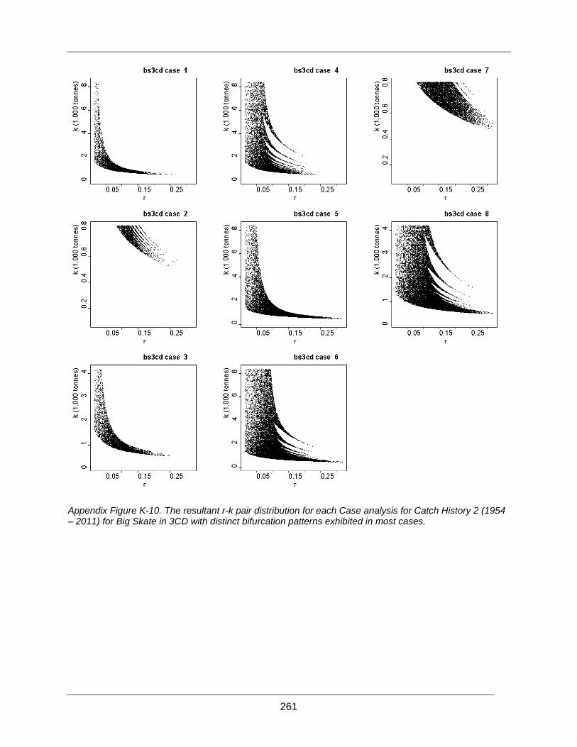
261

Appendix Figure K-10. The resultant r-k pair distribution for each Case analysis for Catch History 2 (1954 – 2011) for Big Skate in 3CD with distinct bifurcation patterns exhibited in most cases.

262

Appendix Figure K-11. The resultant r-k pair distribution for Case 6 for Catch History 2 (1954 – 2011) for Big Skate in 3CD with starting biomass sequential increments of a) 10 tonnes and b) 1 tonnes.

263

Appendix Figure K-12. The resultant r posterior density distribution for each case analysis for Catch History 2 (1954 – 2011) for Big Skate in 5CDE. The thick solid line is the geometric mean, dashed lines are 5%, 50% (median) and 95% quantiles. Red line is prior distribution.

264

Appendix Figure K-13. Results for Longnose Skate Catch History 1 (1996 – 2011) Case 1 (baseline). a) the resultant r-k pair distribution b) r posterior density distribution; c) k (thousand of tonnes) posterior density distribution for Skate Management Area 3CD only since distributions from the other Skate Management Areas were similar in shape. The resultant MSY (thousand of tonnes) posterior density distributions for d) 3CD; e) 5AB; f) 5CDE and g) coastwide. The thick solid lines are geometric means, dashed lines are 5%, 50% (median) and 95% quantiles, red lines are prior distributions.

265

Appendix Figure K-14. Results for Longnose Skate Catch History 2 (1954 – 2011) Case 3 (mid k). a) the resultant r-k pair distribution b) r posterior density distribution; c) k (thousand of tonnes) posterior density distribution for Skate Management Area 3CD only since distributions from the other Skate Management Areas were similar in shape. The resultant MSY (thousand of tonnes) posterior density distributions for d) 3CD; e) 5AB; f) 5CDE and g) coastwide. The thick solid lines are geometric means, dashed lines are 5%, 50% (median) and 95% quantiles, red lines are prior distributions.

266

Appendix Figure K-15. Results for Longnose Skate Catch History 1 (1996 – 2011) Case 4 (wider λ bounds). a) the resultant r-k pair distribution b) r posterior density distribution; c) k (thousand of tonnes) posterior density distribution for Skate Management Area 3CD only since distributions from the other Skate Management Areas were similar in shape. The resultant MSY (thousand of tonnes) posterior density distributions for d) 3CD; e) 5AB; f) 5CDE and g) coastwide. The thick solid lines are geometric means, dashed lines are 5%, 50% (median) and 95% quantiles, red lines are prior distributions.

267

Appendix Figure K-16. Results for Longnose Skate Catch History 1 (1996 – 2011) Case 5 (wider μ bounds). a) the resultant r-k pair distribution b) r posterior density distribution; c) k (thousand of tonnes) posterior density distribution for Skate Management Area 3CD only since distributions from the other Skate Management Areas were similar in shape. The resultant MSY (thousand of tonnes) posterior density distributions for d) 3CD; e) 5AB; f) 5CDE and g) coastwide. The thick solid lines are geometric means, dashed lines are 5%, 50% (median) and 95% quantiles, red lines are prior distributions.

268

Appendix Figure K-17. Results for Longnose Skate Catch History 1 (1996 – 2011) Case 6 (wider λ and μ bounds). a) the resultant r-k pair distribution b) r posterior density distribution; c) k (thousand of tonnes) posterior density distribution for Skate Management Area 3CD only since distributions from the other Skate Management Areas were similar in shape. The resultant MSY (thousand of tonnes) posterior density distributions for d) 3CD; e) 5AB; f) 5CDE and g) coastwide. The thick solid lines are geometric means, dashed lines are 5%, 50% (median) and 95% quantiles, red lines are prior distributions.

269

Appendix Figure K-18. Results for Longnose Skate Catch History 1 (1996 – 2011) Case 8 (wider λ and μ bounds; mid k). a) the resultant r-k pair distribution b) r posterior density distribution; c) k (thousand of tonnes) posterior density distribution for Skate Management Area 3CD only since distributions from the other Skate Management Areas were similar in shape. The resultant MSY (thousand of tonnes) posterior density distributions for d) 3CD; e) 5AB; f) 5CDE and g) coastwide. The thick solid lines are geometric means, dashed lines are 5%, 50% (median) and 95% quantiles, red lines are prior distributions.

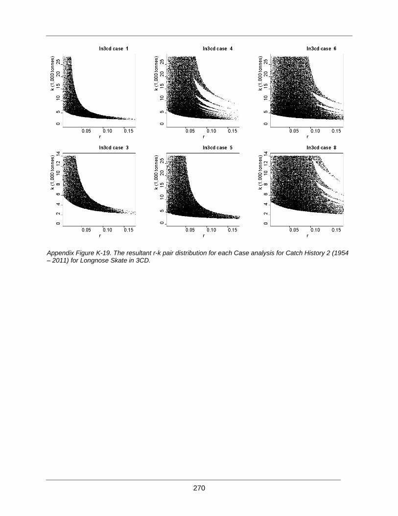
270

Appendix Figure K-19. The resultant r-k pair distribution for each Case analysis for Catch History 2 (1954 – 2011) for Longnose Skate in 3CD.

271

Appendix Figure K-20. The resultant r-k pair distribution for each Case analysis for Catch History 2 (1954 – 2011) for Longnose Skate coastwide.

272

Appendix Figure K-21. The resultant r posterior density distribution for each Case analysis for Catch History 2 (1954 – 2011) for Longnose Skate in 3CD. The thick solid line is the geometric mean, dashed lines are 5%, 50% (median) and 95% quantiles. Red line is prior distribution.

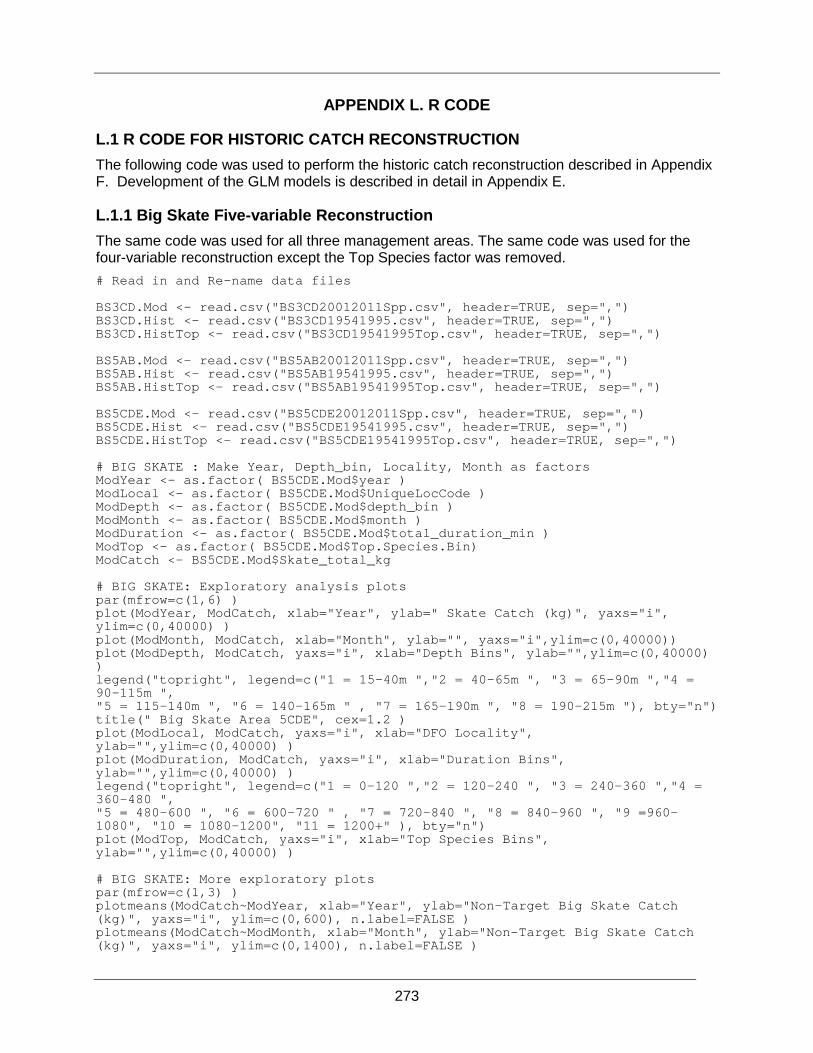
273

R CODE APPENDIX L.

L.1 R CODE FOR HISTORIC CATCH RECONSTRUCTION The following code was used to perform the historic catch reconstruction described in Appendix F. Development of the GLM models is described in detail in Appendix E.

L.1.1 Big Skate Five-variable Reconstruction The same code was used for all three management areas. The same code was used for the four-variable reconstruction except the Top Species factor was removed. # Read in and Re-name data files BS3CD.Mod <- read.csv("BS3CD20012011Spp.csv", header=TRUE, sep=",") BS3CD.Hist <- read.csv("BS3CD19541995.csv", header=TRUE, sep=",") BS3CD.HistTop <- read.csv("BS3CD19541995Top.csv", header=TRUE, sep=",") BS5AB.Mod <- read.csv("BS5AB20012011Spp.csv", header=TRUE, sep=",") BS5AB.Hist <- read.csv("BS5AB19541995.csv", header=TRUE, sep=",") BS5AB.HistTop <- read.csv("BS5AB19541995Top.csv", header=TRUE, sep=",") BS5CDE.Mod <- read.csv("BS5CDE20012011Spp.csv", header=TRUE, sep=",") BS5CDE.Hist <- read.csv("BS5CDE19541995.csv", header=TRUE, sep=",") BS5CDE.HistTop <- read.csv("BS5CDE19541995Top.csv", header=TRUE, sep=",") # BIG SKATE : Make Year, Depth_bin, Locality, Month as factors ModYear <- as.factor( BS5CDE.Mod$year ) ModLocal <- as.factor( BS5CDE.Mod$UniqueLocCode ) ModDepth <- as.factor( BS5CDE.Mod$depth_bin ) ModMonth <- as.factor( BS5CDE.Mod$month ) ModDuration <- as.factor( BS5CDE.Mod$total_duration_min ) ModTop <- as.factor( BS5CDE.Mod$Top.Species.Bin) ModCatch <- BS5CDE.Mod$Skate_total_kg # BIG SKATE: Exploratory analysis plots par(mfrow=c(1,6) ) plot(ModYear, ModCatch, xlab="Year", ylab=" Skate Catch (kg)", yaxs="i", ylim=c(0,40000) ) plot(ModMonth, ModCatch, xlab="Month", ylab="", yaxs="i",ylim=c(0,40000)) plot(ModDepth, ModCatch, yaxs="i", xlab="Depth Bins", ylab="",ylim=c(0,40000) ) legend("topright", legend=c("1 = 15-40m ","2 = 40-65m ", "3 = 65-90m ","4 = 90-115m ", "5 = 115-140m ", "6 = 140-165m " , "7 = 165-190m ", "8 = 190-215m "), bty="n") title(" Big Skate Area 5CDE", cex=1.2 ) plot(ModLocal, ModCatch, yaxs="i", xlab="DFO Locality", ylab="",ylim=c(0,40000) ) plot(ModDuration, ModCatch, yaxs="i", xlab="Duration Bins", ylab="",ylim=c(0,40000) ) legend("topright", legend=c("1 = 0-120 ","2 = 120-240 ", "3 = 240-360 ","4 = 360-480 ", "5 = 480-600 ", "6 = 600-720 " , "7 = 720-840 ", "8 = 840-960 ", "9 =960-1080", "10 = 1080-1200", "11 = 1200+" ), bty="n") plot(ModTop, ModCatch, yaxs="i", xlab="Top Species Bins", ylab="",ylim=c(0,40000) ) # BIG SKATE: More exploratory plots par(mfrow=c(1,3) ) plotmeans(ModCatch~ModYear, xlab="Year", ylab="Non-Target Big Skate Catch (kg)", yaxs="i", ylim=c(0,600), n.label=FALSE ) plotmeans(ModCatch~ModMonth, xlab="Month", ylab="Non-Target Big Skate Catch (kg)", yaxs="i", ylim=c(0,1400), n.label=FALSE )

274

title(" Big Skate Area 5CDE" ) plotmeans(ModCatch~ModDepth, xlab="Depth Bin", ylab="Non-Target Big Skate Catch (kg)", yaxs="i", ylim=c(0,1000), n.label=FALSE ) legend("topright", legend=c("1 = 15-40m ","2 = 40-65m ", "3 = 65-90m ","4 = 90-115m ", "5 = 115-140m ", "6 = 140-165m " , "7 = 165-190m ", "8 = 190-215m "), bty="n") par(mfrow=c(1,3) ) plotmeans(ModCatch~ModLocal, xlab="DFO Locality", ylab="Non-Target Big Skate Catch (kg)", yaxs="i", ylim=c(0,900), n.label=FALSE) plotmeans(ModCatch~ModDuration, xlab="Duration Bin", ylab="Non-Target Big Skate Catch (kg)", yaxs="i", ylim=c(0,3800), n.label=FALSE) title(" Big Skate Area 5CDE" ) plotmeans(ModCatch~ModTop, xlab="Top Species Bin", ylab="Non-Target Big Skate Catch (kg)", yaxs="i", ylim=c(0,700), n.label=FALSE) # Subset Positive Tows for BIG SKATE PosiCatchBS <- subset( BS5CDE.Mod, Skate_total_kg > 0 ) # Re-name and factor for big skate PosiBS <- log(PosiCatchBS$Skate_total_kg) PosiDur <- as.factor(PosiCatchBS$total_duration_min) PosiDep <- as.factor(PosiCatchBS$depth_bin) PosiMon <- as.factor(PosiCatchBS$month) PosiLoc <- as.factor(PosiCatchBS$UniqueLocCode) PosiTop <- as.factor(PosiCatchBS$Top.Species.Bin) # GLM on one variable only (BIG) PosiDepth.glm <- glm( PosiBS ~ PosiDep, family="gaussian"(link="identity") ) PosiMonth.glm <- glm( PosiBS ~ PosiMon, family="gaussian"(link="identity") ) PosiDur.glm <- glm( PosiBS ~ PosiDur, family="gaussian"(link="identity") ) PosiLocal.glm <- glm( PosiBS ~ PosiLoc, family="gaussian"(link="identity") ) PosiTop.glm <- glm( PosiBS ~ PosiTop, family="gaussian"(link="identity") ) # GLM on top variable and subsequently adding other variables (BIG) PosiDurLoc <- glm( PosiBS ~ PosiDur + PosiLoc, family="gaussian"(link="identity") ) PosiDurDepth <- glm( PosiBS ~ PosiDur + PosiDep, family="gaussian"(link="identity") ) PosiDurMonth <- glm( PosiBS ~ PosiDur + PosiMon, family="gaussian"(link="identity") ) PosiDurTop <- glm( PosiBS ~ PosiDur + PosiTop, family="gaussian"(link="identity") ) # GLM (BIG) PosiLocDurMon <- glm( PosiBS ~ PosiDur + PosiLoc + PosiMon, family="gaussian"(link="identity") ) PosiLocDurDep <- glm( PosiBS ~ PosiDur + PosiLoc + PosiDep, family="gaussian"(link="identity") ) PosiLocDurTop <- glm( PosiBS ~ PosiDur + PosiLoc + PosiTop, family="gaussian"(link="identity") ) #GLM (BIG) PosiLocDurDepMon <- glm( PosiBS ~ PosiDur + PosiLoc + PosiDep + PosiMon, family="gaussian"(link="identity") ) PosiLocDurDepTop <- glm( PosiBS ~ PosiDur + PosiLoc + PosiDep + PosiTop, family="gaussian"(link="identity") ) # All Variables (BIG) PosiAllVar <- glm( PosiBS ~ PosiLoc + PosiDur + PosiTop + PosiMon + PosiDep, family="gaussian"(link="identity") )

275

PosiPred <- fitted(PosiAllVar, data=PosiCatchBS) # Observed and predicted comparison plots (BIG) Year <- as.factor(PosiCatchBS$year) PredMeanYear <- by(exp(PosiPred), PosiCatchBS$year, mean) ObsMeanYear <- by(exp(PosiBS), PosiCatchBS$year, mean) plot(levels(Year), PredMeanYear, yaxs="i", xlab="Year", ylab="Big Skate Catch (kg)", type="b", ylim=c(0,500000), xlim=c(2001,2011)) points(levels(Year), ObsMeanYear, type="b", col="red") legend("topright", col=c("red","black"), lty=c(1,1), pch=c(21,21), legend=c( "Observed", "Predicted")) par(mar=c(5,4,2,2)+0.1) plot(exp(PosiBS)/1000, exp(PosiPred)/1000, xlab=" Observed Big Skate Catch (tonnes)", ylab="Predicted Big Skate Catch (tonnes)", xaxs="i", yaxs="i", ylim=c(0, 2), yaxt="n", xlim=c(0,2)) axis(2, las=2) lines( x=c(0:4), y=c(0:4), col="blue", lty=1 ) # Histogram of standardized residuals StdResidsPosi <- stdres( PosiAllVar ) hist(StdResidsPosi, xlab="Standardized Residuals", breaks=100, main="" ) # Recode data to change positive catches to 1 (BIG) BinomData <- recode( BS5CDE.Mod$Skate_total_kg,"0='0';0.00001:40000='1'" ) # Binomial GLM (BIG) LogitDepth.glm <- glm( BinomData ~ ModDepth, family="binomial"(link="logit") ) LogitMonth.glm <- glm( BinomData ~ ModMonth, family="binomial"(link="logit") ) LogitDur.glm <- glm( BinomData ~ ModDuration, family="binomial"(link="logit") ) LogitLocal.glm <- glm( BinomData ~ ModLocal, family="binomial"(link="logit") ) LogitTop.glm <- glm( BinomData ~ ModTop, family="binomial"(link="logit") ) # Binomial GLM (BIG) LogitDepLoc <- glm( BinomData ~ ModLocal + ModDepth , family="binomial"(link="logit") ) LogitLocTop <- glm( BinomData ~ ModLocal + ModTop, family="binomial"(link="logit") ) LogitLocDur <- glm( BinomData ~ ModLocal + ModDuration, family="binomial"(link="logit") ) LogitLocMonth <- glm( BinomData ~ ModLocal + ModMonth, family="binomial"(link="logit") ) # Binomial GLM (BIG) LogitLocDurTop <- glm( BinomData ~ ModLocal + ModDuration + ModTop, family="binomial"(link="logit") ) LogitLocDurDep <- glm( BinomData ~ ModLocal + ModDuration + ModDepth, family="binomial"(link="logit") ) LogitLocDurMon <- glm( BinomData ~ ModLocal + ModDuration + ModMonth, family="binomial"(link="logit") ) # Binomial GLM (BIG) LogitLocDurDepTop <- glm( BinomData ~ ModLocal + ModDuration + ModDepth + ModTop, family="binomial"(link="logit") ) LogitLocDurDepMon <- glm( BinomData ~ ModLocal + ModDuration + ModDepth + ModMonth, family="binomial"(link="logit") ) # Binomial GLM (BIG) LogitAllVar <- glm( BinomData ~ ModTop + ModLocal + ModDuration + ModMonth + ModDepth, family="binomial"(link="logit") ) # Use logit to find probabilities greater than 0.50 (BIG)

276

PredLogit <- predict.glm(LogitAllVar, data= BS5CDE.Mod, type="response") BS5CDE.Mod[,19] <- PredLogit # Positive tows are assumed to have probabilities greater than 0.50 posTows <- subset(BS5CDE.Mod, BS5CDE.Mod$V19 >= 0.50) # Fit predicted positive tows using lognormal GLM (BIG) # New factors need to have same names as factors used in GLM in # order for predict.glm() to work PosiDur <- as.factor(posTows$total_duration_min) PosiDep <- as.factor(posTows$depth_bin) PosiLoc <- as.factor(posTows$UniqueLocCode) PosiMon <- as.factor(posTows$month) PosiTop <- as.factor(posTows$Top.Species.Bin) PosData <- data.frame( as.vector(PosiDur), as.vector(PosiLoc) , as.vector(PosiDep) , as.vector(PosiMon), as.vector(PosiTop) ) colnames(PosData) <- c("PosiDur","PosiLoc", "PosiDep","PosiMon", "PosiTop") # Use logit model to predict catch from positive tows only posTowPred <- predict.glm(PosiAllVar, newdata=PosData ) # Compare predictions to observed data (BIG) PosiLogitPredMeanYear <- by(exp(posTowPred), posTows$year, mean) posYear <- as.factor(posTows$year) plot(levels(Year), PosiLogitPredMeanYear, yaxs="i", xlab="Year", ylab="Big Skate Catch (kg)", type="b", ylim=c(0,700)) points(levels(Year), ObsMeanYear, type="b", col="red") legend("topright", col=c("red", "black"), lty=c(1,1), pch=c(21,21), legend=c("Observed", "Predicted")) # Historical Reconstruction BIG HistLocal <- as.factor( BS5CDE.HistTop$UniqueLocCode ) HistDepth <- as.factor( BS5CDE.HistTop$depth_bin ) HistMonth <- as.factor( BS5CDE.HistTop$month ) HistDuration <- as.factor( BS5CDE.HistTop$total_duration_min ) HistTop <- as.factor( BS5CDE.HistTop$Top.Species.Bin) HistData <- data.frame( as.vector(HistLocal), as.vector(HistDuration), as.vector(HistDepth), as.vector(HistMonth), as.vector(HistTop) ) # Colnames need to match factor names from GLMs colnames(HistData) <- c("ModLocal","ModDuration", "ModDepth","ModMonth","ModTop") # First, predict positive tows from historical data set HistPredLogit <- predict(LogitAllVar, newdata= HistData, type="response") BS5CDE.HistTop[,17] <- HistPredLogit # Records with probabilities greater than 0.50 are assumed positive HistposTows <- subset(BS5CDE.HistTop, BS5CDE.HistTop$V17 >= 0.50) # The use predicted positive tows to predict catch using lognormal GLM (BIG) HistPosiDur <- as.factor(HistposTows$total_duration_min) HistPosiDep <- as.factor(HistposTows$depth_bin) HistPosiLoc <- as.factor(HistposTows$UniqueLocCode) HistPosiMon <- as.factor(HistposTows$month) HistPosiTop <- as.factor(HistposTows$Top.Species.Bin) HistPosData <- data.frame( as.vector(HistPosiDur), as.vector(HistPosiLoc) , as.vector(HistPosiDep), as.vector(HistPosiMon), as.vector(HistPosiTop) )

277

# Colnames need to match those used in original GLM in order for reconstruction to work colnames(HistPosData) <- c("PosiDur", "PosiLoc", "PosiDep", "PosiMon", "PosiTop") HistposTowPred <- predict.glm(PosiAllVar, newdata=HistPosData) # Plot historic predictions based on GLM results (BIG) HistPosiLogitPredMeanYear <- by(exp(HistposTowPred), HistposTows$year, mean) plot(levels(as.factor( HistposTows$year)), HistPosiLogitPredMeanYear, yaxs="i", xlab="Year", ylab="Predicted Big Skate Catch (kg)", type="b", ylim=c(0,800)) # Table of Year, Mean Reconstructed Catch, Sum of Catch per Year HistPosiLogitPredSumYear <- by(exp(HistposTowPred), HistposTows$year, sum) Results <- cbind(levels(as.factor( HistposTows$year)),HistPosiLogitPredMeanYear, HistPosiLogitPredSumYear) write.csv(Results, "Results_5CDE_Top.csv") # Sum of catch by year for historic and modern data (how similar are they?) AllYears <- c(levels(as.factor( HistposTows$year)), levels(ModYear)) ModSumYear <- by(ModCatch, ModYear, sum) plot(AllYears, c(HistPosiLogitPredSumYear/1000,ModSumYear/1000), xlab="Year", ylab="Big Skate Catch (tonnes)", xaxs="i", yaxs="i", ylim=c(0,800)) Longnose Skate Five-variable Reconstruction The same code was used for all three management areas. The same code was used for the four-variable reconstruction except the Top Species factor was removed. # Read in data files LN3CD.Mod <- read.csv("LN3CD20012011Spp.csv", header=TRUE, sep=",") LN3CD.Hist <- read.csv("LN3CD19541995.csv", header=TRUE, sep=",") LN3CD.HistTop <- read.csv("LN3CD19541995Top.csv", header=TRUE, sep=",") LN5AB.Mod <- read.csv("LN5AB20012011Spp.csv", header=TRUE, sep=",") LN5AB.Hist <- read.csv("LN5AB19541995.csv", header=TRUE, sep=",") LN5AB.HistTop <- read.csv("LN5AB19541995Top.csv", header=TRUE, sep=",") LN5CDE.Mod <- read.csv("LN5CDE20012011Spp.csv", header=TRUE, sep=",") LN5CDE.Hist <- read.csv("LN5CDE19541995.csv", header=TRUE, sep=",") LN5CDE.HistTop <- read.csv("LN5CDE19541995Top.csv", header=TRUE, sep=",") # LONGNOSE: Make Year, Depth_bin, Locality, Month as factors LNModYear <- as.factor( LN5CDE.Mod$year ) LNModLocal <- as.factor( LN5CDE.Mod$UniqueLocCode ) LNModDepth <- as.factor( LN5CDE.Mod$depth_bin ) LNModMonth <- as.factor( LN5CDE.Mod$month ) LNModDuration <- as.factor( LN5CDE.Mod$total_duration_min ) LNModTop <- as.factor( LN5CDE.Mod$Top.Species.Bin) LNModCatch <- LN5CDE.Mod$LNS_total_kg # LONGNOSE SKATE: Exploratory analysis plots par(mfrow=c(1,6) ) plot(LNModYear, LNModCatch, xlab="Year", ylab=" Skate Catch (kg)", yaxs="i", ylim=c(0,4000) ) plot(LNModMonth, LNModCatch, xlab="Month", ylab="", yaxs="i",ylim=c(0,4000)) plot(LNModDepth, LNModCatch, yaxs="i", xlab="Depth Bins", ylab="",ylim=c(0,4000) ) legend("topright", legend=c("1 = 15-40m ","2 = 40-65m ", "3 = 65-90m ","4 = 90-115m ", "5 = 115-140m ", "6 = 140-165m " , "7 = 165-190m ", "8 = 190-215m "), bty="n") title(" Longnose Skate Area 5CDE", cex=1.2 ) plot(LNModLocal, LNModCatch, yaxs="i", xlab="DFO Locality", ylab="",ylim=c(0,4000) )

278

plot(LNModDuration, LNModCatch, yaxs="i", xlab="Duration Bins", ylab="",ylim=c(0,4000) ) legend("topright", legend=c("1 = 0-120 ","2 = 120-240 ", "3 = 240-360 ","4 = 360-480 ", "5 = 480-600 ", "6 = 600-720 " , "7 = 720-840 ", "8 = 840-960 ", "9 =960-1080", "10 = 1080-1200", "11 = 1200+" ), bty="n") plot(LNModTop, LNModCatch, yaxs="i", xlab="Top Species Bins", ylab="",ylim=c(0,4000) ) # LONGNOSE SKATE: More exploratory plots par(mfrow=c(1,3) ) plotmeans(LNModCatch~LNModYear, xlab="Year", ylab="Non-Target Longnose Skate Catch (kg)", yaxs="i", ylim=c(0,80), n.label=FALSE ) plotmeans(LNModCatch~LNModMonth, xlab="Month", ylab="", yaxs="i", ylim=c(0,80), n.label=FALSE ) title(" Longnose Skate Area 5CDE" ) plotmeans(LNModCatch~LNModDepth, xlab="Depth Bin", ylab="", yaxs="i", ylim=c(0,80), n.label=FALSE ) legend("topright", legend=c("1 = 15-40m ","2 = 40-65m ", "3 = 65-90m ","4 = 90-115m ", "5 = 115-140m ", "6 = 140-165m " , "7 = 165-190m ", "8 = 190-215m "), bty="n") par(mfrow=c(1,3) ) plotmeans(LNModCatch~LNModLocal, xlab="DFO Locality", ylab="Non-Target Longnose Skate Catch (kg)", yaxs="i", ylim=c(0,140), n.label=FALSE) plotmeans(LNModCatch~LNModDuration, xlab="Duration Bin", ylab="", yaxs="i", ylim=c(0,140), n.label=FALSE) title(" Longnose Skate Area 5CDE" ) plotmeans(LNModCatch~LNModTop, xlab="Top Species Bin", ylab="", yaxs="i", ylim=c(0,60), n.label=F, mean.label=F, ci.label=F) # Subset Positive Tows for LN SKATE PosiCatchLN <- subset( LN5CDE.Mod, LNS_total_kg > 0 ) # Re-name and factor for longnose skate PosiLN <- log(PosiCatchLN$LNS_total_kg) PosiDurLN <- as.factor(PosiCatchLN$total_duration_min) PosiDepLN <- as.factor(PosiCatchLN$depth_bin) PosiMonLN <- as.factor(PosiCatchLN$month) PosiLocLN <- as.factor(PosiCatchLN$UniqueLocCode) PosiTopLN <- as.factor(PosiCatchLN$Top.Species.Bin) # GLM on one variable only (LONGNOSE) LNPosiDepth.glm <- glm( PosiLN ~ PosiDepLN, family="gaussian"(link="identity") ) LNPosiMonth.glm <- glm( PosiLN ~ PosiMonLN, family="gaussian"(link="identity") ) LNPosiDur.glm <- glm( PosiLN ~ PosiDurLN, family="gaussian"(link="identity") ) LNPosiLocal.glm <- glm( PosiLN ~ PosiLocLN, family="gaussian"(link="identity") ) LNPosiTop.glm <- glm( PosiLN ~ PosiTopLN, family="gaussian"(link="identity") ) # GLM on top variable and subsequently adding other variables (LONGNOSE) LNPosiLocDur <- glm( PosiLN ~ PosiLocLN + PosiDurLN, family="gaussian"(link="identity") ) LNPosiLocDepth <- glm( PosiLN ~ PosiLocLN + PosiDepLN, family="gaussian"(link="identity") ) LNPosiLocMonth <- glm( PosiLN ~ PosiLocLN + PosiMonLN, family="gaussian"(link="identity") ) LNPosiLocTop <- glm( PosiLN ~ PosiLocLN + PosiTopLN, family="gaussian"(link="identity") ) # GLM (LONGNOSE)

279

LNPosiDurLocDep <- glm( PosiLN ~ PosiLocLN + PosiDurLN + PosiDepLN, family="gaussian"(link="identity") ) LNPosiDurLocMon <- glm( PosiLN ~ PosiLocLN + PosiDurLN + PosiMonLN, family="gaussian"(link="identity") ) LNPosiDurLocTop <- glm( PosiLN ~ PosiLocLN + PosiDurLN + PosiTopLN, family="gaussian"(link="identity") ) # GLM (LONGNOSE) LNPosiDurLocMonDep <- glm( PosiLN ~ PosiLocLN + PosiDurLN + PosiMonLN + PosiDepLN, family="gaussian"(link="identity") ) LNPosiDurLocMonTop <- glm( PosiLN ~ PosiLocLN + PosiDurLN + PosiMonLN + PosiTopLN, family="gaussian"(link="identity") ) # All Variables (LONGNOSE) AllVarLN <- glm( PosiLN ~ PosiDurLN + PosiLocLN + PosiDepLN + PosiMonLN + PosiTopLN, family="gaussian"(link="identity") ) PosiPredLN <- fitted(AllVarLN, data=PosiCatchLN) # Observed versus predicted plots (LONGNOSE) Year <- as.factor(PosiCatchLN$year) PredMeanYearLN <- by(exp(PosiPredLN), PosiCatchLN$year, mean) ObsMeanYearLN <- by(exp(PosiLN), PosiCatchLN$year, mean) plot(levels(Year), PredMeanYearLN, yaxs="i", xlab="Year", ylab="Longnose Skate Catch (kg)", type="b", ylim=c(0,150), xlim=c(2001,2011)) points(levels(Year), ObsMeanYearLN, type="b", col="red") legend("topright", col=c("red","black"), lty=c(1,1), pch=c(21,21), legend=c( "Observed", "Predicted")) par(mar=c(5,4,2,2)+0.1) plot(exp(PosiLN)/1000, exp(PosiPredLN)/1000, xlab="Observed Longnose Skate Catch (tonnes)", ylab="Predicted Longnose Skate Catch (tonnes)", xaxs="i", yaxs="i", ylim=c(0,1), yaxt="n", xlim=c(0,1)) axis(2, las=2) lines( x=c(0:1), y=c(0:1), col="blue", lty=1 ) # Histogram of standardized residuals StdResidsPosiLN <- stdres( AllVarLN ) hist(StdResidsPosiLN, xlab="Standardized Residuals", breaks=100, main="" ) # Recode data to change positive catches to 1 (LONGNOSE) LNBinom <- recode( LN5CDE.Mod$LNS_total_kg,"0='0';0.00001:10000='1'" ) # Binomial GLM (LONGNOSE) LNLogitDepth <- glm( LNBinom ~ LNModDepth, family="binomial"(link="logit") ) LNLogitMonth <- glm( LNBinom ~ LNModMonth, family="binomial"(link="logit") ) LNLogitDur <- glm( LNBinom ~ LNModDuration, family="binomial"(link="logit") ) LNLogitLocal <- glm( LNBinom ~ LNModLocal, family="binomial"(link="logit") ) LNLogitTop <- glm( LNBinom ~ LNModTop, family="binomial"(link="logit") ) # Binomial GLM (LONGNOSE) LNLogitLocTop <- glm( LNBinom ~ LNModLocal + LNModTop, family="binomial"(link="logit") ) LNLogitLocDepth <- glm( LNBinom ~ LNModLocal + LNModDepth, family="binomial"(link="logit") ) LNLogitLocMonth <- glm( LNBinom ~ LNModLocal + LNModMonth, family="binomial"(link="logit") ) LNLogitLocDur <- glm( LNBinom ~ LNModLocal + LNModDuration, family="binomial"(link="logit") ) # Binomial GLM (LONGNOSE) LNLogitLoxDurTop <- glm( LNBinom ~ LNModLocal + LNModDuration + LNModTop, family="binomial"(link="logit") )

280

LNLogitLocDurMon <- glm( LNBinom ~ LNModLocal + LNModDuration + LNModMonth, family="binomial"(link="logit") ) LNLogitLocDurDepth <- glm( LNBinom ~ LNModLocal + LNModDuration + LNModDepth, family="binomial"(link="logit") ) # Binomial GLM (LONGNOSE) LNLogitTopDurLocDep <- glm( LNBinom ~ LNModLocal + LNModDuration + LNModDepth + LNModTop, family="binomial"(link="logit") ) LNLogitMonDurLocDep <- glm( LNBinom ~ LNModLocal + LNModDuration + LNModDepth + LNModMonth, family="binomial"(link="logit") ) # Binomial GLM (LONGNOSE) LNLogitAllVar <- glm( LNBinom ~ LNModLocal + LNModDuration + LNModDepth + LNModTop + LNModMonth, family="binomial"(link="logit") ) # Use logit to find probabilities greater than 0.50 (LONGNOSE) LNPredLogit <- predict.glm(LNLogitAllVar, data= LN5CDE.Mod, type="response") LN5CDE.Mod[,19] <- LNPredLogit LNposTows <- subset(LN5CDE.Mod, LN5CDE.Mod$V19 >= 0.50) # Fit predicted positive tows using lognormal GLM (LONGNOSE) PosiDurLN <- as.factor(LNposTows$total_duration_min) PosiDepLN <- as.factor(LNposTows$depth_bin) PosiLocLN <- as.factor(LNposTows$UniqueLocCode) PosiMonLN <- as.factor(LNposTows$month) PosiTopLN <- as.factor(LNposTows$Top.Species.Bin) PosDataLN <- data.frame( as.vector(PosiDurLN), as.vector(PosiLocLN), as.vector(PosiDepLN) , as.vector(PosiMonLN), as.vector(PosiTopLN) ) # Factor names need to be the same as those used for fitting GLM colnames(PosDataLN) <- c("PosiDurLN","PosiLocLN", "PosiDepLN","PosiMonLN","PosiTopLN") LNposTowPred <- predict.glm(AllVarLN, newdata=PosDataLN ) # Compare predictions to observed data (LONGNOSE) LNPosiLogitPredMeanYear <- by(exp(LNposTowPred), LNposTows$year, mean) LNposYear <- as.factor(LNposTows$year) plot(levels(LNposYear), LNPosiLogitPredMeanYear, yaxs="i", xlab="Year", ylab="Longnose Skate Catch (kg)", type="b", ylim=c(0,150)) points(levels(LNposYear), ObsMeanYearLN, type="b", col="red") legend("topright", col=c("red", "black"), lty=c(1,1), pch=c(21,21), legend=c("Observed", "Predicted")) # Historical Four Var Long LNHistLocal <- as.factor( LN5CDE.HistTop$UniqueLocCode ) LNHistDepth <- as.factor( LN5CDE.HistTop$depth_bin ) LNHistMonth <- as.factor( LN5CDE.HistTop$month ) LNHistDuration <- as.factor( LN5CDE.HistTop$total_duration_min ) LNHistTop <- as.factor( LN5CDE.HistTop$Top.Species.Bin ) LNHistData <- data.frame( as.vector(LNHistLocal), as.vector(LNHistDuration), as.vector(LNHistDepth), as.vector(LNHistMonth), as.vector(LNHistTop) ) # Colnames need to match factor names from GLMs colnames(LNHistData) <- c("LNModLocal","LNModDuration", "LNModDepth","LNModMonth", "LNModTop") # First, predict positive tows from historical data set LNHistPredLogit <- predict(LNLogitAllVar, newdata= LNHistData, type="response")

281

LN5CDE.HistTop[,17] <- LNHistPredLogit LNHistposTows <- subset(LN5CDE.HistTop, LN5CDE.HistTop$V17 >= 0.50) # Then use predicted positive tows to predict catch using lognormal GLM (BIG) LNHistPosiDur <- as.factor(LNHistposTows$total_duration_min) LNHistPosiDep <- as.factor(LNHistposTows$depth_bin) LNHistPosiLoc <- as.factor(LNHistposTows$UniqueLocCode) LNHistPosiMon <- as.factor(LNHistposTows$month) LNHistPosiTop <- as.factor(LNHistposTows$Top.Species.Bin) LNHistPosData <- data.frame( as.vector(LNHistPosiDur), as.vector(LNHistPosiLoc) , as.vector(LNHistPosiDep), as.vector(LNHistPosiMon), as.vector(LNHistPosiTop) ) # Colnames need to match those used in original GLM in order for reconstruction to work colnames(LNHistPosData) <- c("PosiDurLN", "PosiLocLN", "PosiDepLN", "PosiMonLN", "PosiTopLN") LNHistposTowPred <- predict.glm(AllVarLN, newdata=LNHistPosData) # Plot historic predictions based on GLM results (LONGNOSE) LNHistPosiLogitPredMeanYear <- by(exp(LNHistposTowPred), LNHistposTows$year, mean) plot(levels(as.factor( LNHistposTows$year)), LNHistPosiLogitPredMeanYear, yaxs="i", xlab="Year", ylab="Predicted Longnose Skate Catch (kg)", type="b", ylim=c(0,80)) # Table of Year, Mean Reconstructed Catch, Sum of Catch per Year LNHistPosiLogitPredSumYear <- by(exp(LNHistposTowPred), LNHistposTows$year, sum) Results <- cbind(levels(as.factor( LNHistposTows$year)),LNHistPosiLogitPredMeanYear, LNHistPosiLogitPredSumYear) write.csv(Results, "Results_LN5CDE_Top.csv") # Sum of catch by year for historic and modern data (how similar are they?) AllYears <- c(levels(as.factor( LNHistposTows$year)), levels(LNModYear)) LNModSumYear <- by(LNModCatch, LNModYear, sum) plot(AllYears, c(LNHistPosiLogitPredSumYear/1000,LNModSumYear/1000), xlab="Year", ylab="Longnose Skate Catch (tonnes)", xaxs="i", yaxs="i", ylim=c(0,80)) R Code for Groundfish survey Indices Trawl Survey Biomass The following R code was used to calculate the bootstrapped biomass indices for Groundfish trawl surveys as described in Appendix H. # R code (revised) to calculate survey indices and confidence # intervals using bootstrapping. # Provided by Norm Olsen September 7, 2012. ############################################################################# # get.sql.data # Executes a SQL command on an external SQL Server database and returns a # data frame of the results, if applicable. ############################################################################# get.sql.data <- function(sql, db="PacHarvest", svr="SVBCPBSGFIIS", ...) { # Requires the RODBC package require("RODBC", keep.source=FALSE, quietly=TRUE) # Construct a connection string constr <- paste("Driver={SQL Server};Server=",svr,";Database=",db,";", sep="") # Connect to the database cnn <- odbcDriverConnect(constr) # Execute the SQL command and store the results in a data frame df <- sqlQuery(cnn, sql, ...)

282

# Close the connection odbcClose(cnn) # Return the results return(df) } ############################################################################# # calc.biomass # Resamples catch densities with replication from catch matrix output and # calculates a total biomass based on the average catch density per # stratum multiplied by the stratum area, summed over all strata for # the total biomass ############################################################################# calc.biomass <- function(dat, i, sa, is_ll=FALSE, is_sable=FALSE) { # If i is only a single number, use a vector of the row indices instead # (used for testing) if (length(i)==1) i <- 1:nrow(dat) # Resample from the data frame using the vector i dat <- dat[i,] # Calculate the mean biomass (kg/km2) for each stratum. The "if-else" structure # is for handling the special cases of a longline (is_ll) and sablefish # (is_sable) surveys that use different measures of catch. mu <- numeric(nrow(sa)) if (is_ll | is_sable) { mb <- tapply(dat$CPUE_PPT, list(dat$GROUPING_CODE), mean) mu[sa$GROUPING_CODE %in% names(mb)] <- mb res <- mean(mu) } else { mb <- tapply(dat$DENSITY_KGPM2 * 1000000, list(dat$GROUPING_CODE), mean) mu[sa$GROUPING_CODE %in% names(mb)] <- mb res <- sum(mu * sa$AREA_KM2) } #mu[sa$GROUPING_CODE %in% names(mb)] <- mb # Expand mean biomass per stratum to the entire survey area to get total biomass #return(sum(mu * sa$AREA_KM2)) return(res) } ############################################################################# # boot.species # Performs a bootstrap procedure for a given species from a given survey # and returns a list containing various elements from the bootstrap # analysis. ############################################################################# boot.species <- function(survey_id, species_code, stat=calc.biomass, r=1000, is_ll=FALSE, is_sable=FALSE, resample=FALSE) { # Requires the boot package require(boot, quietly=TRUE) # Get a dataframe of the number of sets and area per survey stratum sa <- get.sql.data(paste("EXEC proc_stratum_info", survey_id), "GFBioSQL") # Get a data frame of the catch density per fishing event for the # species/survey

283

# Sablefish surveys have to be handled by a seperate procedure. if (is_sable) { dm <- get.sql.data(paste("EXEC proc_catmat_sable ", survey_id, ", '", species_code, "'", sep=""), "GFBioSQL", as.is=c(F,F,T,T,F,F,F,F,F,F,F,F,F,F,F,F,F)) } else if(is_ll) { dm <- get.sql.data(paste("EXEC proc_catmat_ll ", survey_id, ", '", species_code, "'", sep=""), "GFBioSQL", as.is=c(F,F,T,T,F,F,F,F,F,F,F,F,F,F,F,F,F)) } else { dm <- get.sql.data(paste("EXEC proc_catmat_2011 ", survey_id, ", '", species_code, "'", sep=""), "GFBioSQL", as.is=c(F,F,T,T,F,F,F,F,F,F,F,F,F,F,F,F,F,F,F,F,F,F)) } # This is a kludge for the Hecate Strait multispecies survey, where only # the first 7 strata are used for biomass indices calculation. if (survey_id >= 4 & survey_id <= 14) { dm <- dm[dm$GROUPING_CODE >= 77 & dm$GROUPING_CODE <= 83,] sa <- sa[sa$GROUPING_CODE >= 77 & sa$GROUPING_CODE <= 83,] } # specific strata for synoptic surveys for big skate or longnose skate: # if (species_code=="056" & dm$SURVEY_SERIES_ID == 1){ # QCS BS # dm <- dm[dm$GROUPING_CODE == 18 | dm$GROUPING_CODE == 22,] # sa <- sa[sa$GROUPING_CODE == 18 | sa$GROUPING_CODE == 22,] # } # Are we resampling? if (resample) { dm <- resample(survey_id, dm) } # Construct a data frame to store results smy <- data.frame("species_code"=character(1), "biomass"=numeric(1), "boot_mean"=numeric(1), "boot_median"=numeric(1), "boot_lower_ci"=numeric(1), "boot_upper_ci"=numeric(1), "boot_re"=numeric(1), "catch_weight"=numeric(1), "num_sets"=numeric(1), "num_pos_sets"=numeric(1), "year"=numeric(1), "survey_id"=numeric(1), "survey_series_id"=numeric(1), "survey"=character(1), stringsAsFactors=FALSE) # Perform the bootstrap analysis. If the data frame has no rows or if # the catch densities or catch counts are all zero (i.e. the species # wasn't caught) # then return "NA" if (nrow(dm) > 0 & !(!is_ll & all(dm$DENSITY_KGPM2==0)) | !(is_ll & all(dm$CATCH_COUNT==0))) { # Perform the bootstrap boot_obj <- boot(dm, stat, r, strata=dm$GROUPING_CODE, sa=sa, is_ll=is_ll, is_sable=is_sable, sim="ordinary") # Calculate the bias corrected and adjusted confidence limits bootci_obj <- boot.ci(boot_obj, type="perc") # Save various elements to the results data frame smy$species_code <- species_code smy[1,2:13] <- c(boot_obj$t0, mean(boot_obj$t), median(boot_obj$t), bootci_obj$bca[1,4], bootci_obj$perc[c(4,5)], sd(boot_obj$t) / mean(boot_obj$t), sum(dm$CATCH_WEIGHT, na.rm=TRUE), nrow(dm),

284

max(length(dm$CATCH_WEIGHT[dm$CATCH_WEIGHT > 0]), length(dm$CATCH_COUNT[dm$CATCH_COUNT > 0])), dm$YEAR[1], dm$SURVEY_ID[1], dm$SURVEY_SERIES_ID[1]) smy[1,14] <- dm$SURVEY_DESC[1] # Build a list of final results results <- list("stratum_info"=sa, "catch_matrix"=dm, "boot_obj"=boot_obj, "bootci_obj"=bootci_obj, "summary"=smy, "species_code"=smy$species_code, "survey_id"=survey_id) class(results) <- "bootres" } else { warning(paste("Survey Id", survey_id, "Species", species_code, "produces an empty catch matrix")) results <- NA } # Return the results list return(results) } ############################################################################# # boot.survey # A wrapper for boot.species; performs the bootstrap analysis for multiple # species for a given survey. The list of species is obtained from a query # that returns all fish species that were caught in a given survey. ############################################################################# boot.survey <- function(survey_id, is_ll=FALSE, is_sable=FALSE, resample=FALSE) { # build a species table just for big skate and longnose skate species <- data.frame(SPECIES_CODE = c("056","059"),SPECIES_NAME = c("Big Skate","Longnose Skate")) # Run the boot.species function for each species in the list, collecting # only the summary information from each run. res <- boot.species(survey_id, species$SPECIES_CODE[1], is_ll=is_ll, is_sable=is_sable, resample=resample)$summary for (i in 2:nrow(species)) { cat(species$SPECIES_CODE[i], "\n") br <- boot.species(survey_id, species$SPECIES_CODE[i], is_ll=is_ll, is_sable=is_sable, resample=resample) if (class(br)=="bootres") { br <- br$summary res <- rbind(res, br) } } # Return the data frame of summary information. Each row of this data frame # gives the information for a species. return(res) } ############################################################################# # run the code on selected surveys ############################################################################# library(RODBC) ch <- odbcConnect("") # get list of survey IDs that correspond to certain survey series #

285

# 1 = QCS Synoptic # 2 = HS Multispecies # 3 = HS Synoptic # 4 = WCVI Synoptic # 5 = HS PCod # 6 = QCS Shrimp * note: no skate prior to 2003 # 7 = WCVI Shrimp * note: no skate prior to 2003 # 16 = WCHG Synoptic * note: only one year of big skate # 15 = YOY lingocd * note: not used b/c insufficient skate # 21 = GIG Retrospecitive * most years have insufficient skate # 30 = WCHG Synoptic with deepest stratum removed!! skate_surveys <- sqlQuery(ch, "SELECT Survey_Series.SURVEY_SERIES_ID, Survey.SURVEY_ID, Survey.SURVEY_DESC FROM Survey_Series INNER JOIN Survey ON Survey_Series.SURVEY_SERIES_ID = Survey.SURVEY_SERIES_ID WHERE (((Survey_Series.SURVEY_SERIES_ID) Between 1 And 7 Or (Survey_Series.SURVEY_SERIES_ID)=16 Or (Survey_Series.SURVEY_SERIES_ID)=21 Or (Survey_Series.SURVEY_SERIES_ID)=30 ))") survey_ids <- skate_surveys[,2] # run boot.survey for each survey ID, and collapse result into a single # dataframe skate.index.list <- tapply(survey_ids,c(1:length(survey_ids)),boot.survey) skate.index.df <- do.call("rbind",skate.index.list) # convert kg to tonnes for biomass variables skate.index.df[,2:6] <- skate.index.df[,2:6]/1000 write.table(skate.index.df,file="skate_index.csv",row.names=F,sep=",",quote=F) odbcCloseAll() Longline Survey CPUE # R code to calculate bootstrapped mean CPUE and confidence intervals # for groundfish longline surveys # Follows general methodology of Norm Olsen's "boot.species" and # "boot.survey" functions. library(boot) ############################################################################# # samplemean # version of "mean" function that will work with the boostrap # obtained from http://www.mayin.org/ajayshah/KB/R/documents/boot.html ############################################################################# samplemean <- function(x, d) { return(mean(x[d])) } ############################################################################# # LLboot2 # bootstrap non-transformed CPUE ############################################################################# LLboot2 <- function(data,zeros=TRUE) { npos <- count(data$cpue) nset <- length(data$cpue) if (zeros==TRUE){ data$cpue[is.na(data$cpue)] <- 0 } else { data <- data[!is.na(data$cpue),] }

286

boot.obj <- boot(data$cpue,samplemean,R=1000) bootobj.ci <- boot.ci(boot.obj,type="perc") # set up dataframe to store results smy <- data.frame("area"=character(1),"survey"=character(1),"year"=numeric(1),"n_sets"=numeric(1),"n_pos_sets"=numeric(1),"mean_cpue"=numeric(1),"boot_mean"=numeric(1),"boot_lower_ci"=numeric(1),"boot_upper_ci"=numeric(1), "boot_CV"=numeric(1),stringsAsFactors=FALSE) # put results in dataframe smy[1,1:10] <- c( as.character(data$sma[1]),as.character(data$survey[1]),data$year[1],nset,npos,mean(data$cpue),mean(boot.obj$t),bootobj.ci$percent[1,4:5],apply(boot.obj$t,2,sd)/mean(boot.obj$t)) return(smy) } ############################################################################# # run the code on the longline surveys # hl.cpue$id is an index created by concatenating the survey name, year, # and area (e.g. "IPHC.2003.3CD") ############################################################################# #get data in hl.cpue <- read.table("HL_cpue2.csv",sep=",",header=T) # split dataframe by species hl.cpue.bs <- data.frame(hl.cpue[,1:6],cpue=hl.cpue$bs) hl.cpue.lns <- data.frame(hl.cpue[,1:6],cpue=hl.cpue$lns) # run boostrap for each species and include zeros # collapse resultant list into a dataframe and export res.bs <- by(hl.cpue.bs,hl.cpue.bs$id,LLboot2,zeros=T) res.bs.df <- data.frame(do.call("rbind",res.bs),row.names=NULL) res.bs.df write.table(res.bs.df,file="LLboot2_bs.csv",row.names=F,sep=",",quote=T) res.lns <- by(hl.cpue.lns,hl.cpue.lns$id,LLboot2,zeros=T) res.lns.df <- data.frame(do.call("rbind",res.lns),row.names=NULL) res.lns.df write.table(res.lns.df,file="LLboot2_lns.csv",row.names=F,sep=",",quote=T) R Code for Surplus Production Model case study The following R code was used for the Surplus Production Model case study described in Appendix I. # CODE BY ROBYN FORREST. OCTOBER 2006. R.FORREST@FISHERIES.UBC.CA # Leslie Matrix demographic method for estimating intrinsic rate of increase of a population # Model by McAllister et al. 2001. CJFAS 58, 1871-1890 rm(list=ls(all=TRUE)) graphics.off() ########################### Data Section ########################### poppars = read.table("rajapars.csv", header=T, sep=",") spp=as.vector(poppars[,1]) NumSpp=length(spp) species = 1:NumSpp CV=0.1 sd_k=0.2 #SET NUMBER OF SIMULATIONS

287

MonteCarlo=2500 #########################.Procedure Section.################### demographicmodel = function(pars) { No = 1000 years = 300 amax=pars[1] LS=pars[2] amat=pars[3] natmort=pars[4] nages=0:amax ###################################################################### #set counters midages = 1:amax nages = 0:amax nyears = 1:years #Initialise vectors and matrices Nt = matrix(0,nrow=amax+1, ncol=years) Deltat = matrix(0,nrow=amax+1, ncol=years) DeltatSum = vector(length=years-1) Pt = vector(length=years) r_m = vector(length=years-1) ConvergeCheck=vector(length=years-1) sa = exp( -1 * natmort ) #FECUNDITY AND MATURITY SCHEDULE matsteep = 0.1 mat=plogis(nages,amat,matsteep*amat) fa=LS*mat la_0 = sa^(nages) #Calculate numbers at age and time in Leslie Matrix # This is only for year 1 Nt[, 1] = No * la_0 Pt[1]=sum(Nt[, 1]) #Now run population dynamics for all years > 1 for ( i in 2:years ) { #Recruits produced by age 0 class Nt[1, i] = sum(fa*Nt[,(i-1)]) #Update numbers at age and time for (j in 2:(amax+1)) { Nt[j, i] = sa * Nt[(j-1), (i-1)] } Pt[i] =sum(Nt[, i]) for (j in 1:(amax+1)) { b=Nt[j,i]/Pt[i] w=Nt[j,(i-1)]/Pt[i-1] Deltat[j,i]=(b-w)/w } r_m[i-1]=log(Pt[i]/Pt[i-1])

288

DeltatSum[i]=sum(Deltat[,i])/amax DeltatSum[i]=100*DeltatSum[i] if(abs(DeltatSum[i])<0.0001) { ConvergeCheck[i]=1 } if(abs(DeltatSum[i])>0.0001) { ConvergeCheck[i]=0 }} plot(2:years,r_m, type="l", main="r convergence check", lwd=2, col=2, ylab="r", xlab="Year", cex.lab=1.5) if(sum(ConvergeCheck[(years-9):years]) ==10)r_m=log(Pt[years]/Pt[years-1]) if(sum(ConvergeCheck[(years-9):years]) <10)r_m=-1 return(r_m) } rundogDemo=function() { rmatrix=matrix(0,nrow=MonteCarlo, ncol=NumSpp) meanvbk=mean(poppars[,11], na.rm=TRUE) #Loop over species for (x in 1:NumSpp) { #Get list of parameters for species x spar = poppars[x,] print(spp[x]) #set parameter values needed in model meanamax=spar$tmax meanLS=0.5*spar$LS meanamat=spar$tmat meanM=spar$natmort #Fixed parameters lmat=spar$lmat pupsize=spar$PupSize lwa=spar$lwa lwb=spar$lwb tto=spar$tto linf=spar$linf*1.2 nages=1:meanamax #Get missing parameter values #trial values of tto ttoseq=seq(1,-7.5,-0.2) ttotry=length(ttoseq) #CALCULATE TTO FROM THE GROWTH CURVE, GIVEN VBK AND PUP SIZE AT BIRTH if(tto==0) { l1=linf*(1-exp(-meanvbk*(0-ttoseq))) l1list=as.matrix(cbind(ttoseq,l1)) l1list2=l1list[l1list[,2]<pupsize,] tto_index=length(l1list2[,1]) #get tto

289

tto=l1list[(tto_index+1),1] } if(meanamat==0) { #run growth model ltest = linf * (1 - exp(-meanvbk * (nages - tto))) ltest = cbind(nages,ltest) ltest2 = ltest[ltest[,2]<(lmat+1),] tmat_index = length(ltest2[,1]) #get amat meanamat=ltest[tmat_index,1] } #Get parameters for Monte Carlo amax=runif(MonteCarlo, meanamax-3, meanamax+3) amax=as.integer(amax) LS=runif(MonteCarlo, meanLS-4, meanLS+4) amat=runif(MonteCarlo, meanamat-3, meanamat+2) M <- runif(MonteCarlo, meanM-0.05, meanM+0.05) natmort <- sample( M , MonteCarlo , replace=TRUE ) ################################################################ #put parameters into matrix pars=cbind(amax,LS,amat,natmort) ################################################################## #Get r rmatrix[,x]=t(apply(pars,1,demographicmodel)) } return(rmatrix) } ######################### Main Section ####################### Result=rundogDemo() write.table(Result,file="Allr.csv", sep=",",row.names=F) means=vector(length=NumSpp) medians=vector(length=NumSpp) modes=vector(length=NumSpp) sds=vector(length=NumSpp) count=0 for(i in 1:NumSpp)# { SpeciesName=spp[i] count=count+1 r_m=as.numeric(Result[,i]) rPlaus=r_m[r_m>0.01] Umsy=rPlaus/2 dr=density(r_m, na.rm=TRUE) drplaus=density(rPlaus, na.rm=TRUE) means[i]=mean(rPlaus) sds[i]=sd(rPlaus) medians[i]=median(rPlaus) x=hist(rPlaus, breaks=seq(0,1,by=0.005),plot=FALSE) print(SpeciesName) rbreaks=cbind(x$mids,x$counts) moder=rbreaks[which(rbreaks[,2] == max(rbreaks[,2])),1] moder=mean(moder)

290

modes[i]=moder win.metafile(paste("r_",paste(SpeciesName),".wmf")) par(cex=1.2, cex.axis=1.2) plot(drplaus$x, drplaus$y/max(drplaus$y), main="", type="l",xlab=expression(italic(r)), ylab= "Relative density", cex.lab=1.5, cex=1.5, cex.axis=1.5, xlim=c(0, 1.1*max(drplaus$x))) mtext(paste(SpeciesName),side=3, outer=FALSE, line=-1.5, cex=1.5) dev.off() write.table(rPlaus, file=paste("r_possible",paste(SpeciesName),".csv"), sep=",", row.names=FALSE,col.names=TRUE) write.table(r_m, file=paste("r_AllValues",paste(SpeciesName),".csv"), sep=",", row.names=FALSE,col.names=TRUE) } Stats=cbind(means, medians, modes, sds) write.table(Stats, file="StatsDemographic.csv", sep=",", row.names=FALSE) ######################### Surplus Production Model ########################## # Code by Sabrina Garcia # Read in catch, effort and survey data for NHS NHS <- read.csv("5CDECatch.csv", header=T, sep=",") # Re-name columns, assume no catch prior to 1996 NHS_Year <- NHS[,1] NHS[,2][is.na(NHS[,2])]=0 NHS_Catch <- NHS[,2] NHS_CPUE <- NHS[,3] HSMS_Index <- NHS[,4] # Catch, CPUE, and Survey plots par( mar=c(5,4,2,2) + 0.1 ) plot(NHS_Year[13:28], NHS_Catch[13:28], xlab="Year", ylab="", pch=21, type="b", xlim=c(1996,2011), yaxt="n", xaxt="n", ylim=c(0,1200), yaxs="i", bg="black") axis(2, at=seq(0,1200,200), labels=expression(0,200,400,600,800,1000,1200), las=2) axis(1, at=seq(1996,2012,2), labels=expression(1996,1998,2000,2002,2004,2006,2008,2010,2012)) mtext("Big Skate Landings plus Discards (tonnes)", side=2, line=3) par( mar=c(5,4,2,2) + 0.1 ) plot(NHS_Year[13:28], NHS_CPUE[13:28], xlab="Year", ylab="", pch=21, type="b", xlim=c(1996,2011), yaxt="n", xaxt="n", ylim=c(0,1.5), yaxs="i", bg="black") axis(2, at=seq(0,1.5,0.3), labels=expression(0,0.3,0.6,0.9,1.2,1.5), las=2) axis(1, at=seq(1996,2012,2), labels=expression(1996,1998,2000,2002,2004,2006,2008,2010,2012)) mtext("Standardized Catch-Per-Unit-Effort", side=2, line=3) par( mar=c(5,4.75,2,2) + 0.1 ) plot(NHS_Year, HSMS_Index, xlab="Year", ylab="", pch=21, type="p", xlim=c(1984,2004), yaxt="n", xaxt="n", ylim=c(0,0.1), yaxs="i", bg="black") axis(2, at=seq(0,0.1,0.025), labels=expression(0,0.025,0.05,0.075,0.1), las=2) axis(1, at=seq(1984,2004,4), labels=expression(1984,1988,1992,1996,2000,2004)) mtext("Multispcies Survey Index (tonnes/hr)", side=2, line=3.5) NHSBDM <- function(theta) { # Initialize parameter values r_fit <- theta[1] # intrinsic growth rate of the population K_fit <- exp( theta[2] ) # carrying capacity

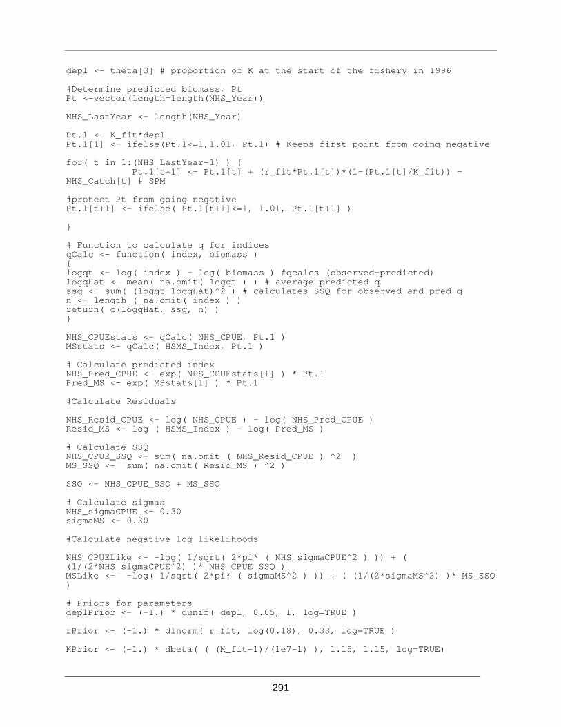
291

depl <- theta[3] # proportion of K at the start of the fishery in 1996 #Determine predicted biomass, Pt Pt <-vector(length=length(NHS_Year)) NHS_LastYear <- length(NHS_Year) Pt.1 <- K_fit*depl Pt.1[1] <- ifelse(Pt.1<=1,1.01, Pt.1) # Keeps first point from going negative for( t in 1:(NHS_LastYear-1) ) { Pt.1[t+1] <- Pt.1[t] + (r_fit*Pt.1[t])*(1-(Pt.1[t]/K_fit)) - NHS_Catch[t] # SPM #protect Pt from going negative Pt.1[t+1] <- ifelse( Pt.1[t+1]<=1, 1.01, Pt.1[t+1] ) } # Function to calculate q for indices qCalc <- function( index, biomass ) { logqt <- log( index ) - log( biomass ) #qcalcs (observed-predicted) logqHat <- mean( na.omit( logqt ) ) # average predicted q ssq <- sum( (logqt-logqHat)^2 ) # calculates SSQ for observed and pred q n <- length ( na.omit( index ) ) return( c(logqHat, ssq, n) ) } NHS_CPUEstats <- qCalc( NHS_CPUE, Pt.1 ) MSstats <- qCalc( HSMS_Index, Pt.1 ) # Calculate predicted index NHS_Pred_CPUE <- exp( NHS_CPUEstats[1] ) * Pt.1 Pred_MS <- exp( MSstats[1] ) * Pt.1 #Calculate Residuals NHS_Resid_CPUE <- log( NHS_CPUE ) - log( NHS_Pred_CPUE ) Resid_MS <- log ( HSMS_Index ) - log( Pred_MS ) # Calculate SSQ NHS_CPUE_SSQ <- sum( na.omit ( NHS_Resid_CPUE ) ^2 ) MS_SSQ <- sum( na.omit( Resid_MS ) ^2 ) SSQ <- NHS_CPUE_SSQ + MS_SSQ # Calculate sigmas NHS_sigmaCPUE <- 0.30 sigmaMS <- 0.30 #Calculate negative log likelihoods NHS_CPUELike <- -log( 1/sqrt( 2*pi* ( NHS_sigmaCPUE^2 ) )) + ( (1/(2*NHS_sigmaCPUE^2) )* NHS_CPUE_SSQ ) MSLike <- -log( 1/sqrt( 2*pi* ( sigmaMS^2 ) )) + ( (1/(2*sigmaMS^2) )* MS_SSQ ) # Priors for parameters deplPrior <- (-1.) * dunif( depl, 0.05, 1, log=TRUE ) rPrior <- (-1.) * dlnorm( r_fit, log(0.18), 0.33, log=TRUE ) KPrior <- (-1.) * dbeta( ( (K_fit-1)/(1e7-1) ), 1.15, 1.15, log=TRUE)

292

NHSTotal_Like <- MSLike + NHS_CPUELike + rPrior + deplPrior + KPrior # Create a list to hold results Results <- list() Results$Catch <- NHS_Catch Results$SSQ <- SSQ Results$Pt <- Pt Results$F <- NHS_Catch/Pt Results$Indexq <- exp( MSstats[1] ) Results$CPUEq <- exp ( NHS_CPUEstats[1] ) Results$Pred_Survey <- Pred_MS Results$Pred_Fishery <- NHS_Pred_CPUE Results$pars <- c(r_fit, K_fit, depl) Results$sigmas <- c( NHS_sigmaCPUE, sigmaMS ) Results$like <- NHSTotal_Like Results$rNLike <- rPrior return(Results) } #Function to return the likelihood LikeValue_NHS <-function(theta){ (-1) * NHSBDM(theta)$like } # Run optim to find parameter values using likelihood BestFitLike <- optim(par=c(0.25,13,0.50),fn=LikeValue_NHS, method="BFGS", hessian=T, control=list(fnscale=-1) ) # Run MCMC chains on the three parameter values postSamp_NHS <- MCMCmetrop1R(fun=LikeValue_NHS, theta.init=BestFitLike$par,mcmc=4000000, burnin=2000,thin=1000, verbose=TRUE, tune=1.25, force.samp=FALSE) NHSBDM_r <-as.vector( postSamp_NHS[,1] ) NHSBDM_K <- as.vector( exp( postSamp_NHS[,2] ) ) NHSBDM_depl <- as.vector( postSamp_NHS[,3] ) NHSBDM_MCMC <- cbind( NHSBDM_r, NHSBDM_K, NHSBDM_depl ) # SPM to return final biomass based on posterior values of r and catch NHS_SPM <- function ( pars ) { r <- pars[1] K <- pars[2] depl <- pars[3] Bt <-vector( length=length(NHS_Year) ) Bt.1 <-vector( length=length(NHS_Year) ) NHS_LastYear <- length( NHS_Year ) Bt.1 <- K*depl Bt[1] <- ifelse(Bt.1<=1,1.01, Bt.1) for( t in 1:(NHS_LastYear-1) ) { Bt.1[t+1]<- Bt.1[t] + (r*Bt.1[t])*(1-(Bt.1[t]/K)) - NHS_Catch[t] #protect Pt from going negative Bt.1[t+1] <- ifelse( Bt.1[t+1]<=1, 1.01, Bt.1[t+1] ) Bt[t+1] <- Bt.1[t+1] }

293

qCalc <- function( index, biomass ) { logqt <- log( index ) - log( biomass ) #qcalcs (observed-predicted) logqHat <- mean( na.omit( logqt ) ) # average predicted q ssq <- sum( (logqt-logqHat)^2 ) # calculates SSQ for observed and pred q n <- length ( na.omit( index ) ) return( c(logqHat, ssq, n) ) } NHS_CPUEstats <- qCalc( NHS_CPUE, Bt ) MSstats <- qCalc( HSMS_Index, Bt ) # Calculate predicted index NHS_Pred_CPUE <- exp( NHS_CPUEstats[1] ) * Bt Pred_MS <- exp( MSstats[1] ) * Bt Results <- list() Results$Ct <- NHS_Catch Results$FinalBt <- Bt[NHS_LastYear] Results$Bt <- Bt Results$Bt_K <- Bt/ K Results$Pred_CPUE <- NHS_Pred_CPUE Results$Pred_MSsurv <- Pred_MS Results$qCPUE_NHS <- exp( NHS_CPUEstats[1] ) Results$qMS <- exp( MSstats[1] ) return(Results) } # Apply each row of the MCMC to Graham-Schafer model NHSBDM_Post <- apply(NHSBDM_MCMC, MARGIN=1, FUN=NHS_SPM ) NHSFinal_Bt <- vector("numeric", length=nrow(NHSBDM_MCMC) ) NHSBt_Matrix <- matrix(data=NA, ncol=length( NHS_Year ), nrow=nrow( NHSBDM_MCMC ) ) # Bt_Matrix will have the predicted biomass for all years and all rows of the MCMC chain for (i in 1:nrow(NHSBDM_MCMC) ) { NHSFinal_Bt[i] <- NHSBDM_Post[[i]]$FinalBt NHSBt_Matrix[i,] <- NHSBDM_Post[[i]]$Bt } # Management target plots NHS_MSY <- ( NHSBDM_r * NHSBDM_K ) / 4 par( mar=c(5,4,2,1) + 0.1 ) plot( density(NHS_MSY/1000), main="", xlab="Maximum Sustainable Yield (1000s tonnes)", yaxs="i", xaxs="i", xlim=c(0,100), ylim=c(0, 1.5e-2), yaxt="n", ylab=expression(paste("Density"," ","(","10"^{-2},")" )) ) axis(2, at =seq(0, 1.5e-2, 0.5e-2) , labels = expression(0,0.5,1,1.5), las=2 ) # Mode of MSY plot d.MSY = density(NHS_MSY) d.x = d.MSY$x d.y = d.MSY$y d.MSY.max = d.MSY$x[which.max(d.MSY$y)] d.MSY.max NHS_Bmsy <- NHSBDM_K/ 2

294

plot( density(NHS_Bmsy/1000), main="", xlab=expression(paste(B[MSY]," ", "(1000s tonnes)" ) ), yaxs="i", xaxs="i", xlim=c(0,4e3), ylim=c(0,10e-4), ylab=expression(paste("Density"," ","(","10"^{-4},")" )), yaxt="n" ) axis(2, at =seq(0, 10e-4, 2e-4) , labels = expression(0,2,4,6,8,10), las= 2 ) d.BMSY = density(NHS_Bmsy) d.x = d.BMSY$x d.y = d.BMSY$y d.BMSY.max = d.BMSY$x[which.max(d.BMSY$y)] d.BMSY.max NHS_Fmsy <- NHSBDM_r/2 plot( density( NHS_Fmsy ), xlab=expression(paste(F[MSY]) ), main="", xaxs="i", yaxs="i", xlim=c(0,0.25), ylim=c(0,15), yaxt="n" ) axis(2, at =seq(0, 15, 5) , labels = expression(0,5, 10, 15), las= 2 ) d.FMSY = density(NHS_Fmsy) d.x = d.FMSY$x d.y = d.FMSY$y d.FMSY.max = d.FMSY$x[which.max(d.FMSY$y)] d.FMSY.max # Overlay rm and r prior for Graham-Schaefer par( mar=c(5,4,2,2) + 0.1 ) plot(density(rPlaus), xaxs="i", yaxs="i", ylim=c(0,8), main="",xaxs="i", xlim=c(0,0.40), xlab=expression(paste("Intrinsic population growth rate, r"," ","(","year"^{-1},")" ))) lines(density(rpri), lty="dashed") # Overlay r prior and r posterior par( mar=c(5,4,2,2) + 0.1 ) rpri <- rlnorm( 1000000, log(0.18), 0.33 ) plot( density(rpri) , type="l", lty="solid", xlab=expression(paste("Intrinsic growth rate, r"," ","(","year"^{-1},")" )), yaxs="i", ylim=c(0,8), main="", xaxs="i", xlim=c(0,0.50), yaxt="n" ) axis(2, at=seq(0,8,2), labels=expression( 0,2,4,6,8), las=2) lines(density(NHSBDM_r), type="l", lty="dashed" ) d.r = density(NHSBDM_r) d.r.x = d.r$x d.r.y = d.r$y d.r.max = d.r.x[which.max(d.r.y)] d.r.max # Overlay K prior and K posterior par( mar=c(5,4,2,2) + 0.1 ) Kpri <- 1 + rbeta(1000000, 1.15, 1.15 )*(1e7-1) plot( density(Kpri,kernel=c( "rectangular" ) ) , xlab=" Carrying Capacity, K (tonnes)", ylab=expression(paste("Density"," ","(","10"^{-3},")" )), main="", yaxs="i", lty="solid", yaxt="n", xaxt="n", xlim=c(1,1e7), xaxs="i", ylim=c(0,6e-7) ) axis(1, at =c(1,2e6,4e6,6e6,8e6,1e7) , labels = expression(1,2e6,4e6,6e6,8e6,1e7) ) axis(2, at =seq(0, 6e-7, 2e-7) , labels = expression(0,2,4,6), las=2 ) lines ( density(NHSBDM_K),lty="dashed" ) d.K = density(NHSBDM_K) d.K.x = d.K$x d.K.y = d.K$y

295

d.K.max = d.K.x[which.max(d.K.y)] d.K.max # Overlay depl prior and depl posterior par( mar=c(5,4,2,2) + 0.1 ) deplpri <- runif(1000000, 0.05, 1 ) plot( density(deplpri,kernel=c( "rectangular" ) ) , xlab="Depletion", main="", yaxs="i", lty="solid", xlim=c(0,1), xaxs="i", ylim=c(0,2.5), yaxt="n" ) axis(2, at =c( seq(0,2.5,0.5) ) , labels = expression(0, 0.5,1,1.5,2,2.5), las=2 ) lines ( density(NHSBDM_depl),lty="dashed", xlim=c(0.05,1) ) d.depl = density(NHSBDM_depl) d.depl.x = d.depl$x d.depl.y = d.depl$y d.depl.max = d.depl.x[which.max(d.depl.y)] d.depl.max # Biomass trajectory myplotter <- function(NHSBt_Matrix) { x1 <- 1984:2011 x2 <- rev(x1) xx<- c(x1,x2) y1 <- apply(NHSBt_Matrix,2,FUN=function(x) quantile(x,prob=0.05)) y2 <- apply(NHSBt_Matrix,2,FUN=function(x) quantile(x,prob=0.95)) yy <- c(y1,rev(y2)) y3 <- apply(NHSBt_Matrix,2,FUN=function(x) quantile(x,prob=0.10)) y4 <-apply(NHSBt_Matrix,2,FUN=function(x) quantile(x,prob=0.90)) yy2 <- c(y3,rev(y4)) y5 <- apply(NHSBt_Matrix,2,FUN=function(x) quantile(x,prob=0.25)) y6 <-apply(NHSBt_Matrix,2,FUN=function(x) quantile(x,prob=0.75)) yy3 <- c(y5,rev(y6)) y0 <- apply(NHSBt_Matrix,2,FUN=function(x) quantile(x,prob=0.5)) plot(x1,y1, xlim=c(1984,2011), ylim=c(8,16),yaxt="n", type="n",xlab="",ylab="",xaxs="r") polygon(xx,yy,col=grey(.9),border=grey(.9)) polygon(xx,yy2,col=grey(.8),border=grey(.8)) polygon(xx,yy3,col=grey(.5),border=grey(.5)) lines(x1,y0) axis(2, at =seq(8,16,2) , labels = expression(8,10,12,14,16), las=2 ) } par( mar=c(5,4,2,2) + 0.1 ) myplotter( log(NHSBt_Matrix ) ) # "total" is the mcmc chain of total abundance in each year (rows are the mcmc run, columns for each year) title(xlab="Year",ylab=" Log Predicted Biomass of Big Skate, 5CDE (tonnes) ",main="") # Observed versus predicted indices of abundance median_r <- median( postSamp_NHS2[,1] ) median_K <- median( postSamp_NHS2[,2] ) median_depl <- median( postSamp_NHS2[,3] ) NHSModel <- NHS_SPM(c(median_r, exp(median_K), median_depl)) par( mfrow=c(1,2), mar=c(5,4,2,2) + 0.1 ) plot(NHS_Year, NHS_CPUE, xlab="Year", ylab="Standardized CPUE", type="p", yaxs="i", ylim=c(0,1.5), pch=21, bg="black") lines(NHS_Year, NHSModel$Pred_CPUE, type="l", lty="solid")

296

legend("topleft", legend="a.", bty="n") Index_plot <- c(0.0138, 0.0160,0.0639, 0.0173, 0.0364,0.0257,0.0296,0.0183,0.0277,0.0182, 0.0602) NHS_Year_plot <- c(1984, 1987, 1989, 1991, 1993, 1995, 1996, 1998, 2000, 2002, 2003) plot( NHS_Year_plot, Index_plot , xlab="Year", ylab=" Multispecies Survey Index (tonnes/hr)", type="p", yaxs="i", ylim=c(0,0.14), pch=21, bg="black", xlim=c(1984, 2010), yaxt="n") axis(2, las=2) lines(NHS_Year, NHSModel$Pred_MSsurv, type="l", lty="solid") legend("topleft", legend="b.", bty="n")

L.2 R CODE FOR DEPLETION-CORRECTED AVERAGE CATCH CASE STUDY The following R code was used to for the Depletion Corrected Average Catch (DCAC) case study described in Appendix J. ############# DCAC #################################### NHS_sumC <- sum(NHS_Catch) NHS_n <- length( NHS_Year ) NHS_B0 <- NHSBDM_K NHS_Ypot <- 0.4 * NHS_Fmsy * NHS_B0 par(mar=c(5,4,2,2) + 0.1) plot( density(NHS_Ypot/1000), xlab="Yield (1000s tonnes)", main="", ylim=c(0, 14e-3), yaxs="i", xaxs="i", xlim=c(0,200), lty="solid", yaxt="n", ylab=expression(paste("Density"," ","(","10"^{-3},")" )) ) axis(2, at =seq(0, 14e-3, 7e-3) , labels = expression(0,7,14) ) lines( density(NHS_MSY/1000), lty="dashed" ) d.Ypot = density(NHS_Ypot) d.Ypot.x = d.Ypot$x d.Ypot.y = d.Ypot$y d.Ypot.max = d.Ypot.x[which.max(d.Ypot.y)] d.Ypot.max #8830 iterations <- length( NHS_Fmsy ) delta.1 <- sample(delta, iterations, sample=TRUE) NHS_W_Ypot <- delta.1 / ( 0.4 * NHS_Fmsy ) NHS_W_Ypot.Plaus <- NHS_W_Ypot[NHS_W_Ypot > -28] NHS_Ysust <- sum(NHS_Catch) / ( NHS_n + NHS_W_Ypot.Plaus ) plot( density(NHS_Ysust, kernel="gaussian"), xlab=" Sustainable Yield (tonnes)", main="" , xaxs="i", ylim=c(0, 8e-3), yaxs="i" , xlim=c(200, 2200), yaxt="n", xaxt="n", ylab=expression(paste("Density"," ","(","10"^{-3},")" )), bty="o" ) axis(2, at =seq(0, 8e-3, 2e-3) , labels = expression(0,2,4,6,8) ) axis(1, at=seq(200, 2200, 500), labels=NULL) d.Ysust = density(NHS_Ysust) d.Ysust.x = d.Ysust$x d.Ysust.y = d.Ysust$y d.Ysust.max = d.Ysust.x[which.max(d.Ysust.y)] d.Ysust.max

297

R Code for Catch MSY The following R code was used to for the Catch MSY analyses described in Appendix K. # Revised (Jan 2013) by J. King from CatchMSY_2.r by Martell and Froese # downloaded (Oct 2012) from http://www.fishbase.de/rfroese/ set.seed(999) # for same random sequence require(hacks) require(truncnorm) rm(list=ls()) # Read Data for stock, year=yr, catch=ct, and species=spp. Expects semi-colon delimited file with header yr ct and years in integer and catch in real with decimal point filename <- "*.csv" cdat <- read.csv2(filename, header=T, dec=".") cat("\n", "File", filename, "read successfully","\n") stock_id <- unique(as.character(cdat$stock)) # Loop through stocks for(stock in stock_id) { yr <- cdat$yr[as.character(cdat$stock)==stock] ct <- as.numeric(cdat$ct[as.character(cdat$stock)==stock])/1000 # assumes that catch is given in tonnes, transforms to '000 tonnes spp <- unique(as.character(cdat$spp[as.character(cdat$stock)==stock])) # species identifier for separate r distributions below nyr <- length(yr) # number of years in the time series cat("\n","Stock",stock,"\n") flush.console() # PARAMETER SECTION n <- 100000 # number of iterations #making a scenario object scenarios=list() #s#=order of parameters in each scenario s1=c(100,0.5,0.9,0.3,0.7)#upper k, lower and upper initial depletion, lower and upper final depletion s2=c(10,0.5,0.9,0.3,0.7) s3=c(50,0.5,0.9,0.3,0.7) s4=c(100,0.1,0.9,0.3,0.7) s5=c(100,0.5,0.9,0.1,0.9) s6=c(100,0.1,0.9,0.1,0.9) s7=c(10,0.1,0.9,0.1,0.9) s8=c(50,0.1,0.9,0.1,0.9) ncase=8#this number must be changed to match the number of scenarios listed above scenarios$s1=s1 scenarios$s2=s2 scenarios$s3=s3 scenarios$s4=s4 scenarios$s5=s5 scenarios$s6=s6 scenarios$s7=s7 scenarios$s8=s8 for(case in 1:ncase) #loop for doing ncase scenarios { #make an object called parameters (denoted p) and define the values in the different scenarios

298

p=scenarios[[case]] start_r <- if(spp == "bs") {c(0.0135, 0.3201)} #these are the initial bounds for big skate else if(spp == "ln") {c(0.0115, 0.1707)} #these are the initial bounds for longnose start_k <- c(max(ct),p[1]*max(ct)) # upper k as defined above by scenario startbio <- c(p[2],p[3]) # assumed biomass range at start of time series, as fraction of k finalbio <- c(p[4], p[5]) # biomass range after last catches, as fraction of k startbt <- seq(startbio[1], startbio[2], by = 0.05) # apply range of start biomass in steps of 0.05 parbound <- list(r = start_r, k = start_k, lambda = finalbio) # FUNCTIONS schaefer <- function(theta) { with(as.list(theta), { # for all combinations of ri & ki bt=vector() ell = 0 # initialize ell for (j in startbt) { if(ell == 0) { bt[1]=j*k*exp(rnorm(1,0, sigR)) # set biomass in first year for(i in 1:nyr) # for all years in the time series { xt=rnorm(1,0, sigR) bt[i+1]=(bt[i]+r*bt[i]*(1-bt[i]/k)-ct[i])*exp(xt) # calculate biomass as function of previous year's biomass plus net production minus catch } #Bernoulli likelihood, assign 0 or 1 to each combination of r and k ell = 0 if(bt[nyr+1]/k>=lam1 && bt[nyr+1]/k <=lam2 && min(bt) > 0 && max(bt) <=k && bt[which(yr==interyr)]/k>=interbio[1] && bt[which(yr==interyr)]/k<=interbio[2]) ell = 1 } } return(list(ell=ell)) }) } sraMSY <-function(theta, N) { #This function conducts the stock reduction #analysis for N trials #args: # theta - a list object containing: # r (lower and upper bounds for r) # k (lower and upper bounds for k) # lambda (limits for current depletion) with(as.list(theta), { ri = if(spp == "bs") rtruncnorm(N, a=start_r[1], b=start_r[2], mean=0.146, sd=0.06) #this is the big skate r prior distribution shape

299

else if(spp == "ln") rbeta(N,2.79,36.37) #this is the longnose r prior distribution ki = exp(runif(N, log(start_k[1]), log(start_k[2])))# get N values between lower k and upper k, passing to ki itheta=cbind(r=ri,k=ki, lam1=lambda[1],lam2=lambda[2], sigR=sigR) # assign ri, ki, and final biomass range to itheta M = apply(itheta,1,.schaefer) # call Schaefer function with parameters in itheta i=1:N # prototype objective function get.ell=function(i) M[[i]]$ell ell = sapply(i, get.ell) return(list(r=ri,k=ki, ell=ell)) }) } # MAIN R1 = sraMSY(parbound, n) # Calculating number of r-k pairs r1 <- R1$r[R1$ell==1] k1 <- R1$k[R1$ell==1] if(length(r1)<10) { cat("Too few (", length(r1), ") possible r-k combinations, check input parameters","\n") flush.console() } if(length(r1)>=10) { # Get statistics on r, k and msy r = R1$r[R1$ell==1] k = R1$k[R1$ell==1] msy = r * k / 4 mean_ln_msy = mean(log(msy)) median_msy = median(msy) mean_msy = mean(msy) #Write posteriors into a file, by stock, by case posteriors=data.frame(r, k, msy) write.table(posteriors, file=paste(stock,"posteriors",case,".txt"), sep=";", dec=".", row.names=FALSE, col.names=TRUE) # Write summary results into outfile, in append mode (no header in file, existing files will be continued) output = data.frame(stock, case, startbio[1], startbio[2], finalbio[1], finalbio[2], min(yr), max(yr), max(ct), ct[1], ct[nyr], length(r), exp(mean(log(r))), sd(log(r)), min(r), quantile(r,0.05), median(r), quantile(r,0.95), max(r), exp(mean(log(k))), sd(log(k)), min(k), quantile(k, 0.05), median(k), quantile(k, 0.95), max(k), exp(mean(log(msy))), sd(log(msy)), min(msy), quantile(msy, 0.05), median(msy), quantile(msy, 0.95), max(msy)) write.table(output, file = outfile, append = TRUE, sep = ";", dec = ".", row.names = FALSE, col.names = FALSE) } } # End of stock loop, get next stock or exit }

300

DATABASE QUERIES APPENDIX M.Database queries are provided for the convenience of DFO staff and to document the complex steps taken to obtain the data used in this assessment. Access to groundfish catch databases is restricted to DFO staff members with valid SQL Server or ORACLE accounts, who have signed an agreement with the Groundfish Data Unit. These databases contain confidential information protected under the Access to Information Act and the Privacy Act. For more information, please contact the Groundfish Data Unit:

Norm Olsen Database Administrator / Programmer Pacific Biological Station 3190 Hammond Bay Road Nanaimo, British Columbia, Canada Phone: (250) 756-7328 FAX : (250) 756-7053 E-Mail: Norm.Olsen@DFO-MPO.GC.CA

M.1 OVERVIEW Groundfish catch data can be obtained from five databases managed by the Groundfish Data Unit at the Pacific Biological Station (Fisheries and Oceans Canada, Pacific Region). GFCatch, PacHarvTrawl, PacHarvHL and PacHarvSable are Microsft Access 2002 front ends on Microsoft Structured Query Language (SQL) Server databases, while GFFOS is a Microsft Access 2002 front end on an Oracle view of a more complex database managed by Fisheries and Aquaculture Management Information Services (Fisheries and Oceans Canada, Pacific Region).

M.2 AVAILABLE DATA

M.2.1 Modern Data (1996 – 2011) Trawl data from 1996 is obtained from the PacHarvTrawl and GFFOS databases, which include catch and effort (tow duration) data from observer logbooks and fisher logbooks, as well as validation records from the Dockside Monitoring Program (DMP). Both databases contain tables of "Official Catch", with landings and discards normalized into separate columns. "Official Catch" tables contain one data source per fishing event (fishing tow or set), include start and end times (when available) for fishing events from which trawl effort can be calculated, and use observer logbooks preferentially over fisher logbooks; in addition, DMP landed catch weights are used to groundtruth the retained catch estimates, and to provide weights for species that are landed with no record of a retained catch (Wyeth 2010). "Official Catch" tables were used for all database queries to obtain trawl catch and effort data.

Line data from 1997 is obtained from the PacHarvHL, PacHarvSable, and GFFOS databases, which include validation records from the dockside monitoring program (DMP), as well as fisher logbooks when available. "Line" data actually encompasses catch data from a variety of gear types which may or may not be specified, including longline, troll, handline, rod and reel and trap; however, when gear is specified, skate are predominantly caught on longline gear, and the term "line" has been used to refer to catch on all these gear types (including when the type of "line" gear is unspecified). As for trawl data, the databases contain tables of "Official Catch" which are based on combined fisher logbook and DMP data. However, in PacHarvHL, "Official Catch" is only available for the ZN and Schedule II fisheries for 2001 onwards; data for other time periods and fisheries must be obtained from the fisher logbook data or DMP data.

301

PacHarvHL contains data for the halibut, ZN, Schedule II, and combined sablefish-halibut (K/L) fisheries, while PacHarvSable contains data for the sablefish fishery only (and does not include K/L). GFFOS line records, starting in 2006, cover all line fisheries. Line effort has not been utilized because of inconsistencies in logbook recording of number of hooks set.

M.2.2 Historic Data (1954 – 1995) Trawl data from 1954 to 1995 is obtained from the GFCatch database which is described in detail by Rutherford (1999). GFCatch includes catch and effort (tow duration) data from fisher logbooks, as well as catch from landing records (sales slips or validation records), and anecdotal information. Data from the different sources was combined during data processing to produce "best" estimates of catch for a trip. In addition, individual tows which occurred during the same trip at the same fishing ground were "rolled up" or grouped into a single record.

M.3 CODE TABLES For the five databases, a variety of different area codes are used to denote the Groundfish Managament Unit (GMU) Major Areas (Appendix Table M-1).

Skate management areas were defined as in Section 1.5.1 (Appendix Table M-2 and Figure 3):

• Skate Management Area 3CD: West Coast Vancouver Island, including Juan de Fuca Strait (Major Areas 3C, 3D, and Minor Areas 19 and 20 of 4B);

• Skate Management Area 5AB: Queen Charlotte Sound, including Queen Charlotte Strait (Major Areas 5A, 5B, and Minor Area 12 of 4B);

• Skate Management Area 5CDE: Hecate Strait and West Coast Haida Gwaii (Major Areas 5C, 5D, and 5E.)

• Strait of Georgia (Minor Areas 13 – 18, 28 and 29 of Major Area 4B)

For GFFOS, FISHERY_SECTORs were renamed and combined under the same fishery names as the other databases (Appendix Table M-3).

Depth bins.were created, representing average tow depth for bottom trawl fishing events in the modern and historic data (Appendix Table M-4).

M.4 DESCRIPTION OF QUERIES

M.4.1 Targeted fishing events Since 1996, targeted trawl fisheries for Big Skate and Longnose Skate have existed in all Major Areas except 5E; however, information on target species by fishing event (tow) is only available from 2001 onwards.

For trawl data, prior to querying the databases to obtain landed and discarded catch, it was first necessary to obtain a list of fishing events which targeted Big Skate or Longnose Skate (Appendix Table M-5). For each skate species in each database a table of targeted fishing events was created which could then be used in any subsequent query which required information on targeting.

M.4.2 PacHarvTrawl Queries were written to obtain landings and discards from the trawl fishery for Big Skate and Longnose Skate from the Official Catch tables of the PacHarvTrawl database for all years available; landings and discards were initially each summed by year and Major Area (Appendix

302

Table M-6). Landings and discards for Minor Areas 12 (northern Strait of Georgia) and 19 – 20 (Juan de Fuca Strait) were obtained in separate queries. Targeted landings and discards were obtained summed by year and Major area.

M.4.3 PacHarvHL Queries were written to obtain landings and discards (where available) from line fisheries for Big Skate and Longnose Skate from the logbook, DMP, and official catch tables of the PacHarvHL database for all years available. Logbook queries provided information on landings and discards for halibut, ZN, and Schedule II (Appendix Table M-7). DMP queries provided information on landings only for all line fisheries (Appendix Table M-8). Official Catch Queries provided information on landings and discards for ZN and Schedule II fisheries (Appendix Table M-9). Landings and discards were initially each summed by year and Major Area. Landings and discards for Minor Areas 12 (northern Strait of Georgia) and 19 – 20 (Juan de Fuca Strait) were obtained in separate queries.

M.4.4 PacHarvSable Queries were written to obtain landings and discards from the sablefish fishery for Big Skate and Longnose Skate from the official catch tables of the PacHarvSable database for all years available (Appendix Table M-10).

M.4.5 GFFOS Queries were written to obtain landings and discards from trawl and line fisheries for Big Skate and Longnose Skate from the Official Catch tables of the GFFOS database for all years available; landings and discards in kg were initially each summed by year and Major Area (Appendix Table M-11). Landings and discards for Minor Areas 12 (northern Strait of Georgia) and 19 – 20 (Juan de Fuca Strait) were obtained in separate queries. Targeted trawl landings and discards were obtained summed by year and Major area.

Additional queries were written to obtain discards for the line fisheries in kg by applying average piece weights obtained either from the trip landed piece weights, or from the annual average piece weight in the appropriate Skate Management Area (Appendix Table M-12). Discards in kg were summed by year and Skate Management Area.

M.4.6 Rolled up Trawl Fishing Events M.4.6.1 Overview Historic trawl data from GFCatch (1954 – 1995) are already rolled up (grouped) within a trip based on fishing location and depth, with depth criteria applied on a case by case basis, either by fishers recording data in their logbooks or during data processing by DFO staff – i.e. there were no consistent depth “bins” into which tows were grouped. Depth bins consistent with those used for the modern data were assigned to the historic trawl data (Appendix Table M-4). No tows in 1954 – 1995 targeted skate.

To improve comparability of modern trawl data from PacHarvTrawl and GFFOS (2001 – 2011) with historic data from GFCatch (1954 – 1995), modern trawl tows were rolled up by trip, targeting (targeted on Big Skate or not), fishing location, and tow depth, where depth was catagorized into depth bins (Appendix Table M-4). Only the tows that did not target skate are considered comparable with historic tows. Tows from 1996 – 2000 were not rolled up be as targeting information was not recorded during this time period. A code table was created to represent all vessels fishing from 1954 – 2011; although used in the queries to extract rolled up

303

data, this code table is not presented in this document because individual vessel information is protected under the Privacy Act.

For both the historic and modern rolled up trawl data, a number of fields were calculated including total catch of Big Skate (landings + discards), total landings by fish species, and total landings of all fish species were summed for each rollup. Effort was the total time spent trawling for each rolled up fishing event (i.e. the sum of individual effort for each tow included in the rolled up event). In addition, the "Top Species" (the individual species with the largest landed value by weight) was determined for each rolled up fishing event. For rolled up events where there were ties between two or more species, no Top Species was recorded.

M.4.6.2 GFCatch Queries were written to obtain the rolled up trawl effort data for all bottom trawl trips from the Trip and Event tables of the GFCatch database for 1954 – 1995 (Appendix Table M-13). Trips from 1954 to 1990 are stored in the database already rolled up, while trips from 1991 – 1995 are stored in tow-by-tow format, with a rollup ID provided so that they can be rolled up in comparable format to older trips (Rutherford 1999). The Rollup ID constitutes a unique identifier or key field for each rolled up fishing event.

Queries were written to obtain the individual species with the largest landed value by weight for each rolled up fishing event (Appendix Table M-14). The total landed weights for each fish species and the maximum total landed weight was determined for each rolled up fishing event. The matching species for the value of the maximum landed weight was determined, and ties (maximum weight that corresponded to more than one species) were identified by Rollup ID. The top species information was associated with the effort data for the appropriate rolled up event using rollup ID as the key field. Rolled up fishing events were assigned to depth bins based on the Avg_Depth field in GFCatch to facilitate comparison with modern data.

M.4.6.3 PacHarvTrawl and GFFOS Rolled up Big Skate and Longnose Skate catch, along with effort data and Top Species information for all groundfish bottom trawl tows in 2001 – 2011, were obtained separately from the PacHarvTrawl and GFFOS databases for tows not targeting Big Skate, and for tows not targeting Longnose Skate. As the structure of the queries was similar in each case, only the Big Skate GFFOS queries are presented as examples in this document.

Queries were writtend to obtain the rolled up bottom trawl effort data along with targeting information, with depth categorized into depth bins (Appendix Table M-15). Tows were assigned to depth bins based on, in preferential order, the average of the start and end depths, the provided “mid” depth, the start depth, the end depth, the average of the minimum and maximum depths, the miminum depth, or the maximum depth, depending on what data were available. In GFFOS, a "best depth" has already been determined using this rationale in the Official Catch table (Wyeth 2010), whereas in PacHarvTrawl the "best depth" was determined by querying the provided depth fields. As the FOS database on which GFFOS is based is intended to be an electronic replica of the underlying source data such as fisher lobooks, occasionally there are errors such as invalid dates included in the database which cannot be corrected (Wyeth 2010); therefore, following inspection of the initial data extraction from GFFOS, a number of queries were written to exclude trips which contained incorrect date information. No such correction was required for PacHarvTrawl data.

Queries were written to obtain the individual species with the largest landed value by weight for each rolled up fishing event (Appendix Table M-16). The extremely large number of database records required each year to be queried separately, with the results appended to a single catch table. The top associated species was determined by matching the maximum landed weight

304

per rolled up fishing event with the corresponding species code, in the same way as for GFCatch. In addition, the total catch (landings plus discards) of Big Skate and Longnose Skate were determined for each rolled up fishing event.

M.5 REFERENCES Rutherford, K. L. 1999. A Brief History of GFCATCH (1954 – 1995), the Groundfish Catch and

Effort Database at the Pacific Biological Station. Can. Tech. Rep. Fish. Aquat. Sci. 2299: 66 p.

Wyeth, M. 2010. FOS for Groundfish: GFFOS Manual, Version 2.1. September 16, 2010. Unpublished report. DFO Pacific Region, Nanaimo, BC.

305

Appendix Table M-1. Groundfish Management Unit (GMU) Major Areas and corresponding area codes utilized by the PacHarvTrawl, PacHarvHL, and PacHarvSable databases for logbook, observer, and "official catch" data, by GFFOS for all data, and by PacHarvHL for dockside monitoring program (DMP) data for records associated with skate catch (Fisheries and Oceans Canada, Pacific Region, Groundfish Data Unit). Note that the numeric DMP area codes correspond to Pacific Fishery Management Areas and correspondence to GMU Major Areas is approximate.

Major Area Area Name

Area Code PacHarvTrawl

PacHarvHL PacHarvSable

GFCatch

GFFOS All data

PacHarvHL DMP

UNK UNKNOWN 0 0 0 00

4B 4B:STRAIT OF GEORGIA 1 01 4B 12

3C 3C:S. W. VANCOUVER ISLAND 3 03 3C 123 124

3D 3D:N. W. VANCOUVER ISLAND 4 04

3D 26 27 125 126 127

5A 5A:SOUTHERN Q. C. SOUND 5 05 5A 11 111

5B 5B:NORTHERN Q. C. SOUND 6 06

5B 7 8 9

10 107 108 109 130

5C 5C:SOUTHEN HECATE STRAIT 7 07

5C 6

102 106

5D 5D:NORTHERN HECATE STRAIT 8 08

5D 1 5 4 3

101 104 105

5E 5E:WEST COAST Q. C. ISLANDS 9 09 5E 142

306

Appendix Table M-2. Skate Management Areas and corresponding Major and Minor Areas for records associated with skate catch (Fisheries and Oceans Canada, Pacific Region, Groundfish Data Unit).

Skate Management Area Major Area Minor Area

SofG 01

28 18 17 16 15 14 13 29

3CD

01 19 20

03

21 23 24 99

04

99 25 26 27

5AB

01 12

05 11 99 09

06 08 99

5CDE

07

99 02 06 07

08

99 05 04 01 03

09

31 34 35 99

UNK 00 00

307

Appendix Table M-3. Custom labels applied to groundfish fishery sector names from the GFFOS database (Fisheries and Oceans Canada, Pacific Region, Groundfish Data Unit).

Fishery Label FISHERY_SECTOR Trawl GROUNDFISH TRAWL Halibut HALIBUT Sablefish & K/L SABLEFISH Sablefish & K/L HALIBUT AND SABLEFISH ZN ROCKFISH INSIDE ZN ROCKFISH OUTSIDE SchedII LINGCOD SchedII SPINY DOGFISH

Appendix Table M-4. Bins used to categorize average tow depth in metres

Depth Bin Depth Range (m) 0 ≤ 15 1 > 15 and ≤ 40 2 > 40 and ≤ 65 3 > 65 and ≤ 90 4 > 90 and ≤ 115 5 > 115 and ≤ 140 6 > 140 and ≤ 165 7 > 165 and ≤ 190 8 > 190 and ≤ 215 9 > 215

308

Appendix Table M-5. Structured Query Language (SQL) code used in groundfish catch databases (Fisheries and Oceans Canada, Pacific Region, Groundfish Data Unit) to obtain Fishing Events which target Big Skate or Longnose Skate.

Query Description SQL code (Access 2002)

PacHarvTrawl: Big Skate targeted

trawl fishing events

SELECT B3_Target_Species.OBFL_HAIL_IN_NO, B3_Target_Species.OBFL_SET_NO, "Yes" AS DirectedBS INTO [Directed BigSkate Fishing Events]

FROM B3_Target_Species WHERE (((B3_Target_Species.OBFL_SPECIES_CDE)="056")) GROUP BY B3_Target_Species.OBFL_HAIL_IN_NO,

B3_Target_Species.OBFL_SET_NO ORDER BY B3_Target_Species.OBFL_HAIL_IN_NO,

B3 Target Species.OBFL SET NO;

PacHarvTrawl: Longnose Skate

targeted trawl fishing events

SELECT B3_Target_Species.OBFL_HAIL_IN_NO, B3_Target_Species.OBFL_SET_NO, "Yes" AS DirectedLN INTO [Directed LongnoseSkate Fishing Events]

FROM B3_Target_Species WHERE (((B3_Target_Species.OBFL_SPECIES_CDE)="059")) GROUP BY B3_Target_Species.OBFL_HAIL_IN_NO,

B3_Target_Species.OBFL_SET_NO ORDER BY B3_Target_Species.OBFL_HAIL_IN_NO,

B3 Target Species.OBFL SET NO;

GFFOS: Big Skate targeted

trawl fishing events

SELECT GF_FE_TARGET_SPECIES.FISHING_EVENT_ID, "Yes" AS DirectedBS1 INTO [Directed BigSkate Fishing Events]

FROM GF_FE_TARGET_SPECIES GROUP BY GF_FE_TARGET_SPECIES.FISHING_EVENT_ID,

GF_FE_TARGET_SPECIES.SPECIES_CODE HAVING (((GF FE TARGET SPECIES.SPECIES CODE)="056"));

GFFOS: Longnose Skate

targeted trawl fishing events

SELECT GF_FE_TARGET_SPECIES.FISHING_EVENT_ID, "Yes" AS DirectedLN1 INTO [Directed LongnoseSkate Fishing Events]

FROM GF_FE_TARGET_SPECIES GROUP BY GF_FE_TARGET_SPECIES.FISHING_EVENT_ID,

GF_FE_TARGET_SPECIES.SPECIES_CODE HAVING (((GF FE TARGET SPECIES.SPECIES CODE)="059"));

309

Appendix Table M-6. Structured Query Language (SQL) code used to query the PacHarvTrawl database to obtain trawl landings and discards, including targeted landings and discards, for Big Skate and Longnose Skate in 1996 – 2007 (Fisheries and Oceans Canada, Pacific Region, Groundfish Data Unit).

Query Description SQL code (Access 2002)

PacHarvTrawl: Big Skate &

Longnose Skate: All Trawl Landings

TRANSFORM Sum(D_Official_Catch.LANDED) AS SumOfLANDED SELECT D_Official_Catch.SPECIES_CODE AS SPECIES,

Year([OFFLOAD_DATE]) AS [YEAR] FROM D_Official_Catch WHERE (((D_Official_Catch.SPECIES_CODE)="056" Or

(D_Official_Catch.SPECIES_CODE)="059")) GROUP BY D_Official_Catch.SPECIES_CODE, Year([OFFLOAD_DATE]) ORDER BY D_Official_Catch.SPECIES_CODE, Year([OFFLOAD_DATE]),

D_Official_Catch.GMU_AREA PIVOT D Official Catch.GMU AREA;

PacHarvTrawl: Big Skate &

Longnose Skate: All Trawl Landings

for 4B Area 12 &

4B Juan de Fuca Strait

TRANSFORM Sum(D_Official_Catch.LANDED) AS SumOfLANDED SELECT D_Official_Catch.SPECIES_CODE AS SPECIES,

Year([OFFLOAD_DATE]) AS [YEAR] FROM D_Official_Catch WHERE (((D_Official_Catch.SPECIES_CODE)="056" Or

(D_Official_Catch.SPECIES_CODE)="059") AND ((D_Official_Catch.GMU_AREA)="4B") AND ((D_Official_Catch.MINOR_STAT_AREA)=12 Or (D_Official_Catch.MINOR_STAT_AREA)=19 Or (D_Official_Catch.MINOR_STAT_AREA)=20))

GROUP BY D_Official_Catch.SPECIES_CODE, Year([OFFLOAD_DATE]) ORDER BY D_Official_Catch.SPECIES_CODE, Year([OFFLOAD_DATE]),

D_Official_Catch.MINOR_STAT_AREA PIVOT D Official Catch.MINOR STAT AREA;

PacHarvTrawl: Big Skate &

Longnose Skate: All Trawl Discards

TRANSFORM Sum(D_Official_Catch.DISCARDED) AS SumOfDISCARDED SELECT D_Official_Catch.SPECIES_CODE AS SPECIES,

Year([OFFLOAD_DATE]) AS [YEAR] FROM D_Official_Catch WHERE (((D_Official_Catch.SPECIES_CODE)="056" Or

(D_Official_Catch.SPECIES_CODE)="059")) GROUP BY D_Official_Catch.SPECIES_CODE, Year([OFFLOAD_DATE]) ORDER BY D_Official_Catch.SPECIES_CODE, Year([OFFLOAD_DATE]),

D_Official_Catch.GMU_AREA PIVOT D Official Catch.GMU AREA;

PacHarvTrawl: Big Skate &

Longnose Skate: All Trawl Discards

for 4B Area 12 &

4B Juan de Fuca Strait

TRANSFORM Sum(D_Official_Catch.DISCARDED) AS SumOfDISCARDED SELECT D_Official_Catch.SPECIES_CODE AS SPECIES,

Year([OFFLOAD_DATE]) AS [YEAR] FROM D_Official_Catch WHERE (((D_Official_Catch.SPECIES_CODE)="056" Or

(D_Official_Catch.SPECIES_CODE)="059") AND ((D_Official_Catch.GMU_AREA)="4B") AND ((D_Official_Catch.MINOR_STAT_AREA)=12 Or (D_Official_Catch.MINOR_STAT_AREA)=19 Or (D_Official_Catch.MINOR_STAT_AREA)=20))

GROUP BY D_Official_Catch.SPECIES_CODE, Year([OFFLOAD_DATE]) ORDER BY D_Official_Catch.SPECIES_CODE, Year([OFFLOAD_DATE]),

D_Official_Catch.MINOR_STAT_AREA PIVOT D Official Catch.MINOR STAT AREA;

310

Query Description SQL code (Access 2002)

PacHarvTrawl: Big Skate

Directed Trawl Landings

TRANSFORM Sum(D_Official_Catch.LANDED) AS SumOfLANDED SELECT D_Official_Catch.SPECIES_CODE AS SPECIES,

Year([OFFLOAD_DATE]) AS [YEAR] FROM D_Official_Catch LEFT JOIN [Directed BigSkate Fishing Events]

ON (D_Official_Catch.HAIL_IN_NO = [Directed BigSkate Fishing Events].OBFL_HAIL_IN_NO) AND (D_Official_Catch.SET_NO = [Directed BigSkate Fishing Events].OBFL_SET_NO)

WHERE ((([Directed BigSkate Fishing Events].DirectedBS)="yes") AND ((D_Official_Catch.SPECIES_CODE)="056"))

GROUP BY D_Official_Catch.SPECIES_CODE, Year([OFFLOAD_DATE]) ORDER BY D_Official_Catch.SPECIES_CODE, Year([OFFLOAD_DATE]),

D_Official_Catch.GMU_AREA PIVOT D Official Catch.GMU AREA;

PacHarvTrawl: Longnose Skate Directed Trawl

Landings

TRANSFORM Sum(D_Official_Catch.LANDED) AS SumOfLANDED SELECT D_Official_Catch.SPECIES_CODE AS SPECIES,

Year([OFFLOAD_DATE]) AS [YEAR] FROM D_Official_Catch LEFT JOIN [Directed LongnoseSkate Fishing

Events] ON (D_Official_Catch.HAIL_IN_NO = [Directed LongnoseSkate Fishing Events].OBFL_HAIL_IN_NO) AND (D_Official_Catch.SET_NO = [Directed LongnoseSkate Fishing Events].OBFL_SET_NO)

WHERE (((D_Official_Catch.SPECIES_CODE)="059") AND (([Directed LongnoseSkate Fishing Events].DirectedLN)="yes"))

GROUP BY D_Official_Catch.SPECIES_CODE, Year([OFFLOAD_DATE]) ORDER BY D_Official_Catch.SPECIES_CODE, Year([OFFLOAD_DATE]),

D_Official_Catch.GMU_AREA PIVOT D Official Catch.GMU AREA;

PacHarvTrawl: Big Skate

Directed Trawl Discards

TRANSFORM Sum(D_Official_Catch.DISCARDED) AS SumOfDISCARDED SELECT D_Official_Catch.SPECIES_CODE AS SPECIES,

Year([OFFLOAD_DATE]) AS [YEAR] FROM D_Official_Catch LEFT JOIN [Directed BigSkate Fishing Events]

ON (D_Official_Catch.HAIL_IN_NO = [Directed BigSkate Fishing Events].OBFL_HAIL_IN_NO) AND (D_Official_Catch.SET_NO = [Directed BigSkate Fishing Events].OBFL_SET_NO)

WHERE ((([Directed BigSkate Fishing Events].DirectedBS)="yes") AND ((D_Official_Catch.SPECIES_CODE)="056"))

GROUP BY D_Official_Catch.SPECIES_CODE, Year([OFFLOAD_DATE]) ORDER BY D_Official_Catch.SPECIES_CODE, Year([OFFLOAD_DATE]),

D_Official_Catch.GMU_AREA PIVOT D Official Catch.GMU AREA;

PacHarvTrawl: Longnose Skate Directed Trawl

Discards

TRANSFORM Sum(D_Official_Catch.DISCARDED) AS SumOfDISCARDED SELECT D_Official_Catch.SPECIES_CODE AS SPECIES,

Year([OFFLOAD_DATE]) AS [YEAR] FROM D_Official_Catch LEFT JOIN [Directed LongnoseSkate Fishing

Events] ON (D_Official_Catch.HAIL_IN_NO = [Directed LongnoseSkate Fishing Events].OBFL_HAIL_IN_NO) AND (D_Official_Catch.SET_NO = [Directed LongnoseSkate Fishing Events].OBFL_SET_NO)

WHERE (((D_Official_Catch.SPECIES_CODE)="059") AND (([Directed LongnoseSkate Fishing Events].DirectedLN)="yes"))

GROUP BY D_Official_Catch.SPECIES_CODE, Year([OFFLOAD_DATE]) ORDER BY D_Official_Catch.SPECIES_CODE, Year([OFFLOAD_DATE]),

D_Official_Catch.GMU_AREA PIVOT D Official Catch.GMU AREA;

311

Appendix Table M-7. Structured Query Language (SQL) code used to query logbook records in the PacHarvHL database to obtain landings and discards for Halibut, ZN, and Schedule II fisheries for Big Skate and Longnose Skate in 1997 – 2006 (Fisheries and Oceans Canada, Pacific Region, Groundfish Data Unit).

Query Description SQL code (Access 2002)

PacHarvHL Logbooks All skate

Halibut, ZN, and Schedule II

SELECT B4_Catches.OBFL_SPECIES_CDE AS Species, C_Fishery.FISHERY_NME AS Fishery, B3_Fishing_Events.OBFL_HAIL_IN_NO AS Hail, Year([OBFL_OFFLOAD_DT]) AS [Year], Month([OBFL_OFFLOAD_DT]) AS [Month], B3_Fishing_Events.OBFL_SET_NO AS [Set], CInt(nz([OBFL_MAJOR_STAT_AREA_CDE],0)) AS Major, B3_Fishing_Events.OBFL_MINOR_STAT_AREA_CDE AS Minor, B4_Catches.OBFL_EST_WEIGHT AS Catch_kg, B4_Catches.OBFL_EST_COUNT AS Catch_pcs, IIf([OBFL_CATCH_UTILIZATION_CDE]=4,"DISCARDED", IIf([OBFL_CATCH_UTILIZATION_CDE]=6,"DISCARDED","LANDED")) AS UTIL

FROM ((B2_Trips INNER JOIN B3_Fishing_Events ON (B2_Trips.OBFL_HAIL_IN_NO = B3_Fishing_Events.OBFL_HAIL_IN_NO) AND (B2_Trips.OBFL_LOG_TYPE_CDE = B3_Fishing_Events.OBFL_LOG_TYPE_CDE)) INNER JOIN B4_Catches ON (B3_Fishing_Events.OBFL_SET_NO = B4_Catches.OBFL_SET_NO) AND (B3_Fishing_Events.OBFL_LOG_TYPE_CDE = B4_Catches.OBFL_LOG_TYPE_CDE) AND (B3_Fishing_Events.OBFL_HAIL_IN_NO = B4_Catches.OBFL_HAIL_IN_NO)) INNER JOIN C_Fishery ON B2_Trips.OBFL_FISHERY_ID = C_Fishery.FISHERY_ID

WHERE (((B4_Catches.OBFL_SPECIES_CDE) Like "05*" And (B4 Catches.OBFL SPECIES CDE)<>"050"));

PacHarvHL Logbooks

Big Skate & Longnose Skate: Halibut, ZN, and

Schedule II Landings

TRANSFORM Sum([logbooks: all fisheries].Catch_kg) AS SumOfCatch_kg SELECT [logbooks: all fisheries].Species, [logbooks: all

fisheries].Fishery, [logbooks: all fisheries].Year FROM [logbooks: all fisheries] LEFT JOIN C_Major_Stat_Area ON

[logbooks: all fisheries].Major = C_Major_Stat_Area.MAJOR_STAT_AREA_CDE

WHERE ((([logbooks: all fisheries].Species)="056" Or ([logbooks: all fisheries].Species)="059") AND (([logbooks: all fisheries].UTIL)="LANDED"))

GROUP BY [logbooks: all fisheries].Species, [logbooks: all fisheries].Fishery, [logbooks: all fisheries].Year

ORDER BY [logbooks: all fisheries].Species, [logbooks: all fisheries].Fishery, [logbooks: all fisheries].Year, C_Major_Stat_Area.GMU_AREA

PIVOT C Major Stat Area.GMU AREA;

PacHarvHL Logbooks

Big Skate & Longnose Skate: Halibut, ZN, and

Schedule II Landings for 4B Area 12 &

4B Juan de Fuca Strait

TRANSFORM Sum([logbooks: all fisheries].Catch_kg) AS SumOfCatch_kg SELECT [logbooks: all fisheries].Species, [logbooks: all

fisheries].Fishery, [logbooks: all fisheries].Year FROM [logbooks: all fisheries] WHERE ((([logbooks: all fisheries].Major)=1) AND (([logbooks: all

fisheries].Minor)=12 Or ([logbooks: all fisheries].Minor)=19 Or ([logbooks: all fisheries].Minor)=20) AND (([logbooks: all fisheries].Species)="056" Or ([logbooks: all fisheries].Species)="059") AND (([logbooks: all fisheries].UTIL)="LANDED"))

GROUP BY [logbooks: all fisheries].Species, [logbooks: all fisheries].Fishery, [logbooks: all fisheries].Year

ORDER BY [logbooks: all fisheries].Fishery, [logbooks: all fisheries].Year, [logbooks: all fisheries].Minor

PIVOT [logbooks: all fisheries].Minor;

312

Query Description SQL code (Access 2002)

PacHarvHL Logbooks

Big Skate & Longnose Skate: Halibut, ZN, and

Schedule II Discards

TRANSFORM Sum([logbooks: all fisheries].Catch_kg) AS SumOfCatch_kg SELECT [logbooks: all fisheries].Species, [logbooks: all

fisheries].Fishery, [logbooks: all fisheries].Year FROM [logbooks: all fisheries] LEFT JOIN C_Major_Stat_Area ON

[logbooks: all fisheries].Major = C_Major_Stat_Area.MAJOR_STAT_AREA_CDE

WHERE ((([logbooks: all fisheries].Species)="056" Or ([logbooks: all fisheries].Species)="059") AND (([logbooks: all fisheries].UTIL)="DISCARDED"))

GROUP BY [logbooks: all fisheries].Species, [logbooks: all fisheries].Fishery, [logbooks: all fisheries].Year

ORDER BY [logbooks: all fisheries].Species, [logbooks: all fisheries].Fishery, [logbooks: all fisheries].Year, C_Major_Stat_Area.GMU_AREA

PIVOT C Major Stat Area.GMU AREA;

PacHarvHL Logbooks

Big Skate & Longnose Skate: Halibut, ZN, and

Schedule II Discards for

4B Area 12 & 4B Juan de Fuca

Strait

TRANSFORM Sum([logbooks: all fisheries].Catch_kg) AS SumOfCatch_kg SELECT [logbooks: all fisheries].Species, [logbooks: all

fisheries].Fishery, [logbooks: all fisheries].Year FROM [logbooks: all fisheries] WHERE ((([logbooks: all fisheries].Major)=1) AND (([logbooks: all

fisheries].Minor)=12 Or ([logbooks: all fisheries].Minor)=19 Or ([logbooks: all fisheries].Minor)=20) AND (([logbooks: all fisheries].Species)="056" Or ([logbooks: all fisheries].Species)="059") AND (([logbooks: all fisheries].UTIL)="DISCARDED"))

GROUP BY [logbooks: all fisheries].Species, [logbooks: all fisheries].Fishery, [logbooks: all fisheries].Year

ORDER BY [logbooks: all fisheries].Fishery, [logbooks: all fisheries].Year, [logbooks: all fisheries].Minor

PIVOT [logbooks: all fisheries].Minor;

313

Appendix Table M-8. Structured Query Language (SQL) code used to query validation records from the Dockside Monitoring Program (DMP) in the PacHarvHL database to obtain landings for all line fisheries for Big Skate and Longnose Skate in 1997 – 2006 (Fisheries and Oceans Canada, Pacific Region, Groundfish Data Unit).

Query Description SQL code (Access 2002)

PacHarvHL DMP

All skate All line fisheries

SELECT B5_Validation_Header.vrec_hail_in_no, C_Fishery.FISHERY_NME AS Fishery, Year([vrec_offload_dt]) AS [Year], Month([vrec_offload_dt]) AS [Month], B6_Validation_Species.vrec_species_cde AS Species, Nz([vrec_mgmt_catch_area],0) AS vrec_area, B6_Validation_Species.vrec_landed_weight AS wt, B7_Validation_Areas.vrec_weight_percentage AS [percent], IIf([percent] Is Not Null,CDbl([wt]*[percent]/100),CDbl(Nz([vrec_landed_weight],0))) AS wtperarea

FROM (((B5_Validation_Header INNER JOIN B6_Validation_Species ON B5_Validation_Header.vrec_hail_in_no = B6_Validation_Species.vrec_hail_in_no) LEFT JOIN B7_Validation_Areas ON (B6_Validation_Species.vrec_species_cde = B7_Validation_Areas.vrec_species_cde) AND (B6_Validation_Species.vrec_hail_in_no = B7_Validation_Areas.vrec_hail_in_no)) INNER JOIN C_Species ON B6_Validation_Species.vrec_species_cde = C_Species.SPECIES_CDE) INNER JOIN C_Fishery ON B5_Validation_Header.vrec_fishery_id = C_Fishery.FISHERY_ID

WHERE (((B6_Validation_Species.vrec_species_cde) Like "05*" And (B6_Validation_Species.vrec_species_cde)<>"050"))

ORDER BY Year([vrec offload dt]), Month([vrec offload dt]);

PacHarvHL DMP

Big Skate & Longnose Skate All line fisheries

Landings

TRANSFORM Sum([wtperarea]/2.2046/1000) AS Expr1 SELECT [vrec: all fisheries].Species, [vrec: all

fisheries].Fishery, [vrec: all fisheries].Year FROM [vrec: all fisheries] LEFT JOIN [Area Codes - vrec mgmt areas]

ON [vrec: all fisheries].vrec_area = [Area Codes - vrec mgmt areas].vrec_mgmt_catch_area

WHERE ((([vrec: all fisheries].Species)="059" Or ([vrec: all fisheries].Species)="056"))

GROUP BY [vrec: all fisheries].Species, [vrec: all fisheries].Fishery, [vrec: all fisheries].Year

ORDER BY [vrec: all fisheries].Species, [vrec: all fisheries].Fishery, [vrec: all fisheries].Year, [Area Codes - vrec mgmt areas].major_area

PIVOT [Area Codes - vrec mgmt areas].major area;

PacHarvHL DMP

Big Skate & Longnose Skate All line fisheries

Landings for 4B Area 12 &

4B Juan de Fuca Strait

TRANSFORM Sum([wtperarea]/2.2046/1000) AS Expr1 SELECT [vrec: all fisheries].Species, [vrec: all

fisheries].Fishery, [vrec: all fisheries].Year FROM [vrec: all fisheries] LEFT JOIN [Area Codes - vrec mgmt areas]

ON [vrec: all fisheries].vrec_area = [Area Codes - vrec mgmt areas].vrec_mgmt_catch_area

WHERE ((([Area Codes - vrec mgmt areas].major_area)="4B") AND (([Area Codes - vrec mgmt areas].vrec_mgmt_catch_area)="12" Or ([Area Codes - vrec mgmt areas].vrec_mgmt_catch_area)="19" Or ([Area Codes - vrec mgmt areas].vrec_mgmt_catch_area)="20") AND (([vrec: all fisheries].Species)="059" Or ([vrec: all fisheries].Species)="056"))

GROUP BY [vrec: all fisheries].Species, [vrec: all fisheries].Fishery, [vrec: all fisheries].Year

ORDER BY [vrec: all fisheries].Species, [vrec: all fisheries].Year, [Area Codes - vrec mgmt areas].vrec_mgmt_catch_area

PIVOT [Area Codes - vrec mgmt areas].vrec mgmt catch area;

314

Appendix Table M-9. Structured Query Language (SQL) code used to query Official Catch records in the PacHarvHL database to obtain landings and discards for ZN and Schedule II fisheries for Big Skate and Longnose Skate in 1997 – 2006 (Fisheries and Oceans Canada, Pacific Region, Groundfish Data Unit).

Query Description SQL code (Access 2002)

PacHarvHL Official catch

All skate ZN and

Schedule II

SELECT D_OFFICIAL_CATCH.OBFL_SPECIES_CDE AS Species, C_Fishery.FISHERY_NME AS Fishery, D_OFFICIAL_CATCH.OBFL_HAIL_IN_NO AS Hail, Year([Offload_Dt]) AS [Year], Month([Offload_Dt]) AS [Month], Nz([MAJOR_AREA],"UNK") AS Major, D_OFFICIAL_CATCH.OBFL_DFO_MGMT_AREA_CDE AS PFMA, CDbl(Sum(Nz([CATCH_LBS],0)/2.2046)) AS Landed_kg, CDbl(Sum(Nz([DISCARDED_LBS],0)/2.2046)) AS Discarded_kg

FROM D_OFFICIAL_CATCH INNER JOIN C_Fishery ON D_OFFICIAL_CATCH.OBFL_FISHERY_ID = C_Fishery.FISHERY_ID

GROUP BY D_OFFICIAL_CATCH.OBFL_SPECIES_CDE, C_Fishery.FISHERY_NME, D_OFFICIAL_CATCH.OBFL_HAIL_IN_NO, Year([Offload_Dt]), Month([Offload_Dt]), Nz([MAJOR_AREA],"UNK"), D_OFFICIAL_CATCH.OBFL_DFO_MGMT_AREA_CDE

HAVING (((D_OFFICIAL_CATCH.OBFL_SPECIES_CDE) Like "05*" And (D OFFICIAL CATCH.OBFL SPECIES CDE)<>"050"));

PacHarvHL Official catch Big Skate &

Longnose Skate: ZN and

Schedule II Landings

TRANSFORM Sum([official catch: all fisheries].Landed_kg) AS Expr1 SELECT [official catch: all fisheries].Species, [official catch:

all fisheries].Fishery, [official catch: all fisheries].Year FROM [official catch: all fisheries] WHERE ((([official catch: all fisheries].Species)="059" Or

([official catch: all fisheries].Species)="056")) GROUP BY [official catch: all fisheries].Species, [official catch:

all fisheries].Fishery, [official catch: all fisheries].Year ORDER BY [official catch: all fisheries].Species, [official catch:

all fisheries].Fishery, [official catch: all fisheries].Year, [official catch: all fisheries].Major

PIVOT [official catch: all fisheries].Major;

PacHarvHL Official catch Big Skate &

Longnose Skate: ZN and

Schedule II Landings for 4B Area 12 &

4B Juan de Fuca Strait

TRANSFORM Sum([official catch: all fisheries].Landed_kg) AS Expr1 SELECT [official catch: all fisheries].Species, [official catch:

all fisheries].Fishery, [official catch: all fisheries].Year FROM [official catch: all fisheries] WHERE ((([official catch: all fisheries].Major)="4B") AND

(([official catch: all fisheries].PFMA)=12 Or ([official catch: all fisheries].PFMA)=19 Or ([official catch: all fisheries].PFMA)=20) AND (([official catch: all fisheries].Species)="059" Or ([official catch: all fisheries].Species)="056"))

GROUP BY [official catch: all fisheries].Species, [official catch: all fisheries].Fishery, [official catch: all fisheries].Year

ORDER BY [official catch: all fisheries].Species, [official catch: all fisheries].Fishery, [official catch: all fisheries].Year, [official catch: all fisheries].PFMA

PIVOT [official catch: all fisheries].PFMA;

PacHarvHL Official catch Big Skate &

Longnose Skate: ZN and

Schedule II Discards

TRANSFORM Sum([official catch: all fisheries].Discarded_kg) AS SumOfDiscarded_kg

SELECT [official catch: all fisheries].Species, [official catch: all fisheries].Fishery, [official catch: all fisheries].Year

FROM [official catch: all fisheries] WHERE ((([official catch: all fisheries].Species)="059" Or

([official catch: all fisheries].Species)="056")) GROUP BY [official catch: all fisheries].Species, [official catch:

all fisheries].Fishery, [official catch: all fisheries].Year ORDER BY [official catch: all fisheries].Species, [official catch:

all fisheries].Fishery, [official catch: all fisheries].Year, [official catch: all fisheries].Major

PIVOT [official catch: all fisheries].Major;

315

Query Description SQL code (Access 2002)

PacHarvHL Official catch Big Skate &

Longnose Skate: ZN and

Schedule II Discards for

4B Area 12 & 4B Juan de Fuca

Strait

TRANSFORM Sum([official catch: all fisheries].Discarded_kg) AS SumOfDiscarded_kg

SELECT [official catch: all fisheries].Species, [official catch: all fisheries].Fishery, [official catch: all fisheries].Year

FROM [official catch: all fisheries] WHERE ((([official catch: all fisheries].Major)="4B") AND

(([official catch: all fisheries].PFMA)=12 Or ([official catch: all fisheries].PFMA)=19 Or ([official catch: all fisheries].PFMA)=20) AND (([official catch: all fisheries].Species)="059" Or ([official catch: all fisheries].Species)="056"))

GROUP BY [official catch: all fisheries].Species, [official catch: all fisheries].Fishery, [official catch: all fisheries].Year

ORDER BY [official catch: all fisheries].Species, [official catch: all fisheries].Fishery, [official catch: all fisheries].Year, [official catch: all fisheries].PFMA

PIVOT [official catch: all fisheries].PFMA;

316

Appendix Table M-10. Structured Query Language (SQL) code used to query Official Catch records in the PacHarvSable database to obtain landings and discards for the sablefish fishery for Big Skate and Longnose Skate in 2000 – 2005 (Fisheries and Oceans Canada, Pacific Region, Groundfish Data Unit).

Query Description SQL code (Access 2002)

PacHarvSable Official catch

All skate

SELECT D_Official_Catch.SPECIES_CODE AS Species, Year([OFFLOAD_DT]) AS [Year], Month([OFFLOAD_DT]) AS [Month], D_Official_Catch.HAIL_IN_NO AS Hail, D_Official_Catch.TRIP_ID AS Trip, "SABLEFISH" AS Fishery, D_Official_Catch.GEAR AS Gear, D_Official_Catch.GMU_AREA AS Major, Sum(D_Official_Catch.LANDED) AS Landed_kg, Sum(D_Official_Catch.DISCARDED) AS Discarded_kg, "PacHarvSable Official Catch" AS Source

FROM D_Official_Catch GROUP BY D_Official_Catch.SPECIES_CODE, Year([OFFLOAD_DT]),

Month([OFFLOAD_DT]), D_Official_Catch.HAIL_IN_NO, D_Official_Catch.TRIP_ID, D_Official_Catch.GEAR, D_Official_Catch.GMU_AREA

HAVING (((D_Official_Catch.SPECIES_CODE) Like "05*" And (D_Official_Catch.SPECIES_CODE)<>"050"))

ORDER BY D_Official_Catch.SPECIES_CODE, Year([OFFLOAD_DT]), Month([OFFLOAD DT]);

PacHarvSable Official catch Big Skate &

Longnose Skate Landings

TRANSFORM Sum([Landed_kg]/1000) AS Expr1 SELECT [Skate official landings and discards].Species, [Skate

official landings and discards].Year FROM [Skate official landings and discards] WHERE ((([Skate official landings and discards].Species)="056" Or

([Skate official landings and discards].Species)="059")) GROUP BY [Skate official landings and discards].Species, [Skate

official landings and discards].Year ORDER BY [Skate official landings and discards].Species, [Skate

official landings and discards].Year, [Skate official landings and discards].Major

PIVOT [Skate official landings and discards].Major;

PacHarvSable Official catch Big Skate &

Longnose Skate Discards

TRANSFORM Sum([Discarded_kg]/1000) AS Expr2 SELECT [Skate official landings and discards].Species, [Skate

official landings and discards].Year FROM [Skate official landings and discards] WHERE ((([Skate official landings and discards].Species)="056" Or

([Skate official landings and discards].Species)="059")) GROUP BY [Skate official landings and discards].Species, [Skate

official landings and discards].Year ORDER BY [Skate official landings and discards].Species, [Skate

official landings and discards].Year, [Skate official landings and discards].Major

PIVOT [Skate official landings and discards].Major;

317

Appendix Table M-11. Structured Query Language (SQL) code used to query the GFFOS database to obtain trawl and line landings and discards, including targeted trawl landings and discards, for Big Skate and Longnose Skate in 2006 – 2011 (Fisheries and Oceans Canada, Pacific Region, Groundfish Data Unit).

Query Description SQL code (Access 2002)

GFFOS: All skate, all

fisheries

SELECT GF_D_OFFICIAL_FE_CATCH.DATA_SOURCE_CODE, GF_D_OFFICIAL_FE_CATCH.FISHERY_SECTOR, IIf([FISHERY_SECTOR] Like "*ROCK*","ZN ",IIf([FISHERY_SECTOR] Like "*dog*","SCHEDII",IIf([FISHERY_SECTOR] Like "*LING*","SCHEDII",[FISHERY_SECTOR]))) AS Fishery, GF_D_OFFICIAL_FE_CATCH.GEAR, Year([BEST_DATE]) AS [YEAR], Month([BEST_DATE]) AS [MONTH], GF_D_OFFICIAL_FE_CATCH.TRIP_ID, GF_D_OFFICIAL_FE_CATCH.FISHING_EVENT_ID, Nz([MAJOR_STAT_AREA_CODE],"00") AS MAJOR, Nz([MINOR_STAT_AREA_CODE],"00") AS MINOR, GF_D_OFFICIAL_FE_CATCH.LOCALITY_CODE, GF_D_OFFICIAL_FE_CATCH.START_LATITUDE, GF_D_OFFICIAL_FE_CATCH.START_LONGITUDE, GF_D_OFFICIAL_FE_CATCH.END_LATITUDE, GF_D_OFFICIAL_FE_CATCH.END_LONGITUDE, GF_D_OFFICIAL_FE_CATCH.SPECIES_CODE, GF_D_OFFICIAL_FE_CATCH.LANDED_ROUND_KG, GF_D_OFFICIAL_FE_CATCH.LANDED_COUNT, GF_D_OFFICIAL_FE_CATCH.BEST_RETAINED_ROUND_KG, GF_D_OFFICIAL_FE_CATCH.BEST_RETAINED_COUNT, GF_D_OFFICIAL_FE_CATCH.TOTAL_RELEASED_ROUND_KG, GF_D_OFFICIAL_FE_CATCH.SUBLEGAL_RELEASED_COUNT, GF_D_OFFICIAL_FE_CATCH.LEGAL_RELEASED_COUNT, GF_D_OFFICIAL_FE_CATCH.SUBLEGAL_LICED_COUNT, GF_D_OFFICIAL_FE_CATCH.LEGAL_LICED_COUNT, [BEST_DEPTH_FM]*1.8288 AS DEPTH_M INTO [SKATE CATCH]

FROM GF_D_OFFICIAL_FE_CATCH WHERE (((Year([BEST_DATE]))<2012) AND

((GF_D_OFFICIAL_FE_CATCH.SPECIES_CODE) Like "05*" And (GF_D_OFFICIAL_FE_CATCH.SPECIES_CODE)<>"050"))

ORDER BY GF D OFFICIAL FE CATCH.FISHERY SECTOR, Year([BEST DATE]);

GFFOS Big Skate &

Longnose Skate: Landings from all fisheries by

Major Area

TRANSFORM Sum([SKATE CATCH].LANDED_ROUND_KG) AS SumOfLANDED_ROUND_KG

SELECT [SKATE CATCH].FISHERY_SECTOR, [SKATE CATCH].SPECIES_CODE, [SKATE CATCH].YEAR

FROM [SKATE CATCH] INNER JOIN MajorArea ON [SKATE CATCH].MAJOR = MajorArea.MAJOR_STAT_AREA_CODE

WHERE ((([SKATE CATCH].SPECIES_CODE)="056" Or ([SKATE CATCH].SPECIES_CODE)="059"))

GROUP BY [SKATE CATCH].FISHERY_SECTOR, [SKATE CATCH].SPECIES_CODE, [SKATE CATCH].YEAR

ORDER BY [SKATE CATCH].FISHERY_SECTOR, [SKATE CATCH].SPECIES_CODE, [SKATE CATCH].YEAR, MajorArea.GMU

PIVOT MajorArea.GMU;

GFFOS Big Skate &

Longnose Skate: Landings from all fisheries for 4B Area 12 &

4B Juan de Fuca Strait

TRANSFORM Sum([SKATE CATCH].LANDED_ROUND_KG) AS SumOfLANDED_ROUND_KG

SELECT [SKATE CATCH].Fishery, [SKATE CATCH].SPECIES_CODE, [SKATE CATCH].YEAR

FROM [SKATE CATCH] WHERE ((([SKATE CATCH].SPECIES_CODE)="056" Or ([SKATE

CATCH].SPECIES_CODE)="059") AND (([SKATE CATCH].MAJOR)="01") AND (([SKATE CATCH].MINOR)="12" Or ([SKATE CATCH].MINOR)="19" Or ([SKATE CATCH].MINOR)="20"))

GROUP BY [SKATE CATCH].Fishery, [SKATE CATCH].SPECIES_CODE, [SKATE CATCH].YEAR

ORDER BY [SKATE CATCH].Fishery, [SKATE CATCH].SPECIES_CODE, [SKATE CATCH].YEAR, [SKATE CATCH].MINOR

PIVOT [SKATE CATCH].MINOR;

318

Query Description SQL code (Access 2002)

GFFOS Big Skate &

Longnose Skate: Discards from all fisheries by

Major Area

TRANSFORM Sum([SKATE CATCH].TOTAL_RELEASED_ROUND_KG) AS SumOfTOTAL_RELEASED_ROUND_KG

SELECT [SKATE CATCH].FISHERY_SECTOR, [SKATE CATCH].SPECIES_CODE, [SKATE CATCH].YEAR

FROM [SKATE CATCH] INNER JOIN MajorArea ON [SKATE CATCH].MAJOR = MajorArea.MAJOR_STAT_AREA_CODE

WHERE ((([SKATE CATCH].SPECIES_CODE)="056" Or ([SKATE CATCH].SPECIES_CODE)="059"))

GROUP BY [SKATE CATCH].FISHERY_SECTOR, [SKATE CATCH].SPECIES_CODE, [SKATE CATCH].YEAR

ORDER BY [SKATE CATCH].FISHERY_SECTOR, [SKATE CATCH].SPECIES_CODE, [SKATE CATCH].YEAR, MajorArea.GMU

PIVOT MajorArea.GMU;

GFFOS Big Skate &

Longnose Skate: Discards from all fisheries for 4B Area 12 &

4B Juan de Fuca Strait

TRANSFORM Sum([SKATE CATCH].TOTAL_RELEASED_ROUND_KG) AS SumOfTOTAL_RELEASED_ROUND_KG

SELECT [SKATE CATCH].Fishery, [SKATE CATCH].SPECIES_CODE, [SKATE CATCH].YEAR

FROM [SKATE CATCH] WHERE ((([SKATE CATCH].SPECIES_CODE)="056" Or ([SKATE

CATCH].SPECIES_CODE)="059") AND (([SKATE CATCH].MAJOR)="01") AND (([SKATE CATCH].MINOR)="12" Or ([SKATE CATCH].MINOR)="19" Or ([SKATE CATCH].MINOR)="20"))

GROUP BY [SKATE CATCH].Fishery, [SKATE CATCH].SPECIES_CODE, [SKATE CATCH].YEAR

ORDER BY [SKATE CATCH].Fishery, [SKATE CATCH].SPECIES_CODE, [SKATE CATCH].YEAR, [SKATE CATCH].MINOR

PIVOT [SKATE CATCH].MINOR;

GFFOS: Big Skate

Directed Trawl Landings

TRANSFORM Sum([SKATE CATCH].LANDED_ROUND_KG) AS SumOfLANDED_ROUND_KG

SELECT [SKATE CATCH].SPECIES_CODE, [SKATE CATCH].YEAR FROM ([SKATE CATCH] INNER JOIN MajorArea ON [SKATE CATCH].MAJOR =

MajorArea.MAJOR_STAT_AREA_CODE) LEFT JOIN [Directed BigSkate Fishing Events] ON [SKATE CATCH].FISHING_EVENT_ID = [Directed BigSkate Fishing Events].FISHING_EVENT_ID

WHERE ((([Directed BigSkate Fishing Events].DirectedBS1)="Yes") AND (([SKATE CATCH].FISHERY_SECTOR) Like "*trawl*") AND (([SKATE CATCH].SPECIES_CODE)="056"))

GROUP BY [SKATE CATCH].SPECIES_CODE, [SKATE CATCH].YEAR ORDER BY [SKATE CATCH].SPECIES_CODE, [SKATE CATCH].YEAR,

MajorArea.GMU PIVOT MajorArea.GMU;

GFFOS: Longnose Skate Directed Trawl

Landings

TRANSFORM Sum([SKATE CATCH].LANDED_ROUND_KG) AS SumOfLANDED_ROUND_KG

SELECT [SKATE CATCH].SPECIES_CODE, [SKATE CATCH].YEAR FROM ([SKATE CATCH] INNER JOIN MajorArea ON [SKATE CATCH].MAJOR =

MajorArea.MAJOR_STAT_AREA_CODE) LEFT JOIN [Directed LongnoseSkate Fishing Events] ON [SKATE CATCH].FISHING_EVENT_ID = [Directed LongnoseSkate Fishing Events].FISHING_EVENT_ID

WHERE ((([SKATE CATCH].FISHERY_SECTOR) Like "*trawl*") AND (([SKATE CATCH].SPECIES_CODE)="059") AND (([Directed LongnoseSkate Fishing Events].DirectedLN1)="yes"))

GROUP BY [SKATE CATCH].SPECIES_CODE, [SKATE CATCH].YEAR ORDER BY [SKATE CATCH].SPECIES_CODE, [SKATE CATCH].YEAR,

MajorArea.GMU PIVOT MajorArea.GMU;

319

Query Description SQL code (Access 2002)

GFFOS: Big Skate

Directed Trawl Discards

TRANSFORM Sum([SKATE CATCH].TOTAL_RELEASED_ROUND_KG) AS SumOfTOTAL_RELEASED_ROUND_KG

SELECT [SKATE CATCH].SPECIES_CODE, [SKATE CATCH].YEAR FROM ([SKATE CATCH] INNER JOIN MajorArea ON [SKATE CATCH].MAJOR =

MajorArea.MAJOR_STAT_AREA_CODE) LEFT JOIN [Directed BigSkate Fishing Events] ON [SKATE CATCH].FISHING_EVENT_ID = [Directed BigSkate Fishing Events].FISHING_EVENT_ID

WHERE ((([Directed BigSkate Fishing Events].DirectedBS1)="Yes") AND (([SKATE CATCH].FISHERY_SECTOR) Like "*trawl*") AND (([SKATE CATCH].SPECIES_CODE)="056"))

GROUP BY [SKATE CATCH].SPECIES_CODE, [SKATE CATCH].YEAR ORDER BY [SKATE CATCH].SPECIES_CODE, [SKATE CATCH].YEAR,

MajorArea.GMU PIVOT MajorArea.GMU;

GFFOS: Longnose Skate Directed Trawl

Discards

TRANSFORM Sum([SKATE CATCH].TOTAL_RELEASED_ROUND_KG) AS SumOfTOTAL_RELEASED_ROUND_KG

SELECT [SKATE CATCH].SPECIES_CODE, [SKATE CATCH].YEAR FROM ([SKATE CATCH] INNER JOIN MajorArea ON [SKATE CATCH].MAJOR =

MajorArea.MAJOR_STAT_AREA_CODE) LEFT JOIN [Directed LongnoseSkate Fishing Events] ON [SKATE CATCH].FISHING_EVENT_ID = [Directed LongnoseSkate Fishing Events].FISHING_EVENT_ID

WHERE ((([SKATE CATCH].FISHERY_SECTOR) Like "*trawl*") AND (([SKATE CATCH].SPECIES_CODE)="059") AND (([Directed LongnoseSkate Fishing Events].DirectedLN1)="yes"))

GROUP BY [SKATE CATCH].SPECIES_CODE, [SKATE CATCH].YEAR ORDER BY [SKATE CATCH].SPECIES_CODE, [SKATE CATCH].YEAR,

MajorArea.GMU PIVOT MajorArea.GMU;

320

Appendix Table M-12. Structured Query Language (SQL) code used to query the GFFOS database to obtain line discards in kg for Big Skate and Longnose Skate in 2006 – 2011 (Fisheries and Oceans Canada, Pacific Region, Groundfish Data Unit).

Query Description SQL code (Access 2002)

GFFOS: Line landings and discards by fishing

event (in kg and pieces)

SELECT [SKATE CATCH].SPECIES_CODE, [FISHERY labels].Fishery, [SKATE CATCH].YEAR, [SKATE CATCH].TRIP_ID, [SKATE CATCH].FISHING_EVENT_ID, [Skate Management Areas].SMA, [Skate Management Areas].MAJOR, CDbl(nz([LANDED_ROUND_KG],0)) AS landings_kg, [SKATE CATCH].BEST_RETAINED_ROUND_KG AS retained_kg, CDbl(nz([BEST_RETAINED_COUNT],0)) AS retained_pcs, CDbl(nz([TOTAL_RELEASED_ROUND_KG],0)) AS discards_kg, (CDbl(nz([SUBLEGAL_RELEASED_COUNT],0)+nz([LEGAL_RELEASED_COUNT],0)+nz([SUBLEGAL_LICED_COUNT],0)+nz([LEGAL_LICED_COUNT],0))) AS discards_pcs

FROM ([SKATE CATCH] INNER JOIN [FISHERY labels] ON [SKATE CATCH].FISHERY_SECTOR = [FISHERY labels].FISHERY_SECTOR) INNER JOIN [Skate Management Areas] ON ([SKATE CATCH].MINOR = [Skate Management Areas].MINOR) AND ([SKATE CATCH].MAJOR = [Skate Management Areas].MAJOR)

WHERE ((([SKATE CATCH].SPECIES_CODE)="056" Or ([SKATE CATCH].SPECIES_CODE)="059") AND (([SKATE CATCH].YEAR) Between 2006 And 2011))

GROUP BY [SKATE CATCH].SPECIES_CODE, [FISHERY labels].Fishery, [SKATE CATCH].YEAR, [SKATE CATCH].TRIP_ID, [SKATE CATCH].FISHING_EVENT_ID, [Skate Management Areas].SMA, [Skate Management Areas].MAJOR, CDbl(nz([LANDED_ROUND_KG],0)), [SKATE CATCH].BEST_RETAINED_ROUND_KG, CDbl(nz([BEST_RETAINED_COUNT],0)), CDbl(nz([TOTAL_RELEASED_ROUND_KG],0)), (CDbl(nz([SUBLEGAL_RELEASED_COUNT],0)+nz([LEGAL_RELEASED_COUNT],0)+nz([SUBLEGAL_LICED_COUNT],0)+nz([LEGAL_LICED_COUNT],0)))

HAVING ((([FISHERY labels].Fishery)<>"Trawl")) ORDER BY [SKATE CATCH].SPECIES_CODE, [FISHERY labels].Fishery,

[SKATE CATCH].YEAR, [Skate Management Areas].SMA;

GFFOS: Weight per piece by Fishing Event for landed and

retained line catch

SELECT [skate line landings & discards by FE (kg and pcs)].SPECIES_CODE, [skate line landings & discards by FE (kg and pcs)].Fishery, [skate line landings & discards by FE (kg and pcs)].YEAR, [skate line landings & discards by FE (kg and pcs)].TRIP_ID, [skate line landings & discards by FE (kg and pcs)].FISHING_EVENT_ID, [skate line landings & discards by FE (kg and pcs)].SMA, [skate line landings & discards by FE (kg and pcs)].MAJOR, [skate line landings & discards by FE (kg and pcs)].landings_kg, [skate line landings & discards by FE (kg and pcs)].retained_kg, [skate line landings & discards by FE (kg and pcs)].retained_pcs, [retained_kg]/[retained_pcs] AS piece_weight

FROM [skate line landings & discards by FE (kg and pcs)] WHERE ((([skate line landings & discards by FE (kg and

pcs)].retained_kg)>0) AND (([skate line landings & discards by FE (kg and pcs)].retained_pcs)>0) AND (([retained_kg]/[retained_pcs]) Between 3.01 And 25))

ORDER BY [skate line landings & discards by FE (kg and pcs)].SPECIES CODE, [retained kg]/[retained pcs];

GFFOS: Weight per piece

by trip

SELECT [weight per piece].SPECIES_CODE, [weight per piece].YEAR, [weight per piece].TRIP_ID, [weight per piece].SMA, Avg([weight per piece].piece_weight) AS trip_piece_weight

FROM [weight per piece] GROUP BY [weight per piece].SPECIES_CODE, [weight per piece].YEAR,

[weight per piece].TRIP_ID, [weight per piece].SMA ORDER BY [weight per piece].SPECIES_CODE, [weight per piece].YEAR,

[weight per piece].TRIP ID, [weight per piece].SMA;

321

Query Description SQL code (Access 2002)

GFFOS: Weight per piece by year and Skate Management Area

SELECT [weight per piece by trip].SPECIES_CODE, [weight per piece by trip].YEAR, [weight per piece by trip].SMA, Avg([weight per piece by trip].trip_piece_weight) AS area_piece_weight

FROM [weight per piece by trip] GROUP BY [weight per piece by trip].SPECIES_CODE, [weight per piece

by trip].YEAR, [weight per piece by trip].SMA ORDER BY [weight per piece by trip].SPECIES_CODE, [weight per piece

by trip].YEAR, [weight per piece by trip].SMA;

GFFOS: Line discards in kg by Fishing

Event

SELECT [skate line landings & discards by FE (kg and pcs)].SPECIES_CODE, [skate line landings & discards by FE (kg and pcs)].YEAR, [skate line landings & discards by FE (kg and pcs)].SMA, [skate line landings & discards by FE (kg and pcs)].TRIP_ID, [skate line landings & discards by FE (kg and pcs)].FISHING_EVENT_ID, [skate line landings & discards by FE (kg and pcs)].discards_pcs, [weight per piece by trip].trip_piece_weight, [weight per piece by SMA and year].area_piece_weight, IIf([trip_piece_weight] Is Not Null,[discards_pcs]*[trip_piece_weight],[discards_pcs]*[area_piece_weight]) AS discards_kg

FROM ([skate line landings & discards by FE (kg and pcs)] INNER JOIN [weight per piece by SMA and year] ON ([skate line landings & discards by FE (kg and pcs)].SMA = [weight per piece by SMA and year].SMA) AND ([skate line landings & discards by FE (kg and pcs)].YEAR = [weight per piece by SMA and year].YEAR) AND ([skate line landings & discards by FE (kg and pcs)].SPECIES_CODE = [weight per piece by SMA and year].SPECIES_CODE)) LEFT JOIN [weight per piece by trip] ON ([skate line landings & discards by FE (kg and pcs)].YEAR = [weight per piece by trip].YEAR) AND ([skate line landings & discards by FE (kg and pcs)].SMA = [weight per piece by trip].SMA) AND ([skate line landings & discards by FE (kg and pcs)].SPECIES_CODE = [weight per piece by trip].SPECIES_CODE) AND ([skate line landings & discards by FE (kg and pcs)].TRIP_ID = [weight per piece by trip].TRIP_ID)

WHERE ((([skate line landings & discards by FE (kg and pcs)].discards pcs)>0));

GFFOS: Line discards in

kg by Skate Management Area

TRANSFORM Sum([weight per piece: converted discards (kg)].discards_kg) AS SumOfdiscards_kg

SELECT [weight per piece: converted discards (kg)].SPECIES_CODE, [weight per piece: converted discards (kg)].YEAR

FROM [weight per piece: converted discards (kg)] GROUP BY [weight per piece: converted discards (kg)].SPECIES_CODE,

[weight per piece: converted discards (kg)].YEAR ORDER BY [weight per piece: converted discards (kg)].SPECIES_CODE,

[weight per piece: converted discards (kg)].YEAR, [weight per piece: converted discards (kg)].SMA

PIVOT [weight per piece: converted discards (kg)].SMA;

322

Appendix Table M-13. Structured Query Language (SQL) code used to query the GFCatch database to obtain rolled up bottom trawl effort for groundfish trips in 1954 – 1995 (Fisheries and Oceans Canada, Pacific Region, Groundfish Data Unit).

Query Description SQL code (Access 2002)

GFCatch: Trawl events with

effort

SELECT B1_Trips.Source, B2_Events.Rollup_Id, B1_Trips.Trip, B1_Trips.Vessel, B1_Trips.Date, B2_Events.Event, B2_Events.Tow_No, C_Gear.Gear_Type, B2_Events.Major_Area, B2_Events.Minor_Area, B2_Events.Locality, [Time]*60 AS duration_min, [Avg_Depth]*1.8288 AS depth_m INTO [All Bottom Trawl Events with effort and depth]

FROM C_Gear INNER JOIN (B1_Trips INNER JOIN B2_Events ON B1_Trips.Trip = B2_Events.Trip) ON C_Gear.Gear = B2_Events.Gear

WHERE (((B1_Trips.Source)=1 Or (B1_Trips.Source)=2) AND ((C_Gear.Gear_Type) Not Like "*midwater*"))

ORDER BY B2 Events.Rollup Id;

GFCatch: Rolled up trawl

fishing events with effort

SELECT Year([Date]) AS [year], Month([Date]) AS [month], IIf([Rollup_Id] Is Null,[Event],[Rollup_ID]) AS Rollup_ID1, [All Bottom Trawl Events with effort and depth].Trip AS trip, [All Bottom Trawl Events with effort and depth].Major_Area AS maj, [All Bottom Trawl Events with effort and depth].Minor_Area AS [min], [All Bottom Trawl Events with effort and depth].Locality AS loc, Sum([All Bottom Trawl Events with effort and depth].duration_min) AS total_duration_min, Avg([All Bottom Trawl Events with effort and depth].depth_m) AS avg_depth_m, Count([All Bottom Trawl Events with effort and depth].Event) AS event_count, [GFCatch vessel code table to use].vessel INTO [rollup original]

FROM [All Bottom Trawl Events with effort and depth] INNER JOIN [GFCatch vessel code table to use] ON [All Bottom Trawl Events with effort and depth].Vessel = [GFCatch vessel code table to use].GFCatch_code

GROUP BY Year([Date]), Month([Date]), IIf([Rollup_Id] Is Null,[Event],[Rollup_ID]), [All Bottom Trawl Events with effort and depth].Trip, [All Bottom Trawl Events with effort and depth].Major_Area, [All Bottom Trawl Events with effort and depth].Minor_Area, [All Bottom Trawl Events with effort and depth].Locality, [GFCatch vessel code table to use].vessel

ORDER BY Year([Date]), Month([Date]);

323

Appendix Table M-14. Structured Query Language (SQL) code used to query the GFCatch database to obtain rolled up trawl catch for fish species from groundfish trips in 1954 – 1995 (Fisheries and Oceans Canada, Pacific Region, Groundfish Data Unit).

Query Description SQL code (Access 2002)

GFCatch: All groundfish

species landings by fishing event

SELECT [fishing events with depth bins].Rollup_ID1, [fishing events with depth bins].trip, [fishing events with depth bins].fishing_event, B3_Catch.Species, Sum(CDbl([Catch])/2.2046) AS landed_kg INTO [all species landings by event]

FROM [fishing events with depth bins] INNER JOIN B3_Catch ON ([fishing events with depth bins].trip = B3_Catch.Trip) AND ([fishing events with depth bins].fishing_event = B3_Catch.Event)

WHERE (((B3_Catch.Utilization)<>4 And (B3_Catch.Utilization)<>6)) GROUP BY [fishing events with depth bins].Rollup_ID1, [fishing

events with depth bins].trip, [fishing events with depth bins].fishing_event, B3_Catch.Species

HAVING (((B3_Catch.Species) Not Like "*[a-z]*" And (B3_Catch.Species)<>"004" And (B3_Catch.Species)<>"015" And (B3 Catch.Species) Not Like "9##"));

GFCatch: Total landings (all species summed)

for each rollup

SELECT [all species landings by event].trip, [all species landings by event].Rollup_ID1, Sum([all species landings by event].landed_kg) AS total_landed_kg

FROM [all species landings by event] GROUP BY [all species landings by event].trip, [all species

landings by event].Rollup ID1;

GFCatch: Total landings by species for each

rollup

SELECT [all species landings by event].trip, [all species landings by event].Rollup_ID1, [all species landings by event].Species, Sum([all species landings by event].landed_kg) AS SumOflanded_kg

FROM [all species landings by event] GROUP BY [all species landings by event].trip, [all species

landings by event].Rollup_ID1, [all species landings by event].Species;

GFCatch: Maximum total

landed weight for each rollup

SELECT [rolled up total landings by species (orig rollup)].trip, [rolled up total landings by species (orig rollup)].Rollup_ID1, Max([rolled up total landings by species (orig rollup)].SumOflanded_kg) AS MaxOfSumOflanded_kg

FROM [rolled up total landings by species (orig rollup)] GROUP BY [rolled up total landings by species (orig rollup)].trip,

[rolled up total landings by species (orig rollup)].Rollup ID1;

GFCatch: Top species for

each rollup with ties

SELECT [rolled up total landings by species (orig rollup)].trip, [rolled up total landings by species (orig rollup)].Rollup_ID1, [rolled up total landings by species (orig rollup)].Species AS top_species, [rolled up total landings by species (orig rollup)].SumOflanded_kg AS top_species_landed_kg

FROM [max landings (original rollup)] INNER JOIN [rolled up total landings by species (orig rollup)] ON ([max landings (original rollup)].MaxOfSumOflanded_kg = [rolled up total landings by species (orig rollup)].SumOflanded_kg) AND ([max landings (original rollup)].Rollup_ID1 = [rolled up total landings by species (orig rollup)].Rollup_ID1) AND ([max landings (original rollup)].trip = [rolled up total landings by species (orig rollup)].trip);

324

Query Description SQL code (Access 2002)

GFCatch: Ties in top

species

SELECT [max landings with associated sp (original rollup) - with ties].trip, [max landings with associated sp (original rollup) - with ties].Rollup_ID1, Count([max landings with associated sp (original rollup) - with ties].top_species) AS CountOftop_species INTO [ties in top species (orig rollup)]

FROM [max landings with associated sp (original rollup) - with ties]

GROUP BY [max landings with associated sp (original rollup) - with ties].trip, [max landings with associated sp (original rollup) - with ties].Rollup_ID1

HAVING (((Count([max landings with associated sp (original rollup) - with ties].top species))>1));

GFCatch: Top species for

each rollup without ties

SELECT [max landings with associated sp (original rollup) - with ties].trip, [max landings with associated sp (original rollup) - with ties].Rollup_ID1, [max landings with associated sp (original rollup) - with ties].top_species, [max landings with associated sp (original rollup) - with ties].top_species_landed_kg INTO [top species without ties (orig rollup)]

FROM [max landings with associated sp (original rollup) - with ties] LEFT JOIN [ties in top species (orig rollup)] ON ([max landings with associated sp (original rollup) - with ties].trip = [ties in top species (orig rollup)].trip) AND ([max landings with associated sp (original rollup) - with ties].Rollup_ID1 = [ties in top species (orig rollup)].Rollup_ID1)

WHERE ((([ties in top species (orig rollup)].trip) Is Null));

GFCatch: Rolled up fishing events with Top

Associated Species

SELECT [rollup original].Rollup_ID1, [rollup original].year, [rollup original].month, [rollup original].trip, [rollup original].maj, [rollup original].min, [rollup original].loc, [rollup original].total_duration_min, [rollup original].avg_depth_m, IIf([avg_depth_m]>15 And [avg_depth_m]<=40,1,IIf([avg_depth_m]>40 And [avg_depth_m]<=65,2,IIf([avg_depth_m]>65 And [avg_depth_m]<=90,3,IIf([avg_depth_m]>90 And [avg_depth_m]<=115,4,IIf([avg_depth_m]>115 And [avg_depth_m]<=140,5,IIf([avg_depth_m]>140 And [avg_depth_m]<=165,6,IIf([avg_depth_m]>165 And [avg_depth_m]<=190,7,IIf([avg_depth_m]>190 And [avg_depth_m]<=215,8,IIf([avg_depth_m]>215,9,0))))))))) AS depth_bin, IIf([year]>1990,[event_count]) AS no_sets, [rollup original].vessel, [top species without ties (orig rollup)].top_species, [top species without ties (orig rollup)].top_species_landed_kg, CDbl(nz([total_landed_kg],0)) AS Rollup_total_landed_kg INTO [rolled up with top associated sp (orig rollup)]

FROM ([rollup original] LEFT JOIN [total landings each rollup (orig rollup)] ON ([rollup original].Rollup_ID1 = [total landings each rollup (orig rollup)].Rollup_ID1) AND ([rollup original].trip = [total landings each rollup (orig rollup)].trip)) LEFT JOIN [top species without ties (orig rollup)] ON ([rollup original].trip = [top species without ties (orig rollup)].trip) AND ([rollup original].Rollup_ID1 = [top species without ties (orig rollup)].Rollup_ID1)

WHERE (((IIf([avg_depth_m]>15 And [avg_depth_m]<=40,1,IIf([avg_depth_m]>40 And [avg_depth_m]<=65,2,IIf([avg_depth_m]>65 And [avg_depth_m]<=90,3,IIf([avg_depth_m]>90 And [avg_depth_m]<=115,4,IIf([avg_depth_m]>115 And [avg_depth_m]<=140,5,IIf([avg_depth_m]>140 And [avg_depth_m]<=165,6,IIf([avg_depth_m]>165 And [avg_depth_m]<=190,7,IIf([avg_depth_m]>190 And [avg_depth_m]<=215,8,IIf([avg_depth_m]>215,9,0)))))))))) Between 1 And 8));

325

Appendix Table M-15. Example of Structured Query Language (SQL) code used to query the PacHarvTrawl and GFFOS databases to obtain rolled up trawl effort with targeting information from groundfish trips in 2001 – 2011 (Fisheries and Oceans Canada, Pacific Region, Groundfish Data Unit).

Query Description SQL code (Access 2002)

GFFOS: All fishing events

with targeting information for Big

Skate

SELECT Year([BEST_DATE]) AS [year], GF_D_OFFICIAL_FE_CATCH.VESSEL_REGISTRATION_NUMBER, GF_D_OFFICIAL_FE_CATCH.BEST_DATE, GF_D_OFFICIAL_FE_CATCH.TRIP_ID, GF_D_OFFICIAL_FE_CATCH.FISHING_EVENT_ID, GF_D_OFFICIAL_FE_CATCH.GEAR, GF_D_OFFICIAL_FE_CATCH.GEAR_SUBTYPE, GF_D_OFFICIAL_FE_CATCH.MAJOR_STAT_AREA_CODE, GF_D_OFFICIAL_FE_CATCH.MINOR_STAT_AREA_CODE, GF_D_OFFICIAL_FE_CATCH.LOCALITY_CODE, GF_D_OFFICIAL_FE_CATCH.BEST_DEPTH_FM, nz([DirectedBS1],"No") AS targeted INTO [all fishing events from official catch GFFOS]

FROM GF_D_OFFICIAL_FE_CATCH LEFT JOIN [Directed BigSkate Fishing Events GFFOS] ON GF_D_OFFICIAL_FE_CATCH.FISHING_EVENT_ID = [Directed BigSkate Fishing Events GFFOS].FISHING_EVENT_ID

WHERE (((GF_D_OFFICIAL_FE_CATCH.FISHERY_SECTOR)="GROUNDFISH TRAWL"))

GROUP BY GF_D_OFFICIAL_FE_CATCH.VESSEL_REGISTRATION_NUMBER, GF_D_OFFICIAL_FE_CATCH.BEST_DATE, GF_D_OFFICIAL_FE_CATCH.TRIP_ID, GF_D_OFFICIAL_FE_CATCH.FISHING_EVENT_ID, GF_D_OFFICIAL_FE_CATCH.GEAR, GF_D_OFFICIAL_FE_CATCH.GEAR_SUBTYPE, GF_D_OFFICIAL_FE_CATCH.MAJOR_STAT_AREA_CODE, GF_D_OFFICIAL_FE_CATCH.MINOR_STAT_AREA_CODE, GF_D_OFFICIAL_FE_CATCH.LOCALITY_CODE, GF_D_OFFICIAL_FE_CATCH.BEST_DEPTH_FM, nz([DirectedBS1],"No")

HAVING (((Year([BEST DATE])) Between 2007 And 2011));

GFFOS: Year associated with each trip ID

SELECT [all fishing events from official catch GFFOS].TRIP_ID, Year([BEST_DATE]) AS [year]

FROM [all fishing events from official catch GFFOS] GROUP BY [all fishing events from official catch GFFOS].TRIP_ID,

Year([BEST DATE]);

GFFOS: Trip IDs to

exclude due to errors in date field

(incorrect year)

SELECT [all fishing events from official catch GFFOS (years for trips)].TRIP_ID, Count([all fishing events from official catch GFFOS (years for trips)].year) AS CountOfyear

FROM [all fishing events from official catch GFFOS (years for trips)]

GROUP BY [all fishing events from official catch GFFOS (years for trips)].TRIP_ID

HAVING (((Count([all fishing events from official catch GFFOS (years for trips)].year))>1));

326

Query Description SQL code (Access 2002)

GFFOS: Fishing events with depth bins (midwater tows and trips with invalid dates

excluded)

SELECT Year([BEST_DATE]) AS [year], [GFFOS vessel codes].vessel, Month([BEST_DATE]) AS [month], [all fishing events from official catch GFFOS].TRIP_ID AS trip, [all fishing events from official catch GFFOS].FISHING_EVENT_ID AS fishing_event, [all fishing events from official catch GFFOS].MAJOR_STAT_AREA_CODE AS maj, [all fishing events from official catch GFFOS].MINOR_STAT_AREA_CODE AS [min], [all fishing events from official catch GFFOS].LOCALITY_CODE AS loc, Nz([BEST_DEPTH_FM],0)*1.8288 AS depth_m, IIf([depth_m]>15 And [depth_m]<=40,1,IIf([depth_m]>40 And [depth_m]<=65,2,IIf([depth_m]>65 And [depth_m]<=90,3,IIf([depth_m]>90 And [depth_m]<=115,4,IIf([depth_m]>115 And [depth_m]<=140,5,IIf([depth_m]>140 And [depth_m]<=165,6,IIf([depth_m]>165 And [depth_m]<=190,7,IIf([depth_m]>190 And [depth_m]<=215,8,IIf([depth_m]>215,9,0))))))))) AS depth_bin, [all fishing events from official catch GFFOS].targeted, DateDiff("n",[START_DATE],[END_DATE]) AS duration INTO [fishing events with depth bins GFFOS]

FROM ([all fishing events from official catch GFFOS] LEFT JOIN [all fishing events from official catch GFFOS (trips > 1year)] ON [all fishing events from official catch GFFOS].TRIP_ID = [all fishing events from official catch GFFOS (trips > 1year)].TRIP_ID) INNER JOIN [GFFOS vessel codes] ON [all fishing events from official catch GFFOS].VESSEL_REGISTRATION_NUMBER = [GFFOS vessel codes].GFFOS_code

WHERE (((Year([BEST_DATE])) Between 2007 And 2011) AND (([all fishing events from official catch GFFOS].GEAR_SUBTYPE) Not Like "*midwater*") AND (([all fishing events from official catch GFFOS (trips > 1year)].TRIP_ID) Is Null))

ORDER BY Year([BEST_DATE]), [all fishing events from official catch GFFOS].TRIP_ID, [all fishing events from official catch GFFOS].FISHING EVENT ID;

GFFOS: Empty table to

contain rolled up trips

SELECT [Rolled up trips GFFOS (empty table)].Rollup_ID, [Rolled up trips GFFOS (empty table)].trip, [Rolled up trips GFFOS (empty table)].year, [Rolled up trips GFFOS (empty table)].month, [Rolled up trips GFFOS (empty table)].maj, [Rolled up trips GFFOS (empty table)].min, [Rolled up trips GFFOS (empty table)].loc, [Rolled up trips GFFOS (empty table)].depth_bin, [Rolled up trips GFFOS (empty table)].targeted, [Rolled up trips GFFOS (empty table)].duration, [Rolled up trips GFFOS (empty table)].vessel INTO [Rolled up trips GFFOS]

FROM [Rolled up trips GFFOS (empty table)];

327

Query Description SQL code (Access 2002)

GFFOS: Rolled up trips

INSERT INTO [Rolled up trips GFFOS] ( trip, [year], [month], maj, [min], loc, depth_bin, targeted, duration, vessel )

SELECT [fishing events with depth bins GFFOS].trip, [fishing events with depth bins GFFOS].year, Max([fishing events with depth bins GFFOS].month) AS MaxOfmonth, [fishing events with depth bins GFFOS].maj, [fishing events with depth bins GFFOS].min, [fishing events with depth bins GFFOS].loc, [fishing events with depth bins GFFOS].depth_bin, [fishing events with depth bins GFFOS].targeted, [fishing events with depth bins GFFOS].duration, [fishing events with depth bins GFFOS].vessel

FROM [fishing events with depth bins GFFOS] GROUP BY [fishing events with depth bins GFFOS].trip, [fishing

events with depth bins GFFOS].year, [fishing events with depth bins GFFOS].maj, [fishing events with depth bins GFFOS].min, [fishing events with depth bins GFFOS].loc, [fishing events with depth bins GFFOS].depth_bin, [fishing events with depth bins GFFOS].targeted, [fishing events with depth bins GFFOS].duration, [fishing events with depth bins GFFOS].vessel

HAVING ((([fishing events with depth bins GFFOS].depth_bin) Between 1 And 8));

GFFOS: associate fishing events with

Rollup IDs

SELECT [Rolled up trips GFFOS].Rollup_ID, [Rolled up trips GFFOS].trip, [Rolled up trips GFFOS].year, [fishing events with depth bins GFFOS].fishing_event, [Rolled up trips GFFOS].targeted

FROM [Rolled up trips GFFOS] INNER JOIN [fishing events with depth bins GFFOS] ON ([Rolled up trips GFFOS].trip = [fishing events with depth bins GFFOS].trip) AND ([Rolled up trips GFFOS].maj = [fishing events with depth bins GFFOS].maj) AND ([Rolled up trips GFFOS].min = [fishing events with depth bins GFFOS].min) AND ([Rolled up trips GFFOS].loc = [fishing events with depth bins GFFOS].loc) AND ([Rolled up trips GFFOS].depth_bin = [fishing events with depth bins GFFOS].depth_bin) AND ([Rolled up trips GFFOS].targeted = [fishing events with depth bins GFFOS].targeted);

GFFOS: Sum tow duration and associate with

rolled up data

SELECT [duration for rolled up trips GFFOS].Rollup_ID1, [Rolled up trips GFFOS].trip, [Rolled up trips GFFOS].year, [Rolled up trips GFFOS].month, [Rolled up trips GFFOS].maj, [Rolled up trips GFFOS].min, [Rolled up trips GFFOS].loc, [Rolled up trips GFFOS].depth_bin, [Rolled up trips GFFOS].targeted, [Rolled up trips GFFOS].vessel, Sum([duration for rolled up trips GFFOS].duration) AS total_duration_min, Count([duration for rolled up trips GFFOS].fishing_event) AS no_sets

FROM [Rolled up trips GFFOS] INNER JOIN [duration for rolled up trips GFFOS] ON [Rolled up trips GFFOS].Rollup_ID = [duration for rolled up trips GFFOS].Rollup_ID1

GROUP BY [duration for rolled up trips GFFOS].Rollup_ID1, [Rolled up trips GFFOS].trip, [Rolled up trips GFFOS].year, [Rolled up trips GFFOS].month, [Rolled up trips GFFOS].maj, [Rolled up trips GFFOS].min, [Rolled up trips GFFOS].loc, [Rolled up trips GFFOS].depth_bin, [Rolled up trips GFFOS].targeted, [Rolled up trips GFFOS].vessel;

328

Appendix Table M-16. Example of Structured Query Language (SQL) code used to query the PacHarvTrawl and GFFOS databases to obtain rolled up trawl catch for fish species from groundfish trips in 2001 – 2011 (Fisheries and Oceans Canada, Pacific Region, Groundfish Data Unit).

Query Description SQL code (Access 2002)

GFFOS: Total landings for each fish species by fishing event with associated

rollup ID

INSERT INTO [catch from rolled up trips GFFOS] ( [year], Rollup_ID1, trip, fishing_event, targeted, species, landed, discarded )

SELECT [fishing events with rollup IDs GFFOS].year, CInt([Rollup_ID]) AS Expr1, [fishing events with rollup IDs GFFOS].trip, [fishing events with rollup IDs GFFOS].fishing_event, [fishing events with rollup IDs GFFOS].targeted, GF_D_OFFICIAL_FE_CATCH.SPECIES_CODE AS species, GF_D_OFFICIAL_FE_CATCH.LANDED_ROUND_KG AS landed, GF_D_OFFICIAL_FE_CATCH.TOTAL_RELEASED_ROUND_KG AS discarded

FROM [fishing events with rollup IDs GFFOS] INNER JOIN GF_D_OFFICIAL_FE_CATCH ON ([fishing events with rollup IDs GFFOS].fishing_event = GF_D_OFFICIAL_FE_CATCH.FISHING_EVENT_ID) AND ([fishing events with rollup IDs GFFOS].trip = GF_D_OFFICIAL_FE_CATCH.TRIP_ID)

GROUP BY [fishing events with rollup IDs GFFOS].year, CInt([Rollup_ID]), [fishing events with rollup IDs GFFOS].trip, [fishing events with rollup IDs GFFOS].fishing_event, [fishing events with rollup IDs GFFOS].targeted, GF_D_OFFICIAL_FE_CATCH.SPECIES_CODE, GF_D_OFFICIAL_FE_CATCH.LANDED_ROUND_KG, GF_D_OFFICIAL_FE_CATCH.TOTAL_RELEASED_ROUND_KG

HAVING ((([fishing events with rollup IDs GFFOS].year)=2011) AND ((GF_D_OFFICIAL_FE_CATCH.SPECIES_CODE) Not Like "*[a-z]*" And (GF_D_OFFICIAL_FE_CATCH.SPECIES_CODE)<>"004" And (GF D OFFICIAL FE CATCH.SPECIES CODE)<>"015"));

GFFOS: Total catch

(landings plus discards) of Big

Skate by rolled up fishing event

SELECT [catch from rolled up trips GFFOS].Rollup_ID1, [catch from rolled up trips GFFOS].species, Sum(Nz([landed],0)+Nz([discarded],0)) AS BS_total_kg1

FROM [catch from rolled up trips GFFOS] GROUP BY [catch from rolled up trips GFFOS].Rollup_ID1, [catch from

rolled up trips GFFOS].species HAVING ((([catch from rolled up trips GFFOS].species)="056") AND

((Sum(Nz([landed],0)+Nz([discarded],0)))>0));

GFFOS: Total landings by species for each

rollup

SELECT [catch from rolled up trips GFFOS].Rollup_ID1, [catch from rolled up trips GFFOS].species, Sum(Nz([landed],0)) AS landed_kg

FROM [catch from rolled up trips GFFOS] GROUP BY [catch from rolled up trips GFFOS].Rollup_ID1, [catch from

rolled up trips GFFOS].species HAVING (((Sum(Nz([landed],0)))>0));

GFFOS: Maximum total

landed weight for each rollup

SELECT [rolled up associated species catch GFFOS].Rollup_ID1, Max([rolled up associated species catch GFFOS].landed_kg) AS MaxOfLanded_kg

FROM [rolled up associated species catch GFFOS] GROUP BY [rolled up associated species catch GFFOS].Rollup_ID1;

329

Query Description SQL code (Access 2002)

GFFOS: Top associated species for each

rollup

SELECT [rolled up top associated catch GFFOS].Rollup_ID1, [rolled up associated species catch GFFOS].species AS top_species, [rolled up associated species catch GFFOS].landed_kg AS top_species_landed_kg INTO [rolled up top associated species (without ties) GFFOS]

FROM [rolled up top associated catch GFFOS] INNER JOIN [rolled up associated species catch GFFOS] ON ([rolled up top associated catch GFFOS].Rollup_ID1 = [rolled up associated species catch GFFOS].Rollup_ID1) AND ([rolled up top associated catch GFFOS].MaxOfLanded_kg = [rolled up associated species catch GFFOS].landed kg);

GFFOS: Rolled up fishing events with effort

and Top Associated

Species

SELECT [rolled up trips with duration and towcount GFFOS].Rollup_ID1 AS Rollup_ID, [rolled up trips with duration and towcount GFFOS].trip, [rolled up trips with duration and towcount GFFOS].year, [rolled up trips with duration and towcount GFFOS].month, [rolled up trips with duration and towcount GFFOS].maj, [rolled up trips with duration and towcount GFFOS].min, [rolled up trips with duration and towcount GFFOS].loc, [rolled up trips with duration and towcount GFFOS].depth_bin, [rolled up trips with duration and towcount GFFOS].targeted, [rolled up trips with duration and towcount GFFOS].vessel, [rolled up trips with duration and towcount GFFOS].total_duration_min, [rolled up trips with duration and towcount GFFOS].no_sets, nz([BS_total_kg1],0) AS BS_total_kg, [rolled up top associated species (without ties) GFFOS].top_species, [rolled up top associated species (without ties) GFFOS].top_species_landed_kg, nz([SumOflanded],0) AS Rollup_total_landed_kg INTO [rolled up BS catch and associated sp GFFOS]

FROM (([rolled up trips with duration and towcount GFFOS] LEFT JOIN [rolled up BS catch GFFOS] ON [rolled up trips with duration and towcount GFFOS].Rollup_ID1 = [rolled up BS catch GFFOS].Rollup_ID1) LEFT JOIN [rolled up top associated species (without ties) GFFOS] ON [rolled up trips with duration and towcount GFFOS].Rollup_ID1 = [rolled up top associated species (without ties) GFFOS].Rollup_ID1) LEFT JOIN [total landings for each Rollup] ON [rolled up trips with duration and towcount GFFOS].Rollup_ID1 = [total landings for each Rollup].Rollup_ID1

WHERE (((nz([SumOflanded],0))>0));