3BerlinHeidelbergNew YorkHong KongLondonMilanParisTokyo

EmbeddedSoftware

Third International Conference, EMSOFT 2003Philadelphia, PA, USA, October 13-15, 2003Proceedings

1 3

Volume Editors

Rajeev AlurInsup LeeUniversity of PennsylvaniaDepartment of Computer and Information Science3330 Walnut Street, PhiladelphiaPA 19104-6389, USAE-mail: alur,lee@cis.upenn.edu

Cataloging-in-Publication Data applied for

A catalog record for this book is available from the Library of Congress.

Bibliographic information published by Die Deutsche BibliothekDie Deutsche Bibliothek lists this publication in the Deutsche Nationalbibliografie;detailed bibliographic data is available in the Internet at <http://dnb.ddb.de>.

CR Subject Classification (1998): C.3, D.1-4, F.3

ISSN 0302-9743ISBN 3-540-20223-4 Springer-Verlag Berlin Heidelberg New York

This work is subject to copyright. All rights are reserved, whether the whole or part of the material isconcerned, specifically the rights of translation, reprinting, re-use of illustrations, recitation, broadcasting,reproduction on microfilms or in any other way, and storage in data banks. Duplication of this publicationor parts thereof is permitted only under the provisions of the German Copyright Law of September 9, 1965,in its current version, and permission for use must always be obtained from Springer-Verlag. Violations areliable for prosecution under the German Copyright Law.

Springer-Verlag Berlin Heidelberg New Yorka member of BertelsmannSpringer Science+Business Media GmbH

http://www.springer.de

© Springer-Verlag Berlin Heidelberg 2003Printed in Germany

Typesetting: Camera-ready by author, data conversion by PTP Berlin GmbHPrinted on acid-free paper SPIN: 10960394 06/3142 5 4 3 2 1 0

Preface

The purpose of the EMSOFT series is to provide an annual forum to researchers,developers, and students from academia, industry, and government to promotethe exchange of state-of-the-art research, development, and technology in embed-ded software. The previous meetings in the EMSOFT series were held in LakeTahoe, California in October 2001, and in Grenoble, France in October 2002.This volume contains the proceedings of the third EMSOFT held in Philadelphiafrom October 13 to 15, 2003. This year’s EMSOFT was closely affiliated with thenewly created ACM SIGBED (Special Interest Group on Embedded Systems).

Once the strict realm of assembly programmers, embedded software has be-come one of the most vital areas of research and development in the field ofcomputer science and engineering in recent years. The program reflected thistrend and consisted of selected papers and invited talks covering a wide rangeof topics in embedded software: formal methods and model-based development,middleware and fault-tolerance, modeling and analysis, programming langua-ges and compilers, real-time scheduling, resource-aware systems, and systems onchips. We can only predict that this trend will continue, and hope that the voidin universally accepted theoretical and practical solutions for building reliableembedded systems will be filled with ideas springing from this conference. Theprogram consisted of six invited talks and 20 regular papers selected from 60regular submissions. Each submission was evaluated by at least four reviewers.

We would like to thank the program committee members and reviewers fortheir excellent work in evaluating the submissions and participating in the onlineprogram committee discussions. Special thanks go to Alan Burns (University ofYork, UK), Alain Deutsch (Polyspace Technologies, France), Kim G. Larsen(Aalborg University, Denmark), Joseph P. Loyall (BBN Technologies, USA),Keith Moore (Hewlett-Packard Laboratories, USA), and Greg Spirakis (Intel,USA) for their participation as invited speakers. We are also grateful to theSteering Committee for helpful guidance and support.

Many other people worked hard to make EMSOFT 2003 a success, and wethank Stephen Edwards for maintaining the official Web page and handlingpublicity, Oleg Sokolsky and Kathy Venit for local arrangements, Usa Sammapunfor setting up the registration Web page, and Li Tan for putting together theproceedings. Without their efforts, this conference would not have been possible,and we are truly grateful to them.

We would like to express our gratitude to the US National Science Foundationand the University of Pennsylvania for financial support. Their support helpedus to reduce the registration fee for graduate students.

July 2003 Rajeev Alur and Insup Lee

Organizing Committee

Program Co-chairs Rajeev Alur (University of Pennsylvania)Insup Lee (University of Pennsylvania)

Local Organization Oleg Sokolsky (University of Pennsylvania)Publicity Stephen Edwards (Columbia University)

Program Committee

Rajeev Alur, Co-chair (University of Pennsylvania, USA)Albert Benveniste (IRISA/INRIA, France)Giorgio C. Buttazo (University of Pavia, Italy)Rolf Ernst (Technical University of Braunschweig, Germany)Hans Hansson (Malardalen University, Sweden)Kane Kim (University of California at Irvine, USA)Hermann Kopetz (Technical University of Vienna, Austria)Luciano Lavagno (Politecnico di Torino, Italy)Edward A. Lee (University of California at Berkeley, USA)Insup Lee, Co-chair (University of Pennsylvania, USA)Sharad Malik (Princeton University, USA)Jens Palsberg (Purdue University, USA)Martin C. Rinard (Massachusetts Institute of Technology, USA)Heonshik Shin (Seoul National University, Korea)Kang Shin (University of Michigan, USA)John Stankovic (University of Virginia, USA)Janos Sztipanovits (Vanderbilt University, USA)Wayne Wolf (Princeton University, USA)Sergio Yovine (Verimag, France)

Steering Committee

Gerard Berry (Estrel Technologies, France)Thomas A. Henzinger (University of California at Berkeley, USA)Hermann Kopetz (Technical University of Vienna, Austria)Edward A. Lee (University of California at Berkeley, USA)Ragunathan Rajkumar (Carnegie Mellon University, USA)Alberto L. Sangiovanni-Vincentelli (University of California at Berkeley, USA)Douglas C. Schmidt (Vanderbilt University, USA)Joseph Sifakis (Verimag, France)John Stankovic (University of Virginia, USA)Reinhard Wilhelm (Universitat des Saarlandes, Germany)Wayne Wolf (Princeton University, USA)

VIII Organization

Sponsors

School of Engineering and Applied Science, University of PennsylvaniaUS National Science FoundationUniversity Research Foundation, University of Pennsylvania

Referees

Evans AaronSherif AbdelwahedAstrit AdemajLuis AlmeidaDavid ArneyAndre ArnoldTed BaptyMarius BozgaVictor BrabermanBenoit CaillaudLuca CarloniPaul CaspiElaine CheongNamik ChoChun-Ting ChouThao DangLuca de AlfaroWilfried ElmenreichGian Luca FerraroDiego GarbervetskyAlain GiraultFlavius GruianZonghua GuRhan HaWolfgang HaidingerSeongsoo Hong

Haih HuangZhining HuangThierry JeronBernhard JoskoGabor KarsaiJesung KimMoon H. KimRaimund KirnerSanjeev KohliBen LeeJaejin LeeXavier LeroyXiaojun LiuThmoas LosertFlorence MaraninchiEleftherios MatsikoudisAnca MuschollSandeep NeemaSteve NeuendorfferRamine NikoukhahDavid NowakIleana OberIulian OberRoman ObermaisserPhilipp PetiBabu Pillai

Sophie PinchinatPeter PuschnerDaji QiaoWei QinSubbu RajagopalanAnders RavnVlad RusuUsa SammapunInsik ShinOleg SokolskyWilfried SteinerLi TanStavros TripakisManish VachharajaniMarisol Garcia VallsIgor WalukieviczHangsheng WangShaojie WangShige WangJian WuYang ZhaoHaiyang ZhengRachel ZhouXinping Zhu

Table of Contents

Invited Contributions

A Probabilistic Framework for Schedulability Analysis . . . . . . . . . . . . . . . . . 1Alan Burns, Guillem Bernat, Ian Broster

Resource-Efficient Scheduling for Real Time Systems . . . . . . . . . . . . . . . . . . 16Kim G. Larsen

Emerging Trends in Adaptive Middleware and Its Application toDistributed Real-Time Embedded Systems . . . . . . . . . . . . . . . . . . . . . . . . . . . 20

Joseph P. Loyall

Regular Papers

Heterogeneous Reactive Systems Modeling andCorrect-by-Construction Deployment . . . . . . . . . . . . . . . . . . . . . . . . . . . . . . . . 35

Albert Benveniste, Luca P. Carloni, Paul Caspi,Alberto L. Sangiovanni-Vincentelli

HOKES/POKES: Light-Weight Resource Sharing . . . . . . . . . . . . . . . . . . . . . 51Herbert Bos, Bart Samwel

Rate Monotonic vs. EDF: Judgment Day . . . . . . . . . . . . . . . . . . . . . . . . . . . . 67Giorgio C. Buttazzo

Translating Discrete-Time Simulink to Lustre . . . . . . . . . . . . . . . . . . . . . . . . . 84Paul Caspi, Adrian Curic, Aude Maignan, Christos Sofronis,Stavros Tripakis

Minimizing Variables’ Lifetime in Loop-Intensive Applications . . . . . . . . . . 100Noureddine Chabini, Wayne Wolf

Resource Interfaces . . . . . . . . . . . . . . . . . . . . . . . . . . . . . . . . . . . . . . . . . . . . . . . . 117Arindam Chakrabarti, Luca de Alfaro, Thomas A. Henzinger,Marielle Stoelinga

Clocks as First Class Abstract Types . . . . . . . . . . . . . . . . . . . . . . . . . . . . . . . . 134Jean-Louis Colaco, Marc Pouzet

Energy-Conscious Memory Allocation and Deallocation forPointer-Intensive Applications . . . . . . . . . . . . . . . . . . . . . . . . . . . . . . . . . . . . . . 156

Victor De La Luz, Mahmut Kandemir, Guangyu Chen, Ibrahim Kolcu

X Table of Contents

Space Reductions for Model Checking Quasi-Cyclic Systems . . . . . . . . . . . 173Matthew B. Dwyer, Robby, Xianghua Deng, John Hatcliff

Intelligent Editor for WritingWorst-Case-Execution-Time-Oriented Programs . . . . . . . . . . . . . . . . . . . . . . 190

Janosch Fauster, Raimund Kirner, Peter Puschner

Clock-Driven Automatic Distribution of Lustre Programs . . . . . . . . . . . . . . 206Alain Girault, Xavier Nicollin

Reasoning about Abstract Open Systems with GeneralizedModule Checking . . . . . . . . . . . . . . . . . . . . . . . . . . . . . . . . . . . . . . . . . . . . . . . . . 223

Patrice Godefroid

Schedule-Carrying Code . . . . . . . . . . . . . . . . . . . . . . . . . . . . . . . . . . . . . . . . . . . 241Thomas A. Henzinger, Christoph M. Kirsch, Slobodan Matic

Energy-Efficient Multi-processor Implementation ofEmbedded Software . . . . . . . . . . . . . . . . . . . . . . . . . . . . . . . . . . . . . . . . . . . . . . . 257

Shaoxiong Hua, Gang Qu, Shuvra S. Bhattacharyya

A Methodology and Tool Support for Generating Scheduled NativeCode for Real-Time Java Applications . . . . . . . . . . . . . . . . . . . . . . . . . . . . . . . 274

Christos Kloukinas, Chaker Nakhli, Sergio Yovine

Constraint-Based Design-Space Exploration andModel Synthesis . . . . . . . . . . . . . . . . . . . . . . . . . . . . . . . . . . . . . . . . . . . . . . . . . . 290

Sandeep Neema, Janos Sztipanovits, Gabor Karsai, Ken Butts

Eliminating Stack Overflow by Abstract Interpretation . . . . . . . . . . . . . . . . 306John Regehr, Alastair Reid, Kirk Webb

Event Correlation: Language and Semantics . . . . . . . . . . . . . . . . . . . . . . . . . 323Cesar Sanchez, Sriram Sankaranarayanan, Henny Sipma, Ting Zhang,David Dill, Zohar Manna

Generating Heap-Bounded Programs in a Functional Setting . . . . . . . . . . . 340Walid Taha, Stephan Ellner, Hongwei Xi

Pre-Scheduling: Integrating Offline and Online Scheduling Techniques . . . 356Weirong Wang, Aloysius K. Mok, Gerhard Fohler

Author Index . . . . . . . . . . . . . . . . . . . . . . . . . . . . . . . . . . . . . . . . . . . . . . . . 373

A Probabilistic Framework for Schedulability Analysis

Alan Burns, Guillem Bernat, and Ian Broster

Real-Time Systems Research GroupDepartment of Computer Science

University of York, UK

Abstract. The limitations of the deterministic formulation of scheduling are out-lined and a probabilistic approach is motivated. A number of models are reviewedwith one being chosen as a basic framework. Response-time analysis is extendedto incorporate a probabilistic characterisation of task arrivals and execution times.Copulas are used to represent dependencies.

1 Introduction

Scheduling work in real-time systems is traditionally dominated by the notion of absoluteguarantee. The load on a system is assumed to be bounded and known, worst-caseconditions are presumed to be encountered, and static analysis is used to determine thatall timing constraints (deadlines) are met in all circumstances.

This deterministic framework has been very successful in providing a solid engineer-ing foundation to the development of real-time systems in a wide range of applicationsfrom avionics to consumer electronics. The limitations of this approach are, however,now beginning to pose serious research challenges for those working in scheduling anal-ysis. A move from a deterministic to a probabilistic framework is advocated in this paperwhere we review a number of approaches that have been proposed. The sources of thelimitations are threefold:

1. Fault tolerant systems are inheritly stochastic and cannot be subject to absoluteguarantee.

2. Application needs are becoming more flexible and/or adaptive – work-flow does notfollow pre-determined patterns, and algorithms with a wide variance in computationtimes are becoming more commonplace.

3. Modern super-scalar processor architectures with features such as cache, pipelines,branch-prediction, out-of-order execution etc. result in computation times for evenstraight-line code that exhibits significant variability. Also, execution time analysistechniques are pessimistic and can only provide upper bounds on the execution timeof programs.

Note, these characteristics are not isolated to so called ‘soft real-time systems’but areequally relevant to the most stringent hard real-time application. Nevertheless, the earlywork on probabilistic scheduling analysis has been driven by a wish to devise effectiveQoS control for soft real-time systems [1,17,18,38].

R. Alur and I. Lee (Eds.): EMSOFT 2003, LNCS 2855, pp. 1–15, 2003.c© Springer-Verlag Berlin Heidelberg 2003

2 A. Burns, G. Bernat, and I. Broster

In this paper we consider four interlinked themes:

1. Probabilistic guarantees for fault-tolerant systems2. Representing non-periodic arrival patterns3. Representing execution-time4. Estimating extreme values for execution times.

In the third and fourth themes it will become clear that one of the axioms of thedeterministic framework – a well founded notion of worst-case execution time – is notsustainable. The parameterisation of work-flow needs a much richer description than hasbeen needed hitherto.

The above themes are discussed in Sections 3 to 5 of this paper. Before that we givea short review of standard schedulability analysis using a fixed priority scheme as theunderlying dispatching policy (see Burns and Wellings [11] for a detailed discussionof this analysis). We restrict our consideration to the scheduling of single resources –processors or networks. In Section 6 we bring the discussion together and draw someconclusions.

2 Standard Scheduling Analysis

For the traditional fixed priority approach, it is assumed that there is a finite number(N ) of tasks (τ1 .. τN ). Each task has the attributes of minimum inter arrival time,T , worst-case execution time, C, deadline, D and priority P . Each task undertakes apotentially unbounded number of invocations; each of which must be finished by thedeadline (which is measured relative to the task’s invocation/release time). All tasks aredeemed to share a critical instance in which they are all released together; this is oftentaken to occur at time 0. It is important to emphasise that the standard analysis assumesthat the two limits on load (minimum T and maximum C) are actually observed at runtime. No compensation for average or observed T or C is accommodated.

We assume a single processor platform and restrict the model to tasks with D ≤ T .For this restriction, an optimal set of priorities can be derived such that Di < Dj ⇒Pi > Pj for all tasks τi, τj [26]. Tasks may be periodic or sporadic (as long as twoconsecutive releases are separated by at least T ). Once released, a task is not suspendedother than by the possible action of a concurrency control protocol surrounding the useof shared data. A task, however, may be preempted at any time by a higher priority task.System overheads such as context switches and kernel manipulations of delay queuesetc. can easily be incorporated into the model [21][10] but are ignored here.

The worst-case response time (completion time) Ri for each task (τi) is obtainedfrom the following [20][2]:

Ri = Ci + Bi +∑

j∈hp(i)

⌈Ri

Tj

⌉Cj (1)

where hp(i) is the set of higher priority tasks (than τi), and Bi is the maximum blockingtime caused by a concurrency control protocol protecting shared data.

A Probabilistic Framework for Schedulability Analysis 3

Table 1. Example Task Set

Task P T C D B R Schedulableτ1 1 100 30 100 0 30 TRUEτ2 2 175 35 175 0 65 TRUEτ3 3 200 25 200 0 90 TRUEτ4 4 300 30 300 0 150 TRUE

To solve equation (1) a recurrence relation is produced:

rn+1i = Ci + Bi +

∑

j∈hp(i)

⌈rni

Tj

⌉Cj (2)

where r0i is given an initial value of 0. The value rn can be considered to be a compu-

tational window into which an amount of computation Ci is attempting to be placed. Itis a monotonically non-decreasing function of n. When rn+1

i becomes equal to rni then

this value is the worst-case response time, Ri [10]. However if rni becomes greater than

Di then the task cannot be guaranteed to meet its deadline, and the full task set is thusunschedulable. It is important to note that a fixed set of time points are considered in theanalysis: 0, r1

i , r2i , ..., rn

i .Table 1 describes a simple 4 task system, together with the worst-case response

times that are calculated by equation (2). Priorities are ordered from 1, with 4 beingthe lowest value, and blocking times have been set to zero for simplicity. Schedulinganalysis is independent of time units and hence simple integer values are used (they canbe interpreted as milliseconds).

All tasks are released at time 0. For the purpose of schedulability analysis, we canassume that their behaviour is repeated every LCM, where LCM is the least commonmultiple of the task periods. When faults are introduced it will be necessary to knowfor how long the system will be executing. Let L be the lifetime of the system. Forconvenience we assume L is an integer multiple of the LCM. This value may howeverbe very large (for example LCM could be 200ms, and L fifteen years!).

3 Probabilistic Guarantees for Fault-Tolerant Systems

In this review we restrict our consideration to transient faults. Castillo at al [13] in theirstudy of several systems indicate that the occurrences of transient faults are 10 to 50times more frequent than permanent faults. In some applications this frequency can bequite large; one experiment on a satellite system observed 35 transient faults in a 15minute interval due to cosmic ray ions [12].

Hou and Shin [19] have studied the probability of meeting deadlines when tasksare replicated in a hardware-redundant system. However, they only consider permanentfaults without repair or recovery. A similar problem was studied by Shin et al [36].Kim et al [22] consider another related problem: the probability of a real-time controllermeeting a deadline when subject to permanent faults with repair.

4 A. Burns, G. Bernat, and I. Broster

To tolerate transient faults at the task level will require extra computation. This couldbe the result of restoration and re-execution of some routine, the execution of an exceptionhandler or a recovery block. Various algorithms have been published which attempt tomaximise the available resources for this extra computation [37,35,3]. Here we considerthe nature of the guarantee that these algorithms provide. Most approaches make thecommon homogeneous Poisson process (HPP) assumptions that the fault arrival rate isconstant and that the distribution of the fault-count for any fixed time interval can beapproximated using a Poisson probability distribution. This is an appropriate model fora random process where the probability of an event does not change with time and theoccurrence of one fault event does not affect the probability of another such event. AHPP process depends only on one parameter, viz., the expected number of events, λ, inunit time; here events are transient faults with λ = 1/MTBF , where MTBF is theMean Time Between transient Faults1. Per the definition of a Poisson Distribution,

Prn(t) =e−λt(λt)n

n!(3)

gives the probability of n events during an interval of duration t. If we take an event tobe an occurrence of a transient fault and Y to be the random variable representing thenumber of faults in the lifetime of the system (L), then the probability of zero faults isgiven by

Pr(Y = 0) = e−λL

and the probability of at least one fault

Pr(Y > 0) = 1 − e−λL

Modelling faults as stochastic events means that an absolute guarantee cannot begiven. There is a finite probability of any number of faults occurring within the deadlineof a task. It follows that the guarantee must have a confidence level assigned to it andthis is most naturally expressed as a probability. One way of doing this is to calculatethe worst case fault behaviour that can (just) be tolerated by the system, and then usethe system fault model to assign a probability to that behaviour. Two ways of doing thishave been studied in detail.

– Calculate the maximum fault arrival rate that can be tolerated [9] – represented byTF , the minimum fault arrival interval.

– Calculate the maximum number of faults each task can tolerate before its deadline[31].

The first approach is more straightforward (there is only a single parameter) and isreviewed in the following section. The basic form of the analysis is to obtain TF from thetask set, and then to derive a probabilistic guarantee from TF . An alternative formulation

1 MTBF usually stands for mean time between failures, but as the systems of interest are faulttolerant many faults will not cause system failure. Hence we use the term MTBF to model thearrival of transient faults.

A Probabilistic Framework for Schedulability Analysis 5

is to start with a required guarantee (for example, probability of fault per task release of10−6) and to then test for schedulability. This is the approach of Broster et al [6] and isoutlined in Section 3.2.

3.1 Probabilistic Guarantee for TF

Let Fk be the extra computation time needed by τk if an error is detected during itsexecution. This could represent the re-execution of the task, the execution of an exceptionhandler or recovery block, or the partial re-execution of a task with checkpoints. In thescheduling analysis the execution of task τi will be affected by a fault in τi or any higherpriority task. We assume that any extra computation for a task will be executed at thetask’s (fixed) priority2.

Hence if there is just a single fault, equation (1) will become [33][7]3:

Ri = Ci + Bi +∑

j∈hp(i)

⌈Ri

Tj

⌉Cj + max

k∈hep(i)(Fk) (4)

where hep(i) is the set of tasks with priority equal or higher than τi, that is hep(i) =hp(i) ∪ τi.

This equation can again be solved for Ri by forming a recurrence relation. If all Ri

values are still less than the corresponding Di values then a deterministic guarantee isfurnished.

Given that a fault tolerant system has been built it can be assumed (although thiswould need to be verified) that it will be able to tolerate a single isolated fault. Andhence the more realistic problem is that of multiple faults; at some point all systems willbecome unschedulable when faced with an arbitrary number of fault events.

To consider maximum arrival rates, first assume that Tf is a known minimum arrivalinterval for fault events. Also assume the error latency is zero (this restriction is easilyremoved [9]). Equation (4) becomes [33,7]:

Ri = Ci + Bi +∑

j∈hp(i)

⌈Ri

Tj

⌉Cj +

⌈Ri

Tf

⌉max

k∈hep(i)(Fk) (5)

Thus in interval (0 Ri] there can be at most⌈

Ri

Tf

⌉fault events, each of which can

induce Fk amount of extra computation. The validity of this equation comes from notingthat fault events behave identically to sporadic tasks, and they are represented in thescheduling analysis in this way [2].

Table 2 gives an example of applying equation (5). Here full re-execution is requiredfollowing a fault (ie. Fk = Ck). Two different fault arrival intervals are considered. Forone the system remains schedulable, but for the shorter interval the final task cannot beguaranteed. In this simple example, blocking and error latency are assumed to be zero.Note that for the first three tasks, the new response times are less than the shorter Tf

value, and hence will remain constant for all Tf values greater than 200.2 Recent results had improved the following analysis by allowing the recovery actions to be

executed at a higher priority [27].3 We assume that in the absence of faults, the task set is schedulable.

6 A. Burns, G. Bernat, and I. Broster

Table 2. Example Task Set - Tf = 300 and 200

Task P T C D F R RTf = 300 Tf = 200

τ1 1 100 30 100 30 60 60τ2 2 175 35 175 35 100 100τ3 3 200 25 200 25 155 155τ4 4 300 30 300 30 275 UNSCH

Table 3. Example Task Set - TF set at 275

Task P T C D RTF = 275

τ1 1 100 30 100 60τ2 2 175 35 175 100τ3 3 200 25 200 155τ4 4 300 30 300 275

The above analysis has assumed that the task deadlines remain in effect even duringa fault handling situation. Some systems allow a relaxed deadline when faults occur (aslong as faults are rare). This is easily accommodated into the analysis.

Limits to Schedulability

Having formed the relation between schedulability and Tf , it is possible to apply sensi-tivity analysis to equation (5) to find the minimum value of Tf that leads to the systembeing just schedulable. As indicated earlier, let this value be denoted as TF (it is thethreshold fault interval).

Sensitivity analysis [39,24,23,34] is used with fixed priority systems to investigatethe relationship between values of key task parameters and schedulability. For an un-schedulable system it can easily generate (using simple branch and bound techniques)factors such as the percentage by which all Cs must be reduced for the system to becomeschedulable.

Similarly for schedulable systems, sensitivity analysis can be used to investigate theamount by which the load can be increased without jeopardising the deadline guarantees.Here we apply sensitivity analysis to Tf to obtain TF .

When the above task set is subject to sensitivity analysis it yields a value of TF of275. The behaviour of the system with this threshold fault interval is shown in Table 3.A value of 274 would cause τ4 to miss its deadline.

In the paper cited earlier for this work, formulae are derived for the probability thatduring the lifetime of the system, L, no two faults will be closer than TF . This is denotedby Pr(W < TF ); where W denotes the actual (unknown) minimum inter-fault gap. Ofcourse, Pr(W < TF ) is equivalent to 1 − Pr(W ≥ TF ). The exact formulation is

A Probabilistic Framework for Schedulability Analysis 7

Pr(W ≥ TF ) =∞∑

n=0

Pn, (TF/L) e−λL (λL)n

n!

= e−λL

1 + λL +

⌈L

TF

⌉∑

n=2

(1 − (n−1)

(TF

L

))n (λL)n

n!

= e−λL

1 + λL +

⌈L

TF

⌉∑

n=2

λn

n!(L − (n−1)TF )n

(6)

this leads to

Pr(W ≥ TF ) = e−λL

1 + λL +

∞∑

n=2

(λL − (n − 1)λTF )n+

n!

(7)

Fortunately upper and lower bands can also be derived.

Theorem 1. If L/(2TF ) is a positive integer then

Pr(W<TF ) < 1 +[e−λTF (1 + λTF )

] LTF

−1 − 2[e−2λTF (1 + 2λTF )

] L2TF

Theorem 2. If L/(2TF ) is a positive integer then

Pr(W<TF ) > 1 − [e−λTF (1 + λTF )

] LTF

which gives rise to the approximations

Corollary 1. An approximation for the upper bound on Pr(W<TF ) given by Theorem 1is 3

2λ2LTF , provided that λTF , λ2LTF are small, and LTF .

Corollary 2. An approximation for the lower bound on Pr(W<TF ) given by Theorem 2is 1

2λ2LTF , provided only that λTF , λ2LTF are small.

The important upper bound approximation of Corollary 1 can be written in the form32 (λL)(λTF ). It will often be the case that λTF < 10−2; indeed this constraint allowedthe approximations to deliver useful values. But λL can vary quite considerably from10−2 or less in friendly environments to 103 or more in long-life, hostile domains.

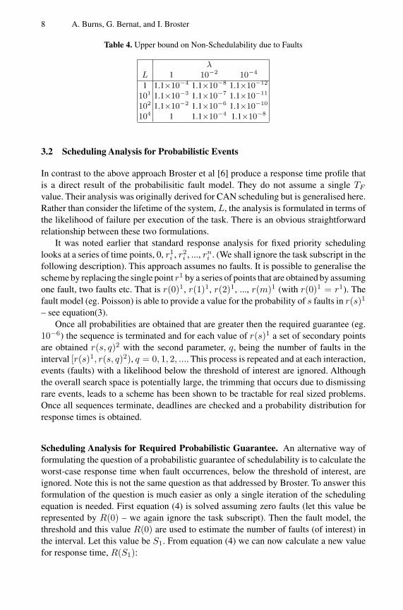
The example introduced in earlier had a TF value of 275ms. Table 4 gives the upperbound on the probability guarantee for various values of λ and L (in seconds).

A typical outcome of this analysis is that in a system that has a non-stop run-time(L) of 10 hours with a mean time between transient faults of 1000 hours and a toleranceof faults that do not appear closer than 1/100 of an hour, the probability of missing adeadline is upper bounded by 1.5×10−7. A lower bound is also derived (Corollary 4)and this yields a value of 0.5×10−7. For these parameters the exact analysis produces avalue very close to 1.0×10−7.

When λL<10−2, λL approximates the probability of any fault happening during themission of duration L. So, 2

3 (λTF )−1 represents the gain in reliability that is achievedby the use of fault tolerance, under the other assumptions stated. For example, in Table4, when λ = 10−2 and L = 1 the gain is approximately 106.

8 A. Burns, G. Bernat, and I. Broster

Table 4. Upper bound on Non-Schedulability due to Faults

λL 1 10−2 10−4

1 1.1×10−4 1.1×10−8 1.1×10−12

101 1.1×10−3 1.1×10−7 1.1×10−11

102 1.1×10−2 1.1×10−6 1.1×10−10

104 1 1.1×10−4 1.1×10−8

3.2 Scheduling Analysis for Probabilistic Events

In contrast to the above approach Broster et al [6] produce a response time profile thatis a direct result of the probabilisitic fault model. They do not assume a single TF

value. Their analysis was originally derived for CAN scheduling but is generalised here.Rather than consider the lifetime of the system, L, the analysis is formulated in terms ofthe likelihood of failure per execution of the task. There is an obvious straightforwardrelationship between these two formulations.

It was noted earlier that standard response analysis for fixed priority schedulinglooks at a series of time points, 0, r1

i , r2i , ..., rn

i . (We shall ignore the task subscript in thefollowing description). This approach assumes no faults. It is possible to generalise thescheme by replacing the single point r1 by a series of points that are obtained by assumingone fault, two faults etc. That is r(0)1, r(1)1, r(2)1, ..., r(m)1 (with r(0)1 = r1). Thefault model (eg. Poisson) is able to provide a value for the probability of s faults in r(s)1

– see equation(3).Once all probabilities are obtained that are greater then the required guarantee (eg.

10−6) the sequence is terminated and for each value of r(s)1 a set of secondary pointsare obtained r(s, q)2 with the second parameter, q, being the number of faults in theinterval [r(s)1, r(s, q)2), q = 0, 1, 2, .... This process is repeated and at each interaction,events (faults) with a likelihood below the threshold of interest are ignored. Althoughthe overall search space is potentially large, the trimming that occurs due to dismissingrare events, leads to a scheme has been shown to be tractable for real sized problems.Once all sequences terminate, deadlines are checked and a probability distribution forresponse times is obtained.

Scheduling Analysis for Required Probabilistic Guarantee. An alternative way offormulating the question of a probabilistic guarantee of schedulability is to calculate theworst-case response time when fault occurrences, below the threshold of interest, areignored. Note this is not the same question as that addressed by Broster. To answer thisformulation of the question is much easier as only a single iteration of the schedulingequation is needed. First equation (4) is solved assuming zero faults (let this value berepresented by R(0) – we again ignore the task subscript). Then the fault model, thethreshold and this value R(0) are used to estimate the number of faults (of interest) inthe interval. Let this value be S1. From equation (4) we can now calculate a new valuefor response time, R(S1):

A Probabilistic Framework for Schedulability Analysis 9

Ri(S1) = Ci + Bi +∑

j∈hp(i)

⌈Ri

Tj

⌉Cj + S1 max

k∈hep(i)(Fk) (8)

The number of faults of interest in R(S1) is then calculated. If this new value, S2,is equal to S1 then the formulation is stable and R(S1) is the worst case response time.Alternatively equation (8) is solved for S2 and the process continues until either stabilityis obtained or a response time greater than deadline is calculated and unschedulabilityis proclaimed.

To illustrate the approach consider the small example given earlier for the otherapproach. If we set the threshold value to 10−6 and assume λ is obtained from a meantime between errors of 0.1 seconds then the same response time give in Table 3 areobserved (eg. 60, 100, 155 and 275).

Note that the above analysis is relatively straightforward when a Poisson derivedfault model is assumed. Nevertheless, the framework can still be used if other arrivaldistributions are more appropriate.

3.3 Summary

The schemes reviewed in this section all have a common theme. Scheduling approachesare used to maximise the effective resources that can be made available, when required,for fault tolerance. Then limits to schedulability are derived in conjuction with the prob-ability of those limits being observed during execution. This furnishes the probabilisticguarantee. Alternatively, a standard yes/no guarantee is obtained while faults below athreshold of likelihood are ignored.

4 Probabilistic Guarantees with Non-periodic Work

Initially scheduling analysis assumed a purely periodic work flow [28]. The sporadicjobs were incorporated by assuming a minimum arrival time, that in the worst case wasexhibited by the system. In effect a sporadic job behaved exactly the same as a periodicone. Response time analysis, as outlined in Section 2 can actually deal with a muchmore general model of non-periodic work. Let Ak(t) be defined to be a function thatdelivers the maximum number of arrivals of task k in any interval [0,t). Then equation(1) becomes

Ri = Ci + Bi +∑

j∈hpp(i)

⌈Ri

Tj

⌉Cj +

∑

k∈hpn(i)

Ak(Ri)Ck (9)

where hpp(i) is now the set of higher priority periodic tasks, and hpn(i) the set ofhigher priority non-periodic tasks.

Although a useful generalisation, equation (9) is still a deterministic one. It assumesthat the worst-case number of arrivals of all sporadics tasks will occur with probabilityone. To deal with non-periodic tasks that follow a stochastic model a different frameworkis needed. First, some form of probabilistic density function will be needed for all sources

10 A. Burns, G. Bernat, and I. Broster

of sporadic work. If nothing is known about the arrival pattern of work then clearly noguarantee, not even a probabilistic one, can be given. One method of incorporating thisstochastic work load is to use the same approach as for fault tolerance. After all, faultshandling routines are, from a scheduling point of view, just one form of non-periodicwork. The approach outlined in Section 3.2 can then be applied.

A probability threshold for the system must be defined. This is the value below whichevents are sufficiently rare to be ignored. Let ρ be this threshold value. We redefinedthe function A given earlier in this section as follows: Ak(ρ, t) is the number of arrivalevents in any interval of length t with a probability of more than ρ. So Ak(10−6, 30),for example, would give the result 2 if the probability of 3 or more arrivals in 30 timeunits is less than 10−6 (and the probability of 2 is more than this value). Equation (9)then becomes:

Ri = Ci + Bi +∑

j∈hpp(i)

⌈Ri

Tj

⌉Cj +

∑

k∈hpn(i)

Ak(ρ, Ri)Ck (10)

This approach contains some explicit assumptions that would need to be clarified.For example, it assumes each source of arrivals is independent of each other; also thatthe computation time of the job is independent of the arrival behaviour. The existenceof correlations would complicate the analysis – but pessimistic assumptions may berelatively straightforward to incorporate (see later discussion on the use of Copulas).

Care must of course be taken with choosing the probability threshold for the system.If an application is, by its specification, meant to deal with rare events then the thresh-old must be chosen so that such events (at least one in any small interval) are alwaysincorporated into the run-time behaviour that is being analysed.

5 Representing Execution Time

The above discussions have generalised the notion of work flow by allowing the arrivalof work to be described stochastically. However the worst-case resource requirementof each job is still represented by a single parameter C. This represents the maximumprocessor (resource) time needed by the job on each and every arrival. In developinga general framework for scheduling analysis, where application code and processorbehaviour combined to produce a rich execution profile, it is not surprising that thissingle parameter approach is becoming limited in its application. Even a two (averageand worst-case) or three (add minimum) parameter scheme is far from adequate.

In other works [8,16,4] we have argued that it is now inadequate to use analysisalone to obtain a single worst-case execution time (WCET) value. Rather a combinationof analysis and measurement must be used to obtain a probabilistic representation ofthe entire execution profile of the task. Moreover, this probability density function mustextend beyond observed data to predict the likelihood of experiencing, during the realexecution of the system, extreme (large) values for execution time. Data obtained frommeasurement of relatively straightforward code illustrates two general characteristics ofexecution time profiles (let O be the maximum observed value during meansurement).

A Probabilistic Framework for Schedulability Analysis 11

– Large observed values for computation time may be sufficiently rare that for non-hard systems it would be inappropriate for any schedulability test to assume thisvalue for every task’s execution (ie. O is too large to use).

– Large observed values for computation time may not represent the worst-case thatwill be experienced during real execution, and extrapolations beyond observed val-ues will be needed for some hard real-time systems (ie. O is too small to use).

The alternative to simple parameterisation is to model execution time as a randomvariable following some probability distribution. These distributions (execution timeprofiles) being derived from measurement. But the granularity of measurement remainsan open issue. Three levels are possible:

1. The basic block - a sequence of instructions.2. The task - which consists of a number of basic blocks.3. The system - which consists of a number of tasks.

If measurement is used at the task level then knowledge about the structure of thetask is being ignored, however uncertainties arising from the interactions of basic blocksare being sampled. If analysis is used at the task level (with measurements only beingdone for basic blocks) then the rules for combining the execution time profiles need tobe articulated. A similar trade-off exists at the system level.

In the work we have undertaken, we have used measurement only at the basic blocklevel and hence we must address the issue of how to combine probability distributions.If independence could be assumed then standard statistical methods could be applied.Unfortunately there seems to be ample evidence that this assumption would be overtlyoptimistic. A series of basic blocks may be strongly correlated. Moreover a series oftask executions within a schedule may also be dependent upon one another. Indeed theexecution of the same task, one or more times, within the response time of a lowerpriority task may exhibit a strong correlation. These may be positive (a long executiontime is more likely to be followed by another large one) or negative (long will induce ashort one next time).

5.1 Use of Copulas

Copulas are a general mathematical tool to construct multivariate distributions and toinvestigate dependence structures between random variables [32]. A copula is basicallya joint distribution function with uniform marginals. The main feature is that they allowone to separate the marginal distributions from the dependency between the two randomvariables, therefore given a joint probability distribution it is possible to characterizeit uniquely with the marginal distributions and a copula. Similarly, given two marginaldistributions and a copula, it is possible to derive the joint distribution and this is unique.

The importance is that the copula captures the dependence structure between randomvariables. So given two joint distributions with different marginal distributions but thatcapture the same dependency process, they would have the same copula.

There are two additional results of importance for this analysis, the first one is that theset of copulas is a partially ordered set and there exist two special copulas, called the lower

12 A. Burns, G. Bernat, and I. Broster

and upper Frechet bounds that characterize the maximum and minimum dependencebetween random variables.

The problem of timing analysis can be formulated as follows, if X and Y are tworandom variables that represent the execution time of two blocks of code with respec-tive distribution functions FX(t) and FY (t), we want to determine the distribution ofZ = X + Y which is the execution time of X followed by Y , FZ(t). If X and Y areindependent, the probability density function of Z corresponds to the standard convolu-tion of the probability density functions of X and Y . However, if this hypothesis is notcorrect then we can use the theory of copulas to construct FZ(t).

If the joint distribution is known, (or its copula) then the distribution of Z is astraightforward generalisation of the convolution but using the joint distribution instead.More importantly, if the dependency is not known, then it is possible to find upperand lower bounds of the distribution function for any possible dependency between themarginal distributions [5,29,14]. Some generalisations of these results allow to tighteneven more these bounds if partial knowledge of the dependence is known.

5.2 Representing Extreme Execution Times

It was noted earlier that for some hard real-time systems execution time values beyondwhat have been observed during tests need to be taken into account if very low levels offailure are to be tolerated. One means of addressing this issue is to apply the branch ofstatistics concerned with extreme values. One of the three extreme value distributions isused to ‘fit’ the data and then give predictions beyond the observed data range. We havehad some success [16] in fitting the Gumble distribution but it is still not clear if this isa general purpose technique. What this approach provides is a probability distributionfor the worst-case value for a task’s execution. One useful result of this study is that acollection of tasks has a bounded behaviour. Let C1..CN be the worst-case times derivedfrom the above approach with probability threshold ρ; then the sequential execution ofeach task will have a total expected execution time of C1 + C2 + C3 + .. + CN withprobability bound ρ.

6 Other Relevant Work on Probabilistic Analysis

There have been some other approaches using probabilistic methods in real-time systems.The work of Diaz et.al. [15] computes probability distributions of the response times ofentirely periodic (fixed release times) task systems with random execution times. Thework relies on the independence of the execution times of the different tasks. The workimproves on an earlier work by Gardner et.al. [18]. The works of Nissanke [25] and Eles[30] also tackle this problem. However, none of these approaches address the issue ofextreme distributions or dependencies between execution times or task arrivals.

A Probabilistic Framework for Schedulability Analysis 13

7 Conclusion: A Probabilistic Framework

Bringing together the above approaches we are able to postulate one means of construct-ing a scheduling framework that can deal with stochastic parameterisation of work flow.The following are the main components of such a framework.

1. All tasks have an arrival pattern expressed as A(ρ, t) - the number of instances ofthe task likely to occur in any interval of length t, where the probability of greaterthan A(ρ, t) occurring is less than ρ.

2. All tasks have an execution profile derived that extends beyond the data observedduring test.

3. A threshold probability is defined for the system. Events (task arrivals or execu-tion times) with a likelihood of occurring less than this threshold are ignored. Thethreshold could be expressed as a likelihood of failure per execution of any task ofinterest.

4. A worst-case response time of each task is calculated from the above data as follows:– An initial estimate, R0, is obtained by assuming all tasks arrive once with

execution times derived from their profiles and ρ.– The number of tasks arriving in R0 is derived (using A(ρ, R0) and any depen-

dency relationships).– A conservative copula is used to combine the execution profiles of those jobs.– A new value for R0 (i.e. R1) is obtained by using the threshold probability value

on this derived distribution.– Repeat until a stable value of R is obtained (or R expands beyond the task’s

deadline).

It would be at least theoretically possible to vary the probability threshold to derivea relation between response time and this threshold.

In conclusion, we have argued in support of the developed the notion of a probabilis-tic assessment of schedulability and shown how it can be derived from the stochasticbehaviour of the work that the real-time system must accomplish. Many aspects of thisframework require significant further study, and we aim to continue with this line ofinvestigation.

References

1. A.K. Atlas and A. Bestavros. Statistical rate monotonic scheduling. In Proceedings of the19th IEEE Real-Time Systems Symposium, Madrid, Spain, pages 123–132. IEEE ComputerSociety Press, 1998.

2. N. C. Audsley, A. Burns, M. Richardson, K. Tindell, and A. J. Wellings. Applying newscheduling theory to static priority pre-emptive scheduling. Software Engineering Journal,8(5):284–292, 1993.

3. G. Bernat and A. Burns. New results on fixed priority aperiodic servers. In 20th IEEEReal-Time Systems Symposium, Phoenix. USA, December 1999.

4. G. Bernat,A. Colin, and S. M. Petters. WCET analysis of probabilistic hard real–time systems.In Proceedings of the 23rd Real-Time Systems Symposium RTSS 2002, pages 279–288,Austin,Texas, USA, 2002.

14 A. Burns, G. Bernat, and I. Broster

5. G. Bernat and M. Newby. Probabilistic WCET analysis, an approach using copulas. Technicalreport, Department of Computer Science University of York, Technical Report, 2003.

6. I. Broster, A. Burns, and G. Rodrıguez-Navas. Probabilistic analysis of CAN with faults. InProceedings of the 23rd Real-time Systems Symposium, Dec 2002.

7. A. Burns, R. I. Davis, and S. Punnekkat. Feasibility analysis of fault-tolerant real-time tasksets. Euromicro Real-Time Systems Workshop, pages 29–33, June 1996.

8. A. Burns and S. Edgar. Predicting computation time for advanced processor architectures. InProceedings 12th EUROMICRO conference on Real-time Systems, 2000.

9. A. Burns, S. Punnekkat, L. Strigini, and D.R. Wright. Probabilistic scheduling guarantees forfault-tolerant real-time systems. In Proceedings of the 7th International Working Conferenceon Dependable Computing for Critical Applications. San Jose, California, pages 339–356,1999.

10. A. Burns and A. J. Wellings. Engineering a hard real-time system: From theory to practice.Software-Practice and Experience, 25(7):705–26, 1995.

11. A. Burns and A. J. Wellings. Real-Time Systems and Programming Languages. AddisonWesley Longman, 3rd edition, 2001.

12. A. Campbell, P. McDonald, and K. Ray. Single event upset rates in space. IEEE Transactionson Nuclear Science, 39(6):1828–1835, December 1992.

13. X. Castillo, S.P. McConnel, and D.P. Siewiorek. Derivation and Calibration of a TransientError Reliability Model. IEEE Transactions on Computers, 31(7):658–671, July 1982.

14. H. Cossette, M. Denuit, and E. Marceau. Distributional bounds for functions of dependentrisks. Technical report, Bulletin suisse des actuaires., 2001.

15. J.L. Diaz, D. F. Garcıa, K. Kim, C.-G. Lee, L.L. Bello, J.M. Lopez, S.L. Min, and O. Mirabella.Stochastic analysis of periodic real-time systems. In 22nd IEEE Real-Time Systems Sympo-sium., Austin, TX. USA, 2002.

16. S. Edgar and A. Burns. Statistical analysis of WCET for scheduling. In Proceedings IEEEReal-Time Systems Symposium, 2001.

17. M. K. Gardner. Probabilstic Analysis and Scheduling of Critical Soft Real-time Systems. PhDthesis, University of Illinois, Computer Science, Urbana, Illinois, 1999.

18. M. K. Gardner and J.W. Lui. Analysing stochastic fixed-priority real-time systems. InProceedings of the 5th International Conference on Tools and Algorithms for the Constructionand Analysis of Systems, 1999.

19. C.-J. Hou and K. G. Shin. Allocation of periodic task modules with precedence and deadlineconstraints in distributed real-time systems. IEEE Transactions on Computers, 46(12):1338–1356, 1997.

20. M. Joseph and P. Pandya. Finding response times in a real-time system. BCS ComputerJournal, 29(5):390–395, 1986.

21. D.I. Katcher, H. Arakawa, and J.K. Strosnider. Engineering and analysis of fixed priorityschedulers. IEEE Trans. Softw. Eng., 19, 1993.

22. H. Kim, A.L.White, and K. G.Shin. Reliability modeling of hard real-time systems. InProceedings 28th Int. Symp. on Fault-Tolerant Computing (FTCS-28), pages 304–313. IEEEComputer Society Press, 1998.

23. M. H. Klein, T.A. Ralya, B. Pollak, R. Obenza, and M. G. Harbour. A Practitioner’s Handbookfor Real-Time Analysis: A Guide to Rate Monotonic Analysis for Real-Time Systems. KluwerAcademic Publishers, 1993.

24. J.P. Lehoczky, L. Sha, and V. Ding. The rate monotonic scheduling algorithm: Exact charac-terization and average case behavior. Tech report, Department of Statistics, Carnegie-Mellon,1987.

25. A. Leulseged and N. Nissanke. Stochastic analysis of periodic real-time systems. In 9thIntl. Conf. on Real-Time and Embeded Computing Systems and applications (RTCSA 2003),Taiwan, 2003.

A Probabilistic Framework for Schedulability Analysis 15

26. J.Y.T. Leung and J. Whitehead. On the complexity of fixed-priority scheduling of periodic,real-time tasks. Performance Evaluation (Netherlands), 2(4):237–250, 1982.

27. G. Lima and A. Burns. An optimal fixed-priority assignment algorithm for supporting fault-tolerant hard real-time systems. IEEE Transactions on Computer Systems (to appear), 2003.

28. C.L. Liu and J.W. Layland. Scheduling algorithms for multiprogramming in a hard real-timeenvironment. JACM, 20(1):46–61, 1973.

29. G.D. Makarov. Estimates for the distribution function of a sum of two random variales whenthe marginal distributions are fixed. Theory Probab. Appli., 26:803–806, 1981.

30. S. Manolache, P. Eles, and Z. Peng. Memory and time efficient schedulability analysis oftask sets with stochastic execution time. In Proceedings 13th EUROMICRO conference onReal-time Systems, 2001.

31. N. Navet, Y.-Q.Song, and F. Simonot. Worst-case deadline failure probability in real-timeapplications distributed over controller area network. Journal of Systems Architecture,46(1):607–617, 2000.

32. R.B. Nelsen. An introduction to Copulas. Springer, 1998.33. S. Punnekkat. Schedulability Analysis for Fault Tolerant Real-time Systems. PhD thesis,

Dept. Computer Science, University of York, 1997.34. S. Punnekkat, R. Davis, and A. Burns. Sensitivity analysis of real-time task sets. In Pro-

ceedings of the Conference of Advances in Computing Science - ASIAN ’97, pages 72–82.Springer, 1997.

35. S. Ramos-Thuel and J.P. Lehoczky. On-line scheduling of hard deadline aperiodic tasks infixed-priority systems. In Proceedings of 14th IEEE Real-Time Systems Symposium, pages160–171, December 1993.

36. K. G. Shin, M. Krishna, and Y. H. Lee. A unified method for evaluating real-time computercontrollers its application. IEEE Transactions on Automatic Control, 30:357–366, 1985.

37. M. Silly, H. Chetto, and N. Elyounsi. An optimal algorithm for guaranteeing sporadic tasksin hard real-time systems. In Proceedings 2nd IEEE Symposium on Parallel and DistributedSystems, pages 578–585, 1990.

38. T.S. Tia, Z. Deng, M. Shankar, M. Storch, J. Sun, L.C. Wu, and J.S. Liu. Probabilisitcperformance guenrantee for real-time tasks with varying computation times. In Proceedingsof the Real-Time Technology and Applications Symposium, pages 164–173, 1995.

39. S. Vestal. Fixed Priority Sensitivity Analysis for Linear Compute Time Models. IEEETransactions on Software Engineering, 20(4):308–317, April 1994.

Resource-Efficient Scheduling for Real Time Systems

Kim G. Larsen

BRICS, Aalborg University DenmarkFredrik Bajers Vej 7, 9220 Aalborg Ø – Denmark

kgl@cs.auc.dk

1 Introduction

For embedded systems efficient utilization of resources is an acute problem arisingfrom the increasing computational demands in all sorts of applications. The consumersconstantly demand better functionality and flexibility of embedded products which implyan increase in the resources needed for their realization. In several areas – e.g. portabledevices such as PDAs, mobile phones and laptops as well as mission critical systemssuch as space applications – the ability to design resource efficient solutions is crucial.

Our own work in this area include development and applications of the real-timeverification tool Uppaal to the modeling, analysis and synthesis of resource-efficientand -optimal schedules for real-time systems. Whereas (hard) timeliness and resource-efficiency may be seen as conflicting goals, this approach allows for both goals to beachieved.

2 Verification Using UPPAAL

Uppaal [20] is an integrated tool environment for modeling, simulating and verificationof real-time systems, developed jointly by BRICS at Aalborg University in Denmarkand by DoCS at Uppsala University in Sweden. The modeling language of Uppaalsupports model checking safety and (bounded) liveness properties of systems that canbe modeled as a collection of timed automata communicating through (broadcast aswell as binary) channels or shared variables. Typical application areas include real-time controllers where timely execution of a number of (periodic or sporadic) tasksis controlled by a particular scheduling policy. Given timed automata models of thetasks, the scheduler(s) as well as the real-time environment of the control systems theverification engine of Uppaal may validate (or refute) the correctness and resoucerequirements of the particular scheduling policy applied.

In a number of papers [13,16,11] this approach has been applied to systems controlledby LEGO MINDSTORMTM bricks. Here the Uppaal models of task are automaticallysynthesised from the RCXTM programs together with a model of the (round-robin)scheduling policy applied. The significant difference in the frequency by which changesoccur in the scheduler (numerous samples per second) and in the environment (possiblyseconds between changes) causes a fragmentation of the symbolic state space of Uppaal. Basic Research in Computer Science (www.brics.dk), funded by the Danish National Rese-

arch Foundation.

R. Alur and I. Lee (Eds.): EMSOFT 2003, LNCS 2855, pp. 16–19, 2003.c© Springer-Verlag Berlin Heidelberg 2003

Resource-Efficient Scheduling for Real Time Systems 17

As a remedy an exact acceleration technique has been developed [12] and demonstratedefficient on a number of examples.

3 Optimal Scheduling Using UPPAAL

In more recent work Uppaal has been applied to the synthesis of the scheduling policyitself. This work was initiated during the now terminated ESPRIT project VHS [21] andis continuing within the ongoing IST project AMETIST [2]. Modeling the tasks to bescheduled, the constraining, shared resources involved as well as timing assumptionsof the environment allows the scheduling problem to be stated as a (time-bounded)reachability question. The (possible) diagnostic trace provided by Uppaal offers a validschedule to the problem. Extending Uppaal with mechanisms for guiding the explorationhas proved extremely successful in obtaining feasible solutions to industrial schedulingproblems including the synthesis of production schedules for a the Steel ProductionPlant SIDMAR in Ghent, Belgium [10,14].

Often one want not just a an arbitrary valid schedule but rather a schedule which isoptimal with respect to some suitable cost measure (e.g. in terms of total elapsed timedor total power consumption). For this purpose an extension of the timed automata modelwith a notion of cost was introduced in [5]: each action transition has an associated price,and likewise, each location has an associate rate giving the increase in cost for delaying ontime-unit. In [5], and independently in [1], computabitlity of minimal-cost reachabilitywas demonstrated based on a cost-extension of the classical notion of regions. Later,in [6,17], efficient zone-based algorithms for computing minimum-time respectivelyminimum-cost reachability has been given and applied to a range of optimal schedulingproblems including job shop scheduling problems and aircraft landing problems. Theoptimization criteria distinguish scheduling algorithms from classical, full state spaceexploration model checking algorithms. In the Uppaal implementation [3] they are areused together with, for example, branch-and-bound techniques to prune parts of thesearch space that are guaranteed not to contain optimal solutions.

Current research considers efficient computation of optimal infinite schedules aswell as optimal dynamic schedules (i.e. optimal under uncertainty or in the presence ofuncontrollable behaviour).

4 Applications

Emphasis in the talk will be given to the application of Uppaal to two industrial schedul-ing problems focusing on memory utilization and power/energy consumption respec-tively.

The first case study [4] is provided by Terma A/S who is developing and producingradar sensor equipment. The case study, conducted in the ISTAMETIST project, focuseson the memory interface of the video processing board of a radar sensor system usedfor ground surveillance at airports and for coastal surveillance. The task of the memoryinterface is to control access to a single memory bus used by 9 different (buffered)data streams. A valid scheduler must guarantee that none of the data streams are everinterrupted, and efficiency is measured in the requirement to buffer sizes. During the first

18 K.G. Larsen

year of AMESTIST several models has been developed including models in Uppaal[19], where verification has confirmed the validity of the scheduling principle appliedby Terma today. Also, the developed models have lead to identification of a memory-optimal, new scheduling principle [22].

The second case study focuses on Dynamic Voltage Scaling, which appears as one ofthe most promising methods for reducing energy consumption. The principle consists indynamically adjusting the clock-cycle length as well as the supply voltage depending onthe actually task load in the system. However, optimality depends highly on the concretehardware platform as well as the type of applications. Within the newly formed Danishcenter for embedded software systems, CISS [8], and in collaboration with AnalogDevices various DVS scheduling principles are modeled, simulated and analyzed, withAnalog Devices Blackfin DSP processor (ADSP-21535 EZ-KIT Lite) as ultimate target.

References

1. R. Alun, S. La Torre, and G. J. Pappas. Optimal paths in weighted timed automata. To appearin HSCC2001.

2. The AMETIST home page. http://ametist.cs.utwente.nl.3. G. Behrmann. Guiding and cost optimizing uppaal. Web-page, 2002.4. G. Behrmann, S. Bernicot, T. Hune, K.G. Larsen, S. Lecamp, and A. Skou. Case study 2: A

memory interface for radar systems. Deliverable for AMETIST.5. Gerd Behrmann, Ansgar Fehnker, Thomas Hune, Kim G. Larsen, Paul Pettersson, Judi

Romijn, and Frits Vaandrager. Minimum-Cost Reachability for Priced Timed Automata.In Maria Domenica Di Benedetto and Alberto Sangiovanni-Vincentelli, editors, Proceedingsof the 4th International Workshop on Hybrid Systems: Computation and Control, number2034 in Lecture Notes in Computer Sciences, pages 147–161. Springer–Verlag, 2001.

6. Gerd Behrmann, Ansgar Fehnker, Thomas Hune, Kim G. Larsen, Paul Pettersson, and JudiRomijn. Efficient Guiding Towards Cost-Optimality in Uppaal. In T. Margaria and W. Yi,editors, Proceedings of the 7th International Conference on Tools and Algorithms for theConstruction and Analysis of Systems, number 2031 in Lecture Notes in Computer Science,pages 174–188. Springer–Verlag, 2001.

7. Johan Bengtsson, Kim G. Larsen, Fredrik Larsson, Paul Pettersson, Yi Wang, and CarstenWeise. New Generation of Uppaal. In Int. Workshop on Software Tools for TechnologyTransfer, June 1998.

8. The CISS home page. http://ciss.auc.dk.9. H. Dierks, G. Behrmann, and K.G. Larsen. Solving planning problems using real-time model

checking (translating pddl3 into timed automata). 2003.10. A. Fehnker. Citius, Vilius, Melius - Guiding and Cost-Optimality in Model Checking of Timed

and Hybrid Systems. PhD thesis, KUN Nijmegen, 2002.11. M. Hendriks. Translating uppaal to not quite c. Technical Report 8, Nijmegen University,

2001.12. M. Hendriks and K. G. Larsen. Exact acceleration of real-time model checking. In E. Asarin,

O. Maler, and S. Yovine, editors, Electronic Notes in Theoretical Computer Science, vol-ume 65. Elsevier Science Publishers, April 2002.

13. Thomas Hune. Modelling a Real-Time Language. In proceedings of 4th Workshop on FormalMethods for Industrial Critical Systems, FMICS’99., 1999.

Resource-Efficient Scheduling for Real Time Systems 19

14. Thomas Hune, Kim G. Larsen, and Paul Pettersson. Guided Synthesis of Control ProgramsUsing Uppaal. In Ten H. Lai, editor, Proc. of the IEEE ICDCS International Workshop onDistributed Systems Verification and Validation, pages E15–E22. IEEE Computer SocietyPress, April 2000.

15. Thomas Hune, Kim G. Larsen, and Paul Pettersson. Guided Synthesis of Control Programsusing Uppaal. Nordic Journal of Computing, 8(1):43–64, 2001.

16. Torsten K. Iversen, Kare J. Kristoffersen, Kim G. Larsen, Morten Laursen, Rune G. Madsen,Steffen K. Mortgensen, Paul Pettersson, and Chris B. Thomasen. Model-Checking Real-TimeControl Programs. To be published in Proceedings of Euromicro 2000.

17. Kim G. Larsen, Gerd Behrmann, Ed Brinksma, Ansgar Fehnker, Thomas Hune, Paul Petters-son, and Judi Romijn. As cheap as possible: Efficient cost-optimal reachability for pricedtimed automata. In G. Berry, H. Comon, and A. Finkel, editors, Proceedings of CAV 2001,number 2102 in Lecture Notes in Computer Science, pages 493–505. Springer–Verlag, 2001.

18. Kim G. Larsen, Gerd Behrmann, Ed Brinksma, Ansgar Fehnker, Thomas Hune, Paul Petters-son, and Judi Romijn. As cheap as possible: Efficient cost-optimal reachability for pricedtimed automat. In G. Berry, H. Comon, and A. Finkel, editors, Proceedings of CAV 2001,number 2102 in Lecture Notes in Computer Science, pages 493–505. Springer–Verlag, 2001.

19. E. Seshauskaire and M. Mikucionis. Memory interface analysis using the real-time modelchecker uppaal. Deliverable for AMETIST.

20. The Uppaal home page. http://www.uppaal.com.21. The VHS home page. http://www-verimag.imag.fr//VHS/main.html.22. Gera Weiss. Optimal Scheduler for a Memory Card. Research report, Weizmann, 2002.

R. Alur and I. Lee (Eds.): EMSOFT 2003, LNCS 2855, pp. 20–34, 2003.© Springer-Verlag Berlin Heidelberg 2003

Emerging Trends in Adaptive Middleware and ItsApplication to Distributed Real-Time Embedded Systems

Joseph P. Loyall

BBN TechnologiesCambridge, MA

jloyall@bbn.com

Abstract. Embedded systems have become prevalent in today’s computingworld and more and more of these embedded systems are highly distributed andnetwork centric. This adds increasing degrees of resource contention,unpredictability, and dynamism to software that has traditionally been designedwith resources being provisioned statically and for the worst case. This paperdescribes the research that we’ve been doing in the development of middlewarefor QoS adaptive systems – an extension to standard off-the-shelf distributedobject middleware – and its application to two military distributed real-timeembedded systems. These real-world evaluations of the technology thenmotivate a discussion of the next directions in which we are taking thisresearch.

1 Introduction

Over 99% of all microprocessors are now used for embedded systems [2] that controlphysical, chemical, biological, or defense processes and devices in real-time.Increasingly, these embedded systems are part of larger distributed embeddedsystems, such as military combat or command and control systems, manufacturingplant process systems, emergency response systems, and telecommunications. Arecent OMG workshop on real-time embedded and distributed object computing hadcommercial representatives describing distributed, real-time embedded (DRE)systems in the following domains [17]:

• Avionics• Submarine combat control• Satellite flight control• Signal analysis• Software defined radio• Industrial production• Automated assembly

Middleware, such as CORBA, is being applied to these types of applicationsbecause of its ability to abstract issues of distribution, heterogeneity, andprogramming language from the design of systems. CORBA, specifically, hasspearheaded this trend because of its development of standards supporting the needs

Emerging Trends in Adaptive Middleware 21

of DRE systems, such as RTCORBA [18], FT-CORBA [15], and MinimumCORBA [16].

More and more of these systems are networked systems of systems, withheterogeneous platforms and networks. Because of this, predictable real-timebehavior in these DRE systems relies on the ability to do the following:

• Manage resources end-to-end. Real-time performance might be dominated by asingle, most constrained or loaded resource, but it will rely on all the resourcesend-to-end, processing at each node and the network link between each node alongeach source-to-sink data path.

• Adapting and reconfiguring to changing conditions. In DRE systems of systems,participants might come and go, failures will happen, and mission modes willchange. The system must be able to compensate for additional and changingdemands, changing mission requirements and priorities, and failures.

Another characteristic of these DRE systems is that their heterogeneous resourceswill often have varying degrees of available control. For example, a military combatand command/control system that includes unmanned aerial vehicles (UAVs), fighteraircraft, and ground and air command and control (C2) nodes will include a variety ofprocessing nodes, from embedded VME boards to workstations, and a variety ofnetwork links, from tactical radio links to ground IP-based network links. Tacticallinks currently utilize statically allocated and preconfigured time slots for dividing upthe available bandwidth. Once time slots are allocated to a source-sink link, theycannot be easily changed. In contrast, dynamic reservation-based and priority-basednetwork management is becoming available for wired, IP networks.

This motivates the need for middleware that extends the current distribution,abstraction, and limited QoS support provided in CORBA. DRE systems need QoSadaptive middleware, which supports the following:

• Specification of QoS and mission requirements, mission modes and system states,priorities, and trade offs.

• Measurement of system conditions, delivered QoS, and resource availability andconstraints.

• Control of resource mechanisms, managers, and services, and of application levelbehavior (such as data manipulation).

• Adaptation and reconfiguration to compensate for changing system conditions,mission modes, and failures.

In this paper, we describe the Quality Objects (QuO) QoS adaptive middleware,which we have applied to the development of several DRE applications. We will firstdescribe QuO. Then we will describe a couple of DRE applications which we havedeveloped using QuO. Finally, we will describe the directions in which the research isproceeding.

2 Overview of the Adaptive QuO Middleware

Quality Objects (QuO) is a distributed object computing (DOC) framework designedto develop distributed applications that can specify (1) their QoS requirements, (2) thesystem elements that must be monitored and controlled to measure and provide QoS,

22 J.P. Loyall

and (3) the behavior for controlling and providing QoS and for adapting to QoSvariations that occur at run-time. By providing these features, QuO separates the roleof functional application development from the role of developing the QoS behaviorof the system.

Figure 1 illustrates a client-to-object logical method call in distributed objectcomputing as instantiated by the CORBA standard. In a traditional DOC application,a client makes a logical method call to a remote object. A local ORB proxy (i.e., astub) marshals theargument data, whichthe local ORB thentransmits across thenetwork. The ORB onthe server side receivesthe message call, and aremote proxy (i.e., askeleton) thenunmarshals the dataand delivers it to theremote servant. Uponmethod return, the process is reversed.

A method call in the QuO framework is a superset of a traditional DOC call, andincludes the following components, illustrated in Figure 2:

• Contracts negotiate the QoS an application needs, the QoS available in the system,and the policies formediating, con-trolling, and adaptingto changes.

• Delegates act as localproxies for remoteobjects. Each dele-gate provides an in-terface similar to thatof the remote objectstub, but adds locallyadaptive behaviorbased upon thecurrent state of QoS in the

• System condition objects pORBs in the system that ne

• Callback objects provideapplication.

QuO applications can usmanagers, such as RSVP neRTCORBA [18], and the AQ

Besides the traditional appimplementations) and mechmanagers, and other distribu

FQ

CLIENT

DelegateContract

SysCond

Contract

Network

MECHANISM/PROPERTYMANAGER

operation()in args

out args + return value

IDLSTUBS

Delegate

SysCond

SysCond

SysCond

IDLSKELETON OBJECT

ADAPTER

ORB IIOP ORBIIOP

CLIENT OBJECT(SERVANT)OBJECT(SERVANT)

OBJREF

ig. 2. QuO adds components to control, measure, and adapt tooS aspects of an application

CLIENT

Network

operation()in args

out args + return value

IDLSTUBS

IDLSKELETON OBJECT

ADAPTER

ORB IIOP ORBIIOP

CLIENT OBJECT(SERVANT)OBJECT(SERVANT)

OBJREF

Fig. 1. The CORBA computing model

system, as measured by the contract.rovide interfaces to resources, mechanisms, objects, anded to be measured and controlled by QuO contracts. notification interfaces to clients or objects in the

e specialized QoS mechanisms, ORBs, services andtwork reservation [27], the TAO real-time ORB [23],uA dependability manager [4], respectively.lication developers (who develop the client and object

anism developers (who develop the ORBs, propertyted resource control infrastructure), QuO middleware

Emerging Trends in Adaptive Middleware 23

supports another development role, namely QoS developers or Qoskateers.Qoskateers are responsible for defining contracts, system condition objects, callbackmechanisms, and object delegate behavior. To support the added role of Qoskateer,we have developed an open-source QuO toolkit [12, 13, 25], consisting of thefollowing:

• A set of aspect languages, collectively called Quality Description Languages(QDL) for describing QoS contracts and the adaptive behavior of objects andobject interactions [12, 13].

• Code generators that weave measurement, control, and adaptation code intoapplication programs [12].

• A library of reusable system condition objects that provide interfaces to systemresources, mechanisms, services, and managers; and guidelines for building customsystem condition objects.

• A runtime kernel, which coordinates evaluation of contracts and monitoring ofsystem condition objects [25].

• Object gateways for inserting measurement, control, and adaptation beneath theORB layer [19].

• An encapsulation model, called Qoskets, for localizing the code associated with alogically connected QoS adaptive behavior so that it can be referred to, and reused,as a single component, even though the behavior might be woven into various,distributed locations in the executable code [20].

2.1 In-Band and Out-of-Band Adaptation

The QuO architecture supports two means for triggering adaptation at many levelsthroughout the system, e.g., (property) manager-level, middleware-level, and applica-tion-level, as illustrated inFigure 3. QuO delegatestrigger in-band adaptationby making choices uponmethod calls and returns. Adelegate intercepts allmethod calls to sets ofremote objects and adaptsits interactions to theremote objects based on thecurrent QoS region givenby the contract. Contractstrigger out-of-bandadaptation when changes inobserved system conditionobjects cause region transi-tions. In this way, thecontract monitors andcontrols the system’s QoS,but operates orthogonal toand outside the in-band

CLIENT

DelegateContract

SysCond

Contract

Network

MECHANISM/PROPERTYMANAGER

operation()in args

out args + return value

IDLSTUBS

Delegate

SysCond

SysCond

SysCond

IDLSKELETON OBJECT

ADAPTER

ORB IIOP ORBIIOP

CLIENT OBJECT(SERVANT)OBJECT(SERVANT)

OBJREF

(a) QuO’s delegates provide in-band adaptation on messagecall and return

CLIENT

DelegateContract

SysCond

Contract

Network

MECHANISM/PROPERTYMANAGER

operation()in args

out args + return value

IDLSTUBS

Delegate

SysCond

SysCond

SysCond

IDLSKELETON OBJECT

ADAPTER

ORB IIOP ORBIIOP

CLIENT OBJECT(SERVANT)OBJECT(SERVANT)

OBJREF

(b) Out-of-band adaptation occurs when system conditionobjects and contracts recognize system changes

Fig. 3. QuO supports adaptation upon method call/returnand in response to changes in the system

24 J.P. Loyall

functional behavior of the system. For example, Section 3 describes QuO’s use in anavionics dynamic mission replanning system. In this system, in-band QuO adaptationis used to measure the progress of and change the size of data (using tiling and qualitycontrols) being exchanged between aircraft across a constrained network link.Meanwhile, out-of-band QuO adaptation is used to monitor the available CPU and aidin scheduling of the hard and soft real-time avionics tasks.

2.2 The Qosket Encapsulation Model

One goal of QuO is to separate the role of QoS (or systemic) programmer from that ofapplication programmer. A complementary goal of this separation of programmingroles is that systemic behaviors can be encapsulated into reusable units that are notonly developed separately from the applications that use them, but that can be reusedby selecting, customizing, and binding them to an application program. To supportthis goal, we have defined Qoskets as a unit of encapsulation and reuse in QuOapplications. Qoskets are used to bundle in one place all of the specifications andobjects for controlling systemic behavior, as illustrated in Figure 4, independent of theapplication in which the behavior might end up being used, and whether or not thebehavior will be used in-band or out-of-band.

Qoskets encapsulate, as reusable components, the following systemic aspects:

• Adaptation policies –As expressed inQuO contracts

• Measurement andcontrol – As definedby system conditionobjects and callbackobjects

• Adaptive behaviors– Some of which arepartially specifieduntil they arespecialized to afunctional interface.

• QoS implementation– Defined by qosketmethods.

For example, the UAV imagincludes qoskets that help mainresource availability, e.g., CPU a

• adaptation policies to maintaimagery;

• measurement of video througand network resources;

F

Qosket

Contracts SystemConditionObjects

CallbackObjects

QosketImplementation

HelperMethods

DelegateTemplates

SysCond

SysCondSysCondSysCond

SysCondSysCond

SysCond

SysCondSysCondSysCond

SysCondSysCond

CLIENT

Network

operation()in args

out args + return value

IDLSTUBS

ORB

CLIENT OBJ OBJECT(SERVANT)

OBJECTOBJREF

ORB

OBJECT(SERVANT)

OBJECT

ORBNetwork

CLIENT

Network

operation()in args

out args + return value

IDLSTUBS

ORB

CLIENT OBJ OBJECT(SERVANT)

OBJECTOBJREF

ORB

OBJECT(SERVANT)

OBJECT

ORBNetwork

CLIENT

NetworkNetwork

operation()in argsin args

out args + return value

IDLSTUBS

ORB

CLIENT OBJ OBJECT(SERVANT)

OBJECTOBJECT(SERVANT)

OBJECTOBJREF

ORB

OBJECT(SERVANT)

OBJECTOBJECT(SERVANT)

OBJECT

ORBNetworkNetwork

Delegate Delegate Contract Contract ContractContractContract ContractContract ContractContract

SysCond

SysCondSysCondSysCond

SysCondSysCond

SysCond

SysCondSysCondSysCond

SysCondSysCond

CLIENT

Network

operation()in args

out args + return value

IDLSTUBS

ORB

CLIENT OBJ OBJECT(SERVANT)

OBJECTOBJREF

ORB

OBJECT(SERVANT)

OBJECT

ORBNetwork

CLIENT

Network

operation()in args

out args + return value

IDLSTUBS

ORB

CLIENT OBJ OBJECT(SERVANT)

OBJECTOBJREF

ORB

OBJECT(SERVANT)

OBJECT

ORBNetwork

CLIENT

NetworkNetwork

operation()in argsin args

out args + return value

IDLSTUBS

ORB

CLIENT OBJ OBJECT(SERVANT)

OBJECTOBJECT(SERVANT)

OBJECTOBJREF

ORB

OBJECT(SERVANT)

OBJECTOBJECT(SERVANT)

OBJECT

ORBNetworkNetwork

Delegate Delegate Contract Contract ContractContractContract ContractContract ContractContract

ig. 4. Qoskets encapsulate QuO objects into reusablebehaviors.

e dissemination application described in Section 5tain the QoS of image delivery in the face of limitednd network. It includes qoskets that encapsulate

in appropriate timeliness and fidelity tradeoffs for the

hput and network and CPU load and control of CPU

Emerging Trends in Adaptive Middleware 25

• adaptive behaviors that shape the imagery, reserve and prioritize resources, andmigrate functionality;

• QoS implementation that provides setup of the qosket objects and helper methodsfor shaping specific image formats and fragmenting packets to facilitate networkmanagement.

3 DRE Application of QoS Adaptive Middleware – WeaponsSystem Open Architecture

The Weapons System Open Architecture (WSOA) program prototyped a dynamiccollaborative mission planning capability that could be used in-flight between acommand and control (C2) aircraft and a fighter aircraft. As illustrated in Figure 5,the fighter aircraft and the C2 aircraft establish a collaboration to exchange virtualtarget folders (VTFs), consisting of images and plain text data to update the fighter’smission [3, 14].

WSOA is built upon a layeredarchitecture of domain-specific,QoS adaptive, and distributionmiddleware; as well as QoSmechanisms, services, andmanagers. Middleware on thefighter node consists of

• The Bold Stroke avionicsmiddleware [24]

• QuO QoS adaptive middle-ware

• TAO distribution middleware

The C2 node utilizes ORBexpress, a CORBA ORB supporting the C2 legacysoftware applications written in Ada, and Visibroker. QoS mechanisms, services, andmanagers in WSOA consist of

• RT-ARM [7], a CPU admission control service, on the fighter node• Kokyu [6], a real-time scheduling and dispatching service, on the fighter node• Tactical communication links, using legacy Link 16 incorporated on the C2 and

fighter nodes using portable protocols. Link 16 utilizes statically allocated timeslots for network allocation.

3.1 QoS Management in WSOA

Processing on the fighter node involves hard and soft real-time tasks. Hard real-timetasks are statically scheduled to assign rates and priorities. WSOA uses QuO, RT-ARM, and Kokyu to schedule soft real-time tasks in the extra CPU availabilityavailable for the worst case, but unused in the usual case, and to adapt processing and

VTFs

Adaptation, resource mgmtand RT scheduling

Pro

cess

orR

M

TAO

QuOSoft RT tasksHard RT tasks

C2

Fighter Target

SMSNAV

HUD

Fig. 5. The C2 aircraft sends VTF data to the fighteraircraft for dynamic mission planning

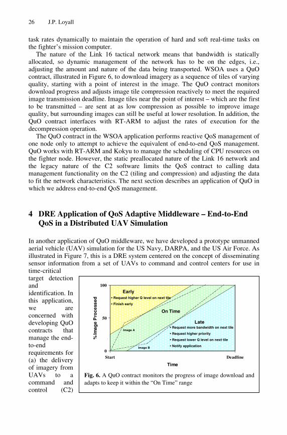
26 J.P. Loyall

task rates dynamically to maintain the operation of hard and soft real-time tasks onthe fighter’s mission computer.

The nature of the Link 16 tactical network means that bandwidth is staticallyallocated, so dynamic management of the network has to be on the edges, i.e.,adjusting the amount and nature of the data being transported. WSOA uses a QuOcontract, illustrated in Figure 6, to download imagery as a sequence of tiles of varyingquality, starting with a point of interest in the image. The QuO contract monitorsdownload progress and adjusts image tile compression reactively to meet the requiredimage transmission deadline. Image tiles near the point of interest – which are the firstto be transmitted – are sent at as low compression as possible to improve imagequality, but surrounding images can still be useful at lower resolution. In addition, theQuO contract interfaces with RT-ARM to adjust the rates of execution for thedecompression operation.

The QuO contract in the WSOA application performs reactive QoS management ofone node only to attempt to achieve the equivalent of end-to-end QoS management.QuO works with RT-ARM and Kokyu to manage the scheduling of CPU resources onthe fighter node. However, the static preallocated nature of the Link 16 network andthe legacy nature of the C2 software limits the QoS contract to calling datamanagement functionality on the C2 (tiling and compression) and adjusting the datato fit the network characteristics. The next section describes an application of QuO inwhich we address end-to-end QoS management.

4 DRE Application of QoS Adaptive Middleware – End-to-EndQoS in a Distributed UAV Simulation

In another application of QuO middleware, we have developed a prototype unmannedaerial vehicle (UAV) simulation for the US Navy, DARPA, and the US Air Force. Asillustrated in Figure 7, this is a DRE system centered on the concept of disseminatingsensor information from a set of UAVs to command and control centers for use intime-criticaltarget detectionandidentification. Inthis application,we areconcerned withdeveloping QuOcontracts thatmanage the end-to-endrequirements for(a) the deliveryof imagery fromUAVs to acommand andcontrol (C2)

0

50

100

Start Deadline

Time

% Im

age

Pro

cess

ed

Early

Late

On Time

• Request more bandwidth on next tile

• Request higher priority

• Request lower Q level on next tile

• Notify application

• Request higher Q level on next tile

• Finish early

Image A

Image B

Fig. 6. A QuO contract monitors the progress of image download andadapts to keep it within the “On Time” range

Emerging Trends in Adaptive Middleware 27

pdintoc

wcthadpbethHfofoUpteomfoPCESp

m

Q(image display)

Q(video capture,processing)

Q(data)Q(bandwidth)

Q(bandwidth)

Q(bandwidth)

Q(networkmanagement)

Video Processing,ATR

CommandDecision

Q(CPU)

Q(FT)

1 plot/4 secs

UAVControl1 fix/

10 secs

Q(platform steering,navigation,weapon targeting)

Q(controlsignals)

Surveillance

Fig. 7. The prototype UAV image dissemination system requires end-to-end QoSmanagement

latform (e.g., a ground station, air C2 node, or shipboard environment) and (b) theelivery of control signals from the C2 platform back to the UAVs. QoS managementcludes trading off image quality and timeliness and managing resources from end--end, with heterogeneous resources (e.g., tactical radio and wired IP networks),

hanging mission requirements, and dynamic environmental conditions.Figure 8 illustrates the architecture of the prototype. It is a three-stage pipeline,

ith simulated UAVs or live UAV surrogates (such as airships with mountedameras) sending imagery to processes (distributors), which distribute the imagery toe simulated C2 stations, which display, collect, or process the imagery (e.g., with an

utomated target recognition process). Various versions of the UAV imageisseminationrototype haveeen used forvaluation withine US Navy’siPER-D plat-rm, as a basisr US Army andS Air Forcerototype sys-ms, and as anpen experi-ental platformr DARPA’s

rogramomposition ofmbeddedystems (PCES)rogram [5].

The current UAV anagement strategie

Control Station Host 5

CORBA A/V Streaming Service

UAV Host 1

ImageFile

ImageFile

Host 4

Wired

WirelessEthernet

ImageDistributorProcess 1

ImageDistributorProcess 2

ImageDistributorProcess 3

UAV Host 2

ImageFile

ImageFile

UAV Host 3

Control Station Host 6

Control Station Host 7

ATR

… …

Fig. 8. Architecture of the UAV Prototype

prototype uses the QuO middleware to integrate several QoSs, services, and mechanisms:

28 J.P. Loyall

• End-to-end priority-based resource management, using RTCORBA and schedulingservices for CPU resource management and Differentiated Services (DiffServ) [8]for network priority management.

• End-to-end reservation-based resource management, using the CPU reservationcapabilities of Timesys Linux and RSVP network reservation [27].

• Application-level management, including data management strategies (e.g.,filtering, tiling, compression, scaling, and rate shaping) and process migration.

The UAV image dissemination prototype employs QoS management all along thepipeline, with CPU management at each node, network management at each link, andin-band and out-of-band application QoS management at several locations.Preliminary results of experiments for end-to-end QoS management capabilities aredescribed in [21]. This work is ongoing as part of the PCES program; more detail isavailable in [1, 9, 10, 21].

5 Next Steps in Research of QoS Adaptive Middleware for DRESystems

We have made great strides in the development of QoS adaptive middlewaretechnology and applying it to the problems of DRE systems. However, there is stillmuch research to be done. Three areas in which we are currently building upon ourQuO research to tackle larger, more ambitious problems of adaptive DRE systems arethe following:• Higher level abstraction and specification of large-scale, system-wide adaptation

strategies with synthesis of middleware code• Control-based adaptation strategies to replace and complement reactive based

strategies• Component-based middleware and applications as a basis for constructing DRE

systems by composing reusable pieces.

The following sections provide a preview of each of these.

5.1 Modeling of QoS Adaptation Strategies

QoS aspects define a space, illustrated in Figure 9, in which an application hasunacceptable quality of service attributes if the measure of any dimension of interestfalls below the minimal operating threshold. Above a maximum operating threshold,improvements in QoS make no difference in application operation. Between theminimum and maximum thresholds is a space in which tradeoffs and adaptations canbe made in order to maintain as high a level as feasible of acceptable quality ofservice. While Figure 9 illustrates three dimensions – corresponding to thedimensions of amount of data, fidelity, and latency – the space can consist of anynumber of dimensions, 1, 2, … N, corresponding to the QoS dimensions relevant tothe application.

Emerging Trends in Adaptive Middleware 29

While the mini-mum and maximumthresholds define anacceptable operatingspace, it is usuallynot the case thatevery point in theacceptable space isequivalent. Nor is ittrue that it is alwayspossible to movesmoothly from onepoint in the space toanother. Theunderlying system,mechanisms, andresource managersprovide knobs tocontrol the level ofQoS (e.g., throughresource allocation,rate or priority adjustment, adapted depends on these knfrequently affect other QoS more bandwidth). Finally, ttradeoffs and adaptations are

Under the auspices of tintegrated computing (Mparameterizing, and manaapplications. We are develanguage using the Generic level design of QoS adaptatand code generators to derivhigh-level representation.

The main goal of our reseindicate how the adaptationspace as system, functional, which adaptation behaviors which they are employed, tadaptation. To this end, ourQoS adaptive runtime system

• The application’s structuincluding data and contro

• Mission requirements – application. These help dpoints in the adaptation sp

• Minimum and maximum bound on the level of acce

Figlow

Dat

a A

mo

un

t

1/Latency

Fideli

ty

Acceptable

Unacceptable

Latency Invariant

Data AmountInvariant

Fidelity Invariant

. 9. QoS aspects define an operating space. When QoS is too performance of the application is unacceptable. Adaptation

or data shaping). The granularity at which QoS can beobs. Furthermore, adaptation of one QoS dimension willdimensions (e.g., increasing the amount of data will use

he application’s requirements will often mean that some preferred over others.

he DARPA MoBIES program, we are applying modelIC) to the problems of designing, customizing,ging the adaptive runtime characteristics of DREloping a semantically rich, domain-specific modelingModeling Environment (GME) [11] supporting the high-ion strategies and designing and implementing mappingse runtime interfaces and middleware constructs from the

arch is modeling Adaptation Strategy Preferences, which moves the application through the acceptable operatingand mission conditions change. These preferences specifyand mechanisms are employed, the manner and order inhe tradeoffs to be made, and the conditions that trigger modeling language supports the following elements of a

:

re – Primarily the functional structure of the application,l flow and points for inserting adaptive decisions.The functional and QoS goals that must be met by theetermine the relative merit of possible adaptations andace.

acceptable ranges of operation – This includes the lowerptable QoS below which the system is unacceptable for a

30 J.P. Loyall

given mission and the upper bound above which additional resources lead to noimprovement in system QoS.

• Observable parameters – The system conditions that need to be monitored atruntime in order to determine the system’s QoS state and drive adaptation.Examples include latency, throughput, and bandwidth between a pair of hosts, aswell as reflective information about application execution, such as the nature ofdata content or the speed of operation. These parameters determine theapplication’s current position in the adaptation space.

• Controllable parameters and adaptation behaviors – The knobs available to theapplication for QoS control and adaptation. These can be in the form of interfacesto mechanisms, managers or resources, or in the form of packaged adaptations,such as those provided by QuO’s Qoskets.

• The system dynamics – The interactions between observable and controllableparameters and adaptation behaviors. These help define the set of possibletrajectories that an application can take through the N-dimensional QoS parameterspace.

• Adaptation strategies – The adaptation strategy specifies the adaptations employedand the tradeoffs made in response to dynamic system conditions in order tomaintain an acceptable mission posture.

5.2 Control-Based Adaptation Strategies

Also as part of our MoBIES research, we are investigating the use of control theorybased strategies for designing the adaptation strategies. Many of our existingapplications of QuO in DRE systems have been reactive, gracefully degrading in thepresence of limited resource availability or overload situations. Others have beenmore proactive, such as reserving resources for critical operations or informationdelivery, but have often been based upon local information. Control theory offers apromising avenue to build systems that are predictable and proactive. The adaptationstrategy would be modeled as a controller and instantiated as a set of deterministiccontracts that lead the system through a controlled set of adaptive behaviors.

We expect that large DRE systems can benefit from a hierarchy of controllers, inwhich the outermost tries to maximize a measure of utility based upon the overallmission requirements and system dynamics. We have identified and defined two typesof controllers that we expect to be useful for modeling controlled behavior andgenerating predictable QoS adaptive middleware software: supervisory controllersand classical compensators. Supervisory controllers are represented by finite statemachines, readily modeled in GME and then translated into QuO contracts. We willmodel classical compensators as difference/differential equations, from which we willgenerate functions, contained in qoskets and referenced by contracts.

This research will ease the programming of controlled behavior, a crucial piece oftraditional deterministic embedded systems. It will not be intertwined with thefunctional code, but will be developed separately in middleware, facilitating reuse,maintenance, and changing control policies.

Emerging Trends in Adaptive Middleware 31

5.3 Towards QoS Adaptive Component Architectures

Component middleware is becoming prevalent in the development of large-scaledistributed applications, especially enterprise applications. However, conventionalcomponent middleware is not yet well suited for DRE systems because it is stilllacking much of the type of QoSmanagement support that we havediscussed in this paper. In jointactivities with WashingtonUniversity, St. Louis, and VanderbiltUniversity, we are enhancing thestandard CORBA ComponentModel (CCM) with static QoSprovisioning (a static QoSimplementation of CCM in TAOcalled CIAO) and dynamicadaptation behaviors based on QuO.

In the object form of QuO describe(such as contracts, system condition objobjects in the system. In the compondeveloping, design-time Qosket elementime qosket components, as illustrated iqosket components can operate in-band out-of-band between the functional coresources that comprise the environmen

Developing dynamic QoS support iQuO, offers several advantages over obmodel already provides encapsulation single logical behavior, moving to CCelements comprising behaviors. This while other CCM elements, such as cocreation, respectively, of the runtime ele

The CCM life-cycle definition shocomposition and late binding of QoS cobased support for hooking up componenis currently written by hand in the Qotime at which target platform informatiobe constructed, with many resource, hosuntil deployment time. QuO adds thproviding the capabilities to defer decisi

Dynamic QoS-enabled component mgreat promise in moving toward constrcontrolled behavior by composition of work is available in [26].

qosket2qosket1

C1 C2In-band In-band

Out-of-band

Fig. 10. Qosket design-time code will bedistributed as qosket runtime components thatoperate in-band or out-of-band

d in Section 2, design-time Qosket elementsects, and delegates) are distributed among theent version of QuO that we are currentlyts will be encapsulated into distributed run-

n Figure 10. As in the object version of QuO,between functional component interactions ormponents and the containers, platform, andt.n CCM, and thereby component support inject-based architectures. Whereas the Qosketof reusable design-time code representing aM also encapsulates the collocated runtime

makes the runtime elements more reusable,ntainers and homes, support placement and

ments.

ws promise for supporting construction byncerns. CCM’s assembly stage promises tool-ts, both functional and QoS – something that

sket code. CCM’s deployment stage offers an will be known, so that flexible systems cant, and network specific details left unspecifiede runtime stage to the CCM lifecycle, byons and information binding until runtime.iddleware, utilizing QuO and CIAO, shows

ucting robust DRE systems with predictable,reusable components. More detail about this

32 J.P. Loyall

6 Conclusions

Embedded applications are becoming increasingly networked and distributed. TheseDRE applications are becoming more and more infeasible to develop in the custom-programmed, stove-piped manner in which embedded systems have historically beendeveloped. This has led to a trend of developing DRE systems using layers ofmiddleware – a trend already adopted elsewhere, such as in Internet and enterpriseapplications, for similar reasons. However, DRE systems have stricter QoS concernsthat are not completely supported by existing domain-specific and distributionmiddleware. Thus, an important layer for DRE systems is a layer that can supportQoS control, which cross-cuts multiple layers in applications, requires end-to-endenforcement, and involves trading off competing QoS requirements among distributedcomponents. Furthermore, because of the dynamic, unpredictable, and hostile natureof many of the environments in which DRE systems are deployed, and the presence ofchanging mission modes, requirements, and priorities, static QoS policies andallocation are not sufficient. DRE systems need support for dynamic QoS control andadaptation.

BBN’s Quality Objects middleware supports the separate programming of QoSaspects and supports the development of systems that are less brittle and moreadaptive in the face of constrained, dynamic conditions. The QuO approach todynamic QoS management and adaptation has been evaluated and validated in severalDRE military applications. As we focus the QuO research on the development oflarger-scale DRE systems, it is important to focus on higher-level abstractions andmodeling of system-wide behaviors; control based adaptive behaviors; componentabstractions to support reuse, encapsulation, and construction by composition; anddeveloping tools to support a more standard methodology for effectively fieldingsystems with these attributes.

QuO software is available in open-source format at quo.bbn.com.

Acknowledgements. The author would like to acknowledge the contributions of theother members of the Distributed Systems Technology group at BBN Technologiesfor their contributions to the research described in this paper: Rick Schantz, JohnZinky, Partha Pal, Rich Shapiro, Michael Atighetchi, Gary Duzan, Craig Rodrigues,Paul Rubel, Chris Jones, Praveen Sharma, and Prakash Manghwani. The author wouldalso like to acknowledge the collaborations with Vanderbilt University, Boeing,Washington University, St. Louis, and many other researchers.

This work was supported by the Defense Advanced Research Projects Agency(DARPA) and Air Force Research Laboratory under contracts F30602-98-C-0187,F33615-00-C-1694, and F33615-02-C-4037.

References

1. BBN Technologies, http://www.dist-systems.bbn.com/projects/AIRES/UAV2. A. Burns, A. Wellings. Real-Time Systems and Programming Languages, 3rd Edition.

Addison Wesley Longmain, 2001.

Emerging Trends in Adaptive Middleware 33

3. D. Corman,, “WSOA–Weapon Systems Open Architecture Demonstration–UsingEmerging Open System Architecture Standards to Enable Innovative Techniques for TimeCritical Target (TCT) Prosecution,” 20th Digital Avionics Systems Conference (DASC),Daytona Beach, Florida, October 2001.

4. M. Cukier, J. Ren, C. Sabnis, D. Henke, J. Pistole, W. Sanders, D. Bakken, M. Berman, D.Karr, R. Schantz, “AQuA: An Adaptive Architecture that Provides Dependable DistributedObjects ”, Proceedings of the 17th IEEE Symposium on Reliable Distributed Systems,pages 245–253, October 1998.

5. DARPA, http://dtsn.darpa.mil/ixo/programdetail.asp?progid=376. C. Gill, D. Levine, and D. Schmidt, "The Design and Performance of a Real-Time

CORBA Scheduling Service", Real-Time Systems, The International Journal of Time-Critical Computing Systems, special issue on Real-Time Middleware, Kluwer, 2001.

7. J. Huang, R. Jha, W. Heimerdinger, M. Muhammad, S. Lauzac, B. Kannikeswaran, K.Schwan, W. Zhao, R. Bettati, “RT-ARM: A Real-Time Adaptive Resource ManagementSystem for Distributed Mission-Critical Applications,” Workshop on Middleware forDistributed Real-Time Systems, RTSS–97, San Francisco, California, 1997.

8. IETF, An Architecture for Differentiated Services, http://www.ietf.org/rfc/rfc2475.txt9. D. Karr, C. Rodrigues, J. Loyall, R. Schantz, Y. Krishnamurthy, I. Pyarali, D. Schmidt,

“Application of the QuO Quality-of-Service Framework to a Distributed VideoApplication,” Proceedings of the International Symposium on Distributed Objects andApplications, Rome, Italy, 18–20 September 2001.

10.D. Karr, C. Rodrigues, J. Loyall, R. Schantz, “Controlling Quality-of-Service in aDistributed Video Application by an Adaptive Middleware Framework,” Proceedings ofACM Multimedia 2001, Ottawa, Ontario, Canada, 30 September – 5 October 2001.

11. A. Ledeczi, M. Maroti, A. Bakay, G. Karsai, J. Garrett, C. Thomason, G. Nordstrom, J.Sprinkle, P. Volgyesi. “The Generic Modeling Environment,” WISP'2001, May 2001,Budapest, Hungary.

12. J. Loyall, D. Bakken, R. Schantz, J. Zinky, D. Karr, R. Vanegas, K. Anderson, “QoSAspect Languages and Their Runtime Integration,” Lecture Notes in Computer Science,1511, Springer-Verlag. Proceedings of the Fourth Workshop on Languages, Compilers,and Run-time Systems for Scalable Computers (LCR98), Pittsburgh, Pennsylvania, 28–30May 1998.

13. J. Loyall, R. Schantz, J. Zinky, D. Bakken, “Specifying and Measuring Quality of Servicein Distributed Object Systems”, Proceedings of The 1st IEEE International Symposium onObject-oriented Real-time distributed Computing (ISORC 98), 1998.

14. J. Loyall, J. Gossett, C. Gill, R. Schantz, J. Zinky, P. Pal, R. Shapiro, C. Rodrigues, M.Atighetchi, D. Karr, “Comparing and Contrasting Adaptive Middleware Support in Wide-Area and Embedded Distributed Object Applications,” Proceedings of the 21st IEEEInternational Conference on Distributed Computing Systems (ICDCS–21), Phoenix,Arizona, 16–19 April 2001.

15. Object Management Group, Fault Tolerant CORBA Specification, OMG Documentorbos/99–12–08, December 1999.

16. Object Management Group, Minimum CORBA – Joint Revised Submission, OMGDocument orbos/98–08–04, August 1998.

17. OMG Real-Time and Embedded Distributed Object Systems Workshop, July 15–18, 2002,Arlington, Virginia.

18. Object Management Group, Real-Time CORBA 2.0: Dynamic Scheduling Specification,OMG Final Adopted Specification, September 2001,http://cgi.omg.org/docs/ptc/01–08–34.pdf.

19. R. Schantz, J. Zinky, D. Karr, D. Bakken, J. Megquier, J. Loyall, “An Object-levelGateway Supporting Integrated-Property Quality of Service”, Proceedings of The 2ndIEEE International Symposium on Object-oriented Real-time distributed Computing(ISORC 99), May 1999.

34 J.P. Loyall

20. R. Schantz, J. Loyall, M. Atighetchi, Partha Pal, “Packaging Quality of Service ControlBehaviors for Reuse, Proceedings of the 5th IEEE International Symposium on Object-Oriented distributed Computing, (ISORC 02), Washington DC, April 29–May1 2002.

21. R. Schantz, J. Loyall, C. Rodrigues, D. Schmidt, Y. Krishnamurthy, I. Pyarali, “Flexibleand Adaptive QoS Control for Distributed Real-time and Embedded Middleware,”Proceedings of the ACM/IFIP/USENIX International Middleware Conference, Rio deJaneiro, Brazil, June 2003.

22. D. Schmidt, “ACE: an Object-Oriented Framework for Developing DistributedApplications,” Proceedings of the 6th USENIX C++ Technical Conference, April 1994.

23. D. Schmidt, D.Levine, and S. Mungee, “The Design and Performance of Real-Time ObjectRequest Brokers,” Computer Communications, April 1998.

24. D. Sharp, “Reducing Avionics Software Cost Through Component Based Product LineDevelopment,” Proceedings of the 10th Annual Software Technology Conference, 1998.

25. R. Vanegas, J. Zinky, J. Loyall, D. Karr, R. Schantz, D. Bakken, “QuO's Runtime Supportfor Quality of Service in Distributed Objects,” Proceedings of Middleware 98, the IFIPInternational Conference on Distributed Systems Platform and Open DistributedProcessing, September 1998.

26. N. Wang, C. Gill, D. Schmidt, A. Gokhale, B. Natarajan, J. Loyall, R. Schantz, C.Rodrigues, “QoS-Enabled Middleware,” Middleware for Communications, Qusay H.Mahmoud ed., John Wiley & Sons, Ltd, 2003.

27. L. Zhang, S. Deering, D. Estrin, S. Shenker, and D. Zappala, “RSVP: A New ResourceReSerVation Protocol,” IEEE Network, September 1993.

Heterogeneous Reactive Systems Modeling andCorrect-by-Construction Deployment

Albert Benveniste1, Luca P. Carloni3, Paul Caspi2, andAlberto L. Sangiovanni-Vincentelli3

1 Irisa/Inria, Campus de Beaulieu, 35042 Rennes cedex, France,Albert.Benveniste@irisa.fr

http://www.irisa.fr/sigma2/benveniste/2 Verimag, Centre Equation, 2, rue de Vignate, F-38610 Gieres,

Paul.Caspi@imag.frhttp://www.imag.fr/VERIMAG/PEOPLE/Paul.Caspi

3 U.C. Berkeley, Berkeley, CA 94720,lcarloni,alberto@eecs.berkeley.edu

http://www-cad.eecs.berkeley.edu/HomePages/lcarloni,alberto

Abstract. We propose a mathematical framework to deal with the com-position of heterogeneous reactive systems. Our theory allows to establishtheorems, from which design techniques can be derived. We illustrate thisby two cases: the deployment of synchronous designs over GALS archi-tectures, and the deployment of synchronous designs over the so-calledLoosely Time-Triggered Architectures.

1 Introduction

The notion of time has been a crucial aspect of electronic system design for years.Dealing with concurrency, time and causality has become increasingly difficultas the complexity of the design grows. The synchronous programming model hashad major successes at the specification level because it provides a simpler wayto access the power of concurrency in functional specification. Synchronous Lan-guages like Esterel [8], Lustre [14], and Signal [19], the Statecharts mod-eling methodology [15], and design environments like Simulink/Stateflow [23]all benefit from the simplicity of the synchronous assumption, i.e.: (1) the systemevolves through an infinite sequence of successive atomic reactions indexed by aglobal logical clock, (2) during a reaction each component computes new eventsfor all its output signals based on the presence/absence of events computed inthe previous reaction and, (3) the communication of events among componentsoccur instantaneously between two successive reactions.

However, if the synchronous assumption simplifies system specification, theproblem of deriving a correct physical implementation from it does remain. In This research was supported in part by the European Commission under the projects

COLUMBUS, IST-2002-38314, and ARTIST, IST-2001-34820, by the NSF under theproject ITR (CCR-0225610), and by the GSRC.

R. Alur and I. Lee (Eds.): EMSOFT 2003, LNCS 2855, pp. 35–50, 2003.c© Springer-Verlag Berlin Heidelberg 2003

36 A. Benveniste et al.

particular, difficulties arise when the target architecture for the embedded sys-tem has a distributed nature that badly matches the synchronous assumptionbecause of large variance in computation and communication times and becauseof the difficulty of maintaining a global notion of time. This is increasingly thecase for many important classes of embedded applications in avionics, indus-trial plants, and the automotive industry. Here, multiple processing elementsoperating at different clock frequencies are distributed on an extended area andconnected via communication media such as busses (e.g., CAN for automotiveapplications, ARINC for avionics, and Ethernet for industrial automation) or se-rial links. Busses and serial links can, however, be carefully designed to complywith a notion of global synchronization as the family of Time-Triggered Archi-tectures (tta), introduced and promoted by H. Kopetz [17], testifies. A syn-chronous implementations must be conservative, forcing the clock to run as slowas the slowest computation/communication process (worst-case approach). Theoverhead implied by time-triggered architectures and synchronous implementa-tions is often enough to convince designers to use asynchronous communicationarchitectures such as the ones implemented by the busses mentioned above.

We argue that imposing an “homogeneous” design policy, such as the fullysynchronous approach, on complex designs will be increasingly difficult. Hetero-geneity will manifest itself at the component level where different models of com-putation may be used to represent component operation and, more frequently,at different levels of abstraction, where, for example, a synchronous-languagespecification of the design may be refined into a globally asynchronous locallysynchronous (GALS) architecture.

In this paper, we provide a mathematical framework for the heterogeneousmodeling of reactive and real-time systems to allow freedom of choice betweendifferent synchronization policies at different stages of the design. The focus ofour framework is handling communication and coordination among heteroge-neous processes in a mathematically sound way. Interesting work along similarlines has been the Ptolemy project [13,22], the MoBIES project [1], the Model-Integrated Computing (MIC) framework [16], and Interface Theories [12].

Our main contributions are a mathematical model for heterogeneous sys-tem built as a variation of the “Tagged-Signal Model” of Lee and Sangiovanni-Vincentelli [21] (in this paper, called the LSV model) and a set of theorems thatsupport effective techniques to generate automatically correct-by-constructionadaptors between designs formulated using different design policies. We illus-trate these concepts with two applications that are of particular relevance forthe design of embedded systems: the deployment of a synchronous design overa GALS architecture and over a so-called Loosely Time-Triggered Architecture(Ltta) [7]. The idea followed in these examples is to abstract away from thesynchronous specifications the constraints among events of different signals dueto the synchronous paradigm and, then, to map the “unconstrained” design intoa different architecture characterized by a novel set of constraints among events.In doing so, we must make sure that, when we remap the design, the intended“behaviour” of the system is retained. To do so we introduce a formal notion

Heterogeneous Reactive Systems Modeling 37

of semantic preserving transformation. The constraints on coordination amongprocesses are captured by using the “tags” in the LSV model and the trans-formations are handled with morphisms among tag sets. For more details, thereader is referred to the extended version [5] of this paper.

2 Tagged Systems and Heterogeneous Systems

In this section, we build on the Lee and Sangiovanni-Vincentelli (LSV) “Tagged-Signal Model” [21]. For reasons that will be clear in the sequel, we slightly deviatefrom the original LSV model.

2.1 Tagged Systems

Symbol N denotes the set of positive integers. X → Y denotes the set of allmaps having X as domain, and whose range is contained in Y . Also, if (X,≤X)and (Y,≤Y ) are partial orders, a map f ∈ X → Y is called nondecreasing if

∀x, x′ ∈ X : x ≤X x′ ⇒ ¬[f(x′) <Y f(x)] (1)

Condition (1) expresses that a nondecreasing map cannot invert orders. However,it can add or remove some orders. Thus, nondecreasing is weaker than increasing.

Definitions. We assume an underlying partially ordered set T of tags, we denoteby ≤ the partial oder on T , and we write τ < τ ′ iff τ ≤ τ ′ and τ = τ ′. A clock isa nondecreasing map h ∈ N → T . Assume an underlying set V of variables, withdomain D. For V ⊂ V finite, a V -behaviour, or simply behaviour, is an element:

σ ∈ V → N → (T ×D), (2)

meaning that, for each v ∈ V , the n-th occurrence of v in behaviour σ has tagτ ∈ T and value x ∈ D. For v a variable, the map σ(v) ∈ N → (T ×D) is calleda signal. For σ a behaviour, an event of σ is a tuple (v, n, τ, x) ∈ V ×N×T ×Dsuch that σ(v)(n) = (τ, x); thus we can regard behaviours as sets of events. Werequire that, for each v ∈ V , the 1st projection of the map σ(v) (it is a mapN → T ) is nondecreasing. Thus it is a clock, we call it the clock of v in σ.

A tagged system is a triple P = (V, T , Σ), where V is a finite set of variables,T is a tag set, and Σ a set of V -behaviours. If T1 = T2 =def T , the parallelcomposition of systems P1 and P2 is by intersection:

P1 ‖P2 =def (V1 ∪ V2, T , Σ1 ∧Σ2), whereΣ1 ∧Σ2 =def

σ

∣∣ σ|Vi

∈ Σi, i = 1, 2

,(3)

and σ|W denotes the restriction of σ to a subset W of variables. The set T oftags can be adjusted to account for different classes of systems.

38 A. Benveniste et al.

Synchronous Systems. To represent synchronous systems with our model,take for T a totally ordered set, and require that all clocks are strictly increasing.The tag index set T organizes behaviours into successive reactions, as explainednext. Call reaction a maximal set of events of σ with identical τ . Since clocksare strictly increasing, no two events of the same reaction can have the samevariable. Regard a behaviour as a sequence of global reactions: σ = σ1, σ2, . . .,with tags τ1, τ2, . . . ∈ T . Thus T provides a global, logical time basis. Particularinstances for T correspond to different views of synchronous systems:

– Taking T = N means that we assume some basic logical clock (the identitymap, from N to N), which is global to all considered systems, and all clocksare sub-clocks of this basic one. This is a good model for closed systems.

– Now, take for T a totally ordered dense set—e.g., T = R, the set of realnumbers, or Q, the set of rational numbers. Then, for any given clock h, thereexists another clock k whose range has empty intersection with the range of h.This models the fact that, for any given system, there exists another systemthat is working while the former is sleeping; this is a suitable model for opensystems. In fact, adequate models for open systems are stuttering invariantsystems we define next. Call time change any bijective and strictly increasingfunction ρ : T → T , and denote by RT the set of all time changes over T .Then a synchronous system P = (V, T , Σ) is called stuttering invariant iffit is invariant under time change, i.e., for every behaviour σ ∈ Σ and everytime change ρ ∈ RT , then σρ ∈ Σ holds, where

(v, n, τ, x) ∈ σρ ⇔def σ(v, n, ρ(τ), x) ∈ σ. (4)

Examples of stuttering invariant systems are the stallable processes oflatency-insensitive design [9], where T = N.

Timed Synchronous Systems. Timed synchronous systems are synchronoussystems in which physical time is available, in addition to the ordering of suc-cessive reactions. Note that events belonging to the same reaction may occurat different physical instants. For this case we take T = Tsynch × Tϕ, whereTsynch indexes the reactions, and Tϕ is the physical time basis (e.g., Tϕ = R forreal-time).

Asynchronous Systems. The notion of asynchronicity is vague. Any systemthat is not synchronous could be called asynchronous, but we often want to re-strict somewhat this notion to capture particular characteristics of a model. Inthis paper, we take a very liberal interpretation for an asynchronous system. Ifwe interpret a tag set as a constraint on the coordination of different signals ofa system and the integer n ∈ N as the basic constraint of the sequence of eventsof the behaviour of a variable, then the most “coordination unconstrained” sys-tem, the one with most degrees of freedom in terms of choice of coordinationmechanism, could be considered an ideal asynchronous system. Then an asyn-chronous system corresponds to a model where the tag set does not give any

Heterogeneous Reactive Systems Modeling 39

information on the absolute or relative ordering of events. In more formal way,take T = ., the trivial set consisting of a single element. Then, behavioursidentify with elements σ ∈ V → N → D.

Running example. This simple example will be used throughout the rest ofthe paper to illustrate our results and their implications. Let P and Q be twosynchronous systems involving the same set of variables: b of type boolean, andx of type integer. Each system possesses only a single behaviour, shown on theright hand side of P : . . . and Q : . . ., respectively. Each behaviour consists of asequence of successive reactions, separated by vertical bars. Events sitting in thesame reaction can be seen aligned. Each reaction consists of an assignment ofvalues to a subset of the variables; a blank indicates the absence of the consideredvariable in the considered reaction.

P :b : t f t f t f . . .x : 1 1 1 . . . , Q : b : t f t f t f . . .

x : 1 1 1 . . .

One of the questions addressed in this paper is how to deploy a synchronousdesign on a less constrained architecture. The general strategy we follow is toeliminate first the constraints introduced by the synchronous assumption andthen to map the resulting asynchronous system on a less constrained architecturethat may range from asynchronous to relaxed versions of timed-triggered archi-tectures. The desynchronization of a synchronous system like P or Q consistsin (1) removing the synchronization barriers separating the successive reactions,and, then, (2) compressing the sequence of values for each variable, individually.This yields:

Pα = Qα :b : t f t f t f . . .x : 1 1 1 . . .

where the subscript α refers to asynchrony. The reader may think that eventshaving identical index for different variables are aligned, but this is not thecase. In fact, as the absence of vertical bars in the diagram suggests, there is noalignment at all between events associated with different variables.

Regarding desynchronization, the following comments are in order. Note thatP = Q but Pα = Qα. Next, the synchronous system R defined by R = P ∪Q, thenondeterministic choice between P and Q, possesses two behaviours. However,its desynchronization Rα equals Pα, and possesses only one behaviour.

Now, we use the proposed framework to derive formal models for P, Q, andPα. For the synchronous systems P and Q, we take T = N to index the successivereactions. P possesses a single behaviour (note the absence of x at tag 2n):

σ(b)(2n− 1) = (2n− 1, t) , σ(b)(2n) = (2n, f)σ(x)(n) = (2n− 1, 1) (5)

For Q, we have (note the difference):

σ(b)(2n− 1) = (2n− 1, t) , σ(b)(2n) = (2n, f)σ(x)(n) = (2n, 1) (6)

40 A. Benveniste et al.

For the asynchronous systems Pα = Qα, we take T = ., the trivial set with asingle element. The reason is that we do not need any additional time stampinginformation. Thus, Pα = Qα possess a single behaviour:

σα(b)(2n− 1) = t, σα(b)(2n) = f, and σα(x)(n) = 1. (7)

Discussion. A proactive reader would immediately criticize the definition (2)of behaviours. Our definition uses two indexing mechanisms, namely N, to orderevents in each individual signal, and T , to order (time stamp) events globallyacross signal boundaries. Of course, since the events of a signal are totally orderedby their “time stamps”, their local index n results redundant. The redundancyof the indexing is particularly visible in (5) and (6). The reason for introducingthe redundancy is related to the different semantics of the two orders: one isintrinsic in the very notion of events of a signal, the other is related to theconstraints on event ordering due to the synchronous assumption. Decouplingthe two orders allows us to represent cleanly the desynchronization operationand the deployment on more general architectures. We refer to [5] for a moredetail discussion with respect to the original LSV model.

2.2 Heterogeneous Systems

Assume a functional system specification using a synchronous approach, for sub-sequent deployment over a distributed asynchronous architecture (synchronousand asynchronous are considered in the sense of subsection 2.1). When we de-ploy the design on a different architecture, we must make sure that the originalintent of the designer is maintained. This step is non trivial because the infor-mation on what is considered correct behaviour is captured in the synchronousspecifications that we want to relax in the first place. We introduce the no-tion of semantic-preserving transformation to identify precisely what is a correctdeployment. We present the idea with our running example:

Running example, cont’d. The synchronous parallel composition of P and Q,defined by intersection: P ‖Q =def P ∩Q, is empty. The reason is that P and Qdisagree on where to put absences for the variable x. On the other hand, sincePα = Qα, then Pα ‖Qα =def Pα∩Qα = Pα = Qα = ∅. Thus, for the pair (P, Q),desynchronization does not preserve the semantics of parallel composition, inany reasonable sense. How to model that semantics is preserved when replacing the ideal synchronousbroadcast by the actual asynchronous communication? In the case of deploymentusing the Ltta-protocol, we face the same issues, but with the occurrence of timeas an additional component of tags. In fact, an elegant solution was proposed byLe Guernic and Talpin for the former GALS case [20]. We cast their approachin the framework of tagged systems and we generalize it.

Heterogeneous Reactive Systems Modeling 41

Morphisms. For T , T ′ two tag sets, call morphism a map ρ : T → T ′ which isnondecreasing and surjective 1. For ρ : T → T ′ a morphism, and σ ∈ V → N →(T ×D) a behaviour, replacing τ by ρ(τ) in σ defines a new behaviour havingT ′ as tag set, we denote it by

σρ, or by σρ. (8)

Performing this for every behaviour of a tag system P yields the tag system

Pρ. (9)

For T1ρ1−→ T ρ2←− T2 two morphisms, define:

T1 ρ1×ρ2 T2 =def (τ1, τ2) | ρ1(τ1) = ρ2(τ2) . (10)

A case of interest is Ti = T ′i × T , i = 1, 2, and the T ′

i are different. ThenT1 ρ1×ρ2 T2 identifies with the product T ′

1 × T × T ′2 .

Desynchronization. For example, the desynchronization of synchronous systemsis captured by the morphism α : Tsynch → ., which erases all global timinginformation (see Equations (5,6), and (7)).

Heterogeneous Parallel Composition. In this subsection we define the com-position of two tagged systems Pi = (Vi, Ti, Σi), i = 1, 2, when T1 = T2. Thisdefinition is provided in two stages. For the first stage, we assume that T1 = T2.For σi a behaviour of Pi, say that (σ1, σ2) is a unifiable pair, written

σ1 σ2 iff σ1|V1∩V2 = σ2|V1∩V2 .

For σ1 σ2, the unification of σ1 and σ2 is the behaviour σ1σ2 having V1∪V2as set of variables, and such that:

(σ1 σ2)|Vi= σi, i = 1, 2.

Now, return to the case T1 = T2, and assume two morphisms T1ρ1−→ T ρ2←− T2.

Write:

σ1 ρ1ρ2 σ2 iff σ1ρ1 σ2ρ2. (11)

For (σ1, σ2) a pair satisfying (11), define

σ1 ρ1ρ2 σ2 (12)

as being the set of events (v, n, (τ1, τ2), x) such that ρ1(τ1) = ρ2(τ2) =def τand (v, n, τ, x) is an event of σ1ρ1 σ2ρ2. We are now ready to define theheterogeneous conjunction of Σ1 and Σ2 by:

Σ1 ρ1∧ρ2 Σ2 =def σ1 ρ1ρ2 σ2 |σ1 ρ1ρ2 σ2 (13)1 Strictly speaking, these are not morphisms of order structures. We use this word by

abuse of terminology.

42 A. Benveniste et al.

Finally, the heterogeneous parallel composition of P1 and P2 is defined by:

P1 (ρ1‖ρ2) P2 = ( V1 ∪ V2 , T1 ρ1×ρ2 T2 , Σ1 ρ1ρ2 Σ2 ) . (14)

We simply write (ρ1‖ instead of (ρ1‖ρ2) when ρ2 is the identity.

GALS and Hybrid Timed/Untimed Systems. To model the interactionof a synchronous system with its asynchronous environment, take the het-erogeneous composition P (α‖ A, where P = (V, Tsynch, Σ) is a synchronoussystem, A = (W, ., Σ′) is an asynchronous model of the environment, andα : Tsynch → . is the trivial morphism, mapping synchrony to asynchrony(hence the special notation).

For GALS, take T1 = T2 = Tsynch, where Tsynch is the tag set of synchronoussystems. Then, take T = . is the tag set of asynchronous ones. Take α :Tsynch → ., the trivial morphism. And consider P1 (α‖α) P2.

For timed/untimed systems, consider P (ρ‖ Q, where P = (V, Tsynch × Tϕ, Σ)is a synchronous timed system, Q = (W, Tsynch, Σ′) is a synchronous but untimedsystem, and ρ : Tsynch × Tϕ → Tsynch is the projection morphism.

3 Application to Correct Deployment

In this section we formalize the concept of semantics preserving and present ageneral result on correct-by-construction deployment.

3.1 Preserving Semantics: Formalization

We are given a pair Pi = (Vi, Ti, Σi), i = 1, 2, such that T1 = T2, and a pairT1

ρ−→ T ρ←− T2 of identical morphisms. We can consider two semantics:

The strong semantics : P1 ‖P2

The weak semantics : P1 (ρ‖ρ) P2.

We say that ρ is semantics preserving with respect to P1 ‖P2 if

P1 (ρ‖ρ) P2 ≡ P1 ‖P2. (15)

Running example, cont’d. The reader can check the following as an exercise:P ‖Q = ∅, and, as we already discussed, Pα ‖Qα = Pα. Now we computeP (α‖α) Q. From (12) we get that, using obvious notations, (σP , σQ) is a pair ofbehaviours that are unifiable modulo desynchronization, i.e., σP αα σQ. Then,unifying these yields the behaviour σ such that:

∀n ∈ N : σ(b)(n) = ((n, n), vb) and σ(x)(n) = ((2n− 1, 2n), 1) (16)

where vb = t if n is odd, and vb = f if n is even. In (16), the expression forσ(b)(n) reveals that desynchronizing causes no distortion of logical time for b,

Heterogeneous Reactive Systems Modeling 43

since (n, n) attaches the same tag to the two behaviours for unification. Onthe other hand, the expression for σ(x)(n) reveals that desynchronizing actuallycauses distortion of logical time for x, since (2n − 1, 2n) attaches different tagsto the two behaviours for unification. Thus P ‖Q = ∅, but P (α‖α) Q consistsof the single behaviour defined in (16). Hence, P (α‖α) Q ≡ P ‖Q in this case:semantics is not preserved.

3.2 A General Result on Correct Deployment

Here we analyse requirement (15). The following theorem holds (see (9) for thenotation Pρ used in this theorem):

Theorem 1. The pair (P1, P2) satisfies condition (15) if it satisfies the follow-ing two conditions:

∀i ∈ 1, 2 : (Pi)ρ is in bijection with Pi (17)(P1 ‖ P2)ρ = (P1)ρ ‖ (P2)ρ (18)

Comments. The primary application of this general theorem is when P and Qare synchronous systems, and ρ = α is the desynchronization morphism. Thisformalizes GALS deployment. Thus, Theorem 1 provides sufficient conditions toensure correct GALS deployment.

Conditions (17) and (18) are not effective because they involve (infinite) be-haviours. In [3,4], for GALS deployment, condition (17) was shown equivalent tosome condition called endochrony, expressed in terms of the transition relation,not in terms of behaviours. Similarly, condition (18) was shown equivalent tosome condition called isochrony, expressed in terms of the pair of transition re-lations, not in terms of pairs of sets of behaviours. Endochrony and isochrony aremodel checkable and synthesizable, at least for synchronous programs involvingonly finite data types (see [3,4] for a formal definition of these conditions).

In the same references, it was claimed that the two conditions (17) and (18)“mean” the preservation of semantics for a GALS deployment of a synchronousdesign. Several colleagues pointed to us that they did not see why this claimshould be obvious. In the subsequent paper [2], an attempt was provided to fillthis gap, with no real formalization, however. Theorem 1 provides the missingformal justification for this claim.

Proof. Inclusion ⊇ in (15) always hold, meaning that every pair of behavioursunifiable in the right hand side of (15) is also unifiable in the left hand side.Thus it remains to show that, if the two conditions of Theorem 1 hold, theninclusion ⊆ in (15) does too. Now, assume (17) and (18). Pick a pair (σ1, σ2)of behaviours which are unifiable in P1 (ρ‖ρ) P2. Then, by definition of (ρ‖ρ) ,the pair ((σ1)ρ, (σ2)ρ) is unifiable in (P1)ρ ‖ (P2)ρ. Next, (18) guarantees that(σ1)ρ (σ2)ρ is a behaviour of (P1 ‖P2)ρ. Hence there must exist some pair(σ′

1, σ′2) unifiable in P1 ‖ P2, such that (σ′

1 σ′2)ρ = (σ1)ρ (σ2)ρ. Using the

same argument as before, we derive that ((σ′1)ρ, (σ′

2)ρ) is also unifiable withrespect to its associated (asynchronous) parallel composition, and (σ′

1)ρ(σ′2)ρ =

44 A. Benveniste et al.

(σ1)ρ (σ2)ρ. But (σ′1)ρ is the restriction of (σ′

1)ρ (σ′2)ρ to its events labeled by

variables belonging to V1, and similarly for (σ′2)ρ. Thus (σ′

i)ρ = (σi)ρ for i = 1, 2follows. Finally, using (17), we know that if (σ′

1, σ′2) is such that, for i = 1, 2:

(σ′i)ρ = (σi)ρ, then: σ′

i = σi. Hence (σ1, σ2) is unifiable in P1 ‖P2. Corollary 1. Let P1 and P2 be synchronous systems whose behaviors areequipped with some equivalence relation ∼, and assume that P1 and P2 are closedwith respect to ∼. Then, the pair (P1, P2) satisfies condition (15) if it satisfiesthe following two conditions:

∀i ∈ 1, 2 : (Pi)ρ is in bijection with Pi/∼ (19)(P1 ‖ P2)ρ = (P1)ρ ‖ (P2)ρ (20)

where Pi/∼ is the quotient of Pi modulo ∼.

Proof. Identical to the proof of Theorem 1 until the paragraph starting with“Finally”. Finally, using (19), we know that if (σ′

1, σ′2) is such that, for i = 1, 2:

(σ′i)ρ = (σi)ρ, then: σ′

i ∼ σi. Hence (σ1, σ2) is unifiable in P1 ‖P2, since allsynchronous systems we consider are closed under ∼. This result if of particular interest when ∼ is the equivalence modulo stuttering,defined by (4).

Running example, cont’d. Since P and Q possess a single behaviour, they clearlysatisfy condition (17). However, the alternative condition (18) is violated: the lefthand side is empty, while the right hand side is not. This explains why semanticsis not preserved by desynchronization, for this example. In fact, it can be shownthat the pair (P, Q) is not isochronous in the sense of [3,4]. More examples andcounter-examples can be found in [5].

Discussion. In [10] the following result was proved. For P and Q two syn-chronous systems such that both P , Q, and P ‖Q are functional, clock-consistent, and with loop-free combinational part, then P ‖Q can be seen asa Kahn network—for our purpose, just interpret Kahn networks as functionalasynchronous systems. This result applies to functional systems with inputs andoutputs, it gives no help for partial designs or abstractions. Our conditions ofendochrony and isochrony allows us to deal even with partial designs, not onlywith executable programs. Hence, they do represent effective techniques thatcan be used as part of the formal foundation for a successive-refinement designmethodology.

As said before, this paper extends the ideas of [20] on desynchronization. Amore naive “token-based” argument to explain GALS deployment is also foundin [6], Sect. V.B. This argument is closely related to the use of Marked Graphsin [11] to justify GALS desynchronization in hardware.

Another example can be found in theory of latency-insensitive design [9]:here, if P ‖Q is a specification of a synchronous system and P and Q are stallableprocesses, then it is always possible to automatically derive two corresponding

Heterogeneous Reactive Systems Modeling 45

Fig. 1. The Ltta-protocol

patient processes Pp and Qp that seamlessly compose to give a system imple-mentation Pp ‖Qp that preserves semantics while being also robust to arbitrary,but discrete, latency variations between P and Q. Again, Pp ‖Qp is a correctdeterministic executable system made of endochronous sub-systems. In fact, asthe notion of stallable system and patient system correspond respectively to thenotion of stuttering-invariant system and endochronous system, the extensionto Theorem 1 subsumes the result presented in [9] on the compositionality oflatency-insensitivity among patient processes.

4 Deploying Timed Synchronous Specifications over Ltta

Loosely Time-Triggered Architectures (Ltta) were introduced in [7] as a weak-ening of H. Kopetz’ tta. We revisit the results of [7] and complete them, byusing the results from the previous section.

4.1 The Ltta-Protocol and Its Properties

See Figure 1 for an illustration of this protocol (the three watches shown indi-cate a different time, they are not synchronized). We consider three devices,the writer, the bus, and the reader, indicated by the superscripts (.)w, (.)b,and (.)r, respectively. Each device is activated by its own, approximately pe-riodic, clock. The different clocks are not synchronized. In the following spec-ification, the different sequences written, fetched, or read, are indexed by theset N = 1, 2, 3, . . . , n, . . . of natural integers, and we reserve the index 0 forthe initial conditions, whenever needed. Set N will serve to index the successiveevents of each individual signal, exactly as in our model of Section 2.1. Thus ourinformal description below is in agreement with our formal model. On the otherhand, we believe that this informal description is quite natural.

The writer: At the time tw(n) of the n-th tick of his clock, the writer generatesa new value xw(n) and a new alternating flag bw(n) with:

bw(n) =

false if n = 0not bw(n− 1) otherwise

46 A. Benveniste et al.

and stores both in its private output buffer. Thus at any time t, the writer’soutput buffer content mw is the last value that was written into it, that is theone with the largest index whose tick occurred before t:

mw(t) = (xw(n), bw(n)) , where n = supn′ | tw(n′) < t (21)

The bus: At the time tb(n) of its n-th clock tick, the bus fetches the value inthe writer’s output buffer and stores it, immediately after, in the reader’s inputbuffer. Thus, at any time t, the reader’s input buffer content offered by the bus,denote it by mb, is the last value that was written into it, i.e., the one writtenat the latest bus clock tick preceding t:

mb(t) = mw(tb(n)) , where n = supn′ | tb(n′) < t (22)

The reader: At the time tr(n) of its n-th clock tick, the reader copies the valueof its input buffer into auxiliary variables x(n) and b(n):

(x(n), b(n)) = mb(tr(n))

Then, the reader extracts from the x sequence only the values correspondingto the indices for which b has alternated. This can be modeled thanks to thecounter c, which counts the number of alternations that have taken place up tothe current cycle. Hence, the value of the extracted sequence at index k is thevalue read at the earliest cycle when the counter c exceeded k:

c(n) =

0 if n = 0c(n− 1) + 1 if b(n) = b(n− 1)c(n− 1) otherwise

xr(k) = x(n) , where k = c(n) (23)

Call Ltta-protocol the protocol defined by the formulas (21,22,23).

Theorem 2 ([7]). Let the writing/bus/reading be systems with physically pe-riodic clocks of respective periods w/b/r. Then, the Ltta-protocol satisfies thefollowing property whatever the written input sequence is:

∀k : xr(k) = xw(k), (24)

iff the following conditions hold:

w ≥ b , and⌊w

b

⌋≥ r

b, (25)

where, for x a real, x denotes the largest integer ≤ x.

Condition (24) means that the bus provides a coherent system of logical clocks.Note that, since w ≥ b, then w/2b < w/b follows. On the other hand, w/b ≤w/b, and w/b ∼ w/b for w/b large. Hence, for a fast bus, i.e. b ∼ 0, theconditions (25) of Theorem 2 reduce to w b, w > r. In [7], Theorem 2 is

Heterogeneous Reactive Systems Modeling 47

extended to clocks subject to time-varying jitter, assuming some bounds for thisjitter, and the case of multiple-users is briefly discussed.

Let us now consider a more involved situation, where several units commu-nicate, and where there are data dependencies between communicated values. Asimple example would be that the reader, upon receiving x(n) has to send backy(n) = f(x(n)) to the writer, by using the same protocol. Thus, the reader hasalso to maintain its own br and to update an output buffer mr. It now computes,at the time tr(n) of its n-th clock tick:

(x(n), b(n)) = mb(tr(n))

c(n) =

0 if n = 0c(n− 1) + 1 if b(n) = b(n− 1)c(n− 1) otherwise

xr(k) = x(n)yr(k) = f(xr(k))

br(k) =

false if k = 0not br(k − 1) otherwise

mr(tr(n)) = (yr(k), br(k)) , where k = c(n)

This means that the computations indexed by k are only performed when thecounter is increased, i.e., when the reader sees a bit alternation coming from thewriter.

Timing issues: Theorem 2 says that, for the sake of protocol correctness, thereader should be faster than the writer. But now, the reader is also a writer andconversely. Hence, we need to distinguish between the period ri at which anyof these actors (reader or writer) i reads, and the period wi at which the sameactor i writes (updates its output buffer). This yields the following condition:

∀i, j,⌊wi

b

⌋≥ rj

b

Comparison with Lamport’s logical clocks [18]: When several communicatingactors are involved, the Ltta protocol is very reminiscent of Lamport’s logicalclock synchronization: in Lamport’s protocol, each actor maintains a logical clockand when sending a message, time-stamps it with this clock. When receiving amessage, the receiver compares its own clock with the time-stamp of the message.If its own clock is late with respect to the received time-stamps, it updates it. Wecould have stated the Ltta protocol similarly, by time-stamping the messagesby the values of the counter c. Yet, the problem with Lamport’s time-stamps isthat they are ever increasing and, thus, subject to overflow. Here, the knowledgeof periods and the properties of the Ltta architecture allow us to abstract thesetime-stamps into boolean ones:

b(n) =

false if c(n) = 0 modulo 2true otherwise

48 A. Benveniste et al.

4.2 Correct Ltta Deployment

Here, our work is slightly more involved. The reason is that the systems con-sidered also involve physical time. And they involve physical time in two forms:absolute physical time and approximate physical time as provided by the imper-fect watches. More precisely, in analyzing the deployment of synchronous designsover Ltta, the following notions need to be considered:

– Synchronous logical time to index the successive reactions of the synchronousspecification.

– Physical global time as provided by an ideal and perfect clock. Correspondingdates can be used as part of the system specification.

– Actual local physical time as provided by each quasi-periodicwriter/reader/bus clock (recall these are only loosely synchronized).

These are different “times”, for combination and use at different stages of thedesign. As expected, heterogeneous systems will solve the problem.

The Ideal Design. Our reference is the so-called ideal design. It consists of apair of timed synchronous specifications (P1, P2) for deployment over an idealtimed synchronous channel. The ideal channel is denoted by Id , it implementsthe logically instantaneous broadcast between P1 and P2, with some constantphysical delay δ regarding dates. We adopt the following notational convention:if x1 is output by P1 toward P2, the corresponding input for P2 is denoted byx2, and vice versa. Then, Id implements x2 := x1 with physical delay δ. Sincewe consider timed synchronous systems, we take as tag set: Tsynch × Tϕ.

The Actual Deployment. It is modeled by P1 (α‖ Ltta ‖α) P2, where α isthe canonical date-preserving desynchronization morphism:

α : Tsynch × Tϕ −→ . × Tϕ,

and Ltta, the model of the Ltta medium, is a timed and asynchronous systemwith tag set .×Tϕ. By Theorem 2, Ltta preserves the sequence of values of in-dividual signals (this is the flow invariance condition of [20]). Regarding timing,if we assume bounded delay for the bus and bounded jitter due to asynchrony insampling, then Ltta communication occurs with a nondeterministic delay withinthe bounds [δ − ε, δ + η], where δ is the delay of the ideal medium. Semanticspreserving, from ideal design to actual implementation, is captured as follows:

(a) The preservation of the functional semantics is modeled by the followingrequest, which the reader should compare to relation (15):

P1 ((α,t)‖t) Ltta (t‖(t,α)) P2 ≡ P1 (t‖t) Id (t‖t) P2. (26)

In (26), t denotes the morphism consisting of the removal of physical timefrom the tag, α is our desynchronization morphism introduced before, and

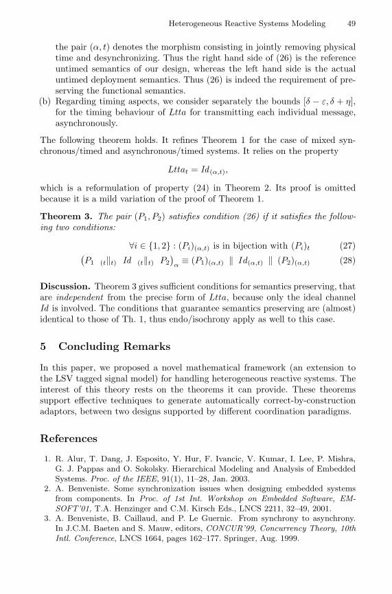
Heterogeneous Reactive Systems Modeling 49

the pair (α, t) denotes the morphism consisting in jointly removing physicaltime and desynchronizing. Thus the right hand side of (26) is the referenceuntimed semantics of our design, whereas the left hand side is the actualuntimed deployment semantics. Thus (26) is indeed the requirement of pre-serving the functional semantics.

(b) Regarding timing aspects, we consider separately the bounds [δ − ε, δ + η],for the timing behaviour of Ltta for transmitting each individual message,asynchronously.

The following theorem holds. It refines Theorem 1 for the case of mixed syn-chronous/timed and asynchronous/timed systems. It relies on the property

Lttat = Id (α,t),

which is a reformulation of property (24) in Theorem 2. Its proof is omittedbecause it is a mild variation of the proof of Theorem 1.

Theorem 3. The pair (P1, P2) satisfies condition (26) if it satisfies the follow-ing two conditions:

∀i ∈ 1, 2 : (Pi)(α,t) is in bijection with (Pi)t (27)(P1 (t‖t) Id (t‖t) P2

)α≡ (P1)(α,t) ‖ Id(α,t) ‖ (P2)(α,t) (28)

Discussion. Theorem 3 gives sufficient conditions for semantics preserving, thatare independent from the precise form of Ltta, because only the ideal channelId is involved. The conditions that guarantee semantics preserving are (almost)identical to those of Th. 1, thus endo/isochrony apply as well to this case.

5 Concluding Remarks

In this paper, we proposed a novel mathematical framework (an extension tothe LSV tagged signal model) for handling heterogeneous reactive systems. Theinterest of this theory rests on the theorems it can provide. These theoremssupport effective techniques to generate automatically correct-by-constructionadaptors, between two designs supported by different coordination paradigms.

References

1. R. Alur, T. Dang, J. Esposito, Y. Hur, F. Ivancic, V. Kumar, I. Lee, P. Mishra,G. J. Pappas and O. Sokolsky. Hierarchical Modeling and Analysis of EmbeddedSystems. Proc. of the IEEE, 91(1), 11–28, Jan. 2003.

2. A. Benveniste. Some synchronization issues when designing embedded systemsfrom components. In Proc. of 1st Int. Workshop on Embedded Software, EM-SOFT’01, T.A. Henzinger and C.M. Kirsch Eds., LNCS 2211, 32–49, 2001.

3. A. Benveniste, B. Caillaud, and P. Le Guernic. From synchrony to asynchrony.In J.C.M. Baeten and S. Mauw, editors, CONCUR’99, Concurrency Theory, 10thIntl. Conference, LNCS 1664, pages 162–177. Springer, Aug. 1999.

50 A. Benveniste et al.

4. A. Benveniste, B. Caillaud, and P. Le Guernic. Compositionality in dataflow syn-chronous languages: specification & distributed code generation. Information andComputation, 163, 125–171 (2000).

5. A. Benveniste, L. P. Carloni, P. Caspi, and A. L. Sangiovanni-Vincentelli. Heteroge-neous reactive systems modeling and correct-by-construction deployment. Techni-cal Report UCB/ERL M03/23, Electronics Research Lab, University of California,Berkeley, CA 94720, June 2003.

6. A. Benveniste, P. Caspi, S. Edwards, N. Halbwachs, P. Le Guernic, and R. de Si-mone. The Synchronous Language Twelve Years Later. Proc. of the IEEE,91(1):64–83, January 2003.

7. A. Benveniste, P. Caspi, P. Le Guernic, H. Marchand, J-P. Talpin and S. Tripakis.A Protocol for Loosely Time-Triggered Architectures. In Embedded Software. Proc.of the 2nd Intl. Workshop, EMSOFT 2002, Grenoble, France, Oct. 2002.

8. G. Berry. The Foundations of Esterel. MIT Press, 2000.9. L. P. Carloni, K. L. McMillan, and A. L. Sangiovanni-Vincentelli. Theory of

Latency-Insensitive Design. IEEE Trans. on Computer-Aided Design of IntegratedCircuits and Systems, 20(9):1059–1076, September 2001.

10. P. Caspi, “Clocks in Dataflow languages”, Theoretical Computer Science, vol.94:125–140, 1992.

11. J. Cortadella, A. Kondratyev, L. Lavagno, and C. Sotiriou. A concurrent modelfor de-synchronization. In Proc. Intl. Workshop on Logic Synthesis, May 2003.

12. L. de Alfaro and T.A. Henzinger. Interface Theories for Component-Based Design.In Proc. of 1st Int. Workshop on Embedded Software, EMSOFT’01, T.A. Henzingerand C.M. Kirsch Eds., LNCS 2211, 32–49, Springer Verlag, 2001.

13. J. Eker, J.W. Janneck, E.A. Lee, J. Liu, J. Ludwig, S. Neuendorffer, S. Sachs, andY. Xiong. Taming heterogeneity–The Ptolemy approach. Proc. of the IEEE, 91(1),127–144, Jan. 2003.

14. N. Halbwachs, P. Caspi, P. Raymond, and D. Pilaud. The Synchronous Data FlowProgramming Language LUSTRE. Proc. of the IEEE, 79(9):1305–1320, Sep. 1991.

15. D. Harel. Statecharts: A visual formalism for complex systems. Science of Com-puter Programming, 8(3):231–274, June 1987.

16. G. Karsai, J. Sztipanovits, A. Ledeczi, and T. Bapty. Model-Integrated Develop-ment of Embedded Software. Proc. of the IEEE, 91(1), 127–144, Jan. 2003.

17. H. Kopetz, Real-Time Systems: Design Principles for Distributed Embedded Ap-plications. Kluwer Academic Publishers. 1997. ISBN 0-7923-9894-7.

18. L. Lamport. Time, clocks and the ordering of events in a distributed system. Com-munication of the ACM, 21:558–565, 1978.

19. P. Le Guernic, T. Gautier, M. Le Borgne, and C. Le Maire. Programming real-timeapplications with SIGNAL. Proc. of the IEEE, 79(9):1326–1333, Sep. 1991.

20. P. Le Guernic, J.-P. Talpin, J.-C. Le Lann, Polychrony for system design. Journalfor Circuits, Systems and Computers. World Scientific, April 2003.

21. E.A. Lee and A. Sangiovanni-Vincentelli. A Framework for Comparing Models ofComputation. IEEE Trans. on Computer-Aided Design of Integrated Circuits andSystems, 17(12), 1217–1229, Dec. 1998.

22. E.A. Lee and Y. Xiong. System-Level Types for Component-Based Design. InProc. of 1st Int. Workshop on Embedded Software, EMSOFT’01, T.A. Henzingerand C.M. Kirsch Eds., LNCS 2211, 32–49, Springer Verlag, 2001.

23. M. Mokhtari and M. Marie. Engineering Applications of MATLAB 5.3 andSIMULINK 3. Springer Verlag, 2000.

HOKES/POKES: Light-Weight ResourceSharing

Herbert Bos and Bart Samwel

LIACS, Leiden University,Niels Bohrweg 1, 2333 CA, The Netherlands

herbertb,bsamwel@liacs.nl

Abstract. In this paper, we explain mechanisms for providing embed-ded network processors and other low-level programming environmentswith light-weight support for safe resource sharing. The solution consistsof a host part, known as HOKES, and a network processor part, known asPOKES. As common operating system concepts are considered to be tooheavy-weight for this environment, we developed a system that pushesresource control all the way to the compiler. The HOKES/POKES ar-chitecture is described in detail and its implementation evaluated.

1 Introduction

In this paper, we explain how to provide light-weight support for resource sharingin network processors (NPs) and operating system (OS) kernels. In many em-bedded systems, the programming environment offers little support for resourcesharing and safety. Often, the software consists of a single, monolithic applica-tion that is special-purpose and well-tested, and not supported by hardware-assisted memory isolation, privileged instructions, or the like. This is true notonly for special-purpose signal-processors, but also for reconfigurable comput-ing, such as FPGAs. Increasingly, however, embedded hardware allows for moreflexible application domains. The network processor (NP) is an example of thistrend [Coo02,Mic99]. It may contain on-chip a general-purpose control processorand a set of independent processing engines all running in parallel (an example isshown in Figure 2). The engines, commonly known as microengines (MEs), runtheir own micro-applications and share the resources on the board (for instance,buses, memories, data streams, etc.).

In practice, however, the code running on NPs still consists of a single mono-lithic application (albeit with various parallel components). The reason that NPsare not really shared by multiple programs is not that it would not be beneficialto applications. On the contrary, there are systems that could exploit such func-tionality to their profit, if only it existed. For example, plugged into a router,an NP board could forward packets on most of its MEs, while using the remain-ing ones to run user code (e.g. a monitoring application, or a filter). As a moreconcrete example, the EU SCAMPI project develops a monitoring platform forhigh-speed links that aims to allow multiple monitoring applications to be active

R. Alur and I. Lee (Eds.): EMSOFT 2003, LNCS 2855, pp. 51–66, 2003.c© Springer-Verlag Berlin Heidelberg 2003

52 H. Bos and B. Samwel

simultaneously on the same network card [SCA01]. The real reason why such ar-chitectures are not shared is that there are simply no appropriate mechanismsfor doing so. For example, the time-sharing techniques developed for general-purpose operating systems such as UNIX are not appropriate, as they are tooheavy-weight.

In this paper we describe the details of a solution known as OKE that pushesthe burden of resource sharing in environments without explicit hardware sup-port for this purpose all the way to the compiler. The focus is on NPs and OSkernels and a C-like language. In our terminology, the OKE part that is runningon host-like systems is known as HOKES (host OKE system), while POKES(peripheral OKE system) is the part running on the MEs of the NP. Together,they are able to provide a measure of safety to the system by restricting codein its usage of processing time, memory and APIs. A complete HOKES imple-mentation for the Linux kernel is available under the GNU Public License fromwww.liacs.nl/˜herbertb/projects/oke. We have also started the POKES im-plementation and will evaluate the overhead in the results section. Furthermore,we maintain that the principles described in this paper may apply to other en-vironments also. A high-level overview of an early version of HOKES was givenin [BS02]. This paper describes the implementation of the low-level mechanisms,compiler support and NP-specific issues.

In Section 2, we describe the HOKES/POKES architecture. Section 3 ex-plains how isolation and resource safety are subject to higher-level policies. InSection 4, we discuss the various mechanisms that we employ to provide resourcesafety. In Section 5, we evaluate our work. Related work is discussed in Section 6,and conclusions are drawn in Section 7.

2 Architecture

2.1 Processing Hierarchy

As shown in Figure 2, the architecture that we wish to program consists of a five-level (L0,L1,...,L4) processing hierarchy. In our case, it comprises one or morehost processors running Linux (with the usual kernel/userspace domains), andone or more Intel IXP network processors, each containing a StrongARM controlprocessor running embedded Linux (also with kernel and userspace code) and aset of microengines that run no OS whatsoever. Observe that, besides the PCIdistance and amount of available resources, there is very little to distinguishbetween the combinations of levels L1/L2 and L3/L4. Indeed, although theyprobably will be used for different purposes, in our implementation they aretreated the same. The application granularity of L0 is assumed to be the ME,so application foo runs on (at least) one ME, dedicated to foo.

In the implementation we have used a P4 1.8 GHz host processor and an IntelIXP1200 NP running at 200 Mhz, with a StrongARM control processor, and 6MEs with 4 hardware contexts each. The NP is mounted on an ENP2506 boardfitted with 2 1Gbps Ethernet ports and 256MB SDRAM and 8MB SRAM.

HOKES/POKES: Light-Weight Resource Sharing 53

CL = code loaderNP = network processorME = microengineCREC = compilation recordOKE = open kernel environmentHOKES = host-like OKE systemPOKES = peripheral OKE systemESC = environment setup codeFEC = forward error correctionGC = garbage collectorSC = stack checkingDM = dynamic memory managementPC = pointer checksMT = multithreading protectionTP = processing time protection

Fig. 1. Glossary

userspace

linux kernel

CPU(Pentium)

userspacelinux kernel

control processor

(StrongARM)

microcode

microengine

microcode

microengine

microcode

microengine

microcode

microengine

microcode

microengine

microcode

microengineSRAM

SDRAM

GigE GigE

PCI

scratch FIFO

Network processor

(Intel IXP1200)

HostMemory

L4: host userspace

L3: host kernel code

L0: microcode on microengines

L2: control processor userspace

HOKES

L1: control processor kernel

POKES

HOKES

Fig. 2. Processing hierarchy and HOKES/POKES domains

2.2 Software

The problem of efficient resource sharing in this hierarchy is difficult, especiallyfor levels L0, L1 and L3 which concern environments without hardware supportfor isolation. Worse, we cannot apply traditional OS approaches, as these aretoo heavy-weight (in particular for the MEs). Instead, we have developed newabstractions for code isolation that push, to a large extent, resource control allthe way to the compiler. In our software model, given the appropriate (and ex-plicit) privileges, application code is allowed to run anywhere in the processinghierarchy. However, what such code is allowed to do is limited by static and dy-namic checks that may control any resource, including memory and bus access,processing time, stack space, etc. The generic solution for any of the levels inthe hierarchy is known as the Open Kernel Environment (OKE). The implemen-tation of OKE on a host-like system, i.e. a system running a general-purposeoperating system, such as the Pentium and StrongARM in Figure 2, is knownas HOKES. The microengines on the NP do not run any OS whatsoever andhence require a somewhat different approach to achieve the same goal. This isknown as a peripheral OKE system, or POKES. For the evaluation of HOKESwe will use the implementation on the actual host processor (Pentium), as it ismore convenient for performing measurements and data collection than the em-bedded StrongARM. For POKES, however, we have no choice other than usingthe microengines directly.

In order to make programming safe, efficient, and familiar to programmers,we extended and modified the Cyclone programming language, which itself isa dialect of C (retaining the C ‘look and feel’) [JMG+02]. The result is knownas OKE-Cyclone. The trust management used in the compilation and loadingprocess is based on KeyNote [BFIK99] and described in detail in [BS02].

The idea is that a code loader explictly grants users the right to load code ofa specific type, where ‘type’ means: ‘subject to a set of restrictions on resourceusage’. For this purpose, they request a compiler to compile their code according

54 H. Bos and B. Samwel

user

"Bygwyn"trustedcompiler Kernel/NP

User

module A

module B

module C

Code Loader

credentialsuser

compilationrecord

module Cobject code

runtimesupport

ESCparameters

"type" (ESC)

module Csource code

compilationrecord

module Cobject code

(a) (b)

remote procedure call(RPC)

remote procedure call(RPC)

credentials

resourcecapacity

Fig. 3. User (a) compiles and (b) loads code using RPC from a remote site

to this type. A type is defined by so-called ‘environment-set-up code’, or ESC,that is associated with a user’s program (and which instruments the code andchecks whether specific conditions on resource usage hold) and is instantiatedby the user by parameterisation. For example, the ESC may specify that themaximum amount of heap that can be used is 1 MB, while the parameterisationmay indicate that the real maximum to be used for this code is only 0.5 MB.ESC will not normally be written by the users themselves, but defined onceand for all by the authority that wants to restrict a specific group of users ina specific way. For example, there could be an ESC for ‘students in a course ofembedded software’. The compiler compiles the code with the ESC specified andthen generates and signs a proof stating that this code was compiled with theserestrictions by this compiler. The exact steps are the following(see Figure 3):

– To a (possibly remote) compile-server we submit (1) our source, and (2) the‘type’, or ESC, to which the object code should comply.

– This trusted compile-server, known as bygwyn, first creates a combined trans-lation unit that incorporates the ESC and our source code.

– Bygwyn then calls the OKE-Cyclone compiler to generate object code usingcustom language constructs to enforce safety (and isolation).

– Bygwyn returns the object code (an OKE module) and a signed compilationrecord (CREC) that vouches for the code’s compliance to the ESC.

– Users may then submit the object code, the CREC and ESC to an OKEcode loader (CL) at a site where the code should be executed.

– The CL uses the CREC to check whether the (1) object code matches thegiven ESC, (2) the compiler that signed the CREC is trusted, and (3) thereis sufficient resource capacity to accommodate the request. It also checks theusers’ credentials to see if they are allowed to load code corresponding tothis ESC. If none of the checks fail, the code is loaded.

3 Safety Policy (ESC)

In essence, an ESC is policy code that is prepended to, and sets up a compile-time environment for, the user-supplied code. For example, it defines run-time

HOKES/POKES: Light-Weight Resource Sharing 55

support code and explicitly declares the permissible API, restricting the code tojust this API, by taking away the ability to (1) declare/import new APIs, (2)access the “private” parts of the ESC, and (3) perform privileged (unsafe) oper-ations. ESCs are parameterised by the user to include, limit or remove certaincapabilities. For example, users may specify that they have no need for dynamicmemory, so that the support code that would otherwise be needed can be re-moved (yielding more efficient code). An ESC also has a component specifyingparameter limitations. For default parameter values that may be overwritten byusers with the appropriate credentials, this includes the range of valid values. Itmay also include a FINALLY keyword to indicate that this parameter may not beoverwritten by users. This permits one to specify for instance that some usersmight be allowed to specify that they need up to 1 MB of dynamic memory, whileothers might be allowed to specify only 0.5 MB (or may not even be allowed touse heap memory at all). Apart from the ESC, these limitations are expressedin the users’ credentials.

When user code is compiled with a given policy (ESC), the trusted compile-server creates a translation unit that consists of (1) parameterisation of theESC (in the form of macro definitions), (2) ESC, and (3) user code. This isprocessed by the OKE-Cyclone compiler to generate compliant object code. TheOKE assumes a closed world, allowing for whole program analysis to optimiseaway dynamic checks that are only needed in an open world. This does notmean that modules consisting of multiple components cannot be composed. Aslong as the APIs are declared in the ESC, users can build larger programs byexplicitly clicking together a score of modules. Even so, the OKE is especiallyuseful for applications in restricted areas (e.g. kernels and embedded systems)and, therefore, the modules are often fairly small (i.e. contained in a single unit).

4 Language Features for Safety

Given the trust mechanism, we still need to ensure that code complies with agiven safety policy at compile time. The following issues must be addressed if wewant to enable users to run applications in any environment in a safe manner:

1. memory protection in the spatial domain (bounds checking);2. memory protection in the temporal domain (references to freed memory);3. stack overrun protection;4. processing time restriction;5. API restrictions;6. hiding of sensitive data;7. removing/disabling misbehaving code.

4.1 HOKES/POKES Spatial Pointer Safety

Cyclone is strongly typed and provides pointer safety in the following ways.Firstly, it provides bounded pointers that are statically tagged with a ‘valid

56 H. Bos and B. Samwel

length’ or number of elements that must exist in the memory the pointer pointsto. These pointers are either NULL or point to at least the number of elementsindicated by their ‘valid length’. Conversions between these pointers are checkedstatically. Secondly, Cyclone provides non-nullable pointers, that can be stati-cally proven to be non-NULL. Unlike ‘normal’ C pointers, non-nullable pointersdo not need dynamic checks when they are dereferenced. Converting pointersto non-nullable pointers before using them in a loop, allows programmers toremove dynamic NULL-checks from inner loops. Thirdly, Cyclone also supports‘normal’ C pointers, e.g. pointers with bounds that are only known at run-timeand which incur run-time checks on all accesses.

4.2 HOKES/POKES Temporal Pointer Safety

Bounds checking solves the problem of spatial pointer safety, but not that oftemporal pointer safety, such as returning the address of local variable. Cyclonesolves this by including region information in pointer types [GMJ+02]. The mech-anism statically tags every pointer type with an identifier of the region of thememory it points to. A pointer that is tagged to point to a region foo is onlycapable of pointing to memory in region foo or in region bar that outlives foo,i.e., a region whose memory is guaranteed to exist when foo goes out of scope.In addition, foo’s memory can store only pointers to memory that outlives foo(because otherwise a “shorter-lived” region might disappear during the life offoo, leaving a dangling pointer in foo). When the address of a local variable offunction foo is taken, the result will be a pointer into the region of foo’s localvariables. Any attempt to return it, or store it globally, will lead to region er-rors at compile time. Region tags can be explicitly specified by the programmerto express certain exceptional situations, but in C-like code the default regiontags usually suffice (i.e., the code looks and feels like C, but has invisible safetyenforcement). The region system is not used within the dynamic memory heap,which is normally garbage collected.

The Cyclone regions work well for Cyclone-only programs, but there aresafety issues when interoperating with explicitly memory-managed languagessuch as C, as is the case, for instance, in HOKES. When a module holds a pointerto a kernel memory block that is explicitly memory managed, the memory blockmay be released, leaving the pointer dangling. For HOKES, we have thereforeimplemented Linux support for delayed freeing, ensuring that any memory re-leased by the kernel is not immediately reused, but instead placed on a kill list,a list of blocks that still need to be “physically released”.

In addition, we have written a HOKES garbage collector (GC) from scratch.We have placed the GC under user control, so that users may explicitly request aGC round (e.g. to clean up their own heap memory), or postpone it indefinitely.However, just prior to becoming active, every HOKES module which may havepointers to kernel memory always initiates a GC round (this is known at compiletime). GC takes O(n), where n is the number of memory blocks allocated by themodule. During garbage collection, all memory on the module’s heap that canno longer be reached will be released.

HOKES/POKES: Light-Weight Resource Sharing 57

During a module’s garbage collection phase the HOKES detects whetheror not a module holds pointers to ‘freed’ memory from the explicitly memory-managed region and acts appropriately by nullifying the pointers or by termi-nating the module (if the pointers are non-nullable). Once we have verified thatno module holds pointers to a ‘freed’ memory block, the memory block is alsophysically freed. Currently, the released memory blocks are physically releasedeven earlier, immediately after all modules have deactivated. This puts somerestrictions on the programming model, because modules cannot safely stay ac-tive for very long times without exhausting the kernel’s memory resources. Wedon’t think this limitation is inherent in the approach, it is only caused by thesimplicity of the current implementation. A more important limitation is thatkernel memory cannot currently contain pointers back to memory controlled byHOKES’s GC, because the GC cannot detect the kernel’s references. All memoryshared by HOKES and the kernel must be explicitly managed by the kernel.

We stress that delayed freeing is only needed for those modules that canactually hold pointers to kernel memory. This is a property that is checked atcompile time: programs that do not contain any pointers tagged “kernel region”cannot point to explicitly memory-managed kernel memory. In other words,when considering a free for a chunk of kernel memory, there is no need to waitfor modules to become inactive if they are guaranteed not to have pointers tothis memory anyway.

Our current GC implementation uses a mark-and-sweep GC algorithm and isprecise (it assumes strong typing and does not need to assume that all memorypotentially contains pointers). The GC is supported by automatically generatedcode based on whole program analysis, which is done in the front end of the OKE-Cyclone compiler. The compiler detects which types of memory can be allocatedby a module (by enumerating the types of all new and malloc expressions inthe program) and generates marking functions for every type it encounters. Amarking function for a type defines how a memory block of the type can bescanned for pointers, it contains a call to a function of the GC for every pointerin the type. The memory allocation calls in the module are then modified to passto the memory subsystem pointers to the marking functions corresponding to theallocated type. Whenever the memory subsystem wants to find out which othermemory blocks are referenced by a given memory block, it calls the markingfunction associated with the block and the marking function will call the GCwith the addresses of all the other blocks referenced in this block.

POKES has no GC and currently does not even support truly dynamic mem-ory. It is assumed that all memory accessible to MEs is statically declared.Region-based protection is still used, but in a more restricted version (e.g. toguard against common programming errors). As we shall see in 4.8, the memorymay well be shared between MEs.

4.3 HOKES/POKES Language Restrictions

Although regions and pointer tags provide pointer safety, they provide no accessrestrictions for APIs and unsafe language features. To be able to restrict explic-

58 H. Bos and B. Samwel

itly access to unsafe language features and APIs, we added the construct forbidto the language. Using this construct, it is possible to restrict access to featureslike extern "C" (which would allow users to import C APIs they don’t have ac-cess to), extern "C include" (a Cyclone construct that allows for the inclusionof unsafe C code). In addition to that, forbid namespace enables us to forbidaccess to a complete namespace to all the code following this declaration. Thisallows an ESC to declare private helper functions and to import APIs in a privatenamespace, and to remove this namespace from the user code’s view afterwards,leaving only the permissible APIs. In HOKES, unauthorised interaction withother modules is prevented by opening a random namespace for the user code.Because HOKES uses Cyclone’s exception mechanism to interrupt misbehavingcode in a safe manner, it is not safe for HOKES modules to catch certain types ofexceptions. To prevent this we created the construct forbid catch, that allowsexception access control at exception type granularity.

4.4 HOKES/POKES Wrapping: APIs and Entry Points

Upon entry from the environment into code that is part of a HOKES or POKESmodule, some entry/exit code needs to be executed, e.g. to perform HOKESgarbage collection or catch any exceptions thrown from the module. We realisedthat it would be very useful indeed to be able to pass function pointers to externalcode so that such code may call these functions directly. However, to do so safely,we need to be able to wrap each of these functions. For this purpose, we created anew construct, wrap extern, that automatically wraps every exported (extern)function with wrapping code specified by the wrap extern declaration. At thesame time, we prevent taking the address of functions that were not declaredextern, so function pointers to non-extern, unwrapped functions cannot exist.In restrospect, our decision to bind the concept of “potential entry point” tothe keyword “extern” has turned out to be inconvenient, because it forces theaddition of entry/exit code even to functions that are never used outside of themodule, but are called through function pointers.

The structure of the OKE also does not allow an ESC to make an externalAPI directly accessible to an application. The reason is related to timeouts, asubject we will discuss in Section 4.7. Moreover, when an API is potentiallyunsafe, e.g. if it returns explicitly memory-managed memory directly or if ithas weak parameter checking, extra work is needed to make Cyclone and theexternal API interoperate safely. In these situations, the APIs are wrapped bythe ESC.

4.5 HOKES/POKES Protection of Sensitive Data

When data is shared between programs, we often want only certain fields of astructure to be shared, while others should not be exposed. In network moni-toring, for instance, it may not be permissible for applications to find out whichwebsites a user visits. To prevent this, the IP address of a packet is often scram-bled (anonymised). However, scrambling takes time, even if the application is

HOKES/POKES: Light-Weight Resource Sharing 59

A()

B()

C()

= checkpoint

Dynamic call graph: application of checkpoints at runtime

D()

A()

B()

A()

C()

D()

int D() return 0;

int C() return D();

int B() if (cond) return C(); else return A();

int A() return B();

2

2

2

2 2

2

2 2

4

4

6

6

Fig. 4. Dynamic call graph: all functions take 2 units of stack (granularity = 6)

perfectly safe and does not even attempt to access the sensitive field. To addressthis, we created a new type modifier locked in OKE-Cyclone. The value of alocked variable cannot be used in calculations and cannot be converted to anyother type, and is therefore rendered unusable at zero run-time overhead. AnESC can declare certain fields of structures locked to prevent user code fromaccessing them. The fact that a field is locked does not imply that the fieldcannot be written! The Cyclone language already has a construct to expressthis, const. In fact, locked non-const fields provide the interesting possibilityto enforce a certain ‘dataflow’, that is, if a module is supposed to create a certaindata structure to achieve it’s task and one of the fields of this data structure isdeclared locked, then it can only fill this field using a source of locked datathat the ESC provides: it is not possible to cast an existing non-locked valueto a locked value.

4.6 HOKES Stack Overrun Protection

Unfortunately, HOKES stack overruns are hard to prevent without dynamicchecking (in POKES this is not a problem as the MEs do not support a stack).However, we do have the advantage of having whole program analysis at ourdisposal, and use this to reduce the amount of checks. Stack overrun protectionis configured by two variables, the bound and the granularity. The bound definesthe amount of stack space that a program is allowed to use, while the granularitydefines the maximum distance (measured in stack space) between checks in theprogram.

The process is illustrated in Figure 4 (it is assumed that for each functioncall the required stack space is 2 units). The OKE-Cyclone compiler analysesthe entry points and the code’s call graph to determine good locations for thecheckpoints that satisfy the granularity constraint. For example, consider theset of (partly recursive) function calls of Figure 4. Suppose checkpoints were

60 H. Bos and B. Samwel

placed at the entry points of A() and the entry point of D() only (and not inthe other two functions). Now, whenever A() is called, it is possible to checkwhether enough stack space exists to reach each of the following checkpoints. Inthe figure, bent arrows denote the distance between checkpoints, while straightarrows represent the call graph. A check is needed whether there is enough stackto store all of A’s local variables (in the general case: in the example there are nolocal variables), make a function call to B, store all local variables in B() on thetwo (different) paths to the next function calls (either A() or C()) and finally tomake these calls. In case of a call to C(), we repeat this process until we havereached a checkpoint, i.e. we check whether there is enough stack to call D().In other words, at the entrypoint of A() we need a total of at least 6 units ofstack space. Even though no checkpoints were added in B() or C() at all, we areensured that whenever either of these functions is called, there will be enoughstack space to proceed to the next checkpoint.

Discussion. In the current implementation it is not possible for the programmerto directly control the locations of the checkpoints, but as this can be added fairlyeasily, it is expected to be in the next HOKES release. Right now, checkpointingis done by the compiler which tries to balance bound and granularity (minimisingthe number of checkpoints, while not placing them too far away from each other).For safety, we assume that all calls to imported functions may result in calls toall entry points into the code, while this is usually not the case. Performancewould benefit if the ESC could specify whether an imported function can resultin a callback or not.

4.7 HOKES Processing Time Protection

On many host systems that HOKES targets, processor time is a resource thatmust be protected. To prevent user code from getting stuck in an endless loop orto use up all processor time for too long, we had a choice between two solutions.The first involves the addition of dynamic checks in backward jumps, which in-curs considerable run-time overhead and was therefore not used in HOKES. Thesecond involves a limited amount of OS and hardware dependency, exploitingthe timer interrupt in Linux. The implication is that for every new OKE envi-ronment, either a new method should be invented or dynamic checks should beused. For example, in the next section we will show that for POKES we adopteda very different solution to limit processing time.

HOKES uses the platform’s timer interrupt to check for timeouts. TheHOKES timers are checked on returning from a timer interrupt, i.e. after alltruly time-critical tasks have been handled, but before returning control to theinterrupted code. When a timeout flag is detected, HOKES jumps to a callbackfunction that was registered by the ESC. When appropriate, the callback throwsan exception to terminate the computation. The timeout mechanism takes intoaccount whether a modules is executing HOKES or OS code when the timeoutoccurs. When executing system code, written in a different language, we cannot

HOKES/POKES: Light-Weight Resource Sharing 61

throw a Cyclone exception and rewind the stack at that point in time. Rather,a flag is set to indicate to the ESC’s wrapper functions that they should notreturn control to the user code but throw a timeout exception instead.

4.8 POKES Processing Time Protection

As each application runs on a separate processor, POKES processor time is notconsidered to be a shared resource. Hence, there is no use for the timeout mech-anisms discussed in the previous section. However, as throughput is essential,packets have to be processed in time and memory is shared between the applica-tions. So we rephrased the processing time constraints in terms of cycle budgets,memory sharing and locking issues. In POKES, MEs are assumed to share asingle data stream and the memory in which the stream is stored is a sharedresource. If an application is not able to keep up with the arrival rate of thedata, the backlog of data-to-process grows and the throughput drops. This isparticularly bad in NPs where the goal is precisely to keep up with line speedand which have only a small cycle budget per packet (or set of packets).

Processing time protection in the current POKES is closely tied to the ap-plication framework, which reserves a single ME for receiving packets from thenetwork and storing them in memory. All other MEs are available to the appli-cations. The ESC for this framework provides for each ME a ‘main’ loop whichprefilters packets and makes them available to the ME hardware contexts. Giventhe appropriate credentials, programmers may ‘plug in’ application code in thisloop (with POKES restrictions) and load the complete program on the ME.

The packet fetch ME dedicates a single thread (known as ‘mop-up’) to deal-ing with tardy applications. Whenever an ME is falling behind too much (it hasnot processed enough packets in a given amount of time), the mop-up terminatesit. We consider this to be the NP equivalent of timeouts. The ME only posts akill request, the actual termination is done by the StrongARM. The packet fetchthat we implemented places packets in a circular buffer spread over SRAM andSDRAM. The actual packets are stored in SDRAM, while buffer control struc-tures are kept in SRAM. For example, a bit field per microengine per bufferedpacket is used to indicate whether a ME is ‘done’ with this packet. Applica-tions may choose to process every packet or only a percentage of the packets.However, for all packets in the buffer they have to set their ‘done’ flag in time.In the same structure we also keep bit fields to implement readers/writers locks(with readers’ preference) and fields indicating whether the packet has been fullyreceived.

Packets are written in 64 byte chunks and applications do not have to waitfor the packets to be received in their entirety: as soon as the first chunk of byteshas arrived, they may start processing. The point is that they need to processthe packets within the cycle budget. This is enforced by the mop-up. At somedistance from the writing position the mop-up thread explicitly removes packetsfrom the circular buffer. If the mop-up finds that, for any ME, the ‘done’ bit isnot set, it means the corresponding application has not completed the processingof this packet. In other words, the application is too slow and will be terminated.

62 H. Bos and B. Samwel

By varying the distance between mop-up and receive, we may limit or extendthe cycle budget for sets of packes available to applications.

Finally, we extended the default Intel device driver to provide memory map-ping of all the IXP’s SDRAM all the way to the host applications running inuserspace. MEs may pass a reference to a packet to a queue destined for hostapplications, which prompts these applications to process the packet further onthe host (accessing the required data from across the PCI bus).

Discussion: A POKES Compiler. Although there is currently no full com-piler support for POKES, all mechanisms have been implemented and evaluatedin isolation by handcrafting the code exactly like it will be generated by the com-piler. Furthermore, we are in the process of implementing a compiler for POKESthat will be rather simple in that it generates microengine C, an Intel-proprietarydialect of C with ME programming extensions. The current compiler is capableof producing ANSI C, so the translation to microengine C is fairly straightfor-ward, requiring mainly 2 things: (1) as the storage class for all variables canbe explicitly specified in microengine C, the compiler needs to be extended withstorage class specifiers, and (2) we need to deal with the presence of many intrin-sic functions in microengine C (but as these intrinsics have the same appearanceas function calls, they are easy to support).

5 Evaluation

5.1 HOKES: Full Kernel-Based Monitoring and Transcoding

HOKES has been evaluated in various kernel experiments in network transcod-ing. The most interesting example applications are (1) transcoding with increas-ing packet size, adding forward error correction (FEC) to packet payloads, and(2) transcoding with decreasing packet size (resampling audio packets to con-tain only 50% of the original data).They were implemented directly in a singlemodule that attaches itself to a Linux netfilter hook. The ESC is responsiblefor removing the appropriate IP packets from the netfilter framework, castingthe packet structure to the corresponding types in OKE-Cyclone and passingit to the module (ensuring that the appropriate fields are made const and/orlocked). It is also responsible for transmitting packets again.

For both cases, Table 2 shows the results for both the HOKES kernel codeand the exact same implementation in C (also running in the kernel). In bracketsthe relative overhead is mentioned. Because the overhead varies with the packetsize (more data needs to be processed), we listed both the overhead for minimumsized and maximum sized packets. A lot of the overhead, especially in the audioresampling transcoder, consists of initial costs. After that, in the loop of thetranscoder, there is hardly any overhead. For this reason the difference betweenoptimal C code and the HOKES solution is smaller, percentage-wise, for largerpackets.

HOKES/POKES: Light-Weight Resource Sharing 63

Table 1. Overhead of various aspects of OKE mechanism

Test Aspect measured ResultSC1 init time at entry point ≈ 1 cycleSC2 additional time to process checkpoint code 5-10 cyclesSC3 code size increase 16 instr. at entrypoint

15 instr. at other checkpointsPC1 overhead per normal (C-style) pointer dereference ≈ 1 cyclePC2 code size increase 3 instr.

(commonly only 2 executed)MT1 overhead at entry point 35 cyclesMT2 code size increase at entry point 15 instr.TP1 overhead at entry point 68 cyclesTP2 extra overhead for calling kernel from HOKES module 10 cyclesTP3 code size increase per entry point 24 instr.GC4 overhead for turning GC on, but not using it 10 cycles (for check)GC5 overhead for user requesting GC round with nothing to do 98 cyclesGC6 overhead for GC round for checking 1 non-collectible pointer 73 cyclesGC7 overhead for GC round for checking 1 collectible pointer 440 cyclesGC8 time to sweep a block 10-41 cycles (plus cost of kfree)

5.2 HOKES Micro-Measurements

Given the appropriate privileges, an ESC may be parameterised to ‘turn off’specific OKE mechanisms (e.g. a module may be compiled without the GC,and/or without stack checks, etc). If such parameters are not explicitly declaredas FINAL, they may be overwritten by users with the appropriate credentials,allowing them to determine what runtime support is included in the compilation.This conveniently allows us to test the overhead of many of our mechanisms inisolation. In this section we measure the runtime overhead of various aspects of:stack checking (SC), garbage collection (GC), dynamic memory management(DM), pointer checks (PC), overhead incurred by spinlocks to prevent multiplethreads from accessing the same module at the same time (MT), and processingtime protection (TP). For each of these items we measure various aspects, assummarised in Table 1.

All speed measurements are in cycles and were conducted on an Intel P4running a Linux 2.4.20 kernel and are fast-path values (i.e. without initial cachemisses and inaccurate branch predictions and without any misbehaviour in thecode that would cause it to be terminated). After startup, in the applications ofSection 5.1, the fast-paths are always taken as the system was used solely usedfor packet transcoding. All code was compiled to object code using gcc-2.9.5.We suspect that using gcc-3.2 performance will be better as the abstractionpenalty (putting all components in function calls, etc.) in gcc-3.2 is less severe(e.g. because its support for inlining has improved). We should stress than inPOKES the overheads (and indeed the mechanisms) for GC, TP and SC do notexist.

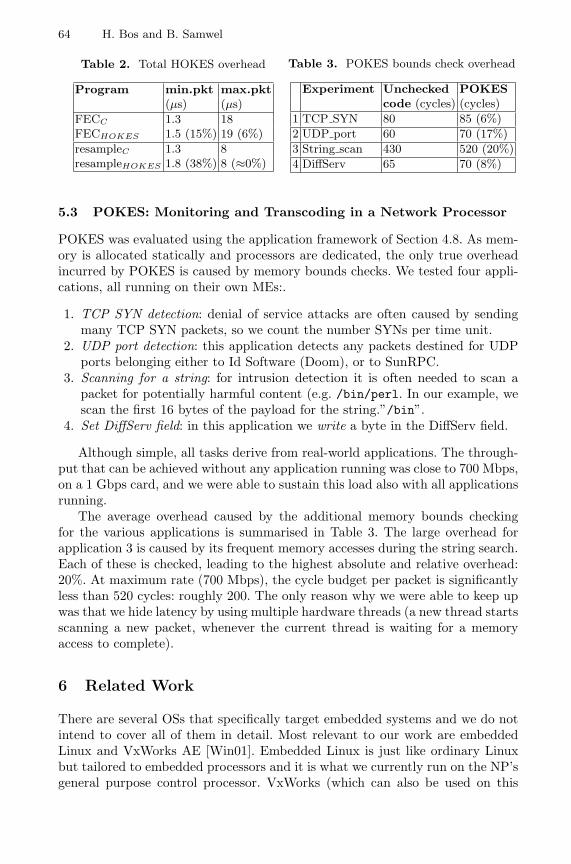
64 H. Bos and B. Samwel

Table 2. Total HOKES overhead

Program min.pkt max.pkt(µs) (µs)

FECC 1.3 18FECHOKES 1.5 (15%) 19 (6%)resampleC 1.3 8resampleHOKES 1.8 (38%) 8 (≈0%)

Table 3. POKES bounds check overhead

Experiment Unchecked POKEScode (cycles) (cycles)

1 TCP SYN 80 85 (6%)2 UDP port 60 70 (17%)3 String scan 430 520 (20%)4 DiffServ 65 70 (8%)

5.3 POKES: Monitoring and Transcoding in a Network Processor

POKES was evaluated using the application framework of Section 4.8. As mem-ory is allocated statically and processors are dedicated, the only true overheadincurred by POKES is caused by memory bounds checks. We tested four appli-cations, all running on their own MEs:.

1. TCP SYN detection: denial of service attacks are often caused by sendingmany TCP SYN packets, so we count the number SYNs per time unit.

2. UDP port detection: this application detects any packets destined for UDPports belonging either to Id Software (Doom), or to SunRPC.

3. Scanning for a string: for intrusion detection it is often needed to scan apacket for potentially harmful content (e.g. /bin/perl. In our example, wescan the first 16 bytes of the payload for the string.”/bin”.

4. Set DiffServ field: in this application we write a byte in the DiffServ field.

Although simple, all tasks derive from real-world applications. The through-put that can be achieved without any application running was close to 700 Mbps,on a 1 Gbps card, and we were able to sustain this load also with all applicationsrunning.

The average overhead caused by the additional memory bounds checkingfor the various applications is summarised in Table 3. The large overhead forapplication 3 is caused by its frequent memory accesses during the string search.Each of these is checked, leading to the highest absolute and relative overhead:20%. At maximum rate (700 Mbps), the cycle budget per packet is significantlyless than 520 cycles: roughly 200. The only reason why we were able to keep upwas that we hide latency by using multiple hardware threads (a new thread startsscanning a new packet, whenever the current thread is waiting for a memoryaccess to complete).

6 Related Work

There are several OSs that specifically target embedded systems and we do notintend to cover all of them in detail. Most relevant to our work are embeddedLinux and VxWorks AE [Win01]. Embedded Linux is just like ordinary Linuxbut tailored to embedded processors and it is what we currently run on the NP’sgeneral purpose control processor. VxWorks (which can also be used on this

HOKES/POKES: Light-Weight Resource Sharing 65

processor) is a real-time OS that is widely adopted in the embedded industryto control hardware. Moreover, it provides more than just CPU protection. Forexample, it is able to use the MMUs of modern microprocessors to provide parti-tioning and protection of memory in a flexible manner (“dial-in protection”). Itdiffers from our work in that we attempt to provide isolation to systems withouthaving to rely on such hardware assists.

In research labs, we have also seen a number of general-purpose OSs thatcan be safely extended (e.g.Nemesis [LMB+96], ExoKernels, [EKO94], and SPIN[BCE+95]). Of these SPIN, which makes use of language-specific safety proper-ties to ensure that applications do not interfere with each other, is most similarto our work. Unfortunately, all of these systems are research-oriented and notwidely used, certainly not in embedded systems. Our aim is to provide isolationmechanisms that can be applied in a popular OS (notably Linux), and even insystems without OS support whatsoever (notably the MEs of an NP).

Previous attempts at providing software-based isolation include interpretedsolutions(e.g. BPF [MJ93]), and native code solutions like Software Fault Iso-lation (SFI) [WLAG93] and Proof Carrying Code (PCC) [NL96]. We do notconsider interpreted solutions suitable for high-throughput systems. Instead, itis our explicit goal to open up lower levels of the processing hierarchy to fullyoptimised code. SFI uses run-time checks to enforce safety. Not only are suchchecks costly , they also only take into account memory isolation (e.g. boundschecking), and not control isolation (e.g. branch checking). PCC provides codesafety by supplying a proof of correctness, so that the loading site may check thecorrectness of code prior to loading it. The problem here is that generating proofsis a complex task which, to date, cannot be fully automated. Other approachesthat allow programmers to load code in the Linux kernel are SILK [SPB+02] andFLAME [AIM+02]. SILK differs from our work in that it does not provide safety,and FLAME in that it is limited to monitoring functionality. RBClick describedin [PL03] is similar to OKE, but differs in that all checks are completely static.

7 Conclusions

In this paper we have described the low-level mechanisms and compiler supportfor the Open Kernel Environment (OKE) which provides light-weight supportfor resource sharing and isolation in a processing hierarchy consisting of hostprocessors and network processors. We have discussed both host side (HOKES)and network processor side (POKES). Policies are used to restrict a user’s codein terms of access to resources. Whether or not users are granted access to re-sources is determined by their credentials. At the same time, the OKE targetsperformance by focusing on fully optimised code. Experimental results in thefields of monitoring and transcoding show that in Linux the overhead rangesfrom roughly 5 to 40 percent, and experimental results on Intel IXP1200 net-work processors show overheads of up to 20 percent. The OKE is currently acomponent in the operating system support for the EU SCAMPI project.

66 H. Bos and B. Samwel

Acknowledgements. This work was supported by the EU SCAMPI project(IST-2001-32404). We would like to thank Lennert Buytenhek and Mihai Cristeafor their help.

References

[AIM+02] K. G. Anagnostakis, S. Ioannidis, S. Miltchev, J. Ioannidis, Michael B.Greenwald, and J. M. Smith. Efficient packet monitoring for networkmanagement. In Proc. of NOMS’2002, April 2002.

[BCE+95] B. Bershad, C. Chambers, S. Eggers, C. Maeda, D. McNamee, P. Pardyak,S. Savage, and E. Gun Sirer. Protection is a software issue. In HotOS-V,May 1995.

[BFIK99] M. Blaze, J. Feigenbaum, J. Ioannidis, and A. Keromytis. The KeyNotetrust-management system version 2. NWG, RFC 2704, September 1999.

[BS02] H. Bos and B. Samwel. Safe kernel programming in the OKE. In Pro-ceedings of OPENARCH’02, New York, USA, June 2002.

[Coo02] Intel Coorp. Internet exchange architecture: Programmable network pro-cessors for today’s modular networks. White Paper, 2002.

[EKO94] D. Engler, F. Kaashoek, and J. O’Toole Jr. The exokernel approach toextensibility. In Proc. of USENIX OSDI, Monterey, Cal., November 1994.

[GMJ+02] D. Grossman, G. Morrisett, T. Jim, M. Hicks, Y. Wang, and J. Cheney.Region-based memory management in Cyclone. In Proc. of PLDI’02,Berlin, Germany, June 2002.

[JMG+02] T. Jim, G. Morrisett, D. Grossman, M. Hicks, J. Cheney, and Y. Wang.Cyclone: A safe dialect of C. In Proc. of USENIX’2002, June 2002.

[LMB+96] I. Leslie, D. McAuley, R. Black, T. Roscoe, P. Barham, D. Evers, R. Fair-bairns, and E. Hyden. The Design and Implementation of an OperatingSystem to Support Distributed Multimedia Applications. JSAC, 14(7),September 1996.

[Mic99] IBM Microelectronics. The network processor enabling technology forhigh-performance networking. White Paper, 1999.

[MJ93] S. McCanne and V. Jacobson. The BSD Packet Filter: A new architecturefor user-level packet capture. In Proc. of USENIX, San Diego, Jan. 1993.

[NL96] G. Necula and P. Lee. Safe kernel extensions without run-time checking.In Proceedings of OSDI’96, Seattle, Washington, October 1996.

[PL03] P. Patel and J. Lepreau. Hybrid resource control of active extensions. InProc. of OPENARCH’03, San Francisco, CA, April 2003.

[SCA01] SCAMPI Consortium. SCAMPI - A SCAlable Monitoring Platform forthe Internet. Technical report, EU IST Research Project, Proposal Num-ber: IST-2001-32404, Action Line IST-2001-IV.2.2, April 2001.

[SPB+02] N. Shalaby, L. Peterson, A. Bavier, Y. Gottlieb abd S. Karlin, A. Nakao,X. Qie, T. Spalink, and M. Wawrzoniak. Extensible routers for activenetworks. In DARPA AN Conference and Exposition, June 2002.

[Win01] Wind River Systems MCL-DS-VAE-0111. VxWorks AE Datasheet.http://www.windriver.com/products/vxworks5/, 2001.

[WLAG93] R. Wahbe, S. Lucco, T.E. Anderson, and S.L. Graham. Efficient software-based fault-isolation. In SOSP’03, pages 203–216, December 1993.

Rate Monotonic vs. EDF: Judgment Day

G.C. Buttazzo

University of Pavia, Italybuttazzo@unipv.it

Abstract. Since the first results published in 1973 by Liu and Laylandon the Rate Monotonic (RM) and Earliest Deadline First (EDF) algo-rithms, a lot of progress has been made in the schedulability analysis ofperiodic task sets. Unfortunaltey, many misconceptions still exist aboutthe properties of these two scheduling methods, which usually tend tofavor RM more than EDF. Typical wrong statements often heard in tech-nical conferences and even in research papers claim that RM is easier toanalyze than EDF, it introduces less runtime overhead, it is more pre-dictable in transient overload conditions, and causes less jitter in taskexecution. Since the above statements are either wrong, or not precise,it is time to clarify these issues in a systematic fashion, because the useof EDF allows a better exploitation of the available resources and signifi-cantly improves system’s performance. This paper compares RM againstEDF under several aspects, using existing theoretical results or simplecounterexamples to show that many common beliefs are either false oronly restricted to specific situations.

1 Introduction

Before a comprehensive theory was available, the most critical control applica-tions were developed using an off-line table-driven approach (timeline schedul-ing), according to which the time line is divided into slots of fixed length (minorcycle) and tasks are statically allocated in each slot based on their rates andexecution requirements. Although very predictable, such a technique is fragileduring overload conditions and it is not flexible enough for supporting dynamicsystems [24].

Such problems can be solved by using a priority-based approach, accordingto which each task is assigned a priority (which can be fixed or dynamic) and theschedule is generated on line based on the current priority value. In 1973, Liuand Layland [23] analyzed the properties of two basic priority assignment rules:the Rate Monotonic (RM) algorithm and the Earliest Deadline First (EDF)algorithm. According to RM, tasks are assigned fixed priorities that are pro-portional to their rate, so the task with the smallest period receives the highestpriority. According to EDF, priorities are assigned dynamically and are inverselyproportional to the absolute deadlines of the active jobs.

Assuming that each task is characterized by a worst-case execution time Ci

and a period Ti, Liu and Layland showed that the schedulability condition of

R. Alur and I. Lee (Eds.): EMSOFT 2003, LNCS 2855, pp. 67–83, 2003.c© Springer-Verlag Berlin Heidelberg 2003

68 G.C. Buttazzo

a task set can be derived by computing the processor utilization factor Up =∑ni=1 Ci/Ti. Clearly, if Up > 1 no feasible schedule exists for the task set with

any algorithm. If Up ≤ 1, the feasibility of the schedule depends on the task setparameters and on the scheduling algorithm used in the system.

The Rate Monotonic algorithm is the most used priority assignment in real-time applications, because it is very easy to implement on top of commercialkernels that do not support explicit timing constraints. On the other hand, im-plementing a dynamic scheme, like EDF, on top of a priority-based kernel wouldrequire to keep track of all absolute deadlines and perform a dynamic mappingbetween absolute deadlines and priorities. Such an additional implementationcomplexity and runtime overhead often prevents EDF to be implemented on topof commercial real-time kernels, even though it would increase the total processorutilization.

At present, only a few research kernels support EDF as a native schedulingscheme. Examples of such kernels are Hartik [8], Shark [15], Erika [14], Spring[33], and Yartos [17]. A new trend in some recent operating system is to providesupport for the development of a user level scheduler. This is the approachfollowed in MarteOS [27].

In addition to resource exploitation and implementation complexity, thereare other evaluation criteria that should be taken into account when selectinga scheduling algorithm for a real-time application. Moreover, there are a lot ofmisconceptions about the properties of these two scheduling algorithms, that fora number of reasons penalize EDF more than it should be. The typical motiva-tions that are usually given in favor of RM state that RM is easier to implement,it introduces less runtime overhead, it is easier to analyze, it is more predictablein transient overload conditions, and causes less jitter in task execution.

In the following sections we show that most of the claims stated above areeither false or do not hold in the general case. Although some discussion of therelative costs of RM and EDF appear in [35], in this paper the behavior of thesetwo algorithms is analyzed under several perspectives, including implementationcomplexity, runtime overhead, schedulability analysis, robustness during tran-sient overloads, and response time jitter. Moreover, the two algorithms are alsocompared with respect to other issues, including resource sharing, aperiodic taskhandling, and QoS management.

2 Implementation Complexity

When talking about the implementation complexity of a scheduling algorithm,we have to distinguish the case in which the algorithm is developed on top of ageneric priority based operating system, from the case in which the algorithm isimplemented from scratch, as a basic scheduling mechanism in the kernel.

When considering the development of the scheduling algorithm on top of akernel based on a set of fixed priority levels, it is indeed true that the EDFimplementation is not easy, nor efficient. In fact, even though the kernel allowstask priorities to be changed at runtime, mapping dynamic deadlines to pri-

Rate Monotonic vs. EDF: Judgment Day 69

orities cannot always be straightforward, especially when, as common in mostcommercial kernels, the number of priority levels is small. If the algorithm isdeveloped from scratch in the kernel using a list for the ready queue, then theonly difference between the two approaches is that, while in RM the ready queueis ordered by decreasing fixed priority levels, under EDF it has to be orderedby increasing absolute deadlines. Thus, once the absolute deadline is availablein the task control block, the basic kernel operations (e.g., insertion, extraction,getfirst, dispatch) have the same complexity, both under RM and EDF.

An advantage of RM with respect to EDF is that, if the number of prioritylevels is not high, the RM algorithm can be implemented more efficiently bysplitting the ready queue into several FIFO queues, one for each priority level.In this case, the insertion of a task in the ready queue can be performed inO(1). Unfortunately, the same solution cannot be adopted for EDF, becausethe number of queues would be too large (e.g., equal to 232 if system time isrepresented by four byte variables).

Another disadvantage of EDF is that absolute deadlines change from a jobto the other and need to be computed at each job activation. Such a runtimeoverhead is not present under RM, since periods are typically fixed. However, theproblem of evaluating the runtime overhead introduced by the two algorithms ismore articulated, as discussed in the next section.

3 Runtime Overhead

It is commonly believed that EDF introduces a larger runtime overhead thanRM, because in EDF absolute deadlines need to be updated from a job to theother, so slightly increasing the time needed to execute the job activation prim-itive. However, when context switches are taken into account, EDF introducesless runtime overhead than RM, because it reduces the number of preemptionsthat typically occur under RM.

The example illustrated in Figure 1 shows that, under RM, to respect thepriority order given by periods, the high priority task τ1 must preempt everyinstance of τ2, whereas under EDF preemption occurs only once in the entirehyperperiod1. For larger task sets, the number of preemptions caused by RMincreases, thus the overhead due to the context switch time is higher under RMthan EDF.

To evaluate the behavior of the two algorithms with respect to preemptions,a number of simulation experiments have been performed using synthetic tasksets with random parameters.

Figure 2 shows the average number of preemptions introduced by RM andEDF as a function of the number of tasks. For each point in the graph, the av-erage was computed over 1000 independent simulations, each running for 1000units of time. In each simulation, periods were generated as random variables

1 The hyperperiod is defined as the smallest interval of time after which the schedulerepeats itself and it is equal to the least common multiple of the task periods.

70 G.C. Buttazzo

τ 1

τ 1

τ 2

τ 2

5 10 20 25 30 35

5 20 25 30 3510

0 7 14 21 28 35

0 7 14 21 28 35(b)

(a)deadline miss

Fig. 1. Preemptions introduced by RM (a) and EDF (b) on a set of three periodic tasks.Adjacent jobs of τ2 are depicted with different colours to better distinguish them.

with uniform distribution in the range of 10 to 100 units of time, whereas exe-cution times were computed to create a total processor utilization of 0.9.

As shown in the plot, each curve has two phases: the number of preemptionsoccurring in both schedules increases for small task sets and decreases for largertask sets. This can be explained as follows. For small task sets, the number ofpreemptions increases because the chances for a task to be preempted increasewith the number of tasks in the system. As the number of tasks gets higher, how-ever, task execution times get smaller in the average, to keep the total processorutilization constant, hence the chances for a task to be preempted reduce. Asevident from the graph, such a reduction is much more significant under EDF.

In another experiment, we tested the behavior of RM and EDF as a functionof the processor load, for a fixed number of tasks. Figure 3 shows the averagenumber of preemptions as a function of the load for a set of 10 periodic tasks.Periods and computation times were generated with the same criterion used inthe previous experiment, but to create an average load ranging from 0.5 to 0.95.

It is interesting to observe the different behavior of RM and EDF for highprocessor loads. Under RM, the number of preemptions constantly increaseswith the load, because tasks with longer execution times have more chances tobe preempted by tasks with higher priorities. Under EDF, however, increasingtask execution times does not always imply a higher number of preemptions,because a task with a long period could have an absolute deadline shorter thanthat of a task with smaller period. In certain situations, an increased executiontime can also cause a lower number of preemptions.

This phenomenon is illustrated in Figure 4, which shows what happens whenthe execution time of τ3 is increased from 4 to 8 units of time. When C3 =4, the second instance of τ2 is preempted by τ1, that has a shorter absolute

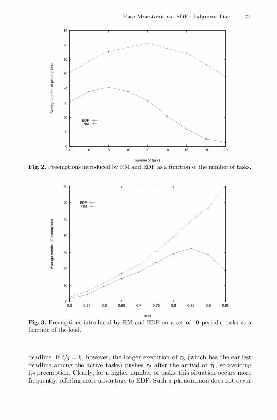
Rate Monotonic vs. EDF: Judgment Day 71

0

10

20

30

40

50

60

70

80

4 6 8 10 12 14 16 18 20

Ave

rage

num

ber

of p

reem

ptio

ns

number of tasks

EDFRM

Fig. 2. Preemptions introduced by RM and EDF as a function of the number of tasks.

10

20

30

40

50

60

70

80

0.5 0.55 0.6 0.65 0.7 0.75 0.8 0.85 0.9 0.95

Ave

rage

num

ber

of p

reem

ptio

ns

load

EDFRM

Fig. 3. Preemptions introduced by RM and EDF on a set of 10 periodic tasks as afunction of the load.

deadline. If C3 = 8, however, the longer execution of τ3 (which has the earliestdeadline among the active tasks) pushes τ2 after the arrival of τ1, so avoidingits preemption. Clearly, for a higher number of tasks, this situation occurs morefrequently, offering more advantage to EDF. Such a phenomenon does not occur

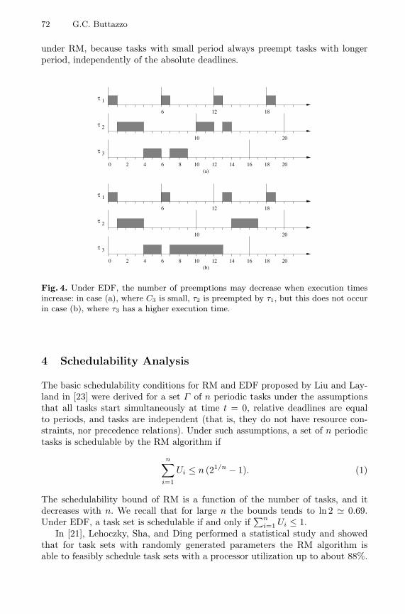
72 G.C. Buttazzo

under RM, because tasks with small period always preempt tasks with longerperiod, independently of the absolute deadlines.

τ 1

τ 2

τ 3

τ 1

τ 2

τ 3

0 2 4 6 8 12 14 16 1810 20

6 12 18

10 20

0 2 4 6 8 12 14 16 1810 20

6 12 18

10 20

(a)

(b)

Fig. 4. Under EDF, the number of preemptions may decrease when execution timesincrease: in case (a), where C3 is small, τ2 is preempted by τ1, but this does not occurin case (b), where τ3 has a higher execution time.

4 Schedulability Analysis

The basic schedulability conditions for RM and EDF proposed by Liu and Lay-land in [23] were derived for a set Γ of n periodic tasks under the assumptionsthat all tasks start simultaneously at time t = 0, relative deadlines are equalto periods, and tasks are independent (that is, they do not have resource con-straints, nor precedence relations). Under such assumptions, a set of n periodictasks is schedulable by the RM algorithm if

n∑

i=1

Ui ≤ n (21/n − 1). (1)

The schedulability bound of RM is a function of the number of tasks, and itdecreases with n. We recall that for large n the bounds tends to ln 2 0.69.Under EDF, a task set is schedulable if and only if

∑ni=1 Ui ≤ 1.

In [21], Lehoczky, Sha, and Ding performed a statistical study and showedthat for task sets with randomly generated parameters the RM algorithm isable to feasibly schedule task sets with a processor utilization up to about 88%.

Rate Monotonic vs. EDF: Judgment Day 73

However, this is only a statistical result and cannot be taken as an absolutebound for performing a precise guarantee test.

A more efficient schedulability test, known as the Hyperbolic Bound (HB),was proposed by Bini et al. in [6]. This test has the same complexity as the Liuand Layland one, but improves the acceptance ratio up to a limit of

√2 for large

n. According to this method, a set of periodic tasks is schedulable by RM if

n∏

i=1

(Ui + 1) ≤ 2. (2)

For RM, the schedulability bound improves when periods have harmonicrelations. A common misconception, however, is to believe that the schedulabilitybound becomes 1.00 when the periods are multiple of the smallest period. Thisis not true, as can be seen from the example reported in Figure 5.

τ 1

τ 2

τ 3

0 2 4 6 8 12 14 16 1810 20 22 24

Fig. 5. A task set in which all periods are multiple of the shortest period is not sufficientto guarantee a schedulability bound equal to one.

Here, tasks τ2 and τ3 have periods T2 = 8 and T3 = 12, which are multiple ofT1 = 4. Since all tasks have a computation time equal to two, the total processorutilization is

U =12

+14

+16

=1112

0.917

and, as we can see from the figure, the schedule produced by RM is feasible.However, it easy to see that increasing the computation time of any task by asmall amount τ3 will miss its deadline. This means that, for this particular taskset, the utilization factor cannot be higher than 11/12.

The correct result is that the schedulability bound becomes 1.00 only whenany pair of periods is in harmonic relation. As an example, Figure 6 shows that,if T3 = 16, then not only T2 and T3 are multiple of T1, but also T3 is multiple ofT2. In this case, the RM generates a feasible schedule even when C3 = 4, that iswhen the total processor utilization is equal to 1.00.

In the general case, exact schedulability tests for RM yielding to necessaryand sufficient conditions have been independently derived in [18,21,2]. Usingthe Response Time Analysis (RTA) proposed in [2], a periodic task set (withdeadlines less than or equal to periods) is schedulable with the RM algorithm ifand only if the worst-case response time of each task is less than or equal to its

74 G.C. Buttazzo

τ 1

τ 2

τ 3

0 2 4 6 8 12 14 16 1810 20 22 24

Fig. 6. When any pair of periods is in harmonic relation the schedulability bound ofRM is equal to one.

deadline. The worst-case response time Ri of a task can be computed using thefollowing iterative formula:

R(0)i = Ci

R(k)i = Ci +

∑

j:Dj<Di

⌈R

(k−1)i

Tj

⌉

Cj .(3)

where the worst-case response time of task τi is given by the smallest value ofR

(k)i such that R

(k)i = R

(k−1)i . It is worth noting, however, that the complexity

of the exact test is pseudo-polynomial, thus it is not suited to be used for onlineadmission control in applications with large task sets. To solve this problem, anapproximate fesibility test with a tunable complexity has been proposed by Biniand Buttazzo in [7].

Under EDF, the schedulability analysis of periodic tasks with relative dead-lines less than periods can be performed using the Processor Demand Criterionproposed by Baruah, Howell, and Rosier [5]. According to this method, a set oftasks is schedulable by EDF if and only if

∀L > 0,

n∑

i=1

⌊L + Ti − Di

Ti

⌋

Ci ≤ L (4)

As the response time analysis, this test has also a pseudo-polynomial com-plexity. It can be shown that the number of points in which the test has to beperformend can be significantly restricted to those L equal to deadlines less thana certain value L∗, that is:

∀L ∈ D, D = dk : dk < min(L∗, H)where H = lcm(T1, . . . , Tn) is the hyperperiod and

L∗ =∑n

i=1 Ui(Ti − Di)1 − U

.

In conclusion, if relative deadlines are equal to periods, exact schedulabiltyanalysis can be performed in O(n) under EDF, whereas is pseudo-polynomialunder RM. When relative deadlines are less than periods, the analysis is pseudo-polynomial for both scheduling algorithms.

Rate Monotonic vs. EDF: Judgment Day 75

5 Robustness During Overloads

Another common misconception about RM is to believe that, in the presence oftransient overload conditions, deadlines are missed predictably, that is, the firsttasks that fail are those with the longest period. Unfortunately, this propertydoes not hold under RM (neither under EDF), and can easily be confuted by thecounterexample shown in Figure 7. In this figure, there are four periodic taskswith computation times C1 = 2, C2 = 3, C3 = 1, C4 = 1, and periods T1 = 5,T2 = 9, T3 = 20, T4 = 30. In normal load conditions, the task set is schedulableby RM. However, if there is a transient overload in the first two instances of taskτ1 (in the example, the jobs have an overrun of 1.5 time units), the task thatmisses its deadline is not the one with the longest period (i.e., τ4), but τ2.

τ 1

τ 2

5 20 25 30100 15

5 20 25 30100 15

τ 3

τ 4

0

0 279deadline miss

18

20

Fig. 7. Under overloads, only the highest priority task is protected under RM, butnothing can be ensured for the other tasks.

So the conclusion is that, under RM, if the system becomes overloaded, anytask, except the highest priority task, can miss its deadline, independently ofits period. The situation is not better under EDF. The only difference betweenRM and EDF is that, under RM, an overrun in task τi cannot cause tasks withhigher priority to miss their deadlines, whereas under EDF any other task couldmiss its deadline.

The problem caused by execution overruns can be solved by enforcing tem-poral isolation among tasks through a resource reservation mechanism in thekernel. This issue has been investigated both under RM and EDF and it isdiscussed in Section 7.

6 Jitter

In a feasible periodic task system, the computation performed by each job muststart after its release time and must complete within its deadline. Due to thepresence of other concurrent tasks that compete for the processor, however, a

76 G.C. Buttazzo

task may evolve in different ways from instance to instance; that is, the instruc-tions that compose a job can be executed at different times, relative to the releasetime, within different jobs. The maximum time variation (relative to the releasetime) in the occurence of a particular event in two consecutive instances of atask defines the jitter for that event. So, for example, the start time jitter of atask is the maximum time variation between the relative start times of any twoconsecutive jobs. If si,k denotes the start time of the kth job of task τi, then thestart time jitter (STJi) of task τi is defined as

STJi = maxk

|si,k+1 − si,k|. (5)

Similarly, the response time jitter is defined as the maximum difference betweenthe response times of any consecutive jobs. If Ri,k denotes the response time ofthe kth job of task τi, then the response time jitter (RTJi) of task τi is definedas

RTJi = maxk

|Ri,k+1 − Ri,k|. (6)

In real-time applications, the jitter can be tolerated when it does not degrade theperformance of the system. In many control applications, however, a high jittercan cause instability or a jerky behavior of the controlled system [25], hence itmust be kept as low as possible.

Another misconception about RM is to believe that the fixed priority assign-ment used in RM reduces the jitter during task execution, more than under EDF.This is false, as it is shown by the following example. Consider a set of threeperiodic tasks with computation times C1 = 2, C2 = 3, C3 = 2, and periodsT1 = 6, T2 = 8, T3 = 12. For this example we consider the response time jitter,as defined by equation (6). Figure 8 illustrates that, under RM, the three tasksexperience a response time jitter equal to 0, 2, and 8, respectively. Under EDF,the same tasks have a response time jitter equal to 1, 2, and 3, respectively.Hence, under RM, the jitter experienced by task τ3 is much higher than thatgiven under EDF.

Notice that this example does not prove that EDF always introduces lessjitter than RM, but just confutes the common belief that RM outperforms EDFin reducing jitter.

7 Other Issues

7.1 Resource Sharing

If tasks share mutually exclusive resources, particular care must be used foraccessing shared data. In fact, if critical sections are accessed through classicalsemaphores, then tasks may experience long delays due to a phenomenon knownas priority inversion, where a task may be blocked by a lower priority taskfor an unbounded amount of time. The problem can be solved by adoptingspecific concurrency control protocols for accessing critical sections, such as thePriority Inheritance Protocol (PIP) or the Priority Ceiling Protocol (PCP), both

Rate Monotonic vs. EDF: Judgment Day 77

τ 1

τ 2

τ 3

τ 1

τ 2

τ 3

RTJ 3 = 8

RTJ 2 = 2

RTJ 1 = 0

RTJ 3 = 3

RTJ 2 = 2

RTJ 1 = 1

(a)

(b)

0 2 4 6 8 12 14 16 1810 20 22 24

6 12 18

8 16

0 2 4 6 8 12 14 16 1810 20 22 24

6 12 18

8 16

Fig. 8. Response time jitter introduced under RM (a) and under EDF (b).

developed by Sha, Rajkumar and Lehoczky in [28]. For the reason that bothPIP and PCP are well known in the real-time literature and were originallydeviced for RM, some people believe that only RM can be predictably used andanalyzed in the presence of shared resources. However, this is not true, because anumber of protocols also exist for accessing shared resources under EDF, such asthe Dynamic Priority Ceiling (DPC) [12], the Stack Resource Policy (SRP) [3],and other similar methods specifically developed for deadline-based schedulingalgorithms [16,35].

7.2 Aperiodic Task Handling

When real-time systems include soft aperiodic activities to be scheduled togetherwith hard periodic tasks, RM and EDF show a significant difference in achiev-ing good aperiodic responsiveness. In this case, the objective is to reduce theaperiodic response times as much as possible, still guaranteeing that all periodictasks complete within their deadlines.

Several aperiodic service methods have been proposed under both algorithms.The common approach adopted in such cases is to schedule aperiodic requeststhrough a periodic server, which allocates a certain amount of budget Cs, foraperiodic execution, in every period Ts. Under RM, the most used service mech-anisms are the Deferrable Server [20,34], and the Sporadic Server [29], which

78 G.C. Buttazzo

have good responsiveness and easy implementation complexity. Under EDF, themost efficient service mechanism in terms of performance/cost ratio is the TotalBandwidth Server (TBS), proposed by Spuri and Buttazzo in [30,32].

The superior performance of EDF-based methods in aperiodic task handlingcomes from the higher processor utilization bound. In fact, the lower schedula-bility bound of RM limits the maximum utilization (Us = Cs/Ts) that can beassigned to the server for guaranteeing the feasibility of the periodic task set.As a consequence, the spare processor utilization that cannot be assigned tothe server is wasted as a background execution. This problem does not occurunder EDF, where, if Up is the processor utilization of the periodic tasks, thefull remaining fraction 1−Up can always be allocated to the server for aperiodicexecution.

A different approach used under RM to improve aperiodic responsiveness isthe one adopted in the Slack Stealing algorithm, originally proposed by Lehoczkyand Thuel in [22]. The main idea behind this method is that there is no benefit incompleting periodic tasks much before their deadlines. Hence, when an aperiodicrequest arrives, the Slack Stealer steals all the available slack from periodic tasks(pushing them as much as possible towards their deadlines) and uses the slackto execute aperiodic requests as soon as possible. Although the Slack Stealerperforms much better than the Deferrable Server and the Sporadic Server, itis not optimal, in the sense that it cannot minimize the response times of theaperiodic requests.

Tia, Liu, and Shankar [36] proved that, if periodic tasks are scheduled using afixed-priority assignment, no algorithm can minimize the response time of everyaperiodic request and still guarantee the schedulability of the periodic tasks. Inparticular, the following theorems were proved in [36]:

Theorem 1 (Tia-Liu-Shankar). For any set of periodic tasks ordered on agiven fixed-priority scheme and aperiodic requests ordered according to a givenaperiodic queueing discipline, there does not exist any valid algorithm that min-imizes the response time of every soft aperiodic request.

Theorem 2 (Tia-Liu-Shankar). For any set of periodic tasks ordered on agiven fixed-priority scheme and aperiodic requests ordered according to a givenaperiodic queueing discipline, there does not exist any on-line valid algorithmthat minimizes the average response time of the soft aperiodic requests.

Notice that Theorem 1 applies both to clairvoyant and on-line algorithms,whereas Theorem 2 only applies to on-line algorithms. These results are not truefor EDF, where otpimal algorithms have been found for minimizing aperiodicresponse times. In particular, the Improved Total Bandwith server (ITB) [10]assigns an initial deadline to an aperiodic request according to a TBS with abandwidth Us = 1 − Up. Then, the algorithm tries to shorten this deadlineas much as possible to enhance aperiodic responsiveness, still maintaining theperiodic tasks schedulable. When the deadline cannot be furtherly shortened,it can be used to schedule the task with EDF, thus minimizing its response

Rate Monotonic vs. EDF: Judgment Day 79

time. The algorithm that stops the deadline shortening process after N steps isdenoted as TB(N). Thus, TB(0) denotes the standard TBS and TB* denotesthe optimal algorithm which continues to shorten the deadline until its minimumvalue.

Figure 9 shows the performance of the Slack Stealer against TB(0), TB(1),TB(3), and TB* as a function of the aperiodic load, when the periodic utilizationis Up = 0.85. The periodic task set has been chosen to be schedulable bothunder RM and EDF. As can be seen from the plots, the Slack Stealer performsbetter than the standard TBS. However, just one iteration on the TBS deadlineassignment, TB(1), dominates the Slack Stealer.

Fig. 9. Performance of the TB(N) against the Slack Stealer.

7.3 Resource Reservation

The problem caused by execution overruns can be solved by enforcing tem-poral isolation among tasks through a resource reservation mechanism in thekernel. This issue has been investigated both under RM and EDF and severalapproaches have been proposed in the literature. Under RM, the problem has

80 G.C. Buttazzo

been investigated by Mercer, Savage and Tokuda [26], who proposed a capac-ity reserve mechanism that assigns each task a given budget in every periodand downgrades the task to a background level when the reserved capacity isexhausted.

Under EDF, a similar mechanism has been proposed by Abeni and Buttazzo,through the Constant Bandwidth Server [1]. This method also uses a budget toreserve a desired processor bandwidth for each task, but it is more efficient in thatthe task is not executed in background when the budget is exhausted. Insteada deadline postponement mechanism guarantees that the used bandwidth neverexceeds the reserved value.

Resource reservation mechanisms are essential for preventing task interfer-ence during execution overruns, and this is particularly important in applicationtasks that have highly variable computation times (e.g., multimedia activities).In addition, isolating the effects of overruns within individual tasks allows re-laxing worst case assumptions, increasing efficiency and performing much betterquality of service control.

8 Conclusions

In this paper we compared the behavior of the two most famous policies usedtoday for developing real-time applications: the Rate Monotonic (RM) and theEarliest Deadline First (EDF) algorithm. Although widely used, in fact, there arestill many misconceptions about the properties of these two scheduling methods,mainly concerning their implementation complexity, the runtime overhead theyintroduce, their behavior during transient overloads, the resulting jitter, andtheir efficiency in handling aperiodic activities. For each of these issues we triedto confute some typical misconception and tried to clarify the properties of thealgorithms by illustrating simple examples or reporting formal results from theexisting real-time literature. In some cases, specific simulation experiments havealso been performed to verify the overhead introduced by context switches andthe effectiveness in improving aperiodic responsiveness.

In conclusion, the real advantage of RM with respect to EDF is its sim-pler implementation in commercial kernels that do not provide explicit supportfor timing constraints, such as periods and deadlines. Other properties typicallyclaimed for RM, such as predictability during overload conditions, or better jittercontrol, only apply for the highest priority task, and do not hold in general. Onthe other hand, EDF allows a full processor utilization, which implies a more effi-cient exploitation of computational resources and a much better responsiveness ofaperiodic activities. These properties become very important for embedded sys-tems working with limited computational resources, and for multimedia systems,where quality of service is controlled through resource reservation mechanismsthat are much more efficient under EDF. In fact, most resource reservation algo-rithms are implemented using service mechanisms similar to aperiodic servers,which have better performance under EDF.

Rate Monotonic vs. EDF: Judgment Day 81

Finally, both RM and EDF are not very well suited to work in overload con-ditions and to achieve jitter control. To cope with overloads, specific extensionshave been proposed in the literature, both for aperiodic [9] and periodic [19,11]load. Also a method for jitter control under EDF has been addressed in [4] andcan be adopted whenever needed.

References

1. L. Abeni and G. Buttazzo, “Integrating Multimedia Applications in Hard Real-Time Systems”, Proc. of the IEEE Real-Time Systems Symposium, Madrid, Spain,December 1998.

2. N.C. Audsley, A. Burns, M. Richardson, K. Tindell and A. Wellings, “ApplyingNew Scheduling Theory to Static Priority Preemptive Scheduling”, Software En-gineering Journal 8(5), pp. 284–292, September 1993.

3. T.P. Baker, Stack-Based Scheduling of Real-Time Processes, The Journal of Real-Time Systems 3(1), pp. 76–100, (1991).

4. S. Baruah, G. Buttazzo, S. Gorinsky, and G. Lipari, “Scheduling Periodic TaskSystems to Minimize Output Jitter,” Proceedings of the 6th IEEE InternationalConference on Real-Time Computing Systems and Applications, Hong Kong, De-cember 1999.

5. S. K. Baruah, R. R. Howell, and L. E. Rosier, “Algorithms and Complexity Con-cerning the Preemptive Scheduling of Periodic Real-Time Tasks on One Processor,”Real-Time Systems, 2, 1990.

6. E. Bini, G. C. Buttazzo and G. M. Buttazzo, “A Hyperbolic Bound for the RateMonotonic Algorithm”, Proceedings of the 13th Euromicro Conference on Real-Time Systems, Delft, The Netherlands, pp. 59–66, June 2001.

7. E. Bini and G. C. Buttazzo, “The Space of Rate Monotonic Schedulability”, Pro-ceedings of the 23rd IEEE Real-Time Systems Symposium, Austin, Texas, Decem-ber 2002.

8. G. C. Buttazzo, “HARTIK: A Real-Time Kernel for Robotics Applications”, Pro-ceedings of the 14th IEEE Real-Time Systems Symposium, Raleigh-Durham, De-cember 1993.

9. G. Buttazzo and J. Stankovic, “Adding Robustness in Dynamic PreemptiveScheduling”, in Responsive Computer Systems: Steps Toward Fault-Tolerant Real-Time Systems, Edited by D. S. Fussell and M. Malek, Kluwer Academic Publishers,Boston, 1995.

10. G. Buttazzo and F. Sensini, “Optimal Deadline Assignment for Scheduling SoftAperiodic Tasks in Hard Real-Time Environments,“ IEEE Transactions on Com-puters, Vol. 48, No. 10, October 1999.

11. G. Buttazzo, G. Lipari, M. Caccamo, and L. Abeni, “Elastic Scheduling for FlexibleWorkload Management”, IEEE Transactions on Computers, Vol. 51, No. 3, pp.289–302, March 2002.

12. M.I. Chen, and J.K. Lin, Dynamic Priority Ceilings: A Concurrency Control Pro-tocol for Real-Time Systems, Journal of Real-Time Systems 2, (1990).

13. M.L. Dertouzos, “Control Robotics: the Procedural Control of Physical Processes,”Information Processing, 74, North-Holland, Publishing Company, 1974.

14. P. Gai, G. Lipari, M. Di Natale, “A Flexible and Configurable Real-Time Kernel forTime Predictability and Minimal Ram Requirements,” Technical Report, ScuolaSuperiore S. Anna, Pisa, RETIS TR2001–02, March 2001.

82 G.C. Buttazzo

15. P. Gai, L. Abeni, M. Giorgi, G. Buttazzo, “A New Kernel Approach for ModularReal-TIme Systems Development”, Proceedings of the 13th Euromicro Conferenceon Real-Time Systems, Delft (NL), June 2001.

16. K. Jeffay, “Scheduling Sporadic Tasks with Shared Resources in Hard-Real-TimeSystems,” Proceedings of IEEE Real-Time System Symposium, pp. 89–99, Decem-ber 1992.

17. K. Jeffay, D.L. Stone, and D. Poirier, “YARTOS: Kernel support for efficient, pre-dictable real-time systems,” Real-Time Systems Newsletter, Vol. 7, No. 4, pp. 8–13,Fall 1991. Republished in Real-Time Programming, W. Halang and K. Ramam-ritham, eds. Pergamon Press, Oxford, UK, 1992.

18. M. Joseph and P. Pandya, “Finding Response Times in a Real-Time System,” TheComputer Journal, 29(5), pp. 390–395, 1986.

19. G. Koren and D. Shasha, “Skip-Over: Algorithms and Complexity for OverloadedSystems that Allow Skips,” Proc. of the IEEE Real-Time Systems Symposium,1995.

20. J. P. Lehoczky, L. Sha, and J. K. Strosnider, “Enhanced Aperiodic Responsivenessin Hard Real-Time Environments,” Proceedings of the IEEE Real-Time SystemsSymposium, pp. 261–270, 1987.

21. J. P. Lehoczky, L. Sha, and Y. Ding, “The Rate-Monotonic Scheduling Algorithm:Exact Characterization and Average Case Behaviour”, Proceedings of the IEEEReal-Time Systems Symposium, pp. 166–171, 1989.

22. J. P. Lehoczky and S. Ramos-Thuel, “An Optimal Algorithm for Scheduling Soft-Aperiodic Tasks in Fixed-Priority Preemptive Systems,” Proceedings of the IEEEReal-Time Systems Symposium, 1992.

23. C.L. Liu and J.W. Layland, “Scheduling Algorithms for Multiprogramming in aHard real-Time Environment”, Journal of the ACM 20(1), 1973, pp. 40–61.

24. J. Locke, “Designing Real-Time Systems”, Invited talk, IEEE International Con-ference of Real-Time Computing Systems and Applications (RTCSA ’97), Taiwan,December 1997.

25. P. Marti, G. Fohler, K. Ramamritham, and J.M. Fuertes, “Control performanceof flexible timing constraints for Quality-of-Control Scheduling,” Proc. of the 23rdIEEE Real-Time System Symposium, Austin, TX, USA, December 2002.

26. C.W. Mercer, S. Savage, and H. Tokuda, “Processor Capacity Reserves for Multi-media Operating Systems,” Technical Report, Carnegie Mellon University, Pitts-burg (PA), CMU-CS-93-157, May 1993.

27. M. Aldea Rivas and M. Gonzalez Harbour, “POSIX-Compatible Application-Defined Scheduling in MaRTE OS,” Euromicro Conference on Real-Time Systems(WiP), Delft, The Netherlands, June 2001.

28. L. Sha, R. Rajkumar, and J. P. Lehoczky, “Priority Inheritance Protocols: An Ap-proach to Real-Time Synchronization,” IEEE Transactions on Computers, 39(9),pp. 1175–1185, 1990.

29. B. Sprunt, L. Sha, and J. Lehoczky, “Aperiodic Task Scheduling for Hard Real-Time System,” Journal of Real-Time Systems, 1, pp. 27–60, June 1989.

30. M. Spuri, and G.C. Buttazzo, “Efficient Aperiodic Service under Earliest Dead-line Scheduling”, Proceedings of IEEE Real-Time System Symposium, San Juan,Portorico, December 1994.

31. M. Spuri, G.C. Buttazzo, and F. Sensini, “Robust Aperiodic Scheduling underDynamic Priority Systems”, Proc. of the IEEE Real-Time Systems Symposium,Pisa, Italy, December 1995.

32. M. Spuri and G.C. Buttazzo, “Scheduling Aperiodic Tasks in Dynamic PrioritySystems,” Real-Time Systems, 10(2), 1996.

Rate Monotonic vs. EDF: Judgment Day 83

33. J. Stankovic and K. Ramamritham, “The Design of the Spring Kernel,” Proceedingsof the IEEE Real-Time Systems Symposium, December 1987.

34. J.K. Strosnider, J.P. Lehoczky, and L. Sha, “The Deferrable Server Algorithmfor Enhanced Aperiodic Responsiveness in Hard Real-Time Environments”, IEEETransactions on Computers, 44(1), January 1995.

35. J. Stankovic, K. Ramamritham, M. Spuri, and G. Buttazzo, Deadline Schedulingfor Real-Time Systems, Kluwer Academic Publishers, Boston-Dordrecht-London,1998.

36. T.-S. Tia, J. W.-S. Liu, and M. Shankar, “Algorithms and Optimality of SchedulingAperiodic Requests in Fixed-Priority Preemptive Systems,” Journal of Real-TimeSystems, 10(1), pp. 23–43, 1996.

Translating Discrete-Time Simulink to Lustre

Paul Caspi, Adrian Curic, Aude Maignan, Christos Sofronis, and Stavros Tripakis

VERIMAGCentre Equation, 2, avenue de Vignate, 38610 Gieres, France.

twww-verimag.imag.fr

Abstract. We present a method of translating discrete-time Simulink models toLustre programs. Our method consists of three steps: type inference, clock infer-ence and hierarchical bottom-up translation. In the process, we formalise typingand timing mechanisms of Simulink. The method has been implemented in a pro-totype tool called S2L. The tool has been used to translate part of an industrialautomotive controller provided by Audi.

1 Introduction

Model-based design has been established as an important paradigm in the developmentof embedded systems today. The main principle of the paradigm is to use models all alongthe development cycle, from design to implementation. Using models, rather than, say,building prototypes, is essential for keeping the development costs manageable. How-ever, models alone are not enough. They need to be accompanied by powerful reasoningtools: simulation, verification, synthesis, code generation, and so on. Automation hereis the key: high system complexity and short time-to-market make model reasoning ahopeless task, unless it is largely automatised.

In previous work [4] we have proposed a design approach in three layers (Simulink,Lustre, TTA) and sketched how passing from one layer to another can be automatised.In this paper, we focus on the first two layers, Simulink and Lustre. We describe in detaila technique for translating discrete-time Simulink models into Lustre programs. In theprocess, we formalise important parts of the semantics of Simulink, such as typing andtiming.1

The motivation for using Simulink as a high-level design model comes from the factthat this language has become a de-facto standard in many application domains, suchas automotive control. We assume that the designer uses Simulink blocks to design acontroller. The designer can benefit from Simulink’s simulator and graphical capabilities

Matlab, Simulink and Stateflow are Registered Trademarks of MathWorks, Inc. SCADE andSimulink Gateway are Registered Trademarks of Esterel Technologies, SA. This work has beensupported in part by European IST projects “NEXT TTA” under project No IST-2001-32111and “RISE” under project No IST-2001-38117.

1 It can be claimed that “Simulink has no semantics”. We take a different view, namely, thatSimulink has many semantics (depending on user-configurable options), they are not formal,but can be defined as “what is given by the simulator” (e.g., what is observed in terms ofinputs/outputs).

R. Alur and I. Lee (Eds.): EMSOFT 2003, LNCS 2855, pp. 84–99, 2003.c© Springer-Verlag Berlin Heidelberg 2003

Translating Discrete-Time Simulink to Lustre 85

to check the correctness of the controller and measure its performance, in closed-loopwith a plant, also modelled in Simulink.

As the first implementation step, we propose the translation of the Simulink modelinto the synchronous language Lustre [9]. There are a number of reasons motivating thischoice. Lustre has been conceived primarily as a programming language, in particularfor critical applications, and has several features desirable in such applications, such asformal semantics, strong typing and modularity. A number of formal validation toolsexist for Lustre, such as the model-checker Lesar [17], the tester Lurette [18], plus anumber of other tools for simulation, static-analysis and controller synthesis. Regardingimplementation, a number of techniques and tools exist for generating C code fromLustre programs. In particular, SCADE, the graphical version of Lustre commercialisedby Esterel Technologies, is endowed with a DO178B-level-A code generator whichallows it to be used in highest criticality applications. SCADE has been used in importantEuropean avionic projects (Airbus A340-600, A380, Eurocopter) and is also becominga de-facto standard in this field.

Simulink, on the other hand, started purely as a simulation environment and lacksmany desirable features of programming languages. Simulink has a multitude of seman-tics (depending on user-configurable options), informally and sometimes partially docu-mented. Although commercial code generators exist for Simulink (Real-time workshopfrom Mathworks, TargetLink from dSpace) these present major restrictions. For exam-ple, TargetLink does not generate code for blocks of the “Discrete” library of Simulink,but only for blocks of the dSpace library, and currently handles mono-periodic systems.Another issue not addressed by these tools is the preservation of semantics. Indeed, therelation between the behaviours of the generated code and those of the simulated modelis unclear. Often, speed and memory optimisation is given more attention than semanticconsistency.

In the rest of the paper, we present our translation method. Section 2 contains a moretechnical discussion of the main differences between Simulink and Lustre and statesthe main goals and limitations of our translation. In Section 3 we give a short descrip-tion of Lustre. We assume that the reader is more or less familiar with Simulink (seehttp://www.mathworks.comwww.mathworks.com). Important Simulink features arediscussed in the corresponding sections of the paper. Sections 4, 5 and 6 present thetranslation method, which consists of three steps: type inference, clock inference andhierarchical translation. The algorithms have been implemented in a prototype tool. Thetool has been used to translate an industrial Simulink model, provided by Audi. Forreasons of space, this is not presented here and can be found in [3].

Related Work. [22] report on an approach to co-simulate discrete controllers mod-elled in the synchronous language Signal [8] along with continuous plants modelled inSimulink. [6] present tools for co-simulation of process dynamics, control task executionand network communication in a distributed real-time control system. [20] use a model-checker to verify a Simulink/Stateflow model from the automotive domain, however,they translate their model manually to the input language of the model-checker.

A number of approaches are based in extending Simulink with libraries of prede-fined blocks and then using Simulink as a front-end or simulator. The hybrid-system

86 P. Caspi et al.

model-checker CheckMate uses such an approach [19,7]. [13] extend Simulink withthe capability of expressing designs in the time-triggered language Giotto. [1] translatehybrid automata into Simulink and use its advanced numerical integration algorithmsand user interface to perform simulation.

[10] report on translating Simulink to the SPI model, a model of concurrent processescommunicating with FIFO queues or registers. The focus seems to be the preservation ofvalue over-writing which can occur in multi-rate systems when a “slower” node receivesinput from a “fast” one.

[11] report on MAGICA, a type-inference engine for Matlab. The focus is on derivinginformation such as whether variables have real or imaginary values, array sizes for non-scalars, and so on.

[21] gives a formal semantics to Stateflow models using communicating pushdownautomata. [16] presents the data model of Simulink and Stateflow as a UML classdiagram.

2 The Goals of the Translation

Simulink and Lustre are models manipulating signals and systems. Signals are functionsof time. Systems take as input signals and produce as output other signals. In Simulink,which has a graphical language, the signals are the “wires” connecting the various blocks.In Lustre, the signals are the program variables, called flows. In Simulink, the systems arethe built-in blocks (e.g., adders, gains, transfer functions) as well as composite blocks,called subsystems. In Lustre, the systems are the various built-in operators as well asuser-defined operators called nodes.

In the sequel, we use the following terminology. We use the term block for a basicSimulink block (e.g., adder, gain, transfer function) and the term subsystem for a com-posite Simulink block. We will use the term system for the root subsystem. We use theterm operator for a basic Lustre operator and the term node for a Lustre node.

Simulink Lustre

Signals “wires” flowsSystems adder, gain, unit delay, ..., subsystems +, pre, when, current, ..., nodes

2.1 Differences of Simulink and Lustre

Both Simulink and Lustre are dataflow-like languages.2 They both allow the represen-tation of multi-periodic sampled systems. However, despite their similarities, they alsodiffer in many ways:

– Lustre has a discrete-time semantics, whereas Simulink has a continuous-time se-mantics. It is important to note that even the “Discrete library” Simulink blocksproduce piecewise-constant continuous-time signals.3

2 The foundations of data-flow models were laid by Kahn [12]. Various such models are studiedin [14,15,5].

3 Thus, in general, it is possible to feed the output of a continuous-time block into the input of adiscrete-time block and vice-versa.

Translating Discrete-Time Simulink to Lustre 87

– Lustre has a unique, precise semantics. The semantics of Simulink depends onthe choice of a simulation method. For instance, some models are accepted if onechooses variable-step integration solver and rejected with a fixed-step solver.

– Lustre is a strongly-typed language with explicit types for each flow. In Simulink,explicit types are not mandatory, although they can be set (e.g., using the data typeconverter block, or an expression such as single(1.2) for the constant 1.2 of typesingle).

– Lustre is modular in certain aspects, while Simulink is not, in the sense that aSimulink model may contain implicit inputs (cf. 5.2).

– Hierarchy in Simulink is present both at the definition and at the execution levels.In Lustre, the execution graph is hierarchical (nodes calling other nodes), whereasthe definition of nodes is not.

2.2 Translation Goals and Limitations

The ultimate objective of the translation is to automatise the implementation of embeddedcontrollers as much as possible. We envisage a tool chain where controllers are designedin Simulink, translated to Lustre, and implemented on a given platform using the LustreC code generator and a C compiler for this platform.

We only translate the discrete-time part of a Simulink model. Concretely, this meansblocks of the “Discrete” library (such as “Unit-delay”, “Zero-order hold”, “Discretefilter” and “Discrete transfer function”), generic mathematical operators such as sum,gain, logical and relational operators, other useful operators such as switches, and, finally,subsystems or triggered subsystems. Discrete-time Simulink encompasses also blocks,like the “Read” and “Write” blocks, which exhibit side effects: their behaviour thendepends on complex characteristics of the Simulink simulation algorithm and look poorlydeterministic. As their use can be considered quite unsafe, they are not translated.

Of course, controllers can be modelled in continuous-time as well. This is typicallydone in control theory, so that analytic results for the closed-loop system can be provided(e.g., regarding its stability). Analytical results can also be provided using the sampled-data control theory.

In any case, the implemented controller must be discrete-time. How to obtain thiscontroller is a control problem which is clearly beyond the scope of this paper.4

Other goals and limitations of our translation are the following.(1) We aim at a translation method that preserves the semantics of Simulink. This

means that the original Simulink model and the generated Lustre program should havethe same observable output behaviour, given same inputs, modulo precisely definedconditions. Since Simulink semantics depends on the simulation method, we restrainourselves only to one method, namely, “solver: fixed-step, discrete” and “mode: auto”.We also assume that the Lustre program is run at the time period the Simulink model wassimulated. Thus, an outcome of the translation must be the period at which the Lustreprogram shall be run (see also Section 5).

4 According to classical text-books [2], there are two main ways of performing this task: eitherdesign a continuous-time controller and sample it or sample the environment and design asampled controller.

88 P. Caspi et al.

(2) We do not translate S-functions or Matlab functions. Such functions are oftenhelpful. On the other hand, they can also create side-effects, which is something to beavoided and contrary to the “functional programming” spirit of Lustre.

(3) As the Simulink models to be translated are in principle controllers embedded inlarger models containing both discrete and continuous parts, we assume that for everyinput of the model to be translated (i.e., every input of the controller) the sampling timeis explicitly specified. This also helps the user to see the boundaries of the discrete andthe continuous parts in the original model.

(4) In accordance with the first goal, we want the Lustre program produced bythe translator to type check if and only if the original Simulink model “type checks”(i.e., is not rejected by Simulink because of type errors). However, the behaviour ofthe type checking mechanism of Simulink depends on the simulation method and the“Boolean logic signals” flag (BLS). Thus, apart from the simulation method which mustbe set as mentioned in (1), we also assume that BLS is on. When set, BLS imposes thatinputs and outputs of logical blocks (and, or, not) be of type boolean. Not only this isgood modelling and programming practice, it also makes type inference more precise(see also Section 4) and simplifies the verification of the translated Simulink modelsusing Lustre-based model-checking tools. We also set the “algebraic loop” detectionmechanism of Simulink to the strictest degree, which rejects models with such loops.These loops correspond to cyclic data dependencies in the same instant in Lustre. TheLustre compiler rejects such programs.

(5) For reasons of traceability, the translation must preserve the hierarchy of theSimulink model as much as possible. Since Lustre has a textual language and nodes aredeclared sequentially rather than nested one inside another, the way to preserve hierarchyis by suitable naming.

(6) Current limitations of our tool are that it only handles scalar Simulink signalsand does not translate “virtual blocks” such as “Mux”.

It should also be noted that Simulink is a product evolving in time. This evolutionhas an impact on the semantics of the tool. For instance, earlier versions of Simulinkhad weaker type-checking rules. We have developed and tested our translation methodand tool with Simulink 4.1 (Matlab 6 release 12). All examples given in this report referto this version as well.

3 A Short Description of Lustre

A Lustre program essentially defines a set of equations:

x1 = f1(x1, ..., xn, u1, ..., um)...

xn = fn(x1, ..., xn, u1, ..., um)

where xi are internal or output variables, and ui are input variables. The variables inLustre are also called flows. A flow is a partial function x : N → Vx, where N is theset of natural numbers and Vx is the domain of x. N models logical time, counted ininstants, i = 0, 1, 2, ....

Translating Discrete-Time Simulink to Lustre 89

The functions fi are made up of usual arithmetic operations, control-flow operators(e.g., if then else), plus a few more operators, namely, pre, ->, when and current.

pre is used to give memory (state) to a program. More precisely, pre(x) defines aflow y, such that the value of y at instant i is equal to the value of x at instant i − 1 (ati = 0, the value of y is undefined).

-> initialises a flow. If z = x->y, then the value of z is equal to the value of xfor i = 0 and equal to the value of y for i ≥ 1. The operator -> is typically used toinitialise a flow obtained using pre. For example, a counter is defined by the equationx = 0->(pre(x) + 1).

when is used to sample a flow: x when b, where x is a flow and b is a boolean flowdefined at the same instants as x, defines a flow y which is defined only at instants iwhere b(i) = t (where t is the boolean value “true” and f is the boolean value “false”).For these instants, y(i) = x(i).

current is used to extend the instants where a sampled flow y is defined. If y =x when b and z = current(y) then z is defined at all instants where x is defined. At allinstants i where y is defined, z(i) = y(i). At instants where y is undefined, z keeps itsprevious value.

Structure is given to a Lustre program by declaring and calling Lustre nodes, in muchthe same way as, say, C functions are declared and called. Here is an example:

node A(b: bool; i: int; x: real) returns (y: real);var j: int; z: real;let j = if b then 0 else i;

z = B(j, x);y = if b then pre(z) else C(z);

tel.

A is a node taking as inputs a boolean flow b, an integer flow i and a real flow x andreturning a real flow y. A uses internal flows j and z (with usual scope rules). The bodyof A is declared between the let and tel keywords. A calls node B to compute z andnode C to compute y (conditionally). Nodes B and C are declared elsewhere.

4 Type Inference

4.1 Types in Lustre

Lustre is a strongly typed language, meaning that every variable has a declared type andoperations have precise type signatures. For instance, we cannot add an integer with aboolean or even an integer with a real.5 Each flow has a type. Basic types in Lustre arebool, int and real.

4.2 Types in Simulink

In Simulink, types need not be explicitly declared. However, Simulink does have typingrules: some models are rejected because of type errors. The objective of the type inference

90 P. Caspi et al.

Table 1. Types of some Simulink blocks.

Constantα : α, α ∈ SimNum

Adder : α × · · · × α → α, α ∈ SimNum

Gain : α → α, α ∈ SimNum

Relation : α × α → boolean, α ∈ SimNum

Switch : α × β × α → α, α, β ∈ SimNum

Logical Operator : boolean × · · · × boolean → boolean

Discrete Transfer Function : double → double

Zero-Order Hold, Unit Delay : α → α, α ∈ SimT

Data Type Converterα : β → α, α, β ∈ SimT

InPort, OutPort : α → α, α ∈ SimT

step is to find the type of each Simulink signal, which will then be used as the type ofthe corresponding Lustre flow.

Basic “data types” in Simulink are: boolean, double, single, int8, uint8, int16, uint16,int32, uint32. Informally, the type system of Simulink can be described as follows. Bydefault, all signals are double, except when: (1) the user explicitly sets the type of asignal to another type (e.g., by a Data Type Converter block or by an expression such assingle(23.4)); or (2) a signal is used in an operation which demands another type (e.g.,all inputs and outputs of Logical Operator blocks are boolean. A type error occurs whenincompatible types are used in an operation (e.g., trying to add a boolean or trying toinput an explicitly defined int8 into a Discrete Transfer Function block).

We can formalise the above type system as follows. First, denote by SimT the set ofall Simulink types and let SimNum = SimT − boolean. Then, the type system ofSimulink can be seen as a standard type system with type classes (SimT , SimNum,boolean). Every Simulink block has a (polymorphic) type, given in Table 1.

4.3 Type Inference

The type inference algorithm is a standard fix-point computation on the lattice shown inFigure 1. ⊥ is the undefined type and error means type error (model rejected).

The fix-point is computed on a set of equations derived according to Table 2. Inthe table, x1, x2, ..., y are variables of the Simulink model and xT

1 , xT2 , ..., yT are their

corresponding types (which must be inferred by the fix-point computation). For eachSimulink equation, the table gives the corresponding type equations. The order ≤ andthe sup operator are for the lattice of Figure 1. For example, double ≤ single andsup(double, boolean) = error. In the “Switch” block, x2 is the input deciding (basedon a threshold) whether the output y will be set to x1 or x3. Thus, the type of x2 doesnot influence the types of x1, x3, y.

5 Predefined casting operators such as int2real can be used in the latter case.

Translating Discrete-Time Simulink to Lustre 91

Fig. 1. The type lattice

Table 2. Type inference equations.

Simulink equation Type equationsy = Adder(x1, ..., xk) yT = xT

1 = · · · = xTk = sup(double, yT , xT

1 , ..., xTk )

y = Constantα yT = if yT ≤ α then α else errory = Data Type Converterα(x) yT = if yT ≤ α then α else errory = Unit Delay(x) xT = yT

y = Zero-Order Hold(x) xT = yT

y = Transfer Function(x) yT = xT = if yT ≤ double then double else errory = Relation(x1, x2) xT

1 = xT2 = sup(double, xT

1 , xT2 ), yT = boolean

y = Logical(x1, ..., xk) yT = xT1 = · · · = xT

k = booleany = Switch(x1, x2, x3) xT

1 = xT3 = yT = sup(xT

1 , xT3 , yT )

The right-hand sides of equations in Table 2 define a monotonic function in the typelattice. However, we can notice that the equations are not always oriented from inputs tooutputs. Thus, it can be the case that several equations apply to the same variable, onewhen the variable acts as an output and some other ones when it acts as an input. Thisis not a conventional fix-point system of equations. However we can easily turn it to aconventional one; if several equations apply to the same variable:

xT = e1

... = ...

xT = en

these equations are replaced by the single one:

xT = sup(e1, . . . , en)

Thus a least fix-point exists. Computing it takes O(n3) time, where n is the number ofsignals in the model. Indeed, there can be at most n equations (one for each basic block,each block having at least one output signal) of n variables. The fix-point is reached inO(n) iterations. In each iteration, at most n equations are examined. Examining eachequation takes O(n) time.

92 P. Caspi et al.

Once the inference of Simulink types is performed, these types are mapped to Lustretypes as follows: boolean is mapped to bool; int8, uint8, int16, uint16, int32 and uint32are mapped to int; single and double are mapped to real; ⊥ is mapped to real. The lattercase is consistent with the fact that the default type in Simulink is double. Note that thetype of some signals may indeed remain undefined (⊥) until the end. For example, thisis the case of a system consisting of a single “unit-delay” block.

5 Clock Inference

5.1 Time in Lustre

As mentioned in Section 3, Lustre time is logical and is counted in discrete instants.Logical time means there is no a-priori notion of instant duration or time elapsingbetween two instants. Associated with each Lustre flow x is a boolean flow bx, calledthe clock of x, and specifying the instants when x is defined: x is defined at instant i iffbx(i) = t. For example, if x is defined at i = 0, 2, 4, ... then bx = t f t f · · ·.

Input variables are by definition defined at every instant: their clock is called the basicclock, represented by the boolean flow true = t t · · ·. “Slower” clocks are obtainedfrom the basic clock using the when operator. For example, if in is an input then theflow x defined only at even instants can be generated by the following Lustre code:

cl1_2 = true -> not pre(cl1_2) ;x = in when cl1_2 ;

Clocks can be seen as extra typing information. The compiler ensures that the Lustreprogram satisfies a set of constraints on clocks, otherwise the program is rejected. Forexample, in the expression x + y, x and y must have the same clock, which is also theclock of the resulting flow. The set of these constraints and how to calculate clocks iscalled clock calculus. A simplified version of this calculus is shown in Table 3.

Table 3. Clock calculus of Lustre.

expression e clock(e) constraintsinput x basicx + y clock(x) clock(x) = clock(y)pre(x) clock(x)

x when b b clock(x) = clock(b), b booleancurrent(x) clock(clock(x))

It is worth mentioning that the Lustre compiler checks clock correctness in asyntactic, not semantic manner. Indeed, finding whether two boolean flows are se-mantically equivalent is an undecidable problem. Therefore, in an expression such as(x when b) + (y when b′), b and b′ must be identical for the expression to clock-check.

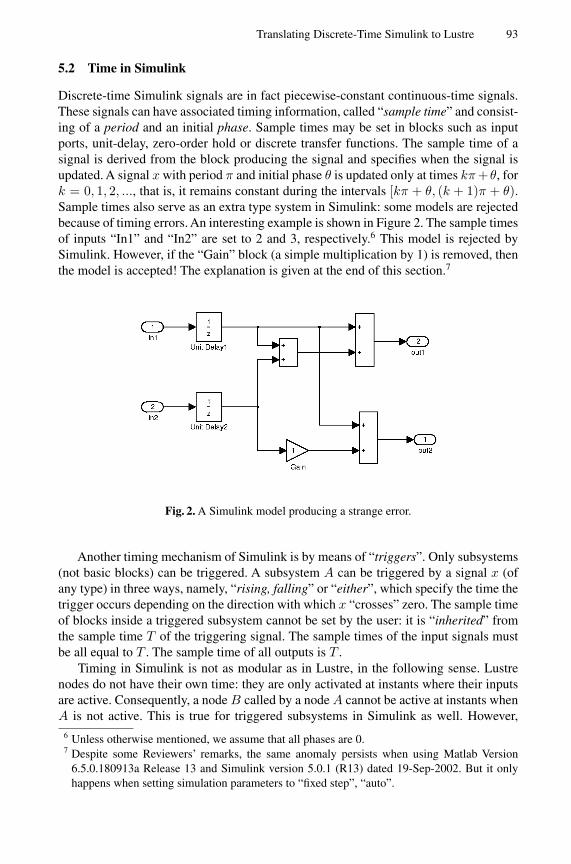
Translating Discrete-Time Simulink to Lustre 93

5.2 Time in Simulink

Discrete-time Simulink signals are in fact piecewise-constant continuous-time signals.These signals can have associated timing information, called “sample time” and consist-ing of a period and an initial phase. Sample times may be set in blocks such as inputports, unit-delay, zero-order hold or discrete transfer functions. The sample time of asignal is derived from the block producing the signal and specifies when the signal isupdated. A signal x with period π and initial phase θ is updated only at times kπ +θ, fork = 0, 1, 2, ..., that is, it remains constant during the intervals [kπ + θ, (k + 1)π + θ).Sample times also serve as an extra type system in Simulink: some models are rejectedbecause of timing errors. An interesting example is shown in Figure 2. The sample timesof inputs “In1” and “In2” are set to 2 and 3, respectively.6 This model is rejected bySimulink. However, if the “Gain” block (a simple multiplication by 1) is removed, thenthe model is accepted! The explanation is given at the end of this section.7

Fig. 2. A Simulink model producing a strange error.

Another timing mechanism of Simulink is by means of “triggers”. Only subsystems(not basic blocks) can be triggered. A subsystem A can be triggered by a signal x (ofany type) in three ways, namely, “rising, falling” or “either”, which specify the time thetrigger occurs depending on the direction with which x “crosses” zero. The sample timeof blocks inside a triggered subsystem cannot be set by the user: it is “inherited” fromthe sample time T of the triggering signal. The sample times of the input signals mustbe all equal to T . The sample time of all outputs is T .

Timing in Simulink is not as modular as in Lustre, in the following sense. Lustrenodes do not have their own time: they are only activated at instants where their inputsare active. Consequently, a node B called by a node A cannot be active at instants whenA is not active. This is true for triggered subsystems in Simulink as well. However,

6 Unless otherwise mentioned, we assume that all phases are 0.7 Despite some Reviewers’ remarks, the same anomaly persists when using Matlab Version

6.5.0.180913a Release 13 and Simulink version 5.0.1 (R13) dated 19-Sep-2002. But it onlyhappens when setting simulation parameters to “fixed step”, “auto”.

94 P. Caspi et al.

Simulink allows a block inside a (non-triggered) subsystem to have any sample time,possibly smaller than the parent subsystem. Thus, the block can be active while its parentsystem is inactive. This can be considered a useful mechanism which allows so-called“oversampling”. However, when used in conjunction with the “enabling” mechanism,it can give birth to real monsters whose behaviour is hardly understandable. The basicreason is that an extra, implicit input: the “absolute simulation time” — appears to flowthrough every block (but the triggered ones), even when this block is not enabled. Weconsider this a non-modular feature of Simulink.8

Another difference lies in how changes of timing are performed in the two languages.In Lustre, this can only be done using the when and current operators. In Simulink, thesample time of a signal can be changed using the “unit-delay” block or the “zero-orderhold” block. In order to do this, however, the following rules must be obeyed:9

1. “When transitioning from a slow to fast rate, a Unit Delay running at the slow ratemust be inserted between the two blocks. When transitioning from a fast to a slowrate, a Zero Order Hold running at the slow rate must be inserted between the twoblocks.”

2. “Illegal rate transition found involving Unit Delay block ... When using this block totransition rates, the input must be connected to the slow sample time and the outputmust be connected to the fast sample time. The Unit Delay must have a sample timeequal to the slow sample time and the slow sample time must be a multiple of thefast sample time. Also, the sample times of all destination blocks must be the samevalue.”

3. “Illegal rate transition found involving Zero Order Hold block ... When using thisblock to transition rates, the input must be connected to the fast sample time andthe output must be connected to the slow sample time. The Zero Order Hold musthave a sample time equal to slow sample time and the slow sample time must be amultiple of the fast sample time. Also, the sample times of all source blocks must bethe same value.”10

The second rule explains why the model of Figure 2 is rejected when the “Gain” blockis present and accepted otherwise. Indeed, after computing the sample times accordingto the method described in the following section, we find that the output of “Unit Delay2” has sample time 3. This output is “fed” to the “Gain” block, which also has sampletime 3, and to the left-most “Adder” block, which has sample time 1 (the GCD of 2 and3). This violates the second rule above.

8 Still, we are able to translate such models in Lustre, by calling the parent node with the “faster”clock (on which the child block will run) and passing as parameter the “slower” clock as well.

9 These rules are quoted from error messages produced by the Simulink tool.10 The third rule may seem strange since it implies that a zero-order hold block can have more

than one inputs. In fact, this happens when the input to this block comes from a “Mux” block,thus, encoding a vector of signals.

Translating Discrete-Time Simulink to Lustre 95

5.3 Clock Inference

The objective of clock inference is to compute the period and phase of each Simulinksignal and use this information (1) when creating the corresponding Lustre flows and(2) for defining the period at which the Lustre program must be run.

The clock inference algorithm is based on a fix-point computation on a lattice rep-resenting the sample times. The lattice is defined to be ST = (Q × Q) ∪ ⊥, where Qis the set of non-negative rational numbers (of finite precision). A pair (π, θ) representsthe sample time with period π and initial phase θ. ⊥ represents the undefined sampletime. The order in this lattice is defined as follows:

(π1, θ1) ≤ (π2, θ2) ≡ ∃κ.π1 = κπ2 ∧ (θ1 = θ2 ∨ (θ2 = 0 ∧ ∃λ.θ1 = λπ2)) (1)

The formula is slightly complicated because of the phases. If both phases are zero, thenthe order reduces to π1 being a multiple of π2 (κ and λ are integers). Naturally, we alsoset ⊥ ≤ (π, θ), for all (π, θ) ∈ ST . For example, (8, 2) ≤ (4, 2) ≤ (2, 0) ≤ (1, 0), but(4, 1) and (2, 0) are incomparable.

The order ≤ formalises the term “multiple” in the three Simulink rules quoted inSection 5.2. Thus, sample time s1 is a “multiple” of sample time s2 means s1 ≤ s2.

The sup operator in this lattice corresponds essentially to a GCD (greatest commondivisor) operation, complicated by the presence of phases. The precise definition is givenin the lemma below.

Lemma 1. Let (πi, θi) ∈ ST , for i = 1, 2. Then (π, θ) = sup((π1, θ1), (π2, θ2)) existsand is equal to:

π =

gcd(π1, π2), if θ1 = θ2gcd(π1, π2, θ1, θ2), otherwise

θ =

θ1, if θ1 = θ20, otherwise

For example,

sup((2, 0), (3, 0)) = (1, 0) sup((12, 3), (6, 3)) = (6, 3)sup((12, 6), (12, 0)) = (6, 0) sup((12, 3), (12, 4)) = (1, 0)

The fix-point is computed on a set of equations derived according to Table 4. Inthe table, x1, x2, ... are variables of the Simulink model and xC

1 , xC2 , ... are their corre-

sponding sample-times. The equation for “Triggered” refers to the out-most triggeredsubsystem: we do not need to infer sample times inside a triggered subsystem, since theyare all of type “inherited”. The equation for “DTL” refers to blocks of the “Discrete”library. The user can set the sample time of such blocks, denoted st in the table. Thedefault value of st is −1, meaning the sample time is “inherited” from the input.

Monotonicity ensures existence of a least fix-point.Although ST is an infinite lattice,the fix-point computation terminates. This is because there is a finite number of sampletimes in a given model. If the smallest fractional part among these sample times is 10−k

then it can be shown that the sample time (10−k, 0) is above all others according to theorder ≤ defined above, thus acts as a “top” element for the given model.

Once the sample times are calculated, a number of rules need to be verified. First,we must verify a strange restriction of Simulink, which forbids sample times (π, θ) with

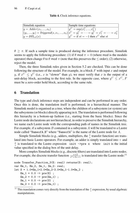
96 P. Caspi et al.

Table 4. Clock inference equations.

Simulink equation Sample time equationsy = Adder(x1, ..., xk) yC = sup(xC

1 , ..., xCk )

(y1, ..., yl) = Triggered(s, x1, ..., xk) sC = yC1 = · · · = yC

l = xC1 = · · · = xC

k

y = DTLst(x) yC = if st = −1 then xC else st

θ ≥ π. If such a sample time is produced during the inference procedure, Simulinkseems to apply the following procedure: (1) if θ mod π = 0 (where mod is the modulooperator) then change θ to θ mod π (note that this preserves the ≤ order); (2) otherwise,reject the model.

Then, the three Simulink rules given in Section 5.2 are checked. This can be donefollowing the structure of the model. For example, in a block F with input x and outputy, if xC ≤ yC (i.e., x is “slower” than y), we must verify that x is the output of aunit-delay block, according to the first rule. In the opposite case, where yC ≤ xC , Fmust be a zero-order hold block, according to the same rule.

6 Translation

The type and clock inference steps are independent and can be performed in any order.Once this is done, the translation itself is performed, in a hierarchical manner. TheSimulink model is organised as a tree, where the children of a subsystem (or system) arethe subsystems (or blocks) directly appearing in it. The translation is performed followingthis hierarchy in a bottom-up fashion (i.e., starting from the basic blocks). Since theLustre node declarations are not hierarchical, in order to preserve the Simulink hierarchy,we name each Lustre node with the corresponding path of names in the Simulink tree.For example, if a subsystem B contained in a subsystem A will be translated to a Lustrenode called “NameofA B” where “NameofA” is the name of the Lustre node for A.

Simple Simulink blocks (e.g., adders, multipliers, the 1z transfer function) are trans-

lated into basic Lustre operators. For example, an adder is simply translated into + andxz is translated to the Lustre expression init ->pre x where init is the initialvalue specified in the dialog box of the unit delay.

More complex Simulink blocks (e.g., discrete filters) are translated into Lustre nodes.For example, the discrete transfer function z+2

z2+3z+1 is translated into the Lustre node:11

node Transfer_Function_3(E: real) returns(S: real);var Em_1, Em_2, Sm_1, Sm_2: real;let S = 1.0*Em_1+2.0*Em_2-3.0*Sm_1-1.0*Sm_2 ;

Em_1 = 0.0 -> pre(E) ;Em_2 = 0.0 -> pre(Em_1) ;Sm_1 = 0.0 -> pre(S) ;Sm_2 = 0.0 -> pre(Sm_1) ;

11 This translation comes very directly from the translation of the xz

expression, by usual algebraicmanipulations.

Translating Discrete-Time Simulink to Lustre 97

tel.

A Simulink subsystem is translated into a Lustre node, possibly containing calls toother nodes. The Lustre node has the same inputs and outputs as the Simulink subsystem,plus, sometimes, the clock of some of its inputs (this is done for modularity). Here isan example of such a translation. Consider the Simulink model shown in Figure 3, withsubsystems A and B. The Lustre code generated for this example is as shown below:

node A(A_in1, A_in2, A_in3 : real) returns (A_out1, A_out2 : real);let A_out1 = B(A_in1 , A_in2);

A_out2 = ...tel.

node B(B_in1, B_in2 : real) returns (B_out : real);...

An example where it is necessary to pass clock information as input to the Lustre nodeis given in [3].

Simulink signals are mapped into Lustre flows. When a block changes the sampletime of a signal, the appropriate when and current operations need to be applied. Thismust also be done for triggered subsystems, as well as in cases where a subsystemreceives input signals with different sample times.

For example, consider a “Zero-Order-Hold” block and assume that the sample timeof input x is 1 and the sample time set to the zero-order hold block is 2. Then, the sampletime of the output y is also 2 and the generated Lustre code is as follows:

cl1_2 = true -> not pre(cl1_2) ;y = x when cl1_2 ;

Fig. 3. Simulink system A with subsystem B.

We implemented the algorithms described above in a prototype tool, called S2L. Thetool is written in Java. It takes as input a Simulink model (“.mdl” file) and produces a

98 P. Caspi et al.

Lustre program (“.lus” file) or an error message in case the input model contains type ortiming errors. S2L uses an intermediate representation of the Simulink model, in XML.This is done to facilitate evolution of the tool as the syntax of the “.mdl” file changes.

7 Conclusions

We have presented a method for translating a discrete-time subset of Simulink modelsinto Lustre programs. The translation is done in three steps: type and clock inference,followed by a hierarchical bottom-up translation. We have implemented the method in atool called S2L and applied it to a controller used in Audi cars. The interest of our tool isthat it opens the way to the use of formal and certified verification and implementationtools attached to the Lustre tool chain. Also, in the process of translation, we formalised(for the first time, to our knowledge) the typing and timing mechanisms of Simulink.

Perhaps the most significant drawback of our approach is its dependency on syntaxand semantics of Simulink models. New versions of Simulink appear as often as every sixmonths and sometimes major changes are made with respect to previous versions. Thissituation seems difficult to avoid given the relative “monopoly” of Simulink/Stateflow inthe control design landscape. Another weakness of our tool is its incompleteness: severalunsafe constructs of Simulink are not translated. Yet this can be seen as the price to payfor having a sound translation.

We are currently enhancing the capabilities of S2L. Features such as “masked” sub-systems are already handled. We are now studying the translation of some “virtual”blocks such as “Mux”. We are also currently studying the translation of Stateflow. State-flow presents a number of semantic problems, such as behaviour depending on how themodel is graphically drawn, or non-termination of a simulation step. Our first goal is toidentify a subset of Stateflow avoiding these problems.

References

1. E. Asarin, T. Dang, and J. Esteban. Simulation of hybrid automata using Matlab/Simulink.Technical report, Verimag, 2003.

2. K.J. Astrom and B. Wittenmark. Computer Controlled Systems. Prentice-Hall, 1984.3. P. Caspi, A. Curic, A. Maignan, C. Sofronis and S. Tripakis. Translating Discrete-Time

Simulink to Lustre. Verimag Research Report, July 2003.4. P. Caspi, A. Curic, A. Maignan, C. Sofronis, S. Tripakis, and P. Niebert. From Simulink

to SCADE/Lustre to TTA: a layered approach for distributed embedded applications. InLanguages, Compilers, and Tools for Embedded Systems (LCTES’03). ACM, 2003.

5. P. Caspi and M. Pouzet. Synchronous Kahn networks. In ACM SIGPLAN InternationalConference on Functional Programming, pages 226–238, 1996.

6. Anton Cervin, Dan Henriksson, Bo Lincoln, and Karl-Erik Arzen. Jitterbug and Truetime:Analysis tools for real-time control systems. In Proceedings of the 2ndWorkshop on Real-TimeTools, Copenhagen, Denmark, August 2002.

7. A. Chutinan and B.H. Krogh. Computational techniques for hybrid system verification. IEEETrans. Automatic Control, 48(1), 2003.

8. P. Le Guernic, T. Gautier, M. Le Borgne, and C. Le Maire. Programming real-time applicationswith signal. Proc. of the IEEE, 79(9):1321–1336, 1991.

Translating Discrete-Time Simulink to Lustre 99

9. N. Halbwachs, P. Caspi, P. Raymond, and D. Pilaud. The synchronous dataflow programminglanguage Lustre. Proceedings of the IEEE, 79(9), September 1991.

10. M. Jersak, D. Ziegenbein, F. Wolf, K. Richter, R. Ernst, F. Cieslog, J. Teich, K. Strehl, andL. Thiele. Embedded system design using the SPI workbench. In Proc. of the 3rd InternationalForum on Design Languages, 2000.

11. P.G. Joisha and P. Banerjee. The MAGICA type inference engine for MATLAB. In CompilerConstruction (CC). LNCS 2622, Springer, 2003.

12. G. Kahn. The semantics of a simple language for parallel programming. In Proc. of the IFIPCongress, 1974.

13. C.M. Kirsch, M.A. Sanvido, T.A. Henzinger, and W. Pree. A Giotto-based helicopter controlsystem. In EMSOFT’02. LNCS 2491, Springer, 2002.

14. E. Lee and D. Messerschmitt. Synchronous data flow. Proceedings of the IEEE, 75, 1987.15. E. Lee and T. Parks. Dataflow process networks. Proceedings of the IEEE, pages 773–799,

May 1995.16. S. Neema. Simulink and Stateflow data model. Technical report, ISIS, Vanderbilt University,

2001.17. C. Ratel, N. Halbwachs, and P. Raymond. Programming and verifying critical systems by

means of the synchronous data-flow programming language Lustre. In ACM-SIGSOFT Con-ference on Software for Critical Systems, 1991.

18. P. Raymond, D. Weber, X. Nicollin, and N. Halbwachs. Automatic testing of reactive systems.In 19th IEEE Real-Time Systems Symposium, Madrid, Spain, December 1998.

19. B.I. Silva, K. Richeson, B.H. Krogh, and A. Chutinan. Modeling and verifying hybrid dy-namical systems using CheckMate. In ADPM, 2000.

20. S. Sims, K. Butts, R. Cleaveland, and S. Ranville. Automated validation of software models.In ASE, 2001.

21. A. Tiwari. Formal semantics and analysis methods for Simulink Stateflow models. Technicalreport, SRI International, 2002.

22. S. Tudoret, S. Nadjm-Tehrani, A. Benveniste, and J.-E. Stromberg. Co-simulation of hybridsystems: Signal-Simulink. In FTRTFT, 2000.

Minimizing Variables’ Lifetime in Loop-IntensiveApplications

Noureddine Chabini and Wayne Wolf

Computer Engineering, Department of Electrical Engineering, Princeton UniversityMail address: Engineering Quadrangle, Olden Street, Princeton, NJ 08544, USA.

nchabini,wolf@ee.princeton.edu

Abstract. In this paper, we address a set of research problems regarding loop-intensive applications. The first problem consists of minimizing variables’lifetime under timing constraints. Any variable that is alive for more than oneiteration must be saved by for instance storing it into a register. The secondproblem is derived from the first one, and consists of balancing variables’lifetime for a target total number of registers and under timing constraints. Forthe third problem, we focus on minimizing variables’ lifetime in the context ofsoftware pipelining in the case of one loop as well as nested loops. We providemethods to solve these three problems, and show that a set of them havepolynomial run-time. Once these methods are used, one may need to solve theproblem of generating the transformed code and reducing its size. We providealgorithms to solve this fourth problem. Designers face these problems duringhardware-software co-design, and in designing embedded systems as well assystem-on-chip. Solving these problems is also useful in low power design. Weexercise some of these methods on known benchmarks, and provide obtainednumerical results that show their effectiveness.We solve these problems using techniques related to retiming, an algorithmoriginally developed for hardware optimization.

1 Introduction

Loops are found in many real applications. This kind of applications can be found inthe domain of image processing as well as in the domain of digital signal processing.For instance, an image is represented as a two dimensional array where each cell of thearray is used to store one pixel of the image. Processing the image then transforms todoing some processing on the array using for instance “for” loops to access the array’selements.

Multimedia applications are another example of loop-intensive real applications.These applications require a high processor speed. Since some of them are portableapplications, reducing their power consumption is required to increase the battery life.Note that prolonging battery life (for portable systems) is became a productdifferentiator in the market.

Loop-intensive applications can be classified as computational intensive, dataintensive, or computational-and-data intensive applications. There are three ways toimplement these applications: hardware, software or hardware-and-softwareimplementations. To satisfy performance requirements, hardware implementations are

R. Alur and I. Lee (Eds.): EMSOFT 2003, LNCS 2855, pp. 100−116, 2003. Springer-Verlag Berlin Heidelberg 2003

the most targeted for the first and third classes, and imply a high design cost. Due tothe low cost of the implementation and the ease of changing it, softwareimplementations are targeted whenever they can satisfy the performance requirements.For all these three ways of implementing loop-intensive applications, there is a needfor some optimizations as shown by Fig. 1 from [2].

One common optimization to these three kinds of implementations is theminimization of variables’ lifetime. A variable is alive from the time it is produceduntil the last time it is used. For the case of software implementations for instance, avariable that is alive for long time may be transferred from the register where it isstored to the main memory if the number of simultaneous alive variables is greater thanthe number of the available registers; this implies an increase of run-time as well aspower consumption due to the transfer between registers and the main memory. Thesize of memory has an implicit impact on both performance and power consumption.Also, it has an impact on the cost in dollars for the case of hardware implementations.The total size of memories must be reduced in the case of embedded systems as wellas of system-on-chip. Sometimes, there is more than one way to minimize variables’lifetime for a target total size of memories. In this case, one needs to chose the way thatmay allow to increase performance and/or to reduce power consumption.

Fig. 1. Loop optimizations in the co-design flow.

In this paper, we address four research problems related to the minimization ofvariables’ lifetime in loop-intensive applications. We first address the problem ofminimizing variables’ lifetime under timing constraints. We then investigate theproblem of balancing variables’ lifetime for a target total number of registers and undertiming constraints. These two problems can be seen as platform independent, andhence approaches to solve them allow a source-to-source code transformation. Besidesthese two problems, we address the problem of minimizing variables’ lifetime in thecontext of software pipelining in the case of one loop as well as nested loops. The latterproblem is platform dependent. We provide methods to solve these three problems, andshow that a set of them have polynomial run-time. Once these methods are used, onemay need to solve the problem of generating the transformed code and reducing its

Algorithmic Description

Partitionning

Hardware Software

Synthesis Compilation

Optimizations

Optimizations Optimizations

101Minimizing Variables´ Lifetime in Loop-Intensive Applications

size, which is useful for memory-size-constrained systems such as system-on-chip andembedded systems. We provide algorithms to solve this fourth problem. We exercisesome of these methods on known benchmarks. Obtained numerical results show thatthe sum of variables’ lifetime can be reduced by factors as high as 33.33%.

Basic retiming has been proposed in [1] as an optimization technique forsynchronous sequential circuits. This technique changes the location of registers in thedesign in order to achieve one of the following goals: (i) minimizing the clock period,(ii) minimizing the number of registers, or (iii) minimizing the number of registers fora target clock period.

There is a relation ship between a register in the context of hardwareimplementations and an iteration in the context of software implementations. In thecontext of software implementations, moving for instance one register from the inputsof an operator to its outputs transforms to (i) delaying by one iteration theconsummation of the result produced by this operator, and (ii) advancing by oneiteration the consummation of the operands of that operator. Based on this relationship, we exploit basic retiming to develop the methods for solving the four presentedproblems above. Using basic retiming to optimize loops is not new as we will presentlater in the paper. However, it is the first time that basic retiming is used in this paperto solve these problems that are to the best of our knowledge not addressed by any otherpaper.

2 Preliminaries

2.1 Cyclic Graph Model

In this paper, we are interested in “for”-type loops as the one in Fig. 2 (a). We assumethat the body of the loop is constituted by a set of computational and/or assignmentinstructions only (i.e., no conditional or branch instruction like for instance if-then-elseis inside the body).

We model a loop by a directed cyclic graph , where V is the set ofinstructions in the loop body, and E is the set of edges that represent data dependencies.Each vertex v in V has a non-negative integer execution delay . Each edge

, from vertex to vertex , has a weight , which meansthat the result produced by at any iteration i is consumed by at iteration

.Fig. 2 presents a simple loop and its directed cyclic graph model. For Fig. 2 (b), the

execution delay of each instruction is specified as a label on the left of each node ofthe graph, and the weight of each arc is in bold. For instance, theexecution delay of is 10 and the value 2 on the arc means that instructionat any iteration i uses the result produced by instruction at iteration .

G V E d w, , ,( )=

d v( ) N∈eu v, E∈ u V∈ v V∈ w eu v,( ) N∈

u vi w eu v,( )+( )

Siw eu v,( ) eu v, E∈

S1 eS1 S2, S2S1 i 2–( )

102 N. Chabini and W. Wolf

Fig. 2. A simple loop and its directed cyclic graph model.

We also address perfect nested “for”-type loops in this paper. For this kind of nestedloops, no computational or assignment instructions must be between two successive“for”-type nested loops. All the instructions must be in the body of the innermost loopof the nest. We assume that this body does not contain conditional or branch instructionlike if-then-else for instance. This kind of nested loops can be modeled as we did forthe case of one loop. The weight of each arc in the graph transforms to a vector with adimension equal to the number of loops in the nest. For an example of perfect nested“for”-type loops and its cyclic graph model, the reader is referred to [8].

2.2 Introduction to Basic Retiming

A synchronous sequential design can be modeled as a directed cyclic graph as we didfor loops in Section 2.1. Instructions become computational elements of the design,edges become wires, and s become the number of registers on the wire betweenu and v.

Let be a synchronous sequential digital design. Basic retiming (orretiming for short in this paper) [1] is defined as a function , whichtransforms to a functionally equivalent synchronous sequential digital design

. The set represents natural integers.The weight of each edge in is defined as follows:

. (1)

Since the weight of each edge in represents the number of registers on that edge,then we must have:

. (2)

Any retiming that satisfies Equation (2) is called a valid retiming. From expressions(1) and (2) one can deduce the following inequality:

. (3)

Let us denote by a path from node u to node v in V. Equation (1) impliesthat for every two nodes u and v in V, the change in the register count along any path

depends only on its two endpoints:

S1

20

2010

0

10

2

010

0

2

0

main () int a[U], b[U], c[U], d[U], e[U], i;

for (i=2; i<= U; i++) S1: a[i] = 1 + d[i];S2: b[i] = 1 + a[i-2];S3: c[i] = b[i] * e[i];S4: d[i] = 2 * c[i];S5: e[i] = 1 + c[i-2];

(a) Simple loop. (b) Directed cyclic graph model.

S2 S3

S4 S5

w eu v,( )

G V E d w, , ,( )=r r : V Z→

GGr V E d wr, , ,( )= Z

eu v, Gr

wr eu v,( ) w eu v,( ) r v( ) r u( ), eu v, E∈∀–+=

Gr

wr eu v,( ) 0, eu v, E∈∀≥

r

r u( ) r v( )– w eu v,( ), eu v, E∈∀≤

P u v,( )

P u v,( )

103Minimizing Variables´ Lifetime in Loop-Intensive Applications

, (4)where:

. (5)

Let us denote by the delay of a path from node u to node v.is the sum of the execution delays of all the computational elements that

belong to .A 0-weight path is a path such that . The minimal clock period of a

synchronous sequential digital design is the longest 0-weight path. It is defined by thefollowing equation:

. (6)Two matrices called W and D are very important to the retiming algorithms. They

are defined as follows [1]:

, and (7)

. (8)

The matrices W and D can be computed as explained in [1].One application of retiming is to minimize the clock period of synchronous

sequential digital designs. For instance, by thinking on Fig. 2 (b) as a synchronoussequential design, the clock period of that design is , which is equal to the sumof execution delays of computational elements (i.e.,

). However, we can obtain if we applythe following retiming vector to the vector of nodes in .The retimed graph is presented by Fig. 3.

Fig. 3. A retimed graph with .Π = 30

For the purpose of this paper, we extract from [1] the following theorem, which isalso proved in [1].

Theorem 1 : Let be a synchronous digital design, and let be a positivereal number. Then there is a retiming r of G such that the clock period of the resulting retimeddesign is less than or equal to if and only if there exists an assignment of integer valuer(v) to each node v in V such that the following conditions are satisfied: (1)

, and (2).

q

wr P u v,( )( ) w P u v,( )( ) r v( ) r u( ), u v, V∈∀–+=

w P u v,( )( ) w ex y,( )ex y, P u v,( )∈∑=

d P u v,( )( ) P u v,( )d P u v,( )( )

P u v,( )w P u v,( )( ) 0=

Π Max u∀ v V∈, d P u v,( )( ) | w P u v,( )( ) 0=( ) =

W u v,( ) Min w P u v,( )( )( ) , u v, V∈∀=

D u v,( ) Max d P u v,( )( ) | w P u v,( )( ) W u v,( )= , u v, V∈∀=

Π 60=vi 1 ... 4, ,=

Π 60 d v2( ) d v3( ) d v4( ) d v1( )+ + += = Π 30=2 1 1 2 0, , , , 1 2 3 4 5, , , , G

Gr

4

3

1

20

2010

1

510

1

1210

0

1

0

G V E d w, , ,( )= Π

Gr Π

r u( ) r v( )– w eu v,( )≤ eu v, E∈∀,r u( ) r v( )– W u v,( ) 1–≤ u∀ v V∈, such that D u v,( ) Π>,

104 N. Chabini and W. Wolf

Once a retiming defined on is computed for solving a target problem, it can thenbe transformed to a non-negative retiming without impact on the solution of theproblem. Indeed, let . Then the function defined as

, , is a non-negative retiming (i.e., takes non-negativevalues). In the rest of the paper, we consider non-negative retiming only.

3 Minimizing the Sum of Variables’ Lifetime under TimingConstraints

In this section, we focus on minimizing the sum of the lifetime of all variables in theloop’s body of unidimensional loops under a target latency constraint. This latency isdefined here as the time required to execute, using unlimited number of computationalelements, all the instructions of the loop’s body at any iteration of the loop. We denoteby the target latency. We represent the loop by a directed cyclic graph asintroduced in Section 2.1.

Assume that we want for the simple loop in Fig. 2. In this case, we havethat variables produced by instructions and are alive for two iterations. The sumof variables’ lifetime in this case is 4 iterations, and hence 4 registers are required tostore these variables. Can one reduce the sum of variables’ lifetime while still having

? The response is yes if we do not have constraints on the number ofcomputational elements. Indeed, by thinking on as a synchronous digital design, aretiming vector can be applied to obtain a sum of variables’ lifetimeequal to two. The resulted retimed graph is presented by Fig. 4. In this case, onlyvariable produced by is alive for 2 iterations, which now requires 2 registerscompared to 4 previously.

Fig. 4. Retiming Fig. 2 (b) using the retiming vector . 2 0 0 2 0, , , ,

By applying retiming on the graph modeling the loop, it is then possible to reducethe sum of variables’ lifetime while still having a target latency . But, can this bealways possible? If yes, how one can derive an algorithm to do it?

The response to the first question is yes, and our focus in the rest of this section isto provide an algorithm as a response to the second question. The proposed algorithmtake the form of a mathematical linear program.

By thinking on as a synchronous digital design and on as its clock period, onecan derive from Theorem 1 the following theorem that will be used to derive themathematical linear program.

Z

m Min r v( ) v V∈∀, = gg v( ) r v( ) m–= v V∈∀ g

Π G

Π 60=S1 S3

Π 60=G

2 0 0 2 0, , , ,

S3

4

3

1

20

2010

2

510

2

02

10

0

0

0

Π

G Π

105Minimizing Variables´ Lifetime in Loop-Intensive Applications

Theorem 2 : Let be a synchronous digital design, and let be a positivereal number. Then there is a retiming r of G such that the clock period of the resulting retimeddesign is less than or equal to if and only if there exists an assignment of non-negativeinteger values to r(v) and b(v) for each node v in V such that the following conditions aresatisfied: (1) , (2)

, and (3).

q

Proof: It can be easily derived from Theorem 1. Inequality (1) can always besatisfied by first applying Theorem 1.

qThe second and third inequalities of Theorem 2 are the same as in Theorem 1. But,

what is the objective from its first inequality? It allows to reduce the lifetime of thevariable produced by the instruction at the node u by reducing the variable upper bound

.The system of inequalities of Theorem 2 may have an infinite number of possible

solutions (regarding the unknown variables and ). Hence, to find a solutionthat allows to minimize the sum of the lifetime of variables in the loop’s body, one canconstraint this system by minimizing the objective function:

, (9)

which leads to the Integer Linear Program (ILP) constituted by (10)-(14).

Theorem 3 : The ILP (10)-(14) has always a solution, and its optimal solution can be found inpolynomial run-time.

q

Proof: If Theorem 1 applies, then Theorem 2 applies too. In this case, ILP (10)-(14)has always a solution since Theorem 2 applies. It can be optimally solved inpolynomial run-time. Indeed, The right hand sides of inequalities (11)-(13) are alwaysintegers. From linear programming theory [12], we know that if the constraint matrixA of an ILP is totally unimodular and if the right hand sides of inequalities (as (11)-(13) in our case) are integers then the ILP and its relaxation obtained by ignoring theconstraints integers (ignoring (14) in our case) have the same optimal solution. Thisrelaxed ILP is a linear program, and hence it can be solved optimally in polynomialrun-time by using for instance methods [13][14]. The constraint matrix A of ILP (10)-(14) is totally unimodular since it satisfies the following theorem from [15].

Theorem 4 : A matrix X is totally unimodular if and only if for every square eulerian submatrix

Y of X, we have that the sum of the entries of Y divides by 4.

q

(10)

Subject to:(11)

G V E d w, , ,( )= Π

Gr Π

b u( ) r u( ) r v( )–+ w eu v,( )≥ , eu v, E∈∀r v( ) r u( )– w– eu v,( )≥ , eu v, E∈∀r v( ) r u( )– 1 W u v,( )–≥ u∀ v V∈, such that D u v,( ) Π>,

b u( )

b v( ) r v( )

b v( )v V∈∑

Minimize b v( )v V∈∑

b u( ) r u( ) r v( )–+ w eu v,( )≥ , eu v, E∈∀

106 N. Chabini and W. Wolf

(12)

(13)

and are non-negative integers, (14)

4 Balancing the Lifetime of Variables for a Target Sum ofVariables’ Lifetime and Timing Constraints

Again, a loop is modeled as a directed cyclic graph as introduced in Section 2.1. Inthis section, we address a problem derived from the one targeted in Section 3. Theproblem consists in balancing the lifetime of variables under a target latency (as wedefined in Section 3) while keeping the sum of variables’ lifetime less than or equal toa target value say B. One can fix B to the minimal value of the objective function in (9)by solving (10)-(14). The problem can be viewed as the problem of maximizing thenumber M of edges of non-zero weight in under a target latency while satisfying

.

Is it important to solve this problem? It is important for instance in the case ofhardware implementations that require reduction of power consumption. Indeed, anedge of non-zero weight means we have at least one register on that edge. Havingregisters distributed on the output of many computational elements allows to reducethe power consumption due to switching activities. In the case of softwareimplementations, it allows to reduce the length of critical (or pseudo critical) paths, andhence to increase the number of instructions that can simultaneously be executed.

Let us give an example to show how solving this problem can help in optimizingsome figures of merit. Let us use Fig. 2. Assume that we want (i) and (ii)

. By thinking again on as a synchronous digital design and applyingretiming on it, we can obtain Fig. 3, which satisfies both (i) and (ii). In the case ofhardware implementations, Fig. 3 is preferable since, besides reducing the switchingactivities, it allows to apply supply voltage scaling for node 5 that is off critical paths;hence, to reduce power consumption.

How to solve the problem? To solve it, we again use basic retiming and provide aninteger linear program as we did in Section 3. Although ILPs are NP-hard in general,we show that this ILP can be solved in polynomial run-time as we did in Section 3.

After retiming , let be the resulted retimed graph. For every arc in ,let be a 0-1 unknown variable defined as follows. takes the value 1 if

, and 0 otherwise. Based on the definition of ‘s and Inequality (2),we then have:

, and (15)

. (16)

Using Equation (3), we can transform (16) to:. (17)

r v( ) r u( )– w– eu v,( )≥ , eu v, E∈∀

r v( ) r u( )– 1 W u v,( )–≥ u∀ v V∈, such that D u v,( ) Π>,

b v( ) r v( ) v V∈∀

G

Π

G Πb v( )

v V∈∑ B≤

Π 30=b v( )

v V∈∑ 3≤ G

G Gr eu v, Grm eu v,( ) m eu v,( )

wr eu v,( ) 1≥ m eu v,( )

0 m eu v,( ) 1≤ ≤ , eu v, E∈∀

m eu v,( ) wr eu v,( )≤ , eu v, E∈∀

m eu v,( ) r u( ) r v( )–+ w eu v,( )≤ , eu v, E∈∀

107Minimizing Variables´ Lifetime in Loop-Intensive Applications

From Theorem 2, we can derive the following theorem that we will use to derive amethod to solve the problem.

Theorem 5 : Let be a synchronous digital design, and let be a positivereal number and a non-negative integer. Then there is a retiming r of G such that the clockperiod of the resulted retimed design is less than or equal to if and only if there exists anassignment of non-negative integer values to r(v) and b(v) for each node v in V, and 0/1 value

to each arc in E, such that the following conditions are satisfied: (1), (2) , (3)

, (4)and (5) .

q

Proof: It is omitted due to space limitation, but can be easily derived from Theo-rem 1.

q

The number of edges of non-zero weight in is:

. (18)

The system of Inequalities in Theorem 5 may have many possible solutions. Tohave a solution that maximizes M, one can add formula

(19)

to that system as well as integrality constraints on the unknown variables. The resultedsystem is an Integer Linear Program (ILP), and given by (20)-(27).

Theorem 6 : The ILP (20)-(27) has always a solution, and its optimal solution can be found inpolynomial run-time. q

Proof: It is omitted due to space limitation, but can be derived as we did for the caseof Theorem 3.

q

G V E d w, , ,( )= ΠB

Gr Π

m eu v,( ) eu v,0 m eu v,( ) 1≤ ≤ , eu v, E∈∀ m eu v,( ) r u( ) r v( )–+ w eu v,( )≤ , eu v, E∈∀r u( ) r v( )– W u v,( ) 1–≤ u∀ v V∈, such that D u v,( ) Π>,b u( ) r u( ) r v( )–+ w eu v,( )≥ , eu v, E∈∀ b v( )

v V∈∑ B≤

Gr

M m eu v,( )eu v, E∈∑=

Maximize m eu v,( )eu v, E∈∑

(20)

Subject to:(21)

(22)

(23)

(24)

(25)

Maximize m eu v,( )eu v, E∈∑

m– eu v,( ) 0≤ , eu v, E∈∀

m eu v,( ) 1≤ , eu v, E∈∀

m eu v,( ) r u( ) r v( )–+ w eu v,( )≤ , eu v, E∈∀

r u( ) r v( )– W u v,( ) 1–≤ u∀ v V∈, such that D u v,( ) Π>,

b u( )– r u( ) r v( )+– w– eu v,( )≤ , eu v, E∈∀

108 N. Chabini and W. Wolf

, and are non-negative integers, , (27)

5 Transformed-Code Generation and Reduction of Its Size

For software implementations, the approaches for solving the problem of Section 3 or4 constitute a source-to-source code transformation. The size of the transformed codeis not unique. It depends on the retiming used. In this section, we show how to obtainthis transformed code, and why the size of this code is not unique. We also provide amethod to find a retiming that allows to obtain a code with a small size.

The transformed code is constituted by three parts: Prologue, Loop, and Epilogue.The Prologue is the segment of the original code that must be executed before arepetitive processing appears that corresponds to the Loop. The Epilogue is thesegment of the original code that cannot be executed by the Loop and the Prologue.

In Section 3, we showed that to minimize the sum of variables’ lifetime for the loopin Fig. 2, the retiming vector can be applied on Fig. 2 (b). For this vectorof retiming, the code for the transformed loop as well as its directed cyclic graph aregiven on Fig. 5.

Fig. 5. Source code after application of a retiming on a loop.

Let . With the help of Fig. 5, one can then easily double-

m eu v,( ) b v( ) r v( ) eu v, E∈∀ v V∈∀

2 0 0 2 0, , , ,

main ()

int a[U], b[U], c[U], d[U], e[U], i;

/* Prologue */S2: b[2] = 1 + a[0]; S3: c[2] = b[2] * e[2];S5: e[2] = 1 + c[0];S2: b[3] = 1 + a[1]; S3: c[3] = b[3] * e[3];S5: e[3] = 1 + c[1];/* New Loop */for (i=4; i<= U; i++)

S1: a[i-2] = 1 + d[i-2];S2: b[i] = 1 + a[i-2];S3: c[i] = b[i] * e[i];S4: d[i-2] = 2 * c[i-2];S5: e[i] = 1 + c[i-2];

/* Epilogue */S1: a[U-1] = 1 + d[U-1];S4: d[U-1] = 2 * c[U-1];S1: a[U] = 1 + d[U];S4: d[U] = 2 * c[U];

S1

20

2010

2

10

2

010

0

0

0

S2 S3

S4 S5

(b) Directed cyclic graph model for (a).

(a) Code after retiming.

M Max r v( ) v V∈∀, =

109Minimizing Variables´ Lifetime in Loop-Intensive Applications

b v( )v V∈∑ B≤ (26)

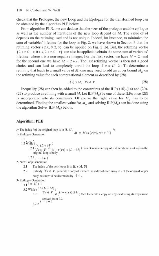
check that the Prologue, the new Loop and the Epilogue for the transformed loop canbe obtained by the algorithm PLE below.

From algorithm PLE, one can deduce that the sizes of the prologue and the epilogueas well as the number of iterations of the new loop depend on M. The value of Mdepends on the retiming used and is not unique. Indeed, for instance, to minimize thesum of variables’ lifetime for the loop in Fig. 2, we have shown in Section 3 that theretiming vector can be applied on Fig. 2 (b). But, the retiming vector

can also be applied to obtain the same sum of variables’lifetime, where x is a non-negative integer. For the first vector, we have , andfor the second one we have . The last retiming vector is then not a goodchoice and can lead to completely unroll the loop if . To determine aretiming that leads to a small value of M, one may need to add an upper bound onthe retiming value for each computational element as described by (28).

. (28)

Inequality (28) can then be added to the constraints of the ILPs (10)-(14) and (20)-(27) to produce a retiming with a small M. Let ILP(Mu) be one of these ILPs once (28)is incorporated into its constraints. Of course the right value for has to bedetermined. Finding the smallest value for and solving ILP(Mu) can be done usingthe algorithm Solve_ILP(Mu) below.

Algorithm: PLE

/* The index i of the original loop is in [L, U]. */1- Prologue Generation

1.11.2 While ( )

1.2.1 , if ( ) then Generate a copy of v at iteration i as it was in theoriginal loop’s body.

1.2.2 2- New Loop Generation

2.1 The index of the new loops is in [L + M, U]2.2 Its body: , generate a copy of v where the index of each array in v of the original loop’s

body has now to be decreased by .3- Epilogue Generation

3.13.2 While ( )

3.2.1 , if ( ) then Generate a copy of v by evaluating its expressionderived from 2.2.

3.2.2

2 0 0 2 0, , , , 2 x+ 0 x+ 0 x+ 2 x+ 0 x+, , , ,

M 2=M 2 x+=

x U 2–=Mu

r v( ) Mu≤ , v V∈∀

MuMu

M Max r v( ) v V∈∀, =

i L=i L M+( )<

v V∈∀ i r v( )+( ) L M+( )<

i i 1+=

v V∈∀r v( )

i U 1+=i U M+( )≤

v V∈∀ i r v( )–( ) U≤

i i 1+=

110 N. Chabini and W. Wolf

Algorithm: Solve_ILP(Mu)

1- Solve ILP(Mu) without considering (28). Put the solution in and the value of the objective

function in OptimalVal.

2- Using , do .

3- Let and .

4- while ( ) do

4.1

4.2 If ILP(Mu) has a solution and the value of the objective function is OptimalVal

then do and , else do .

5- Solve ILP(Mu). If it doesn’t have a solution then use as a solution.

6 Minimizing Variables’ Lifetime in Case of Software Pipelining

Software pipelining is a loop scheduling technique. It allows to increase the instructionlevel parallelism, which is useful for processors such as VLIW and superscalarprocessors. This instruction level parallelism is increased by reducing the difference ofthe start times of each two successive iterations of the loop. For an introduction tosoftware pipelining and to its related techniques, the reader is referred to [7].

Software pipelining of single loop has been widely addressed in the literature [7].Modulo scheduling is one of the approaches proposed for software pipelining. It is aperiodic function that determines the start time for each instruction of theloop’s body. This function is defined as follows:

, (29)

where is the start time of the first instance of the instruction , and is theperiod of . Let C be the set of directed cycles in the directed cyclic graph modelingthe loop. Based on data dependency constraints only, the minimum value of is theinverse of the value in (30). This value can be computed in polynomial run-time, since(30) is an instance of a Minimum-Cost-to-Time Ratio Cycle Problem [10]. In thesequel, we assume that is given.

. (30)

Since software pipelining reduces the difference of the start times of each twosuccessive iterations of the loop, it then increases the number of required registers tostore alive variables. Our objective in the rest of this section is to show how to reducethe number of required registers for modulo scheduling.

Using the graph modeling the loop, let be any one of the successors of . Theresult of the instruction of iteration say that is started at time will be

S0

S0 Mmax Max r v( ) v V∈∀, =

Mu Mmax= Mmin 0=

Mmin Mmax≠

Mu Mmin Mmax+( ) 2⁄=

S ≤

S0 S= Mmax Mu= Mmin Mu=

S0

s : N V× Q→

sk v( ) s0 v( ) P k⋅ , k N∈∀ , v V∈∀+=

s0 v( ) v Ps

P

P

Minc C∈ w eu v,( )eu v, c∈∑

d u( )v V∈∀ and eu v, c∈∑

⁄

G v uu k Sk u( )

111Minimizing Variables´ Lifetime in Loop-Intensive Applications

available at time . This result must still be alive until the start time ofat iteration . Hence, the relative lifetime of this result is:

. (31)

Of course, we have:. (32)

Using (29), we can then rewrite (31) as follows:

. (33)

By considering all the successors of , the lifetime of any result of operation then satisfies the following:

. (34)

From (32), (33) and (34), we can derive the following system of inequalities (35)and (36):

(35)

(36)

To find a modulo schedule that minimizes the sum of variables’ lifetime, one thencan solve the linear program (38)-(40). The number of registers required for each resultproduced by u is:

. (37)Hence, linear program (38)-(40) allows to determine a schedule that reduces therequired number of registers.

By dividing all the expressions (38)-(40) by , replacing by , andadding integrality constraints on , we obtain an MILP to determine a schedule thatminimizes the required number of registers. MILPs cannot be in general solved withpolynomial run-time. But, they can be solved with a small run-time when the size ofthe formulation is small. However, when and all execution delays are integers,then one can prove as done for Theorem 3 that the MILP can be solved in polynomialrun-time.

(38)

Subject to:(39)

(40)

Although software pipelining can be extended to nested loops by applying it on oneloop at each time, modulo scheduling has been used in the case of perfect nested loops

Sk u( ) d u( )+( ) vk w eu v,( )+( ) tv u( )

tv u( ) sk w eu v,( )+ v( ) sk u( ) d u( )+( )– , k N∈∀ , eu v, E∈∀=

tv u( ) 0, eu v, E∈∀≥

tv u( ) s0 v( ) s0 u( ) P w eu v,( )⋅ d u( )–+– , eu v, E∈∀=

u t u( )u

t u( ) tv u( ), eu v, E∈∀≥

t u( ) s0 u( ) s0 v( )–+ P w eu v,( )⋅ d u( )–≥ , eu v, E∈∀

s0 v( ) s0 u( )– d u( ) P w eu v,( )⋅ , eu v, E∈∀–≥

T u( ) t u( ) P⁄ u V∈∀,=

P T u( )( ) P⁄( ) T u( )T u( )

P 1=

Minimize t v( )v V∈∑

t u( ) s0 u( ) s0 v( )–+ P w eu v,( )⋅ d u( )–≥ , eu v, E∈∀

s0 v( ) s0 u( )– d u( ) P w eu v,( )⋅ , eu v, E∈∀–≥

112 N. Chabini and W. Wolf

[8] to do software pipelining on all the loops of the nest in the same time. This moduloscheduling is as (29) but and become vectors. To determine the value of , alinear program is proposed in [8]. This linear program computes also the start time ofthe first instance of each instruction in the loop’s body.

In the case of modulo scheduling for perfect nested loops, is it possible to minimizethe sum of variables’ lifetime? The response is yes, and our objective in the rest of thissection is to show how it can be done.

A perfect nested loop can be modeled as we did for the case of one loop. The weightof each arc transforms to a vector (see [8] for more details). Without

loss of generality, we assume that all components of are non-negativeintegers.

Basic retiming has been extended to the multidimensional case. Multidimensionalretiming has been used to reduce the length of critical paths in the case of perfectnested loops [11]. For this kind of retiming, (1) transforms to:

, (41)

and (2) transforms to:, (42)

where means lexicographically non-negative, which is required to exclude thecase of consuming a result of an operation before this result becomes available. Sincewe assume that all the components of are non-negative integers, then insteadof (42) we require in this paper that a valid multidimensional retiming must satisfy thefollowing condition: all the components of are non-negative integers. Werepresent this condition by:

. (43)

The system of inequalities (35) and (36) holds for the case of modulo scheduling inthe case of perfect nested loop. When a multidimensional retiming is applied on thenested loops, this system transforms to (44)-(46):

(44)

(45)

(46)

For a given vector that can be computed using the linear program in [8], to finda modulo schedule that minimizes the number of registers, one can then solve theMILP constituted by (48)-(52) and derived from (44)-(46), where:

. (47)

This MILP also applies to the case of one loop only.

P k P

v

w eu v,( ) W eu v,( )W eu v,( )

R

Wr eu v,( ) W eu v,( ) R v( ) R u( ), eu v, E∈∀–+=

Wr eu v,( ) 0, eu v, E∈∀⊇

⊇

W eu v,( )

Wr eu v,( )

Wr eu v,( ) 0, eu v, E∈∀»

t u( ) s0 u( ) s0 v( )–+ P Wr eu v,( )⋅ d u( )–≥ , eu v, E∈∀

s0 v( ) s0 u( )– d u( ) P Wr eu v,( )⋅ , eu v, E∈∀–≥

Wr eu v,( ) 0, eu v, E∈∀»

P

c eu v,( ) P W eu v,( )⋅ d u( )– , eu v, E∈∀=

113Minimizing Variables´ Lifetime in Loop-Intensive Applications

7 Related Work

An approach to minimize variables’ lifetime without timing constraints has beenproposed in [2]. An exact algorithm is proposed for one loop, and extended to addressheuristically the case of nested loops. The disadvantages of this approach is that it cantransform the loop body to an other one where the instructions can no longer beexecuted in parallel. Hence, it can increase the execution time. This approach does notaddress the problem of generating the transformed code as well as how to reduce itssize. The transformed code by this approach is not useful for low power design, sinceit can generate non-balanced paths. Having non-balanced paths increases powerconsumption due to switching activities.

An approach to address a version of the problem of balancing variables’ lifetimeunder timing constraints has been recently proposed in [3], and exploited in analgorithm [3] for reducing dynamic power consumption for sequential designs.

The problem of reducing code size when software pipelining is used to optimizeloops is addressed in [4] and [5]. These papers have presented an approach based onretiming for this problem in the case of one loop only.

Code transformation regarding memories in the context of hardware and softwarehas been investigated in [6] and [9].

8 Experimental Results

For any loop, let B and be the sum of variable’s lifetime and the number of zero-weight arcs, respectively. For the original loop, we denote B and as Bo and ,respectively. We denote by B* the value of (10), and by the number of zero-weightarcs once (20)-(27) is solved. We define and as follows:

, and

.

(48)

Subject to:(49)(50)

(51)

and all the components of are non-negative integers, (52)

Minimize t v( )v V∈∑

t u( ) s0 u( ) s0 v( ) P R u( ) R v( )–( )⋅+–+ c eu v,( )≥ , eu v, E∈∀s0 v( ) s0 u( ) P R v( ) R u( )–( )⋅+– c– eu v,( ), eu v, E∈∀≥

R v( ) R u( )– W eu v,( )+ 0, eu v, E∈∀»

t v( ) R v( ) v V∈∀

MM M0

M∗RD1 %( ) RD2 %( )

RD1 %( ) Bo B∗–( ) Bo⁄( ) 100×=

RD2 %( ) M0 M∗–( ) M0⁄( ) 100×=

114 N. Chabini and W. Wolf

We have shown with the help of examples how it is important to solve the problemsreported in this paper. Our objective in this section is to experimentally measure thevalues of and using some known benchmarks. For thesebenchmarks, we think on the cyclic graph modeling some circuits such as thecorrelator from [1] and circuits from ISCAS’89 benchmarks [17] as they are cyclicgraphs modeling loops. The name of circuits used for this experiment are given in thefirst row of Table 1.

Rows 2 and 3 of this table report the values of and , respectively.To obtained these values, we solve the ILPs (10)-(14) and (20)-(27), respectively. Foreach circuit, the ILPs are automatically generated by a module we coded in C++, andsolved using [16]. For each ILP, the value of is fixed to its minimal possible valuefound by applying a retiming for minimal clock period on the corresponding circuit.For ILP (20)-(27), we first solve ILP (10)-(14), and then fix B in (27) to the value of(10).

As Table 1 reports, it is possible to obtain values as high as 33.33% and 28.57% forand , respectively.

Table 1. Assessment of the approaches for the first two problems.

9 Conclusions

Many real applications are loop-intensive. Since many of them require high speedprocessing, low power or both of two, minimizing variables’ lifetime is required whenimplementing these applications as hardware, software or hardware-and-software.Such a minimization is also useful for system-on-chip design and embedded systems.

In this paper, we have addressed three problems related to minimizing variables’lifetime in loop-intensive applications. We have proposed methods to solve theseproblems and showed that a set of them have polynomial run-time. We have alsodevised algorithms to the problem of deriving the code as well as reducing its size afterapplication of these methods.

CircuitName

AllPoleLat-iceFilter

SecondAvenh-ausFilter

FifthOrderWaveDigitalFilter

FourAven-haus Filter

Polyn-omDivider

SecondOrderIIR

Correlator

S344 S641 S713 S1238 S1423

RD1(%) 33.33 0.00 0 12.50 20.00 20.00 20 0.00 15.79 15.0 0.00 0.00

RD2(%) 0.00 27.27 9.3 17.65 28.57 0.0 0 13.4 8.72 7.6 1.37 3.23

RD1 %( ) RD2 %( )

RD1 %( ) RD2 %( )

Π

RD1 %( ) RD2 %( )

115Minimizing Variables´ Lifetime in Loop-Intensive Applications

References

1. Leiserson C.E., Saxe J.B. : Retiming Synchronous Circuitry. Algorithmica (January 1995)5–35.

2. Fraboulet A., Mignotte A., Huard G. : Loop alignment for memory accesses optimization.Proc. of the 12th International Symposium on System Synthesis (November 1999) 71–77.

3. Chabini N., Wolf W. : Reducing Dynamic Power Consumption in Synchronous SequentialDigital Designs Using Retiming and Supply Voltage Scaling. Submitted to IEEETransactions on VLSI (March 2003).

4. Zhuge Q., Shao Z., Sha E. H.-M. : Optimal Code Size Reduction for Software-PipelinedLoops on DSP Applications. Proceedings of the International Conference on ParallelProcessing, Vancouver, Canada (August 2002).

5. Zhuge Q., Xiao B., Sha E. H.-M. : Code Size Reduction Technique and Implementation forSoftware-Pipelined DSP Applications. Submitted to ACM Transcations in EmbeddedComputing Systems.

6. Catthoor F., Danckaert K., Wuytack S., Dutt N.-D. : Code transformations for data transferand storage exploration preprocessing in multimedia processors. IEEE Design & Test ofComputers,Vol.18, Issue 3 (May 2001) 70–82.

7. Allan V., Jones R.B., Lee R.M., Allan S.J. : Software Pipelining. ACM ComputmgSurveys, Vol. 27, No. 3 (September 1995).

8. Ramanujam J. : Optimal Software Pipelining of Nested Loops. Proceeding 8thInternational Parallel Processing Symposium (April 1994) 335–342.

9. Panda P.-R., and al. : Data and memory optimization techniques for embedded systems.ACM Trans. on Design Automation of Electronic Systems, Vol.6, No.2 (April 2001).

10. Dasdan A., Gupta R. K. : Faster Maximum and Minimum Mean Cycle Algorithms forSystem Performance Analysis. IEEE Transactions on Computer-Aided Design ofIntegrated Circuits and Systems, Vol. 17, No. 10 (October 1998).

11. Passos N.-L., Sha E.H.-M. : Achieving full parallelism using multidimensional retiming.IEEE Transactions on Parallel and Distributed Systems, Vol. 7, Issue 11, (November 1996)1150–1163.

12. Schrijver A. : Theory of linear and integer programming. John Wiley and Sons (1986).13. Khachian L.-G. : A polynomial algorithm in linear programming. Soviet Math Doklady,

Vol.20 (1979).14. Karmakar N. : A new polynomial-time algorithm for linear programming. Combinatorica,

Vol.4 (1984).15. Camion P. : Characterisation of totally unimodular matrices. Proc. of the Amer. Math. Soc.,

Vol. 16 (1965).16. The LP_Solve Tool: ftp://ftp.ics.ele.tue.nl/pub/lp_solve/17. ISCAS’89 Benchmark suite. North Carolina State University, Department of Computer

Science. http://www.cbl.ncsu.edu/benchmarks/

116 N. Chabini and W. Wolf

Resource Interfaces

Arindam Chakrabarti1, Luca de Alfaro2, Thomas A. Henzinger1, andMarielle Stoelinga2

1 Electrical Engineering and Computer Sciences, UC Berkeley2 Computer Engineering, UC Santa Cruz

Abstract. We present a formalism for specifying component interfacesthat expose component requirements on limited resources. The formal-ism permits an algorithmic check if two or more components, when puttogether, exceed the available resources. Moreover, the formalism can beused to compute the quantity of resources necessary for satisfying therequirements of a collection of components. The formalism can be in-stantiated in several ways. For example, several components may drawpower from the same source. Then, the formalism supports compatibilitychecks such as: can two components, when put together, achieve theirtasks without ever exceeding the available amount of peak power? or,can they achieve their tasks by using no more than the initially availableamount of energy (i.e., power accumulated over time)? The correspond-ing quantitative questions that our algorithms answer are the following:what is the amount of peak power needed for two components to be puttogether? what is the corresponding amount of initial energy? To solvethese questions, we model interfaces with resource requirements as gameswith quantitative objectives. The games are played on state spaces whereeach state is labeled by a number (representing, e.g., power consump-tion), and a play produces an infinite path of labels. The objective maybe, for example, to minimize the largest label that occurs during a play.We illustrate our approach by modeling compatibility questions for thecomponents of robot control software, and of wireless sensor networks.

1 Introduction

In component-based design, a central notion is that of interfaces: an interfaceshould capture those facts about a component that are necessary and sufficientfor determining if a collection of components fits together. The formal notionof interface, then, depends on what “fitting together” means. In a simple case,an interface exposes only type information about the component’s inputs andoutputs, and “fitting together” is determined by type checking. In a more ambi-tious case, an interface may expose also temporal information about inputs andoutputs. For example, the temporal interface of a file server may specify that the This research was supported in part by the DARPA grant F33615-00-C-1693, the

MARCO grant 98-DT-660, the ONR grant N00014-02-1-0671, and the NSF grantsCCR-0085949, CCR-0132780, CCR-0234690, and CCR-9988172.

R. Alur and I. Lee (Eds.): EMSOFT 2003, LNCS 2855, pp. 117–133, 2003.c© Springer-Verlag Berlin Heidelberg 2003

118 A. Chakrabarti et al.

open file method must be called before the read file method is invoked. If aclient, instead, calls read file before open file, then an interface violation oc-curs. In [2], we argued that temporal interfaces are games. There are two players,Input and Output, and an objective, namely, the absence of interface violations.Then, an interface is well-formed if the corresponding component can be used insome environment; that is, player Input has a strategy to achieve the objective.Moreover, two interfaces are compatible if the corresponding components can beused together in some environment; that is, the composition of the two games iswell-formed, and specifies the composite interface.

Here, we develop the theory of interfaces as games further, by introducinginterfaces that expose resource information. Consider, for example, componentswhose power consumption varies. We model the interface of such a component asa control flow graph whose states are labeled with integers, which represent thepower consumption while control is at that state. For instance, in the thread-based programming model for robot motor control presented in Section 5, thepower consumption of a program region depends on how many motors and otherdevices are active. Now suppose that we want to put together two threads, eachof which consumes power, but the overall amount of available peak power islimited to a fixed amount ∆. The threads are controlled by a scheduler, whichat all times determines the thread that may progress. Then the two threads are∆-compatible if the scheduler has a strategy to let them progress in a way so thattheir combined power consumption never exceeds ∆. In more detail, the gameis set up as follows: player Input is the scheduler, and player Output is the com-position of the two threads. At each round of the game, player Input determineswhich thread may proceed, and player Output determines the successor state inthe control flow graph of the scheduled thread. In this game, in order to avoid asafety violation (power consumption greater than ∆), player Input may not letany thread progress. To rule out such trivial schedules, one may augment thesafety objective with a secondary, liveness objective, say, in the form of a Buchicondition, which specifies that the scheduler must allow each thread to progressinfinitely often. The resulting compatibility check, then, requires the solution ofa Buchi game: the two threads are ∆-compatible iff player Input has a strategyto satisfy the Buchi condition without exceeding the power threshold ∆.

The basic idea of formalizing interfaces as such Buchi threshold games oninteger-labeled graphs has many applications besides power consumption. Forexample, access to a mutex resource can be modeled by state labels 0 and 1,where 1 represents usage of the resource. Then, if we choose ∆ = 1, two or morethreads are ∆-compatible if at any time at most one of the threads uses theresource. In Section 5, we will also present an interface model for the clientsof a wireless network, where each state label represents the number of activemessages at a node of the network, and ∆ represents the buffer size. In thisexample, the ∆-compatibility check synthesizes not a scheduling strategy but arouting protocol that keeps the message buffers from overflowing.

A wide variety of other formalisms for the modeling and analysis of resourceconstraints have been proposed in the literature (e.g., [7,8,9,11]). The essential

Resource Interfaces 119

difference between these papers and our work is that we pursue a compositionalapproach, in which the models and analysis techniques are based on games.Once resource interfaces are modeled as games on graphs with integer labels,in addition to the boolean question of ∆-compatibility, for fixed ∆, we can alsoask a corresponding quantitative question about resource requirements: What isthe minimal resource level (peak power, buffer size, etc.) ∆ necessary for two ormore given interfaces to be compatible? To formalize the quantitative question,we need to define the value of an outcome of the game, which is the infinitesequence of states that results from playing the game for an infinite number ofrounds. For Buchi threshold games, the value of an outcome is the supremumof the power consumption over all states of the outcome. The player Input (thescheduler) tries to minimize the value, while the player Output (the thread set)tries to maximize. The quantitative question, then, asks for the inf-sup of thevalue over all player Input and Output strategies.

The threshold interfaces, where an interface violation occurs if a powerthreshold is exceeded at any one time, provide but one example of how thecompatibility of resource interfaces may be defined. We also present a seconduse of resource interfaces, where a violation occurs when an initially availableamount ∆ of energy (given, say, by the capacity of a battery) is exhausted. Inthis case, the value u of a finite outcome is defined as the sum (rather thanmaximum) over all labels of the states of the outcome, and player Input (thescheduler) wins if it can keep ∆− u nonnegative forever, or until a certain taskis achieved. Note that in this game, negative state labels can be used to modela recharging of the energy source. Achieving a task might be modeled again bya Buchi objective, but for variety’s sake, we use a quantitative reward objec-tive in our formalization of such energy interfaces. For this purpose, we labeleach state with a second number, which represents a reward, and the objectiveof player Input is to obtain a total accumulated reward of Λ. The boolean ∆-compatibility question, then, asks if Λ can be obtained from the composition oftwo interfaces without exceeding the initial energy supply ∆. The correspondingquantitative resource-requirement question asks for the minimum initial energysupply ∆ necessary to achieve the fixed reward Λ. Dually, a similar algorithmcan be used to determine the maximal achievable reward Λ given a fixed initialenergy supply ∆. In particular, if every state offers reward 1, this asks for themaximum runtime of a system (in number of state transitions) that a schedulercan achieve with a given battery capacity.

The paper is organized as follows. Section 2 reviews the definitions neededfor modeling temporal (resourceless) interfaces as games and Section 3 adds re-sources to these games: we introduce integer labels on states to model resourceusage, and we define boolean as well as quantitative objective functions on theoutcomes of a game. As examples, we define four specific resource-interface the-ories: threshold games without and with Buchi objectives, and energy gameswithout and with reward objectives. For these four theories, Section 4 gives al-gorithms for solving the boolean ∆-compatibility and the quantitative resource-requirement questions. These interface theories are also used in the two case

120 A. Chakrabarti et al.

studies of Section 5, one on scheduling embedded threads for robot control, andthe other on routing messages across wireless networks.

2 Preliminaries

An interface is a system model that represents both the behavior of a com-ponent, and the behavior the component expects from its environment [2]. Aninterface communicates with its environment through input and output vari-ables. The interface consists of a set of states. Associated with each state isan input assumption, which specifies the input values that the component isready to accept from the environment, and an output guarantee, which speci-fies the output values that the component can generate. Once the input valuesare received and the output values are generated, these values cause a transi-tion to a new state. In this way, both input assumptions and output guaranteescan change dynamically. Formally, an assume-guarantee (A/G) interface [3] is atuple M = 〈V i, V o, Q, q, φi, φo, ρ〉 consisting of:

– Two finite sets V i and V o of boolean input and output variables. We requirethat V i ∩ V o = ∅.

– A finite set Q of states, including an initial state q ∈ Q.– Two functions φi and φo which assign to each state q ∈ Q a satisfiable

predicate φi(q) on V i, called input assumption, and a satisfiable predicateφo(q) on V o, called output guarantee.

– A function ρ which assigns to each pair q, q′ ∈ Q of states a predicate ρ(q, q′)on V i∪V o, called the transition guard. We require that for every state q ∈ Q,we have (1) (φi(q) ∧ φo(q)) ⇒ ∨

q′∈Q ρ(q, q′) and (2)

∧q′,q′′∈Q((ρ(q, q′) ∧

ρ(q, q′′)) ⇒ (q′ = q′′)). Condition (1) ensures nonblocking; condition (2)ensures determinism.

We refer to the states of M as QM , etc. Given a set V of boolean variables,a valuation v for V is a function that maps each variable x ∈ V to a booleanvalue v(x). A valuation for V i (resp. V o) is called an input (resp. output) valu-ation. We write V

i and Vo for the sets of input and output valuations.

Interfaces as Games. An interface is best viewed as a game between twoplayers, Input and Output. The game GM = 〈Q, q, γi, γo, δ〉 associated withthe interface M is played on the set Q of states of the interface. At each stateq ∈ Q, player Input chooses an input valuation vi that satisfies the input assump-tion, and simultaneously and independently, player Output chooses an outputvaluation vo that satisfies the output guarantee; that is, at state q the movesavailable to player Input are γi(q) = v ∈ V

i | v |= φi(q), and the movesavailable to player Output are γo(q) = v ∈ V

o | v |= φo(q). Then the gameproceeds to the state q′ = δ(q, vi, vo), which is the unique state in Q such that(vi vo) |= ρ(q, q′). The result of the game is a run. A run of M is an infinitesequence π = q0, (vi

0, vo0), q1, (v

i1, v

o1), q2, . . . of alternating states qk ∈ Q, input

valuations vik ∈ V

i, and output valuations vok ∈ V

o, such that for all k ≥ 0, wehave (1) vi

k ∈ γi(qk) and vok ∈ γo(qk), and (2) qk+1 = δ(qk, vi

k, vok). The run π is

Resource Interfaces 121

initialized if q0 = q. A run prefix is a finite prefix of a run which ends in a state.Given a run prefix π, we write last(π) for the last state of π.

In a game, the players choose moves according to strategies. An input strategyis a function that assigns to every run prefix π an input valuation in γi(last(π)),and an output strategy is a function that assigns to every run prefix π an outputvaluation in γo(last(π)). We write Σi and Σo for the sets of input and outputstrategies. Given a state q ∈ Q, and a pair σi ∈ Σi and σo ∈ Σo of strategies, theoutcome of the game from q is the run out(q, σi, σo) = q0, (vi

0, vo0), q1, (v

i1, v

o1), . . .

such that (1) q0 = q and (2) for all k ≥ 0, we have vik = σi(q0, . . . , qk) and

vok = σo(q0, (vi

0, vo0), q1, . . . , qk).

The size of the A/G interface M is taken to be the size of the associatedgame GM : define |M | =

∑q∈Q |γi(q)| · |γo(q)|. Since the interface M is specified

by predicates on boolean variables, the size |M | may be exponentially largerthan the syntactic description of M , which uses formulas for φi, φo.Compatibility and Composition. The basic principle is that two interfacesare compatible if they can be made to work together correctly. When two in-terfaces are composed, the outputs of one interface may be fed as inputs to theother interface. Thus, the possibility arises that the output behavior of one in-terface violates the input assumptions of the other. The two interfaces are calledcompatible if the environment can ensure that no such I/O violations occur. Theassurance that the environment behaves in a way that avoids all I/O violationsis, then, the input assumption of the composite interface. Formally, given twoA/G interfaces M and N , define V o = V o

M ∪ V oN and V i = (V i

M ∪ V iN ) \ V o.

Let Q = QM × QN and q = (qM , qN ). For all (p, q), (p′, q′) ∈ QM × QN , letφo(p, q) = (φo

M (p) ∧ φoM (q)) and ρ((p, q), (p′, q′)) = (ρM (p, p′) ∧ ρN (q, q′)). The

interfaces M and N are compatible if (1) V oM ∩V o

N = ∅ and (2) there is a functionψi that assigns to all states (p, q) ∈ Q a satisfiable predicate on V i such that:

For all initialized runs (p0, q0), (vi0, v

o0), (p1, q1), (vi

1, vo1), . . . of the A/G

interface 〈V i, V o, Q, q, ψi, φo, ρ〉 and all k ≥ 0, we have (vik vo

k) |=(φi

M (pk) ∧ φiN (qk)). (†)

IfM andN are compatible, then the composition M‖N = 〈V i, V o, Q, q, φi, φo, ρ〉is the A/G interface with the function φi that maps each state (p, q) ∈ Q to asatisfiable predicate on V i such that for all functions ψi that satisfy the condi-tion (†), and all (p, q) ∈ Q, we have ψi(p, q) ⇒ φi(p, q); i.e., the input assump-tions φi are the weakest conditions on the environment of the composite interfaceM‖N which guarantee the input assumptions of both components. Algorithmsfor checking compatibility and computing the composition of A/G interfaces aregiven in [3]. These algorithms use the game representation of interfaces.

3 Resource Interfaces

Let Z∞ = Z ∪ ±∞. A resource algebra is a tuple A = 〈L,⊕, Θ〉 consisting of:

– A set L of resource labels, each signifying a level of consumption or produc-tion for a set of resources.

122 A. Chakrabarti et al.

– A binary composition operator ⊕: L2 → L on resource labels.

– A value function Θ: Lω → Z∞, which assigns an integer value (or infinity)

to every infinite sequence of resource labels.

A resource interface over A is a pair R = (M,λ) consisting of an A/G interfaceM = 〈·, ·, Q, q, ·, ·, ·〉 and a labeling function λ: Q → L, which maps every stateof the interface to a resource label. The size of the resource interface is |R| =|M | +

∑q∈Q |λ(q)|, where | | is the space required to represent the label ∈ L.

The runs of R are the runs of M , etc. Given a run π = q0, (vi0, v

o0), q1, (v

i1, v

o1), . . . ,

we write λ(π) = λ(q0), λ(q1), . . . for the induced infinite sequence of resourcelabels. Given a state q ∈ Q, the value at q is the minimum value that playerInput can achieve for the outcome of the game from q, irrespective of the moveschosen by player Output: val(q) = infσi∈Σi supσo∈Σo Θ(λ(out(q, σi, σo))). Thestate q is ∆-compliant, for ∆ ∈ Z∞, if val(q) ≤ ∆. We write Qrc

∆ ⊆ Q for theset of ∆-compliant states. The resource interface R is ∆-compliant if the initialstate q is ∆-compliant, and the value of R is val(q).

Given two resource interfaces R = (MR, λR) and S = (MS , λS) over thesame resource algebra A, define λ: QR × QS → L such that λ(p, q) = λR(p) ⊕λS(q). The resource interfaces R and S are ∆-compatible, for ∆ ∈ Z∞, if (1) theunderlying A/G interfaces MR and MS are compatible, and (2) the resourceinterface (MR‖MS , λ) over A is∆-compliant. Note that∆-compatibility does notrequire that both component interfaces R and S are ∆-compliant. Indeed, if Rconsumes a resource produced by S, it may be the case that R is not∆-complianton its own, but is ∆-compliant when composed with S. This shows that differentapplications call for different definitions of composition for resource interfaces,and we refrain from a generic definition. We use, however, the abbreviationR‖S = (MR‖MS , λ).

The class of resource interfaces over a resource algebra A is denoted R[A].We present four examples of resource algebras and the corresponding interfaces.

Pure Threshold Interfaces. The resource labels of a threshold interface spec-ify, for each state q, an amount λ(q) ∈ N of resource usage in q (say, powerconsumption). When the states of two interfaces are composed, their resourceusage is additive. The number ∆ ≥ 0 provides an upper bound on the amountof resource available at every state. A state q is ∆-compliant if player Input canensure that, when starting from q, the resource usage never exceeds ∆. The valueat q is the minimum amount ∆ of resource that must be available at all statesfor q to be ∆-compliant. Formally, the pure threshold algebra At is the resourcealgebra with L

t = N and ⊕t = + and Θt(n0, n1, . . . ) = supk≥0 nk. The resourceinterfaces in R[At ] are called pure threshold interfaces. Throughout the paper,we assume that all numbers, including the state labels λ(q) of pure thresholdinterfaces as well as ∆, can be stored in space of a fixed size. It follows that thesize of a pure threshold interface R = (M,λ) is equal to the size of the underlyingA/G interface M .

Resource Interfaces 123

5

9

99

59

15

219

5

B

HD

FA

E

G

C

(a)

5

9

99

59

15

2

5

B

HD

FA

E

G

C

19

(b)

5

9

99

59

15

19

B

HD

FA

E

G

C

−10

−9

(c)

5

9

99

59

15

19

B

HD

FA

E

G

C

−10

−9

(1) (1)

(d)

Fig. 1. Games illustrating the four classes of resource interfaces.Example 1. Figure 1(a) shows the game associated with a pure thresholdinterface. For simplicity, the example is a turn-based game in which player Inputmakes moves in circle states, and player Output makes moves in square states.The numbers inside the states represent their resource labels. The solid arrowsshow the moves available to the players, and the dashed arrows indicate theoptimal strategies for the two players. Note that at the initial state a, state eis a better choice than c for player Input in spite of having a greater resourcelabel. It is easy to see that the value of the game (at a) is 15. Buchi Threshold Interfaces. While pure threshold interfaces ensure the safeusage of a threshold resource, they may allow some systems to never use theresource by not doing anything useful. To rule out this possibility, we may aug-ment the pure threshold algebra with a generalized Buchi objective, which re-quires that certain state labels be visited infinitely often. A state q, then, is∆-compliant if player Input can ensure that, when starting from q, the Buchiconditions are satisfied and resource usage never exceeds ∆. The formal defini-tion of Buchi conditions within a resource algebra is somewhat technical. TheBuchi threshold algebra Abt is defined as follows, for a fixed set of labels L:

– Lbt consists of triples 〈n, α, β〉 ∈ N × 2L × 2L, where n ∈ N indicates the

current level of resource usage, α ⊆ L is a set of state labels that each needto be repeated infinitely often, and β ⊆ L is the set of state labels that aresatisfied in the current state.

– 〈n, α, β〉 ⊕bt 〈n′, α′, β′〉 = 〈n+ n′, α α′, β β′〉.– We distinguish two cases, depending on whether or not the generalized Buchi

objective is violated: Θbt(〈n0, α0, β0〉, 〈n1, α1, β1〉, . . . ) = +∞ if there is an ∈ α0 and a k ≥ 0 such that for all j ≥ k, we have ∈ βj ; otherwise,Θbt(〈n0, α0, β0〉, 〈n1, α1, β1〉, . . . ) = supk≥0 nk.

The resource interfaces in R[Abt ] are called Buchi threshold interfaces. The num-ber of Buchi conditions of a Buchi threshold interface R = (M,λ) is |α|, whereα is the second component of the label λ(q) for the initial state q of M .

Example 2. Figure 1(b) shows a Buchi threshold game with a single Buchicondition. The graph is the same as in Example 1. The states with double bordersare Buchi states, i.e., one of them needs to be repeated infinitely often. Note thatthe optimal output strategy at e has changed, because c is a Buchi state but his not. This forces player Input to prefer at a state f over e in order to satisfythe Buchi condition. The value of the game is now 19.

124 A. Chakrabarti et al.

Pure Energy Interfaces. The resource labels of an energy interface specify, foreach state q, the amount of energy λ(q) ∈ Z that is produced (if λ(q) > 0) or con-sumed (if λ(q) < 0) at q. When the states of two interfaces are composed, theirenergy expenditures are added. The number∆ ≥ 0 provides the initial amount ofenergy available. A state q is ∆-compliant if player Input can ensure that, whenstarting from q, the system can run forever without the available energy droppingbelow 0. The value at q is the minimum amount ∆ of initial energy necessaryfor q to be ∆-compliant. Formally, the pure energy algebra Ae is the resourcealgebra with L

e = Z and ⊕e = + and Θe(d0, d1, . . . ) = − infk≥0∑

0≤j≤k dj .The resource interfaces in R[Ae ] are called pure energy interfaces. To character-ize the complexity of the algorithms, we let the maximal energy consumption ofa pure energy interface R = (M,λ) be 1 if λ(q) ≥ 0 for all states q ∈ Q, and− minq∈Q λ(q) otherwise.

Example 3. Figure 1(c) shows a pure energy game. Player Input has a strat-egy to run forever when starting from the initial state a with 9 units of energy,but 8 is not enough initial energy; thus the game has the value 9.

Reward Energy Interfaces. Some systems have the possibility of saving en-ergy by doing nothing useful. To rule out this possibility, we may use a Buchiobjective as in the case of threshold interfaces. For variety’s sake, we provide adifferent approach. We label each state q not only with an energy expenditure,but also with a reward, which represents the amount of useful work performedby the system when visiting q. A reward energy algebra specifies a minimumacceptable reward Λ. A state q, then, is ∆-compliant if player Input can ensurethat, when starting from q with energy ∆, the reward Λ can be obtained withoutthe available energy dropping below 0. For Λ ∈ N, the Λ-reward energy algebraAre

Λ is defined as follows:

– Lre = Z×N. The first component of each resource label represents an energy

expenditure; the second component represents a reward.– 〈d, n〉 ⊕re 〈d′, n′〉 = 〈d+ d′, n+ n′〉.– There are two cases: Θre

Λ (〈d0, n0〉, 〈d1, n1〉, . . . ) = +∞ if∑

j≥0 nj <Λ; otherwise, let k∗ = mink≥0(

∑0≤j≤k nj ≥ Λ) and define

ΘreΛ (〈d0, n0〉, 〈d1, n1〉, . . . ) = − inf0≤k≤k∗

∑0≤j≤k dj .

The resource interfaces in R[AreΛ ] are called Λ-reward energy interfaces. The

maximal energy consumption of a reward energy interface is defined as for pureenergy interfaces, with the proviso that only the energy (i.e., first) componentsof resource labels are considered.

Example 4. Figure 1(d) shows a Λ-reward energy game with Λ = 1. The num-bers in parentheses represent rewards; states that are not labeled with paren-thesized numbers have reward 0. The optimal choice of player Input at state ais e, precisely the opposite of the pure energy case. If player Output chooses gat e, then the reward 1 is won, and player Input’s objective is accomplished. Ifplayer Output instead chooses h at e, then 4 units of energy are gained in the

Resource Interfaces 125

cycle a,e,h,a. By pumping this cycle, player Input can gain sufficient energy toeventually choose the path a,c,d and win the reward 1. Hence the game has thevalue 5. Note that this example shows that reward energy games may not havememoryless winning strategies.

4 Algorithms

Let A be a resource algebra. We are interested in the following questions:

Verification Given two resource interfaces R,S ∈ R[A], and ∆ ∈ Z∞, are Rand S ∆-compatible?

Design Given two resource interfaces R,S ∈ R[A], for which values ∆ ∈ Z∞are R and S ∆-compatible?

To answer these questions, we first need to check the compatibility of the under-lying A/G interfaces MR and MS . Then, for the qualitative verification question,we need to check if the resource interface R‖S ∈ R[A] is ∆-compliant, and forthe quantitative design question, we need to compute the value of R‖S. Below,for A ∈ At , Abt , Ae , Are, we provide algorithms for checking if a given resourceinterface R ∈ R[A] is ∆-compliant, and for computing the value of R. We presentthe algorithms in terms of the game representation GR = 〈Q, q, γi, γo, δ〉 of theinterface. The algorithms have been implemented in our tool Chic [12].

Pure Threshold Interfaces. For n ∈ N, let Q≤n = q ∈ Q | λ(q) ≤ n.For ∆ ≥ 0, a pure threshold interface R is ∆-compliant iff player Input canwin a game with the safety objective of staying forever in Q≤∆. Such safetygames can be solved as usual using a controllable predecessor operator CPre:2Q → 2Q, defined for all X ⊆ Q by CPre(X) = q ∈ Q | ∃vi ∈ γi(q).∀vo ∈γo(q). δ(q, vi, vo) ∈ X. The set of ∆-compliant states can then be written as thelimit Qrc

∆ = limk→∞Xk of the sequence defined by X0 = Q and, for k ≥ 0, byXk+1 = Q≤∆ ∩ CPre(Xk). This algorithm can be written in µ-calculus notationas Qrc

∆ = νX. (Q≤∆ ∩ CPre(X)), where ν is the greatest fixpoint operator.To compute the value of R, we propose the following algorithm. We introduce

two mappings lmax: 2Q → N and below: 2Q → 2Q. For X ⊆ Q, let lmax(X) =maxλ(q) | q ∈ X be the maximum label of a state in X, and let below(X) =q ∈ X | λ(q) < lmax(X) be the set of states with labels below the maximum.Then, define X0 = Q and, for k ≥ 0, define Xk+1 = νX. (below(Xk)∩CPre(X)).For k ≥ 0 and q ∈ Xk \Xk+1, we have val(q) = lmax(Xk).

While it may appear that computing the fixpoint νX. (Q≤∆ ∩ CPre(X))requires quadratic time (computing CPre is linear in |R|, and we need at most|Q| iterations), this can be accomplished in linear time. The trick is to use arefined version of the algorithm, where each move pair 〈vi, vo〉 is considered atmost once. First, we remove from the fixpoint all states q′ such that λ(q′) > ∆.Whenever a state q′ ∈ Q is removed from the fixpoint, we propagate the removalbackward, removing for all q ∈ Q any move pair 〈vi, vo〉 ∈ 〈γi(q), γo(q)〉 suchthat δ(q, vi, vo) = q′ and, whenever 〈vi, vo〉 is removed, removing also 〈vi, vo〉 forall vo ∈ γo(q). The state q is itself removed if all its move pairs are removed. Once

126 A. Chakrabarti et al.

the removal propagation terminates, the states that have not been removed areprecisely the ∆-compliant states. In order to implement efficiently the algorithmfor computing the value of a threshold interface, we compute Xk+1 from Xk

by removing the states having the largest label, and then back-propagating theremoval. In order to compute below(Xk) efficiently for all k, we construct a listof states sorted according to their label.

Theorem 1. Given a pure threshold interface R of size n, and ∆ ∈ Z∞, wecan check the ∆-compliance of R in time O(n), and we can compute the valueof R in time O(n · log n).

Buchi Threshold Interfaces. Given a Buchi threshold interface R, let λ(q) =〈n, α, β〉, |α| = m, and α = α1, α2, . . . , αm. Let Bi = q ∈ Q | λ(q) =〈nq, αq, βq〉 and αi ∈ βq be the i-th set in the generalized Buchi objective, for1 ≤ i ≤ m. We can compute the set of ∆-compliant states of R by adapting thefixpoint algorithm for solving Buchi games [5] as follows. Given two sets Z, T ⊆ Qof states, we define Reach(Z, T ) ⊆ Q as the set of states from which player Inputcan force the game to T while staying in Z. Formally, define Reach(Z, T ) =limk→∞Wk, where W0 = ∅ and Wk+1 = Z ∩ (T ∪ CPre(Wk)) for k ≥ 0. Then,for Z ⊆ Q and 1 ≤ i ≤ m, we compute the sets Y i ⊆ Q as follows. Leti′ = (i mod m) + 1 be the successor of i in the cyclic order 1, 2, . . . ,m, 1, . . .Let Y i

0 = Q, and for j ≥ 0, let Y ij+1 = Reach(Z,Bi ∩ CPre(Y i′

j )). Intuitively,the set Y i

j+1 consists of the states from which Input can, while staying in Z,first reach Bi and then go to Y i′

j . For 1 ≤ i ≤ m, let the fixpoint be Y i =limj→∞ Y i

j : from Y i, Input can reachBi while staying in Z; moreover, once atBi,Input can proceed to Y i′

. Hence, Input can visit the sets B1, B2, . . . , Bm, B1, . . .cyclically, satisfying the generalized Buchi acceptance condition. Denoting byGBuchi(Z,B1, . . . , Bm) = Y 1 ∪ Y 2 ∪ . . . ∪ Y m, we can write the set of ∆-compliant states of the interface as Qrc

∆ = GBuchi(Q≤∆, B1, . . . , Bm).

The algorithm for computing the value of a Buchi threshold interface canbe obtained by adapting the algorithm for ∆-compliance, similarly to thecase for pure threshold interfaces. Let X0 = Q, and for k ≥ 1, let Xk+1 =GBuchi(below(Xk), B1, . . . , Bm). Then, for a state q ∈ Xk \ Xk+1, we haveval(q) = lmax(Xk).

Since the set Reach(Z, T ) can be computed in time O(m · |R|), using againa backward propagation procedure, the computation of the set of ∆-compliantstates of the interface requires time O(m · |R|2), in line with the complexity forsolving Buchi games. The value of Buchi threshold games can also be computedin the same time. In fact, Y i for iteration k + 1 (denoted Y i(k + 1)) can beobtained from Y i for k (denoted Y i(k)) by Y i

0 (k + 1) = Y i(k) and, for j ≥ 0,by Y i

j+1(k + 1) = Reach(Xk ∩ Y i(k), Bi ∩ CPre(Y i′j (k + 1))). We then have

Y i(k + 1) = limj→∞ Y ij (k + 1). Hence, for 1 ≤ i ≤ m, the sets Y i(0), Y i(1),

Y i(2), . . . can be computed by progressively removing states. As each removal(which requires the computation of Reach) is linear-time, the overall algorithmis quadratic.

Resource Interfaces 127

Theorem 2. Given a Buchi threshold interface R of size n with m Buchiconditions, and ∆ ∈ Z∞, we can check the ∆-compliance of R and compute itsvalue in time O(n2 ·m).

Pure Energy Interfaces. Given a pure energy interface R, the value at stateq ∈ Q is given by val(q) = infσi∈Σi supσo∈ΣoΘ(λ(out(q, σi, σo))). To computethis value, we define an energy predecessor operator EPre: (Q → Z∞) → (Q →Z∞), defined for all f : Q → Z∞ and q ∈ Q by

EPre(f)(q) = −λ(q) + max0, minvi∈γi(q)

maxvo∈γo(q)

f(δ(q, vi, vo)).

Intuitively, EPre(f)(q) represents the minimum energy Input needs for perform-ing one step from q without exhausting the energy, and then continuing withenergy requirement f . Consider the sequence of functions f0, f1, . . . : Q → Z∞,where f0 is the constant function such that f0(q) = −∞ for all q ∈ Q, andwhere fk+1 = EPre(fk) for k ≥ 0. The functions in the sequence are pointwiseincreasing: for all q ∈ Q and k ≥ 0, we have fk(q) ≤ fk+1(q). Hence the limitf∗ = limk→∞ fk (defined pointwise) always exists. From the definition of EPre,it can be shown by induction that f∗(q) = val(q). The problem is that the se-quence f0, f1, . . . may not converge to f∗ in a finite number of iterations. Forexample, if the game has a state q with λ(q) < 0 and whose only transitionsare self-loops, then f∗(q) = +∞, but the sequence f0(q), f1(q), . . . never reaches+∞. To compute the limit in finitely many iterations, we need a stopping cri-terion that allows us to distinguish between divergence to +∞ and convergenceto a finite value. The following lemma provides such a stopping criterion.

Lemma 1. For all states q of a pure energy interface, either val(q) = +∞ orval(q) ≤ −∑

p∈Q min0, λ(p).This lemma is proved in a fashion similar to a theorem in [4], by relating thevalue of the energy interface to the value along a loop in the game. Let v+ =− ∑

p∈Q min0, λ(p). If fk(q) > v+ for some k ≥ 0, we know that f∗(q) = +∞.This suggests the definition of a modified operator ETPre: (Q → Z∞) → (Q →Z∞), defined for all f : Q → Z∞ and q ∈ Q by

ETPre(f)(q) =

EPre(f)(q) if EPre(f)(q) ≤ v+,+∞ otherwise.

We have f∗ = limk→∞ fk, where f0(q) = −∞ for all q ∈ Q, and fk+1 =ETPre(fk) for k ≥ 0. Moreover, there is k ∈ N such that fk = fk+1, indi-cating that the limit can be computed in finitely many iterations. Once f∗ hasbeen computed, we have val(q) = f∗(q) and Qrc

∆ = q ∈ Q | f∗(q) ≤ ∆.Let be the maximal energy consumption of R. We have v+ ≤ |Q|· . Consider

now the sequence f0, f1, . . . converging to f∗: for all k ≥ 0, either fk+1 = fk (inwhich case f∗ = fk and the computation terminates), or there must be q ∈ Qsuch that fk(q) < fk+1(q). Thus, the limit is reached in at most v+ · |Q| ≤ |Q|2 · iterations. Each iteration involves the evaluation of the ETPre operator, whichrequires time linear in |R|.

128 A. Chakrabarti et al.

Theorem 3. Given a pure energy interface R of size n with maximal energyconsumption , and ∆ ∈ Z∞, we can check the ∆-compliance of R and computeits value in time O(n3 · ).

Reward Energy Interfaces. Given a Λ-reward energy interface R and ∆ ∈ Z,to compute Qrc

∆ and val, we use a dynamic programming approach reminiscentof that used in the solution of shortest-path games [6]. We iterate over a set ofreward-energy allocations E : Q → (0, . . . , Λ → Z∞). Intuitively, for f ∈ E ,q ∈ Q, and r ∈ 0, . . . , Λ, the value f(q)(r) indicates the amount of energynecessary to achieve reward r before running out of energy. For e1, e2 ∈ Z,let Mxe(e1, e2) = maxe1, e2 if maxe1, e2 ≤ v+, and Mxe(e1, e2) = +∞otherwise. For r ∈ N, let Mxr(r) = max0, r. For q ∈ Q, use λ(q) = 〈d(q), n(q)〉.We define an operator ERPre: E → E on energy-reward allocations by lettingg = ERPre(f), where g ∈ E is such that for all q ∈ Q we have g(q)(0) = 0, andfor all r ∈ 0, . . . , Λ− 1,

g(q)(r) = Mxe(−d(q),−d(q) + minvi∈γi(q)

maxvo∈γo(q)

f(δ(q, vi, vo))(Mxr(r − n(q)))).

Intuitively, given an energy-reward allocation f , a state q, and a reward r,ERPre(f)(q)(r) represents the minimum energy to achieve reward r from stateq given that the next-state energy-reward allocation is f . Let f0 ∈ E be de-fined by f0(q)(r) = +∞, for q ∈ Q and r ∈ 0, . . . , Λ, and for k ≥ 0, letfk+1 = ERPre(fk). The limit f∗ = limk→∞ fk (defined pointwise) exists; in fact,for all q ∈ Q and r ∈ 0, . . . , Λ, we have fk+1(q)(r) ≤ fk(q)(r). For all q ∈ Q,we then have val(q) = f∗(q)(Λ), and q ∈ Qrc

∆ if f∗(q)(Λ) ≤ ∆.The complexity of this algorithm can be characterized as follows. For all

q ∈ Q, r ∈ 0, . . . , Λ, and f ∈ E , the energy f(q)(r) can assume at most1 + v+ ≤ 1 + · |Q| values, where is the maximal energy consumption in R.Since each of these values is monotonically decreasing, the limit f∗ is computedin at most O(|Q|2 · · Λ) iterations. Each iteration has cost |R| · Λ.

Theorem 4. Given a Λ-reward energy interface R of size n with maximalenergy consumption , and ∆ ∈ Z∞, we can check the ∆-compliance of R andcompute its value in time O(n3 · · Λ2).

5 Examples

We sketch two small case studies that illustrate how resource interfaces can beused to analyze resource-constrained systems.

5.1 Distribution of Resources in a Lego Robot System

We use resource interfaces to analyze the schedulability of a Lego robot controlprogram comprising several parallel threads. In this setup, player Input is a“resource broker” who distributes the resources among the threads. The systemis compatible if Input can ensure that all resource constraints are met.

Resource Interfaces 129

The Lego Robot. We have programmed a Lego robot that must execute vari-ous commands received from a base station through infrared (ir) communication,as well as recover from bumping into obstacles. Its software is organized in 5 par-allel threads, interacting via a central repository. The thread Scan Sensors (S)scans the values of the sensors and puts these into the repository, Motion (M)executes the tasks from the base station, Bump Recovery (B) is executed whenthe robot bumps into an object, Telemetry (T ) is responsible for communicationwith the base station and the Goal Manager (G) manages the various goals.There are 3 mutex resources: the motor (m), the ir sensor (s) and the centralrepository (c). Furthermore, energy is consumed by the motor and ir sensor. Wemodel each thread as a resource interface; our model is open, as more threadscan be added later.

Checking Schedulability Using Pure Threshold Interfaces. First, we dis-regard the energy consumption and consider the question whether all the mutexrequirements can be met. To this end, we model each thread i ∈ S,M,B, T,Gas a threshold interface (M i, λi) with threshold value ∆ = 1. The resource la-beling λi = (λi

m, λic, λ

is) is such that λi

R(q) indicates whether, in state q, threadi owns resource R. The underlying A/G interface Mi has, for each resourceR ∈ m, c, s, a boolean input variable gri

R (abbreviated R in the figures) indi-cating whether Input grants R to i. We also model a resource interface (ME , λE)for the environment, expressing that bumps do not occur too often. This inter-face does not use any resources, i.e. λE

r (q) = 0 for all states q and all resources R.These resource interfaces are 1-compatible iff all mutex requirements are met.1

Due to space limitations, Figure 2 only presents the A/G interfaces for Mo-tion and Goal Manager; the others be modeled in a similar fashion. Also, ratherthan with ρ(p, q), we label the edges ρ(p, q) ∧ φi(p) ∧ φo(q). The tread Motionin Figure (2a) has one boolean output variable finM, indicating whether it hasfinished a command from the base station. Besides the input variables grMm, grMcand grMs discussed above, Motion has an input variable fr controlled by ScanSensors that counts the steps since the last scanning of the sensors. In the initiallocation M0, Motion waits for a command go from the Goal Manager. Its in-put assumption is ¬m∧ ¬c, indicating that Motion needs neither the motor northe repository. When receiving a command, Motion moves to the location wait,where it tries to get hold of the motor and of the repository. Since Motion needsfresh sensor values, it requires fr ≤ 2 to move on the next location; otherwise itdoes not need either resource. In the locations go1, go2 and go3, Motion executesthe command. It needs the motor and repository in go1, and the motor only ingo2 and go3. If, in locations go1 or go2, the motor is retrieved from Motion (input¬m ∧ ¬c, typically if Bump Recovery needs the motor), the thread goes backto location wait. When leaving location go3, Motion sets finM = t, indicatingthe completion of a command. We let finM = f on all other transitions. Thelabeling λM

r for r ∈ R is given by: λMm(go1) = λM

m(go2) = λMm(go3) = λM

c (go1).

1 Note that the resource compliance of (Buchi) threshold games with multiple resourcelabelings can be checked along the same lines as the resource compliance of thresholdgames with single resource labelings.

130 A. Chakrabarti et al.

Fig. 2. A/G interfaces modeling a Lego robot.

λMr (q) = 0 in all other cases. (Note that λi

R(q) is derivable from griR by con-

sidering edges leading to q.) The interface for Goal Manager (Figure(2b)) hasoutput variables go and snd through which it starts up the threads Motion andTelemetry in location G0 and then waits for them to be finished. It does not useany resources.

Checking Schedulability Using Buchi Threshold Interfaces. The thresh-old interfaces before express safety, but not liveness: the resource broker is notforced to ever grant the motor to Motion or Telemetry, in which case they stayforever in the locations wait or wait1 respectively. To enforce the progress of thethreads, we add a Buchi condition expressing that the locations G0 should bevisited infinitely often. Thus, each state is a state label and we define the locationlabeling of thread G by κG(q) = (λG(q), G0, q) and for i ∈ S,M,B, T,Eby κi(q) = (λi(q), ∅, ∅), where λi is as before. Then all mutex requirements canbe met, with the state G0 being visited infinitely often, iff the resource interfacesare 1-compatible.

Analyzing Energy Consumption Using Reward Energy Interfaces. En-ergy is consumed by the motor and the ir sensor. We define the energy expensefor thread i at state q as λi

e(q) = 5λim(q) + 2λi

s(q), expressing that the motoruses 5 energy units and the ir sensor 2. Currently, the system will always runout of energy because it is never recharged, but it is easy to add an interfacefor that. To prevent the system from saving energy by doing nothing at all, wespecify a reward. A naive attempt would be to assign the reward to each locationin each thread and sum the rewards upon composition. However, suppose thatthe reward acquired per energy unit is higher when executing Motion than whenexecuting Telemetry. Then, the highest reward is obtained by always execut-ing Motion and never doing Telemetry. This phenomenon is not a deficit of thetheory, it is inherent when managing various goals. Since the latter is exactlythe task of the goal manager, we reward the completion of a round of the goalmanager. That is, we put λG

r (G0) = 1 and λir(q) = 0 in all other cases. Then all

mutex requirements can be met, while the system never runs out of power, iffthe threshold interfaces interfaces (as defined before) are 1-compatible and theircomposition is 0-compliant as an energy reward interface.

Resource Interfaces 131

5.2 Resource Accounting for the PicoRadio Network Layer

The PicoRadio [1] project aims to create large-scale, self-organizing sensor net-works using very low-power, battery-operated piconodes that communicate overwireless links. In these networks, it is not feasible to connect each node individ-ually to a power line or to periodically change its battery. Energy-aware rout-ing [10] strategies have been found necessary to optimize use of scarce energyresources.We show how our methodology can be profitably applied to evaluatenetworks and synthesize optimal routing algorithms.

A PicoRadio Network. A piconet consists of a set of piconodes that cancreate, store, or forward packets using multi-hop routing. The piconet topologydescribes the position, maximal packet-creation rate, and packet-buffer capacityat each piconode, and capacity of each link. Each packet has a destination,which is a node in the network. A configuration of the network represents thenumber of packets of each destination currently stored in the buffer of eachpiconode. A configuration that assigns more packets to a node than its buffersize is not legal.The network moves from one configuration to another in a round.We assume that a piconode always uses its peak transmission capacity on anoutgoing link as long as it has enough packets to forward on that link. Wirelesstransmission costs energy. Each piconode starts with an initial amount of energy,and can possibly gain energy by scavenging.

We are given a piconet with known topology and initial energy levels at eachpiconode. We wish to find a routing algorithm that makes the network satisfy acertain safety property, e.g., that buffer overflows do not occur (or that when-ever a node has a packet to forward, it has enough energy to do so). A piconettogether with such a property represents a concurrent finite-state safety gamebetween player Packet Generator, and player Router. Each legal configuration ofthe network is represented by a game state; the state error represents all illegalconfigurations. The guarded state transitions reflect the configuration changesthe network undergoes from round to round as the players concurrently makepacket creation and routing choices under the constraints imposed by the net-work topology. The state error has a self-loop with guard t and no outgoingtransitions. The initial state corresponds to the network configuration that as-signs 0 packets to each node. The winning condition is derived from the propertythe network must satisfy. If player Router has a winning strategy σ, a routing al-gorithm that makes the network satisfy the given property under the constraintsimposed by the topology exists and can be found from σ; else no such routingalgorithm exists. We present several examples.

Finding a Routing Strategy to Prevent Buffer Overflows. Let λ(qc) = 0for each state qc that represents a legal configuration c, and let λ(error) = 1.If the pure threshold interface thus constructed is ∆-compliant for ∆ = 0, thena routing algorithm that prevents buffer overflow exists and can be synthesizedfrom a winning strategy for player Router.

Finding the Optimal Buffer Size for a Given Topology. We wish to findout the smallest buffer capacity (less than a given bound) each piconode must

132 A. Chakrabarti et al.

have so that there exists a routing algorithm that prevents buffer overflows. Letλ(qc) = maxi

∑j cij for all nodes i and packet destinations j, where cij is the

number of packets with destination j in node i in configuration c. The value ofthe pure threshold interface thus constructed gives the required smallest buffersize.

Checking if the Network Runs Forever Using Energy Interfaces. Wewish to find if there exists a routing algorithm Af that enables a piconet torun forever, assuming each piconode starts with energy e. Let esc be the en-ergy scavenged by a piconode in each round. Let λ(qc) = esc − maxi

∑j(p ·

min(cij , li(ri(j)))), where qc, i, j, and cij are as above, p is the energy spent totransmit a packet, li(x) is the capacity of the link from node i to node x, and riis the routing table at node i; and λ(error) = −1. If the pure energy interfacethus constructed is ∆-compliant for ∆ = e, then Af exists and is given by theRouter strategy.

Finding the Minimum Energy Required to Achieve a Given Lifetime.We wish to find the minimum initial energy e such that there exists a routingalgorithm Ar that makes each piconode run for at least r rounds. Let λ(qc) =(ec, 1), where ec is the energy label of configuration qc defined in the pure energyinterface above, and 1 is a reward; and λ(error) = (−1, 0). For Λ = r, thevalue of the Λ-reward energy interface thus constructed gives e, and the Routerstrategy gives Ar.

References

1. J.L. da Silva Jr., J. Shamberger, M.J. Ammer, C. Guo, S. Li, R. Shah, T. Tuan,M. Sheets, J.M. Rabaey, B. Nikolic, A. Sangiovanni-Vincentelli, and P. Wright.Design methodology for pico-radio networks. In Proc. Design Automation andTest in Europe, pp. 314–323. IEEE, 2001.

2. L. de Alfaro and T.A. Henzinger. Interface automata. In Proc. Foundations ofSoftware Engineering, pp. 109–120. ACM, 2001.

3. L. de Alfaro and T.A. Henzinger. Interface theories for component-based design.In Embedded Software, LNCS 2211, pp. 148–165. Springer, 2001.

4. A. Ehrenfeucht and J. Mychielski. Positional strategies for mean-payoff games.Int. J. Game Theory, 8:109–113, 1979.

5. E.A. Emerson and C.S. Jutla. Tree automata, µ-calculus, and determinacy. InProc. Foundations of Computer Science, pp. 368–377. IEEE, 1991.

6. J. Filar and K. Vrieze. Competitive Markov Decision Processes. Springer, 1997.7. M. Hennessy and J. Riely. Information flow vs. resource access in the asynchronous

π-calculus. In Proc. Automata, Languages, and Programming, LNCS 1853, pp.415–427. Springer, 2000.

8. I. Lee, A. Philippou, and O. Sokolsky. Process-algebraic modeling and analysis ofpower-aware real-time systems. Computing and Control Engineering J., 13:180–188, 2002.

9. M. Nunez and I. Rodrıgez. Pamr: a process algebra for the management of re-sources in concurrent systems. In Proc. Formal Techniques for Networked andDistributed Systems, pp. 169–184. Kluwer, 2001.

Resource Interfaces 133

10. R. Shah and J.M. Rabaey. Energy-aware routing for low-energy ad-hoc sensornetworks. In Proc. Wireless Communications and Networking Conference, pp.812–817. IEEE, 2002.

11. D. Walker, K. Crary, and G. Morrisett. Typed memory management via staticcapabilities. ACM Trans. Programming Languages and Systems, 22:701–771, 2000.

12. Chic: Checker for Interface Compatibility. www.eecs.berkeley.edu/∼tah/Chic.

Clocks as First Class Abstract Types

Jean-Louis Colaco1 and Marc Pouzet2

1 ESTEREL Technologies,Park Avenue 9, Rue Michel Labrousse 31100 Toulouse, France

Jean-Louis.Colaco@esterel-technologies.com2 Laboratoire LIP6, Universite Pierre et Marie Curie,

8 rue du Capitaine Scott, 75015 Paris, France.Marc.Pouzet@lip6.fr

Abstract. Clocks in synchronous data-flow languages are the naturalway to define several time scales in reactive systems. They play a funda-mental role during the specification of the system and are largely usedin the compilation process to generate efficient sequential code. Basedon the formulation of clocks as dependent types, the paper presents asimpler clock calculus reminiscent to ML type systems with first orderabstract types a la Laufer & Odersky. Not only this system providesclock inference, it shares efficient implementations of ML type systemsand appears to be expressive enough for many real applications.

1 Introduction

1.1 Synchronous Data-Flow Programming

Synchronous languages have been introduced to deal with real-time systems, thatis, systems requiring the ability to react to their environnement in bounded timeand memory. These languages introduce a discrete and logical notion of time.In this logical time, events and the reaction of the system to their occurenceshave to be simultaneous and instantaneous. This hypothesis of instantaneousreaction, called the synchronous hypothesis, allow a concurrent but deterministicdescription of systems and efficient compilation of programs into sequential code.

Several languages have been designed on top of the synchronous hypoth-esis, imperative ones (Esterel [5]), graphical ones (Argos [18], SyncCha-

rts [1], Ptolemy [7]) or data-flow ones (Lustre [14], Signal [3], Lucid Syn-

chrone [23,11]). Synchronous data-flow languages manage (possibly) infinitesequences or streams as primitive values. Synchrony appears naturally in thismodel: streams are time indexed sequences and at time n, every stream takesits nth value. Synchronous data-flow languages have proved to be well adaptedto the design of sampled systems.

Lustre [14] has been successfully used by several industrial companies toimplement safety critical systems in various domains like nuclear plants, civilaircrafts, transport and automotive systems. All these developments have beendone using Scade, a graphical environment based on Lustre and distributedby Esterel Technologies [25].

R. Alur and I. Lee (Eds.): EMSOFT 2003, LNCS 2855, pp. 134–155, 2003.c© Springer-Verlag Berlin Heidelberg 2003

Clocks as First Class Abstract Types 135

1.2 Clocks

Synchronous systems can be described as the parallel composition of several pro-cesses [4]. Naturally, there arises a need to compose several processes computedon different rates. Rates in synchronous data-flow programming find a naturalexpression: the logical time defines the fastest possible rate in the system, calledthe base clock. All the other rates, or clocks, are derived from the base clock.The other clocks are slower than the base clock and are obtained by stating thata stream, on a given instant of the logical time, can be either absent or present.In the following example, x and y are two streams, and y is twice slower than x:

x 0 1 2 3 4 5 6 ...y 0 1 2 3 ...

However, combining streams on different rates, such as x and y, can be tricky.In general, some synchronisation mechanism using possibly unbounded memorymay be needed at run-time if such combinations are allowed [8]. Thus, data-flowsynchronous languages provide a static analysis, checking that all combinationof streams, even on different rates, can be evaluated without synchronisationmechanism (i.e, buffering mechanism). This analysis is known as the clock cal-culus.

Clocks have been originaly introduced in Lustre and Signal. In this paper,we focus our attention on the language Lucid Synchrone. Lucid Synchrone

is as an extension of Lustre with features from ML-like languages, while retain-ing its fundamental properties: it is based on the same Kahn model [15]; it usesclocks as a way to deal with several time scales in a real-time system and pro-grams are compiled into finite memory transition systems. Moreover, it providespowerfull extensions such as higher-order features, data-types, type and clockinference. Being an extension of Lustre, the results presented in the paper canbe applied to Lustre as well. The language is used today by the Scade teamat Esterel Technologies for the development of a new compiler of Scade,the industrial version of Lustre (see [12], for example).

1.3 Contribution

Previous works have shown that the clock calculus of Lustre could be defined asa classical dependent type system [10]. This clock calculus has been implementedin the first compiler of Lucid Synchrone (in 1996) and has proved to be bothsimple and expressive. It has served as a basis to implement a clock verifierinside a compiler for Scade at Esterel Technologies (in 2001). This compilerhas been used in experiments on real-size examples (more than 50000 lines ofcode) and the dependent-based clock verifier appeared to be fast and satisfactory.Finally, a shallow embedding of Lucid Synchrone and its semantics into theCoq [13] proof assistant has been realised, establishing a correctness proof ofthe calculus [6].

Nonetheless, looking at real applications written in Scade, we observed thatcomplex dependent clocks were not useful in many cases: most of the time,

136 J.-L. Colaco and M. Pouzet

clocks are used locally in the so-called activation condition as a way to samplea process and clock inference could be obtained with a simpler calculus. Thus,this paper presents a new clock calculus which is expressive enough for mostapplications found in Scade. This calculus is based on classical Hindley-Milnertype systems [20] with a restricted form of existential types as proposed byLaufer & Odersky [16]. This calculus shares efficient implementation techniquesof ML type systems, it provides higher-order features and clock inference whichis mandatory in a graphical environment such as Scade.

Section 2 gives an overview of this new calculus. Examples will be given inLucid Synchrone syntax 1. Examples will be kept first order such that theycan be easily translated to Lustre syntax. In section 3, we define a (higher-order) synchronous data-flow kernel on which Lucid Synchrone is based andgive it a Kahn semantics and a synchronous data-flow semantics. Section 4 isdevoted to the clock calculus presentation. Section 5 illustrates its expressivenesson some typical examples. In section 7, we discuss related works and we concludein section 8.

2 Overview

As any synchronous data-flow language, Lucid Synchrone is buit on top ofa host language 2 used for writting primitive computations overs streams. Pro-grams are written in an ML syntax but every ground type and value importedfrom the host language is implicitly lifted to streams. For example, int standsfor the type of sequence of integers, 1 stands for the constant stream of values1; + adds point-wise its two input streams and if/then/else is the point-wiseconditional.

In the sequel we give on the right the graphical representation of some of theprimitives in Scade.

1 1 1 1 . . .x x0 x1 x2 . . .y y0 y1 y2 . . .x + y x0 + y0 x1 + y1 x2 + y2 . . .c t f t . . .if c then x else y x0 y1 x2 . . .

Furthermore, pre (for “previous”) is an instant delay operator and -> is aninitialization operator. The first value of pre y is undefined and noted nil 3. fbyis the initialised delay 4 and satisfies x fby y = x -> pre y.

1 A tutorial of Lucid Synchrone is available atwww-spi.lip6.fr/lucid-synchrone.html.

2Ocaml [17] in the case of Lucid Synchrone.

3 An initialisation analysis may check that the result of a program does not dependon these nil values [12].

4 The operator was first introduced in Lucid [2].

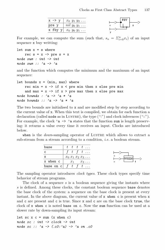
Clocks as First Class Abstract Types 137

x -> y x0 y1 y2 . . .pre y nil y0 y1 . . .x fby y x0 y0 y1 . . .

For example, we can compute the sum (such that, sn = Σni=0xi) of an input

sequence x buy writting:

let sum x = s whererec s = x -> pre s + x

node sum : int -> intnode sum :: ’a -> ’a

and the function which computes the minimum and the maximum of an inputsequence:

let bounds x = (min, max) whererec min = x -> if x < pre min then x else pre minand max = x -> if x > pre max then x else pre max

node bounds : ’a -> ’a * ’anode bounds :: ’a -> ’a * ’a

The two bounds are initialised to x and are modified step by step according tothe current value of x. When this text is compiled, we obtain for each function adeclaration (called node as in Lustre), the type (“:”) and clock inferences (“::”).For example, the clock ’a -> ’a states that the function sum is length preserv-ing: it returns a value every time it receives an input. Clocks are introducedbelow.

when is the down-sampling operator of Lustre which allows to extract asub-stream from a stream according to a condition, i.e. a boolean stream.

base t t t t . . .c f t f t . . .x x0 x1 x2 x3 . . .x when c x1 x3 . . .base on c f t f t . . .

The sampling operator introduces clock types. These clock types specify timebehavior of stream programs.

The clock of a sequence s is a boolean sequence giving the instants wheres is defined. Among these clocks, the constant boolean sequence base denotesthe base clock of the system: a sequence on the base clock is present at everyinstant. In the above diagram, the current value of x when c is present when xand c are present and c is true. Since x and c are on the base clock true, theclock of x when c is noted base on c. Now the sum function can be used at aslower rate by down-sampling its input stream:

let sc x c = sum (x when c)node sc : int -> clock -> intnode sc :: ’a -> ( c0:’a) -> ’a on c0

138 J.-L. Colaco and M. Pouzet

sc has a function clock which follows its type structure. This clock says thatfor any clock ’a, if the first argument x of the function has clock ’a and thesecond argument named _c0 has clock ’a, then the result is on clock ’a on _c0(variables are renamed in the clock type to avoid name conflicts). An expressionon clock ’a on _c0 is present when the clock ’a is true and the boolean stream_c0 is present and true.

Now, the sampled sum can be instanciated with an actual clock. We firstdefine a periodic clock which is true one instant of ten.

(* a sampler that counts modulo n *)let sample n = ok where

rec cpt = 0 -> if pre cpt = n - 1 then 0else pre cpt + 1

and ok = cpt = 0node sample : int -> boolnode sample :: ’a -> ’a

(* defining a periodic 1/10 clock *)let clock ten = sample 10node ten : clocknode ten :: ’a

let sum one over ten x = sc x tennode sum one over ten : int -> intnode sum one over ten :: ’a -> ’a on ten

Thus, sum_one_over_ten x computes the sum of the sub-stream (x10n)n∈IN .Here, boolean streams used to sample a stream have to be first introduced withthe special construction let clock.

Programs must satisfy some clock constraints, as examplified on the follow-ing:

let unbounded x = x + (x when ten)> x + (x when ten)> ˆˆˆˆˆˆˆˆˆˆThis expression has clock ’b on ten, but is used with clock ’b.

which adds the stream x to the sub-sequence of x made by filtering nine itemover ten. Thus, it should compute the sequence (xn + x10n)n∈IN which is clearlynot bounded memory. This is why this program is rejected when dealing withreal-time programming.

merge conversely allows slow processes to communicate with faster ones bymerging sub-streams into “larger” ones:

c f t f t . . .x x0 x1 . . .y y0 y1 . . .merge c x y y0 x0 y1 x1 . . .

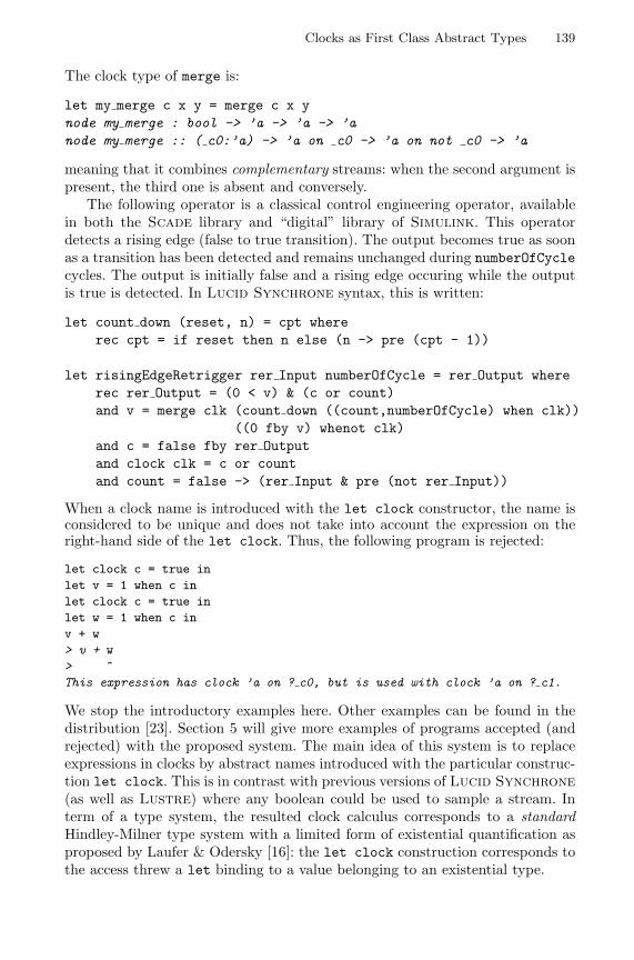
Clocks as First Class Abstract Types 139

The clock type of merge is:

let my merge c x y = merge c x ynode my merge : bool -> ’a -> ’a -> ’anode my merge :: ( c0:’a) -> ’a on c0 -> ’a on not c0 -> ’a

meaning that it combines complementary streams: when the second argument ispresent, the third one is absent and conversely.

The following operator is a classical control engineering operator, availablein both the Scade library and “digital” library of Simulink. This operatordetects a rising edge (false to true transition). The output becomes true as soonas a transition has been detected and remains unchanged during numberOfCyclecycles. The output is initially false and a rising edge occuring while the outputis true is detected. In Lucid Synchrone syntax, this is written:

let count down (reset, n) = cpt whererec cpt = if reset then n else (n -> pre (cpt - 1))

let risingEdgeRetrigger rer Input numberOfCycle = rer Output whererec rer Output = (0 < v) & (c or count)and v = merge clk (count down ((count,numberOfCycle) when clk))

((0 fby v) whenot clk)and c = false fby rer Outputand clock clk = c or countand count = false -> (rer Input & pre (not rer Input))

When a clock name is introduced with the let clock constructor, the name isconsidered to be unique and does not take into account the expression on theright-hand side of the let clock. Thus, the following program is rejected:

let clock c = true inlet v = 1 when c inlet clock c = true inlet w = 1 when c inv + w> v + w> ˆThis expression has clock ’a on ? c0, but is used with clock ’a on ? c1.

We stop the introductory examples here. Other examples can be found in thedistribution [23]. Section 5 will give more examples of programs accepted (andrejected) with the proposed system. The main idea of this system is to replaceexpressions in clocks by abstract names introduced with the particular construc-tion let clock. This is in contrast with previous versions of Lucid Synchrone

(as well as Lustre) where any boolean could be used to sample a stream. Interm of a type system, the resulted clock calculus corresponds to a standardHindley-Milner type system with a limited form of existential quantification asproposed by Laufer & Odersky [16]: the let clock construction corresponds tothe access threw a let binding to a value belonging to an existential type.

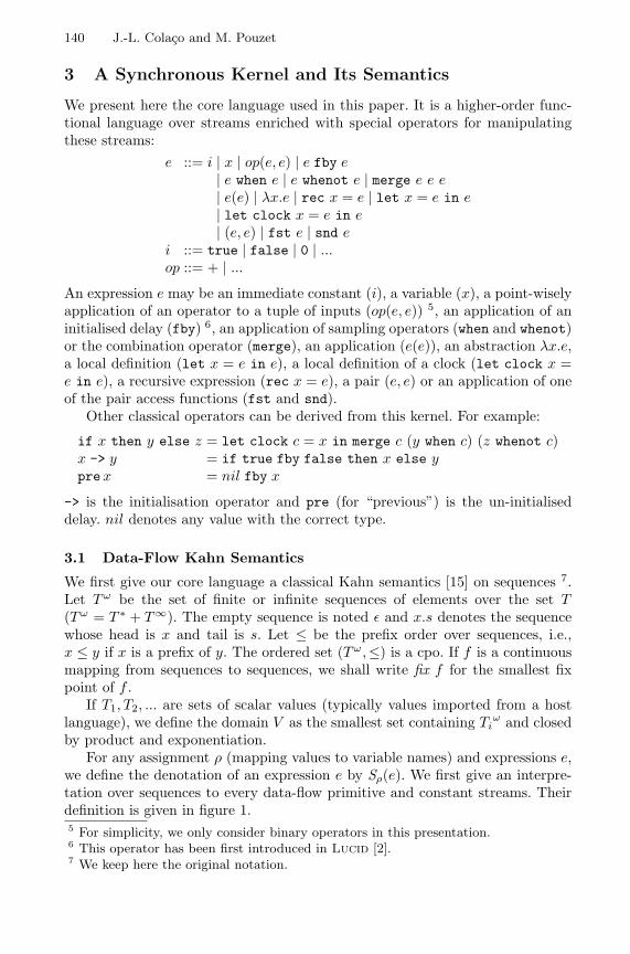
140 J.-L. Colaco and M. Pouzet

3 A Synchronous Kernel and Its Semantics

We present here the core language used in this paper. It is a higher-order func-tional language over streams enriched with special operators for manipulatingthese streams:

e ::= i | x | op(e, e) | e fby e| e when e | e whenot e | merge e e e| e(e) | λx.e | rec x = e | let x = e in e| let clock x = e in e| (e, e) | fst e | snd e

i ::= true | false | 0 | ...op ::= + | ...

An expression e may be an immediate constant (i), a variable (x), a point-wiselyapplication of an operator to a tuple of inputs (op(e, e)) 5, an application of aninitialised delay (fby) 6, an application of sampling operators (when and whenot)or the combination operator (merge), an application (e(e)), an abstraction λx.e,a local definition (let x = e in e), a local definition of a clock (let clock x =e in e), a recursive expression (rec x = e), a pair (e, e) or an application of oneof the pair access functions (fst and snd).

Other classical operators can be derived from this kernel. For example:

if x then y else z = let clock c = x in merge c (y when c) (z whenot c)x -> y = if true fby false then x else yprex = nil fby x

-> is the initialisation operator and pre (for “previous”) is the un-initialiseddelay. nil denotes any value with the correct type.

3.1 Data-Flow Kahn Semantics

We first give our core language a classical Kahn semantics [15] on sequences 7.Let Tω be the set of finite or infinite sequences of elements over the set T(Tω = T ∗ + T∞). The empty sequence is noted ε and x.s denotes the sequencewhose head is x and tail is s. Let ≤ be the prefix order over sequences, i.e.,x ≤ y if x is a prefix of y. The ordered set (Tω,≤) is a cpo. If f is a continuousmapping from sequences to sequences, we shall write fix f for the smallest fixpoint of f .

If T1, T2, ... are sets of scalar values (typically values imported from a hostlanguage), we define the domain V as the smallest set containing Ti

ω and closedby product and exponentiation.

For any assignment ρ (mapping values to variable names) and expressions e,we define the denotation of an expression e by Sρ(e). We first give an interpre-tation over sequences to every data-flow primitive and constant streams. Theirdefinition is given in figure 1.5 For simplicity, we only consider binary operators in this presentation.6 This operator has been first introduced in Lucid [2].7 We keep here the original notation.

Clocks as First Class Abstract Types 141

i# = i.i#

op#(s1, s2) = ε if s1 = ε or s2 = ε

op#(v1.s1, v2.s2) = (v1 op v2).op#(s1, s2)

fby#(ε, ys) = ε

fby#(v.xs, ys) = v.ys

when#(s1, s2) = ε if s1 = ε or s2 = ε

when#(v1.s1, true.s2) = v1.(when#(s1, s2))when#(v1.s1, false.s2) = when#(s1, s2)

merge#(s1, s2, s3) = ε if s1 = ε or s2 = ε or s3 = ε

merge#(true.s1, v2.s2, s3) = v2.merge#(s1, s2, s3)

merge#(false.s1, s2, v3.s3) = v3.merge#(s1, s2, s3)

Fig. 1. Data-flow Kahn semantics

– immediate values (i) are lifted into infinite constant streams.– operations are applied point-wisely to their arguments.– the initialised delay (fby) conses the head of its first input to its second

input.– when and merge are filtering and combination operators overs sequences.

The operation when emits a sub-sequence of its inputs corresponding to theinstants where the condition is true. The operation merge merges two sub-sequences into a sequence: it emits the current value of its second inputswhen the condition is true and the current value of its third input when thecondition is false.

Sρ(op(e1, e2)) = op#(Sρ(e1))(Sρ(e2))Sρ(e1 fby e2) = fby#(Sρ(e1),Sρ(e2))

Sρ(e1 when e2) = when#(Sρ(e1),Sρ(e2))Sρ(e1 whenot e2) = when#(Sρ(e1),Sρ(not e2))

Sρ(merge e1 e2 e3) = merge#(Sρ(e1),Sρ(e2),Sρ(e3))Sρ(x) = ρ(x)Sρ(i) = i#

Sρ(let x = e1 in e2) = Sρ[x←Sρ(e1)](e2)

Sρ(let clock x = e1 in e2) = Sρ[x←Sρ(e1)](e2)

Sρ(λx.e) = λy.Sρ[x←y](e) where y ∈ Dom(ρ)Sρ(e1(e2)) = Sρ(e1)(Sρ(e2))Sρ(e1, e2) = (Sρ(e1),Sρ(e2))Sρ(fst e) = v1 if Sρ(e) = (v1, v2)Sρ(snd e) = v2 if Sρ(e) = (v1, v2)

Sρ(rec x = e) = ρ[x← x∞] where x∞ = fix λy.Sρ[x←y](e)

142 J.-L. Colaco and M. Pouzet

We can easily check that the primitives are continuous for the prefix order. Thedenotational semantics for other constructions is defined as usual (see [24]). Werecall it here shortly.

The semantics gives meaning to any Kahn network. Nonetheless, it is wellknown that simple data-flow networks cannot always be executed in boundedmemory even when they are only composed of bounded memory operators. Thisproblem appears when non length preserving functions (i.e, sampling functions)are considered [8] and has been exemplified in section 2.

3.2 Synchronous Data-Flow Semantics

In order to model synchronous execution, we describe a lower level data-flowsemantics where absence of a stream is made explicit. The set of instantaneousvalues is enrichied with a special value abs representing the absence. The setof finite and infinite sequences of values belonging to T complemented with theabsent value is noted Tω

abs where Tabs = T ∪ abs. That is:

Stream (T ) = T.Stream (T ) + εValue (T ) = abs + TClocked-Stream (T ) = Stream (Value (T ))Clock = Stream (bool)

A clocked stream (element of Clocked-Stream (T )) is made of present or absentvalues. We define the clock of a sequence s as a boolean sequence (without absentvalues) indicating when a value is present:

clock (ε) = εclock (abs.xs) = false.clock (xs)clock (x.xs) = true.clock (xs)

We give a new interpretation to constant streams, to operators applied point-wisely and to synchronous primitives. This interpretation is given in figure 2 andis discussed below:

Constant Streams. This operator becomes polymorphic since it may producea value (or not) according to the environment. For this reason, we add an extraargument giving its clock. Thus, i[s] denotes a constant stream with clock s.

Point-Wise Application. We must decide here what to do, in the case of abinary operator, when only one of the argument is present. Three choices arepossible:

1. store the available value in a state variable implementing a FIFO queue untilthe other input is present;

2. generate a run-time error;3. reject statically this situation.

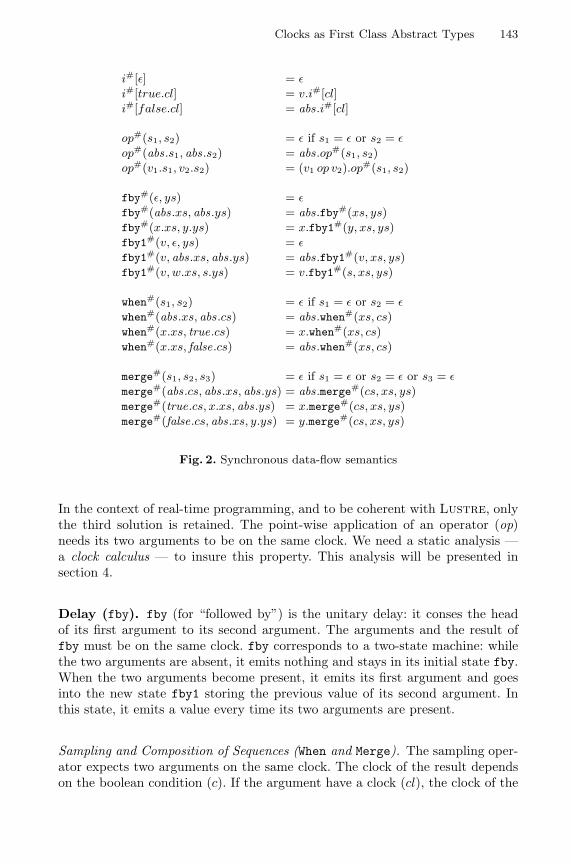
Clocks as First Class Abstract Types 143

i#[ε] = ε

i#[true.cl] = v.i#[cl]i#[false.cl] = abs.i#[cl]

op#(s1, s2) = ε if s1 = ε or s2 = ε

op#(abs.s1, abs.s2) = abs.op#(s1, s2)op#(v1.s1, v2.s2) = (v1 op v2).op#(s1, s2)

fby#(ε, ys) = ε

fby#(abs.xs, abs.ys) = abs.fby#(xs, ys)fby#(x.xs, y.ys) = x.fby1#(y, xs, ys)fby1#(v, ε, ys) = ε

fby1#(v, abs.xs, abs.ys) = abs.fby1#(v, xs, ys)fby1#(v, w.xs, s.ys) = v.fby1#(s, xs, ys)

when#(s1, s2) = ε if s1 = ε or s2 = ε

when#(abs.xs, abs.cs) = abs.when#(xs, cs)when#(x.xs, true.cs) = x.when#(xs, cs)when#(x.xs, false.cs) = abs.when#(xs, cs)

merge#(s1, s2, s3) = ε if s1 = ε or s2 = ε or s3 = ε

merge#(abs.cs, abs.xs, abs.ys) = abs.merge#(cs, xs, ys)merge#(true.cs, x.xs, abs.ys) = x.merge#(cs, xs, ys)merge#(false.cs, abs.xs, y.ys) = y.merge#(cs, xs, ys)

Fig. 2. Synchronous data-flow semantics

In the context of real-time programming, and to be coherent with Lustre, onlythe third solution is retained. The point-wise application of an operator (op)needs its two arguments to be on the same clock. We need a static analysis —a clock calculus — to insure this property. This analysis will be presented insection 4.

Delay (fby). fby (for “followed by”) is the unitary delay: it conses the headof its first argument to its second argument. The arguments and the result offby must be on the same clock. fby corresponds to a two-state machine: whilethe two arguments are absent, it emits nothing and stays in its initial state fby.When the two arguments become present, it emits its first argument and goesinto the new state fby1 storing the previous value of its second argument. Inthis state, it emits a value every time its two arguments are present.

Sampling and Composition of Sequences (When and Merge). The sampling oper-ator expects two arguments on the same clock. The clock of the result dependson the boolean condition (c). If the argument have a clock (cl), the clock of the

144 J.-L. Colaco and M. Pouzet

result is (cl on c) such that:

on#(true.cl, true.cs) = true.on#(cl, cs)on#(true.cl, false.cs) = false.on#(cl, cs)on#(false.cl, abs.cs) = false.on#(cl, cs)on#(cl, c) = ε if cl = ε or c = ε

We can notice that the clock is a simple sequence without absent values. Thedefinition of merge states that one branch must be present when the other isabsent.

Since this semantics is a partial semantics, we shall introduce clock con-straints to reject programs which cannot be executed synchronously. This se-mantics has been described in the proof assistant Coq [6]. The use of an explicitabsent value is part of the semantics of Signal [21]. Nonetheless, Signal can-not receive a Kahn semantics (functional and without absence) whereas in thecase of Lustre and Lucid Synchrone, the use of absence is only done forcharacterising networks which can be executed synchronously.

4 Clock Calculus

We present now the clock calculus as a type system. The goal of the clock calculusis to produce jugments of the form H e : cl meaning that “the expression ehas clock cl in the environment H”.

σ ::= ∀β1, ..., βn.∀α1, ..., αm.∀X1, ..., Xk.cl n, m, k ∈ INcl ::= cl→ cl | cl × cl | β | s | (c : s)s ::= base | s on c | s on not c | αc ::= X | n

H ::= [x1 : σ1, ..., xn : σn]

Clock types are decomposed into two categories, clock schemes (σ) and clocks(cl). Clock schemes are regular clocks quantified over clock type variables (β),stream clock type variables (α) and carrier variables (X). Regular clocks (cl)may be functional (cl → cl), products (cl × cl), variables (β), stream clocks (s)and dependences (c : s). A stream clock may be the base clock (base), a sampledclock (s on c or s on not c) or a stream clock variable (α). A carrier (c) can beeither a name (n) or a carrier variable (X).

We define the set of free variables FV (cl) of a clock cl composed of free clockvariables (β), free stream clock variables (α) and free carrier variables (X). Weextend it to clock schemes and environments. Dom(H) is the domain of H. N (cl)returns the set of abstract names from cl. Their definitions are classical and notgiven in the paper.

Programs are clocked in an initial environment H0 giving clocks to syn-chronous primitives. To make the clock calculus shorter, a synchronous expres-sion like e1 fby e2 is treated as a regular application of a synchronous primitive

Clocks as First Class Abstract Types 145

to expressions and is clocked as if it were written (fby (e1)) e2.

H0 = [fby : ∀α.α→ α→ αwhen : ∀α.∀X.α→ (X : α)→ α on Xwhenot : ∀α.∀X.α→ (X : α)→ α on not Xmerge : ∀α.∀X.(X : α)→ α on X → α on not X → αfst : ∀β1, β2.β1 × β2 → β1,snd : ∀β1, β2.β1 × β2 → β2]

The first entry in this initial environment states that the clock of x fby y is theone of x and y. A boolean expression e with clock (c : s) states that e is presentwhen s is true and has the abstract value c. Thus, an expression e1 when e2 iswell clocked if the two inputs are synchronous on the clock α. In that case, theclock of the result is a subclock α on X of α where X stands for the value of e2.An expression merge e e1 e2 is well clocked and on clock α if e is on clock α andis equal to some X, e1 is on clock α on X and e2 on clock α on not X.

Clocks may be instanciated and generalised in the following way:

inst(∀β.α.X.cl′) = cl′[cl/β][s/α][c/X]

genH(cl) = ∀β1, ..., βn.∀α1, ..., αm.∀X1, ..., Xk.clwhere β1, ..., βn, α1, ..., αm, X1, ..., Xk = FV (cl)\FV (H)

It states that a clock scheme can be instanciated by replacing clock variables byclocks, stream clock variables by stream clocks and carrier variables by carriers.Moreover, any variable can be generalized as soon as it does not appear free inthe environment. The clocking rules are now given in figure 3.

– a constant stream may have any clock (rule (IM))– the inputs of imported primitives must all be on the same clock (rule (OP))– the rules for variables (INST), functions (FUN), applications (APP), local defi-

nitions (LET) and products (PAIR) are the classical typing rules of ML.– a clock definition clock x = e defines a new clock name n which has the

clock type s. In doing this, n must be a fresh name, that is, it must notappear free in the environment nor in the returned clock cl2. It states thatif x evaluates to some value n and is on clock s, then the clock of e2 is cl2.The symbol n is an abstraction of the actual value of e1 and is consideredto be unique.

The clocking rule for the let clock construction is a particular case of thetyping rule for let in the Laufer & Odersky type system. Here, the abstractname n corresponds to the introduction of a fresh skolem name.

4.1 Correctness Theorem and the Use of Clocks

The clock calculus is used for giving a synchronous data-flow semantics to pro-grams and to establish a correctness property: well clocked programs can be ex-ecuted synchronously in the synchrounous data-flow semantics without raising

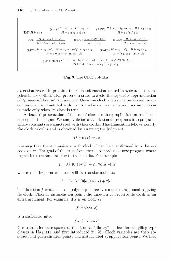
146 J.-L. Colaco and M. Pouzet

(IM) H i : s

H e1 : s H e2 : s(OP)H op(e1, e2) : s

H e1 : cl2 → cl1 H e2 : cl2(APP)H e1 (e2) : cl1

H, x : cl1 e : cl2(FUN)H λx.e : cl1 → cl2

cl = inst(H(x))(INST)H x : cl

H, x : s e : s(REC)H rec x = e : s

H e1 : cl1 H, x : genH(cl1) e2 : cl2(LET)H let x = e1 in e2 : cl2

H e1 : cl1 H e2 : cl2(PAIR)H (e1, e2) : cl1 × cl2

H e1 : s H, x : (n : s) e2 : cl2 n ∈ N (H, cl2)(LET-clock)H let clock x = e1 in e2 : cl2

Fig. 3. The Clock Calculus

execution errors. In practice, the clock information is used in synchronous com-pilers in the optimization process in order to avoid the expensive representationof “presence/absense” at run-time. Once the clock analysis is performed, everycomputation is annotated with its clock which serves as a guard: a computationis made only when its clock is true.

A detailed presentation of the use of clocks in the compilation process is outof scope of this paper. We simply define a translation of programs into programswhere constants are annotated with their clocks. This translation follows exactlythe clock calculus and is obtained by asserting the judgment:

H e : cl⇒ ce

meaning that the expression e with clock cl can be transformed into the ex-pression ce. The goal of this transformation is to produce a new program whereexpressions are annotated with their clocks. For example:

f = λx.(0 fby x) + 2 : ∀α.α→ α

where + is the point-wise sum will be transformed into:

f = λα.λx.(0[α] fby x) + 2[α]

The function f whose clock is polymorphic receives an extra argument α givingits clock. Then at instanciation point, the function will receive its clock as anextra argument. For example, if x is on clock s1:

f (x when c)

is transformed into:f s1 (x when c)

Our translation corresponds to the classical “library” method for compiling typeclasses in Haskell and first introduced in [26]. Clock variables are then ab-stracted at generalisation points and instanciated at application points. We first

Clocks as First Class Abstract Types 147

Fig. 4. Transforming streams into clocked-streams

introduce two auxiliary functions:

gencodeH(cl, ce) = λα1, ..., αm.X1, ..., Xk.cewhere β1, ..., βn, α1, ..., αm, X1, ..., Xk = FV (cl)\FV (H)

instcodecl(x) = xinstcode∀β.α.X.cl′(x) = x s1...sn.c1...ckwhere inst(∀β.α.X.cl′) = cl′[cl/β][s/α][c/X]

The predicate is defined in figure 4.

– immediate constants receive an extra argument giving their clock.– rules for abstractions (FUN), applications (APP), recursions (REC), products

(PAIR) are simple morphisms.– clocks are passed at instantiation points (rule (INST)) and abstracted at gen-

eralization points (rule (LET)). Here, only stream clock variables (s) or carriervariables (X) from the scheme clock are used since only they may appear inthe sampling of a stream value.

– for clock definitions (rule (LET-clock)), the name n is introduced in the gen-erated code since it may appear in some computation of a clock.

We then prove that this transformation will not provide programs produc-ing incomplete pattern failure. For this purpose, we define a valuation V fromvariables to boolean streams and lift it to clocks such that:

V(base) = trueV(s on c) = on#(V(s),V(c))V(s on not c) = on#(V(s), not#(V(c)))

148 J.-L. Colaco and M. Pouzet

We define interpretation functions I.(.) relating clock schemes and set of values.An interpretation is such that:

v ∈ IV(s) iff clock (v) ≤ V(s) where ≤ stands for the prefix orderv ∈ IV((c : s)) iff v ∈ IV(s) and v = V(c)v ∈ IV(cl1 → cl2) iff for all v1 such that v1 ∈ IV(cl1), v(v1) ∈ IV(cl2)(v1, v2) ∈ IV(cl1 × cl2) iff v1 ∈ IV(cl1) and v2 ∈ IV(cl2)v ∈ IV(∀β1, ..., βk.σ) iff for all cl1, ..., clk, v ∈ IV(σ[cl1/β1, ..., clk/βk])v ∈ IV(∀α1, ..., αn.X1, ..., Xk.σ) iff for all s1, ..., sn, c1, ..., ck,

v (Vs1), ..., (Vsn) (Vc1), ..., (Vck) ∈IV(cl[s1/α1, ..., sn/αn, c1/X1, ..., ck/Xk])

Theorem 1 (Clock Soundness). If [x1 : σ1, ..., xn : σn] e : cl⇒ ce then forall valuation V., for all interpretation function I.(.), for all v1, ..., vn such thatv1 ∈ IV(σ1), ..., vn ∈ IV(σn), we have SV[v1/x1,...,vn/xn](ce) ∈ IV(cl).

The proof is given in appendix A.

The clock calculus presented in this paper is implemented in the Lucid Syn-

chrone compiler and is in used for more than one year. Classical implementationtechniques for ML type systems have been used (e.g, destructive unification). Thetechnique for checking that the introduced name in the rule (LET-clock) is a freshname and does not escape its scope is due to Pottier [19] and is used for theefficient implementation of the Laufer & Odersky system.

Practical experiments show that the clock calculus is as fast as the typeinference which means that it can be applied to real-size examples.

5 Examples

We illustrate the expressivity of this calculus on some typical examples. A Lucid

Synchrone program is a sequence of global declarations. A global declarationdefines a name which can be used after its declaration. Every global declarationis analysed sequentially and compiled.

5.1 Activation Conditions

A classical primitive in a block diagram framework (such as the one of Scade)is the activation condition (also known as enable sub-system in Simulink). Itconsists of executing a node only when a condition is true. In term of clocks,it corresponds to filtering the input of that node on a certain clock clk and toproject the result on the base clock. Such an operation is a higher-order constructand can be defined like the following:

let condact clk f input init =let rec u = merge clk (f (input when clk))

((init fby u) whenot clk) inu

node condact : clock -> (’a -> ’b) -> ’a -> ’b -> ’bnode condact :: (clk:’a) -> (’a on clk -> ’a on clk) -> ’a -> ’a -> ’a

Clocks as First Class Abstract Types 149

Fig. 5. Scade notation for activation condition.

Its graphical representation in Scade is given in figure 5. Using the condactprimitive, we can rewrite the rising edge retrigger as it is written in the Scade

library.

let risingEdgeRetrigger rer Input numberOfCycle = rer Output whererec rer Output = (0 < v) & (c or count)and v = condact clk count down (count,numberOfCycle) 0and c = false fby rer Outputand clock clk = c or countand count = false -> (rer Input & pre (not rer Input))

Its graphical representation is given in figure 6.

Fig. 6. The risingEdgeRetrigger in Scade

5.2 Iteration

The symetric operation of the activation condition is an iterator. It correspondsto the writting of an internal for or while loop. This operator consists in iter-ating a function on an input.

let iter clk init f input =let rec o = f iand i = merge clk input ((init fby o) whenot clk) ino when clk

node iter :: (clk:’a) -> ’a -> (’a -> ’a) -> ’a on clk -> ’a on clk

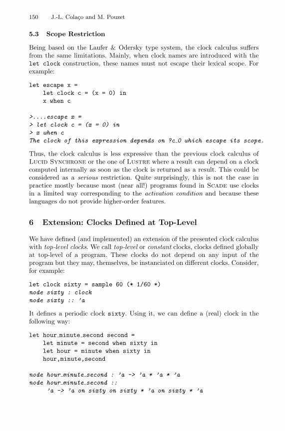
150 J.-L. Colaco and M. Pouzet

5.3 Scope Restriction

Being based on the Laufer & Odersky type system, the clock calculus suffersfrom the same limitations. Mainly, when clock names are introduced with thelet clock construction, these names must not escape their lexical scope. Forexample:

let escape x =let clock c = (x = 0) inx when c

>....escape x => let clock c = (x = 0) in> x when cThe clock of this expression depends on ?c 0 which escape its scope.

Thus, the clock calculus is less expressive than the previous clock calculus ofLucid Synchrone or the one of Lustre where a result can depend on a clockcomputed internally as soon as the clock is returned as a result. This could beconsidered as a serious restriction. Quite surprisingly, this is not the case inpractice mostly because most (near all!) programs found in Scade use clocksin a limited way corresponding to the activation condition and because theselanguages do not provide higher-order features.

6 Extension: Clocks Defined at Top-Level

We have defined (and implemented) an extension of the presented clock calculuswith top-level clocks. We call top-level or constant clocks, clocks defined globallyat top-level of a program. These clocks do not depend on any input of theprogram but they may, themselves, be instanciated on different clocks. Consider,for example:

let clock sixty = sample 60 (* 1/60 *)node sixty : clocknode sixty :: ’a

It defines a periodic clock sixty. Using it, we can define a (real) clock in thefollowing way:

let hour minute second second =let minute = second when sixty inlet hour = minute when sixty inhour,minute,second

node hour minute second : ’a -> ’a * ’a * ’anode hour minute second ::

’a -> ’a on sixty on sixty * ’a on sixty * ’a

Clocks as First Class Abstract Types 151

A stream on clock ’a on sixty on sixty is only present one instant over 3600instants which match perfectly what we are expecting.

Using clocks defined globally, we can write simple over-sampling functions.Consider, for example, the computation of the sequence (on)n∈IN such that:

o2n = xn

o2n+1 = xn

It can be programmed in the following way:

let clock half = h whererec h = true -> not (pre h)

let stuttering x = o whererec o = merge half x (0 -> (pre o) whenot half)

node stuttering :: ’a on half -> ’a

This is a true example of oversampling, that is, a function whose internal clockis faster than the clock of its input. This example shows that some limited formof oversampling — which is possible in Signal and not in Lustre — can beachieved with simple typing techniques.

It appears that top-level clocks are sufficient to express many programs ap-pearing in the Scade environment. In particular, many clocks are periodic 8.Periodic (constant) clocks are useful for specifying hard real-time constraintsfrom the environment and to direct the scheduling strategy of the compiler [9].It is an open question to know whether constant clocks — which only need avery modest, dependent-less type system — are sufficient for this purpose.

In term of type system, these constant clocks defined at top-level do not raiseany technical difficulty. Clock names defined at top-level are constant names andact as new type constructors with arity zero defined in ML languages. Then, asit is the case for clock names defined locally, two clocks are equal if they havethe same name.

7 Related Works

Lucid Synchrone has been originally developed as a functional extension ofLustre and to serve as an experimental language for prototyping extensions forit. It is based on the same semantic model and clocks are largely reminiscentof the ones in Lustre. Up to syntactic details, the clock calculus presented inthis paper can be applied directly to Lustre programs. Nonetheless, the clockcalculus is expressed here as a typing problem: this allows clocks to be automat-ically inferred using standard techniques and is compatible with higher-order.In comparison, Lustre is first-order and clocks are verified instead of being in-ferred. Clock inference is mandatory in a graphical programming environmentsuch as the one of Scade (the clock of intermediate wires must be computed8 Typically, an application is made of several main behaviors, each of them being

executed at different periodic (constant) clocks, e.g., corresponding to 60hz, 200hz.

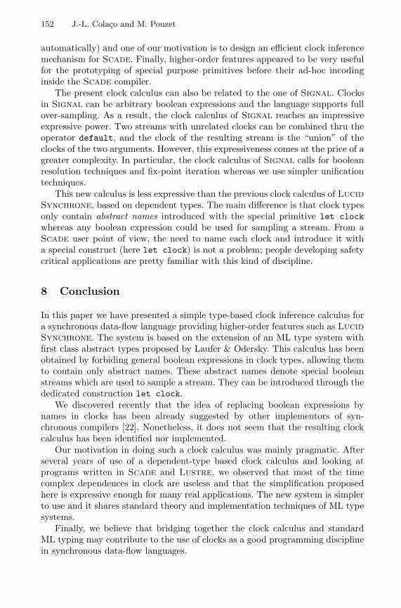
152 J.-L. Colaco and M. Pouzet

automatically) and one of our motivation is to design an efficient clock inferencemechanism for Scade. Finally, higher-order features appeared to be very usefulfor the prototyping of special purpose primitives before their ad-hoc incodinginside the Scade compiler.

The present clock calculus can also be related to the one of Signal. Clocksin Signal can be arbitrary boolean expressions and the language supports fullover-sampling. As a result, the clock calculus of Signal reaches an impressiveexpressive power. Two streams with unrelated clocks can be combined thru theoperator default, and the clock of the resulting stream is the “union” of theclocks of the two arguments. However, this expressiveness comes at the price of agreater complexity. In particular, the clock calculus of Signal calls for booleanresolution techniques and fix-point iteration whereas we use simpler unificationtechniques.

This new calculus is less expressive than the previous clock calculus of Lucid

Synchrone, based on dependent types. The main difference is that clock typesonly contain abstract names introduced with the special primitive let clockwhereas any boolean expression could be used for sampling a stream. From aScade user point of view, the need to name each clock and introduce it witha special construct (here let clock) is not a problem; people developing safetycritical applications are pretty familiar with this kind of discipline.

8 Conclusion

In this paper we have presented a simple type-based clock inference calculus fora synchronous data-flow language providing higher-order features such as Lucid

Synchrone. The system is based on the extension of an ML type system withfirst class abstract types proposed by Laufer & Odersky. This calculus has beenobtained by forbiding general boolean expressions in clock types, allowing themto contain only abstract names. These abstract names denote special booleanstreams which are used to sample a stream. They can be introduced through thededicated construction let clock.

We discovered recently that the idea of replacing boolean expressions bynames in clocks has been already suggested by other implementors of syn-chronous compilers [22]. Nonetheless, it does not seem that the resulting clockcalculus has been identified nor implemented.

Our motivation in doing such a clock calculus was mainly pragmatic. Afterseveral years of use of a dependent-type based clock calculus and looking atprograms written in Scade and Lustre, we observed that most of the timecomplex dependences in clock are useless and that the simplification proposedhere is expressive enough for many real applications. The new system is simplerto use and it shares standard theory and implementation techniques of ML typesystems.

Finally, we believe that bridging together the clock calculus and standardML typing may contribute to the use of clocks as a good programming disciplinein synchronous data-flow languages.

Clocks as First Class Abstract Types 153

References

1. Charles Andre. Representation and Analysis of Reactive Behaviors: A Syn-chronous Approach. In CESA, Lille, july 1996. IEEE-SMC. Available at:www-mips.unice.fr/∼andre/synccharts.html.

2. E. A. Ashcroft and W. W. Wadge. Lucid, the data-flow programming language.Academic Press, 1985.

3. A. Benveniste, P. LeGuernic, and Ch. Jacquemot. Synchronous programming withevents and relations: the SIGNAL language and its semantics. Science of ComputerProgramming, 16:103–149, 1991.

4. G. Berry. Real time programming: Special purpose or general purpose languages.Information Processing, 89:11–17, 1989.

5. G. Berry and G. Gonthier. The Esterel synchronous programming language, de-sign, semantics, implementation. Science of Computer Programming, 19(2):87–152,1992.

6. Sylvain Boulme and Gregoire Hamon. Certifying Synchrony for free. In Interna-tional Conference on Logic for Programming, Artificial Intelligence and Reasoning(LPAR), volume 2250, La Havana, Cuba, December 2001. Lecture Notes in Ar-tificial Intelligence, Springer-Verlag. Short version of A clocked denotational se-mantics for Lucid-Synchrone in Coq, available as a Technical Report (LIP6), athttp://www-spi.lip6.fr/lucid-synchrone.

7. J. Buck, S. Ha, E. Lee, and D. Messerschmitt. Ptolemy: A framework for simu-lating and prototyping heterogeneous systems. International Journal of computerSimulation, 1994. special issue on Simulation Software Development.

8. P. Caspi. Clocks in dataflow languages. Theoretical Computer Science, 94:125–140,1992.

9. P. Caspi, A. Curic, A. Maignan, C. Sofronis, S. Tripakis, P. Niebert From Simulinkto SCADE/Lustre to TTA: a layered approach for distributed embedded applica-tions. LCTES’03.

10. Paul Caspi and Marc Pouzet. Synchronous Kahn Networks. In ACM SIGPLANInternational Conference on Functional Programming, Philadelphia, Pensylvania,May 1996.

11. Paul Caspi and Marc Pouzet. Lucid Synchrone, a functional extension of Lustre.submitted to publication, 2001.

12. Jean-Louis Colaco and Marc Pouzet. Type-based Initialization of a SynchronousData-flow Language. In Synchronous Languages, Applications, and Programming,volume 65. Electronic Notes in Theoretical Computer Science, 2002.

13. The coq proof assistant, 2002. http://coq.inria.fr.14. N. Halbwachs, P. Caspi, P. Raymond, and D. Pilaud. The synchronous dataflow

programming language lustre. Proceedings of the IEEE, 79(9):1305–1320,September 1991.

15. G. Kahn. The semantics of a simple language for parallel programming. In IFIP74 Congress. North Holland, Amsterdam, 1974.

16. Konstantin Laufer and Martin Odersky. An extension of ML with first-class ab-stract types. In ACM SIGPLAN Workshop on ML and its Applications, SanFrancisco, California, pages 78–91, June 1992.

17. Xavier Leroy. The Objective Caml system release 3.06. Documentation and user’smanual. Technical report, INRIA, 2002.

18. Florence Maraninchi and Yann Remond. Argos: an automaton-based synchronouslanguage. Computer Languages, (27):61–92, 2001.

154 J.-L. Colaco and M. Pouzet

19. Michel Mauny and Francois Pottier. An implementation of Caml Light with exis-tential types. Technical Report 2183, INRIA, October 1993.

20. R. Milner. A theory of type polymorphism in programming. Journal of Computerand System Science, 17:348–375, 1978.

21. D. Nowak, J. R. Beauvais, and J. P. Talpin. Co-inductive axiomatisation of syn-chronous language. In International Conference on Theorem Proving in Higher-Order Logics (TPHOLs’98). Springer Verlag, October 1998.

22. Lecheck Olendersky. Private communication, December 2002. Workshop Synchron,Toulon, France.

23. Marc Pouzet. Lucid Synchrone, version 2. Tutorial and reference manual.Universite Pierre et Marie Curie, LIP6, Mai 2001. Distribution available at:www-spi.lip6.fr/lucid-synchrone.

24. John C. Reynolds. Theories of Programming Languages. Cambridge UniversityPress, 1998.

25. SCADE. http://www.esterel-technologies.com/scade/.26. P. Wadler and S. Blott. How to make ad-hoc polymorphism less ad-hoc. In Con-

ference Record of the 16th Annual ACM Symposium on Principles of ProgrammingLanguages, pages 60–76. ACM, January 1989.

A Proof of Theorem 1 (Clock Soundness)

The property is proved by induction on the structure of expressions.

Case e′ = i. We have i : s⇒ i[s]. By definition, clock (SV(i[s])) = V(s).

Case e′ = x. We have H, x : σ x : cl ⇒ instcodeH(x). There are several cases.Either σ = cl or some variables are universally quantified.

– If σ = cl then H, x : cl x : cl⇒ x and the property holds by definition.– Let σ = ∀β1, ..., βn.α1, ..., αm.X1, ..., Xk.cl. Let H = [σ1/x1, ..., σp/xp, σ/x]

be the typing environment and [v1/x1, ..., vp/xp, v/x] the correspondingenvironment for the evaluation. Let ρ = V[v1/x1, ..., vp/xp, v/x].

Let v such that v ∈ IV(∀β1, ..., βn.α1, ..., αm.X1, ..., Xk.cl). Accordingto the definition of I.(.), for all cl1, ..., cln, s1, ..., sm, c1, ..., ck, we havev (Vs1)...(Vsn).(Vc1)...(Vck) ∈ IV(cl[cl1/β1, ..., cln/βn][s1/α1, ..., sm/αm][c1/X1, ..., ck/Xk]).The property holds since:v (Vs1)...(Vsn).(Vc1)...(Vck) = (Sρ(x s1...sn.c1...ck)) = Sρ(instcodeH(x)).

Case of Primitives. Direct recurrence.

Case e′ = e1(e2). Let H be the typing environment and ρ, the correspond-ing evaluation environment. Suppose the property holds for e1 and e2, that isSV(ce1) ∈ IV(cl1 → cl2) and SV (ce2) ∈ IV(cl1). According to the definition ofthe interpretation I.(.), for any v ∈ IV(cl1) we have (SV(ce1))(v) ∈ IV(cl2).Thus, (SV(ce1))(SV(ce2)) = SV(ce1(ce2)) ∈ IV(cl2). Thus the property holds.

Clocks as First Class Abstract Types 155

Case e′ = λy.e. Let H be the typing environment and ρ, the correspondingevaluation environment. Suppose that H, y : cly e : cl ⇒ ce. Applying the re-currence hypothesis, for all ρ corresponding to H and for all vy ∈ IV(cly) we haveSV[vy/y](ce) ∈ IV(cl). Thus, for all vy ∈ IV(cly), we have SV[vy/y]((λy.ce) y) ∈IV(cl). Thus, for all vy ∈ IV(cly), we have (SV(λy.ce))(vy) ∈ IV(cl). Thus theproperty holds.

Case of e′ = let y = e1 in e2. Direct recurrence and combination of the pre-ceding rules.

Case of Clock Declarations e = let clock x = e1 in e2. Suppose that theproperty holds for H e1 : s1 ⇒ ce1, that is, for all V and [v1/x1, ..., vn/xn]such that v1 ∈ IV(σ1), ..., vn ∈ IV(σn), SV[v1/x1,...,vn/xn](ce1) ∈ IV(s1). Let n bea fresh name n ∈ N (H). Let V ′ be an extension of V such that V ′(z) = V(z) ifz = n. Then for all V ′ extending V, for all v1 ∈ IV′(σ1), ..., vn ∈ IV′(σn) we haveSV′[v1/x1,...,vn/xn](ce1) ∈ IV′(s1).

Suppose that the property holds for H, x : (n : s1) e2 : cl2 ⇒ ce2 wheren ∈ N (H) and n ∈ N (cl2), that is for all V ′, for all v1 ∈ IV′(σ1), ..., vn ∈IV′(σn), vx ∈ IV′((n : s1)), we have SV′[v1/x1,...,vn/xn,vx/x](ce2) ∈ IV′(cl2).vx ∈ IV′((n : s1)) means that vx ∈ IV′(s1) and V ′(n) = vx. Since n is afresh name, this means that for all z V ′(z) = V(z) is z = n and V ′n = vx

otherwise, that SV′[v1/x1,...,vn/xn,vx/x](ce2) = SV[v1/x1,...,vn/xn,vx/x,vx/n](ce2) andfinally, that IV′(cl2) = IV(cl2). Thus, SV[v1/x1,...,vn/xn,vx/x,vx/n](ce2) ∈ IV(cl2),that is SV[v1/x1,...,vn/xn](let x = ce1 in let n = x in ce2) ∈ IV(cl2) which isthe expected result.

Case of Recursions e′ = (rec x = e). Let f : y → SV[y/x](ce). We have ε ∈ IV(s).For all v1 ∈ IV(σ1), ..., vn ∈ IV(σn), v ∈ IV(s), SV[v/x](ce) ∈ IV(s), that isf(v) ∈ IV(s). Thus, for all n, fn(ε) ∈ IV(s). For all n, fn(ε) ≤ limn→∞(fn(ε)).limn→∞(fn(ε)) ∈ IV(s), means that clock (limn→∞(fn(ε))) ≤ V(s). Thus, thereexists a k such that fk(ε) ≤ V(s) which is contradictory. Thus, we get theexpected result.

Energy-Conscious Memory Allocation and Deallocationfor Pointer-Intensive Applications

Victor De La Luz1, Mahmut Kandemir1, Guangyu Chen1, and Ibrahim Kolcu2

1 Department of Computer Science and EngineeringThe Pennsylvania State UniversityUniversity Park, PA 16802, USA

delaluzp,kandemir,gchen@cse.psu.edu2 Computation Department

UMISTManchester M60 1QD, UKikolcu@co.umist.ac.uk

Abstract. A multi-bank memory architecture is composed of multiple memorybanks, each of which can be energy-managed independently. In this paper, wepresent a set of strategies for reducing energy consumption in a multi-bank mem-ory architecture using energy-conscious dynamic memory allocation/deallocation.Applications that make dynamic memory allocations are used very frequently inmobile computing/networking area. Our strategies focus on such applications andtry to cluster dynamically created data with temporal affinity in the physical ad-dress space such that the data occupy a small number of memory banks. Theremaining banks can be shut off, saving energy. All of our strategies have beenimplemented and tested using an in-house energy simulator and an applicationsuite that consists of nine pointer-intensive real-life applications. Our results showthat all the strategies considered in this paper save energy (e.g., our user-initiatedstrategy saves 49% leakage energy on the average). The results also indicate thatthe best savings are obtained when energy-aware memory allocation/deallocationis combined with automatic data migration.

1 IntroductionIn many embedded/portable systems, memory subsystem is a major energy consumer.For example, recent studies (e.g., [1,26]) indicate that main memory consumes nearly90% of overall system energy excluding I/O units. In particular, in mobile/embeddedenvironments where energy is at premium, memory energy consumption can be a realproblem. Consequently, software optimizations that reduce energy consumption in mem-ory during the execution of a mobile application can be very useful in practice. One wayof reducing energy consumption in memory subsystem is to employ a multi-bank mem-ory architecture. In a multi-bank memory architecture, the memory is divided into banksand each bank can be power-managed independently. Chen et al. [3] discuss that up to70% savings in overall leakage energy consumption are possible if unused SRAM banksare turned off by the garbage collector in a Java-based environment. While dynamic(switching) energy is consumed only when the bank is accessed, the leakage energy isconsumed as long as the bank is powered on (active), even if it is not used by the current

R. Alur and I. Lee (Eds.): EMSOFT 2003, LNCS 2855, pp. 156–172, 2003.c© Springer-Verlag Berlin Heidelberg 2003

Energy-Conscious Memory Allocation 157

computation. Optimizing leakage energy consumption is particularly important as thecurrent trends [2,22,18,17,21,12] indicate that it will form a large portion of overallenergy consumption in upcoming process technologies.

In this paper, we present a set of strategies for reducing leakage energy consump-tion in a multi-bank memory architecture. Our strategies focus on applications (mainlypointer-based codes) that make frequent dynamic memory allocations (using malloc()or similar routines) and deallocations (using free() or similar routines). Such applica-tions are very frequently used in mobile environments and networking area (e.g., see [7,24,13] and the references therein). The optimization algorithms proposed in this papercluster dynamically-created data with temporal affinity in the physical address spacesuch that the data occupy a small number of memory banks. The remaining banks can beshut off, saving leakage energy. We investigate this issue at several levels. First, we studya user-initiated energy-saving scheme where the user indicates (by using a modified formof conventional malloc()) which data objects are related (i.e., exhibit temporal affin-ity). Based on this, our strategy clusters these objects (i.e., the corresponding pages inthe physical address space) to minimize the number of banks active (powered on) at anygiven time. Our experience with this implementation indicates that it requires minimalchange to the program source and is very effective in practice. Second, we explore auser-transparent scheme where dynamically-created data are clustered automatically.An important advantage of this scheme is that it requires no change to the program athand; only the implementations of malloc() and free() need to be modified. Ourcompiler analyzes the code and replaces the original memory allocation calls with theirenergy-aware counterparts. Our energy-conscious memory allocation strategies work inconjunction with a memory-aware deallocation (a modified form of the free() utility).Finally, we investigate the support for automatic (user-transparent) data migration forsaving energy. All our strategies have been implemented and tested using an in-houseenergy simulator and an application suite that consists of nine pointer-intensive real-life applications. Our experimental results show that all the strategies considered in thispaper save leakage energy. They also indicate that the best savings are obtained whenmemory allocation/deallocation is used in conjunction with automatic data migration.

2 Architecture and Background

2.1 ArchitectureIntegrated circuit technology continues to advance at an unrelenting pace. With theadvent of 0.18 micron and finer process technologies, it is now possible to pack an entireelectronic system onto a small set of chips. In this paper, we focus on an architecture withmultiple SRAM banks (as main memory) and investigate necessary software support toreduce memory energy consumption. SRAMs (static RAMs) are popular main memorybuilding blocks in some embedded/mobile environments [1]. In our multi-bank memoryarchitecture, each memory bank can be powered on and off independently using a sleepsignal (per bank) issued by the memory controller. In particular, unused memory bankscan be turned off to save energy. The sleep signals can be activated/deactivated by settingappropriate bits in a register in the memory controller. Apart from the banked memoryarchitecture, our architecture also has a CPU core, a data cache, an instruction cache,

158 V. De La Luz et al.

a hardware accelerator (e.g., a co-processor), and a custom logic (ASIC). The last twocomponents are optional and not considered in this work.

It should be made clear that, in our work, memory banking is exclusively usedfor improving energy consumption. This is an entirely different strategy than memoryinterleaving where banking is used to increase memory-level parallelism. In memory-interleaving, the main objective is to keep as many banks active at the same time aspossible (to maximize parallelism). This is exactly the opposite of our goal, which is tolimit the number of accesses to small set of banks (at a given time period) so that we cansave energy by placing the unused banks into a power-saving mode.

2.2 malloc() and free()

In pointer-intensive mobile applications, dynamic memory space (heap) is manipulatedusing memory allocation (malloc()) and deallocation (free()) calls. Since these callsmanipulate memory space, their implementation can be modified to make better use ofthe banked nature of the memory architecture from the energy viewpoint. Therefore, wefirst discuss the functionalities of malloc() and free().

In a virtual memory based system, operating system (OS) governs the virtual-to-physical address mapping. If a requested physical page is not in memory, a page faultis generated and subsequently processed by the page fault handler [23]. In this subsec-tion, we present a brief overview of malloc() and free() implementations in currentsystems. The malloc() and free() routines provide a memory allocation/deallocationpackage. The malloc() function allocates uninitialized space for a data object whosesize is specified by the size parameter:

void * malloc(size t size)

The BSD Unix malloc() function maintains multiple lists of free blocks accordingto size, allocating space from the appropriate list [16]. The allocated space is suitablyaligned (after possible pointer coercion) for storage of any type of object. If the spaceis of page size or larger, the memory returned will be page-aligned. One important factabout this routine is that when invoked it allocates only virtual memory space. Later,when the allocated region is accessed, a page fault occurs and physical memory is al-located. In other words, the operating system comes into picture only when a referenceto the allocated region is made. There is one important exception, though. If the virtualmemory space is full, an OS call called brk() is invoked to increase the virtual addressspace (so that the allocation request can be completed). There are many other imple-mentations of malloc(). For example, Lea [19] implemented an enhanced form of thestandard first-fit algorithm by using an array of free lists segregated by object size. Al-ternative memory/heap/region allocation algorithms include Haertel’s hybrid algorithm[10], Weinstock and Wulf’s fast segregated algorithm (called quickfit [28]), and others(e.g., [27,25,11]). Among the important objectives of any memory allocation algorithmare maximizing portability and compatibility, minimizing memory allocation time, max-imizing locality (in virtual address space), and improving error messaging [19]. All theseimplementations mentioned above, however, differ in how they manage virtual addressspace. In this paper, we are more interested in managing physical address space. Conse-quently, we focus on the BSD Unix malloc() function only. The argument to free()

Energy-Conscious Memory Allocation 159

is a pointer to a block previously allocated by malloc(). This space is made availablefor further allocation after the free() routine is executed. In this work, we modify theimplementations of malloc() and free() routines as well as the default OS page faulthandler to make them energy-conscious (i.e., more suitable for a mobile environment).This can be achieved by taking into account the banked nature of the memory system.We also show how an optimizing compiler can make use of these new memory allocationand deallocation routines.

Allocated MemoryBenchmark Memory Allocations Description Data Structure LinesAtr 812KB 324 Network address translation Double-linked list 626SP 1,068KB 620 All-nodes shortest path algorithm Array of double-linked lists 1,028Encr 792KB 335 Digital signature for security Array of single-linked lists 1,411Hyper 1,285KB 928 Machine simulation Quad-tree 583Wood 1,010KB 669 Color-based surface inspection method Array of double-linked lists 978Usonic 1,044KB 830 Feature-based estimation algorithm Binary tree 1,005Jpegview 1,308KB 796 JPEG image display Array of double-linked lists 665Pscheduler 1,181KB 841 Monthly personal scheduler Array of double-linked lists 821Wbrowser 1,477KB 918 Wed-browser for hand-held devices Arbitrary graph of linked-lists 1,266

Fig. 1. Applications used in our experiments. The third column gives the total number of dynamicmemory allocations made during execution and the second column shows the total memory spaceallocated (when the entire program execution is considered). The fifth column indicates the maindynamic data structure maintained by each application and the last column gives the number oflines in the code.

2.3 Energy Consumption and Leakage Optimization

Energy consumption has two major components [2]: dynamic energy and static energy.While in current CMOS circuits dynamic energy is the dominant part (between 80% and90%), trends indicate that the contribution of static energy (also called leakage) to theoverall energy budget will increase exponentially in upcoming circuit generations [2,17].

The leakage energy is consumed as long as the circuit is powered on (whether it isaccessed or not). This is in contrast to dynamic energy which is spent only when thereis a bit transition activity. The leakage energy consumption of SRAM modules (banks)can be optimized using several circuit techniques. One of these techniques is gating thesupply voltage [2]. This is achieved through a sleep signal which can be controlled byhardware, software, or a mix of both. When this signal is activated, the supply voltageto the circuit is gated and the leakage energy consumption of the bank is eliminated. Inthis study, we assume that each memory bank can be in one of the three states: R/W(Read/Write), Active, and Inactive. In the R/W state, the memory bank is being read orwritten. It consumes full dynamic energy as well as full leakage energy. In the active state,the memory bank is active (powered on) but not being read or written. It consumes someamount of dynamic (pre-charge) energy and full leakage energy. Finally, in the inactivestate, the bank does not contain any useful data and is supply-gated. We conservativelyassume that when in the inactive state (i.e., when supply-gating is used) a memory

160 V. De La Luz et al.

bank consumes 5% of its original leakage energy (normally, it should consume evenless). While placing unused memory banks in inactive state may save significant leakageenergy, it may also cause some performance degradation. Specifically, when a bank in theinactive state is accessed (to service a memory request), it takes some time to transitionto the active state [3]. In this paper, we term this time as the resynchronization time (orresynchronization penalty), and it is assumed to be 350 cycles (to be on the conservativeside). It should be mentioned that both inactive state leakage energy consumption andresynchronization time are highly implementation dependent and are affected by thesizing of the driving transistors. Finally, we also assume that the per cycle leakageenergy consumed during resynchronization is the average of per cycle leakage energyconsumed when the system is in the active state and that consumed when it is in theinactive state. To be fair, any evaluation of a leakage optimization scheme based onsupply gating should take into account the resynchronization time and energy as well.All absolute energy numbers presented in this paper are for 0.18 micro technology.

3 Benchmarks, Simulation Environment, and Energy Distribution

To test the effectiveness of our strategies in reducing energy consumption, we used a suiteof nine real-life applications. A common characteristic of these applications is that all ofthem are pointer-intensive. Figure 1 lists important characteristics of these applications.To perform our experiments, we used an in-house simulation environment built on top ofthe Shade tool-set [5]. Shade is an execution-driven ISA and cache memory simulator forSparc architectures. We simulated a mobile architecture composed of a Sparc-IIep basedembedded core processor, data and instruction caches, TLB, memory controller, and abanked memory architecture. The simulator outputs the leakage and dynamic energyconsumptions in these components and overall application execution time. In particular,it simulates a data access in detail (by enhancing Shade); it tracks the virtual-to-physicaladdress translation and records the accesses to memory controller, TLB (which has 32entries), and page table. It also counts the number of page faults. In this work, we assumethat each page fault costs 4.1 mJ energy and 14 msec time penalty. These values aresimilar to those given for an IBM Travelstar 48GH Disk for mobile and laptop systems[14]. Obviously, the secondary storage might be an off-chip DRAM (in an embeddedenvironment), in which case these values are highly conservative. We assume that whena page fault occurs, the processor does not do any useful work until the data arrives. Theenergy consumed in main memory is divided into static and dynamic components. Fordynamic energy in caches and SRAM banks, the model given by Kamble and Ghose[15] is used. In computing the leakage energy, we assumed that the leakage energy percycle of the entire memory is equal to the dynamic energy consumed per access (notethat several prior work also operate with similar assumptions e.g., [17]). According toChandrakasan et al. [2], the leakage energy is expected to be the dominant componentin energy consumption in the future; consequently, this is a reasonable assumption.The energy consumed in the processor core is estimated by counting the number ofinstructions of each type and multiplying the count by the base energy consumptionof the corresponding instruction. The base energy consumption of different instruction

Energy-Conscious Memory Allocation 161

types is obtained using a publicly-available, cycle-accurate, architectural-level energysimulator [26].

The default bank configuration used in our simulations has 16 SRAM banks, eachof which is 32KB (a total memory capacity of 512KB), with a page size of 4KB. Thedefault configuration also has an 8KB, 2-way set-associative data cache and an 8KB,direct-mapped instruction cache, both with a cache line size of 32 bytes. In this work, wefocus only on “data accesses” and assume that program code, OS code, and page tablereside in a separate set of banks (i.e., 512KB is used only for the application data, whichis a realistic assumption as, for example, Java Virtual Machine for embedded devices(KVM) uses even smaller heap sizes for objects). Figure 2 shows the energy consumptionbreakdown for our architecture when no leakage optimization is applied. The energyconsumption of each application is divided into several parts: the energy consumed inthe CPU core, the energy consumed in data cache, the leakage energy consumed in mainmemory, the dynamic energy consumed in main memory, the energies spent in TLB,page table accesses, and memory controller, and the energy consumed in handling pagefaults (off-chip energy). We observe that the main memory energy (leakage + dynamic)dominates the overall energy consumption (72.6% on the average). Since the number ofpage faults is low (due to high locality), the contribution of off-chip accesses is around5.7%. The contribution of energy consumed in TLB, page table, and memory controller(due to data accesses) is 8.6%, mainly because these units are small in size. We see fromthese results that memory leakage energy constitutes a significant portion of the energybudget (45.8% on average), and therefore, it is a suitable target for energy optimization.

Fig. 2. Energy breakdown due to data accesses (16 × 32KB banks). Above each bar is the totalenergy consumption (in millijoules).

162 V. De La Luz et al.

4 Memory Allocation Strategies

4.1 Comparison to Previous Work

There are numerous published work in memory allocation/deallocation. Some of thesetechniques [10,28,19,16] focus on efficient (fast) malloc() implementations, whereasothers specifically focus on data locality [8,9]. There is an important difference betweenour work and these. While all these studies target specifically the virtual address space,our work targets the physical address space. This difference arises because of the factthat in many of the previous studies, the main objective is optimizing cache (or page) lo-cality. This objective can be achieved (to some extent) by focusing on the virtual addressspace, incurring inefficiencies only at page boundaries. Our objective, however, is verydifferent. We would like to shut off idle (inactive) memory banks for saving energy in amobile environment. This can only be achieved by working with physical addresses, arequirement which makes our implementation and optimization strategy entirely differ-ent from the related work. Chilimbi et al. [4] present two semi-automatic tools, namely,cache-conscious reorganization and cache-conscious allocation, for optimizing cache lo-cality in pointer-intensive mobile applications. The compiler analysis performed in ourwork is similar to that would be required by the cache-conscious allocation but targetsthe physical address space. Also, in addition to a user-assisted approach, we also presenta fully-automatic, compiler-based strategy to take advantage of energy-aware memoryallocator. Finally, we also optimize memory deallocation. We believe that cache localityoptimizations and data clustering for energy optimization are complementary; and thebest energy results can be obtained by employing both the techniques. To the best of ourknowledge, no previous paper studied energy-efficient malloc()/free() implemen-tations for mobile computing environments and their use in a given application.

A related group of studies focus on optimizing dynamic energy consumption of amulti-bank memory architecture using OS-based techniques (e.g., [20]) and compiler-based approaches (e.g., [6]). Lebeck et al. [20] present an elegant strategy that changesthe OS page allocation policy to minimize dynamic energy consumption. While suchan approach is very effective in some cases, it is not an application-sensitive strategy.Instead, as will be illustrated in the following sections, our approach can be used inconjunction with a compiler analysis to reduce leakage energy (The advantage of thestrategy discussed in [20] over ours is that it can be used even if the source code of theapplication to be optimized is not available.) It should also be noted that, in additionto memory allocation, we also energy-optimize memory deallocation. The previouscompiler work [6], on the other hand, focuses on program transformations for array-intensive applications (static data allocation) and assumes that there is no virtual memorysupport (some embedded systems work without virtual memory).

4.2 ea malloc(), ea free(), and User-Specified Affinity

Ideally, an energy-conscious memory bank management strategy for a mobile environ-ment should have two main objectives: (i) using as few memory banks as possible and(ii) colocating data with temporal affinity as much as possible. Both memory allocation

Energy-Conscious Memory Allocation 163

I II

I II

I IIIII

I III II

(a)

(b)

(c)

(d)

IV

IV

Fig. 3. Different memory allocations forfour objects (I, II, III, and IV) in a two-bank memory system.

[00100-00111] 20 1

[00010-00011] 25 0

[10000-10111] 1

[01000-01011]

20

25 0

[00100-00111] 20 1

[00010-00011] 25 0

[10000-10111] 120

[01100-01110] 30 2

AfterPage Fault

Handler

[01000-01011], 25 [01100-01110], 30

[00100-00111] 20 1

[00010-00011] 25 0

[10000-10111] 1

[01000-01011]

20

25

[00100-00111] 20 1

[00010-00011] 25 0

[10000-10111] 120

[01100-01110] 30 **

After ea_malloc()

Invocation

AFFINITY TABLE (AT)

Virtual Address Range Bank NumberAffinity Index

[00100-00111] 20 1

[00010-00011] 25 0

[10000-10111] 120

Fig. 4. Affinity table and two different entry insertionscenarios (assuming no space problem on the banksin question). Virtual address ranges are given as thestart and end page numbers (in binary).

and deallocation can help in achieving these objectives. To show these points, let us con-sider two scenarios. Figures 3(a) and (b) show two example memory allocations for twoobjects (I and II) in a two-bank memory system. We can clearly see that the allocationin (b) is much better than that in (a) in terms of energy consumption (as only one bank isactivated), illustrating the importance of memory allocation. In another scenario, let usconsider the memory allocation of four objects (I, II, III, IV) in a two-bank system (seeFigures 3(c) and (d)). If objects I and III have the same lifetime (i.e., they die at aroundthe same time), the allocation in Figure 3(d) is much better than that in (c), as in theformer, when the two objects (I and III) die, we can shut off the bank. This last scenarioshows that even during deallocation we can save energy. In this section, we presentour energy-aware memory allocator (ea malloc()) and deallocator (ea free()), andshow how they can be used by an application programmer.

Our new energy-aware memory allocation routine has the following interface:

ea malloc(size t size, long int affinity index)

Here,sizedenotes thesizeof the data object to be allocated (in bytes) andaffinity in-dex is a positive integer number used to “capture the temporal affinity” between differentallocations. In other words, two different dynamic data allocations with the same affinityindex are assumed to have temporal affinity; that is, the associated data will be usedtogether in the course of execution. So, these two allocations should be made from thesame bank if it is possible to do so. While an optimizing compiler can analyze a givencode and replace the original malloc() calls with their energy-aware counterparts (asdiscussed in the next subsection), it is also not very difficult for the programmer to useea malloc() directly. All she/he simply needs to do is to use the same affinity index

164 V. De La Luz et al.

for each related memory allocation. Therefore, it requires minimal modification to thesource code being optimized.

In order to implement ea malloc(), we need to establish a mapping from affinityindices to memory banks. Establishing the index-to-bank mapping is not very trivial asa typical implementation of malloc() does not allocate physical memory at malloc()invocation time; it allocates only virtual memory (see Section 2.2). Physical memory islater allocated (following a page fault) when the data in the allocated region is referenced.Consequently, in order to energy-manage physical memory, we need to “propagate”some information from the malloc() invocation time to the data reference time. Ourimplementation achieves this by using the following approach. In the ea malloc()invocation time, we record the virtual address space region requested by ea malloc()along with the corresponding affinity index in a data structure called “affinity table (AT).”An affinity table entry contains the triplet:

(virtual address range, affinity index, bank number)

The top portion of Figure 4 shows a typical AT that contains three entries. Since inea malloc() invocation time the bank number is not known, only the first two fieldsare entered in the AT; the third field is marked using ‘*’. The middle part of Figure 4illustrates two different scenarios when different entries are entered into AT shown inthe top portion. For example, when the virtual address range is [01000-01011] and theaffinity index is 25, we enter ([01000-01011],25,*) in the AT. Later, when an access tothat region is made, we incur a page fault. In our modified page fault routine, we takeinto account the affinity index and perform an energy-aware page allocation.

In order to explain the activities in our modified page fault handler, let us first assumethat we do not experience a space problem for the bank which we want to allocate thedata from. If we already have a bank number (in AT) associated with the current affinityindex, the new allocation also gets the same bank number, and the allocation is madefrom that bank. The left-bottom part of Figure 4 depicts this case. Since when we incur apage fault for the range [01000-01011], we already have the affinity index 25 associatedwith bank number 0 in AT (i.e., the entry ([00010-00011],25,0)), we simply rewrite([01000-01011],25,*) as ([01000-01011],25,0) and perform the allocation in questionfrom bank 0. If, on the other hand, we do not have a bank number associated withthe current affinity index, we select an unused bank number and associate that banknumber with the current affinity index. This is illustrated in the right-bottom portionof Figure 4. When we incur a page fault with the virtual address region [01100-01110]and the affinity index 30, we first check whether the affinity index 30 appears in the AT.Since it does not, we pick up a new bank number, which is 2 in our example, and rewritethe entry ([01100-01110],30,*) as ([01100-01110],30,2); that is, the allocation is madefrom bank 2. Note that, in this case, we select a bank number “not” associated in the ATwith any entry. This is because selecting an already used bank number would colocatedata that do not exhibit temporal affinity. In some cases, it might be beneficial to do suchcolocations, but this should be indicated by the programmer/compiler using the “same”affinity index. To summarize, in the page fault handler, we record the bank number fromwhich the current allocation has been made along with the virtual address space regionand affinity index.

Energy-Conscious Memory Allocation 165

In order to illustrate the case where we experience space problem, we consider oncemore theAT shown in the top portion of Figure 4.Assume that the next memory allocationrequest has the entry ([11000-11011],20,*). When the corresponding page fault occurs,the page fault handler would want to rewrite this entry as ([11000-11011],20,1); that is,it would want to allocate the data from the bank 1. Assume now that this bank is fulland cannot accept more data. In this case, the handler selects a new bank, say bank 2,rewrites the entry as ([11000-11011],20,2), and allocates data from this new bank.

Figures 5(a) and (b) give sketches for ea malloc() and the modified page faulthandler, respectively. The ea malloc() routine allocates virtual memory, inserts anentry to the AT, and returns. The ea fault handler() routine, on the other hand, first

166 V. De La Luz et al.

checks whether there is already a bank number associated with the affinity index of thedata. We refer to this bank as the “first-try bank.” If so and if that bank has available spaceto accommodate the data, data is allocated from that bank. Otherwise, a new bank number(which does not appear in any entry in the AT) is selected and the data is allocated fromthat bank. If there is no such a bank, a bank that appears in the AT with sufficient spaceis selected (if there exists one). If all these fail, that means the physical memory is full.In this case, we return to the first-try bank and, using the page replacement algorithm,replace a page from that bank. If there is no first-try bank for the current data allocation(i.e., its affinity index is not associated with any bank number), we run the original(default) page replacement algorithm for the entire memory. It should be noted that ourea malloc() implementation tries not to colocate data with different affinity indicesas much as possible. Therefore, it is an “affinity-based” clustering strategy. A pure datacolocation algorithm (one that does not consider temporal affinity between data objects),on other hand, would first try to fill the banks that are listed in AT as much as possible(before going to a new bank). It our scheme, it is entirely user’s responsibility to associateaffinity indices with memory allocations. The system just obeys what the user indicatesand tries to colocate as many related data allocations as possible in a small number ofbanks. The allocations with different affinity indices, on the other hand, go to differentbanks (if possible). Therefore, if the user wants to colocate unrelated allocations, sheshould enforce it using the same affinity index for these allocations.

It should be emphasized that memory allocation can save energy only until the wholememory space is filled up. After that point, to continue saving energy, we need to be ableto “shut off” the banks that are not occupied by any live data. Consequently, we imple-mented an energy-aware version of the free() routine. This routine, called ea free(void *), has the same interface as the original free() routine; its implementation,however, is different. Specifically, when invoked, it first performs the deallocation re-quired, removes the entry from the AT, and then “checks whether there is any live datain the current bank” after this deallocation. This is done by checking the last fields ofthe entries in the AT. If the deallocated data was the last data in the bank, the bank isturned off. A sketch of our ea free(void *) implementation appears in Figure 6. It iseasy to see that it requires a minimal modification to the original free() routine.

We evaluated the effectiveness of our user-specified strategy using the nine appli-cations in our experimental suite. By analyzing the memory allocations and their sizesin each code carefully, we converted the original malloc() calls to ea malloc() callsand the original free() calls to ea free() calls by hand. That is, we identified whichmemory allocations are related and assigned the affinity indices accordingly. It shouldbe mentioned that in some cases we assigned the same affinity index even to unrelateddata allocations if we felt that there is sufficient space on the bank to hold all data. Note,however, that being able to make such colocation decisions requires some knowledgeabout program access pattern, sizes of dynamically allocated data, number of banks, andbank capacities.

Our results are presented in Figures 9 and 10 as percentage leakage energy savingsand percentage overall energy savings, respectively, over the default memory manage-ment strategy (which treats the entire memory space as a big monolithic bank). In bothour strategy and the default strategy, however, if a bank is not used at all, it is kept in

Energy-Conscious Memory Allocation 167

the inactive state. Therefore, the energy benefits reported come solely from our energy-aware allocation/deallocation. The default strategy can allocate a page from anywherein memory (depending on the current state of its free list queue), even from an otherwiseinactive bank. It should also be noted that our optimization strategy might affect thedynamic energy consumption due to additional code executed in the modified memoryallocator and page fault handler. These variations are also included in the results shownin Figures 9 and 10. That is, the reported energy results also include all the energyoverheads involved in our strategy. In Figure 9, the first bar (of each application) givesthe percentage reduction in memory leakage energy due to this “user-initiated strategy.”We see that on the average 49.0% leakage energy is saved. The first bar in Figure 10, onthe other hand, shows the percentage savings in overall energy (which includes energiesexpended in the cache, TLB, memory controller and processor core as well as the dy-namic energy spent in main memory and in handling the page faults). It can be observedfrom Figure 10 that the overall energy savings range from 14.9% to 27.4%, averagingin 20.8%, clearly showing the effectiveness of our energy optimization strategy. Wealso note that all applications in our experimental suite benefit from our energy-awarememory allocation. In SP and Pscheduler, the original memory allocation is relativelyeffective. Consequently, the overall energy improvement is not too high. In Usonic,on the other hand, frequent memory allocations are done within the innermost search-and-insert loop. In this application, by using affinity indices carefully, we were able toimprove the overall energy consumption by 27.4%.

4.3 User-Transparent Clustering

It is also possible to convert the original malloc() (free()) calls in a given codeto ea malloc() (ea free()) calls automatically. The main task of such a strategy isto capture the temporal affinity relations from the code. To achieve this, in this paper,we focus on two compiler-based strategies. The first strategy, called “loop-based,” as-sumes temporal affinity between memory allocations occurring in the same loop and,conversely, assumes that no temporal affinity exists between allocations made in dif-ferent (independent) loops. The memory allocations that occur outside of any loop areassumed to be enclosed within an imaginary loop that iterates only once. The rationale

168 V. De La Luz et al.

behind this approach is that the loop iteration counts are in general large1 and that thedata allocated within the same loop are expected to be used (together) during the entireloop execution. The second strategy, referred to as “expression-based,” considers twomemory allocations related if and only if the associated data accesses occur in the samestatement. This strategy might perform better than the loop-based strategy if the loopbodies are very large and not all dynamically-allocated data are used uniformly acrossthe loop body. In order to illustrate the difference between these two strategies, we con-sider a code fragment from Encr. The original code fragment, the loop-based version,and the expression-based version are shown in Figures 7(a), (b), and (c), respectively.The loop-based version assumes that all memory allocations in this fragment have tem-poral affinity, whereas the expression-based version associates only the first and thirdallocations.

The second bar in Figure 9 (resp. Figure 10) for each application show the percentagememory leakage saving (resp. overall energy saving) for the loop-based strategy. Thethird bar, on the other hand, gives the corresponding savings for the expression-basedmethod. From these results, we observe the following. The average leakage savings forthe loop-based and expression-based strategies are 39.4% and 41.6%, respectively. Thecorresponding overall energy savings are 15.3% and 16.1%. In general, the expression-based strategy generates better results than the loop-based strategy. The reason for thisis that not all memory allocations done in a given loop are correlated (see for exampleFigure 7). Consequently, the loop-based strategy sometimes tries to colocate unrelateddata as it happens in Atr, SP, and Encr. Note that the potential negative impact of fine-grain behavior of the expression-based allocation is eliminated (in most cases) by thehigh-level grouping discussed in the previous paragraph. In two applications (Hyper andWood), these two strategies result in the same code. In Usonic, on the other hand, theloop-based strategy performs better as the allocations done in innermost loops do notoccupy large space (two very large memory allocations are done outside inner loops);therefore, clustering the inner-loop allocations in the same set of banks generates a betterresult. In fact, it is possible to achieve even better results by capturing the affinity by oneof the large allocations occurring outside innermost loop and the allocations done in theinnermost loop (this is the additional benefit brought by the user-specified method overthe loop-based strategy in this application). The expression-based strategy generates thesame result as the user-specified method in two applications (SP and Hyper).

Our energy-conscious memory allocation approach improves energy due to two rea-sons: “energy-aware bank assignment” and “colocation of data that exhibit temporalaffinity.” We now show how energy-aware bank assignment alone and colocation alonewould perform. That is, we study the individual contributions of colocation and energy-aware bank assignment. The colocation technique that we use clusters the data with tem-poral affinity in the virtual address space, and is similar to the Chilimbi’s ccmalloc()strategy [4]. The energy-aware bank assignment strategy is, on the other hand, a sequen-tial first-touch policy (discussed in [20]) that tries to minimize the number banks used.It achieves this by filling an entire bank before allocating any object from another bank.However, all the versions use ea free(). The last two bars (for each application) inFigures 9 and 10 give the percentage leakage and overall energy savings due to these

1 Our experience shows that this is the case even with the pointer-intensive codes.

Energy-Conscious Memory Allocation 169

two strategies. We can see from these results that, except for the Atr and Pschedulerbenchmarks, the energy-aware bank assignment (denoted Min-Bank in the figures) per-forms worse than the rest. The reason for this is that trying to co-locate the objectswithout affinity (while it can improve short-term energy behavior due to initializationphases in codes) does not lead to affinity-based clustering in general. While we mayhave good bank locality until the memory is filled (i.e., we fill the banks slowly), thisstrategy does not necessarily place the relevant objects in the same bank. Consequently,one has less opportunity to turn off the banks. Also, such a bank assignment degradesthe performance more than other energy-sensitive assignments. The average leakageand overall energy improvements due to Min-Bank are 28.8% and 11.2%, respectively.The ccmalloc() version, on the other hand, performs better than Min-Bank in most ofthe cases, resulting in an average leakage (resp. overall) energy saving of 33.4% (resp.12.1%). However, its energy performance is still lower than our strategies in general.This is mainly because the ccmalloc() focuses only on the virtual address space, andthere is no guarantee that the objects colocated in the virtual address space will also becolocated in the physical address space. Based on these results, we can conclude that forthe best energy behavior both colocation and careful bank assignment are crucial.

4.4 Automatic Data Migration for Energy

Our memory allocation strategy tries to use as fewer banks as possible while ensuringcolocation of data with temporal affinity. However, in the course of execution, as dynamicdata are allocated and deallocated, significant bank fragmentation might occur. A bankfragmentation corresponds to a case where the live data occupies larger number of banksthan necessary. This occurs when the data objects are scattered in the physical addressspace and there are large gaps between different objects residing in the same bank. Insome cases, a bank needs to be powered on for a long time just to maintain a smallamount of data. In such cases, migrating such data to other (relatively full) active banksmight enable us to shut off the bank in question and save energy.

Our automatic migration strategy achieves this by using a “migration threshold(MT).” An MT is the minimum amount of total data in a bank that prevents migra-tion of data from that bank to others. If the total size of the data residing in a given bankreduces below MT, all the data in that bank are migrated to other active banks (if there areany) using memory-to-memory copy operation. To implement this strategy, we need tokeep track of the amount of data in each bank, which is done by modifying the page faulthandler. Also, after migrating (copying) the data, we need to update the associated TLBentries. The sketch of our energy-conscious memory deallocator with migration support(ea free migrate()) is given in Figure 8. Since migration is a costly operation fromboth energy and execution cycles perspectives (as it involves bank-to-bank data copies),ea free migrate() attempts migration only if the bank in question cannot be turnedoff after the last ea free() operation. It should be mentioned that due to aliasing andparameter passing, in C programs, dynamically allocated data cannot be relocated ingeneral in the virtual address space. However, it should also be noted that, in our case,we are relocating data in the physical address space (by moving the data physically andupdating the TLB entry), which should not cause any problem.

170 V. De La Luz et al.

Fig. 5. Percentage leakage savings when automatic data migration is employed (MT=4KB).

Selecting a suitable MT that works across multiple applications is an important issue.Working with small MT values postpones migration activity and when MT is reachedit might be very late to take any advantage of. Similarly, in very large MT values, itmight be difficult to find an active bank (or a set of banks) which has sufficient emptyspace. We believe that it is difficult to determine the optimum MT value statically. In thiswork, we experimented with different MT values and found that 4KB is a reasonableMT value. We show in Figure 5 the migration results (percentage energy savings) whenea free migrate() is used alone and together with ea malloc()/ea free() withan MT value of 4KB. We see that in two applications, SP and Hyper, ea free migrate() could not find an opportunity for migration. The reason for this is that in thesetwo applications when a bank reaches the migration threshold, the other active banksare almost full and cannot accept data. In Atr, data migration increased the energyconsumption (with respect to ea free()) as high energy cost of migration could not becompensated for by the additional bank turn off. In the rest of our applications, automaticmigration increased energy savings. Overall, when it is used alone, the average leakageenergy saving is 21.8%. When used in conjunction with user-specified, loop-based, andexpression-based strategies, the average leakage energy savings are, respectively, 56.3%,46.3%, and 48.7% (the overall energy savings are not presented in detail due to lack ofspace).

5 Concluding Remarks

A contribution of this work is the substantial reduction in leakage energy consumptionthat our optimizations enable, with tolerable impact on performance. As mobile systemsare becoming more and more energy-sensitive and circuit-based energy management isapproaching to its limits, we believe that software-based energy optimization strategiesare very important. Our energy-aware memory management routines can be used byapplication programmer as well as an optimizing compiler.

Energy-Conscious Memory Allocation 171

References

1. F. Catthoor, S. Wuytack, E. D. Greef, F. Balasa, L. Nachtergaele, and A. Vandecappelle.Custom Memory Management Methodology – Exploration of Memory Organization for Em-bedded Multimedia System Design. Kluwer Academic Publishers, June 1998.

2. A. Chandrakasan, W. J. Bowhill, and F. Fox. Design of High-Performance MicroprocessorCircuits. IEEE Press, 2001.

3. G. Chen, R. Shetty, M. Kandemir, N. Vijaykrishnan, M. J. Irwin, and M. Wolczko. Tuninggarbage collection in an embedded Java environment. In Proc. the 8th International Sympo-sium on High-Performance Computer Architecture, Cambridge, MA, February 2–6, 2002.

4. T. M. Chilimbi, M. D. Hill, and J. R. Larus. Cache-conscious structure layout. In Proc. theACM Conference on Programming Languages Design and Implementation, May 1999.

5. B. Cmelik and D. Keppel. Shade: A Fast Instruction-Set Simulator for Execution Profiling.In Proc. the ACM SIGMETRICS Conference on the Measurement and Modeling of ComputerSystems, pp. 128–137, May 1994.

6. V. Delaluz, M. Kandemir, N. Vijaykrishnan, A. Sivasubramaniam, and M. J. Irwin. DRAMenergy management using software and hardware directed power mode control. In Proc.the 7th International Conference on High Performance Computer Architecture, Monterrey,Mexico, January 2001.

7. P. Ellervee, M. Miranda, F. Catthoor, andA. Hemani. System-level data format exploration fordynamically allocated data structures. In Proc. the 37th ACM Design Automation Conference,Los Angeles, CA, June 2000, pp. 556–559.

8. D. Grunwald and B. Zorn. CUSTOMALLOC: efficient synthesized memory allocators. Tech-nical Report CU-CS-602-92, Department of Computer Science, University of Colorado, Boul-der, CO, July 1992.

9. D. Grunwald, B. Zorn, and R. Henderson. Improving the cache locality of memory allocation.In Proc. the ACM Conference on Programming Languages and Implementation, pp. 177–186,June 1993.

10. M. Haertel. GNU malloc. ftp://ftp.cs.colorado.edu/pub/misc/malloc-implementations/11. D. R. Hanson. Fast allocation and deallocation of memory based on object lifetimes. Software-

Practice and Experience, 20(1), pp. 5–12, January 1990.12. H. Hanson, M. S. Hrishikesh, V. Agarwal, S. W. Keckler, and D. Burger. Static energy re-

duction techniques for microprocessor caches. In Proc. the 2001 International Conference onComputer Design, 2001.

13. A. Hemani, B. Svantesson, P. Ellervee, A. Postula, J. Oberg, A. Jantsch, and H. Tenhunen.High-level synthesis of control and memory intensive communication systems. In Proc. the8th Annual IEEE International ASIC Conference and Exhibit, pp. 185–191, September 1995.

14. IBM Datasheet for Travelstar 48GH Disk, 2000.15. M. Kamble and K. Ghose. Analytical energy dissipation models for low power caches. In

Proc. the International Symposium on Low Power Electronics and Design, page 143, August1997.

16. C. Kingsley. Description of a very fast storage allocator. Documentation of 4.2 BSD Unixmalloc implementation, February 1982.

17. S. Kaxiras, Z. Hu, and M. Martonosi. Cache decay: exploiting generational behavior to reducecache leakage power. In Proc. the 28th International Symposium on Computer Architecture,Sweden, June 2001.

18. N. S. Kim, K. Flautner, D. Blaauw, and T. Mudge. Drowsy instruction caches. In Proc. the35th International Symposium on Microachitecture, Istanbul, Turkey, 2002.

19. D. Lea. G++ malloc. http://g.oswego.edu/dl/html/malloc.html.

172 V. De La Luz et al.

20. A. R. Lebeck, X. Fan, H. Zeng, and C. S. Ellis. Power aware page allocation. In Proc. theNinth International Conference on Architectural Support for Programming Languages andOperating Systems, November 2000.

21. L. Li, I. Kadayif, Y-F. Tsai, N. Vijaykrishnan, M. Kandemir, M. J. Irwin, and A. Sivasubra-maniam. Leakage energy management in cache hierarchies. In Proc. the 11th InternationalConference on Parallel Architectures and Compilation Techniques, Charlottesville, Virginia,September, 2002.

22. M. D. Powell, S. Yang, B. Falsafi, K. Roy, and T. N. Vijaykumar. Reducing Leakage in aHigh-Performance Deep-Submicron Instruction Cache. IEEE Transactions on VLSI, Vol. 9,No. 1, February 2001.

23. A. Silberschatz, P. Galvin, and G. Gagne. Applied Operating System Concepts, John Wiley &Sons, Inc., 2000.

24. P. Slock, S. Wuytack, F. Catthoor, and G. de Jong. Fast and extensive system-level memoryexploration for ATM applications. In Proc. the 10th ACM/IEEE International Symposium onSystem Level Synthesis, pp. 74–81, September 1997.

25. D. Stoutamire. Portable, modular expression of locality. Ph.D. Thesis, University of Californiaat Berkeley, CA, 1997.

26. N. Vijaykrishnan, M. Kandemir, M. J. Irwin, H. Y. Kim, and W. Ye. Energy-driven integratedhardware-software optimizations using SimplePower. In Proc. the International Symposiumon Computer Architecture, June 2000.

27. K.-P. Vo. Vmalloc: a general and efficient memory allocator. Software Practice & Experience,vol.26, pp.1–18, 1996.

28. C. B. Weinstock and W. A. Wulf. Quickfit: an efficient algorithm for heap storage allocation.ACM Notices, 23(10):141–144, October 1988.

Space Reductions for Model CheckingQuasi-Cyclic Systems

Matthew B. Dwyer, Robby, Xianghua Deng, and John Hatcliff

Department of Computing and Information Sciences, Kansas State University234 Nichols Hall, Manhattan KS, 66506, USA.dwyer,robby,deng,hatcliff@cis.ksu.edu

Abstract. Despite significant research on state-space reductions, thepoor scalability of model checking for reasoning about behavioral mod-els of large, complex systems remains the chief obstacle to its broadacceptance. One strategy for making further progress is to exploit char-acteristics of classes of systems to develop domain-specific reductions.In this paper, we identify a structural property of system state-spaces,which we call quasi-cyclic structure, that can be leveraged to significantlyreduce the space requirements of model checking. We give a formal char-acterization of quasi-cyclic state-spaces and describe a state-space explo-ration algorithm for exploiting that structure. In addition, we describea class of real-time embedded systems that are quasi-cyclic, we outlinehow we customized an existing model checking framework to implementspace-efficient search of quasi-cyclic systems, and we present experimen-tal data that demonstrate multiple orders of magnitude reductions inspace consumption.

1 Introduction

Model checking is maturing into an effective technology for automated analysisof system designs. It has been used widely in validating hardware designs andis beginning to be applied in reasoning about behavioral models of software(e.g., [3,9,10]). Model checking is an attractive validation technology because itis automatic and it is significantly more thorough in considering the possiblebehaviors of a system than traditional testing methods. Thus, model checkingholds the promise of providing high-levels of assurance of system correctnessproperties without the need for significant human effort; existing methods forhigh-assurance development, in contrast, are very labor intensive (e.g., [6]).

Despite a decade of intensive research on general techniques for reducing thecomplexity of model checking (e.g., see [4]), scalability remains the chief obstacleto its wide-spread adoption. It is common-place for model checkers to exhaustavailable memory when analyzing even highly-abstract models of real systems. This work was supported in part by the U.S. Army Research Office

(DAAD190110564), by DARPA/IXO’s PCES program (AFRL Contract F33615-00-C-3044), by NSF award CCR-0306607, and by Rockwell-Collins.

R. Alur and I. Lee (Eds.): EMSOFT 2003, LNCS 2855, pp. 173–189, 2003.c© Springer-Verlag Berlin Heidelberg 2003

174 M.B. Dwyer et al.

While general reduction methods are effective (e.g., partial order reductions canlead to order of magnitude space reductions), we believe that information aboutthe system domain can be exploited to enable further significant space reduc-tions. In recent work on model checking system design models, we have exploredseveral strategies for exploiting information about the design and run-time en-vironment of distributed real-time embedded (DRE) systems built on CORBA-compliant middleware platforms [14]. These techniques have been implementedin a model checking framework, called Bogor, that is designed for ease of exten-sion and customization [13]. We have customized Bogor to exploit informationabout the scheduling policy, the abstract behavior of middleware services, andthe time-triggered system environment. This has resulted in orders of magni-tude space reductions [5,9], however, even more reduction is needed before thesetechniques can be applied effectively to design models of production systems.

In this paper, we present an algorithm for decomposing a global state-space search into a number of independent predicate-bounded sub-searches whosescopes are defined by a predicate over program states. We have identified a classof systems, which we term quasi-cyclic, for which a projection of the system’sstate-space is cyclic. Defining a predicate that identifies the recurring statesin those cycles leads to a quasi-cyclic predicate bounded search. Intuitively, aquasi-cyclic system is one whose traces are characterized by repeated visits tostates that share the same values for a subset t1, . . . , tn of state variables.The state-space of a quasi-cyclic system consists of regions that are bounded bystates containing repeated t1, . . . , tn-sub-states (i.e., states where projectingonto the values for t1, . . . , tn yields a sub-state that was encountered previ-ously in the search). One can decompose the state-space search of a quasi-cyclicsystem into independent searches of these bounded regions. Conceptually, onecan use any form of search for the different parts of a decomposed search, but forclarity in our presentation we consider a version that performs depth-first search(DFS) within regions and breadth-first search (BFS) across region boundaries.Each DFS is limited to the states within a single bounded region; such a searchresults in the generation of system states that define new region boundaries.

Those boundary states generate additional regions that are searched in first-in-first-out order, thereby forming a BFS of the reachable regions. In additionto following this search strategy, we apply a key heuristic: we only store theboundary states plus the states generated by the DFS on the current region –after a DFS search of a region is completed the stored states for that region arepurged.

This offers the potential for significant reduction in the memory requirementsof model checking since search storage is localized to region state-spaces. Thesize of the reduction depends on several factors including the number of regionboundary states and the number of states calculated for each region. Whenthe former is large and the latter small the reductions can be many ordersof magnitude, as discussed in Section 5. As is shown in Section 2, memoryconsumption when model checking cyclic systems is bounded by the sum ofthe number of region boundary states and the number of states in the largest

Space Reductions for Model Checking Quasi-Cyclic Systems 175

individual region search. On many realistic scalable examples this results insub-linear space growth as system size increases. This space reduction enableschecking properties of systems that could not otherwise be checked withoutexhausting available memory, but it may incur a significant overhead in thetime required to check a system. This stems from the fact that individual regionstate-spaces may overlap and force the combined BFS-DFS algorithm to revisitstates multiple times. This redundancy may actually increase state-space searchtime, but we demonstrate that our decomposition results in sub-searches thatare completely independent and thus amenable to parallel execution; we presentdata on the effectiveness of parallelism in combating increased execution time.

Decomposed searches of quasi-cyclic systems preserve reachability properties.They also allow region-bounded properties to be checked in individual regionDFS. Global state-space properties can also be preserved, but we do not considerthat issue in this paper.

A broad range of realistic systems can be characterized as quasi-cyclic.Any system with a control loop (e.g., graphical user interfaces, web-servers)can be considered quasi-cyclic. Periodic real-time systems repeatedly wait fortime-triggered interrupts to initiate processing in a frame and are thus quasi-cyclic. In this paper, we consider behavioral design models of DRE systemsfrom Boeing’s Bold Stroke avionics framework. These systems can be classifiedas quasi-cyclic, and our decomposed search algorithm enables multiple orders-of-magnitude reduction in memory consumption over existing highly-optimizedsearch algorithms. This is part of our larger effort on Cadena – an integrateddevelopment environment that we are building to provide support for modelling,analysis, and implementation of DRE systems built using the CORBA Compo-nent Model (CCM).

The specific contributions of this paper are the: (i) definition of a method fordecomposing state-space search into a set of independent predicate-bounded sub-searches that are amenable to effective parallelization, (ii) identification of quasi-cyclic-ness as a state-space characteristic that enables predicate-bounded searchdecomposition and yields significant memory reduction, (iii) characterization ofa class of periodic real-time systems as quasi-cyclic, and (iv) description of animplementation and evaluation of the effectiveness of quasi-cyclic state-spacesearch over a range of example systems.

This paper continues in Section 2 with the definition of quasi-cyclic state-spaces and presentation of the decomposed search algorithm. Section 3 describesCadena design models for DRE systems built in the Bold Stroke framework andcharacterizes them as quasi-cyclic. Sections 4 and 5 describe the implementationand evaluation of decomposed search, respectively, over a collection of Cadenadesign models. Section 6 discusses related work, and Section 7 concludes.

2 Quasi-Cyclic State Space Search

A transition system is a tuple (S, s0, E, →), where S is a set of states, s0 ∈ Sis the initial state, E ⊆ S are designated end states, and →⊆ S × S is the

176 M.B. Dwyer et al.

state transition relation; →∗ denotes the reflexive and transitive closure of thetransition relation. The state-space of a system is the set of states, Sreach ⊆ S,that are reachable from s0 (i.e., Sreach = s | s0 →∗ s).

States S are defined by the values of a set of state variables V . Variablesare partitioned into two sub-groups: ti ∈ T for variables whose values aretransient in that they return to the same fixed values at region boundaries,and gi ∈ G for variables whose values may vary globally across entire sys-tem executions. A state s ∈ S binds values cv to variables v ∈ V written ass = [ct1 , . . . , ctn , cg1 , . . . , cgm ]. Let πU (s) be the projection onto variables U ⊆ Vfrom state s, written [cu1 , . . . , cun ]. Thus, πT (s) is the projection onto transientvariables and πG(s) the projection onto global variables. An equality predicatepU (s) def= (πU (s) = [cu1 , . . . , cun ]) defines values for a subset of the state vari-ables and is true in and only in states that have those state variable values; wesometimes write predicates as p[cu1 ,... ,cun ]. We refer to the set of states satisfyinga predicate p as p-states.

For convenience, we can evaluate a predicate pU to access the values testedby a predicate (i.e., [cu1 , . . . , cun ]). For disjoint sets of variables, we can combinepredicates/projections to generate new predicates/projections. In the subsequentpresentation, we use the combination pT .πG(s) to generate a new state s′ =[cp

t1 , . . . , cptn

, csg1

, . . . , csgm

], where the cp values are those tested by the predicateand the cs values are projected from s.

We say that a p-state leads-to a p′-state when all sequences of transitionsstarting at the p-state pass through some p′-state. A state-space is quasi-cyclic ifthere exists a predicate pT such that: s0 leads-to a pT -state, every pT -state leadsto a pT -state or an end state. Intuitively, a quasi-cyclic state-space is one whoseexecution traces are characterized by regions that are bounded by transientvariables reaching fixed values, defined by pT , and where global variables are freeto retain their values across region boundaries.

Consider a simple guarded assignment system:

l1: y = 0; goto l2;l2: x = 0; goto l3;l3: true -> x = 2; goto l4;

true -> x = 3; goto l4;l4: y = y + x; goto l5;l5: y>5 -> skip; goto end;

y<=5 -> skip; goto l2;end:

The state of this system is described by three variables: a location counter (beforeexecuting the location), ranging over values li, and integer variables x and y.The left side of Figure 1 illustrates the full state-space of the example, wherestates are of the form [pc, x, y] and T = pc, x. We note that this state-spaceis quasi-cyclic since pT = [l3, 0] satisfies the condition defined above. Given thispredicate one can decompose the state-space into regions bounded by the 11pT -states (and end states) as illustrated on the right side of Figure 1. We call

Space Reductions for Model Checking Quasi-Cyclic Systems 177

(l3,0,2)

(end,3,8)(end,2,7)(end,2,6)

(end,3,7)

(l1,0,0)

(l2,0,0)

(l4,2,0)

(l5,2,2)

(l2,2,2)

(l4,3,0)

(l5,3,3)

(l2,3,3)

(l4,3,2) (l4,2,3)

(l5,3,5) (l5,2,5)

(l4,3,3)

(l5,3,6)

(l4,3,5)(l4,2,5)

(l5,2,7)(end,2,7)

(l5,3,8)(end,3,8)

(l4,2,2)

(l5,2,4)

(l2,2,4)

(l5,2,6) (l5,3,7)

(end,3,7)(end,2,6)

(l3,0,2)

(l3,0,0)

(l3,0,4)

(l4,2,4) (l4,3,4)

(l3,0,5)

(l2,3,5) (l2,2,5)

(l3,0,3)

(end,3,6)

(l1,0,0)

(l3,0,4) (l3,0,5)

(l3,0,0)

(end,3,6)

(l3,0,3)

Fig. 1. Quasi-Cyclic State Space Example

the global projections of these boundary states the projected global state-space.Note that the shaded areas in the left and right figures correspond to the sameregion.

The key insight of our method is that one can search these regions indepen-dently and still preserve the ability to check a broad range of properties. Thiscan provide a space savings when the size of the overall state-space is largerthan the size of the state-space of the largest region; for this to happen, theremust be some transient data. In Section 5 we discuss the potential increase inrun-time that arises from duplicating explorations from common states in dif-ferent regions. There is only one such common state in the example of Figure 1,(l3, 0, 5), and since it is a region boundary state it will be explored a single time.

Algorithm 1(a) depicts the classic explicit depth-first state-space search al-gorithm [4]. We contrast this with our quasi-cyclic state-space search, which isshown in Algorithm 1(b). The chief difference between the algorithms is thatthe quasi-cyclic search performs a series of DFSs (lines b.3 and b.8), one foreach global state projection that is encountered (line b.8), rather than a singleDFS from the initial state (line a.2). The quasi-cyclic search employs a predicate-bounded DFS where successor-less end states and states satisfying pT define themaximum depth of the search. Each DFS instance in the quasi-cyclic searchstarts with a set containing only the initial state as the seent set (line b.7); thus,a quasi-cyclic search requires only as much memory as is needed for the largestDFS search in addition to the number of boundary states. Each DFS collectsthe set of pT -states that bounded the search and adds them to the queue (linesb.19-b.22). The global projection onto those states that have not been seen be-fore (seeng) and that are not queued for search are enqueued (line b.22) for aBFS of quasi-cycles.

The action of this algorithm on the above example would be to perform p[l3,0]-bounded DFS instances for the regions shown on the right side in Figure 1 inthe following breadth-first order: (l1, 0, 0), (l3, 0, 0), (l3, 0, 2), (l3, 0, 3), (l3, 0, 4),(l3, 0, 5). This search requires worst-case storage of five projected global states,

178 M.B. Dwyer et al.

(a) Classic State-space Search1 seen := s02 DFS(s0)

DFS(s)3 workSet(s) := enabled(s)4 while workSet(s) = ∅5 let α ∈ workSet(s)6 workSet(s) := workSet(s) \ α7 s′ := α(s)8 if s′ ∈ seen then9 seen := seen ∪ s′10 pushStack(s′)11 DFS(s′)12 popStack()end DFS

(b) Quasi-Cyclic State-space Search1 seeng := ∅2 seent := s03 DFS(pT , s0)4 while ¬queueEmpty()5 sg := dequeue()6 seeng := seeng ∪ sg7 seent := pT .sg8 DFS(pT , pT .sg)

DFS(pT , s)9 workSet(s) := enabled(s)10 while workSet(s) = ∅11 let α ∈ workSet(s)12 workSet(s) := workSet(s) \ α13 s′ := α(s)14 if s′ ∈ seent ∧ ¬pT (s′) then15 seent := seent ∪ s′16 pushStack(s′)17 DFS(pT , s′)18 popStack()19 if pT (s′) then20 s′

g := πG(s′)21 if s′

g ∈seeng∧¬inQueue(s′g) then

22 enqueue(s′g)

end DFS

Algorithm 1: Classical Search vs. Quasi-Cyclic Search

seeng = 0, 2, 3, 4, 5, and nine states in the largest DFS instance (the instanceheaded by (l3, 0, 0)). The total space consumption for this quasi-cyclic searchis much less than the forty-one states that are stored by the classic state-spacesearch shown on the left side of the figure.

It is interesting to note that the behavior of Algorithm 1(b) reduces tobreadth-first search if pT is true (and all state variables are considered global)and to depth-first search if pT is false. Thus, for non-trivial predicate definitionsthe algorithm performs a search that is a hybrid of DFS and BFS. Regardless ofthe definition of pT it is guaranteed to reach every state that is reached by theclassic search.

Proposition 1 (State Coverage). For a given system, quasi-cyclic state-spacesearch visits all of the states that are visited in the classic DFS state-space search.

Proof: Every state s′ produced at line 7 of Algorithm 1(a) is the re-sult of exploring a trace [s0, s1, . . . , s′] whose states are stored on thestack of recursive DFS() calls. Algorithm 1(b) explores each such tracein segments [s0, . . . , sb1 ], [sb1 , . . . , sb2 ], . . . , [sbn , . . . , s′] where sbi is apT -state. Each segment is explored in a separate recursive DFS traversal

Space Reductions for Model Checking Quasi-Cyclic Systems 179

and−correlation

Event Correlation

source (event published)

sink (event consumed)

Event Ports

receptacle (interface used)

facet (interface provided)

Interface (Data) Ports

enabled disabled

stale fresh

disabled enabled

Timer[20]

Timer[1]

Timer[5]

GPS

TacticalSteering

LazyActive

PushDataSource

Navigator

Passive

NavSteeringPoints

Modal2

NavSteering

Display

Display

ModeSource

PilotControlAirFrame

Device

Modal1Modal

Fig. 2. Simple avionics system

and the projection onto a boundary pT -state is stored in the queue andused to initiate the DFS traversal of the subsequent segment. The ex-haustive consideration of all such boundary states in the loop beginningat line 6 assures that all segments will be explored.

Proposition 1 implies that quasi-cyclic state-space search preserves reacha-bility properties of systems. It is also clear that any intra-region safety propertyis also preserved since those properties would be checked independently duringthe course of each DFS() call initiated at line 11 of Algorithm 1(b). We areworking on extending quasi-cyclic state-space search to efficiently analyze LTLproperties.

Proposition 2 (Space Consumption). Quasi-cyclic state-space search re-quires memory bounded asymptotically by the sum of the number of distinct statesin the projected global state-space and the maximal size of a region DFS.

Proof: The maximal space consumption of Algorithm 1(b) is boundedby the size of seeng and seent. seeng is at its largest at the end ofthe algorithm when the global projection of all boundary states havebeen stored. Each DFS() call is executed in sequence, thus the space forseent of each depth-first search is reused across the set of searches. Thismeans that the largest seent set for all DFS determines the maximalspace consumption.

3 Cadena Designs

We now give a brief overview of the structure of DRE systems that are designedusing Cadena, and we explain how they give rise to quasi-cyclic state-spaces.

Figure 2 presents the CORBA component model (CCM) architecture for avery simple avionics system that shows steering cues on a pilot’s navigational

180 M.B. Dwyer et al.

display. Although quite small, this system is indicative of the kind of systemstructure found in Boeing Bold Stroke designs. In the system, the pilot canchoose between two different display modes: a tactical display mode displayssteering cues related to a tactical (i.e., mission) objective, while a navigationdisplay mode displays cues related to a navigational objective. Cues for thenavigation display are derived in part from navigation steering points data thatcan be entered by the navigator.

The system is realized as a collection of components coupled together viainterface and event connections. Input position data is gathered periodically at arate of 20 Hz in the GPS component and then passed to an intermediate AirFramecomponent, which in a more realistic system would take position data from avariety of other sensors. Both the NavSteering and TacticalSteering componentproduce cue data for Display based on air frame position data. The Navigatorcomponent polls for inputs from the plane’s navigator at a rate of 5 Hz that areused to form NavSteeringPoints data. This data is then used to form navigationalsteering cues in NavSteering. PilotControl polls for a pilot steering mode at a rateof 1 Hz and enables or disables NavSteering and TacticalSteering accordingly.NavSteering and TacticalSteering are referred to as modal components since theyeach contain a mode variable (represented as a component attribute) whosevalue (enabled,disabled) determines the component’s behavior. When a steeringcomponent is in enabled mode, it processes data from AirFrame and notifies theDisplay component that its data is ready to be retrieved over one of the modalcomponent’s interface connections. When a steering component is in disabledmode, all incoming events from AirFrame are ignored and the component takesno other action.

There are many interesting aspects to this system and its development inCadena that we cannot explain here due to lack of space (see [5] for more details).We focus here on issues related to the quasi-cyclic structure of the state-spacesof these systems.

In Bold Stroke applications, even though at a conceptual level componentevent source ports are connected to event sink ports, in the implementation,event communication is factored through a real-time CORBA event channel. Useof such infrastructure is central to Bold Stroke computation because it providesnot only a mechanism for communicating events, but also a pool-based threadingmodel, time-triggered periodic events, and event correlation. In order to shieldapplication components from the physical aspects of the system, for product-lineflexibility, and for run-time efficiency, all components are passive (i.e., they donot contain threads) – instead, component methods are run by event-channelthreads that dispatch events by calling the event handlers (“push methods” inCORBA terminology) associated with event sink ports. Thus, the event channellayer is the engine of the system in the sense that the threads from its pooldrive all the computation of the system. The Event Channel also provides eventcorrelation and event filtering mechanisms. In the example system of Figure 2,and -correlation is used, for instance, to combine event flows from NavSteeringand AirFrame into Display. The semantics of and -correlation on two events e1

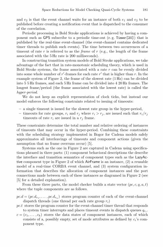
Space Reductions for Model Checking Quasi-Cyclic Systems 181

and e2 is that the event channel waits for an instance of both e1 and e2 to bepublished before creating a notification event that is dispatched to the consumerof the correlation.

Periodic processing in Bold Stroke applications is achieved by having a com-ponent such as GPS subscribe to a periodic time-out (e. g. Timer[20]) that ispublished by the real-time event-channel (the event-channel contains dedicatedtimer threads to publish such events). The time between two occurrences of atimeout of rate r is referred to as the frame of r (e.g., the length of the frameassociated with the 5 Hz rate is 200 milliseconds).

In constructing transition system models of Bold Stroke applications, we takeadvantage of the fact that in rate-monotonic scheduling theory, which is used inBold Stroke systems, the frame associated with a rate r can be evenly dividedinto some whole number of r′-frames for each rate r′ that is higher than r. In theexample system of Figure 2, the frame of the slowest rate (1 Hz) can be dividedinto 5 5 Hz frames, and each 5 Hz frame can be divided into 4 20 Hz frames. Thelongest frame/period (the frame associated with the lowest rate) is called thehyper-period.

We do not keep an explicit representation of clock ticks, but instead ourmodel enforces the following constraints related to issuing of timeouts:

– a single timeout is issued for the slowest rate group in the hyper-period,– timeouts for rate groups, ri and rj where ri > rj , are issued such that ri/rj

timeouts of rate ri are issued in a rj frame.

These constraints determine the total number and relative ordering of instancesof timeouts that may occur in the hyper-period. Combining these constraintswith the scheduling strategy implemented in Bogor for Cadena models safelyapproximates all interleavings of timeouts and component actions (given theassumption that no frame overruns occur) [5].

Systems such as the one in Figure 2 are captured in Cadena using specifica-tions phrased in three parts: (1) component behavioral descriptions the describethe interface and transition semantics of component types such as the LazyAc-tive component type in Figure 2 of which AirFrame is an instance, (2) a reusablemodel of a real-time CORBA event channel, and (3) system configuration in-formation that describes the allocation of component instances and the portconnections made between each of these instances as diagramed in Figure 2 (see[5] for a detailed explanation).

From these three parts, the model checker builds a state vector (pc, c, q, a, t)where the tuple components are as follows.

pc.d = (pc.dr1 , . . . , pc.drn) stores program counter of each of the event-channeldispatch threads (one thread per each rate group ri)

pc.t stores the program counter for the event-channel timer thread that respondsto system timer interrupts and places timeout events in dispatch queues qri .

c = (c1, . . . , ck) stores the data states of component instances, each of whichconsists of a, possibly empty, set of mode attributes as defined by ci’s com-ponent type.

182 M.B. Dwyer et al.

q = (qr1 , . . . , qrn) are rate-specific queues of pairs, (c, e), recording the dispatchof event e to port c.

a = (a1, . . . , al) stores the current states of each of the event correlation recog-nition automata.

t records an abstraction of time used to trigger timeouts.

Note that in a real avionics system, there would be significant numeric computa-tion to transform raw GPS data into a form that is useful for other componentssuch as AirFrame. We do not represent this computation in our model for sev-eral significant reasons. First, in the actual systems supplied to us by Boeing,all such computation is stripped out for security reasons and to avoid dissem-ination of propriety information. Second, Boeing engineers are often concernedwith reasoning about control properties associated with modes, and the elideddata computations rarely influence the modal behavior of the system. In essence,Boeing engineers have by happenstance performed a manual abstraction of thesystem – an abstraction that produces a system that is very well-suited for modelchecking in that remaining mode data domains are finite and small.

Other information such as the connection information between componentinstances is required to define the semantics of Cadena systems. However, we donot store connection information in the state vector at all since this informationremains constant through the lifetime of Bold Stroke systems.

Of the state vector components listed above, only the values c of the compo-nent mode variables are considered global according to the classification schemeof Section 2 – all the remaining values are transient. State spaces generated fromCadena models are quasi-cyclic in the sense of Section 2 because there exists apredicate pC

T on transient components of the state vector that holds when

– each of the dispatch thread program counters pc.dri holds the value of theinitial thread control point,

– the program counter pc.t holds the value of the initial thread control point,– each of the dispatch queues qri are empty,– each of the automata aj is in its initial state, and– the abstraction of time t is zero (i.e., start of hyper-period).

To explore how our proposed state-space optimization techniques scale alongvarious axes, we consider a parameterized family of systems built off of thebasic system shown in Figure 2. Those extensions were obtained by instantiatingparameters m, c, and v from the following description:

– m modal components are added between GPS and NavDisplay.– Each new mode variable from the m components above is changed non-

deterministically by a new component ModalControl that is running at 1 Hz.We put a bound c on the maximum number of modal values that can bechanged during a single run of ModalControl’s 1 Hz timeout handler.

– Each new mode variable from the m-components above can have v differentvalues.

Space Reductions for Model Checking Quasi-Cyclic Systems 183

4 Implementation in Bogor

Bogor [13] is an extensible and highly modular explicit-state model checkingframework. It provides a rich modeling language including features that allowfor dynamic creation of objects and threads, garbage collection, virtual methodcalls and exception handling. It also provides extension mechanisms that easethe task of customization to provide domain-specific abstraction layer and to ac-commodate, for example, variations in scheduling policies, search modes for stateexploration, state encodings, and checkers for specification languages. Bogor em-ploys state-of-the-art reduction techniques such as collapse compression [11],heap symmetry [12], thread symmetry [2], and partial-order reductions.

We have customized Bogor to support checking of Cadena models [5] thatgives orders of magnitude space reduction from previous approaches [9]. This wasdone by providing a builtin abstraction of CORBA event channel semantics, andby customizing Bogor’s scheduler to enforce constraints on time-triggered eventoccurrences and scheduling policy described in the previous section, In addition,Bogor was easily configured to identify static component connection data thatdid not need to be stored in the state vector.

4.1 Quasi-Cyclic Search

We have implemented quasi-cyclic state-space search for Cadena on top of theprevious customized implementation. We describe how we extended our existingCadena-oriented checker to implement Algorithm 1(b).

We modified the classical DFS algorithm used in [5] so that it only exploresone hyper-period for each invocation of the DFS algorithm. This modificationis done in the search module of Bogor. We use the predicate pC

T defined in theprevious section as the condition to determine when the end of the hyper-periodis encountered in the search (lines b.19-b.22). The pC

T predicate is implementedin a straight-forward manner because the interface to the state representationin Bogor provides methods to query the program counter of each thread, globaland local variables.

After each transition in the search, the current state is inspected to seewhether it satisfies pC

T . If so, we then apply the πG function to extract eachmodal component’s modal value from the state. The relatively small state vectorconsisting of only modal values is then enqueued (lines b.21-b.22) if it is not inthe queue and it has not been explored before. Once the state vector is enqueued,then the search backtracks to continue its search of the current hyper-period.

For each state vector of modal values sg in the queue, the DFS algorithmis then started with a state that is constructed using pT and sg (lines b.8).In the actual implementation, a new instance of the Bogor model checker iscreated for each of these searches, thus, the stored states of previous hyper-periodare garbage-collected and only the state vectors of mode values are preservedthrough-out the complete search.

184 M.B. Dwyer et al.

Bogor’s open design allowed us to implement this extension in less than 200lines of Java code and less than one day. An additional 40 lines of Java codewere needed to implement the parallel search.

4.2 Parallel Quasi-Cyclic Search

As will be shown in the next section, the quasi-cyclic search may potentially havea significant runtime overhead. This happens when there are many overlappingstates between the quasi-cyclic regions. Since the seent is always reset for eachDFS call, overlapping states will be revisited. In contrast, the classical DFS willbacktrack when such overlapping states are encountered.

In order to alleviate the time overhead, we have implemented a parallel ver-sion of the quasi-cyclic search. Note that because of the decomposition of thesearch that is performed by quasi-cyclic search, each DFS call (line b.8) is com-pletely independent and may be executed in a separate thread. The DFS searchesonly interact by updating the shared queue and the shared set seeng, which canbe accessed in parallel; we synchronize those specific access points (lines b.4-b.6and b.21-b.22). In our implementation, the user can specify how many threadsto use to perform parallel DFS searches.

5 Evaluation on Realistic Designs

Our goal is to evaluate the extent to which quasi-cyclic state-space search iseffective for reasoning about behavioral models of real systems. We have per-formed an evaluation in the context of a collection of Cadena design modelsthat encode Bold Stroke system designs provided by Boeing engineers. The orig-inal Bold Stroke designs were developed to illustrate structural aspects foundin real designs as a means of evaluating a wide variety of design-time analyses,but as standalone designs they reflect neither the complexity nor scale of real-istic designs. In this study, we have adapted several of these Cadena designs tomake them scalable in ways that correspond to the way that real system designsscale (as explained to us by Boeing engineers); specifically as systems scale thefollowing trends are typically followed:

1. the number of modal components increases to comprise as much as one-thirdof the total number of system components;

2. modal components are rarely independent and can often be grouped intodependent clusters that change value in the same hyper-period (e.g., com-ponents that are always enabled/disabled as a group);

3. the domain of values for mode variables can become larger in realistic sys-tems; boolean modes remain, but the progression of mode variable values ingeneral becomes more complex (e.g., implementing a state machine); and

4. the number of modal components that change value independently during ahyper-period is generally bounded by a small constant that depends on thespecific system.

Space Reductions for Model Checking Quasi-Cyclic Systems 185

We have adapted two existing modal design models, ModalSP and Medi-umSP, to introduce new modal and non-modal components in a manner thatis consistent with these constraints. We experimented with variations on thesemodels to understand the scalability of quasi-cyclic state-space search. For eachmodel we varied the number of components added (denoted m), the number ofmodal components that change in a hyper-period (c), and the number of valuesthat the added modal components will take on (v); a model configuration isdenoted by the triple (m, c, v).

We summarize results for a selection of checks on these models; the completedata set is available online [1]. The classic model checks were run using thecustomization of Bogor for Cadena models [5], discussed in Section 3, and as suchthey represent highly-optimized state-space searches. The quasi-cyclic checksused the Bogor implementation described in Section 4.1. Data on total run-timeand space usage were obtained on a single user workstation with a 2.53MhzPentium 4 and running JDK 1.4.1 on Windows XP Pro with the maximum heapof 1350Mbytes allowed for the JVM.

Figure 3 plots memory and space consumption for classical checks of threevariations of the ModalSP; in its original form the ModalSP has 8 componentsand 125 event publications per hyper-period. The shape of these plots is charac-teristic of what we found for further scaling of the models; we show these smallervariations since for the larger ones the classic searches run out of memory veryquickly and are therefore not suitable for comparative evaluation. From theseplots three trends are clear1: (1) quasi-cyclic search requires significantly lessspace than the classic search, (2) the consumption of memory for quasi-cyclicsearch scales extremely well with increasing system size and complexity, and (3)quasi-cyclic search can incur a significant run-time overhead relative to classicsearch.

The MediumSP is significantly more complex than the ModalSP having 50components and 820 events publications per hyper-period. Its state-space is morethan an order of magnitude larger and consequently classic checks run out ofmemory even for small model configurations. Data for the (3, 1, 2) and (3, 1, 3)configurations of MediumSP are representative of the overall data we collected.Classical search of (3, 1, 2) required 9.5 hours and used more than 650 Mbytesof memory, whereas quasi-cyclic search required 20 hours, but only 150 Mbytesof memory. Classical search of the (3, 1, 3) configuration exhausted availablememory, while quasi-cyclic search takes several days, but uses only slightly morethan 150 Mbytes of memory. The rate of growth of memory for quasi-cyclicsearch suggests that scaling to significantly larger systems is possible, but therun-time cost of sequential search quickly becomes prohibitive.

The prototype parallel quasi-cyclic search was used to check several config-urations of the ModalSP system on a quad-processor 500Mhz Pentium Xeonsystem with 4 Gbytes of memory. For ModalSP (3, 1, 4) classical checking took

1 Note that the dashed-line for the space consumption of quasi-cyclic search is a bitdifficult to see. It is just above and nearly parallel to the horizontal axis in the plots.The actual memory used for each of those checks was less than 8 Mbytes.

186 M.B. Dwyer et al.

0100200300400500600

2 3 4 5 6 7

Mem

ory

(Mb)

v

ModalSP (3,1,v) − Space

ClassicalCyclic

01234567

2 3 4 5 6 7

Tim

e (h

ours

)

v

ModalSP (3,1,v) − Time

ClassicalCyclic

050

100150200250300350400450500550

2 3 4 5 6 7

Mem

ory

(Mb)

v

ModalSP (3,2,v) − Space

ClassicalCyclic

0123456789

10

2 3 4 5 6 7

Tim

e (h

ours

)

v

ModalSP (3,2,v) − Time

ClassicalCyclic

0100200300400500600700

2 3 4 5

Mem

ory

(Mb)

v

ModalSP (4,1,v) − Space

ClassicalCyclic

0369

121518

2 3 4 5

Tim

e (h

ours

)

v

ModalSP (4,1,v) − Time

ClassicalCyclic

Fig. 3. Quasi-cyclic Performance for ModalSP Configurations

201 minutes, sequential quasi-cyclic checking took 360 minutes, and four-wayparallel quasi-cyclic checking took 152 minutes.

5.1 Discussion

It is difficult to quantify the extent to which quasi-cyclic search will effectivelyscale with system size. The data collected to date suggests that explosive memorygrowth can be moderated significantly, but that large-scale parallelism will berequired to control the growth in analysis time. Based on an informal analysisof the available parallelism in quasi-cyclic search we believe that fine-tuning ofour parallel implementation (e.g., to work around the sequentiality of garbagecollection in the JVM) will allow near linear speedup to be achieved for largenumbers of processors. We are aggressively pursuing this line of research andconducting a broad empirical evaluation of the scalability of parallel quasi-cyclicsearch’s run-time performance.

Our study was limited to Bold Stoke system design models for which quasi-cyclic search appears to be very effective at reducing memory requirements. Webelieve that quasi-cyclic search can also be effective for reasoning about otherclasses of periodic real-time systems as well as more general control-loop basedsoftware systems (e.g., user interface systems, web-servers). We are working toapply quasi-cyclic search to this broader class of systems.

Space Reductions for Model Checking Quasi-Cyclic Systems 187

This form of search is especially effective when a significant portion of theprogram data is transient and when the global data transitions deterministicallyacross a series of quasi-cyclic regions. This latter observation suggests that care-ful modeling of the way that a system’s environment can influence transitionsof its global data is warranted. We experimented with some different environ-ment models including a completely non-deterministic environment that simplychooses among possible mode variable settings and noticed a negative impacton performance. We found that capturing assumptions about environment be-havior that determinize the transition of mode values (e.g., encoding sequencingof flight mode values from takeoff through ascent, flight, descent and landing)reduced run-time.

6 Related Work

Godefroid et. al. [8] introduced state-space caching techniques to increase thesize of systems for which model checking is feasible. The main idea of the workis that one can perform a state-space search by storing only a portion of the seenbefore set. Studies have shown that, in general, randomly selecting the states topreserve in the seen set yields the best performance. The algorithm may visitsome states several times because they have been removed from the seen set. Inaddition, to detect termination the algorithm needs at least as much memory asis required to store the states of the longest DFS stack. In contrast, we use spe-cific knowledge of the system, encoded as a predicate, to identifying quasi-cyclicregions in the state-space. Quasi-cyclic search is guaranteed to find all states thatthe classical DFS (or state-caching search) finds and only those states; hence, itterminates whenever the classical DFS can terminate. Our algorithm may alsovisit states multiple times, however, based on our preliminary experiments, theability to parallelize the search compensates for this redundant calculation.

Godefroid [7] introduced state-less search to model check systems that havea relatively small number of states that are revisited in the search and thathave little non-determinism. State-less search is also effective for systems wherepartial order reduction significantly reduces the number of paths that need to beexplored. It does not work well for systems such as the Cadena models becauseof the non-determinism used for safely modeling timeouts and priority-basedscheduling. The non-determinism in modeling the scheduler introduces manystates that need to be revisited. We implemented a state-less search for a singlequasi-cyclic region of the (3, 1, 2) ModalSP configuration; it ran for several hoursbefore we terminated it in contrast to the 30 seconds required by the statefulquasi-cyclic search.

7 Conclusions

We have developed a search algorithm that decomposes a state-space searchinto local regions, defined by a predicate over state vectors, that can be searched

188 M.B. Dwyer et al.

independently. The algorithm is quite general, but in this paper we have empha-sized how the manual definition of a predicate that captures the cyclic structureof a projection of a system’s state-space can significantly reduce the memoryrequirements of the search. Ongoing work is seeking to automate the identifica-tion of region-defining predicates, thereby significantly increasing the breadth ofapplicability of our algorithm.

We have identified a class of quasi-cyclic design models for event-drivencomponent-based designs of distributed real-time embedded systems. We de-scribed how these systems can naturally be mapped onto the quasi-cyclic searchalgorithm which can be implemented in the Bogor model checking framework.Preliminary experimental evaluation confirmed that the memory consumption ofthe algorithm scales extremely well with increasing system complexity; in fact,for our experiments memory consumption was nearly constant. While quasi-cyclic search does incur significant overhead, up to a factor of three slowdownfor the systems we considered, that overhead can be overcome by even a modestparallelization of the search. We believe that significantly greater performancecan be achieved through large-scale parallelism and are undertaking an experi-mental study to assess that hypothesis.

References

1. http://cadena.projects.cis.ksu.edu, 2003.2. D. Bosnacki, D. Dams, and L. Holenderski. Symmetric spin. In International

Journal on Software Tools for Technology Transfer. Springer-Verlag, 2002.3. W. Chan, R. J. Anderson, P. Beame, D. Notkin, D. H. Jones, and W. E. Warner.

Optimizing symbolic model checking for statecharts. IEEE Transactions on Soft-ware Engineering, 27(2):170–190, 2001.

4. E. Clarke, O. Grumberg, and D. Peled. Model Checking. MIT Press, 2000.5. W. Deng, M. Dwyer, J. Hatcliff, G. Jung, and Robby. Model-checking middleware-

based event-driven real-time embedded software. In Proceedings of the 1st Inter-national Symposium on Formal Methods for Component and Objects, 2002.

6. M. Dyer. The Cleanroom Approach to Quality Software Development. Wiley, 1992.7. P. Godefroid. Model-checking for programming languages using VeriSoft. In Pro-

ceedings of the 24th ACM Symposium on Principles of Programming Languages(POPL’97), pages 174–186, Jan. 1997.

8. P. Godefroid, G. J. Holzmann, and D. Pirottin. State-space caching revisited. InG. von Bochmann and D. K. Probst, editors, Proc. Fourth International Conferenceon Computer Aided Verification, volume 663 of Lecture Notes in Computer Science,pages 178–191. Springer, June 1993.

9. J. Hatcliff, W. Deng, M. Dwyer, G. Jung, and V. Prasad. Cadena: An integrateddevelopment, analysis, and verification environment for component-based systems.In Proceedings of the 25th International Conference on Software Engineering, 2003.

10. T. A. Henzinger, R. Jhala, R. Majumdar, and G. Sutre. Lazy abstraction. InProceedings of the 29th ACM Symposium on Principles of Programming Languages,pages 58–70, Jan. 2002.

11. G. J. Holzmann. The model checker SPIN. IEEE Transactions on Software Engi-neering, 23(5):279–294, May 1997.

Space Reductions for Model Checking Quasi-Cyclic Systems 189

12. R. Iosif. Symmetry reduction criteria for software model checking. In Proceedingsof Ninth International SPIN Workshop, volume 2318 of Lecture Notes in ComputerScience, pages 22–41. Springer-Verlag, Apr. 2002.

13. Robby, M. B. Dwyer, and J. Hatcliff. Bogor: An extensible and highly-modularmodel checking framework. In Proceedings of the 9th European Software Engi-neering Conference held jointly with the 11th ACM SIGSOFT Symposium on theFoundations of Software Engineering, 2003.

14. D. Sharp. Reducing avionics software cost through component based product linedevelopment. In Proceedings of the Software Technology Conference, Apr. 1998.

Intelligent Editor for WritingWorst-Case-Execution-Time-Oriented

Programs

Janosch Fauster, Raimund Kirner, and Peter Puschner

Institut fur Technische Informatik,Technische Universitat Wien,

Treitlstraße 3/182/1,A-1040 Wien, Austria

Abstract. To guarantee timeliness in hard real-time systems the know-ledge of the worst-case execution time (WCET) for its time-critical tasksis mandatory. Accurate and correct WCET analysis for modern proces-sor is a quite complex problem. Path analysis is required to identify aminimal set of possible execution paths. Further, the modeling of a pro-cessor’s internal states for features like caches or pipelines requires toconsider possible interferences of these features.This paper presents a new software engineering paradigm tailored tothe development of real-time software. This paradigm results into morepredictable programs and is therefore well-suited for the developmentof real-time systems. New software development tools are necessary tosupport developers in writing efficient code for this new paradigm. In thispaper an editor is described that highlights all code that is not conformwith this programming paradigm.

1 Introduction

The knowledge of the worst-case execution time (WCET) of tasks is crucial forthe design of real-time systems. Only if safe upper bounds for the WCET of alltime-critical tasks have been established, it becomes possible to verify the time-liness of the whole real-time system. Over the last one-and-a-half decades rese-arch in WCET analysis and real-time computing has solved many sub-problemsof WCET analysis. Despite this progress in WCET analysis, there still existthree fundamental problems in the current state of the art in WCET analysis[8]:

First, WCET analysis needs exact knowledge about the possible executionpaths through the analyzed code. Deriving this information automatically is,however, not possible in the general case. This is due to the fact that the con-trol flow of a program typically depends on the input data of the program and This work has been supported by the IST research project “High-Confidence Ar-

chitecture for Distributed Control Applications (NEXT TTA)” under contract IST-2001-32111.

R. Alur and I. Lee (Eds.): EMSOFT 2003, LNCS 2855, pp. 190–205, 2003.c© Springer-Verlag Berlin Heidelberg 2003

Intelligent Editor 191

a WCET bound thus cannot be predicted purely from code analysis. Further,the fully automatic program analysis to derive descriptions about possible con-trol flows automatically is in conflict to the halting problem. Therefore, currentWCET analysis tools rely on the provision of the lacking path information [2,3].

The second major problem is obtaining correct and accurate models aboutthe timing behavior of modern processors. These processors typically use featureslike caches or pipelines to improve their peak-performance. The effects of thesehardware features interfere with each other and are therefore hard to predict.Even worse, the behavior of a processor generally is scarely documented [1].These facts taken together make it difficult if not impossible, to build for WCETanalysis tools a correct and accurate hardware model of the target processor.

The third major problem is the complexity of the WCET analysis. Besidethe problems in identifying the possible execution paths and obtaining detailedhardware-timing data, the complexity of WCET analysis itself is a problem. Thenumber of paths that have to be analyzed to calculate a precise WCET boundare growing exponentially with the number of consecutive branches. Full pathenumeration therefore becomes infeasible, except for programs having a verysimple control flow [4]. To overcome this problems, approximating analysis tech-niques are used. These approximations causes overestimation and consequentlylead to a system design with decreased utilization of hardware resources.

A possible solution to the above problems is the use of new software enginee-ring paradigms tailored to the development of real-time software. A recentlydeveloped paradigm for this new area of software engineering is WCET-orientedprogramming [8,7]. It represents an unconventional way on how to write pro-grams. The fundamental motivation of WCET-oriented programming is to re-duce the number of program statements input-data dependent control flow. Newsoftware development tools are necessary to support software developers in writ-ing efficient programs for this new software engineering paradigm.

In this paper we describe an editor that is able to highlight code that is notconform with this programming paradigm. The described analysis method tohighlight the code is integrated as plug-in into a popular editor.

This article is structured as follows: Section 2 discusses WCET-oriented pro-gramming and introduces the single-path approach to increase predictability inreal-time programs. Section 3 describes an analysis method to detect programstatements causing an input-data dependent control flow. The integration of thisanalysis into an editor is explained in section 4. Examples are shown in section 5to demonstrate the features of this program analysis methods. Section 6 gives aconclusion to the article.

2 Writing WCET-Oriented Programs

WCET-oriented programming is a software engineering paradigm especially tai-lored to the development of real-time software. This section discusses its novelaspects compared to traditional performance oriented programming. Further,

192 J. Fauster, R. Kirner, and P. Puschner

the single path approach – a paradigm to increase predictability of real-timesoftware – is described.

2.1 Traditional Performance-Oriented Coding

Non real-time programmers typically aim at a good average performance to allowfor a high throughput. Therefore, the primary performance goal of non real-timeprogrammers is the speed optimization for the most probable (i.e., frequent)scenarios. In order to be able to favor the frequent cases the code tests theproperties of input-data sets and chooses the actions to be performed during anexecution based on input data. Using input-data dependent control decisions isan effective way to achieve short execution times for the favored input-data sets.This approach is therefore suitable for optimizing the average execution time.In contrast to this, a programming style that is based on input-data dependentcontrol decisions adversely affects the quality of the achievable WCET. This isdue to the following reasons:

– Tests to identify the current input data: Even if an input-data set is notamong the ”favored” inputs it has to be tested at the points where thecontrol flow between favored and non favored inputs splits. While the fastcode makes up for the cost of the control decisions in the case of favoredinputs, the execution time of the input-data tests add up to the executiontime without compensation for all other data.

– Branching costs: Similarly to the previous argument, not just the costs fortesting the properties of input data but also the costs for branching to therespective code sections increase the total execution time of non-favoredcases.

– Information-theoretical imbalance: Every functionality on a defined input-data space and available data memory has a specific complexity. The overallproblem complexity determines the number and types of operations neededto solve the problem for the given input-data space. Performance oriented,non real-time programming spreads this overall complexity unevenly over theinput-data scenarios: to facilitate a high throughput, the frequent input-datascenarios are treated at computational cost that are below the complexitythat would result if the total complexity would be evenly distributed toall scenarios. As the complexity inherent to a problem is constant, a costreduction for some part of the input-data space necessarily causes highercosts for the rest of the inputs. Again, this impairs the achievable WCET(example: average versus worst-case transmission time of a string coded inHuffman code respectively a constant-length code).

Data-dependent control decisions are the results of traditional performance-optimization patterns. In the following we show that we have to apply a comple-tely different and not so common optimization strategy, if we aim at optimizingthe worst-case completion time.

Intelligent Editor 193

2.2 Programming for the Worst-Case

As shown in the previous section, traditional (non real-time) programming tendsto produce code that has a high WCET. We observe that it is the differenttreatment of scenarios, i.e., favoring certain input-data sets over others, thatcauses an increased WCET. The reasons for this were detailed above. In or-der to write code that has a good WCET the shortcomings of the traditionalprogramming style have to be avoided. A novel programming strategy is nee-ded. WCET-oriented programming (i.e., programming that aims at generatingcode with a good WCET) tries to produce code that is free from input-datadependent control flow decisions or, if this cannot be completely achieved, re-stricts operations that are only executed for a subset of the input-data space toa minimum. Note that in some applications it is impossible to treat all inputsidentically. This can be due to the inherent semantics of the given problem orthe limitations of the programming language used. WCET-oriented program-ming needs a way of thinking that is quite different from the solution strategieswe normally use. As a consequence, it produces unconventional algorithms thatmay not look straightforward at the first sight. The resulting pieces of code,however, are characterized by competitive WCETs due to the small numberof tests (and branches) on input data and the minimal information-theoreticalimbalance. A small number of input-data dependent alternatives does not onlykeep the WCET down. It also keeps the total number of different executionpaths through a piece of code low. Identifying and characterizing a smaller num-ber of paths for WCET analysis is easier and therefore much less error-pronethan dealing with a huge number of alternatives. In this way, WCET-orientedprogramming does not only produce code with better WCET performance butalso yields more dependable WCET-analysis results and thus more dependablereal-time code than traditional programming.

2.3 The Single-Path Approach for Predictable Code

As mentioned before, the problem of WCET analysis is in general complex be-cause programs behave differently for different input data, i.e., different inputdata cause the code to execute on different execution paths with differing execu-tion times. In the following we propose an approach that avoids this complexityby ensuring that the code to be WCET-analyzed has only a single executionpath. This approach uses code transformations to transform input-data depen-dent branches and their alternatives into sequential code (input-data indepen-dent branches are not transformed). To be precise, the code resulting from thetransformation avoids data dependencies in execution times by keeping input-data dependent branching local to single operations with data-independent exe-cution times.

Constant-Time Conditional Expression. The key feature to ourpredictable-programming approach is the so-called constant-time conditional ex-pression operation (CTCE). A CTCE consists of a boolean expression and two

194 J. Fauster, R. Kirner, and P. Puschner

expressions. It evaluates the two expressions and returns one out of the two re-sults. Which of the two results is actually selected depends on the truth value ofthe condition. Throughout this paper we use the following notation for CTCEs:

cond # expr1 : expr2

cond represents the condition of the constant-time conditional, expr1 andexpr2 stand for the two expressions that are evaluated. If cond yields true thenthe value of the CTCE is the result of expr1. If cond evaluates to false theCTCE returns the value of expr2. What has been described above may remindthe reader of the conditional assignment operator ”?:” of the C programminglanguage. Indeed, as we assume that expr1 and expr2 do not have any sideeffects, the final result of both types of statements is the same. That is also whythe syntax of the CTCE has been chosen similar to that of the C conditionalexpression (?:). Note, however, that there are significant differences in the controlflow of the two constructs. The C conditional expression works like an if-then-else construct. It first evaluates the condition and then executes one of the twobranches. In contrast to the conditional expression in C, the CTCE evaluatesboth expressions. Having computed the expressions it evaluates the conditionand returns one of the two expression results as the value of the whole constant-time conditional expression. In [8] the different semantics of the two conditionaloperators are described in more detail.

Obviously, evaluating a conditional expression with the new operator takeslonger than using an operator with the semantics of the C construct (the oldoperator evaluates only one expression while the new one has to evaluate both).The big advantage of the CTCE shows, however, when it comes to executiontime prediction. In the C conditional the two alternatives of the branch performdifferent operations, and this usually implies that the alternatives have differentexecution times. In the general case it is therefore impossible to predict theexact execution time of the conditional. The constant-time implementation hasa single, constant execution time. Its execution time is therefore predictable. Thisis achieved as follows: First, both alternative expressions execute in sequence.Executing both expressions unconditionally avoids the problem of finding outhow the conditional behaves in a worst-case execution. Second, the result of theoverall conditional is selected and returned in a simple operation with constantexecution time.

The CTCE can be realized with a conditional move instruction, which isimplemented on a number of modern processors [8].

2.4 Converting WCET-Analyzable Code into Single-Path Code

The CTCE is a construct to make the single-path approach explicit. In the fol-lowing we illustrate how every well structured and WCET-analyzable piece ofprogram code can be translated into code with a single execution path. By theterm WCET-analyzable code we understand code for which the maximum num-ber of iterations of every loop is known; a WCET bound is thus computable.

Intelligent Editor 195

The translation replaces all input-data dependent branches by sequential codethat uses CTCEs [6].

We only consider structured data dependent branchings of high-level lan-guages like conditional statements (e.g., if statement) and loops; gotos or exitstatements are leaved out. In order to translate a piece of code into temporallypredictable code we transform these two statement types into non-branchingcode.

– Conditional branching statements conditionally change the values of a num-ber of variables. The transformation of such conditional branches is straight-forward. The translation process generates sequential code with constant-time conditional assignments for each of the conditionally changed variables.When translating assignments in nested conditional branches, the conditionsof all nested branches have to combined in the conditions of the generatedconditional assignments.

– Loops with input-data dependent termination conditions are translated intwo steps. First, the loop is changed into a simple counting loop with aconstant iteration count. The iteration count of the new loop is set to themaximum iteration count of the original loop. The old termination conditionis used to build a new branching statement inside the new loop. This newconditional statement is placed around the body of the original loop andsimulates the data dependent termination of the original loop in the newlygenerated counting loop. The second step of the loop translation transformsthe new conditional statement, that has been generated from the old loopcondition, into a constant-time conditional assignment. This way the entireloop executes in constant time.

Note that applying the described transformation to existing real-time codemay yield temporal predictability at a very high cost in terms of executiontime. Thus we consider the illustration of the transformation as a demonstrationof the general applicability of our approach, rather than proposing to use thetransformation for generating temporally predictable code from arbitrary real-time programs.

In order to come up with code that is both temporally predictable and wellperforming the programmer needs to use adequate algorithms, i.e., algorithmswith no or minimal input-data dependent branching. This new paradigm tailoredto the development of real-time software is called WCET-oriented programming.Special software engineering tools can help the software developer in writingWCET-oriented software. In the following sections a special feature for an editoris described that provides the developer with additional information about thepredictability of the code. Statements that cause an input-data dependent changeof the control flow (i.e., statements that violates the single-path approach) arehighlighted. This information allows the developer to check the predictability ofthe current code. Based on this information, a refinement of the code may bepossible to avoid any performance decrease caused by the automatic translationof the program into single-path code.

196 J. Fauster, R. Kirner, and P. Puschner

3 Control Flow Analysis

We developed a plug-in for an editor to support the development of WCEToriented code. This plug-in can analyze the source code and mark every control-flow that violates the single-path paradigm.

In order to analyze the source code, our first task is to detect all basic blocksin the code and to construct a control flow graph representing all control flowsbetween the basic blocks. The second step is to extract data information frominput code and to analyze the data flow in the function. For that reason we needa data structure that supports a correct and efficient analysis of the code. Thedata flow information we need, can be represented as a semi-lattice, where theelements of the lattice constitute abstract properties of the program. In our caseeach variable is mapped to a lattice shown in figure 1 containing the followingthree elements:

– the bottom element (⊥) that marks an “unreachable value”– maybe input dependent (MBID) that marks a variable as “possibly input

dependent” and finally– not input dependent (NID) that marks an element as surly “independent

from the input”

MBID

NID

Fig. 1. Hasse Diagram of Lattice

This semi-lattice induces a partial order on its elements. The diagram repre-sents the information content of the values, i.e. upper values have a less preciseinformation content than lower values.

The initial state of the semi-lattice is NID for all elements in all basic blocks.But there is an exception. The start node contains all the informations that wehave at the beginning of the algorithm and so it gets initialized as follows:

– all global variables are marked as “maybe input dependent”, because weconsider only intra-procedural control flows and so we don’t know whathappens outside a function.

– all parameters of the function are considered as input dependent too. Thisis evident, because these parameters are the input for the function.

– all locally defined variables are initialized as “not input dependent”.

After this initialization we have a complete control flow graph and we cansolve the problem with a modified fixpoint iteration scheme. For that purposewe have developed an analysis algorithm which is subdivided into three levels:

Intelligent Editor 197

1. basic block level analysis2. statement level analysis3. expression level analysis

Each of this steps will now be covered in detail.

3.1 Basic Block Analysis

First of all we take an arbitrary basic block out of the control flow graph. Eachbasic block has an input vector and an output vector, in which the state (MBID,NID or ⊥) at the entry point and at the exit point of the basic block for allvariables is saved. Then we have to compute the current input vector. If a basicblock can be reached by only one other basic block, we simply set the inputvector to the output vector of that basic block. Otherwise, if the basic block canbe reached by more than one control path, we have to apply an union operationon all output vectors of the preceding basic blocks in order to get the inputvector of the current node. This union operation is defined in the following way:

⋃bb

(p1 . . . pn) =

⊥ if ∀j ∈ 1 . . . n : ij =⊥MBID if ∃j ∈ 1 . . . n : ij = MBIDNID otherwise

(1)

which means that if the state of a variable is NID in all vectors, it remainsNID in the input vector, but if the state in only one of the considered outputvectors is MBID, the new value is MBID.

After we have computed the input vector, all statements and all expressionsin these statements are analyzed. Details regarding those analyses are given inthe next sections. The whole procedure for calculating the output vectors of allbasic blocks in the control flow graph is repeated until the output values arestable for all nodes. It can be shown that this algorithm always terminates.

3.2 Statement Analysis

As mentioned before, each statement in a basic block must be analyzed sepa-rately. It is important to notice, that a vector is associated to each statement,in which the state of all variables in that particular code location is stored. Sothe first task is to update the current vector. If the statement to be analyzedis the first in the basic block it takes over the input vector of the basic block,otherwise it uses the vector of the statement preceding it.The statement analysis module mainly extracts all expressions from the sta-tement and passes them to a dedicated expression analyzer. This is true forsimple arithmetic expressions, but also for the conditional expressions in while-,do/while-, for-, if/else- and switch/case-statements. The second job for this mo-dule is to detect indirect control flow dependencies.

The example in figure 2 shows such an indirect dependency. The first if-statement in the illustration depends on a global value. That means, that theassignment-expression b=2 is also input dependent, although b is assigned only

198 J. Fauster, R. Kirner, and P. Puschner

main()

int b;if (a)

b=2;if (b)

doSomething;

Fig. 2. Code Example for Indirect Flow Dependency

a constant. That means furthermore that also the second if-statement dependson global input data and should be marked accordingly.

3.3 Expression Analysis

This is the central part of the analysis, because here we actually set the state ofthe variables. Each expression has a set of input parameters in = in1 . . . innand a set of output parameters out = out1 . . . outn, where it is possible todeduce the state of all output parameters from the state of the input parametersusing following function:

∀outi ∈ out :

outi =⋃

exprin1 . . . inn =

⊥ if ∀j ∈ 1 . . . n : inj =⊥MBID if ∃j ∈ 1 . . . n : inj = MBIDNID otherwise

(2)

We distinguish the following cases:

– assignments, like a=b+c. in = b, c, out = a.All elements at the right side of the assignment are input elements, thevariable at the left side is the output element. This means, that if all elementsat the right side of the assignment are NID, then also the variable at theleft side is NID. But if at least one element at the right side has the valueMBID, then also the variable at the left side gets MBID.

– functions. in = MBID, out =global variables, return-value, referencedvalues of pointers in arguments.Functions need a more complicated handling. At this point it is importantto remember that we make only intraprocedural and no interprocedural ana-lysis. Thus after a function call we must assume, that all globally declaredvariables could have been changed during the function call and for that rea-son the value of all those variables is set to MBID. Further, the return valueof the function is always input dependent. Finally, another case must beconsidered: if one of the arguments of the called function is a pointer, itsreferenced value is set to MBID, too.

Intelligent Editor 199

– constants. in = ∅, out =constants.Constants are considered to be always NID.

– structures/unions. Each member of a structure is treated separately. Thusa single member can have the value MBID, while other ones are in the stateNID. Special care must be taken for recursive structures, e.g. datastructuresused for trees and lists. Here we restrict the accuracy of the analysis toassure the correctness of the algorithm. We assume that each locally definedstructure is NID at the beginning. But if at least one member gets MBID,the whole structure turns to MBID and cannot be changed any longer toNID.

– pointers. Each pointer is represented by two state values. One for the poin-ter itself and a second one for the referenced variable. The pointer itselfcan be treated like a common variable, but the referenced variable needsspecial attention, because it could be referenced by more than one pointer.For that purpose we have two different strategies. The easier one assumesthat all referenced variables have always MBID as their current state, whilethe more sophisticated strategy uses alias-informations to handle referen-ces by pointers. More informations about the alias-analysis can be found insection 3.4.

– arrays. Arrays are handled similarly as pointers, i.e. each array is representedwith two states, one for the array itself and one for all its references. Thus,if one array entry changes its state from NID to MBID, the whole array isconsidered to be MBID and remains in this states forever. This is necessarybecause the analysis doesn’t keep track of individual array cells and so ifone value changes its state to MBID, later we don’t know which cell wasaffected by this change and thus we must assume, that all cells could bein the state MBID. We have chosen this way to handle arrays, because it’squite simple, whereas developing a method that considers each element of anarray individually would be complex and leads to higher computation andmemory consumption. Arrays can be subject to aliasing too and thereforewe use our aliasing analysis with arrays as well.

3.4 Alias Analysis

One or more pointers can reference the same memory location. If one pointerchanges the value of that location, all other pointers that reference the samelocation will see this new value, too. Thus we must ensure that our analysistakes into consideration this behavior. As mentioned before, a simple strategywould be that all referenced variables are always set to MBID. By assumingthe “worst case”, we can be sure that our analysis will always be correct. Inmost cases this treatment of pointers (and arrays) is sufficient, but there areother cases were a more accurate view is needed. For more accurate results wehave developed an alias analysis, which recognizes pointers that could referencethe same memory location. To keep things simple, we have put a restriction onour implementation: all global variables (including globally declared pointers)are assumed to refer to the same memory location. In most cases this will not

200 J. Fauster, R. Kirner, and P. Puschner

be true, but our analysis is “safe”, i.e. if an element is set to NID it is surlynot input dependent, whereas if it is set to MBID it may depend on the inputvalues. Following this restriction, all these global variables have to be marked as“aliased”.

int a;main()

int *x, *y, *z;

y=z;x=y;

*w=a;

Fig. 3. Example for Aliasing Analysis

The example in figure 3 shows a typical case, where an alias analysis shouldbe used. The first statement (y=z) means that both y and z reference the samememory location and thus have to be aliased. The result is shown in figure 4a,where each variable has its own list containing those variables to which it couldbe aliased (for a more detailed description of the used data structures refer tosection 4).

x →y → z →z → y →

a) aliased variables 1

x → y → z →y → z → x →z → y → x →

b) aliased variables 2

Fig. 4. Aliased Variables for the Example Code

The second statements adds further aliasing information. After the executionof the statement (x=y), x, y and z are aliased. The result is shown in figure 4b.

Now, the last statement in the example will need the collected aliasing infor-mations to produce a correct result. Here the referenced variable of the pointerw gets a new, input dependent, value and so it is set to MBID. Now the analyzersees that aliasing information is connected with this variable and therefore up-dates also the states of the other two pointers. At the end of this piece of codethe output vector which stores the input dependency information is shown infigure 5.

Intelligent Editor 201

a x *x y *y z *zMBID 1 0 1 0 1 0 1

Fig. 5. Flow Dependency Output Vector

4 Editor with Integrated CFA

We have implemented a plug-in for an editor that supports the data flow analysisdescribed in the previous chapter. By using this enhanced editor the programmerhas two possibilities:

1. writing programs in such a manner that nothing will be highlighted. Withthis proceeding one can be sure, that the program is conform to the singlepath approach.

2. often the first procedure is not possible, because a program already existsin large parts or the restrictions implied to are too big. In this case theadvanced features of the editor are use to highlight all code that could violatethe single path approach and one can verify, whether they are really criticalor still tolerable.

We have implemented a plug-in for vim1, that is capable of analyzingANSI C89 code, but for more programming conveniences it supports also manyANSI C99 [5] and GNU C-expansions [9], for example additional datatypes andthe //-comment. The CTCE, which is described in section 2.3, is also supportedby the analysis. It has the following syntax:

<expr> = <cond> <expr1> : <expr2>.

This expression is translated into two conditional expressions, where <expr1> or<expr2> is assigned to <expr>. According to the single path approach <expr1>and <expr2> have to be free of side effects. In languages with pointers its verydifficult to locate such side effects and so we put the following constraints onthese expressions:

<expr1>, <expr2> ∈ CONST, VAR,where CONST stands for a numerical constant (independent from the type) andVAR is an identifier representing a variable name.

The plug-in for vim is written in the vi scripting language. It executes thefollowing steps:

– First of all it starts an external program, which analyzes the source code. Thisexternal program writes the results of the analysis, i.e. those line numbersin which there is code that violates the single path approach, in a file.

– Now we use a small program called “sequencer”, which extracts from thisfile and returns the next line to be highlighted.

1 http://www.vim.org

202 J. Fauster, R. Kirner, and P. Puschner

– We use the built-in features of vim to highlight this line.– The sequencer-program is called in a loop until all flow dependent lines are

highlighted.

The program that analyzes the code reconstructs a control flow graph afterparsing the code. Each node in the control flow graph contains its assigned state-ments and pointers to its successor and predecessor nodes. Besides each node hastwo bitvectors storing the states of all variables at the entry and exit point of thebasic block (input and output vectors). The dataflow analysis was implemen-ted using the three-level algorithm presented in section 3. At statement level thedetection of indirect control flow dependencies in nested loops was implementedusing a global stack storing flags. If the flag at the top of the stack is set, theanalyzer knows that he is currently inside a conditional expression dependent onthe input value. At expression level we have some more datastructures: a currentvector that stores the state of all variables after the execution of that expressionand a field of lists storing the collected alias-informations by using the algorithmpresented in section 3.4. The datastructure for storing aliasing information wasinitially implemented as a simple bit-matrix, where an entry x/y is true if thevariables x and y are aliased. Tests have shown that this matrix could becomelarge in functions with many variables, but is typically only sparse. Therefore wedecided to implement that matrix in form of a vector with references to simplelists. Each variable has its own list, where each list entry represents a variableto which this variable is aliased.

An expression is analyzed by going recursively to the innermost subexpres-sion. This one is inspected and the results are passed back to the surroundingexpression. By using the results of all subexpressions, the current expression canbe examined. This mechanism is repeated until the whole expression is analyzed.After all variable states are stable, i.e. the output vector of all nodes does notchange for a whole iteration, the algorithm terminates by collecting the resultsand highlighting them in the editor.

5 Examples

The examples given in this section illustrate the software engineering paradigmof WCET-oriented programming and demonstrate the program analysis to testwhether a code is conform to this paradigm.

5.1 Example for WCET Oriented Programming

WCET-oriented programming is intended to increase the predictability of a real-time programs. Figure 6a) shows a traditional performance-oriented implemen-tation of find first. Its behavior is that the loop is left as the first occurrence ofa key value is found within the array. In contrast, the WCET-oriented imple-mentation shown in figure 6b) has an almost input-data independent runtimebehavior. Its only control-flow variance comes from the (?:) operator. Therefore,

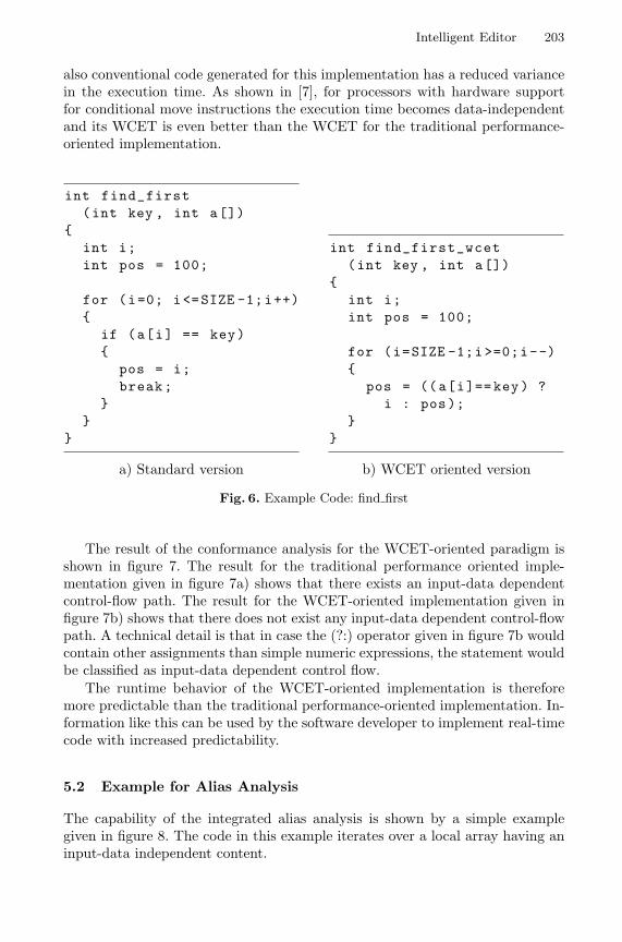
Intelligent Editor 203

also conventional code generated for this implementation has a reduced variancein the execution time. As shown in [7], for processors with hardware supportfor conditional move instructions the execution time becomes data-independentand its WCET is even better than the WCET for the traditional performance-oriented implementation.

int find_first(int key , int a[])

int i;int pos = 100;

for (i=0; i<=SIZE -1;i++)

if (a[i] == key)

pos = i;break;

a) Standard version

int find_first_wcet(int key , int a[])

int i;int pos = 100;

for (i=SIZE -1;i>=0;i--)

pos = ((a[i]==key) ?i : pos);

b) WCET oriented version

Fig. 6. Example Code: find first

The result of the conformance analysis for the WCET-oriented paradigm isshown in figure 7. The result for the traditional performance oriented imple-mentation given in figure 7a) shows that there exists an input-data dependentcontrol-flow path. The result for the WCET-oriented implementation given infigure 7b) shows that there does not exist any input-data dependent control-flowpath. A technical detail is that in case the (?:) operator given in figure 7b wouldcontain other assignments than simple numeric expressions, the statement wouldbe classified as input-data dependent control flow.

The runtime behavior of the WCET-oriented implementation is thereforemore predictable than the traditional performance-oriented implementation. In-formation like this can be used by the software developer to implement real-timecode with increased predictability.

5.2 Example for Alias Analysis

The capability of the integrated alias analysis is shown by a simple examplegiven in figure 8. The code in this example iterates over a local array having aninput-data independent content.

204 J. Fauster, R. Kirner, and P. Puschner

a) traditional performance-oriented implementation

b) WCET-oriented implementa-tion

Fig. 7. Input Dependency Analysis for find first

a) without alias analysis b) with alias analysis

Fig. 8. Input Dependency Analysis with Alias Information

As shown in figure 8a the conformance analysis for the WCET-oriented pa-radigm will classify the if statement as input-data dependent. The result for theconformance analysis with enabled alias analysis shown in figure 8b detects thatthis conditional control flow based on a pointer reference is input-data indepen-dent.

Due to the inherent complexity of an alias analysis for a programming langu-age like C, our implementation is not able to precisely detect every input-dataindependent control-flow. But the alias analysis is safe in the sense that noinput-data dependent control-flow will be classified as input-data independent.

6 Summary and Conclusion

To guarantee the timeliness of hard real-time systems it is necessary to performWCET analysis for their time-critical tasks. Programs can be easily analyzedfor their WCET, if they are translated into single-path code. To increase the

Intelligent Editor 205

efficiency of the translated code, a new programming paradigm – called WCET-oriented programming – has been developed. New software development tools arenecessary to support developers in writing efficient code for this new paradigm.

In this paper we presented a method based on control and data flow analysisto analyze the conformance of a code with the single-path approach. The analysishas been implemented as a plug-in for the editor vim.

Experiments have been done to illustrate the application of the conformanceanalysis to sample algorithms. The results of the implementations for the tra-ditional performance-oriented programming and WCET-oriented programminghave been compared to demonstrate the improved predictability of WCET-oriented programming.

References

1. Pavel Atanassov, Raimund Kirner, and Peter Puschner. Using real hardware tocreate an accurate timing model for execution-time analysis. In International Works-hop on Real-Time Embedded Systems RTES (in conjunction with 22nd IEEE RTSS2001), London, UK, Dec. 2001.

2. Antoine Colin and Isabelle Puaut. Worst case execution time analysis for a processorwith branch prediction. Real-Time Systems, 18(2):249–274, May 2000.

3. Jakob Engblom and Andreas Ermedahl. Modeling complex flows for worst-caseexecution time analysis. In Proc. 21st IEEE Real-Time Systems Symposium (RTSS),Orlando, Florida, USA, Dec. 2000.

4. Thomas Lundqvist and Per Stenstrom. Timing analysis in dynamically scheduledmircoprocessors. In Proc. 20th IEEE Real-Time Systems Symposium (RTSS), pages12–21, Dec. 1999.

5. American National Standards Insitute/International Standards Organisation.ISO/IEC 9899:1999 Programming Languages – C. American National StandardsInstitute, New York, USA, 2 edition, Dec. 1999.

6. Peter Puschner. Transforming execution-time boundable code into temporally pre-dictable code. In Bernd Kleinjohann, K.H. (Kane) Kim, Lisa Kleinjohann, andAchim Rettberg, editors, Design and Analysis of Distributed Embedded Systems,pages 163–172. Kluwer Academic Publishers, 2002. IFIP 17th World ComputerCongress - TC10 Stream on Distributed and Parallel Embedded Systems (DIPES2002).

7. Peter Puschner. Algorithms for Dependable Hard Real-Time Systems. In Proc. 8thIEEE International Workshop on Object-Oriented Real-Time Dependable Systems,Jan. 2003.

8. Peter Puschner and Alan Burns. Writing Temporally Predictable Code. In Pro-ceedings of the 7th IEEE International Workshop on Object-Oriented Real-TimeDependable Systems, pages 85–91, Jan. 2002.

9. Richard Stallman. Using and Porting the GNU Compiler Collection (GCC). iUni-verse.com, Inc., USA, 2000. gcc-2.96, ISBN 0-595-10035-X.

Clock-Driven Automatic Distribution of LustrePrograms

Alain Girault1 and Xavier Nicollin2

1 Inria Rhone-Alpes, Pop Art project, France,Alain.Girault@inrialpes.fr

2 INPG/Verimag, France,Xavier.Nicollin@imag.fr

Abstract. Data-flow programming languages use clocks as powerfulcontrol structures to manipulate data, and clocks are a form of temporaltypes. The clock of a flow defines the sequence of logical instants whereit bears a value. This is the case of the synchronous language Lustre.We propose a solution for distributing Lustre programs, such that thedistribution is driven by the clocks of the source program. The motiva-tion is to take into account long duration tasks inside Lustre programs:these are tasks whose execution time is long compared to the othercomputations in the application, and whose maximal execution rate isknown and bounded. Such a long duration task could be given a slowclock, but this would violate the synchronous abstraction. DistributingLustre programs can solve this problem: the user gives a partition ofthe set of clocks into as many subsets as he desires computing locations,and our distribution algorithm produces one program for each suchcomputing location. Each program only computes the flows whoseclock belongs to it, therefore giving time to each long duration task tocomplete.

Keywords. Automatic distribution, synchronous abstraction, data-flowlanguages, clocks, long duration tasks, reactive systems.

1 Introduction

1.1 Reactive Systems

Reactive systems are computer systems that react continuously to their environ-ment, at a speed determined by the latter [15]. This class of systems contrasts,with transformational systems (whose inputs are available at the beginning oftheir execution, and which deliver their outputs when terminating: e.g., compil-ers), and with interactive systems (which react continuously to their environ-ment, but at their own speed: e.g., operating systems). Most industrial real-timesystems are reactive systems: control, supervision, signal-processing systems . . .They must meet the following requirements:Temporal requirements. This concerns the input rate as well as theinput/output response time. To check their satisfaction on the implementation,

R. Alur and I. Lee (Eds.): EMSOFT 2003, LNCS 2855, pp. 206–222, 2003.c© Springer-Verlag Berlin Heidelberg 2003

Clock-Driven Automatic Distribution of Lustre Programs 207

it is necessary to know bounds on the execution time of each computation aswell as on the maximal input rate.Safety requirements. These systems are often critical ones, hence they re-quire rigorous design methods and languages as well as formal verification andvalidation of their behavior.Parallelism requirements. At least, the design must take into account theparallelism between the system and its environment. These systems are also oftenimplemented on parallel architectures, for reasons of processor load, performanceincrease, fault tolerance or geographical distribution. Finally, it is convenient andnatural to design such systems as sets of cooperating parallel components.

1.2 The Synchronous Data-Flow Approach and Clocks

The synchronous approach has been proposed to ease the design of reactive sys-tems. It is based on the synchronous abstraction [4],which is similar to the abstraction made when de-signing synchronous circuits at the gate level. Con-cerning the implementation, synchronous programsare embedded inside a periodic execution loop ofthe form presented to the right.

loop each tickread inputscompute next statewrite outputs

end loop

There are numerous languages based upon the synchronous abstraction,among which three are data-flow languages: Lustre [14], Signal [12], andLucid Synchrone [11]. Such languages use clocks as powerful control structuresto manipulate data [7]. In data-flow languages, each variable manipulated bythe program is a flow, which is an infinite sequence of typed data, and clocksare a form of temporal types. The clock of a flow defines the sequence of logicalinstants where the flow bears a value. Unlike many hardware modelling tools,in Lustre any Boolean flow can be a clock. A predefined clock always exists:it is the base clock of the program, which is the sequence of its activation in-stants. That is, the base clock is the flow of ticks of the periodic executionloop. Lustre, Signal, and Lucid Synchrone offer operators to upsample anddownsample flows. Downsampling allows the definition of a slower clock, whileupsampling allows the projection of a slow flow onto a faster clock. All the clocksof a program can be represented within a single clocks tree, whose root is thebase clock.1 A clock C1 is then said to be faster than another clock C2 iff C2 isin the subtree whose root is C1.

Below is an example of a Lustre program (to the left) along with its clocktree (to the right). Each node of this tree is decorated with the inputs andoutputs whose clock matches the node. Note that when, current, pre, and -> arerespectively the downsampling, upsampling, delay, and initialisation operators.The FILTER program has two clocks (the base clock of the program, and theBoolean CK), two inputs (the Boolean CK whose clock is the base clock, and theinteger IN whose clock is CK), and two outputs (the integer RES whose clock isthe base clock, and the integer OUT whose clock is CK; OUT is computed by calling1 Actually, this is not true in Signal, where it is a forest instead of a tree.

208 A. Girault and X. Nicollin

the external function SLOW, and this occurs each time CK is true). The followingtable gives an example of a run of this program:

node FILTER (CK : bool; (IN : int) when CK)returns (RES : int; (OUT : int) when CK);

letRES = current ((0 when CK) -> pre OUT);OUT = SLOW (IN);

tel.function SLOW (A : int) returns (B : int);

base RES, CK↓CK IN, OUT

Fig. 1. The Lustre FILTER program and its clock tree.

base clock cycle number 1 2 3 4 5 6 7 8 9 ...

CK T F F T F F T F F ...IN 13 9 40 ...OUT 42 27 69 ...

pre OUT nil 42 27 ...0 when CK 0 0 0 ...

(0 when CK) -> pre OUT 0 42 27 ...RES 0 0 0 42 42 42 27 27 27 ...

1.3 Clock-Driven Automatic Distribution

In this paper, we present a method to achieve the clock-driven automatic distri-bution of Lustre programs.

By automatic distribution, we mean that, given a centralised source pro-gram and some distribution specifications, we will automatically build as manyprograms as required by the distribution specifications2. These programs willcommunicate harmoniously, so that their combined behaviour be functionallyequivalent to the behaviour of the initial centralised source program.

By clock-driven, we mean that the distribution specifications will be ex-pressed as a partition of the set of clocks of the centralised source programinto several subsets, one for each computing location desired by the user.

1.4 Motivation: Long Duration Tasks

One of the main motivations for clock-driven distribution is the handling of longduration tasks, which have the following characteristics: their execution time islong compared to the other computations in the application; their execution timeis known and bounded ; and their maximal execution rate is known and bounded.

The function SLOW invoked within the FILTER program of Fig. 1 is an exampleof a long duration task, whose rate is given by the clock CK.2 This is sometimes called semi-automatic distribution since the user has to provide

the distribution specifications.

Clock-Driven Automatic Distribution of Lustre Programs 209

Of course, the execution time and execution rate of a long duration taskmust be consistent with the performance of the hardware running the system.Otherwise the temporal requirements of the system will never be met. We willcome back to this point in § 5.1.

Many reactive systems involve long duration tasks. This is the case of theCO3N4 software control system, developed at Schneider Electric for nuclearplants. One of CO3N4’s subsystems had a very tight timing constraint, and itsfirst implementation could not meet it. This subsystem consisted of two parts, aslow one performing a long duration task, and a fast one performing everythingelse. The engineers came up with a solution where the slow part was cut in twosubparts, with the system performing at each of its cycles the fast part, andalternately the first slow subpart and the second slow subpart.

Consider a system with three tasks: task A performs slow computations (du-ration=8, period=deadline=32); task C performs the fast and urgent compu-tations (duration=4, period=deadline=8); and finally task B performs mediumand less urgent computations (duration=6, period=deadline=24). There are twoways to implement such a system:1. Manual task slicing. Tasks A and B are sliced into small chunks, which areinterleaved with task C (Fig. 2). This is very hard to achieve, error prone, anddifficult to debug. The main reasons are that the slicing itself is complex, in thegeneral case various subparts may communicate with each other, and finally itis difficult to come up with a correct and deadlock-free implementation.

C A1 B1 C A2 B2 C A3 B3 C A4 B1 C

A B C

282624 34323018 3620 224 12 14 166 8 100 2time

duration / period / deadline 4 / 8 / 86 / 24 / 248 / 32 / 32task

Fig. 2. Manual task slicing.

2. Distribution into three processes. Tasks A, B, and C are performed byone process each, and the task slicing is done by the scheduler of the underlyingRTOS, with some priority policy.3 There are two ways to achieve this:

(a) Manually programming three asynchronous tasks. The example of the MarsRover Pathfinder4 shows the limitation of this approach for critical systems:several parallel tasks had to share common resources; during execution, apriority inversion occurred [22], causing a total system reset! The system’sintrinsic non-determinism combined with the fact that each subsystem wasdesigned separately made the problem all the more difficult to debug. Weclaim that this approach makes the program harder to debug, test, and verify.

3 This priority problem is orthogonal to the scope of this paper.4 Story report at http://www.cs.cmu.edu/afs/cs/user/raj/www/mars.html.

210 A. Girault and X. Nicollin

(b) Distributing a centralised program into three processes. To achieve automat-ically a distributed implementation, we choose the object code distributionmethod : first the centralised program is compiled into a single object code(a single task program), which is then distributed according to the systemdesigner’s specifications. The main advantage is that it is harder and error-prone to design directly a distributed system, hence the recent success ofautomatic distribution methods [13,10]. The other advantage is the possi-bility to debug and formally verify the centralised program before its dis-tribution, which is easier and faster than debugging a distributed program.Finally, there remains the issue of the correctness of this approach: it will beaddressed in § 3.1.

In other words, the solution we propose avoids, 2(b), not only the manual par-tition of A and B into small chunks Ai and Bi (as in solution 1), but also themanual partition of the whole program into A, B, and C (as in solution 2(a)).Moreover, since the distribution will be automated, it will allow the user to testseveral partitions along with several priority policies.

1.5 Outline of the Paper

Section 2 introduces the internal format of our programs. Section 3 presents afirst attempt of automatic distribution and discusses why this does not work.Section 4 details our clock-driven automatic distribution method. Finally, Sec-tion 5 discusses issues like worst case execution time, implementation, and relatedwork, and provides some concluding remarks.

2 Preliminaries

Our method for achieving the clock-driven distribution of Lustre programsheavily uses past work on their automatic distribution, based on the OC internalformat. In this section, we present first this format, then the basic distributionalgorithm, the communication primitives we use, and finally an OC programthat will serve as a running example in future sections.

2.1 Internal Format

Our distribution algorithm [10] uses an internal format called OC (for ObjectCode [20]). OC is an object code format common to several synchronous lan-guages such as Esterel [5] and Lustre [14]. An OC program is a finite de-terministic automaton. This state graph can be cyclic, but in each state, thereis sequential acyclic code, represented by a rooted binary directed acyclic graph(DAG) of actions. A program manipulates three kinds of variables: input vari-ables can only be used as r-values; local and output variables can also be usedas l-values; output variables can also be written to the environment.

Each DAG has one root (graphically represented by a circled dot), severalunary and binary nodes, and one or more leaves:

Clock-Driven Automatic Distribution of Lustre Programs 211

– Unary nodes are sequential actions, which can be either an assignment to alocal or output variable: var:=exp, where exp can contain external func-tion calls; an output writing : write(var); or an external procedure call :proc(. . . ,vari,. . . )(. . . ,valj,. . . ), where vari and valj are respectivelythe variable and value parameters.

– Binary nodes are deterministic branchings: if var then p else q endif,where p and q are subdags.

– Leaves, and only leaves, denote the next state number: goto n.

The outcome of the Lustre compiler is an OC program that performs exclu-sively the compute next state and write outputs phases of the executionloop (see § 1.2). It is a transformational function that terminates after complet-ing one transition of the automaton. The loop itself and the read inputs phaseare performed by a special synchronous/asynchronous interface that samples theinputs, stores their values in the local memory, and invokes the OC program.The same behaviour holds for the Esterel compiler [1].

This synchronisation of the program with its environment is not explicitin OC. Since we will need to manipulate precisely the OC code, including itsinteractions with the environment, we add an explicit action at the root of eachDAG: it materialises the read inputs phase. We call this special action go, withthe input signals as arguments. The go action indicates that the inputs have beenread and that their values are available in the local memory.

This internal format is quite general since programs written in a classicalimperative programming language can be compiled into this format. In fact, anyOC program can be translated into a flow graph of basic blocks, and vice-versa.

2.2 The FILTER OC Program

We consider the OC program FILTER, obtained by compiling the Lustre pro-gram of Fig. 1. It has two states, depicted in Fig. 3 below along with the DAGof state 1. Besides the clocks, inputs, and outputs of the Lustre program, theOC program has one local variable, the integer V. The program stays in state 0until the first time CK bears the value true; then it moves to state 1. This is dueto the initialisation operator -> in the Lustre program.

Below is an example of a run of the FILTER program (Fig. 4). The sub-scripts indicate the cycle number (logical time). Note that RES4 is equal to OUT1.Throughout the paper, we suppose that SLOW takes 7 time units to complete andthat, altogether, the other computations of the program take 1 time unit. Thus,the Worst Case Execution Time (WCET) of FILTER is 8 time units (7+1). In therun of Fig. 4, it is reached at cycles 1 and 4. So the period of the execution loop(that is, the rate of the base clock) cannot be smaller than 8 time units. If thetemporal requirements impose a smaller period, then the synchronous abstrac-tion cannot be validated. The purpose of our distribution method is to achievea smaller period for the computations scheduled on the base clock. In Section 3,we show that the simple distribution of FILTER in two communicating tasksdoes not solve the problem because these two tasks still share the same logical

212 A. Girault and X. Nicollin

state 0:go(CK,IN);if (CK) then RES:=0;write(RES);V:=0;OUT:=SLOW(IN);write(OUT);goto 1;

else RES:=V;write(RES);goto 0;

endif;

state 1:go(CK,IN);if (CK) then RES:=OUT;V:=OUT;OUT:=SLOW(IN);write(OUT);

else RES:=V;

endif;write(RES);goto 1;

state 1:

go(IN,CK)

if (CK)

goto 1

write(RES)

RES:=OUT

V:=OUT

OUT:=SLOW(IN)

write(OUT)

RES:=V

Fig. 3. The centralised FILTER program: textual representations of states 0 and 1 andgraphical representations of state 1.

FILTFILT FILTFILT

OUT1=42RES1=0 RES2=0 RES3=0

OUT2=27RES4=42

IN2=9CK4=T

IN1=13CK1=T CK2=F CK3=F

4/13/1 logical time/state1/0 2/1

Fig. 4. A run of the centralised FILTER program.

time, and hence the same period. Next, in Section 4, we present our method todesynchronise further the two tasks, so that the fast computations be performedat a faster rate.

3 A First Attempt of Clock-Driven AutomaticDistribution

3.1 Automatic Distribution AlgorithmThe distribution algorithm we use in this paper is fully presented in [10]. Weonly outline it here. It involves the following successive steps:1. assign a unique computing location to each sequential action, according to

the distribution specifications; these specifications are a partition of the setof inputs and outputs of the program into n subsets, one for each computinglocation of the final parallel program; note that achieving the “best” locali-sation (whatever the optimisation criterium) of the sequential actions is outof the scope of this paper: readers interested in these topics can refer to [13];

2. replicate the program on each location;3. on each location, suppress the sequential actions not belonging to the con-

sidered location;4. on each state of the automaton, insert sending actions in order to solve the

data dependencies between two distinct locations;

Clock-Driven Automatic Distribution of Lustre Programs 213

5. on each state, insert receiving actions in order to match the sending actions;6. if required by the user, on each state, add the needed dummy communica-

tions in order to resynchronise the distributed program; we will not considerthis step until Section 4.3.

This algorithm has been implemented and tested in the ocrep tool. It acts asa post-processor for the various synchronous languages compilers. Concretely, ittakes as input an OC program foo.oc, and a file foo.rep containing the distri-bution specifications (see item 1 above). Also, its correctness has been formallyproved in [6]: the obtained distributed program is functionally equivalent to theinitial centralised one.

3.2 Communication Primitives

We choose to have two FIFO channels for each pair of locations, one in eachdirection. This is quite cheap in terms of execution environment, and has provedto work satisfactorily [9]. Concretely, we use two communication primitives:

The send primitive send(dst,var) sends the current value of variable varto location dst by inserting it into the queue directed towards dst.

The receive primitive var:=receive(src) extracts the head value from thequeue starting at location src and assigns it to variable var, which is the localcopy of the distant variable maintained by the distant computing location src.

These primitives perform both the data-transfer and the synchronisationneeded between locations: when the queue is empty, receive is blocking. Theonly requirement on the network is that it must preserve ordering and integrityof messages.

3.3 Clock-Driven Distribution

From now on, let us assume that the userwishes his FILTER program to run over twocomputing locations L and M, according to theclock distribution specifications on the right.

location name assigned clocksL baseM CK

We now need to derive the corresponding distribution specifications, ex-pressed on the inputs and outputs of the program instead of the assigned clocks(as required by ocrep). To do this, we just assign to a given computing locationall the inputs and outputs whose clock belongs to it.

We also infer the clock of each location: this is necessary in order to knowthe rate of each location. Indeed, the knowledge of these rates will be requiredto compute the final WCET (in § 5.1). To compute the inferred clock of anygiven location, we take the root of the smallest subtree containing all the clocksassigned by the user. For the above distribution specifications, we obtain:

location name assigned clocks infered inputs & outputs infered location clockL base CK, RES baseM CK IN, OUT CK

214 A. Girault and X. Nicollin

Applied to the FILTER program of Fig. 3, these distribution specifications yieldthe following distributed program, shown in Fig. 5.

location L (clock base) location M (clock CK)state 0:go(CK);send(M,CK);if (CK) then RES:=0;write(RES);V:=0;goto 1;

else RES:=V;write(RES);goto 0;

endif;

state 1:go(CK);send(M,CK);if (CK) then OUT:=receive(M);RES:=OUT;V:=OUT;

else RES:=V;

endif;write(RES);goto 1;

state 0:go(IN);CK:=receive(L);if (CK) then OUT:=SLOW(IN);write(OUT);goto 1;

else goto 0;

endif;

state 1:go(IN);CK:=receive(L);if (CK) then send(L,OUT);OUT:=SLOW(IN);write(OUT);

else endif;goto 1;

Fig. 5. The FILTER program distributed over two locations L and M.

The distributed program of Fig. 5 calls for the following remarks:

1. The go(CK,IN) action from the centralised FILTER program has been splitinto two actions: go(CK) on location L and go(IN) on location M. This is adirect consequence of our distribution specifications.

2. On location M, all computations are scheduled on its clock CK. Hence, theyare necessarily inside the then branch of the test if(CK). Only a goto canappear in the else branch, which is the case of state 0.

3. The value of CK is sent by location L to location M at each cycle of the baseclock. As a result, location M actually runs at the speed of the base clockinstead of CK.

Fig. 6 below is an example of a run of the distributed FILTER program, where Land M are both embedded in their own periodic execution loop.

MM

L

M M M

LLLL

CK1=T CK2=F CK3=F CK4=T

RES1=0 RES2=0 RES3=0 RES4=42

CK1

IN1=13OUT2=27OUT1=42

IN2=9

OUT1CK2 CK3 CK4

1/0 3/1

1/0 2/1 3/1 4/1 logical time/state for L

4/1 logical time/state for M2/1

Fig. 6. A run of the distributed FILTER program.

Assume that the communications take 1 time unit. The new WCETs are re-spectively 2 and 8 time units for L and M. On a multi-processor architecture,

Clock-Driven Automatic Distribution of Lustre Programs 215

the global WCET is 8, hence the situation is the same as before; on a single-processor architecture, it is worse since the global WCET is 10. One reason isthat CK is sent by L to M at each cycle. Would the period of L be smaller thanthat of M, the size of the FIFO queue would be unbounded.

Instead of the distributed program of Fig. 5, we would like location M to runat the speed of its assigned clock, that is CK. This would give enough time for thecomputation of the long duration task embedded in SLOW. In the next section,we explain in details our method to achieve this.

4 The Proposed Method

In location M of the distributed program of Fig. 5, the go(IN) action could beperformed inside the then branch of the test if(CK). Indeed, the clock of IN isCK, and therefore a new value of IN is only expected at those cycles where CK istrue. If we manage to move the go(IN) action inside the then branch of the test,then a carefully chosen bisimulation should be able to detect useless branchings.Suppressing such a useless if(CK) test on location M will obviate the sending ofCK by location L, therefore allowing the two programs to be desynchronised.

4.1 Moving the go Actions Downward

Moving the go actions downward concerns only the programs of the computinglocations whose clock is not the base clock. For each such program, let CK be itsclock and IN1,...,INn be its n inputs, as specified in the distribution specifi-cations. Hence, the current action at the root of its DAGs is go(IN1,...,INn).Then, we traverse each of its DAGs downward, starting from the root, as follows:

– On a unary node, continue in the next node.– On a branching if(var), if var is CK, then insert go(IN1,...,INn) at the

beginning of the then branch, mark the DAG, and continue in the branchingclosure; otherwise continue in both branches then and else.

– On a branching closure, continue in the next node.– On a leaf, do nothing.– At the end of the traversal, if the DAG is marked, then remove the go at its

root. It means that a go action has been inserted somewhere in the DAG.

To illustrate this algorithm, we apply it to the FILTER program. According toour distribution specifications (see § 3.3), only the DAG of location M needs tobe traversed. Fig. 7 shows the result for state 0 (it is similar for state 1).

216 A. Girault and X. Nicollin

loc. M (clock CK) - state 0go(IN);if (CK) then OUT:=SLOW(IN);write(OUT);goto 1;

else goto 0;

endif;

loc. M (clock CK) - state 0if (CK) then go(IN);OUT:=SLOW(IN);write(OUT);goto 1;

else goto 0;

endif;

Fig. 7. State 0 of location M: before and after the traversal.

4.2 Suppressing Useless Branchings

In [8], we have presented an algorithm for suppressing binary branching whosebranches are observationally equivalent. Explaining this algorithm in details isout of the scope of the present article. Shortly, it involves traversing each DAGdownward from its root, and for each branching encountered, in checking whetheror not both branches are observationally equivalent. If they are, then the branch-ing is suppressed; otherwise, it is kept. Checking if two branches are observation-ally equivalent is done with an on-the-fly bisimulation, called test bisimulation.This test bisimulation is formally expressed by three axioms and six inferencerules, whose soundness and completeness have been proved in [8].

For our method to work, we divide Step 4 of our distribution algorithm (see§ 3.1) into two parts. The test bisimulation and branching suppression will takeplace between these two parts. During the first part, we only insert the sendactions concerning the unary nodes of the DAG, that is, everything but thebranchings. During the second part, we insert the send actions concerning thebinary nodes, that is the branchings that were not suppressed.

goto 1

goto 1

go(IN)

write(OUT)

OUT:=SLOW(IN)

write(OUT)

send(L,OUT)

go(IN)

goto 1

OUT:=SLOW(IN)

goto 1

OUT:=SLOW(IN)

write(OUT)

go(IN) goto 0if (CK)

OUT:=SLOW(IN)

write(OUT)

send(L,OUT)

go(IN)

if (CK) q1 q0

p1 p0

Fig. 8. Suppression of the branchings in the DAGs of location M.

Fig. 8 above shows the result of applying our test bisimulation to the DAGs oflocation M. In state 1, the parts labelled q1 and q0 are found to be bisimilar,hence the branching is suppressed. The same goes in state 0 for p1 and p0, eventhough there is a goto in the else branch.

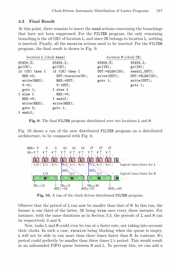
Clock-Driven Automatic Distribution of Lustre Programs 217

4.3 Final Result

At this point, there remains to insert the send actions concerning the branchingsthat have not been suppressed. For the FILTER program, the only remainingbranching is the if(CK) of location L, and since CK belongs to location L, nothingis inserted. Finally, all the receive actions need to be inserted. For the FILTERprogram, the final result is shown in Fig. 9:

location L (clock base) location M (clock CK)state 0:go(CK);if (CK) then RES:=0;write(RES);V:=0;goto 1;

else RES:=V;write(RES);goto 0;

endif;

state 1:go(CK);if (CK) then OUT:=receive(M);RES:=OUT;V:=OUT;

else RES:=V;

endif;write(RES);goto 1;

state 0:go(IN);OUT:=SLOW(IN);write(OUT);goto 1;

state 1:go(IN);send(L,OUT);OUT:=SLOW(IN);write(OUT);goto 1;

Fig. 9. The final FILTER program distributed over two locations L and M.

Fig. 10 shows a run of the new distributed FILTER program on a distributedarchitecture, to be compared with Fig. 6.

LLLL L L L

MM M M

LLL

OUT2OUT1

T T FFTFFCK= F

27F

270 424200RES=

OUT2=27OUT1=42 OUT3=69IN1=13

27

IN3=40

42

IN2=9

3/1 logical time/state for L9/18/14/1 7/1

1/0

6/15/1

logical time/state for M3/1

1/0 2/1

2/1

Fig. 10. A run of the clock-driven distributed FILTER program.

Observe that the period of L can now be smaller than that of M. In this run, theformer is one third of the latter, CK being true once every three instants. Forinstance, with the same durations as in Section 3.3, the periods of L and M canbe respectively 3 and 9.

Now, tasks L and M could even be run at a faster rate, not taking into accounttheir clocks. In such a case, receive being blocking when the queue is empty,L will not be able to run more than three times faster than M. In contrast, M’speriod could perfectly be smaller than three times L’s period. This would resultin an unbounded FIFO queue between M and L. To prevent this, we can add a

218 A. Girault and X. Nicollin

dummy communication, sent by L in state 1 at the beginning of its then branch,and received by M in state 1 just before its goto (represented by the dashed linein Fig. 10). This is exactly the purpose of Step 6 of our distribution algorithm.Such a dummy communication would force L and M to be loosely synchronised.

On a centralised architecture, Fig. 11 shows the schedule obtained when theperiods of L and M are respectively 5 and 15. No communication takes place beforethe second occurrence of CK, which corresponds to cycle 4 of task L and to thebeginning of cycle 2 of task M. At this point, task L begins and is suspended assoon as it reaches the OUT:=receive(M) action since the queue is empty. Then, Mbegins and immediately sends OUT, which resumes L. Since L has a higher priority,it preempts M and completes its execution. Then, M resumes and continues untilthe beginning of L’s cycle 5 when it is preempted by L. This results in slicingM into M1, M2, and M3. Here, the deadlines are met thanks to the distribution intwo processes.

L M1 L M2 L M3L M1 L M2 L M3 L

LML M1

logical time/state for M

logical time/state for L3/12/11/0

2/1

6/15/14/1

1/0

OUT1

4 36time

30 32 3424 26 2818 20 2212 14 16620 8 10

Fig. 11. Centralised schedule obtained with the clock-driven distribution.

4.4 The New Distribution Algorithm

Taking into account the two modifications described above, our new distributionalgorithm involves the following successive steps:

1. locate each sequential action; same as § 3.1-Step 1;2. replicate the program; same as § 3.1-Step 2;3. suppress the sequential actions; same as § 3.1-Step 3;4. on each state and each location, move the go action downward according to

the clock of the computing location; see § 4.1;5. on each state of the automaton, insert send actions to solve the data depen-

dencies between two distinct locations, except when concerning branchingactions;

6. on each state and each location, suppress the useless branchings; see § 4.2;7. on each state, insert send actions to solve the data dependencies concerning

the branching actions that were not suppressed during Step 6;8. insert receive actions; same as § 3.1-Step 5;9. add dummy communications; same as § 3.1-Step 6.

Clock-Driven Automatic Distribution of Lustre Programs 219

5 Discussion

5.1 Validating the Synchronous Abstraction

Validating the synchronous abstraction is always crucial when programming re-active systems. This involves computing the WCET of the object code generatedby the compiler, and comparing it to the execution loop period it is embeddedin (see § 1.2). In our case, it is more complex because the program is distributedinto n processes. We thus have n WCET, each corresponding to a program whoseexecution rate is the location’s clock (see § 3.3). We then compute the utilisationfactor of the processor and check the Liu&Layland condition to know whethera static or dynamic priority schedule is feasible or not [17]: namely Rate Mono-tonic (RM) for the static priority policy and Earliest Deadline First (EDF) forthe dynamic priority policy. Note that to avoid uncontrollable context switchingbetween tasks, static priorities are preferable for hard real-time systems.

Concerning our FILTER example, the WCET of locations L and M are re-spectively 2 and 8. Since the rates of locations L and M arerespectively 5 and 15, the Liu&Layland condition for RMholds, see besides. As a result, the schedule shown in Fig. 11

25

+815

=1415

≤ 1

above is feasible with static priorities (RM policy). Note that, 15 being a multipleof 5, the bound on the utilisation factor is 1 instead of 2(

√2 − 1).

5.2 Implementation

The method presented in this paper has been implemented in two software tools:on one hand the ocrep tool5, to distribute automatically OC programs with thebranching reduction, and on the other hand the ludivin6 GUI [21], to buildautomatically the clocks tree of a Lustre program, help the user specify adesired distribution, and call ocrep to do the job.

5.3 Related Work

Our work is related to Giotto [16], a compiler for embedded systems. Its abstrac-tion consists of instantaneous communication, time-deterministic computation,and value-deterministic computation. This is very much like the synchronousabstraction. Giotto’s basic functional unit is the task, which is a periodicallyexecuted piece of code. One important point is that the period must be static.In contrast, clocks can specify dynamic periods. A Giotto program can also beannotated with platform constraints, which are similar to our distribution spec-ifications: a constraint may map a particular task to a particular CPU. TheGiotto compiler schedules the tasks on the target architecture, and guaranteesthat the logical semantics is preserved (both functionality and timing). How-ever, a Giotto program might be over constrained when it does not permit anyexecution consistent with the platform constraints. In such a case, the compiler5 ocrep is available at www.inrialpes.fr/pop-art/people/girault/Ocrep.6 ludivin is available at www.inrialpes.fr/pop-art/people/girault/Ludivin.

220 A. Girault and X. Nicollin

rejects it as non valid. In contrast, our method always produces an executabledistributed program. Then, determining whether this program meets the desiredtiming constraints is left to the user. Since we use finite deterministic automata,computing such a worst case execution time is straightforward.

Also perhaps related is the code generator Real-Time Workshop [23] forSimulink, which includes multi-tasking support for multi-rate models. The au-thors do not know if this solution would allow a similar schedulability analysisfor real-time applications.

Another related work is Esterel’s asynchronous tasks mechanism [19]. Ba-sically, a synchronous Esterel program can launch an asynchronous task bymeans of a dedicated output signal (called exec), and then be warned of its ter-mination by means of a dedicated input signal (called return). Although not aspowerful and flexible as clocks, this mechanism allows long duration tasks to betaken into account. However, they are handled externally w.r.t. the synchronousprogram, while our method allows them to be handled inside the program.

Finally, there has been a lot of work done on the automatic distribution ofSignal programs [18,2,3]. Distribution in Signal is performed by first com-piling the program into a hierarchical data-flow graph with conditional depen-dency equations, called a Synchronised Data-Flow Graph (SDFG). Vertices ofthis SDFG are signals and variables, while the edges are labelled with clocks.Therefore, each vertex is located in a hierarchy of clocks. In the most generalcase, the set of all the program’s clocks form a forest instead of a tree. This meansthat the program does not have a base clock, which raises code generation prob-lems since the periodic rate of the program cannot be statically determined. Yet,for a wide class of programs, the forest is reduced to a single tree and the pro-gram does have a base clock. Such programs are called endochronous. Once theSDFG is built, communications are inserted in it, then subgraphs are extractedcorresponding to different computing locations, and finally sequential code isgenerated from each subgraph.

L M1 L M2 L M3L M1 L M2 L M3 L

OUT2OUT1

logical time/state for L

logical time/state for M

3/12/11/0

2/1

6/15/14/1

1/0

4 36time

30 32 3424 26 2818 20 2212 14 162 6 8 100

Fig. 12. Centralised schedule obtained when OUT is sent as soon as possible.

5.4 Concluding Remarks

To conclude, we would like to stress the original contributions of our work. Weoffer a method and tool to automatically distribute Lustre programs accordingto the clocks of the source code, hence avoiding the manual partition of an entiresystem into several tasks with different periods (the user only needs to partitionthe set of the program’s clocks). This allows long duration tasks to be taken into

Clock-Driven Automatic Distribution of Lustre Programs 221

account inside a synchronous program, which would not be otherwise possible.Once the distribution is done, the Liu&Layland conditions can be checked tochoose the most suited priority policy.

Finally, in the program of Fig. 9, a standard data-flow analysis could allowus to move the sending of OUT from M to L backwards, that is just after theassignment to OUT. As a result, the preemptions taking place in Fig. 11 wouldnot occur, therefore resulting in the run shown in Fig. 12. This future extensionwould have to take place as the very last step of our distribution algorithm, thatis, even after the optional resynchronisation step.

References

1. C. Andre, F. Boulanger, and A. Girault. Software implementation of synchronousprograms. In International Conference on Application of Concurrency to SystemDesign, ICACSD’01, pages 133–142, Newcastle, UK, June 2001. IEEE.

2. P. Aubry, P. Le Guernic, and S. Machard. Synchronous distributions of Signalprograms. In 29th Hawaii International Conference on System Sciences, HICSS-29, pages 656–665, Honolulu, USA, January 1996. IEEE.

3. A. Benveniste, B. Caillaud, and P. Le Guernic. Compositionality in dataflow syn-chronous languages: Specification and distributed code generation. Informationand Computation, 163:125–171, 2000.

4. A. Benveniste, P. Caspi, S. Edwards, N. Halbwachs, P. Le Guernic, and R. de Si-mone. The synchronous languages twelve years later. Proceedings of the IEEE,2002. Special issue on embedded systems.

5. G. Berry and G. Gonthier. The Esterel synchronous programming language: De-sign, semantics, implementation. Science of Computer Programming, 19(2):87–152,1992.

6. B. Caillaud, P. Caspi, A. Girault, and C. Jard. Distributing automata for asyn-chronous networks of processors. European Journal of Automation (RAIRO-APII-JESA), 31(3):503–524, 1997. Research report Inria 2341.

7. P. Caspi. Clocks in data-flow languages. Theoretical Computer Science, 94:125–140, 1992.

8. P. Caspi, J.-C. Fernandez, and A. Girault. An algorithm for reducing binarybranchings. In P.S. Thiagarajan, editor, 15th Conference on the Foundationsof Software Technology and Theoretical Computer Science, FST&TCS’95, volume1026 of LNCS, Bangalore, India, December 1995. Springer-Verlag.

9. P. Caspi and A. Girault. Execution of distributed reactive systems. In S. Haridi,K. Ali, and P. Magnusson, editors, 1st International Conference on Parallel Pro-cessing, EURO-PAR’95, volume 966 of LNCS, pages 15–26, Stockholm, Sweden,August 1995. Springer-Verlag.

10. P. Caspi, A. Girault, and D. Pilaud. Automatic distribution of reactive systemsfor asynchronous networks of processors. IEEE Trans. on Software Engineering,25(3):416–427, May/June 1999.

11. P. Caspi and M. Pouzet. Lucid synchrone: une extension fonctionnelle de Lus-tre. In Journees Francophones des Langages Applicatifs (JFLA), Morzine, France,February 1999. Inria.

12. P. Le Guernic, T. Gautier, M. Le Borgne, and C. Lemaire. Programming real-timeapplications with Signal. Proceedings of the IEEE, 79(9):1321–1336, September1991.

222 A. Girault and X. Nicollin

13. R. Gupta, S. Pande, K. Psarris, and V. Sarkar. Compilation techniques for parallelsystems. Parallel Computing, 25(13):1741–1783, 1999.

14. N. Halbwachs, P. Caspi, P. Raymond, and D. Pilaud. The synchronous data-flow programming language Lustre. Proceedings of the IEEE, 79(9):1305–1320,September 1991.

15. D. Harel and A. Pnueli. On the development of reactive systems. In Logic andModels of Concurrent Systems, NATO. Springer-Verlag, 1985.

16. T.A. Henzinger, B. Horowitz, and C.M. Kirsch. Giotto: A time-triggered lan-guage for embedded programming. In First International Workshop on EmbeddedSoftware, EMSOFT’01, volume 2211 of LNCS, Tahoe City, USA, October 2001.Springer Verlag.

17. C.L. Liu and J.W. Layland. Scheduling algorithms for multiprogramming in hardreal-time environnement. Journal of the ACM, 20(1):46–61, January 1973.

18. O. Maffeıs. Ordonnancements de graphes de flots synchrones ; Application a lamise en œuvre de Signal. PhD Thesis, University of Rennes I, Rennes, France,January 1993.

19. J.-P. Paris. Execution de taches asynchrones depuis Esterel. PhD Thesis, Universityof Nice, Nice, France, 1992.

20. J.A. Plaice and J.-B. Saint. The Lustre-Esterel Portable Format. Inria, Sophia-Antipolis, France, 1987. Unpublished report.

21. F. Salpetrier. Interface graphique utilisateur pour la repartition de programmesLustre dirigee par les horloges. Master’s thesis, ESISAR, Valence, France, June2002.

22. L. Sha, R. Rajkumar, and J.P. Lehoczky. Priority inheritance protocols: An ap-proach to real-time synchronization. IEEE Trans. on Computers, 39:1175–1185,September 1990.

23. The MathWorks, Inc. Real-Time Workshop User’s Guide, Version 3, January 1999.

Reasoning about Abstract Open Systems withGeneralized Module Checking

Patrice Godefroid

Bell Laboratories, Lucent Technologies,god@bell-labs.com

Abstract. We present a framework for reasoning about abstract opensystems. Open systems, also called “reactive systems” or “modules”,are systems that interact with their environment and whose behaviorsdepend on these interactions. Embedded software is a typical exampleof open system. Module checking [KV96] is a verification technique forchecking whether an open system satisfies a temporal property no matterwhat its environment does. Module checking makes it possible to checkadversarial properties of the “game” played by the open system with itsenvironment (such as “is there a winning strategy for a malicious agenttrying to intrude a secure system?”). We study how module checkingcan be extended to reason about 3-valued abstractions of open systemsin such a way that both proofs and counter-examples obtained by verify-ing arbitrary properties on such abstractions are guaranteed to be sound,i.e., to carry over to the concrete system. We also introduce a new veri-fication technique, called generalized module checking, that can improvethe precision of module checking. The modeling framework and verifi-cation techniques developed in this paper can be used to represent andreason about abstractions automatically generated from a static analy-sis of an open program using abstraction techniques such as predicateabstraction. This application is illustrated with an example of open pro-gram and property that cannot be verified by current abstraction-basedverification tools.

1 Introduction

Software verification via automatic abstraction and model checking is currentlyan active area of research (e.g., [BR01,CDH+00,DD01,HJMS02,VHBP00]). Thisapproach consists of automatically extracting a model out of a program by stat-ically analyzing its code, and then of analyzing this model using model-checkingtechniques. If the model-checking results are inconclusive due to too much infor-mation being lost in the current abstraction, the model can then be automati-cally refined into a more detailed one provided the abstraction process can beparameterized and adjusted dynamically guided by the verification needs, as isthe case with predicate abstraction [GS97] for instance. Current frameworks andtools that follow the above paradigm typically use traditional formalisms (suchas Kripke structures or Labeled Transition Systems) for representing models,

R. Alur and I. Lee (Eds.): EMSOFT 2003, LNCS 2855, pp. 223–240, 2003.c© Springer-Verlag Berlin Heidelberg 2003

224 P. Godefroid

while the soundness of their analysis is based on using a simulation relation forrelating the abstract model to the concrete program being analyzed. Two well-known drawbacks of these design choices are that the scope of verification is thenlimited to universal properties, and that counter-examples are generally unsoundsince abstraction usually introduces unrealistic behaviors that may yield spuri-ous errors being reported when analyzing the model. In practice, the secondlimitation is perhaps more severe since the relative popularity of model checking(especially in industry) is due to its ability to detect errors that would be veryhard to find otherwise, and not so much to its ability to prove “correctness”.

Recently [GJ02,GHJ01,HJS01,BG00,BG99], it was shown how automatic ab-straction can be performed to verify arbitrary formulas of the propositional µ-calculus [Koz83] in such a way that both correctness proofs and counter-examplesare guaranteed to be sound. The key to make this possible is to represent abstractsystems using richer models that distinguish properties that are true, false andunknown of the concrete system. Reasoning about such systems thus requires 3-valued temporal logics [BG99], i.e., temporal logics whose formulas may evaluateto true, false or ⊥ (“unknown”) on a given model. Then, by using an automaticabstraction process that generates by construction an abstract model which isless complete than the concrete system with respect to a completeness preorderlogically characterized by 3-valued temporal logic, every temporal property φthat evaluates to true (resp. false) on the abstract model automatically holds(resp. does not hold) of the concrete system, hence guaranteeing soundness ofboth proofs and counter-examples. In case φ evaluates to ⊥ on the model, a moreprecise verification technique called generalized model checking [BG00,GJ02] canbe used to check whether there exist concretizations of the abstract model thatsatisfy φ or violate φ; if a negative answer is obtained in either one of these twotests, φ does not hold (resp. holds) of the concrete system. Otherwise, the anal-ysis is still inconclusive and a more complete (i.e., less abstract) model is thennecessary to provide a definite answer concerning this property of the concretesystem. This approach can be used to both prove and refute arbitrary formulasof the propositional µ-calculus.

In this paper, we investigate how the scope of program verification via au-tomatic abstraction can be extended to deal with programs implementing opensystems. An open system, also called “reactive system” or “module”, is a sys-tem that interacts with its environment and whose behavior depends on thisinteraction. Embedded software is a typical example of open system. It has beenargued [KV96] that temporal properties of an open system should be verifiedwith respect to all possible environments for that system. This problem is knownas the module checking problem [KV96]. Module checking makes it possible tocheck adversarial properties of the “game” played by the open system and itsenvironment (such as “is there a winning strategy for a malicious agent tryingto intrude a secure system?”).

We study how module checking can be extended to reason about 3-valued ab-stractions of open systems in such a way that both proofs and counter-examplesobtained by verifying arbitrary properties of such abstractions are guaranteed

Reasoning about Abstract Open Systems 225

to be sound, i.e., to carry over to the concrete system. We also introduce anew verification technique, called generalized module checking, that can im-prove the precision of module checking. The practical motivation of this paperis thus to develop a framework for representing and reasoning about abstrac-tions automatically generated from a static analysis of an open program usingabstraction techniques such as predicate abstraction. Our framework is illus-trated by an example of application in Section 6. Note that existing softwareverification-by-abstraction frameworks and tools (e.g., [BR01,CDH+00,DD01,HJMS02,VHBP00]) do not currently support verification techniques for openprograms.

2 Background

2.1 3-Valued Models and Generalized Model Checking

In this section, we recall the main ideas and key notions behind the frameworkof [BG99,BG00,GHJ01,HJS01] for reasoning about partially defined systems. Ex-amples of modeling formalisms for representing such systems are partial Kripkestructures (PKS) [BG99], Modal Transition Systems (MTS) [LT88,GHJ01] orKripke Modal Transition Systems (KMTS) [HJS01].

Definition 1. – A KMTS M is a tuple (S, P,must−→ ,

may−→, L), where S is anonempty finite set of states, P is a finite set of atomic propositions,may−→⊆ S × S and must−→⊆ S × S are transition relations such that must−→⊆may−→,and L : S × P → true,⊥, false is an interpretation that associates a truthvalue in true,⊥, false with each atomic proposition in P for each state inS.

– An MTS is a KMTS where P = ∅.– A PKS is a KMTS where must−→=

may−→.– A Kripke structure (KS) is a PKS where ∀s ∈ S : ∀p ∈ P : L(s, p) =⊥.

The third value ⊥ (read “unknown”) and may-transitions unmatched by must-transitions are used to model explicitly a loss of information due to abstractionconcerning, respectively, state or transition properties of the concrete systembeing modeled. A standard, complete Kripke structure is a special case of KMTSwhere must−→=

may−→ and L : S × P → true, false, i.e., no proposition takes value⊥ in any state. It is worth noting that PKSs, MTSs and KMTSs are all equallyexpressive (i.e., one can translate any formalism into any other) [GJ03].

In interpreting propositional operators on KMTSs, we use Kleene’s strong3-valued propositional logic [Kle87]. Conjunction ∧ in this logic is defined asthe function that returns true if both of its arguments are true, false if eitherargument is false, and ⊥ otherwise. We define negation ¬ using the function‘comp’ that maps true to false, false to true, and ⊥ to ⊥. Disjunction ∨ isdefined as usual using De Morgan’s laws: p ∨ q = ¬(¬p ∧ ¬q). Note that thesefunctions give the usual meaning of the propositional operators when applied tovalues true and false.

226 P. Godefroid

Propositional modal logic (PML) is propositional logic extended with themodal operator AX (which is read “for all immediate successors”). Formulas ofPML have the following abstract syntax: φ ::= p | ¬φ | φ1 ∧ φ2 | AXφ, wherep ranges over P . The following 3-valued semantics generalizes the traditional2-valued semantics for PML.

Definition 2. The value of a formula φ of 3-valued PML in a state s of a KMTSM = (S, P,

must−→ ,may−→, L), written [(M, s) |= φ], is defined inductively as follows:

[(M, s) |= p] = L(s, p)[(M, s) |= ¬φ] = comp([(M, s) |= φ])

[(M, s) |= φ1 ∧ φ2] = [(M, s) |= φ1] ∧ [(M, s) |= φ2]

[(M, s) |= AXφ] =

true if ∀s′ : smay−→ s′ ⇒ [(M, s′) |= φ] = true

false if ∃s′ : smust−→ s′ ∧ [(M, s′) |= φ] = false

⊥ otherwise

This 3-valued logic can be used to define a preorder on KMTSs that reflectstheir degree of completeness. Let ≤ be the information ordering on truth values,in which ⊥ ≤ true, ⊥ ≤ false, x ≤ x (for all x ∈ true,⊥, false), and x ≤ yotherwise.

Definition 3 ( ). Let MA = (SA, P,must−→A,

may−→A, LA) and MC = (SC , P,must−→C

,may−→C , LC) be KMTSs. The completeness preorder is the greatest relation

B ⊆ SA × SC such that (sa, sc) ∈ B implies the following:

– ∀p ∈ P : LA(sa, p) ≤ LC(sc, p),– if sa

must−→A s′a, there is some s′

c ∈ SC such that scmust−→C s′

c and (s′a, s′

c) ∈ B,– if sc

may−→C s′c, there is some s′

a ∈ SA such that samay−→A s′

a and (s′a, s′

c) ∈ B.

This definition allows to abstract MC by MA by letting truth values of proposi-tions become ⊥ and by letting must-transitions become may-transitions, but allmay-transitions of MC must be preserved in MA. We then say that MA is moreabstract, or less complete, than MC . The inverse of the completeness preorder iscalled refinement preorder in [LT88,HJS01,GHJ01]. Note that relation B reducesto a simulation relation when applied to MTSs with may-transitions only.

It can be shown that 3-valued PML logically characterizes the completenesspreorder [BG99,HJS01,GHJ01].

Theorem 1. Let MA = (SA, P,must−→A,

may−→A, LA) and MC = (SC , P,must−→C

,may−→C , LC) be KMTSs such that sa ∈ SA and sc ∈ SC , and let Φ be the set

of all formulas of 3-valued PML. Then,

sa sc iff (∀φ ∈ Φ : [(MA, sa) |= φ] ≤ [(MC , sc) |= φ]).

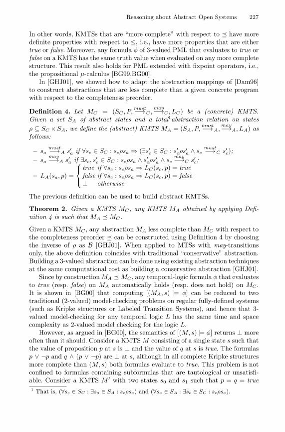
Reasoning about Abstract Open Systems 227

In other words, KMTSs that are “more complete” with respect to have moredefinite properties with respect to ≤, i.e., have more properties that are eithertrue or false. Moreover, any formula φ of 3-valued PML that evaluates to true orfalse on a KMTS has the same truth value when evaluated on any more completestructure. This result also holds for PML extended with fixpoint operators, i.e.,the propositional µ-calculus [BG99,BG00].

In [GHJ01], we showed how to adapt the abstraction mappings of [Dam96]to construct abstractions that are less complete than a given concrete programwith respect to the completeness preorder.

Definition 4. Let MC = (SC , P,must−→C ,

may−→C , LC) be a (concrete) KMTS.Given a set SA of abstract states and a total1abstraction relation on statesρ ⊆ SC ×SA, we define the (abstract) KMTS MA = (SA, P,

must−→A,may−→A, LA) as

follows:

– samust−→A s′

a if ∀sc ∈ SC : scρsa ⇒ (∃s′c ∈ SC : s′

cρs′a ∧ sc

must−→C s′c);

– samay−→A s′

a if ∃sc, s′c ∈ SC : scρsa ∧ s′

cρs′a ∧ sc

may−→C s′c;

– LA(sa, p) =

true if ∀sc : scρsa ⇒ LC(sc, p) = truefalse if ∀sc : scρsa ⇒ LC(sc, p) = false⊥ otherwise

The previous definition can be used to build abstract KMTSs.

Theorem 2. Given a KMTS MC , any KMTS MA obtained by applying Defi-nition 4 is such that MA MC .

Given a KMTS MC , any abstraction MA less complete than MC with respect tothe completeness preorder can be constructed using Definition 4 by choosingthe inverse of ρ as B [GHJ01]. When applied to MTSs with may-transitionsonly, the above definition coincides with traditional “conservative” abstraction.Building a 3-valued abstraction can be done using existing abstraction techniquesat the same computational cost as building a conservative abstraction [GHJ01].

Since by construction MA MC , any temporal-logic formula φ that evaluatesto true (resp. false) on MA automatically holds (resp. does not hold) on MC .It is shown in [BG00] that computing [(MA, s) |= φ] can be reduced to twotraditional (2-valued) model-checking problems on regular fully-defined systems(such as Kripke structures or Labeled Transition Systems), and hence that 3-valued model-checking for any temporal logic L has the same time and spacecomplexity as 2-valued model checking for the logic L.

However, as argued in [BG00], the semantics of [(M, s) |= φ] returns ⊥ moreoften than it should. Consider a KMTS M consisting of a single state s such thatthe value of proposition p at s is ⊥ and the value of q at s is true. The formulasp ∨ ¬p and q ∧ (p ∨ ¬p) are ⊥ at s, although in all complete Kripke structuresmore complete than (M, s) both formulas evaluate to true. This problem is notconfined to formulas containing subformulas that are tautological or unsatisfi-able. Consider a KMTS M ′ with two states s0 and s1 such that p = q = true1 That is, (∀sc ∈ SC : ∃sa ∈ SA : scρsa) and (∀sa ∈ SA : ∃sc ∈ SC : scρsa).

228 P. Godefroid

Logic MC SAT GMCPropositional Logic Linear NP-complete NP-complete

PML Linear PSPACE-complete PSPACE-completeCTL Linear EXPTIME-complete EXPTIME-complete

µ-calculus NP∩co-NP EXPTIME-complete EXPTIME-completeLTL PSPACE-complete PSPACE-complete EXPTIME-complete

Fig. 1. Known results on the complexity in the size of the formula for (2-valued and3-valued) model checking (MC), satisfiability (SAT) and generalized model checking(GMC).

in s0 and p = q = false in s1, and with a may-transition from s0 to s1. Theformula AXp∧¬AXq (which is neither a tautology nor unsatisfiable) is ⊥ at s0,yet in all complete structures more complete than (M ′, s0) the formula is false.This observation is used in [BG00] to define an alternative 3-valued semanticsfor temporal logics called the thorough semantics since it does more than theother semantics to discover whether enough information is present in a KMTSto give a definite answer. Let the completions C(M, s) of a state s of a KMTSM be the set of all states s′ of complete Kripke structures M ′ such that s s′.

Definition 5. Let φ be a formula of any two-valued logic for which a satisfactionrelation |= is defined on complete Kripke structures. The truth value of φ in astate s of a KMTS M under the thorough interpretation, written [(M, s) |= φ]t,is defined as follows:

[(M, s) |= φ]t =

true if (M ′, s′) |= φ for all (M ′, s′) in C(M, s)false if (M ′, s′) |= φ for all (M ′, s′) in C(M, s)⊥ otherwise

It is easy to see that, by definition, we always have [(M, s) |= φ] ≤ [(M, s) |=φ]t. In general, interpreting a formula according to the thorough three-valuedsemantics is equivalent to solving two instances of the generalized model-checkingproblem [BG00].

Definition 6 (Generalized Model-Checking Problem). Given a state s ofa KMTS M and a formula φ of a temporal logic L, does there exist a state s′ ofa complete Kripke structure M ′ such that s s′ and (M ′, s′) |= φ ?

This problem is called generalized model-checking since it generalizes both modelchecking and satisfiability checking. At one extreme, where M = (s0, P,

must−→=may−→= (s0, s0), L) with L(s0, p) =⊥ for all p ∈ P , all complete Kripke structuresare more complete than M and the problem reduces to the satisfiability problem.At the other extreme, where M is complete, only a single structure needs to bechecked and the problem reduces to model checking.

Algorithms and complexity bounds for the generalized model-checking prob-lem for various temporal logics were presented in [BG00]. In the case ofbranching-time temporal logics, generalized model checking has the same com-plexity in the size of the formula as satisfiability. In the case of linear-time

Reasoning about Abstract Open Systems 229

boil

teacoffee

choose

Fig. 2. Example of open system

temporal logic, generalized model checking is EXPTIME-complete in the size ofthe formula, i.e., harder than both satisfiability and model checking, which areboth PSPACE-complete in the size of the formula for LTL. Figure 1 summarizesthe complexity results of [BG00]. These results show that the complexity in thesize of the formula of computing [(M, s) |= φ]t (GMC) is always higher than thatof computing [(M, s) |= φ] (MC).

Regarding the complexity in the size of the model |M |, it is shown in [GJ02]that generalized model checking can in general require quadratic running timein |M |, but that the problem can be solved in time linear in |M | in the caseof (LTL or BTL) persistence properties, i.e., properties recognizable by (wordor tree) automata with a co-Buchi acceptance condition. Persistence propertiesinclude several important classes of properties of practical interest, such as allsafety properties.

2.2 Module Checking

The framework described in the previous section assumes that the abstract sys-tem M is closed, i.e., that its behavior is completely determined by the state ofthe system. But what if M is an abstraction of an open system?

An open system is a system that interacts with its environment and whosebehavior depends on this interaction. Such systems are also often called reac-tive. In [KV96], Kupferman and Vardi argued that verifying temporal properties(especially those specified in branching temporal logics) of open systems mustbe handled differently than traditional model checking. Their argument is bestillustrated with a simple example. Consider a vending machine M which repeat-edly boils water, asks the environment to choose between coffee and tea, anddeterministically serves a drink according to the external choice. This machineis depicted in Figure 2, where dotted transitions represent transitions taken bythe environment. The machine has four states: boil, choose, coffee and tea. WhenM is in state boil, we know exactly what its possible next states are (namely,choose and boil). In contrast, when M is in state choose, the set of possible nextstates is unknown since it depends on the environment: it could be any subsetof the set coffee, tea. To see the difference this makes semantically, considerthe property “is it always possible for M to eventually serve tea?”, which canbe represented as the CTL formula2 AGEF tea. If we evaluate this formula on2 See [Eme90] for a general introduction to the temporal logics used in this paper.

230 P. Godefroid

M viewed as a traditional Kripke structure, thus ignoring whether transitionsare taken by the system or its environment, we obtain [M |= AGEF tea] = true,since, for every state of M , there exists a path from that state to state tea. Incontrast, if we take into account transitions taken by the environment, the an-swer should be false since, if the environment decides to always choose coffee,the machine M will never serve tea. This observation prompted the introductionof a variant of the model-checking problem for reasoning about open systems,called the module checking problem:

Given a module (M, s) and a temporal logic formula φ, does (M, s)satisfy φ in all possible environments?

Formally, a module is defined in [KV96] as a Kripke structure whose set ofstates is partitioned into two sets: a set of system states, representing the stateswhere the system can make transitions (such as the states boil, coffee and tea inthe example above), and a second set of environment states, where the environ-ment can make transitions (such as the state choose in the previous example).Here, we will use an alternative formalization (already suggested in [KV96]) andrepresent modules as Modal Transition Systems instead: must-transitions willmodel system transitions while may-transitions will model environment transi-tions. Note that this second formalization is more general since it allows statesfrom which both system and environment transitions exist. To simplify nota-tions, we also use a set of atomic propositions and associate with each state alabeling from every propositions to the set true, false.

Definition 7 (Module). A module is a tuple (S, P,must−→ ,

may−→, L), where S is anonempty finite set of states, P is a finite set of atomic propositions,

may−→⊆ S×S

and must−→⊆ S × S are transition relations such that must−→⊆may−→, and L : S × P →true, false is an interpretation that associates a truth value in true, false witheach atomic proposition in P for each state in S.

A module is thus modeled as a KMTS where no proposition takes the value ⊥.In this context, module checking can then be formally defined as follows. Recallthat C(M, s) denotes the set of completions of a KMTS/module M (see previoussection): C(M, s) = (M ′, s′)|s s′ and M ′ is a KS.

Definition 8 (Module Checking). Given a module (M, s) and a temporallogic formula φ, we say that the module (M, s) satisfies φ, denoted (M, s) |=r φ,if ∀(M ′, s′) ∈ C(M, s) : (M ′, s′) |= φ. Checking whether (M, s) |=r φ is called themodule-checking problem.

Formalized this way3, it is clear that module checking (ModC) is related to gen-eralized model checking (GMC). In the next section, we study this relationship.3 The definition of module checking in [KV96] actually requires the transition rela-

tion of any (M ′, s′) in C(M, s) to be total, which has the effect of preventing theenvironment from blocking the system by refusing to execute any transition; thisassumption is eliminated here to simplify the presentation.

Reasoning about Abstract Open Systems 231

3 Comparing Module Checking and GMC

We first consider the case of properties specified in linear temporal logic (LTL) orin universal branching temporal logics such as ∀CTL and ∀CTL∗. In this case,[KV96] shows that module checking and model checking coincide. Indeed, bydefinition, an LTL or universal property holds of a model if and only if all pathsin that model satisfy the given (path) property. In the case of a module, modulechecking can be reduced to checking whether the property holds of the modulewhen placed in the maximal environment consisting of all possible environmenttransitions, which in turns is equivalent to model checking. This implies thatLTL module checking has the same complexity as LTL model checking: it isPSPACE-complete in the size of the formula and can be done in linear time inthe size of the model (it is also known to be NLOGSPACE-complete in |M |).In contrast, it is shown in [BG00,GJ02] that GMC for LTL can be more precisebut also more expensive than LTL model checking: GMC for LTL is EXPTIME-complete in the size of the formula [BG00] and can be done in quadratic time inthe size of the model [GJ02].

In the case of properties specified in branching temporal logics (BTL), thusincluding existential quantification, [KV96] shows that the complexity of mod-ule checking is higher than that of model checking, and is in fact as hard assatisfiability.

The following theorem states that, in the BTL case, GMC and module check-ing are interreducible.

Theorem 3. For any branching temporal logic L, the GMC problem and themodule checking problem for L are interreducible in linear time and logarithmicspace.

Proof. Consider a formula φ of the logic L and a module (M, s) represented by a KMTSas defined in Section 2.2. We have (M, s) |=r φ iff ∀(M ′, s′) ∈ C(M, s) : (M ′, s′) |= φ(by Definition 8) iff ¬∃(M ′, s′) ∈ C(M, s) : (M ′, s′) |= φ. For any branching temporallogic, the latter is equivalent to ¬GMC((M, s), ¬φ) (by Definition 6). Thus, we have(M, s) |=r φ iff GMC((M, s), ¬φ) does not hold. Conversely, GMC((M, s), φ) holds iff(M, s) |=r ¬φ.

In the BTL setting, generalized model checking and module checking are thusvery closely related. One could even say that they are the “dual” of each other,in the same sense as the quantifier ∀ is the dual of ∃ since ∀ = ¬∃¬. The previoustheorem also explains why both problems have the same complexity in the caseof BTL. For instance, [KV96] pointed out that the complexity in the size of theformula of module checking for a BTL L is the same as that of satisfiability forL, while a similar result was proved independently for GMC in [BG00].

This close correspondence also makes it possible to transfer unmatched re-sults obtained for one problem to the other. For instance, [KV96] only showsthat module checking for CTL can be done in PTIME in the size of M . Usingthe results of [GJ02] concerning the complexity of GMC in the size of M , weimmediately obtain that module checking for CTL can require quadratic run-ning time in |M |, but that it can be solved in time linear in |M | in the case of

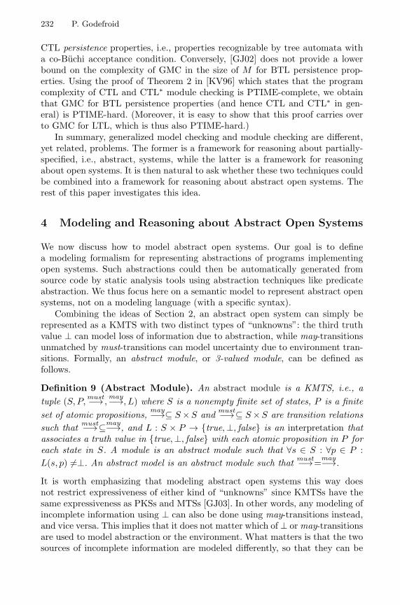
232 P. Godefroid

CTL persistence properties, i.e., properties recognizable by tree automata witha co-Buchi acceptance condition. Conversely, [GJ02] does not provide a lowerbound on the complexity of GMC in the size of M for BTL persistence prop-erties. Using the proof of Theorem 2 in [KV96] which states that the programcomplexity of CTL and CTL∗ module checking is PTIME-complete, we obtainthat GMC for BTL persistence properties (and hence CTL and CTL∗ in gen-eral) is PTIME-hard. (Moreover, it is easy to show that this proof carries overto GMC for LTL, which is thus also PTIME-hard.)

In summary, generalized model checking and module checking are different,yet related, problems. The former is a framework for reasoning about partially-specified, i.e., abstract, systems, while the latter is a framework for reasoningabout open systems. It is then natural to ask whether these two techniques couldbe combined into a framework for reasoning about abstract open systems. Therest of this paper investigates this idea.

4 Modeling and Reasoning about Abstract Open Systems

We now discuss how to model abstract open systems. Our goal is to definea modeling formalism for representing abstractions of programs implementingopen systems. Such abstractions could then be automatically generated fromsource code by static analysis tools using abstraction techniques like predicateabstraction. We thus focus here on a semantic model to represent abstract opensystems, not on a modeling language (with a specific syntax).

Combining the ideas of Section 2, an abstract open system can simply berepresented as a KMTS with two distinct types of “unknowns”: the third truthvalue ⊥ can model loss of information due to abstraction, while may-transitionsunmatched by must-transitions can model uncertainty due to environment tran-sitions. Formally, an abstract module, or 3-valued module, can be defined asfollows.

Definition 9 (Abstract Module). An abstract module is a KMTS, i.e., atuple (S, P,

must−→ ,may−→, L) where S is a nonempty finite set of states, P is a finite

set of atomic propositions,may−→⊆ S ×S and must−→⊆ S ×S are transition relations

such that must−→⊆may−→, and L : S × P → true,⊥, false is an interpretation thatassociates a truth value in true,⊥, false with each atomic proposition in P foreach state in S. A module is an abstract module such that ∀s ∈ S : ∀p ∈ P :L(s, p) =⊥. An abstract model is an abstract module such that must−→=

may−→.

It is worth emphasizing that modeling abstract open systems this way doesnot restrict expressiveness of either kind of “unknowns” since KMTSs have thesame expressiveness as PKSs and MTSs [GJ03]. In other words, any modeling ofincomplete information using ⊥ can also be done using may-transitions instead,and vice versa. This implies that it does not matter which of ⊥ or may-transitionsare used to model abstraction or the environment. What matters is that the twosources of incomplete information are modeled differently, so that they can be

Reasoning about Abstract Open Systems 233

distinguished in the model. Indeed, these two types of partial information aretreated differently, as we will see later.

We now turn to the definition of abstract module checking, or 3-valued modulechecking. For doing so, we first need to define the set of possible environmentsin which an abstract module can be executed. We formally represent this set asthe set of completions of the abstract module with respect to a preorder MTS ,which we define as follows.

Definition 10 ( MTS). Let MA = (SA, P,must−→A,

may−→A, LA) and MC = (SC , P,must−→C ,

may−→C , LC) be KMTSs. The preorder MTS is the greatest relation B ⊆SA × SC such that (sa, sc) ∈ B implies the following:

– ∀p ∈ P : LA(sa, p) = LC(sc, p),– if sa

must−→A s′a, there is some s′

c ∈ SC such that scmust−→C s′

c and (s′a, s′

c) ∈ B,– if sc

may−→C s′c, there is some s′

a ∈ SA such that samay−→A s′

a and (s′a, s′

c) ∈ B.

The preorder MTS is similar to the completeness preorder on MTSs [LT88], butis defined on KMTSs and leaves truth values of atomic propositions unchanged.Definition 10 is also similar to Definition 3 defining on KMTSs except forthe first condition which prevents the refinement of unknown truth values. LetCMTS((M, s)) = (M ′, s′)|s MTS s′ and M ′ is a PKS denote the set of com-pletions of a module (M, s) with respect to MTS . We can now define abstractmodule checking as follows.

Definition 11 (Abstract Module Checking). Given an abstract module(M, s) and a temporal logic formula φ, computing the value

[(M, s) |=r φ] =

true if ∀(M ′, s′) ∈ CMTS(M, s) : [(M ′, s′) |= φ] = truefalse if ∃(M ′, s′) ∈ CMTS(M, s) : [(M ′, s′) |= φ] = false⊥ otherwise

is defined as the abstract module checking problem.

The previous definition generalizes the definition of module checking: when(M, s) is a concrete module (i.e., a module where no atomic proposition hasthe value ⊥ in any state), Definition 11 coincides with Definition 8 definingmodule checking.

Abstract module checking defines a new 3-valued logic for reasoning aboutabstract modules: its syntax is as usual and its semantics is defined by [(M, s) |=r

φ]. The following preorder PKS on KMTSs measures the degree of completenessof abstract modules with respect to the new semantics derived from abstractmodule checking.

Definition 12 ( PKS). Let MA = (SA, P,must−→A,

may−→A, LA) and MC = (SC , P,must−→C ,

may−→C , LC) be KMTSs. The preorder PKS is the greatest relation B ⊆SA × SC such that (sa, sc) ∈ B implies the following:

1. ∀p ∈ P : LA(sa, p) ≤ LC(sc, p),

234 P. Godefroid

2. if samay−→A s′

a, there is some s′c ∈ SC such that sc

may−→C s′c and (s′

a, s′c) ∈ B,

3. if samust−→A s′

a, there is some s′c ∈ SC such that sc

must−→C s′c and (s′

a, s′c) ∈ B,

4. if scmay−→C s′

c, there is some s′a ∈ SA such that sa

may−→A s′a and (s′

a, s′c) ∈ B,

5. if scmust−→C s′

c, there is some s′a ∈ SA such that sa

must−→A s′a and (s′

a, s′c) ∈ B.

The preorder PKS is similar to the completeness preorder on PKSs [BG99],but is defined on KMTSs and requires a bisimulation-like relation on both mayand must transitions. The above definition extends Definition 3 defining onKMTSs by also requiring conditions (2) and (5). An important property of PKS

is the following.

Lemma 1. Let MA = (SA, P,must−→A,

may−→A, LA) and MC = (SC , P,must−→C ,

may−→C

, LC) be KMTSs. Given any two states sa ∈ SA and sc ∈ SC , sa PKS sc impliesthe two following properties:

– ∀(M ′A, s′

a) ∈ CMTS(MA, sa) : ∃(M ′C , s′

c) ∈ CMTS(MC , sc) : s′a PKS s′

c, and– ∀(M ′

C , s′c) ∈ CMTS(MC , sc) : ∃(M ′

A, s′a) ∈ CMTS(MA, sa) : s′

a PKS s′c.

Intuitively, the previous lemma states that, if sa PKS sc, then the set of “pos-sible environments” (i.e., CMTS) for sa and sc are equivalent: any environmentof sa is a possible environment of sc and vice versa. This lemma is useful toprove our next theorem.

Theorem 4. Let MA = (SA, P,must−→A,

may−→A, LA) and MC = (SC , P,must−→C

,may−→C , LC) be two abstract modules (KMTSs) such that sa ∈ SA and sc ∈ SC ,

and let Φ be the set of all formulas of 3-valued PML. Then,

sa PKS sc iff (∀φ ∈ Φ : [(MA, sa) |=r φ] ≤ [(MC , sc) |=r φ]).

Proof. Omitted due to space limitations.

The previous theorem thus states that 3-valued PML defined with the semantics[(M, s) |=r φ] logically characterizes the preorder PKS .4 This implies that ab-stract module checking cannot distinguish abstract modules that are equivalentwith respect to the preorder PKS . Another important corollary of this theo-rem is that, by generating an abstraction (MA, sa) from (a static analysis of)a concrete module (MC , sc) such that sa PKS sc, we can then both prove anddisprove arbitrary properties of sc by doing module checking of its abstractionsa. How to automatically generate abstractions preserving PKS is discussedwith an example later in Section 6.

In the case of LTL, abstract (3-valued) module checking, i.e., computing[(M, s) |=r φ], reduces to abstract (3-valued) model checking, i.e., comput-ing [(M, s) |= φ] with M viewed as a PKS where all the may-transitions arealso must-transitions. In the BTL case, 3-valued module checking can be ap-proximated by 3-valued model checking using the 3-valued semantics on KMTS4 As in the 2-valued case, this result also holds for the propositional µ-calculus.

Reasoning about Abstract Open Systems 235

defined in Definition 2. Indeed, [(M, s) |= φ] = true (respectively false) im-plies that ∀(M ′, s′) ∈ C(M, s) : (M ′, s′) |= φ (resp., (M ′, s′) |= φ), whichin turn implies that [(M, s) |=r φ] = true (resp., false). We thus always have[(M, s) |= φ] ≤ [(M, s) |=r φ]. Since 3-valued model checking can be done at thesame cost as traditional 2-valued model checking [BG00], computing [(M, s) |= φ]is less computationally expensive than computing [(M, s) |=r φ] in the BTL case(see Theorem 3), and can thus be used as a cheaper but less precise partialalgorithm for testing whether [(M, s) |=r φ] is true or false in that case.

5 Generalized Module Checking

As in the case of 3-valued model checking, precision of 3-valued module checkingcan be improved by defining a 3-valued thorough semantics, denoted [(M, s) |=r

φ]t. Let CPKS((M, s)) = (M ′, s′)|s PKS s′ and M ′ is a module denote theset of possible (concrete) modules for an abstract module (M, s).

Definition 13 (Thorough Abstract Module Checking). Given an abstractmodule (M, s) and a temporal logic formula φ, computing the value

[(M, s) |=r φ]t =

true if (M ′, s′) |=r φ for all (M ′, s′) in CPKS(M, s)false if (M ′, s′) |=r φ for all (M ′, s′) in CPKS(M, s)⊥ otherwise

is defined as the thorough abstract module checking problem.

The next theorem states that thorough abstract module checking is consistentwith abstract module checking.

Theorem 5. For any abstract module (M, s) and temporal logic formula φ, wehave [(M, s) |=r φ] ≤ [(M, s) |=r φ]t.

Proof. By definition, [(M, s) |=r φ] = true implies [(M, s) |=r φ]t = true. Moreover,[(M, s) |=r φ] = false implies [(M, s) |=r φ]t = false since ∃(M ′, s′) ∈ CMTS(M, s) :∀(M ′′, s′′) ∈ CPKS(M ′, s′) : (M ′′, s′) |= φ implies ∀(M ′, s′) ∈ CPKS(M, s) :∃(M ′′, s′′) ∈ CMTS(M ′, s′) : (M ′′, s′) |= φ.

Checking whether [(M, s) |=r φ]t = true can be reduced to solving an instanceof the generalized model checking problem for (M, s) and ¬φ with respect to thecompleteness preorder on KMTSs, because of the two universal quantificationsdefining [(M, s) |=r φ]t = true. In contrast, checking whether [(M, s) |=r φ]t =false involves an alternation between ∃ and ∀, and requires solving an instanceof the following problem, which we call generalized module checking.

Definition 14 (Generalized Module-Checking Problem). Given a state sof an abstract module M and a formula φ of a temporal logic L, does there exista state s′ of a module M ′ such that s PKS s′ and (M ′, s′) |=r φ ?

236 P. Godefroid

Clearly, generalized module checking (GModC) generalizes both module check-ing and generalized model checking for any (i.e., BTL or LTL) temporal logicsince it includes both as particular sub-problems. Hence, generalized modulechecking is at least as hard as generalized model checking, which is itself harderthan module checking in the LTL case and as hard as module checking in theBTL case (see Section 3). Is GModC harder than GMC? The next theorem showsthat this is not the case by providing a reduction from GModC to GMC.

Theorem 6. Given any (LTL or BTL) temporal logic L, any instance of thegeneralized module checking problem for L can be reduced in linear time andlogarithmic space to an instance of the generalized model checking problem for L.

Proof. (Sketch) Consider a formula φ of the logic L and an abstract module (M, s)represented by a KMTS M = (S, P,

must−→ ,may−→, L) as defined in Section 4. Without loss

of generality, let us assume that φ is in positive form in which negation can apply only toatomic propositions. We first define a PKS M ′ = (S′, P ′, →′, L′) that simulates exactlythe may and must transitions of M with an additional proposition pmust as follows:S′ = S × must, may, P ′ = P ∪ pmust, →′= ((s, x), (s′, x′))|(s, s′) ∈may−→, x′ =must if (s, s′) ∈must−→ or x′ = may otherwise, ∀(s, x) ∈ S′ : ∀p ∈ P : L′((s, x), p) =L(s, p), and L′((s, x), pmust) = true if x = must or L′((s, x), pmust) = false otherwise.Second, we translate the formula φ into the formula T (φ) defined with a set P ′ = P ∪pmust of atomic propositions by applying recursively the following rewrite rules: forall p ∈ P , T (p) = p and T (¬p) = ¬p; T (φ1 ∧φ2) = T (φ1)∧T (φ2); T (φ1 ∨φ2) = T (φ1)∨T (φ2); T (AXφ) = AX(T (φ)); T (EXφ) = EX(pmust ∧ T (φ)). (Note that the aboverules are for PML; in the case of the mu-calculus, fixpoint operators are left unchanged;a similar translation exists for LTL). Third, we show that GModC((M, s), φ) = trueiff GMC((M ′, (s, must)), T (φ)) = true.

To summarize, GModC has the same complexity as GMC. This implies thefollowing, maybe surprising, corollary: even though computing [(M, s) |=r φ]t(thorough abstract module checking) can be more precise than computing[(M, s) |=r φ] (abstract module checking), it has the same complexity in theBTL case.

6 Application

The practical motivation for this paper is to provide a framework for verifyingproperties of programs implementing open systems using automatic abstractiontechniques such as predicate abstraction.

An example of program implementing an open system is shown on the left ofFigure 3. In this program, x and y denote variables controlled by the program(system), f denotes some unknown function of the system, while z denotes avariable controlled by the environment. The notation “x, y = 1, 0” means thatvariables x and y are simultaneously assigned to values 1 and 0, respectively.

Imagine we are interested in checking the property “(eventually y is odd)and (at any time, x is odd or y is even)”. From this property, we define twopredicates p : “is x odd?” and q : “is y odd?”. Given these two predicates, theproperty can be represented by the LTL formula φ = q ∧ (p ∨ ¬q).

Reasoning about Abstract Open Systems 237

program C() x,y= 1,0;if (read(z) == 0) then

x,y = 2*f(x),f(y);x,y = 1,0;

elsex,y = f(x),f(y);

(p=T,q=F)

s(p= ,q= )⊥ ⊥(p=T,q=F)

M

(p=F,q= )⊥

Fig. 3. Example of open program and abstract module

Using predicate abstraction techniques and predicates p and q, one can au-tomatically compute an abstract module for this program that satisfies the pre-order PKS and thus Theorem 4, by construction. An example of such an ab-stract module (M, s) for this program is shown on the right of Figure 3. Thetruth values of atomic propositions p and q is defined in each state as indi-cated in the figure. Dotted transitions indicate may-transitions unmatched bymust-transitions and represent transitions controlled by the environment. Notehow the unknown function f is modeled using ⊥, while uncertainty due to theenvironment is modeled using may-transitions.

In this example, we have [(M, s) |=r φ] =⊥, while [(M, s) |=r φ]t = false. Inother words, using the thorough interpretation and generalized module checkingis needed to obtain a definite answer in this case. Indeed, this result is obtainedby proving that, for all possible completions (M ′, s′) such that (M, s) PKS

(M ′, s′), there exists an environment of (M ′, s′) (namely the one which forcesthe system down the leftmost path) where φ is violated. We are not aware ofany decision procedure more efficient than generalized module checking to proveautomatically that the open program C of Figure 3 violates property φ.5

Finally note how GModC differ from GMC in the presence of may-transitions:while GModC((M, s), φ) = false, we have GMC((M, s), φ) =⊥.

7 Conclusions

We have presented a framework for representing and reasoning about abstractopen systems. Our framework is designed to be used in conjunction with auto-matic abstraction tools for generating abstractions from static program analysis.We identified the preorder PKS as the one being logically characterized by the5 Note that, since GMC for LTL can be reduced to SAT for CTL∗ (using Theorem 23

of [BG00]), the above verification results could be obtained using a SAT solver forCTL∗, but at a much higher complexity both in |M | and |φ|.

238 P. Godefroid

Logic MC ModC GModCPropositional Logic Linear Linear NP-complete

PML Linear PSPACE-complete PSPACE-completeCTL Linear EXPTIME-complete EXPTIME-complete

µ-calculus NP∩co-NP EXPTIME-complete EXPTIME-completeLTL PSPACE-complete PSPACE-complete EXPTIME-complete

Fig. 4. Complexity in the size of the formula of model checking (MC), module checking(ModC), and generalized module checking (GModC).

3-valued semantics derived from the definition of module checking of [KV96].Any abstraction that preserves PKS can then be used to both prove and dis-prove arbitrary temporal properties of the concrete program. We introduced newvariants of the module checking problem suitable for reasoning about such ab-stractions, namely abstract, thorough abstract and generalized module checking.We also studied the complexity of these problems. The complexity of generalizedmodule checking is summarized in the last column of Figure 4. The precisionof generalized module checking was illustrated with an example of program andproperty that is beyond the scope of current abstraction-based verification tools.

Note that generating an abstraction (MA, sa) preserving PKS assumes thatit is possible to determine which transitions of the concrete module (MC , sc) arecontrolled by the system and which transitions are controlled by the environ-ment. Our framework does not currently support a way to safely approximate(MC , sc) in the case this information is unknown (i.e., cannot be determinedexactly by a static analysis). Previous work on alternating refinement rela-tions [AHKV98,AH01] provides a way to conservatively abstract a game (like theone played between a system and its environment) while preserving the existenceof a winning strategy for one of the players. However, such game abstractionsdo not preserve the existence of a winning strategy for the other player: theyare conservative in the same sense as a simulation relation defines a conservativeabstraction of a system, which can be used for proving universal properties butnot refuting these. An interesting topic for future work is therefore to study howto combine our framework with techniques for abstracting games with the goalof designing “3-valued game abstractions” that would preserve winning strate-gies for both players while allowing abstraction. Such a way, one could extendthe framework developed in this paper to allow sound approximations of thepartitioning between system and environment transitions while preserving theability to prove and disprove any temporal property of the interaction of thesystem with its environment.

References

[AH01] L. de Alfaro and T. Henzinger. Interface Automata. In Proceedings ofthe 9th ACM Symposium on the Foundations of Software Engineering(FSE’01), 2001.

Reasoning about Abstract Open Systems 239

[AHKV98] R. Alur, T. Henzinger, O. Kupferman, and M. Vardi. Alternating Refine-ment Relations. In Proc. 10th Conference on Concurrency Theory, vol-ume 1466 of Lecture Notes in Computer Science, pages 163–178. Springer-Verlag, 1998.

[BG99] G. Bruns and P. Godefroid. Model Checking Partial State Spaces with3-Valued Temporal Logics. In Proceedings of the 11th Conference on Com-puter Aided Verification, volume 1633 of Lecture Notes in Computer Sci-ence, pages 274–287, Trento, July 1999. Springer-Verlag.

[BG00] G. Bruns and P. Godefroid. Generalized Model Checking: Reasoningabout Partial State Spaces. In Proceedings of CONCUR’2000 (11th In-ternational Conference on Concurrency Theory), volume 1877 of LectureNotes in Computer Science, pages 168–182, University Park, August 2000.Springer-Verlag.

[BR01] T. Ball and S. Rajamani. The SLAM Toolkit. In Proceedings of CAV’2001(13th Conference on Computer Aided Verification), volume 2102 of LectureNotes in Computer Science, pages 260–264, Paris, July 2001. Springer-Verlag.

[CDH+00] J. C. Corbett, M. B. Dwyer, J. Hatcliff, S. Laubach, C. S. Pasareanu,Robby, and H. Zheng. Bandera: Extracting Finite-State Models from JavaSource Code. In Proceedings of the 22nd International Conference onSoftware Engineering, 2000.

[Dam96] D. Dams. Abstract interpretation and partition refinement for model check-ing. PhD thesis, Technische Universiteit Eindhoven, The Netherlands,1996.

[DD01] S. Das and D. L. Dill. Successive Approximation of Abstract TransitionRelations. In Proceedings of LICS’2001 (16th IEEE Symposium on Logicin Computer Science), pages 51–58, Boston, June 2001.

[Eme90] E. A. Emerson. Temporal and Modal Logic. In J. van Leeuwen, editor,Handbook of Theoretical Computer Science. Elsevier/MIT Press, Amster-dam/Cambridge, 1990.

[GHJ01] P. Godefroid, M. Huth, and R. Jagadeesan. Abstraction-based ModelChecking using Modal Transition Systems. In Proceedings of CON-CUR’2001 (12th International Conference on Concurrency Theory), vol-ume 2154 of Lecture Notes in Computer Science, pages 426–440, Aalborg,August 2001. Springer-Verlag.

[GJ02] P. Godefroid and R. Jagadeesan. Automatic Abstraction Using General-ized Model Checking. In Proceedings of CAV’2002 (14th Conference onComputer Aided Verification), volume 2404 of Lecture Notes in ComputerScience, pages 137–150, Copenhagen, July 2002. Springer-Verlag.

[GJ03] P. Godefroid and R. Jagadeesan. On the Expressiveness of 3-Valued Mod-els. In Proceedings of VMCAI’2003 (4th Conference on Verification, ModelChecking and Abstract Interpretation), volume 2575 of Lecture Notes inComputer Science, pages 206–222, New York, January 2003. Springer-Verlag.

[GS97] S. Graf and H. Saidi. Construction of Abstract State Graphs with PVS.In Proceedings of the 9th International Conference on Computer AidedVerification, volume 1254 of Lecture Notes in Computer Science, pages72–83, Haifa, June 1997. Springer-Verlag.

[HJMS02] T. Henzinger, R. Jhala, R. Majumdar, and G. Sutre. Lazy Abstraction. InProceedings of the 29th ACM Symposium on Principles of ProgrammingLanguages, pages 58–70, Portland, January 2002.

240 P. Godefroid

[HJS01] M. Huth, R. Jagadeesan, and D. Schmidt. Modal Transition Systems: aFoundation for Three-Valued Program Analysis. In Proceedings of the Eu-ropean Symposium on Programming (ESOP’2001), volume 2028 of LectureNotes in Computer Science. Springer-Verlag, April 2001.

[Kle87] S. C. Kleene. Introduction to Metamathematics. North Holland, 1987.[Koz83] D. Kozen. Results on the Propositional Mu-Calculus. Theoretical Com-

puter Science, 27:333–354, 1983.[KV96] O. Kupferman and M. Vardi. Module Checking. In Proc. 8th Confer-

ence on Computer Aided Verification, volume 1102 of Lecture Notes inComputer Science, pages 75–86, New Brunswick, August 1996. Springer-Verlag.

[LT88] K. G. Larsen and B. Thomsen. A Modal Process Logic. In Proceedings ofThird Annual Symposium on Logic in Computer Science, pages 203–210.IEEE Computer Society Press, 1988.

[VHBP00] W. Visser, K. Havelund, G. Brat, and S. Park. Model Checking Programs.In Proceedings of ASE’2000 (15th International Conference on AutomatedSoftware Engineering), Grenoble, September 2000.

Schedule-Carrying Code

Thomas A. Henzinger, Christoph M. Kirsch, and Slobodan Matic

EECS, University of California, Berkeley

Abstract. We introduce the paradigm of schedule-carrying code (SCC).A hard real-time program can be executed on a given platform only ifthere exists a feasible schedule for the real-time tasks of the program.Traditionally, a scheduler determines the existence of a feasible sched-ule according to some scheduling strategy. With SCC, a compiler provesthe existence of a feasible schedule by generating executable code thatis attached to the program and represents its schedule. An SCC exe-cutable is a real-time program that carries its schedule as code, which isproduced once and can be revalidated and executed with each use. Weevaluate SCC both in theory and practice. In theory, we give two scenar-ios, of nonpreemptive and distributed scheduling for Giotto programs,where the generation of a feasible schedule is hard, while the validationof scheduling instructions that are attached to the programs is easy. Inpractice, we implement SCC and show that explicit scheduling instruc-tions can reduce the scheduling overhead up to 35% and can provide anefficient, flexible, and verifiable means for compiling Giotto programs oncomplex architectures, such as the TTA.

1 Introduction

Giotto is a high-level programming language for hard real-time applications [4].A Giotto program consists of a collection of modes, each specifying the releasetimes and deadlines of a set of periodic tasks. In Giotto, the semantics of valuepropagation between tasks is defined independent of the system scheduler, andtherefore deterministic: as long as the scheduler maintains all deadlines, theoutputs of all task invocations are determined by the sensor inputs, and donot depend on the task ordering, distribution, or preemption mechanism of aparticular RTOS. A Giotto program is executable only if there exists a schedulethat meets all deadlines on a given hardware platform, with given resourcesand performance. An executable combination of Giotto program and platformdata (primarily worst-case execution times for all tasks) is called time-safe [5].The Giotto compiler must, in addition to generating code, prove time safety [6].The proof of time safety establishes the existence of a feasible schedule, and indoing so, produces the schedule. We introduce the idea of schedule-carrying code(SCC): once a feasible schedule has been produced, it can be attached to the code This work was supported by the AFOSR MURI grant F49620-00-1-0327, the Califor-

nia MICRO grant 01-037, the DARPA grant F33615-C-98-3614, the MARCO grant98-DT-660, and the NSF grants CCR-0208875, CCR-0085949, and CCR-0225610.

R. Alur and I. Lee (Eds.): EMSOFT 2003, LNCS 2855, pp. 241–256, 2003.c© Springer-Verlag Berlin Heidelberg 2003

242 T.A. Henzinger, C.M. Kirsch, and S. Matic

to serve as a witness for time safety, in case the code source is untrusted, or if thecode is moved to multiple targets. Thus, SCC is the paradigm of proof-carryingcode [10] extended from traditional safety properties, such as memory safety,to real-time properties. SCC, however, offers an even more important capabilitythan the reuse of time-safety proofs. If the schedule itself is provided in the formof executable instructions, properly attached to the code generated from Giotto,then SCC renders the system scheduler of the target platform obsolete. Thisleads to dramatic performance improvements in executing Giotto programs [7].

Let us be more precise. We define two virtual execution engines called theE(mbedded) machine, and the S(cheduling) machine. The E machine executesE code generated from a Giotto program [5]. E code is reactive code: it managesthe release times and deadlines of software tasks in reaction to environmentevents, such as clock ticks. When an environment interrupt occurs, E code maycall a driver that reads a sensor port, or writes an actuator port, or transfers avalue between ports, and it may release a task to the system. If an RTOS is used,the released task enters the ready queue, and can be dispatched by the systemscheduler. A Giotto compiler that proves time safety is a schedule-generatingcompiler : it generates, in addition to E code, also S code, which represents afeasible schedule for the generated E code. S code is executed by the S machine,which replaces the system scheduler. S code is proactive code: it manages theexecution of released tasks on the available CPUs. S code may dispatch a task fora certain amount of time (time-slice preemptive scheduling), or until another taskis released (priority preemptive), or until the task completes (nonpreemptive).In other words, the S language is an expressive, executable schedule descriptionlanguage. Our implementation executes intertwined E and S code produced bythe Giotto compiler, and thus provides the kernel functionality of an RTOS.

The usefulness of SCC rests on two premises. First, the execution of S codeis more efficient, and at least as flexible, as the use of the scheduler providedby an RTOS. This is substantiated by our experiments, where we achieve upto 35% overhead reduction and demonstrate the ability to change schedulingstrategies when switching Giotto modes [7]. Second, it is often more efficient tocheck the feasibility of a schedule than to generate the schedule (“proof checkingis easier than proof generation”). Whenever this is the case, then it is beneficialto have the Giotto compiler generate a feasible schedule once, and attach it tothe generated E code in the form of S code. Then, before execution, the targetplatform may check the schedule in order to be sure that it can execute thecode without time-safety violations (i.e., without missing any deadlines specifiedby the original Giotto program). While preemptive single-CPU scheduling forGiotto is simple [6], it is NP-hard to generate nonpreemptive or distributedschedules for Giotto programs, even if the program has only a single mode. Weshow that these schedules, once expressed in S code, can be checked in timelinear in the size of the E code and the frequency of events. More generally,SCC provides an efficient implementation of Giotto in the presence of manyscheduling constraints. In particular, in Section 4 we show how Giotto can becompiled onto a time-triggered architecture using SCC.

Schedule-Carrying Code 243

Completion Ports

MachineEmbedded

PortsEnvironment

PortsTask

PortsDriver Driver

Ports

SchedulingMachineEnvironment Tasks Hardware

DriverPorts

DriverPorts

PortsHardware

PortsTask

Release Ports

Fig. 1. The E machine and the S machine

2 SCC: Embedded Code Plus Scheduling Code

The E machine [5] is a virtual machine that interpretes E code, which supervisesthe execution of software tasks in response to physical events. The S machineis a virtual machine that interpretes S code, which specifies the temporal or-der of task execution. Figure 1 shows how E and S machine interact with thephysical environment, software tasks, and hardware platform. We first reviewthe E machine and then introduce the S machine.

2.1 The Embedded Machine

Interface. Physical environment processes communicate information to the E ma-chine through environment ports, such as clocks and sensors, and applicationsoftware processes, called tasks, communicate information to the E machinethrough task ports. The E machine communicates information to the environ-ment and the tasks by calling system software processes, called drivers, whichwrite to driver ports, for instance actuators. The E machine releases tasks forexecution to the task scheduler (the S machine, or the scheduler of an RTOS)by writing to release ports, and the scheduler signals the completion of tasksto the E machine through completion ports. Hence, the environment, task, andcompletion ports are the input ports of the E machine. A change of value at aninput port is an input event and causes an interrupt. The E machine monitorsthe occurrence of input events through triggers. In this paper, we consider onlytime triggers. A time trigger can be specified as a positive integer δ; it watches anenvironment clock and becomes enabled δ clock ticks after its activation. Tasks,drivers, and triggers are external to the E machine and must be implemented insome programming language like C. Tasks are preemptive, user-level code with-out internal synchronization points; drivers are system-level code during whoseexecution all interrupts that correspond to input events are disabled. The taskidle is a special task that never completes.

E code. There are three non-control-flow E code instructions. The call(d) in-struction initiates the execution of a driver d, and the E machine waits until d

244 T.A. Henzinger, C.M. Kirsch, and S. Matic

while ProgramCounter = ⊥ doi := Instruction(ProgramCounter)if call(d) = i thenif driver d accesses a port of a task t that has been released but not completedthen throw a time-safety exception else execute d

else if schedule(t) = i thenif task t has already been released but not yet completedthen throw a time-safety exception else emit a signal on the release port of t

else if future(g, a) = i thenappend the trigger binding (g, a, s) to TriggerQueue, where s is the currentstate of the input ports that occur in g

end ifProgramCounter := Next(ProgramCounter)

end while

Algorithm 1: The E code interpreter

is finished before proceeding to the next E code instruction. The schedule(t)instruction releases a task t to be executed, concurrently with other releasedtasks, and then the E machine proceeds immediately to the next E code instruc-tion. The schedule instruction does not order the execution of tasks, nor doesit relinquish control of the CPU to the scheduler. The future(g, a) instructionactivates the trigger g and marks the E code at address a for execution at thefuture time instant when g becomes enabled. In order to handle multiple activetriggers, the E machine maintains a queue of trigger bindings (g, a, s), where s isthe current state of the input ports watched by the trigger g, which is requiredfor evaluating g in the future. E code has also control-flow instructions suchas if(c, a) and return. In the former case, if the condition c (a predicate oninput ports) evaluates to true, then the E machine proceeds to address a; other-wise it proceeds to the next instruction. The return instruction terminates theexecution of E code.

Algorithm 1 summarizes the E code interpreter. For each input event, theE machine checks the trigger bindings in TriggerQueue. The first trigger binding(g, a, s) in the queue with an enabled trigger g is removed from the queue and theinterpreter is invoked with ProgramCounter set to address a. This is repeateduntil the queue contains no trigger binding with an enabled trigger. Then, theE machine relinquishes control of the CPU to the task scheduler, which is eitherprovided by an RTOS [5] or implemented as S machine (see below). The goalof the scheduler is to execute the released tasks so that they complete beforetheir deadlines. E code specifies task deadlines in two ways: once released, a taskt must complete (1) before any driver accesses a port of t, and (2) before t isreleased again. If a task violates one of these conditions, then the E machinethrows a time-safety exception; otherwise the execution is time-safe.

Example. Figure 2 shows a Giotto program [4] in the left column and, in themiddle and right column, E code generated by the Giotto compiler [6]. TheGiotto program is a simplified version of a program that implements the flight

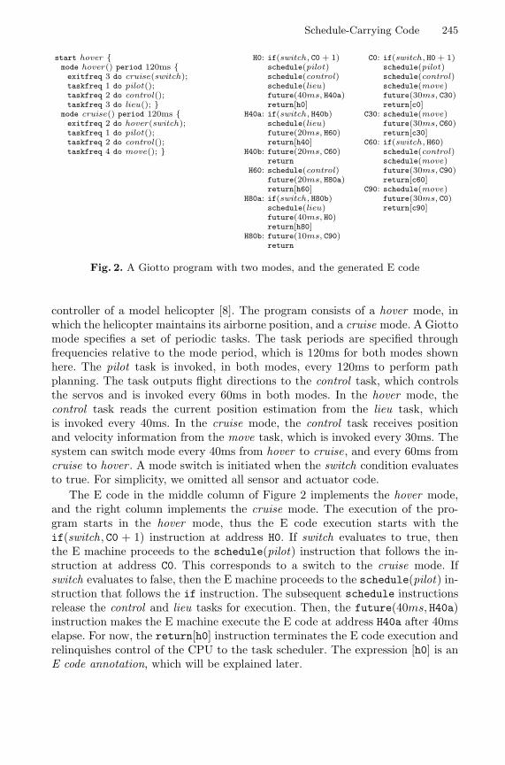
Schedule-Carrying Code 245

start hover mode hover() period 120ms exitfreq 3 do cruise(switch);taskfreq 1 do pilot();taskfreq 2 do control();taskfreq 3 do lieu();

mode cruise() period 120ms exitfreq 2 do hover(switch);taskfreq 1 do pilot();taskfreq 2 do control();taskfreq 4 do move();

H0: if(switch, C0 + 1)schedule(pilot)schedule(control)schedule(lieu)future(40ms, H40a)return[h0]

H40a: if(switch, H40b)schedule(lieu)future(20ms, H60)return[h40]

H40b: future(20ms, C60)return

H60: schedule(control)future(20ms, H80a)return[h60]

H80a: if(switch, H80b)schedule(lieu)future(40ms, H0)return[h80]

H80b: future(10ms, C90)return

C0: if(switch, H0 + 1)schedule(pilot)schedule(control)schedule(move)future(30ms, C30)return[c0]

C30: schedule(move)future(30ms, C60)return[c30]

C60: if(switch, H60)schedule(control)schedule(move)future(30ms, C90)return[c60]

C90: schedule(move)future(30ms, C0)return[c90]

Fig. 2. A Giotto program with two modes, and the generated E code

controller of a model helicopter [8]. The program consists of a hover mode, inwhich the helicopter maintains its airborne position, and a cruise mode. A Giottomode specifies a set of periodic tasks. The task periods are specified throughfrequencies relative to the mode period, which is 120ms for both modes shownhere. The pilot task is invoked, in both modes, every 120ms to perform pathplanning. The task outputs flight directions to the control task, which controlsthe servos and is invoked every 60ms in both modes. In the hover mode, thecontrol task reads the current position estimation from the lieu task, whichis invoked every 40ms. In the cruise mode, the control task receives positionand velocity information from the move task, which is invoked every 30ms. Thesystem can switch mode every 40ms from hover to cruise, and every 60ms fromcruise to hover . A mode switch is initiated when the switch condition evaluatesto true. For simplicity, we omitted all sensor and actuator code.

The E code in the middle column of Figure 2 implements the hover mode,and the right column implements the cruise mode. The execution of the pro-gram starts in the hover mode, thus the E code execution starts with theif(switch, C0 + 1) instruction at address H0. If switch evaluates to true, thenthe E machine proceeds to the schedule(pilot) instruction that follows the in-struction at address C0. This corresponds to a switch to the cruise mode. Ifswitch evaluates to false, then the E machine proceeds to the schedule(pilot) in-struction that follows the if instruction. The subsequent schedule instructionsrelease the control and lieu tasks for execution. Then, the future(40ms, H40a)instruction makes the E machine execute the E code at address H40a after 40mselapse. For now, the return[h0] instruction terminates the E code execution andrelinquishes control of the CPU to the task scheduler. The expression [h0] is anE code annotation, which will be explained later.

246 T.A. Henzinger, C.M. Kirsch, and S. Matic

while ProgramCounter = ⊥ doi := Instruction(ProgramCounter)ProgramCounter := Next(ProgramCounter)if call(d) = i thenif driver d accesses a port of a task t that has been released but not completedthen throw a time-safety exception else execute delse if dispatch(t, h, a) = i then

if there is a thread instance in ThreadSet with a non-idle task thenthrow a time-sharing exception

elseinsert the thread instance (t,ProgramCounter , h, a,ReferenceTime)into ThreadSet and set ProgramCounter to ⊥

end ifelse if idle(h) = i then

insert the thread instance (idle, ⊥, h,ProgramCounter ,ReferenceTime)into ThreadSet and set ProgramCounter to ⊥

else if fork(a) = i theninsert the thread instance (idle, ⊥, true, a, s) into ThreadSet , where s is thecurrent value of the system clock

end ifend while

Algorithm 2: The S code interpreter

2.2 The Scheduling Machine

Interface. The hardware on which the S machine runs communicates informationto the S machine through hardware ports, such as clocks and message buffers,and the tasks communicate information to the S machine through task ports.The S machine communicates information to the hardware and the tasks bycalling drivers. An external task handler (in our case, the E machine) signalsthe release of tasks to the S machine through release ports, and the S machinesignals the completion of tasks to the task handler by writing to completionports. Hardware, task, and release ports are input ports for the S machine, andchanges in their values are input events. The S machine monitors input eventsthrough timeouts. In this paper, we consider two kinds of timeouts. A clocktimeout is specified by a nonnegative integer δ; it watches a system clock andexpires δ clock ticks into the S code thread that contains the timeout. The releasetimeout Θ expires as soon as any task is released.

S code. There are four non-control-flow S code instructions. The call(d) instruc-tion initiates the execution of a driver d. Similar to the E machine, the S machinewaits until d is finished before proceeding to the next S code instruction. Thedispatch(t, h, a) instruction begins or resumes the execution of a task t until thetimeout h expires. There are two possible outcomes: (1) the S machine proceedsto the next instruction when t completes, in case this happens before the timeouth expires, or (2) the S machine proceeds to the instruction at address a when thetimeout h expires, in case this happens before t completes. Case (1) applies also if

Schedule-Carrying Code 247

RM: dispatch(lieu, +4)dispatch(control, +3)dispatch(pilot, +2)idle()fork(RM)return

EDF0/60: dispatch(lieu, +4)dispatch(control, +3)dispatch(pilot, +2)idle()fork(EDF40/80)return

EDF40/80: dispatch(control, +4)dispatch(lieu, +3)dispatch(pilot, +2)idle()fork(EDF0/60)return

Fig. 3. Rate-monotonic (RM) and earliest-deadline-first (EDF) S programs for thehover mode of the Giotto program from Figure 2

t has not been released or has already completed when the dispatch instructionis encountered. The idle(h) instruction makes the S machine idle until the time-out h expires even when there are released tasks that have not been completed.The S machine proceeds to the subsequent instruction when the timeout expires.The fork(a) instruction marks the S code at address a for execution in parallelto the S code that follows the instruction. The S code at a is a new thread ofexecution. In order to handle multiple threads, the S machine maintains a set ofthread instances. S code may also have control-flow instructions, but we do notconsider them here. The call, fork, and control-flow instructions of S code aretransient instructions, as they execute, like E code instructions, in logical zerotime. In contrast, the dispatch and idle instructions are timed instructions, asthey cause a passage of time.

Algorithm 2 summarizes the S code interpreter, which maintains the setThreadSet of thread instances. A thread instance has the form (t, b, h, a, s), whereeither t is the idle task and b = ⊥, or t is a regular task and b is the address atwhich the S machine continues executing when t completes before the timeout hexpires. When h expires before t completes, the S machine continues executing,instead, the S code at address a. The reference time s is the time when thethread instance was created by a fork instruction, which is required for evalu-ating clock timeouts. The S machine is woken up by an input event: a hardwareport may signal the completion of a task or the expiration of a clock timeout,or a release port may signal the release of a task. If a task t completes, then thethread instances of the form (t, b, ·, ·, s) become enabled, with ProgramCounterset to b, and ReferenceTime set to s. If a timeout h expires, then the thread in-stances of the form (·, ·, h, a, s) become enabled, with ProgramCounter = a andReferenceTime = s. With each input event, every enabled thread instance isremoved from ThreadSet and executed until a timed instruction is encountered(at that time, ProgramCounter is set to ⊥ by the interpreter). The executionorder for the enabled thread instances in ThreadSet is chosen nondeterministi-cally. If control ends at dispatch instructions in more than one thread, then atime-sharing exception occurs, because only one task can be dispatched on theCPU; otherwise the execution is time-sharing.

Examples. The left column of Figure 3 shows an S program with the initialaddress RM which implements rate-monotonic (RM) scheduling of the tasks in thehover mode of the Giotto program from Figure 2. The S program only works ifno mode switching occurs; S code that supports mode switching will be discussedbelow. We use idle() to abbreviate idle(Θ) and dispatch(t, +n) to abbreviate

248 T.A. Henzinger, C.M. Kirsch, and S. Matic

NP0: dispatch(move)dispatch(control)idle()fork(NP30)return

NP30: dispatch(move)dispatch(pilot, NP60)idle()fork(NP60)return

NP60: dispatch(pilot)dispatch(move)idle()fork(NP90)return

NP90: dispatch(control)dispatch(move)idle()fork(NP0)return

Fig. 4. Nonpreemptive (NP) S program for the cruise mode

dispatch(t, Θ, a + n), where a is the address of the instruction itself and n is arelative offset. In the example, the offsets in dispatch instructions always pointto fork instructions. The S program dispatches the tasks in a fixed, RM orderstarting with the task that has the highest frequency. Suppose that the tasksin the hover mode have been released by the E machine. Now, the S machinestarts executing the dispatch(lieu, +4) instruction. The lieu task executes untilit either completes or is preempted by the release of some other task. If the lieutask completes first, then the S machine proceeds to the dispatch(control , +3)instruction and executes the control task. Otherwise, if some task is releasedbefore lieu completes, the S machine proceeds to the fork(RM) instruction andforks a new thread starting again at address RM. The following return instructionterminates the current thread. If all tasks complete during the execution of athread, then the idle() instruction is reached and the S machine waits until sometask is released to start a new thread. Note that the execution of the S code istime sharing, and if there exists a feasible RM schedule for the tasks of the hovermode, then the S code guarantees the time-safe execution of the E code for thehover mode.

As an alternative to RM scheduling, the S code in the middle and rightcolumn implements earliest-deadline-first (EDF) scheduling of the tasks in thehover mode. The initial address of the EDF S program is EDF0/60. The threadat EDF0/60 initially dispatches the lieu task followed by the control and pilottasks. However, unlike the RM S program, as soon as the lieu task is releasedagain, the S machine forks a new thread at address EDF40/80 and terminates thecurrent thread. Now, at the 40ms instant, the control task is dispatched beforethe lieu task, because the control task has an earlier absolute deadline than thelieu task. If the control task already completed before the 40ms instant, thenthe S machine immediately proceeds to the next instruction and dispatches thelieu task. At the 60ms instant, the situation is the same as at 0ms. So, we forkagain a thread at EDF0/60. At the 80ms instant, the absolute deadlines of alltasks are the same. Thus we can use the thread at EDF40/80 again.

The S code of Figure 4 implements nonpreemptive (NP) scheduling of thetasks in the cruise mode. The initial address of the NP S program is NP0. We usedispatch(t) to abbreviate dispatch(t, false, a), where a is the address of the nextinstruction. Thus a dispatch(t) instruction executes the task t until completion.Given the worst-case execution time w(t) of each task t, the S program guaran-tees time safety if w(move) + w(control) ≤ 30ms and 2 · w(move) + w(pilot) ≤60ms. Time sharing is ensured because the S program dispatches all tasks non-preemptively, i.e., each task completes before another task is dispatched. Tasksmay still be preempted by E code and S code, but not by other tasks.

Schedule-Carrying Code 249

h0/h60:dispatch(lieu, +3)dispatch(control, +2)dispatch(pilot, +1)return

h40/h80:dispatch(control, +3)dispatch(lieu, +2)dispatch(pilot, +1)return

c0/c30/c60/c90:dispatch(move, +3)dispatch(control, +2)dispatch(pilot, +1)return

Fig. 5. Earliest-deadline-first (EDF) S program for both modes

Figure 5 shows an S program that EDF schedules the tasks of both modes. Inorder to facilitate the interaction of E and S code in the presence of conditional-branch instructions (mode switching) in E code, we allow the E code to fork anew thread instance of S code through E code annotations. Recall the E code ofFigure 2. The return[h0] instruction of the code block at address H0 terminatesthe execution of the code block and, in addition, forks a new thread of S codeat address h0. We start running the E program and S program by executing theE code at the initial address H0. Now the initial address of the S program isnot required and thus ⊥. The E code releases all three tasks of the hover modeand then creates a new S code thread starting at h0. The thread dispatchesthe three tasks in EDF order. Suppose that the lieu task completes before the40ms instant, but not the control task. Thus, at the 40ms instant, the E code atH40a preempts the control task. Now, suppose that we switch from the hover tothe cruise mode. We branch to the E code at H40b, which does not release anytasks but only jumps to the E code at C60 after another 20ms elapse. Therefore,after executing the E code at H40b, the current S code thread continues where itwas preempted by resuming the execution of the control task. No new thread iscreated. Now, suppose that the control task completes before the 60ms instant,but not the pilot task. Now, at the 60ms instant, the E code at C60 preempts thepilot task. Unlike before, the control task is released now, no matter if we switchmode or not. Since the current S code thread becomes enabled upon the releaseof a task, the thread is terminated by jumping to the return instruction of thecode block at h0. Suppose that we stay in the cruise mode, i.e., the code blockat C60 is executed. In addition to the control task, the move task is releasedand a new S code thread at c60 is created, which dispatches now the tasks ofthe cruise mode in EDF order. Note that the S code for the cruise mode isequivalent to RM S code, because the task frequencies in the cruise mode areharmonic. The execution of the remaining E and S code works in a similar way.The S program is time sharing, and since EDF is optimal for Giotto programswith multiple modes [6], if there exists a feasible, preemptive schedule for thetasks of the hover and cruise modes, then the EDF S program guarantees thetime-safe execution of the E program regardless of any mode switching.

2.3 Schedule-Carrying Code

An SCC program is a pair (E , S) consisting of an E program E that shares a setof tasks with an S program S. If E contains conditional-branch instructions, thenits return instructions may be annotated with S code addresses as shown in theexample above. The runtime system for SCC is the E machine interacting with

250 T.A. Henzinger, C.M. Kirsch, and S. Matic

the S machine through release and completion ports. The machines are invokedas follows: (1) if there is an enabled thread instance that contains a completedtask, then the S machine must handle that thread instance before the E machinehandles any enabled triggers; (2) if there is an enabled trigger binding, thenthe E machine must handle that trigger binding before the S machine handlesany expired timeouts. The reason for (1) is that, when a task completes, thedispatching thread must be processed before any E code is executed in order toenable the prompt handling of output data upon task completion, say throughdriver calls in S code. The reason for (2) is that the E machine must be invokedbefore the S machine when an E code trigger is enabled at the same time whenan S code timeout expires, because the E code may release tasks that requirescheduling service from the S code. This will be formalized in the next section.

Implementation. With the help of Marco Sanvido, we have developed a mi-crokernel on a StrongARM SA-1110 processor with 206MHz which executesSCC programs using an integrated implementation of the E and S machine [7].The microkernel has a footprint of 8kB. We have tested the microkernel withSCC programs that implement four periodic, nonharmonic task sets with 4,10, 50, and 100 tasks. Each set consists of four equally large task groups with16.66Hz, 33.33Hz, 50Hz, and 100Hz tasks. The microkernel is invoked every 1msby a timer. The periodic release of the tasks is described by E code. We havecompared the performance of an EDF scheduler with S code that specifies EDFscheduling. The average time spent in the EDF scheduler is 1.4µs to schedule4 tasks and 35µs to schedule 100 tasks. The average time to execute, instead, theEDF S code grows from 2.2µs for scheduling 4 tasks to only 3.9µs for schedul-ing 100 tasks. With 100 tasks, EDF S code performs 35% better than the EDFscheduler (51% vs. 78% CPU utilization). For details, the reader is referred to [7].

3 Generating SCC vs. Checking SCC

We show that checking the time safety of given S code can be exponentiallysimpler than generating time-safe S code. Checking the time safety of SCC is aprogram-analysis problem. Following the tradition of path-insensitive programanalysis, we define the abstract semantics of SCC, which ignores all port valuesand assumes that both branches of conditionals can be taken. On this abstractsemantics, we present an efficient algorithm that provides a sufficient check forthe time safety of SCC generated from single-mode Giotto, which specifies a setof periodic tasks.

3.1 Abstract Semantics of SCC

An abstract E program E = (V, E, κ, λ, v) over a set T of tasks consists of acontrol-flow graph (V, E) which is a binary1 digraph, two edge-labeling functionsκ and λ, and an initial node v ∈ V . Each edge e ∈ E is labeled with an instructionκ(e) and an argument λ(e) as follows:1 Each node has at most two successors.

Schedule-Carrying Code 251

– κ(e) = call and λ(e) ⊆ T . The execution of e calls a driver that accessesports of the tasks in λ(e).

– κ(e) = schedule and λ(e) ∈ T . The execution of e releases the task λ(e).– κ(e) = future and λ(e) ∈ N>0 × V . The execution of e activates the trigger

with the binding λ(e) = (δ, u), which means that after δ time units, E codewill be executed starting from control location u.

We require that the initial node v has a single successor v′ ∈ V such thatκ(v, v′) = future and v′ is a leaf. We assume that a driver can access the portsof at most two (or any fixed number) of tasks, and that all integers δ can bestored in constant space; hence the size of E is |V |. A state q = (v, r, s, τ) of Econsists of a program counter v ∈ V , a status s: T → N ∪ , ⊥ for each task,and a queue τ ⊆ (N × V )∗ of trigger bindings. For each task t ∈ T , the statuss(t) = indicates that t has been released at the current time instant and notyet executed; the status s(t) ∈ N indicates that t has been released at a previoustime instant and executed for s(t) ≥ 0 time units; the status s(t) = ⊥ indicatesthat t has been completed (or not yet released). Note that the number of differentstatus functions, and hence the number of states, is exponential in |T |.

An abstract S program S = (V, E, µ, ν, κ, λ) over a set T of tasks consists of acontrol-flow graph (V, E) which is a binary digraph, two node-labeling functionsµ and ν, and two edge-labeling functions κ and λ. Each control location v ∈ Vis labeled by one of the following:

– µ(v) = dispatch and ν(v) ∈ T and v has a successor v1 such thatλ(v, v1) = ⊥, and possibly a second successor v2 such that either λ(v, v2) = ∗or λ(v, v2) ∈ N. The execution of v dispatches the task ν(v). If λ(v, v2) = ∗and a task is released before ν(v) completes, control proceeds to v2; ifλ(v, v2) ∈ N and ν(v) does not complete within the first λ(v, v2) time unitsfrom the time at which the current thread was created, control proceedsto v2; otherwise, control proceeds to v1 when ν(v) completes.

– µ(v) = idle and v has a single successor v′ such that either λ(v, v′) = ∗ orλ(v, v′) ∈ N. The execution of v idles the processor until a task is released(if λ(v, v′) = ∗), or until λ(v, v′) ∈ N time units pass from the time at whichthe current thread was created.

– µ(v) = . This indicates that control is at a transient instruction.

If e = (v, v′) and µ(v) = , then the edge e ∈ E is labeled by one of the following:

– κ(e) = call and λ(e) ⊆ T . The execution of e calls a driver that accessesports of the tasks in λ(e).

– κ(e) = fork and λ(e) ∈ V . If λ(e) = u, then the execution of e creates anew thread, which starts at control location u.

By our assumptions, the size of S is |V |. A state q = (s, θ) of S consists of thestatus s: T → N ∪ , ⊥ for each task, and a set θ of threads. Each thread(u, δ) consists of a program counter u ∈ V and a number δ ∈ N of time unitsfor which the thread has been executed. If u is a leaf, then the thread (u, δ) hasterminated and may be removed from θ.

252 T.A. Henzinger, C.M. Kirsch, and S. Matic

An abstract single-processor SCC program Π = (E , S, Φ) over a set T of tasksconsists of an abstract E program E over T , an abstract S program S over T , andan annotation function Φ that maps each leaf in the control graph of E to a nodein the control graph of S. When the E code execution arrives at a leaf v, thiscreates a new thread of S code which starts at control location Φ(v). A state of Πis a tuple q = (v, s, τ, θ) such that (v, s, τ) is a state of E , and (s, θ) is a state of S.The state q violates nonpreemption if there exist two different tasks t1, t2 ∈ Tsuch that s(t1), s(t2) ∈ , 0, ⊥. The state q violates time sharing if there existtwo different threads (u1, ·), (u2, ·) ∈ θ such that µ(u1) = µ(u2) = dispatch ands(ν(u1)) = ⊥ and s(ν(u2)) = ⊥. The state q violates time safety if there existsa task t ∈ T with s(t) = ⊥ and one of the following: (1) v has a successor v′

in E with either κ(v, v′) = call and t ∈ λ(v, v′), or κ(v, v′) = schedule andt = λ(v, v′); or (2) there exists a thread (u, ·) ∈ θ such that µ(u) = and uhas a successor u′ in S with κ(u, u′) = call and t ∈ λ(u, u′). The state q has atransition to the state q′ = (v′, s′, τ ′, θ′) if one of the following:

Completion S transition The state q is completion enabling, that is, thereexist a thread (u, δ) ∈ θ and a successor u′ of u in S such that µ(u) =dispatch and s(ν(u)) = ⊥ and λ(u, u′) = ⊥. Then (v′, s′, τ ′) = (v, s, τ) andθ′ = (θ\(u, δ)) ∪ (u′, δ).

Transient S transition The state q is transient enabling, that is, there exista thread (u, δ) ∈ θ and a successor u′ of u in S such that µ(u) = . Then(v′, s′, τ ′) = (v, s, τ) and one of the following:– κ(u, u′) = call and θ′ = (θ\(u, δ)) ∪ (u′, δ).– κ(u, u′) = fork and λ(u, u′) = u and θ′ = (θ\(u, δ)) ∪ (u′, δ), (u, 0).

E transition q is neither completion nor transient enabling but E enabling,that is, either (1) v has no successor and (0, u) ∈ τ for some u, or (2) v hasa successor v′ in E . If (1) let (0, u′) be the first such pair in τ . Then v′ = u′

and s′ = s and τ ′ = τ \ (0, u′) and θ′ = θ. If (2) then one of the following:– κ(v, v′) = call and s′ = s and τ ′ = τ .– κ(v, v′) = schedule and λ(v, v′) = t and s′(t) = and s′(t′) = s(t′) for

all tasks t′ ∈ T\t, and τ ′ = τ .– κ(v, v′) = future and s′ = s and τ ′ = τ λ(v, v′).

In all three cases, if v′ is a leaf, then θ′ = θ ∪ (Φ(v′), 0); otherwise θ′ = θ.Timeout S transition The state q is neither completion nor transient nor E

enabling but timeout enabling, that is, there exist a thread (u, δ) ∈ θ anda successor u′ of u in S such that µ(u) ∈ dispatch, idle and either(1) λ(u, u′) ∈ N and λ(u, u′) ≤ δ, or (2) λ(u, u′) = ∗ and s(t) = for sometask t ∈ T . Then (v′, s′, τ ′) = (v, s, τ) and θ′ = (θ\(u, δ)) ∪ (u′, δ).

Time transition The state q is neither completion nor transient nor timeoutnor E enabling. Then v′ = v. For all tasks t ∈ T , if there exists a thread(u, δ) ∈ θ with µ(u) = dispatch and ν(u) = t, then either s(t) = ands′(t) = 1, or s(t) ∈ N and s′(t) = s(t) + 1, or s′(t) = ⊥; if no such threadexists, then either s(t) = and s′(t) = 0, or s′(t) = and s′(t) = s(t). Incase s′(t) = ⊥, we say that on the transition (q, q′), task t completes afterexecution time s(t)+1. The queue τ ′ results from τ by replacing each trigger

Schedule-Carrying Code 253

binding (δ, u) by (δ−1, u). The set θ′ results from θ by replacing each thread(u, δ) by (u, δ + 1).

Note the priorities implied by this definition: transient S code that is enabledby the completion of tasks has priority over E code, which has priority overall remaining S code. A trace of the abstract single-processor SCC program Πis a sequence γ = q0, q1, . . . , qn of states of Π such that (1) q0 = (v, s, ∅, ∅),where v is the initial node of E , and s(t) = ⊥ for all tasks t ∈ T , and (2) forall i ≥ 0, there is a transition from qi to qi+1. The trace γ is time-safe (resp.time-sharing ; nonpreemptive) if no state of γ violates time safety (time sharing;nonpreemption).

An abstract multiprocessor SCC program Π over a set P of processors and aset T of tasks is a function that assigns to each processor p ∈ P a pair (Tp, Πp),where Tp ⊆ T such that Tp | p ∈ P is a partition of the task set T , and Πp

is an abstract single-processor SCC program over the set Tp of tasks. A trace γof Π is a function that assigns to each processor p ∈ P a trace γp of Πp suchthat all single-processor traces γp contain the same number of time transitions.The trace γ is time-safe (resp. time-sharing; nonpreemptive) if γp is time-safe(time-sharing; nonpreemptive) for all p ∈ P . A wcet map w: P × T → N assignsto every processor p and task t a worst-case execution time w(p, t) > 0. There area number of techniques for obtaining wcet maps, e.g. [2]. If P is a set of identicalprocessors, then w(p1, t) = w(p2, t) for all processors p1, p2 ∈ P and tasks t ∈ T .The trace γ of Π is an w-trace if for all processors p ∈ P , tasks t ∈ T , and i ≥ 0,if t completes on the transition (qi, qi+1) of γp, then it completes with executiontime at most w(p, t). The abstract (single- or multiprocessor) SCC program Π istime-safe (resp. time-sharing ; nonpreemptive) for wcet map w if all w-traces ofΠ are time-safe (time-sharing; nonpreemptive). The time safety (time sharing;nonpreemption) of an abstract SCC program can be checked by searching thestate space, but the number of states is exponential in the number of tasks. Wewill see that the check is simpler for SCC programs of a special form.

3.2 Giotto-Generated SCC

The E programs generated from Giotto programs have a special form [6]. Let Gbe a Giotto program [4] with task set T and a single mode m, let πm be the periodof m, let ft be the frequency in mode m of task t, and let fm be the least commonmultiple of all task and actuator frequencies in m. Then dm = πm/fm denotesthe time interval between consecutive input events. The abstract E programE = (V, E, κ, λ, v) over a set T ′ ⊆ T of tasks is G-generated if the control graph(V, E) consists, in addition to the initial location v and its successor v′, of a setof fm acyclic digraphs Ei, for 0 ≤ i < fm, such that every node in Ei has at mostone successor, and Ei consists of a source node vi followed by (1) a sequence ofO(|G|) edges (v, v′) with κ(v, v′) = call, followed by (2) a sequence of edges(v, v′) with κ(v, v′) = schedule and λ(v, v′) = t for each task t ∈ T ′ for which(i · ft/fm) ∈ N, followed by (3) a single edge (v, v′) with κ(v, v′) = futureand λ(v, v′) = (dm, v(i+1)modfm

). Moreover, λ(v, v′) = (0, v0). If all numbers in G

254 T.A. Henzinger, C.M. Kirsch, and S. Matic

(mode period as well as task and actuator frequencies) are bounded by n, we have|V | = O(|G| · n). An abstract single-processor SCC program Π = (E , ·, ·) is G-generated if E is a G-generated abstract E program over the set T of all Giottotasks. An abstract multiprocessor SCC program Π is G-generated if for eachprocessor p ∈ P , if Πp = (Ep, ·, ·), then Ep is a G-generated abstract E programover the set Tp of tasks that are assigned to processor p.

Proposition 1. Let P be a set of identical processors, let G be a single-modeGiotto program with task set T , and let w be a wcet map for P and T . It is NP-hard in the strong sense to decide if there is a G-generated abstract multiprocessorSCC program over P and T which is time-safe and time-sharing for w.

Proof. Reduction from bin packing [3]. Given an instance of bin packing, wechoose as many processors as there are bins, and construct a single-mode Giottoprogram whose tasks have periods equal to the bin capacity.

Proposition 2. Let G be a single-mode Giotto program with task set T , and letw be a wcet map for T . It is NP-hard in the strong sense to decide if there is a G-generated abstract single-processor SCC program over T which is nonpreemptive,time-safe, and time-sharing for w.

Proof. Reduction from nspt (nonpreemptive scheduling of periodic tasks) [1].

Checking time safety becomes simpler if we restrict also the shape of S code.Let G be a Giotto program with task set T and numbers bounded by n, asabove. The abstract S program S = (V, E, µ, ν, κ, λ) is simple if the controlgraph (V, E) is acyclic and for every node v ∈ V , (1) if µ(v) = , then v hasat most one successor, and (2) if µ(v) = and v′ is a successor of v withκ(v, v′) = fork, then v′ is a leaf. Condition (1) ensures that the S code doesnot contain conditional branching. Condition (2) ensures that the S code issingle-threaded, i.e., during execution, there is always at most one thread inthe thread set. Single-threadedness, in turn, implies time sharing. An abstractsingle-processor SCC program Π = (E , S, Φ) is simple G-generated if (1) E is aG-generated abstract E program over T , (2) S is a simple abstract S program ofsize O(|G| · n) which does not contain numbers (clock timeouts) larger than thetime step dm, and (3) for each leaf v of E , if v is not the successor of the initialnode of E , then Φ(v) is a leaf of S. An abstract multiprocessor SCC program Πis simple G-generated if for each processor p ∈ P , the single-processor programΠp over Tp satisfies conditions (1)–(3). Note that for the Giotto program Gfrom Figure 2, the E code from Figure 2 together with the S code samples fromFigures 3 and 4 yields simple G-generated SCC programs.

Proposition 3. Let P be a set of (nonidentical) processors, let G be a single-mode Giotto program with task set T and numbers bounded by n, and let w bea wcet map for P and T . It can be checked in time O(|G| · n) if a given simpleG-generated abstract multiprocessor SCC program is time-safe (resp. nonpreemp-tive) for w.

Schedule-Carrying Code 255

h0:dispatch(lieu, 10, +2)idle(10)call(ctrl in)dispatch(lieu, +2)dispatch(control, +1)return

h40:dispatch(control, +2)dispatch(lieu, +1)return

h60:dispatch(lieu, +2)dispatch(control, +1)return

h80:dispatch(lieu, 30, +4)dispatch(control, 30, +2)idle(30)call(lieu out)dispatch(control, +1)return

c0:dispatch(move, 10, +2)idle(10)call(ctrl in)dispatch(move, +2)dispatch(control, +1)return

c30/c60:dispatch(move, +2)dispatch(control, +1)return

c90:dispatch(move, 20, +4)dispatch(control, 20, +2)idle(20)call(move out)dispatch(control, +1)return

p0:call(pilot in)dispatch(pilot, +3)idle(120)call(pilot out)return

Fig. 6. Distributed, TDMA-based S code for a two-processor TTA

Proof. For unconditional single-threaded S code, if all traces in which each taskcompletes with an execution time equal to the time given by the wcet map wis time-safe, than all w-traces are time-safe. Therefore all transitions are deter-ministic, and it suffices to check the time-safety of a trace whose duration corre-sponds to one mode period. The number of states thus explored is O(|G| · n).

For multimode Giotto programs, we know that if each mode in isolation is time-safe under EDF scheduling, then the whole program is time-safe under EDF [6].Furthermore, we can check the EDF schedulability of a single mode by solvinga utilization equation [6]. Hence, for SCC, it remains to be checked if a givenabstract SCC program represents an EDF schedule, such as the example fromFigure 5. This can be done in time linear in the size of the Giotto program.

4 SCC for Time-Triggered Networks

We illustrate how to generate distributed SCC programs that run on a time-triggered architecture (TTA) [9], whose nodes are connected by a bus on whichall communication is scheduled according to a collision-free TDMA protocol.Each time slot assigns exclusive network access to one of the nodes to send data.Each node has a host and a network processor connected by a send and a receivebuffer. Thus the host processor can execute programs while data is being sent orreceived. To send data, the host processor loads the send buffer before its timeslot arrives. Similarly, to receive data, the host reads the receive buffer after atime slot ends. There are an E machine and an S machine running on each hostprocessor. The E code portion of a distributed SCC program may be generatedfrom Giotto. The S code portion specifies the execution order of released tasks,and also calls drivers that transport data between message buffers and tasksbefore and after the appropriate time slots. Thus the TDMA protocol imposesadditional timing constraints on the tasks.

Example. Figure 6 shows distributed, TDMA-based S code for two host proces-sors, p0 and p1, which execute the Giotto program from Figure 2. Suppose that

256 T.A. Henzinger, C.M. Kirsch, and S. Matic

p0 executes the pilot task, while p1 takes care of the other tasks by executingthe E code in Figure 2 with the schedule(pilot) instructions removed. For p1,we use the E code P0: schedule(pilot); future(120, P0); return[p0]. Supposethat the output of the pilot task is read by the control task, while the outputsof the lieu and move tasks are read by the pilot task. For this purpose, we use aTDMA-schedule with two time slots, l0 and l1, where l0 is from 0ms to 10ms, andl1 is from 110ms to 120ms. Processor p0 sends during l0, and p1 sends during l1.The pilot out driver writes the output of the pilot task into the send buffer of p0.Similarly, the pilot in driver reads the input for the pilot task from the receivebuffer of p0. On processor p1, the ctrl in driver reads the input for the controltask from the receive buffer. The lieu out and move out drivers write the out-puts of the lieu and move tasks, respectively, to the send buffer. Note that tasksmay be executed during the time slots l0 and l1, because in a TTA each host hasa separate network processor that handles the network traffic. For example, thepilot task may run for its full period of 120ms. The control task, on the otherhand, cannot start before 10ms elapse from the beginning of the mode period,because its inputs depend on values received during the time slot l0. Likewise,the lieu and move tasks must complete before 110ms. The S code represents anEDF schedule under the constraints imposed by the TDMA protocol. As theconstraints are the same for all modes of the Giotto program, it can be shownthat this schedule is optimal.

References

1. Y. Cai and M.C. Kong. Nonpreemptive scheduling of periodic tasks in uni- andmultiprocessor systems. Algorithmica 15:572–599, 1996.

2. C. Ferdinand, R. Heckmann, M. Langenbach, F. Martin, M. Schmidt, H. Theiling,S. Thesing, R. Wilhelm. Reliable and precise WCET determination for a real-lifeprocessor. In Embedded Software, LNCS 2211, pp. 469–485. Springer, 2001.

3. M.R. Garey and D.S.Johnson. Computers and Intractability: A Guide to the Theoryof NP-Completeness. Freeman, 1979.

4. T.A. Henzinger, B. Horowitz, C.M. Kirsch. Giotto: a time-triggered language forembedded programming. Proc. IEEE 91:84–99, 2003.

5. T.A. Henzinger and C.M. Kirsch. The Embedded Machine: predictable, portablereal-time code. In Proc. Programming Language Design and Implementation, pp.315–326. ACM, 2002.

6. T.A. Henzinger, C.M. Kirsch, R. Majumdar, S. Matic. Time-safety checking forembedded programs. In Embedded Software, LNCS 2491, pp. 76–92. Springer, 2002.

7. C.M. Kirsch, T.A. Henzinger, M.A.A. Sanvido. A Programmable Microkernel forReal-Time Systems. Technical Report CSD-03-1250, UC Berkeley, 2003.

8. C.M. Kirsch, M.A.A. Sanvido, T.A. Henzinger, W. Pree. A Giotto-based helicoptercontrol system. In Embedded Software, LNCS 2491, pp. 46–60. Springer, 2002.

9. H. Kopetz. Real-Time Systems: Design Principles for Distributed Embedded Ap-plications. Kluwer, 1997.

10. G.C. Necula. Proof-carrying code. In Proc. Principles of Programming Languages,pp. 106–119. ACM, 1997.

Energy-Efficient Multi-processorImplementation of Embedded Software

Shaoxiong Hua, Gang Qu, and Shuvra S. Bhattacharyya

Electrical and Computer Engineering Department and Institute for AdvancedComputer Studies University of Maryland, College Park, MD 20742, USA

shua,gangqu,ssb@eng.umd.edu

Abstract. This paper develops energy-driven completion ratio guaran-teed scheduling techniques for the implementation of embedded softwareon multi-processor system with multiple supply voltages. We leverageapplication’s performance requirements, uncertainties in execution time,and tolerance for reasonable execution failures to scale processors’ sup-ply voltages at run-time to reduce energy consumption. Specifically, westudy how to trade the difference between the highest achievable com-pletion ratio Qmax and the required completion ratio Q0 for energy sav-ing. We propose several on-line scheduling policies, which are all capableof providing Q0, based on the knowledge about application’s executiontime. We show that significant energy saving is achievable when onlythe worst/best case execution time are known and further energy reduc-tion is possible with the probabilistic distribution of execution time. Theproposed algorithms have been implemented and their energy-efficiencyhave been verified by simulations over real-life DSP applications and theTGFF random benchmark suite.

1 Introduction

Performance guarantee and energy efficiency are becoming increasingly impor-tant for the implementation of embedded software. Traditionally, the worst caseexecution time (WCET) is considered to provide performance guarantee, how-ever, this often leads to over-designing the system (e.g., more hardware and moreenergy consumed than necessary). We discuss the problem of how to implementmulti-processor embedded systems to deliver performance guarantee with re-duced energy consumption.

Many applications, such as multimedia and digital signal processing (DSP)applications, are characterized by repetitive processing on periodically arrivinginputs (e.g., voice samples or video frames). Their processing deadlines, whichare determined by the throughput of the input data streams, may occasionallybe missed without being noticeable or annoying to the end user. For example, inpacket audio applications, loss rates between 1% - 10% can be tolerated [2], whiletolerance for losses in low bit-rate voice applications may be significantly lower[13]. Such tolerance gives rise to slacks that can be exploited when streamliningthe embedded processing associated with such applications. Specifically, when

R. Alur and I. Lee (Eds.): EMSOFT 2003, LNCS 2855, pp. 257–273, 2003.c© Springer-Verlag Berlin Heidelberg 2003

258 S. Hua, G. Qu, and S.S. Bhattacharyya

the embedded processing does not interact with a lossy communication channel,or when the channel quality is high compared to the tolerable rate of misseddeadlines, we are presented with slacks in the application that can be used toreduce cost or power consumption.

Typically, slacks arise from the run-time task execution time variation andcan be exploited to improve real-time application’s response time or reducepower. For example, Bambha and Bhattacharyya examined voltage scaling formulti-processor with known computation time and hard deadline constraints[1]. Luo and Jha presented a power-conscious algorithm [14] and static battery-aware scheduling algorithms for distributed real-time battery-powered systems[15]. Zhu et al. introduced the concept of slack sharing on multi-processor sys-tems to reduce energy consumption [26]. The essence of these works is to exploitthe slacks by using voltage scaling to reduce energy consumption without suf-fering any performance degradation (execution failures).

The slack we consider in this paper comes from the tolerance of executionfailures or deadline missings. In particular, since the end user will not notice asmall percentage of execution failure, we can intentionally drop some tasks tocreate slack for voltage scaling as long as we keep the loss rates to be tolerable.Furthermore, much richer information than task’s WCET is available for manyDSP applications. Examples include the best case execution time (BCET), exe-cution time with cache miss, when interrupt occurs, when pipeline stalls or whendifferent conditional branch happens. More important, most of these events arepredictable and we will be able to obtain the probabilities that they may happenby knowing (e.g. by sampling technique) detailed timing information about thesystem or by simulation on the target hardware [24]. This gives another degreeof freedom to explore on-line and offline voltage scaling for energy reduction.

Dynamic voltage scaling(DVS), which can vary the supply voltage and clockfrequency according to the workload at run-time, can exploit the slack timegenerated by the workload variation and achieve the highest possible energyefficiency for time-varying computational loads [3,19]. It is arguably the mosteffective technique to reduce the dynamic energy, which is still the dominatepart of system’s energy dissipation despite the fast increase of leakage power onmodern systems. The most relevant works on DVS, to this paper, are on theenergy minimization of dependent tasks on multiple voltage processors. Schmitzand Al-Hashimi investigated DVS processing elements power variations basedon the executed tasks, during the synthesis of distributed embedded systems,and its impact on the energy saving [21]. Gruian and Kuchcinski introduced anew scheduling approach, LEneS, that uses list-scheduling and a special priorityfunction to derive static schedules with low energy consumption. The assignmentof tasks to multiple processors is assumed to be given [8]. Luo and Jha presentedstatic scheduling algorithm based on critical path analysis and task executionorder refinement. An on-line scheduling algorithm is also developed to reduce theenergy consumption for real-time heterogeneous distributed embedded systemswhile providing the best-effort services to soft aperiodic tasks. The deadlines andprecedence relationships of hard real-time periodic tasks are guaranteed [16]. In

Energy-Efficient Multi-processor Implementation of Embedded Software 259

[18], Mishra et al. proposed static and dynamic power management schemes fordistributed hard real-time systems, where the communication time is significantand tasks may have precedence constraints. However, these algorithms use theslacks to reduce energy but they do not drop tasks to create more slacks. Differentfrom them, some energy reduction techniques on single processor have beenproposed by Hua et al. for multimedia applications with tolerance to deadlinemisses while providing a statistical completion ratio guarantee [10].

Finally, we mention that early efforts on multi-processor design range fromthe design space exploration algorithm [12] to the implementation of such sys-tems [7,23]. And scalable architectures and co-design approaches have beendeveloped for the design of multi-processor DSP systems (e.g., see [11,20]).These approaches, however, do not provide systematic techniques to handle volt-age scaling, non-deterministic computation time, or completion ratio tolerance.Performance-driven static scheduling algorithms that allocate task graphs tomulti-processors [22] can be used in conjunction with best- or average-case taskcomputation time to generate an initial schedule for our proposed methods. Itcan then interleave performance monitoring and voltage adjustment functional-ity into the schedule to streamline its performance.

A Motivational Example

We consider a simple case when a multiple-voltage processor executes threetasks A, B, C in that order repetitively. Table 1(a) gives each task’s only twopossible execution time and the probabilities that they occur. Table 1(b) showsthe normalized power consumption and processing speed of the processor atthree different voltages.

Table 1. Characteristics of the tasks and the processor. (a): each entry shows thebest/worst case execution time at v1 and the probability this execution time occurs atrun time. (b): power is normalized to the power at v1 and delay column gives thenormalized processing time to execute the same task at different voltages.

task BCET WCET voltage power delayA (1, 80%) (6, 20%) v1 = 3.3V 1 1B (2, 90%) (7, 10%) v2 = 2.4V 0.30 1.8C (2, 75%) (5, 25%) v3 = 1.8V 0.09 3.4

(a) Three tasks. (b) Processor parameters.

Suppose that each iteration of “A → B → C” must be completed in 10 CPUunits and we can tolerate 40% of the 10,000 iterations to miss their deadlines.We now compare the following three different algorithms:(I) For each iteration, run at the highest voltage v1 to the completion or the

deadline whichever happens first.(II) Assign deadline pairs (0,6), (5,8), and (10,10) to A, B, and C respectively. For

each task, terminate the current iteration if the task cannot be completedby its second and longer deadline at v1; otherwise, run at the lowest voltagewithout violating its first and shorter deadline or run at v1 to its completion.

260 S. Hua, G. Qu, and S.S. Bhattacharyya

(III) In each iteration, assign 1, 7, and 2 (a total of 10) CPU units to A, B, andC respectively. Each task can only be executed within its assigned slot: if itcannot be finished at v1, terminate; otherwise run at the lowest voltage tocompletion.

Assuming that the execution time of each task follows the above probability,for each algorithm, we obtain the completion ratio Q, each iteration’s averageprocessing time (at different voltages) and power consumption (Table 2). Wemention that 1) algorithm I gives the highest possible completion ratio; 2) algo-rithm II achieves the same ratio with less energy consumption; and 3) algorithmIII trades unnecessary completion for further energy reduction. Although algo-rithm I is a straightforward best-effort approach, the settings for algorithms IIand III are not trivial: Why the deadline pairs are determined for A and B?Is it a coincidence that such setting achieves the same completion ratio as algo-rithm I? How to set execution slot for each task in algorithm III to guaranteethe 60% completion ratio, in particular if we cannot find 80% and 75% whoseproduct gives the desired completion ratio?

Table 2. Expected completion ratio and energy consumption for the three algorithms.t@v1, t@v2, and t@v3 are the average time that the processor operates at three voltagesfor each iteration; E is the average energy consumption to complete one iteration; andthe last column, obtained by E ·60%/Q, corresponds to the case of shutting the systemdown once 6,000 iterations are completed.

Q t@v1 t@v2 t@v3 E E@(Q = 60%)I 91.5% 6.94 0 0 6.94 4.55II 91.5% 4.21 4.54 0 5.57 3.65III 60% 2.56 0 4.90 3.00 3.00

In this paper, i) we first formulate the energy minimization problem with dead-line miss tolerance on multi-processor (DSP) systems; ii) we then develop on-linescheduling techniques to convert deadline miss tolerances into energy reductionvia DVS; iii) this departs us from the conservative view of over-implementing theembedded software in order to meet deadlines under WCET; iv) our result is analgorithmic framework that integrates considerations of iterative multiprocessorscheduling, voltage scaling, non-deterministic computation time, and completionratio requirement, and provides robust, energy-efficient multi-processor imple-mentation of embedded software for embedded DSP applications.

2 Problem Formulation

We consider the task graph G = (V, E) for a given application. Each vertexin the graph represents one computation and directed edges represent the datadependencies between vertices. For each vertex vi, we associate it with a finiteset of possible execution time ti,1 < ti,2 < · · · < ti,ki and the correspondingset of probabilities pi,1, pi,2, · · · , pi,ki |

∑ki

l=1 pi,l = 1 that such execution timemay occur. That is, with probability pi,j , vertex vi requires an execution time

Energy-Efficient Multi-processor Implementation of Embedded Software 261

in the amount of ti,j . Note that ti,ki is the WCET and ti,1 is the BCET for taskvi. We then define the prefix sum of the occurrence probability

Pi,l =l∑

j=1

pi,j (1)

Clearly, Pi,l measures the probability that the computation at vertex vi can becompleted within time ti,l and we have Pi,ki = 1 which means that a completionis guaranteed if we allocate CPU to vertex vi based on its WCET ti,ki .

A directed edge (vi, vj) ∈ E shows that the computation at vertex vj requiresdata from vertex vi. For each edge (vi, vj), there is a cost for inter-processor com-munication (IPC) wvi,vj , which is the time to transfer data from the processorthat executes vi to a different processor that will execute vj . There is no IPCcost, i.e. wvi,vj = 0, if vertices vi and vj are mapped to the same processor bythe task scheduler. For a given datapath < v1v2 · · · vn >, its completion time isthe sum of the execution time at run-time, of each vertex, ei, and all the IPCcosts. That is,

C(< v1v2 · · · vn >) = e1 +n∑

i=2

(wvi−1,vi+ ei) (2)

The completion time for the entire task graph G (or equivalently the given ap-plication), denoted by C(G), is equal to the completion time of its critical path,which has the longest completion time among all its datapaths.

We are also given a deadline constraint M, which specifies the maximumtime allowed to complete the application. The application (or its task graph)will be executed on a multi-processor system periodically with its deadline Mas the period. We say that an iteration is successfully completed if its completiontime, which depends on the run-time behavior, C(G) ≤ M. Closely relatedto M is a real-valued completion ratio constraint(or requirement) Q0 ∈ [0, 1],which gives the minimum acceptable completion ratio over a sufficiently largenumber of iterations. Alternatively, Q0 can be interpreted as a guarantee on theprobability with which an arbitrary iteration can be successfully completed.

Finally, we assume that there are multiple supply voltage levels available atthe same time for each processor in the multi-processor system. This type ofsystem can be implemented by using a set of voltage regulators each of whichregulates a specific voltage for a given clock frequency. In this way, the operatingsystem can control the clock frequency at run-time by writing to a register inthe system control state exactly the way as in [3] except that the system doesnot need to wait for the voltage converter to generate the desired operatingvoltage. In sum we can assume that each processor can switch its operatingvoltage from one level to another instantaneously and independently with thepower dissipation P ∝ CV 2

ddf and gate delay d ∝ Vdd

(Vdd−Vth)α at supply voltageVdd and threshold voltage Vth, where 1 < α ≤ 2 is a constant depends on thetechnology [4]. Furthermore, on a multiple voltage system, for a task under anytime constraint, the voltage scheduling with at most two voltages minimizes theenergy consumption and the task is finished just at its deadline [19].

262 S. Hua, G. Qu, and S.S. Bhattacharyya

In this paper, we consider the following problem:

For a given task graph G with its deadline M and completion ratio con-straint Q0, find a scheduling strategy for a multi-processor multi-voltagesystem (a means of (1) assigning vertices to processors, (2) determiningthe execution order of vertices on the same processor, and (3) selectingthe supply voltage for each processor) such that the energy consumptionto satisfy the completion ratio constraint Q0 is minimized.

It is well-known that the variable voltage task scheduling for low power isin general NP-hard [9,19]. On the other hand, there exist intensive studies onmulti-processor task scheduling problem with other optimization objectives suchas completion time or IPC cost [17,22]. In this paper, We focus on developingon-line algorithms for voltage scaling (and voltage selection in particular) on ascheduled task graph. That is, we assume that tasks have already been assignedto processors and our goal is to determine when and at which voltage each taskshould be executed in order to minimize the total energy consumption whilemeeting the completion ratio constraint Q0.

3 Energy-Driven Voltage Scaling Techniques withCompletion Ratio Constraint

In this section, we first obtain, with a simple algorithm, the best completionratio on multi-processor system for a given task assignment. We then give alower bound on the energy consumption to achieve the best completion ratio.Our focus will be on the development of on-line energy reduction algorithms thatleverage the required completion ratio, which is lower than the best achievable.

3.1 Qmax: The Highest Achievable Completion Ratio

Even when there is only one supply voltage, which results in a fixed processingspeed, and each task has its own fixed execution time, the problem of deter-mining whether a set of tasks can be scheduled on a multi-processor system tobe completed by a specific deadline remains NP-complete (this is the multipro-cessor scheduling problem [SS8], which is NP-complete for two processors [6].).However, for a given task assignment, the highest possible completion ratio canbe trivially achieved by simply applying the highest supply voltage on all theprocessors. That is, each processor keeps on executing whenever there exist tasksassigned to this processor ready for execution;and stops when it completes allits assigned tasks in the current iteration or when the deadline M is reached. Inthe latter, if any processor has not finished its execution, we say the current iter-ation is failed; otherwise, we have a successful completion or simply completion.Clearly this naıve method is a best-effort approach in that it tries to completeas many iterations as possible. Since it operates all the processors at the highestvoltage, the naıve approach will provide the highest possible completion ratio,denoted by Qmax. In another word, if a completion ratio requirement cannot

Energy-Efficient Multi-processor Implementation of Embedded Software 263

be achieved by this naıve approach within the given deadline M, then no otheralgorithms can achieve it either.

When the application-specified completion ratio requirement Q0 < Qmax, asimple counting mechanism can be used to reduce energy consumption. Specif-ically we cut the N iterations into smaller groups and shut the system downonce sufficient iterations have been completed in each group. For example, ifan MPEG application requires a 90% completion ratio, we can slow down thesystem (or switch the CPU to other applications) whenever the system has cor-rectly decoded 90 out of 100 consecutive frames. This counting mechanism savestotal energy by preventing the system from over-serving the application.

For system with multiple operating voltages, we mention that energy couldhave been saved over the above naıve approach in the following scenario: i) if weknew that an iteration would be completed earlier than the deadline M, we couldhave processed with a lower voltage; and ii) if we knew that an iteration cannot becompleted and have stopped the execution earlier. To save the maximal amountof energy, we want to determine the lowest voltage levels to lead us to completionsright at the deadline M and find the earliest time to terminate an incompletableiteration. However, additional information about the task’s execution time (e.g.WCET, BCET, and/or the probabilistic distribution) is required to answer thesequestions. In the rest of this section, we propose on-line voltage scaling techniquesto reduce energy with the help of such information.

3.2 BEEM: Achieving Qmax with the Minimum Energy

The best-effort energy minimization (BEEM) technique proposed by Hua et al.gives the minimum energy consumption on a single processor system to providethe highest achievable completion ratio [10]. We extend this approach and pro-pose algorithm BEEM1 for the multi-processor system and BEEM2 that doesnot assume tasks’ execution time are known as a priori.

We define the latest completion time T vl and the earliest completion time T v

e

for a vertex v using the following recursive formulas:

T ve = T v

l = M (if v is a sink node) (3)T vi

e = minT vje − tj,kj − wvi,vj |(vi, vj) ∈ E (4)

T vi

l = minTvj

l − tj,1 − wvi,vj |(vi, vj) ∈ E (5)

where tj,1 and tj,kj are the BCET and WCET of vertex vj , wvi,vj is the cost ofIPC from vertices vi to vj which is 0 if the two vertices are assigned to the sameprocessor.

Lemma 1. If an algorithm minimizes energy consumption, then vertex vi’scompletion time cannot be earlier than T vi

e .

[Proof]: Clearly such algorithm will complete each iteration at deadline M.Otherwise, one can always reduce the operating voltage and processing speed

264 S. Hua, G. Qu, and S.S. Bhattacharyya

(or adjust the combination of two operating voltages) for the last task to savemore energy.

Let t be vertex vi’s completion time at run time. If t < T vie , for any path

from vi to a sink node v, u0 = vi, u1, · · · , uk = v, let WCETujbe the worst case

execution time of vertex uj , then the completion time of this path will be

T ≤ t +k−1∑

j=0

(wuj ,uj+1 + WCETuj+1) < T vie +

k−1∑

j=0

(wuj ,uj+1 + WCETuj+1)

= Tu0e + wu0,u1 + WCETu1 +

k−1∑

j=1

(wuj ,uj+1 + WCETuj+1)

≤ Tu1e +

k−1∑

j=1

(wuj ,uj+1 + WCETuj+1) ≤ · · · ≤ T ve = M

This implies that even when the WCET happens for all the successor verticesof vi on this path, the completion of this path occurs before the deadline M.Note that this is true for all the path, therefore the iteration finishes earlier andthis cannot be the most energy efficient. Contradiction.

Lemma 2. If vertex vi’s completion time t > T vi

l , then the current iterationis not completable by deadline M.

[Proof]: Assuming that best case execution time occur for all the rest verticesat time t when vi is completed, this gives us the earliest time that we cancomplete the current iteration and there exists at least one path from vi toone sink node v (u0 = vi, u1, · · · , uk = v), and for each pair (uj , uj+1) T

uj

l =T

uj+1l − BCETuj+1 − wuj ,uj+1 . The completion of this path happens at time

T = t +k−1∑

j=0

(wuj ,uj+1 + BCETuj+1) > T vi

l +k−1∑

j=0

(wuj ,uj+1 + BCETuj+1)

= Tu1l +

k−1∑

j=1

(wuj ,uj+1 + BCETuj+1) = · · · = T vl = M

Combining these two lemmas and the naıve approach that achieves the high-est possible completion ratio Qmax, we have:

Theorem 3. (BEEM1) If we know the execution time tve of vertex v, thefollowing algorithm achieves Qmax with the minimum energy consumption.

Let t be the current time that v is going to be processed and tve be v’sreal execution time,

Energy-Efficient Multi-processor Implementation of Embedded Software 265

– if t + tve > T vl , terminate the current iteration;

– if t + tve < T ve , scale voltage such that v will be completed at T v

e ;– otherwise, process at the highest voltage as in the naıve approach;

However, it is unrealistic to have each task’s real execution time known as apriori, we hereby propose algorithm BEEM2, another version of BEEM that doesnot require tasks’ real-time execution time to make decisions, yet still achievesthe highest completion ratio Qmax:

Algorithm BEEM2Let t be the current time that v is going to be processed,– if t + BCETv > T v

l , terminate the current iteration;– if t + WCETv < T v

e , scale voltage such that WCETv will be com-pleted at T v

e ;– otherwise, process at the highest voltage;

Without knowing task’s real execution time, BEEM2 conservatively i) ter-minates an iteration if it is incompletable even in vertex v’s best case executiontime BCETv; and ii) slows down to save energy while still guaranteeing thatvertex v’s worst case execution time WCETv can be completed at its earliestcompletion time T v

e . We mention that the pair T ve , T v

l can be computed of-fline only once and both BEEM1 and BEEM2 algorithms require at most twoadditions and two comparisons. Therefore, the on-line decision making takesconstant time and will not increase the run time complexity. Finally, similar toour discussion for the naıve approach, further energy reduction is possible if therequired completion ratio Q0 < Qmax.

3.3 QGEM: Completion Ratio Guaranteed Energy Minimization

Both the naıve approach and BEEM algorithms achieve the highest completionratio. Although they can also be adopted to provide exactly the required com-pletion ratio Q0 for energy reduction, they may not be the most energy efficientway to do so when Q0 < Qmax. In this section, we propose a hybrid offlineon-line completion ratio Q guaranteed energy minimization (QGEM) algorithm,which consists of three steps:

In Step 1, we seek to find the minimum effort (that is, the least amount ofcomputation tis we have to process on each vertex vi) to provide the requiredcompletion ratio Q0 (Fig. 1). Starting with the full commitment to serve ev-ery task’s WCET (line 2), we use a greedy heuristic to lower our commitmentthe vertices along critical paths (lines 6-13). Vertex vj is selected first if thereduction from its WCET tj,kj to tj,kj−1 (or from the current tj,l to tj,l−1) max-imally shortens the critical paths and minimally degrades the completion ratio,measuring by their product (line 10).

The goal in Step 2 is to allocate the maximum execution time tiq for eachtask vi to process the minimum computation tis and to have the completion timeL close to deadline M (Fig. 2). Lines 3-9 repetitively scale tiq for all the tasks.

266 S. Hua, G. Qu, and S.S. Bhattacharyya

Fig. 1. QGEM’s offline part to determine the minimum commitment to provide Q0.

Because the IPCs are not scaled, maximally extending the allocated executiontime to each task by a factor of M/L (line 6) may not stretch the completiontime from L to M. Furthermore, this unevenly extends each path and we re-evaluate the completion time (and critical path) at line 7. To prevent an endlessrepetition, we stop when the scale factor r is less than a small number ε (line5), which is set as 10−6 in our simulation. Lines 11-22 continue to scale tiq forvertices off critical paths in a similar way.

Now for vertex vi, we have the pair (tis, tiq) which represent the minimum

amount of work and maximal execution time we commit to vi. Define, recursively,the expected drop-time for vi to be

Di = tiq + maxDk + wvk,vi |(vk, vi) ∈ E (6)

Step 3 defines the on-line voltage scheduling policy for the QGEM approach inFig. 3, where we scale voltage to complete a task vi by its expected drop-time Di

assuming that the real-time execution time requirement equals to the minimumworkload tis we have committed to vi (line 2). If vi demands more, it will befinished after Di and we will drop the current iteration (line 4).

Note that if every task vi has real execution time less than tis in an iteration,QGEM’s on-line scheduler will be able to complete this iteration. On the otherhand, if longer execution time occurs at run-time, QGEM will terminate theiteration right after the execution of this task. From the way we determine tis(in Fig. 1), we know that the required completion ratio Q0 will be guaranteed.Energy saving comes from two mechanisms: the early termination of unnecessaryiterations (line 5 in Fig. 3) and the use of low voltage to fully utilize the timefrom now to a task’s expected drop-time (line 2 in Fig. 3). We will confirmour claim on QGEM’s completion ratio guarantee and demonstrate its energyefficiency by simulation in the next section.

Energy-Efficient Multi-processor Implementation of Embedded Software 267

Fig. 2. QGEM’s offline part to allocate execution time for each task.

/* Step 3: On-line voltage scheduling. */1. t = current time when vertex vi is ready for processing;2. scale voltage such that the fixed workload ti

s can be completed by time Di;3. execute task vi to its completion;4. if the completion occurs later than Di

5. report failure; break and wait for the next iteration;

Fig. 3. On-line scheduling policy for algorithm QGEM.

4 Simulation Results

In this section we present the simulation results to verify the efficacy of ourproposed approaches. We have implemented the proposed algorithms and simu-lated them over a variety of real-life and random benchmark graphs. Some taskgraphs, such as FFT(Fast Fourier Transform), Laplace(Laplace transform) andkarp10 (Karplus-Strong music synthesis algorithm with 10 voices), are extractedfrom popular DSP applications. The others are generated by using TGFF [5],which is a randomized task graph generator. We assume that there are a set ofhomogeneous processors available. However, our approaches are general enoughto be applied to embedded systems with heterogeneous multi-processors.

Before we apply our approaches to the benchmark graphs, we need to scheduleall of tasks to available processors based on the performance such as latency. Here

268 S. Hua, G. Qu, and S.S. Bhattacharyya

we use the dynamic level scheduling (DLS) [22] method to schedule the tasks,however, our techniques could be used with any alternative static schedulingstrategy. The DLS method accounts for interprocessor communication overheadwhen mapping precedence graphs onto multiple processors in order to achievethe latency from the source to the sink as small as possible. We apply thismethod to the benchmarks and obtain the scheduling results which include thetask execution order in each processor and interprocessor communication linksand costs. Furthermore, we assume that the interprocessor communication isfull-duplex and the intraprocessor data communication cost can be neglected.

After we obtain the results from DLS, we apply the proposed algorithms tothem. There are several objectives for our experiments. First, we want to com-pare the energy consumption by using different algorithms under same deadlineand completion ratio requirements. Secondly, we want to investigate the im-pact of completion ratio requirement and deadline requirement to the energyconsumption of the proposed approaches. Finally, we want to study the energyefficiency of our algorithms with different number of processors.

We set up our experiments in the following way. For each task, there are threepossible execution time, e0 < e1 < e2, that occur at the following correspondingprobabilities p0 >> p1 > p2 respectively. All processors support real time volt-age scheduling and power management (such as shut down) mechanism. Fourdifferent voltage levels, 3.3V, 2.6V, 1.9V, and 1.2V are available with thresholdvoltage 0.5V. For each pair of deadline M and completion ratio Q0, we simulate1,000,000 iterations for each benchmark by using each algorithm. Because naıve,BEEM1 and BEEM2 all provide the highest possible completion ratio that ishigher than the required Q0, in order to reduce the energy, we take 100 itera-tions as a group and stop execution once 100Q0 iterations in the same grouphave been completed.

Table 3 reports the average energy consumption per iteration by different al-gorithms on each benchmark with deadline constraint M and completion ratioconstraint Q0(0.900). From the table we can see that both BEEM1 and BEEM2provide the same completion ratio with an average of nearly 29% and 26%energy saving over naıve. Compared with BEEM2, BEEM1 saves more energybecause it assumes that the actual execution time can be known a priori. How-ever, without this assumption the QGEM approach can still save more energythan BEEM2 in most benchmarks. Specifically, it provides 36% and 12% en-ergy saving over naıve and BEEM2 and achieves 0.9111 average completion ratiowhich is higher than the required completion ratio 0.9000. It is mentioned thatfor FFT2 benchmark, QGEM has negative energy saving compared to BEEM2because the deadline M is so long that BEEM2 can scale down the voltage toexecute most of the tasks and save energy.

Fig. 4 depicts the completion ratio requirement’s impact to energy efficiencyof different algorithms with same deadline M(9705). We can see that with thedecrement of Q0, the energy consumption of each algorithm is decreased. How-ever, different from naıve, BEEM1 and BEEM2, the energy consumption ofQGEM doesn’t change dramatically. Therefore, although under high completion

Energy-Efficient Multi-processor Implementation of Embedded Software 269

Table 3. Average energy consumption per iteration by naıve, BEEM1, BEEM2 andQGEM to achieve Q0 = 0.900 with deadline constraints M. (n: number of vertices inthe benchmark task graph; m: number of processors; Q: the actual completion ratioachieved by QGEM without forcing the processors stop at Q0; energy is in the unit ofthe dissipation in one CPU unit at the reference voltage 3.3V.)

naıve BEEM1 BEEM2 QGEMNo. saving saving saving savingBenchmark n mIPCs

Menergy vs. vs. vs. vs. Q

naıve naıve naıve BEEM2FFT1 28 2 15 1275 1040.4 6.78% 6.07% 35.71% 31.56% 0.9118FFT2 28 2 16 2445 2122.4 18.15% 18.15% 15.96% -2.67% 0.9104

Laplace 16 2 13 2550 1799.7 42.75% 32.63% 45.12% 18.53% 0.9232karp10 21 2 12 993 592.8 23.44% 15.84% 50.54% 41.23% 0.9392TGFF1 39 2 20 4956 4437.7 33.98% 30.75% 38.94% 11.82% 0.9090TGFF2 51 3 36 4449 6102.8 34.20% 31.27% 34.36% 4.49% 0.9185TGFF3 60 3 51 5487 8541.2 29.73% 27.01% 33.13% 8.39% 0.9034TGFF4 74 2 49 9216 8838.9 32.08% 30.68% 38.67% 11.53% 0.9109TGFF5 84 3 74 6990 11137.6 29.38% 27.85% 34.56% 9.31% 0.9065TGFF6 91 2 59 11631 10799.3 33.23% 32.25% 41.16% 13.16% 0.9057TGFF7 107 3 89 9129 13608.3 31.15% 29.71% 36.23% 9.28% 0.9027TGFF8 117 3 111 9705 15674.0 28.30% 27.07% 34.51% 10.21% 0.9074TGFF9 131 2 85 15225 15165.7 31.00% 30.31% 37.81% 10.77% 0.9084TGFF10 147 4 163 10124 21925.8 30.09% 29.04% 31.69% 3.71% 0.9029TGFF11 163 3 159 13068 22984.4 25.61% 24.95% 31.76% 9.08% 0.9100TGFF12 174 4 169 12183 25220.2 29.89% 29.08% 33.35% 6.02% 0.9074

average 28.73% 26.42% 35.84% 12.28% 0.9111

ratio requirement (Q0 >0.75 in Fig. 4), using QGEM consumes the least energy,it may consume more energy than BEEM1, BEEM2 even naıve when Q0 is low.

0.450.50.550.60.650.70.750.80.850.90.4

0.6

0.8

1

1.2

1.4

1.6x 10

4

Completion ratio requirement

Ener

gy c

onsu

mpt

ion

per i

tera

tion

Naive approach with shut−downBEEM 1 with shut−down BEEM 2 with shut−down QGEM

Fig. 4. Different completion ratio requirement’s impact to the average energy con-sumption per iteration on benchmark TGFF8 with 3 processors.

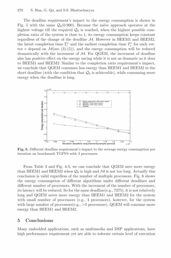
270 S. Hua, G. Qu, and S.S. Bhattacharyya

The deadline requirement’s impact to the energy consumption is shown inFig. 5 with the same Q0(0.900). Because the naıve approach operates at thehighest voltage till the required Q0 is reached, when the highest possible com-pletion ratio of the system is close to 1, its energy consumption keeps constantregardless of the change of the deadline M. However in BEEM1 and BEEM2,the latest completion time T v

l and the earliest completion time T ve for each ver-

tex v depend on M(see (3)-(5)), and the energy consumption will be reduceddramatically with the increment of M. For QGEM, the increment of deadlinealso has positive effect on the energy saving while it is not as dramatic as it doesto BEEM1 and BEEM2. Similar to the completion ratio requirement’s impact,we conclude that QGEM consumes less energy than BEEM1 and BEEM2 in theshort deadline (with the condition that Q0 is achievable), while consuming moreenergy when the deadline is long.

0.8 0.85 0.9 0.95 1 1.05 1.1 1.15 1.2 1.25 1.3

x 104

0.8

0.9

1

1.1

1.2

1.3

1.4

1.5

1.6x 10

4

Iteration deadline requirement(sample period)

Ener

gy c

onsu

mpt

ion

per i

tera

tion Naive approach with shut−down

BEEM 1 with shut−down BEEM 2 with shut−down QGEM

Fig. 5. Different deadline requirement’s impact to the average energy consumption periteration on benchmark TGFF8 with 3 processors.

From Table 3 and Fig. 4-5, we can conclude that QGEM save more energythan BEEM1 and BEEM2 when Q0 is high and M is not too long. Actually thisconclusion is valid regardless of the number of multiple processors. Fig. 6 showsthe energy consumption of different algorithms under different deadlines anddifferent number of processors. With the increment of the number of processors,its latency will be reduced. So for the same deadline(e.g., 7275), it is not relativelylong and QGEM saves more energy than BEEM1 and BEEM2 for the systemwith small number of processors (e.g., 4 processors), however, for the systemwith large number of processors(e.g., >5 processors), QGEM will consume moreenergy than BEEM1 and BEEM2.

5 Conclusions

Many embedded applications, such as multimedia and DSP applications, havehigh performance requirement yet are able to tolerate certain level of execution

Energy-Efficient Multi-processor Implementation of Embedded Software 271

2 3 4 5 6 7 80.7

0.8

0.9

1

1.1

1.2

1.3

1.4

1.5

1.6

1.7x 10

4

Number of processors

Ener

gy c

onsu

mpt

ion

per i

tera

tion

13525

7275 59254725

Naive approach with shut−downBEEM 1 with shut−down BEEM 2 with shut−down QGEM

Fig. 6. The average energy consumption per iteration on benchmark TGFF8 withdifferent number of processors and different deadlines(13525, 7275, 5925 and 4725).

failures. We investigate how to trade this tolerance for energy efficiency, anotherincreasingly important concern in the implementation of embedded software.In particular, we consider systems with multiple supply voltages that enabledynamic voltage scaling, arguably the most effective energy reduction technique.We present several on-line scheduling algorithms that scale operating voltagebased on some parameters pre-determined offline. All the algorithms have lowrun-time complexity yet achieve significant energy saving while providing therequired performance, measured by the completion ratio.

References

1. N. K. Bambha and S. S. Bhattacharyya. “A Joint Power/Performance Optimiza-tion Technique for Multiprocessor Systems Using a Period Graph Construct”, Pro-ceedings of the International Symposium on System Synthesis, pp. 91–97, 2000.

2. J. Bolot and A. Vega-Garcia. “Control Mechanisms for Packet Audio in the Inter-net”, Proceedings of IEEE Infocom, pp. 232–239, March 1996.

3. T.D. Burd, T. Pering, A. Stratakos, and R. Brodersen. “A Dynamic Voltage ScaledMicroprocessor System”, IEEE J. Solid-State Circuits, Vol. 35, No.11, pp. 1571–1580, November 2000.

4. A.P.Chandrakasan, S.Sheng, and R.W.Broderson. “Low-Power CMOS Digital De-sign”, IEEE Journal of Solid-State Circuits, Vol. 27, No. 4, pp. 473–484, 1992.

5. R. P. Dick, D. L. Rhodes, and W. Wolf. “TGFF: Task Graphs for Free”, Proc. Int.Workshop Hardware/Software Codesign, pp. 97–101, Mar. 1998.

6. M.R.Garey and D.S.Johnson. Computer and Intractability: A Guide to the Theoryof NP-Completeness. W.H. Freeman and Company, New York, NY, 1979.

7. A. Grbic, S. Brown, S. Caranci, et al. “Design and Implementation of the NU-MAchine Multiprocessor”, 35th ACM/IEEE Design Automation Conference, pp.65–69, June 1998.

8. F. Gruian and K. Kuchcinski. “LEneS: Task Scheduling for Low-Energy SystemsUsing Variable Supply Voltage Processors” Proc. of Asia and South Pacific DesignAutomation Conference, pp. 449–455, 2001

272 S. Hua, G. Qu, and S.S. Bhattacharyya

9. I. Hong, M. Potkonjak, and M.B. Srivastava. “On-Line Scheduling of Hard Real-Time Tasks on Variable Voltage Processor”, IEEE/ACM International Conferenceon Computer Aided Design, pp. 653–656, 1998.

10. S. Hua, G. Qu, and S. S. Bhattacharyya. “Energy Reduction Techniques for Multi-media Applications with Tolerance to Deadline Misses”, 40th ACM/IEEE DesignAutomation Conference, pp. 131–136, June 2003.

11. R. S. Janka and L. M. Wills. “A Novel Codesign Methodology for Real-Time Em-bedded COTS Multiprocessor-Based Signal Processing Systems”, Proceedings ofthe International Workshop on Hardware/Software Co-Design, pp. 157–161, 2000.

12. I. Karkowski and H. Corporaal. “Design Space Exploration Algorithm For Het-erogeneous Multi-processor Embedded System Design”, 35th ACM/IEEE DesignAutomation Conference, pp. 82–87, June 1998.

13. M. J. Karam and F. A. Tobagi. “Analysis of the Delay and Jitter of Voice TrafficOver the Internet”, Proceedings of IEEE Infocom, pp. 824–833, April 2001.

14. J. Luo and N. K. Jha. “Power-Conscious Joint Scheduling of Periodic Task Graphsand Aperiodic Tasks in Distributed Real-Time Embedded Systems”, IEEE/ACMInternational Conference on Computer-Aided Design, pp. 357–364, November 2000.

15. J. Luo and N. K. Jha. “Battery-Aware Static Scheduling for Distributed Real-Time Embedded Systems”, 38th ACM/IEEE Design Automation Conference, pp.444–449, June 2001.

16. J. Luo and N. K. Jha. “Static and Dynamic Variable Voltage Scheduling Algorithmsfor Real-Time Heterogeneous Distributed Embedded Systems”, Proc. of Asia andSouth Pacific Design Automation Conference, pp. 719–726, Jan. 2002.

17. C.L. McCreary, A.A. Khan, J.J. Thompson, and M.E. McArdle. “A Comparisonof Heuristics for Scheduling DAGs on Multiprocessors”, Proceedings of the Inter-national Parallel Processing Symposium, pp. 446–451, April 1994.

18. R. Mishra, N. Rastogi, D. Zhu, D. Mosse, and R. Melhem. “Energy Aware Schedul-ing for Distributed Real-Time Systems”, International Parallel and DistributedProcessing Symposium, Apr. 2003.

19. G. Qu. “What is the Limit of Energy Saving by Dynamic Voltage Scaling?”IEEE/ACM International Conference on Computer-Aided Design, pp. 560–563,November 2001.

20. D. Scherrer and H. Eberle. “A Scalable Real-time Signal Processor for Object-oriented Data Flow Applications”, Proceedings of the International Conference onParallel and Distributed Computing Systems, pp. 183–189, September 1998.

21. M. T. Schmitz and B. M. Al-Hashimi. “Considering Power Variations of DVSprocessing elements for energy minimisation in distributed systems”, Proceedingsof 14th International Symposium on System Synthesis, pp. 250–255, 2001.

22. G.C. Sih and E.A. Lee. “A Compile-Time Scheduling Heuristic for Interconnection-Constrained Heterogeneous Processor Architectures”, IEEE Tran. on Parallel andDistributed Systems, Vol. 4, No. 2, February 1993.

23. R.A. Sutton, V.P. Srini, and J.M. Rabey. “A Multiprocessor DSP System Us-ing PADDI-2”, 35th ACM/IEEE Design Automation Conference, pp. 62–65, June1998.

24. T.S. Tia, Z. Deng, M. Shankar, M. Storch, J. Sun, L.-C. Wu, and J.W.-S. Liu.“Probabilistic Performance Guarantee for Real-Time Tasks with Varying Com-putation Times”, Proc. Real-Time Technology and Applications Symposium, pp.164–173, 1995

25. V. Tiwari, D. Singh, S. Rajgopal, G. Mehta, R. Patel, and F. Baez. “ReducedPower in High-Performance Microprocessors”, 35th ACM/IEEE Design Automa-tion Conference pp. 732–737, June 1998

Energy-Efficient Multi-processor Implementation of Embedded Software 273

26. D. Zhu, R. Melhem and B. Childers. “Scheduling with Dynamic Voltage/Speed Ad-justment Using Slack Reclamation in Multi-Processor Real-Time Systems”, IEEE22nd Real-Time Systems Symposium pp. 84–94, 2001

A Methodology and Tool Support for GeneratingScheduled Native Code for Real-Time Java Applications

Christos Kloukinas, Chaker Nakhli, and Sergio Yovine

VERIMAG Centre Equation, 2 Ave. Vignate, 38610 Gieres, FranceChristos.Kloukinas,Chaker.Nakhli,Sergio.Yovine@imag.fr

1 Introduction

Current trends in industry are leading towards the use of Java [5] as a programminglanguage for implementing embedded and real-time applications. From the softwareengineering perspective, the Java environment is indeed a very attractive developmentframework. Object-oriented programming provides encapsulation of abstractions intoobjects that communicate through clearly defined interfaces. Dynamic loading eases themaintenance and improvement of complex applications with evolving requirements andfunctionality. Besides, Java provides built-in support for multi-threading.

However, the semantics of Java do not guarantee a predictable run-time behavior,which is an essential issue in embedded real-time software. To overcome this problem,work has been done to extend the language and the platform to accommodate to therequirements of real-time systems by focusing on current practices. Among such work,we should mention the Real-Time Specification for Java [11], and the Real-Time CoreExtension for the Java Platform [12], that provide support for real-time programming(timers, clocks, handlers, priorities, . . . ). Still, these extensions leave some importantissues unspecified, like the scheduling algorithm to be used, allowing an implementationto resolve them at will.

In order to obtain more precise semantics, domain-specific profiles have also beendefined, such as the Ravenscar-Java [8] high-integrity profile for safety-critical systems.This profile settles an execution model based on a two/three-phase program execution,comprising an initialization phase and a mission phase (possibly followed by a ter-mination phase), and multi-threading semantics relying on fixed priority preemptivescheduling and priority ceiling inheritance. Though designed to ease analysis and pro-gramming, this profile still has some drawbacks. For instance, it does not directly supportthreads which synchronize and communicate using the wait and notify methods ofJava. Besides, the underlying schedulability analysis is pessimistic by nature and notwell adapted for systems with heterogeneous tasks and constraints.

The other important issue is performance. Though there are efforts to produce ef-ficient implementations of Java Virtual Machines (e.g., [1,15]), the slowdown due tothe VM remains an argument against adopting Java for real-time applications. Real-timesystems can afford neither the overhead nor the non-determinism of using a Just-In-Time(JIT) compiler (e.g., [3,14]).An alternative approach consists in using anAhead-of-Time(AOT) compiler (e.g., [10,17]) to generate executable code for a run-time system and to Partially supported by the RNTLproject Expresso(http://www.irisa.fr/rntl-expresso).

R. Alur and I. Lee (Eds.): EMSOFT 2003, LNCS 2855, pp. 274–289, 2003.c© Springer-Verlag Berlin Heidelberg 2003

A Methodology and Tool Support 275

provide a native implementation of the real-time primitives. A major advantage of AOTcompilation is that it allows performing sophisticated analysis techniques to producehighly optimized code.

In this paper we present an approach that takes into account the demands of bothprecise semantics and performance. Our work is based on the two/three-phase executionmodel and API of the Expresso High-Integrity Profile [4], which itself inherits conceptsfrom the Ravenscar-Java profile and the RTSJ API. However, the semantics proposed bythe profile do not fit the needs of applications that would demand alternative schedul-ing and synchronization paradigms, and handling quality of service requirements. Toaccommodate to such demands, our approach focuses primarily on the application.

ModelAutomata

Timed SchedulerSynthesis

Table ofDynamicPriorities

Program

Java

Information

WCET

InstrumentedJava

Program

Compiler

JavaTurboJ

Executable

Native

Run−Time

RT OS

(POSIX / eCos)

(per state)

ModelGenerator

Scheduler

Support Library

Fig. 1. Code analysis & generation chain

Following [13], we first extract a formal model of the behavior of the applicationprogram as an extended automaton (see Fig. 1 & section 2). Then, we synthesize anapplication-dependent scheduler (see sections 3–4) which is safe (i.e., it is deadlockfree and meets all timing constraints) and QoS extendible (i.e., it can be extended tohandle QoS requirements, such as reducing response jitter, power consumption or contextswitches). This synthesized scheduler is meant to be used with an appropriate native run-time support we have developed, which itself uses the underlying R-T OS’s primitives(see section 5). Our scheduler also needs an instrumented version of the original Javacode (also produced by our model extracting tool), so as to be able to follow the changesof thread states (i.e., the instrumentation implements an abstract program counter). The

276 C. Kloukinas, C. Nakhli, and S. Yovine

test-bed we have developed has been integrated together with the Expresso High-IntegrityAPI and the TurboJ [17] Java-to-native compiler.

This framework provides a complete analysis and compilation chain for embeddedreal-time systems based on Java, allowing one to substitute RMA/EDF & PCP with ascheduler which is still safe but not as pessimistic. In this article, we describe the modelgenerator, the scheduler architecture and synthesis methodology, and the prototype test-bed implemented using POSIX [6] primitives.

We will illustrate our approach throughout the paper with a case study inspired by therobotic arm system described in [9] (see Fig. 2). The arm is programmed to take objectsfrom a conveyor belt, to store them in a buffer shelf, and to put them into a basket. Thearm is controlled by threads running on a single processor. The TrajectoryControlthread reads commands from a shared buffer and issues set-points to the low-level armcontroller Controler. If there are no commands to process, it holds, otherwise readssensor values and computes the new set-point. Its execution time is between 5ms and6ms. The Lifter thread is activated periodically every 40ms. Its role is to command thearm to pick objects from the conveyor belt. Upon termination, it issues a command to theTrajectoryControl and activates the Putter. Its execution time is between 4ms to8ms. The Putter thread sends commands to take the object from the buffer shelf and putit into the basket. Its execution time is between 4ms to 8ms. The SensorReader threadreads sensors every 24ms. Its execution time is 1ms. The results of the sensors are usedby TrajectoryControl. Controler is a periodic thread with period 16ms. Notice inFig. 2 how, according to the Expresso HIP-API, waitForPeriod returns a boolean valuewhich is false if the thread misses its period. In such a case, the application ends themission phase and goes into a termination phase which is omitted here. In this paper weonly consider the problem of synthesizing a scheduler for the mission phase.

The paper is organized as follows. Section 2 presents the technique we use to gen-erate models from Java source code. Section 3 explains the scheduler architecture andexecution semantics, while section 4 describes our methodology for synthesizing anapplication-dependent scheduler. Section 5 discusses our test-bed implementation.

2 Model Generation

We consider real-time Java applications made up of a fixed number of threads that syn-chronize and communicate through a fixed set of global shared objects. There is a distin-guished thread, namely Main, which is the first thread to wake up at application startupand the unique entry-point of the application. We assume that Main is programmed ac-cording to the Expresso HIP, that is, all the shared objects and threads are created duringthe initialization phase.

The model of a Java program is a transition system which abstracts program actionsand states. Each state in the model is an abstraction of a program state at run-time.Transitions are associated with source code and capture the change that its executionmakes to the program state. More formally, let Θ = thi be a finite set of threads,Ω = Oibe a finite set of shared objects, andAbe a set of labels. Labels may correspondto large blocks of source code or to specific statements, such as: lock (corresponding tothe Java-bytecode monitorEnter), unlock (monitorExit), wait, waitTimed (the Java

A Methodology and Tool Support 277

Fig. 2. Robotic arm system architectureIntervals preceding computations give their minimum & maximum execution duration.

Transitions T 9 → T 10 (setPoint), L 1 → L 2, P 8 → P 9, S 2 → S 3 and C 2 → C 3correspond to code which has been sliced away.

wait method with a timeout parameter), and waitForPeriod (the method of the classPeriodicThread in the Expresso profile, which blocks a thread until its next period).The model is a tuple P = (S, A, T ) where: S is a finite set of states, and T ⊆ S ×A×Sis a transition relation. We define TH : T −→ Θ to be the function mapping eachtransition to the corresponding executing thread.

278 C. Kloukinas, C. Nakhli, and S. Yovine

For each thread th we define Σth : S −→ 2Ω × 2Ω , where Σth(s) = (Σ+, Σ−)is called the synchronization context of th at the state s. Σ+ contains the set of objectswhich are locked by th , when th is at state s. Σ− is either the empty set or a singletoncontaining the object that cannot be synchronized by th at s (and thus cannot be addedto Σ+) which corresponds to the lock released when wait or waitTimed are invoked onthat object. This is done to keep the synchronization context consistent during the modelextraction process. Let Σ = (Σ+, Σ−) be a synchronization context, and ω ⊂ Ω a setof global objects. We define:

Σ Add ω = (Σ+ ∪ (ω \ Σ−), Σ−)Σ Remove ω = (Σ+ \ ω, Σ− ∪ ω)

The Add operation appends objects to the synchronization context by adding them to theΣ+ set, as long as these objects are not in the Σ− set. The Remove operation removesobjects from the set of locked ones, and records them in the Σ− set.

beginsynch

endsynch

Σ

Σ

Body

synchronized(O) Body

endsynch

beginsynch

Σ

Σ

O.lock

O.unlock

ΣAddO

ΣAddO

Th Th

Th

Th

(a) synchronized block

?O

endwait

beginwait

Σ

Σ

O.unlock

O.lockTh

Th

Th

ΣRemoveO

ΣRemoveO

O.wait();

endwait

beginwait

Σ

Th

Σ

(b) wait() statement

Fig. 3. Graph rewrite rules for the generation of models

Our model generator constructs a model from the source code by applying graphrewriting rules on the control flow graph. A segment P of sequential source code ismodeled by a state labelled beginP denoting the control state preceding the executionof P , a transition labelled by P , and a state labelled endP denoting the control statefollowing P . The translation could be kept at this abstraction level or may be refined

A Methodology and Tool Support 279

recursively. Therefore, the granularity of the model can be controlled by the designer.The translation of control-flow statements (e.g., ;, if-then-else, while, . . . ) is doneaccording to standard rewriting rules. Synchronization statements are treated speciallythough. The synchronized statement (characterized by the requested object O) istranslated as shown in Fig. 3(a). Entry in the synchronized block is modeled by atransition labeled with a lock on object O, while the exit is modeled by a transitionlabeled with an unlock. The fact that the thread Th holds the lock of O is recordedby adding O to the Σ of the synchronized statement. An invocation of wait on Ois translated by three transitions (Fig. 3(b)): one modeling the lock release and leadingto a waiting state, another labelled by a reception-of-notification action, and a finaltransition modeling the lock request. These graph-rewrite rules allow us to obtain anextended automaton at the desired level of abstraction for each application thread. Theinformation encoded in the synchronization context Σ of each state of these automata isused for informing the scheduler synthesis program about the resources which are usedat the states of a thread. They are also used for constructing a resource allocation graphwhich is subsequently used for deriving a set of initial constraints against the deadlocksof the system. These constraints can be used as an initial scheduler, so as to decrease thepossible behaviors of the system.

3 Scheduler Architecture and Semantics

3.1 Architecture

The architecture of the schedulers we synthesize consists of two three-layered stacks [7],as shown in Fig. 4. The left stack selects a thread for execution. The right stack selectsa thread for the reception of a notification. Being able to control which thread will benotified for a particular event is something that other scheduling policies do not offer,since they concentrate only on the selection of threads for execution. After one of thescheduler stacks is finished, it passes control to an underlying R-T OS which provideslow-level kernel mechanisms such as thread creation, suspension and resumption, andtimeout enabling/disabling.

Controlling the Executing Thread. The left stack takes control of the system whenthe application calls one of lock, unlock, waitForPeriod, wait and waitTimed. Inthese cases, it must choose one of the available threads as the thread which should beexecuted next. It does this in three steps, each one performed at a different layer. Inthe first layer, referred to as the Ready-Exec scheduler, it calculates the set of threadsRexec which are ready to execute without directly blocking due to mutual exclusion.The Safe-Exec scheduler layer is responsible for calculating the subset Sexec of Rexec,consisting of those threads which can safely execute, that is, their execution will not causea deadlock nor a deadline miss. The third layer QoS-Exec calculates the set Qexec ⊆Sexec, consisting of those safe threads which also respect the QoS requirements of theapplication.

280 C. Kloukinas, C. Nakhli, and S. Yovine

Application TasksApplication

Guarantee Deadlines

Avoid Deadlocks

Assure the QoS

CANDIDATES FOR EXECUTION

Provide low−level mechanismsR−T OS

Assure the QoSScheduler

Mutual Exclusion Rules

READY TASKS

Scheduler

SAFE TASKS

Avoid Deadlocks

Guarantee DeadlinesScheduler

Execution Scheduler Stack

EXECUTING TASKS

CANDIDATES FOR NOTIFICATIONS

Condition Var. Notification RulesScheduler

Scheduler

Scheduler

Notification Scheduler Stack

SAFE TARGETS

READY TO BE NOTIFIED

TASKS TO WAKE UP

CnotifCexec

Choose one among Qexec for execution Notify tasks in Qnotif

Rexec ⊆ Cexec

Ready-Exec

Sexec ⊆ Rexec

Safe-Exec

QoS-Exec

Rnotif ⊆ Cnotif

Snotif ⊆ Rnotif

Ready-Notif

Safe-Notif

QoS-Notif

Qexec ⊆ Sexec Qnotif ⊆ Snotif

Fig. 4. Scheduler architecture

Controlling the Notified Thread. The right stack is passed control when the applicationcalls notify or notifyAll. The reason for this is that the threads which will be notified(if any) cannot ever be selected for execution. This is because they will immediatelytry to re-enter the monitor after being notified and thus get blocked by the notifier(which is already in the monitor). Nevertheless, we can control which among the threadswaiting for the notification should receive the notification, if there are more than onethreads waiting and we are not performing a notifyAll. Thus, the top layer Ready-Notifcalculates the set Rnotif of threads waiting on the condition variable being notified.The middle layer Safe-Notif , calculates the subset Snotif of Rnotif consisting of thosethreads which, if notified, will not cause the system to enter into a deadlock state orto miss a deadline. The Safe-Notif layer passes the Snotif set to the bottom QoS-Notiflayer, which calculates the subset Qnotif of Snotif , consisting of the threads which canbe safely notified and also respect the QoS requirements.

QoS Policies. The complexity of the QoS layer is controlled by the application designer.In choosing a QoS policy (or policies, since these are composable) the designer canbalance between the execution time and extra memory space needed by the policy andthe gains to the overall system quality the particular policy can offer. A QoS policy is,for example, the minimization of the response jitter of some thread (e.g., if it controlsa physical device), or the local minimization of context switches (LMCS) in order tospeed-up the execution and (hopefully) minimize cache misses/flushes and, thus, also

A Methodology and Tool Support 281

energy consumption. This latter policy can be implemented quite easily, since all oneneeds to examine is whether the currently executing thread TExec is in the set Sexec ofthreads which are safe to execute next. If this is the case, then we can let it continue itsexecution, by setting the set Qexec equal to the singleton TExec.

Other, more complex policies may take their decisions by examining applicationvariables and/or (parts of) the execution history.

3.2 Semantics

The model of the system we construct is the parallel composition of: (i) an automatonwhich is responsible for advancing time and firing timeouts, (ii) one automaton for eachof the application threads, and (iii) two more automata, for the QoS-Exec and the QoS-Notif scheduler layers respectively. The application automata are those obtained fromthe Java source code, appropriately annotated with the timing constraints modeling theexecution times of the code that has been abstracted away.

The state of the system model comprises of:

– a program counter (PCi) for each of the application threads,– a local clock (Ci) for each thread, which is used for their computations and the

timeouts if they execute a waitTimed,– a global clock (CSystemi) for modeling the periods of each periodic thread,– a variable (TExec) holding the currently executing thread,– two boolean variables (Exec Sched Enabled & Notif Sched Enabled) for controlling

whether it is one of the scheduler automata (and which one of them), or the time(when they are both true) or the time and application automata (when they are bothfalse) which should execute, and

– the boolean variables of the application threads used in conditionals associated withwaiting statements.

The system goes through three different modes of execution, as shown in Fig. 5(c).In the “Time Only” mode (where Exec Sched Enabled = Notif Sched Enabled = true)the automaton responsible for advancing time and firing timeouts (shown in Fig. 5(a))is the sole automaton enabled in the system and it can fire one or more timeouts, ifany is enabled, corresponding to the expiration of a waitTimed or waitForPeriod.If a timeout is fired then the execution mode changes to “Schedulers Only” (whereExec Sched Enabled = ¬Notif Sched Enabled), so that our scheduler can handle it. Ifthere is no timeout to be fired then the execution mode changes to “Time and Applica-tion” (where Exec Sched Enabled = Notif Sched Enabled = false). At this mode, boththe time automaton and the automata of the application are enabled. If the applicationautomaton needs to execute a time guarded action (i.e., a computation), then it blocks,allowing time to advance. The time automaton then performs a tick (i.e., a time step)and we pass back to the “Time Only” mode, so as to check if a timeout has now beenenabled. If, however, an application automaton needs to perform an action which causesre-scheduling, then it passes control back to the schedulers (i.e., the mode now becomes“Schedulers Only”).

282 C. Kloukinas, C. Nakhli, and S. Yovine

A

Timeouttimeout=⇒ change state & pass control to the scheduler

¬ Timeout ∧ ¬ (Compute ∨ wait)appli=⇒ allow application to run

¬ Timeout ∧ (Compute ∨ wait)tick=⇒ advance clocks

(a) Time automaton

ti ∈ Rexec ∩ Sexec ∩ QexecChoose ti=⇒ T ′

Exec = ti

A

(b) QoS-Exec Scheduler automaton

New tick, so check timeouts

No Timeouts ⇒ Allow Application to run

Re-Sch

edule

Timeout(s) fired

Checktim

eouts

SchedulersOnly

TimeOnly

Timeand

Application

(c) Model execution modes

Fig. 5. Time & Scheduler automata and system execution modes

4 Scheduler Synthesis

In order to synthesize the Safe-Exec and Safe-Notif scheduler layers, we first constructthe set of reachable states and, thus, identify the deadlocks. These are the states wherethe application threads are deadlocked, or the states where some thread has missed itsdeadline or period (since in that case we block the system explicitly). The existence ofthese states indicates that the predicate we are currently using to describe the set Sexec(resp. Snotif ) needs to be constrained even further. This predicate starts with the valueof true, thus accepting initially all threads in the set Rexec (resp. Rnotif ) as safe, whereRexec has been calculated during the extraction of the model from the source code.Having obtained the deadlocked states, we do a backwards traversal of the whole statespace starting from the deadlocked states, until we reach a state which corresponds to achoice of one of the scheduler automata. There, we identify the choice TExec = ti whichallowed the path leading to a deadlock state(s) and create a new constraint for the layerSafe-Exec (resp. Safe-Notif ). This constraint is constructed by changing the set Sexec(resp. Snotif ) to be:

S ′exec(

−−→state) = Sexec(−−→state) \ ti

If at some point we find that S ′exec(

−−→state) is equal to the empty set, then we add thecurrent state to the set of deadlocks and continue the synthesis procedure.

4.1 State-Space Reduction and Application Analysis

Even though the basic idea of synthesizing the Safe-Exec and Safe-Notif schedulerlayers is simple, it is evident that in practice it suffers from the state explosion problem.

A Methodology and Tool Support 283

Therefore, it is imperative that we use techniques to minimize the size of the state space.Our method consists of synthesizing schedulers for successively more detailed models,adding thus complexity to a model only when we have already calculated how we canconstrain the more abstract one. The scheduler synthesis is performed in five major steps.

Compositional Synthesis. First, we decompose the system and synthesize constraintsindependently for each of the components. We then apply the synthesis algorithm againon the parallel composition of the already constrained models. In the case study, wedecided to decompose the application in two sub-systems, one consisting of 4 threads,namely, Lifter, Putter, SensorReader, and TrajectoryControl, and another onecomprising the Controler thread. The decision was mainly taken because of the sizeof the corresponding models (see Table 1). This approach allows us to start the synthesiswith a model about 84% smaller than the original one.

Table 1. Model abstractions and optimizations

In the “original” models the IDLE task is allowed to execute only when no other task is safe.Otherwise, the state-spaces explode - the 5-thread system has more than 404 M states.

Model kind States Red. Trans. Red. Dead.

Model Abstractions & Optimizations for 4 threads

T original (i.e., P) 92382 0.00% 103658 0.00% 61U 3320 96.41% 4680 95.49% 0T NP 74650 19.19% 83018 19.91% 61T P, bbe 20866 77.41% 25020 75.86% 1T NP, bbe 18304 80.19% 21738 79.03% 1

Model Abstractions & Optimizations for 5 threads

T original (i.e., P) 600086 0.00% 695653 0.00% 1814U 5080 99.15% 8232 98.82% 0T NP 445979 25.68% 511809 26.43% 1579T P, bbe 221750 63.05% 271429 60.98% 1T NP, bbe 171238 71.46% 206655 70.29% 1

Abstraction of Time. Second, we consider the issue of time. We examine the untimedmodel (U) of the system and search for constraints which can guarantee the absence ofdeadlocks. Searching for deadlocks in the untimed model allows us to examine a muchsmaller search space. In the case study we observed a reduction of 96% for the 4-threadsubsystem and 99% for the whole system (see Table 1). More importantly, finding andremoving all deadlocks in the untimed model means that the application is logicallycorrect. An initial set of deadlocks can actually be obtained during the generation ofthe model from the source code by applying standard analysis techniques for deadlockdetection (typically a search for loops in a dependency graph). Our model generatorimplements such an analysis as well.

284 C. Kloukinas, C. Nakhli, and S. Yovine

Having found all the potential deadlocks in the untimed system, we add the synthe-sized Sexec and Snotif scheduler sets obtained so far to the timed model (T), in order tosearch for the timeliness constraints, which can guarantee that all threads will meet theirdeadlines. In order to make the problem more tractable, we reduced the timed modelmodulo the branching bisimulation equivalence (bbe) reduction [16], which eliminates“unobservable” actions (in our case the Tick action) but only when doing so preservesthe branching structure of processes. Given a set of equivalent states under the bbe re-duction, we elect as a representative of this set the state which has the maximum globalclock value.

Execution Model. Third, we analyze the behavior of the system for two differentexecution models, namely preemptive and non-preemptive. We first consider that theapplication threads cannot be preempted while they are computing. The non-preemptiveexecution model hypothesis reduces the state space, since it removes all the cases wherethe execution of a thread is suspended so as to handle an interrupt. Once we can indeedsafely schedule the system under the hypothesis that threads are never preempted, thenwe can use the constraints obtained during this step to reduce even further the state spacethat we have to construct and analyze when we do allow threads to be preempted. Thenon-preemption of threads is easily added to our models through the use of a QoS policythat forbids the schedulers from choosing a thread for execution, when another thread isalready in a state where it is performing a computation:

Qexec(−−→state) = t . t ∈ Sexec(

−−→state) ∧ ¬∃t′ = t . computes(t′)In the case study, the combination of the non-preemptive execution model (NP) withthe bbe leads to a reduction of about 80% for the 4-thread subsystem and 70% for the 5threads. However, we cannot safely schedule all systems when we do not allow threadsto be preempted. This means that for these systems we will not obtain any schedulingconstraints and, therefore, will be obliged to examine the larger, unconstrained statespace of the timed model, which corresponds to a preemptive execution model.

Observability of Clocks. Having synthesized a safe scheduler for an application doesnot necessarily mean that we can implement it easily with an existing R-T OS though.The difficulty of implementing it as is, arises from the fact that the constraints we produceduring the synthesis use the state of the system to decide what are the safe choices ateach point during the execution and, therefore, also make reference to the values of thelocal clocks of the threads. However, these clocks do not really exist in the applicationbut were only introduced as a way to model the computations of the threads. Introducingthem in the final code means that we will have to add for each thread an additionaltimer object and reset and activate (resp. deactivate) the timer before (resp. after) eachcomputation and read its value when making a scheduling decision. As using timers maysubstantially increase the execution time of the scheduler, we investigate the possibilityof synthesizing a clock-free one, which only examines the PCs of the threads. This willmake the scheduler itself faster to execute, since in order to make a scheduling decisionit now only needs to examine the n values of the different PCs and not the 2n+1 valuesof the PCs, the local thread clocks and the global clock.

A Methodology and Tool Support 285

On the other hand, removing the clocks from the constraints can introduce stateswhere the scheduler will take the wrong decision and cause a thread to miss its deadline.These states are those where a scheduler gets called at the same configuration of threadPCs but at different time instances. Since the time instances (and therefore the clockvalues) are different, the safe sets Sexec of these states can be different themselves as well.When we decide to not observe the clock values while scheduling, we are effectivelyunable to differentiate among these different sets and all these states become equivalent,as far as our scheduler is concerned. Therefore, if we wish our scheduler to always makea decision which is safe, then the Sexec set of this equivalence class of states shouldbe the intersection of the Sexec sets of the states which belong to the same equivalenceclass.

Sexec(−−−→classj) =

⋂

statei∈classj

Sexec(−−→statei)

Sometimes, the Sexec(−−−→classj) set will be empty, if the scheduler decisions at the members

of this equivalence class were conflicting. When encountering such an equivalence classwhose Sexec set is the empty set, we need to add its members to the set of deadlockedstates and continue the synthesis algorithm, until we find a set of constraints which helpsus to avoid the whole class, if any.

Other QoS Policies. Once we have synthesized a safe scheduler, we can compose itwith other QoS policies to choose among the safe threads those which better realize theQoS requirements of the system. Actually, as Altisen et al. [2] showed, a QoS policy canalso be used from the start of the synthesis as an initial scheduling policy, so as to reducethe size of the model we want to analyze. In this case, the QoS policy used should givepreference to tasks of the system which have a higher probability to miss their deadlines.

Table 2. Synthesis steps

Model kind States Red. Trans. Red. Dead. Constr.

Synthesis Steps for 4 threads

U 3320 96.41% 4680 95.49% 0 0U, No Deadlocks 3320 96.41% 4680 95.49% 0 0T NP, bbe , No Deadlocks 18304 80.19% 21738 79.03% 1 0T NP, bbe , Safe 13830 85.03% 16196 84.38% 0 15T P, bbe , No Clocks 16807 81.81% 20003 80.70% 1 15T P, bbe , No Clocks, Safe 16249 82.41% 19245 81.43% 0 23

Synthesis Steps for 5 threads

T LMCS, bbe , 4 threads Safe 23302 96.12% 26515 96.19% 1 23T LMCS, bbe 15742 97.38% 17584 97.47% 0 38T LMCS, bbe , No Clocks (Safe) 15742 97.38% 17584 97.47% 0 38

286 C. Kloukinas, C. Nakhli, and S. Yovine

Table 2 shows the results obtained when applying our methodology on the casestudy. First we synthesized a safe scheduler consisting of 15 constraints for the 4-threadsubsystem, considering that the execution mode is non-preemptive. Then we used theseconstraints to render the state space smaller once we choose a preemptive executionmode and we no longer observe clocks. This lead to another 8 constraints, with whichthe 4-thread subsystem is indeed always safe. Then, we used the 23 constraints wesynthesized for the 4-thread subsystem, to minimize the 5-thread one. In parallel, wealso used a QoS policy which locally minimizes context switches (LMCS), so as torender the state space even smaller. This produced another 15 constraints, under whichthe 5-thread system is safe, when it is running with the LMCS QoS policy.

5 Scheduler Implementation

Once the scheduler has been synthesized using the model, it has to be implemented andintegrated with the code generated by the TurboJ compiler. The structure of the executablecode is depicted in Fig. 6. The generated code consists of two parts, namely, the applica-tion code and the synthesized scheduling predicates.The application code is instrumentedto call the application-level scheduler called J_Scheduler when an application threadexecutes the code corresponding to the Java-bytecode statements monitorEnter ormonitorExit, and the methods notify, notifyAll, wait, waitTimed and waitForPeriod.J_Scheduler calls the function Synthesized_Predicates which evaluates the syn-thesized predicates corresponding to the different scheduler layers. The application-levelscheduler is implemented on top of an accompanying run-time library, which offers animplementation in native code of the aforementioned statements and methods.

Application code

Expresso HIP−API

POSIX RT OS

J_lock(), J_unlock(), ...scheduler constraints

synthesized

Fig. 6. System decomposition

More precisely, our implementation uses a subset of Posix, i.e., it uses mutexes(without any priority inheritance protocol), condition variables & priorities. Indeed, itdoes not use real-time timers, since one of the underlying OS’s we needed to support(in the context of the Expresso project) does not provide any. More specifically, we usea single mutex (sched mx) and provide to each application thread a unique conditionvariable. These condition variables are all associated with the aforementioned mutex(a capability which exists in Posix but not in Java). Finally, we use three different

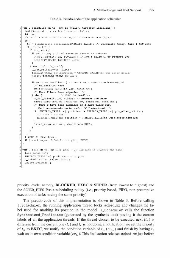
A Methodology and Tool Support 287

Table 3. Pseudo-code of the application scheduler

priority levels, namely, BLOCKED, EXEC & SUPER (from lowest to highest) andthe SCHED_FIFO Posix scheduling policy (i.e., priority based, FIFO, non-preemptiveexecution of tasks having the same priority).

The pseudo-code of this implementation is shown in Table 3. Before callingJ_Scheduler, the running application thread locks sched mx and changes the la-bel used for marking its position in the model. J_Scheduler calls the functionSynthesized_Predicates (generated by the synthesis tool) passing it the currentlabels of all the application threads. If the thread chosen to be executed next (tn) isdifferent from the current one (tc) and tc is not doing a notification, we set the priorityof tn to EXEC, we notify the condition variable of tn (cv tn) and finish by having tcwait on its own condition variable (cv tc ). This final action releases sched mx just before

288 C. Kloukinas, C. Nakhli, and S. Yovine

blocking, thus allowing the notified thread tn to resume execution. If tn happens to bethe same as tc, then the application scheduler returns normally and tc unlocks sched mx.

The algorithm changes somewhat when calling the application scheduler because ofa waitTimed or a waitForPeriod. In this case, we also pass to our scheduler the timethat the current thread should wait. The scheduler then performs a timed wait on cv tc

using as timeout the absolute deadline passed as an argument, instead of doing a simplewait. In addition, it also increases the priority of tc to SUPER just before performingthe timed wait, so that tc has the chance to get the CPU as soon as it timeouts. If tcdoes indeed timeout, it re-calculates the scheduler predicates so as to find out if it isindeed safe to continue execution. Functions J_timed_wait and J_wait set the fieldTHREADS_TABLE[].pos_after_notif right before calling function J_Scheduler tobe the label corresponding to the internal state of the wait where the thread has been noti-fied but has not yet reacquired the mutex of the object on which it was waiting. In a sim-ilar manner, the field pos_after_timeout is set by the functions J_timed_wait, andJ_wait_for_period to the label corresponding to the internal state of the waitTimed,or the label corresponding to the first statement following the beginning of a new period.

We have successfully executed our implementation over two different combinationsof hardware architecture and embedded OS’s, namely an Intel Pentium II (333MHz)running eCos over Linux and a PowerPC simulator (PSIM) using the proprietary OS ofan industrial partner of the Expresso project. The experiments we performed with eCosshowed that the execution time of the synthesized predicates (i.e., the execution timeof function Synthesized_Predicates called by J_Scheduler) is comparable to theexecution time of locking an (unlocked) mutex, having a WCET of the order of 4µs.

Besides, we have a non-Posix prototype implementation over eCos that uses alarmsand alarm handlers, thus allowing us to support deadline and period miss handlers asproposed by the RTSJ, but disallowed by the Expresso and the Ravenscar-Java profiles.

6 Conclusions

We have presented a complete application-driven scheduler synthesis chain that allowsto automatically generate native code for embedded real-time systems based on Java.In addition, it allows one to substitute RMA/EDF & PCP with a scheduler which isstill safe but not as pessimistic and which can be easily extended with QoS schedulingpolicies. We are not aware of any other similar chain. The full integration of the model-generation and scheduler-synthesis tools with the compiler is under test as it requires aclose collaboration with the TurboJ development team.

References

1. AICAS. http://www.aicas.com/jamaica.html. JamaicaVM.2. K. Altisen, G. Goessler, and J. Sifakis. Scheduler modeling based on the controller synthesis

paradigm. Real-Time Systems, 23(1), 55–84, July 2002.3. B. Delsart,V. Joloboff, and E. Paire. JCOD:A Leightweight Modular Compilation Technology

for Embedded Java. In EMSOFT’02, Grenoble, France, October , 2002.

A Methodology and Tool Support 289

4. L. Gauthier and M. Richard-Foy. Expresso RNTL Project - High Integrity Profile, 2002.Available from urlhttp://www.irisa.fr/rntl-expresso/docs/hip-api.pdf

5. J. Gosling, B. Joy, and G. Steele. The Java Language Specification. Addison-Wesley, Reading,MA, USA, 1996.

6. IEEE. POSIX.1. IEEE Std 1003.1:2001. Standard for Information Technology - PortableOperating System Interface (POSIX). The Institute of Electrical and Electronic Engineers,2001.

7. Ch. Kloukinas and S.Yovine. Synthesis of Safe, QoS Extendible, Application Specific Sched-ulers for Heterogeneous Real-Time Systems. In Proceedings of 5th Euromicro Conferenceon Real-Time Systems (ECRTS’03), Porto, Portugal, July 2003.

8. J. Kwon, A. J. Wellings, and S. King. Ravenscar-Java: A High-Integrity Profile for Real-TimeJava. In Java Grande, pp. 131–140, 2002.

9. M. Lusini and E. Vicario. Static analysis and dynamic steering of time-dependent systemsusing Petri Nets. Technical Report # 28.98, University of Florence, 1998.

10. G. Muller, B. Moura, F. Bellard, and Ch. Consel. Harissa: A flexible and efficient Javaenvironment mixing bytecode and compiled code. In Proc. of Usenix COOTS’97, Berkeley,1997.

11. Real-Time for Java Expert Group. The Real-Time Specification for Java, 2001. Availablefrom urlhttp://www.rtj.org

12. Real-Time Java Working Group. Real-Time Core Extensions, revision 1.0.14, 2001. Avail-able from urlhttp://www.j-consortium.org/rtjwg.

13. J. Sifakis, S. Tripakis, and S. Yovine. Building models of real-time systems from applicationsoftware. In Proceedings of the IEEE, Special issue on modeling and design of embeddedsoftware, 91(1):100–111, January 2003. IEEE.

14. Sun Microsystems. The Java HotSpot Performance Engine Architecture. url-http://java.sun.com/products/hotspot/whitepaper.html, April 1999.

15. TimeSys. urlhttp://www.timesys.com. JTime.16. R. J. van Glabbeek and W. P. Weijland. Branching time and abstraction in bisimulation

semantics. JACM, 43(3), 1996.17. M. Weiss, F. de Ferriere, B. Delsart, Ch. Fabre, F. Hirsch, E. A. Johnson, V. Joloboff, F. Roy,

F. Siebert, and X. Spengler. TurboJ, a Java bytecode-to-native compiler. In Proc. of LCTES’98,volume 1474 of LNCS, 1998.

R. Alur and I. Lee (Eds.): EMSOFT 2003, LNCS 2855, pp. 290–305, 2003.© Springer-Verlag Berlin Heidelberg 2003

Constraint-Based Design-Space Exploration and ModelSynthesis

Sandeep Neema1, Janos Sztipanovits

1, Gabor Karsai

1, and Ken Butts

2

1Institute for Software Integrated Systems, Vanderbilt University, P.O. Box 1829 Sta. B. Nash-

ville, TN 37235, USAsandeep.neema,janos.sztipanovits,gabor.karsai@vanderbilt.edu

2Ford Motor Company, MD 7, 20600 Rotunda Dr, Dearborn, MI, 48124

kbutts1@ford.com

Abstract. An important bottleneck in model-based design of embedded systemsis the cost of constructing models. This cost can be significantly decreased byincreasing the reuse of existing model components in the design process. Thispaper describes a tool suite, which has been developed for component-basedmodel synthesis. The DESERT tool suite can be interfaced to existing modelingand analysis environments and can be inserted in various, domain specific de-sign flows. The modeling component of DESERT supports the modeling of de-sign spaces and the automated search for designs that meet structuralrequirements. DESERT has been introduced in automotive applications andproved to be useful in increasing design productivity.

1 Introduction

Extensive modeling and model analysis is a crucial element of design flows for em-bedded systems. The cost of the design process is largely influenced by the cost ofconstructing models for detailed analysis and code generation. There is a significantpressure toward tool manufacturers to decrease this cost by increasing the automationof the modeling process. A promising approach to achieve this goal is to take advan-tage of reusable modeling components and automated model composition. An expo-sition of this problem was detailed by Ken Butts and others [8] describing the need fora model compiler in automotive applications.

Automotive controller modeling is typically done by means of model-based toolsuites, such as MathWorks Simulink®1 and Stateflow® [2]. According to the authors[1], building models for powertrain controller assemblies requires selection of 75-100component models from thousands for each of the 130 vehicle types. The modelcomponents include 1 to 3 sampling contexts (crankshaft position or time) and on theaverage 20 inputs and 14 outputs. This means that the complete model has over 100scheduling connections and 2000 data connections. Components cannot be selected ∗ Support for this research was provided by NSF ITR Grant CCR-0225610 and DARPA Mo-

BIES grant F30602-00-1-05801 MATLAB, Simulink and Stateflow are registered trademarks of The MathWorks, Inc., Na-

tick, MA.

Constraint-Based Design-Space Exploration and Model Synthesis 291

independently from each other. There are complex compatibility relationships amongmodel components. Selection of components may require selection of others and theoverall component structure influences or determines basic performance characteris-tics of the design.

The goal of our research has been the design of a component-based model synthe-sis tool, which given a set of models for subcomponents, composes a system model mautomatically such that a set of design constraints are satisfied. The design require-ments for the tools have been inspired by the practical needs of automotive controlengineers:

1. Model components are MATLAB®, Simulink®, Stateflow® models.2. Model components are characterized by a set of component attributes

(component type like “continuous” and “discrete”, input/output (I/O)definitions, essential parameters, solver used in simulation, sampling time,etc.) that influence composability and capture performance characteristics.

3. Model architectures are described by an abstract, hierarchical, high-levelmodeling language, whose leaf nodes refer to model components definedabove.

4. There is a rich set of compatibility relations among model components.Structural constraints focus on I/O signal types and simulation properties.Component compatibility relates components via high-level design goals,such as “fun-to-drive” or “green”.

The challenge is to synthesize integrated models that meet set design goals andperformance targets using the available model components. While the original modelcompiler challenge [8] is defined in the context of Simulink® models, we generalizedthe method and tools developed and made them independent from the actual domainspecific modeling languages and modeling tools used in a particular design flow.

The primary contribution of the described work is the DEsign Space ExploRationTool (DESERT), which starts with carefully constructed design spaces representingdesign templates and synthesizes fully specified models that meet selected designconstraints. DESERT is a domain independent tool chain for defining design spacesand executing constraint-based design space exploration. The DESERT tool chain canbe linked to different domain specific modeling environments via model transforma-tions. These domain specific modeling environments may include hardware architec-ture or software architecture models.

The paper first gives a short summary of relevant concepts. This will be followedby a discussion on constructing, shaping and aggregating design spaces. The paperconcludes with a description of our constraint-based model synthesis technique,which is currently based on a symbolic representation of the design space and sym-bolic pruning of the design alternatives.

2 Background and Terminology

In model-based design, systems are described by models expressed in domain specificmodeling languages (DSML). Formally, a DSML is a five-tuple of concrete syntax(C), abstract syntax (A), semantic domain (S) and semantic and syntactic mappings(MS, and MC) [9]:

L = < C, A, S, MS, MC>

292 S. Neema et al.

The C concrete syntax defines the specific (textual or graphical) notation used toexpress models, which may be graphical, textual or mixed. The A abstract syntaxdefines the concepts, relationships, and integrity constraints available in the language.Thus, the abstract syntax determines all the (syntactically) correct “sentences” (in ourcase: models) that can be built. (It is important to note that the abstract syntax in-cludes semantic elements as well. The integrity constraints, which define well-formedness rules for the models, are frequently called “static semantics”.) The S se-mantic domain is usually defined by means of some mathematical formalism in termsof which the meaning of the models is explained. The MC : A→C mapping assignssyntactic constructs (graphical, textual or both) to the elements of the abstract syntax.The MS: A→S semantic mapping relates syntactic concepts to those of the semanticdomain.

Any DSML, which is to be used in the development process of embedded systems,requires the precise specification (or modeling) of all five components of the languagedefinition. The languages, which are used for defining components of DSMLs arecalled meta-languages and the concrete, formal specifications of DSMLs are calledmetamodels [1].

The specification of the abstract syntax of DSMLs requires a meta-language thatcan express concepts, relationships, and integrity constraints. In our work in Model-Integrated Computing (MIC) [4], we adopted UML class diagrams and the ObjectConstraint Language (OCL) as meta-language. This selection is consistent withUML’s four layer meta-modeling architecture [16], which uses UML class diagramsand OCL as meta-language for the abstract syntax specification of UML.

The semantic domain and semantic mapping defines semantics for a DSML. Therole of semantics is to give a precise interpretation for the meaning of models that wecan create using the modeling language. Naturally, models might have different in-teresting properties; therefore a DSML might have a multitude of semantic domainsand semantic mappings associated with it. For example, structural and behavioralsemantics are frequently associated with DSMLs. The structural semantics of a mod-eling language describes the meaning of the models in terms of the structure of modelinstances: all of the possible sets of components and their relationships, which areconsistent with the well-formedness rules in defined by the abstract syntax (structuralsemantics is frequently called instance semantics [16]). Accordingly, the semanticdomain for structural semantics is defined by some form of set-relational mathemat-ics. The behavioral semantics describes the evolution of the state of the modeledartifact along some time model. Hence, behavioral semantics is formally modeled bymathematical structures representing some form of dynamics, such as discrete transi-tion system [2] or Hybrid Systems [3].

Although specification of semantics is commonly done informally using Englishtext (see e.g. the specification of UML 1.3 [16]), the desirable solution is explicit,formal specification. There are two frequently used methods for specifying semantics:the metamodeling approach and the translational approach (see Figure 1).• In the meta-modeling approach (see e.g. [5]), the semantics is defined by a meta-

language that already has a well-defined semantics. For example, the UML/OCLmeta-language that we use for defining the abstract syntax of a DSML has astructural semantics: it describes the possible components and structure of valid,syntactically correct domain models. The semantics of this meta-language can berepresented by using a formal language, which supports the precise definition of

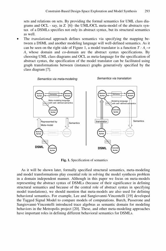
Constraint-Based Design-Space Exploration and Model Synthesis 293

sets and relations on sets. By providing the formal semantics for UML class dia-grams and OCL - say, in Z [6]- the UML/OCL meta-model of the abstracts syn-tax of a DSMLs specifies not only its abstract syntax, but its structural semanticsas well.

• The translational approach defines semantics via specifying the mapping be-tween a DSML and another modeling language will well-defined semantics. As itcan be seen on the right side of Figure 1, a model translator is a function T : A1→A2 whose domain and co-domain are the abstract syntax specifications. Bychoosing UML class diagrams and OCL as meta-language for the specification ofabstract syntax, the specification of the model translator can be facilitated usinggraph transformations between (instance) graphs generatively specified by theclass diagram [7].

As it will be shown later, formally specified structural semantics, meta-modelingand model transformations play essential role in solving the model synthesis problemin a domain independent manner. Although in this paper we focus on meta-modelsrepresenting the abstract syntax of DSMLs (because of their significance in definingstructural semantics and because of the central role of abstract syntax in specifyingmodel translations), we should mention that meta-models are also used for definingbehavioral semantics. For example, Lee and Sangiovanni-Vincentelli [19] developedthe Tagged Signal Model to compare models of computations. Burch, Passerone andSangiovanni-Vincentelli introduced trace algebras as semantic domain for modelingbehaviors in the Metropolis project [20]. These, and other meta-modeling approacheshave important roles in defining different behavioral semantics for DSMLs.

1

ConcreteSyntax

AbstractSyntax

SemanticDomain

Semantics

parses to

Meta-modeling languagewith well -defined semantics

ConcreteSyntax

AbstractSyntax

SemanticDomain

Semantics

parses to

Represented by

Meta-modelSemantics

DSML ConcreteSyntax

AbstractSyntax

SemanticDomain

Semantics

parses to

ConcreteSyntax

AbstractSyntax

Semantics

parses to

SemanticDomain

translator

DSML

Semantics

Modeling languagewith well -defined semantics

Semantics via meta-modeling Semantics via translation

Fig. 1. Specification of semantics

294 S. Neema et al.

3 Construction of the Design Space

Model structures for automotive control are specified as refinements of a genericarchitecture [8] shown in Figure 2. Each top-level model component, such as trans-mission, transmission control T/M, etc., has many alternative realizations with differ-ent parameters and internal structure - arranged in a refinement hierarchy.Accordingly, components at any level in the refinement hierarchy may have alterna-tive implementations. We call components with alternative implementations tem-plates. At the leaf nodes of the refinement hierarchy are the primitive modelcomponents, which may also be templates with alternative (primitive) implementa-tions. In our specific application context, the primitive model components are Simu-link® models. (The “Bus” concepts on the diagram represent a set of variables sharedamong the model components.)

The template concept has a significant impact on the structural semantics of mod-els. Without templates, each m model is unique, i.e. represents a point design. Byintroducing templates in the specification of the modeling language, each model in-cluding templates defines a set of models, MD, which we call design space. An mj∈MD model instance in the design space is defined by binding the component templatesto one of the alternative implementations and by the binding the parameter values ofthe parameterized components to a specific value.

Fig. 2. Top-level Model Architecture in Automotive Systems

Remark 1: The scalability of hierarchically structured alternatives in capturinglarge design space can be judged from the following example: With aalternative implementations per Template, and n Template blocks oneach level of an m -level deep refinement hierarchy, this representation

can define: mka design configurations, where ( ) nkk mm ×+= − 11 , and

nk =1 , using just ( )mna × primitives. As an example, with 4=n ,

3=a , and 3=m , a total of 1728 primitives can represent 843 designconfigurations!

Constraint-Based Design-Space Exploration and Model Synthesis 295

Remark 2: The design space captures all possible mj∈ MD model instances definedby the instantiation of templates and model parameters. Therefore, theessential semantics of a DSML, which is extended with the templateand parameter concepts is structural semantics.

The goal of model synthesis is to find model instances in the design space, whichsatisfy design constraints regarding the feasible composition of model components(see Compatibility Constraints in section 5.3) and satisfy selected structural charac-teristics. Structural characteristics can be directly derived from structural features ofthe model. For example, let C be the set of all primitive control components and letCj=c|c∈C,c∈mj is the subset of primitive controller components, which are ele-ments of model mj∈MD. Furthermore, let cost(ci) is a function, which assigns andestimated implementation cost for each primitive controller components. Since theoverall cost of the controller implementation for mj is (approximately) the sum of theimplementation cost of all controller components: cost(Cj)=∑i cost(ci|ci∈C,ci∈mj), wecan further restrict the design space with a cost constraint L:

MD,<L=mj∈MD|cost(Cj)<L

where MD,<L is the set of all models in the design space, whose controller cost is lessthen L. The significance of structural constraints is that constraint-based design spaceexploration tools can efficiently restrict the design space using computationally inex-pensive techniques.

Remark 3: As opposed structural constraints, behavioral constraints, such as con-troller dynamic performance, require behavioral analysis of designsusing simulation or other analysis tools. Since simulation for largemodels is expensive, it is a good strategy to restrict the design spacefirst by means of structural constraints and explore only the structur-ally correct designs using simulation.

It is interesting to relate our concept of design space with the concept of platformin Sangiovanni-Vincentelli’s platform-based design [21]. Applying the definition ofplatforms in [22] we can conclude that the set of all designs that can arise from com-posing the C set of primitive model components form a platform (we will refer to thisplatform as Model Platform, MP). Clearly, the set of all designs, which can be gener-ated by combining the primitive model components (i.e. the Model Platform) is notpractical for automated model synthesis. The size of this set is unbounded and in-cludes practically only meaningless configurations, therefore any automated search inthat space would be hopeless. The top-down refinement strategy followed in our de-sign space construction strategy starts with an application (or a set of applications,such as automotive controllers) and incrementally refines it to MP. Using the termi-nology of platform-based design [21][22], we start by selecting a point or a set ofpoints in an Application Platform (formed by the interesting set of automotive con-trollers) and capture the feasible refinement paths to MP via hierarchically layeredalternative refinements and parameterization. The resulting set of designs MD ⊂ MPrestricts tremendously the number of meaningless configurations. The remaining,meaningless configurations in the top-down refinement strategy are the result of com-patibility violations and neglected interdependences among design decisions. How-ever, we can express these formally by means of compatibility and interdependencyconstraints, which than can be used for further restricting the design space.

296 S. Neema et al.

Creation of extensive well-structured design spaces for different categories of ap-plications requires significant effort. However, this effort is not required in the formof an initial investment, which is to be done before design space exploration can start.We envision design space construction as byproduct of product development process;the creation of a structured repository where design experience is accumulated.

4 Overview of the DESERT Design Flow

Our goal with DESERT has been to provide a model synthesis tool suite, which canrepresent large design spaces and can manipulate them by means of structural con-straints. The place of these steps in the overall design flow is shown in Figure 3. Theinputs to the DESERT tool suite are models and model components used for behav-ioral modeling and analysis (in our case Simulink® models). DESERT does not requireall details of Simulink models, only those, which are required to specify the basicstructure of designs.

1. The Component Abstraction tool maps Simulink® model components intoAbstract Components by executing the TA model transformation. The Ab-stract Components preserve the structure of I/O interfaces (using interfacetypes) and configurable parameters.

2. The Design Space Modeling tool supports the construction of MD designspaces using Abstract Components. Templates and parameters are theadded language constructs that enable modelers define design spaces in-stead of point designs.

3. The Design Space Encoding tool maps the MD design space into a repre-sentation form, which is suitable for manipulating/changing the space byrestricting it with various design constraints.

4. The Design Space Pruning tool performs the design space manipulationand enables the user to select a design, which meets all structural designconstraints.

5. The Design Decoding tool reconstructs the selected design from its en-coded version.

6. The Component Reconstruction tool takes the design with abstractedcomponents and reconstructs the detailed design suitable for behavioralanalysis (i.e. it synthesizes the detailed Simulink model in our example).

In the following sections we describe the key principles we used in implementing thesystem.

5 Specification of DSMLs in the DESERT Design Flow

As we discussed earlier, the domain and codomain of model transformations in thedesign flow are represented through meta-models specifying the abstract syntax of themodeling languages. The DESERT design flow includes several transformations onthe models. These transformations decouple the complex design space explorationtools (Design Space Encoding and Design Space Pruning) from the domain (and tool)specific detailed Simulink® component models and from the Design Space Modeling

Constraint-Based Design-Space Exploration and Model Synthesis 297

tool, which still uses a modeling language with domain specific flavor (although ituses abstracted components). In this section we show some of the important compo-nents of the design flow focusing more on the approach rather than the technicaldetails.

Fig. 3. DESERT Design flow

5.1 Component Abstraction

The TA model transformation receives Simulink® model components and generatesabstract components for Design Space Modeling. The domain of TA is represented bythe meta-model of the Simulink® models, which is shown in Figure 4. (Detailed de-scription of the Simulink® meta-model can be found in [10].) In short, the Systemclass encapsulates a system model in Simulink. It serves as a container for the blockdiagram that models a dynamical system. It contains Block objects and connections(Line objects) between the Block objects. Some of these Block objects may be Sub-system objects. A Subsystem can be composed as a block diagram. The compositionis indirect through a System object i.e. every Subsystem object contains a single Sys-tem object. This enables hierarchical representation of a complex system. EveryModel/Subsystem object contains a single System object. A System object may alsocontain Annotation objects that are used to add documentary information/user com-ments to the system models. The System class has a small set of attributes that cap-ture various visual preferences, printing preferences, and system information.

The codomain of the TA model transformation is represented by the meta-model ofthe Design Space Modeling tool. The meta-model is shown in Figure 5.

Similarly to the Simulink meta-model, the Design Space meta-model specifies alsoa hierarchical block diagram language with object types Compound, Template andSimulinkSystem. The SimulinkSystem objects refer to the abstracted components im-ported from the Simulink environment. The Simulink and Design Space meta-modelsin Figures 4 and 5 clearly show the role of the TA (Component Abstraction) transfor-mation: internal details of the Simulink model objects are suppressed, only the name(Name attribute in the System object) I/O interfaces (InputPort and OutputPort) andparameters (Parameter object) are preserved in the Design Space Modeling environ-ment. The specific new constructs added to the meta-model for modeling Design

298 S. Neema et al.

Spaces are the Template-s (see our earlier discussion on templates) and Constraint-s.In DESERT’s Design Space Modeling environment the constraints are described asOCL expressions [13].

-Name : String

Model

BlockDefaultsAnnotationDefault

s LineDefaults

-Name : String

System

-Name : String

Block

Subsystem Reference Primitive

1

1

1 *

1

1

Port

Masked Normal

Line

InputPort OutputPort

1

*

1*

1

-dstPort

1

1

-srcPort 1

11

1

1

Annotation

11

1*

Branch

DirectLineBranchedLine

DirectBranch NestedBranch

1

1..*

11..*

1

-dstPort

1

-Name : String

Parameter

-Value : String

Text

-Value : Boolean

Boolean

-Value : String

Enumeration

-Value : Integer

Integer

-Value : Double

Double

-Value : Variant

Vector

-Value : Variant

Type

1

0..*

Fig. 4. Meta-model of Simulink®

5.2 Design Space Modeling

As we described earlier, the MD design space is constructed manually by DesignSpace Modelers (see Figure 3). The DESERT tool suit uses Vanderbilt/ISIS Graphi-cal Modeling Environment (GME) as Design Space Modeling tool. GME is a metap-rogrammable graphical model builder [11], which can be customized to a DSML viaabstract syntax and concrete syntax specification in terms of meta-models. The latestpublic release of GME3 is downloadable from the ISIS web site [12].

Constraint-Based Design-Space Exploration and Model Synthesis 299

Abstracted Simulink Model Components

Fig. 5. Design Space meta-model

Design space modeling is essentially creating product line model architectures:modelers incrementally build, expand the MD space by adding new primitive modelcomponents (abstracted from Simulink® models), and compose them into new ver-sions of plant and controller models. Note that this process is not the enumeration ofall possible designs; the designer merely specifies alternatives on various levels of thehierarchy. As a consequence of this, we are not considering explicit traversal of thedesign space during the pruning process. While adding new implementation alterna-tives to plant and controller models on various levels of the refinement hierarchy, therapidly expanding design space can be restricted by new compatibility and otherstructural constraints. To remain consistent with the selected meta-modeling language(UML class diagrams and OCL), we use OCL-based constraints [13] to “shape” thedesign space. While the meaning of these constraints is domain-specific, there aretypical constraint categories that are suitable to demonstrate the method.

1. Compatibility constraints – Matching interfaces are not sufficient conditionsfor composability. In fact, in many situations selection of implementationalternatives are not orthogonal due to the lack of semantic compatibility. Asimple example for a semantic compatibility constraint for a design space de-fined in a signal processing domain is shown in Figure 6. The meaning of theconstraint is that “Spectral domain correlation composes only with Spectraldomain filters and Spatial domain correlation composes only with Spatialdomain filters”.

300 S. Neema et al.

2. Inter-aspect constraints – Inter-aspect constraints express interdependenciesamong design spaces defined for capturing different aspects of designs. Forexample, plant models and controller models can be represented in two sepa-rate design spaces. Naturally, a large number of inter-dependencies existbetween the plant model configurations and controller configurations. Com-posing an end-to-end system requires evaluating these inter-aspect con-straints. Inter-aspect constraints can be used to explicate these dependenciesand relations as a constraint network, which can then be subsequently util-ized in the design space exploration to systematically synthesize a point-design for the aggregate system.

Fig. 6. Example for semantic composability constraints

5.3 Design Space Encoding and Pruning

Up to this point, we identified constructs and methods for defining, aggregating andconstraining design spaces. The roles of the next two steps in the DESERT designflow (see Figure 3) Design Space Encoding and Design Space Pruning are the fol-lowings:

1. understand whether or not we have created inconsistency during designspace modeling (meaning that the design space is ‘empty’), and

2. find models that meet the required structural constraints.Since we are focusing on structural semantics of the design space and intend to

compute with structural constraints, manipulation of design-spaces can be reduced toset operations: calculating product spaces (composition of design spaces) and findingsubspaces that satisfy various (structural) constraints. Since the size of design-spacesis frequently huge, execution of these set manipulation operations with enumeratingall elements is hopeless. Therefore, we choose to perform the manipulation operationssymbolically. Two problems had to be solved: 1) symbolic representation of design-spaces, and 2) symbolic representation of constraints.

If we restrict the parameters of model objects to finite domains, the design spacewill be also finite. By introducing a binary encoding of the elements in a finite set, alloperations involving the set and its subsets can be represented as Boolean functions

Constraint-Based Design-Space Exploration and Model Synthesis 301

[15]. These can then be symbolically manipulated with Ordered Binary DecisionDiagrams (OBDD-s), a powerful tool for representing, and performing operationsinvolving Boolean function. The choice of encoding scheme has a strong impact onthe scalability of the symbolic manipulation algorithms, as it determines the numberof binary variables required for representing the sets. The details of our encodingscheme has been described in [14], here we only demonstrate the approach.

Figure 7 shows the encoding of a simple design space formed by hierarchicallystructured alternatives. In this example, s, the top-level node in the design space is atemplate, which has three alternative implementations: s1 or s2 or s3. s1 is also atemplate with three alternative implementations: s11 or s12 or s13. s2’s implementa-tion requires three components, s21 and s22 and s23. Out of these components, s21and s23 are templates with two-two alternative implementations, s211 or s212 ands231 or s232, respectively. The prefix-based binary encoding scheme [14] assignsbinary code to each element such that each configuration receives a unique encodingvalue. In the example, four Boolean variables, [ν0, ν1, ν2, ν3] are required for the en-coding of the structure. Figure 8 shows the symbolic Boolean representation of thisdesign space, given the encoding. For example, the binary code of node s2 in thedesign space is S2=¬ν0ν1. As it can be seen, s2 represents a subspace in the designspace with four alternative configurations.

S

S1 S2 S3

S11 S12 S13 S21 S22 S23

S211 S212 S231 S232

_ _ _ _

_ _ 0 0 _ _ 1 0 _ _ 0 1

0 0 0 0 1 0 0 0 0 1 0 0

_ 0 1 0 _ 1 1 0 0 _ 1 0 1 _ 1 0

S

S1 S2 S3

S11 S12 S13 S21 S22 S23

S211 S212 S231 S232

_ _ _ _

_ _ 0 0 _ _ 1 0 _ _ 0 1

0 0 0 0 1 0 0 0 0 1 0 0

_ 0 1 0 _ 1 1 0 0 _ 1 0 1 _ 1 0

Fig. 7. Encoding abstracted design-spaces

S=S1∨S2∨S3

S1=S11∨S12∨S13

S2=S21∧S22∧S23

S21=S211∨S212

S23=S231∨S232

S11=¬v0¬v1¬v2¬v3

S12=¬v0¬v1¬v2v3

S13=¬v0¬v1v2¬v3

S22=¬v0v1

S3=v0¬ v1

S211=¬v0v1¬v2

S212=¬v0v1v2

S231=¬v0v1¬v3

S232=¬v0v1v3

S=S1∨S2∨S3

S1=S11∨S12∨S13

S2=S21∧S22∧S23

S21=S211∨S212

S23=S231∨S232

S11=¬v0¬v1¬v2¬v3

S12=¬v0¬v1¬v2v3

S13=¬v0¬v1v2¬v3

S22=¬v0v1

S3=v0¬ v1

S211=¬v0v1¬v2

S212=¬v0v1v2

S231=¬v0v1¬v3

S232=¬v0v1v3

Fig. 8. Symbolic Boolean representation of abstracted design-spaces

302 S. Neema et al.

In addition to encoding the structure of the design-space, the encoding scheme hasto encode the parameters of the parameterized model components. Subsequent toencoding, and deciding the variable ordering, the symbolic Boolean representation ismapped to an OBDD representation in a straightforward manner [14].

Earlier we listed some basic categories of structural constraints. Symbolic repre-sentation of each of these categories of constraints is summarized below.

1. Compatibility and Inter-aspect constraints – These constraints specify rela-tions among subspaces in the overall design space. Symbolically, the con-straints can be represented as a Boolean expression over the Booleanrepresentation of the design-space. Figure 9 shows an example of a compati-bility constraint, and its symbolic Boolean representation. The compatibilityconstraint in the example expresses interdependency between implementa-tion decisions. Specifically, selection of implementation s211 for templates21 implies that s231 must be the selected implementation for template s23.In the Boolean space, this constraint is expressed by the following Booleanexpression: cc= S211 ⇒ S231=S211∧ S231∨ ¬S211

2. Resource constraints – Resource constraints specify bounds on the resourceneeds of a composed system. These may be in the form of size, weight, en-ergy, cost, etc. As we described earlier, the important limitations for the re-source constraints, which DESERT is able to manage is that they are derivedfrom structural characteristics of designs. In general, resource constraints aremore challenging to represent symbolically, than composability or inter-aspect constraints. Different resource attributes compose differently, e.g. costcan be composed additively, reliability can be composed multiplicatively,latency can be composed as additively for pipelined components, and asmaximum for parallel components, etc. DESERT provides some built-incomposition functions (addition, maximum, minimum, etc.), and has a well-defined interface for creating custom composition functions.

S

S1 S2 S3

S11 S12 S13 S21 S22 S23

S211 S212 S231 S232

_ _ _ _

_ _ 0 0 _ _ 1 0 _ _ 0 1

0 0 0 0 1 0 0 0 0 1 0 0

_ 0 1 0 _ 1 1 0 0 _ 1 0 1 _ 1 0

cc=S211⇒S231

cc=S211∧S231∨¬S211

cc=¬v0v1¬v2¬v3∨v0∨¬v1∨v2

S

S1 S2 S3

S11 S12 S13 S21 S22 S23

S211 S212 S231 S232

_ _ _ _

_ _ 0 0 _ _ 1 0 _ _ 0 1

0 0 0 0 1 0 0 0 0 1 0 0

_ 0 1 0 _ 1 1 0 0 _ 1 0 1 _ 1 0

S

S1 S2 S3

S11 S12 S13 S21 S22 S23

S211 S212 S231 S232

_ _ _ _

_ _ 0 0 _ _ 1 0 _ _ 0 1

0 0 0 0 1 0 0 0 0 1 0 0

_ 0 1 0 _ 1 1 0 0 _ 1 0 1 _ 1 0

cc=S211⇒S231

cc=S211∧S231∨¬S211

cc=¬v0v1¬v2¬v3∨v0∨¬v1∨v2

Fig. 9. Symbolic representation of a compatibility constraint

In addition to these basic categories of constraints, complex constraints may be ex-pressed by combining one or more of these constraints with first order logic connec-tives. The symbolic representation of the complex constraints can be accomplishedsimply by composing the symbolic representation of the basic constraints.

Constraint-Based Design-Space Exploration and Model Synthesis 303

The symbolic pruning of the design-space, as observed earlier, in essence, is a setmanipulation problem. Constraint-based pruning is a restriction of the aggregate spacewith the constraints. Symbolic pruning is simply the logical conjunction of the sym-bolic representation of the space with the symbolic representation of the constraints. Itis worth emphasizing that during the pruning process all of the (potentially very large)design spaces are evaluated simultaneously. Figure 9 illustrates the process of sym-bolic design-space pruning. As the figure shows, the Design Space Pruning tool isprepared for applying constraints on the Design Space. According to our experience,OBDD based representations scale well for representing the structure of the designspace (nested AND/OR expressions). The critical challenge in scalability occurs dur-ing the design-space pruning step. Automatic application of complex constraints tolarge spaces may result in explosion of the OBDD-s therefore DESERT has an inter-active user interface to influence this process. Users can control the importance ofconstraints and select the sequence order of their application. We are experimentingwith re-encoding the design-space after each pruning step, which usually results in adrastic decrease in the number of binary variables (see Figure 10).

The primary advantage of the symbolic design space pruning approach is that it isexhaustive: the pruned space includes all of the designs, which meet the applied de-sign constraints. As experience with scalability in real-life industrial applications atFord accumulate, we will be able to see the limitations of the method.

A significantly simpler, but still useful alternative approach to design space prun-ing is to find a single design configuration (not all), which satisfies the selected designconstraints. We currently experiment with various constraint solvers and languages,such as Oz [17] to develop solution for this approach.

Design Space1 (Hier. Alt)

Constraints

Binary Encoding

OBDD Representation

OBDD Representation

Symbolic Design Space

Pruned Design Space

Apply

Re-encoding/Iterative Pruning

Parsing/ Composing

Design Space2 (Hier. Alt)

Binary Encoding

OBDD Representation

Design Spacen (Hier. Alt)

Binary Encoding

OBDD Representation

…

Design Space1 (Hier. Alt)

Constraints

Binary Encoding

OBDD Representation

OBDD Representation

Symbolic Design Space

Pruned Design Space

Apply

Re-encoding/Iterative Pruning

Parsing/ Composing

Design Space2 (Hier. Alt)

Binary Encoding

OBDD Representation

Design Spacen (Hier. Alt)

Binary Encoding

OBDD Representation

…

Fig. 10. Symbolic design space pruning

304 S. Neema et al.

5.4 Reconstructing Detailed Design

The concluding steps of the DESERT design flow (see Figure 3) are the decoding ofthe selected abstract design from its binary code and reconstructing the detailed mod-els from the abstract design. The decoding process involves reconstructing a datastructure from the encoded form, where the data structure is an abstracted representa-tion of the actual design. The design space encoder and decoder components operateon a shared “dictionary”, which captures what specific design space model elementscorrespond to what codes. The resulting data structure is a specific, point design (i.e. asingle model m), which can be looked at in the modeling tool. Naturally, it does nothave any templates (i.e. no alternatives).

The final step is the creation of the actual design model in Simulink®. The designmodel created in the design decoding step is follows the Design Space metamodel(from Figure 5), and from it a model is constructed that follows the Simulink® meta-model (from Figure 4). This construction is mostly straightforward, the only compli-cation arises because of the connections: the blocks in the final design have to be“wired-up” as required. However, this wiring can be algorithmically generated fromthe (higher-level) buses and wires captured in the design space models.

6 Conclusions and Future Work

Design space modeling and model synthesis are important part of the design flow forembedded systems. Automated tools can offer major productivity advantages forpracticing engineers. During the development of the DESERT tool suite the Vander-bilt/ISIS team has been in close interaction with Ford, which was essential in identi-fying the crucial challenges engineers face. At this point, the prototype tool is fieldtested in real-life vehicle development programs.

The method described has been based on the structural semantics of models. Therole of model synthesis based on structural constraints is to prune the design spacebefore the computationally more expensive behavioral analysis methods are used forfinding optimal design solutions. Since structural semantics is defined for all domainspecific modeling languages, the tool suite can be interfaced to many design flows(independently from the behavioral semantics of the languages). We have been usingthis opportunity extensively in other domains, such as modeling environment forpower-aware computing [18].

References

[1] Karsai, G., Sztipanovits, J., Ledeczi, A., Bapty, T.: “Model-Integrated Development ofEmbedded Software”, Proceedings of the IEEE, Vol. 91, No.1., pp.145–164, January,2003

[2] D. Harel and M. Politi, Modeling Reactive Systems with Statecharts: The STATEMATEApproach, McGraw-Hill, 1998

[3] Thomas A. Henzinger. The theory of hybrid automata. Proceedings of the 11th AnnualSymposium on Logic in Computer Science (LICS), IEEE Computer Society Press, 1996,pp. 278–292

Constraint-Based Design-Space Exploration and Model Synthesis 305

[4] J. Sztipanovits and G. Karsai: “Model-Integrated Computing,” IEEE Computer, April,1997 (1997) 110–112

[5] Clark, T., Evans, A., Kent, S.: “Engineering Modeling Languages: A Precise Meta-modeling Approach,” R.-D. Kutsche and H. Weber (Eds.): FASE 2000, LNCS 2306, pp.159–173, 2002

[6] Evans, A., France, R., Lano, K., Rumpe, B. : « Developing UML as a Formal ModelingNotation,”LNCS 1357, pp. 145–150, Springer Verlag Berlin, 1997

[7] Levendovszky, T., Karsai G.: “Model reuse with metamodel based-transformations,”ICSR, LNCS, Austin, TX, April 18, 2002.

[8] Butts, K., Bostic, D., Chutinan, A., Cook, J., Milam, B., Wand, Y.: “Usage Scenarios foran Automated Model Compiler,” EMSOFT 2001, LNCS 2211, Springer. (2001) 66–79

[9] T. Clark, A. Evans, S. Kent, P. Sammut: “The MMF Approach to Engineering Object-Oriented Design Languages,” Workshop on Language Descriptions, Tools and Applica-tions (LDTA2001), April, 2001

[10] Neema, S.: “Simulink and Stateflow Data Model”, see www.isis.vanderbilt.edu.[11] Nordstrom G., Sztipanovits J., Karsai G., Ledeczi, A.: "Metamodeling - Rapid Design and

Evolution of Domain-Specific Modeling Environments", Proceedings of the IEEEECBS'99, Nashville, TN, April, 1999. (1999) 68–75

[12] Generic Modeling Environment documents,http://www.isis.vanderbilt.edu/projects/gme/Doc.html

[13] Object Constraint Language Specification, ver. 1.1, Rational Software Corporation, et al.,Sept. 1997. (1997)

[14] Neema, S., “Design Space Representation and Management for Embedded Systems Syn-thesis,” Technical Report, ISIS-01-203, February 2001.http://www.isis.vanderbilt.edu/publications/archive/Neema_S_2_0_2003_Design_Spa.pdf

[15] Bryant R., “Symbolic Manipulation with Ordered Binary Decision Diagrams,” School ofComputer Science, Carnegie Mellon University, Technical Report CMU-CS-92-160, July1992

[16] UML Semantics, Ver. 1.1., Rational Software Corporation, 1997.[17] http://www.mozart-oz.org/[18] Ledeczi A., Davis J., Neema S., Eames B., Nordstrom G., Prasanna V., Raghavendra, C.,

Bakshi A., Mohanty S., Mathur V., Singh M.: Overview of the Model-based IntegratedSimulation Framework, Tech. Report, ISIS-01-201, January 30, 2001.

[19] Lee, E.A., Sangiobanni-Vincentelli, A.L.: “A framework for comparing models of com-putations,” IEEE Transactions on Computer Aided Design Integrated Circuits,17(12):1217–1229, Dec. 1998.

[20] Burch, J.R., Passerone, R., Sangiovanni-Vincentelli, A.L.: “Modeling Techniques inDesign-by-Refinement Methodologies, Proc. of IDPT-2002, June, 2002

[21] Sangiovanni-Vincentelli, A.L.: “ Defining platform-based design,” EEDesign, February,2002

[22] Lee, E.A., Neuendorffer, S., Wirthlin, M.J.: “Actor-Oriented Design of Hardware andSoftware Systems,“ (to be published in Journal of Circuits, Systems and Computers)Technical Memorandum UCB/ERL M02/13, University of California, Berkeley, CA94720, May 1, 2002

Eliminating Stack Overflow by Abstract Interpretation

John Regehr, Alastair Reid, and Kirk Webb

School of Computing, University of Utah

Abstract. An important correctness criterion for software running on embeddedmicrocontrollers is stack safety: a guarantee that the call stack does not over-flow. We address two aspects of the problem of creating stack-safe embeddedsoftware that also makes efficient use of memory: statically bounding worst-casestack depth, and automatically reducing stack memory requirements. Our firstcontribution is a method for statically guaranteeing stack safety by performingwhole-program analysis, using an approach based on context-sensitive abstractinterpretation of machine code. Abstract interpretation permits our analysis to ac-curately model when interrupts are enabled and disabled, which is essential foraccurately bounding the stack depth of typical embedded systems. We have imple-mented a stack analysis tool that targets Atmel AVR microcontrollers, and testedit on embedded applications compiled from up to 30,000 lines of C. We exper-imentally validate the accuracy of the tool, which runs in a few seconds on thelargest programs that we tested. The second contribution of this paper is a novelframework for automatically reducing stack memory requirements. We show thatgoal-directed global function inlining can be used to reduce the stack memoryrequirements of component-based embedded software, on average, to 40% of therequirement of a system compiled without inlining, and to 68% of the requirementof a system compiled with aggressive whole-program inlining that is not directedtowards reducing stack usage.

1 Introduction

Inexpensive microcontrollers are used in a wide variety of embedded applications such asvehicle control, consumer electronics, medical automation, and sensor networks. Staticanalysis of the behavior of software running on these processors is important for twomain reasons:

– Embedded systems are often used in safety critical applications and can be hard toupgrade once deployed. Since undetected bugs can be very costly, it is useful toattempt to find software defects early.

– Severe constraints on cost, size, and power make it undesirable to overprovisionresources as a hedge against unforeseen demand. Rather, worst-case resource re-quirements should be determined statically and accurately, even for resources likememory that are convenient to allocate in a dynamic style.

In this paper we describe the results of an experiment in applying static analysistechniques to binary programs in order to bound and reduce their stack memory require-ments. We check embedded programs for stack safety: the property that they will not

R. Alur and I. Lee (Eds.): EMSOFT 2003, LNCS 2855, pp. 306–322, 2003.c© Springer-Verlag Berlin Heidelberg 2003

Eliminating Stack Overflow by Abstract Interpretation 307

stack

upper boundon stack depth

stack

0 KB

4 KB

data, BSS

heap

worst observed depth

0 KB

4 KB

Without stack bounding

data, BSS

heap

With static stack bounding

true worstcase depth?

true worst casedepth must liewithin this range

Fig. 1. Typical RAM layout for an embedded program with and without stack bounding.Without a bound, developers must rely on guesswork to determine the amount of storageto allocate to the stack.

run out of stack memory at run time. Stack safety, which is not guaranteed by traditionaltype-safe languages like Java, is particularly important for embedded software becausestack overflows can easily crash a system. The transparent dynamic stack expansionthat is performed by general-purpose operating systems is infeasible on small embeddedsystems due to lack of virtual memory hardware and limited availability of physicalmemory. For example, 8-bit microcontrollers typically have between a few tens of bytesand a few tens of kilobytes of RAM. Bounds on stack depth can also be usefully incorpo-rated into executable programs, for example to assign appropriate stack sizes to threadsor to provide a heap allocator with as much storage as possible without compromisingstack safety.

The alternative to static stack depth analysis that is currently used in industry is toensure that memory allocated to the stack exceeds the largest stack size ever observedduring testing by some safety margin. A large safety margin would provide good in-surance against stack overflow, but for embedded processors used in products such assensor network nodes and consumer electronics, the degree of overprovisioning must bekept small in order to minimize per-unit product cost. Figure 1 illustrates the relationshipbetween the testing- and analysis-based approaches to allocating memory for the stack.

Testing-based approaches to software validation are inherently unreliable, and test-ing embedded software for maximum stack depth is particularly unreliable because itsbehavior is timing dependent: the worst observed stack depth depends on what code isexecuting when an interrupt is triggered and on whether further interrupts trigger beforethe first returns. For example, consider a hypothetical embedded system where the maxi-mum stack depth occurs when the following events occur at almost the same time: 1) themain program summarizes data once a second spending 100 microseconds at maximumstack depth; 2) a timer interrupt fires 100 times a second spending 100 microseconds atmaximum stack depth; and 3) a packet arrives on a network interface up to 10 times asecond; the handler spends 100 microseconds at maximum stack depth. If these events

308 J. Regehr, A. Reid, K. Webb

occur independently of each other, then the worst case will occur roughly once every 10years. This means that the worst case will probably not be discovered during testing, butwill probably occur in the real world where there may be many instances of the embed-ded system. In practice, the events are not all independent and the timing of some eventscan be controlled by the test environment. However, we would expect a real system tospend less time at the worst-case stack depth and to involve more events.

Another drawback of the testing-based approach to determining stack depth is thatit treats the system as a black box, providing developers with little or no feedback abouthow to best optimize memory usage. Static stack analysis, on the other hand, identifiesthe critical path through the system and also the maximum stack consumption of eachfunction; this usually exposes obvious candidates for optimization.

Using our method for statically bounding stack depth as a starting point, we havedeveloped a novel way to automatically reduce the stack memory requirement of anembedded system. The optimization proceeds by evaluating the effect of a large numberof potential program transformations in a feedback loop, applying only transformationsthat reduce the worst-case depth of the stack. Static analysis makes this kind of optimiza-tion feasible by rapidly providing accurate information about a program. Testing-basedapproaches to learning about system behavior, on the other hand, are slower and typicallyonly explore a fraction of the possible state space.

Our work is preceded by a stack depth analysis by Brylow et al. [3] that also performswhole-program analysis of executable programs for embedded systems. However, whilethey focused on relatively small programs written by hand in assembly language, wefocus on programs that are up to 30 times larger, and that are compiled from C to aRISC architecture. The added difficulties in analyzing larger, compiled programs ne-cessitated a more powerful approach based on context-sensitive abstract interpretationof machine code; we motivate and describe this approach in Section 2. Section 3 dis-cusses the problems in experimentally validating the abstract interpretation and stackdepth analysis, and presents evidence that the analysis provides accurate results. In Sec-tion 4 we describe the use of a stack bounding tool to support automatically reducing thestack memory consumption of an embedded system. Finally, we compare our researchto previous efforts in Section 5 and conclude in Section 6.

2 Bounding Stack Depth

Embedded system designers typically try to statically allocate resources needed by thesystem.This makes systems more predictable and reliable by providing a priori bounds onresource consumption. However, an almost universal exception to this rule is that memoryis dynamically allocated on the call stack. Stacks provide a useful model of storage, withconstant-time allocation and deallocation and without fragmentation. Furthermore, thenotion of a stack is designed into microcontrollers at a fundamental level. For example,hardware support for interrupts typically pushes the machine state onto the stack beforecalling a user-defined interrupt handler, and pops the machine state upon termination ofthe handler. For developers of embedded systems, it is important not only to know thatthe stack depth is bounded, but also to have a tight bound — one that is not much greater

Eliminating Stack Overflow by Abstract Interpretation 309

than the true worst-case stack depth. This section describes the whole-program analysisthat we use to obtain tight bounds on stack depth.

Our prototype stack analysis tool targets programs for the Atmel AVR, a popularfamily of microcontrollers. We chose to analyze binary program images, rather thansource code, for a number of reasons:

– There is no need to predict compiler behavior. Many compiler decisions, such asthose regarding function inlining and register allocation, have a strong effect onstack depth.

– Inlined assembly language is common in embedded systems, and a safe analysismust account for its effects.

– The source code for libraries and real-time operating systems are commonly notavailable for analysis.

– Since the analysis is independent of the compiler, developers are free to changecompilers or compiler versions. In addition, the analysis is not fragile with respectto non-standard language extensions that embedded compilers commonly use toprovide developers with fine-grained control over processor-specific features.

– Adding a post-compilation analysis step to the development process presents devel-opers with a clean usage model.

2.1 Analysis Overview and Motivation

The first challenge in bounding stack depth is to measure the contributions to the stackof each interrupt handler and of the main program. Since indirect function calls andrecursion are uncommon in embedded systems [4], a callgraph for each entry point intothe program can be constructed using standard analysis techniques. Given a callgraph itis usually straightforward to compute its stack requirement.

The second, more difficult, challenge in embedded systems is accurately estimatinginteractions between interrupt handlers and the main program to compute a maximumstack depth for the whole system. If interrupts are disabled while running interrupthandlers, one can safely estimate the stack bound of a system containing n interrupthandlers using this formula:

stack bound = depth(main) + maxi=1..n

depth(interrupti)

However, interrupt handlers are often run with interrupts enabled to ensure that otherinterrupt handlers are able to meet real-time deadlines. If a system permits at most oneconcurrent instance of each interrupt handler, the worst-case stack depth of a system canbe computed using this formula:

stack bound = depth(main) +∑

i=1..n

depth(interrupti)

Unfortunately, as we show in Section 3, this simple formula often provides unnecessarilypessimistic answers when used to analyze real systems where only some parts of someinterrupt handlers run with interrupts enabled.

310 J. Regehr, A. Reid, K. Webb

in r24, 0x3f ; r24 <- CPU status registercli ; disable interruptsadc r24, r24 ; carry bit <- prev interrupt statuseor r24, r24 ; r24 <- 0adc r24, r24 ; r24 <- carry bitmov r18, r24 ; r18 <- r24

... critical section ...

and r18, r18 ; test r18 for zerobreq .+2 ; if zero, skip next instructionsei ; enable interruptsret ; return from function

Fig. 2. This fragment of assembly language for Atmel AVR microcontrollers motivatesour approach to program analysis and illustrates a common idiom in embedded software:disable interrupts, execute a critical section, and then reenable interrupts only if they hadpreviously been enabled

To obtain a safe, tight stack bound for realistic embedded systems, we developeda two-part analysis. The first must generate an accurate estimate of the state of theprocessor’s interrupt mask at each point in the program, and also the effect of eachinstruction on the stack depth. The second part of the analysis — unlike the first —accounts for potential preemptions between interrupts handlers and can accurately boundthe global stack requirement for a system.

Figure 2 presents a fragment of machine code that motivates our approach to programanalysis. Analogous code can be found in almost any embedded system: its purpose isto disable interrupts, execute a critical section that must run atomically with respect tointerrupt handlers, and then reenable interrupts only if they had previously been enabled.There are a number of challenges in analyzing such code.

First, effects of arithmetic and logical operations must be modeled with enoughaccuracy to track data movement through general-purpose and special-purpose registers.In addition, partially unknown data must be modeled. For example, analysis of the codefragment must succeed even when only a single bit of the CPU status register — themaster interrupt control bit — is initially known.

Second, dead edges in the control-flow graph must be detected and avoided. Forexample, when the example code fragment is called in a context where interrupts aredisabled, it is important that the analysis conclude that the sei instruction is not executedsince this would pollute the estimate of the processor state at subsequent addresses.

Finally, to prevent procedural aliasing from degrading the estimate of the machinestate, a context sensitive analysis must be used. For example, in some systems the code inFigure 2 is called with interrupts disabled by some parts of the system and is called withinterrupts enabled by other parts of the system. With a context-insensitive approach, theanalysis concludes that since the initial state of the interrupt flag can vary, the final state

Eliminating Stack Overflow by Abstract Interpretation 311

0 1

⊥(a) Lattice for eachbit in the machinestate

and1 0 ⊥

1 1 0 ⊥0 0 0 0⊥ ⊥ 0 ⊥

or1 0 ⊥

1 1 1 10 1 0 ⊥⊥ 1 ⊥ ⊥

xor1 0 ⊥

1 0 1 ⊥0 1 0 ⊥⊥ ⊥ ⊥ ⊥

merge1 0 ⊥

1 1 ⊥ ⊥0 ⊥ 0 ⊥⊥ ⊥ ⊥ ⊥

(b) Logical operations on abstract bits and combining ma-chine states at merge points

Fig. 3. Modeling machine states and operations in the abstract interpretation

of the interrupt flag can also vary and so analysis of both callers of the function wouldproceed with the interrupt flag unknown. This can lead to large overestimates in stackbounds since unknown values are propagated to any code that could execute after thecall. With a context-sensitive analysis the two calls are analyzed separately, resulting inan accurate estimate of the interrupt state.

The next section describes the abstract interpretation we have developed to meetthese challenges.

2.2 Abstracting the Processor State

The purpose of our abstract interpretation is to generate a safe, precise estimate of thestate of the processor at each point in the program; this is a requirement for finding atight bound on stack depth. Designing the abstract interpretation boils down to two maindesign decisions.

First, how much of the machine state should the analysis model? For programs thatwe have analyzed, it is sufficient to model the program counter, general-purpose registers,and several I/O registers. Atmel AVR chips contain 32 general-purpose registers and 64I/O registers; each register stores eight bits. From the I/O space we model the registersthat contain interrupt masks and the processor status register. We do not model mainmemory or most I/O registers, such as those that implement timers, analog-to-digitalconversion, and serial communication.

Second, what is the abstract model for each element of machine state? We choseto model the machine at the bit level to capture the effect of bitwise operations on theinterrupt mask and condition code register — we had initially attempted to model themachine at word granularity and this turned out to lose too much information throughconservative approximation. Each bit of machine state is modeled using the lattice de-picted in Figure 3(a). The lattice contains the values 0 and 1 as well as a bottom element,⊥, that corresponds to a bit that cannot be proven to have value 0 or 1 at a particularprogram point.

Figure 3(b) shows abstractions of some common logical operators. Abstractions ofoperators should always return a result that is as accurate as possible. For example, whenall bits of the input to an instruction have the value 0 or 1, the execution of the instruction

312 J. Regehr, A. Reid, K. Webb

should have the same result that it would have on a real processor. In this respect ourabstract interpreter implements most of the functionality of a standard CPU simulator.

For example, when executing the and instruction with 1, 1, 0, 0, 1, 1, 0, 0 as one ar-gument and ⊥,⊥,⊥,⊥, 1, 1, 1, 1 as the other argument, the result register will containthe value ⊥,⊥, 0, 0, 1, 1, 0, 0. Arithmetic operators are treated similarly, but requiremore care because bits in the result typically depend on multiple bits in the input. Fur-thermore, the abstract interpretation must take into account the effect of instructions onprocessor condition codes, since subsequent branching decisions are made using thesevalues.

The example in Figure 2 illustrates two special cases that must be accounted forin the abstract interpretation. First, the add-with-carry instruction adc, when both ofits arguments are the same register, acts as rotate-left-through-carry. In other words, itshifts each bit in its input one position to the left, with the leftmost bit going into theCPU’s carry flag and the previous carry flag going into the rightmost bit. Second, theexclusive-or instruction eor, when both of its arguments are the same register, acts likea clear instruction — after its execution the register is known to contain all zero bitsregardless of its previous contents.

2.3 Managing Abstract Processor States

An important decision in designing the analysis was when to create a copy of the abstractmachine state at a particular program point, as opposed to merging two abstract states.The merge operator, shown in Figure 3(b), is lossy since a conservative approximationmust always be made. We have chosen to implement a context-sensitive analysis, whichmeans that we fork the machine state each time a function call is made, and at no otherpoints in the program. This has several consequences. First, and most important, it meansthat the abstract interpretation is not forced to make a conservative approximation when afunction is called from different points in the program where the processor is in differentstates. In particular, when a function is called both with interrupts enabled and disabled,the analysis is not forced to conclude that the status of the interrupt bit is unknown insidethe function and upon return from it. Second, it means that we cannot show terminationof a loop implemented within a function. This is not a problem at present since loopsare irrelevant to the stack depth analysis as long as there is no net change in stack depthacross the loop. However, it will become a problem if we decide to push our analysisforward to bound heap allocation or execution time. Third, it means that we can, inprinciple, detect termination of recursion. However, our current implementation rarelydoes so in practice because most recursion is bounded by values that are stored on thestack — which our analysis does not model. Finally, forking the state at function callsmeans that the state space of the stack analyzer might become large. This has not beena problem in practice; the largest programs that we have analyzed cause the analyzer toallocate about 140 MB. If memory requirements become a problem for the analysis, arelatively simple solution would be to merge program states that are identical or that aresimilar enough that a conservative merging will result in minimal loss of precision.

Eliminating Stack Overflow by Abstract Interpretation 313

2.4 Abstract Interpretation and Stack Analysis Algorithms

The program analysis begins by initializing a worklist with all entry points into theprogram; entry points are found by examining the vector of interrupt handlers that isstored at the bottom of a program image, which includes the address of a startup routinethat eventually jumps to main(). For each item in the worklist, the analyzer abstractlyinterprets a single instruction. If the interpretation changes the state of the processor atthat program point, items are added to the worklist corresponding to each live controlflow edge leaving the instruction. Termination is assured because the state space for aprogram is finite and because we never revisit states more than once.

The abstract interpretation detects control-flow edges that are dead in a particularcontext, and also control-flow edges that are dead in all contexts. In many systems wehave analyzed, the abstract interpretation finds up to a dozen branches that are provablynot taken. This illustrates the increased precision of our analysis relative to the dataflowanalysis that an optimizing compiler has previously performed on the embedded programas part of a dead code elimination pass.

In the second phase, the analysis considers there to be a control flow edge fromevery instruction in the program to the first instruction of every interrupt handler thatcannot be proven to be disabled at that program point. An interrupt is disabled if eitherthe master interrupt bit is zero or the enable bit for the particular interrupt is zero. Oncethese edges are known, the worst-case stack depth for a program can be found using themethod developed by Brylow et al. [3]: perform a depth-first search over control flowedges, explicit and implicit, keeping track of the effect of each instruction on the stackdepth, and also keeping track of the largest stack depth seen so far.

A complication that we have encountered in many real programs is that interrupthandlers commonly run with all interrupts enabled, admitting the possibility that a newinstance of an interrupt handler will be signaled before the previous instance terminates.From an analysis viewpoint reentrant interrupt handlers are a serious problem: systemscontaining them cannot be proven to be stack-safe without also reasoning about time.In effect, the stack bounding problem becomes predicated on the results of a real-timeanalysis that is well beyond the current capabilities of our tool.

In real systems that we have looked at reentrant interrupt handlers are so common thatwe have provided a facility for working around the problem by permitting a developer tomanually assert that a particular interrupt handler can preempt itself only up to a certainnumber of times. Programmers appear to commonly rely on ad hoc real-time reasoning,e.g., “this interrupt only arrives 10 times per second and so it cannot possibly interruptitself.” In practice, most instances of this kind of reasoning should be considered to bedesign flaws — few interrupt handlers are written in a reentrant fashion so it is usuallybetter to design systems where concurrent instances of a single handler are not permitted.Furthermore, stack depth requirements and the potential for race conditions will be keptto a minimum if there are no cycles in the interrupt preemption graph, and if preemptionof interrupt handlers is only permitted when necessary to meet a real-time deadline.

2.5 Other Challenges

In this section we address other challenges faced by the stack analysis tool: loads intothe stack pointer, self-modifying code, indirect branches, indirect stores, and recursive

314 J. Regehr, A. Reid, K. Webb

function calls. These features can complicate or defeat static analysis. However, em-bedded developers tend to make very limited use of them, and in our experience staticanalysis of real programs is still possible and, moreover, effective.

We support code that increments or decrements the stack pointer by constants, forexample to allocate or deallocate function-scoped data structures. Code that adds non-constants to the stack pointer (e.g., to allocate variable sized arrays on the stack) wouldrequire some extra work to bound the amount of space added to the stack. We also donot support code that changes the stack pointer to new values in a more general way, asis done in the context switch routine of a preemptive operating system.

The AVR has a Harvard architecture, making it possible to prove the absence ofself-modifying code simply by ensuring that a program cannot reach a “store programmemory” instruction. However, by reduction to the halting problem, self-modifying codecannot be reliably detected in the general case. Fortunately, use of self-modifying codeis rare and discouraged — it is notoriously difficult to understand and also precludesreducing the cost of an embedded system by putting the program into ROM.

Our analysis must build a conservative approximation of the program’s control flowgraph. Indirect branches cause problems for program analysis because it can be difficultto tightly bound the set of potential branch targets. Our approach to dealing with indirectbranches is based on the observation that they are usually used in a structured way, andthe structure can be exploited to learn the set of targets. For example, when analyzingTinyOS [6] programs, the argument to the function TOS post is usually a literal constantrepresenting the address of a function that will be called by an event scheduling loop.The value of the argument is identified by abstract interpretation, but the connectionbetween posting an event and making the indirect call must be established manually.Making it easier to express such connections is an area of future work.

The stack analysis cannot deal with the form of indirect branch found in the contextswitch routine of a preemptive real-time operating system — the set of potential targetsis too large. However, these branches need not be analyzed: since switching context toa new thread involves a change to a completely separate stack, it suffices to learn theworst-case stack usage of the operating system code and add it to the worst-case stackusage for each thread.

Memory writes can compromise our static analysis in two ways. First, an out-of-bounds store may overwrite a return address on the call stack, causing the programto return to an unforeseen location. Second, since the AVR maps its registers into lowmemory, a stray write could change a register in a way invisible to the analysis. We dealwith direct stores by ensuring that they reference an appropriate range of RAM that isnot occupied by the registers or call stack. Indirect stores are simply assumed not tooverwrite a register or return address; our rationale is that a program containing thisbehavior is so flawed that its stack safety is irrelevant. In the long run a better solutionwould be to construct embedded software in a type-safe language.

Recursive code is uncommon in embedded software. For example, Engblom [4]studied a collection of embedded systems containing over 300,000 lines of C code, andit contained only 14 recursive loops. Our approach to dealing with recursion, therefore,is blunt: we require that developers explicitly specify a maximum iteration count for

Eliminating Stack Overflow by Abstract Interpretation 315

each recursive loop in a system. The analysis returns an unbounded stack depth if thedevelopers neglect to specify a limit for a particular loop.

It would be straightforward to port our stack analyzer to other processors: the analysisalgorithms, such as the whole-program analysis for worst-case stack depth, operate onan abstract representation of the program that is not processor dependent. However,the analysis would return pessimistic results for register-poor architectures such as theMotorola 68HC11, since code for those processors makes significant use of the stack, andstack values are not currently modeled by our tool. In particular, we would probably notobtain precise results for code equivalent to the code in Figure 2 that we used to motivateour approach. To handle register-poor architectures we are developing an approach tomodeling the stack that is based on a simple type system for registers that are used aspointers into stack frames.

2.6 Using the Stack Tool

We have a prototype tool that implements our stack depth analysis. In its simplest modeof usage, the stack tool returns a single number: an upper bound on the stack depth fora system. For example:

$ ./stacktool -w flybywire.elftotal stack requirement from global analysis = 55

To make the tool more useful we provide a number of extra features, includingswitching between context-sensitive and context-insensitive program analysis, creatinga graphical callgraph for a system, listing branches that can be proven to be dead in allcontexts, finding the shortest path through a program that reaches the maximum stackdepth, and printing a disassembled version of the embedded program with annotationsindicating interrupt status and worst-case stack depth at each instruction. These are alluseful in helping developers understand and manually reduce stack memory consumptionin their programs.

There are other obvious ways to use the stack tool that we have not yet implemented.For example, using stack bounds to compute the maximum size of the heap for a system sothat it stops just short of compromising stack safety, or computing a minimum safe stacksize for individual threads in a multi-threaded embedded system. Ideally, the analysiswould become part of the build process and values from the analysis would be useddirectly in the code being generated.

3 Validating the Analysis

We used several approaches to increase our confidence in the validity of our analysistechniques and their implementations.

3.1 Validating the Abstract Interpretation

To test the abstract interpretation, we modified a simulator for AVR processors to dumpthe state of the machine after executing each instruction. Then, we created a separate

316 J. Regehr, A. Reid, K. Webb

program to ensure that this concrete state was “within” the conservative approximationof the machine state produced by abstract interpretation at that address, and that thesimulator did not execute any instructions that had been marked as dead code by thestatic analysis. During early development of the analysis this was helpful in finding bugsand in providing a much more thorough check on the abstract interpretation than manualinspection of analysis results — our next-best validation technique. We have tested thecurrent version of the stack analysis tool by executing at least 100,000 instructions ofabout a dozen programs, including several that were written specifically to stress-testthe analysis, and did not find any discrepancies.

3.2 Validating Stack Bounds

There are two important metrics for validating the bounds returned by the stack tool.The first is qualitative: Does the tool ever return an unsafe result? Testing the stack toolagainst actual execution of about a dozen embedded applications has not turned up anyexamples where it has returned a bound that is less than an observed stack depth. Thisjustifies some confidence that our algorithms are sound.

Our second metric is quantitative: Is the tool capable of returning results that are closeto the true worst-case stack depth for a system? The maximum observed stack depth,the worst-case stack depth estimate from the stack tool, and the (non-computable) trueworst-case stack depth are related in this way:

worst observed ≤ true worst ≤ estimated worst

One might hope that the precision of the analysis could be validated straightforwardlyby instrumenting some embedded systems to make them report their worst observed stackdepth and comparing these values to the bounds on stack depth. For several reasons, thisapproach produces maximum observed stack depths that are significantly smaller thanthe estimated worst case and, we believe, the true worst case. First, the timing issuesthat we discussed in Section 1 come into play, making it very hard to observe interrupthandlers preempting each other even when it is clearly possible that they may do so.Second, even within the main function and individual interrupt handlers, it can be verydifficult to force an embedded system to execute the code path that produces the worst-case stack depth. Embedded systems often present a narrower external interface than dotraditional applications, and it is correspondingly harder to force them to execute certaincode paths using test inputs. While the difficulty of thorough testing is frustrating, it doessupport our thesis that static program analysis is particularly important in this domain.

The 71 embedded applications that we used to test our analysis come from threefamilies. The first is Autopilot, a simple cyclic-executive style control program for anautonomous helicopter [10]. The second is a collection of application programs that aredistributed with TinyOS version 0.6.1, a small operating system for networked sensornodes. The third is a collection of application programs that are distributed with TinyOS1.0 [6]. Version 1.0 is a complete rewrite of TinyOS using nesC [5], a programminglanguage very similar to C that is compiled by translating into C. All programs werecompiled from C using gcc version 3.0.2 or 3.1.1, and all target the ATmega103 chip,a member of the Atmel AVR family that contains 4 KB of RAM and 128 KB of flashmemory.

Eliminating Stack Overflow by Abstract Interpretation 317

3.3 Validating Analysis of Individual Interrupts

To quantitatively evaluate the stack tool, we wrote a program that modifies the assemblylanguage version of an AVR program in such a way that each interrupt is handled onits own stack. This makes stack measurement timing-independent, but still leaves thedifficult problem of making the main function and each interrupt handler execute thepath to the worst-case stack depth.

We found that a perfect match between predicted and actual stack depth could onlybe obtained for slightly modified versions of simple embedded applications such as theBlinkTask TinyOS kernel whose function is to flash an LED. Even for this example,we were forced to comment out a call to a function supporting one-shot timers in a timermodule: it contributed to the worst-case stack depth, but could never be called in oursystem. After making this small modification and adding serial-line driver code to enablereporting of stack depths to a separate computer, the BlinkTask application containedabout 4000 lines of C code, even after a dead-code elimination pass performed by nesC.Running the stack analysis on this modified kernel produced the following results:

Stack depths:vector 0 main = 33, at d30vector 15 _output_compare0_ = 32, at 50avector 18 _uart_recv_ = 27, at 3e8vector 20 _uart_trans_ = 23, at a90

This shows the estimated worst-case stack depth of each entry point into the programand also an address at which this depth is reached. We then ran this kernel on an AVRprocessor and queried it to learn the worst observed stack depth; it reported the samestack depths as the analysis reported.

3.4 Evaluating the Global Analysis

Of the 71 applications used to test our analysis, there are seven that defeat our analysistool, for example because they make an indirect jump based on a value that is not aliteral constant, or they load an indeterminate value into the stack pointer. We believethat some of these applications could be successfully analyzed by a slightly improvedversion of our stack tool, but for now we disregard them.

The stack analysis results from the remaining 64 kernels are too large to display in afigure so we have chosen, at random, 15 TinyOS 0.6.1 applications and 15 TinyOS 1.0applications and displayed them in Figure 4.Analysis of the results for all 64 applicationsshows that on average, the context insensitive global analysis returns a stack bound that is15% lower than the bound determined by summing the requirements of interrupt handlersand the main function, and that on average the context sensitive analysis returns a boundthat is 35% lower than the bound computed by summing interrupts.

Another metric that can be used to compare the context sensitive and insensitiveanalyses is the number of instructions for which each method fails to identify a con-crete interrupt mask. The context insensitive analysis was unable to identify a concreteinterrupt mask for 41% of the instructions in a given kernel, on average. The contextsensitive analysis, on the other hand, failed to identify a concrete value for the interrupt

318 J. Regehr, A. Reid, K. Webb

0

100

200

300St

ack

Dep

th B

ound

(by

tes)

Autopilot TinyOS 0.6.1 TinyOS 1.0

Summation of interruptsGlobal context insensitive analysisGlobal context sensitive analysis

flyb

ywir

e

gene

ric_

base

_hig

h_sp

eed

cnt_

to_l

eds

cnt_

to_l

eds_

and_

rfm

bles

s_ba

serf

m_t

o_le

dsm

icas

b_te

st1

rout

er_t

est

test

_sou

nder

wav

eco

ryha

llcn

t_to

_rfm

laba

ppos

cillo

scop

ese

nse2

tone

_det

ect

Cnt

ToL

edsA

ndR

fmB

APB

ase

Tes

tTem

pD

iagn

ostic

Sens

eToL

eds

Blin

kT

estS

nooz

eM

yapp

Sens

eTas

kSe

nse

Rfm

ToL

eds

Chi

rpB

ombi

llaM

icaH

WV

erif

yT

estT

imer

Fig. 4. Comparing stack bounds for summation of interrupts, global context insensitiveanalysis, and context sensitive analysis

mask for only 2.2% of instructions, which mostly fall into two categories. First, instruc-tions whose interrupt mask would become analyzable if the call stack were modeled.Second, instructions whose interrupt mask is genuinely ambiguous — within a singlecontext they can be shown to execute both with interrupts disabled and enabled.

Since increased precision in the analysis translates directly into memory savingsfor embedded developers, we believe that the added complexity of the context-sensitiveanalysis is justified. In most cases where the more powerful analysis did not decrease thestack bound — for example, the Autopilot application — there was simply nothing thatthe tool could do: these applications run all interrupt handlers with interrupts enabled,precluding tight bounds on stack depth. Finally, the stack depth analysis requires lessthan four seconds of CPU time on a 1.4 GHz Athlon for all of our example programs,and for many applications it requires well under one second.

4 Reducing Stack Depth

Previous sections described and evaluated a tool for bounding stack depth. In this sectionwe go a step further by exploring the use of the stack bounding tool as an essential partof a method for automatically reducing the stack memory requirements of embeddedsoftware. Reducing stack depth is useful because it potentially frees up more storage forthe heap, permits more threads to be run on a given processor, or permits a product tobe based on a less expensive CPU with fewer on-chip resources.

Eliminating Stack Overflow by Abstract Interpretation 319

Fig. 5. Overview of stack depth reduction

The basic observation that makes stack minimization possible is that given a wayto quickly and accurately bound the stack depth of a program, it becomes possible fora compiler or similar tool to rapidly evaluate the effect of a large number of programtransformations on the stack requirements of a system. We then choose to apply onlythe transformations that improve stack memory usage.

Figure 5 illustrates our approach to automatic stack depth reduction. Although thistechnique is generic and would admit a variety of program transformations, so far theonly transformation we have experience with is global function inlining. Inlining is acommon optimization that replaces a function call with a copy of the function body.The immediate effect of function inlining on stack usage is to avoid the need to push areturn address and function arguments onto the stack. More significantly, inlining allowsintraprocedural optimizations to apply which may simplify the code to the extent thatfewer temporary variables are required, which may further reduce stack usage. Inliningalso allows better register allocation since the compiler considers the caller and the calleesimultaneously instead of separately. In general, inlining needs to be used sparingly. If afunction is inlined many times, the size of the compiled binary can increase. Furthermore,aggressive inlining can actually increase stack memory requirements by overloading thecompiler’s register allocator. In previous work [11], we developed a global functioninliner for C programs that can perform inlining on complete programs instead of withinindividual C files. To support the work reported in this paper, we modified this inlinerto accept an explicit list of callgraph edges to inline.

To reduce the stack depth requirements of an embedded system we perform a heuristicsearch that attempts to minimize the cost of a program, where cost is a user-suppliedfunction of stack depth and code size. For example, one obvious cost function minimizesstack depth without regard to code size. Another useful cost function is willing to tradeone byte of stack memory for 32 bytes of code memory, since the processors we currentlyuse have 32 times more code memory than data memory.

Systems that we have analyzed contain between 80 and 670 callgraph edges thatcould be inlined, leading in the worst case to 2670 possible inlining decisions. Since thisspace obviously cannot be searched exhaustively, we use a heuristic search. We havefound that an effective approach is to bound the degree of inlining “from above” and“from below” and then perform a random search of the space in between. Minimizing

320 J. Regehr, A. Reid, K. Webb

5000

6000

7000

8000

9000

10000

11000

12000

13000

75 100 125 150 175 200 225

code

siz

e (b

ytes

)

upper bound on stack size (bytes)

nesC

no inlining

maximum inlining

different tradeoffs in jointlyminimizing stack size and code size

Fig. 6. Comparing stack reduction tradeoffs with default compilation methods for anexample TinyOS kernel. Note that the origin of the graph is not at 0, 0.

code size is often best accomplished by starting with no functions inlined and thenrepeatedly picking an uninlined function and inlining it only if this improves the costmetric. Minimizing stack depth, on the other hand, is often best accomplished by startingwith all functions inlined and then repeatedly picking an inlined function and droppingthe inlining if this improves the cost metric. To see why this is more effective at reducingstack depth, consider a system where there are two paths to the maximum stack depth.Separately considering inlining decisions on either path will not improve the stack depth:it is only by considering both inlinings at once that their benefit is seen.

Having found upper and lower bounds on the inlining decisions, we search the spacebetween the bounds by accepting inlinings where the previous solutions agreed, and thenrepeatedly test inlinings that they disagreed on. In practice this step often finds solutionsmissed by the previous two steps.

Figure 6 shows the results of applying the stack depth / code size reduction algorithmto the TinyOS kernel CntToLedsAndRfm. There are three data points correspondingrespectively to a system compiled without any function inlining, to a system compiledwith as much inlining as possible (subject to limitations on inlining recursive functionsand indirect calls), and to a system compiled by the nesC compiler [5], which performsfairly aggressive global function inlining on its own. The remaining data points werecollected by running our stack reduction algorithm with a variety of cost functionsranging from those that gave high priority to reducing stack depth to those that gavehigh priority to reducing code size. These results are typical: we applied stack depthreduction to a number of TinyOS kernels and found that we could usually use about40% of the stack required by a kernel without any inlining, and about 68% of the stackrequired by kernels compiled using nesC.

Eliminating Stack Overflow by Abstract Interpretation 321

5 Related Work

The previous research most closely related to our work is the stack depth analysis byBrylow et al. [3]. Their analysis was designed to handle programs written by hand thatare on the order of 1000 lines of assembly language; the programs we analyze, onthe other hand, are compiled and are up to 30 times larger. Their contribution was tomodel interrupt-driven embedded systems, but their method could only handle immediatevalues loaded into the interrupt mask register — an ineffective technique when appliedto software where all data, including interrupt masks, moves through registers. Our workgoes well beyond theirs through its use of an aggressive abstract interpretation of ALUoperations, conditional branches, etc. to track the status of the interrupt mask.

Palsberg and Ma [9] provide a calculus for reasoning about interrupt-driven systemsand a type system for checking stack boundedness. Like us, they provide a degree ofcontext sensitivity (in their type system this is encoded using intersection types). Unlikeus, they model just the interrupt mask register, which would prevent them from accuratelymodeling our motivating example in Figure 2. The other major difference is that theirfocus is on the calculus and its formal properties and so they restrict their attentionto small examples (10–15 instructions) that can be studied in detail, and they restrictthemselves to a greatly simplified language that lacks pointers and function calls.

AbsInt makes a commercial product called StackAnalyzer [1]; its goal is to estimatestack depth in embedded software. We were not able to find much information aboutthis tool. In particular, there is no indication that it is attempting to model the status ofthe interrupt mask, the most important feature of our analysis.

Our abstract interpretation is largely a combination of standard techniques. Javavirtual machines perform an intraprocedural stack depth analysis [8], and program mod-eling at the bit-level has been done before (see, for example, the discussion of possiblelattices for MIT’s Bitwise project [12]). Our contribution here lies in determining whichcombination of techniques obtains good results for our particular problem.

Function inlining has traditionally been viewed as a performance optimization [2] atthe cost of a potentially large increase in code size. More recent work [7] has examinedthe use of inlining as a technique to reduce both code size and runtime. We are not awareof any previous work that uses function inlining specifically to reduce stack size or, infact, of any previous work on automatically reducing the stack memory requirements ofembedded software.

6 Conclusion

The potential for stack overflow in embedded systems is hard to detect by testing. Wehave developed a static analysis that can prove that an embedded system will not overflowits stack, and demonstrated that the analysis provides accurate results. Experiments showthat modeling the enabling and disabling of interrupt handlers using context sensitiveabstract interpretation produces estimates that are an average of 35% lower than estimatesproduced using the simpler approach of summing the stack requirements of interrupthandlers and the main function. We have also demonstrated a novel use of this analysisto drive a search for function inlining decisions that reduce stack depth. Experiments on

322 J. Regehr, A. Reid, K. Webb

a number of component-based embedded applications show that this approach reducesstack memory requirements by an average of 32% compared with aggressive globalinlining without the aid of a stack depth analysis.

Availability. Source code for the stack analyzer is available underhttp://www.cs.utah.edu/flux/stacktool, and the global inliner can bedownloaded from http://www.cs.utah.edu/flux/alchemy/software.html.

Acknowledgments. The authors would like to thank Dennis Brylow, Eric Eide, MatthewFlatt, Wilson Hsieh, Jay Lepreau, and Michael Nahas for providing helpful feedback ondrafts of this paper.

References

1. AbsInt. StackAnalyzer. http://www.absint.com/stackanalyzer.2. Andrew Ayers, Robert Gottlieb, and Richard Schooler. Aggressive inlining. In Proc. of

Programming Language Design and Implementation, pages 134–145, Las Vegas, NV, June1997.

3. Dennis Brylow, Niels Damgaard, and Jens Palsberg. Static checking of interrupt-drivensoftware. In Proc. of the 23rd Intl. Conf. on Software Engineering, pages 47–56, Toronto,Canada, May 2001.

4. Jakob Engblom. Static properties of commercial embedded real-time programs, and theirimplication for worst-case execution time analysis. In Proc. of the 5th IEEE Real-TimeTechnology and Applications Symp., Vancouver, Canada, June 1999.

5. David Gay, Phil Levis, Robert von Behren, Matt Welsh, Eric Brewer, and David Culler. ThenesC language:A holistic approach to networked embedded systems. In Proc. of ProgrammingLanguage Design and Implementation, pages 1–11, San Diego, CA, June 2003.

6. Jason Hill, Robert Szewczyk, Alec Woo, Seth Hollar, David Culler, and Kristofer Pister.System architecture directions for networked sensors. In Proc. of the 9th Intl. Conf. onArchitectural Support for Programming Languages and Operating Systems, pages 93–104,Cambridge, MA, November 2000.

7. Rainer Leupers and Peter Marwedel. Function inlining under code size constraints for em-bedded processors. In Proc. of the International Conference on Computer-Aided Design,pages 253–256, San Jose, CA, November 1999.

8. Tim Lindholm and Frank Yellin. The Java Virtual Machine Specification. The Java Series.Addison-Wesley, January 1997.

9. Jens Palsberg and Di Ma. A typed interrupt calculus. In Proc. of Formal Techniques inReal-Time and Fault-Tolerant Systems, volume 2469 of Lecture Notes in Computer Science,pages 291–310. Springer Verlag, 2002.

10. The Autopilot Project. http://autopilot.sourceforge.net.11. Alastair Reid, Matthew Flatt, Leigh Stoller, Jay Lepreau, and Eric Eide. Knit: Component

composition for systems software. In Proc. of the 4th Symp. on Operating Systems Designand Implementation, pages 347–360, San Diego, CA, October 2000.

12. Mark Stephenson, Jonathan Babb, and Saman Amarasinghe. Bitwidth analysis with applica-tion to silicon compilation. In Proc. of Programming Language Design and Implementation,pages 108–120, Vancouver, Canada, June 2000.

Event Correlation: Language and Semantics

Cesar Sanchez, Sriram Sankaranarayanan, Henny Sipma,Ting Zhang, David Dill, and Zohar Manna

Computer Science DepartmentStanford University

cesar,srirams,sipma,tingz,dill,zm@CS.Stanford.EDU

Abstract. Event correlation is a service provided by middleware plat-forms that allows components in a publish/subscribe architecture to sub-scribe to patterns of events rather than individual events. Event corre-lation improves the scalability and performance of distributed systems,increases their analyzability, while reducing their complexity by movingfunctionality to the middleware. To ensure that event correlation is pro-vided as a standard and reliable service, it must possess well-defined andunambiguous semantics.In this paper we present a language and formal model for event corre-lation with operational semantics defined in terms of transducers. Thelanguage has been motivated by an avionics application and includesconstructs for modes in addition to the more common constructs suchas selection, accumulation and sequential composition. Prototype eventprocessing engines for this language have been implemented in both C++and Java and are now being integrated with third-party event channels.

1 Introduction

Publish-subscribe is an event-based model of distributed systems that decouplespublishers from consumers. Consumers register their interests with the middle-ware by means of a subscription policy. Events published to the middlewareare delivered only to those consumers that expressed an interest. The publish-subscribe paradigm is useful in practice for building large systems in which notall components are known at design time, or components may be dynamicallyadded at runtime (such as in mobile systems). These systems may even extendworld wide. Crowcroft et al [5] predict a world in which pervasive computingdevices generate 10,000,000,000 events per second, with billions of subscribersfrom all over the planet. Clearly, extensive filtering and correlation are requiredat multiple levels and locations to manage these volumes.

Several middleware platforms provide event notification services. Examplesinclude Gryphon [1], Ace-Tao [19], Siena [3], Elvin [2]. An overview andcomparison of such systems is in [15]. In some middleware platforms, such as the This research was supported in part by NSF grants CCR-01-21403, CCR-02-20134

and CCR-02-09237, by ARO grant DAAD19-01-1-0723, and by ARPA/AF contractsF33615-00-C-1693 and F33615-99-C-3014.

R. Alur and I. Lee (Eds.): EMSOFT 2003, LNCS 2855, pp. 323–339, 2003.c© Springer-Verlag Berlin Heidelberg 2003

324 C. Sanchez et al.

real-time event channel (RTEC) of ACE-TAO [19], consumers subscribe with themiddleware with a list of event types or sources they wish to receive. Supplierspublish their events to the RTEC, which then distributes them to the subscribedconsumers. This service is called event filtering.

Event correlation extends filtering with more complex subscriptions, includ-ing combinations of events and temporal patterns. Providing event correlationas a standard middleware service further enhances the performance of embeddedapplications. However, more importantly, it enables the transfer of functionalityfrom application components to the middleware, which

– reduces software development and maintenance cost by decreasing the num-ber of special-purpose components to be developed, as complexity is factoredout of the component into the middleware;

– increases reliability, as this service can be verified and tested once as part ofthe platform and reused many times;

– increases the analyzability of the system, and accuracy of schedulability.Where event dependencies were before largely hidden inside application com-ponents, with event correlation provided, these dependencies are availableexplicitly to analysis tools in the form of event correlation expressions withwell-defined semantics;

– increases flexibility in configuration: event correlation expressions can bechanged on a shorter notice than components.

To enable event correlation to be provided as a standard, reliable middlewareservice, it must come with a well-defined, unambiguous semantics. In addition,it is desirable that the event-processing code be generated automatically fromthe (declarative) event correlation expressions. This ensures adherence to thesemantics by construction.

In this paper, we present a language and a computational model for eventcorrelation that provides an unambiguous semantics for event correlation ex-pressions. The model is based on automata/transducers, a well-studied domainwith a large body of analysis methods and tools. Another attractive property oftransducers is that it is an operational model: they can be used directly in theRTEC to process events interpretatively, or used to automatically generate thecode to process the events.

The development of this language was initiated to enable the use of eventcorrelation in the Boeing Open Experimental Platform for the DARPA Informa-tion Exploitation Office Program Composition for Embedded Systems (PCES)program, based on Boeing’s Bold Stroke avionics architecture [20]. Some of theconstructs included in the language were directly motivated by Boeing productscenarios which illustrate important component level interactions in associatedavionics applications.

The paper is organized as follows. In section 2 we give an intuitive overviewof the features of a simple version of our event correlation expression language.In section 3 we present the new model of correlation machines and its extensioncorrelation modules that are used to define the operational semantics of theconstructs in the correlation language. This translation is described in section 4.

Event Correlation: Language and Semantics 325

In section 5 we briefly present some related work. Finally, section 6 contains theconclusions and outlines some directions for future research.

2 Event Correlation Language

Syntax: An ECL expression is constructed out of predicates over events, to whichwe apply the combination operators shown below.

A predicate formula is itself a correlation expression. If φ, φ1 . . . φn are cor-relation expressions then so are

accumulateφ1, . . . , φn failφselectφ1, . . . , φn push(x)φsequentialφ1, . . . , φn persistφdoφ1unlessφ2 repeatφparallelφ1, . . . , φn loopφ

An informal description of each of the constructs follows.In general, an expression is evaluated over an input stream of events. On any

event the evaluation may complete successfully, complete in failure, or may notcomplete. processed.

Basic Constructs: The lowest-level construct is a simple event predicate on asingle event. This may range from being an enumeration on a finite alphabet tofirst-order predicates on the source, timestamp, type, and data content of theevent. In the context of the language described here we are only concerned withwhether or not an event satisfies the predicate. In general we assume we have aneffective way of deciding this. To simplify this presentation we assume a finitealphabet of input events.

The evaluation of a predicate expression completes successfully when theevent received satisfies the predicate. It does not complete on any other event.In particular, the expression never fails: events that do not satisfy the predicateare simply ignored.

Simple predicate expressions may be combined using the standard booleanoperators with the usual semantics into compound predicate expressions. Anexample of a compound predicate expression is 〈source = GPS〉∧〈type = DATA〉which is satisfied by any event that meets both conditions.

The boolean constants true and false are available as trivial predicate ex-pressions. The predicate true completes successfully upon the reception of anyevent; false is never satisfied, and hence never completes. Note that it doesnot complete in failure either (it simply blocks waiting for an event satisfying“false”).

Simple Correlator Expressions: Predicate expressions can be combined into cor-relator expressions that may need to consume multiple events before they com-plete.

326 C. Sanchez et al.

The most commonly seen event correlation constructs are the accumulationand selection operators, with various semantics. In our semantics the evaluationof an accumulation expression evaluates all subexpressions in parallel. It com-pletes successfully when all subexpressions have completed successfully, and itcompletes with failure when one of the subexpressions results in failure. Theselection operator is the dual of the accumulation operator. Here the subexpres-sions are also evaluated in parallel, but the evaluation completes if one of thesubexpressions completes successfully and fails if all subexpressions complete infailure. An alternative semantics of selection, denoted by select* is sometimesuseful, in which the evaluation completes in failure when one of the subexpres-sions ends in failure.

A sequential operator is less commonly seen in the popular middle-ware plat-forms. However it is useful in forming more complex patterns. The evaluationof a sequential expression proceeds sequentially, where the evaluation of φi+1 isstarted after successful completion of φi. The expression completes successfullyupon successful completion of φn. It ends in failure when any of the subexpres-sions ends in failure.

None of the constructs presented so far can lead to completion in failure.(Note that the accumulation and selection operator can propagate failure, butnot cause it.) The do-unless operator is the first operator that can cause anexpression to end in failure. It was inspired by the, less general, sequential un-less operator in GEM [14]. The evaluation of the do-unless expression evaluatesthe two subexpressions in parallel. It completes successfully when φ1 completessuccessfully, it completes with failure when either φ1 completes in failure or φ2completes successfully. Note that completion of φ2 in failure does not affect theevaluation of φ1. The do-unless expression is useful to preempt other expressions,especially those that do not complete by themselves.

The fail operator “inverts” its argument. That is, a fail expression completessuccessfully when φ completes in failure and vice-versa.

Repetition: The language provides several constructs for repetition, which maybe parameterized by the maximum of number of repetitions. The constructsdiffer in their handling of failure of the subexpressions. The evaluation of arepeat expression repeats φ, irrespective of its failure or success. With a persistexpression, φ is repeated until success, while a loop expression repeats φ untilfailure.

Generating Output: The expressions presented so far do not generate any output.The purpose of the language is to provide a means to notify the consumer thatcertain patterns of events have occurred, and therefore specific operators areintroduced to generate output. The simplified version of the language presentedin this paper does not support the forwarding of events. The only output thatcan be generated are tokens from an alphabet of constants. The push expressionpush(x)φ outputs character x upon the successful completion of φ, after whichit completes successfully. If φ completes with failure no output is generated andthe push expression itself completes with failure.

Event Correlation: Language and Semantics 327

Parallel Expressions: Correlator expressions may be combined into parallel ex-pressions. In the previous subsection, several subexpressions were said to beevaluated in parallel. However, their evaluations were linked in the sense thatcompletion of one of them affected the completion or termination of the others.

On the other hand, in a parallel expression, the subexpressions are evaluatedindependently of each other. Thus, the completion of any subexpression does notaffect the evaluation of any other. A parallel expression never completes, but itcan be preempted by, for example, an unless expression. Typically, a parallelexpression would contain multiple repeat subexpressions.

Mode Expressions: Mode expressions were directly motivated by the avionicsapplications that initiated this work. Mode expressions provide a convenientway to support different modes of operation. They allow simultaneous modeswitching of multiple components in a system without any direct coordinationbetween these components.

A mode expression has multiple modes, each consisting of a predicate ex-pression called the mode guard, and a correlator expression. The mode guardsare expected to be mutually exclusive, such that at any time exactly one modeis active.

in (p1) do φ1. . .in (pn) do φn

A mode i is activated when its mode-guard pi completes successfully. Uponactivation of a new mode, evaluation of the expression in the current mode isterminated, and the evaluation of the expression associated with the new modeis started. Like the parallel expression, the mode expression does not completeby itself, but it can be preempted by other expressions.

3 Correlation Machines

ECL expressions can be viewed as temporal filters, that is, for a given inputsequence of events they specify “what” must be transmitted to the consumer,and “when”.

Definition 1 (Input-Output pair). Let Σin be a finite alphabet of inputevents and Σout be a finite alphabet of output constants. Let σ : e1, e2, . . . bea sequence of events with ei ∈ Σin, and κ : o1, o2, . . . be a sequence of out-put constants with oi ∈ Σout. An input-output pair is a pair (σ, 〈κ, f〉) withf : N+ → N a weakly increasing function that specifies the position of the out-puts relative to the input sequence. That is, for each i > 0, oi is produced whileor after the event ef(i) is consumed, and strictly before ef(i)+1 (if present) isconsumed.

328 C. Sanchez et al.

Example 1. The input-output pair (σ, 〈κ, f〉) with

σ : e1, e2, e3, e4, e5κ : o1, o2

f(1) = 2, f(2) = 4

specifies that output o1 should be produced between the consumption of eventse2 and e3, and output o2 should be produced after consumption of event e4.

Although it may be interesting to define the semantics of ECL expressionsdirectly in terms of input-output pairs, we have found it more practical to doit operationally in terms of transducers. The main advantage of this approachis that it immediately provides a standard implementation for each correlatorexpression.

To facilitate a compositional definition of the semantics of ECL expressionswe introduce the correlation machine, a finite-state transducer extended withfacilities for concurrency and reset in a way similar to Petri Nets [18], thatsupports a concise representation of simultaneous evaluation and preemption.Concurrency is provided by having transitions that map sets of sets of states intosets of states, such that multiple states may have to be active for the transition tobe enabled. Reset is provided by explicitly including a clear set in the transition,which may be a superset of the enabling condition. A similar way of reset wasalso proposed in [21].

The addition of concurrency makes the transducer potentially nondetermin-istic, which is undesirable for an operational model. In the compositional con-struction of the correlators we have found it convenient to eliminate this non-determinism by means of a partial order on transitions that specifies a priorityordering among enabled transitions.

Correlation machines may have internal transitions, that is, transitions thatdo not consume any input events. To enable uniform treatment of all transitionswe define expanded input and output sequences that are padded with emptyinput events and empty output constants in such a way that the constraints onthe relative positions of input and output are preserved.

We will use Σin for Σin ∪ ε, and Σout for Σout ∪ ε.

Definition 2 (Expanded input-output pair). The pair (σ′, κ′) is an expan-sion of (σ, 〈κ, f〉) if σ′ (resp. κ′) is equal to σ (resp. κ) interleaved with finitesequences of the empty input (resp. output) event ε. Let g, h be the (weakly in-creasing) functions that map the indices of the elements in σ, κ into the indicesof the corresponding elements in σ′, κ′. We say that the expansion respects f ifthe outputs in the expansion are produced “at the right time”, that is, if for alli > 0

g(f(i)) ≤ h(i) < g(f(i) + 1)

Example 2. For the sequences σ, κ in example 1 the expansion

σ′ : e1 ε ε e2 ε ε e3 e4 e5 ε εκ′ : ε ε ε ε o1 ε ε o2 ε ε ε

Event Correlation: Language and Semantics 329

respects f , as g(f(1)) = g(2) = 4, g(f(1) + 1) = g(3) = 7, and h(1) = 5 for thefirst output, and g(f(2)) = g(4) = 8, g(f(2) + 1) = g(5) = 9, and h(2) = 8 forthe second output.

Definition 3 (Correlation Machine). A correlation machine Ψ : 〈Q, I, T , ≺〉has the following components

– Q: a finite set of states,– I ⊆ Q: the set of initial states,– T : a finite set of transitions τ = (En, a,Clr,Tgt, o) ∈ T , with En ⊆ 2Q, the

enabling states, Clr ⊆ Q, the clear states, Tgt ⊆ Q, the target states, anda ∈ Σin, the input event, and o ∈ Σout, the output character, and

– ≺⊆ T × T : a partial order on transitions.

Definition 4 (Behavior). An input-output pair (σ, 〈κ, f〉) is a behavior of acorrelation machine Ψ : 〈Q, I, T , ≺〉 if there exists an expansion (σ′, κ′),

σ′ : y0 y1 y2 y3 . . .κ′ : w0 w1 w2 w3 . . .

that respects f , and if there exists a sequence of sets of states and sets of tran-sitions S0, T0, S1, T1, . . . such that

Initiation (I): S0 = IConsecution : for each j ≥ 0

(C0) all transitions in Tj are enabled, that is, for all τ = (Enτ , . . .) ∈ Tj, forall sets s ∈ Enτ at least one state q is in the current set of states:

∀s ∈ Enτ ∃q ∈ s . q ∈ Sj

(C1) all transitions τ ∈ Tj are taken:

Sj+1 = (Sj −⋃

τ∈Tj

Clrτ ) ∪⋃

τ∈Tj

Tgtτ

(C2) all transitions τ ∈ Tj are minimal in the partial order with respect to alltransitions that are enabled on Sj, that is, for all τ ′ ∈ T , τ ′ ≺ τ

∃s ∈ Enτ ′ ∀q ∈ s . q ∈ Sj

and Tj is maximal, that is, it contains all transitions that are enabledand minimal with respect to the partial order.

(C3) for all transitions τ = (. . . , a, . . . , o) ∈ Tj, the input event a agrees withthe input event in the input sequence in σ′, and the output o agrees withthe output constant in κ′, that is, a = yj and o = wj.

330 C. Sanchez et al.

q2 q3 q6

a

q4

b

q5

c

q1

x

Fig. 1. Correlation automaton

Several transitions can be run in parallel. Condition C0 says that all of them haveto be enabled, while condition C3 establishes that they have to be consistentwith the input and output. Conditions C1 and C2 establish that the set offired transitions is the greatest set of enabled transitions that are minimal withrespect to the partial order.

Note, in particular, that if in state Sj no transition is enabled, or no enablingtransition is interested in input event yj then Tj = ∅ and Sj+1 = Sj .

Example 3. Consider the correlation machine A = 〈Q, I, T , ≺〉 with components

– Q = q1, q2, q3, q4, q5, q6, with I = q1,– T = τ1, τ2, τ3, τ4, τ5 with

τ1 = (q1, ε, q1, q2, q3, q6, ε)τ2 = (q2, a, q2, q4, ε)τ3 = (q3, b, q3, q5, ε)τ4 = (q4, q5, ε, Q, q1, x)τ5 = (q6, c, Q, q1, ε)

– ≺= ∅.

Remark: In the rest of the paper, when the enabling condition of a transitionconsists of a single set we write just the set rather than the set of that set, toavoid clutter in notation.

A graphical representation of the machine is shown in figure 1. In the figuretransitions are shown by rectangles. The automaton produces an output x afterevery a and b in any order, without an intervening c. For example, the eventsequence aabbcba produces the run and output sequence shown in figure 2. Noticethe reset effect of transitions τ4 and τ5. Both clear all currently active states andstart afresh.

Event Correlation: Language and Semantics 331

σ : a a b b c b a

π : q1 τ1

q2

q3

q6

τ2

q4

q3

q6

∅q4

q3

q6

τ3

q4

q5

q6

τ4 q1 τ1

q2

q3

q6

τ3

q2

q5

q6

τ5 q1 τ1

q2

q3

q6

τ3

q2

q5

q6

τ2

q4

q5

q6

τ4 q1 τ1

q2

q3

q6

κ : x x

Fig. 2. Run of A on event sequence aabbcba

e

q2q1

Fig. 3. Correlation module for a single event e

Correlation Module: Correlation machines for correlation expressions are con-structed in a bottom-up fashion from the subexpressions. The building block,called a correlation module is a correlation machine extended with two finalstates: s to indicate successful completion and f to indicate failure of a subex-pression. Final states only have significance in the modular construction; theybecome regular states in the final machine. In the following section we introducethe correlation module for some of the constructs defined in section 2.

4 Translation

Single Input Event: The correlation module for a single input event e ∈ Σin isshown in figure 3. It has three states, q1, q2, q3, of which q1 is initial, and onetransition, 〈q1, e, q1, q2, ε)〉, that takes the given event as input and movesto the success state without producing any output. The success state is q2 andthe failure state is q3. Notice that q3 is not reachable, reflecting the fact that apredicate expression cannot complete in failure.

Compound Expressions: The description of the construction of correlation mod-ules for compound expressions assumes the correlation modules M1, . . .Mn forthe subexpressions have already been constructed. We describe the construc-tion for the accumulation expression in some detail to illustrate the constructionmethod and mostly rely on the figures for the other constructs.

The correlation module M = 〈Q, I, T , ≺, s, f〉 for an accumulation expres-sion accumulateφ1, φ2 with correlation modules M1 and M2 for φ1 and φ2respectively is shown in figure 4(a). It consists of the following components:

– The set of states is the union of the set of states for the subexpressionsextended with two new states (not appearing in Q1 or Q2) to be the newsuccess and failure states. The set of initial states is set to reflect that bothsubexpressions should be evaluated in parallel:

Q = Q1 ∪ Q2 ∪ q1, q2 with I = I1 ∪ I2

332 C. Sanchez et al.

f1

s1

s2

f2

q2

q1

(a) accumulation

f1

s1

s2

f2

q2

q1

(b) selection

in

s1

f1

in

s2

f2

q1

q2

(c) sequential

Fig. 4. Correlation modules for accumulation, selection and sequential. The shadedcircles denote the success and failure nodes of the modules M1,2, and the unshadedcircles denote the success and failure nodes of the resulting module. Transitions withconjunctive enabling condition are shown shaded and disjunctive transitions are un-shaded.

– The set of transitions is the union of the sets of transitions of the subexpres-sions, extended with two new internal transitions that complete the evalua-tion of the accumulation expression:

T = T1 ∪ T2 ∪ τ1, τ2

withτ1 = (s1, s2, ε, Q1 ∪ Q2, q1, ε)τ2 = (f1, f2, ε, Q1 ∪ Q2, q2, ε)

Notice that the enabling condition of τ1 is conjunctive: both states must bepresent, while the enabling condition of τ2 is disjunctive: the transition isenabled if one of the states is present.

– The partial orders of the two subexpressions are combined and the newtransitions are given lower priority

≺ = ≺1 ∪ ≺2 ∪ (T1 ∪ T2, τ1, τ2, τ3) ∪ (τ1, τ2)

Event Correlation: Language and Semantics 333

to reflect that internal transitions of the subexpressions must always betaken before the internal transitions of this module, to make sure the subex-pressions have finished their “cleaning up”. The pair (τ1, τ2) is added toeliminate the potential nondeterminism if these transitions become enabledsimultaneously: it gives priority to success.

– The final states are the two newly added states s = q1 and f = q2.

The correlation module for the selection expression selectφ1, φ2 is illus-trated in figure 4(b). As mentioned before, the selection expression is the dualof the accumulation expression, which is reflected in the dualization of the tran-sitions τ1 and τ2:

τ1 = (s1, s2, ε, Q1 ∪ Q2, q1, ε)τ2 = (f1, f2, ε, Q1 ∪ Q2, q2, ε).

The correlation module for sequential composition sequentialφ1, φ2 isshown in figure 4(c). It adds two new states, the success state q1 and the failurestate q2, and four internal transitions

τ1 = (s1, ε, Q1, I2, ε)τ2 = (f1, ε, Q1, q2, ε)τ3 = (s2, ε, Q2, q1, ε)τ4 = (f2, ε, Q2, q2, ε)

where τ1 links the success state of the first module to the initial states of thesecond module.

The correlation module for an unless expression, doφ1 unlessφ2 is shownin figure 5(a). The two new transitions have transition relation

τ1 = (s1, ε, Q1 ∪ Q2, q1, ε)τ2 = (f1, s2, ε, Q1 ∪ Q2, q2, ε)

where transition τ1 is the success transition, while τ2 leads to failure. As men-tioned in section 2, the unless expression can cause an expression to fail, aswitnessed by τ2, which leads from s2 (a success state) to q2 (a failure state).

Output Expressions: The correlation module for the push expressionpush (x) φ, shown in figure 5(b), adds two transitions

τ1 = (s1, ε, Q1, q1, x)τ2 = (f1, ε, Q1, q2, ε)

the first of which outputs constant x upon successful completion of the modulefor φ, while τ2 simply propagates the failure.

334 C. Sanchez et al.

f1

s1

s2

f2 q2

q1

(a) unless

s1 x

f1

q1

q2

(b) push

Fig. 5. Correlation modules for unless and push.

Mode Expressions: The correlation module M for a mode expression with cor-relation modules Mi for φi,i = 1, . . . n, and Mgi for pi, i = 1 . . . n consists ofthe following components:

– The set of states, Q, is the union of the states of the guards and the expres-sions and two additional states for the new success and failure state. Theinitial states are those of the first expression, φ1, combined with the initialstates of the guards of the other expressions.

– The set of transitions includes the transitions of the expressions and theguards, and is extended with one mode entry transition τi for each mode φi,i = 1 . . . n with transition relation τi = (sgi, ε, Q, Ii ∪ Gi, ε) where Gi isthe union of the set of initial states of the guards other than pi. Both thesuccess and failure state of this module are unreachable.

– The partial orders of all modules are combined, and the transitions belongingto the guard expressions are given higher priority than those belonging tothe expressions, to reflect that the preemption of a mode by another modehas higher priority than the consumption of the same event within a mode.

Example 4. Figure 7 shows an example of a small avionics scenario inspired bya real-life system. It consists of seven components which are triggered eitherperiodically by time-out, manually by the pilot, or by notification of a correla-tion expression. The purpose of the system is to control the data displayed onthe navigation display. The displayed data can be navigational steering data ortactical steering data, as selected by the pilot. Only components that contributeto the selected data should be activated. Figures 8 and 9 show the result ofthe bottom-up construction of the correlation module, and the pruned corre-lation machine, respectively, for the navigation display component. These weregenerated automatically from the correlation expression.

Event Correlation: Language and Semantics 335

p1

p2

in s

f

in

s

f

Fig. 6. Correlation module for mode expression

component trigger outputglobal positioning time-out gpsnavigator time-out navpilot control manual tm,nmairframe repeatnotifygps af

tactical steeringmodesintmdorepeatnotifyafinnmdofalse

tacst

navigational steering

modesintmdofalseinnmdorepeat

notifyselectnav,afnavst

navigation display

modesintmdorepeat

notify accumulateaf,tacstinnmdorepeat

notify accumulateaf,navst

Fig. 7. Scenario for controlling a navigation display

5 Related Work

Several proposals for specification languages for event correlation appear in theliterature. In [4], a language based on typed λ-calculus is used, where compositeevents are represented by curried functional expressions with a formal semanticsdefined in terms of reduction rules.

Zhu and Sethi [22] propose a language that includes a negation operator.Expressions are evaluated relative to some fixed or sliding time window; thenegation operator precludes the occurrence of its argument during that window.

336 C. Sanchez et al.navigation_display

s3

t7

s4s2

tm

s6 t3

s7 t4s5

af

s9

s10s8

tacst

s11

^

s12

s13

t6

s14

s15

s16

s18

t15

s19

s17 nm

s21 t11

s22 t12

s20 af

s24

s25

s23 navst

s26

^

s27

s28

t14

s29

s30

s31

s0

s1

Fig. 8. Correlation module for the navigation display

navigation_display

s23

navst

s11 ^

s21tt11

s3 tt7

s6 tt3

s24

s13tt6

s26 ^

s17 nm

s20 af

s5

afs8 tacst

s18

tt15

s2tm

s9

s28tt14

Fig. 9. Correlation machine for the navigation display

COBEA [13] is an event-based architecture that includes an evaluation enginefor composite events specified in the Cambridge Composite Event Language [9,10]. The semantics is defined in terms of push-down machines.

The use of composite temporal events has received much attention in theactive database community. Gehani et al. [7] propose a language for specify-ing composite events with semantics in terms of event history maps, which isexpressively equivalent to regular expressions and can be translated into NFA.Coordination of subexpressions is done through correlation variables to allowparameterization. The method is implemented in COMPOSE [6]. In [16,17] Mo-takis and Zaniolo propose a specification language based on Datalog. Their pat-

Event Correlation: Language and Semantics 337

tern language allows parameterization, with parameter instantiations propagatedthrough the expression.

6 Conclusion and Future Directions for Research

We have presented a declarative language to express event correlation expressionsfor publish-subscribe systems. The semantics of this language was defined interms of correlation machines, an operational model that can be directly usedas an event processing engine in an event channel.

Applications and Implementation: The language presented here has been appliedin Boeing’s Open Experimental Platform (OEP). It was found that the use ofevent correlation expressions reduced the need for special-purpose componentsby moving functionality to the event channel. A prototype event processor basedon correlation machines has been implemented in C++ and is being integrated inthe OEP. A separate event processor has been implemented in Java and has beenintegrated with FACET [12], a real-time event channel developed at WashingtonUniversity at St Louis.

Analysis: Publish-subscribe systems are used in mission-critical avionic appli-cations [19] and may potentially be used in other safety-critical systems. Theavailability of analysis tools for event correlation expressions will contribute tothe acceptance of this technology as a reliable addition to simple event filtering.Since these machines are essentially finite state, we believe that many of theanalysis problems are tractable. Some of these include:

– checking expressions for triviality, (i.e. whether the expression filters in ev-erything), or vacuity (where the expression rejects everything),

– checking liveness, that is, at any point it is possible for some event-sequenceto lead the machine to acceptance,

– checking containment among correlators,– checking correlation expressions against event-loops for equivalence,– checking event dependencies.

Optimization: The correlation machines that are generated by the construc-tion method described are obviously rather inefficient; they contain unreach-able states and redundant internal transitions. Other transformations may beenvisaged for time/space trade-offs. Our current model favors a concise repre-sentation. However this comes at the price of increased event processing time.In time-critical applications, for example, one may want to eliminate the con-currency and fully determinize the transducer.

Evaluation Strategies: A large system may have many subscriptions. Hence, themiddleware is faced with the task of evaluating each of these expressions foreach incoming event. This can cause a severe overhead and lead to performancedegradation. There are two complementary approaches to alleviate this problem.

338 C. Sanchez et al.

The first tactic is to compose correlation machines. Consider a number ofconsumers with different subscriptions. A naive implementation would run allthe correlators in parallel. A more efficient version should try to reuse the workof the evaluation of different machines. In [1] a first approach to this problemhas been considered. This problem resembles that of performing multiple parallelsearches in a string [8].

The second tactic is to decompose a machine into many machines and dis-tribute these along the network. Thus, if while routing an event, a determinationcan be made that it is not of interest, it can be discarded. This can save networkbandwidth and yield more processing time. This has been called the quenchingproblem in [11].

References

1. M. Aguilera, R. Storm, D. Sturman, M. Astley, and T. Chandra. Matching eventsin a content based subscription system. In PODC, 1999.

2. B.Segall and S. Arnold. Elvin has left the building: A publish/subscribe notifica-tion service with quenching. In Queensland AUUG Summer Technical Conference,Brisbane, Australia, 1997.

3. A. Carzaniga, D. S. Rosenblum, and A. L Wolf. Design and evaluation of awide-area event notification service. ACM Transactions on Computer Systems,19(3):332–383, August 2001.

4. S. Courtenage. Specifying and detecting composite events in content-based pub-lish/subscribe systems. In Proc. DEBS’02, 2002.

5. J. Crowcroft, J. Bacon, P. Pietzuch, G. Coulouris, and H. Naguib. Channel islandsin a reflective ocean: Large-scale event distribution in heterogeneous networks.IEEE Communications Magazine, (9):112–115, September 2002.

6. N.H. Gehani, H.V. Jagadish, and Oded Shmueli. COMPOSE. a system for compos-ite event specification and detection. Technical report, AT&T Bell Laboratories,1992.

7. N.H. Gehani, H.V. Jagadish, and Oded Shmueli. Composite event specificationin active databases: Model and implementation. In Proceeding VLDB’92, pages327–338, 1992.

8. D. Gusfield. Algorithms on strings, trees and sequences. Cambridge Univ. Press,1997.

9. R. Hayton, J. Bacon, J. Bates, and K. Moody. Using events to build large scaledistributed applications. In Proc. ACM SIGOPS European Workshop, pages 9–16.ACM, September 1996.

10. Richard Hayton. OASIS. An Open Architecture for Secure Internetworking Ser-vices. PhD thesis, Fitzwilliam College, University of Cambridge, 1996.

11. Y. Huang and H. Garcia-Molina. Publish/subscribe in a mobile environment. InProc. MobiDE, 2001.

12. Frank Hunleth, Ron Cytron, and Christopher Gill. Building customizable middle-ware using aspect oriented programming. In Workshop on Advanced Separation ofConcerns (OOPSLA’01), 2001.

13. Chaoying Ma and Jean Bacon. COBEA: A CORBA-based event architecture. InProc. USENIX COOTS’98, pages 117–131, April 1998.

14. M. Mansouri-Samani and M. Sloman. GEM, a generalised event monitoring lan-guage for distributed systems. In Proceedings of ICODP/ICDP’97, 1995.

Event Correlation: Language and Semantics 339

15. R. Meier. State of the art review of distributed event models. Technical report,University of Dublin, Trinity College, 2000.

16. I. Motakis and C. Zaniolo. Composite temporal events in active database rules: Alogic-oriented approach. In Proceedings of DOOD’95, volume 1013 of LNCS, pages19–37. Springer-Verlag, 1995.

17. I. Motakis and C. Zaniolo. Formal semantics for composite temporal events inactive database rules. Journal of Systems Integration, 7(3–4):291–325, 1997.

18. W. Reisig. Petri Nets: An Introduction, volume 4 of EATCS Monographs on The-oretical Computer Science. Springer-Verlag, Berlin, 1985.

19. D. Schmidt, D. Levine, and T. Harrison. The design and performance of a real-timeCORBA object event service. In Proceedings of OOPSLA ’97, 1997.

20. David Sharp. Reducing avionics software cost through component based productline development. In Proceedings of the Software Technology Conference, 1998.

21. T. Vesper and M. Weber. Structuring with distributed algorithms. In Proceedingof CS&P98, September 1998.

22. D. Zhu and A. S. Sethi. SEL, a new event pattern specification language for eventcorrelation. In Proc. ICCCN-2001,, pages 586–589, October 2001.

Generating Heap-Bounded Programs in aFunctional Setting

Walid Taha1, Stephan Ellner1, and Hongwei Xi2

1 Rice University, Houston, TX, USAtaha,besan@cs.rice.edu

2 Boston University, Boston, MA, USAhwxi@cs.bu.edu

Abstract. High-level programming languages offer significant expres-sivity but provide little or no guarantees about resource utilization.Resource-bounded languages provide strong guarantees about the run-time behavior of programs but often lack mechanisms that allow pro-grammers to write more structured, modular, and reusable programs. Toovercome this basic tension in language design, this paper advocates tak-ing into account the natural distinction between the development plat-form and the deployment platform for resource-sensitive software.To illustrate this approach, we develop the meta-theory for GeHB, a two-level language in which first stage computations can involve arbitraryresource consumption, but the second stage can only involve functionalprograms that do not require new heap allocations. As an example ofa such a second-stage language we use the recently proposed first-orderfunctional language LFPL. LFPL can be compiled directly to malloc-free, imperative C code. We show that all generated programs in GeHBcan be transformed into well-typed LFPL programs, thus ensuring thatthe results established for LFPL are directly applicable to GeHB.

1 Introduction

Designers of embedded and real-time software attend not only to functional spec-ifications, but also to a wider range of concerns, including resource consumptionand integration with the physical world. Because of the need for strong a-prioriguarantees about the runtime behavior of embedded software, resource-boundedlanguages (c.f. [19,8,9,28,29]) generally trade expressivity for guarantees aboutruntime behavior. Depending on the kind of guarantees required, a resource-bounded language may have to deprive the programmer from useful abstractionmechanisms such as higher-order functions, dynamic data structures, and gen-eral recursion. We argue that this trade-off can be avoided if the language itselfcan express the distinction between computation on the development platformand computation on the deployment platform. Such a language could provide abridge between traditional software engineering techniques on one side, and thespecific demands of the embedded software domain on the other. Supported by NSF grants ITR-0113569, CCR-0224244 and CCR-0229480.

R. Alur and I. Lee (Eds.): EMSOFT 2003, LNCS 2855, pp. 340–355, 2003.c© Springer-Verlag Berlin Heidelberg 2003

Generating Heap-Bounded Programs in a Functional Setting 341

LFPL: Bounded Space and Functional In-Place Update. Recently, Hof-mann proposed the resource-bounded programming language LFPL [8,10], afirst-order functional language with constructors and destructors for dynamicdata structures. The type system of LFPL ensures that all well-typed programscan be compiled into malloc-free, imperative C code. [8]. Without any specialoptimizations, the performance of resulting programs is competitive with theperformance of programs generated by the OCaml native code compiler.

The essential idea behind LFPL is the use of a linear type system that ensuresthat references to dynamically allocated structures are not duplicated at runtime.The key mechanism to achieving this is ensuring that certain variables in thesource program are used at most once (linearity). Constructors for dynamicstructures carry an extra field that can be informally interpreted as a capability.The following is an implementation of insertion sort over lists in LFPL [10]: 1

let rec insert(d,a,l) =case l ofnil -> cons(a, nil) at d

| cons(b,t) at d’ -> if a < bthen cons(a, cons(b, t) at d’) at delse cons(b, insert(d’,a, t)) at d

let rec sort(l) =case l ofnil -> nil

| cons(a,t) at d -> insert(d, a, sort(t))

The main function, sort, takes a list l and returns a sorted list. Using patternmatching (the case-statement), the function checks if the list is empty. If so, theempty list is returned. If the list is non-empty, the constructor cons for the listcarries three values: the head a, the tail t, and a capability d for the locationat which this list node is stored. Note that the capability d is passed to insert,along with the head of the list and the result of recursively calling sort on thetail. The type system ensures that well-typed programs do not duplicate suchcapabilities. This is achevied by ensuring that a variable like d is not used morethan once.

It has been shown that any LFPL program can be compiled to a C programthat requires no heap allocation, and therefore no dynamic heap management[8,10]. Instead of allocating new space on the heap, constructor applications areimplemented by modifying heap locations of previously allocated data structures.

Expressivity. The example above points out a common limitation of resource-bounded languages. In particular, we often want to parameterize sorting func-tions by a comparison operation that allows us to reuse the same function tosort different kinds of data (c.f. [14]). This is especially problematic with largerand more sophisticated sorting algorithms, as it would require duplicating thesource code for such functions for every new data structure. In practice, this canalso cause code duplication, thus increasing maintenance cost.1 We use an OCaml-like concrete syntax for LFPL.

342 W. Taha, S. Ellner, and H. Xi

Such parameterization requires higher-order functions, which are usually ab-sent from resource-bounded languages: implementing higher-order functions re-quires runtime allocation of closures on the heap. Furthermore, higher-orderfunctions are expressive enough to encode dynamically allocated data structuressuch as lists.

Contributions. A key observation behind our work is that even when targetingresource-bounded platforms, earlier computations that lead to the constructionof such programs are often not run on resource-bounded development platforms.Commercial products such as National Instrument’s LabVIEW Real-Time [20]and LabVIEW FPGA [21] already take advantage of such stage distinctions.The question this paper addresses is how to reflect this reality into the designof a language that gives feedback to the programmer as soon as possible as towhether the “final product” is resource-bounded or not.

We demonstrate that ideas from two-level and multi-stage languages can beused to develop natural, two-stage extensions of a resource-bounded language.The focus of this paper is on developing the meta-theory for GeHB, a statically-typed two-stage language that extends LFPL. The resulting language is moreexpressive and takes advantage of the realistic assumption of having two dis-tinct stages of computation. In the first stage, general higher-order functionscan be used. In the second (or “LFPL”) stage, no dynamic heap allocation isallowed. Type-checking a GeHB program (which happens before the first stage)statically guarantees that all second-stage computations are heap-bounded. Thisstrong notion of static typing requires that we type check not only first-stagecomputations, but also templates of second-stage programs. Compared to tra-ditional statically-typed multi-stage languages, the technical challenge lies inensuring that generated programs satisfy the linearity conditions that Hofmanndefines for LFPL. While a direct combination of a multi-stage language andLFPL does not work, we show how this problem can be addressed using the re-cently proposed notion of closed types [4,7]. Finally, we show that all generatedprograms can be transformed into well-typed LFPL programs, thus ensuringthat the results established for LFPL are directly applicable to GeHB.

The results presented here are a step toward our long-term goal of develop-ing an expressive statically-typed functional language that can be used in thechallenging context of embedded systems [27].

Organization of This Paper. Section 2 introduces the basic concepts ofgeneral-purpose multi-stage programming, and points out a technical problemin the direct combination of a multi-stage type system with the type system ofLFPL. Section 3 formalizes the type system and semantics of GeHB, and presentsa type preservation result for first-stage evaluation. The section also shows thatsecond-stage values determine LFPL programs and that results about LFPLapply to GeHB. Section 4 illustrates programming in GeHB and the impact oftyping rules from the programmer’s perspective. Sections 5 and 6 discuss variousaspects of the work and conclude.

Generating Heap-Bounded Programs in a Functional Setting 343

2 Multi-stage Programming

Multi-stage languages [22,13,24] provide light-weight, high-level annotations thatallow the programmer to break down computations into distinct stages. Thisfacility supports a natural and algorithmic approach to program generation,where generation occurs in a first stage, and the synthesized program is executedduring a second stage. The annotations are a small set of constructs for theconstruction, combination, and execution of delayed computations. Underlyingprogram generation problems, such as avoiding accidental variable capture andthe representation of programs, are completely hidden from the programmer(c.f. [24]). The following is a simple program written in the multi-stage languageMetaOCaml [17]:

let rec power n x = if n=0 then <1> else <˜x * ˜(power (n-1) x)>let power3 = <fun x -> ˜(power 3 <x>)>

Ignoring the staging annotations (brackets <e> and escapes ˜e) 2, the above codeis a standard definition of a function that computes xn, which is then used todefine the specialized function x3. Without staging, the last step just produces aclosure that invokes the power function every time it gets a value for x. The effectof staging is best understood by starting at the end of the example. Whereas aterm fun x -> e x is a value, an annotated term <fun x -> ˜(e <x>)> is not.Brackets indicate that we are constructing a future stage computation, and anescape indicates that we must perform an immediate computation while buildingthe bracketed computation. The application e <x> has to be performed eventhough x is still an uninstantiated symbol. In the power example, power 3 <x>is performed immediately, once and for all, and not repeated every time wehave a new value for x. In the body of the definition of the function power, therecursive application of power is escaped to ensure its immediate execution in thefirst stage. Evaluating the definition of power3 produces <fun x -> x*x*x*1>.

General-purpose multi-stage languages provide strong safety guarantees. Forexample, a program generator written in such a language is not only type-safein the traditional sense, but the type system also guarantees that any generatedprogram will be type safe. Traditionally, multi-stage languages were used forquantitative benefits (speed-up). In this work, the benefit is more qualitative,in that it allows programmers to write programs that previously could not beexpressed in a resource-bounded language.

A Naive Approach to Generating LFPL Programs. Combining the typesystems for multi-stage languages and LFPL is not trivial. In particular, it cannotbe achieved by simply treating level 0 variables as non-linear variables (thatcan be used multiple times). The level of a term e is 0 if it is executed inthe first stage, or 1 if it is executed in the second. A term is at level 0 bydefault, unless it occurs (unescaped) inside brackets. For example, consider theexpression <fun x -> ˜(power 3 <x>)>. The use of power is surrounded by2 In the implementation of MetaOCaml, dots are used around brackets and before

escapes to disambiguate the syntax.

344 W. Taha, S. Ellner, and H. Xi

one set of brackets and one escape, therefore power is used at level 0. The useof x is surrounded by two sets of brackets and one escape, and therefore occursat level 1. Similarly, the binding of x occurs at level 1. Treating level 0 variablesas non-linear and level 1 variables as linear is problematic for two reasons:

1. Some level 0 variables must be treated linearly: Variables bound at level 0 canrefer to computations that contain free level 0 variables. A simple exampleis the following:

<fun x -> ˜((fun y -> <(˜y,˜y)>) <x>)>

In this term, x is bound at level 1, while y is bound at level 0. Note that xis used only once in the body of the term, and is therefore linear. However,if we evaluate the term (performing the first stage computation) we get theterm

<fun x -> (x,x)>

where x is no longer used linearly. This occurs because y was not used linearlyin the original term. Thus, one must also pay attention to linearity even forlevel 0 variables such as y.

2. Not all level 1 variables need to be linear: Hofmann’s type system is param-eterized by a signature of function names. Such functions can be used manytimes in an LFPL program. A natural way to integrate such function namesinto our formulation is to treat them as non-linear variables. 3

Ignoring the first point leads to an unsound static type system: it fails to ensurethat generated programs require no heap allocation in the second stage. Ignoringthe second leads to an overly restrictive type system.

3 GeHB: Generating Heap Bounded Programs

The syntax of the subset of GeHB that we study is defined as follows:

e ::= i | x | λx.e | e(e) | let x = e in e | (e, e) | π1 e | π2 e | if e then e else e |let rec f(x) = e in e | [e] | let [x] = e in e | 〈e〉 | ˜e | nil | cons(e, e)at e |case e of nil → e ′|′ cons(x, y)at z → e

The first line introduces integers, variables, lambda-abstractions, applications,local variable bindings, pairs, and conditionals. The second line introduces re-cursive definitions, as well as the closedness annotations [e] and let [x] = e0 in e1.(We read [e] as “closed of e”.)

Intuitively, closedness annotations are assertions reflected in the type andchecked by the type system. The first annotation instructs the type checker3 While Hofmann’s type system for LFPL does not include an explicit typing rule for

function definitions, it is essential that functions not introduce new resources whenthey are applied. A natural way to achieve this, as we show here, is for the body ofa function definition to be typed in an environment where only non-linear variablesare visible.

Generating Heap-Bounded Programs in a Functional Setting 345

Fig. 1. Type System for GeHB

to ensure that the value resulting from evaluating e can be safely duplicated,without leading to any runtime heap allocation. If e can be type-checked assuch, then the term [e] is assigned a special type. By default, variables will beconsidered linear. The second annotation allows the programmer to promote thevalue resulting from evaluating e0 to a special type environment for non-linearvariables, if the type type of e0 indicates that it can be safely duplicated. Theconstruct then binds this value to x, and makes x available for an arbitrarynumber of uses in e1. The syntax for these constructs was inspired by the syntaxfor S4 modal logic used by Davies and Pfenning [7].

Next in the definition of the syntax are brackets and escapes, which have beendescribed in the previous section. The remaining constructs are constructors andpattern matching over lists. We avoid artificial distinctions between the syntaxof terms that will be executed at level 0 and terms executed at level 1. As muchas possible, we delegate this distinction to the type system. This simplifies themeta-theory, and allows us to focus on typing issues.

346 W. Taha, S. Ellner, and H. Xi

Type System. The syntax of types for GeHB is defined as follows:

t ::= int | t → t | t ∗ t | | [t] | 〈t〉 | list(t)

The first three types are standard. The type (read “diamond”) can be intu-itively interpreted as the type of the capability for each heap-allocated value.The type [t] (read “closed of t”) indicates that a value of that type can be safelyduplicated. The semantics for this type constructor was inspired by both thelinear type system of LFPL and the closed type constructor used for type-safereflective and imperative multi-stage programming [24,18,4]. The type 〈t〉 (read“code of t”) is the type of second-stage computations and is associated with allgenerated LFPL programs. The type list(t) is an example of a dynamic datastructure available in the second stage.

Different types are valid at each level:

n

int

0 t0

0 t1

0 t0 → t1

n

t0n

t1n

t0 ∗ t11

0 t

0 [t]

1 t

0 〈t〉

1 t

1 list(t)

We will write write tn for a type t whenn

t is derivable.Two kinds of typing environments will be used. The first holds values that can

be safely duplicated, whereas the second holds linear values. The environmentswill have the following form:

Γ ::= ∅ | Γ, x : (t0, 0) | Γ, x : (t1 → t1, 1) and ∆ ::= ∅ | ∆, x : (tn, n)

Thus, all environments carry mappings from variable names to pairs of types andbinding levels. In Γ , for any given variable binding, if the binding level is 0 thenthe type can be any type valid at level 0. If the binding level is 1, however, onlyfunctions bound at level 1 are allowed. In particular, the only use of Γ at level1 is to express that functions defined at level 1 (using let rec) can be safely usedmultiple times in the body of a program. For ∆, the situation is straightforward.A valid combined environment Γ ; ∆ is a pair Γ and ∆ such that any variable xeither occurs exactly once in one of them or occurs in neither.

We will write Γn (and similarly ∆n) for a Γ where all bindings are at level n.

The judgment Γ ; ∆n

e : t presented in Figure 1 defines the type system forGeHB. The environment Γ is standard whereas the environment ∆ is linear.This distinction manifests itself in the type system as a difference in the waythese environments are propagated to subterms. As a simple example, considerthe rule for application e0(e1). The environment Γ is used in type checking bothterms. In contrast, the linear environment ∆ is split into two parts by patternmatching it with ∆0 and ∆1, and exactly one of these two parts is used in typechecking each of the subterms e0 and e1.

Proposition 1. 1. If Γ ; ∆n

e : t is derivable, then so isn

t.

2. If Γ ; ∆, x : (t0, 0)m

e : t′ is derivable, then x occurs at most once in e.

Generating Heap-Bounded Programs in a Functional Setting 347

The first eight rules are essentially standard. Integers are available at bothlevels. Two rules are needed for variables, one for the non-linear environment(VARN) and one for the linear environment (VARL). Note that the variable rulesrequire that the binding level be the same as the level at which the variable isused. Additionally, the (VARN) rule only applies at level 0. We can only lookupa level 1 variable bound in Γ if it is used in an application at level 1 (APPF).Lambda abstractions are mostly standard, but they are only allowed at level 0.

The rule for function definitions (REC) makes the newly defined functionavailable as a non-linear variable. To make sure that this is sound, however, wehave to require that the body e0 of this definition be typable using no linearvariables except for the function’s parameter.

The rule for close (CLOS) uses a similar condition: a closedness annotationaround a term e is well typed only if e can be typed without reference to anylinear variables introduced by the context. The rule for let-close (LETC) is theelimination rule for the closed type constructor [t]. The rule allows us to takeany value of closed type and add it to the non-linear environment Γ .

The next two rules for projection and pairing are essentially standard. Therules for brackets and escapes are standard in multi-stage languages. The re-maining rules define conditions for terms that are valid only at level 1, and comedirectly from LFPL.

Lemma 1 (Weakening). If Γn

e : t then

1. Γ, x : (t′, n′); ∆n

e : t, and

2. Γ ; ∆, x : (t′, n′)n

e : t

Lemma 2 (Substitution).

1. If Γ ; ∆00 e1 : t1 and Γ ; ∆1, x : (t1, 0)

n

e2 : t2 then Γ ; ∆0, ∆1n

e2[x := e1] :t2.

2. If Γ ; ∅0 e1 : t1 and Γ, x : (t1, 0); ∆1

n

e2 : t2 then Γ ; ∆1n

e2[x := e1] : t2.

Operational Semantics for First Stage. The judgment e0n→ e1 presented

in Figure 2 defines the operational semantics of GeHB programs. Even thoughthe evaluation function used in this paper uses an index n, it is not defining howevaluation occurs during both stages. Rather, it defines how the mix of bothlevel 0 and level 1 terms are evaluated during the first stage. When the index nis 0 we say we are evaluating e0, and when the index is 1 we say we are rebuildingthis term. Note that this judgment defines only what gets done during the firststage of execution, namely, the generation stage. Execution in the second stageis defined in terms of Hofmann’s semantics for LFPL terms (Section 3).

Lemma 3 (Type Preservation). If Γ 1, ∆1n

e : t and en→ e′ then Γ 1, ∆1

n

e′ : t.

348 W. Taha, S. Ellner, and H. Xi

in→ i x

1→ x λx.e

0→ λx.e

e00

→ λx.e2 e10

→ e3 e2[x := e3]0

→ e4

e0(e1)0

→ e4

e01

→ e2 e11

→ e3

e0(e1)1

→ e2(e3)

e0n→ e2 e1

n→ e3

(e0, e1)n→ (e2, e3)

e0

→ (e1, e2)

πi(e)0

→ ei

e01

→ e1

πi(e0)1

→ πi(e1)

e00

→ e2 e1[x := e2]0

→ e3

let x = e0 in e10

→ e3

e01

→ e2 e11

→ e3

let x = e0 in e11

→ let x = e2 in e3

e00

→ i i = 0 e10

→ e3

if e0 then e1 else e20

→ e3

e00

→ 0 e20

→ e3

if e0 then e1 else e20

→ e3

e01

→ e3 e11

→ e4 e21

→ e5

if e0 then e1 else e21

→ if e3 then e4 else e5

e1[f := let rec f(x) = e0 in λx.e0]0

→ e2

let rec f(x) = e0 in e10

→ e2

e01

→ e2 e11

→ e3

let rec f(x) = e0 in e11

→ let rec f(x) = e2 in e3

e0n→ e1

[e0]n→ [e1]

e00

→ [e3] e1[x := e3]0

→ e2

let [x] = e0 in e10

→ e2

e01

→ e2 e11

→ e3

let [x] = e0 in e11

→ let [x] = e2 in e3

e01

→ e1

〈e0〉 0→ 〈e1〉

e00

→ 〈e1〉˜e0

1→ e1 nil

1→ nil

e01

→ e3 e11

→ e4 e21

→ e5

cons(e0, e1)at e21

→ cons(e3, e4)at e5

e01

→ e3 e11

→ e4 e21

→ e5

case e0 of

nil → e1′|′ cons(x, y)at z → e2

1→ case e3 of

nil → e4

′|′ cons(x, y)at z → e5

Fig. 2. Operational Semantics of First Stage in GeHB

Generated Programs as LFPL Programs. Hofmann’s type system doesnot have an explicit rule for recursive definitions. Instead, the system assumesa signature of top-level functions under which programs are typable. It remainsfor us to show that programs generated by GeHB can be converted into LFPLprograms. The key observations needed to make this connection are as follows:

1. A code value 〈e〉 generated by evaluating a GeHB program is free of escapesand level 0 terms.

2. The typing of let rec ensures that all such declarations can be lifted to top-level.

3. The result of lifting is a sequence of function declarations ending with aproper LFPL term.

Generating Heap-Bounded Programs in a Functional Setting 349

In what follows we justify these claims.

Code Values Are Escape Free. To establish this property it is simpler to workwith a superset of typed terms called expression families [24,26]. Expressionfamilies classify terms based on appropriateness for appearing at a certain level:

en ∈ En ::= i | x | en(en) | let x = en in en | (en, en) | π1 en | π2 en |

if en then en else en | let rec f(x) = en in en

e0 ∈ E0 += λx.e0 | [e0] | let [x] = e0 in e0 | 〈e1〉

e1 ∈ E1 += ˜e0 | nil | cons(e1, e1)at e1 | case e1of nil → e1 ′|′ cons(x, y)at z → e1

The first line defines expressions that can be associated with either level. Thesecond and third definitions extend the set of terms that can be associated withlevels 0 and 1, respectively. Values are defined similarly:

v ∈ V0 ::= i | λx.e0 | (v, v) | [v] | 〈g〉

g ∈ V1 ::= i | x | g(g) | let x = g in g | (g, g) | π1 g | π2 g |

if g then g else g | let rec f(x) = g in g

nil | cons(g, g)at g | case g of nil → g ′|′ cons(x, y)at z → g

For level 0 values, the first three cases are standard. Values with the closed codeconstructor at the head must carry a level 0 value (thus [t] is a strict constructor).Code values must carry a subterm that is a level 1 value. Level 1 values are level1 expressions that do not contain escapes.

Proposition 2. 1. Vn ⊆ E

n, 2. Γ ; ∆n

e : t implies e ∈ En, and 3. en n

→ e′implies e′ ∈ V

n.

Function Declarations Can Be Lifted. The subset of GeHB terms corre-sponding to LFPL terms is easily defined as the following subset of V

1: 4

h ∈ H ::= i | x | h(h) | let x = h in h | (h, h) | π1 h | π2 h | if h then h else hnil | cons(h, h)at h | case h of nil → h ′|′ cons(x, y)at z → h

A term h is typable in our system as fi : (t1i → t′1i , 1); ∅1 h : t if and only

if it is typable as ∅ h : t in LFPL’s type system under a function signaturefi : t1i → t′1i .

Lifting recursive functions can be performed by a sequence of reductions car-ried out in the appropriate context. Declaration contexts are defined as follows:

D ∈ D ::= [] | let rec f(x) = D[h] in D

4 The LFPL calculus has no explicit let construct, but let has no effect on heap usage.

350 W. Taha, S. Ellner, and H. Xi

We will show that for every term g there is a unique term of the form D[h]. Theessence of the argument is the following partial function from V

1 to V1:

i → i x → x

g1 → D1[h1] g2 → D2[h2]g1(g2) → D1[D2[h1(h2)]]

g1 → D1[h1] g2 → D2[h2] x ∈ FV (D2)let x = g1 in g2 → D1[D2[let x = h1 in h2]]

g1 → D1[h1] g2 → D2[h2](g1, g2) → D1[D2[(h1, h2)]]

g → D[h]πi g → D[πi h]

g1 → D1[h1] g2 → D2[h2] g3 → D3[h3]if g1 then g2 else g3 → D1[D2[D3[if h1 then h2 else h3]]]

g1 → D1[h1] g2 → D2[h2]let rec f(x) = g1 in g2 → let rec f(x) = D1[h1] in D2[h2]

nil → nilg1 → D1[h1] g2 → D2[h2] g3 → D3[h3]

cons(g1, g2)at g3 → D1[D2[D3[cons(h1, h2)at h3]]]

g1 → D1[h1] g2 → D2[h2] g3 → D3[h3] x, y, z ∈ FV (D2)case g1 of nil → g2

′|′ cons(x, y)at z → g3→ D1[D2[D3[case h1 of nil → h2

′|′ cons(x, y)at z → h3]]]

The definition above uses the Barendregt convention [1] of assuming that allbound variables are distinct in terms such as D1[h1] and D2[h2]. This allowsus to construct terms such as D1[D2[h1(h2)]] without introducing accidentalvariable capture.

Proposition 3. The following properties capture the basic features of lifting anddeclaration contexts:

1. g → e implies that there is a unique pair D and h such that D[h] = e.

2. Γ ; ∆1 D[e] : t implies that there exists a Γ ′ = fi : (t1i → t′1i , 1) such that

Γ, Γ ′; ∆1 e : t. Furthermore, if Γ, Γ ′; ∆

1 e′ : t, then Γ ; ∆

1 D[e′] : t.

Finally, x ∈ dom(∆) implies x ∈ FV (D).

3. Γ ; ∆1 g : t and g → e implies Γ ; ∆

1 e : t. (Type-preservation for lifting.)

4. Γ ; ∆1 g : t implies there is an e such that g → e. (Totality for lifting.)

Proof. Part 1 is by a simple induction over the lifting derivation. Part 2 is byinduction over the structure of D, and noting that let recs only extend Γ . Part 3is by induction over the height of the lifting derivation, using the first fact in Part2 as well as weakening. Part 4 is by induction over the typing derivation, andnoting that the only risk to totality is the side conditions on free variables. Theseside conditions only arise with binding constructs, namely, let and case. For bothconstructs, the last observation in Part 2 implies that these side conditions hold.

Generating Heap-Bounded Programs in a Functional Setting 351

Theorem 1 (Generated Programs are LFPL Programs).

Whenever ∅; xj : (, 1)0 e : 〈t〉 and e

0→ e′, then

– there exists a term g such that 〈g〉 = e′,– there exists D and h such that g → D[h],

– there exists Γ ′ = fi : (t1i → t′1i , 1) such that Γ ′; xj : (, 1)1 h : t, and

– the LFPL judgment xj : h : t is derivable under signature fi : t1i → t′1i .

4 Parameterized Insertion Sort in GeHB

GeHB allows us to parameterize the insertion sort function presented in theintroduction with a comparison operator. This generalization takes advantageof both staging and closedness annotations. Intuitively, this function will takeas argument a staged comparison function, a second-stage list computation, andreturns a second-stage list computation. Formally, the type of such a functionwould be:

(<A>*<A> -> <int>) * <list(A)> -> <list(A)>

for any given type A. But because this function will itself be a generator of func-tion declarations, and the body of a function declaration cannot refer to anylinear variables except for its arguments, we will need to use closedness annota-tions to express the fact that we have more information about the comparisonoperator. In particular, we require that the comparison operation not be allowedto allocate second-stage heap resources. The closed type constructor [...] al-lows us to express this requirement in the type of the generalized sort functionas follows:

[<A>*<A> -> <int>] * <list(A)> -> <list(A)>

The staged parameterized sort function itself can be defined as follows:

let rec sort_gen(f,ll) =let [f’] = f in<let rec insert(d,a,l) =

case l ofnil -> cons(a, nil) at d

| cons(b,t) at d’ -> if ˜(f’(<a>, <b>))then cons(a, cons(b, t) at d’) at delse cons(b, insert(a, d’, t)) at d

in let rec sort(l) =case l ofnil -> nil

| cons(a,t) at d -> insert(d, a, sort(t))in sort(˜ll)>

in sort_gen([fun (x,y) -> <fst(˜x) > fst(˜y)>],

352 W. Taha, S. Ellner, and H. Xi

<cons((3,33), cons((100,12), cons((44,100),cons((5,13),nil) at d4) at d3) at d2) at d1>)

Without the staging and the closedness annotations, this definition is standard.We assume that we are given four free heap locations d1 to d4 to work with.As illustrated in Section 2, the staging annotations separate first stage compu-tations from second stage ones. Closedness annotations appear in two placesin the program. Once on the second line of the program, and once aroundthe first argument to the sort_gen function at the end of the program. Theclosedness annotation at the end of the program asserts that the program frag-ment fun (x,y) -> <fst(˜x) > fst(˜y)> is free of operations that allocateresources on the heap during the second stage. Because function parameters arelinear, and function definitions can only use their formal parameters, the vari-able f cannot be used in the body of the (inner) declaration of insert. Knowingthat this variable has closed type, however, allows us to use the constructionlet [f’]=f to copy the value of f to the non-linear variable f’, which canthereafter be used in the body of insert.

Evaluating the GeHB program above generates the following code fragment:

<let rec insert(d,a,l) =case l of nil -> cons(a, nil) at d

| cons(b,t) at d’ -> if fst(a) > fst(b)))then cons(a, cons(b, t) at d’) at delse cons(b, insert(a, d’, t)) at d

in let rec sort(l) =case l of nil -> nil

| cons(a,t) at d -> insert(d, a, sort(t))

in sort(cons((3,33), cons((100,12), cons((44,100),cons((5,13),nil) at d4) at d3) at d2) at d1)>

The generated program is a valid LFPL program, and in this particular case,no lifting of function declarations is required. Note also that because higher-order functions are only present in the first stage, there is no runtime cost forparameterizing insert with respect to the comparison operator f. In particular,the body of the comparison operation will always be inlined in the generatedsorting function.

5 Discussion

An unexpected finding from the study of GeHB is that generating LFPL pro-grams requires the use of a primarily linear type system in the first stage. This isachieved using a single type constructor [t] that captures both linearity [3] andclosedness [4,24]. Both notions can separately be interpreted as comonads (c.f.[3] and [2]). The type constructor [t] seems novel in that it compacts two comon-ads into one constructor. From a language design perspective, the possibility ofcombining two such comonads into one is attractive, because it reduces annota-tions associated with typing programs that use these comonads. A natural and

Generating Heap-Bounded Programs in a Functional Setting 353

important question to ask is whether the compactness of [t] is an accident oran instance of a more general pattern. It will be interesting to see whether theuseful composability of monads translates into composability of comonads.

GeHB provides new insights about multi-stage languages. In particular, wefind that the closed type constructor is useful even when the language does notsupport reflection (the run construct). Because the notion of closedness is self-motivated in GeHB, we are hopeful that it will be easy to introduce a constructlike run to this setting. With such a construct, not only will the programmer beable to construct computations for an embedded platform, but also to executeand receive results of such computations. An important practical problem forgeneral multi-stage programming is code duplication. In the language presentedhere, no open code fragments can be duplicated. It will be interesting to seeif, in practice, a linear typing approach could also be useful to address codeduplication in multi-stage languages.

Czarnecki et al. [6] describe a template-based system for generating embeddedsoftware for satellite systems. In this approach programs are generated automat-ically from XML specifications and domain-specific libraries written in languageslike Ada and Fortran. Their system was designed with the explicit goal of produc-ing human-readable code and relies on the programmer to verify its correctness.In contrast, our goal is to design languages that let programmers reason aboutgenerated programs while they are reading and writing the generator. If enoughguarantees can be made just by type checking the generator, then we knowthat the full family of programs produced by this generator is well-behaved. Thecontributions of GeHB and Czarnecki et al. are orthogonal and compatible.

6 Conclusions and Future Work

We have presented the two-level language GeHB that offers more expressivitythan LFPL and at the same time offers more resource guarantees than general-purpose multi-stage languages. The technical challenge in designing GeHB liesin finding the appropriate type system. The development is largely modular, inthe sense that many results on LFPL can be reused. While we find that a naivecombination of two-level languages and LFPL is not satisfactory, we are able toshow that recently proposed techniques for type-safe, reflective, and imperativemulti-stage programming can be used to overcome these problems.

Future work will focus on studying the applicability of two-level languages forother kinds of resource bounds. For example, languages such as RT-FRP [28]and E-FRP [29] have complete bounds on all runtime space allocation. This isachieved by interpreting recursive definitions as difference equations indexed bythe sequence of events or stimuli that drive the system. An important directionfor future work is to define a useful class of terminating recursive definitions witha standard interpretation. Three interesting approaches appear in the literature,which we plan to investigate in future work: The use of a type system thatexplicitly encodes an induction principle, which allows the programmer to userecursion, as long as the type system can check that it is well-founded [12,11],the use of special iterators that are always guaranteed to terminate [5], enriching

354 W. Taha, S. Ellner, and H. Xi

all types with information about space needed to store values of the respectivetypes, and the use of the principle of non-size-increasing parameters [16,15].

Acknowledgements. Eric Allen and Jonathan Bannet read and commentedon early drafts. We would also like to thank Paul Hudak and Valery Trifonovfor discussions when these ideas were in their formative stages.

References

1. Barendregt, H. P. Lambda calculi with types. In Handbook of Logic in Com-puter Science, S. Abramsky, D. M. Gabbay, and T. S. E. Maibaum, Eds. OxfordUniversity Press, Oxford, 1991.

2. Benaissa, Z. E.-A., Moggi, E., Taha, W., and Sheard, T. Logical modalitiesand multi-stage programming. In Federated Logic Conference (FLoC) SatelliteWorkshop on Intuitionistic Modal Logics and Applications (IMLA) (1999).

3. Benton, N., and Wadler, P. Linear logic, monads and the lambda calculus. Inthe Symposium on Logic in Computer Science (LICS ’96) (New Brunswick, 1996),IEEE Computer Society Press.

4. Calcagno, C., Moggi, E., and Taha, W. Closed types as a simple approachto safe imperative multi-stage programming. In the International Colloquium onAutomata, Languages, and Programming (ICALP ’00) (Geneva, 2000), vol. 1853of Lecture Notes in Computer Science, Springer-Verlag, pp. 25–36.

5. Crary, K., and Weirich, S. Resource bound certification. In the Symposiumon Principles of Programming Languages (POPL ’00) (N.Y., Jan. 19–21 2000),ACM Press, pp. 184–198.

6. Czarnecki, K., Bednasch, T., Unger, P., and Eisenecker, U. Generativeprogramming for embedded software: An industrial experience report. In Gen-erative Programming and Component Engineer SIGPLAN/SIGSOFT Conference,GPCE 2002 (Oct. 2002), D. Batory, C. Consel, and W. Taha, Eds., vol. 2487 ofLecture Notes in Computer Science, ACM, Springer, pp. 156–172.

7. Davies, R., and Pfenning, F. A modal analysis of staged computation. Journalof the ACM 48, 3 (2001), 555–604.

8. Hofmann, M. Linear types and non-size-increasing polynomial time computation.In the Symposium on Logic in Computer Science (LICS ’99) (July 1999), IEEE,pp. 464–473.

9. Hofmann, M. A type system for bounded space and functional in-place update.Nordic Journal of Computing 7, 4 (Winter 2000).

10. Hofmann, M. A type system for bounded space and functional in-place update. InEuropean Symposium on Programming (ESOP) (2000), Lecture Notes in ComputerScience, Springer-Verlag.

11. Hughes, R., and Pareto, L. Recursion and dynamic data-structures in boundedspace: Towards embedded ML programming. In Proceedings of the Fourth ACMSIGPLAN International Conference on Functional Programming (ICFP-99) (N.Y.,Sept. 27–29 1999), vol. 34.9 of ACM Sigplan Notices, ACM Press, pp. 70–81.

12. Hughes, R., Pareto, L., and Sabry, A. Proving the correctness of reactivesystems using sized types. In In proceedings of the ACM Symposium on Principlesof Programming Languages (POPL) (St Petersburg, Florida, 1996), G. L. S. Jr,Ed., vol. 23, ACM Press.

Generating Heap-Bounded Programs in a Functional Setting 355

13. Jones, N.D., Gomard, C.K., and Sestoft, P. Partial Evaluation and Auto-matic Program Generation. Prentice-Hall, 1993.

14. Kamin, S., Callahan, M., and Clausen, L. Lightweight and generative com-ponents II: Binary-level components. In [25] (2000), pp. 28–50.

15. Lee, C. S. Program termination analysis in polynomial time. In Generative Pro-gramming and Component Engineering: ACM SIGPLAN/SIGSOFT Conference,GPCE 2002 (Oct. 2002), D. Batory, C. Consel, and W. Taha, Eds., vol. 2487 ofLecture Notes in Computer Science, ACM, Springer, pp. 218–235.

16. Lee, C. S., Jones, N. D., and Ben-Amram, A. M. The size-change princi-ple for program termination. In ACM Symposium on Principles of ProgrammingLanguages (january 2001), vol. 28, ACM press, pp. 81–92.

17. MetaOCaml: A compiled, type-safe multi-stage programming language. Availableonline from http://www.cs.rice.edu/ taha/MetaOCaml/, 2001.

18. Moggi, E., Taha, W., Benaissa, Z. E.-A., and Sheard, T. An idealizedMetaML: Simpler, and more expressive. In European Symposium on Programming(ESOP) (1999), vol. 1576 of Lecture Notes in Computer Science, Springer-Verlag,pp. 193–207.

19. Mycroft, A., and Sharp, R. A statically allocated parallel functional language.In Automata, Languages and Programming (2000), pp. 37–48.

20. National Instruments. Introduction to LabVIEW Real-Time. Available on-line from http://volt.ni.com/niwc/labviewrt/lvrt intro.jsp?node=2381&node=2381,2003.

21. National Instruments. LabVIEW FPGA Module. Available online fromhttp://sine.ni.com/apps/we/nioc.vp?cid=11784&lang=US, 2003.

22. Nielson, F., and Nielson, H. R. Two-Level Functional Languages. No. 34 inCambridge Tracts in Theoretical Computer Science. Cambridge University Press,Cambridge, 1992.

23. Oregon Graduate Institute Technical Reports. P.O. Box 91000, Portland,OR 97291-1000,USA. Available online from ftp://cse.ogi.edu/pub/tech-reports/README.html.

24. Taha, W. Multi-Stage Programming: Its Theory and Applications. PhD thesis,Oregon Graduate Institute of Science and Technology, 1999. Available from [23].

25. Taha, W., Ed. Semantics, Applications, and Implementation of Program Gener-ation (Montreal, 2000), vol. 1924 of Lecture Notes in Computer Science, Springer-Verlag.

26. Taha, W. A sound reduction semantics for untyped CBN multi-stage computation.Or, the theory of MetaML is non-trivial. In Proceedings of the Workshop on PartialEvaluation and Semantics-Based Program Maniplation (PEPM) (Boston, 2000),ACM Press.

27. Taha, W., Hudak, P., and Wan, Z. Directions in functional programming forreal(-time) applications. In the International Workshop on Embedded Software(EMSOFT ’01) (Lake Tahoe, 2001), vol. 221 of Lecture Notes in Computer Science,Springer-Verlag, pp. 185–203.

28. Wan, Z., Taha, W., and Hudak, P. Real-time FRP. In the International Con-ference on Functional Programming (ICFP ’01) (Florence, Italy, September 2001),ACM.

29. Wan, Z., Taha, W., and Hudak, P. Event-driven FRP. In Proceedings ofFourth International Symposium on Practical Aspects of Declarative Languages(Jan 2002), ACM.

Pre-Scheduling: Integrating Offline and OnlineScheduling Techniques

Weirong Wang1, Aloysius K. Mok1, and Gerhard Fohler2

1 Department of Computer SciencesUniversity of Texas at Austin

Austin, Texas 78712-1188weirongw, mok@cs.utexas.edu

http://www.cs.utexas.edu/˜weirong,˜mok2 Department of Computer Engineering

Malardalen University, Swedengerhard.fohler@mdh.se

http://www.idt.mdh.se/˜gfr/

Abstract. The issue of integrating event-driven workload into existingstatic schedules has been addressed by Fohler’s Slot Shifting method[5] [6]. Slot Shifting takes a static schedule for a time-driven workloadas input, analyzes its slacks off-line, and makes use of the slacks to ac-commodate an event-driven workload on-line. The Slot Shifting methoddoes not address how to produce a static schedule which it assumes asgiven. We propose an integrated approach with an off-line pre-schedulerand an on-line scheduler. The pre-scheduler produces a pre-schedule ofthe time-driven workload with sufficient embedded slacks to accommo-date the event-driven workload. The on-line scheduler schedules all work-loads by EDF with one extra constraint: the order of execution of thetime-driven workload must follow the pre-schedule. Our pre-schedulerproduces a valid pre-schedule if and only if one exists and is thereforeoptimal. We shall show that the choice of the pre-schedule cannot beconsidered independent of the event-driven workload.

1 Introduction

An embedded computer system may be required to process time-driven as wellas event-driven tasks. Consider a node in a wireless sensor network. The wirelessnode may collect information from its sensors and performs signal processingtransformations on the data at fixed time intervals, and these time-driven tasksmay be characterized by periodic tasks [8]. The node may also perform modechanges and relay control signals among the nodes, and these event-driven tasksmay be characterized as sporadic tasks [9]. This paper addresses the problemof scheduling a combination of periodic tasks and sporadic tasks by introducingthe concept of “pre-scheduling” which integrates off-line and on-line schedulingtechniques.

R. Alur and I. Lee (Eds.): EMSOFT 2003, LNCS 2855, pp. 356–372, 2003.c© Springer-Verlag Berlin Heidelberg 2003

Pre-Scheduling: Integrating Offline and Online Scheduling Techniques 357

The Cyclic Executive (CE) [1] is a well accepted scheduling technique forperiodic tasks. A CE schedule is produced off-line to cover the length of a hyper-period, i.e., the least common multiple of the periods of all the tasks. The CEschedule is represented as a list of “executives”, where each executive defines aninterval of time in a hyper-period to be allocated to a specific task. During on-line execution, a CE scheduler partitions the time line into an infinite number ofconsecutive hyper intervals, each the length of a hyper-period, and repeats theCE schedule within each hyper interval. The significant advantages of CE includethe following: (1) the on-line overhead of CE is very low, O(1) and can usually bebounded by a small constant. (2) a variety of timing constraints, such as mutualexclusion and distance constraints can be solved by off-line computation [12],which might otherwise be difficult to handle by typical on-line schedulers suchas the Earliest Deadline First (EDF) scheduler. However, the drawback of CEis that it does not provide sufficient flexibility for handling the unpredictablearrival times of sporadic tasks. Even though sporadic tasks can be modeled aspseudo periodic tasks [9] and can therefore be scheduled by CE, this methodmay reserve excessive capacity whenever the deadline of a sporadic task is shortcompared with its mean time of arrival, as is typically the case of mode changesin state machines.

The Earliest Deadline First scheduler (EDF) is known to be optimal forscheduling periodic and sporadic tasks [8] [9]. EDF requires that at any momentduring on-line scheduling, among all arrived but unfinished jobs, the job with thenearest deadline be selected for execution. However, the on-line complexity ofEDF is O(lgn), which is higher than that of CE (O(1)). Other than the potentialproblem with over capacity as mentioned above, the EDF scheduler does notprovide strong predictability as the CE scheduler in terms of guaranteeing theordering of jobs, which is unknown off-line in general. This ordering may beimportant if programmers exploit this ordering to minimize the use of datalocks at run time, as is common practice in avionics software systems.

Seeking a balanced solution, Fohler has investigated the issue of integrat-ing event-driven workload, modeled as aperiodic tasks into pre-computed staticschedules by the Slot Shifting [5] method. Isovic and Fohler further integratedsporadic tasks into this approach [6]. In the Slot Shifting approach, the “slacks”left within the static schedule are computed off-line and then applied on-line toaccommodate event-driven workload. While the Slot Shifting approach tests ifa given set of aperiodic or sporadic tasks can be scheduled within a given staticschedule, this method does not address how to generate a static schedule forperiodic tasks to fit with the aperiodic and sporadic tasks if both the periodicand sporadic workload are given as input.

In this paper we propose an integrated approach consisting of an off-linecomponent and an on-line component, as shown in Figure 1. The off-line com-ponent is called Slack-Reserving Pre-scheduler (SRP), and it produces a flexiblepre-schedule with slacks embedded in it. A pre-schedule consists of a list of jobfragments, and it defines a fixed order by which the fragments of periodic jobsare to be scheduled. A pre-schedule is not a schedule, because it does not de-

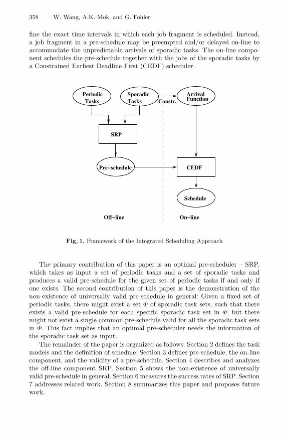
358 W. Wang, A.K. Mok, and G. Fohler

fine the exact time intervals in which each job fragment is scheduled. Instead,a job fragment in a pre-schedule may be preempted and/or delayed on-line toaccommodate the unpredictable arrivals of sporadic tasks. The on-line compo-nent schedules the pre-schedule together with the jobs of the sporadic tasks bya Constrained Earliest Deadline First (CEDF) scheduler.

TasksSporadicTasks

ArrivalFunction

Schedule

PeriodicConstr.

Pre−schedule

On−lineOff−line

SRP

CEDF

Fig. 1. Framework of the Integrated Scheduling Approach

The primary contribution of this paper is an optimal pre-scheduler – SRP,which takes as input a set of periodic tasks and a set of sporadic tasks andproduces a valid pre-schedule for the given set of periodic tasks if and only ifone exists. The second contribution of this paper is the demonstration of thenon-existence of universally valid pre-schedule in general: Given a fixed set ofperiodic tasks, there might exist a set Φ of sporadic task sets, such that thereexists a valid pre-schedule for each specific sporadic task set in Φ, but theremight not exist a single common pre-schedule valid for all the sporadic task setsin Φ. This fact implies that an optimal pre-scheduler needs the information ofthe sporadic task set as input.

The remainder of the paper is organized as follows. Section 2 defines the taskmodels and the definition of schedule. Section 3 defines pre-schedule, the on-linecomponent, and the validity of a pre-schedule. Section 4 describes and analyzesthe off-line component SRP. Section 5 shows the non-existence of universallyvalid pre-schedule in general. Section 6 measures the success rates of SRP. Section7 addresses related work. Section 8 summarizes this paper and proposes futurework.

Pre-Scheduling: Integrating Offline and Online Scheduling Techniques 359

2 Task Model

We shall adopt the usual model of real-time tasks and assume that a task can bemodeled either as a periodic task or as a sporadic task with preperiod deadlines.All workloads are modeled as being made up of a periodic task set TP and asporadic task set TS. Each task T in either TP or TS is an infinite sequence ofjobs. A job is defined by a triple: ready time, deadline and execution time andis written as (r, d, c); the job must receive a total execution time of c betweentime r and time d at run-time. A periodic task is defined by a 4-tuple: initialoffset, period, relative deadline, and execution time and is written as (o, p, l, c).The first job of a periodic task is ready at time o, and the subsequent jobs areready at the beginning of each period exactly p time units apart. We shall adoptas a convention in this paper the notation X.a which denotes the attribute aof entity X. The jth job of a periodic task T may be written as (T.o + j · T.p,T.o + j · T.p + T.l, T.c), starting with job 0. Similarly, a sporadic task is definedby a tuple: (p, l, c), with its attributes defined the same way as a periodic task,except that the period of a sporadic task is the minimal length of the timeinterval between two consecutive jobs, and the actual ready time of any job ofa sporadic task cannot be known until it arrives at run-time. We use an arrivalfunction A to represent the arrival times of sporadic jobs in a particular run.A valid arrival function must satisfy the minimal arrival interval constraint: forany two consecutive jobs Ji and Ji+1 of a sporadic task T , it must be the casethat A(Ji+1)−A(Jj) ≥ T.p. A job J of sporadic task T will be written as (A(J),A(J) + T.l, T.c).

Let the hyper-period P be the least common multiple of the periods of allperiodic tasks in TP and all sporadic tasks in TS. For any natural number n,the time interval (n ·P , (n+1) ·P ) is called a hyper interval. Our scheduler willgenerate a pre-schedule for the length of one hyper-period and repeat the samesequence of jobs of the periodic tasks every hyper interval at run-time, i.e., theon-line component of our scheduler restarts the pre-schedule at the beginning ofevery hyper interval. For ease of discussion, let JP represent the list of the jobsof the periodic tasks within one hyper interval. Every job in JP occurs exactlyonce in every hyper interval, and will be called a periodic job in the remainderof this paper. Notice that in this terminology, there are as many periodic jobs inJP from the same periodic task as the number of periods of the task in a hyper-period. For each periodic task T in TP, for any natural number j less thanP

T.p , there is a periodic job in JP which is defined by (r, d, c) = (T.o + j · T.p,T.o + j · T.p + T.l, T.c).

Job J is before job J ′ and job J ′ is after job J if and only if either (1)J.r < J ′.r and J.d ≤ J ′.d; or (2) J.r ≤ J ′.r and J.d < J ′.d. Job J contains jobJ ′ or job J ′ is contained by job J if and only if J.r < J ′.r and J ′.d < J.d. JobJ is parallel with job J ′ if and only if J.r = J ′.r and J.d = J ′.d. For schedulingpurposes, parallel periodic jobs can be transformed into a single periodic jobwith their aggregate execution time. Therefore, we shall not consider paralleljobs in the remainder of the paper. We assume that JP is sorted such that a jobwith lower index is either before or contained by a job with higher index.

360 W. Wang, A.K. Mok, and G. Fohler

Example 1. The task sets TP and TS defined below are used in later examplesin this paper.

TP = (90, 225, 30, 5), (0, 75, 75, 15), (0, 225, 225, 150); TS = (225, 25, 25)

The hyper-period of the task sets P is 225. The set of periodic jobs JP isdefined as follows.

JP = [(0, 75, 15), (90, 120, 5), (75, 150, 15), (0, 225, 150), (150, 225, 15)]

Fig. 2 illustrates the periodic tasks and the periodic jobs. The vertical barsindicate the ready times and deadlines of periodic jobs, and the length of thebox inside the scope of a periodic job indicates its execution time.

J0 J2 J4

J3

J1

0 225

75 150

90 120

0 225

P

T

T

T

0

1

2

Fig. 2. Definition of TP and JP

We shall assume that all tasks are preemptable and are scheduled on a singleprocessor. A schedule is represented by a function S which maps each job to aset of time intervals. For instance, S(J) = (b0, e0), (b1, e1) means that job Jis scheduled to two time intervals (b0, e0) and (b1, e1). A schedule must satisfythe following two constraints. Firstly, there is at most one job to be scheduledat any point in time, i.e., at any time t, there exists at most one job J , by which(b, e) ∈ S(J) and b < t < e. Secondly, the accumulated time allocated to each jobbetween its ready time and deadline must be no less than its specified executiontime, i.e., for any job J ,

∑(b,e)∈S(J)(min(J.d, e) − max(J.r, b)) ≥ J.c.

3 Definitions of Pre-Schedule and the Online Component

A pre-schedule F is a list of fragments, where a fragment F is defined by a 5-tuple, (j, k, r, d, c) with the following meaning. Suppose J is the jth periodic jobin job list JP. F is the kth (starting from 0) fragment in the pre-schedule of job

Pre-Scheduling: Integrating Offline and Online Scheduling Techniques 361

J , and job J is scheduled for at least a total execution time of c between timesr and time d in every hyper interval.

The CEDF scheduler is the EDF scheduler plus one additional constraint:the sequencing of the periodic jobs must agree with the pre-schedule exactly.This may be implemented as follows. At the beginning of each hyper interval,let the first fragment in the pre-schedule be marked as “current”. Define R asthe set of sporadic jobs waiting to be scheduled. The set R is initialized at time0 as an empty set. When a sporadic job becomes ready, it is added into R; whenit is completely scheduled, it is removed from R. At any time, if the deadline dof the current fragment is earlier than the deadline of any job in R, the currentfragment is scheduled; otherwise, the sporadic job with the earliest deadline inR is scheduled. When the execution time of the current fragment is completelyscheduled, mark the next fragment in the pre-schedule as “current”, and so on.

Example 2. Pre-schedule F is a pre-schedule for JP and TS defined in Exam-ple 1.

F = [(0, 0, 0, 75, 15), (3, 0, 0, 120, 60), (2, 0, 75, 120, 15),(1, 0, 90, 120, 5), (3, 1, 90, 225, 90), (4, 0, 150, 225, 15)]

Suppose that the first job of a sporadic task T3, written as JS arrives at dif-ferent times in two different runs of the system, denoted by the arrival functionsA and A′, such that A(JS) = 0 and A′(JS) = 30. The on-line scheduler willproduce two different schedules S and S′, as illustrated in Fig. 3. Each box inthe schedule represents an interval of time scheduled to a job. The fragmentscorresponding to periodic jobs being scheduled are on the top of the boxes inthe figure. Notice that the start times and the finish times of periodic jobs mayvary to accommodate the arrivals of sporadic jobs, but the order defined by thepre-schedule is always followed.

Js J0 J3

F0 F1

F0 F1 F1

JsJ0 J3J3

F2 F4F3

J3

F5

J2

115 120 210

1 J4

225

F2 F4F3

J3

F5

J2

115 120 210

1 J4

225

S0 25 40 100

J

S’0 15 30 55 100

J

Fig. 3. Schedules Accommodating Different Arrival Functions

A pre-schedule is valid if and only if the following three conditions are satis-fied. Firstly, under any valid arrival function A of TS, CEDF always producesa valid schedule for TS and JP. Secondly, for any fragment F , suppose J is itscorresponding periodic job. Then the ready time and the deadline of F will be

362 W. Wang, A.K. Mok, and G. Fohler

within the effective scheduling scope of J , i.e., J.r ≤ F.r ≤ F.d ≤ J.d. Third, forany fragment F , the execution time F.c is greater than or equal to 0.

4 The Offline Component

The off-line component SRP produces a pre-schedule in three steps. The firststep establishes F(j,k), a list of partially defined fragments, in which only theattributes j and k of each fragment are defined. Essentially, the first step definesa total order of fragments in the pre-schedule. The following two steps will notchange the order of the fragments. They only define the other attributes foreach fragment. The second step defines the ready time r and deadline d of eachfragment and produces F(j,k,r,d). The third step defines the execution time c ofeach fragment to produce F(j,k,r,d,c), the completed pre-schedule which is alsorepresented as F. We shall describe SRP in detail step by step and show thatSRP produces a valid pre-schedule if and only if one exists.

4.1 Step 1: Generating F(j,k)

In this step, a partially defined pre-schedule F(j,k) is created according to thefollowing constraint-based definition.

A periodic job in JP is a top periodic job if and only if it does not containany other periodic job in JP. Constraint 1 and 2 are about the fragments of topperiodic jobs.

Constraint 1 Each top periodic job has one and only one fragment.Constraint 2 Let J and J ′ be any pair of top periodic jobs, and F and F ′

be their corresponding fragments. Fragment F is before fragment F ′ if and onlyif periodic job J is before periodic job J ′.

Constraint 3 and Constraint 4 are about the fragments of non-top periodicjobs. For convenience, we introduce the concept of “gap”. A gap is a sub-sequenceof non-top fragments in F(j,k). Let FT0 and FTt−1 be the first and the last topjob fragments. All fragments before FT0 are in a gap denoted as (⊥, FT0), and allfragments after FTt−1 are in a gap denoted as (FTt−1 , ⊥). Let FTx and FTx+1 betwo consecutive fragments of top jobs, and all fragments of non-top jobs betweenthem are in a gap denoted as (FTx , FTx+1). Fragments FT0 , FTt−1 FTx and FTx+1

are “boundary fragments” of gaps.Constraint 3 If a periodic job J contains at least one of the top jobs cor-

responding to the boundary fragments of a gap, then there exists one and onlyone fragment of J in the gap; otherwise, there exists no fragment of J in thatgap.

Constraint 4 Suppose that both fragment F of periodic job J and fragmentF ′ of periodic job J ′ are in the same gap. Case 1: J is before J ′. F is beforeF ′. Case 2: J contains J ′. If the gap is (⊥, FT0), F is before F ′; if the gapis (FTt−1 , ⊥), F ′ is before F ; if the gap is (FTx , FTx+1), and J ′ contains thecorresponding job of FTx+1 , F is before F ′; if the gap is (FTx , FTx+1), and J ′

does not contain the corresponding job of FTx+1 , F ′ is before F .

Pre-Scheduling: Integrating Offline and Online Scheduling Techniques 363

Example 3. JP is defined in Example 1. Jobs J0, J1, and J4 are top jobs, whilejob J2 and J3 are not. Partially defined pre-schedule F(j,k) is shown below.

F(j,k) = [(0, 0), (3, 0), (2, 0), (1, 0), (2, 1), (3, 1), (4, 0)]

4.2 Step 2: Generating F(j,k,r,d)

This step augments F(j,k) to F(j,k,r,d); in other words, it defines the ready timer and deadline d for each fragment. The ready times of fragments are definedas the earliest times satisfying the following constraints: (1) the ready timeof each fragment is not earlier than the ready time of its corresponding job;(2) the ready times of fragments in F(j,k,r,d) are non-decreasing. Similarly, thedeadlines of fragments are defined as the latest times satisfying the followingconstraints: (1) the deadline of each fragment is not later than the deadline of itscorresponding job; (2) the deadlines of fragments in F(j,k,r,d) are non-decreasing.

Example 4. JP and F(j,k) are defined in Examples 1 and 3. F(j,k,r,d) is definedfollows.

F(j,k,r,d) = [(0, 0, 0, 75), (3, 0, 0, 120), (2, 0, 75, 120), (1, 0, 90, 120),(2, 1, 90, 150), (3, 1, 90, 225), (4, 0, 150, 225)]

4.3 Step 3: Generating F(j,k,r,d,c)

This step augments F(j,k,r,d) to F(j,k,r,d,c) by assigning the execution time c foreach fragment. At the beginning of this step, we augment F(j,k,r,d) to F(j,k,r,d,x),representing the execution time of each fragment as a variable; then we solve thevariables with a Linear Programming (LP) solver under three sets of constraints:non-negative constraints, sufficiency constraints and slack-reserving constraints,which are defined as follows.

Non-negative constraints require that the execution times to be non-negative;i.e., for every fragment F , F.x ≥ 0.

Notice that a fragment may have zero execution time. A fragment with zeroexecution time is called a zero fragment; otherwise it is a non-zero fragment. Zerofragments are trivial in the sense that we can either delete or add them from orto a pre-schedule, and the schedule produced according to the pre-schedule willnot be modified at all.

Sufficiency constraints require that for every periodic job J in JP, the ag-gregate execution time of its fragments in the pre-schedule shall be equal to theexecution time of J ; i.e.,

∑F.x = J.c, where F is any fragment of J .

A slack-reserving constraint requires that the aggregate execution time offragments and all sporadic jobs that must be completely scheduled within a

364 W. Wang, A.K. Mok, and G. Fohler

time interval shall be less than or equal to the length of the time interval. Sincean execution may start at time 0 but may last forever, therefore the number oftime intervals is infinite. In order to make the pre-scheduling problem solvable,we must establish a finite number of critical slack-reserving constraints, suchthat if all critical slack-reserving constraints are satisfied by a pre-schedule, allslack-reserving constraints are satisfied. For this purpose, we define critical timeintervals.

A time interval (b, e) is critical if and only if all of the following conditions aretrue. First, there exists a periodic job J in JP and J.r = b. Second, the lengthof the time interval is shorter than or equal to the hyper-period; i.e., e − b ≤ P .Third, at least one of the following cases is true: there exists a periodic job J ′

in JP and either J ′.d = e or J ′.d + P = e; or there exists a sporadic task T inTS, such that e − b = T.p · n + T.d, where n is a natural number.

In order to define slack-reserving constraints on critical intervals, we intro-duce two functions, E(b, e) and Slack(l). Function E(b, e) represents the aggre-gate execution time of all fragments that must be completely scheduled betweencritical time interval (b, e), and function Slack(l) represents the maximal aggre-gate execution time of sporadic jobs that must be completely scheduled within atime interval of length l. The slack-reserving constraint on a critical time interval(b, e) is E(b, e) ≤ e − b − Slack(e − b).

Function E(b, e) is computed with the following two cases. For the first case,time interval (b, e) is within one hyper interval (0, P ), i.e., e ≤ P . Let Fb bethe first fragment with a ready time greater than or equal to b, Fe be the lastfragment with a deadline less than or equal to e; then E(b, e) =

∑F.x, where

F is between and including Fb and Fe. For the second case, time interval (b, e)straddles hyper interval (0, P ) and hyper interval (P, 2P ), i.e., e > P . Thenlet Fb be the first fragment with a ready time equal or after to b, and let Fe

be the last fragment with a deadline earlier than or equal to e − P , functionE(b, e) =

∑F.x, where F is any fragment including and after Fb or before and

including Fe.Function Slack(l) is computed as follows. Let function n(T, l) be the maximal

number of jobs of T that must be completely scheduled within l. If l− lT.p·T.p <

T.d, n(T, l) = lT.p; otherwise, n(T, l) = l

T.p + 1. Function Slack(l) is equalto

∑T∈TS

T.c · n(T, l).Function E(b, e) is a linear function of a set of variables, and Slack(e − b) is

a constant; therefore, the slack-reserving constraint is a linear constraint.Non-negative constraints, sufficiency constraints and slack-reserving con-

straints on critical intervals are all linear and their total number is finite; there-fore, the execution time assignment problem is a LP problem, which can besolved optimally in the sense that if there exists an assignment to the execu-tion times under these constraints, the assignment will be found in finite time.Optimal LP solvers are widely available. If an optimal LP solver returns an as-signment to execution times, SRP produces a fully defined pre-schedule with theexecution times; otherwise, SRP returns failure.

Pre-Scheduling: Integrating Offline and Online Scheduling Techniques 365

Example 5. Assume that JP and TS are defined in Example 1, and F(j,k,r,d) isdefined in Example 4.

All non-negative constraints are listed as follows.

F0.x ≥ 0; F1.x ≥ 0; F2.x ≥ 0; F3.x ≥ 0; F4.x ≥ 0; F5.x ≥ 0

All sufficiency constraints are listed as follows.

F0.x = 15; F3.x = 5; F2.x + F4.x = 15; F1.x + F5.x = 150; F6.x = 15

The slack-reserving constraints on many critical time intervals will be triviallysatisfied. For instance, time interval (0, 75) is a critical time interval, however,E(0, 25) = F0.x = 15, Slack(75−0) = 25, therefore the slack-reserving constrainton this time interval is always satisfied. We list all non-trivial slack-reservingconstraints below.

F1.x + F2.x ≤ 75 critical interval (0, 120)F4.x + F5.x ≤ 90 critical interval (90, 225)

The pre-schedule F in Example 2 satisfies all the above constraints, so it is avalid pre-schedule.

4.4 Optimality and Computational Complexity

We prove the optimality and complexity of SRP in Theorem 1 and 2. Due tothe page limitation, proofs for Lemma 1 and Lemma 2 can not be provided inthis paper. They are available on-line at [13].

Lemma 1. Slack-reserving constraints on all time intervals are satisfied by apre-schedule produced by SRP.

Lemma 2. If SRP produces a pre-schedule F, then F is valid.

Lemma 3. If a valid pre-schedule exists, SRP produces one pre-schedule.

Proof. The strategy of our proof is as follows. Suppose F′ is a valid pre-schedule.First we transform F′ into another valid pre-schedule F1 which can be obtainedby augmenting attributes r, d, and c to each fragment of F(j,k), the partiallydefined pre-schedule generated by Step 1 of SRP. Then we further transform F1

to F2, which can be obtained by augmenting attribute c to each fragment ofF(j,k,r,d) generated by Step 2 of SRP. Because F2 is a valid pre-schedule, thereexists a pre-schedule satisfying all constraints in Step 3 of SRP, and so SRP mustproduce a pre-schedule. We define the transformations and show the correctnessof the claims below.

Transformation 1: from F′ to F1

366 W. Wang, A.K. Mok, and G. Fohler

Apply the following rules one at a time to the pre-schedule, until no rule canbe further applied.

Rule 1: If Fb and Fe are two consecutive fragments of the same job J , mergethem into one fragment F of job J , with F.c = Fb.c + Fe.c, F.r = Fb.r andF.d = Fe.d.

To facilitate other rules, we first define a primitive Swap(Jf , Jr, Fb, Fe),which swaps all non-zero fragments (fragments with non-zero execution times)of job Jf before all non-zero fragments of job Jr between and including fragmentsFb and Fe. It may be implemented as follows. Let Cf be the aggregate executiontime of all fragments of job Jf between and including Fb and Fe. Let C[x,y) bethe aggregate execution time of all fragments of job Jf or Jr including and afterFx but before Fy. Let Fm be the latest fragment of either job Jf or job Jr, suchthat C[b,m) is less than or equal to Cf . For every fragment F of job Jr includingand after Fb but before Fm, change it to a fragment of job Jf without changingits ready time, deadline, or execution time. Similarly, for every fragment F ofjob Jf after Fm but before and including Fe, change it to a fragment of jobJr. If C[b,m) = Cf , make Fm a fragment of Jr. Otherwise, split Fm into twoconsecutive fragments Fmf of job Jf and Fmr of job Jr, such that the readytimes and deadlines of Fmf and Fmr are the same as those of Fm, but Fmf .c =Cf − C[b,m) and Fmr.c = Fm − Fmf .c.

Rule 2: Assume that job Jf is before job Jr. Let Fb be the first non-zerofragment of Jr, and Fe be the last non-zero fragment of Jf . If Fb is before Fe inthe pre-schedule, apply Swap(Jf , Jr, Fb, Fe).

Rule 3: Assume that job Jf contains job Jr. Let Fb and Fe be the first and thelast non-zero fragments of Jr. If there exists a non-zero fragment of Jr betweenFb and Fe, apply Swap(Jf , Jr, Fb, Fe).

Rule 4: Assume that non-zero fragment Fb of non-top job Jf is before non-zero fragment Fe of non-top job Jr, and Fb and Fe are within the same gap(defined in Step 1 of SRP), represented as (x, y), where x and y are either ⊥ orthe boundary fragments. Apply Swap(Jf , Jr, Fb, Fe) if and only if one of thefollowing cases is true. Case 1: Jf is contained by Jr, y is not ⊥ and Jf containsthe top job corresponding to y. Case 2: Jf contains Jr, and either y is ⊥ or Jr

does not contain the top job corresponding to y.Claim 0: Transformation 1 terminates.Proof of this claim can be found in [13].Claim 1: Pre-schedule F1 is a valid pre-schedule.None of the transformation rules will change the aggregate execution time

of any periodic job or any critical time interval. Also, the ready time and dead-line of a fragment in transformation is maintained within the valid scope of itscorresponding job.

Claim 2: Pre-schedule F1 can be obtained by augmenting F(j,k).By the transformation rules, if F1 does not satisfy the constraints listed in

Step 1 of SRP, Transformation 1 won’t terminate. Notice that if there is nofragment F of J between any consecutive pair of fragments of top jobs in F1,we can always plug in a fragment F of job J with 0 execution time at proper

Pre-Scheduling: Integrating Offline and Online Scheduling Techniques 367

position. Therefore, there is a one-to-one in-order mapping between F1 andF(j,k), which implies the claim.

Transformation 2: from F1 to F2

Re-assign attribute r and d of every fragment according to the algorithm inStep 2 of SRP.

Claim 3: F2 is a valid pre-schedule.For every fragment, its ready time and deadline are still within the valid

range of its corresponding periodic job, and the execution time of each fragmentremains unchanged. If F2 is not valid, there must exist an arrival function A,such that CEDF fails with it at a time e, which is either the deadline of a sporadicjob or a periodic job. Let b be the latest idle time before e or time 0 if such anideal time does not exist. Let F 2

b be the first fragment in F2 with a ready timeat or after time b and F 2

e be the last fragment in F2 with a deadline before or attime e. Fragment F 2

b must be the first fragment of its corresponding job Jb andF 2

b .r = Jb.r. Let F 1b be the corresponding fragment in F1, then F 2

b .r ≤ F 1b .r.

Similarly, F 1e .d ≤ F 2

e .d. Then all fragments between and including F 1b and F 1

e

must be scheduled between time b and e when CEDF schedules according toF1. With the same arrival function A, CEDF must also fail with F1, whichcontradicts with Claim 1.

Claim 4: F2 can be obtained by augmenting F(j,k,r,d).Follows Claim 2 and the fact that the attributes r and d of fragments in F2

are defined by the algorithm in Step 2 of SRP.Claim 5: SRP must produce a pre-schedule.It is easy to show that all non-negative, sufficient execution time and slack-

reserving constraints are necessary for a valid pre-schedule. Because of Claim 3,F2 satisfies all these constraints. Together with Claim 4, F2 implies the existenceof an execution time augment to F(j,k,r,d) that satisfies all those constraints.Therefore Step 3 of SRP must return a pre-schedule.

Immediately follows Lemma 2 and Lemma 3, we have the following theorem.

Theorem 1. Given JP and TS, SRP produces a valid pre-schedule if and onlyif it exists.

Theorem 2. The computational complexity of SRP is O(C(n2p, np · (np + ns)),

where np and ns are the number of periodic jobs and the maximal number ofsporadic jobs in one hyper-period respectively, and C(n, m) represents the com-plexity of the LP solver with n variables and m constraints.

Proof. The complexity of the LP solver is the major factor. The maximal numberof fragments is bounded by n2

p. The number of non-negative constraints and thenumber of execution time constraints are bounded by np, and the number ofslack-reserving constraints on critical intervals is bounded by np · (np + ns).

368 W. Wang, A.K. Mok, and G. Fohler

5 The Non-existence of Universally Valid Pre-Schedule

The slack embedded in a pre-schedule by SRP specifically targets one given setof sporadic tasks. Is it possible to produce a one-size-fits-all pre-schedule? Toformalize the discussion, we define the concept of universally valid pre-schedule.For a given periodic task set TP, a pre-schedule FU is universally valid if andonly if the following condition is true for any sporadic task set TS: either FU

is a valid pre-schedule for TP and TS or there exists no valid pre-schedule forthem. If a universally valid pre-schedule exists for every periodic task set, thena more dynamic optimal integrating scheduling scheme could be constructed:A universally valid pre-schedule might be produced off-line without requiringthe knowledge of the sporadic task set, and the sporadic task set might beallowed to change on-line, under the admission control of a schedulability test asdefined in [6]. The optimality criterion for scheduling here means that if a specificsporadic task set is rejected on-line, then no valid pre-schedule of the periodictasks exists for this sporadic task set. However, by Example 6, we can show thatthe one-size-fits-all pre-schedules are impossible: universally valid pre-scheduledoes not exist in general, so the more dynamic scheme we surmise above cannotbe done.

Example 6. Suppose one periodic task set and two alternative sporadic task setsare defined as follows:

TP = (56, 100, 19, 9), (0, 100, 100, 71); Ts = (50, 10, 10); T′s = (20, 4, 4)

With both sets of sporadic tasks, hyper-period P = 100, and the periodic joblist is defined as follows.

Jp = [(56, 75, 9), (0, 100, 71)]

There exists a valid pre-schedule F for TP and TS, and a valid pre-schedule F′

for TP and T′S, defined as follows.

F = [(1, 0, 0, 75, 46), (0, 0, 56, 75, 9), (1, 1, 56, 100, 25)]F′ = [(1, 0, 0, 75, 48), (0, 0, 56, 75, 9), (1, 1, 56, 100, 23)]

Suppose there is a universally valid pre-schedule FU. Let Xb be the total exe-cution time of all fragments of J1 before the last fragment of J0 in FU; let Xa

be the aggregate execution time of all fragments of J1 after the first fragment ofJ0 in FU. A universally valid pre-schedule FU must satisfy the following set ofcontradicting constraints, therefore does not exist.

Xb + Xa ≥ 71 sufficiency constraint for J1

Xb ≤ 46 slack-reseving constraint on (0, 75) for TS

Xa ≤ 23 slack-reseving constraint on (56, 100) for T′S

Pre-Scheduling: Integrating Offline and Online Scheduling Techniques 369

6 Experiments

We investigate the performance of SRP in terms of the success rate of pre-schedule generation. As we mentioned, [5] and [6] address the issue of validitytesting on pre-schedules but do not provide any specific pre-scheduling algorithm.So for comparison purposes, we need to consider “reasonable” pre-scheduling al-gorithms which do not take into account the sporadic workload. Accordingly, wechoose a well-understood pre-scheduling algorithm called Offline-EDF(OEDF).Given a set of periodic jobs, OEDF first schedule the periodic jobs according toEDF in one hyper period, which is a sequence of fragments. Without changingthe sequence of fragments, OEDF then minimizes the ready-times and maximizethe deadlines of fragments under the following constraints: The sequence of allready-times and the sequence of all deadlines are both non-decreasing, and theready-time and deadline of each fragment is within the range of its correspond-ing periodic job. OEDF is aggressive in preparing pre-schedules to accommodatethe impact of sporadic tasks; we deem it a reasonable pre-scheduler for a faircomparison with SRP.

We measure the success rate of both SRP and OEDF on the same eightgroups of test cases. There are 100 cases for each group. Tasks in each test caseare randomly generated, but they must satisfy the following requirements. Thetotal utilization rate of sporadic tasks is always between 10% and 20%. Therelative deadline of each sporadic task is between its execution time and itsperiod. The total utilization rate of periodic tasks are set to different ranges indifferent test groups, as shown in Table 1. The relative deadline of each periodictask is always equal to its period.

Table 1. SRP vs. OEDF

Sporadic Utl. Rate (%) 10-20Periodic Utl. Rate (%) 0.01-10 10-20 20-30 30-40 40-50 50-60 60-70 70-80SRP Success Rate (%) 100 99 97 98 98 97 97 89

OEDF Success Rate (%) 100 96 77 57 35 33 29 28

The measurement shows that when total utilization rate is not low, the differ-ence between SRP and OEDF is significant. Take the last group as an example:When the total utilization rate is between 80% and 100% (70% to 80% periodictask utilization plus 10% to 20% sporadic task utilization), SRP can success-fully produce valid pre-schedule for 89 cases out of 100 cases, while OEDF canproduce valid pre-schedule for only 28 cases.

370 W. Wang, A.K. Mok, and G. Fohler

7 Related Work

In the introduction section, we have reviewed the Slot Shifting scheme [5] [6],CE scheduler [1] and EDF scheduler [8]. In this section, we review other relatedwork.

Gerber et al propose a parametric scheduling scheme [7]. They assume thatthe execution order of real-time tasks is given, the execution times of tasks mayrange between upper and lower bounds, and there are relative timing constraintsbetween tasks. The scheduler consists of an off-line component and an on-linecomponent. The off-line component formulates a “calendar” which stores twofunctions to compute the lower and upper bounds of the start time for eachtask. The bound functions of a task take the parameters of tasks earlier in thesequence as variables and can therefore be solved on-line. Based on the bounds onthe start time, the on-line dispatcher decides when to start scheduling the real-time task. The parametric scheduling scheme and our integrated approach sharethe following similarities: (1) Both schemes make use of off-line computation toreduce on-line scheduling overhead and yet guarantee schedulability. (2) Bothschemes make use of slacks to handle a non-deterministic workload representedeither as variable parameters or as sporadic tasks. Yet, the parametric schedulingscheme assumes that the sequencing order of the tasks is given, but our integratedapproach does not. Instead, the order is established by the pre-scheduler in ourcase. The techniques applied in these two schemes are also quite different.

The pre-scheduling techniques in our integrated approach are more related toa line of research by Erschler et al [4] and Yuan et al [14], even though their workfocuses on non-preemptive scheduling of periodic tasks. Erschler et al introducethe concept of “dominant sequence” which defines the set of possible sequencesfor non-preemptive schedules. They also introduce the concept of “top job”.Building upon the work of Erschler et al, Yuan et al propose a “decompositionapproach”. Yuan et al define several relations between jobs, such as “leading”and “containing”, and apply them in a rule-based definition of “super sequence”which is equivalent to dominant sequence. The partially defined pre-scheduleF(j,k) in our paper is similar to the dominant sequence or the super sequence,and we adopt some of their concepts and terminology as mentioned. However, inview of the NP-hardness of the non-preemptive scheduling problem, approximatesearch algorithms are applied to either the dominant sequence or super sequenceto find a schedule in [4] and [14]. In this paper, the execution time assignmentproblem on the partially defined pre-schedule can be solved optimally by LPsolver.

General composition approaches have been proposed in recent years, such asthe open system environment [3] by Deng and Liu, temporal partitioning [10] byMok and Feng, and hierarchical schedulers [11] by Regehr and Stankovic. Thegeneral composition schemes usually focus on the segregation between compo-nents or schedulers, which means that the behavior of a component or schedulerwill be independent to the details of other components or schedulers. In contrast,our integrated approach focuses on paying the scheduling overhead off-line and

Pre-Scheduling: Integrating Offline and Online Scheduling Techniques 371

yet provides strict ordering and deadline guarantees by making intensive use ofthe information available about all tasks.

8 Conclusion

This paper proposes an integrated approach that combines the advantages ofCE and EDF schedulers. We present an off-line Slack Reserving Pre-schedulingalgorithm which is optimal in the sense that given a periodic task set and asporadic task set, SRP produces a valid pre-schedule if and only if one exists.Experiment shows that SRP has a much higher success rate than that of anEDF-based pre-scheduling algorithm. We also demonstrate the non-existence ofuniversally valid pre-schedules, which implies that every optimal pre-schedulingalgorithm requires both the periodic task set and the sporadic task set as input.

For future work, SRP may be extended to accommodate workload modelsother than periodic and sporadic tasks with preperiod deadlines, such as complexinter-task dependencies. We may also apply the pre-scheduling techniques toother forms of integrated schedulers, such as a combination of CE and the fixedpriority scheduler.

References

1. T. P. Baker, A. Shaw. The cyclic executive model and Ada, Proceedings of IEEEReal-Time Systems Symposium, pp.120–129, December 1988.

2. G. B. Dantzig. Linear Programming and Extensions, Princeton University Press,1963.

3. Z. Deng and J. Liu. Scheduling Real-Time Applications in an Open Environment.Real-Time Systems Symposium, pp. 308–319, December 1997.

4. J. Erschler, F. Fontan, C. Merce, F. Roubellat. A New Dominance Concept inScheduling n Jobs on a Single Machine with Ready Times and Due Dates, Opera-tions Research, 31:114-127.

5. G. Fohler. Joint Scheduling of Distributed Complex Periodic and Hard AperiodicTasks in Statically Scheduled Systems, Real-Time Systems Symposium, pp. 152–161, December 1995.

6. D. Isovic, G. Fohler. Handling Sporadic Tasks in Off-line Scheduled DistributedReal-Time Systems, the 11th EUROMICRO Conference on Real-Time Systems,pp. 60–67, York, England, July 1999.

7. R. Gerber, W. Pugh, and M. Saksena. Parametric Dispatching of Hard Real-TimeTasks, IEEE Trans. on Computers, Vol.44, No.3, pp. 471–479, Mar 1995.

8. C.L. Liu and J.W. Layland. Scheduling Algorithms for Multi-programming in HardReal-time Environment. Journal of ACM 20(1), 1973.

9. A. K. Mok. Fundamental Design Problems of Distributed Systems for the Hard-Real-Time Environment. Ph.D. thesis. MIT. 1983.

10. A. K. Mok, X. Feng. Towards Compositionality in Real-Time Resource PartitioningBased on Regularity Bounds. Real-Time Systems Symposium, pp. 129–138, 2001.

11. J. Regehr, J. A. Stankovic. HLS: A Framework for Composing Soft Real-TimeSchedulers. Real-Time Systems Symposium, pp. 3–14, 2001.

372 W. Wang, A.K. Mok, and G. Fohler

12. Duu-Chung Tsou. Execution Environment for Real-Time Rule-Based Decision Sys-tems. PhD thesis, Department of Computer Sciences, The University of Texas atAustin, 1997.esting for Real-Time Tasks, Real-Time Systems, Vol. 11, No. 1, pp. 19–39, 1996.

13. W. Wang, A. K. Mok, G. Fohler. Pre-Scheduling: Integrating Off-line and On-lineScheduling Techniques, http://www.cs.utexas.edu/users/mok/RTS/pubs.html.

14. X. Yuan, M.C. Saksena, A.K. Agrawala, A Decomposition Approach to Non-Preemptive Real-Time Scheduling, Real-Time Systems, Vol. 6, No. 1, pp. 7–35,1994.

Author Index

Benveniste, Albert, 35Bernat, Guillem, 1Bhattacharyya, Shuvra S., 257Bos, Herbert, 51Broster, Ian, 1Burns, Alan, 1Buttazzo, Giorgio C., 67Butts, Ken, 290

Carloni, Luca P., 35Caspi, Paul, 35, 84Chabini, Noureddine, 100Chakrabarti, Arindam, 117Chen, Guangyu, 156Colaco, Jean-Louis, 134Curic, Adrian, 84

Deng, Xianghua, 173de Alfaro, Luca, 117De La Luz, Victor, 156Dill, David, 323Dwyer, Matthew B., 173

Ellner, Stephan, 340

Fauster, Janosch, 190Fohler, Gerhard, 356

Girault, Alain, 206Godefroid, Patrice, 223

Hatcliff, John, 173Henzinger, Thomas A., 117, 241Hua, Shaoxiong, 257

Kandemir, Mahmut, 156Karsai, Gabor, 290Kirner, Raimund, 190Kirsch, Christoph M., 241Kloukinas, Christos, 274Kolcu, Ibrahim, 156

Larsen, Kim G., 16Loyall, Joseph P., 20

Maignan, Aude, 84Manna, Zohar, 323Matic, Slobodan, 241Mok, Aloysius K., 356

Nakhli, Chaker, 274Neema, Sandeep, 290Nicollin, Xavier, 206

Pouzet, Marc, 134Puschner, Peter, 190

Qu, Gang, 257

Regehr, John, 306Reid, Alastair, 306Robby, 173

Samwel, Bart, 51Sanchez, Cesar, 323Sangiovanni-Vincentelli, Alberto L., 35Sankaranarayanan, Sriram, 323Sipma, Henny, 323Sofronis, Christos, 84Stoelinga, Marielle, 117Sztipanovits, Janos, 290

Taha, Walid, 340Tripakis, Stavros, 84

Wang, Weirong, 356Webb, Kirk, 306Wolf, Wayne, 100

Xi, Hongwei, 340

Yovine, Sergio, 274

Zhang, Ting, 323