Population Economics

Editorial Board

John ErmischBengt-Arne WickstromKlaus F. Zimmermann

Springer-Verlag Berlin Heidelberg GmbH

Titles in the Series

Jacques 1.Siegers . Jenny de Jong-Gierveld . Evert van Imhoff (Eds.)Female Labour Market Behaviour and Fertility

Hendrik P. van DalenEconomic Policy in a Demographically Divided World

Dieter Bas· Sijbren Cnossen (Eds.)Fiscal Implications of an Aging Population

Klaus F.Zimmermann (Ed.)Migration and Economic Development

Nico HeerinkPopulation Growth, Income Distribution, and Economic Development(out of print)

Tommy Bengtsson (Ed.)Population, Economy, and Welfare in Sweden

1.Haisken-De NewMigration and the Inter-Industry Wage Structure in Germany

D. A. Ahlburg . A. C. Kelley . K. Oppenheim Mason (Eds.)The Impact of Population Growth on Well-beingin Developing Countries

BoninGenerational Accounting

Klaus F. ZimmermannMichael VoglerEditors

Family, Householdand Work

With 26 Figuresand 106 Tables

Springer

Professor Dr. Klaus F. ZimmermannDr. Michael Vogler

Forschun gsinstitui zur Zukunft der Arbeil (IZA)Schaumburg-Lippe-SlraBe 7-953113 Bonn, Ge rma nyHomepage: www.iza.org

BiMiogra phic informal ion published by Oie Deersche Bibliol;hekDie Deutsc he Bibliothek lish Ih is pubtica lio n in IIM: De etscbe Nlltionalbibliogr alie;4etaikd bibliographic da la available in the inlernc:1 al 'mpJ/dnb.ddb.de

Th is wor k is subiecl to copyright . AII righls are reserved, whether Ihe wtlole or pa " o f lhemater ial i, ccncemed.specmcafty Ihe rig tlls o f translanon. rep rin ling. reuse o f iIluSlral ions,recit,lIlion. broadcasl ing, reprod uct ion on microlilm o r in an y Ol tler way, and seorage ind ata bank$. Duplicat ion of ltlis pubfication o r part e lhereof is permiued only und e r theprovisions of the German Co pyrighl Law o f Sept ember 9,1965. in its current ve rsloa, a ndpe rmission for use must always be ob ta ine d from Springe r-Vertag. Violalio liSare liab lefor proseccnon unde r the German Co Pyrillhl Law.

htlp:llwww.spri nger.4eCISpringer·Verlag Berlin Heidelberg 2003Oris:irvJly published by SpringCl", Verille Berlin Heidelberg New York io 2(0)

soneo ver reprin l o f thc: twdcover 1si edi tion 2003The USoC of ge neral descript ive O1Imes.registered n,ames.. lJademarts.ele. in lhis publialtiondces noi imply.eve n io the abseece of II speci fic Slaleme nt. tha l sueh names are u emptfrOfll Ihe relevant prceecnve laws and regulalions and therefore frec for general U$C.

Ccver~gn: Erich Kirchncr. Heidd be rg

SP IN 10908JS8 -4213130 - .5 " ) 2 I O- Prinled on acid frcc paper

ISBN 978-3-642-62439-1 ISBN 978-3-642-55573-2 (eBook)DOI 10.1007/978-3-642-55573-2

Preface

Demographic changes are now at the heart of the development of theeconomy. Within the area of Population Economics, the interest inhousehold and family issues has been steadily rising in the last fewyears, which is reflected in the number of papers published by scientificjournals, and in the programs of economics conferences. While this in­terest was fostered by rapid and ongoing changes in family structuresover the last decades, only the growing availability of high-quality microdatasets and the required computer capabilities made it possible to dealmore intensively with this topic. The increasing empirical evidence alsoproduced further challenges to develop the theoretical framework.In the editorial process of the Journal of Population Economics manypapers have passed our desks and only the best of them have been pub­lished after a refereeing process. Given the increasing interest in thematter and the high quality of the research published in our journal, wesaw a substantial value-added to publish a selection of recent contribu­tions to make the work more accessible to the scientific community.Hence, we are very glad to present the book herewith. It is divided inthree parts, "Time use and non-market work", "Household and familydevelopment" and "Transition to work and younger employees". Ofcourse, there are close interactions between these topics. The followingeditorial shall give a short overview.We would like to take the opportunity to thank Springer-Verlag forthe fruitful cooperation over the past years.

KLaus F. ZimmermannMichaeL VogLer

Editorial

by Klaus F Zimmermann and Michael Vogler

During the last decades, the appearance of a family has changed sub­stantially. Not long ago a typical family consisted of a husband who lefthome in the morning to go to work, while his wife was tended to thehousework during the day. They normally lived together for their wholelife times, having one or more children, which primarily were raised bythe wife. Although this model for most people might still be the optimalway of living together, in practice differing living models became muchmore common than before. Statistics provide clear observations of thetrends: The number of single-person households increased. Age of mar­riage, as well as women's age at first motherhood became remarkablyhigher. Fertility has fallen rapidly. The number of divorces has steadilyincreased.The ancestral role allocation became less relevant in practice, becausetoday neither economic nor social constraints are as import for the de­cision to start a family as they were in the past. From an economic pointof view, there are several reasons. Among them: In the course of increas­ing equality today the average woman is by far better educated thanbefore. In some industrial countries she even has a school education su­perior to that of the average man. This led to more financial autonomyand higher professional ambitions. Furthermore, the expansion of socialsecurity systems decreased the need of family assistance in distress andold age. In the face of decreasing fertility in industrialized countries, itis often argued that legal and fiscal provisions even discriminate fami­lies.The perception and valuation of housework and child care respective­ly, has changed. On the one hand this should to some degree be a resultof changing family structures, while on the other hand it probably evencontributed to the latter. With a growing number of single-personhouseholds and two-earner couples, men have taken over more respon­sibilities at home although it is still common that women stay at homeafter their children are born. Yet we are still witnessing a lack of knowl­edge in economics about the mechanisms of household time allocation.Little attention has been given to this topic, because housework normal­ly is regarded as non-market work and time not spent on paid work sim­ply has been defined as leisure time. Only in the last few years, there hasbeen a rising interest in the 'time use' of people.The first chapter ("Time use and non-market work") starts with a

study of Daniel S. Hamermesh, who points out that the dissociationfrom the standard view on labor supply provides useful new insights inthe topic of time use. Sebastien Lecocq, as well as Steinar Vagstad, andThomas Aronsson, Sven-Olov Daunfeldt and Magnus Wikstrom use the

VIII Editorial

'household production model' as a starting point to empirically and the­oretically analyze various aspects of the intra-household time alloca­tion. Alfonso Sousa-Poza, Hans Schmid and Rolf Widmer, as well asMichael Lundholm and Henry Ohlsson take a closer look especially atthe time parents dedicate to child care.The ongoing changes in family structures generate people, whose no­tion of a family is completely different from that of their grandparents,not only regarding family size. Undoubtedly, it is social progress thatchildlessness, divorce, or single motherhood are no longer stigmatizedby society. However, because less children experience the traditionalfamily model, its assumed merits could get more and more forgottenover time. There is increasing evidence that disturbed family structureslead to unfavorable development of children. Divorces are often not on­ly accompanied by psychological strains but also by financial problems.Apart from aspects of social behavior, from an economic point of viewit is argued that affected children have lower achievement potential.The second chapter ("Household and family development") providesspecial attention to the important influence of the household back­ground, mainly in terms of income and household formation, on the de­velopment of the family and children respectively. The study by StephenJenkins deals with income dynamics, which not only are influenced byeconomic factors but also by changes in the family composition, Ales­sandra Guariglia takes a closer look at the relationship between incomeuncertainty and saving behavior of households. John F. Ermisch andMarco Francesconi, Andrew McCulloch and Heather E. Joshi, and Mar­tha S. Hill, Wei-Jun 1 Jeung and Greg Duncan analyze the effects of fam­ily structure and wealth on children's cognitive and educational devel­opment. Maite Martinez-Granado and Javier Ruiz-Castillo, as well asStephen Garasky, R. Jean Haurin and Donald R. Haurin examine thedecisions of adolescents whether to stay with or leave their parentalhome and their favorite living models.Nearly all statistics show that young adults face an above-average riskof being unemployed. School-to-work transition and early years of la­bor market participation are subject to mechanisms, which are differentthan those for experienced workers. Entering the labor market, all ado­lescents inevitably belong to the unemployed first and have to searchfor a job. Being 'outsiders' they are especially affected by structural andcyclical labor market problems. Furthermore, depending on age andpersonal development, young people often do not have a profoundknowledge of their abilities and options. Not surprisingly, the exits fromemployment are substantially higher than those for more experiencedworkers. Because young women have to decide whether and when theywant to bear children, their job decisions are influenced by additionalaspects. To the contrary, fertility decisions are affected by the labor mar­ket situation, too.In the last chapter ("Transition to work and younger employees") thefirst set of papers deals with the determinants of youth's labor marketsuccess. Regina T. Riphahn analyses the determinants of school-to-worktransition in general, Oivind Anti Nilsen, Alf Erling Risa and Alf

Editorial IX

Torstensen deal with the exits of youths from employment, while PaulFronstin, David H. Greenberg and Philip K. Robins especially concen­trate on the identifying effects of parental disruption on the labor mar­ket performance of children. The second focus of this chapter is onyoung females. Siv Gustafsson gives an overlook of the economic viewon timing of fertility. Focusing on different countries, Adriaan S. Kalwij(for the Netherlands), Namkee Ahn and Pedro Mira (for Spain), andLinda Adair, David Guilkey, Eilene Bisgrove and Soccoro Gultiano (forthe Philippines) analyze the relationship between childbearing and thesituation in the local labor markets.

Time use and non-market work

Most studies on time allocation are based on the so-called 'householdproduction model', which was introduced by Gary Becker and radicallywidened the economic view of non-market activities at home. The basicnotion is that households combine time and market goods to producecommodities that enter their utility function. Household members spe­cialize according to their comparative advantages and also allocate in­vestments according to this point of view. Most attention was given tothe modeling of the household utility function, abandoning the originalassumption of households as being single utility maximizing units. Apopular model is the so-called 'collective model' by Pierre-Andre Chi­appori. However, there still are a lot of theoretical questions that areopen, and empirical evidence in the past often suffered from the scarcityof usable data sets.

Hamermesh stresses the fact that household structure not only ac­counts for people's supply of paid work in terms of hours, but also de­termines people's preferences on when to work. Pleasant working timescan be seen as a non-monetary benefit, an aspect which is especially im­portant to two earner couples and families that prefer to spend as muchcommon time at home as possible. Using data from the U.S. CurrentPopulation Survey (CPS), he shows that evening and night work de­creased since the early 70s. Rising real earnings power obviously hasbeen used to shift away from unpleasant work time. At the same time,not only earnings inequality increased but also the distribution of un­pleasant working times, with low wage worker having to accept a largerfraction of evening and night work. An analysis of spouses' decisionsrevealed that common leisure time actually is a determinant of individ­uallabor supply, and that income increases are partly converted to therealization of togetherness.The "household production model" is a common starting point for thestudy of time allocation. For econometric reasons, the absence of con­crete commodities led researchers to construct a function which isweakly separable in goods and time used for the production of com­modities in the sense of the household production model. Using Frenchdata, Lecocq tests this so-called 'weak separation hypothesis'. His re­sults for instance show that meal preparation actually is separable fromrestaurant expenditures, market goods inputs and household leisure

x Editorial

time. However, opposed to the hypothesis' assumption, it is not separa­ble from time inputs devoted to other household activities. In his theo­retical study, Vagstad shows the consequences of non common prefer­ences of family members, and thus abandons an usual assumption.Although the mechanisms of specialization keep valid as suggested bythe household production model, neither investments in specializationremain efficient nor the time allocations to it. Aronsson, Daunfeldt andWikstrom use an extended version of the mentioned 'collective model'to estimate the intra-family distribution of income, leisure and house­hold production from Swedish household data. In contradiction to otherstudies, their results confirm the importance of the 'pooling hypothesis',which states that only the aggregated income, but not income distribu­tion, determines the intra-household allocation of time. Education andthe number of children are the most important factors for the allocationof housework and leisure.

Sousa-Poza, Schmid and Widmer take a closer look at the allocationof time to housework and child care. Using Swiss data they can confirmthat the presence of children primarily influences women's behavior.The time men invest in housework does not rise when children arepresent, and only little time is dedicated to child care. Furthermore, theresults show that men with higher education allocate more time tohousework and child care. Lundholm and Ohlsson extend the 'quality­quantity model', which says that increased income could not only in­crease demand for children, but also could be used for investments inthe quality of children. The study shows that, if parents face restrictionsin terms of time and the possibility to purchase child care, income in­creases still are ambiguous regarding fertility outcomes.

Family structure and development

While the model of an optimal family should not have changed so muchin the mind of most people, in practice there have been rapid changesin the realized living models. In research there is a growing awarenessconcerning the consequences of these changes, not only in sociology butalso in (population) economics. These new family backgrounds, whichoften entail economic and psychological problems, might produce chil­dren who are left aggrieved with regard to different aspects, e.g. in theircognitive development and educational attainment. Revolving aroundthis focus, the chapter presents new insights concerning household in­come formation and its consequences, family structure and develop­ment, and the decisions of youths regarding their living arrangementstowards autonomy.Although, of course, labor earnings of the household head are crucialfor family care, looking at the poverty dynamics reveals that over timeother factors play an important role as well. In his study for BritainJenkins shows that, overall, demographic events (e.g. partnership disso­lution) are more important for poverty spell beginnings than changes inthe household head's labor earnings. In the case of spell endings, demo­graphic events do not have this same relevance. However, it is shown

Editorial XI

that other, additional money income, such as the spouse's labor earningsand benefits, overall are of higher importance for leaving poverty thanthe head's earnings. In her study, which also uses the British HouseholdPanel Survey,Guariglia analyzes the influence of income uncertainty onhousehold saving behavior. Her results show that there actually is a gen­eral component of precautionary savings. Furthermore, in accordancewith the life cycle model, expected financial deteriorations let peopleaccumulate reserves.The development of a family and children respectively, is primarily anoutcome of the underlying 'in-house' background although external in­fluences, of course, also might play an important role. Most attention isgiven to the relevance of household wealth and family structure. Er­misch and Francesconi, using data from the British Household PanelSurvey, show that children from a single-parent family not only are ag­grieved in terms of education and have a higher risk of inactivity, butalso more often suffer from health problems. Hill, Yeung and Duncan,using U.S. panel data (PSID), find that parental marital change hasstronger influences when the event occurs during late childhood. Intheir study family income appears to be the most important factor forbetter educational attainment and lowers daughter's risk of a nonmari­tal birth. Based on British data,McCulloch and Joshi conclude that fam­ily poverty is associated with poorer average cognitive development ofchildren. However, material disadvantages obviously can be overcomeby positive parental care, which is mostly depending on the mother'seducation.

Martinez-Granado and Ruiz-Castillo analyze three import decisionsof adolescents towards their autonomy: Whether to study, to work andto leave the parental home, or not. Their study for Spain explicitly con­siders the interdependencies of these decisions. Among other interest­ing results, they find that education has a positive influence on the prob­ability of males leaving their homes, while this is not the case forfemales. Housing prices clearly matter, but living in metropolitan areasby itself, leads to a higher propensity to leave. Using a national Ameri­can sample of adolescents aged between 16 and 30,Garasky, Haurin andHaurin look at the factors, which influence adolescents' choices of des­tination when exiting the parents' home. They also realize that thehome-leaving decision is arrived at differently by males and females.Furthermore, while economic variables are relevant for the leave, thedecision to move into large or small groups is solely influenced by socio­demographic factors.

Transition to work and young employees

Labor markets in industrial countries suffer from high youth unemploy­ment. Many governments started policy measures to fight the threatthat the persistence problem creates a generation with a substantialfraction of hopeless people. This would not only mean a waste of humanresources, but also would cause substantial long-term economic and so­cietal problems. There are no doubts that in a globalized world educa-

XII Editorial

tion is the key for future development, and that the course can only beset accordingly during childhood if there are to be reasonable perspec­tives. Furthermore, there is a clear relationship between the situation inlabor markets and fertility decisions of young women. While causalityin principle works both ways, for industrialized countries the effects ofthe labor market situation on the fertility decision is of greater interestin practice.While Riphahn investigates the determinants of school-to-work tran­sitions in Germany, using data from the German Socio-Economic-Panel(GSOEP), Nilsen, Risa and Torstensen analyze the exits from employ­ment based on a large representative sample of young Norwegian work­ers. Both studies confirm the importance of human capital acquisition,especially measured by school type, experience and age. In general goodeducational attainment secures a lower risk of unemployment, as pre­dicted by the human capital theory. Nilsen, Risa and Torstensen andRiphahn also show that, given the personal characteristics, the condi­tions of local labor markets and in industrial sections have a strong in­fluence on the employment of young workers. Considering the institu­tional framework and past legal measures both studies provide usefulinsights into youth labor market policy in particular. Using British dataFronstin, Greenberg and Robins show that the accumulation of humancapital is highly dependent on parental disruptions during early child­hood. Divorce or parental death lead to lower educational attainmentand worse labor market outcomes. The scope of these effects depend onthe age of children at the time the disruption occurs, and surprisingly isdifferent for male and females. The importance of the family back­ground, too, is relevant in the study of Riphahn, who shows that parents'educational attainment positively influences the labor market successof their children.

In her study on the optimal age of motherhood, Gustafsson providesan overlook of economic determinants of fertility timing. While unem­ployment and income can always be found in the spotlight of studies,she realizes that consumption smoothing and individual career planningalso playa major role in practice. Kalwij shows that in the Netherlands,controlling for other characteristics, employed women schedule the firstchildren later in life and overall bear fewer children during their lifespans than unemployed women. Educational attainment seems to haveno direct effect on motherhood but works via the employment status.Looking at the 'fertility crisis' in Spain Ahn and Mira, explicitly focuson the importance of the male employment status. Their results showthat spells of male unemployment have a negative effect on the timingof marriage, and subsequently on the decision to have the first child.Focusing on the effects of childbearing on women's earning, in theirstudy of the Philippines Adair, Guilkey, Bisgrove and Gultiano not onlyconcentrate on the type of work but also on supplied hours. Allocatingrestricted time between child care and work it might be optimal to havelower paid but more flexible work. In fact the results clearly show thata higher number of children lead to lower earnings. However, this effectis only remarkable in presence of babies, which shows that women ad­just work time in favor of child care.

Contents

Time use and non-market work

Hamermesh DSTiming, togetherness and time windfalls 1

Lecocq SThe allocation of time and goods in household activities:A test of separability . . . . . . . . . . . . . . . . . 25

Vagstad SOn private incentives to acquire household production skills. . . 39

Aronsson T, Daunfeldt S-O, Wikstrom MEstimating intrahousehold allocation in a collective modelwith household production. . . . . . . . . . . . . . . 51

Sousa-PozaA, Schmid H, Widmer RThe allocation and value of time assigned to houseworkand child-care: An analysis for Switzerland . . . . . . . . . 67

Lundholm M, Ohlsson HWho takes care of the children?The quantity-quality model revisited . . . . . . . . . . . 87

Household and family development

Jenkins SPModelling household income dynamics . . . . . . . . . . 95

Guariglia ASaving behaviour and earnings uncertainty:Evidence from the British Household Panel Survey . . . . . .135

Ermisch JF, Francesconi MFamily structure and children's achievements . . . . . . . .151

Hill MS, Yeung W-JJ, Duncan GJChildhood family structure and young adult behaviors . . . . .173

XIV Contents

McCulloch A, Joshi HEChild development and family resources:Evidence from the second generationof the 1958 British birth cohort .. 203

Martinez-Granado M, Ruiz-Castillo JThe decisions of Spanish youth: A cross-section study . . . . . 225

Garasky S, Haurin RJ, Haurin DRGroup living decisions as youths transition to adulthood . . . .251

Transition to work and younger employees

Riphahn RTResidential location and youth unemployment:The economic geography of school-to-work transitions. . . . .273

Nilsen 0A, Risa AE, Torstensen ATransitions from employment among young Norwegian workers .295

Fronstin P, Greenberg DH, Robins PKParental disruption and the labour market performanceof children when they reach adulthood . . . . . . . . . . 309

Gustafsson SOptimal age at motherhood.Theoretical and empirical considerations on postponementof maternity in Europe . . . . . . . . . . . . . . . .345

Kalwij ASThe effects of female employment status on the presenceand number of children. . . . . . . . . . . . . . . .369

Ahn N, Mira PJob bust, baby bust?: Evidence from Spain ........389

Adair L, Guilkey D, Bisgrove E, Gultiano SEffect of childbearing on Filipino women's work hoursand earnings. . . . . . . . . . . . . . . . . . . . 407

Timing, togetherness and time windfalls

Daniel S. Hamermesh

Department of Economics, University of Texas, Austin, TX 78712-1173 USA(Fax: +1-512-471-3510; e-mail: hamermes@eco.utexas.edu)

Received: 6 July 2000jAccepted: 20 January 2001

Abstract. With appropriate data the analysis of time use, labor supply and lei­sure can move beyond the standard questions of wage and income elasticitiesofhours supplied. I present four examples: 1) American data from 1973 through1997 show that the amount ofevening and night work in the U.S. has decreased.2) The same data demonstrate that workers whose relative earnings increaseexperience a relative diminution of the burden of work at unpleasant times. 3)U.S. data for the 1970s and 1990s demonstrate that spouses' work schedulesare more synchronized than would occur randomly; synchrony among workingspouses diminished after the 1970s; and the full-income elasticity of demandfor it was higher among wives than among husbands in the 1970s but equal inthe 1990s. 4) Dutch time-budget data for 1990 show that the overwhelmingmajority of the windfall hour that occurred when standard time resumed wasused for extra sleep.

JEL classification: 120

Key words: Leisure, time use, work amenities

1. Introduction

For many years labor supply has been the single most heavily researched topicin the subfield of labor economics (Stafford, 1986). Nearly all of this research

Daniel S. Hamermesh is Edward Everett Hale Centennial Professor, University of Texas at Austin;research associate, National Bureau of Economic Research, and Forschungsinstitut zur Zukunftder Arbeit. I thank the National Science Foundation for support under Grants SBR-9422429 andSES-9904699, and two anonymous referees, Gerard Pfann, the late Lee Lillard, Gerald Oettinger,Steve Trejo and participants at the ESPE Conference and at seminars at the University of Bristoland Warwick University for helpful comments. Responsible editor: Klaus F. Zimmermann.

2 D. S. Hamermesh

has been based on data derived from questions about how many hours, weeksor years people have been engaged in market-based activities. The focus hasbeen on the integration of workers' time to derive the fraction of some partic­ular interval that is spent in market work. Very little research has examinedtime use - how individuals spend their time at work and in other activities; andalmost none has examined the economic implications ofwhen people engage inwork and nonwork activities.These little-studied supply-related topics can provide insights into a variety

of questions that have been addressed in other ways, and often not so success­fully, using more standard approaches and more commonly used data. Forexamples, changes in the distribution of workers' well-being depend not onlyon the monetary returns to work, but also on the changing distribution of suchnonmonetary returns as the timing of work. The issue ofjointness in a marriedcouple's supply of labor can only be addressed if we know when the couple isworking. Simply examining how the total of one spouse's hours affects theother's is not informative about their decisions on supplying labor as affectedby what is presumably their desire to be together, or by their possible need forchildcare. As still another example, there is an immense literature attemptingto estimate pure income effects on labor supply. Yet equally important, andfor obvious reasons essentially unstudied, is the pure full-income effect of anincrease in available time.The purpose in this study is not to provide a definitive list of new ways

of viewing time use that might be generally interesting to economists and tolabor economists/demographers especially. Rather, it is to give what I believeare some novel and interesting examples that I hope might inspire others toapproach these and similarly motivated issues using the many underutilizedsets of data that are available for this purpose. This is a much more fruitfulendeavor than the development of ever more complex econometric models oflabor supply that focus on the same standard questions of measuring wageand income effects on hours/weeks worked using standard data sets. I hope todemonstrate that moving beyond refinements to the standard model and itsestimation can be useful and interesting.Accordingly, in Sect. 2 I examine the role of work timing - when people

work - as an amenity of the employment relation and consider how changesin timing in the United States might be taken as reflecting changes in the well­being of the average worker. Section 3 uses this same idea to consider how ourunderstanding of labor-market inequality is altered when we take nonmonetarycharacteristics of work, in this case the timing of work, into consideration. InSect. 4 I study the demand for work timing in the context of the household,focusing particularly on whether spouses' "togetherness" is affected by theirincomes and how this demand has changed over time. Section 5 focuses onexamining responses to an exogenous increase in the time at their disposal bya random sample of households. These ideas and empirical analyses are tiedtogether by the common themes that they illustrate new ways of thinking aboutlabor supply and leisure and that they test how shocks to the economy alteroutcomes along a variety of dimensions of time use and the timing of activities.

2. Work timing as a workplace amenity

The argumentation here and in the rest of the study compares outcomes acrossequilibria in the labor market. Unsurprisingly, very little can be inferred out-

Timing, togetherness and time windfalls 3

side of equilibrium, especially if the burden of the disequilibria varies acrossworkers. The value of this standard, neoclassical approach lies in its predictiveability, so that the contribution of these analyses must be measured by whetherthe facts that are uncovered accord with the theory that is outlined.

It is easy to see how changes in amenities are altered when the real earningscapacities ofworkers in different groups change. View workers as being able toobtain a combination of real earnings, other monetary benefits (which I hence­forth subsume under earnings), and nonmonetary benefits from the jobs theyoccupy (as originally in Rosen 1974). Workers sort themselves among jobs thatdiffer by the amenities that the jobs offer according to their preferences fornonmonetary amenities and earnings. Workers who especially prefer amenities(e.g., are extremely averse to working at night) will sort into jobs that avoidnight work. Jobs that fail to offer the amenity ofday work must compensate forits absence through higher wages in order to attract workers. We will observethat otherwise identical workers obtain higher wages in those jobs, so that theymay be viewed as offering premium wages (see Kostiuk 1990, for evidence onthis). Because workers whose overall earnings ability is low require earnings justto get by, they will be especially willing to accept unpleasant jobs that compen­sate for the unpleasantness by offering higher wages.What will happen in such a labor market as full earnings rise generally? We

will observe ever-fewer workers who are willing to accept work at undesirabletimes. This will induce employers to: 1) Offer higher premia to attract workersto such times; but 2) Price out of the market some employers who would other­wise have conducted their business at evening/night. We should observe theprice (compensating wage differential) for such work rising, while the quantityof such work falls. Indeed, if we are uncertain about the path of real earnings(perhaps, as in the United States, because of difficulties measuring indexes ofliving costs, Boskin et al. 1998), a good indication that real earnings have risenis that the quantity of disamenities observed in the labor market, includingwork at undesirable times, has fallen (barring major changes in legal restric­tions on the provision of amenities/disamenities, none ofwhich occurred in theUnited States during this period).This entire discussion is from the supply side of the labor market and en­

tirely ignores the effects of possible shocks to employers' labor demand. Iftechnical change makes evening/night work more expensive for employers at agiven set of supply conditions, we would observe a decline in the quantity ofsuch work performed even though workers' full earnings have not risen. Whilethis is possible and is extremely difficult to contradict, most observers of thelabor market argue that technology has shifted people toward a 24-hour econ­omy, implying that the bias in technology has been toward an increase in thedemand for evening/night work, other things equal. Thus ifwe find despite thisthat the amount ofevening/night work has declined, we can reasonably assumethat supply behavior has dominated this implicit market.To illustrate this approach I take data from the United States Current

Population Survey May Supplements for 1973, 1978, 1985, 1991 and 1997 (theearliest four ofwhich are also used for a related purpose in Hamermesh 1999a).In these few surveys (and in the May Supplements from 1974 through 1977)respondents were questioned about the starting and ending times on their mainjobs: "At what time of day did ... begin (end) work on this job most days lastweek?" Regrettably the questions are not specific to each day of the week, butrather talk about what the worker "usually" does. The ideal, a set of repeated

4 D. S. Hamennesh

cross-sections of large numbers of time diaries showing exactly when people areat work for each of a number ofdays, is simply unavailable in the United Statesor elsewhere. To ensure that the workers in the sample are at work at thesehours on most days, only employees with at least 20 hours ofwork per week areincluded in the analysis in this section.From the information the respondents provided I can construct a set of

24 indicators, List, for each worker i interviewed in year t, with the indicatorequaling 1 if the responses imply that the person worked in the market at hourS, 0 if not. This is different from identifying workers as being on shifts, as hasbeen done by, for example, Mellor (1986). Because a majority of workers onthe job at, for example, 3AM would not be classified as night-shift workers(Hamermesh 1996), this hour-by-hour approach gives a fuller picture of thedistribution of work.Before examining how the distribution has changed, we need to establish

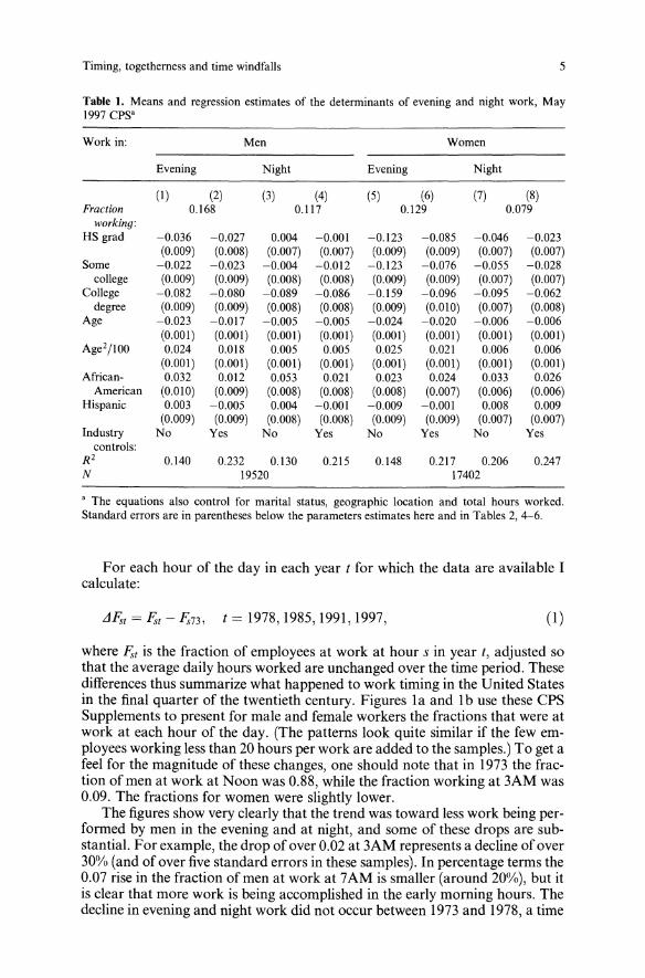
whether in fact there is a consistent pattern relating work at various times of theday to workers' demographic characteristics. To save space I define the varia­bles EVE = 1if the worker was on the job at any time between 7PM and 10PM,ootherwise, and NIGHT = 1 if he/she was on the job at any time between10PM and 6AM, 0 otherwise. I relate these variables to workers' educationalattainment, their age, ethnic/racial status and other controls available in theCPS. In addition, in the some of the estimates I hold constant for the workers'detailed industry affiliation (thus controlling for potential differences causedby employers' rather than the workers' behavior).The top row of Table I presents for both genders the mean fractions of

employees working evenings or nights. Unsurprisingly, men are more likely tobe working during these unusual hours than are women. Below these meansthe Table lists the coefficients from linear-probability estimates of the deter­minants of EVE and NIGHT for all workers in the May 1997 Supplementwhose usual weekly hours were 20 or more. (Probits yield qualitatively similarconclusions.) For both EVE and NIGHT the first column in each pair presentsestimates that exclude industry indicators, while the second includes them.The results make it very clear that evening or night work disproportionatelyburdens those with lower educational attainment (since the excluded categoryis workers with less than a high-school diploma). Similarly, the U-shaped re­lationship between age and the incidence of evening or night work shows thatsuch labor is disproportionately done by younger workers or those nearingretirement. Holding constant their total workhours, the lowest probability ofwork outside the standard workday is among workers around age 50, roughlythe peak of age-earnings profiles. This negative relationship between the prob­ability of working evening or night and a worker's earnings ability is changedonly slightly even when we account for the worker's detailed industry affilia­tion.The estimates in Table I also provide some evidence that evening and night

work is performed disproportionately by minorities, especially by African­Americans, even after accounting for racial/ethnic differences in age and edu­cational attainment. There are essentially no differences in the probabilities ofevening and night work between nonhispanic whites (the excluded category)and Hispanics. The differences in the probabilities of working evenings/nightsare consistent with the notion that workers whom the labor market rewards lessare more likely to work evenings or nights. By inference, evening/night work isa disamenity.

Timing, togetherness and time windfalls 5

Table 1. Means and regression estimates of the determinants of evening and night work, May1997 CPS·

Work in: Men Women

Evening Night Evening Night

(I) (2) (3) (4) (5) (6) (7) (8)Fraction 0.168 0.117 0.129 0.079

working:HS grad -0.036 -0.027 0.004 -0.001 -0.123 -0.085 -0.046 -0.023

(0.009) (0.008) (0.007) (0.007) (0.009) (0.009) (0.007) (0.007)Some -0.022 -0.023 -0.004 -0.012 -0.123 -0.076 -0.055 -0.028college (0.009) (0.009) (0.008) (0.008) (0.009) (0.009) (0.007) (0.007)College -0.082 -0.080 -0.089 -0.086 -0.159 -0.096 -0.095 -0.062degree (0.009) (0.009) (0.008) (0.008) (0.009) (0.010) (0.007) (0.008)Age -0.023 -0.017 -0.005 -0.005 -0.024 -0.020 -0.006 -0.006

(0.001) (0.001) (0.001) (0.001) (0.001) (0.001) (0.001) (0.001)Age2jlO0 0.024 O.oJ8 0.005 0.005 0.025 0.021 0.006 0.006

(0.001) (0.001) (0.001) (0.001) (0.001) (0.001) (0.001) (0.001)African- 0.032 0.012 0.053 0.021 0.023 0.024 0.033 0.026American (0.010) (0.009) (0.008) (0.008) (0.008) (0.007) (0.006) (0.006)Hispanic 0.003 -0.005 0.004 -0.001 -0.009 -0.001 0.008 0.009

(0.009) (0.009) (0.008) (0.008) (0.009) (0.009) (0.007) (0.007)Industry No Yes No Yes No Yes No Yescontrols:

R 2 0.140 0.232 0.130 0.215 0.148 0.217 0.206 0.247N 19520 17402

• The equations also control for marital status, geographic location and total hours worked.Standard errors are in parentheses below the parameters estimates here and in Tables 2, 4-6.

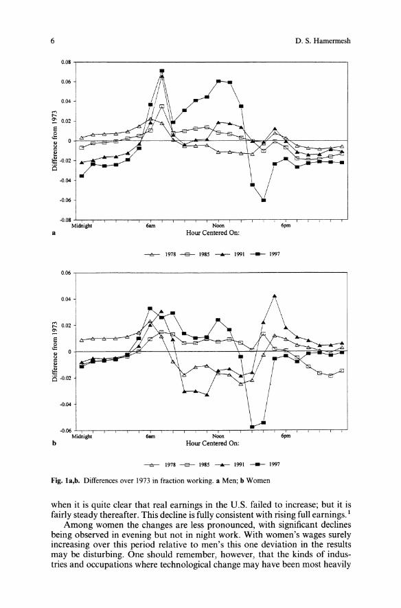
For each hour of the day in each year t for which the data are available Icalculate:

LJF'st = F'st - F's73, t = 1978,1985,1991,1997, (1)

where F'st is the fraction of employees at work at hour s in year t, adjusted sothat the average daily hours worked are unchanged over the time period. Thesedifferences thus summarize what happened to work timing in the United Statesin the final quarter of the twentieth century. Figures la and 1b use these CPSSupplements to present for male and female workers the fractions that were atwork at each hour of the day. (The patterns look quite similar if the few em­ployees working less than 20 hours per work are added to the samples.) To get afeel for the magnitude of these changes, one should note that in 1973 the frac­tion ofmen at work at Noon was 0.88, while the fraction working at 3AM was0.09. The fractions for women were slightly lower.The figures show very clearly that the trend was toward less work being per­

formed by men in the evening and at night, and some of these drops are sub­stantial. For example, the drop of over 0.02 at 3AM represents a decline of over30% (and of over five standard errors in these samples). In percentage terms the0.07 rise in the fraction ofmen at work at 7AM is smaller (around 20%), but itis clear that more work is being accomplished in the early morning hours. Thedecline in evening and night work did not occur between 1973 and 1978, a time

6 D. S. Hamermesh

0.08,_-----------------------------,

0.06

0.04

-0.04

·0.06

6pmNoonHour Centered On:

6am-0.08 .L..,-_~~~-_~~~-~~~~~-,_~ __-r_~~___..,____,-.,.-J

Midni8ht

a

-e- 1978 -S- 1985 -.- 199\ __ 1997

0.06 -,--------------------------------,

0.04

-0.04

6pmNoonHour Centered On:

6am

-0.06 .L..-_~~~-_~~_-r__~~___,- _ _T___-r__~___..,____,-.,.-J

Midnight

b

-e- \978 -e- \985 -.- \991 __ 1997

Fig. la,b. Differences over 1973 in fraction working. a Men; b Women

when it is quite clear that real earnings in the U.S. failed to increase; but it isfairly steady thereafter. This decline is fully consistent with rising full earnings. 1Among women the changes are less pronounced, with significant declines

being observed in evening but not in night work. With women's wages surelyincreasing over this period relative to men's this one deviation in the resultsmay be disturbing. One should remember, however, that the kinds of indus­tries and occupations where technological change may have been most heavily

Timing, togetherness and time windfalls 7

biased toward night work are those that are especially female-intensive, par­ticularly service and retail industries. Those occupations/industries may besufficient in number that the bias of technology toward night work is sufficientto have outweighed the induced reduction in supply of night-time labor.The main point of this section is that, almost certainly contrary to popular

belief, the best evidence suggests that evening/night work in the United Stateshas diminished in importance since the early 1970s. As shown in Hamermesh(1999a, Fig. 3), evening and night work among all workers decreased through1991 among men in all major industries except the tiny (in the United States)agriculture sector. The same is true for evening work in all major industriesamong women. This is consistent with the view that workers' real earningpower has increased and that they have used part of it to shift away from workat an unpleasant time. Whether this is true universally is unclear; but theapproach taken here should be applicable in other economies. Examining sec­ular changes in other labor economies would be a useful approach to under­standing the changing well-being of their workers.

3. Work timing and economic inequality

In the past 20 years, whether because of increased international trade (Leamer1996), technical change that is biased toward skilled workers (Berman et al.1998), declines in institutions that protect low-skilled workers, or still othercauses, shocks to the labor market have raised the earnings ability of skilledworkers relative to unskilled workers essentially worldwide (Pereira and Mar­tins 2000). These changes have implied a relative improvement in the prospectsof those who would have earned more even without them. This should havecaused those workers, even more than before, to shy away from jobs that lacksuch workplace amenities as desirable schedules, since their earning power hasincreased most. Obversely, low-skilled workers will be observed occupying aneven greater fraction of the jobs that have undesirable characteristics: Becausethe supply of skilled workers to those jobs is reduced, employers offering themwill pay higher wage premiums; and, with their earnings ability falling relativeto other workers, the relative supply of lower-skilled workers to jobs offeringthese premiums will be higher than before.Changes in the distribution of workplace amenities should thus mirror

changes in the distribution of wages. We would expect that the widening dis­tribution of earnings would have been accompanied by an increasingly unequaldistribution of the burden of unpleasant workplace characteristics. This willbe true so long as employers' ability to offer daytime jobs has not changed dif­ferentially by the skill of its workers. In other words, only skill-biased technicalchange in the provision of the amenity, working during the day, will cause thisprediction to fail.While it is clear that sorting in the changing implicit market for the amenity

of desirable work timing will cause a change in the distribution of the amenity,the implications for inequality of full earnings - wages plus the value of theamenity - are unclear. Write full earnings E in logarithmic form as:

E= W+8D, (2)

where 8 is the premium for evening/night work, and D equals 1 if the worker

8 D. S. Hamennesh

works evenings/nights. Imagine a shock to the labor market that increases thevariance of full earnings. Assume that the full-income elasticity of demand forthe amenity exceeds unity by enough to offset the rise in e(an assumption thatis consistent with evidence showing very high income elasticities of demandfor monetary benefits, Woodbury and Hamermesh 1992). We will then observethat an increase in the variance of log-wages (W) will be accompanied by anincrease in the variance of E.Having shown that workers with lower earnings potential have a greater

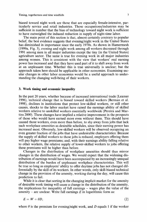
likelihood of performing evening/night work, we can examine how patterns ofwork timing have changed in relation to changing earnings differences. As inthe literature on earnings inequality (Juhn et al. 1993), I base the comparisonson the weekly earnings of full-time (35+ hours per week) workers. To verifythat the earnings of full-time workers in these May CPS Supplements exhibitthe same rise in inequality that has been noted more generally, Fig. 2 presentsestimates of:

q = 1,2,3, t = 1978,1985,1991,1997, (3)

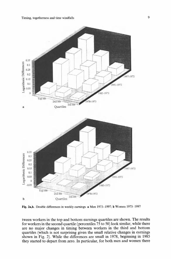
where W is the logarithm of average weekly earnings among workers in earn­ings quartile q in year t, and the superscript 4 refers to workers in the bottomquartile of earnings. 2 The measures il 2 w;q for men and women thus show per­centage changes in average earnings within each of the three upper quartilessince 1973 compared to percentage changes in earnings in the lowest quartile.The estimates of these double-differences in earnings are shown in Figs. 2a

and 2b for men and women. The results parallel what has been demonstratedgenerally for the United States over this period. For both genders there hasbeen a very sharp rise in earnings inequality since the early 1970s, with much ofthe increase coming between 1978 and 1985. The biggest relative increases havebeen in the top earnings quartile, with increases generally being somewhatlarger among men than women. Similar patterns to these, and to the remainingresults in this section, are shown if we disaggregate the full-time workforce byearnings decile.The data are sorted by weekly earnings, and for each worker the fraction

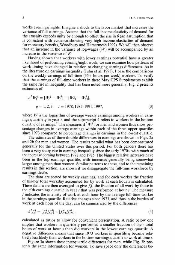
of his/her total workday accounted for by work at each hour s is calculated.These data were then averaged to give Is'l, the fraction of all work by those inthe q'th earnings quartile in year t that was performed at hour s. The measuref indicates the intensity of work at each hour by the average full-time workerin the earnings quartile. Relative changes since 1973, and thus in the burden ofwork at each hour of the day, can be summarized by the differences

(4)

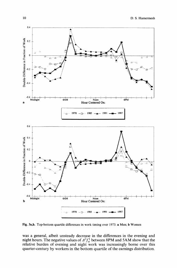
calculated as ratios to allow for convenient presentation. A ratio below oneimplies that workers in quartile q performed a smaller fraction of their totalhours of work at hour s than did workers in the lowest earnings quartile. Anegative difference means that since 1973 workers in quartile q became rela­tively less likely than workers in the bottom earnings quartile to work at time s.Figure 3a shows these interquartile differences for men, while Fig. 3b pre­

sents the same information for women. To save space only the differences be-

Timing, togetherness and time windfalls 9

0.35

'"'"g 0.3

'"~ 0.25

o 0.2

.~ 015E .-= 0.1.;:

~ 0,05o...l 0

a

0.35'"~ 0.3ce 0.25

~ 0.2o<J 0.15

'E 0.1

:E 0.05'"gf 0...l -0.05

b

Fig.2a,b. Double differences in weekly earnings. a Men 1973-1997; b Women 1973-1997

tween workers in the top and bottom earnings quartiles are shown. The resultsfor workers in the second quartile (percentiles 75 to 50) look similar, while thereare no major changes in timing between workers in the third and bottomquartiles (which is not surprising given the small relative changes in earningsshown in Fig. 2). While the differences are small in 1978, beginning in 1985they started to depart from zero. In particular, for both men and women there

10 D. S. Hamennesh

0.4 r----------,-.----------------------,

a

-0.6 -Y__+--+-----;-+--+--+-t-+--+-~+__+____i-+__+___t-+_--:---+-+_--:-_+-f__lMidnight 6AM Noon 6PM

Hour Centered On:

"'C'" 1978 -& - 1985 1991 _ 19971

0.6

"" 0.46~'-0c 0.2.9;:;f!

l.l.

.5 0

g!!~9 -0.2..:0::I

8 -0.4

b

-0.6 -'---t-+_-+---+-+_-+--+-l-+--+---1-+-_+---t--'--'---+-+_-+---+-+--+-_+-f-JMidnight" 6AM Noon 6PM

Hour Centered On:

_ 1978 -:=- - 1985 1991 _ 19971

Fig.3a,b. Top-bottom quartile differences in work timing over 1973. a Men; b Women

was a general, albeit unsteady decrease in the differences in the evening andnight hours. The negative values of"j2fs) between 8PM and SAM show that therelative burden of evening and night work was increasingly borne over thisquarter-century by workers in the bottom quartile of the earnings distribution.

Timing, togetherness and time windfalls II

The negative values of Ll 2/,: between 8PM and 5AM must be offset by pos­itive values at other times. These offsets occur especially at the fringes of the"normal" workday. Implicitly, higher-wage workers, whose total workhourshave been increasing (see Juhn et al. 1991), have been spreading their workdaysto early morning and late afternoon, at the same time that they have been cut­ting back from working in the evenings and at night (at least compared tolower-wage workers). The double differences for 1997 are quite similar for menand women; but for women the decline in evening/night work and the rise inwork at the edges of the regular workday do not exhibit the same steady trendthat they do among men. Since similar steady changes exist for men by majorindustry, but not for women, this gender difference is not a reflection of thesexes' different representations by industry.I have demonstrated that there has been a relative decline in work at un­

desirable times of the day among precisely those workers whose earnings haverisen relatively. To infer the strength of the relationship between changes in theincidence ofevening and night work and changes in relative earnings I estimate:

F/! - F.; = a + b[ u-;q - ~4], S= I, ... ,24, (5)

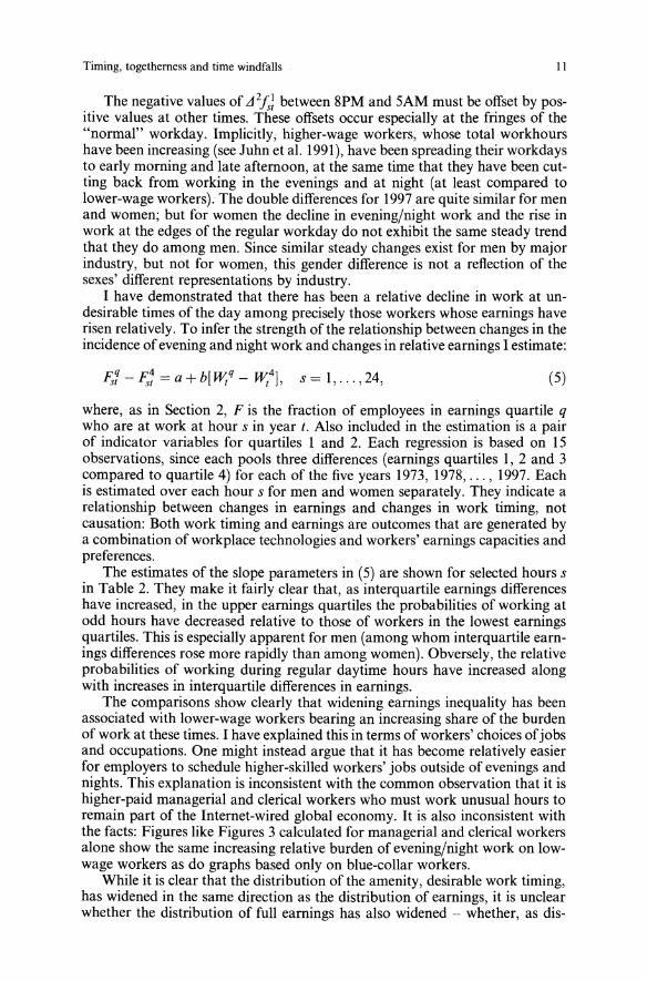
where, as in Section 2, F is the fraction of employees in earnings quartile qwho are at work at hour s in year t. Also included in the estimation is a pairof indicator variables for quartiles I and 2. Each regression is based on 15observations, since each pools three differences (earnings quartiles I, 2 and 3compared to quartile 4) for each of the five years 1973, 1978, ... , 1997. Eachis estimated over each hour s for men and women separately. They indicate arelationship between changes in earnings and changes in work timing, notcausation: Both work timing and earnings are outcomes that are generated bya combination of workplace technologies and workers' earnings capacities andpreferences.The estimates of the slope parameters in (5) are shown for selected hours s

in Table 2. They make it fairly clear that, as interquartile earnings differenceshave increased, in the upper earnings quartiles the probabilities of working atodd hours have decreased relative to those of workers in the lowest earningsquartiles. This is especially apparent for men (among whom interquartile earn­ings differences rose more rapidly than among women). Obversely, the relativeprobabilities of working during regular daytime hours have increased alongwith increases in interquartile differences in earnings.The comparisons show clearly that widening earnings inequality has been

associated with lower-wage workers bearing an increasing share of the burdenof work at these times. I have explained this in terms of workers' choices ofjobsand occupations. One might instead argue that it has become relatively easierfor employers to schedule higher-skilled workers' jobs outside of evenings andnights. This explanation is inconsistent with the common observation that it ishigher-paid managerial and clerical workers who must work unusual hours toremain part of the Internet-wired global economy. It is also inconsistent withthe facts: Figures like Figures 3 calculated for managerial and clerical workersalone show the same increasing relative burden of evening/night work on low­wage workers as do graphs based only on blue-collar workers.While it is clear that the distribution of the amenity, desirable work timing,

has widened in the same direction as the distribution of earnings, it is unclearwhether the distribution of full earnings has also widened - whether, as dis-

12 D. S. Hamermesh

Table 2. The relation between interquartile differences in the fraction at work and interquartiledifferences in earnings, May CPS 1973, 1978, 1985, 1991, 1997

Work at: Men Women(I) (2)

Midnight -0.105 -0.071(0.031) (0.041)

3AM -0.062 -0.033(0.021) (0.037)

6AM -0.014 0.016(0.036) (0.043)

9AM 0.334 0.085(0.083) (0.042)

Noon 0.241 0.209(0.059) (0.061)

3PM 0.357 0.188(0.106) (0.068)

6PM -0.089 0.081(0.046) (0.060)

9PM -0.221 -0.069(0.037) (0.036)

cussed above, the amenity is a luxury good. Under certain very restrictive as­sumptions about homotheticity of workers' preferences and employers' profitfunctions, the full-earnings elasticities of demand for desirable work timing farexceed unity (Hamermesh 1999b). This is consistent with evidence on the de­mand for monetary nonwage job characteristics such as pensions and healthcare (e.g., Woodbury and Hamermesh 1992). We can be quite sure that thedistribution of the amenity has widened substantially in the U.S.: The burdenof working at bad times has increasingly been borne by low-skilled workers.We cannot, however, be sure that price changes in this amenity have beensufficiently small to ensure that the distribution of full earnings (includingthis amenity) has widened more in percentage terms than the distribution ofearnings.

4. Joint decision-making about the timing of leisure

The jointness of spouses' work/leisure choices cannot be inferred by concen­trating on the quantities that they consume over some interval of time. Giventhe relatively small fractions of the week that people in developed economiestypically work in the market, we could very easily find that husbands' longerweekly hours are associated with wives' longer weekly hours, holding theirwage rates constant, although each one is at home while the other works.Understanding the extent of jointness in time use requires analyzing wheneach spouse works in the market, i.e., the extent of overlap in the spouses' useof time. A couple can consume more leisure jointly when the number of hoursthat both spouses are at home is greater, not when the partial correlations oftheir total work times are higher.In order to analyze the instantaneous jointness of spouses' decision-making,

we need to specify the household's utility in arguments defined over points in

Timing, togetherness and time windfalls 13

time. Let the basic unit of time be the day, divided arbitrarily into 24 hours.Then we can write the household's maximand as:

V( UM ([I - Lfl], ... , [1 - Lft])), UF ([I - LiJ, ... , [I - L~]),

UJ (Z{, ... , Zf4) ,C), (6)

where Z; = [1 - L,M][1 - L{], C is the household's consumption, and M andF denote the husband and wife respectively. The household's monetary gainsare implicitly spent entirely on the one composite (household) public good. Ialso assume that each hour is indivisible, with the individual either workingthe entire hour or enjoying leisure. Equation (6) is maximized subject to thespending constraint:

C = 2:)wfILfI + w{L{j,s

(7)

where wi = wj [1 + Os]. Each spouse j faces an exogenous wage rate that variesover s around w j by a percentage Os that is determined by the market supplyand demand for labor at hour s and that faces all workers regardless of sex.Maximizing (6) subject to (7) yields the couple's optimizing sequences of

market work times, {LsM

} and {L{}. If the sequences were integrated overthe day, they would yield each spouse's daily hours supplied to the market,Hj. A spouse will be working at hour s if wi> wf', the spouse's reservationwage for working at that hour. These reservation wages vary over s and maybe determined jointly by the spouses' bargaining. The object of interest hereis to infer whether or not the subfunction UJ =0, that is, whether the out­come of the spouses' bargaining reflects any interest they may have in being athome together, conditional on their working in the market for given numbersof hours. (Alternatively, one might observe that couples' behavior is joint butimplies a preference for being apart.) Only through this approach can we ex­amine whether consuming synchronous leisure matters to the couple.To examine the possibility of jointness in the timing of potential leisure I

combine all the available data from the May 1970s CPS Supplements into onedata set, and combine the data from the 1991 and 1997 May Supplements intoanother. In each CPS Supplement I match husbands' and wives' records tocreate a record for the couple that generates the sequences {L,M} and {Lnand uses them to create the sequences Z;. 3 Any matched couple in which onespouse was age 60 or over was excluded from the sample, since the purpose isto focus on market work and its complement. Only couples with both spousesworking are included in the samples, both to avoid problems with comer solu­tions to the maximization of (6) and because our definition of joint leisure isidentically the inverse of the working spouse's market time if there is a non­working spouse. The usual CPS controls are used; and for each spouse I mea­sure total daily hours of market work using the sequence {L{} and infer fullhourly earnings using usual weekly earnings.Whether the spouses are actually enjoying leisure jointly when Z; = 1 is

not clear. It might well be that one partner is out carousing while the other isat home; perhaps they are both home in separate parts of the house; or perhapsthey are together physically but not engaged in the same activity (Larson andRichards 1994, Chapt. 5). The data do not allow us to distinguish these possi-

14 D. S. Hamennesh

'"ug.0.6o

U...oco.~ 0.4

....

0.2

i·

\ \\'.\ \\"?

\\..\"II\\,I

\\,\.It-

•

~•JiJIiI~

1/i

lOpm8pm

.~

o L,---,--,r-r--.---,---,..-_~Ii=~.~-~---~-~.....~----~-~---,.---,...---,----r-,--.---.-----.-----,JMidnight 2am 4<im 68m 8lim lOam Noon 2pm 4pm

Hour___ 19905 -2- - 1970.

Fig. 4. Fraction of working couples at leisure, 1970s and 1990s

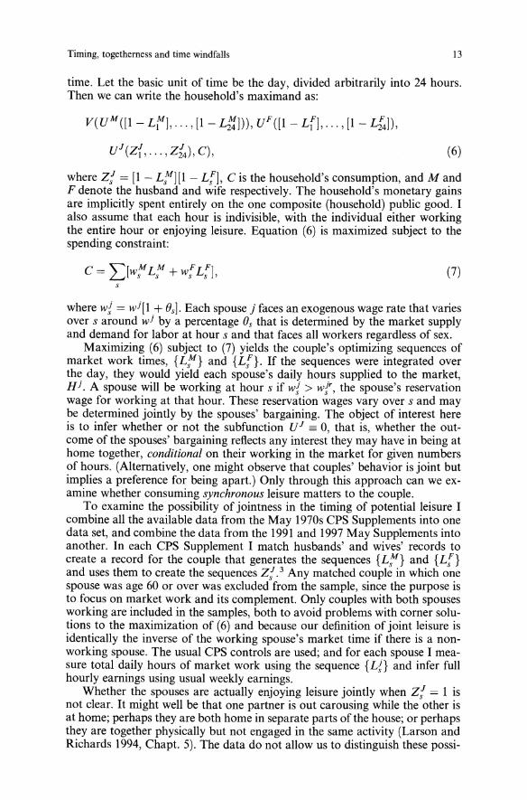
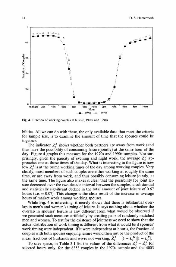
bilities. All we can do with these, the only available data that meet the criteriafor sample size, is to examine the amount of time that the spouses could betogether.The indicator Z; shows whether both partners are away from work (and

thus have the possibility of consuming leisure jointly) at the same hour of theday. Figure 4 graphs this measure for the 1970s and 1990s samples. Not sur­prisingly, given the paucity of evening and night work, the average Z; ap­proaches one at those times of the day. What is interesting in the figure is howlow Z; is at the prime working times of the day among working couples. Veryclearly, most members of such couples are either working at roughly the sametime, or are away from work, and thus possibly consuming leisure jointly, atthe same time. The figure also makes it clear that the possibility for joint lei­sure decreased over the two-decade interval between the samples, a substantialand statistically significant decline in the total amount of joint leisure of 0.67hours (s.e. = 0.07). This change is the clear result of the increase in averagehours of market work among working spouses.While Fig. 4 is interesting, it merely shows that there is substantial over­

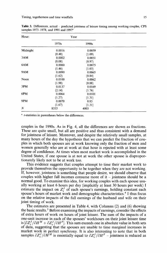
lap in men's and women's timing of leisure. It says nothing about whether theoverlap in spouses' leisure is any different from what would be observed ifwe generated such measures artificially by creating pairs of randomly matchedmen and women. To test for the existence of jointness we need to show that theactual distribution of work timing is different from what it would be if spouses'work timing were independent. If it were independent at hour s, the fraction ofcouples with both spouses enjoying leisure would then just be the product of themean fractions of husbands and wives not working, i; = [1 - LsMJ[l - Ln.To save space, in Table 3 I list the values of the differences Z; - i: for

selected hours only, for the 8353 couples in the 1970s sample and the 4003

Timing, togetherness and time windfalls 15

Table 3. Differences, actual - predicted jointness of leisure timing among working couples, CPSsamples 1973-1978, and 1991 and 1997"

Hour: Year

1970s 1990s

Midnight 0.0016 0.0059(0.48) (1.09)

3AM 0.0002 0.0051(0.08) (0.97)

6AM 0.0060 0.0075(1.46) (1.03)

9AM 0.0090 0.0065(1.62) (0.84)

Noon 0.0100 0.0062(1.98) (0.88)

3PM 0.0137 0.0169(2.14) (1.76)

6PM 0.0064 0.0101(1.27) (1.31)

9PM 0.0070 0.85(1.67) (1.31)

N 8353 4003

" t-statistics in parentheses below the differences.

couples in the 1990s. As in Fig. 4, all the differences are shown as fractions.These are quite small, but all are positive and thus consistent with a demandfor jointness of leisure. Moreover, and despite the relatively small samples, atmany hours of the day the hypothesis that we can predict the fraction of cou­ples in which both spouses are at work knowing only the fraction of men andwomen generally who are at work at that hour is rejected with at least somedegree of confidence. At times when most market work is accomplished in theUnited States, if one spouse is at not at work the other spouse is dispropor­tionately likely not to be at work too.This evidence suggests that couples attempt to time their market work to

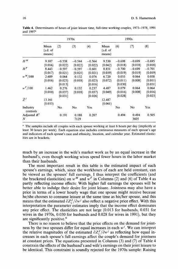
provide themselves the opportunity to be together when they are not working.If, however, jointness is something that people desire, we should observe thatcouples with higher full incomes consume more of it - jointness should be anormal good. To examine this idea, for working couples with each spouse usu­ally working at least 6 hours per day (implicitly at least 30 hours per week) Iestimate the impact on Zf of each spouse's earnings, holding constant eachspouse's hours of market work and demographic characteristics. 4 I thus focuson the relative impacts of the full earnings of the husband and wife on theirjoint timing of work.The estimates are presented in Table 4, with Columns (2) and (6) showing

the basic results. 5 Before examining the impacts ofearnings, consider the effectsof extra hours of work on hours of joint leisure. The sum of the impacts of aone-unit increase in each of the spouses' workhours on their joint leisure timeis [aZf /aH M + aZf /aHF ]. This sum exceeds one in absolute value in both setsof data, suggesting that the spouses are unable to time marginal increases inmarket work in perfect synchrony. It is also interesting to note that in bothsamples aZf /aH M is essentially equal to aZf /aH F - jointness is reduced as

16 D. S. Hamermesh

Table 4. Determinants of hours of joint leisure time, full-time working couples, 1973-1978, 1991and 1997"

1970s 1990s

Mean (2) (3) (4) Mean (6) (7) (8)(s.d. of (s.d. ofmeans) means)

H M 9.107 -0.538 -0.544 -0.564 9.530 -0.698 -0.699 -0.695(0.016) (0.022) (0.022) (0.022) (0.042) (0.018) (0.018) (0.018)

H F 8.443 -0.597 -0.597 -0.601 8.851 -0.700 -0.699 -0.701(0.017) (0.021) (0.021) (0.021) (0.039) (0.019) (0.019) (0.019)

wM/IOO 2.689 0.064 0.132 0.076 6.720 0.055 0.064 0.058(0.016) (0.023) (0.018) (0.023) (0.072) (0.011) (0.008) (0.011)

[O.OI3J [0.0161 [0.030J [0.03IJwF/loo 1.462 0.276 0.132 0.237 4.487 0.079 0.064 0.064

(0.010) (0.037) (0.018) (0.037) (0.049) (0.016) (0.008) (0.016)[0.03IJ [0.0261 [0.028J [0.023J

i J 13.161 12.487(0.033) (0.061)

Industry No No Yes No No YescontrolsAdjusted R2 0.191 0.188 0.207 0.494 0.494 0.505N 7129 3605

" The samples include all couples with each spouse working at least 6 hours per day (implicitly atleast 30 hours per week). Each equation also includes continuous measures of each spouse's ageand indicators of each spouse's race and ethnicity, location, and calendar year. Estimated elastic-ities are in brackets.

much by an increase in the wife's market work as by an equal increase in thehusband's, even though working wives spend fewer hours in the labor marketthan their husbands.The most important result in this table is the estimated impact of each

spouse's earnings, which, since the workhours of each are held constant, canbe viewed as the spouses' full earnings. I thus interpret the coefficients (andthe bracketed elasticities) on wM and wF in Columns (2) and (6) of Table 4 aspartly reflecting income effects: With higher full earnings the spouses will bebetter able to indulge their desire for joint leisure. Jointness may also have aprice in terms of a lower hourly wage that one spouse might receive becausehe/she chooses to consume leisure at the same time as his/her spouse, and thismeans that the estimated oZf /owl also reflect a negative price effect. With thisinterpretation the parameter estimates imply that the income effect dominatesany price effect. The elasticities are not large (0.013 for husbands, 0.031 forwives in the 1970s, 0.030 for husbands and 0.028 for wives in 1991), but theyare significantly positive.6

There is no reason to believe that the price effects on the demand for joint­ness by the two spouses differ for equal increases in each wl. We can interpretthe relative magnitudes of the estimated oZf /owl as reflecting how equal in­creases in each spouse's full earnings affect the couple's demand for jointnessat constant prices. The equations presented in Columns (3) and (7) of Table 4constrain the effects of the husband's and wife's earnings on their joint leisure tobe identical. This constraint is soundly rejected for the 1970s sample: Raising

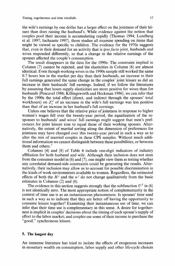
Timing, togetherness and time windfalls 17

the wife's earnings by one dollar has a larger effect on the jointness of their lei­sure than does raising the husband's. While evidence against the notion thatcouples pool their income is accumulating rapidly (Thomas 1994; Lundberget al. 1997; Inchauste 1997), those studies all examine spending on items thatmight be viewed as specific to children. The evidence for the 1970s suggeststhat, even in their demand for an activity that is ipso facto joint, husbands andwives responded differently, so that a change in the relative earnings of thespouses affected the couple's consumption.The result disappears in the data for the 1990s: The constraint implied in

Column (7) cannot be rejected, and the elasticities in Column (6) are almostidentical. Even though working wives in the 1990s sample still worked the same0.7 hours less in the market per day than their husbands, an increase in theirfull earnings generated the same change in the couples' joint leisure as did anincrease in their husbands' full earnings. Indeed, if we follow the literaturesby assuming that hours supply elasticities are more positive for wives than forhusbands (Pencavel 1986; Killingsworth and Heckman 1986), we can infer thatby the 1990s the total effect (direct, and indirect through the spouses' totalworkhours) on Z[ of an increase in the wife's full earnings was less positivethan that of an increase in her husband's full earnings.Unless one believes that the relative price of jointness in response to higher

women's wages fell over the twenty-year period, the equalization of the re­sponses to husbands' and wives' full earnings might suggest that men's pref­erences for joint leisure rose to equal those of their working spouses. Alter­natively, the extent of marital sorting along the dimension of preferences forjointness may have changed over this twenty-year period in such a way as toalter the mix of married couples in these CPS samples. Without much addi­tional information we cannot distinguish between these possibilities, or betweenthem and others. 7

Columns (4) and (8) of Table 4 include one-digit indicators of industryaffiliation for both husband and wife. Although their inclusion does not stemfrom the consumer model in (6) and (7), one might view them as testing whetherany correlated demand-side constraints could be generating the results. Alter­natively, their inclusion may allow us to account for possible discrimination inthe kinds ofwork environments available to women. Regardless, the estimatedeffects of both the H j and the w j do not change qualitatively from the basicestimates in Columns (2) and (6).The evidence in this section suggests strongly that the subfunction U J in (6)

is not identically zero. The most appropriate notion of complementarity in thecontext of time use is as an instantaneous phenomenon: Is spouses' time usedin such a way as to indicate that they are better off having the opportunity toconsume leisure together? Examining their instantaneous use of time, we caninfer that their time use is complementary in this sense. A desire for together­ness is implicit in couples' decisions about the timing of each spouse's supply ofeffort to the labor market; and couples use some of their income to purchase the"good," synchronous leisure.

5. The longest day

An immense literature has tried to isolate the effects of exogenous increasesin monetary wealth on consumption, labor supply and other life-cycle choices

18 D. S. Hamel1llesh

(e.g., efforts such as Holtz-Eakin et al. 1993, and Imbens et al. 1999). Exoge­nous increases in the other component of full income, the amount of time atthe worker-consumer's disposal, have been investigated much more rarely. Iam aware only of one attempt (Hamermesh 1984) that examined the responsesof consumption and labor supply to exogenous differences in time endowmentsin the form of greater expected longevity, and one other (summarized in Biddleand Hamermesh 1990) in which people offered subjective responses about howthey would spend a hypothetical increase in their endowment of time.There is clearly room for interesting empirical research here. One can imag­

ine, for examples, examining behavior after such unusual (and often depress­ing) cases as surprising cures from or diagnoses of usually fatal diseases, late­term miscarriages or stillbirths, prison early-release programs, and others. Thedifficulty, ofcourse, is that data on these events and on the consumption-leisurechoices of their victims or beneficiaries are difficult to come by.There is one exogenous, albeit completely foreknown event that affects res­

idents ofmost industrialized societies - the annual loss of one hour on a Sundayearly in spring and the gain of one hour on a Sunday early in autumn. Whilethis is not a perfect natural experiment - it is hardly unexpected - it provides arare opportunity to examine how people respond to a truly exogenous changein their endowment of time. The data set that provides this opportunity is theDutch Tijdbestedingsonderzoek of 1990, a time-budget study of over 3000 in­dividuals ages 12 and up. Each respondent maintained a diary of his/her activ­ities that he/she filled out for the previous day each morning. The diaries werekept for seven days, Sunday through Saturday. The list of activities was sub­sequently coded into over 200 categories, and the data are presented showingeach person's activities for each of 96 quarter-hours on each of the seven sam­pled days.Half the sample kept diaries for a week in early October of 1990; the other

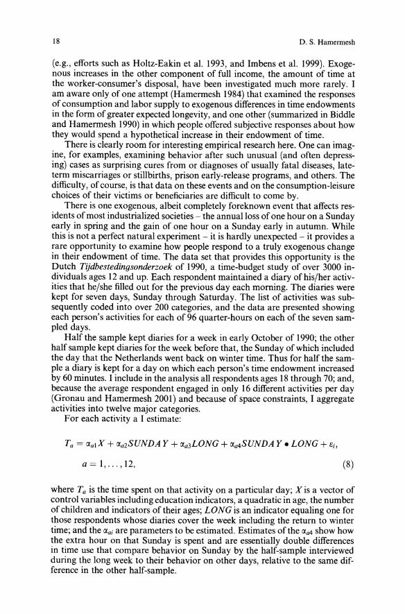
half sample kept diaries for the week before that, the Sunday ofwhich includedthe day that the Netherlands went back on winter time. Thus for half the sam­ple a diary is kept for a day on which each person's time endowment increasedby 60 minutes. I include in the analysis all respondents ages 18 through 70; and,because the average respondent engaged in only 16 different activities per day(Gronau and Hamermesh 200 I) and because of space constraints, I aggregateactivities into twelve major categories.For each activity a I estimate:

a= 1, ... ,12, (8)

where Ta is the time spent on that activity on a particular day; X is a vector ofcontrol variables including education indicators, a quadratic in age, the numberof children and indicators of their ages; LONG is an indicator equaling one forthose respondents whose diaries cover the week including the return to wintertime; and the CJ.ai are parameters to be estimated. Estimates of the CJ.a4 show howthe extra hour on that Sunday is spent and are essentially double differencesin time use that compare behavior on Sunday by the half-sample interviewedduring the long week to their behavior on other days, relative to the same dif­ference in the other half-sample.

Timing, togetherness and time windfalls 19

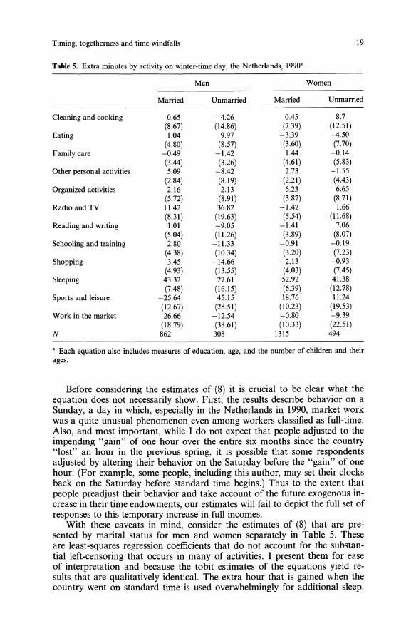
Table 5. Extra minutes by activity on winter-time day, the Netherlands, 1990·

Men Women

Married Unmarried Married Unmarried

Cleaning and cooking -0.65 -4.26 0.45 8.7(8.67) (14.86) (7.39) (12.51)

Eating 1.04 9.97 -3.39 -4.50(4.80) (8.57) (3.60) (7.70)

Family care -0.49 -1.42 1.44 -0.14(3.44) (3.26) (4.61) (5.83)

Other personal activities 5.09 -8.42 2.73 -1.55(2.84) (8.19) (2.21) (4.43)

Organized activities 2.16 2.13 -6.23 6.65(5.72) (8.91) (3.87) (8.71)

Radio and TV 11.42 36.82 -1.42 1.66(8.31) (19.63) (5.54) (11.68)

Reading and writing 1.01 -9.05 -1.41 7.06(5.04) (11.26) (3.89) (8.07)

Schooling and training 2.80 -11.33 -0.91 -0.19(4.38) (10.34) (3.20) (7.23)

Shopping 3.45 -14.66 -2.13 -0.93(4.93) (13.55) (4.03) (7.45)

Sleeping 43.32 27.61 52.92 41.38(7.48) (16.15) (6.39) (12.78)

Sports and leisure -25.64 45.15 18.76 11.24(12.67) (28.51) (10.23) (19.53)

Work in the market 26.66 -12.54 -0.80 -9.39(18.79) (38.61) (10.33) (22.51)

N 862 308 1315 494

• Each equation also includes measures of education, age, and the number of children and theirages.

Before considering the estimates of (8) it is crucial to be clear what theequation does not necessarily show. First, the results describe behavior on aSunday, a day in which, especially in the Netherlands in 1990, market workwas a quite unusual phenomenon even among workers classified as full-time.Also, and most important, while I do not expect that people adjusted to theimpending "gain" of one hour over the entire six months since the country"lost" an hour in the previous spring, it is possible that some respondentsadjusted by altering their behavior on the Saturday before the "gain" of onehour. (For example, some people, including this author, may set their clocksback on the Saturday before standard time begins.) Thus to the extent thatpeople preadjust their behavior and take account of the future exogenous in­crease in their time endowments, our estimates will fail to depict the full set ofresponses to this temporary increase in full incomes.With these caveats in mind, consider the estimates of (8) that are pre­

sented by marital status for men and women separately in Table 5. Theseare least-squares regression coefficients that do not account for the substan­tial left-censoring that occurs in many of activities. I present them for easeof interpretation and because the tobit estimates of the equations yield re­sults that are qualitatively identical. The extra hour that is gained when thecountry went on standard time is used overwhelmingly for additional sleep.

20 D. S. Hamermesh

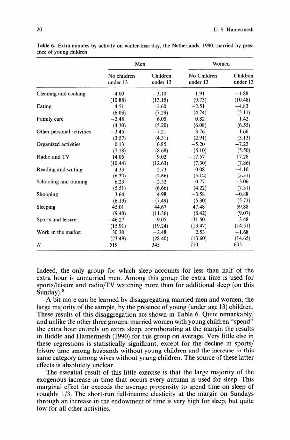
Table 6. Extra minutes by activity on winter-time day, the Netherlands, 1990, married by pres-ence of young children

Men Women

No children Children No Children Childrenunder 13 under 13 under 13 under 13

Cleaning and cooking 4.00 -3.10 1.91 -1.88(10.88) (13.15) (9.73) (10.48)

Eating 4.51 -2.60 -2.51 -4.83(6.03) (7.29) (4.74) (5.11)

Family care -2.48 6.05 0.82 1.42(4.30) (5.20) (6.08) (6.55)

Other personal activities -3.45 -7.21 3.76 1.66(3.57) (4.31) (2.91) (3.13)

Organized activities 0.13 6.85 -5.20 -7.23(7.18) (8.68) (5.10) (5.50)

Radio and TV 14.05 9.02 -17.57 17.28(10.44) (12.63) (7.30) (7.86)

Reading and writing 4.33 -2.73 0.08 -4.16(6.33) (7.66) (5.12) (5.51)

Schooling and training 6.23 -2.52 0.77 -3.06(5.51) (6.66) (4.22) (7.31)

Shopping 3.64 4.98 -3.58 -0.88(6.19) (7.49) (5.30) (5.71)

Sleeping 45.01 44.67 47.48 59.88(9.40) (11.36) (8.42) (9.07)

Sports and leisure -46.27 9.05 31.50 3.48(15.91) (19.24) (13.47) (14.51)

Work in the market 30.30 -2.48 2.53 -1.68(23.49) (28.40) (13.60) (14.65)

N 519 343 710 605

Indeed, the only group for which sleep accounts for less than half of theextra hour is unmarried men. Among this group the extra time is used forsports/leisure and radio/TV watching more than for additional sleep (on thisSunday). 8

A bit more can be learned by disaggregating married men and women, thelarge majority of the sample, by the presence of young (under age 13) children.These results of this disaggregation are shown in Table 6. Quite remarkably,and unlike the other three groups, married women with young children "spend"the extra hour entirely on extra sleep, corroborating at the margin the resultsin Biddle and Hamermesh (1990) for this group on average. Very little else inthese regressions is statistically significant, except for the decline in sports/leisure time among husbands without young children and the increase in thissame category among wives without young children. The source of these lattereffects is absolutely unclear.The essential result of this little exercise is that the large majority of the

exogenous increase in time that occurs every autumn is used for sleep. Thismarginal effect far exceeds the average propensity to spend time on sleep ofroughly 1/3. The short-run full-income elasticity at the margin on Sundaysthrough an increase in the endowment of time is very high for sleep, but quitelow for all other activities.

Timing, togetherness and time windfalls

6. Conclusions and new directions

21

The results make several new facts clear. Between 1973 and 1997 the burden ofinequality in the job disamenity, working at a generally unpleasant time ofday, appears to have shifted in the same direction as the burden of earnings in­equality. This suggests that measures of changes in earnings inequality under­state the extent of change in inequality in the overall returns to market work.There is clear evidence that couples arrange their work schedules to allow timefor leisure that they consume jointly. Moreover, the demand for joint leisure isnot inferior - all else equal, those couples with higher earning capacities enjoymore of it. Finally, an expected windfall of time, the one-hour gain that occursevery autumn when clocks are turned back to standard time, is consumedmainly as sleep, especially by married women with young children.These few examples here have been designed to demonstrate that there are

many potential avenues for learning about time use beyond the standard onesof examining weekly or other aggregations of reported hours of work. Thereare some cases, such as issues of spouses' togetherness, where going beyondstandard analyses is the only way to understand the underlying behavior. Thereare others where this approach can generate tests of ideas examined in othercontexts, such as markets for amenities, economic inequality, and power rela­tionships within households, that may expand upon and possibly surpass con­ventional approaches in their ability to allow us to understand behavior.

Endnotes

1 At least through 1991 these changes occurred independently of any changes in demographics orin the distribution of workers across one-digit industries or occupations (Hamermesh 1999b).

2 I multiply top-coded earnings by 1.5, as is common in this literature. Unlike the literature onearnings inequality, which compares earnings across points in the distribution, these calculationsare based on averages across workers in different quartiles. This is done for comparison purposesto the distribution of work timing: It would make no sense to compare work histories of thosefew individuals who happen to be at particular points in an earnings distribution.

3 Individuals were matched as spouses based upon listing as household head or spouse and on linenumber (the person's position in the household) in the CPS records. Only people whose maritalstatus was denoted as married, spouse present, are included in the match. Given the possibilitythat unmarried siblings are in the same residence, the data do not allow us to perform similaranalyses for cohabiting unmarried couples.

4 If we include all working couples the results are quite similar, except for a substantially lowercoefficient on wife's hours. The same measures of the presence of children cannot be includedfor both samples, so that for purposes ofcomparability I exclude them in the Table. Nonetheless,when the equations for the 1970s and 1990s are expanded to include indicators of the presenceof children and their ages, the conclusions about the impacts of hours and weekly earnings onjointness are unaffected.

5 A regional difference exists in the demand for jointness. In the "Rust Belt," defined here as theNew England, Mid-Atlantic and East North Central subregions, joint leisure was a significant0.4 hours per day lower in both the 1970s and the 1990s than in the rest of the United Statesamong otherwise identical couples. Whether this reflects differences in tastes or differences in the(unmeasured) constraints on couples' choices is not clear.

6 An additional test of the validity of this approach asks how well one could have predicted Z§oswith knowledge of the structure of the relationship in the 1970s and the means of the determi­nants of Z§os' Using the PCE deflator to adjust 1990s wages, and the coefficients in Columns (2)and (6), this decomposition shows that only 26% of the change in ZJ between the 1970s and the1990s was explicable by changes in the independent variables. Most of the change resulted fromchanges in the coefficients.

22 D. S. Hamermesh

7 Among married couples under age 60, in the 19705 the likelihood that both spouses wereworking was lower than in the I990s. This selectivity (of wives into the work force) may affectour results, but the direction of any bias is unclear, as it depends on the nature of the selectivity.This is not chiefly an issue of wives' market wages, since we hold those constant. One reason­able possibility is that wives who worked in the 1970s had relatively more power compared totheir husbands than wives in the I990s. If so, accounting for this change in selectivity wouldstrengthen the inference that husbands' and wives' preferences for joint leisure converged overthis time interval.

8 The data set regrettably contains no information on individuals' wage rates, but it does haveinformation on the household's net income. I included this variable in reestimates of the equa­tions presented here, with little change in the estimated lXai.

References

Becker G (1965) A Theory of the Allocation of Time. Economic Journal 75(3):493-517Berman E, Bound J, Machin S (1998) Implications of Skill-Biased Technological Change: Inter­national Evidence. Quarterly Journal of Economics 113(4): 1245-1280

Biddle J, Hamermesh D (1990) Sleep and the Allocation of Time. Journal of Political Economy98(5):922-943

Boskin M, Dulberger E, Gordon R, Griliches Z, Jorgenson D (1998) Consumer Prices, the Con­sumer Price Index, and the Cost of Living. Journal of Economic Perspectives 12(1):3-26

Gronau R, Hamermesh D (2001) The Demand for Variety: A Household Production Perspective.National Bureau of Economic Research, Working Paper No. 8509, October

Hamermesh D (1984) Life Cycle Effects on Consumption and Retirement. Journal ofLabor Eco­nomics 2(3):353-370

Hamermesh D (1996) Workdays, Workhours and Work Schedules: Evidence for the United Statesand Germany. The W.E. Upjohn Institute, Kalamazoo, MI

Hamermesh D (1999a) The Timing ofWork Over Time. Economic Journal 109(1):37-66Hamermesh D (1999b) Changing Inequality in Markets for Workplace Amenities. Quarterly

Journal of Economics 114(4):1085-1123Holtz-Eakin D, Joulfaian D, Rosen H (1993) The Carnegie Conjecture: Some Empirical Evidence.

Quarterly Journal ofEconomics 108(2):413--435Imbens G, Rubin D, Sacerdote B (1999) Estimating the Effects of Unearned Income on LaborSupply, Earnings, Savings, and Consumption: Evidence from a Survey of Lottery Players.National Bureau of Economic Research, Working Paper No. 7001, March

Inchauste G (1997) Education, Labor Supply, and Household Expenditures in Bolivia. UnpublishedPh.D. dissertation, University of Texas

Juhn C, Murphy KM, Topel R (1991) Why Has the Natural Rate of Unemployment Increasedover Time? Brookings Papers on Economic Activity (2):75-142

Juhn C, Murphy KM, Pierce B (1993) Wage inequality and the rise in returns to skill. Journal ofPolitical Economy 101(3):410--442

Killingsworth M, Heckman J (1986) Female Labor Supply: A Survey. In: Ashenfelter 0, LayardR (eds) Handbook of Labor Economics. North-Holland, Amsterdam, 103-204

Kostiuk P (1990) Compensating Differentials for Shift Work. Journal of Political Economy98(5): 1054-1075

Larson R, Richards M (1994) Divergent Realities: The Emotional Lives of Mothers, Fathers, andAdolescents. Basic Books, New York

Leamer E (1996) Wage Inequality from International Competition and Technological Change:Theory and Country Experience. American Economic Review 86(2):309-314

Lundberg S, Pollak R, Wales T (1997) Do Husbands and Wives Pool their Resources? Evidencefrom the U.K. Child Benefit. Journal of Human Resources 32(3):463--480

Mellor E (1986) Shift Work and Flexible Time: How Prevalent Are They? Monthly Labor Review109(11):14-21

Pereira PT, Martins PS (2000) Does Education Reduce Wage Inequality: Evidence from FifteenEuropean Countries. Institute for the Study of Labor (IZA), Working Paper No. 120, Bonn,February

Pencavel J (1986) Labor Supply of Men: A Survey. In: Ashenfelter 0, Layard R (cds) HandbookofLabor Economics. North-Holland, Amsterdam, 3-102

Timing, togetherness and time windfalls 23

Rosen S (1974) Hedonic Prices and Implicit Markets. Journal of Political Economy 82(1):34-55Stafford F (1986) Forestalling the Demise of Empirical Economics: The Role of Microdata inLabor Economics Research. In: Ashenfelter 0, Layard R (eds) Handbook ofLabor Economics.North-Holland, Amsterdam, 387-423

Thomas D (1994) Like Father, Like Son: Like Mother, Like Daughter: Parental Resources andChild Height. Journal of Human Resources 29(1):950-988

Woodbury S, Hamennesh D (1992) Taxes, Fringe Benefits and Faculty. Review of Economics andStatistics 84(2):287-296

The allocation of time and goods in household activities:A test of separability

Sebastien Lecocq

Institut National de la Recherche Agronomique (INRA), 65 boulevard de Brandebourg,94205 Ivry-sur-Seine Cedex, France (Fax: +33-1-49-59-69-90; e-mail: lecocq@ivry.inra.fr)

Received: 24 November 1999/Accepted: 16 November 2000

Abstract. In this paper, we test for the weak separability hypothesis imposedby the household production model between goods and time inputs used in theproduction of different commodities. Our data come from a French surveywhich reports both expenditures and time that households devote to someactivities. The results allow us to show that the weak separability assumptioncannot be rejected only when households are strongly time constrained. In theopposite case, home time uses are found to be nonseparable.

JEL classification: D 13

Key words: Conditional demand functions, household production model, sep­arability test

1. Introduction

By formulating the household production theory, Becker (1965) provided anew approach to the theory of household behaviour and laid the foundationsof new home economics. This 'new' approach assumes that households com­bine market goods and time in household production functions to producecommodities that directly enter their utility function. This theory is very usefulin the analysis of behaviours ignored by traditional theory and related to suchdiverse fields as the allocation of nonmarket time, education or fertility.

The author is grateful to INSEE, J.-M. Hourriez and C. Montmarquette for providing and for­matting the data. The author is also indebted to M. Browning, F. Bourguignon, F. Caillavet,F. Gardes, V. Lechene, L. Uvy-Garboua, C. Meghir, C. Montmarquette, R.A. Pollak, J.-M.Robin and an anonymous referee for valuable comments. Responsible editor: John F. Ermisch.

26 S. Lecocq

For practical reasons, empirical studies devoted to household productiontheory are not based directly on Becker's model, but on a simplified version.The absence of a direct measure of commodities indeed lead researchers tofocus on the allocation of time and goods between household activities (Pollakand Wachter 1975).1 That is, the household production functions are intro­duced into the utility function to obtain what Michael and Becker (1973) callthe 'derived utility function', in terms of market goods, time and environ­mental variables (durables, for example). In this case, estimation of the modelonly depends on the econometrician's ability to distinguish goods and time usein activity i from their use in other activities. The main characteristic of thisfunction is to be weakly separable in the goods and time devoted to the pro­duction of a given commodity. For example, inputs in meal preparation areweakly separable from inputs in dressmaking. This restriction is extremelyimportant since it partitions goods and time uses in groups of substitutes andcomplements. However, it has never been tested, for lack of satisfactory data.The purpose of this paper is to provide such a test. We use a data set that is

particularly suited for this purpose: the French Modes de Vie survey, led fromNovember 1988 to November 1989 by the Institut National de la Statistique etdes Etudes Economiques (INSEE). This survey contains information on sev­eral wide domains of household production: meal preparation; cleaninghouse; washing dishes, laundry; child care; dressmaking, seaming, knitting;gardening; pottering about; hunting, fishing and gathering. For each domain,the survey is interested in the way the household proceeds, the nature and thevalue of the ingredients it uses, the time it spends, the quantity and the natureof goods or services it produces. In addition to the questionnaire, a time diaryrecords all activities by the head of the household and his or her conjoint, andan expenditures and fitting book allows the household to note all its expen­ditures for a week and to describe its fitting in durable goods. A last book re­cords the contents of the deep freezer (if the family has one) and the stock ofhomemade tinned. Although this survey studies many household activities, wefocus here on the 'meal preparation' activity, which seems to be the most ap­propriate given the problem we want to deal with.Clearly, our aim in this paper is not to test for the empirical validity of

alternative models of decision within the household (as in Fortin and Lacroix1997). We are only interested here in the test of the separability hypothesis.This should allow us to answer the question: do households allocate time andgoods in the way stated by the home production model?The paper is organised as follows. In Sect. 2 the separability test principle

is presented. In Sect. 3 we report the empirical results. Section 4 contains someconcluding remarks.

2. Separability test principle

We consider a household composed of at least two adults, a male and afemale, with a utility function of the form

(1)

where z, and Z2 are the quantities of commodities resulting respectively fromthe meal preparation activity and other household activities, x; is the 'quan­tity' of meals taken outside the home (a priori substitutable for zd, 1m and It

Time and goods in household activities 27

represent the pure leisure time of male and female, respectively, and d denotesa vector of socio-demographic variables. The household production obeys thefollowing relations

(2)

where Xi is the quantity of market goods devoted to activity i, tim and tif arethe time devoted to activity i by male and female, respectively.2 The house­hold faces a budget constraint

PIX, +P2X2 +P;x; = wmnm+ wfnf + v, (3)

where PI' P2 and P; are the prices of XI, X2 and x;, respectively,3 wm and wfare respectively the male and female wages (which can also be viewed as theprices of time), nm and nf denote the time devoted to market work by maleand female, respectively, and v is nonlabor income. In addition, the householdfaces time constraints

~+tlj+t2j+nj=T, J=m,j, (4)

where T represents total time available for j. These three last constraints, (3)and (4), can be regrouped into the full income constraint

PIXI +P2X2 +P;x; + L Wj(~ + tlj + t2j) = L wjT + v = S, (5)j=m,j j=m,j

where S is full income, that is the income the household would earn if bothmale and female spent all their time on market work. Then, the householdproblem is to choose the quantities of goods and time maximising its utilityfunction (1) subject to the technological (2) and the full income (5) constraints.When the household production functions (2) are introduced into the util­

ity function (I), one obtains the derived utility function, in terms of marketgoods and time

(6)

According to the household production theory, the derived utility function isweakly separable in the goods and time used to produce a given commodity,that is inputs XI, tim and tlf are weakly separable from X2, t2m and t2f. In otherwords, marginal rates of substitution for pairs of inputs in meal preparationare functionally independent of the quantities of inputs in other householdactivities. In this case, relation (6) becomes

(7)

Then, optimal quantities are obtained by maximising the derived utility func­tion, (7) if it is consistent with the theory, (6) if it is not, subject to the full in­come constraint (5).Now, assume that x;, 1m, It, X2, t2m and t2f are preallocated, in the sense

that the household's consumption of these goods is determined before heenters the market (Pollak 1969, 1971). The household is then supposed tochoose quantities of XI, tim and tlf so as to maximise (6) or (7) subject to thenew full income constraint

(8)

28 S. Lecocq

where Y is total expenditure devoted to meal preparation inputs, and theadditional constraints

(9)

The maximisation of (6) or (7) subject to (8) and (9) yields two different con­ditional demand systems for meal preparation inputs (Pollak 1971 andBrowning and Meghir 1991). The one related to the nonseparable derivedutility function (6) is the following

(10)

where q is the vector of inputs in meal preparation, while the one corre­sponding to the weakly separable derived utility function (7) is of the form

(II)

Therefore, a simple way to know whether, in the derived utility function,inputs used in the production of ZI are weakly separable from inputs used inthe production of Z2, consists in testing whether the coefficients associatedwith X2, t2m and t2f in (10) are not significantly different from zero.From an empirical point of view, we have to mention the following prob­

lems related to our data set. First, the survey records no prices. Actually, XIand X2 are market goods expenditures devoted to meal preparation and toother household activities, respectively, and x; is expenditures devoted tofood-out. Moreover, hourly wages are not available in the data set. This latterprovides annual wages, but not the number of hours worked during the year.As we shall see in the next section, only proxies can be constructed.Without price indices or good measures of wages, we cannot estimate a

sophisticated demand system. So, we consider the estimation of a simpleWorking-Leser model, without prices or wages. 4 In this case, the conditionaldemand functions (10) can be written as

Si = ali + a2i Iny + fllix; + fl2Jm + fl3ilj + YliX2 + Y2i t2m + Y3; t2f + Jid + Gi,

(12)

for i = 1,2,3, where ai, fli' Yi and J i are unknown parameters (the a;'s, fl;'s andy;'s are scalars, and Ji is a vector), Gi is an error term with the usual properties,and where SI, S2 and S3 are the shares of expenditures on inputs XI, tIm and tlf'respectively, in total expenditure devoted to meal preparation, Y = XI + Wmtlm+Wftlf. 5 Formally, SI = XI/Y, S2 = Wmtlm/Y, and S3 = wftlf/Y. Estimating (12)equation by equation by ordinary least squares (OLS) yields a set of param­eters that satisfies adding-up automatically. Note that wages appear in theright hand side ofeach equation through total expenditure. This latter will thushave to be instrumented, not only because of its simultaneous determinationwith expenditure shares, but also because of the measurement errors on wages.Given this parameterisation, the test to know whether Xl, tIm and tlf are

weakly separable from X2, t2m and t2f simply consists in testing whether theparameters Yi are not significantly different from zero. Furthermore, if theform of the derived utility function is really given by (7), that is x;, 1m and ljare nonseparable from XI, tim and tlf, the parameters fli in (12) have to besignificantly different from zero.

Time and goods in household activities

3. Empirical results

29

The Modes de vie survey records household expenditures on a weekly basis.For each household, we constructed XI as the total amount spent on foodproducts and drinks, x; as the amount spent on food-out, and X2 as the dif­ference between total expenditure and the sum of XI and x; .Each time in the survey is reported for one day, which may be either a

weekday or a weekend day. Unfortunately, we have no information about theday the household has answered. Time recordings are thus not representativeof the household average timetable, and we shall have to be very cautious ininterpreting the results below. We defined tim and tlf as the time spent onmeal preparation and food shopping by male and female, respectively, t2m andt2f as the difference between total time devoted to household activities by maleand female and tim and tlf, respectively, 1m and l;- as the pure leisure time ofmale and female, respectively. For convenience, expenditures and time werethen expressed as monthly expenditures and monthly time. Note that theseconversions cannot alter the results of the test.Only male and female yearly wage incomes are available in the survey.6 A

monthly wage can however be computed by dividing yearly wage income bythe number of months in the year on which the income has been earned. Butwe cannot compute hourly wages because the number of hours worked duringthe month is not recorded. We only have the time worked by male and femalefor the time recording day, which cannot be used to the extent that it includescommuting time and that it should be zero or close to zero for a large numberof the households who have answered a weekend day. As an alternative, weexploited an information that is available in the data set and that gives theratio, lower than or equal to one, of the time worked by each individual part­time or full-time employed to the time he would have worked if he had beenfull-time employed. For example, a ratio of 0.5 means that the individual haveworked half-time. So, to obtain the monthly working time of each individual,we had to multiply that ratio by the number of hours worked by a full-timeworker. Given that all individuals kept in our subsample are wage-earners, weassumed this number to be 39 hours a week (the legal working duration inFrance at the time of the survey), that is 169 hours per month. We finally de­termined proxies for hourly wages Wm and wf by dividing monthly wages bythe resulting working time. Of course, this calculation does not take into ac­count the fact that some high-wage workers may work more than the legalduration. Hourly wages will in this case be overestimated and, since wagesenter the right hand side of (12) through total expenditure, a bias in theparameter estimates may arise. As pointed out at the end of the previous sec­tion, standard instrumental variable techniques will therefore have to be ap­plied to obtain consistent estimates.In the vector d, we included male age, seven dummy variables for the

degree obtained by male (from no degree to university degree, classified byincreasing order of education level), the number of children in each of four agegroups (0 to 1 year old, 2 to 7 years old, 8 to 14 years old, and 15 to 24 yearsold), and a dummy variable indicating whether the household is homeowner. 7From our initial data set, we selected a subsample of 1099 households

composed of at least a male and a female who were both working as wage­earners. For these households, we observed a significant number of null ob­servations for the dependent variable of the second equation: the share of

30 S. Lecocq

male time expenditures in total expenditure devoted to meal preparation wasequal to zero in 239 cases, while the two other dependent variables, the sharesof market goods and female time expenditures in total expenditure devoted tomeal preparation, were null in only 5 and 20 cases, respectively. To avoidcorner solutions, we deleted observations for which at least one meal prepa­ration input was zero, keeping then 840 households. Our aim being only totest for the separability on a part of the population, without extending theconclusions to the whole population, we do not think that the bias that mayresult from this selection has any importance. Moreover, although descriptivestatistics show some observable differences between the sample of corner solu­tions and the sample of interior solutions,8 none of them is found to be sig­nificant. Table I, column (I), contains some descriptive statistics for the mainvariables used in the estimation.As we previously noticed, total expenditure cannot be taken as exogenous

in the conditional demand system, because it is simultaneously determinedwith market goods and time expenditures devoted to meal preparation, andbecause it is a function of wages that are not accurately measured. So, we in­strumented it, not with income since this latter is used to determine wages, butwith socio-demographic variables: male age and its square, degree obtained bymale, two dummy variables indicating whether the male and the female havethe french nationality, the number of children in each of the four age groups, adummy variable equals to one if the household is homeowner and zero other­wise, a dummy variable indicating whether the male profession has a publicstatus, and seven dummy variables for the household city size (classified byincreasing order of number of inhabitants). Total expenditure is not the onlyvariable that may be endogenous however. Individuals with long hours ofwork (and thus high hourly wages) will presumably have few hours to devoteto leisure, to other household activities and/or to meal preparation, and willprobably spend more on market goods. We would thus expect these variablesto also be correlated to the error terms of (12). We performed Hausman(1978) exogeneity tests for food-out expenditures, inputs in other householdactivities, and male and female leisure time, together with Sargan tests fororthogonality of instruments. These latter were the same socio-demographicvariables as those used in the instrumentation of total expenditure. This onewas instrumented both under the null and under the alternative. Instrumentsrequired for identification are male age squared, and the dummy variablesrelated to the male and female french nationality, to the male professionpublic status, and to the household city size. Sargan statistics show that vari­ables used as instruments in the demand system have the required properties. 9

Yet, the endogeneity hypothesis is strongly rejected by Hausman statistics. Itis also strongly rejected when we focus on inputs devoted to other householdactivities only. These results can be interpreted in two different ways. Eitherthe instruments, which are not correlated with the residuals of the demandequations, are not correlated enough with the variables to instrument, or theprevious hypothesis of preallocation is verified. Unfortunately, we have nomean to settle between these two interpretations. Estimation results are pre­sented in Table 2.Table 2, column (1), shows that, among the 19 variables considered, 6 are

significant. The share of market goods expenditures in total expenditure de­voted to meal preparation increases with the number of children, regardless oftheir age, and decreases with the time spent on other household activities by

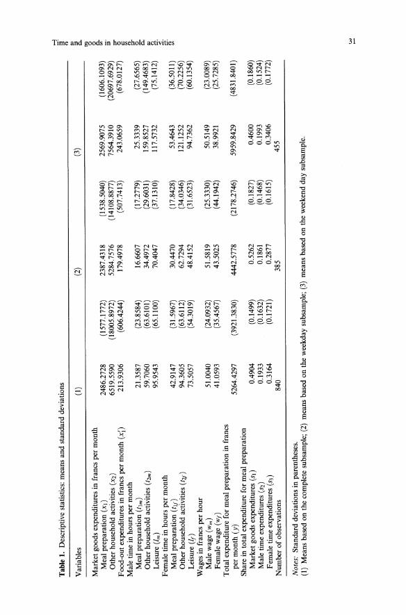
Tab

le1.Descriptivestatistics:meansandstandarddeviations

~ "Variables

(I)

(2)

(3)

'" = Po (JQMarketgoodsexpendituresinfrancspermonth

0

Mealpreparation

(XI)

2486.2728

(1577.1772)

2387.4318

(1538.5040)

2569.9075

(1606.1093)

e.Otherhouseholdactivities

(X2)

6519.5590

(18005.8972)

5284.7576

(14108.8877)

7564.3910

(20697.6929)

5' ::r

Food-outexpendituresinfrancspermonth

(x;)

213.9306

(606.4244)

179.4978

(507.7413)

243.0659

(678.0127)

0 c:Maletimeinhourspermonth

~

Mealpreparation

(tim

)21.3587

(23.8584)

16.6607

(17.2779)

25.3339

(27.6565)

::r 0

Otherhouseholdactivities

(t2m

)59.7060

(63.6101)

34.4972

(29.6031)

159.8527

(149.4683)

c: '"Leisure

(1m)

95.9543

(65.1100)

70.4047

(37.1310)

117.5732

(75.1412)

n ~.Femaletimeinhourspermonth

g:Mealpreparation

(til

)42.9147

(31.5967)

30.4470

(17.8428)

53.4643

(36.5011)

'"Otherhouseholdactivities

(t2/)

94.3605

(63.6112)

62.7294

(34.0346)

121.1252

(70.2256)

Leisure

(It)

73.5057

(54.3019)

48.4152

(31.6523)

94.7362

(60.1354)

Wagesinfrancsperhour

Malewage

(wm

)51.0040

(24.0932)

51.5819

(25.3330)

50.5149

(23.0089)

Femalewage

(wI)

41.0593

(35.4567)

43.5025

(44.1942)

38.9921

(25.7285)

Totalexpenditureformealpreparationinfrancs

permonth

(y)

5264.4297

(3921.3830)

4442.5778

(2178.2746)

5959.8429

(4831.8401)

Shareintotalexpenditureformealpreparation

Marketgoodsexpenditures

(SI)

0.4904

(0.1499)

0.5262

(0.1827)

0.4600

(0.1860)

Maletimeexpenditures

(S2)

0.1933

(0.1632)

0.1861

(0.1468)

0.1993

(0.1524)

Femaletimeexpenditures

(S3)

0.3164

(0.1721)

0.2877

(0.1615)

0.3406

(0.1772)

Numberofobservations

840

385

455

Not

es:Standarddeviationsinparentheses.

(1)Meansbasedonthecompletesubsample;(2)meansbasedontheweekdaysubsample;(3)meansbasedontheweekenddaysubsample.

w -

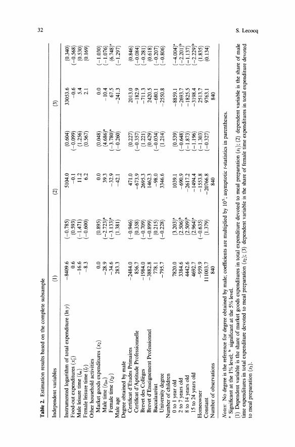
wT

able2.Estimationresultsbasedonthecompletesubsample

N

Independentvariables

(1)

(2)

(3)

Instrumentedlogarithmoftotalexpenditure(lny)

-8409.6

(-0.785)

5104.0

(0.604)

33053.6

(0.340)

Food-outexpenditures

(x;)

0.6

(0.593)

-0.1

(-0.099)

-0.6

(-0.568)

Maleleisuretime

(1m)

-16.6

(-1.471)

11.2

(1.256)

5.4

(0.530)

Femaleleisuretime

(1/)

-8.3

(-0.600)

6.2

(0.567)

2.1

(0.169)

Otherhouseholdactivities

Marketgoodsexpenditures

(X2)

0.0

(0.895)

0.0

(0.048)

0.0

(-1.030)

Maletime

(12m

)-28.9

(-2.723)'

39.3

(4.686)'

-10.4

(-1.076)

Femaletime

(/2/

)-34.6

(-3.133)'

-32.9

(-3.780)'

67.5

(6.748)'

Maleage

283.3

(1.381)

-42.1

(-0.260)

-241.3

(-1.297)

Degreeobtainedbymale

Certificatd'EtudesPrimaires

-2484.0

(-0.946)

471.0

(0.227)

2013.0

(0.846)

Certificatd'AptitudeProfessionnelle

856.7

(0.358)

-673.9

(-0.357)

-182.9

(-0.084)

BrevetdesColleges

-1984.0

(-0.709)

2695.3

(1.221)

-711.3

(-0.281)

Brevetd'EnseignementProfessionnel

-3882.8

(-0.899)

1462.3

(0.429)

2420.5

(0.618)

Baccalaureat

778.1

(0.215)

-98.0

(-0.034)

-680.1

(-0.207)

Universitydegree

-795.7

(-0.228)

3346.6

(1.214)

-2550.8

(-0.806)

Numberofchildren

otoIyearold

7820.0

(3.203)'

1039.1

(0.539)

-8859.1

(-4.004)'

2to7yearsold

3384.6

(2.506)b

-690.9

(-0.648)

-2693.7

(-2.201)b

8to14yearsold

4442.6

(2.509)b

-2617.2

(-1.873)

-1825.5

(-1.137)

15to24yearsold

4692.7

(2.964)'

-1494.4

(-1.196)

-3198.4

(-2.229)b

Homeowner

-959.9

(-0.635)

-1553.8

(-1.303)

2513.7

(1.835)

Constant

111003.7

(1.379)

-20766.8

(-0.327)

9763.1

(0.134)

Numberofobservations

840

840

840

Nol

es:Nodegreeisthereferencefordegreeobtainedbymale;coefficientsaremultipliedby105;asymptoticI-statisticsinparentheses.

,SignificantattheI%level;

bsignificantatthe5%level.

(1)Dependentvariableistheshareofmarketgoodsexpendituresintotalexpendituredevotedtomealpreparation(sIl;(2)dependentvariableistheshareofmale

timeexpendituresintotalexpendituredevotedtomealpreparation

(S2)

;(3)dependentvariableistheshareoffemaletimeexpendituresintotalexpendituredevoted

tomealpreparation

(S3)

'

~ ~ .§

Time and goods in household activities 33

male and female. Only 2 variables are significant in column (2). The share ofmale time expenditures in total expenditure devoted to meal preparation in­creases with the time spent on other household activities by male, and de­creases with female time spent on other household activities. Finally, 4 varia­bles are significant in column (3). The share of female time expenditures intotal expenditure devoted to meal preparation increases with the time spent onother household activities by female, and decreases with the number of chil­dren of 0 to 1 year old, of 2 to 7 years old, and of 15 to 24 years old.Note that food-out expenditures, market goods expenditures devoted to

other household activities, and male and female leisure time are never signifi­cant, hence suggesting that XI, tim and tlf are weakly separable from xl' X2, 1mand lr. Furthermore, 5 variables are significant in at least two equations.These are the number of children of 0 to 1 year old, of 2 to 7 years old, of 15to 24 years old, and especially the time spent on other household activities bymale and female. The only variable that is significant in all three systemequations is the time spent by female on other household activities. Hence, XI

and tim are nonseparable from t2m and t2f' and tlf is nonseparable from t2f·

This is clearly not consistent with the household production model.We mentioned earlier that the day the household has reported his time uses

might be either a weekday or a weekend day, and that we had not this infor­mation. Given that behaviours observed during a weekday are likely to bequite different from behaviours observed during a weekend day, we mightwonder whether the previous results are not due to the lack of informationabout the time recording day. To answer this question, we performed OLSregressions of the three conditional demand functions, by adding in all equa­tions a dummy variable constructed so as to indicate if the household has an­swered a weekday or a weekend day. Actually, more than a weekday or aweekend day answer, this dummy variable indicates the level of the time con­straint faced by the household. It was constructed on the basis of the timeworked by male and female during the time recording day. If both male andfemale had worked at least seven hours, they were assumed to have answereda weekday, and the dummy variable was set to 1. Conversely, if male or fe­male had worked less than seven hours, they were assumed to have answereda weekend day, and the dummy variable was set to O. We chose seven hours tobe consistent with the hypothesis that a full-time wage-earner works 39 hoursa week.Estimation shows that the dummy variable is significant in the first and the

third equations. Its coefficients take the expected sign: when the household issupposed to have answered a weekday, the share of market goods expen­ditures increases and the share of female time expenditures decreases. Con­cerning the other variables, there is only little change for the second and thethird equations. But for the first equation, the time spent by male and femaleon other household activities is no longer significant. The effect of the dummyvariable dominate the effects of these two quantities. Thus, the fact that thehousehold has answered a weekday or a weekend day seems to have someimportance.So, we divided the previous subsample into two subsamples, according to

the value of the dummy variable. The first subsample consists of the house­holds assumed to have answered a weekday, and the second subsample con­sists of the households assumed to have answered a weekend day. Some de­scriptive statistics for the main variables used in the estimation are presented

34 s. Lecocq

for these two subsamples in Table 1, columns (2) and (3), respectively. Then,we reestimated the conditional demand system on the two subsamples. Table3 presents the results obtained on the weekday subsample, and Table 4 pre­sents the results obtained on the weekend day subsample.Table 3 shows that the only significant variable for all three system equa­

tions is the number of children of 15 to 24 years old in column (1). None ofthe preallocated quantities is significant, hence suggesting that the derivedutility function is weakly separable for a weekday. Conversely, Table 4 givesresults that are close to those obtained on the complete subsample. The onlydifferences are that the time spent on other household activities by male andthe number of children of 15 to 24 years old in column (1), and the numberof children of 8 to 14 years old in column (3) are no longer significant. But asfor the complete subsample, the time spent on other household activities byfemale is significant in all three system equations.The difference between the results obtained on the weekday subsample and

on the weekend day subsample could be explained in terms of time constraint.Households who belong to the weekday subsample are subject to a strongtime constraint. Both male and female have worked at least seven hours, sothey have little time left. They have however to spend a minimum of this timeon vital activities. But the constraint they face is such that they may not beable to make time choices and to decide to substitute time from a givenactivity to another activity. The time they spend on each activity would be theminimum time required and thus could not be reduced. This may explain theweak separability of the derived utility function for a weekday.In the weekend day subsample, households are not strongly time con­

strained. They can decide to spend more time on a given activity by reducingthe time spent on other activities. This possibility of making time choicesduring a weekend day may explain the rejection of the weak separability as­sumption.

4. Conclusion

As far as we know, this paper is the first attempt to test for the weak separabilityhypothesis imposed by the household production model between inputs ofdifferent home activities. Using original data, we estimated a Working-Lesersystem of three conditional demand functions for meal preparation withip thehousehold. When households are not strongly time constrained, which is un­doubtedly the most interesting case, our results show that inputs devoted tomeal preparation are separable from restaurant expenditures, mar\cet goodinputs devoted to other household activities, and male and female leisure time;but contrary to what is stated by the theory, they are nonseparable from maleand especially female time inputs devoted to other household activities.These results are interesting for several reasons. First, they show that food­

out cannot be considered as a substitute for food-in. This could mean for ex­ample that food-out is constrained by professional activity and/or that thiskind of expenditures belongs to another activity. Next, the weak separabilityobserved between market good expenditures confirms that one can estimate ademand system for food products independently of other goods. Finally, theseresults show that activities that are weakly separable in goods may be non­separable in time. This is what we observe here for meal preparation and otherhousehold activities, when households are not strongly time constrained.

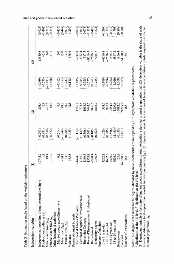
--l

Tab

le3.Estimationresultsbasedontheweekdaysubsample

~.

Independentvariables

(I)

(2)

(3)

~ =' e>.

(JQ

Instrumentedlogarithmoftotalexpenditure(Iny)

-12745.2

(-0.793)

-805.4

(-0.069)

13550.6

(0.923)

0 0 e>.

Food-outexpenditures

(x;)

1.8

(0.881)

0.8

(0.553)

-2.6

(-1.402)

C/>

Maleleisuretime

(1m)

19.4

(0.658)

-25.5

(-1.191)

6.0

(0.223)

S' ::rFemaleleisuretime

(It)

-31.7

(-0.872)

48.7

(1.856)

-17.1

(-0.515)

0 c:Otherhouseholdactivities

C/> '"

Marketgoodsexpenditures

(X2)

0.1

(0.714)

0.0

(-0.412)

0.0

(-0.455)

::r S-Maletime

(t2m

)-64.1

(-1.748)

49.2

(1.853)

15.0

(0.447)

e>.

~

Femaletime

(t2[)

33.0

(0.964)

-30.7

(-1.243)

-2.2

(-0.072)

~:Maleage

335.8

(1.051)

42.8

(0.185)

-378.6

(-1.297)

::::.

Degreeobtainedbymale

'"C/>Certificatd'EtudesPrimaires

-4494.0

(-1.110)

4786.8

(1.635)

-292.8

(-0.079)

Certificatd'AptitudeProfessionnelle

4145.9

(1.149)

-793.5

(-0.304)

-3352.4

(-1.017)

BrevetdesColleges

1369.5

(0.306)

-1052.0

(-0.325)

-317.5

(-0.078)

Brevetd'EnseignementProfessionnel

1573.8

(0.241)

7442.7

(1.577)

-9016.5

(-1.513)

Baccalaureat

-590.4

(-0.105)

3096.5

(0.761)

-2506.1

(-0.488)

Universitydegree

2386.5

(0.460)

4818.2

(1.285)

-7204.7

(-1.521)

Numberofchildren

otoIyearold

4232.1

(1.026)

324.7

(0.109)

-4556.8

(-1.209)

2to7yearsold

1602.5

(0.785)

923.6

(0.626)

-2526.1

(-1.355)

8to14yearsold

4429.2

(1.596)

-2554.1

(-1.272)

-1875.1

(-0.739)

15to24yearsold

5676.7

(2.405)b

-1809.6

(-1.060)

-3867.2

(-1.793)

Homeowner

125.9

(0.053)

-2082.3

(-1.208)

1956.4

(0.898)

Constant

140150.2

(1.161)

24219.9

(0.277)

-64370.1

(-0.584)

Numberofobservations

385

385

385

Not

es:Nodegreeisthereferencefordegreeobtainedbymale;coefficientsaremultipliedby105 ;asymptotict-statisticsinparentheses.

aSignificantatthe1%level;

bsignificantatthe5%level.

(1)Dependentvariableistheshareofmarketgoodsexpendituresintotalexpendituredevotedtomealpreparation

(sI)

;(2)dependentvariableistheshareofmale

timeexpendituresintotalexpendituredevotedtomealpreparation

(S2)

;(3)dependentvariableistheshareoffemaletimeexpendituresintotalexpendituredevoted

tomealpreparation

(S3)

'w V

I

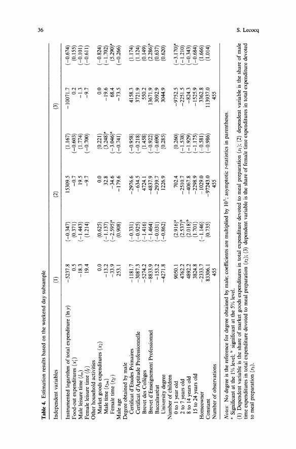
...,T

able4.Estimationresultsbasedontheweekenddaysubsample

0-

Independentvariables

(I)

(2)

(3)

Instrumentedlogarithmoftotalexpenditure(In

y)-5237.8

(-0.347)

15309.5

(1.167)

-10071.7

(-0.674)

Food-outexpenditures(xi)

0.5

(0.371)

-0.7

(-0.603)

0.2

(0.155)

Maleleisuretime

(1m)

-18.3

(-1.443)

19.5

(1.774)

-1.3

(-0.101)

Femaleleisuretime

(If)

19.4

(1.214)

-9.7

(-0.700)

-9.7

(-0.611)

Otherhouseholdactivities

Marketgoodsexpenditures

(X2)

0.0

(0.625)

0.0

(0.221)

0.0

(-0.824)

Maletime

(12m

)-13.2

(-1.137)

32.8

(3.248)'

-19.6

(-1.702)

Femaletime

(l2f

)-33.9

(-2.595)'

-34.6

(-3.046)'

68.4

(5.290)'

Maleage

253.1

(0.908)

-179.6

(-0.741)

-73.5

(-0.266)

Degreeobtainedbymale

Certificatd'EtudesPrimaires

-1181.7

(-0.331)

-2976.6

(-0.958)

4158.3

(1.174)

Certificatd'AptitudeProfessionnelle

-3087.3

(-0.925)

-634.5

(-0.218)

3721.9

(1.124)

BrevetdesColleges

-5274.2

(-1.416)

4724.1

(1.458)

550.2

(0.149)

Brevetd'EnseignementProfessionnel

-8833.9

(-1.464)

-4837.9

(-0.922)

13671.9

(2.286)"

Baccalaureat

-153.2

(-0.031)

-2939.7

(-0.690)

3092.9

(0.637)

Universitydegree

-4271.8

(-0.862)

1226.9

(0.285)

3044.9

(0.620)

Numberofchildren

otoIyearold

9050.1

(2.916)'

702.4

(0.260)

-9752.5

(-3.170)'

2to7yearsold

4762.2

(2.537)"

-2510.7

(-1.538)

-2251.5

(-1.210)

8to14yearsold

4892.2

(2.018)"

-4067.8

(-1.929)

-824.3

(-0.343)

15to24yearsold

3824.8

(1.701)

-2298.9

(-1.175)

-1525.9

(-0.684)

Homeowner

-2333.7

(-1.146)

-1029.0

(-0.581)

3362.8

(1.666)

Constant

83306.1

(0.735)

-9724j.0

(-0.986)

113937.0

(1.014)

Numberofobservations

455

455

455

Nol

es:Nodegreeisthereferencefordegreeobtainedbymale;coefficientsaremultipliedby105;asymptoticI-statisticsinparentheses.

,Significantatthe1%level;"significantatthe5%level.

(I)Dependentvariableistheshareofmarketgoodsexpendituresintotalexpendituredevotedtomealpreparation(Sl);(2)dependentvariableistheshareofmale

~

timeexpendituresintotalexpendituredevotedtomealpreparation

(S2)

;(3)dependentvariableistheshareoffemaletimeexpendituresintotalexpendituredevoted

htomealpreparation

(S3)

'~ ~

Time and goods in household activities

Endnotes

37

1 Some references are Azzi and Ehrenberg (1975), Gronau (1977), Wales and Woodland (1977),Kooreman and Kapteyn (1987), and Biddle and Hamermesh (1990). Rosenzweig and Schultz(1983) use birth weight as an indicator of the output of the household health production func­tion. But the model they estimate is still far from Becker's.

2 The survey contains no information about these time uses for children (and other adults).However, to the extent that the value of time for parents is largely higher than the value of timefor children, the contribution of the latter to the value of household production can be con­sidered as negligeable.

3 In the present work, we assume that these prices are identical through households. But it shouldbe more realistic to consider that they differ with the structure of the household.

4 However, to make sure of the robustness of the results, we also proceeded to the estimation ofthe system with the logarithm of wages (instrumented) included in the set of independent vari­ables. The results of the separability test remained unchanged.

5 We reason here in terms of opportunity cost by valuing an hour of male and female time at theirmarket wage.

6 For practical reasons that will become clear further on, only wage-earners are selected in oursubsample.

7 We have no information about female age and the degree she obtained. Note also that childrenare not considered here as household production, but only as control variables.

8 For example, the average time spent at work and in transports during the time recording day is60 min. higher for male and 41 min. lower for female when they belong to the sample of comersolutions than when they belong to the sample of interior solutions.

9 We also added identifying instruments in the demand system. Estimation showed that none wassignificant.

References

Azzi C, Ehrenberg R (1975) Household Allocation of Time and Church Attendance. Journal ofPolitical Economy 83(1):27-56

Becker GS (1965) A Theory of the Allocation of Time. Economic Journal 75(299):493-517Biddle JE, Hamermesh DS (1990) Sleep and the Allocation of Time. Journal ofPolitical Economy98(5):922-943

Browning M, Meghir C (1991) The Effect of Male and Female Labor Supply on CommodityDemands. Econometrica 59(4):925-951

Fortin B, Lacroix G (1997) A Test of the Neoclassical and Collective Models of HouseholdLabour Supply. Economic Journal 107(443):933-955

Gronau R (1977) Leisure, Horne Production, and Work - the Theory of the Allocation of TimeRevisited. Journal of Political Economy 85(6):1099-1123

Hausman JA (1978) Specification Tests in Econometrics. Econometrica 46(6):1251-1271Kooreman P, Kapteyn A (1987) A Disaggregated Analysis of the Allocation of Time within theHousehold. Journal of Political Economy 95(2):223-249

Michael RT, Becker GS (1973) On the New Theory of Consumer Behavior. Swedish Journal ofEconomics 75:378-395

Pollak RA (1969) Conditional Demand Functions and Consumption Theory. Quaterly Journal ofEconomics 83:70-78

Pollak RA (1971) Conditional Demand Functions and the Implications of Separable Utility.Southern Economic Journal 37:423-433

Pollak RA, Wachter ML (1975) The Relevance of the Household Production Function and ItsImplications for the Allocation of Time. Journal ofPolitical Economy 83(2):255-277

Rosenzweig MR, Schultz TP (1983) Estimating a Household Production Function: Heterogeneity,the Demand for Health Inputs, and Their Effects on Birth Weight. Journal of Political Econ­omy 91(5):723-746

Wales TJ, Woodland AD (1977) Estimation of the Allocation of Time for Work, Leisure, andHousework. Econometrica 45( I): 115-132

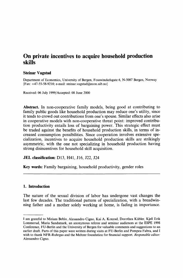
On private incentives to acquire household productionskills

Steinar Vagstad

Department of Economics, University of Bergen, Fosswinckelsgate 6, N-5007 Bergen, Norway(Fax: +47-55-58-9210; e-mail: steinar.vagstad@econ.uib.no)

Received: 06 July 1999/Accepted: 08 June 2000

Abstract. In non-cooperative family models, being good at contributing tofamily public goods like household production may reduce one's utility, sinceit tends to crowd out contributions from one's spouse. Similar effects also arisein cooperative models with non-cooperative threat point: improved contribu­tion productivity entails loss of bargaining power. This strategic effect mustbe traded against the benefits of household production skills, in terms of in­creased consumption possibilities. Since cooperation involves extensive spe­cialization, incentives to acquire household production skills are strikinglyasymmetric, with the one not specializing in household production havingstrong disincentives for household skill acquisition.

JEL classification: DB, H41, Jl6, 122, J24

Key words: Family bargaining, household productivity, gender roles

1. Introduction

The nature of the sexual division of labor has undergone vast changes thelast few decades. The traditional pattern of specialization, with a breadwin­ning father and a mother solely working at home, is fading in importance.

I am grateful to Miriam Beblo, Alessandro Cigno, Kai A. Konrad, Dorothea Kubler, Kjell ErikLommerud, Maria Sandsmark, an anonymous referee and seminar audiences at the ESPE 1998Conference, FU-Berlin and the University of Bergen for valuable comments and suggestions to anearlier draft. Parts of this paper were written during visits at FU-Berlin and Pompeu Fabra, and Iwish to thank NFR-Ruhrgas and the Meltzer foundation for financial support. Responsible editor:Alessandro Cigno.

40 S. Vagstad

However, also modem households practice a substantial degree of speciali­zation, for instance with women choosing working arrangements that arecompatible with having the main responsibility for children. 1 Also in familieswithout small children we find a pattern of women taking more than half ofthe household work, while men typically spend more hours than women inpaid work. The existence of comparative advantages is one explanation of thisphenomenon. Gary Becker (1991) has pointed out that even small compara­tive advantages may lead to substantial specialization. Moreover, in order tomaximize family output the family members should allocate their productiveinvestments (their "education") according to the sector of specialization: theone specializing in household production should invest to improve his - orrather her, to frame the discussion using traditional gender stereotypes ­household production skills, while the one specializing in market work shouldundertake investments that improve his labor market performance. Thisimplies that even if "natural" differences between men and women may berather small, these differences tend to increase as a consequence of invest­ment decisions. 2 If there is learning-by-doing this would work in the samedirection.A problem with Becker's explanation of how comparative advantages may

have evolved is that it cannot account for the fact that already at the date ofmarriage the family members have developed substantial comparative advan­tages, along traditional gender roles. It is well-known that women and meneducate in different directions. 3 Perhaps even more striking are the differencesbetween the sexes in what can be called domestic skills: an average womanabout to be married is much better skilled to keep and maintain a house thanis her coming husband, and this difference is found for a broad range ofhousekeeping activities: caring and nursing children, washing and mendingclothes, shopping, house cleaning, cooking, baking, etc. 4 These are skills thatare rarely acquired through formal educational, but rather passed on fromparents to children or acquired by self studies.Another problem with Becker's explanation is that what is in a family's

joint interest is not necessarily in the interest of the individual family mem­bers. 5 In particular, the investments ("education") required to maximizefamily output is not necessarily serving the interests of the individuals whohave to make those investments. Therefore, families and households shouldnot be treated as single-person decision-makers, but rather as a collection ofindividuals with some degree of conflicting interests. Consequently, the factthat specialization maximizes family output is not a fully satisfactory expla­nation of the observed division of labor: it has to be verified that specializationis in the individual's interest. This applies in particular to decisions that aremade before families are formed.Often, skill acquisition, choice of education and many other decisions in

life do not reflect rational decision-making but can rather be seen as responsesto some social norms. This raises the question how these social norms havedeveloped. The present paper also attempts to give an answer based on indi­vidual incentives - measured by private returns to improve one's householdproduction skills.Our point of departure is a non-cooperative model of family decisions, as

laid out by Konrad and Lommerud (1995). On the topic of private provisionof public goods, see Bergstrom et al. (1986). In their model, each of the twofamily members divide their time between market work and household work.

Incentives to acquire household production skills 41

Household work produces a household good that is jointly consumed by bothfamily members - i.e., it is a public good - while market work yields moneyincome that is a private good for the individual worker. As is well-knownfrom other private-provision-of-public-goods problems, there tends to be un­derprovision (relative to first-best) of the public good, due to the free riderproblem. Moreover, the time spent in household production depends posi­tively on one's productivity in the household production (hereafter calledcontribution productivity) and negatively on the spouse's contribution produc­tivity. This implies that while there is an obvious positive direct effect of in­creased contribution productivity - the same amount of household goods canbe produced with less effort - there is also a strategic effect working in theopposite direction. Thus, improved contribution productivity is not necessar­ily good for one's utility, even if the costs of improving one's household pro­duction skills are zero.As a description of actual family life the non-cooperative model rests on

quite pessimistic assumptions, and a natural way to proceed is to investi­gate the extent to which similar incentives can also arise in more cooperativefamilies. Here I proceed along the lines of Konrad and Lommerud (2000),who assumes that i) education investments that determine individual wagesare determined non-cooperatively; ii) time allocations are determined cooper­atively; and iii) the outcome of the bargaining process can be described by theNash bargaining solution, using equilibrium utilities in the non-cooperativemodel as fallback. While Konrad and Lommerud (2000) study incentives toimprove one's wage, I study incentives to improve one's productivity in thehousehold sector. A more important difference is that while Konrad andLommerud focus on symmetric incentives to over- or underinvest in educa­tion, a key point of the present paper is that investment incentives may bestrikingly asymmetric. There are also some technical differences that will becommented on in due course.In short, also in the cooperative model there are direct and strategic effects,

but there are important differences, too. First, in the cooperative model pre­sented there will be full specialization, implying that one of the family mem­bers spends all time at home while her spouse devotes all his attention tomarket work. 6 This maximizes the joint surplus that will subsequently bedivided according to the Nash bargaining solution. Since only the one with thehighest contribution productivity works at home, there will be no direct effectof increasing her spouse's contribution productivity. In contrast, there is astrong direct effect of increasing her own contribution productivity. The stra­tegic effect now works through the fallback payoffs, and it is clear that itwill be negative for both parties: it can be shown that in the non-cooperativemodel it is always better to have one's spouse improve the contribution pro­ductivity than to improve one's own. (This holds for both family members.)Thus, the less productive will experience no direct effect and a negative stra­tegic effect, so he will have disincentives to improve his domestic skills.Moreover, his spouse will experience a strong positive direct effect, and thiseffect will be only partially offset by the strategic effect, implying that she willstill have incentives to improve her domestic skills.The paper proceeds as follows. In the next section I present a cooperative

family model with non-cooperation as the bargaining threat point. Then Iderive the equilibrium payoffs to the family members for different combina­tions of contribution productivities. By performing comparative statics on the

42 S. Yagstad

equilibrium payoffs, incentives to invest in household production skills arederived. Discussions are found in Sect. 3, while Sect. 4 concludes the paper.

2. Model

Consider the following simple family model with two persons, 1 and 2, whichcan be interpreted as a woman and her husband. Utility of person i E {I, 2} isgiven by a Cobb-Douglas function defined over one private and one publicgood;

Uj=XjG, iE{1,2}, (1)

where Xj is individual consumption of a private good and G is the (common)consumption of the public good. The two goods are produced by devotingtime to either of two tasks: paid work or (unpaid) household production. LetCj denote the time person i spends on household production and the remainingtime 1 - Cj in the labor market. The production function for the public good isgiven by

(2)

where the parameters hI and h2 will be referred to as contribution productiv­ities. In what follows we will assume that individual 1 is more productive inthe household activity, that is, hI > h2•

Individual income is given by

(3)

where Wj denotes a person's wage. Then individual utility can be written

(4)

Our description of the cooperative model contains three elements: i) Acharacterization of efficient allocations and the utility possibility set (i.e., thePareto frontier); ii) A presentation of the threat point, which will be taken tobe the utilities in the non-cooperative model (for a discussion of this approach,see Konrad and Lommerud 2000; and iii) A characterization of equilibriumallocations using the Nash bargaining solution. After the equilibrium is found,what remains is to perform comparative statics on equilibrium payoffs inorder to assess the incentives to improve one's domestic skills.

The utility possibility set. By construction the cooperative outcome is efficient.Suppose that a transfer of size t goes from individual 1 to individual 2. Thenwe can write the sum of utilities as

(5)

which is independent of t. Hence a necessary condition for an allocation tobe efficient is that it maximizes xG, where x == Xl + X2. In what follows wenormalize both wages to 1. In the working paper version (Vagstad 1999) I

Incentives to acquire household production skills 43

provide the extension to cases in which wages may differ. Clearly, at leastone of the family members will be fully specialized, implying that (sincehi > h2) either CI = I or C2 = 0 or both. 7 Suppose that CI = 1. Then the opti­mal C2 maximizes aggregate utility given by u = (2 - CI - c2)(h l cl + h2C2) =(1 - c2)(h l + h2C2), and

(6)

yielding C2 = O. Conversely, suppose that C2 = O. Then the optimal CI max­imizes u = (2 - CI - c2)(h l cl + h2C2) = (2 - cI)hlcl. Then

(7)

implying that CI should be set equal to 1. In conclusion, the unique efficientallocation of effort entails full specialization. The resulting aggregate utilityto be shared is then given by u = hi. The solution above implies that thefamily members' bargaining problem is reduced to bargaining over how todivide an aggregate amount x = 1 of the private good, both agreeing on ajoint consumption of G = hi of the public good. Consequently, the utilitypossibility set is given by {(UI, U2) lUI + U2 ~ hI}.

Fallback utilities. We take non-cooperation as the alternative to reaching anagreement in the cooperative model. Therefore, the fallback utilities will betaken to be the payoffs in a non-cooperative model, in which the familiymembers simultaneously and non-cooperatively decide how to allocate theirtime. An interior Nash equilibrium in pure strategies exists if the two contri­bution productivities do not differ too much. We therefore make the followingassumption on productivity differences: hi < 2h2•

Now the (interior) non-cooperative equilibrium is found by first solving theset of first order conditions for CI and C2 and then substituting the solution

back into the variable definitions above. The first order conditions (aaul =CI

(hi - 2h l ci - h2C2)WI = 0 and aaU2 = (h2 - hici - 2h2C2)W2 = 0) yield Ci =C2

*_2hi -hj G G*-l(h h) d *_wi(h h)(" {12}ci = 3hi

' = = 3" 1+ 2 an Xi = Xi = 3hi1+ 2 I, ] E , /\

i =fi j). Note that ~~* < 0, telling us that improved productivity leads to a re-i

duction in one's spouse's contribution to the public good. What we are mostinterested in is equilibrium utilities, since these will serve as the threat points inthe bargaining game:

iE{I,2}. (8)

For use in the subsequent discussion, we will take a closer look at investmentincentives in a purely non-cooperative model before we proceed. Differentiat­ing individual utility with respect to the contribution productivities yields

44

out 2Wioh

i= 9h

i(hi + hz) > 0, and

out Wi [(hi)Z] 'ffohi = 9" 1 - h; > 0 I hi > hi'

S. Vagstad

(9)

(10)

(13)

(12)

Both these partials are interesting in the sense that they say somethingabout private incentives to influence the contribution productivities in a non­cooperative family. The first one, (9), tells us that it is in a family member'sinterest that the other family member improves his or her contribution pro­ductivity. The second one, (10), reveals that it is unclear whether it is an ad­vantage or not to be productive in the household sector:

Proposition 1. If time allocation is decided non-cooperatively, the individualhaving the highest contribution productivity would prefer to be even more pro­ductive, while the individual having the lowest contribution productivity wouldprefer to have even lower productivity.

Note that Proposition 1 depends on our particular model fonnulation.Most important is the degree of substitution implicitly assumed by our choiceof utility function. Clearly, as the strategic effect works mainly through sub­stitution between the two goods, any utility function involving less sub­stitutability will entail weaker strategic effects with the possibility of bothindividuals having incentives to improve their domestic skills, 8 while utilityfunctions involve more substitutability may result in both partners havingnegative investment incentives.

Nash bargaining. It is somewhat dissatisfactory to base one's results on anassumption of families being unable to reach efficient decisions. From now onwe will work with the opposite assumption: that decisions in the family areefficient. However, we maintain the assumption that decisions taken beforefamilies are fonned are made non-cooperatively (and that such decisions maytherefore not be efficient). To be more precise, suppose that the family mem­bers decide cooperatively how to allocate their time (i.e., effort), but thatproductivities are decided before the families are fonned. To avoid the com­plications arising if the choice of productivity investments affects who marrieswhom, we will leave the discussion of possible marriage market effects untilSect. 3. That is, in this section we assume that men and women match ran­domly to fonn families.Let LJ denote the gains from bargaining, defined as follows:

LJ = UI + Uz - (u; + un = hi - (9~1 (hi + hz)z + 9~z (hi + hz)Z) (11)

In the Nash bargaining solution this gain will be split evenly, implying thatindividual utilities in the bargaining equilibrium equal

1 z LJ 1 1 hi - hz ZUI =9h

l(hI +hz) +2'=2hl -18~(hl+hz)

1 z LJ 1 1 hi - hz zUz = 9h

z(hi + hz) +2' = 2 hl + 18~(hl + hz)

Incentives to acquire household production skills 45

Incentives to improve contribution productivities. Differentiating these expres­sions for individual equilibrium payoffs yields

OUt I 8h?hz - 2hf - h~ 0 (14)oh1 18 h?hz >

ouz I 2hf + lOh?hz + h~ 0 (IS)ohl 18 h?hz >

OUI I hlhi + 2h~ + hf 0 (16)ohz 18 h,hi >

oUZ I hlhi + 2hi + hf 0 (17)ohz -18 hlhi <

Again both cross partials are positive, but for slightly different reasons thanbefore. When the more productive family member improves - hi increases ­his spouse gains twofold. First, the set of feasible allocations expands. Second,the spouse's relative bargaining position improves.9 When it is the less pro­ductive who improves, the first effect is absent: due to complete specializa­tion, it is only the most productive's productivity parameter that matters forthe utility possibility set. However, the second effect - on bargaining position- is still there. In sum, also in the cooperative model an individual benefitsfrom having a spouse who has a high contribution productivity.More interesting is the own derivatives, as they determine the incentives

to acquire household production skills. We see that - qualitatively speaking ­the results from the non-cooperative model are valid also in the cooperativemodel:

Proposition 2. Also in the cooperative model, the most productive family mem­ber has incentives to improve, while the less productive has disincentives to do so.

The intuitions behind Propositions I and 2 are slightly different, however.Consider a change in the most productive person's contribution productivity.Such a change affects the utility possibility set: when hi increases, the Paretofrontier shifts outward. (Clearly, this has some of the same flavor as the directeffect in the non-cooperative model, but it should be noted that they are notthe same.) Moreover, increasing hi reduces person l's bargaining power, ina way that resembles the strategic effect in the non-cooperative model. Butagain they are different. One important difference becomes evident when thecontribution productivities are almost equal. In the non-cooperative model we

then know that incentives in either direction are weak (~~~ = ~ [I - (t)Z]OUIoh l

~ 0 when hi ~ hj). In contrast, in the cooperative model

I 8h?hz - 2hl3 - hZ

3 _ 5 ouz I hlhi + 2hi + hf 4.- and - ~ when18 h?hz ~ 18 ohz - -18 hlhi ~-18

hi ~ hz, implying that even the smallest difference in contribution productiv­ities produces distinct incentives to differentiate further.

46 S. Vagstad

Second, consider a change in the less productive's contribution produc­tivity. Such a change does not affect the utility possibility set, implying thatin the cooperative model there are no positive effects on Uz from increasing hz.The change affects the bargaining positions, however, and this effect is strongand clear even at the smallest possible differences.

3. Discussion

We have seen that wage differences do not affect contributions in the non­cooperative model. In the cooperative model things are more complicated. Inthe working paper version (Vagstad 1999) I allow for differences in labormarket skills as well as household production skills. In what follows I brieflysketch the method and the main result, and refer the interested reader toVagstad (1999) for details.First, efficient allocations maximize aggregate utility given by u =

(Xl +xz)G = ((1 - C.)WI + (1 - cz)wz)(hici + hzcz). Depending on absoluteas well as comparative advantages, efficiency may entail full specialization(i.e., one family member works full time in the market while the other worksfull time in household production) or only partial specialization (i.e., only onemember is fully specialized while the other split his or her attention betweenhousehold production and market work).After finding the efficient allocations, we employ the Nash bargaining

solution to find how the gains from cooperation is split. This yields equilib­rium payoff of each family member as explicit functions of all the parametersof the problem, that is, WI, Wz, hi and hz. Finally, investment incentives arefound by differentiation of equilibrium payoffs. One robust result stands outfrom the crowd of partial derivatives (proof in Vagstad 1999):

Proposition 3. The one with a comparative advantage for market work getsmore than 500/0 of total output. Moreover, the same person would prefer to beeven less domestically skilled, and would also prefer to have a spouse with evenlower wage.

Many matters of interest have been left out of the above analysis. In thecooperative model investigated above I have implicitly assumed that it isclear who will have the higher contribution productivity already at the timewhen the investments in household production skills are made. This is astrong assumption, if we are talking about the way children are brought up.The assumption may nevertheless be reasonable in a particular sense: even if acouple does not know the identity of their daughter's particular future hus­band, they may rationally believe that he will be brought up as a typical boy,that is, not being taught how to run a household. Conversely, parents of boysmay rationally believe that his prospective wife will be brought up to have arather high contribution productivity. Consequently, it appears that rationalexpectations may tum into self-fulfilling expectations.This is not at all clear, however. Even if the average suitor has little

household production skills, it is possible for a girl (or her parents) to under­cut that level by appropriate (lack of) skill acquisition. How come parents donot engage in such undercutting? One possible explanation could be that itmay be undesirable to have two persons without household production skills

Incentives to acquire household production skills 47

form a family - such families suffer in terms of a small utility possibility set.In this sense specialized upbringing can be seen as a coordination device ­it assures that at least one of the family members is skilled in householdproduction. lo

Another explanation can be sought in marriage market forces. Supposethat instead of random matching, matching is based on utility-maximizingbehavior - behavior that can be turned into forces of supply and demand.What follows is a brief discussion of the demand for partners with certainproductivity parameters. I also discuss the demand for what can be seen as thealternative to domestic skills: labor market skills (measured by wage levels).Underlying the discussion is an assumption of highly incomplete marriagecontracts. In particular, a marriage contract is taken to be only a commitmentto playa particular game (either the non-cooperative or the cooperative game)with a specific partner - there are no up-front payments (i.e., no dowries orbride prices).First, in the cooperative model as well as the non-cooperative model there

will be a positive demand for spouses with high contribution productivities,suggesting that the negative incentives to acquire household production skillsmay be mitigated by forces in the marriage market: having high skills forhousehold production may be bad for you once you are married, but it makesyou more attractive as a marriage partner.Perhaps more interesting is the demand for labor market characteristics: in

the non-cooperative model, wages are irrelevant as a sorting criterion - theyare neutral as regards contribution to the public good. This is not so in thecooperative model. The most plausible assumption is perhaps that womenhave an absolute advantage in household production while men have an ab­solute advantage in the labor market. If so, the strategic effect then dominatesin two cases: the husband's utility is decreasing in his wife's wage as well as inhis own contribution productivity, while all other derivatives (own and cross)are positive (see Vagstad 1999, for details). The intuition for this pattern isthat since the wife will spend all her time in household production and thehusband will spend all his time in market work, increasing the wife's wagemarginally will not affect the utility possibility set at all, it will only make herdemand a larger share of total output.Finally, the demand for high-wage husbands is somewhat unclear a priori.

The effect on the utility possibility set suggests that there will be a demandfor high-wage men, but since high-wage men (just like high-wage women) willdemand a larger share of total output, it is a priori unclear whether there willbe demand for high-wage men. In this model, however, the positive effectalways dominates, creating a positive demand for high-wage men.To sum up the marriage market effects, the above discussion suggests that

women improve their market positions by investing in household productionskills and disinvest in improving their labor market performance. In contrast,for men both attributes are valuable in the marriage market. There will bea certain demand for men with high contribution productivities, because suchmen will demand a smaller fraction of output. But there will also be demandfor high-wage men, in spite of such men being more demanding, becausethey expand the utility possibility set. ll Consequently, optimizing women willconcentrate on household production skills, while optimizing men will try toimprove along two dimensions, which is to say that women have strongerincentives to become domestically skilled.

48

4. Concluding remarks

S. Vagstad

Iffamily members have common preferences, Becker (1991) - among others­has argued that family members will specialize according to comparativeadvantages, not only regarding division of labor, but also when it comes toinvestments that improve one's skills. Therefore, investments tend to increaseany productivity differences. We have seen that even if families are less har­monic, Becker is basically right on this point: individual investment incentivestend to increase specialization also when we allow for explicit conflicts ofinterest between family members.Becker's second hypothesis concerns efficiency: with common preferences,

investments as well as time will be allocated in a way that maximize jointsurplus. This result does not hold when we relax the assumptions of commonpreferences. To be more specific: with truly non-cooperative families, neitherinvestments nor time allocations will be efficient, for well-known reasons:there are strong positive externalities from contributing to household pro­duction as well as from investing in domestic skills, giving rise to a seriousfree-rider problem. In what I have called a cooperative family, time allo­cations will be efficient (by assumption), but this may give rise to evenless efficient investments, in order to affect the outcome of the bargainingprocess.I conclude with a short list of issues for further research. The first concerns

policy issues. My analysis points at two problems that I believe deserve at­tention. First, from an efficiency point of view one should be concerned aboutthe welfare effects of underinvestment in household production skills. Second,from a distributional point of view one should be concerned that investmentincentives increase the gender differences, not only in time and investment al­locations (which is hardly a problem in itself) but, more seriously, in equilib­rium payoffs.The fact that a decrease in one person's contribution to the public good

increases the other person's contribution is what gives rise to underinvestment.Consequently, anything that can break the substitutability between the familymembers' contributions should in principle reduce the underinvestment prob­lem. The government may affect this substitutability in many ways. First, thethey may promote the provision of close substitutes to the household publicgood (publicly provided day care for children is only one example), implyingthat if one family member contributes less than his or her "just" share, he orshe may be told to buy the rest in the market. Second, also taxation may affectspecialization. In particular, progressive taxation based on individual laborincome will discourage specialization and therefore reduce substitution. Third,implementing a cap on how many hours a week one is allowed to work willalso limit specialization. It is more difficult to imagine explicit regulation ofdivision of labor within the family, but social norms may have a similar effect:if the public goods to be provided can be divided in "male" and "female"tasks that are socially sanctioned, this should have a beneficial effect on in­vestment incentives - although the benefits must of course be traded againstthe possible inefficiencies such rigidities may entail.Finally, the marriage market forces discussed in the previous section war­

rants more analysis. In particular, important features of modern societies likethe increase in divorce rates and the number of single-person householdsshould be incorporated in future work.

Incentives to acquire household production skills

Endnotes

49

1 For some US evidence, see, e.g., Fuchs (1989) and Hersch (1991). Relevant facts from Britainand Germany are found in Joshi (1989) and Beblo (1998), respectively.

2 From nature's side men and women's comparative advantages in market work and householdproduction appear to be of limited importance today. Women's natural advantage in takingcare of children should apply only for small babies, and physical strength is of little or noimportance in most jobs today.

3 Looking at education we see - roughly speaking - that women choose educations that arecompatible with housekeeping: nurses and kindergarten teachers are prime examples. In con­trast, men educate themselves to traditional bread-winning positions in the labor market:industrial workers, engineers and managers.

4 There are of course exceptions to this general pattern, however: different types of light main­tainance work - e.g., fixing the car when it is broken - are typically done by men. What shouldbe noted, however, is that the activities in which the women are more skilled comprise the bulkof household production activities.

5 This was first formally analyzed by Manser and Brown (1980) and McElroy and Horney(1981). More recent contributions include Lundberg and Pollak (1993) and Konrad andLommerud (1995, 2000). For surveys, see Ott (1992) or Lommerud (1997).

6 Clearly, this result depends upon the particular parameterization of the mode!. More generallyone will expect cooperation to promote specialization, with similar qualitative effects.

7 If none were fully specialized, then output could be increased with the same total effort byshifting attention in the direction of comparative advantages.

8 See e.g. Konrad and Lommerud (2000), whose model features quasi-linear utility.9 For this to be the case, ui must increase more than uj when hi increases. Simple differentiaton

au' au' I 2h2 - h2h l + h2 .. .reveals that ah2 - -hI = - (hI + h2) I 2 2 > 0 whether hI > h2 or not. This Imphes

I a I 9 hI h2that one's bargaining position always deteriorates with increasing contribution productivity.

10 A full-fledged analysis of the interplay between beliefs and investment decisions is beyond thescope of this paper. See Francois (1998) and, in particular, Lommerud and Vagstad (2000) fora discussion of the considerations involved in such an analysis.

11 Some limited support for these conjectures is found in data for firms doing professional mar­riage partner search in Germany (see Nitschke 1998). Such firms typically price discriminate bycharging lower prices if you are attractive yourself, and by looking at prices, Nitschke findsthat what makes a man attractive is a high ability to provide money, while what makes awoman attractive is being young and pretty. He also quotes figures telling that it is particularlydifficult to find partners to older women with higher education (i.e., high potential wages).

References

Beblo M (1998) Intrafamily Time Allocation: A Panel-Econometric Analysis of the Division ofHousework Timing among German Couples. Discussion Paper no. 1998/23, Department ofEconomics, FU-Berlin

Becker G (1991) A Treatise on the Family. En!. Ed. Harvard University Press, Cambridge, MassBergstrom T, Blume L, Varian H (1986) On the Private Provision of Public Goods. Journal of

Public Economics 29:25-49Francois P (1998) Gender Discrimination Without Gender Difference: Theory and Policy Re­sponses. Journal of Public Economics 68:1-32

Fuchs V (1989) Women's Quest for Economic Equality. Journal ofEconomic Perspectives 3:25-41Hersch J (1991) The Impact of Nonmarket Work on Market Wages. American Economic Review81: Papers and Proceedings 157-160

Joshi H (1988) Changing Roles of Women in the British Labour Market and the Family. Dis­cussion Paper in Economics 88/13, Birkbeck College

Konrad KA, Lommerud KE (1995) Family Policy with Non-Cooperative Families. ScandinavianJournal ofEconomics 97:581-601

Konrad KA, Lornmerud KE (2000) The Bargaining Family Revisited. Canadian Journal of Eco­nomics 33:471-487

50 S. Vagstad

Lomrnerud KE (1989) Marital Division of Labor with Risk of Divorce: The Role of "Voice"Enforcement of Contracts. Journal of Labor Economics 7: 113-27

Lomrnerud KE (1997) Battles of the Sexes: Noncooperative Games in the Theory of the Family.In: Jonung C, Persson I. The Economics of the Family Policies. Routledge, London

Lommerud KE, Vagstad S (2000) Mommy Tracks and Public Policy. On Self-Fulfilling Prophe­cies and Gender Gaps in Promotion. CEPR Discussion Paper No 2378

Lundberg S, Pollak RA (1993) Separate Spheres Bargaining and the Marriage Market. Journal ofPolitical Economy 101:988-1010

Manser M, Brown M (1980) Marriage and Household Decision-Making: A Bargaining Analysis.International Economic Review 21:31-44

McElroy MB, Homey MJ (1981) Nash-Bargained Household Decisions: Toward a Generaliza­tion of the Theory of Demand. International Economic Review 22:333-349

Nitschke K (1998) Das Geschiift mit der Liebe: professionelle Partnersuche kostet viel Geld [TheLove Business: Professional Search for a Partner is Very Expensive]. Die Zeit: 49 (26November 1998): 36

Ott N (1992) Intrafamity Bargaining and Household Decision Making. Springer, Berlin HeidelbergNew York

Vagstad S (1999) On Private Incentives /0 Acquire Household Production skills. WP 1499, De­partment of Economics, University of Bergen

Estimating intrahousehold allocation in a collectivemodel with household production

Thomas Aronsson, Sven-Olov Daunfeldt, Magnus Wikstrom

Department of Economics, Umeii University, S-901 87 Umeii, Sweden (Fax: +46-90-772 302;e-mail: thomas.aronsson@econ.umu.se;so.daunfeldt@econ.umu.se; magnus.wikstrom@econ.umu.se)

Received: 14 April 2000/Accepted: 12 January 2001

Abstract. The purpose of this paper is to estimate the intra-family distributionof income and the individual demand for leisure and household productionfrom Swedish cross-sectional household data. As a basis for the analysis, weuse a collective model where each individual is characterized by his or her ownutility function and divides total time between leisure, household productionand market work. For the purpose of comparison, we also estimate a versionthat is consistent with a more traditional model of labor supply, the unitarymodel.

JEL classification: DB, 122

Key words: Time-use, household production, collective model

1. Introduction

Traditionally, the household has been considered as a single utility maximiz­ing agent. This so called unitary model has lately been criticized both from atheoretical and an empirical viewpoint. It has been argued that a multipersonhousehold cannot be modeled as a single individual because it contradictsthe neoclassical starting point that every individual should be characterized byhis/her own preferences. Moreover, the unitary model only considers alloca­tions between households and disregards questions concerning intra-householdinequalities, which may lead to wrong welfare implications (see Haddad and

All correspondence to Sven-Olov Daunfeldt. We would like to thank Alessandro Cigno, JonasNordstrom and an anonymous referee for valuable comments. A research grant from HSFR isgratefully acknowledged. Responsible editor: Alessandro Cigno.

52 T. Aronsson et al.

Kanbur 1990, 1992). One testable restriction imposed by the unitary model isthat the distribution of nonlabor income across spouses is not important forbehavior: only the sum of the spouses' nonlabor income matters. This so calledpooling restriction has also been rejected in several empirical studies, e.g., inSchultz (1990); Thomas (1990) and Kawaguchi (1994).The theoretical and empirical criticism against the unitary model has lead to

other models of household behavior, where individual preferences are recog­nized. One model that has received widespread attention is the collective model,developed by Chiappori (1988, 1992). In the collective model, the household isassumed to reach a Pareto-efficient outcome. Within this framework, testablerestrictions can be derived and the intra-household distribution of income canbe estimated. As pointed out by Becker (1965) a significant amount of timenot used for market work is used for household production. Apps and Rees(1997) extend Chiappori's model by introducing a good produced by the house­holds. They show that the sharing arrangement underlying the collective modelcannot be retrieved unless specific assumptions are made. Chiappori (1997)shows that when the household good is tradable at a given price, the sharingarrangement may still be retrieved up to an additive constant.There have been few empirical studies based on the collective model.

Among the exceptions are Browning et al. (1994); Fortin and Lacroix (1997)and Chiappori et al. (1998). The results from their studies are generally sup­portive of the collective model. However, none of these studies have con­sidered household production. The purpose of our study is to use the extendedcollective model to estimate simultaneously the intra-family distribution ofincome, individual leisure demands and the household production functionfrom Swedish cross-sectional household data. Two versions of the model areestimated, one that is consistent with the household good being tradable onthe market, and the other where households cannot buy or sell the householdgood. For purposes of comparison, we also estimate a version that is consis­tent with the unitary model.The paper is organized as follows. In the next section, we present the the­

oretical background of our study based on Chiappori's (1997) work. Section 3consists of a description of the data used in the empirical study. In Sect. 4, wepresent the empirical model and the estimation results. Section 5 concludes thepaper.

2. Theory

We consider a two-member household where m denotes the male and f denotesthe female. Assume that individual i's direct utility function can be written

Utility is defined over three different goods: leisure, h, a market consumptiongood, Ci, and a consumption good, Xi, that is produced within the household.The vector of demographic characteristics of the individual is denoted as Zi.Let us for the time being assume that Xi is marketable, i.e., it can be sold andbought on the market. The household production function, h(tm, tl; a), isassumed to be characterized by constant returns to scale l

, where tm and tlare hours of household work for the male and the female respectively, and

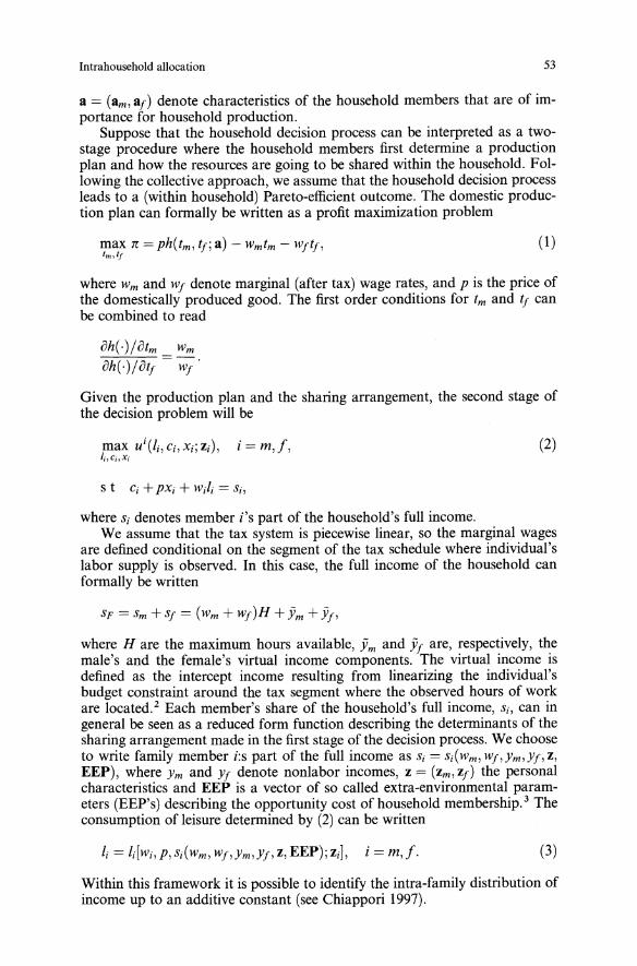
Intrahousehold allocation 53

a = (am, af) denote characteristics of the household members that are of im­portance for household production.Suppose that the household decision process can be interpreted as a two­

stage procedure where the household members first determine a productionplan and how the resources are going to be shared within the household. Fol­lowing the collective approach, we assume that the household decision processleads to a (within household) Pareto-efficient outcome. The domestic produc­tion plan can formally be written as a profit maximization problem

(I)

where Wm and wf denote marginal (after tax) wage rates, and p is the price ofthe domestically produced good. The first order conditions for 1m and If canbe combined to read

Oh(')/Olm Wmoh(,)/olf wf

Given the production plan and the sharing arrangement, the second stage ofthe decision problem will be

max Ui(li,Ci,Xi;Zi), i = m,j,Ij,Cj,Xj

(2)

where Si denotes member i's part of the household's full income.We assume that the tax system is piecewise linear, so the marginal wages

are defined conditional on the segment of the tax schedule where individual'slabor supply is observed. In this case, the full income of the household canformally be written

SF = Sm + Sf = (wm+ wf)H + jim +h,where H are the maximum hours available, jim and h are, respectively, themale's and the female's virtual income components. The virtual income isdefined as the intercept income resulting from linearizing the individual'sbudget constraint around the tax segment where the observed hours of workare located. 2 Each member's share of the household's full income, Si, can ingeneral be seen as a reduced form function describing the determinants of thesharing arrangement made in the first stage of the decision process. We chooseto write family member i:s part of the full income as Si = Si(Wm, wf,Ym,Yf,z,EEP), where Ym and Yf denote nonlabor incomes, Z = (zm, zf) the personalcharacteristics and EEP is a vector of so called extra-environmental param­eters (EEP's) describing the opportunity cost of household membership.3 Theconsumption of leisure determined by (2) can be written

(3)

Within this framework it is possible to identify the intra-family distribution ofincome up to an additive constant (see Chiappori 1997).

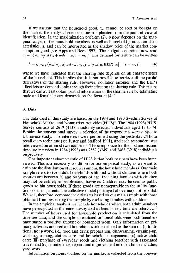
54 T. Aronsson et al.

If we assume that the household good, Xi, cannot be sold or bought onthe market, the analysis becomes more complicated from the point of view ofidentification. In the maximization problem (2), P now depends on the mar­ginal wages of the household members as well as household production char­acteristics, a, and can be interpreted as the shadow price of the market con­sumption good (see Apps and Rees 1997). The budget constraints now readCi +p(wm , Wj, a)xi + W;li = Si, i = m,f. The demand for leisure can be written

where we have indicated that the sharing rule depends on all characteristicsof the household. This implies that it is not possible to retrieve all the partialderivatives of the sharing rule. However, nonlabor incomes and the EEP'saffect leisure demands only through their effect on the sharing rule. This meansthat we can at least obtain partial information of the sharing rule by estimatingmale and female leisure demands on the form of (4).4

3. Data

The data used in this study are based on the 1984 and 1993 Swedish Survey ofHousehold Market and Nonmarket Activities (HUS)5. The 1984 (1993) HUS­Survey consists of 2619 (4137) randomly selected individuals aged 18 to 74.Besides the conventional survey, a selection of the respondents were subject toa time-use study. The interviews were performed using the yesterday 24 hourrecall diary technique (see Juster and Stafford 1991), and each respondent wasinterviewed on at most two occasions. The sample size for the first and secondtime-use interview in 1984 (1993) was 2552 (3249) and 2468 (3218) individualsrespectively.One important characteristic of HUS is that both partners have been inter­

viewed. This is a necessary condition for our empirical study, as we want toestimate the distribution of resources among the household members. Our mainsample refers to two-adult households with and without children where bothspouses are between 20 and 60 years of age. Including families with childrenmay not be entirely unproblematic, however. Children may be seen as publicgoods within households. If these goods are nonseparable in the utility func­tions of their parents, the collective model portrayed above may not be valid.We will, therefore, compare the estimates based on our main sample with thoseobtained from restricting the sample by excluding families with children.In the empirical analysis we include households where both adult members

have participated in the main survey and at least in one time-use interview. 6

The number of hours used for household production is calculated from thetime use data, and the sample is restricted to households were both membershave stated a positive amount of household work. Only information on pri­mary activities are used and household work is defined as the sum of: (i) tradi­tional housework, i.e., food and drink preparation, dishwashing, cleaning-up,washing, ironing, clothes care and household management; (ii) active childcare; (iii) purchase of everyday goods and clothing together with associatedtravel; and (iv) maintenance, repairs and improvement on one's home includingyard work.Information on hours worked on the market is collected from the conven-

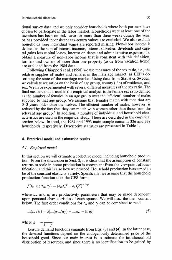
Intrahousehold allocation 55

(5)

tionaI survey data and we only consider households where both partners havechosen to participate in the labor market. Households were at least one of themembers has been on sick leave for more than three weeks during the year,or has provided inconsistent tax-return values are excluded. We also excludehouseholds were individual wages are reported missing. Non-labor income isdefined as the sum of interest incomes, interest subsidies, dividends and capi­tal gains less capital losses, interest on debts and administrative expenses. Toobtain a measure of non-labor income that is consistent with this definition,farmers and owners of more than one property (aside from vacation home)are excluded from the 1984 data.Following Chiappori et al. (1998) we use measures of the sex ratio, i.e., the

relative supplies of males and females in the marriage market, as EEP's de­scribing the state of the marriage market. Using data from Statistics Sweden,we calculate sex ratios on the basis of age group, county (Ian) of residence, andsex. We have experimented with several different measures of the sex ratio. Thefinal measure that is used in the empirical analysis is the female sex ratio definedas the number of females in an age group over the 'efficient' number of malessupplied to that age group. We assume that females match with men that are0-3 years older than themselves. The efficient number of males, however, isreduced by the fact that they can match with women other than those from therelevant age group.7 In addition, a number of individual and household char­acteristics are used in the empirical study. These are described in the empiricalsection below. In total, the 1984 and 1993 main sample contains 326 and 338households, respectively. Descriptive statistics are presented in Table 1.

4. Empirical model and estimation results

4.1. Empirical model

In this section we will estimate a collective model including household produc­tion. From the discussion in Sect. 2, it is clear that the assumption of constantreturns to scale in home production is convenient from the viewpoint of iden­tification, and this is also how we proceed. Household production is assumed tobe of the constant elasticity variety. Specifically, we assume that the householdproduction function take the CES-form;

where am and af are productivity parameters that may be made dependentupon personal characteristics of each spouse. We will describe their contentbelow. The first order conditions for tm and tf can be combined to read

In(tm/tf) = It[ln(wm/wf) -lnam+ lnaf]

Iwhere It = - --.

l+pLeisure demand functions emanate from Eqs. (3) and (4). In the latter case,

the demand functions depend on the endogenously determined price of thehousehold good. Since our main interest is to estimate the intrahouseholddistribution of resources, and since there is no identification to be gained by

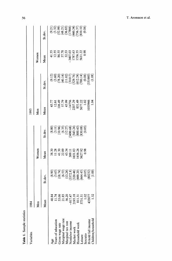
Tab

le1.Samplestatistics

VI '"

Variables

1984

1993

Men

Women

Men

Women

Mean

St.dev.

Mean

St.dev.

Mean

St.dev.

Mean

St.dev.

Age

40.84

(8.90)

38.30

(8.80)

43.77

(9.12)

41.55

(9.21)

Yearsofeducation

11.74

(3.63)

11.28

(3.11)

12.61

(3.60)

12.55

(3.32)

Grosswagerate

53.06

(18.74)

41.30

(10.96)

106.49

(78.20)

86.55

(52.99)

Marginalwagerate

21.85

(6.53)

22.89

(6.35)

57.79

(40.14)

57.78

(48.21)

Marginaltaxrate

56.20

(13.24)

43.34

(12.27)

43.99

(11.02)

32.53

(36.83)

Nonlaborincome

-817.47

(5572.8)

509.11

(3490.68)

-14756

(31017)

-3407.03

(17866)

Marketwork

2193.18

(320.46)

1651.83

(543.24)

2207.29

(329.76)

1787.63

(460.34)

Householdwork

811.31

(600.20)

1456.26

(800.43)

851.49

(612.24)

1336.55

(756.37)

Leisure

5731.51

(664.43)

5627.92

(830.08)

5677.22

(700.14)

5611.22

(810.10)

Sexratio

1.02

(0.05)

0.98

(0.05)

1.02

(0.06)

0.98

(0.06)

H-holdfullincome

433077

(80232)

1055946

(531660)

Children/household

1.32

(1.00)

1.04

(1.08)

cl ;l> 8 c ~ c ~ ~

Intrahousehold allocation 57

explicitly modelling the price of the household good, we choose not to modelthe price function explicitly. Instead, we specify leisure demand functions on'semi-reduced' forms, i.e. they depend on cross wages as well as spouse char­acteristics. We shall also assume that the leisure demand functions are linear;

~=~~+~~+~~+~+~ (~

lj = Pfwf + ofwm+ Yfsf + zm + zf (7)

where Sm and sf denote, as before, the male and female share of the householdsfull income. The scalars zm, zf' zm, and zf, should now be interpreted to containcharacteristics originating from the utility function as well as from the produc­tion function, and Ph Oi, Yi' i = m, f, are parameters to be estimated. Charac­teristics are assumed to include age, a dummy variable indicating the presenceof children in a specific age bracket (0-6,7-12 and 13-17 years of age) and adummy variable reflecting the educational attainment of the individual. Theeducational dummy variable takes the value one if the respondent has a uni­versity or a university college degree. Equations (5), (6), and (7) correspond toour most general model specification, which is the case where the householdgood cannot be traded. We will below discuss how to impose restrictions inorder to make the empirical model compatible with alternative theoreticalinterpretations.Denote by Om the male's relative share of full income such that Sm = OmSF.

Consequently, Of = 1 - Om is the female's relative share. We assume that theserelative shares are determined by marginal wages and nonlabor incomes, and,in addition, a number of other exogenous variables (to be described below)reflecting the income sharing arrangement. Following Browning et al. (1994)we assume that the relative shares can be modelled by a logistic function,i.e., Om = 1/(1 + exp(d)), and Of = 1 - 1/(1 + exp(d)), where d contains thevariables affecting the income sharing arrangement.In specifying the determinants of the sharing rule, the reader should first

observe that when the household good is tradable, it can be seen from Eq. (3)that iJli/iJzj = iJI;jiJsi · iJsi/iJzj , meaning that the characteristics of the partneronly affect the leisure demand via the sharing rule. Therefore, spouse charac­teristics can be used to obtain identification of the parameters of the sharingrule in this case. This could be done for instance by including differences inwage rates and other characteristics between the household members (see alsoBrowning et al. 1994, for a similar argument). If, on the other hand, the house­hold good cannot be traded, identification of the sharing rule originates fromthe nonlabor income of the spouses and the EEP's, since spouse characteristicswill in this case affect Ii both via the sharing arrangement and via the price of thehousehold good. We assume that the sharing rule is determined by the femalesex ratio and by the differences in age, the number of years of schooling, mar­ginal wages, and nonlabor incomes between the household members. Finally,since the sharing rule cannot be fully recovered in either of the two models setout in Sect. 2, the mean of the sharing rule is centered around one half.In an economy without nonlinear taxation the wage rate is exogenous to

hours ofwork. However, under progressive income taxation the marginal wagerate is endogenous. To address this problem, estimation is accomplished usingan instrumental variables method. The instruments chosen for the marginalwage rate are the gross wage rate, the square of the gross wage rate, capitalincome and capital income squared. Similarly, full income of the household is

58 T. Aronsson et al.

also endogenous under nonlinear taxation and is instrumented as well. In thiscase, capital income, the gross wage rate for both spouses and nontaxablebenefits are used as instruments. The final Eqs. (5), (6), and (7) are then esti­mated jointly using the nonlinear least-squares estimator, where cross equationrestrictions pertaining to the sharing rule parameters are invoked and thestochastic specification allows for contemporaneous correlations of the errorterms.

4.2. Estimation results

The estimation results are presented in Tables 2 and 3. The tables contain threedifferent versions of the empirical model. Model I refers to the full model givenby Eqs. (5), (6), and (7). Model II is a restricted version ofmodel I, where cross­wage effects are set to zero in the leisure demand equations, and the spouse'scharacteristics affect leisure demands solely via the sharing rule. Model III,finally, is based on the assumption that the sharing rule is constant by imposingthe restrictions that Of = Om = 1/2. With reference to the theoretical section,we can interpret these models as consistent with the non-marketable householdgood case (model I), the marketable household good case (model II), and theunitary model (model III). The restrictions imposed by models II and III caneasily be tested against the more general alternative (model I).We start by comparing the estimates ofmodel I with those ofmodels II and

III by performing Wald tests. Comparing model I and model III, the latter isobtained as a special case of the former by setting the five parameters in thesharing rule to zero. The critical value for rejecting the null at the conventional95% level of significance is X2(5) = 11.07. The Wald-test statistic is 3.96 and46.7 for the 1984 and 1993 data respectively. A similar test of model II yieldsthe Wald-test statistics 6.59 and 17.59 (the critical value is in this case given by12.59). Hence, we are not able to reject model II and model III using the 1984data, while using the 1993 data both models II and III can be rejected. We havealso tested the null hypothesis of constant parameters over time. This hypoth­esis was clearly rejected.The reader should note that, since identification of the sharing rule in model

I is obtained by assumptions regarding functional form, the test discussedabove can also be interpreted as tests of functional form; It is, therefore, im­portant to impose as few restrictions as possible during estimation. In additionto the estimates presented in Tables 2 and 3, we have tried other more complexfunctional forms of the leisure demand equations, for instance by allowing forquadratic wage effects. However, the additional parameters introduced did notcontribute significantly to the value of the likelihood function. Therefore, ourconclusions regarding model selection may not depend much on the choice ofthe functional form for the leisure demand functions.Turning to the individual parameter estimates, note first that the (relative)

amount of time spent working in the household is insensitive to the relativewage. Similarly, the wage and income effects are generally not significantlydetermined in the leisure demand equations, and the point estimates differ be­tween the different versions of the collective model.As can be seen from Tables 2 and 3, the estimates suggest that the presence

of pre-school children (0-6 years of age) reduces leisure time for both spouses.In addition, younger school children (7-12 years of age) significantly reduces

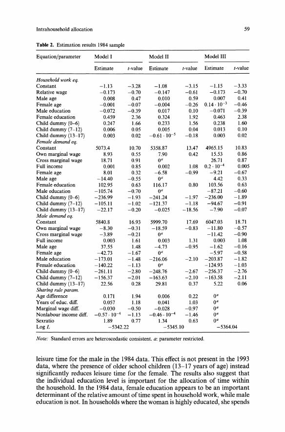
Intrahousehold allocation 59

Table 2. Estimation results 1984 sample

Equation/parameter Modell Model II Model III

Estimate t-value Estimate t-value Estimate t-value

Household work eg.Constant -1.13 -3.28 -1.08 -3.15 -1.15 -3.33Relative wage -0.173 -0.70 -0.147 -0.61 -0.173 -0.70Male age 0.008 0.47 0.010 0.59 0.007 0.41Female age -0.001 -0.07 -0.004 -0.26 0.14.10-3 -0.46Male education -0.072 -0.39 0.017 0.10 -0.071 -0.39Female education 0.459 2.36 0.324 1.92 0.463 2.38Child dummy (0-6) 0.247 1.66 0.233 1.56 0.238 1.60Child dummy (7-12) 0.006 0.05 0.005 0.04 0.013 0.10Child dummy (13-17) 0.003 0.02 -0.61 . 10-5 -0.18 0.003 0.02Female demand eg.Constant 5073.4 10.70 5358.87 13.47 4965.15 10.83Own marginal wage 8.93 0.55 7.90 0.42 15.53 0.86Cross marginal wage 18.71 0.91 0" 26.71 0.87Full income 0.001 0.85 0.002 1.08 0.2.10-4 0.005Female age 8.01 0.32 -6.58 -0.99 -9.21 -0.67Male age -14.40 -0.55 0" 4.42 0.33Female education 102.95 0.63 116.17 0.80 103.56 0.63Male education -105.74 -0.70 0" -87.21 -0.60Child dummy (0-6) -236.99 -1.93 -241.24 -1.97 -236.00 -1.89Child dummy (7-12) -105.11 -1.02 -121.37 -1.18 -94.67 -0.91Child dummy (13-17) -22.17 -0.20 -0.025 -18.56 -7.90 -0.07Male demand eg.Constant 5840.8 16.93 5999.70 17.69 6047.03 18.71Own marginal wage -8.30 -0.31 -18.59 -0.83 -11.80 -0.57Cross marginal wage -3.89 -0.21 0" -11.42 -0.90Full income 0.003 1.61 0.003 1.31 0.003 1.08Male age 37.55 1.48 -4.73 -0.95 -1.62 -0.16Female age -42.73 -1.67 0" -5.97 -0.58Male education -173.01 -1.48 -216.06 -2.10 -203.87 -1.82Female education -140.22 -1.13 0" -124.93 -1.03Child dummy (0-6) -261.11 -2.80 -248.76 -2.67 -256.37 -2.76Child dummy (7-12) -156.37 -2.01 -163.63 -2.10 -163.58 -2.11Child dummy (13-17) 22.56 0.28 29.81 0.37 5.22 0.06Sharing rule paramoAge difference 0.171 1.94 0.006 0.22 0"Years of educ. diff. 0.057 1.18 0.041 1.03 0"Marginal wage diff. -0.030 -0.50 -0.028 -0.97 0"Nonlabour income diff. -0.57.10-4 -1.13 -0.46.10-4 -1.46 0"Sexratio 1.89 0.77 1.34 0.63 0"LogL -5342.22 -5345.10 -5364.04

Note: Standard errors are heteroscedastic consistent. a: parameter restricted.

leisure time for the male in the 1984 data. This effect is not present in the 1993data, where the presence of older school children (13-17 years of age) insteadsignificantly reduces leisure time for the female. The results also suggest thatthe individual education level is important for the allocation of time withinthe household. In the 1984 data, female education appears to be an importantdeterminant of the relative amount of time spent in household work, while maleeducation is not. In households where the woman is highly educated, she spends

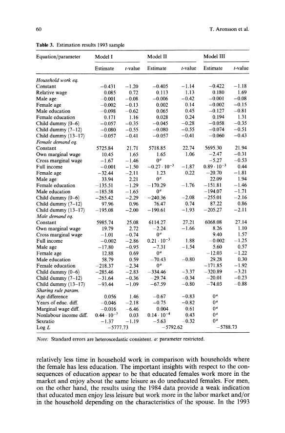
60 T. Aronsson et al.

Table 3. Estimation results 1993 sample

Equation/parameter Model I Model II Model III

Estimate t-value Estimate t-value Estimate t-value

Household lVork eq.Constant -0.431 -1.20 -0.405 -1.14 -0.422 -1.18Relative wage 0.085 0.72 0.113 1.13 0.180 1.69Male age -0.001 -0.08 -0.006 -0.42 -0.001 -0.08Female age -0.002 -0.13 0.002 0.14 -0.002 -0.15Male education -0.098 -0.62 0.065 0.45 -0.127 -0.81Female education 0.171 1.16 0.028 0.24 0.194 1.31Child dummy (0-6) -0.057 -0.35 -0.045 -0.28 -0.058 -0.35Child dummy (7-12) -0.080 -0.55 -0.080 -0.55 -0.074 -0.51Child dummy (13-17) -0.057 -0.41 -0.057 -0.41 -0.060 -0.43Female demand eq.Constant 5725.84 21.71 5718.85 22.74 5695.30 21.94Own marginal wage 10.45 1.65 1.65 1.06 -2.47 -0.31Cross marginal wage -1.67 -1.46 0° -5.27 -0.53Full income -0.001 -1.50 -0.27.10-3 -1.87 0.89. 10-3 0.44Female age -32.44 -2.11 1.23 0.22 -20.70 -1.81Male age 33.94 2.21 0° 22.09 1.94Female education -135.51 -1.29 -170.29 -1.76 -151.81 -1.46Male education -185.58 -1.65 0° -194.07 -1.71Child dummy (0-6) -265.42 -2.29 -240.36 -2.08 -255.01 -2.16Child dummy (7-12) 97.96 0.96 76.47 0.74 87.22 0.86Child dummy (13-17) -195.08 -2.00 -190.61 -1.93 -205.27 -2.11Male demand eq.Constant 5985.74 25.08 6114.27 27.21 6068.08 27.14Own marginal wage 19.79 2.72 -2.24 -1.66 8.26 1.10Cross marginal wage -1.01 -0.74 0° 9.40 1.57Full income -0.002 -2.86 0.21 . 10-3 1.88 -0.002 -1.25Male age -17.80 -0.95 -7.31 -1.54 5.60 0.57Female age 12.88 0.69 0° -12.03 -1.22Male education 58.79 0.59 -70.43 -0.80 29.28 0.30Female education -218.37 -2.34 0° -171.85 -1.92Child dummy (0-6) -285.46 -2.83 -334.46 -3.37 -320.89 -3.21Child dummy (7-12) -31.64 -0.36 -29.74 -0.34 -20.01 -0.23Child dummy (13-17) -93.44 -1.09 -67.59 -0.80 -74.03 -0.88Sharing rule paramoAge difference 0.056 1.46 -0.67 -0.83 0°Years of educ. diff. -0.046 -2.18 -0.75 -0.82 0°Marginal wage diff. -0.016 -6.46 0.004 0.61 0°Nonlabour income diff. 0.44· 10-7 0.03 0.14. 10-4 0.43 0°Sexratio -1.37 -1.19 -5.63 -0.32 0°Log L -5777.73 -5792.62 -5788.73

Note: Standard errors are heteroscedastic consistent. a: parameter restricted.

relatively less time in household work in comparison with households wherethe female has less education. The important insights with respect to the con-sequences of education appear to be that educated females work more in themarket and enjoy about the same leisure as do uneducated females. For men,on the other hand, the results using the 1984 data provide a weak indicationthat educated men enjoy less leisure but work more in the labor market and/orin the household depending on the characteristics of the spouse. In the 1993

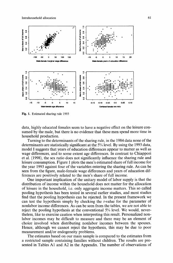
Intrahousehold allocation 61

"

,J':l', t', ', ..

"....., " '\'. ....

.. :3

i ~, "!15

0

i ....,;.- OJj 0

g

,.:iiiiiIiii !;~:: .." II "I....

, ,

.1()O -50 0 50 100 150

MaJ&._aIelll8flllnal_ cItIenlnce

·10 -5 10 15 20

, . , lj:"

'·,ii~!illll'l"i:,;,:• .., I I·:

•• • tt -.­.... ."

:3

i ~,~

15

i ....,;

i OJ0

::i0.,;

·15 ·10 ·5 0

MaIe-IemaJe age cItIerence

10 15

:3r----------:-------,

1":1 .- -••• : .-" : 1"1:' 111 1::,: I

:::!! i1 111 ii,,: ii!!' ,.!. :.. :! I ••..•..... .

, ..(l.15 .(l.10 .(l.OS 0.0 O.OS 0.10

CentenJd temale sex 18110

Fig. 1. Estimated sharing rule 1993

data, highly educated females seem to have a negative effect on the leisure con­sumed by the male, but there is no evidence that these men spend more time inhousehold production.Turning to the determinants of the sharing rule, in the 1984 data none of the

determinants are statistically significant at the 5% level. By using the 1993 data,model I suggests that years of education differences appear to matter as well aswage differences, and to some extent age differences. In contrast to Chiapporiet al. (1998), the sex ratio does not significantly influence the sharing rille andleisure consumption. Figure 1 plots the men's estimated share offull income forthe year 1993 against four of the variables entering the sharing rule. As can beseen from the figure, male-female wage differences and years of education dif­ferences are positively related to the men's share of full income.One important implication of the unitary model of labor supply is that the

distribution of income within the household does not matter for the allocationof leisure in the household, i.e. only aggregate income matters. This so calledpooling hypothesis has been tested in several earlier studies, and most studiesfind that the pooling hypothesis can be rejected. In the present framework wecan test the hypothesis simply by checking the t-value for the parameter ofnonlabor income differences. As can be seen from the tables, we are not able toreject the pooling hypothesis at the conventional 5% level. We would, never­theless, like to exercise caution when interpreting this result. Personalized non­labor incomes may be difficult to measure and there may be an element ofchoice involved when distributing nonlabor incomes between the spouses.Hence, although we cannot reject the hypothesis, this may be due to poormeasurement and/or endogeneity problems.The estimates based on our main sample is compared to the estimates from

a restricted sample containing families without children. The results are pre­sented in Tables Al and A2 in the Appendix. The number of observations of

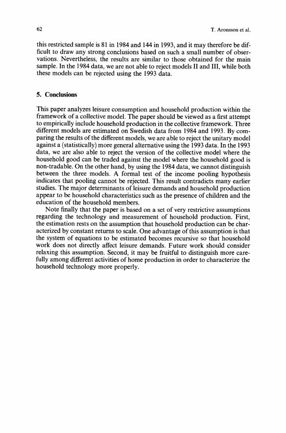
62 T. Aronsson et al.

this restricted sample is 81 in 1984 and 144 in 1993, and it may therefore be dif­ficult to draw any strong conclusions based on such a small number of obser­vations. Nevertheless, the results are similar to those obtained for the mainsample. In the 1984 data, we are not able to reject models II and III, while boththese models can be rejected using the 1993 data.

5. Conclusions

This paper analyzes leisure consumption and household production within theframework of a collective model. The paper should be viewed as a first attemptto empirically include household production in the collective framework. Threedifferent models are estimated on Swedish data from 1984 and 1993. By com­paring the results of the different models, we are able to reject the unitary modelagainst a (statistically) more general alternative using the 1993 data. In the 1993data, we are also able to reject the version of the collective model where thehousehold good can be traded against the model where the household good isnon-tradable. On the other hand, by using the 1984 data, we cannot distinguishbetween the three models. A formal test of the income pooling hypothesisindicates that pooling cannot be rejected. This result contradicts many earlierstudies. The major determinants of leisure demands and household productionappear to be household characteristics such as the presence of children and theeducation of the household members.Note finally that the paper is based on a set of very restrictive assumptions

regarding the technology and measurement of household production. First,the estimation rests on the assumption that household production can be char­acterized by constant returns to scale. One advantage of this assumption is thatthe system of equations to be estimated becomes recursive so that householdwork does not directly affect leisure demands. Future work should considerrelaxing this assumption. Second, it may be fruitful to distinguish more care­fully among different activities of home production in order to characterize thehousehold technology more properly.

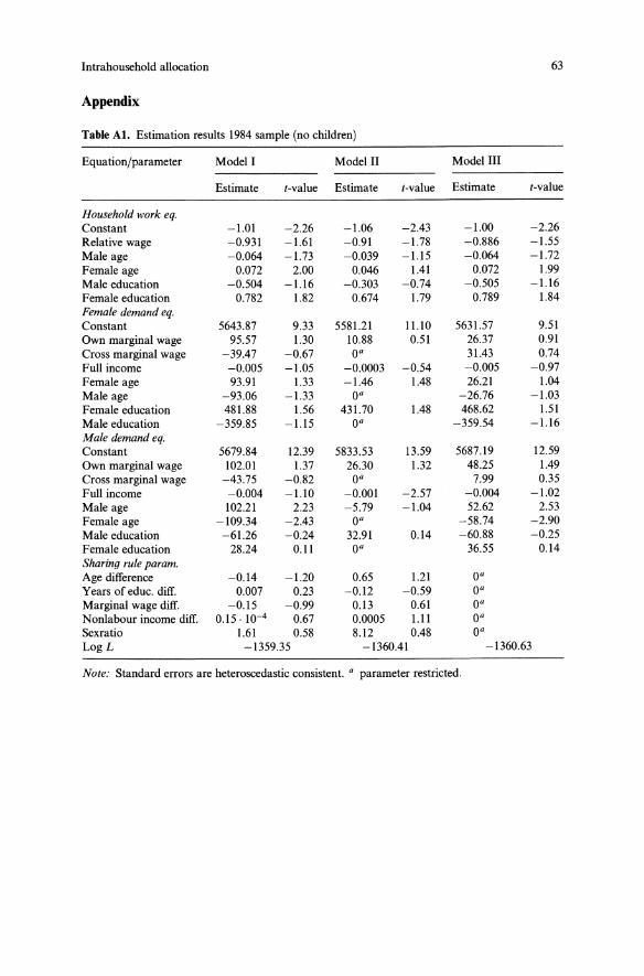
Intrahousehold allocation 63

Appendix

Table AI. Estimation results 1984 sample (no children)

Equation/parameter Model I Model II Model III

Estimate t-value Estimate t-value Estimate t-value

Household lVork eq.Constant -1.01 -2.26 -1.06 -2.43 -1.00 -2.26Relative wage -0.931 -1.61 -0.91 -1.78 -0.886 -1.55Male age -0.064 -1.73 -0.039 -1.15 -0.064 -1.72Female age 0.072 2.00 0.046 1.41 0.072 1.99Male education -0.504 -1.16 -0.303 -0.74 -0.505 -1.16Female education 0.782 1.82 0.674 1.79 0.789 1.84Female demand eq.Constant 5643.87 9.33 5581.21 11.10 5631.57 9.51Own marginal wage 95.57 1.30 10.88 0.51 26.37 0.91Cross marginal wage -39.47 -0.67 0° 31.43 0.74Full income -0.005 -1.05 -0.0003 -0.54 -0.005 -0.97Female age 93.91 1.33 -1.46 1.48 26.21 1.04Male age -93.06 -1.33 0° -26.76 -1.03Female education 481.88 1.56 431.70 1.48 468.62 1.51Male education -359.85 -1.15 0° -359.54 -1.16Male demand eq.Constant 5679.84 12.39 5833.53 13.59 5687.19 12.59Own marginal wage 102.01 1.37 26.30 1.32 48.25 1.49Cross marginal wage -43.75 -0.82 0° 7.99 0.35Full income -0.004 -1.10 -0.001 -2.57 -0.004 -1.02Male age 102.21 2.23 -5.79 -1.04 52.62 2.53Female age -109.34 -2.43 0° -58.74 -2.90Male education -61.26 -0.24 32.91 0.14 -60.88 -0.25Female education 28.24 0.11 0° 36.55 0.14Sharing rule paramoAge difference -0.14 -1.20 0.65 1.21 0°Years of educ. diff. 0.007 0.23 -0.12 -0.59 0°Marginal wage diff. -0.15 -0.99 0.13 0.61 0°Nonlabour income diff. 0.15. 10-4 0.67 0.0005 1.11 0°Sexratio 1.61 0.58 8.12 0.48 0°LogL -1359.35 -1360.41 -1360.63

Note: Standard errors are heteroscedastic consistent. ° parameter restricted.

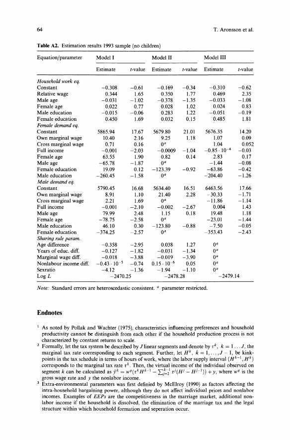
64 T. Aronsson et al.

Table A2. Estimation results 1993 sample (no children)

Equation/parameter Model I Model II Model III

Estimate t-value Estimate t-value Estimate t-value

Household work eq.Constant -0.308 -0.61 -0.169 -0.34 -0.310 -0.62Relative wage 0.344 1.65 0.350 1.77 0.469 2.35Male age -0.031 -1.02 -0.378 -1.35 -0.033 -1.08Female age 0.022 0.77 0.028 1.02 0.024 0.83Male education -0.015 -0.06 0.283 1.22 -0.051 -0.19Female education 0.450 1.69 0.032 0.15 0.485 1.81Female demand eq.Constant 5865.94 17.67 5679.80 21.01 5676.35 14.20Own marginal wage 10.40 2.16 9.25 1.18 1.07 0.09Cross marginal wage 0.71 0.16 oa 1.04 0.052Full income -0.001 -2.03 -0.0009 -1.04 -0.85.10-4 -0.03Female age 63.55 1.90 0.82 0.14 2.83 0.17Male age -65.78 -1.87 oa -1.44 -0.08Female education 19.09 0.12 -123.39 -0.92 -63.86 -0.42Male education -260.45 -1.58 oa -204.40 -1.26Male demand eq.Constant 5790.45 16.68 5634.40 16.51 6463.56 17.66Own marginal wage 8.91 1.10 21.40 2.28 -30.33 -1.71Cross marginal wage 2.21 1.69 oa -11.86 -1.14Full income -0.001 -2.10 -0.002 -2.67 0.004 1.43Male age 79.99 2.48 1.15 0.18 19.48 1.18Female age -78.75 -2.58 oa -23.01 -1.44Male education 46.10 0.30 -123.80 -0.88 -7.50 -0.05Female education -374.25 -2.57 oa -353.43 -2.43Sharing rule paramoAge difference -0.358 -2.95 0.038 1.27 oaYears of educ. diff. -0.127 -1.82 -0.031 -1.34 oaMarginal wage diff. -0.018 -3.88 -0.019 -3.90 oaNonlabour income diff. -0.43.10-5 -0.74 0.15· 10-6 0.05 oaSexratio -4.12 -1.36 -1.94 -1.10 oaLogL -2470.25 -2478.28 -2479.14

Note: Standard errors are heteroscedastic consistent. a parameter restricted.

Endnotes

1 As noted by Pollak and Wachter (1975), characteristics influencing preferences and householdproductivity cannot be distinguish from each other if the household production process is notcharacterized by constant returns to scale.

2 Formally, let the tax system be described by J linear segments and denote by ,k, k = 1... J, themarginal tax rate corresponding to each segment. Further, let H k , k = 1, ... ,J - 1, be kink­points in the tax schedule in terms of hours ofwork, where the labor supply interval (H k - 1, H k )

corresponds to the marginal tax rate ,k. Then, the virtual income of the individual observed onsegment k can be calculated as jik = w9(,kH k- 1 - ,,£:=-;1 ,J(HJ - HJ-l)) + y, where w9 is thegross wage rate and y the nonlabor income.

3 Extra-environmental parameters was first definied by McElroy (1990) as factors affecting theintra-household bargaining power, although they do not affect individual prices and nonlaborincomes. Examples of EEPs are the competitiveness in the marriage market, additional non­labor income if the household is dissolved, the elimination of the marriage tax and the legalstructure within which household formation and seperation occur.

Intrahousehold allocation 65

4 To see this, note that the derivates with respect to nonlabor income are given by ~/; =uYj

01; os; ..' .. os; -OSj h',- ,,---, I, } = m, f. Smce S; = SF - Sj, where SF IS known, It holds that ,,--- = -0-' T IS meansus; uYj uYj uYjthat we have four unknown partial derivates on the right hand side of the above equation,

OIm olt oSm -osJ oSJ -osm .. f . ffi h."-,,,---,,- = -0-' and .,,- = --. ThIS IS equal to the number 0 Income e ects t at canuSm uSJ UYm UYm uYJ oYJbe identified, i.e., the partials on the right hand side of the above equation are exactly identified.For discussions about identification in the extended collective model, see Apps and Ress (1997)and Chiappori (1997).

5 For further details about HUS, see Klevmarken and Olovsson (1993) and Flood et aI. (1997).6 For individuals that have been interviewed about their time allocation once on a weekend andonce during the working week, time used for each household activity is computed as a weightedaverage with the weights 5/7 for week days and 2/7 for weekend days.

7 The sex ratio for the female is computed as:

F,

( F, ) (F, )M, . + ... + Mt+3 .F, + F,_I + F'-2 + F'-3 F'+3 + Ft+2 + Ft+1 + F,

where M, and F, are the number of males and females of age t in a specific region (county). In asimilar vein, we have constructed a male sex ratio. The two measures, however, are highly corre­lated (the correlation coefficient is -0.73 in 1984 and -0.71 in 1993). Therefore we have chosen toinclude only the female sex ratio in the empirical analysis.

References

Apps PF, Rees R (1997) Collective Labor Supply and Household Production. Journal of PoliticalEconomy 105(I): 178-190

Becker GS (1965) A Theory of the Allocation of Time. Economic Journal 75(299):493-517Browning M, Bourguignon F, Chiappori PA, Lechene V (1994) Income and Outcomes: A Struc­tural model oflntrahousehold Allocation. Journal of Political Economy 102(6):1067-1096

Chiappori PA (1988) Rational Household Labour Supply. Econometrica 56(1):63-89Chiappori PA (1992) Collective Labor Supply and Welfare. Journal of Political Economy100(3):437-467

Chiappori PA (1997) Introducing Household Production in Collective Models of Labor Supply.Journal of Political Economy 105(1):191-209

Chiappori PA, Fortin B, Lacroix G (1998) Household Labor Supply, Sharing Rule and the Mar­riage Market. Paper presented at the Second CILN Conference on Labour Market Institutionsand Labour Market Outcomes: International Perspectives

Flood L, Klevmarken NA, Olovsson P (1997) Household Market and Nonmarket Activities, vol3-6. Uppsala University, Uppsala

Fortin B, Lacroix G (1997) A Test of the Unitary and Collective Models of Household LabourSupply. Economic Journal 103(443):933-955

Haddad L, Kanbur R (1990) How Serious is the Neglect of Intra-household Inequality. EconomicJournal 100(402):866-881

Haddad L, Kanbur R (1992) Intrahousehold Inequality and the Theory of Targeting. EuropeanEconomic Review 36(2/3):372-378

Juster TF, Stafford FP (1991) The Allocation of Time: Empirical Findings, Behavioral Modelsand Problems of Measurement. Journal ofEconomic Literature 29(2):471-522

Kawaguchi A (1994) Testing Neoclassical and Non-neoclassical Models of Household LabourSupply. Applied Economics 26(1):9-19

Klevmarken NA, Olovsson P (1993) Household Market and Nonmarket Activities. Procedures andCodes 1984-1991. The Industrial Institute for Economic and Social Research, Stockholm

66 T. Aronsson et al.

McElroy MB (1990) The Empirical Content of Nash-Bargained Household Behavior. Journal ofHuman Resources 25(4):559-583

Pollak RA, Wachter ML (1975) The Relevance of Household Production Function and ItsImplication for the Allocation of Time. Journal of Political Economy 83(2):255-277

Schultz PT (1990) Testing the Neoclassical Model of Family Labor Supply and Fertility. Journalof Human Resources 25(4):599-634

Thomas D (1990) Intra-Household Resource Allocation: An Inferential Approach. Journal ofHuman Resources 25(4):635-664

The allocation and value of time assigned to houseworkand child-care: An analysis for Switzerland

Alfonso Sousa-Poza, Hans Schmid, RolfWidmer

Department of Economics and Research Institute for Labour Economics and Labour Law at theUniversity of St. GaIlen, Guisanstrasse 92, CH-9010 St. GaIlen, Switzerland(Fax: +41-71-224-2807; e-mail: alfonso.sousa-poza@unisg.ch)

Received: 15 April I999/Accepted: 5 May 2000

Abstract. In this paper, data from the 1997 Swiss Labour Force Survey areused to analyse the allocation and value of time assigned to housework andchild-care. It is shown that men's allocation of time to housework and child­care is largely invariant to changes in socio-economic factors. Women's allo­cation of time to housework and child-care, on the other hand, is shown todepend on several social, economic, and demographic factors. The value oftime assigned to housework and child-care is calculated with two market re­placement cost methods and three opportunity cost methods. The results showthat the value of time assigned to housework and child-care ranges from 27%to 39% and from 5% to 8% ofGDP (in 1997), respectively. The value of timeassigned to housework and child-care is also calculated for different householdstructures.

JEL classification: Dl3, 113, 122

Key words: Time allocation, child-care, household production

AIl correspondence to Alfonso Sousa-Poza. A part of this paper, namely the valuation of time, isthe product of a mandate that the authors had from the Swiss Federal Statistical Office (SFSO).The authors would like to thank Claire Jobin, Brigitte Buhmann, Ruth Meier, Phillip Kl1ttel,and Jacqueline Bl1hlmann for their co-operation and advice. Extracts of this paper were pre­sented at the 47th International Atlantic Economic Conference, Vienna, 16-23 March 1999; at theAnnual Congress of the Swiss Society of Statistics and Economics, Freiburg, 25-26 March 1999;and at the 52nd Session of the International Statistical Insitute, Helsinki, 10-18 August 1999. Theauthors would like to thank the participants for valuable discussions. Furthermore, the authorswould also like to thank Hedwig Prey, Winfried Stier, JiIl Tiefenthaler and two anonymous ref­erees for comments on an earlier version of this paper. AIl errors remain the sole responsibility ofthe authors. Responsible editor: John F. Ermisch

68

1. Introduction

A. Sousa-Poza et al.

Time is one of society's most important economic resources, and yet only afraction of households' time, namely that time spent on market activities, hasreceived attention in economic teaching and research. Time spent on house­work and child-care has gone largely unnoticed. Shelton reflects that this isprimarily because "what goes on in the household is not intrinsically interest­ing since (I) women do it, (2) it is not in the public sphere, and (3) it is notsubject to change through policy" (Shelton 1992, p. 64). Although these threereasons still (to a large extent) reflect our society at the end of the twentiethcentury, some change is taking place in most industrialised countries (see alsoHewitt 1993, pp. 55-56). First, the traditional gender roles (i.e., the man atwork, the woman at home) are being questioned, and more women are activelyparticipating in the labour market. Although it would be naive to suggest thatmen take on just as much responsibility in the household as women, theredoes appear to be an increased willingness on behalf of men to participate inthe running of the household. Second, because of the increased participationof women in the political debate, the public is being made aware of the factthat the household distribution of time and the value of unpaid labour isindeed a topic for the public sphere, and that it can (at least partially) bedirected by public policies. Currently, in Switzerland, topics concerning un­paid labour are very often encountered in public debate and political action. 1

Yet, although the time spent on unpaid activities in the household has alreadyentered the Swiss public sphere, very little is known about the way this time isallocated and what the value of this time is (see, however, Schellenbauer andMerk 1994; Sousa-Poza and Widmer 1998; Schmid et at. 1999).This paper aims to, first, analyse the determinants of the allocation of time

assigned to housework and child-care and, second, to calculate the monetaryvalue of this time. Both of these topics have been extensively researched inother countries (for an overview see Gronau 1997; Juster and Stafford 1991;OECD 1996).2 The structure of this paper is as follows: Sect. 2 presentsthe theoretical framework. Section 3 discusses the methodological issues andthe empirical specification. Section 4 analyses the data. Section 5 presents theresults, and Sect. 6 concludes.

2. Theoretical background

The conceptual framework of this study is based on the household theory de­veloped by Becker (1965) and extended by, among others, Gronau (1977). It isknown as the "New Home Economics" (NHE) theory. In traditional micro­economic theory, households maximise their utility by consuming a combi­nation of goods and subject to a budget constraint. Becker (1965) extendedand modified this traditional model in two ways (see also Gronau 1986): first,Becker argued that it was not the goods as such which render utility, but,instead, the "commodities" in which these goods serve as inputs. Second,Becker expanded the set of inputs. According to him, commodities are notonly produced through the combination of market goods, but also with acertain amount of time. This implies that a household is restricted not only bya budget constraint, but also by a time constraint. Individuals therefore max-

Time assigned to housework and child-care 69

imise a utility function which has commodities (which are produced by marketgoods and consumption time) as arguments and subject to a time and budgetconstraint. The result of this maximisation problem will give rise to demandfunctions for the arguments of the utility function and the inputs used in theproduction of home goods. The reduced form equation for the demand ofunpaid labour time can be written as follows:

H =/(Z)

where H is the time spent doing unpaid work and Z is a vector of socio­economic variables such as age, education, presence of children, potentialwage, etc. The comparative static properties of such a model are discussed inGronau (1977).Compared to the sociological theories underlying the division of the allo­

cation of time within a household3 , NHE provides a framework which is par­simonious and which can be reasonably well tested empirically. Nevertheless,this framework has been criticised on a number of grounds (see, for example,Hannan 1982; Ben-Porath 1982; Pollak 1985; Ferber and Birnbaum 1977;Berk 1985). Perhaps the main criticism of the NHE model is aimed at itsanalogy between households and firms, where individuals within the house­hold operate in an "implicit" rather than an explicit market (Folbre 1986).The NHE model then applies techniques developed for studying the firm. Thisanalogy between households and firms is, however, often strained: transac­tions taking place within a household do not conform closely to those of acompetitive market, demand and supply are often embedded in the same per­son, costs are seldom exogenous, and households may not maximise profits.Furthermore, since it is assumed that firms operate in frictionless and efficientmarkets, a similar assumption applies to households. A consequence thereofis that the internal structure and organisation of households playas minor arole as that in the neo-c1assical theory of the firm. Although the whole notionof well-behaved markets may appropriately be applied to the analysis of thefirm, it makes little sense in the analysis of household behaviour. According toBen-Porath, "once we deal with transactions within small groups, the natureof markets and equilibria, the meaning of prices and competition cannot betaken for granted, and strategic behaviour is likely to be relevant, and thusthere is need for greater variety in the theoretical inputs" (Ben-Porath 1982,p.61).4NHE has, however, established itself as the leading economic theory with

regard to the allocation of time. In this study, the factors which determine theallocation of time to housework and child-care are analysed. This analysis willprimarily revolve around the insights gained from NHE. Nevertheless, theapproach taken here is an eclectic one in the sense that a certain amountof theorising will be based on insights from other theoretical traditions, orsimply through educated guesses. Considering the limitations of the NHEtheory, such a broader approach is indispensable; without it, a more or lessall-encompassing analysis of the determining factors of time assigned tounpaid labour becomes virtually impossible (see also Berk 1985, p. 34). Thevaluation of time is also strongly based on NHE theory. This applies espe­cially to the opportunity cost methods, which build on the NHE notion thatindividuals maximise their utility by freely choosing between different timecategories.

70

3. Methodological issues and empirical specification

3.1. The determinants of the allocation of time

A. Sousa-Poza et al.

In order to analyse the determinants of the allocation of time to unpaidlabour, functions of the following form need to be estimated:

H; = P;X; +e;

where H is the number of hours spent doing a specific unpaid activity (herehousework and child-care), X is a vector of explanatory variables, Pis a vectorof coefficients to be estimated, and e is a stochastic disturbance term. As alarge portion of the population did not spend any time on child-care (18% offemales and 29% of males which have children under the age of 14 reporteddoing no child-care) and housework (6% of females and 16% of males re­ported doing no housework), one is confronted with a limited-dependentvariable problem. The usual way of tackling this problem is by estimating astandard tobit model. The latent (dependent) variable of the tobit model isusually interpreted as being the propensity, capacity or desire to assign time toa certain activity. Thus, although a large portion of the population reportedhaving spent the same amount of time on child-care or housework (i.e., 0hours), certain individuals may differ in their desire to provide such time. 5

In this study, tobit models were estimated. A similar approach was taken byGustafsson and Kjulin (1994) and Malathy (1994).The dependent variables in the hour equations are the number of hours

spent per week on housework and child-care. Housework includes the follow­ing activities: preparing meals, waShing-up, setting the table, shopping, clean­ing, vacuum-cleaning, tidying-up, making the beds, washing, ironing, repairing,renovating, sewing, knitting, taking care of the pets, gardening, and adminis­trative work. Child-care includes: feeding, bathing, helping with homework,going for walks, and accompanying children.The explanatory variables are the following: age, age squared, high educa­

tion, low education6 , children aged 0 to 1, children aged 1 to 2, children aged2 to 6, children aged 6 to 14, children aged 14 to 20, ownership of a largehome (more than 4 rooms), ownership ofa small home (4 rooms or less), largerented home, small rented home, marital status, Swiss nationality, Germanspeaking, rural area, and the logarithm of the (imputed) hourly wage rate.Since the analysis of child-care is restricted to individuals with children aged 0to 14, the variable "children aged 6 to 14" was used as the reference categoryin the child-care regressions. The imputed wage rates were computed, forwomen, with maximum-likelihood estimates ofa sample-selection model 7 , and,for men, by an OLS model. Such an approach is appropriate since males are toover 90% employed, i.e., the degree ofcensuring is small. The extended human­capital wage functions estimated in this study are of the following form:

W; = iXo + CXl • EDU; + CX2 • EXP; + CX3 • EXP2; + CX4 •MANAG;

+ CXs • TEN; + e;

where e is a stochastic disturbance term; the cx/s are the coefficients to beestimated; EDU characterises the number of years schooling; EXP captures

Time assigned to housework and child-care 7J

the years of working experience; EXP2 is the corresponding squared term;MANAG is a dummy variable depicting whether or not the individual has amanagement position; TEN captures the years oftenure8 . The wage rate (W)used here is the logarithm of a net hourly wage rate based on the number ofpaid hours usually worked per year.

3.2. The value of time

The two most common methods used to value the amount of time spent onunpaid labour are the market replacement cost method and the opportunitycost method (see, for example, Chadeau 1992). The market replacement costmethod multiplies the number of hours by the wage rate of a market substi­tute. Usually, the wage rate of a professional housekeeper is used. In thisstudy, the average wage rate of a so-called "hauswirtschaftliche Angestellte"(in essence, a housekeeper) is used (equal to Fr. 16.35 per hour, net of taxesand based on paid working time). This version of the market replacement costmethod is often called the generalist method. The specialist method is anotherversion of the market replacement cost method. With this method, the valueof time spent on unpaid labour is obtained by multiplying the wage rate of aprofessional with the amount of time spent on the corresponding activity forwhich this professional is a specialist. Thus, for example, the number of hoursspent cooking is multiplied by the average wage rate of a cook. A refinementof the specialist method can be obtained by creating equivalence groups (see,for example, Chandler 1994). An equivalence group is a collection of profes­sions which can serve as equivalent substitutes for a specific unpaid labouractivity. In this study, such equivalence groups are used. 9

The opportunity cost method values the time spent on unpaid labour bymultiplying the number of hours by a measure for the "forgone profits" in­curred by not spending that time on another activity. These "forgone profits"can be quantified in a number of ways. The most common approach is to de­fine them with the forgone earnings that an individual faces by not spendingthat time working in the market. For employed individuals, these forgoneearnings are equal to the hourly wage rate they earn. For non-employed in­dividuals, these forgone earnings can be estimated by calculating their poten­tial wages with wage functions. A second way to quantify these "forgoneprofits" is by estimating an individual's reservation wage, i.e., that wage rateat which an individual is indifferent between a unit of time spent workingin the market and a unit of time at home. According to the neo-classicalhousehold model, these reservation wages are equal to the market wage foremployed individuals. Non-employed individuals, however, have reservationwages above their potential wages since they have decided not to participate inthe market (see, for example, Gronau 1986 and Chiswick 1982). Since thereservation wage for non-employed individuals is unobservable, they have tobe estimated with the aid of an econometric model. The model used in thisstudy is that of Nelson (1977), which is a censored regression model with un­observed stochastic threshold. It can be formulated as follows (see Maddala1983, pp. 174-178):

Yli = P; Xli + Uli

72

Yli observed only if Yli ~ Y2i

Y2i = P~X2i + U2i and Y 2i is unobserved and stochastic

A. Sousa-Poza et aJ.

where Y j , the wage rate, is assumed to be a linear function of certain socio­economic variables Xl (namely education and experience) and a stochasticdisturbance term Uj. The wage rate is only observed when individuals partici­pate in the paid labour market, and this is the case when the wage rate is atleast greater than or equal to the reservation wage Y2. The reservation wagecannot be observed, but it is assumed that it can be characterised as a linearfunction of certain socio-economic variables X2 (such as experience, educa­tion, presence of children, and marital status). The corresponding stochasticdisturbance term is U2. The coefficients to be estimated are PI and P2 for thewage and reservation functions respectively. This model has also been used byHoman (1988) to value the time spent on unpaid labour. In this study, thetwo-step estimation of this model as described in Maddala (1983) is used (seeAppendix B).A number of statistical bureaus use gender-specific average wages as a

measure for the opportunity costs (see OECD 1996; Schmid et al. 1999).Furthermore, the "opportunity costs" are usually calculated for the wholepopulation, i.e., including individuals who are not in the active labour force.Needless to say, using average wage rates gives rise to very rudimentaryapproximations for the value of time, and, furthermore, when applied to thewhole population, characterising this approach as an opportunity cost methodis somewhat of a misnomer. Nevertheless, for the sake of completeness, suchaverage wage rates are also applied in this study. 10Two important questions arise when trying to calculate the hourly wage

rate used to value the time spent on unpaid labour: (i) Should net or grosswages be used? (ii) Should actual or paid working time be used? Unfortun­ately, for most methods there is no precise prescription, and there is also verylittle consensus in the prevailing practice. Yet the choice of wage concept isimportant, since the calculated value is very sensitive to this choice. The mar­ket replacement cost methods are, strictly speaking, based on a market substi­tution perspective, i.e., unpaid labour is valued with the wage rate of somemarket substitute. The hypothetical situation is one in which all unpaid labourwere to be replaced by the market sector. If this perspective is taken at facevalue, then the cost of employing a worker should be used in the calculation.A gross wage concept (i.e., before taxes and after employer contributions)based on paid working time would therefore seem the most appropriate. Defacto, however, no taxes and no employer contributions arise in the householdproduction process. If one were to accept this "institutional framework" (seeSchafer and Schwarz 1994, p. 603-604; Statistisches Bundesamt Deutschland1993, p. 7-8), then a net wage concept based on the actual working time is themost suitable. In this study net hourly wages based on actual working time areused. In theory, the opportunity cost method should use wages, on which in­dividuals base their time-allocation decisions. This means that net (disposable)wages are the most appropriate. Furthermore, the hourly wage rates should becalculated using paid working time. In this study net hourly wages based onpaid working time are therefore used.Net wages are calculated by deducting income taxes and compulsory social

security contributions (made by the employee) from a gross wage. The social

Time assigned to housework and child-care 73

security contributions are: unemployment insurance ("Arbeitslosenversicher­ung"), accident insurance ("Nichtbetriebsunfallversicherung"), pension fundcontributions ("Pensionskassenbeitrage"), and old-age insurance scheme pay­ments ("AHV-, IV-, EO-Beitrage")Y Income taxes are made-up of two parts:community taxes ("Kantons-, Gemeinde- und Kirchensteuer") and federaltaxes ("Bundessteuer"). In Switzerland, community-level tax rates differ sub­stantially from community to community, and therefore only an approxima­tion of the individual tax burden (based on individual and household charac­teristics) can be made. The community tax rates were approximated by indicescalculated by the Swiss Federal Tax Office. 12 Federal tax rates were calculatedaccording to the relevant law ("Bundesgesetz tiber die direkte Bundes­steuer").13 In order to obtain hourly wage rates, one needs to divide theannual wage by the number of hours worked per year. In general, one candistinguish two hour concepts: (i) paid working hours, and (ii) actual hoursworked. Paid working hours are determined by law or collective agreements,and they include paid holidays and sick leave. Actual hours worked are basedon the usual hours worked in a year. This includes paid and unpaid overtimeand excludes holidays and weekends.

4. Data

The data for this study are taken from the 1997 Swiss Labour Force Survey(SLFS). The SLFS is a nation-wide and representative survey conducted an­nually by the Swiss Federal Statistical Office. During telephone interviewslasting approximately 20 minutes, individuals are questioned on a number oflabour-market related topics. The 1997 SLFS collected (for the first time) timedata on unpaid labour activities. A total of 16,207 respondents were ques­tioned on 14 individual unpaid labour activities which can be collected into4 broad categories: household work, child-care, care of elderly householdmembers, and community services. This study restricts the analysis to thefirst two mentioned categories. Besides containing time-use data, the SLFSdata set also has a number of socio-demographic and earnings variables (seeBundesamt fUr Statistik, 1996).14In analysing the determinants of the allocation of time, only individuals

between the ages of 18 and 62 were considered. Unemployed individuals,military recruits, and apprentices were also ignored. In other words, the anal­ysis is restricte9 to individuals who (to a greater or lesser extent) can freelychoose between paid and unpaid labour time. The same applies to the valua­tion of unpaid labour with the opportunity cost methods. This assumption(namely that individuals can freely choose between time categories) does not,however, apply to the market replacement cost methods. Therefore, thesemethods were applied to the whole population, i.e., to all individuals olderthan 14 years of age.

5. Results

5.1. The determinants of the allocation of time

The results of the tobit regressions are depicted in table 1. Only the marginaleffects at the sample means are discussed. On average, men spend about half

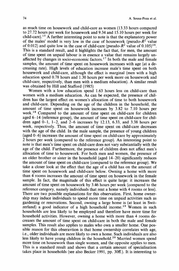
74 A. Sousa-Poza et at.

as much time on housework and child-care as women (13.33 hours comparedto 27.72 hours per week for housework and 9.34 and 15.10 hours per week forchild-care). 15 A further interesting point to note is that the explanatory powerof the males' model is very low in the case of housework (pseudo-R2 valueof 0.012) and quite low in the case of child-care (pseudo-R 2 value of 0.105)16.This is a standard result, and it highlights the fact that, for men, the amountof time spent on unpaid labour is in essence a value that remains largely un­affected by changes in socio-economic factors. 17 In both the male and femalesamples, the amount of time spent on housework increases with age (at a de­creasing rate). High levels of education increase male's time spent on bothhousework and child-care, although the effect is marginal (men with a higheducation spend 0.78 hours and 1.30 hours per week more on housework andchild-care, respectively, than men with a medium education). A similar resultwas obtained by Hill and Stafford (1985)Women with a low education spend 1.63 hours less on child-care than

women with a medium education. As can be expected, the presence of chil­dren has the largest effect on women's allocation of time to both houseworkand child-care. Depending on the age of the children in the household, theamount of time spent on housework increases by 3.82 to 7.10 hours perweek. is Compared to the amount of time spent on child-care for childrenaged 6-14 (reference group), the amount of time spent on child-care for chil­dren aged 0-1, 1-2, and 2-6 increases by 12.13, 6.33, and 3.38 hours perweek, respectively. Thus, the amount of time spent on child-care decreaseswith the age of the child. In the male sample, the presence of young children(aged 0-6) increases the amount of time spent on child-care by approximately2 hours per week (compared to the reference group). An interesting point tonote is that men's time spent on child-care does not vary substantially with theage of the child. Furthermore, the presence of children does not affect men'sallocation of time to housework. For both men and women, the presence ofan older brother or sister in the household (aged 14-20) significantly reducesthe amount of time spent on child-care (compared to the reference group). Wetake a closer look at the effect that the age of a child has on the amount oftime spent on housework and child-care below. Owning a home with morethan 4 rooms increases the amount of time spent on housework in the femalesample. In fact, the magnitude of this effect is quite large: it increases theamount of time spent on housework by 3.46 hours per week (compared to thereference category, namely individuals that rent a home with 4 rooms or less).There are two possible explanations for this observation. First, home owner­ship may induce individuals to spend more time on unpaid activities such asgardening or renovations. Second, owning a large home is (at least in Swit­zerland) a good indicator of a high household income. 19 Women in suchhouseholds are less likely to be employed and therefore have more time forhousehold activities. However, owning a home with more than 4 rooms de­creases the amount of time spent on child-care in both the male and femalesamples. This result also applies to males who own a smaller home. One pos­sible reason for this obseravtion is that home ownership correlates with age,i.e., older individuals are more likely to own a home. Such individuals are alsoless likely to have young children in the household. 20 Married women spendmore time on housework than single women, and the opposite applies to men.This is a standard result and shows that a certain amount of specialisationtakes place in households (see also Becker 1991, pp. 30ff.). It is interesting to

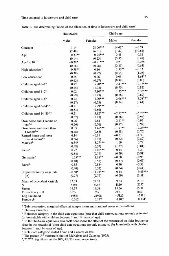
Time assigned to housework and child-care 75

Table 1. The determining factors of the allocation of time to housework and child-care"

Housework Child-eare

Males Females Males Females

Constant l.l4 28.06*** 14.42* -6.59(2.48) (6.01) (7.47) (10.65)

Age 0.33** 0.94*** -0.41 -0.38(0.14) (0.23) (0.37) (0.48)

Agel x 10-2 -0.29* -0.81*** 0.23 -0.075(0.16) (0.28) (0.45) (0.63)

High educationb 0.78** 0.16 1.30** -0.13(0.38) (0.87) (0.58) (1.08)

Low educationb -0.65 0.06 -0.05 - 1.63**(0.62) (0.67) (0.98) (0.80)

Children aged 0- Ib 0.97 5.90*** 2.47*** 12.13***(0.75) (1.02) (0.70) (0.82)

Children aged 1_2b -0.02 7.10*** 1.35*** 6.33***(0.89) (1.23) (0.76) (0.89)

Children aged 2-6b -0.72 6.00*** 2.06*** 3.38***(0.57) (0.75) (0.54) (0.61)

Children aged 6_14b•c -0.21 5.99***(0.53) (0.66)

Children aged 14_20b•d -0.21 3.82*** -2.92*** -5.76***(0.67) (0.83) (0.86) (0.96)

Own home and 4 rooms or -0.26 0.64 -2.11** -0.97lessb •• (0.56) (0.76) (0.87) (0.97)

Own home and more than 0.03 3.46*** -1.97** -2.26***4 roomsb•• (0.48) (0.65) (0.68) (0.75)Rented home and more 0.14 -0.15 -0.51 -1.39than 4 roomsb•• (0.66) (0.91) (0.82) (0.89)

Marriedb -0.84* 5.27*** 1.09 0.79(0.48) (0.57) (1.37) (0.81)

Swissb 0.27 -2.06*** 0.44 1.34(0.54) (0.77) (0.79) (0.91)

Germanicb 1.35*** l.l8** -0.08 -0.98(0.40) (0.53) (0.57) (0.63)

Ruralb 0.55 0.88* 0.30 -0.32(0.40) (0.53) (0.54) (0.61)

(Imputed) hourly wage rate -0.50* - 11.21 *** -0.14 9.45***(In) (0.27) (2.77) (0.69) (3.51)

Mean of dependent variable 13.33 27.72 9.34 15.10N 5369 5956 1819 2057Sigma 16.37 19.58 15.66 15.31Proportion y = 0 16% 6% 29% 18%Log likelihood -19861 -24998 -5820 -7311Pseudo-R 2 0.012' 0.147' 0.105' 0.304'

" Tobit regression: marginal effects at sample mean and standard errors in parenthesis.b Dummy variables.c Reference category in the child-care equations (note that child-eare equations are only estimatedfor households with children between I and 14 years of age).d In the child-care equations, this coefficient shows the effect of the presence of an older brother orsister in the household (since child-eare equations are only estimated for households with childrenbetween I and 14 years of age) .• Reference category: rented home and 4 rooms or less., The pseudo-R 2 measure is that of McKelvey and Zavoina (1975).*/**/*** Significant at the 10%/5%/1% level, respectively.

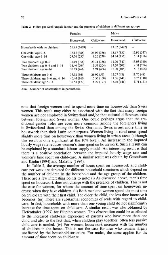
76 A. Sousa-Poza et aI.

Table 2. Hours per week unpaid labour and the presence of children in different age groups

Females Males

Housework Child-care Housework Child-care

Households with no children 21.95 (3439) 13.32 (3422)

One child: age 0-6 32.15 (386) 24.02 (386) 13.67 (337) 13.96 (337)One child: age 6-14 29.74 (230) 9.20 (230) 14.24 (156) 6.14 (156)

Two children: age 0-6 35.49 (356) 23.31 (356) 11.90 (340) 13.03 (340)Two children: age 0-6 and 6-14 34.40 (204) 13.59 (204) 13.20 (206) 9.51 (206)Two children: age 6-14 35.29 (466) 6.94 (466) 12.90 (405) 5.18 (405)

Three children: age 0-6 37.92 (56) 26.92 (56) 12.57 (48) 11.75 (48)Three children: age 0-6 and 6- I4 40.44 (160) 15.35 (160) 11.76 (148) 8.75 (148)Three children: age 5-14 37.58 (177) 6.29 (177) 13.98 (141) 5.71 (141)

Note: Number of observations in parenthesis.

note that foreign women tend to spend more time on housework than Swisswomen. This result may either be associated with the fact that many foreignwomen are not employed in Switzerland and/or that cultural differences existbetween foreign and Swiss women. One could perhaps argue that the tra­ditional gender roles are even more common among the foreigners livingin Switzerland than among the Swiss. Germanic Swiss invest more time inhousework than their Latin counterparts. Women living in rural areas spendslightly more time on housework than women living in urban areas (althoughthis result is only significant at the 10% level). An increase in the imputedhourly wage rate reduces women's time spent on housework. Such a result canbe explained by a standard labour supply model. An interesting result is thatthere is a positive correlation between the imputed hourly wage rate andwomen's time spent on child-care. A similar result was obtain by Gustafssonand Kjulin (1994) and Malathy (1994).In Table 2, the average number of hours spent on housework and child­

care per week are depicted for different household structures which depend onthe number of children in the household and the age group of the children.There are a few interesting points to note: (i) As discussed above, men's timespent on housework does not change with the presence of children. This is notthe case for women, for whom the amount of time spent on housework in­crease when they have children. (ii) Both men and women spend the most timeon child-care with their first child. The older the child, the less time intensive itbecomes. (iii) There are substantial economies of scale with regard to child­care. In fact, households with more than one young child do not significantlyincrease the time spent on child-care. A similar result was also obtained byTiefenthaler (1997) for Filipino women. This observation could be attributedto the increased child-care experience of parents who have more than onechild and also to the fact that, when children play together, often less passivechild-care is needed. (iv) For women, housework increases with the numberof children in the house. This is not the case for men who remain largelyunaffected by the household structure. For males, the same applies for theamount of time spent on child-care.

Time assigned to housework and child-care 77

Table 3. The value of time assigned to housework and child-care (Mill. Fr.) in 1997

Method Males Females Total

House- Child- House- Child- House- Child-work care work care work care

Market replacement cost methods'Generalist method 38,107 7,016 85,031 11,420 123,138 18,436

(10.30) (1.90) (22.98) (3.09) (33.27) (4.98)Specialist method 44,154 11,150 95,315 17,530 139,467 28,680

(11.93) (3.01) (25.76) (4.74) (37.69) (7.75)Opportunity cost methodsb

Gender-specific average wage: 51,483 9,479 92,762 12,458 144,245 21,937all individuals (13.91) (2.56) (25.07) (3.37) (38.98) (5.93)

Gender-specific average wage: 39,222 9,300 70,312 12,224 109,534 21,525individuals aged 18-62 (10.60) (2.51) (19.00) (3.30) (29.60) (5.82)

Potential wage 37,623 9,932 66,366 13,186 103,989 23,118(10.17) (2.68) (17.93) (3.56) (28.10) (6.25)

Reservation wage 37,623 9,932 63,938 13,061 101,561 22,993(10.17) (2.68) (17.28) (3.53) (27.44) (6.21)

Note: Percentage of GDP in parenthesis.• Calculated with net wage rates based on actual hours worked.b Calculated with net wage rates based on paid working hours.

5.2. The value of time

The value of time assigned to housework and child-care is depicted in Table 3.The market replacement cost methods are calculated using net wage rates andbased on actual hours worked by an individual. The opportunity cost methodsare calculated using net wage rates and based on paid working time. Fur­thermore, the market replacement cost methods are calculated for the wholepopulation (i.e., all individuals older than 15 years), whereas the opportunitycost methods are restricted to individuals between the age of 18 and 62(although we also apply the opportunity cost method based on gender-specificaverage wages to the whole population).Depending on the methodology used, the value assigned to housework can

vary from approximately 27% to 39% of GOP. For child-care, the value canrange from 5% to 8% of GOP. In the case of housework, the largest value isobtained with gender-specific average wages and applied to the whole popul­ation. The lowest value is obtained when using reservation wages. Whenmeasuring the value of time assigned to child-care, the largest result is ob­tained with the specialist method, and the lowest with the generalist method.As one may expect, the contribution made by women is substantially largerthan that of men. Using the market replacement cost methods the contri­bution made by men is approximately half of that made by women. Since menon average earn higher wages than women, the opportunity cost measuresincrease men's proportion compared to the market replacement cost methods.One anomaly to note is that, for the sample as a whole, the reservation

wage is lower than the potential wage. 21 As was discussed above, for non­employed individuals the reservation wage should (from a theoretical per­spective) lay above the potential wage. Thus, the value of time calculated withreservation wages should be higher that when potential wages are applied. As

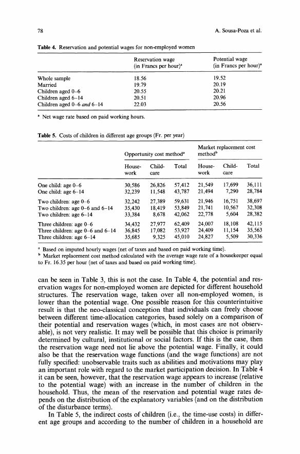
78

Table 4. Reservation and potential wages for non-employed women

Reservation wage(in Francs per hour)"

A. Sousa-Poza et al.

Potential wage(in Francs per hour)"

Whole sampleMarriedChildren aged 0-6Children aged 6-14Children aged 0-6 and 6-14

18.5619.7920.5520.5122.03

19.5220.1920.2120.9620.56

" Net wage rate based on paid working hours.

Table 5. Costs of children in different age groups (Fr. per year)

Market replacement costOpportunity cost method" methodb

House- Child- Total House- Child- Totalwork care work care

One child: age 0-6 30,586 26,826 57,412 21,549 17,699 36,111One child: age 6-14 32,239 11,548 43,787 21,494 7,290 28,784

Two children: age 0-6 32,242 27,389 59,631 21,946 16,751 38,697Two children: age 0-6 and 6-14 35,430 18,419 53,849 21,741 10,567 32,308Two children: age 6-14 33,384 8,678 42,062 22,778 5,604 28,382

Three children: age 0-6 34,432 27,977 62,409 24,007 18,108 42,115Three children: age 0-6 and 6-14 36,845 17,082 53,927 24,409 11,154 35,563Three children: age 6-14 35,685 9,325 45,010 24,827 5,509 30,336

" Based on imputed hourly wages (net of taxes and based on paid working time).b Market replacement cost method calculated with the average wage rate of a housekeeper equalto Fr. 16.35 per hour (net of taxes and based on paid working time).

can be seen in Table 3, this is not the case. In Table 4, the potential and res­ervation wages for non-employed women are depicted for different householdstructures. The reservation wage, taken over all non-employed women, islower than the potential wage. One possible reason for this counterintuitiveresult is that the neo-classical conception that individuals can freely choosebetween different time-allocation categories, based solely on a comparison oftheir potential and reservation wages (which, in most cases are not observ­able), is not very realistic. It may well be possible that this choice is primarilydetermined by cultural, institutional or social factors. If this is the case, thenthe reservation wage need not lie above the potential wage. Finally, it couldalso be that the reservation wage functions (and the wage functions) are notfully specified: unobservable traits such as abilities and motivations may playan important role with regard to the market participation decision. In Table 4it can be seen, however, that the reservation wage appears to increase (relativeto the potential wage) with an increase in the number of children in thehousehold. Thus, the mean of the reservation and potential wage rates de­pends on the distribution of the explanatory variables (and on the distributionof the disturbance terms).In Table 5, the indirect costs of children (i.e., the time-use costs) in differ­

ent age groups and according to the number of children in a household are

Time assigned to housework and child-care 79

presented. For the sake of clarity, only the two most common valuationmethods, namely the opportunity cost method (calculated with imputedwages) and the market replacement cost method (calculated with the averagewage rate of a housekeeper) have been used. An only child between the age ofoand 6 will give rise to time-use costs of Fr. 57,412 per year when using theopportunity cost method and Fr. 36, III per year when using the market re­placement cost method. This large difference is due to the fact that house­keepers in Switzerland earn a relatively low wage (Fr. 16.35 per hour, net oftaxes). Depending on the household structure, the indirect costs of childrenrise to Fr. 62,409 if the opportunity cost method is applied and Fr. 42,115 ifthe market replacement cost method is used (for households with three chil­dren, all under the age of 6).

6. Conclusion

The aim of this study was to analyse the allocation and value of time assignedto housework and child-care in Switzerland. The analysis in this paper wasbased on data from the 1997 Swiss Labour Force Survey, which containsnation-wide and representative data on the amount of time spent on specificunpaid labour activities. The results show that men spend about half as muchtime on housework and child-care as women, and that men's time allocationto unpaid labour is, to a large extent, invariant to changes in socio-economicfactors. For the female sample, it was shown that a number of socio-economicfactors influence the decision to invest time in housework and child-care. Es­pecially the presence of children, the marital status, and the imputed hourlywage rate play an important role. The value of time assigned to houseworkand child-care was calculated with two market replacement cost methods andthree opportunity cost methods. In the former case, a generalist method anda specialist method were applied. In the latter case, gender-specific averagewages, potential wages and reservation wages were used. The results showthat, depending on the methodology used, the values range from approxi­mately 27% to 39% ofGDP in the case of housework and from approximately5% to 8% of GDP in the case of child-care. The generalist method and theopportunity cost method based on potential wages were also used to calculatethe time-use costs of children for different household structures. It was shownthat a single child between the age of 0 and 6 gives rise to time-use costs (forhousework and child-care) of Fr. 57,412 per year if the opportunity costmethod is used, and Fr. 36,111 per year if the market replacement costmethod is used.

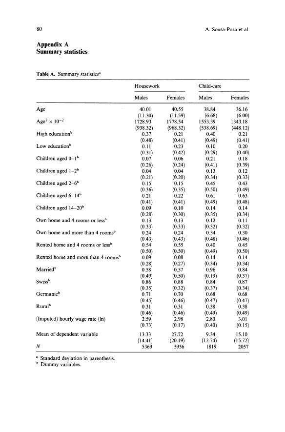
80 A. Sousa-Poza et al.

Appendix ASummary statistics

Table A. Summary statistics'

Housework Child-care

Males Females Males Females

Age 40.01 40.55 38.84 36.16(11.30) (11.59) (6.68) (6.00)

Age2 x 10-2 1728.93 1778.54 1553.39 1343.18(938.32) (968.32) (538.69) (448.12)

High educationb 0.37 0.21 0.40 0.21(0.48) (0.41) (0.49) (0.41)

Loweducationb 0.11 0.23 0.10 0.20(0.31) (0.42) (0.29) (0.40)

Children aged 0-1 b 0.07 0.06 0.21 0.18(0.26) (0.24) (0.41) (0.39)

Children aged 1-2b 0.04 0.04 0.13 0.12(0.21) (0.20) (0.34) (0.33)

Children aged 2-6b 0.15 0.15 0.45 0.43(0.36) (0.35) (0.50) (0.49)

Children aged 6-14b 0.21 0.22 0.61 0.63(0.41) (0.41) (0.49) (0.48)

Children aged 14-20b 0.09 0.10 0.14 0.14(0.28) (0.30) (0.35) (0.34)

Own home and 4 rooms or lessb 0.13 0.13 0.12 0.11(0.33) (0.33) (0.32) (0.32)

Own home and more than 4 roomsb 0.24 0.24 0.34 0.30(0.43) (0.43) (0.48) (0.46)

Rented home and 4 rooms or lessb 0.54 0.55 0.40 0.45(0.50) (0.50) (0.49) (0.50)

Rented home and more than 4 roomsb 0.09 0.08 0.14 0.14(0.28) (0.27) (0.34) (0.34)

Marriedb 0.58 0.57 0.96 0.84(0.49) (0.50) (0.19) (0.37)

Swissb 0.86 0.88 0.84 0.87(0.35) (0.32) (0.37) (0.34)

Germanicb 0.71 0.70 0.68 0.68(0.45) (0.46) (0.47) (0.47)

Ruralb 0.31 0.31 0.38 0.38(0.46) (0.46) (0.49) (0.49)

(Imputed) hourly wage rate (In) 2.59 2.98 2.80 3.01(0.73) (0.17) (0.40) (0.15)

Mean of dependent variable 13.33 27.72 9.34 15.10(14.41) (20.19) (12.74) (15.72)

N 5369 5956 1819 2057

• Standard deviation in parenthesis.b Dummy variables.

Time assigned to housework and child-care

Appendix BEstimating reservation wage functions

81

The model to be estimated is the following (see Maddala 1983, pp. 174­178):

Yli = 13; Xli + Uli

Y li observed only if Y li ~ Y2i

Y2i = 13~X2i + U2i and Y2i is unobserved and stochastic

Y} is the wage rate and Y2 is the reservation wage. Xl and X 2 are vectors ofregressors for the two functions respectively. The corresponding stochasticdisturbance terms are Ul and U2. 131 and 132 are the coefficient vectors to beestimated. For employed individuals, Y1 is observed, and, for non-employedindividuals, Y1 is not observed.If one assumes that UI and U2 are IN, with zero means and covariance

matrix,

then if follows that

It can now be shown that the likelihood function to be maximised is the fol­lowing:

where

and where L is the sum over the N} observations for which Y1 is observed,1

and L is the sum over the (N - N l ) observations for which Yt is not ob-o

served. This function can be estimated with the aid of a numerical algorithm.Note that a sufficient condition for the identification of the model is that atleast one variable in Xl is not included in X2.Maddala (1983) describes a simpler two-stage estimation ofthis model (see

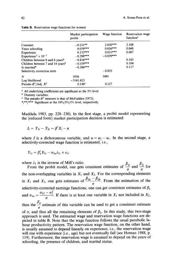
82

Table B. Reservation wage functions for women

A. Sousa-Poza et al.

Market participation Wage function Reservation wageprobit function'

ConstantYears schoolingExperienceExperience2 x 10-2

Children between 0 and 6 yearsb

Children between 7 and 14 yearsb

Is marriedb

Selectivity correction term

NLog likelihoodPseudo-R2/Adj. R 2

-0.251 **0.039***0.132***-0.298***-0.816***-0.519***-0.586***

5956-3141.623

0.148'

2.058***0.056***0.033***-0.059***

-0.035

3491

0.127

2.1080.0480.007

0.1630.1040.117

, All underlying coefficients are significant at the 5% level.b Dummy variables., The pseudo-R2 measure is that of McFadden (1973).*/**/*** Significant at the 10%/5%/1% level, respectively.

Maddala 1983, pp. 228-230). In the first stage, a probit model representingthe (reduced form) market participation decision is estimated:

Ii = Y li - Y2i = p'Xi - U

where I is a dichotomous variable, and u = U2 - UI. In the second stage, aselectivity-corrected wage function is estimated, i.e.,

where Al is the inverse of Mill's ratio. P . P.From the probit model, one gets consistent estimates of -.!L and --3!... for

(J (J

the non-overlapping variables in XI and X2• For the corresponding elements

in XI and X2, one gets estimates of Plk - P2k. From the estimation of the(J

selectivity-corrected earnings functions, one can get consistent estimates ofPI2

and (Jlu = (J12 - (JI . If there is at least one variable in Xl not included in X2,(J

then the Pi) estimate of this variable can be used to get a consistent estimate(J

of (J, and thus all the remaining elements of P2' In this study, this two-stageapproach is used. The estimated wage and reservation wage functions are de­picted in table B. Note that the wage function follows the usual parabolic la­bour productivity pattern. The reservation wage function, on the other hand,is usually assumed to depend linearly on experience, i.e., the reservation wagewill rise with experience (i.e., age) but not eventually fall (see Homan 1988, p.119). Furthermore, the reservation wage is assumed to depend on the years ofschooling, the presence of children, and marital status.

Time assigned to housework and child-care

Endnotes

83

I A number of parliamentarians and the Swiss Federal Council have, for example, expressed theneed to value unpaid labour. See the following inquiries: Bacciarini (18/03/81 and 31/01/83);Fankhauser (01/06/94); Goll (17/06/94); FDP (02/02/95); Roth-Bernasconi (03/10/96).

2 The analysis of the determinants of the allocation of time to housework and child-care is in­teresting from a sociological perspective since it tells us something about the society we live in,especially with regard to the differing gender roles. There are in essence three reasons forwanting to ascribe a monetary value to the time spent on unpaid labour. First, unpaid labourgenerates wealth and contributes substantially to a society's welfare. As a number of authorshave come to recognise, this welfare contribution goes unnoticed in the conventional GDPmeasure (see, for example, Eisner 1988 and Gronau 1986). Consequently, various nationalstatistical bureaus have, in the past decade, institutionalised the monetary valuation of unpaidlabour. One field of research which has arisen from the valuation of unpaid labour is theanalysis of the distribution of extended income (see Bonke 1992 and Jenkins and O'Leary1996). Certain authors have further argued that policymakers should consider this source ofwealth in tax and insurance schemes in order to guarantee a more equitable treatment offamilies (see, for example, Peskin 1984). A second reason is that such a monetary value isoften needed in litigation testimony, in which the value of unpaid labour is used to deter­mine appropriate compensations in case of injury, death, and divorce (see, for example,Douglass et al. 1990). Especially in Swiss legal practice there is a strong need for reliablevaluation data since the current practice is based not only on antiquated data but also onan unsound methodological framework. A third important reason for the valuation of unpaidlabour is that, one could argue, only an explicit monetary valuation catches the public'sattention.

3 Mention should be made of the "conjugal power" school which tries to explain the allocationoftime on the basis of role and authority patterns, exchange and choice, family role typologies,and family decision-making. See Berk (1985), pp. 1Off.

4 Further criticisms of NHE theory include: (i) the NHE assumption that a single individualmaximises a household utility function obscures the fact that often household members havediffering interests, (ii) cultural and institutional aspects are given no consideration, and (iii) itsusefulness for empirical research is, to some extent, limited.

5 The fact that there is a large portion of individuals that do not spend any time on child-caremay come as a surprise. It can, however, be explained by: (i) time spent on active child-caresuch as feeding or bathing diminishes with the age of the child, and (ii) the reference period ofthe questions in the SLFS is based on the previous day. Thus, individuals were questioned onhow much time they spent doing a certain unpaid activity on the previous day. Needless to say,such a short reference period may give rise to numerous "zero observations" (especially forthose individuals with older children in the household). Other studies that analyse theallocation of time to child-care face similar levels of "zero observations" (see, for example,Gustafsson and Kjulin 1994; Malathy 1994).

6 In this study two dummy variables are used to identify individuals with a high or low educa­tion. Degrees from the following institutions were considered as "high education": university,technical college ("hohere Berufsausbildung", "Technikum", "hohere Fachschule"), and highschool ("Matura"). The following categories were considered as "low education": no degree,only compulsory schooling, one-year housekeeper apprenticeship ("Haushaltslehrjahr"), andlower apprenticeship schemes ("Anlehre"). The reference category was primarily made up ofapprenticeships ("Berufslehre") and similar qualifications ("Vollzeitberufsschule").

7 The selection equation depicts a woman's choice to participate in the market or not. Thefollowing explanatory variables were used: age, age squared, years of schooling, children aged0-6, children aged 6-14, and marital status.

8 The TEN and the MANAGE variables were set to zero for persons not employed. Further­more, it should be noted that there is a potential endogeneity problem in including variablessuch as experience and tenure when calculating imputed wages for the hour functions sincethese variables reflect past time in paid employment which, in turn, is jointly determined withunpaid labour time.

9 We have refrained from presenting the exact structure of the equivalence groups. These areavailable from the authors upon request.

84 A. Sousa-Poza et al.

10 It is beyond the scope of this paper to comprehensively discuss all the methods used to valuethe time spent on unpaid activities. The interested reader is referred to Goldschmidt-Clermont(1993), Chadeau (1992), and Schmid et al. (1999).

11 These contributions were calculated according to the regulations laid down by the relevantlaws. Due to the lack of information, in certain cases the deductions had to be approximated.For a more precise description, see Schmid et al. (1999).

12 See Eidgenossische Steuerverwaltung (1997a, I997b).13 Due to the lack of information, a number of possible tax deductions could not be considered,i.e., only those tax deductions were considered which could convincingly be made based on theinformation available in the Swiss Labour Force Survey. See Schmid et al. (1999).

14 It is often argued that telephone time-use surveys are less reliable that those conducted by thediary method (see, for example, Robinson 1985 and Niemi 1993). Robinson (1986) argues thatthe stylised questions used in telephonic surveys (for example, "How much time did you spendcooking yesterday?") will tend to overestimate the true value. Unfortunately, there is no ref­erence data set (i.e., a time-use survey conducted by the diary method) in Switzerland whichcan be used to judge the reliability and validity of the SLFS data set. In Schmid et al. (1999),however, it is shown that, at an aggregate level, the amount of time spent on unpaid labouractivities - as derived from the SLFS data set - is similar to the amount of time spent onunpaid labour in other OECD countries (which use the diary method).

15 These averages apply to the observed dependent variable, i.e., zero values were treated as such.16 The pseudo-R2 value is that of McKelvey and Zavoina (1975). Although McKelvey andZavoina (1975) did not explicitly consider the tobit model with their pseudo-R 2 expression,Veall and Zimmermann (1994) show that it is also valid for the tobit model. Furthermore, theyshow that, compared to a number of other pseudo-R2 expressions, this pseudo-R2 performs thebest as a "closeness to OLS-R 2" criterion. See also Veall and Zimmermann (1996).

17 According to Jenkins and O'Leary, "the smaller extent of unexplained variation in domesticwork time amongst females than amongst males might be explained by greater perpetuation oftraditional home-making roles amongst women ('new men' increase the variance)" (Jenkinsand O'Leary 1995, p. 274).

18 As has been pointed out in other studies (see, for example, Malathy 1994), there is a potentialendogeneity problem in incorporating these children variables. The authors have, however,estimated the reduced form equations (i.e., excluding the children variables), and the resultsobtained are quite similar.

19 The SLFS data set does contain a variable for the non-labour income earned in a household.Unfortunately, this variable is most probably quite unreliable, and the large number of missingvalues restricts the sample size considerably. The situation is aggravated by the fact thatindividuals were allowed to make gross or net replies. One therefore further restricts the dataset by having to decide on one of the two measures. The authors of this study did try to esti­mate (selectivity-corrected) imputed values. The underlying regressions were, however, verypoor, thus giving rise to a variable with a very low variance. It was not possible to incorporatesuch a variable in the hour functions. Despite the important role non-labour income plays(especially with regard to the market-participation decision of women), a variable character­ising such non-labour income has therefore been omitted in the analysis.

20 We do not, however, observe a serious multicollinearity problem in our regressions.21 The reservation and potential wages are calculated with the estimates presented in table BI (inthe appendix).

References

Becker GS (1965) A Theory of the Allocation of Time. Economic Journal 75:493-517Becker GS (1991) A Treatise on the Family. Harvard University Press, Cambridge, MABen-Porath Y (1982) Economics and the Family - Match or Mismatch? A Review of Becker's 'ATreatise on the Family'. Journal of Economic Literature 20:52-64

Berk SF (1985) The Gender Factory. The Apportionment of Work in American Households. PlenumPress, New York

Bonke J (1992) Distribution of Economic Resources: Implications of Including Household Pro­duction. Review ofIncome and Wealth 38:281 -293

Time assigned to housework and child-care 85

Bundesamt fiir Statistik (1996) Die Schweizerische Arbeitskriifteerhebung (SAKE): Konzepte,methodische Grundlagen, praktische Ausfiihrung. BFS, Berne

Chadeau A (1992) What is Households' Non-Market Production Worth. OECD Economic Stud­ies

Chandler W (1994) The Value of Household Work in Canada, 1992. Statistical Journal of theUnited Nations 171-182

Chiswick CU (1982) The Value of a Housewife's Time. Journal of Human Resources 17:413­425

Douglass JB, Kenny GM, Miller TR (1990) Which Estimates of Household Production are Best?Journal ofForensic Economics 4:25-45

Eidgenossische Steuerverwaltung (1997a) Steuerbelastung in der Schweiz. Natiirliche Personennach Gemeinden. BFS, Berne

Eidgenossische Steuerverwaltung (1997b) Steuerbelastung in der Schweiz. Kantonshauptorte. BFS,Berne

Eisner R (1988) Extended Accounts for National Income and Product. Journal of Economic Lit­erature 1611-1684

Ferber MA, Birnbaum BG (1977) The 'New Home Economics': Retrospects and Prospects.Journal of Consumer Research 4:19-28

Folbre N (1986) Hearts and Spades: Paradigms of Household Economics. World Development14:245-255

Goldschmidt-Clermont L (1993) Monetary Valuation of Non-Market Productive Time. Method­ological Considerations. Review of Income and Wealth 39:419-433

Gronau R (1977) Leisure, Home Production and Work - the Theory of the Allocation of TimeRevisited. Journal of Political Economy 85:1099-1123

Gronau R (1986) Home Production - a Survey. In: Ashenfelter 0, Layard R (ed) Handbook ofLabor Economics. Vol. 1, North-Holland, Amsterdam, 273-304

Gronau R (1997) The Theory of Home Production: The Past Ten Years. Journal of Labor Eco­nomics 15:197-205

Gustafsson B, Kjulin U (1994) Time Use in Child Care and Housework and the Total Cost ofChildren. Journal of Population Economics 7:287-306

Hannan MT (1982) Families, Markets, and Social Structures: An Essay on Becker's 'A Treatiseon the Family'. Journal of Economic Literature 20:65-72

Hewitt P (1993) About Time: The Revolution in Work and Family Life. Rivers Oram Press,London

Hill CR, Stafford FP (1985) Parental Care of Children: Time Diary Estimates of Quality, Pre­dictability, and Variety. In: Juster FT, Stafford FP (ed) Time, Goods, and Well-Being. SRC,Institute for Social Research, University of Michigan, Michigan, 415-438

Homan ME (1988) The Allocation of Time and Money in One-Earner and Two-Earner Families;An Economic Analysis. Dissertation, Erasmus University, Rotterman

Jenkins SP, O'Leary NC (1995) Modelling Domestic Working Time. Journal of Population Eco­nomics 8:265-279

Jenkins SP, O'Leary NC (1996) Household Income Plus Household Production: The Distributionof Extended Income in the U.K. Review of Income and Wealth 42:401-419

Juster TF, Stafford FP (1991) The Allocation of Time: Empirical Findings, Behavioral Models,and Problems of Measurement. Journal ofEconomic Literature 29:471-522

Maddala GS (1983) Limited Dependent and Qualitative Variables in Econometrics. CambridgeUniversity Press, Cambridge

Malathy R (1994) Education and Women's Time Allocation to Nonmarket Work in an UrbanSetting in India. Economic Development and Cultural Change 743-760

McFadden D (1973) Conditional Logit Analysis of Qualitative Choice Behavior. In: Zarembka P(ed) Frontiers in Econometrics. Academic Press, New York, 105-142

McKelvey R, Zavoina W (1975) A Statistical Model for the Analysis of Ordinal Level DependentVariables. Journal of Mathematical Sociology 4: I03-120

Nelson FD (1977) Censored Regression Model with Unobserved, Stochastic Censoring Thresh­olds. Journal of Econometrics 6:309-327

Niemi I (1993) Systematic Error in Behavioural Measurement: Comparing Results From Inter­view and Time Budget Studies. Social Indicators Research 30:229-244

Organisation for Economic Co-operation and Development (OECD) (1996) Household Produc­tion in OECD Countries: Data Sources and Measurement Methods. OECD, Paris

86 A. Sousa-Poza et al.

Peskin J (1984) The Value of Household Work in the 1980's. In: 1983 Proceeding of the SocialStatistical Section. American Statistical Association, Washington, 266-271

Pollak RA (1985) A Transaction Cost Approach to Families and Households. Journal of Eco­nomic Literature, 23:581-608

Robinson JP (1985) The Validity and Reliability of Diaries versus Alternative Time Use Mea­sures. In: Juster TF, Stafford FP (ed) Time, Goods, and Well-being. SRC, Institute for SocialResearch, University of Michigan, Michigan, 33-62

Schiifer D, Schwarz N (1994) Wert der Haushaltsproduktion. Wirtschaft und Statistik 8:597-612Schellenbauer P, Merk S (1994) Bewertung der Haushalts-, Erziehungs- und Betreuungsarbeit.BIGA, Berne

Schmid H, Sousa-Poza A, Widmer R (1999) Monettire Bewertung der unbezahlten Arbeit. Eineempirische Analyse fur die Schweiz anhand der Schweizerischen Arbeitskriifteerhebung. BFS,Berne

Schuler M (1997) Die Raumgliederung der Schweiz. BFS, BerneShelton BA (1992) Women, Men and Time: Gender Differences in Paid Work, Housework and

Leisure. Greenwood Press, New YorkSousa-Poza A, Widmer R (1998) The Determinants of the Allocation ofTime to Paid and UnpaidLabour in Switzerland: A Preliminary Empirical Analysis. Swiss Journal ofSociology 24:269­289

Statistisches Bundesamt Deutschland (1993) Sitzung des projektbegleitenden Beirates 'Zeitbudge­terhebung' am 28. Januar 1993. Besprechungsunterlagen, mimeo

Tiefenthaler J (1997) Fertility and Family Time Allocation in the Philippines. Population andDevelopment Review 23:377-397

Veall MR, Zimmermann KF (1994) Goodness of Fit in the Tobit Model. Oxford Bulletin ofEconomics and Statistics 56:485-499

Veall MR, Zimmermann KF (1996) Pseudo-R2 Measures for Some Common Limited DependentVariable Models. Journal of Economic Surveys 10:241-259

Who takes care of the children? The quantity-qualitymodel revisited

Michael Lundholm1, Henry Ohlsson2

I Department of Economics, Stockholm University, SE-106 91 Stockholm, Sweden(Fax: +46-816-1425; e-mail: mlu@ne.su.se)2 Department of Economics, Goteborg University, Box 640, SE-405 30 Goteborg, Sweden(Fax: +46-317-7326; e-mail: henry.ohlsson@economics.gu.se)

Received: 12 November I999/Accepted: I September 2000

Abstract. We study the Becker and Lewis (1973) quantity-quality model of chil­dren adding an explicit child care time constraint for parents. Parents can takecare of the children themselves or purchase day care. Our results are: (i) If thereonly is own care, a quantity-quality trade-off, different from that of Becker andLewis (1973), arises. The income effect on fertility is positive if child quantityis a closer complement than child quality to the consumption of goods. (ii)If, instead, there is a combination of purchased and own care, the effect of in­come on fertility is ambiguous, even if quantity of children is a normal good inthe standard sense. This is the Becker and Lewis (1973) result extended to asituation with a binding child care time constraint. The conclusion is that theBecker and Lewis (1973) result holds as long as at least some child care ispurchased.

JEL classification: D 1, J13

Key words: Fertility, child care, quantity-quality trade-off

All Correspondence to Michael Lundholm. This paper is a part of the project "Wages for womenand publicly financed day care" (project F0754/96), financed by the Swedish Council for Researchin the Humanities and Social Sciences. The work started while visiting Institut fUr Finanzwissen­schaft, Humboldt Universitat zu Berlin in October 1997. We thank Professor Dr Bengt-ArneWickstrom and the University for their hospitality and financial support to Michael Lundholm.Part of the work was done visiting ERMES, Universite PantMon-Assas, Paris II in May 1998. Wethank Professeur Gerard Ballot and Maitre de Conferences Ali Skalli for hospitality and financialsupport to Henry Ohlsson. We have also benefited from comments by a referee, the editor, semi­nar participants at Uppsala University and participants attending a family economics workshop inJanuary 1999 at Stockholm University. Responsible editor: Alessandro Cigno.

88

1. Introduction

M. Lundholm, H. Ohlsson

How does increased family income affect fertility? The standard answer is thatfertility increases with income if the quantity of children is a normal good.The seminal contribution of Becker and Lewis (1973) (henceforth denoted BL)shows that this answer is seriously misleading. 1 A ceteris paribus increase inquality implies an increase in the marginal rate of substitution between quan­tity and quality, if quantity is a normal good. But such an increase in qualityalso increases the relative price of quantity in the BL model unlike standardmodels where prices are constant. The direction of the change in quantitywhen income increases is, therefore, indeterminate.BL use a single period model that includes all phases of life for parents.

Sometimes, see Hotz et al. (1997), the perspective of a newly married couple isemphasised. Recent empirical studies, e.g., Connelly (1992), Powell (1997),and Blau and Hagy (1998), adopt this perspective. They also recognise thatsmall children require child care, which BL do not. 2Our purpose is to study how changes in income affect fertility in the

quantity-quality model when parents face an explicit child care time con­straint. We assume that the quality of children depends on the type of childcare provided. In addition to taking care of the children themselves (own care)parents can also purchase care (day care).3In some cases we replicate the BL results, in other cases we do not. Our

main results are: If parents exclusively take care of the children themselves, aquantity-quality trade-off, of a different kind than that of Becker and Lewis(1973), arises. The income effect on fertility is positive if the quantity ofchildrenis a closer complement to consumption goods than the quality of children.If there is a combination of own and purchased care, we find that the effect

of income on fertility still is ambiguous when the quantity of children is anormal good. Necessary conditions for a solution with both own and pur­chased care are, however, that the marginal utility of spending time withthe children is low and that the marginal utility of an additional child is high.This combination of conditions is not impossible but is somewhat odd.4 Butthis is the Becker and Lewis (1973) result extended to a situation with abinding child care time constraint. The main conclusion is, therefore, that theBecker and Lewis (1973) result holds as long as at least some child care ispurchased.In Sect. 2 we describe our generalisation of the BL model. Section 3 derives

the results and Sect. 4 concludes the paper.

2. Model

A parent reproduces asexually and chooses the quantity of children n E N ={n E lR+ : n ~ I}. Child quality q E lR+ is only acquired through child care,which is produced by the parent herself or purchased. Producing the careherself, the parent spends c E lR+ of her own time to take care of her n chil­dren. The number of purchased hours of day care are d E lR+ during whichthe child gets the full attention of a care taker. The total care time during thechildhood of each child is d + c. 5 This must not be less than the total child­hood time D during which each child needs care; D ~ c + d.The quality of own care for each child equals the average time during

Who takes care of the children? 89

which a child gets the full attention of the care taker; i.e., ~. Purchased qualityn

per child is proportional to the number of purchased hours of day care. As amatter of convenience we choose units so that an hour of day care yields aunit of quality. Own and purchased quality are perfect substitutes and theparent treats all children identically.

Average quality is q = ~ + d. We assume that the child care time constraint

is binding, i.e., D = c+ d~ This implies that q = D - (n - 1) c and oq/oc =n

n-1 - 1 :s; 0. Substitution of day care for own care reduces average qualitywhen the child care time constraint is binding. 6

Working hours hE IR++ are fixed and paid the wage rate w. Lifetimeincome is spent on own lifetime consumption (x E IR+), the price of which isnumeraire and normalised to unity, or on purchased quality pnd, where p isthe unit price of purchased day care, n is the number of children, and dis Jhequantity of purchased care per child. The parent's budget constraint is wh =x+pnd.The total time endowment during the lifetime T is spent on market work,

taking care of one's children and leisure time (t E IR+): T -h = c+ t. Natu­rally, total childhood time is less than total time, D :s; T. The assumption thattime in market work is fixed, leaves the parent with an own child care-leisurechoice in the time dimension.Parents have preferences represented by the quasi-concave utility function

U* : IR~ x IR++ x N -> IR defined by U*(x,h,c,t,q,n). We use the notation

Ut = o~:(-) etc to denote the partial derivatives and assume that Ut > 0,Ui < 0, U3* ~ 0, U; > 0, Us > °and U; > 0. Hence, we do not make anyparticular assumption about how the parent values the time spent with herown children.Combining the time constraints yields

T - h - D = t - d.

Substituting for c, t, and q, the problem of a parent can be written as

max U(x,d,n) S.t. wh = x+pnd and d ~ 0,x,d,n

(1)

(2)

(- - D-d )where U(x,d,n) = U* x,h,D - d, T - h - D + d,d +-n-,n .Thisprob-

lem has the following first order conditions for x* > 0, d* ~°and n* ~ I

Ux - A* = 0,

Ud - A*pn* - f.1.* :s;° d* ~ ° f.1.*d* = 0,

Un - A*pd* = 0, and

wh - x* - pn*d* =°

(3a)

(3b)

(3c)

(3d)

90 M. Lundholm, H. Ohlsson

where A.' > 0 and p' are the Lagrange multipliers in the optimal point asso­ciated with the constraints. Alternatively, we can express the derivatives of Uin terms of derivatives of U', i.e.,

U •• n-I *d = -U3 + U4 +--Usn

U D - d U. *n = - --2- S + U6 .

n

3. Quality vs. quantity

and

(4a)

(4b)

(4c)

We now revisit the problem of quantity versus quality of children and ask howfertility is affected by income changes when there is an explicit child care timeconstraint. We make the analysis in two steps: In Subsect. 3.1 we consider thecorner solution where the parent produces all child care herself (d* = 0). Theinterior solution when child care is arranged through a combination of pur­chased care (d' > 0) and own care is discussed in Subsect. 3.2.

3.1. Only own care

Suppose that there is only own care; i.e., d' = O. Then (3b) impliesUd - A. 'pn* .:s; 0, possibly with a strict inequality. This situation may occurwhen the parent loves staying home to take care of the children and, therefore,U3* > 0 and also relatively high. Consumptiop is given by equation (3d) andequals income, which can be defined as y = who The main issue is how fertility

is affected by income changes; i.e., what is the sign of :;?When we consider the effect on an income increase the first order condition

describing individual behaviour simplifies to Un = 0, with the second ordercondition ,12 := Unn < O. In the notation of the general model we have

D. *Un = - 2" Us + U6 = 0 andn

U D U. D2

• 2D * • 0nn = 3 s + 4 Uss - -2 US6 + U66 < .n n n

(Sa)

(Sb)

If Unn < 0 we can continue with the comparative static analysis. However,this is not necessarily the case. Because quality is non-linear in quantity a so­lution satisfying the first order condition may be a local optimum only, givinglower or the same utility as the global optimum. Also, the global optimummay be the corner solution n = I. In the following we disregard these prob­lems and assume that the second order condition is satisfied so that there ex­ists a unique interior solution (n' > I) for the quantity of children.

Who takes care of the children? 91

(6)

Total differentiation of the quantity of children n with respect to exoge­nous income ji yields

8n 1 [D * *]8ji = ,12 n2 USI - U61 ,

where the denominator is negative by the second order condition.The Eq. (6) shows the quantity-quality trade-offwhen there is no purchased

care. This condition states that if the quantity of children is a sufficientlycloser complement to the consumption of goods than quality in the sense ofD2" U;l - U61 < 0, then increased exogenous income will increase the quantitynof children. This would be the case, for example, if quality is a substitute

and quantity is a complement to the consumption of goods. 7 Since :~ =-Dn-2 <°the quality of children will be reduced. However, if the qualityof children is a closer complement to consumption of goods than quantity in

the sense of ~ US*I - U 61 > 0, then increased exogenous income will reducen

the quantity of children and also increase the quality of children.

3.2. Purchased and own care

In a completely interior solution the parent is using purchased as well asown care. Then (3b) is strictly binding and fl* = °so that d* > 0. Let the(assumed) unique solution satisfying these first order conditions (3a)-(3d) bedenoted (x(ji),d(ji),n(ji)). Once again the issue is how fertility is affected by

. h . h· h· f 8n?Income c anges; I.e., w at IS t e SIgn 0 8y"

Consider the optimal non-linear solution evaluated i!l a linear model. Insuch a model we can write the budget as 1 = Pniz + Pdd +_x, where 1 = ji+pd(ji)n(ji) is full income, Pn = pd(ji) and Pd = pn(ji). Let Sij denote the sub­s~ituti~n effect in the linear model where i, j = P, d. Standard symmetry givesSij = Sji. Then we have

8n8ji

8iz(I) ( S _ 1) _ 8d(I) S81 P dn 81 P nn

2 - - - 2P SddSnn - (pSdn - 1)

(7)

where 8~~) and 8~~) are standard incom: effects. Normality of the quantityof children in the standard sense implies 8~~) > 0, but this is not sufficient to

sign Eq. (7); see Razin and Sadka (1995, p. 20f) for a discussion about variousconditions signing (7). This is essentially the BL result. The difference is that'total quality' in their model corresponds to 'purchased quality', i.e., day care,in our model.Necessary conditions for an interior solution are that the marginal utilities

of purchased care and quantity are positive; i.e., Ud > °and Un > 0. Although

92 M. Lundholm, H. Ohlsson

these marginal utilities look similar to the marginal utilities in BL we see thedifference clearly if we study the signs of (4b) and (4c) rather than simply thesigns of the derivatives of U. Then we see that given our assumptions Ud ~ 0and Un ~ O.Utility is affected through three different channels when the parent pur­

chases an additional unit of day care. First, by the child care time constraint,the amount of time spent with children is reduced. This reduces utility if theparent likes to be with the children. Second, by the time constraint, moreleisure time becomes available since working hours are fixed, which increasesutility. Third, the quality per child is affected. As a direct effect, quality increaseswith one unit while the reduction of own care with one unit only reducesquality with n-1 units. Therefore, the quality effect is non-negative since weassume that n* ~ 1. This means that the marginal utility of purchased care ispositive if the second and third effects dominate the first effect.When the quantity of children is increased marginally there will be a direct

positive effect on utility and an indirect negative effect through reduced qual­ity. If the direct effect dominates the indirect effect, then additional childrenwill increase utility.We can note that the necessary condition for purchased day care is met if

the parent dislikes spending own time to take care of the children. In otherwords, U; < 0 in the optimal point is sufficient for Ud > O. Moreover, thenecessary condition for the quantity of children is met if all care is purchased.In other words, d* = D is sufficient for Un ~ O. But this would move us froman interior solution to a corner solution or even beyond that. When the parentpurchases more day care than necessary the child care time constraint is nolonger binding and we are back to the model and the results of BL.

4. Conclusions

Becker and Lewis (1973) show that the effect of income on fertility is ambig­uous, even if the quantity of children is a normal good in the standard sense.In this paper we have shown that this result extends to a situation whereparents face an explicit child care time constraint and choose a combination ofpurchased day care and child care produced by themselves. 8

On the other hand, if parents exclusively care for the children themselves, adifferent kind of quantity-quality trade-off arises. More children reduce thequality of an hour of the parent's time spent on child care. The income effectof fertility now is positive if the quantity of children is a closer complementthan quality to the consumption of goods.Consequently, the conclusion is that the Becker and Lewis (1973) result

extends to a situation with a binding child care time constraint as long as atleast some child care is purchased.

Endnotes

1 For an early discussion see Becker (1960) and for further development Becker and Tomes(1976). For policy discussions see, e.g., Batina (1986), Cigno (1983, 1986), Ermisch (1989), andNerlove et al. (1984, 1986).

2 See also Lundholm and Ohlsson (1998) who apply the same perspective to analyse wage deter­mination and female labour force participation.

Who takes care of the children? 93

3 We also assume that parents without constraints can choose how much day care they want topurchase.

4 Odd since parents on the margin like having more children but have, in a sense, a low preferencefor spending more time with them.

5 We abstract from parents' infrequent and short-time purchases of other peoples time to takecare of children, e.g., baby sitting.

6 If the child care time constraint is not binding, D < c + d, which occurs if the parent purchasesa lot of quality, then the model becomes analogous to the BL-model. Their results are alsoreplicated.

7 Note that this definition of complementarity, the Pareto-Georgescu criterion, may deviatefrom the standard definition that the compensated cross elasticity should be positive. See e.g.,Samuelson (1974).

8 We assume that the parent has a time choice between own care and leisure while time in marketwork is exogenous. A natural extension of this analysis is to instead allow for an own care ­labor supply choice.

References

Batina RG (1986) The Optimal Linear Income Tax with Credits Contingent on Fertility. Journalof Public Economics 30(2):219-235

Becker GS (1960) An Economic Analysis of Fertility. In: Demographic and Economic Change inDeveloped Countries, Universities-National Bureau Conference Series 11. Princeton UniversityPress, Princeton, NJ

Becker GS, Lewis HG (1973) On the Interaction Between the Quantity and Quality of Children.Journal of Political Economy 81 (2):S279-S288

Becker GS, Tomes N (1976) Child Endowments and the Quantity and Quality of Children. Jour­nal of Political Economics 84(4):SI43-S162

Blau DH, Hagy AP (1998) The Demand for Quality in Child Care. Journal of Political Economy106(1):104-146

Cigno A (1983) On Optimal Family Allowances. Oxford Economic Papers 35(1):13-22Cigno A (1986) Fertility and the Tax-Benefit System: A Reconsideration of the Theory of FamilyTaxation. Economic Journal 96(384): I035-1051

Connelly B (1992) The Effect of Child Care Costs on Married Women's Labor Force Participa­tion. Review ofEconomics and Statistics 74(1):83-90

Ermisch J (1989) Purchased Child Care, Optimal Family Size and Mother's Employment: Theoryand Econometric Analysis. Journal ofPopulation Economics 2:79-102

Hotz VJ, Klerman JA, Willis RJ (1997) The Economics of Fertility in Developed Countries: ASurvey. In: Rosenzweig MR, Stark 0 (eds) Handbook of Population and Family Economics,vol. 1A, Chapt. 7. North-Holland, Amsterdam 275-347

Lundholm M, Ohlsson H (1998) Wages, Taxes and Publicly Provided Day Care. Journal of Pop­ulation Economics 11(2): 185-204

Nerlove M, Razin A, Sadka E (1984) Income Distribution Policies with Endogenous Fertility.Journal of Public Economics 24(2):221-230

Nerlove M, Razin A, Sadka E (1986) Some Welfare Theoretic Implications of Endogenous Fer­tility. International Economic Review 27(1):3-31

Powell LM (1997) The Impact of Child Care Costs on the Labour Supply of Married Mother:Evidence from Canada. Canadian Journal of Economics 30(3):577-594

Razin A, Sadka E (1995) Population Economics. MIT Press, Cambridge, MA and London,England

Samuelson P (1974) Complementarity. An essay on the 40th Anniversary of the Hicks-AllenRevolution in Demand Theory. Journal of Economic Literature 12(4):1255-1289

Modelling household income dynamics

Stephen P. Jenkins

Institute for Social and Economic Research, University of Essex, Colchester C04 3SQ, UK(Fax: +44-1206-873151; e-mail: stephenj@essex.ac.uk)

Received: 7 January I999jAccepted: 22 July 1999

Abstract. This paper is about income and poverty dynamics and their socio­economic correlates. The first half of the paper aims to establish some ofthe salient facts for Britain, applying the pioneering methods of Bane andEllwood (1986). Important for poverty dynamics are changes in labour earn­ings from persons other than the household head, changes in non-labourincome (including benefits), and changes in household composition, in addi­tion to changes in the heads' labour earnings. The second half of the paper is areview and critique of the multivariate modelling frameworks which might beused to explain and forecast these salient facts for Britain or elsewhere.

JEL classification: C23, C41, D31, 132

Key words: Income dynamics, poverty dynamics, income distribution

1. Introduction

This lecture is about the longitudinal dynamics of personal economic well­being, i.e. the patterns of change, from one year to the next, of needs-adjusted

Revised version of Presidential Address to the European Society for Population EconomicsTwelfth Annual Congress, Amsterdam, 4-6 June 1998. The core funding support of the Economicand Social Research Council and the University of Essex is gratefully acknowledged. For helpfuldiscussions and comments lowe many thanks to my ISER colleagues, especially Richard Ber­thoud, Nick Buck, John Ermisch, and Sarah Jarvis, and also to Co-Editor Paul Schultz, two ref­erees, and to Bob Baulch, Anders Bjorklund, Simon Burgess, Rebecca Endean, Gordon Harris,Martha Hill, John Hills, Arie Kapteyn, Neil McCulloch, John Micklewright, Mike Noble, JanOndrich, Carol Propper, Martin Ravallion, and Tim Smeeding. Responsible editor: T. PaulSchultz.

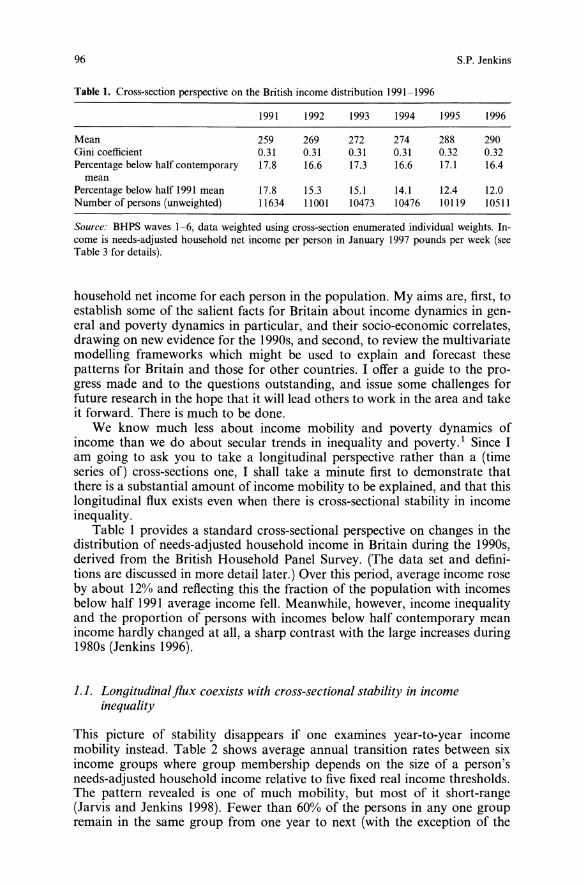
96

Table 1. Cross-section perspective on the British income distribution 1991-1996

S.P. Jenkins

1991 1992 1993 1994 1995 1996

Mean 259 269 272 274 288 290Gini coefficient 0.31 0.31 0.31 0.31 0.32 0.32Percentage below half contemporary 17.8 16.6 17.3 16.6 17.1 16.4mean

Percentage below half 1991 mean 17.8 15.3 15.1 14.1 12.4 12.0Number of persons (unweighted) 11634 11001 10473 10476 10119 10511

Source: BHPS waves 1-6, data weighted using cross-section enumerated individual weights. In-come is needs-adjusted household net income per person in January 1997 pounds per week (seeTable 3 for details).

household net income for each person in the population. My aims are, first, toestablish some of the salient facts for Britain about income dynamics in gen­eral and poverty dynamics in particular, and their socio-economic correlates,drawing on new evidence for the 1990s, and second, to review the multivariatemodelling frameworks which might be used to explain and forecast thesepatterns for Britain and those for other countries. I offer a guide to the pro­gress made and to the questions outstanding, and issue some challenges forfuture research in the hope that it will lead others to work in the area and takeit forward. There is much to be done.We know much less about income mobility and poverty dynamics of

income than we do about secular trends in inequality and poverty.! Since Iam going to ask you to take a longitudinal perspective rather than a (timeseries of) cross-sections one, I shall take a minute first to demonstrate thatthere is a substantial amount of income mobility to be explained, and that thislongitudinal flux exists even when there is cross-sectional stability in incomeinequality.Table 1 provides a standard cross-sectional perspective on changes in the

distribution of needs-adjusted household income in Britain during the 1990s,derived from the British Household Panel Survey. (The data set and defini­tions are discussed in more detail later.) Over this period, average income roseby about 12% and reflecting this the fraction of the population with incomesbelow half 1991 average income fell. Meanwhile, however, income inequalityand the proportion of persons with incomes below half contemporary meanincome hardly changed at all, a sharp contrast with the large increases during1980s (Jenkins 1996).

1.1. Longitudinalflux coexists with cross-sectional stability in incomeinequality

This picture of stability disappears if one examines year-to-year incomemobility instead. Table 2 shows average annual transition rates between sixincome groups where group membership depends on the size of a person'sneeds-adjusted household income relative to five fixed real income thresholds.The pattern revealed is one of much mobility, but most of it short-range(Jarvis and Jenkins 1998). Fewer than 60% of the persons in anyone groupremain in the same group from one year to next (with the exception of the

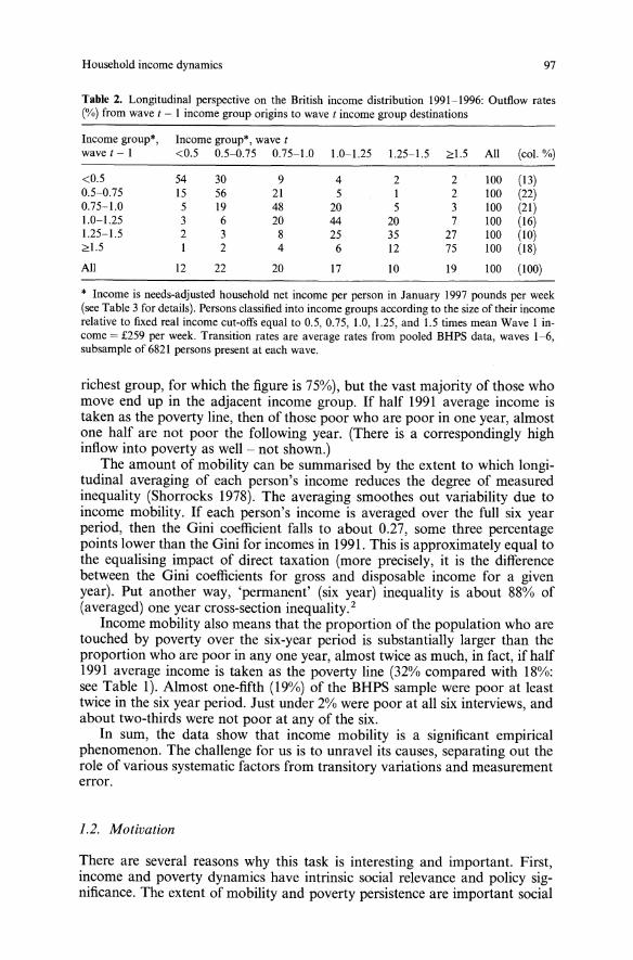
Household income dynamics 97

Table 2. Longitudinal perspective on the British income distribution 1991-1996: Outflow rates(%) from wave I - 1 income group origins to wave I income group destinations

Income group·, Income group·, wave I

wave 1-1 <0.5 0.5-0.75 0.75-1.0 1.0-1.25 1.25-1.5 ~1.5 All (col. %)

<0.5 54 30 9 4 2 2 100 (13)0.5-0.75 15 56 21 5 1 2 100 (22)0.75-1.0 5 19 48 20 5 3 100 (21)1.0-1.25 3 6 20 44 20 7 100 (16)1.25-1.5 2 3 8 25 35 27 100 (10)~1.5 1 2 4 6 12 75 100 (18)

All 12 22 20 17 10 19 100 (100)

• Income is needs-adjusted household net income per person in January 1997 pounds per week(see Table 3 for details). Persons classified into income groups according to the size of their incomerelative to fixed real income cut-offs equal to 0.5, 0.75, 1.0, 1.25, and 1.5 times mean Wave 1 in­come = £259 per week. Transition rates are average rates from pooled BHPS data, waves 1-6,subsample of 6821 persons present at each wave.

richest group, for which the figure is 75%), but the vast majority of those whomove end up in the adjacent income group. If half 1991 average income istaken as the poverty line, then of those poor who are poor in one year, almostone half are not poor the following year. (There is a correspondingly highinflow into poverty as well - not shown.)The amount of mobility can be summarised by the extent to which longi­

tudinal averaging of each person's income reduces the degree of measuredinequality (Shorrocks 1978). The averaging smoothes out variability due toincome mobility. If each person's income is averaged over the full six yearperiod, then the Gini coefficient falls to about 0.27, some three percentagepoints lower than the Gini for incomes in 1991. This is approximately equal tothe equalising impact of direct taxation (more precisely, it is the differencebetween the Gini coefficients for gross and disposable income for a givenyear). Put another way, 'permanent' (six year) inequality is about 88% of(averaged) one year cross-section inequality. 2

Income mobility also means that the proportion of the population who aretouched by poverty over the six-year period is substantially larger than theproportion who are poor in anyone year, almost twice as much, in fact, if half1991 average income is taken as the poverty line (32% compared with 18%:see Table I). Almost one-fifth (19%) of the BHPS sample were poor at leasttwice in the six year period. Just under 2% were poor at all six interviews, andabout two-thirds were not poor at any of the six.In sum, the data show that income mobility is a significant empirical

phenomenon. The challenge for us is to unravel its causes, separating out therole of various systematic factors from transitory variations and measurementerror.

1.2. Motivation

There are several reasons why this task is interesting and important. First,income and poverty dynamics have intrinsic social relevance and policy sig­nificance. The extent of mobility and poverty persistence are important social

98 S.P. Jenkins

indicators to be placed alongside information about the income distribution ata point in time. For example a former British Minister of Social Security,Peter Lilley, recently discounted the rising incidence of low income during the1980s with reference to new evidence about longitudinal income mobility:

Social mobility is considerable. Discussion about poverty is often based on the assumption thatfigures for households on low incomes describe a static group of people trapped in poverty unableto escape and getting poorer. However, this picture has been blown apart by recent studies. Theyshow that the people in the lowest income category are not the same individuals as were in lastyear, still less fifteen years ago. (P. Lilley, speech in Southwark Cathedral on 13 June 1996, quotedby Hills 1998, p. 52.)

Regardless of whether the conclusions Mr Lilley drew from the evidence werecorrect (they are debatable), my point is that the evidence is seen as importantby many. That it is of interest to a wide range of people is underlined by thefact that mobility findings by Sarah Jarvis and myself (Jarvis and Jenkins1996) were reported not only in The Financial Times, but also on the frontpage of Socialist Worker.Moreover, longitudinal analysis is an essential ingredient in policy formu­

lation. Researchers in the US and UK have long drawn attention to the dif­ferences between the poverty experience of the population over a period oftime and the poverty at a one particular time, and emphasised that the designof anti-poverty policy measures should depend on whether poverty is a short­duration event which most people experience at one time or a long-durationevent concentrated amongst particular identifiable groups in the population. 3

Indeed a dynamic perspective leads to different anti-poverty strategies, asDavid Ellwood, a leading researcher recruited as welfare reform advisor byPresident Clinton, has pointed out:

[D]ynamic analysis gets us closer to treating causes, where static analysis often leads us towardstreating symptoms.... If, for example, we ask who are the poor today, we are led to questionsabout the socioeconomic identity of the existing poverty population. Looking to policy, we thentypically emphasise income supplementation strategies. The obvious static solution to poverty is togive the poor more money. If instead, we ask what leads people into poverty, we are drawn toevents and structures, and our focus shifts to looking for ways to ensure people escape poverty.(Ellwood 1998, p. 49.)

The New Deal policies for the unemployed and lone parents which have beenintroduced in the UK by Tony Blair's Labour government are an example ofthis change in focus.In this lecture I take it for granted that we are concerned with doing

something about reducing poverty by raising exit rates and lowering entryrates. To do this we need empirical models in order to engage with and influ­ence policy-makers and their advisers. Achieving this policy relevance mightconflict with the imperative of producing papers rated highly by our fellowacademics, a trade-off I return to later.A second reason for discussing income and poverty dynamics is that vir­

tually all the widely-varying interests and disciplinary affiliations of the ESPEmembership are relevant. To study income dynamics one must draw onaspects of household and labour economics, economic demography, publiceconomics, and econometrics and statistics. There is something for almosteveryone.A third reason for the topic is that, even for those who have little interest

in engaging with 'real world' of policy, there are many academic challenges

Household income dynamics 99

raised by income dynamics, for both theoretical and applied researchers. Ishall be emphasising the roles played by changes in labour earnings frompersons other than the household head, changes in non-labour income (in­cluding benefits), and by changes in household composition generally, where­as our current analytical frameworks for income dynamics are best suited tocharacterising the employment earnings dynamics of prime-age male house­hold heads. There is much work yet to be done on developing more compre­hensive models.Income and poverty dynamics are of interest, fourth, because remarkably

little research has been done on them. Although there has been much work onthe dynamics of specific income sources for particular population subgroups(wage dynamics and benefit dynamics especially), this has not been matchedby analysis of total (needs-adjusted) income for the whole population. 4 Mostof the work which has been done refers to the USA, and many of my themeshave been inspired by US researchers. However I make little apology for em­phasising their points anew, especially since even in the US there has beensurprisingly little research and, in any case, it is important to investigatewhether US findings are applicable in Europe. My British examples, to follow,are a contribution to that task.The availability of suitable longitudinal data has been a constraint on

European research, but new opportunities are opening up. This is the fifthreason for addressing my topic. Major household panel surveys began in 1984in Germany, the Netherlands and Sweden, and in a number of other countriessubsequently. These surveys are becoming increasing useful as they mature.One of the most important developments in European data is the EuropeanCommunity Household Panel, established in 1995, which aims to providecomparable panel data for more than ten European Union member coun­tries. 5 I shall be illustrating my arguments with analysis of data from inter­view waves 1-6 of the British Household Panel Survey (covering 1991-1996),of which more below.

1.3. Outline

The remainder of the lecture is organised as follows. In Sect. 2, I offer aworking definition of personal economic well-being and its constituent com­ponents, and then use this to raise some methodological issues and organisemy discussion of the socio-economic correlates of income and poverty dy­namics. I also provide some introductory summary statistics. In Sect. 3 Iestablish some salient facts about British poverty dynamics and its socio­economic correlates. Arnold Zellner's (1992) Presidential Address to theAmerican Statistical Association enjoined us to always ensure we 'GET THEFACTS', and that is my aim. I apply the pioneering methods of Bane andEllwood (1986). Although I shall be examining Britain in the first half of the1990s rather than the US in the 1970s, and utilising six years of data ratherthan twelve, my findings echo theirs. I shall demonstrate that analysis whichconcentrates on the earnings dynamics of continuously-working households islikely to miss a great deal of the dynamics of poverty for the population aswhole.I tum from description to modelling, from cross-tabulations to multi­

variate regression, in Sect. 4. I shall not present any of my own estimates;

100 S.P. Jenkins

rather, I shall present an overview of the multivariate approaches which havebeen used in the literature, and attempt to clarify their strengths and weak­nesses. This is a manifesto for a future research programme for myself and - Ihope - others. The final section contains some brief concluding comments.Overall my aim is to draw attention to issues and stimulate interest in them,rather than to present particular solutions or findings.

2. A definition of economic well-being to organise the analysis

Suppose economic well-being for each person in each household h = 1,2, ... ,H, at each time period t = 1,2, ... ,T, is summarised by their 'personal in­come-equivalent' (PI), which is the needs-adjusted household net income ofthe household to which s/he belongs, nt: 6

(I)

The numerator is a double summation: over all persons in the householdj = 1,2, ... ,nh

, and over each money income source xl/a' k = 1,2, ... ,K,where these include net transfer income from the government (benefits lesstaxes). The denominator is a household equivalence scale factor which de­pends on household size nh and household composition and other character­istics summarised by the vector ah .

This definition prompts several observations. First, PI depends both onhousehold money income and on household demographic composition. Andtherefore changes in PI may arise through changes in money income (of one'sown or of other household members, via the numerator), or changes inhousehold composition (via the numerator and the denominator), or both. Toput things another way, if everyone lived alone, then there would be a directlink between one's labour market status and one's economic well-being.However the majority of the population live together in household units withthe opportunity to pool and share resources. More persons means (poten­tially) more income earners, for example from labour earnings or from socialsecurity benefits. But more persons also means that a given amount of moneyincome is worth less in per capita terms.This discussion leads naturally to a distinction between income events

and demographic events when examining the correlates of income dynamics.Income events are those associated with changes in different types of income(labour earnings of different household members, investment income, publicand private transfers net of taxes, etc.). Demographic events include joiningevents, such as the arrival of a new baby or partnership formation, and leav­ing events, such as death of a partner, marital dissolution, or a child leavinghome.My second observation is that the population of interest includes every

individual in the population, adults and children, those in work and out ofwork - this follows directly from the policy relevance constraint stated earlier.Of course different income and demographic events may have different im­pacts amongst different subgroups within the population. This raises the

Household income dynamics 101

methodological question of whether it is best to derive the required picture foreveryone via separate models for each of the most important subgroups orincome components, and then reassemble the material later, or to have an all­encompassing model. Most economists' reaction has been to focus on partic­ular subgroups or income sources (working households and earnings, benefitrecipients and welfare benefits), but the overall picture is rarely drawn. Thisstrategy is not defensible on the grounds that income mobility for non­working households is negligible relative to that for working households, as Ishow below (also see Jarvis and Jenkins 1998). And it is important to incor­porate groups such as the elderly and lone parents into the analysis, since theyhave notably high risks of poverty at a point in time and attract much policyattention. I return later to the 'unit of analysis' issue.My third observation concerns the question of what dimension(s) of in­

come dynamics one should focus on, supposing we have available a sequenceof observations on PI for a sample of individuals over a number of years. Thefirst important distinction to be made here is between income dynamics andpoverty dynamics - a focus on mobility throughout the whole distributionof income (changes in a continuous variable) or simply transitions above orbelow some low income cut-off (movements between discrete states). 7 There isno right answer here of course. I simply note that most research to date onhousehold income has focused on poverty dynamics, most probably reflectinggreater social and policy concern about low income transitions rather thanincome mobility in general. This paper will focus on poverty dynamics aswell.The second important distinction is between analysis in which the depen­

dent variable is the longitudinal sequence as a whole and analysis of changeswithin the sequence. Much of the poverty dynamics literature, following Baneand Ellwood (1986) takes a spell-based perspective, in which the focus is onconsecutive observations within a given state (single spell 'poverty duration'analysis). By contrast several authors have made a good case for distinguishingbetween different longitudinal patterns of poverty experience, thus incorpora­ting incidence, prevalence and spell repetition elements. Early US studies ofpoverty dynamics defined the persistently poor as those experiencing morethan some large number of years of poverty within some observation window(e.g. 8 years out of 10).8 This approach is open to criticism because it fails totake account of left- and right-censoring of poverty spells at the boundaries ofthe observation window. However the approach is valid when the observationwindow covers a complete life stage such as 'childhood': see for exampleAshworth et al. (1994) who differentiate between transient, persistent, perma­nent, occasional, recurrent, and chronic child poverty patterns. A different,but related, tradition distinguishes between observed and chronic povertywhere the latter is defined to be when a person's longer-period income (de­rived by some type of longitudinal averaging) falls below the poverty line. 9

Obviously it would be nice to be able to build up descriptions of wholesequences of poverty 'experience' from characterisations of its constituentcomponents, and there has been some research doing this, as I discuss later.My empirical illustration takes a spell based approach, following Bane andEllwood (1986), in part because one needs relatively mature panel surveys todifferentiate sequence patterns (only 6 waves of BHPS data were availableat the time of writing). But following Stevens (1994, 1995, 1999), I providesome description of poverty re-entry rates in addition to poverty exit rates.

102 S.P. Jenkins

My final observation is that PI is measured here in terms of income ratherthan consumption, reflecting that fact that all existing annual household panelsurveys contain measures of income rather than consumption expenditures.This is a potential problem because temporarily high or low income valuesmay not reflect a person's true economic well-being because borrowing orsaving allows consumption smoothing. One must therefore take transitoryincome variations into account.

2.1. The data set (British Household Panel Survey waves 1-6) and definitionsused in the paper

Before turning to these illustrations, I need to be more specific about my dataset, the British Household Panel Survey waves 1-6 (1991-1996), and the pre­cise definitions of variables such as PI. The first wave of the British HouseholdPanel Survey (BHPS) was designed as a nationally representative sample ofthe population of Great Britain living in private households in 1991. Originalsample respondents have been followed and they, and their co-residents,interviewed at approximately one year intervals subsequentIy.lO Children ofsample members begin to be interviewed as sample members in their ownright when they reach age 16. Most of my analysis is based on an unbalancedpanel subsample of more than 10,000 persons (adults and children) in com­plete respondent households for all waves for which they are in the panel.All analyses of income distribution, whether cross-sectional or longitudi­

nal, have to make assumptions about the definition of PI (the components ofmoney income and the equivalence scale), and the income accounting unit andmeasurement period. The choices made for this paper, summarised in Table 3,are a conventional set of assumptions, at least in the context of British re­search, and match those used to derive the official British low income statistics(Department of Social Security 1997).The definitions are somewhat different from those used in much income

dynamics research based on e.g. the US PSID. In that literature, a pre-taxpost-transfer (rather than post-tax post-transfer) income definition is morecommon, and the sharing unit is typically the family (a single person or per­sons related by blood or marriage living together) rather than the household.The British McClements equivalence scale corresponds to a Buhmann et al.(1988) parametric equivalence scale with household size elasticity of about0.6-0.7 (Coulter et al. 1992; Jenkins and Cowell 1994), whereas the needsrelativities most commonly used in the US (those implicit in the official pov­erty line) correspond to an household size elasticity of 0.56 (Burkhauser et al.1996).Perhaps the major difference between my standard British definition and

the standard US one is the time period over which money incomes are mea­sured. In Britain it is (broadly speaking) the month prior to the interview, inthe US, the year. An annual income definition is often judged to be superioron the grounds that a longer period measure is less likely to reflect transitoryvariations. In the absence of annual income data, I am forced to assume thatincome and poverty status round about the time of the interview proxy annualincome and poverty status. This should be kept in mind when, for brevity'ssake, I refer later in the paper to movements in and out of poverty from oneyear to the next.

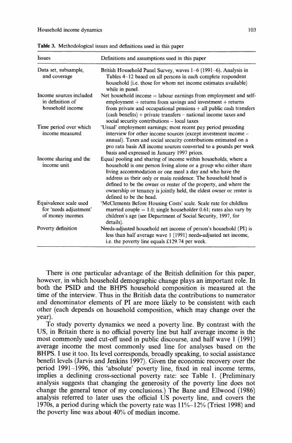
Household income dynamics

Table 3. Methodological issues and definitions used in this paper

103

Issues

Data set, subsample,and coverage

Income sources includedin definition ofhousehold income

Time period over whichincome measured

Income sharing and theincome unit

Equivalence scale usedfor 'needs adjustment'of money incomes

Poverty definition

Definitions and assumptions used in this paper

British Household Panel Survey, waves 1-6 (1991-6). Analysis inTables 4-12 based on all persons in each complete respondenthousehold (i.e. those for whom net income estimates available)while in panel.Net household income = labour earnings from employment and self­employment + returns from savings and investment + returnsfrom private and occupational pensions + all public cash transfers(cash benefits) + private transfers - national income taxes andsocial security contributions - local taxes'Usual' employment earnings; most recent pay period precedinginterview for other income sources (except investment income­annual). Taxes and social security contributions estimated on apro rata basis All income sources converted to a pounds per weekbasis and expressed in January 1997 prices.

Equal pooling and sharing of income within households, where ahousehold is one person living alone or a group who either shareliving accommodation or one meal a day and who have theaddress as their only or main residence. The household head isdefined to be the owner or renter of the property, and where theownership or tenancy is jointly held, the eldest owner or renter isdefined to be the head.'McClements Before Housing Costs' scale. Scale rate for childlessmarried couple = 1.0; single householder 0.61; rates also vary bychildren's age (see Department of Social Security, 1997, fordetails).Needs-adjusted household net income of person's household (PI) isless than half average wave I (1991) needs-adjusted net income,i.e. the poverty line equals £129.74 per week.

There is one particular advantage of the British definition for this paper,however, in which household demographic change plays an important role. Inboth the PSID and the BHPS household composition is measured at thetime of the interview. Thus in the British data the contributions to numeratorand denominator elements of PI are more likely to be consistent with eachother (each depends on household composition, which may change over theyear).To study poverty dynamics we need a poverty line. By contrast with the

US, in Britain there is no official poverty line but half average income is themost commonly used cut-off used in public discourse, and half wave 1 (1991)average income the most commonly used line for analyses based on theBHPS. I use it too. Its level corresponds, broadly speaking, to social assistancebenefit levels (Jarvis and Jenkins 1997). Given the economic recovery over theperiod 1991-1996, this 'absolute' poverty line, fixed in real income terms,implies a declining cross-sectional poverty rate: see Table 1. (Preliminaryanalysis suggests that changing the generosity of the poverty line does notchange the general tenor of my conclusions.) The Bane and Ellwood (1986)analysis referred to later uses the official US poverty line, and covers the1970s, a period during which the poverty rate was 11%-12% (Triest 1998) andthe poverty line was about 40% of median income.

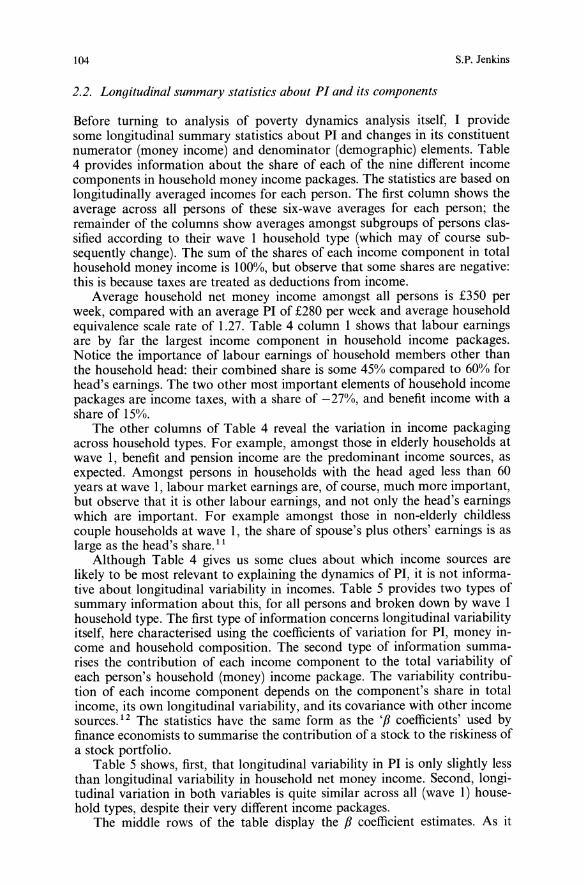
104

2.2. Longitudinal summary statistics about PI and its components

S.P. Jenkins

Before turning to analysis of poverty dynamics analysis itself, I providesome longitudinal summary statistics about PI and changes in its constituentnumerator (money income) and denominator (demographic) elements. Table4 provides information about the share of each of the nine different incomecomponents in household money income packages. The statistics are based onlongitudinally averaged incomes for each person. The first column shows theaverage across all persons of these six-wave averages for each person; theremainder of the columns show averages amongst subgroups of persons clas­sified according to their wave I household type (which may of course sub­sequently change). The sum of the shares of each income component in totalhousehold money income is 100%, but observe that some shares are negative:this is because taxes are treated as deductions from income.Average household net money income amongst all persons is £350 per

week, compared with an average PI of £280 per week and average householdequivalence scale rate of 1.27. Table 4 column 1 shows that labour earningsare by far the largest income component in household income packages.Notice the importance of labour earnings of household members other thanthe household head: their combined share is some 45% compared to 60% forhead's earnings. The two other most important elements of household incomepackages are income taxes, with a share of -27%, and benefit income with ashare of 15%.The other columns of Table 4 reveal the variation in income packaging

across household types. For example, amongst those in elderly households atwave 1, benefit and pension income are the predominant income sources, asexpected. Amongst persons in households with the head aged less than 60years at wave I, labour market earnings are, of course, much more important,but observe that it is other labour earnings, and not only the head's earningswhich are important. For example amongst those in non-elderly childlesscouple households at wave I, the share of spouse's plus others' earnings is aslarge as the head's share. 11

Although Table 4 gives us some clues about which income sources arelikely to be most relevant to explaining the dynamics of PI, it is not informa­tive about longitudinal variability in incomes. Table 5 provides two types ofsummary information about this, for all persons and broken down by wave 1household type. The first type of information concerns longitudinal variabilityitself, here characterised using the coefficients of variation for PI, money in­come and household composition. The second type of information summa­rises the contribution of each income component to the total variability ofeach person's household (money) income package. The variability contribu­tion of each income component depends on the component's share in totalincome, its own longitudinal variability, and its covariance with other incomesources. 12 The statistics have the same form as the 'fJ coefficients' used byfinance economists to summarise the contribution of a stock to the riskiness ofa stock portfolio.Table 5 shows, first, that longitudinal variability in PI is only slightly less

than longitudinal variability in household net money income. Second, longi­tudinal variation in both variables is quite similar across all (wave I) house­hold types, despite their very different income packages.The middle rows of the table display the fJ coefficient estimates. As it

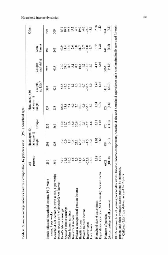
Tab

le4.Six-wave-averageincomesandtheircomposition,byperson'swaveI(1991)householdtype

::c 0 cHeadaged60+

'"All

Headaged<60

Other

C> ::rpersons

(atwaveI)

(atwaveI)

0 0:Single

Couple

Single

Couple,

Couple

Lone

S'

nokids·

andkid(s)

Parent

() 0 3 C>

Needs-adjustedhouseholdincome,PI(6-wave

280

201

252

359

367

262

197

279

Q.

'<mean,£perweek)

I:l ll'

Householdnetincome(6-wavemean,£perweek)

350

125

262

253

421

405

243

309

2.In

com

eso

urce

as%

ofh

ouse

hold

net

inco

me:

() '"

Head'slabourearnings

59.7

6.2

10.0

100.6

58.8

71.0

40.9

45.1

Spouse'slabourearnings

33.9

0.0

10.7

13.8

45.5

39.0

11.4

10.2

Otherlabourearnings

10.5

1.9

6.6

2.4

12.1

8.8

13.4

39.5

Investmentincome

4.8

10.5

13.0

6.0

5.3

3.1

2.6

5.2

Private

&occupationalpensionincome

5.0

23.1

30.6

2.7

5.0

0.6

0.8

4.2

Benefitincome

14.8

65.2

38.3

10.3

6.0

10.4

41.7

19.0

Privatetransferincome

1.4

0.1

0.1

0.9

0.7

1.2

6.7

4.6

Incometaxes

-27.0

-1.5

-5.2

-33.3

-30.5

-31.0

-14.0

-23.9

Localtaxes

-3.3

-6.2

-4.6

-3.3

-3.0

-3.0

-3.7

-3.9

Householdsize:6-wavemean

3.08

1.02

2.11

1.24

2.45

4.17

3.36

2.28

Equivalencescalerate(McClements):6-wavemean

1.27

0.62

1.05

0.70

1.16

1.56

1.26

1.13

Numberofpersons

6821

484

770

329

1410

3063

441

324

(Aspercentageofallpersons)

(100.0)

(7.1)

(11.3)

(4.8)

(20.7)

(44.9)

(6.5)

(4.8)

BHPSsubsampleisallpersonspresentall6waves.Income,incomecomponents,householdsizeandhouseholdequivalencescaleratelongitudinallyaveragedforeach

person,andthenaveragedacrosspersonsbysubgroup.

•Children('kids')aredefinedasaged0-16years.

5;

Table5.Longitudinalvariabilityofincomeandhouseholdsize,andtheproportionatecontributionofincomecomponentstolongitudinalincomevariability,by

~person'swaveIhouseholdtype

All

Headaged60+

Headaged<60

Other

persons

(atwaveI)

(atwaveI)

Single

Couple

Single

Couple,

Couple

Lone

nokids

andkid(s)

Parent

CV(needs-adjustedhouseholdincome,

0.25

0.24

0.23

0.27

0.25

0.25

0.28

0.28

PI)-

CV(householdnetincome)-

0.27

0.25

0.25

0.30

0.27

0.26

0.33

0.33

Pro

port

iona

teco

ntri

buti

ono

finc

ome

com

pone

ntto

long

itud

inal

inco

me

vari

abil

ity

rpco

effi

cien

t')"

Head'slabourearnings

0.49

0.06

0.13

0.81

0.55

0.64

0.33

0.22

Spouse'slabourearnings

0.31

0.00

0.14

0.23

0.42

0.41

0.21

0.11

Otherlabourearnings

0.20

0.01

0.11

0.03

0.25

0.20

0.26

0.63

Investmentincome

0.09

0.22

0.23

0.09

0.09

0.04

0.04

0.09

Private

&occupationalpensionincome

0.04

0.17

0.15

0.01

0.00

0.01

0.01

0.05

Benefitincome

0.13

0.52

0.28

0.14

0.04

0.05

0.29

0.10

Privatetransferincome

0.01

0.01

0.02

0.01

0.01

0.00

0.04

0.07

Incometaxes

-0.28

-0.01

-0.D

7-0.31

-0.35

-0.36

-0.18

-0.25

Localtaxes

-0.00

0.01

0.01

-0.01

-0.00

0.01

-0.01

-0.02

CV(householdsize)-

0.09

0.01

0.05

0.13

0.13

0.08

0.13

0.22

CV(McClementsequivalencescalerate)-

0.09

0.01

0.05

0.09

0.10

0.09

0.14

0.18

Numberofpersons

6821

484

770

329

1410

3063

441

324

(Aspercentageofallpersons)

(100.0)

(7.1)

(11.3)

(4.8)

(20.7)

(44.9)

(6.5)

(4.8)

BHPSsubsampleisallpersonspresentall6waves.

-Coefficientsofvariationforincome,householdsizeandhouseholdequivalencescaleratecalculatedlongitudinallyforeachperson,andthenaveragedacross

enpersonsbysubgroup.

"tl--Theslopecoefficientfromasix-observationregression,foreachperson,ofeachincomecomponentontotalnetincome,averagedacrosspersonsbysubgroup

......

(seetext).

'"c:> ~ c:> '"

Household income dynamics 107

happens, patterns correspond closely to those shown by the income shares inTable 4. (The most notable exception is the Pcoefficient for benefit incomewhich is lower than its share.) In other words, the greatest contribution tolongitudinal variability in household net money income appears to be thelabour earnings of the household head for the majority of households. How­ever the contributions of other labour earnings are also relatively large. Indeedfor persons in non-elderly couple households, the combined contribution ofsecondary earnings is greater than for head's labour earnings.The final rows of Table 5 suggest that variability in household net money

income (the numerator of PI) is greater than variability in household needssummarised by either household size or equivalence scale rate (the denomi­nator of PI). However it is arguable whether the measures are fully compara­ble given the contrasting metrics for the variables (continuous versus intrinsi­cally discrete). Let us then examine the extent of household demographicchange directly: see Table 6.The most commonly used indicator of demographic change is a change in

a person's household head. The top panel of Table 6 shows the cumulativeproportion of persons with a change in their household head, by wave, first forall persons, and then broken down by the person's wave 1 household type.Between waves 1 and 2, almost one tenth of all persons had experienced achange in household head, but by wave 6, the figure was more than one fifth.The experience of demographic change varies substantially by household type.The greatest contrast is between single elderly persons (for whom the eventis virtually non-existent by definition - it would require a new partnershipand change in responsibility for housing costs) to non-elderly 'other' persons,mostly unrelated adults, amongst whom 38% experienced a household changebetween waves 1 and 6.When the definition of demographic change is extended to include all types

of events in which people either join or leave the household, or both, manymore persons are counted as experiencing it. Between waves 1 and 2, almostone fifth experienced some kind of demographic change; by wave 6, that figurehad more than doubled, to almost one half (47%).These statistics demonstrate clearly that the incidence of demographic

events is substantial, and therefore cannot be ignored in any study of the cor­relates of income dynamics. There is an important corollary: if one restrictsanalysis to persons and households who do not experience compositionalchange, one will be omitting a significant fraction of the population andintroducing a form of selection bias. (See Duncan and Hill 1985, for theauthoritative statement of this case.) The results also raise questions aboutthe use of the household as the unit of analysis when estimating life cycleconsumption expenditure and saving models. 13

3. Some salient facts about British poverty dynamics and its socio-economiccorrelates

The aim of this section is to establish the main socio-economic correlates oftransitions into and out of poverty in Britain. I shall first provide some factsabout poverty dynamics, and then examine the relative roles played by incomeand demographic events using methods pioneered by Bane and Ellwood(1986).

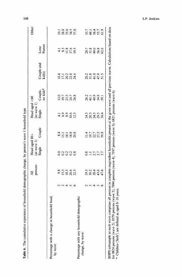
Tab

le6.Thecumulativeexperienceofhouseholddemographicchange,byperson'swaveIhouseholdtype

:; oeAll

Headaged60+

Headaged<60

Other

persons

(atwaveI)

(atwaveI)

Single

Couple

Single

Couple,

Coupleand

Lone

nokids·

kid(s)

Parent

Percentagewithachangeinhouseholdhead,

bywave:

29.8

0.0

8.4

4.1

13.0

10.8

4.1

19.1

315.5

0.2

15.1

6.9

19.7

17.1

8.5

28.8

418.5

0.2

16.1

8.9

23.5

20.2

11.8

35.6

520.6

0.2

18.8

10.6

24.7

22.8

17.6

34.5

622.5

0.8

20.8

12.5

26.8

24.4

19.5

37.8

Percentagewithanyhouseholddemographic

change,bywave:

219.3

0.8

11.4

14.5

26.2

20.2

20.7

33.7

330.2

1.1

19.7

20.3

41.1

31.8

31.8

48.1

438.4

2.7

22.7

24.5

49.9

41.0

49.0

58.4

543.6

2.7

27.2

29.5

54.9

47.9

56.8

55.7

647.4

3.7

39.8

34.4

59.1

51.5

62.6

61.9

BHPSsubsampleateachwavecomprisesallpersonsincompleterespondenthouseholdspresentatthegivenwaveandallpreviouswaves.Calculationsbasedondata

for9824persons(wave2);8579persons(wave3);7894persons(wave4);7197persons(wave5);6821persons(wave6).

•Children('kids')aredefinedasaged0-16years.

V'1 ~ ~ i:I i";'

~.

Household income dynamics

3.1. Poverty exit rates and re-entry rates

109

Table 7 shows Kaplan-Meier product-limit estimates of poverty exit rates(and their standard errors) for a cohort of persons starting a poverty spell,together with estimates of the proportions remaining poor after given lengthsof time. Table 8 provides similar information, but about re-entry rates topoverty for those people who end a poverty spell. 14The tables immediately reveal some of the problems which arise in empir­

ical implementation. First, the amount of information is relatively limited.Because there are only six waves of data, exit rates at long durations cannotbe estimated. There is typically little exogenous time series variation in thedata, which hinders identification of some effects. And relatively small sub­sample numbers constrain breakdowns by population subgroups.Second there are potential measurement error issues. My poverty line de­

lineating the states of 'poor' and 'not poor' is arbitrarily defined, like virtuallyall low income cut offs. It is implausible to treat small income changes - forexample from one pound below the line to one pound above or vice versa - asa genuine transition out of or into poverty, when it is as likely due to transi­tory variation or measurement error. To avoid these threshold effects, I counta rise in PI as a poverty exit only if the post-transition PI value is at least 10%higher than the poverty line. Similarly I require PI to fall below 90% of thepoverty line to count as a transition into poverty. Adjustments such as thesehave been implemented in most previous studies: see for example Bane andEllwood (1986) and Duncan et al. (1993). I have also made a further mea­surement error adjustment to the data. Preliminary analysis revealed that anon-trivial number of poverty transitions were accounted for by implausiblechanges in benefit income from one year to the next. Transitions have beencensored in these cases. 15Consider now the substantive estimates, beginning with poverty exits. By

construction (the exclusion of left-censored spells), all persons starting a pov­erty spell are poor for at least one year. However almost one half (47%) of thiscohort leave poverty the following year, and the exit rate falls further to aboutone third and one fifth for the subsequent two years, raising the issue of du­ration dependence. The exit rate for the fifth year is not lower still, but higher(0.32), albeit with a larger standard error. (The secular growth in averageincomes between 1991-1996, combined with the fixed poverty line, is onepotential reason for the rise.)The exit rates imply a median poverty spell duration for a cohort begin­

ning a spell of between two and three years and after five years, almost four­fifths of an entry cohort would have escaped poverty. Equivalently - morepessimistically and emphasising poverty persistence - about one fifth of theentry cohort are still poor after five years. Without a longer panel, and thenceestimates of exit rates at longer durations, we can only speculate about theincidence of very long poverty spells. If we assume that the exit rates were 0.25for all years after the fifth, then just over one-twentieth (0.06) of those begin­ning a spell would be poor at least ten years and the average duration about3.8 years. 16This picture of poverty persistence describes the experience of those begin­

ning a poverty spell. But, as many have emphasised, the length of completedpoverty spells for those who are currently poor is rather different. Althoughonly a small fraction of people entering poverty have long spells, the stock of

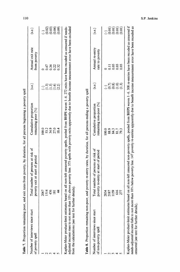
Table7.Proportionremainingpoor,andexitratesfrompoverty,byduration,forallpersonsbeginningapovertyspell

o

Numberofinterviewssincestart

Totalnumberofpersonsatriskof

Cumulativeproportion

(s.e.)

Annualexitrate

ofpovertyspell

povertyexitatstartofperiod

remainingpoor('Yo)

frompoverty

I2067

100.0

(-)

02

1514

53.2

(1.3)

0.47

3436

34.9

(1.5)

0.34

4181

27.0

(1.6)

0.22

544

18.4

(2.2)

0.32

(s.e.)

(-)(0.02)

(0.03)

(0.04)

(0.09)

Kaplan-Meierproduct-limitestimatesbasedonallnon-leftcensoredpovertyspells,pooledfromBHPSwaves1-6.272exitshavebeenrecodedascensoredifneeds­

adjustedincomerisestonotmorethan10%abovepovertyline.375spellswithpovertyexitsapparentlyduetobenefitincomemeasurementerrorhavebeenexcluded

fromthecalculations(seetextforfurtherdetails).

Table8.Proportionremainingnon-poor,andpovertyre-entryrates,byduration,forallpersonsendingapovertyspell

Numberofinterviewssincestart

Totalnumberofpersonsatriskof

Cumulativeproportion

(s.e.)

Annualre-entry

(s.e.)

ofnon-povertyspell

povertyre-entryatstartofperiod

remainingnon-poor(%)

ratetopoverty

12834

100.0

(-)

0(-

)2

2187

88.9

(0.7)

0.11

(0.01)

31159

84.3

(0.8)

0.05

(0.01)

4616

81.7

(1.0)

0.03

(0.01)

5277

79.3

(1.3)

0.03

(0.01)

Kaplan-Meierproduct-limitestimatesbasedonallnon-leftcensorednon-povertyspells,pooledfromBHPSwaves1-6.308re-entrieshavebeenrecodedascensoredif

needs-adjustedincomefallstonotmorethan10%belowpovertyline.147povertyre-entriesapparentlyduetobenefitincomemeasurementerrorhavebeenrecodedas

censored(seetextforfurtherdetails).

Vl "0 '- g ~ ::l '"

Household income dynamics III

poverty is dominated by those with long spells because those with short spellsleave. It is straightforward to illustrate this, assuming a no-growth steady­state in which the poverty inflow rate is constant. In this case, and assumingthe exit rate is 0.25 for all years after the fifth, then, of those who are poor ina given year, the fraction with a poverty spell length of at least 10 years isalmost one-fifth (0.18) and the median completed spell length between 4 and5 years, and the average completed spell length, 5.9 years. 17These calculations underestimate people's total experience of poverty over

a given period because they ignore the fact that a significant fraction of peopleexperience multiple spells of poverty. Stevens (1995, 1999), using US PSIDdata, has shown most effectively that combining information on poverty re­entry rates with poverty exit rates provides much better predictions of povertyexperience than does relying on single spell estimates (as above). 18Table 8 provides information about poverty re-entry rates for all persons

ending a poverty spell (again left-censored spells have been excluded from thecalculations). Re-entry rates fall from 0.11 in the second year after leavingpoverty to less than one third of that rate after five years, 0.03. (The numberof persons 'at risk' at the start of the period is larger than in Table 7 becauseof the high prevalence of left-censored poverty spells in this short panel.) There-entry rates imply that about one-fifth of those leaving a poverty spell willhave experienced another spell within the subsequent five years. This reiteratesthe point made by Jarvis and Jenkins, using BHPS waves 1-4, that 'the pathout oflow income is not a one-way up-escalator: ... there is a not insignificantchance of finding oneself on the down escalator to low income again' (1997,p. 131).The different pictures about persistence provide different impressions

about the concentration amongst the poor of receipts of social assistance andother benefits for poverty alleviation. A focus on the poverty stock tells us thatthe persistently poor receive most of the total resources devoted to povertyalleviation at a point in time. But a focus on flows, both out of and (back) intopoverty, reminds us that the number of people who are ever helped by povertyalleviation measures is many more than those currently poor.This is of course the same message as provided by the US literature. In this

connection it is interesting to note that the exit rates shown in Table 7 arebroadly similar to the estimates reported by Bane and Ellwood (1986) for theUS in the 1970s. On the other hand, the poverty re-entry rates shown in Table8 are noticeably lower than those reported by Stevens (1994) using PSID datafor 1970-1987. Taken at face value this cross-national comparison suggestsgreater poverty turnover in the US than in Britain. This conclusion mustremain tentative however, given the differences in periods covered, definitionof income, equivalence scale and the poverty line, and in the population sub­samples examined.

3.2. The definition of income events and demographic events

It is now time to put the information about income and demographic eventstogether with the data about spells. I use the decomposition methods pio­neered by Bane and Ellwood (1986) to determine the main events associatedwith poverty spell endings and beginnings. 19 I will return later to evaluate theadvantages and shortcomings of this approach.

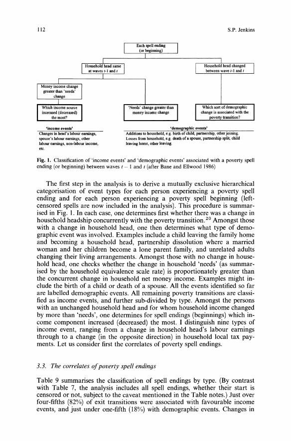
112 S.P. Jenkins

'Needs' change greater thanmoney income change

Household head changedbetween wave /·1 and /

Which sort ofdemographicchange is associated with thepoverty transition?

'income events'Changes in head's labour earnings.spouse's labour eamings. otherlabour earnings. Don-labour income.etc.

'demogr.phic events'Additions to household, e.g. birth of child, partnership. other joining.Losses from household, e.g. death of a spouse. partnership spli~ childleaving home. other leaving.

Fig. I. Classification of 'income events' and 'demographic events' associated with a poverty spellending (or beginning) between waves t - I and t (after Bane and Ellwood 1986)

The first step in the analysis is to derive a mutually exclusive hierarchicalcategorisation of event types for each person experiencing a poverty spellending and for each person experiencing a poverty spell beginning (left­censored spells are now included in the analysis). This procedure is summar­ised in Fig. I. In each case, one determines first whether there was a change inhousehold headship concurrently with the poverty transition. 20 Amongst thosewith a change in household head, one then determines what type of demo­graphic event was involved. Examples include a child leaving the family homeand becoming a household head, partnership dissolution where a marriedwoman and her children become a lone parent family, and unrelated adultschanging their living arrangements. Amongst those with no change in house­hold head, one checks whether the change in household 'needs' (as summar­ised by the household equivalence scale rate) is proportionately greater thanthe concurrent change in household net money income. Examples might in­clude the birth of a child or death of a spouse. All the events identified so farare labelled demographic events. All remaining poverty transitions are classi­fied as income events, and further sub-divided by type. Amongst the personswith an unchanged household head and for whom household income changedby more than 'needs', one determines for spell endings (beginnings) which in­come component increased (decreased) the most. I distinguish nine types ofincome event, ranging from a change in household head's labour earningsthrough to a change (in the opposite direction) in household local tax pay­ments. Let us consider first the correlates of poverty spell endings.

3.3. The correlates ofpoverty spell endings

Table 9 summarises the classification of spell endings by type. (By contrastwith Table 7, the analysis includes all spell endings, whether their start iscensored or not, subject to the caveat mentioned in the Table notes.) Just overfour-fifths (82%) of exit transitions were associated with favourable incomeevents, and just under one-fifth (18%) with demographic events. Changes in

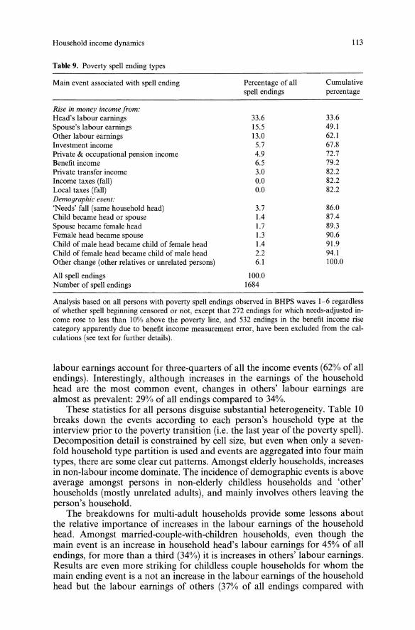
Household income dynamics

Table 9. Poverty spell ending types

Main event associated with spell ending

Rise in money income from:Head's labour earningsSpouse's labour earningsOther labour earningsInvestment incomePrivate & occupational pension incomeBenefit incomePrivate transfer incomeIncome taxes (fall)Local taxes (fall)Demographic event:'Needs' fall (same household head)Child became head or spouseSpouse became female headFemale head became spouseChild of male head became child of female headChild of female head became child of male headOther change (other relatives or unrelated persons)

All spell endingsNumber of spell endings

Percentage of allspell endings

33.615.513.05.74.96.53.00.00.0

3.71.41.71.31.42.26.1

100.01684

113

Cumulativepercentage

33.649.162.167.872.779.282.282.282.2

86.087.489.390.691.994.1100.0

Analysis based on all persons with poverty spell endings observed in BHPS waves 1-6 regardlessof whether spell beginning censored or not, except that 272 endings for which needs-adjusted in­come rose to less than 10% above the poverty line, and 532 endings in the benefit income risecategory apparently due to benefit income measurement error, have been excluded from the cal­culations (see text for further details).

labour earnings account for three-quarters of all the income events (62% of allendings). Interestingly, although increases in the earnings of the householdhead are the most common event, changes in others' labour earnings arealmost as prevalent: 29% of all endings compared to 34%.These statistics for all persons disguise substantial heterogeneity. Table 10

breaks down the events according to each person's household type at theinterview prior to the poverty transition (i.e. the last year of the poverty spell).Decomposition detail is constrained by cell size, but even when only a seven­fold household type partition is used and events are aggregated into four maintypes, there are some clear cut patterns. Amongst elderly households, increasesin non-labour income dominate. The incidence of demographic events is aboveaverage amongst persons in non-elderly childless households and 'other'households (mostly unrelated adults), and mainly involves others leaving theperson's household.The breakdowns for multi-adult households provide some lessons about

the relative importance of increases in the labour earnings of the householdhead. Amongst married-couple-with-children households, even though themain event is an increase in household head's labour earnings for 45% of allendings, for more than a third (34%) it is increases in others' labour earnings.Results are even more striking for childless couple households for whom themain ending event is a not an increase in the labour earnings of the householdhead but the labour earnings of others (37% of all endings compared with

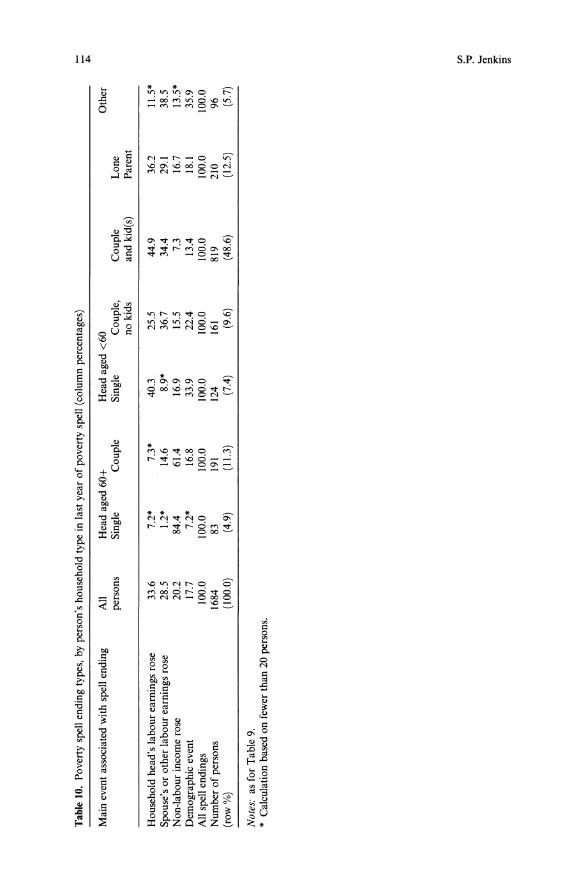
Tab

le10

.Povertyspellendingtypes,byperson'shouseholdtypeinlastyearofpovertyspell(columnpercentages)

Headaged60+

Single

Couple

Headaged<60

Single

Couple,

nokids

Maineventassociatedwithspellending

Householdhead'slabourearningsrose

Spouse'sorotherlabourearningsrose

Non-labourincomerose

Demographicevent

Allspellendings

Numberofpersons

(row%)

Not

es:asforTable9.

*Calculationbasedonfewerthan20persons.

Allpersons

33.6

28.520.217.7

100.0

1684(100.0)

7.2*1.2*

84.4 7.2*

100.0

83 (4.9)

7.3*

14.6

61.416.8

100.0

191(11.3)

40.3 8.9*

16.9

33.9

100.0

124 (7.4)

25.536.715.5

22.4

100.0

161 (9.6)

- :i:Other

Couple

Lone

andkid(s)

Parent

44.9

36.2

11.5*

34.4

29.1

38.5

7.3

16.7

13.5*

13.4

18.!

35.9

100.0

100.0

100.0

819

210

96(48.6)

(12.5)

(5.7)

Vl

~ g c. a

Household income dynamics 115

26%). Others' labour earnings are also important for persons in lone parenthouseholds prior to the poverty transition. In this case, the extra earnings willtypically be those of other adults sharing the household (but not a spouse). 21The results suggest that increases in a lone parents' own labour earnings aremore important than re-partnering for getting out of poverty - at least in theshort-term. It should be remembered that the method of analysis used herefocuses on contemporaneous changes; the correlates of long-tenn sustainedescapes from poverty may be different from the short-term correlates.These results underline the importance for poverty dynamics of changes in

'secondary' labour earnings rather than head's earnings amongst working agehouseholds. In each case increases in labour earnings may arise for a varietyof reasons: for example, an unemployed person taking a job, or someonealready with a job working more hours or being promoted, etc. Amongst thepersons for whom a rise in household head's labour earnings was the mostimportant event associated with a poverty spell ending, the household headchanged from 'not working' to 'working' in about one-half (51%) of the cases.And amongst the persons for whom a rise in the others' labour earnings wasthe most important event associated with a poverty spell ending, there was achange from neither the spouse nor others (besides the head) working to atleast one earning in one-half (50%) of the cases.

3.4. The correlates ofpoverty spell beginnings

Consider now the main events associated with poverty spell beginnings. Table11 displays the breakdown for all persons. One notable finding is that demo­graphic events account for a greater proportion (38%) of the spell beginningsthan of spell endings (18%: see Table 9). Income events account for 62% ofbeginnings (cf. 82% of endings). Although most types of demographic eventare relatively more numerous, what is driving the results is the 'new entrants'category, accounting for some 15% of all spell beginnings. These refer to per­sons who are present in the household currently (but who are not the house­hold head) and who were not present prior to the poverty transition (i.e. at thelast wave). Many of these individuals are children born into poverty. Otherpersons under this heading are new partners of the household head or otheradults in a household which is poor when they are present. The figure for thisgroup is an over-estimate because, when constructing the table, I assumed thatthese persons were not poor prior to joining their current household: somesuch assumption has to be made because, by definition, the income of theirprevious household is not observed in the panel. However, even if one tookthe opposite view, and assumed that they were all previously poor (and thusexcluded from the table), the general cOl'lclusion about the relative incidenceof income and demographic events for the spell beginning case compared tothe spell ending one, would not change.The poverty spell beginnings are broken down in Table 12 by event and

household type in the first year of the poverty spell. Broadly speaking, thediversity of patterns by household type is similar to that in Table 10, but witha shift within each household type subgroup towards a higher incidence ofdemographic events. These events are particularly important amongst peoplebelonging to non-elderly single person or lone parent households and 'other'households (mostly unrelated adults sharing). For the first of these groups,

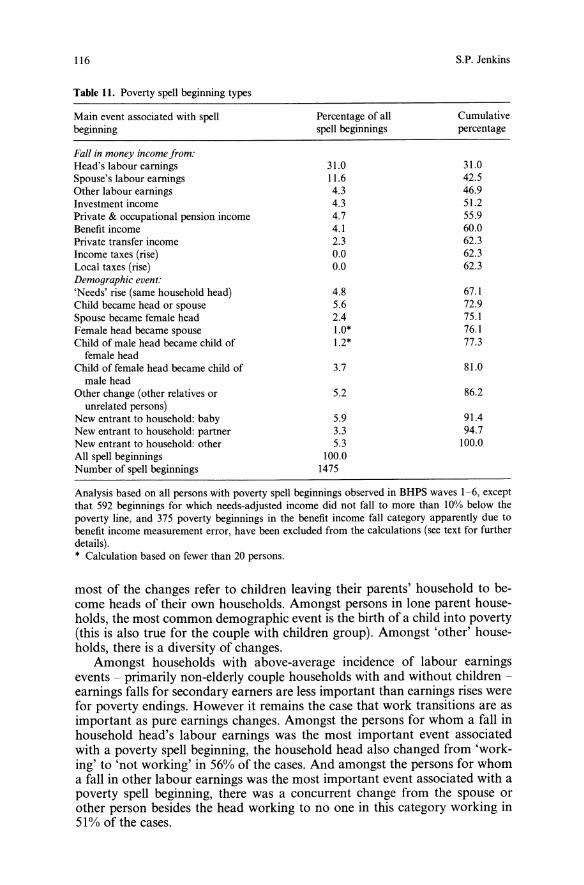
116

Table 11. Poverty spell beginning types

Main event associated with spellbeginning

Fall in money income from:Head's labour earningsSpouse's labour earningsOther labour earningsInvestment incomePrivate & occupational pension incomeBenefit incomePrivate transfer incomeIncome taxes (rise)Local taxes (rise)Demographic event:'Needs' rise (same household head)Child became head or spouseSpouse became female headFemale head became spouseChild of male head became child offemale head

Child of female head became child ofmale head

Other change (other relatives orunrelated persons)

New entrant to household: babyNew entrant to household: partnerNew entrant to household: otherAll spell beginningsNumber of spell beginnings

Percentage of allspell beginnings

31.011.64.34.34.74.12.30.00.0

4.85.62.41.0*1.2*

3.7

5.2

5.93.35.3100.01475

S.P. Jenkins

Cumulativepercentage

31.042.546.951.255.960.062.362.362.3

67.172.975.176.177.3

81.0

86.2

91.494.7100.0

Analysis based on all persons with poverty spell beginnings observed in BHPS waves 1-6, exceptthat 592 beginnings for which needs-adjusted income did not fall to more than 10% below thepoverty line, and 375 poverty beginnings in the benefit income fall category apparently due tobenefit income measurement error, have been excluded from the calculations (see text for furtherdetails).* Calculation based on fewer than 20 persons.

most of the changes refer to children leaving their parents' household to be­come heads of their own households. Amongst persons in lone parent house­holds, the most common demographic event is the birth of a child into poverty(this is also true for the couple with children group). Amongst 'other' house­holds, there is a diversity of changes.Amongst households with above-average incidence of labour earnings

events - primarily non-elderly couple households with and without children ­earnings falls for secondary earners are less important than earnings rises werefor poverty endings. However it remains the case that work transitions are asimportant as pure earnings changes. Amongst the persons for whom a fall inhousehold head's labour earnings was the most important event associatedwith a poverty spell beginning, the household head also changed from 'work­ing' to 'not working' in 56% of the cases. And amongst the persons for whoma fall in other labour earnings was the most important event associated with apoverty spell beginning, there was a concurrent change from the spouse orother person besides the head working to no one in this category working in51% of the cases.

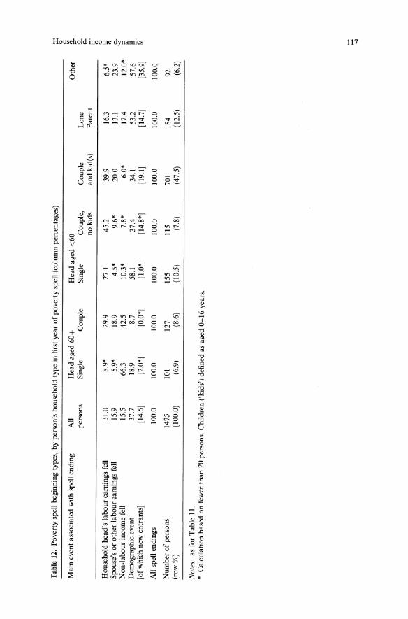
Tab

le12.Povertyspellbeginningtypes,byperson'shouseholdtypeinfirstyearofpovertyspell(columnpercentages)

::r:: 0 l:

Maineventassociatedwithspellending

All

Headaged60+

Headaged<60

Other

III ::rpersons

Single

Couple

Single

Couple,

Couple

Lone

0 0:nokids

andkid(s)

Parent

S'() 0

Householdhead'slabourearningsfell

31.0

8.9*

29.9

27.1

45.2

39.9

16.3

6.5*

3 '"Spouse'sorotherlabourearningsfell

15.9

5.9*

18.9

4.5*

9.6*

20.0

13.1

23.9

c..

'<Non-labourincomefell

15.5

66.3

42.5

10.3*

7.8*

6.0*

17.4

12.0*

::> I'l

Demographicevent

37.7

18.9

8.7

58.1

37.4

34.1

53.2

57.6

2.[ofwhichnewentrants]

[14.5]

[2.0*]

[0.0*]

[1.0*]

[14.8*]

[19.IJ

[14.7]

[35.9J

() '"

Allspellendings

100.0

100.0

100.0

100.0

100.0

100.0

100.0

100.0

Numberofpersons

1475

101

127

155

115

701

184

92(row%)

(100.0)

(6.9)

(8.6)

(10.5)

(7.8)

(47.5)

(12.5)

(6.2)

Not

es:asforTableII.

*Calculationbasedonfewerthan20persons.Children('kids')definedasaged0-16years.

- -..l

118

3.5. Summary: events and poverty transitions

S.P. Jenkins

In sum, even where income dynamics are more closely associated with labourearnings dynamics, we need to recognise that earnings dynamics are often amixture of the earnings dynamics of several persons, not only the householdhead, and for each of these persons, a mixture of job dynamics and earningsdynamics for those continuously in work. 22 Moreover there are some house­holds especially the elderly for whom the main events are changes in non­labour income. And the incidence of demographic change as a main eventis not insignificant for large numbers of persons in the population. It is alsoimportant to account for measurement error.These findings for Britain echo those of Bane and Ellwood (1986) for the

USA. They reported that:

less than 40 percent of poverty spells begin because ofa drop ofhead's earnings, while 60 percent ofthe spells end when the heads' earnings increase. Thus, researchers must focus on household forma­tion decisions and on the behavior of secondary family members. (Bane and Ellwood 1986, p. I.)

My findings have given a greater role to secondary earners and a lesser one todemographic events than Bane and Ellwood. However more substantivecomparisons of Bane and Ellwood's findings and my own are necessarilyconstrained by important differences - e.g. they use a different income defini­tion, equivalence scale and poverty line, and focus on non-elderly householdsonly. Also, Britain in the early 1990s is different from the USA in the 1970s:dual-earner households are more prevalent now than then, in the USA as wellas Britain (Gregg and Wadsworth 1996). Moreover I have used the householdas the income unit - reflecting British conventions - rather than the narrowerconcept of the family as they did, so allowing greater scope for householdmembers other than the head and spouse to playa role.An interesting issue for further research is whether the results generalize to

other European countries. Some existing research suggests that they may. Forexample, Fritzell (1990) found that family composition changes were a majorcause of income changes in Sweden as well as the USA.The general message, notwithstanding various definitional questions (and

further checks of the sensitivity of conclusions to choice of poverty line), re­mains the same. Analysis which concentrates on the earnings dynamicsof continuously-working household heads is likely to miss a much of thedynamics of poverty even for working households let alone the population aswhole.The Bane and Ellwood approach, on which I have relied heavily thus far,

provides a particularly useful framework for isolating the 'salient facts' aboutpoverty dynamics and its socioeconomic correlates, as well as raising otherissues such as measurement error. But this social arithmetic is not modelling.More particularly, first, the approach does not provide a means for simulatingfuture poverty experience. Second, the differentiation between income anddemographic events using a mutually exclusive hierarchy does not allow oneto unravel the separate effects of events which occur simultaneously. A lonemother may both repartner and take up a job, but the Bane and Ellwoodapproach attributes importance to just one of these events. Third, and arelated point, the approach does not provide a clear cut link with structuralmodels of the labour market and household formation processes which liebehind the poverty transitions and PI changes more generally.

Household income dynamics 119

Most applied economists would probably think some form of multivariateregression model is a better approach for addressing these issues. To whatextent is this so? To answer this question, we need to consider what sorts ofdynamic models there are and we also require a set of evaluation criteriaagainst which to judge them.

4. Multivariate models of income and poverty dynamics

There are four main types of multivariate dynamic model which have beenapplied in the income and poverty dynamics literature to date:

• longitudinal poverty pattern models,• transition probability models,• variance components models, and• structural models.

I shall discuss the first of these rather briefly and then focus on the others inmore detail. The number of applications of these multivariate models to in­come dynamics is actually very small, at least by comparison with models ofthe dynamics of wages, welfare benefit receipt, (un)employment, and house­hold formation. Since the models share the same technical structures (whichare relatively well-known), I can concentrate on the features of particular rel­evance to income dynamics.Before proceeding to the models, I wish to set out three criteria for evalu­

ating them. (These are ideals: inevitably achievement in some dimensions willlead to sacrifices in other dimensions.) I believe models should be practical, fitthe past and be able to provide forecasts about the future, and be structural.Let me elaborate.

• Be practical. We need empirical models which can provide useful results inreasonable time. Practicality and feasibility are natural goals given the de­sire for policy relevance I expressed earlier. This is not to dismiss theoreticalmodels - indeed theoretical models addressing all the various dynamic pro­cesses would be valuable, though undoubtedly hard to produce (a challengeto theorists!).

• Fit the past and provide forecasts about future poverty experience. Here theissues concern whether a model satisfactorily characterises the salient factsabout income and poverty dynamics, and not only 'goodness of fit' andother econometric specification tests. At one level, there are questions suchas: is the type of model suitable and is the specification of covariates ap­propriate, given the main patterns of poverty dynamics? For example, ifpoverty spell repetition is empirically important, is this modelled? Is a modelbased on the behaviour of heads of households appropriate when behaviourof other household members is also significant? At another level, the issue iswhether the full potential of estimated models has been realised: it is insuf­ficient to simply estimate models and discuss the signs of coefficients. Giventhe policy relevance constraint which I have insisted on, one needs to drawout the implications of the estimates for individuals' future poverty experi­ence under different scenarios. At its simplest, this might be involve simpleextrapolations using the fitted model; more sophisticated forecasting mayinvolve complex micro-simulation of poverty experience under different

120 S.P. Jenkins

policy scenarios. 23 The ability to do this depends partly on the extent towhich my third criterion is achieved.

• Be structural. As economists, we take it for granted that understanding ofincome and poverty dynamics would be advanced if there were a directconnection between our empirical models and structural models of the un­derlying dynamic processes of market and household formation. Recogni­tion of these processes immediately raises questions about simultaneity andendogeneity biases in empirical work too. The appropriate balance betweenstructural sophistication and feasibility is an issue I shall return to.

4.1. Longitudinal poverty pattern models

These models differ from the others because the dependent variable is based oncomplete longitudinal sequence of income for each person (see the discussionin Sect. 1). Examples include models of the probability of being 'chronicallypoor' where a person is defined as 'chronically poor' if her longitudinally­averaged income falls below the poverty line. A variant on this is a Tobit re­gression model of individuals' 'chronic poverty gaps', or some function of thegaps, where these gaps take into account the amount by which longitudinally­averaged income falls below the poverty line. Regressors include a variety ofpersonal and household characteristics, but the nature of the model requiresall covariates to be either fixed (for example sex, race), or else fixed at theirvalues at the start of the sequence. See for example, Jalan and Ravallion(1997) and Hill and Jenkins (1999), who use the models to compare the char­acteristics of persons who are 'chronically poor' and those who are counted aspoor using standard cross-section poverty indices. The results are relevant toassessing the targeting of poverty alleviation measures.The models have a rather different focus of these models from the others I

discuss: they do not typically look at income and poverty dynamics per se.Instead longitudinal data is used to derive (fixed) measures of 'permanent'income or 'chronic' poverty. Given this different focus, I shall not discussthem further. The distinction between transitory and 'permanent' differencesis an important one nonetheless, and a fundamental part of the income vari­able components models discussed shortly.

4.2. Transition probability models

This class of models is perhaps the one which most applied economists wouldimmediately think of. The most commonly estimated models are of povertyexit transition probabilities, of the form

prob(person i is not poor in year tlperson i is poor in year t - 1; Zj, Xit, B)

(2)

but there are also models of poverty entry, or re-entry probabilities, of theform

prob(person i is poor in year tlperson i is not poor in year t - 1; Zj, Xit, B)

(3)

Household income dynamics 121

where Z; is a vector of fixed covariates, Xii is a vector of time-varyingcovariates (which may include duration), and e is a vector of parameters. Thecovariates might also include lagged values of covariates (e.g. XiI-d, andthence events (L1XiI ). These are of course examples of event history (or hazardrate or duration) models. From the fitted conditional probabilities and thencethe survivor function, one can derive the predicted spell length distribution foreach person with a given set of characteristics. These are of course directextensions, with covariates, of the Kaplan-Meier transition model estimates inTables 7 and 8.Let me focus on a few selected examples. Hill et al. (1998) estimate poverty

entry and exit rates for young adults using US PSID data. Poverty exit rateregressions are estimated by Canto Sanchez (1998) for persons in householdsresponding to the Spanish quarterly labour force panel survey (ECPF), andby Muffels et al. (1990) and van Leeuwen and Pannekoek (1999) using Dutchpanel survey data. Schluter (1997) and Van Kerm (1998) estimate povertyexit and re-entry rates using German and Wallonian panel data respectively.Stevens (1995, 1999) estimates exit and re-entry rates, for all persons and byrace, using the US PSID. Her model is by far the most sophisticated oneeconometrically. She allows for unobserved heterogeneity in both exit and re­entry rates using bivariate hazard models, checks for the potential bias intro­duced by excluding left-censored spells, and provides standard error estimateswhich account for the occurrence of repeated observations from a givenhousehold in her sample. How do these models compare with each other andagainst my evaluation criteria, and what issues do they raise?One contrast between the models is the types of covariates used, and

income and demographic event variables in particular. Hill et al. (1998) forexample, include marriage and divorce and child birth events as time-varyingcovariates (L1XiI ). Canto Sanchez's covariates include (un)employment eventsand changes in household size and number of income recipients. In bothpapers, these variables are found to be statistically significant alongsideother personal characteristics. Interestingly, Stevens incorporated income anddemographic events, defined in a Bane-Ellwood hierarchical fashion, in oneversion of her model but found relatively few significant effects. Her explana­tion was that she had controlled 'for several personal and household charac­teristics in addition to incorporating the event indicators. In particular inclu­sion of age and female headship controls reduces the estimated effects ofmanyof the beginning and ending event variables' (1995, p. 21).The different strategies raise several as-yet unresolved issues concerning

whether such event variables should be used as covariates. One view is thatthey should, on the grounds that it facilitates Fit: after all, the earlier de­scriptive analysis assumes that income and demographic events are impor­tant socioeconomic correlates of transitions. Moreover the inclusion of eventsprovides a direct link between poverty transitions and the underlying labourmarket and household formation processes, an advantage with referenceto the Be Structural criterion. There are several contrary positions however.The first is that inclusion of event variables is likely to lead to econometricproblems of endogeneity and simultaneity, since the underlying behaviouralprocesses are likely to be jointly determined. To me the real issue is notwhether this problem exists (for it undoubtedly does), but how large thebiases are which are introduced. We do not know whether the bias in ourestimates is 5% or 105%. If the biases are large, there is clearly great scope

122 S.P. Jenkins

for econometricians to develop suitable methods to handle them (this is achallenge!)A second problem is that we may not be able to identify separately the

effects of labour market and demographic event variables once one hasalready controlled for labour market status and demographic status at thepoint in time (the point raised by Stevens: see above). The issue essentiallyconcerns the incidence of events amongst subgroups of individuals at risk ofthe event: for example, amongst unemployed poor men included in a povertyexit rate regression in which current employment status is a covariate, howmany end poverty spells by getting jobs? Answers presumably depend on theparticular data set and context.A third point is whether inclusion of event variables is akin to 'over-fitting'

the model, i.e. whether (after controlling for personal characteristics) experi­ence of specific events is synonymous with a poverty transition. For example, ithas been put to me that it is hardly surprising or indeed interesting that jobloss is strongly associated with entry to poverty. I am not wholly persuaded bythis argument, primarily because poverty status depends on the incomes of allhousehold members and the job loss (or other event) of one member need notmake household income fall below the critical cut-off with a probability equalto one. The size of that probability does deserve investigation.A fourth point concerns the construction of the covariates used to encap­

sulate the impact of each event variable. I have been implicitly assuming thatthey would be summarised by a binary variable which is equal to one in theinterval the event occurred and equal to zero for all other intervals. This sup­poses that effects are entirely contemporaneous. But what if the impact of anevent persists over time (in which case the event variable needs to be 'turnedon' for several periods, but how many?), or what if events are anticipatedby individuals, leading them to change their behaviour (a question hard toanswer without some structural model)?Further issues arise with the use of event variables, or in fact any time­

varying covariate, when assessing model fit and preparing forecasts and sim­ulations. The reason is that one has to specify a longitudinal sequence ofvalues for such variables, conditioned on other characteristics, in order toderive predicted spell length probabilities for each individual. 24 For exampleconsider not only event variables, but also, say, a covariate summarising theage of the youngest child in each interval at risk of a transition, or a covariatessummarising the state of the macro-economic environment. The most com­mon practice in event history modelling is simply to use some fixed value forthese covariates in a simulation, but this is rather unsatisfactory. Hill et al.(1998) grasp the nettle, and specify a set of temporal sequences of covariatepatterns, including assumptions about marriage and birth events and theirtiming, and predict sequences of poverty risks using these.Arguably this issue is less of a problem for some sorts of policy advice.

Consider for example the case where transition rate models are to be used totarget those most at risk of long poverty spells, in the knowledge that theresearch users will only have at their disposal information about the currentcharacteristics of the relevant population at risk. In this case there is somesense in estimating models with only fixed personal covariates. However Iwould not wish to push this argument too far: for example if the state ofthe macro-economy has an significant impact on poverty transition rates,then presumably this information should be incorporated into the predictions,

Household income dynamics 123

especially if the impact differs between subgroups within the population. Al­though these covariate specification issues arise in all types of socioeconomicevent history modelling - not simply poverty dynamics - it is remarkable howlittle explicit attention they have received.Another issue concerns the unit of analysis or subsample used in the model

(this point also arises for variance components models). For example, shouldthe models be estimated using a sample of only adults or also include children.There is a reasonable a priori case for the former practice as it is the choicesof adults which determine household income. However the argument is notdecisive - it depends in part on how structural a model one wants. For purelydescriptive purposes there is a case for using all observations, adults andchildren.My final remarks under this heading are about fitting and prediction of

individuals' total experience of poverty over a period of time. Much analysissuggests that spell repetition is a significant empirical phenomenon, and yetmost models either examine single poverty spells or, if they have estimatedmodels of poverty re-entry probabilities as well, have not combined the modeloutputs to examine the implications for total poverty experienced over someinterval. Stevens (1995, 1999) is a notable exception. One explanation for theomission is that the derivations are technically demanding. It would thereforebe interesting to know the pay-off to simpler models from which it is mucheasier to derive multi-spell predictions.A two-state first order Markov transition model (see Boskin and Nold

1975; Amemiya 1986, Chapt. 10) is an obvious example of a simpler model.This can be interpreted as discrete-time hazard rate regression model inwhich, crucially, it is assumed that there is no duration dependence in eitherthe exit or entry transition rate. Because of this, the model is clearly likely tobe a misspecification but the assumption brings advantages. The model isstraightforward to estimate and there are very simple expressions for expectedpoverty spell durations, the total proportion of time spent poor, and meanpoverty recurrence times for persons with different characteristics. See VanKerm (1998) for an example. 25 Such models are a prime example of wherethe appropriate balance between Practicality (in particular the feasibility ofsimulation) and Goodness of Fit deserves further investigation.

4.3. Income variance components models

Under this heading I group models used to describe the longitudinal co­variance structure of PI (rather than poverty itself), but from which resultsabout poverty dynamics can and have been derived. The basic methods werefirst developed by Lillard and Willis (1978), albeit with an application tomen's labour earnings and the persistence of low pay. There have been manysubsequent developments of the model and further applications to earnings:see inter alia Hause (1980) and Abowd and Card (1989). See also the earlierliterature on Galtonian regression models of income dynamics, reviewed byfor example Creedy (1985).The first application of variance components models to household income

and poverty dynamics was by Duncan (1983), and later work by Duncan andRodgers (1991) and Stevens (1995, 1999). A prototypical model is

124

log(P lit) = Zjlx + XitP + Git

where the error structure of the model takes the form

Vit = YVit-1 + rJit

S.P. Jenkins

(4)

(5)

and where bi is a random individual component with mean zero and variancea} and rJit is a purely random i.i.d. component with mean zero and variancea;. The Y is a serial correlation coefficient common to all persons. As Lillardand Willis (1978, p. 988-989) explain, the bi terms encapsulate individualheterogeneity in average (log) PI, whereas the serial correlation coefficient Ymay be interpreted as reflecting either the effects of random shocks whichpersist but whose effects deteriorate over time, or serially correlated un­observed individual-specific variables. Later applications have used increas­ingly more sophisticated specifications of the error structure than this simpleone, for example heterogeneity in the component variances across popula­tion subgroups, a variety of higher-order autocorrelated moving average(ARIMA) error structures rather than the simple AR(I) one shown here, andcalendar-time specific parameters and component variances to account forobserved non-stationarity in covariances. 26 There is trade-off between modelcomplexity and data availability: with short panels the number of time­varying parameters which can be estimated is relatively small.Several implications for poverty dynamics can be derived. For example,

assuming the distributions of the error components takes a particular form,such as Normal, one may calculate the proportion of population whose ex­pected (or 'permanent') income is below the poverty line (see Lillard andWillis 1978, Eq. 3.12). One may also calculate the probabilities of observingspecific T-year poverty sequences (for example T consecutive years of pov­erty), though the length of the sequence is currently constrained by the need tocalculate the values of a T-variate normal distribution. (Deriving such pre­dictions is harder in these models than in the transition probability models, forwhich such survivor rates are integral outputs). The more widespread avail­ability of simulation-based estimation methods may alleviate this problem: seethe survey of these by Stem (1997). Alternatively, Stevens (1995, 1999) simu­lates the distribution of Plover a T-year period for her sample using randomdraws from a (bivariate) Normal distribution calibrated from the variancecomponent estimates, and calculates the distribution of years poor over a givenperiod across the subsample of individuals who are estimated to start a povertyspell. These simulation results are in a form which can be compared withthose from her hazard rate models and from tabulations of the actual data.The appeal of the variance components models is threefold. First, there are

attractions to analysing income itself, rather than discretising a continuousvariable ab initio using a poverty line which is arbitrary and also therebythrowing a lot of information away (Ravallion 1996). In particular, one couldhave estimates describing whether people moving out of poverty move justabove the poverty line or become well-off (cf. the transition probabilitymodels).Second, there is the long standing appeal to economists of the fundamental

decomposition of income and income changes into 'permanent' and 'transi-

Household income dynamics 125

tory' components: controlling for systematic observed differences (via Zj andXit), each person is assumed to have some latent level of PI which is perma­nently fixed (or evolving very slowly), about which there may be temporaryvariations. As Duncan and Rodgers have pointed out,

[this] seems reasonable in the face of unfavorable events like short-term unemployment and illnessor beneficial events like the overtime hours provided by a temporary increase in labor demand.The strength of this approach lies in its quantification of the components in the overall distribu­tion of poverty. (Duncan and Rodgers 1991, p. 540-541.)

However there are disadvantages too, as they also point out:

[The approach] does not, however, provide an individual-level measure of permanent poverty,and it may not be as well-suited as other measures, such as spell-based measures, for takinginto account the permanent changes in economic status which accompany events like divorce,remarriage, widowhood, or a long-term disability. (Duncan and Rodgers 1991, p. 540-541.)

To their list of permanent changes, one might also add: demographic eventssuch as the birth of a child (perhaps combined with a mother's withdrawalfrom the labour market), or departure of an adult child from the household,or labour market events such as long-term unemployed household head get­ting a job, or a mother returning to work. A further disadvantage of thevariance components models is that the dynamic processes are assumed to thesame for all income groups, rich and poor, which is unlikely.My view in the light of such comments has been that variance-components

models are likely best suited for the phenomena and subgroups for which theywere originally developed (such as men's earnings dynamics), rather thanhousehold income and poverty dynamics. This is because, first, focusing onhomogeneous subgroups (e.g. prime age men) makes the assumption of asimple covariance structure more plausible. Second, modelling a single incomesource (earnings), the effects of accounting for the combination of differentincome sources and household composition change are obviated. Moreoverthere is no explicit or obvious link between the variance component specifi­cations and the underlying labour market and household formation processes(a deficiency with reference to the Be Structural goal). And with an eye to thePracticality goal, it is worth mentioning that there are as yet no softwarepackages available with canned routines for estimation of variance compo­nents models in the same way as there is for hazard models (though non-linearGLS modules, which can be used to derive GMM estimates of variance com­ponents models, are becoming available.)Stevens's (1995, 1999) valuable work allows us to assess my opinions about

the relative merits of variance components and hazard rate models in a moresystematic manner, because she has estimated various versions of both classesof model on the same data set, and compared their predictions of povertypersistence over a fixed time interval for her subsample with direct tabulationsfrom the data. Stevens favours the hazard models rather than the variancecomponents ones, especially for describing dynamics for male-headed house­holds. Her conclusion was that

these comparisons suggest that the hazard model developed here comes close to replicating thedistributions of time in poverty from a relatively simple method of directly tabulating years inpoverty from the panel data.... The components-of-variance approach seems to over-estimatetime in poverty among male household heads, and may under-estimate time poor among femalehousehold heads. While the three methods yield similar results, these discrepancies suggest thatattention to the accuracy of variance-components models in predicting dynamic patterns near the

126 S.P. Jenkins

bottom of the income distribution may be an important area for further research. (Stevens 1995,p.36.)

Further evaluative work of this kind, especially research based on data sets forcountries other than the US, would be particularly valuable (though it is notwork for the technically faint-hearted).

4.4. Structural models

The final model type on my list refers to disaggregate structural models,though I am aware of only one example of these. This is Burgess and Prop­per's (1998) innovative model describing poverty dynamics amongst a sampleof American women aged 20-35 years from the National Longitudinal Surveyof Youth (NLSY).Rather than relating poverty transitions directly to explanatory variables,

as in the other approaches described so far, the authors model the underlyingdynamic processes which determine earnings - marriage, fertility, and labourforce participation - and the earnings associated with the outcomes of theseprocesses. From these, income and poverty status are calculated. The model isestimated separately for black and white women.More specifically, Burgess and Propper first estimate hazard models for the

probability of marital partnership formation and the probability of partner­ship dissolution, and a bivariate probit model of the probability of having achild during the relevant year and of working in the same year. Second, theymodel the distribution of labour market earnings separately for each combi­nation of outcomes of the marriage, fertility, and labour force participationchoices, controlling for sample selection into each state. Third, a model ofhusband's earnings is estimated using data about male NLSY respondents.Fourth, each woman's (expected) family income is calculated as a mixturedistribution, the sum of the probabilities of being in each {marriage, fertility,work} state times state-conditional earnings where, for the relevant states,earnings includes estimated earnings of a spouse as well as the woman'searnings. Finally, each woman's poverty status for the year is determined bycomparing estimated family income to the poverty line for her family type.Burgess and Propper compare poverty rates fitted using their model with

the actual poverty rates. They produce a close fit for the women when aged25-30, but at ages 20-25, poverty rates are over-predicted by up to 50%. AsBurgess and Propper remark, this over-prediction 'probably arises because[they] have not modelled income from adults other than partners, but in theunder-25 age group there are a significant minority of individuals who still livein the parental home' (1998, pp. 40-41). Fit is also examined in terms of thefraction of time individuals spend poor over the 15 year period. The authors'assessment is that 'the approach does a reasonable job of separating peoplelikely to spend a long time poor from those likely to be never poor' (1998,p. 41), though there is some systematic bias: the number of women who arefrequently poor is under-predicted and the number of women rarely poor isover-predicted. Overall I am not as sanguine as the authors are about thegoodness of fit of the model, in part because their sample (described above) isrelatively homogeneous compared to those for whom poverty experience isestimated by, say, Stevens (1995, 1999). But, as the authors point out (p. 40),

Household income dynamics 127

none of their estimation and predictions used the data on poverty status at all;recognising this, the fit is more impressive.There is no doubt that this model comes far closer to satisfying the Be

Structural criterion than any of other modelling approaches considered so far.This is demonstrated by the way in which Burgess and Propper employ it tounravel the causes of poverty in general and the sources of the differences inpoverty rates between black and white women in particular. Using counter­factual simulations, they consider the impact of, first, differences in personalcharacteristics such as years of education and family background, and differ­ences in socioeconomic origins at age 19 (for example, being a non-workinglone mother versus being a childless single working woman). Education isfound to be the variable with the largest impact on poverty rates. Burgess andPropper are able to analyse the mechanism by which this occurs: the effect ofhaving more education comes about more by increasing the likelihood of beingin states which are associated with higher incomes (such as being married withchildren and working) than by increasing earnings per se. Second, Burgess andPropper examine the effects on poverty rates of differences in black and whitewomen's behaviour, as summarised by the estimated coefficients in the variousbehavioural process equations. These are found to have make a major con­tribution to inter-racial differences in poverty compared to differences insocio-economic origins at age 19 and family background: 'While ... all tran­sition rates matter, rates of marriage appear to the single most importantfactor, as marriage gives access to another income stream' (1998, p. 50). Dif­ferences in short-term and long-term impacts are also revealed.This sort of detailed unravelling of causes plus simulation is not possible

within the reduced form models of dynamics discussed earlier. And observetoo that the issue for those models about having to specify longitudinal se­quences for time-varying covariates when doing· simulations also does notarise: the relevant values are generated within the system.Are structural models the future for income and poverty dynamics analysis

then? 1 believe that they are an exciting and innovative approach, and stronglysupport further development of them. Several directions for this suggestthemselves to me. One of the weaker links in the Burgess-Propper model is thetreatment of other adults in the household and non-labour income. Theirmodel of husbands' earnings is less developed than for women (in part re­flecting the nature of the NLSY data), and they simply ignore all other incomein household (which largely explains the worse fit for the 20-25 year olds).For the reasons given in their paper, omission of income from investmentsand savings and benefits such as AFDC is not likely to be an important sourceof bias. But this is not necessarily so in applications of such a model to coun­tries other than the USA (for example Europe, where there are typically morebenefits available, including for working households). And in analysis ofpopulations of persons representing a more heterogeneous mixture of life­cycle stages than the NLSY subsample of young women, the incidence ofmulti-adult households is likely to be much greater.One might also criticise some of the econometric methods and question the

robustness of the identification assumptions. Certainly one valuable servicedone by Burgess and Propper is to reveal the sorts of assumptions which needto made in order to implement a structural approach, in particular thoseabout correlations of unobservables across processes and across time. (Ichallenge econometricians to develop more sophisticated estimation methods

128 S.P. Jenkins

for simultaneous dynamic processes.) Nonetheless there is a more funda­mental question of whether a reliable structural model is a Holy Grail sincein many plausible specifications of the underlying equations, arguably'everything depends on everything else'. Moreover one may make a good casethat for many of processes concerned, pure randomness is intrinsic. If onetakes on board these various arguments, then structural models and the moresophisticated of the reduced form models discussed earlier are more similarthan at first appears. Both strands could draw more on the literature on dy­namic microsimulation: see example, Harding (1993, 1996) and referencestherein.Overall I believe that despite their attractions, structural models are likely

to remain relatively rare, if only for the simple reason that they are immenselycomplex and very time-consuming to develop. This is another example of theBe Practical criterion in head-on conflict with the Be Structural one.

5. Concluding comments

In his recent Presidential Address to the Royal Economic Society, AB Atkin­son stated that his 'principal purpose ... has been to argue that the economicanalysis of the distribution is in need of further development before we canhope to give a definitive answer to the questions in which the ordinary personis interested - such as what determines the extent of inequality and why hasinequality increased?' (1997, p. 317). My aim, like Atkinson's, has been'Bringing income distribution analysis in from the cold' (the title of his lec­ture), though I have taken a rather different, albeit complementary, perspec­tive - the longitudinal one. I have directed attention more at questions such as'how long do the poor stay poor?' and 'does getting a job get someone andtheir household out of poverty?'.These questions are of widespread interest amongst the general public and

amongst policy-makers. To answer them we analysts need to develop model­ling approaches which better incorporate the impact of changes in individuals'household contexts - changes in the incomes contributed by others (especially'secondary' labour earnings, but also non-labour income) and changes inhousehold composition. This much is clear from both descriptive decomposi­tion analysis of the sort pioneered by Bane and Ellwood (1986) and applied toBritish data in Sect. 3, and also from the review of multivariate models ofincome and poverty dynamics in Sect. 4.I have drawn attention to a tension between the goals of practicality, fit,

and being structural in developing models, and I hope that in future we canimprove models according to all three criteria. I acknowledge that this may bedifficult. It is easier to focus on dynamics for specific income sources or par­ticular subgroups, and on estimation without simulation. This perhaps ex­plains why the literature on income dynamics is relatively small, even in theUSA where household panel data have been available for the longest. Incen­tive structures in the profession may exacerbate this problem. For academicsin today's increasingly 'publish or perish' environment, it may be more re­warding to work on models which focus on particular aspects of the incomedetermination process rather than attempting to characterise the 'big picture'for income (or rather PI) itself. I hope nonetheless that ESPE members andothers will take up the many interesting theoretical and empirical challenges

Household income dynamics 129

which the study of income and poverty dynamics offers and exploit the newlongitudinal data sources now becoming available.

Endnotes

1 See inter alia Atkinson et al. (1995) and Gottschalk and Smeeding (1997) for reviews of thesubstantial increase in inequality during the 1980s in many (but not all) Western developednations, and Schultz (1998) about trends in world income inequality.

2 This is the estimated value of a Shorrocks (1978) immobility index, which is equal to the Ginicoefficient for cumulated six-wave incomes divided by a weighted average of the Gini co­efficients for the income distribution in each of the six years. All calculations cited in thisparagraph and the next are based on the balanced subsample of 6821 persons present at all sixBHPS waves.

3 See inter alia Duncan et al. (1984), and Bane and Ellwood (1986) for the USA, and Walkerwith Ashworth (1994) for the UK.

4 For a survey of earnings mobility research, see Atkinson et al. (1992). For recent UK studies ofthe dynamics ofmen's labour earnings, see Dickens (1997), Gosling et al. (1997), Ramos (1997),and Stewart and Swaffield (1997). On the dynamics of social assistance (Income Support) re­ceipt, see Shaw et al. (1996) and Noble et al. (1998).

5 Cross-nationally comparable household panel data sets are also being constructed: cf. theSyracuse University PSID/GSOEP Equivalent File (Burkhauser et al. 1995), now being ex­tended to include the BHPS, and the PACO project (Schmaus and Riebschliiger 1995). Panelsderived by record linkage of administrative registers on income, as in the Nordic countries, arepromising sources too. By contrast, the possibility of using retrospective survey information toanalyse income dynamics is severely limited.

6 This definition incorporates the almost universally made assumption in the income distributionliterature that all incomes are pooled within the income unit (assumed here to be the house­hold) and equally shared out amongst household members. See Jenkins (1991) and Lazear andMichael (1988) for critiques and alternative strategies. For economic models of within­household distribution see inter alia Apps and Rees (1996) and Chiappori (1992).

7 There is also the methodological issue of whether to model poverty or, instead, to model PIand derive the implications for poverty from this. I return to this later.

8 See for example Duncan et al. (1984) and Hill (1981). Similar methods have been applied toGerman data by Headey et al. (1991) and Krause (1998), to British data by Jarvis and Jenkins(1997), to Hungarian data by Speder (1998), and to Wallonia (Belgium) by Van Kerm (1998).

9 See for example Duncan and Rodgers (1991), Rodgers and Rodgers (1992), Jalan andRavallion (1997), and Hill and Jenkins (1999).

10 For a detailed discussion of BHPS methodology, see Taylor (1994) and Taylor (1998). Thederived net income variables are a publicly-available supplement to the main BHPS data set.For a detailed discussion of their creation, see Jarvis and Jenkins (1995, Appendix) andRedmond (1997).

11 According to my household type definition, couple households may, in principle, include adultsin addition to the household head and spouse (if present). A finer partition to distinguish thesecases would results in cell sizes which were too small.

12 More formally, for each person, the P coefficients satisfy the relationship EkPk = I, wherePk = pkak/a, Pk is the correlation between component k and the person's total net income(summed over six years), ak is the longitudinal standard deviation of component k, and a is thelongitudinal standard deviation of total income. For each person, this is the same as the slopecoefficient from a six-observation regression of the given income component on total netincome. Equivalently, Pk = Pk(llk/Il) J lzk/h where Ilk and Il are the longitudinal means ofcomponent k and total net income, and lzk and lz are half the squared longitudinal coefficientsof variation of component k and total net income. Hence the remark in the text linking Pco­efficients with covariances, income shares, and longitudinal variability. Income distributionspecialists will recognise the Pcoefficient as a longitudinal version of Shorrocks's (1982) mea­sure of the proportionate contribution of an income component to total inequality in a cross­section of persons.

130 S.P. Jenkins

13 Cf. Miles (1997) who estimated dynamic models for households from cross-section data, andBanks, Blundell and Preston (1994) who use pseudo-cohort data.

14 For more extensive analysis, based on BHPS waves 1-4, see Jarvis and Jenkins (1997).15 Reported household benefit income for these persons changed substantially from one year tothe next even though there was typically no concurrent change in household composition orwork pattern. (I.e. there were poverty spell exits associated with large rises in benefit incomeand poverty spell entries associated with large falls in benefits. Detailed case-by-case exami­nation revealed no obvious reason for these changes. I suspect they are due to some form oftransitory recall measurement error rather than genuine changes arising, say, from changes inbenefit take-up or exhaustion. For the present, a straightforward rule of thumb was used toidentify these unreliable cases: they were defined to be those persons for whom a change intheir household's benefit income was the most important event associated with a povertytransition (as defined below) and where the benefit income change comprised more than 75% ofthe total household net money income change.

16 These estimates are not very sensitive to the assumption about the exit rate. If it were 0.3 ratherthan 0.25, the proportion of those beginning a spell with a spell length of 10 or more years is0.04 and the mean duration, 3.7 years. If the exit rate were 0.02, the corresponding estimatesare 0.07 and 3.9 years.

17 The calculations use the exit rates in Table 7 and Bane and Ellwood (1986, Eq. 2). Answers arelittle different with the alternative exit rate assumptions of the previous footnote. The impor­tance of the distinction between the average of all completed spell lengths and the averagecompleted spell length for those in the stock has also been stressed in the unemployment liter­ature: see for example Akerlof and Main (1980).

18 The importance of spell repetition has been stressed in the welfare benefit dynamics literature:see for example Gottschalk and Moffitt (1994) and Blank and Ruggles (1994), and Shaw et al.(1996).

19 Other poverty dynamics applications to US data have been by Bane (1986) and Duncan andRodgers (1988). A seven country cross-national study using similar methods is by Duncan et al.(1993). Bane and Ellwood (1994, Chapt. 2) applied the methods to AFDC benefit dynamics. Apioneering British poverty dynamics study is by Hancock (I985), with notable attention givento potential problems arising from data unreliability. Jarvis and Jenkins (1997) were the first toapply similar methods to BHPS data (for waves 1-4).

20 See Bane and Ellwood's (1986, p. 9) discussion of the importance of the event and thence jus­tification for giving it special treatment.

21 Recall that re-partnership of a lone mother concurrent with a poverty exit would be counted asa demographic event, since the new male partner would virtually always be labelled the newhousehold head.

22 This point about earnings dynamics is also made by Swaffield and Stewart (1997) in theiranalysis of low pay dynamics using BHPS waves 1-4.

23 All the comparisons of fitted and actual patterns which I know of are based on within-samplecomparisons. It would be interesting to have some out-of-sample predictions and assessments.

24 This issue arises even if the time-varying covariate is exogenous or deterministic rather thanendogenous: the problem is that they are determined outside the system. There is an analogousproblem in simulation using macro-economic models, except that the magnitude of the prob­lem is much greater here: conditional predictions have to be made for a large number of in­dividuals than a single economy (or small number of sectors).

25 Schluter (1997) also estimated such a model, but did not draw out the implications of theparameter estimates for poverty spell durations and spell repetition. Nor did Muffels et al.(1992).

26 If time-varying covariance parameters are used, they raise the same issues for simulation astime-varying covariates do in the transition probability models.

References

Abowd J, Card D (1989) On the covariance structure of earnings and hours changes. Econo­metrica 57:411-445

Akerlof GA, Main BMG (1980) Unemployment spells and unemployment experience. AmericanEconomic Review 70:885-893

Household income dynamics 131

Amimeya T (1986) Advanced Econometrics. Blackwell, OxfordApps PF, Rees R (1996) Labor supply, household production and intra-family welfare distribu­tion. Journal of Public Economics 60:199-220

Ashworth K, Hill M, Walker R (1994) Patterns of childhood poverty: new challenges for policy.Journal of Policy Analysis and Management 13:658-680

Atkinson AB (1997) Bringing income distribution in from the cold. Economic Journal 107:297­321

Atkinson AB, Bourguignon F, Morrisson C (1992) Empirical studies of earnings mobility.Harwood Academic Publishers, Chur CH

Atkinson AB, Rainwater L, Smeeding T (1995) Income distribution in OEeD countries: evidencefrom the Luxembourg Income Study. OECD, Paris

Bane MJ (1986) Household composition and poverty. In: Danziger SH, Weinberg DH (eds)Fighting poverty what works and what doesn't. Harvard University Press, Cambridge MA

Bane MJ, Ellwood DT (1986) Slipping into and out of poverty: the dynamics of spells. Journal ofHuman Resources: 21, 1-23

Bane MJ, Ellwood DT (1994) Welfare realities: from rhetoric to reform. Harvard University Press,Cambridge MA

Banks J, Blundell R, Preston I (1994) Life-cycle expenditure allocations and the consumptioncosts of children. European Economic Review 38: 1391-\4\0

Blank R, Ruggles P (1994) Short-term recidivism among public-assistance recipients. AmericanEconomic Review (Papers and Proceedings) 84:49-53

Boskin MJ, Nold FC (1975) A Markov model of turnover in Aid for Families with DependentChildren. Journal of Human Resources \0:476-48\

Buhmann B, Rainwater L, Schmaus G, Smeeding T (1988) Equivalence scales, well-being, in­equality and poverty: sensitivity estimates across ten countries using the Luxembourg IncomeStudy (LIS) database. Review of Income and Wealth 34:115-142.

Burgess S, Propper C (1998) An economic model ofhousehold income dynamics, with an applicationto poverty dynamics among American women. Discussion Paper No. 1830, Centre for Eco­nomic Policy Research, London

Burkhauser RV, Butrica BA, Daly MC (1995) The Syracuse University PSID-GSOEP equivalentdata file: a product ofcross-national research. Cross-national Studies in Aging Program PolicyProject Paper 26, Syracuse University, Syracuse NY

Burkhauser RV, Smeeding T, Merz J (1996) Relative inequality and poverty in Germany andthe United States using alternative equivalence scales. Review of Income and Wealth 42:381­400

Canto Sanchez 0 (1998) The dynamics ofpoverty in Spain: the permanent and the transitory poor.Unpublished paper, European University Institute, Florence

Chiappori P-A (1992) Collective labor supply and welfare. Journal of Political Economy 100:437­467

Coulter FAE, Cowell FA, Jenkins SP (1992) Equivalence scale relativities and the extent ofinequality and poverty. Economic Journal 102:1067-1082

Creedy J (1985) Dynamics of income distribution. Basil Blackwell, OxfordDepartment of Social Security (1997) Households below average income 1979-1994/5. The Statio­nery Office, London

Dickens R (1996) The evolution of individual male earnings in Great Britain: 1975-94, DiscussionPaper No. 306, Centre for Economic Performance, London School of Economics

Duncan GJ (1983) The implications of changing family composition for the dynamic analysisof family economic well-being. In: Atkinson AB, Cowell FA (eds) Panel Data on Incomes.Occasional Paper No.2, ICERD, London School of Economics, London

Duncan GJ, Coe RD, Hill MS (1984) The dynamics of poverty. In: Duncan GJ, Coe RD,Corcoran ME, Hill MS, Hoffman SD, Morgan IN (eds) Years ofpoverty, years ofplenty: thechanging economic fortunes of American workers and families. Institute for Social Research,University of Michigan, Ann Arbor MI

Duncan GJ, Hill MS (1985) Conceptions of longitudinal households: fertile or futile? Journal ofEconomic and Social Measurement 13:361-375

Duncan GJ, Rodgers W (1988) Longitudinal aspects of child poverty. Journal ofMarriage and theFamily 50:1007-1021

Duncan GJ, Rodgers W (1991) Has child poverty become more persistent? American SociologicalReview 56:538-550

132 S.P. Jenkins

Duncan GJ, Gustafsson B, Hauser R, Schmauss G, Messinger H, Muffels R, Nolan B, Ray J-C(1993) Poverty dynamics in eight countries. Journal of Population Economics: 6, 295-234

Ellwood D (1998) Dynamic policy making: an insiders account of reforming US welfare. In:Leisering L, Walker R (eds) The dynamics of modern society: policy, poverty and welfare.The Policy Press, Bristol

Fritzell J (1990) The dynamics of income distribution: economic mobility in Sweden in compari­son with the United States. Social Science Research 19:17-46

Gosling A, Johnson P, McRae J, Paull G (1997) The dynamics of low pay and unemployment inearly I990s Britain. Institute for Fiscal Studies, London

Gottschalk P, Moffitt R (1994) Welfare dependence: concepts, measures, and trends. AmericanEconomic Review (Papers and Proceedings) 84:38-42

Gottschalk P, Smeeding TM (1997) Cross-national comparisons of earnings and income inequal­ity. Journal of Economic Literature 35:633-687

Gregg P, Wadsworth J (1996) It takes two: employment polarisation in the OECD. DiscussionPaper 304, Centre for Economic Performance, London School of Economics, London

Hancock R (1985) Explaining changes in families relative net resources: an analysis of the FamilyFinances and Family Resources surveys. TlDI Discussion Paper No. 84, STICERD, LondonSchool of Economics, London

Harding A (1993) Lifetime income distribution and redistribution: applications ofa microsimulationmodel. North-Holland, Amsterdam

Harding A (ed) (1996) Microsimulation and public policy. North-Holland, AmsterdamHause JC (1980) The fine structure of earnings and the on-the-job training hypothesis. Econo­

metrica 48:1013-1029Headey P, Krause P, Habich R (1991) The two-thirds society: social fact or fiction? DiscussionPaper No. 38, Deutsches Institut fiir Wirtschaftsforschung, Berlin

Hill MS, Hill D, Walker R (1998) Intergenerational dynamics in the USA: poverty processes inyoung adulthood. In: Leisering L, Walker R (eds) The dynamics of modern society: policy,poverty and welfare. The Policy Press, Bristol

Hill MS, Jenkins SP (1999) Poverty amongst British children: chronic or transitory? Work­ing Paper 99-23, ESRC Research Centre on Micro-Social Change, University of Essex,Colchester

Hills J (1998) Income and wealth: the latest evidence. Joseph Rowntree Foundation, YorkJalan J, Ravallion M (1997) Consumption variability and rural poverty in post-reform China.Unpublished paper, Policy Research Department, World Bank, Washington DC

Jarvis S, Jenkins SP (1995) Do the poor stay poor? New evidence about income dynamics fromthe British Household Panel Survey. Occasional Paper No. 95-2, ESRC Research Centre onMicro-Social Change, University of Essex, Colchester

Jarvis S, Jenkins SP (1996) Changing places: income mobility and poverty dynamics in Britain.Working Paper No. 96-19, ESRC Research Centre on Micro-Social Change, University ofEssex, Colchester

Jarvis S, Jenkins SP (1997) Low income dynamics in 1990s Britain. Fiscal Studies 18:1-20Jarvis S, Jenkins SP (1998) How much income mobility is there in Britain? Economic Journal108:428-443

Jenkins SP (1991) Poverty measurement and the within-household distribution: agenda for action.Journal ofSocial Policy 20:457-483

Jenkins SP (1996) Recent trends in the UK income distribution: what happened and why. OxfordReview of Economic Policy 12:29-46

Jenkins SP, Cowell FA (1994) Parametric equivalence scales and scale relativities. EconomicJournal 104:891-900

Krause P (1998) Low income dynamics in unified Germany. In: Leisering L, Walker R (eds) Thedynamics ofmodern society: policy, poverty and welfare. The Policy Press, Bristol

Lazear E, Michael R (1988) Allocation of income within the household. University of ChicagoPress, Chicago IL

Lillard LA, Willis RJ (1978) Dynamic aspects of earnings mobility. Econometrica 46:985-1012Miles D (1997) A household level study of the determinants of income and consumption. Eco­

nomic Journal 107:1-25Muffels R, Berghman J, Dirven H-J (1992) A multi-method approach to monitor the evolution ofpoverty. Journal of European Social Policy 2: 193-213

Household income dynamics 133

Noble M, Cheung SY, Smith G (1998) Origins and destinations - social security claimantdynamics. Journal ofSocial Policy, 27:351-369

Ramos X (1997) UK earnings inequality and earnings mobility: evidence from the BHPS 1991­1994. Unpublished PhD thesis, ESRC Research Centre on Micro-Social Change, Universityof Essex, Colchester

Ravaillion M (1996) Issues in measuring and modelling poverty. Economic Journal 106: 1328-1343Redmond G (1997) Imputing Council tax bands for households in the British Household Panel

Study. Working Paper 97-17, ESRC Research Centre on Micro-Social Change, University ofEssex, Colchester

Rodgers JR, Rodgers JL (1993) Chronic poverty in the United States. Journal of Human Re­sources 28:25-54

Shaw A, Walker R, Ashworth K, Jenkins S, Middleton S (1995) Moving off income support:barriers and bridges. Research Report No 53, Department of Social Security, HMSO, London

Schluter C (1997) On the non-stationarity of German income mobility (and some observations onpoverty dynamics). DARP Discussion Paper No. 30, STICERD, London School of Eco­nomics, London

Schmaus G, Riebschlager M (1995) PACO user guide. Comparative Research on HouseholdPanel Studies Document No.9, CEPS/INSTEAD, Luxembourg

Shorrocks AF (1978) Income inequality and income mobility. Journal of Economic Theory19:376-393

Shorrocks AF (1982) Inequality decomposition by factor components. Econometrica 50:193-212.Schultz TP (1998) Inequality in the distribution of personal income in the world: how is it chang­ing and why. Journal of Population Economics 11:305-452.

Speder Z (1998) Poverty dynamics in Hungary during the transformation. Economics ofTransition6:1-21

Stern S (1997) Simulation-based estimation. Journal of Economic Literature 35:2006-2039.Stevens AH (1994) Persistence in poverty and welfare: the dynamics of poverty spells: updatingBane and Ellwood. American Economic Review (Papers and Proceedings) 84:34-37

Stevens AH (1995) Climbing out ofpoverty, falling back in: measuring the persistence of povertyover multiple spells. Working Paper No. 5390, National Bureau of Economic Research,Cambridge MA

Stevens AH (1999) Climbing out of poverty, falling back in: measuring the persistence of povertyover multiple spells. Journal of Human Resources 34:557-588

Stewart MB, Swaffield J (1997) The dynamics of low pay in Britain. In: Gregg P (ed) Jobs, wagesand poverty: patterns ofpersistence in the flexible labour market. Centre for Economic Perfor­mance, London School of Economics, London

Taylor A (1994) Appendix: sample characteristics, attrition and weighting. In: Buck N, GershunyJ, Rose D, and Scott J (eds) Changing Households: the British Household Panel Survey 1990­1992. ESRC Research Centre on Micro-Social Change, University of Essex, Colchester

Taylor MF (ed) (1998) British Household Panel Survey user manual: introduction, technical reportsand appendices. ESRC Research Centre on Micro-Social Change, University of Essex,Colchester

Triest RK (1998) Has poverty gotten worse? Journal ofEconomic Perspectives 12:97-114Van Kerm P (1998) Low income turnover in Wallonia: evidence from the Panel Study on Belgian

Households. Unpublished paper, GREBE, Facultes Universitaires Notre-Dame de la Paix,Namur, Belgium

van Leeuwen J, Pannekoek J (1999) To work oneself out ofpoverty: the Dutch experience 1989­1996. Research paper 9910, Statistics Netherlands Division of Research and Development,Voorburg, The Netherlands

Walker R with Ashworth K (1994) Poverty dynamics: issues and examples. Avebury, AldershotZellner A (1992) Statistics, science and public policy. Journal of the American Statistical Associa­

tion 87:1-6

Saving behaviour and earnings uncertainty:Evidence from the British Household Panel Survey

A1essandra Guariglia

Department of Economics, Keynes College, University of Kent at Canterbury, Canterbury,CT2 7NP, United Kingdom (Fax: +44-1227-827850; e-mail: a.guariglia@ukc.ac.uk)

Received: 15 June 1999jAccepted: 4 January 2001

Abstract. For the first time, this paper uses a panel data set, the British House­hold Panel Survey, to analyse saving behaviour in Britain. One objective is totest the precautionary saving hypothesis, according to which households saveto self-insure against uncertainty. Our results show that in accordance withthis hypothesis, various measures of uncertainty based on earnings variabilityhave a statistically significant effect on households' saving decisions. More­over, in accordance with the life cycle model, households save more if theyexpect their financial situation to deteriorate.

JEL classification: D12, D91, E21

Key words: Precautionary saving, uncertainty, earnings variability

1. Introduction

Saving rates differ significantly across countries. At one extreme, duringthe period 1984-1993, East Asian and Pacific countries witnessed averagesaving ratios of 27.6%. At the other extreme, the corresponding rates for Sub­Saharian African countries were of 6.4% (Schmidt-Hebbel and Serven 1997).These strong differences in saving ratios between countries are definitely dueto the very particular historical, economical, demographic, and institutional

I wish to thank an anonymous referee, A. Booth, A. Carruth, M. Francesconi, A. Lusardi,M. Rossi, the participants to the 1999 Royal Economic Society Conference, and the participantsto the University of Essex Institute for Labour Research Seminar for suggestions and comments. Iam also indebted to C. M. Schmidt for editorial comments. I alone, of course, am responsible forerrors. Responsible editor: Christoph M. Schmidt.

136 A. Guariglia

characteristics of the countries. However, differences in saving ratios also existwithin countries, across different groups of the population. For instance, Bankset al. (1994) used the UK Financial Research Survey for the years 1991-1992and found a strong concentration of financial wealth at the top of the distri­bution. They also found that almost half the households in the survey had fi­nancial wealth of £455 or less, and that over one-tenth had no financial wealthat all. This indicates that some groups of the UK population have very highsaving ratios, while other groups save very little or not at all. It is thereforean interesting exercise to try and analyse the factors that determine house­holds' saving decisions. The aim of this paper is to gain a better understandingof saving behaviour in Britain over time, trying, in particular, to assess howmuch of this saving occurs for precautionary reasons.From a theoretical point of view, the model most frequently used to ana­

lyse consumption and saving issues is the life-cycle/permanent income model,originated by Modigliani and Bromberg (1954), and Friedman (1957). Oneprediction of this model is that people save "for a rainy day". Saving shouldtherefore be equal to the expected present value of the future declines in in­come to maintain a smooth consumption path throughout the life cycle.The life-cycle/permanent income model, in its certainty-equivalence ver­

sion, is based on a number of restrictive assumptions, such as the existence ofquadratic preferences, the additivity of the utility function over time, and theabsence of liquidity constraints. Over the years, the model has been amended inseveral ways, and the restrictive assumptions have been relaxed (see Browningand Lusardi 1996, for an overview of the literature). Allowing for the presenceof uncertainty in the model, in the form ofa non-quadratic utility function, wasat the heart of the research on the precautionary motive for saving. If the mar­ginal utility ofconsumption is convex, then increases in uncertainty, which raisethe expected variance of consumption, lead to an increase in saving.The empirical research based on quantifying the importance of the pre­

cautionary motive for saving has either focused on equations ofwealth, saving,or consumption; or on Euler equations. Some measure of uncertainty was in­cluded in these equations, and a test for its significance was performed. The re­sults of this research have been highly inconclusive, with some papers findinga strong precautionary saving motive, and others finding almost no evidencefor it (see Browning and Lusardi 1996, for a survey). Most of the studies inthis literature have either used cross-sectional data (Guiso et al. 1992; Lusardi1998 etc.), or time series of repeated cross-sections (Merrigan and Normandin1996; Banks et al. 1999 etc.). To our knowledge, only Kuehlwein (1991), Dynan(1993), Carroll and Samwick (1997, 1998), and Kazarosian (1997) have usedpanel data to evaluate whether US households' saving decisions react to sev­eral indicators of earnings uncertainty. The wealth equations that Carroll andSamwick (1997, 1998) and Kazarosian (1997) estimated to assess the existenceof a precautionary motive for saving were, however, only based on a cross­section of their data. These authors only used the panel dimension of theirdata set to calculate their proxies for uncertainty and permanent income.This paper gives an original contribution to the existing literature in the

field by using for the first time a panel data set to analyse saving behaviour inBritain. Based on the first eight waves of the British Household Panel Survey(BHPS), corresponding to the period 1991-1998, we construct various mea­sures of earnings uncertainty. As in Lusardi (1998), our first measure is a func­tion of the subjective probability that household heads attribute to losing their

Saving behaviour and earnings uncertainty 137

job. We then construct three panel-based measures of uncertainty, which focuson the variability of the eight time-series observations on earnings availablefor each household. These household-specific measures of uncertainty are thenused as explanatory variables in our saving equations. Their signs and signif­icance levels will allow us to assess the importance of a precautionary savingmotive in Britain.The remainder of the paper is organised as follows. In Sect. 2, we summarise

the existing literature on precautionary saving in the UK. Section 3 describesthe BHPS data set and the measures of earnings uncertainty that are used. Italso provides some descriptive statistics of households' saving behaviour andearnings uncertainty. In Sect. 4, we present the results of the estimation of ourcross-sectional and random-effects Tobit regressions for saving. We find thatall our measures ofuncertainty significantly affect households' saving decisions,supporting the precautionary saving hypothesis. Moreover, if individuals ex­pect their financial situation to deteriorate, they tend to save more, in accor­dance with the predictions of the life-cycle model. Section 5concludes the paper.

2. Existing evidence on precautionary saving in the UK

A number of studies have focused on saving behaviour in the UK to quantifythe importance of the precautionary motive. Among these, we can mentionDardanoni (1991), Miles (1997), Merrigan and Normandin (1996), and Bankset al. (1999). All these studies used the Family Expenditure Survey (FES),which is a time-series of repeated cross-sections.Dardanoni (1991) only based his analysis on the 1984 cross-section of the

FES. Within this cross-section, he used the variability of earnings in differentoccupations as a measure of uncertainty. He regressed average total expendi­ture in each occupational group on average disposable income and uncertainty.His results suggest that more than 60% of saving in the sample arise for pre­cautionary motives. Miles (1997) used the 1968, 1977, 1983, 1986, and 1990cross-sections of the FES. He first regressed household disposable income onage and age squared of the household head, and other demographic variables,separately for each of the cross-sections. He then used the fitted values fromthese regressions as a proxy for permanent income, and the square of the re­siduals as a measure of uncertainty. Regressing consumption on his proxies forpermanent income and uncertainty, he found that, for each cross-section, thelatter variable played a statistically significant role in determining consump­tion. Although Dardanoni (1991) and Miles (1997) both used the FES, theirstudies are only based on separate cross-sections of the data set.Merrigan and Normandin (1996) and Banks et al. (1999) went one

step further in the sense that they exploited not only the cross-sectional, butalso the time-series dimension of their data set. Merrigan and Normandin(1996) estimated a model where expected consumption growth is a function ofexpected squared consumption growth and demographic variables. A largerexpected squared consumption growth reflects greater uncertainty, and in thepresence of a precautionary saving motive should be associated with largersaving. Their results, based on the period 1968-1986, suggest that precau­tionary saving is a non-negligible part of household behaviour. Using a fewmore cross-sections of the same data set, Banks et al. (1999) estimated an au­toregressive moving-average process for cohort income. From the time-series

138 A. Guariglia

innovation of this process, they obtained two components of income uncer­tainty: one which is common to all cohorts, and another which is specificto particular cohorts. Including these measures of uncertainty as separate re­gressors in a consumption growth equation, together with labour market anddemographic variables, they found that it is essentially the latter componentof uncertainty that plays an important role in determining changes in con­sumption.The present paper improves on the existing studies on precautionary saving

in the UK because it uses a panel data set, rather than time series of repeatedcross-sections. Within a panel, the same households are interviewed every year.This allows us to calculate time-varying household-specific measures of un­certainty and to take into account unobserved household heterogeneity.

3. Main features of the data and descriptive statistics

3.1. The data set

We use waves one to eight of the BHPS, covering the years 1991 to 1998. Arepresentative sample of 10,000 individuals living in Britain was interviewedin 1991. These individuals, together with their co-residents, were interviewedagain each year thereafter. The BHPS provides information on respondents'demographic, occupational, educational, and income characteristics. 1 In eachwave, individuals are asked the following questions on their saving behaviour:

"Do you save any amount ofyour income, for example by putting somethingaway now and then in a bank, building society, or Post Office account other thanto meet regular bills? Please include share purchase schemes and Personal Eq­uity Plan schemes. "If the answer to this question is positive, then respondents (the savers) are

asked the following:"About how much on average do you personally manage to save a month?"The information that is provided in these questions only refers to positive

saving. Dissaving in the form of decumulation of financial assets is not con­sidered, which makes the saving variable that we use in our analysis censoredat zero. All the relevant income and saving variables are expressed in 1995pounds. 2

Since saving decisions are likely to be taken at the household level, weaggregate the individual saving observations accordingly. We thus considerthe household as our unit of observation.

3.2. Measuring earnings uncertainty

We use four measures of earnings uncertainty. The first one is similar to thatused by Lusardi (1998). In waves 6 and 7 of the survey, respondents are askedthe following question:

"In the next twelve months, how likely do you think it is that you will becomeunemployed?' ,The possible answers that can be given are: very likely, likely, unlikely, and

very unlikely. After rescaling these responses to 0-1, we can interpret them as

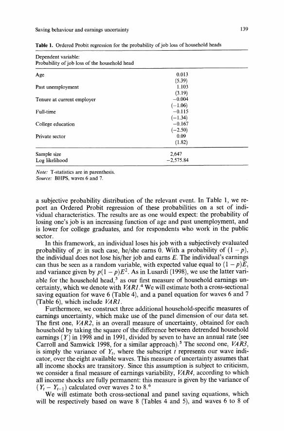
Saving behaviour and earnings uncertainty

Table 1. Ordered Probit regression for the probability of job loss of household heads

Dependent variable:Probability of job loss of the household head

139

Age

Past unemployment

Tenure at current employer

Full-time

College education

Private sector

Sample sizeLog likelihood

Note: T-statistics are in parenthesis.Source: BHPS, waves 6 and 7.

0.013(5.39)1.103(3.19)-0.004(-1.06)-0.115(-1.34)-0.167(-2.50)0.09(1.82)

2,647-2,575.84

a subjective probability distribution of the relevant event. In Table 1, we re­port an Ordered Probit regression of these probabilities on a set of indi­vidual characteristics. The results are as one would expect: the probability oflosing one's job is an increasing function of age and past unemployment, andis lower for college graduates, and for respondents who work in the publicsector.

In this framework, an individual loses his job with a subjectively evaluatedprobability of p: in such case, he/she earns O. With a probability of (1 - p),the individual does not lose his/her job and earns E. The individual's earningscan thus be seen as a random variable, with expected value equal to (1 - p)E,and variance given by p(l - p)E2• As in Lusardi (1998), we use the latter vari-able for the household head, 3 as our first measure of household earnings un­certainty, which we denote with VARI. 4 We will estimate both a cross-sectionalsaving equation for wave 6 (Table 4), and a panel equation for waves 6 and 7(Table 6), which include VARI.Furthermore, we construct three additional household-specific measures of

earnings uncertainty, which make use of the panel dimension of our data set.The first one, VAR2, is an overall measure of uncertainty, obtained for eachhousehold by taking the square of the difference between detrended householdearnings (Y) in 1998 and in 1991, divided by seven to have an annual rate (seeCarroll and Samwick 1998, for a similar approach).5 The second one, VARJ,is simply the variance of Yt , where the subscript t represents our wave indi­cator, over the eight available waves. This measure of uncertainty assumes thatall income shocks are transitory. Since this assumption is subject to criticism,we consider a final measure of earnings variability, VAR4, according to whichall income shocks are fully permanent: this measure is given by the variance of(1'; - 1';-1) calculated over waves 2 to 8.6

We will estimate both cross-sectional and panel saving equations, whichwill be respectively based on wave 8 (Tables 4 and 5), and waves 6 to 8 of

140 A. Guariglia

the survey (Table 6), and will include in turn VAR2, VARJ, and VAR4. In thepanel regressions, we will allow our measures of earnings uncertainty to varyacross waves. In general terms, VAR2 t (t = 6,7,8) will be defined as the dif­ference between Y; and YI, divided by (t - I) to have an annual rate. Simi­larly, VARJ t (VAR4t ) will be defined as the variance of Y;(Y; - Y;-I) in thet(t - I) waves of the survey preceding and including year t. 7 This procedureassumes that households update their perceived earnings uncertainty in eachwave, using the information on earnings that becomes available.

3.3. Sample restrictions and descriptive statistics

As in Carroll and Samwick (1997), we restrict our sample to households wherethe same person is head in each year, and where the spouse/partner, if present,remains the same. We exclude those households whose head is younger than25 or older than 65, and those who do not have valid data on saving and netearnings.In those specifications that use VARI as a measure of earnings uncertainty,

we further restrict the sample to those households whose head is in employ­ment. 8 Since information on the subjective probabilities of job loss is onlyprovided in waves 6 and 7 of the survey, the sample that can be used in esti­mation is limited to those two waves and consists of 2,750 household-years.In those specifications which use VAR2, VARJ, or VAR4 as measures of

earnings uncertainty, the data set is restricted to those households who havebeen present in all the waves (balanced panel). We want in fact our measuresof earnings variability to be calculated over the same number of years for eachhousehold. We also limit the sample to those households where at least onemember was in paid employment in one or more of the eight waves. Moreover,as in Carroll and Samwick (1997), we exclude those households whose earn­ings in any year were less than 20% of the average over the period. If thesehouseholds were included, our measures of earnings variability would be dom­inated by these few observations. Finally, since we calculate the variances overperiods of at least six years, the waves that can be used in estimation in thiscase are waves 6 to 8, corresponding to 1,785 household-years.In Table 2, we present descriptive statistics for the two samples de­

scribed above. The Table reports the percentage of households where at leastone member saved in the relevant period, and the average montWy saving ofthese households. We distinguish households by demographic characteristics,age, education and occupation of the head. About 65% of the households savewhen we consider the first sub-sample. The corresponding figure for the secondsub-sample is 73%. As expected, the highest proportions of households whosave can be found among married or cohabiting couples with no dependentchildren, among the more educated groups, and among the managers andadministrators, and the professional, associate professional, and technical oc­cupational categories. The non-zero average monthly saving is also generallyhigher for the above mentioned categories. Finally, looking at the differencesin saving behaviour across age groups, we can see that in both sub-samples,those households whose head is aged between 35 and 44 are characterised bylower non-zero average monthly saving.Table 3 describes how our measures of uncertainty differ across age, edu-

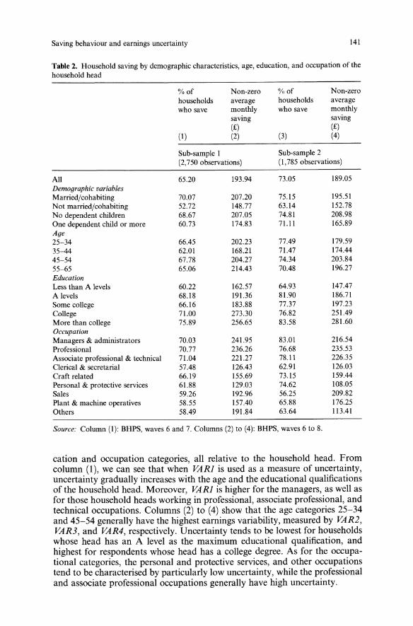
Saving behaviour and earnings uncertainty 141

Table 2. Household saving by demographic characteristics, age, education, and occupation of thehousehold head

%of Non-zero %of Non-zerohouseholds average households averagewho save monthly who save monthly

saving saving(£) (£)

(1 ) (2) (3) (4)

Sub-sample I Sub-sample 2(2,750 observations) (1,785 observations)

All 65.20 193.94 73.05 189.05Demographic variablesMarried/cohabiting 70.07 207.20 75.15 195.51Not married/cohabiting 52.72 148.77 63.14 152.78No dependent children 68.67 207.05 74.81 208.98One dependent child or more 60.73 174.83 71.11 165.89Age25-34 66.45 202.23 77.49 179.5935-44 62.01 168.21 71.47 174.4445-54 67.78 204.27 74.34 203.8455-65 65.06 214.43 70.48 196.27EducationLess than A levels 60.22 162.57 64.93 147.47A levels 68.18 191.36 81.90 186.71Some college 66.16 183.88 77.37 197.23College 71.00 273.30 76.82 251.49More than college 75.89 256.65 83.58 281.60OccupationManagers & administrators 70.03 241.95 83.01 216.54Professional 70.77 236.26 76.68 235.53Associate professional & technical 71.04 221.27 78.11 226.35Clerical & secretarial 57.48 126.43 62.91 126.03Craft related 66.19 155.69 73.15 159.44Personal & protective services 61.88 129.03 74.62 108.05Sales 59.26 192.96 56.25 209.82Plant & machine operatives 58.55 157.40 65.88 176.25Others 58.49 191.84 63.64 113.41

Source: Column (I): BHPS, waves 6 and 7. Columns (2) to (4): BHPS, waves 6 to 8.

cation and occupation categories, all relative to the household head. Fromcolumn (I), we can see that when VARI is used as a measure of uncertainty,uncertainty gradually increases with the age and the educational qualificationsof the household head. Moreover, VARI is higher for the managers, as well asfor those household heads working in professional, associate professional, andtechnical occupations. Columns (2) to (4) show that the age categories 25-34and 45-54 generally have the highest earnings variability, measured by VAR2,VAR3, and VAR4, respectively. Uncertainty tends to be lowest for householdswhose head has an A level as the maximum educational qualification, andhighest for respondents whose head has a college degree. As for the occupa­tional categories, the personal and protective services, and other occupationstend to be characterised by particularly low uncertainty, while the professionaland associate professional occupations generally have high uncertainty.

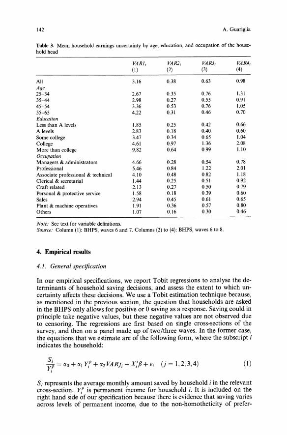
142 A. Guariglia

Table 3. Mean household earnings uncertainty by age, education, and occupation of the house­hold head

VARI, VAR2, VAR3, VAR4,(I) (2) (3) (4)

All 3.16 0.38 0.63 0.98Age25-34 2.67 0.35 0.76 1.3135-44 2.98 0.27 0.55 0.9145-54 3.36 0.53 0.76 1.0555-65 4.22 0.31 0.46 0.70EducationLess than A levels 1.85 0.25 0.42 0.66A levels 2.83 0.18 0.40 0.60Some college 3.47 0.34 0.65 1.04College 4.61 0.97 1.36 2.08More than college 9.82 0.64 0.99 1.10OccupationManagers & administrators 4.66 0.28 0.54 0.78Professional 5.46 0.84 1.22 2.01Associate professional & technical 4.10 0.48 0.82 1.18Clerical & secretarial 1.44 0.25 0.51 0.92Craft related 2.13 0.27 0.50 0.79Personal & protective service 1.58 0.18 0.39 0.60Sales 2.94 0.45 0.61 0.65Plant & machine operatives 1.91 0.36 0.57 0.80Others 1.07 0.16 0.30 0.46

Note: See text for variable definitions.Source: Column (I): BHPS, waves 6 and 7. Columns (2) to (4): BHPS, waves 6 to 8.

4. Empirical results

4.1. General specification

In our empirical specifications, we report Tobit regressions to analyse the de­terminants of household saving decisions, and assess the extent to which un­certainty affects these decisions. We use a Tobit estimation technique because,as mentioned in the previous section, the question that households are askedin the BHPS only allows for positive or 0 saving as a response. Saving could inprinciple take negative values, but these negative values are not observed dueto censoring. The regressions are first based on single cross-sections of thesurvey, and then on a panel made up of two/three waves. In the former case,the equations that we estimate are of the following form, where the subscript iindicates the household:

Si _ P . I )y p - IXo + IXI Yi + IX2 VAR); + Xi P+ ei (j = 1,2,3,4,(I)

Si represents the average monthly amount saved by household i in the relevantcross-section. Y( is permanent income for household i. It is included on theright hand side of our specification because there is evidence that saving variesacross levels of permanent income, due to the non-homotheticity of prefer-

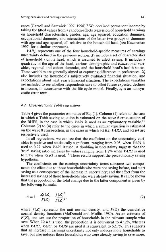
Saving behaviour and earnings uncertainty 143

ences (Carroll and Samwick 1997, 1998).9 We obtained permanent income bytaking the fitted values from a random-effects regression of household earningson household characteristics, gender, age, age squared, education dummies,occupational dummies, and interactions of the latter two groups of dummieswith age and age squared, all relative to the household head (see Kazarosian1997, for a similar approach).

VARji represents one of the four household-specific measures of earningsuncertainty defined in the previous section. Xi includes a set of characteristicsof household i or its head, which is assumed to affect saving. It includes aquadratic in the age of the head, various demographic and educational vari­ables, regional and cohort dummies, and the household head's health status.These variables are generally aimed at capturing differences in preferences. Xialso includes the household's subjectively evaluated financial situation, andexpectations about next year's financial situation. The expectations variablesare included to see whether respondents save to offset future expected declinesin income, in accordance with the life cycle model. Finally, ei is an idiosyn­cratic error term.

4.2. Cross-sectional Tobit regressions

Table 4 gives the parameter estimates of Eq. (1). Column (1) refers to the casein which a Tobit saving equation is estimated on the wave 6 cross-section ofthe BHPS, in the case in which VARI is used as an explanatory variable. 1o

Columns (2) to (4) refer to the cases in which a similar equation is estimatedon the wave 8 cross-section, in the cases in which VAR2, VARJ, and VAR4 arerespectively used.

In all regressions, we can see that the coefficient on the uncertainty vari­ables is positive and statistically significant, ranging from 0.05, when VARI isused to 0.27, when VARJ is used. A doubling in uncertainty suggests that the'true' saving ratio increases by values ranging from 1.8% when VAR2 is usedto 5.7% when VARI is used. 11 These results support the precautionary savinghypothesis.The coefficients on the earnings uncertainty terms subsume two compo­

nents: the effect due to those households who were not saving before, and startsaving as a consequence of the increase in uncertainty; and the effect from theincreased savings of those households who were already saving. It can be shownthat the proportion of the total change due to the latter component is given bythe following formula:

A = 1 _ Zj(Z) _ j(Z)2F(Z) F(Z)2'

(2)

where j(Z) represents the unit normal density, and F(Z) the cumulativenormal density functions (McDonald and Moffitt 1980). As an estimate ofF(Z), one can use the proportion of households in the relevant sample whosave. When VARI is used, the proportion A is equivalent to 47.2%, whereaswhen VAR2, VARJ, or VAR4 are used it is equivalent to 52.7%. This suggeststhat an increase in earnings uncertainty not only induces more households tosave, but also induces those households who were already saving to save more.

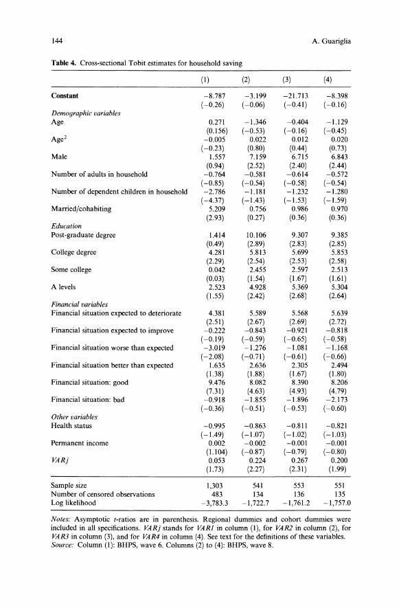
144 A. Guariglia

Table 4. Cross-sectional Tobit estimates for household saving

(I) (2) (3) (4)

Constant -8.787 -3.199 -21.713 -8.398(-0.26) (-0.06) (-0.41) (-0.16)

Demographic variablesAge 0.271 -1.346 -0.404 -1.129

(0.156) (-0.53) (-0.16) (-0.45)Age 2 -0.005 0.022 0.012 0.020

(-0.23) (0.80) (0.44) (0.73)Male 1.557 7.159 6.715 6.843

(0.94) (2.52) (2.40) (2.44)Number of adults in household -0.764 -0.581 -0.614 -0.572

(-0.85) (-0.54) (-0.58) (-0.54)Number of dependent children in household -2.786 -1.181 -1.232 -1.280

(-4.37) (-1.43) (-1.53) (-1.59)Married/cohabiting 5.209 0.756 0.986 0.970

(2.93) (0.27) (0.36) (0.36)EducationPost-graduate degree 1.414 10.106 9.307 9.385

(0.49) (2.89) (2.83) (2.85)College degree 4.281 5.813 5.699 5.853

(2.29) (2.54) (2.53) (2.58)Some college 0.042 2.455 2.597 2.513

(0.03) (1.54) (1.67) (1.61)A levels 2.523 4.928 5.369 5.304

(1.55) (2.42) (2.68) (2.64)Financial variablesFinancial situation expected to deteriorate 4.381 5.589 5.568 5.639

(2.51) (2.67) (2.69) (2.72)Financial situation expected to improve -0.222 -0.843 -0.921 -0.818

(-0.19) (-0.59) (-0.65) (-0.58)Financial situation worse than expected -3.019 -1.276 -1.081 -1.168

(-2.08) (-0.71) (-0.61) (-0.66)Financial situation better than expected 1.635 2.636 2.305 2.494

(1.38) (1.88) (1.67) (1.80)Financial situation: good 9.476 8.082 8.390 8.206

(7.31) (4.63) (4.93) (4.79)Financial situation: bad -0.918 -1.855 -1.896 -2.173

(-0.36) (-0.51) (-0.53) (-0.60)Other variablesHealth status -0.995 -0.863 -0.811 -0.821

(-1.49) (-1.07) (-1.02) (-1.03)Permanent income 0.002 -0.002 -0.001 -0.001

(1.104) (-0.87) (-0.79) (-0.80)VARj 0.053 0.224 0.267 0.200

(1.73) (2.27) (2.31) (1.99)

Sample size 1,303 541 553 551Number of censored observations 483 134 136 135Log likelihood -3,783.3 -1,722.7 -1,761.2 -1,757.0

Notes: Asymptotic t-ratios are in parenthesis. Regional dummies and cohort dummies wereincluded in all specifications. VARj stands for VARI in column (I), for VARl in column (2), forVARJ in column (3), and for VAR4 in column (4). See text for the definitions of these variables.Source: Column (I): BHPS, wave 6. Columns (2) to (4): BHPS, wave 8.

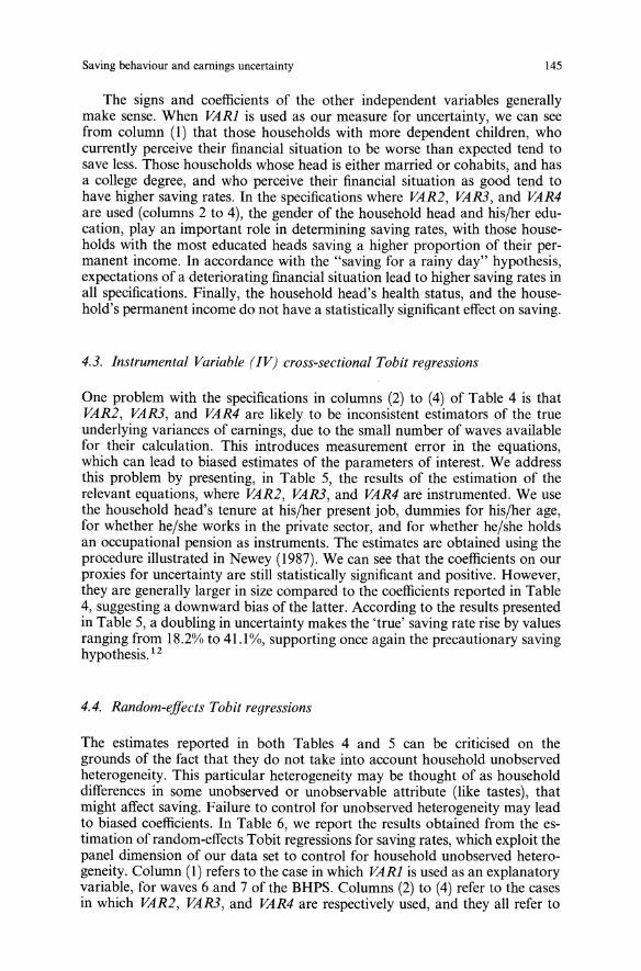
Saving behaviour and earnings uncertainty 145

The signs and coefficients of the other independent variables generallymake sense. When VARI is used as our measure for uncertainty, we can seefrom column (1) that those households with more dependent children, whocurrently perceive their financial situation to be worse than expected tend tosave less. Those households whose head is either married or cohabits, and hasa college degree, and who perceive their financial situation as good tend tohave higher saving rates. In the specifications where VAR2, VARJ, and VAR4are used (columns 2 to 4), the gender of the household head and his/her edu­cation, play an important role in determining saving rates, with those house­holds with the most educated heads saving a higher proportion of their per­manent income. In accordance with the "saving for a rainy day" hypothesis,expectations of a deteriorating financial situation lead to higher saving rates inall specifications. Finally, the household head's health status, and the house­hold's permanent income do not have a statistically significant effect on saving.

4.3. Instrumental Variable (IV) cross-sectional Tobit regressions

One problem with the specifications in columns (2) to (4) of Table 4 is thatVAR2, VAR3, and VAR4 are likely to be inconsistent estimators of the trueunderlying variances of earnings, due to the small number of waves availablefor their calculation. This introduces measurement error in the equations,which can lead to biased estimates of the parameters of interest. We addressthis problem by presenting, in Table 5, the results of the estimation of therelevant equations, where VAR2, VAR3, and VAR4 are instrumented. We usethe household head's tenure at his/her present job, dummies for his/her age,for whether he/she works in the private sector, and for whether he/she holdsan occupational pension as instruments. The estimates are obtained using theprocedure illustrated in Newey (1987). We can see that the coefficients on ourproxies for uncertainty are still statistically significant and positive. However,they are generally larger in size compared to the coefficients reported in Table4, suggesting a downward bias of the latter. According to the results presentedin Table 5, a doubling in uncertainty makes the 'true' saving rate rise by valuesranging from 18.2% to 41.1%, supporting once again the precautionary savinghypothesis. 12

4.4. Random-effects Tobit regressions

The estimates reported in both Tables 4 and 5 can be criticised on thegrounds of the fact that they do not take into account household unobservedheterogeneity. This particular heterogeneity may be thought of as householddifferences in some unobserved or unobservable attribute (like tastes), thatmight affect saving. Failure to control for unobserved heterogeneity may leadto biased coefficients. In Table 6, we report the results obtained from the es­timation of random-effects Tobit regressions for saving rates, which exploit thepanel dimension of our data set to control for household unobserved hetero­geneity. Column (1) refers to the case in which VARI is used as an explanatoryvariable, for waves 6 and 7 of the BHPS. Columns (2) to (4) refer to the casesin which VAR2, VARJ, and VAR4 are respectively used, and they all refer to

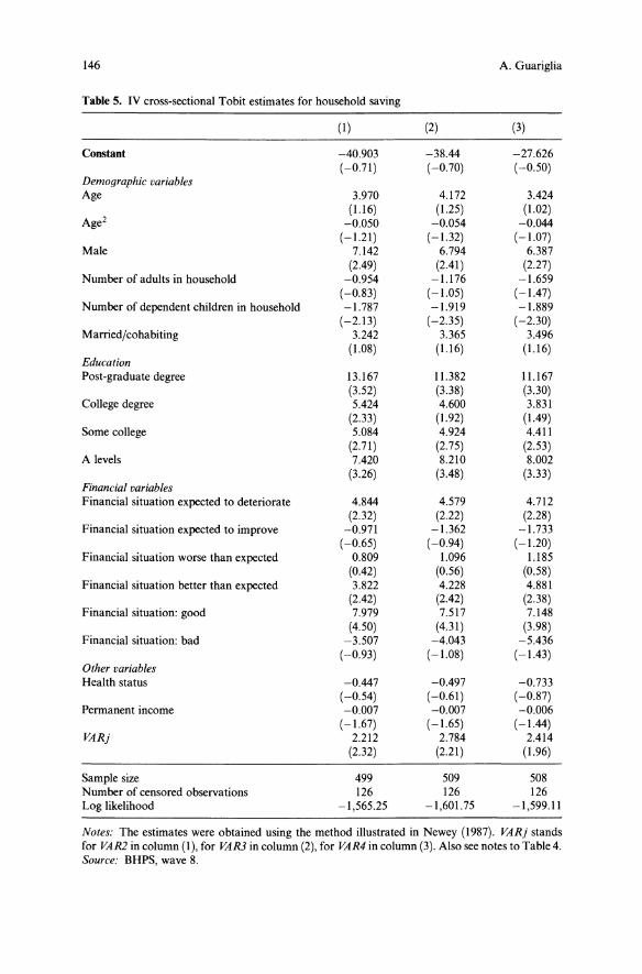
146 A. Guariglia

Table 5. IV cross-sectional Tobit estimates for household saving

(I) (2) (3)

Constant -40.903 -38.44 -27.626(-0.71) (-0.70) (-0.50)

Demographic variablesAge 3.970 4.172 3.424

(1.16) (1.25) (1.02)Age2 -0.050 -0.054 -0.044

(-1.21) (-1.32) (-1.07)Male 7.142 6.794 6.387

(2.49) (2.41) (2.27)Number of adults in household -0.954 -1.176 -1.659

(-0.83) (-1.05) (-1.47)Number of dependent children in household -1.787 -1.919 -1.889

(-2.13) (-2.35) (-2.30)Married/cohabiting 3.242 3.365 3.496

(1.08) (1.16) (1.16)EducationPost-graduate degree 13.167 11.382 11.167

(3.52) (3.38) (3.30)College degree 5.424 4.600 3.831

(2.33) (1.92) (1.49)Some college 5.084 4.924 4.4]]

(2.71) (2.75) (2.53)A levels 7.420 8.210 8.002

(3.26) (3.48) (3.33)Financial variablesFinancial situation expected to deteriorate 4.844 4.579 4.712

(2.32) (2.22) (2.28)Financial situation expected to improve -0.971 -1.362 -1.733

(-0.65) (-0.94) (-1.20)Financial situation worse than expected 0.809 1.096 1.185

(0.42) (0.56) (0.58)Financial situation better than expected 3.822 4.228 4.881

(2.42) (2.42) (2.38)Financial situation: good 7.979 7.517 7.148

(4.50) (4.31) (3.98)Financial situation: bad -3.507 -4.043 -5.436

(-0.93) (-1.08) (-1.43)Other variablesHealth status -0.447 -0.497 -0.733

(-0.54) (-0.61) (-0.87)Permanent income -0.007 -0.007 -0.006

(-1.67) (-1.65) (-1.44)VARj 2.212 2.784 2.414

(2.32) (2.21) (1.96)

Sample size 499 509 508Number of censored observations 126 126 126Log likelihood -1,565.25 -1,601.75 -1,599.]]

Notes: The estimates were obtained using the method illustrated in Newey (1987). VARj standsfor VAR2 in column (I), for VARJ in column (2), for VAR4 in column (3). Also see notes to Table 4.Source: BHPS, wave 8.

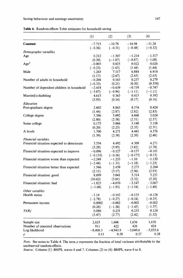
Saving behaviour and earnings uncertainty 147

Table 6. Random-effects Tobit estimates for household saving

(I) (2) (3) (4)

Constant -7.715 -10.78 -16.98 -11.28(-0.36) (-0.31) (-0.48) (-0.32)

Demographic variablesAge 0.212 -1.507 -1.214 -1.517

(0.20) (-1.07) (-0.87) (-1.08)Age2 -0.003 0.025 0.022 0.026

(-0.23) (1.63) (1.44) (1.64)Male 1.243 7.117 6.884 6.914

(1.17) (2.67) (2.63) (2.63)Number of adults in household -0.204 0.163 0.237 0.279

(-0.35) (0.21) (0.30) (0.354)Number of dependent children in household -2.418 -0.639 -0.739 -0.747

(-5.87) (-0.94) (-1.11) (-1.11)Married/cohabiting 4.615 0.363 0.415 0.392

(3.95) (0.14) (0.17) (0.16)EducationPost-graduate degree 2.602 8.845 8.374 8.424

(1.44) (2.87) (2.82) (2.83)College degree 3.396 5.092 4.868 5.024

(2.80) (2.58) (2.51) (2.57)Some college 0.175 3.066 3.148 3.108

(0.20) (2.25) (2.35) (2.31)A levels 1.700 4.271 4.441 4.376

(1.59) (2.38) (2.50) (2.46)Financial variablesFinancial situation expected to deteriorate 3.554 4.492 4.309 4.271

(3.29) (3.95) (3.82) (3.78)Financial situation expected to improve -0.096 -0.127 -0.137 -0.101

(-0.133) (-0.16) (-0.175) (-0.13)Financial situation worse than expected -2.248 -1.253 -1.10 -1.150

(-2.48) (-1.33) (-1.18) (-1.23)Financial situation better than expected 1.546 2.459 2.273 2.264

(2.11) (3.17) (2.96) (2.93)Financial situation: good 8.699 5.041 5.314 5.221

(10.62) (5.01) (5.32) (5.20)Financial situation: bad -1.823 -4.070 -3.147 -3.067

(-1.08) (-1.93) (-1.54) (-1.49)Other variablesHealth status -1.14 -0.142 -0.125 -0.128

(-2.78) (-0.27) (-0.24) (-0.25)Permanent income 0.0002 -0.002 -0.002 -0.002

(0.26) (-1.56) (-1.43) (-1.37)VARj 0.086 0.231 0.235 0.124

(3.47) (2.77) (2.42) (1.52)

Sample size 2,623 1,606 1,636 1,630Number of censored observations 911 422 426 424Log likelihood -8,406.3 -4,943.9 -5,049.6 -5,035.6p 0.11 0.58 0.57 0.58

Note: See notes to Table 4. The term p represents the fraction of total variance attributable to theunobserved random-effects.Source: Column (I): BHPS, waves 6 and 7. Columns (2) to (4): BHPS, wave 6 to 8.

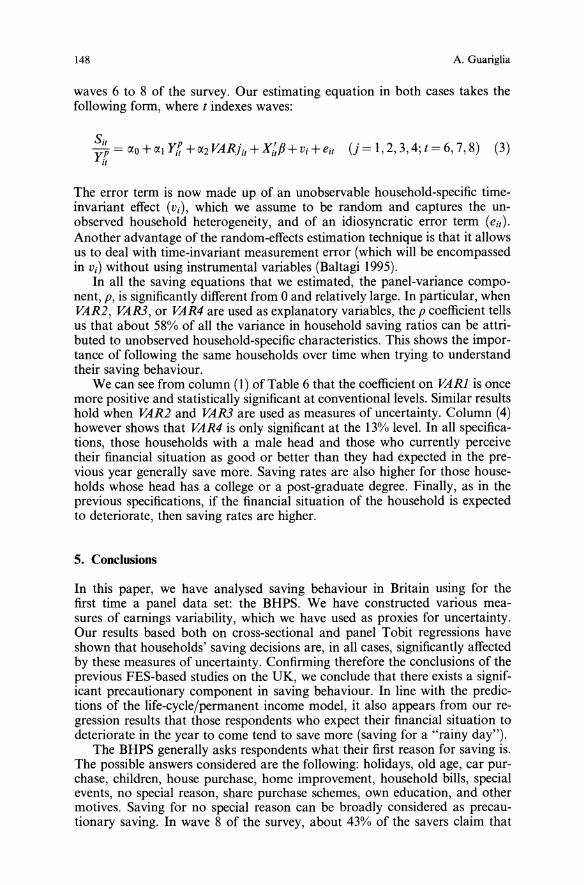
148 A. Guariglia

waves 6 to 8 of the survey. Our estimating equation in both cases takes thefollowing form, where t indexes waves:

Sit _ yP J,T AR . X'PyP - Cto+Ctt it + Ct21'./1 Jit+ it +Vi+eitII

(j= 1,2,3,4;t=6, 7,8) (3)

The error term is now made up of an unobservable household-specific time­invariant effect (Vi), which we assume to be random and captures the un­observed household heterogeneity, and of an idiosyncratic error term (eit).Another advantage of the random-effects estimation technique is that it allowsus to deal with time-invariant measurement error (which will be encompassedin Vi) without using instrumental variables (Baltagi 1995).In all the saving equations that we estimated, the panel-variance compo­

nent, p, is significantly different from 0 and relatively large. In particular, whenVAR2, VARJ, or VAR4 are used as explanatory variables, the p coefficient tellsus that about 58% of all the variance in household saving ratios can be attri­buted to unobserved household-specific characteristics. This shows the impor­tance of following the same households over time when trying to understandtheir saving behaviour.We can see from column (1) of Table 6 that the coefficient on VARl is once

more positive and statistically significant at conventional levels. Similar resultshold when VAR2 and VAR3 are used as measures of uncertainty. Column (4)however shows that VAR4 is only significant at the 13% level. In all specifica­tions, those households with a male head and those who currently perceivetheir financial situation as good or better than they had expected in the pre­vious year generally save more. Saving rates are also higher for those house­holds whose head has a college or a post-graduate degree. Finally, as in theprevious specifications, if the financial situation of the household is expectedto deteriorate, then saving rates are higher.

5. Conclusions

In this paper, we have analysed saving behaviour in Britain using for thefirst time a panel data set: the BHPS. We have constructed various mea­sures of earnings variability, which we have used as proxies for uncertainty.Our results based both on cross-sectional and panel Tobit regressions haveshown that households' saving decisions are, in all cases, significantly affectedby these measures of uncertainty. Confirming therefore the conclusions of theprevious FES-based studies on the UK, we conclude that there exists a signif­icant precautionary component in saving behaviour. In line with the predic­tions of the life-cycle/permanent income model, it also appears from our re­gression results that those respondents who expect their financial situation todeteriorate in the year to come tend to save more (saving for a "rainy day").The BHPS generally asks respondents what their first reason for saving is.

The possible answers considered are the following: holidays, old age, car pur­chase, children, house purchase, home improvement, household bills, specialevents, no special reason, share purchase schemes, own education, and othermotives. Saving for no special reason can be broadly considered as precau­tionary saving. In wave 8 of the survey, about 43% of the savers claim that

Saving behaviour and earnings uncertainty 149

they save for no special reason. This tends to confirm our results of a strongprecautionary motive for saving.Earnings variability is however not the only possible source of uncertainty.

Health risk and longevity risk might also playa significant part in determiningindividuals' saving behaviour. These alternative types of uncertainty, needfurther investigation on British data. This will be the object of future research.

Endnotes

[ Infonnation is provided both at the individual and the household level. For more details on theBHPS, see Taylor (1994) and Taylor (1999).

2 The variables are deflated using the Retail Price Index.3 Following Guiso et al. (1992) and Lusardi (1997, 1998), we can justify this procedure by theunderlying assumption that the variance of household earnings can be reasonably proxied bythe variance of the earnings of the head of the household.

4 Note that we do not use the respondents' subjective probability of job loss (p) itself as a proxyfor uncertainty for the following reason. Suppose that an individual is certain that he/she willlose his/her job in the near future, due to an announced close down of the finn where he/sheworks. In this case, if the individual saves more, his/her extra saving cannot be classified asprecautionary: Increased saving in response to an expected drop in the mean of future incomearises in fact in a standard certainty equivalence model (see Alessie and Lusardi 1997, for aninvestigation of this issue). One limitation of our approach is that it only takes into account theprobability of job loss in the next twelve months, and not afterwards.

5 Since we are trying to measure uncertainty, we are not interested in that part of the variabilityof earnings, which is due to predictable life-cycle changes in earnings. In our fonnulas forVAR2, VARJ, and VAR4, we therefore use detrended net monthly household earnings (Y). Weobtain Y by taking the residuals from a random-effects regression of net monthly householdearnings on household characteristics, gender, age, age squared, educational and occupationalcharacteristics, and interactions of the latter two groups of dummy variables with age and agesquared (all relative to the household head).

6 We thank an anonymous referee for suggesting this alternative measure of uncertainty.7 This framework assumes that households consider past earnings volatility as a measure oflikely future volatility. See Guariglia and Rossi (2001) for evidence on the fact that in theBHPS, there appears to be some fonn of ARCH behaviour in earnings, which would justifythe above assumption. Also see Banks et al. (1999) who make a similar assumption.

S We exclude the self-employed because a measure of net earnings is not provided for them.9 Yt can also be seen as a proxy for household wealth.10 Similar results were obtained for wave 7. We do not report them for brevity.[1 These numbers are elasticities, evaluated at sample means. By 'true' saving rate, we mean thelatent variable underlying the Tobit model. We thank an anonymous referee for suggesting thiscalculation.

[2 The R2s in the first stage regressions are respectively 0.104,0.112, and 0.111, when VAR2,VARJ, and VAR4 are the variables instrumented for.

References

Alessie R, Lusardi A (1997) Saving and Income Smoothing: Evidence from Panel Data. EuropeanEconomic Review 41:1251-1279

Baltagi B (1995) Econometric Analysis of Panel Data. Wiley, ChichesterBanks J, Blundell R, Brugiavini A (1999) Risk Pooling, Precautionary Saving and ConsumptionGrowth. Working Paper No. W99/19, Institute for Fiscal Studies

Banks J, Dilnot A, Low H (1994) The Distribution of Wealth in the UK. Commentary No. 45,Institute for Fiscal Studies

Browning M, Lusardi A (1996) Household Saving: Micro Theories and Micro Facts. Journal ofEconomic Literature 34:1797-1855

150 A. Guariglia

Carroll C, Samwick A (1997) The Nature of Precautionary Wealth. Journal of Monetary Eco­nomics 40:41-71

Carroll C, Samwick A (1998) How Important is Precautionary Saving? Review of Economics andStatistics 80:410-419

Dardanoni V (1991) Precautionary Savings under Income Uncertainty: A Cross-Sectional Anal-ysis. Applied Economics 23: 153-160

Dynan K (1993) How Prudent are Consumers? Journal of Political Economy 101(6):1104-1113Friedman M (1957) A Theory of the Consumption Function. Princeton University Press, PrincetonGuariglia A, Rossi M (2001) Consumption, Habit Formation, and Precautionary Saving: Evi-dence from the British Household Panel Survey. Oxford Economic Papers (forthcoming)

Guiso L, Jappelli T, Terlizzese D (1992) Earnings Uncertainty and Precautionary Saving. Journalof Monetary Economics 30:307-337

Kazarosian M (1997) Precautionary Savings- A Panel Study. Review of Economics and Statistics79(2):241-247

Kuehlwein M (1991) A Test for the Presence of Precautionary Saving. Economics Letters 37:471­475

Lusardi A (1997) Precautionary Saving and Subjective Earning Variance. Economics Letters57:319-326

Lusardi A (1998) On the Importance of the Precautionary Saving Motive. American EconomicReview Papers and Proceedings 88(2):449-453

McDonald J, Moffitt R (1980) The Uses of Tobit Analysis. Review of Economics and Statistics62:318-321

Merrigan P, Normandin M (1996) Precautionary Saving Motives: An Assessment from UK TimeSeries of Cross-Sections. Economic Journal I06: 1193-1208

Miles D (1997) A Household Level Study of the Determinants of Income and Consumption.Economic Journal 107:1-25

Modigliani F, Brumberg R (1954) Utility Analysis and the Consumption Function: An Interpre­tation of the Cross-Section Data. In: Kurihara K (ed) Post-Keynesian Economics. RutgersUniversity Press, New Brunswick

Newey W (1987) Efficient Estimation of Limited Dependent Variable Models with EndogenousExplanatory Variables. Journal of Econometrics 36:231-250

Schmidt-Hebbel K, Serven L (1997) Saving across the World. Puzzles and Policies. DiscussionPaper No. 354, The World Bank

Taylor A (1994) Appendix: Sample Characteristics, Attrition and Weighting. In: Buck N,Gershuny J, Rose D, Scott J (eds) Changing Households: The British Household Panel Survey1990-1992. ESRC Research Center on Micro-Social Change, University of Essex

Taylor M (ed) (1999) British Household Panel Survey User Manual Volume A: Introduction,Technical Reports, and Appendices. ESRC Research Center on Micro-Social Change, Uni­versity of Essex

Family structure and children's achievements

John F. Ermisch, Marco Francesconi

Institute for Social and Economic Research, University of Essex, Colchester C04 3SQ,United Kingdom (Fax: ++44-1206-873151; e-mail: mfranc@essex.ac.uk)

Received: 24 August 1998/Accepted: 21 January 2000

Abstract. In this paper we estimate the relationships between several outcomesin early adulthood (educational attainment, economic inactivity, early child­bearing, distress and smoking) and experience of life in a single-parent familyduring childhood. The analysis is performed using a special sample of youngadults, who are selected from the first five waves of the British HouseholdPanel Survey (1991-95) and can be matched with at least one sibling over thesame period. We also perform level (logit) estimation using another sample ofyoung adults from the BHPS. We find that: (i) experience of life in a single­parent family is usually associated with disadvantageous outcomes for youngadults; (ii) most of the unfavourable outcomes are linked to an early familydisruption, when the child was aged 0-5; and (iii) level estimates, whosecausal interpretation relies on stronger assumptions, confirm the previous re­sults and show that, for most outcomes, the adverse family structure effectpersists even after controlling for the economic conditions of the family oforigin.

JEL classification: 112, 120, 130

Key words: Family structure, intergenerational links, siblings estimators

All correspondence to Marco Francesconi. We are grateful to Nick Buck, Irwin Garfinkel, RobertHaveman, Martha Hill, Stephen Jenkins, Sara McLanahan, Wilbert van der Klaauw, BarbaraWolfe, and seminar participants at the London School of Economics, University of Essex, and theEuropean Society for Population Economics June 1998 (Amsterdam) for useful discussions andsuggestions, and especially to two anonymous referees for helpful comments on earlier version ofthis paper. The financial support of the Economic and Social Research Council and the Depart­ment of Social Security is gratefully acknowledged. The views expressed in this paper are those ofthe authors and do not necessarily reflect those of the ESRC or DSS. Responsible editor: T. PaulSchultz.

152

1. Introduction

J.F. Ermisch, M. Francesconi

This paper asks whether a number of outcomes in early adulthood are asso­ciated with experience of life in a single-parent family during childhood.Economists have long identified the family as one the most importantinstitutions in a market economy that fosters the transmission of incomeinequality over time (Knight 1935; Becker 1981) and may act as a potentialincome equaliser across family members (Griliches 1979). A large literaturehas extensively studied the effect of children on marital instability and otherhousehold behaviour (e.g., Becker et al. 1977; Browning 1992 for a survey).Only in recent years, however, has the intergenerational transmission ofhuman and social capital received empirical attention, with studies thatexamine the correlation between children's outcomes as young adults and avariety of parental circumstances and events during childhood, includingfamily structure. 1

A legitimate concern with much of this new literature is that the estimatedeffect of childhood family structure on children's achievements might be spur­ious (Manski et al. 1992; Mayer 1997). This is due to the mutual associationthat family structure and children's outcomes share with some unmeasuredtrue causal factor. For example, the association between having experiencedlife in a single-parent family and, say, experiencing difficulties in the labourmarket may not be necessarily the result of family structure during childhood.Rather, differences in labour market success may simply reflect the character­istics of families in which the children of single mothers are brought up.For a broad set of young people's outcomes (education, inactivity, earlychildbearing and health), we estimate both level (cross-sectional) models andfamily-specific fixed-effects models. 2

Although the use of sibling data has become increasingly common ineconomics, most of the empirical studies linking parents' behaviour andchildren's attainments have not addressed the problem of unmeasured heter­ogeneity with sibling estimators. 3 We show that the effect of family structureon outcomes can be identified with sibling differences if family structure doesnot respond to "idiosyncratic endowments" of children. On this assumption,our sibling-difference estimates would measure the causal impact of childhoodfamily structure on young adults' achievements. But note that, in addition toinherent differences between siblings (e.g., one born with a disability), differ­ences between siblings in their idiosyncratic endowments include differencesover time in parental attitudes and behaviour which may affect both familystructure and children's outcomes. For example, the father may develop analcohol addiction, giving rise to a situation in which an elder sibling spendsonly a small part of his childhood with an alcoholic father while the youngesthas one for most of her childhood. The father's alcohol problem may directlyaffect investment in the youngest child, and her parents may also divorcebecause of it, thereby causing correlation between idiosyncratic endowmentsand family structure. Thus, while the assumption of no such correlation isweaker than the assumptions needed in the cross-sectional model (see theAppendix), it is still a strong one. A causal interpretation of the level estimatesrelies on even stronger assumptions, but such estimates are useful for com­paring our results to those provided in other studies. It is, therefore, safest tointerpret both sets of estimates as suggestive associations, with the sibling­difference estimates controlling for more aspects of family background than

Family structure and children's achievements 153

the level estimates, making them less contaminated by unmeasured factorsassociated with both family structure and children's outcomes.Most of what we know of the relationship between family background and

children's outcomes is from the United States. Little is known about Britishcohorts born since 1958. In a recent study, Kiernan (1997) finds that, amongmembers of the 1958 birth cohort, divorce during childhood is associatedwith outcomes - for educational attainment, economic situation, partnershipformation and dissolution and parenthood behaviour in adulthood - whichwe would generally interpret to be worse than the same outcomes for youngadults from intact families. Similarly, the study by Fronstin et al. (forthcom­ing) suggests that a parental disruption adversely affects labour market out­comes of children at age 33 (in 1991). Their results indicate that the effectoccurs primarily through decreased employment for men and decreasedwage rates for women. These studies build on earlier research by Elliot andRichards (1991), Ni Bhrolchain et al. (1994) and Kiernan (1996) on schoolingand socio-economic performance, and Kiernan (1992) and Cherlin et al.(1995) on demographic outcomes. All use samples from the National ChildDevelopment Study (NCDS) for the 1958 birth cohort.Our analysis uses, instead, a special sample of young adults from the first

five waves (1991-1995) of the British Household Panel Survey (BHPS), whocan be matched with at least one sibling over the same period. 4 These youngadults are then linked to their mothers' family history collected in the 1992wave, as well as to other information about the mother from the mother'sinterviews during the panel,s and they are followed over the panel years. Wealso analyse another sample, in which young adults need not be matched witha sibling, but, as in the Sibling Sample, they must live with their mothers for atleast one of the five panel years. The BHPS data have some clear advantagesover the NCDS data. They are a better reflection of contemporary impacts offamily background, which may be particularly important for that of familystructure, because the incidence of single parenthood is now much higher thanamong the parents of the 1958 cohort. Moreover, they allow for better (al­though not ideal) measurement of family economic circumstances. 6 Moreimportantly, with the information on siblings, they allow us to control forunobserved additive effects that are shared by children who belong to thesame family. 7

We find that experience of life in a single-parent family is typically asso­ciated with unfavourable outcomes for young adults. They achieve lowereducational levels, face higher risks of economic inactivity and early birth, andthey also have higher chances of smoking and feeling more distressed. Familystructure in early childhood (ages 0-5 of the child) has the strongest associa­tions with all the outcomes under analysis (similar to the impact of income onoutcomes found by Duncan et al. 1997).8 All these results also emerge withlevel estimates, whose causal interpretation relies on even stronger identifyingassumptions than in the case of sibling differences. Our level estimatesare consistent with most of the available evidence in this literature. As inMcLanahan (1997), they confirm that, for almost all the outcomes underanalysis, experience in a single-parent family during childhood still mattersafter taking the economic circumstances of the family of origin into account.The rest of the paper is organised as follows. Section 2 describes the data

and the estimation procedures, Sect. 3 presents our main results, and Sect. 4concludes. The Appendix outlines the identification problem that is common

154 J.F. Ennisch, M. Francesconi

to all studies of the relationship between family structure during childhoodand children's outcomes.

2. Data

2.1. Estimating samples and family background measures

The data come from a special sample selected using the first five waves of theBritish Household Panel Survey (BHPS). In Autumn 1991, the BHPS inter­viewed a representative sample of 5,500 households, containing about 10,000persons. The same individuals are reinterviewed each successive year, andif they leave their original households to fonn new households, all adultmembers of these new households are also interviewed. Similarly, children inoriginal households are interviewed when they reach the age of 16. Thus, thesample remains broadly representative of the population of Britain as itchanges through the I990s. 9The second wave (1992) of the BHPS contains retrospective infonnation

on complete fertility, marital and cohabitation histories for all adult panelmembers in that year. Our analysis proceeds as if all children lived with theirmothers throughout their years of dependency, which we assume to be untiltheir sixteenth birthday.lO This infonnation provides the basis for our familystructure measure: whether or not the young adult spent time in a single­parent family during his/her childhood. A child is defined as being brought upin an intact family if he/she lived continuously with both biological (or adop­tive) parents, up to his/her 16-th birthday. Thus, according to our definition, achild would have spent some time in a single-parent family if he/she ever livedwith a biological or adoptive mother who was not cohabiting nor marriedbefore his/her 16-th birthday, either because of a partnership dissolution orbecause he/she was born outside of a live-in partnership and the motherdid not cohabit or marry within one year of the birth. 11 This measure is alsobroken down by the timing of the start of a spell in a lone parent family,distinguishing between three different child developmental stages, ages 0-5,6-10, and 11-16.12By matching young adults with their mothers, we are also able to measure

other family background characteristics that would be unavailable otherwise,such as age of the mother at the young person's birth, mother's education,parents' real income when the child was aged 16 (or the youngest age at whichwe observe the child living with parents), whether or not parents are owner­occupiers, and if so, house value when the child was aged 16, years spent atthe address occupied by the child at age 16 and current age of the child. Wealso obtain infonnation on the smoking behaviour of the mother at the timethe mother and her young-adult child lived together, which will be used forone of the health-related outcomes defined below (smoking). In addition,the third wave (1993) of the BHPS contains retrospective infonnation on jobhistories for all adult panel members. 13 With this infonnation we detenninethe proportion of months that mothers worked in each of the three devel­opmental stages and over the entire childhood of the young adults. 14In our analysis, we use two samples. The first sample (labelled as "Indi­

vidual Sample") consists of 764 individuals who: (i) were observed living withtheir mother when aged 16 or 17 during any of the first five waves (1991-

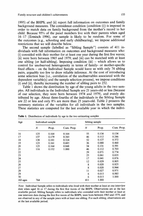
Family structure and children's achievements 155

1995) of the BHPS; and (ii) report full information on outcomes and familybackground measures. The coresidence condition (condition (i)) is imposed inorder to match data on family background from the mother's record to herchild. Because 95% of the panel members live with their parents when aged16-17 (Ermisch 1996), our sample is likely to be random. For some ofthe outcomes (e.g., schooling and early childbearing), we impose additionalrestrictions that we will describe below.The second sample (labelled as "Sibling Sample") consists of 411 in­

dividuals with full information on outcomes and background measures who:(i) coresided with their mother for at least one year during the first five waves;(ii) were born between 1965 and 1979; and (iii) can be matched with at leastone sibling (or half-sibling). Imposing condition (iii) - which allows us tocontrol for unobserved heterogeneity in terms of family- or mother-specificfixed effects - on the Individual Sample would leave us with only 74 siblingpairs, arguably too few to draw reliable inference. At the cost of introducingsome selection bias (i.e., correlation of the unobservables associated with thedependent variable(s) and the sample selection process), we impose conditions(i) and (ii), thereby increasing the number of sibling pairs to 252.Table 1 shows the distribution by age of the young adults in the two sam­

ples. All individuals in the Individual Sample are 21 years-old or less (becauseof our selection, they were born between 1974 and 1979), and evenly dis­tributed by age. About three-fourths of the individuals in the Sibling Sampleare 22 or less and only 8% are more than 25 years-old. Table 2 presents thesummary statistics of the variables for all individuals in the two samples.These statistics are computed for the last available year in which the indivi-

Table 1. Distribution of individuals by age in the two estimating samples

Age Individual sample Sibling sample

N Prop. Cum. Prop. N Prop. Cum. Prop.

16 125 0.164 0.164 55 0.134 0.13417 137 0.179 0.343 46 0.112 0.24618 138 0.181 0.524 52 0.127 0.37219 123 0.161 0.685 36 0.088 0.46020 125 0.164 0.848 54 0.131 0.59121 116 0.152 1.000 46 0.112 0.70322 29 0.071 0.77423 25 0.061 0.83524 17 0.041 0.87625 12 0.029 0.90526 8 0.020 0.92527 8 0.020 0.94428 11 0.027 0.97129 6 0.015 0.98530 6 0.015 1.000All ages 764 411 1.000

Note: Individual Sample refers to individuals who lived with their mother at least at one interviewdate when aged 16 or 17 during the first five waves of the BHPS. Observations are at the lastavailable period. Sibling Sample refers to individuals who coresided with their mother at least atone interview date during the first five waves of the BHPS, were born between 1965 and 1979, andare observed in any of the sample years with at least one sibling. For each sibling, observations areat the last available period.

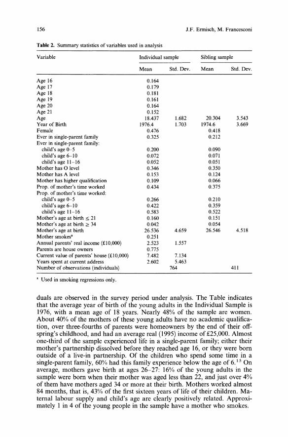
156 I.F. Ermisch, M. Francesconi

Table 2. Summary statistics of variables used in analysis

Variable Individual sample Sibling sample

Mean Std. Dev. Mean Std. Dev.

Age 16 0.164Age 17 0.179Age 18 0.181Age 19 0.161Age 20 0.164Age 21 0.152Age 18.437 1.682 20.304 3.543Year of Birth 1976.4 1.703 1974.6 3.669Female 0.476 0.418Ever in single-parent family 0.325 0.212Ever in single-parent family:child's age 0-5 0.200 0.090child's age 6-10 0.072 0.071child's age 11-16 0.052 0.051Mother has 0 level 0.346 0.350Mother has A level 0.153 0.124Mother has higher qualification 0.109 0.066Prop. of mother's time worked 0.434 0.375Prop. of mother's time worked:child's age 0-5 0.266 0.210child's age 6-10 0.422 0.359child's age 11-16 0.583 0.522Mother's age at birth::; 21 0.160 0.151Mother's age at birth ~ 34 0.042 0.054Mother's age at birth 26.536 4.659 26.546 4.518Mother smokes' 0.251Annual parents' real income (£10,000) 2.523 1.557Parents are house owners 0.775Current value of parents' house (£10,000) 7.482 7.134Years spent at current address 2.602 5.463Number of observations (individuals) 764 411

• Used in smoking regressions only.

duals are observed in the survey period under analysis. The Table indicatesthat the average year of birth of the young adults in the Individual Sample is1976, with a mean age of 18 years. Nearly 48% of the sample are women.About 40% of the mothers of these young adults have no academic qualifica­tion, over three-fourths of parents were homeowners by the end of their off­spring's childhood, and had an average real (1995) income of £25,000. Almostone-third of the sample experienced life in a single-parent family; either theirmother's partnership dissolved before they reached age 16, or they were bornoutside of a live-in partnership. Of the children who spend some time in asingle-parent family, 60% had this family experience below the age of 6.15 Onaverage, mothers gave birth at ages 26-27: 16% of the young adults in thesample were born when their mother was aged less than 22, and just over 4%of them have mothers aged 34 or more at their birth. Mothers worked almost84 months, that is, 43% of the first sixteen years of life of their children. Ma­ternal labour supply and child's age are clearly positively related. Approxi­mately 1 in 4 of the young people in the sample have a mother who smokes.

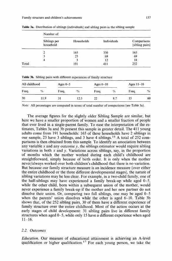
Family structure and children's achievements

Table 3a. Distribution of siblings (individuals) and sibling pairs in the sibling sample

157

Number of:

Siblings per Households Individuals Comparisonshousehold (sibling pairs)

2 165 330 1653 23 69 694 3 12 18

Total 191 411 252

Table 3b. Sibling pairs with different experiences of family structure

All childhood

Freq.

30

%

I\.9

Ages 0-5

Freq.

31

%

12.3

Ages 6-10

Freq.

22

%

8.7

Ages 11-16

Freq.

15

%

60

Note: All percentages are computed in terms of total number of comparisons (see Table 3a).

The average figures for the slightly older Sibling Sample are similar, buthere we have a smaller proportion of women and a smaller fraction of peoplethat ever lived in a single-parent family. To ease the interpretation of the es­timates, Tables 3a and 3b present this sample in greater detail. The 411 youngadults come from 191 households: 165 of these households have 2 siblings inour sample, 23 have 3 siblings, and 3 have 4 siblings. 16 A total of 252 com­parisons is then obtained from this sample. To identify an association betweenany variable x and any outcome y, the siblings estimator would require siblingvariations in both x and y. Variations across siblings, say, in the proportionof months which the mother worked during each child's childhood arestraightforward, simply because of birth order. It is only when the mothernever/always worked over both children's childhood that there is no variation.But because our family structure measure is an incidence measure (over eitherthe entire childhood or the three different developmental stages), the nature ofsibling variations may be less clear. For example, in a two-child family, one ofthe half-siblings may have experienced a family break-up while aged 0-5,while the other child, born within a subsequent union of the mother, wouldnever experience a family break-up if the mother and her new partner do notdissolve their union. Or, comparing two full siblings, one may be aged 0-5when the parents' union dissolves while the other is aged 6-10. Table 3bshows that, of the 252 sibling pairs, 30 of them have a different experience offamily structure over the entire childhood. Most of the action occurs at theearly stages of child development: 31 sibling pairs live in different familystructures when aged 0-5, while only 15 have a different experience when aged11-16.

2.2. Outcomes

Education. Our measure of educational attainment is achieving an A-levelqualification or higher qualification. 17 For each young person, we take the

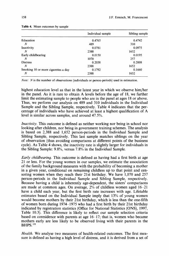
158

Table 4. Mean outcomes by sample

J.F. Ennisch, M. Francesconi

EducationNInactivity

NEarly childbearing

NDistress

NSmoking 10 or more cigarettes a day

N

Individual sample

0.47654890.0781

23880.0150

10700.2038

23880.1792

2388

Sibling sample

0.47423100.0975

16520.01952570.2008

16520.1660

1652

Note: N is the number of observations (individuals or person-periods) used in estimation.

highest education level as that in the latest year in which we observe him/herin the panel. As it is rare to obtain A levels before the age of 18, we furtherlimit the estimating sample to people who are in the panel at ages 18 or above.Thus, we perform our analysis on 489 and 310 individuals in the IndividualSample and the Sibling Sample, respectively. Table 4 indicates that the per­centage of individuals who have achieved at least a highest qualification of Alevel is similar across samples, and around 47.5%.

Inactivity. This outcome is defined as neither working nor being in school norlooking after children, nor being in government training schemes. The analysisis based on 2,388 and 1,652 person-periods in the Individual Sample andSibling Sample, respectively. This last sample matches siblings on the yearof observation (thus avoiding comparisons at different points of the businesscycle). As Table 4 shows, the inactivity rate is slightly larger for individuals inthe Sibling Sample: 9.8%, versus 7.8% in the Individual Sample.

Early childbearing. This outcome is defined as having had a first birth at age21 or less. For the young women in our samples, we estimate the associationof the family background measures with the probability of becoming a motherin a given year, conditional on remaining childless up to that point and cen­soring women when they reach their 21st birthday. We have 1,070 and 257person-periods in the Individual Sample and Sibling Sample, respectively.Because having a child is inherently age-dependent, the sisters' comparisonsare made at common ages. On average, 2% of childless women aged 16-21have a child each year, but the first birth rate increases with age. Lifetableestimates based on the Individual Sample imply that 13% of young womenwould become mothers by their 21 st birthday, which is less than the one-fifthof women born during 1974-1975 who had a first birth by their 21st birthdayindicated by registration statistics (Office for National Statistics (ONS), 1997,Table 10.3). This difference is likely to reflect our sample selection criteriabased on coresidence with parents at age 16-17; that is, women who becamemothers early are less likely to be observed living with their parents in theBHPS. 18

Health. We analyse two measures of health-related outcomes. The first mea­sure is defined as having a high level of distress, and it is derived from a set of

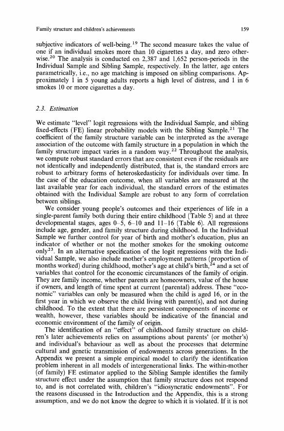
Family structure and children's achievements 159

subjective indicators of well-being. 19 The second measure takes the value ofone if an individual smokes more than 10 cigarettes a day, and zero other­wise. 20 The analysis is conducted on 2,387 and 1,652 person-periods in theIndividual Sample and Sibling Sample, respectively. In the latter, age entersparametrically, i.e., no age matching is imposed on sibling comparisons. Ap­proximately I in 5 young adults reports a high level of distress, and I in 6smokes 10 or more cigarettes a day.

2.3. Estimation

We estimate "level" logit regressions with the Individual Sample, and siblingfixed-effects (FE) linear probability models with the Sibling Sample. 21 Thecoefficient of the family structure variable can be interpreted as the averageassociation of the outcome with family structure in a population in which thefamily structure impact varies in a random way.22 Throughout the analysis,we compute robust standard errors that are consistent even if the residuals arenot identically and independently distributed, that is, the standard errors arerobust to arbitrary forms of heteroskedasticity for individuals over time. Inthe case of the education outcome, when all variables are measured at thelast available year for each individual, the standard errors of the estimatesobtained with the Individual Sample are robust to any form of correlationbetween siblings.We consider young people's outcomes and their experiences of life in a

single-parent family both during their entire childhood (Table 5) and at threedevelopmental stages, ages 0-5, 6-10 and 11-16 (Table 6). All regressionsinclude age, gender, and family structure during childhood. In the IndividualSample we further control for year of birth and mother's education, plus anindicator of whether or not the mother smokes for the smoking outcomeonly23. In an alternative specification of the logit regressions with the Indi­vidual Sample, we also include mother's employment patterns (proportion ofmonths worked) during childhood, mother's age at child's birth,24 and a set ofvariables that control for the economic circumstances of the family of origin.They are family income, whether parents are homeowners, value of the houseif owners, and length of time spent at current (parental) address. These "eco­nomic" variables can only be measured when the child is aged 16, or in thefirst year in which we observe the child living with parent(s), and not duringchildhood. To the extent that there are persistent components of income orwealth, however, these variables should be indicative of the financial andeconomic environment of the family of origin.The identification of an "effect" of childhood family structure on child­

ren's later achievements relies on assumptions about parents' (or mother's)and individual's behaviour as well as about the processes that determinecultural and genetic transmission of endowments across generations. In theAppendix we present a simple empirical model to clarify the identificationproblem inherent in all models of intergenerational links. The within-mother(of family) FE estimator applied to the Sibling Sample identifies the familystructure effect under the assumption that family structure does not respondto, and is not correlated with, children's "idiosyncratic endowments". Forthe reasons discussed in the Introduction and the Appendix, this is a strongassumption, and we do not know the degree to which it is violated. If it is not

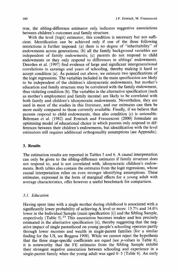
160 J.F. Ermisch, M. Francesconi

true, the sibling-difference estimator only indicates suggestive associationsbetween children's outcomes and family structure.With the level (Iogit) estimator, this condition is necessary but not suffi­

cient. Identification can be achieved only if one of the three followingrestrictions is further imposed: (a) there is no degree of "inheritability" ofendowments across generations; (b) all the family background variables areindependent of family endowments; (c) parents do not respond to childendowments or they only respond to differences in siblings' endowments.Dearden et al. (1997) find evidence of large and significant intergenerationalcorrelations in earnings and years of schooling, thereby making it hard toaccept condition (a). As pointed out above, we estimate two specifications ofthe logit regressions. The variables included in the main specification are likelyto be independent of the children's idiosyncratic endowments, but mother'seducation and family structure may be correlated with the family endowment,thus violating condition (b). The variables in the alternative specification (suchas mother's employment and family income) are likely to be correlated withboth family and children's idiosyncratic endowments. Nevertheless, they areused in most of the studies in this literature, and our estimates can then bemore easily compared to those currently available. Finally, if we believe thatparents respond to child endowments, then also condition (c) is untenable.Behrman et al. (1982) and Ermisch and Francesconi (2000) formulate anoptimising model of educational choice in which parents only respond to dif­ferences between their children's endowments, but identification with the levelestimators still requires additional orthogonality assumptions (see Appendix).

3. Results

The estimation results are reported in Tables 5 and 6. A causal interpretationcan only be given to the sibling-difference estimates if family structure doesnot respond to, and is not correlated with, idiosyncratic children's endow­ments. Both tables also contain the estimates from the logit regressions, whosecausal interpretation relies on even stronger identifying assumptions. Theseestimates, expressed in the form of marginal effects for a young adult withaverage characteristics, offer however a useful benchmark for comparison.

3.1. Education

Having spent time with a single mother during childhood is associated with asignificantly lower probability of achieving A level or more: 13.7% and 14.6%lower in the Individual Sample (main specification (i)) and the Sibling Sample,respectively (Table 5).25 This association becomes weaker and less preciselyestimated in the alternative specification (ii), thereby suggesting that the neg­ative impact of single parenthood on young people's schooling operates partlythrough lower incomes and wealth in single-parent families (for a similarfinding for the US, see Boggess 1998). While we cannot reject the hypothesisthat the three stage-specific coefficients are equal (see p-values in Table 6),it is noteworthy that the FE estimates from the Sibling Sample exhibittheir strongest negative association between schooling and experience in asingle-parent family when the young adult was aged 0-5 (Table 6). An early

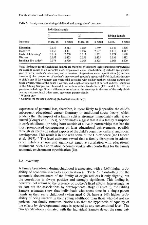
Family structure and children's achievements 161

Table 5. Family structure during childhood and young adults' outcomes

Individual sample

(i) (ii) Sibling Sample

Outcome Marg. eff. It-ratiol Marg. eff. It-ratiol Coeff. It-ratiol

Education -0.137 2.913 -0.083 1.749 -0.146 1.896Inactivity 0.056 3.901 0.037 2.577 0.018 0.917Early childbearing" 0.Ql8 2.250 0.012 1.531 0.024 1.688Distress 0.055 2.453 0.056 2.455 0.036 1.412Smoking 10+ a dayb 0.073 2.790 0.063 2.325 0.068 2.670

Note: Estimates for the Individual Sample are marginal effects from logit regressions computed atthe average values of all variables used. Regressions under specification (i) include: age, gender,year of birth, mother's education, and a constant. Regressions under specification (ii) includethose in (i) plus: proportion of mother's time worked, mother's age at child's birth, family incomeat child's age 16 (or youngest age when child coresided with his/her mother), whether parents arehouse owners, value of the house if owners, and length of time spent at current address. Estimatesin the Sibling Sample are obtained from within-mother fixed-effects (FE) model. All FE re­gressions include age. Sisters' differences are taken at the same age in the case of the early child­bearing outcome; in all other cases, age enters parametrically.a Women only.b Controls for mother's smoking (Individual Sample only).

experience of parental loss, therefore, is more likely to jeopardise the child'ssubsequent educational career. Contrary to traditional stress theory, whichpredicts that the impact of a family split is strongest immediately after it oc­curred (Conger et al. 1993), our estimates suggest that it is a family disruptionin early childhood (or being born outside of a live-in partnership) that has themost pronounced consequences on later educational achievements, possiblythrough its effects on salient aspects of the child's cognitive, cultural and socialdevelopment. This result is in line with some of the US evidence (see Duncanet al. 1997).26 The level estimates reveal that a family disruption in adoles­cence exhibits a large and significant negative correlation with educationalattainment. Such a correlation becomes weaker after controlling for the familyeconomic environment (specification (ii)).

3.2. Inactivity

A family breakdown during childhood is associated with a 5.6% higher prob­ability of economic inactivity (specification (i), Table 5). Controlling for theeconomic circumstances of the family of origin reduces it only slightly, butthe correlation is always positive and strongly significant. This finding is,however, not robust to the presence of mother's fixed effects. Interestingly, aswe sort out the associations by developmental stage (Tables 6), the SiblingSample estimates show that individuals who spent time in a single-parentfamily in their early childhood (when aged 0-5), have a 14% higher prob­ability of being inactive in their young adulthood than those who did not ex­perience that family structure. Notice also that the hypothesis of equality ofthe effects by developmental stage is rejected at any conventional level. Thetwo specifications estimated with the Individual Sample detect the same pat-

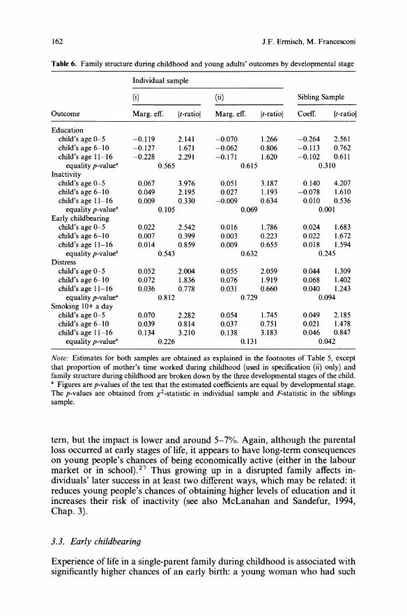
162 I.F. Ennisch, M. Francesconi

Table 6. Family structure during childhood and young adults' outcomes by developmental stage

Individual sample

(i) (ii) Sibling Sample

Outcome Marg. elf. It-ratiol Marg. elf. It-ratiol Coelf. It-ratiol

Educationchild's age 0-5child's age 6-10child's age 11-16equality p-value"

Inactivitychild's age 0-5child's age 6-10child's age 11-16equality p-valuea

Early childbearingchild's age 0-5child's age 6-10child's age 11-16equality p-valuea

Distresschild's age 0-5child's age 6-10child's age 11-16equality p-value"

Smoking 10+ a daychild's age 0-5child's age 6-10child's age 11-16equality p-valuea

-0.119 2.141-0.127 1.671-0.228 2.291

0.565

0.067 3.9760.049 2.1950.009 0.330

0.105

0.022 2.5420.007 0.3990.014 0.859

0.543

0.052 2.0040.072 1.8360.036 0.778

0.812

0.070 2.2820.039 0.8140.134 3.210

0.226

-0.070 1.266-0.062 0.806-0.171 1.620

0.615

0.051 3.1870.027 1.193-0.009 0.634

0.069

0.016 1.7860.003 0.2230.009 0.655

0.632

0.055 2.0590.076 1.9190.031 0.660

0.729

0.054 1.7450.037 0.7510.138 3.183

0.131

-0.264 2.561-0.113 0.762-0.102 0.611

0.310

0.140 4.207-0.078 1.6100.010 0.536

0.001

0.024 1.6830.022 1.6720.018 1.594

0.245

0.044 1.3090.068 1.4020.040 1.243

0.094

0.049 2.1850.021 1.4780.046 0.847

0.042

Note: Estimates for both samples are obtained as explained in the footnotes of Table 5, exceptthat proportion of mother's time worked during childhood (used in specification (ii) only) andfamily structure during childhood are broken down by the three developmental stages of the child.a Figures are p-values of the test that the estimated coefficients are equal by developmental stage.The p-values are obtained from x2-statistic in individual sample and F-statistic in the siblingssample.

tern, but the impact is lower and around 5-7%. Again, although the parentalloss occurred at early stages of life, it appears to have long-term consequenceson young people's chances of being economically active (either in the labourmarket or in school).27 Thus growing up in a disrupted family affects in­dividuals' later success in at least two different ways, which may be related: itreduces young people's chances of obtaining higher levels of education and itincreases their risk of inactivity (see also McLanahan and Sandefur, 1994,Chap. 3).

3.3. Early childbearing

Experience of life in a single-parent family during childhood is associated withsignificantly higher chances of an early birth: a young woman who had such

Family structure and children's achievements 163

an experience has a 1.8% per annum higher chance of early childbearing thana woman who did not (specification (i), Table 5). This association diminisheswhen the economic variables are included in estimation, but it is still quitelarge. Better economic circumstances appear, therefore, to play a role inreducing the risk of an early birth for women who grew up in a single-parentfamily but do not eliminate it. 28 A young woman's lower education andemployment expectations (two characteristics that are common to womenwith experience in a single-parent family during their childhood) are likelyto reduce her perception of the costs of early childbearing, and a birth mayreduce her educational attainments. This illustrates the value of analysingyoung people's outcomes jointly. The estimates from the Sibling Sample arelarge and confirm that the positive association between family structure andearly birth persists even when we control for mother's fixed effects. Havingexperienced a family breakdown increases the probability of early mother­hood by 2.4% per annum (t-ratio = 1.69). While an early family disruption(when the girl was in pre-school years) exhibits a stronger association (bothsamples, Tables 6), the three stage-specific estimates from either sample arenot statistically different from each other. While restating the importance ofan early parental loss, this finding also suggests that family disruptions duringschool years and adolescence are likely to lessen monitoring of children'sactivities, and those are the times when parental supervision could preventbehaviour that leads to early childbearing (Thornton and Camburn 1987; Hillet al. 1998).

3.4. Distress

The level estimates show a positive and significant association between familystructure and level of distress before and after including the economic varia­bles in estimation: having spent time in a single-parent family during child­hood increases the probability of having a high level of distress by 5.5%. Thisresult is consistent with the large psychological literature in this area, whichhas shown that children and adults in non-intact families are at greater risk forpsychological adjustment problems compared to those in families with bothbiological parents (e.g., Amato and Keith 1991; Bruce and Kim 1992). Familydisruptions that occurred either in pre-school (ages 0-5) or in primary schoolyears (ages 6-10) exhibit the strongest associations: for example, young adultswhose parents separated when they were between 6 and 10 years of age areabout 7% more likely to report high levels of distress than young adults wholived in an intact family during their entire childhood. After controlling formother's fixed effects, however, the relationship between distress and familystructure (at any developmental stage) is not statistically significant. The factthat this correlation is imprecisely measured when we account for unobservedheterogeneity may, however, reflect measurement error in our measure ofdistress rather than the absence of a robust relationship. It is well known thatthe presence of modest errors in variables can wipe out most of the associa­tions of interest and that sibling differences exacerbate this effect of measure­ment error (Griliches 1979). The information on distress is, in fact, elicitedin the self-completion questionnaire of the BHPS by a series of questionsregarding the way the respondent has been feeling over the last few weeks.The exact phrasing is: "Have you recently ... (felt under strain, depressed,

164 J.F. Ennisch, M. Francesconi

etc.)?". Given the subjective measure of the answer and the relatively shortreference period (the last few weeks), this measure is likely to pick up a lot ofnoise and other (possible temporary) aspects of psychological well-being. 29

3.5. Smoking

The association between family structure and smoking 10 or more cigarettes aday is always strong and well determined: having spent time with a singlemother during childhood increases the probability of heavy smoking by about7%. This association persists even after controlling for the economicconditions of the family of origin and falls only to 6.3%. Accounting forunobservable factors that are shared by children who belong to the samefamily (born to the same mother) confirms this finding, with the effect being6.8%. Family disruptions that occurred either during pre-school years (bothsamples) or during adolescence (Individual Sample only) seem to have astronger relationship with heavy smoking. 30 In the case of the Sibling Sample,we reject the hypothesis that the estimated coefficients are equal acrossthe three developmental stages at conventional levels of significance. But thishypothesis cannot be rejected for the estimates obtained with the IndividualSample. In general, our findings confirm the evidence, documented in manysocial medicine studies, that children of single mothers have an increased riskof being smokers regardless of whether or not the mother smokes (Green et al.1990; Turner-Warwick 1992). This suggests that, beside mother's smokingbehaviour, other characteristics of single-parent families (such as lower pa­rental control or lower expected human capital) foster children's smoking.

4. Conclusions

In this paper we estimate the relationship between several outcomes in earlyadulthood (educational attainment, economic inactivity, early childbearing,distress and smoking) and the experience of life in a single-parent familyduring childhood. We use a sample of young adults, selected from the first fivewaves of the BHPS (1991-1995), who can be matched with at least one siblingover the same period. This sample allows us to estimate the relationships ofinterest by sibling differences. We also perform our analysis on another sam­ple which we estimate using a level (Iogit) model. These estimates are usefulfor comparison with the existing evidence.We draw attention to four aspects of our findings. First, we show that

sibling differences require a weaker assumption (as compared to the assump­tions imposed by standard level estimators) for the identification of the familystructure effect, namely that family structure is not correlated with children'sidiosyncratic endowments, but it is still a strong one. Second, using such sib­ling differences, we find that experience of life in a single-parent family duringchildhood is usually associated with negative outcomes for children as youngadults: lower educational attainments, higher risks of inactivity and earlybirth, and higher chances of being a heavy smoker and experiencing higherlevels of distress in early adulthood. Third, family structure in early childhood(when the child was between the ages of 0 and 5) appears to be more impor­tant for shaping achievement, behaviour and mental health than does family

Family structure and children's achievements 165

structure during primary school years or adolescence. Fourth, the level esti­mates, whose causal interpretation relies on even stronger assumptions, con­firm our results and are consistent with much of the evidence available in thisliterature. In addition, they allow us to show that the adverse family structureassociation generally persists even after controlling for the economic circum­stances of the family of origin. 31Although we are only able to interpret these results as suggestive associa­

tions, the sibling-difference estimates control for more family backgroundfactors than has been usual in the literature. Identification of a causal impactmust, however, await data which contain sufficiently convincing instrumentsthat allow family structure to be modelled as an endogenous variable.

Appendix: The identification problem

Letj index family and i index individuals (or, interchangeably, young adultsand children). For convenience, assume that the relationship that we estimateis given by the following linear probability model (see Angrist and Lavy1996):

Pij = PXij + uij, (1)

where Pij is a dichotomous variable indicating one of the outcomes, taking thevalue of 1 if the outcome under study occurs and 0 otherwise; Xij is a vector ofexplanatory variables, such as age, family structure during childhood, mother'seducation and parental income (Sect. 2 gives a complete list of the variablesused in estimation); uij is a random shock with zero mean. In this for­mulation, the parameters P are assumed to be the same for all individuals.Arguably, the effect of family structure is heterogeneous (i.e., some childrenmight be better off in a non-intact family, while others might be worse off).Notice, however, that the methodology proposed here would apply even if onespecifies a random-coefficients model in which Pj = P + rPj' and E(rPjuij) =E(rPjXij) = O.Our objective is to provide consistent estimates of the "effect" of family

structure (contained in X) on the probability of various children's outcomes,p. Consistent estimation of P in (1) requires that the variables measuringmother's (or parents') behaviour during childhood contained in X be un­correlated with the disturbance term u. We investigate this issue using aframework suggested by Behrman et al. (1994) and Rosenzweig and Wolpin(1995). Consider a two-child family. For the i-th child in family j with siblingk,

(2)

(3)

(4)

Equation (2) decomposes uij into four elements: a mother-specific fixedeffect common to both siblings, !Yj; two distinct stochastic components that

166 J.F. Ermisch, M. Francesconi

depend on the endowments of each sibling, cij and Ckj; and measurement error,flij' The parameters <5) and <52 capture the parental (or own) response to childendowments that are observable to all family members but are not observedby the econometrician. We assume that E(cij) = E(flij) = E((J.j} = E(cijflij) =E(ckjflij) = E((J.jflij) = 0, for all i, k, andj.Equation (3) is a type of Galton's law of heritability of endowments (see

Becker and Tomes 1986), with regression to the mean across generations(0 ~ p < I); Cj is the zero-mean parents' (or mother's) endowment and vij is anidiosyncratic disturbance with zero mean, and uncorrelated with Cj and withVkj (the analogous disturbance for sibling k).Equation (4) relates the variables in Xij to the parental endowment, Cj,

a mother-specific fixed effect, ()j, and the idiosyncratic endowments of thechildren, '7ij and '7kj, where n, Y1 and Y2 are conformable vectors of parame­ters. The parameters in n capture the mother's (or parents') response to her(their) own endowment, while Yl and Y2 measure the parental response tochild-specific idiosyncratic endowments. Equation (4) allows for the possibilitythat aspects of family environment, including family structure, may be influ­enced by the family's as well as the children's endowments. We assume thatE('7ij) = E('7kj) = E(()j) = E('7ij'7kj) = E('7ij()j) = E('7ijcj} = 0, for all i, k, andj. We further assume that E('7ij(J.j) = E('7kj(J.j) = E('7ijflij) = E('7kjflij) =E(vij()j) = E(VkA) = E(VijVkj) = E(flij()j) = 0.This formulation introduces three different sources of family-specific het­

erogeneity: in Eq. (3), Cj is transmitted through the endowments, cij and Ckj, towhich parents' or individuals' behaviour (via <5) and <52) can respond; anothercomponent, ()j in Eq. (4), affects children's outcomes indirectly throughthe parental behaviour measured by Xij; the last source of heterogeneity, (J.j,affects the outcome Pij directly (through Eq. (2)), regardless of individualearnings endowments.Substituting (3) in (2) yields uij = <5) vij + <52Vkj + (<51+ <52)PCj + flij + (J.j. The

level estimates of fJ in (I) are consistent if the covariance (vector) between Xijand the error term uij is zero. However, from (4),

(5)

where 0-; = var(Cj), a yz = cov(y,z), for y,z = (J.j,Cj, ()j, flij' '7ij' and vij' In gen­eral (5) is not zero, in which case estimates of fJ are inconsistent. Even afterintroducing other orthogonality assumptions, i.e., aa.e = aeo = aaO, we still findthat cov(Xij,uij) = n(<5[ + <52)pa; + (y)<5) + Y2<52)al/v, and this covariance dis­appears only if: a) either n = 0, or <5[ = -<52, or p = 0; and b) aI/v = 0, or<51= -<52 and Y[ = Y2' or Y[ = Y2 = 0. It is not implausible that at least some ofthe variables in Xij depend on the family endowment cj, that is, n "1= 0. Forexample, mother's education depends on Cj' If we believe that there exists apositive degree of "inheritability", through genetic and cultural transmissionof endowments, then also p is non-zero. Furthermore, if we believe that pa­rents respond to child earnings endowments, then <51+ <52 "1= 0. Behrman et al.(1982) and Ermisch and Francesconi (2000) do, however, present a familymodel of endogenous education in which <5) = -<52. For consistent estimatesof fJ in this model, however, it is also necessary to assume that the variables in

Family structure and children's achievements 167

X do not respond to child idiosyncratic endowments, so that Yl = Y2. 32 That is,when 01 = -02 is coupled with the orthogonality assumption (Jas = 0, Yl = Y2is sufficient for identification of the parameter p.Many of the problems of the level estimates have to do with the presence

of mother-specific fixed effects. 33 A siblings estimator of the components ofpfor which the elements of Xij differ between siblings is based on the differencesbetween siblings, and such fixed effects would be eliminated via differencing.In our two-child family case, this is

Ap = pAX + (0\ - 02)Ae + Af.l

= pAX + A¢, (6)

where Az = zij - ZkJ> for any term z, and A¢ = (0\ - 02)Ae + Af.l. From Eq.(4), it follows that AX = (Y\ - Y2)A11. Thus, the covariance between AX andthe disturbance term in (6) is given by

Our previous assumptions that E(f.lij) = E(f.lik) = E(11ij) = E(J1k) = E(11ijf.lij)= E(11kjf.lij) = °guarantee that the second term of (7) is always zero. We thenonly need to assume that either (J"v = 0, or 0\ = 02, or Y\ = Y2 to identify p.The conditions (J"v = °(or, if 11ij = vij as in Rosenzweig and Wolpin (1995)and Ermisch and Francesconi (1997), (J~ = 0) and 0\ = 02 are difficult to jus­tify by theoretical arguments. It may, however, be plausible that many aspectsof the family environment do not respond to children's idiosyncratic attrib­utes, so that Y\ = Y2. This latter condition may be met by some family back­ground variables used in the empirical analysis, like mother's education, be­cause the children's idiosyncratic endowments are only apparent at their birthor afterwards. But other family behaviour, like mother's work patterns, mayinstead be the result of child-specific idiosyncratic attributes rather than thecause of the young adult's achievements. For this reason, with the SiblingSample we estimate a model that contains only (sibling differences in) age,gender, and family structure during childhood. In other words, identificationof the family structure "effect" with our data requires that family structuredoes not respond to, and is not correlated with, children's idiosyncratic en­dowments. The level (logit) regressions performed with the Individual Samplein specification (i) also contain year of birth and mother's education, variablesthat are likely to be insensitive to the child's idiosyncratic attributes. As mostof the studies in this literature, in specification (ii) we add mother's employ­ment patterns during childhood, mother's age at child's birth, family income,and other "economic" variables that control for the economic circumstancesof the family of origin. This allows for a comparison of our estimates withthose currently available in the literature, but imposes stronger identifyingassumptions.

In sum the identification of the family structure effect on children'sachievements rests both on the availability of "prior information" about theprocess generating parental behaviour and children's outcomes, and on theresearchers' willingness to make specific assumptions on such a process. We

168 J.F. Ermisch, M. Francesconi

share Manski et al. (1992) view that "as long as social scientists are heteroge­neous in their beliefs about this process, their estimates of family structureeffects may vary" (p. 36).

Endnotes

1 For a detailed overview of existing studies, see McLanahan and Sandefur (1994), Havemanand Wolfe (1995) and Mayer (1997).

2 Throughout the paper, the terms "mother-specific fixed effects" and "family-specific fixedeffects" are used interchangeably, because of the data that we analyse. But it should be em­phasized that our fixed-effects estimator eliminates the influence of all unmeasured persistentmother, family and community characteristics that do not differ by siblings.

3 Recent exceptions are the longitudinal studies by Duncan et al. (1997) and Blau (1999) on theeffect of family income on schooling and child development, and by Grogger and Ronan(1996) on the effect of fatherlessness on education and wages.

4 Recent studies using BHPS data similar to those employed here include Ermisch and Fran­cesconi (1997), who investigate the association of several family structure measures on educa­tional attainments, and Ermisch and Francesconi (2000), who analyse the relationship betweenfamily background and young people's earnings.

5 For data on household income, we use information from fathers, stepfathers or other adults, ifpresent in the household.

6 On the other hand, the NCDS does have larger sample sizes and more measures of non­economic background factors.

7 By collecting information on individuals born in the first week of March 1958, the NCDS dataare instead not suitable for this estimation procedure. By 1991 in the NCDS sample used inDearden (1998), there are only 27 pairs of twins.

8 This finding has never been emphasised before in the British context, partly because the NCDSdata could not reliably identify family breakdowns from birth up until age 5. As a result, mostof the studies with NCDS data use samples that are typically restricted to individuals whoseparents were in an intact family at age 7. An exception is Frostin et al. (forthcoming). Some oftheir regressions are estimated for a sample of NCDS children aged 33 in 1991, which includedthose whose parents were not in an intact family either at birth or at age 7 of the child.

9 Of those interviewed in wave I (1991),88% were re-interviewed in wave 2. The wave-on-waveresponse rates from the third wave onwards have been consistently above 95%. The BHPS dataare therefore unlikely to suffer from serious attrition bias.

10 The first five waves of the BHPS indicate that 93% of single-parent families are headed by themother and that 86% of dependent children living with a step-parent lived with their naturalmother.

II If the birth occurred outside of a partnership and the mother partnered within one year, weassumed that the mother had moved in with the biological father (as assumed in Bumpass et al.(1995) and Ermisch and Francesconi (forthcoming)). For adopted children, we use informationon the year in which they were adopted to match in the mother's family history appropriately.In 96% of the cases, the children are natural children.

12 Ermisch and Francesconi (1997) experiment with other, more detailed measures of familystructure, e.g., step-families and durations of different family structures. But this simple di­chotomy by developmental stage performs as well in predicting educational attainment asmore complex measures. In addition, Ermisch and Francesconi (forthcoming) find that only242 women had a pre-partnership birth as of 1992 (wave 2), representing 0.05% of all womenin that survey year. Since we cannot determine whether or not they subsequently lived with thechild's father, we assume that the women who formed a union within one year of the birth didso with the father. Of the 242 women who had a pre-partnership birth, 77 (32%) lived with thechild's father. Because of the small sample sizes, therefore, we cannot explore the distinctionbetween children who experienced a family disruption when age 0-5 and children born into asingle-parent family.

13 That is, the third wave contains retrospective information on jobs held by aU adults since theyleft full-time education, including their current work if it started before September 1990, up to

Family structure and children's achievements 169

September 1990. For jobs started after that date, we use information collected in the panelwave-on-wave work history.

14 We performed a similar analysis using more complex measures of mother's employment pat­terns over her child's childhood, including the proportions of months worked in full-time andpart-time jobs and the proportion of months worked in broad occupation groups. Our mainresults are unchanged.

15 While the overall figure may appear high, it is consistent with life table estimates by Ermischand Francesconi (forthcoming), which indicate that 40% of mothers in the BHPS will spendsome time as the only parent. The stage-specific figures may also appear large in the light ofdivorce registration statistics which indicate that about 40% of dependent children of divorcingparents are aged under 6. Recall, however, that single-parent families are also formed by thedissolution of cohabitations and births outside of a partnership. In the BHPS data, these lasttwo categories account for 35% of instances of single parenthood. If, in conjunction with thedivorce registration statistics, we assume that all dissolving cohabitations involve children un­der 6, then 60% of instances of single parenthood would start when the child is aged under 6.

16 The 165 two-sibling households give rise to 165 comparisons, one per siblings' pair; the 23three-sibling households produce 69 comparisons, 3 in each household; and the 3 four-siblinghouseholds give rise to 18 comparisons, 6 in each household.

17 For readers unfamiliar with the British education system, "A(Advanced) level" corresponds toeducation beyond high school, but short of a university degree. At least one A level is necessaryto be admitted to a university.

18 In line with official statistics, data from the original representative BHPS sample show thatapproximately 20% of women have a baby by age 21. Registration statistics also indicate that,for the most recent cohorts of women for which we have data (women born in the late 1960s),the median age at first birth was 27 (ONS 1997, Table 10.3). The original BHPS data producea similar figure.

19 Distress is measured in comparison with "usual" conditions. The subjective indicators are: (i)loss of concentration; (ii) loss of sleep; (iii) playing a useful role; (iv) capable of making deci­sions; (v) constantly under strain; (vi) problem overcoming difficulties; (vii) enjoy day-to-dayactivities; (viii) ability to face problems; (ix) unhappy or depressed; (x) losing confidence; (xi)believe in self-worth; (xii) general happiness. Each indicator is measured over a scale that runsfrom I to 4. Recording I and 2 values on individual indicators to 0, and 3 and 4 values to I,and then summing over all indicators gives a new scale running from 0 (the least distressed) to12 (the most distressed). The scale is known in the health literature as caseness. For each youngadult, our mental health measure takes the value of one if his/her caseness variable has a valueof 3 or more, and zero otherwise. See Cox et al. (1994). Because collapsing the distress scale toa dichotomous variable may reduce the outcome variability, we also perform our analysistreating it as a continuous measure.

20 The cut-off choice for the number of cigarettes smoked in a day is arbitrary. We also per­formed the analysis with a variable taking value of one if the respondent smokes and zerootherwise. The results are qualitatively identical to those reported below.

21 A well-known problem inherent to all linear probability models is that the predicted outcomesare not constrained to lie between zero and one. This may obviously compromise the inter­pretation of the estimates as the probability that the event under study will occur. To gaugehow serious this problem can be with our data, we first estimate our five outcomes with theIndividual Sample using a linear probability model. We then use the estimated coefficients tocompute the conditional expectation E(ylx), where y is an outcome and x is the appropriatevector of explanatory variables. We predict, at most, 2 cases outside the unit interval for theeducation outcome (that is, 0.41% of the 489 observations used in this estimation), and 6 casesoutside the unit interval for the inactivity outcome (0.25% of the observations). The maximumnumber of predictions that do not lie between zero and one is always lower for the other threeoutcomes. Therefore, the prediction problem of the linear probability model is arguably in­consequential for the samples used in this study.

22 For expositional purposes, the model in the Appendix does not allow for heterogeneity in thefamily structure effect.

23 There are six age dummies (age 16 is the base) in the Individual Sample. Mother's education isgrouped in four categories: no qualification (base), 0 level, A level, and higher qualification. Inthe Sibling Sample, age enters non-parametrically only in the case of early childbearing, i.e.,when sisters' comparisons are made at a common age.

170 J.F. Ermisch, M. Francesconi

24 We distinguish three stages of mother's age at birth: young (maternal age less than or equal to21), middle (maternal age between 22 and 33, base); and old (maternal age greater than orequal to 34).

25 As a way of checking whether the differences between individual-based and sibling-based esti­mates arise from the different age distributions in the two samples (see Table 2), we have alsoestimated level models using the Sibling Sample for all outcomes. In general the point estimatesare very close to those found with the Individual Sample while the standard errors are some­what larger (presumably due to the smaller sample sizes). This suggests that the differences inresults across samples do not systematically depend on their different age distributions. Forexample, the level estimates (in terms of marginal effects) of the education outcome found withthe Sibling Sample are -0.138 (t-ratio = -2.187) and -0.122 (t-ratio = 2.042) for specification(i) and (ii), respectively.

26 Duncan et al. (1998) find that "early childhood appears to be the stage in which family eco­nomic conditions matter most" (p. 420). Our findings are consistent with their result, giventhat the impact of family structure on educational attainment may operate partly throughfamily income.

27 For the estimates obtained from specification (ii) of the Individual Sample, we can reject thehypothesis of equality of the estimated stage-specific coefficients at the 10% level but not atthe 5% level. For the estimates from specification (i), we instead never reject the equalityhypothesis.

28 The results from specification (ii) also reveal that if the mother herself was aged 21 or less whenher daughter was born, then the odds that the daughter has an early birth are higher. Thus,there is evidence of a recurrence of early motherhood across generations. This association be­comes slightly weaker when the economic circumstances of the family of origin are controlledfor. On the other hand, if mothers were aged 34 or more at birth, the chance of their daughtershaving an early birth are lower.

29 When the distress measure is treated as a continuous variable, we again find positive and well­measured estimates of family structure using the Individual Sample. For example, in compar­ison with the results reported in Table 5, having spent some time in a single-parent familyduring childhood increases the distress level (which on average equals 1.364) by 0.384 points(t-ratio = 2.864) in specification (i) and by 0.388 points (t-ratio = 2.843) in specification (ii).The estimates obtained from the Sibling Sample are always positive, but somewhat smaller andnever statistically significant. In sum, these results provide evidence comparable to that foundwith our dichotomous measure.

30 We also find a high persistence in smoking behaviour across generations. In the IndividualSample, a young adult whose mother smokes has approximately 15% higher chances of being aheavy smoker than a young adult (with similar characteristics) whose mother does not smoke.This association is always significant at any conventional level. The inclusion of mother'ssmoking behaviour, however, may be problematic for identification of the family structureeffect (see Sect. 2.3 and the Appendix). Its exclusion from the level regressions does not alterour results.

31 Discussing the findings from twelve different papers, McLanahan (1997) argues that growingup in a single-parent family has negative consequences for children's well-being across severaldomains (e.g., test scores, education, behavioural and psychological problems, jobs and in­come) even after taking family income into account.

32 We discount the unlikely case that a~v =o.33 Given the data analysed in this study and the setup of the model presented here, the definitionof "mother-specific fixed effect" is equivalent to that of "family-specific fixed effect". In par­ticular, our fixed-effects estimator captures all persistent mother, family and community effectsthat do not differ by siblings. The two labels are therefore equivalent and used interchangeablythroughout the paper.

References

Amato PR, Keith B (1991) Parental divorce and the well-being of children: A meta-analysis.Psychological Bulletin 110:26-46

Angrist JD, Lavy V (1996) The effect of teen childbearing and single parenthood on childhooddisabilities and progress in school. NBER Working Paper No. 5807, October

Family structure and children's achievements 171

Becker GS (1981) A treatise on the family Harvard University Press, Cambridge, MassBecker GS, Landes EM, Michael RT (1977) An economic analysis of marital instability. Journal

of Political Economy 85(6):1141-1187Becker GS, Tomes N (1986) Human capital and the rise and fall of families. Journal of Labor

Economics 4:SI-S39Behrman JR, Pollak R, Taubman P (1982) Parental preferences and provision for progeny. Jour­

nal of Political Economy 90(1 ):52-73Behrman JR, Rosenzweig MR, Taubman P (1994) Endowments and the allocation of schooling inthe family and in the marriage market: the twins experiment. Journal of Political Economy102(6):1131-1174

Blau DM (1999) The effect of income on child development. Review of Economics and Statistics81 (2):261-276

Boggess S (1998) Family structure, economic status, and educational attainment. Journal of Pop­ulation Economics 11(2):205-222

Browning M (1992) Children and household economic behavior. Journal of Economic Literature30(3): 1434-1475

Bruce ML, Kim KM (1992) Differences in the effects of divorce on major depression in men andwomen. American Journal of Psychiatry 149:914-917

Bumpass LL, Raley RK, Sweet JA (1995) The changing character of stepfamilies: implications ofcohabitation and nonmarital childbearing. Demography 32:425-436

Charlton A, Blair V (1989) Predicting the onset of smoking in boys and girls. Social Science andMedicine 29:813-819

Cherlin AJ, Kiernan KE, Chase-Lansdale PL (1995) Parental divorce in childhood and demo­graphic outcomes in young adulthood. Demography 32:299-318

Conger RD, Conger KJ, Elder GH, Lorenz FO, Simons RL, Whitbeck LB (1993) Family eco­nomic stress and adjustment of early adolescent girls. Developmental Psychology 29(2):206­219

Cox DR, Fitzpatrick R, Fletcher AE, Gore SM, Spiegelhalter DJ, Jones DR (1994) Quality oflifeassessment: can we keep it simple? Journal of the Royal Statistical Society (Series A) 155:353­393

Dearden L (1998) Ability, families, education and earnings in Britain. Institute for Fiscal Studies,Working Paper No. W98/14, June

Dearden L, Machin S, Reed H (1997) Intergenerational mobility in Britain. Economic Journal107:47-66

Duncan GJ, Teachman J, Yeung WJ (1997) Childhood family income and completed schooling:results from sibling models. Unpublished paper, Northwestern University, Institute for PolicyResearch, July

Duncan GJ, Yeung WJ, Brooks-Gunn J, Smith J (1998). How much does childhood poverty affectthe life chances of children? American Sociological Review 63(3):406-423

Elliot BJ, Richards MPM (1991) Children and divorce: educational performance, and behaviour,before and after parental separation. International Journal of Law, Policy and the Family5:258-276

Ermisch JF (1996) Parental support for human capital investment by young adults. Centre forEconomic Policy Research Discussion Paper No. 1536

Ermisch JF (1999) Prices, parents and young people's household formation. Journal of UrbanEconomics 45:47-71

Ermisch JF, Francesconi M (1997) Family matters. Centre for Economic Policy Research Dis­cussion Paper No. 1591

Ermisch JF, Francesconi M (2000) Educational choice, families and young people's earnings.Journal of Human Resources 35(1):143-176

Ermisch JF, Francesconi M. The increasing complexity of family relationships: lifetime experienceof single motherhood and stepfamilies in Great Britain. European Journal of Population(forthcoming)

Fronstin P, Greenberg DH, Robins PK. Parental disruption and the labour market performanceof children when they reach adulthood. Journal of Population Economics (forthcoming)

Green G, Macintyre S, West P, Ecob R (1990) Do children of lone parents smoke more becausetheir mothers do? British Journal ofAddiction 85: 1497-1500

Griliches Z (1979) Sibling models and data in economics: beginning of a survey. Journal of Polit­ical Economy 87(5):S37-S64

172 J.F. Ennisch, M. Francesconi

Grogger J, Ronan N (1996) The intergenerational effects offatherlessness on educational attain­ment and entry-level wages. Unpublished paper, University of California Santa Barbara, July

Haveman R, Wolfe B (1995) The detenninants of children's attainments: a review of methods andfindings. Journal of Economic Literature 33: 1829-1878

Hill MS, Yeung WJ, Duncun GJ (1998) Childhood family structure and young adult behaviors.Unpublished paper, University of Michigan, August

Kiernan KE (1992) The impact of family disruption in childhood on transitions made in youngadult life. Population Studies 46:213-234

Kiernan KE (1996) Lone motherhood, employment and outcomes for children. InternationalJournal ofLaw, Policy and the Family 10:233-249

Kiernan KE (1997) The legacy of parental divorce: social, economic and demographic experiencesin adulthood. Centre for Analysis of Social Exclusion, London School of Economics, CASE­paper I

Knight FH (1935) The ethics of competition. Allen and Unwin, New YorkManski CF, Sandefur GD, McLanahan S, Powers D (1992) Alternative estimates of the effect offamily structure during adolescence on high school graduation. Journal of the American Sta­tistical Association 87:25-37

McLanahan SS (1988) Family structure and dependency: early transitions to female householdheadship. Demography 25(1):1-16

McLanahan SS (1997) Parent absence or poverty: which matter more? In: Duncan GJ, Brooks­Gunn J (eds) Consequences ofgrowing up poor. Russell Sage Foundation, New York

McLanahan SS, Sandefur G (1994) Growing up with a single parent. Harvard University Press,Cambridge

Ni Bhrolchain M, Chappel R, Diamond I (1994) Scolarite et autres caracteristiques socio­demographiques des enfants de mariages rompus [Educational and socio-demographic out­comes among the children of disrupted and intact marriages]. Population 49:1585-1612

Mayer SE (1997) What money can't buy: Family income and children's life chances. Harvard Uni­versity Press, Cambridge

Office for National Statistics (1997) Birth Statistics 1995. HMSO, LondonRosenzweig MR, Wolpin KI (1995) Sisters, siblings, and mothers: the effect of teen-age child­bearing to birth outcomes in a dynamic family context. Econometrica, 63(2):303-326

Thornton A, Camburn D (1987) The influence of the family on premarital sexual attitudes andbehavior. Demography 24:323-340

Turner-Warwick M (1992) Smoking and the Young. Report ofa working party of the Royal Col­lege of Physicians of London, London

Childhood family structure and young adult behaviors

Martha S. Hill!, Wei-Jun J. Yeung!, Greg J. Duncan2

1 Institute for Social Research, University of Michigan, P.O. Box 1248 Ann Arbor,MI 48106-1248, USA (FAX: +1-734-647-4575; e-mail: hillm@umich.edu;jeany@umich.edu)2 Institute for Policy Research, Northwestern University, 2040 Sheridan Rd., Evanston,IL 60202, USA (FAX: 847-491-9916; e-mail: greg-duncan@nwu.edu)

Received: II September I998/Accepted: 27 March 2000

Abstract. This paper examines a wide variety of forms, and full histories, offamily structure to test existing theories of family influences and identifyneeds for new theories. The focus is on links between childhood family struc­ture and both completed schooling and risk of a nonmarital birth. Using a27-year span of panel (PSID) data for U.S. children, we find that: (a) change isstressful, (b) timing during childhood is relevant, (c) adults other than parentsare important, and (d) two more recently studied family structures (mother­with-grandparent(s) and mother-with-stepfather) do not fit the molds of exist­ing theories. The findings suggest that new theories should consider allocationof resources and reasons people group into family structures.

JEL classification: 112, 113, 116

Key words: Demographic economics, marital dissolution, family structure

1. Introduction

In recent decades, new forms of family structure have assumed prominence inthe lives of U.S. children. Aspects of these changes have been documentedrepeatedly in cross-sectional studies but less fully explored in a panel context.

All correspondence to Martha S. Hill. The research summarized in this paper was funded by theNational Institute for Child Health and Development's Family and Child Well-Being ResearchNetwork (UOI HD30947-06), whose generosity is greatly appreciated. We are grateful to SheldonDanziger, John Ermisch, Marco Francesconi, Christopher Jencks, Saul Hoffman, Gary Solon andtwo anonymous reviewers for their many helpful suggestions and to Don Hernandez for kindlyproviding estimates of children's family structures from other sources. Responsible editor: John F.Ermisch.

174 M.S Hill et al.

Much remains to be learned about what they mean for children. Fortunately,panel studies are now yielding data tracing children and their family life frombirth into young adulthood, all during this historical period of greater diver­sity in family structure. This affords a unique opportunity for a better under­standing of how family life operates, the relevance of existing theories offamily influences, and new directions for identifying underlying mechanisms.A particular focus of this paper is the importance of childhood stage to the

influence of family structure on children. Taking account of possible variationin effects of family structure by timing of occurrence allows for the possibilitythat a particular family structure mechanism, be it stress from disruption infamily routines, change in the amount or quality of parental supervision, orlow levels of economic resources, has stronger effects at some stages of child­hood than others because of differences in children's developmental needs orsusceptibility to problem behavior. Caring and nurturing, along with nutritionand a good learning environment, are viewed by developmentalists as crucialin early childhood, whereas parental supervision and emotional support maybe important in late childhood when risks of behaviors such as dropping outof high school or having a nonmarital birth come into play. Information onthe full history of the family structures children encounter while growing upallows us to test the sensitivity of the influence of the family structure to theages when children encounter it.The paper also provides a novel perspective on mother-only and non-intact

structures by highlighting living arrangements that combine a single motherwith grandparent(s) or combine a mother and stepfather. Though still rela­tively rare, these structures appear to be on the rise. Casper and Bryson (1998),for example, report a 118% increase between 1970 and 1997 in the numberof children living in mother-with-grandparent(s) households. However, timeseries estimates of the proportion of children in mother-with-grandparent(s)and in mother-with-stepfather families are difficult to locate, and, as far as wecan tell, there are no published figures regarding proportions of children everin such structures, much less what parts of their childhood they spent thatway. Research attention is beginning to be directed both to the factors thatencourage these living arrangements (e.g., Mauldon and Maestas 1998) and toways these family structures affect children and adults.There is clear interest in mother-with-stepfather families because of

high divorce and remarriage rates. Interest in mother-with-grandparent(s)families is piqued by the beginnings of a complicated picture of social andeconomic differences associated with this family structure. Research suggeststhat grandparent-grandchild coresidence tends to be associated with highersatisfaction on the part of adolescents with their parental relationships, lessdelinquent activity, but lower grades (Kirby and Uhlenberg 1999).Observational and ethnographic studies suggest that the added adults in

multigenerational families do not necessarily enhance the supervision of youthand can create confusion over who is in charge (Chase-Lansdale et al. 1994;Pattillo-McCoy 1999). Such studies also suggest that children in multigenera­tional families tend to take on adult roles more quickly because the genera­tions are close in age and this blurs developmental role boundaries to thepoint that children and parents may behave as siblings (Burton, Obeidallahand Allison, 1996). Analysis of Current Population Survey data indicatesthat children coresiding with grandparent(s) tend to fare worse economically(Casper and Bryson 1998). All told, however, surprisingly little is known

Family structure and young adult behaviors 175

about mother-with-grandparent(s) structures. Although our results regardingthese noteworthy but rare structures should be viewed cautiously owing tomodest sample sizes, they are provocative and call for further research.Our investigation emphasizes the timing of membership in each family

structure in two regards: childhood stage and length of elapsed time. Wealso examine transitions between structures. Other researchers (e.g., Wu andMartinson 1993; Martinson and Bumpass 1990; and Bumpass and McLana­han 1989), using different data and specifications, have investigated aspectsof non-intact or mother-only structures, but they have not specifically exam­ined the mother-with-grandparent(s) structure, nor have they examined themother-with-stepfather structure at different childhood stages.Data from the Panel Study of Income Dynamics (PSID) are the basis

for our empirical investigation. These data span all years from birth throughyoung adulthood for a representative sample of cohorts born in the late 1960sand early 1970s. With these data, and a focus on family influences on child­ren's educational attainment and daughter's risk of non-marital childbirth, wefind some support for existing theories about the ways families influence chil­dren. But much of what we find is at odds with these theories.Our analysis indicates that the stress and economic hardship associated

with other-than-two-parent family structures are more important than socialcontrol. However, some of our evidence is not well accounted for in any ofthese theories: (1) parental remarriage and having a stepfather present tendto have beneficial consequences for daughters if these things occurred duringadolescence, (2) parental divorce or separation experienced in adolescencetends to have a positive association with sons' education, and (3) the familystructure with the greatest detrimental consequences for children, particularlyif experienced during adolescence, appears to be one with grandparent(s)present along with a single mother. In addition, variations in consequencesby timing of the family structure over the course of childhood do not alwaysfit well with the implications of existing theories.There is a clear need for further research and for further development of

theories about family mechanisms. Our findings suggest that new theories need totake into account the timing of family structure and events, as well as integratea variety of dimensions, including factors associated with the reasons peoplegroup into particular family structures. We leave the task of formulating newtheories to future research, but sketch out the terrain they should cover.The paper begins with a review of existing theories and evidence on the

mechanisms by which family structure affects children's characteristics andbehaviors. We then focus on our analysis of the PSID data. To set the stagewe first examine patterns of childhood family structure experiences. Next wedescribe the approach and measures used for determining the relevance ofexisting theories. Estimates for the models are then presented, with discussionhighlighting both results that fit and results that do not fit the theories. We endwith a discussion of the implications of the findings and further needs forresearch, with a focus on developing theories and some important aspectsto consider when formulating such theories.

2. Existing theories and relevant literature

The social science literature posits a number of different causal mechanismsrelating family structure to children's outcomes. Our analysis focuses on two

176 M.S Hill et al.

of the major theories - stress and social control, and takes into accountanother possible mechanism: family income as emphasized by economic re­source theory.Stress theory posits change in family life as the central cause of family

structure effects on children, the idea being that change in family structureprompts reorganization of the roles of family members and adversely affectsthe nurturing and support provided by parents. (For relevant discussion, seeMcLoyd et al. 1994; Conger et al. 1993, 1992; Wojtkiewicz 1993; Cherlin et al.1991; McLanahan 1988; Booth et al. 1984; and Elder 1974). Key aspects offamily life for this theory are parental marital events. Family reorganizationprompted by parental divorce or (re)marriage is viewed as stressful to parentsand children, and the resulting weakening of emotional security and bonds isthought to encourage problem behaviors in children.Social control theory views adult supervision and monitoring of children's

behaviors as important means by which children are kept from engaging inproblem behaviors. (For relevant discussion see Brooks-Gunn, forthcoming;Chase-Lansdale et al. 1994; Thornton 1991; McLanahan and Bumpass 1988;Steinberg 1987; Thornton and Camburn 1987; Dornbusch et al. 1985; Hoganand Kitagawa 1985; Hetherington 1979; Cherlin 1978; and Mueller and Pope1977). Key aspects, according to this theory, are number and types of adultsoverseeing children. Social control is thought to increase with the number ofadults present in the child's home. The more distant the relationship of theadult to the child, though, the weaker the social control. Some types ofparents (stepparents) or substitute parents (grandparents) are likely to exertless authority and social control than biological parents because of their moretenuous relationship to the child and because the parenting roles of such rel­atives are ill-defined (Brooks-Gunn forthcoming; Cherlin 1978). In childhoodhomes containing both biological parents and grandparents, disagreementsbetween the two regarding parenting style may undermine the social controlexerted by both (Chase-Lansdale et al. 1994).Family income is the operative mechanism in economic hardship theory.

(For relevant discussion, see Dodge et al. 1994; Zill and Nord 1994; McLeodand Shanahan 1993; Axinn and Thornton 1992; DaVanzo and Goldscheider1990; Goldscheider and DaVanzo 1989; Goldscheider and Goldscheider 1987;Weiss 1979; Rubin 1976; and Elder 1974.) Family income is likely to varywith family structure (mother-only families tend to have lower income thantwo-parent families) and to change with its changes (children's family incometends to drop substantially after parental marital disruption and rise withparental (re)marriage). It can be difficult to distinguish effects of income fromother influences of family structure without precise and comprehensive mea­sures of both over the entire course of childhood, and past research has rarelyhad such measures.Correlational evidence repeatedly indicates that children fare much worse

when raised in non-intact homes (see McLanahan and Sandefur 1994 andSeltzer 1994 for reviews of past research, and, in McLanahan and Sandefur1994, a comprehensive multi-dataset analysis). Evidence suggests that thesecorrelations are not merely due to lack of control for measured and un­measured family characteristics (Sandefur and Wells 1997). That childrenfrom non-intact homes fare worse could be consistent with social control,stress, and economic hardship theories.Evidence relating more directly to social control theory indicates that

Family structure and young adult behaviors 177

children in single-parent families are more susceptible to peer pressure thanchildren in two-parent families (Steinberg 1987; Dornbusch et al. 1985). Lackof social control and more emphasis on peers could result in children havingmore disciplinary problems and, in adolescence, more intensive dating andsexual involvement. These behaviors, in tum, may encourage young people toleave school early and to form families or unions prematurely, and the effectsmay be strongest in adolescence. Studies have shown that parental maritaldisruption leads to early and more frequent sexual activity, premarital preg­nancy and births and to the early formation of unions, and some of theevidence suggests that lack of parent supervision is one of the operativemechanisms (see, for example, Thornton 1991; McLanahan and Bumpass1988; Thornton and Camburn 1987; and Hogan and Kitagawa 1985).Research regarding stress theory shows that, at least among adolescents,

there are linkages between disruptive family events, parents' depression, im­paired parenting behavior, and children's impaired school performance, socialbehavior, and self-esteem (McLoyd et al. 1994; Conger et al. 1992, 1993).Furthermore, Wu and Martinson (1993) and Wu (1996) find that it is changein childhood family structure rather than a prolonged period living in amother-only family that is most strongly linked to young women's chances ofhaving a premarital birth. Wojtkiewicz (1993) also finds that transition into amother-only family is more important to chances of high school graduationthan is duration of time spent in a mother-only family. Some ofWojtkiewicz'sfindings about other non-intact structures, however, are not entirely consistentwith the theory that changes are more important than the length of time spentin a non-intact family.Few studies of the effects of growing up in single-parent households have

had access to sufficiently reliable measures of family income and other family­process measures to provide a complete accounting of why children raised insingle-parent families do so much worse than children from two-parent fami­lies. The handful that have, however, tend to indicate that economic differ­ences account for a sizable portion, but not all, of the adverse effects of beingraised in a single-parent household. For example, McLanahan (1985), Hilland Duncan (1987) and McLanahan and Sandefur (1994) all find that paren­tal-income differences account for between one-third and two-thirds of theestimated impact on completed schooling of living in a single-parent family.Other studies find that income differences playa less important role (e.g.,Sandefur et al. 1992) or a complex role that varies by type of non-intactfamily, accounting for single-parent influences but not influences of mother­with-stepfather (Boggess 1998).The literature indicates differential influences of family structure by sex and

age of the child, as well as race (e.g., Boggess 1998). Married parents treat sonsand daughters differently, and this may be a factor in the sex differences ineffects of changes in family structure (see Seltzer's, 1994, review). Hetherington(1979, 1987) found sex differences in reaction to both parents' marital disrup­tion and remarriage. Soon after parental divorce, as well as several years later,sons in families where the divorced mother did not remarry displayed a numberof problematic behaviors, including noncompliant behavior. Sons were betteradjusted if the custodial mother did remarry; however, daughters were betteradjusted if the mother did not remarry. Findings such as these, however, arenot entirely consistent with other research (see Seltzer 1994 for a review).Findings are mixed regarding variation in the influence of family structure

178 M.S Hill et al.

by child's age (childhood stage). As summarized in Wojtkiewicz (1993), boththe amount of time young children spend in the home and their inability tounderstand and cope with marital disruptions lead us to expect family com­position changes occurring early in a child's life to be most harmful, and someresearch bears this out (Krein 1986; Krein and Beller 1988). However, Wojt­kiewicz finds that years spent in mother-only families between the ages of 11and 15 as opposed to younger ages were associated with substantially reducedchances of graduating from high school. McLanahan and Sandefur (1994)report an insignificant six-percentage-point increase in the risk of droppingout of high school if a marital disruption occurred before age 6 as opposedto after age 12. Haveman and Wolfe (1994) find no significant effect on com­pleted schooling of the timing of years spent living with one parent (althoughtheir analysis omits the very early years of childhood).With such diverse findings in the literature, there is no clear picture of

the mechanisms involved and policy implications of the detrimental effectsof shifts away from intact families. As some researchers (e.g., Seltzer 1994;Wu and Martinson 1993; and Wojtkiewicz 1993) are beginning to show, ourunderstanding of the underlying processes may be clouded by the failure ofempirical measures to reflect the dynamics and many-faceted nature of familystructure. Much of the research on childhood family structure has approachedthe issues as if children experienced the same family structure throughoutchildhood. Wu (1996) and Wu and Martinson (1993) in their dynamic analysisof young women's premarital births and Wojtkiewicz (1993) in his dynamicanalysis of high school graduation help to correct some of these problems.However, this research does not include recent cohorts of young adults andlacks comprehensive control for income.Wu and Martinson investigate cohorts born 1938-1969 and control for

possible cohort differences using only an additive control distinguishing threesubgroups - those born 1938-1947 vs. 1948-1957 vs. 1958-1969. Wu (1996)and Wojtkiewicz (1993) examine cohorts born 1958-1965. Given the dramaticincrease in non-intact families, effects for earlier cohorts may well differ fromthose for more recent ones. Wu and Martinson and Wojtkiewicz include nomeasures of childhood family income, and Wu (1996) includes only measuresof family income during adolescence.The research presented in this paper extends the boundaries of the territory

charted by these authors by: (a) examining more recent cohorts of children,(b) measuring family structure with shorter recall, (c) considering struc­tures not yet investigated or little researched (mother-with-grandparent(s) andmother-with-stepfather), and (d) incorporating more comprehensive measuresof family income that are well matched to the family structure measures. Inextending this work we pay particular attention to: (1) the stage of childhoodwhen a family structure or change in family structure was experienced, (2)presence of adults other than parents (e.g., step-parents or grandparents), (3)parental marital changes as well as associated family structure, (4) family in­come throughout the course of childhood, and (5) other types of changes thataccompany family structure changes (e.g., movement to a different residence,which McLanahan and Sandefur 1994 find important, or changes in mothers'work commitment and consequently in the amount of time spent with theirchildren, which Seltzer, et al. 1989, document as important). We also focus ontwo types of outcomes for children as young adults - educational attainmentand, for daughters, nonmarital childbirth.

Family structure and young adult behaviors

3. Family structure experiences

179

The dramatic growth in mother-only families has fueled much of the researchon family structure in recent decades (see, for example, Duncan et al. 1994;Hernandez 1993; Moffitt and Rendall 1993; Duncan and Rodgers 1990; Hof­ferth 1985; and Bumpass 1984). Yet some of this growth may reflect shifts tofamily structures that are more complex than a single-parent situation. Thepresence in single-parent families of adults other than parents rarely has beentaken into account, and a family structure consisting of grandparents alongwith the mother has often been classified as mother-only by researchers.

3.1. Data

The Panel Study of Income Dynamics (PSID) data allow us to investigate awide range of possible family structures and track children's experience offamily structures from birth through late childhood. For observing the com­plete childhood experiences, as well as for the tests of family structure mech­anisms reported later in this paper, we rely on 27 years of PSID data. Since1968 the PSID has followed and annually interviewed a representative sampleof about five thousand families. (See Hill 1992 for a full description of thedataset.) Splitoff families are formed when children leave home, when couplesdivorce, and when more complicated changes break families apart. This pro­cedure produces an unbiased sample of families each year, as well as a con­tinuously representative sample of children born into families. The survey'soriginal design focused on poverty by oversampling lower-income and minorityhouseholds. Our sample consists of the 1,325 PSID individuals born between1967 and 1973 and present! in the PSID every wave from birth to age 20.Since this includes individuals from the oversampled households, the data areweighted to adjust for this feature of the sample design as well as differentialnonresponse. Barring any nonresponse bias remaining uncorrected by theweighting adjustments we employ, the experiences of this group of childrenare nationally representative of the cohorts from which they were sampled. 2

3.2. Family structure measures

Our family structure measures are constructed to facilitate investigation ofstructures that have received relatively little attention in the literature. Wedistinguish between different types of structures with only one parent, and weseparate structures containing a stepparent from other two-parent structures.Our measures are based on demographic information provided in the maindata files from the 1968-1991 interviews, plus data from the 1968-1985 Re­lationship File, which consolidates many years of data to determine all possi­ble pairwise relationships.Our child-based family structure measures are constructed from the PSID's

annual (time-of-interview) categorization of the following family types:

a) "two-parent family": child living with both biological or adoptive parents;3b) "mother-only family": child living with the biological or adoptive motherand no other person older than age 21 other than a sibling;

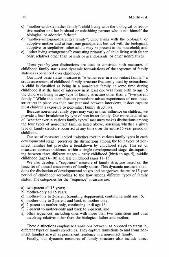
180 M.S Hill et al.

c) "mother-with-stepfather family": child living with the biological or adop­tive mother and her husband or cohabiting partner who is not himself thebiological or adoptive father;4

d) "mother-with-grandparent(s) family": child living with the biological oradoptive mother and at least one grandparent but not with the biological,adoptive, or stepfather; other adults may be present in the household; and

e) "other living arrangement": consisting primarily of child living with fatheronly, relatives other than parents or grandparents, or other nonrelatives.

These year-by-year distinctions are used to construct both measures ofchildhood family status and dynamic formulations of the sequence of familystatuses experienced over childhood.Our most basic status measure is "whether ever in a non-intact family," a

crude assessment of childhood family structure frequently used by researchers.A child is classified as being in a non-intact family at some time duringchildhood if at the time of interview in at least one year from birth to age ISthe child was living in any type of family structure other than a "two-parentfamily." While this identification procedure misses experiences of non-intactstructures in place less than one year and between interviews, it does capturemost children's exposure to non-intact family structures.Because non-intact family types may vary in their influence on children, we

provide a finer breakdown by type of non-intact family. Our more detailed setof "whether ever in various family types" measures makes distinctions amongthe four types of non-intact families listed above, assessing whether a giventype of family structure occurred at any time over the entire IS-year period ofchildhood.Our set of measures labeled "whether ever in various family types in each

developmental stage" preserves the distinctions among the four types of non­intact families but provides a breakdown by childhood stage. This set ofmeasures assesses incidence within a single developmental stage, distinguish­ing between three different stages - early childhood (birth to age 5), middlechildhood (ages 6-10) and late childhood (ages II-IS).We also develop a "sequence" measure of family structure based on the

basic set of annual assessments of family status. This dynamic measure aban­dons the distinction of developmental stages and categorizes the entire IS-yearperiod of childhood according to the flow among different types of familystatus. The categories for the "sequence" measure are:

a) two-parent all IS years;b) mother-only all IS years;c) mother-only to 2-parent (counting stepparents), continuing until age IS;d) mother-only to 2-parent and back to mother-only;e) 2-parent to mother-only, continuing until age IS;f) 2-parent to mother-only and back to 2-parent, andg) other sequences, including ones with more than two transitions and onesinvolving relatives other than the biological father and mother.

These distinctions emphasize transitions between, as opposed to status in,different types of family structures. They capture transitions to and from non­intact families as well as permanent residence in a non-intact family.Finally, our dynamic measures of family structure also include direct

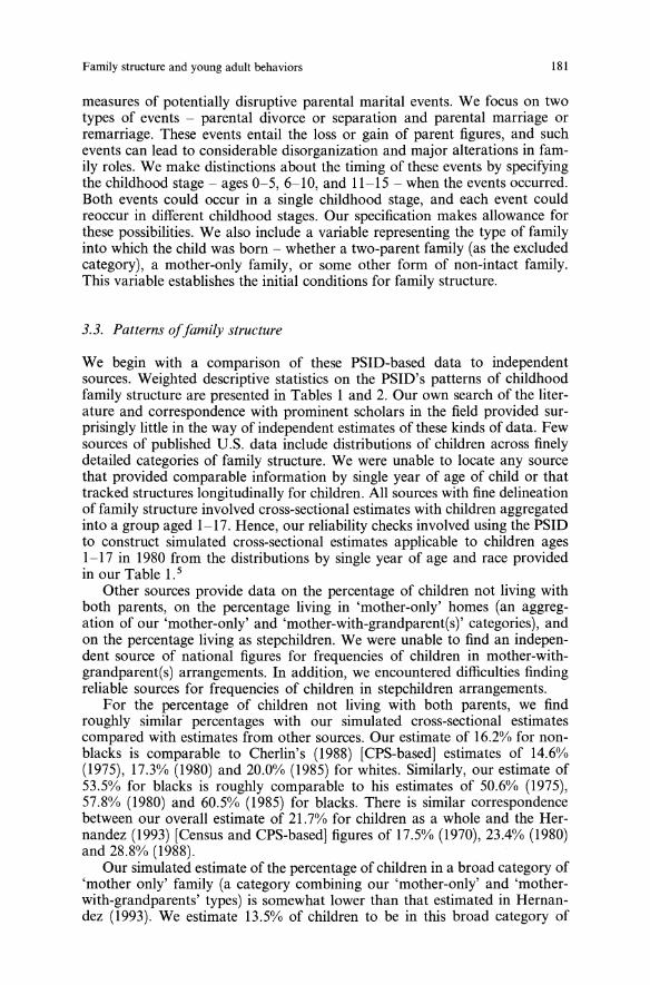
Family structure and young adult behaviors 181

measures of potentially disruptive parental marital events. We focus on twotypes of events - parental divorce or separation and parental marriage orremarriage. These events entail the loss or gain of parent figures, and suchevents can lead to considerable disorganization and major alterations in fam­ily roles. We make distinctions about the timing of these events by specifyingthe childhood stage - ages 0-5,6-10, and 11-15 - when the events occurred.Both events could occur in a single childhood stage, and each event couldreoccur in different childhood stages. Our specification makes allowance forthese possibilities. We also include a variable representing the type of familyinto which the child was born - whether a two-parent family (as the excludedcategory), a mother-only family, or some other form of non-intact family.This variable establishes the initial conditions for family structure.

3.3. Patterns offamily structure

We begin with a comparison of these PSID-based data to independentsources. Weighted descriptive statistics on the PSID's patterns of childhoodfamily structure are presented in Tables I and 2. Our own search of the liter­ature and correspondence with prominent scholars in the field provided sur­prisingly little in the way of independent estimates of these kinds of data. Fewsources of published U.S. data include distributions of children across finelydetailed categories of family structure. We were unable to locate any sourcethat provided comparable information by single year of age of child or thattracked structures longitudinally for children. All sources with fine delineationof family structure involved cross-sectional estimates with children aggregatedinto a group aged 1-17. Hence, our reliability checks involved using the PSIDto construct simulated cross-sectional estimates applicable to children ages1-17 in 1980 from the distributions by single year of age and race providedin our Table 1. 5

Other sources provide data on the percentage of children not living withboth parents, on the percentage living in 'mother-only' homes (an aggreg­ation of our 'mother-only' and 'mother-with-grandparent(s)' categories), andon the percentage living as stepchildren. We were unable to find an indepen­dent source of national figures for frequencies of children in mother-with­grandparent(s) arrangements. In addition, we encountered difficulties findingreliable sources for frequencies of children in stepchildren arrangements.For the percentage of children not living with both parents, we find

roughly similar percentages with our simulated cross-sectional estimatescompared with estimates from other sources. Our estimate of 16.2% for non­blacks is comparable to Cherlin's (1988) [CPS-based] estimates of 14.6%(1975), 17.3% (1980) and 20.0% (1985) for whites. Similarly, our estimate of53.5% for blacks is roughly comparable to his estimates of 50.6% (1975),57.8% (1980) and 60.5% (1985) for blacks. There is similar correspondencebetween our overall estimate of 21.7% for children as a whole and the Her­nandez (1993) [Census and CPS-based] figures of 17.5% (1970), 23.4% (1980)and 28.8% (1988).Our simulated estimate of the percentage of children in a broad category of

'mother only' family (a category combining our 'mother-only' and 'mother­with-grandparents' types) is somewhat lower than that estimated in Hernan­dez (1993). We estimate 13.5% of children to be in this broad category of

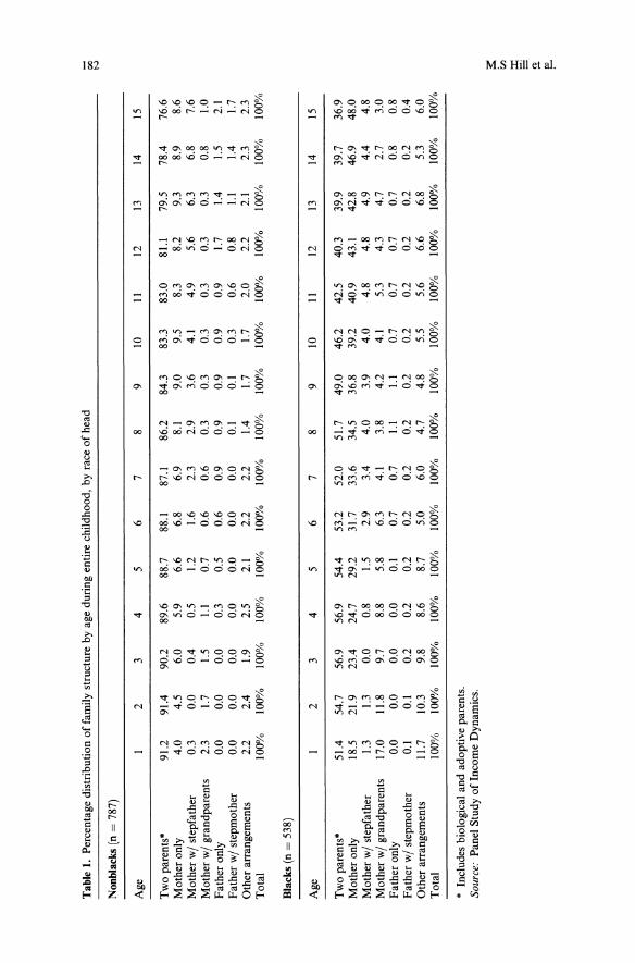
Table1.Percentagedistributionoffamilystructurebyageduringentirechildhood,byraceofhead

00 tv

Nonblacks(n=787)

Age

I2

34

56

78

910

II12

1314

15

Twoparents·

91.2

91.4

90.2

89.6

88.7

88.1

87.1

86.2

84.3

83.3

83.0

81.1

79.5

78.4

76.6

Motheronly

4.0

4.5

6.0

5.9

6.6

6.8

6.9

8.1

9.0

9.5

8.3

8.2

9.3

8.9

8.6

Mother

wistepfather

0.3

0.0

0.4

0.5

1.2

1.6

2.3

2.9

3.6

4.1

4.9

5.6

6.3

6.8

7.6

Mother

wigrandparents

2.3

1.7

1.5

1.1

0.7

0.6

0.6

0.3

0.3

0.3

0.3

0.3

0.3

0.8

1.0

Fatheronly

0.0

0.0

0.0

0.3

0.5

0.6

0.9

0.9

0.9

0.9

0.9

1.7

1.4

1.5

2.1

Father

wistepmother

0.0

0.0

0.0

0.0

0.0

0.0

0.0

0.1

0.1

0.3

0.6

0.8

1.1

1.4

1.7

Otherarrangements

2.2

2.4

1.9

2.5

2.1

2.2

2.2

1.4

1.7

1.7

2.0

2.2

2.1

2.3

2.3

Total

100%

100%

100%

100%

100%

100%

100%

100%

100%

100%

100%

100%

100%

100%

100%

Blacks(n=538)

Age

I2

34

56

78

910

II12

1314

15

Twoparents·

51.4

54.7

56.9

56.9

54.4

53.2

52.0

51.7

49.0

46.2

42.5

40.3

39.9

39.7

36.9

Motheronly

18.5

21.9

23.4

24.7

29.2

31.7

33.6

34.5

36.8

39.2

40.9

43.1

42.8

46.9

48.0

Mother

wistepfather

1.3

1.3

0.0

0.8

1.5

2.9

3.4

4.0

3.9

4.0

4.8

4.8

4.9

4.4

4.8

Mother

wigrandparents

17.0

11.8

9.7

8.8

5.8

6.3

4.1

3.8

4.2

4.1

5.3

4.3

4.7

2.7

3.0

Fatheronly

0.0

0.0

0.0

0.0

0.1

0.7

0.7

1.1

1.1

0.7

0.7

0.7

0.7

0.8

0.8

Father

wistepmother

0.1

0.1

0.2

0.2

0.2

0.2

0.2

0.2

0.2

0.2

0.2

0.2

0.2

0.2

0.4

Otherarrangements

11.7

10.3

9.8

8.6

8.7

5.0

6.0

4.7

4.8

5.5

5.6

6.6

6.8

5.3

6.0

Total

100%

100%

100%

100%

100%

100%

100%

100%

100%

100%

100%

100%

100%

100%

100%

•Includesbiologicalandadoptiveparents.

Sour

ce:PanelStudyofIncomeDynamics.

~ tn ;; = ~ !!'-

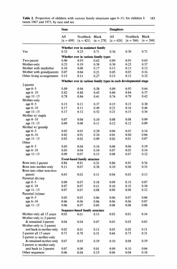
Table 2. Proportion of children with various family structures ages 0-15, for children b 183tween 1967 and 1973, by race and sex

Sons Daughters

All Nonblack Black All Nonblack Black(n = 699) (n =421) (n = 278) (n = 626) (n = 366) (n = 260)

Whether ever in nonintact familyYes 0.32 0.25 0.71 0.36 0.30 0.71

Whether ever in various family typesTwo-parent 0.90 0.95 0.62 0.89 0.93 0.65Mother-only 0.25 0.19 0.58 0.30 0.25 0.57Mother with stepfather 0.10 0.09 0.17 0.13 0.13 0.12Mother with grandparents 0.07 0.04 0.21 0.05 0.03 0.16Other living arrangements 0.13 0.11 0.27 0.15 0.12 0.32

Whether ever in various family types in each developmental stage2-parentage 0-5 0.89 0.94 0.58 0.89 0.93 0.64age 6-10 0.82 0.88 0.45 0.80 0.84 0.57age 11-15 0.78 0.84 0.41 0.74 0.79 0.42

Mother-onlyage 0-5 0.15 0.11 0.37 0.15 0.13 0.30age 6-10 0.17 0.11 0.49 0.21 0.16 0.46age 11-15 0.17 0.12 0.52 0.21 0.15 0.54Mother wi stepfaage 0-10 0.07 0.06 0.10 0.08 0.08 0.09age 11-15 0.09 0.08 0.11 0.12 0.12 0.09Mother wi grandpage 0-5 0.05 0.03 0.20 0.04 0.03 0.14age 6-10 0.02 0.01 0.10 0.01 0.00 0.06age 11-15 0.03 0.02 0.09 0.02 0.01 0.07

Otherage 0-5 0.05 0.04 0.16 0.08 0.06 0.19age 6-10 0.05 0.04 0.10 0.07 0.05 0.14age 11-15 0.09 0.07 0.15 0.08 0.07 0.12

Event-based family structureBorn into 2-parent 0.86 0.91 0.51 0.86 0.91 0.54Born into mother-only 0.11 0.07 0.38 0.10 0.06 0.33Born into other non-two-parent 0.03 0.02 0.11 0.04 0.03 0.13Parental div/sepage 0-5 0.09 0.07 0.18 0.09 0.10 0.07age 6-10 0.07 0.07 0.11 0.10 0.10 0.10age 11-15 0.07 0.07 0.08 0.09 0.08 0.12

Parental (re)marage 0-5 0.05 0.05 0.06 0.06 0.07 0.04age 6-10 0.06 0.06 0.06 0.06 0.06 0.07age 11-15 0.06 0.07 0.05 0.08 0.08 0.08

Sequence-based family structureMother-only all IS years 0.03 0.01 0.13 0.03 0.01 0.14Mother-only to 2-parent

& remained 2-parent 0.04 0.04 0.07 0.03 0.03 0.03Mother-only to 2-parentand back to mother-only 0.02 0.01 0.13 0.03 0.02 0.11

2-parent all IS years 0.71 0.78 0.31 0.66 0.73 0.312-parent to mother-only

& remained mother-only 0.07 0.05 0.19 0.10 0.08 0.192-parent to mother-onlyand back to 2-parent 0.07 0.08 0.01 0.09 0.10 0.04

Other sequences 0.06 0.04 0.15 0.06 0.04 0.18

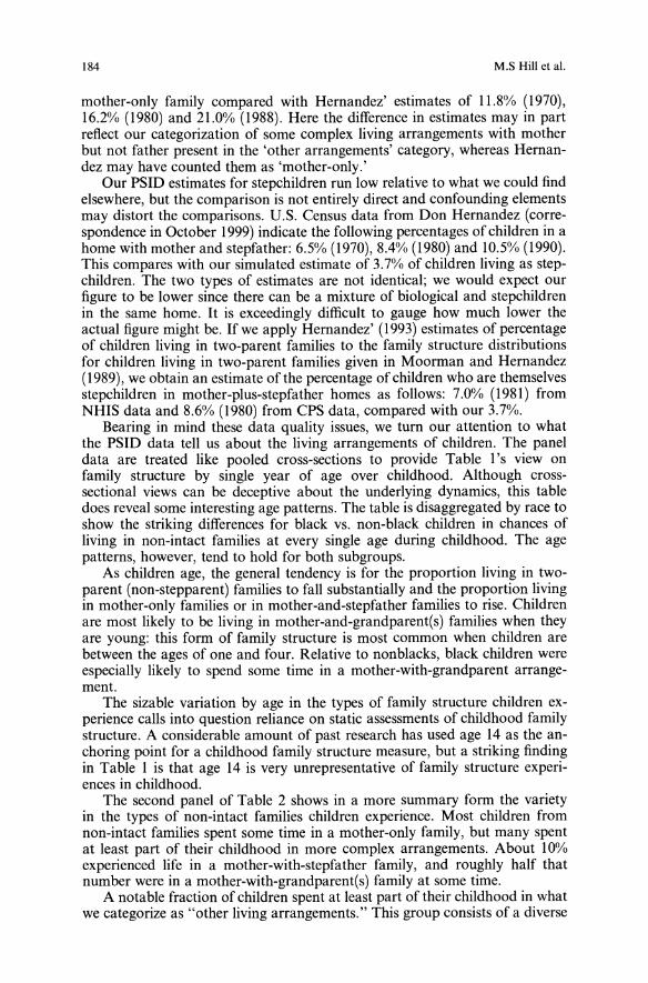
184 M.S Hill et al.

mother-only family compared with Hernandez' estimates of 11.8% (1970),16.2% (1980) and 21.0% (1988). Here the difference in estimates may in partreflect our categorization of some complex living arrangements with motherbut not father present in the 'other arrangements' category, whereas Hernan­dez may have counted them as 'mother-only.'Our PSID estimates for stepchildren run low relative to what we could find

elsewhere, but the comparison is not entirely direct and confounding elementsmay distort the comparisons. U.S. Census data from Don Hernandez (corre­spondence in October 1999) indicate the following percentages of children in ahome with mother and stepfather: 6.5% (1970),8.4% (1980) and 10.5% (1990).This compares with our simulated estimate of 3.7% of children living as step­children. The two types of estimates are not identical; we would expect ourfigure to be lower since there can be a mixture of biological and stepchildrenin the same home. It is exceedingly difficult to gauge how much lower theactual figure might be. If we apply Hernandez' (1993) estimates of percentageof children living in two-parent families to the family structure distributionsfor children living in two-parent families given in Moorman and Hernandez(1989), we obtain an estimate of the percentage of children who are themselvesstepchildren in mother-plus-stepfather homes as follows: 7.0% (1981) fromNHIS data and 8.6% (1980) from CPS data, compared with our 3.7%.Bearing in mind these data quality issues, we turn our attention to what

the PSID data tell us about the living arrangements of children. The paneldata are treated like pooled cross-sections to provide Table l's view onfamily structure by single year of age over childhood. Although cross­sectional views can be deceptive about the underlying dynamics, this tabledoes reveal some interesting age patterns. The table is disaggregated by race toshow the striking differences for black vs. non-black children in chances ofliving in non-intact families at every single age during childhood. The agepatterns, however, tend to hold for both subgroups.As children age, the general tendency is for the proportion living in two­

parent (non-stepparent) families to fall substantially and the proportion livingin mother-only families or in mother-and-stepfather families to rise. Childrenare most likely to be living in mother-and-grandparent(s) families when theyare young: this form of family structure is most common when children arebetween the ages of one and four. Relative to nonblacks, black children wereespecially likely to spend some time in a mother-with-grandparent arrange­ment.The sizable variation by age in the types of family structure children ex­

perience calls into question reliance on static assessments of childhood familystructure. A considerable amount of past research has used age 14 as the an­choring point for a childhood family structure measure, but a striking findingin Table 1 is that age 14 is very unrepresentative of family structure experi­ences in childhood.The second panel of Table 2 shows in a more summary form the variety

in the types of non-intact families children experience. Most children fromnon-intact families spent some time in a mother-only family, but many spentat least part of their childhood in more complex arrangements. About 10%experienced life in a mother-with-stepfather family, and rougWy half thatnumber were in a mother-with-grandparent(s) family at some time.A notable fraction of children spent at least part of their childhood in what

we categorize as "other living arrangements." This group consists of a diverse

Family structure and young adult behaviors 185

set of nontraditional family structures containing fathers only or relativesother than parents or grandparents. Each of these component structures tendsto have an associated sample size too small for separate analysis. Black chil­dren were especially likely to experience these nontraditional structures, withabout 30% in such a family at some point during childhood.The event-based measures of family structure show that at each childhood

stage roughly 10% of the children experienced a parental divorce or separationand about 5% experienced parental marriage or remarriage. The sequence­based measures of family structure show that only 3% of the children spenttheir entire childhood in a mother-only family, whereas 6% were born to amother-only family and later switched either temporarily (especially likely forblack children) or permanently to a two-parent family. Of the children in amother-only family at some point, blacks were much more likely than non­blacks to have that type of structure as their only childhood family structure.About 15% were born to a two-parent family and later experienced life in amother-only family either in transition to a new two-parent family or for theremainder of their childhood, and those situations were equally likely.

4. How well do the theories fit the data?

Our investigation of the relevance of existing theories focuses on two out­comes for children as young adults - educational attainment and, for females,risk of a first premarital birth. We analyze sons and daughters separately sincethe child development and sociological literatures frequently find differinginfluences of family structure by sex of the child. We do not estimate separatemodels for blacks and non-blacks, owing to the small sample sizes when thesample is divided into race-sex subgroups. Our investigation of possible raceinteractions yielded few notable instances of them.Our models assume individual decision-making on the part of the young

adult is influenced by exogenous childhood family history. Implicit in thismodel is the strong assumption that there are no unobserved processes jointlyaffecting both family background and children's attainments. Yet one hy­pothesis noted in the economic literature on intergenerational influences isthat parents respond to children's mental and physical endowments in theirfinancial support of children's education. To the extent that there is inter­generational correlation in these endowments and children's endowments areunobserved in the data, family income and parents' education may not beexogenous to children's educational attainment (Ermisch and Francesconi2000, 2001). Sibling models, for example, could identify the influences offamily background under weaker assumptions; however, modest sample sizesfor sibling pairs in unusual family structures at different childhood stagesrestrict our ability to estimate sibling models for the wide variation in familystructure central to our research. Because of such limitations, we retain ourapproach of modeling family background as exogenous but are cautious indrawing conclusions about what the results reveal about causal linkages.

4.1. Outcome measures

The most recent report of completed schooling, typically that given in the1995 interview, forms the basis of the years of schooling measure. The age at

186

1.00 ...~=-:-------------,0.90

z 0.80 --------------00.70 -----------------------------------~ 0.60 - - - - - - - - - - - - - - - - - - - - - - - - - - - - - - - - - - -00.50 ------------------------------------a, 0.40 - - - - - - - - - - - - - - - - - - - - - - - - - - - - - - - - - - - -g: 0.30 ----------------------------------­

0.20 - - - - - - - - - - - - - - - - - - - - - - - - - - - - - - - - - - - -~10 -----------------------------------0.00 +--+---"f---+--+-+--+--If---+--+--I

15 16 17 18 19 20 21 22 23 24 25

AGE (Iny...)

Fig I. Proportion of daughters with no nonrnarita1 birth by age

M.S Hill et al.

which the schooling was reported was between 20 and 25, depending on thepoint at which data for the individual became censored. To minimize potentialbiases from any systematic components in the differential censoring, our re­gression analyses of educational attainment include a control variable reflect­ing age at censoring. Educational attainment measured in this way was, onaverage, about one half year beyond high school, with little difference in meanlevel for young men versus young women (12.7 years for sons and 12.8 yearsfor daughters, with standard deviations of 1.6 for each).Risk of a first nonmarital birth is examined only for daughters because of

concerns about reliability for a comparable measure for sons. 6 This focuseson the age at which a first nonmarital birth occurred, if ever, during the ob­servation period. This event-history analysis of nonmarital fertility begins atage 16 and tracks on a monthly basis birth and marital events up throughthe 1992 interview. Since the majority of sample daughters will never have anonmarital birth, there is a great deal of right-censorship in these data. Inaddition, a case could be censored either by attrition from the study or firstmarriage. The maximum age at the time of right-censorship is age 25.Figure 1 traces, by age, the fraction of daughters having no nonmarital

birth. It shows that nonmarital first births were most likely to occur to youngwomen between the ages of 18 and 22: about 10% had a nonmarital first birthby age 18, compared to about 25% by age 22; relatively few had a nonmaritalfirst birth after age 22.

4.2. Models estimated

In preliminary work we estimated several distinct models of family structureinfluences. To conserve on space we focus on just two, one that omits familyincome and one that includes family income. Both control for time-invariantcharacteristics of the individual and family. The first model facilitatescomparisons of findings with prior research having no access to an incomemeasure. The second model helps determine the relevance of the economichardship theory and provides a base for assessing the relevance of othertheories independent of the influence of economic hardship.All models include time-invariant controls for: (a) race of the head of the

family in the year of the child's birth (black = 1, non-black = 0); (b) mother'seducation (years of completed schooling); (c) age of the mother at the time ofthe child's birth, with missing data set to zero; (d) a dichotomous indicator of

Family structure and young adult behaviors 187

whether there is non-missing data on the mother's age at the time of thechild's birth (yes = 1, no = 0); (e) total number of the child's siblings; (f) res­idence in the South (ever yes = 1, never = 0); (g) the average unemploymentrate in the child's county of residence between ages 11 and 15; and (h) theaverage AFDC benefit in the child's state of residence at age 14, expressed inthousands of 1993 dollars. Means and standard deviations for these variablesare provided in the Appendix Table 1.Two distinct measures of childhood family income are used in our estima­

tion process. When a measure of the family structure itself is the focus, familyincome is measured as average annual income (inflation-adjusted to units of10,000 1993 dollars).7 When parental marital events are the focus, familyincome is measured in terms of change, specifying whether or not there was adrop in family income of 50% or more during the specified period. 8 Familyincome is adjusted for family size with the inclusion of controls for familystructure (which assesses presence of adults) and number of siblings.

4.3. How results compare to findings in the literature

Comparisons with prior research findings are complicated by differences inspecification. These differences include: sample construction (other researchershave often combined sons and daughters, disaggregated by race, or both);disaggregation of family structure by types (e.g., other researchers have clas­sified mother-with-grandparent(s) as part of mother-only); specification of theoutcome (e.g., other researchers sometimes use high school completion ratherthan years of education as their education outcome); and choice of controlvariables (e.g., other researchers have tended to omit factors such as child­hood family income, area-based measures, or age ofmother at the birth of thechild).For tightest comparability to prior research, we look to findings with

family structure designated in terms of the dichotomy of 'whether ever in anon-intact family' during childhood and with childhood family income omit­ted from the regressions (see first panel of estimates in Table 3). Coefficientsare in the directions expected from comparable prior research, showing timespent in a non-intact family to be associated with lower levels of educationalattainment and a higher risk of non-marital birth. 9

Disaggregating non-intact family by type (second panel in Table 3) revealssimilarities as well with earlier findings in terms of the direction of associationsfor more specific types of non-intact families. In our findings for both mother­only and mother-with-grandparent(s) structures we see negative associationswith educational attainment and positive associations with risk of a non­marital birth. Wojtkiewicz's (1993) and Wu and Martinson's (1993) findingsusing an aggregated form of mother-only structure that include the mother­with-grandparent(s) type yielded coefficients in the same directions. 10 Resultsfor mother-with-stepfather structures also bear similarities to prior research:like Wojtkiewicz (1993) we find no evidence of a relationship to educationalattainment, and like Wu and Martinson's (1993) results for blacks, though notfor whites, we find no evidence of a relationship to risk of a non-intact birth. 11Regarding structures rarely viewed in the literature, we find weak evidence

for the importance of mother-and-grandparent(s) structure, at least with re­gard to children's education. This type of non-intact structure displays large

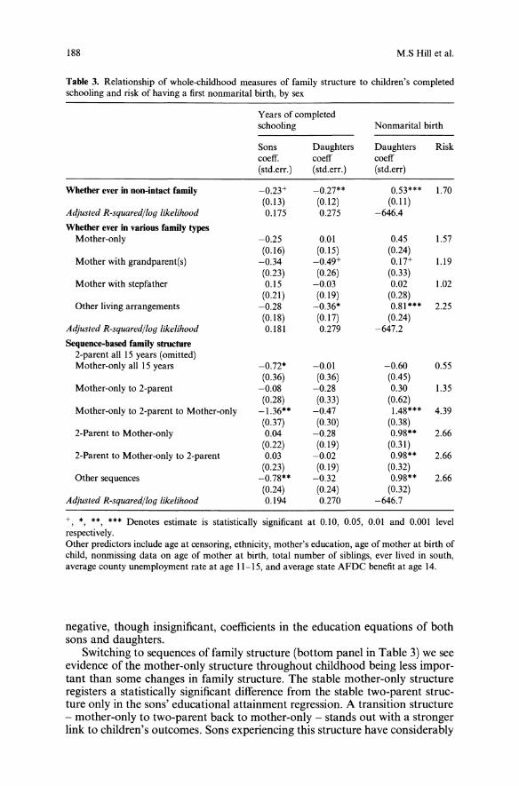
188 M.S Hill et al.

Table 3. Relationship of whole-ehildhood measures of family structure to children's completedschooling and risk of having a first nonmarital birth, by sex

Years of completedschooling Nonmarital birth

Sons Daughters Daughters Riskcoeff. coeff coeff(std.erL) (std.erL) (std.err)

Whether ever in non-intact family -0.23+ -0.27** 0.53*** 1.70(0.13) (0.12) (0.11)

Adjusted R-squared/log likelihood 0.175 0.275 -646.4

Whether ever in various family typesMother-only -0.25 0.01 0.45 1.57

(0.16) (0.15) (0.24)Mother with grandparent(s) -0.34 -0.49+ 0.17+ 1.19

(0.23) (0.26) (0.33)Mother with stepfather 0.15 -0.03 0.02 1.02

(0.21) (0.19) (0.28)Other living arrangements -0.28 -0.36* 0.81 *** 2.25

(0.18) (0.17) (0.24)Adjusted R-squared/log likelihood 0.181 0.279 -647.2

Sequence-based family structure2-parent all 15 years (omitted)Mother-only all 15 years -0.72* -0.01 -0.60 0.55

(0.36) (0.36) (0.45)Mother-only to 2-parent -0.08 -0.28 0.30 1.35

(0.28) (0.33) (0.62)Mother-only to 2-parent to Mother-only -1.36** -0.47 1.48*** 4.39

(0.37) (0.30) (0.38)2-Parent to Mother-only 0.04 -0.28 0.98** 2.66

(0.22) (0.19) (0.31)2-Parent to Mother-only to 2-parent 0.03 -0.Q2 0.98** 2.66

(0.23) (0.19) (0.32)Other sequences -0.78** -0.32 0.98** 2.66

(0.24) (0.24) (0.32)Adjusted R-squared/log likelihood 0.194 0.270 -646.7

+ * ** , *** Denotes estimate is statistically significant at 0.10, 0.05, 0.01 and 0.001 level,respectively.Other predictors include age at censoring, ethnicity, mother's education, age of mother at birth ofchild, nonrnissing data on age of mother at birth, total number of siblings, ever lived in south,average county unemployment rate at age 11-15, and average state AFDC benefit at age 14.

negative, though insignificant, coefficients in the education equations of bothsons and daughters.Switching to sequences of family structure (bottom panel in Table 3) we see

evidence of the mother-only structure throughout childhood being less impor­tant than some changes in family structure. The stable mother-only structureregisters a statistically significant difference from the stable two-parent struc­ture only in the sons' educational attainment regression. A transition structure- mother-only to two-parent back to mother-only - stands out with a strongerlink to children's outcomes. Sons experiencing this structure have considerably

Family structure and young adult behaviors 189

lower educational attainment than sons from two-parent or mother-onlystructures. Daughters from this transition structure have a higher risk of a non­marital birth than daughters from stable two-parent or mother-only structures.Indeed, daughters from most any transition structure run a higher risk ofa non­marital birth than daughters from the stable structures. Yet family structuresequences matter little for daughters' educational attainment, with transitionstructures showing negative but insignificant coefficients and the stable mother­only structure having an essentially zero coefficient. The tenor of these findingsis roughly consistent with that of Wojtkiewicz (1993) and Wu and Martinson(1993). Given the differentials we find for sons' and daughters' educationalattainment, collectively our results are in line with Wojtkiewicz's major con­clusions regarding children's odds of finishing high school: a negative associa­tion with change in family structure and no association with prolonged stay in amother-only family. Our results showing the heightened linkage of daughters'risk of a non-marital birth to transition structures fit with Wu and Martinson'sfinding that, for both white and black daughters, risk of a non-marital birthincreases with number of changes in family structure.Overall, our results tend to show similar but weaker associations than those

of earlier researchers, with many of our coefficients failing to achieve signifi­cance at conventional levels. It is possible that these differences in findings areattributable to cohort differences since the other researchers investigated earliercohorts of children, who were less likely to experience a mother-only structureand hence may have experienced greater differences in family life. The influenceof non-intact family structures may well have diminished as they have becomemore common, but tests of such an assertion await further research.

4.4. Timing during childhood

One of the unique contributions of this paper is being able to observe varia­tion in the influence of family structure over the course of childhood. To as­sess the role of timing of family structure influences, we turn to stage-specificmeasures constructed separately for early childhood (ages 0-5), middle child­hood (ages 6-10) and late childhood (ages 11-15). Tables 4 and 5 presentregression results regarding these stage-specific measures. Table 4 focuses onthe type of family structure experienced at each stage of childhood. Table 5focuses on change in family structure, with the change assessed in terms ofparental marital events at different stages of childhood (controlling for thefamily structure children are born into).These tables, each with precise timing of family structure experiences, em­

phasize the importance of: (1) timing, (2) new types of family structure, and(3) change as opposed to extended stay in non-intact families. Predictivepower improves when we switch from regressions using 'whether ever in anon-intact family' as the sole indicator of childhood family structure to spec­ifications differentiated by childhood stage and type of non-intact family(not shown)Y The enhanced predictive power appears to be concentratedin distinguishing two family structures, mother-with-stepfather and mother­with-grandparent(s), at particular childhood stages (see Table 4).There is suggestive evidence that the mother-with-stepfather arrangement

has some importance for daughters' subsequent educational attainment withthe direction of the association differing by childhood stage. Daughters in

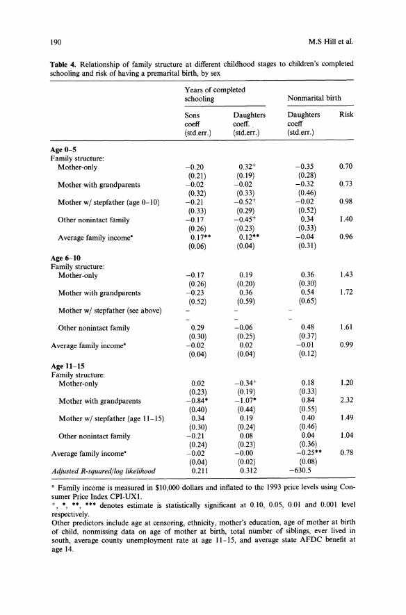
190 M.S Hill et al.

Table 4. Relationship of family structure at different childhood stages to children's completedschooling and risk of having a premarital birth, by sex

Years of completedschooling Nonrnarital birth

Sons Daughters Daughters Riskcoeff coeff. coeff(std.err.) (std.err.) (std.err.)

Age 0-5Family structure:Mother-only -0.20 0.32+ -0.35 0.70

(0.21) (0.19) (0.28)Mother with grandparents -0.02 -0.02 -0.32 0.73

(0.32) (0.33) (0.46)Mother wi stepfather (age 0-10) -0.21 -0.52+ -0.02 0.98

(0.33) (0.29) (0.52)Other nonintact family -0.17 -0.45+ 0.34 1.40

(0.26) (0.23) (0.33)Average family income" 0.17" 0.12" -0.04 0.96

(0.06) (0.04) (0.31)

Age 6-10Family structure:Mother-only -0.17 0.19 0.36 1.43

(0.26) (0.20) (0.30)Mother with grandparents -0.23 0.36 0.54 1.72

(0.52) (0.59) (0.65)Mother wi stepfather (see above)

Other nonintact family 0.29 -0.06 0.48 1.61(0.30) (0.25) (0.37)

Average family income" -0.02 0.02 -0.01 0.99(0.04) (0.04) (0.12)

Age 11-15Family structure:Mother-only 0.02 -0.34+ 0.18 1.20

(0.23) (0.19) (0.33)Mother with grandparents -0.84· -1.07· 0.84 2.32

(0.40) (0.44) (0.55)Mother wi stepfather (age 11-15) 0.34 0.19 0.40 1.49

(0.30) (0.24) (0.46)Other nonintact family -0.21 0.08 0.04 1.04

(0.24) (0.23) (0.36)Average family income" -0.02 -0.00 -0.25" 0.78

(0.04) (0.02) (0.08)Adjusted R-squared/log likelihood 0.211 0.312 -630.5

" Family income is measured in $10,000 dollars and inflated to the 1993 price levels using Con-sumer Price Index CPI-UXI.+ • ••, ... denotes estimate is statistically significant at 0.10, 0.05, 0.01 and 0.001 level, ,respectively.Other predictors include age at censoring, ethnicity, mother's education, age of mother at birthof child, nonrnissing data on age of mother at birth, total number of siblings, ever lived insouth, average county unemployment rate at age 11-15, and average state AFDC benefit atage 14.

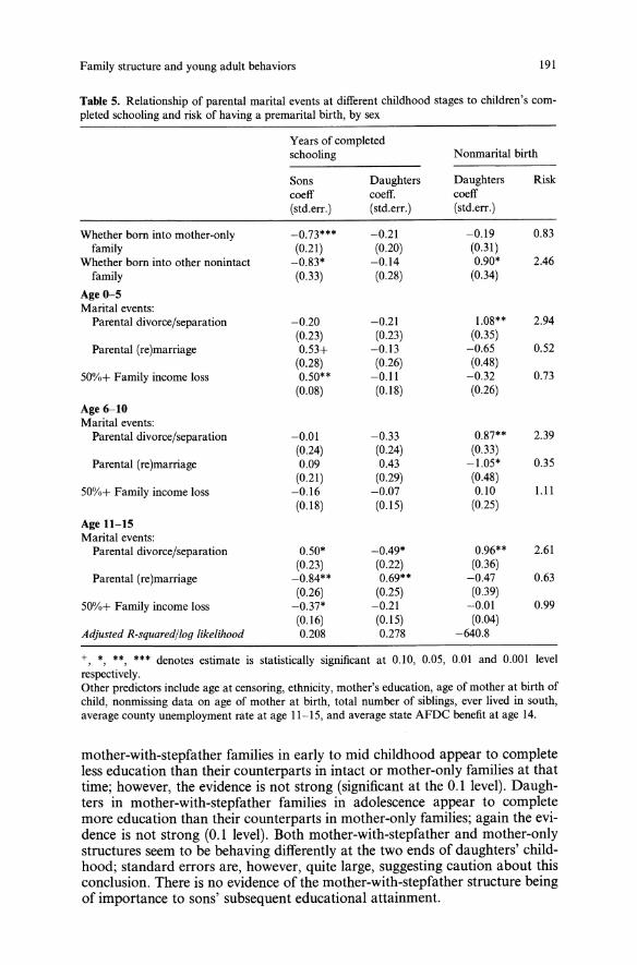
Family structure and young adult behaviors 191

Table 5. Relationship of parental marital events at different childhood stages to children's com­pleted schooling and risk of having a premarital birth, by sex

Years of completedschooling Nonmarital birth

Sons Daughters Daughters Riskcoeff coeff. coeff(std.err.) (std.err.) (std.err.)

Whether born into mother-only -0.73*** -0.21 -0.19 0.83family (0.21) (0.20) (0.31)

Whether born into other nonintact -0.83* -0.14 0.90* 2.46family (0.33) (0.28) (0.34)

Age 0-5Marital events:Parental divorce/separation -0.20 -0.21 1.08** 2.94

(0.23) (0.23) (0.35)Parental (re)marriage 0.53+ -0.13 -0.65 0.52

(0.28) (0.26) (0.48)50%+ Family income loss 0.50** -0.11 -0.32 0.73

(0.08) (0.18) (0.26)

Age 6-10Marital events:Parental divorce/separation -0.01 -0.33 0.87** 2.39

(0.24) (0.24) (0.33)Parental (re)marriage 0.09 0.43 -1.05* 0.35

(0.21) (0.29) (0.48)50%+ Family income loss -0.16 -0.D7 0.10 1.11

(0.18) (0.15) (0.25)

Age 11-15Marital events:Parental divorce/separation 0.50* -0.49* 0.96** 2.61

(0.23) (0.22) (0.36)Parental (re)marriage -0.84** 0.69** -0.47 0.63

(0.26) (0.25) (0.39)50%+ Family income loss -0.37* -0.21 -0.01 0.99

(0.16) (0.15) (0.04)Adjusted R-squared/log likelihood 0.208 0.278 -640.8

+ * **, *** denotes estimate is statistically significant at 0.10, 0.05, 0.01 and 0.001 level, ,respectively.Other predictors include age at censoring, ethnicity, mother's education, age of mother at birth ofchild, nonmissing data on age of mother at birth, total number of siblings, ever lived in south,average county unemployment rate at age 11-15, and average state AFDC benefit at age 14.

mother-with-stepfather families in early to mid childhood appear to completeless education than their counterparts in intact or mother-only families at thattime; however, the evidence is not strong (significant at the 0.1 level). Daugh­ters in mother-with-stepfather families in adolescence appear to completemore education than their counterparts in mother-only families; again the evi­dence is not strong (0.1 level). Both mother-with-stepfather and mother-onlystructures seem to be behaving differently at the two ends of daughters' child­hood; standard errors are, however, quite large, suggesting caution about thisconclusion. There is no evidence of the mother-with-stepfather structure beingof importance to sons' subsequent educational attainment.

192 M.S Hill et al.

It is in late childhood that the mother-with-grandparent(s) structure showsits strongest associations with subsequent educational attainment, and herethe associations are similar for sons and daughters. Young adults, sons as wellas daughters, who lived in a mother-with-grandparent(s) structure during theiradolescent years tended to have about one year less completed schooling thanotherwise similar young adults who lived in two-parent families at that stageof childhood.From the size of the coefficients alone, it would appear that the mother­

with-grandparent(s) structure in late childhood has the strongest negativeassociation with the outcomes we examine of any non-intact structure at anychildhood stage. However, this conclusion is tempered by results of statisticaltests for differences in coefficients both across the late-childhood structuresand for the mother-with-grandparent(s) structure across the different child­hood stages. Whether the mother-with-grandparent(s) structure is, of all thenon-intact structures in late childhood, the most negative in its associationwith subsequent educational attainment is unclear. The coefficient on themother-with-grandparent(s) variable is (at 0.05 significance level) more nega­tive than that of all other non-intact structures in late childhood except, fordaughters, the mother-only structure and, for sons, the 'other' set of struc­tures. More lenient significance thresholds (0.15 significance level) support thedifference between the mother-with-grandparent(s) structure and the mother­only structure in late childhood. Tests for differences in coefficients for themother-with-grandparent(s) structure at different childhood stages also yieldresults highly sensitive to the significance threshold. The coefficient on themother-with-grandparent(s) variable in late childhood is not perceived aslarger than the coefficients on that same structure at earlier childhood stageswhen the significance threshold is set at the 0.05 levels. A more lenient signif­icance level of 0.1 0 yields significant differences for daughters, though still notsons. On the whole, the evidence suggests the cautious observation that thereis a good chance that the mother-with-grandparent(s) structure in late child­hood is especially detrimental to children's education. The mother-with­grandparent(s) structure clearly merits further research as something distinctfrom the mother-only structure.The evidence provides little support for social control theory's contention

that additional adults in non-intact families lessen detrimental influences ofthe structure. Children spending time in mother-with-stepfather families ormother-with-grandparent(s) families do not tend to have higher levels of sub­sequent educational attainment or lower risks of a nonmarital birth than thosespending time in mother-only families. The one exception is daughters inmother-with-stepfather families late in childhood.Changes in parents' marital arrangements, especially those occurring in

late childhood, show several strong associations with children's adult behav­iors (see Table 5). The pattern, though, varies with the type of parental event,its timing in terms of childhood stage, and the sex of the child. One patternthat holds for both sons and daughters is a tendency for parental marital dis­ruption and parental (re)marriage to show opposite associations with thechildren's young adulthood outcomes. Each of these changes, however, seemsto influence sons and daughters differently.Relative to otherwise similar counterparts, daughters who experienced pa­

rental marital disruption at any childhood stage tended to have a higher riskof a nonmarital birth (two and one-half to three times as high). Daughters

Family structure and young adult behaviors 193

who experienced parental marital disruption in late childhood also tended tohave less subsequent completed schooling (about one half year less). Sons, onthe other hand, who experienced parental marital disruption in adolescencetended to have more, rather than less, subsequent educational attainment(about one-half year more) than their otherwise similar counterparts.Parental (re)marriage experienced in middle childhood is associated with

a lower risk for daughters of a nonmarital birth (one-third as high). Parental(re)marriage experienced in adolescence is associated, for daughters, withhigher (about two-thirds of a year more) educational attainment. For sons, onthe other hand, parental (re)marriage at that late stage of childhood is asso­ciated with less (about four-fifth of a year less) educational attainment.The strength of the relationship between parental (re)marriage and subse­

quent educational attainment differs depending on the timing of this event.Much of this difference is in terms of whether there is or is not a notableassociation. The difference is more striking, though, in the case of early versuslate childhood parental re(marriage) experienced by sons. There is weak evi­dence of parental (re)marriage early in childhood being associated with more(by about one-half year), rather than less (compared with, in late childhood,one year less), subsequent educational attainment. This suggests that the tim­ing of parental marital events is especially important for sons' educationalattainment.

5. Discussion

With data on full childhood family experiences, we estimate models of edu­cational attainment and nonmarital births that provide a variety of views ofthe role of family structure in shaping children's lives. To distinguish the waysin which family structure operates, we introduce into our models various setsof control variables. We cannot entirely rule out possibilities of endogeneityfor all control variables; hence our findings are tempered with some caution.In general, our findings are more consistent with the underlying family

mechanisms posited by stress theory (stress caused by disruptions in familystructure) than those posited by social control theory (tighter supervisionthrough larger numbers of parents or substitute parents). Change rather thantype of structure predominates in the strength of association with children'sadult behaviors, and there is no evidence that the number of adults in thechild's home, per se, reduces detrimental influences of exposure to a non­intact family. We find that parental marital change has a more pronouncedassociation with the outcomes we examine if the events occurred in latechildhood. This is consistent with stress theory also, which posits that changein family structure will have its greatest effects close to the time of the change.Because educational attainment and nonmarital births are observed in theyears most immediately following late childhood, it is that stage of childhoodthat is closest in timing.Yet some of the findings are also at odds with stress theory. Most especi­

ally, change is not always tied to the outcomes in a detrimental way. Parentalmarital change is not always associated with lower educational attainment ora higher risk of nonmarital birth; it sometimes has an association in the op­posite direction, and many times has no association that is statistically differ­ent from zero at conventional levels. In addition, the young adult outcomes

194 M.S Hill et al.

we examined appear to be unrelated to several sequences of transitions infamily structure.Our analysis also allows us to investigate the economic hardship theory,

matching the measure of childhood family income to that of family structure.From Tables 4 and 5 we see that childhood family income is linked to child­ren's educational attainment and daughters' risk of a nonmarital birth, thoughnot at all childhood stages. Average childhood family income relates to edu­cational attainment and risk of a nonmarital birth in the expected direction:when average childhood income is included in combination with stage-specificfamily structure measures (not shown), income is positively related to child­ren's education and negatively related to daughters' risk of a nonmaritalbirth. t3 Predictive power improves, however, when the match in timing ofincome and family structure is tighter. 14 Our disaggregation of family incomeallows us to see what appears to be differential concentration of family incomelinkages by childhood stage. It is the income during early childhood that ismost strongly linked to sons' and daughters' subsequent educational attain­ment. On the other hand, it is the income during late childhood that moststrongly links level of income to daughters' risk of a nonmarital birth. Latechildhood also appears to be the time of strongest linkage between incomeloss and subsequent lower levels of educational attainment, as the results inTable 5 indicate. Oddly enough, for sons family income loss in early child­hood is associated with higher, rather than, lower, completed schooling. Es­pecially since no similar findings appear for daughters, it is difficult to knowwhat to make of this. Taken as a whole, childhood family income appearsto play an important role in the outcomes examined, though the role is notentirely straightforward and shows strong evidence of notable differences bychildhood stage.Childhood family income does not appear to account for linkages between

childhood family structure and the outcomes we examine. Those linkagesappear to be largely independent of family income (a finding consistent withWu 1996). When we estimate the models presented in Tables 4 and 5 omittingincome as a control, the coefficients on the family-structure and parental­marital event variables are hardly affected.To assess other possible mechanisms, we also investigated three other ways

in which childhood family structure might influence educational attainmentand nonmarital birth: via intergenerational transmission of reliance on publicsupport, reduced attention from the mother because of her greater workcommitment, and disruptive influences of residential relocation. 15 Of thethree, residential relocation exhibits the strongest relationship to the outcomeswe examine. Such moves, for daughters, are associated with reduced educa­tional attainment if the move occurred in middle or late childhood (see Ap­pendix Table 1). In analysis not shown here, residential moves were alsofound to account for part of the negative association between daughters'educational attainment and parental marital events or living in a mother-with­stepfather family during adolescence. Mother's market work commitment aswell as receipt of AFDC showed no notable relationships to the outcomes weexamined.Some of the findings simply do not fit the major existing theories and call

out for further theoretical development. The mother-with-grandparent struc­ture is not well understood; our findings suggest that it merits more attentionin both empirical research and theories of family structure influences. Though

Family structure and young adult behaviors 195

our modest sample sizes preclude strong conclusions, our results suggest thistype of structure experienced late in childhood could be strongly tied toreduced educational attainment and enhanced risks of a nonmarital birth.Because it is a type of structure rather than a change in structure, this findingdoes not fit with stress theory. Because it involves more adults than a mother­only structure, it does not fit with social control theory either. Because thestrength of the relationship holds even with controls for family income, it doesnot fit with economic hardship theory.Why would the mother-with-grandparent(s) structure during late child­

hood be so negatively related to young adult outcomes, and why would thatsame structure early in childhood have little association with children's long­run outcomes? One possibility is that conflicts in rearing practices may be es­pecially important in adolescence. The two generations of adults - parent andgrandparent - may have conflicting ideas about how to raise teenagers, andinconsistency in their supervisory activities undermines their ability to steeradolescents away from destructive behaviors. Another possibility is that theobserved associations reflect something about the reason the structure wasformed. In late childhood such a structure probably means one of two things- that the child's mother has recently had a marital disruption and is gettinghelp from the child's grandparents or that the child's grandmother is in needof financial assistance or help with activities and has moved into the child'sfamily to receive such help. Both possibilities can mean, relative to intactfamilies, that less of the total family income is allocated to children, thatchildren have less privacy, and that children are expected to devote more timeto responsibilities at home. This points to differences in within-family resourceallocation as a possible underlying mechanism, with family structure as a de­terminant of within-family resource allocation patterns (Chase-Lansdale et al.1994).Findings for some types of parental marital events at certain stages of

childhood also merit further thought to suggest theories about the underlyingmechanisms. Parental (re)marriage in late childhood is positively related todaughters' educational attainment, and in middle childhood this event is neg­atively related to their risk of a nonmarital birth. In addition, parental divorceor separation in late childhood is positively related to son's educational at­tainment. Stress theory predicts the opposite because parental marital changemeans change in organization. The findings for parental (re)marriage might fitwith social control theory (because the change adds a substitute parent).However, why is the association of this event with subsequent educationalattainment so different (and strongly negative) for sons? A possible explana­tion for the pattern of results regarding parental (re)marriage may lie in dif­ferences between fathers and stepfathers in their commitment to adolescents.Men who marry into families with children in or near adolescence may tend tobe more supportive because they self-select themselves into that position andthat responsibility. Their support may benefit girls more than boys becausegirls may tend to accept their support whereas boys may tend to resist it, inpart because boys may resent the stepfather stepping into the father role at atime when they feel they are old enough to be 'man of the family.' It is possi­ble that something of a mirror image accounts for the positive association ofparental divorce or separation late in childhood with sons' subsequent educa­tional attainment: boys may take adult roles more seriously when they feelthey are the 'man of the family.'

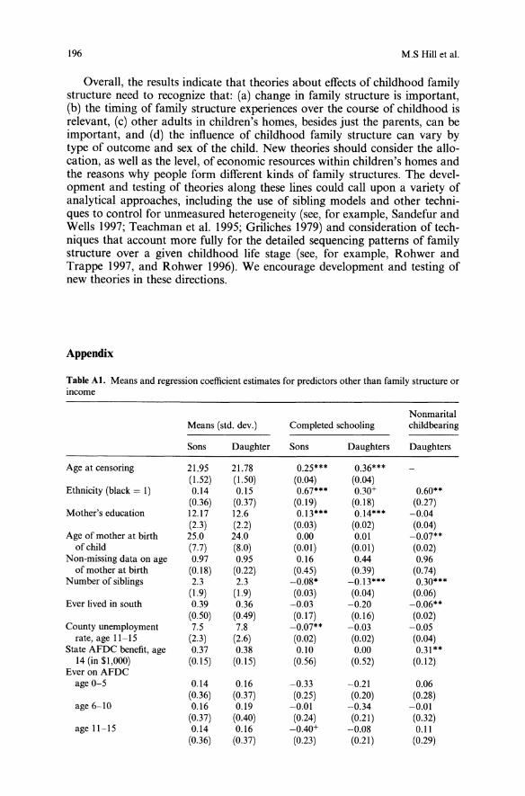
196 M.S Hill et al.

Overall, the results indicate that theories about effects of childhood familystructure need to recognize that: (a) change in family structure is important,(b) the timing of family structure experiences over the course of childhood isrelevant, (c) other adults in children's homes, besides just the parents, can beimportant, and (d) the influence of childhood family structure can vary bytype of outcome and sex of the child. New theories should consider the allo­cation, as well as the level, of economic resources within children's homes andthe reasons why people form different kinds of family structures. The devel­opment and testing of theories along these lines could call upon a variety ofanalytical approaches, including the use of sibling models and other techni­ques to control for unmeasured heterogeneity (see, for example, Sandefur andWells 1997; Teachman et al. 1995; Griliches 1979) and consideration of tech­niques that account more fully for the detailed sequencing patterns of familystructure over a given childhood life stage (see, for example, Rohwer andTrappe 1997, and Rohwer 1996). We encourage development and testing ofnew theories in these directions.

Appendix

Table At. Means and regression coefficient estimates for predictors other than family structure orincome

NonrnaritalMeans (std. dev.) Completed schooling childbearing

Sons Daughter Sons Daughters Daughters

Age at censoring 21.95 21.78 0.25*** 0.36***(1.52) (1.50) (0.04) (0.04)

Ethnicity (black = I) 0.14 0.15 0.67*** 0.30+ 0.60**(0.36) (0.37) (0.19) (0.18) (0.27)

Mother's education 12.17 12.6 0.13*** 0.14*** -0.04(2.3) (2.2) (0.03) (0.02) (0.04)

Age of mother at birth 25.0 24.0 0.00 0.01 -0.07**of child (7.7) (8.0) (0.01) (0.01) (0.02)Non-missing data on age 0.97 0.95 0.16 0.44 0.96of mother at birth (0.18) (0.22) (0.45) (0.39) (0.74)Number of siblings 2.3 2.3 -0.08* -0.13*** 0.30***

(1.9) (1.9) (0.03) (0.04) (0.06)Ever lived in south 0.39 0.36 -0.03 -0.20 -0.06**

(0.50) (0.49) (0.17) (0.16) (0.02)County unemployment 7.5 7.8 -0.07** -0.03 -0.05rate, age 11-15 (2.3) (2.6) (0.02) (0.02) (0.04)State AFDC benefit, age 0.37 0.38 0.10 0.00 0.31**14 (in $1,000) (0.15) (0.15) (0.56) (0.52) (0.12)Ever on AFDCage 0-5 0.14 0.16 -0.33 -0.21 0.06

(0.36) (0.37) (0.25) (0.20) (0.28)age 6-10 0.16 0.19 -0.01 -0.34 -0.01

(0.37) (0.40) (0.24) (0.21) (0.32)age 11-15 0.14 0.16 -0.40+ -0.08 0.11

(0.36) (0.37) (0.23) (0.21) (0.29)

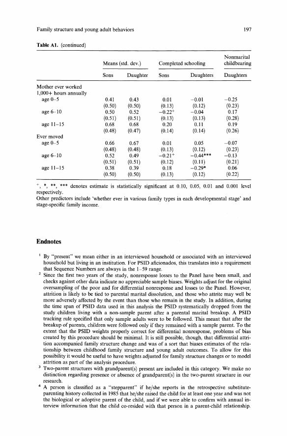
Family structure and young adult behaviors

Table AI. (continued)

Means (std. dev.) Completed schooling

197

Nonmaritalchildbearing

Sons Daughter Sons Daughters Daughters

Mother ever worked1,000+ hours annuallyage 0-5 0.41 0.43 0.01 -0.01 -0.25

(0.50) (0.50) (0.13) (0.12) (0.23)age 6-10 0.50 0.52 -0.22+ -0.04 0.17

(0.51) (0.51) (0.13) (0.13) (0.28)age 11-15 0.68 0.68 0.20 0.11 0.19

(0.48) (0.47) (0.14) (0.14) (0.26)Ever movedage 0-5 0.66 0.67 0.01 0.05 -0.07

(0.48) (0.48) (0.13) (0.12) (0.23)age 6-10 0.52 0.49 -0.21+ -0.44*** -0.13

(0.51) (0.51) (0.12) (0.11 ) (0.21)age 11-15 0.38 0.39 0.18 -0.29* 0.06

(0.50) (0.50) (0.13) (0.12) (0.22)

+ * ** *** denotes estimate is statistically significant at 0.10, 0.05, 0.01 and 0.001 level, , ,respectively.Other predictors include 'whether ever in various family types in each developmental stage' andstage-specific family income.

Endnotes

I By "present" we mean either in an interviewed household or associated with an interviewedhousehold but living in an institution. For PSID aficionados, this translates into a requirementthat Sequence Numbers are always in the I-59 range.

2 Since the first two years of the study, nonresponse losses to the Panel have been small, andchecks against other data indicate no appreciable sample biases. Weights adjust for the originaloversampling of the poor and for differential nonresponse and losses to the Panel. However,attrition is likely to be tied to parental marital dissolution, and those who attrite may well bemore adversely affected by the event than those who remain in the study. In addition, duringthe time span of PSID data used in this analysis the PSID systematically dropped from thestudy children living with a non-sample parent after a parental marital breakup. A PSIDtracking rule specified that only sample adults were to be followed. This meant that after thebreakup of parents, children were followed only if they remained with a sample parent. To theextent that the PSID weights properly correct for differential nonresponse, problems of biascreated by this procedure should be minimal. It is still possible, though, that differential attri­tion accompanied family structure change and was of a sort that biases estimates of the rela­tionship between childhood family structure and young adult outcomes. To allow for thispossibility it would be useful to have weights adjusted for family structure changes or to modelattrition as part of the analysis procedure.

3 Two-parent structures with grandparent(s) present are included in this category. We make nodistinction regarding presence or absence of grandparent(s) in the two-parent structure in ourresearch.

4 A person is classified as a "stepparent" if he/she reports in the retrospective substitute­parenting history collected in 1985 that he/she raised the child for at least one year and was notthe biological or adoptive parent of the child, and if we were able to confirm with annual in­terview information that the child co-resided with that person in a parent-ehild relationship.

198 M.S Hill et al.

However, limiting identification of stepparent situations to this definition alone misses somestepparent situations. This is because fertility and marital histories were not gathered until 1985and not all adults who had co-resided with children at some point prior to 1985 survived in thepanel until 1985. In particular, if a man was living in the family of the child as a husband orpermanent partner of the mother prior to 1985 but was lost to attrition before 1985, we couldnot establish a definitive relationship between that man and the child. In such cases, we as­sumed that the man was the biological or adoptive father if the mother reported being marriedto the man and the man was co-residing with the child at the time of the child's birth; other­wise, we assumed he was a stepfather.

S The PSID estimates average across several calendar years and apply to single year of age forages 1-15. To simulate estimates for a cross-section of children of all ages, we weighted thefigures given in Table I according to the age distribution of children in 1980 (approximatelythe midpoint for the PSID data). The age distribution figures were those for July I, 1980 ob­tained from Bureau of the Census (1990), Table I. We also assumed the PSID family structuredistribution for age 15 applied to ages 16 and 17 as well.

6 Rendall et al. (1997) find, in both British and V.S. panel data, that reports of men's fertilityshow an overall deficit of between one-third and one-half of non-marital births, with the deficitespecially high for V.S. black men. Non-reporting accounts for most of the deficit in the non­marital births.

7 The means (standard deviations) for Average Annual Total Family Income (in 1993 $10,0(0)are: 4.49 (2.9) over all 15 years; 3.7 (2.1) during ages 0-5; 4.6 (3.1) during ages 6-10; and 5.2(4.1) during ages 11-15. For the measure of whether ever in a non-intact family and for thesequence of family structure types, annual income is averaged over the entire childhood.

8 The means (standard deviations) for whether there was a 50% or more Income Loss are: 0.12(0.33) for ages 0-5; 0.15 (0.37) for ages 6-10; and 0.15 (0.36) for ages 11-15.

9 Regarding the association of ever in a non-intact family to risk of a non-marital birth, Wu andMartinson (1993) estimate coefficients of 0.50 for whites and 0.28 for blacks, both significant atthe 0.01 level, and Bumpass and McLanahan's (1989) estimates are similar.

10 The coefficient (standard error) on the more aggregated version of mother-only structure is-0.406 (0.070) in Wojtkiewicz's (1993) odds of high school graduation regression for sons anddaughters combined. The coefficients are 0.56 and 0.32, both significant at the 0.01 level, inWu and Martinsons' (1993) risk of premarital birth regressions for white and black daughters,respectively.

11 The coefficient (standard error) for mother-with-stepfather in Wojtkiewicz's (1993) odds ofhigh school graduation regression is -0.075 (0.105). The coefficients in Wu and Martinson's(1993) risk of a non-marital birth regression are 0.47 for whites, significant at the 0.05 level,and 0.23 for blacks, not significant at the 0.05 level.

12 Moving from the single non-intact family indicator to our stage-specific, type-specific charac­terization and continuing to omit childhood family income from the predictors, adjusted R­squareds increase from 0.175 to 0.189 in the education regression for boys and from 0.275 to0.287 in the education regression for girls. The log likelihood in the nonmarital birth equationdecreases from -646.4 to -642.6.

13 The following are the coefficients (standard errors) on average childhood family income whenit is substituted for stage-specific family income in the Table 4 regressions: 0.11 (0.03) for sons'seducation; 0.08 (0.02) for daughters' education; -0.28 (0.08) for daughters' risk of a non­marital birth.

14 The R-squareds with income averaged over all of childhood are 0.206 for sons and 0.307 fordaughters. The log likelihood is -634.6. This compares to R-squareds of 0.211 and 0.312, re­spectively, and a log likelihood of -630.5 with the stage-specific average family income mea­sures of Table 4.

1S These additional predictor variables are specified as childhood-stage specific measures of: (a)family receipt of income from the Aid to Families With Dependent Children program (coded Iif the child's family ever received income from AFDC during the specified childhood stage andzero otherwise); (b) whether the mother devoted substantial time to market work (coded I ifthe child's mother ever worked an average of 1000 or more annual hours during the specifiedchildhood stage and zero otherwise); and (c) whether the child's family moved (coded I if thefamily ever changed residences during the specified childhood stage). Each of these variables isbased on information obtained in annual interviews. Appendix Table I shows the means andstandard deviations.

Family structure and young adult behaviors

References

199

Axinn WG, Thornton A (1992) The Influence of Parental Resources on the Timing of the Tran­sition to Marriage. Social Science Research 21:261-285

Boggess S (1998) Family Structure, Economic Status, and Educational Attainment. Journal ofPopulation Economics II :205-222

Booth A, BrinkerhoffD, White L (1984) The Impact of Parental Divorce on Courtship. Journal ofMarriage and the Family 46:85-94

Brooks-Gunn J (forthcoming) Policy and Research Issues in the Study of Remarriage. In: Dunn J,Booth A (ed.) Remarriage and Children. Erlbaum, Hillsdale, NJ

Bumpass LL (1984) Children and Marital Disruption: A Replication and Update. Demography21:71-82

Bureau of the Census (January 1990) Current Population Reports, United States Population Esti­mates, by Age, Sex, Race, and Hispanic Origin: 1980 to 1988. Series P-25, No. 1045

Burton LM, Obeidallah DA, Allison K (1996) Ethnographic Insights on Social Context andAdolescent Development among Inner-City African-American Teens. In: Jessor R, Colby JA,Shweder RA (eds.) Ethnography and Human Development: Context and Meaning in SocialInquiry. University of Chicago Press, Chicago 556-579

Casper LM, Bryson KR (1998) Co-resident Grandparents and Their Grandchildren: GrandparentMaintained Families. U.S. Bureau of the Census, Population Division Working Paper No. 26,March

Chase-Lansdale PL, Brooks-Gunn J, Zamsky E (1994) Young African-American Multigenera­tional Families in Poverty: Quality of Mothering and Grandmothering. Child Development65(2):373-393

Cherlin AJ (1988) The Changing American Family and Public Policy. Urban Institute Press,Washington, D.C.

Cherlin A (1978) Remarriage As An Incomplete Institution. American Journal of Sociology86:636-650

Cherlin A, Furstenberg FF Jr, Chase-Lansdale PL, Kiernan KE, Robins PK, Morrison DR,Teitler JO (1991) Longitudinal Studies of Effects of Divorce on Children in Great Britain andthe United States. Science 252:1386-1389

Conger RD, Conger KJ, Elder GH, Lorenz FO, Simons RL, Whitbeck LB (1992) A FamilyProcess Model of Economic Hardship and Adjustment of Early Adolescent Boys. Child De­velopment 63:526-541

Conger RD, Conger KJ, Elder GH, Lorenz FO, Simons RL, Whitbeck LB (1993) Family Eco­nomic Stress and Adjustment of Early Adolescent Girls. Developmental Psychology29(2):206-219

DaVanzo J, Goldscheider F (1990) Coming Home Again: Returns to the Nest in Young Adult­hood. Population Studies 44:241-255

Dodge K, Petit G, Bates J (1994) Socialization Mediators of the Relation Between SocioeconomicStatus and Child Conduct Problems. Child Development 65:649-665

Dornbusch SM, Carlsmith JM, Bushwall SJ, Ritter PL, Leiderman H, Hastorf AH, Gross RT(1985) Single Parents, Extended Households and the Control of Adolescents. Child Develop­ment 56:326-341

Duncan GJ, Rodgers W (1990) Lone-Parent Families and Their Economic Problems: Persistent orTransitory? In: Duskin B (ed.) Lone Parents: The Economic Challenge. OECD, Paris. 43-68

Duncan GJ, Yeung W-JJ, Rodgers W (1994) Lone-parent Families in the United States: Dy­namics, Economic Status and Developmental Consequences. Population 49(6):1419-1436,Paris

Ermisch J, Francesconi M (2000) Educational Choice, Families, and Young People's Earnings.Journal of Human Resources 35 (forthcoming)

Ermisch J, Francesconi M (2001) Family Structure and Children's Achievements Journal ofPopulation Economics (forthcoming)

Elder GH Jr (1974) Children of the Great Depression: Social Change in Life Experience. Universityof Chicago Press, Chicago

Fitzgerald J, Gottschalk P, Moffitt R (1998) The Impact of Attrition in the PSID on Inter­generational Analysis. Journal of Human Resources 33:300-344

Goldscheider FK, Goldscheider C (1987) Moving Out and Marriage: What do Young AdultsExpect? American Sociological Review 52:278-285

200 M.S Hill et al.

Goldscheider FK, DaVanzo J (1989) Pathways to Independent Living in Early Adulthood: Mar­riage, Semiautonomy, and Premarital Residential Independence. Demography 26:597-614

Griliches Z (1979) Sibling Models and Data in Economics: Beginnings of a Survey. Journal ofPolitical Economy 87(5) Part 2:S37-S64

Haveman R, Wolfe B (1994) Succeeding Generations. Russell Sage, New YorkHernandez DJ (1993) American's Children: Resourcesfrom Family, Government, and the Economy.Russell Sage Foundation, New York

Hernandez DJ (1993) America's Children: Resources From Family, Government and the Economy.Russell Sage Foundation, New York

Hetherington EM (1979) Divorce, a Child's Perspective. American Psychologist 34:851-858Hetherington EM (1987) Family Relations Six Years After Divorce. In: Pasley K, Ihinger­Tallman M (eds.) Remarriage and Stepparenting Today: Current Research and Theory.Guilford Press, New York

Hill MS, Duncan GJ (1987) Parental family income and the socioeconomic attainment of chil­dren. Social Science Research 16:9-73

Hofferth SL (1985) Updating Children's Life Course. Journal of Marriage and the Family 47:93­115

Hogan DP, Kitagawa EM (1985) The Impact of Social Status, Family Structure, and Neigh­borhood on the Fertility of Black Adolescents. American Journal of Sociology 90:825­855

Kirby JB, Uhlenberg P (1999) The Wellbeing of Adolescents: Do Coresident Grandparents Makea Difference? Working paper, University of North Carolina

Krein SF (1986) Growing Up in a Single Parent Family: The Effect on Education and Earnings ofYoung Men. Family Relations 35:161-168

Krein SF, Beller AH (1988) Educational Attainment of Children from Single-Parent Families:Differences by Exposure, Gender, and Race. Demography 25:221-234

McLanahan S (1988) Family Structure and Dependency: Early Transitions to Female HouseholdHeadship. Demography 25(1):1-16

McLanahan S, Sandefur G (1994) Growing up With a Single Parent. Harvard University Press,Cambridge, MA

McLanahan S, Bumpass L (1988) Intergenerational Consequences of Family Disruption. Ameri­can Journal of Sociology 94(1): 130-152

McLeod JD, Shanahan MJ (1993) Poverty, Parenting and Children's Mental Health. AmericanSociological Review 58:351-366

McLoyd V, Jayaratne T, Ceballs R, Borquez J (1994) Unemployment and Work Interruptionamong African American Single Mothers: Effects on Parenting and Adolescent Socioemo­tional Functioning. Child Development 65:562-589

Moffitt R, Rendal M (1993) Cohort Trends in the Lifetime Distribution of Female Headship inthe U.S., 1968-1985. Population Studies and Training Center, Brown University. Mimeo

Moorman JE, Hernandez DJ (1989) Married-Couple Families with Step, Adopted, and BiologicalChildren. Demography 26(2):267-277

Mauldon J, Maestas N (1998) Which Children Live with Their Grandparents, and Why? Workingpaper, Berkeley, Goldman School of Public Policy

Mueller C, Pope H (1977) Marital Instability: A Study of the Transmission between Generations.Journal of Marriage and the Family 39:83-92

Pattillo-McCoy M (1999) Black Picket Fences: Privilege and Peril Among the Black Middle Class.University of Chicago Press, Chicago

Rendall M, Clarke L, Peters E, Ranjit N, Verropoulou G (1999) Incomplete Reporting of Men'sFertility in the United States and Britain: A Research Note. Demography 36(1):135-144

Rohwer G (1996) TDA User's Manual, Part IX: Sequence Data. Max Planck Institut furBildungsforschung, Berlin

Rohwer G, Heike T (1997) Describing Life Courses. An Illustration Based on NLSY Data. Paperprepared for the POLIS project conference at the European University Institute, Florence,February 28-March I, 1997

Rubin LB (1976) Worlds of Pain: Life in the Working-Class Family. Basic, New YorkSandefur G, Wells T (1997) Using Siblings to Investigate the Effects of Family Structure onEducational Attainment. Institute for Research on Poverty. Discussion Paper No. 1144-97

Sandefur G, McLanahan S, Wojtkiewicz R (1992) The Effects of Parental Marital Status duringAdolescence on High School Graduation. Social Forces 71:103-121

Family structure and young adult behaviors 201

Seltzer JA (1994) Consequences of Marital Dissolution for Children. Annual Review of Sociology20:235-266

Steinberg L (1987) Single Parents, Stepparents, and the Susceptibility of Adolescents to AntisocialPeer Pressure. Child Development 58:269-275

Teachman JD, Carver K, Day R (1995) A Model for the Analysis of Paired Data. Journal ofMarriage and the Family 57:1011-1024

Thornton A (1991) Influence of the Marital History of Parents on the Marital and CohabitationalExperiences of Children. American Journal ofSociology 96(4):868-894

Thornton A, Camburn D (1987) The Influence of the Family on Premarital Sexual Attitudes andBehavior. Demography 24:323-340

Weiss R (1979) Growing Up A Little Faster: The Experience of Growing Up in a Single-ParentHousehold. Journal ofSocial Issues 35:97-111

Wojtkiewicz RA (1993) Simplicity and Complexity in the Effects of Parental Structure on HighSchool Graduation. Demography 30(4):701-717

Wu LL (1996) Effects of Family Instability, Income, and Income Instability on the Risk of APremarital Birth. American Sociological Review 61:386-406

Wu LL, Martinson BC (1993) Family Structure and The Risk of A Premarital Birth. AmericanSociological Review 58:210-232

Zill N, Nord CW (1994) Running In Place: How American Families Are Faring in A ChangingEconomy and An Individualistic Society. Child Trends, Inc.

Child development and family resources: Evidence fromthe second generation of the 1958 British birth cohort

Andrew McCuUoch 1, Heather, E. Joshj2

1 Kings Fund, 11-13 Cavendish Square, London WCI OAG, UK (Fax: +44-11206-873151;e-mail: amccul@essex.ac.uk)2 Centre for Longitudinal Studies, Institute of Education, London, WCIH OAL, UK(Fax: +44-0207-612-6880; e-mail: hj@c1s.ioe.ac.uk)

Received: 31 July I999/Accepted: 26 September 2000

Abstract. Studies of American and recently British children suggest that thereis a link between family income and child development, in particular thatone consequence of child poverty is to hold back cognitive development.This paper investigates the impact of family income, material deprivation,maternal education and child-rearing behaviour on an indicator of cognitivefunctioning, using British data on children aged 6 to 17 whose mothers aremembers of the 1958 Birth Cohort Study. The poorer average cognitive func­tioning among children from the lowest income groups could largely be ac­counted for, statistically, by the greater material disadvantage of these groups.These analyses provide evidence to suggest that low income has detrimentaleffects on children's cognitive functioning through the operation of longer­term material disadvantage, and that these effects may be mitigated by posi­tive parental behaviours.

JEL classification: 113, no, 130

Key words: Poverty, deprivation, child development

1. Introduction

Poverty among children, as of anyone else, is of concern from the point ofview of equity in immediate living standards, but it is also of concern in thelonger term, from the point of view of efficiency. Empirical studies in many

All correspondence to Andrew McCulloch. This paper represents work funded by grant noL129100168, in the ESRC Programme on Children 5-16. We are grateful for the referees' forsuggestions. Responsible editor: Christoph Schmidt.

204 A. McCulloch, H.E. Joshi

countries show that children who are worst off in terms of their socioeconomicposition, are also worst off when it comes to their health and cognitive devel­opment (McLanahan and Sandefur 1994; Duncan and Brooks-Gunn 1997;Gregg et al. 1999). During the 1980's poverty among children increased fasterin the UK than in any other member state of the European Community(O'Higgins and Jenkins 1990). By the end of the decade nearly one child inthree was living below a relative poverty line drawn at half average equiv­alised income (Gregg et al. 1999). At least in part this reflected an increase inchildren living in families with an unemployed head, or a lone parent. Thesefamilies are more likely to live in poorer quality housing and to depend onstate benefits. Does this lack of financial and material resources lead, throughreduced parents' investment in the 'quality' of their children, to poorer out­comes for children? Can such pathways be identified and can the outcomes bequantified?Researchers have assessed the impact of poverty and socioeconomic status

on various indicators of cognitive functioning during early childhood. Anumber of US studies that controlled for mother's education, and a range ofother maternal characteristics, have 'reported significant effects of poor cir­cumstance on children's cognitive and verbal skills (for example, Korenman etal. 1995, Chase-Lansdale et al. 1997). Duncan et al. (1994) found that familyincome and poverty status were significant predictors of IQ scores in five­year-olds, even after accounting for maternal education, family structure andethnicity and other differences between low and high-income families. Duncanand Brooks-Gunn (1997) assemble a collection ofsuch studies which all includefamily structure among the controls. Although these studies also indicate thatincome may not be so powerful a predictor of behavioural outcomes and ofachievements by adolescents and young adults, among children, income is atleast as important as the absence of a father in predicting cognitive outcomes(McLanahan 1997).Our own previous study, focussed on family structure, of two cognitive

and one behavioural outcome, in samples of British as well as Americanschool-age children, found income to be among the factors which reduced thesize and significance of family structure as a predictor (Joshi et al. 1999).However, Lefebvre and Merrigan (I998) point out that income effects, thoughsignificant may not be large. The multiple stresses of living in poverty increasechildren's susceptibility to other problems, for example delinquency and teenpregnancy, and are often manifested as chronic disorders with an early onset(Kratzer and Hodgins 1997). These behaviours do not usually occur in isola­tion: in fact, they often occur together and have common risk factors includ­ing large family size, family discord and parental mental illness. This paper isintended to contribute new evidence to an understanding of the link betweenfamily income and child development in Britain.Although disadvantage goes hand in hand with low income, there is no

perfect association (Davies et al. 1997). People observed once in lower incomegroups are not necessarily deprived of material resources, whereas the absenceof resources indicates deprivation only when it is enforced by income. Lowincome in itself is not an adequate proxy for deprivation, particularly if it istemporary. Hill and Jenkins (1999) examine the extent to which child povertyin Britain is chronic or transitory in nature. They find that children, especiallyvery young children, have high long-term poverty risks compared to othergroups in the population.

Child development and family resources 205

The causal mechanisms linking relative deprivation and children's out­comes are not well understood. Factors that are probably involved in anydirect effect include adverse housing conditions (Macintyre et al. 1998) anda lack of cognitively stimulating resources, such as books, in the home(Baharudin and Luster 1998). Second, the low income family may suffer dis­advantages from living in a disadvantaged locality with poor services and lowsocial capital (Brooks-Gunn et al. 1997). Third, relative deprivation mighttranslate into poor cognitive outcomes indirectly, involving among others be­havioural factors. Living in a family with a lack ofmaterial or social resourcesmight, for example, affect parental feelings of self esteem which is likely tohave a negative effect on parenting and mental or emotional well being.Fourth, the child's development and the family's circumstances may both bethe joint outcome of other factors, notably parental human capital, a culturalor biological inheritance (Duncan and Brooks-Gunn 1997; Haveman andWolfe 1995; Hobcraft 1998).The last decades of the Twentieth Century saw substantial changes in

family structure in Britain. Lone parents with dependent children constitutean increasing proportion of households with children: 19% of children livedwith a lone mother in 1994-1995 (Church 1996). The increase in the numberof lone parent families since 1972 can be attributed mostly to a rising rate ofpartnership dissolution and also some growth in single motherhood. Over onethird (34%) of births were outside of marriage in 1995, although roughly halfof these were registered by two parents living at the same address (Office ofNational Statistics 1997). Currently 41% of marriages are projected to end indivorce in England and Wales, if hitherto rising divorce rates remain at their1993-1994 levels (Haskey 1994). Similarly, children born to married parentsface a 28% risk that their parents would divorce before they reach age 16(Haskey 1997).There have also been major structural changes in the labour market. The

number of households without an employed member rose sharply in the re­cession of the 1980's but nearly all the subsequent recovery in employmentoccurred in households with one person already in work (Gregg and Wads­worth 1996). Women with a pre-school child were least likely to be in paidwork in 1991 (Church 1997). Although economic activity has increasedamong married women (Office of National Statistics 1998), less than one infive lone mothers with a child under five years was in paid employment. As aconsequence of the changes in labour market activity and family structure, theshare of men's earnings in total family income fell dramatically over the1980's (Harkness et al. 1996). Families with children were over-represented atthe bottom of the income distribution, especially where there was no father inemployment. (Gregg et al. 1999). Low income families are more likely to livein deprived physical environments than those higher on the income scale, withthe majority of families receiving state benefits living in social rented proper­ties (Marsh and McKay 1993; Macintyre et al. 1998).In this paper, we examine the association of a range of indicators of socio­

economic position including family income and other indicators of materialdisadvantage with one indicator of children's cognitive functioning. The aimof the paper is, firstly, to examine whether income is independently associatedwith children's cognitive outcomes; secondly, to assess how far such associa­tion reflects high levels of disadvantages in low income groups; and thirdly,to examine which specific disadvantage contributes most to the link between

206 A. McCulloch, H.E. Joshi

income and child outcomes. This might elicit indications of any mechanismby which deprivation affects children's outcomes, though it cannot provecausation.

2. Data and methods

The National Child Development Study (NCDS) is a study of over 17,000people in Britain born between the 3rd and 9th of March in 1958. Follow-upsweeps took place in 1965, 1969, 1974, 1981 and 1991. The 1991 NCDSfollow-up obtained information not only from the cohort member, but fromthe children of I in 3 randomly sampled cohort members (Ferri 1993). In thispaper we restrict the analyses to children who were aged 6 or older in 1991and who had a mother who was an NCDS cohort member, and who wereresident with her in 1991. This excludes only a small number of children whowere not living with their cohort member mothers (see Joshi et al. 1999).Children with fathers in the cohort were not included because the informationon them was in various ways less complete. Any children over 13 would havebeen born to a teenage mother. Thus the sample design imposes an artificialinverse correlation of the ages of children and the age of the mother at birth.The data are more representative of children with teenaged, and hence lesseducated, mothers, than a full cross-section of children. As shown in Table 1,the family structures in which the children were living are strongly related tothe age of the child and therefore, to the age of the mother at the time thechild was born. Younger women are more likely to have births outside part­nerships; and older children have had more chance of experiencing a changein the family situation (Clarke et al. 1997).

2.1. Cognitive functioning

In this paper we use performance on the Peabody Picture Vocabulary Test(PPVT) as an indicator of children's cognitive functioning. The PPVT isan individually administered test of hearing vocabulary, with 175 test itemsarranged in order of increasing difficulty. Each item presents a multiple choicebetween four illustrations, the aim being to select the picture best illustratingthe meaning of a stimulus word, presented orally by the examiner.We selected the PPVT score as a broad single-variable measure of child­

ren's cognitive ability, after earlier work with other outcome measures, suchas maths and reading and behavioural adjustment scores. One of the mostbasic skills that children need in order to succeed in school is the ability to uselanguage. When children do not learn to use vocabulary, their general knowl­edge, their spelling, writing and reading abilities suffer. Children's vocabularydevelopment serves as a major foundation for all school-based learning, andwithout it, the chances for academic and occupational success are limited.Vocabulary subscales of tests of children's cognitive abilities correlate morehighly with full scale IQ scores than any other subscales (Wechsler 1974), andbecause the median correlation between the PPVT and the full scale Stanford­Binet (IQ test) across a number of tests is 0.71 (Dunn and Dunn 1981), we canassume that the PPVT scores reported in this paper are related to the scores

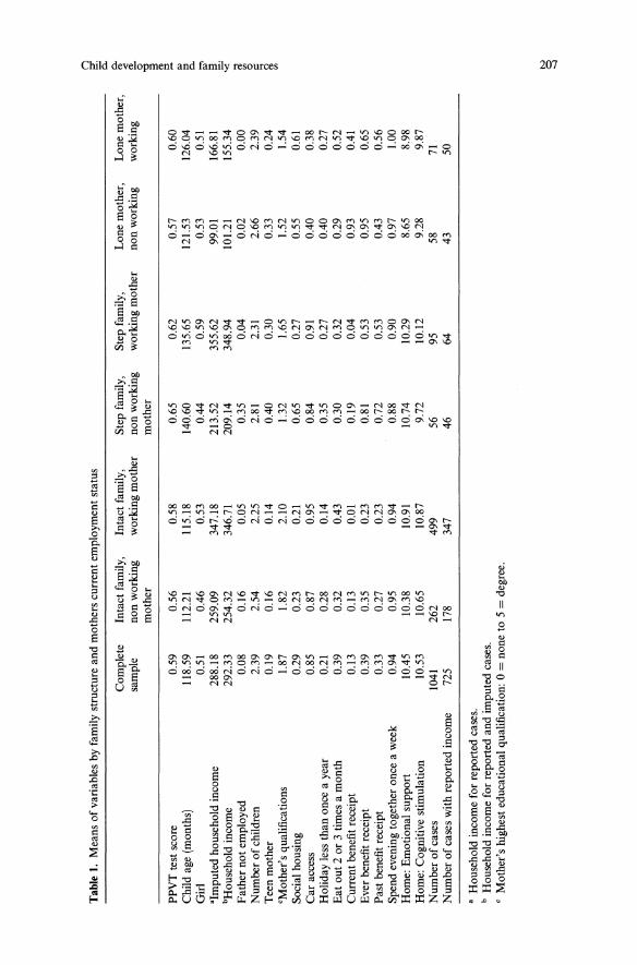
Tab

le1.Meansofvariablesbyfamilystructureandmotherscurrentemploymentstatus

(j e: 0:

Complete

Intactfamily,

Intactfamily,

Stepfamily,

Stepfamily,

Lonemother,

Lonemother,

fr <sample

nonworking

workingmother

nonworking

workingmother

nonworking

working

'" 0-mother

mother

"0 3 '"PPVTtestscore

0.59

0.56

0.58

0.65

0.62

0.57

0.60

S-Childage(months)

118.59

112.21

115.18

140.60

135.65

121.53

126.04

III ::; Cl-

Girl

0.51

0.46

0.53

0.44

0.59

0.53

0.51

j;>"Imputedhouseholdincome

288.18

259.09

347.18

213.52

355.62

99.01

166.81

g,bHouseholdincome

292.33

254.32

346.71

209.14

348.94

10l.21

155.34

'<

Fathernotemployed

0.08

0.16

0.05

0.35

0.04

0.02

0.00

<i1 V>

Numberofchildren

2.39

2.54

2.25

2.81

2.31

2.66

2.39

0 :::Teenmother

0.19

0.16

0.14

0.40

0.30

0.33

0.24

(1 '"CMother'squalifications

1.87

1.82

2.10

1.32

1.65

1.52

1.54

V>

Socialhousing

0.29

0.23

0.21

0.65

0.27

0.55

0.61

Caraccess

0.85

0.87

0.95

0.84

0.91

0.40

0.38

Holidaylessthanonceayear

0.21

0.28

0.14

0.35

0.27

0.40

0.27

Eatout2or3timesamonth

0.39

0.32

0.43

0.30

0.32

0.29

0.52

Currentbenefitreceipt

0.13

0.13

0.01

0.19

0.04

0.93

0.41

Everbenefitreceipt

0.39

0.35

0.23

0.81

0.53

0.95

0.65

Pastbenefitreceipt

0.33

0.27

0.23

0.72

0.53

0.43

0.56

Spendeveningtogetheronceaweek

0.94

0.95

0.94

0.88

0.90

0.97

1.00

Home:Emotionalsupport

10.45

10.38

10.91

10.74

10.29

8.65

8.98

Home:Cognitivestimulation

10.53

10.65

10.87

9.72

10.12

9.28

9.87

Numberofcases

1041

262

499

5695

5871

Numberofcaseswithreportedincome

725

178

347

4664

4350

"Householdincomeforreportedcases.

bHouseholdincomeforreportedandimputedcases.

CMother'shighesteducationalqualification:0=noneto5=degree.

N S

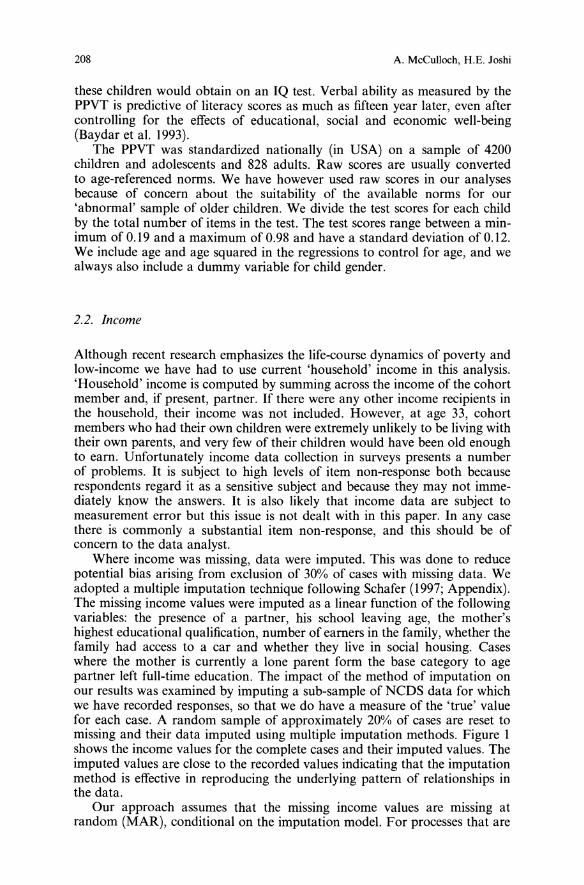
208 A. McCulloch, H.E. Joshi

these children would obtain on an IQ test. Verbal ability as measured by thePPVT is predictive of literacy scores as much as fifteen year later, even aftercontrolling for the effects of educational, social and economic well-being(Baydar et al. 1993).The PPVT was standardized nationally (in USA) on a sample of 4200

children and adolescents and 828 adults. Raw scores are usually convertedto age-referenced norms. We have however used raw scores in our analysesbecause of concern about the suitability of the available norms for our'abnormal' sample of older children. We divide the test scores for each childby the total number of items in the test. The test scores range between a min­imum of 0.19 and a maximum of 0.98 and have a standard deviation of 0.12.We include age and age squared in the regressions to control for age, and wealways also include a dummy variable for child gender.

2.2. Income

Although recent research emphasizes the life-course dynamics of poverty andlow-income we have had to use current 'household' income in this analysis.'Household' income is computed by summing across the income of the cohortmember and, if present, partner. If there were any other income recipients inthe household, their income was not included. However, at age 33, cohortmembers who had their own children were extremely unlikely to be living withtheir own parents, and very few of their children would have been old enoughto earn. Unfortunately income data collection in surveys presents a numberof problems. It is subject to high levels of item non-response both becauserespondents regard it as a sensitive subject and because they may not imme­diately kl10w the answers. It is also likely that income data are subject tomeasurement error but this issue is not dealt with in this paper. In any casethere is commonly a substantial item non-response, and this should be ofconcern to the data analyst.Where income was missing, data were imputed. This was done to reduce

potential bias arising from exclusion of 30% of cases with missing data. Weadopted a multiple imputation technique following Schafer (1997; Appendix).The missing income values were imputed as a linear function of the followingvariables: the presence of a partner, his school leaving age, the mother'shighest educational qualification, number of earners in the family, whether thefamily had access to a car and whether they live in social housing. Caseswhere the mother is currently a lone parent form the base category to agepartner left full-time education. The impact of the method of imputation onour results was examined by imputing a sub-sample of NCDS data for whichwe have recorded responses, so that we do have a measure of the 'true' valuefor each case. A random sample of approximately 20% of cases are reset tomissing and their data imputed using multiple imputation methods. Figure Ishows the income values for the complete cases and their imputed values. Theimputed values are close to the recorded values indicating that the imputationmethod is effective in reproducing the underlying pattern of relationships inthe data.Our approach assumes that the missing income values are missing at

random (MAR), conditional on the imputation model. For processes that are

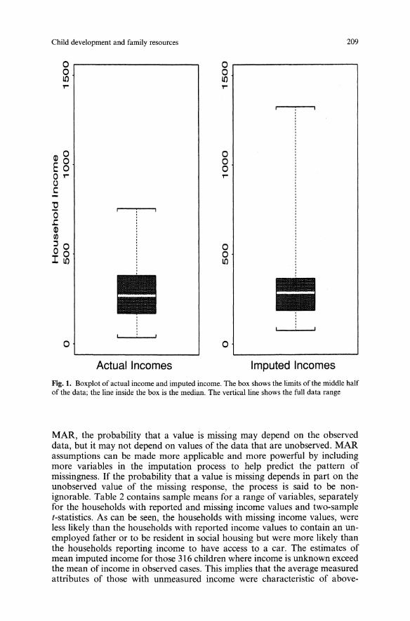
Child development and family resources

Or-------------,oLOT"

209

Or----------.....,oLOT"

Q) 0E8o T"

oC-:!2o.cQ)(/)

:::l 0o 0ILO

o

o

o

,

•Actual Incomes

oooT"

ooLO

o

o

o

o,

o

,,

,

•,,

Imputed Incomes

Fig. 1. Boxplot of actual income and imputed income. The box shows the limits of the middle halfof the data; the line inside the box is the median. The vertical line shows the full data range

MAR, the probability that a value is missing may depend on the observeddata, but it may not depend on values of the data that are unobserved. MARassumptions can be made more applicable and more powerful by includingmore variables in the imputation process to help predict the pattern ofmissingness. If the probability that a value is missing depends in part on theunobserved value of the missing response, the process is said to be non­ignorable. Table 2 contains sample means for a range of variables, separatelyfor the households with reported and missing income values and two-samplet-statistics. As can be seen, the households with missing income values, wereless likely than the households with reported income values to contain an un­employed father or to be resident in social housing but were more likely thanthe households reporting income to have access to a car. The estimates ofmean imputed income for those 316 children where income is unknown exceedthe mean of income in observed cases. This implies that the average measuredattributes of those with unmeasured income were characteristic of above-

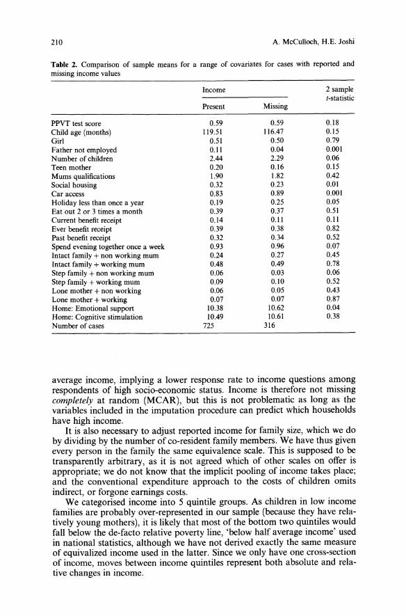
210 A. McCulloch, H.E. Joshi

Table 2. Comparison of sample means for a range of covariates for cases with reported andmissing income values

Income 2 sampleI-statistic

Present Missing

PPVT test score 0.59 0.59 0.18Child age (months) 119.51 116.47 0.15Girl 0.51 0.50 0.79Father not employed 0.11 0.04 0.001Number of children 2.44 2.29 0.06Teen mother 0.20 0.16 0.15Mums qualifications 1.90 1.82 0.42Social housing 0.32 0.23 0.01Car access 0.83 0.89 0.001Holiday less than once a year 0.19 0.25 0.05Eat out 2 or 3 times a month 0.39 0.37 0.51Current benefit receipt 0.14 0.11 0.11Ever benefit receipt 0.39 0.38 0.82Past benefit receipt 0.32 0.34 0.52Spend evening together once a week 0.93 0.96 0.07Intact family + non working mum 0.24 0.27 0.45Intact family +working mum 0.48 0.49 0.78Step family + non working mum 0.06 0.Q3 0.06Step family +working mum 0.09 0.10 0.52Lone mother + non working 0.06 0.05 0.43Lone mother +working 0.07 0.07 0.87Home: Emotional support 10.38 10.62 0.04Home: Cognitive stimulation 10.49 10.61 0.38Number of cases 725 316

average income, implying a lower response rate to income questions amongrespondents of high socio-economic status. Income is therefore not missingcompletely at random (MCAR), but this is not problematic as long as thevariables included in the imputation procedure can predict which householdshave high income.

It is also necessary to adjust reported income for family size, which we doby dividing by the number of co-resident family members. We have thus givenevery person in the family the same equivalence scale. This is supposed to betransparently arbitrary, as it is not agreed which of other scales on offer isappropriate; we do not know that the implicit pooling of income takes place;and the conventional expenditure approach to the costs of children omitsindirect, or forgone earnings costs.We categorised income into 5 quintile groups. As children in low income

families are probably over-represented in our sample (because they have rela­tively young mothers), it is likely that most of the bottom two quintiles wouldfall below the de-facto relative poverty line, 'below half average income' usedin national statistics, although we have not derived exactly the same measureof equivalized income used in the latter. Since we only have one cross-sectionof income, moves between income quintiles represent both absolute and rela­tive changes in income.

Child development and family resources

2.3. Family structure

211

In all but the first model we include a set of variables which describe thenumber of people in the child's family, whether the mother and father, ifpresent, have paid work and whether the mother started child-bearing as ateenager. The latter term is intended to allow for the peculiarities of a sampleof the children of one cohort, and appears as a dichotomy because age ofmother at first birth is highly collinear with other terms such as child age andmaternal qualifications. The number of children gives some idea of the com­petition for parental time. The presence of a father is included on the pre­sumption that children thrive when they have the attention of more than oneadult, particularly if the father is the child's natural father. Children livingwith step fathers are likely to have had some experience of change and or loneparent living, and the step father may not devote as much attention as a nat­ural father to the index child. The employment of the mother is interactedwith family structure, because there can be no more than one earner in a loneparent family. The employment of the mother may be expected to have mixedeffects on a child's development. It may deprive a child of maternal time,though this depends on the time they do spend together; on the other hand, itmay, depending on the quality of alternative care, hasten the child's social andpsychological development. Since these effect are likely to be lagged, we mightnot expect to find much of an association of vocabulary score with currentemployment, but perhaps there is a weak presumption that children whosemothers are in employment might do somewhat worse on their test score.Table 1 shows that family disruption is highly associated with early

motherhood, low maternal educational qualifications and social housing (i.e.rented from councilor housing association). There are differences in economicactivity between family types: of these school age children living with lonemothers, 54% had an employed mother compared to 58% in step families and66% in intact families. In accordance with the differences in employmentstatus by family structure, lone parent and step families where the mother isnot earning have the lowest mean family incomes. The polarisation of unem­ployment is apparent in the concentration of non-earning fathers in familieswith a non-earning mother (Gregg and Wadsworth 1996; Davies et al. 1998),particularly here in the step families. 35% of children living in step familieswith a non-employed mother also have an unemployed step father. In com­parison, 16% of children living in intact families with a non-employed motherhave an unemployed father. A larger proportion of children living in loneand step parent families than intact families have a parent with a history ofdrawing means-tested benefit - 81% and 95% of children who have a non­employed mother living with step fathers or with no partner, respectively,compared with 23% in intact families with an employed mother.

2.4. Family resources

Current income may not reflect lifetime income or assets such as saving orearning power. As an indicator of maternal resources we include the mother'seducational attainment. Preliminary analyses suggested a linear trend inPPVT scores across the categories of educational attainment so this variablewas entered in the model as a linear term. We examine a number of other

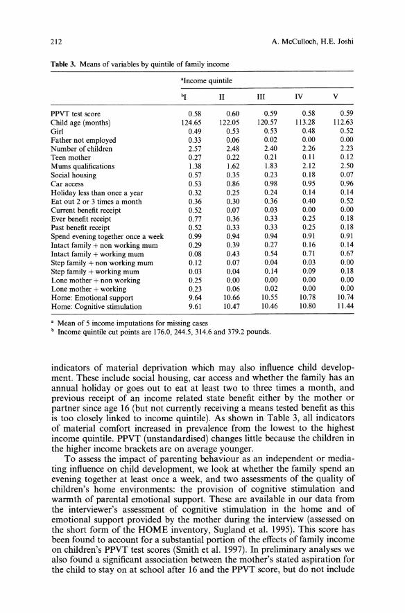
212 A. McCulloch, H.E. Joshi

Table 3. Means of variables by quintile of family income

"Income quintile

bI II III IV V

PPVT test score 0.58 0.60 0.59 0.58 0.59Child age (months) 124.65 122.05 120.57 113.28 112.63Girl 0.49 0.53 0.53 0.48 0.52Father not employed 0.33 0.06 0.02 0.00 0.00Number of children 2.57 2.48 2.40 2.26 2.23Teen mother 0.27 0.22 0.21 0.11 0.12Mums qualifications 1.38 1.62 1.83 2.12 2.50Social housing 0.57 0.35 0.23 0.18 0.Q7Car access 0.53 0.86 0.98 0.95 0.96Holiday less than once a year 0.32 0.25 0.24 0.14 0.14Eat out 2 or 3 times a month 0.36 0.30 0.36 0.40 0.52Current benefit receipt 0.52 0.07 0.03 0.00 0.00Ever benefit receipt 0.77 0.36 0.33 0.25 0.18Past benefit receipt 0.52 0.33 0.33 0.25 0.18Spend evening together once a week 0.99 0.94 0.94 0.91 0.91Intact family + non working mum 0.29 0.39 0.27 0.16 0.14Intact family + working mum 0.08 0.43 0.54 0.71 0.67Step family + non working mum 0.12 0.07 0.04 0.03 0.00Step family + working mum 0.03 0.04 0.14 0.09 0.18Lone mother + non working 0.25 0.00 0.00 0.00 0.00Lone mother +working 0.23 0.06 0.02 0.00 0.00Home: Emotional support 9.64 10.66 10.55 10.78 10.74Home: Cognitive stimulation 9.61 10.47 10.46 10.80 11.44

" Mean of 5 income imputations for missing casesb Income quintile cut points are 176.0,244.5, 314.6 and 379.2 pounds.

indicators of material deprivation which may also influence child develop­ment. These include social housing, car access and whether the family has anannual holiday or goes out to eat at least two to three times a month, andprevious receipt of an income related state benefit either by the mother orpartner since age 16 (but not currently receiving a means tested benefit as thisis too closely linked to income quintile). As shown in Table 3, all indicatorsof material comfort increased in prevalence from the lowest to the highestincome quintile. PPVT (unstandardised) changes little because the children inthe higher income brackets are on average younger.To assess the impact of parenting behaviour as an independent or media­

ting influence on child development, we look at whether the family spend anevening together at least once a week, and two assessments of the quality ofchildren's home environments: the provision of cognitive stimulation andwarmth of parental emotional support. These are available in our data fromthe interviewer's assessment of cognitive stimulation in the home and ofemotional support provided by the mother during the interview (assessed onthe short form of the HOME inventory, Sugland et al. 1995). This score hasbeen found to account for a substantial portion of the effects of family incomeon children's PPVT test scores (Smith et al. 1997). In preliminary analyses wealso found a significant association between the mother's stated aspiration forthe child to stay on at school after 16 and the PPVT score, but do not include

Child development and family resources 213

it in the final model because of possible reverse causation, perhaps throughthe downward revision of aspirations as children grow older and the limits oftheir capabilities become apparent. All other regressors are assumed to beexogenous.

2.5. Statistical models

To model the cognitive functioning of children within families we use theframework of the hierarchical linear model (Goldstein 1995). This is a variantof the multiple linear regression model for data with a hierarchical nestingstructure. First consider a two-level multi-level model of children nested infamilies. Children (level-l units) are indicated by i and families by j. Thedependent variable must be defined at the lowest level, that of the individual,and it is denoted by Yij' A simple two level model can be formulated as:

(1)

where Yij is the value of the dependent variable, POj is the family-specificintercept, PI is the fixed regression slope, xij is the value of the explanatoryvariable, and eij is the unexplained part of the dependent variable Yij. It isconvenient to separate the coefficient POj in (1) into a fixed part (the mean) anda random part (with mean 0):

POj = Yoo + VOj (2)

where Yoo is the population mean of the intercepts and VOj is the family­specific part of the intercept. Substitution of the models describing the varia­tion of the coefficients between families into (1) then yields the combinedmodel formula:

(3)

This is often referred to as a variance components model. The model con­tains two random effects: VOj and eij which are both assumed to have N(O, a2)

normal distributions. Each of these indicates a different source of unexplainedvariation. The random intercept VOj indicates unexplained differences betweenfamilies in the average Y-values (controlling for the effect of xij). The randomresidual eij, indicates unexplained variation among the individuals, relative totheir families. In the present exercise we analyze 1041 children (level 1) of 729mothers (level 2).

It is appropriate to treat VOj as a random effect because the objective is touse the individual observations to make inferences about the population ofchildren. A fixed effects model would treat VOj as a fixed variable. While ap­pealing in that few assumptions need to be imposed on VOj, this procedure hasthe drawback that it implies that out interest centres on the outcome of anindividual child. Furthermore, and perhaps more restrictive, only the effects ofcovariates that change between siblings can be estimated.

214

3. Results

A. McCulloch, H.E. Joshi

The results from estimating variance components models for PPVT test scoresare presented in Table 4. The income coefficients are averages of the coefficientsfrom separate analyses using 5 imputation estimates of family income (Schafer1997). The P values for the income coefficients are computed using the percen­tiles of the (-distribution (Rubin 1987). The analyses are organised as follows:Model A contains age terms, the child's gender and income quintiles. Model Badds a summary of the child's family structure and current employment statusof the parents. Model C adds controls for maternal qualifications. In com­parison to Model C, Model D substitutes indicators of material deprivationfor maternal qualifications and Model E substitutes indicators of parentingand the home environment for maternal qualifications. Model F examines theeffect of all variables simultaneously. The comparison of results from thissequence of models allows us to see how far PPVT scores are associated withfamily income. It also allows us to see how far any association might beaccounted for, or mediated by the social and human capital available to thechild, the material disadvantage associated with the child's family circum­stances, and the mode of parenting such resources may permit.In Model A mean PPVT test scores increased with increasing income in

comparison to the lowest income quintile controlling for child age and gen­der. The difference of test scores from the 1st quintile is statistically significantfrom the 3rd quintile upwards but the coefficients are of a modest order ofmagnitude: the top fifth of children by family income have PPVT scores 3.7%points higher on average than children in the lowest income bracket. This isnot large in comparison with the age-adjusted standard deviation of PPVT at7.5 percentage points. The estimates of the random part of the model suggeststhat families do differ in their average PPVT scores and that there is evenmore variation among children within families. The variance component be­tween children (eij) in Model A is around one and a half times that betweenfamilies (UOj )'

Introduction of information on the structure and number of earners inthe family confines the statistically significant difference from the bottomincome quintile to the top 2 quintiles (Model B). Given the control for incomelevel, the family structure terms themselves do not predict much systematicadvantage to having two natural parents, nor in general, much disadvantageto having a mother in employment. Children in step families appear at adisadvantage if the mother is employed. Unemployment of the father has anegative, but non-significant coefficient. Cognitive outcomes are lower infamilies with large numbers of children and in families where the mother hadher first child when aged under 20. This term does not affect the estimatedage coefficients, as it might have done, had the latter contained a strong age­at-parenthood element.Introduction of information on the mother's qualifications (Model C)

removes the remaining significant income coefficients (given the critical valuefor the ( statistic on the imputed income variables is 3.1). Information aboutthe maternal endowment seems to act as an alternative signal to current in­come of the resources available to the child. It also attenuates the teenagemother effect. As an indicator of human capital transmitted by at least oneparent, maternal qualifications are a strong predictor of high test scores andteen motherhood a strong predictor of low test scores (McCloyd 1998; Joshi

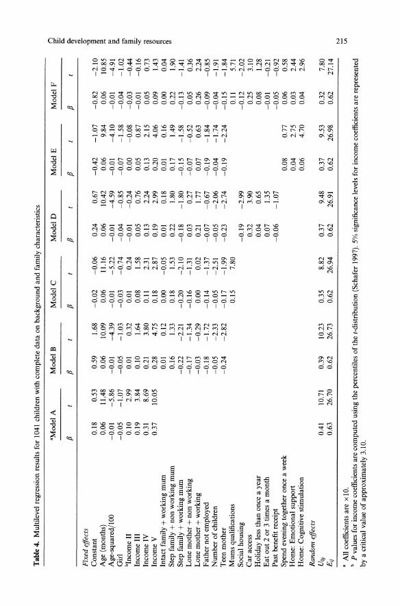
Tab

le4.Multilevelregressionresultsfor

1041childrenwithcompletedataonbackgroundandfamilycharacteristics

"ModelA

ModelB

ModelC

ModelD

ModelE

ModelF

(') e: 0:

fJI

fJI

fJI

fJI

fJI

fJI

Cl-

C'O < ~F

ixed

effe

cls

0 '"Constant

0.18

0.53

0.59

1.68

-0.02

-0.06

0.24

0.67

-0.42

-1.07

-0.82

-2.10

3 C'OAge(months)

0.06

11.48

0.06

10.09

0.06

11.16

0.06

10.42

0.06

9.84

0.06

10.85a

Age-squared/I00

-0.01

-5.86

-0.01

-4.39

-0.01

-5.22

-0.01

-4.59

-0.01

-4.10

-0.01

-4.91

P> ::>Girl

-0.05

-1.07

-0.05

-1.03

-0.03

-0.74

-0.04

-0.85

-0.07

-1.58

-0.04

-1.02

Cl- ;>

bIncomeII

0.10

2.99

0.01

0.32

0.01

0.24

-0.01

-0.24

0.00

-0.08

-0.03

-0.44

e.IncomeIII

0.19

3.84

0.10

1.64

0.08

1.58

0.05

0.76

0.05

0.87

-om

-0.16

.:<IncomeIV

0.31

8.69

0.21

3.80

0.11

2.31

0.13

2.24

0.13

2.15

0.05

0.73

@ '"IncomeV

0.37

10.05

0.28

4.75

0.18

2.87

0.19

2.99

0.20

4.06

0.09

1.43

0 '"Intactfamily

+workingmum

0.01

0.12

0.00

-0.05

0.01

0.18

0.01

0.16

0.00

0.04

.... (')C'O

Stepfamily

+nonworkingmum

0.16

1.33

0.18

1.53

0.22

1.80

0.17

1.49

0.22

1.90

'"Stepfamily

+workingmum

-0.22

-2.21

-0.20

-2.10

-0.18

-1.80

-0.15

-1.58

-0.13

-1.41

Lonemother+nonworking

-0.17

-1.34

-0.16

-1.31

0.03

0.27

-0.07

-0.52

0.05

0.36

Lonemother+working

-0.03

-0.29

0.00

0.02

0.21

1.77

0.07

0.63

0.26

2.24

Fathernotemployed

-0.18

-1.72

-0.14

-1.37

-0.07

-0.67

-0.19

-1.84

-0.09

-0.85

Numberofchildren

-0.05

-2.33

-0.05

-2.51

-0.05

-2.06

-0.04

-1.74

-0.04

-1.91

Teenmother

-0.24

-2.82

-0.17

-1.99

-0.23

-2.74

-0.19

-2.24

-0.15

-1.84

Mumsqualifications

0.15

7.80

0.11

5.71

Socialhousing

-0.19

-2.99

-0.12

-2.02

Caraccess

0.32

3.90

0.25

3.10

Holidaylessthanonceayear

0.04

0.65

0.08

1.28

Eatout2or3timesamonth

0.07

1.35

-om

-0.21

Pastbenefitreceipt

-0.06

-1.07

-0.05

-0.92

Spendeveningtogetheronceaweek

0.08

0.77

0.06

0.58

Home:Emotionalsupport

0.04

2.75

0.03

2.44

Home:Cognitivestimulation

0.06

4.70

0.04

2.96

Ran

dom

effe

cls

VOj

0.41

10.71

0.39

10.23

0.35

8.82

0.37

9.48

0.37

9.53

0.32

7.80

Eij

0.63

26.70

0.62

26.73

0.62

26.94

0.62

26.91

0.62

26.98

0.62

27.14

N ....."Allcoefficientsarex10.

lJl

bPvaluesforincomecoefficientsarecomputedusingthepercentilesoftheI-distribution(Schafer1997).5%significancelevelsforincomecoefficientsarerepresented

byacriticalvalueofapproximately3.10.

216 A. McCulloch, H.E. Joshi

et al. 1999). The significant (adverse) term for an employed mother living witha step family remains.In Model D, indicators of material deprivation rather than mother's qual­

ifications also remove the statistically significant impact of income on child­ren's test scores (and the special case of the step families with employedmothers). The indicators of material deprivation which account for mostvariation in the test scores, (and also for the association between test scoresand family status), are social housing and lack of a car. Children who aregrowing up in such a materially deprived family are disadvantaged in theircognitive development at all levels of current family income, though as Table3 shows, most of the families without cars or in social housing do have lowincome. As Table 3 also shows, not all of the families with low current incomeare social tenants or without cars. The finding of this model suggests that it isin those low income families who are in these categories that children arefalling behind.Model E substitutes parenting behaviour for the material deprivation

terms. The level of maternal emotional support and the level of cognitivestimulation in the home (e.g. academic and language) both show statisticallysignificant positive associations with children's test scores. Whether the familyspends time together (at least one evening a week) does not show much pre­dictive power. Introduction of these terms (on top of those in Model B) con­fines the statistically significant impact of income on test scores to the topincome quintile. Our measure of a stimulating home environment is almostas successful in explaining the association of children's test scores with familyincome as the measures of more permanent living standards and social statusin Model D.In our model containing all predictors (Model F), all the income terms

become insignificant. We have thus succeeded in our search for factors whichlie behind the association we reported in Model A. Other coefficients fromprevious models show little change in sign or statistical significance. One ex­ception is that the teenage mother term becomes insignificant. The distin­guishing characteristics of teenaged mothers have been captured elsewhere.Another distinction of the full model is the statistically significant positiveestimate that children living with an employed lone mother do better, for agiven level of maternal and family resources, than children in intact familieswith non-employed mothers.

4. Discussion

We started with a model of vocabulary attainment (PPVT) where the onlyexplanatory variable, apart from basic controls for age and sex, was a five­fold grouping of income. This showed a significant relationship with testscores. We then introduced various combinations of other variables throughwhich an income effect might work, or which might in themselves offer supe­rior explanatory power. The introduction of measures of more permanentliving standards and social status, particularly car access and housing tenure,eliminates the income differentials in test scores. We conclude that currentincome alone is not a complete yardstick for children at risk of impaireddevelopment. Our indicators of more long-term deprivation (car access andhousing tenure) suggest that a more sustained experience of poverty is more

Child development and family resources 217

damaging. The indicators of income and deprivation taken together show amore robust relationship with the PPVT than does, for the most part, familystructure and current parental employment. The relative importance of mate­rial resources we find here is consistent with the analyses of the NCDS firstgeneration offered by Gregg et al. (1999) and the American findings reportedin the studies assembled by Duncan and Brooks-Gunn (1997) with respect toacademic and cognitive outcomes of children of school age. It should also benoted that these estimates of income effects on PPVT scores of children aged6-17, are modest, like those of Lefebvre and Merrigan (1998) for Canadianchildren aged 4-5. It would take very large increases in income to produce agreat effect on children's proficiency at the vocabulary test. Model A says thata child from the bottom income quintile has a score 3.7 points below anotherwise identical child in the top quintile. This extreme move in incomeis equivalent to half an age standardized standard deviation in PPVT. Theparameters of Model F imply that to move a child out a situation where thefather was unemployed, the family lived in council housing, took a holidayless than once a year and ate out less than 2 or 3 times per month to theopposite of all these, would imply an increased PPVT score of 5 points. We donot directly replicate the finding of Lefebvre and Merrigan (1998) that incomeeffects are strongest at very low levels of income.Other variables contributed, at least partially independent, explanatory

power. Our measure of the endowment of parental human capital in terms ofmother's educational qualifications, was uniformly associated with higherPPVT test scores, and this relationship was independent of the household'seconomic status. To the extent that this endowment can be acquired througheducation, an across-the-board improvement of mothers' education by onegrade would raise the average PPVT score by 1.1 percentage points. Althoughthis would not be cheap or immediate, this long term effect might be equiva­lent to that of raising into home and car ownership all families currentlywithout them (Model D parameters). Turning to variables about parenting,the findings on the home environment, as assessed on the HOME scale, indi­cate that children with better home environments appeared able to overcomethe barriers set by low material circumstances. Of the two types of environ­ment, the provision of stimulating and learning oriented experiences appearedto exert a greater influence on children than the degree of parental encour­agement. Although our data are limited in the extent to which we can measurefamily processes, there is some evidence that parental 'competence' plays animportant role which is independent of income. The measures of the homeenvironment are not as successful in explaining the association of children'stest scores with family income as the measures of more permanent livingstandards and social status. It appears that parenting differences are not theprincipal route through which children in more advantaged families benefitfrom parents' cash resources. A similar conclusion is reached by Hanson et al.(1997) although other US studies they cite had found a connection frompoverty, or perceived financial stress, to poor parenting. Smith et al. (1997)found that the inclusion of Home scores in the analysis of PPVT scores of USchildren aged 5 mediated the mother's education term more than the incomecoefficient.We found that family income (as we have been able to measure it) is only

weakly related to effective parenting. Consequently, differences in parentingdo not account for much of the association between economic resources and

218 A. McCulloch, H.E. Joshi

children's test scores. We examined the extent to which the effect of mother'seducation worked through income rather than income and maternal educa­tion having independent effects. Mother's education was found to contributeto child test scores even after controlling for family income, in contrast to ourearlier results for family structure (Joshi et al. 1999). Improved mother's edu­cation raises children's emotional adjustment through complex mechanisms.Education may provide mothers with the knowledge, skills and self-confidencenecessary for happy marital relationships and successful child rearing. On theother hand, lack of educational qualifications may also be a more generalindicator of inherited social disadvantage. Perhaps our most surprising findingis that we find little evidence that a father's absence is related to children's testscores. Indeed living with a working single mother increased the test scoresof children. This could be due to selection into employment, but it echoesa finding of Kiernan (1996) on the previous generation of NCDS. Thedaughters of lone mothers who were employed when the girls were aged 16showed no disadvantage vis a vis their counterparts in intact families. Kiernansuggests that a positive role model may be part of the explanation. Our resultsmay also be due to the fact that the children in the NCDS were born toyounger than average mothers. Whatever the reason, the overall pattern ofresults obtained on children in single-parent families suggests that their out­comes are not significantly different from those exhibited by their two-parentcounterparts, controlling for levels of economic and parenting resources.The implication that material disadvantage can, at least partly, be over­

come by positive parental behaviour offers one ray of hope for the futureprospects of children growing up in persistent poverty. A substantial body ofresearch has shown that parental warmth, involvement, and moderate controlfacilitate children's adjustment and achievement (McLoyd 1998). Direct ob­servations of family interactions also suggest a link between parenting behav­iour and economic stress. Economic pressure and marital conflict may lead tofinancial conflict and hostility between parents and adolescents. Economicdeprivation also appears to be the best predicted concomitant of divorce,consequently placing a strain on the family's lifestyle, relationships and op­portunities (Conger et al. 1990). Children may perceive remarriage as com­pounding these emotional stresses. Nevertheless, it can improve the possibilityof financial support. Our finding of poor scores in stepfamilies with an em­ployed mother (Models Band C) is a bit of a puzzle, because these should bethe stepfamilies with the most cash resources, but their association with theother deprivation indicators (see Table 1) suggests that they are not particu­larly comfortably off.The unobserved family effects in our analyses are substantial and point

to major sources of unobserved variation between families independent ofhousehold income, material disadvantage, maternal education and measuredparenting. Finally the unobserved variation among children points to the bigrole of chance (or other unobserved factors like individual motivation) in dis­tributing success and failure in dealing with a vocabulary test, if not the rest oflife. More recent evidence suggests that the level of income in neighbour­hoods, over and above family income, is also associated with early school agedevelopmental outcomes (Brooks-Gunn et al. 1993). We cannot begin how­ever to allow for any teacher, school, or neighbourhood effect with the presentdataset, although the public housing indicator may contain some informationabout the neighbourhood.

Child development and family resources 219

While it is customary to bemoan the lack of income data in many Britishdata sets, this evidence suggest that current income is not the best indicator offamilies at risk, if evidence of more sustained long-term deprivation is avail­able. A general picture emerges of an accumulation of risk factors. Thesefactors include a lack of economic resources and having mothers with loweducational attainment and little involvement in their children's development.Each factor is associated with a gradual increase in the risk of a poor outcomerather than a threshold precipitating poor outcomes. Poor cognitive outcomesduring childhood increase the risk of many other negative outcomes duringchildhood, such as poor school performance and weak social skills, and alsopredicts an accumulation of economic and social problems over children'ssubsequent lives (Kratzer and Hodgins 1997; Hobcraft 1998). Although ourevidence of a link from economic to educational disadvantage is systematicand statistically significant, it is not spectacular - small changes in familieseconomic circumstance could not be expected to yield more than small changesin cognitive attainment. Our results are consistent with the growing realisationthat causal structure of cognitive outcomes in children is likely to be com­plex. There are few interventions that will single-handedly yield significantimprovements in children's abilities, but reducing child poverty should help.

Appendix: Income imputation

There are a number of methods for dealing with missing data. The mostcommon approach is simply to eliminate entire observations when anyonevariable is missing (listwise deletion). Other general purpose methods includemean substitution (imputing the univariate mean of the observed observa­tions), imputing a zero and then adding an additional dummy variable tocontrol for the imputed value, and hot deck imputation (imputing a completeobservation that is similar in as many observed ways as possible to the ob­servation that has a missing value). However, even if the answers we make upfor nonresponding respondents are right on average, these procedures consid­erably overestimate the certainty with which we know those answers. Conse­quently estimated standard errors will be too small.Statisticians and methodologists have agreed on a widely applicable

approach to many missing data problems based on the concept of multipleimputation. Implementing multiple imputation requires a statistical modelfrom which to compute the imputations for each missing value in a data set.One model that has proven to be useful for missing data problems in a sur­prisingly wide variety of data types, assumes that the variables are jointlymultivariate normal. Let Y denote an n x r matrix of multivariate data whereeach row of Y is a joint realization of variables Y" ... , Yr. Denote the com­plete data by Y = (Yobs , Ymis) where Yobs and Ymis are the observed andmissing portions of the matrix respectively. We assume that Y\, . .. , Yr have amultivariate normal distribution with mean vector Il and covariance matrix I;that is:

YI, Y2"'" Yrl B '" iidN(Il,I)

where B= (Il, I) is the unknown parameter. In multiple imputation, one must

220 A. McCulloch, H.E. Joshi

generate M independent draws Y~i~"'" Y~~) from a posterior predictivedistribution of the missing data:

where P(01 Y obs ) is proportional to the product of the observed-data likelihoodfunction:

P(01 Yobs) = JL(01 Y) dYmis

and a prior density function n(O). After imputation, the resulting M versionsof the complete data are separately analyzed using complete-data methods,and the results are combined to obtain inferences that effectively incorporateuncertainty due to missing data. The difficulty in using this model is takingrandom draws from the posterior distribution P( Ymisl Yobs).

It is possible to create random draws of Y mis from P( Ymisl Y ooo ) usingtechniques of Markov Chain Monte Carlo (MCMC). Consider an iterativesimulation algorithm in which the current version of the unknown parameter0(1) = (J1.(I) , 1:(1)) and the missing data Ymis (t) are updated in two steps:

O(HI) ~ P(OI Y. y(t) )000, m,s

(HI) P( 1 y. 0(1+1))Yi(mis) ~ Yi(mis) obs,

Given starting values 0(0) and Y(O)mis, these two steps define a Gibbs samplerin which the sequences O(t) and Y(I)mis converge in distribution to P(OI Yobs)and P( Ymisl Y obs ) , respectively. Implementation of the Gibbs sampler requiresus to specify a prior distribution for O. For simplicity we apply an inverse­Wishart distribution 1:-1 ~ W(v,A) where W(v,A) denotes a Wishart distri­bution with v> 0 degrees of freedom and mean vA > O. Small values for vmakes the prior density relatively diffuse, reducing its impact on the finalinferences. For J1., we use a conditionally multivariate normal density J1.11: ~N(J1.ol,-I1:) where the hyperparameters are fixed and known. Under thesepriors, the conditional distribution of Yi(mis) given Yi(obs) and 0 is multivariatenormal. The complete data posterior P(OI Y mis , Yobs) is a normal inverted­Wishart distribution

J1.11: ~ N(J1.o, ,-11:)

1: ~ W- I (v, A)

for some (" v, J1.0, A) determined by the prior, the observed data Yobs and theimputed missing data Y~?s (Schafer 1997, p. 181-184).For multiple imputation problems, we have the additional requirement

that the draws we use for imputations must be statistically independent, whichis not a characteristic of successive draws from Markov chain methods. Someresearchers reduce dependence by using every nth random draw (where n is

Child development and family resources 221

determined by examining the autocorrelation function of each of the param­eters), but Schafer (1997), following Gelman and Rubin (1992), recommendsaddressing both problems by creating one independent Markov chain for eachof the desired m imputations, with starting values drawn randomly from anoverdispersed (normal-inverted Wishart distribution) approximation distribu­tion. The difficult with taking every rth draw from one chain is the interpre­tation of autocorrelation functions (requiring analysts of cross-sectional datato be familiar with time series methods); whereas the difficulty of runningseparate chains is that the run time is increased by a factor ofm.The M completed data sets are then analysed using complete data methods

giving M sets of completed-data statistics, for example point estimates fh andvariances Uk, k = 1, ... M. The M sets of completed-data statistics are com­bined to create one multiple-imputation inference as follows (Rubin 1987).The estimate of () is (}bar:

the average of the M completed-data estimates of (). Also, let Ubar be theaverage of the M completed-data variances, and:

be the between imputation variance of the completed data estimates of ().Then the total variance of (() - (}bar) is given by the sum of the within impu­tation component (Ubar) and the between imputation component (B) multi­plied by a finite M correction (1 + M- l ), that is:

Interval estimates and significance levels are obtained using at-distributionwith center (}bar, scale V- 1/2 , and degrees of freedom v = (M - 1)(1 + q-I f,where q = (1 + M- l )B/ Ubar, is the ratio of the between-imputation compo­nent of variance to the within-imputation component. The two-sided p-valuefor the null hypothesis Ho: () = 0 is computed by comparing (}bar/VI/2 with at-distribution with v degrees of freedom.Some variables in our imputation are clearly nonnormal (ie. discrete) but

are completely observed, therefore the multivariate normal model may still beused for inference given that (a) it is plausible to model the incomplete varia­bles as conditionally normal given a linear function of the complete ones, and(b) the parameters of inferential interest pertain only to this conditional dis­tribution. Convergence of the Gibbs sampler was assessed by examining plotsof the sample trace for draws of missing income values. A bum-in of 5000iterations was found to be adequate to achieve convergence. Figure 2 showsthe simulated income values from one household where income was not re­ported using a further 1000 iterations of the Gibbs sampler.

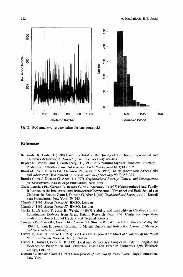
15001000500o

o

800 1000600400200o

222 A. McCulloch, H.E. Joshi

0onC\I

8on

00C\I

Q)

E 0 00 8 on()

.E ~ Q;'0 .D(5 E~ ::>Q) ZIII 8::>0 ~

J:

00on

:il

Imputation Number Household Income

Fig. 2. 1000 simulated income values for one household

References

Baharudin R, Luster T (1998) Factors Related to the Quality of the Home Environment andChildren's Achievement. Journal ofFamily Issues 19(4):375-403

Baydar N, Brooks-Gunn J, Furstenberg FF (1993) Early Warning Signs of Functional IIIiteracy­Predictors in Childhood and Adolescence. Child Development 64(3):815-829

Brooks-Gunn J, Duncan GJ, Klebanov PK, Sealand N (1993) Do Neighborhoods Affect Childand Adolescent Development? American Journal ofSociology 99(2):353-395

Brooks-Gunn J, Duncan G, Aber JL (1997) Neighbourhood Poverty: Context and Consequencesfor Development. Russell Sage Foundation, New York

Chase-Lansdale PL, Gordon R, Brooks-Gunn J, Klebanov P (1997) Neighbourhood and FamilyInfluences on the Intellectual and Behavioural Competence of Preschool and Early School-ageChildren. In: Brooks-Gunn J, Duncan G, Aber L (eds) Neighbourhood Poverty, vol I. RussellSage Foundation, New York, 79-145

Church J (1996) Social Trends 26. HMSO, LondonChurch J (1997) Social Trends 27. HMSO, LondonClarke L, Di Salvo P, Joshi H, Wright J (1997) Stability and Instability in Children's Lives:Longitudinal Evidence from Great Britain. Research Paper 97-1, Centre for PopulationStudies, London School of Hygiene and Tropical Sciences

Conger RD, Elder GH, Lorenz FO, Conger KJ, Simons RL, Whitbeck LB, Huck S, Melby IN(1990) Linking Economic Hardship to Marital Quality and Instability. Journal of Marriageand the Family 52(3):643-656

Davies H, Joshi H, Clarke L (1997) Is it Cash the Deprived are Short of? Journal of the RoyalStatistical Society Series A 160(1):107-126

Davies H, Joshi H, Peronaci R (1998) Dual and Zero-earner Couples in Britain: LongitudinalEvidence on Polarization and Persistence. Discussion Paper in Economics 8/98, BirkbeckCollege, London

Duncan G, Brooks-Gunn J (1997) Consequences of Growing up Poor. Russell Sage Foundation,New York

Child development and family resources 223

Duncan G, Brooks-Gunn J, Klebanov P (1994) Economic Deprivation and Early ChildhoodDevelopment. Child Development 65(2):296-318

Dunn LM, Dunn LM (1981) Peabody Picture Vocabulary Test-Revised. American Guidance Ser­vice, Circle Pines, MN

Ferri E (1993) Life at 33: The Fifth Follow-up of the National Child Development Study. NationalChildren's Bureau, London

Goldstein H (1995) Multilevel Models in Educational and Social Research, 2nd Ed. EdwardArnold, London

Gregg P, Harkness S, Machin S (1999) Child Development and Family Income. Joseph RowntreeFoundation, York

Gregg P, Wadsworth J (1996) More Work in Fewer Households. In: Hills J (ed) New Inequalities.The Changing Distribution of Income and Wealth in the United Kingdom. Cambridge Univer­sity Press, Cambridge, 181-207

Hanson TL, McLanahan S, Thomson E (1997) Economic Resources, Parental Practices andChildren's Well-Being. In: Duncan J, Brooks-Gunn J (eds) Consequences of Growing up Poor.Russell Sage Foundation, New York, 190-238

Harkness S, Machin S, Waldfogel J (1996) Women's Pay and Family Incomes in Britain, 1979­91. In: Hills J (ed) New Inequalities. The Changing Distribution of Income and Wealth in theUnited Kingdom. Cambridge University Press, Cambridge, 181-207

Haveman R, Wolfe B (1995) Succeeding Generations. Russell Sage Foundation, New YorkHaskey J (1994) Stepfamilies and Stepchildren in Great Britain. Population Trends 76:17-28Haskey J (1997) Children who experience Divorce in their Family. Population Trends 87:5-10Hill MS, Jenkins SP (1999) Poverty among British Children: Chronic or Transitory? Institute forSocial and Economic Research, Essex University, Working Paper 99/23

Hobcraft J (1998) Intergenerational and Life-Course Transmission of Social Exclusion: Influencesof Childhood Poverty, Family Disruption, and Contact with the Police. CASEpaper 15,Centre for Analysis of Social Exclusion, London School of Economics

Joshi H, Cooksey C, Wiggins RD, McCulloch A, Verropoulou G, Clarke L (1999) DiverseFamily Living Situations and Child Development: A Multi-level Analysis omparing Longi­tudinal Evidence from Britain and the United States. International Journal ofLaw, Policy andthe Family 13(2):292-314

Kiernan KE (1996) Lone Motherhood, Employment and Outcomes for Children. InternationalJournal ofLaw, Policy and the Family 10(2):233-256

Korenmann S, Miller J, Sjaastad J (1995) Long-term Poverty and Child Development Evidencefrom the NLSY. Children and Youth Services Review 17(1):127-155

Kratzer L, Hodgins S (1997) Adult Outcomes of Child Conduct Problems: A Cohort Study.Journal of Abnormal Child Psychology 25(1):65-81

Lefebvre P, Merrigan P (1998) Work Schedules, Job Characteristics, Parenting Practices andChildren's Outcomes. Working Paper 77, Center for Research on Economic Fluctuations andEmployment, Universite du Quebec a Montreal

Macintyre S, Ellaway A, Der G, Ford G, Hunt K (1998) Do Housing Tenure and Car Accesspredict Health because they are simply Markers of Income or Self-Esteem? A Scottish Study.Journal of Epidemiology and Community Health 52(10):657-664

Marsh A, McKay S (1993) Families, Work and Benefits. Policy Studies Institute, LondonMcLanahan S (1997) Parent Absence or Poverty: which matters more? In: Duncan J, Brooks­Gunn J (eds) Consequences of Growing up Poor. Russell Sage Foundation, New York, 35-48

McLanahan S, Sandefur G (1994) Growing Up With a Single Parent: What Hurts, What Helps.Harvard University Press, Cambridge, MA

McLoyd VC (1998) Socioeconomic Disadvantage and Child Development. American Psychologist53(2): 185-204

Office of National Statistics (1997) Birth Statistics 1995, Series FM1: 17. HMSO, LondonOffice of National Statistics (1998) Social Focus on Women and Men. HMSO, LondonO'Higgins M, Jenkins S (1990) Poverty in the EC. In: Teehens R, van Praag B (eds). Analysing

Poverty in the European Community. Eurostat, Luxembourg, 64-87Rubin DB (1987) Multiple Imputation for Nonresponse in Surveys. Wiley, New YorkSchafer JL (1997) Analysis of Incomplete Multivariate Data (Monographs on Statistics andApplied Probability 72.) London, Chapman and Hall

Smith JR, Brooks-Gunn J, Klebanov PK (1997) Consequences of Living in Poverty for YoungChildren's Cognitive and Verbal Ability and Early School Achievement. In: Duncan J,

224 A. McCulloch, H.E. Joshi

Brooks-Gunn J (eds) Consequences o/Growing up Poor. Russell Sage Foundation, New York,132-189

Sugland B, Zaslow M, Smith J, Brooks-Gunn J, Coates D, Blumenthal C, Moore K, Griffin T,Bradley R (1995) The Early Childhood HOME Inventory and HOME Short Form in differ­ing Racial/Ethnic Groups: Are there Differences in Underlying Structure, Internal Consis­tency of Subscales, and Patterns of Prediction. Journal 0/ Family Issues 16(5):632-663

Wechsler D (1974) Manual/or the Wechsler Intelligence Scale/or Children-Revised. PsychologicalCorporation, New York

The decisions of Spanish youth: A cross-section study

Maite Martinez-Granado, Javier Ruiz-Castillo

Departamento de Economia, Universidad Carlos III de Madrid, Cj. Madrid 126,28903 Getafe,Madrid, Spain (Fax: +34-1-624-9875; e-mail: mmartine@eco.uc3m.es;jrc@eco.uc3m.es)

Received: 18 September 1998jAccepted: 24 October 2000

Abstract. This paper presents a simultaneous model for the joint decisionsof working, studying and leaving the parental household by young people inSpain. Using cross-section data from the 1990-1991 Encuesta de PresupuestosFamiliares, the model is estimated by a two stage estimation method. Endo­geneity of the three decisions proves to be important in order to understandthe dynamics of household formation. Our results also confirm a number ofplausible intuitions about the effect of individual characteristics and economicvariables on these decisions, and provide some new insights into the reasonsfor young people in Spain remaining in large numbers in the parental home.Most of the results are gender independent.

JEL classification: JI2, 121

Key words: Household formation, working and studying decisions, two stageestimation

1. Introduction

Contrary to Anglo-Saxon and central European countries but in line withother Southern European nations, in Spain the proportion of young people

All correspondence to Maite Martinez-Granado. Financial support from Projects 96-0118 andPB98-1058 of the Spanish DGES are gratefully acknowledged. We are grateful to Manuel Arellanofor very helpful discussions and suggestions. We would also like to acknowledge comments fromCesar Alonso, Raquel Carrasco, Adriaan Kalwij, Sergi Jimenez, Jose Maria Labeaga, BarbaraPetrongolo, Maria Jesus San Segundo and participants at the Universidad del Pais Vasco seminarand at the "Twelfth Annual Conference of the European Society for Population Economics" held inAmsterdam in June 1998. The paper benefited very much from the comments of two anonymousreferees. All remaining errors are our own. Responsible editor: T. Paul Schultz.

226 M. Martinez-Granado, J. Ruiz-Castillo

living with their parents is very high. Del Rio and Ruiz-Castillo (1997) de­scribes the evolution of living arrangements and living standards during the1980's in Spain. They find that the young (defined as individuals from 16 to 30years of age) who live as dependents in the parental home, is one of the pop­ulation subgroups with the highest social welfare indices in the distribution ofhousehold expenditures adjusted for household size. Jurado (1997) providesan interesting analysis of how regional variation in housing and labor marketconditions, as well as education enrolment rates, are associated with regionalvariation in the rate of coresidence in a selected number of Spanish regions.However, we do not know of any econometric work that attempts an expla­nation of this important phenomenon using multivariate techniques.A natural starting point for an economic analysis of household formation

decisions by young adults is a utility comparison framework. Using a Nashbargaining model of family behavior, McElroy (1985) is the first paper togenerate the indirect utility functions for this framework. The model is used toexamine the joint determination of market work and family status of youngmen in the U.S. Among other things, the results indicate that the option tolive in the parental household serves as "unemployment insurance". This pro­vides a valuable insight into the Spanish case, where the unemployment rateamong the young is one of the highest in the EU. 1However, it should be noted that more than 50% of all young people core­

siding in the parental home2 have a job. It is true that the vast majority of thisemployment is temporary and not well paid. From this perspective, parentsmight be providing means to compensate for job insecurity, low wages and/or high housing costs. However, it is less well known that the family as a safetynet in Spain also works the other direction. Sastre (1999) shows that, under theassumption that all household members pool their economic resources, youngdependents' income contributes to a decrease in household income inequality.On the other hand, Canto and Mercader (1999) show that the employed youngdependents reduce the risk of poverty for the rest of the household members,particularly when the household head is out of work. In brief, there are manyreasons why the living arrangements and the labor participation decisions inSpain should be treated simultaneously.A general model would have to take into account the interaction between

parents and their descendants' decisions in a dynamic context. The morecomplete dynamic model of household formation is the one by Rosenzweigand Wolpin (1993) (or RW for short). The authors formulate an altruistic,imperfect-foresight, overlapping generations model, incorporating humancapital investments, interhousehold transfers, and household formation. Thepresence of the human capital investment dimension is important in our case,because Spain has one of the largest enrolment rates in higher educationamong the OECD countries. From this perspective, parents are helping tofinance their sons and daughters' investment in human capital by providingthem with shelter, and possibly other goods and services, while coresiding,or with direct transfers when their offspring are living apart. However, theinvestment in school in RW is simply modeled as an all-or-nothing option.Moreover, the labor/leisure margin is not included. Accordingly, all youngpeople are assigned some gross potential earnings (in Mincer's sense), depend­ing on their own accumulated human capital in school or at work. In a similarspirit but in a much simpler context, Ermish (1996) (or E for short) explicitlytakes into account the public good aspect of housing, and incorporates the

Decisions of Spanish youth 227

human capital investment decision in a two period dynamic model in whichthe young adults face a binding borrowing constraint. Unfortunately, like RW,this model does not include the labor/leisure choice. Instead, in this work allyoung people are assigned some potential earnings, which varies with indi­vidual ability.3Ideally, young people's decisions should be analyzed with panel data. 4

Moreover, the theories just reviewed demand a rich data set. As RW pointout, their model indicates that information on the contemporary life-cycleearnings of both generations and their components, the human capital invest­ments of the second generation, the household living arrangements, and theparental transfers are, at a minimum, required. Unfortunately, our data are farfrom these standards. In this paper we use the 1990-1991 Encuesta de Pre­supuestos Familiares (EPF), a large household budget survey gathered by theInstituto Nacional de Estadistica (INE) with the main purpose of estimatingthe aggregate weights of the Consumer Price Index. Like other similar surveys,the main shortcoming of the 1990-1991 EPF is that it lacks data on wealth andpermanent income for all households and on parental income and parentalcharacteristics for the young people living independently. On the bright side,our survey's information on individual and household characteristics is com­pleted with a variety of variables that reflect potentially important regionaldifferences in housing and labor market conditions.Combining the residence and the parental transfer decisions, both RWand

E lead to a number of mutually exclusive states, which can be analyzed bymeans of a multinomial empirical model. We could always attempt to extendthis utility maximizing framework in order to make the two additional deci­sions we are interested in truly endogeneous: the labor participation decision,and the decision to pursue some education. This approach has the disadvan­tage of imposing a particular form of endogeneity and simultaneity on thedecisions involved. Moreover, the small sample size of some of the categoriesdoes not allow the identification of all the parameters of interest with our dataset.Alternatively, in this paper we use a multivariate probit model in which it is

the propensity to select a state, rather than its occupancy, which determines theprobability that a state is actually occupied. 5 In particular, we study the jointdecision by young people aged 19-35 on whether to remain in the parentalhousehold, whether to work, and whether to keep on studying. Parental trans­fers and other non labor income are treated as exogenous variables condition­ing these three simultaneous decisions. In principle, one could also attempt toendogenize the marriage decision. But we present evidence showing that, in theSpanish case, this is not necessary: the decision to marry or to leave the parentalhome almost always takes place simultaneously. Our probability model is esti­mated adapting a two-stage method proposed by Arellano and Bover (1997)in a related context.Our results indicate that a rich pattern of interdependencies exists between

the three decisions, and that both individual characteristics and economic vari­ables playa significant explanatory role in the three propensities modeled inthe paper. In particular, we establish that the following factors increase thepropensity of young people to coreside with their parents: to be unemployed orinactive; to study; to have no income different from labor earnings or parentaltransfers; to have achieved a higher educational level; to live in a small village;to live in a region with high housing prices or little availability of rental hous-

228 M. Martinez-Granado, J. Ruiz-Castillo

ing, and to live in a region with a higher unemployment rate or a higher illit­eracy rate. Most of these factors are common to male and female.The rest of the paper is organized in four sections. Section 2 discusses in

more detail the existing theory before presenting the empirical model. Section3 is devoted to the data, Sect. 4 contains the results, and Sect. 5 concludes.

2. The empirical model

2.1. The existing theoretical literature

In order to structure the empirical analysis, our starting point is the singleperiod framework of McElroy (1985) in which young people make decisionsabout living arrangements and labor force participation. 6 In another strand ofthe literature during the late 1980s, Cox (1987) presents a utility maximizingmodel containing both altruistic and exchange motives for private inter vivostransfers. In Cox (1990), a simple two period model in which the parent hasaccess to capital markets but the child does not, is used to analyze whetherprivate intergenerational transfers function as loans or as subsidies that areused to help family units to overcome liquidity constraints. However, Cox'smodels ignore the decision concerning the coresidence of family members. Butto the extent that households contain public goods that can be jointly con­sumed, residence sharing is cheaper for the parent than providing an almostequivalent service without coresidence.These different strands of the literature converge in the type of full-blown

dynamic theory of household formation due to RW. Combining the residenceand transfer decisions, this model leads to three mutually exclusive states: (i)living apart-receiving parental transfers; (ii) coresiding, and (iii), living apart­not receiving parental transfers. 7 As pointed out in the Introduction, we couldalways extend this framework to treat the decisions about labor participationand human capital investment endogenously. Consider, for example, a simpletwo period dynamic model in which all households consist of a one-childfamily. In this case, the three mutually exclusive states in RW and E become12, depending on whether the child studies or not and, in addition, on whethers/he works or not in the first period. Even ifwe consider that parental transfersare predetermined variables for the young offspring, as we do in our empiricalanalysis, the number of states would still be 8.What in RW, or in E is a reasonable specification, becomes an intractable

one with our data when, together with the residence decision, we want to coverthe labor participation and the human capital decisions as well. Moreover, themultinomiallogit framework precludes us from asking whether the propensity(and/or the fact) that an adult child is employed has some explanatory role inthe probability that this person lives independently. Analogously, this way ofsetting up the estimation problem forces us to ignore the possibility that thepropensity (and/or the decision) to coreside with one's parents, enjoying thecorresponding material advantages, might influence the probability that onefinds a job in the labor market.Our conclusion from the above discussion is that the multinomial logit

empirical model, which can be rationalized quite directly with the help of theexisting optimization theory, has certain disadvantages. 8 Alternatively, webelieve that it is fruitful to take as our starting point the idea that household

Decisions of Spanish youth 229

formation by young people is intrinsically linked to other decisions with regardto job or education status. Given this idea, the existing literature will be sys­tematically used in the selection of explanatory variables and the interpretationof our empirical results.

2.2. The empirical model

We assume that the young decide simultaneously whether to remain in theparental household, whether to work, and whether to keep on studying. Em­pirically, there are different ways of expressing the interrelation among thethree decisions. Our basic assumption is that it is the propensity to select astate, rather than its occupancy, which determines the probability that a stateis actually occupied. In order to analyze the mutual influences among thethree propensities, we consider the following simultaneous equations modelin which each of the three propensities is defined in terms of the other pro­pensities and a set of exogenous variables:

(1)

(2)

(3)

The variable It is the underlying individual propensity to leave the parentalhouse, Ii represents the propensity to work, and 13* is the propensity to study.Xl, X2 and X3 are sets of exogenous demographic and economic variables thatcondition each equation. The {J and b vectors are the parameters of interest,and the error terms U\, U2 and U3 are assumed to be jointly normally distri­buted. This approach has the empirical attractiveness of allowing us to test theendogeneity and simultaneity of the three decisions. 9

In the data set we observe the outcomes of the choices, not the underlyingpropensities. That is, we observe whether an individual is independent fromhis/her parents, whether s/he is working and whether s/he is studying. Theconnection between our observations and the corresponding latent variables isgiven by the following three dichotomous variables:

Iii = 1 if II~ > 0

Iii = 0 otherwise

h= 1 if I2~ > 0

h=O otherwise

h; = 1 if 13*; > 0

h;=O otherwise

(4)

(5)

(6)

We are interested in the estimation of the set of parameters e = {{Jl,{J2,{J3,

230 M. Martinez-Granado, J. Ruiz-Castillo

<>12, <>13, <>21, <>23, <>31, <>32} from the simultaneous probability model consistingof Eqs. (I) to (3) and the observability conditions (4) to (6). Given the inter­dependence among the unobserved latent variables, we face a trivariate probit.Although estimation by numerical methods in a Simulated Maximum Likeli­hood routine could be used to achieve full efficiency, two-stage methods pro­vide consistent estimates of the parameters of interest and they are easy toimplement in spite of some efficiency 10ss.IO As discussed below, the methodwe use minimizes this efficiency loss.Arellano and Bover (1997) propose a two-stage estimator for limited depen­

dent variable models from panel data. In the first stage, reduced form equationsfor the endogenous variables are derived and estimated as independent probitequations; 11 in the second stage, the reduced form linear predictions replaceall the unobservable latent variables.This methodology can be readily extended to our case in which a simul­

taneous probability model must be estimated using a cross-section. This ap­proach has two advantages over other methods that also estimate a probit onthe second stage. First, given the assumption of unitary variance of the distur­bances on the reduced form equations in these methods, the parameters ofinterest can only be recovered up to scale. However, because OLS in the secondstage does not impose such identification conditions, the Arellano and Boverstrategy allows us to recover the actual parameters without the scale restriction.Moreover, in an additional step, the Arellano and Bover method, allows for(i) the computation of a linear GMM estimator that is asymptotically efficient(relative to the first stage estimation), and (ii) the construction ofa specificationtest for the overidentifying restrictions.More explicitly, in the first stage, we consider the reduced form equations

for the three endogenous variables,

(7)

(8)

(9)

where X includes all variables in XI, X2 and X3. The error terms, Vii, V2i andV3i, are assumed to be jointly normally distributed with variance equal to 1.The parameters in Eqs. (7) to (9) are estimated by separate probit !TIaximumlikelihood, and ,the predictions for the unobserved latent variables, II: = ft; Xi,

12: = ft2X i and 13: = ft3X i , are then computed.In the second stage, we use these predictions to replace both types of

unobservable latent variables: the endogenous explanatory variables and thedependent ones. Then, the parameters can be consistently recovered by apply­ing OLS to the following equations:

(10)

(11)

(12)

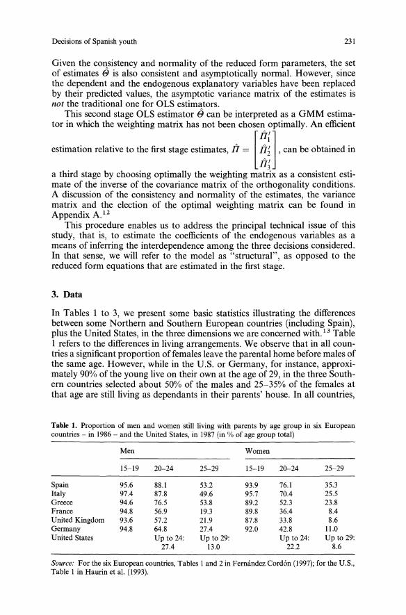
Decisions of Spanish youth 231

Given the c0I!sistency and nonnality of the reduced fonn parameters, the setof estimates e is also consistent and asymptotically nonnal. However, sincethe dependent and the endogenous explanatory variables have been replacedby their predicted values, the asymptotic variance matrix of the estimates isnot the traditional one for OLS estimators.This second stage OLS estimator ecan be interpreted as a GMM estima­

tor in which the weighting matrix has not been chosen optimally. An efficient

estimation relative to the first stage estimates, h ~ [~;], can he ohtained ina third stage by choosing optimally the weighting matrix as a consistent esti­mate of the inverse of the covariance matrix of the orthogonality conditions.A discussion of the consistency and nonnality of the estimates, the variancematrix and the election of the optimal weighting matrix can be found inAppendix A. 12This procedure enables us to address the principal technical issue of this

study, that is, to estimate the coefficients of the endogenous variables as ameans of inferring the interdependence among the three decisions considered.In that sense, we will refer to the model as "structural", as opposed to thereduced fonn equations that are estimated in the first stage.

3. Data

In Tables 1 to 3, we present some basic statistics illustrating the differencesbetween some Northern and Southern European countries (including Spain),plus the United States, in the three dimensions we are concerned with. 13 TableI refers to the differences in living arrangements. We observe that in all coun­tries a significant proportion offemales leave the parental home before males ofthe same age. However, while in the U.S. or Gennany, for instance, approxi­mately 90% of the young live on their own at the age of 29, in the three South­ern countries selected about 50% of the males and 25-35% of the females atthat age are still living as dependants in their parents' house. In all countries,

Table 1. Proportion of men and women still living with parents by age group in six Europeancountries - in 1986 - and the United States, in 1987 (in % of age group total)

Men Women

15-19 20-24 25-29 15-19 20-24 25-29

Spain 95.6 88.1 53.2 93.9 76.1 35.3Italy 97.4 87.8 49.6 95.7 70.4 25.5Greece 94.6 76.5 53.8 89.2 52.3 23.8France 94.8 56.9 19.3 89.8 36.4 8.4United Kingdom 93.6 57.2 21.9 87.8 33.8 8.6Germany 94.8 64.8 27.4 92.0 42.8 11.0United States Up to 24: Up to 29: Up to 24: Up to 29:

27.4 13.0 22.2 8.6

Source: For the six European countries, Tables I and 2 in Fernandez Cordon (1997); for the U.S.,Table I in Haurin et al. (1993).

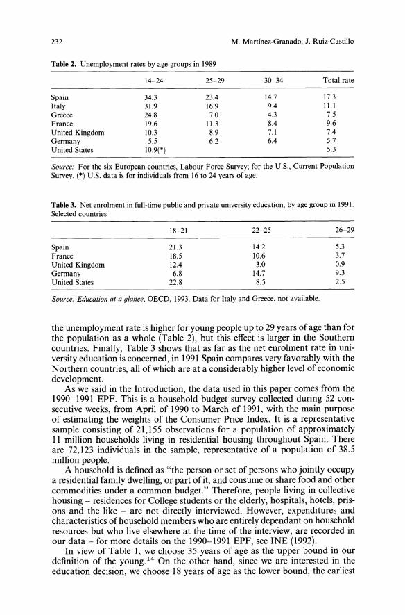
232

Table 2. Unemployment rates by age groups in 1989

M. Martinez-Granado, J. Ruiz-Castillo

14-24 25-29 30-34 Total rate

Spain 34.3 23.4 14.7 17.3Italy 31.9 16.9 9.4 Il.lGreece 24.8 7.0 4.3 7.5France 19.6 11.3 8.4 9.6United Kingdom 10.3 8.9 7.1 7.4Germany 5.5 6.2 6.4 5.7United States 10.9(*) 5.3

Source: For the six European countries, Labour Force Survey; for the U.S., Current PopulationSurvey. (*) U.S. data is for individuals from 16 to 24 years of age.

Table 3. Net enrolment in full-time public and private university education, by age group in 1991.Selected countries

18-21 22-25 26-29

Spain 21.3 14.2 5.3France 18.5 10.6 3.7United Kingdom 12.4 3.0 0.9Germany 6.8 14.7 9.3United States 22.8 8.5 2.5

Source: Education at a glance, OECD, 1993. Data for Italy and Greece, not available.

the unemployment rate is higher for young people up to 29 years ofage than forthe population as a whole (Table 2), but this effect is larger in the Southerncountries. Finally, Table 3 shows that as far as the net enrolment rate in uni­versity education is concerned, in 1991 Spain compares very favorably with theNorthern countries, all of which are at a considerably higher level of economicdevelopment.As we said in the Introduction, the data used in this paper comes from the

1990-1991 EPF. This is a household budget survey collected during 52 con­secutive weeks, from April of 1990 to March of 1991, with the main purposeof estimating the weights of the Consumer Price Index. It is a representativesample consisting of 21,155 observations for a population of approximatelyII million households living in residential housing throughout Spain. Thereare 72,123 individuals in the sample, representative of a population of 38.5million people.A household is defined as "the person or set of persons who jointly occupy

a residential family dwelling, or part of it, and consume or share food and othercommodities under a common budget." Therefore, people living in collectivehousing - residences for College students or the elderly, hospitals, hotels, pris­ons and the like - are not directly interviewed. However, expenditures andcharacteristics ofhousehold members who are entirely dependant on householdresources but who live elsewhere at the time of the interview, are recorded inour data - for more details on the 1990-1991 EPF, see INE (1992).In view of Table 1, we choose 35 years of age as the upper bound in our

definition of the young. 14 On the other hand, since we are interested in theeducation decision, we choose 18 years of age as the lower bound, the earliest

Decisions of Spanish youth 233

age at which people in Spain are supposed to decide whether to continue theirstudies beyond secondary education. This gives us a sample of 9,741 malesand 9,534 females. Ceuta and Melilla residents are not considered since someregional variables are not available for them.All the endogenous and exogenous variables are described in the Data

Appendix B. As far as the endogenous variables, we observe in Table B.l thatthe proportion of young females living on their own is 44% versus only 33%among the males, while the proportion of females studying is almost 5 percent­age points above the males. On the other hand, the female employment rate isonly 37% as opposed to 63% for the males; however, although not shown here,the female unemployment rate is 28%, which is around ten percentage pointshigher than the male rate. Table B.2 shows the sample distribution accordingto the three dependent variables. With reference only to the minority groups,around 5% of males and females work and follow some type of studies at thesame time, while only 2% of females and 0.5% of males study and are inde­pendent.The exogenous variables entering Eqs. (I) to (3) are of two types: individ­

ual characteristics, and economic variables. We have information on the fol­lowing individual characteristics: education, age, whether residing in a largecity or in a small village, parental transfers, and other non labor income. Weshould point out that, in addition to coresidence, there are two ways parentscan help their offspring: by a cash transfer, and by financing all or part of thehousing services consumed by their descendants when they live independently.In fact, more than 80% of those independent males and females receiving anykind of transfer live in dwellings subsidized by some family member. Bothtypes of parental transfers are assumed to be optimally selected by the parents.Hence, they are a predetermined variable for the young individuals. Only2.19% of young people coresiding with their parents receive a cash transfer.Therefore, we are forced to add up both types of transfers, forfeiting the pos­sibility of identifying the role of parental cash transfers. The final individualcharacteristic is the remaining non labor income. Unfortunately, it has beenimpossible to identify the effect of both variables separately. Therefore, in thefinal specification non labor income is the sum of parental transfers and othernon labor income. In principle, both the parental transfers and the educa­tional attainment could be considered endogenous variables. However, theirexogeneity, as well as the exogeneity of the rest of explanatory variables istested making use of the Sargan test of overidentifying restrictions proposed inAppendix A.Our data source lacks information on three potentially important individ­

ual characteristics: the type of contract - temporary or indefinite - of thoseyoung people holding a job, the marital status and the fertility behavior ofanyone different from the household head (defined as the household memberwith the highest earnings) and his/her spouse. The majority of the employedyoung people in Spain has a temporary job. 15 Our lack of data in this respectprecludes a study of the interaction between the decision to leave one's parentshouse made by those who are employed and the type of contract they have.However, it should be noted that even having the data, we could not simplyinclude the type of contract as an exogenous variable in the present frame­work. The recognition of its endogenous nature would possibly call for anindependent analysis among the employed.On the other hand, there is some empirical evidence that marriage is an

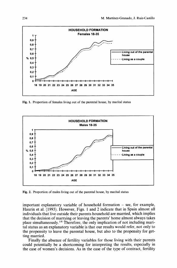
234 M. Martinez-Granado, J. Ruiz-Castillo

HOUSEHOLD FORMATIONFemales 18-35

--Living out of the parentalhouse

•••••• Living as a couple

........

0,9

0,8

0,7

0,6

'Y. 0,5

0,4

0,3

0,2

0,1

O+'-''+--+--+--+--+--+-+-+--+--f----ll--I--+-+-+-+-l18 19 20 21 22 23 24 25 26 27 28 29 30 31 32 33 34 35

AGE

Fig. I. Proportion of females living out of the parental house, by marital status

HOUSEHOLD FORMATIONMales 18-35

1

0,9

0,8,-- ..

..-.- .,.0,7 ,

0,6 --Living out of the parental'Y. 0,5 house

0,4 •••••• Living as a couple

0,3,.,

0,2.... .'

0,1 ......0

,

18 19 20 21 22 23 24 25 26 27 28 29 30 31 32 33 34 35

AGE

Fig. 2. Proportion of males living out of the parental house, by marital status

important explanatory variable of household formation - see, for example,Haurin et al. (1993). However, Figs. 1 and 2 indicate that in Spain almost allindividuals that live outside their parents household are married, which impliesthat the decision ofmarrying or leaving the parents' home almost always takesplace simultaneously. 16 Therefore, the only implication of not including mari­tal status as an explanatory variable is that our results would refer, not only tothe propensity to leave the parental house, but also to the propensity for get­ting married.Finally the absence of fertility variables for those living with their parents

could potentially be a shortcoming for interpreting the results, especially inthe case of women's decisions. As in the case of the type of contract, fertility

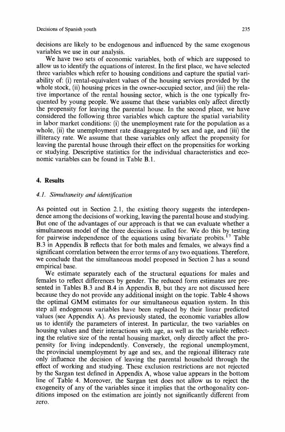
Decisions of Spanish youth 235

decisions are likely to be endogenous and influenced by the same exogenousvariables we use in our analysis.We have two sets of economic variables, both of which are supposed to

allow us to identify the equations of interest. In the first place, we have selectedthree variables which refer to housing conditions and capture the spatial vari­ability of: (i) rental-equivalent values of the housing services provided by thewhole stock, (ii) housing prices in the owner-occupied sector, and (iii) the rela­tive importance of the rental housing sector, which is the one typically fre­quented by young people. We assume that these variables only affect directlythe propensity for leaving the parental house. In the second place, we haveconsidered the following three variables which capture the spatial variabilityin labor market conditions: (i) the unemployment rate for the population as awhole, (ii) the unemployment rate disaggregated by sex and age, and (iii) theilliteracy rate. We assume that these variables only affect the propensity forleaving the parental house through their effect on the propensities for workingor studying. Descriptive statistics for the individual characteristics and eco­nomic variables can be found in Table B.I.

4. Results

4.1. Simultaneity and identification

As pointed out in Section 2.1, the existing theory suggests the interdepen­dence among the decisions ofworking, leaving the parental house and studying.But one of the advantages of our approach is that we can evaluate whether asimultaneous model of the three decisions is called for. We do this by testingfor pairwise independence of the equations using bivariate probits. 1 7 TableB.3 in Appendix B reflects that for both males and females, we always find asignificant correlation between the error terms ofany two equations. Therefore,we conclude that the simultaneous model proposed in Section 2 has a soundempirical base.We estimate separately each of the structural equations for males and

females to reflect differences by gender. The reduced form estimates are pre­sented in Tables B.3 and B.4 in Appendix B, but they are not discussed herebecause they do not provide any additional insight on the topic. Table 4 showsthe optimal GMM estimates for our simultaneous equation system. In thisstep all endogenous variables have been replaced by their linear predictedvalues (see Appendix A). As previously stated, the economic variables allowus to identify the parameters of interest. In particular, the two variables onhousing values and their interactions with age, as well as the variable reflect­ing the relative size of the rental housing market, only directly affect the pro­pensity for living independently. Conversely, the regional unemployment,the provincial unemployment by age and sex, and the regional illiteracy rateonly influence the decision of leaving the parental household through theeffect of working and studying. These exclusion restrictions are not rejectedby the Sargan test defined in Appendix A, whose value appears in the bottomline of Table 4. Moreover, the Sargan test does not allow us to reject theexogeneity of any of the variables since it implies that the orthogonality con­ditions imposed on the estimation are jointly not significantly different fromzero.

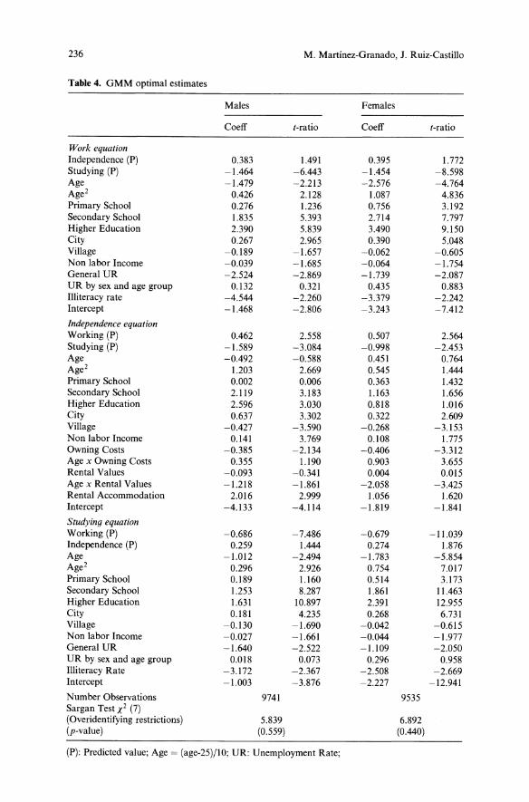
236 M. Martinez-Granado, J. Ruiz-Castillo

Table 4. GMM optimal estimates

Males Females

Coeff t-ratio Coeff t-ratio

Work equationIndependence (P) 0.383 1.491 0.395 1.772Studying (P) -1.464 -6.443 -1.454 -8.598Age -1.479 -2.213 -2.576 -4.764Age2 0.426 2.128 1.087 4.836Primary School 0.276 1.236 0.756 3.192Secondary School 1.835 5.393 2.714 7.797Higher Education 2.390 5.839 3.490 9.150City 0.267 2.965 0.390 5.048Village -0.189 -1.657 -0.062 -0.605Non labor Income -0.039 -1.685 -0.064 -1.754General UR -2.524 -2.869 -1.739 -2.087UR by sex and age group 0.132 0.321 0.435 0.883Illiteracy rate -4.544 -2.260 -3.379 -2.242Intercept -1.468 -2.806 -3.243 -7.412

Independence equationWorking (P) 0.462 2.558 0.507 2.564Studying (P) -1.589 -3.084 -0.998 -2.453Age -0.492 -0.588 0.451 0.764Age2 1.203 2.669 0.545 1.444Primary School 0.002 0.006 0.363 1.432Secondary School 2.119 3.183 1.163 1.656Higher Education 2.596 3.030 0.818 1.016City 0.637 3.302 0.322 2.609Village -0.427 -3.590 -0.268 -3.153Non labor Income 0.141 3.769 0.108 1.775Owning Costs -0.385 -2.134 -0.406 -3.312Age x Owning Costs 0.355 1.190 0.903 3.655Rental Values -0.093 -0.341 0.004 0.015Age x Rental Values -1.218 -1.861 -2.058 -3.425Rental Accommodation 2.016 2.999 1.056 1.620Intercept -4.133 -4.114 -1.819 -1.841

Studying equationWorking (P) -0.686 -7.486 -0.679 -11.039Independence (P) 0.259 1.444 0.274 1.876Age -1.012 -2.494 -1.783 -5.854Age2 0.296 2.926 0.754 7.017Primary School 0.189 1.160 0.514 3.173Secondary School 1.253 8.287 1.861 11.463Higher Education 1.631 10.897 2.391 12.955City 0.181 4.235 0.268 6.731Village -0.130 -1.690 -0.042 -0.615Non labor Income -0.027 -1.661 -0.044 -1.977General UR -1.640 -2.522 -1.109 -2.050UR by sex and age group 0.018 0.073 0.296 0.958Illiteracy Rate -3.172 -2.367 -2.508 -2.669Intercept -1.003 -3.876 -2.227 -12.941

Number Observations 9741 9535Sargan Test X2 (7)(Overidentifying restrictions) 5.839 6.892(p-value) (0.559) (0.440)

(P): Predicted value; Age = (age-25)/10; UR: Unemployment Rate;

Decisions of Spanish youth

4.2. Interdependence

237

As expected, working increases the propensity to leave on one's own sinceindividuals who work have access to the necessary funds that allow them tobe independent from their family. By the same token, not working - i.e., beingunemployed or inactive - increases the propensity to coreside. This is the im­portant "unemployment insurance" effect discovered by McElroy (1985) forthe 19-24, never married, out of school, U.S. males in 1971. On the otherhand, living independently has a positive effect, although only marginally sig­nificant, on the propensity to work; that is to say, the increased costs thatthe individuals face when living on their own act as an incentive to work.Equivalently, it appears that coresiding is weakly associated with a greaterpropensity for being unemployed or out of the labor force.Studying strongly increases the propensity to coreside. 18 This result reflects

the conditions of the publicly dominated Spanish university system: as inGreece, Italy, France or Portugal, tuition costs in public Universities arenominal - less than 500 Ecus per year; moreover, the spatial dissemination ofCollege centers in Spain reduces the costs of studying through coresidence.The opposite result in Ennish (1996) reflects the British University system,which strongly encourages people to study in a different locality from theirparents. 19 On the other hand, although not very significant, the positive effectof living apart on the propensity to study is the only puzzling result in thissubsection. We have to bear in mind that we are considering every type ofcourse not only official studies. In particular, among the women living inde­pendently, 47% report following "other studies" different from primary, sec­ondary, or College studies.Unsurprisingly, the propensity to work strongly reduces the propensity to

study. Conversely, to follow any type of studies significantly reduces the pro­pensity to work.It is important to emphasize that the nature of the interaction between the

three pairs of decisions is similar for both men and women.

4.3. Individual characteristics

Age, although significant in most equations, does not have a clear interpreta­tion since it enters the equations through many channels (age, age squared, thegroup specific unemployment rate, and interactions with housing prices).The role of the education variables is important. In the first place, the higher

the level of education attained by the individual, the higher the propensity towork - a plausible result. In the second place, given that the level of educationcan be considered a predetennined variable in the equation for studying, it isalso plausible that the higher the level of education attained the higher thepropensity to continue studying. In the third place, the effect of education onthe propensity to leave the parental house has a differentiated effect for malesand females. For males, education has a positive independent effect on theprobability of fonning a household, which reflects the fact that the more edu­cated individuals are also those with higher earnings and, presumably, the moreattractive partners in the marriage market. There is also a strong indirect effectthrough the increase on the propensity of working, offset by the increase in the

238 M. Martinez·Granado, J. Ruiz-Castillo

propensity to study. For women, the indirect effects work in the same directionand are even stronger, but education does not have an independent effect on itsown: only if the woman has finished secondary school is she more likely to beliving on her own. Since most individuals living apart from their parents aremarried, this decreasing effect of education may merely reflect the postpone­ment of marriage decisions by more educated women.Parental transfers and other non labor income have a positive effect on the

probability of leaving the parental home: access to more economic resourceshelps individuals to afford the expenses of living on their own and, therefore,increases the probability of leaving the parental house. On the other hand,non labor income has the usual negative effect on the propensity to work (andto study). This effect is stronger for females, possibly because a larger nonlabor income allows them to spend their time in other activities such as takingcare of the family or having children.Living in a large city increases the propensity to form a household, while

living in a small village decreases it. This effect is especially strong for males.It probably reflects the fact that the traditional pattern of "extended families",where several generations cohabit under the same roof and cooperate in thesame productive activities, is more prevalent in rural areas. On the other hand,the effect of the municipal size on the propensity to work and to study revealsthat there are more jobs and opportunities to study as the municipal sizeincreases. However, the effect pattern differs by gender. For males, relativeto medium sizes municipalities, there is a negative effect in small villages, anda positive effect in big cities. For females, there is a clear discontinuity: thereis only a significant strong positive effect in big cities.

4.4. Economic variables

All the variables reflecting the spatial variation in housing conditions havethe expected influence on the propensity to live apart. In the first place, thehigher the rental equivalence value of the whole stock and, above all, thehigher the owner-occupied housing prices are, the lower the propensity to liveindependently. The difference between these two variables is that the effect ofthe second one decreases with age. In the second place, the variable reflectingthe availability of rental housing has a strong and significant positive effect onthe probability of living independently. These results are in agreement withthose obtained in Borsch-Supan (1985), Haurin et al. (1993, 1994), Ermishand Di Salvo (1997) and Ermish (1999), emphasizing the role of housing costs- and not only own income - as a basic determinant of the household for­mation and related demographic decisions.The gender and age group specific unemployment rate does not have any

significant effect on the propensity to work: it appears that individuals per­ceive the general unemployment rate as the relevant variable. Of course, thegeneral unemployment rate has a significant negative effect on the propensityto work, revealing the lower probability of receiving a job offer, as well as thediscouraging worker effect that reduces the effort of looking for a job. Notethat the indirect effect of unemployment on coresidence by lowering the pro­pensity to work reinforces the role of the family in Spain as a cushion inthe face of unfavorable labor market conditions. 20 On the other hand, given

Decisions of Spanish youth 239

job status, the unemployment rate has a negative effect on the probability ofstudying for both men and women. Therefore, unemployment works in twoways: it reduces the probability of finding a job, favoring the studying option(opportunity cost effect), but it directly reduces the probability of studying(discouraging effect due to the poorer job perspectives).The illiteracy rate has a strong negative effect on the propensity to study

and to work. The first effect is consistent with different explanations. It canreflect a peer effect, so that young individuals in areas where not many peoplehave studied in the past also tend not to study. It could also be reflecting howregions with a more educated stock of human capital have developed a widernet of possibilities for the young people to continue their studies after thecompulsory age. Finally, the negative effect on the propensity to work canreflect the fact that areas with a more educated workforce may have better jobopportunities through higher investment (and job creation) by the firms settledthere - for a theoretical exposition of this idea, see Acemoglu (1996).

5. Conclusions

As far as we know, this paper constitutes the first econometric attempt toexplain why parents and young descendants between 18 and 35 years of agedecide to live together in Spain in rather large proportions. Lacking longitu­dinal data, we have found it interesting to work with a sufficiently rich, largeand readily available household budget survey - the 1990-1991 EPF - col­lected by the Spanish INE with completely different aims in mind. The reason isthat, even with cross-section data one can start addressing the issues involvedin joint decision making. The major novelty in the paper is that, in addition tothe joint decision of whether to remain in the parental house and whether towork, we have been able to add the decision of whether to continue studying.The analysis is implemented through a two-stage method developed by

Arellano and Bover (1997) for limited dependent variable models from paneldata, which has been adapted here to the case of simultaneous probabilitymodels using cross-section data. Our results indicate that the behavior ofSpanish youth is amenable to careful empirical analysis with standard tools.From a methodological point of view, we have shown that the endogenous

and simultaneous treatment of the three decisions should occupy the core ofany attempt to understand the issues involved. Otherwise, seriously misleadingresults could be obtained, a possibility we have illustrated when the propen­sities to work or to study are treated as mere exogenous variables influencingthe decision to abandon the parental household.As pointed out in the Introduction, we have confirmed that there exists a

rich pattern of interdependencies between the three decisions, and that bothindividual characteristics and economic variables have a significant explan­atory role in the three propensities modeled in the paper. More specifically,our results show that the pattern of interdependencies among the three deci­sions, as well as the effect of the economic variables, are qualitatively the samefor males and females. In particular, we have found support for the followingregularities: (i) parents help their young offspring through coresidence whenthe latter do not have a job or are studying; (ii) living independently has a pos­itive effect on the propensity to work, (iii) housing conditions significantly affect

240 M. Martinez-Granado, J. Ruiz-Castillo

the living arrangements of the young in a direct way, while (iv) unemploymentexerts its influence indirectly through its negative effect on the propensities towork and to study.However, there are also subtle differences in gender behavior. (i) More

educated women tend to postpone longer than men the decision to marry andform a new household; (ii) increases in non labor income have a stronger neg­ative effect on the propensities to work and to study for women, and (iii) thedecrease in the propensities to work, to study and to form a new household ina small village is stronger for men, while the increase in the first two propen­sities in a large city is greater for women.This paper has several obvious shortcomings. In the first place, as we have

pointed out from the beginning, even in a static framework the data we haveused is rather incomplete. It lacks information on potentially important indi­vidual characteristics of young people, as well as on a host of fundamentalvariables reflecting the family background of the individuals living apart fromtheir parents. More importantly, perhaps, is that all of our cross-section resultsare rather suspect because they reflect the combined impacts of both inflowsand outflows from a certain work, study or living arrangement situation. In thisrespect, the present study can only be taken as a first step towards an under­standing of the decisions of the Spanish youth that we have focused on here.In the second place, we have been unable to provide any explanation for

the role of the Spanish family, mentioned in the Introduction, as a safety netin the opposite direction of the one usually stressed. We refer to the evidenceindicating that young people with a job in poorer households are making adecisive contribution in raising the standard of living of the remaining house­hold members. To study this question, one would certainly need data on such"reverse transfers" - as well as data on the parental socioeconomic charac­teristics of all the young people in the population. Furthermore, to rationalizethese transfers in a theoretical model, one could follow one of two routes: topostulate strong altruistic motives on the part of the young offspring; or toextend the existing exchange models substituting transfers from the youngfor parental loans. As a matter of fact, this line of thought might lead to abetter understanding of the fact revealed by Rosenzweig and Wolpin (1993)and Ermish (1996), that, contrary to existing theory, higher parental incomeincreases the probability of their offspring living independently.In the third place, only an appropriate comparative study including non

Southern European countries, would allow us to estimate the effect that insti­tutions and public policies may have on the behavior of the young. Meanwhile,we have already mentioned that public policy in Spain favors high enrolmentrates in public universities. To this we may add that, as pointed out in Cantoand Mercader (1999), social protection in Spain has developed during the1980s, maintaining the pension and the unemployment subsidy programs atthe center of the system. Thus, public protection for unemployed youth is eithernot available at all in the case of the "first-job-seekers" (35 and 28% of theunemployed males and females in our sample, respectively), or very limitedindeed for "early-age-unemployed" holding mere temporary jobs. Moreover,general family support systems and child-care policies in particular are under­developed in the Spanish welfare state. Finally, housing policies tend to favorowner-occupied housing, which is the most inaccessible tenure choice for theyoung. One may assume, of course, that all these policies tend to reinforce theimportance of coresidence in Spain.

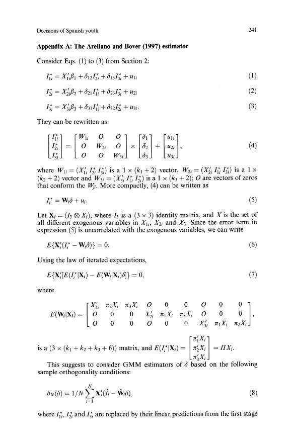
Decisions of Spanish youth

Appendix A: The Arellano and Bover (1997) estimator

Consider Eqs. (1) to (3) from Section 2:

They can be rewritten as

241

(I)

(2)

(3)

(4)

where Wli = (X{i Ii; 13:) is a I x (k l + 2) vector, W2i = (Xli II: 13:) is a I x(k2+ 2) vector and W3i = (X3i Iti 12:) is a I x (k3 + 2); 0 are vectors of zerosthat conform the Uji. More compactly, (4) can be written as

1/ = WiJ+Ui. (5)

Let Xi = (h (8) Xi), where h is a (3 x 3) identity matrix, and X is the set ofall different exogenous variables in Xli, X2i and X3. Since the error term inexpression (5) is uncorrelated with the exogenous variables, we can write

Using the law of iterated expectations,

E{X;[E(I/IXi) - E(W;/Xi)J]} = 0,

where

(6)

(7)

[

X{i

E(WdXi) = ~

o o oooo

[

n;Xi]is a (3 x (k l + k2+ k3+ 6)) matrix, and E(ItIXi) = n~Xi = IIXi.

7r3Xi

This suggests to consider GMM estimators of J based on the followingsample orthogonality conditions:

N

bN(J) = I/N'L,X;(ii - WiJ),i=1

(8)

where II:' Ii; and 13: are replaced by their linear predictions from the first stage

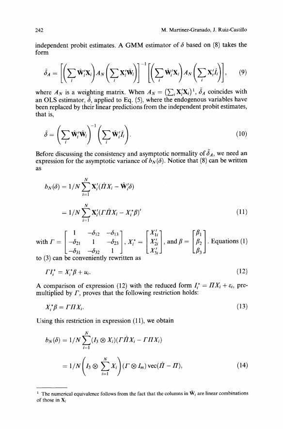
242 M. Martinez-Granado, J. Ruiz-Castillo

independent probit estimates. A GMM estimator of J based on (8) takes theform

where AN is a weig,hting matrix. When AN = (LiX;Xi)l, JA coincides withan OLS estimator, J, applied to Eq. (5), where the endogenous variables havebeen replaced by their linear predictions from the independent probit estimates,that is,

(10)

Before discussing the consistency and asymptotic normality ofJA , we need anexpression for the asymptotic variance of bN(J). Notice that (8) can be writtenas

N

bN(J) = I/NLX;(IIXi - W;J)i=1

N~ I' • I

= liN L..JXj(TIlXi - Xi P)i=1

with T = [-~21 -~12 =~::], Xt =

-J31 -J32 1to (3) can be conveniently rewritten as

(11 )

[X{i] [PI]X~i ,and P = P2 . Equations (1)

X3i P3

(12)

A comparison of expression (12) with the reduced form It = IlXi +ci, pre­multiplied by T, proves that the following restriction holds:

X;'P = TIlXi·

Using this restriction in expression (11), we obtain

N

bN(J) = I/NL(I3 ® Xi)(TnXj - TIlXi)i=1

(13)

(14)

I The numerical equivalence follows from the fact that the columns inWj are linear combinationsof those in Xi

Decisions of Spanish youth

and consequently

with V· = (r @ 1m ) var(vec(it))(r' @ 1m ). Hence, it can be proven that

243

(15)

where Mxw = Plim(X~i), and fb = var(bN ). A consistent estimate of the

asymptotic variance of JA is given by

where Mxw and Cb are consistent estimates of Mxw and Vt, respectively. Themost efficient estimator relative to it is obtained by choosing optimally AN asa consistent estimate of the inverse of the covariance matrix of the orthogo­nality conditions

(18)

Now we only need an estimate for var(vec(it)). Let us consider

(19)

where Lj , j = 1,2,3, is the corresponding likelihood functi9n. Subject to suit­able regularity conditions, a first order expansion of aL(Il)jall around thetrue value of II gives

( (a2L )) A-1 j N diag anja~; ,jNvec(II - II)

which suggests an estimate for the variance of the form

var(vec(it)) = iI-lljfiI-I,

(20)

(21)

244 M. Martinez-Granado, J. Ruiz-Castillo

where iI = diag(N- 102Ljlon/3n;) and tfr = N- 1 L:{oLijlonj}' {oLihlonJ.}I

Finally, under the null hypothesis of lack of misspecification, a test statisticof the overidentifying restrictions can be derived for the optimal GMMestimator,

2~ X3m-(k, +k2+K3+6) ' (22)

where Ui = it - WiJA .

In brief, the method discussed above works as follows:1. First, the reduced form estimates are obtained.2. Second, using these reduced form estimates, a sub-optimal GMM estimatoris implemented that allows us to compute a consistent estimate of Vt,.

3. The consistent estimate of Vt, and the reduced form estimates are used toobtain the most efficient estimates relative to the first-stage reduced formones.

Appendix B: Data

Endogenous variables

Independent: Dummy variable that equals one if the individual does not live inthe parental home.Work: Dummy variable that equals one if the individual is working (full orpart time) at the interview date.Studying: Dummy variable that equals one if the individual is carrying on anytype of education. It is worth noting that 21.9% of female students are saidto attend "other type of education", different from primary, secondary, andCollege education, while only 14.9% of male students declare to do so.

Exogenous variables

• Individual characteristics:Educational: We define three dummy variables reflecting the highest degreecompleted by the individual. Educ2 equals one if the individual has finishedprimary school, Educ3 equals one if s/he has finished secondary school andEduc4 equals one if some College degree has been attained.City: Dummy variable that equals one if the individual lives in a large city(more than 500,000 inhabitants).Village: Dummy variable that equals one if the individual lives in a smallvillage (less than 2,000 inhabitants).Parental transfers: Regular or occasional cash transfers, plus housing sub­sidies received by the young offspring living apart.Other non labor income: This is the summation of all types of current incomesources, different from parental transfers and labor earnings or public sub-

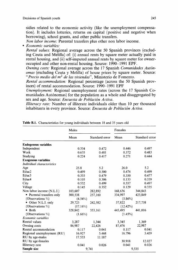
Decisions of Spanish youth 245

sidies related to the economic activity (like the unemployment compensa­tion). It includes lotteries, returns on capital (positive and negative whenborrowing), school grants, and other public transfers.Non labor income: Parental transfers plus other non labor income.

• Economic variables:Rental values: Regional average across the 50 Spanish provinces (exclud­ing Ceuta and Melilla) of: (i) annual rents by square meter actually paid inrental housing, and (ii) self-imputed annual rents by square meter for owner­occupied and other non-rental housing. Source: 1990-1991 EPF.Owning costs: Regional average across the 17 Spanish Comunidades Auton­omas (excluding Ceuta y Melilla) of house prices by square meter. Source:"Precio medio del m2 de las viviendas", Ministerio de Fomento.Rental accommodation: Regional percentage (across the 50 Spanish prov­inces) of rental accommodation. Source: 1990-1991 EPFUnemployment: Regional unemployment rates (across the 17 Spanish Co­munidades Autonomas) for the population as a whole and disaggregated bysex and age. Source: Encuesta de Poblacion Activa.Illiteracy rate: Number of illiterate individuals older than 10 per thousandinhabitants in every province. Source: Encuesta de Poblacion Activa.

Table 8.1. Characteristics for young individuals between 18 and 35 years old

Males Females

Mean Standard error Mean Standard error

Endogenous variablesIndependent 0.334 0.472 0.446 0.497Work 0.635 0.481 0.372 0.483Studying 0.224 0.417 0.271 0.444Exogenous variablesIndividual characteristicsAge 25.8 5.2 26.0 5.2Educ2 0.499 0.500 0.474 0.499Educ3 0.355 0.479 0.350 0.477Educ4 0.105 0.306 0.133 0.339City 0.532 0.499 0.557 0.497Village 0.145 0.352 0.129 0.335Non labor income (N.L.!.) 103,607 282,892 168,636 344,843• Parental transfers only 300,538 257,160 334,997 423,849(Observations %) (4.54%) (5.86%)• Other N.L.I. only 29,723 242,582 57,822 217,738(Observations %) (17.16%) (12.42%)

• Both 328,842 353,161 445,495 441,016(Observations %) (1.66%) (1.45%)

Economic variablesRental values 3,287 1,344 3,345 1,369Owning costs 86,987 22,426 87,476 22,987Rental accommodation 0.117 0.041 0.117 0.041Regional unemployment (RU) 16.927 5.468 16.796 5.459RUby age-males 17.533 11.187RUby age-females 30.918 12.027Illiteracy rate 0.041 0.026 0.041 0.026Sample size 9,741 9,535

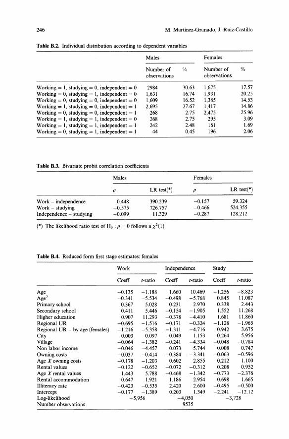
246 M. Martinez-Granado, J. Ruiz-Castillo

Table B.2. Individual distribution according to dependent variables

Males

Number of %observations

Females

Number of %observations

Working = I, studying = 0, independent = 0Working = 0, studying = I, independent = 0Working = 0, studying = 0, independent = 0Working = I, studying = 0, independent = 1Working = 0, studying = 0, independent = IWorking = I, studying = I, independent = 0Working = I, studying = I, independent = IWorking = 0, studying = I, independent = I

29841,6311,6092,69526826824244

30.6316.7416.5227.672.752.752.480.45

1,6751,9311,3851,4172,475295161196

17.5720.2514.5314.8625.963.091.692.06

Table B.3. Bivariate probit correlation coefficients

Males Females

Work - independenceWork - studyingIndependence - studying

p

0.448-0.575-0.099

LR test(-)

390.239726.75711.329

p

-0.157-0.466-0.287

LR test(-)

59.324524.355128.212

(-) The likelihood ratio test of Ho : p = 0 follows a X2( I)

Table B.4. Reduced form first stage estimates: females

Work Independence Study

Coeff I-ratio Coeff I-ratio Coeff I-ratio

Age -0.135 -1.188 1.660 10.469 -1.256 -8.823Age2 -0.341 -5.534 -0.498 -5.768 0.845 11.087Primary school 0.367 5.028 0.231 2.970 0.338 2.443Secondary school 0.411 5.446 -0.154 -1.905 1.552 11.268Higher education 0.907 11.293 -0.378 -4.410 1.681 11.860Regional UR -0.695 -1.516 -0.171 -0.324 -1.128 -1.965Regional UR - by age (females) -1.216 -5.358 -1.311 -4.716 0.942 3.675City 0.003 0.097 0.049 1.153 0.264 5.956Village -0.064 -1.382 -0.241 -4.334 -0.048 -0.784Non labor income -0.046 -4.457 0.073 5.744 0.008 0.747Owning costs -0.037 -0.414 -0.384 -3.341 -0.063 -0.596Age X owning costs -0.178 -1.203 0.602 2.855 0.212 1.100Rental values -0.122 -0.652 -0.072 -0.312 0.208 0.952Age X rental values 1.443 5.788 -0.468 -1.342 -0.773 -2.376Rental accommodation 0.647 1.921 1.186 2.954 0.698 1.665Illiteracy rate -0.423 -0.535 2.420 2.600 -0.495 -0.500Intercept -0.177 -1.389 0.203 1.349 -2.241 -12.12Log-likelihood -5,956 -4,050 -3,728Number observations 9535

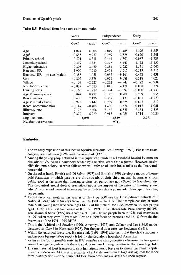
Decisions of Spanish youth

Table 8.5. Reduced form first stage estimates: males

Work Independence

247

Study

Coeff t-ratio Coeff t-ratio Coeff t-ratio

AgeAge2

Primary schoolSecondary schoolHigher educationRegional URRegional UR - by age (males)CityVillageNon labor incomeOwning costsAge X owning costsRental valuesAge X rental valuesRental accommodationIlliteracy rateInterceptLog-likelihoodNumber observations

Endnotes

1.024 8.006-0.685 -9.9570.591 8.3110.259 3.5540.203 2.489-3.909 -7.710-0.288 -1.051-0.206 -5.378-0.107 -2.227-0.077 -7.510-0.163 -1.7290.047 0.2770.430 2.1260.923 3.142-0.147 -0.4082.176 2.6040.872 6.929-5,086

2.049 11.485-0.269 -2.6260.441 5.3900.378 4.4450.231 2.522-2.694 -5.012-0.062 -0.1640.025 0.581-0.272 -4.9420.046 4.121-0.394 -3.0970.176 0.7810.358 1.4300.239 0.6251.480 3.6746.162 6.531-0.915 -6.086

-3,8599741

-1.296 -8.8550.670 8.241-0.087 -0.7331.192 10.1361.571 12.646-0.313 -0.5160.448 1.4310.318 7.025-0.122 -1.9340.038 3.324-0.080 -0.7300.209 1.055-0.061 -0.270-0.627 -1.819-0.017 -0.041-2.484 -2.525-1.714 -10.20

-3,571

1 For an early exposition of this idea in Spanish literature, see Revenga (1991). For more recentanalysis, see Robinson (1998) and Toharia et al. (1998).

2 Among the young people studied in this paper who reside in a household headed by someoneelse, almost 7% live in a household headed by a relative, other than a parent. However, to sim­plify the terminology, in what follows we will refer to all such households as the "parental"household.

3 On the other hand, Ermish and Di Salvo (1997) and Ermish (1999) develop a model of house­hold formation in which parents are altruistic about their children, and housing is a localpublic good in the sense that housing services per person are not affected by household size.The theoretical model derives predictions about the impact of the price of housing, youngadults' income and parental income on the probability that a young adult lives apart from his/her parents.

4 Recent empirical work in this area is of this type. RW use the kinship-linked cohorts of 9National Longitudinal Surveys from 1967 to 1981 in the U.S. Their sample consists of morethan 5,000 young men who were ages 14-17 at the time of the 1966 interview. E uses peopleaged 16-29 in the first four waves of the 1991-1994 British Household Panel Survey (BHPS).Ermish and di Salvo (1997) use a sample of 10,500 British people born in 1958 and interviewedin 1991 when they were 33 years old. Ermish (1999) focus on persons aged 16-30 from the firstfive waves of the 1991-1995 BHPS.

5 This is the Ashford and Sowden (1970), Amemiya (1975) and Zellner and Lee (1965) model,discussed as Case 3 in Heckman (1978). For the panel data case, see Heckman (1981).

6 Within the empirical literature, Haurin et al. (1993, 1994) also insist that the child's income isendogenous because labor supply is jointly decided along household formation.

7 As far as the fourth possible state, in RW transfers are always positive whenever the two gener­ations live together, while in E there is no data on non-housing transfers to the coresiding child.

8 In a multinomiallogit framework, data limitations would force us to ignore the human capitalinvestment decision. At any rate, estimates of a 4 state multinomiallogit arising from the laborforce participation and the household formation decisions are available upon request.

248 M. Martinez-Granado, J. Ruiz-Castillo

9 Similar simultaneous equation models have been used in other contexts in order to analyze therelationship between disability and labor force participation (Stem 1989), or the relationshipbetween employment and care giving to elderly parents (Wolf and Soldo 1994).

10 Mallar (1977) or Heckman (1978), among others, propose two-stage methods in this type ofsituation. For a revision of these methods, see Maddala (1983).

11 Independent equation estimation at the first-stage will in general yield inefficient estimatesbecause it ignores the possible dependence among the equations through the error terms, uji.

Taking into account such dependence would typically require the use of simulation basedestimators (see Hajivassiliou and Ruud 1994).

12 If the three decisions in Eqs. (I) to (3) were not simultaneous and we were only interestedin the study of the decision of leaving the parental household, a single equation with two en­dogenous dummies could also be estimated. However, the two-stage estimators we have dis­cussed could not be implemented, and some simulation technique of estimation had to be ap­plied. Finally, note that a multivariate probit with endogenous dummies will also complicatethe estimation.

13 The six European countries are the ones studied in Fernandez Cordon (1997) using the LaborForce Survey. For another compartive study between Northern and Southern European coun­tries, using the European Household Panel, see Iacovou (1998).

14 Results for an upper bound of 30 years are available on request. They are not very sensitive tothe choice of the upper bound, especially for males. For females, although in general the signand size of the estimated parameters are comparable for both age groups, the overidentifyingrestrictions are marginally rejected. Moreover, the independence variable, that is marginallysignificant for women between 18-35 in the equations of working and studying losses com­pletely its significance when considering only women between 18 and 30 years of age.

15 Table 2 of Canto and Mercader (1999) show the entry-level jobs in 1996 by new schoolleavers(aged 16 to 29) one year after leaving education in different selected European countries. Spainis an outlier: 80% of this group hold a temporary job. On the other hand, according to Giielland Petrongolo (2000), in 1990 less than 15% of all temporary contracts become indefinite.Finally, Jimeno and Toharia (1993) and De la Rica and Felgueroso (1999) find that the tempo­rary workers earn approximately 10% less than permanent ones, after controlling for observablepersonal and job characteristics.

16 This is confirmed by all demographic studies in the subject. See, for instance, Verges (1997) orJurado (1997).

17 We thank an anonymous referee for this suggestion.18 The results are substantially different when ignoring the endogeneity of the working andstudying decisions. For women, we find a positive effect of the propensity to work and to studyon the probability of coresidence. For males, working provides incentives to leave the parentalhouse but studying has no effect on the household formation decision.

19 According to Ermish (1996), the positive effect found by Rosenzweig and Wolpin (1993) mayreflect the different definition of coresidence among students: young men who are at collegeand away from home are classified as coresiding with their parents if they report themselves asattached to their parents' household. Nevertheless, in their fixed effects multinomial logitmodel, Rosenzweig and Wolpin (1993) also find a positive effect of attending college on theprobability of receiving a parental transfer.

20 Rosenzweig and Wolpin (1993) find a positive but small direct effect of the weeks spent inunemployment on coresidence, as well as on the parental transfers when living apart. Thus, inthe U.S., the family acts as a cushion in bad times independent of living arrangements.

References

Acemoglu D (1996) A Microfoundation for Social Increasing Returns in Human Capital Accu­mulation. Quarterly Journal of Economics 111(3):779-804

Amemiya T (1975) Qualitative Response Models. Annals of Economic and Social Measurement4:363-372

Arellano M, Bover 0 (1997) Estimating Dynamic Limited Dependent Variable Models fromPanel Data. Investigaciones Economicas XXI(2): 141-165

Decisions of Spanish youth 249

Ashford JR, Sowden RR (1970) Multivariate Probit Analysis. Biometrics 26:535-546Borsch-Supan A (1986) Household Formation, Housing Prices, and Public Policy Impacts. Journal

of Public Economics 30:145-164Canto-Sanchez 0, Mercader-Prats M (1999) Poverty among Children and Youth in Spain: TheRole of Parents and Youth Employment Status. Document de Treball 99-07, Departamentd'Economia Aplicada, Universitat Autonoma de Barcelona

Cox D (1987) Motives for Private Income Transfers. Journal ofPolitical Economy 95:508-546Cox D (1990) Intergenerational Transfers and Liquidity Constraints. Quarterly Journal of Eco­

nomics 105:187-217De la Rica S, Felgueroso F (1999) Wage Differentials Between Permanent and TemporaryWorkers: Further Evidence. mimeo

Del Rio C, Ruiz-Castillo J (1997) Demographic Trends and Living Standards. Working Paper 97­67, Economic Series 33, Universidad Carlos III de Madrid

Ermish J (1996) Parental Support for Human Capital Investment by Young Adults. DiscussionPaper No. 1536, CEPR

Ermish J (1999) Prices, Parents and Young People's Household Formation. Journal of UrbanEconomics 45:47-71

Ermisch J, Di Salvo P (1997) The Economic Determinants of Young People's Household For­mation. Economica 64:627-44

Fernandez Cordon JA (1997) Youth Residential Independence and Autonomy: A ComparativeStudy. Journal ofFamily Issues 18:576-607

Giiell M, Petrongolo B (2000) Workers' Transitions from Temporary to Permanent Employment:the Spanish Case. mimeo, Universidad Carlos III

Hajivassiliou VA, Ruud PA (1994) Classical Estimation Methods for LDV Models Using Simu­lation. In: Engle RF, McFadden DL (eds) Handbook ofEconometrics, vol. 4. North-Holland,Amsterdam

Haurin DR, Hendershott PH, Dongwook K (1993) The Impact of Real Rents and Wages onHousehold Formation. The Review of Economics and Statistics 75:284-293

Haurin DR, Hendershott PH, Dongwook K (1994) Housing Decisions of American Youth.Journal of Urban Economics 35:28-45

Heckman 11 (1978) Dummy Endogenous Variables in a Simultaneous Equation System. Econo­metrica 46(6):931-957

Heckman 11 (1981) Statistical Models for Discrete Panel Data. In: Manski CF, McFadden DStructural Analysis of Discrete Data with Econometric Applications (ed) The MIT Press,Cambridge, Massachusetts

Iacovou M (1998) Young People in Europe. mimeo, Institute for Social and Economic Research,University of Essex

INE (1992) Encuesta de Presupuestos Familiares 1990-1991. Metodologia, MadridJimeno JF, Toharia L (1993) The Effects of Fixed-term Employment on Wages: Theory and Ev­idence from Spain. Investigaciones Econonomicas 27:475-494

Jurado Guerrero T (1997) Un analisis regional de los modelos de convivencia de los jovenesespaiioles. Las cuatro Espaiias de la emancipacion familiar. Estudios de Juventud 39:17-35

Maddala GS (1983) Limited Dependent and Qualitative Variables in Econometrics. EconometricSociety Monographs, Cambridge University Press

Mallar CD (1977) The Estimation of Simultaneous Probability Models. Econometrica 45(7):1717­1722

McElroy MB (1985) The Joint Determination of Household Membership and Market Work: TheCase of Young Men. Journal of Labor Economics 3(3):293-316

Revenga A (1991) La liberalizacion economica y la distribucion de la renta: la experiencia espa­fiola. Moneda y Credito 193:179-224

Robinson A (1998) Spanish Family Values: Spain's Welfare system is let off the hook by the family,New Economy 4:188-92

Rosenzweig M, Wolpin K (1993) Intergenerational Support and the Life Cycle Incomes of YoungMen and Their Parents: Human Capital Investments, Coresidence, and IntergenerationalFinancial Transfers. Journal of Labor Economics II :84-112

Sastre M (1999) Los ingresos y los gastos en las EPF Ensayos sobre desigualdad y bienestar.Unpublished Ph. D. Dissertation, Universidad Complutense de Madrid

Stem S (1989) Measuring the Effect of Disability on Labor Force Participation. Journal ofHumanResources 24(3):361-395

250 M. Martinez-Granado, J. Ruiz-Castillo

Toharia LA, Cebrian C, Garcia Serrano I, Garcia Mainar C, Malo I, Moreno MA, Villagomez E(1998) El mercado de trabajo en Espana. McGraw-Hili/Interamericana de Espana, S.A.U.

Verges R (ed) (1997) La edad de emancipaci6n de losj6venes. Centre de Cultura Contemporania deBarcelona

Wolf DA, Soldo BJ (1994) Married Women's Allocation of Time to Employment and Care ofElderly Parents. Journal of Human Resources 29(4):1259-1276

Zellner A, Lee T (1965) Joint Estimation of Relationships Involving Discrete Random Variables.Econometrica 33:382-394

Group living decisions as youths transition to adulthood

Steven Garaskyl, R. Jean Haurin2, Donald R. Haurin3

1 Department of Human Development and Family Studies, Iowa State University, 1086LeBaron St., Ames, Iowa, USA 50011 (Fax: +1-515-294-2502; e-mail: sgarasky@iastate.edu)2 Center for Human Resource Research, The Ohio State University, 921 Chatham Lane, Suite200, Columbus, OH, USA 43221 (Fax: +1-614-442-7329; e-mail: haurin.l@osu.edu)3 Departments of Economics, Finance, and Public Policy, The Ohio State University, 1010Derby Hall, 154 N. Oval Mall, Columbus, OH, USA 43210 (Fax: +1-614-292-9530;e-mail: haurin.2@osu.edu)

Received: 15 July I999/Accepted: 15 May 2000

Abstract. This study follows teens through young adulthood as they transitionto independent living. We focus on a little studied issue: why some youths livein groups rather than alone or with parents. This choice is important becausethe size of the group has a substantial impact on the demand for dwellingunits; the more youths per dwelling the lower is aggregate demand and thegreater is population density. Our study also adds to the knowledge of whichfactors influence youths' choice of destination as they leave the parental home.The empirical testing uses a discrete hazard model within a multinomial logitframework to allow for more than one possible state transition. We find thateconomic variables have little impact on the decision of whether to exit to alarge versus a small group, while socio-demographic variables matter. We alsotest a new push-pull hypothesis and find that the pull of economic variableson the probability of exiting the parental home increases as youths reach theirmid to late twenties.

JEL classification: 01,112, R20

Key words: Group living, household formation, home~leaving

1. Introduction

Interest in the process of youths leaving the parental home and moving to anindependent living arrangement continues to be high. Recent studies about

All correspondence to Donald R. Haurin. The authors gratefully acknowledge the research assis­tance ofCathy Hockaday and thank John Ermisch and an anonymous referee for their comments.This research was supported, in part, by the Iowa Agriculture and Home Economics ExperimentStation, Ames, Iowa, Project No. 3523, and supported by the Hatch Act and State of Iowa funds.Responsible editor: John F. Ermisch.

252 S. Garasky et al.

youths' tendency to leave home include analyses of the impact of the cost ofshelter and potential earnings (Haurin et al. 1993, 1994; Bourassa et al. 1994;Whittington and Peters 1996; Ermisch and Di Salvo 1997; Johnson andDaVanzo 1998; Ermisch 1999), the impact offamily structure (Aquilino 1991;Goldscheider and Goldscheider 1998), the impact of gender, religion, andethnic differences (Goldscheider and DaVanzo 1989; Buck and Scott 1993),and the impact of parental and youths' normative expectations about home­leaving (Goldscheider and Goldscheider 1993b). A fairly comprehensive por­trait of the sociological, psychological, demographic, and economic explan­atory factors is emerging.Understanding home-leaving is key to modeling household formation.

Household formation impacts aggregate housing demand, population density,fertility, labor force mobility, and the demand for public services. We arguethat while the substantial attention paid to the timing of youths' departurefrom the parental home is appropriate, careful study of all destination possi­bilities is equally important as is understanding whether the magnitude of anexplanatory factor's influence differs by respondent age.There is some controversy about the appropriate categorization of exit

types. Early studies focused on a dichotomous choice: exit or remain in theparental home. More recently, multiple exit "destinations" have been consid­ered where a destination is defined as a type of living arrangement outside theparental home. Examples include exiting to marry, live alone, live with a rel­ative, or live in a group. Studies have attempted to sort out the impact ofexplanatory factors on the probabilities of exiting to each of the destinationcategories. However, the choice of destination categories has often been dic­tated by data limitations or been the result of an apparently arbitrary choice.When refocusing research from the origin (parental home) of a youth's tran­sition to the destination, a more systematic approach to study alternativeconfigurations of destinations should be employed. We recognize that theextent of disaggregation of destinations is limited by sample size; the morecategories, the smaller the number of exits to a particular category. If desti­nations are highly disaggregated, empirical analysis becomes more difficultand inferences of relationships are harder to draw with confidence. However,when there is a compelling theoretical reason for making a distinction amongdestination types, exits should be disaggregated by type. 1

We focus on the question of which social, demographic, and economicfactors influence the tendency of a youth to exit to a small group livingarrangement compared with a large group. Although exiting to a group hasbeen included as a destination category, to our knowledge, no studies havedistinguished the size of grouped arrangements. From a theoretical perspec­tive, we conduct new tests of factors hypothesized to influence destinationchoice, focusing on a comparison of economic with socio-demographic vari­ables. The goal of our analysis is to determine whether a finer differentiationof exits to groups of small or large size is needed in the analysis of youths'home-leaving.Failure to disaggregate destination categories could lead to the statistical

problem of aggregation bias. For example, an explanatory variable such asthe cost of shelter could negatively influence the tendency to exit to a smallgroup, but positively influence the tendency to exit to a large group. If exitsto small and large groups are combined into a single category, it is possiblethat the resulting estimation would indicate that this explanatory variable had

Group living decisions 253

no impact on the tendency to exit to a group. Inappropriate aggregation ofvarious group sizes into a single category may lead to biased statistical in­ferences.Weighting our sample data allows us to describe U.S. patterns in youths'

tendencies to exit to small compared with large groups where a small groupis defined as the respondent and one other adult other than spouse or op­posite sex partner. The percentage of youths selecting to exit to smallgroups is 18 and the percentage exiting to large groups is 15. Clearly, groupliving is an important destination when exiting the parental home. Further,the near equality of the two percentages suggests that both categories areimportant.

2. Literature

2.1. Types of transitions

Groups serve important social, psychological and economic functions. Dif­ferences in the expected outcome of living in a large compared with a smallgroup form the basis for our hypotheses. The size of the group chosen shouldbe a function of economic resources. Large groups may afford greater finan­cial sharing opportunities and advantage can be taken of economies of scalein obtaining shelter. Financial risks are spread more widely in a larger group;that is, if one resident leaves the dwelling, the temporary increase in coststo remaining residents is lower in a large group. Socially, group living offerscompanionship with one or more others as an alternative to the social envi­ronment of the family. Individuals will tend to live with others who sharesimilar personality characteristics, have common roles and interests, and sim­ilar biological traits (Hare 1982). Psychologically, group living provides inde­pendence from parental supervision and freedom from the psychological andsexual commitment required of married or partnered relationships. Also, thechoice of group size depends on an individual's preference for privacy. Whilesmall groups offer greater intimacy, they provide less security and less stabilityfor the individual if some group member should decide to withdraw (Hare1981). The choice between living alone and living in a group likely dis­tinguishes individuals with greater self-confidence in their skills for total ver­sus partially independent living; e.g., the abilities to cook, clean, do laundryand handle financial matters. In this sense, large groups require the least in­dependence.We account for types of exits other than to groups by including two other

destination categories: exiting to live alone and exiting to marry or live with apartner. The contemporary trend toward slower entry into marriage has haddivergent effects. Myers (1992) notes the positive relationship of this trendwith a rise in nonfamily households, specifically an increase in the number ofyouths living alone. Others have associated the trend with an increase inthe tendency of youths to remain in their parental home (Heer et al. 1985;Buck and Scott 1993; Goldscheider and Goldscheider 1993a). We followprior studies of the transition of young adults to independent living byseparating marriage and other sexually partnered relationships from livingalone (Thornton et al. 1993).

254

2.2. Explaining the transitions: Economic factors

S. Garasky et al.

In the literature, factors associated with leaving home fall into several majorcategories: economic factors, family background and family structure, anddemographic and personal characteristics. Characteristics of both youths andparents have been considered relevant to the decision of when a youth leaveshome. Underlying the inclusion of these measures are arguments regardingmotivations for leaving home. These include normative or age-appropriateexpectations about when to leave home, stress factors motivating an exit,opportunities motivating an exit, a general preference for autonomy andprivacy, and intergenerational transfers (Rosenzweig and Wolpin 1993, 1994).Our discussion focuses on hypotheses related to the tendency to exit to smallversus large groups.Household formation should depend on the cost of independent living,

with the cost of shelter as one component. While most demographic studieshave omitted this intuitively influential factor, the empirical economic litera­ture finds that high housing costs reduce the tendency of youths to resideoutside the parental home (Borsch-Supan 1986; Haurin et al. 1993, 1994, 1997;Bourassa et al. 1994; Ermisch 1999). Ermisch and Di Salvo (1997) find thathigher housing costs reduce the tendency of British women, but not men, tolive outside the parental home. Johnson and DaVanzo (1998) find this effectfor Malaysian sons, but not daughters.Ermisch and Di Salvo (1997) and Ermisch (1999) show that the long run

impact of the cost of shelter on a youth's living arrangement is theoretic­ally indeterminate. They argue that variations in housing cost affect both thehousing consumed by a youth living outside the parental home and the hous­ing consumed by the parents. For example, comparing a high housing costlocality to a low cost area, the parents' quantity of housing consumed will berelatively small, as is a youth's potential quantity consumed. Thus, it is notclear that a youth is better off remaining with parents. Ermisch and Di Salvofind that if the absolute value of the price elasticity of housing demand is lessthan or equal to one (as in the U. S. and Great Britian), then youths shouldrespond to higher housing costs by remaining with their parents. We followErmisch and Di Salvo and hypothesize that the greater the cost of shelter, theless likely is a youth to live alone rather than remain with a parent. We extendtheir model by hypothesizing that as housing costs increase, the greater isthe likelihood of living in a group compared with living alone. Further, theprobability of living in a large group should rise, the higher are housing costs.As a youth's earnings ability rises, we expect the tendency to live in a large

group to decline. Generally, the literature has measured an individual's abilityto pay the cost of independent living by using personal income (Ermisch andOverton 1985; Goldscheider and DaVanzo 1985; Avery et al. 1992). However,as argued in Haurin et al. (1993), Bourassa et al. (1994), and Whittington andPeters (1996), income is the product of the wage rate and the amount of laborsupplied. Participation in the paid labor force is a decision that occurs jointlywith the decision on household formation. For example, a youth may notwork because he or she is subsidized in the parental household. Similarly,observed wages may not accurately reflect earnings capacity if the current jobis part-time (which is more likely if the youth does not reside alone). There­fore, the potential wage, or the wage that could be earned if a youth took onthe responsibility of independent living, is the theoretically preferred predictor

Group living decisions 255

of the tendency to reside outside the parental household. We estimate a po­tential wage for each respondent for each year using the procedure describedin the appendix.Neither the research on the impact of housing costs nor the more sub­

stantial research on the impact of income or wages on household formationhas considered whether the influence of these factors varies with a youth'sage. We argue that the impact of a unit change in an economic variable in­creases as a youth ages. At very young ages (15-18), we expect the impactof socio-demographic variables to dominate the explanation for leaving theparental home, but for older youths (25+), we expect both economic andsocio-demographic variables to play significant roles. Underlying this hypoth­esis is an argument that teens leave the parental home if "pushed" by socialfactors. The "pull" of economic variables such as a high potential wage orlow housing cost is ineffective because, typically, parents act as an economicbuffer. However, for older youths, the desire for independence from parentsreinforces the pull of favorable economic factors, making a transition from theparental home more likely. Parental resources have been shown to be impor­tant to a youth's transition to independent living. Avery et al. (1992), Whit­tington and Peters (1996), Ermisch and Di Salvo (1997), and Ermisch (1999)argue that parents with sufficient resources influence their children's choice ofliving arrangement by altering financial transfers they make with the children.The direction of impact may depend on the youth's age. For example, parentscould use their resources to keep children at home during the teenage years,but then use their resources to promote home-leaving when the youth becomesa young adult. As an alternative to parental income (not observed in ourdata), we include a measure of parental education. Conditional on exiting theparental home, we expect increased parental resources to increase the ten­dency of exiting to small groups relative to large.Macro-level economic characteristics of a youth's environment such as the

availability of public assistance and local unemployment may affect housingdecisions. Haurin et al. (1993) and Whittington and Peters (1996) argue thatyoung adult women consider the availability of public assistance benefitsthrough the Aid to Families with Dependent Children (AFDC) program indeciding whether to leave home. Untested is whether this availability has animpact on their tendencies to group-up or live alone. Whittington and Petersargue that a youth's response to AFDC will be age-linked. If 18 or older, ahigher AFDC payment rate should encourage an exit from the parents' home,if less than 18, the youth's parents should desire to retain the child in theirhome. In all cases, the impact of AFDC on residence should be limited toeligible youths. We create an indicator variable reflecting eligibility and inter­act it with a measure of AFDC payment rates.A higher rate of local area unemployment lowers the probability of secur­

ing a job that pays the youth's potential wage and thus increases the financialrisk of independent living (Ermisch and Di Salvo 1997; Haurin et al. 1997).Thus, we expect youths in localities with high unemployment to be more likelyto exit to a large group than to a small group.

2.3. Explaining the transitions: Family background and family structure

One of the largest areas of interest with regard to the transition of youths toresidential independence has been prior family structure and relationships. Of

256 S. Garasky et aI.

particular interest has been analysis of the impact of prior residence with astepmother or a stepfather (White and Booth 1985; Mitchell et al. 1989;Aquilino 1991; Avery et al. 1992; Haurin et al. 1997; Goldscheider andGoldscheider 1998). Family stress deriving from these parental residential sit­uations and exposure to unsuccessful relationships are often cited as the un­derlying cause for a youth's early exit from the parental home. However, thistheory does not suggest a particular impact on an exiting youth's choice ofgroup size. Single parent households are likely to have lower income; thus,they are able to provide less financial support for an exiting child. We expectthat youths exiting from single parent households will be more likely to exit toa large group.We expect that the greater the number of siblings living outside the pa­

rental home, the more likely is a transition to a large group. The justificationfor this hypothesis is that there is an enlarged pool of potential roommateswhen there are more siblings living independently. We expect that the greaterthe number of siblings who continue to reside in the parental home, the morelikely will be the selection of a large group, assuming exiting youths continueto prefer to live with a large number of people. First born youths are morelikely to have the skills needed for independent living; thus, we expect them tobe more likely to exit to live alone or in small groups compared with large.Avery et al. (1992) suggest that responsibility for minor own-children has

mixed effects on leaving home. Young unwed parents have greater need forsupport from their own parents, but the presence of grandchildren reducesprivacy for the parents of the young adults. An increased number of own­children should decrease the likelihood of leaving home for large groups.Because Catholic youths tend to be raised in large families, their expecta­

tion may be that large families are normative. This observation suggests thatexiting to a large group is more likely. However, as noted above, we controlfor the number of siblings. Finding a significant impact of being Catholic onthe tendency to exit to a large group suggests that the norms supporting livingin large groups exist for Catholic youths independently of the actual numberof siblings.

2.4. Explaining the transitions: Demographic and personal characteristics

Large groups offer enhanced safety, and we expect that women select resi­dences to enhance safety more so than do males. Offsetting this effect is theobservation that young women are more likely to have the skills for inde­pendent living than young men, hence would be less likely to live in largegroups. Allowing gender specific behaviors suggests that we should testthe assumption that the samples of men and women can be pooled by firstestimating separate models and then testing whether a combined model is ac­ceptable. We find that the impacts of the explanatory factors differ signifi­cantly by gender; thus, we present only separate results. 2

The youngest members of our sample are less likely to have confidencein their skills for independent living. The implication is that we expect olderyouths to be less likely to exit to large groups, and somewhat less likely to exitto small groups.Discrimination in the housing market could limit the residential choices of

Black and possibly of Hispanic youths, perhaps leading to a greater tendency

Group living decisions 257

to exit to large groups. Following Whittington and Peters (1996), we do notestimate separate models by race, the reason being our concern about the rel­atively small number of exits per race/gender category.Students in college and not living in a dorm are likely to seek financial

sharing of shelter costs by living in a large group. Including as an explanatoryvariable a measure of a youth's earning ability is not sufficient to capture thiseffect because college students have relatively high earnings potential, but theyare likely to have relatively low current income, hence they have an incentiveto share shelter costs. We include an indicator variable for a youth being incollege.Another variable not typically considered is a youth's health. We expect

that poor health reduces a youth's ability to live independently. If a youth re­ports a health concern and exits the parental home, there are potentially off­setting factors impacting the choice of living arrangement. A youth with ahealth problem may seek to live in a large group to more efficiently sharehousehold responsibilities. However, finding roommates may be more difficultfor someone with a health impairment.We test for the impact of living in an urban area on transition proba­

bilities. Urban areas tend to have relatively high crime rates; thus, we expectyouths will tend to form large groups for additional security. Urban areas alsoare associated with relatively high shelter costs, but we control directly for thisvariable. We also include three dummy variables indicating the region of res­idence in the U.S.

3. Hazard model

Our model describes an individual's decision at any point in time to reside inone of five possible arrangements. We estimate a reduced form model using acompeting risks framework (Kalbfleisch and Prentice 1980). The occurrenceof a transition from the parental home to another living arrangement removesthe individual from the risk of experiencing any other transition. The com­peting risks framework characterizes each transition by a separate transitionrate and hazard function.The type-specific hazard function is defined as the probability that an in­

dividual will move from the parental home to living arrangement type j aftert + L1 t years given that they lived in their parental home at least t years(Kalbfleisch and Prentice 1980; Allison 1984). The hazard rate h is defined tobe a function of time and a set of explanatory variables:

hj(t,Z) = lim[P(t'::;;T<t+L1,J=jIT~t,Z)/L1tl j=I, ... ,m (I)Llt--->O

where j is the destination living arrangement following the transition; t isthe number of years living in the parental home; and Z is a vector of socio­demographic and economic factors that may change in value over time. Theoverall hazard function is the sum of all the type-specific hazard functions.The period of observation begins with a youth living in his or her parentalhome and we follow the youth until the first exit from the parental home oruntil the observation is right censored. We use a discrete-time framework to

258 S. Garasky et al.

estimate the model because of the annual nature of the data; that is, we canidentify the time of transition only by comparing responses in adjacentsurvey years. The model is multinomiallogit because there are four exit types(Greene 1993).

4. Sample and variables

4.1. Sample characteristics

We employ annual data from the 1979 to 1992 waves of the U.S. NationalLongitudinal Survey of Youth (Center for Human Resource Research 1993).The NLSY79 contains a national sample of youths aged 14 to 21 in 1979.Oversamples of Blacks, Hispanics and economically disadvantaged whitespermit statistical analyses of these population subgroups. Survey attritionrates are low with approximately 90 percent of the eligible sample retained asof the 1992 survey.We limit our study sample to respondents age 14 to 17 who resided in their

parental household in 1979. Residential locations are followed through thefirst exit or until 1992, yielding 27,472 person-year observations. Becauseexiting prior to age 16 is highly unlikely, we omit 919 observations when arespondent is age 14 or 15, these ages only observed in 1979 or 1980. Missingdata reduce our final sample to 16,184 person-year observations (7,360 forfemales and 8,824 for males) for which 2,661 exits are observed. 3

4.2. Dependent variable

The dependent variable is a categorical measure of the five possible currentliving arrangement of the respondent. The types of exits are coded as: '0' ifcontinuing to reside in the parental home, '1' if exited to live alone with orwithout own-children, '2' if exited to live with a spouse or partner and possi­bly children, '3' if exited to live with a group that includes one nonspouse/nonpartner adult, and '4' if exited to live in a group with more than one othernonspouse/nonpartner adult. The distribution of these exits in our sample is28% to living alone, 39% to living with spouse/partner, 18% to living in asmall group, and 15% to living in a large group. Descriptive statistics for thedependent and independent variables are listed in Table 1. These statisticscover the 1979-1992 period and include all person-year observations.

4.3. Explanatory variables

Housing cost is a continuous variable representing the constant-quality hous­ing cost in the area in which the respondent resides. By using a constant­quality measure, variations in the average amount of housing consumed be­tween communities and over time are controlled. 4 Another economic factor isPotential Wage, a continuous variable that estimates the wage the respondentcould obtain if he or she worked full-time. We estimate wage using a two-stepframework that is described in the appendix (Heckman 1979; Greene 1995).

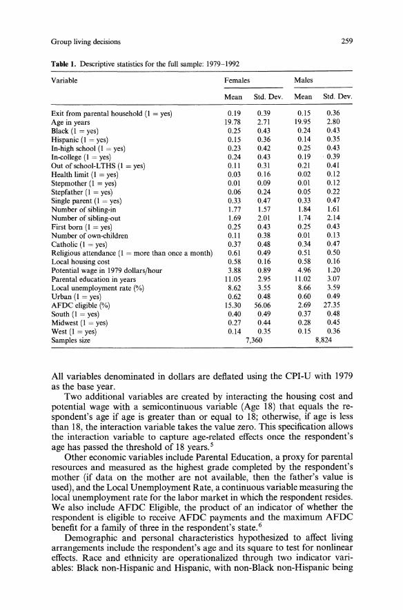
Group living decisions 259

Table 1. Descriptive statistics for the full sample: 1979-1992

Variable Females Males

Mean Std. Dev. Mean Std. Dev.

Exit from parental household (I = yes) 0.19 0.39 0.15 0.36Age in years 19.78 2.71 19.95 2.80Black (I = yes) 0.25 0.43 0.24 0.43Hispanic (I = yes) 0.15 0.36 0.14 0.35In-high school (I = yes) 0.23 0.42 0.25 0.43In-college (I = yes) 0.24 0.43 0.19 ·0.39Out ofschool-LTHS (I = yes) 0.11 0.31 0.21 0.41Health limit (I = yes) 0.03 0.16 0.02 0.12Stepmother (I = yes) 0.01 0.09 0.01 0.12Stepfather (I = yes) 0.06 0.24 0.05 0.22Single parent (I = yes) 0.33 0.47 0.33 0.47Number of sibling-in 1.77 1.57 1.84 1.61Number of sibling-out 1.69 2.01 1.74 2.14First born (I = yes) 0.25 0.43 0.25 0.43Number of own-children 0.11 0.38 0.01 0.13Catholic (I = yes) 0.37 0.48 0.34 0.47Religious attendance (I = more than once a month) 0.61 0.49 0.51 0.50Local housing cost 0.58 0.16 0.58 0.16Potential wage in 1979 dollars/hour 3.88 0.89 4.96 1.20Parental education in years 11.05 2.95 11.02 3.07Local unemployment rate (%) 8.62 3.55 8.66 3.59Urban (I = yes) 0.62 0.48 0.60 0.49AFDC eligible (%) 15.30 56.06 2.69 27.35South (I = yes) 0.40 0.49 0.37 0.48Midwest (I = yes) 0.27 0.44 0.28 0.45West (I = yes) 0.14 0.35 0.15 0.36Samples size 7,360 8,824

All variables denominated in dollars are deflated using the CPI-U with 1979as the base year.Two additional variables are created by interacting the housing cost and

potential wage with a semicontinuous variable (Age 18) that equals the re­spondent's age if age is greater than or equal to 18; otherwise, if age is lessthan 18, the interaction variable takes the value zero. This specification allowsthe interaction variable to capture age-related effects once the respondent'sage has passed the threshold of 18 years. 5

Other economic variables include Parental Education, a proxy for parentalresources and measured as the highest grade completed by the respondent'smother (if data on the mother are not available, then the father's value isused), and the Local Unemployment Rate, a continuous variable measuring thelocal unemployment rate for the labor market in which the respondent resides.We also include AFDC Eligible, the product of an indicator of whether therespondent is eligible to receive AFDC payments and the maximum AFDCbenefit for a family of three in the respondent's state. 6

Demographic and personal characteristics hypothesized to affect livingarrangements include the respondent's age and its square to test for nonlineareffects. Race and ethnicity are operationalized through two indicator vari­ables: Black non-Hispanic and Hispanic, with non-Black non-Hispanic being

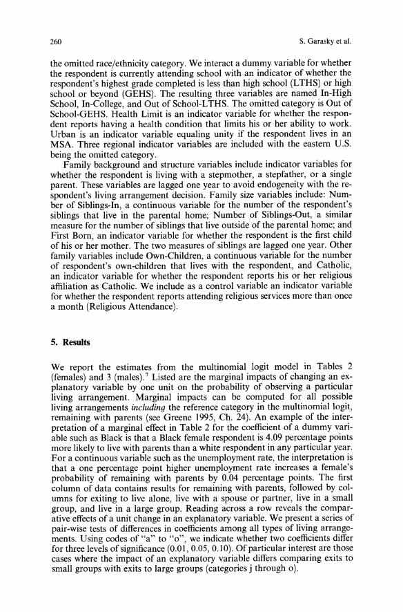
260 s. Garasky et al.

the omitted race/ethnicity category. We interact a dummy variable for whetherthe respondent is currently attending school with an indicator of whether therespondent's highest grade completed is less than high school (LTHS) or highschool or beyond (GEHS). The resulting three variables are named In-HighSchool, In-College, and Out of School-LTHS. The omitted category is Out ofSchool-GEHS. Health Limit is an indicator variable for whether the respon­dent reports having a health condition that limits his or her ability to work.Urban is an indicator variable equaling unity if the respondent lives in anMSA. Three regional indicator variables are included with the eastern U.S.being the omitted category.Family background and structure variables include indicator variables for

whether the respondent is living with a stepmother, a stepfather, or a singleparent. These variables are lagged one year to avoid endogeneity with the re­spondent's living arrangement decision. Family size variables include: Num­ber of Siblings-In, a continuous variable for the number of the respondent'ssiblings that live in the parental home; Number of Siblings-Out, a similarmeasure for the number of siblings that live outside of the parental home; andFirst Born, an indicator variable for whether the respondent is the first childof his or her mother. The two measures of siblings are lagged one year. Otherfamily variables include Own-Children, a continuous variable for the numberof respondent's own-children that lives with the respondent, and Catholic,an indicator variable for whether the respondent reports his or her religiousaffiliation as Catholic. We include as a control variable an indicator variablefor whether the respondent reports attending religious services more than oncea month (Religious Attendance).

5. Results

We report the estimates from the multinomial logit model in Tables 2(females) and 3 (males).7 Listed are the marginal impacts of changing an ex­planatory variable by one unit on the probability of observing a particularliving arrangement. Marginal impacts can be computed for all possibleliving arrangements including the reference category in the multinomiallogit,remaining with parents (see Greene 1995, Ch. 24). An example of the inter­pretation of a marginal effect in Table 2 for the coefficient of a dummy vari­able such as Black is that a Black female respondent is 4.09 percentage pointsmore likely to live with parents than a white respondent in any particular year.For a continuous variable such as the unemployment rate, the interpretation isthat a one percentage point higher unemployment rate increases a female'sprobability of remaining with parents by 0.04 percentage points. The firstcolumn of data contains results for remaining with parents, followed by col­umns for exiting to live alone, live with a spouse or partner, live in a smallgroup, and live in a large group. Reading across a row reveals the compar­ative effects of a unit change in an explanatory variable. We present a series ofpair-wise tests of differences in coefficients among all types of living arrange­ments. Using codes of "a" to "0", we indicate whether two coefficients differfor three levels of significance (0.01,0.05,0.10). Of particular interest are thosecases where the impact of an explanatory variable differs comparing exits tosmall groups with exits to large groups (categories j through 0).

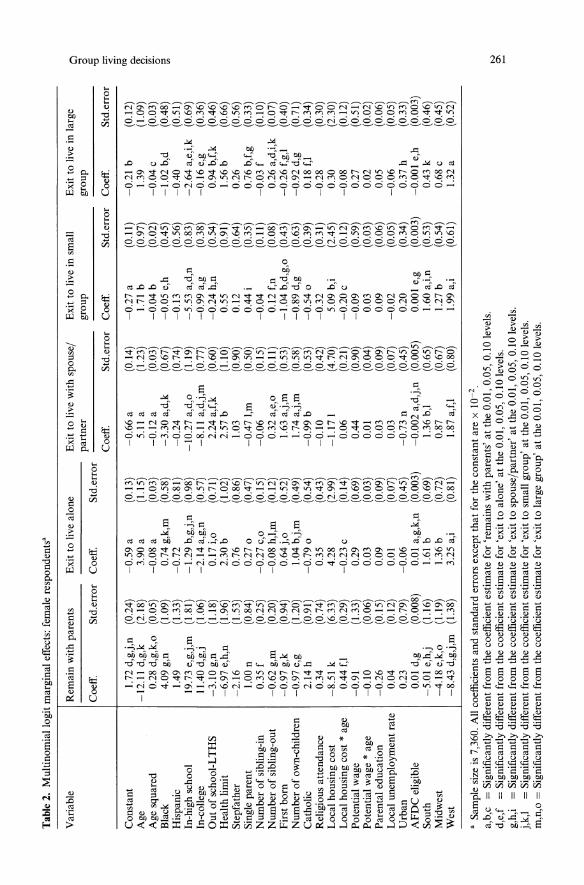
Tab

le2.Multinomiallogitmarginaleffects:femalerespondents'

Variable

Remainwithparents

Exittolivealone

Exittolivewithspouse/

Exittoliveinsmall

Exittoliveinlarge

Clpartner

..,group

group

0Coeff.

Std.errorCoeff.

Std.error

'"'1:l

Coeff.

Std.errorCoeff.

Std.errorCoeff.

Std.error

~: ::l

Constant

I.72d,g,j,n(0.24)

-0.59a

(0.13)

-0.66a

(0.14)

-0.27a

(0.11)

-0.21b

(0.12)

(JQ 0-

Age

-12.11d,g,k

(2.18)

3.90a

(1.15)

5.11a

(1.23)

1.71b

(0.97)

1.39

(1.09)

(1) Q.

Agesquared

0.28d,g,k,o(0.05)

-0.08a

(0.03)

-0.12a

(0.03)

-0.04b

(0.02)

-0.04c

(0.03)

~. 0

Black

4.09g,n

(1.09)

0.74g,k,m

(0.58)

-3.30a,d,k

(0.67)

-0.05e,h

(0.45)

-1.02b,d

(0.48)

::l '"

Hispanic

1.49

(1.33)

-0.72

(0.81)

-0.24

(0.74)

-0.13

(0.56)

-0.40

(0.51)

In-highschool

19.73e,g,j,m(1.81)

-1.29b,g,j,n(0.98)

-10.27a,d,o

(1.19)

-5.53a,d,n

(0.83)

-2.64a,e,i,k(0.69)

In-college

11.40d,g,j

(1.06)

-2.14a,g,n

(0.57)

-8.11a,d,j,m

(0.77)

-0.99a,g

(0.38)

-0.16e,g

(0.36)

Outofschool-LTHS

-3.10g,n

(1.18)

0.17i,o

(0.71)

2.24a,f,k

(0.60)

-0.24h,n

(0.54)

0.94b,f,k

(0.46)

Healthlimit

-6.97e,h,n

(1.96)

2.30b

(1.02)

2.57b

(1.10)

0.55

(0.91)

1.56b

(0.66)

Stepfather

-2.16

(1.53)

0.76

(0.86)

1.03

(0.90)

0.12

(0.64)

0.26

(0.56)

Singleparent

1.00n

(0.84)

0.270

(0.47)

-0.47I,m

(0.50)

0.44i

(0.35)

0.76b,f,g

(0.33)

Numberofsibling-in

0.35f

(0.25)

-0.27c,o

(0.15)

-0.06

(0.15)

-0.04

(0.11)

-0.03f

(0.10)

Numberofsibling-out

-0.62g,m

(0.20)

-0.08h,l,m

(0.12)

0.32a,e,o

(0.11)

0.12f,n

(0.08)

0.26a,d,i,k(0.07)

Firstborn

-0.97g,k

(0.94)

0.64j,o

(0.52)

1.63a,j,m

(0.53)

-1.04b,d,g,o(0.43)

-0.26f,g,!

(0.40)

Numberofown-children

-0.97e,g

(1.20)

1.04b,j,m

(0.49)

1.74a,j,m

(0.58)

-0.89d,g

(0.63)

-0.92d,g

(0.71)

Catholic

2.14h

(0.91)

-0.790

(0.54)

-0.99b

(0.53)

-0.540

(0.39)

0.18f,1

(0.34)

Religiousattendance

0.34

(0.74)

0.35

(0.43)

-0.10

(0.42)

-0.32

(0.31)

-0.28

(0.30)

Localhousingcost

-8.51k

(6.33)

4.28

(2.99)

-1.171

(4.70)

5.09b,i

(2.45)

0.30

(2.30)

Localhousingcost

*age

0.44f,1

(0.29)

-0.23c

(0.14)

0.06

(0.21)

-0.20c

(0.12)

-0.08

(0.12)

Potentialwage

-0.91

(1.33)

0.29

(0.69)

0.44

(0.90)

-0.09

(0.59)

0.27

(0.51)

Potentialwage

*age

-0.10

(0.06)

0.03

(0.03)

0.01

(0.04)

0.03

(0.03)

0.02

(0.02)

Parentaleducation

-0.26

(0.15)

0.09

(0.09)

0.03

(0.09)

0.09

(0.06)

0.05

(0.06)

Localunemploymentrate

0.04

(0.12)

0.01

(0.07)

0.03

(0.07)

-0.02

(0.05)

-0.06

(0.05)

Urban

0.23

(0.79)

-0.06

(0.45)

-0.73n

(0.45)

0.20

(0.34)

0.37h

(0.33)

AFDCeligible

0.01d,g

(0.008)

0.01a,g,k,n(0.003)

-0.002a,d,j,n(0.005)

0.001e,g

(0.003)

-0.001e,h

(0.003)

South

-5.01e,h,j

(1.16)

1.61b

(0.69)

1.36b,1

(0.65)

1.60a,i,n

(0.53)

0.43k

(0.46)

Midwest

-4.18e,k,o

(1.19)

1.36b

(0.72)

0.87

(0.67)

1.27b

(0.54)

0.68c

(0.45)

West

-8.43d,g,j,m(1.38)

3.25a,i

(0.81)

1.87a,f,1

(0.80)

1.99a,i

(0.61)

1.32a

(0.52)

,Samplesizeis7,360.Allcoefficientsandstandarderrorsexceptthatfortheconstantarex10-2.

a,b,c

=Significantlydifferentfromthecoefficientestimatefor'remainswithparents'atthe0.01,0.05,0.10levels.

Nd,e,f

=Significantlydifferentfromthecoefficientestimatefor'exittoalone'atthe0.01,0.05,0.10levels.

~g,h,i

=Significantlydifferentfromthecoefficientestimatefor'exittospouse/partner'atthe0.0I,0.05,0.10levels.

j,k,1

=Significantlydifferentfromthecoefficientestimatefor'exittosmallgroup'atthe0.0I,0.05,0.10levels.

m,n,o

=Significantlydifferentfromthecoefficientestimatefor'exittolargegroup'atthe0.01,0.05,0.10levels.

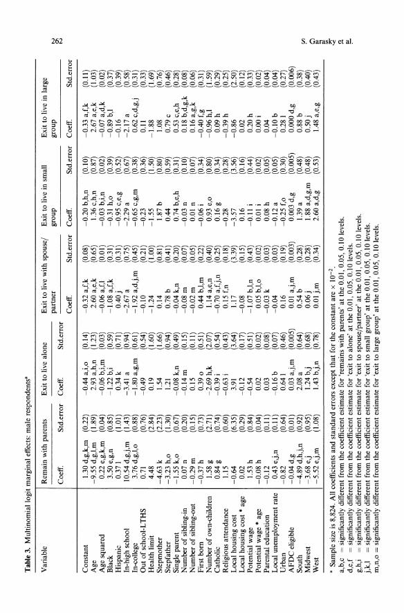
Tab

le3.Multinomiallogitmarginaleffects:malerespondents'

Variable

Remainwithparents

Exittolivealone

Exittolivewithspouse/Exittoliveinsmall

Exittoliveinlarge

partner

group

group

N 0\

Coeff.

Std.errorCoeff.

Std.error

N

Coeff.

Std.errorCoeff.

Std.errorCoeff.

Std.error

Constant

1.30d,g,k,m(0.22)

-0.44a,i,o

(0.14)

-0.32a,f,k

(0.08)

-0.20b,h,n

(0.10)

-0.33a,f,k

(0.\1)

Age

-9.55d,g,l,m

(1.89)

2.93a,h,n(1.23)

2.60a,e,k

(0.65)

1.36c,h,n

(0.87)

2.67a,e,k

(1.03)

Agesquared

0.22e,g,k,m

(0.04)

-0.06b,i,m

(0.03)

-0.06a,f,1

(0.01)

-0.03b,i,n

(0.02)

-0.07a,d,k

(0.02)

Black

3.50e,g,n

(0.85)

-1.22b,i

(0.59)

-1.08a,f,k

(0.31)

-0.31h,o

(0.39)

-0.89b,1

(0.37)

Hispanic

0.371

(1.01)

0.34k

(0.71)

0.40j

(0.31)

-0.95c,e,g

(0.52)

-0.16

(0.39)

In-highschool

10.54d,g,j,m

(1.43)

-3.41a

(0.94)

-2.67a

(0.75)

-2.29a

(0.67)

-2.17a

(0.58)

In-college

3.76d,g,l,o

(0.88)

-1.80a,g,m(0.61)

-1.92a,d,j,m(0.45)

-0.65c,g,m

(0.38)

0.62c,d,g,j(0.31)

Outofschool-LTHS

0.71

(0.76)

-0.49

(0.54)

-0.10

(0.21)

-0.23

(0.36)

0.11

(0.33)

Healthlimit

4.48

(2.84)

0.19

(1.60)

-1.24

(1.00)

-1.55

(1.50)

-1.88

(1.69)

Stepmother

-4.63k

(2.23)

1.54

(1.66)

0.14

(0.81)

1.87b

(0.80)

1.08

(0.76)

Stepfather

-3.23h,o

(1.30)

1.21

(0.94)

0.78b

(0.41)

0.44

(0.59)

0.79c

(0.46)

Singleparent

-1.55k,o

(0.67)

-0.08k,n

(0.49)

-0.04k,n

(0.20)

0.74b,e,h

(0.31)

0.53c,e,h

(0.28)

Numberofsibling-in

0.07n

(0.20)

-0.14m

(0.15)

-0.08m

(0.07)

-0.03n

(0.10)

0.18b,d,g,k(0.08)

Numberofsibling-out

-0.29m

(0.15)

0.15

(0.11)

-0.02m

(0.05)

0.01n

(0.07)

0.16a,g,k

(0.06)

Firstborn

-0.37h

(0.73)

0.390

(0.51)

0.44b,l,m

(0.22)

-0.06i

(0.34)

-0.40f,g

(0.31)

Numberofown-children

1.58g

(2.71)

-2.69h,k

(2.07)

1.14a,e,n

(0.40)

0.93e,o

(0.80)

-0.96h,1

(1.59)

Catholic

0.84g

(0.74)

-0.39i

(0.54)

-0.70a,f,j,n

(0.25)

0.16g

(0.34)

0.09h

(0.29)

Religiousattendance

1.15

(0.60)

-0.63

i(0.43)

0.15f,n

(0.18)

-0.28

(0.28)

-0.39h

(0.25)

Localhousingcost

-0.64

(6.35)

3.91

(3.64)

1.17

(3.39)

-3.57

(3.56)

-0.86

(2.50)

Localhousingcost•age

0.02

(0.29)

-0.12

(0.17)

-0.08

(0.15)

0.16

(0.16)

0.Q2

(0.12)

Potentialwage

1.53h

(0.84)

-0.54

(0.51)

-1.07b,l,n

(0.43)

-0.11i

(0.44)

0.20h

(0.33)

Potentialwage•age

-0.08h

(0.04)

0.02

(0.02)

0.05b,l,o

(0.02)

0.01i

(0.02)

0.00i

(0.02)

Parentaleducation

-0.12

(0.\1)

0.03

(0.08)

-0.03k

(0.03)

0.08h

(0.05)

0.04

(0.04)

Localunemploymentrate

0.43e,j,n

(0.11)

-0.16b

(0.07)

-0.04

(0.03)

-0.12a

(0.05)

-0.10b

(0.04)

Urban

-0.82

(0.64)

0.641

(0.46)

0.16

(0.19)

-0.25f,o

(0.30)

0.281

(0.27)

AFDCeligible

-0.04d,g

(0.01)

0.03a,j,m

(0.005)

0.01a,j,m

(0.003)

0.003d,g

(0.005)

0.000d,g

(0.006)

South

-4.89d,h,j,n

(0.92)

2.08a

(0.64)

0.54b

(0.28)

1.39a

(0.48)

0.88b

(0.38)

~Midwest

-3.68e,j

(0.95)

1.24b,j

(0.68)

0.06j

(0.28)

1.88a,d,g,m(0.48)

0.50j

(0.40)

ClWest

-5.52e,j,m

(1.08)

1.43b,j,n

(0.78)

0.01j,m

(0.34)

2.60a,d,g

(0.53)

1.48a,e,g

(0.43)

I» .., I» en•Samplesizeis8,824.Allcoefficientsandstandarderrorsexceptthatfortheconstantarex10-2

:0<'

'<a,b,c=significantlydifferentfromthecoefficientestimatefor'remainswithparents'atthe0.0

I,0.05,0.10levels.

~

d,e,f=significantlydifferentfromthecoefficientestimatefor'exittoalone'atthe0.01,0.05,0.10levels.

f'?-g,h,i=significantlydifferentfromthecoefficientestimatefor'exittospouse/partner'atthe0.0

I,0.05,0.10levels.

j,k,1=significantlydifferentfromthecoefficientestimatefor'exittosmallgroup'atthe0.0

I,0.05,0.10levels.

m,n,o=significantlydifferentfromthecoefficientestimatefor'exittolargegroup'atthe0.01,0.05,0.10levels.

Group living decisions

5.1. Economicfactors

263

The impact of an increased potential wage on home-leaving is generally asexpected and is large. A one dollar increase in female wages reduces herannual probability of remaining with parents by 2.9 to 3.9 percentage pointsas age rises from 20 to 30. The results are much less strong for males. In­creased wages have the effect of reducing the probability of remaining withparents once a male is age 19, but even at age 30, the impact of a one dollarincrease is slightly less than one percentage point. We find no difference in theimpact of a higher wage on the tendency to exit to small compared to largegroups for either gender.A higher housing cost increases the probability of a female remaining

with parents once she becomes at least age 20. The probability of remainingwith parents is 2.7 percentage points higher for a female age 30 residing ina locality where the cost of shelter is double the sample average comparedwith a female living in an area with shelter cost equal to the sample average.Her probability of living alone is 1.5 percentage points lower when sheltercosts are double the sample average. For male youths, we find no statisticallysignificant effects. Finding a response for women, but not men, agrees withthe results in Errnisch and Di Salvo (1997) who studied a sample of Britishyouths. There is no impact of housing cost on the tendency to exit to smallversus large groups.Female youths eligible for AFDC are less likely to exit to marriagej

partnering. There is no difference of the impact of AFDC eligibility on thetendency to exit to large or small groups. Eligible male youths are less likely toremain with parents or exit to any group than exit to marriage or live alone. 8

A higher local unemployment rate raises the probability of remaining withparents for male youths compared to exiting to live alone or either type ofgroup. The effect of variations in the unemployment rate on females livingarrangements is small. 9 The better educated are parents (our proxy for pa­rental resources), the lower the chance of males exiting to marriage comparedwith exiting to a small group. We find no impact of parents' education on thedistribution of females' exit types. 10

5.2. Demographic characteristics

We find that as a youth ages, the most likely destination of the first exit fromthe parental home differs. 11 For men, the probability of exiting to a largegroup peaks at age 19.9, followed by peaks for a small group (age = 21.8),living alone (23.8), and marriagejpartnering (25.4). For women, the samepattern is observed; exits peak first for a large group (age = 18.3), then a smallgroup (20.1), followed by living alone (23.0), and marriagejpartnering (23.8).Controlling for other socioeconomic and demographic variables, Black

males and females are less likely to exit to marriage or a large group and aremore likely to live with parents than white youths. Black males are less likelyto exit to live alone than stay with parents. These observations are consistentwith the hypothesis that discrimination in the housing market reduces thetendency of Black youths to leave home because of the greater difficulty ofsecuring shelter in any type of living arrangement. Unexpectedly; Black malesare more likely to exit to small compared with large groups.

264 S. Garasky et al.

In contrast, the only significant finding for Hispanic youths is a lower ten­dency for males to exit to small groups than remain with their parents, livealone, or marry. This result is consistent with the lower level of housing mar­ket discrimination encountered by Hispanics compared with Blacks (Yinger1991 ).Being a high school student greatly increases the probability of remaining

with parents and reduces the probability of exiting to all other living arrange­ments. Being a post high school student increases the probability of remainingwith parents (or living in a dormitory) and reduces the probability of exiting toliving alone, marriage/partnering, or a small group. Both males and femalesare more likely to exit to a large group compared with a small group when incollege, this result expected for cost conscious college students, but the result isonly statistically significant for males.The impact of ill health differs greatly by gender. A female youth with a

health problem that limits her work is less likely to remain with parents and ismore likely to exit to live alone, married/partnered, or a large group. In con­trast, males with a health problem are more likely to remain with parents, butthe coefficient is not significant.Male youths residing in urban areas are less likely to exit to a small group

than to a large group or to live alone. Female youths in urban areas areless likely to exit to marriage/partnering and are more likely to exit to largegroups. Finding that women in urban areas tend to live in large groups is ex­pected, likely a result of seeking greater safety.Compared to respondents living in the eastern U.S., all youths are less

likely to remain with their parents. Exits to all destinations are more likely forthose in the south, midwest, and west relative to those in the east, althoughsome of the estimated effects are not statistically significant.

5.3. Family background andfamily structure characteristics

The impact of living with a stepmother is estimated only for males becauseof colinearity problems when this variable is included in the estimation forfemales. For males, the effect of a stepmother is to reduce the probability ofremaining in the parental home by five percentage points. Living with a step­father reduces the likelihood of remaining with parents by two percentagepoints for female youths and three for males. These results are as expected andare consistent with the finding of Avery et al. (1992). There are no differencesin the impact on exits to small or large groups.The number of siblings and birth order affect exit choices. First born chil­

dren are more likely to exit to live with a spouse or partner than are childrenborn second or later. They also tend to live alone rather than in a group, thisexpected. Increased number of siblings in the parental home reduces the like­lihood of exiting to live alone (females only), and increases the probability ofexiting to a large group (males only), but the impacts are small. The greater thenumber of siblings living outside the parental home the greater the likelihood ofexiting to marriage/partnering (females), and group arrangements. As ex­pected, the largest effect of having more siblings outside the parental home is toincrease the probability ofexiting to a large group compared with small groups.An increased number of respondent's own-children reduces the tendency

of a female youth to remain in the parental home or exit to live in a small

Group living decisions 265

or large group. Males with own-children are unlikely to exit to live alone or tolarge groups compared with remaining with parents or exiting to marriage orsmall groups.Individuals raised as Catholics are more likely to remain with parents and

are less likely to exit to live alone or with a spouse/partner compared withexiting to large groups. Catholic females are less likely to exit to a small groupthan a large group. We are surprised by the lower probability of exiting to themarriage destination; however, this category includes living with a partner.Thus, the negative marginal impact of being Catholic on exiting to marriage/partnering may result from the dominant effect of a much lower rate of exitingto live with a partner. Males who attend church frequently are more likely toexit the parent's home to marry than to live in a large group or live alone.The impact of the explanatory variables is shown in greater detail in Table

4. We establish a base case by applying a set of assumptions to a 16 yearold white youthY We follow the youth for 13 years and cumulate theprobability distribution of possible exit types. The table lists the cumulativedistributions for the base case and many variations. In the base case for men,the most likely exit is to marriage/partner (39%), followed by living alone(34%), exiting to a small group (13%), and to a large group (11%). There isonly a 3% chance that this male youth will continuously live at home throughage 29. For women, the distribution of exit probabilities differs: 49% to mar­riage/partner, 21% to small groups, 19% to alone, 9% to large groups, and 2%remain in the parental home.Variations in the base case include increasing the house price by one stan­

dard deviation, reducing the unemployment rate by 25%, increasing parents'education to 16 years, and raising the youth's mental ability score by onestandard deviation. Other variations include changing the youth's race/ethnicity to Black or Hispanic, having a child at age 18, being a collegegraduate, and having a stepfather or stepmother.We also report the expected duration of stay in the parental home, this

value equaling 4.9 years for males and 4.1 for females in the base case. Themost notable changes in the expected duration of stay with parents occurwhen a youth's education is increased to 16 years from 12 (stay with parentsfor one year longer), when a youth is Black (stay with parents for one yearlonger), or when a male lives with a stepparent (stay with parents is nearly oneyear shorter).Reading across a row reveals the impact of a change in an explanatory

variable on that exit type. In general, the effects are consistent with the previ­ous discussion. The table also reveals the overall size of the impact on thedistribution of exits. The biggest effects, arbitrarily measured as the sum ofabsolute values of deviations from the base case probabilities, are for a youthwho has a child at age 18, being Black, completing college, having a step­father, and living in a high house price locality.

6. Conclusions

In recent years, spurred by the availability of longitudinal data, significantprogress has occurred in understanding the factors that explain when youthsleave their parental homes. Our study complements those analyses byadding detail to the list of potential destinations and by adding to the list of

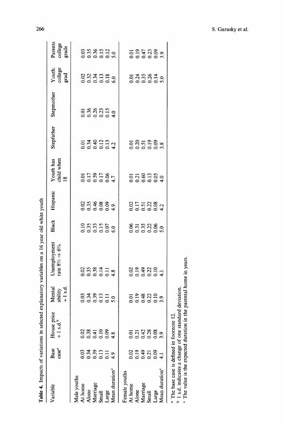
N

Tab

le4.Impactsofvariationsinselectedexplanatoryvariablesona16yearoldwhiteyouth

~

Variable

Base

Houseprice

Mental

Unemployment

Black

Hispanic

Youthhas

Stepfather

Stepmother

Youth:

Parents

case"

+Is.d.

bability

rate8%

=>6%

childwhen

college

college

+Is.d.

18grad

grads

Maleyouths

Athome

0.03

0.02

0.03

0.02

0.10

0.02

0.01

0.01

0.01

0.02

0.03

Alone

0.34

0.38

0.34

0.35

0.35

0.35

0.17

0.34

0.36

0.32

0.35

Marriage

0.39

0.41

0.39

0.38

0.33

0.46

0.59

0.40

0.26

0.34

0.36

Small

0.13

0.10

0.13

0.14

0.15

0.08

0.17

0.12

0.23

0.13

0.15

Large

0.11

0.09

0.11

0.11

0.G7

0.09

0.06

0.13

0.15

0.18

0.12

Meanduration'

4.9

4.8

5.0

4.8

6.0

4.9

4.7

4.2

4.0

6.0

5.0

Femaleyouths

Athome

0.02

0.01

0.01

0.02

0.06

0.02

0.01

O.oI

0.01

O.oI

Alone

0.19

0.21

0.19

0.19

0.31

0.17

0.21

0.20

0.24

0.19

Marriage

0.49

0.42

0.48

0.49

0.35

0.51

0.60

0.51

0.35

0.47

Small

0.21

0.28

0.22

0.22

0.22

0.22

0.13

0.19

0.26

0.23

Large

0.09

0.08

0.10

0.10

0.06

0.08

0.05

0.09

0.14

0.09

Meanduration'

4.1

3.9

3.9

4.1

5.0

4.2

4.0

3.8

5.0

3.9

"Thebasecaseisdefinedinfootnote12.

bIs.d.indicatesachangeofonestandarddeviation.

,Thevalueistheexpecteddurationintheparentalhomeinyears.

~ a ~ ;;l '" ~ ~ ~

Group living decisions 267

explanatory factors. Our national sample is of American youths ages 16 to 30in the period 1979-1992. We focus on exits to small and large groups, withabout one-third of all exits being to groups.We comprehensively model economic and socio-demographic factors ex­

pected to influence a youth's decision of whether to leave the parental homeand what living arrangement to select. We highlight economic factors hy­pothesized to impact home-leaving and test whether the influence of thesefactors varies with a respondent's age.The estimation technique is a multi­nomiallogit analysis.Our first finding is that male and female home-leaving must be modeled

separately. Gender specific differences in exit tendencies include responses tovariations in the wage that could be earned in full-time employment, the localunemployment rate, the local cost of shelter, race and ethnicity, health prob­lems, and residence in an urban area.We test for and find some evidence of an age linked impact of econ­

omic factors. Our hypothesis is that parents shelter teens from economicfactors such as a high cost of shelter and low potential income; however, thissheltering is reduced as the children age. Higher wages reduce the likelihoodof staying with parents for youths older than 20. Higher housing costs increasethe probability of staying with parents for women older than 20. No sign­ificant effect is found for men.We hypothesized that socio-demographic factors dominate explanations of

why youths leave the parental home when they are teens, but economic factorsincrease in influence as a youth matures. Our results support this hypothesismost strongly for female youths. A possible modification of our hypothesis isto argue that parents shelter their daughters from economic factors more sothan they do their sons. Similar age linked responses to variations in parentalincome and AFDC payments were hypothesized by Whittington and Peters(1996), but we do not find support for their hypotheses.Our results for housing costs and wage impacts on home-leaving are not

as strong as in Haurin et al. (1993). One reason is that this paper's sampleincludes young teens while Haurin et al. (1993) did not. Another substantialdifference is that Haurin et al. studied the current living arrangement of allyouths while we analyze only their first exit destination. It may be that returnsto the parental home are influenced by housing costs and earnings. Iftrue, these variables would affect the results in Haurin et al. but not this study.Ermisch (1999) finds strong support for the argument that high housing costsand low incomes increase the rate of return to the parental home.While understanding the likelihood of exiting to living alone or marriage

is of interest, we highlight the study of exits to small and large groups.Exiting to a large group tends to be the first path out of the parental home forteens, followed by exiting to a small group. Table 5 summarizes the statisti­cally significant impacts of the explanatory variables on youths' exits from theparents' home to large compared with small groups. Some results are as ex­pected; for example, youths with a larger number of siblings living outside theparental home tend to exit to a large group (which may include some siblings).Also, college students have a greater tendency to exit to live in large groups.Black youths are more likely to exit to small groups than large, the unex­pected effect statistically significant only for males. Youths dropping out ofhigh school, Catholics, and youths in urban areas tend to exit to large groups.We find that the determinants of whether youths exit the parents' home

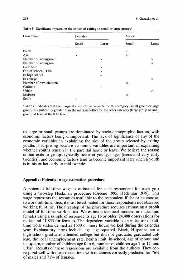
268 S. Garasky et al.

Table 5. Significant impacts on the choice of exiting to small or large groups·

Group Size Females Males

Small Large Small Large

Black xAge x xNumber of siblings-out x xNumber of siblings-in xFirst born xOut ofschool-LTHS xIn high school xIn college xNumber of own-children xCatholic xUrban xMidwest xSouth x

• An 'x' indicates that the marginal effect of this variable for this category (small group or largegroup) is significantly greater than the marginal effect for the other category (large group or smallgroup) at least at the 0.10 level.

to large or small groups are dominated by socio-demographic factors, witheconomic factors being unimportant. The lack of significance of any of theeconomic variables in explaining the size of the group selected by exitingyouths is surprising because economic variables are important in explainingwhether youths remain in the parental home or leave. We believe the reasonis that exits to groups typically occur at younger ages (teens and very earlytwenties), and economic factors tend to become important later when a youthis in his or her early to mid twenties.

Appendix: Potential wage estimation procedure

A potential full-time wage is estimated for each respondent for each yearusing a two-step Heckman procedure (Greene 1995; Heckman 1979). Thiswage represents the resources available to the respondent if she or he choosesto work full-time; thus, it must be estimated for those respondents not observedworking full-time. The first step of the procedure requires estimating a probitmodel of full-time work status. We estimate identical models for males andfemales using a sample of respondents age 16 or older: 24,408 observations formales and 21,855 for females. The dependent variable is an indicator of full­time work status defined as 1600 or more hours worked during the calendaryear. Explanatory terms include: age, age squared, Black, Hispanic, not ahigh school graduate, attended college but did not graduate, graduated col­lege, the local unemployment rate, health limit, in-school, age of spouse andits square, number of children age 0 to 6, number of children age 7 to 17, andurban. Results of these regressions are available from the authors. They cor­respond well with our expectations with outcomes correctly predicted for 76%of males and 71% of females.

Group living decisions 269

The second step 1S to estimate a wage equation for those respondentsworking full-time. For male respondents, full-time work was performedin 14,404 (59.0%) of the person-years. Females worked full-time in 10,599(48.5%) of the person-years. The dependent variable is a continuous measureof the hourly rate of pay the respondent received in his or her current job.Preliminary exploration with the dependent variable transformed into logsyielded inferior results.Explanatory terms included in the wage equation are age, age squared,

Black, Hispanic, not a high school graduate, attended college but did notgraduate, graduated college, urban, health limit, the local unemployment rate,job tenure, a measure of the respondent's mental ability, a series of 13 yearspecific dummy variables, and the sample selection correction variable (in­verse Mills ratio) generated from the full-time work status equation. Resultsfor these regressions are available from the authors. The equations for malesand females are generally similar. Significant and negative is Black (4% lowerwage for males and 6% lower wage for females) and the local unemploymentrate. Significant and positive are attended college but did not graduate (a 4%­8% higher wage) and graduated college (a 25%-33% higher wage). Also sig­nificant is urban (a 12%-14% higher wage) and the score on the mental abilitytest (a one standard deviation increase raises wage by 10%-11%). In bothcases the potential wage rises with respondent's age; for example, as age risesfrom 20 to 30, potential wages for males and females rise by 15% and 18%respectively.The variable included in the multinomial logit is the predicted value from

the wage equation. Over time, it is updated as a respondent's age and othercharacteristics change.

Endnotes

1 We do not focus on exits to institutional group arrangements, but should clarify how we cate­gorize exits to college dormitories and military. In the literature, exits to institutions have beenconsidered separate destinations (Goldscheider and DaVanzo 1985, 1989), or have beenundifferentiated from parental living arrangements (Buck and Scott 1993). Whittington andPeters (1996) generally treat college students as residing with parents (unless self-supporting),but combine those in the military with those living alone in noninstitutional arrangements. Ourstudy classifies college students and military members according to their current residence. Weconsider youths residing in dormitories, fraternities, or barracks to be in temporary quartersand classify them as not exiting the parental home. College students and military membersliving elsewhere are distributed among our destination categories (alone, married/partnered, orin a small or large group). Our conceptualization reflects a youth's choice to reside in a par­ticular living arrangement rather than the choice to enter college or the military.

2 The critical Chi-squared value at the 0.01 level with 25 degrees of freedom is 45. Twice thedifference in log likelihood values comparing the pooled model to the sum of the gender spe­cific models is 126. These results clearly reject pooling the male and female samples.

3 In the sample of 26,553 youths, missing values occur most often for wages, housing costs, andthe measure of the mother's intellect (12%,11%, and 15% of the sample, respectively).

4 Dwelling cost is derived from the Freddie Mac-Fannie Mae (FF) repeat sales house priceindex, augmented by data from the American Chamber of Commerce Research Association(ACCRA 1993). The FF index covers more than 100 MSAs and all states and is a pure timeseries price index. We use the 1982 ACCRA data for 88 MSAs and rural areas in 50 states todevelop a baseline cross-sectional price index. The final index is developed by applying the FFindex to the ACCRA data, yielding a nominal house price index with excellent spatial cover­age.

270 S. Garasky et aI.

5 We experimented with age thresholds other than 18 but found 18 yields the best fit.6 A respondent is eligible if there is at least one own-ehild living in the household and therespondent is not married. The maximum benefit is the amount of assistance a family wouldreceive if it had no income (Committee on Ways and Means 1996). We select this measurebecause it is exogenous; that is, it is invariant to the respondent's choices of participation in theAFDC program and supply of labor.

7 We do not report multinomial estimation coefficients because their values are difficult tointerpret; however, they are available from the authors.

8 AFDC Eligible was interacted with Age 18, but the estimated coefficient is not significant.9 We found no impact of including a variable interacting Unemployment with Age 18.10 We tested for differing impacts depending on the age of the respondent, but failed to findsupportive evidence.

11 These calculations include the effects of changing age, age squared, and the age interactionterms with house price and wage.

12 The assumptions include: the youth stay in school until age 18 and leaves with a high schooldegree. The youth lives in an urban area in the southern U.S. where the housing cost equals thesample's mean and the unemployment rate is eight percent. The youth's parents have 12 yearsof education. The youth has good health, no children, no stepmother or stepfather, is notCatholic but attends church at least once per month, is not first born, has two resident parents,and is not AFDC eligible. The youth has one sibling in the parental home and one out untilage 24 when both siblings are out of the parent's home. Wages also are set by the base caseassumptions and vary as we change the values of explanatory variables.

References

ACCRA (1993) Cost of Living Index Manual. Louisville Chamber of Commerce, Louisville KYAllison PD (1984) Event History Analysis. Sage, Newbury Park, CAAquilino WS (1991) Family Structure and Home-leaving: A Further Specification of the Rela­tionship. Journal of Marriage and the Family 53:999-1010

Avery R, Goldscheider F, Speare A (1992) Feathered Nest/Gilded Cage: Parental Income andLeaving Home in the Transition to Adulthood. Demography 29:375-388

Borsch-Supan A (1986) Household Formation, Housing Prices, and Public Policy Impacts. Jour­nal of Public Economics 30:145-164

Bourassa S, Haurin RJ, Haurin DR, Hendershott PH (1994) Independent Living and Home­ownership: An Analysis of Australian Youth. Australian Economic Review 107:29-45

Buck N, Scott J (1993) She's Leaving Home: But Why? An Analysis of Young People Leaving theParental Home. Journal of Marriage and the Family 55:863-874

Center for Human Resource Research (1993) NLSY Handbook. Ohio State University, ColumbusOH

Center for Human Resource Research (1997) NLSY79 User's Guide. Ohio State University, Co­lumbusOH

Committee on Ways and Means, U. S. House of Representatives (1996) Overview of EntitlementPrograms: 1996. Government Printing Office, Washington DC

Ermisch J (1999) Prices, Parents, and Young People's Household Formation. Journal of UrbanEconomics 45:47-71

Ermisch J, Di Salvo P (1997) The Economic Determinants of Young People's Household For­mation. Economica 64:627-644

Ermisch J, Overton E (1985) Minimal Household Units: A New Approach to the Analysis ofHousehold Formation. Population Studies 39:33-54

Goldscheider FK, DaVanzo J (1985) Living Arrangements and the Transition to Adulthood.Demography 22:545-563

Goldscheider FK, DaVanzo J (1989) Pathways to Independent Living in Early Adulthood: Mar­riage, Semiautonomy, and Premarital Residential Independence. Demography 26:597-614

Goldscheider FK, Goldscheider C (1993) Leaving Home Before Marriage. University ofWiscon­sin Press, Madison WI

Goldscheider FK, LeBourdais C (1986) The Decline in Age at Leaving Home, 1920-1979. Soci­ology and Social Research 70:143-145

Group living decisions 271

Goldscheider FK, Thornton A, Young-DeMarco L (1993) A Portrait of the Nest-leaving Processin Early Adulthood. Demography 30:683-699

Greene WH (1993) Econometric Analysis, 2nd Ed. Macmillan, New York, NYGreene WH (1995) LIMDEP Version 7.0 User's Manual. Econometric Software, Bellport, NYHare AP (1981) Group Size. American Behavioral Scientist 24:695-708Hare AP (1982) Creativity in Small Groups. Sage, Beverly Hills CAHaurin DR, Hendershott PH, Kim D (1993) The Impact of Real Rents and Wages on HouseholdFonnation. Review oj Economics and Statistics 75:284-293

Haurin DR, Hendershott PH, Kim D (1994) Housing Decisions of American Youth. Journal ojUrban Economics 35:28-45

Haurin RJ, Haurin DR, Hendershott PH, Bourassa SC (1997) Home or Alone: The Costs ofIndependent Living for Youth. Social Science Research 26:135-152

Heckman J (1979) Sample Selection Bias as a Specification Error. Econometrica 47:152-161Heer D, Hodge R, Felson M (1985) The Cluttered Nest: Evidence that Young Adults are moreLikely to Live at Home than in the Recent Past. Social Science Research 69:436---441

Johnson RW, DaVanzo J (1998) Economic and Cultural Influences on the Decision to LeaveHome in Peninsular Malaysia. Demography 35:97-114

Kalbfleisch JD, Prentice RL (1980) The Statistical Analysis oj Failure Time Data. Wiley, NewYork

Mitchell BA, Wister AV, Burch TK (1989) The Family Environment and Leaving the ParentalHome. Journal oj Marriage and the Family 51:605-613

Myers D (1992) Analysis with Local Census Data. Academic Press, BostonRosenzweig MR, Wolpin K (1993) Intergenerational Support and the Life Cycle Incomes ofYoung Men and Their Parents' Human Capital Investments, Coresidence, and Intergenera­tional Financial Transfers. Journal ojLabor Economics II :84-112

Rosenzweig MR, Wolpin K (1994) Parental and Public Transfers to Young Women and TheirChildren. American Economic Review 84:1195-1212

Thornton A, Young-DeMarco L, Goldscheider FK (1993) Leaving the Parental Nest: The Expe­rience of a Young White Cohort in the 1980s. Journal ojMarriage and the Family 55:216-229

White LK, Booth A (1985) The Quality and Stability of Remarriages: The Role of Step-children.American Sociological Review 50:689-698

Whittington LA, Peters HE (1996) Economic Incentives for Financial and Residential Indepen­dence. Demography 33:82-97

Residential location and youth unemployment:The economic geography of school-to-work transitions

Regina T. Riphahn

Department of Economics, University of Mainz, D-55099 Mainz, Gennany(Fax: +49-6131-392-3563; e-mail: riphahn@wiwi.uni-mainz.de) IZA and DIW Berlin, Gennany

Received: 30 November I999jAccepted: 3 August 2000

Abstract. In response to increased international policy attention to youth un­employment this study investigates post-secondary school transitions of schoolleavers. Multinomiallogit models are estimated for male and female Germanyouth. The models control for individual, parent, and household character­istics, for those of the youth's region of residence and local labor markets. Thefindings suggest that immigrant youth has particularly low participation ratesin continued education, and that youth unemployment is centered in highunemployment states and metropolitan areas. More generous academic bene­fit policies seem to be correlated with increased academic enrollment, andmen's transitions to the military do reflect recent changes in defense policies.

JEL Codes: 124, 164, 168

Key words: School-to-work, youth unemployment, local labor markets

1. Introduction

As of 1998 youth unemployment in the European Union was at 19.1% of theyouth labor force. The literature provides ample evidence on the lifetime scarsearly unemployment experiences leave on workers' labor market and criminalrecords (Ellwood 1982; Freeman and Rodgers 1999; for Germany Franz et al.1997). This dramatic situation prompted government responses in several

Helpful comments of Christian Dustmann, Jochen Mayer, Jan van Ours, Ralph Rotte, Alessan­dra Venturini and two anonymous referees on earlier versions of this paper are gratefullyacknowledged. I thank Thomas Kasperski for excellent research assistance. Responsible editor:Alan Barrett.

274 R. T. Riphahn

countries. France launched an ambitious youth unemployment program in1997, which as of November 1998 covered 152,000 persons aiming at 350,000by 2000 (OECD 1999a). The German government passed a "100,000 Jobs forYouth" program, with DM 2 bio allocated for the fiscal years 1999 and 2000each.With youth unemployment high on the policy agenda, it is important to

understand its determinants and the potential role for labor market policies.So far, only a few studies investigated the labor market transitions of schoolleavers. The issue was discussed in the United Kingdom due to a concernabout declining participation in continued education. The German case foundattention in the United States following the Clinton administration's sugges­tion to install some features of the German apprenticeship system there(Clinton and Gore 1992). Overall, existing studies are highly specific in theirtopics. Only few attempt to answer the broader questions of what youngpeople do after leaving school, how their choices are affected by regional labormarkets and by policy changes, and to what degree parental and householdcharacteristics affect these transitions.This study addresses these important issues at the example of Germany.

It applies a comprehensive modelling approach to investigate the transitionchoices of all youth leaving school between 1984 and 1997, as observed inthe German Socioeconomic Panel (GSOEP). This dataset permits the consid­eration of detailed household and parent background variables, which wereomitted in prior analyses. The findings are relevant to the evaluation of theGerman government's "100,000 Jobs for Youth" program, as one of thecriticisms of this program relates to the equal spreading of program activitiesacross labor market regions. To the degree that local factors are importantfor the success of youth labor market entry, regional differentiations in activelabor market policies may be required. Finally, the study evaluates whetherchanges in training grant and military policies affected school-to-work transi­tion patterns.The paper proceeds with a summary of the German institutional frame­

work for school-to-work transitions, and of policy changes, that may haveaffected transition decisions. It describes the German youth labor market, themain features of the" 100,000 Jobs for Youth" program, and briefly surveysthe school-to-work literature in Sect. 2. Section 3 discusses the econometricspecification, presents the data and the estimation strategy. The results arediscussed in Sect. 4. The study concludes with a summary, highlighting policyimplications.

2. Institutional background and review of the literature

2.1. Schoo/-la-work in Germany

In contrast to other countries, the German school system introduces differen­tiated educational tracks after the first four grades of primary education. Thetracks differ in their academic orientation and requirements. The basic school(Hauplschu/e) graduates individuals after six years of secondary education andis a preparation for blue collar occupations. The middle school (Rea/schu/e)also lasts six years and provides training for white collar jobs. Only the highesttrack (Gymnasium) provides another nine years of schooling. Graduating from

Residential location and youth unemployment 275

the Gymnasium is a precondition for university studies. In addition, compre­hensive schools (Gesamtschule) were introduced in the 1970s, which grant de­grees of either track. Depending on the track, pupils typically finish schoolaged 16 or 19. Of the l.l mio schoolleavers in 19977% had not obtained adegree, 25% graduated from basic school, 38% from middle school, and 22%from the Gymnasium (with the rest in the "other" category).Once they leave school, individuals can choose from a number of alter­

native paths. This choice is restricted only for healthy young men above age18, who are typically drafted for military or conscientious objector service.The most common transition after school is that into apprenticeship training.Apprenticeships last between .2 and 4 years, and combine vocational on thejob training with formal education in vocational schools (Berufsschule).Particularly in the mid 1980s, when the German baby-boom generation

left school, insufficient apprenticeship positions were available for schoolleavers. For them and to provide training for certain occupations withoutapprenticeship programs, vocational schools are available to meet excess de­mand for vocational training. These offer (i) full time general schooling forthose not previously qualified for apprenticeships in a one year 'vocationalpreparation year' (Berufsvorbereitungsjahr) program. Here individuals cancomplete their basic school degree (Hauptschulabschluj3). In a program (ii)called 'elementary vocational year' (Berufsgrundbildungsjahr) students maylearn occupation-specific skills which - if successfully completed - allowsthem to shorten a later apprenticehip. The third type (iii) labelled 'specialvocational school' (Berufsfachschule) offers a variety of training opportunities.More than fifty percent of the students graduating from these three vocationalschools continue their education with an apprenticeship.In addition to the military, apprenticeship, and vocational school options,

graduates may choose employment without training, they may leave the laborforce, become unemployed or begin an academic education. A policy affectingthe decision to take up academic training is the financial support programBafog. Since 1971 benefits are available to children of non-wealthy parents,who pursue an academic education. 1 The law has been changed repeatedly,with the most influential adjustments in 1983, when the program switchedfrom grants to loans, and again in 1990 when it was stipulated that only halfof the program benefits had to be repaid. Figure 1 shows that after 1983 theshare of schoolleavers going on to university declined. However, the fractionof university students increased again in subsequent years with a steep jump in1990, when the new grant system was passed.A set of policies likely to affect males' transition decision relates to the

military draft. Most influential here is the leniency in the requirements forphysical fitness and the flexibility of postponing the draft to complete voca­tional and academic training. The evidence suggests that prior to the end ofthe cold war in 1990 the draft was rather strict. The size of the German armydeclined from half a million in the mid 1980s (West Germany) to about350,000 soldiers (united Germany), as determined in the unification treatiesafter 1990 (Rotte 1996). At that time drafting procedures were loosened andthe duration of military service was cut from 15 to 12 months in 1991. Thetreatment of draftees was tightened again recently (since 1995) after the mili­tary engagements in Bosnia and Kosovo had caused an increase in the shareof conscienious objectors (BREG 1996). The impact of these developments onindividual transitions is analysed below.

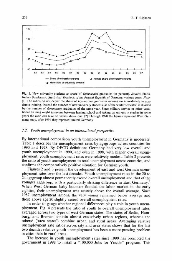
276 R. T. Riphahn

120 ,.-------------------------------,

100

80

60

40 L....I_--'-_--'--_-'----_L.-----'_--'-_--'--_-'----_L-----'_----'-_-'-_-'----_'------'--'

82 83 84 85 86 87 88 89 90 91 92 93 94 95 96 97

- Share of university entrants -6- Female share of university entrants

...... Male share of university entrants

Fig. 1. New university students as share of Gymnasium graduates (in percent). Source: Statis­tisches Bundesamt, Statistical Yearbook of the Federal Republic of Germany, various years. Note:(I) The ratios do not depict the share of Gymnasium graduates moving on immediately to aca­demic training. Instead the number of new university students (as of the winter semester) is dividedby the number of Gymnasium graduates of the same year. Since military service or other voca­tional training might intervene between leaving school and taking up university studies in someyears the ratio can take on values above one. (2) Through 1990 the figures represent West Ger­many only, after 1991 they represent united Germany

2.2. Youth unemployment in an international perspective

By international comparison youth unemployment in Germany is moderate.Table 1 describes the unemployment rates by agegroups across countries for1990 and 1998. By OECD definitions Germany had very low overall andyouth unemployment in 1990, and even in 1998, with higher overall unem­ployment, youth unemployment rates were relatively modest. Table 2 presentsthe ratio of youth unemployment to total unemployment across countries, andconfirms the comparatively positive situation for German youth.Figures 2 and 3 present the development of east and west German unem­

ployment rates over the last decades. Youth unemployment rates in the 20 to24 agegroup almost permanently exceed overall unemployment and that of theyounger agegroup, with a particularly striking difference in East Germany. 2

When West German baby boomers flooded the labor market in the earlyeighties, their unemployment was acutely above the overall average. Since1987 unemployment among the very young remained below average andthose above age 20 slightly exceed overall unemployment rates.

In order to gauge whether regional differences playa role in youth unem­ployment, Fig. 4 presents the ratio of youth to overall unemployment rates,averaged across two types of west German states: The states of Berlin, Ham­burg, and Bremen contain almost exclusively urban regions, whereas theothers3 ('area states') combine urban and rural areas. Averaging relativeunemployment rate ratios across city and area states shows that for the lasttwo decades relative youth unemployment has been a more pressing problemin cities than in rural areas.The increase in youth unemployment rates since 1990 has prompted the

government in 1998 to install a "100,000 Jobs for Youths" program. This

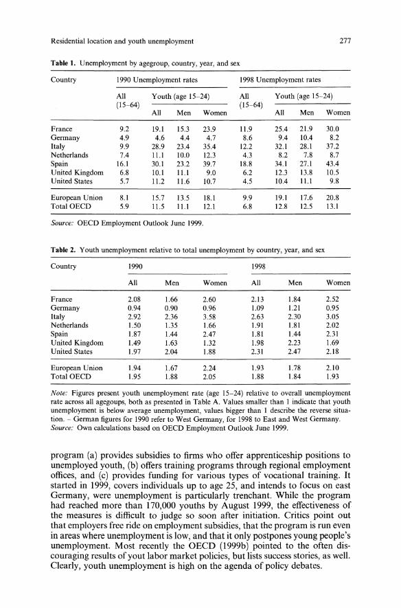
Residential location and youth unemployment 277

Table I. Unemployment by agegroup, country, year, and sex

Country 1990 Unemployment rates 1998 Unemployment rates

All Youth (age 15-24) All Youth (age 15-24)(15-64) (15-64)

All Men Women All Men Women

France 9.2 19.1 15.3 23.9 11.9 25.4 21.9 30.0Germany 4.9 4.6 4.4 4.7 8.6 9.4 10.4 8.2Italy 9.9 28.9 23.4 35.4 12.2 32.1 28.1 37.2Netherlands 7.4 11.1 10.0 12.3 4.3 8.2 7.8 8.7Spain 16.1 30.1 23.2 39.7 18.8 34.1 27.1 43.4United Kingdom 6.8 10.1 11.1 9.0 6:2 12.3 13.8 10.5United States 5.7 11.2 11.6 10.7 4.5 10.4 11.1 9.8

European Union 8.1 15.7 13.5 18.! 9.9 19.1 17.6 20.8TotalOECD 5.9 11.5 11.1 12.1 6.8 12.8 12.5 13.1

Source: OECD Employment Outlook June 1999.

Table 2. Youth unemployment relative to total unemployment by country, year, and sex

Country 1990 1998

All Men Women All Men Women

France 2.08 1.66 2.60 2.13 1.84 2.52Germany 0.94 0.90 0.96 1.09 1.21 0.95Italy 2.92 2.36 3.58 2.63 2.30 3.05Netherlands 1.50 1.35 1.66 1.91 1.81 2.02Spain 1.87 1.44 2.47 1.81 1.44 2.31United Kingdom 1.49 1.63 1.32 1.98 2.23 1.69United States 1.97 2.04 1.88 2.31 2.47 2.18

European Union 1.94 1.67 2.24 1.93 1.78 2.10TotalOECD 1.95 1.88 2.05 1.88 1.84 1.93

Note: Figures present youth unemployment rate (age 15-24) relative to overall unemploymentrate across all agegoups, both as presented in Table A. Values smaller than I indicate that youthunemployment is below average unemployment, values bigger than I describe the reverse situa­tion. - German figures for 1990 refer to West Germany, for 1998 to East and West Germany.Source: Own calculations based on OECD Employment Outlook June 1999.

program (a) provides subsidies to firms who offer apprenticeship positions tounemployed youth, (b) offers training programs through regional employmentoffices, and (c) provides funding for various types of vocational training. Itstarted in 1999, covers individuals up to age 25, and intends to focus on eastGermany, were unemployment is particularly trenchant. While the programhad reached more than 170,000 youths by August 1999, the effectiveness ofthe measures is difficult to judge so soon after initiation. Critics point outthat employers free ride on employment subsidies, that the program is run evenin areas where unemployment is low, and that it only postpones young people'sunemployment. Most recently the OECD (1999b) pointed to the often dis­couraging results ofyout labor market policies, but lists success stories, as well.Clearly, youth unemployment is high on the agenda of policy debates.

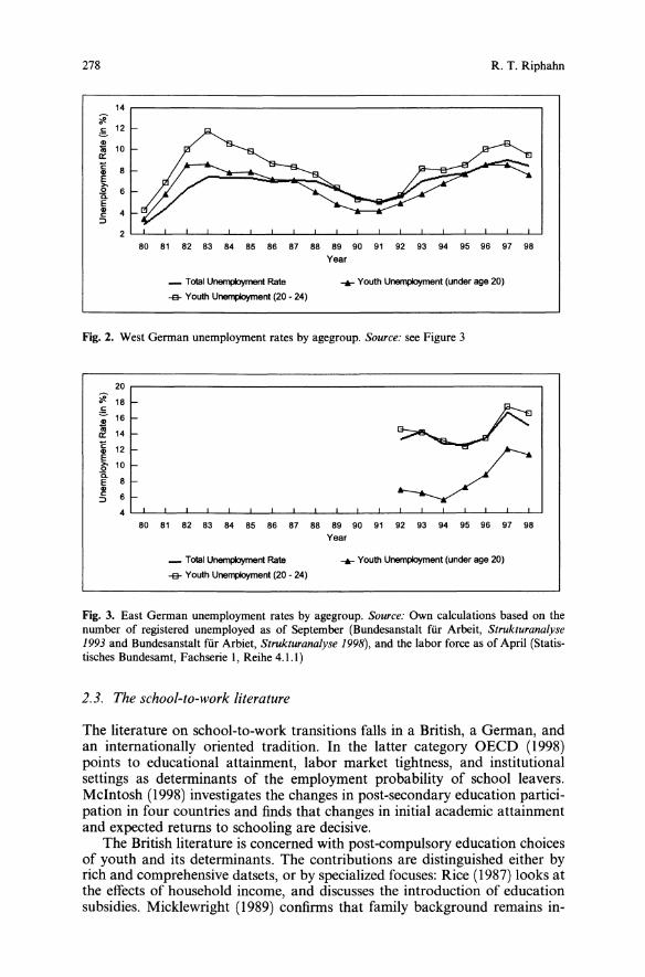
278

14

~:§. 12

$ 10IVCl:

~ 8[.Q 6CoE~ 4=>

R. T. Riphahn

2L......l_-'--------'-_L-...I....-.I._.l...---'----'_-'-----'-_L.-...I....-.I._.l...---'----'_-'-----'-....J80 81 82 83 84 85 86 87 88 89 90 91 92 93 94 95 96 97 98

Year

_ Total Unemployment Rate

-e- Youth UllllI1lJloYment (20 - 24)

...... Youth UnertlJIoyment (under age 20)

Fig. 2. West Gennan unemployment rates by agegroup. Source: see Figure 3

20

<f. 18c'=- 16$IV 14Cl:C 12CDE~ 10Co

8ECDc 6=>

4

80 81 82 83 84 85 86 87 88 89 90 91 92 93 94 95 96 97 98Year

_ Total Unert1IJk7>'rnent Rate ...... Youth UnertlJIoyment (under age 20)

-e- Youth UnertlJIoyment (20 - 24)

Fig. 3. East Gennan unemployment rates by agegroup. Source: Own calculations based on thenumber of registered unemployed as of September (BundesanstaIt fiir Arbeit, Strukturanalyse1993 and BundesanstaIt fiir Arbiet, Strukturanalyse 1998), and the labor force as of April (Statis­tisches Bundesamt, Fachserie I, Reihe 4.1.1)

2.3. The school-to-work literature

The literature on school-to-work transitions falls in a British, a Gennan, andan internationally oriented tradition. In the latter category OECD (1998)points to educational attainment, labor market tightness, and institutionalsettings as detenninants of the employment probability of school leavers.McIntosh (1998) investigates the changes in post-secondary education partici­pation in four countries and finds that changes in initial academic attainmentand expected returns to schooling are decisive.The British literature is concerned with post-compulsory education choices

of youth and its detenninants. The contributions are distinguished either byrich and comprehensive datsets, or by specialized focuses: Rice (1987) looks atthe effects of household income, and discusses the introduction of educationsubsidies. Micklewright (1989) confinns that family background remains in-

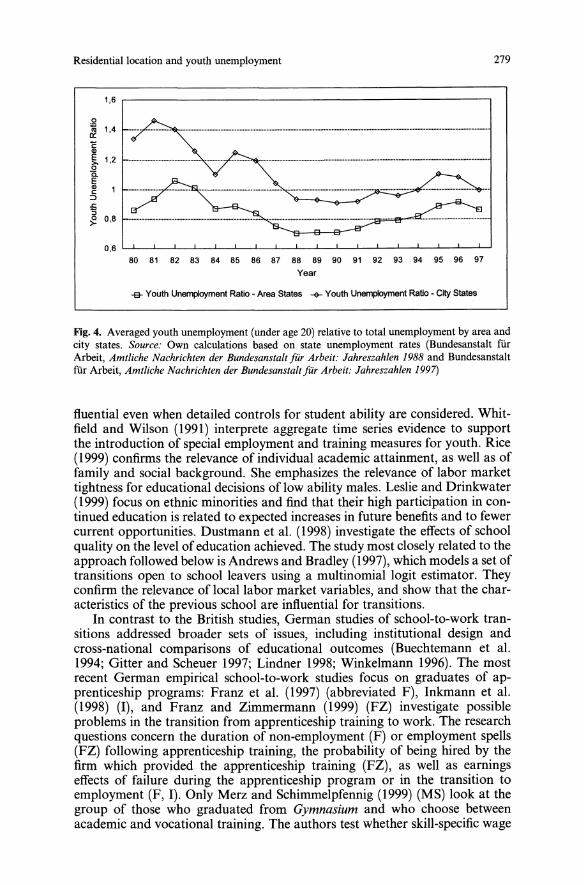
Residential location and youth unemployment

1,6 r-----------------------------,

279

o~ 1,4

'ECI>

[ 1,2oQ.

~::::l£:J~ 0,8

0,6 L......I._-'------'-_'--....I--'-_-'---'------'_--'-----'-_.L-....I-----'-_-'------'-----''----'---'

80 81 82 83 84 85 86 87 88 89 90 91 92 93 94 95 96 97

Year

-e- Youth Unemployment Ratio - Area States -$- Youth Unemployment Ratio - City States

Fig, 4. Averaged youth unemployment (under age 20) relative to total unemployment by area andcity states. Source: Own calculations based on state unemployment rates (Bundesanstalt fUrArbeit, Amtliche Nachrichten der Bundesanstalt fur Arbeit: Jahreszahlen 1988 and BundesanstaltfUr Arbeit, Amtliche Nachrichten der Bundesanstaltfur Arbeit: Jahreszahlen 1997)

fluential even when detailed controls for student ability are considered. Whit­field and Wilson (1991) interprete aggregate time series evidence to supportthe introduction of special employment and training measures for youth. Rice(1999) confirms the relevance of individual academic attainment, as well as offamily and social background. She emphasizes the relevance of labor markettightness for educational decisions of low ability males. Leslie and Drinkwater(1999) focus on ethnic minorities and find that their high participation in con­tinued education is related to expected increases in future benefits and to fewercurrent opportunities. Dustmann et al. (1998) investigate the effects of schoolquality on the level ofeducation achieved. The study most closely related to theapproach followed below is Andrews and Bradley (1997), which models a set oftransitions open to school leavers using a multinomial logit estimator. Theyconfirm the relevance of local labor market variables, and show that the char­acteristics of the previous school are influential for transitions.In contrast to the British studies, German studies of school-to-work tran­

sitions addressed broader sets of issues, including institutional design andcross-national comparisons of educational outcomes (Buechtemann et al.1994; Gitter and Scheuer 1997; Lindner 1998; Winkelmann 1996). The mostrecent German empirical school-to-work studies focus on graduates of ap­prenticeship programs: Franz et al. (1997) (abbreviated F), Inkmann et al.(1998) (I), and Franz and Zimmermann (1999) (FZ) investigate possibleproblems in the transition from apprenticeship training to work. The researchquestions concern the duration of non-employment (F) or employment spells(FZ) following apprenticeship training, the probability of being hired by thefirm which provided the apprenticeship training (FZ), as well as earningseffects of failure during the apprenticeship program or in the transition toemployment (F, I). Only Merz and Schimmelpfennig (1999) (MS) look at thegroup of those who graduated from Gymnasium and who choose betweenacademic and vocational training. The authors test whether skill-specific wage

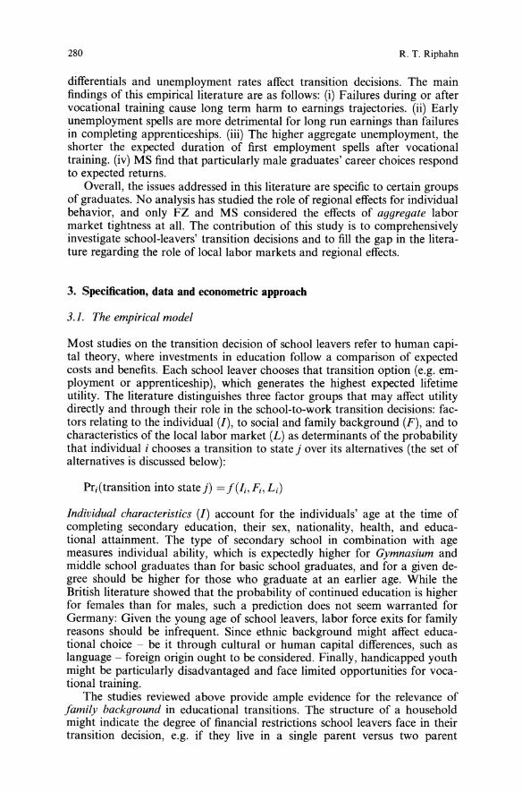
280 R. T. Riphahn

differentials and unemployment rates affect transition decisions. The mainfindings of this empirical literature are as follows: (i) Failures during or aftervocational training cause long term harm to earnings trajectories. (ii) Earlyunemployment spells are more detrimental for long run earnings than failuresin completing apprenticeships. (iii) The higher aggregate unemployment, theshorter the expected duration of first employment spells after vocationaltraining. (iv) MS find that particularly male graduates' career choices respondto expected returns.Overall, the issues addressed in this literature are specific to certain groups

of graduates. No analysis has studied the role of regional effects for individualbehavior, and only FZ and MS considered the effects of aggregate labormarket tightness at all. The contribution of this study is to comprehensivelyinvestigate school-Ieavers' transition decisions and to fill the gap in the litera­ture regarding the role of local labor markets and regional effects.

3. Specification, data and econometric approach

3.1. The empirical model

Most studies on the transition decision of school leavers refer to human capi­tal theory, where investments in education follow a comparison of expectedcosts and benefits. Each schoolleaver chooses that transition option (e.g. em­ployment or apprenticeship), which generates the highest expected lifetimeutility. The literature distinguishes three factor groups that may affect utilitydirectly and through their role in the school-to-work transition decisions: fac­tors relating to the individual (I), to social and family background (F), and tocharacteristics of the local labor market (L) as determinants of the probabilitythat individual i chooses a transition to state j over its alternatives (the set ofalternatives is discussed below):

Pr;(transition into state j) = f(I;, F;, L;)

Individual characteristics (I) account for the individuals' age at the time ofcompleting secondary education, their sex, nationality, health, and educa­tional attainment. The type of secondary school in combination with agemeasures individual ability, which is expectedly higher for Gymnasium andmiddle school graduates than for basic school graduates, and for a given de­gree should be higher for those who graduate at an earlier age. While theBritish literature showed that the probability of continued education is higherfor females than for males, such a prediction does not seem warranted forGermany: Given the young age of school leavers, labor force exits for familyreasons should be infrequent. Since ethnic background might affect educa­tional choice - be it through cultural or human capital differences, such aslanguage - foreign origin ought to be considered. Finally, handicapped youthmight be particularly disadvantaged and face limited opportunities for voca­tional training.The studies reviewed above provide ample evidence for the relevance of

family background in educational transitions. The structure of a householdmight indicate the degree of financial restrictions school leavers face in theirtransition decision, e.g. if they live in a single parent versus two parent

Residential location and youth unemployment 281

household. Since Micklewright (1989) and Andrews and Bradley (1997) showthat the number of younger siblings affects youth educational choices, thisindicator is considered as well. Parental background is likely to influencetastes and preferences of the offspring as well as their academic attainment insecondary school. Therefore we control for the impact of parental education,ethnic background, and labor force status.Finally, regional and labor market indicators may be important factors in

school Ieavers' transition decisions. These variables have been neglected inGerman studies, but the international literature speaks to their relevance. 4

The measures considered here describe the individuals' regions of residenceby community size, the local unemployment rate, and an indicator of whetherit is in East or West Germany. The underlying hypothesis is that the size andstructure of the local labor market affects youth behavior. Clearly, perfectmobility would render such effects irrelevant, but particularly for young schoolIeavers financial constraints may restrict mobility. We expect youth to be morelikely to find a job or an apprenticeship the larger the local labor market andthe more extensive labor demand. The same rationale applies to transitionsto academic training. Whereas youth living in a major town might have theopportunity to study while living at home, academic training may be muchmore costly for those living in the countryside. In addition to regional indi­cators the consideration of unemployment rates permits more direct controlsfor labor market effects.

3.2. The data

The data is taken from the first 14 waves of the German Socioeconomic Panel(GSOEP, 1984-1997). The sample is restricted to individuals aged 15 to 25.Observations are censored when the individual does not respond to a survey,when measures on core variables such as age, sex, or household identifiers aremissing, or when the interview was incompletely conducted. 5

The dependent variable describes the individuals' training or employmentstatus at the annual interview in the year after leaving secondary school. Togenerate this variable, one first has to determine in which year the person leftschool. There are two ways to determine schooling status within the GSOEP:The first is based on a survey question where individuals above age 16 areasked about current participation in schooling or training activities and aboutthe type of schooling currently pursued. We consider an individual as inschool if either Grundschule, Sonderschule, Hauptschule, Realschule, Gymna­sium or Gesamtschule are indicated. 6 For individuals under age 16 informa­tion on current schooling is gathered from the household head. A school exitis coded if an individual was in school in one year and out of school in thenext year. The second way to determine schooling status is based on a ques­tion, which asks individuals whether they obtained a degree in the precedingcalendar year. 68% of all school exits are identified by both indicators. In caseswhere the coding procedure resulted in more than one exit from secondaryschool, only the exit indicated last was considered, assuming that the inter­mittent failure to indicate school attendance resulted from measurementerror. 7A wide set of alternative transitions is available for school leavers. It

ranges from continued schooling in vocational schools, polytechnical schools,

282 R. T. Riphahn

and universities over immediate employment, apprenticeship, military or sub­stitute service for men, to unemployment, or out of the labor force spells.In contrast to the recent German school-to-work literature a comprehen­sive set of alternatives is captured in the dependent variable here, where allschool leavers are considered and transitions into the following activities aremodelled:

(1) full time or parttime employment without training,(2) apprenticeship,(3) vocational training without employment,(4) university or polytechnical schools,(5) military or substitute service for men,(6) unemployment or out of the labor force (OLF).

Military and substitute service are considered as endogenous outcomes, be­cause it is possible to influence the timing of these activities. While unemploy­ment and OLF are typically separate outcomes, they are combined, becauseschool leavers have no claim to unemployment benefits and because unem­ployed seekers of apprenticeship positions are not defined as unemployed.The distribution of the 2,702 schoolleavers across these states is presented

in Table 3 by various characteristics. Almost half of all graduates take upan apprenticeship, and 22% seek vocational training through the alternativesoffered in the vocational schooling system. The shares of individuals in non­training employment, in academic training, and military/substitute service arebelow ten percent each. A substantial fraction of about 12% of all schoolleavers is either unemployed or out of the labor force one year after exitingsecondary school.The main difference between the two sexes lies in the share of immediate

transitions into academic training, which is higher among females becausemale Gymnasium leavers are typically drafted immediately. More surprisingly,the share of nonemployed females clearly exceeds the sample average. Thecomparison between East and West German transitions yields a substantiallyhigher coverage of East German youth with training programs: Jointly 76% ofEast German school leavers are in vocational training, compared to 66% inthe West. This is balanced by a higher share of West German youth in non­employment one year after finishing school. While the latter outcome seemssurprising in view of higher overall unemployment in East vs. West Germany,Figs. 2 and 3 do suggest that the difference in unemployment rates for youthunder age 20 is indeed minor.The comparison of transitions by national origin shows substantive differ­

ences, in that immigrant youth have much higher probabilities of immediateemployment and nonemployment than native youth. Panel B of Table 3describes transition distributions by community size, health, and regional un­employment. Most striking are the high nonemployment rates in large com­munities, and the sensitivity to state unemployment rates. Health does notappear to be strongly correlated with transition decisions. Panel C shows thedistribution of transitions by type of school and agegroup. Nonemploymentrates are highest for those in 'other' schools. Transition into military or sub­stitute service is highest among Gymnasium graduates because they reach draftage when leaving school. This difference by age is also reflected in the last twocolumns of panel C. Panel D presents the distribution of destination states

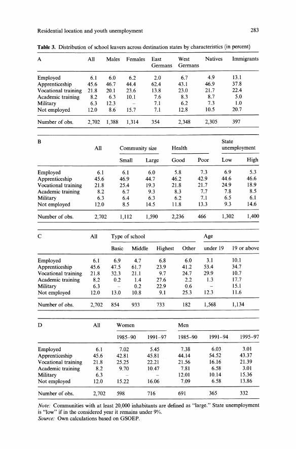
Residential location and youth unemployment 283

Table 3. Distribution of school leavers across destination states by characteristics (in percent)

A All Males Females East West Natives ImmigrantsGermans Germans

Employed 6.1 6.0 6.2 2.0 6.7 4.9 13.1Apprenticeship 45.6 46.7 44.4 62.4 43.1 46.9 37.8Vocational training 21.8 20.1 23.6 13.8 23.0 21.7 22.4Academic training 8.2 6.3 10.1 7.6 8.3 8.7 5.0Military 6.3 12.3 7.1 6.2 7.3 1.0Not employed 12.0 8.6 15.7 7.1 12.8 10.5 20.7

Number of obs. 2,702 1,388 1,314 354 2,348 2,305 397

B StateAll Community size Health unemployment

Small Large Good Poor Low High

Employed 6.1 6.1 6.0 5.8 7.3 6.9 5.3Apprenticeship 45.6 46.9 44.7 46.2 42.9 44.6 46.6Vocational training 21.8 25.4 19.3 21.8 21.7 24.9 18.9Academic training 8.2 6.7 9.3 8.3 7.7 7.8 8.5Military 6.3 6.4 6.3 6.2 7.1 6.5 6.1Not employed 12.0 8.5 14.5 11.8 13.3 9.3 14.6

Number of obs. 2,702 1,112 1,590 2,236 466 1,302 1,400

C All Type of school Age

Basic Middle Highest Other under 19 19 or above

Employed 6.1 6.9 4.7 6.8 6.0 3.1 10.1Apprenticeship 45.6 47.5 61.7 23.9 41.2 53.4 34.7Vocational training 21.8 32.3 21.1 9.7 24.7 29.9 10.7Academic training 8.2 0.2 1.4 27.6 2.2 1.3 17.7Military 6.3 0.2 22.9 0.6 15.1Not employed 12.0 13.0 10.8 9.1 25.3 12.3 11.6

Number of obs. 2,702 854 933 733 182 1,568 1,134

D All Women Men

1985-90 1991-97 1985-90 1991-94 1995-97

Employed 6.1 7.02 5.45 7.38 6.03 3.01Apprenticeship 45.6 42.81 45.81 44.14 54.52 43.37Vocational training 21.8 25.25 22.21 21.56 16.16 21.39Academic training 8.2 9.70 10.47 7.81 6.58 3.01Military 6.3 12.01 10.14 15.36Not employed 12.0 15.22 16.06 7.09 6.58 13.86

Number of obs. 2,702 598 716 691 365 332

Note: Communities with at least 20,000 inhabitants are defined as "large." State unemploymentis "low" if in the considered year it remains under 9%.Source: Own calculations based on GSOEP.

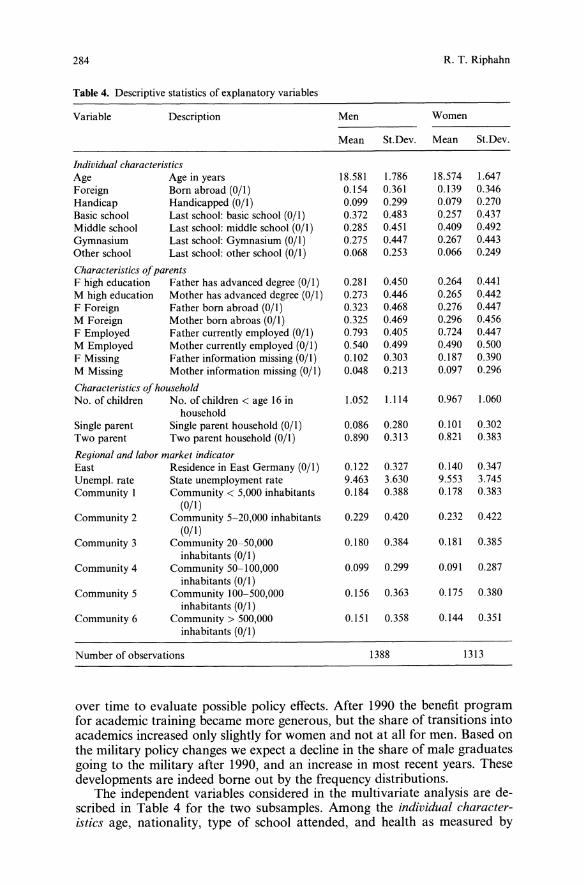
284 R. T. Riphahn

Table 4. Descriptive statistics of explanatory variables

Variable Description Men Women

Mean St.Dev. Mean St.Dev.

Individual characteristicsAge Age in years 18.581 1.786 18.574 1.647Foreign Born abroad (Ojl) 0.154 0.361 0.139 0.346Handicap Handicapped (Ojl) 0.099 0.299 0.079 0.270Basic school Last school: basic school (Ojl) 0.372 0.483 0.257 0.437Middle school Last school: middle school (OJ I) 0.285 0.451 0.409 0.492Gymnasium Last school: Gymnasium (OJ I) 0.275 0.447 0.267 0.443Other school Last school: other school (Ojl) 0.068 0.253 0.066 0.249

Characteristics ofparentsF high education Father has advanced degree (Ojl) 0.281 0.450 0.264 0.441M high education Mother has advanced degree (Ojl) 0.273 0.446 0.265 0.442F Foreign Father born abroad (Ojl) 0.323 0.468 0.276 0.447M Foreign Mother born abroas (Ojl) 0.325 0.469 0.296 0.456F Employed Father currently employed (Ojl) 0.793 0.405 0.724 0.447M Employed Mother currently employed (Ojl) 0.540 0.499 0.490 0.500F Missing Father information missing (Ojl) 0.102 0.303 0.187 0.390M Missing Mother information missing (Ojl) 0.048 0.213 0.097 0.296

Characteristics ofhouseholdNo. of children No. of children < age 16 in 1.052 1.114 0.967 1.060

householdSingle parent Single parent household (OJ I) 0.086 0.280 0.101 0.302Two parent Two parent household (Ojl) 0.890 0.313 0.821 0.383

Regional and labor market indicatorEast Residence in East Germany (Ojl) 0.122 0.327 0.140 0.347Unempl. rate State unemployment rate 9.463 3.630 9.553 3.745Community I Community < 5,000 inhabitants 0.184 0.388 0.178 0.383

(Ojl)Community 2 Community 5-20,000 inhabitants 0.229 0.420 0.232 0.422

(Ojl)Community 3 Community 20-50,000 0.180 0.384 0.18\ 0.385

inhabitants (Ojl)Community 4 Community 50-100,000 0.099 0.299 0.091 0.287

inhabitants (OJ I)Community 5 Community \00-500,000 0.156 0.363 0.175 0.380

inhabitants (OJ I)Community 6 Community> 500,000 0.151 0.358 0.144 0.351

inhabitants (Ojl)

Number of observations 1388 1313

over time to evaluate possible policy effects. After 1990 the benefit programfor academic training became more generous, but the share of transitions intoacademics increased only slightly for women and not at all for men. Based onthe military policy changes we expect a decline in the share of male graduatesgoing to the military after 1990, and an increase in most recent years. Thesedevelopments are indeed borne out by the frequency distributions.The independent variables considered in the multivariate analysis are de­

scribed in Table 4 for the two subsamples. Among the individual character­istics age, nationality, type of school attended, and health as measured by

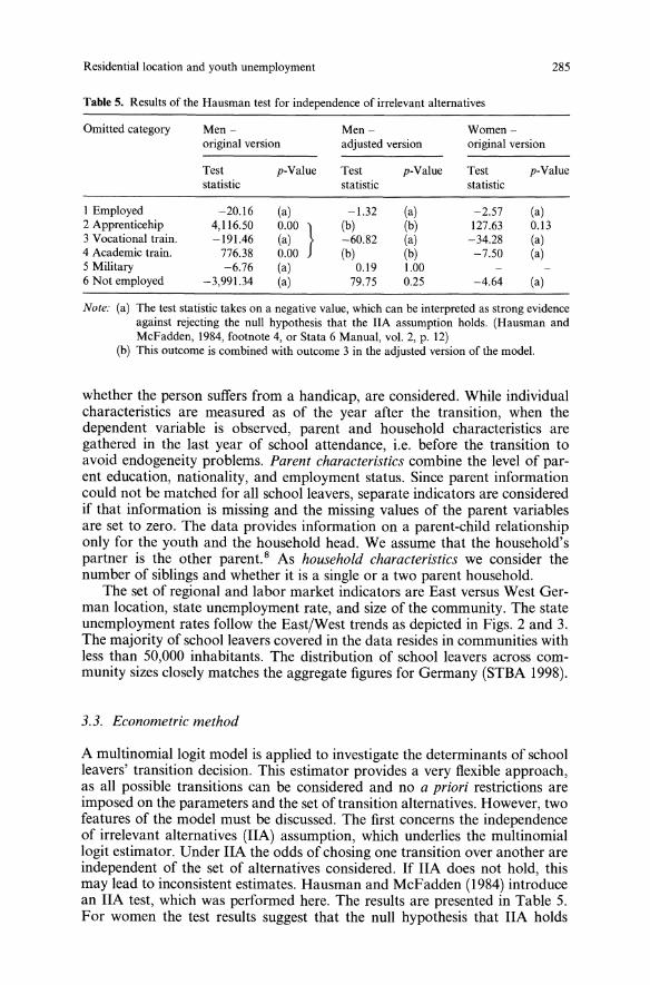
Residential location and youth unemployment

Table 5. Results of the Hausman test for independence of irrelevant alternatives

285

Omitted category Men- Men- Women -original version adjusted version original version

Test p-Value Test p-Value Test p-Valuestatistic statistic statistic

I Employed -20.16 (a) -1.32 (a) -2.57 (a)2 Apprenticehip 4,116.50 0.00 } (b) (b) 127.63 0.133 Vocational train. -191.46 (a) -60.82 (a) -34.28 (a)4 Academic train. 776.38 0.00 (b) (b) -7.50 (a)5 Military -6.76 (a) 0.19 1.006 Not employed -3,991.34 (a) 79.75 0.25 -4.64 (a)

Note: (a) The test statistic takes on a negative value, which can be interpreted as strong evidenceagainst rejecting the null hypothesis that the IlA assumption holds. (Hausman andMcFadden, 1984, footnote 4, or Stata 6 Manual, vol. 2, p. 12)

(b) This outcome is combined with outcome 3 in the adjusted version of the model.

whether the person suffers from a handicap, are considered. While individualcharacteristics are measured as of the year after the transition, when thedependent variable is observed, parent and household characteristics aregathered in the last year of school attendance, i.e. before the transition toavoid endogeneity problems. Parent characteristics combine the level of par­ent education, nationality, and employment status. Since parent informationcould not be matched for all school Ieavers, separate indicators are consideredif that information is missing and the missing values of the parent variablesare set to zero. The data provides information on a parent-child relationshiponly for the youth and the household head. We assume that the household'spartner is the other parent. 8 As household characteristics we consider thenumber of siblings and whether it is a single or a two parent household.The set of regional and labor market indicators are East versus West Ger­

man location, state unemployment rate, and size of the community. The stateunemployment rates follow the East/West trends as depicted in Figs. 2 and 3.The majority of schoolleavers covered in the data resides in communities withless than 50,000 inhabitants. The distribution of school Ieavers across com­munity sizes closely matches the aggregate figures for Germany (STBA 1998).

3.3. Econometric method

A multinomiallogit model is applied to investigate the determinants of schoolleavers' transition decision. This estimator provides a very flexible approach,as all possible transitions can be considered and no a priori restrictions areimposed on the parameters and the set of transition alternatives. However, twofeatures of the model must be discussed. The first concerns the independenceof irrelevant alternatives (IIA) assumption, which underlies the multinomiallogit estimator. Under IIA the odds of chosing one transition over another areindependent of the set of alternatives considered. If IIA does not hold, thismay lead to inconsistent estimates. Hausman and McFadden (1984) introducean IIA test, which was performed here. The results are presented in Table 5.For women the test results suggest that the null hypothesis that IIA holds

286 R. T. Riphahn

cannot be rejected. For men this was not the case. When outcomes 2 (ap­prenticeship) or 4 (academic training) were eliminated from the set of alter­natives, the null hypothesis was rejected at high significance levels. Thereforethe outcomes apprenticeship, vocational, and academic training are combinedto an adjusted dependent variable, for which the IIA hypothesis cannot berejected. 9

Second, Moulton (1990) showed that in models where aggregate infor­mation, such as state unemployment rates, is considered jointly with indivi­dual characteristics, the disturbances may be correlated within aggregationgroups (here states). This can bias the standard errors downwards. To addressthis problem a nonparametric random effects estimator, as developed byHeckman and Singer (1984), was applied to the multinomiallogit estimator,which permits tests for correlation among the unobservables of individuals ina given state (see Riphahn 1999 for a more detailed description). This yieldeda significant improvement of the likelihood function only for the female sam­ple. 10 Therefore a standard multinomial logit model was estimated for menand a model with corrected standard errors is provided for women. 11 The nextsection discusses the determinants of transition choices.

4. Results

The two estimated models differ in that the model for women does not containthe transitions into military or substitute service and that the transitions intofurther training (apprenticeship, vocational, and academic training) are con­sidered jointly in the model for men. The interpretation of the coefficients iscomplicated because they describe the probability of each outcome relative tothe omitted category - the transition to apprenticeship training - and becausethe signs of coefficients can deviate from those of marginal effects. Therefore,the interpretation first evaluates the statistical significance of the estimates,and then interprets the substantive evidence based on simulation results.Table 6 presents the results of joint significance tests for coefficients across

the full models, estimated for the male and female samples. The indicators forage and prior schooling have the most significant impact on transition out­comes for both samples. 12 Jointly they represent potent indicators of studentability, as weaker students may take additional years before they are able tograduate from a given secondary school. Of high overall statistical significanceare the indicators for parent education. The effect of these variables is wellestablished in the literature (Merz and Schimmelpfennig 1999; Rice 1999).13In the model for men the indicators for the number of children yield surpris­ingly significant influences on labor market transitions.Among the regional effects we observe significant differences between the

transition probabilities of the East and West German samples. The stateunemployment rate, which is hypothesized to affect transitions through theavailability of employment and training opportunities and at the same timeas a determinant of the expected future payoff of additional training, is notjointly significant in either subsample. This outcome is sensitive to the con­sideration of year fixed effects in the model: In models, which consider only alinear time trend instead of the fixed effect control, unemployment was sig­nificant for both samples. Finally, the indicators of the size of an individual'scommunity of residence are jointly significant.

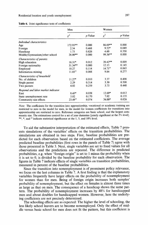
Residential location and youth unemployment

Table 6. Joint significance tests of coefficients

287

Individual characteristicsAgeForeignHandicapMiddle/Gymnasium/other school

Characteristics ofparentsHigh educationForeign nationalityEmployedInformation missing

Characteristics ofhouseholdNo. of childrenSingle parentTwo parents

Regional and labor market indicatorEastState unemployment rateCommunity size effects

Men

172.95**2.541.7526.00**

16.31 *31.34**10.2711.03°

11.27*2.294.02

8.43*5.0223.49°

Women

p-Value X2 p-Value

0.000 86.69** 0.0000.468 9.52* 0.0490.626 4.60 0.3300.000 99.36** 0.000

0.012 20.42** 0.0090.000 12.13 0.1450.114 14.71° 0.0650.088 9.84 0.277

0.010 3.37 0.4980.514 3.30 0.5080.259 3.75 0.440

0.038 12.69* 0.0130.170 7.02 0.1350.074 34.00* 0.026

Note: The coefficients for the transition into apprenticeship, vocational or academic training arerestricted to zero in the model for men, in the model for women coefficients for transitions intoapprenticeship are restricted to zero. Reference categories are basic school, and the largest com­munity size. The estimations control for a set of year dummies (jointly significant at the 2% level).**, *, and ° indicate statistical significance at the I, 5, and 10% level.

To aid the substantive interpretation of the estimated effects, Table 7 pres­ents simulations of the variables' effects on the transition probabilities. Thesimulations are obtained in two steps. First, baseline probabilities are pre­dicted for each observation based on the estimated coefficients. The averagepredicted baseline probabilities (first rows in the panels of Table 7) agree withthose presented in Table 3. Next, single variables are set to fixed values for allobservations and the predictions are repeated. The difference in predictedprobabilities, e.g. when "foreign origin" is set to I minus the probability whenit is set to 0, is divided by the baseline probability for each observation. Thefigures in Table 7 indicate effects of single variables on transition probabilities,measured in percent of the baseline probabilities.Since the transition into nonemployment is of prominent policy relevance,

we focus on the last columns in Table 7. A first finding is that the explanatoryvariables frequently have larger effects on the probability of nonemploymentfor women than for men. Being of foreign origin increases both samples'probability of nonemployment, but the effect on females is almost three timesas large as that on men. The consequence of a handicap shows the same pat­tern. The probability of nonemployment increases by 48% for handicappedmen and about doubles for handicapped women. However, here the underly­ing coefficients are not precisely determined.The schooling effects are as expected: The higher the level of schooling, the

less likely school leavers are to become nonemployed. Only the effect of mid­dle versus basic school for men does not fit the pattern, but this coefficient is

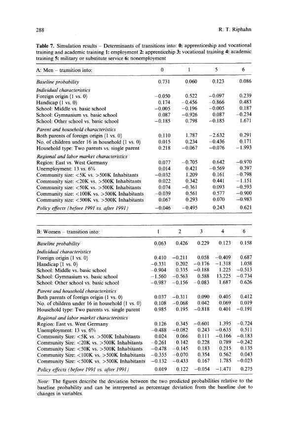
288 R. T. Riphahn

Table 7. Simulation results - Determinants of transitions into: 0: apprenticeship and vocationaltraining and academic training 1: employment 2: apprenticehip 3: vocational training 4: academictraining 5: military or substitute service 6: nonemployment

A: Men - transition into: 0 5 6

Baseline probability 0.731 0.060 0.123 0.086

Individual characteristicsForeign origin (I vs. 0) -0.050 0.522 -0.097 0.239Handicap (I vs. 0) 0.174 -0.456 -0.866 0.483School: Middle vs. basic school -0.005 -0.196 -0.005 0.187School: Gymnasium vs. basic school 0.087 -0.926 0.087 -0.234School: Other school vs. basic school -0.185 0.798 -0.185 1.671

Parent and household characteristicsBoth parents of foreign origin (I vs. 0) 0.110 1.787 -2.632 0.291No. of children under 16 in household (I vs. 0) 0.015 0.234 -0.436 0.171Household type: Two parents vs. single parent 0.218 -0.067 -0.076 -1.993

Regional and labor market characteristicsRegion: East vs. West Germany 0.077 -0.705 0.642 -0.970Unemployment: 13 vs. 6% 0.014 0.421 -0.569 0.397Community size: <5K vs. >500K Inhabitants -0.032 1.209 0.161 -0.798Community size: <20K vs. >500K Inhabitants 0.022 0.342 0.441 -1.151Community size: <50K vs. >500K Inhabitants 0.074 -0.361 0.093 -0.593Community size: <lOOK vs. >5OOK Inhabitants -0.039 0.561 0.577 -0.900Community size: <5OOK vs. >5OOK Inhabitants 0.067 0.293 0.070 -0.983

Policy effects (before /99/ vs. after /99/) -0.046 -0.495 0.243 0.621

B: Women - transition into: 2 3 4 6

Baseline probability 0.063 0.426 0.229 0.123 0.158

Individual characteristicsForeign origin (I vs. 0) 0.410 -0.211 0.058 -0.409 0.687Handicap (I vs. 0) -0.331 0.202 -0.176 -1.318 1.058School: Middle vs. basic school -0.904 0.335 -0.188 1.225 -0.513School: Gymnasium vs. basic school -1.560 -0.563 0.588 13.225 -0.734School: Other school vs. basic school -0.987 -0.156 -0.083 1.687 0.626

Parent and household characteristicsBoth parents of foreign origin (I vs. 0) 0.037 -0.311 0.090 0.405 0.412No. of children under 16 in household (I vs.O) 0.108 -0.068 0.042 0.069 0.019Household type: Two parents vs. single parent 0.985 0.195 -0.818 MOl -0.191

Regional and labor market characteristicsRegion: East vs. West Germany 0.126 0.345 -0.601 1.395 -0.724Unemployment: 13 vs. 6% -0.488 -0.082 0.243 -0.635 0.511Community Size: <5K vs. >5OOK Inhabitants 0.024 0.066 0.111 -0.166 -0.183Community Size: <20K vs. >5OOK Inhabitants -0.261 0.142 0.228 0.789 -0.242Community Size: <50K vs. >5OOK Inhabitants -0.478 -0.145 0.183 0.215 0.135Community Size: <lOOK vs. >5OOK Inhabitants -0.355 -0.070 0.354 0.562 0.043Community Size: <500K vs. >5OOK Inhabitants -0.132 -0.433 0.167 1.785 -0.023

Policy effects (before /99/ vs. after /99/) 0.019 0.122 -0.054 -1.471 0.275

Note: The figures describe the deviation between the two predicted probabilities relative to thebaseline probability and can be interpreted as percentage deviation from the baseline due tochanges in variables.

Residential location and youth unemployment 289

statistically insignificant. Females with middle school or Gymnasium degreeshave lower risks of nonemployment relative to basic schooling. Women in the"other school" category have an elevated risk of nonemployment, but also asurprisingly high transition probability into academic training.Independent of the nationality of the graduates themselves, the nationality

of their parents has sizeable effects on youth labor market outcomes. If bothparents are non-natives, the probability of nonemployment increases by 29%for men and by again a more sizeable 41% for women. Also, all indicators ofnon-native nationality yield increased probabilities of immediate employmentafter school. These results raise concerns, as they show that independent ofability, non-native ethnic background seems to hinder continued training. Theeffects of non-native ethnicity in the British data are typically reverse: Rice(1999) and Andrews and Bradley (1997) show that non-whites have higherprobabilities of participating in continued education. A possible rationale forthe different ethnicity effects in the u.K. and German framework might bethat the German non-native population consists mostly of blue-collar guest­workers whereas British immigrants are more favorably self-selected in termsof preferences for human capital.The indicator of the number of young siblings in the household has a sig­

nificant and sizeable effect on men's transitions into nonemployment. Havingone versus no child under age 16 in the household increases the probability ofnonemployment (as well as of immediate employment) by about 20%. Theindicator has not been considered in the German literature so far, however,the results confirm Micklewright (1989), who finds that youth with more sib­lings have a lower probability of continued education. The mechanism behindthis effect is likely to be related to parents' financial and time constraints. Themore siblings there are to care for, the fewer financial resources are availableto finance continued education, or to support job search activities. 14 The samepattern is likely to be behind the result that youth from two parent householdshave a smaller risk of nonemployment than those from single parent house­holds. For men also the probability of immediate employment falls and thatof continued training increases, if they come from a two as opposed to a singleparent household.Confirming the distribution discussed above, East German youth has a

lower probability of nonemployment than youth in the West. East Germanmen have a high transition probability into military service, an about equalprobability of training, and a much lower probability of starting employmentimmediately after leaving school. For East German females the probability ofacademic training exceeds that of women in the West by far, a phenomenonwhich is likely to be related to higher female labor force participation andthus higher expected lifetime returns to education in East compared to WestGermany.As expected, state unemployment yields sizeable effects on nonemploy­

ment transitions. Again, female schoolleavers are more strongly affected by agiven change in unemployment than their male classmates. Women's transi­tion probabilities into immediate employment also decline drastically if stateunemployment is high. The effect on male youths surprisingly points in theopposite direction. Their negative response in the probability of a transition tomilitary service, when unemployment is high, is also difficult to rationalize.For females the probability of taking up apprenticeship training declines intimes of high unemployment and that of other vocational training increases, a

290 R. T. Riphahn

plausible pattern, as the availability of apprenticeship positions should becorrelated with the overall labor market tightness.The community size effects are evaluated by comparing transition prob­

abilities in smaller communities with those for a metropolitan center. Fourpatterns emerge: (i) The probability of nonemployment is largest in themetropolitan center. (ii) The probability of taking up military service is lowestfor men in metropolitan areas. (iii) Men are least likely to start immediateemployment in metropolitan areas. (iv) The probability of a transition intovocational or academic training for women is particularly low in metropolitanareas, where a wider pool of apprenticeship positions might be availableinstead. It appears that school leavers outside of metropolitan centers makeup for a lack of apprenticeship positions by chosing vocational school oracademic training. For women in midsize towns this pattern is quite c1ear. is

Finally, it is interesting to look at policy effects. The first hypothesis isthat the probability of academic training increased after the generosity of theBalog benefit system was expanded in 1990. The probability distributions inTable 3D indicated no such effect for men, and only a slight increase in theprobability of academic training for women. In the multivariate frameworkthis correlation can only be examined for females, since the dependent vari­able for men combines academic training with other outcomes. The simu­lations suggest that there is a strong increase in the probability of taking upacademic training after 1990 for women by about 150% of the baseline prob­ability. This suggests a clear response in individual behaviors to the relaxationof financial constraints.The second policy hypothesis refers to changes in military policy. The

above discussion suggests that the probability of a transition to military orsubstitute service should be high before 1990, decline after the cold war, andrise again in the last years of our data. Averaging the predicted probabilitiesof a transition into military service over the relevant periods yields a meanprobability of 11.6% for 1985-1990, of 8.6 for 1991-1993, and of 17.2 for1994-1997. These figures (not presented in Table 7) indicate a close correla­tion with the expected pattern.

5. Conclusion

Motivated by the increasing attention of labor market policies to the youthunemployment problem, this study investigates labor market transitions ofsecondary schoolleavers in Germany. Using a detailed dataset and a flexiblemodelling approach, the determinants of such transitions are evaluated. Aspotentially influential factors characteristics of the youth, household, andparents, as well as indicators of the region of residence, and local labor mar­kets are considered.The findings confirm many of the conclusions from the British school­

to-work literature. Overall the most significant effects are those describing theability level of the individual, as reflected in the indicators of age and schooltype. The latter expectedly yields that the probability of nonemployment isleast for those youth with the highest completed degree. The results permitconclusions as to the groups most vulnerable to the risk of nonemployment, orof foregoing continued education: Youth with a handicap and immigrantssuffer substantial nonemployment problems. The latter effect is obtained based

Residential location and youth unemployment 291

both on the nationality of the individual as well as on the parents', and it isconsistent in both, the male and female subsamples.Two findings that are new to the literature are that the educational

attainment of parents has a significant effect on youth labor market transitionsand that youth from two-parent families are in a much better position to takeup vocational training after secondary school than individuals from singleparent families, an outcome which holds particularly for young men. Thesimulation results yield a clear correlation between the probability of takingup academic training and expansions in the student-benefit program in 1990.This agrees with Rice (1987), who found that the introduction of an educa­tional allowance would have positive effects on the participation in continuededucation. - Additionally, men's participation in military service seems to re­spond to general trends in military policy.With respect to regional and local labor market effects, living in a high

unemployment state is correlated with higher risks of nonemployment forschool leavers. Given state unemployment rates, the risk of nonemploymentis highest for youth in large metropolitan areas. These results suggest thatyouth labor market policies should focus on disadvantaged regions with tightoverall labor markets, emphasize metropolitan areas, and possibly pay par­ticular attention to the needs of immigrant youth.

Endnotes

1 The benefit program also provides payments to high school students and participants in certainvocational training programs under restricitive and complex regulations. Since most of theprogram expenditures are alloted to university students, the discussion focuses on this programaspect. For detail see e.g. BMA (1995).

2 This may in part be due to the definitional exclusion of "apprenticeship seekers" from theranks of the unemployed. Franz et al. (1997) show that their inclusion would drive up youthunemployment rates by about 20%.

3 Bavaria, Baden-Wiirttemberg, Hesse, Lower Saxony, Northrhine-Westfalia, Rhineland­Palatinate, Saarland, ScWeswig-Holstein.

4 Micklewright (1989) and Rice (1999) find highly significant differences in the educationalchoices of students in different areas of the country, as well as by local labor market conditions.

5 Imposing an age limit on the considered observations is important and necessary to avoidmeasurement errors, that might otherwise occur with the consideration of outlier observations(of schoolleavers above age 25) in the sample. When normal school exit age is 16 or at most19, considering an additional 9 to 6 years covers the relevant population. Also, it is unlikelyand not plausible that the omission of observations with missing values on explanatory varia­bles or on school participation biases the estimation, since survey responses of typicallyother members of the household should be uncorrelated with post-secondary schoolingtransition decisions. Therefore the selection mechanisms should be neutral to the estimationresults.

6 For a description of these institutions see Sect. 2 above. Sonderschule provides special educa­tion for those unable to pass basic school. Grundschule is elementary school.

7 About 20% of all observations were affected by multiply coded school exits.8 In addition, parent information was used, which was explicitly gathered in the survey of1986.

9 Initial adjustments of combining smaller subsets of transition outcomes did not satisfy the llAassumption.

10 For the male sample the log likelihood could not be improved beyond the value of 888.20obtained before, for women the consideration of controls for correlated errors improved thelog likelihood from 1,455.55 to 1,449.56, which is statistically significant at the 5% level giventhat 5 additional parameters were estimated.

292 R. T. Riphahn

11 To save space the full set of coefficient and standard error results is not presented. Preliminaryestimations showed that a different health indicator did not affect the results, that a richer setof indicators for parent schooling degrees, and the consideration of parents' age, or of immi­grant students' language capacity did not significantly add to the explanatory power of themodel, that unemployment rates measured at a more disaggregated level had less explanatorypower, than the state level ones, and that a variable controlling for the number of personsliving in a household did not significantly improve the model fit.

12 The schooling coefficients in the model for a transition into military service were restricted tozero, because the fact that Gymnasium graduates have reached draft age at graduation causedan unreasonably large coefficient in this model. To provide an indirect test for the potentialendogeneity of the school type, estimations without these variables were performed. The resultsdid not differ in major ways.

13 It is a striking advantage of the GSOEP that it provides indicators for parent educational sta­tus. The studies by Inkmann et al.( 1998) and Franz and Zimmermann (1999) are based on adataset with more observations, but which apparently does not permit this type of control.Only Franz et al. (1997) are able to consider controls for the vocational background of thehousehold head, which they find to be influential. Neither partner information nor the educa­tional status of the household head are considered.

14 For women this conclusion is somewhat counterbalanced by the higher probability of a tran­sition into vocational or academic training.

15 Critics may argue that the community effects are subject to the reflection problem pointed outby Manski (1993). He argues that the effect of (the characteristics of) an aggregate, e.g. a state,on the behavior of a unit of observation typically cannot be identified. For our case this impliesthat parents' decision to move e.g. to a large town is determined by similar factors and motivesas the outcome of their child's post-school transition. One condition for such an argument tohold is that households can indeed be observed to move. A dataset generated before definingthe transition variable, contained panel information on a multitude of households with andwithout a graduating youth, before and after a possible graduation. In this dataset, with morethan 90,000 household-year observations, 0.74% of the observations moved between states. Inthe final sample the share of moving households dropped to 0.1%, suggesting that very littlemoving takes place. Overall the argument that the decision of parents to move between statesis correlated with a transition decision of their children at a possibly much later date is notconvincing. Therefore endogenous moves are not likely to bias the presented results.

References

Andrews M, Bradley S (1997) Modelling the Transition from School and the Demand for Train­ing in the United Kingdom. Economica 64(255):387-413

BMA (Bundesministerium fur Arbeit und Sozialordnung) (1995) Ubersicht iiber das Sozialrecht.Bonn

BREG (Bundesregierung) (1996) lahresbericht der Bundesregierung 1996. BonnBuechtemann CF, Schupp J, Soloff D (1994) From School to Work: Patterns in Germany and theUnited States. In: Schwarze J, Buttler F, Wagner GG (eds.) Labour Market Dynamics inPresent Day Germany. Campus Verlag, Frankfurt a.M., New York, 112-141

Clinton WJ, Gore A (1992) Putting People First: A National Economic Strategy for America.Business Week. Sept. 7, 30

Dustmann C, Rajah N, van Soest A (1998) School Quality, Exam Performance, and CareerChoice, CentER Discussion Paper No. 9816, Tilburg, The Netherlands

Ellwood DT (1982) Teenage Unemployment: Permanent Scars or Temporary Blemishes? In:Freeman RB, Wise DA (eds.) The Youth Labor Market Problem: Its Nature, Causes andConsequences. The University of Chicago Press, Chicago, 349-385

Franz W, Inkmann J, Pohlmeier W, Zimmermann V (1997) Young and Out in Germany: On theYouths' Chances of Labor Market Entrance in Germany. NBER Working Paper No. 6212

Franz W, Zimmermann V (1999) Mobilitiit nach der berullichen Ausbildung: Eine empirischeStudie fUr Westdeutschland. ZEW Discussion Paper No. 99-21

Freeman RB, Rodgers III WM (1999) Area Economic Conditions and the Labor Market Out­comes of Young Men in the 1990s Expansion. NBER Working Paper No. 7073

Residential location and youth unemployment 293

Gitter RJ, Scheuer M (1997) U.S. and German Youths: Unemployment and the Transition fromSchool to Work. Monthly Labor Review 120(3):16-20

Hausman JA, McFadden D (1984) Specification Tests for the Multinomial Logit Model. Econo­metrica 52(5):1219-1240

Heckman JJ, Singer B (1984) A Method for Minimizing the Impact of Distributional Assump­tions in Econometric Models for Duration Data. Econometrica 52(2):271-320

Inkmann J, Klotz S, Pohlmeier W (1998) Growing into Work: Pseudo Panel Data Evidence onLabor Market Entrance in Germany. ZEW Discussion Paper No. 98-47

Leslie D, Drinkwater S (1999) Staying on in Full-Time Education: Reasons for Higher Partici­pation Rates Among Ethnic Minority Males and Females. Economica 66(261 ):63-77

Lindner A (1998) Modelling the German System of Vocational Education. Labour Economics5(4):411-423

Manski CF (1993) Identification of Endogenous Social Effects: The Reflection Problem. Review ofEconomic Studies 60:531-542

McIntosh S (1998) The Demand for Post-Compulsory Education in Four European Countries,London School of Economics. Centre for Economic Performance Discussion Paper No. 393

Merz M, Schimmelpfennig A (1999) Career Choices ofGerman High School Graduates: Evidencefrom the German Socio-Economic Panel. European University Institute Working PaperNo. 99/11

Micklewright J (1989) Choice at Sixteen. Economica 56(221):25-39Moulton B (1990) An Illustration of a Pitfall in Estimating the Effects of Aggregate Variables onMicro Units. Review of Economics and Statistics 72(2):334-338

OECD (Organisation for Economic Co-Operation and Development) (1998) OECD EmploymentOutlook 1998 - Chapter 3. Paris, 81-122

OECD (Organisation for Economic Co-Operation and Development) (1999a) OECD EconomicSurveys: France 1999. Paris

OECD (Organisation for Economic Co-Operation and Development) (1999b) OECD Employ­ment Outlook /999 - Editorial. Paris, 7-11

Rice P (1987) The Demand for Post-compulsory Education in the UK and the Effects fo Educa­tional Maintenance Allowances. Economica 54(216):465-476

Rice P (1999) The Impact of Local Labour Markets on Investment in Further Education: Evi­dence from the England and Wales Youth Cohort Studies. Journal of Population Economics12(2):287-312

Riphahn RT (1999) Disability Retirement Among German Men in the 1980s. Industrial andLabor Relations Review 52(4):628-647

Rotte R (1996) Das Ende der Wehrpflicht in Europa? Merkur 50:460-465STBA (Statistisches Bundesamt) (1998) Statistisches Jahrbuchfur die Bundesrepublik Deutschland1998. Metzler Poeschel, Wiesbaden

Whitfield K, Wilson R (1991) Staying on in Full-time Education: The Educational ParticipationRate of 16 Year Olds. Economica 58(231):391-404

Winkelmann R (1996) Employment Prospects and Skill Acquisition of Apprenticeship - TrainedWorkers in Germany. Industrial and Labor Relations Review 49(4):658-672

Transitions from employmentamong young Norwegian workers

0ivind Anti Nilsen1, Alf Erling Risa1, Air Torstensen2

I Department of Economics, Fosswinckelsgate 6, N-5007 Bergen, Norway(Fax: +47-5558-9210; e-mail: oivind.nilsen@econ.uib.no; alf.risa@econ.uib.no)2 GUM FT/0A, Statoil, Forusbeen 50, N-4033 Stavanger, Noway(Fax: +47-5199-5790; e-mail: alftor@statoil.com)

Received: 17 October 1996/Accepted: 5 March 1999

Abstract. In a large representative sample of young Norwegian workers, weestimate gross transitions to unemployment, education, and other exits in amultinomiallogit. In line with received literature, we find that individuals withhigh education, experience, and income have significantly lower probabilitiesof job exits. While female education rates have increased to surpass those ofmales, female labour market outcomes are still more responsive to familyrelated background characteristics as compared with the outcomes for males.

JEL classification: J64, 121

Key words: Competing risk, youth employment, youth unemployment

1. Introduction

There is a wealth of studies evaluating policies to facilitate transitions intowork from unemployment. Among several notable American contributions,we mention Card and Sullivan (1988), and Meyer (1990), while Ackum (1991)and Torp (1994) have studied Scandinavian labour markets, and Winkelmann(1997) offers a recent comparison between Germany and the United States.However, even when the main focus is on unemployment, it is important to

All correspondence to Alf Erling Risa. The data for this analysis are provided by The NorwegianSocial Data Services (NSD). Comments and suggestions from seminar participants in Uppsalaand Perth are appreciated. Financial support by the EU Program for Targeted Socio-EconomicResearch and the Norwegian Research Council is gratefully acknowledged. We would also like tothank two anonymous referees for helpful reports and the responsible editor for thorough andconstructive comments. The usual disclaimer applies. Responsible editor: Christoph M. Schmidt.

296 0.A. Nilsen et al.

understand events within the work state: why do some individuals exit fromwork while others don't? This point has been convincingly made in a seriesof pioneering papers by Clark and Summers, several of which are collectedin Summers (1990). It is reiterated by Layard, et al. (1991, p. 297) in an eval­uation of youth unemployment where they conclude that: "Unemployment is,of course, almost everywhere more common among young people than amongadults. Very often, the difference results from higher inflow rates - and certainlynot from unusual duration."We follow this lead, and investigate exits from work (including both lay­

offs and quits) among young Norwegian workers between January 1989 andDecember 1990. This was a period of a cyclical downturn in Norway, suchthat quite a few youngsters lost their jobs due to layoffs. A recent survey ofthe Norwegian labour market situation in this period is given in Torp (1996).Our investigation is made possible by the availability of a new Norwegiandatabase that contains a wealth of information on a randomly selected 10%sample of the Norwegian population. We have extracted as many as 32202workers between ages 18-29 from this base. The available data set permits usto identify different end-states out of employment such as unemployment,further education, or other exits out of the labour force. We analyse straight­forwardly the gross exits to these states by means of a reduced form multi­nomial logit. Thus, we capture the competing risk aspect of the inflow fromemployment to youth unemployment.In the next section, we briefly discuss our methodological approach.

Section 3 presents the data, and an overview of destination states. Summarystatistics and the results of the multinomiallogit are presented, and interpretedin Sect. 4, while Sect. 5 concludes.

2. Method

Our reduced form multinomial logit formulation answers a simple empiricalquestion: What factors affect the probability of being observed in the endstates work, unemployment, education, and other in December 1990, condi­tional on being in the state work in January 1989? If there were no round­tripping, i.e. individuals moving in and out of the different states in the interimperiod, our approach would also capture net flows, but not durations. Theoccurrence of round tripping in our material is illustrated by the followingfigures: 70% of those that occupied a job in the end state had held that samejob during the two years, while 80% of the unemployed became unemployedwithin the last six months before our time of final observation. These figuresindicate that round tripping is nowhere nearly as prominent in our sampleas in the sample of teenagers analysed in Clark and Summers (1982), forinstance.Clark and Summers (1982), Flinn and Heckman (1982), and more recently

G6niil (1992) have addressed the question whether unemployment and out ofthe labour force are distinct states for youngsters. They investigate whetherreported job search promotes employment. The results are mixed. From ourperspective, we focus on the idea that the policy, and labour market, im­plications for youngsters that leave the labour force to enter education aredifferent from those that exit altogether. Further education may reasonably be

Transitions from employment 297

interpreted as a commitment to return to the labour force at a later date, whilestopping search may be a less active alternative. Therefore, we have separatedthose two alternatives of leaving the labour force, so we are left with exitsfrom work to three alternative states, where the individuals are unemployed,under education, or belonging to others. We implement the estimation throughthe multinomial logit

eblXi

Probe Y; = j) = -3-- ,

2: ebixi

j=O

(1)

where Y; = j indicates that the dependent state variable Y for individual itakes the value j = 0, 1,2,3. In Sect. 4 we focus on competing risks, andreport the marginal effects found by differentiating equation (1):

op. [ 3 ]-!!. = p .. b· - "" Pk·bkO Jl) ~ I ,

Xi k=Oj = 0, 1,2,3, (2)

where Pji equals Prob(Y; = j) as defined in equation (1). Our explanatoryvariables, Xi, comprise personal and demographic variables such as numberof children, marital status, education and age, and labour market relatedvariables such as experience, income, replacement rate, and unemploymentrates. We allow these effects to have various impacts on the flow to differentstates for the two genders by doing the analysis separately for males andfemales.

3. Data

3.1. Data sources

The analysis draws on data from the KIRUT database. (KIRUT is a Nor­wegian acronym which roughly translates to "Clients into and through theSocial Insurance System"). The base contains detailed individual informationon socio-economic background, labour market participation, and social in­surance payments for a random 10% sample of the Norwegian populationbetween ages 16-67. The information is merged from several different publicregisters, with the consent and supervision of the Norwegian Data ProtectionAgency. The large sample provided in KIRUT (the total sample exceeds300000 individuals), combined with the fact that such wealth of informationon each individual is merged from diverse administrative records, makes thisdatabase an interesting source of analysis to complement analyses based ontailor-made surveys.Our sample includes observations of individuals aged 18-29 that occupy a

permanent job on January 1, 1989. To eliminate students working part-time,we only include youngsters that are registered with taxable earnings greater orequal to NOK 60000 (about £ 6000) in the previous year. This corresponds tothe limit set by Norwegian educational authorities, above which all rights to

298 0.A. Nilsen et al.

public support for students are forfeited. Individuals working less than 4 hoursper week and individuals who are registered as job-seekers are excluded fromthe sample. Finally, we drop 788 observations due to missing variables. Weend up with a final sample of 32 202 individuals.All individuals in the final sample are classified into one of four groups

based on their labour market status two years later, on December 15, 1990.These groups are; work, unemployment, education and other. The classificationprocedure is as follows. First, all individuals are classified as other. Second,an individual that is registered as a student and works less than 20 hoursper week is classified as student. Individuals registered as job-seekers, andagain, work less than 20 hours per week, are classified as unemployed. Finally,students or job-seekers working 20 hours or more per week, together withindividuals registered working 4 hours or more and not found in any of theother registers, are classified as workers. This latter requirement is appliedto ensure consistency with the criterion used to exclude non-workers in thebeginning of the sample period. Note that all classifications are based onpublic, administrative records. Therefore, to be registered as unemployed, forinstance, an individual must be registered as a job seeker with the labourmarket authorities.

3.2. Variables

All the explanatory variables are measured at January I, 1989. There are fourfamily related variables; marital status (I if married, 0 otherwise), number ofchildren less than II years old, an interaction term between unmarried andnumber of children less than II years old, and spouse income. Citizenship (I ifNorwegian, 0 otherwise), and number of years of education are also includedin our model. The probabilities of transiting from one state to another mayalso be a function of age and four age dummies are therefore included. We useage dummies to accommodate potential non-linearities. The dummies aregrouped over three-year intervals, while differences over single-year cohortsmay be dominated by stochastic elements.Our proxies of experience are based on information about pension points

earned in the National Social Insurance Scheme (referred to as P.P. in thetables). Pension points earned is a piecewise linear function of income andonly earned in years when income exceed NOK 37300. 1 Our two experienceproxies are as follows. Experience A; the number of years with positive pen­sion points. Experience B; the aggregate number of pension points earned. Inaddition to the experience variables, information about the quality or skills ofan individual may be contained by income in the previous year. This incomealso proxies expected future income. Therefore, it is expected to increase theprobability of staying in the work state. To allow for non-linearities in theincome variable, we also include income squared in the model. Our replace­ment rate proxy variable is also based on income. The unemployment benefitsin Norway are 62.4% of income previous year up to NOK 223800. For in­comes higher than NOK 223800 unemployment benefits are constant suchthat the replacement ratio declines. Therefore our replacement variable is de­fined as the deviation in income from the threshold value of NOK 223 800 forthose individuals with income higher than this value, and zero otherwise. Anincreasing value of this variable indicates a decreasing replacement rate.

Transitions from employment 299

Therefore, we expect the probability of entering the unemployment state todecrease in this proxy. Note that income, and income squared, already enterthe equation, such that the replacement rate proxy captures whether some­thing happens around the break-point of NOK 223800. All income variables(spouse income, own income, own income squared and replacement rate) aremeasured in NOK 10000.Finally, the transition to unemployment is likely to depend both on the

industry where an individual works and the local unemployment. To controlfor such effects, the unemployment rate in the local municipality of each in­dividual is included in the model together with nine industry dummies.

4. Empirical results

For well-known reasons we follow standard practice in labour market analysisand run separate analyses for males and females.

4.1. Descriptive statistics

Summary statistics by labour market status at the end of 1990 are given inTable 1. The frequency ofmarriage, and the number of children, are lower formen relative to women. This difference is caused by the fact that the averageage ofmarriage is higher for males relative to females. The average age of firstmarriage in 1989 was 28.3 for males and 25.8 for females (NOS PopulationStatistics). Comparing different end-states, workers have the highest frequencyof marriage, while students are at the other end of the scale. The frequencyof foreigners in the sample is low, and they are more likely to end up takingmore education relative to Norwegian youngsters. Finally, individuals withhigh initial education tend to return to further schooling. Men have morework experience, and higher incomes, relative to women. Males also havea slightly higher probability of staying employed (79.6%) as compared withfemales (76.4%). For incomes higher than the threshold value, where thereplacement rate starts to decrease, individuals are more likely to stay in work.Clearly, further analysis is needed to disentangle income and replacementeffects. The summary statistics also indicate that individuals living in munici­palities with a higher unemployment rate are more likely to be unemployed, asexpected.

4.2. Multinomiallogit model results

In Table 2 the marginal effects of the multinomiallogit model are given. Themarginal effects both reflect an impact from the coefficients, and from com­peting risk, as shown in equation (2).2 The reported marginal effects cannotbe given a clear structural interpretation in our reduced form regression.Moreover, some of our regressors may be plagued by potential endogeneityproblems due to selection processes on unobserved background character­istics. For instance, the estimated marginal effects of education and experiencemay reflect both the impact of the variables themselves, and potential unob­served innate characteristics. The estimated implicit returns to these variables

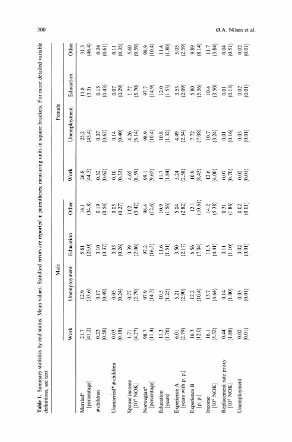
Tab

le1.Summarystatisticsbyendstatus.Meanvalues.Standarderrorsarereportedinparentheses;measuringunitsinsquarebrackets.Formoredetailedvariable

w

definitions,seetext

8

Male

Female

Work

Unemployment

Education

Other

Work

Unemployment

Education

Other

Married"

21.7

12.9

5.61

14.1

26.8

25.2

11.8

31.3

[percentage]

(41.2)

(33.6)

(23.0)

(34.8)

(44.3)

(43.4)

(3.3)

(46.4)

#children

0.23

0.17

0.10

0.19

0.32

0.37

0.15

0.34

(0.58)

(0.49)

(0.37)

(0.54)

(0.62)

(0.67)

(0.43)

(0.61)

Unmarried*#children

0.03

0.05

0.05

0.05

0.10

0.14

0.07

0.11

(0.18)

(0.24)

(0.26)

(0.27)

(0.33)

(0.40)

(0.29)

(0.35)

Spouseincome

1.71

0.77

0.39

1.02

4.65

4.26

1.77

5.60

[104NOKj

(4.27)

(2.79)

(2.06)

(3.42)

(8.59)

(8.14)

(5.70)

(9.59)

Norwegian"

98.7

97.9

97.2

98.4

99.1

98.9

97.7

98.9

[percentage]

(11.4)

(14.3)

(16.5)

(12.6)

(9.65)

(1M)

(14.9)

(10.4)

Education

11.3

10.5

11.6

10.9

11.7

10.8

12.0

11.4

[years]

(1.76)

(1.25)

(1.51)

(1.56)

(1.84)

(1.32)

(1.53)

(1.80)

ExperienceA

6.01

5.21

3.50

5.04

5.24

4.49

3.53

5.05

[yearswithp.p.]

(2.79)

(2.90)

(2.17)

(2.82)

(2.58)

(2.54)

(2.09)

(2.59)

ExperienceB

16.3

12.2

6.56

12.1

10.9

7.72

5.80

9.89

[p,p.]

(12.0)

(10.4)

(7.04)

(10.61)

(8.43)

(7.08)

(5.56)

(8.14)

Income

16.1

13.7

11.5

14.2

12.6

10.7

10.4

11.7

[104NOK]

(5.32)

(4.64)

(4.41)

(5.38)

(4.00)

(3.24)

(3.50)

(3.84)

Q

Replacementrateproxy

0.44

0.14

0.11

0.31

0.07

0.01

0.01

0.04

~[104NOK]

(1.88)

(1.00)

(1.10)

(1.86)

(0.70)

(0.16)

(0.13)

(0.51)

~

Unemployment

0.02

0.03

0.02

0.02

(;;'

0.02

0.03

0.02

0.02

'" i:l(0.01)

(0.01)

(0.01)

(0.01)

(0.01)

(0.01)

(0.01)

(0.01)

~ ~

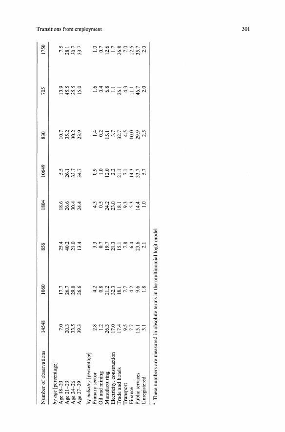
-lNumberofobservations

14548

1060

856

1804

10649

830

705

1750

.., I'> ::l =..b

yag

e[percentage]

o' ::lAge18-20

7.0

17.7

25.4

18.6

5.5

10.7

13.9

7.5

'"Age21-23

20.3

26.7

40.2

26.6

26.!

35.2

45.5

28.1

::;> 0Age24-26

33.5

29.0

21.0

30.4

33.7

30.2

25.5

30.7

S (1)

Age27-29

39.3

26.6

13.4

24.4

34.7

23.9

15.0

33.7

S '0by

indu

stry[percentage]

0" '<

Primarysector

2.8

4.2

3.3

4.3

0.9

1.4

1.6

1.0

S (1)Oilandmining

1.2

0.8

0.7

0.5

1.0

0.2

0.4

0.7

aManufacturing

26.3

21.2

19.7

24.2

12.0

15.1

6.8

12.6

Electricity,construction

17.0

32.3

21.3

23.0

2.2

3.7

1.1

1.7

Tradeandhotels

17.4

18.1

15.1

18.1

21.1

32.7

26.1

26.8

Transport

9.5

7.7

7.8

9.3

7.1

4.5

4.3

7.0

Finance

7.7

4.2

6.4

5.3

14.3

10.0

11.1

12.5

Publicservices

15.!

9.6

23.6

14.4

33.7

29.9

46.7

35.7

Unregistered

3.1

1.8

2.1

1.0

5.7

2.5

2.0

2.0

aThesenumbersaremeasuredinabsolutetermsinthemultinomiallogitmodel

t» S

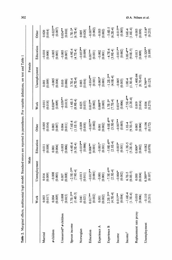
Tab

le2.Marginaleffects,multinomiallogitmodel.Standarderrorsarereportedinparentheses.Forvariabledefinitions,seetextandTableI

w 0 tv

Male

Female

Work

Unemployment

Education

Other

Work

Unemployment

Education

Other

Married

0.003

0.014

-0.011

-0.005

-0.011

0.001

-0.010

0.020

(0.017)

(0.009)

(0.008)

(0.014)

(0.018)

(0.009)

(0.008)

(0.014)

#children

0.004

-0.008

0.001

0.003

0.036**

-0.005

-0.005

-0.025**

(0.009)

(0.005)

(0.004)

(0.007)

(0.009)

(0.004)

(0.005)

(0.007)

Unmarried*#children

-0.008

0.007

-0.003

0.004

-0.039**

0.010

-0.005

0.034**

(0.015)

(0.008)

(0.006)

(0.011)

(0.013)

(0.006)

(0.007)

(0.010)

Spouseincome

3.7E-3**

-2.5E-3**

-4.4E-4

-7.6E-4

-1.4E-3

3.7E-4

-6.9E-4

I.7E-3*

(1.4E-3)

(7.9E-4)

(6.3E-4)

(I.IE-3)

(8.9E-4)

(4.7E-4)

(4.7E-4)

(6.7E-4)

Norwegian

0.041

-0.013

-0.019**

-0.009

0.025

0.003

-0.033**

0.005

(0.021)

(0.011)

(0.006)

(0.018)

(0.033)

(0.016)

(0.009)

(0.028)

Education

0.017**

-0.015**

0.006**

-0.007**

0.015**

-0.014**

0.007**

-0.007**

(0.002)

(0.001)

(0.001)

(0.002)

(0.002)

(0.001)

(0.001)

(0.002)

ExperienceA

0.001

-0.001

-0.001*

0.001

0.008**

-0.003*

-0.002

-0.003

(0.002)

(0.001)

(0.001)

(0.002)

(0.003)

(0.001)

(0.001)

(0.002)

ExperienceB

2.2E-3**

-7.3E-4**

-5.8E-4**

-9.0E-4**

1.7E-3*

-1.2E-3**

-4.7E-4

-5.6E-5

(4.5E-4)

(2.3E-4)

(2.IE-4)

(3.5E-4)

(7.7E-4)

(4.0E-4)

(3.9E-4)

(6.2E-4)

Income

0.015**

-0.004*

-0.003*

-0.007**

0.031**

-0.005

-0.011**

-0.015**

(0.004)

(0.002)

(0.001)

(0.003)

(0.006)

(0.003)

(0.002)

(0.005)

Income2

-1.6E-4

6.7E-5

-1.3E-5

I.IE-4

-7.5E-4**

1.0E-4

3.0E-4**

3.6E-4

Q(1.3E-4)

(8.0E-5)

(5.2E-5)

(9.3E-5)

(2.2E-4)

(1.3E-4)

(9.0E-5)

(I.8E-4)

~

Replacementrateproxy

-0.010

0.000

0.006*

0.005

0.019

-1.40E-04

-0.013

-0.005

~ u;

(0.006)

(0.004)

(0.002)

(0.004)

(0.014)

(8.7E-03)

(0.009)

(0.009)

'"0 '"Unemployment

-0.110

0.389**

-0.082

-0.196

0.034

0.799**

-0.320**

-0.514*

-(0.211)

(0.107)

(0.070)

(0.172)

(0.275)

(0.123)

(0.109)

(0.235)

~

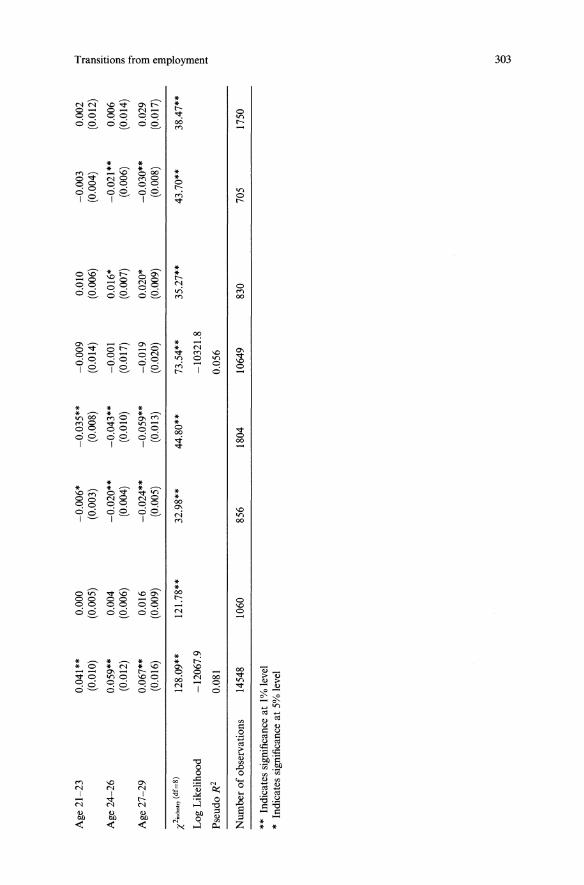
Age21-23

0.041**

0.000

-0.006*

-0.035**

-0.009

0.010

-0.003

0.002

--l ...

(0.010)

(0.005)

(0.003)

(0.008)

(0.014)

(0.006)

(0.004)

(0.012)

l» ::l f!l.

Age24-26

0.059**

0.004

-0.020**

-0.043**

-0.001

0.016*

-0.021**

0.006

g.(0.012)

(0.006)

(0.004)

(0.010)

(0.017)

(0.007)

(0.006)

(0.014)

::l '" ::;>

Age27-29

0.067**

0.016

-0.024**

-0.059**

-0.019

0.020*

-0.030**

0.029

0 3(0.016)

(0.009)

(0.005)

(0.013)

(0.020)

(0.009)

(0.008)

(0.017)

<1> 3

X2;""

"",,,

(df~8)

128.09**

121.78**

'E..

32.98**

44.80**

73.54**

35.27**

43.70**

38.47**

0 '<

LogLikelihood

-12067.9

-10321.8

3 <1> aPseudo

R2

0.081

0.056

Numberofobservations

14548

1060

856

1804

10649

830

705

1750

**IndicatessignificanceatI%level

*Indicatessignificanceat5%level

w o w

304 0.A. Nilsen et al.

may therefore be biased upwards. However, with due caution in interpreta­tion, our analysis does identify factors that affect the probability of enteringthe different states. Furthermore, the multinomial formulation aids a richerunderstanding of exits from work as compared to models with single exitroutes. For instance, the factors behind a decision to stay at home with chil­dren are different from those that may explain the transition from work tounemployment.

Family related variables. Although there are some surprises, family relatedcharacteristics confirm some traditional gender differences. The presence ofchildren has no significant effects on males, while females are affected. Formarried females there is a significant tendency to increase the probability ofstaying employed with increasing number of children, while the probability ofleaving the labour force decreases. These marginal effects of children areerased for unwed mothers. 3 However, remember that we are investigating thebehaviour of females that had chosen to work at the time. Labour force par­ticipation by a mother of several children is probably an indication of a highendowment of personal human resources. Non-participating mothers withmany children may not be as fortunate on the average, so selection effects mayplaya role. Increased spouse income increases the probability for women toleave the labour force. For males, the effect of increased spouse income isopposite, increasing the probability of staying in a job and decreasing theprobability of being unemployed. This pattern for the males may also be dueto selection, through assortative mating.

Other individual characteristics. Non-Norwegian citizenship increases theprobability of transiting from work to school, like in Table 1. Individuals withhigher education have higher chances of staying employed, and correspond­ingly, lower probability of being unemployed. In addition, we find that in­dividuals with a relative high education tend to take more education if leavinga job. All effects relating to education are statistically significant for bothmales and females. For the transition from work to other, the marginal effectsof education are negative and significant, while the coefficients are positiveand significant for both genders. This illustrates that the direct effects mea­sured by the estimated coefficients can deviate significantly from the marginaleffects due to competing risk, as shown in equation (2). However, this is theonly instance where we obtain such significant differences between coefficientsand marginal effects.With few exceptions, the age dummies show a monotonic increasing or

decreasing pattern, depending on the transition. For males, age increases theprobability of staying employed, and decreases the probability of taking moreeducation or ending in the unspecified group. For females, the effects of ageon the transition to education are similar to the ones for males, while age in­creases the probability of being unemployed. While age obviously is stronglyexogenous, it interacts in the regression with experience, income and othervariables that may be prone to potentially endogenous selection processes aswe have discussed earlier. For instance, when we run a regression for femaleswith only age dummies as regressors, age decreases the probability of becom­ing unemployed. While such a regression is misspecified, it inspires caution inthe interpretation of the results, both regarding age and obviously those vari­ables that are prone to selectivity.

Transitions from employment 305

Labour market variables. Increased experience is associated with a higherprobability of staying employed, and lower probabilities of entering all otherstates. For males, this effect is significant only for the aggregate pension pointexperience variable (Experience B). For females, both aggregate pensionpoints and number of years affect the probability of staying employed, ortransiting to unemployment, in a significant and expected manner. The mar­ginal effects of income are as expected both for males and females. Increasedincome increases the probability of staying employed and decreases the prob­ability of transiting to the other labour market states. There are some signifi­cant second order effects of income for females, while such effects are notpresent for males. The replacement rate proxy does not explain much. Thismay both result from low variance in the variable, and that income variablescatch some of the potential effects.A high local unemployment rate, not surprisingly, increases the probability

of becoming unemployed. However, it decreases the probability of droppingout of the labour force. This is one of the few observed patterns in Table 2that points at systematic differences in transitions to unemployment as com­pared to out of the labour force. In most instances, explanatory variablestend to influence all transitions out of employment in the same qualitativemanner. In this way, inspection of Table 2 does not reveal strong indicationsthat the recruitment processes to unemployment as compared to out ofthe labour forces are different. However, when we test whether all the mar­ginal effects are equal across two and two states by a chi-square test, the nullhypothesis of no differences are strongly rejected, in all states and for bothgenders.The industry chi-square test indicates that there are important sectoral

differences. These differences may be due to business cycles, since the demandand activity level varied substantially for different sectors and industries inthe period 1989-1991. In particular the construction industry experienced aserious recession these years. Finally, the data fit the multinomial logitmodel (measured by Pseudo R 2) somewhat better for males as compared tofemales.

Gender differences. Looking at the number of observations in each state inTable I, and the pattern of marginal effects in Table 2, we find that there aresignificant gender differences. To test what the driving forces behind thesedifferences are, we run a regression of the multinomiallogit model where thetwo sub-samples of males and females are merged. 4 We include a genderdummy (I if female, 0 otherwise) separately, in addition to interaction termsbetween the explanatory variables and this gender dummy.5 A significantinteraction indicates gender differences in transitions due to the explanatoryvariable concerned. We wish to explore gender differences in transitions fur­ther. To accommodate this, we group the interaction terms according to ourprevious labelling; family related variables, other individual characteristics,and labour market variables. For each of these groups, we run chi-square teststo evaluate gender differences in transitions to the end states. The chi-squaretests indicate that the family related variables are most important in explain­ing gender differences in the transits. However, the transition from work toeducation is an exception. For this latter transition, the labour market vari­ables are jointly statistically significant, while the family related variables arenot. Again, caution is in order. The summary statistics over end states, re-

306 0.A. Nilsen et al.

ported in Table I, reveal that both males and females returning to more edu­cation are less likely to have a family on their own. For instance, only 11.8%of females in the end state education are married, while the correspondingnumber in all other states is above 25%. Given that few individuals takingfurther education have a family, it may come as no great surprise that familyrelated variables are not significant explanatory factors in this transition. Thisconclusion is also borne out by the insignificant marginal effects of familyrelated variables for the end state education in Table 2. However, for all stateswhere the incidence of marriage is higher, family related variables are themost important factors explaining gender differences.

5. Conclusion

The results of our analysis can be interpreted in several directions. First, theindustry dummies and the local unemployment rate are highly significantvariables. This indicates that many exits may be due to insufficient demand insome sectors. Furthermore, our replacement rate proxy gives no indication ofadverse incentive effects from the social insurance system. However, theavailable data are not particularly well suited to reveal such effects. Second,experience as well as higher income increase the probability of staying em­ployed and decrease the probabilities of transiting to one of the three otherstates. One interpretation of these findings may be that it is not only importantto get youths into a job to secure future labour market participation. It is alsoimportant to hold a good job with a reasonable high income to reduce theprobability of future exits. This latter interpretation relies on exogenous in­come and experience variables. However, selectivity biases may operate here.If only the ablest of the youngsters manage to build experience in a well-paidjob, the benign effect of these observable characteristics is overstated. In themost extreme case, placing less able workers in well-paid jobs with high de­mands on skills may even produce the opposite results, i.e. higher exit rates.Finally, the numbers of years of education increase the probability of stayingemployed, and decrease the probability of being unemployed or ending in theresidual group. These results may be interpreted to support the clearly statedpolicy of the Norwegian labour market authorities to increase resources toeducation as a primary strategy to combat youth unemployment. However, itis not clear that the importance of education will be the same in a populationof youths where everyone has a higher education level both due to selectivitybias and potential job competition. 6

In recent years, the education pattern and labour market behaviour ofyoung males and females in Norway have displayed a converging pattern.Notice, for instance, that the mean education levels reported in Table I arehigher for females as compared to males in all destination groups. While theyoung males in this respect are lagging behind in educational attainments,traditional gender roles still matter for early labour market experiences.Family related variables, age, and experience still play a different role formales and females; and these differences are compatible with the hypothesisthat females still respond more in their labour market decisions to changeswithin the family.

Transitions from employment

Endnotes

I The pension points function is defined as:

307

{

i_ 9

pension points = 7 9 I i - 8g+--­3 9

8.33

where

9 = NOK 37300

if 9 ~ i ~ 8g

if 8g < i ~ 12g'

if i > 12g

i = income.2 The coefficients of the multinomiallogit are available from the authors upon request.3 The marginal effects of an increased number of children for unmarried women are -0.003 and-0.009 (work and other, respectively).

4 These results are not reported for sake of brevity, but are available from the authors uponrequest.

S The following model is estimated:

where bfiff is a vector of parameters which give the difference in the importance of the relevantregressors, and D('males is a dummy-variable taking the value. of one for females and zerootherwise. The coefficient vector will be bj for males and (bj + bfifJ) for females. We refer to thevariables that are different for males and females, Xj . Dremales, as the difference variables.

6 Further analysis is needed to resolve this issue. A relevant recent study is van Ours and Ridder(1995).

References

Ackum S (1991) Youth unemployment, labour market programmes and subsequent earnings.Scandinavian Journal ofEconomics 93:531-543

Card D, Sullivan D (1988) Measuring the effect of subsidized training programs on movements inand out of employment. Econometrica 56:497-530

Clark KB, Summers LH (1982) Labour force participation: Timing and persistence. Review ofEconomic Studies 49(5):825-844

Flinn C, Heckman J (1982) New methods for analyzing structural models oflabor force dynamics.Journal ofEconometrics 18(1):115-168

Goniil F (1992) New evidence on whether unemployment and out of the labor force are distinctstates. Journal ofHuman Resources 27(2):329-361

Layard R, Nickell S, Jackman R (1991) Unemployment. Oxford University Press, OxfordMeyer BD (1990) Unemployment insurance and unemployment spells. Econometrica 58:757-782NOS Population Statistics (1995) Statistical Yearbook 1995. Statistics Norway, NorwaySummers LH (1990) Understanding unemployment. MIT Press, Cambridge, MATorp H (1994) The impact of training on employment: Assessing a Norwegian labour marketprogramme. Scandinavian Journal ofEconomics 96:531-550

308 0.A. Nilsen et al.

Torp H (1996) Unemployment in Norway. In: Wadensjo E (ed) The Nordic labour markets in the1990's. Elsevier, Amsterdam, The Netherlands

van Ours JC, Ridder G (1995) Job matching and job competition: Are lower educated workers atthe back of job queues? European Economic Review 39(9):1717-1731

Winkelmann R (1997) How young workers get their training: A survey of German versus theUnited States. Journal of Population Economics 10(2):159-170

Parental disruption and the labour market performanceof children when they reach adulthood

Paul Fronstint, David H. GreenbergZ, Philip K. Robins3

'Employee Benefit Research Institute, 2121 K St., NW, Suite 600, Washington, DC, 20037, USA(Fax: +1-202-775-6312; email: fronstin@ebri.org)2University of Maryland, Baltimore County, Department of Economics, 1000 Hilltop Circle,Baltimore, MD 21250, USA (Fax: +1-410-455-1054; e-mail: dhgreenb@umbc.edu)3University of Miami, Department of Economics, P.O. Box 248126, Coral Gables, FL 33124,USA (Fax: +1-305-284-2985; e-mail: probins@miami.edu)

Received: 22 May I998/Accepted: 27 April 1999

Abstract. This paper uses data from the age 33 wave of the British NationalChild Development Survey (NCDS) to analyze the effects of a parental dis­ruption (divorce or death of a father) on the labour market performance ofchildren when they reach adulthood. The NCDS is a longitudinal study of allchildren born during the first week of March 1958 in England, Scotland, andWales. Controlling for a rich set of pre-disruption characteristics, the resultsindicate that a parental disruption leads to moderately less employmentamong males and considerably lower wage rates among females at age 33. Ifpre-disruption characteristics are not controlled for, larger effects are esti­mated for both males and females. Parental disruption also seems to causesubstantial reductions in educational attainment for both males and females.

JEL classification: JI2, 122, 124

Key words: Marital disruptions, labour supply, educational attainment, wagerates

1. Introduction

As is well known, the rise in parental marital disruptions in recent decades(i.e., a divorce or the death of a parent) has meant that children have becomeincreasingly likely to spend at least part of their childhood living in a single­parent household. 1 There is considerable evidence suggesting that living in

All correspondence to Philip K. Robins. This study was supported primarily by NICHD GrantHD25936. We thank Andrew Cherlin for his guidance and encouragement throughout the courseof this study and for his insightful comments on a previous draft. We are also grateful to twoanonymous referees for helpful comments. Responsible editor: John F. Ermisch.

310 P. Fronstin et al.

a disrupted family has short-run detrimental effects on children. However,comparatively little evidence exists concerning the longer-run effects of livingarrangements on children's labour market performance when they reachadulthood. Knowledge of such longer-run effects is important because, if theyexist, children who are subjected to a parental disruption will suffer a loss ofincome and society will lose productive output.The purpose of this paper is to examine the effects of parental disruption on

the labour market performance of children when they reach adulthood, usinga database (the British National Child Development Survey, or NCDS) thatfollows individuals from birth to age 33. We investigate whether a parentaldisruption affects the amount of formal education obtained and whether itaffects two labour market outcomes at age 33: hourly earnings and labourmarket status (i.e., whether individuals are employed, unemployed, or out ofthe labour force).The remainder of this paper is organized as follows. Section 2 discusses the

theoretical relationship between parental disruptions and adult labour marketperformance. Section 3 describes the NCDS and its advantages for examiningthe effects of parental disruption on labour market performance. Section 4reviews previous empirical studies of the effect of parental disruptions onadult labour market performance. Section 5 describes the methodology usedin the empirical analysis. Section 6 presents the findings. Finally, Sect. 7 offerssome conclusions.

2. The relation between parental marriage disruptions and adult labour marketperformance

There are at least three reasons why a parental marital disruption mightadversely affect the longer-term labour market performance of a child. First,income in the household in which the child grows up is likely to be lower,often much lower (Duncan and Hoffman 1985). Even if the absent parent isalive and provides child support, the economic cost of running two house­holds, rather than one, reduces the amount of income available to the child.As implied by the household production model developed by Becker andothers (see, for example, Becker 1981; Becker and Tomes 1986; and Michaeland Becker 1973), a decline in available income will reduce investments in thechild's human capital. Such a reduction in human capital may manifest itselfas a decrease in formal education, because the child is forced to leave schoolearlier than normal as a result of funding constraints and the need to obtainfull-time employment. It may also occur in other ways - for example, fewerprivate out-of-school lessons and living in less desirable neighborhoods withlower quality schools. These reduced investments in human capital may ulti­mately result in detrimental effects on the labour market performance of thechild when he or she reaches adulthood.A second adverse consequence is that a marital disruption tends to reduce

the amount of time parents devote to their children. The absent parent willprobably spend less time with his or her child, even if the cause of the dis­ruption is divorce, rather than death, and he or she exercises full visitationrights. Furthermore, the custodial parent may spend additional time partic­ipating in the labour market and, in addition, have more responsibilitieswithin the household. Consequently, the custodial parent may have less time

Labour market performance of children 311

to devote to the child. The household production model implies that thesereduced time inputs, like the diminished income, will decrease the humancapital of children - for example, there will be less opportunity for parents toserve as role models or to pass on their knowledge to their children.Third, a divorce or a parent's premature death may subject a child to

emotional stress that may negatively affect the child's labour market perfor­mance in later years. Emotional stress could be caused directly by the disrup­tion itself or from the changes in lifestyle that result - for example, from resi­dential moves and transfers to new schools.The emotional stress that may result from a parental disruption has some­

what different implications for children's labour market perfonnance as adultsthan do losses of income and time inputs. For example, the loss of incomeand time inputs may have larger effects if the disruption occurs at a younger,rather than an older, age simply because the loss of these inputs occurs over alonger time. It is not clear how the emotional stress that accompanies a maritaldisruption is related to the age at which the event occurs, but a longer passageof time between the event and adulthood may well allow for a fuller recovery.Furthennore, in the case of a divorce, there is evidence that non-custodialfathers maintain more contact with sons than with daughters (Hetherington etal. 1982) and provide more educational financing for sons than for daughters(Wallerstein and Corbin 1986). The emotional stress from the loss of a malerole model in the home might be greater for boys, however. In addition, lossesof income and time inputs are typically more severe if the disruption resultsfrom a parent's death, rather than from a divorce. Emotional stress, in con­trast, could be greater as the result of a divorce, especially if the child is caughtin the middle of a continuing struggle between the parents.Being subjected to a family disruption does not necessarily have an un­

ambiguously negative impact on the labour market perfonnance of childrenas adults. As adults, individuals may well be able to overcome apparentlydevastating events that occurred earlier in their lives. In addition, time spentwith some parents - for example, those that are active alcoholics or mentallyand physically abusing - may exert negative, rather than positive, influenceson children. Moreover, living in a household in which parents are in constantconflict may conceivably cause more emotional stress than living in a single­parent household. Furthennore, the impact of a parental disruption on thelabour market perfonnance of children may be mitigated to some degreeby the fact that the missing parent was a consumer of household inputs (i.e.,income and the remaining spouse's time), as well as a provider of inputs to hisor her children. Thus, the effect of a parental disruption on the labor marketperfonnance of children when they reach adulthood becomes ultimately anempirical question.

3. Data

To investigate the effects of marital disruptions on the labour market perfor­mance of children when they reach adulthood, we use the National ChildDevelopment Survey (NCDS). The NCDS is a longitudinal study of all Britishchildren born during the first week of March 1958 in England, Scotland, andWales. A total of 17,414 mothers, representing 98% of all births occurring thatweek, were interviewed (Shepherd 1985).2 The original purpose of the survey

312 P. Fronstin et al.

was to identify social and obstetric factors associated with stillbirth and deathin early infancy, but the survey was later expanded to measure other importanteconomic and social phenomena associated with the interviewed parents andchildren.The first three follow-up interviews were conducted when the children were

ages 7 (n = 15,458), II (n = 15,503), and 16 (n = 14,761). These ages werechosen because they represented important transition points in the Britishschool system for individuals born in 1958. On each occasion, wide-ranginginformation was collected from the parents, teachers, and school medicalofficers. In 1981, a professional survey research organization was used to traceand re-interview the children, who at this time were age 23. A sample of12,537 young adults participated in the 1981 interview. All four interviews (atages 7, 11, 16, and 23) collected detailed information on the socioeconomic andpsychological characteristics of the parents and children.The fifth and most recent follow-up interview was conducted in 1991, when

sample members were age 33. Over 13,400 cohort members were traced,although only 11,407 interviews were ultimately conducted (Ferri 1993). (The84% response rate among those traced to age 33 is reasonable given the com­prehensiveness of the questionnaires and the great demands placed on the timeof the respondents.) As is evident, the combined effects of adulthood and thelengthy period between interviews resulted in substantial sample attrition. 3

The fifth followup interview was the first to ask detailed questions aboutearnings and work experience. In addition, a question about parental disrup­tion and the age at which a disruption occurred was asked of all respondents.The NCDS provides researchers an unprecedented opportunity to learn

about the effects of parental disruption on adult labour market performance,while being able to control for other factors that also affect labour marketperformance. Because of the long time span covered by the NCDS, parentaldisruptions at earlier stages of life and labour market performance at a laterprime-age stage in life can both be observed. With the wealth of data collectedby the NCDS, it is possible to control for children's psychological andintellectual functioning and family socioeconomic status prior to a parentaldisruption.4 In addition, the size of the sample allows researchers to distin­guish between disruptions that result from the death of the parent and thosethat stem from parental divorce and between impacts on sons and those ondaughters. Finally, the NCDS is ideal for investigating whether the age atwhich the disruption occurred influences the size of effects resulting from thedisruption. One disadvantage of the NCDS is that detailed information aboutfamily income is not available.

4. Previous studies

Numerous studies of the long-term effects ofmarital disruptions on children inboth Britain and the United States have now been conducted. Most of thesestudies are concerned with divorce; studies of the long-term consequences ofthe death of a parent are comparatively rare, although sometimes disruptionsthat occur as a result of either divorce or death are combined into a singleexplanatory variable. Moreover, most previous studies focus on the effects ofdivorce on children's educational attainment. Until very recently, only a fewstudies examined effects on labour market outcomes. For example, in a meta-

Labour market performance of children 313

analysis of studies of the long-tenn consequences of parental divorce, Amatoand Keith (1991) found 18 studies that examine educational attainment.In contrast, they did not find any studies of the effects of divorce on labourmarket status or earnings. However, they did uncover nine studies thatexamined outcomes that tend to be correlated with earnings - for example,occupational status, job autonomy, and job satisfaction. (Blau and Duncan's(1967) study of the relation between divorce, educational attainment, andoccupational status was the first of these.) Moreover, they excluded studies byMueller and Cooper (1986) that used unemployment status as an outcome,Wadsworth and Maclean (1986) that used income, and Greenberg and Wolf(1982) and Krein (1986), that used earnings.Nonetheless, it seems evident that before the 1990s studies of the effects

of divorce on children's labour market status and earnings were fairly rare.Perhaps stimulated by increases in divorce rates and improvements in avail­able data, the number of such studies greatly expanded during the 1990s.Examples include Haveman et at. (1991), Peters (1992), Wojtkiewicz (1993),Garasky (1995), Grogger and Ronan (1995), Lillard and DeCicca (1995),Couch and Lillard (1995), Kiernan (1997), Francesconi and Ennisch (1998),Gregg and Machin (1998), and Boggess (1998).Although they do not always obtain statistically significant findings, pre­

vious studies consistently imply that the effects of parental divorce on educa­tional attainment, employment, unemployment, occupational quality, andearnings are adverse. However, the estimated effects are usually moderate.For example, Amato and Keith's sample of studies implied that a parentaldivorce caused educational attainment to fall by a bit over one-quarter of astandard deviation and occupational quality to fall by just over one-tenth of astandard deviation. 5 In addition, Amato and Keith found that studies thatused control variables to take account of pre-divorce family economic statusand parental characteristics obtained substantially smaller estimated effectsthan studies that did not use such controls.The NCDS offers some important advantages over the data sets used in

many previous studies of parental disruption on adult labour market perfor­mance. First, many (but not all) previous studies were based on limited in­fonnation on family circumstances prior to the parental disruption. Therefore,it is difficult to detennine whether estimates of detrimental effects on the childare linked to the disruption itself or merely to family and individual conditionsthat existed before the disruption. 6 For example, if earnings appear to benegatively related to parental divorce, it is important to distinguish whetherthis is due to the divorce event itself or due instead to having lived in an intact,but possibly, dysfunctional family prior to the divorce. The NCDS containsricher infonnation than is available in most data sets covering individualsduring their childhood, pennitting one to better make such a distinction.A second important advantage of the NCDS is that it follows children

for a longer period of time than most panel studies. The data used in many(although far from all) previous studies only allow children to be observedduring early adulthood, a time when their careers may still be in consider­able flux. Even the education data for the sampled population is incompletein some studies and, thus, the measure of educational attainment that is usedis restricted to a simple indicator of high school graduation. More impor­tantly, in studies that use earnings as an outcome, this variable is often mea­sured while the individuals sampled were still in their 20s. (See, for example,

314 P. Fronstin et al.

Greenberg and Wolf 1982, Peters 1992, Grogger and Ronan 1995, and Lillardand DeCicca 1995.) Earnings this early in the life cycle may be only weaklyrelated to earnings during prime-age. Moreover, the effects of a parental dis­ruption may fade over time and, thus, be stronger in one's 20s than later inlife. As previously indicated, the NCDS measures the educational attainment,earnings, and labour market status of individuals at age 33.A third advantage of the NCDS is that it allows investigation of whether

the age at which the disruption occurred influences the size of effects resultingfrom the disruption. We found only two non-NCDS studies that do this. 7

Lillard and DeCicca (1995), who used U.S. data, compare the effects ofmarital disruption on the earnings of two groups of male children: those forwhom the disruption occurred between ages 14 and 21 and those for whomthe disruption occurred between ages 22 and 25. They find larger effects forthe younger group. Francesconi and Ermisch (1998), who used British data,distinguish among three groups of children who spent at least part of theirchildhood in a single parent family: those who began their spell in a singleparent family between the ages of zero and 5, those who began between 6and 10, and those who began between II and 16. They examine a numberof outcomes, including educational attainment and unemployment, and findevidence that children who lived in a single parent family early in life expe­rienced the largest adverse effects as adults.Given the advantages of the NCDS for examining the effects of parental

disruption on education and adult labour market outcomes, it is not surprisingthat two studies in addition to ours have used the NCDS for this purpose:Gregg and Machin (1998) and Kiernan (1997).8 However, our study focusesexclusively on education and labour market outcomes, while the other twostudies examine additional outcomes as well. Furthermore, our study placesgreater emphasis on formal tests of whether competing model specificationsare statistically different than do the other two studies.The objectives of Gregg and Machin's 1998 study differ from those of our

study. They are concerned with how a broad range of factors associated withchildhood disadvantage, only one of which is parental marital disruption,affect various outcomes at ages 16, 23, and 33. Thus, while we examinewhether the effects of parental disruption vary with the age at which it occursand with whether it results from divorce or death, they do not. Consequently,they estimate the effects of disruption using a single dummy variable, while weuse a number of variables to distinguish among divorce, death of a parent,and the age of the disruption. To construct their disruption variable, theyassigned a value of one to individuals who ever lived in a single parent familybefore age 16, but whose families never faced economic difficulty during thisperiod, and a value of zero to all other persons. 9 Thus, effects that are esti­mated with this variable pertain only to persons who experienced parentaldisruption, but not economic hardship, as children. Such individuals may beatypical products of disruption.Gregg and Machin find that these individuals had a lower level of educa­

tional attainment than other persons did. They also find that males (but notfemales) who lived in single parent families as children had higher unemploy­ment at age 23 and received lower hourly wages at age 33 (but not at age 23).Kiernan (1997) focuses exclusively on parental divorce, while we examine

parental death, as well as divorce. Her objectives, however, are similar to ours.Like us, she is interested in whether disadvantages that children of divorce

Labour market performance of children 315

have as adults are attributable to the divorce itself or to factors that antecedethe disruption. In addition, both her study and our study examine whether theage at which a parental divorce occurs influences the size of effects of divorceon children as adults. Unlike our study, however, she does not use formalstatistical tests to examine this issue. In conducting her study, Kiernan firstconstructs several dichotomous measures of educational and labour marketoutcomes - specifically, whether at age 33 individuals have no educationalqualifications, have high level qualifications, were unemployed, and haveearnings in the upper quartile. She then runs logistic regressions on thesemeasures and reports the resulting odds ratios. As will be seen, we use asomewhat different specification of educational and labor market outcomes.Kiernan finds that children whose parents divorced before they were 16 are

worse off than other adults at age 33 in terms of most (but not all) the edu­cation and labour market outcomes she examines. However, she also findsthat these effects usually diminish, or even disappear, when family circum­stances that existed before the divorce, especially financial circumstances, aretaken into account. This suggests that the children of divorce not only fareworse because of the divorce itself, but also because they were worse off beforethe divorce occurred. Finally, Kiernan finds that parental divorce occurringafter men were 21 is associated with reduced levels of educational attainmentand increased levels of unemployment. Similar associations were not foundfor women, however. As will be seen, there are both important similarities anddifferences between our findings and Kiernan's.

5. Methodology

5.1. Outcomes analyzed

As indicated earlier, we analyze two labour market outcomes at age 33 - grosshourly earnings (or wage rates) and labour market status. 10 We also examinethe effects of parental disruption on educational attainment. The means ofthese outcomes are presented in Table I. Following previous studies, as wellas the previously mentioned evidence that income and time input losses fromdivorce are greater for girls than for boys, separate analyses of the outcomesare conducted for males and females. (Previous research by Cherlin et aI.(1991) found that the effect of parental divorce or separation on behavioraland educational outcomes differed for boys and girls.)We use the multinomial logit model to estimate the effects of parental dis­

ruption on adult labour market status. A 3-choice model is estimated for males(employed, unemployed, and not in the labour force), and a 4-choice model isestimated for females (employed full-time, employed part-time, unemployed,and not in the labour force). According to Table I, 90.6% of the males in oursample were employed at age 33, 6.6% were unemployed, and 2.8% were notin the labour force. Less than 1% of the males was employed part-time (notshown in Table I) and that is why we do not distinguish between full-time andpart-time employment for males. Females were much more likely than malesto be employed part-time and they were much more likely to be out of thelabour force. Specifically, 35.3% of the women were employed full-time,3I.2% were employed part-time, 2.3% were unemployed, and 3I.2% were notin the labour force.

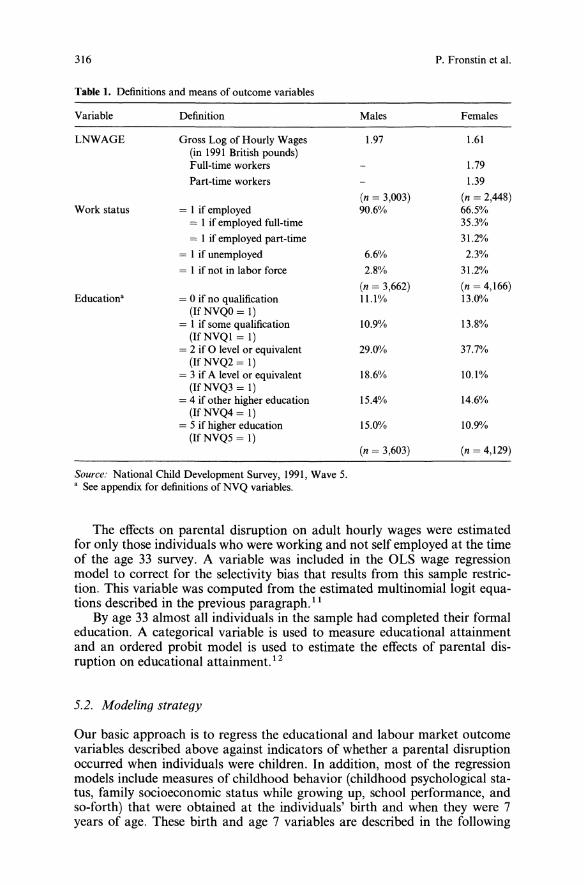
316 P. Fronstin et al.

Table 1. Definitions and means of outcome variables

Variable Definition Males Females

LNWAGE Gross Log of Hourly Wages 1.97 1.61(in 1991 British pounds)Full-time workers 1.79

Part-time workers 1.39

(n = 3,003) (n = 2,448)Work status = I if employed 90.6% 66.5%

= I if employed full-time 35.3%

= I if employed part-time 31.2%

= I if unemployed 6.6% 2.3%

= 1 if not in labor force 2.8% 31.2%

(n = 3,662) (n = 4,166)Education' = 0 if no qualification 11.1% 13.0%

(IfNVQO= I)= 1 if some qualification 10.9% 13.8%(IfNVQI = I)= 2 if 0 level or equivalent 29.0% 37.7%(If NVQ2 = 1)= 3 if A level or equivalent 18.6% 10.1%(If NVQ3 = 1)

= 4 if other higher education 15.4% 14.6%(IfNVQ4 = 1)= 5 if higher education 15.0% 10.9%(If NVQ5 = 1)

(n = 3,603) (n = 4,129)

Source: National Child Development Survey, 1991, Wave 5., See appendix for definitions of NVQ variables.

The effects on parental disruption on adult hourly wages were estimatedfor only those individuals who were working and not self employed at the timeof the age 33 survey. A variable was included in the OLS wage regressionmodel to correct for the selectivity bias that results from this sample restric­tion. This variable was computed from the estimated multinomial logit equa­tions described in the previous paragraph. 11

By age 33 almost all individuals in the sample had completed their formaleducation. A categorical variable is used to measure educational attainmentand an ordered probit model is used to estimate the effects of parental dis­ruption on educational attainment. 12

5.2. Modeling strategy

Our basic approach is to regress the educational and labour market outcomevariables described above against indicators of whether a parental disruptionoccurred when individuals were children. In addition, most of the regressionmodels include measures of childhood behavior (childhood psychological sta­tus, family socioeconomic status while growing up, school performance, andso-forth) that were obtained at the individuals' birth and when they were 7years of age. These birth and age 7 variables are described in the following

Labour market performance of children 317

subsection. They are included in the regressions to control for children's psy­chological and intellectual functioning and family socioeconomic status priorto age 7, as these factors may be correlated with both parental disruption andchildren's labour market performance as adults.This modeling strategy raises a serious issue that must be dealt with in

estimation. Parental disruptions occur when children are at different ages. Asa consequence, variables in the NCDS are measured prior to the disruptionfor some individuals and subsequent to the disruption for others. Compare,for example, a 33-year-old male whose parents divorced before he was age 7with one whose parents divorced between the time he was ages 7 and 11. Thechildhood psychological and socioeconomic status variables at age 7 will bemeasured post-divorce for the first individual, but pre-divorce for the secondindividual. Thus, the age 7 childhood status variables for the first individualwill probably be influenced by the divorce event, but the age 7 childhood sta­tus variables for the second individual should not be influenced by the divorceevent (although they could be influenced by factors that caused the divorce).Consequently, if both individuals are included in the same regression, it willbe extremely difficult to interpret the estimated coefficients on these variables.We employ an estimation strategy that circumvents this endogeneity

problem. In many of the regression specifications we report, the sample isrestricted to only individuals whose parents were intact at age 7. 13 Becausethe control variables are measured at birth and at age 7, they can be includedin these regressions without introducing endogeneity into the estimated co­efficients. 14 Other regressions that we report, however, are estimated for asample that includes individuals whose parents were not intact at birth or atage 7. We avoid endogeneity in these regressions by limiting the independentvariables to those that are truly exogenous. For example, only disruptionvariables are included in regressions based on samples that include individualswhose parents were not intact at birth; other control variables are omitted.Similarly, only variables measured at birth in addition to the disruption vari­ables are used as explanatory variables in regressions based on samples in­cluding individuals whose parents were intact at birth, but not necessarily atage 7.The main sample used to estimate labour market status at age 33 consists

of 4,166 females and 3,662 males. This sample includes all individuals inter­viewed at age 33 whose parents were intact at age 7 and who had valid dataon parental divorce and death, hourly earnings, and work status. 15 The wageequations are estimated for a sub-group of this sample - namely, those whoworked at age 33. To minimize the missing data problem for explanatoryvariables other than the disruption variables, each explanatory variable inour regressions is paired with a dummy variable equaling 1 whenever the ex­planatory variable has a missing value, and 0 otherwise. The explanatoryvariables are set equal to 0 whenever their value is missing. 16In a few specifications of the labour market outcome regressions, educa­

tion is included as an explanatory variable. Because education is measuredat age 33, it is likely to be endogenous with respect to parental disruptionsoccurring earlier. The purpose of estimating these models is to determine theextent to which the effects of parental disruptions on labour market outcomesare attributable to the effects of disruption on educational attainment. Becauseof the potential for endogeneity, these results should be interpreted withcaution. (Estimating a simultaneous equation model that takes into account

318 P. Fronstin et al.

the endogeneity of education is beyond the scope of the present paper. AsFrancesconi and Ermisch (1998) demonstrate, finding a suitable instrumentalvariable for education to enable identification is difficult.)

5.3. Explanatory variables

Summary statistics for the explanatory variables are given in Table 2. Adescription of the construction of selected explanatory variables is given in theAppendix (for further details, see Cherlin et al. 1995). The explanatory vari­ables are of three types: parental disruption variables, control variables mea­sured at birth, and control variables measured at age 7.The parental disruption variables, which are the major variables of interest

in this study, consist of a set of dummy variables denoting whether a parentaldivorce or father's death1? occurred at various ages (DVO, DV06, DV710,DV1115, DV1622, DV2333, DTHOI5, and DTHI622).18 In addition, we alsoestimate partially constrained models in which a single divorce dummy(whether the individual's parents ever divorced, DV) and a single deathdummy (whether the individual's father ever died, DTH) are used in place ofthe age-specific dummies. Finally, we also estimate fully constrained modelsthat replace the DV and DTH variables with a single disruption dummy(DISRUPT), which indicates whether a disruption occurred, regardless ofthe age at which it occurred or whether it was due to a parental divorce or afather's death.The control variables measured at birth consist of the age of the mother

(MOMAGE), the age difference between the mother and the father (AGE­DIFF), the birth weight of the child (BIRTHWGT),19 the time between theparent's marriage and the mother's first birth (INTERVALl-INTERVAL4),whether the mother was single at first pregnancy (INTERVALO), the mater­nal grandfather's social class (MGCLASS1, MGCLASS2, MGMINER),whether the maternal grandfather was dead or away (MGDEAD), the num­ber of persons in the household per room (PERSPROOM), and the occupa­tional social class of the father (FSOC-CLASSI and FSOC-CLASS2). Inaddition, there is a set of variables denoting whether the mother worked dur­ing pregnancy and, if she did, the number of weeks she worked (PREGNO­WORK, PREGWORK1, PREGWORK2, and PREGWORK3). The age 7variables consist of measures of behavioral problems (BEHPROB7), read­ing achievement scores (READTEST7), arithmetic achievement scores(MATHTEST7), and school performance (SCHPER7). The age 7 variablesalso include measures that denote whether the mother's or father's educationexceeds the minimum (MOMEDUC and DADEDUC), the age the father leftschool (AGELEFT), and the birth order of the child (YOUNG2, OLDEST2,YOUNG3, MIDDLE3, OLDEST3).

6. Results

Seven different models are estimated to determine the effects of parental dis­ruption on education and labour market outcomes. One of the models uses thefull sample of families at birth, including both intact and non-intact families,

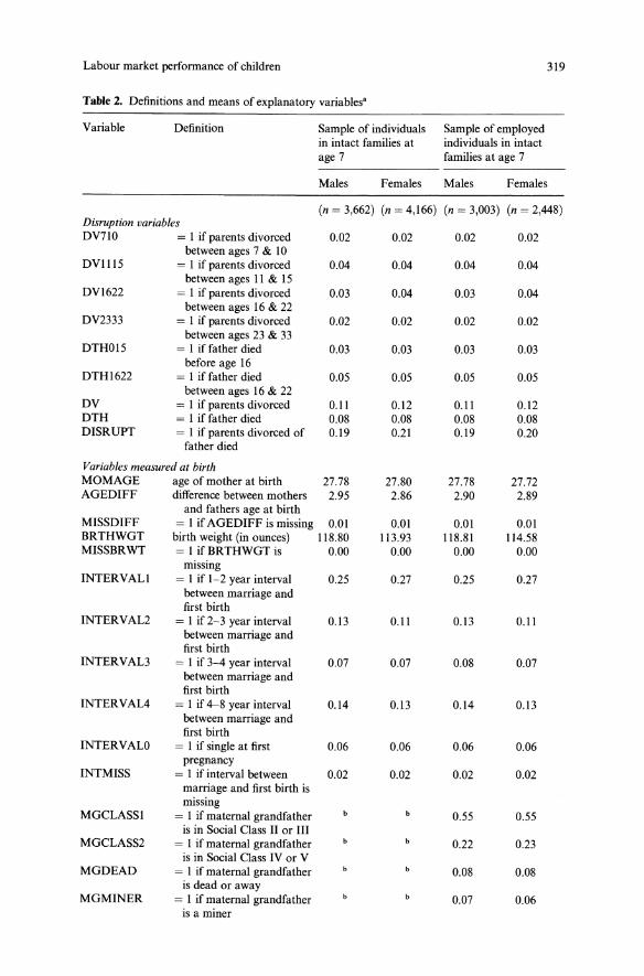
Labour market performance of children 319

Table 2. Definitions and means of explanatory variables'

Variable Definition Sample of individuals Sample of employedin intact families at individuals in intactage 7 families at age 7

Males Females Males Females

(n = 3,662) (n = 4,166) (n = 3,003) (n = 2,448)Disruption variablesDV710 = I if parents divorced 0.02 0.02 0.02 0.02

between ages 7 & 10DVII15 = I if parents divorced 0.04 0.04 0.04 0.04

between ages 11 & 15DVI622 = I if parents divorced 0.03 0.04 0.03 0.04

between ages 16 & 22DV2333 = I if parents divorced 0.02 0.02 0.02 0.02

between ages 23 & 33DTHOl5 = I if father died 0.03 0.03 0.03 0.03

before age 16DTHI622 = I if father died 0.05 0.05 0.05 0.05

between ages 16 & 22DV = I if parents divorced 0.11 0.12 0.11 0.12DTH = I if father died 0.08 0.08 0.08 0.08DISRUPT = I if parents divorced of 0.19 0.21 0.19 0.20

father died

Variables measured at birthMOMAGE age of mother at birth 27.78 27.80 27.78 27.72AGEDIFF difference between mothers 2.95 2.86 2.90 2.89

and fathers age at birthMISSDIFF = I if AGEDIFF is missing 0.01 0.01 0.01 0.01BRTHWGT birth weight (in ounces) 118.80 113.93 118.81 114.58MISSBRWT = I if BRTHWGT is 0.00 0.00 0.00 0.00

missingINTERVALI = I if 1-2 year interval 0.25 0.27 0.25 0.27

between marriage andfirst birth

INTERVAL2 = I if 2-3 year interval 0.13 0.11 0.13 0.11between marriage andfirst birth

INTERVAU = I if 3-4 year interval 0.07 0.07 0.08 0.07between marriage andfirst birth

INTERVAL4 = I if 4-8 year interval 0.14 0.13 0.14 0.13between marriage andfirst birth

INTERVALO = I if single at first 0.06 0.06 0.06 0.06pregnancy

INTMISS = 1 if interval between 0.02 0.02 0.02 0.02marriage and first birth ismissing

MGCLASSI = I ifmaternal grandfather 0.55 0.55is in Social Class II or III

MGCLASS2 = I if maternal grandfather 0.22 0.23is in Social Class IV or V

MGDEAD = I if maternal grandfather 0.08 0.08is dead or away

MGMINER = I if maternal grandfather 0.07 0.06is a miner

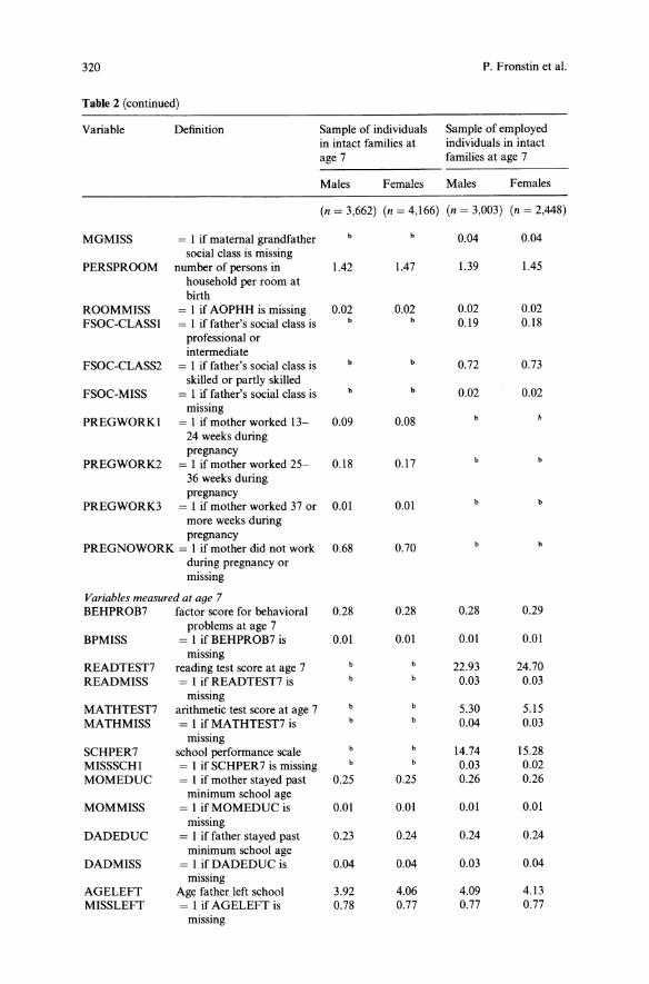
320 P. Fronstin et al.

Table 2 (continued)

Variable Definition Sample of individuals Sample of employedin intact families at individuals in intactage 7 families at age 7

Males Females Males Females

(n = 3,662) (n = 4,166) (n = 3,003) (n = 2,448)

MGMISS = I if maternal grandfather 0.04 0.04social class is missing

PERSPROOM number of persons in 1.42 1.47 1.39 1.45household per room atbirth

ROOMMISS = I if AOPHH is missing 0.02 0.02 0.02 0.02FSOC-CLASSI = I if father's social class is b 0.19 0.18

professional orintermediate

FSOC-CLASS2 = I if father's social class is 0.72 0.73skil\ed or partly skilled

FSOC-MISS = I if father's social class is 0.02 0.02missing

PREGWORKI = I if mother worked 13- 0.09 0.0824 weeks duringpregnancy

PREGWORK2 = I if mother worked 25- 0.18 0.1736 weeks duringpregnancy

PREGWORK3 = I if mother worked 37 or 0.01 0.01more weeks duringpregnancy

PREGNOWORK = I if mother did not work 0.68 0.70during pregnancy ormissing

Variables measured at age 7BEHPROB7 factor score for behavioral 0.28 0.28 0.28 0.29

problems at age 7BPMISS = I if BEHPROB7 is 0.01 0.01 0.01 0.01

missingREADTEST7 reading test score at age 7 22.93 24.70READMISS = I if READTEST7 is 0.03 0.03

missingMATHTEST7 arithmetic test score at age 7 5.30 5.15MATHMISS = I if MATHTEST7 is 0.04 0.03

missingSCHPER7 school performance scale 14.74 15.28MISSSCHI = I if SCHPER7 is missing 0.03 0.02MOMEDUC = I if mother stayed past 0.25 0.25 0.26 0.26

minimum school ageMOMMISS = I if MOMEDUC is 0.01 0.01 0.01 0.01

missingDADEDUC = I if father stayed past 0.23 0.24 0.24 0.24

minimum school ageDADMISS = I if DADEDUC is 0.04 0.04 0.03 0.04

missingAGELEFT Age father left school 3.92 4.06 4.09 4.13MISSLEFT = I if AGELEFT is 0.78 0.77 0.77 0.77

missing

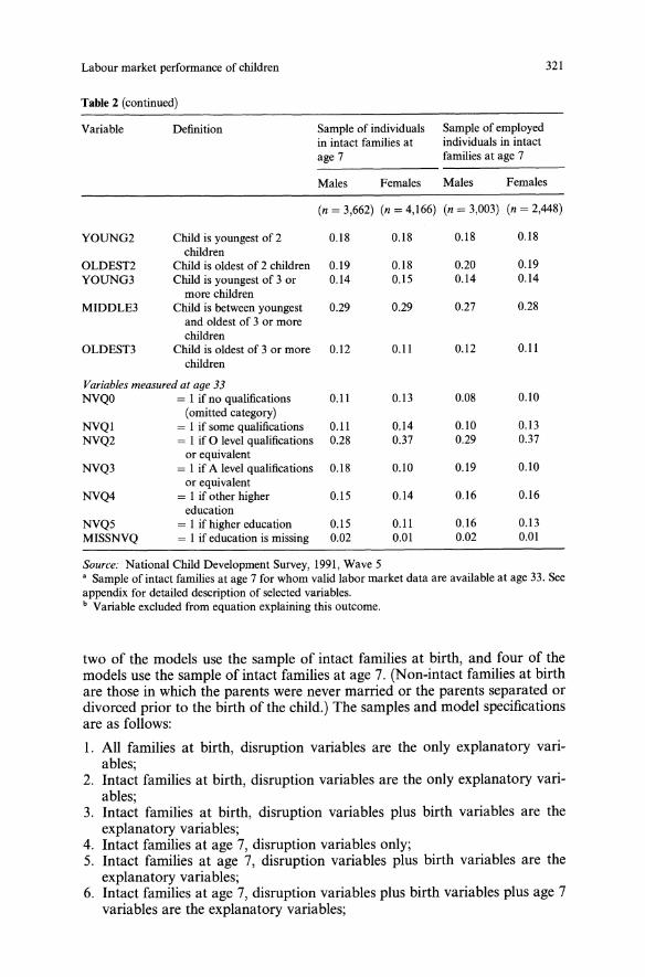
Labour market performance of children

Table 2 (continued)

321

Variable Definition Sample of individualsin intact families atage 7

Sample of employedindividuals in intactfamilies at age 7

Males Females Males Females

(n = 3,662) (n = 4,166) (n = 3,003) (n = 2,448)

YOUNG2 Child is youngest of 2 0.18 0.18 0.18 0.18children

OLDEST2 Child is oldest of 2 children 0.19 0.18 0.20 0.19YOUNG3 Child is youngest of 3 or 0.14 0.15 0.14 0.14

more childrenMIDDLE3 Child is between youngest 0.29 0.29 0.27 0.28

and oldest of 3 or morechildren

OLDESn Child is oldest of 3 or more 0.12 0.11 0.12 0.1lchildren

Variables measured at age 33NVQO = I if no qualifications 0.11 0.13 0.08 0.10

(omitted category)NVQI = I if some qualifications 0.1l 0.14 0.10 0.13NVQ2 = I if 0 level qualifications 0.28 0.37 0.29 0.37

or equivalentNVQ3 = I if A level qualifications 0.18 0.10 0.19 0.10

or equivalentNVQ4 = I if other higher 0.15 0.14 0.16 0.16

educationNVQ5 = I if higher education 0.15 0.11 0.16 0.13MISSNVQ = I if education is missing 0.02 0.01 0.02 om

Source: National Child Development Survey, 1991, Wave 5• Sample of intact families at age 7 for whom valid labor market data are available at age 33. Seeappendix for detailed description of selected variables.b Variable excluded from equation explaining this outcome.

two of the models use the sample of intact families at birth, and four of themodels use the sample of intact families at age 7. (Non-intact families at birthare those in which the parents were never married or the parents separated ordivorced prior to the birth of the child.) The samples and model specificationsare as follows:

I. All families at birth, disruption variables are the only explanatory vari­ables;

2. Intact families at birth, disruption variables are the only explanatory vari­ables;

3. Intact families at birth, disruption variables plus birth variables are theexplanatory variables;

4. Intact families at age 7, disruption variables only;5. Intact families at age 7, disruption variables plus birth variables are theexplanatory variables;

6. Intact families at age 7, disruption variables plus birth variables plus age 7variables are the explanatory variables;

322 P. Fronstin et al.

7. Intact families at age 7, disruption variables plus birth variables plus age 7variables plus age 33 education variables are the explanatory variables.

A comparison ofModels 1 and 2 provides an indication ofwhether exclud­ing non-intact families at birth alters the effects of a parental disruption. Acomparison of Models 2 and 3 provides an indication of whether controllingfor pre-disruption characteristics at the time of the birth of the child altersthe independent effects of disruption. A comparison of Models 2 and 4 pro­vides an indication of whether the effects of parental disruption on labourmarket outcomes are altered by restricting the sample to families that wereintact at age 7. A comparison of Models 4 and 5 provides an indication ofwhether controlling for pre-disruption characteristics at the time of the birthof the child alters the independent effects of disruption on the age 7 intactsample. A comparison of Models 5 and 6 provides an indication of whethercontrolling for pre-disruption characteristics between the time of birth and age7 alters the independent effects of disruption on the age 7 intact sample.Finally, a comparison of Models 6 and 7 provides an indication of whetherthe effects of parental disruption on labour market outcomes are mitigated byeffects on education. Of course, when education is the outcome, Model 7 isnot estimated.As indicated above, the effects of disruption are captured by a series of

dummy variables representing the age range during which a disruptionoccurred. Specifically, in keeping with the survey design, we distinguishamong divorces occurring between the ages of zero and 6, 7 and 10, 11 and 15,16 and 22, and 23 and 33. Because there are few deaths of a father prior to age15, we only distinguish between deaths occurring from ages 0 to 15 and fromages 16 to 22 (recall that the NCDS does not contain information about thedeath of a father after the child reaches age 22). As indicated earlier, much ofthe sociological and psychological literature suggests that the size of the effectsof parental disruption depends on whether the disruption occurs in early orlate childhood, the type of disruption (divorce or death), and the sex of thechild (Cherlin et at. 1991). We explicitly test for differences in the effects ofdisruption by age and type of disruption, but we maintain separate analysesfor males and females.

6.1. Effects on educational attainment

Table 3 presents the estimated effects of disruption on educational attain­ment at age 33. Both the fully unconstrained and the constrained disrup­tion coefficients are reported. Chi-square statistics for the test of equality ofthe disruption coefficients across the various age and disruption categoriesare also reported. The full set of coefficient estimates for the unconstrainedversion of Model 6 is presented in Appendix Tables A.l (for males) and A.2(for females).2oAs Table 3 indicates, males and females that grew up in a family that

experienced a marital disruption have significantly lower levels of educationalattainment. Even after controlling for the effects of individual characteristicsmeasured at birth and at age 7 (Model 6), both males and females who expe­rienced a marital disruption have lower levels of education. In the case ofmales, this effect is reduced by about three fifths after controlling for the birth

Labour market performance of children 323

and age 7 variables (Model 4 versus Model 6). Although in Models 4-6 wecannot reject the hypothesis of a constant disruption effect across disruptiontypes, most of the effect for males appears to be due to a parental divorce thatoccurred between the ages of 7 and 15.21 A statistically significant effect of afather's death (almost equal in magnitude to the effect of a parental divorce)becomes statistically insignificant after controlling for family circumstancesat age 7 (e.g., comparing Model 6 with ModelS). The results for the effectsof disruptions subsequent to age 7 do not appear to be sensitive to restrictingthe estimation sample to families intact at age 7. Moreover, it appears thatdivorce at younger ages (but subsequent to birth) has an effect similar to thatbetween ages 7 and 10.In the case of females, the effect is reduced by about two fifths when we

control for pre-disruption characteristics (Models 4 and 6). Unlike males, wecan reject the hypothesis of a constant disruption effect across age and dis­ruption type for females for all models except Model 6. As in the case ofmales, most of the effect for females is due to a divorce that occurred beforeage 16. In addition, the effect of the death of a father prior to age 16 is alsostatistically significant. Like males, the results for females do not appear to bevery sensitive to restricting the sample to intact families at age 7. However, theeffects of divorce between the ages 0 and 6 appear to be slightly larger than theeffects of a divorce between the ages of 7 and 15. Unlike males, the effect of afather's death remains for females even after controlling for family circum­stances at age 7.Table 4 uses the ordered probit coefficients in the unconstrained specifica­

tion of Models 1-6 to determine which levels of education are affected by aparental divorce occurring between the ages of 7 and 10 and II and 15 (thecoefficients are statistically significant for both males and females). As all sixmodel specifications reported in the table indicate, parental divorce causes anincrease in the probability of not going beyond the lower education levels(that is, levels 0-2; see the Appendix for definitions) for both males andfemales and a decrease in the probability of reaching the higher educationlevel (levels 3-5). For example, in the case of a divorce between the ages of 7and 10 for Model 6, there is about a 5-percentage point lower probability ofattaining education level 5 for males and about a 4 percentage point lowerprobability of attaining the same education level for females (first degree,postgraduate diploma, masters, Ph.D.). As indicated by Table 2, this is abouta one-third reduction for both males and females. Clearly, a parental divorceoccurring before age 16 for boys and girls has substantial adverse con­sequences on ultimate educational attainment.Our finding that a parental disruption adversely affects educational attain­

ment is consistent with the results of previous studies. The fact that the effectfor both males and females is substantially reduced when we control for pre­disruption family circumstances illustrates the importance of accounting forsuch family circumstances when drawing inferences about the effects ofa parental disruption on educational attainment. In this sense, our resultsagree with those of Kiernan (1997), who finds that families that experience adivorce are generally worse off before the disruption occurred. Unlike mostprevious studies, we have examined the effect of a father's death on educa­tional attainment. We find that females, but not males, appear to be adverselyaffected by a father's death, particularly when the death occurs before thechild's 16th birthday.

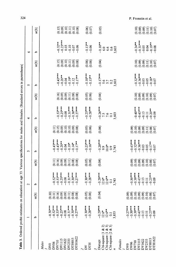
Tab

le3.Orderedprobitestimatesoneducationatage33.Variousspecificationsformalesandfemales.(Standarderrorsinparentheses)

\H N .j>.

23

45

6

bse(b)

bse(b)

bse(b)

bse(b)

bse(b)

bse(b)

Mal

esI DVO

-0.30"*

(0.10)

DV06

-0.52*"

(0.11)

-0.52"*

(0.11)

-0.43"*

(0.11)

DV710

-0.53***

(0.16)

-0.53***

(0.16)

-0.43***

(0.15)

-0.53***

(0.16)

-0.43***

(0.15)

-0.32**

(0.15)

DVII15

-0.25*"

(0.09)

-0.25***

(0.09)

-0.20**

(0.09)

-0.25***

(0.09)

-0.20**

(0.09)

-0.23***

(0.09)

DVI622

-0.08

(0.09)

-0.08

(0.09)

-0.04

(0.10)

-0.08

(0.09)

-0.04

(0.10)

0.03

(0.10)

DV2333

-0.31***

(0.11)

-0.31***

(0.11)

-0.19*

(0.10)

-0.31***

(0.11)

-0.19*

(0.11)

-0.10

(0.11)

DTHOl5

-0.30***

(0.08)

-0.30***

(0.08)

-0.14*

(0.09)

-0.30***

(0.09)

-0.12

(0.09)

-0.07

(0.10)

DTHI622

-0.27***

(0.08)

-0.27***

(0.08)

-0.17**

(0.08)

-0.27***

(0.08)

-0.17**

(0.08)

-0.06

(0.08)

2 DV

-0.30"*

(0.05)

-0.30***

(0.05)

-0.23***

(0.05)

-0.25***

(0.05)

-0.18***

(0.06)

-0.13**

(0.06)

DT

H-0.28***

(0.06)

-0.28***

(0.06)

-0.16***

(0.06)

-0.28***

(0.06)

-0.15"

(0.06)

-0.06

(0.07)

3 Disrupt

-0.29***

(0.04)

-0.29***

(0.04)

-0.20***

(0.04)

-0.26***

(0.04)

-0.17***

(0.04)

-0.10**

(0.05)

Chi-square(I

&2)

12.6*

12.6*

9.9

7.5

5.6

6.0

Chi-square(1

&3)

12.6**

12.6**

10.8*

7.6

5.7

6.6

Chi-square(2

&3)

0.1

0.1

0.9

0.1

0.2

0.6

n3,853

3,743

3,743

3,603

3,603

3,603

Fem

ales

1 DVO

-0.27***

(0.09)

:-0DV06

-0.50***

(0.09)

-0.50***

(0.09)

-0.43***

(0.09)

'Tl

DV710

-0.39***

(0.10)

-0.39***

(0.10)

-0.32***

(0.10)

-0.40***

(0.10)

-0.32***

(0.10)

-0.24**

(0.10)

.., 0DVlII5

-0.43***

(0.09)

-0.43"*

(0.09)

-0.36***

(0.09)

-0.43***

(0.09)

-0.36***

(0.09)

-0.31***

(0.09)

., ~.DVI622

-0.13

(0.09)

-0.13

(0.09)

-0.03

(0.09)

-0.13

(0.09)

-0.03

(0.09)

-0.05

(0.09)

.,DV2333

-0.11

(0.10)

-0.11

(0.10)

-0.05

(0.11)

-0.11

(0.10)

-0.05

(0.11)

0.04

(0.11)

~

DTHOl5

-0.23***

(0.08)

-0.23***

(0.08)

-0.17**

(0.08)

-0.20**

(0.09)

-0.18*

(0.10)

-0.19**

(0.10)

~

DTHI622

-0.09

(0.07)

-0.09

(0.07)

-0.07

(0.07)

-0.09

(0.07)

-0.07

(0.07)

-0.08

(0.07)

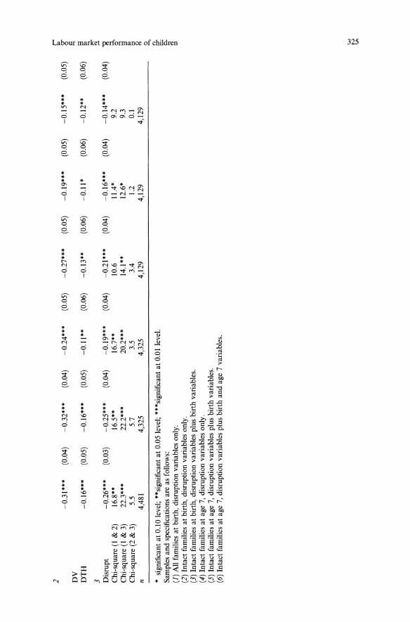
2-0.31***

(0.04)

-0.32***

(0.04)

-0.24***

DV

DT

H-0.16***

(0.05)

-0.16***

(0.05)

-0.11**

3 Disrupt

-0.26***

(0.03)

-0.25***

(0.04)

-0.19***

Chi-square(I

&2)

16.8**

16.5**

16.7**

Chi-square(I

&3)

22.3***

22.2***

20.2***

Chi-square(2

&3)

5.5

5.7

3.5

n4,481

4,325

4,325

*significantat0.10level;**significantat0.05level;***significantat0.01level.

Samplesandspecificationsareasfollows:

(1)Allfamiliesatbirth,disruptionvariablesonly.

(2)Intactfamiliesatbirth,disruptionvariablesonly.

(3)Intactfamiliesatbirth,disruptionvariablesplusbirthvariables.

(4)Intactfamiliesatage7,disruptionvariablesonly.

(5)Intactfamiliesatage7,disruptionvariablesplusbirthvariables.

(6)Intactfamiliesatage7,disruptionvariablesplusbirthandage7variables.

l:""'

l>J

(0.05)

-0.27***

(0.05)

-0.19***

(0.05)

-0.15***

(0.05)

r:T 0 '"....

(0.06)

-0.13**

(0.06)

-0.11*

(0.06)

-0.12**

(0.06)

3 l>J .... :0<"~

(0.04)

-0.21***

(0.04)

-0.16***

(0.04)

-0.14***

(0.04)

~10.6

11.4*

9.2

.... 0'14.1**

12.6*

9.3

33.4

1.2

0.1

l>J i:l

4,129

4,129

4,129

@ 0 ...., (") :r. c: Cil i:l W N VI

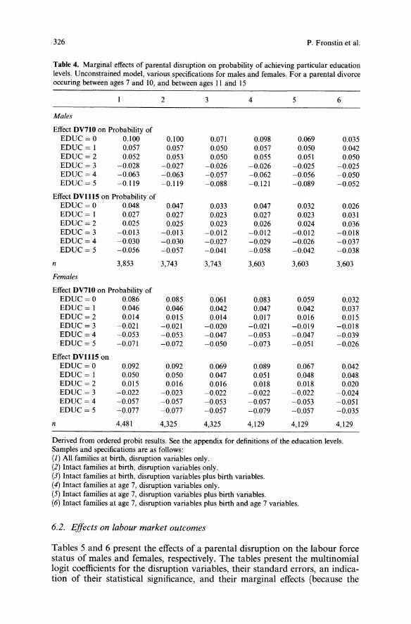
326 P. Fronstin et al.

Table 4. Marginal effects of parental disruption on probability of achieving particular educationlevels. Unconstrained model, various specifications for males and females. For a parental divorceoccuring between ages 7 and 10, and between ages II and 15

2 3 4 5 6

Males

Effect DV710 on Probability ofEDUC=O 0.100 0.100 0.071 0.098 0.069 0.035EDUC= I 0.057 0.057 0.050 0.057 0.050 0.042EDUC=2 0.052 0.053 0.050 0.055 0.051 0.050EDUC = 3 -0.028 -0.027 -0.026 -0.026 -0.Q25 -0.025EDUC=4 -0.063 -0.063 -0.057 -0.062 -0.056 -0.050EDUC = 5 -0.119 -0.119 -0.088 -0.121 -0.089 -0.052

Effect DVl11S on Probability ofEDUC = 0 0.048 0.047 0.033 0.047 0.032 0.026EDUC= I 0.027 0.027 0.023 0.027 0.023 0.031EDUC=2 0.Q25 0.025 0.023 0.026 0.024 0.036EDUC = 3 -0.013 -0.013 -0.012 -0.012 -0.012 -0.018EDUC=4 -0.030 -0.030 -0.027 -0.029 -0.026 -0.037EDUC= 5 -0.056 -0.057 -0.041 -0.058 -0.042 -0.Q38

n 3,853 3,743 3,743 3,603 3,603 3,603

Females

Effect DV710 on Probability ofEDUC=O 0.086 0.085 0.061 0.083 0.059 0.032EDUC= I 0.046 0.046 0.042 0.047 0.042 0.037EDUC=2 0.014 0.015 0.014 0.017 0.016 O.oI5EDUC = 3 -0.021 -0.021 -0.020 -0.021 -0.019 -0.018EDUC=4 -0.053 -0.053 -0.047 -0.053 -0.047 -0.039EDUC= 5 -0.071 -0.072 -0.050 -0.073 -0.051 -0.026

Effect DVll1S onEDUC=O 0.092 0.092 0.069 0.089 0.067 0.042EDUC= I 0.050 0.050 0.047 0.051 0.048 0.048EDUC=2 0.015 0.016 0.016 0.018 0.018 0.020EDUC= 3 -0.022 -0.023 -0.022 -0.022 -0.022 -0.024EDUC=4 -0.057 -0.057 -0.053 -0.057 -0.053 -0.051EDUC= 5 -0.077 -0.077 -0.057 -0.079 -0.057 -0.035

n 4,481 4,325 4,325 4,129 4,129 4,129

Derived from ordered probit results. See the appendix for definitions of the education levels.Samples and specifications are as follows:(1) All families at birth, disruption variables only.(2) Intact families at birth, disruption variables only.(3) Intact families at birth, disruption variables plus birth variables.(4) Intact families at age 7, disruption variables only.(5) Intact families at age 7, disruption variables plus birth variables.(6) Intact families at age 7, disruption variables plus birth and age 7 variables.

6.2. Effects on labour market outcomes

Tables 5 and 6 present the effects of a parental disruption on the labour forcestatus of males and females, respectively. The tables present the multinomiallogit coefficients for the disruption variables, their standard errors, an indica­tion of their statistical significance, and their marginal effects (because the

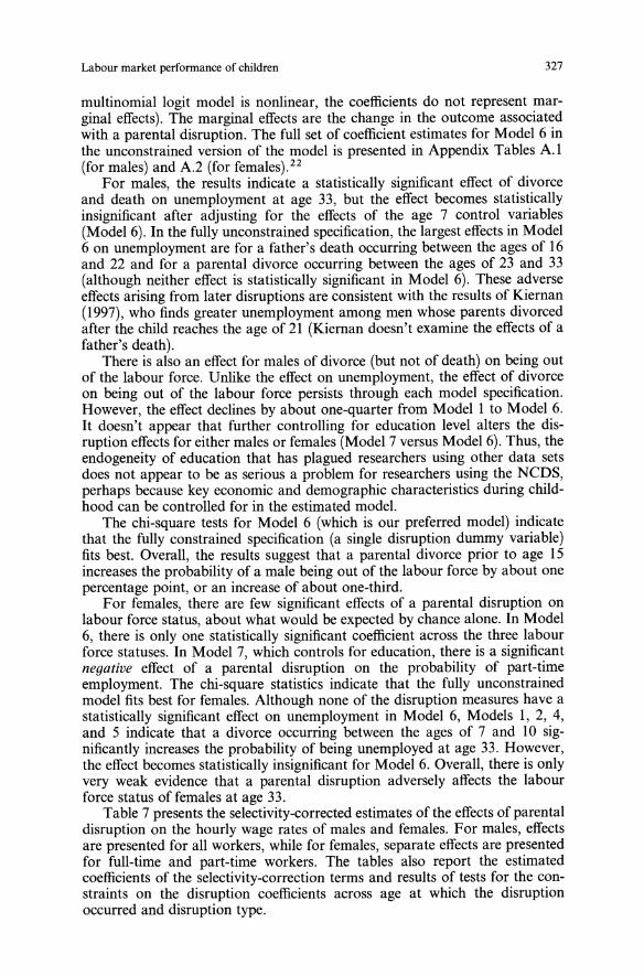
Labour market performance of children 327

multinomial logit model is nonlinear, the coefficients do not represent mar­ginal effects). The marginal effects are the change in the outcome associatedwith a parental disruption. The full set of coefficient estimates for Model 6 inthe unconstrained version of the model is presented in Appendix Tables A.l(for males) and A.2 (for females). 22

For males, the results indicate a statistically significant effect of divorceand death on unemployment at age 33, but the effect becomes statisticallyinsignificant after adjusting for the effects of the age 7 control variables(Model 6). In the fully unconstrained specification, the largest effects in Model6 on unemployment are for a father's death occurring between the ages of 16and 22 and for a parental divorce occurring between the ages of 23 and 33(although neither effect is statistically significant in Model 6). These adverseeffects arising from later disruptions are consistent with the results of Kiernan(1997), who finds greater unemployment among men whose parents divorcedafter the child reaches the age of 21 (Kiernan doesn't examine the effects of afather's death).There is also an effect for males of divorce (but not of death) on being out

of the labour force. Unlike the effect on unemployment, the effect of divorceon being out of the labour force persists through each model specification.However, the effect declines by about one-quarter from Model 1 to Model 6.It doesn't appear that further controlling for education level alters the dis­ruption effects for either males or females (Model 7 versus Model 6). Thus, theendogeneity of education that has plagued researchers using other data setsdoes not appear to be as serious a problem for researchers using the NCDS,perhaps because key economic and demographic characteristics during child­hood can be controlled for in the estimated model.The chi-square tests for Model 6 (which is our preferred model) indicate

that the fully constrained specification (a single disruption dummy variable)fits best. Overall, the results suggest that a parental divorce prior to age 15increases the probability of a male being out of the labour force by about onepercentage point, or an increase of about one-third.For females, there are few significant effects of a parental disruption on

labour force status, about what would be expected by chance alone. In Model6, there is only one statistically significant coefficient across the three labourforce statuses. In Model 7, which controls for education, there is a significantnegative effect of a parental disruption on the probability of part-timeemployment. The chi-square statistics indicate that the fully unconstrainedmodel fits best for females. Although none of the disruption measures have astatistically significant effect on unemployment in Model 6, Models 1, 2, 4,and 5 indicate that a divorce occurring between the ages of 7 and 10 sig­nificantly increases the probability of being unemployed at age 33. However,the effect becomes statistically insignificant for Model 6. Overall, there is onlyvery weak evidence that a parental disruption adversely affects the labourforce status of females at age 33.Table 7 presents the selectivity-corrected estimates of the effects of parental

disruption on the hourly wage rates of males and females. For males, effectsare presented for all workers, while for females, separate effects are presentedfor full-time and part-time workers. The tables also report the estimatedcoefficients of the selectivity-correction terms and results of tests for the con­straints on the disruption coefficients across age at which the disruptionoccurred and disruption type.

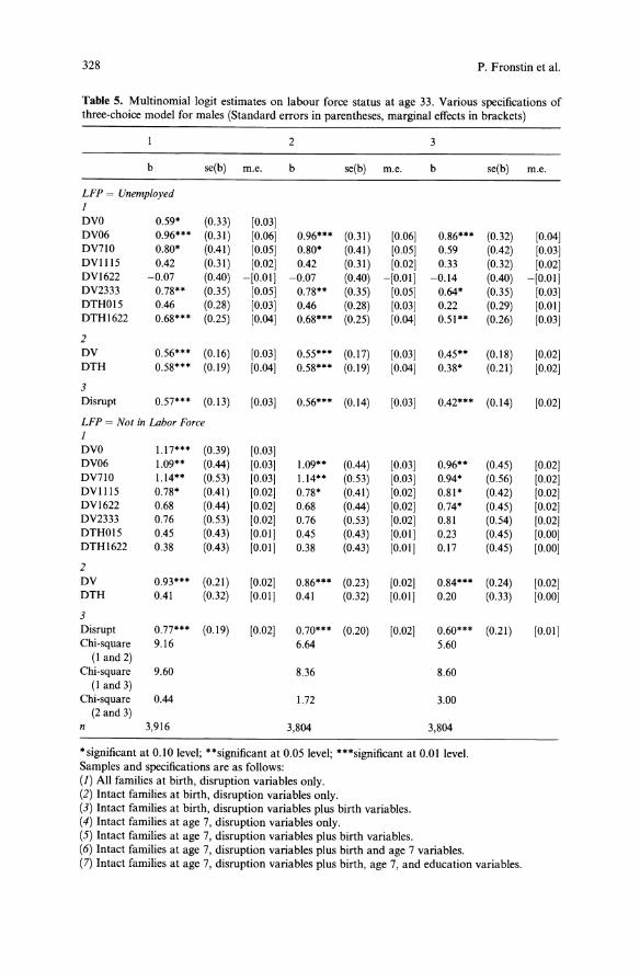
328 P. Fronstin et al.

Table 5. Multinomial logit estimates on labour force status at age 33. Various specifications ofthree-choice model for males (Standard errors in parentheses, marginal effects in brackets)

2 3

b se(b) m.e. b se(b) m.e. b se(b) m.e.

LFP = UnemployedJDVO 0.59* (0.33) [0.03]DV06 0.96*** (0.31) [0.06] 0.96*** (0.31) [0.06J 0.86*** (0.32) [0.04]DV710 0.80* (0.41) [0.05] 0.80* (0.41) [0.05] 0.59 (0.42) [0.03]DVII15 0.42 (0.31) [0.02] 0.42 (0.31) [0.02J 0.33 (0.32) [0.02]DVI622 -0.07 (0.40) -[0.01] -0.07 (0.40) -[0.01] -0.14 (0.40) -[O.OIJDV2333 0.78** (0.35) [0.05] 0.78** (0.35) [0.05J 0.64* (0.35) [0.03]DTHOl5 0.46 (0.28) [0.03] 0.46 (0.28) [0.03J 0.22 (0.29) [0.01]DTHI622 0.68*** (0.25) [0.04] 0.68*** (0.25) [O.04J 0.51** (0.26) [0.03]

2DV 0.56*** (0.16) [0.03] 0.55*** (0.17) [0.03] 0.45** (0.18) [0.02]DTH 0.58*** (0.19) [O.04J 0.58*** (0.19) [0.04] 0.38* (0.21) [0.02]

3Disrupt 0.57*** (0.13) [0.03] 0.56*** (0.14) [0.03] 0.42*** (0.14) [0.02]

LFP = Not in Labor ForceIDVO 1.17*** (0.39) [0.03]DV06 1.09** (0.44) [0.03] 1.09** (0.44) [0.03] 0.96** (0.45) [0.021DV710 1.14** (0.53) [0.03J 1.14** (0.53) [0.03] 0.94* (0.56) [0.02]DVII15 0.78* (0.41) [0.02] 0.78* (0.41) [0.02] 0.81* (0.42) [0.02JDVI622 0.68 (0.44) [0.021 0.68 (0.44) [0.02] 0.74* (0.45) [0.02)DV2333 0.76 (0.53) [0.02] 0.76 (0.53) [0.02] 0.81 (0.54) [0.02JDTHOl5 0.45 (0.43) [0.01] 0.45 (0.43) [0.01] 0.23 (0.45) [O.OOJDTHI622 0.38 (0.43) [0.01] 0.38 (0.43) [0.01] 0.17 (0.45) [0.00]

2DV 0.93*** (0.21) [0.02] 0.86*** (0.23) [0.02] 0.84*** (0.24) [0.02JDTH 0.41 (0.32) [0.01] 0.41 (0.32) [0.011 0.20 (0.33) [O.OOJ

3Disrupt 0.77*** (0.19) [0.02] 0.70*** (0.20) [0.02] 0.60*** (0.21) [0.01]Chi-square 9.16 6.64 5.60(I and 2)

Chi-square 9.60 8.36 8.60(I and 3)

Chi-square 0.44 1.72 3.00(2 and 3)

n 3,916 3,804 3,804

*significant at 0.10 level; **significant at 0.05 level; ***significant at 0.0 I level.Samples and specifications are as follows:(1) All families at birth, disruption variables only.(2) Intact families at birth, disruption variables only.(3) Intact families at birth, disruption variables plus birth variables.(4) Intact families at age 7, disruption variables only.(5) Intact families at age 7, disruption variables plus birth variables.(6) Intact families at age 7, disruption variables plus birth and age 7 variables.(7) Intact families at age 7, disruption variables plus birth, age 7, and education variables.

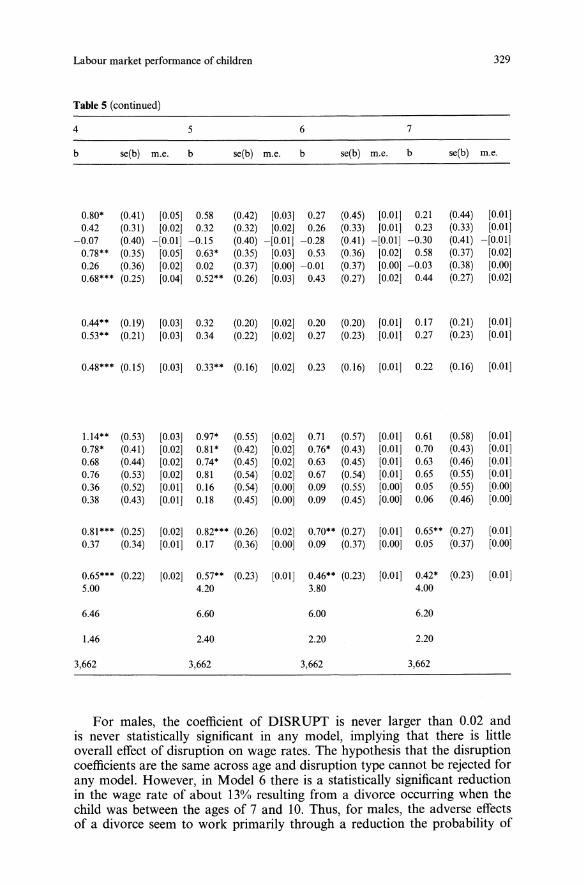
Labour market performance of children

Table 5 (continued)

329

4

b

5

se(b) m.e. b

6

se(b) m.e. b

7

se(b) m.e. b se(b) m.e.

0.80* (0.41) [0.05J 0.58 (0.42) [0.03] 0.27 (0.45) [0.01] 0.21 (0.44) [0.01]0.42 (0.31) [0.02J 0.32 (0.32) [0.02J 0.26 (0.33) [0.01] 0.23 (0.33) [0.01]-0.07 (0.40) -[0.01] -0.15 (0.40) -[0.01] -0.28 (0.41) -[0.01] -0.30 (0.41) -[0.0110.78** (0.35) [0.05] 0.63* (0.35) [0.03] 0.53 (0.36) [0.02] 0.58 (0.37) [0.02]0.26 (0.36) [0.02] 0.02 (0.37) [0.00] -0.01 (0.37) [0.00] -0.03 (0.38) [0.00]0.68*** (0.25) [0.04] 0.52** (0.26) [0.03] 0.43 (0.27) [0.02] 0.44 (0.27) [O.02J

0.44** (0.19) [0.03] 0.32 (0.20) [0.02] 0.20 (0.20) [0.01] 0.17 (0.21) [0.01]0.53** (0.21) [0.03] 0.34 (0.22) [0.02] 0.27 (0.23) [0.01] 0.27 (0.23) [0.01]

0.48*** (0.15) [0.03] 0.33** (0.16) [0.02] 0.23 (0.16) [0.01] 0.22 (0.16) [0.01]

1.14** (0.53) [0.03] 0.97* (0.55) [0.02] 0.71 (0.57) [0.01] 0.61 (0.58) [0.01]0.78* (0.41) [0.02] 0.81* (0.42) [0.02] 0.76* (0.43) [0.01] 0.70 (0.43) [0.01]0.68 (0.44) [0.02] 0.74* (0.45) [0.02] 0.63 (0.45) [0.01] 0.63 (0.46) [0.01]0.76 (0.53) [0.02] 0.81 (0.54) [0.02] 0.67 (0.54) [0.01] 0.65 (0.55) [0.01]0.36 (0.52) [0.01] 0.16 (0.54) [0.00] 0.09 (0.55) [0.00] 0.05 (0.55) [0.00]0.38 (0.43) [0.01] 0.18 (0.45) [O.ooJ 0.09 (0.45) [O.ooJ 0.06 (0.46) [0.00]

0.81 *** (0.25) [0.02] 0.82*** (0.26) [0.02] 0.70** (0.27) [O.OIJ 0.65** (0.27) [0.01]0.37 (0.34) [0.01] 0.17 (0.36) [0.00] 0.09 (0.37) [O.ooJ 0.05 (0.37) [0.00]

0.65*** (0.22) [0.02] 0.57** (0.23) [0.01] 0.46** (0.23) [0.01] 0.42* (0.23) [0.01]5.00 4.20 3.80 4.00

6.46 6.60 6.00 6.20

1.46 2.40 2.20 2.20

3,662 3,662 3,662 3,662

For males, the coefficient of DISRUPT is never larger than 0.02 andis never statistically significant in any model, implying that there is littleoverall effect of disruption on wage rates. The hypothesis that the disruptioncoefficients are the same across age and disruption type cannot be rejected forany model. However, in Model 6 there is a statistically significant reductionin the wage rate of about 13% resulting from a divorce occurring when thechild was between the ages of 7 and 10. Thus, for males, the adverse effectsof a divorce seem to work primarily through a reduction the probability of

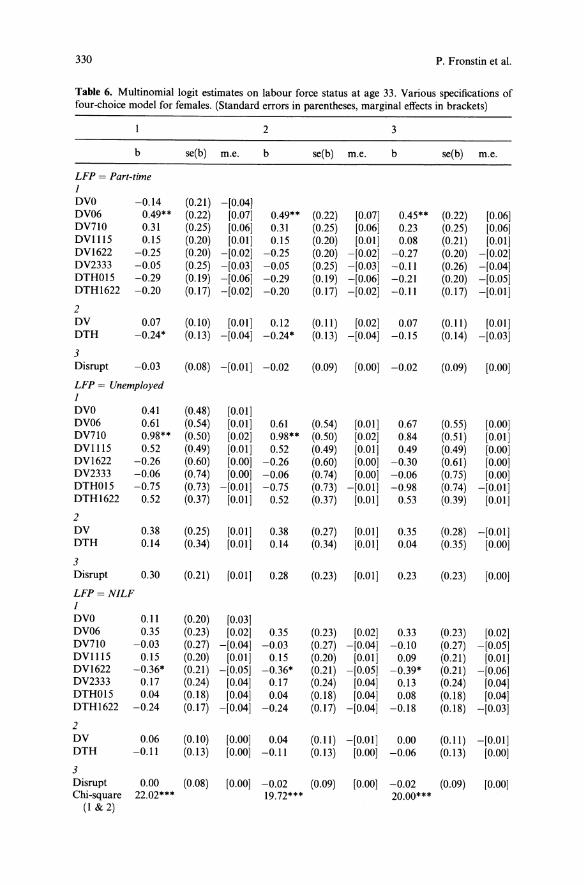
330 P. Fronstin et al.

Table 6. Multinomial logit estimates on labour force status at age 33. Various specifications offour-choice model for females. (Standard errors in parentheses, marginal effects in brackets)

2 3

b se(b) m.e. b se(b) m.e. b se(b) m.e.

LFP = Part-time1DVO -0.14 (0.21) -[O.04JDV06 0.49** (0.22) [0.07J 0.49** (0.22) [0.07] 0.45** (0.22) [0.06]DV710 0.31 (0.25) [0.06] 0.31 (0.25) [0.06J 0.23 (0.25) [0.06JDVII15 0.15 (0.20) [O.OIJ 0.15 (0.20) [O.OIJ 0.08 (0.21) [0.01]DVI622 -0.25 (0.20) -[0.02] -0.25 (0.20) -[0.02J -0.27 (0.20) -[0.02]DV2333 -0.05 (0.25) -[0.03] -0.05 (0.25) -[0.03] -0.11 (0.26) -[0.04]DTHOl5 -0.29 (0.19) -[0.06] -0.29 (0.19) -[0.06] -0.21 (0.20) -[0.05]DTHI622 -0.20 (0.17) -[0.02] -0.20 (0.17) -[0.02J -0.11 (0.17) -[0.01]

2DV 0.Q7 (0.10) [0.01] 0.12 (0.11) [0.02J 0.07 (0.11) [0.01]DTH -0.24* (0.13) -[0.04] -0.24* (0.13) -[O.04J -0.15 (0.14) -[0.031

3Disrupt -0.03 (0.08) -[0.01] -0.02 (0.09) [O.OOJ -0.02 (0.09) [0.00]

LFP = Unemployed1DVO 0.41 (0.48) [0.01]DV06 0.61 (0.54) [0.01] 0.61 (0.54) [0.01] 0.67 (0.55) [0.00]DV710 0.98** (0.50) [0.02] 0.98** (0.50) [0.02J 0.84 (0.51) [0.01]DVI1I5 0.52 (0.49) [0.01] 0.52 (0.49) [0.01] 0.49 (0.49) [O.OOJDVI622 -0.26 (0.60) [0.00] -0.26 (0.60) [0.00] -0.30 (0.61) [O.OOJDV2333 -0.06 (0.74) [O.OOJ -0.06 (0.74) [0.00] -0.06 (0.75) [0.001DTHOl5 -0.75 (0.73) -[0.01] -0.75 (0.73) -[0.01] -0.98 (0.74) -[0.01]DTHI622 0.52 (0.37) [0.01] 0.52 (0.37) [0.01] 0.53 (0.39) [O.OIJ

2DV 0.38 (0.25) [0.01] 0.38 (0.27) [0.01] 0.35 (0.28) -[O.OIJDTH 0.14 (0.34) [0.01] 0.14 (0.34) [0.01] 0.04 (0.35) [O.OOJ

3Disrupt 0.30 (0.21) [0.011 0.28 (0.23) [0.01] 0.23 (0.23) [0.00]

LFP= NILF1DVO 0.11 (0.20) [O.03JDV06 0.35 (0.23) [0.02] 0.35 (0.23) [0.02] 0.33 (0.23) [0.02]DV710 -0.03 (0.27) -[O.04J -0.03 (0.27) -[0.04] -0.10 (0.27) -[0.05]DVII15 0.15 (0.20) [0.011 0.15 (0.20) [0.01] 0.09 (0.21) [0.01]DVI622 -0.36* (0.21) -[0.05] -0.36* (0.21) -[0.05] -0.39* (0.21) -[0.06]DV2333 0.17 (0.24) [0.04] 0.17 (0.24) [0.04] 0.13 (0.24) [0.04]DTHOl5 0.04 (0.18) [0.04] 0.04 (0.18) [O.04J 0.08 (0.18) [O.04JDTHI622 -0.24 (0.17) -[0.04] -0.24 (0.17) -[0.04] -0.18 (0.18) -[0.03J

2DV 0.06 (0.10) [0.00] 0.04 (0.11) -[0.01] 0.00 (0.11) -[0.01]DTH -0.11 (0.13) [0.00] -0.11 (0.13) [0.00] -0.06 (0.13) [0.00]

3Disrupt 0.00 (0.08) [0.00] -0.02 (0.09) [0.00] -0.02 (0.09) [0.00]Chi-square 22.02*** 19.72*** 20.00***(I &2)

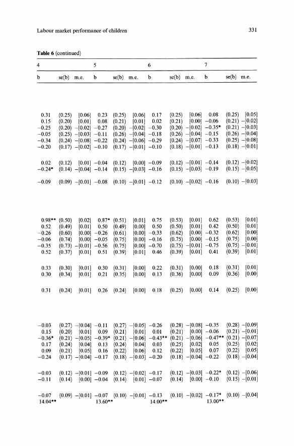
Labour market performance of children

Table 6 (continued)

331

4

b

5

se(b) m.e. b

6

se(b) m.e. b

7

se(b) m.e. b se(b) m.e.

0.31 (0.25) [0.06J 0.23 (0.25) [0.06J 0.17 (0.25) [0.06J 0.08 (0.25) [0.05J0.15 (0.20) [O.OIJ 0.08 (0.21) [O.OIJ 0.02 (0.21) [O.OOJ -0.06 (0.21) -[0.02J-0.25 (0.20) -[0.02J -0.27 (0.20) -[0.02J -0.30 (0.20) -[0.02J -0.35* (0.21) -[0.03J-0.05 (0.25) -[0.03J -0.11 (0.26) -[0.04] -0.18 (0.26) -[O.04J -0.15 (0.26) -[O.04J-0.34 (0.24) -[0.08J -0.22 (0.24) -[0.06J -0.29 (0.24) -[0.07] -0.33 (0.25) -[0.08J-0.20 (0.17) -[0.02J -0.10 (0.17) -[0.01] -0.10 (0.18) -[0.01] -0.13 (0.18) -[O.OIJ

0.02 (0.12) [O.OIJ -0.04 (0.12) [O.OOJ -0.09 (0.12) -[O.OIJ -0.14 (0.12) -[0.02J-0.24* (0.14) -[O.04J -0.14 (0.15) -[0.03J -0.16 (0.15) -[0.03] -0.19 (0.15) -[0.05J

-0.09 (0.09) -[O.OIJ -0.08 (0.10) -[O.OIJ -0.12 (0.10) -[0.02] -0.16 (0.10) -[0.03J

0.98** (0.50) [0.02J 0.87* (0.51) [O.OIJ 0.75 (0.53) [O.OIJ 0.62 (0.53) [O.OIJ0.52 (0.49) [O.OIJ 0.50 (0.49) [O.OOJ 0.50 (0.50) [0.01] 0.42 (0.50) [O.OIJ-0.26 (0.60) [O.OOJ -0.26 (0.61) [O.OOJ -0.33 (0.62) [0.00] -0.32 (0.62) [O.OOJ-0.06 (0.74) [O.OOJ -0.05 (0.75) [O.OOJ -0.16 (0.75) [0.00] -0. I5 (0.75) [O.OOJ-0.35 (0.73) -[O.OIJ -0.56 (0.75) [O.OOJ -0.70 (0.75) -[0.01] -0.75 (0.75) -[O.OIJ0.52 (0.37) [O.OIJ 0.51 (0.39) [O.OIJ 0.46 (0.39) [0.01] 0.41 (0.39) [O.OIJ

0.33 (0.30) [O.OIJ 0.30 (0.31) [O.OOJ 0.22 (0.31) [0.00] 0.18 (0.31) [O.OIJ0.30 (0.34) [O.OIJ 0.21 (0.35) [O.OOJ 0.13 (0.36) [0.00] 0.09 (0.36) [O.OOJ

0.31 (0.24) [O.OIJ 0.26 (0.24) [O.OOJ 0.18 (0.25) [O.OOJ 0.14 (0.25) [O.OOJ

-0.03 (0.27) -[O.04J -0.11 (0.27) -[0.05J -0.26 (0.28) -[0.08J -0.35 (0.28) -[0.09J0.15 (0.20) [O.OIJ 0.09 (0.21) [0.01] O.oI (0.21) [O.OOJ -0.06 (0.21) -[O.OIJ-0.36* (0.21) -[0.05J -0.39* (0.21) -[0.06J -0.43** (0.21) -[0.06] -0.47** (0.21) -[0.07]0.17 (0.24) [O.04J 0.13 (0.24) [O.04J 0.03 (0.25) [0.02] 0.05 (0.25) [0.02J0.09 (0.21) [0.05J 0.16 (0.22) [0.06] 0.12 (0.22) [0.05J 0.07 (0.22) [0.05]-0.24 (0.17) -[O.04J -0.17 (0.18) -[0.03J -0.20 (0.18) -[O.04J -0.22 (0.18) -[O.04J

-0.03 (0.12) -[0.01] -0.09 (0.12) -[0.02J -0.17 (0.12) -[0.03J -0.22* (0.12) -[0.06J-0.11 (0.14) [O.OOJ -0.04 (0.14) [O.OIJ -0.07 (0.14) [0.00] -0.10 (0.15) -[O.OIJ

-0.07 (0.09) -[O.OIJ -0.07 (0.10) -[O.OIJ -0.13 (0.10) -[0.02] -0.17* (0.10) -[O.04J14.04** 13.60** 14.00** 13.00**

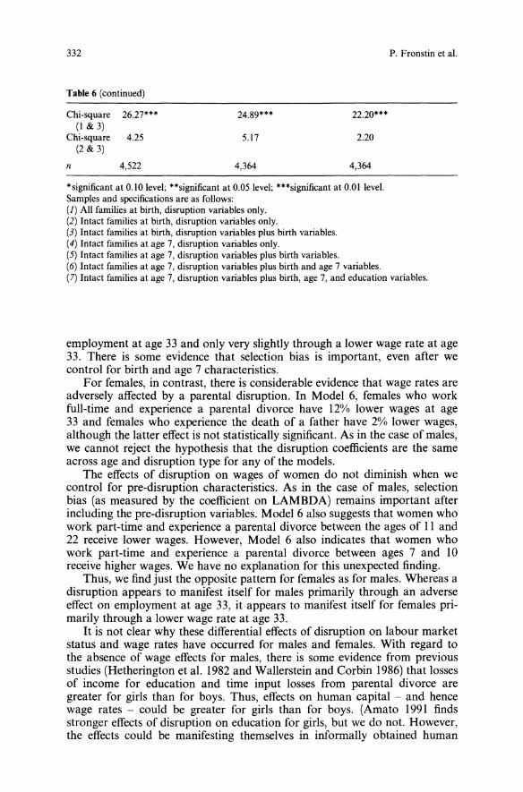
332

Table 6 (continued)

Chi-square 26.27*** 24.89*** 22.20***(1 & 3)

Chi-square 4.25 5.17 2.20(2 & 3)

n 4,522 4,364 4,364

P. Fronstin et al.

*significant at 0.10 level; **significant at 0.05 level; ***significant at 0.01 level.Samples and specifications are as follows:(1) All families at birth, disruption variables only.(2) Intact families at birth, disruption variables only.(3) Intact families at birth, disruption variables plus birth variables.(4) Intact families at age 7, disruption variables only.(5) Intact families at age 7, disruption variables plus birth variables.(6) Intact families at age 7, disruption variables plus birth and age 7 variables.(7) Intact families at age 7, disruption variables plus birth, age 7, and education variables.

employment at age 33 and only very slightly through a lower wage rate at age33. There is some evidence that selection bias is important, even after wecontrol for birth and age 7 characteristics.For females, in contrast, there is considerable evidence that wage rates are

adversely affected by a parental disruption. In Model 6, females who workfull-time and experience a parental divorce have 12% lower wages at age33 and females who experience the death of a father have 2% lower wages,although the latter effect is not statistically significant. As in the case of males,we cannot reject the hypothesis that the disruption coefficients are the sameacross age and disruption type for any of the models.The effects of disruption on wages of women do not diminish when we

control for pre-disruption characteristics. As in the case of males, selectionbias (as measured by the coefficient on LAMBDA) remains important afterincluding the pre-disruption variables. Model 6 also suggests that women whowork part-time and experience a parental divorce between the ages of II and22 receive lower wages. However, Model 6 also indicates that women whowork part-time and experience a parental divorce between ages 7 and 10receive higher wages. We have no explanation for this unexpected finding.Thus, we find just the opposite pattern for females as for males. Whereas a

disruption appears to manifest itself for males primarily through an adverseeffect on employment at age 33, it appears to manifest itself for females pri­marily through a lower wage rate at age 33.

It is not clear why these differential effects of disruption on labour marketstatus and wage rates have occurred for males and females. With regard tothe absence of wage effects for males, there is some evidence from previousstudies (Hetherington et al. 1982 and Wallerstein and Corbin 1986) that lossesof income for education and time input losses from parental divorce aregreater for girls than for boys. Thus, effects on human capital - and hencewage rates - could be greater for girls than for boys. (Amato 1991 findsstronger effects of disruption on education for girls, but we do not. However,the effects could be manifesting themselves in informally obtained human

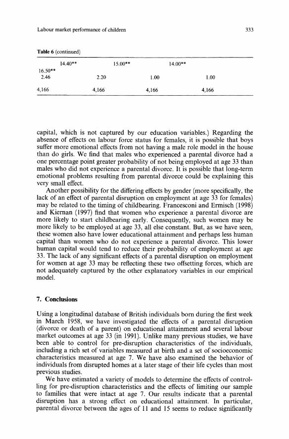
Labour market performance of children

Table 6 (continued)

333

14.40**

16.50**2.46

4,166

2.20

4,166

15.00**

1.00

4,166

14.00**

1.00

4,166

capital, which is not captured by our education variables.) Regarding theabsence of effects on labour force status for females, it is possible that boyssuffer more emotional effects from not having a male role model in the housethan do girls. We find that males who experienced a parental divorce had aone percentage point greater probability of not being employed at age 33 thanmales who did not experience a parental divorce. It is possible that long-termemotional problems resulting from parental divorce could be explaining thisvery small effect.Another possibility for the differing effects by gender (more specifically, the

lack of an effect of parental disruption on employment at age 33 for females)may be related to the timing of childbearing. Francesconi and Ermisch (1998)and Kiernan (1997) find that women who experience a parental divorce aremore likely to start childbearing early. Consequently, such women may bemore likely to be employed at age 33, all else constant. But, as we have seen,these women also have lower educational attainment and perhaps less humancapital than women who do not experience a parental divorce. This lowerhuman capital would tend to reduce their probability of employment at age33. The lack of any significant effects of a parental disruption on employmentfor women at age 33 may be reflecting these two offsetting forces, which arenot adequately captured by the other explanatory variables in our empiricalmodel.

7. Conclusions

Using a longitudinal database of British individuals born during the first weekin March 1958, we have investigated the effects of a parental disruption(divorce or death of a parent) on educational attainment and several labourmarket outcomes at age 33 (in 1991). Unlike many previous studies, we havebeen able to control for pre-disruption characteristics of the individuals,including a rich set of variables measured at birth and a set of socioeconomiccharacteristics measured at age 7. We have also examined the behavior ofindividuals from disrupted homes at a later stage of their life cycles than mostprevious studies.We have estimated a variety of models to determine the effects of control­

ling for pre-disruption characteristics and the effects of limiting our sampleto families that were intact at age 7. Our results indicate that a parentaldisruption has a strong effect on educational attainment. In particular,parental divorce between the ages of 11 and 15 seems to reduce significantly

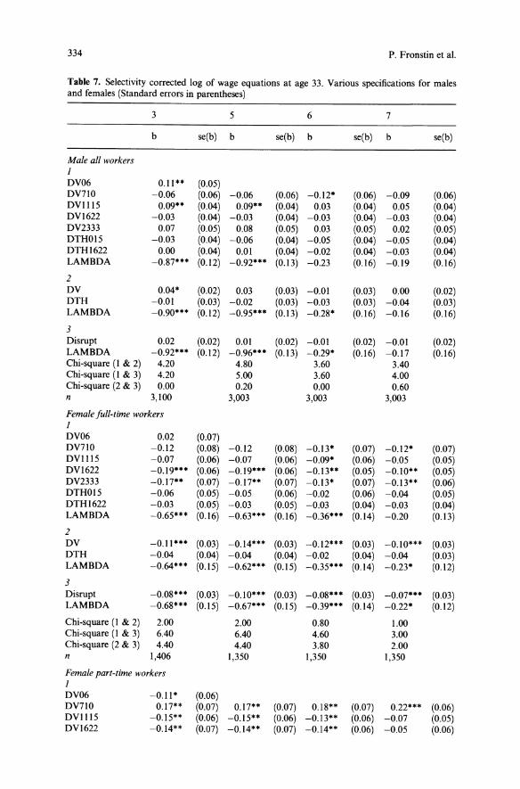
334 P. Fronstin et al.

Table 7. Selectivity corrected log of wage equations at age 33. Various specifications for malesand females (Standard errors in parentheses)

3 5 6 7

b se(b) b se(b) b se(b) b se(b)

Male all workers1DV06 0.11" (0.05)DV710 -0.06 (0.06) -0.06 (0.06) -0.12* (0.06) -0.09 (0.06)DVII15 0.09** (0.04) 0.09** (0.04) 0.03 (0.04) 0.05 (0.04)DVI622 -0.03 (0.04) -0.03 (0.04) -0.03 (0.04) -0.03 (0.04)DV2333 0.07 (0.05) 0.08 (0.05) 0.03 (0.05) 0.02 (0.05)DTHOl5 -0.03 (0.04) -0.06 (0.04) -0.05 (0.04) -0.05 (0.04)DTHI622 0.00 (0.04) 0.01 (0.04) -0.D2 (0.04) -0.03 (0.04)LAMBDA -0.87*** (0.12) -0.92*** (0.13) -0.23 (0.16) -0.19 (0.16)

2DV 0.04* (0.02) 0.03 (0.03) -O.oI (0.03) 0.00 (0.02)DTH -0.01 (0.03) -0.D2 (0.03) -0.03 (0.03) -0.04 (0.03)LAMBDA -0.90*** (0.12) -0.95*" (0.13) -0.28* (0.16) -0.16 (0.16)

3Disrupt 0.02 (0.02) 0.01 (0.02) -0.01 (0.02) -0.01 (0.02)LAMBDA -0.92*** (0.12) -0.96*** (0.13) -0.29* (0.16) -0.17 (0.16)Chi-square (I & 2) 4.20 4.80 3.60 3.40Chi-square (I & 3) 4.20 5.00 3.60 4.00Chi-square (2 & 3) 0.00 0.20 0.00 0.60n 3,100 3,003 3,003 3,003

Female full-time workers1DV06 0.02 (0.07)DV710 -0.12 (0.08) -0.12 (0.08) -0.13* (0.07) -0.12* (0.07)DVII15 -0.07 (0.06) -0.07 (0.06) -0.09* (0.06) -0.05 (0.05)DVI622 -0.19*** (0.06) -0.19*** (0.06) -0.13** (0.05) -0.10** (0.05)DV2333 -0.17** (0.07) -0.17** (0.07) -0.13* (0.07) -0.13** (0.06)DTHOl5 -0.06 (0.05) -0.05 (0.06) -0.02 (0.06) -0.04 (0.05)DTHI622 -0.03 (0.05) -0.03 (0.05) -0.03 (0.04) -0.03 (0.04)LAMBDA -0.65*** (0.16) -0.63*** (0.16) -0.36"* (0.14) -0.20 (0.13)

2DV -0.11*** (0.03) -0.14*** (0.03) -0.12*** (0.03) -0.\0*" (0.03)DTH -0.04 (0.04) -0.04 (0.04) -0.02 (0.04) -0.04 (0.03)LAMBDA -0.64*** (0.15) -0.62"* (0.15) -0.35*** (0.14) -0.23* (0.12)

3Disrupt -0.08"* (0.03) -0.\0*** (0.03) -0.08*" (0.03) -0.07*** (0.03)LAMBDA -0.68*** (0.15) -0.67*** (0.15) -0.39*** (0.14) -0.22* (0.12)

Chi-square (I & 2) 2.00 2.00 0.80 1.00Chi-square (I & 3) 6.40 6.40 4.60 3.00Chi-square (2 & 3) 4.40 4.40 3.80 2.00n 1,406 1,350 1,350 1,350

Female part-time workers1DV06 -0.11* (0.06)DV710 0.17** (0.07) 0.17** (0.07) 0.18** (0.07) 0.22*** (0.06)DVI1I5 -0.15** (0.06) -0.15** (0.06) -0.13** (0.06) -om (0.05)DVI622 -0.14** (0.07) -0.14** (0.07) -0.14** (0.06) -0.05 (0.06)

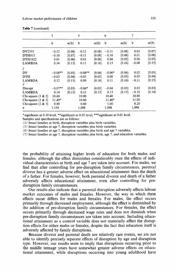
Labour market performance of children 335

Table 7 (continued)

3 5 6 7

b se(b) b se(b) b se(b) b se(b)

DV2333 -0.12 (0.08) -0.12 (0.08) -0.11 (0.08) 0.03 (0.07)DTHOl5 -0.10 (0.07) -0.11 (0.08) -0.10 (0.08) 0.01 (0.08)DTHI622 0.01 (0.06) om (0.06) 0.04 (0.05) 0.06 (0.05)LAMBDA 0.14 (0.15) 0.11 (0.16) 0.13 (0.16) -0.08 (0.15)

2DV -0.08** (0.03) -0.08** (0.04) -0.06* (0.04) 0.02 (0.03)DTH -0.03 (0.04) -0.03 (0.05) 0.00 (0.05) 0.05 (0.04)LAMBDA 0.12 (0.15) 0.09 (0.16) 0.11 (0.16) -0.11 (0.15)3Disrupt -0.07** (0.03) -0.06* (0.03) -0.04 (0.03) 0.03 (0.03)LAMBDA 0.14 (0.15) 0.11 (0.15) 0.13 (0.15) -0.10 (0.14)Chi-square (I & 2) 10.60 10.00 10.40 10.80Chi-square (I & 3) 11.40* 10.60 11.40* 11.00Chi-square (2 & 3) 0.80 0.60 1.00 0.20n 1,154 1,098 1,098 1,098

*significant at 0.10 level; **significant at 0.05 level; ***significant at 0.01 level.Samples and specifications are as follows:(3) Intact families at birth, disruption variables plus birth variables.(5) Intact families at age 7, disruption variables plus birth variables.(6) Intact families at age 7, disruption variables plus birth and age 7 variables.(7) Intact families at age 7, disruption variables plus birth, age 7, and education variables.

the probability of attaining higher levels of education for both males andfemales, although the effect diminishes considerably once the effects of indi­vidual characteristics at birth and age 7 are taken into account. For males, wefind that after controlling for pre-disruption family circumstances, parentaldivorce has a greater adverse effect on educational attainment than the deathof a father. For females, however, both parental divorce and death of a fatheradversely affects educational attainment, even after controlling for pre­disruption family circumstances.Our results also indicate that a parental disruption adversely affects labour

market outcomes of males and females. However, the way in which theseeffects occur differs for males and females. For males, the effect. occursprimarily through decreased employment, although the effect is diminished bythe addition of pre-disruption family circumstances. For females, the effectoccurs primarily through decreased wage rates and does not diminish whenpre-disruption family circumstances are taken into account. Including educa­tional attainment as a control variable does not materially affect the disrup­tion effects for either males or females, despite the fact that education itself isadversely affected by family disruptions.Because divorce and parental death are relatively rare events, we are not

able to identify precisely separate effects of disruption by age and disruptiontype. However, our results seem to imply that disruptions occurring prior tothe middle teenage years have somewhat greater adverse effects on educa­tional attainment, while disruptions occurring into young adulthood have

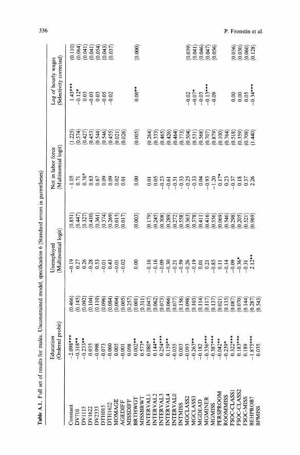
Tab

leA.I.Fullsetofresultsformales.Unconstrainedmodel,specification6(Standarderrorsinparentheses)

w w 0-

Education

Unemployed

Notinlaborforce

Logofhourlywages

(Orderedprobit)

(Multinomiallogit)

(Multinomiallogit)

(Selectivitycorrected)

Constant

-2.098***

(0.466)

-0.19

(0.851)

-1.05

(1.225)

1.43***

(0.110)

DV710

-0.318**

(0.145)

0.27

(0.447)

0.71

(0.574)

-0.12*

(0.064)

DVll15

-0.233**

(0.092)

0.26

(0.327)

0.76*

(0.427)

0.03

(0.041)

DVI622

0.035

(0.104)

-0.28

(0.410)

0.63

(0.453)

-0.03

(0.041)

DV2333

-0.098

(0.110)

0.53

(0.361)

0.67

(0.544)

0.03

(0.054)

DTHOl5

-0.073

(0.096)

-0.01

(0.374)

0.09

(0.546)

-0.05

(0.043)

DTH1622

-0.060

(0.084)

0.43

(0.269)

0.09

(0.455)

-0.02

(0.037)

MOMAGE

0.005

(0.004)

-0.01

(0.015)

0.02

(0.021)

AGEDIFF

-0.001

(0.005)

-0.02

(0.017)

0.01

(0.026)

MISSDIFF

0.098

(0.257)

BRTHWGT

0.002**

(0.001)

0.00

(0.003)

0.00

(0.005)

0.00**

(0.000)

MISSBRWT

0.573*

(0.311)

INTERVALI

0.080*

(0.047)

-0.16

(0.179)

0.01

(0.264)

INTERVAL2

0.144**

(0.062)

-0.16

(0.245)

0.05

(0.333)

INTERVAU

0.254***

(0.073)

-0.09

(0.308)

-0.23

(0.465)

INTERVAL4

0.159**

(0.066)

-0.30

(0.289)

-0.61

(0.426)

INTERVALO

-0.035

(0.077)

-0.21

(0.272)

-0.51

(0.464)

INTMISS

0.003

(0.156)

-0.59

(0.558)

-0.33

(0.773)

MGCLASS2

-0.093

(0.098)

-0.26

(0.363)

-0.25

(0.504)

-0.02

(0.039)

MGCLASS3

-0.263**

(0.103)

-0.19

(0.378)

-0.33

(0.531)

-0.07*

(0.041)

MGDEAD

-0.182

(0.114)

0.01

(0.411)

0.04

(0.568)

-0.03

(0.046)

MGMINER

-0.336***

(0.117)

0.21

(0.416)

-0.93

(0.707)

-0.13***

(0.047)

MGMISS

-0.387***

(0.137)

-0.85

(0.556)

-1.20

(0.879)

-0.09

(0.056)

PERSPROOM

-0.042**

(0.021)

0.11

(0.069)

0.17*

(0.100)

ROOMMISS

-0.239*

(0.135)

-0.14

(0.546)

0.23

(0.764)

:-0FSOC-CLASSI

0.322***

(0.087)

-0.09

(0.298)

-0.37

(0.518)

0.00

(0.036)

"T'l ..,

FSOC-CLASS2

0.183***

(0.070)

-0.36*

(0.205)

0.18

(0.359)

0.00

(0.030)

0 ::s '"FSOC-MISS

0.189

(0.144)

-0.31

(0.521)

0.37

(0.708)

0.05

(0.060)

g.BEHPROB7

-1.875***

(0.287)

2.12**

(0.969)

2.26

(1.440)

-0.34***

(0.128)

~

BPMISS

0.035

(0.543)

~

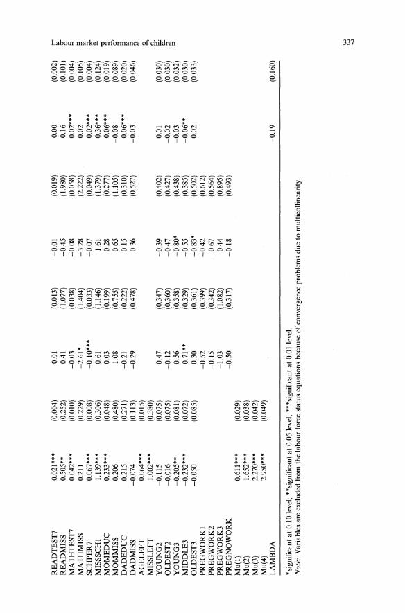
READTEST7

0.021***

(0.004)

0.01

(0.013)

-0.01

(0.019)

0.00

(0.002)

t""

l»

READMISS

0.505**

(0.252)

0.41

(1.077)

-0.45

(1.980)

0.16

(0.101)

8"MATHTEST7

0.042***

(0.010)

-0.03

(0.038)

-0.08

(0.058)

0.02***

(0.004)

c ..,MATHMISS

0.211

(0.229)

-2.61*

(1.404)

-3.28

(2.222)

0.02

(0.105)

3 l»SCHPER7

0.067***

(0.008)

-0.10***

(0.033)

-0.07

(0.049)

0.02***

(0.004)

.., :-:-MISSSCHI

1.139***

(0.306)

0.61

(1.146)

1.61

(1.379)

0.36***

(0.124)

~

MOMEDUC

0.233***

(0.048)

-0.03

(0.199)

0.28

(0.277)

0.06***

(0.019)

1l ..,MOMMISS

0.206

(0.480)

1.08

(0.755)

0.65

(1.105)

-0.08

(0.089)

0'DADEDUC

0.215

(0.271)

-0.21

(0.222)

0.15

(0.310)

0.06***

(0.020)3 l»

DADMISS

-0.074

(0.113)

-0.29

(0.478)

0.36

(0.527)

-0.03

(0.046)

::> IilAGELEFT

0.064***

(0.015)

0MISSLEFT

1.002***

(0.380)

-, '"YOUNG2

-0.115

(0.075)

0.47

(0.347)

-0.39

(0.402)

O.oI

(0.030)

e: c:OLDEST2

-0.016

(0.075)

-0.12

(0.360)

-0.47

(0.427)

-0.02

(0.030)

.., '"YOUNG3

-0.205**

(0.081)

0.56

(0.358)

-0.80*

(0.438)

-0.03

(0.032)

::>

MIDDLE3

-0.232***

(0.072)

0.71**

(0.329)

-0.55

(0.385)

-0.06**

(0.030)

OLDEST3

-0.050

(0.085)

0.30

(0.361)

-0.83*

(0.502)

0.02

(0.033)

PREGWORKI

-0.52

(0.399)

-0.42

(0.612)

PREGWORK2

-0.15

(0.342)

-0.67

(0.564)

PREGWORK3

-1.03

(1.082)

0.44

(0.895)

PREGNOWORK

-0.50

(0.317)

-0.18

(0.493)

Mu(l)

0.611***

(0.029)

Mu(2)

1.652***

(0.038)

Mu(3)

2.270***

(0.042)

Mu(4)

2.950***

(0.049)

LAMBDA

-0.19

(0.160)

*significantat0.10level;**significantat0.05level;***significantat0.01level.

Not

e:Variablesareexcludedfromthelabourforcestatusequationsbecauseofconvergenceproblemsduetomulticollinearity.

w W -J

Tab

leA.2.Fullsetofresultsforfemales.Unconstrainedmodel,specification6(Standarderrorsinparentheses)

w w 00

Education

Employedpart-time

Unemployed

Notinlaborforce

Logofhourlywages

Logofhourlywages

(Orderedprobit)

(Multinomiallogit)

(Multinomiallogit)

(Multinomiallogit)

forfull-time

forpart-time

(Selectivity

(Selectivity

corrected)

corrected)

Constant

-1.985***

(0.424)

3.53***

(0.973)-3.55

(2.471)

4.07***

(1.005)

2.29***

(0.365)

0.96***

(0.287)

DV710

-0.236**

(0.098)

0.17

(0.253)

0.75

(0.527)-0.26

(0.276)

-0.13*

(0.070)

0.18**

(0.092)

DVII15

-0.311***

(0.090)

0.02

(0.210)

0.50

(0.502)

0.01

(0.210)

-0.09*

(0.056)

-0.13*

(0.072)

DVI622

-0.051

(0.093)-0.30

(0.205)

-0.33

(0.620)

-0.43**

(0.212)

-0.13**

(0.055)

-0.14*

(0.078)

DV2333

0.037

(0.113)-0.18

(0.259)-0.16

(0.750)

0.03

(0.247)

-0.13*

(0.066)

-0.11

(0.096)

DTHOl5

-0.195**

(0.095)-0.29

(0.245)-0.70

(0.754)

0.12

(0.220)-0.02

(0.058)-0.10

(0.101)

DTHI622

-0.084

(0.072)-0.10

(0.176)

0.46

(0.392)-0.20

(0.179)-0.03

(0.045)

0.04

(0.066)

MOMAGE

0.013***

(0.004)

-0.02**

(0.009)

0.03

(0.022)

-0.02**

(0.009)

AGEDIFF

-0.011**

(0.005)

0.01

(0.011)

0.02

(0.030)

0.01

(0.011)

MISSDIFF

-0.378

(0.254)

BRTHWGT

0.001*

(0.001)

0.00

(0.002)

-O.oI

(0.005)

0.00

(0.002)

0.00

(0.000)

0.00

(0.001)

MISSBRWT

0.485*

(0.291)

INTERVALI

0.111**

(0.044)

0.05

(0.101)

-0.05

(0.265)

0.04

(0.103)

INTERVAL2

0.149**

(0.059)

-0.28**

(0.141)

-0.41

(0.412)

0.02

(0.136)

INTERVAU

0.178**

(0.076)

0.15

(0.169)

0.13

(0.475)

0.33**

(0.168)

INTERVAL4

0.086

(0.062)-0.08

(0.142)

-0.84*

(0.485)

0.15

(0.140)

INTERVALO

-0.199**

(0.078)-0.27

(0.180)-0.54

(0.474)

-0.15

(0.177)

INTMISS

0.100

(0.125)-0.14

(0.298)

0.13

(0.671)

0.23

(0.279)

MGCLASS2

0.011

(0.089)

0.48**

(0.226)

0.79

(0.750)

0.33

(0.208)

0.11**

(0.053)-0.05

(0.112)

MGCLASS3

-0.054

(0.095)

0.70***

(0.238)

0.90

(0.776)

0.44**

(0.222)

0.15**

(0.061)-0.09

(0.119)

MGDEAD

-0.021

(0.105)

0.81***

(0.259)

0.46

(0.872)

0.36

(0.248)

0.13**

(0.067)-0.09

(0.131)

MGMINER

-0.145

(0.107)

0.49*

(0.273)

1.59**

(0.804)

0.43*

(0.255)

0.12*

(0.069)

-0.21*

(0.124)

MGMISS

-0.064

(0.119)

0.86***

(0.295)

0.74

(0.953)

0.53*

(0.285)

0.22***

(0.081)

-0.01

(0.137)

:-0PERSPROOM

-0.006

(0.019)

-0.11**

(0.047)

0.06

(0.109)-0.06

(0.046)

." ...ROOMMISS

-0.243**

(0.120)

-0.11

(0.287)

0.73

(0.659)-0.25

(0.301)

0 0 '"FSOC-CLASSI

0.267***

(0.081)

0.02

(0.192)-0.76

(0.478)-0.30

(0.187)-0.04

(0.051)

0.10

(0.069)

e. 0FSOC-CLASS2

0.168***

(0.063)-0.03

(0.152)

-0.76**

(0.315)

-0.29**

(0.146)

0.01

(0.042)

0.05

(0.054)

~

FSOC-MISS

0.165

(0.144)

~

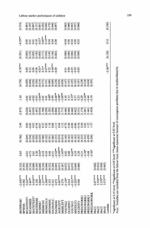
BEHPROB7

-2.658***

(0.332)

0.65

(0.766)

2.49

(1.873)

1.10

(0.759)

-0.76***

(0.201)

-0.59**

(0.274)

t""'

I'>BPMISS

-0.082

(0.593)

a"0

READTEST7

0.022***

(0.004)

-0.01

(0.009)

0.00

(0.024)

-O.oJ

(0.009)

0.00

(0.003)

0.00

(0.003)

~ ..,READMISS

0.407*

(0.216)-0.72

(0.534)-0.45

(1.437)

0.02

(0.494)

0.12

(0.133)

0.01

(0.195)

3 I'>MATHTEST7

0.034***

(0.009)

0.01

(0.020)

0.03

(0.058)-0.02

(0.020)

0.00

(0.005)

0.01

(0.007)

.., ~MATHMISS

0.100

(0.195)

0.20

(0.509)-0.54

(1.601)-0.03

(0.500)-0.06

(0.142)-0.18

(0.157)

~

SCHPER7

0.060***

(0.008)

-0.03*

(0.019)-0.07

(0.054)

-0.04**

(0.019)

0.01*

(0.005)

0.01*

(0.007)

~

MISSSCHI

1.217***

(0.224)-0.19

(0.588)

0.23

(1.598)

-0.61

(0.572)

0.31*

(0.171)

0.45**

(0.202)

g,MOMEDUC

0.308***

(0.044)-0.10

(0.102)

0.20

(0.298)

0.01

(0.101)

0.07***

(0.026)

0.10***

(0.040)3 I'>

MOMMISS

0.553

(0.552)

0.44

(0.531)

1.18

(1.282)

0.88*

(0.490)

0.22

(0.145)

0.04

(0.178)

::s RDADEDUC

-0.221

(0.284)

-0.51

(0.586)

0.60

(1.096)-0.99

(0.690)

0.44***

(0.146)

0.04

(0.046)

0DADMISS

0.073

(0.095)

-0.54**

(0.233)-1.13

(0.888)

-0.46**

(0.234)-0.00

(0.063)

0.08

(0.097)

-, (")

AGELEFT

0.047***

(0.013)

-0.09***

(0.033)

0.04

(0.078)

-0.06*

(0.029)

:l" 6:

MISSLEFT

0.279

(0.367)

-1.95**

(0.814)

1.12

(1.775)

-2.00**

(0.858)

.., <>YOUNG2

-0.130*

(0.072)

0.02

(0.169)-0.70

(0.460)

0.10

(0.167)

0.01

(0.040)-0.04

(0.062)

::s

OLDEST2

0.018

(0.071)

0.08

(0.162)-0.40

(0.484)

0.12

(0.163)

0.00

(0.040)

0.00

(0.060)

YOUNG3

-0.321***

(0.079)

0.42**

(0.183)-0.09

(0.448)

0.35*

(0.183)-0.05

(0.046)-0.04

(0.063)

MIDDLE3

-0.205***

(0.069)

0.19

(0.165)-0.46

(0.422)

0.17

(0.165)-0.05

(0.039)

0.00

(0.057)

OLDEST3

0.008

(0.080)

0.28

(0.183)-0.16

(0.531)

0.23

(0.187)-0.05

(0.049)

0.02

(0.066)

PREGWORKI

-0.31

(0.233)

0.50

(1.174)-0.29

(0.238)

PREGWORK2

-0.38*

(0.210)

0.92

(1.067)

-0.54**

(0.218)

PREGWORK3

-0.68

(0.439)

1.22

(1.461)-0.44

(0.424)

PREGNOWORK

-0.36*

(0.200)

1.57

(1.029)-0.18

(0.205)

Mu(I)

0.677***

(0.026)

Mu(2)

1.976***

(0.035)

Mu(3)

2.339***

(0.036)

Mu(4)

3.075***

(0.045)

Lambda

-0.36***

(0.138)

0.13

(0.190)

*significantat0.10level;**significantat0.05level;***significantat0.01level.

Not

e:Variablesareexcludedfromthelabourforcestatusequationsbecauseofconvergenceproblemsduetomulticollinearity.

w w \0

340 P. Fronstin et al.

adverse effects on certain labour market outcomes. In all our specifications, ifwe do not control for pre-disruption characteristics, we estimate much largereffects on educational attainment for both males and females and on labourmarket outcomes for males. This suggests that the pre-disruption character­istics often control for unobserved, shared incapacities or difficulties of theparents and children (e.g., family dysfunctioning). For example, if there isa shared family history of depression (which, in part, might be geneticallyderived), this could have affected both the child's age 7 behavioral problemsand the parents' likelihood of divorcing.Although we find strong effects of a parental disruption on educational

attainment, we also find independent effects of disruption on labour marketoutcomes. However, to fully investigate the avenues through which familydisruption affects labour market outcomes requires a more comprehensivestructural model of educational attainment and labour market behavior,something that has not been attempted here. Future research on the economicconsequences of parental disruption using a structural framework mightbe better able to unravel the routes through which family disruption affecteconomic well being in the adult years.

Appendix: Construction of selected explanatory variables

FSOC-CLASS2 = I if father's occupational class is professional (i.e. doctor,lawyer) or intermediate (i.e. manager, teacher)

FSOC-CLASS3 = I if father's occupational class is skilled non-manual (i.e.clerk, shop assistant), skilled manual (i.e. miner, bricklayer),or partly skilled (i.e. mail carrier, bus conductor) (base groupfor FSCL is unskilled (i.e. cleaner, labourer), unemployed,student, sick, or retired)

BEHPROB7 factor score for behavioral problems at age 7 (from Cherlin,Kiernan, and Chase-Lansdale 1995); includes logarithm ofparent-rated behavior problems, logarithm of teacher-ratedbehavior problems, use of social services, and family reporteddifficulties.

READTEST7 Southgate Group Reading Test at age 7-standardized test ofhow well children have learned to read in school (involvingboth word recognition and sentence completion). As such, itprobably confounds children's cognitive ability with theirmastery of reading.

MATHTEST7 Mathematics Achievement Test at age 7-score represents thenumber of correctly answered questions in a 10 questionproblem arithmetic test. Developed specifically for NCDS.

SCHPER7 School performance scale at age 7-summed scale of theteacher's responses to 5 school performance items, each ofwhich was rated I to 5. Includes oral ability, the child'sawareness of the world around him or her, reading, creativ­ity, and number work.

Labour market performance of children 341

NVQl

NVQ2

NVQ3

NVQ4

NVQ5

Endnotes

= 1 if some qualifications (RSA Stage 1, CSE Grades 2 to 5,other technical and business qualifications)

= 1 if 0 levels or equivalent (Joint Industry Board Techni­cians Certificate CGLI Operative, Insignia Award and otherqualifications, RSA Stages 2 and 3, Scottish Standard Grade,o Grade, 0 Level, CSE Grade 1, GCSE)= 1 if A Level Equivalent (TEC, BEC, BTEC National Cer­tificate or Diploma, Joint Industry Board ONC/OND, CGLIAdvanced Part 2, Scottish Certificate of 6th Form Studies,GCE and Scottish Highers, Scott Beck Awards, GCE Alevel)

= 1 if Other Higher Education (Training College Certificate,non-validated diploma or certificate, nursing qualification,professional qualification, TEC/BET/BETEC and Scottishequivalent, Higher National Diploma, Joint Industry Board,HNC/HND, CGLI full technical qualification)

= 1ifHigher Education (First Degree, Postgraduate Diploma,Masters, Ph.D.)

I For example, the divorce rate for England and Wales in 1961 was 2.1 per 1,000 married per­sons, by 1971 it was 6.0, and in 1980 it was 12.0 and has remained more or less steady sincethen (Kiernan 1988). Many of these divorcing parents - 55% in 1985, for example - havechildren under age 16 (Kiernan 1988). At present, divorce rates in Britain are the highest inWestern Europe.

2 In addition, between 1958 and 1965, a supplementary sample was added consisting of 1,142children from recent immigrant families, who were also born during the first week of March1958. Hence, the total initial sample was 18,556. We do not use the supplementary sample inour analysis.

3 While only 65 percent of the original cohort was interviewed at age 33, Shepherd (1993) arguesthat the age 33 sample is representative of the original cohort and is similar to other nationallyrepresentative samples of a comparable age group.

4 Because the NCDS survey contains comprehensive measures of childhood experiences over anumber of years, it is not likely to suffer from the "window problem" that occurs when chil­dren's attainments are linked causally to events or circumstances occurring at a single point intime during childhood (e.g., see Wolfe et aI., 1996).

5 Interestingly, at least two U.S. studies have obtained rather large negative estimates of theimpact of parental divorce on the earnings of adult white males. Findings from Greenberg andWolf (1982) imply a 28% earnings reduction and those from Grogger and Ronan (1995) implya 12% earnings reduction. However, both studies also found that parental divorce had a posi­tive impact on the adult earnings of black males, although this finding was not statisticallysignificant in the Greenberg and Wolf study.

6 In some studies (for example, Couch and Lillard, 1995), few or no pre-disruption control vari­ables are available for use. Other studies (for example, Krein 1986; Boggess 1998 and Kiernan1998) use independent variables, such as measures of family financial status, that were mea­sured after the marriage disruption occurred and, hence, are potentially endogenous to thedisruption. Sometimes the researchers seem unaware of this problem. More often, however, theresearchers are aware, but want to determine whether the effects of disruption on children aremore attributable to the disruption per se or to changes in family circumstances that resultfrom the disruption. Nonetheless, because of the endogeneity problem, the findings in thesestudies are somewhat difficult to interpret.

342 P. Fronstin et al.

7 While not directly examining this issue, however, Haveman and Wolfe (1994) and Boggess(1998) used U.S. data to find that the length of time that children live with one parent adverselyaffects the educational attainment of children in most demographic groups. Boggess attributesmost of this duration effect to the economic deprivation that often occurs in single parentfamilies.

8 In addition, Wadsworth and Maclean (1986) used longitudinal data for 5,362 children born inGreat Britain in March 1946 to examine the effects of parental disruptions on children's edu­cation attainment and adult income. The data they used are similar in many respects to theNCDS. They found that educational attainment and income were both lower for children whoexperienced a parental disruption before age 14.

9 This somewhat restrictive measure of disruption was apparently adopted to eliminate col­linearity with another variable of interest, whether individuals lived in families that facedfinancial difficulties before they were 16 years old.

10 Gross hourly earnings are derived from a survey question about usual gross pay beforedeductions. The respondent was asked the time period covered by the earnings response: 37%said one week, 1% said a fortnight, 4% said four weeks, 25% said one month, and 32% saidone year. The responses were all converted to hourly terms using usual hours of work. Self­employed individuals, who comprised 14% of the sample, were asked to report earnings inweekly terms. Self-employed individuals were not asked about usual hours of work so they arenot included in our sample.

11 Lee (1983) describes the computation of this estimator and explains the rationale for usingit (the procedure is summarized in Greene 1998). To identify the wage regressions, the explan­atory variables in the wage regressions differ from those in the multinomiallogit equations (seeTables A.I and A.2).

12 In England, an individual's formal education is represented by the qualifications they receive.Qualification levels are a reflection of course work and level of education in years. In addition,some qualification levels can be obtained only if certain tests are passed. England's NationalCouncil for Vocational Qualifications have grouped qualification levels into six NationalVocational Qualification (NVQ) levels in order to have a standardized measure of educationlevels. These six levels are represented as follows: no qualifications (NVQO), some qualifica­tion (NVQI), 0 levels or equivalent (NVQ2), A level or equivalent (NVQ3), other highereducation (NVQ4), and higher education (NVQ5). For further details, see the Appendix.

13 However, restricting the sample to individuals living in intact households at age 7 introducesfurther potential sample selectivity problems. We tested for the possibility of sample selectionbias from using the age 7 sample. These tests indicated that using the age 7 sample does notsignificantly alter our results. As discussed in the text, we also estimate several models usingmore inclusive samples.

14 Because we use this approach, in estimating wage regressions, we exclude variables that aretypically included in a wage equation - for example, firm size, education, and work experience.Such variables, which are measured in the NCDS at age 33, may be endogenous with respect toparental disruption. In one specification, however, we do include education as an explanatoryvariable.

15 Out of the original total sample of 17,414, 9,723 were interviewed at both age 7 and age 33. Ofthese, 70 did not have valid data on parental disruptions, 753 did not have valid data on workstatus at age 33, and 677 had experienced a parental disruption by age 7. This leaves a sampleof 7,828 (3,662 males and 4,166 females). A slightly smaller sample (3,603 males and 4,129females) is used in the education regressions because of missing data on education.

16 In our sample, 13.2% of the observations have at least one missing value for an explanatoryvariable. Nearly 70% of these observations (9.1% of the total sample) have only one missingvalue. The missing data problem is thus minimal with regard to individual observations, asmost have missing data for only one variable. Moreover, for most individual variables, fewerthan 3% of the observations have missing values (see Table 2). A comparison of the means ofthe samples with and without missing data indicates that the two samples are quite similar.

17 Information about the death of a mother is not included in the NCDS and information aboutthe death of a father is not included subsequent to the child reaching age 22. It is not clear howthe complete lack of information about the death of a mother affects our findings. On theone hand, for this age cohort, the death of the father was more likely to be associated with areduction in family income than the death of a mother. On the other hand, the loss of timeinputs and emotional effects resulting from the death of a mother could be significant. The lack

Labour market performance of children 343

of data about the death of a father subsequent to age 22 probably is not an important short­coming since the child had probably already left home by that time.

18 The variables we use to measure a parental divorce were carefully constructed to be consistentacross waves of the NCDS. Information on parental divorce is available in NCDSI-3 andretrospectively in NCDS5 (no information on divorce was obtained in NCDS4). Briefly, ifa divorce was indicated in either NCDSI-3 or NCDS5, the divorce was considered to haveoccurred. If the information was inconsistent across surveys, the information in NCDS5 wasconsidered correct. A detailed memorandum on how the divorce variables were constructed isavailable from the authors.

19 To test for possible threshold effects for birth weight, we estimated an alternative model with aseries of four dummy variables for birth weight « 5 Ibs., between 5 and 6 Ibs., between 6 and7 Ibs., and between 7 and 8 Ibs.). We could not reject the hypothesis that birth weight effectswere the same across categories, so a linear effect was specified.

20 Although not the focus of this study, there are some interesting results for the nondisruptionvariables. The results indicate, for example, that education is positively related to the child'sbirth weight, the length of time between the parents' marriage and the birth of their first child,the social class of the maternal grandfather, the social class of the father, reading and arith­metic test scores at age 7, school performance at age 7, the mother's education, and the age thefather left school, and negatively related to the degree of behavioral problems at age 7 and thenumber of persons per room in the household at the time of the birth.

21 This result that most of the effect is for divorces that occur prior to age 15 differs somewhatfrom Kiernan (1997), who finds that parental divorce after age 21 also adversely affectsthe educational attainment of males. In Models I through 5, we find an effect for males fordivorces occurring after age 23, but the effect becomes statistically insignificant in Model 6when we control for age 7 family characteristics.

22 Again, although not the focus of this study, there are a few interesting results for the non­disruption variables. The most important is that for both males and females, the probabilityof being unemployed or out of the labour force at age 33 is positively related to the extent ofbehavioral problems at age 7.

References

Amato PR, Keith B (1991) Parental Divorce and Adult Well-Being: A Meta-Analysis. Journal ofMarriage and the Family 53:43-58

Becker GS (1981) A Treatise on the Family. Harvard University Press, Cambridge, MassBecker GS, Tomes N (1986) Human Capital and the Rise of Families. Journal of Labour Eco­

nomics 4:SI-S39Blau PM, Duncan OD (1967) The American Occupational Structure. Wiley, New YorkBlundell R, Dearden L, Goodman A, Reed H (1997) Higher Education, Employment, and Earn­

ings in Britain. The Institute for Fiscal Studies, LondonBoggess S (1998) Family Structure, Economic Status, Education Attainment. Journal of Popula­

tion Economics II :205-222Cherlin AJ, Furstenberg FF Jr., Chase-Lansdale PL, Kiernan KE, Robins PK, Morrison DR,Teitler JO (1991) Longitudinal Studies of Effects of Divorce on Children in Great Britain andthe United States. Science 252:1386-1389

Cherlin AJ, Kiernan KE, Lindsay CLP (1995) Parental Divorce in Childhood and DemographicOutcomes in Young Adulthood. Demography 32(3):299-318

Couch KA, Lillard DR (1997) Divorce, Educational Attainment and the Earnings Mobility ofSons. Journal of Family and Economic Issues 18:231-245

Duncan GJ, Hoffman SD (1985) A Reconsideration of the Economic Consequences of MaritalDisruption. Demography 22:485-498

Ferri E (ed) (1993) Life at 33: The Fifth Follow-up of the National Child Development Study.National Children's Bureau and City University, London

Francesconi M, Errnisch JF (1998) Family Structure and Children's Achievements (unpublishedmanuscript)

Garasky S (1995) The Effects of Family Structure on Educational Attainment: Do the EffectsVary by the Age of the Child? American Journal of Economics and Sociology 54:89-105

344 P. Fronstin et al.

Greenberg D, Wolf D (1982) The Economic Consequences of Experiencing Parental MaritalDisruptions. Children and Youth Services Review 4:141-162

Greene WH (1998) Limdep Version 7.0: User's Manual. Econometric Software, Plainview, NYGregg P, Machin S (1998) Child Development and Success or Failure in the Youth LabourMarket. Discussion Paper 397, London: Centre for Economic Performance, London Schoolof Economics

Grogger J, Ronan N (1995) The Intergenerational Effects of Fatherlessness on EducationalAttainment and Entry-level Wages. (unpublished manuscript)

Haveman R, Wolfe BL (1994) Succeeding Generations: On the Effects of Investments in Children.Russell Sage, New York

Haveman R, Wolfe BL, Spaulding 1 (1991) Childhood Events and Circumstances InfluencingHigh School Completion. Demography 28:133-157

Hetherington EM, Cox M, Cox R (1982) Effects of Divorce on Parents and Children. In: Lamb M(ed) Nontraditional Families: Parenting and Child Development. Hillsdale, NJ: LawrenceErlbaum, pp. 223-288

Kiernan KE (1988) The British Family: Contemporary Trends and Issues. Journal of FamilyIssues 9:298-316

Kiernan K (1997) The Legacy of Parental Divorce: Social, Economic and Demographic Experi­ences in Adulthood. CASE Paper, London: Centre for Analysis of Social Exclusion, LondonSchool of Economics

Krein SF (1986) Growing Up in a Single-Parent Family: The Effect on Education and Earnings ofYoung Men. Family Relations 35:161-168

Lee L (1983) Generalized Econometric Models with Selectivity. Econometrica 51:507-512Lillard DR, DeCicca P (1995) Marital Disruption and the Earnings Mobility of Sons. (un­published manuscript)

Michael RT, Becker GS (1973) On the New Theory of Consumer Behavior. Swedish Journal ofEconomics 75:378-395

Mueller DP, Cooper PW (1986) Children of Single Parent Families: How They Fare As YoungAdults. Family Relations 35: 169-176

Peters HE (1992) Patterns of Intergenerational Mobility in Income and Earnings. The Review ofEconomics and Statistics 74:456-466

Shepherd PM (1985) The National Child Development Study: An Introduction to the Back­ground of the Study and the Methods of Data Collection. Social Science Research Unit, CityUniversity, London

Shepherd PM (1993) Appendix I: Analysis of Response Bias. In: Ferri E (ed) Life at 33: The FifthFollow-up of the National Child Development Study. National Children's Bureau and CityUniversity, London, pp. 184-188

Wadsworth MEl, Maclean M (1986) Parents' Divorce and Children's Life Chances. Children andYouth Services Review 8:145-159

Wallerstein JS, Corbin SB (1986) Father-Child Relationships after Divorce: Child Support andEducational Opportunities. Family Law Quarterly 20:109-128

Wojtkiewicz RA (1993) Simplicity and Complexity in the Effects of Parental Structure on HighSchool Graduation. Demography 30:701-717

Wolfe B, Haveman R, Ginther D, Chong BA (1996) The 'Window Problem' in Studies of Chil­dren's Attainments: A Methodological Exploration. Journal of the American Statistical Asso­ciation 91(435):970-982

Optimal age at motherhood. Theoretical and empiricalconsiderations on postponement of maternity in Europe

Siv Gustafsson

Department of Economics, University of Amsterdam, Roetersstraat 11, 1018 WB Amsterdam,The Netherlands (Fax: +31-20-525-4254; e-mail: siv@fee.uva.nl)

Received: 23 September I999jAccepted: 15 May 2000

Abstract. The age at which women become mothers has increased to an alltime high in most European countries in the past decennia. This increase ofage at first birth is the main explanatory variable for the rapid decrease infertility in European countries which has occurred at different points of timeearlier in North and West Europe than in South Europe. To understand thedevelopment of the period fertility rate it is therefore crucial to understand thedeterminants of optimal age at maternity. This paper reviews empirical andtheoretical literature and tries to give suggestions on future research direc­tions. The econometric so called timing and spacing literature has used currentfemale wages and male incomes as the main explanatory variables. However,theoretical research identifies on the one hand consumption smoothing, andon the other hand career planning of the woman as the main explanations tothe postponement of maternity.

JEL classification: DI, Jl

Key words: Postponement of maternity, economic theories of timing offertility

1. Introduction

Increasingly young women in all European countries educate themselves for alifelong labour market career. Many women find that there is no room forchildren, and sometimes they are given promotion only on the condition that

Presidential address of the 13th annual meeting of the European Society for Population Economics,June 24-26, 1999, Torino Italy.

346 S.S. Gustafsson

they are not pregnant or do not plan on a child in the near future, which resultsin postponing or refraining from children altogether. For example, in 1990 are61% of Dutch women of the age group 25-29 still childless, a number, whichsurpasses with a broad margin the second runner up, which is Germany with57 percent. In Sweden, the corresponding number is 49% (Bosveld 1996). Untilrecently the research agenda on the lack of equal opportunities betweenwomen and men focussed on labour force participation of women with youngchildren, whereas the consequences of working life for fertility and timingand spacing of births has received less attention. On the other hand, researchon the determinants of fertility has recognized the importance of timing inexplaining period total fertility rates. (Ermisch 1990; Cigno 1991; Heckmanand Walker 1990; Hotz et al. 1997). The purpose of this paper is to reviewrelated literature in demography, economic theory and econometrics in orderto review the extent of postponement in different European countries, to for­mulate hypotheses on the determinants of optimal age at maternity and topresent empirical evidence if available.The postponement of births that we have observed in Europe creates also a

biological strain. Biological and medical literature reviewed by Wetzels (1999Chapt. 7) stress for example the medical costs associated with the realizationof a desire to give birth by older couples who are less fecund. One estimatecited by Wetzels is (Fauser 1998) for the Netherlands in 1995 close to 2,000births out of 190500 live births, were the result of In Vitro Fertilization (IVF).Costs for IVF are estimated by another study Bonsel and Van der Maas(1994) for the Netherlands in 1991 at 33 million Dutch guilders (1.8 guildersto a US dollar). Many of these costs could probably have been avoided, if thecouple had chosen for parenthood at a younger age.This paper starts with a presentation of the extent of postponement of

maternity in some European countries in Sect. 2. The third section reviews themain results of the econometric timing and spacing literature which uses cur­rent incomes and wages as main determinants. Section 4 explains the theoret­ical shadow price at giving birth. Section 5 analyses consumption smoothingand husbands earnings as determinants ofmother's age of first birth. Section 6develops the career-planning motive which is subdivided into five subsectionsof variables that affect the woman's life time earnings by different decisions ontiming of maternity. In Sect. 7 some results from biological, medical andhealth research are reviewed. Section 8 concludes.

2. The ageing of fertility in Europe

Bosveld (1996) is a careful demographic analysis of the ageing of fertilityin Europe. This section presents and evaluates her main findings. Total fertil­ity rates declined sharply in Europe during the first demographic transition,which for most European countries occurred between 1880 and 1940. In somecountries fertility fell below replacement level by 1940. This was the case inBelgium, Switzerland, France, England and Wales and Sweden. Demogra­phers at that time expected fertility to stabilize at a low level but between 1940and 1960 total fertility rates increased in many countries creating what hasbeen termed the 'post second world war baby boom.' However, since 1965 asecond decreasing fertility trend started, resulting in fertility levels far belowreplacement in almost all European countries. Van de Kaa (1987) termed this

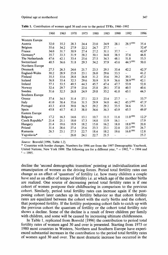
Optimal age at motherhood 347

Table 1. Contribution of women aged 30 and over to the period TFRs, 1960-1992

1960 1965 1970 1975 1980 1985 1990 1992 1996

Western EuropeAustria 32.0 35.2 28.3 24.4 23.0 24.9 28.1 28.5 1991 35.4Belgium 35.6 34.2 27.9 22.2 24.7 27.7 32.4'France 34.0 31.7 30.9 27.4 27.2 31.1 37.7 42.6b

Germany* 35.7 33.3 31.9 28.2 30.1 34.8 38.5 37.6 46.8The Netherlands 47.6 42.1 33.4 25.6 27.5 34.3 48.1 51.8 53.5Switzerland 40.5 36.6 31.8 29.3 34.2 37.9 43.6 44.3 1991 50.0Northern EuropeDenmark 27.3 26.3 24.6 21.7 23.5 29.5 35.4 42.2 42.3'England-Wales 30.2 28.9 25.8 23.1 26.0 29.6 33.5 41.2Finland 35.5 33.6 28.8 26.8 31.2 35.6 39.2 39.3 47.2Iceland 36.8 35.4 32.5 29.6 30.9 31.9 36.6 38.9 1991 42.1Ireland 57.1 53.5 49.5 44.3 45.7 47.4 47.7 53.9 52.8Norway 32.4 29.7 27.9 23.6 25.8 29.1 37.8 40.5 40.6Sweden 31.6 32.5 26.8 24.9 29.8 35.2 41.0 43.1 44.3Southern EuropeGreece 37.4 34.5 31.4 27.1 22.5 23.4 27.7 33.7'Italy 41.0 38.4 35.6 31.5 29.9 34.0 44.2 45.5 1991 47.3'Portugal 43.3 43.8 39.8 36.5 29.2 29.2 33.5 34.6 35.3Spain 45.8 45.7 41.5 38.0 34.6 36.3 43.9 45.5 49.0'Eastern EuropeBulgaria 17.2 16.3 14.6 13.1 10.7 11.5 11.6 11.01991 12.2'Czech Republic* 21.4 21.1 18.0 17.3 14.8 13.9 16.1 17.9Hungary 21.4 19.6 18.9 18.2 15.0 16.2 18.0 18.8 1991 20.8Poland 31.4 28.6 27.4 25.6 23.3 23.1 22.0 22.3 1991 26.7Rumania 26.3 23.1 27.5 22.7 18.4 18.2 19.6 16.8 1991 12.8Yugoslavia* 26.0 24.1 22.7 21.5 25.2

Source: Bosveld (1996, Table 1.2).* Countries with border changes. Numbers for 1996 are from the 1997 Demographic Yearbook,United Nations, New York 1999. The following are for a different year, a = 1992, b = 1994 andc = 1995.

decline the 'second demographic transition' pointing at individualization andemancipation of women as the driving forces. Period total fertility rates canchange as an effect of 'quantum' of fertility i.e. how many children a couplehave and as an effect of tempo of fertility i.e. at which age of the mother birthsare realized. One source of decreasing period total fertility rates is if onecohort of women postpone their childbearing in comparison to the previouscohort. Similarly, period total fertility rates can increase again if the post­poning cohort later catches up its fertility behavior so that cohort fertilityrates are equalized between the cohort with the early births and the cohort,that postponed fertility. If the fertility postponing cohort fails to catch up withthe previous cohort the quantum of fertility or the cohort total fertility rateshows a decline. Some of the decline is a result of fewer children per familywith children, and some will be caused by increasing ultimate childlessness.

In Table I, replicated from Bosveld (1996) the contribution to period totalfertility rates of women aged 30 and over is presented. Starting from 1975 or1980 most countries in Western, Northern and Southern Europe have experi­enced substantial increases in the contribution to the period total fertility ratesof women aged 30 and over. The most dramatic increase has occurred in the

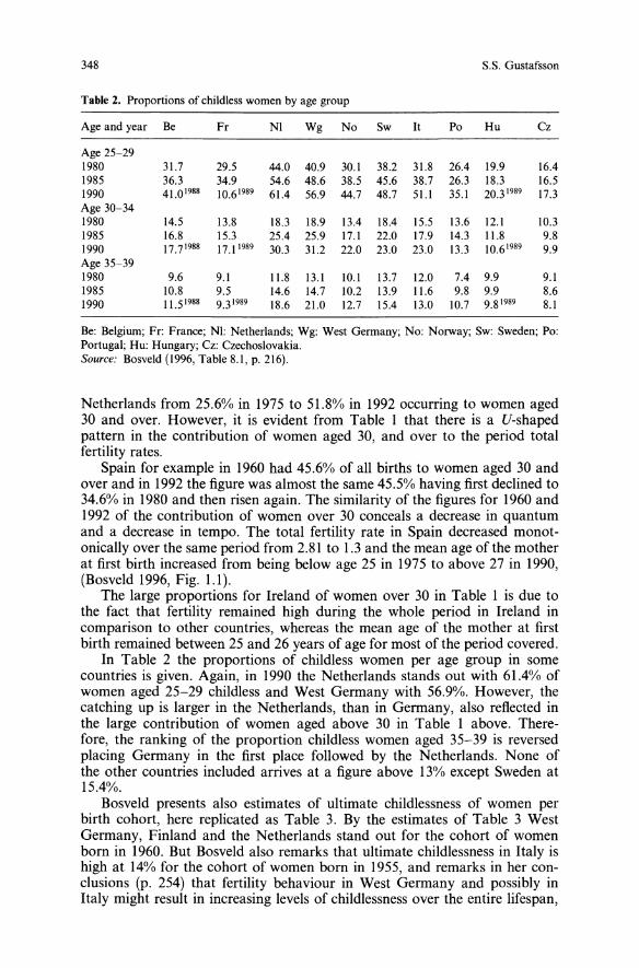
348 S.S. Gustafsson

Table 2. Proportions of childless women by age group

Age and year Be Fr NI Wg No Sw It Po Hu Cz

Age 25-291980 31.7 29.5 44.0 40.9 30.1 38.2 31.8 26.4 19.9 16.41985 36.3 34.9 54.6 48.6 38.5 45.6 38.7 26.3 18.3 16.51990 41.0 1988 10.6 1989 61.4 56.9 44.7 48.7 51.1 35.1 20.3 1989 17.3Age 30-341980 14.5 13.8 18.3 18.9 13.4 18.4 15.5 13.6 12.1 10.31985 16.8 15.3 25.4 25.9 17.1 22.0 17.9 14.3 11.8 9.81990 17.7 1988 17.1 1989 30.3 31.2 22.0 23.0 23.0 13.3 10.6 1989 9.9Age 35-391980 9.6 9.1 11.8 13.1 10.1 13.7 12.0 7.4 9.9 9.11985 10.8 9.5 14.6 14.7 10.2 13.9 11.6 9.8 9.9 8.61990 11.5 1988 9.3 1989 18.6 21.0 12.7 15.4 13.0 10.7 9.8 1989 8.1

Be: Belgium; Fr: France; NI: Netherlands; Wg: West Germany; No: Norway; Sw: Sweden; Po:Portugal; Hu: Hungary; Cz: Czechoslovakia.Source: Bosveld (1996, Table 8.1, p. 216).

Netherlands from 25.6% in 1975 to 51.8% in 1992 occurring to women aged30 and over. However, it is evident from Table 1 that there is a V-shapedpattern in the contribution of women aged 30, and over to the period totalfertility rates.Spain for example in 1960 had 45.6% of all births to women aged 30 and

over and in 1992 the figure was almost the same 45.5% having first declined to34.6% in 1980 and then risen again. The similarity of the figures for 1960 and1992 of the contribution of women over 30 conceals a decrease in quantumand a decrease in tempo. The total fertility rate in Spain decreased monot­onically over the same period from 2.81 to 1.3 and the mean age of the motherat first birth increased from being below age 25 in 1975 to above 27 in 1990,(Bosveld 1996, Fig. 1.1).The large proportions for Ireland of women over 30 in Table 1 is due to

the fact that fertility remained high during the whole period in Ireland incomparison to other countries, whereas the mean age of the mother at firstbirth remained between 25 and 26 years of age for most of the period covered.In Table 2 the proportions of childless women per age group in some

countries is given. Again, in 1990 the Netherlands stands out with 61.4% ofwomen aged 25-29 childless and West Germany with 56.9%. However, thecatching up is larger in the Netherlands, than in Germany, also reflected inthe large contribution of women aged above 30 in Table 1 above. There­fore, the ranking of the proportion childless women aged 35-39 is reversedplacing Germany in the first place followed by the Netherlands. None ofthe other countries included arrives at a figure above 13% except Sweden at15.4%.Bosveld presents also estimates of ultimate childlessness of women per

birth cohort, here replicated as Table 3. By the estimates of Table 3 WestGermany, Finland and the Netherlands stand out for the cohort of womenborn in 1960. But Bosveld also remarks that ultimate childlessness in Italy ishigh at 14% for the cohort of women born in 1955, and remarks in her con­clusions (p. 254) that fertility behaviour in West Germany and possibly inItaly might result in increasing levels of childlessness over the entire lifespan,

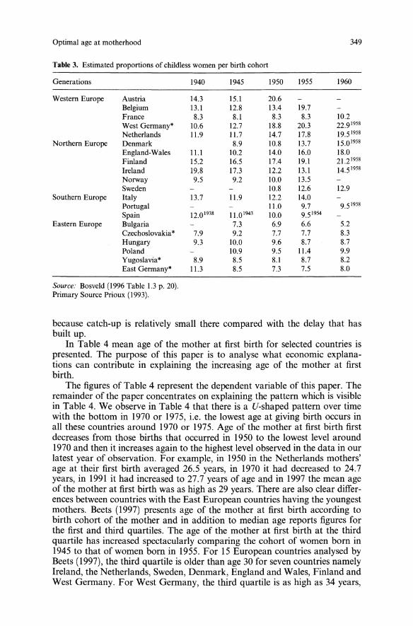
Optimal age at motherhood 349

Table 3. Estimated proportions of childless women per birth cohort

Generations 1940 1945 1950 1955 1960

Western Europe Austria 14.3 15.1 20.6Belgium 13.1 12.8 13.4 19.7France 8.3 8.1 8.3 8.3 10.2West Germany* 10.6 12.7 18.8 20.3 22.9 1958

Netherlands 11.9 11.7 14.7 17.8 19.5 1958

Northern Europe Denmark 8.9 10.8 13.7 15.0 1958

England-Wales 11.1 10.2 14.0 16.0 18.0Finland 15.2 16.5 17.4 19.1 21.2 1958

Ireland 19.8 17.3 12.2 13.1 14.5 1958

Norway 9.5 9.2 10.0 13.5Sweden 10.8 12.6 12.9

Southern Europe Italy 13.7 11.9 12.2 14.0Portugal 11.0 9.7 9.5 1958

Spain 12.0 1938 11.01943 10.0 9.5 1954

Eastern Europe Bulgaria 7.3 6.9 6.6 5.2Czechoslovakia* 7.9 9.2 7.7 7.7 8.3Hungary 9.3 10.0 9.6 8.7 8.7Poland 10.9 9.5 11.4 9.9Yugoslavia* 8.9 8.5 8.1 8.7 8.2East Germany* 11.3 8.5 7.3 7.5 8.0

Source: Bosveld (1996 Table 1.3 p. 20).Primary Source Prioux (1993).

because catch-up is relatively small there compared with the delay that hasbuilt up.In Table 4 mean age of the mother at first birth for selected countries is

presented. The purpose of this paper is to analyse what economic explana­tions can contribute in explaining the increasing age of the mother at firstbirth.The figures of Table 4 represent the dependent variable of this paper. The

remainder of the paper concentrates on explaining the pattern which is visiblein Table 4. We observe in Table 4 that there is a U-shaped pattern over timewith the bottom in 1970 or 1975, i.e. the lowest age at giving birth occurs inall these countries around 1970 or 1975. Age of the mother at first birth firstdecreases from those births that occurred in 1950 to the lowest level around1970 and then it increases again to the highest level observed in the data in ourlatest year of observation. For example, in 1950 in the Netherlands mothers'age at their first birth averaged 26.5 years, in 1970 it had decreased to 24.7years, in 1991 it had increased to 27.7 years of age and in 1997 the mean ageof the mother at first birth was as high as 29 years. There are also clear differ­ences between countries with the East European countries having the youngestmothers. Beets (1997) presents age of the mother at first birth according tobirth cohort of the mother and in addition to median age reports figures forthe first and third quartiles. The age of the mother at first birth at the thirdquartile has increased spectacularly comparing the cohort of women born in1945 to that of women born in 1955. For 15 European countries analysed byBeets (1997), the third quartile is older than age 30 for seven countries namelyIreland, the Netherlands, Sweden, Denmark, England and Wales, Finland andWest Germany. For West Germany, the third quartile is as high as 34 years,

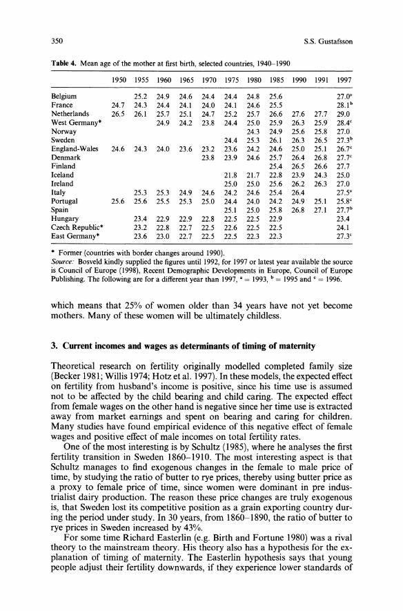
350 S.S. Gustafsson

Table 4. Mean age of the mother at first birth, selected countries, 1940-1990

1950 1955 1960 1965 1970 1975 1980 1985 1990 1991 1997

Belgium 25.2 24.9 24.6 24.4 24.4 24.8 25.6 27.0"France 24.7 24.3 24.4 24.1 24.0 24.1 24.6 25.5 28.1 b

Netherlands 26.5 26.1 25.7 25.1 24.7 25.2 25.7 26.6 27.6 27.7 29.0West Germany· 24.9 24.2 23.8 24.4 25.0 25.9 26.3 25.9 28.4c

Norway 24.3 24.9 25.6 25.8 27.0Sweden 24.4 25.3 26.1 26.3 26.5 27.3b

England-Wales 24.6 24.3 24.0 23.6 23.2 23.6 24.2 24.6 25.0 25.1 26.7c

Denmark 23.8 23.9 24.6 25.7 26.4 26.8 27.7c

Finland 25.4 26.5 26.6 27.7Iceland 21.8 21.7 22.8 23.9 24.3 25.0Ireland 25.0 25.0 25.6 26.2 26.3 27.0Italy 25.3 25.3 24.9 24.6 24.2 24.6 25.4 26.4 27.5"Portugal 25.6 25.6 25.5 25.3 25.0 24.4 24.0 24.2 24.9' 25.1 25.8c

Spain 25.1 25.0 25.8 26.8 27.1 27.7b

Hungary 23.4 22.9 22.9 22.8 22.5 22.5 22.9 23.4Czech Republic· 23.2 22.8 22.7 22.5 22.6 22.5 22.5 24.1East Germany· 23.6 23.0 22.7 22.5 22.5 22.3 22.3 27.3c

• Former (countries with border changes around 1990).Source: Bosveld kindly supplied the figures until 1992, for 1997 or latest year available the sourceis Council of Europe (1998), Recent Demographic Developments in Europe, Council of EuropePublishing. The following are for a different year than 1997, " = 1993, b = 1995 and c = 1996.

which means that 25% of women older than 34 years have not yet becomemothers. Many of these women will be ultimately childless.

3. Current incomes and wages as determinants of timing of maternity

Theoretical research on fertility originally modelled completed family size(Becker 1981; Willis 1974; Hotz et al. 1997). In these models, the expected effecton fertility from husband's income is positive, since his time use is assumednot to be affected by the child bearing and child caring. The expected effectfrom female wages on the other hand is negative since her time use is extractedaway from market earnings and spent on bearing and caring for children.Many studies have found empirical evidence of this negative effect of femalewages and positive effect of male incomes on total fertility rates.One of the most interesting is by Schultz (1985), where he analyses the first

fertility transition in Sweden 1860-1910. The most interesting aspect is thatSchultz manages to find exogenous changes in the female to male price oftime, by studying the ratio of butter to rye prices, thereby using butter price asa proxy to female price of time, since women were dominant in pre indus­trialist dairy production. The reason these price changes are truly exogenousis, that Sweden lost its competitive position as a grain exporting country dur­ing the period under study. In 30 years, from 1860-1890, the ratio of butter torye prices in Sweden increased by 43%.For some time Richard Easterlin (e.g. Birth and Fortune 1980) was a rival

theory to the mainstream theory. His theory also has a hypothesis for the ex­planation of timing of maternity. The Easterlin hypothesis says that youngpeople adjust their fertility downwards, if they experience lower standards of

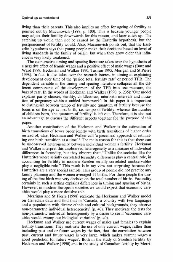
Optimal age at motherhood 351

living than their parents. This also implies an effect for ageing of fertility aspointed out by Macunovich (1998, p. 100). This is because younger peoplemay adjust their fertility downwards for this reason, and later catch up. Thecatching up would then not be caused by the Easterlin hypothesis, but thepostponement of fertility would. Also, Macunovich points out, that the East­erlin hypothesis says that young people make their decisions based on level ofliving standards in the family of origin, but when they grow older this influ­ence is very likely weakened.The econometric timing and spacing literature takes over the hypothesis of

a negative effect of female wages and a positive effect of male wages (Butz andWard 1979; Heckman and Walker 1990; Tasiran 1995; Merigan and St Pierre1998). In fact, it also takes over the research interest in aiming at explainingdevelopment over time of the 'period total fertility rate' or period TFR. Thedependent variable in the timing and spacing literature collapses all the dif­ferent components of the development of the TFR into one measure, thehazard rate. In the words of Heckman and Walker (1990, p. 235): 'Our modelexplains parity choices, sterility, childlessness, interbirth intervals and initia­tion of pregnancy within a unified framework'. In this paper it is importantto distinguish between tempo of fertility and quantum of fertility because thefocus is on the age at first birth, i.e. tempo of fertility, whereas the numberof children born, 'the quantum of fertility' is left out. Therefore, it is also notan advantage to discuss the different aspects together for the purpose of thispaper.Another contribution of the Heckman and Walker is the estimation of

birth transitions of lower order jointly with birth transitions of higher orderinstead of, what Heckman and Walker call 'a piecemeal approach of estimat­ing one birth transition at a time'. 1 The main reason for this is that there canbe unobserved heterogeneity between individual women's fertility. Heckmanand Walker interpret this unobserved heterogeneity as a measure of individualdifferences in fecundity, but they observe that: "Unlike for societies like theHutterites where serially correlated fecundity differences playa central role, inaccounting for fertility in modem Sweden serially correlated unobservablesplaya negligible role." This result is in my view not surprising because theHutterites are a very special sample. This group of people did not practice anyfamily planning and the women averaged 11 births. For these people the tim­ing of the first birth was very decisive on the total number of births. Fecunditycertainly in such a setting explains differences in timing and spacing of births.However, in modem European societies we would expect that economic vari­ables would playa more decisive role.Merrigan and St Pierre (1998) replicate the Heckman and Walker model

on Canadian data and find that in 'Canada, a country with two languagesand a population with diverse ethnic and cultural backgrounds, they observenon-parametric individual heterogeneity' (p. 40). They motivate the tests fornon-parametric individual heterogeneity by a desire to see if 'economic vari­ables would swamp out biological variation' (p. 40).Heckman and Walker use current wages of males and females to explain

fertility transitions. They motivate the use of only current wages, rather thanincluding past and or future wages by the fact, that 'the correlation betweenpast, current and future wages is very large, which makes current wages agood prediction for future wages'. Both in the study of Swedish fertility byHeckman and Walker (1990) and in the study of Canadian fertility by Merri-

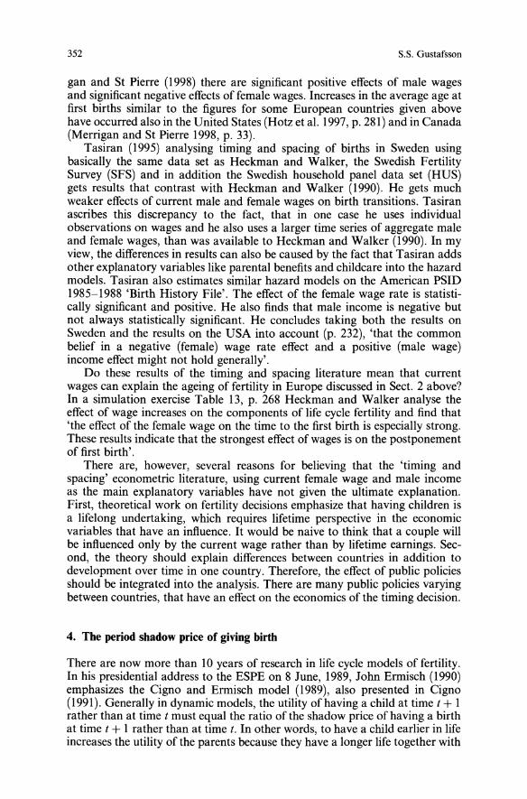
352 S.S. Gustafsson

gan and St Pierre (1998) there are significant positive effects of male wagesand significant negative effects of female wages. Increases in the average age atfirst births similar to the figures for some European countries given abovehave occurred also in the United States (Hotz et al. 1997, p. 281) and in Canada(Merrigan and St Pierre 1998, p. 33).Tasiran (1995) analysing timing and spacing of births in Sweden using

basically the same data set as Heckman and Walker, the Swedish FertilitySurvey (SFS) and in addition the Swedish household panel data set (HUS)gets results that contrast with Heckman and Walker (1990). He gets muchweaker effects of current male and female wages on birth transitions. Tasiranascribes this discrepancy to the fact, that in one case he uses individualobservations on wages and he also uses a larger time series of aggregate maleand female wages, than was available to Heckman and Walker (1990). In myview, the differences in results can also be caused by the fact that Tasiran addsother explanatory variables like parental benefits and childcare into the hazardmodels. Tasiran also estimates similar hazard models on the American PSID1985-1988 'Birth History File'. The effect of the female wage rate is statisti­cally significant and positive. He also finds that male income is negative butnot always statistically significant. He concludes taking both the results onSweden and the results on the USA into account (p. 232), 'that the commonbelief in a negative (female) wage rate effect and a positive (male wage)income effect might not hold generally'.Do these results of the timing and spacing literature mean that current

wages can explain the ageing of fertility in Europe discussed in Sect. 2 above?In a simulation exercise Table 13, p. 268 Heckman and Walker analyse theeffect of wage increases on the components of life cycle fertility and find that'the effect of the female wage on the time to the first birth is especially strong.These results indicate that the strongest effect ofwages is on the postponementof first birth'.There are, however, several reasons for believing that the 'timing and

spacing' econometric literature, using current female wage and male incomeas the main explanatory variables have not given the ultimate explanation.First, theoretical work on fertility decisions emphasize that having children isa lifelong undertaking, which requires lifetime perspective in the economicvariables that have an influence. It would be naive to think that a couple willbe influenced only by the current wage rather than by lifetime earnings. Sec­ond, the theory should explain differences between countries in addition todevelopment over time in one country. Therefore, the effect of public policiesshould be integrated into the analysis. There are many public policies varyingbetween countries, that have an effect on the economics of the timing decision.

4. The period shadow price of giving birth

There are now more than 10 years of research in life cycle models of fertility.In his presidential address to the ESPE on 8 June, 1989, John Ermisch (1990)emphasizes the Cigno and Ermisch model (1989), also presented in Cigno(1991). Generally in dynamic models, the utility of having a child at time t + 1rather than at time t must equal the ratio of the shadow price of having a birthat time t + 1 rather than at time t. In other words, to have a child earlier in lifeincreases the utility of the parents because they have a longer life togetherwith

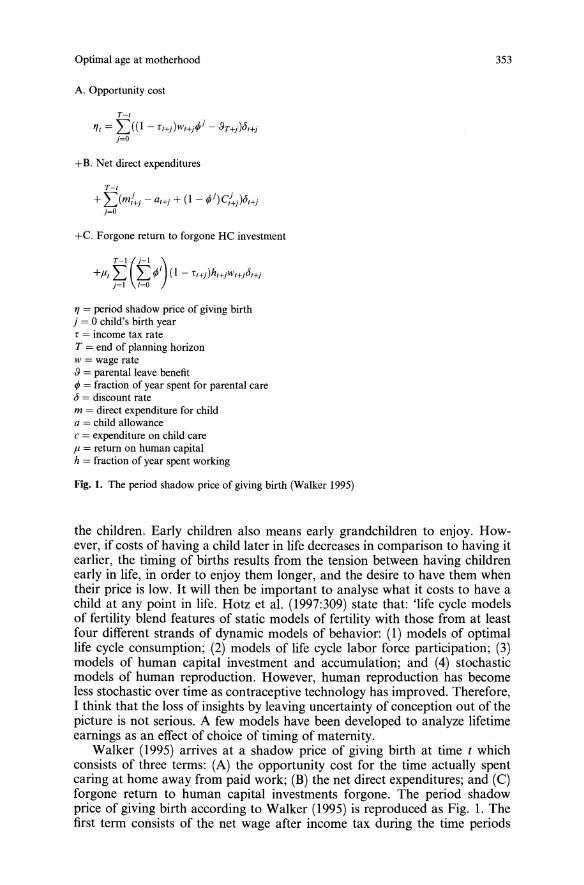
Optimal age at motherhood

A. Opportunity cost

T-/

'It = L((l- r/+j)wl+j¢Jj

- fh+j)<5'+j

j=O

+8. Net direct expenditures

T-I

+L(m{+j - a/+j + (I - ¢Jj)C/+j )<5t+jj=O

+c. Forgone return to forgone He investment

" = period shadow price of giving birthj = 0 child's birth yearr = income tax rateT = end of planning horizonW = wage rate[) = parental leave benefit¢J = fraction of year spent for parental care<5 = discount ratem = direct expenditure for childa = child allowancec = expenditure on child careJ1. = return on human capitalh = fraction of year spent working

Fig. 1. The period shadow price of giving birth (Walker 1995)

353

the children. Early children also means early grandchildren to enjoy. How­ever, if costs of having a child later in life decreases in comparison to having itearlier, the timing of births results from the tension between having childrenearly in life, in order to enjoy them longer, and the desire to have them whentheir price is low. It will then be important to analyse what it costs to have achild at any point in life. Hotz et aI. (1997:309) state that: 'life cycle modelsof fertility blend features of static models of fertility with those from at leastfour different strands of dynamic models of behavior: (1) models of optimallife cycle consumption; (2) models of life cycle labor force participation; (3)models of human capital investment and accumulation; and (4) stochasticmodels of human reproduction. However, human reproduction has becomeless stochastic over time as contraceptive technology has improved. Therefore,I think that the loss of insights by leaving uncertainty of conception out of thepicture is not serious. A few models have been developed to analyze lifetimeearnings as an effect of choice of timing of maternity.Walker (1995) arrives at a shadow price of giving birth at time t which

consists of three terms: (A) the opportunity cost for the time actually spentcaring at home away from paid work; (B) the net direct expenditures; and (C)forgone return to human capital investments forgone. The period shadowprice of giving birth according to Walker (1995) is reproduced as Fig. 1. Thefirst term consists of the net wage after income tax during the time periods

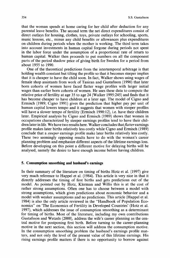
354 s.s. Gustafsson

that the woman spends at home caring for her child after deduction for anyparental leave benefits. The second term the net direct expenditures consist ofdirect outlays for housing, clothes, toys, private outlays for schooling, sports,music lessons, etc., minus any child benefits or allowances plus expenditureson children during periods when the mother is working. The third term takesinto account investments in human capital forgone during periods not spentin the labor force under the assumption of a proportional rate of return tohuman capital. Walker then proceeds to put numbers on all the componentparts of the period shadow price of giving birth for Sweden for a period fromabout 1955 to 1990.One of the theoretical predictions from the intertemporal arbitrage is that

holding wealth constant but tilting the profile so that it becomes steeper impliesthat it is cheaper to have the child soon. In fact, Walker shows using wages offemale shop assistants from work of Tasiran and Gustafsson (1990) that laterborn cohorts of women have faced flatter wage profiles with larger initialwages than earlier born cohorts of women. He uses these data to compute therelative price of fertility at age 35 to age 24 (Walker 1995:245) and finds that ithas become cheaper to have children at a later age. The model of Cigno andErmisch (1989; Cigno 1991) gives the prediction that higher pay per unit ofhuman capital lowers tempo and it suggests that women with steeper profileswill have a slower tempo of fertility (Ermisch 1990:12), i.e. have their childrenlater. Empirical analysis by Cigno and Ermisch (1989) shows that women inoccupations characterized by steeper earnings profiles tend to have their chil­dren later in life. We have two results here. Walker concludes thatfiatter earningsprofile makes later births relatively less costly while Cigno and Ermisch (1989)conclude that a steeper earnings profile make later births relatively less costly.These two seemingly opposing results have to do with the woman's careerplanning problem and emphasize different aspects of the lifetime earnings loss.Before developing on this point a different motive for delaying births will beanalysed, namely the desire to have enough income before having children.

5. Consumption smoothing and husband's earnings

In their summary of the literature on timing of births Hotz et al. (1997) givevery much reference to Happel et at. (1984). This article is very nice in that itdirectly addresses the timing of first births and gets predictions out of themodel. As pointed out by Hotz, Klerman and Willis this is at the cost ofrather strong assumptions. Often one has to choose between a model withstrong assumptions, which gives predictions about economic behavior and amodel with weaker assumptions and no predictions. This article (Happel et al.1984) is also the only article reviewed in the "Handbook of Population Eco­nomics" on 'The Economics of Fertility in Developed Countries' (Hotz et al.1997), which addresses the issue of consumption smoothing as a determinantfor timing of births. Most of the literature, including my own contributionsGustafsson and Wetzels (2000), address the wife's career planning as the cen­tral motive for postponing first birth. Before turning to the career-planningmotive in the next section, this section will address the consumption motive.In the consumption smoothing problem the husband's earnings profile mat­ters, and not only the level of the present value of this lifetime earnings. Hisrising earnings profile matters if there is no opportunity to borrow against

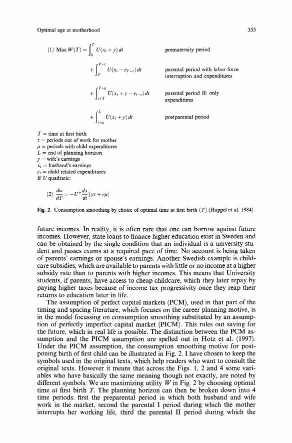
Optimal age at motherhood

(I) Max W(T) =rU(xr +y)dt

JTH

+ T U(xr - eT_,)dt

JT+~

+ U(xi +Y - er-,) dtr+T

T = time at first birthr = periods out of work for mother11 = periods with child expendituresL = end of planning horizony = wife's earningsXI = husband's earningsel = child related expendituresIf U quadratic:

(2) dw I/dx[ I- = -U - yr+elldT dt

prematernity period

parental period with labor forceinterruption and expenditures

parental period II: onlyexpenditures

postparental period

355

Fig. 2. Consumption smoothing by choice of optimal time at first birth (T) (Happel et al. 1984)

future incomes. In reality, it is often rare that one can borrow against futureincomes. However, state loans to finance higher education exist in Sweden andcan be obtained by the single condition that an individual is a university stu­dent and passes exams at a required pace of time. No account is being takenof parents' earnings or spouse's earnings. Another Swedish example is child­care subsidies, which are available to parents with little or no income at a highersubsidy rate than to parents with higher incomes. This means that Universitystudents, if parents, have access to cheap childcare, which they later repay bypaying higher taxes because of income tax progressivity once they reap theirreturns to education later in life.The assumption of perfect capital markets (PCM), used in that part of the

timing and spacing literature, which focuses on the career planning motive, isin the model focussing on consumption smoothing substituted by an assump­tion of perfectly imperfect capital market (PICM). This rules out saving forthe future, which in real life is possible. The distinction between the PCM as­sumption and the PICM assumption are spelled out in Hotz et al. (1997).Under the PICM assumption, the consumption smoothing motive for post­poning birth of first child can be illustrated in Fig. 2. I have chosen to keep thesymbols used in the original texts, which help readers who want to consult theoriginal texts. However it means that across the Figs. 1, 2 and 4 some vari­ables who have basically the same meaning though not exactly, are noted bydifferent symbols. We are maximizing utility W in Fig. 2 by choosing optimaltime at first birth T. The planning horizon can then be· broken down into 4time periods: first the preparental period in which both husband and wifework in the market, second the parental I period during which the motherinterrupts her working life, third the parental II period during which the

356 S.S. Gustafsson

mother returns to work but there are child related direct expenses as in theparental I period and fourth and finally the postparental period in which thereare no longer any child related expenses. Then if the utility of consumptionmoney is a quadratic function as in expression (2) of Fig. 2, we know thatwhen the parenthesis increases, the optimal time till first birth will increase.One example given by Happel et al. (1984) is that policies which decrease thetime spent out of work by the mother, such as more daycare for children willlower the tempo of first birth. Note that this is because the second periodbecomes shorter in Fig. 2 and it applies irrespective of whether the mother hasany prospects for human capital investments. In fact, in Fig. 2 mother's earn­ings are assumed constant over the whole lifetime. In expression (2) also if childexpenditures (e) are lowered by a child benefit, if the time until adulthood isshorter as in the case for children with shorter education, and if mother's earn­ings (y) are smaller the tempo of fertility decreases and women are younger atmotherhood. Also in this formulation the optimal time to have the first birth iswhen husband's income (XI) is the highest. In the formulation of Fig. 2, meanlifetime consumption is independent of T (time of first birth), therefore, if hus­bands earnings increase over time, life-eycle utility is maximized when birthsare delayed to the biological limit. The household smoothes its consumptionprofile and therefore raises its economic welfare, by delaying the r periods ofthe woman's nonemployment and the f1. periods of child expenses to a timewhen the man's earnings are relatively high (Happel et al. 1984:305)

6. Career planning

The potential detrimental effects on the mother's job career is the part ofcosts of children that has received most attention in economic research. See,for example, Joshi (1990, 1994, 1998) mainly for Great Britain, Dankmeyer(1996) and Meertens (1998) for the Netherlands. These costs consist of twomain parts: the direct forgone wages by time spent out of the labor force andthe human capital loss. In models analysing the optimal time of giving birthfrom the point of view of its effects on mother's lifetime earnings we assumethat capital markets are perfect allowing borrowing and saving across periods.In what follows, the analysis is carried out for a given time preference forchildren. Another way of stating this is that we do not consider the benefits ofchildren, only the cost of children. The fact that births are not always delayedto the fecundity limit, is an indication that benefits of children most oftenwork in the direction of earlier births. Also, husband's earnings are left out ofthe analysis, assuming that his labor market career is not affected by birthtiming. In the previous section the consumption smoothing motive of birthtiming was seen to give a role to the earnings profile of the husband and also ahigher husband's lifetime earnings generally will act as an income effect whichenables a couple to fulfil their wish for a child earlier in life. However, we willdisregard these influences for now and concentrate on the mother's potentialearnings for a given present value of husband's earnings. The determinants ofoptimal time at maternity then depend on:

1. The woman's accumulated human capital at the beginning of the planningperiod;

Optimal age at motherhood

2. the rate at which the woman's job skills decay;3. the rate of return to human capital investments;4. the profile of human capital investments;5. the length of time spent out of the labor force;6. the size of child quality expenditures.

357

Some variants of the effect of birth timing on lifetime earnings of the motherare shown in Fig. 3, with panel A showing a relatively steep linear earningsprofile, panel B showing a relatively less steep linear earnings profile and panelC showing a non-linear earnings profile. In the following I will discuss howeach of the six determinants mentioned above enter into the determination ofoptimal age at giving birth drawing on the three models Happel et al. (1984)Cigno and Ermisch (l989) as presented in Cigno 1991, Chapt. 8 and Walker(1995). I will also try to evaluate their importance drawing from empiricalliterature that has come to my attention.

6.1. Preparental human capital

Does a larger amount of preparental human capital have an effect on timingof maternity? A larger amount of preparental human capital will be shown asa larger intercept in Fig. 3. In the Happel, Hill and Low model the larger thepreparental work experience the more likely the first birth is delayed. This isbecause the probability of total skill loss during home time is then less and thiswas the only case in which an early birth was preferred to a late birth in theirmodel. Cigno (1991: 124) concludes by his model that: 'women who entermarriage better endowed with market specific human capital will have fewerchildren and sooner'. They will have them sooner because of the income effect,because parents have a positive time preference. This result is at odds with theHappel, Hill and Low result that women with larger preparental human cap­ital will tend to delay births. However, the reason the Happel, Hill and Lowhigher educated women would have delayed births was that they were less atrisk of losing all their job skills and not positive time preference for births.Going back to Walker (1995) Fig. I above there is no mechanism by whichpreparental human capital enters the determination of optimal birth timing.However, Walker concludes using wage data for shop assistants that wageprofiles have become flatter and at a higher level. This in general consideringFig. 3 would make the direct opportunity cost relatively larger for early birthswhile the capital cost will decline. Therefore, Walker concludes in an inter­esting simulation Walker (1995, Fig. 13, p. 245) that the relative shadow priceof having a birth at age 35 has decreased in comparison to having a birth atage 24. However, empirical work by Gustafsson and Wetzels (2000) showsthat higher educated women have their children later than less educatedwomen and they are also the ones that have postponed first birth the mostcomparing the 1990s to the 1980s.

6.2. Depreciation ofhuman capital due to non-use

In Fig. 3 a situation in which there is depreciation of human capital due to ahome time period to give birth and care for a child is represented by a point p

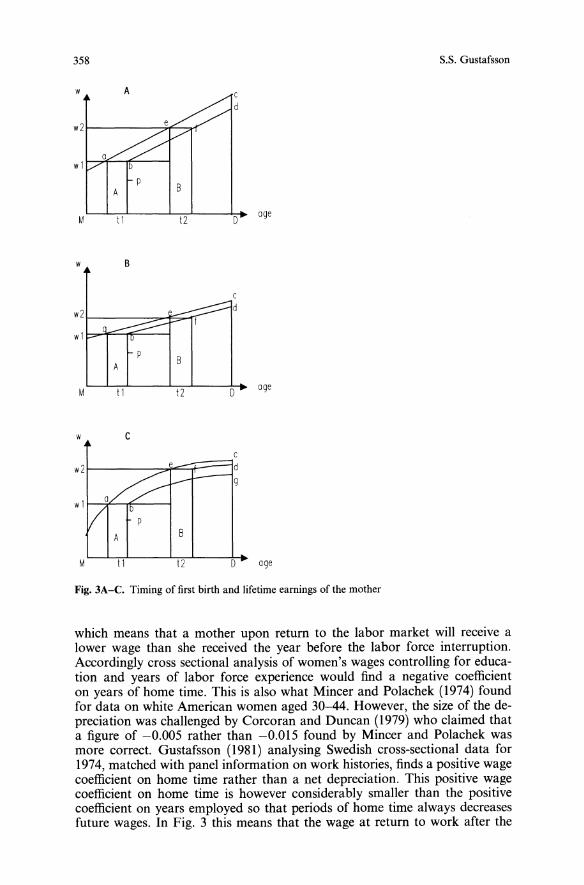
358 S.S. Gustafsson

w A cd

w2

w1

A B

M \1 12 Dage

w B

c

w2 d

wI

AB

M 11 12 D age

w C

w2 e

A B

M 11 12 D age

Fig. 3A-C. Timing of first birth and lifetime earnings of the mother

which means that a mother upon return to the labor market will receive alower wage than she received the year before the labor force interruption.Accordingly cross sectional analysis of women's wages controlling for educa­tion and years of labor force experience would find a negative coefficienton years of home time. This is also what Mincer and Polachek (1974) foundfor data on white American women aged 30-44. However, the size of the de­preciation was challenged by Corcoran and Duncan (1979) who claimed thata figure of -0.005 rather than -0.015 found by Mincer and Polachek wasmore correct. Gustafsson (1981) analysing Swedish cross-sectional data for1974, matched with panel information on work histories, finds a positive wagecoefficient on home time rather than a net depreciation. This positive wagecoefficient on home time is however considerably smaller than the positivecoefficient on years employed so that periods of home time always decreasesfuture wages. In Fig. 3 this means that the wage at return to work after the

Optimal age at motherhood 359

labor force interruption is above b. Depreciation of human capital plays animportant role in the Happel, Hill and Low model, since in the absence ofdepreciation timing of birth will have no effect on mother's lifetime earnings.The wife has an amount of human capital accumulated called w at the start ofmarriage and there is a linear increase in human capital for each year of laborforce participation t. Then the earnings loss upon return to the labor market isyr, where r is the home time and y the rate of depreciation. The result is thatcouples will begin childbearing either very early or very late in marriage. Thepostponement occurs when only a fraction of the wife's job skills are lostduring the labor fore interruption. If most of the job skills are lost then it isbetter to have the child as early as possible. In fact, the model predicts that thesolution is in one of the two comer solutions, either directly after marriage orat the limit of the fecund period. The models by Cigno and Ermisch (Cigno1991) and by Walker (1995) assume a zero rate of depreciation of humancapital.

6.3. The rate of return to human capital investments

In Fig. 3 the slope of the age earnings curve is the product of the rate of returnto human capital investments and the investment profile. In the formulationof Cigno (1991) represented in Fig. 4 here the investment profile increaseslinearly whereas the rate of return to human capital is a constant. (See Fig. 4Eq. 4.) According to Ermisch (1990: 12): 'The model also predicts that higherpay per unit of human capital lowers tempo and it suggests that women withsteeper earnings profiles will have a slower tempo of fertility'. The secondstatement about the steeper earnings profiles according to the CignojErmischformulation must be due to a higher rate of human capital investments. Thereason an increase in the rate of return per unit of human capital lowerstempo, i.e. causes couples to have the first birth early in marriage, is spelledout Cigno (1991:125) in the following way: 'By contrast a rise in w wouldcause the opportunity-cost component (wage plus capital loss) of PI to growfaster if the timing of births were not modified. Since the growth rate of II doesnot depend on w (see Eq. 6, Fig. 4) the growth rate of the ratio ofPt! VI wouldthen rise'. Note that PI is the period shadow price of a birth and VI is theutility to parents of having a birth at time period t. See Fig. 4, Eq. (3) and (6).But the ratio of the period shadow price of birth to the period utility of birth(Pt! Vr) must according to the equilibrium condition grow at the same rate asthe interest rate and if the interest rate is not changed, a smaller PI must bepicked by having a birth earlier. Therefore, if the return per unit of humancapital is increased, other things equal couples will have their children earlierin married life. In Walkers' formulation the rate of return to human capital (J.lin Fig. I) is predetermined by calendar time, setting it to 4.1% before 1966,2.7% 1966-1975 and 1.3% 1976-1989, but he only uses this in his calculationof capital loss, and not in the determination of his wage, which is differentfrom the Cigno (1991) formulation. He uses age specific earnings for femaleshop assistants, directly observed and he probably does not see the rate ofreturn as a return to 'on the job investments'. Returns to on the job investmentin human capital frequently is in the form of job mobility between occupa­tions, which is ruled out by studying wages of only one occupation. Happel etal. (1984) do not discuss the capital cost part of the opportunity cost of child

360

Parent's utility function:

(I) V = V(C,B)

B == nq i.e. number of children times child quality

For the timing model:

D

(2) B = L: VI(I,)BII=M

D

(3) C = L: V,(C,)'=M

I-I

(4) W, = wk, k, = k M +PL: LIr-M

D D

(5) L:lC, + (II +eD- tP)BI]r M

-' ~ A + L:L,W,r M-'

~M ~M

period shadow price of birth

D

(6) P, = eO - tP + I, + WI + pw L: Lrr l-r

r=I+1

L I =m-B,L, = labor supply of wifem = work capacityB, = the rate of birth at tI, = the amount invested in a child born at teO = minimum costs of procuring a birth of a childC, = amount of adult consumptionr = rate of discountM = date at marriagew, = wage at time tw = rate of return to human capitalK, = amount of human capital accumulated at tKM = premarital human capitalP= rate of growth of capital

Fig. 4. Model of birth timing (Cigno 1991)

S.S. Gustafsson

timing, nor do they discuss effects of the size of rate of return to humancapital.

6.4. The profile ofhuman capital investment

In the Cigno and Ermisch (1989) study the investment profile is central. Womenwho are employed in occupations with a steeper rising earnings profile willtend to lower their tempo of fertility. They find that women in semi-skilledor manual occupations have earlier births than women in the more skilledclerical occupations. Also, Happel et al. (1984:309) find that women in high

Optimal age at motherhood 361

skilled occupations have their first child later than women in low skill occu­pations.Gustafsson and Wetzels (2000) find that higher educated women delayed

first birth more than less educated women comparing births of the 1990s tobirths of the 1980s for all the four countries studied (Germany, Great Britain,the Netherlands and Sweden). It is easy to see for a zero discount rate in Fig. 3comparing panels A and B that the capital loss is higher for a steeper earningsprofile panel A than for a flatter earnings profile. This works in the directionof delaying births. On the other hand the direct wage cost is bigger for laterbirths. If the earnings profile is convex to the origin rather than linear as inpanel C the capital cost of a later birth will be very much smaller than thecapital cost of an early birth. Panel C is in accordance with the originalMincer (1974) formulation and is also the shape of the earnings functionusually estimated in empirical work. The theoretical foundation for a qua­dratic earnings function is that life is finite and the investment motive becomesweaker the closer retirement a worker gets, therefore his or her incentive tofurther improve skills declines since fewer periods are left to reap the returnsto investment in human capital. If the rate of human capital investment de­creases with age instead of being linear in labor force experience as in all themodels discussed in this paper, the incentive to postpone first birth will bestronger since the difference between direct wage loss of a late birth to an earlybirth is smaller comparing panel C to panel A and the capital loss of a latebirth area delineated by efcd is smaller in panel C than in panel A. Recruit­ment policies of firms into career tracks reinforce the postponement in­centives, since they often concentrate on recruiting young talents and it is lesscommon to recruit a person in the postparental phase into a positioninvolving a large amount of training.

6.5. The length of time spent out of the labor force

Does the length of time spent out of the labor force have any effect on thetiming of first birth? Happel et al. (1984) answer yes in their model representedas Fig. 2 above. If there are imperfect capital markets and husband's incomeprofile increases with time then the longer the planned time spent out of thelabor force the stronger the motive to postpone childbirth. Also by the hypo­thetical age earnings curves of Fig. 3 it is clear that, if mothering is seen astotally incompatible with paid work it is better to delay childbearing as longas possible because that will decrease lifetime earnings loss.Dutch mothers until recently, particularly if they have little education have

followed such a pattern. Dankmeyer (1996) using a cross section from 1990finds that low educated women with 2 children born when the mother is 25and 28 years old will keep only 13% of the lifetime income of a correspondingwoman without children. The computation is based on I) a wage regression,2) a participation logit, 3) an hours regression and simulations for represen­tative women differing in education. Consequently, the labor force participa­tion rate is predicted for each year for a woman without children and for atwo child woman's lifetime earnings using the wage regression and the par­ticipation logit. Further, if the probability of labor force participation duringone particular year of age exceeds 0.5, the earnings for that year are computed

362 S.S. Gustafsson

using the hours regression to predict hours of work and then multiply by pre­dicted wages to get income.Meertens (1998) using a cross section of Dutch women from 1992 esti­

mates a tobit on annual income, where years of schooling is a crucial expla­natory variable. The results of Meertens' analysis are more dismal since highereducated women with children by her method only have a marginally largerincome than lower educated women with children. This means that womencan always increase their lifetime income by having their child later. However,a cross sectional analysis of labor force participation and earnings are a badpredictor for the decision of young women, who now are in the situation ofdetennining when to have their first birth, particularly as now is the case in theNetherlands, there are large cohort effects, where younger cohorts are increas­ing their labor force participation very much in comparison to older cohorts.In Walker's work (1995:240) the time absent from the labor market follow­

ing a birth is the single most important assumption used in the construction ofthe period shadow price of fertility. He varies his absence assumption from a)short absence i.e. - one year full time absence plus one year part-time employ­ment and b) long absence, which equals six years fulltime withdrawal andone year part-time work. All his cost items shown in Fig. 2 except the directexpenditure for the child (m) depend on this assumption. The direct expendi­ture for the child (m) are computed in two ways. First based on an estimatefrom 1969 of household expenditure for a household without children incomparison to a household with children and second just assuming that achild costs 20% of household expenditures. However, Walker's period shadowprice of giving birth of Fig. 2 also takes account of child care subsidies, andparental leave benefits which all have lowered the cost of children in Swedenduring the period he studies. These factors are not discussed in the Cigno andEnnisch (1989) work.Walker (1995) takes the approach of using the pattern of absence which

are implied by Swedish policy makers namely, one year of fulltime homecaring, followed by five years of 3/4 of full time work followed by full timework for the rest of the lifetime. This is of course a very unjust assumption forthe earlier part of the time period he studies, which starts in 1955 and runsuntil 1990, but it is a reasonable assumption for the more recent mothers,since those policy measures have been introduced gradually starting in 1974and becoming in full effect by 1989 (Gustafsson 1984, 1994; Gustafsson andStafford 1992; Sundstrom and Stafford 1992).A similar approach is used by Gustafsson and Wetzels (2000). Their result is

that postponement of births will always be beneficial in the sense that thelifetime earnings loss is diminished. This is true also for stepping out of workonly one year and then return to fulltime work, although in this case the costsare a very small proportion a few per cent of a life time income.

6.6. The size of child quality expenses

The more money parents spend on a child including educational expenses andthe longer the period parents keep paying for their child, the higher will be theshadow price of a child. In the Happel et al. (1984) model with imperfectcapital markets the larger the expenses are the later in life the parents want tohave the child. This is if the consumption smoothing motive is important and

Optimal age at motherhood 363

if wages increase over lifetime. High educated people who have steeply risingearnings want to have high educated children, who therefore cost much. Thismotive will therefore strenghten the incentive for high educated people todelay parenthood.

7. Biological - medical aspects

In this paper it has been shown that age of the mother at first birth has beenincreased in most European countries with the exception of Eastern Europeuntil 1990. We have seen that there are many mechanisms which tend to pushmaternity towards the biological limit. The economic theoretical models dis­cussed above all assume that the biological fecundity limit is known to thedecision making couple. The closer a woman gets to her fecundity limit themore important it becomes for her to have knowledge about possible con­sequences of late motherhood.One study Gilbert et al. (1999), addresses the question of childbearing

beyond age 40. The study is based on data from birth certificates and hospitaldischarge records of all births that occurred in Californian hospitals duringthe period January 1, 1992 including December 31, 1993. There were 24,032deliveries of women aged 40 and over which corresponds to 2% of all births inthis two year period, of these 20% 4,777 were nulliparous i.e. had their firstbirth. The data of the older mothers were compared to a control group ofwomen who were 20-29 at giving birth. The results are, that women who hadtheir first child above age 40, have a higher risk of operative delivery (61% ofwhich Caesarean 47%) than do younger nulliparous (35% of which Caesarean22,5%). The study also presents medical problems of mother and child arounddelivery such as prematurity, malpresentation and obstructed labor and 8 otherdisorders. Older first time mothers are over represented as compared toyounger first time mothers on all reported disorders. Older first time mothersalso have children with lower birth weight and have a shorter gestationalperiod than the control group. The authors hope that: "These data will allowus better to counsel patients about their pregnancy expectations and possibleoutcomes" (Gilbert et al. 1999:9). This article is a warning against increasedcomplications around childbirth but does not say anything about any lastingconsequences of being an older mother.

In order to say something about fecundity limits one would need data onprobability of successful pregnancies among women who intend to becomepregnant. Another study Waldron, Weiss and Hughes (1998:216) find that:"as predicted by the Age-Related Parental Role Strain Hypothesis: youngerage at first birth, particularly a teenage birth, appeared to result in moreharmful health effects". The data of this study is from the United StatesNational Longitudinal Study and the study of mother's age at first birth doesnot include women who had their first birth after age 30. This study includeslong-run effects on the health of mothers since in some cases the mothers arefollowed until their children are teenagers. However, there are no long rundata on the health of children. What one can conclude from the two studiesmentioned that it is not good to be a very young mother, and there are someimmediate negative effects from being a first time mother aged 40 and over.By a study (Treloar 1981) cited by Dorland, Kooij and te Velde it is con­

cluded that 12.5% of women were in the menopause at age 46 and therefore a

364 8.8. Gustafsson

similar percentage would have fecundity problems already at age 36. At age31 half of all women have experienced decrease in fecundity, at age 41 half ofall women have experienced infecundity and at age 51 half of all women havereached the menopause.Medical research also concludes, that it is very likely, that the age at

menopause is genetically determined and also the age determined decrease infecundity. Generally, the quality of the egg cell deteriorates which results insmaller likelihood that the egg cell gets planted and a larger risk of chromosomatic changes as Down's syndrome. The conclusion of Dorland et al.(1997:39) is that about 50% of women aged between 30 and 40 will have mildor serious fecundity problems. These women will make use of medical assis­tance for these problems. Therefore, medical fecundity treatment thereforewill become a rather normal procedure in family planning.Den Ouden et al. (1997) summarize medical research about health con­

sequences for mother and child. They point out that the probability of success­ful pregnancy already at age 30 of the woman decreases and that the fecundityof the man from age 45 decreases. They summarize the problems of late birthsas the following consequences for the mother: longer waiting time to concep­tion, more miscarriages, more multiple births, more pregnancy complications,more caesareans and more breast cancer. The consequences for the child ofbeing born to an older mother are: more still births, more infant deaths, morepremature births, more chromo somatic problems and more often learningproblems.

8. Conclusions

In this paper it has been shown that European women have delayed their ageat first birth substantially since the 1970s and that the postponement is largealso comparing births during the 1990s to those of the 1980s. Economic the­orizing on the optimal age at giving birth in general weighs the pleasure ofearly births against the lower cost of later births. One model reviewed (Happelet al. 1984) finds that with perfectly imperfect capital markets the man'sincome profile matters and its effect is to delay births until a moment whencosts of the child can be offset by his higher earnings. The most importantfactor which works for later births is the woman's career costs. These costsare basically of two kinds her direct wage loss during labor force withdrawalsand her loss of human capital investments and returns to these investments.Parameters which have effects on the career costs outcome are of five differentkinds:

I. The amount of prematernity human capital;2. the rate of depreciation of human capital due to non-use;3. the rate of return to human capital investments;4. the profile of human capital investments;5. the length of time spent out of the labor force.

Increases in all these parameters tend to make postponement of birth morefavorable except in one formulation by Cigno and Ermisch (1989) where alarge initial human capital by its income effect will bring forward births. Theanalysis shows that any public policies that will lead to decreases in time spent

Optimal age at motherhood 365

out of work, which is the most important part of the period shadow price ofgiving birth will have an effect of decreasing age at maternity. Biologicalmedical research shows that the risks around pregnancy and delivery increasefor first time mothers aged 40 and above, that the probability of conceptiondecreases for some women already after age 30 and that about half of a pop­ulation will have mild or serious fecundity problems already from age 36.Research about long run effects on health of mothers and children born toolder mothers are also not very optimistic. Therefore, there are good argu­ments for governments to consider political measures like paid parentalleaves, subsidized childcare and consider the school and work organizationsso as to facilitate the combination of either being a student and a mother orbeing a worker and a mother. Such measures will again have a tendency todecrease age of maternity, which will lead to healthier and happier mothersand children and more generally happier fathers and grandparents.

Endnotes

1 In the mid-1980s I was a visiting scholar to the University of Chicago, and I was told by JimWalker at that time, that the computer program took 6 hours to estimate. I thought, that therewere never going to be any replications of their model but technology develops and we nowhave replications by other authors and other data sets) e.g. Tasiran (1994) and Merrigan and StPierre (1998).

References

Bonsel GJ, Van der Maas PJ (1994) Aan de wieg van de toekomst; scenario's van de zorg rond demenselijke voortplanting, 1995-2010. Stafleu Van Lochem, Houten

Becker GS (1981) A Treatise on the Family. Harvard University Press, LondonBeets GCN (1997) Kinderen worden later geboren: een demografische analyse. In: Beets GCN,Bouwens A, Schippers JJ (eds.) Uitgesteld ouderschap. Thesis publishers, Amsterdam: 13­31

Bosveld W (1996) The Ageing of Fertility in Europe. A Comparative Demographic - AnalyticStudy, PDOD. Thesis Publishers, Amsterdam

Butz WP, Ward MP (1979) The Emergence of Countercyclical US Fertility. American EconomicReview 69:318-328

Cigno A (1991) Economics of the Family. Clarendon Press, OxfordCigno A, Ermisch J (1989) A Micro-Economic Analysis of the Timing of Births. European Eco­

nomic Review 33:737-760Corcoran M, Duncan G (1979) Work History, Labor Force Attachment, and Earnings Differ­entials Between the Races and the Sexes. The Journal of Human Resources 14:3-20

Council of Europe (1998) Recent Demographic Developments in EuropeDankmeyer B (1996) Long Run Opportunity-Cost of Children according to Education of theMother in the Netherlands. Journal of Population Economics 9:349-361

Demographic Yearbook (1997) United Nations (1999), New YorkDen Ouden L, Verloove-Vanhorick P, Bruinse HW (1997) Zwangerschappen op oudere leeftijd:gevolgen voor moeder en kind. In: Beets GCN, Bouwens A, Schippers JJ (eds.) UitgesteldOuderschap. Thesis Publishers, Amsterdam, 41-47

Dorland RM, Van Kooij RJ, Te Velde ER (1997) Medische grenzen aan gezinsplanning. In: BeetsGCN, Bouwens A, Schippers JJ (eds) Uitgesteld ouderschap. Thesis Publishers, Amsterdam,33-47

Easterlin RA (1980) Birth and Fortune. Grand-McIntyre, LondonErmisch J (1990) European Women's Employment and Fertility Again. Journal of Population

Economics 3:3-18

366 S.S. Gustafsson

Fauser BCMJ (1998) Inaugurale Rede als Hoogleraar Gyneacologische Endocrinologie. ErasmusUniversiteit Rotterdam, 29 januari

Gilbert WM, Nesbitt TS, Danielsen B (1999) Childbearing Beyond Age 40: Pregnancy Outcomein 24032 Cases. Obstetrics and Gynaecology 93:9-14

Gustafsson SS (1981) Male Female Lifetime Earnings Differentials and Labor Force History.In: Eliasson G, Holmlund B, Stafford FP (eds) Studies in Labor Market Behavior, Swedenand the United States. The Industrial Institute in Economic and Social Research, Stock­holm, 235-300

Gustafsson SS (1984) Equal Opportunity Policies in Sweden. In: Schmid G, Weitzel R (eds) SexDiscrimination and Equal Opportunity, The Labour Market and Employment Policy. Wissen­schaftzentrum, West Berlin and Gower Publishing Company, England, 132-154

Gustafsson SS, Stafford F (1992) Daycare Subsidies and Labor Supply in Sweden. Journal ofHuman Resources (Winter) 27(1):204-230

Gustafsson SS (1994) Childcare and Types of Welfare States. In: Sainsbury D (ed) GenderingWelfare States. Sage Publications, London, 45-62

Gustafsson SS, Wetzels CMMP (1997) Paid Careers and the Timing and Spacing of Births inGennany, Great Britain and Sweden. In: Tijdens K, Doorne-Huiskes A, van, Willemsen T.Time Allocations and Gender. The Relationship Between Paid Labour and Household Work.Tilburg University Press, Tilburg 99-122

Gustafsson SS, Wetzels CMMP (2000) Optimal Age at Giving Birth: Gennany, Great Britain, theNetherlands and Sweden. In: Gustafsson SS, Meulders DE. Gender and the Labour Market.Econometric Evidence on Obstacles in Achieving Gender Equality. MacMillan, London

Happel SK, Hill JK, Low SA (1984) An Economic Analysis of the Timing of Childbirth. Popu­lation Studies 38:299-311

Heckman J, Walker J (1990) The Relationship Between Wages and Income and the Timingand Spacing of Births: Evidence from Swedish Longitudinal Data. Econometrica 58:1411­1441

Heckman J, Walker J (1990) The Third Birth in Sweden. Journal of Population Economics 3:295­275

Hotz VJ, Klennan JA, Willis RJ (1997) The Economics of Fertility in Developed Countries. In:Rosenzweig MR, Stark 0 (eds) Handbook of Population and Family Economics. Elsevier,Amsterdam, 275-347

Joshi H (1990) The Cash Alternative Costs of Childbearing: An Approach to Estimation usingBritish Data. Population Studies 44:41-60

Joshi H (1994) The Forgone Earnings of Europe's Mothers. In: Ekert-Jaffe 0 (ed) Standards ofLiving and Families: Observation and Analysis. John Libbey, London, 101-134

Joshi J (1998) The Opportunity Costs of Childbearing: More than Mother's Business. Journal ofPopulation Economics 11:161-183

Kaa DJ van de (1987) Europe's Second Demographic Transition. Population Bulletin 42: (March)Population Reference Bureau, Washington D.C.

Macunovich DJ (1998) Fertility and the Easterlin Hypothesis: An Assessment of the Literature.Journal of Population Economics II :53-111

Meertens EHM (1998) Loopbaanonderbrekingen en kinderen: gevolgen voor de beloning vanvrouwen, Ridderprint Ridderkerk (diss.)

Merrigan P, St-Pierre Y (1998) An Econometric and Neoclassical Analysis of the Timing andSpacing of Births in Canada from 1950 to 1990. Journal of Population Economics 11:29-51

Mincer J, Polachek S (1974) Family Investments in Human Capital. Earnings ofWomen. Journalof Political Economy, Part II

Prioux F (1993) L' infecondite en Europe. In: Blum A, Rallu JL (eds) European Population, IIDemographic Dynamics, Montrouge. John Libbey Eurostat and INED, 231-251

Schultz TP (1985) Changing World Prices, Women's Wages and the Fertility Transition: Sweden1860-1910. Journal of Political Economy 93:1126-1154

Sundstrom M, Stafford FP (1992) Parental Leaves, Female Labor Force Participation and PublicPolicy in Sweden. European Journal of Population 8:199-215

Tasiran AC (1995) Fertility Dynamics. Spacing and Timing of Births in Sweden and the UnitedStates. Elsevier, Amsterdam

Tasiran AC, Gustafsson B (1992) The Monthly Wage Earnings of Salesmen and Shop Assistants,Memorandum Department of Economics. Gothenburg University, no. 158

Treloar AE (1981) Menstrual Cyclicity and the Pre-Menopause. Maturitas 3:2249-2264

Optimal age at motherhood 367

Walker JR (1995) The Effect of Public Policies on Recent Swedish Fertility Behavior. Journal ofPopulation Economics 8:223-251

Waldron I, Weiss CC, Hughes ME (1998) Interacting Effects of Multiple Roles on Women'sHealth. Journal of Health and Social Behavior 39:216-236

Wetzels CMMP (1999) Squeezing Birth into Working Life. Household Panel Data AnalysesComparing Germany, Great Britain, Sweden and the Netherlands. Tinbergen Institute Re­search Series, Amsterdam

The effects of female employment status on the presenceand number of children

Adriaan S. Kalwij

Institute of Economics and Statistics, University of Oxford, St. Cross Building, Manor Road,Oxford OXI 3UL, United Kingdom(Fax: +44-1865-271094; e-mail: adriaan.kalwij@economics.ox.ac.uk)

Received: 3 November I998/Accepted: 22 September 1999

Abstract. The main concern of this paper is to analyze the effects of femaleemployment status on the presence and number of children in households inthe Netherlands. For this purpose a hurdle count data model is formulatedand estimated by the generalized method of moments. The hurdle takes ex­plicitly into account the interrelationship between female employment statusand timing of first birth. The number of children, once children are present inthe household, is modeled conditional on female employment status. Theempirical results show that female employment status is a major determinantof the presence and number of children in households: employed womenschedule children later in life and have fewer children compared to non­employed women, holding educational attainment constant. After controllingfor female employment status, the educational attainment of both the womanand the man in the households are found to have relatively small effects on thepresence and number of children.

JEL classification: C35, 113, 120

Key words: Hurdle count data model, fertility, female employment

I would like to thank 10ao Santos Silva, Frank Windmeijer and three anonymous referees forhelpful comments and suggestions. I gratefully acknowledge the hospitality of the InternationalResearch Centre for Economic Research in Torino (ICER) where most of the writing up has beendone. The empirical analysis has been carried out at the Economics Institute Tilburg while beingemployed there. The data was provided by Statistics Netherlands (CBS). The views expressed inthis paper are those of the author and do not necessarily reflect the views of the CBS. Responsibleeditor: Rainer Winkelmann.

370

1. Introduction

A.S. Kalwij

The main concern of this paper is to analyze the effects of female employmentstatus on the presence and number of children in households in the Nether­lands. For this purpose a hurdle count data model is formulated and esti­mated. The hurdle takes into account the interrelationship between femaleemployment status and timing of first birth. Once children are present in thehousehold, the number of children, i.e. the count variable, is modeled condi­tional on female employment status. This approach takes the endogeneity offemale employment status explicitly into account and makes it possible todisentangle the effects of female employment status and educational attain­ment of both the man and woman in the household on the presence and thenumber of children. In the empirical analysis, only the conditional expectationof the number of children is specified and a generalized method of momentsestimator is employed. This approach relaxes the distribution assumptionsthat are conventionally made when estimating count data models using fertil­ity data.The outline of the paper is as follows: Section 2 discusses the relevant lit­

erature and the main contribution of this paper to the literature. Section 3discusses the data. Section 4 formulates the hurdle count data model, specifiesthe moment conditions and describes the estimation procedure. Section 5 dis­cusses the estimation results and Sect. 6 concludes.

2. Previous empirical studies

Becker (1960) argues that socioeconomic variables affect the fertility decisionsof households and that fertility decisions can be analyzed within an economicframework. He emphasizes the relationship between household income and thenumber of children and concludes that there is a positive correlation betweenhousehold income and the number of children, after controlling for contra­ceptive knowledge. Most research on the analysis of the number of childrenbuilds on this pioneering study of Becker and is concerned with the determi­nants of the number of children in a household (see for instance, Willis 1973,and more recently Siegers 1985; O'Malley Borg 1989; Cigno 1991). During thelast two decades the emphasis has been on life-cycle fertility behavior and re­search has shifted towards investigating the timing of births rather than com­pleted fertility (see for instance, Newman and McCulloch 1984; Heckman andWalker 1990; Groot and Pott-Buter 1992). These studies on fertility dynamicsemploy hazard rate models to analyze the timing and spacing of births. One ofthe empirical findings in the literature on fertility dynamics is that women withhigh opportunity costs of having children (e.g. high wage women) schedulebirths later in life and have fewer children compared to women with low op­portunity costs. An important implication of the empirical findings in thesestudies on household fertility decisions is that the presence and number ofchildren are not exogenous constraints imposed on the household decisionmaking but are outcomes of household decisions and are affected by socio­economic variables. Furthermore, the female labor supply literature providesmore than sufficient evidence that the presence of children has a significantnegative effect on the female employment probability (see for instance, Heck­man and Macurdy 1980; Mroz 1987). As a consequence, one may consider

Female employment and number of children 371

female employment and fertility decisions to be closely interrelated. In orderto get a better understanding of life-cycle fertility behavior and its determi­nants, one cannot ignore this interrelationship with life-cycle female employ­ment, and vice versa.Conventionally, empirical studies investigating the interrelationship be­

tween female employment and fertility decisions at the household level em­ploy a simultaneous equations model. Studies such as Willis (1973) and Sieg­ers (1985) use a static framework and investigate jointly the female laborsupply decisions and completed fertility, in line with the pioneering study ofBecker (1960). Later studies of Blau and Robins (1989); Hotz and Miller(1988); Moffitt (1984); Walker (1995) and Bloemen and Kalwij (1996) modelbirth decisions rather than completed fertility jointly with the female employ­ment decisions. The empirical analysis of Hotz and Miller is restricted tocouples who have at least one child. This may be rationalized in theirapproach, but especially around the birth of the first child the interrelationshipbetween fertility and female labor supply is observed to be strongest, hence itwould be desirable to model this. Moffitt (1984) skillfully demonstrates theimportance of taking the interrelationship into account but his results alsosuggest that timing issues cannot be investigated properly using a staticeconometric framework. Blau and Robins (1989) have taken a dynamicapproach. Although they acknowledge the importance of the interrelationshipbetween fertility and labor supply decisions, the econometric framework uti­lized (a competing risks model) does not allow for this. Basically they im­plicitly assume independence between female labor market transitions and thetiming of births. Walker (1995) and Bloemen and Kalwij (1996) utilize a dy­namic econometric model, a multiple state transition model, which explicitlytakes the interrelationship between the female employment and fertility deci­sions into account. Such an approach makes it possible to analyze the effectsof socioeconomic characteristics of the household on the timing of births andlifecycle female employment simultaneously and, consequently, the number ofchildren at the end of a woman's fertile period.Given the main concern of this paper, this latter approach of employing a

multiple state transition model seems most appropriate 1. However, the data

requirements for estimating such a dynamic model are high: panel data with alarge time dimension or retrospective data on the complete female employ­ment and fertility histories. Usually a researcher has available only cross­section data or panel data with a short time dimension. Fertility history maybe reconstructed on the basis of the age of the children in the household butthe complete labor market history of the woman in the household will bemore difficult or even impossible to reconstruct. Typically one observes foreach household the number of children present and the employment status ofthe woman in the household at the time of interview. The observed values ofthese two variables are the outcomes of a sequential decision-making processof the household up to the time of interview. Therefore this paper adopts acount data model to analyze the effects of female employment status on thenumber of children. Conceptually such a model takes the underlying dynamicnature of the stochastic process into account and can be estimated on a singlecross-section.Count data models have already been applied in the demographic litera­

ture. Typically, the numbers of children observed are assumed to be realiza­tions of a (generalized) Poisson process (e.g. Winkelmann 1995 and Wang and

372 A.S. Kalwij

Famoye, 1997) or of a more complex process taking hurdles into account(Santos Silva and Covas 1998). (An excellent discussion on hurdle count datamodels can be found in Mullahy (1986, 1998) and Cameron and Trivedi(1998).) These studies either do not model female employment status or in­clude it as an exogenous explanatory variable. If female employment status isincluded as an explanatory variable then it is almost always found to be adominating variable, in both the relative impact on the number of childrenand the level of significance. However, a discussion regarding the possibleendogeneity of this variable is usually absent. If one acknowledges a possibleinterrelationship between female employment status and the presence andnumber of children, then one important reason for not explicitly modelingfemale employment status is that one cannot estimate a simultaneous equa­tions model for female employment and the number of children using a Pois­son based count data model. See, for instance, Windmeijer and Santos Silva(1997) for a discussion on this. Basically, for internal consistency reasons, oneneeds to assume that the presence and number of children does not affect thefemale employment probability. This makes it extremely hard, if not impos­sible, to come up with an instrument to identify the effect of female employ­ment status on the number of children.Santos Silva and Covas (1998) demonstrate the importance of taking hur­

dles into account when modeling completed fertility and convincingly arguethat hurdles may be the reason for the observed underdispersion characteriz­ing completed fertility data. Given the discussion above, a woman (or house­hold) presumably faces the largest hurdle at the time of first birth, largely be­cause of the interrelationship with female employment status and the timingof first birth. A hurdle count data model is not only considered to be a moreappropriate way of modeling household fertility, relatively to a standardcount data model, it also makes it possible to take into account the simulta­neity between the presence of children and female employment status. Thisapproach partly solves the limitation of modeling simultaneously femaleemployment status and the number of children using a generalized Poissonregression model. This is the route followed in this paper and is considered tobe the main contribution to the literature. As a consequence of using suchan approach, the effects of female employment status and the educationalattainment on the number of children can be disentangled.

3. Data: the Dutch SocioEconomic Panel

The empirical analysis is based on micro-data from the SocioEconomic Panel(SEP) of the Netherlands. At the time of starting this research all waves from1986 up to and including 1994 were available. About 5000 households re­spond to the survey in each wave. There can be more than one respondent perhousehold and each respondent is asked questions about his socioeconomicand demographic situation. (A respondent is a person at least 16 years old. Inprinciple each person in the household over 15 should complete the question­naire.) Up to 1990 the survey has been conducted twice a year, a wave in Apriland a wave in October. The relevant questions for this paper are asked inOctober. From 1990 onwards the survey has been conducted only once a yearand all information is collected in May. Although the empirical analysis ofthis paper is based on panel data, the econometric model proposed in Sect. 4

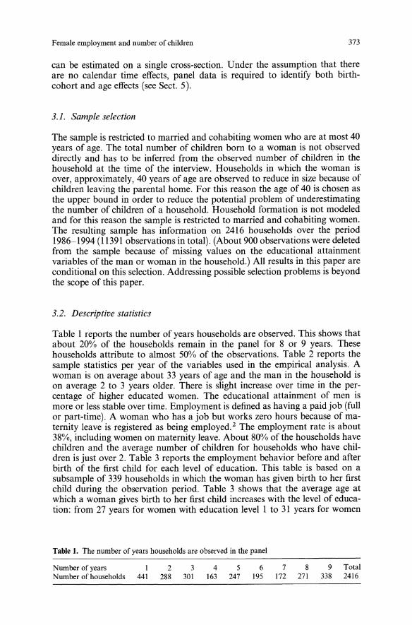
Female employment and number of children 373

can be estimated on a single cross-section. Under the assumption that thereare no calendar time effects, panel data is required to identify both birth­cohort and age effects (see Sect. 5).

3.1. Sample selection

The sample is restricted to married and cohabiting women who are at most 40years of age. The total number of children born to a woman is not observeddirectly and has to be inferred from the observed number of children in thehousehold at the time of the interview. Households in which the woman isover, approximately, 40 years of age are observed to reduce in size because ofchildren leaving the parental home. For this reason the age of 40 is chosen asthe upper bound in order to reduce the potential problem of underestimatingthe number of children of a household. Household formation is not modeledand for this reason the sample is restricted to married and cohabiting women.The resulting sample has information on 2416 households over the period1986-1994 (11391 observations in total). (About 900 observations were deletedfrom the sample because of missing values on the educational attainmentvariables of the man or woman in the household.) All results in this paper areconditional on this selection. Addressing possible selection problems is beyondthe scope of this paper.

3.2. Descriptive statistics

Table 1 reports the number of years households are observed. This shows thatabout 20% of the households remain in the panel for 8 or 9 years. Thesehouseholds attribute to almost 50% of the observations. Table 2 reports thesample statistics per year of the variables used in the empirical analysis. Awoman is on average about 33 years of age and the man in the household ison average 2 to 3 years older. There is slight increase over time in the per­centage of higher educated women. The educational attainment of men ismore or less stable over time. Employment is defined as having a paid job (fullor part-time). A woman who has a job but works zero hours because of ma­ternity leave is registered as being employed. 2 The employment rate is about38%, including women on maternity leave. About 80% of the households havechildren and the average number of children for households who have chil­dren is just over 2. Table 3 reports the employment behavior before and afterbirth of the first child for each level of education. This table is based on asubsample of 339 households in which the woman has given birth to her firstchild during the observation period. Table 3 shows that the average age atwhich a woman gives birth to her first child increases with the level of educa­tion: from 27 years for women with education level 1 to 31 years for women

Table 1. The number of years households are observed in the panel

Number of years I 2 3 4 5 6 7 8 9 TotalNumber of households 441 288 301 163 247 195 172 271 338 2416

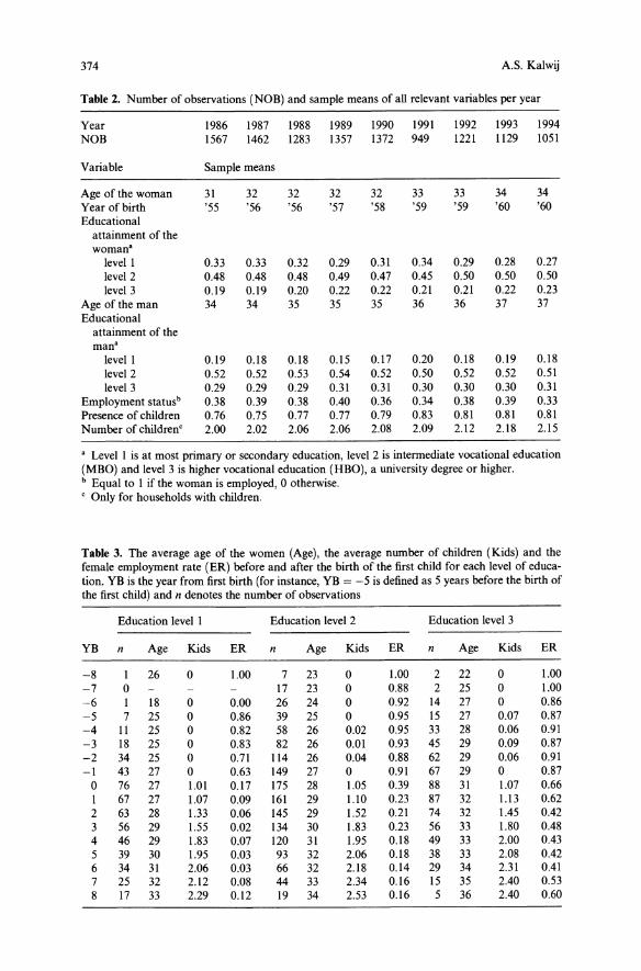
374 A.S. Kalwij

Table 2. Number of observations (NOB) and sample means of all relevant variables per year

Year 1986 1987 1988 1989 1990 1991 1992 1993 1994NOB 1567 1462 1283 1357 1372 949 1221 1129 1051

Variable Sample means

Age of the woman 31 32 32 32 32 33 33 34 34Year of birth '55 '56 '56 '57 '58 '59 '59 '60 '60Educationalattainment of thewomana

level I 0.33 0.33 0.32 0.29 0.31 0.34 0.29 0.28 0.27level 2 0.48 0.48 0.48 0.49 0.47 0.45 0.50 0.50 0.50level 3 0.19 0.19 0.20 0.22 0.22 0.21 0.21 0.22 0.23

Age of the man 34 34 35 35 35 36 36 37 37Educationalattainment of themanalevel I 0.19 0.18 0.18 0.15 0.17 0.20 0.18 0.19 0.18level 2 0.52 0.52 0.53 0.54 0.52 0.50 0.52 0.52 0.51level 3 0.29 0.29 0.29 0.31 0.31 0.30 0.30 0.30 0.31

Employment statusb 0.38 0.39 0.38 0.40 0.36 0.34 0.38 0.39 0.33Presence of children 0.76 0.75 0.77 0.77 0.79 0.83 0.81 0.81 0.81Number of childrenc 2.00 2.02 2.06 2.06 2.08 2.09 2.12 2.18 2.15

a Level I is at most primary or secondary education, level 2 is intermediate vocational education(MBO) and level 3 is higher vocational education (HBO), a university degree or higher.b Equal to I if the woman is employed, 0 otherwise.C Only for households with children.

Table 3. The average age of the women (Age), the average number of children (Kids) and thefemale employment rate (ER) before and after the birth of the first child for each level of educa-tion. YB is the year from first birth (for instance, YB = -Sis defined as 5 years before the birth ofthe first child) and n denotes the number of observations

Education level I Education level 2 Education level 3

YB n Age Kids ER n Age Kids ER n Age Kids ER

-8 I 26 0 1.00 7 23 0 1.00 2 22 0 1.00-7 0 17 23 0 0.88 2 25 0 1.00-6 I 18 0 0.00 26 24 0 0.92 14 27 0 0.86-5 7 25 0 0.86 39 25 0 0.95 IS 27 0.07 0.87-4 11 25 0 0.82 58 26 0.02 0.95 33 28 0.06 0.91-3 18 25 0 0.83 82 26 0.01 0.93 45 29 0.09 0.87-2 34 25 0 0.71 114 26 0.04 0.88 62 29 0.06 0.91-I 43 27 0 0.63 149 27 0 0.91 67 29 0 0.870 76 27 1.01 0.17 175 28 1.05 0.39 88 31 1.07 0.66I 67 27 1.07 0.09 161 29 1.10 0.23 87 32 1.13 0.622 63 28 1.33 0.06 145 29 1.52 0.21 74 32 1.45 0.423 56 29 1.55 0.02 134 30 1.83 0.23 56 33 1.80 0.484 46 29 1.83 0.07 120 31 1.95 0.18 49 33 2.00 0.435 39 30 1.95 0.03 93 32 2.06 0.18 38 33 2.08 0.426 34 31 2.06 0.03 66 32 2.18 0.14 29 34 2.31 0.417 25 32 2.12 0.08 44 33 2.34 0.16 15 35 2.40 0.538 17 33 2.29 0.12 19 34 2.53 0.16 5 36 2.40 0.60

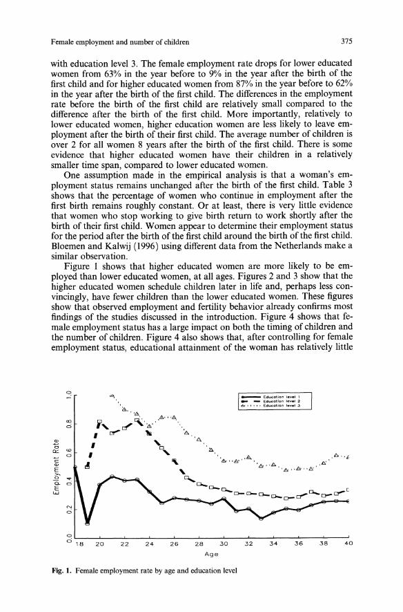
Female employment and number of children 375

with education level 3. The female employment rate drops for lower educatedwomen from 63% in the year before to 9% in the year after the birth of thefirst child and for higher educated women from 87% in the year before to 62%in the year after the birth of the first child. The differences in the employmentrate before the birth of the first child are relatively small compared to thedifference after the birth of the first child. More importantly, relatively tolower educated women, higher education women are less likely to leave em­ployment after the birth of their first child. The average number of children isover 2 for all women 8 years after the birth of the first child. There is someevidence that higher educated women have their children in a relativelysmaller time span, compared to lower educated women.One assumption made in the empirical analysis is that a woman's em­

ployment status remains unchanged after the birth of the first child. Table 3shows that the percentage of women who continue in employment after thefirst birth remains roughly constant. Or at least, there is very little evidencethat women who stop working to give birth return to work shortly after thebirth of their first child. Women appear to determine their employment statusfor the period after the birth of the first child around the birth of the first child.Bloemen and Kalwij (1996) using different data from the Netherlands make asimilar observation.Figure I shows that higher educated women are more likely to be em­

ployed than lower educated women, at all ages. Figures 2 and 3 show that thehigher educated women schedule children later in life and, perhaps less con­vincingly, have fewer children than the lower educated women. These figuresshow that observed employment and fertility behavior already confirms mostfindings of the studies discussed in the introduction. Figure 4 shows that fe­male employment status has a large impact on both the timing of children andthe number of children. Figure 4 also shows that, after controlling for femaleemployment status, educational attainment of the woman has relatively little

0

00

6

20

<0a:::6

C'"E>.0 ....a. 6Ew

N

6

__ Education I."el 1_ _ Educotlon level 2

6 •• I , I , Education le"'e' 3

. A ,I""L'&"'8'" • ~

·t::" •• A .. ""...i!Y"~"

o6 '-'-8--2.....0--2'-2----'2'--4----'26--2....1.

8--

3....0--

3-'-2--3-'-4--3-'-6--3....8-----J

40

Age

Fig. 1. Female employment rate by age and education level

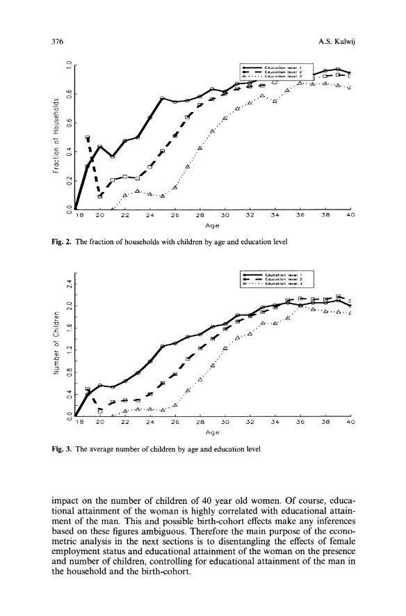
376 A.S. Kalwij

0

00

U)0

,J!:! 'f::!.:o? Ii'0 J!:!'.<=

~Q) J!:iU) <0:> 0 ,0 {!>'I: II'0 ,c ....

IJ ~0 0v rf2 (iiI..L..

0-0-0/N

0 ,.&,

(!>' ' .8. , '4>, , '4>'~

00 18 20 22 24 26 28 30 32 34 36 38 40

Age

Fig. 2. The fraction of households with children by age and education level

4038363432

.t:i.

3028

{fi'

262422

Jii' .. ~ .&.4>' ••4>' , .4>•• '8' '

....N

C!N

C

~.",

<0

.<= -U

'0~

N

Q)

.D

E:> 00:z

0

....0

00 18 20

_ Educ:otion 1.".1 I_ _ Education '.vel 26· ••••• Educotion level .l

Age

Fig. 3. The average number of children by age and education level

impact on the number of children of 40 year old women. Of course, educa­tional attainment of the woman is highly correlated with educational attain­ment of the man. This and possible birth-cohort effects make any inferencesbased on these figures ambiguous. Therefore the main purpose of the econo­metric analysis in the next sections is to disentangling the effects of femaleemployment status and educational attainment of the woman on the presenceand number of children, controlling for educational attainment of the man inthe household and the birth-cohort.

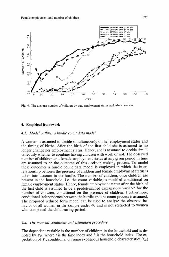
Female employment and number of children

__ Education le 1 1. No job_ _ Education _e el 2. No .Job

O' I , , I • Education lev.t .3, No Job• __ , Education I....... I . .Job()o EducoHo,. level 2. Job

0_ " Education l....e' 3. Job

C>

N

c~-0 <0

.r::: -U

'0~ NQ.l.D

E:::l DO:z 6

Fig. 4. The average number of children by age, employment status and education level

4. Empirical framework

4.1. Model outline: a hurdle count data model

377

A woman is assumed to decide simultaneously on her employment status andthe timing of births. After the birth of the first child she is assumed to nolonger change her employment status. Hence, she is assumed to decide simul­taneously whether to combine having children with work or not. The observednumber of children and female employment status at any given period in timeare assumed to be the outcome of this decision making process. To modelthese outcomes a hurdle count data model is employed in which the inter­relationship between the presence of children and female employment status istaken into account in the hurdle. The number of children, once children arepresent in the household, i.e. the count variable, is modeled conditional onfemale employment status. Hence, female employment status after the birth ofthe first child is assumed to be a predetermined explanatory variable for thenumber of children, conditional on the presence of children. Furthermore,conditional independence between the hurdle and the count process is assumed.The proposed reduced form model can be used to analyze the observed be­havior of all women in the sample under 40 and is not restricted to womenwho completed the childbearing period.

4.2. The moment conditions and estimation procedure

The dependent variable is the number of children in the household and is de­noted by Yth, where t is the time index and h is the household index. The ex­pectation of Yth conditional on some exogenous household characteristics (Zth)

378 A.S. Kalwij

is denoted by E[YthIZth; 0], where 0 denotes the parameters of interest. Typi­cally one is interested in the marginal effects of some exogenous characteristicon the expected number of children: oE( YthlZth; O)/OZth. If one is prepared tospecify the distribution of Yth the maximum likelihood estimator can be usedand, under the assumption of a correctly specified distribution, leads to themost efficient consistent estimates of 0 (see for instance, Mullahy 1986; Pohl­meier and Ulrich 1995). If one assumes Yth is Poisson distributed one canemploy a pseudo-maximum likelihood estimator which results in consistentestimates even if the true distribution is not Poisson (see for instance, Cameronand Trivedi 1986). Unfortunately, for a hurdle type of distribution no pseudo­likelihood type result is known. Hence, misspecification of the distributionresults in inconsistent estimates. For this reason a generalized methods ofmoments estimator (e.g. Hansen 1982), is employed as proposed by SantosSilva and Windmeijer (1998) and Mullahy (1998). Only the first moment ofthe distribution is specified, hence the marginal effects oE( Yth IZth i 0) / OZth areidentified.Given the model outlined above and using the law of iterative expectation,

the conditional expectation of Yth can be written as follows:

(I)

where Wth denotes female employment status (Wth = I if the woman is em­ployed and °otherwise). I( Yth>O) is an indicator function for the presence ofchildren. Equation (I) shows that the interrelationship between children andfemale employment status is only allowed for in the first step, i.e. the hurdle.In the second step, once children are present in the household, female em­ployment status is assumed to be predetermined. Given the binary nature offemale employment status and the indicator function, Eq. (I) can be written asfollows:

E[YthIZth, OJ

= P(I(Yth>o) = Ilzth,a)

X {P(Wth = 0II(Yth>o) = liZth,a)E[YthIWth = O'/(Yth>O) = liZth,P)]

+P(Wth = III(yth>o) = liZth,a)

(2)

where OT = (aT,pT,pJ). Note that in the case where there are no children inthe household, i.e. I( Yth>O) = 0, the conditional expectation of Yth is equal to 0,irrespective of female employment status.Once the functional forms of the choice probabilities and the conditional

expectation of the number of children are specified, one can obtain estimatesof all parameters of interest using the empirical moment condition implied by(2). However, in practice this is extremely difficult and for this reason themoment conditions implied by the conditional moment condition (2) are usedto estimate all parameters of interest stepwise. In total, six moment conditionsare formulated:

Female employment and number of children

ElWth(I-I(Yth>O») -Pr(Wth = 1,I(Yth>O) =OIZth,IX)IZthJ =0;

El(1 - Wth)I(Yth>o) - Pr(Wth = O,I(yth>O) = IIZth' IX) IZthJ = OJ

ElwthI(Yth>O) - Pr(Wth = 1,I(Yth>O) = IIZth, IX) IZthJ = OJ

E[(Yth - E[Ythl Wth = 0, I(Yth>o) = I; Zth,Pd IZth] = 0,

if Wth =° and Yth > OJ

if Wth = I and Yth > OJ

E[Yth - P(Wth = O,I(Yth>O) = IIZth, IX)E[Ythj Wth = O,I(Yth>O) = IjZth,Pd

- P(Wth = 1,I(yth>O) = IIZth,IX)

379

(3)

(4)

(5)

(6)

(7)

(8)

The observed number of children is denoted by Yth and the observed femaleemployment status is denoted by Wth. The estimation of the parameters of in­terest can be done in two stages. In the first stage GMM estimates of IX areobtained by exploiting the moment conditions (3) to (5). Given the binarynature of the dependent variables entering these three moment conditions,specifying the probability distribution function and employing a maximumlikelihood estimator yields identical estimates. In the second stage the sampleis restricted to those couples who are observed to have children (Yth > 0) andthe resulting sample is split on the basis of the observed female employmentstatus (Wth)' Estimates of PI and P2 are obtained by exploiting the momentconditions (6) and (7). The additional moment condition (8) yields over­identification and is used for a specification test. For this purpose, a condi­tional moment test statistic is constructed based on the estimates obtained fromusing the first five moment conditions (see e.g., Davidson and MacKinnon,Chapt. 16).For the empirical analysis one needs to specify the probability distribution

function of female employment status and the presence of children and theconditional expectation of the number of children. The joint distribution offemale employment status and the presence of children is specified as follows:

(9)

where S is the set of feasible alternatives, S = {(O, 0), (1,0), (0, I), (I, I)}. Thisprobability distribution function is the well-known multinomial distributionand the normalization chosen is IX(O,O) = 0, hence IX

T = (IX(~,O)'IX[o,I),IX0,1))'Alternative one can choose a bivariate probit model. However, in a bivariateprobit model the interrelationship between female employment status and thepresence of children is only allowed for through the error terms. The multi-

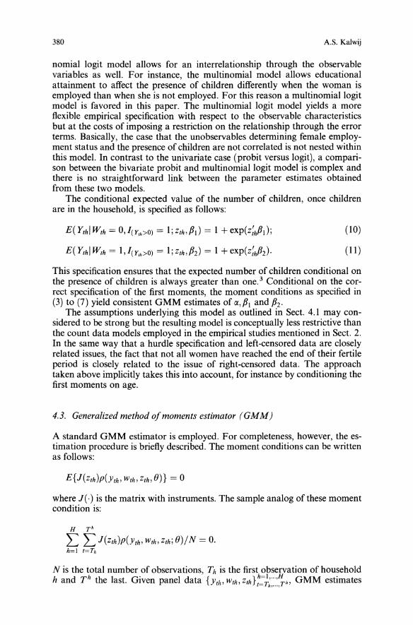
380 A.S. Kalwij

nomial logit model allows for an interrelationship through the observablevariables as well. For instance, the multinomial model allows educationalattainment to affect the presence of children differently when the woman isemployed than when she is not employed. For this reason a multinomiallogitmodel is favored in this paper. The multinomial logit model yields a moreflexible empirical specification with respect to the observable characteristicsbut at the costs of imposing a restriction on the relationship through the errorterms. Basically, the case that the unobservables determining female employ­ment status and the presence of children are not correlated is not nested withinthis model. In contrast to the univariate case (probit versus logit), a compari­son between the bivariate probit and multinomiallogit model is complex andthere is no straightforward link between the parameter estimates obtainedfrom these two models.The conditional expected value of the number of children, once children

are in the household, is specified as follows:

E(YthlWth = O'/(Yth>O) = Ijzth,Pd = 1+exp(z:hPd;

E(YthlWth = 1'/(Yth>O) = Ijzth,P2) = I +exp(z:hP2)'

(10)

(11 )

This specification ensures that the expected number of children conditional onthe presence of children is always greater than one. 3 Conditional on the cor­rect specification of the first moments, the moment conditions as specified in(3) to (7) yield consistent GMM estimates of tX,PI and P2'The assumptions underlying this model as outlined in Sect. 4.1 may con­

sidered to be strong but the resulting model is conceptually less restrictive thanthe count data models employed in the empirical studies mentioned in Sect. 2.In the same way that a hurdle specification and left-censored data are closelyrelated issues, the fact that not all women have reached the end of their fertileperiod is closely related to the issue of right-censored data. The approachtaken above implicitly takes this into account, for instance by conditioning thefirst moments on age.

4.3. Generalized method ofmoments estimator (GMM)

A standard GMM estimator is employed. For completeness, however, the es­timation procedure is briefly described. The moment conditions can be writtenas follows:

where J(.) is the matrix with instruments. The sample analog of these momentcondition is:

H T h

L L J(Zth)p(Yth' Wth, Zthj 0)/N = O.h=! t=Th

N is the total number of observations, Th is the first observation of householdhand T h the last. Given panel data {Yth' Wth, Zth} :i~::::~h' GMM estimates

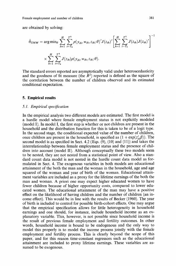
Female employment and number of children

are obtained by solving:

381

H Th

X L L J(Zth)p(Yth' Wth, Zthj ()).h=1 t=Th

The standard errors reported are asymptotically valid under heteroscedasticityand the goodness of fit measure (the R 2) reported is defined as the square ofthe correlation between the number of children observed and its estimatedconditional expectation.

5. Empirical results

5.1. Empirical specification

In the empirical analysis two different models are estimated. The first model isa hurdle model where female employment status is not explicitly modeled(model I). In model I, the first step is whether or not children are present in thehousehold and the distribution function for this is taken to be of a logit type.In the second stage, the conditional expected value of the number of children,once children are present in the household, is specified as (1 + exp(z:hP)). Thesecond model is as specified in Sect. 4.2 (Eqs. (9), (10) and (11)) and takes theinterrelationship between female employment status and the presence of chil­dren into account (model II). Although conceptually these two models seemto be nested, they are not nested from a statistical point of view. Also a stan­dard count data model is not nested in the hurdle count data model as for­mulated in Sect. 4. The exogenous variables in both models are educationalattainment of the both the man and the woman in the household, age and agesquared of the woman and year of birth of the woman. Educational attain­ment variables are included as a proxy for the lifetime earnings of the both theman and woman. A priori one may expect higher educated women to havefewer children because of higher opportunity costs, compared to lower edu­cated women. The educational attainment of the man may have a positiveeffect on the likelihood of having children and the number of children (an in­come effect). This would be in line with the results of Becker (1960). The yearof birth is included to control for possible birth-cohort effects. One may arguethat the empirical specification allows for little heterogeneity in householdearnings and one should, for instance, include household income as an ex­planatory variable. This, however, is not possible since household income isthe result of previous female employment and fertility outcomes. In otherwords, household income is bound to be endogenous and the only way tomodel this properly is to model the income process jointly with the femaleemployment and fertility process. This is clearly beyond the scope of thispaper, and for this reason time-constant regressors such as the educationalattainment are included to proxy lifetime earnings. These variables are as­sumed to be exogenous.

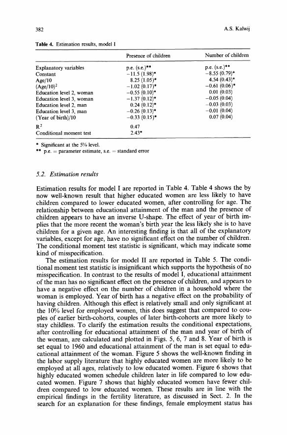
382

Table 4. Estimation results, model I

Presence of children

A.S. Kalwij

Number of children

Explanatory variablesConstantAge/IO(Age/IO)lEducation level 2, womanEducation level 3, womanEducation level 2, manEducation level 3, man(Year of birth)/IO

R 2

Conditional moment test

p.e. (s.e.)-­-1l.5 (1.98)-8.25 (1.05)­-1.02 (0.17)--0.55 (0.10)--1.37 (0.12)-0.24 (0.12)­-0.26 (0.13)--0.33 (0.15)-

0.472.43-

p.e. (s.e.)-­-8.55 (0.79)­4.54 (0.43)­-0.61 (0.06)-0.01 (0.03)-0.05 (0.04)-0.03 (0.03)-0.01 (0.04)0.07 (0.04)

- Significant at the 5% level.-- p.e. = parameter estimate, s.e. = standard error

5.2. Estimation results

Estimation results for model I are reported in Table 4. Table 4 shows the bynow well-known result that higher educated women are less likely to havechildren compared to lower educated women, after controlling for age. Therelationship between educational attainment of the man and the presence ofchildren appears to have an inverse V-shape. The effect of year of birth im­plies that the more recent the woman's birth year the less likely she is to havechildren for a given age. An interesting finding is that all of the explanatoryvariables, except for age, have no significant effect on the number of children.The conditional moment test statistic is significant, which may indicate somekind of misspecification.The estimation results for model II are reported in Table 5. The condi­

tional moment test statistic is insignificant which supports the hypothesis of nomisspecification. In contrast to the results of model I, educational attainmentof the man has no significant effect on the presence of children, and appears tohave a negative effect on the number of children in a household where thewoman is employed. Year of birth has a negative effect on the probability ofhaving children. Although this effect is relatively small and only significant atthe 10% level for employed women, this does suggest that compared to cou­ples of earlier birth-cohorts, couples of later birth-cohorts are more likely tostay childless. To clarify the estimation results the conditional expectations,after controlling for educational attainment of the man and year of birth ofthe woman, are calculated and plotted in Figs. 5, 6, 7 and 8. Year of birth isset equal to 1960 and educational attainment of the man is set equal to edu­cational attainment of the woman. Figure 5 shows the well-known finding inthe labor supply literature that highly educated women are more likely to beemployed at all ages, relatively to low educated women. Figure 6 shows thathighly educated women schedule children later in life compared to low edu­cated women. Figure 7 shows that highly educated women have fewer chil­dren compared to low educated women. These results are in line with theempirical findings in the fertility literature, as discussed in Sect. 2. In thesearch for an explanation for these findings, female employment status has

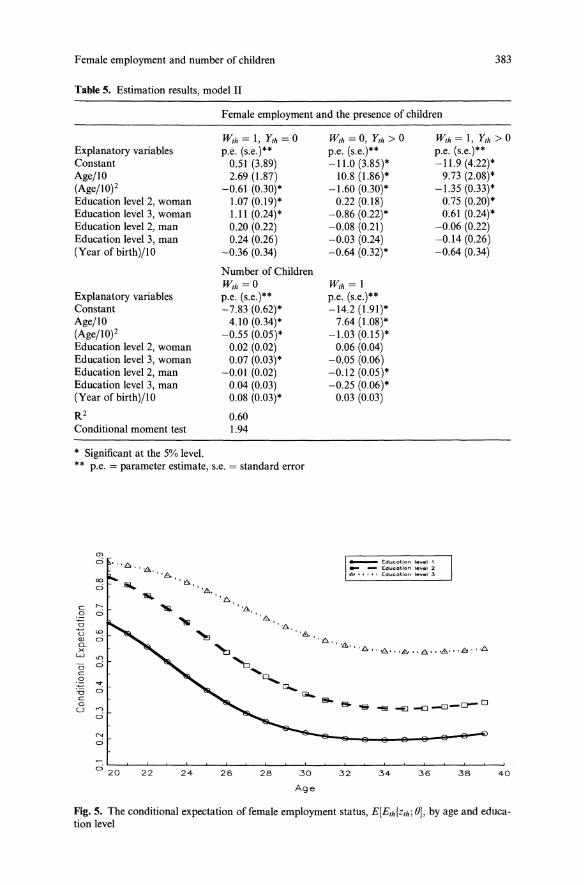
Female employment and number of children

Table 5. Estimation results, model II

Female employment and the presence of children

383

Explanatory variablesConstantAge/l 0(Age/l0j2Education level 2, womanEducation level 3, womanEducation level 2, manEducation level 3, man(Year ofbirth)/IO

Explanatory variablesConstantAge/l 0(Age/l0j2Education level 2, womanEducation level 3, womanEducation level 2, manEducation level 3, man(Year ofbirth)/IO

R2Conditional moment test

Wth = I, Yth =0p.e. (s.e.)**0.51 (3.89)2.69 (1.87)-0.61 (0.30)*1.07 (0.19)*1.11 (0.24)*0.20 (0.22)0.24 (0.26)-0.36 (0.34)

Number of ChildrenWth =0p.e. (s.e.)**-7.83 (0.62)*4.10 (0.34)*-0.55 (0.05)*0.02 (0.02)0.07 (0.03)*-0.01 (0.02)0.04 (0.03)0.08 (0.03)*

0.601.94

W,h = 0, Yth > 0p.e. (s.e.)**-11.0 (3.85)*10.8 (1.86)*-1.60 (0.30)*0.22 (0.18)-0.86 (0.22)*-0.08 (0.21)-0.Q3 (0.24)-0.64 (0.32)*

W,h= Ip.e. (s.e.)**-14.2 (1.91)*7.64 (1.08)*-1.03 (0.15)*0.06 (0.04)-0.05 (0.06)-0.12 (0.05)*-0.25 (0.06)*0.Q3 (0.03)

W,h = I, Y,h > 0p.e. (s.e.)**-11.9 (4.22)*9.73 (2.08)*-1.35 (0.33)*0.75 (0.20)*0.61 (0.24)*-0.06 (0.22)-0.14 (0.26)-0.64 (0.34)

* Significant at the 5% level.** p.e. = parameter estimate, s.e. = standard error

m0

000

c r-.~ 00

U <D

'" 00..xW""<3 0

c

:8 ...u 0c0

U n0

N

0

___ Education level 1_ _ Edueollon tevel 26· • , .. . Education 1.".1 .}

',1>.

'n

" ',1>'" t'>,. '8,. '1'> •• 08 ..• ,£;••• "" •• •,1>... f'>" 08

020 22 24 26 28 30

Age

32 34 36 38 40

Fig. 5. The conditional expectation of female employment status, E[Eth IZ,h; 8], by age and educa­tion level

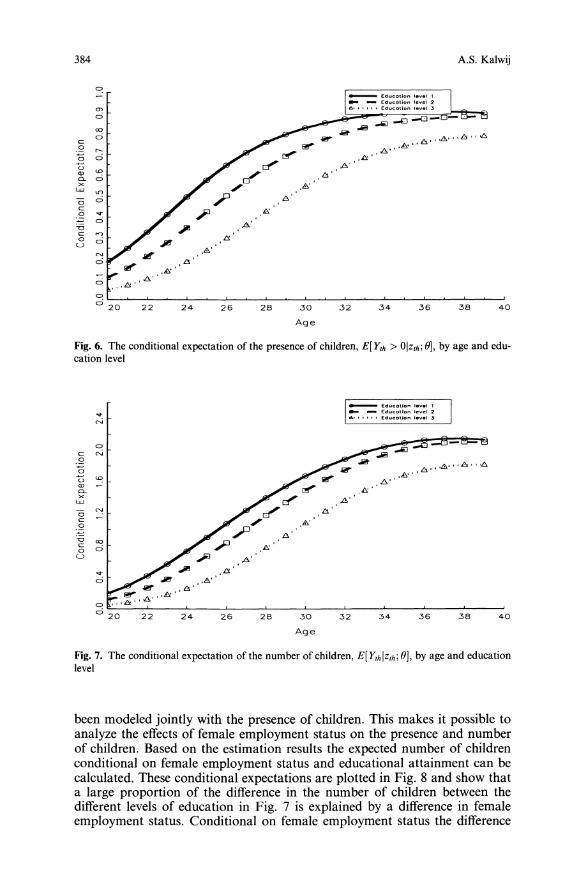
,t!;'

,,s,.'

8'

4038

A.S. Kalwij

3634

-'J-o­..li!l..-J

0" ,8" ,e,., '8

8"'''''''

~"

__ Education 'e"'et 1_ _ Education level 26· • , • .. Education 1.",.1 .3

3230

Age

282624

,R>.'

22

384

C!

en0

co

c 0.S' r-

:§ 0u co'"a. 0xW <I)

0 0c .....S:>.- 0-0C ...,0 0u"!0

0

C!020

Fig. 6. The conditional expectation of the presence of children, E[ Yth > 0IZth; OJ, by age and edu­cation level

403836

A" ,.e" "8,0"'=..",

8'"

34

,~.

4'

32

,,s,.'

30

Age

2826

,£I

2422

~ ~ l>",t!;'

~ 8",8'"o , ..6"020

....o

....N

0c ('oJ

.S':§

cou

'"a.xw

0('oJ

c.S'.--0 coC 00u

__ Education I.....t 1_ _ Education level 26· , • ••• Education le",el "

Fig. 7. The conditional expectation of the number of children, E[Ythlzth; OJ, by age and educationlevel

been modeled jointly with the presence of children. This makes it possible toanalyze the effects of female employment status on the presence and numberof children. Based on the estimation results the expected number of childrenconditional on female employment status and educational attainment can becalculated. These conditional expectations are plotted in Fig. 8 and show thata large proportion of the difference in the number of children between thedifferent levels of education in Fig. 7 is explained by a difference in femaleemployment status. Conditional on female employment status the difference

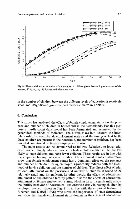
Female employment and number of children 385

",6"'&"'6"'8

__ Education 1......1 1 . No Job_ _ Educotion level 2 • No Job

~•••• , • Education 1.",.1 .3 , No JQb___ , Ed...eotion 1.....1 1 • ,Job

()t" ........ Education level 2 . ..Job9_ ,. Educotion le...e' 3 • ,Job....

'"0

c '"0

2 <0U(l) -Cl.X

I..LJ

0 ~

c0~

" roc 00u

.... IS0

00 20 22 24 26 28 30 32 34 36 38 40

Age

Fig. 8. The conditional expectation of the number of children given the employment status of thewoman, E[YthIWth,Z'h; OJ, by age and education level

in the number of children between the different levels of education is relativelysmall and insignificant, given the parameter estimates in Table 5.

6. Conclusions

This paper has analyzed the effects of female employment status on the pres­ence and number of children in households in the Netherlands. For this pur­pose a hurdle count data model has been formulated and estimated by thegeneralized methods of moments. The hurdle takes into account the inter­relationship between female employment status and the timing of first birth.Once children are present in the household, the number of children, has beenmodeled conditional on female employment status.The main results can be summarized as follows. Relatively to lower edu­

cated women, highly educated women schedule children later in life, are lesslikely to have children and have fewer children. These results are in line withthe empirical findings of earlier studies. The empirical results furthermoreshow that female employment status has a dominant effect on the presenceand number of children: being employed significantly reduces both the likeli­hood of having children and the number of children. The direct effect of edu­cational attainment on the presence and number of children is found to berelatively small and insignificant. In other words, the effects of educationalattainment on the observed fertility pattern runs via the effects of educationalattainment on female employment status, which in its turn significantly affectsthe fertility behavior of households. The observed delay in having children byemployed women, shown in Fig. 8, is in line with the empirical findings ofBloemen and Kalwij (1996) who stress the importance of state-dependenceand show that female employment status dominates the effects of educational

386 A.S. Kalwij

attainment on the timing of first birth. Here, in addition, it is shown that fe­male employment status also has a dominant effect on the number of childrenat all ages. These empirical results emphasize the importance of explicitlymodeling female employment status when analyzing and trying to understandthe observed fertility behavior of households, hence life-cycle female employ­ment behavior.The econometric model as outlined in this paper only partly solves the

endogeneity problems of simultaneously analyzing the outcomes of femaleemployment and fertility decisions. Intuitively this model may be consideredappropriate in this particular empirical analysis. However, tackling the prob­lems surrounding simultaneity issues in (hurdle) count data models is consid­ered to be a necessary and fruitful route to follow for future research. Fur­thermore, the model employed here is a reduced form model used to gain abetter understanding of observed life-cycle female employment and fertilitybehavior. To address more fundamental issues related to, for instance, policyschemes to increase the female employment rate after the birth of the firstchild, a more structural approach needs to be taken. First steps in this direc­tion have been taken in Francesconi (1996) and Kalwij (1999, Chapt. 4).

Endnotes

1 A perhaps more appealing approach is to formulate and estimate a structural model based on alife-cycle model of household behavior. Francesconi (1996) and Kalwij (1999) take such anapproach. Because of the computational difficulties involved in estimating such a model it is fairto say that these models are not very practical. Estimating such a model is clearly beyond thescope of this paper.

2 The maternity period is at most up to 3 months after the birth of the child. In 1991 a papentalleave scheme was introduced. This makes it possible for a further 6 months leave. The maternityand parental leave schemes are a bit more complex than sketched here, but they roughlyamount to a maximum period ofleave, and registered as being employed, of one year. After thisleave the woman has to return to work.

3 Alternatively one may favor a truncated Poisson distribution for the underlying DGP andspecify the conditional expectation as: exp(z;hP)/(1 - exp( -exp(z;hP))), The main empiricalfindings of this paper remain unchanged when this alternative specification is used.

References

Becker GS (1960) An economic analysis of fertility. In: Universities National Bureau Committeefor Economic Research (ed.). Demographic and Economic Change in Developed Countries,Princeton University Press, Princeton, N.J., pp 209-231

Blau DM, Robins PK (1989) Fertility, Employment, and Child-Care Costs. Demography,26(2):287-299

Bloemen H, Kalwij A (1996) Female Employment and Timing of Births Decisions: a MultipleState Transition Model. CentER discussion paper, Tilburg University

Cameron AC, Trivedi PK (1986) Econometric models based on count data: comparisons andapplications of some estimators and tests. Journal ofApplied Econometrics 1:29-53

Cameron AC, Trivedi PK (1998) Regression Analysis of Count Data. Econometric Society Mon­ographs, no. 30, Cambridge University Press, Cambridge

Cigno A (1991) Economics of the family. 1994 ed, Oxford University Press, OxfordDavidson R, MacKinnon JG (1993) Estimation and Inference in Econometrics. Oxford UniversityPress, Oxford

Francesconi M (1996) Part-Time and Full-Time Work and Fertility of Married Women: A JointDynamic Model. Working paper, University of Essex

Female employment and number of children 387

Groot W, Pott-buter HA (1992) The timing of maternity in the Netherlands. Journal ofPopulationEconomics. 5: 155-172

Hansen LP (1982) Large sample properties of generalized method of moments estimators. Econ­ometrica 50: 1029-1054

Heckman JJ, Macurdy TE (1980) A Life-Cycle Model of Female Labour Supply. Review of Eco­nomic Studies 47-74

Heckman JJ, Walker JR (1990) The relationship between wages and income and the timing andspacing of births: evidence from Swedish longitudinal data. Econometrica 58:1411-1441

Hotz VJ, Miller KI (1988) An Empirical Analysis of Life-Cycle Fertility and Female Labor Sup­ply. Econometrica 56:91-118

Kalwij AS (1999) Household Consumption, Female Employment and Fertility Decisions: a Micro­econometric Analysis, Ph.D. dissertation, Tilburg University

Moffitt RA (1984) Profiles of Fertility, Labor Supply, and Wages of Married Women: A Com­plete Life-Cycle Model. Review of Economic Studies 51(2):263-278

Mroz TA (1987) The sensitivity of an empirical model of married women's hours of work toeconomic and statistical assumptions. Econometrica 55(4):765-799

Mullahy J (1986) Specification and testing of some modified count data models. Journal ofEconometrics 33:341-365

Mullahy J (1998) Much ado about two: reconsidering the two-part model in health econometrics.Working paper, University ofWisconsin-Madison and NBER.

Newman JL, McCulloch CE (1984) A hazard rate approach to the timing of births. Econometrica52(4)

O'Malley Borg M (1989) The Income-Fertility Relationship: Effect of the Net Price of a Child.Demography 26(2):301-310

Pohlmeier W, Ulrich V (1995) An Econometric Model of the Two-Part Decision Process in theDemand for Health. Journal ofHuman Resources 30:339-361

Santos Silva JMC, Covas F (1998) A Modified Hurdle Model for Completed Fertility. Workingpaper, ISEGjUniversidade Tecnica de Lisboa

Santos Silva JMC, Windmeijer FAG (1998) Two-Part MUltiple Spell Models for Health CareDemand. Working paper, ISEGjUniversidade Tecnica de LisboajThe Institute for FiscalStudies

Siegers JJ (1985) Arbeidsaanbod en kindertal: een micro-economische analyse. Ph.D. dissertation,University of Groningen

Walker JR (1995) Parental Benefits and Employment and Fertility Dynamics. Working paper,University of Wisconsin

Wang W, Famoye F (1997) Modeling Household Fertility Decisions with Generalized PoissonRegression. Journal of Population Economics 10:273-283

Winkelmann R (1995) Duration Dependence and Dispersion in Count Data Models. Journal ofBusiness & Economic Statistics 13:467-474

Willis RJ (1973) A new approach to the economic theory of fertility behavior. Journal ofpoliticalEconomy SI4-S64.

Windmeijer FAG, Santos Silva JMC (1997) Endogeneity in count data models: an application todemand for health care. Journal ofApplied Econometrics. 12:281-294

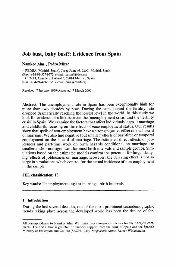
Job bust, baby bust?: Evidence from Spain

Namkee Abo!, Pedro Mira2

I FEDEA (Madrid, Spain), Jorge Juan 46,28001 Madrid, Spain(Fax: +34-91-577-9575; e-mail: nahn@fedea.es)2 CEMFI, Casado del Alisal 5, 28014 Madrid, Spain(Fax: +34-91-429-1056; e-mail: mira@cemfi.es)

Received: 7 January 1999/Accepted: 7 March 2000

Abstract. The unemployment rate in Spain has been exceptionally high formore than two decades by now. During the same period the fertility ratedropped dramatically reaching the lowest level in the world. In this study welook for evidence of a link between the 'unemployment crisis' and the 'fertilitycrisis' in Spain. We examine the factors that affect individuals' ages at marriageand childbirth, focusing on the effects ofmale employment status. Our resultsshow that spells ofnon-employment have a strong negative effect on the hazardofmarriage. We also find negative (but smaller) effects of part-time or temporalemployment on the hazard of marriage. The estimated direct effects of job­lessness and part-time work on birth hazards conditional on marriage aresmaller and/or not significant for most birth intervals and sample groups. Sim­ulations based on the estimated models confirm the potential for large 'delay­ing' effects of joblessness on marriage. However, the delaying effect is not solarge in simulations which control for the actual incidence of non-employmentin the sample.

JEL classification: 13

Key words: Unemployment, age at marriage, birth intervals

1. Introduction

During the last several decades, one of the most prominent sociodemographictrends taking place across the developed world has been the decline of fer-

All correspondence to Namkee Ahn. We thank two anonymous referees for their helpful com­ments. The first author is grateful for financial support from the Bank of Spain and the SpanishMinistry of Education and Culture (SEC97-1249). Responsible editor: Rainer Winkelmann

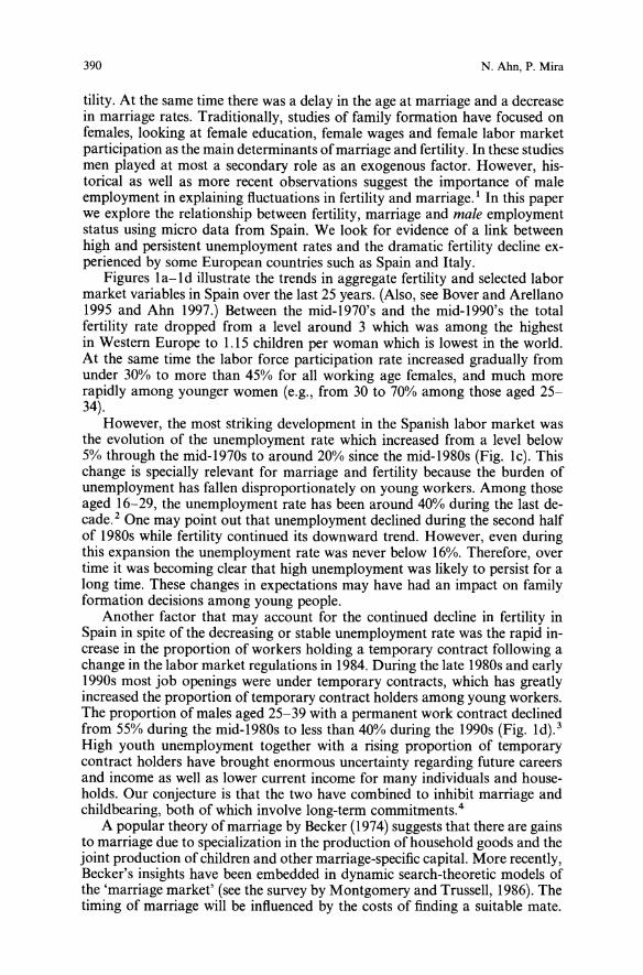
390 N. Ahn, P. Mira

tility. At the same time there was a delay in the age at marriage and a decreasein marriage rates. Traditionally, studies of family formation have focused onfemales, looking at female education, female wages and female labor marketparticipation as the main determinants ofmarriage and fertility. In these studiesmen played at most a secondary role as an exogenous factor. However, his­torical as well as more recent observations suggest the importance of maleemployment in explaining fluctuations in fertility and marriage. 1 In this paperwe explore the relationship between fertility, marriage and male employmentstatus using micro data from Spain. We look for evidence of a link betweenhigh and persistent unemployment rates and the dramatic fertility decline ex­perienced by some European countries such as Spain and Italy.Figures la-ld illustrate the trends in aggregate fertility and selected labor

market variables in Spain over the last 25 years. (Also, see Bover and Arellano1995 and Ahn 1997.) Between the mid-1970's and the mid-1990's the totalfertility rate dropped from a level around 3 which was among the highestin Western Europe to U5 children per woman which is lowest in the world.At the same time the labor force participation rate increased gradually fromunder 30% to more than 45% for all working age females, and much morerapidly among younger women (e.g., from 30 to 70% among those aged 25­34).However, the most striking development in the Spanish labor market was

the evolution of the unemployment rate which increased from a level below5% through the mid-1970s to around 20% since the mid-1980s (Fig. lc). Thischange is specially relevant for marriage and fertility because the burden ofunemployment has fallen disproportionately on young workers. Among thoseaged 16-29, the unemployment rate has been around 40% during the last de­cade. 2 One may point out that unemployment declined during the second halfof 1980s while fertility continued its downward trend. However, even duringthis expansion the unemployment rate was never below 16%. Therefore, overtime it was becoming clear that high unemployment was likely to persist for along time. These changes in expectations may have had an impact on familyformation decisions among young people.Another factor that may account for the continued decline in fertility in

Spain in spite of the decreasing or stable unemployment rate was the rapid in­crease in the proportion of workers holding a temporary contract following achange in the labor market regulations in 1984. During the late 1980s and early1990s most job openings were under temporary contracts, which has greatlyincreased the proportion of temporary contract holders among young workers.The proportion ofmales aged 25-39 with a permanent work contract declinedfrom 55% during the mid-1980s to less than 40% during the 1990s (Fig. Id).3High youth unemployment together with a rising proportion of temporarycontract holders have brought enormous uncertainty regarding future careersand income as well as lower current income for many individuals and house­holds. Our conjecture is that the two have combined to inhibit marriage andchildbearing, both of which involve long-term commitments. 4

A popular theory ofmarriage by Becker (1974) suggests that there are gainsto marriage due to specialization in the production of household goods and thejoint production ofchildren and other marriage-specific capital. More recently,Becker's insights have been embedded in dynamic search-theoretic models ofthe 'marriage market' (see the survey by Montgomery and Trussell, 1986). Thetiming of marriage will be influenced by the costs of finding a suitable mate.

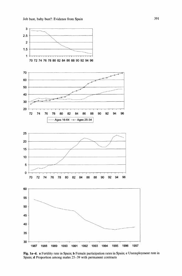
lob bust, baby bust?: Evidence from Spain

3 -,---------------,

~2.5 +---..::..;~,.-------------1

2+----~~~-----j

1.5-t-------~------j

70 72 74 76 78 80 82 84 86 88 90 92 94 96

70 -,---------------------~

6O+---------------- Jr::...---------1

50+----------------:;*--------___1

40 +--------~,c---------:;o-'"-=:::----___1

I-==.......---:::;;:;;;----;;;;;~~~:::::.:::========:::::_----------.j30 +

72 ~ ro n 60 ~ 84 00 00 00 ~ 94 00

1-Ages 16-64 --<>- Ages 25-34 I

391

25

20

15

10

5

o

~ ;----/ ~

//

~

60 -,-------------------------,

55

50

45

40

35

3O+--~-~-~-__,-___r-__,--,.__-_.___-~-~--j

1987 1988 1989 1990 1991 1992 1993 1994 1995 1900 1997

Fig. la-d. a Fertility rate in Spain; b Female participation rates in Spain; c Unemployment rate inSpain; d Proportion among males 25-39 with permanent contracts

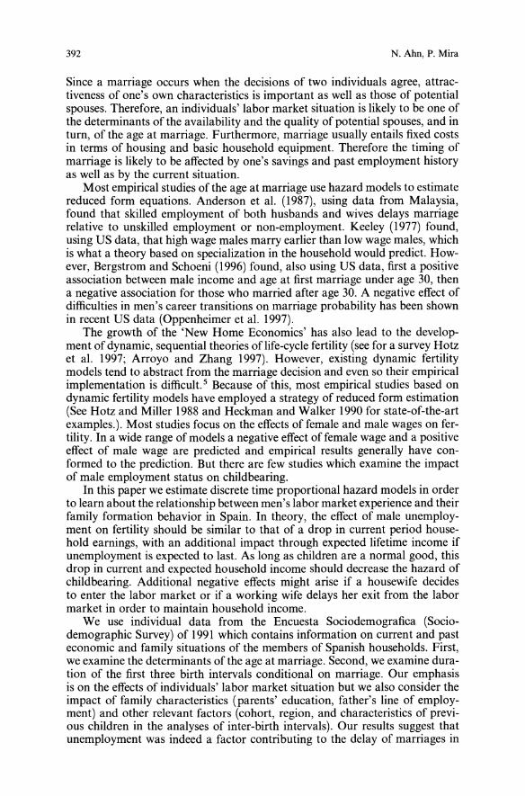
392 N. Ahu, P. Mira

Since a marriage occurs when the decisions of two individuals agree, attrac­tiveness of one's own characteristics is important as well as those of potentialspouses. Therefore, an individuals' labor market situation is likely to be one ofthe determinants of the availability and the quality of potential spouses, and inturn, of the age at marriage. Furthermore, marriage usually entails fixed costsin terms of housing and basic household equipment. Therefore the timing ofmarriage is likely to be affected by one's savings and past employment historyas well as by the current situation.Most empirical studies of the age at marriage use hazard models to estimate

reduced form equations. Anderson et al. (1987), using data from Malaysia,found that skilled employment of both husbands and wives delays marriagerelative to unskilled employment or non-employment. Keeley (1977) found,using US data, that high wage males marry earlier than low wage males, whichis what a theory based on specialization in the household would predict. How­ever, Bergstrom and Schoeni (1996) found, also using US data, first a positiveassociation between male income and age at first marriage under age 30, thena negative association for those who married after age 30. A negative effect ofdifficulties in men's career transitions on marriage probability has been shownin recent US data (Oppenheimer et al. 1997).The growth of the 'New Home Economics' has also lead to the develop­

ment of dynamic, sequential theories oflife-cycie fertility (see for a survey Hotzet al. 1997; Arroyo and Zhang 1997). However, existing dynamic fertilitymodels tend to abstract from the marriage decision and even so their empiricalimplementation is difficult. 5 Because of this, most empirical studies based ondynamic fertility models have employed a strategy of reduced form estimation(See Hotz and Miller 1988 and Heckman and Walker 1990 for state-of-the-artexamples.). Most studies focus on the effects of female and male wages on fer­tility. In a wide range ofmodels a negative effect offemale wage and a positiveeffect of male wage are predicted and empirical results generally have con­formed to the prediction. But there are few studies which examine the impactof male employment status on childbearing.In this paper we estimate discrete time proportional hazard models in order

to learn about the relationship between men's labor market experience and theirfamily formation behavior in Spain. In theory, the effect of male unemploy­ment on fertility should be similar to that of a drop in current period house­hold earnings, with an additional impact through expected lifetime income ifunemployment is expected to last. As long as children are a normal good, thisdrop in current and expected household income should decrease the hazard ofchildbearing. Additional negative effects might arise if a housewife decidesto enter the labor market or if a working wife delays her exit from the labormarket in order to maintain household income.We use individual data from the Encuesta Sociodemografica (Socio­

demographic Survey) of 1991 which contains information on current and pasteconomic and family situations of the members of Spanish households. First,we examine the determinants of the age at marriage. Second, we examine dura­tion of the first three birth intervals conditional on marriage. Our emphasisis on the effects of individuals' labor market situation but we also consider theimpact of family characteristics (parents' education, father's line of employ­ment) and other relevant factors (cohort, region, and characteristics of previ­ous children in the analyses of inter-birth intervals). Our results suggest thatunemployment was indeed a factor contributing to the delay of marriages in

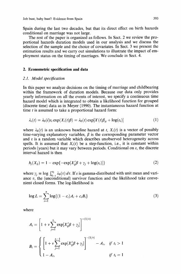
Job bust, baby bust?: Evidence from Spain 393

Spain during the last two decades, but that its direct effect on birth hazardsconditional on marriage was not large.The rest of the paper is organized as follows. In Sect. 2 we review the pro­

portional hazards duration models used in our analysis and we discuss theselection of the sample and the choice of covariates. In Sect. 3 we present theestimation results and we carry out simulations to illustrate the impact of em­ployment status on the timing of marriages. We conclude in Sect. 4.

2. Econometric specification and data

2.1. Model specification

In this paper we analyze decisions on the timing of marriage and childbearingwithin the framework of duration models. Because our data only providesyearly information on all the events of interest, we specify a continuous timehazard model which is integrated to obtain a likelihood function for grouped(discrete time) data as in Meyer (1990). The instantaneous hazard function attime t is assumed to take a proportional hazard form:

Ai(t) = .-1oU)ei exp(Xi(t)f3) = AO(t) exp[X(t)f3it + log(ei)] (1)

where .-1o(t) is an unknown baseline hazard at t, Xi(t) is a vector of possiblytime-varying explanatory variables, f3 is the corresponding parameter vectorand e is a random variable which describes unobserved heterogeneity acrossspells. It is assumed that Xi(t) be a step-function, i.e., it is constant withinperiods (years) but it may vary between periods. Conditional on e, the discreteinterval hazard is then

(2)

where Yj == log faa~, AoCr) dr:. Ife is gamma-distributed with unit mean and vari­ance v, the (unconditional) survivor function and the likelihood take conve­nient closed forms. The log-likelihood is

n

10gL = 2:)og{(1 - ci)Ai + CiBi}i=)

where

[

(. ] -(l/v)

Ai = 1 + vt exp[Xijf3 + Yj]J=l

._{ [1 + vf exp[Xijf3 + Yj]]-()IV) - Ai, if ti > 1B, - j=)

l-~, if4=1

(3)

394 N. Ahn, P. Mira

where tj is the observed duration of spell i, Cj = 1 indicates a complete spelland, Cj = 0 a censored spell. As the variance of the gamma distribution goes tozero, the likelihood converges to that of proportional hazards model with nounobserved heterogeneity. The parameters of interest are p, v and the sequencedescribing the non-parametric baseline hazard. 6

For the analysis of the age at marriage, we construct person-year data foreach year since the completion of schooling until the time of the event occur­rence (completed duration) or until the survey time (censored duration). For theanalyses of inter-birth durations we construct similar person-year data startingat the time at the birth interval of interest. Model (3) is estimated separately foreach of the events (marriage, first birth, second birth, third birth).7 Heckmanand Walker (1990) warned that this "piece-meal" approach may yield biasedestimates in the presence of individual-specific unobservables correlated overspells. However, in their empirical study using Swedish data they found thatthis form of unobservable heterogeneity was empirically unimportant. It isworth noting that in Spain fertility outside marriage during the sample periodwas negligible, and cohabitation was quite rare. 8 Furthermore, very few peoplemarry before completing school. 9

2.2. Sample selection

The data are drawn from the Spanish Socio-demographic Survey (EncuestaSociodemognifica) carried out by the Spanish Statistical Institute (INE) duringthe third quarter of 1991. The principal objective of the Survey was to gatherinformation about individuals' history of family situation, residence and hous­ing, economic activities and occupation, and education. The Survey containsinformation on 159,154 principal interviewees (a representative sample of theSpanish population of ages 10 and over) and their households.We limit our analysis to prime-aged males. We do this because our survey

(as most other surveys) records labor market histories only for the principalrespondents (one person for each household surveyed). Given our interest inthe effect ofmale employment status on marriage and fertility, this limitation isovercome by taking the male respondents as our working sample. An impor­tant advantage of using male samples and focusing on the effect of male em­ployment status is that, unlike female employment status, male employmentstatus can be treated more safely as exogenous with respect to the decisions ofmarriage and childbearing. For example, recent work by Angrist and Evans(1998) shows strong evidence of endogeneity of female labor supply and forexogeneity of male labor supply in childbearing decisions among couples inthe United States.In most societies the ages at marriage of male and female spouses are

highly correlated. The correlation coefficient for Spain in our data is 0.97 andhighly significant. Given that most childbearing occurs within stable unions(births from non-stable unions accounted for less than 5% in our data), thefather's and mother's ages at birth are also highly correlated. Therefore wethink the results of the analysis of the age at marriage and childbearing formales can be interpreted as applying to both sexes once we adjust for the agegaps between husbands and wives. Appendix 1 gives some descriptive pro­portions of ever married and the number of children by sex, age and cohort.

Job bust, baby bust?: Evidence from Spain 395

Our working sample consists of all principal male respondents aged 26-40at the time of survey. The reason why we do not include people younger than26 is that the majority (60%) of Spanish males are still unmarried by this age.By excluding those over 40 we reduce recall error about life histories arisingfrom the retrospective nature of the Survey. Since most marriages and birthsoccur after age 20, almost all the decisions recorded in our sample correspondto the 1970's and 80's, including the period of rapid fertility decline whichstarted in the mid-1970s.

2.3. Choice of covariates

Using retrospective information about individuals' work histories, we constructindividuals' yearly employment status. Unfortunately, within non-employmentperiods we cannot further distinguish between unemployment and out of laborforce states. However, considering that our working samples contain onlyprime-aged males, we think it is reasonable to interpret non-employment pe­riods as periods of unemployment.One of the main factors examined in numerous studies of age at marriage

and childbearing is completed education (Montgomery and Trussell 1986;Schultz 1997; Hotz et al. 1997). Most of these studies focus on women, andthey generally find a strong delaying effect of education on marriage and fer­tility. However, a conceptual problem is that education is very likely to be anendogenous variable in marriage and childbearing decisions. In order to dealwith this problem instrumental variable or simultaneous equation estimationtechniques have been applied. Nevertheless the problem persists in most casesdue to the difficulties in finding adequate instruments or due to tenuous iden­tification. In any case, education is not one of our main variables of interest.Our goal is rather to establish the effects of male employment status on thehazards of family formation events from the age of school completion, condi­tional on education. However, we would like to allow for interactions betweeneducation and some of the other covariates. In particular, since men do notmarry before they leave school and the ages at school completion are so dif­ferent by education, it would seem too restrictive to impose the same patternof duration dependence for all levels of education. It is for this reason thatwe estimate the models of marriage and the first birth separately for eacheducational category.lO We break our sample of men into three groups withprimary education, secondary education, and college education. For the sakeof homogeneity, we further restricted the sample to include only individualswho completed schooling by a given age: age 14 for the primary educationgroup (60% of this group), ages between 17 and 19 for the secondary educa­tion group (59% of this group), and ages 20 through 25 for the college edu­cation group (62% of this group),uThe duration variables are the waiting time (in years) until marriage and

the duration in years of the first, second and third birth intervals conditionalon marriage. The covariates included are employment status, age at the surveydate (as a control of cohort and trend effects), and regional dummies. In theanalyses of birth intervals we also include the wife's education and variablesrelated to previous births, such as survival status of previous children, durationof previous birth intervals, and the gender of existing children. In the model ofduration to marriage we also included the duration of the (unemployment)

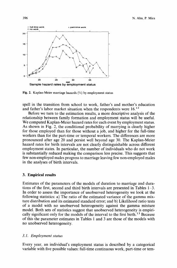
396

o full-time worko no work

20

15

10

5

0

20 25

N. Ahn, P. Mira

6 part-time work

30 35age

Sample hazard rates by employment status

Fig. 2. Kaplan-Meier marriage hazards (%) by employment status

spell in the transition from school to work, father's and mother's educationand father's labor market situation when the respondents were 16. 12

Before we turn to the estimation results, a more descriptive analysis of therelationship between family formation and employment status will be useful.We computed Kaplan-Meier hazard rates for each event by employment status.As shown in Fig. 2, the conditional probability of marrying is clearly higherfor those employed than for those without a job, and higher for the full-timeworkers than for the part-time or temporal workers. The differences are morepronounced after age 20 and persist well beyond age 30. The Kaplan-Meierhazard rates for birth intervals are not clearly distinguishable across differentemployment states. In particular, the number of individuals who do not workis substantially reduced making the comparison less precise. This suggests thatfew non-employed males progress to marriage leaving few non-employed malesin the analyses of birth intervals.

3. Empirical results

Estimates of the parameters of the models of duration to marriage and dura­tions of the first, second and third birth intervals are presented in Tables 1-3.In order to assess the importance of unobserved heterogeneity we look at thefollowing statistics: a) The ratio of the estimated variance of the gamma mix­ture distribution and its estimated standard error; and b) Likelihood ratio testsof a model with no unobserved heterogeneity against the gamma mixturemodel. Both sets of statistics suggest that unobserved heterogeneity is empiri­cally significant only for the models of the interval to the first birth. 13 Becauseof this the parameter estimates in Tables I and 3 are those of the models withno unobserved heterogeneity.

3.1. Employment status

Every year, an individual's employment status is described by a categoricalvariable with five possible values: full-time continuous work, part-time or tem-

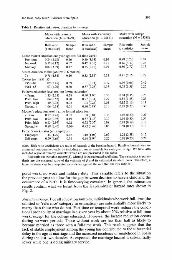
Job bust, baby bust?: Evidence from Spain

Table I. Relative risk ratios, duration to marriage

397

Males with primaryeducation (N = 56791)

Males with secondaryeducation (N = 25133)

Males with collegeeducation (N = 13388)

Risk ratio Sample Risk ratio Sample Risk ratio Sample(t statistics) mean (t-statistics) mean (t statistics) mean

Labor market situation one year ago (re: full-time work)Part-time 0.84 (3.98) 0.16 0.80 (3.03) 0.10 0.98 (0.28) 0.09No work 0.57 (6.12) 0.07 0.42 (7.36) 0.21 0.46 (8.32) 0.28Military 0.82 (3.89) 0.17 0.85 (2.16) 0.19 0.80 (2.77) 0.17

Search duration to first job (re: 0-6 months)7+ 0.75 (4.84) 0.10 0.83 (2.84) 0.18 0.81 (3.16) 0.28

Cohort (re.: 1951-55)1956-60 1.09 (2.45) 0.39 1.01 (0.14) 0.39 0.99 (0.06) 0.421961-65 1.07 (1.70) 0.30 0.87 (2.26) 0.37 0.75 (3.59) 0.25

Father's education level (re.: no formal education)<Prim. J.l3(2.18) 0.38 0.90 (1.00) 0.35 0.94 (0.35) 0.23Prim. low 1.04 (0.52) 0.20 0.97 (0.31) 0.29 0.81 (1.28) 0.26Prim. high J.lO (0.78) 0.03 1.03 (0.24) 0.08 0.82 (J.l6) 0.11Second.+ 1.06 (0.38) 0.01 0.90 (0.89) 0.10 0.97 (0.22) 0.30

Mother's education level (re.: no formal education)<Prim. 0.87 (2.41) 0.37 1.08 (0.81) 0.38 1.03 (0.20) 0.29Prim. low 0.92 (0.98) 0.19 0.87 (1.33) 0.30 1.04 (0.30) 0.34Prim. high 0.63 (2.97) 0.02 0.72 (2.37) 0.08 0.91 (0.59) 0.12Second.+ 0.88 (0.45) 0.004 0.92 (0.49) 0.03 0.94 (0.37) 0.13

Father's work status (re.: employee)Employer J.l4 (1.29) 0.02 J.lO (1.06) 0.07 1.21 (2.38) 0.12Self-emp. 0.79 (6.64) 0.31 0.90 (1.94) 0.25 0.98 (0.23) 0.22

Note: Risk ratio coefficients are ratios of hazards to the baseline hazard. Baseline hazard rates areestimated non-parametrically by including a dummy variable for each year of age. We have alsoincluded regional dummy variables which are not presented in the table.Risk ratios in the table are exp(p), wherePis the estimated coefficient. The t-statistics in paren­

thesis are the unsigned ratio of the estimate of Pand its estimated standard error. Therefore, alarge t-statistic can be interpreted as evidence against the null that the risk ratio is I.

poral work, no work and military duty. This variable refers to the situationthe previous year to allow for the gap between decision to have a child and theoccurrence of a birth. It is time-varying covariate. In general, the estimationresults confirm what we learnt from the Kaplan-Meier hazard rates shown inFig. 2.

Age at marriage. For all education samples, individuals who work full-time (theomitted or 'reference' category in estimation) are substantially more likely tomarry than those who do not. Part-time or temporal work reduces the condi­tional probability ofmarriage in a given year by about 20% relative to full-timework, except for the college educated. However, the largest reduction occursduring no-work periods. Those without work are less than half as likely tobecome married as those with a full-time work. This result suggests that thelack of stable employment among the young has contributed to the substantialdelay in the age at marriage and the increased incidence of singlehood in Spainduring the last two decades. As expected, the marriage hazard is substantiallylower while one is doing military service.

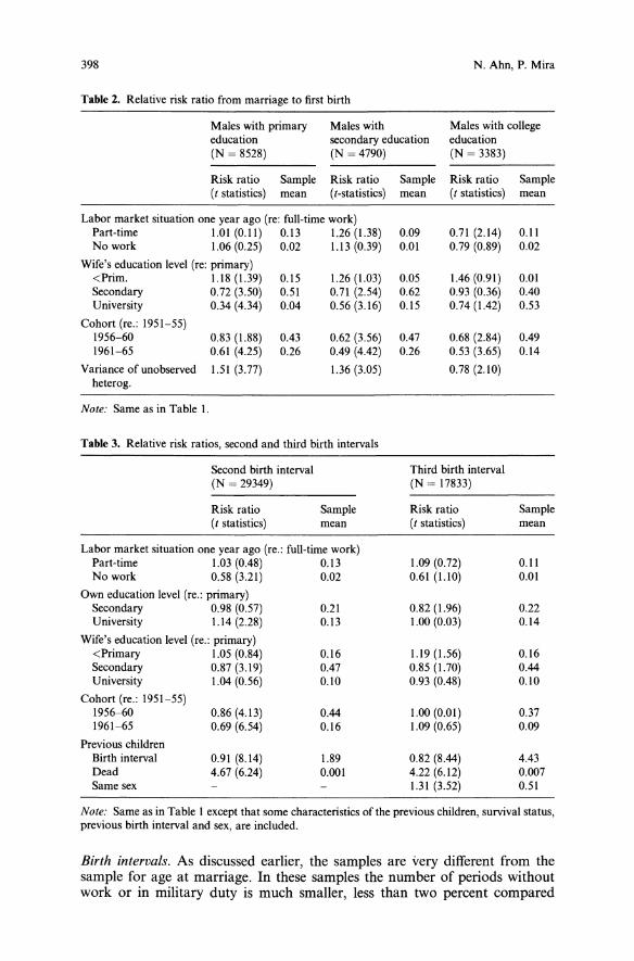
398

Table 2. Relative risk ratio from marriage to first birth

N. Ahn, P. Mira

Males with primaryeducation(N = 8528)

Males withsecondary education(N = 4790)

Males with collegeeducation(N = 3383)

Risk ratio(t statistics)

Sample Risk ratiomean (t-statistics)

Sample Risk ratiomean (t statistics)

Samplemean

Labor market situation one year ago (re: full-time work)Part-time 1.01 (0.11) 0.13 1.26 (1.38) 0.09 0.71 (2.14) 0.11No work 1.06 (0.25) 0.02 1.13 (0.39) 0.01 0.79 (0.89) 0.02

Wife's education level (re: primary)<Prim. 1.18 (1.39) 0.15 1.26 (1.03) 0.05 1.46 (0.91) 0.01Secondary 0.72 (3.50) 0.51 0.71 (2.54) 0.62 0.93 (0.36) 0.40University 0.34 (4.34) 0.04 0.56 (3.16) 0.15 0.74 (1.42) 0.53

Cohort (re.: 1951-55)1956-60 0.83 (1.88) 0.43 0.62 (3.56) 0.47 0.68 (2.84) 0.491961-65 0.61 (4.25) 0.26 0.49 (4.42) 0.26 0.53 (3.65) 0.14

Variance of unobserved 1.51 (3.77) 1.36 (3.05) 0.78 (2.10)heterog.

Note: Same as in Table I.

Table 3. Relative risk ratios, second and third birth intervals

Second birth interval(N = 29349)

Risk ratio(t statistics)

Samplemean

Third birth interval(N = 17833)

Risk ratio(t statistics)

Samplemean

Labor market situation one year ago (re.: full-time work)Part-time 1.03 (0.48) 0.13 1.09 (0.72) 0.11No work 0.58 (3.21) 0.02 0.61 (1.10) 0.01

Own education level (re.: primary)Secondary 0.98 (0.57) 0.21 0.82 (1.96) 0.22University 1.14 (2.28) 0.13 1.00 (0.03) 0.14

Wife's education level (re.: primary)<Primary 1.05 (0.84) 0.16 1.19 (1.56) 0.16Secondary 0.87 (3.19) 0.47 0.85 (1.70) 0.44University 1.04 (0.56) 0.10 0.93 (0.48) 0.10

Cohort (re.: 1951-55)1956-60 0.86 (4.13) 0.44 1.00 (0.01) 0.371961-65 0.69 (6.54) 0.16 1.09 (0.65) 0.09

Previous childrenBirth interval 0.91 (8.14) 1.89 0.82 (8.44) 4.43Dead 4.67 (6.24) 0.001 4.22 (6.12) 0.007Same sex 1.31 (3.52) 0.51

Note: Same as in Table I except that some characteristics of the previous children, survival status,previous birth interval and sex, are included.

Birth intervals. As discussed earlier, the samples are very different from thesample for age at marriage. In these samples the number of periods withoutwork or in military duty is much smaller, less than two percent compared

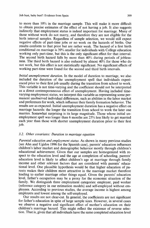
Job bust, baby bust?: Evidence from Spain 399

to more than 10% in the marriage sample. This will make it more difficultto obtain precise estimates of the effect of not having a job. It also suggestsindirectly that employment status is indeed important for marriage. Many ofthose without work do not marry, and therefore they are not eligible for thebirth interval samples. Regardless of sample selection, we would still expectnegative effects of part-time jobs or no work on the hazards of births. Ourresults conform to that prior but are rather weak. The hazard of a first birthconditional on marriage is 39% smaller for individuals with College educationworking only part-time, but this is the only significant effect for that interval.The second birth hazard falls by more than 40% during periods of jobless­ness. The third birth hazard is also reduced by almost 40% for those who donot work, but this effect is not statistically significant. No significant effects ofworking part-time were found for the second and third birth intervals.

Initial unemployment duration. In the model of duration to marriage, we alsoincluded the duration of the unemployment spell that individuals experi­enced prior to their first job usually during the transition from school to work.This variable is not time-varying and the coefficient should not be interpretedas a direct contemporaneous effect of unemployment. Having included time­varying employment status, we interpret this variable as representing some per­manent unobserved individual differences, such as abilities in the labor marketand preferences for work, which influence their family formation behavior. Theresults are as expected. Initial unemployment duration has a negative effect onmarriage hazards: the longer the transition from school to work the later onemarries. Somewhat surprising is its large magnitude. Those whose initial un­employment spell was longer than 6 months are 25% less likely to get marriedeach year than those with shorter unemployment duration prior to their firstjob.

3.2. Other covariates: Duration to marriage equation

Parental education and employment status. As shown in many previous studies(see Ahn and Ugidos 1996 for the Spanish case), parents' education influenceschildren's labor market and demographic behavior mostly through children'seducational achievement. Given that our samples are homogenized with re­spect to the education level and the age at completion of schooling, parents'education level is likely to affect children's age at marriage through familyincome and other relevant factors that are correlated with parents' educa­tional level. One plausible hypothesis would be that higher education of pa­rents makes their children more attractive in the marriage market thereforeleading to earlier marriage other things equal. Given the parents' educationlevel, father's occupation may be a proxy for the economic situation of thefamily. We distinguish three employment categories: employer, paid worker(reference category in our estimation models) and self-employed without em­ployees. According to previous studies, the average income is highest amongemployers and lowest among the self-employed.Our results are not clear-cut. In general, the coefficients are not significant

for father's education in spite of large sample sizes. However, in several caseswe observe a negative and significant effect of mother's education on theirchildren's marriage hazard. This might reflect the existence of reverse selec­tion. That is, given that all individuals have the same completed education level

400 N. Ahn, P. Mira

in our samples, the mother's education might be negatively correlated with thechild's unobserved ability. Children with more educated mothers are supposedto have higher education, either for genetic reasons or because they receivemore human capital at home.With respect to father's employment status our results indicate that the

children of 'employer' fathers have higher marriage probabilities than those of'employee' fathers, while the marriage hazard of individuals with self-employedfathers is the lowest. This seems to be in agreement with our 'family income'conjecture - that the higher the family income the higher the marriage prob­ability; however, the effects are not significant for all education categories.

Birth cohort. There are some differences between cohorts. Among the sec­ondary and college education samples the marriage hazard was significantlylower for the youngest cohort (1961-1965). This decrease was greater for thecollege graduates, which may reflect the rapid increase in college enrollmentrate among their potential spouses. Among the primary education sample, theyoungest cohort (61-65) had lower marriage hazards than the intermediatecohort (56-60), but marginally higher than the oldest (51-55).

3.3. Other covariates: Birth interval equations

Birth cohort. The more recent cohorts had lower birth hazards. A strong andsignificant downward trend is observed for the hazards in the first and secondbirth intervals across all three education groups. The effect was strongestamong the secondary education group; for instance, the hazard rates in thefirst birth interval decreased by as much as 50%. No significant trend is de­tected for birth hazards in the third birth interval. 14

Wife's education. The birth hazards decrease with the wife's education. Thesecoefficients are generally large and significant, especially so for the first birthinterval.

Previous children, interval to second birth. We have included some variablesregarding the first child. First, the variable indicating the death of the firstchild is included as a time-varying dummy equal to one for all periods afterthe death of the child. Since infant and child mortality rates are low, there is avery small number of person-years for which this indicator is one (less than0.3 percent of the total). It is well known that subsequent births tend to occursooner due to both biological and behavioral reasons when a child dies. Thissame result is observed in our estimates. The death of the first child increasesthe hazard of a second birth by a factor of more than four.We included the duration of the interval from marriage to the first birth.

This variable is likely to work as a proxy for the couples' fecundity and pref­erences for children, which we do not observe. Under this hypothesis, shorterprevious intervals would lead to shorter subsequent intervals, which is con­firmed in our results. Every year added to the previous interval reduces thesecond birth hazard by about 10%. However, this should not be interpreted asa causal effect since both are likely to be determined by common unobservedfactors.

Previous children, Interval to third birth. Again, the death of the first or second

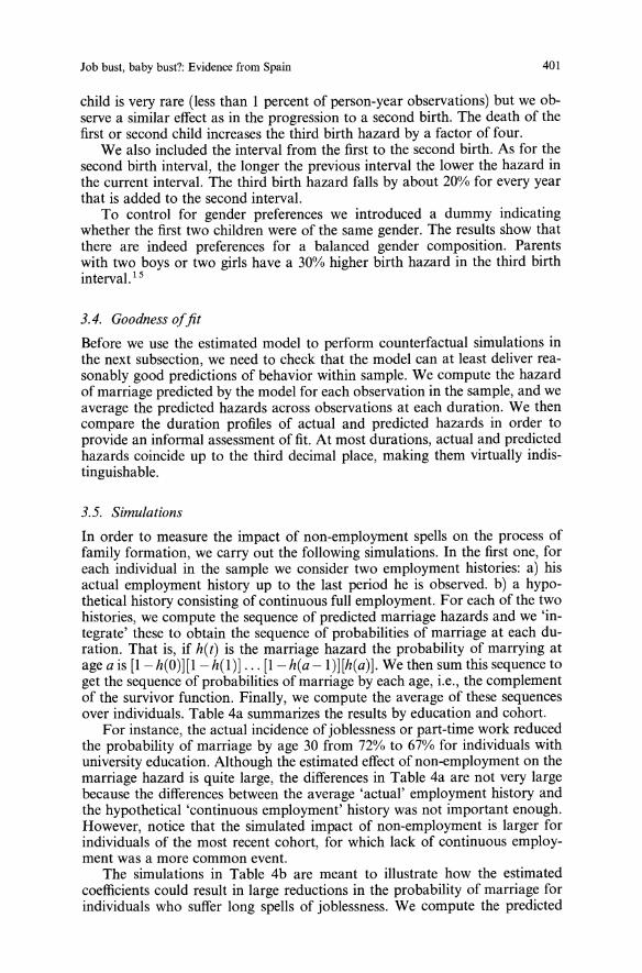
Job bust, baby bust?: Evidence from Spain 401

child is very rare (less than I percent of person-year observations) but we ob­serve a similar effect as in the progression to a second birth. The death of thefirst or second child increases the third birth hazard by a factor of four.We also included the interval from the first to the second birth. As for the

second birth interval, the longer the previous interval the lower the hazard inthe current interval. The third birth hazard falls by about 20% for every yearthat is added to the second interval.To control for gender preferences we introduced a dummy indicating

whether the first two children were of the same gender. The results show thatthere are indeed preferences for a balanced gender composition. Parentswith two boys or two girls have a 30% higher birth hazard in the third birthinterval. 15

3.4. Goodness olfit

Before we use the estimated model to perform counterfactual simulations inthe next subsection, we need to check that the model can at least deliver rea­sonably good predictions of behavior within sample. We compute the hazardofmarriage predicted by the model for each observation in the sample, and weaverage the predicted hazards across observations at each duration. We thencompare the duration profiles of actual and predicted hazards in order toprovide an informal assessment of fit. At most durations, actual and predictedhazards coincide up to the third decimal place, making them virtually indis­tinguishable.

3.5. Simulations

In order to measure the impact of non-employment spells on the process offamily formation, we carry out the following simulations. In the first one, foreach individual in the sample we consider two employment histories: a) hisactual employment history up to the last period he is observed. b) a hypo­thetical history consisting of continuous full employment. For each of the twohistories, we compute the sequence of predicted marriage hazards and we 'in­tegrate' these to obtain the sequence of probabilities of marriage at each du­ration. That is, if h(t) is the marriage hazard the probability of marrying atage a is [I - h(O)][1 - h( I)J ... [1 - h(a - 1)][h(a)J. We then sum this sequence toget the sequence of probabilities ofmarriage by each age, i.e., the complementof the survivor function. Finally, we compute the average of these sequencesover individuals. Table 4a summarizes the results by education and cohort.For instance, the actual incidence of joblessness or part-time work reduced

the probability of marriage by age 30 from 72% to 67% for individuals withuniversity education. Although the estimated effect of non-employment on themarriage hazard is quite large, the differences in Table 4a are not very largebecause the differences between the average 'actual' employment history andthe hypothetical 'continuous employment' history was not important enough.However, notice that the simulated impact of non-employment is larger forindividuals of the most recent cohort, for which lack of continuous employ­ment was a more common event.The simulations in Table 4b are meant to illustrate how the estimated

coefficients could result in large reductions in the probability of marriage forindividuals who suffer long spells of joblessness. We compute the predicted

402 N. Ahn, P. Mira

Table 4. The impact of employment status on the probability of marriage. a Simulated impact ofsample non-employment on the probability of marriage by education and cohort

Employment history By Age 25 By Age 30 By Age 35

Cohort 61-65 56-60 51-55 56-60 51-55 51-55

Primary educ. Continuous fun-time 0.55 0.55 0.50 0.82 0.77 0.84Actual 0.51 0.52 0.48 0.79 0.76 0.83

Secondary educ. Continuous fun-time 0.40 0.46 0.46 0.79 0.78 0.87Actual 0.37 0.43 0.44 0.76 0.76 0.86

University educ. Continuous fun-time 0.18 0.28 0.28 0.72 0.72 0.86Actual 0.15 0.24 0.25 0.67 0.68 0.83

Table 4b. Simulated impact of the duration of post-school joblessness on the probability of mar­riage. Evaluated at sample mean characteristics

Years of Survival probability from marriage Survival probability from marriagenon-work until 5th year until 10th year

Primary Secondary University Primary Secondary University

0 0.888 0.834 0.522 0.393 0.345 0.198I 0.915 0.862 0.614 0.495 0.413 0.2792 0.919 0.869 0.652 0.497 0.416 0.2963 0.925 0.880 0.703 0.500 0.421 0.3194 0.936 0.903 0.789 0.506 0.432 0.3585 0.950 0.938 0.892 0.514 0.449 0.4056 0.528 0.476 0.4627 0.554 0.514 0.5348 0.587 0.560 0.6069 0.628 0.621 0.67710 0.668 0.687 0.753

probability that an individual with sample mean characteristics will remainunmarried 5 and 10 years after leaving school as a function of the number ofyears spent without a job. For instance, the probability that the average indi­vidual with university education will remain unmarried 10 years after leavingschool is only 20% if he was continuously employed during the interval, but itjumps to 75% if he was continuously unemployed.

4. Discussion and conclusions

In this study we have looked for evidence of a link between the 'unemploy­ment crisis' and the 'fertility crisis' in Spain. We have examined the factorsthat affect individuals' ages at marriage and childbirth, focusing on the effectsofmale employment status. Our results suggest that spells of non-employmenthave a strong negative effect on the hazard of marriage. We also find negative(but smaller) effects of part-time or temporal employment on the hazard ofmarriage. Simulations based on the estimated models confirm the potentialfor large 'delaying' effects of joblessness on marriage. However, the delayingeffect is not so large in simulations which control for the actual incidence ofnon-employment in the sample.

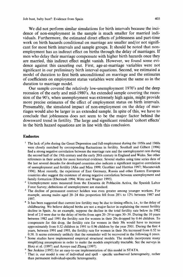
Job bust, baby bust?: Evidence from Spain 403

We did not perform similar simulations for birth intervals because the inci­dence of non-employment in the sample is much smaller for married indi­viduals. Furthermore, the estimated direct effects of joblessness and part-timework on birth hazards conditional on marriage are smaller and/or not signifi­cant for most birth intervals and sample groups. It should be noted that non­employment has an indirect effect on births through the delay of marriages. Ifmen who delay their marriage compensate with higher birth hazards once theyare married, this indirect effect might vanish. However, we found some evi­dence against this canceling out. First, age-at-marriage variables were notsignificant in our preliminary birth interval equations. Second, we estimated amodel of duration to first birth unconditional on marriage and the estimatesof coefficients on employment status variables were almost the same as in theduration to marriage model.Our sample covered the relatively low-unemployment 1970's and the deep

recession of the early and mid-1980's. An extended sample covering the reces­sion of the 90's, when unemployment was extremely high again, might providemore precise estimates of the effect of employment status on birth intervals.Presumably, the simulated impact of non-employment on the delay of mar­riages would also be larger in an extended sample. In spite of this, we have toconclude that joblessness does not seem to be the major factor behind thedownward trend in fertility. The large and significant residual 'cohort effects'in the birth hazard equations are in line with this conclusion.

Endnotes

1 The lack of jobs during the Great Depression and full employment during the 1950s and 1960swere closely matched by corresponding fluctuations in fertility. Southall and Gilbert (1996)find a strong negative correlation between the marriage rate and the unemployment rate duringthe second half of the 19th century and the early 20th century in England and Wales. See otherreferences in their article for more historical evidence. Several studies using time series data ofthe last several decades for developed countries also indicate a significant negative correlationof unemployment and fertility (Ahn and Mira 1999; Gauthier and Hatzius 1997; Macunovich1996). Most recently, the experience of East Germany, Russia and other Eastern Europeancountries also suggest the existence of strong negative correlation between unemployment andfamily formation (Eberstadt 1994; Witte and Wagner 1995).

2 Unemployment rates measured from the Encuesta de Poblaci6n Activa, the Spanish LaborForce Survey; definitions of unemployment are standard.

3 The decline of permanent contract holders was even greater among younger workers. Forexample, among males aged 20-24 this proportion fell from 28% to 12% between 1987 and1997.

4 It has been suggested that current low fertility may be due to timing effects, i.e., to the delay ofchildbearing. We believe delayed births are not a major factor in explaining the recent fertilitydecline in Spain. As an example, suppose the decline in the total fertility rate below its 1982level of 2.0 were due to the delay of births from ages 20-29 to ages 30-39. During the 10 yearsbetween 1982 and 1991 the fertility rate for women in their 20s dropped by 0.44 children. Tocompensate for this drop, the fertility rate for women in their 30s would have to increaseapproximately from 0.52 children in 1991 to 0.96 children by the year 2001. During the first 4years, between 1991 and 1995, the fertility rate for women in their 30s increased from 0.52 to0.58. It seems extremely unlikely that the remainder will be recovered in the following 6 years.

5 Some studies have implemented empirical structural models. The models incorporate manysimplifying assumptions in order to make the models empirically tractable. See the surveys inHotz et al. (1997) and Arroyo and Zhang (1997).

6 See Jenkins (1995) for an easy-to-use implementation of this model in STATA.7 That is, our model is one of individual and spell - specific unobserved heterogeneity, ratherthan permanent individual-specific heterogeneity.

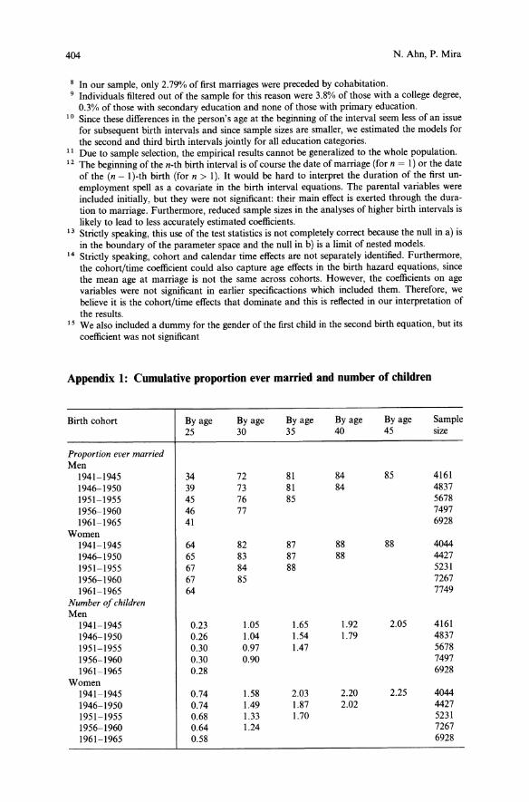
404 N. Ahn, P. Mira

8 In our sample, only 2.79% of first marriages were preceded by cohabitation.9 Individuals filtered out of the sample for this reason were 3.8% of those with a college degree,0.3% of those with secondary education and none of those with primary education.

10 Since these differences in the person's age at the beginning of the interval seem less of an issuefor subsequent birth intervals and since sample sizes are smaller, we estimated the models forthe second and third birth intervals jointly for all education categories.

11 Due to sample selection, the empirical results cannot be generalized to the whole population.12 The beginning of the n-th birth interval is of course the date of marriage (for n = I) or the dateof the (n - I)-th birth (for n > I). It would be hard to interpret the duration of the first un­employment spell as a covariate in the birth interval equations. The parental variables wereincluded initially, but they were not significant: their main effect is exerted through the dura­tion to marriage. Furthermore, reduced sample sizes in the analyses of higher birth intervals islikely to lead to less accurately estimated coefficients.

13 Strictly speaking, this use of the test statistics is not completely correct because the null in a) isin the boundary of the parameter space and the null in b) is a limit of nested models.

14 Strictly speaking, cohort and calendar time effects are not separately identified. Furthermore,the cohort/time coefficient could also capture age effects in the birth hazard equations, sincethe mean age at marriage is not the same across cohorts. However, the coefficients on agevariables were not significant in earlier specificactions which included them. Therefore, webelieve it is the cohort/time effects that dominate and this is reflected in our interpretation ofthe results.

15 We also included a dummy for the gender of the first child in the second birth equation, but itscoefficient was not significant

Appendix 1: Cumulative proportion ever married and number of children

Birth cohort By age By age By age By age By age Sample25 30 35 40 45 size

Proportion ever marriedMen1941-1945 34 72 81 84 85 41611946-1950 39 73 81 84 48371951-1955 45 76 85 56781956-1960 46 77 74971961-1965 41 6928

Women1941-1945 64 82 87 88 88 40441946-1950 65 83 87 88 44271951-1955 67 84 88 52311956-1960 67 85 72671961-1965 64 7749

Number of childrenMen1941-1945 0.23 1.05 1.65 1.92 2.05 41611946-1950 0.26 1.04 1.54 1.79 48371951-1955 0.30 0.97 1.47 56781956-1960 0.30 0.90 74971961-1965 0.28 6928

Women1941-1945 0.74 1.58 2.03 2.20 2.25 40441946-1950 0.74 1.49 1.87 2.02 44271951-1955 0.68 1.33 1.70 52311956-1960 0.64 1.24 72671961-1965 0.58 6928

Job bust, baby bust?: Evidence from Spain

References

405

Ahn N (1997) Labor Market Crisis and Demographic Crisis in Spain. Paper presented in the II thAnnual Conference of the European Society for Population Economics in Essex

Ahn N, Mira P (1999) A Note on the Changing Relationship Between Fertility and FemaleEmployment Rates in Developed Countries. Working Paper No. 9903, CEMFI, Madrid

Ahn N, Ugidos A (1996) The Effects of the Labor Market Situation of Parents on Children:Inheritance of Unemployment. Investigaciones Economicas XX:23-41

Anderson KH, Hill MA, Butler JS (1987) Age at Marriage in Malaysia: A Hazard Model ofMarriage Timing. Journal ofDevelopment Economics 26(2):223-234

Arroyo CR, Zhang J (1997) Dynamic Microeconomic Models of Fertility Choice: A Survey.Journal of Population Economics 10:23-65

Angrist JD, Evans WN (1998) Children and Their Parents' Labor Supply: Evidence from Exoge­nous Variation in Family Size. American Economic Review 88(3):450-477

Becker GS (1974) A Theory of Marriage. In: Schultz TW (ed) Economics ofthe Family: Marriage,Children, and Human Capital. University of Chicago Press, Chicago, 299-344

Bergstrom T, Schoeni RF (1996) Income Prospects and Age-at-marriage. Journal of PopulationEconomics 9: 115-130

Bover 0, Arellano M (1995) Female Labor Force Participation in the 1980s: The Case of Spain.Investigaciones Economicas, Mayo: 171-194

Eberstadt N (1994) Demographic Shocks after Communisom: Eastern Germany, 1989-1993.Population and Development Review 20(1):137-152

Gauthier AH, Hatzius J (1997) Family Benefits and Fertility: An Econometric Analysis. PopulationStudies 51 :295-306

Heckman JJ, Walker JR (1990) The Relationship Between Wages and Income and the Timingand Spacing of Births: Evidence from Swedish Longitudinal Data. Econometrica 58(6):1411­1441

Hotz VJ, Miller R (1988) An Empirical Analysis of Life Cycle Fertility and Female Labor Supply.Econometrica 56:91-118

Hotz VJ, Klerman J, Willis R (1997) The Economics of Fertility in Developed Countries. Hand­book ofPopulation and Family Economics: 275-347

Jenkins SP (1995) Easy Estimation Methods for Discrete-time Duration Models. Oxford Bulletinof Economics and Statistics 57(1):129-138

Keeley M (1977) The Economics of Family Formation. Economic Inquiry 15:238-250Macunovich DJ (1996) Relative Income and Price of Time: Exploring Their Effects on US Fer­tility and Female Labor Force Participation. Population and Development Review 22(Supple­ment): 223-257

Meyer BD (1990) Unemployment Insurance and Unemployment Spells. Econometrica 58(4):757­782

Montgomery MR, Trussell J (1986) Models of Marital Status and Childbearing. In: Ashenfelter0, Layard R (eds) Handbook of Labor Economics, vol. 1,205-269

Oppenheimer VK, Kalmijn M, Lim N (1997) Men's Career Development and Marriage TimingDuring a Period of Rising Inequality. Demography 34(3):311-330

Schultz TP (1997) Demand for Children in Low Income Countries. Handbook of Population andFamily Economics, 349-430

Southall H, Gilbert D (1996) A Good Time to Wed?: Marriage and Economic Distress in Englandand Wales, 1983-1914. Economic History Review XLIX(I):35-57

Witte JC, Wagner GG (1995) Declining Fertility in East Germany After Unification: A Demo­graphic Response to Socioeconomic Change. Population and Development Review 21(2):38­397

Effect of childbearing on Filipino women's work hoursand earnings

Linda Adairl, David Guilkeyl, Eilene Bisgrove2, Socorro Gultiano3

1 Carolina Population Center, University of North Carolina, 123 W. Franklin St., Chapel Hill,NC 27516, USA (Fax: +1-919-966-9159; e-mail: Linda_adair@unc.edu;david_guilkey@unc.edu)21700 Open Air Camp Road, Durham NC 27712, USA(e-mail: urholy@duke.edu)3 Office of Population Studies, University of San Carlos, 6000 Cebu, Philippines(Fax: +1\-63-32-3466-050; e-mail: connie@mangga.usc.edu.ph)

Received: 16 July 1998jAccepted: 22 March 2001

Abstract. The effects of childbearing and work sector on women's hours andearnings in the 8 years following an index pregnancy were examined in a co­hort of more than 2,000 women in the Cebu Longitudinal Health and Nutri­tion Survey. Change in cash earnings and hours worked were each modeledjointly with sector of labor force participation using an estimation strategythat deals with endogeneity of childbearing decisions and selectivity into sec­tor of work. Two or more additional children born in the 8 year interval sig­nificantly reduced women's earnings, while having an additional child under 2years of age in 1991 reduced hours worked.

JEL classification: Jl3, 121

Key words: Labor force participation, childbearing, wages

1. Introduction

It is generally assumed by those who promote family planning that havingfewer children improves child health and survival, and also contributes in pos-

All correspondence to Linda Adair. The authors wish to thank Family Health International andthe U.S. Agency for International Development (USAID) for their generous support. This publi­cation was funded by USAID under Cooperative Agreement USAIDjCCP-3060-A-OG-3021-00 toFamily Health International (FHI). David Guilkey's participation in this paper was also sup­ported by the MEASURE Evaluation Project also with support from the United States Agencyfor International Development (USAID) under Contract Number HRN-A-00-97-oo018-00. Theconclusions expressed in this report do not necessarily reflect the policies of FHI or USAID.Helpful comments by two anonymous referees are gratefully acknowledged. Responsible editor:T. Paul Schultz.

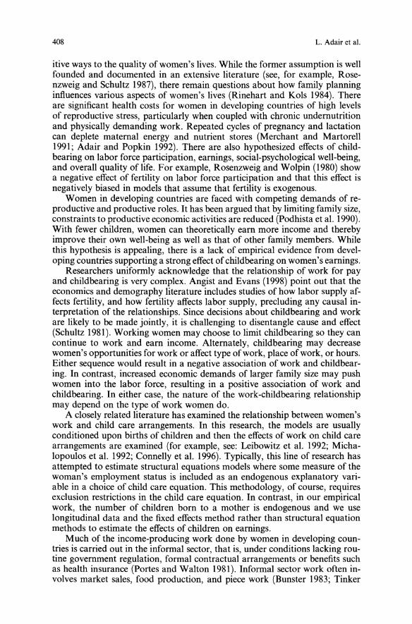
408 L. Adair et al.

itive ways to the quality of women's lives. While the former assumption is wellfounded and documented in an extensive literature (see, for example, Rose­nzweig and Schultz 1987), there remain questions about how family planninginfluences various aspects of women's lives (Rinehart and Kols 1984). Thereare significant health costs for women in developing countries of high levelsof reproductive stress, particularly when coupled with chronic undernutritionand physically demanding work. Repeated cycles of pregnancy and lactationcan deplete maternal energy and nutrient stores (Merchant and Martorell1991; Adair and Popkin 1992). There are also hypothesized effects of child­bearing on labor force participation, earnings, social-psychological well-being,and overall quality of life. For example, Rosenzweig and Wolpin (1980) showa negative effect of fertility on labor force participation and that this effect isnegatively biased in models that assume that fertility is exogenous.Women in developing countries are faced with competing demands of re­

productive and productive roles. It has been argued that by limiting family size,constraints to productive economic activities are reduced (Podhista et al. 1990).With fewer children, women can theoretically earn more income and therebyimprove their own well-being as well as that of other family members. Whilethis hypothesis is appealing, there is a lack of empirical evidence from devel­oping countries supporting a strong effect ofchildbearing on women's earnings.Researchers uniformly acknowledge that the relationship of work for pay

and childbearing is very complex. Angist and Evans (1998) point out that theeconomics and demography literature includes studies of how labor supply af­fects fertility, and how fertility affects labor supply, precluding any causal in­terpretation of the relationships. Since decisions about childbearing and workare likely to be made jointly, it is challenging to disentangle cause and effect(Schultz 1981). Working women may choose to limit childbearing so they cancontinue to work and earn income. Alternately, childbearing may decreasewomen's opportunities for work or affect type ofwork, place ofwork, or hours.Either sequence would result in a negative association of work and childbear­ing. In contrast, increased economic demands of larger family size may pushwomen into the labor force, resulting in a positive association of work andchildbearing. In either case, the nature of the work-childbearing relationshipmay depend on the type of work women do.A closely related literature has examined the relationship between women's

work and child care arrangements. In this research, the models are usuallyconditioned upon births of children and then the effects of work on child carearrangements are examined (for example, see: Leibowitz et al. 1992; Micha­lopoulos et al. 1992; Connelly et al. 1996). Typically, this line of research hasattempted to estimate structural equations models where some measure of thewoman's employment status is included as an endogenous explanatory vari­able in a choice of child care equation. This methodology, of course, requiresexclusion restrictions in the child care equation. In contrast, in our empiricalwork, the number of children born to a mother is endogenous and we uselongitudinal data and the fixed effects method rather than structural equationmethods to estimate the effects of children on earnings.Much of the income-producing work done by women in developing coun­

tries is carried out in the informal sector, that is, under conditions lacking rou­tine government regulation, formal contractual arrangements or benefits suchas health insurance (Portes and Walton 1981). Informal sector work often in­volves market sales, food production, and piece work (Bunster 1983; Tinker

Childbearing and women's earnings 409

1981; Cohen and House 1996). Self-employed workers in the informal sectoroften own their own means of production. Compared to work in the formalsector, informal sector work offers women flexibility in hours, but less security,status, and non-wage benefits such as social security, health insurance, or paidsick leave. Given its greater flexibility, women may regard informal sector workas more compatible with childbearing. In contrast, work in the formal sectoroffers greater stability, some non-wage benefits, and greater structure, but gen­erally longer hours and a work site typically away from home (Anker and Hein1985).Becker (1981) hypothesizes that formal sector work away from home pre­

sents higher opportunity costs, and thus acts as a greater deterrent to child­bearing. Under this premise, limiting family size should promote participa­tion in the formal work sector, but have relatively little impact on the informalwork sector where opportunity costs are lower and productive and reproduc­tive roles are more compatible.The type of work selected by women is affected by a wide range of fac­

tors including education and training, prior work experience, earning poten­tial, compatibility with other roles (childbearing, elder care, other householdresponsibilities etc.), household characteristics including income, partner's ed­ucation, and presence of childcare substitutes, and community level charac­teristics such as infrastructure, labor opportunities and wage structure. Formany women in the Philippines, work is regarded solely as an economic ne­cessity. For some, work is a choice that carries other benefits, including statusand a sense of personal achievement. Thus, the choice to work or not, and thetype of work selected may differ at opposite ends of the income distribution.Women from higher income households may elect not to work unless they arealso highly educated while women from poor households may be driven towork by economic necessity.To understand the effect of childbearing on women's earnings, it is impor­

tant to consider not only the type of work women do but also the hours theywork. Women may increase earnings by working more hours, but this maycreate more competition between their productive and reproductive roles, andthus result in no net gain in other quality of life outcomes. One strategy toovercome the time demand dilemma is for women with children to select jobswith more flexible hours but lower pay (Becker 1981). It is therefore importantto explore the effects of childbearing on earnings both as a function of hoursand of earnings per unit of time worked.Childbearing is likely to affect women's earnings in 2 major ways. Child­

bearing may influence whether or not women work for pay at various pointsin their reproductive years, and having small children may influence the hoursand earnings of women who are working. These effects will likely be mediatedby the type of work women do and by the availability of childcare substitutes.Mothers working in the formal wage sector where opportunity costs are

high and flexibility for childbearing is more limited, may withdraw from thelabor force for a period of time or may shift to a lower-paying but more flex­ible job. Women from lower income households may be less able to withdrawfrom the labor force and may continue working at the same or reduced hours.For women who shift to a lower-paying job without increasing hours, child­bearing would result in reduced income. Self-employed women with work thatis relatively compatible with child care may be able to continue their work andmay see little decrease in income. In their study of piece workers in Mexico

410 L. Adair et al.

City, Beneria and Roldan (1987) found that compatibility with childcare is areason often given by women for why they are involved in piece work. Womenengaged in piece work or whose self-employed work is fairly demanding maywork similar hours, but find that they are less productive because of the de­mands of child-care. These women may earn less income, may increase theirwork hours to maintain their profits, or may switch to work that is less de­manding and usually less profitable.Finally, the effects of childbearing are likely to depend on its different

phases. Late in pregnancy, women may find it difficult to continue workingbecause of physical constraints. Mothers of infants and young children facethe time demands of more intensive childcare and breast-feeding. As childrenget older, these demands may decline or child care may be more easily assumedby alternate care givers. In studies of US women showing a relationship ofchildbearing and earnings, the age of the youngest child at the time of mea­surement is a stronger predictor of wages than the total number of children(Lehrer 1992). In a summary of several studies that used mainly US data, Ko­renman and Neumark (1992) concluded that "children appear to reduce wagesprimarily 'indirectly' by reducing labor force participation and accumulationof human capital rather then 'directly' by lowering the productivity of other­wise similar work." In their own study, Korenman and Neumark control forthe endogeneity of children through the use of longitudinal data and a fixedeffects estimator. After this endogeneity is controlled, the effect of children onwages is found to be insignificant (Korenman and Neumark 1992).Given the vast differences in labor markets in developed versus develop­

ing countries, it may not be possible to generalize results from the US. Furtherresearch in developing countries is needed to explore the effects of number andages of children on women's earnings. Such research requires detailed longi­tudinal data on women at different stages of their reproductive lives. Of par­ticular importance is the ability to document the sequence of work and child­bearing events.We use data from the Cebu Longitudinal Health and Nutrition Survey

(CLHNS) to explore the determinants of change in women's hours workedand earnings over an 8 year period, while controlling for the selectivity intoworking for pay and the endogeneity of childbearing and work sector. TheCLHNS is particularly well suited to this purpose, since data are available onwork patterns, earnings, and reproductive events in a large cohort of womenover an 8 year period. Prospective data allow us to examine changes in wom­en's labor force participation and earnings subsequent to a well documentedpregnancy, but also conditioned on prior reproductive experiences and a widerange of other maternal characteristics. Detailed data on type of work allowdifferentiation by wage, self-employment, and piece work sectors.

2. Data

CLHNS data were collected from 1983 to 1991 in Metro Cebu, the secondlargest metro area in the Philippines, and a major shipping center undergoingrapid urban development and population growth. Like the rest of the Philip­pines, the Central Visayas region where Cebu is located, has a moderatelyhigh fertility rate. In 1993, the total fertility rate (TFR) for this region was 4.38,compared to 4.09 for the entire country. These levels represent only modest

Childbearing and women's earnings 411

declines from the previous decade, when TFR was 4.7 for the entire country(DHS 1994).The study area encompasses the densely populated urban areas of Cebu

City and other contiguous smaller cities, peri-urban areas around these cities,and more isolated rural areas in the mountains and on smaller islands. TheCLHNS is a community based study of a cohort of childbearing women, ages14 to 47 at entry into the study. Following a census of all urban and ruralbarangays (administrative units) of the Metro Cebu area, 33 barangays wererandomly selected for the study. All pregnant women in these barangays whosubsequently had a birth or pregnancy termination in a one year period from1983 to 1984 were recruited into the study (n = 3,327). The study sample isrepresentative of childbearing Women in communities of Metro Cebu, with apreponderance of low income families, a wide range of variability in income,education, and level of modernization.Highly trained interviewers from the Office of Population Studies at the

University of San Carlos visited each household to collect sociodemographic,environment, health, nutrition, and reproductive history data. Data collectiontook place during the 6th to 7th month of pregnancy, then at bimonthly inter­vals for 2 years. The first follow-up survey was conducted in 1991, and 2,395women (72% of the baseline sample) were located and re-interviewed. We fo­cus this analysis on the women present at the 1991 follow-up.In the majority of cases, loss to follow-up occurred because families moved

away from the Metro Cebu area. Most migration took place during the firstseveral years of the study. Relatively little migration occurred from 1986 to1991 resulting in low rates of loss to follow-up during this period. Comparedto the women in the 1991 survey, those lost to follow-up (n = 932) were onaverage, I year younger, completed about I additional year of schooling, ofslightly lower parity, and more likely to be from urban areas. Despite mea­surable differences in characteristics ofmigrants, in previous studies of health­related outcomes, we found no significant biases in multi variate results at­tributable to loss to follow-up (Guilkey et al. 1989).

2.1. Definition ofstudy variables

I. Labor force participation was defined for purposes of this study as "workingfor pay". During the baseline survey, women were asked if they were currentlydoing any work for pay, or whether they had worked in the previous 4 months.We define as working, those women with affirmative answers to either question,since women may have recently stopped working because of advancing preg­nancy. Only 10% of the women we classified as working were not currentlyworking but were working 4 months ago. Excluded from this classification ofwork are those women who are unpaid workers in a family business or farm.This type of work was excluded because we wanted to focus on women's cashearnings. The same criteria were used to identify work status ofwomen in 1991.Work done by Cebu women was categorized into 3 work sectors based on

the mode of pay. Data were not collected on contractual arrangements, so wedo not use the standard formal-informal sector dichotomy. Wage workers arepaid on a time basis (most often daily or hourly), and mayor may not haveformal contracts and benefits. Most wage workers are in service-related jobs(clerical, domestic help, etc.). Piece workers are paid by the amount of goods

412 L. Adair et al.

they produce. Most piece work in Cebu involves manufacture of shell, woodor fabric handicrafts. Self-employed women run their own small businesses.Many of these are small "sari-sari" stores which have a limited inventory ofsundries and food items, and are typically located in the woman's own homeor a neighboring building. Other small businesses may involve selling preparedfoods.

2. Total household income was determined based on a series of questionsabout earnings in primary and secondary jobs, and in family businesses (in­cluding raising of livestock, sale of produce). Income was measured during thebaseline survey, at 12 and 24 months postpartum, and in 1991 using the sameset of questions to insure comparability across the surveys. Using Philippinesconsumer price indices, income values were deflated to a common time pointin 1983 so that real changes in income could be determined.Change in women's total weekly cash earnings and change in weekly hours

worked in the interval from the baseline survey to 1991 are the main dependentvariables in our analysis. We restrict our analysis to cash income for severalreasons. First, while the tradition in the Philippines is for men to turn over theirearnings to their wives, Filipino women, like women elsewhere, have more au­tonomy in spending their own cash income, and tend to spend their earnings tobenefit their children and themselves (Bruce et al. 1995; Kennedy and Peters1992; Bisgrove and Popkin 1996; Haddad et al. 1997). Second, the non-cashcomponent of income, typically derived from work on a farm or in a familybusiness, is a measure of household activity. We have no precise measures ofwomen's contributions, and their incomes could only be estimated with con­siderable error.

3. Hours worked. Women were asked to report the usual number of hoursper day, and the number of days per week they worked in the past 4 months.Hours were summed for main and secondary jobs.

4. Childbearing patterns were determined from detailed reproductive his­tories. The multi variate model includes a variable indicating change in thenumber of surviving children under two years of age and a set of dummy vari­ables indicating the number ofchildren born after the index child, and still aliveand in the household at the time of the 1991 survey.

5. Other covariates. Mother's age, education, place of residence (urban orrural community), and family structure (presence of spouse, presence of in­dividuals who may serve as alternate care givers, including grandmothers, andother adult females) were also entered into analysis. Finally, we have com­munity level information about the prices of major commodities that may in­directly affect the outcome variables. The prevailing community-specific wagerate for yayas (child-care providers) may serve as a demand side control forlabor market conditions.The mean and standard deviations of all variables used in the multi variate

analysis are presented in Table 1. The earnings equations are estimated for thesub-sample of women who were working for pay both in 1983 and 1991, so thedescriptive statistics are presented for this sample. In addition, this equation isestimated in differenced form and we present sample statistics for these differ­enced variables. The bottom halfof the table presents statistics for the variablesused to explain work sector. We estimate separate equations for choice ofsectorat baseline and 1991 and means and standard deviations for both time vary­ing and time invariant explanatory variables are presented. Frequencies for thesector choice variable are presented in Table 2 and discussed in the next section.

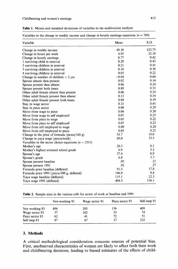
Childbearing and women's earnings

Table 1. Means and standard deviations of variables in the multivariate analysis

Variables in the change in weekly income and change in hourly earnings equations (n = 769)

413

Variable

Change in weekly incomeChange in hours per weekChange in hourly earningsI surviving child in interval2 surviving children in interval3 surviving children in interval4 surviving children in intervalChange in number of children < 2 yrsSpouse absent then presentSpouse present then absentSpouse present both timesOther adult female absent then presentOther adult female present then absentOther adult female present both timesStay in wage sectorStay in piece sectorMove from wage to pieceMove from wage to self employedMove from piece to wageMove from piece to self employedMove from self employed to wageMove from self employed to pieceChange in the price of formula (pesos/I 00 g)Change in yaya wage (pesos/week)Variables in the sector choice equations (n = 2311)Mother's ageMother's highest attained school gradeSpouse's ageSpouse's gradeSpouse present baselineSpouse present 1991Formula price baseline (deflated)Formula price 1991 (pesos/IOO g, deflated)Yaya wage baseline (deflated)Yaya wage 1991 (deflated)

Mean

49.384.950.770.280.210.160.05-0.040.020.060.890.060.130.040.210.090.040.070.050.070.090.0555.769.0

26.36.927.66.8.95.92

91.5146.9115.1404.5

S.D.

123.7532.180.420.450.410.360.220.640.140.240.310.240.340.190.410.290.200.250.220.250.280.2119.033.5

6.13.38.93.7.21.2717.88.622.5116.1

Table 2. Sample sizes in the various cells for sector of work at baseline and 1991

Not working 83Wage sector 83Piece sector 83Selfemp 83

3. Methods

Not working 91

496576287

Wage sector 91

2951624167

Piece sector 91

136337237

Selfemp 91

4097451232

A critical methodological consideration concerns sources of potential bias.First, unobserved characteristics of women are likely to affect both their workand childbearing decisions, leading to biased estimates of the effects of child-

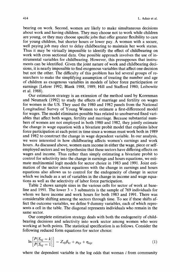
414 L. Adair et al.

(1)

bearing on work. Second, women are likely to make simultaneous decisionsabout work and having children. They may choose not to work while childrenare young, or they may choose specific jobs that offer greater flexibility to carefor young children, but shorter hours or lower pay. A woman with a secure,well paying job may elect to delay childbearing to maintain her work status.Thus it may be virtually impossible to identify the effect of childbearing onwork with cross sectional data. One possible approach involves the use of in­strumental variables for childbearing. However, this presupposes that instru­ments can be identified. Given the joint nature of work and childbearing deci­sions, it is nearly impossible to find exogenous variables that affect one decisionbut not the other. The difficulty of this problem has led several groups of re­searchers to make the simplifying assumption of treating the number and ageof children as exogenous variables in models of labor force participation orearnings (Lehrer 1992; Blank 1988, 1989; Hill and Stafford 1980; Leibowitzet al. 1988).Our estimation strategy is an extension of the method used by Korenman

and Neumark (1992) to study the effects of marriage and fertility on wagesfor women in the US. They used the 1980 and 1982 panels from the NationalLongitudinal Survey of Young Women to estimate a first-differenced modelfor wages. The model eliminates possible bias related to unobserved fixed vari­ables that affect both wages, fertility and marriage. Because substantial num­bers of women are not employed in both 1980 and 1982, they jointly estimatethe change in wage equation with a bivariate probit model that explains laborforce participation at each point in time since a woman must work both in 1989and 1982 to construct the change in wage dependent variable. In our analysis,we were interested in how childbearing affects women's earnings and workhours. As discussed above, women earn income in either the wage, piece or self­employed sectors and we hypothesize that these sectors have differing effects onwages and income. Thus rather than simply estimating a bivariate probit tocontrol for selectivity into the change in earnings and hours equations, we esti­mate multinomiallogit models for sector choice in 1983 and 1991. Joint esti­mation of the sector choice equations with the change in earnings and hoursequations also allows us to control for the endogeneity of change in sectorwhich we include as a set of variables in the change in income and wage equa­tions as well as the selectivity of labor force participation.Table 2 shows sample sizes in the various cells for sector of work at base­

line and 1991. The lower 3 x 3 submatrix is the sample of 769 individuals forwhom we have income and work hours for both 1983 and 1991. There wasconsiderable shifting among the sectors through time. To see if these shifts af­fect the outcome variables, we define 9 dummy variables, each of which repre­sents a cell in the table. The diagonal represents individuals who remain in thesame sector.Our complete estimation strategy deals with both the endogeneity of child­

bearing decisions and selectivity into work sector among women who wereworking at both points. The statistical specification is as follows. Consider thefollowing reduced form equations for sector choice:

[P(Stij = k)] _

In P(Stij= 1) -Ztij{Jkt+fJ.kjt+YJkijt

where the dependent variable is the log odds that woman i from community

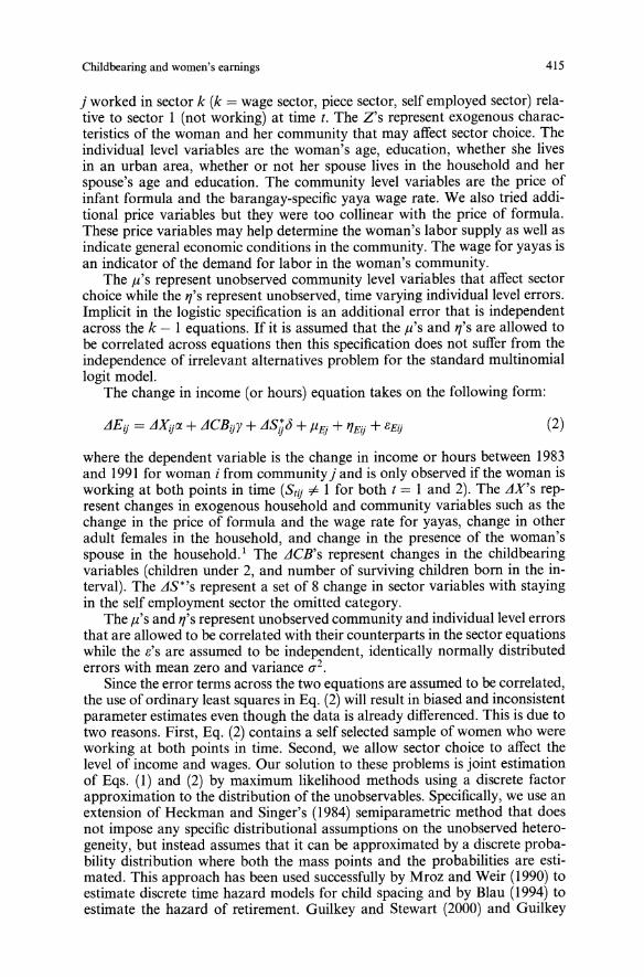
Childbearing and women's earnings 415

j worked in sector k (k = wage sector, piece sector, self employed sector) rela­tive to sector 1 (not working) at time t. The Z's represent exogenous charac­teristics of the woman and her community that may affect sector choice. Theindividual level variables are the woman's age, education, whether she livesin an urban area, whether or not her spouse lives in the household and herspouse's age and education. The community level variables are the price ofinfant formula and the barangay-specific yaya wage rate. We also tried addi­tional price variables but they were too collinear with the price of formula.These price variables may help determine the woman's labor supply as well asindicate general economic conditions in the community. The wage for yayas isan indicator of the demand for labor in the woman's community.The f.1'S represent unobserved community level variables that affect sector

choice while the 1"/'S represent unobserved, time varying individual level errors.Implicit in the logistic specification is an additional error that is independentacross the k - 1 equations. If it is assumed that the f.1'S and 1"/'S are allowed tobe correlated across equations then this specification does not suffer from theindependence of irrelevant alternatives problem for the standard multinomiallogit model.The change in income (or hours) equation takes on the following form:

LlEij = LlXijIX + LlCBijY + LlSijJ + f.1Ej + 1"/Eij + eEij (2)

where the dependent variable is the change in income or hours between 1983and 1991 for woman i from community j and is only observed if the woman isworking at both points in time (Slij of- 1 for both t = 1 and 2). The LlX's rep­resent changes in exogenous household and community variables such as thechange in the price of formula and the wage rate for yayas, change in otheradult females in the household, and change in the presence of the woman'sspouse in the household. 1 The LlCB's represent changes in the childbearingvariables (children under 2, and number of surviving children born in the in­terval). The LlS*'s represent a set of 8 change in sector variables with stayingin the self employment sector the omitted category.The f.1'S and 1"/'S represent unobserved community and individual level errors

that are allowed to be correlated with their counterparts in the sector equationswhile the e's are assumed to be independent, identically normally distributederrors with mean zero and variance (72.Since the error terms across the two equations are assumed to be correlated,

the use of ordinary least squares in Eq. (2) will result in biased and inconsistentparameter estimates even though the data is already differenced. This is due totwo reasons. First, Eq. (2) contains a self selected sample of women who wereworking at both points in time. Second, we allow sector choice to affect thelevel of income and wages. Our solution to these problems is joint estimationof Eqs. (1) and (2) by maximum likelihood methods using a discrete factorapproximation to the distribution of the unobservables. Specifically, we use anextension of Heckman and Singer's (1984) semiparametric method that doesnot impose any specific distributional assumptions on the unobserved hetero­geneity, but instead assumes that it can be approximated by a discrete proba­bility distribution where both the mass points and the probabilities are esti­mated. This approach has been used successfully by Mroz and Weir (1990) toestimate discrete time hazard models for child spacing and by Blau (1994) toestimate the hazard of retirement. Guilkey and Stewart (2000) and Guilkey

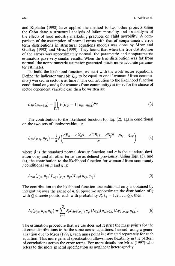
416 L. Adair et al.

and Riphahn (1998) have applied the method to two other projects usingthe Cebu data: a structural analysis of infant mortality and an analysis ofthe effects of food industry marketing practices on child morbidity. A com­parison of the assumption of normal errors with that of nonparametric errorterm distributions in structural equations models was done by Mroz andGuilkey (1992) and Mroz (1999). They found that when the true distributionof the errors was approximately normal, the parametric and nonparametricestimators gave very similar results. When the true distribution was far fromnormal, the nonparametric estimator generated much more accurate parame­ter estimates.To build the likelihood function, we start with the work sector equations.

Define the indicator variable hijt to be equal to one if woman i from commu­nity j worked in sector k at time t. The contribution to the likelihood functionconditional on fl and '7 for woman i from community j at time t for the choice ofsector dependent variable can then be written as:

4

LSijt(fljt>'7ijt) = II P(hijt = I Iflkjt>'7kijt)hij,

k=1

(3)

The contribution to the likelihood function for Eq. (2), again conditionalon the two sets of unobservables, is:

(4)

where rP is the standard normal density function and (J is the standard devi­ation of 8ij and all other terms are as defined previously. Using Eqs. (3), and(4), the contribution to the likelihood function for woman i from communityj conditional on fl and '7 is:

(5)

The contribution to the likelihood function unconditional on '7 is obtained byintegrating over the range of '7. Suppose we approximate the distribution of '7with Q discrete points, each with probability Pq (q = 1,2, ... ,Q), then:

Q

Lij(fljl, flj2' flE) = L PqLSijl (fljl, '7ql )LSij2 (flj2, '7q2)LEij(flEj' '7Eq)' (6)q=1

The estimation procedure that we use does not restrict the mass points for thediscrete distributions to be the same across equations. Instead, using a gener­alization due to Mroz (1997), each mass point is estimated separately for eachequation. This more general specification allows more flexibility in the patternof correlations across the error terms. For more details, see Mroz (1997) whorefers to the more general specification as nonlinear heterogeneity.

Childbearing and women's earnings 417

The product of (6) over the ~ women in community j yields the contri­bution to the likelihood function for community j conditional on J1:

Nj

L}(J1jl ,J1j2' J1E) = II Lij(J1jl' J1j2, J1Ej)i=l

(7)

The contribution to the likelihood function for community j unconditionalon J1 is obtained by integrating over the range of J1. Suppose we approxi­mate the distribution of J1 with R discrete points, each with probability Pr(1' = 1,2, ... ,R), then:

R

Lj = LPrLj (J1Ir>J12r>J1Er)r=1

(8)

where we again allow the mass points to differ across equations. The likeli­hood function is simply the product of (8) over the J communities.The discrete factor FIML method is identified without exclusion restric­

tions. However, we do not need to rely on nonlinearities to obtain identifica­tion. The exclusion restrictions used to identify the model are discussed in theempirical results section of the paper.

4. Results

Results presented here are for the 2,309 women who were participants in the1991 follow-up survey, and who had complete data on the variables of inter­est. As discussed below, two formulations of the dependent variable were used:change in the woman's weekly income and change in her work hours. For eachdependent variable, Eq. (2) was estimated jointly with the two equations speci­fied in Eq. (1) for time periods 1983 and 1991.Before turning to a discussion of the substantive results, we first discuss

estimates of the heterogeneity parameters. In the change in income model, 2mass points were optimal for the individual level heterogeneity (1'/s) and 6mass points were optimal for community level heterogeneity (J1's). The esti­mated mass points are at the bottom of Table 3 for choice of sector, Table 4for change in income. Note that the first mass point is normalized to zerosince it cannot be separately identified from the constant term. The estimatedprobability weights for the individual level heterogeneity are 0.32 and 0.68respectively (see Eq. (6)). The probability weights at the community level are0.22,0.12,0.06,0.13,0.34, and 0.13 (see Eq. (8)). As can be seen from the ta­bles, many of the heterogeneity parameters are highly significant. A joint testof the null hypothesis that the heterogeneity parameters are all zero yields achi square statistic of 344.2. Since the critical value for a 1% test with 48 de­grees of freedom is 73.7, there is strong evidence of the importance of con­trolling for unobserved heterogeneity.Because the parameters of the heterogeneity distributions are difficult to

interpret, we also calculated the correlations in the community level errors im­plied by the estimated discrete distributions. Rather than presenting the entire

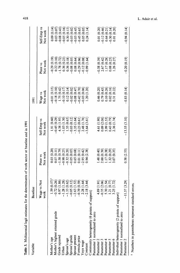
"""T

able3.Multinomiallogitestimatesforthedeterminantsofworksectoratbaselineandin1991

;;;

Variable

Baseline

1991

WagevsNot

Piecevs

Self-Empvs

Wagevs

Piecevs

Self-Empvs

work

Notwork

Notwork

Notwork

Notwork

Notwork

Mother'sage

1.59(0.57)1

0.03(0.20)

1.91(0.60)

-om(0.15)

-0.29(0.19)

0.09(0.14)

Mother'shighestattainedgrade

-0.72(0.26)

0.07(0.11)

-0.45(0.29)

-0.18(0.10)

0.22(0.10)

0.03(0.07)

Gradesquared

6.97(1.86)

-1.58(0.79)

4.38(1.93)

1.75(0.42)

-1.78(0.72)

-0.08(0.43)

Urban

-1.28(1.28)

-0.98(0.25)

-1.03(1.30)

-0.10(0.17)

0.36(0.23)

-0.05(0.16)

Spouse'sage

-1.33(0.62)

-0.32(0.20)

1.55(0.63)

0.12(0.14)

0.36(0.18)

0.30(0.13)

Spouse'sgrade

-0.05(0.12)

-0.05(0.03)

-0.03(0.12)

-0.02(0.02)

-0.08(0.03)

-0.03(0.02)

Spousepresent

-2.63(1.52)

0.65(0.68)

-3.35(1.64)

-0.08(0.47)

0.08(0.64)

-0.03(0.45)

Formulaprice

-0.39(0.59)

0.01(0.11)

-0.23(0.61)

-0.42(0.70)

-0.29(0.96)

-0.45(0.65)

Yayawage

2.28(1.64)

-2.95(0.42)

2.48(1.76)

-0.03(0.06)

-0.12(0.08)

0.05(0.05)

Constant

-2.18(3.44)

0.94(2.38)

-3.64(3.61)

1.20(1.20)

-0.99(1.64)

0.24(1.14)

Communityheterogeneity(6pointsofsupport)

Parameter

Inormalizedtozero

Parameter2

4.89(1.91)

1.48(0.40)

4.61(1.90)

0.46(0.20)

-0.58(0.39)

0.01(0.20)

Parameter3

-0.35(2.06)

2.00(0.39)

0.09(2.06)

0.79(0.43)

2.67(0.42)

-0.12(0.46)

Parameter4

5.30(1.54)

1.17(0.38)

5.99(1.53)

0.10(0.26)

1.17(0.28)

0.64(0.21)

Parameter5

1.21(0.77)

1.32(0.29)

0.43(0.79)

0.Q2(0.16)

0.08(0.23)

-0.30(0.14)

Parameter6

3.25(1.72)

3.07(0.35)

2.36(1.74)

0.31(0.22)

1.26(0.27)

0.01(0.20)

Individualheterogeneity(2pointsofsupport)

ParameterInormalizedtozero

Parameter2

-11.57(3.29)

0.58(2.53)

-13.55(3.10)

-0.83(0.14)

-0.20(0.19)

-0.94(0.14)

1Numbersinparenthesesrepresentstandarderrors.

r :> 0- ~. .., ~ ~

Childbearing and women's earnings 419

7 X 7 correlation matrix, we only present correlations of the six multinomiallogit equations with the change in income equation for baseline and 1991, re­spectively:

Wage vs not workPiece vs not workSelf employed vs not work

Baseline

0.3540.2000.313

1991

0.562-0.2580.068

The effects of these across-equation error correlations on the substantive re­sults are discussed below.The bottom of Table 5 presents the results for the heterogeneity param­

eters in the change in hours equation. In this equation, the distribution of theunobserved heterogeneity was best approximated with 6 mass points for thecommunity level error and 3 mass points for individual level heterogeneity.The probability weights were 0.12, 0.29, 0.06, 0.18, 0.12, and 0.23 and 0.13,0.46, and 0.41 for community and individual heterogeneity respectively. A chisquared test of the null hypothesis that all the heterogeneity parameters arezero resulted in a test statistic of 486. Since the critical value for a 1% test with56 degrees of freedom is 83.5, we again see significant improvement in the like­lihood function with these controls.We now present the substantive results. We first discuss the results for the

two multinomial logit estimations for the choice of sector of employment atbaseline and in 1991. As stated above, we did pair wise estimation of the twoset of sector choice equations (see Eq. (1)) with change in weekly income andchange in hour, see Eq. (2), so two sets of results are available for the choiceof sector at baseline and 1991. Since the choice of sector equations are reducedform equations, we did not expect to see much difference in the results fromestimating them with the change in income or change in hourly earnings equa­tions and this is exactly what we find. Therefore, Table 3 only presents resultsfor the determinants of sector choice estimated jointly with the change in in­come equation.

4.1. Women's choice o/work sector in 1983 and 1991

The results of the multinomial logit estimations for choice of sector in 1983and 1991 are presented in Table 3. We present the log odds (and standarderrors) of working in the wage, piece and self employed sectors relative to notworking. This set of equations are estimated to control for the self selection ofwomen into working at both points in time and are not the equations of pri­mary interest. Since they are reduced form equations, they are difficult to in­terpret and so we only present some fairly general observations.Not surprisingly the strongest predictors for work sector are woman's ed­

ucation and education squared. At both baseline and 1991, grade squared isstrongly positively associated with working for wage and strongly negativelyassociated with doing piece work. The other education results are somewhatmixed with some sign flips between 1983 and 1991. However, the sign flips arenot associated with strongly significant estimated coefficients. Mother's age is

420 L. Adair et al.

a strong predictor of wage and self employed categories versus not working in1983 but age seems to have little effect in 1991. Interestingly, spouse's age alsoeffects these two categories in 1983. In 1991, spouse's age has a positive effectfor all three work categories relative to not working. Formula price appearsto have little effect on work sector while the wage rate for yayas is a positivepredictor of the wage and self employed categories relative to not working in1983 but has little effect in 1991.In summary, there are several significant predictors of work sector with

stronger results for 1983 than for 1991. This may reflect the different com­position of the reference group at each point in time, or differences in the re­productive status of working and non-working women. In 1983, all womenwere pregnant and very few had no other children, whereas in 1991, 8.3%were pregnant, and about 20% had no surviving child. Alternately, with thetrend toward higher labor force participation rates, fewer factors differentiateworkers and non-workers. These reduced form equations are not of muchsubstantive interest for this paper. The important result is that there are sig­nificant predictors of work sector that do not have direct effects on change inearnings, the results for which we discuss below.

4.2. Change in earnings and hours

We calculated the change in weekly earnings from the baseline (1983) to 1991for the 769 women working at both points in time. Earnings are highly vari­able and skewed. On average, women earned 46.6 pesos/week more in 1991,but the median change was 29.6 pesos/wk. The mean change represents a 49%increase over women's mean weekly earnings of 94 pesos per week in 1983­1984. The mean change in earnings for women with no subsequent survivingchild in the 8.5 year period was 2.3 times higher than that of women with atleast one additional child (69.7 vs. 26.4 pesos/wk).The overall change in income is in part, a reflection of an increase in the

mean number of hours worked per week from 41.6 in 1983 to 46.1 in 1991.More than half of sample women increased their work hours. This reflects atendency to move from part-time to full time work. Changes in income variedsubstantially across sector of employment at baseline, with piece workers hav­ing the lowest mean gains (18.6 pesos/wk) and wage workers having the highestgain (62.9 pesos/wk). Among women working at both points in time, earningsrepresented 34.9% and 36.7% of total household earnings in 1983-1984 and1991, respectively.The model specification includes dummy variables representing the num­

ber of children born in the interval from 1983 to 1991 (1,2, 3,4+) and sur­viving at the time of the 1991 survey, change in the number of children lessthan 2 years of age, change in the presence of spouse and other adult femalesin the household, and a set of eight dummy variables for sector change withstaying self employed the omitted category. We also tested but found no sig­nificant effect of interactions of sector of employment with childbearing andspouse present variables.Table 4 presents results from the selectivity corrected change in weekly in­

come regression, and Table 5 presents results from the change in hours regres­sion. Children born during the 8 year interval decrease weekly income. The ef­fect strengthens with each additional child going from a non-significant level

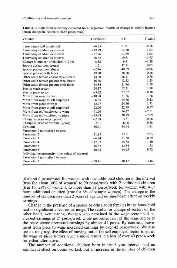
Childbearing and women's earnings 421

Table 4. Results from selectivity corrected linear regression models of change in weekly income(mean change in income = 46.56 pesos/week)

Variable Coefficient S.E. T-value

I surviving child in interval -6.35 11.01 -0.582 surviving children in interval -19.79 12.20 -1.623 surviving children in interval -27.96 13.69 -2.044 surviving children in interval -38.32 19.61 -1.95Change in number of children < 2 yrs -8.88 6.91 -1.29Spouse absent then present 1.51 32.11 0.05Spouse present then absent -2.46 40.59 -0.06Spouse present both times 19.20 28.28 0.68Other adult female absent then present 14.08 18.11 0.78Other adult female present then absent 16.36 12.33 1.33Other adult female present both times 34.84 21.96 1.59Stay in wage sector 24.17 12.21 1.98Stay in piece sector -3.92 22.02 -0.18Move from wage to piece -40.98 21.86 -1.88Move from wage to self employed -6.65 15.66 -0.42Move from piece to wage 42.27 24.76 1.71Move from piece to self employed 22.00 22.79 0.97Move from self employed to wage -41.06 16.37 -2.51Move from self employed to piece -43.78 20.99 -2.09Change in yaya wage (pesos) -2.38 3.51 -0.68Change in price offormula (pesos) 2.31 6.06 0.38Constant 56.41 34.94 1.61Parameter I normalized to zeroParameter 2 31.85 15.51 2.05Parameter 3 -6.24 21.58 -0.29Parameter 4 -17.07 15.54 -1.10Parameter 5 -16.63 12.54 -1.33Parameter 6 10.38 14.45 0.72Individual heterogeneity (two points of support)Parameter I normalized to zeroParameter 2 -58.16 18.42 -3.16

of about 6 pesos/week for women with one additional children in the interval(true for about 30% of women) to 20 pesos/week with 2 additional children(true for 29% of women), to more than 38 pesos/week for women with 4 ormore additional children (true for 6% of sample women). The change in thenumber of children less than 2 years of age had no significant effect on weeklyearnings.Change in the presence of a spouse or other adult females in the household

had no significant effect on earnings. The results for change of sector, on theother hand, were strong. Women who remained in the wage sector had in­creased earnings of 24 pesos/week while movement out of the wage sector tothe piece sector decreased earnings by almost 41 pesos. By contrast, move­ment from piece to wage increased earnings by over 42 pesos/week. We alsosee a strong negative effect of moving out of the self employed sector to eitherthe wage or piece sectors. Such a move results in a loss of over 40 pesos/weekfor either alternative.The number of additional children born in the 8 year interval had no

significant effect on hours worked, but an increase in the number of children

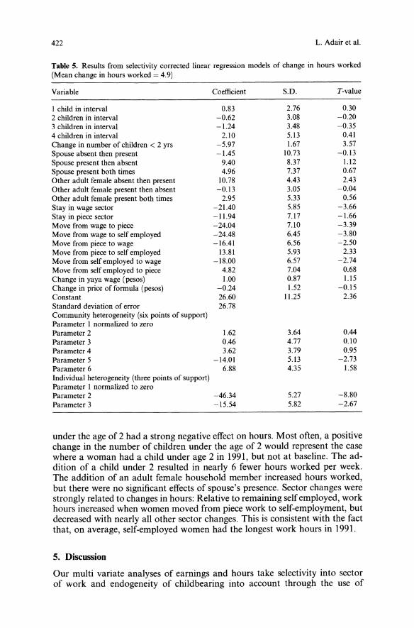
422 L. Adair et al.

Table 5. Results from selectivity corrected linear regression models of change in hours worked(Mean change in hours worked = 4.9)

Variable Coefficient S.D. T-value

I child in interval 0.83 2.76 0.302 children in interval -0.62 3.08 -0.203 children in interval -1.24 3.48 -0.354 children in interval 2.10 5.13 0.41Change in number of children < 2 yrs -5.97 1.67 3.57Spouse absent then present -1.45 10.73 -0.13Spouse present then absent 9.40 8.37 1.12Spouse present both times 4.96 7.37 0.67Other adult female absent then present 10.78 4.43 2.43Other adult female present then absent -0.13 3.05 -0.04Other adult female present both times 2.95 5.33 0.56Stay in wage sector -21.40 5.85 -3.66Stay in piece sector -11.94 7.17 -1.66Move from wage to piece -24.04 7.10 -3.39Move from wage to self employed -24.48 6.45 -3.80Move from piece to wage -16.41 6.56 -2.50Move from piece to self employed 13.81 5.93 2.33Move from self employed to wage -18.00 6.57 -2.74Move from self employed to piece 4.82 7.04 0.68Change in yaya wage (pesos) 1.00 0.87 1.15Change in price of formula (pesos) -0.24 1.52 -0.15Constant 26.60 11.25 2.36Standard deviation of error 26.78Community heterogeneity (six points of support)Parameter I normalized to zeroParameter 2 1.62 3.64 0.44Parameter 3 0.46 4.77 0.10Parameter 4 3.62 3.79 0.95Parameter 5 -14.01 5.13 -2.73Parameter 6 6.88 4.35 1.58Individual heterogeneity (three points of support)Parameter I normalized to zeroParameter 2 -46.34 5.27 -8.80Parameter 3 -15.54 5.82 -2.67

under the age of 2 had a strong negative effect on hours. Most often, a positivechange in the number of children under the age of 2 would represent the casewhere a woman had a child under age 2 in 1991, but not at baseline. The ad­dition of a child under 2 resulted in nearly 6 fewer hours worked per week.The addition of an adult female household member increased hours worked,but there were no significant effects of spouse's presence. Sector changes werestrongly related to changes in hours: Relative to remaining self employed, workhours increased when women moved from piece work to self-employment, butdecreased with nearly all other sector changes. This is consistent with the factthat, on average, self-employed women had the longest work hours in 1991.

5. Discussion

OUf multi variate analyses of earnings and hours take selectivity into sectorof work and endogeneity of childbearing into account through the use of

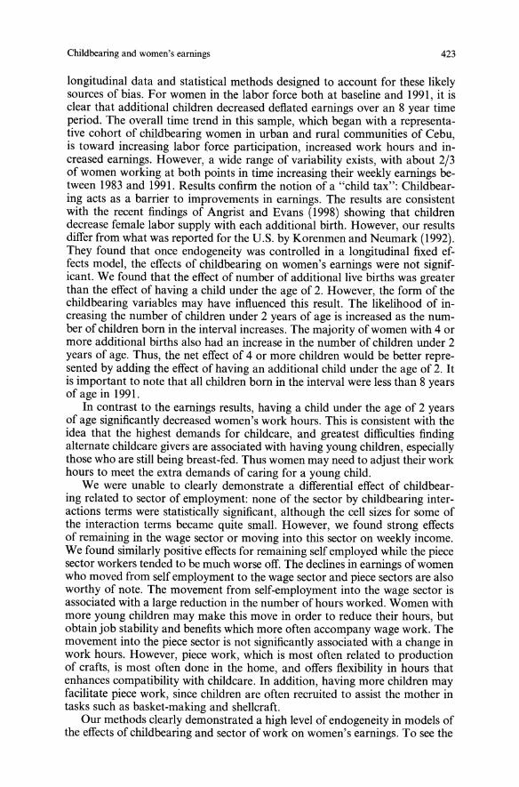
Childbearing and women's earnings 423

longitudinal data and statistical methods designed to account for these likelysources of bias. For women in the labor force both at baseline and 1991, it isclear that additional children decreased deflated earnings over an 8 year timeperiod. The overall time trend in this sample, which began with a representa­tive cohort of childbearing women in urban and rural communities of Cebu,is toward increasing labor force participation, increased work hours and in­creased earnings. However, a wide range of variability exists, with about 2/3of women working at both points in time increasing their weekly earnings be­tween 1983 and 1991. Results confirm the notion of a "child tax": Childbear­ing acts as a barrier to improvements in earnings. The results are consistentwith the recent findings of Angrist and Evans (1998) showing that childrendecrease female labor supply with each additional birth. However, our resultsdiffer from what was reported for the U.S. by Korenmen and Neumark (1992).They found that once endogeneity was controlled in a longitudinal fixed ef­fects model, the effects of childbearing on women's earnings were not signif­icant. We found that the effect of number of additional live births was greaterthan the effect of having a child under the age of 2. However, the form of thechildbearing variables may have influenced this result. The likelihood of in­creasing the number of children under 2 years of age is increased as the num­ber of children born in the interval increases. The majority ofwomen with 4 ormore additional births also had an increase in the number of children under 2years of age. Thus, the net effect of 4 or more children would be better repre­sented by adding the effect of having an additional child under the age of 2. Itis important to note that all children born in the interval were less than 8 yearsof age in 1991.

In contrast to the earnings results, having a child under the age of 2 yearsof age significantly decreased women's work hours. This is consistent with theidea that the highest demands for childcare, and greatest difficulties findingalternate childcare givers are associated with having young children, especiallythose who are still being breast-fed. Thus women may need to adjust their workhours to meet the extra demands of caring for a young child.We were unable to clearly demonstrate a differential effect of childbear­

ing related to sector of employment: none of the sector by childbearing inter­actions terms were statistically significant, although the cell sizes for some ofthe interaction terms became quite small. However, we found strong effectsof remaining in the wage sector or moving into this sector on weekly income.We found similarly positive effects for remaining self employed while the piecesector workers tended to be much worse off. The declines in earnings ofwomenwho moved from self employment to the wage sector and piece sectors are alsoworthy of note. The movement from self-employment into the wage sector isassociated with a large reduction in the number of hours worked. Women withmore young children may make this move in order to reduce their hours, butobtain job stability and benefits which more often accompany wage work. Themovement into the piece sector is not significantly associated with a change inwork hours. However, piece work, which is most often related to productionof crafts, is most often done in the home, and offers flexibility in hours thatenhances compatibility with childcare. In addition, having more children mayfacilitate piece work, since children are often recruited to assist the mother intasks such as basket-making and shellcraft.Our methods clearly demonstrated a high level of endogeneity in models of

the effects of childbearing and sector of work on women's earnings. To see the

424 L. Adair et al.

Table 6. Alternate models of women's earnings, 1983 and 1991

Variable Random effects First differencesSelectivity corrected 1 modeF model 3

Coefficient Standard Coefficient Standard Coefficient Standarddeviation deviation deviation

I child 2.73 5.92 0.12 6.52 -6.98 10.882 children -7.10 6.42 -5.63 6.84 -21.57 12.123 children -12.54 7.54 -16.20 8.11 -28.80 13.684 children -15.58 12.29 -30.08 14.17 -36.80 19.885 or more children 33.37 25.79 10.83 27.54Wage sector 6.64 11.61 22.95 7.41Self employed 21.20 11.24 32.73 6.90Stay in wage sector 30.15 11.81Stay in piece sector -47.33 15.85

1 Regression model for weekly earnings, selectivity-corrected for working for pay.2 Random effects model for weekly earnings, ignoring selectivity for working for pay.3 First differences model for change in weekly income for women working for pay in both 1983and 1991. Note that child variables represent children born during the 1983 to 1991 interval.

substantive impact of our methods on the empirical results, we compare theeffects of young children on weekly income for 4 estimations:1. We estimated a model in levels for weekly income as a function of

dummy variables for number of children under 7 and sector of employment.The regressions also contained a set of control variables that included the cor­responding variables in levels for all variables in Table 4, plus the respondent'sage and education as well as the age and level ofeducation of her spouse, plus adummy to indicate whether the observations was from 1983 or 1991. We con­trolled for selection into working for pay through the use of a standard Heck­man selectivity correction assuming multi variate normality for the error termdistribution. 2 In this exercise, we simply pooled data for 1983 and 1991 and soa woman could have reported weekly income at either point in time. The re­sults for the variables of interest are presented in Table 6.The children dummies specify the number of children younger than 7 years

of age. The omitted categories were no children under 7 and working for piece(income is missing for women who are not employed). The results provideweak evidence of a negative effect of young children on weekly earnings ex­cept at the extremes which are imprecisely estimated. The results for sector arealso weak but we see that women who are self employed have the highest levelof earnings.2. The next estimator is also in levels and simply ignores the selectivity into

working for a wage both in 1983 and 1991 and estimates a model in levels withweekly income as the dependent variable for women who where working atboth points in time (i.e, the same sample of women who were used in the dif­ferenced estimations). Note that each woman contributes 2 observations to thedata set.The results for the children dummies are similar across the 2 sets of runs

for 2 and 3 children under 7 years of age, while the effect of 4 children under 7years of age is more pronounced in the random effects estimations. The sectoreffects are much stronger in the random effects estimations with working for

Childbearing and women's earnings 425

wage and self employed sectors resulting in substantially higher weekly earn­ings than the piece sector. This should not be very surprising since we have notcontrolled for the self selectivity into working at both points in time in theserandom effects estimations.3. The third estimation is for change in income between 1983 and 1991

without controls for selectivity into working for a wage at both points in time.The model specification is exactly that of Table 4 except that no heterogeneityparameters are estimated. The model specification is different from 1 and 2above since all variables are specified as differences. In the results in Table 6,we use dummies for number of children born in the 8 year interval as is donein our main analysis.

It is clear that the effects of small children become much more pronouncedwhen we control for the endogeneity of young children through the use of firstdifferences. The bias towards zero in the effect of young children in the levelsmodels is consistent with positive error correlation in unobservable fixed vari­ables across equations that explain positive weekly earnings and number ofsmall children. A comparison of the effects of the children born in the intervaldummies between the table above and Table 4 where we control for the selec­tivity of sector ofwork yield very little differences across all dummy categories.This means that the simple difference model appears to have almost fully con­trolled for the endogeneity of children born in the interval. However, we dosee that the coefficients of the sector dummies are strongly affected by controlsfor self selection of sector of work. This may not be surprising and seems toindicate that unobserved, time varying variables affect sector choice and earn­ings which means that differencing the data is not sufficient to control for thisselectivity.Finally we note that in another set of studies, we show that childbearing

affects other aspects of women's lives (Borja and Adair 1997). After control­ling for changes in income, an increased number of births in the 1983-1991study interval was associated with declines in material well-being measured bythe value of household assets, ownership of labor-saving devices such as re­frigerators, maternal health, and well being of the index child. By reducing thenumber of children through use of family planning methods, our models pre­dict that women's earnings would increase. However, it appears that womenincrease their earnings largely as a function of increasing hours at work. Theincrease in work hours may exacerbate the conflict between women's produc­tive and reproductive roles. Work hours increased to more than 46 hours/weekin 1991. Given that women also report, on average, more than 23 hours perweek doing household chores and related activities, their combined marketand domestic work burden is substantial. Thus improvements in income maycome only at the expense of leisure time or other non-material aspects of theirlives. In conclusion, these results show strong negative effects of additionallive births on women's weekly earnings, and a strong negative effect of havinga child under 2 years of age on work hours, suggesting a strong potential forfamily planning, if it limits births, to affect women's economic well-being.

Endnotes

1 Both the presence of the spouse and other adults in the household are potentially endogenous.However, if it is assumed that any correlation is through unobserved, fixed household charac­teristics, then differencing the data removes this potential source of bias.

426 L. Adair et al.

2 In this selectivity model in levels, the same set of variables were used in the working for payselectivity equation as were used in the earnings equation for those who were working. Identi­fication is only achieved through the non-linearity introduced through the assumption of mul­tivariate normality. As discussed in the introduction, it is very difficult to justify exclusion re­strictions in this context and many authors have simply chosen to ignore the endogeneity of thechoice to work for pay. Our estimation results were robust to minor differences in the specifi­cations of the two equations and so we feel comfortable presenting these results for comparisonto the main results of the paper.

References

Adair LS, Popkin BM (1992) Prolonged Lactation Contributes to Depletion of Energy Reservesof Filipino Women. Journal of Nutrition 122:1643-1655

Angrist JD, Evans WN (1998) Children and Their Parent's Labor Supply: Evidence from Exoge­nous Variation in Family Size. American Economic Review 88:450-477

Anker R, Hein C (1985) Sex Inequalities in Urban Employment in the Third World. St. Martin'sPress, New York

Becker S (1981) A Treatise on the Family. Harvard University Press, Cambridge, MABeneria L, Roldan M (1987) Industrial Homework, Subcontracting, and Household Dynamics

in Mexico City. Crossroads of Class and Gender: Women in Culture and Society. University ofChicago Press, Chicago, IL

Bisgrove EZ, Popkin BM (1996) Does Women's Work Improve Their Nutrition: Evidence fromthe Urban Philippines. Social Science and Medicine 43:1475-1488

Blank RM (1988) Simultaneously Modeling the Supply of Weeks and Hours of Work amongFemale Household Heads. Journal of Labor Economics 6:177-204

Blank RM (1989) The Role of Part Time Work in Women's Labor Market Choices over Time.American Economic Review 79:295-299

Bruce J, Lloyd CB, Leonard A (1995) Families in Focus: New Perspectives on Mothers, Fathers,and Children. The Population Council, New York

Borja JR, Adair LS (1997) Effect of Family Planning on the Quality ofWomen's Lives. Proceed­ings of the IUSSP. International Population Conference, Bejing 1997, Vol. 2. Liege, Belgium,pp. 681-698

Bunster X (1983) Market Sellers in Lima Peru: Talking about Work. In: Buvinic M, Lycette MA,McGreevey WP (eds) Women and Poverty in the Third World. Johns Hopkins Press, Mary­land

Cohen B, House WJ (1996) Labor Market Choices, Earnings, and Informal Networks in Khar­toum, Sudan. Economic Development and Cultural Change 44:589-618

Connelly R, DeGraff D, Levison D (1996) Women's Employment and Child Care in Brazil.Economic Development and Cultural Change 44:619-656

Demographic and Health Surveys (1994) National Demographic Survey. Philippines 1993. Na­tional Statistics Office, Manila, Philippines

Guilkey DK, Popkin BM, Akin JS, Wong E (1989) Prenatal Care and Pregnancy Outcomes in thePhilippines. Journal of Development Economics 30:241-272

Guilkey DK, Riphahn R (1998) The Determinants of Child Mortality in the Philippines: Estima­tion of a Structural Model. Journal of Development Economics 56:281-305

Guilkey DK, Stewart JF, (2000) Estimating the Health Impact of Industry Infant Food Market­ing Practices in the Philippines. The Journal of Development Studies 36:50-77

Haddad L, Alderman HJ (eds) (1997) Intrahousehold Resource Allocation in Developing Countries:Methods, Models, and Policy. International Food Policy Research Institute and Johns Hop­kins Press, Baltimore, MD

Heckman J, Singer B (1984) A Method for Minimizing the Impact of Distribution Assumptions inEconometric Models for Duration Data. Econometrica 58:271-320

Hill CR, Stafford FP (1980) Parental Care of Children: Time Diary Estimates of Quantity, Pre­dictability and Variety. Journal of Human Resources 12:219-239

Kennedy E, Peters P (1992) Household Food Security and Child Nutrition: The Interaction of in­come and gender of household. World Development 20(8):1077-1085

Korenman S, Newmark D (1992) Marriage, Motherhood and Wages. Journal ofHuman Resources27:233-255

Childbearing and women's earnings 427

Lehrer EL (1992) The Impact of Children on Married Women's Labor Supply. Journal ofHumanResources 27:422-444

Leibowitz A, Waite LJ, Jones EB (1988) Childcare for Preschoolers: Difference by Child's Age.Demography 25:205-220

Leibowiz A, Klerman JA, Waite LJ (1992) Employment ofNew Mothers and Child Care Choice:Differences by Child Age. Journal of Human Resources 27:112-133

Merchant K, Martorell R (1991) Frequent Reproductive Cycling: Does it lead to NutritionalDepletion of Mothers? Progress in Food and Nutrition Science 12:339-369

Michalopoulos C, Robins PK, Garfinkel I (1992) A Structural Model of Labor Supply and ChildCare Demand. Journal of Human Resources 27:166-203

Mroz T, Guilkey DK (1997) Discrete Factor Approximations in Simultaneous Equation Models:Estimating the Impact of a Dummy Endogenous Variable on a Continuous Outcome. Manu­script, University of North Carolina, Chapel Hill, NC

Mroz T (1999) Discrete Factor Approximations in Simultaneous Equations Models: Estimatingthe Impact of a Dummy Endogenous Variable on a Continuous Outcome. Journal of Econo­metrics 92:233-274

Podhista C, Havanon N, Knodel J, Sittirai W (1990) Women's Work and Family Size in RuralThailand. Asia-Pacific Population Journal 5:31-54

Portes A, Walton J (1981) Labor, Class, and the International System. Academic Press, New York,NY

Rinehart W, Kols A (1984) Healthier Mothers and Children Through Family Planning. Popula­tion Reports, Series J 27:657-658; 673-679

Rosenzweig MR, Wolpin KI (1980) Life-eycle Labor Supply and Fertility. Causal Inferences fromHousehold Models. Journal of Political Economy 88:328-348

Rosenzweig MR, Schultz TP (1987) Fertility and Investments in Human Capital: Estimates of theConsequences of Imperfect fertility control in Malaysia. Journal of Econometrics 36:163-183

Schultz TP (1981) Economics ofPopulation. Addison-Wesley, Reading MAShapiro D, Mott F (1994) Long Term Employment and Earnings of Women in Relation to Em­ployment Behavior Surrounding the First Birth. Journal of Human Resources 29:248-275

Tinker I (1981) New Technologies for Food Related Activities: an Equity Strategy. In: Dauber R,Cain M (eds) Women and Technological Change in Developing Countries. American Associa­tion of Advanced Sciences, Washington DC