BELLE2-PTHESIS-2020-001.pdf - Belle II Document Server
204
Dottorato di Ricerca in Fisica Graduate Course in Physics University of Pisa PhD Thesis: Search for an invisible Z 0 in μ + μ - plus missing energy events at Belle II Candidate Supervisor Laura Zani Prof. Francesco Forti
-
Upload
khangminh22 -
Category
Documents
-
view
1 -
download
0
Transcript of BELLE2-PTHESIS-2020-001.pdf - Belle II Document Server

Dottorato di Ricerca in Fisica
Graduate Course in Physics
University of Pisa
PhD Thesis:
Search for an invisible Z ′ in µ+µ− plusmissing energy events at Belle II
Candidate SupervisorLaura Zani Prof. Francesco Forti

Dottorato di Ricerca in Fisica
Dottorato di Ricerca in Fisica XXXII ciclo

Contents
Contents i
Introduction 1
1 Physics motivations 5
1.1 Introduction to the Standard Model . . . . . . . . . . . . . . . . . . . . . . . . 5
1.2 Dark Matter puzzle . . . . . . . . . . . . . . . . . . . . . . . . . . . . . . . . . . 12
1.3 Light Thermal Dark Matter and possible SM extensions . . . . . . . . . . . . . 15
1.4 Dark Matter detection methods . . . . . . . . . . . . . . . . . . . . . . . . . . . 18
1.5 Dark sector searches at accelerators . . . . . . . . . . . . . . . . . . . . . . . . . 23
1.5.1 Search for invisible particles at accelerators . . . . . . . . . . . . . . . . 24
1.5.2 Dark photon searches at lepton colliders . . . . . . . . . . . . . . . . . . 25
1.6 Alternative SM extensions: the Lµ − Lτ model . . . . . . . . . . . . . . . . . . 28
1.6.1 Invisible Z ′ produced in dimuon plus missing energy events in e+e−
collisions at Belle II . . . . . . . . . . . . . . . . . . . . . . . . . . . . . 31
2 SuperKEKB accelerator 33
2.1 Introduction on experiments at the B factories . . . . . . . . . . . . . . . . . . 33
2.1.1 The asymmetric B factory concept . . . . . . . . . . . . . . . . . . . . . 34
2.1.2 The first generation of B factories: PEP-II and KEKB . . . . . . . . . . 35
2.2 The second generation: SuperKEKB design upgrades . . . . . . . . . . . . . . . 38
2.2.1 Nano beam scheme overview . . . . . . . . . . . . . . . . . . . . . . . . 39
2.3 SuperKEKB commissioning and running phases . . . . . . . . . . . . . . . . . . 41
2.3.1 Phase 1: first beam background measurements . . . . . . . . . . . . . . 42
2.3.2 Phase 2: first collisions . . . . . . . . . . . . . . . . . . . . . . . . . . . . 43
2.3.3 Phase 3: first physics with the full vertex detector . . . . . . . . . . . . 45
3 Belle II experiment 49
3.1 Belle II upgrade overview . . . . . . . . . . . . . . . . . . . . . . . . . . . . . . 49
3.1.1 The Pixel Detector . . . . . . . . . . . . . . . . . . . . . . . . . . . . . . 51
3.1.2 The Silicon Vertex Detector . . . . . . . . . . . . . . . . . . . . . . . . . 52
3.1.3 The Central Drift Chamber . . . . . . . . . . . . . . . . . . . . . . . . . 54
3.1.4 Particle Identification devices . . . . . . . . . . . . . . . . . . . . . . . . 55
3.1.5 The Electromagnetic Calorimeter . . . . . . . . . . . . . . . . . . . . . . 57
3.1.6 The neutral kaon and muon detector . . . . . . . . . . . . . . . . . . . . 58
3.2 The trigger system at Belle II . . . . . . . . . . . . . . . . . . . . . . . . . . . . 60
i

3.3 Overview of the Belle II analysis software framework . . . . . . . . . . . . . . . 613.3.1 The basf2 code . . . . . . . . . . . . . . . . . . . . . . . . . . . . . . . . 613.3.2 Input/output: simulation and reconstruction in basf2 . . . . . . . . . . . 633.3.3 Condition Data . . . . . . . . . . . . . . . . . . . . . . . . . . . . . . . . 64
3.4 Data sets . . . . . . . . . . . . . . . . . . . . . . . . . . . . . . . . . . . . . . . 643.4.1 Monte Carlo samples . . . . . . . . . . . . . . . . . . . . . . . . . . . . . 643.4.2 Experimental data set . . . . . . . . . . . . . . . . . . . . . . . . . . . . 663.4.3 Belle II detector during Phase 2 . . . . . . . . . . . . . . . . . . . . . . 66
4 Analysis overview and event selection 694.1 Analysis Strategy . . . . . . . . . . . . . . . . . . . . . . . . . . . . . . . . . . . 694.2 Candidate Reconstruction . . . . . . . . . . . . . . . . . . . . . . . . . . . . . . 714.3 Event Selection . . . . . . . . . . . . . . . . . . . . . . . . . . . . . . . . . . . . 724.4 Background Rejection: τ suppression and analysis optimization . . . . . . . . . 75
4.4.1 LFV Z ′ to invisible . . . . . . . . . . . . . . . . . . . . . . . . . . . . . . 83
5 Signal study 875.1 Signal yield extraction . . . . . . . . . . . . . . . . . . . . . . . . . . . . . . . . 87
5.1.1 Signal shape study . . . . . . . . . . . . . . . . . . . . . . . . . . . . . . 875.1.2 Signal width . . . . . . . . . . . . . . . . . . . . . . . . . . . . . . . . . 90
5.2 Recoil mass resolution . . . . . . . . . . . . . . . . . . . . . . . . . . . . . . . . 90
6 Data validation studies 976.1 Data validation with ee sample . . . . . . . . . . . . . . . . . . . . . . . . . . . 986.2 Data validation with µ+µ−γ sample . . . . . . . . . . . . . . . . . . . . . . . . 996.3 Data validation with a reversed τ suppression procedure . . . . . . . . . . . . . 1036.4 Trigger data validation . . . . . . . . . . . . . . . . . . . . . . . . . . . . . . . . 1076.5 Data validation summary . . . . . . . . . . . . . . . . . . . . . . . . . . . . . . 108
7 Detector studies and systematic uncertainty evaluation 1117.1 Main systematic uncertainty sources . . . . . . . . . . . . . . . . . . . . . . . . 1117.2 Trigger efficiency . . . . . . . . . . . . . . . . . . . . . . . . . . . . . . . . . . . 1147.3 Particle ID selection . . . . . . . . . . . . . . . . . . . . . . . . . . . . . . . . . 1157.4 Tracking efficiency . . . . . . . . . . . . . . . . . . . . . . . . . . . . . . . . . . 115
8 Results and conclusions 1298.1 Expected sensitivities . . . . . . . . . . . . . . . . . . . . . . . . . . . . . . . . 1298.2 Results on Phase 2 data . . . . . . . . . . . . . . . . . . . . . . . . . . . . . . . 1348.3 Phase 3 improvement and prospects . . . . . . . . . . . . . . . . . . . . . . . . 138
8.3.1 The luminosity increase . . . . . . . . . . . . . . . . . . . . . . . . . . . 1388.3.2 The muon ID improvement . . . . . . . . . . . . . . . . . . . . . . . . . 1388.3.3 The VXD impact on recoil mass resolution . . . . . . . . . . . . . . . . 1398.3.4 Projection results . . . . . . . . . . . . . . . . . . . . . . . . . . . . . . . 1408.3.5 Next plans . . . . . . . . . . . . . . . . . . . . . . . . . . . . . . . . . . 142
8.4 Conclusions . . . . . . . . . . . . . . . . . . . . . . . . . . . . . . . . . . . . . . 143
Appendices 145

iii
A Event selection and signal shape study results 147A.1 The standard Z ′ selection results . . . . . . . . . . . . . . . . . . . . . . . . . . 147A.2 The LFV Z ′ selection results . . . . . . . . . . . . . . . . . . . . . . . . . . . . 150A.3 Signal shape study: toy MC results . . . . . . . . . . . . . . . . . . . . . . . . . 151
B Performance studies on Phase 2 data 155B.1 The trigger efficiency study . . . . . . . . . . . . . . . . . . . . . . . . . . . . . 155
B.1.1 Plateau efficiency . . . . . . . . . . . . . . . . . . . . . . . . . . . . . . . 156B.1.2 Systematic uncertainty evaluation . . . . . . . . . . . . . . . . . . . . . 157
B.2 The lepton identification study . . . . . . . . . . . . . . . . . . . . . . . . . . . 158B.3 The track reconstruction efficiency study . . . . . . . . . . . . . . . . . . . . . . 160
B.3.1 Calibration procedure . . . . . . . . . . . . . . . . . . . . . . . . . . . . 166B.3.2 Systematic uncertainty evaluation . . . . . . . . . . . . . . . . . . . . . 170
C Upper limit calculation 173C.1 Bayesian approach procedure and results . . . . . . . . . . . . . . . . . . . . . . 173
C.1.1 LFV Z ′ expected sensitivity results . . . . . . . . . . . . . . . . . . . . . 175C.2 Frequentist approach procedure and results . . . . . . . . . . . . . . . . . . . . 177C.3 Null hypothesis testing . . . . . . . . . . . . . . . . . . . . . . . . . . . . . . . . 184
D Phase 3 improvement and prospects: supplementary plots 187
Acknowledgment 189
Bibliography 191

iv

Introduction
The Standard Model (SM) of particle physics has been proven by many experimental re-sults to be a predictive theory and currently the best known description of the fundamentalconstituents of nature and their interactions. However, it cannot account for some knownphenomena, such as the existence of dark matter, established by many astrophysical and cos-mological observations which provide the measurement for its relic abundance. Dark matter(DM) is among the most compelling issues for new physics beyond the SM, but remains acomplicated mystery to solve, since almost nothing is known about its origin and its nature.Therefore it deserves to be searched for with all available experimental tools.
The dark matter puzzle can be addressed by assuming a thermal production in the earlyuniverse. In most of the theoretical frameworks, to account for the measured relic abundanceand avoid DM overproduction, a new mediator that can couple to DM and SM particlesis required to enhance the DM annihilation rate. A simple solution to extend the SM andaccount for this additional mediator is by considering a dark gauge UD(1) invariance whichis associated with a new massive boson that can connect the SM particles to the unknownconstituents of a new hidden sector.
The work presented in this thesis concerns the search for an invisibly decaying Z ′ bosonproduced radiatively in e+e− annihilations to a final state with a muon pair + missing energy.The analyzed data have been recorded during the pilot run of the Belle II experiment, installedat the SuperKEKB electron-positron collider at the KEK laboratory, in Tsukuba (Japan),which took its first physics data from April to July 2018.
An overview of the dark matter problem is presented in chapter 1, motivating the search forlight dark sectors and DM mediators. I introduce the three portals allowed by renormalisabletheories, in particular focusing on the vector portal which envisions the existence of a new spin-1 massive boson (dark photon) coupling SM and dark sector particles. The kinetic mixingmechanism responsible for the coupling is described, along with the theoretical frameworkrelated to the Lµ−Lτ symmetry, one of the possible SM extensions based on a new ULµ−Lτ (1)gauge symmetry used to interpret the results presented in this thesis. The detection methodscurrently exploited for DM searches are briefly described, with a particular focus on the searchfor direct DM production at particle accelerators and on the different signatures that can beused, depending on the type of the DM mediator under study and the experimental facilities.
The second generation of B factories, the SuperKEKB collider, plays an important rolein this search. Chapter 2 describes the B factory concept and the main upgrades neededto achieve the design SuperKEKB luminosity of 8 × 1035 cm−2s−1, 40 times higher than itspredecessor KEKB. It also presents the main phases of the accelerator commissioning and itsluminosity run plan, which is crucial for the data taking and physics reach of the Belle IIexperiment, discussed in detail in chapter 3. In particular, I summarize the improvements

2 Introduction
with respect to Belle needed to meet the high luminosity requirements, and briefly describethe sub-detectors, the trigger system, and the software framework relevant for this analysis,as well as the different data sets, both from real collisions and from Monte Carlo simulation,that have been used for this study.
The analysis strategy is detailed in chapter 4, where the signal signature for the detectionof the process e+e− → µ+µ−Z ′, with the Z ′ decaying to an invisible final state, is describedand it should be noticed this is the first time the invisible signature has been explored. Themain observable for this search is the invariant mass of the recoil system against the combinedfour-vector of two reconstructed muons in the center-of-mass frame, in events where nothingelse is detected. The criteria for selecting the interesting events and the optimal strategy tosuppress the main backgrounds, coming mostly from QED processes and four-lepton final-stateevents that could mimic the two-muon + missing energy signal signature, are also presented.The same analysis chain, except for the particle identification requirements, can be appliedto the final state with a muon-electron pair, which allows the measurement of the expectedbackground rate for the process e+e−→ µ±e∓ + invisible, that could be explained by modelsinvolving a Lepton Flavor Violating (LFV) Z ′.
The signal extraction strategy is based on a Poisson counting experiment technique, moti-vated by the low statistics of the expected yields, and is explained in chapter 5, along with thefull simulation study of the signal shape and the extrapolation of the signal width needed forthe binning scheme definition. Finally, I present the comparisons of the recoil mass resolutionas measured in simulation and in actual data, where differences have found to be negligible.
Since this study is optimized as a blind analysis, we could not look at the recoil massdistribution of the reconstructed signal candidate in data before the approval for unblinding.Therefore, in order to measure the agreement between data and Monte Carlo and to estimatethe systematic uncertainty on the expected background yields and signal efficiencies evaluatedfrom simulation, we compared data and simulated distributions for different signal-free controlsamples. The data validation studies, which are an essential part of the analysis, are describedin chapter 6.
All the performance studies on Belle II 2018 data which have been implemented to mea-sure the efficiencies entering the analysis selections and to evaluate the associated systematicuncertainties are reported in chapter 7. In particular, I developed the analysis to measurethe discrepancy of track reconstruction efficiency between data and simulation exploiting aspecific decay topology of the process e+e−→ τ+τ−. A summary of the study and the mainfindings are reported at the end of chapter 7 and further details are given in Appendix B.
To conclude, in chapter 8 the expected sensitivities from the simulation are computed andcompared to the results on Belle II 2018 data, from which upper limits at 90% credibilitylevel (CL) are provided. The statistical analysis of the expected background yields has beendeveloped in a Bayesian approach, which has been compared to the results from frequentisttechniques and turned out to provide the most conservative limits. The technical details of theimplemented strategy are given in the Appendix C. The application of the statistical analysisto the unblinded data showed no significant excess in neither the standard nor the LFV Z ′
channels. The 90% CL upper limit on the cross section for the process e+e− → µ+µ−Z ′,Z ′ → invisible is measured and also interpreted as an exclusion limit in the space of the Z ′
coupling constant g′ as a function of the reconstructed Z ′ mass. The 90% CL upper limiton the quantity cross section times efficiency for the LFV Z ′ search is also provided. Apaper reporting the results from the analysis on Belle II 2018 data has been submitted to

Introduction 3
Physical Review Letters. Finally, I discuss the prospects of this analysis on Belle II 2019data, considering several improvement factors related to the fully installed detector and theincreased luminosity.
In summary, this work measures the first upper limit on the cross section for the invisiblydecaying Z ′ produced in association with a muon pair at e+e− collisions at the Belle IIexperiment and it provides also the first upper limit on the model independent search for aLFV Z ′. Moreover, this thesis assesses the capability to provide competitive constraints onthe Lµ − Lτ model with the upcoming Belle II 2019 data, that could solve both the knowntension in the SM regarding the anomalous magnetic moment of the muon and one of themost compelling issue for modern particle physics such as dark matter.

4 Introduction

Chapter 1
Physics motivations
The Standard Model (SM) of elementary particle physics is a unified gauge theory of elec-troweak and strong interactions that is currently our best understanding of the fundamentalconstituents of nature and of three of the four fundamental forces that rule matter interac-tions. Although its many successes in predicting almost all the experimental results with thehighest accuracy, the Standard Model cannot answer to some open questions in physics andmoreover it does not include the gravity in its unified treatment of the fundamental interac-tions. Some of the most striking phenomena that are unexplained by the Standard Model arethe existence of a kind of matter that almost does not interact with the SM particles, if notgravitationally, the dark matter (DM); the different abundance of matter and anti-matter inthe Universe that seems to imply an over abundance of matter, known as baryon asymmetry ;the neutrino oscillations and their masses; the fundamental hierarchy problem, concerning thenumber of lepton and quark families and their mass differences.
Therefore the effort to search for physics beyond the SM is well motivated, and the searchfor a dark sector, that feebly couples to the SM particles and could both explain some of themeasured tensions between theory and experiments and the nature of the dark matter, is ofparticular interest.
After a brief overview of the SM in Section 1.1, the rest of the chapter introduces theproblem of dark matter (Section 1.2) and the main evidences for it, specifically focusingon the possibility of a light dark matter scenario (Section 1.3). The experimental methodsto search for dark matter are summarized in Section 1.4, with a special focus on searchesfor dark sector signatures at accelerators (Section 1.5). Finally, in Section 1.6 among thepossible alternative SM extensions foreseen by light dark matter scenarios, the Lµ−Lτ modelframework will be addressed and the motivations to search for an invisibly decaying darkboson Z ′ at electron-positron colliders in the reaction e+e− → µ+µ−Z ′, Z ′→invisible will begiven, being this search the main topic of this thesis work.
1.1 Introduction to the Standard Model
The Standard Model is the phenomenological description of electromagnetism, weak andstrong interactions. Formally, it is a unified quantum field theory obeying the gauge groupsymmetry SU(3)c × SU(2)L × U(1)Y
1. The model includes a unified description of electro-
1here c denotes the color charge, L the chiral component and Y the hyper-charge.

6 Physics motivations
magnetic and weak interactions within the electroweak theory, which possesses the symmetrygroup SU(2)⊗U(1) and correlates the electromagnetic and weak coupling constants, and thetheory of quantum chromodynamics (QCD), describing the strong interaction phenomena.
According to the SM description of nature, matter is composed of two kinds of 12 -spin par-
ticles ( fermions ): leptons and quarks. Leptons denote particles that, if charged, interact bothelectromagnetically and weakly, if neutral only weakly. Quarks are the fermionic constituentsof hadrons — and then nuclei — and they interact strongly, weakly and electromagnetically.
Both leptons and quarks consist of six types of particles gathered into doublets, whichgive rise to the three mass generations, or families. The same structure is repeated for anti-particles. All stable matter in the universe belongs to the first and lightest generation, whilethe heavier doublets correspond to unstable particles which decay to the lighter generations.All doublets have two components differing for one unit charge.
Leptons (e, µ, τ) with a unitary electric charge are coupled in doublets to a neutral lepton,the neutrino, and they are assigned a lepton number, which is a conserved quantum numberin SM interactions. Anti-leptons have the same masses and opposite quantum numbers.
Quarks exist in 6 types, known as flavors, and have a fractionary electric charge equalto +2
3e and −13e for up− and down− type quarks, respectively. Moreover they possess an
additional strong charge, the color. Three colors exist in the theory of strong interaction, asdescribed in the QCD, which predicts that when quarks combine to form a meson (boundstate of quark-antiquark) or a baryon (bound state of three quarks) they must produce acolorless object, due to the confinement principle.
The SM framework interprets the interactions between matter particles through the ex-change of virtual bosons, the force-carrying particles, which arise as excitations of the associ-ated gauge fields:
the photons and the weak bosons W+/−, Z0 for the electroweak interactions;
the gluons, for strong interaction;
additionally, the Higgs boson, as unique scalar field of the theory, provide the mechanismfor particles to acquire masses.
The mass mechanism in the SM is implemented through the spontaneous symmetry break-ing introduced by the Higgs complex scalar field, which has a non-zero vacuum expectationvalue (vev) and generates the masses of the gauge vector bosons (W+,W−, Z0) and all thefermions in the model [1]. Figure 1.1 shows all the particles, fermions and bosons, mentionedabove and reports also their main properties (mass, charge, spin).
The mathematical description of the SM is summarized by the Lagrangian that in a generalrenormalisable form can be written as:
LSM = Lkin + LEW + LQCD + LHiggs + LY uk (1.1)
The term Lkin is the kinetic part associated to the gauge bosons and describes their self-interactions, expressed through the strength tensors of the gauge boson fields Bµ, associatedto the U(1)Y hypercharge symmetry, W a
µ , for the SU(2)L chiral symmetry and the eight gluon
generators GAµ for SU(3)c:
Lkin = −1
4BµνB
µν − 1
4W aµνW
µνa −
1
4GAµνG
µνA .

1.1 Introduction to the Standard Model 7
Figure 1.1: The Standard Model particles are shown. For each particle, mass, charge, spin and nameare given. All the fermions are gathered in the first, second and third column, representing the threemass generations. Quarks are grouped in the first two rows. Their masses varies from a few MeV/c2
(u, d) to a hundred GeV/c2 (t). In the third and fourth rows, the leptons doublets are shown, withmasses going from fractions of eV/c2 to almost 2 GeV/c2 (τ). The fourth column contains the gaugebosons, the force carrying particles of fundamental interactions. The Higgs boson is represented onthe top right corner of this chart.
The term LEW describes the electroweak theory:
LEW = ψfγµ(i∂µ −
1
2g′YWBµ −
1
2gτaW
aµ )ψf ,
where the fermions fields ψ are represented through Dirac spinors, with the index f runningon the flavors. The partial derivatives give the fermion kinetic term. The coupling constantsg′ and g are respectively the electromagnetic and weak couplings correlated by the theory;YW is the hypercharge coupling defined by the identity Q = T3 + YW /2, being Q the electriccharge and T3 the third component of the weak isospin. Finally the τa matrices are the Paulimatrices, whose eigenvalues give the isospin charges of particles interacting with the W±
fields.
The term LQCD is instead the description of quark-gluon interactions according to theQCD theory,
LQCD = ψf,iγµ(igSGA,µTA,ij)ψf,j ,
where gS is the strong coupling constant and TA,ij = λA,ij/2, with λij the matrices of SUc(3)and i, j = 1, .., 3 are the color indices.
The term LHiggs includes the Higgs kinetic contribution and its interactions with thegauge bosons of the theory through the covariant derivatives, plus the quartic potential:
LHiggs = Lderivatives + µ2|φ|2 − λ|φ|4 (1.2)
where φ =
(φ+
φ0
)is the Higgs complex scalar field. Choosing µ2 < 0 and λ > 0 the scalar
potential in Equation 1.2 is (up to a constant term):
LHiggs,φ = −λ(φ†φ− v
2
)2

8 Physics motivations
which is minimized by φ2 = µ2/λ, meaning that the field acquires a non-zero vacuum expec-
tation value (vev), 〈φ〉 = v/√
2, with v2 = −µ2
λ . Only the length of the vector φ is fixed,but not its direction, which is arbitrarily chosen to point to the real direction of the downcomponent:
〈φ〉 =
(0
v/√
2
).
The interaction of the quarks and leptons with the Higgs field is described by the last partLY uk, where fermions are represented as doublets and singlets of the SU(2)L chiral group:
LY uk = ydijQiLφD
jR + yuijQ
iLφ†U jR + yeije
iLφe
jR + h.c.,
where QiL is the left-handed quark doublet, Di ( U i ) the right-handed down(up)-type quark
singlet and similarly for leptons, the left-handed doublet eiL and the right-handed singlet ejR.The indices i, j run over the three generations, being i(j) associated to the left(right)-handed
multiplet, while the constants yu,d,eij are the elements of the Yukawa mass matrices respectivelyfor up-type, down-type quarks and leptons. After spontaneously symmetry breaking the Higgsdoublet in unitary gauge is:
φ(x) =1√2
(0
v + h(x)
),
and for example writing out the Higgs-lepton interaction term
L = −yeij√
2v(eLeR + eReL)−
yeij√2h(eLeR + eReL),
it can be noticed that, if the the Yukawa coupling is chosen to be consistent with the observedlepton masses me
ij = yeijv/√
2, the fermion masses arise from the coupling of the left-handedand right-handed massless chiral fermions to the Higgs field through its non-zero vacuumexpectation value.
In general the mqij matrices for quarks are not diagonal and a basis change represented by
a unitary transformation is needed to diagonilize them:
mqij = V q
Likmqkl(V
q†R )lj ,
where mqij indicates the diagonalised matrix. This corresponds to write the left-chiral and
right-chiral interaction-basis fields as the mass-basis fields (primed) rotated by VL and VRrespectively:
qiL = (V qL)ijq
′jL
qiR = (V qR)ijq
′jR ,
where the interaction-basis fields (left side of the formula) are obtained as a linear combinationof mass-basis fields (right side of the formula). In the mass basis, the Yukawa interactions arediagonal, but as a consequence of the basis change the matrix expressing the couplings of theW bosons is not:
LWqq ∝ =g√2uLγµdLW
µ → g√2u′Lγµ(VuLV
†dL)d′LW
µ . (1.3)
1.1 Introduction to the Standard Model 9
The element VuLV†dL = Vud indicates the Cabibbo-Kobayashi-Maskawa (CKM) unitary matrix
which represents the basis change:
VCKM =
Vud Vus VubVcd Vcs VcbVtd Vts Vtb
. (1.4)
Four free parameters are needed to describe it: three mixing angles which are real parametersand one irreducible complex phase. The CKM matrix describes the flavor transitions betweenquarks, which are mediated by the weak interaction charged currents. Transitions are allowedbetween up and down-type quarks, not only within the same doublets, but also betweendifferent generations, even though the latter are suppressed. Nicola Cabibbo first explainedthis suppression through the principle of the quark mixing describing the aforementionedrotation of the mass quark eigenstates (d′, s′) to the weak interaction eigenstates (d, s) [2]:
|d〉 = cos θC |d′〉+ sin θC |s′〉 , (1.5)
|s〉 = − sin θC |d′〉+ cos θC |s′〉 . (1.6)
Experimental observations allowed Cabibbo to estimate sin θC ' 0.23, which explains themixing in the scenario of two quark families. The extension to the three quark generations isprovided by the Kobayashi-Maskawa mechanism [3] which explains the source of the violationof the combined symmetries of charge-conjugation and parity (CP ) in the SM. In the standardparameterization the CKM matrix is:
VCKM =
c12c13 s12c13 s13e−iδ
−s12c23 − c12s23s13eiδ c12c23 − s12s23s13e
iδ s23c13
s12s23 − c12c23s13eiδ −c12s23 − s12c23s13e
iδ c23c13
. (1.7)
It is written as the composition of three rotations and its elements are given in terms of sine(sij) and cosine (cij) of the three mixing angles (θij) and the complex phase δ. The Cabibbo2 × 2 matrix is embodied in the CKM extension and |Vus| = s12 = sinθC . Experimentalobservations establish |Vub| = s13 ∼ 10−3, from which it can be derived that c13 is closeto one. The hierarchical trend of the mixing angles s13 s23 s12 1 is highlightedby the Wolfenstein parameterization, which is an expansion in terms of the small parameterλ = 0.2272±0.0010 = s12. The CKM mixing matrix expressed as function of the independentparameters (A, λ, ρ, η) becomes:
VCKM =
1− λ2/2 λ Aλ3(ρ− iη)−λ 1− λ2/2 Aλ2
Aλ3(1− ρ− iη) −Aλ2 1
+O(λ4) . (1.8)
In this parameterization the CP violation arises from the imaginary part η and the connectionbetween the two formalisms is given by the transformation rules:
s12 = λ =|Vus|√
|Vud|2 + |Vus|2, s23 = Aλ2 = λ
|Vcb||Vus|
, s13eiδ = Aλ3(ρ+ iη) = V ∗ub , (1.9)
and finally:
ρ =s13
s23s12cos δ η =
s13
s23s12sin δ

10 Physics motivations
Figure 1.2: The normalized unitarity triangle in the (ρ, η) plane. The vertex A has coordinates (ρ, η).
The Wolfenstein parameterization underlines that the diagonal elements are close to one, whilethe mixing strength is reduced for off-diagonal elements, resulting in smaller couplings thatexplain the favored transitions within the same quark doublet. The expansion until O(λ4) forthe matrix element is meaningful, since the first corrections only occurs at O(λ7)−O(λ8) forVus ,Vcb.
The unitarity of CKM matrix is translated into relations between the rows and columnsof the matrix itself. In particular, for j 6= k the relations
∑i VijV
∗ik = 0 can be regarded as
triangles in the complex plane (ρ, η). They all have the same area corresponding to half ofthe Jarlskog invariant J which is a phase-convention independent measure of the occurringCP violation, Im[VijVklV
∗ilV∗kj ] = J
∑m,n εikmεjln. The most studied triangle is the one given
by:VudV
∗ub + VcdV
∗cb + VtdV
∗tb = 0 . (1.10)
Dividing the above equation by VcdV∗cb one gets:
VudV∗ub
VcdV∗cb
+ 1 +VtdV
∗tb
VcdV∗cb
(1.11)
known as the normalized unitarity triangle. Its representation is given in Figure 1.2. Thenormalized side of the triangle has vertices (0, 0) and (0, 1) in the (ρ, η) plane. The remainingvertex has coordinates (ρ, η), with ρ = ρ(1 − λ2/2) and η = η(1 − λ2/2). The three internalangles can also be defined as function of the CKM matrix elements:
α = arg
[V ∗ubVudV ∗tbVtd
], β = arg
[V ∗tbVtdV ∗cbVcd
], γ = arg
[V ∗cbVcdV ∗ubVud
]. (1.12)
The CP -violating condition corresponds to η 6= 0 or equivalently to a non-vanishing area ofthe unitarity triangle (J 6= 0). An overview of the most recent experimental limits for ρ, ηis given in Figure 1.3. Precise measurements of CKM observables are one of the main goalsof the B factories (see also chapter 2), to better constrain the SM tensions and to look forphysics Beyond the Standard Model (BSM) by exploiting the luminosity frontier.

1.1 Introduction to the Standard Model 11
Figure 1.3: Constraints on the CKM parameterization in the ρ, η plane; results of the most up-to-dateextrapolations from the CKM Fitter group (ICHEP 2018 conference) are shown.

12 Physics motivations
Figure 1.4: Measured rotation curve of NCG 3198 galaxy (dots with error bars), compared totheoretical prediction for a velocity due to a massive disk plus a DM halo components (solid lines), asmodeled in [4].
1.2 Dark Matter puzzle
One of the most compelling motivations to look for BSM physics is the dark matter puzzle,which is yet unsolved. Since the beginning of the 20th century, many astrophysical andcosmological observations have proved the existence of a type of matter which seems to interactonly gravitationally with the SM particles and it is blind to strong and electroweak forces,hence being dark. The first claim for a large dark matter (DM) abundance in our Universecame from the observed discrepancy between the measured rotation curves of spiral galaxiesand the virial theorem prediction, based on standard gravity. From the Newtonian potential
law, the rotational velocity is expected to fall as v =
√GM(r)
r at a distance r >> Rg, beingRg the galaxy disk radius. Zwicky in 1933 was the first using this theorem while studying thevelocity dispersion of galaxies in the Coma cluster to postulate the existence of dark matterin the Universe in a much larger amount than the luminous matter. In 1978, Vera Rubinmeasured the first experimental evidence, followed by many other observations [4], for thepresence of dark matter as theorized by Zwicky almost 40 years before with the application ofthe virial theorem, showing that the rotation curves from experimental data were flat (datareported in Figure 1.4). Therefore, given v = const, the observations could be explained byassuming a spherical mass halo of not-luminous matter with a density ρ = 1
r2and consequently
an effective mass at distance r which is linearly growing with the radius itself, M(r) ∼ r.Other evidences for DM are the lensing effect observed in elliptical galaxies and galaxy-
cluster collisions, which again point to a larger mass content with respect to the visible (elec-tromagnetically detectable) amount and the precision measurement of the Cosmic MicrowaveBackground (CMB) small fluctuations [5], provided by the Cosmic Microwave BackgroundExplorer (COBE) and the Wilkinson Microwave Anisotropy Probe (WMAP). These obser-

1.2 Dark Matter puzzle 13
vations provided a solid experimental basis for the standard model of cosmology, the ΛCDMcosmological model. According to this model, the total energy-matter density Ω is consistentwith the inflationary paradigm of a flat-geometry space time, which corresponds to Ω = 1.Less than 5% can be attributed to the normal baryonic matter, ΩB = 0.05; almost 23%of the energy-matter content of the Universe is associated to the cold dark matter (CDM),ΩC = 0.23, while the largest contribution (more than 70%) is attributed to the dark energy,ΩΛ = 0.72, which is related to the non-zero cosmological constant Λ of Einstein’s equationsof general relativity, responsible for the accelerated expansion rate of the Universe. Thoughthe cosmological model and the dark energy do not directly impact our understanding ofparticle physics, the experimental confirmation of the cosmological model has reached such alevel of accuracy that provides important constraints on the particle content of the Universe.Moreover, the particle content itself determines the way how the large-scale structures evolvedin the Universe: lighter particles remaining relativistic during the expansion and cooling ofthe Universe affect differently its evolution than massive particles, which can be considerednon-relativistic just a few years after the Big Bang.
So far the nature of DM is completely unknown and its properties don’t match any knownSM particle, being very stable with a lifetime comparable to that of the Universe and showinga relic abundance observed from precision CMB measurements which exceeds by almost afactor 5 the ordinary baryonic matter abundance. The study of cosmological history indicatesthat non-relativistic cold dark matter is required to explain clusters formation in the earlyUniverse and create any structure such as stars an galaxies. However, alternative explanationsfor dark matter have been also postulated, such as for example a modified Newtonian gravityor furthermore the existence of DM candidates that are not necessarily new particles.
Massive Astrophysical Compact Halo Objects (MACHOs) are possible non-particle DMcandidates. The MACHOs are interpreted in the context of a galactic DM Halo as compactobjects detected through the lensing effect produced by their transit [6, 7]. Viable candidatescan be highly condensed objects, such as black holes, neutron stars, brown dwarfs, planets.Recently, new constraints from astrophysics observations regarding optical microlensing effectsand dynamics of stars capture and destruction of white dwarfs draw new attention to thehypothesis of primordial black holes that could potentially account for all the dark matter [8].
Axions are other possible non-baryonic CDM candidates, that however possesses a particlenature. Axions were introduced to solve the CP violation problem in strong interaction [9],which is an example of fine-tuning problem: it happens when a parameter allowed by the-ory has to take a very precise value to be consistent with experimental results. The famoussolution proposed by Peccei and Quinn [10] postulates an additional chiral U(1) invarianceassociated to a dynamic field, whose spontaneous symmetry breaking results in a new mas-sive particle, the axion. The strongest constraints come from astrophysical observations, fromstellar cooling and processes related to supernovae dynamics, which limit the axions massto be lower than tens of meV and disfavor their thermal production, given their very lowinteraction rate [11]. Nonetheless, they remain a viable DM solution and many dedicatedexperiments look for them [12, 13, 14].

14 Physics motivations
The thermal DM scenario: freeze-out mechanism
For analogy with the successful description of ordinary matter given by the Standard Modeland based on the concepts of particles and their interactions, the possibility of rich darksectors seems well motivated. Dark sectors include new particles that do not couple directlyto the SM and they are theoretically well-motivated frameworks, supported by string theoriesand many BSM scenarios. Dark matter could be either secluded in dark sectors or mediateinteractions with the SM particles. Within this assumption, several hypotheses have beenmade for possible DM candidates. Usually, the standard DM production as explained through
DM SM
SMDM
Figure 1.5: On the left, the dark matter annihilation process into SM particles is depicted. On theright, the relic abundance is shown as a function of x = mχ/T , for an assumed mχ = 100 GeV/c2,being T the temperature reached during the expansion, for different annihilation cross sections in thefreeze out scenario. The black solid line reports the relic abundance observed from Planck results.Picture taken from [15].
the freeze-out mechanism [16] derived from the Boltzmann equations, relies on the thermalequilibrium between dark matter and the plasma in the early Universe through dark matterannihilation processes. A visualization of such process is given in Figure 1.5. While theUniverse expands and the plasma temperature decreases, the DM number density is alsoexponentially suppressed and the annihilation rate becomes too small at the temperatureto which the Universe has cooled. Dark matter decouples and the relic density is reached.The temperature of the decoupling also allow to estimate the needed cross section to observeDM-SM interactions, which turns out to be of order of weak-interaction (σDM−DM = 3 ×10−36 cm2). Neutrinos were considered as relativistic DM candidate, but being their densityconstrained also by their fermionic nature and being neutrinos hot DM candidates, they couldnot account for the observed relic abundance and they have been discarded in favor of sterileneutrinos, that could additionally explain the problem of the smallness of neutrino masses.The thermal origin suggesting a non gravitational interaction and a mass scale comparable tothe weak scale made the Weakly Interacting Massive Particle (WIMP) paradigm one of themost compelling solution for the DM problem. WIMPs are cold DM candidates, with a massfrom below few GeV/c2 to several TeV/c2, whose properties correspond to the description ofparticle candidates predicted by supersymmetric (SUSY) models, as the weakly interactingneutralino. This unexpected matching between SUSY candidates and DM candidates is what

1.3 Light Thermal Dark Matter and possible SM extensions 15
is known as the WIMP miracle [17].
However, despite the strong theoretical motivations for such a candidate, the lack ofexperimental evidences and the rising of several theories for low mass DM, consistent withthe boundaries imposed by the cosmological history of the Universe, have strongly motivateda new light dark matter scenario, with candidates in the mass range between keV/c2 andfew GeV/c2. The simple thermal relic framework, with abundance fixed by freeze-out inthe early Universe, allows DM in the MeV-GeV mass range if there are light mediators thatcontrol the annihilation rate [18]. Further motivation for light mediators comes from DMself-interactions [19], that might explain the discrepancies between N -body simulations ofcollisionless cold DM and observations on small scales [20].
The Dark Matter inquiry has therefore not only to answer the question what dark matteris made of, but it has also to explain the cosmological observations and the measured relicabundance in a coherent picture and in this context, the null results from the direct searchesfor thermal dark matter (WIMP) further motivates the effort to search for light dark sectorsignatures.
Alternative non-thermal DM production
Other possibilities for light DM production include the asymmetric DM paradigm. It arisesfrom the consideration that the baryon density and the DM density in the Universe aremeasured to be the same order of magnitude, ρDM = 4.5ρbaryon from cosmological observation.Therefore, similarly to what has been postulated to explain the baryon-antibaryon asymmetryin the Universe, that cannot be consistent with a thermal freeze-out production, a possibleexplanation for the measured dark matter abundance arises from a dark matter particle-antiparticle asymmetry, related to the baryon number (B) and lepton number (L) asymmetry.Models that foresee a DM interaction carrying a non-zero B −L charge may account for thisasymmetry and explain the non-thermal production of Asymmetric Dark Matter [21]. Sincethe dark matter relic density is set by the baryon asymmetry, the numerical density forbaryon and DM candidates is predicted to be the same, nDM ∼ nB, and therefore ρDM ∼(mDM/mB)ρB, which gives a candidate with a mass of order mDM ∼ 5 GeV/c2.
Another paradigm to explain the observed relic density is given by a class of theories thatintroduce a number changing 3 → 2 annihilation of Strongly Interacting Massive Particles(SIMPs) [22] in a secluded dark sector. They predict a DM mass that belongs to the sub-GeVrange and couplings within the expected sensitivities of DM direct production at accelerators.
1.3 Light Thermal Dark Matter and possible SM extensions
The thermal production scenario can account for light DM candidates and explain the ob-served relic abundance only in presence of DM mediators, which are required to enhance theDM annihilation rate and avoid DM overproduction, as exemplified in Figure 1.6, a). In thatscenario, the annihilation cross section able to reproduce the measured relic abundance canbe written as a function of the SM and DM couplings and the masses of the DM candidatemχ and the mediator mφ, as
〈σv〉relic ∼gDgSMm
2χ
m4φ
.

16 Physics motivations
b)c)
a) χ
χ
χ
χ
χ
χ
Figure 1.6: On the left, a) the Feynman diagram representation of a DM annihilation processinvolving a mediator φ is shown. On the right, the processes depicting DM-SM interactions throughb) a scalar and c) a vector portal are reported.
Being gD < O(1), the mediator mass appears to be constrained by the DM candidate massand the measured relic abundance, m4
φ < m2χ/〈σv〉. As a consequence, below a certain DM
mass threshold, the required mediator mass is lighter than any other known SM gauge bosonmasses, therefore requiring the existence of a new mediator. The possible mediators mustbe neutral under the SM and have dimensionless coupling, hence acting as a renormalisableportal between dark sectors and SM particles. Given the allowed symmetries of the SM, theparity and spin of the mediators, three different portals can be postulated:
the neutrino portal is of particular interest since it may explain a rich DM-neutrinos phe-nomenology while accounting for the observational results coming from indirect searchesrelated to charged leptons. The basic ingredient is a sizable mixing between SM neutri-nos and new sterile neutrinos which mediate the DM interactions. The SM Lagrangiancan be therefore extended as:
L = LSM + N(i∂µγµ −mN )N − yLeLφN
where N is the fermionic field associated to the right-handed sterile neutrino portal,which mixes with the SU(2)L leptonic doublet eL through the SM Higgs φ (here φ =iσ2φ, is the Hermitian conjugate of the Higgs complex scalar field), with interactionsproportional to the Yukawa coupling yL. The existence of a scalar field is required forsuch kind of interaction and some model introduces also a dark scalar field Φ. PossibleDM-SM processes mediated by a right-handed neutrino field N are shown in Figure 1.7.Existing experiments limit the allowed mass of the fermionic mediator to the rangeMeV/c2- GeV/c2, constraining theoretical models dealing with sterile neutrinos [23];
the scalar portal assumes the existence of a new spin-0 boson S coupled to a fermionicDM candidate χ and which mixes with the SM Higgs field φ as described by the phe-

1.3 Light Thermal Dark Matter and possible SM extensions 17
χ
χ
χ
χ
χ
χ
Figure 1.7: Feynman diagrams for processes involving a right-handed sterile neutrino N acting asportal between DM fermionic candidates (χ) and SM particles. Here Φ denotes the dark scalar field,while φ stands for the Higgs isodoublet; n,Z,H are the SM left-handed neutrinos, Z and Higgs bosonsrespectively. The center and right diagrams show possible one-loop couplings to SM neutral bosonsinduced by neutrinos coupled to the dark scalar.
nomenological Lagrangian:
Lφ,S = (µS + λS2)φ†φ.
The Feynman diagram for a possible process involving such interaction is depicted inFigure 1.6, b). According to the mass regime for the dark scalar and the DM candidate,several signatures may be searched for. Invisible SM Higgs decays are a suitable scenariofor these searches at LHC. Given that the DM candidate does not interact directly withthe SM particles, it would remain undetected and a typical signal at LHC may bea reconstructed final state with missing energy that accompanies dijet production inproton-proton collisions. Other interesting possibilities, especially at B factories, arethe searches for invisibly decaying mediators in rare mesons decays. A smoking guncould be the process B+ → K+φ, which is mainly constrained by the branching fractionfor the decay B+ → K+νν. However, the paradigm of a scalar mediator decaying toDirac fermion DM is already constrained for most of the available phase space by acombination of limits from above mentioned searches at colliders, rare meson decaysand direct detection experiments. The visible final state addressing the mass regimewith a scalar mediator lighter than the DM and thus decaying to visible SM particlesis still a viable option, despite also in this case tight constraints can be derived fromsupernovae cooling data, beam dump experiments and direct searches (more details canbe found in [24]);
the vector portal relies on a new massive spin-1 boson A′ associated to a U(1)D gaugeinvariance of the dark sector [25, 26, 27]. A possible way to couple to the SM is throughthe kinetic mixing [28] mechanism, with ε being the kinetic mixing strength. Thementioned process mixes the dark boson A′ with the SM photon as represented in

18 Physics motivations
Figure 1.6, c), and the corresponding term in the phenomenological Lagrangian can beshown to be parity-conserving and proportional to the kinetic mixing strength ε:
LA′,γ =ε
2BµνF
′µν ,
with Bµν the strength tensor associated to the SM hypercharge field Bµ, and F ′µν thestrength tensor of the new dark gauge boson A′, defined as F ′µν = ∂µA
′ν − ∂νA′µ. After
fields redefinition, the interaction term can be written as LA′,γ ∼ εeA′µJµEM , where the
mixing between the electromagnetic current JµEM and the new gauge boson is madeexplicit. The coupling is possible only to electrically charged particles and is naturallysuppressed due to the smallness of ε, which may be due to both perturbative and non-perturbative effects. The former involve quantum loop corrections that can account forε in the range 10−8 − 10−2, due to heavy messengers that are charged under both theU(1)Y hypercharge symmetry and the dark U(1)D gauge invariance. If large volume non-perturbative effects are also considered (such as in many string theories), the possiblevalues of ε can be made even smaller, reaching 10−12 − 10−3. In many dark sector sce-narios, the vector portal through the boson A′ may represent the only non-gravitationalinteraction of DM with SM particles. The new gauge boson is often called dark photonand usually it acquires mass through the Higgs mechanism. Beside the kinetic mixingmechanism to couple to the SM photon, other types of vector couplings can be foreseen,which still requires dark sectors containing a new massive gauge boson. AlternativeSM extensions will be introduced later in this chapter (Section 1.6). According to thespecific model, the dark photon can couple only to quarks, only to leptons, or to bothtypes of fermions, and possibly with different strength to down-type and up-type quarks.
To conclude the mediator overview, axions can also be considered as pseudo-scalar portalwhich results from a non-renormalisable SM extension via the Lagrangian term:
La =1
faaFµνFµν ,
where Fµν is the dual tensor of the strength tensor Fµν , built from the SM photon field Aµ,Fµν = ∂µAν − ∂νAµ. The pseudo-scalar axion field a couples to the SM model through thedimensional axion decay constant fa as determined in the Peccei-Quinn work [10], inverselyproportional to the axion mass.
These portal interactions result in specific DM signatures that can be searched for atdifferent experimental facilities and with different techniques. The next section introducesthe existing methods and experiments looking for thermal DM candidates and for rich darksectors.
1.4 Dark Matter detection methods
There are three possible detection methods currently exploited to investigate the particlenature of DM, whose main techniques and related experiments are summarized below.

1.4 Dark Matter detection methods 19
χ χ
q
N N
χ χ
q
N+
e-x*x
DM-nucleus scattering DM-electron scattering
Figure 1.8: The scattering processes of WIMPs interacting with nuclei (left) or electrons (right) ofthe detector medium are shown.
Direct detection
Direct detection of dark matter relies on low-background underground experiments which aimat detecting the SM particles scattered by the incoming dark matter. This technique mainlytargets the WIMP-nucleon interactions which consist in the WIMP scattering on the nucleusof the detector atoms. The expected rate per unit mass of detector material depends onthe WIMP density and velocity distribution in the galaxy and on the estimated interactioncross section. WIMP-nucleon interactions are depicted in Figure 1.8 (left) and the observableis the energy released by the nuclear recoil in the detector medium, usually of order of fewkeV. It can be computed assuming a Boltzmann velocity distribution for the DM candidate
which transfers a momentum q, corresponding to an energy of Er = |q|22mN
. Interactions maydepend on the spin of the hit particle, being proportional to the factor J(J + 1), while for thespin-independent cross section (σSI) there is an enhancement factor due to its dependence onthe square atomic mass A, being σSI ∼ A2. An annual modulation of the observed signal ratemay be also expected, due to the earth relative motion with respect to a WIMP wind cominguniformly from the galactic halo. This modulation can be exploited to reject background indirect detection experiments [29]. Results from DAMA/LIBRA experiment, which exploitsthe equivalent of ≈ 250 kg of radio-pure Na(Tl) target detectors, report about the observationof an annual DM modulation at a confidence level that exceeds 9σ, over the 14 year cycles ofdata collected during phase 1 and 2. However, no other direct search experiment have beenable to confirm those results yet.
To detect the nuclear recoil there are two main experimental techniques which correspondto two different categories of experiments: the detection of ionization induced by the nuclearrecoil through the scintillation light produced in iodide crystals or in noble gas detectors; thedetection of phonons and/or ionization produced by WIMP-SM particle interactions in solidstate detectors exploiting cryogenic devices. Large mass detectors based on the concept ofdual-phase time projection chambers (TPCs), such as Xenon1T and DarkSide, belong to thefirst type of experiments; low threshold bolometers based on germanium or silicon sensors are

20 Physics motivations
2
Figure 1.9: Upper limits and sensitivity curves to the WIMP-nucleon spin-independent cross sectionas a function of the mass of the DM candidate from various direct search experiments are reported.Credit to X.Li for the picture (European Strategy in Granada, 2019).
instead exploited by SuperCDMS and CRESST experiments, which are an example of thesecond category. The status and prospects of direct detection searches are summarized in theplot in Figure 1.9.
Indirect detection
Indirect detection searches aim at measuring the flux of visible particles (mainly positrons,anti-protons and photons) produced through three main mechanisms, depicted in Figure 1.10:the DM self-annihilations, the DM decays and the DM conversions. DM annihilations in thegalaxy can be detected by spaced-based experiments as an excess of the measured positronfraction in cosmic rays, not accompanied by a visible excess of the anti-proton flux. Thismay be interpreted as the interactions with light mediators that couple only to leptons amongthe SM particles. Such an excess has been observed for the energy range 20 − 200 GeVby both FERMI and PAMELA experiments [30, 31] and also confirmed by AMS [32]. Thelatter extended the observation up to 500 GeV, reporting the evidence of a possible changein the positron flux power low above the threshold of 350 GeV, which seems to indicate thepositron flux start decreasing again. The main challenge for these measurements is to supplymodels that reliably predict the SM positron fraction expected to come from pulsars andother astrophysical objects. DM annihilations may be detected also via the observation ofgamma rays from galactic sources: for this purpose, it is more suitable to arrange satelliteexperiments, since observations made from the earth have to deal with the photon conversionand the reconstruction of their electromagnetic shower. In fact, with typical energy of GeV-TeV, photons would have a not negligible interaction probability to convert into electron-positron pairs passing through the terrestrial atmosphere, loosing much information abouttheir original energy and directionality.
DM decays may be due to right-handed sterile neutrinos decaying into photons andSM neutrinos, as shown in Figure 1.10, which can be constrained by X-ray imaging and

1.4 Dark Matter detection methods 21
a) DM self-annihilations b) DM decays c) DM conversions
Figure 1.10: Three main mechanisms of interactions between DM candidates and SM particlesexploited by dark matter indirect searches.
spectrometer-based experiments. An interesting result is the so called 3.5 keV feature, whichis an excess observed independently by four detectors (XMM-MOS, Chandra, NuStar andSuzaku) that could point to such kind of sterile DM neutrino interactions. However, a betterunderstanding of the analysis-dependent and target-dependent systematics has to be providedfor the correct estimate of the expected backgrounds.
Finally, experiments devoted to search for axion conversions into photons in presence of amagnetic field or axions decays and stimulated emission complete the scenario of the indirectsearch techniques. Giving a list of the many experiments devoted to axion detection is beyondthe scope of this work, the interested reader can find more details in [33]. The state of the artabout the current parameter space investigation for Peccei-Quinn axion searches is reported inFigure 1.11. The possibility to probe axion conversion also from gravitational waves detectionand radio observations is mainly unexplored yet, but it has gained much interest recently [34].
Direct production
DM candidates can be produced in SM particle annihilations resulting in several signatureswhich involve DM mediators. The search for such hidden particles mediating the interactionbetween DM and SM has been actively pursued by both fixed-target experiments and collid-ers. As regards the former, electron-beam and proton-beam experiments on fixed target aresensitive to different mass ranges and have both unique discovery potentials in DM productionsearches. Electron fixed-target detectors allow to investigate the vector portal scenario, withdark photons within the mass range 2me < mA′ < GeV and kinetic mixing larger than 10−10.The production process is the A′ bremsstrahlung off an electron beam impinging a fixed tar-

22 Physics motivations
Figure 1.11: The parameter space for the Peccei-Quinn axion searches is shown, picture taken from[33].
get, as depicted in Figure 1.12 (top). The advantages of fixed-target experiments compared tolepton colliders are the larger luminosity, the scattering cross section enhancement due to thenuclear charge coherence and a resulting boosted final state that can be revealed by compactspecial-purpose detectors of three different types: the dual-arm spectrometers (for exampleHall A at Jefferson Lab and MAMI at Mainz); the forward vertexing spectrometers, such asthe silicon based project developed by the Heavy Photon Search (HPS) collaboration; fullfinal-state reconstruction detectors (DarkLight project at JLAB FEL). However, the signalsignatures already explored at beam dump experiments mainly look for dark photon decaysinto a pair of SM fermions (mostly electrons). The main source of backgrounds are illustratedin Figure 1.12 (bottom) and consists of QED radiative production (a) and Bethe-Heitler tri-dent (b) processes.
Proton beam fixed-target experiments can also be exploited to look for new light, weaklycoupled mediators from dark sectors. Neutrino facilities are suitable for this purpose, as forexample MiniBooNE, T2K, LSND, MINOS experiments [33, 35], which share the commonsetup made of an intense proton beam impinging on a target and producing a shower of sec-ondary hadrons, which then decay into neutrinos and other particles. The decay productsare left to propagate through shields or earth: all particles are absorbed except for neutrinoswhose flux can be measured by downstream detectors. Similarly, one can expect to producea beam of dark sector particles leaving detectable signatures at near detectors. The reactionof interest consists of neutral pions produced in primary collisions decaying into a pair ofphotons γ which are allowed to couple to the dark photon A′ through the kinetic mixing. Thedark photon can either travel through the detector or interact decaying into electron-positronpairs. The observation of such signature is optimized at near-detector neutrino facilities and

1.5 Dark sector searches at accelerators 23
Figure 1.12: The Feynman diagram for the reaction of A′ bremsstrahlung off electrons that scatteron target nuclei with atomic number Z is shown (top). The radiative (a) and Bethe-Heitler trident(b) reactions, being the main QED backgrounds expected for DM searches at electron fixed-targetexperiments are also illustrated (bottom).
can provide unique constraints in the mA′-ε parameter space.
The first two detection methods will not be addressed in this work and further detailsmay be found in the comprehensive review on DM searches and direct detection experimentsin [16]. The DM production at colliders is instead the main topic of the next Section 1.5,where an overview of the strategies to search for dark sector signatures at particle acceleratorsis given.
1.5 Dark sector searches at accelerators
A complementary experimental tool to DM direct and indirect detection is the DM productionat colliders in SM particle annihilations. Colliders equipped with well-understood detectorscould shed new light on the existence of invisible particles and their interactions with theSM matter, which may be very feeble, due to the small couplings or the heavy mass ofthe new mediators. Since the new particles are expected to be highly elusive, the mostpromising signature is an invisible final state that can be searched for as missing energy.Both high-luminosity and high-energy machines are important to investigate BSM physics,especially for this missing energy searches, where their complementarity is crucial to cross-check experimental results and ensure an efficient interplay with different theoretical models.

24 Physics motivations
1.5.1 Search for invisible particles at accelerators
The success in measuring at accelerator invisible particles production is well-established, start-ing from the determination of the invisible width of the SM Z boson, at LEP [36]. The directmeasurement has been performed by looking at invisible decays of the Z boson, associatedto Initial State Radiation (ISR) photon emission. The signal signature in this case is thedetection of a single high energetic photon and missing transverse energy ET reconstructedas the recoil against the visible particles in the event. The shape of this variable (and ofthe related missing transverse momentum) is known for SM processes and the event rate iswell predictable, being mainly dominated by the decay Z → νν. Any measured deviationscould be interpreted as a sign for the existence of a new invisible particle with mass lowerthan half the mass of the Z boson. Also invisible decays of the SM Higgs boson of the typeh→ ZZ,Z → νν may be enhanced by the presence of new invisible particles. Invisible decaysmediated by the Z or Higgs bosons are specific cases of the more generic BSM mediation ofinvisible particle, that includes also heavier BSM mediators. This latter case is indeed inter-esting to be looked for at hadron colliders, since the distribution of ET is expected to be verydifferent from that determined by SM processes. Moreover, to be model-independent and testsimultaneously a large variety of DM theoretical frameworks, only very few assumptions onthe visible objects in the recoil are tolerable: the ISR + ET search first exploited by LEP hasbecome the most promising signature to detect invisible particles.
At hadron colliders, interesting signatures consist of jets, photons or massive gauge bosons+ ET , also known as mono-X searches, and have to face many experimental challenges. Allthe physics objects belonging to the hard scatter event contribute to the missing energymeasurements and it is crucial to reject the contamination from debris coming from additionalproton-proton interactions which happen simultaneously to the hard scatter process (pileup).In this regard, only a fraction of proton-proton collision events can be recorded for furtherprocessing and a very fast and efficient hardware-based selection (trigger) to keep only themost interesting ones is required. A key ingredient for these selections is a substantial ET andfor example an isolated ISR photon or very collimated jets. Further details on the selectioncriteria applied in these searches and other viable signatures at hadron colliders are providedin [37]. Other interesting channels to be studied at LHC for light DM searches are:
Dilepton and b-quark resonances in Higgs decays investigated by both ATLAS and CMSexperiments [38, 39];
semileptonic B meson decays that allow to search for new lepton resonances as forexamples the study of B → K0∗µ+µ− performed by LHCb [40];
the searches for long-lived particles which open a very promising scenario to look forDM production by exploiting the displaced-vertex signatures [41].
The current exclusion limits constraining the light DM scenario and combined projectionsfrom accelerator searches which rely on missing energy/momentum/mass measurements areshown in Figure 1.13. The lower mass region is effectively investigated by proton and electronfixed-target experiments, while at higher masses, for mediators of few GeV, the mono-photonsearches at B factories provide more stringent limits. Specific mass ranges can be constrainedby searching for invisible pion, kaon and rare meson decays, while mono-jet searches, despitebeing less constraining, are relevant in testing the leptophobic nature of these mediators and

1.5 Dark sector searches at accelerators 25
their couplings to quarks. The above mentioned results and more details on acceleratorsconstraints can be found in [42].
Figure 1.13: Constraints and projected limits (LDMX, Belle II) on DM yields (y displayed onthe vertical axis) from searches dealing with kinetically mixed dark photons that couple to (nearly)elastically scattered light DM at beam-dump, missing mass and missing momentum experiments, asa function of the DM candidate mass. Common assumptions for the presented limits are: the massof the vector mediator satisfies mA′ = 3mχ; the dark photon coupling is gχ = 0.5, where applicable.Picture taken from [43]
1.5.2 Dark photon searches at lepton colliders
One of the strongest motivations for dark photon searches at lepton colliders comes fromthe famous tension measured in the muon magnetic moment that could be explained by thepresence of a new vector boson. The gyromagnetic moment of the muon is one of the bestknown quantities, both experimentally and theoretically, and very sensitive to new physicsthrough loop corrections. Vector mediator exchange could induce corrections to the muon(and also electron) anomaly aµ(e) = g − 2 : the contribution arising from the additionalexchange term due to the dark photon is a positive one and would go in the right direction toexplain the observed deviation of 3.6σ in the current measurement of aµ with respect to theSM prediction. Therefore, a favored region in the parameter space ε2-mA′ can be identified,as shown in Figure 1.14, and a dark photon of a mass within 20-200 MeV and a coupling oforder ε ∼ 2− 4 · 10−3 could effectively solve the measured (g − 2)µ discrepancy.
Dark photon production processes
A light vector mediator with a mass in the range MeV/c2- GeV/c2 can be radiatively producedin e+e− collisions, resulting in detectable signatures at electron-positron colliders [37]. Theinteresting reaction is schematically given in Figure 1.15, where the main feature of the signaldetection is the presence of a high energetic ISR photon. Previously the BABAR experimentexplored this possibility [45, 46, 47], raising new theoretical interest which turns out in a

26 Physics motivations
Figure 1.14: Dark photon parameter space with bounds that are independent from the dark photondecay branching ratio. The green band is the region within which the 3.6σ deviation in aµ can beexplained by the dark photon at 90% CL. The three ae curves represent respectively the 3σ, 2σ, and95% CL bounds coming from the anomalous magnetic moment of the electron. Figure taken from [44].
rich phenomenology accessible to the B factories [48]. Several mechanisms at e+e− colliders
χ
χ
χ
χ
Figure 1.15: The Feynman diagram representing the ISR production of a dark photon in e+e−
collisions is shown. According to the dark photon mass regime, different final-states are considered.
may contribute to dark photon production, but for the purposes of this work, only the directproduction from electron-positron pair annihilations, excluding therefore the study of Υ (nS)resonances invisible decays to DM, is relevant. This production mode relies on the couplingto electrons and naturally favor the vector portal searches. The cross section for the processe+e−→ γA′ increases with the square of the kinetic mixing coupling ε and decreases with thereverse of the square CM energy s, being proportional to ε2α2/s, where α is the fine-structureconstant. Depending on the mass range of the mediator, different final states may be takeninto account:

1.5 Dark sector searches at accelerators 27
Figure 1.16: Expected limits for Belle II dark photon search in the single photon and dileptonchannels for different size of the Belle II data set. On the left, projected upper limits on ε for theprocess e+e−→ γA′ , A′ → invisible, for a 20 fb−1 Belle II data set (solid black curve). On theright, existing exclusion regions (90% Confidence Level) on the dark photon mixing parameter ε andmass MA′ (solid regions) for A′ → ll, with projected limits for Belle II and other future experiments.Figures taken from The Belle II Physics Book [43].
the mediator mass mA′ is at least twice the mass of a lighter DM stable particle (mχ)and it will decay into invisible final states A′ → χχ;
the mediator mass satisfies mA′ < 2mχ and only decays to SM particles are allowed; acleaned signature is given by the two-lepton final state, if at least mA′ > 2me.
The dilepton channel has been already searched for by the BABAR experiment on a data setof 514 fb−1 and the resulting upper limits are reported in [46]. However, despite the dileptonresonance signature A′ → l+l− would be less challenging and easily detectable as a peak inthe dilepton invariant mass distribution, there are no clear hints to assume that A′ is thelightest DM candidate. Searches for invisible decays A′ → χχ are complementary to visibleones, have unique sensitivity below the dilepton invariant mass threshold and complete the fullphase space investigation. Experimentally, the most challenging aspect of these searches is thededicated trigger that must be implemented for these specific signatures. The ISR productionof a dark photon invisibly decaying [49], i.e. the process e+e−→ γA′ , A′ → invisible, whichcan be detected as a single photon associated with missing energy, is a promising signatureto be searched at lepton colliders. Moreover, the good acceptance coverage and the detectorhermeticity make this search perfectly suitable for B factory experiments and an improvedsensitivity is expected with the Belle II experiment, due to its more efficient first level triggerfor single-photon event detection. This trigger was only partially available at BABAR, whichalready performed the search for an invisible dark photon on 53 fb−1 e+e− collision data [47].The current exclusion limits and sensitivity projections for both the invisible and visible decaymodes of the dark photon are shown in Figure 1.16.
Besides the above mentioned ISR production, the search for the dark photon can exploitalso the reaction e+e− → µ+µ−A′, where the dark photon (usually denoted as Z ′ in thiscontext) decays into a variety of final states [50], including invisible ones. The BABAR exper-iment has performed the search for a muonic dark force as a dark photon decaying to two

28 Physics motivations
muons [51], which together with the limits from the neutrino trident production studies [52]are the only constraints currently existing on such production channel. The search for theinvisible dark photon decay in the above mentioned reaction hasn’t been performed yet, beinghowever a viable option for DM searches at the second generation of B factories (Chapter 2).The Belle II experiment has an interesting potential in detecting such processes, which wouldconsist in e+e− collisions where just a pair of muons has been produced and nothing elseis detected. This reaction may be sensitive to higher Z ′ masses than the single ISR photonsearch and to mixing parameter values at the level of 10−4–10−3. The physics motivations anda theoretical framework overview for the search e+e− → µ+µ−Z ′, Z ′ → invisible are given inthe next section.
1.6 Alternative SM extensions: the Lµ − Lτ model
The search for an invisibly decaying Z ′ refers to the class of viable extension of the SMwhich deal with a new light boson associated to an additional U(1) gauge symmetry. Theanalysis presented in this work is performed in a model-independent approach, nonethelesstwo interesting theoretical frameworks have been considered:
1. a Z ′ boson belonging to the Lµ − Lτ symmetry;
2. a Z ′ coupling to all leptons and violating Lepton Flavor conservation (LFV Z ′).
The first case deals with a light vector boson in the mass range of MeV/c2– GeV/c2 and witha new coupling constant g′ ∼ 10−6–10−3, which gained a lot of attention from a theoreticalpoint of view thanks to the minimal U(1)Lµ − Lτ model, achievable by gauging the Lµ − Lτcurrent. This model predicts a dark photon candidate coupled only to the heaviest generationsof leptons (µ, τ and their corresponding neutrinos νµ, ντ ), free of gauge anomalies without anyextension of particle content [50, 53, 54].
Moreover, it can solve many open issues in particle physics, like the well-known discrepancyassociated with the anomalous magnetic moment of the muon and simultaneously, it couldexplain the high energy cosmic neutrino spectrum, since the same region in the parameterspace favored by the muon (g−2)µ anomaly, corresponding to MZ′' [5 ·10−3, 2 ·10−1] GeV/c2
and g′ ' [3 · 10−4, 1 · 10−3], could also solve the gap in the distribution of the high-energeticcosmic neutrinos observed by the IceCube experiment [55]. Additionally, this search can targetthe problem of DM abundance, since the Z ′ may provide a way to balance the annihilationrate to sterile neutrinos in the early universe and explain the observed DM relic density [56].Furthermore, it may explain the rare B decay anomalies [57] observed in the B → Kl+l−
analyses and specifically in the angular observables of the B → K∗µ+µ− decays [58].Existing limits for the low mass range are provided by visible Z ′ decay searches, as for
example the one performed by the BABAR experiment [51], which looked for a visible finalstate with the Z ′ decaying into a pair of muons and cannot therefore provide any informationbelow the dilepton invariant mass threshold (212 MeV/c2). A similar search for four-muonevents production at
√s = 13 TeV has been performed also by the CMS experiment [59], but
no signal for a Z ′ boson was found. The region in the Z ′ parameter space constrained bythe visible searches is shown in Figure 1.17. Limits on the visible Z ′ decays can be derivedalso from neutrino-nucleus scattering processes at neutrino beam dump experiments (neutrinotrident production processes [52]), as measured, for instance, by the CCFR experiment [60].

1.6 Alternative SM extensions: the Lµ − Lτ model 29
Figure 1.17: Existing limits at 90% CL on the new gauge boson coupling g′ as a function of theZ ′ mass, together with the constraints derived from the production of neutrino nucleus scattering inneutrino trident production processes [52, 60]. The parameter space that could explain within 2σ theobserved discrepancy between experimental and theoretical values of the anomalous magnetic momentof the muon is shaded in red. Picture taken from [51].
The first search for an invisibly decaying Z ′ is reported here in this thesis: it can constrainnew parameter space and mass regions lower than the dimuon threshold; moreover, it has aunique sensitivity to models that allow light dark matter with mass mDM < MZ′/2, due to theassumption of BF (Z ′ → χχ) = 1, if kinematically accessible dark matter candidates exist. Inthis case, all the branching fraction for SM final states would turn out to be largely suppressedand consequently, the invisible search result is not directly comparable to the existing limitsfrom visible decays and rather complementary to them. The Feynman diagram depicting theprocess of interest for this search based on e+e− collision data is shown in Figure 1.18. Theinteraction Lagrangian in the Lµ − Lτ model can be written as:
L =∑l
θg′ lγµZ ′µl (1.13)
where the sum include the heaviest leptons species and their associated (left-handed) neutri-nos, for l = µ, τ, νLµ , ν
Lτ , and θ = −1 if l = µ, νLµ , or θ = 1 if l = τ, νLτ . The partial decay
widths derived from [61, 54] are also given:
Γ(Z ′ → l+l−) =(g′)2MZ′
12π
(1 +
2M2l
M2Z′
)√1−
4M2l
M2Z′θ(MZ′ − 2Ml); (1.14)
Γ(Z ′ → νν) =(g′)2MZ′
24π; (1.15)
where it can be noticed that the probability to decay to one neutrino species is half theprobability for decaying to one charged lepton flavor, due to the fact that the dark force

30 Physics motivations
Figure 1.18: The Feynman diagram for the production of a light Z ′ in e+e− annihilations into apair of muons is shown, accompanied by the subsequent Z ′ decay to neutrinos (νν) or DM candidates(χχ).
mediator couples only to left-handed neutrino chiralities, while it couples to both left- andright-handed charged leptons. The branching fraction for the process Z ′→ invisible can becomputed:
BF (Z ′ → invisible) =2Γ(Z ′ → νlνl)
2Γ(Z ′ → νlνl) + Γ(Z ′ → µ+µ−) + Γ(Z ′ → τ+τ−). (1.16)
Therefore, the expected branching fractions of final states with neutrinos, according to theconsidered mass regime, are:
MZ′ < 2Mµ : BF (Z ′ → invisible) = 1
2Mµ < MZ′ < 2Mτ : BF (Z ′ → invisible) ' 1
2
MZ′ > 2Mτ : BF (Z ′ → invisible) ' 1
3
If DM candidates with mass 2mχ < MZ′ exists, it is then assumed that the dark photon willdecay to DM with a branching fraction BF (Z ′ → χχ) = 1.
As far as the second theoretical framework is concerned, the Z ′ is allowed to couple to allleptons and charged lepton flavor violation is also embedded, resulting in possible final statesfor which almost no SM background is expected [62, 63]. The proposed model in the workreferred to in [62] suggests a scalar light mediator that couples chirally to different flavor leptonpairs and may solve the γ-ray excess from the galactic center observed by Fermi-LAT [64] andalso be a viable portal for DM self-interaction explanations of small scale structure anomalies,while still providing a solution for the anomalous magnetic moment of the muon.

1.6 Alternative SM extensions: the Lµ − Lτ model 31
The processes of interest being investigated are the following:
e+e− → µ+µ−Z ′, Z ′ → invisible (1.17)
e+e− → e±µ∓Z ′, Z ′ → invisible (1.18)
where the most sensitive variable for the experimental search is the recoil mass squared, definedas the square invariant mass of the system recoiling against the muon (electron-muon) pairin the center-of-mass (CM) frame:
M2rec = s+M2
µ+µ− − 2√s(E∗µ+ + E∗µ−) (1.19)
being s the square CM energy, M2µ+µ− the invariant mass of the combined four vector of the
detected muon pair and E∗µ+(−) the energy of the positive (negative) muon in the CM frame;
similarly for the LFV case:
M2rec = s+M2
e±µ∓ − 2√s(E∗e± + E∗µ∓). (1.20)
The recoil mass squared can have negative values due to experimental resolution effects inthe reconstruction of track momenta and deposited energies. Therefore, not to loose thisinformation, whenever the recoil mass is used hereafter, it is meant the signed recoil mass,defined as
Mrec =√M2rec, if M2
rec > 0;
Mrec = −√−M2
rec, if M2rec < 0.
The signal signature in both searches would be an excess of event in the recoil mass distributionpeaking at the mass of the invisible Z ′.
1.6.1 Invisible Z ′ produced in dimuon plus missing energy events in e+e−
collisions at Belle II
The goal of the thesis is to define and optimize the analysis strategy to search for an invisibleZ ′ produced in association with muon pairs in e+e− collision data collected by the pilotrun of the Belle II experiment, taken in April-July 2018 (Phase 2, see Section 2.3.2). Theonly existing limit on the Z ′ production in association to muons have been provided bythe BABAR experiment [51] with a search on the full collected data set of 514 fb−1 for thevisible decays Z ′ → µ+µ−. The invisible signature explored in this thesis is motivated by thelack of any direct constraints on this specific channel, being it investigated here for the firsttime. Furthermore, given the reduced size of the Belle II 2018 sample (less than 500 pb−1),only a search that has not been performed yet on the BABAR or Belle data sets can producecompetitive results, due to the low statistics available. Nonetheless, the invisible Z ′ analysiscan already investigate an unexplored corner of the Z ′ parameter space in the mass regionbelow the dimuon threshold and is sensitive to models involving light dark matter candidateswith masses smaller than half the Z ′ mass.
This search is performed as a model-independent analysis and the signal signature isgeneric enough to be interpreted by a wide range of different dark sector models. Accordingto the theory chosen when interpreting the results from the data, it may give limits on the

32 Physics motivations
newly introduced parameters related to the specific model or also put new constraints to lightDM candidates. A null results, consisting in a measured event rate compatible with the SMexpectation, would still allow to provide the first upper limit at 90% confidence level (CL)on the cross section for the process e+e− → µ+µ−Z ′, Z ′→ invisible and, in the lepton flavorconserving (standard Z ′) case, within the Lµ−Lτ symmetry model this can also be interpretedas exclusion limit in the parameter space of the new coupling constant g′ and the mass of theZ ′ boson. For the LFV Z ′ search, at the time this work has been accomplished, the MonteCarlo generator model embedded in the simulation software is not mature enough to providereliable information regarding the main features of the signal distribution to compare to thebackground expectation. Therefore, the search has been fully optimized on the standard Z ′
case, for which reliable signal simulations were available, and it has been applied to the LFVcase with the needed adjustments, to provide a measurement of the observed backgroundcross section for the process e+e− → e±µ∓ + missing energy, constraining the product of thecross section times signal efficiency (σ × ε).
To summarize the physics motivations for this thesis, the search for an invisibly decayingZ ′ boson produced in association to muon pairs in e+e− collisions has never been investigatedbefore and is a well motivated analysis program to pursue at the Belle II experiment, whichalready with the data collected in 2018 can constrain a new corner in the Z ′ parameter space.This study may help to solve several tensions observed in particle physics, and especially thedark matter puzzle, which remains one of the most compelling issue pointing to the existenceof new physics beyond the SM. Therefore, it deserves to be looked for with all the availableexperimental tools, data and analysis efforts.

Chapter 2
SuperKEKB accelerator
The strategy to look for new physics at accelerators is double: a viable way is to achieve thehighest energy in order to produce directly new heavy particles, which is known as energyfrontier. A complementary option consists in indirectly looking for new physics by performingprecision measurements at lower energy, with the highest luminosity, known as the intensityfrontier. The Large Hadron Collider at CERN, with the ATLAS and CMS experiments, isan example of the first category, while electron-positron colliders at B factories belong to theintensity frontier class. B factories have been crucial in the the past decades to establish theCKM mechanism and to provide precision tests of the SM as well as a complementary tool tothe energy frontier experiments for the search of forbidden processes and new physics. TheBelle II detector operates at the SuperKEKB asymmetric-energy electron-positron collider,at KEK laboratory in Tsukuba (Japan), will continue exploring the intensity frontier andinvestigating flavor and BSM physics thanks to an unprecedented luminosity. This will allowBelle II to collect a data set which is 50 times that recorded by its predecessor.
In the next Section 2.1 a brief introduction to the experiments at B factories will beprovided, focusing on the asymmetric energy concept and on the first generation experiments.In Section 2.2 the overview on the upgrade to the second generation B factory SuperKEKBwill be given and the last part of the chapter (Section 2.3) will be devoted to the descriptionof the commissioning results and the three running phases of SuperKEKB, concluding withthe luminosity prospects and future plans for the accelerator, which plays a crucial role indetermining the physics reach of Belle II.
2.1 Introduction on experiments at the B factories
Before 1964, it was known that the fundamental symmetries of charge conjugation (C) andparity (P ) were individually violated by the weak interaction, but no evidence for a CP vi-olation had been found. The revolutionary result of the experiment by Cronin and Fitch onthe neutral K system provided the first experimental evidence that the laws of nature are notthe same for matter and antimatter and CP symmetry is violated. In 1973, Kobayashi andMaskawa showed in their paper that CP violation could naturally arise in the Standard Modelthanks to the irreducible complex phase in the weak interaction quark-flavor-mixing matrix, ifonly the quark flavors were six [3]. At that time, only the three lightest quarks—u, d, s—wereexperimentally known. By 1980, after the charm and beauty quark discovery, the Cabibbo-
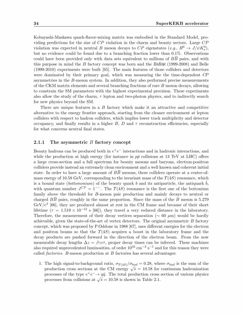
34 SuperKEKB accelerator
Kobayashi-Maskawa quark-flavor-mixing matrix was embodied in the Standard Model, pro-viding predictions for the size of CP violation in the charm and beauty sectors. Large CPviolation was expected in neutral B meson decays to CP eigenstates (e.g., B0 → J/ψK0
s ),but no evidence could be found due to a branching fraction lower than 0.1%. Observationscould have been provided only with data sets equivalent to millions of BB pairs, and withthis purpose in mind the B factory concept was born and the BABAR (1999-2008) and Belle(1999-2010) experiments were built [65]. The main features of those colliders and detectorswere dominated by their primary goal, which was measuring the the time-dependent CPasymmetries in the B-meson system. In addition, they also performed precise measurementsof the CKM matrix elements and several branching fractions of rare B meson decays, allowingto constrain the SM parameters with the highest experimental precision. These experimentsalso allow the study of the charm, τ lepton and two-photon physics, and to indirectly searchfor new physics beyond the SM.
There are unique features in a B factory which make it an attractive and competitivealternative to the energy frontier approach, starting from the cleaner environment at leptoncolliders with respect to hadron colliders, which implies lower track multiplicity and detectoroccupancy, and finally results in a higher B, D and τ reconstruction efficiencies, especiallyfor what concerns neutral final states.
2.1.1 The asymmetric B factory concept
Beauty hadrons can be produced both in e+e− interactions and in hadronic interactions, andwhile the production at high energy (for instance in pp collisions at 13 TeV at LHC) offersa large cross-section and a full spectrum for beauty mesons and baryons, electron-positroncolliders provide instead an extremely clean environment and a well known and coherent initialstate. In order to have a large amount of BB mesons, these colliders operate at a center-of-mass energy of 10.58 GeV, corresponding to the invariant mass of the Υ (4S) resonance, whichis a bound state (bottomonium) of the beauty quark b and its antiparticle, the antiquark b,with quantum number JCP = 1−−. The Υ (4S) resonance is the first one of the bottoniumfamily above the threshold for B-meson pair production and mainly decays to neutral orcharged BB pairs, roughly in the same proportion. Since the mass of the B meson is 5.279GeV/c2 [66], they are produced almost at rest in the CM frame and because of their shortlifetime (τ = 1.519 × 10⁻¹² s [66]), they travel a very reduced distance in the laboratory.Therefore, the measurement of their decay vertices separation (∼ 60 µm) would be hardlyachievable, given the state-of-the-art of vertex detectors. The original asymmetric B factoryconcept, which was proposed by P.Oddone in 1988 [67], uses different energies for the electronand positron beams so that the Υ (4S) acquires a boost in the laboratory frame and thedecay products are pushed forward in the direction of the electron beam. From the nowmeasurable decay lengths ∆z = βγcτ , proper decay times can be inferred. These machinesalso required unprecedented luminosities, of order 1033 cm−2 s−1 and for this reason they werecalled factories. B-meson production at B factories has several advantages:
1. The high signal-to-background ratio, σΥ (4S)/σhad = 0.28, where σhad is the sum of theproduction cross sections at the CM energy
√s = 10.58 for continuum hadronization
processes of the type e+e−→ qq. The total production cross section of various physicsprocesses from collisions at
√s = 10.58 is shown in Table 2.1.

2.1 Introduction on experiments at the B factories 35
2. Clean events with a higher mean charged multiplicity (∼ 11) with respect to the back-grounds are expected, as shown in Figure 2.1. The event rate (10 Hz) is also quite lowand allows relatively simple trigger strategies.
3. The possibility to build hermetic detectors with excellent reconstruction of neutrals,which result in a very high detection efficiency for final states involving π0 and photonsand consequently in the possibility to close the event kinematics. This feature is crucialto perform missing energy searches and look for invisible particles that may be hint ofnew physics.
4. The absence of fragmentation products and the kinematics of the Υ (4S) decay alsoreduces the combinatorial backgrounds. In fact, the initial state and also the momentummagnitudes of B mesons in the CM frame are completely known, allowing therefore toset kinematic constraints on reconstructed candidates, which results in a very powerfultool for suppressing backgrounds. Off-resonance data sets, collected at a center-of-massenergy 40 MeV below the peak of the Υ (4S) are also relevant to study continuumbackground coming from qq hadronization processes and subtract it from the BB signalyields.
e+e− → Cross-section (nb)
Υ (4S) 1.05uu(γ) 1.61dd(γ) 0.40ss(γ) 0.38cc(γ) 1.30
τ+τ− 0.94µ+µ− 1.16e+e− ∼ 40
Table 2.1: Production cross-sections forthe main processes in e+e− collisions at acenter-of-mass energy
√s = m(Υ (4S)) =
10.58 GeV.
Figure 2.1: The number of charged tracks perevent is shown, for different processes. Histogramtaken from The physics at B Factories, Ch. 7, B-meson reconstruction [65].
2.1.2 The first generation of B factories: PEP-II and KEKB
The BABAR and Belle experiments were installed respectively at the high luminosity e+e−
colliders PEP-II at SLAC, in California, and KEKB at KEK, in Tsukuba (Japan) and collecteddata for about a decade, starting from 1999 until 2008 and 2010, respectively. At boththe accelerators, in order to achieve asymmetric energies, two dedicated rings were needed:the High Energy Ring (HER) for electrons, and the Low Energy Ring (LER) for positrons.A schematic view of PEP-II and KEKB colliders is shown in Figure 2.2. For luminosityoptimization, both facilities had a single Interaction Region (IR): unusual beam optics veryclose to the Interaction Point (IP) became necessary to accommodate for high luminosity

36 SuperKEKB accelerator
Figure 2.2: PEP-II (left) and KEKB (right) e+e− storage rings.
requirements, needed to compensate cross sections of order of∼ nb and to collect the necessarystatistics. In terms of the collider parameters, the luminosity is expressed by:
L =Nbne−ne+f
Aeff(2.1)
where Nb is the number of bunches, ne− and ne+ respectively the numbers of electrons andpositrons per bunch, f the circulating frequency, and Aeff the effective overlapping in thetransverse area of the two beams at the interaction point. To ensure good performances andlimit the damaging effect of synchrotron radiation and high beam currents, a high qualityvacuum was needed throughout all the beampipe.
In addition, it was fundamental to introduce the beam-separation scheme, in order tohandle the short bunch spacing in a two ring machine. At PEP-II interaction point, afterthe head-on collision the separation was achieved thanks to the bending magnets, which di-verted the electron and positron bunches soon after their intersection, protecting the beamsfrom parasitic interaction, while KEKB introduced a small crossing angle (∼ 22 mrad), whichsimultaneously allowed to have shorter bunch spacing and more space available for detectorcomponents closer to the IP. This was not without risk, since the crossing angle induces cou-pling effect between transverse betatron oscillations and longitudinal sinchrotron oscillations,inflating instabilities which were finally cured allowing KEKB to reach an instantaneous lu-minosity even twice as large as the originally designed nominal one, for a maximum peak of2× 1034 cm−2 s−1.
In Figure 2.3 the luminosities achieved at PEP-II and at KEKB during different data-taking periods are shown and in Table 2.2 the major parameters of the machines for boththe factories during their final stage of operation are given. The recorded data sets listed in

2.1 Introduction on experiments at the B factories 37
Figure 2.3: The BABAR (left) and Belle (right) luminosities integrated over the Υ (4S) running period,for both the on- and off-resonance operational modes, are shown. Pictures are taken from The physicsof the B Factories [65].
Table 2.2: Main machine parameters for PEP-II and KEKB during their final stage of operation; inthe last column values from Belle II Technical Design Report [68] for SuperKEKB upgrade are listed.
Parameters Units PEP-II KEKB SuperKEKB(HER/LER)
Beam Energy (GeV) 9.0/3.1 8.0/3.5 7.0/4.0Beam Current (I) (A) 1.8/2.7 1.19/1.64 2.62/3.60Beam Size at IP (x) (µm) 140 80 11.2/10.2Beam Size at IP (y) (µm) 3 1 0.0618/0.0483Beam Size at IP (z) (mm) 8.5 5 5/6Luminosity (1034cm−2s−1) 1.2 2.1 80ξy 0.090/0.129 0.088/0.090β∗y (mm) 5.9/5.9 0.41/0.27
Lorentz factor (βγ) 0.56 0.43 0.28Half-crossing angle (mrad) 0 11 41.5
Table 2.3: First generation B factory data sets. Integrated luminosity and equivalent amount ofBB pairs collected at the different Υ resonances are given. Wherever two comma-separated values arespecified, they correspond to the integrated luminosity and corresponding amount of BB pairs.
B factory Υ (4S) off-res Υ (1S) Υ (2S) Υ (3S) Υ (5S)10580 MeV 9460 MeV 10023 MeV 10355 MeV 10876 MeV
L, NBB L L, NBB L, NBB L, NBB L, NBB
[fb−1], [106] [fb−1] [fb−1], [106] [fb−1], [106] [fb−1], [106] [fb−1], [106]
BABAR 433, 471 54 − 14, 99 30, 122 Rb ScanBelle 711, 772 11 6, 102 25, 158 3, 12 121, 36

38 SuperKEKB accelerator
Figure 2.4: A schematic representation of the SuperKEKB asymmetric energy e+e− collider is given.
Table 2.3 are still unique and able to provide competitive results even more than 10 yearslater the end of the data taking. With these samples, the first generation of B factoriesobserved the CP violation in the B-meson system [69, 70] which experimentally confirmedthe CKM mechanism and led to the 2008 Nobel Prize in Physics awarded to Kobayashi andMaskawa. The measurement of the direct CP violation in B → Kπ decays followed, andalso the charm mixing [71] and several B and τ rare decays were measured, as well as manypredicted and unexpected new states, as for example the X(3872) [72] and the tetraquarkcandidate Z(4430)+ [73]. The future promise for flavor physics and BSM searches is nowrepresented by the SuperKEKB accelerator and Belle II experiment.
2.2 The second generation: SuperKEKB design upgrades
The upgrade of the accelerator, whose schematic view is given in Figure 2.4, is the firstnecessary step for the second generation B factory project. The new SuperKEKB colliderwill achieve a design instantaneous luminosity 40 times larger than what achieved by itspredecessor, 8 × 1035 cm−2s−1, by applying the technology first proposed for Super B inItaly, the so-called nano-beam scheme. Essentially, it exploits the inverse proportionality thatrelates the luminosity to the vertical beta function β∗y
1 at the Interaction Point (IP), which
1In Accelerator Physics, the betatron function β(s) describes the displacement of a particle beam due tooscillations in the transverse plane xy with respect to its nominal trajectory in a given point s along the orbit.β∗ denotes the value of the β function at the interaction point. The β function relates to the transverse beamsize according to the formula: x(s) =
√ε√β(s), with ε the emittance, being a constant of motion along the
orbit.

2.2 The second generation: SuperKEKB design upgrades 39
Figure 2.5: The beam collision in the Nano-Beam scheme: the effective beam size d and the half-crossing angle φ are illustrated. Picture taken from the Technical Design Report [68].
will be squeezed by a factor 20, from about 1 µm to 50 nm, while the beam crossing angle willbe increased from 22 to 83 mrad. At the same time, the beam currents will almost double,and as a result of both the squeezed beams and the increased currents, significantly higherbackgrounds in the detector are expected. First, to reduce beam losses caused by Touschekscattering in the low energy ring and second, to limit the power consumption in the highenergy ring, a smaller beam energy asymmetry was chosen, with a 7 GeV electron beam and4 GeV positron beam energy. This results in a smaller boost βγ = 0.28 and therefore ina reduced spatial separation between the B-meson vertices, which will be compensated bythe new VerteX Detector (VXD). Furthermore, the reduced asymmetry will ensure a betterhermeticity for missing energy decays, due to improvements in the solid angle acceptance.
Valuable improvements in several machine parameters are needed to achieve this goal,implying several interventions on the machine structure, on the ring lattices and a completelyredesigned interaction region: a new electron injection gun, a new target for positron pro-duction, and a new additional damping ring for the positron beam are crucial to achieve thedesign luminosity. The upgrade of the accelerator also includes a redesign of the lattices ofthe low energy and high energy rings, replacing short dipoles with longer ones (LER), in-stalling TiN-coated beampipes with ante-chambers and an important rearrengement of theRadio Frequency (RF) system, though using the same technoglogy.
2.2.1 Nano beam scheme overview
The main modification in the nano-beam scheme approach regards the minimization of thelongitudinal size of the beams overlap d (schematic view of the beam intersection is reportedin Figure 2.5), which can be shown to be the lower bound for the β∗y . The formula for d isthe following:
d ' σ∗xφ
(2.2)
The numerator σ∗x represents the horizontal beam size at the IP and φ is the half-crossingangle (∼ 41.5 mrad). If the assumption of flat beams is verified, the luminosity formula atthe IP can be written as:
L =γ±
2ere
(1 +
σ∗yσ∗x
)(I±ξy±β∗y±
)RLRξy
(2.3)
where γ, e, re are respectively the Lorentz factor, the elementary electric charge and theelectron classical radius, while RL, Rξy are the luminosity and vertical beam-beam reduction

40 SuperKEKB accelerator
factors, whose ratio can be approximately considered 1. Since the ratio σ∗y/σ∗x is order 10−3,
the term into brackets can be approximated to one as well. Indices (+,−) refer to electronand positron beam, respectively. From this formula, it can be noticed that there are threefundamental parameters for manipulating the luminosity and they are the beam current (I),the vertical beam-beam parameter (ξy) and the beta function (β∗y) at the IP. A comparisonof the major upgraded parameters between KEKB and SuperKEKB is given in Table 2.2.
Beam background sources
The measurement of the beam backgrounds and the estimation of their expected rates withthe final optics at the design luminosity is crucial to assess the safety of the Belle II detectorand its good performance. The main beam background sources at SuperKEKB are five.The first is the Touschek scattering which is highly enhanced due to the nano-beam schemetechnique and squeezed beams. It is an intra-bunch process which consists in the Coulombscattering of two particles within the same bunch, implying as result a shift in the energies ofthe particles involved, one getting higher and one decreasing of the same amount, thereforedeviating from the nominal energy and from the stable orbit. This effect depends inverselyon the beam size and on the third power of the beam energy. The scattered particles areusually lost at the beampipe inner wall during propagation through the ring and if the losshappens at the IP, the detector might be hit by the shower. To prevent this and mitigateTouschek background both vertical and horizontal movable collimators are used, as well asmetal shields. The expected rate is ∼ 20 times higher than KEKB, just applying a simplere-scaling.
The second source of background is the beam-gas scattering, due to remaining gas moleculesin the beampipe which interact with the beam particles through two main processes: theCoulomb scattering, which changes the direction of the particles, and the bremsstrahlungscattering, responsible for decreasing the particle energy through photon emission. The rateis proportional to the beam current and to the vacuum pressure, and for the Coulomb scatter-ing component, which is the dominant one, it is expected to be ∼ 100 higher than at KEKB,due to the reduced beampipe radius. As for the Touschek scattering the countermeasure isto apply collimators able to shield the IP and protect the detector, absorbing particle losses.However, the width of vertical collimators is the result of a trade off between the necessity toclose them to avoid beam losses and not to incur in Transverse Mode Coupling instabilities.
The third type of background is the synchrotron radiation (SR) emitted by acceleratedparticles, which increases with the square of the particle energy and magnet field strengthsquared. The synchrotron radiation spectrum goes from few to tens of keV and it may severelydamage the vertex detector. It mainly affects the HER ring and the most relevant contri-bution, contrary to what happened in Belle, is due to the final focusing magnets, since thesynchrotron radiation produced in the bending magnet far from the interaction point cannotreach the detector. To avoid SR photons to hit the detector, the inner wall of the incom-ing beampipe is specifically structured to prevent scattered photons to reach the interactionpoint. Nonetheless, the beryllium beampipe inner wall is covered with a gold layer to absorbthe photons which propagate to the direction of Belle II innermost detectors.
The last two types of beam background are generated during collisions and are luminositydependent. The radiative Bhabha scattering produces a copious amount of low energy pho-tons and through the photo-nuclear resonance mechanism also a huge amount of neutrons.

2.3 SuperKEKB commissioning and running phases 41
The production rate is proportional to the luminosity, therefore it is expected to be 40 timesthe background level at KEKB. Neutrons are a background mainly for the outermost detec-tors and a dedicated shielding system in the accelerator tunnel is required to absorb them.As a consequence of the radiative scattering, electron and positron energies decrease: forKEKB, which used a shared final focus quadrupole magnet (QCS) system for both beams,this caused an over-bending of the beam orbits due to the non-null dipole component farfrom the quadrupole center. Deviated beams may hit the magnets wall and produce addi-tional electromagnetic showers. In SuperKEKB, the QCS system is separate for electrons andpositrons, so that the beams can stay centered in their quadrupole magnets and the lossesdue to the over-bending caused by the dipole component out of the quadrupole center arelargely mitigated. Moreover, the beam parameter tuning can be done independently for thetwo rings.
The last beam background source consists of low-momentum electron-positron pairs re-sulting from two-photon processes in e+e− → e+e−e+e− reactions. These pairs can spiralinside the solenoid field and produce additional hits in the Belle II inner detectors.
Finally, when new charge is injected to a circulating beam, it perturbs the particles inthe bunch, causing for few milliseconds a higher background rate which is called injectionbackground. To prevent the possible data stream corruption due to too large occupancies ofthe Belle II subdetectors, a trigger veto is applied for a time window of ∼ 2µs, whose shapeis tuned according to the measurement of the injection background time structure providedby the BEAST II monitoring.
2.3 SuperKEKB commissioning and running phases
The commissioning of SuperKEKB has been carried out in three phases. In Phase 1 (2016) theaccelerator rings have been commissioned without the final focusing system at the interactionpoint and without the Belle II detector. The main goal was to perform sufficient vacuumscrubbing before the Belle II detector was rolled in, tune the basic feedback system andperform machine studies for low-emittance and optics optimization.
During the Phase 2 commissioning (2018), the final focusing and the positron damping ringwere also in place, together with the Belle II detector, except for the vertex detector, replacedby another system of devices dedicated to the beam background study. Also, additional col-limators to protect the Belle II detector have been installed before the beginning of the datataking. The first physics collisions were detected on April 26th, 2018. The data taking contin-ued until July 2018, with a maximum achieved instantaneous luminosity of 0.5×1034 cm−2s−1
and a total integrated luminosity of around 0.5 fb−1. These data have been used to prove theunderstanding of the detector through performance measurements and several rediscoveries.Dark sector searches which were previously limited by inefficient trigger conditions can bealso performed on this data set.
In Phase 3, the full vertex detector has been installed and started taking data with Belle IIin March 2019. The application of the final nano-beam scheme will allow to reach the designluminosity and collect in the next ten years 50 ab−1. Thanks to such a data set a very richphysics program can be pursued, which includes the measurement of time dependent CPviolation and CKM parameters with a precision below the current threshold of percent level,hadronic charmless B decays and direct CP violation, charm and quarkonium physics, τ and

42 SuperKEKB accelerator
low multiplicity studies as well as the search for physics beyond the SM through precisionmeasurements.
2.3.1 Phase 1: first beam background measurements
Phase 1 operation had three main goals: first to ensure beam background levels are safeto install Belle II; second, to provide feedback for the accelerator optimization on how themachine parameters affect background levels; third, to validate the simulation studies onexpected backgrounds, which are crucial to reliably estimate detectorl ifetimes. These goalshave been achieved thanks to the BEAST II detectors system, which is described in detailelsewhere [74].
The BEAST II detector
The complete description of the BEAST II detector is beyond the purposes of this work, andhereby only an introduction will be provided. The BEAST II detector is composed of eightsub-detectors devoted to the measurement of many properties of SuperKEKB backgroundsat the interaction region. The PIN diodes serve as dosimeter at various location of theinteraction region, while diamonds provide fast dose rates at the IP and have been usedin the next phases to implement the beam abort system. The crystals and BGO systemsmeasure instead the electromagnetic background and in the fast readout mode they provideinformation on the time structure of injection backgrounds. Also CLAWS, which coupleplastic scintillators to silicon photo-multiplier (SiPM) readout, are important to capture thetime structure of backgrounds during injection and provide feedback for accelerator tuning.Finally, to measure the very challenging neutron background two systems have been includedin the BEAST II detector: the 3He tubes for thermal neutron counting and the time projectionchambers (TPC) for the counting and tracking of faster, high-energy neutrons. The QCSSplastic scintillators system was not yet part of BEAST II during Phase 1, but it is a goodprototype for background monitors based on plastic scintillators that are small enough tobe placed between the final focus quadrupoles and the Belle II detector, and it has beenintegrated in the BEAST-II monitoring system during Phase 2.
Summary of main Phase 1 findings
The detailed description of the results achieved during Phase 1 commissioning is reportedin [74]. The BEAST II detector recorded data in spring 2016 and was able to observe allthe main background sources, beam-gas, Touschek, beam-dust and injection backgrounds,except for the two background types due to colliding beams, whose measurement have beenpostponed to Phase 2. A limit on the expected synchrotron radiation dose rate at the IP wasalso set. Based on these measurements, the expected background rates for Phase 2 have beenalso extrapolated and judged to be safe for proceeding with further commissioning and theBelle II installation, despite the safety factors have been found to be low for almost all thedetectors and highly dependent on the machine parameter tuning, especially collimators andmagnets alignment.
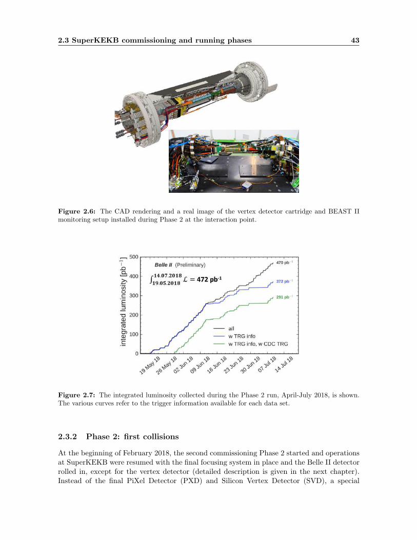
2.3 SuperKEKB commissioning and running phases 43
Figure 2.6: The CAD rendering and a real image of the vertex detector cartridge and BEAST IImonitoring setup installed during Phase 2 at the interaction point.
Figure 2.7: The integrated luminosity collected during the Phase 2 run, April-July 2018, is shown.The various curves refer to the trigger information available for each data set.
2.3.2 Phase 2: first collisions
At the beginning of February 2018, the second commissioning Phase 2 started and operationsat SuperKEKB were resumed with the final focusing system in place and the Belle II detectorrolled in, except for the vertex detector (detailed description is given in the next chapter).Instead of the final PiXel Detector (PXD) and Silicon Vertex Detector (SVD), a special

44 SuperKEKB accelerator
cartridge was installed close to the interaction region, which included the BEAST II detectorsand one single ladder per each layer of PXD and SVD detectors (equivalent to roughly oneoctant of the full vertex detector), a schematic view is provided in Figure 2.6. The goal forsuch a configuration was double: to commission the machine by measuring beam backgroundrates and providing feedback for accelerator tuning and to ensure the radiation safety ofBelle II to run at higher luminosity with the final vertex detector installed, without damagingit. After the first collisions achieved on April 26th 2018, the data taking continued until July17th 2018, reaching a peak luminosity of 5 × 1033 cm−2s−1 and collecting a total data set of∼ 500 pb−1. The main goals of Phase 2 were to verify the nano-beam scheme technique
Figure 2.8: The distribution of the beam-constrained mass mbc showing the peak of the 88 recon-structed B mesons from the analysis of 472 pb−1 collected during Phase 2 (left plot) and the energyloss per path length distribution for charged particles detected by Belle II (right plot). Black dots arecollision data recorded during Phase 2.
Figure 2.9: The two photon invariant mass distribution is shown, with the peak corresponding tothe reconstructed π0 → γγ decays on 5 pb−1 of Phase 2 collision data.
achieving the target luminosity of 1034 cm−2s−1 and to prove the understanding of a new

2.3 SuperKEKB commissioning and running phases 45
detector operating at a new machine. Thanks to the total integrated luminosity recordedduring Phase 2 (Figure 2.7), the first beam-constrained mass distribution 2 was provided,showing the peak at the B-meson mass which comes from the reconstructed 88 BB events(Figure 2.8). Particle identification capability as well as neutral reconstruction were alsotested on the Phase 2 data set. In particular, the distribution of the energy loss per pathlength for charged particles traversing the Belle II tracking devices ( Figure 2.8) is exploitedfor particle identification, while in Figure 2.9 the two photon invariant mass distributionshows the peak of the π0 mass, reconstructed only after one day of data taking with 5 pb−1,proving the excellent detection capability of the electromagnetic calorimeter. During Phase 2the relaxed hardware trigger conditions and the pass-through applied to the software triggerallowed to collect a data set particularly suitable for dark sector searches dealing with missingenergy measurements and requiring nothing in the event except two charged tracks, as it isthe case for the work presented in this thesis. The capability to efficiently reconstruct photonsand veto them has been crucial for such study.
2.3.3 Phase 3: first physics with the full vertex detector
The third commissioning phase with the full vertex detector installed inside Belle II resumedthe operations in March 2019. Phase 3 goal is to collect up to 50 ab−1 of data in the next10 years, by achieving the world highest luminosity of 8 × 1035 cm−2s−1 ( Figure 2.10), andprovide a competitive data set to pursue a rich physics program in a wide range of areas inb-quark and c-quark physics, in τ -lepton, two-photon, quarkonium and exotic studies. Thenew accelerator has sufficient power to deliver e+e− collisions at a center-of-mass energy inthe range from just below Υ (1S), 9.46 GeV, to just above Υ (6S), 11.24 GeV. The majority ofdata will be collected at the center-of-mass energy of Υ (4S), which is a well motivated choice,nonetheless energy scans and running periods at other resonances are also foreseen and stilltopic of discussion for the possibility to collect unique data sets for dark sector and exoticsearches (further details on the Belle II physics program can be found in [43]).
Early Phase 3: main issues and recorded data set
The first data of Phase 3 have been collected since March 25th until June 30th 2019, corre-sponding to a total integrated luminosity which is less than the ∼20 fb−1 of data originallyexpected for the spring run, reaching barely 7 fb−1 (Figure 2.11).
Several issues have slowed down the early Phase 3 data taking, starting from a fire accidenthappened at the beginning of April near the injector linear accelerator (Linac). The Linacprovides the first acceleration boost to electrons and positrons and its accelerating units wereforced to stay off for more than two weeks, preventing SuperKEKB to resume beam collisionsbefore the April 22nd. Beside the external causes, other issues with the new machine andthe implementation of the nano-beam scheme technique when squeezing the beta function atthe interaction point have been responsible for the lower achieved luminosity and the smallercollected data set. Background rates which have been measured to be one order of magnitudehigher then the simulated expectation required further caution in the increasing of the beam
2 The beam-constrained mass is defined as the mass of the reconstructed B-meson mB =√E∗2beam − p∗2B
where the reconstructed energy is constrained to equal the measured beam energy in the center-of-mass frame,E∗beam =
√s/2. It is one of the most useful kinematic variables in B-meson reconstruction, as explained in [65].
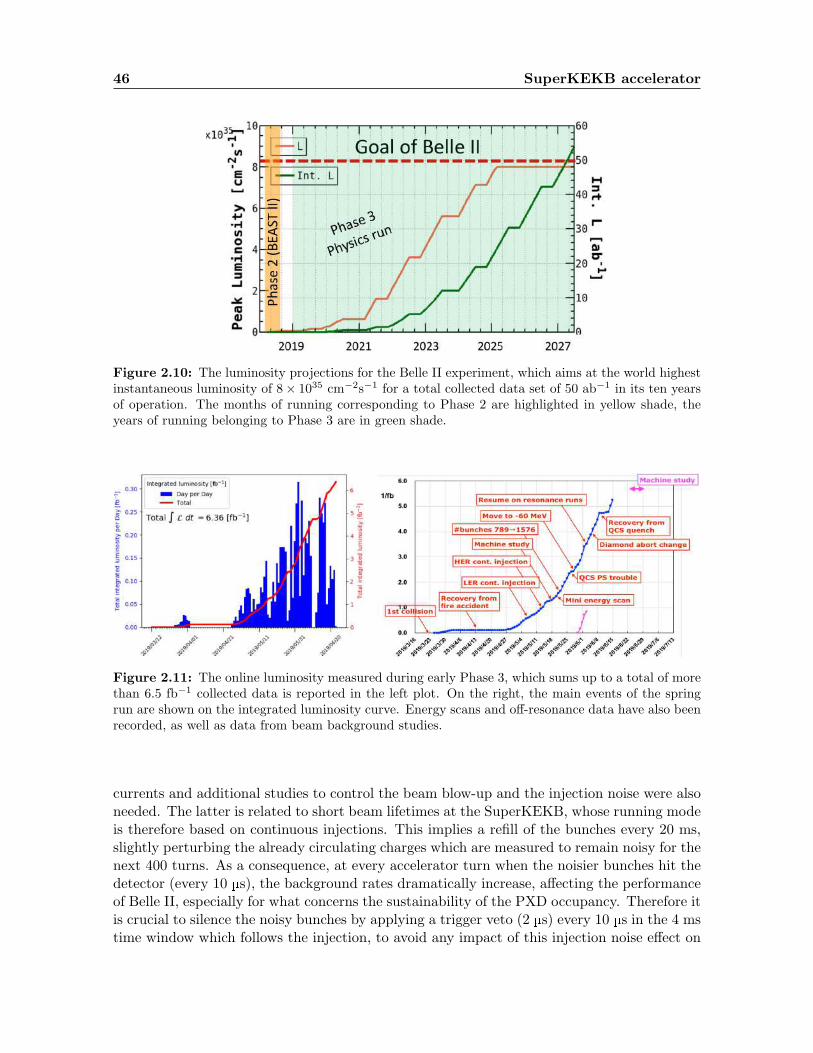
46 SuperKEKB accelerator
Figure 2.10: The luminosity projections for the Belle II experiment, which aims at the world highestinstantaneous luminosity of 8× 1035 cm−2s−1 for a total collected data set of 50 ab−1 in its ten yearsof operation. The months of running corresponding to Phase 2 are highlighted in yellow shade, theyears of running belonging to Phase 3 are in green shade.
Figure 2.11: The online luminosity measured during early Phase 3, which sums up to a total of morethan 6.5 fb−1 collected data is reported in the left plot. On the right, the main events of the springrun are shown on the integrated luminosity curve. Energy scans and off-resonance data have also beenrecorded, as well as data from beam background studies.
currents and additional studies to control the beam blow-up and the injection noise were alsoneeded. The latter is related to short beam lifetimes at the SuperKEKB, whose running modeis therefore based on continuous injections. This implies a refill of the bunches every 20 ms,slightly perturbing the already circulating charges which are measured to remain noisy for thenext 400 turns. As a consequence, at every accelerator turn when the noisier bunches hit thedetector (every 10 µs), the background rates dramatically increase, affecting the performanceof Belle II, especially for what concerns the sustainability of the PXD occupancy. Therefore itis crucial to silence the noisy bunches by applying a trigger veto (2 µs) every 10 µs in the 4 mstime window which follows the injection, to avoid any impact of this injection noise effect on

2.3 SuperKEKB commissioning and running phases 47
Table 2.4: Achieved machine parameters during Phase 3 commissioning. The snapshot of July 1st
provides the latest achieved tuning at the end of the spring running.
Machine Parameter June 20th July 1st
β∗x (mm) 100 80β∗y (mm) 3 2
ILER / IHER (mA) 396/398 799.7/821.2nB 1576 1576
IbLER / IbHER (mA) 0.314/0.317 0.507/0.521ξyLER/ξyHER 0.0335/0.0189 0.0355/0.0197
L (×1033 /cm2/s−1) 0.479 12.294
the data stream.
Also the magnets of the final focusing system showed instabilities that in the worst casesresulted in a certain number of quenches, also related to background burst events. Theseepisodes are particularly dangerous for the safety of the vertex detector, and for all the Belle IIsub-systems in general and a better understanding of the machine background is crucial notto compromise the detector. The main events characterizing the 2019 spring runs are shownin Figure 2.11 and the final parameters achieved are reported in Table 2.4.
Nonetheless, thanks to the hard work of all the people involved in the first running periodoperations and in the analysis of the collected data, already with less than 10 fb−1 it has beenpossible to assess the improved performance of the Belle II detector in its final configuration,especially regarding tracking efficiency and the impact parameter resolution, thanks to thefull VXD installation. Also particle identification, and especially muon detection, has largelyimproved due to the recovery of a well performing muon detector (KLM), now able to providededicated muon identification variables with much higher and reliable efficiency with respectto Phase 2. The early Phase 3 data set has been used to start new physics analyses andprovide detector performance as well as rediscovery studies, as proof of concept of the goodbehavior of the detector and of the capability to understand the collected data.
After the summer shutdown, SuperKEKB resumed operation in October 2019 for theautumn run, which is expected to provide further 20 fb−1 of collision data by the end of theyear, in order to reach 200 fb−1 by summer 2020. First beams were circulated on October 15with the same machine configuration achieved at the end of the 2019 spring run, as shown inTable 2.4. Restarting from the same optics which allowed to achieve β∗y = 2 mm, the betatronfunction at the IP needs to be decreased by at least another order of magnitude to reachthe nominal design value. The main goal for the autumn run is to squeeze down the betafunction at the IP to 1 mm, with decreased beam currents around 300 mA. The injectionbackground is now better controlled thanks to the installation of additional feedback systemsand new collimators achieved during summer 2019, but in order to reach higher currentsfurther beam background reduction is required and to that extent the collimator optimizationwill be crucial.
The integrated luminosity increase (prospects shown in Figure 2.10) will be the key ingre-dient to open new doors and achieve the benchmarks in flavor physics and BSM searches andwith that purpose in mind an efficient interplay between the delicate machine tuning and the

48 SuperKEKB accelerator
detector performance is needed. In the following Chapter, the experimental apparatus thatallows to detect the products of e+e− collisions delivered by SuperKEKB is described, as wellas the software framework needed to analyze the collected data set.

Chapter 3
Belle II experiment
The Belle II detector is described in detail in the Technical Design Report [68], for the purposesof this work only a general overview will be given in Section 3.1. The main changes andimprovements with respect to the Belle detector are highlighted and a brief description of eachsub-detector is provided. In Section 3.2 the Belle II trigger system is described, followed by anoverview of the software framework developed to analyze the collected data sets (Section 3.3),which are finally described in the last Section of this chapter, 3.4.
3.1 Belle II upgrade overview
The aim of the Belle II upgrade is to maintain the same good performance of Belle detectorin the new experimental environment with much higher background levels. A schematiccomparison of the longitudinal view of the new Belle II spectrometer with respect to the oldBelle detector is shown in Figure 3.1. Since the SuperKEKB boost is reduced with respect toKEKB (0.28 instead of 0.43) achieving the same proper time resolution requires better vertexresolution, that can be achieved with the reduction in radius of the first active detector layer.Studies estimate a conservative 20 times increase of the expected background hit rate, due to50 times higher event rates (proportional to the increase of the instantaneous luminosity) andto double beam currents. The modifications studied to ensure a comparable or even betterperformance for the Belle II detector are the following:
the inner part of the vertex silicon strip detector, next to the beam pipe, is replacedby a two-layer silicon pixel detector based on DEPFET technology, placed at smallerradius and with a very light material budget;
the silicon strip detector starts from just outside the pixel detector and reaches a largerradius than in Belle;
the silicon strips readout is based on APV25 chips which have a shorter shaping timewith respect to Belle VA1TA chips to cope with higher background;
the central drift chamber, the main tracking device, extends to a larger radius and ithas a larger number of small-cell layers compared to its predecessor;

50 Belle II experiment
Figure 3.1: The top half shows the upgraded Belle II spectrometer as designed in the TDR[68]; inthe bottom half the longitudinal view of the old Belle detector is shown.

3.1 Belle II upgrade overview 51
the new particle identification devices, both in the barrel and in the endcaps, are morecompact and highly performing, exploiting the Cherenkov image detection method anda very fast readout electronics;
the electronics of the electromagnetic calorimeter is replaced with a fast wave-form-sampling circuit;
in the first two layers of the barrel part and in the endcaps of the muon and KL detector,Resistive Plate Chambers (RPCs) are replaced by scintillators readout with wavelengthshifting fibers and Silicon Photomultiplier (SiPM) called MPPC and produced by Hama-matsu;
a new data acquisition system for handling the higher event rate is provided.
The improvements foreseen for Belle II performance are various, first of all the vertexresolution which benefits from the two innermost pixel layers; second, a better reconstructionefficiency for the KS decaying to charged pions, which is crucial for the analysis of the goldenmode B → J/ψKs exploited in CP asymmetries measurements. In addition, the new particleidentification devices ensure a better pion/kaon separation in the whole kinematics range ofthe experiment. Finally, a better performing electronics for the calorimeter readout reducesthe pile up, improving missing energy measurements.
3.1.1 The Pixel Detector
The expected background rate makes the use of silicon strip sensors at small radius (∼ 20 mm)not feasible because of the high occupancy. Pixel detectors have a much finer segmentationand therefore smaller occupancy (3%), while strips detectors at SuperKEKB can be safelylocated at larger radii.
The PiXel Detector (PXD) concept implemented at Belle II is based on the DEPFET(DEPleted Field Effect Transistor) technology. It allows to have very thin pixel (50 µm)with readout electronics moved outside the acceptance region, therefore reducing the materialbudget that contributes to the multiple scattering. The only part of the electronic readoutbeing inside the tracking volume are the switcher ASICs for which very thin gas pipes havebeen devised to provide the necessary active cooling by means of nitrogen flow. Also radiationtolerance can be achieved engineering the sensors in a dedicated radiation-hard technology.
DEPFET is a semiconductor detector concept able to combine detection and amplificationin one device. A DEPFET pixel consists in a p-channel MOSFET structure integrated ontoa fully depleted silicon substrate. The MOSFET has an internal gate where the electronsgenerated when a charged particle passes through the device are collected. The internal gatemodulates the current at readout time allowing the detection of the collected charge.
The DEPFET sensors are organized into planar modules, the ladders, which compose thetwo layers of the PXD, with radii respectively of 14 and 22 mm. The sensitive lengths ofeach layer are determined by the acceptance requirements of the detector: a polar angularcoverage from 17° to 155° is ensured. The total amount of pixels composing the PXD isaround 8 million organized into arrays. Each DEPFET pixel represents a cell, a monolithicstructure with internal amplification, therefore much thinner than other devices which needadditional amplification. Typical pixel sizes have to meet the vertex resolution requirement,

52 Belle II experiment
Figure 3.2: A CAD rendering of the two-layer pixel detector is shown.
which is 20 µm, and also the thinning feasibility, resulting in a 50×50 µm2 and 50×75 µm2
cells respectively for the inner and outer layers.
Another challenging requirement is the short frame readout time, that is achieved by split-ting the readout on both sides of the pixel matrix and introducing high level of parallelization(a four-row simultaneous readout): the processing time for each pixel row is then manageable,of order of 100 ns, and all the 1600 rows can be read in a total frame time of 20 µs.
The sensors are finally mounted on the supporting structure which is able to slide on thebeam pipe to accommodate for thermal expansion. A schematic view of the total structureof PXD is reported in Figure 3.2. For the early Phase 3 started in March 2019 after theinstallation of the vertex detector, due to problems in the assembling of the PXD ladders,only half of the designed PXD has been installed, consisting in the full first layer and 2 laddersof the second one. The PXD installation is expected to be finalized in 2021.
3.1.2 The Silicon Vertex Detector
Low-momentum particles are crucial for the physics at the B factories, but also a challenge forthe track finding system, since they are heavily affected by multiple scattering. Consequently,one of the fundamental requirements for the Silicon Vertex Detector (SVD) is a very lowmaterial budget, as long as a short shaping time to limit the occupancy under few percentand help the track finding algorithms to reject background. These features determine thegeometrical shape of the sensors and also the choice of the readout electronics. The formerissue is solved by adopting the largest possible silicon wafers and equipping the forward regionwith trapezoidal slanted sensors, while for the latter, the solution came from inheriting theAPV25 chips first used in the tracker of the CMS experiment (LHC), equipped with 128

3.1 Belle II upgrade overview 53
Figure 3.3: Left: Schematic view of the SVD longitudinal section, showing the sensors geometry foreach layer and the number of APV25 chips on each side of the sensors. Right: the windmill structureof the inner sensors, with the Origami concept applied on the upper edge of silicon modules, is shown.The solenoidal ~B field parallel to the z-axis is also indicated in the picture.
channels each and a shaping time of 50 ns. Moreover, the multi-peak operational mode ofthe APV25, where six (or three) consecutive samples along the shaping curve are recordedwith each trigger, ensures a time resolution of order of 3 ns. The excellent SVD performanceresults in a innermost layer occupancy smaller than 1%.
The SVD is composed of four layers of Double-sided Silicon Strip Detectors (DSSDs),located respectively at radii of 39 mm (layer 3 ), 80 mm (layer 4 ), 104 mm (layer 5 ) and135 mm (layer 6 ). The azimuthal angular coverage goes from 17° (the forward region) to150° (backward region). The asymmetry is due to the Lorentz boost in the laboratory frame,which favors events boosted in the forward direction.
There are three different types of sensors used for the SVD: the rectangular ones (bigand small) are produced by Hamamatsu Photonics (HPK), while the trapezoidal ones areproduced by the Micron Semiconductor (UK). The first step for sensor production are six-inches, 300 µm-thick silicon wafers, from which the rectangular sensors are developed in twosizes: for layer 3, which has only the barrel section, smaller sensors are adopted, while forlayers 4 to 6 larger sensors are used for the barrel region. The forward region of layers 4 to 6is covered by trapezoidal slanted sensors which minimize the material budget, simultaneouslyoptimizing the acceptance. The long strips measuring the rφ-coordinate on the p-side are intotal 768, readout by six APV25 chips per sensor. For rectangular sensors they are parallelto and facing the beam axis. The short strips on the n-side, which measure the z-coordinate,are instead 512 for the large rectangular sensors and the trapezoidal ones ( while they are 768as on p-side for the small rectangular sensors used for layer 3), therefore they need only fourAPV25 chips for readout. They are located on the sensor side towards the outside (except forlayer 3, which has an inverted side structure, with the n-side facing the Interaction Point).For the slanted sensor of the forward region the geometry is the same, except for the p-sidestrips which are not parallel to z-axis anymore. Dimensions are given in mm in Figure 3.3and a picture of the real SVD installed in Belle II is provided in Figure 3.4.
The Origami chip-on-sensor concept is a readout modification introduced in Belle II forthe inner sensors, while the forward and backward sensors are readout by conventional APV25chips located outside the acceptance. The Origami concept refers to flexible pitch adapter

54 Belle II experiment
Figure 3.4: The Belle II SVD already matched with the PXD and ready to be installed in at theInteraction Point of the detector (December 2018).
circuits connecting the sensor strips to APV25 chips applied on the outer edge of the sensorsin the windmill structure, as shown in Figure 3.3. The strips on the outer side are read bya planar pitch adapter, while for the strips on the inner side, a flexible pitch adapter bentaround the upper edge of the sensor is needed. This technique aligns all the chips on the outerside, enabling to use only a single cooling system for all the ladder. The cooling is providedby a dual phase CO2 system, whose design aims at minimizing the material budget, adopting1.4 mm-diameter tubes with 0.05 mm-thick walls.
3.1.3 The Central Drift Chamber
The Central Drift Chamber (CDC) fulfills three main functions. First, it contributes withthe SVD and PXD to charged track reconstruction and measures the momentum. Second, ithelps in particle identification thanks to the measurements of the characteristic energy lossof charged particle due to ionization in the gas volume. Finally, it provides reliable triggersignals for charged particle events.
The CDC follows the successful design of its predecessor in Belle: the same structureis implemented and the same material and gas mixture are used. The main modificationsregard:
the readout electronics, which needs to be much faster in order to handle higher triggerrates;
the cylinder radii, where the innermost ones has to be larger to account for a biggerSVD, while the outermost radius has to deal with the more compact barrel detectorfor particle identification, resulting in a 160 mm and 1130 mm radii respectively. The

3.1 Belle II upgrade overview 55
acceptance in azimuthal angle goes from 17° to 150°. Also the wire configuration has tobe adapted.
the three-dimensional trigger information, providing a z trigger (see Section 3.2) whichefficiently helps in reducing beam backgrounds without loosing physics events.
The CDC consists in 56 layers organized in 9 super-layers. The length of the squared cellsvaries from 10 mm for the innermost super-layer to 18.2 mm for the outermost ones. The50% helium-50% ethane gas mixture is filled with a total of 14336 tungsten sense wires of 30µm diameter. For the generation of the needed electric field gradient, aluminum wires of 126µm-diameter are used. The structure is supported by two carbon-fiber reinforced cylinders,terminating with aluminum end-plates. Finally, the measured spatial resolution of the CDCis about 100 µm, while the relative precision on the dE/dx measurement for particles withan incident angle of 90° is around 12%.
3.1.4 Particle Identification devices
Two sub-detectors in Belle II are specifically devoted to particle identification: the Time-Of-Propagation counter in the barrel region and the Aerogel Ring-Imaging Cherenkov counterfor the end-cap. Both the sub-detectors exploit the Cherenkov effect to identify the chargedparticle traversing the spectrometer.
The Time-Of-Propagation counter
The Time-Of-Propagation (TOP) counter, shown in Figure 3.5, measures the time of prop-agation of the Cherenkov photons internally reflected in the quartz bar. Together with thedetected arriving position along the x coordinate of the quartz bar as represented in thepicture, the arrival time allows to reconstruct the Cherenkov angle θC from which the parti-cle velocity v can be inferred and the likelihood for different mass assignment hypothesis iscalculated.
The TOP consists in 16 modules surrounding the outer wall of the CDC. Each module isa quartz radiator composed of two quartz bars glued together for a total length of 2500 mmand a transverse area of 44×20 mm2. Photons emitted in the forward direction are reflectedbackward by a mirror placed at the forward end of the quartz bar. Photons propagating inthe backward direction are collected by different PMT channels, depending on their reflec-tion angles. The critical issue in the TOP performance for PID is the broadening of timeresolution due to the photons chromaticity, which is cured by a focusing system consistingin a slightly concave-shaped mirror, aimed at compensating the chromaticity dispersion ofCherenkov photons: the parallel rays are focused into the same pixel of a photo-sensor, whilethe chromatically-dispersed one are detected by separate channels.
The required time resolution for a single-photon detection is around 50 ps. The goal isachieved by employing as photon detectors the Multi-Channel Plate Photo Multipliers (MCPPMTs), two-stage amplification devices, with a gain of 106 and a very fast response.
The Aerogel Ring-Imaging CHerenkov counter
In the forward end-cap, the particle identification is provided by the proximity focusing Aero-gel Ring-Imaging Cherenkov counter (ARICH), whose schematic view is shown in Figure 3.6.

56 Belle II experiment
Figure 3.5: Conceptual representation of the time-of-propagation counter, which measures both thearriving time and position of the internally reflected Cherenkov photons.
It consists of an aerogel radiator producing Cherenkov photons when a charged particle passesthrough its volume; an expansion volume of 20 cm divides the aerogel tile from the photondetector surface and allows the Cherenkov photons to enlarge into rings. The array of positionsensitive photon detectors provides single photon detection in a high magnetic field (1.5 T)with optimal resolution in two dimensions.
The main parameters describing the detector are the number of detected photons Nγ andthe resolution on the Cherenkov angle σθ. Increasing the radiator thickness, the number ofdetected photons increases and the resolution per charged track improves as σθ/
√Nγ , but the
angular resolution on the single photon (σθ) degrades due to the uncertainty of the emissionpoint. Combining two layers with appropriately tuned refractive indices in order to have twooverlapping rings will reduce the spread due to the emission point uncertainty, achieving aresolution on the Cherenkov angle σθ ' 16 mrad. The performance is optimized for chargedtracks with momentum larger than 3.5 GeV/c, but no significant degradation is shown alsofor lower momentum tracks. A non-homogeneous aerogel radiator ( see Figure 3.6) has beendevised, with a global acceptance covering the azimuthal angular region from 15° to 30°. Theproximity focusing technique is applied by choosing as upstream layer the aerogel with lowerrefractive index (n1 = 1.046) and increasing the refractive index of the downstream layer(n2 = 1.056). Studies have shown that a twice as thick layer of homogeneous aerogel radiatorwould provide the same number of photons, but with a worse resolution σθ ' 20 mrad.The development of reliable photo sensors with good efficiency for single-photon detection inthe high magnetic field is achieved with the Hybrid Avalanche Photo-Detectors (HAPD) byHamamatsu Photonics. Finally, considering the studies on Cherenkov angle resolution andon average 12.7 detected Cherenkov photons as measured during for Phase 3, the precision
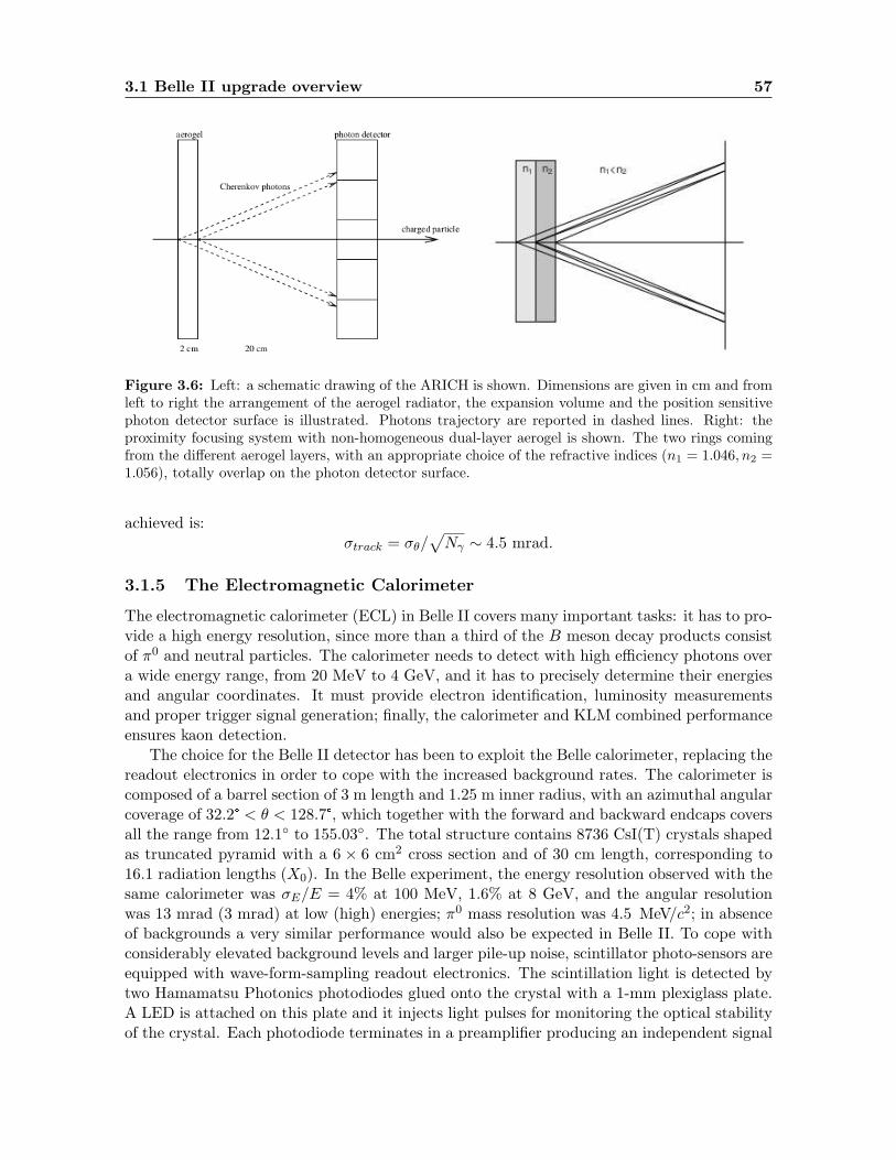
3.1 Belle II upgrade overview 57
Figure 3.6: Left: a schematic drawing of the ARICH is shown. Dimensions are given in cm and fromleft to right the arrangement of the aerogel radiator, the expansion volume and the position sensitivephoton detector surface is illustrated. Photons trajectory are reported in dashed lines. Right: theproximity focusing system with non-homogeneous dual-layer aerogel is shown. The two rings comingfrom the different aerogel layers, with an appropriate choice of the refractive indices (n1 = 1.046, n2 =1.056), totally overlap on the photon detector surface.
achieved is:σtrack = σθ/
√Nγ ∼ 4.5 mrad.
3.1.5 The Electromagnetic Calorimeter
The electromagnetic calorimeter (ECL) in Belle II covers many important tasks: it has to pro-vide a high energy resolution, since more than a third of the B meson decay products consistof π0 and neutral particles. The calorimeter needs to detect with high efficiency photons overa wide energy range, from 20 MeV to 4 GeV, and it has to precisely determine their energiesand angular coordinates. It must provide electron identification, luminosity measurementsand proper trigger signal generation; finally, the calorimeter and KLM combined performanceensures kaon detection.
The choice for the Belle II detector has been to exploit the Belle calorimeter, replacing thereadout electronics in order to cope with the increased background rates. The calorimeter iscomposed of a barrel section of 3 m length and 1.25 m inner radius, with an azimuthal angularcoverage of 32.2° < θ < 128.7°, which together with the forward and backward endcaps coversall the range from 12.1 to 155.03. The total structure contains 8736 CsI(T) crystals shapedas truncated pyramid with a 6 × 6 cm2 cross section and of 30 cm length, corresponding to16.1 radiation lengths (X0). In the Belle experiment, the energy resolution observed with thesame calorimeter was σE/E = 4% at 100 MeV, 1.6% at 8 GeV, and the angular resolutionwas 13 mrad (3 mrad) at low (high) energies; π0 mass resolution was 4.5 MeV/c2; in absenceof backgrounds a very similar performance would also be expected in Belle II. To cope withconsiderably elevated background levels and larger pile-up noise, scintillator photo-sensors areequipped with wave-form-sampling readout electronics. The scintillation light is detected bytwo Hamamatsu Photonics photodiodes glued onto the crystal with a 1-mm plexiglass plate.A LED is attached on this plate and it injects light pulses for monitoring the optical stabilityof the crystal. Each photodiode terminates in a preamplifier producing an independent signal

58 Belle II experiment
and the two pulses are then summed at an external shaper board. The crystals in the barrelsection are structured in multi-cell units divided by 0.5 mm thick aluminum septum wallswhich go from the inner to the outer supporting cylinders. The overall support structure isflushed with dry air to provide a low humidity (5%) environment for the crystals and the heatgenerated by the preamplifiers (about 3 kW in total) is extracted by a water cooling system.The support structure for the endcaps is similar to that of the barrel section.
From calibration with cosmic muons it is known that the average output signal of thecurrent crystals gives 5000 photo-electrons per 1 MeV of deposit energy, with an averagenoise level of 200 keV. The higher background rate is handled with a new readout electronicbased on the signal sampling method.
The intrinsic energy resolution of the calorimeter from a prototype test is given by theapproximated formula:
σEE
=
√(0.066%
E
)2
+
(0.81%
4√E
)2
+ 1.34%2, (3.1)
where E is the energy in GeV and the first term refers to the electronic noise contribution.
3.1.6 The neutral kaon and muon detector
The KL and muon detector (KLM), consisting of alternating 4.7-cm thick iron plates andactive material detectors, is located outside the superconducting solenoid which provides the1.5 T magnetic field used for particle momentum measurements. A schematic overview isshown in Figure 3.7. The iron is needed as magnetic flux return for the solenoid and italso provides the material budget for 3.9 interaction lengths, allowing the KL to hadronicallyshower in its volume. The octagonal barrel section covers the azimuthal region 45° < θ < 125°.Adding the endcaps coverage, the KLM reaches the angular acceptance of 20° < θ < 155°. Theouter layers of the barrel are equipped with glass electrode Resistive Plate Chambers (RPCs),while in the inner two layers and in the endcaps scintillators readout by SiPMs are installed.This replacement is needed to avoid the RCPs efficiency drop in a high rate environment.
The use of scintillator strips equipped with SiPMs ensures an optimal time resolution,which is measured with a trigger provided by cosmic ray events; the time dispersion differencegives σt ∼ 0.7 ns. The good timing performance enables to exploit the KLM endcaps as timeof flight detector for KL. In the barrel section the KL-reconstruction efficiency is measuredto be linearly increasing with the particle momentum up to a plateau of around 80% formomenta higher than 3 GeV/c.
As far as muon identification is concerned, the main strategy is to extrapolate outwardthe tracks reconstructed in the CDC with the mass hypotheses of a pion and checking if, onthe outermost KLM layer crossed by the predicted extrapolation, the actual measured hit canalso be found. In this case, the extrapolation of the track restarts at the entry point in thefirst KLM layer, assuming a muon mass hypothesis. The likelihood for being a muon is thencomputed according to the comparison between the predicted and measured ranges and thegoodness of the track fit, based on Kalman filtering fitting technique. For high-purity samplesof muons (for example from the reactions e+e−→ µ+µ−(γ) and J/ψ → µ+µ−), it has beenestimated that the barrel section of the KLM provides a µ-reconstruction efficiency of 89%for particle momenta above 1 GeV/c.

3.1 Belle II upgrade overview 59
Figure 3.7: A schematic overview of the neutral kaon and muon detector at Belle II is given in thepicture.

60 Belle II experiment
3.2 The trigger system at Belle II
The high luminosity upgrade will increase the total event rate to almost 20 kHz, requiringa robust and at the same time flexible trigger for discriminating the signal events from thebackground rates, which are expected 20-30 times larger than at KEKB. Considering thehigh charged track multiplicity in BB event final states, an obvious trigger requirement ison the number of tracks in the event. However, there are physics processes, e.g., τ leptonicdecays and dark matter searches, that have zero or two tracks only in their final state, whichcauses much more difficulties in signal and background discrimination. In addition, some lowmultiplicity processes have the same topology as the Bhabha scattering events, which havea huge cross section at Υ (4S) CM energy (∼ 300 nb) compared to the typical signal crosssections (1 nb). Therefore, when vetoing Bhabha events for reducing the total event rate, largepart of the trigger efficiency on low multiplicity events is also lost. To preserve high efficiencieson the processes of interest, an effective trigger system is essential. Its implementation followsthe same principle successfully adopted for Belle, but with totally new technologies able tosupport the increased event rates. The trigger system is composed of the Level 1 trigger (L1),implemented in hardware, and the software implementation of the High Level Trigger (HLT).
The L1 Trigger
The L1 trigger system gathers many sub-trigger systems which provide information fromvarious subdetectors, merged by the global reconstruction logic (GRL), whose output is sentto the global decision logic (GDL), responsible for issuing the trigger signal. In Belle II, allthe trigger system components are based on the Field Programmable Gate Array (FPGA)technology, which makes the logic configurable rather than hard-wired. The first combinationof detector information is performed by the GRL and it is mainly based on the drift chambertrigger and on the ECL trigger.
The CDC trigger finds and characterizes the tracks detected in the drift chamber. The2D tracking basically follows the same implementation as Belle. The Belle II CDC detectionimprovement with the 3D tracking, which adds the information on the z-coordinate, allowsto reject the most part of the background coming from Touschek intra-bunch scattering. Infact, these scattering events show a large displacement in their z-position with respect to thenominal interaction region. The maximum 5 µs latency of the L1 trigger system requires avery fast z-vertex reconstruction, to be performed in no more than 1 µs, which is achievedthanks to neural networks techniques.
The calorimeter trigger system adopts two complementary trigger schemes: a total en-ergy trigger and an isolated cluster counting technique, the former being sensitive to eventswith high electromagnetic energy deposition, the latter to multi-hadronic physics events withlow energy clusters and/or minimum ionizing particles. Moreover, the ECL trigger is ableto recognize the back-to-back topology of Bhabha scattering with a high purity, which isfundamental for ensuring a high trigger efficiency of low multiplicity processes.
The single calorimeter cluster trigger, in association with at least one non-electron track inthe opposite direction, is fundamental for the detection of radiative two-track processes, whichinclude the background studies for the dark photon search and for the ALPs search as well.The trigger for non radiative dimuon events e+e−→ µ+µ− exploits instead the combination oftwo-track triggers based on one single detector sub-system (CDC), plus single high-energetic

3.3 Overview of the Belle II analysis software framework 61
track triggers provided by the KLM, for penetrating muons. Finally, a more efficient Bhabhaveto, based on both polar and azimuthal angle information, largely improves the backgroundsuppression. The L1 trigger can sustain a maximum instantaneous rate of 30 kHz, howeverthe goal is to keep the trigger rate as low as possible, while ensuring a high efficiency (largerthan 99%) for physics targets, mainly hadronic events. The L1 output is then forwarded tothe High Level Trigger for further background rejection based on fully reconstructed objects.
The High Level Trigger
The HLT is a software trigger developed to improve the backgrounds suppression and relieson the physics trigger, whose main purpose is to reduce the load of data written on permanentstorage at a maximum design output event rate of 10 kHz. Events preselected by using onlythe information provided by CDC and ECL triggers undergo the full offline reconstruction,involving all output from the subdetectors except the PXD. The physics trigger is then able toclassify the event category ( BB, e+e−→τ+τ−, etc.) and once this has been assigned, the HLTprocessing results containing the event tag and the track parameter estimate are combinedwith the information from the PXD, which enables to calculate the Region of Interest (ROI).Only the pixels belonging to that region are readout and the selected PXD hits are used tocomplete the event reconstruction.
During Phase 2 the HLT was in pass-through and no software filter was applied to thetriggered events, resulting in a very favorable condition to collect events with topologiesinteresting for dark sector searches, that may be suppressed by the HLT filtering necessaryfor the Phase 3 running at higher luminosity.
3.3 Overview of the Belle II analysis software framework
The upgrade of the detector has been crucial to maintain Belle II performances similar to,if not even better than, the ones achieved by Belle, despite the much higher backgroundenvironment. Likewise, the development of a dedicated core software for online and offlinedata handling, with improved reconstruction algorithms is fundamental to pursue the goal.The core software of Belle II includes three main parts which are the specific Belle II analysissoftware framework (basf2) providing all the tools to perform physics analysis; the externals,consisting in third-party code on which basf2 depends; the tools, providing scripts for basf2installation and configuration. More information about the core software and the details ofthe reconstruction algorithms implementation can be found in [75, 76], hereby only a generaldescription of basf2 structure and purposes is provided.
3.3.1 The basf2 code
A typical way to process data is building a chain of smaller processing blocks with very specifictasks, which go from reading the data to the full detector simulation. These small units arecalled modules and can be assembled in paths. Basf2 is a modular analysis framework whoseflexibility relies on two ingredients, the modules to process the data and the data store toshare the data between modules, as schematically represented in Figure 3.8.
The container where the modules live and perform their task is the path, which executeone at the time all the registered modules, in the order specified by the user through dedicated

62 Belle II experiment
Figure 3.8: The data processing flow as handled by basf2 is represented in the scheme.
Python scripts. Data processing can be steered in a customized way by the user, thanks tothe module parameters, which can tailor the module execution and be set at runtime throughthe python steering scripts.
As regards data either from Belle II detector or from the simulation, they are organizedin a set of runs with variable duration, containing a sequence of independent events. Eachevent is defined as the set of measurements produced by an electron-positron collision or thepassage of a cosmic ray. A set of runs sharing similar hardware state and operational featuresdefines an experiment. Each single independent event is then identified in Belle II throughthree unsigned integers standing for the experiment, run and event numbers.
Basf2 modules can be written either in C++ or Python and are derived from the Module
base class which defines five interface methods: initialize() called before the processing of thepath; beginRun() called every time a sequence of events belonging to a new run starts, toproperly initialize the run-dependent parameters, event() which is called for each processedevent; endRun(), called at the end of the sequence of events which belong to the same run, tocollect the run-summary information; terminate() called at the end of all events processing.The sequence of modules to be executed is provided by an instance of the Path() class,that can be called through the steering Python script providing a user-friendly interfaceto set the values of modules parameters and their execution sequence. During execution,modules are able to access and modify the data provided by the Data Store either as singleobject (StoreObjPtr) or as an array of objects (StoreArray), which also keeps track of therelationships between the various objects per each event.

3.3 Overview of the Belle II analysis software framework 63
3.3.2 Input/output: simulation and reconstruction in basf2
Object persistency is implemented using ROOT, which implies all objects stored in the DataStore need a ROOT dictionary. The RootOutputModule writes the Data Store content to afile with two TTrees with permanent and event durability, where each branch corresponds toa Data Store entry. The permanent-durability tree in each output file is the FileMetaData,containing the metadata related to the processed events, which are run, experiment and eventnumbers, as well as the steering file content . Similarly, ROOT files can be read by theRootInputModule.
No assumption is made for the event data model which can be very flexible in its dynamicalimplementation, determined by the modules execution and the creation of objects in theData Store. The only mandatory object is the EventMetaData, which uniquely identifies anevent given the event, run and experiment numbers and a production identifier to distinguishsimulated events from real experimental data.
The raw data format to provide physical quantities from detector information like trackhits or calorimeter clusters, is instead defined by each detector readout. Dedicated unpackermodules are responsible for the conversion of raw data to digit objects, as first step to buildhigh-level objects such as charged tracks and ECL clusters. At that point the hit and cellinformation is discarded and the event size can be reduced by a factor of 40, which howeveris not the final result. High level-objects, like tracks, ECL and KLM clusters which are thefinal output of the reconstruction process are used to produce particle-level information, suchas four momenta and event-shape variables, which compose a subset of data-objects neededfor physics analyses and written in root files as mini data summary tables (mDST).
The tracks reconstruction relies on the information collected by the tracking devices ofthe Belle II detector (CDC, VXD), from which track parameters and their errors are extrap-olated thanks to dedicated fits implemented in the basf2 reconstruction modules and basedon the Kalman filter fit technique [77], a track finding procedure which correctly takes intoaccount effects of multiple scattering and the energy loss in the material. From reconstructedtracks, their associated momenta are measured, while clusters are reconstructed from adja-cent over-threshold crystals in the ECL detector or from the number of hits and longitudinalpenetration length in the KLM and can be associated to charged tracks or identified as neu-tral objects. Particle identification algorithms based on likelihood ratios are then appliedto establish particle identities. The event reconstruction continues with the combination ofstable particles to form a common vertex which indicates composite particle decays. Severaltechniques of vertexing are in place in the basf2 packages and they allow to fit different typesof decay chains, also dealing with neutrals. Finally, the particle lists are filled and availablein the mDST files, where all the information for physics analyses is stored.
For what concerns data from Monte Carlo simulations, the digit objects are producedby the digitizer modules of each detectors from the energy deposition generated throughGeant4 [78] and stored in the common class framework of SimHits. This allow to easilyadd the hits from energy deposition produced by the simulated machine-induced backgroundon those coming from the simulated physics signal process, which is defined as backgroundmixing. After digitization, the simulated digits follow the same reduction path to higher-levelobjects described for real data from the Belle II detector and at the end of the analysis chainthey are also written as mDST objects in rootfiles.
64 Belle II experiment
3.3.3 Condition Data
The information about the specific running conditions during data acquisition are also fun-damental to be stored, in order to properly calibrate the data recorded by the detector whenperforming physics analysis. Condition data are saved in the Belle II Conditions Database asa sequence of payloads reproducing the time evolution of the conditions changing during theexperiment (but not on a per-event base) thanks to an associated Interval of Validity (IoV),uniquely identified by the run and experiment numbers. A collection of payloads with theirassociated IoVs specifying when they are valid is called a Global Tag (GT). The ConditionDatabase design was determined by the main goal of easy and scalable maintainability andtherefore based on the standard industry software tools. Its implementation won’t be dis-cussed in this work and further details can be found in the reference [79].
Finally, a release-XX-YY-ZZ of the basf2 software is a snapshot of basf2 as frozen at aspecific time and unchangeable anymore in its reconstruction and simulation algorithms andcalibrations. Several releases have been produced to reprocess experimental data and producenew Monte Carlo samples with new features, including modifications of the software in theonline fabrication system, and better calibrations. Each data reprocessing is called prodX andto analyze a specific reprocessing of the experimental data set the proper release version andglobal tag must be used, to grant the highest performance, efficiency and repeatability of theanalysis results.
3.4 Data sets
For this work two types of data sets have been exploited: the 11th campaign of the officialMonte Carlo (MC) production MC11 for the simulated samples and the sixth reprocessing ofPhase 2 data prod6 for the experimental data set.
The MC samples are exploited to optimize the event selection and background rejection,to compute the signal efficiency and study the signal shape and resolution, and finally to tunethe upper limit calculation strategy with different statistical approaches.
The experimental data set is used to provide the physics results from this search, as well asfor all the validation and performance studies needed to evaluate the systematic uncertainties.
3.4.1 Monte Carlo samples
Monte Carlo simulation uses event generators, which consist of several packages in the basf2framework that according to theoretical models of particle interactions produce sets of four-vectors describing the final state of e+e− collisions. A particle identity is associated by thegenerators to each four-vector. A combination of both background and signal generators isrequired to properly mimic the event stream of real data.
Background simulation
The production of leptonic event from e+e− collisions is handled by several generators whosedetailed description can be found elsewhere [76]. The muon and τ pair productions are gener-ated with the KKMC [80] package and the τ decays simulation is then handled by TAUOLA [81],while QED background processes like e+e− → e+e−(γ) are simulated using BabaYaga@NLO [82]

3.4 Data sets 65
and four-lepton final states exploit instead AAFH [83]. Finally, radiative decays to two-pionfinal states e+e− → π+π−(γ) have been simulated by using the package PHOKHARA [84]. Thegenerators to produce each background sample used in the analysis are referenced in the lastcolumn of Table 3.1. The propagation of particles in the detector and the physics processesof the interactions between the particles and the detector materials are finally handled bythe Geant4 software package [78], through the specific physics lists recommended by theGeant4 group for high energy physics experiments and embedded in basf2.
The official MC11 samples which have been used for background studies are listed inTable 3.1. They have been simulated using the Phase 2 geometry and adding the officiallyproduced beam background samples. In order to compare the MC results to the experimentaldata, the generated samples have been always normalized to the effective integrated luminosity∫Ldtgood runs reported in Table 3.2 and corrected for the trigger efficiency, according to the
weights:
wi =
∫Ldtgoodruns · εtrg∫Ldtgen,i
(3.2)
where the index i stands for each generated process and εtrg correspond to the measuredefficiency for a given trigger line. Additional background contamination due to continuumhadronization events from e+e−→ qq processes have been checked to give a negligible contri-bution already at the event reconstruction level. Further discussion on a specific veto devisedfor hadronic interaction suppression is reported in Section 4.3.
Table 3.1: Phase 2 MC11 samples used for background studies with the number of generated eventsNevts and the equivalent integrated luminosity
∫Ldt.
Process Nevts [106]∫Ldt [fb−1] Reference
e+e− → µ+µ−(γ) 65 56.621 KKMC [80]e+e− → τ+τ−(γ) 36.8 40.044 KKMC
e+e− → e+e−µ+µ− 140 7.406 AAFH [83]e+e− → π+π−(γ) 210 1372.539 PHOKHARA [84]e+e− → e+e−(γ) 60 0.198 BabaYaga@NLO [82]e+e− → e+e−e+e− 260.6 6.562 AAFH [83]
Signal simulation
The Monte Carlo samples for the signal simulation does not belong to the same official MC11production campaign from which the background samples have been taken and have beenself-produced due to technical difficulties in the integration of the external packages for theMadGraph 5 generator [85] and basf2 [75]. The Phase 2 geometry and beam backgroundhave been added to the simulation of the signal process e+e− → µ+µ−Z ′, Z ′ → invisibleby exploiting the release-02-00-01 basf2 release and with the MadGraph 5 generator [85],according to the model described in Section 1.6. In total, 18 signal MC samples of 20000events each have been generated, for Z ′ boson masses from 0.5 GeV/c2 up to 9 GeV/c2, witha mass step size of 0.5 GeV/c2.

66 Belle II experiment
3.4.2 Experimental data set
All the results based on real data are derived from the analysis of the mDST files fromprod6 reprocessing of Phase 2 runs 0 − 5613, which correspond to an integrated luminosityof∫Ldt = 496.7 pb−1 measured with Bhabha events,
∫Ldt = 493.1 pb−1 with γγ events.
Only data which fire the CDC two-track trigger for the standard Z ′ and the ECL trigger forLFV Z ′ respectively, are used in this work. Due to the trigger configurations and data qualityselections used for the analysis optimization, the effective integrated luminosity of the data isthen reduced to 276 pb−1, with an average trigger efficiency of εCDC(ECL) = 79(96)% for thestandard (LFV) Z ′. Further details about trigger efficiencies are discussed in Section. 7.2. InTable 3.2, a summary of the information about the experimental data set is provided.
The software release version used for the this analysis is the release-02-01-00 of basf2 andthe applied condition data are those provided by the data reprocessing prod6 global tag.
Table 3.2: Sixth Phase 2 reprocessing, prod6, used for producing all the physics results of thiswork, with the measured integrated luminosities (uncertatinties are statistical only [86]) and triggerefficiencies. In the last column, in bracket also the measured efficiency for the trigger line used for theLFV Z ′ search (Section 1.6.1) is given.
Reprocessing∫Ldt
∫Ldtgood runs Trigger efficiency
[pb−1] [pb−1] εCDC (εECL)
prod6 496.7± 0.3 (Bhabha) 276 0.79 (0.96)493.1± 0.7 (γγ)
3.4.3 Belle II detector during Phase 2
Figure 3.9: The distribution of the transverse impact parameter d0 using Belle II 2018 data is shownhere with two different selection: in blue without any specific requirement on the number of PXD hitsper track, in red selecting only tracks with at least one PXD hit, which shows the improved resolution(∼ 12 µm) achievable thanks to the PXD accuracy.

3.4 Data sets 67
An important feature of the Phase 2 pilot run which has a direct impact on the dataanalyzed for this work was the malfunctioning of the kaon and muon detector (KLM), whichdue to technical problems was turned off for most of the time. Consequently, the standardparticle identification variables for muons which exploit the information provided by thissub-detector were not reliably applicable to Phase 2 data and the muon identification hasbeen based on calorimeter information, as it will be explained in detail in Section 4.3 inthe analysis description chapter. This resulted in a higher misidentification rate for pionswrongly identified as muons and therefore contaminating the Phase 2 muon sample. Moreover,firmware and hardware-related issues compromised the performances of the CDC two-tracktrigger, reducing the average plateau efficiency and the usable runs, as it will be discussed inmore details in Section 7.2. Also, it has to be noticed that the absence of the VXD duringPhase 2 affected the tracking efficiency and resolution performance: the expected improvementwith the full vertex detector installed will be also addressed as final prospect of this work inChapter 8. However, preliminary results on VXD performances have been studied on Phase2 data and the achievable resolutions are shown in Figure 3.9.
The muon detection for Belle II 2018 data has been sub-optimal, due to the above men-tioned issues, for which a deep investigation has been devised during this thesis work tounderstand the main feature of such a data set and correct accordingly the results from thesimulation. Nonetheless, this is expected to be cured in 2019 data thanks to the overalldetector and performance improvement.

68 Belle II experiment

Chapter 4
Analysis overview and eventselection
This chapter starts with a brief overview of the analysis strategy, its goal and the searchtechnique, and continues with the description of the candidate reconstruction (Section 4.2), theevent selection (Section 4.3) and the background suppression strategy (Section 4.4), providingthe number of surviving background events and the measured signal efficiencies. The binningscheme of the recoil mass spectrum, crucial for the selection optimization and the bin by binevaluation of the expected background yields is also discussed in this chapter, and the specificformat developed for real data analysis is provided.
4.1 Analysis Strategy
The goal of this work is to search for an invisible Z ′ boson by looking for bumps in the massdistribution of the system recoiling against two muons for the standard Z ′, or an electron-muon pair for the LFV Z ′, where an excess in data peaking at the mass of the new bosonrepresents the signal signature for these searches. The analyzed channels are reported below:
e+e− → µ+µ−Z ′, Z ′ → invisible (4.1)
e+e− → e±µ∓Z ′, Z ′ → invisible. (4.2)
For the LFV Z ′, a model-independent search on the expected background rate for the analyzedchannel is provided, being the quantity constrained by this study the product of the crosssection times the efficiency (σ×ε), since no robust signal simulation is at the moment available,as explained in the first chapter. For the standard Z ′, assuming the Lµ−Lτ model as discussedin Section 1.6, the predicted cross section for the signal process is quadratic in the couplingconstant g′ and decreases at higher Z ′ masses, vanishing when approaching the CM energy.The simulated signal cross section as a function of the Z ′ mass MZ′ , assuming a couplingconstant of g′ = 0.01, is shown in Figure 4.1. At an integrated luminosity of about 0.5 fb−1,the total number of expected signal events for g′ = 0.01 and MZ′ = 1 GeV/c2, assuming abranching fraction BF (Z ′ → invisible) = 1, is
N = σL ∼ 11 · 0.5 ∼ 6,

70 Analysis overview and event selection
]2 [GeV/cZ'M1
inv.
)] [f
b]→
Z'(
- µ+ µ
→ - e+
[eσ
6−10
5−10
4−10
3−10
2−10
1−10
1
10
210
310 invisible)] [fb], g'=0.01→ Z'(-µ+µ → -e+[eσ
]=1, g'=0.01 χ χ → Z'] [fb], BF[Z'-µ+µ → -e+[eσ
Figure 4.1: Numerical cross sections for e+e− → µ+µ−Z ′(→ invisible) obtained with MadGraph 5.The solid line assumes the Lµ − Lτ predicted rates for Z ′ → invisible while the dashed line assumesBF (Z ′ → invisible) = 1. For Z ′ masses approaching the CM energy
√s, the cross section vanishes,
limiting the sensitivity to the parameter space region for MZ′ > 8 GeV/c2.
while it increases to 600 for g′ = 0.1 at the same mass, given the quadratic dependence onthe coupling constant. The impact of the event selection and the background suppressionprocedure on the signal yield will be analyzed in the this chapter. The expected backgroundsmainly come from SM processes producing final states with two muons and missing energythat can mimic the signal signature, namely e+e− → µ+µ−(γ) with one or more photonslost due to inefficiency of the detection or acceptance constraints; e+e− → τ+τ−(γ) eventsinvolving missing energy because of the undetected neutrinos, with τ → µ or τ → π, wherethe latter involves sub-optimal particle identification (PID); e+e− → e+e−µ+µ−, which aretwo photon processes where the electrons and positrons usually are out of acceptance escapingalong the beampipe.
Events are thus selected by requiring two charged tracks identified as muons and noreconstructed photons above a minimum energy in the direction opposite to the dimuonmomentum. This veto is an example of the Rest Of Event selection procedure which isrequired for this analysis. Any other detected clusters or tracks that are not used for thedimuon (electron-muon) candidate reconstruction belong to the Rest Of Event (ROE), towhich also the recoil momentum belongs. Since the goal of this analysis is to reveal a bosondecaying to invisible, it is crucial to have a good control of the ROE, where no known physicalobject is left. Once it has been cleaned from the beam background contamination that do notcome from the primary collision, the ROE has to contain nothing that could be responsible forthe detection of a non-null recoil and could be ascribed to known SM signature. Furthermore,the transverse momentum of the dimuon system is required to be above some threshold whichdepends on the recoil mass, as this selection is very effective against µ+µ−(γ) and e+e−µ+µ−
backgrounds. An additional selection (described in Section 4.4) is then applied to further

4.2 Candidate Reconstruction 71
suppress the τ+τ−(γ) background, which is the dominant contamination for this search. Signalefficiency and background rejection are evaluated from simulations as a function of the recoilmass. The estimate of the surviving background is validated with an extensive use of signal-free control samples, from which correction factors are measured to compensate the observeddiscrepancy between experimental data and simulations and the associated systematic effectsto both the expected number of background events and the signal efficiency are evaluated.The recoil mass distribution in real data which is expected to contain the signal has been kepthidden through all the analysis optimization procedure in order not to introduce any bias,according to the blind analysis principle. Care must be taken to avoid unintentional unblindingfor instance by applying control sample selections with high efficiency for the signal. In all thedata validation studies, as discussed in Chapter 6, it has always been verified that the variousprocedures would not accidentally reveal the signal mass distribution in real data. Finally,through a statistical analysis of the number of selected events, the 90% CL upper limit to theZ ′ cross section is computed by applying a Poisson counting experiment technique for eachbin of the recoil mass distribution (Section 8.1).
For what concerns the LFV Z ′, the same considerations hold with the obvious change ofthe particle identification requirements when identifying two tracks, one of which has to beidentified as a muon and the second as an opposite-sign charge electron. Due to the lack ofa robust signal generator and with the aim to provide a model-independent limit, except forthe above mentioned changes on PID requirements, the same selections as in the standard Z ′
case are applied and 90% CL upper limit is interpreted in terms of the cross section times theefficiency σ × ε.
4.2 Candidate Reconstruction
The event is reconstructed by requiring two opposite charge tracks coming from the InteractionPoint (IP), satisfying the following criteria which define the CleanedTracks selection:
the signed distance dr of the perigee 1 of the track helix from the origin, in the transverseplane r/φ, should satisfy |dr| < 0.5 cm;
the longitudinal signed distance dz of the perigee from the origin should be |dz| < 2 cm;
the selected track must have at least one hit in the CDC.
The muon identification is performed by applying a loose selection based on calorimetricinformation provided by ECL variables:
the energy deposit of the detected cluster must be below a certain threshold, sincemuon are not expected to loose much energy due to electromagnetic shower, clusterE <0.75 GeV
consequently, also the ratio of the energy deposit and the muon momentum in thelaboratory frame must be below 0.5, clusterE/p < 0.5
1A track propagating in vacuum in a constant magnetic field moves along a helix described by five parametersdefined at a point ~P of the trajectory, which in Belle II is identified with the perigee, the point of closestapproach (POCA) to the origin in the r/φ plane

72 Analysis overview and event selection
The selected tracks are combined to form a dimuon candidate and the recoil momentumagainst the dimuon candidate with respect to the center of mass (CM) momentum is com-puted, being the Z ′ candidate for that event. The Rest Of Event (ROE) is built, which isdefined by all the physics objects and reconstructed particles belonging to the Data Store forthe processed event and not used for the specific decay reconstruction, meaning in this caseall charged tracks in the event which do not combine into a dimuon candidate; ECL and KLMclusters not associated with the two selected tracks. A selection on the reconstructed ECLclusters in the event to clean up the ROE from the beam background photons, which arenot coming from physics processes and should not be taken into account for event rejection,has been also applied, based on some standard requirements on cluster shape hypothesis [87],angular acceptance, error on the cluster timing and minimum energy deposit per cluster tobe larger than 100 MeV. Furthermore, for the vetoing procedure, only tracks in the ROEwith at least one hit in the CDC (cdcTracks selection) are considered. As last step, foreach reconstructed Z ′ candidate the kinematic information of the photon closest to the recoilmomentum, including the opening angle with respect to the Z ′ candidate momentum, polarangle and energy in both the laboratory and CM frames, the kinematic information of themost energetic photon and the information of the most probable π0 candidate reconstructedin the event ( see next Section 4.3 for details) is stored, to allow further background rejectionimplemented as veto on certain events.
LFV Z ′ to invisible
For the LFV Z ′ search the same event reconstruction is applied as far as the CleanedTracksselection is concerned. For the particle identification, the dimuon candidate must be replacedby an electron-muon candidate, therefore one track is required to be identified as a muon, asin the standard Z ′ case, and a second good 2 track to be identified as an electron accordingto the following ECL-based selection:
1. clusterE > 1 GeV
2. 0.7 < clusterE/p < 1.3
Then the electron-muon candidate is obtained by combining the electron and muon tracks(with opposite charge) and the reconstruction flow continues exactly as for the standard Z ′
case, with the ROE and the recoil reconstruction.
In both cases, the produced ntuples undergo the event selection as described in the nextsection.
4.3 Event Selection
To further reject the background contamination, a tighter selection is applied to each recon-structed candidate, which has to satisfy the following criteria:
1. the number of CleanedTracks must be exactly two and the opening angle between thetwo muon candidates in the transverse plane must exceed 90, in order to emulate the
2In this work a track is defined good if it satisfies the requirements which define the CleanedTracks selection.

4.3 Event Selection 73
functionality of the CDC two-track trigger which will be described in more details inSection 7.2. Its logical implementation (ffo, trigger bit 7 of the Phase 2 trigger lines)which requires two 2D-tracks with an opening angle larger than 90 is not simulated inthe MC samples and therefore these additional selection requirements have to be satisfiedto correctly reproduce the data. Furthermore, the same opening angle is required to beless than 172, in order to follow the prescriptions provided by the performance studyon Phase 2 data for the trigger efficiency estimate [88], for which the systematic effectsare evaluated;
2. the polar angle of the muon tracks must be within a restricted barrel ECL angularacceptance, 37 < θµ < 120, for a good cluster-matching efficiency and a reliablecontrol of the systematic uncertainties;
3. the recoil momentum must point to the barrel ECL acceptance region, 33 < θrec < 128,to grant a better hermeticity and exclude inefficient regions where photons can passundetected and mimic the signal recoil. This selection is applied only for recoil massesbelow 3 GeV/c2, as for larger masses the photon hypothesis is very unlikely; possibledistortions in the recoil mass spectrum induced by this selection have been checked andfound to be negligible;
4. a tighter ECL-based muon selection, 0.15 < clusterE < 0.4 GeV and clusterE/p < 0.4;
5. all events with the closest reconstructed photon within a 15 cone from the recoil mo-mentum are discarded;
6. the ROE, after cleaning up from beam induced background hits and energy depositions,must not contain any physical objects as follows:
(a) it must have no additional tracks with hits in the CDC (NcdcTracks = 0); onlyvery poor quality tracks not coming from the IP and not detected by the CDCare tolerated, since they are mainly remnants of beam-induced backgrounds notassociated to any physics event;
(b) as most of the physical background comes from τ pair production and π0 are amongthe most common τ decay products, a π0 veto has been devised. All the photonsin the ROE which pass the beam-background rejection are used to reconstruct thedecay π0 → γ γ, requiring in addition that the invariant mass of the two photonsystem is below 200 MeV. Only one π0 candidate per event is selected, by choosingthe one with the invariant mass closest to the nominal π0 mass. The event is thendiscarded if the following conditions are both satisfied: the mass of the candidateis in the range 125 < Mπ0 < 145 MeV/c2 and the remaining energy detected in theROE exceeds 0.20 GeV (see Figure 4.2);
(c) the extra energy in the ECL, which is the energy deposit not associated to anyparticles in the cleaned ROE, is required to be below 0.4 GeV.
7. the transverse momentum of the dimuon candidate in the LAB frame satisfies pTµµ > pTcut,
where pTcut is a linearly decreasing function of the recoil mass and its value is 1.03 GeV/cat a recoil mass of 0.5 GeV/c2 and 0.43 GeV/c at a recoil mass of 9 GeV/c2. Thisrequirement is efficient in removing the dominating background at very low recoil mass

74 Analysis overview and event selection
Figure 4.2: Extra Energy in the ROE as a function of the reconstructed π0 candidate mass forsimulated background events. The veto region is highlighted in black dashed lines. The structureobserved at an extra energy in the ROE of around 0.25 GeV is a result of the selection requirementEγ > 100 MeV on the photons used to reconstruct the π0 candidate.
coming from radiative dimuon events e+e−→µ+µ−γ, anyway in most events is super-seded by tighter selections based again on the momentum of the dimuon candidate anddescribed in the next Section 4.4, which are also effective against the e+e−→τ+τ−(γ).
At this point of the analysis, the main background contributions still come from the threeSM processes e+e− → µ+µ−(γ), e+e− → τ+τ−(γ), e+e− → µ+µ−e+e−, which can mimicthe signal if the photon is not detected and, in the case of the four lepton final state, ifthe electron-positron pair escapes the detector acceptance. The simulated backgrounds affectdifferently the recoil mass spectrum: the e+e− → µ+µ−(γ) events are more relevant in the lowrecoil mass range MZ′ < 2 GeV/c2, while the process e+e− → τ+τ−(γ) dominates most of thephase space available, especially the central region 2 < MZ′ < 7 GeV/c2, and, finally, the maincontamination at higher recoil masses MZ′> 7 GeV/c2 is due to e+e− → µ+µ−e+e− decays.The other sources of background are found to be negligible. The number of background
0 1 2 3 4 5 6 7Cut #
10 1
100
101
102
103
104
105
106
MC
Entri
es
MC11: MC11: MC11: eeMC11: eeeeMC11: eeMC11: MC11: Total
0 2 4 6 8 10Recoil mass [GeV/c2]
10 1
100
101
102
Entri
es/1
25 M
eV/c
2
MC11: MC11: MC11: eeMC11: MC11: Total
Figure 4.3: Surviving background events as a function of the selection steps (left) and the recoil massdistribution (right) for background simulations. The background yields have been normalized to anintegrated luminosity of 276 pb−1 and scaled by the trigger efficiency factor 0.79.

4.4 Background Rejection: τ suppression and analysis optimization 75
events after every selection step listed above and the background spectrum achieved afterthe candidate reconstruction and the event selection, as a function of the recoil mass, areshown in Figure 4.3 (legend in the plots uses a notation for dilepton events without (γ) inthe final state, but radiative contribution are also considered, as listed in the text). All thebackgrounds are normalized to an integrated luminosity of 276 pb−1 and scaled by a triggerefficiency of 0.79 (estimated as discussed in Section 7.2), not simulated in the Monte Carlo.The signal efficiencies for each generated Z ′ mass hypothesis corresponding to every analysisstep listed before are shown in Figure 4.4; they have been computed as the ratio betweenthe selected and the generated events and finally have been also scaled by the 0.79 triggerefficiency factor which is not implemented in the Monte Carlo simulation.
0 1 2 3 4 5 6 7cut #
10
20
30
40
50
60
Effic
ienc
y (%
)
Sig_500MeVSig_1000MeVSig_2000MeVSig_3000MeVSig_4000MeVSig_5000MeVSig_6000MeVSig_7000MeVSig_8000MeVSig_9000MeV
Figure 4.4: Signal efficiencies for different simulated Z ′ masses as a function of the selection step.
4.4 Background Rejection: τ suppression and analysis opti-mization
To suppress the τ pair background, several discriminating variables have been studied at thevarious recoil masses. The first step for the optimization of the background rejection has beento define the signal regions where to count the surviving events and the signal efficiency. Tothis purpose, recoil mass windows are computed for each Z ′ generated mass, centered at thesimulated nominal mass and with a width, defined in term of multiples of the recoil massresolution σ, such that it maximizes the Punzi Figure of Merit FOMPunzi [89] over all thespectrum at the end of the analysis procedure. The optimal value turns out to be a widthof ±2σ, as shown in Figure 4.5 (see also Figure 4.12). Recoil mass resolutions are computedaccording to the results from the signal shape study on MC samples described in the nextChapter 5. Mass window widths vary from 1150 MeV/c2 at MZ′ = 0.5 GeV/c2 to 53 MeV/c2
at MZ′ = 7 GeV/c2, due to the different recoil mass resolution. Only events within the masswindows are considered and the signal inefficiency due to the mass window definition (signalevents outside the window) is mostly caused by the Initial State Radiation (ISR) tail, howeverthe partial signal loss has been found not to affect the analysis optimization procedure.
The guiding principle in discriminating signal from background is that the Z ′ production isa Final State Radiation (FSR) process from a muon leg, while the invisible missing momentum

76 Analysis overview and event selection
2 4 6 8Recoil mass [GeV/c2]
0.80
0.85
0.90
0.95
1.00
1.05
1.10
1.15
1.20
Punz
i[n] /
Pun
zi[2
]
3.0 2.5 2.0 1.5 1.0
Figure 4.5: Ratio of the Punzi FOM at the end of the analysis computed for different recoil masswindow widths in units of recoil mass resolutions σ. All curves are normalized with respect to thatcomputed for a mass window of ±2σ ( reported in Figure 4.12).
in τ pair events, which can mimic the presence of a Z ′, comes from neutrinos from τ decays onboth legs. Therefore the idea is to exploit kinematic variables that can quantify this differentlevel of asymmetry in the event topology. Hereafter, the longitudinal direction correspondsto the z axis, which is defined along the bisector of the angle between the direction of theelectron beam and the reversed direction of the positron beam, while the transverse directionis the projection onto the plane perpendicular to the z axis. All the following variableshave been computed in the CM frame: the longitudinal and transverse recoil momentum(which coincides with the Z ′ momentum in the signal case) projected onto the directions of
the maximum and minimum lepton momenta pl,lmaxrec , pT,lmaxrec , pl,lminrec , pT,lminrec , respectively;opening angles between the recoil momentum and directions of the maximum and minimummomentum of the selected leptons; longitudinal and transverse components of the momentaof the two lepton candidates with respect to the recoil momentum direction; asymmetry of themodulo of the momenta of the two leptons; modulus of the sum of the two lepton momenta;transverse momentum of the dilepton candidate pTµµ(eµ).
A Multivariate Analysis (MVA) software package (scikit-learn Python library [90])available in the basf2 framework is used with the only goal to rank the variables in orderof discriminating power. The final choice is based on discriminating power criteria and thesimplicity of the selection implementation in terms of linear cuts. In fact, at the very begin-ning of the data taking of an almost newborn experiment, the use of more performing MVAalgorithms based on high-level variable is avoided. The goal is to allow a more straightforwardevaluation of systematic uncertainties and detector effects affecting the physics results andproduced by the difference in the shape of the variable distributions exploited in the analysisbetween Monte Carlo and actual data. With these purposes in mind, the chosen variables arethe transverse recoil momentum with respect to the directions of the minimum and maximumlepton momenta pT,lmaxrec , pT,lminrec and the transverse momentum of the dilepton pair pTµµ(eµ).
Bidimensional distributions of pT,lmaxrec versus pT,lminrec and distributions of pTµµ for the eventsin the mass windows corresponding to three different generated samples, MZ′= 2, 5, 7 GeV/c2
respectively, are shown in Figure 4.6, 4.7, 4.8 for both signal and background MC samples.

4.4 Background Rejection: τ suppression and analysis optimization 77
An optimal separating line defined by two parameters, its slope m and the intercept q, in thepT,lmaxrec - pT,lminrec plane and an optimal selection threshold on the pTµµ distribution are searchedby independently varying the three parameters (the slope m(MZ′), the intercept q(MZ′)and the pTµµ(MZ′) threshold) which define the selection requirements. For each variable, aone-dimensional binning has been used and values have been simultaneously varied in nestedloops to find numerically the maximum of the FOMPunzi. The ensemble of variable values thatmaximize the FOMPunzi thus define the optimal selections. The Punzi figure of merit has the
0 1 2 3 4 5pT, l min
rec [GeV/c]
0.0
0.5
1.0
1.5
2.0
2.5
3.0
pT,lm
axre
c [G
eV/c
]
BackgroundSig_2000MeV
0 1 2 3 4 5pT [GeV/c]
10 3
10 2
Entri
es
BackgroundSignal Sig_2000MeV
Figure 4.6: The pT,lmaxrec Vs. pT,lminrec (left) and pTµµ (right) distributions of the simulated events forthe signal (red) and background MC samples in the mass window corresponding to a generated Z ′
mass MZ′=2 GeV/c2.
0.0 0.5 1.0 1.5 2.0 2.5 3.0 3.5 4.0pT, l min
rec [GeV/c]
0.0
0.5
1.0
1.5
2.0
2.5
pT,lm
axre
c [G
eV/c
]
BackgroundSig_5000MeV
0.0 0.5 1.0 1.5 2.0 2.5 3.0 3.5 4.0pT [GeV/c]
10 4
10 3
10 2
Entri
es
BackgroundSignal Sig_5000MeV
Figure 4.7: The pT,lmaxrec Vs. pT,lminrec (left) and pTµµ (right) distributions of the simulated events forthe signal (red) and background (blue) MC samples in the mass window corresponding to a generatedZ ′ mass MZ′=5 GeV/c2.
important advantage to be independent from the unknown signal cross section on which thelimit has to be measured and optimize the exclusion region in the parameter space of (g′,MZ′)to be constrained. The FOMPunzi allows to easily handle two fundamental ingredients of asearch, maximizing the significance and simultaneously ensuring the minimum coverage for a

78 Analysis overview and event selection
0.0 0.5 1.0 1.5 2.0 2.5pT, l min
rec [GeV/c]
0.00
0.25
0.50
0.75
1.00
1.25
1.50
1.75
pT,lm
axre
c [G
eV/c
]BackgroundSig_7000MeV
0.0 0.5 1.0 1.5 2.0 2.5pT [GeV/c]
10 4
10 3
10 2
Entri
es
BackgroundSignal Sig_7000MeV
Figure 4.8: The pT,lmaxrec Vs. pT,lminrec (left) and pTµµ (right) distributions of the simulated events forthe signal (red) and background (blue) MC samples in the mass window corresponding to a generatedZ ′ mass MZ′=7 GeV/c2.
given confidence level (CL):
FOMPunzi =ε(t)
a/2 +√B(t)
. (4.3)
In the above definition, a is the desired CL in units of sigmas corresponding to the one-sided Gaussian test for a given significance, t is set of observables which defines the selection,and ε(t), B(t) are respectively the signal efficiency and the number of remaining backgroundevents as a function of the applied selection t. A 90% CL is chosen (a = 1.64) to compareto the BABAR search. Figure 4.9 shows, for the 2, 5 and 7 GeV/c2 mass samples, the
0 1 2 3 4 5pT, l min
rec [GeV/c]
0.0
0.5
1.0
1.5
2.0
2.5
3.0
pT,lm
axre
c [G
eV/c
]
BackgroundSig_2000MeV
0.0 0.5 1.0 1.5 2.0 2.5 3.0 3.5 4.0pT, l min
rec [GeV/c]
0.0
0.5
1.0
1.5
2.0
2.5
pT,lm
axre
c [G
eV/c
]
BackgroundSig_5000MeV
0.0 0.5 1.0 1.5 2.0 2.5pT, l min
rec [GeV/c]
0.00
0.25
0.50
0.75
1.00
1.25
1.50
1.75
pT,lm
axre
c [G
eV/c
]
BackgroundSig_7000MeV
Figure 4.9: The scatter plot of pT,lmaxrec versus pT,lminrec distributions after the optimal pTµµ selectionfor MZ′ = 2, 5, 7 GeV/c2 signal (left, middle and right respectively, red) and for background (blue).The optimal separation line is superimposed.
bidimensional pT,lmaxrec - pT,lminrec distributions after the optimal pTµµ selection, with the optimalseparation line superimposed. Events above the optimal line are classified as signal, belowas background and therefore discarded. The two line parameters and the values of the pTµµcut are independently fitted (neglecting mutual correlations arising from the optimizationprocedure) with a linear interpolation technique as a function of the recoil mass, implementedwith the Interpolation ROOT class [91], in order to get values of these parameters for a

4.4 Background Rejection: τ suppression and analysis optimization 79
0 2 4 6 8 10Recoil mass [GeV/c2]
1.6
1.4
1.2
1.0
0.8
0.6
0.4
0.2m
Optimization pointInterpolation
0 2 4 6 8 10Recoil mass [GeV/c2]
0.50
0.75
1.00
1.25
1.50
1.75
2.00
2.25
2.50
q [G
eV/c
]
Optimization pointInterpolation
0 2 4 6 8 10Recoil mass [GeV/c2]
0.6
0.8
1.0
1.2
1.4
1.6
1.8
pT [G
eV/c
]
Optimization pointInterpolation
Figure 4.10: Optimal line parameters (left: slope; middle: intercept) and optimal pTµµ selections(right) as a function of the recoil mass. The interpolated values (orange dashed line) in a continuumrange of recoil mass are also shown.
generic recoil mass. Figure 4.10 shows the separation line parameters and the pTµµ optimalselections determined by the optimization procedure, together with the interpolated valuesfrom the linear interpolation technique. Figure 4.11 shows the signal efficiency and the
2 4 6 8Recoil mass [GeV/c2]
0.04
0.06
0.08
0.10
0.12
Effic
ienc
y
0 2 4 6 8 10Recoil mass [GeV/c2]
10 2
10 1
100
101
102
103En
tries
/125
MeV
/c2
MC11: MC11: MC11: eeMC11: MC11: Total
Figure 4.11: Signal efficiency (left) and number of surviving background events (right) computedon the generated MC samples after the final analysis selections, as a function of the recoil mass.Background MC samples have been normalized to an integrated luminosity of 276 pb−1.
surviving background spectrum as a function of the recoil mass. The background rejectionfactor achieved by the τ suppression procedure only, defined as the bin by bin ratio in the recoilmass spectrum of the number of events before and after the described selections, and the PunziFOM as a function of the recoil mass are displayed in Figure 4.12. The residual backgroundoriginating from τ pair production is composed by only 15% of events in which both taus decayleptonically into muons, all the remaining fraction being dominated by τ decaying to pions.This shows a potentially big margin of improvement of this analysis when a more performing,KLM-based muon identification selection will be available (Phase 3 data, see Section 8.3).As a final remark, it should be noticed that this procedure has been specifically devised forsuppressing the τ background, which means that the variables have been chosen based on thetopology of pure τ pair events and their full rejection power applies to the kinematic rangewhere the τ pairs contamination is the dominant source of background (3–7 GeV/c2 recoilmass range). However, to find their selection optimal values, all the simulated background

80 Analysis overview and event selection
2 4 6 8Recoil mass [GeV/c2]
100
101
102
Reje
ctio
n Fa
ctor
2 4 6 8Recoil mass [GeV/c2]
0.01
0.02
0.03
0.04
0.05
0.06
0.07
Punz
i FOM
Figure 4.12: Background rejection factor defined as the bin by bin ratio in the recoil mass spectrumof the number of events before and after the τ suppression procedure only (left). Punzi FOM as afunction of the recoil mass after the optimization process (right).
samples have been included when studying the number of surviving events in the recoil massspectrum. The loss of rejection power for masses above 7 GeV/c2 (Figure 4.12, left) is thusdue to kinematics reasons related to the change of the dominant background source (nowbeing e+e−→ e+e−µ+µ− events), against which the procedure is less effective. Above thatmass threshold, no further optimization could be found and the optimal selection values forthe parameters m, q are therefore fixed to those find at 7 GeV/c2.
The full analysis chain is run on all the signal and the background MC samples. Recoilmass bins, signal efficiencies and number of background events surviving the selections areshown in Table 4.1. Errors therein are Monte Carlo statistical uncertainties only.
The bin choice in Table 4.1 corresponds to the pattern of generated Z ′ masses and is notsuited for an analysis on real data, as it doesn’t cover all the possible recoil mass values.A new choice with contiguous mass intervals is thus made, based again on the signal widthstudy reported in Chapter 5. Recoil mass bin widths and signal efficiencies are interpolatedat the center of each bin and background contributions recomputed in this new defined bin-ning scheme. The new resulting bins with the corresponding signal efficiencies and expectedbackground yields are shown in Figure 4.13 and Figure 4.14. The complete set of numbers isalso reported in Appendix A as supplementary material, in Table A.1. The statistical analysison simulation results (Chapter 8) which provides the expected sensitivities is performed onthese numbers. On real data, an additional binning scheme is defined as a sanity check witha half bin shift in order to conveniently cover hypothetical signals located at the border oftwo contiguous bins.

4.4 Background Rejection: τ suppression and analysis optimization 81
Table 4.1: Signal efficiencies and number of background events after all the analysis selections in Z ′
mass bins. Background normalized to an integrated luminosity of 276 pb−1. Errors on efficiency andbackground events are Monte Carlo statistical uncertainties only. Signal efficiencies and backgroundyields include the 0.79 trigger efficiency (see Section 7.2)
MZ′ [GeV/c2] Mass range [GeV/c2] Efficiency [%] Background events
0.50 -0.15 - 1.15 4.34 ± 0.12 0.67 ± 0.051.00 0.63 - 1.37 6.76 ± 0.15 0.42 ± 0.041.50 1.28 - 1.72 7.82 ± 0.16 0.33 ± 0.042.00 1.84 - 2.16 7.98 ± 0.16 0.21 ± 0.032.50 2.37 - 2.63 8.06 ± 0.16 0.15 ± 0.033.00 2.90 - 3.10 7.96 ± 0.16 0.10 ± 0.023.50 3.42 - 3.58 7.20 ± 0.16 0.14 ± 0.034.00 3.93 - 4.07 7.46 ± 0.16 0.21 ± 0.044.50 4.44 - 4.56 6.74 ± 0.15 0.22 ± 0.035.00 4.95 - 5.05 6.37 ± 0.15 0.19 ± 0.035.50 5.47 - 5.53 5.70 ± 0.14 0.31 ± 0.066.00 5.97 - 6.03 4.97 ± 0.13 0.26 ± 0.056.50 6.47 - 6.53 3.99 ± 0.12 0.25 ± 0.067.00 6.97 - 7.03 4.96 ± 0.13 2.65 ± 0.237.50 7.46 - 7.54 12.96 ± 0.20 69.26 ± 1.138.00 7.97 - 8.03 11.16 ± 0.19 81.07 ± 1.36
Figure 4.13: Signal efficiencies resulting from the interpolation procedure on the contiguous binningscheme are reported as function of the recoil mass, after the τ suppression selection. This formatprovides the numbers to be used in the analysis on real data. The complete list of numbers is alsoshown in Table A.1

82 Analysis overview and event selection
Figure 4.14: Expected background yields for the standard (red dots) and the LFV (blue triangles)Z ′ after the τ suppression selection as a function of the recoil mass in the contiguous binning schemeare reported. These background yields are recomputed after interpolating the generated mass binscenters and width according to the results from the signal shape study discussed in Chapter 5, whichprovide the format to perform the analysis on real data.

4.4 Background Rejection: τ suppression and analysis optimization 83
4.4.1 LFV Z ′ to invisible
As a byproduct of the analysis optimized for the standard Z ′ search, it may be possible toapply a similar selection also to an electron-muon candidate and look for a LFV Z ′, with aminimum set of changes:
the number of CleanedTracks must be equal to 2 and the energy deposit in the calorime-ter associated with the electron track must satisfy clusterE > 1.5 GeV to emulate thefunctionality of the ECL trigger 7.2 (trigger logic hie, corresponding to the bit 8);
a tighter ECL-based muon selection is applied to the muon candidate, which has tosatisfy 0.15 < clusterE < 0.4 GeV and clusterE/p < 0.4, and a tighter ECL-basedelectron selection is required for the electron candidate, 0.8 < clusterE/p < 1.2.
All the other selections are left unchanged, with the obvious replacement of the subscript µwith e where appropriate (e.g. pTeµ).
The surviving background yields after the various analysis steps and the background spec-trum achieved after the candidate reconstruction and the event selection, as a function of therecoil mass, are shown in Figure 4.15: as for the standard Z ′ case, τ pair events (τ+τ−(γ))are largely the main source of background for most of the available phase space, with theexception of a small region at low recoil masses, where radiative dimuon events (µ+µ−(γ))give some contribution. All the background sources are normalized to the same integratedluminosity of 276 pb−1, as in the standard Z ′ analysis, but with a trigger efficiency of 96% (seeSection 7.2 for the complete discussion). At the moment of the writing of this work, no reliable
0 1 2 3 4 5 6 7Cut #
10 1
100
101
102
103
104
105
106
MC
Entri
es
MC11: MC11: MC11: eeMC11: eeeeMC11: MC11: eeMC11: Total
0 2 4 6 8Recoil mass [GeV/c2]
10 1
100
101
102
Entri
es/1
25 M
eV/c
2
MC11: MC11: MC11: eeMC11: eeeeMC11: MC11: eeMC11: Total
Figure 4.15: Surviving background events as a function of the analysis selection step before τsuppression (left) and the resulting recoil mass spectrum (right) are displayed. Background yieldsare normalized to an integrated luminosity of 276 pb−1 and scaled for a trigger efficiency of 0.96.
LFV Z ′ signal simulation is available as mentioned in Section 1.6 and no signal efficiency dueto these selections can be computed. For the same reason, any further signal-like selectionoptimization being impossible, the same τ suppression procedure studied in Section 4.4 forthe standard Z ′ has been applied to the surviving background events. Figure 4.16 shows forthe 2, 5 and 7 GeV/c2 sample masses for background events only the bidimensional pT,lmaxrec -
pT,lminrec distributions after the pTeµ selection, with the separation line as computed from thestandard Z ′ optimization superimposed. Figure 4.17 shows the background rejection factor

84 Analysis overview and event selection
0 1 2 3 4 5pT, l min
rec [GeV/c]
0.0
0.5
1.0
1.5
2.0
2.5
3.0pT,
lmax
rec
[GeV
/c]
Background2000MeV
0.0 0.5 1.0 1.5 2.0 2.5 3.0 3.5 4.0pT, l min
rec [GeV/c]
0.0
0.5
1.0
1.5
2.0
2.5
pT,lm
axre
c [G
eV/c
]
Background5000MeV
0.0 0.5 1.0 1.5 2.0 2.5pT, l min
rec [GeV/c]
0.00
0.25
0.50
0.75
1.00
1.25
1.50
1.75
pT,lm
axre
c [G
eV/c
]
Background7000MeV
Figure 4.16: The bidimensional distributions of pT,lmaxrec versus pT,lminrec after the pTeµ optimal selectionfor background events in the recoil mass windows centered around the simulated masses of 2, 5, 7GeV/c2 (left, middle and right respectively) are shown. The signal-from-background separation line(from standard Z ′ optimization) is also shown for each mass case.
achieved by the τ suppression procedure only and the surviving background spectrum as afunction of the recoil mass. The full analysis chain is run on all the the background sam-
0 1 2 3 4 5 6 7 8 9Recoil mass [GeV/c2]
100
101
102
103
Reje
ctio
n Fa
ctor
0 2 4 6 8 10Recoil mass [GeV/c2]
10 2
10 1
100
101
102
103
Entri
es/1
25 M
eV/c
2
eeeeee
Total
Figure 4.17: Background rejection factor achieved by the τ suppression procedure only is reportedon the left. Values at 0.5 and 3 GeV/c2 could not be computed since no background events survivedthe final selection. The number of surviving background events after final selection as a function of therecoil mass is shown on the right plot. Background yields are normalized to an integrated luminosityof 276 pb−1 and scaled for a trigger efficiency of 0.96.
ples by grouping events in the same recoil mass bins as for the standard Z ′ and results foreach generated mass are provided in Table 4.2. Recoil mass bins and number of backgroundevents surviving the selections are shown in the final contiguous binning scheme providing theanalysis-ready format in Figure 4.14 and the complete list of numbers is reported in Table A.2in Appendix A.

4.4 Background Rejection: τ suppression and analysis optimization 85
Table 4.2: Recoil mass bin center (first column), recoil mass range (second column) and number ofbackground events surviving the selection (third column). Background yields are normalized to anintegrated luminosity of 276 pb−1 and scaled for a trigger efficiency of 0.96. Errors on backgroundevents are Monte Carlo statistical uncertainties only.
MZ′ [GeV/c2] Mass range [GeV/c2] Background events
0.50 -0.15 - 1.15 0.00 ± 0.011.00 0.63 - 1.37 0.01 ± 0.011.50 1.28 - 1.72 0.04 ± 0.022.00 1.84 - 2.16 0.03 ± 0.012.50 2.37 - 2.63 0.03 ± 0.013.00 2.90 - 3.10 0.05 ± 0.023.50 3.42 - 3.58 0.16 ± 0.034.00 3.93 - 4.07 0.17 ± 0.034.50 4.44 - 4.56 0.17 ± 0.035.00 4.95 - 5.05 0.12 ± 0.035.50 5.47 - 5.53 0.18 ± 0.036.00 5.97 - 6.03 0.18 ± 0.066.50 6.47 - 6.53 0.09 ± 0.047.00 6.97 - 7.03 0.69 ± 0.077.50 7.46 - 7.54 29.02 ± 0.488.00 7.97 - 8.03 14.72 ± 0.36

86 Analysis overview and event selection

Chapter 5
Signal study
The strategy to extract the signal yield in each defined recoil mass bin is based on a Poissoncounting experiment technique, for which the definition of the bin width is crucial and has tobe studied on the recoil mass distributions of the simulated signal samples and validated ondata to take into account any resolution effects introduced by the detector. In the followingchapter, the signal yield extraction procedure will be explained and the needed studies on thesignal shape performed both on simulation and real data will be reported.
5.1 Signal yield extraction
The fit to the recoil mass distribution would have improved the sensitivity to a hypotheticalobserved signal, but due to the low statistics expected after the final selections (less than oneevent per bin for most of the spectrum below 6 GeV/c2, as previously shown in Figure 4.14),this option had to be discarded. Based on the Poisson counting experiment technique, thesignal yields per each recoil mass bin are extracted by counting the number of observed eventsin the recoil mass window corresponding to a given Z ′ mass hypothesis and by comparingthe results of the observation to the background yield expectations. The binning scheme onwhich the counting technique is applied has been optimized as a function of the recoil massresolution as explained in Section 4.4. It is found to be optimal when corresponds to a 4σ-wide window centered at the simulated Z ′ mass, with σ being the width of the signal peakdistribution which varies as a function of the recoil mass.
5.1.1 Signal shape study
To find the width of the signal distribution for various mass points, an unbinned maximumlikelihood fit (using RooFit v3.6 [92]) has been performed on the recoil mass distributionof the signal samples generated for various Z ′ masses, after the final selections, includingthe τ suppression procedure, are applied. The signal shape is modeled by a ProbabilityDensity Function (PDF) which includes two contributions: a Crystal Ball (CB) shape functiondescribes the rightmost radiative tail of the recoil mass distribution; a Gaussian is added tomodel the remaining part of the distribution and account for the reconstruction resolutioneffect. As far as the former is concerned, the Crystal Ball Shape function [93] with parameters
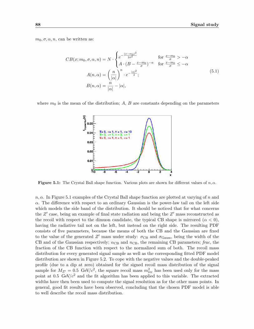
88 Signal study
m0, σ, α, n, can be written as:
CB(x;m0, σ, α, n) = N ·
e−(x−m0)
2
2σ2 for x−m0σ > −α
A · (B − x−m0σ )−n for x−m0
σ ≤ −α
A(n, α) =
(n
|α|
)n· e−
|α|22 ;
B(n, α) =n
|α|− |α|,
(5.1)
where m0 is the mean of the distribution; A, B are constants depending on the parameters
Figure 5.1: The Crystal Ball shape function. Various plots are shown for different values of n, α.
n, α. In Figure 5.1 examples of the Crystal Ball shape function are plotted at varying of n andα. The difference with respect to an ordinary Gaussian is the power-law tail on the left sidewhich models the side band of the distribution. It should be noticed that for what concernsthe Z ′ case, being an example of final state radiation and being the Z ′ mass reconstructed asthe recoil with respect to the dimuon candidate, the typical CB shape is mirrored (α < 0),having the radiative tail not on the left, but instead on the right side. The resulting PDFconsists of five parameters, because the means of both the CB and the Gaussian are fixedto the value of the generated Z ′ mass under study: σCB and σGauss, being the width of theCB and of the Gaussian respectively; αCB and nCB, the remaining CB parameters; frac, thefraction of the CB function with respect to the normalized sum of both. The recoil massdistribution for every generated signal sample as well as the corresponding fitted PDF modeldistribution are shown in Figure 5.2. To cope with the negative values and the double-peakedprofile (due to a dip at zero) obtained for the signed recoil mass distribution of the signalsample for MZ′ = 0.5 GeV/c2, the square recoil mass m2
rec has been used only for the masspoint at 0.5 GeV/c2 and the fit algorithm has been applied to this variable. The extractedwidths have then been used to compute the signal resolution as for the other mass points. Ingeneral, good fit results have been observed, concluding that the chosen PDF model is ableto well describe the recoil mass distribution.

5.1 Signal yield extraction 89
1− 0.5− 0 0.5 1 1.5 2recoil mass squared [GeV]
0
50
100
150
200
250
300
350
400
Eve
nts
/ ( 0
.03
)
=0.5 GeVZ'M
cb_alpha = 1.37 +/- 0.09
cb_n = 0.8 +/- 0.1
cb_sigma = 0.125 +/- 0.005
frac = 0.64 +/- 0.02
g_sigma = 0.52 +/- 0.02
=0.5 GeVZ'M
0 0.5 1 1.5 2 2.5 3recoil mass [GeV]
0
10
20
30
40
50
60
70
80
90
Eve
nts
/ ( 0
.03
)
=1 GeVZ'M
cb_alpha = 1.5 +/- 0.2
cb_n = 1.1 +/- 0.2
cb_sigma = 0.135 +/- 0.009
frac = 0.80 +/- 0.07
g_sigma = 0.31 +/- 0.04
=1 GeVZ'M
1 1.5 2 2.5 3 3.5 4recoil mass [GeV]
0
20
40
60
80
100
120
140
160
Eve
nts
/ ( 0
.03
)
=2 GeVZ'M
cb_alpha = 1.2 +/- 0.1
cb_n = 1.3 +/- 0.2
cb_sigma = 0.066 +/- 0.005
frac = 0.79 +/- 0.10
g_sigma = 0.12 +/- 0.02
=2 GeVZ'M
2.6 2.8 3 3.2 3.4 3.6 3.8 4recoil mass [GeV]
0
10
20
30
40
50
60
70
80
90
Eve
nts
/ ( 0
.015
)
=3 GeVZ'M
cb_alpha = 1.2 +/- 0.5
cb_n = 1.2 +/- 0.2
cb_sigma = 0.04 +/- 0.01
frac = 0.6 +/- 0.3
g_sigma = 0.06 +/- 0.01
=3 GeVZ'M
3.6 3.8 4 4.2 4.4 4.6 4.8 5recoil mass [GeV]
0
20
40
60
80
100
120
140
160
180
Eve
nts
/ ( 0
.015
)
=4 GeVZ'M
cb_alpha = 1.5 +/- 0.1
cb_n = 1.2 +/- 0.1
cb_sigma = 0.031 +/- 0.001
frac = 0.996 +/- 0.004
g_sigma = 0.2 +/- 0.2
=4 GeVZ'M
4.6 4.8 5 5.2 5.4 5.6 5.8 6recoil mass [GeV]
0
20
40
60
80
100
120
140
160
180
Eve
nts
/ ( 0
.015
)
=5 GeVZ'M
cb_alpha = 1.0 +/- 0.2
cb_n = 1.3 +/- 0.1
cb_sigma = 0.016 +/- 0.002
frac = 0.7 +/- 0.1
g_sigma = 0.029 +/- 0.003
=5 GeVZ'M
5.6 5.8 6 6.2 6.4 6.6 6.8 7recoil mass [GeV]
0
20
40
60
80
100
120
140
160
180
200
Eve
nts
/ ( 0
.015
)
=6 GeVZ'M
cb_alpha = 0.8 +/- 0.2
cb_n = 1.6 +/- 0.2
cb_sigma = 0.024 +/- 0.002
frac = 0.60 +/- 0.08
g_sigma = 0.011 +/- 0.001
=6 GeVZ'M
6.8 6.9 7 7.1 7.2 7.3 7.4 7.5 7.6 7.7 7.8recoil mass [GeV]
0
50
100
150
200
250
Eve
nts
/ ( 0
.01
)
=7 GeVZ'M
cb_alpha = 1.23 +/- 0.09
cb_n = 0.92 +/- 0.07
cb_sigma = 0.0090 +/- 0.0006
frac = 0.90 +/- 0.03
g_sigma = 0.033 +/- 0.005
=7 GeVZ'M
7.8 7.9 8 8.1 8.2 8.3 8.4 8.5 8.6 8.7 8.8recoil mass [GeV]
0
100
200
300
400
500
600
700
Eve
nts
/ ( 0
.01
)
=8 GeVZ'M
cb_alpha = 0.57 +/- 0.08
cb_n = 2.3 +/- 0.4
cb_sigma = 0.030 +/- 0.002
frac = 0.39 +/- 0.02
g_sigma = 0.0080 +/- 0.0003
=8 GeVZ'M
Figure 5.2: The recoil mass distribution and the fitted PDF model superimposed (blue line) arereported for every generated signal sample. The contribution of the CB and the Gaussian functionsare shown with a red and green dotted line respectively. The resulting fit parameters are shown in thetop right corner of each graph.

90 Signal study
Toy MC studies
For the validation of the fit, a toy MC study with 1000 samples of 10000 events each hasbeen implemented. The events in each of the toy sample were generated according to theresulting PDF model with parameters fixed to the values extracted from the above describedsignal shape study. By looking at the parameter distributions of the toy MC samples, inparticular the mean, the associated uncertainty and the resulting pull distribution of the twowidths σCB and σGauss for each studied mass point, it is possible to assess that there is nobias in the fit procedure and the uncertainties provided by the fit are correctly estimated.The pull distributions have been fitted with Gaussian functions and since the resulting mean(pullMean) and width (pullSigma) are consistent with 0 and 1 for the studied parameters,the fit algorithm and the chosen PDF model are considered validated and unbiased, and thesignal peak widths can be reliably extracted from this method. All the generated Z ′ masspoints have been tested with this validation procedure and results consistent with normaldistributions are shown in Appendix A in Figure A.2 and in Table A.3 and Table A.4.
5.1.2 Signal width
The selection optimization described in Section 4.4, as well as the signal yield extractionstrategy require to define a signal window for the event counting. The optimal value for thesignal window width as optimized by maximizing the FOMPunzi is found to be 4σ, where σis the computed signal resolution as a function of the recoil mass. The width of the masswindow is thus a function of the signal peak width for each simulated recoil mass distribution,taking into account the different contributions of the CB and Gaussian functions and it iscalculated according to formula:
σw =√
frac× σ2CB + (1− frac)× σ2
Gauss, (5.2)
using as input values for each mass point the σCB, σGauss and frac from the fit results shownin Figure 5.2. The weighted widths computed for every generated Z ′ mass point are given inTable 5.1 and shown in Figure 5.3 as a function of the generated Z ′ mass, MZ′ .
5.2 Recoil mass resolution
The recoil mass resolution may differ in real data from what observed in the simulation dueto unknown detector effect and it is necessary to validate the signal resolution results on realdata control samples, taking care not to unblind the signal recoil mass distribution in data.The strategy is to measure the recoil mass resolution on data by selecting a pure sample ofe+e− → µ+µ− γ events, where the presence of the photon prevents any unblinding issue,and then compare to MC results on the same simulated process. The control sample on realdata and on simulated events has been selected by applying the same analysis requirementsas described in Section 4.3 for steps 1, 2, 3, 4 and 6, while the selection 5 has been reversed,by explicitly requiring the presence of a photon within a 15 cone with respect to the recoilmomentum direction. In addition, to reject contamination from radiative τ pair events, itwas required that the sum of the energies of the two muons and of the photon lies between10 and 12 GeV and no additional photons with energy larger than 100 MeV are detected inthe event.

5.2 Recoil mass resolution 91
Figure 5.3: The signal width σw computed according to Equation 5.2 is shown as a function of thegenerated Z ′ mass.
Table 5.1: The weighted width for every generated Z ′ mass point has been computed according toEquation 5.2 and with the fit results given in Figure 5.2.
MZ′ [GeV/c2] σw [GeV/c2]
0.5 0.3257± 0.01151.0 0.1844± 0.01381.5 0.1089± 0.00752.0 0.0799± 0.00602.5 0.0667± 0.00503.0 0.0504± 0.00553.5 0.0398± 0.00334.0 0.0335± 0.00314.5 0.0278± 0.00285.0 0.0245± 0.00195.5 0.0174± 0.00076.0 0.0175± 0.00176.5 0.0147± 0.00157.0 0.0132± 0.00127.5 0.0182± 0.00088.0 0.0149± 0.0009
The selected events on both data and MC samples are then weighted to match the kine-matic distribution expected for the signal process. The weights have been produced from thebidimensional muon momenta distribution in 0.5 GeV × 0.5 GeV bins for e+e− → µ+µ− Z ′
events at different Z ′ masses ( distributions are reported in Figure 5.4) and then applied to
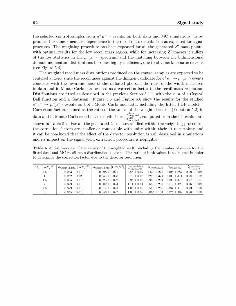
92 Signal study
the selected control samples from µ+µ− γ events, on both data and MC simulations, to re-produce the same kinematic dependence in the recoil mass distribution as expected for signalprocesses. The weighting procedure has been repeated for all the generated Z ′ mass points,with optimal results for the low recoil mass region, while for increasing Z ′ masses it suffersof the low statistics in the µ+µ− γ spectrum and the matching between the bidimensionaldimuon momentum distributions becomes highly inefficient, due to obvious kinematic reasons(see Figure 5.4).
The weighted recoil mass distributions produced on the control samples are expected to becentered at zero, since the recoil mass against the dimuon candidate for e+e−→ µ+µ−γ eventscoincides with the invariant mass of the radiated photon: the ratio of the width measuredin data and in Monte Carlo can be used as a correction factor to the recoil mass resolution.Distributions are fitted as described in the previous Section 5.1.1, with the sum of a CrystalBall function and a Gaussian. Figure 5.5 and Figure 5.6 show the results for the studiede+e− → µ+µ−γ events on both Monte Carlo and data, including the fitted PDF model.Correction factors defined as the ratio of the values of the weighted widths (Equation 5.2) in
data and in Monte Carlo recoil mass distributions,σdataweighted
σMCweighted
, computed from the fit results, are
shown in Table 5.2. For all the generated Z ′ masses studied within the weighting procedure,the correction factors are smaller or compatible with unity within their fit uncertainty andit can be concluded that the effect of the detector resolution is well described in simulationsand its impact on the signal yield extraction procedure is negligible.
Table 5.2: An overview of the values of the weighted width including the number of events for thefitted data and MC recoil mass distributions is given. The ratio of both values is calculated in orderto determine the correction factor due to the detector resolution.
MZ′ [GeV/c2] σweighted,data [GeV/c2] σweighted,MC [GeV/c2]σweighted,data
σweighted,MCNevents,data Nevents,MC
Nevents,data
Nevents,MC
0.5 0.263± 0.012 0.298± 0.021 0.88± 0.07 4432± 275 4498± 287 0.99± 0.091 0.282± 0.020 0.355± 0.028 0.79± 0.08 4220± 374 4309± 371 0.98± 0.12
1.5 0.305± 0.018 0.325± 0.022 0.94± 0.08 3958± 291 4099± 375 0.97± 0.112 0.329± 0.018 0.302± 0.024 1.11± 0.11 3655± 200 3819± 323 0.96± 0.09
2.5 0.329± 0.013 0.314± 0.023 1.05± 0.08 3510± 236 3787± 313 0.93± 0.103 0.355± 0.010 0.356± 0.027 1.00± 0.08 3065± 134 3575± 392 0.86± 0.10

5.2 Recoil mass resolution 93
Phase 2 Data
0 1 2 3 4 5 6 7 8 momentum [GeV] / (80 MeV)+µ
0
1
2
3
4
5
6
7
8 m
omen
tum
[GeV
] / (
80 M
eV)
- µPhase 2 Data Z' mass=500MeV
0 1 2 3 4 5 6 7 8 momentum [GeV] / (80 MeV)+µ
0
1
2
3
4
5
6
7
8
mom
entu
m [G
eV] /
(80
MeV
)- µ
Z' mass=500MeV
Z' mass=1000MeV
0 1 2 3 4 5 6 7 8 momentum [GeV] / (80 MeV)+µ
0
1
2
3
4
5
6
7
8
mom
entu
m [G
eV] /
(80
MeV
)- µ
Z' mass=1000MeV Z' mass=1500MeV
0 1 2 3 4 5 6 7 8 momentum [GeV] / (80 MeV)+µ
0
1
2
3
4
5
6
7
8
mom
entu
m [G
eV] /
(80
MeV
)- µ
Z' mass=1500MeV
Z' mass=3000MeV
0 1 2 3 4 5 6 7 8 momentum [GeV] / (80 MeV)+µ
0
1
2
3
4
5
6
7
8
mom
entu
m [G
eV] /
(80
MeV
)- µ
Z' mass=3000MeV Z' mass=4000MeV
0 1 2 3 4 5 6 7 8 momentum [GeV] / (80 MeV)+µ
0
1
2
3
4
5
6
7
8
mom
entu
m [G
eV] /
(80
MeV
)- µ
Z' mass=4000MeV
Figure 5.4: Bidimensional distributions of muon momenta for µ+µ−γ events in data (top left), andthe same distributions for simulated events of e+e− → µ+µ− Z ′ processes, for different Z ′ masses, areshown: 0.5 GeV (top right), 1 GeV (middle left), 1.5 GeV (middle right), 3 GeV (bottom left), 4 GeV(bottom right).

94 Signal study
recoil mass squared [GeV2] recoil mass squared [GeV2] recoil mass squared [GeV2]
recoil mass squared [GeV2]recoil mass squared [GeV2]recoil mass squared [GeV2]
Figure 5.5: The weighted MC recoil mass distributions and the fitted PDF model superimposed (blueline) are shown for different Z ′ mass point hypothesis. The contribution of the CB and the Gaussianfunction are highlighted with a red and green dotted line respectively. The resulting fit parametersare provided in the top right corner of each graph.

5.2 Recoil mass resolution 95
recoil mass squared [GeV2] recoil mass squared [GeV2] recoil mass squared [GeV2]
recoil mass squared [GeV2]recoil mass squared [GeV2]recoil mass squared [GeV2]
Figure 5.6: The weighted data recoil mass distributions and the fitted PDF model superimposed(blue line) are shown for different Z ′ mass point hypothesis. The contribution of the CB and theGaussian function are highlighted with a red and green dotted line respectively. The resulting fitparameters are provided in the top right corner of each graph.

96 Signal study

Chapter 6
Data validation studies
The goal of the validation procedure is twofold, first to obtain an estimate of the total back-ground yield based on real data and compare to the result of the Monte Carlo simulationand second, to evaluate on real data the effect of the individual analysis selections optimizedon MC samples as described in Chapter 4 for the candidate reconstruction, the event se-lection and the τ suppression procedure, without unblinding the signal in the data sample.The blind analysis principle still holds and for any control samples mentioned below, carefulchecks to ensure the probability to accidentally reveal the signal is negligible have always beenperformed, as it will be discussed in the following sections.
Three different data validation procedures, each corresponding to a differently selectedcontrol sample, were devised:
ee sample. Beside the Bhabha and eeee backgrounds, this sample is dominated by ττ(γ)events, with both τ ’s decaying to electrons, whose kinematics is almost identical to oneof the the dominant Z ′ analysis background, ττ(γ) events, with both τ ’s decaying tomuons. All the analysis selections, with the exception of the PID requirements, andincluding the τ suppression procedure, can thus be checked. Requiring two identifiedelectrons avoids any unblinding issue since the ECL-based identification of electrons iscomplementary to that used for muons and applied for the signal selection;
µµγ, eµγ, eeγ samples. The presence of a photon with a reconstructed energy above1 (or 1.5) GeV decreases the signal efficiency by a factor ∼ αQED, thus avoiding anyunblinding issue. This sample is particularly useful in checking the low recoil massregion, being dominantly composed by the ISR QED process e+e−→ µ+µ−γ. Theseevents are referred to hereafter as the µµγ sample. Similarly, the eµγ and eeγ samplesare used to cross check the µµγ one;
µµ, eµ samples, after the application of a partially reversed τ suppression procedure.This technique allows to strongly suppress any hypothetical signal contributions, thusleaving an almost unbiased background sample, very similar to the one expected for theZ ′ analysis before the τ suppression procedure, with no unblinding risk.
For these procedures extensive comparisons between data and MC on the most important anal-ysis variables were performed as shown hereafter. Beside checking the overall number of eventsin data and in simulations, for each validation sample, the level of agreement was measured in

98 Data validation studies
three different recoil mass regions, as they correspond, for events with two identified muons,to different sources of contributing background: the low recoil mass region −2 < Mrec < 3GeV/c2, dominated by µµ(γ) processes; the intermediate spectrum for 3 < Mrec < 6 GeV/c2,dominated by ττ(γ) events; the high recoil mass region 6 < Mrec < 11 GeV/c2, dominatedby four-lepton final state events, i.e. e+e− → e+e−µ+µ−.
Unless differently and explicitly stated, data events are selected by requiring the CDCtwo-track trigger (line ffo, known as bit 7 among the Phase 2 trigger options) to be fired,whose efficiency evaluated to be 0.79 in Bhabha events as explained later on in Section 7.2 isused to scale all the expected background MC yields. Samples with electrons or photons witha reconstructed energy above 1 GeV can be triggered by the ECL trigger line hie too, thusproviding the possibility of additional cross-checks on the trigger effects, including alternativemeasurements of the CDC trigger efficiency.
6.1 Data validation with ee sample
The ee sample is selected by applying all the requirements described in Section 4.2 on bothdata and Monte Carlo, except for the PID selection for a loose ECL-based muon candidate,replaced by the loose ECL-based electron candidate requirement, clusterE/p > 0.75. Similarlyfor the analysis steps described in Section 4.3, they have been applied on data and MonteCarlo, by replacing the tight-muon PID requirement with 0.8 < clusterE/p < 1.2 for tight-electron selection. Recoil mass distributions for data and Monte Carlo before the application
Figure 6.1: The recoil mass spectrum for the ee validation and the data/MC ratio as a function ofthe recoil mass in the final binning scheme, before the τ suppression procedure, are plotted.
of the τ suppression procedure are reported in Figure 6.1. The agreement between data andsimulation has been measured and results in a data/MC ratio of 0.97± 0.01 averaged overallthe spectrum. After the application of the τ suppression procedure, 20 events are found in datain the first two recoil mass windows while 18.4 are expected in Monte Carlo. These numberscan be interpreted as a validation of the τ suppression procedure with a statistical precisionof 22%, which is used as input only in the upper limit calculations as described in Section 8.1for assessing the systematic error on the background level knowledge coming from the τ

6.2 Data validation with µ+µ−γ sample 99
suppression procedure. The statistical significance of such a check can be slightly improvedby adding the results coming from the eµ sample, largely dominated by ττ(γ) background,which is also the LFV Z ′ sample. About 5 events are expected from the simulation after theluminosity normalization and assuming a similar number of events in data at the moment ofunblinding, that can be justified from the above measured data/MC agreement, the statisticsfor the combined ee+ eµ sample would bring the statistical uncertainty of the τ suppressionprocedure precision at ≈ 20% level.
Square Recoil Mass
Figure 6.2: Distributions for the µµγ validation sample, in the three analyzed mass ranges (clock-wise): −2 <MZ′< 3, 3 <MZ′< 6 and MZ′> 6. Note for the first recoil mass region for MZ′<3 GeV/c2,the square recoil mass is plotted, to cope with negative reconstructed masses due to resolution effects.
6.2 Data validation with µ+µ−γ sample
The default selection described for the standard Z ′ analysis as explained in Section 4.3 isapplied on data with some modifications: a detected photon in the barrel ECL with a recon-structed energy clusterEγ > 1 GeV has been required; the veto on events with a reconstructedphoton within a 15 cone centered on the recoil momentum direction has been removed; therequirement to have an energy deposit in the cleaned ROE (extraEnergy) smaller than 0.4GeV is replaced by the requirement to have (extraEnergy-clusterEγ) <0.4 GeV, all the rest

100 Data validation studies
clust
er m
atch
ing
CDC
acce
ptan
ce
delta
phi>
90°
bit7
==1
reco
il in
bar
rel
PID
Extra
E
pi0
veto
dim
uon
pt
0.60
0.65
0.70
0.75
0.80
0.85
Data
/MC
Figure 6.3: Data/MC ratio as a function of each selection step for the µµγ validation. The 0.79efficiency correction due to the trigger applies only when the requirement of having the CDC triggerbit fired is effective (from the fourth point on).
being the same as described in Section 4.3. The contributing sources of background are thesame as in the standard Z ′ analysis, but it has to be noticed that the generator AAFH, usedto simulate the eeµµ background, has no ISR implemented. To reduce its importance in theselected control sample and reject this contamination on real data, the direct dimuon masshas been constrained to Mµµ > 3 GeV/c2. Even with such countermeasure, the eeµµ appearsstill relevant, especially for high recoil masses Mrec > 6 GeV/c2 for which other validationsamples are more suitable (see next sections). Recoil variables are always referred to thedimuon system, regardless the presence of a reconstructed photon. Data and Monte Carlorecoil mass distributions are compared after the event selection, before applying the τ sup-pression procedure as shown in Figure 6.2, for the three different mass intervals. Discrepanciesof the order of 30% are visible, with data consistently below Monte Carlo expectations ( finalresults reported in summary Table 6.1 at the end of the chapter). This is particularly evident,for statistical reasons, for the first recoil mass window, largely dominated by the radiativeµµγ QED background. It has been checked if the discrepancy might be originated by theµµγ event generator by producing a special sample with the BabaYaga@NLO generator, whichhas been analyzed through the same analysis chain: differences within 1% level are foundwith respect to the standard KKMC generated sample and therefore it has been concluded thediscrepancy could not be ascribed to the MC generator.
The effect of the individual selections is also studied, as shown in the plot in Figure 6.3,which summarizes the data/MC ratio as a function of the applied selection requirement. Forthe background yield considered in the data/MC ratio, the 0.79 efficiency correction dueto the CDC trigger is applied only at the moment in which the requirement of having theffo bit fired is made on data and applied in the simulation as further selection conditionsthat mimic trigger requirements (fourth point in figure); before that analysis step, a 100%trigger efficiency is assumed, which allows to conservatively study the observed discrepancy.In Figure 6.4,Figure 6.5, Figure 6.6 distributions of the most relevant variables for the analysis

6.2 Data validation with µ+µ−γ sample 101
Figure 6.4: Most relevant angular variables exploited in the analysis are shown for µµγ validationsample, as follows (row order):(1) the Polar angle (in the laboratory frame) of the two muons, positive charge (left), negative charge(right);(2) Azimuthal angle (in the laboratory frame) of the two muons, positive charge (left), negative charge(right).
are shown, from which no evident indication of a possible source of discrepancy comes out:most distributions look reasonably flat within the statistical fluctuations, with the exceptionof the data/MC comparison as a function of the azimuthal track angle (see Figure 6.4). TheCDC trigger line ffo in Phase 2 is known to produce strong φ dependencies due to hardwareissues. The presence of the photon with energy above 1 GeV allows one to measure the CDCtrigger efficiency by using the calorimeter trigger line hie (bit 8) as a reference, which hasbeen systematically checked as reported in Section 6.4. The entire data/MC validation withthe µµγ sample can be repeated by requiring only the ECL trigger line to be fired, and thusruling out the possibility that the observed discrepancy may be ascribed to the CDC triggerφ-dependencies. The result of the ECL trigger cross-check is in agreement with that obtainedwith the CDC trigger ffo, as reported in Table 6.1. The eµγ and eeγ final states have alsobeen studied, using both the CDC ffo trigger and the ECL hie trigger. The eµγ samplecontains much less background from µµ and ee final states, due to the PID requirement, andis dominated by radiative τ -pair production, i.e. e+e−→ τ+τ−γ events. For these validationsamples, when the statistics is high enough, the agreement looks much better than for µµγ

102 Data validation studies
Figure 6.5: Most relevant kinematic variables exploited in the analysis are shown for µµγ validationsample, as follows (row order):(1) Cluster energy of the two muons, positive charge (left), negative charge (right);(2) Ratio of the muon cluster energy and the muon track momentum, positive charge (left), negativecharge (right);(3) Transverse momentum of the two muons, positive charge (left), negative charge (right).
events (see Table 6.1), thus suggesting the possibility that the problem is related to muondetection in Phase 2 data. Being the statistical significance either much higher in the firstrecoil mass window or not very high overall the spectrum for the selected control sample (see

6.3 Data validation with a reversed τ suppression procedure 103
Figure 6.6: Transverse momentum (left) and polar angle (right) of the system recoiling against thetwo muons for the µµγ validation sample.
Table 6.1), a complementary validation procedure able to check the full interesting recoil massregion is required and described in the next Sections.
Ɛsig/(
a/2
+ √
B)
Figure 6.7: Punzi FOM as a function of the recoil mass for the final selection applied in the standardanalysis (green) and with a partially reversed τ suppression procedure (red).
6.3 Data validation with a reversed τ suppression procedure
A partially reversed τ suppression procedure is used to select a background sample veryclose to that expected for the standard analysis of the Z ′ search, for the medium-high recoilmass region. Referring to the procedure described in Section 4.4, the selection on pTµµ is not
considered, while the optimal separation line in the bidimensional pT,lmaxrec versus pT,lminrec planeis used in a reversed way, by accepting only events below it (see for example Figure 4.9),which means rejecting the signal and selecting the background. Any hypothetical Z ′ signal isstrongly suppressed, as shown in Figure 6.7, where the Punzi FOM following the applicationof such a procedure is compared with the one obtained at the end of the standard analysis.The distortion in the recoil mass distribution for the background induced by this procedure,

104 Data validation studies
Figure 6.8: The recoil mass distribution for the µµ sample with a partially reversed τ suppressionprocedure is shown, in the three different mass intervals. The data/MC ratio reported in the insetplots confirms the discrepancy observed in the µµγ analysis.
compared to the one in the analysis before the application of the standard τ suppression, isstudied on the ee sample and found to be negligible.
The partially reversed τ suppression procedure is applied on the µµ and eµ samples afterthe default event selection described in Section 4.3, in order to avoid any unblinding issue.

6.3 Data validation with a reversed τ suppression procedure 105
Figure 6.9: Most relevant angular variables exploited in the analysis are shown for µµ validationsample with a partially reversed τ suppression procedure, as follows (row order):(1) the Polar angle (in the laboratory frame) of the two muons, positive charge (left), negative charge(right);(2) Azimuthal angle (in the laboratory frame) of the two muons, positive charge (left), negative charge(right).
Results of the data/MC ratio on the full recoil mass spectrum gives (0.64 ± 0.02) and (0.90± 0.02) for µµ and eµ respectively and for the µµ sample the comparison between data andMonte Carlo is reported in Figure 6.8, for the three different recoil mass intervals. Theseresults fully confirm the data-Monte Carlo discrepancies observed with the µµγ sample (asummary is provided in Table 6.1 at the end of the chapter).
In analogy with the µµγ case in Figure 6.9, Figure 6.10,Figure 6.11 distributions of theimportant variables for the analysis are shown and no clear hint of a possible source of dis-crepancy comes out, being the data/MC ratio for all the distributions reasonably flat withinthe statistical fluctuations, with the exception of the data/MC comparison as a function ofthe azimuthal track angle (Figure 6.9), as already discussed for the µµγ case.

106 Data validation studies
Figure 6.10: Most relevant kinematic variables exploited in the analysis are shown for the µµ vali-dation sample with a partially reversed τ suppression procedure, as follows (row order):(1) Cluster energy of the two muons, positive charge (left), negative charge (right);(2) Ratio of the muon cluster energy and the muon track momentum, positive charge (left), negativecharge (right);(3) Transverse momentum of the two muons, positive charge (left), negative charge (right).

6.4 Trigger data validation 107
Figure 6.11: Transverse momentum (top) and polar angle (bottom) of the system recoiling againstthe two muons in the µµ validation sample with a partially reversed τ suppression procedure.
6.4 Trigger data validation
As already mentioned in the section regarding the µµγ validation sample, a possible causeof the data - Monte Carlo discrepancies could be the CDC ffo trigger, which had hardwareissues during the Phase 2 data taking. Its efficiency is measured to be 0.79 with Bhabhaevents, using the ECL hie trigger as a reference, as documented in Section 7.2. Two muonevents, due to the small energy depositions in the ECL, cannot be triggered by the ECL hie
line, making the CDC trigger efficiency measurement statistically impossible on such sample.On the other hand, µµγ events as selected in Section 6.2 with photon energies above 1 GeVare able to fire the ECL trigger and thus allow the CDC trigger efficiency measurement, asindependent cross-check of the results provided in Section 7.2. On the µµγ validation sampleselected on data, the ECL trigger hie is required to be fired and the CDC trigger efficiencyis defined as the ratio of the number of events where both the ECL and CDC trigger arefired and the number of triggered events, in which at least the ECL hie trigger fired. Theresult measured on µµγ events gives an efficiency εCDC = 0.747 ± 0.007, to be comparedwith 0.79 evaluated in Section 7.2. Since strong non-uniformities in the azimuthal angledistributions induced by the CDC trigger, as reported in Figure 6.4 and Figure 6.9, could beone of the causes of the data-MC discrepancy observed in both the µµγ and the µµ validationsamples, as additional check the trigger efficiency is measured as a function of the minimumand maximum track azimuth angle in the event, as shown in Figure 6.12: regions of highertrigger efficiencies are selected by requiring φmin < −1 rad and (0.5 < φmax < 2) rad andfor events belonging to these ranges the CDC trigger efficiency is recomputed to be ≈ 0.88.Repeating all the validation analysis on the µµγ sample with this angular selection and usingthe corresponding trigger efficiency for normalization finally gives the same data-Monte Carlodiscrepancy as measured in the µµγ sample without these additional angular selections andno real improvement is observed (results in the summary Table 6.1 ).
Furthermore, changing the energy threshold for the reconstructed photon from 1 GeV to1.5 GeV does not affect the final results. As further validation, the CDC trigger efficiencyis measured also in eµ events, by requiring the presence of an electron with an energy largerthan 1 GeV that can fire the orthogonal ECL trigger: very similar results both in terms

108 Data validation studies
of efficiency and final data-Monte Carlo discrepancy have been found. By using the sametechnique of the conditional probability measured with two orthogonal trigger bits, the ECLtrigger efficiency needed for the LFV Z ′ analysis is also provided, having as a reference theCDC trigger, in the µµγ sample and in the eµ sample. Photon and electron reconstructedenergies are required to be above 1.5 GeV in both cases. The results are consistent in bothsamples and give εECL = 0.96± 0.01, where the uncertainty is statistical only.
3 2 1 0 1min_Z0_mue_phi [rad]
0.4
0.5
0.6
0.7
0.8
0.9
1.0
ffo tr
igge
r effi
cienc
y
1.0 0.5 0.0 0.5 1.0 1.5 2.0 2.5 3.0max_Z0_mue_phi [rad]
0.5
0.6
0.7
0.8
0.9
1.0
ffo tr
igge
r effi
cienc
y
Figure 6.12: CDC trigger efficiency as a function of the minimum (left) and the maximum (right)track azimuth angle in µµγ events.
6.5 Data validation summary
The outcome of all data validation procedures discussed in the previous sections are summa-rized in Table 6.1. The results look coherent and point to a data-Monte Carlo discrepancyof ≈ −35% for µµ events, which indicates the efficiency before τ suppression selection is 35%lower in data than in simulation. Similarly for the eµ events, the yield measured in databefore the τ suppression procedure is −10% the yield measured in the simulation. The −10%data-MC discrepancy in eµ events is explained by the tracking inefficiency, as evaluated inSection 7.4. Therefore it is accounted as a measured inefficiency and the simulated samplesare simply rescaled by 0.90 to match the yield observed in data control samples. No system-atic uncertainty due to this discrepancy is additionally assigned to the eµ events, since it isalready accounted for in the systematic uncertainty ascribed to the tracking performance (seeSection 7.4). For the standard Z ′ search, the results of the data validation studies consistentlypoint to a residual −25% unexplained deficit in the two-muon event yield observed in datawith respect to the simulated background yield, which must be managed both in the back-ground and signal efficiency estimate and in the evaluation of the systematic uncertainty inthe background yield and in the signal efficiency, as it will be explained in the next chapters.
A deep investigation has been performed to understand the nature of such a discrepancy,but nothing relevant is found. The most probable explanation is related to the difficultiesin muon detection experienced on several sides, in the trigger, tracking performances and inthe ECL-based identification, that are expected to be cured in the Belle II 2019 data set.

6.5 Data validation summary 109
Moreover, Phase 3 data sets will rely on a recovered KLM detector and a generally improvedtracking system due to the full VXD in place and no actual issues are expected on muondetection from the preliminary performance studies on the new 2019 data. For the Phase 2data analysis, to correctly and reliably account for the outcome of the data validation study,the background predictions from the simulation and the signal efficiency are corrected with ascaling factor of 0.65 for µµ events, as further discussed in Chapter 8, where the associatedsystematic uncertainties will be also explained.

110 Data validation studies
Tab
le6.1
:S
um
mary
of
the
validatio
nstu
dies
for
the
data
/M
onte
Carlo
ratio
on
the
vario
us
sam
ples.
Th
esecon
drow
show
sth
etrigger
line
used
inth
ecorresp
ond
ing
stud
y:
herea
fterth
eC
DC
ffo
trigger
line
isd
efin
edas
bitCDC
an
dth
eE
CLhie
triggerlin
eas
bitECL
.D
ata/MC
ratios
are
show
nfo
rth
reed
ifferen
treco
ilm
assin
tervals
an
dfo
rth
eto
tal
mass
ran
ge.
Mass
win
dow
[GeV/c
2]µµγ
µµγ
eµγ
eµγ
eeγeeγ
µµ
+an
tiτ
eµ+
antiτ
-b
itCDC
bitECL
bitCDC
bitECL
bitCDC
bitECL
bitCDC
bitCDC
-2÷
30.65±
0.020.67±
0.020.8±
0.31.3±
0.30.88±
0.010.99±
0.010.66±
0.060.94±
0.073÷
60.84±
0.070.76±
0.070.9±
0.10.95±
0.131.10±
0.101.14±
0.010.65±
0.020.89±
0.036÷
110.9±
0.1
0.72±0.13
0.9±0.2
0.93±0.15
2.13±0.12
1.3±0.1
0.63±0.03
0.89±0.03
Overa
ll0.68±
0.020.68±
0.020.92±
0.090.96±
0.100.90±
0.010.99±
0.010.64±
0.020.90±
0.02
Chapter 7
Detector studies and systematicuncertainty evaluation
In this chapter the evaluation of the main sources of systematic uncertainty which affect themeasurement of the signal cross section and need to be taken into account for the upperlimit calculation is discussed (Section 7.1). The systematic uncertainties come either fromdetector effects, as in resolutions and in efficiencies that have to be measured on real data,and from the differences between the simulation, used for analysis optimization and for thesignal efficiency estimation, and data. Both types of contributions need to be estimated withdedicated performance and data validation studies.
The validation procedure already allowed to estimate the residual discrepancy observedbetween Monte Carlo and data, after the corrections for the measured efficiencies have beenapplied. This chapter will provide the overview of the methods developed to measure theseefficiencies with their associated systematic uncertainties. Hereafter, the main results of thesestudies (Section 7.2, 7.3, 7.4), which have been described in details elsewhere in dedicatedtechnical notes (see Appendix B), are reported. In the final Section 7.4 the measurementof the discrepancy in the track reconstruction efficiency on data and Monte Carlo will beaddressed in more details, since it has been crucial to partially explain the observed deficit indata-MC comparisons. This study has been one of my major tasks for the Z ′ project, as wellas the full validation procedure developed for the presented search.
7.1 Main systematic uncertainty sources
In each recoil mass bin, the Z ′ cross section can be computed from the measured event yieldaccording to the formula:
σZ′ =Nobs −Bexp
L× εsig, (7.1)
where the inputs are the number of observed events Nobs; the effective data integrated lu-minosity L; the signal efficiency εsig and the expected total background yield Bexp, whichare both computed from the simulated samples, but corrected for the data-MC discrepancyobserved in the validation studies. Their associated systematic uncertainties contribute tothe total systematic error in the measured cross sections, which has to be accounted for when

112 Detector studies and systematic uncertainty evaluation
computing the expected sensitivity (see Section 8.1, the details of the computation are givenin Appendix C.1).
Systematic uncertainty in the luminosity measurement
The effective luminosity L refers to the integrated data luminosity of the runs on whichthe trigger information could be retrieved and whose trigger efficiency could be measured,as explained in Section 7.2. The offline luminosity measurement in Phase 2 is performedindependently on two different samples, radiative Bhabha and two-photon events. The overallmeasurement strategy and the techniques to estimate the associated uncertainty are explainedin the Belle II paper for the offline luminosity measurement in [86]. The relative systematicuncertainty which is taken into account for the upper limit calculation is 1.5%.
Systematic uncertainty in the signal yield
The systematic uncertainty in the number of observed events receives contributions fromthe applied signal yield extraction technique, which relies on a specific signal model for theestimation of the signal width. Dedicated studies reported in Chapter 5 have shown that theimplemented fit procedure to extract the signal width, which is crucial for the binning schemedefinition, is robust and unbiased. Moreover, the detector resolution effect is correctly takeninto account in the simulations and has no additional impact on the estimation of the signalwidth and thus its systematic uncertainty contribution is found to be negligible.
Systematic uncertainty in the background yield
As far as the expected background yield is concerned, its contribution to the systematicuncertainty is mainly due to the effect of the applied selections and to the residual discrepancyobserved between data and Monte Carlo that has been measured on the validation controlsamples. It can be attributed to different sources, as the difference in the track reconstructionefficiency evaluated on data and on simulations and the muon detection in Phase 2 data,which also affect in a totally correlated way the signal efficiency.
After rescaling the expected background yield for the measured data-MC discrepancy asdescribed in the previous chapter, the difference between the simulated number of eventsand the number of events observed in the recoil mass spectrum on data with a reversed τsuppression procedure has been taken as systematic uncertainties on the expected backgroundyield and it is assessed to be 2%.
The τ suppression procedure adds a further contribution to the systematic uncertainty onthe expected background yield, which is driven by the low statistics of the control samplesin data and is evaluated to be 22% from the ee control sample as explained in Section 6.1.However, this uncertainty is not the dominant one when propagating on the signal crosssection computation, since the background yield enters the formula in Equation 7.1 as asubtraction and therefore the associated error is not multiplicative in the estimation of thefinal uncertainty. Moreover, it is statistically driven, therefore it is expected to further reducewith larger data sets.

7.1 Main systematic uncertainty sources 113
Systematic uncertainty in the selection efficiencies
The main source of systematic uncertainty comes from the estimate of the signal efficiency,which receives contributions from the trigger efficiency, the track reconstruction efficiency, theparticle identification efficiency, as well as from the applied requirements for background re-jection (τ suppression procedure). Regarding the latter, its contribution is evaluated throughthe validation procedure (see previous chapter). For the above mentioned efficiencies, a fullprogram of performance studies has been devised on Phase 2 data. In the following sections,the strategy overviews and the results important for this analysis are reported.
Systematic uncertainty summary
A summary of the systematic uncertainty contributions accounted for in the 90% CL exclu-sion upper limit computation is shown in Table 7.1. The systematic uncertainties due totrigger efficiency, tracking efficiency and particle ID selections are considered to affect in acompletely correlated way the signal efficiency and the background yields and similarly forthe luminosity measurement uncertainty, it is assumed to affect in a completely correlatedway the background expectations.
Table 7.1: Systematic uncertainties affecting the µµ and eµ samples, referred to the standard andLFV Z ′, respectively.
Source Affected quantity µµ eµ
Trigger efficiency εsig 6% 1%Tracking efficiency εsig 4% 4%
PID εsig 4% 4%Luminosity L 1.5% 1.5%
τ suppression (background) Bexp 22% 22%Background before τ suppression Bexp 2% 2%Discrepancy in µµ yield (signal) εsig 12.5% -
The data validation procedure has shown a ≈ −35%(10%) discrepancy between data andsimulations for the µµ(eµ) sample, of which ≈10% can be ascribed to the tracking inefficiency.Therefore, while for the eµ sample the full observed discrepancy is understood and explainedby means of performance measurements, for the µµ sample after all the performed studies,no evident explanation could be advocated to explain the residual −25% deficit observed indata when comparing to simulation. Therefore, both the background level and the signalefficiency for the µµ case have been scaled by the factor 0.65 to match MC expectationsto what observed in data and different systematic uncertainties have been assigned to thebackground yields and the signal efficiency, according to the following strategies:
the validation procedure with a reversed τ suppression selection (see Section 6.3) isassumed to provide a reliable estimate of the expected background yield and thus thestatistical uncertainties of this measurement, ±2% (Table 6.1), is assigned as associatedsystematic error, and later on confirmed from the results of the background measure-ment on real data (no reverse τ suppression applied, Figure 8.4), after the approval forunblinding;

114 Detector studies and systematic uncertainty evaluation
an additional systematic uncertainty is assigned to the total number of expected back-ground events only, due to the effect of the τ suppression procedure measured on theee control sample within a statistical accuracy of 22%. This statistical error is thenassigned as systematic uncertainty in the background yield; no systematic uncertaintydue to this effect is considered on the signal efficiency, as this selection is quite mildon the Z ′ side and the distributions on which it is based are well reproduced in thesimulation;
half the size of the discrepancy coming from an unknown source (residual−25% data-MCdiscrepancy) is assigned as a systematic uncertainty in the signal efficiency of ±12.5%.Unlikely to what has been devised for the uncertainty in the background yields due tothe τ suppression procedure (previous point), where the measured data-MC discrepancyis fully used as systematic uncertainty (100% of the dominating statistical error), since itapplies directly to the measured background level, the quoted 12.5% uncertainty in thesignal efficiency corresponds to 50% the measured unknown residual discrepancy in themuon yields. This choice is motivated by the fact that this systematic contribution refersto a correction factor (the 0.65 scaling applied to the efficiency), not directly to the data-MC difference itself. This is an arbitrary and widely established choice, commonly usedin most of the correction procedures applied in high energy physics analyses. It is forexample analogous to what usually happens for PID correction factors, where the bin-by-bin correction extracted from the measured MC-data discrepancy on well defined controlsamples (e.g. thanks to PID table as a function of the main kinematical distributions) isapplied to the simulation and half of the measured discrepancy is additionally associatedas systematic uncertainty in the selection efficiency due to the correction factor applied.Though this is an arbitrary choice, every step of the applied procedure has been clarifiedto the reader, who is thus fully informed on how the measured discrepancy affects theresult.
A summary of the studies of detector effects and systematic uncertainties mentioned in thischapter is reported in the next sections. These studies refer to the standard Z ′ case only,unless where LFV Z ′ is explicitly mentioned.
7.2 Trigger efficiency
Two different trigger lines have been used for the standard and LFV Z ′: the CDC two-tracktrigger and the ECL trigger respectively. The performances of the CDC two-track triggerare studied on data samples selected by means of orthogonal ECL lines. The CDC triggercorresponds to what has been defined in Table 6.1 as trigger bitCDC to underline whichdetector is used to send the trigger. The trigger bitCDC selects non-Bhabha events with atleast two tracks in the CDC acceptance, with opening angle in φ-plane of at least 90°. Toemulate the effects of the trigger selection in simulations, the same criteria required to firethe CDC trigger on data have been added as a part of the event selection (see Section 4.3).The trigger selection efficiency is evaluated with respect to the orthogonal ECL trigger line(bitECL) and it is computed as the ratio between the events which fired both the triggers and

7.3 Particle ID selection 115
the events firing at least the ECL trigger:
εCDC =N(bitCDC AND bitECL)
N(bitECL). (7.2)
It has been found that εCDC varies from runs to runs (the interested reader could see thededicated trigger performance study summarized in Appendix B.1) and to ensure a reliableand stable estimate of the trigger efficiency only runs where the CDC trigger efficiency isvalidated and is higher than 50% have been used for this work. The final trigger efficiency isdefined as the average of efficiencies measured in good runs weighted with the luminosity ofthe corresponding run and gives (79.0 ± 0.1)% for a total integrated luminosity of 276 pb−1,where the uncertainty is statistical only. The systematic uncertainty in the trigger efficiencydue to kinematic dependencies has also been evaluated as the relative variation of the averageefficiency in bins of polar angle, transverse momentum, and number of track hits in theCDC. A 6% variation has been measured and it is assigned as systematic uncertainty in themeasurement of εCDC .
The LFV Z ′ search exploits Phase 2 data selected by the ECL trigger. As this is validatedwith the use of the two-track CDC trigger, the same integrated luminosity of 276 pb−1 isconsidered. The performances of the ECL trigger line have been studied using e+e− → µ+µ−γevents selected with the CDC two-track trigger for photon energies larger than 1 GeV andthe corresponding plateau efficiency is found to be (96 ± 1)%, flat in the ECL barrel region(see Sections 6.4).
7.3 Particle ID selection
Due to the already mentioned problem with the KLM firmware during Phase 2, no KLM-basedmuon identification variables are available for such data set, and the particle identification isperformed through selections based on ECL variables (Section 4.2 and 4.3). The performanceof these selections has been studied in a dedicated technical note, as reported in Appendix B.2.The efficiency of the particle identification selections has been estimated with a self-taggingtechnique on e+e−→ e+e−µ+µ− events on data and simulations. The deviation from unit ofthe measured correction factor, defined as the ratio of efficiencies computed on data and onsimulations, is assigned as systematic uncertainty. In the fiducial kinematic region consideredfor this analysis, which corresponds to the ECL barrel region, the data-MC discrepancies pertrack have been measured to be of order 2%. A systematic uncertainty of 4% is assigned toboth the signal efficiency and the total background yield due to the particle ID selection, wherethe error propagation assumes a 100% positive correlation between the two track probabilities.Though this is a conservative choice that may lead to overestimate the systematic uncertaintycontribution, it has been tested that assuming no correlation and thus a reduced systematic of√
2σtrack = 2.8% has a negligible impact on the computation of the final result (see Section 8.1)and therefore the conservative approach has been preferred.
7.4 Tracking efficiency
The tracking efficiency has been measured by using tag-and-probe techniques in radiativeBhabha events and in e+e−→ τ+τ− events, for the latter exploiting a particular topology,

116 Detector studies and systematic uncertainty evaluation
known as 3x1-prong decay 1. The inefficiency of the tracking system was found to amount to10% for two-track final states, with a 4% systematic uncertainty due to kinematic dependen-cies. Since the tracking efficiency study has been crucial to understand part of the observeddata-MC discrepancy, the rest of the Section will be dedicated to explain the strategy andthe main findings of the second method mentioned above, which exploits the e+e−→ τ+τ−
event topology to infer the existence of a track and measure the detection efficiency of thetrack reconstruction algorithms in both real data and simulations.
The e+e− → τ+τ− process provides an ideal test-bed for the performance of track re-construction algorithms. The cross section for τ -pair production is large and close to thatof B meson pairs at the Υ (4S) resonance energy. In addition, the jet-like topology of τ de-cay products is suitable to study tracking performance in a low multiplicity but high-densitytrack environment. Moreover, the τ -pair kinematics cover a lower track momentum regioncompared, for example, to Bhabha events.
The tracking efficiency is measured using a tag-and-probe method, similar to the onedeveloped previously by the BABAR collaboration [94]. The method targets e+e− → τ+τ−
events, where one τ lepton decays leptonically (τ → `±ν`ντ , ` = e, µ) while the other decayshadronically into three charged pions (τ → 3π±ντ + nπ0). These decays will be referred to,hereafter, as the 1-prong and 3-prong τ -decays, respectively.
Two channels according to the origin of the track from 1-prong τ -decay have been defined:
electron channel — the 1-prong track originates from an electron (τ → e±νeντ ).
muon channel — the 1-prong track originates from a muon (τ → µ±νµντ ) or fromτ → π±ντ + nπ0.In fact, this channel contains a sizable contribution from τ hadronic decays where the 1-prong track originates instead from a charged pion, due to the high misidentification ratefor erroneously identify a pion as a muon. In Phase 2 data, with no muon ID available,it is not possible to distinguish between muons and pions being the ECL-based selectionfor muons the same as for pions.
The tree-level Feynman diagram for the targeted process can be seen in Figure 7.1.Three good quality tracks with total charge ±1 are used to tag τ -pair events, in which
the existence of the additional fourth track can be inferred from charge conservation, since inthe event the total charge must equal to zero. This allows to probe the tracking performanceand to compute the per track reconstruction efficiency εtrack defined by:
εtrack =N4
N3 +N4, (7.3)
where εtrack also include the detector acceptance factor; N4 is the number of events whereall four tracks are found, while N3 is the number of events where the fourth track is notfound. The N4 and N3 samples will be referred to, hereafter, as the 4- and 3-track samples,respectively. Note that the 3-track sample do always include the 1-prong side track.
When performing physics analyses, it is essential to measure the tracking efficiency indata and compare to the results of the same measurement on the MC simulations for two
1The 3x1 prong topology refers to a specific final state of the process e+e−→ τ+τ− where one τ decaysleptonically to one charged lepton and its associated neutrino, and the other decays hadronically with exactly3 charged pions among its decay products.
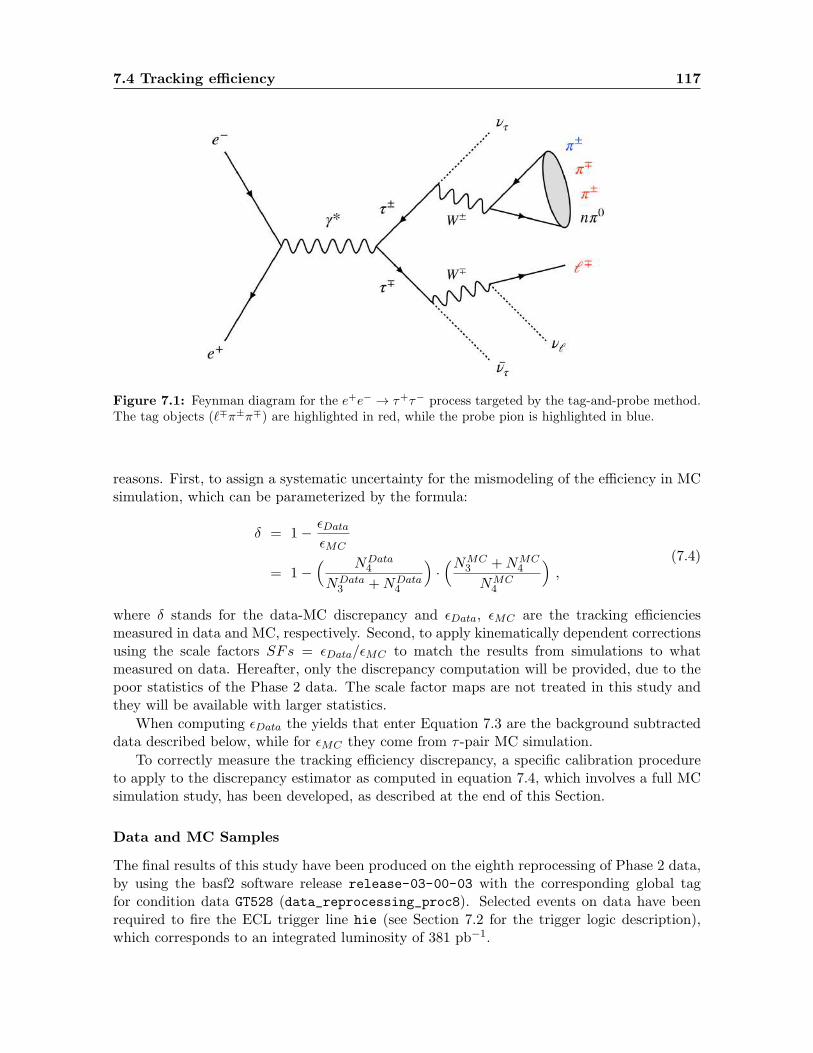
7.4 Tracking efficiency 117
Figure 7.1: Feynman diagram for the e+e− → τ+τ− process targeted by the tag-and-probe method.The tag objects (`∓π±π∓) are highlighted in red, while the probe pion is highlighted in blue.
reasons. First, to assign a systematic uncertainty for the mismodeling of the efficiency in MCsimulation, which can be parameterized by the formula:
δ = 1− εDataεMC
= 1−( NData
4
NData3 +NData
4
)·(NMC
3 +NMC4
NMC4
),
(7.4)
where δ stands for the data-MC discrepancy and εData, εMC are the tracking efficienciesmeasured in data and MC, respectively. Second, to apply kinematically dependent correctionsusing the scale factors SFs = εData/εMC to match the results from simulations to whatmeasured on data. Hereafter, only the discrepancy computation will be provided, due to thepoor statistics of the Phase 2 data. The scale factor maps are not treated in this study andthey will be available with larger statistics.
When computing εData the yields that enter Equation 7.3 are the background subtracteddata described below, while for εMC they come from τ -pair MC simulation.
To correctly measure the tracking efficiency discrepancy, a specific calibration procedureto apply to the discrepancy estimator as computed in equation 7.4, which involves a full MCsimulation study, has been developed, as described at the end of this Section.
Data and MC Samples
The final results of this study have been produced on the eighth reprocessing of Phase 2 data,by using the basf2 software release release-03-00-03 with the corresponding global tagfor condition data GT528 (data_reprocessing_proc8). Selected events on data have beenrequired to fire the ECL trigger line hie (see Section 7.2 for the trigger logic description),which corresponds to an integrated luminosity of 381 pb−1.
118 Detector studies and systematic uncertainty evaluation
For the simulation of the signal and background processes, the official MC11 productionswere used (Table 7.2), which were produced with the nominal beam background conditions.Apart from the signal process e+e− → τ+τ−, the analyzed MC samples correspond to the mainsources of background expected for this study, which include the continuum hadronizationprocesses e+e− → qq, with q = u, d, s, c, the two-lepton (Bhabha, dimuon) and two-pionradiative final-state processes and the four-lepton final state events.
Table 7.2: Summary of the simulated samples used in this study.
Process Cross section Number of events(ECM = Υ (4S))
e+e− → τ+τ− 0.92 nb 36.8 ×10⁶
e+e− → qq 3.69 nb 7.38 ×10⁶
(q = u, d, s, c)e+e− → e+e−γ 300 nb 10 ×106
e+e− → µ+µ−γ 1.148 nb 10 ×106
e+e− → e+e−e+e− 39.7 nb 50 ×106
e+e− → e+e−µ+µ− 18.9 nb 40 ×106
e+e− → π+π−γ 0.03 nb 10 ×106
Trigger
For both the electron and muon τ -decay channels, events in data are required to fire the ECLtrigger bitECL, which has the lowest Level 1 energy threshold among the ECL triggers (1GeV) and includes a Bhabha veto requirement. CDC triggers were also considered, howeverthey were shown to have a lower efficiency and to be correlated by construction to the trackreconstruction efficiency itself, since they rely on the detection of CDC-tracks. Therefore theywere discarded and only used as orthogonal trigger lines to measure the ECL trigger efficiency.
A significant fraction of runs in Phase 2 are missing the ECL trigger information. Becauseof this, only 381 pb−1 of the available 504 pb−1 data set is usable after the ECL triggerrequirement.
In order to measure the ECL trigger efficiency in data, an orthogonal reference trigger(bitCDC) is used:
εECL =N(bitCDC AND bitECL)
N(bitCDC), (7.5)
where the reference trigger requires at least two CDC tracks with an opening angle largerthan 90 and a Bhabha veto requirement.
Figure 7.2 shows the measured ECL trigger efficiency in data as defined in equation 7.5.In this figure, all requirements that will be described below regarding the offline selections areapplied, excluding the invariant mass selections, which were dropped to improve the usablestatistics for this measurement.
Muons deposit less energy in the ECL compared to electrons, so it is more likely for eventsin the muon channel to have a total ECL energy value below the 1 GeV trigger threshold. Thiscan be seen in Figure 7.2, where the ECL trigger efficiency in the muon channel is ∼ 10-20%lower than in the electron channel.

7.4 Tracking efficiency 119
[deg]1-prong
labφ
150− 100− 50− 0 50 100 150
trig
ger
Dat
a∈
0.7
0.75
0.8
0.85
0.9
0.95
1
1.05
1.1 sample 4N
sample3N
2019 (Preliminary)Belle II
-1dt = 381 pbL∫Data (proc8),
[deg]1-prong
labφ
150− 100− 50− 0 50 100 150
trig
ger
Dat
a∈
0.7
0.75
0.8
0.85
0.9
0.95
1
1.05
1.1 sample 4N
sample3N
2019 (Preliminary)Belle II
-1dt = 381 pbL∫Data (proc8),
Figure 7.2: The measured ECL trigger efficiency in data as a function of the 1-prong track φ for theelectron channel (left) and the muon channel (right). The 4- and 3-track samples are shown in blueand red, respectively.
Track selections
Since in the tag-and-probe approach τ -pair events are tagged by the presence of three goodquality tracks with total charge equal to ±1, it is important to define the different classesof selected tracks for this analysis: three categories of tag tracks depending on whether theyoriginates from a pion, electron or muon have been exploited. Regarding the probe track,which belongs to a fourth separate category, a looser pion selection is also defined. The se-lections that define these four classes of tracks are summarized in Table 7.3. Depending
Table 7.3: Track selection criteria are listed below. The selection value which refers to the muonchannel only is indicated in square brackets. Any selections that do not apply to a particular tracktype are indicated by a dash.
Track class Probe pion Tag pion Tag electron Tag muon
pT [MeV] − > 200 [400] > 200 > 400cosθ (-0.8660, 0.9565) (-0.8660, 0.9565) (-0.8660, 0.9565) (-0.8660, 0.9565)|dz| [cm] < 5 < 5 < 5 < 5|dr| [cm] < 1 < 1 < 1 < 1Ecluster
p < 0.8 (0, 0.6) (0.8, 1.2) (0, 0.4)
Ecluster [MeV] − > 0 > 0 (0, 400)nCDCHits − > 0 > 0 > 0
on the channel and sample, events are required to satisfy different track multiplicity require-ments, summarized in Table 7.4. Note that the muon track selections are a subset of the tagpion selections, and that both are a subset of the probe pion selections. Due to the Ecluster
prequirement, the electron track selections are orthogonal to the other track types. Events areallowed to contain additional tracks that fail each of the four track selection criteria definedin Table 7.3.

120 Detector studies and systematic uncertainty evaluation
Table 7.4: Track multiplicity criteria for the tagged event reconstruction are listed below. Anyselections that do not apply to a particular channel and sample are indicated by a dash. Note thatthe muon and pion tag tracks are contained in the probe pion track ensemble, by definition of therespective track lists (see above Table 7.3).
Nprobepion N tag
pion N tagelectron N tag
muon
electron channel, 4-track sample 3 ≥ 2 1 −electron channel, 3-track sample 2 2 1 −muon channel, 4-track sample 4 ≥ 3 − ≥ 1
muon channel, 3-track sample 3 3 − ≥ 1
Background suppression
After requiring events to pass the trigger and track selection requirements, there is still sub-stantial background contamination coming mainly from the QCD continuum (e+e− → qq,q = u, d, s, c) and radiative dilepton processes (e+e− → `+`−γ, ` = e, µ). Additional selec-tions are applied to suppress the background contributions. Hereafter, the two tag-tracksfrom the 3-prong τ -decay will be referred to as the 2-prong tracks.
angular isolation: the τ leptons are produced back-to-back in the CM frame. Theirmomentum in this frame is approximately 2.8 GeV/c such that in most of the cases thedecay products momenta are very collimated along the direction of flight of the parent τand almost back-to-back, with a large angular separation. To exploit this topology, the1-prong track is required to have an opening angle in the CM frame with each 2-prongtracks that is at least 120;
1-prong momentum: the 1-prong track is required to have a CM frame momentumthat is less than 80% and more than 20% of the beam energy. The upper thresholdsignificantly reduces the radiative dilepton background, while the lower threshold helpsto suppress the QCD continuum;
invariant mass: the invariant mass of the 2-prong tracks (mππ) is required to satisfy:
– |mππ − mρ| < 100 MeV, for events where the 2-prong tracks have opposite-signelectric charge (OS charge). This targets hadronic τ -decays with an intermediateρ meson (ρ→ π+π−), and significantly reduces the QCD continuum.
– 300 MeV < mππ < mτ , for events where the 2-prong tracks have same-sign electriccharge (SS charge). This helps to reduce the QCD continuum for SS charge events.
The relevant variables used for background rejection are shown in Figure 7.3 for the MCsamples. Note that only after the angular isolation requirement the 1-prong track is uniquelyidentified per each tagged event, due to the non-orthogonal track lists that are used for themuon channel (muons and tag pions are both sub-ensemble of the probe track list). Beforethis requirement, only with the track selections is not possible to distinguish the 2-prongpions from the 1-prong muon(pion) track. The angular isolation ensures that the candidatemultiplicity in the N3 sample is exactly one, being this crucial to avoid multiple counting. Thishas been checked in both data and simulation. However, multiple N4 candidates per eventare still allowed since they are produced by probe pion tracks which pass all the selections

7.4 Tracking efficiency 121
applied also on the 2-prong pion tracks and therefore the 3-prong side tracks can be mutuallyexchanged. Since the choice of the best candidate would in this case imply a selection on theprobe track and could potentially introduce a bias in the tracking efficiency measurement, allthe possible N4 combinations, which from pure combinatorial counting, without consideringthe charge constraints and the applied track and background reduction selections, could beup to a maximum of three, are accepted and averaged with the weight w = 1/Ncand, whereNcand indicates the event candidate multiplicity after the final selections. Furthermore, anyselections on variables that heavily depend on the existence of the probe track, such as theThrust axis 2 related variables and the total visible energy in the CM frame, have beenavoided. This is because such selections would have significantly different signal efficienciesin the 4- and 3-track samples, and thus bias the tracking efficiency measurement.
s/1pCM2p
0 0.2 0.4 0.6 0.8 1 1.2
Even
ts
0
100
200
300
400
500
600 signal (MC11) ττ bkg (MC11) ττ
qqbar (MC10) bkg other (MC10)
SimulationBelle II
[GeV] 2pM0 0.5 1 1.5 2 2.5 3 3.5 4
Even
ts
0200400600800
10001200140016001800 signal (MC11) ττ bkg (MC11) ττ
qqbar (MC10) bkg other (MC10)
SimulationBelle II
Figure 7.3: Distributions in MC simulation of the 1-prong track momentum in the CM frame relativeto the beam energy
√s/2 (left) and the 2-prong track invariant mass for OS charge events, after the
1-prong momentum cut (right).
Data-MC Comparison
Distributions of the 2-prong track invariant mass are reported in Figure 7.4 and 7.5, for theelectron and muon channels respectively. The distributions of the 1-prong track pT , θ andφ have been also studied and the data/MC ratios have been shown to be flatly distributed.For the 4-track samples they are consistent with 1 within the uncertainty, indicating a goodagreement between simulation and data. For the 3-track samples the data/MC ratios areuniformly distributed around a value above 1, where the fraction of data exceeding unity isdue to the additional inefficiency which affects actual data. All the relevant plots are reportedin Appendix B.3 for the electron and muon channels. All of the requirements previouslydescribed for track selections and background suppression are applied. Additionally, the MC
yields are normalized to the effective luminosity of the sample(Ngenσ[pb] , see Table 7.2
), scaled
to 381 pb−1 and corrected in a bin-by-bin manner by the measured trigger efficiency in data(see Equation 7.5). This applies to all the subsequent plots that will be shown hereafter.
2The Thrust axis is defined as the direction which maximizes the sum of the projections of the decay productmomenta; in analyses with τs, it reliably estimates the direction of flight of the decaying lepton.

122 Detector studies and systematic uncertainty evaluation
[GeV]2-prongM
Even
ts
0
100
200
300
400
500
600
700
800 Data (proc8) MC total signal ττ
(q=u,d,s,c) qq other bkg
2019 (Preliminary)Belle II
-1dt = 381 pbL∫
[GeV]2-prongM0.2 0.4 0.6 0.8 1 1.2 1.4 1.6 1.8
Dat
a / M
C
0.51
1.5
Figure 7.4: Distribution of the 2-prong track invariant mass in the electron τ -decay channel. The3- and 4-track samples as well as the OS and SS charge events are combined. The data (points)are compared to the signal + background expectation (solid blue line). The lower panel shows theData-MC ratio, with the gray band centered around unity indicating the combined MC statistical andsystematic (luminosity and trigger efficiency) uncertainties.
[GeV]2-prongM
Even
ts
0
200
400
600
800
1000
1200Data (proc8) MC total signal ττ
(q=u,d,s,c) qq other bkg
2019 (Preliminary)Belle II
-1dt = 381 pbL∫
[GeV]2-prongM0.2 0.4 0.6 0.8 1 1.2 1.4 1.6 1.8
Dat
a / M
C
0.51
1.5
Figure 7.5: Distribution of the 2-prong track invariant mass in the muon τ -decay channel. The3- and 4-track samples as well as the OS and SS charge events are combined. The data (points)are compared to the signal + background expectation (solid blue line). The lower panel shows theData-MC ratio, with the gray band centered around unity indicating the combined MC statistical andsystematic (luminosity and trigger efficiency) uncertainties.
Calibration of the efficiency estimator
By construction, the efficiency estimator as defined in Equation 7.3 is affected by some combi-natorial effects that can introduce an overestimate of the tracking reconstruction inefficiency.

7.4 Tracking efficiency 123
A purely statistical approach, assuming all tracks are equally exchangeable, allows to estimatethe calibration factor by counting all the possible ways to loose one track. Indeed, one canwrite the N4 sample as ε4 times some proportionality factors depending on branching frac-tions and luminosity that cancel out in the ratio defined in Equation 7.3. Here the efficiencyε represents the probability to reconstruct a track. Similarly, N3 is proportional to ε3(1− ε),where (1 − ε) = q represents instead the probability to loose a track, therefore the track re-construction inefficiency. The only relevant proportionality factor in N3 is the combinatorialone which accounts for the possible permutations of three tag tracks out of four, since allthe other factors cancel out in the ratio. Assuming the only distinguishable tracks are thosecoming from orthogonal lists as defined at the track selection step in the analysis, the electronand muon channel are affected by a different combinatorial contribution:
electron channel: the ambiguity regards only the 3-prong side tracks which is composedby two same-sign tracks with electric charge opposite to the 1-prong track and one trackwith the same electric charge as the electron; therefore, there are two ways to loose oneopposite-sign track with respect to the 1-prong track, while there is just one possibilityto loose the track with the same sign as the electron. From pure combinatorial effect,for the N3 sample, in the electron channel case the proportionality factors would be2 for the OS charge or and 1 for the SS charge. The inefficiency overestimate due tothe combinatorial contribution which enters the formula in Equation 7.3 can be makeexplicit by means of a linear approximation at first order in q, in the limit of a small inef-ficiency q = (1−ε). Rewriting the equation for the track efficiency estimator one obtains:
εtrack =N4
N4 +N3
=ε4
ε4 + 2 · ε3(1− ε)
=1− q
1− q + 2q
≈ 1− 2q +O(q2),
(7.6)
while for the SS charge case the combinatorial coefficient for the N3 sample being one,the same equation gives:
εtrack =N4
N4 +N3
=ε4
ε4 + ε3(1− ε)≈ 1− q.
(7.7)
Note that only in the SS case for the electron channel one would expect to correctlyestimate the probability to loose one of the four tracks, which allows to write the trackreconstruction efficiency as 1 − q, while in the OS case, the inefficiency seems to beoverestimated by a factor 2.
muon channel: due to non-orthogonal lists, the combinatorial factor in this case arisesfrom the possible ways to select three out of four tracks, including also the 1-prong track

124 Detector studies and systematic uncertainty evaluation
among the possible permutations of indistinguishable tracks. Since the charge situationis now completely symmetric, with two pairs of opposite sign tracks (the process e+e−→µ+µ− must always have total null charge), the possible combinations to generate the N3event are the same for the OS and SS charge candidates, and must be averaged on thesign of the 1-prong track in the final state, since we are not considering here differenttrack reconstruction efficiencies for positive or negative charge tracks. Therefore, forthe muon channel from pure statistical effects one would expect an overestimate of thetrack reconstruction inefficiency by a factor 2 for both SS and OS charge events, leadingto the formula ε ≈ 1− 2q +O(q2).
However, the applied offline selections discussed above for background rejection breakthe degeneracy and make the tracks distinguishable, depending on the result of the selections.Therefore the pure statistical treatment is no more sufficient to explain the N3 proportionalityfactor through the number of possible permutations and a deviation from the above computedfactors for the inefficiency overestimate is expected, mainly due to three ingredients:
1. combinatoric due to the possible swapping among the probe and tag tracks on the 3-prong side, if the probe track passes the tighter pion tag selection criteria; moreover,the 1-prong track is uniquely identified after the angular isolation selection for both thestudied channels (electron and muon);
2. the impact of the offline selections for background rejection, which are different for theOS and SS charge samples;
3. the impact of the weights associated to multiple N4 candidates (1/Ncand).
The overall effect should generally go into the direction to reduce the N3 proportionalityfactor compared to the pure combinatorial effect, since the selections optimized to suppress thebackground contamination are expected to reduce the number of indistinguishable tracks perevery tagged event and therefore to mitigate the inefficiency overestimate. A full simulationstudy has been devised to measure the calibration factors as a function of the channel (electron,muon) and the charge (OS, SS) of the selected samples, which provides the track reconstructioninefficiency overestimate and allow to correct the discrepancy estimator in Equation 7.4.
The calibration strategy consists in modifying the reconstructed MC samples by introduc-ing a known per track inefficiency δMC which mimics the additional inefficiency observed indata. The calibration study is performed on simulations, since it requires to know the addi-tional inefficiency introduced in order to calibrate the estimator. The MC signal sample sim-ulating the process e+e− → τ+τ− has been reconstructed in four different cases, adding eachtime a different track reconstruction inefficiency for values of δMC = 0.025, 0.05, 0.075, 0.1.Later on this sample will be called modified MC. For each of these values, the events arereconstructed and analyzed as described at the beginning of this section and the efficiencyestimator on the modified MC is computed as in Equation 7.3,
ε′MC = N4/(N4 +N3)
and exploiting the definition of efficiency as the complementary to unit of the inefficiency, itcan be written also as
ε′MC = εMC(1− δMC),

7.4 Tracking efficiency 125
from which the measured discrepancy estimator is calculated by comparing the efficiency ofthe modified MC to the one measured on the default reconstructed MC sample, εMC :
∆meas = 1− ε′MC/εMC . (7.8)
The distributions for the efficiency estimator computed on the default and modified MC sam-ples for OS and SS charge, for the electron and muon channel events have been studied, fordifferent values of δMC . The plots showing results as a function of the 1-prong φCM , θlab arereported as supplementary material in Appendix B.3.1. The measured discrepancy ∆meas
calculated as in Equation 7.8 shows a deviation from the generated inefficiency δMC whichis flat over the studied kinematic range and indicates an overestimation of the track recon-struction inefficiency. The measured deviation varies depending on the charge (OS, SS) andchannel of the studied sample. As already discussed, this can be explained as the interplaybetween a pure combinatoric effect and the impact of the applied selections. The calibrationcurve reported in Figure 7.6 shows the correlation for both the analyzed channels (electron,muon) between the measured discrepancy ∆meas plotted on the y axis and the simulated MCinefficiency δMC reported on the x axis, known by construction.
MCδ
0 0.02 0.04 0.06 0.08 0.1
MC
∈/δM
C,
∈1-
0
0.02
0.04
0.06
0.08
0.1
0.12
0.14
0.16
0.18 / ndf 2χ 0.7172 / 2Prob 0.6987p0 0.008734± 0.004168 p1 0.1299± 1.675
/ ndf 2χ 0.7172 / 2Prob 0.6987p0 0.008734± 0.004168 p1 0.1299± 1.675
/ ndf 2χ 0.2485 / 2Prob 0.8832p0 0.00508± 0.002529 p1 0.07675± 1.168
/ ndf 2χ 0.2485 / 2Prob 0.8832p0 0.00508± 0.002529 p1 0.07675± 1.168
sig, OSττMC11, sig, SSττMC11,
linear fit, OSlinear fit, SS
1.61 ± 0.03
1.57 ± 0.02
Figure 7.6: Calibration curves showing the measured discrepancy ∆meas as a function of the simulatedone δMC , for the electron (left) and muon (right) channels and for both charges OS (blue) and SS(red). The linear fit results reported in the top left box provide the calibration factors k.
In the same linear approximation for small inefficiencies used before (O(q2)), linear fits toscatter plots ∆meas Vs. δMC reported in Figure 7.6 are performed and the four calibrationfactors, k, are extracted for each charge (OS, SS) and channel (electron, muon). The fit resultswith their associated uncertainties are reported in Table 7.5.
The expectation to observe a reduced calibration factor of the inefficiency overestimatecompared to the pure statistical treatment, due to the impact of the background suppression,holds for the muon channel and the OS charge electron channel, where the calibration factoris measured from the simulation study to be reduced of about 20% with respect to whatcould be computed just from a statistical approach (see previous discussion of Equation 7.6).For the SS charge electron case, after subtracting the fit uncertainty, a calibration factorlarger than unity (see Equation 7.7) is measured. This goes in the opposite direction ofslightly increasing the inefficiency overestimate, despite the background rejection selections,

126 Detector studies and systematic uncertainty evaluation
Table 7.5: Calibration results: k factors and their uncertainties from the fit are reported in the lastcolumn, per each analyzed channel, charge.
Channel Charge k factor
electron OS 1.7± 0.1electron SS 1.17± 0.07muon OS 1.61± 0.03muon SS 1.57± 0.02
and might be explained by the combination of several factors, as for example the invariantmass selection which is much milder for the SS charge sample and could be less effective inrejecting combinatorial background, or furthermore the associated event weight for the N4candidate average.
Nonetheless, being these results produced as a final calibration step which is performedafter the whole analysis chain has been applied, every possible overestimation effect that couldbe introduced by the analysis process and by the estimator computation is taken into account,and we correct for it by applying the calibration factors to the measured discrepancies, both indata and simulation. With this purpose in mind, the linear correlation between the measureddiscrepancy ∆meas and the generated MC inefficiency δMC is inverted and allows to expressthe per-track data-MC true discrepancy δ∗ as a function of measured quantities:
δ∗ = 1/k ·∆meas
= 1/k ·(
1− εDatameas
εMCmeas
)= 1/k ·
(1−
( NData4
NData3 +NData
4
)·(NMC
3 +NMC4
NMC4
)).
(7.9)
For the results presented hereafter, the calibration factors k resulting from the above describedprocedure are always used to correct the measured data-MC discrepancy ∆meas according tothe formula described above.
Systematic uncertainties
Systematic uncertainties have been assigned to the calibrated data-MC discrepancies, evalu-ated as the relative change in their value after varying the following up/down one standarddeviation:
luminosity — the difference between the Bhabha and γγ luminosity measurements, asshown in Table 3.2.
trigger efficiency — uncertainty on the trigger bitECL efficiency measurement, as shownin Figure 7.2.
calibration procedure — uncertainty on the k factors from the calibration procedure, asshown in Table 7.5.
background subtraction — uncertainty associated to the background MC, which entersduring the background subtraction procedure on data.

7.4 Tracking efficiency 127
The systematic variations measured as a function of the 1-prong track pT , θ and φ are shownin Appendix B.3.2.
Data-MC discrepancy final results
The calibrated data-MC discrepancies for the combined electron and muon channels, includingthe systematic uncertainties added in quadrature, are finally computed. The discrepanciesmeasured as a function of the 1-prong track pT , θ and φ are shown in Figure 7.7 below. Theoverall discrepancies integrated over the kinematic range are also displayed in Figure 7.8 andthe final value of the calibrated data-MC discrepancy for Phase 2 data is measured to be:
3.17 ± 0.54 (stat) ± 0.17 (sys) % . (7.10)
From this result, which is consistent with what measured also on the radiative Bhabha events,it is conservatively assessed a 4% systematic uncertainty in the measurement of the Z ′ crosssection related to the tracking performance.
[GeV]1-prong
Tp
0 0.5 1 1.5 2 2.5 3 3.5 4 4.5 5
* MC
∈ * Dat
a∈
1 -
0.05−
0
0.05
0.1
0.15
0.2
0.25
Value Stat. Error Sys. Error
2019 (Preliminary)Belle II
-1dt = 381 pbL∫Data (proc8),
[deg]1-pronglabθ
20 40 60 80 100 120 140
* MC
∈ * Dat
a∈
1 -
0.05−
0
0.05
0.1
0.15
0.2
0.25
Value Stat. Error Sys. Error
2019 (Preliminary)Belle II
-1dt = 381 pbL∫Data (proc8),
[deg]1-prong
labφ
150− 100− 50− 0 50 100 150
* MC
∈ * Dat
a∈
1 -
0.05−
0
0.05
0.1
0.15
0.2
0.25
Value Stat. Error Sys. Error
2019 (Preliminary)Belle II
-1dt = 381 pbL∫Data (proc8),
Figure 7.7: The calibrated data-MC discrepancies for the combined channels as a function of the1-prong track pT (top left), θ (top-right) and φ (bottom) are shown, with the associated statistical(gray) and systematic (blue) uncertainties.

128 Detector studies and systematic uncertainty evaluation
Electron, OS
Electron, SS
Muon, OS Muon, SS
Electron Muon
Combined
* MC
∈ * Dat
a∈
1 -
0.02−
0
0.02
0.04
0.06
0.08
0.1Value Stat. Error Sys. Error
2019 (Preliminary)Belle II
-1dt = 381 pbL∫Data (proc8),
Figure 7.8: The overall data-MC discrepancies for (left to right): the four individual channels,the electron and muon combinations and, finally, the full combination. The statistical (gray) andsystematic (blue) uncertainties are shown.

Chapter 8
Results and conclusions
This chapter addresses the statistical treatment of the yields found after the final selection withthe continuous binning scheme applied and the strategy for the upper limit calculation. Theprocedures implemented to compute expected sensitivities based on the simulated backgroundyields and on the data validation results, on a still blinded data set, are given in the firstSection 8.1. After the approval for unblinding, the same techniques have been applied onthe recoil mass yields measured on real data: no significant excess of events in neither thestandard nor the LFV Z ′ cases has been found and limits on the production cross sections ofboth processes have been measured, as reported in Section 8.2. The upper limit to the crosssection σ[e+e− → µ+µ−Z ′(→ invisible)] is then interpreted in terms of the new couplingconstant g′, whose values larger than few ×(10−2− 10−1) are excluded at the 90% confidencelevel for 10−3 ≤MZ′ ≤ 6 GeV/c2. To conclude, the final part of the chapter (Section 8.3) willgive the prospects for this measurement on Phase 3 data, including the expected improvementdue to luminosity and to the better performance of the complete detector, with the VXDinstalled and a functional muon identification system finally available.
8.1 Expected sensitivities
The statistical analysis of the selected events has been implemented in a Bayesian approachand cross-checked with frequentist techniques, as explained in detail in Appendix C. Theprimary aim with a still blinded data sample is to provide the expected sensitivity to the90% Confidence Level (CL) exclusion curves for the Phase 2 data luminosity. Only simulatedresults from background MC samples are used, additionally taking into account the outcomeof the data-MC validation studies and the systematic uncertainties as evaluated on real data.When computing the expected sensitivities, the results of the data validation studies affectboth the background yields and the signal efficiency. Both have been rescaled for the measureddata-MC discrepancy, by multiplying the background yields and the signal efficiencies for thestandard Z ′ by the factor 0.65 and the background yields for the LFV Z ′ by the factor 0.90,respectively, as measured on the control samples. For the LFV case, being this discrepancycompletely understood and ascribed to the tracking inefficiency, no additional systematic un-certainty due to the applied correction is assigned. On the other hand, for the standard Z ′
case, as discussed previously in Section 6.5, after considering the tracking inefficiency contri-bution, an unexplained data-MC discrepancy of −25% remains and this has to be considered

130 Results and conclusions
differently when assessing the systematic uncertainties in the background expectation and inthe signal efficiency. Since the level of agreement of the background yield between data andsimulation can be directly measured in data control samples (see Section 6.1) and checked alsoafter the unblinding, no further systematic uncertainty due to the residual 25% discrepancyis assigned to the number of expected background events. Unlikely, for the signal efficiencymeasurement there is no control sample available in data to measure the level of agreementwith simulation, unless unblinding the data set, therefore half of the residual unexplained25% discrepancy, ±12.5% is assigned as systematic uncertainty in the signal efficiency. More-over, the following considerations regarding the systematic uncertainties which enter the crosssection estimation, as listed in Table 7.1, hold:
1. the uncertainties related to tracking, trigger and PID selection efficiencies affect boththe background yields and signal efficiency;
2. half of the remaining unknown data-MC discrepancy (−25%) is assigned as systematicuncertainty in the signal efficiency for the standard Z ′ case only, 12.5%;
3. the 22% systematic contribution due to the τ suppression procedure as estimated inSection 6.1 is assigned as uncertainty to the background yields only;
4. a 2% systematic uncertainty on the estimated background yields is assigned, as measuredfrom the the data-MC agreement on the validation control samples before the τ sup-pression application, after applying the data-MC discrepancy corrections as discussedabove (0.65, 0.90 for the µµ, eµ events, respectively).
The upper limit computation is performed within the Bayesian Analysis Tool (BAT) frame-work [95]. Flat priors are assumed for the Z ′ cross section up to 105 fb−1. Each source ofsystematic uncertainty is modeled by a Gaussian function of unit mean and width equal tothe estimated size of the effect, as evaluated from the detector and systematic uncertaintystudies, and it is convoluted with a Poissonian likelihood modeling the number of expectedbackground events. The final results are shown in Figure 8.1 as a function of the recoil mass(blue line) and compared to the ideal case (magenta solid line), which assumes no residualdata-MC discrepancy after the validation study, and thus no additional systematic uncer-tainty in the signal efficiency due to remaining discrepancy and no correction factor appliedto the expected yields.
In the LFV Z ′ case, being at present impossible to estimate a signal efficiency in absenceof a robust model, (σZ′ × εsig) must be considered as a single parameter in the upper limitcomputation, as explained in Appendix C.1.1. The same procedures and similar considera-tions as in the standard Z ′ apply also to the LFV Z ′ case, except for a different correctionfactor (0.90) of the simulated yields. Systematic uncertainties have been treated as discussedpreviously, assuming Gaussian distributions and integrating them out. Moreover, differentlyfrom the standard Z ′ case, no additional systematic uncertainty is assigned due to the data-MC discrepancy, being this -10% mismatching ascribed to the measured tracking inefficiency,for which a systematic error is already considered. The 90% CL upper limit for the LFV Z ′
search is shown in left plot of Figure 8.2 as a function of the recoil mass.
Results on the sensitivity to the process e+e− → µ+µ−Z ′(→ invisible) have been calcu-lated also in a frequentist approach exploiting the Feldman-Cousins techniques [96], of which
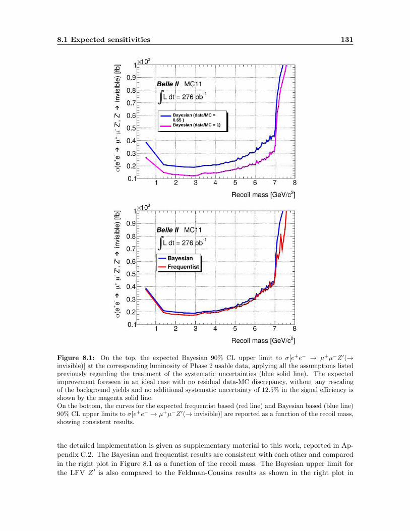
8.1 Expected sensitivities 131
Bayesian (data/MC = 0.65 )Bayesian (data/MC = 1)
Bayesian (data/MC = 0.65 )Bayesian (data/MC = 1)
Figure 8.1: On the top, the expected Bayesian 90% CL upper limit to σ[e+e− → µ+µ−Z ′(→invisible)] at the corresponding luminosity of Phase 2 usable data, applying all the assumptions listedpreviously regarding the treatment of the systematic uncertainties (blue solid line). The expectedimprovement foreseen in an ideal case with no residual data-MC discrepancy, without any rescalingof the background yields and no additional systematic uncertainty of 12.5% in the signal efficiency isshown by the magenta solid line.On the bottom, the curves for the expected frequentist based (red line) and Bayesian based (blue line)90% CL upper limits to σ[e+e− → µ+µ−Z ′(→ invisible)] are reported as a function of the recoil mass,showing consistent results.
the detailed implementation is given as supplementary material to this work, reported in Ap-pendix C.2. The Bayesian and frequentist results are consistent with each other and comparedin the right plot in Figure 8.1 as a function of the recoil mass. The Bayesian upper limit forthe LFV Z ′ is also compared to the Feldman-Cousins results as shown in the right plot in

132 Results and conclusions
]2Recoil mass [GeV/c
0 1 2 3 4 5 6 7 8
invi
sibl
e) [f
b]
±
µ ± e
→ - e+(eσ ⋅ε
0
10
20
30
40
50
60
70
Belle II MC11-1
L dt = 276 pb∫
1 2 3 4 5 6 7 8
]2 Recoil mass [GeV/c
0
10
20
30
40
50
60
70
invi
sibl
e) [f
b]
±
µ ± e
→ - e+(eσ ⋅ε
Belle II MC11-1
L dt = 276 pb∫BayesianFrequentist
Figure 8.2: On the left, the expected Bayesian (blue line) 90% CL upper limit to ε × σ[e+e− →e±µ∓ + invisible] is reported as a function of the recoil mass. On the right, comparison with thefrequentist results (red line) is shown.
Figure 8.2, as a function of the recoil mass.Finally, to conclude the sensitivity studies, cross section results for the standard Z ′ search
are translated in terms of upper limits on the new boson coupling constant g′, as interpretedin the framework of the Lµ − Lτ model. A numerical approach exploiting the MadGraph 5generator has been implemented, being the analytical expression not available. The expectedsensitivities for g′ in both frequentist and Bayesian approaches are finally shown in Figure 8.3(linear and logarithmic scales) as a function of the recoil mass, which corresponds to the massof the reconstructed Z ′ candidate, MZ′ in the plots hereafter.

8.1 Expected sensitivities 133
Figure 8.3: The expected frequentist based (blue line) and Bayesian based (red line) 90% CL upperlimits to coupling constant g′ as a function of the reconstructed Z ′ mass, MZ′ , in linear (top) andlogarithmic (bottom) scales, are shown. The solid line assumes the Lµ − Lτ predicted branchingfraction for Z ′ → invisible, while the dashed line (bottom plot only) assumes BF [Z ′ → invisible]=1.The red band shows the region that could explain the anomalous muon magnetic moment (gµ−2)±2σ,taken from the work referenced in [61].

134 Results and conclusions
8.2 Results on Phase 2 data
A first partial unblinding of Belle II 2018 data has been performed by comparing the recoilmass distribution measured on data and on simulations before the application of the τ sup-pression procedure, with the application of the correction scale factors previously discussed.After rescaling respectively the MC yields for the 0.65, 0.90 discrepancy measured in thevalidation studies, the data-MC ratio is consistent with one within the statistical fluctuationsfor both the channels e+e−→ µ+µ−, e+e−→ e±µ∓ investigated in this analysis, as shown bythe inset plots in Figure 8.4
0 0.5 1 1.5 2 2.5 3
]2 < 3 [GeV/cµµM
0
100
200
2C
ount
s/10
0 M
eV/c
Data-1 = 276 pb Ldt∫
Belle II 2018 )γ(-µ+µ →-e+e
)γ(-τ+τ →-e+e
-µ+µ-e+ e→-e+e
0 0.5 1 1.5 2 2.5 3]2 < 3 [GeV/cµµM
00.5
11.5
2
Dat
a/M
C
3 3.5 4 4.5 5 5.5 6
]2 < 6 [GeV/cµµ3 < M
0
50
2C
ount
s/10
0 M
eV/c
Data-1 = 276 pb Ldt∫
Belle II 2018 )γ(-µ+µ →-e+e
)γ(-τ+τ →-e+e
-µ+µ-e+ e→-e+e
3 3.5 4 4.5 5 5.5 6]2 < 6 [GeV/cµµ3 < M
00.5
11.5
2
Dat
a/M
C
6 6.5 7 7.5 8 8.5 9 9.5 10 10.5 11
]2 > 6 [GeV/cµµM
0
10
20
2C
ount
s/10
0 M
eV/c
Data-1 = 276 pb Ldt∫
Belle II 2018 )γ(-µ+µ →-e+e
)γ(-τ+τ →-e+e
-µ+µ-e+ e→-e+e
6 6.5 7 7.5 8 8.5 9 9.5 10 10.5 11]2 > 6 [GeV/cµµM
00.5
11.5
2
Dat
a/M
C
0 1 2 3 4 5 6 7 8
]2Recoil mass [GeV/c
50
100
Cou
nts
Data-1 = 276 pb Ldt∫
Belle II 2018
)γ(-µ+µ →-e+e
)γ(-τ+τ →-e+e
-µ+µ-e+ e→-e+e
0 1 2 3 4 5 6 7 8]2Recoil mass [GeV/c
00.5
11.5
2
Dat
a/M
C
0 0.5 1 1.5 2 2.5 3
]2 < 3 [GeV/cµµM
0
50
2C
ount
s/10
0 M
eV/c
Data-1 = 276 pb Ldt∫
Belle II 2018 )γ(-µ+µ →-e+e
)γ(-τ+τ →-e+e
-µ+µ-e+ e→-e+e
)γ(-e+ e→-e+e
0 0.5 1 1.5 2 2.5 3]2 < 3 [GeV/cµµM
00.5
11.5
2D
ata/
MC
3 3.5 4 4.5 5 5.5 6
]2 < 6 [GeV/cµµ3 < M
0
50
100
2C
ount
s/10
0 M
eV/c
Data-1 = 276 pb Ldt∫
Belle II 2018 )γ(-µ+µ →-e+e
)γ(-τ+τ →-e+e
-µ+µ-e+ e→-e+e
)γ(-e+ e→-e+e
3 3.5 4 4.5 5 5.5 6]2 < 6 [GeV/cµµ3 < M
00.5
11.5
2D
ata/
MC
6 6.5 7 7.5 8 8.5 9 9.5 10 10.5 11
]2 > 6 [GeV/cµµM
0
20
40
2C
ount
s/10
0 M
eV/c
Data-1 = 276 pb Ldt∫
Belle II 2018 )γ(-µ+µ →-e+e
)γ(-τ+τ →-e+e
-µ+µ-e+ e→-e+e
)γ(-e+ e→-e+e
6 6.5 7 7.5 8 8.5 9 9.5 10 10.5 11]2 > 6 [GeV/cµµM
00.5
11.5
2D
ata/
MC
2− 0 2 4 6 8 10
]2 Recoil mass [GeV/c
0
50
2C
ount
s/10
0 M
eV/c
Data-1 = 276 pb Ldt∫
Belle II 2018
)γ(-µ+µ →-e+e
)γ(-τ+τ →-e+e
-µ+µ-e+ e→-e+e
)γ(-e+ e→-e+e
2− 0 2 4 6 8 10]2 Recoil mass [GeV/c
00.5
11.5
2D
ata/
MC
0 1 2 3 4 5 6 7 8
]2Recoil mass [GeV/c
50
100
Cou
nts
Data-1 = 276 pb Ldt∫
Belle II 2018
)γ(-µ+µ →-e+e
)γ(-τ+τ →-e+e-µ+µ-e+ e→-e+e
)γ(-e+ e→-e+e
0 1 2 3 4 5 6 7 8]2Recoil mass [GeV/c
00.5
11.5
2D
ata/
MC
Figure 8.4: Recoil mass spectrum for the e+e−→ µ+µ−(e±µ∓) sample before the τ suppression pro-cedure is shown on the left (right). The inset plots show the data-MC ratio computed after correctingthe simulated yields as explained in Chapter 6 for the observed data-MC discrepancy (scaling factorof 0.65 applied to the simulated yields in the left plot, 0.90 applied in the right plot). The correcteddistributions show a good data-MC agreement within statistical fluctuations.
The final recoil mass spectrum for the e+e−→ µ+µ− sample, which targets the standardZ ′ search, is shown in Figure 8.5 after the application of the τ suppression procedure on dataand rescaled simulation yields. To look for possible anomalies in data, under the assumptionof the background only hypothesis, p-values have been computed as the probability to geta result (counts) greater than or equal to the observed one, with statistical and systematicuncertainties both taken into account (see Appendix C.3). No evidence of new signal has beenfound, being the computed p-values within the 3σ equivalent for each recoil mass bin, both inthe normal and in the shifted binning option. The previously discussed Bayesian procedure isapplied to compute the 90% CL upper limit to the standard Z ′ cross section. Flat priors areused for all positive values of the cross section and Poissonian likelihoods are assumed for thenumber of observed and Monte Carlo generated events, while Gaussian smearings have beenused to model the systematic uncertainties. Results are cross-checked with the frequentistprocedure following the Feldman-Cousins approach, as reported in Appendix C.2, and foundto be compatible between the two methods. The 90% CL upper limit to the standard Z ′
cross section σ[e+e− → µ+µ−Z ′(→ invisible)] is shown in Figure 8.6 as a function of therecoil mass. Cross section results are then interpreted in terms of 90% CL upper limit on thecoupling constant g′, shown in Figure 8.7.
Concerning the LFV Z ′ search, the final recoil mass spectrum for the e+e−→ e±µ∓
sample is shown in Figure 8.8 (top) after the application of the τ suppression procedure on

8.2 Results on Phase 2 data 135
0 0.5 1 1.5 2 2.5 3
]2 < 3 [GeV/cµµM
0
100
2002
Cou
nts/
100
MeV
/c
Data-1 = 276 pb Ldt∫
Belle II 2018 )γ(-µ+µ →-e+e
)γ(-τ+τ →-e+e
-µ+µ-e+ e→-e+e
)γ(-π+π →-e+e
-e+e-e+ e→-e+e
)γ(-e+ e→-e+e
3 3.5 4 4.5 5 5.5 6
]2 < 6 [GeV/cµµ3 < M
0
5
10
15
2C
ount
s/10
0 M
eV/c
Data-1 = 276 pb Ldt∫
Belle II 2018 )γ(-µ+µ →-e+e
)γ(-τ+τ →-e+e
-µ+µ-e+ e→-e+e
)γ(-π+π →-e+e
-e+e-e+ e→-e+e
)γ(-e+ e→-e+e
6 6.5 7 7.5 8 8.5 9 9.5 10 10.5 11
]2 > 6 [GeV/cµµM
0
0.5
12
Cou
nts/
100
MeV
/c
Data-1 = 276 pb Ldt∫
Belle II 2018 )γ(-µ+µ →-e+e
)γ(-τ+τ →-e+e
-µ+µ-e+ e→-e+e
)γ(-π+π →-e+e
-e+e-e+ e→-e+e
)γ(-e+ e→-e+e
0 1 2 3 4 5 6 7 8
]2Recoil mass [GeV/c
2−10
1−10
1
10
210
Cou
nts
Data-1 = 276 pb Ldt∫
Belle II 2018
)γ(-µ+µ →-e+e
)γ(-τ+τ →-e+e-µ+µ-e+ e→-e+e
)γ(-π+π →-e+e-e+e-e+ e→-e+e
)γ(-e+ e→-e+e
Figure 8.5: Recoil mass spectrum for the e+e− → µ+µ− sample after the τ suppression procedure.Monte Carlo values are rescaled for the luminosity, the trigger efficiency (0.79) and the validationprocedure outcome (0.65). In the recoil mass interval −0.15 ÷ 6.5(7) GeV/c2, 8(17) events are foundin data and 8.6(16.8) in Monte Carlo.
0 1 2 3 4 5 6 7 8
]2Recoil mass [GeV/c
0
100
200
300
400
500
600
700
800
900
1000
invi
sibl
e) [f
b]→
Z',
Z'
- µ+ µ → - e+
(eσ
Belle II 2018
-1 = 276 pbLdt ∫
Figure 8.6: 90% CL upper limits to σ[e+e− → µ+µ−Z ′(→ invisible)].

136 Results and conclusions
1 2 3 4 5
]2 [GeV/cZ'M
4−10
3−10
2−10
1−10
1
U.L
. on
g' (
90%
C.L
.)
τ-LµL
1 inv)=→ , BF(Z'τ-LµL
Belle II 2018
-1 = 276 pbLdt ∫
σ2±µ(g-2)
Figure 8.7: 90% CL upper limits to g′. The solid line assumes the Lµ − Lτ predicted branchingfraction for Z ′ → invisible while the dashed line assumes BF [Z ′ → invisible]=1. The red band showsthe region that could explain the anomalous muon magnetic moment (g − 2)µ ± 2σ.
data and rescaled Monte Carlo. As for the standard Z ′, the background only hypothesis istested by computing p-values as a function of the recoil mass and the outcome is analogousto the standard Z ′ case, with no significant anomalies observed, neither in the normal nor inthe shifted binning scheme. Model independent 90% CL upper limits to the quantity ( crosssection × efficiency) for the LFV Z ′ search are computed in both the Bayesian and frequentistapproaches and found to be consistent. The results are displayed in Figure 8.8 (bottom) as afunction of the recoil mass.

8.2 Results on Phase 2 data 137
0 0.5 1 1.5 2 2.5 3
]2 < 3 [GeV/cµµM
0
20
40
602
Cou
nts/
100
MeV
/c Data
-1 = 276 pb Ldt∫Belle II 2018 )γ(-µ+µ →-e+e
)γ(-τ+τ →-e+e
-µ+µ-e+ e→-e+e
)γ(-π+π →-e+e
-e+e-e+ e→-e+e
)γ(-e+ e→-e+e
3 3.5 4 4.5 5 5.5 6
]2 < 6 [GeV/cµµ3 < M
0
5
10
2C
ount
s/10
0 M
eV/c
Data-1 = 276 pb Ldt∫
Belle II 2018 )γ(-µ+µ →-e+e
)γ(-τ+τ →-e+e
-µ+µ-e+ e→-e+e
)γ(-π+π →-e+e
-e+e-e+ e→-e+e
)γ(-e+ e→-e+e
6 6.5 7 7.5 8 8.5 9 9.5 10 10.5 11
]2 > 6 [GeV/cµµM
0
0.5
1
2C
ount
s/10
0 M
eV/c
Data-1 = 276 pb Ldt∫
Belle II 2018 )γ(-µ+µ →-e+e
)γ(-τ+τ →-e+e
-µ+µ-e+ e→-e+e
)γ(-π+π →-e+e
-e+e-e+ e→-e+e
)γ(-e+ e→-e+e
2− 0 2 4 6 8 10
]2 Recoil mass [GeV/c
1
10
2C
ount
s/10
0 M
eV/c Data
-1 = 276 pb Ldt∫Belle II 2018
)γ(-µ+µ →-e+e)γ(-τ+τ →-e+e
-µ+µ-e+ e→-e+e)γ(-π+π →-e+e-e+e-e+ e→-e+e
)γ(-e+ e→-e+e
0 1 2 3 4 5 6 7 8
]2Recoil mass [GeV/c
2−10
1−10
1
10
210C
ount
s Data
-1 = 276 pb Ldt∫Belle II 2018
)γ(-µ+µ →-e+e)γ(-τ+τ →-e+e
-µ+µ-e+ e→-e+e)γ(-π+π →-e+e-e+e-e+ e→-e+e
)γ(-e+ e→-e+e
0 1 2 3 4 5 6 7 8
]2Recoil mass [GeV/c
0
10
20
30
40
50
60
70
80
invi
sibl
e) [f
b] (
90%
C.L
.)± µ±
e→ - e+
(eσ⋅ε
Belle II 2018
-1 = 276 pbLdt ∫
Figure 8.8: In the top plot, the recoil mass spectrum after the τ suppression procedure on theunblinded e+e− → e±µ∓ data targeting the LFV Z ′ search is shown. Simulated yields values arerescaled for the luminosity, the trigger efficiency (0.96) and the validation procedure outcome (0.9). Inthe recoil mass interval −0.15 ÷ 6.5(7) GeV/c2, 5(9) events are found in data and 4.9(7.9) in MonteCarlo. In the bottom plot, the 90% CL upper limits to ε× σ[e+e− → e±µ∓invisible] are reported.
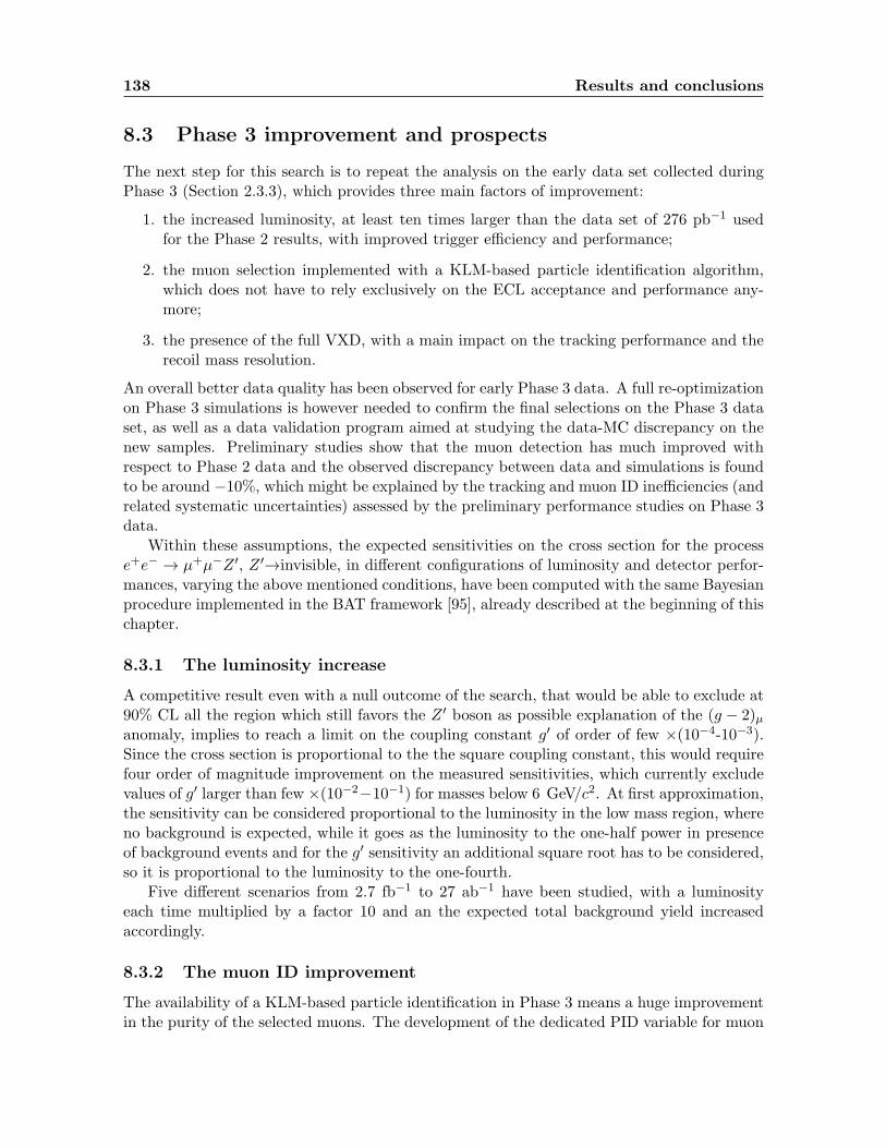
138 Results and conclusions
8.3 Phase 3 improvement and prospects
The next step for this search is to repeat the analysis on the early data set collected duringPhase 3 (Section 2.3.3), which provides three main factors of improvement:
1. the increased luminosity, at least ten times larger than the data set of 276 pb−1 usedfor the Phase 2 results, with improved trigger efficiency and performance;
2. the muon selection implemented with a KLM-based particle identification algorithm,which does not have to rely exclusively on the ECL acceptance and performance any-more;
3. the presence of the full VXD, with a main impact on the tracking performance and therecoil mass resolution.
An overall better data quality has been observed for early Phase 3 data. A full re-optimizationon Phase 3 simulations is however needed to confirm the final selections on the Phase 3 dataset, as well as a data validation program aimed at studying the data-MC discrepancy on thenew samples. Preliminary studies show that the muon detection has much improved withrespect to Phase 2 data and the observed discrepancy between data and simulations is foundto be around −10%, which might be explained by the tracking and muon ID inefficiencies (andrelated systematic uncertainties) assessed by the preliminary performance studies on Phase 3data.
Within these assumptions, the expected sensitivities on the cross section for the processe+e− → µ+µ−Z ′, Z ′→invisible, in different configurations of luminosity and detector perfor-mances, varying the above mentioned conditions, have been computed with the same Bayesianprocedure implemented in the BAT framework [95], already described at the beginning of thischapter.
8.3.1 The luminosity increase
A competitive result even with a null outcome of the search, that would be able to exclude at90% CL all the region which still favors the Z ′ boson as possible explanation of the (g − 2)µanomaly, implies to reach a limit on the coupling constant g′ of order of few ×(10−4-10−3).Since the cross section is proportional to the the square coupling constant, this would requirefour order of magnitude improvement on the measured sensitivities, which currently excludevalues of g′ larger than few ×(10−2−10−1) for masses below 6 GeV/c2. At first approximation,the sensitivity can be considered proportional to the luminosity in the low mass region, whereno background is expected, while it goes as the luminosity to the one-half power in presenceof background events and for the g′ sensitivity an additional square root has to be considered,so it is proportional to the luminosity to the one-fourth.
Five different scenarios from 2.7 fb−1 to 27 ab−1 have been studied, with a luminosityeach time multiplied by a factor 10 and an the expected total background yield increasedaccordingly.
8.3.2 The muon ID improvement
The availability of a KLM-based particle identification in Phase 3 means a huge improvementin the purity of the selected muons. The development of the dedicated PID variable for muon

8.3 Phase 3 improvement and prospects 139
selection (defined as the normalized likelihood ratio of the muon hypothesis and the sumof all the other particle hypotheses) allows to better reject pion contamination, which hasbeen estimated to contribute as 85% of the background yield coming from e+e−→τ+τ−(γ)processes. The main advantage will be the possibility to reduce the expected background dueto the misidentification rate, despite the higher luminosity. Preliminary studies on the datacollected during the Phase 3 spring runs indicate a reduction of a factor 20 in the backgroundrate due to pion misidentification when reconstructing the J/ψ → µ+µ− peak on data witha tighter selection on the muon ID probability. Results from preliminary studies are shownin Figure D.1 reported in Appendix D. This has been taken into account in the projectionstudies as follow:
85% of the background yield coming from e+e−→τ+τ−(γ) events is reduced by thefactor 0.1, which is shown from preliminary performance studies to be a reasonableestimate of the rejection factor expected from a muon ID probability selection > 0.8;
100% of the background yield from e+e−→ π+π−(γ) processes, only due to particlemisidentification, is scaled by the factor 0.1.
While the latter is found to be a negligible contribution in Phase 2 data, the former is themain background component in the medium recoil mass region and therefore a significantimprovement is expected from the muon ID selection on Phase 3 data.
8.3.3 The VXD impact on recoil mass resolution
For each mass point studied on Phase 2 data as reported in Section 3.4.1, signal MC samplesgenerated with the MadGraph 5 generator and the Phase 3 detector geometry have beensimulated. Studies on the improved signal width have been performed by fitting the recoilmass distribution for each generated sample (20000 events) with the same PDF model asdescribed in Section 5.1.1, after selecting the events with exactly the same requirementslisted in Section 4.2, 4.3, before the τ suppression procedure. The results of the fit and thecorresponding values of the shape parameters, particularly the Gaussian and CB functionwidths, are reported in Figure D.2 in Appendix D. From these results, the signal peak widthsfor Phase 3 simulations are computed accordingly to Equation 5.2 as explained in Section 5.1.1,and their values have been compared to those extracted from Phase 2 simulation, as a functionof the recoil mass, shown in Figure 8.9. For recoil masses below 4.5 GeV/c2, an average40% improvement is observed in the signal resolution, mainly due to the better trackingperformance coming from the full installation of the VXD detector. Above 5 GeV/c2 recoilmasses, the tracking system has to deal with low momentum muons affected by multiplescattering which eventually dominates the resolution, due to the additional material budgetintroduced by the full VXD. For the large recoil mass case (> 5 GeV/c2), no significantimprovement is observed in the signal widths, which are comparable to Phase 2 results. Inthe reasonable assumption of a flat background in each recoil mass window, the resolutionimprovement would imply a correspondent 40% reduction of the background yields for recoilmasses below 4.5 GeV. The above condition translates in a reduction factor of 0.60 appliedto the expected background for recoil masses below 4.5, that has been added as furtherimprovement factor to the five luminosity scenarios studied within the new full VXD resolutionhypothesis.

140 Results and conclusions
1 2 3 4 5 6 7 8
0.02
0.04
0.06
0.08
0.1
0.12
0.14
0.16
0.18
0.2] 2
[GeV
/cWσ
Phase 2, Signal Resolution
Phase 3, Signal Resolution
1 2 3 4 5 6 7 8
]2Recoil Mass[GeV/c
0.5
1
Ph
2Wσ/
Ph
3Wσ
Figure 8.9: The signal width σW as computed according to Equation 5.2, as a function of the recoilmass, is compared between Phase 2 (blue triangles) and the Phase 3 (red dots) simulation results. Theratio between Phase 3 and Phase 2 widths per each mass point is shown in the inset plot. It can benoticed that for masses above 5 GeV/c2 the multiple scattering on low-momentum muons, due to theadditional material budget of the full VXD, dominates the resolution and no significant improvementis gained with respect to Phase 2 results.
8.3.4 Projection results
The resulting sensitivities computed on the signal cross section and translated also in termsof the coupling constant g′, as a function of the reconstructed recoil mass, are shown in greenlines in Figure 8.10, compared to the results from Belle II 2018 data, represented by the blueline. The 27 ab−1 scenario is highlighted in magenta solid line.
As previously discussed, several factors of improvement expected on both the survivingbackground events and the associated uncertainties have been considered:
1. for each scenario, the luminosity has been increased by a factor 10 and the systematicuncertainties which are statistically driven (e.g. τ suppression, background yield) havebeen reduced accordingly;
2. the background contamination from e+e−→ τ+τ−(γ) and e+e−→ π+π−(γ) processes,due to particle misidentification, has been scaled as described in subsection 8.3.2;
3. the total number of background events has been scaled by the factor 0.60 for MZ′<4.5 GeV/c2, as described in subsection 8.3.3;
4. the data-MC discrepancy has been reduced to −10% and assumed to come from the in-efficiencies of the track reconstruction algorithms and lepton ID selection performances;half of this residual discrepancy is conservatively assigned as systematic uncertainty inthe signal efficiency;

8.3 Phase 3 improvement and prospects 141
Figure 8.10: In the top plot, the 90% CL upper limit on the cross section of the process e+e− →µ+µ−Z ′ as measured from Phase 2 data is shown (blue solid line), compared to the sensitivitiescomputed for the 10 times increased luminosity scenarios evaluated in the study. The 27 ab−1 thatmay rule out completely the (g-2)µ band is shown in magenta solid line.The same limits translated in terms of the g′ coupling constant are reported in the bottom plot.
5. the discrepancy in the tracking efficiency as measured on data and simulation frompreliminary studies on Belle II 2019 data is assessed to be of order 1% and it is assumedas associated systematic uncertainty due to the track reconstruction performance;
6. studies of the uncertainties associated to the muon ID selection and trigger performanceshave been already set up and official results on Belle II 2019 data are going to bereleased; for this projection study, 4% and 6% systematic errors due respectively tomuon identification and trigger selections, as quoted in Table 7.1, are conservativelyassumed.
The Phase 3 projections shown above have been computed in the same Bayesian approachexploited for the upper limit estimation within the BAT software framework and all theconsiderations listed previously apply to the studied curves in Figure 8.10.

142 Results and conclusions
It should be noticed that the sensitivity ratios between different curves do not scale asthe the power of luminosity, since the luminosity effect combines in a not trivial way with theother scaling factors applied to simulate improved detector conditions and performances, asexplained in the previous subsections.
8.3.5 Next plans
More specific studies are required for repeating the Z ′ analysis on Phase 3 data. Currently theanalysis group is active on the new performance studies necessary to understand the Belle II2019 data. The next steps can be summarized following the three main factors of improvementdiscussed previously:
a run-dependent study of the trigger performances on Phase 3 data is under developmentand preliminary results show a higher and more accurate efficiency due to the overallimprovement of the detector and firmware performances. Moreover, it will benefit fromthe larger statistics of at least 10×( Belle II 2018 data);
the new muon selection based on KLM-information requires a dedicated optimizationand the associated efficiency with its systematic uncertainty needs to be measured onthe new data set;
the track reconstruction efficiency study exploiting the topology of the e+e−→ τ+τ−
events will benefit of both the larger statistics and the improved detector and I amworking on the new analysis on Belle II 2019 data which will provide the measurementof the scale factors and discrepancies for track reconstruction efficiencies measured onPhase 3 data and on simulations;
the signal width study on Phase 3 simulation and the comparison with the recoil massresolution evaluated on data must be repeated; these results will allow to define the newbinning scheme for the recoil mass spectrum measured on Phase 3 data;
given the overall better agreement between data and simulations, two point of theprevious analysis strategy may change:
– the background suppression strategy, and specifically the τ suppression procedure,may benefit from a more sophisticated non-linear selection based on multivariateanalysis methods. A re-optimization of the full selection chain with Boosted Deci-sion Tree and Neural Network algorithms is currently under study; the same controlsamples exploited in the Phase 2 analysis, with larger statistics, will be used fordata validation and the control of the systematic errors;
– the larger statistics and the reduced data-MC discrepancy motivate the estimationof the expected background yields directly from data, by applying the sidebandextrapolation technique. This method aims at estimating locally the expectedbackground yield per each recoil mass bin by fitting the adjacent bin yields andextrapolating the result to the bin under study, before the application of the τsuppression procedure, in order to have enough statistics for a good fit performance.
a newly optimized linear-cut based selection for Belle II 2019 data is under development,to ensure also on the new data set a robust result produced with validated techniques.
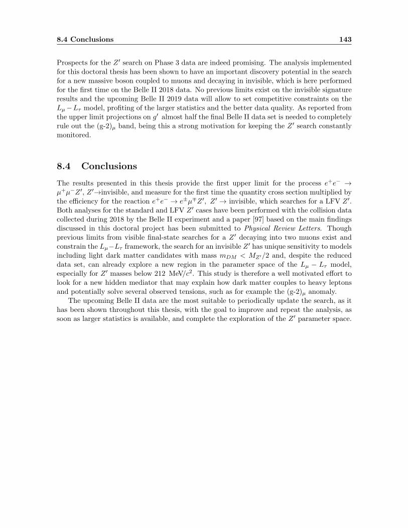
8.4 Conclusions 143
Prospects for the Z ′ search on Phase 3 data are indeed promising. The analysis implementedfor this doctoral thesis has been shown to have an important discovery potential in the searchfor a new massive boson coupled to muons and decaying in invisible, which is here performedfor the first time on the Belle II 2018 data. No previous limits exist on the invisible signatureresults and the upcoming Belle II 2019 data will allow to set competitive constraints on theLµ−Lτ model, profiting of the larger statistics and the better data quality. As reported fromthe upper limit projections on g′ almost half the final Belle II data set is needed to completelyrule out the (g-2)µ band, being this a strong motivation for keeping the Z ′ search constantlymonitored.
8.4 Conclusions
The results presented in this thesis provide the first upper limit for the process e+e− →µ+µ−Z ′, Z ′→invisible, and measure for the first time the quantity cross section multiplied bythe efficiency for the reaction e+e− → e±µ∓Z ′, Z ′ → invisible, which searches for a LFV Z ′.Both analyses for the standard and LFV Z ′ cases have been performed with the collision datacollected during 2018 by the Belle II experiment and a paper [97] based on the main findingsdiscussed in this doctoral project has been submitted to Physical Review Letters. Thoughprevious limits from visible final-state searches for a Z ′ decaying into two muons exist andconstrain the Lµ−Lτ framework, the search for an invisible Z ′ has unique sensitivity to modelsincluding light dark matter candidates with mass mDM < MZ′/2 and, despite the reduceddata set, can already explore a new region in the parameter space of the Lµ − Lτ model,especially for Z ′ masses below 212 MeV/c2. This study is therefore a well motivated effort tolook for a new hidden mediator that may explain how dark matter couples to heavy leptonsand potentially solve several observed tensions, such as for example the (g-2)µ anomaly.
The upcoming Belle II data are the most suitable to periodically update the search, as ithas been shown throughout this thesis, with the goal to improve and repeat the analysis, assoon as larger statistics is available, and complete the exploration of the Z ′ parameter space.

144 Results and conclusions

Appendices


Appendix A
Event selection and signal shapestudy results
A.1 The standard Z ′ selection results
Hereby we report the complete list of final results for signal efficiencies and expected back-ground yields in the contiguous binning scheme which is used for the statistical analysis ofthe data.
Table A.1: Signal efficiencies and number of background events after all the analysis selectionsin contiguous Z ′ mass bins, for the standard Z ′ analysis. Background normalized to an integratedluminosity of 276 pb−1. Signal efficiencies and background yields include the 0.79 trigger efficiency(Section 7.2)
MZ′ [GeV/c2] Mass range [GeV/c2] Efficiency [%] Background events
0.50 -0.15 - 1.15 4.34 ± 0.13 0.67 ± 0.051.39 1.15 - 1.63 7.60 ± 0.16 0.33 ± 0.041.81 1.63 - 1.98 7.93 ± 0.17 0.26 ± 0.032.13 1.98 - 2.29 8.01 ± 0.17 0.22 ± 0.032.42 2.29 - 2.56 8.06 ± 0.17 0.19 ± 0.032.68 2.56 - 2.81 8.03 ± 0.17 0.14 ± 0.032.91 2.81 - 3.02 7.98 ± 0.17 0.12 ± 0.023.11 3.02 - 3.21 7.79 ± 0.17 0.11 ± 0.023.29 3.21 - 3.38 7.51 ± 0.16 0.17 ± 0.033.46 3.38 - 3.54 7.26 ± 0.16 0.16 ± 0.033.62 3.54 - 3.69 7.26 ± 0.16 0.16 ± 0.033.77 3.69 - 3.84 7.34 ± 0.16 0.21 ± 0.033.91 3.84 - 3.98 7.41 ± 0.16 0.26 ± 0.054.04 3.98 - 4.11 7.40 ± 0.16 0.23 ± 0.044.17 4.11 - 4.24 7.21 ± 0.16 0.24 ± 0.044.29 4.24 - 4.36 7.04 ± 0.16 0.25 ± 0.044.41 4.36 - 4.47 6.87 ± 0.16 0.26 ± 0.044.52 4.47 - 4.58 6.72 ± 0.16 0.28 ± 0.05
Continued on next page

148 Event selection and signal shape study results
Table A.1 – Continued from previous page
MZ′ [GeV/c2] Mass range [GeV/c2] Efficiency [%] Background events
4.63 4.58 - 4.69 6.65 ± 0.16 0.22 ± 0.034.74 4.69 - 4.79 6.57 ± 0.15 0.29 ± 0.044.85 4.79 - 4.90 6.49 ± 0.15 0.28 ± 0.054.95 4.90 - 5.00 6.42 ± 0.15 0.32 ± 0.065.05 5.00 - 5.09 6.32 ± 0.15 0.26 ± 0.045.14 5.09 - 5.18 6.19 ± 0.15 0.41 ± 0.085.23 5.18 - 5.27 6.08 ± 0.15 0.23 ± 0.045.31 5.27 - 5.35 5.97 ± 0.15 0.27 ± 0.045.38 5.35 - 5.42 5.86 ± 0.15 0.36 ± 0.065.46 5.42 - 5.49 5.76 ± 0.15 0.31 ± 0.065.53 5.49 - 5.56 5.67 ± 0.14 0.32 ± 0.065.60 5.56 - 5.63 5.57 ± 0.14 0.29 ± 0.055.66 5.63 - 5.70 5.47 ± 0.14 0.34 ± 0.065.73 5.70 - 5.76 5.37 ± 0.14 0.45 ± 0.085.80 5.76 - 5.83 5.27 ± 0.14 0.35 ± 0.065.87 5.83 - 5.90 5.17 ± 0.14 0.39 ± 0.065.94 5.90 - 5.97 5.07 ± 0.14 0.31 ± 0.066.01 5.97 - 6.04 4.96 ± 0.14 0.30 ± 0.056.08 6.04 - 6.11 4.83 ± 0.13 0.58 ± 0.106.15 6.11 - 6.18 4.69 ± 0.13 0.30 ± 0.076.21 6.18 - 6.25 4.56 ± 0.13 0.41 ± 0.086.28 6.25 - 6.31 4.43 ± 0.13 0.37 ± 0.076.34 6.31 - 6.38 4.30 ± 0.13 0.53 ± 0.106.41 6.38 - 6.44 4.17 ± 0.12 0.38 ± 0.096.47 6.44 - 6.50 4.05 ± 0.12 0.35 ± 0.086.53 6.50 - 6.56 4.05 ± 0.12 0.29 ± 0.076.58 6.56 - 6.61 4.16 ± 0.12 0.55 ± 0.106.64 6.61 - 6.67 4.27 ± 0.13 0.57 ± 0.106.69 6.67 - 6.72 4.37 ± 0.13 0.83 ± 0.136.75 6.72 - 6.77 4.47 ± 0.13 1.32 ± 0.186.80 6.77 - 6.83 4.57 ± 0.13 1.18 ± 0.156.85 6.83 - 6.88 4.67 ± 0.13 1.47 ± 0.186.90 6.88 - 6.93 4.77 ± 0.13 1.81 ± 0.206.95 6.93 - 6.98 4.87 ± 0.13 1.85 ± 0.207.01 6.98 - 7.03 5.06 ± 0.14 3.08 ± 0.247.06 7.03 - 7.09 5.92 ± 0.14 9.34 ± 0.377.12 7.09 - 7.14 6.81 ± 0.15 17.47 ± 0.507.17 7.14 - 7.20 7.75 ± 0.16 23.43 ± 0.577.24 7.20 - 7.27 8.74 ± 0.17 32.93 ± 0.717.30 7.27 - 7.33 9.77 ± 0.18 41.23 ± 0.817.37 7.33 - 7.40 10.86 ± 0.19 50.41 ± 0.917.44 7.40 - 7.47 11.98 ± 0.20 62.98 ± 1.067.51 7.47 - 7.55 12.92 ± 0.21 69.32 ± 1.13
Continued on next page

A.1 The standard Z ′ selection results 149
Table A.1 – Continued from previous page
MZ′ [GeV/c2] Mass range [GeV/c2] Efficiency [%] Background events
7.58 7.55 - 7.62 12.66 ± 0.20 73.16 ± 1.197.66 7.62 - 7.69 12.40 ± 0.20 76.22 ± 1.247.73 7.69 - 7.76 12.15 ± 0.20 76.07 ± 1.257.79 7.76 - 7.83 11.91 ± 0.20 79.03 ± 1.307.86 7.83 - 7.89 11.67 ± 0.20 80.55 ± 1.337.92 7.89 - 7.95 11.44 ± 0.20 77.66 ± 1.327.98 7.95 - 8.01 11.22 ± 0.19 80.99 ± 1.368.04 8.01 - 8.07 10.97 ± 0.19 83.10 ± 1.39

150 Event selection and signal shape study results
A.2 The LFV Z ′ selection results
Hereby we report the complete list of final results for expected background yields in thecontiguous binning scheme which is used for the statistical analysis of the data.
Table A.2: Number of background events after all the analysis selections in contiguous mass bins,fro the LFV Z ′. The number of background events is normalized to an integrated luminosity of 276pb−1. Signal efficiencies and background yields include the 0.96 trigger efficiency (see Section 7.2)
MZ′ [GeV/c2] Mass range [GeV/c2] Background events
0.50 -0.15 - 1.15 0.00 ± 0.011.39 1.15 - 1.63 0.02 ± 0.011.81 1.63 - 1.98 0.03 ± 0.012.13 1.98 - 2.29 0.04 ± 0.022.42 2.29 - 2.56 0.01 ± 0.012.68 2.56 - 2.81 0.05 ± 0.022.91 2.81 - 3.02 0.03 ± 0.013.11 3.02 - 3.21 0.07 ± 0.023.29 3.21 - 3.38 0.08 ± 0.023.46 3.38 - 3.54 0.17 ± 0.033.62 3.54 - 3.69 0.11 ± 0.033.77 3.69 - 3.84 0.09 ± 0.023.91 3.84 - 3.98 0.13 ± 0.034.04 3.98 - 4.11 0.18 ± 0.034.17 4.11 - 4.24 0.09 ± 0.024.29 4.24 - 4.36 0.16 ± 0.034.41 4.36 - 4.47 0.13 ± 0.034.52 4.47 - 4.58 0.19 ± 0.044.63 4.58 - 4.69 0.09 ± 0.024.74 4.69 - 4.79 0.15 ± 0.054.85 4.79 - 4.90 0.12 ± 0.034.95 4.90 - 5.00 0.15 ± 0.035.05 5.00 - 5.09 0.07 ± 0.025.14 5.09 - 5.18 0.17 ± 0.055.23 5.18 - 5.27 0.16 ± 0.035.31 5.27 - 5.35 0.20 ± 0.045.38 5.35 - 5.42 0.15 ± 0.035.46 5.42 - 5.49 0.19 ± 0.045.53 5.49 - 5.56 0.16 ± 0.035.60 5.56 - 5.63 0.21 ± 0.055.66 5.63 - 5.70 0.19 ± 0.055.73 5.70 - 5.76 0.20 ± 0.065.80 5.76 - 5.83 0.11 ± 0.035.87 5.83 - 5.90 0.17 ± 0.055.94 5.90 - 5.97 0.27 ± 0.076.01 5.97 - 6.04 0.14 ± 0.04
Continued on next page

A.3 Signal shape study: toy MC results 151
Table A.2 – Continued from previous page
MZ′ [GeV/c2] Mass range [GeV/c2] Background events
6.08 6.04 - 6.11 0.15 ± 0.046.15 6.11 - 6.18 0.13 ± 0.036.21 6.18 - 6.25 0.17 ± 0.056.28 6.25 - 6.31 0.11 ± 0.046.34 6.31 - 6.38 0.17 ± 0.036.41 6.38 - 6.44 0.06 ± 0.026.47 6.44 - 6.50 0.09 ± 0.046.53 6.50 - 6.56 0.11 ± 0.046.58 6.56 - 6.61 0.12 ± 0.046.64 6.61 - 6.67 0.17 ± 0.056.69 6.67 - 6.72 0.19 ± 0.046.75 6.72 - 6.77 0.23 ± 0.066.80 6.77 - 6.83 0.38 ± 0.076.85 6.83 - 6.88 0.34 ± 0.076.90 6.88 - 6.93 0.51 ± 0.096.95 6.93 - 6.98 0.50 ± 0.097.01 6.98 - 7.03 0.94 ± 0.097.06 7.03 - 7.09 5.45 ± 0.227.12 7.09 - 7.14 9.25 ± 0.277.17 7.14 - 7.20 13.13 ± 0.317.24 7.20 - 7.27 18.54 ± 0.397.30 7.27 - 7.33 21.54 ± 0.437.37 7.33 - 7.40 25.00 ± 0.457.44 7.40 - 7.47 28.38 ± 0.497.51 7.47 - 7.55 29.09 ± 0.477.58 7.55 - 7.62 29.22 ± 0.517.66 7.62 - 7.69 26.60 ± 0.477.73 7.69 - 7.76 25.13 ± 0.487.79 7.76 - 7.83 21.96 ± 0.447.86 7.83 - 7.89 19.57 ± 0.437.92 7.89 - 7.95 17.34 ± 0.397.98 7.95 - 8.01 15.26 ± 0.378.04 8.01 - 8.07 13.95 ± 0.36
A.3 Signal shape study: toy MC results
Results from the toy MC validation study, performed on the simulated signals for differentmass hypotheses of the standard Z ′ boson, are reported below.
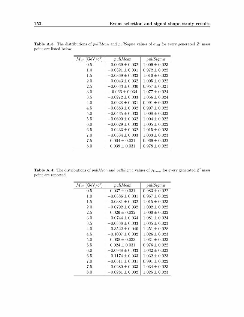
152 Event selection and signal shape study results
Table A.3: The distributions of pullMean and pullSigma values of σCB for every generated Z ′ masspoint are listed below.
MZ′ [GeV/c2] pullMean pullSigma
0.5 −0.0069± 0.032 1.009± 0.0231.0 −0.0321± 0.031 0.972± 0.0221.5 −0.0369± 0.032 1.010± 0.0232.0 −0.0043± 0.032 1.005± 0.0222.5 −0.0633± 0.030 0.957± 0.0213.0 −0.066± 0.034 1.077± 0.0243.5 −0.0272± 0.033 1.056± 0.0244.0 −0.0928± 0.031 0.991± 0.0224.5 −0.0583± 0.032 0.997± 0.0225.0 −0.0435± 0.032 1.008± 0.0235.5 −0.0690± 0.032 1.004± 0.0226.0 −0.0629± 0.032 1.005± 0.0226.5 −0.0433± 0.032 1.015± 0.0237.0 −0.0334± 0.033 1.033± 0.0237.5 0.004± 0.031 0.969± 0.0228.0 0.039± 0.031 0.978± 0.022
Table A.4: The distributions of pullMean and pullSigma values of σGauss for every generated Z ′ masspoint are reported.
MZ′ [GeV/c2] pullMean pullSigma
0.5 0.037± 0.031 0.983± 0.0221.0 −0.0386± 0.031 0.967± 0.0221.5 −0.0381± 0.032 1.015± 0.0232.0 −0.0792± 0.032 1.002± 0.0222.5 0.026± 0.032 1.000± 0.0223.0 −0.0744± 0.034 1.081± 0.0243.5 −0.0338± 0.033 1.035± 0.0234.0 −0.3522± 0.040 1.251± 0.0284.5 −0.1007± 0.032 1.026± 0.0235.0 0.038± 0.033 1.031± 0.0235.5 0.024± 0.031 0.976± 0.0226.0 −0.0938± 0.033 1.032± 0.0236.5 −0.1174± 0.033 1.032± 0.0237.0 −0.0511± 0.031 0.991± 0.0227.5 −0.0280± 0.033 1.034± 0.0238.0 −0.0281± 0.032 1.025± 0.023

A.3 Signal shape study: toy MC results 153
sigma of crystal ball0.025 0.026 0.027 0.028 0.029 0.03 0.031 0.032
Eve
nts
/ ( 8
.065
8e-0
5 )
0
10
20
30
40
50
60
A RooPlot of "sigma of crystal ball"A RooPlot of "sigma of crystal ball"
sigma of crystal ball Error0.00075 0.0008 0.00085 0.0009 0.00095 0.001 0.00105
Eve
nts
/ ( 3
.252
36e-
06 )
0
10
20
30
40
50
A RooPlot of "sigma of crystal ball Error"A RooPlot of "sigma of crystal ball Error"
sigma of crystal ball Pull4− 3− 2− 1− 0 1 2 3 4
Eve
nts
/ ( 0
.081
969
)
0
10
20
30
40
50
A RooPlot of "sigma of crystal ball Pull" 0.032±pullMean = -0.0435
0.023±pullSigma = 1.008
A RooPlot of "sigma of crystal ball Pull"
width of gaussian0.015 0.016 0.017 0.018 0.019 0.02 0.021
Eve
nts
/ ( 7
.056
12e-
05 )
0
10
20
30
40
50
60
A RooPlot of "width of gaussian"A RooPlot of "width of gaussian"
width of gaussian Error0.00020.00040.00060.00080.0010.00120.00140.00160.0018
Eve
nts
/ ( 1
.782
06e-
05 )
0
20
40
60
80
100
A RooPlot of "width of gaussian Error"A RooPlot of "width of gaussian Error"
width of gaussian Pull4− 2− 0 2 4
Eve
nts
/ ( 0
.104
769
)
0
10
20
30
40
50
A RooPlot of "width of gaussian Pull" 0.033±pullMean = 0.038
0.023±pullSigma = 1.031
A RooPlot of "width of gaussian Pull"
Figure A.1: Validation plots of σCB and σGauss for MZ′ = 5 GeV. The pull distribution for everyparameter is fitted with a Gaussian (blue line). The fit results are shown in the top right corner ofthe graph and are consistent with a normalized distribution of null mean and unitary width, whichassesses the signal fit procedure is reliable and unbiased.

154 Event selection and signal shape study results
sigma of crystal ball0.125 0.13 0.135 0.14 0.145
Eve
nts
/ ( 0
.000
2809
05 )
0
10
20
30
40
50
60
A RooPlot of "sigma of crystal ball"A RooPlot of "sigma of crystal ball"
sigma of crystal ball Error0.00240.00260.00280.003 0.00320.00340.00360.0038 0.004
Eve
nts
/ ( 1
.720
91e-
05 )
0
10
20
30
40
50
A RooPlot of "sigma of crystal ball Error"A RooPlot of "sigma of crystal ball Error"
sigma of crystal ball Pull4− 3− 2− 1− 0 1 2 3
Eve
nts
/ ( 0
.080
0219
)
0
5
10
15
20
25
30
35
40
45
A RooPlot of "sigma of crystal ball Pull" 0.031±pullMean = -0.0321
0.022±pullSigma = 0.972
A RooPlot of "sigma of crystal ball Pull"
sigma of crystal ball0.03 0.0305 0.031 0.0315 0.032 0.0325
Eve
nts
/ ( 2
.799
38e-
05 )
0
10
20
30
40
50
A RooPlot of "sigma of crystal ball"A RooPlot of "sigma of crystal ball"
sigma of crystal ball Error0.3 0.32 0.34 0.36 0.38 0.4 0.42
3−10×
Eve
nts
/ ( 1
.490
34e-
06 )
0
20
40
60
80
100
A RooPlot of "sigma of crystal ball Error"A RooPlot of "sigma of crystal ball Error"
sigma of crystal ball Pull3− 2− 1− 0 1 2 3
Eve
nts
/ ( 0
.075
8784
)
0
5
10
15
20
25
30
35
40
45
A RooPlot of "sigma of crystal ball Pull" 0.031±pullMean = -0.0928
0.022±pullSigma = 0.991
A RooPlot of "sigma of crystal ball Pull"
sigma of crystal ball0.0084 0.0086 0.0088 0.009 0.0092 0.0094 0.0096 0.0098
Eve
nts
/ ( 1
.472
02e-
05 )
0
10
20
30
40
50
A RooPlot of "sigma of crystal ball"A RooPlot of "sigma of crystal ball"
sigma of crystal ball Error0.15 0.16 0.17 0.18 0.19 0.2
3−10×
Eve
nts
/ ( 6
.021
91e-
07 )
0
10
20
30
40
50
A RooPlot of "sigma of crystal ball Error"A RooPlot of "sigma of crystal ball Error"
sigma of crystal ball Pull3− 2− 1− 0 1 2 3
Eve
nts
/ ( 0
.075
9377
)
0
5
10
15
20
25
30
35
40
45
A RooPlot of "sigma of crystal ball Pull" 0.033±pullMean = -0.0334
0.023±pullSigma = 1.033
A RooPlot of "sigma of crystal ball Pull"
Figure A.2: Validation plots of σCB for MZ′ = 1 , 4 and 7 GeV. The pull distribution for everyparameter is fitted with a Gaussian (blue line). The fit results are shown in the top right corner ofthe graph and are consistent with a normalized distribution of null mean and unitary width, whichassesses the signal fit procedure is reliable and unbiased.

Appendix B
Performance studies on Phase 2data
B.1 The trigger efficiency study
The complete study is reported in [88], which is an internal Belle II note, therefore for thereaders who cannot access the document it is also summarized hereby.
In Phase 2, two-track events could pass the hardware trigger system by firing the CDC-based trigger ffo, bit 7 of the global decision logic, hereafter defined as bitCDC to adopt thesame convention as in Chapter 7. For an event to comply with bitCDC conditions, it shouldhave more than one 2D-CDC track with the opening angle more than 90 in the transverseplane and not trigger the Bhabha veto. Due to the problems with the readout electronicsand changes of the configuration during the data taking, the real conditions of the bitCDC
fluctuated run by run, thus being a performance study necessary for physics analyses relyingon the CDC trigger.
The CDC trigger performance has been evaluated on events that passed the trigger systemdue to the orthogonal ECL trigger hie (trigger bit 8, hereafter referred to as bitECL). Sincethe CDC and ECL trigger decisions are independent, efficiency of the CDC trigger selectionmeasured for ECL-selected events is assumed to be identical to that for the events that donot fire ECL trigger. Moreover the selected sample on Phase 2 data has to fulfill the followingrequirements:
exactly two good tracks must originate from the vertex with |dz| < 2.0 and |dr| < 0.5and being identified as electrons, with the ratio of energy deposited in ECL to the trackmomentum measured in the laboratory frame higher than 0.8;
the events are required to fire trigger bitECL, which implies the energy deposit in theECL to be higher than 1.5 GeV and not to be rejected by the Bhabha veto;
both tracks should be associated with an ECL cluster detected in the barrel region andhave transverse momentum more than 1 GeV/c.
After these selections, 656103 events were left for the study.

156 Performance studies on Phase 2 data
Bit
7 ef
ficie
ncy
Φ [degdeg ]
Φ1 la
b [
deg
]
Φ2lab
[deg ]
Figure B.1: The trigger bitCDC efficiency as a function of the opening 2D φ angle (left) and thebitCDC efficiency map in bins of the azimuthal angles of the two lepton tracks (right) are reported.
B.1.1 Plateau efficiency
The activation curve of the bitCDC is expected to be a sigmoid as a function of the 2Dopening angle φ, which is defined as the angle between the projections of the two tracks onthe transverse plane perpendicular to the beam pipe. With a finer binning in φ, the efficiencydrop for the back-to-back events corresponding to the high φ values can be observed, as shownin the Figure B.1. The low plateau efficiency and the drop of efficiency in back-to-back eventscan be understood from the analysis of the bitCDC efficiency map calculated in bins of theazimuthal angles of the two tracks (Figure B.1, right plot). The main features of this plothave been investigated:
diagonal lines with 0 efficiency corresponds to the requirement of the two tracks to have90 opening angle;
vertical and horizontal lines of the low efficiency correspond to the φ regions coveredwith malfunctioning modules of the CDC trigger system. Three inefficiency regions canbe spotted in φ with approximate borders at [150, 200], [220, 250] and [300,340];
overlap of horizontal and vertical inefficiency regions can be understood as the twoinefficiency region located at the two diametrically opposite regions of the CDC. Suchoverlaps are responsible for the structure in plateau efficiency observed for the back-to-back events.
For the rest of the study the high-φ regions showing large inefficiencies are not consideredwhen computing the flat plateau efficiency distribution, which is defined as the efficiencyof the selection of two-track events with opening angle higher than 90 and smaller than172, and it is also shown in Figure B.2 as a function of the run number. The total triggerbitCDC efficiency is therefore computed as the average run plateau efficiency, weighted withthe corresponding run luminosity, for all those run i with non-zero CDC trigger efficiency:
εCDC =
∑i ε
bitCDCi × Li∑
i Li. (B.1)

B.1 The trigger efficiency study 157
Bit
7 c
orre
cted
pla
tea
u ef
ficie
ncy
Run Number
Ɛb
it 7
cosθ
Figure B.2: The plateau efficiency as defined after the selections on the opening angle is shown as afunction of the run number (left) and of the cos θ of the selected tracks (right).
Table B.1: Results of the bitCDC trigger efficiency study on the runs selected as previously described,with the list of the corresponding relative systematic uncertainties due to kinematic dependencies. Thetotal relative systematic error is the sum in quadrature of all the contributions.
Efficiency (εCDC) Luminosity [fb−1] σnCDCHit,% σpT ,% σl1 cos θ,% σl2 cos θ,% σφ,%
0.79 276 4 1 1 2 3
B.1.2 Systematic uncertainty evaluation
The systematic uncertainty of the method has been estimated by studying the dependence ofthe plateau efficiency on the kinematic and track-quality variables of the selected candidatesand using its variation in bins of these variables as the systematic uncertainty.
This study shows that the plateau efficiency depends on θ angle of the tracks as shown inthe Figure B.2 (right) and that it drops on the edges of the CDC acceptance, while a flat dis-tribution is shown for tracks with cos(θ) ∈ (−0.5, 0.8), this region being referred to as reducedCDC acceptance. The dependencies on the minimum number of CDC hits (nCDCHits) andon the minimum transverse momentum of the two reconstructed tracks (pTmin) have also beenstudied, and the final results has found to be stable in a reduced CDC acceptance, for theselected events as described above, with back-to-back events excluded from the computation.
The systematic uncertainties in the measurement of εCDC are reported in Table B.1 foreach of the studied kinematic variable and they are calculated as half of the variance in plateauefficiency among different bins of the selected variable divided by the total efficiency. The finalresult of this study assesses a CDC trigger efficiency for events satisfying the above describedselections which correpsonds to (79 ± 6sys)%, where the statistical uncertainty has found tobe negligible and the total systematic uncertainty is the sum in quadrature of the measuredcontributions reported in Table B.1.

158 Performance studies on Phase 2 data
Table B.2: Selection requirements used in the lepton ID performance study and tag requirementto identify the tagged muon track, by exploiting the muon ID probability as computed from KLMinformation only.
Exactly two tracks from the IP |dz| < 2 cm AND |dr| < 0.5 cm
At least one high-momentum track pLAB1 > 0.5 GeV/cOR
pLAB2 > 0.5 GeV/c
Minimum transverse momentum required pTLAB1 > 0.25 GeV/cAND
pTLAB2 > 0.25 GeV/c
Maximum value for the sum |pLAB1 |+ |pLAB2 | > 4 GeV/cof the absolute values of the momenta
Maximum value for total transverse momentum |pTLAB1 + pTLAB2 | < 1.5 GeV/c
Muon tag P (muonID)KLM > 0.1
B.2 The lepton identification study
One of simplest discriminations between electron and muon tracks can be done through theenergy deposition in the electromagnetic calorimeter relative to the momentum of the particlesin the laboratory frame, later on referred to as the E/p variable. Electron tracks are expectedto be absorbed by the material in the ECL and therefore the ratio E/p should peak at 1, whilemuons (and generally hadrons) are expected to pass through the ECL, leaving ∼ 10− 30% ofthe energy there. The goal of the study is to evaluate the probability for a track to be correctlyidentified as a muon, if E/p < 0.4 and the energy deposited in ECL is within [0.15,0.4] GeVwindow. An overview of the analysis strategy and the main findings, which are described withmore details in the dedicated internal note [98], are reported hereafter.
Data sets and event selection
Data collected during Phase 2 and reprocessed during the sixth production campaign (prod6)are exploited, while for what concerns the simulation MC samples from the 11th campaignMC11 have been studied, corresponding to a luminosity of 10 × 106 generated events ofBhabha scattering, e+e−→ e+e−e+e−, e+e−→ e+e−µ+µ− and e+e−→ µ+µ− processes. Also368 ×106 events of the process e+e−→ τ+τ− have been generated.
Events have been selected requiring exactly two charged tracks coming from the IP andthe reconstructed two-track candidate to satisfy the requirements listed in Table B.2. Thepurpose is to perform a self-tagging analysis on e+e−µ+µ− events where electrons escape thedetection along the beam pipe and one of the reconstructed tracks has been correctly taggedas muon by exploiting KLM information. The retention rate (fraction of selected events) foreach generated sample is reported in Table B.3.
During Phase 2, KLM performances were not constant over different runs and hardlypredictable, making impossible to use the KLM information as a reliable and stable selectionin the analysis, without a precise measurement of its run by run efficiency. However, it canbe exploited for self-tagging performance study to test the ECL-based selection efficiency ontracks detected by the KLM. Asking a muon identity probability measured with the KLM only

B.2 The lepton identification study 159
to be > 0.1 acts as self-tag on the selected track, which is then assumed to be a true muon.The fraction of these tracks passing the ECL-based selection is the estimation of the muonselection efficiency expected in this analysis. The study is performed in bins of transverse
Table B.3: Expected contribution of the different simulated processes to the final selected sample.
Sample µ+-tag µ−-tag
Bhabha < 0.05% < 0.05%e+e−→ e+e−e+e− 0.2% 0.1%e+e−→ e+e−µ+µ− 99.1% 99.1%e+e−→ µ+µ− 0.2% 0.2%e+e−→ τ+τ− 0.5% 0.5%
momentum of (pT ; cos(θ)), where borders of momentum bins are 0.3, 0.5, 1, 7 GeV/c, andborders of θ bins correspond to ECL main regions. The efficiency of the muon selection onPhase 2 data using ECL variables is computed as the ratio of the µ-tagged tracks before andafter ECL-based selection in each phase space bin. Correction scale factors due to data-MCdifferences have been computed as the ratio of the efficiencies measured in e+e−µ+µ− eventson data and on simulation. The associated statistical uncertainty is dominated by the sizeof the final selected muon sample and the systematic uncertainty of the method has beenevaluated as the fraction of fake muon tracks passing the selection as measured from thesimulations, which is found to be negligible (< 0.5%) compared to the uncertainty comingfrom the data-MC comparison.
The deviation of the measured correction factors from unit, in bins of (pT , cos θ), givesthe estimation of the systematic uncertainty in the muon selection efficiency for the Z ′ searchstudy. From the results of the self-tagging analysis on the four-lepton final state events,considering the fiducial region which corresponds to the barrel ECL (−0.5 < cos θ < 0.8)and after subtracting the contribution of the statistical uncertainty, the residual data-MCdiscrepancy is found to be 2% per track.

160 Performance studies on Phase 2 data
B.3 The track reconstruction efficiency study
The results of the data/MC comparison referred to in Section 7.4 are hereby reported, forthe electron and muon channels respectively. All of the requirements described for trackselections and background suppression in Section 7.4 are applied. Additionally, the MC yields
are normalized to the effective luminosity of the sample(Ngenσ[pb] , see Table 7.2
), scaled to 381
pb−1 and corrected in a bin-by-bin manner by the measured trigger efficiency in data (seeEquation 7.5).
Electron channel
[GeV]1-prongT
p
Even
ts
0
50
100
150
200
250
300
350Data (proc8) MC total signal ττ
(q=u,d,s,c) qq other bkg
2019 (Preliminary)Belle II
-1dt = 381 pbL∫
[GeV]1-prongT
p0 0.5 1 1.5 2 2.5 3 3.5 4 4.5 5
Dat
a / M
C
0.51
1.5
[GeV]1-prongT
p
Even
ts
0
20
40
60
80
100
120 Data (proc8) MC total signal ττ
(q=u,d,s,c) qq other bkg
2019 (Preliminary)Belle II
-1dt = 381 pbL∫
[GeV]1-prongT
p0 0.5 1 1.5 2 2.5 3 3.5 4 4.5 5
Dat
a / M
C
0.51
1.5
[GeV]1-prongT
p
Even
ts
0
100
200
300
400
500
600
700
800 Data (proc8) MC total signal ττ
(q=u,d,s,c) qq other bkg
2019 (Preliminary)Belle II
-1dt = 381 pbL∫
[GeV]1-prongT
p0 0.5 1 1.5 2 2.5 3 3.5 4 4.5 5
Dat
a / M
C
0.51
1.5
[GeV]1-prongT
p
Even
ts
0
20
40
60
80
100
120
140
160 Data (proc8) MC total signal ττ
(q=u,d,s,c) qq other bkg
2019 (Preliminary)Belle II
-1dt = 381 pbL∫
[GeV]1-prongT
p0 0.5 1 1.5 2 2.5 3 3.5 4 4.5 5
Dat
a / M
C
0.51
1.5
Figure B.3: Distribution of the 1-prong track pT in the electron τ -decay channel for the analyzedsamples: OS charged events in the 4-track sample (top-left), OS charged events in the 3-track sample(top-right), SS charged events in the 4-track sample (bottom-left) and SS charged events in the 3-tracksample (bottom-right).

B.3 The track reconstruction efficiency study 161
[deg]1-pronglabθ
Even
ts
020406080
100120140160180200220
Data (proc8) MC total signal ττ
(q=u,d,s,c) qq other bkg
2019 (Preliminary)Belle II
-1dt = 381 pbL∫
[deg]1-pronglabθ
20 40 60 80 100 120 140
Dat
a / M
C
0.51
1.5
[deg]1-pronglabθ
Even
ts0
10
20
30
40
50
60
70Data (proc8) MC total signal ττ
(q=u,d,s,c) qq other bkg
2019 (Preliminary)Belle II
-1dt = 381 pbL∫
[deg]1-pronglabθ
20 40 60 80 100 120 140
Dat
a / M
C
0.51
1.5
[deg]1-pronglabθ
Even
ts
0
50
100
150
200
250
300
350
400
450Data (proc8) MC total signal ττ
(q=u,d,s,c) qq other bkg
2019 (Preliminary)Belle II
-1dt = 381 pbL∫
[deg]1-pronglabθ
20 40 60 80 100 120 140
Dat
a / M
C
0.51
1.5
[deg]1-pronglabθ
Even
ts
0
10
20
30
40
50
60
70
80
90 Data (proc8) MC total signal ττ
(q=u,d,s,c) qq other bkg
2019 (Preliminary)Belle II
-1dt = 381 pbL∫
[deg]1-pronglabθ
20 40 60 80 100 120 140
Dat
a / M
C
0.51
1.5
Figure B.4: Distribution of the 1-prong track θ in the electron τ -decay channel for the analyzedsamples: OS charged events in the 4-track sample (top-left), OS charged events in the 3-track sample(top-right), SS charged events in the 4-track sample (bottom-left) and SS charged events in the 3-tracksample (bottom-right).

162 Performance studies on Phase 2 data
[deg]1-pronglabφ
Even
ts
020406080
100120140160180200220 Data (proc8) MC total signal ττ
(q=u,d,s,c) qq other bkg
2019 (Preliminary)Belle II
-1dt = 381 pbL∫
[deg]1-pronglabφ
150− 100− 50− 0 50 100 150
Dat
a / M
C
0.51
1.5
[deg]1-pronglabφ
Even
ts0
10
20
30
40
50
60
70
80 Data (proc8) MC total signal ττ
(q=u,d,s,c) qq other bkg
2019 (Preliminary)Belle II
-1dt = 381 pbL∫
[deg]1-pronglabφ
150− 100− 50− 0 50 100 150
Dat
a / M
C
0.51
1.5
[deg]1-pronglabφ
Even
ts
0
100
200
300
400
500Data (proc8) MC total signal ττ
(q=u,d,s,c) qq other bkg
2019 (Preliminary)Belle II
-1dt = 381 pbL∫
[deg]1-pronglabφ
150− 100− 50− 0 50 100 150
Dat
a / M
C
0.51
1.5
[deg]1-pronglabφ
Even
ts
0
20
40
60
80
100
120Data (proc8) MC total signal ττ
(q=u,d,s,c) qq other bkg
2019 (Preliminary)Belle II
-1dt = 381 pbL∫
[deg]1-pronglabφ
150− 100− 50− 0 50 100 150
Dat
a / M
C
0.51
1.5
Figure B.5: Distribution of the 1-prong track φ in the electron τ -decay channel for the analyzedsamples: OS charged events in the 4-track sample (top-left), OS charged events in the 3-track sample(top-right), SS charged events in the 4-track sample (bottom-left) and SS charged events in the 3-tracksample (bottom-right).

B.3 The track reconstruction efficiency study 163
Muon channel
[GeV]1-prongT
p
Even
ts
0
100
200
300
400
500
600Data (proc8) MC total signal ττ
(q=u,d,s,c) qq other bkg
2019 (Preliminary)Belle II
-1dt = 381 pbL∫
[GeV]1-prongT
p0 0.5 1 1.5 2 2.5 3 3.5 4 4.5 5
Dat
a / M
C
0.51
1.5
[GeV]1-prongT
p
Even
ts
020406080
100120140160180200220
Data (proc8) MC total signal ττ
(q=u,d,s,c) qq other bkg
2019 (Preliminary)Belle II
-1dt = 381 pbL∫
[GeV]1-prongT
p0 0.5 1 1.5 2 2.5 3 3.5 4 4.5 5
Dat
a / M
C
0.51
1.5
[GeV]1-prongT
p
Even
ts
0
200
400
600
800
1000
1200Data (proc8) MC total signal ττ
(q=u,d,s,c) qq other bkg
2019 (Preliminary)Belle II
-1dt = 381 pbL∫
[GeV]1-prongT
p0 0.5 1 1.5 2 2.5 3 3.5 4 4.5 5
Dat
a / M
C
0.51
1.5
[GeV]1-prongT
p
Even
ts
0
50
100
150
200
250
300
350
400Data (proc8) MC total signal ττ
(q=u,d,s,c) qq other bkg
2019 (Preliminary)Belle II
-1dt = 381 pbL∫
[GeV]1-prongT
p0 0.5 1 1.5 2 2.5 3 3.5 4 4.5 5
Dat
a / M
C
0.51
1.5
Figure B.6: Distribution of the 1-prong track pT in the muon τ -decay channel for the analyzedsamples: OS charged events in the 4-track sample (top-left), OS charged events in the 3-track sample(top-right), SS charged events in the 4-track sample (bottom-left) and SS charged events in the 3-tracksample (bottom-right).

164 Performance studies on Phase 2 data
[deg]1-pronglabθ
Even
ts
0
50
100
150
200
250Data (proc8) MC total signal ττ
(q=u,d,s,c) qq other bkg
2019 (Preliminary)Belle II
-1dt = 381 pbL∫
[deg]1-pronglabθ
20 40 60 80 100 120 140
Dat
a / M
C
0.51
1.5
[deg]1-pronglabθ
Even
ts0
10
20
30
40
50
60
70
80 Data (proc8) MC total signal ττ
(q=u,d,s,c) qq other bkg
2019 (Preliminary)Belle II
-1dt = 381 pbL∫
[deg]1-pronglabθ
20 40 60 80 100 120 140
Dat
a / M
C
0.51
1.5
[deg]1-pronglabθ
Even
ts
0
100
200
300
400
500 Data (proc8) MC total signal ττ
(q=u,d,s,c) qq other bkg
2019 (Preliminary)Belle II
-1dt = 381 pbL∫
[deg]1-pronglabθ
20 40 60 80 100 120 140
Dat
a / M
C
0.51
1.5
[deg]1-pronglabθ
Even
ts
0
20
40
60
80
100
120
140
160 Data (proc8) MC total signal ττ
(q=u,d,s,c) qq other bkg
2019 (Preliminary)Belle II
-1dt = 381 pbL∫
[deg]1-pronglabθ
20 40 60 80 100 120 140
Dat
a / M
C
0.51
1.5
Figure B.7: Distribution of the 1-prong track θ in the muon τ -decay channel for the analyzed samples:OS charged events in the 4-track sample (top-left), OS charged events in the 3-track sample (top-right),SS charged events in the 4-track sample (bottom-left) and SS charged events in the 3-track sample(bottom-right).

B.3 The track reconstruction efficiency study 165
[deg]1-pronglabφ
Even
ts
020406080
100120140160180200220
Data (proc8) MC total signal ττ
(q=u,d,s,c) qq other bkg
2019 (Preliminary)Belle II
-1dt = 381 pbL∫
[deg]1-pronglabφ
150− 100− 50− 0 50 100 150
Dat
a / M
C
0.51
1.5
[deg]1-pronglabφ
Even
ts0
10
20
30
40
50
60
70
80
90Data (proc8) MC total signal ττ
(q=u,d,s,c) qq other bkg
2019 (Preliminary)Belle II
-1dt = 381 pbL∫
[deg]1-pronglabφ
150− 100− 50− 0 50 100 150
Dat
a / M
C
0.51
1.5
[deg]1-pronglabφ
Even
ts
0
50
100
150
200
250
300
350
400
450 Data (proc8) MC total signal ττ
(q=u,d,s,c) qq other bkg
2019 (Preliminary)Belle II
-1dt = 381 pbL∫
[deg]1-pronglabφ
150− 100− 50− 0 50 100 150
Dat
a / M
C
0.51
1.5
[deg]1-pronglabφ
Even
ts
0
20
40
60
80
100
120
140
160Data (proc8) MC total signal ττ
(q=u,d,s,c) qq other bkg
2019 (Preliminary)Belle II
-1dt = 381 pbL∫
[deg]1-pronglabφ
150− 100− 50− 0 50 100 150
Dat
a / M
C
0.51
1.5
Figure B.8: Distribution of the 1-prong track φ in the muon τ -decay channel for the analyzedsamples: OS charged events in the 4-track sample (top-left), OS charged events in the 3-track sample(top-right), SS charged events in the 4-track sample (bottom-left) and SS charged events in the 3-tracksample (bottom-right).

166 Performance studies on Phase 2 data
B.3.1 Calibration procedure
The distributions for the efficiency estimator computed on the default and modified MCsamples for OS and SS charge, for the electron and muon channel events have been studied,for different values of δMC . The plots showing results as a function of the 1-prong φCM , θlabare reported in FigureB.9, FigureB.10 for the electron decay and in FigureB.11, FigureB.12for the muon decay, divided by charged and channel.
Figure B.9: Efficiency estimator distributions for default (blue crosses) and modified (red crosses)MC as a function of the 1-prong azimuthal (left) and polar (right) angles, for OS charge, electronchannel. The measured discrepancy (black dots) is shown in inset plots compared to the generatedinefficiency δMC (red line). The first row of each block corresponds to a generated δMC = 0.05, thesecond shows results for δMC = 0.075.

B.3 The track reconstruction efficiency study 167
Figure B.10: Efficiency estimator distributions for default (blue crosses) and modified (red crosses)MC as a function of the 1-prong azimuthal (left) and polar (right) angles, for SS charge, electronchannel. The measured discrepancy (black dots) is shown in inset plots compared to the generatedinefficiency δMC (red line). The first row of each block corresponds to a generated δMC = 0.05, thesecond shows results for δMC = 0.075.

168 Performance studies on Phase 2 data
Figure B.11: Muon channel, efficiency estimator distributions for default (blue crosses) and modified(red crosses) MC as a function of the 1-prong azimuthal (left) and polar (right) angles, for OS charge.The measured discrepancy (black dots) is shown in inset plots compared to the generated inefficiencyδMC (red line). The first row of each block corresponds to a generated δMC = 0.05, the second showsresults for δMC = 0.075.

B.3 The track reconstruction efficiency study 169
Figure B.12: Muon channel, efficiency estimator distributions for default (blue crosses) and modified(red crosses) MC as a function of the 1-prong azimuthal (left) and polar (right) angles, for SS charge.The measured discrepancy (black dots) is shown in inset plots compared to the generated inefficiencyδMC (red line). The first row of each block corresponds to a generated δMC = 0.05, the second showsresults for δMC = 0.075.

170 Performance studies on Phase 2 data
B.3.2 Systematic uncertainty evaluation
The results from the evaluation of the various contributions to the systematic uncertainty inthe tracking efficiency measurement as discussed in Section 7.4 are reported below.
[GeV]1-prong
Tp
0 0.5 1 1.5 2 2.5 3 3.5 4 4.5 5
[%
] * M
C∈ * D
ata
∈re
lativ
e va
riatio
n in
0.2−
0.1−
0
0.1
0.2
0.3
0.4
systematic up
systematic down
2019 (Preliminary)Belle II
-1dt = 381 pbL∫Data (proc8),
[GeV]1-prong
Tp
0 0.5 1 1.5 2 2.5 3 3.5 4 4.5 5
[%
] * M
C∈ * D
ata
∈re
lativ
e va
riatio
n in
0.6−
0.4−
0.2−
0
0.2
0.4
0.6
0.8
1systematic up
systematic down
2019 (Preliminary)Belle II
-1dt = 381 pbL∫Data (proc8),
[GeV]1-prong
Tp
0 0.5 1 1.5 2 2.5 3 3.5 4 4.5 5
[%
] * M
C∈ * D
ata
∈re
lativ
e va
riatio
n in
0.6−
0.4−
0.2−
0
0.2
0.4
0.6
0.8
1systematic up
systematic down
2019 (Preliminary)Belle II
-1dt = 381 pbL∫Data (proc8),
[GeV]1-prong
Tp
0 0.5 1 1.5 2 2.5 3 3.5 4 4.5 5
[%
] * M
C∈ * D
ata
∈re
lativ
e va
riatio
n in
0.6−
0.4−
0.2−
0
0.2
0.4
0.6
0.8
1systematic up
systematic down
2019 (Preliminary)Belle II
-1dt = 381 pbL∫Data (proc8),
Figure B.13: Relative variations in the calibrated εData/εMC as a function of the 1-prong trackpT after varying up/down one sigma: the luminosity (top-left), the trigger efficiency (top-right), thecalibration k-factors (bottom-left) and the background subtraction uncertainty (bottom-right).

B.3 The track reconstruction efficiency study 171
[deg]1-pronglabθ
20 40 60 80 100 120 140
[%
] * M
C∈ * D
ata
∈re
lativ
e va
riatio
n in
0.2−
0.1−
0
0.1
0.2
0.3
0.4
systematic up
systematic down
2019 (Preliminary)Belle II
-1dt = 381 pbL∫Data (proc8),
[deg]1-pronglabθ
20 40 60 80 100 120 140
[%
] * M
C∈ * D
ata
∈re
lativ
e va
riatio
n in
0.6−
0.4−
0.2−
0
0.2
0.4
0.6
0.8
1systematic up
systematic down
2019 (Preliminary)Belle II
-1dt = 381 pbL∫Data (proc8),
[deg]1-pronglabθ
20 40 60 80 100 120 140
[%
] * M
C∈ * D
ata
∈re
lativ
e va
riatio
n in
0.6−
0.4−
0.2−
0
0.2
0.4
0.6
0.8
1systematic up
systematic down
2019 (Preliminary)Belle II
-1dt = 381 pbL∫Data (proc8),
[deg]1-pronglabθ
20 40 60 80 100 120 140
[%
] * M
C∈ * D
ata
∈re
lativ
e va
riatio
n in
0.6−
0.4−
0.2−
0
0.2
0.4
0.6
0.8
1systematic up
systematic down
2019 (Preliminary)Belle II
-1dt = 381 pbL∫Data (proc8),
Figure B.14: Relative variations in the calibrated εData/εMC as a function of the 1-prong trackθ after varying up/down one sigma: the luminosity (top-left), the trigger efficiency (top-right), thecalibration k-factors (bottom-left) and the background subtraction uncertainty (bottom-right).

172 Performance studies on Phase 2 data
[deg]1-prong
labφ
150− 100− 50− 0 50 100 150
[%
] * M
C∈ * D
ata
∈re
lativ
e va
riatio
n in
0.2−
0.1−
0
0.1
0.2
0.3
0.4
systematic up
systematic down
2019 (Preliminary)Belle II
-1dt = 381 pbL∫Data (proc8),
[deg]1-prong
labφ
150− 100− 50− 0 50 100 150
[%
] * M
C∈ * D
ata
∈re
lativ
e va
riatio
n in
0.6−
0.4−
0.2−
0
0.2
0.4
0.6
0.8
1systematic up
systematic down
2019 (Preliminary)Belle II
-1dt = 381 pbL∫Data (proc8),
[deg]1-prong
labφ
150− 100− 50− 0 50 100 150
[%
] * M
C∈ * D
ata
∈re
lativ
e va
riatio
n in
0.6−
0.4−
0.2−
0
0.2
0.4
0.6
0.8
1systematic up
systematic down
2019 (Preliminary)Belle II
-1dt = 381 pbL∫Data (proc8),
[deg]1-prong
labφ
150− 100− 50− 0 50 100 150
[%
] * M
C∈ * D
ata
∈re
lativ
e va
riatio
n in
0.6−
0.4−
0.2−
0
0.2
0.4
0.6
0.8
1systematic up
systematic down
2019 (Preliminary)Belle II
-1dt = 381 pbL∫Data (proc8),
Figure B.15: Relative variations in the calibrated εData/εMC as a function of the 1-prong trackφ after varying up/down one sigma: the luminosity (top-left), the trigger efficiency (top-right), thecalibration k-factors (bottom-left) and the background subtraction uncertainty (bottom-right).

Appendix C
Upper limit calculation
C.1 Bayesian approach procedure and results
The 90% Confidence Level (CL) upper limit to the measured Z ′ signal cross section hasbeen computed within the Bayesian Analysis Toolkit (BAT) framework [95], in which all therelevant prior distributions have been defined, according to the following assumptions:
the likelihood of the observed number of events is assumed to be Poissonian;
the prior distribution for the Z ′ cross section is assumed to be flat between 0 and 105 fb;
all the distributions related to systematic uncertainties (trigger efficiency, tracking ef-ficiency, particle ID selection, luminosity determination, τ suppression effect on back-ground, effects on signal efficiency and background level from discrepancies) are mod-eled with Gaussian functions, with a width equal to the estimated size of the effect(Table 7.1);
the expected background number of events (estimated from Monte Carlo and eventu-ally corrected according to the results of the validation procedure) is assumed to bePoissonian.
In the standard Z ′ case, the following equation holds:
Nobs = σZ′ × L× εsig +Bexp (C.1)
where Nobs is the observed number of events, εsig is the -35% rescaled signal efficiency (seeTable A.1), Bexp is the -35% rescaled expected background (see Table A.1). With the previousassumptions on likelihood and distributions, taking the number in Table A.1 as inputs andtaking into account the previous considerations about background and efficiency rescaling, theBAT toolkit can be used to estimate a 90% CL upper limit on σZ′ by means of Equation C.1.With a still blinded data sample, only the expected sensitivity on σZ′ can be computed,defined as the average upper limit obtained by an ensemble of pseudo-experiments with theexpected background Bexp and no signal. The calculation has been worked out by using forNobs a Poissonian distribution convoluted with a Gaussian that summarizes the effects of allthe systematic uncertainties. Results for the sensitivity expected in each mass bin for the crosssection of a standard Z ′ are shown in Table C.1, where efficiency and background numbersare rescaled with respect to the ones in Table A.1.

174 Upper limit calculation
Table C.1: The results of the Bayesian statistical analysis for the standard Z ′ case are shown,where the last column gives the 90% CL upper limit in terms of the cross section measurement. Theuncertainties quoted here are MC statistical only.
MZ′ [GeV/c2] Efficiency Background events σ [fb]
0.500 0.0282 ± 0.0008 0.438 ± 0.034 387.2851.391 0.0494 ± 0.0011 0.213 ± 0.023 208.7231.807 0.0515 ± 0.0011 0.167 ± 0.021 200.2892.134 0.0521 ± 0.0011 0.145 ± 0.020 196.0972.424 0.0524 ± 0.0011 0.121 ± 0.019 190.9182.683 0.0522 ± 0.0011 0.092 ± 0.017 190.3992.911 0.0519 ± 0.0011 0.078 ± 0.016 188.8873.112 0.0506 ± 0.0011 0.073 ± 0.015 192.7543.294 0.0488 ± 0.0011 0.114 ± 0.019 197.8743.461 0.0472 ± 0.0010 0.104 ± 0.018 203.4253.618 0.0472 ± 0.0010 0.102 ± 0.019 203.2553.767 0.0477 ± 0.0011 0.136 ± 0.021 204.2103.909 0.0482 ± 0.0011 0.169 ± 0.029 207.7744.044 0.0481 ± 0.0011 0.151 ± 0.029 206.7424.173 0.0469 ± 0.0010 0.153 ± 0.023 210.6914.295 0.0457 ± 0.0010 0.160 ± 0.029 216.4194.412 0.0446 ± 0.0010 0.171 ± 0.024 219.7854.524 0.0437 ± 0.0010 0.182 ± 0.030 229.6534.633 0.0432 ± 0.0010 0.143 ± 0.022 225.0774.740 0.0427 ± 0.0010 0.186 ± 0.025 232.1044.845 0.0422 ± 0.0010 0.180 ± 0.035 236.4454.947 0.0417 ± 0.0010 0.206 ± 0.040 237.2435.045 0.0411 ± 0.0010 0.166 ± 0.024 242.9665.138 0.0403 ± 0.0010 0.264 ± 0.049 261.7015.226 0.0395 ± 0.0010 0.152 ± 0.029 253.4655.307 0.0388 ± 0.0010 0.175 ± 0.025 257.9605.384 0.0381 ± 0.0010 0.233 ± 0.041 274.4005.457 0.0375 ± 0.0009 0.200 ± 0.040 270.7775.527 0.0368 ± 0.0009 0.211 ± 0.040 279.7225.595 0.0362 ± 0.0009 0.190 ± 0.035 280.3725.663 0.0355 ± 0.0009 0.221 ± 0.037 289.2495.731 0.0349 ± 0.0009 0.291 ± 0.050 304.2785.799 0.0343 ± 0.0009 0.228 ± 0.037 304.0535.868 0.0336 ± 0.0009 0.252 ± 0.042 307.5125.937 0.0329 ± 0.0009 0.202 ± 0.040 306.7526.007 0.0323 ± 0.0009 0.196 ± 0.036 311.2786.077 0.0314 ± 0.0009 0.374 ± 0.065 342.0516.146 0.0305 ± 0.0009 0.194 ± 0.043 328.8226.214 0.0296 ± 0.0008 0.268 ± 0.049 343.7906.280 0.0288 ± 0.0008 0.237 ± 0.048 351.132
Continued on next page
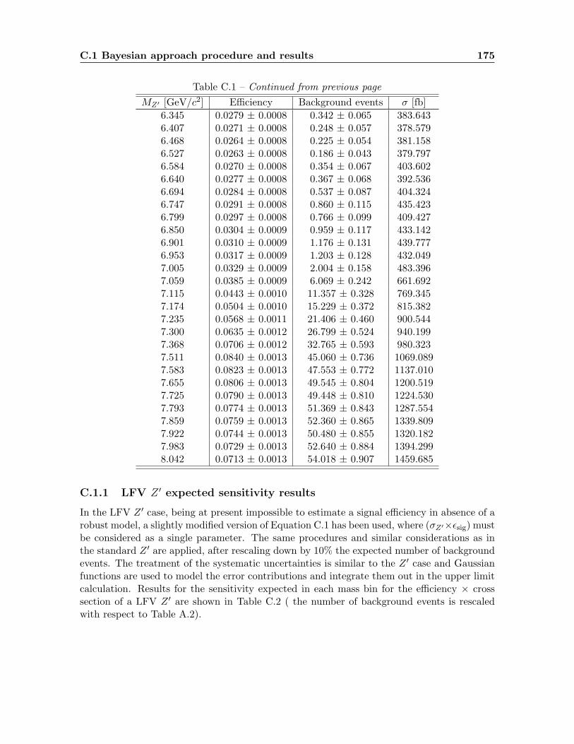
C.1 Bayesian approach procedure and results 175
Table C.1 – Continued from previous page
MZ′ [GeV/c2] Efficiency Background events σ [fb]
6.345 0.0279 ± 0.0008 0.342 ± 0.065 383.6436.407 0.0271 ± 0.0008 0.248 ± 0.057 378.5796.468 0.0264 ± 0.0008 0.225 ± 0.054 381.1586.527 0.0263 ± 0.0008 0.186 ± 0.043 379.7976.584 0.0270 ± 0.0008 0.354 ± 0.067 403.6026.640 0.0277 ± 0.0008 0.367 ± 0.068 392.5366.694 0.0284 ± 0.0008 0.537 ± 0.087 404.3246.747 0.0291 ± 0.0008 0.860 ± 0.115 435.4236.799 0.0297 ± 0.0008 0.766 ± 0.099 409.4276.850 0.0304 ± 0.0009 0.959 ± 0.117 433.1426.901 0.0310 ± 0.0009 1.176 ± 0.131 439.7776.953 0.0317 ± 0.0009 1.203 ± 0.128 432.0497.005 0.0329 ± 0.0009 2.004 ± 0.158 483.3967.059 0.0385 ± 0.0009 6.069 ± 0.242 661.6927.115 0.0443 ± 0.0010 11.357 ± 0.328 769.3457.174 0.0504 ± 0.0010 15.229 ± 0.372 815.3827.235 0.0568 ± 0.0011 21.406 ± 0.460 900.5447.300 0.0635 ± 0.0012 26.799 ± 0.524 940.1997.368 0.0706 ± 0.0012 32.765 ± 0.593 980.3237.511 0.0840 ± 0.0013 45.060 ± 0.736 1069.0897.583 0.0823 ± 0.0013 47.553 ± 0.772 1137.0107.655 0.0806 ± 0.0013 49.545 ± 0.804 1200.5197.725 0.0790 ± 0.0013 49.448 ± 0.810 1224.5307.793 0.0774 ± 0.0013 51.369 ± 0.843 1287.5547.859 0.0759 ± 0.0013 52.360 ± 0.865 1339.8097.922 0.0744 ± 0.0013 50.480 ± 0.855 1320.1827.983 0.0729 ± 0.0013 52.640 ± 0.884 1394.2998.042 0.0713 ± 0.0013 54.018 ± 0.907 1459.685
C.1.1 LFV Z ′ expected sensitivity results
In the LFV Z ′ case, being at present impossible to estimate a signal efficiency in absence of arobust model, a slightly modified version of Equation C.1 has been used, where (σZ′×εsig) mustbe considered as a single parameter. The same procedures and similar considerations as inthe standard Z ′ are applied, after rescaling down by 10% the expected number of backgroundevents. The treatment of the systematic uncertainties is similar to the Z ′ case and Gaussianfunctions are used to model the error contributions and integrate them out in the upper limitcalculation. Results for the sensitivity expected in each mass bin for the efficiency × crosssection of a LFV Z ′ are shown in Table C.2 ( the number of background events is rescaledwith respect to Table A.2).

176 Upper limit calculation
Table C.2: The results of the Bayesian statistical analysis for the LFV Z ′ case are reported, where thelast column shows the 90% CL upper limit in terms of the signal efficiency×cross section measurement.The uncertainties quoted here are MC statistical only.
MZ′ [GeV/c2] Background events εsig × σ [fb]
0.500 0.000 ± 0.000 9.6301.391 0.018 ± 0.010 9.6161.807 0.030 ± 0.013 9.6302.134 0.036 ± 0.015 9.6492.424 0.006 ± 0.006 9.6472.683 0.048 ± 0.017 9.9392.911 0.030 ± 0.013 9.6433.112 0.065 ± 0.020 10.0493.294 0.068 ± 0.020 10.0863.461 0.153 ± 0.030 10.5863.618 0.096 ± 0.023 10.2143.767 0.078 ± 0.021 10.1333.909 0.117 ± 0.026 10.3074.044 0.163 ± 0.031 10.6244.173 0.077 ± 0.021 10.1384.295 0.145 ± 0.029 10.5634.412 0.115 ± 0.026 10.3004.524 0.172 ± 0.032 10.7054.633 0.083 ± 0.022 10.1444.740 0.139 ± 0.041 10.5194.845 0.107 ± 0.025 10.2994.947 0.131 ± 0.028 10.4145.045 0.065 ± 0.020 10.0525.138 0.151 ± 0.042 10.5695.226 0.143 ± 0.029 10.5305.307 0.178 ± 0.033 10.7135.384 0.131 ± 0.028 10.4085.457 0.172 ± 0.032 10.7295.527 0.143 ± 0.029 10.5075.595 0.187 ± 0.044 10.7795.663 0.167 ± 0.043 10.6825.731 0.177 ± 0.052 10.7025.799 0.101 ± 0.025 10.2625.868 0.151 ± 0.042 10.5815.937 0.243 ± 0.063 11.0406.007 0.127 ± 0.040 10.3626.077 0.133 ± 0.040 10.3996.146 0.113 ± 0.026 10.3436.214 0.151 ± 0.042 10.5686.280 0.098 ± 0.038 10.251
Continued on next page

C.2 Frequentist approach procedure and results 177
Table C.2 – Continued from previous page
MZ′ [GeV/c2] Background events εsig × σ [fb]
6.345 0.149 ± 0.030 10.5576.407 0.053 ± 0.018 9.9856.468 0.080 ± 0.036 10.1356.527 0.098 ± 0.038 10.2586.584 0.109 ± 0.039 10.2856.640 0.151 ± 0.042 10.5976.694 0.172 ± 0.032 10.7156.747 0.207 ± 0.054 10.8976.799 0.338 ± 0.067 11.5386.850 0.310 ± 0.066 11.4136.901 0.461 ± 0.078 12.0706.953 0.450 ± 0.078 11.9737.005 0.849 ± 0.082 13.5097.059 4.905 ± 0.194 22.4207.115 8.327 ± 0.244 28.4157.174 11.817 ± 0.283 34.1337.235 16.685 ± 0.352 41.7677.300 19.384 ± 0.385 46.2067.368 22.504 ± 0.403 50.9087.438 25.539 ± 0.437 55.7107.511 26.179 ± 0.427 56.5047.583 26.301 ± 0.456 56.7917.655 23.941 ± 0.427 53.1887.725 22.620 ± 0.428 51.0597.793 19.767 ± 0.400 46.3767.859 17.611 ± 0.387 43.3947.922 15.609 ± 0.354 40.2037.983 13.736 ± 0.336 37.1608.042 12.557 ± 0.325 35.238
C.2 Frequentist approach procedure and results
The expected sensitivity has been computed also with a frequentist approach and comparedto the results obtained from the Bayesian procedure, as cross-check of the robustness of thecalculation, and results have found to be consistent between the two methods, as reported inSection 8.1. Below the description of the frequentist method implemented for this study isprovided.
In their work [96], G.J.Feldman and R.D.Cousins proposed an approach for setting confi-dence intervals that works both for two-sided and and upper limit cases. Following Neyman’sconstruction, the first step is to build a confidence belt in the (observable x; parameter θ)space, which consists of horizontal lines calculated for each value of θ. For Poissonian case,Feldman and Cousins suggest the following algorithm of building such horizontal acceptanceinterval for a given value θ:

178 Upper limit calculation
define θbest that provides the highest Pbest(x) ≡ P (x|θbest), for each integer value of x .
compute the ranking variable R = P (x|θ)/Pbest(x), for each integer value of the observ-able x.
add to the interval values of xi with highest R until∑i
P (xi|θ) ≥ CL
Once the confidence belt is built, the confidence interval for an observed value x0 is obtainedas an intersection of the confidence interval with the vertical line at x0. This procedure isillustrated in Figure C.1. In this analysis, the observable x corresponds to the number ofobserved events in the given bin and the parameter θ can be either the number of signalevents or the cross section of the signal process. The first approach is used for the LFV Z ′
analysis and the second for the standard Z ′ case.
0 1 2 3 4 5 6 7 8 9 10 11 120
2
4
6
8
10
Feldman Cousins confidence belt (b = 3.0)
0.91
0.92
0.93
0.94
0.95
Cove
rage
Figure C.1: Feldman Cousins confidence belt constructed under the assumption of 3 backgroundevents. The red line intercepting with the horizontal acceptance regions shows the upper limit in caseof 3 observed events.
Error propagation
The probability density function P (x|θ) may contain hidden parameters
P (x|θ)→ P (x|θ, b) (C.2)
with values distributed according to some probability density function (PDF) P (b). Thehidden parameter can be integrated out as follows:
P (x|θ) =
∫P (x|θ, b)P (b)db (C.3)

C.2 Frequentist approach procedure and results 179
For this study, the hidden parameter is the expected number of background events, thathas two uncertainties: one comes from the limited size of the simulation samples and is ofstatistical nature; the second comes from the data-MC discrepancy. As far as the former isconcerned, the probability can be modified as:
P (x|θ) =
∞∫Nsel
1 =0
· · ·∞∫
Nseli =0
P (x|θ, N sel1 . . . N sel
i )∏i
P (N seli |N sel
i )dN sel1 . . . dN sel
i (C.4)
This is nothing more but averaging of the P (x|θ) over the possible background yields. Withinthis assumption, the numerical computation of the following equation is implemented:
P (x|θ) ≈ 1
M
∑j
P (x|θ, N sel1 . . . N sel
i ) ≡ 1
M
∑j
P (x|θ,∑i
N seli ) (C.5)
where the sum runs over set of (N sel1 . . . N sel
i ) random vectors of size M , simulated withPoissonian PDF. As for the latter, to account for systematic effects, it is possible to use amixed-Bayesian approach described in [99] that implies modification of P (x|θ,
∑i N
seli ) to
include the systematic uncertainty. This will lead to
P (x|θ) ≈ 1
M
∑j
P (x|θ, ri ×∑i
N seli ) (C.6)
where random vectors (ri, Nsel1 . . . N sel
i ) also include a correction factor ri generated accordingto normal distribution with mean (r) and width (δr) defined from systematics studies.
In the standard Z ′ scenario, the goal is to find the confidence interval for the cross sectionof the signal process. The correlations in the uncertainties of signal and background efficiencieshave to be accounted for when computing the Neyman structure. Thus, θ is considered tobe the studied cross section, and, assuming L to be luminosity and ε to be signal efficiency,Equation C.6 can be written as:
P (x|θ) ≈ 1
M
∑j
P (x|θ × L× ε, ri ×∑i
N seli ) (C.7)
where ε is a random value of efficiency generated according to its PDF simultaneously withri. The Neyman construction obtained for this definition of P (x|θ) will show the number ofobserved events on X axis and cross section values of ee → µµZ ′(Z ′ → invisible) process onY . These values are reported for the standard Z ′ analysis (see Table C.3).
Sensitivity
Following the original suggestion from the paper of Feldman and Cousins [96], the sensitivitiesof the analysis in each recoil mass bin are provided. The sensitivity, which is a characteristicof the method, is an average upper limit obtained by an ensemble of pseudo-experiments withthe expected background and no true signal. In each pseudo-experiment, an upper limit istaken as a numerical solution of the equation
CL =
u.l.∫0
P (N, x+ b)dx
∞∫0
P (N, x+ b)dx
(C.8)

180 Upper limit calculation
where CL is a chosen confidence level (90%), and P is probability to find N events. Followingarguments of section C.2, the sensitivity is calculated as
CL =1
M
∑j
(
u.l.∫0
P (N, x+ bi)dx
∞∫0
P (N, x+ bi)dx
= 0.9) (C.9)
wherebi = ri ×
∑i
N seli . (C.10)
Sensitivity to the cross section
Since some of the systematic uncertainties are the same for the signal and background, theupper limit on cross section is computed as:
CL =1
M
∑j
(
u.l.∫0
P (N,x+bj)dx
∞∫0
P (N,x+bj)dx= 0.9)
εj × L. (C.11)
Here the nominator is identical to that in Equation C.9 and ε is signal efficiency value gener-ated according to its PDF. Let rc and δrc as data-MC correction and its uncertainty commonfor signal and background, and rs(b) and δrs(b) as a signal (background) only corrections anduncertainties, we obtain:
bj = rcj × rbj ×∑i
N seli,j ;
εj = rcj × rsj × εMCj ,
(C.12)
where rc,s,bj are correction values generated as described in section C.2, εMCj is a random value
generated with binomial distribution with mean equal the signal efficiency and square rootof variance centered at the statistical uncertainty of the signal efficiency, and (N sel
1,j . . . Nseli,j )
is vector of random Poisson values. All variables with the same j index are computed simul-taneously M times and sensitivity for the cross section is defined as the average of M upperlimits.
Results
In Table C.3 and Table C.4 the cross section (cross section×selection efficiency for the LFVscenario) under the assumption of background only hypothesis are reported. Both statisticaland systematic uncertainties are taken into account. A graphic visualization of the expectedsensitivities reported in the Table below is given in Section 8.1 where results from the sensi-tivity studies are plotted in Figure 8.1, 8.2.

C.2 Frequentist approach procedure and results 181
Table C.3: Upper and lower limits of 90% CL Feldman Cousins interval (semi-Bayesian approach, in-terval corresponds to number of observed events equal to rounded background expectation), sensitivityto cross section in Z ′ mass bins for standard Z ′. Inputs from Table A.1.
MZ′ [GeV/c2] Exp. bkg 90% CL interval [fb] σ [fb]
0.500000 0.438018 0.0 257.3 376.01.391160 0.212978 0.0 176.4 194.01.807331 0.167320 0.0 169.1 181.02.134437 0.145263 0.0 167.3 179.02.424160 0.120882 0.0 166.3 175.02.683574 0.091934 0.0 166.9 173.02.911720 0.078408 0.0 167.9 174.03.112817 0.072981 0.0 172.0 177.03.294203 0.113736 0.0 178.4 188.03.461637 0.104172 0.0 184.6 193.03.618703 0.102278 0.0 184.5 191.03.767561 0.135967 0.0 167.4 191.03.909355 0.169201 0.0 180.8 194.04.044485 0.150677 0.0 181.2 195.04.173020 0.153202 0.0 185.8 198.04.295278 0.159811 0.0 190.5 206.04.412056 0.171296 0.0 195.1 212.04.524494 0.182473 0.0 182.7 216.04.633830 0.143208 0.0 201.7 215.04.740874 0.186462 0.0 204.1 225.04.845698 0.179773 0.0 189.3 227.04.947710 0.206115 0.0 191.4 235.05.045792 0.166299 0.0 212.1 229.05.138775 0.264052 0.0 198.4 247.05.226076 0.151711 0.0 220.6 240.05.307839 0.175003 0.0 224.7 244.05.384696 0.232739 0.0 209.6 255.05.457585 0.200084 0.0 213.1 256.05.527632 0.210682 0.0 216.8 260.05.595998 0.189942 0.0 240.7 264.05.663653 0.221307 0.0 224.7 270.05.731300 0.291281 0.0 228.8 286.05.799396 0.228373 0.0 233.1 284.05.868171 0.251541 0.0 237.6 293.05.937605 0.201548 0.0 242.4 297.06.007421 0.195543 0.0 270.1 298.06.077127 0.373949 0.0 254.6 334.06.146163 0.193851 0.0 262.0 320.06.214061 0.268015 0.0 269.7 343.06.280470 0.237254 0.0 277.6 344.0
Continued on next page

182 Upper limit calculation
Table C.3 – Continued from previous page
MZ′ [GeV/c2] Exp. bkg 90% CL interval [fb] σ [fb]
6.345147 0.342328 0.0 259.9 368.06.407952 0.247598 0.0 294.3 357.06.468829 0.224963 0.0 303.0 379.06.527794 0.185855 0.0 268.6 379.06.640409 0.367461 0.0 288.0 375.06.694420 0.536907 0.0 383.4 387.06.747235 0.860229 0.0 324.7 430.06.799163 0.766490 0.0 317.5 395.06.850560 0.958621 0.0 310.8 405.06.901827 1.176362 0.0 351.1 423.06.953420 1.202914 0.0 343.9 415.07.005871 2.004179 0.0 375.6 470.07.059783 6.068703 0.0 543.5 556.07.115758 11.356861 0.0 603.2 649.07.174316 15.229113 0.0 657.1 625.07.235851 21.406057 0.0 703.2 670.07.300555 26.799011 0.0 742.9 815.07.368350 32.765375 0.0 777.7 693.07.438796 40.935873 0.0 805.2 853.07.511010 45.060460 0.0 798.5 853.07.583725 47.552798 0.0 899.7 1006.07.655670 49.544840 0.0 979.7 1237.07.725912 49.447739 0.0 900.8 1373.07.793887 51.369198 0.0 985.0 1142.07.859391 52.360280 0.0 1033.7 1237.07.922501 50.480429 0.0 990.8 1173.07.983504 52.640400 0.0 1110.7 1170.08.042857 54.018064 0.0 1172.6 1830.0
Table C.4: Upper and lower limits of 90% CL Feldman Cousins interval (semi-Bayesian approach, in-terval corresponds to number of observed events equal to rounded background expectation), sensitivityto cross section×efficiency in Z ′ mass bins for LFV Z ′. Inputs from Table A.2.
MZ′ [GeV/c2] Exp. bkg 90% CL interval [fb] σ × ε [fb]
0.500000 0.000000 0.0 8.711592 8.361.391160 0.017833 0.0 8.711592 8.451.807331 0.029721 0.0 8.711592 8.562.134437 0.035666 0.0 8.711592 8.582.424160 0.005944 0.0 8.711592 8.392.683574 0.047554 0.0 7.985626 8.612.911720 0.029721 0.0 8.711592 8.563.112817 0.065387 0.0 7.985626 8.71
Continued on next page

C.2 Frequentist approach procedure and results 183
Table C.4 – Continued from previous page
MZ′ [GeV/c2] Exp. bkg 90% CL interval [fb] σ × ε [fb]
3.294203 0.067850 0.0 7.985626 8.803.461637 0.152810 0.0 7.985626 9.123.618703 0.095831 0.0 7.985626 8.893.767561 0.077999 0.0 7.985626 8.823.909355 0.117145 0.0 7.985626 9.014.044485 0.162959 0.0 7.985626 9.194.173020 0.077275 0.0 7.985626 8.844.295278 0.145126 0.0 7.985626 9.194.412056 0.115405 0.0 7.985626 8.964.524494 0.172384 0.0 7.985626 9.204.633830 0.083220 0.0 7.985626 8.914.740874 0.139137 0.0 7.985626 9.154.845698 0.106997 0.0 7.985626 8.894.947710 0.130774 0.0 7.985626 8.985.045792 0.065387 0.0 7.985626 8.705.138775 0.151026 0.0 7.985626 9.145.226076 0.142662 0.0 7.985626 9.165.307839 0.178328 0.0 7.985626 9.285.384696 0.130774 0.0 7.985626 9.085.457585 0.172384 0.0 7.985626 9.195.527632 0.142662 0.0 7.985626 9.075.595998 0.186691 0.0 7.985626 9.195.663653 0.167118 0.0 7.985626 9.545.731300 0.177222 0.0 7.985626 9.205.799396 0.101052 0.0 7.985626 8.925.868171 0.151026 0.0 7.985626 9.085.937605 0.243287 0.0 7.985626 9.536.007421 0.127249 0.0 7.985626 9.086.077127 0.133193 0.0 7.985626 9.116.146163 0.112941 0.0 7.985626 8.916.214061 0.151026 0.0 7.985626 9.606.280470 0.097527 0.0 7.985626 9.016.345147 0.148607 0.0 7.985626 9.056.407952 0.053498 0.0 7.985626 8.676.468829 0.079695 0.0 7.985626 8.736.527794 0.097527 0.0 7.985626 8.816.584937 0.109416 0.0 7.985626 8.966.640409 0.151026 0.0 7.985626 9.236.694420 0.172384 0.0 7.985626 9.366.747235 0.206943 0.0 7.985626 9.556.799163 0.338396 0.0 7.259660 9.996.850560 0.310415 0.0 7.259660 9.866.901827 0.461440 0.0 6.533694 10.39
Continued on next page

184 Upper limit calculation
Table C.4 – Continued from previous page
MZ′ [GeV/c2] Exp. bkg 90% CL interval [fb] σ × ε [fb]
6.953420 0.449552 0.0 6.533694 10.307.005871 0.848923 0.0 9.437558 11.737.059783 4.904603 0.0 18.366940 19.677.115758 8.327218 0.0 23.376105 23.657.174316 11.816673 0.0 30.853555 26.977.235851 16.684712 0.0 37.750231 31.227.300555 19.383820 0.0 38.331004 33.557.368350 22.504177 0.0 46.752210 35.447.438796 25.539436 0.0 52.632534 37.217.511010 26.179010 0.0 49.002704 38.047.583725 26.300923 0.0 47.187789 39.437.655670 23.940717 0.0 47.042596 36.267.725912 22.619869 0.0 46.752210 35.657.793887 19.767324 0.0 41.525255 33.307.859391 17.610801 0.0 39.637743 31.847.922501 15.609016 0.0 37.242055 29.977.983504 13.736242 0.0 32.668469 28.418.042857 12.556923 0.0 32.087697 27.77
C.3 Null hypothesis testing
To perform a model-independent test for non-SM signal, the probability of the null hypothesis,assuming SM yields only, is computed for each recoil mass bin in Table A.1 and Table A.2.Given the number N of observed and number B of background events, the p-value is definedas
p =
x=∞∑x=N
P (x|B) (C.13)
where P is the Poissonian probability. In this analysis, the number of expected backgroundevents is defined with an uncertainty ∆B and thus Equation C.13 is modified as follows:
p =
x=∞∑x=N
∫ b=∞
b=0P (x|B)P (B|b,∆B)db, (C.14)
where P (B|b,∆B) is the PDF for the expected number of background events. The latter canbe written as
B = L×∑i
(σi × εi), (C.15)
where L is the total luminosity and the sum is done over the different background componentswith their own cross section σi and selection efficiencies εi. As the selection efficiencies mea-sured from the simulation might differ from the real ones due to detector effects, Equation C.15becomes:
B = L×∑i
(σi ×N seli
Ngeni
× ri), (C.16)

C.3 Null hypothesis testing 185
where N seli , Ngen
i is the number of selected and generated events of a given background typeand ri is the efficiency correction factor derived from validation on data. Uncertainties on thecomponents in Equation C.16 end up in the total uncertainty ∆B and the individual PDFsfor each background component generate P (B|b,∆B). While for the statistical errors thePDF is known to be Poissonian, for the systematic uncertainties determining its nature is lessstraightforward. Hereby, choosing the proper PDF is the key step to calculate p-values:
for N seli a Poissonian distribution with mean fixed to the result from MC studies is
assumed;
for r the PDF is unknown; this term characterizes the degree of the understanding of thedetector and it is parameterized as a normal distribution with center at r and width ofδ(r) where δ(r) is the uncertainty coming from corrections measured on data validationstudies.
In order to ease the calculations, the p-value is defined as:
p = 1−N−1∑x=0
∞∫r=0
∞∫Nsel
1 =0
· · ·∞∫
Nseli =0
P (x|N sel1 . . . N sel
i , r1 . . . ri)×
×P (r|r)dr ×∏i
P (N seli |N sel
i )dN sel1 . . . dN sel
i .
(C.17)
To further facilitate numerical computations, it can be noticed that the integral in Equa-tion C.17 is nothing but the averaging of the probability over different values of the back-ground and data-MC correction, and hence we can write
p = 1− 1
M
N−1∑x=0
M∑j=1
P (x|(N sel1 . . . N sel
i )j , rj) (C.18)
where the sum runs over a set of (rj , Nsel1 . . . N sel
i )j random vectors of size M simulated withcorresponding PDFs. This exercise has been useful to set up the machinery for the nullhypothesis testing, though the p-values are almost meaningless in absence of data and can beonly a sanity check for the calculation strategy. The null hypothesis test has been calculatedonly after data unblinding with the yields measured from the recoil mass distribution on Phase2 Data. Results are reported in Figure C.2 for the standard Z ′, in Figure C.3 for the LFVZ ′. No significant deviation above the 3σ evidence has been found in neither cases.

186 Upper limit calculation
1 2 3 4 5 6 7 8
]2 Recoil mass [GeV/c
2−10
1−10
1
p-v
alue
Belle II 2018 - Preliminary
-1 = 276 pbL dt ∫1 2 3 4 5 6 7 8
]2 Recoil mass [GeV/c
2−10
1−10
1
p-v
alue
Belle II 2018 - Preliminary
-1 = 276 pbL dt ∫
Figure C.2: The p-values computed on the unblinded e+e−→ µ+µ−Z ′ Phase 2 data as a function ofthe recoil are displayed, for the normal binning scheme (left) and the half bin shifted option (right).
1 2 3 4 5 6 7 8
]2 Recoil mass [GeV/c
2−10
1−10
1
p-v
alue
Belle II 2018 - Preliminary
-1 = 276 pbL dt ∫
Figure C.3: The p-values computed on the unblinded e+e−→ e±µ∓Z ′ Phase 2 data as a function ofthe recoil are displayed.

Appendix D
Phase 3 improvement andprospects: supplementary plots
Results from preliminary lepton ID studies on Phase 3 data are reported here. The improve-ment in background rejection when applying a tight muon ID selection to the reconstructionof the decay J/ψ → µ+µ− is shown in Figure D.1.
Figure D.1: The dimuon invariant mass for the reconstructed J/ψ → µ+µ− events on 0.41 fb−1 ofBelle II 2019 data is here reported. On the left, only loose track quality selections are applied and noselection on the muon ID probability is required, while on the right the muon ID probability is askedto be larger than 0.95. The number of fitted background events reduces of from 23457±55 to 917±11.
Results of the signal shape study performed on signal MC samples simulated with earlyPhase 3 geometry and beam background conditions. The fits to the different Z ′ mass simu-lations and the corresponding values of the shape parameters, particularly the Gaussian andCB function widths, are reported in Figure D.2 in Appendix D.

188 Phase 3 improvement and prospects: supplementary plots
0 0.5 1 1.5 2 2.5 3
0
20
40
60
80
100
120
140
)2
Eve
nts
/ (
0.06
GeV
/c
alpha = -1.597 +/- 0.18
frac = 0.913 +/- 0.038
ncb = 0.79 +/- 0.18
sigmaCB = 0.0895 +/- 0.0068
sigmaGauss = 0.276 +/- 0.059
0 0.5 1 1.5 2 2.5 3
)2recoilMass (GeV/c
3−2−1−0123
pu
ll
1 1.5 2 2.5 3 3.5 4
0
50
100
150
200
250
)2
Eve
nts
/ (
0.06
GeV
/c
alpha = -1.297 +/- 0.17
frac = 0.803 +/- 0.097
ncb = 0.95 +/- 0.12
sigmaCB = 0.0432 +/- 0.0055
sigmaGauss = 0.085 +/- 0.013
1 1.5 2 2.5 3 3.5 4
)2recoilMass (GeV/c
3−2−1−0123
pu
ll
2.6 2.8 3 3.2 3.4 3.6 3.8 4 4.2 4.4
0
50
100
150
200
250
300
)2
Eve
nts
/ (
0.04
GeV
/c
alpha = -1.204 +/- 0.11
frac = 0.915 +/- 0.042
ncb = 1.22 +/- 0.11
sigmaCB = 0.0283 +/- 0.0021
sigmaGauss = 0.083 +/- 0.016
2.6 2.8 3 3.2 3.4 3.6 3.8 4 4.2 4.4
)2recoilMass (GeV/c
3−2−1−0123
pu
ll
3.8 4 4.2 4.4 4.6 4.8 5 5.2 5.4
0
50
100
150
200
250
300
350
)2
Eve
nts
/ (
0.03
4 G
eV/c
alpha = -0.662 +/- 0.46
frac = 0.51 +/- 0.14
ncb = 1.15 +/- 0.17
sigmaCB = 0.0190 +/- 0.0042
sigmaGauss = 0.0254 +/- 0.0015
3.8 4 4.2 4.4 4.6 4.8 5 5.2 5.4
)2recoilMass (GeV/c
3−2−1−01234
pu
ll
4.6 4.8 5 5.2 5.4 5.6 5.8 6
0
50
100
150
200
250
300
350
400
)2
Eve
nts
/ (
0.03
GeV
/c
alpha = -1.674 +/- 0.11
frac = 0.9907 +/- 0.0056
ncb = 0.93 +/- 0.10
sigmaCB = 0.01850 +/- 0.00067
sigmaGauss = 0.135 +/- 0.054
4.6 4.8 5 5.2 5.4 5.6 5.8 6
)2recoilMass (GeV/c
3−2−1−01234
pu
ll
5.6 5.8 6 6.2 6.4 6.6 6.8
0
50
100
150
200
250
300
350
400
450 )2
Eve
nts
/ (
0.02
6 G
eV/c
alpha = -1.035 +/- 0.27
frac = 0.65 +/- 0.14
ncb = 1.13 +/- 0.12
sigmaCB = 0.0112 +/- 0.0018
sigmaGauss = 0.0197 +/- 0.0023
5.6 5.8 6 6.2 6.4 6.6 6.8
)2recoilMass (GeV/c
3−2−1−0123
pu
ll
6.8 6.9 7 7.1 7.2 7.3 7.4 7.5
0
50
100
150
200
250
)2
Eve
nts
/ (
0.01
4 G
eV/c
alpha = -1.416 +/- 0.11
frac = 0.960 +/- 0.017
ncb = 1.00 +/- 0.11
sigmaCB = 0.01064 +/- 0.00064
sigmaGauss = 0.058 +/- 0.016
6.8 6.9 7 7.1 7.2 7.3 7.4 7.5
)2recoilMass (GeV/c
3−2−1−01234
pu
ll
7.8 7.9 8 8.1 8.2 8.3 8.4 8.5
0
50
100
150
200
250
300
350 )2
Eve
nts
/ (
0.01
4 G
eV/c
alpha = -1.490 +/- 0.14
frac = 0.910 +/- 0.021
ncb = 1.03 +/- 0.12
sigmaCB = 0.00752 +/- 0.00044
sigmaGauss = 0.0430 +/- 0.0065
7.8 7.9 8 8.1 8.2 8.3 8.4 8.5
)2recoilMass (GeV/c
3−2−1−0123
pu
ll
Figure D.2: Example of recoil mass distributions of the simulated Phase 3 signal samples, with thefitted PDF model superimposed (blue line), showing both the Gaussian (red filled line) and the CBfunction (red dashed line) components. Fit results are plotted in the upper right box of each graphand the inset plots show the pull distributions.

Acknowledgment
For being arrived at the end of this journey, I have to thank many people and their preciousguidance. I wish to acknowledge them not just because I managed to arrive here, but also forhow I have arrived, for the experience I have lived and shared with them and for everythingI have learned along the way. The first person is of course my professor, supervisor, advisor,mentor Francesco. He has taught me almost everything, but most important it is the wayhe did this, by giving the example in person. From him I learned the importance to bepresent, always focused, always motivated, always determined, eager to stand any effortswhen it’s about to achieve the planned results and, most important, to distinguish what itis meaningful to be pursued and what it’s not worth to spend energies and time for, instead.He taught me that impossible is (almost) nothing, with the right motivation, aware-thinking,dedication and patience. And if things do not go as expected, no defeat exists until one canlearn something and how to better behave at the next challenge. I just wish to be able toalways follow his model, even if I won’t have his office just two doors away from mine anymore.I just wish to continue making him proud of my work and to repay him back for these pricelessyears of learning and guidance with always better and better achievements. And this appliesto all my exceptional colleagues of the Pisa Group: to the tireless Giuliana; to the spectacularGiulia; to the irreplaceable Antonio El Paladin; to Stefano il Super Betta; to the all-knowingEugenio; to the patient Luigi. Of course, I have to include also my colleagues that movedfrom Pisa, the Z ′ gangers who shared the good and bad time of the never-ending analysiseffort and all the people from the Belle II collaboration I have been lucky to work and spendtime with in these years. I know that I owe everything to them, all the achievements, all thefun, all the personal and professional discoveries. No way to survive 24h shift in B3, or todiscover Shibuya party life, or again to eat 16 plates in a row at Genki sushi, if I couldn’thave shared all this with them.
A special thanks goes to my friends, to the ones in Pisa, from University, the ones whomoved away, the ones at home, the ones I have lived with, since they have been always eagerto know my next destination and to support my upcoming adventures, to share worries andlaughter. Also, they managed not to get crazy when I used to be in four different countriesin less than three weeks and they were just trying to understand in which city we could meetfor an aperitivo.
And last, but absolutely not least, thanks to my family, who always took so seriouslymy student and researcher duties, who learned to enjoy with me cold soba and matcha, whoalways supported me. I am aware that you are the reason why I could leave, study andbecome independent, and most of all the reason why it’s worth to always come back to tellyou the things I have seen and the places I have lived. Was I in Japan, Pisa or Marseille, youare always with me.

190 Acknowledgment
Finally, thanks to my dear friend, Japan, that in these last two years brought me to a newlife. It really changed everything drastically and beautifully in the same way as the sakurachanges the cold face of winter into a reborn spring. Arigatou gozaimasu.
What I have learned and I would like to thank for at the end of my PhD is that I have beenso lucky and I received so much in my life, that I just have to keep on trying my best, pursuingmy passions, dedicating to my work, studying and sharing my achievements, my knowledge,my joy with the people I’ll meet along the journey. It could sound obvious, but this is themost important thing to me: happiness is real only when shared. Learning, teaching andpublishing good scientific results is the way I know to do all this. I am deeply grateful.Vielen dank.Grazie.
But it’s been no bed of roses, no pleasure cruise,I consider it a challenge before the whole
human race and I ain’t gonna loose.We are the champions, my friends.We’ll keep on fighting till the end.

Bibliography
[1] J. Bernstein, Spontaneous symmetry breaking, gauge theories, the Higgs mechanism andall that , Rev. Mod. Phys. 46 (Jan, 1974) 7–48.http://link.aps.org/doi/10.1103/RevModPhys.46.7.
[2] N. Cabibbo, Unitary Symmetry and Leptonic Decays, Phys. Rev. Lett. 10 (Jun, 1963)531–533. http://link.aps.org/doi/10.1103/PhysRevLett.10.531.
[3] M. Kobayashi and T. Maskawa, CP Violation in the Renormalizable Theory of WeakInteraction, Prog. Theor. Phys. 49 (1973) 652–657.
[4] T. S. V. Albada, R. Sancisi, M. Petrou, and R. J. Tayler, Dark Matter in SpiralGalaxies [and Discussion] , Phil. Trans. Roy. Soc. Lond. A320 (1986) no. 1556, 447–464.
[5] G. Bertone, D. Hooper, and J. Silk, Particle dark matter: Evidence, candidates andconstraints, Phys. Rept. 405 (2005) 279–390, arXiv:hep-ph/0404175 [hep-ph].
[6] C. Alcock et al., MACHO, The MACHO project: Microlensing results from 5.7 years ofLMC observations, Astrophys. J. 542 (2000) 281–307, arXiv:astro-ph/0001272[astro-ph].
[7] M. Signore and D. Puy, Cosmic microwave background and first molecules in the earlyuniverse, Eur. Phys. J. C59 (2009) 117–172.
[8] P. Montero-Camacho, X. Fang, G. Vasquez, M. Silva, and C. M. Hirata, Revisitingconstraints on asteroid-mass primordial black holes as dark matter candidates, JCAP1908 (2019) 031, arXiv:1906.05950 [astro-ph.CO].
[9] I. I. Y. Bigi, CP violation: An Essential mystery in nature’s grand design, Surveys HighEnerg. Phys. 12 (1998) 269–336, arXiv:hep-ph/9712475 [hep-ph]. [Proc. Int. Sch.Phys. Fermi137,451(1998)].
[10] R. D. Peccei and H. R. Quinn, Constraints imposed by CP conservation in the presenceof pseudoparticles, Phys. Rev. D 16 (Sep, 1977) 1791–1797.https://link.aps.org/doi/10.1103/PhysRevD.16.1791.
[11] G. Bertone, D. Hooper, and J. Silk, Particle dark matter: Evidence, candidates andconstraints, Phys. Rept. 405 (2005) 279–390, arXiv:hep-ph/0404175 [hep-ph].
[12] R. Barbieri, C. Braggio, G. Carugno, C. S. Gallo, A. Lombardi, A. Ortolan, R. Pengo,G. Ruoso, and C. C. Speake, Searching for galactic axions through magnetized media:

192 BIBLIOGRAPHY
the QUAX proposal , Phys. Dark Univ. 15 (2017) 135–141, arXiv:1606.02201[hep-ph].
[13] J. Ferretti, STAX. An Axion-like Particle Search with Microwave Photons, inProceedings, 12th Patras Workshop on Axions, WIMPs and WISPs (PATRAS 2016):Jeju Island, South Korea, June 20-24, 2016, pp. 35–38. 2017. arXiv:1609.05105[hep-ph].
[14] I. Stern, ADMX Status, PoS ICHEP2016 (2016) 198, arXiv:1612.08296[physics.ins-det].
[15] P. S. Bhupal Dev, A. Mazumdar, and S. Qutub, Constraining Non-thermal and Thermalproperties of Dark Matter , Front.in Phys. 2 (2014) 26, arXiv:1311.5297 [hep-ph].
[16] T. Marrodan Undagoitia and L. Rauch, Dark matter direct-detection experiments, J.Phys. G43 (2016) no. 1, 013001, arXiv:1509.08767 [physics.ins-det].
[17] J. McDonald, Generation of WIMP Miracle-like Densities of Baryons and DarkMatter , arXiv:1201.3124 [hep-ph].
[18] C. Boehm and P. Fayet, Scalar dark matter candidates, Nucl. Phys. B683 (2004)219–263, arXiv:hep-ph/0305261 [hep-ph].
[19] S. Tulin, H.-B. Yu, and K. M. Zurek, Beyond Collisionless Dark Matter: ParticlePhysics Dynamics for Dark Matter Halo Structure, Phys. Rev. D87 (2013) no. 11,115007, arXiv:1302.3898 [hep-ph].
[20] M. Vogelsberger, J. Zavala, and A. Loeb, Subhaloes in Self-Interacting Galactic DarkMatter Haloes, Mon. Not. Roy. Astron. Soc. 423 (2012) 3740, arXiv:1201.5892[astro-ph.CO].
[21] D. E. Kaplan, M. A. Luty, and K. M. Zurek, Asymmetric Dark Matter , Phys. Rev.D79 (2009) 115016, arXiv:0901.4117 [hep-ph].
[22] Y. Hochberg, E. Kuflik, T. Volansky, and J. G. Wacker, Mechanism for Thermal RelicDark Matter of Strongly Interacting Massive Particles, Phys. Rev. Lett. 113 (2014)171301, arXiv:1402.5143 [hep-ph].
[23] F. F. Deppisch, P. S. Bhupal Dev, and A. Pilaftsis, Neutrinos and Collider Physics,New J. Phys. 17 (2015) no. 7, 075019, arXiv:1502.06541 [hep-ph].
[24] G. Krnjaic, Probing Light Thermal Dark-Matter With a Higgs Portal Mediator , Phys.Rev. D94 (2016) no. 7, 073009, arXiv:1512.04119 [hep-ph].
[25] R. Essig et al., Working Group Report: New Light Weakly Coupled Particles, inProceedings, 2013 Community Summer Study on the Future of U.S. Particle Physics:Snowmass on the Mississippi (CSS2013): Minneapolis, MN, USA, July 29-August 6,2013. 2013. arXiv:1311.0029 [hep-ph]. http://www.slac.stanford.edu/econf/C1307292/docs/IntensityFrontier/NewLight-17.pdf.

BIBLIOGRAPHY 193
[26] M. Pospelov, A. Ritz, and M. B. Voloshin, Secluded WIMP Dark Matter , Phys. Lett.B662 (2008) 53–61, arXiv:0711.4866 [hep-ph].
[27] N. Arkani-Hamed, D. P. Finkbeiner, T. R. Slatyer, and N. Weiner, A theory of darkmatter , Phys. Rev. D 79 (Jan, 2009) 015014.https://link.aps.org/doi/10.1103/PhysRevD.79.015014.
[28] B. Holdom, Two U(1)’s and Epsilon Charge Shifts, Phys. Lett. 166B (1986) 196–198.
[29] A. K. Drukier, K. Freese, and D. N. Spergel, Detecting cold dark-matter candidates,Phys. Rev. D 33 (Jun, 1986) 3495–3508.https://link.aps.org/doi/10.1103/PhysRevD.33.3495.
[30] M. Ackermann et al., Fermi-LAT, Measurement of separate cosmic-ray electron andpositron spectra with the Fermi Large Area Telescope, Phys. Rev. Lett. 108 (2012)011103, arXiv:1109.0521 [astro-ph.HE].
[31] O. Adriani et al., PAMELA, An anomalous positron abundance in cosmic rays withenergies 1.5-100 GeV , Nature 458 (2009) 607–609, arXiv:0810.4995 [astro-ph].
[32] M. Aguilar et al., AMS, First Result from the Alpha Magnetic Spectrometer on theInternational Space Station: Precision Measurement of the Positron Fraction inPrimary Cosmic Rays of 0.5–350 GeV , Phys. Rev. Lett. 110 (2013) 141102.
[33] Fundamental Physics at the Intensity Frontier. 2012. arXiv:1205.2671 [hep-ex].http://lss.fnal.gov/archive/preprint/fermilab-conf-12-879-ppd.shtml.
[34] A. Hook, Y. Kahn, B. R. Safdi, and Z. Sun, Radio Signals from Axion Dark MatterConversion in Neutron Star Magnetospheres, Phys. Rev. Lett. 121 (2018) no. 24,241102, arXiv:1804.03145 [hep-ph].
[35] B. Batell, R. Essig, and Z. Surujon, Strong Constraints on Sub-GeV Dark Sectors fromSLAC Beam Dump E137 , Phys. Rev. Lett. 113 (2014) no. 17, 171802,arXiv:1406.2698 [hep-ph].
[36] S. Schael et al., ALEPH, DELPHI, L3, OPAL, SLD, LEP Electroweak Working Group,SLD Electroweak Group, SLD Heavy Flavour Group, Precision electroweakmeasurements on the Z resonance, Phys. Rept. 427 (2006) 257–454,arXiv:hep-ex/0509008 [hep-ex].
[37] N. Borodatchenkova, D. Choudhury, and M. Drees, Probing MeV dark matter atlow-energy e+e- colliders, Phys. Rev. Lett. 96 (2006) 141802, arXiv:hep-ph/0510147[hep-ph].
[38] G. Aad et al., ATLAS, Search for Higgs bosons decaying to aa in the µµττ final state inpp collisions at
√s = 8 TeV with the ATLAS experiment , Phys. Rev. D92 (2015) no. 5,
052002, arXiv:1505.01609 [hep-ex].
[39] V. Khachatryan et al., CMS, Search for a very light NMSSM Higgs boson produced indecays of the 125 GeV scalar boson and decaying into τ leptons in pp collisions at√s = 8 TeV , JHEP 01 (2016) 079, arXiv:1510.06534 [hep-ex].

194 BIBLIOGRAPHY
[40] R. Aaij et al., LHCb, Search for hidden-sector bosons in B0→ K∗0µ+µ− decays, Phys.Rev. Lett. 115 (2015) no. 16, 161802, arXiv:1508.04094 [hep-ex].
[41] R. Aaij et al., LHCb, Search for long-lived particles decaying to jet pairs, Eur. Phys. J.C75 (2015) no. 4, 152, arXiv:1412.3021 [hep-ex].
[42] J. Alexander et al., Dark Sectors 2016 Workshop: Community Report , 2016.arXiv:1608.08632 [hep-ph].http://lss.fnal.gov/archive/2016/conf/fermilab-conf-16-421.pdf.
[43] W. Altmannshofer et al., Belle-II, The Belle II Physics Book , arXiv:1808.10567[hep-ex].
[44] H. Davoudiasl, H.-S. Lee, and W. J. Marciano, Muon g − 2, rare kaon decays, andparity violation from dark bosons, Phys. Rev. D89 (2014) no. 9, 095006,arXiv:1402.3620 [hep-ph].
[45] P. del Amo Sanchez et al., BaBar, Search for Production of Invisible Final States inSingle-Photon Decays of Υ (1S), Phys. Rev. Lett. 107 (2011) 021804, arXiv:1007.4646[hep-ex].
[46] J. P. Lees et al., BaBar, Search for a Dark Photon in e+e− Collisions at BaBar , Phys.Rev. Lett. 113 (2014) no. 20, 201801, arXiv:1406.2980 [hep-ex].
[47] J. P. Lees et al., BaBar, Search for Invisible Decays of a Dark Photon Produced in e+e−
Collisions at BaBar , Phys. Rev. Lett. 119 (2017) no. 13, 131804, arXiv:1702.03327[hep-ex].
[48] B. Batell, M. Pospelov, and A. Ritz, Probing a Secluded U(1) at B-factories, Phys.Rev. D79 (2009) 115008, arXiv:0903.0363 [hep-ph].
[49] R. Essig, J. Mardon, M. Papucci, T. Volansky, and Y.-M. Zhong, Constraining LightDark Matter with Low-Energy e+e− Colliders, JHEP 11 (2013) 167, arXiv:1309.5084[hep-ph].
[50] X.-G. He, G. C. Joshi, H. Lew, and R. R. Volkas, Simplest Z-prime model , Phys. Rev.D44 (1991) 2118–2132.
[51] J. P. Lees et al., BaBar, Search for a muonic dark force at BABAR, Phys. Rev. D94(2016) no. 1, 011102, arXiv:1606.03501 [hep-ex].
[52] W. Altmannshofer, S. Gori, M. Pospelov, and I. Yavin, Neutrino Trident Production: APowerful Probe of New Physics with Neutrino Beams, Phys. Rev. Lett. 113 (2014)091801, arXiv:1406.2332 [hep-ph].
[53] W. Altmannshofer, S. Gori, M. Pospelov, and I. Yavin, Quark flavor transitions inLµ − Lτ models, Phys. Rev. D89 (2014) 095033, arXiv:1403.1269 [hep-ph].
[54] T. Araki, S. Hoshino, T. Ota, J. Sato, and T. Shimomura, Detecting the Lµ − Lτ gaugeboson at Belle II , Phys. Rev. D95 (2017) no. 5, 055006, arXiv:1702.01497 [hep-ph].

BIBLIOGRAPHY 195
[55] M. G. Aartsen, M. Ackermann, et al., IceCube Collaboration, Observation ofHigh-Energy Astrophysical Neutrinos in Three Years of IceCube Data, Phys. Rev. Lett.113 (Sep, 2014) 101101.https://link.aps.org/doi/10.1103/PhysRevLett.113.101101.
[56] B. Shuve and I. Yavin, Dark matter progenitor: Light vector boson decay into sterileneutrinos, Phys. Rev. D89 (2014) no. 11, 113004, arXiv:1403.2727 [hep-ph].
[57] W. Altmannshofer, S. Gori, S. Profumo, and F. S. Queiroz, Explaining dark matter andB decay anomalies with an Lµ − Lτ model , JHEP 12 (2016) 106, arXiv:1609.04026[hep-ph].
[58] R. Aaij et al., LHCb, Measurement of Form-Factor-Independent Observables in theDecay B0 → K∗0µ+µ−, Phys. Rev. Lett. 111 (2013) 191801, arXiv:1308.1707[hep-ex].
[59] A. M. Sirunyan et al., CMS, Search for an Lµ − Lτ gauge boson using Z→ 4µ events inproton-proton collisions at
√s = 13 TeV , Phys. Lett. B792 (2019) 345–368,
arXiv:1808.03684 [hep-ex].
[60] S. R. Mishra, S. A. Rabinowitz, C. Arroyo, K. T. Bachmann, R. E. Blair, C. Foudas,B. J. King, W. C. Lefmann, W. C. Leung, E. Oltman, P. Z. Quintas, F. J. Sciulli, B. G.Seligman, M. H. Shaevitz, F. S. Merritt, M. J. Oreglia, B. A. Schumm, R. H. Bernstein,F. Borcherding, H. E. Fisk, M. J. Lamm, W. Marsh, K. W. B. Merritt, H. Schellman,D. D. Yovanovitch, A. Bodek, H. S. Budd, P. de Barbaro, W. K. Sakumoto, P. H.Sandler, and W. H. Smith, Neutrino tridents and W-Z interference, Phys. Rev. Lett. 66(Jun, 1991) 3117–3120. https://link.aps.org/doi/10.1103/PhysRevLett.66.3117.
[61] D. Curtin, R. Essig, S. Gori, and J. Shelton, Illuminating Dark Photons withHigh-Energy Colliders, JHEP 02 (2015) 157, arXiv:1412.0018 [hep-ph].
[62] I. Galon, A. Kwa, and P. Tanedo, Lepton-Flavor Violating Mediators, JHEP 03 (2017)064, arXiv:1610.08060 [hep-ph].
[63] I. Galon and J. Zupan, Dark sectors and enhanced h→ τµ transitions, JHEP 05 (2017)083, arXiv:1701.08767 [hep-ph].
[64] L. Goodenough and D. Hooper, Possible Evidence For Dark Matter Annihilation InThe Inner Milky Way From The Fermi Gamma Ray Space Telescope,arXiv:0910.2998 [hep-ph].
[65] A. J. Bevan et al., The Physics of the B Factories, The European Physical Journal C74 (2014) no. 11, 84–87. http://dx.doi.org/10.1140/epjc/s10052-014-3026-9.
[66] K. A. Olive et al., Particle Data Group, Review of Particle Physics, Chin. Phys. C38(2014) 090001.
[67] P. ODDONE, An Asymmetric B-Factory Based on PEPa, Annals of the New YorkAcademy of Sciences 578 (1989) no. 1, 237–247.http://dx.doi.org/10.1111/j.1749-6632.1989.tb50614.x.

196 BIBLIOGRAPHY
[68] T. Abe et al., Belle-II, Belle II Technical Design Report , arXiv:1011.0352[physics.ins-det].
[69] B. Aubert et al., BaBar, Measurement of CP violating asymmetries in B0 decays to CPeigenstates, Phys. Rev. Lett. 86 (2001) 2515–2522, arXiv:hep-ex/0102030 [hep-ex].
[70] K. Abe et al., Belle, Observation of large CP violation in the neutral B meson system,Phys. Rev. Lett. 87 (2001) 091802, arXiv:hep-ex/0107061 [hep-ex].
[71] M. e. a. Staric, Belle Collaboration, Evidence for D0−D0Mixing , Phys. Rev. Lett. 98
(May, 2007) 211803. https://link.aps.org/doi/10.1103/PhysRevLett.98.211803.
[72] S.-K. e. a. Choi, Belle Collaboration, Observation of a Narrow Charmoniumlike State inExclusive B± → K±π+π−J/ψ Decays, Phys. Rev. Lett. 91 (Dec, 2003) 262001.https://link.aps.org/doi/10.1103/PhysRevLett.91.262001.
[73] S.-K. e. a. Choi, Belle Collaboration, Observation of a Resonancelike Structure in theπ+−ψ
′Mass Distribution in Exclusive B → Kπ+−ψ
′Decays, Phys. Rev. Lett. 100
(Apr, 2008) 142001. https://link.aps.org/doi/10.1103/PhysRevLett.100.142001.
[74] P. M. Lewis et al., First Measurements of Beam Backgrounds at SuperKEKB , Nucl.Instrum. Meth. A914 (2019) 69–144, arXiv:1802.01366 [physics.ins-det].
[75] T. Kuhr, C. Pulvermacher, M. Ritter, T. Hauth, and N. Braun, Belle-II FrameworkSoftware Group, The Belle II Core Software, Comput. Softw. Big Sci. 3 (2019) no. 1, 1,arXiv:1809.04299 [physics.comp-ph].
[76] W. Altmannshofer et al., Belle-II, The Belle II Physics Book , arXiv:1808.10567[hep-ex]. Section 5, Reconstruction Software.
[77] R. Fruhwirth, Application of Kalman filtering to track and vertex fitting , NuclearInstruments and Methods in Physics Research Section A: Accelerators, Spectrometers,Detectors and Associated Equipment 262 (1987) no. 2, 444 – 450.http://www.sciencedirect.com/science/article/pii/0168900287908874.
[78] S. Agostinelli et al., GEANT4, GEANT4: A Simulation toolkit , Nucl.Instrum.Meth.A506 (2003) 250–303.
[79] M. Ritter et al., Belle II Conditions Database, J. Phys. Conf. Ser. 1085 (2018) no. 3,032032.
[80] S. Jadach, B. F. L. Ward, and Z. Was, The Precision Monte Carlo event generator K Kfor two fermion final states in e+ e- collisions, Comput. Phys. Commun. 130 (2000)260–325, arXiv:hep-ph/9912214 [hep-ph].
[81] N. Davidson, G. Nanava, T. Przedzinski, E. Richter-Was, and Z. Was, UniversalInterface of TAUOLA Technical and Physics Documentation, Comput. Phys. Commun.183 (2012) 821–843, arXiv:1002.0543 [hep-ph].

BIBLIOGRAPHY 197
[82] G. Balossini, C. Bignamini, C. M. C. Calame, G. Montagna, O. Nicrosini, andF. Piccinini, Photon pair production at flavour factories with per mille accuracy , Phys.Lett. B663 (2008) 209–213, arXiv:0801.3360 [hep-ph].
[83] F. A. Berends, P. H. Daverveldt, and R. Kleiss, Complete Lowest Order Calculationsfor Four Lepton Final States in electron-Positron Collisions, Nucl. Phys. B253 (1985)441–463.
[84] H. Czyz, M. Gunia, and J. H. Kuhn, Simulation of electron-positron annihilation intohadrons with the event generator PHOKHARA, JHEP 08 (2013) 110,arXiv:1306.1985 [hep-ph].
[85] J. Alwall, R. Frederix, S. Frixione, V. Hirschi, F. Maltoni, O. Mattelaer, H. S. Shao,T. Stelzer, P. Torrielli, and M. Zaro, The automated computation of tree-level andnext-to-leading order differential cross sections, and their matching to parton showersimulations, JHEP 07 (2014) 079, arXiv:1405.0301 [hep-ph].
[86] F. Abudinen et al., Belle-II, Measurement of the integrated luminosity of the Phase 2data of the Belle II experiment , arXiv:1910.05365 [hep-ex].
[87] K. Hanagaki, H. Kakuno, H. Ikeda, T. Iijima, and T. Tsukamoto, Electronidentification in Belle, Nucl. Instrum. Meth. A485 (2002) 490–503,arXiv:hep-ex/0108044 [hep-ex].
[88] I. Komarov and G. Inguglia, Performance of the CDC trigger for very low multiplicitystudies in Phase 2 data, BELLE2-NOTE-TE-2018-017 (Internal), 2018.
[89] G. Punzi, Sensitivity of searches for new signals and its optimization, eConf C030908(2003) MODT002, arXiv:physics/0308063 [physics]. [,79(2003)].
[90] F. Pedregosa, G. Varoquaux, A. Gramfort, V. Michel, B. Thirion, O. Grisel,M. Blondel, P. Prettenhofer, R. Weiss, V. Dubourg, J. Vanderplas, A. Passos,D. Cournapeau, M. Brucher, M. Perrot, and E. Duchesnay, Scikit-learn: MachineLearning in Python, J. Mach. Learn. Res. 12 (Nov., 2011) 2825–2830.http://dl.acm.org/citation.cfm?id=1953048.2078195.
[91] R. Brun and F. Rademakers, ROOT - An Object Oriented Data Analysis Framework,version 6.08/7 , in AIHENP’96 Workshop, Lausane, vol. 389, pp. 81–86. 1997.
[92] W. Verkerke and D. P. Kirkby, The RooFit toolkit for data modeling , eConf C0303241(2003) MOLT007.
[93] T. Skwarnicki, A study of the radiative cascade transitions between the Upsilon-primeand Upsilon resonsances, DESY-F31-86-02, Appendix E, 1986.
[94] T. Allmendinger et al., Track Finding Efficiency in BaBar , Nucl. Instrum. Meth. A704(2013) 44–59, arXiv:1207.2849 [hep-ex].
[95] A. Caldwell, D. Kollar, and K. Kroninger, BAT - The Bayesian analysis toolkit ,Computer Physics Communications 180 (2009) no. 11, 2197 – 2209.

198 BIBLIOGRAPHY
[96] G. J. Feldman and R. D. Cousins, A Unified approach to the classical statistical analysisof small signals, Phys. Rev. D57 (1998) 3873–3889, arXiv:physics/9711021[physics.data-an].
[97] I. Adachi et al., Belle-II, Search for an invisibly decaying Z ′ boson at Belle II ine+e− → µ+µ−(e±µ∓) plus missing energy final states, arXiv:1912.11276 [hep-ex].
[98] I. Komarov, A. Martini, and G. De Pietro, Study of muon identification performance inPhase 2 using ECL variables, BELLE2-NOTE-TE-2018-019 (Internal), 2018.
[99] J. Conrad, O. Botner, A. Hallgren, and C. Perez de los Heros, Including systematicuncertainties in confidence interval construction for Poisson statistics, Phys. Rev. D67(2003) 012002, arXiv:hep-ex/0202013 [hep-ex].