Beamforming Techniques for mmWave Hybrid Analog-Digital ...
125
HAL Id: tel-03595055 https://tel.archives-ouvertes.fr/tel-03595055 Submitted on 3 Mar 2022 HAL is a multi-disciplinary open access archive for the deposit and dissemination of sci- entific research documents, whether they are pub- lished or not. The documents may come from teaching and research institutions in France or abroad, or from public or private research centers. L’archive ouverte pluridisciplinaire HAL, est destinée au dépôt et à la diffusion de documents scientifiques de niveau recherche, publiés ou non, émanant des établissements d’enseignement et de recherche français ou étrangers, des laboratoires publics ou privés. Beamforming Techniques for mmWave Hybrid Analog-Digital Transceivers Nabil Akdim To cite this version: Nabil Akdim. Beamforming Techniques for mmWave Hybrid Analog-Digital Transceivers. Signal and Image processing. Université Paris-Saclay, 2021. English. NNT: 2021UPASG092. tel-03595055
-
Upload
khangminh22 -
Category
Documents
-
view
0 -
download
0
Transcript of Beamforming Techniques for mmWave Hybrid Analog-Digital ...

HAL Id: tel-03595055https://tel.archives-ouvertes.fr/tel-03595055
Submitted on 3 Mar 2022
HAL is a multi-disciplinary open accessarchive for the deposit and dissemination of sci-entific research documents, whether they are pub-lished or not. The documents may come fromteaching and research institutions in France orabroad, or from public or private research centers.
L’archive ouverte pluridisciplinaire HAL, estdestinée au dépôt et à la diffusion de documentsscientifiques de niveau recherche, publiés ou non,émanant des établissements d’enseignement et derecherche français ou étrangers, des laboratoirespublics ou privés.
Beamforming Techniques for mmWave HybridAnalog-Digital Transceivers
Nabil Akdim
To cite this version:Nabil Akdim. Beamforming Techniques for mmWave Hybrid Analog-Digital Transceivers. Signal andImage processing. Université Paris-Saclay, 2021. English. NNT : 2021UPASG092. tel-03595055

Beamforming Techniques for mmWave Hybrid Analog-Digital Transceivers
Thèse de doctorat de l'université Paris-Saclay
École doctorale n°580 : sciences et technologies de l'information et de la communication (STIC)
Spécialité de doctorat : Réseaux, information et communications Unité de recherche : Université Paris-Saclay, CNRS, CentraleSupélec, Laboratoire
des signaux et systèmes, 91190, Gif-sur-Yvette, France. Référent : CentraleSupélec
Thèse présentée et soutenue à Paris-Saclay,
le 13/12/2021, par
Nabil AKDIM
Composition du Jury
Didier le Ruyet Professeur, Conservatoire National des Arts et Métiers
Président & Rapporteur
Ghaya Rekaya Professeure, Télécom Paris Rapporteure & Examinatrice
Direction de la thèse Pierre Duhamel Professeur, CentraleSupélec Directeur de thèse
Yang Sheng Professeur, CentraleSupélec Co-Directeur de thèse
Mustapha Benjillali Professeur, Institut National des Postes et Télécommunications
Invité
Carles Navarro Manchon Professeur associé, Aalborg University Invité
Thès
e de
doc
tora
t N
NT
: 202
1UPA
SG09
2

Maison du doctorat de l’Université Paris-Saclay 2ème étage aile ouest, Ecole normale supérieure Paris-Saclay 4 avenue des Sciences, 91190 Gif sur Yvette, France
Titre : Techniques de formation de beamformers pour les émetteurs-récepteurs hybrides analogiques- numériques mmWave
Mots clés : beamformers, émetteurs-récepteurs hybrides, mmWave
Résumé : La forte augmentation des applications gourmandes en bande passante ces dernières années et la pénurie mondiale des bandes cellulaire dans le spec- tre traditionnel des bandes basses ont rendu le spectre vacant dans les bandes de fréquences à ondes millimétriques (mmWave) d’une importance primordiale pour tous les acteurs clés de l’industrie cellulaire. Cela étant dit, communi- quer sans fil sur les fréquences mmWave serait néanmoins une tâche difficile, principalement en rai-son de la faible réflectivité, de l’absorption élevée et des pertes de prop- agation en espace libre impor-tantes sur des bandes aussi élevées.
L’une des solutions très populaires pour surmonter les problèmes de propagation susmentionnés con-siste à utiliser des réseaux d’antennes massifs, une technique rendue possible grace a la proportionna-lité entre la taille physique du réseau et la longueur d’onde de la porteuse (les fréquences mmWave sont caractérisées par une petite longueur d’onde, ce qui se traduit par réseaux d’antennes compacts avec un grand nombre d’éléments). Cependant, le coût élevé, la consommation d’énergie et la comple-xité du matériel de signal mixte chez mmWave ren-dent impossible l’utilisation de grands réseaux d’an-tennes avec des éléments à commande numérique.
Le cloisonnement des traitements de signal liés aux émetteurs-récepteurs mmWave a rendu possible une mise en œuvre économique et énergétique-ment effi cace de ces derniers. Ces nouvelles archi-tectures sont connues sous le nom d’émetteurs-récepteurs hybrides analogiques/numériques de for-mation de faisceaux.
Ces architectures hybrides divisent le traitement de précodage/combinaison entre les domaines analogique et numérique, ce qui réduit considéra-blement le nombre requis de chaînes RF.
Les structures des réseaux hybrides soulevent néanmoins leurs propres défis, le faible rapport signal sur bruit (SNR) résultant des pertes de pro-pagation élevées, la grande dimensionnalité de la matrice de canaux sans fil Multiple-Input-Multiple-Output (MIMO) et la présence de traitement ana-logique compliquent l’acquisition des informations d’état du canal (CSI) et le calcul des précodeurs et combineurs MIMO.
Relever les défis susmentionnés est essentiel pour activer le cellulaire basé sur mmWave. Avec cette motivation à l’esprit, cette thèse propose de nouvelles solutions algorithmiques qui les abor-dent. Nous proposons des solutions rapides et de faible complexité qui offrent des performances ef-ficaces tout en respectant les contraintes matériel-les. Les principales contributions de la présente thèse consistent à concevoir des algorithmes rapi-des et de faible complexité qui permettent de construire des précodeurs et des combineurs ro-bustes pendant la phase d’apprentissage du be-amformer et sans avoir besoin d’estimer explicite-ment le CSI puis de l’utiliser pour dériver ces be-amformers.

Maison du doctorat de l’Université Paris-Saclay 2ème étage aile ouest, Ecole normale supérieure Paris-Saclay 4 avenue des Sciences, 91190 Gif sur Yvette, France
Title : Beamforming Techniques for mmWave Hybrid Analog-Digital Transceivers.
Keywords : Beamforming, mmWave, Hybrid Analog-Digital Transceivers.
Abstract : The high increase of bandwidth greedy applications in recent years, and the global wireless band- width shortage in the traditional low band spectra has made vacant spectrum in millimeter-wave (mmWave) frequency bands of a paramount importance for all key players in the cellular indus-try. This being said, wireless communications over mmWave frequencies will nevertheless be a chal-lenging task, mainly due to the diffraction capability, high absorption and large free space propagation losses on such high bands.
One of the very popular solutions to overcome the aforementioned propagation issues is to use mas-sive an- tenna arrays, a technique that is made pos-sible because if the proportionality between the ar-ray’s physical size and the carrier wavelength (mmWave frequencies are characterized by small wavelength, which translates to compact antenna arrays with high number of elements). However, the high cost, power consumption and complexity of the mixed signal hardware at mmWave make having large an- tenna arrays with digitally controlled ele-ments infeasible.
The partitioning of the signal processing operations related to the mmWave transceivers made having a cost and energy effective implementation of these latter possi- ble. These novel architectures are known as hybrid analog/digital beamforming trans-ceivers. These hybrid architectures divide the pre-coding/combining processing between the analog and digital domains, which reduces considerably the required number of RF chains.
Hybrid array structures entail nevertheless their own challenges, the low signal-to-noise ration (SNR) resulting from high propagation losses, the large dimensionality of the Multiple-Input-Multiple-Output (MIMO) wireless channel matrix and the presence of analog processing complicate the ac-quisition of the channel state information (CSI) and the computation of the MIMO precoders and combiners.
Addressing the aforementioned challenges is key to enabling mmWave based cellular. With this mo-tivation in mind, this dissertation proposes novel algorithmic solutions that tackle them. We pro-pose fast and low complexity solutions that yield efficient performance while respecting the hardware constraints. The main contributions of the present thesis consist of devising fast and low complexity algorithms that enable building robust precoders and combiners during the beam trai-ning phase and without the need of explicitly esti-mating the CSI and then using it to derive these beamformers.


Beamforming Techniques for mmWave Hybrid Analog-Digital
Transceivers
by
Nabil Akdim
DISSERTATION
Presented to the Faculty of the Graduate School of
CentraleSupélec - Paris-Saclay University
in Partial Fulfillment of the Requirements
for the Degree of
DOCTOR OF PHILOSOPHY
CentraleSupélec - Paris-Saclay University
France
September 2021

Beamforming Techniques for mmWave Hybrid Analog-Digital
Transceivers
Nabil Akdim
CentraleSupélec - Paris-Saclay University, 2021
Abstract
The high increase of bandwidth greedy applications in recent years, and the global wireless band-
width shortage in the traditional low band spectra has made vacant spectrum in millimeter-wave
(mmWave) frequency bands of a paramount importance for all key players in the cellular industry.
This being said, wireless communications over mmWave frequencies will nevertheless be a challenging
task, mainly due to the poor diffraction capability, high absorption and large free space propagation
losses on such high bands.
One of the very popular solutions to overcome the aforementioned propagation issues is to use
massive antenna arrays, a technique that is made possible because of the proportionality between
the array’s physical size and the carrier wavelength. However, the high cost, power consumption and
complexity of the mixed signal hardware at mmWave complicates to a great extent implementing large
antenna arrays with digitally controlled elements.
Nevertheless, the partitioning of the signal processing operations related to the mmWave transceivers
has allowed cost and energy effective implementation of these latter. These novel architectures are
known as hybrid analog/digital beamforming transceivers. These hybrid architectures divide the pre-
coding/combining processing between the analog and the digital domains, which reduces considerably
ii

iii
the required number of RF chains.
Hybrid array structures entail nevertheless their own challenges, the low signal-to-noise ratio (SNR)
resulting from high propagation losses, the large dimensionality of the multiple-input-multiple-output
(MIMO) wireless channel matrix and the presence of analog processing complicate the acquisition of
the channel state information (CSI) and the computation of the MIMO precoders and combiners.
Addressing the aforementioned challenges is key to enabling mmWave based cellular. With this
motivation in mind, this dissertation proposes novel algorithmic solutions that tackle these latter.
We propose fast and low complexity solutions that yield efficient performance while respecting the
hardware constraints. The main contributions of the present thesis are deriving fast and low complexity
algorithms that enable building robust precoders and combiners during the beam training phase and
without the need of explicitly estimating the CSI and then using it to derive these beamformers.
In the first contribution, we use advanced tools from Bayesian active learning and approximate in-
ference theories, to devise a robust and fast hierarchical beam search algorithm that reduces the amount
of time or resources needed for the beam search process while guaranteeing a low beam misalignment
probability. Our second contribution proposes a novel beam training strategy based on alternating
transmissions between two hybrid mmWave transceivers. The main idea behind our proposal is to
exploit the reciprocity of the mmWave MIMO channel between the two transceivers. With appropriate
processing at each device, the alternate transmissions implicitly implement an algebraic power itera-
tion that leads to approximating the top left and right singular vectors of that MIMO channel matrix.
Mathematical analysis as well as numerical simulations illustrate the promising performance of the
proposed solutions, making them as enabling technologies for mmWave hybrid transceiver systems.


Contents
Abstract vii
List of Figures ix
List of Tables xi
1 Introduction 1
1.1 Why do Cellular Communications Need mmWave Bands ? . . . . . . . . . . . . . . . . . 2
1.2 Hybrid Beamforming as an Enabler . . . . . . . . . . . . . . . . . . . . . . . . . . . . . . 5
1.3 Hybrid Beamforming Challenges . . . . . . . . . . . . . . . . . . . . . . . . . . . . . . . 6
1.4 Overview of Contributions . . . . . . . . . . . . . . . . . . . . . . . . . . . . . . . . . . . 6
1.5 Organization . . . . . . . . . . . . . . . . . . . . . . . . . . . . . . . . . . . . . . . . . . 7
2 MmWave Channel Characteristics 9
2.1 MmWave vs. Sub-6 Ghz propagation environements . . . . . . . . . . . . . . . . . . . . 9
2.2 MmWave Channel Models . . . . . . . . . . . . . . . . . . . . . . . . . . . . . . . . . . . 10
2.2.1 Large Scale Fading . . . . . . . . . . . . . . . . . . . . . . . . . . . . . . . . . . . 11
2.2.2 Small Scale Fading . . . . . . . . . . . . . . . . . . . . . . . . . . . . . . . . . . . 14
2.3 MmWave Transceiver Design . . . . . . . . . . . . . . . . . . . . . . . . . . . . . . . . . 20
2.3.1 MmWave Hybrid Digital-Analog Antenna Array Architectures . . . . . . . . . . 22
v

vi CONTENTS
3 mmWave Wireless Channels Variational Online Learning 31
3.1 Overview . . . . . . . . . . . . . . . . . . . . . . . . . . . . . . . . . . . . . . . . . . . . 31
3.2 Introduction . . . . . . . . . . . . . . . . . . . . . . . . . . . . . . . . . . . . . . . . . . . 31
3.3 System Model . . . . . . . . . . . . . . . . . . . . . . . . . . . . . . . . . . . . . . . . . . 35
3.4 RF Codebook . . . . . . . . . . . . . . . . . . . . . . . . . . . . . . . . . . . . . . . . . . 36
3.5 Sequential Beam Pair Search via Variational HiePM . . . . . . . . . . . . . . . . . . . . 38
3.5.1 Sequential Active Learning via the HiePM Strategy . . . . . . . . . . . . . . . . 38
3.5.2 The Variational Expectation Maximization HiePM Scheme: VEM-HiePM . . . . 40
3.5.3 The Variational Model Comparison Based HiePM Scheme : VMC-HiePM . . . . 44
3.6 Numerical Results . . . . . . . . . . . . . . . . . . . . . . . . . . . . . . . . . . . . . . . 48
3.7 Conclusion and Future Work . . . . . . . . . . . . . . . . . . . . . . . . . . . . . . . . . 56
4 Mutli-Stream Beamforming with Hybrid Arrays 57
4.1 Overview . . . . . . . . . . . . . . . . . . . . . . . . . . . . . . . . . . . . . . . . . . . . 57
4.2 Introduction . . . . . . . . . . . . . . . . . . . . . . . . . . . . . . . . . . . . . . . . . . . 58
4.3 System Model . . . . . . . . . . . . . . . . . . . . . . . . . . . . . . . . . . . . . . . . . . 61
4.4 Hybrid Ping Pong Multi Beam Training : Hybrid PPMBT . . . . . . . . . . . . . . . . . 62
4.4.1 Ping-Pong Multi Beam Training with Digital Antenna Arrays: Digital PPMBT . 63
4.4.2 Analog Precoder Multi Level Codebook . . . . . . . . . . . . . . . . . . . . . . . 64
4.4.3 Ping Pong Multi Beam Training with Hybrid Antenna Arrays : Hybrid PPMBT 65
4.5 Numerical Results . . . . . . . . . . . . . . . . . . . . . . . . . . . . . . . . . . . . . . . 69
4.6 Conclusion . . . . . . . . . . . . . . . . . . . . . . . . . . . . . . . . . . . . . . . . . . . 74
5 Concluding Remarks 77
5.1 Summary . . . . . . . . . . . . . . . . . . . . . . . . . . . . . . . . . . . . . . . . . . . . 77
5.2 Future Work . . . . . . . . . . . . . . . . . . . . . . . . . . . . . . . . . . . . . . . . . . 78

CONTENTS vii
Appendices 81
A Variational Hierarchical Posterior Matching for mmWave Wireless Channels Online
Learning 83
B Ping Pong Beam Training for Multi Stream MIMO Communications with Hybrid
Antenna Arrays 89
Bibliography 97


List of Figures
1.1 Estimation of Global Mobile Subscriptions [1] . . . . . . . . . . . . . . . . . . . . . . . . . . 2
1.2 Current Cellular Spectrum in the US [2] . . . . . . . . . . . . . . . . . . . . . . . . . . . . . 3
1.3 Vehicle-To-Everything (V2X) Communication . . . . . . . . . . . . . . . . . . . . . . . . . . 4
1.4 Device to Device for Wearable Devices . . . . . . . . . . . . . . . . . . . . . . . . . . . . . . 5
2.1 MmWave vs. Sub-6 Ghz Propagation Differences . . . . . . . . . . . . . . . . . . . . . . . . 10
2.2 MmWave Blockage Agents . . . . . . . . . . . . . . . . . . . . . . . . . . . . . . . . . . . . 12
2.3 Separate Modeling of LOS and NLOS Links . . . . . . . . . . . . . . . . . . . . . . . . . . . 13
2.4 Two-state Markov Model for Blockage Events . . . . . . . . . . . . . . . . . . . . . . . . 15
2.5 Two-State Shadowing Event with 0dB Threshold Showing Unshadowed (Black Line)
and Shadowed (Red Line) Regions . . . . . . . . . . . . . . . . . . . . . . . . . . . . . . 15
2.6 Time Domain Clusters . . . . . . . . . . . . . . . . . . . . . . . . . . . . . . . . . . . . . 18
2.7 Angular Domain Clusters . . . . . . . . . . . . . . . . . . . . . . . . . . . . . . . . . . . 18
2.8 28 GHz Time Domain Clusters . . . . . . . . . . . . . . . . . . . . . . . . . . . . . . . . 19
2.9 28 GHz Angular Domain Clusters . . . . . . . . . . . . . . . . . . . . . . . . . . . . . . . 19
2.10 MIMO Transceiver Architecture at Frequencies below 6 GHz . . . . . . . . . . . . . . . . . . 21
2.11 MIMO Hybrid Digital-Analog MmWave Transceiver Architecture . . . . . . . . . . . . . . . . 23
2.12 Hybrid Precoding w/ Phase Shifters – Fully Connected . . . . . . . . . . . . . . . . . . . . . 24
2.13 Hybrid Precoding w/ Phase Shifters – Partially Connected . . . . . . . . . . . . . . . . . . . 24
ix

x LIST OF FIGURES
2.14 Hybrid Precoding with Lenses . . . . . . . . . . . . . . . . . . . . . . . . . . . . . . . . . . 25
3.1 Hybrid Transceiver Structure . . . . . . . . . . . . . . . . . . . . . . . . . . . . . . . . . 32
3.2 Structure of a Multi-resolution Codebook with a Resolution Parameter with N = 8 . . . . . . 37
3.3 Resulting Beam Patterns of the Beamforming Vectors in the First Three Codebook Levels of
a Hierarchical Codebook. . . . . . . . . . . . . . . . . . . . . . . . . . . . . . . . . . . . . 37
3.4 Beamforming Loss of the Different search schemes in a Channel with L = 0 Scattered
Components. . . . . . . . . . . . . . . . . . . . . . . . . . . . . . . . . . . . . . . . . . . 51
3.5 Beamforming Loss of the Different Search Schemes in a Channel with L = 0 Scattered
Components. . . . . . . . . . . . . . . . . . . . . . . . . . . . . . . . . . . . . . . . . . . 53
3.6 VMC-HiePM Performance in Channels with Different Power Ratios Between the Dom-
inant Path and L = 3 Scattered Components. . . . . . . . . . . . . . . . . . . . . . . . . 55
4.1 Structure of the Hybrid Transceivers . . . . . . . . . . . . . . . . . . . . . . . . . . . . . 60
4.2 Array Gains Obtained with the Analog Beamformers of the Proposed Multi-Level Code-
book, NA = 16, NRF = 4, LA = 3. . . . . . . . . . . . . . . . . . . . . . . . . . . . . . . 65
4.3 Spectral Efficiency When NRFA =NRF
B = 8, NS=4, L=8, ρ=30dB. . . . . . . . . . . . . . 71
4.4 Spectral Efficiency for Different NS Values. NA=NB=128, NRFA =NRF
B =8, L=8, ρ=30dB. 72
4.5 Spectral Efficiency over Different NS Values. NA=NB=64, NRFA =NRF
B =8, L=7. . . . . 75
(a) Spectral Efficiency over SNR . . . . . . . . . . . . . . . . . . . . . . . . . . . . . . 75
(b) Spectral Efficiency over PP Iterations . . . . . . . . . . . . . . . . . . . . . . . . . 75
4.6 Spectral Efficiency When Device A is Equipped with a Hybrid Array and Device B has
a Full Digital Architecture. NA=128, NB=4, NRFA =16, NS=4, L=40. . . . . . . . . . . . 76

List of Tables
2.1 Omnidirectional Path Loss Models in the Umi Scenario . . . . . . . . . . . . . . . . . . . . . 27
2.2 LOS Probability Models in the Umi Scenario . . . . . . . . . . . . . . . . . . . . . . . . . . 28
2.3 Range for the power Consumption for the different devices in a mmWave front-end . . . . . . 29
xi

Chapter 1
Introduction
1

2 CHAPTER 1. INTRODUCTION
1.1 Why do Cellular Communications Need mmWave Bands ?
The next couple of years are expected to see a surge in the number of mobile subscriptions. According
to a study conducted by the international telecommunication union (ITU) [1], and as can be seen in
Fig. 1.1, the total number of global mobile subscribers is estimated to keep increasing by about 10%
year over year and will attain more than 17 billion by the year 2030.
Figure 1.1: Estimation of Global Mobile Subscriptions [1]
Such a high number of connected wireless devices, together with the emergence of new mobile
applications that require very high data rate communications, emanating from these latter, as well as
the wireless network’s user’s expectation to have a satisfactory end-user experience even in crowded
areas [3], will pose a big challenge ahead of the wireless service providers, who will have to come up
with new and innovative technologies in order to be able to cope with this explosive increase in the
mobile data traffic.
The wireless service providers will also have to overcome the global bandwidth shortage which is
caused by the congestion and fragmentation of the traditional low band spectra [4]. Fig 1.2 [2] shows
how the below 3Ghz cellular spectrum currently in use in the united states shows is badly packed, it
also shows how scarce is the total remaining free bandwidth that can be used for new applications
(only about 600 Mhz) and also how high is the cost to acquire such small bandwidth.
The difficulty to achieve the aforementioned demands faced by wireless service providers, using the

1.1. WHY DO CELLULAR COMMUNICATIONS NEED MMWAVE BANDS ? 3
Figure 1.2: Current Cellular Spectrum in the US [2]
congested and fragmented traditional low spectral bands, has pushed them to start exploring vacant
spectrum at the millimeter-wave (mmWave) frequency bands [4].
Mmwave carrier frequencies span the spectrum range from 30 GHz to 300 GHz, whereas the ma-
jority of to date deployed wireless systems operate in the below 6 Ghz spectra. Going up to such
high frequencies opens up the door to accessing multi-Ghz unused spectral bandwidths, which would
then translate to higher data rates. An example of such use is the WiGig [5] wireless systems that is
deployed in the 60 GHz unlicensed mmWave band and that makes use of a 2 Ghz large bandwidth and
combines with the orthogonal frequency division multiplexing (OFDM) wavefrom modulation scheme
to reach data rates up to 6 Gbps.
Interest in mmWave frequencies for wireless communications dates back to the 19th century. Bose
and Lebedev [6] started experimenting in such high bands already in the 1890s. But, this interest
started to gain momentum and materialise when academia, industry as well as governments, with the
hope of solving the above-mentioned issues related to bandwidth scarcity and fragmentation in the
the sub 6 Ghz spectrum, began backing the idea of deploying a flavor of the 5th generation of cellular
systems, known as 5G new radio (NR) [7], on mmWave bands [8–10]. All these efforts resulted in two
types of 5G NR cellular deployments, the first known as frequency range 1 (FR1) NR option, deployed
on sub 6 Ghz frequencies, and the second known as frequency range 2 NR (FR2) option [11], deployed
over the mmWave frequency bands. This latter FR2 option benefited, in its initial deployment, from

4 CHAPTER 1. INTRODUCTION
large bandwidths (of up to 3 Ghz) in the 28 Ghz and 39 Ghz frequency band [12], which, combined with
advanced multi antenna beamforming techniques, allowed achieving the astonishingly high throughput
of up to 4.3 Gbps on a cellular hand-held device [13].
Aside from cellular applications, mmWave can have many other potential applications. Being
already heavily used in the well established automotive radar business [14], adding the communication
dimension to it would enable new mmWave vehicle-to-everything (V2X) applications like cloud assisted
or fully automated driving, as shown in Fig. 1.31, and would open new possibilities for the assisted
and autonomous driving industry [15].
MmWave is also of interest for high speed wearable networks that connect cell phone, smart watch,
augmented reality glasses and virtual reality headsets [16]. Examples of such use cases are shown in
Fig. 1.3 and Fig. 1.42.
Figure 1.3: Vehicle-To-Everything (V2X) Communication
This being said, wireless communications over mmWave frequencies will nevertheless be a challeng-
ing task, mainly due to the poor diffraction capability, high absorption and large free space propagation
losses on such high bands [17].
1Figure is taken from Professor Robert W. Heath Jr’s mmWave communications tutorial given in the signal processingsummer school that was held in Chalmers University in Gothenburg, Sweden, during summer 2017.
2Similar to Fig. 1.3, this figure is taken from Professor Robert W. Heath Jr’s mmWave communications tutorial givenin the signal processing summer school that was held in Chalmers University in Gothenburg, Sweden, during summer2017.

1.2. HYBRID BEAMFORMING AS AN ENABLER 5
Figure 1.4: Device to Device for Wearable Devices
1.2 Hybrid Beamforming as an Enabler
Fortunately, this frequency range will allow for the use of compact and small antenna arrays with high
number of elements, as the physical size of the array is proportional to the carrier wavelength. The
large beamforming gains that such large-scale arrays enable will be used to compensate for the above
limitations. However, the high cost, power consumption and complexity of the mixed signal hardware
at mm-wave make having large antenna arrays with digitally controlled elements infeasible [18]. A
direct implication of these new hardware constraints is the renewed interest in partitioning the related
signal processing operations between analog and digital domains to reduce the number of required
mixed signal hardware components, like analog-to-digital converters (ADCs), or their resolution, thus
reducing their power consumption and die size footprints. This has led to the development of new and
novel transceiver architectures dubbed hybrid analog/digital beamforming architectures. These hybrid
architectures divide the precoding/combining processing between the analog and digital domains, which
reduces the required number of RF chains. reducing thus hardware implementation complexity and
related power consumption, which enables in turn having portable device being able to communicate
wirelessly over mmWave frequencies.

6 CHAPTER 1. INTRODUCTION
1.3 Hybrid Beamforming Challenges
The hardware constraints associated with the hybrid architectures such as the limitations on the RF
components and the coupling between analog and digital precoders, however, impose new constraints
on the precoding/combining and the wireless channel estimation design problems.
Accurate Channel State information is critical for efficient operation in wireless communication
systems. The task of obtaining such information at hybrid beamforming mmWave systems represents
a major challenge. In addition to the large training overhead associated with the large arrays and
the SNR that is typically low before beamforming design, the hardware constraints, that results from
RF/hybrid precoding, makes the channels at the baseband seen only through the RF lens [18]. This
has renewed the interest in beam training techniques. These techniques make use of multi-stage radio
frequency (RF) codebooks together with adaptive beamwidth beamforning algorithms to jointly design
the transmitter and receiver beamforming vectors with the goal of maximizing the effective receive
gain of the wireless link being used [18, 19]. Despite the reduced complexity of the aforementioned
algorithms, they do entail a large search overhead and are prone to errors in noisy channels. This
has motivated devising novel beam search techniques that are robust both to inter-beam interference
leakage caused by the RF codebook imperfections and to the additive and multiplicative noise that is
inherent to any wireless communication system.
1.4 Overview of Contributions
Addressing the aforementioned challenges is the key to enabling mmWave based cellular. With this
motivation, this dissertation proposes novel algorithmic solutions that tackle them. We propose low-
complexity and fast solutions that yield efficient performance while respecting the hardware constraints.
The primary contributions of this dissertation can be summarized as follows.
• Our first contribution proposes efficient single stream sequential noisy beam search techniques for
mmWave systems with hybrid architectures. We use a combination of bayesian active learning

1.5. ORGANIZATION 7
and of advanced inference techniques to benefit from the reduced search time of the classical
hierarchical beam-search technique, while at the same time reduce this latter’s inherent high
probability of beam misalignment, especially on noisy channels [20].
• Our second contribution proposes a novel beam training strategy based on alternating transmis-
sions between two hybrid mmWave transceivers. The main idea behind our proposal is to exploit
the reciprocity of the mmWave MIMO channel between the two transceivers. With appropriate
processing at each device, the alternate transmissions implicitly implement an algebraic power it-
eration that leads to approximating the top left and right singular vectors of that MIMO channel
matrix [21].
1.5 Organization
The rest of this thesis is organized as follows. In Chapter 2, we introduce mmWave channel character-
istics as well as mmWave hybrid transceiver design challenges. We then detail our first contribution,
dubbed "Variational Hierarchical Posterior Matching for mmWave Wireless Channels Online Learn-
ing" in Chapter 3. We show how the interplay of bayesian active learning and of advanced inference
techniques can devise fast and efficient beam search algorithms for single stream mmWave communi-
cation systems. In Chapter 4, we detail our second contribution, entitled "Ping Pong Beam Training
for Multi Stream MIMO Communications with Hybrid Antenna Arrays". We show how our proposal
approximates singular value decomposition (SVD) precoding with hybrid transceivers, enabling thus
robust multi-stream mmWave wireless communication systems. Concluding remarks and future work
are finally presented in Chapter 5.


Chapter 2
MmWave Channel Characteristics
Understanding the mmWave signal propagation characteristics and properties is fundamental to be
able to come up with accurate mmWave channel models. These latter are needed to help assess the
usability and also compare the different mmWave wireless communication systems. We will discuss in
this chapter the details of such propagation mechanisms.
2.1 MmWave vs. Sub-6 Ghz propagation environements
Spectral wave propagation at mmWave frequencies differ in many aspects from that of the low frequency
bands, mainly due to the very small wavelength compared to the size of most of the objects in the
environment. On one hand, diffraction effects, one of the main propagation mechanisms in sub 6 Ghz
bands [22], contributes much less to the overall mmWave signal propagation due to the reduced Fresnel
zone. Scattering, on the other hand, tends to be higher due to the increased effective roughness of
materials, but remains limited still and not as rich as in lower frequency bands. mmWave propagation
is also characterized by higher absorption and larger free space propagation losses [17,18].
All these differences affect heavily all mmWave channel’s properties. Multi-paths in mmWave tend
to be more clustered and exhibit far fewer paths than on lower frequency channels, leading to more
9
10 CHAPTER 2. MMWAVE CHANNEL CHARACTERISTICS
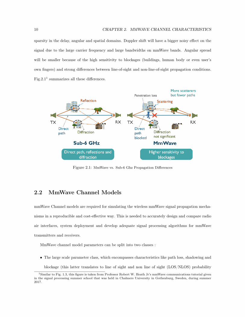
sparsity in the delay, angular and spatial domains. Doppler shift will have a bigger noisy effect on the
signal due to the large carrier frequency and large bandwidths on mmWave bands. Angular spread
will be smaller because of the high sensitivity to blockages (buildings, human body or even user’s
own fingers) and strong differences between line-of-sight and non-line-of-sight propagation conditions.
Fig.2.11 summarizes all these differences.
Figure 2.1: MmWave vs. Sub-6 Ghz Propagation Differences
2.2 MmWave Channel Models
mmWave Channel models are required for simulating the wireless mmWave signal propagation mecha-
nisms in a reproducible and cost-effective way. This is needed to accurately design and compare radio
air interfaces, system deployment and develop adequate signal processing algorithms for mmWave
transmitters and receivers.
MmWave channel model parameters can be split into two classes :
• The large scale parameter class, which encompasses characteristics like path loss, shadowing and
blockage (this latter translates to line of sight and non line of sight (LOS/NLOS) probability1Similar to Fig. 1.3, this figure is taken from Professor Robert W. Heath Jr’s mmWave communications tutorial given
in the signal processing summer school that was held in Chalmers University in Gothenburg, Sweden, during summer2017.

2.2. MMWAVE CHANNEL MODELS 11
models).
• The small scale parameter class, which encompasses characteristics like delay spread, Doppler
spread, angular spread and number of multi-path component clusters.
Let us discuss next the details of each of these two classes.
2.2.1 Large Scale Fading
In this section, we will detail the main large scale parameters of mmWave channel models. These
include path loss and shadowing parameters as well as large scale blockage parameters and related
modelling.
Path Loss and Shadowing Models
Path loss and Shadowing models for mmWave channels are inspired by Friis Law [19] and follow an
additive white noise linear log-distance parametric model [22,23] as shown in equation 2.1 below :
PL(d)[dB] = α+ 10β log10(d) + ξ, ξ ∼ N(0, σ2) (2.1)
d is the distance separating the transmitter and the receiver, α and β are parameter models that
depend on the wavelength λ being used, on the omnidirectional gains of the transmit and receive
antennas, Gt and Gr and on penetration losses of the material that the spectral waves might penetrate
in the surrounding environment. ξ is the log-normal term that accounts for variances in shadowing,
and which is also partially affected by the penetration losses.
Large scale Blockage Models
Blockage is a major impairment at mmWave. As shown in Fig.2.22, it can be caused by surrounding
objects like buildings, by surrounding people, or even by the user’s own body.2Similar to Fig. 1.3, this figure is taken from Professor Robert W. Heath Jr’s mmWave communications tutorial given
in the signal processing summer school that was held in Chalmers University in Gothenburg, Sweden, during summer2017.

12 CHAPTER 2. MMWAVE CHANNEL CHARACTERISTICS
Figure 2.2: MmWave Blockage Agents
On one hand, penetration losses that are caused by building walls can introduce attenuation up to
80 dB [24], and those that are caused by the human body can result for up to 35 dB loss [25]. On the
other hand, reflective capabilities of all these blockers allow them to be important scatterers to enable
coverage via NLOS paths for mmWave cellular systems [26]. Measurements conducted by New York
University (NYU) confirm that even in extremely dense urban environments, coverage is possible up
to 200 m from a potential cell site [4].
Blockage can be modeled in different ways. Random shape theory [27] and stochastic geometry
theory [28] are mathematical tools that can used to evaluate coverage and capacity in mmWave cellular
networks analytically. Data driven methods can also be used to quantify the effect of blockage, an
example of such methods is to model the mmwave wireless link states using a two-state model (LOS
and NLOS) or a three state model (LOS, NLOS, and signal outage), where both model’s states are
chosen to be parametric statistical functions of the distance between transmitters and receivers, and
where each state’s parameters are fit using the field sounding measurements [29], then the resulting
fitted functions are used to calculate the probability of the link being in each of these states. Fig.2.33
shows this separate modeling of LOS and NLOS links.
A widely used two state model [29–32] is described below:
3Similar to Fig. 1.3, this figure is taken from Professor Robert W. Heath Jr’s mmWave communications tutorial givenin the signal processing summer school that was held in Chalmers University in Gothenburg, Sweden, during summer2017.

2.2. MMWAVE CHANNEL MODELS 13
Figure 2.3: Separate Modeling of LOS and NLOS Links
• LOS model i.e not blocked :
PLLOS(d)[dB] = αLOS + 10βLOS log10(d) + ξLOS (2.2)
• NLOS model i.e blocked :
PLNLOS(d)[dB] = αNLOS + 10βNLOS log10(d) + ξNLOS (2.3)
• Choice of LOS or NLOS is determined by a Bernoulli random variable p(d):
PL(d)[dB] = p(d)PLLOS(d)[dB] + (1− p(d))PLNLOS(d)[dB] (2.4)
• The stochastic blocking function p(d) is modeled as:
P(p(d) = 1) = exp−λd (2.5)
Many organizations have conducted extensive mmWave channel field sounding measurements to
help collect data and fit the above statistical model parameters (λ, αLOS, βLOS, αNLOS, βNLOS and
the shadowing variances). The four major ones are :
• The 3rd Generation Partnership Project (3GPP TR 38.901 [32]), which provides channel models
from 0.5–100 GHz based on a modification of 3GPP’s extensive effort to develop models from 6
to 100 GHz in TR 38.900 [33]. 3GPP TR documents are a continual work in progress and serve
as the international industry standard for 5G cellular.

14 CHAPTER 2. MMWAVE CHANNEL CHARACTERISTICS
• 5G Channel Model (5GCM) [34], an ad-hoc group of 15 companies and universities that developed
models based on extensive measurement campaigns and helped seed 3GPP understanding for TR
38.900 [33].
• Mobile and wireless communications Enablers for the Twenty–twenty Information Society (METIS) [35],
a large research project sponsored by European Union.
• Millimeter-Wave Based Mobile Radio Access Network for 5G Integrated Communications (mm-
MAGIC) [36], another large research project sponsored by the European Union.
An example of the results of the measurement campaigns conducted by the above bodies are sum-
marized, for the urban micro-cellular (UMi) propagation scenario, in Table 2.1 for the Omnidirectional
path loss model and Table 2.2 for the LOS probability model.
Blockage introduces not only LOS/NLOS large scale fading effects on the mmWave signal prop-
agation, but also small scale rapid signal variations, mainly caused by people walking between the
transmitter and the receiver. These small scale effects can be by modeled a multi-state Markov model
where transition probability rates can be determined from the field measurements [37]. An example
of such a model is the simple two-state Markov model that is used to characterize unshadowed and
shadowed states for a wireless link in the presence of pedestrian induced variations in received signal
strength [38, 39]. Fig.2.4 shows a diagram of a two-state Markov model where Punshad and Pshad in-
dicate the transition probabilities of going from a shadowed to unshadowed state and an unshadowed
to shadowed state, respectively, and to shadowed state, respectively, and Fig.2.5 depicts the charac-
terization of a typical blockage event with two-states when applying a 0 dB threshold relative to the
zero-crossings for the beginning and end of a shadowing event.
2.2.2 Small Scale Fading
In this section, we will detail the main small scale parameters of mmWave channel models. We fist
motivate the need for using large antenna arrays for mmWave communications. We then explore the

2.2. MMWAVE CHANNEL MODELS 15
Figure 2.4: Two-state Markov Model for Blockage Events
Figure 2.5: Two-State Shadowing Event with 0dB Threshold Showing Unshadowed (Black Line) andShadowed (Red Line) Regions
clustered nature of the such high frequency channels. We discuss finally the impact of large antenna
arrays and the clustering characteristics on the mmwave channel mathematical model formulation.
Motivating large arrays for mmWave
As discussed so far, large free space propagation losses and high sensitivity to blockage make wireless
communications over mmwave channels a very challenging task. Fortunately, such high frequencies
will allow the use of compact and small antenna arrays with high number of elements, as the physical

16 CHAPTER 2. MMWAVE CHANNEL CHARACTERISTICS
size of the array is proportional to the carrier wavelength. The large beamforming gains and adaptive
directionality that such large-scale arrays enable will be used to compensate for the above limitations.
In fact, according to Friis Law, the far field receive power Pr and the transmit power Pt are related
by equation 2.6 in free space propagation :
Pr =Pt
4πR2
λ2
4πGtGr (2.6)
where R is the distance separating the transmitter and the receiver, λ is the wavelength and Gt
and Gr are the transmit and receive antenna gains.
Equation 2.6 can be dissected into three components :
• A first component that depends mainly on the transmit power and on the separation distance
between the transmitter and the receiver. This component is called the receive power spectral
density and is defined by Pt4πR2 .
• A second component that depends mainly on the wavelength used and on the receive antenna
characteristics. This component is called the effective receive aperture and is defined by λ2
4πGr.
• A third component that depends mainly on the transmit antenna characteristics. This component
equals the transmit antenna gain defined by Gt.
The receive antenna gain Gr increases with the number of antennas used at the receiver (effectively,
the more antennas we use for reception, the higher is the power will receive). So knowing that the
antenna size scales inversely to the wavelength (we refer to antenna size relative to wavelength. For
example : a 1/2 wave dipole antenna is approximately half a wavelength long), we can see that the
higher the frequency is (i.e the lower the wavelength), the higher is the number of antennas we can
accommodate in a given physical area, i.e the more effective power we can actually receive receive.
Therefore, the scaling of the antenna gains increases the effective receive aperture λ2
4πGr and more
than compensates for the increased free-space path-loss at mmWave frequencies.

2.2. MMWAVE CHANNEL MODELS 17
Compensating for path loss in this manner will require then directional transmissions with high-
dimensional antenna arrays (32 antennas and above). This explains why large arrays is a defining
characteristic of mmWave communication.
A Clustered Channel Model
Extensive field measurements [40] have shown that mmwave channels usually assume clustered spatio-
temporal models, where the channel’s multipath components are clustered both in time and angular
domains, as shown in Fig.2.6 and Fig.2.74. The time cluster–spatial lobe (TCSL) [41] approach is
then used to develop statistical spatial channel models (SSCM) for mmwave channels, as the TCSL
framework is shown to faithfully reproduce the first- and second-order time and angular statistics of
these types of wireless channels [42].
The mmWave channel’s SSCM small scale parameters are similar to those of low frequency SSCM
channel models, these are the per cluster parametric distributions of delay, power, central angles of
departure (AoD) and angles of arrival (AoA), together with the angle and delay spreads within each
cluster. Field Sounding campaigns show that these small scale characteristics exhibit spatio-temporal
sparsity due to the small angular spread and the low number of clusters caused by the limited scattering
in mmWave bands. Typically, measurements in the 28 GHz band [40] show the existence of two main
clusters in the time domain (Fig.2.8) and 5 main clusters in the angular domain (Fig.2.9)
Small Scale Fading Mathematical Model
The clustered nature of the mmwwave channel models, as well as their inherent need for large antenna
arrays makes many of the statistical fading distributions used for the traditional multiple input multiple
output (MIMO) low frequency channels inaccurate for mmWave channel modeling. For this reason,
we adopt the extended Saleh-Valenzuela [43] based clustered model representation, which allows us to
accurately capture the mathematical structure present in mmWave channels.4Similar to Fig. 1.3, both of these two figures are taken from Professor Robert W. Heath Jr’s mmWave communications
tutorial given in the signal processing summer school that was held in Chalmers University in Gothenburg, Sweden, duringsummer 2017.

18 CHAPTER 2. MMWAVE CHANNEL CHARACTERISTICS
Figure 2.6: Time Domain Clusters
Figure 2.7: Angular Domain Clusters
Consider a mmWave MIMO system with Nt transmit and Nr receive antennas. Assuming a static
2D narrow-band mmWave channels where uniform linear arrays (ULA) are used (extensions to dynamic
3D wide-band models with different array structures are straightforward [18, 40]), then our channel
model can be described by a Nr ×Nt complex matrix H, as set by equation 2.7.
H =
L∑
l=1
αlar(φr,l)aHt (φt,l) (2.7)
We have:
• L : the number of multi-path components.
• The elements on the ULAs are separated by a distance d. Typically d = λ/2, where λ is the the
mmWave wavelength of interest.
• αl is the complex fading channel gain of the l-th multi-path component. αl is typically assumed

2.2. MMWAVE CHANNEL MODELS 19
Figure 2.8: 28 GHz Time Domain Clusters
Figure 2.9: 28 GHz Angular Domain Clusters

20 CHAPTER 2. MMWAVE CHANNEL CHARACTERISTICS
to be complex Gaussian distributed.
• at(φt,l) and ar(φr,l) are the ULA array response vectors of the l-th multi-path component, at
the transmitter and receiver respectively.
• φt,l and φr,l are the incidence angles of the lth multi-path component, at the transmitter
and receiver respectively. These are modeled as at (φt,l) =[1, e−jωt,l , . . . , e−j(Nt−1)ωt,l
]Tand
ar (φr,l) =[1, e−jωr,l , . . . , e−j(Nr−1)ωr,l
]T, with ωt,l(φt,l) = 2π
λ d cos (φt,l) and ωr,l(φr,l) = 2πλ d cos (φr,l)
being the directional cosine angles of the lth multi-path component. The incidence angles φA
and φB are assumed to be sampled from the ranges [θt,1, θt,2] and [θr,1, θr,2] respectively.
2.3 MmWave Transceiver Design
As we saw above, reliable wireless communication over mmWave channels cannot be achieved without
large arrays. We will detail then in this section the challenges that come into picture when dealing
with large array transceiver design.
Signal processing for multiple antenna (MIMO) transceivers at low frequencies happens completely
in the digital baseband domain. This is made possible because in such systems, all antennas can be
digitally controlled through dedicated radio frequency (RF) chains as the number of antennas used in
low bands tend to be small (4 antennas typically), and because the mixed signal and RF components
(digital-to-analog and analog-to-digital converters, power amplifiers and low noise amplifiers) needed
for these RF chains do not consume very high power and are easy to integrate into a single system on
chip (SoC) subsystem. An example of such a transceiver system is shown in Fig. 2.105.
This is not the case for the mmWave communication systems as large antenna arrays are a defining
characteristic of these setups. This will have a big architectural impact on the mmWave transceiver
design.
5Similar to Fig. 1.3, this figure is taken from Professor Robert W. Heath Jr’s mmWave communications tutorial givenin the signal processing summer school that was held in Chalmers University in Gothenburg, Sweden, during summer2017.

2.3. MMWAVE TRANSCEIVER DESIGN 21
Figure 2.10: MIMO Transceiver Architecture at Frequencies below 6 GHz
Current hardware technology makes it very challenging to tie a separate RF chain (and all the
related baseband circuitry) for each antenna at the mmWave frequencies [44]. The array’s antenna
elements should be placed very close to each other to avoid granting lobes, this space limitation makes
it difficult to pack the RF chain needed complicated mixed signal and baseband circuitry behind each
antenna.
Controlling digitally every antenna of the array separately will drive the overall mmWave transceiver
power consumption very high : (i) mixed signal devices like PA and ADCs/DACs are power hungry
at such high frequencies [45]; (ii) benefiting from the large available bandwidth and the MIMO capa-
bilities of the massive arrays used in mmwave would require processing many parallel high throughput
data streams. This will strain the baseband digital signal processing chain and will drive the overall
transceiver’s power consumption excessively high [46].
Other aspects to take into account are the architectural challenges imposed by the mmWave analog
front end domain, where key power greedy hardware components include power amplifiers, phase
shifters, and switches.
A tremendous effort has been spent on building low power amplifiers, as these latter are an es-
sential component in the radio frequency chain, in integrated circuit (IC) design. In contrast, phase

22 CHAPTER 2. MMWAVE CHANNEL CHARACTERISTICS
shifters, originally utilized in radar systems, are the newly-introduced hardware components in hybrid
beamforming systems. Neverthless, the exact power consumption depends on the specifications and
technology used to implement these components. Table 2.3 shows the range of the power consumed by
different devices included in a mmWave front-end. Data were taken from a number of recent papers
proposing protoype devices for PAs [47–49], LNAs [50–53], phase shifters [54–57], VCOs [58–60] and
ADCs [61–64] at mmWave frequencies. Lt(Lr) is the number of RF chains at the TX(RX). A detailed
treatment of mmWave RF and analog devices and multi-gbps digital baseband circuits can be found
in [23].
All these hardware and power consumption constraints have motivated the wireless communication
research community to look into alternative mmWave specific MIMO transceiver architectures where
the required signal processing is split between the analog and digital domains, which are known as
hybrid digital-analog antenna array architectures [65], or where different design trade-offs are made
with respect to number of antennas or resolution of the RF chain’s components (DAC/ADCs, PAs and
phase shifters for example), these are known as low resolution transceivers [66], or some mix of both
of these solutions.
We will review in this section one of the main MIMO architectures for mmWave systems, namely
the hybrid digital-analog antenna array architectures. The reader can refer to [18] for an overview
about all such architectures.
2.3.1 MmWave Hybrid Digital-Analog Antenna Array Architectures
The hybrid digital-analog antenna array architectures, or hybrid beamformers for short, are composed
by large antenna arrays that are steered using analog phase shifters and only a few digitally modulated
radio-frequency (RF) chains. An illustration of such an architecture is shown in Fig.2.116.
The architecture shown in Fig.2.11 divides the mmWave MIMO transceiver between the digital and
6Similar to Fig. 1.3, this figure is taken from Professor Robert W. Heath Jr’s mmWave communications tutorial givenin the signal processing summer school that was held in Chalmers University in Gothenburg, Sweden, during summer2017.

2.3. MMWAVE TRANSCEIVER DESIGN 23
Figure 2.11: MIMO Hybrid Digital-Analog MmWave Transceiver Architecture
the analog domains. The digital component in hybrid architectures can handle each of the baseband
data streams separately, similar to the conventional fully digital MIMO transceivers, allowing thus spa-
tial multiplexing and multiuser MIMO when Ns > 1. The signal processing of the analog components
is however different. Since the transmitted signals for all baseband data streams are mixed together
through digital precoding, and the number of physical antennas is bigger than the number of streams
and RF chains, then the analog network FRF ∈ CNt×lt will be a common component shared by all
these baseband streams. This would impact greatly the algorithm design for such architectures and
would make reusing traditional low frequency channel estimation and precoding/combining techniques
very challenging.
The RF precoding/combining stage can be implemented using different analog approaches like
phase shifters [67], switches [68] or lenses [69]. Two hybrid structures are possible. In the first one
(see Fig.2.12), all the antennas can connect to each RF chain. In the second one (see Fig.2.13), the
array can be divided into subarrays, where each subarray connects to its own individual transceiver.
Having multiple subarrays reduces hardware complexity at the expense of less overall array flexibility.
A complete analysis of the energy efficiency and spectrum-efficieny of both architectures is provided
in [67].
Fig.2.12 and Fig.2.137 show the example of hybrid precoding structures with fully and partially7Similar to Fig. 1.3, both of these two figures are taken from Professor Robert W. Heath Jr’s mmWave communications
tutorial given in the signal processing summer school that was held in Chalmers University in Gothenburg, Sweden, during

24 CHAPTER 2. MMWAVE CHANNEL CHARACTERISTICS
connected phase shifters respectively. Such structures are enabled through digitally controlled phased
shifters with quantized phases, where the digital precoder/combiner can correct for lack of precision in
the analog, for example to cancel residual multi-stream interference, allowing thus hybrid precoding to
approach the performance of the unconstrained solutions [43]. The multi-subarray partially connected
structure allows for a great reduction in hardware complexity and power consumption [67].
Figure 2.12: Hybrid Precoding w/ Phase Shifters – Fully Connected
Figure 2.13: Hybrid Precoding w/ Phase Shifters – Partially Connected
To further reduce the overall implementation and power consumption complexity of the hybrid
architecture, an alternative mmWave hybrid architecture that makes use of switching networks has
been recently proposed [68]. This architecture, illustrated in Fig.2.12, exploits the sparse nature of the
mmwave channel by implementing a compressed spatial sampling of the received signal. The analog
combiner design is performed by a subset antenna selection algorithm instead of an optimization over
summer 2017.
2.3. MMWAVE TRANSCEIVER DESIGN 25
all quantized phase values. Every switch can be connected to all the antennas if the array size is small
or to a subset of antennas for larger arrays.
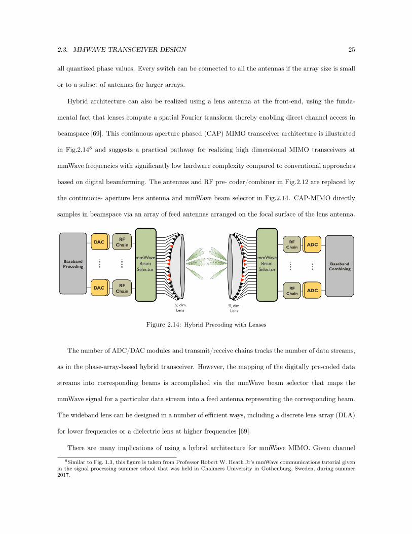
Hybrid architecture can also be realized using a lens antenna at the front-end, using the funda-
mental fact that lenses compute a spatial Fourier transform thereby enabling direct channel access in
beamspace [69]. This continuous aperture phased (CAP) MIMO transceiver architecture is illustrated
in Fig.2.148 and suggests a practical pathway for realizing high dimensional MIMO transceivers at
mmWave frequencies with significantly low hardware complexity compared to conventional approaches
based on digital beamforming. The antennas and RF pre- coder/combiner in Fig.2.12 are replaced by
the continuous- aperture lens antenna and mmWave beam selector in Fig.2.14. CAP-MIMO directly
samples in beamspace via an array of feed antennas arranged on the focal surface of the lens antenna.
Figure 2.14: Hybrid Precoding with Lenses
The number of ADC/DAC modules and transmit/receive chains tracks the number of data streams,
as in the phase-array-based hybrid transceiver. However, the mapping of the digitally pre-coded data
streams into corresponding beams is accomplished via the mmWave beam selector that maps the
mmWave signal for a particular data stream into a feed antenna representing the corresponding beam.
The wideband lens can be designed in a number of efficient ways, including a discrete lens array (DLA)
for lower frequencies or a dielectric lens at higher frequencies [69].
There are many implications of using a hybrid architecture for mmWave MIMO. Given channel
8Similar to Fig. 1.3, this figure is taken from Professor Robert W. Heath Jr’s mmWave communications tutorial givenin the signal processing summer school that was held in Chalmers University in Gothenburg, Sweden, during summer2017.

26 CHAPTER 2. MMWAVE CHANNEL CHARACTERISTICS
state information, new algorithms are needed to design the separate precoders/combiners since they
decompose into products of matrices with different constraints (analog and digital matrices as we saw
above). Learning the channel state is also harder, since training data is sent through analog precoders
and combiners. More challenges are found when going to broadband channels as the analog processing
is frequency flat while the digital processing can be frequency selective. There are many opportunities
for future research into designing cellular networks that support hybrid architectures.

2.3. MMWAVE TRANSCEIVER DESIGN 27
PL[dB], fc is in GHz and d3D is in meters meters Shadow fading std [dB] Applicability range and Parameters
5GCM
5GCM UMi-Street CI Model with 1 m reference distance: σSF = 3.76 6 < fc < 100 GHz
Canyon LOS PL = 32.4 + 21log10(d) + 20log10(fc)
5GCM UMi-Street CI Model with 1 m reference distance:
Canyon NLOS PL = 32.4 + 31.7log10(d) + 20log10(fc) σSF = 8.09 6 < fc < 100 GHz
ABG model:
PL = 22.4 + 35.3log10(d) + 21.3log10(fc) σSF = 7.82
5GCM UMi-Open CI Model with 1 m reference distance: σSF = 4.2 6 < fc < 100 GHz
Square LOS PL = 32.4 + 18.5log10(d) + 20log10(fc)
5GCM UMi-Open CI Model with 1 m reference distance:
Square NLOS PL = 32.4 + 28.9log10(d) + 20log10(fc) σSF = 7.1 6 < fc < 100 GHz
ABG model:
PL =3.66 + 41.4log10(d) + 24.3 log10(fc) σSF = 7.0
3GPP TR 38.901
3GPP UMi-Street PLUMi−LOS =
= 32.4 + 21 log10(d) + 20log10(fc) , 10m < d < dm
= 32.4 + 40 log10(d) + 20log10(fc)− 9.5 log10(d2m + (hBS − hUE)2) , dm < d < 5 km
σSF = 4.0 0.5 < fc < 100 GHz, 1.5 m < hUE < 22.5 m
Canyon LOS , hBS = 10 m, dm is specified in 3GPP TR 38.901
3GPP UMi-Street PL = max(PLUMi−LOS(d), PLUMi−NLOS(d)) σSF = 7.52 0.5 < fc < 100 GHz, 1.5 m < hUE < 22.5 m
Canyon NLOS PLUMi−NLOS = 22.4 + 35.3 log10(d) + 21.310(fc)− 0.3(hUE − 1.5) 10 m < d < 5000 m, hBS = 10 m
METIS
METIS UMi-Street PLUMi−LOS =
= 28.0 + 22 log10(d) + 20log10(fc) + PL0 , 10m < d < dm
= 35.8 + 40 log10(d) + 22 log10(dm) + 22log10(fc)− 18 log10(hBShUE) + PL0 , dm < d < 500 mσSF = 3.1 0.5 < fc < 60 GHz, 1.5 m < hUE < 22.5 m
Canyon LOS , hBS = 10 m, dm is specified in METIS specifications
METIS UMi-Street PL = max(PLUMi−LOS(d), PLUMi−NLOS(d)) σSF = 4.0 0.45 < fc < 6 GHz, 1.5 m < hUE < 22.5 m
Canyon NLOS PLUMi−NLOS = 23.15 + 36.7 log10(d) + 2610(fc)− 0.3(hUE) 10 m < d < 2000 m, hBS = 10 m
mmMAGIC
mmMAGIC UMi-Street PL = 32.9 + 19.2log10(d) + 20.8 log 10(fc) σSF = 2.0 65 < fc < 100 GHz
Canyon LOS
mmMAGIC UMi-Street PL = 31.0 + 45.0log10(d) + 20.0 log 10(fc) σSF = 7.82 65 < fc < 100 GHz
Canyon NLOS
Note : PL is the path loss, d is the T-R Euclidean distance
Table 2.1: Omnidirectional Path Loss Models in the Umi Scenario

28 CHAPTER 2. MMWAVE CHANNEL CHARACTERISTICS
LOS Probability models (distances in meters) Parameters
3GPP TR 38.901 PLLOS(d) = min(d1/d, 1)(1− exp(−d/d2)) + exp(−d/d2) d1 = 18 m, d2 = 36 m
5GCM d1/d2 model: d1/d2 model:
PLLOS(d) = min(d1/d, 1)(1− exp(−d/d2)) + exp(−d/d2) d1 = 20 m, d2 = 39 m
NYU squared model: NYU squared model:
PLLOS(d) = (min(d1/d, 1)(1− exp(−d/d2)) + exp(−d/d2))2 d1 = 22 m, d2 = 100 m
METIS PLLOS(d) = min(d1/d, 1)(1− exp(−d/d2)) + exp(−d/d2) d1 = 18 m, d2 = 36 m
d >= 10 m
mmMAGIC PLLOS(d) = min(d1/d, 1)(1− exp(−d/d2)) + exp(−d/d2) d1 = 18 m, d2 = 36 m
Table 2.2: LOS Probability Models in the Umi Scenario

2.3. MMWAVE TRANSCEIVER DESIGN 29
Device devices Power (mW)
(Per device)
PA Nt(Nr) 40-250
LNA Nt(Nr) 4-86
Phase shifter Nt(Nr)× Lt(Lr) 15-110
ADC Lt(Lr) 15-795
VCO Lt(Lr) 4-25
Table 2.3: Range for the power Consumption for the different devices in a mmWave front-end


Chapter 3
mmWave Wireless Channels
Variational Online Learning
3.1 Overview
We propose in this chapter1 two variational Bayesian acftive learning schemes that enable initial
access for hybrid digital-analog enabled devices operating in mmWave wireless channels. The proposed
schemes are devised with the goal to balance the beam search time and achieving higher beamforming
gain, while accounting for uncertainties on the unknown channel (gain and noise variance).
3.2 Introduction
As we discussed in earlier chapters, mmWave frequency bands (30− 300Ghz) is one of the most promis-
ing technologies that will make 5G and beyond cellular networks able to serve a large number of wireless
terminals with high data rates [4]. We saw how the free space propagation losses, poor diffraction ca-
1This chapter is based on the work published in the conference paper : N. Akdim, C. N. Manchón, M. Benjillali andP. Duhamel, "Variational Hierarchical Posterior Matching for mmWave Wireless Channels Online Learning," 2020 IEEE21st International Workshop on Signal Processing Advances in Wireless Communications (SPAWC), 2020, pp. 1-5, doi:10.1109/SPAWC48557.2020.9154340.
31

32 CHAPTER 3. MMWAVE WIRELESS CHANNELS VARIATIONAL ONLINE LEARNING
pability and high absorption of such high frequencies make building wireless transceivers operating
on such high frequencies a challenging task [17]. We introduced the concept of large antenna arrays
and we saw that the antenna array’s physical size proportionality to the carrier wavelength makes it
feasible to engineer small and compact antenna arrays with large number of elements at mmwave. We
also discussed how the high beamforming gains and the spatial steering capabilities of these arrays can
help greatly compensate the aforementioned limitations on these high bands.
When it comes to implementation, we discussed how the complexity of the mixed signal hardware at
mmWave as well as its high cost and power consumption make having element wise digitally controlled
large antenna arrays operating on such high frequencies infeasible [18]. We argued how such limitations
have motivated the wireless communication community to adopt a novel transceiver architecture termed
the hybrid digital-analog antenna array architecture [65]. This architecture helps bring down the cost
and power consumption of the mmwave transceivers by allowing to steer their large antenna arrays
using only few digitally modulated radio-frequency (RF) chains as shown in Fig. 4.1.
Baseband
Precoder
Baseband
Combiner
RF Chain
RF Chain
RF Chain
RF Chain
RF Precoder RF Combiner
NA N
B
NA
RF
NB
RF
H
TRANSCEIVER A TRANSCEIVER B
Figure 3.1: Hybrid Transceiver Structure
The hybrid digital-analog transceiver architecture brings its own challenges though. As already dis-
cussed, sensing the mmwave wireless channel using hybrid structure allows to access only a compressed

3.2. INTRODUCTION 33
version of it and requires running an exhaustive and time consuming search in the angular domain
to be able to estimate the CSI accurately. Also, using the acquired CSI to build the needed MIMO
precoders and combiners for such large MIMO channel, under the hybrid architecture constraint, is
not an easy task, it requires splitting the MIMO processing into two components, one digital and one
analog, a split that is challenging to properly perform due to the interconnection and interplay of the
analog domain design constraints with those of the digital domain [4, 18].
To overcome the long search time issue, the scientific community explored using the sparsity friendly
techniques for the CSI acquisition and precoding/combining algorithm design. These techniques were
believed, at least theoretically, to help bring down the number of channel measurements needed to
estimate CSI and build robust precoders and combiners. An example of such techniques are the
compressed sensing based approaches [18, 43, 70]. These latter have been shown, however, not only to
feature high computational complexity but also require long search time in general [70].
Other sparsity friendly techniques that are good alternative schemes to alleviate the aforementioned
issues are the hierarchical beam-search algorithms [21, 70]. The beam search mechanism in these
algorithms is designed based on the bisection concept. In particular, these algorithms start initially
by dividing the angular space into a number of partitions, which equivalently divides the AoAs/AoDs
range into a number of intervals, and design the multi-stage training precoding and combining set of
vectors, this group of vectors is known as a hierarchical beamforning codebook. The codebook’s design
is done in a way to let the combined angular spread of each stage, i.e the union of is vectors angular
spreads, cover entirely the AoAs/AoDs range of interest. Vectors of the first stage are used to sense the
angular space partitions, the received signal is then used to determine the partition(s) that are highly
likely to have non-zero element(s) which are further divided into smaller partitions in the later stages
until detecting the non-zero elements, the AoAs/AoDs, with the required resolution. If the number of
precoding vectors used in each stage equals K , where K is a design parameter, then the number of
adaptive stages needed to detect the AoAs/AoDs with a resolution of 2π/N is S = logK N . This shows
that this family of algorithms does reduce the beam search time. Nevertheless, it was demonstrated

34 CHAPTER 3. MMWAVE WIRELESS CHANNELS VARIATIONAL ONLINE LEARNING
that this reduction in the channel measurement overhead comes at the expense of entailing a high
probability of beam misalignment, especially on noisy channels [71]. To overcome the long beam search
overhead while still benefiting from the reduced search time of the hierarchical beam-search algorithms,
Chiu et al. proposed in [72] to use Bayesian active learning. They designed an algorithm which they
dubbed HierPM. This newly proposed scheme augments the hierarchical beam-search schemes with a
technique called posterior matching [73].
HierPM builds upon the connection between unit norm constrained hybrid beafmorning [70] and
noisy Bayesian active learning [74, 75] to, based on the wireless channel’s incidence angles posterior
distribution, sequentially choose the pair of precoder/combiner to use in subsequent measurements;
this choice of the precoder/combiner is performed in a way that is guaranteed to reduce both the
search time and the beam misalignment probability. HierPM as proposed in [72] presents two main
limitations: first, it is derived for systems in which only one of the communicating devices is equipped
with hybrid digital-analog arrays; this makes it not practical for cases when both devices require
beam steering as is common for mmWave communications; second, it requires knowledge of mmwave
wireless channel parameters such as the complex gain of the channel’s line-of-sight (LOS) component
as well as the noise variance. These parameters are assumed to be known or estimated in [72], but no
practical estimation algorithm is proposed to obtain these estimates. This absence of a good estimate
of the wireless channel CSI (channel gain and noise variance) makes the incidence angles posterior
distribution calculation intractable and hinders the proposed algorithm use in practical scenarios.
We will detail here the first contribution of the present thesis. We will discuss two novel sequential
noisy beam search techniques that build on HierPM principle but solve its above mentioned limitations.
Our proposed strategies extend HierPM to bi-directional beam alignemnt, in which both partici-
pating devices need to coordinate to find the correct transmission and reception directions. In addi-
tion, building upon the variational inference concept, namely the variational expectation-maximization
based inference framework [76] and the variational model comparison based inference framework [76],
our newly proposed schemes naturally account for the uncertainty about the channel’s gain and noise

3.3. SYSTEM MODEL 35
variance at the two communicating hybrid array enabled devices. The proposed estimation process
used together with both proposed strategies is gracefully embedded in the HierPM algorithm, and
enables its use in the usual situation in which the channel parameters are unknown. Numerical sim-
ulation results show that the proposed methods are able to effectively handle the uncertainty in the
channel parameters, resulting in beamforming gains close to these of an exhaustive search algorithm
while requiring an amount of pilot measurements comparable to those of hierarchical search algorithms.
We start by describing the system model and the RF codebook used. We next discuss the technical
details of each of our proposed schemes the rest. We finally show through numerical simulations how
effective these are in terms of their beamforming gains.
3.3 System Model
Our system is composed of two hybrid digital analog antenna array devices A and B, equipped with
uniform linear arrays (ULA) of NA and NB antenna elements respectively. The elements on the ULAs
are separated by a distance d = λ/2, where λ is the the mm-Wave wavelength of interest. Device
A (Device B respectively) digitally control its ULA with NRFA (NRF
B respectively) RF chains each.
The two devices communicate over a reciprocal LOS wireless MIMO channel. This is considered to be
static and narrowband, and is modeled according to the finite scatterer channel model with one single
dominant path [21,77] as:
H = α(φB)H(φA) (3.1)
where H ∈ CNB×NA is the wireless channel MIMO matrix, and α is the complex fading channel
gain, modeled as a standard complex Gaussian variable. (φA) and (φB) are the ULA array re-
sponse vectors at devices A and B with incidence angles φA and φB respectively, modeled as (ωA) =
[1, e−jωA , . . . , e−j(NA−1)ωA
]Tand (ωB) =
[1, e−jωB , . . . , e−j(NB−1)ωB
]T, with ωA(φA) = 2π
λ d cos (φA)
and ωB(φB) = 2πλ d cos (φB). The incidence angles φA and φB are modeled as uniformly distributed in
the range [θA,1, θA,2] and [θB,1, θB,2] respectively.

36 CHAPTER 3. MMWAVE WIRELESS CHANNELS VARIATIONAL ONLINE LEARNING
The two devices go through an initial access phase consisting of a pilot based beam alignment
procedure in order to establish the wireless link between them. We assume in this work that, during
this initial access phase, the CSI learning and beam search processes for the two devices are centralized,
i.e one of the devices, say B, is collecting measurements based on device A’s pilot transmission, uses
such measurements to learn the channel’s gain and noise variance and also devises the combiner it will
use for the next pilot reception occasion together with the precoder that device A should use in sending
that pilot. This decision is communicated to device A through an ideal, error-free control channel,
which can e.g. be established via a sub-6 GHz link in a non-stand-alone deployment. The extension
of our proposal to distributed CSI learning and beam search setups will not be discussed here and will
the object of a future work.
At time instant t, device A sends a pilot symbol to B, who after pilot removal observes the signal
yB,t =√PwH
B,tHfA,t +wHB,tnB,t (3.2)
where fA,t ∈ CNA and wB,t ∈ CNB denote the effective precoder and combiner used at time t by
transceivers A and B respectively. These effective precoder and combiner are obtained from hybrid
digital-analog codebooks detailed in the next section. In addition, nB,t ∈ CNB is a complex, circularly-
symmetric additive white Gaussian noise vector, obtained after training sequence removal and with
i.i.d elements, each with variance σ2B .√P is the average transmit power of the pilot signal.
3.4 RF Codebook
The adaptive beamforming strategy proposed herein utilizes the hierarchical beamforming codebook
in [70]. Such a codebook, noted CS hereafter, is designed to have S levels of beam patterns. The beams
in each level l (l = 1, . . . S) are optimized to leverages the digital-analog transceiver architecture of
the devices by properly setting digital and analog beamformers to approach the desired analog beams
shape. These desired beams should have the following ideal properties:
• They divide the angular region of interest, say [θ1, θ2] dyadically in a hierarchical manner,

3.4. RF CODEBOOK 37
• The angular coverage of any two different beams of them are disjoint,
• The union of all such beams is the whole region of interest.
We note Cl the collection of beams belonging to level l. Then, Cl will contain 2l beamforming vectors
that divide the sector [θ1, θ2] into 2l directions, each associated with a certain range of incidence angles
Rml , such that [θ1, θ2] = ∪2l
m=1Rml . We note each of such 2l vectors as either fA (Rml ) or wB (Rml ),
depending on the considered device.
Figure 3.2 shows the first three levels of an example codebook with N = 8, and figure 3.3 illustrates
the beam patterns of the beamforming vectors of each codebook level.
Figure 3.2: Structure of a Multi-resolution Codebook with a Resolution Parameter with N = 8
Figure 3.3: Resulting Beam Patterns of the Beamforming Vectors in the First Three Codebook Levels of aHierarchical Codebook.

38 CHAPTER 3. MMWAVE WIRELESS CHANNELS VARIATIONAL ONLINE LEARNING
3.5 Sequential Beam Pair Search via Variational HiePM
As described in the introduction, to allow devices A and B to run a fast and reliable beam alignment
process, an adaptive beamforming technique termed “Hierarchical Posterior Matching (HierPM)” [72]
is used hereafter. This technique uses the hierarchical beamforming codebook structure described
above to sequentially, i.e based on all available measurements at a certain point of time, choose the
next set of precoder/combiner pairs that shall be used to take a new measurement, so that both the
average best beam pair search time and the beam pair misalignment probability are optimally reduced.
In this section, we first review the details of this adaptive scheme and show that knowledge of the
channel gain α and the noise variance σ2 is necessary to make the strategy usable in practice. We then
detail our contribution. Thee newly proposed schemes overcome the aforementioned shortcomings
of the vanilla HierPM scheme, by either considering the channel’s parameters to be non random
latent unknowns and uses the variational expectation maximization scheme to estimate them, or by
by either considering the channel’s parameters to be random latent variables and resorts to using
a novel variational model comparison based inference framework [76] to account for that. We dub
our novel strategies as “Variational Expectation Maximization Based Hierarchical Posterior Matching
(VEM-HierPM)” and “Variational Model Comparison Based Hierarchical Posterior Matching (VMC-
HierPM)”.
3.5.1 Sequential Active Learning via the HiePM Strategy
We illustrate here the use of the vanilla HiePM scheme [72] for device A (an analogous strategy will
be used for device B). HiePM selects fA,t+1 based on the posterior at time t of the incidence angle
φA. We discretize the noisy beam search problem above by assuming that the beam search resolution
δA is an integer power of two and that the AoA φA is of the form:
φA ∈ φA,1, . . . , φA,δA, φA,i = θA,1 +(i− 1)
δA(θA,2 − θA,1) (3.3)
Note that Such discretization approaches the original problem of initial access as δA → 0 [72]. Note
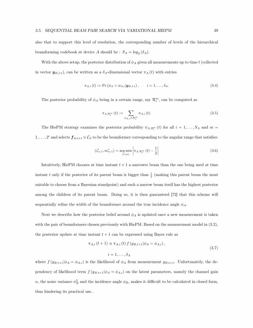
3.5. SEQUENTIAL BEAM PAIR SEARCH VIA VARIATIONAL HIEPM 39
also that to support this level of resolution, the corresponding number of levels of the hierarchical
beamforming codebook at device A should be : SA = log2 (δA).
With the above setup, the posterior distribution of φA given all measurements up to time t (collected
in vector yB,1:t), can be written as a δA-dimensional vector πA (t) with entries
πA,i (t) := Pr (φA = φA,i|yB,1:t) , i = 1, . . . , δA. (3.4)
The posterior probability of φA being in a certain range, say Rmi , can be computed as
πA,Rmi (t) :=∑
φA,i∈Rmi
πA,i (t). (3.5)
The HiePM strategy examines the posterior probability πA,Rmi (t) for all i = 1, . . . , SA and m =
1, . . . , 2i and selects fA,t+1 ∈ CS to be the beamformer corresponding to the angular range that satisfies:
(i∗t+1,m∗t+1) = argmin
(i,m)
∣∣∣∣πA,Rmi (t)− 1
2
∣∣∣∣ (3.6)
Intuitively, HiePM chooses at time instant t+ 1 a narrower beam than the one being used at time
instant t only if the posterior of its parent beam is bigger than 12 (making this parent beam the most
suitable to choose from a Bayesian standpoint) and such a narrow beam itself has the highest posterior
among the children of its parent beam. Doing so, it is then guaranteed [72] that this scheme will
sequentially refine the width of the beamformer around the true incidence angle φA.
Next we describe how the posterior belief around φA is updated once a new measurement is taken
with the pair of beamformers chosen previously with HiePM. Based on the measurement model in (3.2),
the posterior update at time instant t+ 1 can be expressed using Bayes rule as
πA,i (t+ 1) ∝ πA,i (t) f (yB,t+1|φA = φA,i) ,
i = 1, . . . , δA
(3.7)
where f (yB,t+1|φA = φA,i) is the likelihood of φA from measurement yB,t+1. Unfortunately, the de-
pendency of likelihood term f (yB,t+1|φA = φA,i) on the latent parameters, namely the channel gain
α, the noise variance σ2B and the incidence angle φB , makes it difficult to be calculated in closed form,
thus hindering its practical use..

40 CHAPTER 3. MMWAVE WIRELESS CHANNELS VARIATIONAL ONLINE LEARNING
3.5.2 The Variational Expectation Maximization HiePM Scheme: VEM-
HiePM
Our first contribution is based on considering the channel gain α and the noise variance σ2B as classical
unknown parameters, i.e latent parameters that are not probabilistic. We explain first the Variational
Expectation Maximization approximate inference framework used in its most general form. We then
show how to apply it to our problem to account for the unknown parameters, α and σ2B , and to jointly
derive posterior updates of our incidence angles φA and φB .
Primer on the Expectation Maximization framework
We start by listing the different types of variables that the Expectation Maximization (EM) approxi-
mate inference framework builds upon:
• x is the observed data vector, which is in our case yB,1:t+1.
• z = (z1, z2, . . . ,zL) denotes the L-dim vector of latent unknown parameters that parameterize
the measurement model (3.2). In our case, these are the channel’s gain and the noise variance,
i.e z = (α, ν). ν is the inverse of σ2B .
• m ∈ 1, 2, . . . , δA×δB denotes the mth pair of angles (φA,im , φB,jm), with im ∈ 1, . . . , δA, and
jm ∈ 1, . . . , δB. Choosing a certain label m is equivalent to assuming that our measurement
model in (3.2) is parameterized by the the mth pair of angles. m will be our model’s latent
random variable.
The EM framework is used to find an estimate for the hidden unknown parameters of our model,
i.e z, that maximize the log likelihood L(z) = log(x; z). EM assumes that deriving a good maximum
log likelihood estimate of z is not easily solved directly, but that the corresponding problem in which
m is also observed is mathematically tractable and can be solved efficiently.
The EM algorithm starts with some initial guess for the maximum likelihood parameter z(0), and

3.5. SEQUENTIAL BEAM PAIR SEARCH VIA VARIATIONAL HIEPM 41
then proceeds to iteratively generate successive estimates, z(1), z(2), . . . by repeatedly applying the
following two steps, for t = 1, 2, . . . , until convergence is reached :
• E−Step : Compute a distribution q(t) over the range of m such that q(t)(m) = p(m|x; z(t−1)).
• M − Step : Set z(t) to z that maximizes Eq(t) [log(p(x,m; z)]
The recursive operation above solves the issue of having the random variable m latent, i.e unob-
served, by representing its corresponding value by a distribution of values in the E step, and then
performing a maximum likelihood estimation for the join data obtained by combining this with the
known value of the observed variable x.
The VEM-HiePM algorithm
We detail next the VEM-HiePM scheme. Suppose we made t measurements. We have from our
measurement model (3.2)
p(x,m;x) = p(yB,1:t|m; (α, ν))p(m) (3.8)
where
• ν = σ−2 is the noise precision at device B;
• p(y1:t|m; (α, ν)) =∏t+1i=1 CN(yi;
√PαwH
B,iAmfA,i, σ2) is the likelihood of our measurement model
(we assume here that the sequential noise samples are i.i.d)2, Am = (φB,jm)H(φA,im);
• p(m) = 1δAδB
is the prior belief overm, which is assumed to be uniform to make it non informative.
As already discussed, the EM algorithm starts with some initial guess for the maximum likelihood
parameters z(0)t = (α
(0)t , ν
(0)t ), and then proceeds to iteratively generate successive estimates, z(1)
t =
(α(1)t , ν
(1)t ), z(2)
t == (α(2)t , ν
(2)t ), . . . , by repeatedly applying the expectation and maximization steps,
for s = 0, 1, 2, . . . , until convergence is reached.
2In the above, CN(·;µ, λ) denotes the complex Gaussian pdf with mean µ and precision λ, Γ(·; a, b) denotes theGamma pdf with shape and rate parameters a and b.

42 CHAPTER 3. MMWAVE WIRELESS CHANNELS VARIATIONAL ONLINE LEARNING
Let q(s)t , α(s)
t and ν(s)t be the estimates of posterior distribution over m, the channel’s gain and
noise precision, respectively, at the measurement epoch t and after s > 0 iterations. We obtain after
some algebra:
αst =Eq(s−1)t
(∑td=1
(√PwH
B,tAmfA,t
)∗yB,d
)
Eq(s−1)t
(∑td=1
∣∣∣√PwH
B,tAmfA,t
∣∣∣2) (3.9)
νst =t
Eq(s−1)t
(∑td=1
∥∥∥yd −√PwH
B,tAmfA,tα(s)t
∥∥∥2) (3.10)
Now that we know how to derive estimate for α and ν if we are given an estimate for the posterior
distribution over m, let us see how to derive the posterior distribution over m given α and ν estimates.
Let q∞t and q∞t−1 be the estimates for the posterior distribution over m at measurement epochs t − 1
and t, and α(∞)t−1 and ν
(∞)t−1 be the estimates for α and ν respectively, where all these estimates are
considered after that the EM iterations converge. We have
q(∞)t (m)
(a)∼ CN(yt;√PαwH
B,tAmfA,t, ν∞t−1)q
(∞)t−1 (m)
(b)∼t∏
i=1
CN(yi;√PαwH
B,iAmfA,i, ν(∞)t−1 )p(m)
(c)∼ exp (−ν∞t−1
t∑
d=1
∥∥∥yd −√PwH
B,tAmfA,tα(∞)t
∥∥∥2
)p(m)
(3.11)
where (a) results from applying bayes rule on q(∞)t (m) and (b) and (c) are results of direct appli-
cation of our system model assumptions.
The posteriors over φA,im and φB,jm are obtained from the posterior q(∞)t (m) as
qA,t(i) =∑
m:im=iq
(∞)t (m), i = 1, . . . , δA (3.12)
qB,t(j) =∑
m:jm=jq
(∞)t (m), j = 1, . . . , δB (3.13)
The posterior probability of the incidence angles φA and φB to be in a certain range RnA,i and RpB,j
respectively, read as:

3.5. SEQUENTIAL BEAM PAIR SEARCH VIA VARIATIONAL HIEPM 43
qA,t(RnA,i) :=∑
φA,i∈RnA,i
qA,t(i), (3.14)
qB,t(RpB,j) :=∑
φB,j∈RpB,j
qB,t(i), (3.15)
The vanilla HierPM scheme is then applied separately to qA,t(i) and qB,t(j), to choose the pair of
beamformers to use for the next measurement occasion.
Algorithm 1 runs all above operations in a loop, until the measurement budget is exhausted:
device B decides which pair of beamformers devices A and B shall use to take the next measurement
by applying the HiePM scheme separately to the current posteriors qA,t and qB,t, it then takes a new
measurement yB,t+1 with those latter, and finally run variational EM inference to derive estimates of
νB = 1σ2B
and α as well as approximate of φA and φB .
Algorithm 1: VEM-HiePM1 Input : Antenna Array Size NA and NB , The search resolution δA and δB , the codebooksCSA and CSB , Search time τ
2 Output : Estimates of φA, φB ; for t = 1, 2, . . . , τ − 1 do3 #HiePM Based BF selection according to Eq.(3.6)
(fA,t+1,wB,t+1) =(fA
(RkA,t+1
A,lA,t+1
),wB
(RkB,t+1
B,lB,t+1
))
4 #Take next measurement5 yB,t+1 =
√PwH
B,t+1HfA,t+1 + wHB,t+1nB,t+1,
6 #Variational EM Posterior Update7 while (No convergence yet) do8 for m = 1 : δAδB do9 update qt(m) via (3.11)
10 end11 update αt via (3.9)12 update νt via (3.10)13 end14 #Angle and Angular Range Posterior Update15 update qA,t+1(i) via (3.21) and qB,t+1(j) via (3.22)16 update qA,t+1(RnA,i) via (3.23) and qB,t+1(RnB,j) via (3.24)
17 #Final Precoder/Combiner Vector design(lt+1,A, kt+1,A
)= (SA, arg maxk (qA,t+1(k)))
18(lt+1,B , kt+1,B
)= (SB , arg maxk (qB,t+1(k)))
19 end20 Output : φA = φA,kτ,A , φB = φB,kτ,B

44 CHAPTER 3. MMWAVE WIRELESS CHANNELS VARIATIONAL ONLINE LEARNING
3.5.3 The Variational Model Comparison Based HiePM Scheme : VMC-
HiePM
Our second contribution in this chapter is based on considering the channel gain α and the noise
variance σ2 as probabilistic latent variables. We show next, how “VMC-HiePM" is able, using the
variational model based approximate inference framework described in [76], to infer all above unknowns
and uses them efficiently to calculate the posterior update needed for HiePM, in a consistent and elegant
way. Such an inference framework lends itself naturally in the HiePM context: we make the best use
of the measurements by first estimating posteriors over the channel gain and noise variance and then
use those to robustly update the angle of incidence posterior, doing so allows VMC-HiePM to take
the channel’s gain and noise variance estimation uncertainties properly into account when deriving the
posterior of the incidence angles, thus making a robust HiePM based decision when choosing the next
precoder/combiner pair to use.
We explain first the variational model comparison based approximate inference framework used in
its most general form, then show how to apply it to our problem to derive posterior updates for our
parameters of interest.
Primer on the Variational Model Comparison based approximate inference framework
Variational Model Comparison based Posterior Update
As we did for the VEM-HiePM study, We start by listing the different types of variables that the
variational model comparison based approximate inference framework deals with:
• X is the observed data vector, in our case is yB,1:t+1.
• Z = (Z1,Z2, . . . ,ZL) denotes the L-dim vector of latent variables that parameterize the mea-
surement model (3.2). In our case, Z = (α, σ2).
• m ∈ 1, 2, . . . , δA×δB denotes the mth pair of angles (φA,im , φB,jm), with im ∈ 1, . . . , δA, and

3.5. SEQUENTIAL BEAM PAIR SEARCH VIA VARIATIONAL HIEPM 45
jm ∈ 1, . . . , δB. Choosing a certain label m is equivalent to assuming that our measurement
model in (3.2) is parameterized by the the mth pair of angles.
The framework performs joint inference on the hidden variables to find a set of distributions
q(Z|m), q(m)1:m that approximate the true posterior p(Z,m|X), by minimizing the Kullback-Leibler
(KL) divergence:
KL(q(Z|m)q(m), p(Z,m|X)). (3.16)
HiePM then uses the approximate incidence angle posterior q(m) to decide which is the best
measurement model candidate fitting the observed data vector X. Algorithm 2 [76, Chapter 10.4] lists
the steps required to perform such operations.
Algorithm 2: Variational Model Comparison based Posterior Update1 for m = 1 : δAδB do2 while (No convergence yet) do3 for j = 1, 2, . . . , L do4 q(Zj |m) ∝ Ei6=j(log(p(X|Z,m)))
5 Lm =∫Zq(Z|m) log(p(Z,m|X)
q(Z|m) )
6 q(m) ∝ p(m) exp(Lm)
Posterior Update for our measurement Model and the overall V-HiePM Algorithm
From our measurement model (3.2), we have
p(X,Z,m) = p(yB,1:t|α, ν,m)p(α)p(ν)p(m) (3.17)
where
• ν = σ−2 is the noise precision at device B
• p(X|Z,m) = p(yB,1:t|α, νB ,m) =∏t+1i=1 CN(yB,i;
√PαwH
B,iAmfA,i, σ2B) is the likelihood of
our measurement model (we assume here that the sequential noise samples are i.i.d); p(α) =
CN(α;α0, β0) is the prior belief over α, considered to be Gaussian with a known initial mean α0

46 CHAPTER 3. MMWAVE WIRELESS CHANNELS VARIATIONAL ONLINE LEARNING
and initial precision β03. p(νB) = Γ(νB ; a0, b0) is the non informative prior belief over νB , with
parameters a0 = 0 and b0 = 0. Am = (φB,jm)H(φA,im)
• p(m) = 1δAδB
is the prior belief overm, which is assumed to be uniform to make it non informative
as well4.
After some algebra, the obtained approximate posteriors for α and νB , up to the measurement
iteration t, are shown to keep the form of their respective priors, but with parameters that depend on
the measurement vector yB,1:t :
qt(α|m) has the form of complex Gaussian pdf with mean αt,m and precision βt,m reading
βt,m =at,mbt,m
t∑
d=1
∣∣∣√PwH
B,tAmfA,t
∣∣∣2
+ β0 (3.18a)
αt,m =at,m
bt,mβt,m
t∑
d=1
(√PwH
B,tAmfA,t
)∗yB,d +
α0β0
βt,m(3.18b)
qt(νB |m)5follows a Gamma pdf with parameters shape and rate parameters at,m and bt,m given by
at,m = a0 + t, (3.19a)
bt,m = b0 − 2Re(∑t
d=1
(√PwH
B,tAmfA,t
)∗yB,dα
∗t,m
)+
∑td=1
[|yB,d|2 +
(1
βt,m+ |αt,m|2
) ∣∣∣√PwH
B,tAmfA,t
∣∣∣2]
(3.19b)
Note that the choice of our prior distributions is not arbitrary, the priors chosen above correspond to
the maximum entropy distributions [78] that respect constraints that need to be put on their respective
parameters, namely α being a complex variable having a known initial mean and variance, νB being a
non negative variable and m being a discrete variable). Such a choice makes our proposal assume the
least information about our measurement model’s unknowns.3The first and second order moments of α are the only assumed known values in our model.4In the above, CN(·;µ, λ) denotes the complex Gaussian pdf with mean µ and precision λ, Γ(·; a, b) denotes the
Gamma pdf with shape and rate parameters a and b.5Note that (3.18) and (3.19) can be re-written, after performing some algebra, in a recursive format w.r.t their terms
involving summation over measurements epochs. This results in a significant reduction of the algorithm’s memory andcomputation complexity footprint.

3.5. SEQUENTIAL BEAM PAIR SEARCH VIA VARIATIONAL HIEPM 47
The posterior of the model, indexed by m, is then updated following Lines 5 and 6 in Algorithm 2,
where Lm reads
Lt,m = log(1
β2t,m
) + at,m (1− log(bt,m))
+ log(Γ(at,m))− b0at,mbt,m
−(
t∑
d=1
|yB,d|2at,mbt,m
− βt,m |αt,m|2)
(3.20)
The posteriors over φA,im and φB,jm are obtained from the posterior qt(m) as
qA,t(i) =∑
m:im=iqt(m), i = 1, . . . , δA (3.21)
qB,t(j) =∑
m:jm=jqt(m), j = 1, . . . , δB (3.22)
The posterior probability of the incidence angles φA and φB to be in a certain range RnA,i and RpB,j
resp, read as:
qA,t(RnA,i) :=∑
φA,i∈RnA,i
qA,t(i), (3.23)
qB,t(RpB,j) :=∑
φB,j∈RpB,j
qB,t(i), (3.24)
The vanilla HierPM scheme is then applied separately to qA,t(i) and qB,t(j), to choose the pair of
beamformers to use for the next measurement occasion.
Algorithm 3 runs all above operations in a loop, until the measurement budget is exhausted:
device B decides which pair of beamformers devices A and B shall use to take the next measurement
by applying the HiePM scheme separately to the current posteriors qA,t and qB,t, it then takes a
new measurement yB,t+1 with those latter, and finally run variational inference to derive approximate
posteriors of νB = 1σ2B, α as well as of φA and φB .

48 CHAPTER 3. MMWAVE WIRELESS CHANNELS VARIATIONAL ONLINE LEARNING
Algorithm 3: VMC-HiePM1 Input : Antenna Array Size NA and NB , The search resolution δA and δB , the codebooksCSA and CSB , Search time τ
2 Output : Estimates of φA, φB , α and νB3 for t = 1, 2, . . . , τ − 1 do4 #HierPM Based BF selection according to Eq.(3.6)
(fA,t+1,wB,t+1) =(fA
(RkA,t+1
A,lA,t+1
),wB
(RkB,t+1
B,lB,t+1
))
5 #Take next measurement6 yB,t+1 =
√PwH
B,t+1HfA,t+1 + wHB,t+1nB,t+1,
7 #Variational Model Comparison Posterior Update8 for m = 1 : δAδB do9 while (No convergence yet) do
10 update qt+1(α|m) via (3.18) then qt+1(νB |m) via (3.19)11 end12 update qt+1(m) via (3.20)13 end14 #Angle and Angular Range Posterior Update15 update qA,t+1(i) via (3.21) and qB,t+1(j) via (3.22)16 update qA,t+1(RnA,i) via (3.23) and qB,t+1(RnB,j) via (3.24)
17 #Final Precoder/Combiner Vector design(lt+1,A, kt+1,A
)= (SA, arg maxk (qA,t+1(k)))
18(lt+1,B , kt+1,B
)= (SB , arg maxk (qB,t+1(k)))
19 end20 Output : φA = φA,kτ,A , φB = φB,kτ,B
3.6 Numerical Results
To assess the effectiveness of the proposed algorithms, we run Monte Carlo simulations on a setup with
two hybrid digital-analog beamforming devices A and B. The channel matrix H ∈ CNB×NA reads
H = α(φB)H(φA) +
L∑
l=1
αl(φB,l)H(φA,l) (3.25)
and contains one dominant multipath component and L scattered components. All incidence angles
are independently drawn from a uniform distribution between 0 and π. The channel gains are inde-
pendently drawn from a a set of complex Gaussian distribution with mean 0 and variances fulfilling
Varα+∑lVarαl = 1, so that the average SNR ρ between the nth element of the array at A and the
mth element of the array at B equals E|Hnm|2/E|σB |2=1/σ2B
6. In all simulations below, the two
6Hnm is the channel coefficient between device B’s nth array element and device A’s mth array element, and E isthe expectation operator.

3.6. NUMERICAL RESULTS 49
devices are equipped with identical arrays made of NA = NB = 32 elements, digitally controlled with
NRFA = NRF
B = 8 RF chains. Device A uses a codebook CA with a depth of SA = log2(δA), δA = 128.
CA is built using the orthogonal matching pursuit as described in [70]. A similar codebook, CB , is used
for device B.7
We define beamforming gains, achieved after taking t measurements, for our proposed schemes as
follows :
Gx =∣∣∣wH(φB,kt,B )Hf(φA,kt,A)
∣∣∣2
(3.26)
where x can be either em for VEM-HiePM or vh for VMC-HiePM.
We benchmark these beamforming gains with different measurement budget sizes8 and under dif-
ferent channel assumptions, against that of the different state of the art schemes listed below:
• Gph of the vanilla HiePM scheme of [72]. Here, such a scheme assumes that all of the energy in
the channel is concentrated in the path corresponding to the known gain α and all other gains
αl are null, it also assumes that σ2B is known. In such case, the posterior update is done, simply
using Bayes rule as in equation (21) in [72], on the beam pair corresponding to that main path,
and then HiePM is applied to the marginals over those angles separately, similar to what our
schemes do.
• Gbs of the noisy binary search algorithm of [70], which is achieved by 4 log2(maxNA, NB) = 28
measurements.
• Gmax the best achievable beamforming gain of the used codebook, defined as:
Gmax = maxw∈CBSB ,f∈C
ASA
∣∣wHHf∣∣2 . (3.27)
We begin by assuming that the dominant component is the only component that is present in the
channel (i.e. L = 0).
7Note that the multi-RF chain setups are used solely to help build acceptable RF codebooks [70], and are not usedfor multi-stream MIMO operations.
8note the the exhaustive search needs NANB = 16384 measurements to settle.

50 CHAPTER 3. MMWAVE WIRELESS CHANNELS VARIATIONAL ONLINE LEARNING
Fig. 3.4 shows the beamforming losses of the benchmarked algorithms with respect to the optimum
pair of beamformers, defined as Lvh = Gvh/Gmax, Lem = Gem/Gmax, and Lbs = Gbs/Gmax.

3.6. NUMERICAL RESULTS 51
-10
-8-6
-4-2
02
46
81
0
SN
R i
n d
B
0.1
0.2
0.3
0.4
0.5
0.6
0.7
0.8
0.91
Beamforming Gain
Lv
h :
=
28
Le
m :
=
28
Lv
h :
=
56
Le
m :
=
56
Lv
h :
=
100
Le
m :
=
100
Lb
s :
=
28
Figure3.4:
Beamform
ingLo
ssof
theDifferentsearch
schemes
inaCha
nnel
withL
=0ScatteredCom
ponents.

52 CHAPTER 3. MMWAVE WIRELESS CHANNELS VARIATIONAL ONLINE LEARNING
It can be seen that both or our proposed schemes are clearly much better, in all SNR regimes, than
the binary search based beamforming scheme proposed in [70], we see that even with as little as 28
measurements, which is the measurement budget needed by this latter to settle, both of our algorithms
perform quite well in all SNR regimes, we see that even with such a small measurement budget, VMC-
HiePM can achieve at least 50% of the maximum beamforming gain that can be achieved with the
RF codebook being used across all SNR points. Also, We observe that with only 100 measurements
(compare this with the number of measurements needed for exhaustive search to achieve
We compare next the performance of our schemes to that of the vanilla HiePM with perfect CSI
and operating SNR knowledge scheme. Fig. 4.3 shows the beamforming losses of VMC-HiePM, VEM-
HiePM and of vanilla HiePM schemes with respect to the optimum pair of beamformers (these are
defined similar to the above : Lvh = Gvh/Gmax, Lem = Gem/Gmax and Lph = Gph/Gmax) under
the same simulation assumption of Fig. 3.4. The results show that VMC-HiePM can achieve similar or
even better performance compared to vanilla HiePM with perfect CSI and operating SNR knowledge,
we can see as well that VEM-HiePM is underperfoming when copared to the vanilla HiePM scheme.
Also, it can be observed that the vanilla HiePM scheme with perfect channel gain knowledge saturates
at high SNR: this is an effect of the algorithm assuming that the component’s incidence angle lies
on a discrete grid of values, whereas the actual angles are sampled from a continuous distribution.
VMC-HiePM is less sensitive to this model mismatch, due to the estimation of the channel gain and
inverse noise variance: in practice, these estimates partly account for the mismatch in the assumed
values of the angles and provide robustness to the overall procedure.

3.6. NUMERICAL RESULTS 53
-10
-8-6
-4-2
02
46
81
0
SN
R i
n d
B
0.2
0.3
0.4
0.5
0.6
0.7
0.8
0.91
Beamforming Gain
Lv
h :
=
28
Le
m :
=
28
Lp
h :
=
28
Lv
h :
=
56
Le
m :
=
56
Lp
h :
=
56
Lv
h :
=
100
Le
m :
=
100
Lp
h :
=
100
Figure3.5:
Beamform
ingLo
ssof
theDifferentSearch
Schemes
inaCha
nnel
withL
=0ScatteredCom
ponents.

54 CHAPTER 3. MMWAVE WIRELESS CHANNELS VARIATIONAL ONLINE LEARNING
Next, we explore the robustness of our best performing method, namely VMC-HiePM, against
channels containing more than one multipath component. For this, we consider a channel with L = 3
scattered components with gains of equal variance, and with the power ratio between the dominant
and scattered components being LOSR = Eα2/(Eα2 +∑l Eα2
l ). Fig. 4.5 shows beamforming
gains achieved by our algorithm after 100 measurements compared to the maximum gains achievable
Gmax.
As it can be observed, the maximum achievable beamforming gain decreases as the power is more
evenly distributed among the channel’s components. Although VMC-HiePM assumes the existence of
a single component, it shows remarkable resilience to the presence of other components. Even when
all components in the model have comparable power, our proposed method is able to perform within
2 dB of the optimum for sufficiently high SNR.
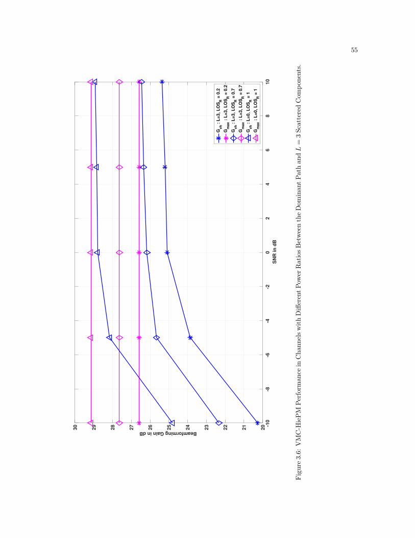
3.6. NUMERICAL RESULTS 55
-10
-8-6
-4-2
02
46
81
0
SN
R i
n d
B
20
21
22
23
24
25
26
27
28
29
30
Beamforming Gain in dB
Gv
h :
L=
3, L
OS
R =
0.2
Gm
ax :
L=
3, L
OS
R =
0.2
Gv
h :
L=
3, L
OS
R =
0.7
Gm
ax :
L=
3, L
OS
R =
0.7
Gv
h :
L=
0, L
OS
R =
1
Gm
ax :
L=
0, L
OS
R =
1
Figure3.6:
VMC-H
iePM
Perform
ance
inCha
nnelswithDifferentPow
erRatiosBetweentheDom
inan
tPathan
dL
=3ScatteredCom
ponents.

56 CHAPTER 3. MMWAVE WIRELESS CHANNELS VARIATIONAL ONLINE LEARNING
3.7 Conclusion and Future Work
We proposed in this work two variational Bayesian online learning schemes that enable initial access
for hybrid digital-analog enabled devices operating in mmWave wireless channels. When compared
to state of the art beam acquisition schemes, our methods shows superiority, in terms of balancing
the beam search time versus achieving higher beamforming gain, in being able to properly do so
while accounting for uncertainties on the unknown CSI (gain and noise variance) and in being very
resilient to the dominant single path assumption. Even though both of the schemes are derived based
on a discretized model of the angles of incidence of the channel’s main component, they showed great
robustness against off-grid angles as well as working with a realistic codebook implementation. Further
research will focus on adapting the proposed online learning algorithms to operating in time-varying
channels.

Chapter 4
Mutli-Stream Beamforming with
Hybrid Arrays
4.1 Overview
In this chapter1 we propose a method to derive precoders and combiners for multi-stream MIMO
transmission be- tween two devices equipped with hybrid digital-analog antenna arrays. The method
relies on a low- complexity “multi-beam split and drop with backtracking” procedure to update the
analog precoders, while digital precoders are computed with the QR-decomposition based method. We
show numerically that for sufficiently large SNRs, our proposal can approximate well the unconstrained
SVD-based precoder design and can thus enable high throughput mmWave communication systems.
1This chapter is based on the work published in the conference paper : N. Akdim, C. N. Manchón, M. Benjillali andE. de Carvalho, "Ping Pong Beam Training for Multi Stream MIMO Communications with Hybrid Antenna Arrays,"2018 IEEE Globecom Workshops (GC Wkshps), 2018, pp. 1-7, doi: 10.1109/GLOCOMW.2018.8644444.
57

58 CHAPTER 4. MUTLI-STREAM BEAMFORMING WITH HYBRID ARRAYS
4.2 Introduction
Upcoming wireless communication networks are expected to provide service to an unprecendently large
number of wireless devices with peak data rates in the order of tens of Gbps.
As we discussed in great details in earlier chapters, the low complexity and power friendly mmWave
Hybrid Antenna array transceivers are seen as a great trasnceiver design that would solve.........
the congestion and fragmentation of the traditional spectral bands below 6GHz has pushed wireless
service providers to explore vacant spectrum at the millimeter-wave (mmWave) frequency bands (30–
300 GHz) in order to fulfill that goal [4]. Having a poor diffraction capability and high absorption and
free space propagation losses, wireless communications over such high frequencies will be a challenging
task [17]. As detailed already, this frequency range will allow for the use of compact and small
antenna arrays with high number of elements, as the physical size of the array is proportional to the
carrier wavelength. The large beamforming gains that such large-scale arrays enable will be used to
compensate for the above limitations.
However, the high cost, power consumption and complexity of the mixed signal hardware at mm-
wave make having large antenna arrays with digitally controlled elements infeasible [18]. This has
motivated the wireless communication research community to look at the hybrid digital-analog antenna
array architectures [65]. In such architectures, the large antenna array is steered using analog phase
shifters and only a few digitally modulated radio-frequency (RF) chains. An illustration of such an
architecture is shown in Fig. 4.1.
Although Hybrid Antenna arrays help making packing large antenna arrays in small devices a
feasible task by reducing the implementation complexity as well as the power consumption of the
overall baseband and RF chains, they do bring their own challenges: the low SNR resulting from high
propagation losses, the large dimensionality of the MIMO channel matrix and the presence of analog
processing complicate the acquisition of the channel state information (CSI) and the computation of
the MIMO precoders and combiners [4,18]. Luckily, channel measurement campaigns [17] have shown

4.2. INTRODUCTION 59
that mm-wave channels are sparse in the angular domain, which enables the proposal of CSI acquisition
and precoding/combining algorithms that exploit such property. An example of these are compressed
sensing based approaches such as [18,43,70], which are generally computationally complex and require
a large amount of channel measurements. An alternative are exhaustive and hierarchical beam-search
techniques, which may entail significant latency and probability of miss detection [71].
In this work, we focus on a beam training strategy based on alternating transmissions between two
transceivers, which has been coined ping pong beam training (PPBT). The main idea behind PPBT
is to exploit the reciprocity of the MIMO channel. With appropriate processing at each device, the
alternate transmissions implicitly implement an algebraic power iteration that leads to approximating
the top left and right singular vectors of the MIMO channel matrix. This idea was first applied in
the digital arrays context for single stream wireless communications in [79, 80], and was extended to
multi stream setups in [81], to large antenna array and frequency selective systems in [82] and to
noisy MIMO channels in [83]. More recently, similar approaches have been proposed in the context of
mmWave communications with hybrid digital-analog antenna arrays, which we review next. In [77], the
basic ping pong beam training method for single-stream MIMO transmission was adapted to the hybrid
array architecture with the inclusion of a “beam split-and-drop” procedure for the setting of analog
precoders. The subspace estimation and decomposition method in [84] proposes a ping pong based
algorithm that iteratively estimates the channel’s right and left eigenvectors using a Krylov subspace
estimation method. This algorithm is based on exhaustive measurements with a large set of different
analog precoders, which are then linearly combined in order to cancel the effect of the analog precoders.
It therefore requires significant amount of transmissions, which imply large signalling overhead and
latency. Lastly, the power iteration based training method introduced in [85] is a technique that
extends the solution proposed in [81] to the multi stream case, where the digital precoders are set
based on an algebraic power iteration technique, while the analog precoders update is done based on
a compressed sensing technique called simultaneous orthogonal matching pursuit [86].
Compared to the above approaches, we propose in this article a strategy that sets the digital and

60 CHAPTER 4. MUTLI-STREAM BEAMFORMING WITH HYBRID ARRAYS
analog precoders of the devices in a way to approximate the top NS left and right singular vectors
of the channel matrix, with NS being the desired number of spatial streams. Our new technique,
which we dub “hybrid ping pong multi beam training“ (Hybrid PPMBT) extends the work done in [77]
to the multi stream case. It adapts the PPBT strategy to hybrid arrays by progressively choosing
the analog precoders at each device from a predefined hierarchical codebook. After one round-trip
transmission, a novel "multi beam split and drop strategy with backtracking" is applied to focus the
analog precoders towards the spatial directions that are most likely containing the channel’s top NS
multipath components. The digital precoders are updated via an orthogonal decomposition operation
on the received signal as described in [81]. In comparison to the approaches in [84] and [85], Hybrid
PPMBT is much simpler from a computational complexity aspect and has a low training overhead as it
requires significantly fewer transmissions. Simulation results show that our proposed scheme performs
very well in retrieving the wanted NS channel’s top eigenmodes for sufficiently large signal-to-noise
ratio, both in terms of accuracy and convergence speed.
Baseband
Precoder
Baseband
Combiner
RF Chain
RF Chain
RF Chain
RF Chain
RF Precoder RF Combiner
NA N
B
NA
RF
NB
RF
H
TRANSCEIVER A TRANSCEIVER B
Figure 4.1: Structure of the Hybrid Transceivers

4.3. SYSTEM MODEL 61
4.3 System Model
We consider a system in which two hybrid analog digital transceivers A and B, equipped with uniform
linear arrays (ULA) composed of NA and NB antenna elements. Such elements are separated with
a distance d = λ/2, where λ is the wavelength of interest. The two devices control digitally their
arrays with NRFA and NRF
B RF chains respectively and exchange data over a reciprocal wireless MIMO
channel using NS parallel data streams. The channel from device A to device B is considered to
be static and narrowband and is modeled according to the finite scatterer channel model with L
propagation paths [77,87], as
H =
√NANBL
L∑
l=1
αl(ΩB,l)H(ΩA,l), (4.1)
here, H ∈ CNB×NA , L is the number of multipath components (MPC), αl is the complex fading channel
gain for MPC l, ΩA,l = 2πλ d cosφA,l and ΩB,l = 2π
λ d cosφB,l are the directional cosines corresponding
to the lth MPC at arrays A and B respectively, where φA,l, φB,l are the angles of incidence of that same
path, and and are the array response vectors at device A and B respectively. The αl are modeled as
independent, standard complex gaussian variables, the φA,l and φB,l as uniformly distributed in the
range [0, 2π) radians and the array responses as (ΩA,l) = [1, e−jΩA,l , . . . , e−j(NA−1)ΩA,l ]T/√NA and
(ΩB,l) = [1, e−jΩB,l , . . . , e−j(NB−1)ΩB,l ]T/√NB .
In order to establish the wireless link with device B, device A (we assume, without loss of generality,
that device A is performing the first transmission) transmits T , an NS × NS orthogonal training
sequence i.e TTH = INS . Upon reception, device B cancels the training sequence effect by multiplying
its received digital signal by TH . The resulting signal can be expressed as:
YB = FHBHFAWA + FH
BNB , (4.2)
where FA ∈ CNA×NRFA and FB ∈ CNB×NRFB contain the states of the analog precoder and com-
biner of transceivers A and B, WA ∈ CNRFA ×NS denotes the digital precoder of transceiver A and
NB ∈ CNB×NS is a complex, circularly-symmetric additive white gaussian noise matrix, obtained
after training sequence removal and with i.i.d elements, each with variance σ2. Transmissions from

62 CHAPTER 4. MUTLI-STREAM BEAMFORMING WITH HYBRID ARRAYS
device B to device A are modeled analogously as
YA = FHAHHFBWB + FH
ANA, (4.3)
where WB ∈ CNRFB ×NS and NA ∈ CNA×NS are defined similar to the above.
4.4 Hybrid Ping Pong Multi Beam Training : Hybrid PPMBT
Given the signal model in (4.2) and (4.3), the beamforming task consists of selecting the set of analog
and digital precoders and combiners that maximize the spectral efficiency over a given channel matrix
H. For transmission from device A to B, and assuming unit transmit power equally allocated across
the NS streams, the spectral efficiency reads
R = log2 det(INS +
R−1NB
NSHeH
He
), (4.4)
where RNB= σ2WH
BFHBFBWB is the noise covariance matrix after receive combining at device B,
He = WHBFH
BHFAWA is the equivalent channel after precoding and combining at both devices. An
analogous expression applies for transmission from device B to device A.
The optimal precoders maximizing (4.4) are known to be the NS top right and left singular vectors
of H. However, the hybrid structure of the antenna array makes the computation of such precoders
challenging. On the one hand, as digital measurements of the channel are only obtained after analog
precoding and combining, estimating the full channel matrix H in order to obtain its singular value
decomposition requires a large number of measurements and hence large overhead and latency [84].
On the other hand, even if the channel matrix H can be estimated, the precoders have to be built
as the product of the analog precoding matrix FA and the digital precoding matrix WA. While the
elements of WA can take any complex value due to its digital implementation, the operation modeled
by FA is implemented via phase shifters and combiners, which restricts the values it can take. In this
work, we restrict the entries of FA to satisfy |(FA)l,i|2 ∈ 1
M(i)A
; 0, where M (i)A being the number of
activated array elements in the ith column of FA, and the option (FA)l,i = 0 accounts for the option of
2(FA)l,i is the entry of the matrix FA belonging to its lth row and ith column.

4.4. HYBRID PING PONG MULTI BEAM TRAINING : HYBRID PPMBT 63
leaving some elements of the array unused. In addition, a transmit power constraint is enforced such
that ‖FAWA‖F = 1.3 With these constraints, finding the combination of digital and analog precoders
to best approximate the channel’s singular vectors becomes a computationally intensive optimization
problem [43].
To overcome such difficulties, we propose an iterative multi beam training scheme based on alternate
transmissions between the two devices, this procedure estimates progressively and simultaneously the
top NS right and left singular vectors of H and sets the digital and analog precoders so that they
approach those singular vectors. It consists of two parts: 1. a "backtracking beam split and drop"
approach to select the analog precoders FA and FB from a predefined multi level codebook, 2. a
method to select the digital precoders WA and WB inspired by the QR decomposition algorithm
described in [81].
We will proceed by reviewing the beam training procedure for digital antenna arrays proposed
in [81], then briefly present the multi level codebook that is used for the analog precoder update, and
finally explain our multi beam training solution.
4.4.1 Ping-Pong Multi Beam Training with Digital Antenna Arrays: Dig-
ital PPMBT
We review the digital PPBT algorithm over a narrowband reciprocal channel H as described in [81].
We consider two devices A and B equipped with digitally controlled antenna arrays with NA and NB
elements respectively. At the initial (0th) iteration, the process starts with a random initialization
of the precoder at device A, W [0]A . A uses then this initial precoder to transmit a training sequence
to B. Upon reception and training sequence removal, device A gets an estimate of HW[0]A , makes a
QR-decomposition on it, and uses the Q part of that decomposition as its precoder W [0]B . It then uses
that precoder to transmit a training sequence back to device A, who will repeat the same operations.
This process is reiterated until convergence, at which, device A gets an estimate of the top NS right
3Obviously, the same constraints apply to the analog precoder of device B.

64 CHAPTER 4. MUTLI-STREAM BEAMFORMING WITH HYBRID ARRAYS
singular vectors of H and device B gets an estimate of the top NS right singular vectors of HH.
Further details on this procedure can be found in [81].
4.4.2 Analog Precoder Multi Level Codebook
We illustrate here the codebook definition for transceiver A (an analogous codebook is used for the
transceiver B). We consider a codebook CA which is composed of LA= log2(NA/NRFA )+1. levels.
Note that for the considered codebook design we constrain NA and NRFA to be both integer pow-
ers of two. For the kth level, we define a subcodebook C(k)A =ϕ(k)
A,i, i=0, 1, . . . ,M(k)A -1 consisting of
M(k)A =NRF
A 2k-1 column vectors, k=1, 2, . . . , LA. Each of the elements of the subcodebook is defined
as :
ϕ(k)A,i=
[1, e-jψ
(k)A,i , . . . , e-j(M
(k)A -1)ψ
(k)A,i ,0T
NA-M(k)A
]T/
√M
(k)A (4.5)
where ψ(k)A,i=π-π(2i+1)/M
(k)A is the directional cosine of the ith vector at the kth level (ϕ(k)
A,i steers the
array in the direction θ(k)A,i= arccosψ
(k)A,i/π, with a lobe whose width decreases with the codebook level
k), and 0N is the N -dimensional column zero vector. Further details about the codebook used here
can be found in [77].
Basically ϕ(j)A,i steers the array in the direction θ
(j)A,i = arccosψ
(j)A,i/π, with a lobe whose width
decreases with the codebook level j. Note that for a fixed level k, the directional cosines θ(k)A,i, i =
0, . . . ,M(k)A − 1 are set to uniformly sample the directional cosine range [−π, π] and as k increases this
range is sampled with larger resolution and more array elements are used for higher-level codebook
elements, resulting in more directive beamforming vectors (an illustration of this is shown in figure 4.2).
For more details about RF codebook optimization methods, we refer the reader to [88,89].
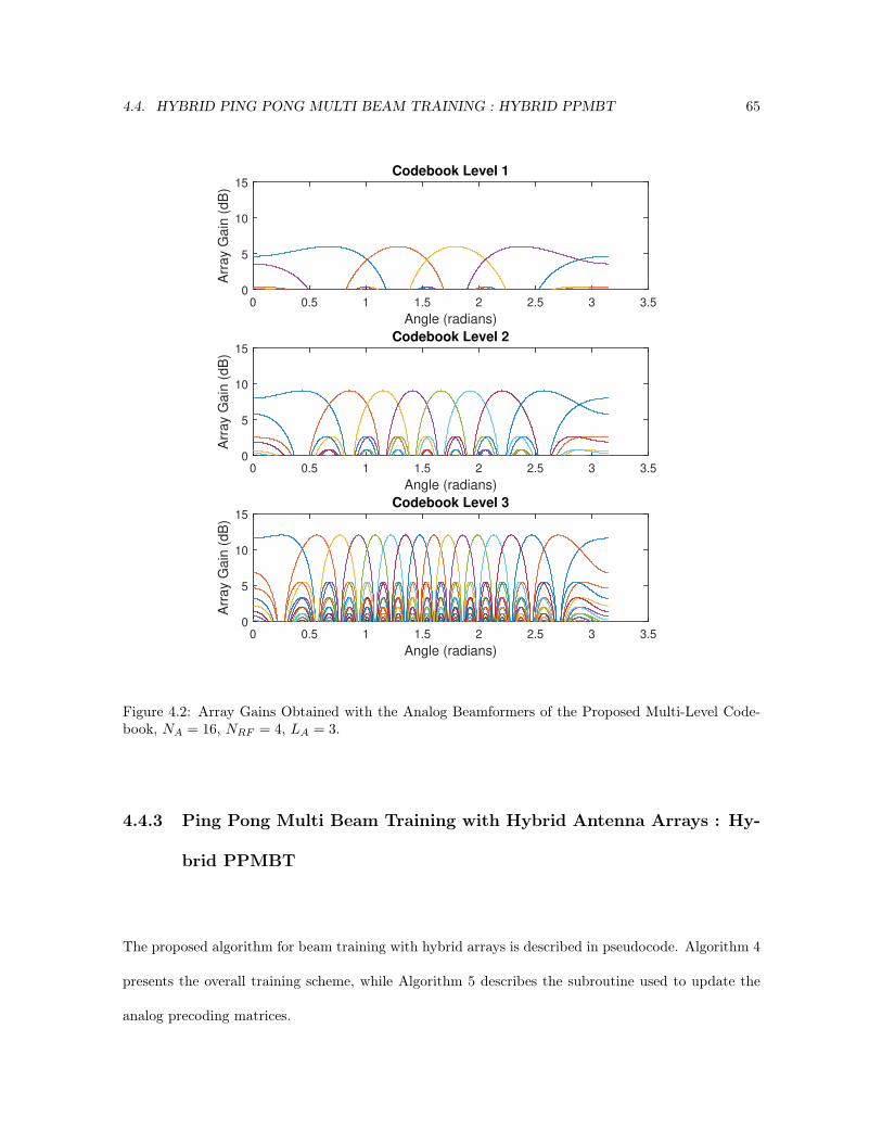
4.4. HYBRID PING PONG MULTI BEAM TRAINING : HYBRID PPMBT 65
Angle (radians)
0 0.5 1 1.5 2 2.5 3 3.5
Arr
ay G
ain
(d
B)
0
5
10
15Codebook Level 1
Angle (radians)
0 0.5 1 1.5 2 2.5 3 3.5
Arr
ay G
ain
(d
B)
0
5
10
15Codebook Level 2
Angle (radians)
0 0.5 1 1.5 2 2.5 3 3.5
Arr
ay G
ain
(d
B)
0
5
10
15Codebook Level 3
Figure 4.2: Array Gains Obtained with the Analog Beamformers of the Proposed Multi-Level Code-book, NA = 16, NRF = 4, LA = 3.
4.4.3 Ping Pong Multi Beam Training with Hybrid Antenna Arrays : Hy-
brid PPMBT
The proposed algorithm for beam training with hybrid arrays is described in pseudocode. Algorithm 4
presents the overall training scheme, while Algorithm 5 describes the subroutine used to update the
analog precoding matrices.

66 CHAPTER 4. MUTLI-STREAM BEAMFORMING WITH HYBRID ARRAYS
Initialization
First, the digital and analog precoders are initialized. FA and FB are initialized to C(1)A and C(1)
B
respectively, while WA is initialized to a random unitary matrix. The columns of WA are then
normalized to fulfill the transmit power constraint of the effective precoder FAWA. Finally, a set of
empty arrays, pB ,kB , iB, are created. Those arrays will store the needed information to perform
the analog precoder updates, as explained below.
Ping Pong Iterations
After the initialization phase, a sequence of alternate pilot transmissions starts between the two devices.
The baseband precoders are updated after each reception step by means of a QR-decomposition,
followed by a normalization step. These two operations are detailed in lines 3-7, 12-16 and 20-24 in
Algorithm. 4. Immediately after updating their baseband precoders upon reception of a transmission,
the devices transmit back with the updated digital precoders and the same analog precoder as used for
reception. Only after the transmission has been made will the transmitting device update its analog
precoders (using Algorithm 5), such that next reception is done with the updated setting. This allows
for the QR based iteration to converge, as each reception-transmission cycle is performed over a static
setting of the analog precoders.
Update of Analog Precoders
The devices invoke the routine outlined in Algorithm 5 to update their analog precoder state. This
routine bases its update on the current state of the device’s RF precoder , its codebook C and on the
update history of its baseband precoder . Using all previous updates of allows for backtracking–i.e,
correcting for wrong RF precoder updates. The routine works as follows:
a) Three sequences of values are generated: kn stores the level of the codebook of the nth column
of , pn stores the squared norm of the nth row of , i.e the aggregate energy received on it, and

4.4. HYBRID PING PONG MULTI BEAM TRAINING : HYBRID PPMBT 67
Algorithm 4: Ping Pong Multi Beam Training with Hybrid Arrays1 Input : Antenna Array Size NA and NB , the codebooks CSA and CSB , Search time τ
2 F[0]A ←
[ϕ
(1)A,0,ϕ
(1)A,1, . . . ,ϕ
(1)
A,M(1)A −1
]
3 F[0]B ←
[ϕ
(1)B,0,ϕ
(1)B,1, . . . ,ϕ
(1)
B,M(1)B −1
]
4 Initialize W[0]A to an orthogonal matrix of its size.
5 for s = 1, 2, . . . , NS − 1 do6 W
[0]A (:, s)←W
[0]A (:, s)/
√NS
∥∥∥F [0]A W
[0]A (:, s)
∥∥∥2
7 end8 pA,kA, iA ← [], [], []9 pB ,kB , iB ← [], [], []
10 A transmits, B receives:11 Y
[0]B =(F
[0]B )HHF
[0]A W
[0]A +(F
[0]B )HN
[0]B
12 [Q,R]← QR(Y[0]B )
13 for s = 1 : NS do14 W
[0]B (:, s)← Q(:, s)
15 W[0]B (:, s)←W
[0]B (:, s)/
√NS
∥∥∥F [0]B W
[0]B (:, s)
∥∥∥2
16 end17 for t = 1, 2, . . . , τ − 1 do18 B transmits, A receives:19 Y
[t]A =(F
[t−1]A )HHHF
[t−1]B W
[t−1]B +(F
[t−1]A )HN
[t]A
20 [Q,R]← qr(Y[t]A )
21 for s = 1 : NS do22 W
[t]A (:, s)← Q(:, s)
23 W[t]A (:, s)←W
[t]A (:, s)/
√NS
∥∥∥F [t−1]A W
[t]A (:, s)
∥∥∥2
24 end25 [F
[t]B , pB ,kB , iB]← Upd.An.Pr[F
[t−1]B ,W
[t−1]B , CB , pB ,kB , iB]
26 A transmits, B receives:27 Y
[t]B =(F
[t]B )HHF
[t−1]A W
[t]A +(F
[t]B )HN
[t]B
28 [Q,R]← qr(Y[t]B )
29 for s = 1 : NS do30 W
[t]B (:, s)← Q(:, s)
31 W[t]B (:, s)← W
[t]B (:,s)
√NS
∥∥∥F [t]B W
[t]B (:,s)
∥∥∥2
32 end33 [F
[t]A , pA,kA, iA]← Upd.An.Pr[F
[t−1]A ,W
[t]A , CA, pA,kA, iA]
34 end35 Output : [F
[τ ]A ],W
[τ ]A ,F
[τ ]B ],W
[τ ]B ]
in stores the index of the nth column of , out of the level of the codebook to which that column
belongs.

68 CHAPTER 4. MUTLI-STREAM BEAMFORMING WITH HYBRID ARRAYS
Algorithm 5: Analog Precoder Update : Upd.An.Pr1 Input : [F , W , C,p,k,i]2 Generate : kn, in, pn, n=1, . . . , NRF , where kn will store the codebook level to which the
′s
nth column belongs, in will store its index out of that level and pn will store the norm of thenth row of , i.e the aggregate energy received on it.
3 p← [p, p1, . . . , pNRF ],4 k← [k, k1, . . . , kNRF ],5 i← [i, i1, . . . , iNRF ]6 Sort p in a descending manner and store the result in pS , then store the arrangement of the
elements of p into pS in pI .7 bI ← []8 bL ← []
9 while n ≤ NRF do10 bI ← [bI , pI,n], pI,n is the nth element of pI , ppI,n ← 0, ppI,n is the pI,nth element of p,11 if kpI,n= log2( N
NRF)+1 or n=NRF -1 then
12 n← n+ 1, bL ← [bL, 1]13 else
14 n← n+ 2, bL ← [bL, 2]
15 for t = 1 : Length(bI) do16 m← bL,t17 if m = 2 then18 F ← [F,ϕ
(km+1)2im
,ϕ(km+1)2im+1 ]
19 else
20 F ← [F,ϕ(km)im
]
21 return F ; p,k, i
b) The sequences generated above will be used to update three vectors: kn will be appended to
k, with k being an array storing the codebook levels of the columns of used over consecutive
ping-pong iterations. pn will be appended to p, with p being an array storing the received energy
over the different spatial directions set by the analog beamformer . in will be appended to i in
a similar manner to the above.
c) Once p is updated, it will be sorted in a descending manner and the resulting sorted indices will
be stored in pI . This newly formed array will be used to find the entries of p that are most likely
to direct the analog precoders where the MPCs of H are.
d) Two new vectors are built: bI contains the K first indexes of pI i.e it identifies the beams that
are most aligned with the channel’s MPCs (K is the length of bI , which can be derived from

4.5. NUMERICAL RESULTS 69
lines 9-13). bL is a vector that is made of 1’s and 2’s. The ith entry of bL is set to 2 when
the precoder corresponding to the ith entry of bI is replaced with the two precoders belonging
to one step higher level of the codebook and that have their beams covering together its same
spatial area, otherwise it is set to 1. Deciding to append 1 or 2 to bL depends on whether we
already consumed all columns of and on whether the element of pI in question belong to the last
level of the codebook or not (see lines 17-21). Line 8 of the algorithm erases the measurement
stored over a beam that is selected to be included in the analog precoding matrix, either directly
or after splitting it into two beams of the immediately higher level. As new measurements
will be obtained over that beam in the next iteration, the old measurement is deleted to avoid
unnecessarily coming back to the previous configuration corresponding to that old measurement.
e) Finally, the RF precoder columns are updated (lines 15-22).
We dub the above procedure for updating the analog precoders “beam split and drop with backtracking”,
owing to the way it operates. At each iteration, a decision is made as to whether a given beam is
split –i.e replaced by two more directive beams– or dropped –i.e. removed from the precoding matrix.
The backtracking feature refers to the fact that, via the vector p, the measurements obtained in prior
ping-pong iterations are kept in memory, allowing for returning to lower level beams in the codebook
in the cases where noise leads to erroneous decisions in the the split-and-drop procedure.
4.5 Numerical Results
In order to assess the effectiveness of the proposed algorithm, we perform Monte Carlo simulations
for multiple configurations of the hybrid arrays at devices A and B. The channel matrix H follows
the model in (4.1). The average SNR for the sth stream link between the nth element of the array at
device B and the mth element of the array at A is defined as ρ=E|Hnm|2/E|Nns|2=1/σ2, where
Nns is the nth entry of the sth column of the noise matrix N . We assume here for simplicity that
the SNR ρ is the same for all streams. Hnm is the channel coefficient between device B’s nth array

70 CHAPTER 4. MUTLI-STREAM BEAMFORMING WITH HYBRID ARRAYS
element and device A’s mth array element, and E is the expectation operator.
We measure the performance with the average spectral efficiency per bits/s/Hz, expressed with :
log2
( ∣∣∣∣INS+R−1N
NSHeH
He
∣∣∣∣)
where He=(F[n−1]B W
[n−1]B )HHF
[n−1]A W
[n]A and RN=σ2(F
[n−1]B W
[n−1]B )HF
[n−1]B W
[n−1]B for integer it-
eration n, and He=(F[n]B W
[n]B )HHF
[n−1]A W
[n]A and RN=σ2(F
[n]B W
[n]B )HF
[n]B W
[n]B for half iteration
n+0.5.
We benchmark the performance of the hybrid PPMBT against the performance of the digital ping
pong multi stream beam training method (digital PPMBT) described in [81], for which the spectral
efficiency is calculated in a similar manner to that of the hybrid PPMBT. We compare it also with
the optimal unconstrained SVD based precoder, which maximize the spectral efficiency and which is
obtained by using the top NS left and right singular vectors of H. Note that the SVD based precoder
derivation requires full channel knowledge at both devices, an information that is hard to get when
hybrid architectures are used as explained earlier, and which our proposed scheme does not need at
the start, but rather learns while setting the precoders.
We start our evaluation in the high SNR regime (ρ=30dB), in which the training process will not
be impaired too much by noise. This allows assessing how the arrays size, the number RF chains and
the number of spatial streams really affect the algorithm’s performance.
Fig. 4.3 depicts the algorithm’s performance over a channel with 8 multipath components, when the
two devices are equipped with identical arrays made of NA=NB=32, 128 or 1024 elements and a fixed
number of RF chains NRFA =NRF
B =8 and try to establish an NS=4 streams MIMO communication.
We see that the algorithm reaches, in very few iterations, for small, medium and large sized arrays, to
about 1 to 2 bits/s/Hz of the digital PPMBT and SVD based precoding schemes performances. We also
see that the convergence speed (in terms of PP iterations) scales inversely to the codebook depth for
each of the topologies: the convergence is slower when large arrays are used because, in such cases, the
codebook has more levels and its few last levels contain a high number of beamformers with very narrow
beams. The selection of such directive beams is more prone to error than those in codebooks with lower
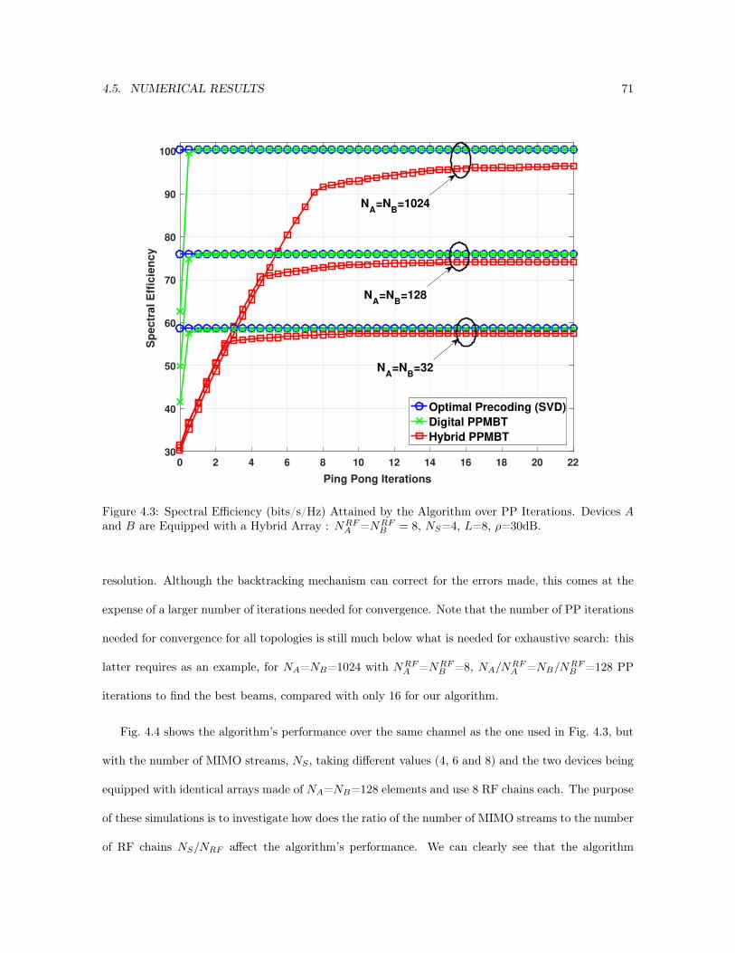
4.5. NUMERICAL RESULTS 71
0 2 4 6 8 10 12 14 16 18 20 22
Ping Pong Iterations
30
40
50
60
70
80
90
100S
pe
ctr
al
Eff
icie
nc
y
Optimal Precoding (SVD)
Digital PPMBT
Hybrid PPMBT
NA
=NB
=1024
NA
=NB
=128
NA
=NB
=32
Figure 4.3: Spectral Efficiency (bits/s/Hz) Attained by the Algorithm over PP Iterations. Devices Aand B are Equipped with a Hybrid Array : NRF
A =NRFB = 8, NS=4, L=8, ρ=30dB.
resolution. Although the backtracking mechanism can correct for the errors made, this comes at the
expense of a larger number of iterations needed for convergence. Note that the number of PP iterations
needed for convergence for all topologies is still much below what is needed for exhaustive search: this
latter requires as an example, for NA=NB=1024 with NRFA =NRF
B =8, NA/NRFA =NB/NRF
B =128 PP
iterations to find the best beams, compared with only 16 for our algorithm.
Fig. 4.4 shows the algorithm’s performance over the same channel as the one used in Fig. 4.3, but
with the number of MIMO streams, NS , taking different values (4, 6 and 8) and the two devices being
equipped with identical arrays made of NA=NB=128 elements and use 8 RF chains each. The purpose
of these simulations is to investigate how does the ratio of the number of MIMO streams to the number
of RF chains NS/NRF affect the algorithm’s performance. We can clearly see that the algorithm

72 CHAPTER 4. MUTLI-STREAM BEAMFORMING WITH HYBRID ARRAYS
behaves in three different ways depending on the aforementioned ratio: 1) When NS ≤ NRF /2,
the convergence is very quick and no backtracking is performed. 2) When NRF /2 < NS < NRF , the
algorithm’s convergence is slowed down and one observes some irregularity of the convergence behavior
over iterations which is due to the backtracking mechanism. 3) When NRF = NS , the algorithm fails
to provide acceptable performance.
0 5 10 15 20 25 30 35 40
Ping Pong Iterations
0
10
20
30
40
50
60
70
80
90
100
110
Sp
ectr
al E
ffic
ien
cy
Optimal Precoding (SVD)
Digital PPMBT
Hybrid PPMBT
NS=4
NS=6
NS=8
Figure 4.4: Spectral Efficiency (bits/s/Hz) Attained by the Algorithm over PP Iterations for DifferentNS Values. Devices A and B are Equipped with a Hybrid Array : NA=NB=128, NRF
A =NRFB =8, L=8,
ρ=30dB.
Next, in Fig. 4.5, we fix the size of antenna arrays and number of RF chains used at both devices to
NA=NB=64 and NRFA =NRF
B =8, and evaluate the algorithm’s performance over a channel with L = 7
multipath components at different SNR values. In Fig. 4.5a, we show the algorithm’s performance
against SNR after training convergence for different NS values. The results show that the number of
streams that the training algorithm can handle efficiently grows with SNR, as is to be expected. At

4.5. NUMERICAL RESULTS 73
low SNR regimes (−15 to 0 dB) the algorithm works better when it attempts to estimate only the
dominant singular vector of the channel; if more singular vectors are estimated, the large estimation
error degrades the overall spectral efficiency of the system. As the SNR grows, an increasing number
of singular vectors can be accurately estimated by the algorithm and, hence, increasing the number of
streams provides significant spectral efficiency gains. For all cases, we observe that the performance
of the Hybrid PPMBT is very close to that of the fully-digital counterpart, and approaches the SVD
precoding performance as the SNR grows. In Fig. 4.5b the convergence behavior of the training
algorithm with different NS settings is evaluated at their respective SNR values of interest. We observe
that the method’s spectral efficiency tends to saturate at around 10 ping pong iterations for moderate
and high SNR. Convergence for lower SNR values is, however, slower. We attribute this effect to the
fact that the large noise power induces numerous incorrect beam selection errors in the updates of the
analog precoder; although the backtracking feature of the algorithm can help correct some of them,
the price to pay is a longer training time. In any case, we remark that the algorithm reaches about
70% of the spectral efficiency obtained at convergence within the first 6 iterations, regardless of the
SNR value and number of spatial streams.
To conclude, we evaluate our proposed training procedure in a system in which only one of the
devices is equipped with a large, hybrid array (NA=256, NRFA =16), while the other has a digitally-
controlled array of moderate size (NB=4). Such topologies can be seen as massive MIMO systems
operating at microwave frequencies. In addition, to reflect the richer scattering experienced in such
frequency bands [90], we adopt the following channel model:
H=√NANBL
ABΛAHA (4.6)
where AA contains in its columns the steering vectors (ΩA,p), p=1, 2, . . . , P , AB is defined analogously,
L is again the number of multipath components, and Λ is a L×L matrix with i.i.d. standard complex
Gaussian entries. This setting will allow to test the validity of our approach in channels with richer
scattering and its robustness against the sparse assumption of the channel.
Fig. 4.6 shows the algorithm’s performance over a rich scattering channel (L=40) when NA=128,

74 CHAPTER 4. MUTLI-STREAM BEAMFORMING WITH HYBRID ARRAYS
NRFA =16, NB=NS=4. It can be seen that the proposed scheme performs remarkably well and very
close to the full digital and optimal SVD based precoder solutions at low, mid and high SNRs. These
results show that, although the algorithm was originally designed to exploit the sparse nature of
mmWave channels, it is robust to channels with richer scattering.
4.6 Conclusion
We proposed a method to derive precoders and combiners for multi-stream MIMO transmission be-
tween two devices equipped with hybrid digital-analog antenna arrays. The method relies on a low-
complexity “multi-beam split and drop with backtracking” procedure to update the analog precoders,
while digital precoders are computed with the QR-decomposition based method in [81]. For sufficiently
large SNR, the resulting precoders approximate well the unconstrained SVD-based precoders, as our
numerical assessment shows. We envision that the proposed algorithm can be especially useful in
mmWave communication systems.
Compared to the state-of-art methods, our approach offers the advantage of computational sim-
plicity while achieving high-spectral efficiency with moderate training overhead. The numerical results
show that the method achieves convergence within NRF (log2(N/NRF )+1) ping pong iterations in the
low SNR regime and log2(N/NRF )+1 iterations in the mid and high SNR regime, assuming both
transceivers are equipped with arrays made of N elements and NRF RF chains. Although the method
was developed with sparse channels in mind, the performance assessment shows that it is robust against
this assumption and also performs well in rich scattering channels.
Also, in order to further reduce the training overhead, the proposed scheme can be interleaved with
transmission of payload with increasing data-rate. This, the extension to multi-user environments and
to time varying channels will be the subject of our future work.

4.6. CONCLUSION 75
-20 -15 -10 -5 0 5 10 15
SNR(dB)
0
5
10
15
20
25
30
35
40
45
50
Sp
ectr
al E
ffic
ien
cy
Optimal Precoding (SVD)
Digital PPMBT
Hybrid PPMBT
NS=2
NS=1
NS=4
(a) Spectral Efficiency over SNR
0 5 10 15 20 25
Ping Pong Iterations
0
5
10
15
20
25
30
35
40
45
50
Sp
etc
ral E
ffic
ien
cy
Optimal Precoding (SVD)
Digital PPMBT
Hybrid PPMBT
ρ=0dB, NS=2
ρ=15dB, NS=4
ρ=-15dB, NS=1
(b) Spectral Efficiency over PP Iterations
Figure 4.5: Spectral Efficiency (bits/s/Hz) Attained by the Algorithm over PP Iterations for DifferentNS Values. Devices A and B are Equipped with a Hybrid Array. NA=NB=64, NRF
A =NRFB =8, L=7.

76 CHAPTER 4. MUTLI-STREAM BEAMFORMING WITH HYBRID ARRAYS
0 2 4 6 8 10 12 14 16
Ping Pong Iterations
0
10
20
30
40
50
60
70
80
Sp
ec
tra
l E
ffic
ien
cy
Optimal Precoding (SVD)
Digital PPMBT
Hybrid PPMBT
ρ=-15dB
ρ=30dB
ρ=0dB
Figure 4.6: Spectral Efficiency (bits/s/Hz) Attained by the Algorithm over PP Iterations. De-vice A is Equipped with a Hybrid Array and Device B has a Full Digital Architecture.NA=128, NB=4, NRF
A =16, NS=4, L=40.

Chapter 5
Concluding Remarks
5.1 Summary
The present thesis focused on developing beam search and beamforning solutions that address key
challenges in mmWave massive MIMO systems. The algorithms proposed herein tackles problems
related to the aforementioned system’s hardware constraints, channel acquisition overhead, and the
related beamforming design complexity.
We first proposed efficient Bayesian active beam search algorithms that suit best the noisy and
sparse nature of the mmWave massive MIMO line of sight channels. We showed how the proposed
techniques alleviate the need for separate channel estimation and beamforming design, while showing
high robustness against noise in low signal to noise ratio regimes. Then, we developed a novel multi
beam search algorithm that relaxes the channel’s line of sight assumption and helps establish multi-
stream mmWave wireless links. By leveraging the iterative power iteration technique, we showed that
our proposed scheme almost approximates singular value decomposition based multi stream beam-
forming.
For the line of sight mmWave massive MIMO systems, we proposed two variational Bayesian active
learning schemes that enable initial access for hybrid digital-analog enabled devices operating in these
77

78 CHAPTER 5. CONCLUDING REMARKS
highly sparse channels. The proposed schemes are devised with the goal to balance the beam search
time and to achieve high beamforming gain, while accounting for uncertainties on the unknown channel
(gain and noise variance). They build upon an active learning algorithm called hierarchical posterior
matching and extend it with tools from Bayesian inference to devise bi-directional beam alignment
algorithms that are numerically shown to effectively handle the uncertainty in the channel parameters,
thus resulting in beamforming gains close to these of exhaustive beam search algorithms, while requiring
an amount of pilot measurements comparable to that of hierarchical search algorithms.
For the multi beam alignment problem, we proposed an algorithm that derives precoders and
combiners for multi-steam MIMO wireless communications systems that are quipped with hybrid
digital-analog arrays. The proposed method uses a novel beam search mechanism called "multi-beam
split and drop with backtracking" to update the analog precoders and combiners, and uses the QR-
decomposition based update to devise the digital ones. Numerical simulations show that our algorithm
can approximate, with low pilot overhead, quite well the unconstrained SVD-based precoder/combiner
design for sufficiently large SNRs.
5.2 Future Work
There are several possible directions for future research.
In Chapter 3, we proposed two variational Bayesian online learning schemes that enable initial
access for hybrid digital-analog enabled devices operating in mmWave wireless channels, for point to
point hybrid array transceivers, communicating over static wireless channels. Both of our schemes
showed superiority, when compared to state of the art, in balancing the beam training overhead versus
attaining high beamforming gain. Further work is still required to adapt our proposals, and especially
the HiePM search mechanism, to both time varying channels as well as multi user environments.
In Chapter 4, we proposed a hybrid scheme that marries the novel multi-beam split and drop
with backtracking search mechanism with the QR-decomposition to devise the analog and digital

5.2. FUTURE WORK 79
precoders and combiners, for point to point hybrid array transceivers, communicating over static
wireless channels.
Theoretical guarantees for ’the multi-beam split and drop with backtracking’ scheme:
For fully digital transceivers, the QR-decomposition based precoding and combining is guaranteed
to converge to the wireless channel’s main singular value decomposition (SVD) components. One
important extension of this work is to consider investigating similar theoretical guarantees for our
hybrid algorithm and see under which conditions can the multi-beam split and drop with backtracking
search algorithm, when combined with QR-decomposition or any other baseband linear subspace search
algorithm, attain the performance of the unconstrained SVD based precoding and combining.
Training Overhead reduction for the proposed Ping Pong Multi Beam Training with
Hybrid Antenna Arrays scheme: Another interesting direction for future study is to investigate
how our proposed scheme can be interleaved with transmission of data payload with increasing data
rate. This would reduce the training overhead and make better use of the wireless channel resources.
Extension to multi-user environments and to time varying channels: One pre-requisite
to have our scheme considered for a concrete implementation in a cellular context is to make it usable
in multi-user environments and robust against the channel’s time variability. Future work in these two
directions is thus of great importance.


Appendices
81


Appendix A
Variational Hierarchical Posterior
Matching for mmWave Wireless
Channels Online Learning
83
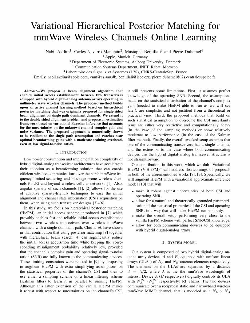
Variational Hierarchical Posterior Matching formmWave Wireless Channels Online Learning
Nabil Akdim1, Carles Navarro Manchon2, Mustapha Benjillali3 and Pierre Duhamel41 Apple, Munich, Germany
2 Department of Electronic Systems, Aalborg University, Denmark3 Communication Systems Department, INPT, Rabat, Morocco
4 Laboratoire des Signaux et Systemes (L2S), CNRS-CentraleSup, FranceEmails: [email protected], [email protected], [email protected], [email protected]
Abstract—We propose a beam alignment algorithm thatenables initial access establishment between two transceiversequipped with hybrid digital-analog antenna arrays operating inmillimeter wave wireless channels. The proposed method buildsupon an active channel learning method based on hierarchicalposterior matching that was originally proposed for single-sidedbeam alignment on single path dominant channels. We extend itto the double-sided alignment problem and propose an estimationframework based on variational Bayesian inference that accountsfor the uncertainties on the unknown channel complex gain andnoise variance. The proposed approach is numerically shownto be resilient to the single path assumption and reaches nearoptimal beamforming gains with a moderate training overhead,even at low signal-to-noise ratios.
I. INTRODUCTION
Low power consumption and implementation complexity ofhybrid digital-analog transceiver architectures have acceleratedtheir adoption as a beamforming solution that can enableefficient wireless communications over the harsh mmWave fre-quency limited-scattering and blockage-prone wireless chan-nels for 5G and beyond wireless cellular networks [1]. Also,angular sparsity of such channels [1], [2] allows for the useof adaptive sparsity-friendly techniques to ease the initialalignment and channel state information (CSI) acquisition onthem, when using such transceiver designs [3]–[6].
In this study, we focus on hierarchical posterior matching(HiePM), an initial access scheme introduced in [7] whichprovably enables fast and reliable initial access establishmentbetween two wireless transceivers over wireless mmWavechannels with a single dominant path. Chiu et al. have shownin that contribution that using posterior matching [8] togetherwith hierarchical beam search [4] can significantly reducethe initial access acquisition time while keeping the corre-sponding misalignment probability relatively low, providedthat the channel’s complex gain and operating signal-to-noiseration (SNR) are fully known to the communicating devices.These limiting constraints were relaxed in [9] by proposingto augment HiePM with extra simplifying assumptions onthe statistical properties of the channel’s CSI and then touse either a sampling scheme or a linear filtering scheme(Kalman filter) to learn it in parallel to running HiePM.Although this latter extension of the vanilla HiePM makesit robust with respect to uncertainties on the channel’s CSI,
it still presents some limitations. First, it assumes perfectknowledge of the operating SNR. Second, the assumptionsmade on the statistical distribution of the channel’s complexgain (needed to make HiePM able to run as we will seelater), are simplistic and not justified from a theoretical orpractical view. Third, the proposed methods that build onsuch statistical assumption to overcome the CSI uncertaintyissue are either very restrictive and computationally heavy(in the case of the sampling method) or show relativelymoderate to low performance (in the case of the Kalmanfilter method). Finally, the overall tweaked setup assumes thatone of the communicating transceivers has a single antenna,and the extension to the case where both communicatingdevices use the hybrid digital-analog transceiver structure isnot straightforward.
Our contribution, in this work, which we dub “VariationalHiePM (V-HiePM)” will address shortcomings of proposalsin both of the aforementioned works [7], [9]. Specifically, wewill augment HiePM with a variational approximate inferencemodel [10] that will:
• make it robust against uncertainties of both CSI andoperating SNR,
• allow for a natural and theoretically grounded parametri-sation of the statistical properties of the CSI and operatingSNR, in a way that will make HiePM run smoothly,
• make the overall setup performing very close to thevanilla HiePM scheme with perfect SNR/CSI knowledge,
• allow for both communicating devices to be equippedwith hybrid digital-analog arrays.
II. SYSTEM MODEL
Our system is composed of two hybrid digital-analog an-tenna array devices A and B, equipped with uniform lineararrays (ULAs) of NA and NB antenna elements respectively.The elements on the ULAs are separated by a distanced = /2, where is the the mmWave wavelength ofinterest. Device A (B respectively) digitally controls its ULAwith NRF
A (NRFB respectively) RF chains. The two devices
communicate over a reciprocal static and narrowband wirelessmmWave MIMO channel, that is modeled as a NB NA

complex matrix H , sampled from the finite scatterer channelmodel [5] with a single dominant path as1:
H = ↵aB(B)aHA(A) (1)
where ↵ is the complex fading channel gain. aA(A) andaB(B) are the ULA array response vectors at devices A andB with incidence angles A and B respectively, modeledas aA (!A) =
1, ej!A , . . . , ej(NA1)!A
Tand aB (!B) =
1, ej!B , . . . , ej(NB1)!BT
, with !A(A) = 2 d cos (A)
and !B(B) = 2 d cos (B). The incidence angles A and
B are assumed to be sampled from the ranges [A,1, A,2]and [B,1, B,2] respectively. 2
The two devices go through an initial access phase con-sisting of a pilot based beam alignment procedure in order toestablish the wireless link between them. We assume in thiswork that, during this initial access phase, the CSI learningand beam search processes for the two devices are centralized,i.e one of the devices, say B, is collecting measurementsbased on device A’s pilot transmission, uses them to learnthe channel’s statistics and devises the beamformer it willuse for the next pilot reception occasion together with thebeamformer that device A should use in sending that pilot,then communicates such information to device A through anideal, error-free control channel3. At time instant t, device Asends a pilot symbol to B, which observes, after pilot removal:
yB,t =p
PwHB,tHfA,t + wH
B,tnB,t (2)where fA,t 2 CNA and wB,t 2 CNB are the effectivebeamformer and combiner used at time t by transceiversA and B respectively. These are chosen from the hybriddigital-analog codebooks detailed next. nB,t 2 CNB is acomplex circularly-symmetric additive white Gaussian noisevector with i.i.d elements with an unknown variance 2
B ,obtained after training sequence removal.
pP is the average
transmit power of the pilot signal.The adaptive beamforming strategy proposed herein utilizes
the hierarchical beamforming codebook of [4]. Such a code-book, noted CS hereafter, is designed to have S levels of beampatterns. We note Cl the collection of beams belonging to levell. Then, Cl contains 2l beamforming vectors that divide thesector [1, 2] into 2l directions, each associated with a certainrange of incidence angles Rm
l , such that [1, 2] = [2l
m=1Rml .
We note each of such 2l vectors as either fA (Rml ) or
wB (Rml ), depending on the considered device.
III. SEQUENTIAL BEAM PAIR SEARCH VIA VARIATIONALHIERARCHICAL POSTERIOR MATCHING
We start this section by first reviewing the details of thevanilla HiePM scheme [7], showing that knowledge of the
1This assumption is used only for the analytical derivation of our scheme.In Section IV, we show numerically that the method is resilient to such alimitation.
2No statistical assumptions on the distribution of the gain and the anglesare made here, we will later justify the choice of distributions we will useduring the inference process.
3Such channel can e.g. be established via a sub-6 GHz link in a non-stand-alone deployment. Control feedback channel design details will not bediscussed here due to space constraints.
channel gain ↵ as well as the noise variance 2 is necessary tomake such a search strategy usable in practice. We then detailour main contribution, which consists of augmenting HiePMwith a novel variational model comparison based approximateinference framework [10] to account for the uncertainties about↵ and 2
B and thus overcome the shortcomings, as detailed inthe introduction, of the vanilla HiePM and modified HiePMschemes proposed in [7] and [9] respectively.
A. Sequential Active Learning via the HiePM Strategy
We illustrate here the use of vanilla HiePM scheme [7]for device A (an analogous strategy will be used for deviceB). HiePM selects fA,t+1 based on the posterior at time t ofthe incidence angle A. We discretize4 the noisy beam searchproblem above by assuming that the beam search resolutionA
5 is an integer power of two and that the AoA A is of theform:A 2 A,1, . . . ,A,A,A,i = A,1+
(i 1)
A(A,2 A,1) (3)
With the above setup, the posterior distribution of A givenall measurements up to time t (collected in vector yB,1:t), canbe written as a A-dimensional vector A (t) with entries
A,i (t) := Pr (A = A,i|yB,1:t) , i = 1, . . . , A. (4)
The posterior probability of A being in a certain range,say Rm
i , can be computed asA,Rm
i(t) :=
X
A,i2Rmi
A,i (t). (5)
The HiePM strategy examines the posterior probabilityA,Rm
i(t) for all i = 1, . . . , SA and m = 1, . . . , 2i and
selects fA,t+1 2 CS to be the beamformer corresponding tothe angular range that satisfies:
(it+1, mt+1) = arg min
(i,m)
A,Rmi
(t) 1
2
(6)
Doing so, it is guaranteed [7] to sequentially refine the widthof the beamformer around the true incidence angle A.
Next we describe how the posterior bielief around A isupdated once a new measurement is taken with the pair ofbeamformers chosen previously with HiePM. Based on themeasurement model in (2), the posterior update at time instantt + 1 can be expressed using Bayes rule as
A,i (t + 1) / A,i (t) f (yB,t+1|A = A,i) ,
i = 1, . . . , A(7)
where f (yB,t+1|A = A,i) is the likelihood of A frommeasurement yB,t+1. Unfortunately, the likelihood term abovecannot be calculated in closed form due to the unknownchannel gain ↵, noise variance 2
B and incidence angle B .We will show next, how “V-HiePM” is able, using the
variational model based approximate inference frameworkdescribed in [10], to infer all above unknowns and uses them
4Such discretization approaches the original problem of initial access asA ! 0 [7].
5To support this level of resolution, the corresponding number of levelsof the hierarchical beamforming codebook at device A should be : SA =log2 (A).
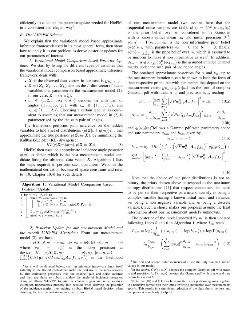
efficiently to calculate the posterior update needed for HiePM,in a consistent and elegant way6.
B. The V-HiePM Scheme
We explain first the variational model based approximateinference framework used in its most general form, then showhow to apply it to our problem to derive posterior updates forour parameters of interest.
1) Variational Model Comparison based Posterior Up-date: We start by listing the different types of variables thatthe variational model comparison based approximate inferenceframework deals with:
• X is the observed data vector, in our case is yB,1:t+1.• Z = (Z1, Z2, . . . , ZL) denotes the L-dim vector of latent
variables that parameterize the measurement model (2).In our case, Z = (↵,2
B).• m 2 1, 2, . . . , A B denotes the mth pair of
angles (A,im,B,jm
), with im 2 1, . . . , A, andjm 2 1, . . . , B. Choosing a certain label m is equiv-alent to assuming that our measurement model in (2) isparameterized by the the mth pair of angles.
The framework performs joint inference on the hiddenvariables to find a set of distributions q(Z|m), q(m)1:m thatapproximate the true posterior p(Z, m|X), by minimizing theKullback-Leibler (KL) divergence:
KL(q(Z|m)q(m), p(Z, m|X)). (8)HiePM then uses the approximate incidence angle posterior
q(m) to decide which is the best measurement model can-didate fitting the observed data vector X . Algorithm 1 liststhe steps required to perform such operations. We omit themathematical derivation because of space constrains and referto [10, Chapter 10.4] for such details.
Algorithm 1: Variational Model Comparison basedPosterior Update
1 for m = 1 : AB do2 while (No convergence yet) do3 for j = 1, 2, . . . , L do4 q(Zj |m) / Ei 6=j(log(p(X|Z, m)))
5 Lm =R
Zq(Z|m) log(
p(Z,m|X)q(Z|m)
)
6 q(m) / p(m) exp(Lm)
2) Posterior Update for our measurement Model andthe overall V-HiePM Algorithm: From our measurementmodel (2), we have
p(X, Z, m) = p(yB,1:t|↵, B , m)p(↵)p(B)p(m) (9)where B = 2
B is the noise precision atdevice B; p(X|Z, m) = p(yB,1:t|↵, B , m) =Qt+1
i=1 CN(yB,i;p
P↵wHB,iAmfA,i,
2B) is the likelihood
6As it will be detailed below, such an inference framework lends itselfnaturally in the HiePM context: we make the best use of the measurementsby first estimating posteriors over the channel gain and noise varianceand then use those to robustly update the angle of incidence posterior,doing so allows V-HiePM to take the channel’s gain and noise varianceestimation uncertainties properly into account when deriving the posteriorof the incidence angles, thus making a robust HiePM based decision whenchoosing the next precoder/combiner pair to use.
of our measurement model (we assume here that thesequential noise samples are i.i.d); p(↵) = CN(↵;↵0,0)is the prior belief over ↵, considered to be Gaussianwith a known initial mean ↵0 and initial precision 0
7;p(B) = (B ; a0, b0) is the non informative prior beliefover B , with parameters a0 = 0 and b0 = 0; finally,p(m) = 1
ABis the prior belief over m, which is assumed to
be uniform to make it non informative as well8. In addition,Am = aB(B,jm
)aHA(A,im
) is the assumed unfaded channelmatrix under the mth pair of incidence angles.
The obtained approximate posteriors for ↵ and B , up tothe measurement iteration t, can be shown to keep the form oftheir respective priors, but with parameters that depend on themeasurement vector yB,1:t: qt(↵|m) has the form of complexGaussian pdf with mean ↵t,m and precision t,m reading
t,m =at,m
bt,m
tX
d=1
p
PwHB,tAmfA,t
2
+ 0 (10a)
↵t,m =at,m
bt,mt,m
tX
d=1
pPwH
B,tAmfA,t
yB,d +
↵00
t,m
(10b)and qt(B |m)9follows a Gamma pdf with parameters shapeand rate parameters at,m and bt,m given by
at,m = a0 + t, (11a)
bt,m = b02RePt
d=1
pPwH
B,tAmfA,t
yB,d↵
t,m
+
Ptd=1
|yB,d|2 +
1
t,m+ |↵t,m|2
p
PwHB,tAmfA,t
2
(11b)Note that the choice of our prior distributions is not ar-
bitrary, the priors chosen above correspond to the maximumentropy distributions [11] that respect constraints that needto be put on their respective parameters, namely ↵ being acomplex variable having a known initial mean and variance,B being a non negative variable and m being a discretevariable). Such a choice makes our proposal assume the leastinformation about our measurement model’s unknowns.
The posterior of the model, indexed by m, is then updatedfollowing Lines 5 and 6 in Algorithm 1, where Lm reads
Lt,m = log(1
2t,m
) + at,m (1 log(bt,m)) + log((at,m))
b0at,m
bt,m
tX
d=1
|yB,d|2at,m
bt,m t,m |↵t,m|2
!(12)
7The first and second order moments of ↵ are the only assumed knownvalues in our model.
8In the above, CN(·; µ,) denotes the complex Gaussian pdf with meanµ and precision , (·; a, b) denotes the Gamma pdf with shape and rateparameters a and b.
9Note that (10) and (11) can be re-written, after performing some algebra,in a recursive format w.r.t their terms involving summation over measurementsepochs. This results in a significant reduction of the algorithm’s memory andcomputation complexity footprint.

The posteriors over A,imand B,jm
are obtained from theposterior qt(m) as
qA,t(i) =X
m:im=iqt(m), i = 1, . . . , A (13)
qB,t(j) =X
m:jm=jqt(m), j = 1, . . . , B (14)
The posterior probability of the incidence angles A andB to be in a certain range Rn
A,i and RpB,j resp, read as:
qA,t(RnA,i) :=
X
A,i2RnA,i
qA,t(i), (15)
qB,t(RpB,j) :=
X
B,j2RpB,j
qB,t(i), (16)
The vanilla HierPM scheme is then applied separately toqA,t(i) and qB,t(j), to choose the pair of beamformers to usefor the next measurement occasion.
The modes ↵t and Bt of the approximate posteriorsqt(↵|m
t ) and qt(B |mt ), with m
t = arg maxm(qt(m)), canbe seen as approximations of the MMSE estimates of ↵ andB respectively. These estimates are given by:
↵t = ↵t,mt, Bt = at,m
t/bt,m
t. (17)
Algorithm 2 runs all above operations in a loop, until themeasurement budget is exhausted: device B decides whichpair of beamformers devices A and B shall use to take thenext measurement by applying the HiePM scheme separatelyto the current posteriors qA,t and qB,t, it then takes a newmeasurement yB,t+1 with those latter, and finally run varia-tional inference to derive approximate posteriors of B = 1
2B
,↵ as well as of A and B .
IV. NUMERICAL RESULTS
To assess the effectiveness of V-HiePM, we run Monte Carlosimulations on a setup with two hybrid digital-analog beam-forming devices A and B. The channel matrix H 2 CNBNA
reads
H = ↵aB(B)aHA(A) +
LX
l=1
↵laB(B,l)aHA(A,l) (18)
and contains one dominant multipath component and L scat-tered components. All incidence angles are independentlydrawn from a uniform distribution between 0 and . Thechannel gains are independently drawn from a a set of complexGaussian distribution with mean 0 and variances fulfillingVar↵+
Pl Var↵l = 1, so that the average SNR between
the nth element of the array at A and the mth element ofthe array at B equals E|Hnm|2/E|B |2=1/2
B10. In all
simulations below, the two devices are equipped with identicalarrays made of NA = NB = 32 elements, digitally controlledwith NRF
A = NRFB = 8 RF chains. Device A uses a codebook
CA with a depth of SA = log2(A), A = 128. CA is built
10Hnm is the channel coefficient between device B’s nth array elementand device A’s mth array element, and E is the expectation operator.
using the orthogonal matching pursuit as described in [4]. Asimilar codebook, CB , is used for device B.11
We benchmark our algorithm’s beamforming gain after tmeasurements, defined as:
Gvh =wH(B,kt,B
)Hf(A,kt,A)2
(19)with different measurement budget sizes and under differentchannel assumptions (note the the exhaustive search needsNANB = 16384 measurements to settle), against that of thedifferent state of the art schemes listed below:
• Gph of the vanilla HiePM scheme of [7]. Here, such ascheme assumes that most of the energy in the channelis concentrated in the path corresponding to the knowngain ↵ and all other gains ↵l are null, it also assumesthat 2
B is known. In such case, the posterior update isdone, simply using Bayes rule as in equation (21) in [7],on the beam pair corresponding to that main path, andthen HiePM is applied to the marginals over those anglesseparately, similar to what V-HiePM does.
• Gbs of the noisy binary search algorithm of [4], which isachieved by 4 log2(maxNA, NB) = 28 measurements.
As a reference, we consider as well the best achievablebeamforming gain of the codebook, defined as
Gmax = maxw2CB
SB,f2CA
SA
wHHf2 . (20)
11Note that the multi-RF chain setups are used solely to help buildacceptable RF codebooks [4], and are not used for multi-stream MIMOoperations.
Algorithm 2: V-HiePM1 Input : Antenna Array Size NA and NB , The search resolution A and B ,
the codebooks CSAand CSB
, Search time 2 Output : Estimates of A, B , ↵ and B
3 for t = 1, 2, . . . , 1 do4 #HierPM Based BF selection according to Eq.(6)
(fA,t+1, wB,t+1) =
fA
RkA,t+1
A,lA,t+1
, wB
RkB,t+1
B,lB,t+1
5 #Take next measurement6 yB,t+1 =
pPwH
B,t+1HfA,t+1 + wHB,t+1nB,t+1,
7 #Variational Model Comparison Posterior Update8 for m = 1 : AB do9 while (No convergence yet) do
10 update qt+1(↵|m) via (10) then qt+1(B |m) via (11)11 end12 update qt+1(m) via (12)13 end
14 #Angle and Angular Range Posterior Update15 update qA,t+1(i) via (13) and qB,t+1(j) via (14)16 update qA,t+1(Rn
A,i) via (15) and qB,t+1(RnB,j) via (16)
17 #Final Precoder/Combiner Vector designlt+1,A, kt+1,A
= (SA, arg maxk (qA,t+1(k)))
18
lt+1,B , kt+1,B
= (SB , arg maxk (qB,t+1(k)))
19 #Channel’s Gain and Noise Precision MAP Estimates update ↵t+1 andBt+1 via (17)
20 end21 Output : A = A,k,A
, B = B,k,B, ↵ = ↵ , B = B

-10 -5 0 5 10
SNR in dB
-25
-20
-15
-10
-5
0
Be
am
form
ing
Lo
ss
in
dB
Lbs
: = 28
Lvh
: = 28
Lph
: =28
Lvh
: = 56
Lph
: =56
Lvh
: = 128
Lph
: =128
Figure 1: Beamforming loss of the different search schemes in achannel with L = 0 scattered components.
We begin by assuming that only the dominant componentis present (i.e. L = 0). Fig. 1 shows the beamforming lossesof the benchmarked algorithms with respect to the optimumpair of beamformers, defined as Lvh = Gvh/Gmax, Lph =Gph/Gmax, and Lbs = Gbs/Gmax. The results show thesuperiority of our scheme compared to the binary search of[4], and that it achieves similar or even better performancecompared to vanilla HiePM with perfect CSI and operatingSNR knowledge. It can be observed that the vanilla HiePMscheme with perfect channel gain knowledge saturates at highSNR: this is an effect of the algorithm assuming that thecomponent’s incidence angle lies on a discrete grid of values,whereas the actual angles are sampled from a continuousdistribution. Our proposed method is less sensitive to thismodel mismatch, due to the estimation of the channel gainand inverse noise variance: in practice, these estimates partlyaccount for the mismatch in the assumed values of the anglesand provide robustness to the overall procedure.
Next, we explore the robustness of the proposed methodagainst channels containing more than one multipath compo-nent. For this, we consider a channel with L = 3 scatteredcomponents with gains of equal variance, and with the powerratio between the dominant and scattered components beingLOSR = E↵2/(E↵2 +
Pl E↵2
l ). Fig. 2 shows beam-forming gains achieved by our algorithm after 100 measure-ments compared to the maximum gains achievable Gmax.
As it can be observed, the maximum achievable beamform-ing gain decreases as the power is more evenly distributedamong the channel’s components. Although V-HiePM assumesthe existence of a single component, it shows remarkableresilience to the presence of other components. Even whenall components in the model have comparable power, ourproposed method is able to perform within 2 dB of theoptimum for sufficiently high SNR.
V. CONCLUSION AND FUTURE WORK
We proposed in this work a variational Bayesian onlinelearning scheme that enables initial access for hybrid digital-analog enabled devices operating in mmWave wireless chan-nels. When compared to state of the art beam acquisitionschemes, our method shows superiority, in terms of balancing
-10 -5 0 5 10
SNR in dB
20
22
24
26
28
30
Be
am
form
ing
Ga
in i
n d
B
Gvh
: L=3, LOSR
= 0.2
Gmax
: L=3, LOSR
= 0.2
Gvh
: L=3, LOSR
= 0.7
Gmax
: L=3, LOSR
= 0.7
Gvh
: L=0, LOSR
= 1
Gmax
: L=0, LOSR
= 1
Figure 2: V-HiePM performance in channels with different powerratios between the dominant path and L = 3 scattered components.
the beam search time versus achieving higher beamforminggain, in being able to properly do so while accounting foruncertainties on the unknown CSI (gain and noise variance)and in being very resilient to the dominant single path assump-tion. Even though the scheme is derived based on a discretizedmodel of the angles of incidence of the channel’s maincomponent, it showed great robustness against off-grid anglesas well as working with a realistic codebook implementation.Further research will focus on adapting the proposed onlinelearning algorithm to operating in time-varying channels.
REFERENCES
[1] R. W. Heath, N. Gonzalez-Prelcic, S. Rangan, W. Roh, and A. M.Sayeed, “An overview of signal processing techniques for millimeterwave MIMO systems,” IEEE Journal of Selected Topics in SignalProcessing, vol. 10, no. 3, pp. 436–453, Apr. 2016.
[2] S. Hur, S. Baek, B. Kim, Y. Chang, A. F. Molisch, T. S. Rappaport,K. Haneda, and J. Park, “Proposal on millimeter-wave channel modelingfor 5G cellular systems,” IEEE Journal of Selected Topics in SignalProcessing, vol. 10, no. 3, pp. 454–469, Apr. 2016.
[3] O. E. Ayach, S. Rajagopal, S. Abu-Surra, Z. Pi, and R. W. Heath,“Spatially sparse precoding in millimeter wave MIMO systems,” IEEETransactions on Wireless Communications, vol. 13, no. 3, pp. 1499–1513, Mar. 2014.
[4] A. Alkhateeb, O. E. Ayach, G. Leus, and R. W. Heath, “Channelestimation and hybrid precoding for millimeter wave cellular systems,”IEEE Journal of Selected Topics in Signal Processing, vol. 8, no. 5, pp.831–846, Oct. 2014.
[5] N. Akdim, C. N. Manchon, M. Benjillali, and E. de Carvalho, “Pingpong beam training for multi stream MIMO communications with hybridantenna arrays,” in 2018 IEEE Globecom Workshops (GC Wkshps), Dec.2018, pp. 1–7.
[6] Y. Ding, S. Chiu, and B. D. Rao, “Bayesian channel estimation algo-rithms for massive MIMO systems with hybrid analog-digital processingand low-resolution ADCs,” IEEE Journal of Selected Topics in SignalProcessing, vol. 12, no. 3, pp. 499–513, Jun. 2018.
[7] S. Chiu, N. Ronquillo, and T. Javidi, “Active learning and CSI acquisi-tion for mmwave initial alignment,” IEEE Journal on Selected Areas inCommunications, pp. 1–1, 2019.
[8] O. Shayevitz and M. Feder, “Optimal feedback communication viaposterior matching,” IEEE Transactions on Information Theory, vol. 57,no. 3, pp. 1186–1222, Mar. 2011.
[9] N. Ronquillo, S. Chiu, and T. Javidi, “Sequential learning of CSIfor mmwave initial alignment,” CoRR, vol. abs/1912.12738, 2019.[Online]. Available: http://arxiv.org/abs/1912.12738
[10] C. M. Bishop, Pattern Recognition and Machine Learning (InformationScience and Statistics). Berlin, Heidelberg: Springer-Verlag, 2006.
[11] M. U. Thomas, “A generalized maximum entropy principle,” OperationsResearch, vol. 27, no. 6, pp. 1188–1196, 1979.

Appendix B
Ping Pong Beam Training for Multi
Stream MIMO Communications with
Hybrid Antenna Arrays
89

Ping Pong Beam Training forMulti Stream MIMO Communications
with Hybrid Antenna ArraysNabil Akdim1, Carles Navarro Manchon2, Mustapha Benjillali3, and Elisabeth de Carvalho2
1 Intel Deutschland, Munich, Germany2 Department of Electronic Systems, Aalborg University, Denmark
3 Communication Systems Department, INPT, Rabat, MoroccoEmails: [email protected], [email protected], [email protected], [email protected]
Abstract—We propose an iterative training procedure that ap-proximates multi-stream MIMO eigenmode transmission betweentwo transceivers equipped with hybrid digital analog antennaarrays. The procedure is based on a series of alternate (pingpong) transmissions between the two devices in order to exploitthe reciprocity of the wireless channel. During the ping pongiterations, the update of the devices’ digital precoders/combinersis performed based on a QR decomposition of the receivedsignal matrix. Concurrently, their analog precoders/combinersare progressively updated by a novel “multi-beam split anddrop with backtracking” mechanism that tracks the channel’smain spatial components. As shown throughout the paper, theproposed algorithm converges with only few iterations, hasminimal computational complexity, and performs very closelyto optimal singular value decomposition based precoding withsufficiently large signal-to-noise ratio.
I. INTRODUCTION
Upcoming wireless communication networks are expectedto provide service to an unprecendently large number of wire-less devices with peak data rates in the order of tens of Gbps.The congestion and fragmentation of the traditional spectralbands below 6GHz has pushed wireless service providers toexplore vacant spectrum at the millimeter-wave (mmWave)frequency bands (30–300 GHz) in order to fulfill that goal [1].Nevertheless, the poor reflectivity and high absorption and freespace propagation losses make communicating wirelessly oversuch high frequencies a challenging task [2]. Fortunately, thisfrequency range will allow for the use of compact and smallantenna arrays with high number of elements, as the physicalsize of the array is proportional to the carrier wavelength. Thelarge beamforming gains that such large-scale arrays enablewill be used to compensate for the above limitations.
However, the high cost, power consumption and complexityof the mixed signal hardware at mm-wave make having largeantenna arrays with digitally controlled elements infeasible [3].This has motivated the wireless communication research com-munity to look at the hybrid digital-analog antenna arrayarchitectures [4]. In such architectures, the large antenna arrayis steered using analog phase shifters and only a few digitallymodulated radio-frequency (RF) chains. An illustration of suchan architecture is shown in Fig. 1.
In addition to their cost and implementation advantages,hybrid array structures entail their own challenges: the lowSNR resulting from high propagation losses, the large dimen-sionality of the MIMO channel matrix and the presence ofanalog processing complicate the acquisition of the channelstate information (CSI) and the computation of the MIMOprecoders and combiners [1], [3]. Luckily, channel measure-ment campaigns [2] have shown that mm-wave channels aresparse in the angular domain, which enables the proposalof CSI acquisition and precoding/combining algorithms thatexploit such property. An example of these are compressedsensing based approaches such as [3], [5], [6], which aregenerally computationally complex and require a large amountof channel measurements. An alternative are exhaustive andhierarchical beam-search techniques, which may entail signif-icant latency and probability of miss detection [7].
In this work, we focus on a beam training strategy basedon alternating transmissions between two transceivers, whichhas been coined ping pong beam training (PPBT). The mainidea behind PPBT is to exploit the reciprocity of the MIMOchannel. With appropriate processing at each device, the alter-nate transmissions implicitly implement an algebraic poweriteration that leads to approximating the top left and rightsingular vectors of the MIMO channel matrix. This idea wasfirst applied in the digital arrays context for single streamwireless communications in [8], [9], and was extended tomulti stream setups in [10], to large antenna array andfrequency selective systems in [11] and to noisy MIMOchannels in [12]. More recently, similar approaches have beenproposed in the context of mmWave communications withhybrid digital-analog antenna arrays, which we review next.In [13], the basic ping pong beam training method for single-stream MIMO transmission was adapted to the hybrid arrayarchitecture with the inclusion of a “beam split-and-drop”procedure for the setting of analog precoders. The subspaceestimation and decomposition method in [14] proposes a pingpong based algorithm that iteratively estimates the channel’sright and left eigenvectors using a Krylov subspace estimationmethod. This algorithm is based on exhaustive measurementswith a large set of different analog precoders, which are then

Baseband
Precoder
Baseband
Combiner
RF Chain
RF Chain
RF Chain
RF Chain
RF Precoder RF Combiner
NA NB
NA
RF
NB
RF
H
WA
FATRANSCEIVER A TRANSCEIVER B
FB
WB
YB[1]
YB[ ]NB
RF
Fig. 1: Structure of the transceivers
linearly combined in order to cancel the effect of the analogprecoders. It therefore requires significant amount of trans-missions, which imply large signalling overhead and latency.Lastly, the power iteration based training method introducedin [15] is a technique that extends the solution proposedin [10] to the multi stream case, where the digital precodersare set based on an algebraic power iteration technique, whilethe analog precoders update is done based on a compressedsensing technique called simultaneous orthogonal matchingpursuit [16].
Compared to the above approaches, we propose in thisarticle a strategy that sets the digital and analog precodersof the devices in a way to approximate the top NS left andright singular vectors of the channel matrix, with NS beingthe desired number of spatial streams. Our new technique,which we dub “hybrid ping pong multi beam training“(Hybrid PPMBT) extends the work done in [13] to the multistream case. It adapts the PPBT strategy to hybrid arrays byprogressively choosing the analog precoders at each devicefrom a predefined hierarchical codebook. After one round-triptransmission, a novel ”multi beam split and drop strategy withbacktracking” is applied to focus the analog precoders towardsthe spatial directions that are most likely containing thechannel’s top NS multipath components. The digital precodersare updated via an orthogonal decomposition operation on thereceived signal as described in [10]. In comparison to theapproaches in [14] and [15], Hybrid PPMBT is much simplerfrom a computational complexity aspect and has a low trainingoverhead as it requires significantly fewer transmissions. Sim-ulation results show that our proposed scheme performs verywell in retrieving the wanted NS channel’s top eigenmodesfor sufficiently large signal-to-noise ratio, both in terms ofaccuracy and convergence speed.
II. SYSTEM MODEL
We consider a system in which two hybrid analog digitaltransceivers A and B, equipped with uniform linear arrays(ULA) composed of NA and NB antenna elements. Suchelements are separated with a distance d = /2, where isthe wavelength of interest. The two devices control digitallytheir arrays with NRF
A and NRFB RF chains respectively and
exchange data over a reciprocal wireless MIMO channel usingNS parallel data streams. The channel from device A to
device B is considered to be static and narrowband and ismodeled according to the finite scatterer channel model withL propagation paths [13], [17], as
H =
rNANB
L
LX
l=1
↵laB(B,l)aHA(A,l), (1)
here, H 2 CNBNA , L is the number of multipath com-ponents (MPC), ↵l is the complex fading channel gain forMPC l, A,l = 2
d cosA,l and B,l = 2 d cosB,l
are the directional cosines corresponding to the lth MPCat arrays A and B respectively, where A,l, B,l are theangles of incidence of that same path, and aA and aB
are the array response vectors at device A and B respec-tively. The ↵l are modeled as independent, standard com-plex gaussian variables, the A,l and B,l as uniformly dis-tributed in the range [0, 2) radians and the array responsesas aA(A,l) = [1, ejA,l , . . . , ej(NA1)A,l ]T/
pNA and
aB(B,l) = [1, ejB,l , . . . , ej(NB1)B,l ]T/p
NB .In order to establish the wireless link with device B, device
A (we assume, without loss of generality, that device A isperforming the first transmission) transmits T , an NS NS
orthogonal training sequence i.e TT H = INS. Upon reception,
device B cancels the training sequence effect by multiplyingits received digital signal by T H . The resulting signal can beexpressed as:
YB = F HBHFAWA + F H
BNB , (2)where FA 2 CNANRF
A and FB 2 CNBNRFB contain the
states of the analog precoder and combiner of transceiversA and B, WA 2 CNRF
A NS denotes the digital precoder oftransceiver A and NB 2 CNBNS is a complex, circularly-symmetric additive white gaussian noise matrix, obtained aftertraining sequence removal and with i.i.d elements, each withvariance 2. Transmissions from device B to device A aremodeled analogously as
YA = F HAHHFBWB + F H
ANA, (3)where WB 2 CNRF
B NS and NA 2 CNANS are definedsimilar to the above.
III. HYBRID PING PONG MULTI BEAM TRAINING :HYBRID PPMBT
Given the signal model in (2) and (3), the beamforming taskconsists of selecting the set of analog and digital precoders andcombiners that maximize the spectral efficiency over a givenchannel matrix H . For transmission from device A to B, andassuming unit transmit power equally allocated across the NS
streams, the spectral efficiency reads
R = log2 detINS
+R1
NB
NSHeH
He
, (4)
where RNB= 2W H
BF HBFBWB is the noise covari-
ance matrix after receive combining at device B, He =W H
BF HBHFAWA is the equivalent channel after precoding
and combining at both devices. An analogous expressionapplies for transmission from device B to device A.
The optimal precoders maximizing (4) are known to be theNS top right and left singular vectors of H . However, thehybrid structure of the antenna array makes the computation

of such precoders challenging. On the one hand, as digitalmeasurements of the channel are only obtained after analogprecoding and combining, estimating the full channel matrixH in order to obtain its singular value decomposition requiresa large number of measurements and hence large overheadand latency [14]. On the other hand, even if the channelmatrix H can be estimated, the precoders have to be builtas the product of the analog precoding matrix FA and thedigital precoding matrix WA. While the elements of WA cantake any complex value due to its digital implementation, theoperation modeled by FA is implemented via phase shiftersand combiners, which restricts the values it can take. Inthis work, we restrict the entries of FA to satisfy |(FA)l,i|12 1
M(i)A
; 0, where M(i)A being the number of activated
array elements in the ith column of FA, and the option(FA)l,i = 0 accounts for the option of leaving some elementsof the array unused. In addition, a transmit power constraint isenforced such that kFAWAkF = 1.2 With these constraints,finding the combination of digital and analog precoders tobest approximate the channel’s singular vectors becomes acomputationally intensive optimization problem [5].
To overcome such difficulties, we propose an iterative multibeam training scheme based on alternate transmissions be-tween the two devices, this procedure estimates progressivelyand simultaneously the top NS right and left singular vectorsof H and sets the digital and analog precoders so that theyapproach those singular vectors. It consists of two parts: 1) a”backtracking beam split and drop” approach to select theanalog precoders FA and FB from a predefined multi levelcodebook, 2) a method to select the digital precoders WA andWB inspired by the QR decomposition algorithm describedin [10].
We will proceed by reviewing the beam training procedurefor digital antenna arrays proposed in [10], then briefly presentthe multi level codebook that is used for the analog precoderupdate, and finally explain our multi beam training solution.
A. Ping-Pong Multi Beam Training with Digital AntennaArrays: Digital PPMBT
We review the digital PPBT algorithm over a narrowbandreciprocal channel H as described in [10]. We consider twodevices A and B equipped with digitally controlled antennaarrays with NA and NB elements respectively. At the initial(0th) iteration, the process starts with a random initializationof the precoder at device A, W
[0]A . A uses then this initial
precoder to transmit a training sequence to B. Upon receptionand training sequence removal, device A gets an estimate ofHW
[0]A , makes a QR-decomposition on it, and uses the Q
part of that decomposition as its precoder W[0]B . It then uses
that precoder to transmit a training sequence back to device A,who will repeat the same operations. This process is reiterateduntil convergence, at which, device A gets an estimate of the
1(FA)l,i is the entry of the matrix FA belonging to its lth row and ithcolumn.
2Obviously, the same constraints apply to the analog precoder of device B.
top NS right singular vectors of H and device B gets anestimate of the top NS right singular vectors of HH. Furtherdetails on this procedure can be found in [10].
Algorithm 1 Ping Pong Multi Beam Training with HybridArrays
1: Initialize:
F[0]A
'
(1)A,0,'
(1)A,1, . . . ,'
(1)
A,M(1)A
1
,
F[0]B
'
(1)B,0,'
(1)B,1, . . . ,'
(1)
B,M(1)B
1
,
Initialize W[0]A to an orthogonal matrix of its size.
for s = 1 : NS do
W[0]A (:, s) W
[0]A
(:,s)pNS
F[0]A
W[0]A
(:,s)2
end forpA, kA, iA [], [], [], pB , kB , iB [], [], [].
2: A transmits, B receives: Y[0]
B =(F[0]B )HHF
[0]A W
[0]A +(F
[0]B )HN
[0]B
3: [Q, R] qr(Y[0]
B )4: for s = 1 : NS do5: W
[0]B (:, s) Q(:, s)
6: W[0]B (:, s) W
[0]B
(:,s)pNS
F[0]B
W[0]B
(:,s)
27: end for8: t 19: loop
10: B transmits,11: A receives Y
[t]A =(F
[t1]A )HHHF
[t1]B W
[t1]B +(F
[t1]A )HN
[t]A
12: [Q, R] qr(Y[t]
A )13: for s = 1 : NS do14: W
[t]A (:, s) Q(:, s)
15: W[t]A (:, s) W
[t]A
(:,s)pNS
F[t1]A
W[t]A
(:,s)
216: end for17: [F
[t]B , pB , kB , iB]
UPD.AN.PR(F[t1]B , W
[t1]B , CB , pB , kB , iB)
18: A transmits,19: B receives: Y
[t]B =(F
[t]B )HHF
[t1]A W
[t]A +(F
[t]B )HN
[t]B
20: [Q, R] qr(Y[t]
B )21: for s = 1 : NS do22: W
[t]B (:, s) Q(:, s)
23: W[t]B (:, s) W
[t]B
(:,s)pNS
F[t]B
W[t]B
(:,s)
224: end for25: [F
[t]A , pA, kA, iA]
UPD.AN.PR(F[t1]A , W
[t]A , CA, pA, kA, iA)
26: t t + 127: end loop
B. Analog Precoder Multi Level Codebook
We illustrate here the codebook definition for transceiverA (an analogous codebook is used for the transceiverB). We consider a codebook CA which is composedof LA= log2 (NA/NRF
A )+13 levels. For the kth level,we define a subcodebook C(k)
A ='(k)A,i, i=0, 1, . . . , M
(k)A -1
consisting of M(k)A =NRF
A 2k-1 column vectors, k=1, 2, . . . , LA.Each of the elements of the subcodebook is defined as
3For the considered codebook design we constrain NA and NRFA to be
both integer powers of two.

'(k)A,i=
1, e-j (k)
A,i , . . . , e-j(M(k)A -1) (k)
A,i ,0TNA-M(k)
A
T
/
qM
(k)A ,
where (k)A,i=-(2i+1)/M
(k)A is the directional cosine of the
ith vector at the kth level ('(k)A,i steers the array in the direction
(k)A,i= arccos
(k)A,i/, with a lobe whose width decreases with
the codebook level k), and 0N is the N -dimensional columnzero vector. Further details about the codebook used here canbe found in [13].
C. Ping Pong Multi Beam Training with Hybrid AntennaArrays : Hybrid PPMBT
The proposed algorithm for beam training with hybridarrays is described in pseudocode. Algorithm 1 presents theoverall training scheme, while Algorithm 2 describes thesubroutine used to update the analog precoding matrices.
1) Initialization: First, the digital and analog precodersare initialized. FA and FB are initialized to C(1)
A and C(1)B
respectively, while WA is initialized to a random unitarymatrix. The columns of WA are then normalized to fulfill thetransmit power constraint of the effective precoder FAWA.Finally, a set of empty arrays, pB , kB , iB, are created.Those arrays will store the needed information to perform theanalog precoder updates, as explained below.
2) Ping Pong Iterations: After the initialization phase,a sequence of alternate pilot transmissions starts between thetwo devices. The baseband precoders are updated after eachreception step by means of a QR-decomposition, followedby a normalization step. These two operations are detailedin lines 3-7, 12-16 and 20-24 in Algorithm. 1. Immediatelyafter updating their baseband precoders upon reception ofa transmission, the devices transmit back with the updateddigital precoders and the same analog precoder as used forreception. Only after the transmission has been made willthe transmitting device update its analog precoders (usingAlgorithm 2), such that next reception is done with the updatedsetting. This allows for the QR based iteration to converge,as each reception-transmission cycle is performed over a staticsetting of the analog precoders.
3) Update of Analog Precoders: The devices invokethe routine outlined in Algorithm 2 to update their analogprecoder state. This routine bases its update on the currentstate of the device’s RF precoder F , its codebook C and on theupdate history of its baseband precoder W . Using all previousupdates of W allows for backtracking–i.e, correcting forwrong RF precoder updates. The routine works as follows:
a) Three sequences of values are generated: kn stores thelevel of the codebook of the nth column of F , pn storesthe squared norm of the nth row of W , i.e the aggregateenergy received on it, and in stores the index of the nthcolumn of F , out of the level of the codebook to whichthat column belongs.
b) The sequences generated above will be used to updatethree vectors: kn will be appended to k, with k beingan array storing the codebook levels of the columns ofF used over consecutive ping-pong iterations. pn will
be appended to p, with p being an array storing thereceived energy over the different spatial directions setby the analog beamformer F . in will be appended to iin a similar manner to the above.
c) Once p is updated, it will be sorted in a descendingmanner and the resulting sorted indices will be storedin pI . This newly formed array will be used to findthe entries of p that are most likely to direct the analogprecoders where the MPCs of H are.
d) Two new vectors are built: bI contains the K first indexesof pI i.e it identifies the beams that are most alignedwith the channel’s MPCs (K is the length of bI , whichcan be derived from lines 9-13). bL is a vector that ismade of 1’s and 2’s. The ith entry of bL is set to 2when the precoder corresponding to the ith entry of bI
is replaced with the two precoders belonging to one stephigher level of the codebook and that have their beamscovering together its same spatial area, otherwise it isset to 1. Deciding to append 1 or 2 to bL depends onwhether we already consumed all columns of F and onwhether the element of pI in question belong to the lastlevel of the codebook or not (see lines 17-21). Line 8 ofthe algorithm erases the measurement stored over a beamthat is selected to be included in the analog precodingmatrix, either directly or after splitting it into two beamsof the immediately higher level. As new measurementswill be obtained over that beam in the next iteration, theold measurement is deleted to avoid unnecessarily comingback to the previous configuration corresponding to that
Algorithm 2 Analog Precoder Update
1: function UPD.AN.PR(F , W , C, p,k,i)2: Generate : kn, in, pn, n=1, . . . , NRF , where kn will store
the codebook level to which the F0s nth column belongs, in
will store its index out of that level and pn will store the normof the nth row of W , i.e the aggregate energy received on it.
3: p [p, p1, . . . , pNRF ], k [k, k1, . . . , kNRF ], i [i, i1, . . . , iNRF ]
4: Sort p in a descending manner and store the result in pS ,then store the arrangement of the elements of p into pS in pI .
5: bI [], bL []6: while n NRF do7: bI [bI , pI,n], pI,n is the nth element of pI ,8: ppI,n 0, ppI,n is the pI,nth element of p,9: if kpI,n = log2(
NNRF )+1 or n=NRF -1 then
10: n n + 1, bL [bL, 1]11: else12: n n + 2, bL [bL, 2]13: end if14: end while15: for t = 1 : Length(bI) do16: m bL,t
17: if m = 2 then18: F [F ,'
(km+1)2im
,'(km+1)2im+1 ]
19: else20: F [F ,'
(km)im
]21: end if22: end for23: return F ; p, k, i24: end function
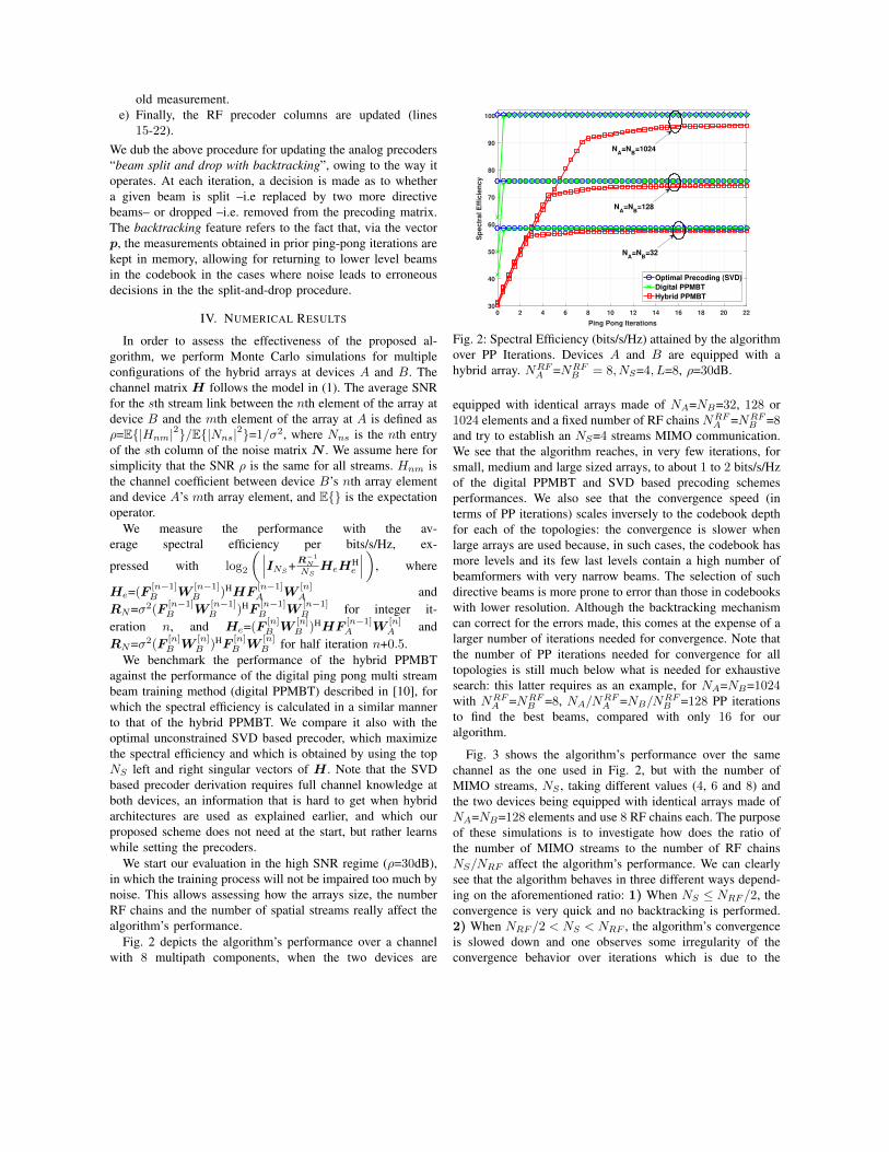
old measurement.e) Finally, the RF precoder columns are updated (lines
15-22).We dub the above procedure for updating the analog precoders“beam split and drop with backtracking”, owing to the way itoperates. At each iteration, a decision is made as to whethera given beam is split –i.e replaced by two more directivebeams– or dropped –i.e. removed from the precoding matrix.The backtracking feature refers to the fact that, via the vectorp, the measurements obtained in prior ping-pong iterations arekept in memory, allowing for returning to lower level beamsin the codebook in the cases where noise leads to erroneousdecisions in the the split-and-drop procedure.
IV. NUMERICAL RESULTS
In order to assess the effectiveness of the proposed al-gorithm, we perform Monte Carlo simulations for multipleconfigurations of the hybrid arrays at devices A and B. Thechannel matrix H follows the model in (1). The average SNRfor the sth stream link between the nth element of the array atdevice B and the mth element of the array at A is defined as=E|Hnm|2/E|Nns|2=1/2, where Nns is the nth entryof the sth column of the noise matrix N . We assume here forsimplicity that the SNR is the same for all streams. Hnm isthe channel coefficient between device B’s nth array elementand device A’s mth array element, and E is the expectationoperator.
We measure the performance with the av-erage spectral efficiency per bits/s/Hz, ex-
pressed with log2
INS+R1
N
NSHeH
He
, where
He=(F[n1]B W
[n1]B )HHF
[n1]A W
[n]A and
RN =2(F[n1]B W
[n1]B )HF
[n1]B W
[n1]B for integer it-
eration n, and He=(F[n]B W
[n]B )HHF
[n1]A W
[n]A and
RN =2(F[n]B W
[n]B )HF
[n]B W
[n]B for half iteration n+0.5.
We benchmark the performance of the hybrid PPMBTagainst the performance of the digital ping pong multi streambeam training method (digital PPMBT) described in [10], forwhich the spectral efficiency is calculated in a similar mannerto that of the hybrid PPMBT. We compare it also with theoptimal unconstrained SVD based precoder, which maximizethe spectral efficiency and which is obtained by using the topNS left and right singular vectors of H . Note that the SVDbased precoder derivation requires full channel knowledge atboth devices, an information that is hard to get when hybridarchitectures are used as explained earlier, and which ourproposed scheme does not need at the start, but rather learnswhile setting the precoders.
We start our evaluation in the high SNR regime (=30dB),in which the training process will not be impaired too much bynoise. This allows assessing how the arrays size, the numberRF chains and the number of spatial streams really affect thealgorithm’s performance.
Fig. 2 depicts the algorithm’s performance over a channelwith 8 multipath components, when the two devices are
0 2 4 6 8 10 12 14 16 18 20 22
Ping Pong Iterations
30
40
50
60
70
80
90
100
Sp
ec
tra
l E
ffic
ien
cy
Optimal Precoding (SVD)
Digital PPMBT
Hybrid PPMBT
NA
=NB
=1024
NA
=NB
=128
NA
=NB
=32
Fig. 2: Spectral Efficiency (bits/s/Hz) attained by the algorithmover PP Iterations. Devices A and B are equipped with ahybrid array. NRF
A =NRFB = 8, NS=4, L=8, =30dB.
equipped with identical arrays made of NA=NB=32, 128 or1024 elements and a fixed number of RF chains NRF
A =NRFB =8
and try to establish an NS=4 streams MIMO communication.We see that the algorithm reaches, in very few iterations, forsmall, medium and large sized arrays, to about 1 to 2 bits/s/Hzof the digital PPMBT and SVD based precoding schemesperformances. We also see that the convergence speed (interms of PP iterations) scales inversely to the codebook depthfor each of the topologies: the convergence is slower whenlarge arrays are used because, in such cases, the codebook hasmore levels and its few last levels contain a high number ofbeamformers with very narrow beams. The selection of suchdirective beams is more prone to error than those in codebookswith lower resolution. Although the backtracking mechanismcan correct for the errors made, this comes at the expense of alarger number of iterations needed for convergence. Note thatthe number of PP iterations needed for convergence for alltopologies is still much below what is needed for exhaustivesearch: this latter requires as an example, for NA=NB=1024with NRF
A =NRFB =8, NA/NRF
A =NB/NRFB =128 PP iterations
to find the best beams, compared with only 16 for ouralgorithm.
Fig. 3 shows the algorithm’s performance over the samechannel as the one used in Fig. 2, but with the number ofMIMO streams, NS , taking different values (4, 6 and 8) andthe two devices being equipped with identical arrays made ofNA=NB=128 elements and use 8 RF chains each. The purposeof these simulations is to investigate how does the ratio ofthe number of MIMO streams to the number of RF chainsNS/NRF affect the algorithm’s performance. We can clearlysee that the algorithm behaves in three different ways depend-ing on the aforementioned ratio: 1) When NS NRF /2, theconvergence is very quick and no backtracking is performed.2) When NRF /2 < NS < NRF , the algorithm’s convergenceis slowed down and one observes some irregularity of theconvergence behavior over iterations which is due to the

0 5 10 15 20 25 30 35 40
Ping Pong Iterations
0
10
20
30
40
50
60
70
80
90
100
110
Sp
ectr
al E
ffic
ien
cy
Optimal Precoding (SVD)
Digital PPMBT
Hybrid PPMBT
NS=4
NS=6
NS=8
Fig. 3: Spectral Efficiency (bits/s/Hz) attained by the al-gorithm over PP Iterations for different NS values. De-vices A and B are equipped with a hybrid array.NA=NB=128, NRF
A =NRFB =8, L=8, =30dB.
backtracking mechanism. 3) When NRF = NS , the algorithmfails to provide acceptable performance.
Next, in Fig. 4, we fix the size of antenna arrays andnumber of RF chains used at both devices to NA=NB=64and NRF
A =NRFB =8, and evaluate the algorithm’s performance
over a channel with L = 7 multipath components at differentSNR values. In Fig. 4a, we show the algorithm’s performanceagainst SNR after training convergence for different NS val-ues. The results show that the number of streams that thetraining algorithm can handle efficiently grows with SNR,as is to be expected. At low SNR regimes (15 to 0 dB)the algorithm works better when it attempts to estimate onlythe dominant singular vector of the channel; if more singularvectors are estimated, the large estimation error degrades theoverall spectral efficiency of the system. As the SNR grows,an increasing number of singular vectors can be accuratelyestimated by the algorithm and, hence, increasing the numberof streams provides significant spectral efficiency gains. Forall cases, we observe that the performance of the HybridPPMBT is very close to that of the fully-digital counterpart,and approaches the SVD precoding performance as the SNRgrows. In Fig. 4b the convergence behavior of the trainingalgorithm with different NS settings is evaluated at their re-spective SNR values of interest. We observe that the method’sspectral efficiency tends to saturate at around 10 ping pongiterations for moderate and high SNR. Convergence for lowerSNR values is, however, slower. We attribute this effect tothe fact that the large noise power induces numerous incorrectbeam selection errors in the updates of the analog precoder;although the backtracking feature of the algorithm can helpcorrect some of them, the price to pay is a longer trainingtime. In any case, we remark that the algorithm reaches about70% of the spectral efficiency obtained at convergence withinthe first 6 iterations, regardless of the SNR value and numberof spatial streams.
-20 -15 -10 -5 0 5 10 15
SNR(dB)
0
5
10
15
20
25
30
35
40
45
50
Sp
ectr
al E
ffic
ien
cy
Optimal Precoding (SVD)
Digital PPMBT
Hybrid PPMBT
NS=2
NS=1
NS=4
(a)
0 5 10 15 20 25
Ping Pong Iterations
0
5
10
15
20
25
30
35
40
45
50
Sp
etc
ral E
ffic
ien
cy
Optimal Precoding (SVD)
Digital PPMBT
Hybrid PPMBT
!=0dB, NS=2
!=15dB, NS=4
!=-15dB, NS=1
(b)Fig. 4: Spectral Efficiency (bits/s/Hz) attained by the al-gorithm over PP Iterations for different NS values. De-vices A and B are equipped with a hybrid array.NA=NB=64, NRF
A =NRFB =8, L=7. (a):Spectral Efficiency over
SNR, (b): Spectral Efficiency over PP Iterations
To conclude, we evaluate our proposed training procedure ina system in which only one of the devices is equipped with alarge, hybrid array (NA=256, NRF
A =16), while the other hasa digitally-controlled array of moderate size (NB=4). Suchtopologies can be seen as massive MIMO systems operatingat microwave frequencies. In addition, to reflect the richerscattering experienced in such frequency bands [18], we adoptthe following channel model:
H=p
NANB
LABAH
A (5)where AA contains in its columns the steering vectorsaA(A,p), p=1, 2, . . . , P , AB is defined analogously, L isagain the number of multipath components, and is a LLmatrix with i.i.d. standard complex Gaussian entries. Thissetting will allow to test the validity of our approach inchannels with richer scattering and its robustness against thesparse assumption of the channel.

0 2 4 6 8 10 12 14 16
Ping Pong Iterations
0
10
20
30
40
50
60
70
80
Sp
ectr
al E
ffic
ien
cy
Optimal Precoding (SVD)
Digital PPMBT
Hybrid PPMBT
!=-15dB
!=30dB
!=0dB
Fig. 5: Spectral Efficiency (bits/s/Hz) attained by the al-gorithm over PP Iterations. Device A is equipped with ahybrid array and device B has a full digital architecture.NA=128, NB=4, NRF
A =16, NS=4, L=40.
Fig. 5 shows the algorithm’s performance over a rich scat-tering channel (L=40) when NA=128, NRF
A =16, NB=NS=4.It can be seen that the proposed scheme performs remarkablywell and very close to the full digital and optimal SVD basedprecoder solutions at low, mid and high SNRs. These resultsshow that, although the algorithm was originally designed toexploit the sparse nature of mmWave channels, it is robust tochannels with richer scattering.
V. CONCLUSION
We proposed a method to derive precoders and combin-ers for multi-stream MIMO transmission between two de-vices equipped with hybrid digital-analog antenna arrays.The method relies on a low-complexity “multi-beam splitand drop with backtracking” procedure to update the analogprecoders, while digital precoders are computed with the QR-decomposition based method in [10]. For sufficiently largeSNR, the resulting precoders approximate well the uncon-strained SVD-based precoders, as our numerical assessmentshows. We envision that the proposed algorithm can be espe-cially useful in mmWave communication systems.
Compared to the state-of-art methods, our approach offersthe advantage of computational simplicity while achievinghigh-spectral efficiency with moderate training overhead. Thenumerical results show that the method achieves conver-gence within NRF (log2(N/NRF )+1) ping pong iterationsin the low SNR regime and log2(N/NRF )+1 iterations inthe mid and high SNR regime, assuming both transceiversare equipped with arrays made of N elements and NRF
RF chains. Although the method was developed with sparsechannels in mind, the performance assessment shows that it isrobust against this assumption and also performs well in richscattering channels.
Also, in order to further reduce the training overhead, theproposed scheme can be interleaved with transmission of
payload with increasing data-rate. This, the extension to multi-user environments and to time varying channels will be thesubject of our future work.
REFERENCES
[1] T. S. Rappaport, S. Sun, R. Mayzus, H. Zhao, Y. Azar, K. Wang, G. N.Wong, J. K. Schulz, M. Samimi, and F. Gutierrez, “Millimeter wavemobile communications for 5G cellular: It will work!” IEEE Access,vol. 1, pp. 335–349, 2013.
[2] S. Hur, S. Baek, B. Kim, Y. Chang, A. F. Molisch, T. S. Rappaport,K. Haneda, and J. Park, “Proposal on millimeter-wave channel modelingfor 5G cellular systems,” IEEE Journal of Selected Topics in SignalProcessing, vol. 10, no. 3, pp. 454–469, Apr. 2016.
[3] R. W. Heath, N. Gonzalez-Prelcic, S. Rangan, W. Roh, and A. M.Sayeed, “An overview of signal processing techniques for millimeterwave MIMO systems,” IEEE Journal of Selected Topics in SignalProcessing, vol. 10, no. 3, pp. 436–453, Apr. 2016.
[4] X. Zhang, A. F. Molisch, and S.-Y. Kung, “Variable-phase-shift-basedRF-baseband codesign for MIMO antenna selection,” IEEE Transactionson Signal Processing, vol. 53, no. 11, pp. 4091–4103, Nov. 2005.
[5] O. E. Ayach, S. Rajagopal, S. Abu-Surra, Z. Pi, and R. W. Heath,“Spatially sparse precoding in millimeter wave MIMO systems,” IEEETransactions on Wireless Communications, vol. 13, no. 3, pp. 1499–1513, Mar. 2014.
[6] A. Alkhateeb, O. E. Ayach, G. Leus, and R. W. Heath, “Channelestimation and hybrid precoding for millimeter wave cellular systems,”IEEE Journal of Selected Topics in Signal Processing, vol. 8, no. 5, pp.831–846, Oct. 2014.
[7] M. Giordani, M. Mezzavilla, and M. Zorzi, “Initial access in 5Gmmwave cellular networks,” IEEE Communications Magazine, vol. 54,no. 11, pp. 40–47, November 2016.
[8] J. B. Andersen, “Intelligent antennas in a scattering environment – anoverview,” in IEEE Global Communications Conference (GLOBECOM),Sydney, Australia, Nov. 1998, pp. 3199–3203 (vol. 6).
[9] ——, “Array gain and capacity for known random channels withmultiple element arrays at both ends,” IEEE Journal on Selected Areasin Communications, vol. 18, no. 11, pp. 2172–2178, Nov. 2000.
[10] T. Dahl, N. Christophersen, and D. Gesbert, “Blind MIMO eigenmodetransmission based on the algebraic power method,” IEEE Transactionson Signal Processing, vol. 52, no. 9, pp. 2424–2431, Sep. 2004.
[11] E. de Carvalho and J. B. Andersen, “Ping-pong beam training forreciprocal channels with delay spread,” in 49th Asilomar Conference onSignals, Systems and Computers, Pacific Grove, CA, USA, Nov. 2015,pp. 1752–1756.
[12] D. Ogbe, D. J. Love, and V. Raghavan, “Noisy beam alignment tech-niques for reciprocal MIMO channels,” IEEE Transactions on SignalProcessing, vol. 65, no. 19, pp. 5092–5107, Oct. 2017.
[13] C. N. Manchon, E. de Carvalho, and J. B. Andersen, “Ping-pongbeam training with hybrid digital-analog antenna arrays,” in IEEEInternational Conference on Communications (ICC), Paris, France, May2017, pp. 1–7.
[14] H. Ghauch, T. Kim, M. Bengtsson, and M. Skoglund, “Subspace esti-mation and decomposition for large millimeter-wave MIMO systems,”IEEE Journal of Selected Topics in Signal Processing, vol. 10, no. 3,pp. 528–542, Apr. 2016.
[15] X. Cheng, N. Lou, and S. Li, “Spatially sparse beamforming trainingfor millimeter wave MIMO systems,” IEEE Transactions on WirelessCommunications, vol. 16, no. 5, pp. 3385–3400, May 2017.
[16] M. F. Duarte and Y. C. Eldar, “Structured compressed sensing: Fromtheory to applications,” IEEE Transactions on Signal Processing, vol. 59,no. 9, pp. 4053–4085, Sept 2011.
[17] A. G. Burr, “Capacity bounds and estimates for the finite scatterersMIMO wireless channel,” IEEE Journal on Selected Areas in Commu-nications, vol. 21, no. 5, pp. 812–818, Jun. 2003.
[18] J. Andersen, “Propagation aspects of MIMO channel modeling,” inSpace-Time Wireless Systems, H. Bolcskei, C. Papadias, D. Gesbert, andA.-J. van der Veen, Eds. Cambridge University Press, 2006, ch. 1.

Bibliography
[1] ITU. (2015) ITU-M.2370-0 : IMT traffic estimates for the years 2020 to 2030. [Online]. Available:
https://www.itu.int/pub/R-REP-M.2370-2015
[2] FCC. (2015) Cellular spectrum in the US. [Online]. Available: https://www.fcc.gov/auctions
[3] ITU. (2015) M.2083 : IMT vision - "Framework and overall objectives of the future development
of IMT for 2020 and beyond". [Online]. Available: https://www.itu.int/rec/R-REC-M.2083/en
[4] T. S. Rappaport, S. Sun, R. Mayzus, H. Zhao, Y. Azar, K. Wang, G. N. Wong, J. K. Schulz,
M. Samimi, and F. Gutierrez, “Millimeter wave mobile communications for 5G cellular: It will
work!” IEEE Access, vol. 1, pp. 335–349, 2013.
[5] IEEE Standards Association. (2014) Wireless LAN Medium Access Control (MAC) and
Physical Layer (PHY) Specifications Amendment 3: Enhancements for Very High Throughput
in the 60 GHz Band. [Online]. Available: https://standards.ieee.org/standard/8802-11-2012-
Amd3 −−2014.html
[6] D. Emerson, “The work of jagadis chandra bose: 100 years of millimeter-wave research,” IEEE
Transactions on Microwave Theory and Techniques, vol. 45, no. 12, pp. 2267–2273, 1997.
[7] 3GPP. (2019) New Radio (NR) Release 15. [Online]. Available: https://www.3gpp.org/release-15
97
98 BIBLIOGRAPHY
[8] W. Roh, J.-Y. Seol, J. Park, B. Lee, J. Lee, Y. Kim, J. Cho, K. Cheun, and F. Aryanfar, “Millimeter-
wave beamforming as an enabling technology for 5g cellular communications: theoretical feasibility
and prototype results,” IEEE Communications Magazine, vol. 52, no. 2, pp. 106–113, 2014.
[9] T. Bai and R. W. Heath, “Coverage and rate analysis for millimeter-wave cellular networks,” IEEE
Transactions on Wireless Communications, vol. 14, no. 2, pp. 1100–1114, 2015.
[10] Federal Communications Commission. (2015) FCC 15-138 notice of proposed rule making. [Online].
Available: https://apps.fcc.gov/edocspublic/attachmatch/FCC − 15− 138A1.pdf
[11] M. Giordani, M. Polese, A. Roy, D. Castor, and M. Zorzi, “A tutorial on beam management for 3gpp
nr at mmwave frequencies,” IEEE Communications Surveys Tutorials, vol. 21, no. 1, pp. 173–196,
2019.
[12] 3GPP. NR Frequency, ARFCN, and operating bands. [Online]. Available:
http://nrexplained.com/band
[13] Ericsson. (2020) Ericsson researchers top 4.3Gbps downlink on 5G millimeter Wave. [Online].
Available: https://www.ericsson.com/en/news/2020/2/ericsson-achieves-record-5g-mmwave-speed
[14] H. Meinel and J. Dickmann, “Automotive radar: From its origins to future directions, microwave
journal,” MICROWAVE JOURNAL, vol. 56, no. 9, pp. 24–57.
[15] C. Sturm and W. Wiesbeck, “Waveform design and signal processing aspects for fusion of wireless
communications and radar sensing,” Proceedings of the IEEE, vol. 99, no. 7, pp. 1236–1259, 2011.
[16] A. Pyattaev, K. Johnsson, S. Andreev, and Y. Koucheryavy, “Communication challenges in high-
density deployments of wearable wireless devices,” IEEE Wireless Communications, vol. 22, no. 1, pp.
12–18, 2015.

BIBLIOGRAPHY 99
[17] S. Hur, S. Baek, B. Kim, Y. Chang, A. F. Molisch, T. S. Rappaport, K. Haneda, and J. Park,
“Proposal on millimeter-wave channel modeling for 5G cellular systems,” IEEE Journal of Selected
Topics in Signal Processing, vol. 10, no. 3, pp. 454–469, Apr. 2016.
[18] R. W. Heath, N. González-Prelcic, S. Rangan, W. Roh, and A. M. Sayeed, “An overview of signal
processing techniques for millimeter wave MIMO systems,” IEEE Journal of Selected Topics in Signal
Processing, vol. 10, no. 3, pp. 436–453, Apr. 2016.
[19] T. Rappaport, Wireless communications: Principles and practice, 2nd ed., ser. Prentice Hall commu-
nications engineering and emerging technologies series. Prentice Hall, 2002, includes bibliographical
references and index.
[20] N. Akdim, C. N. Manchón, M. Benjillali, and P. Duhamel, “Variational hierarchical posterior matching
for mmwave wireless channels online learning,” in 2020 IEEE 21st International Workshop on Signal
Processing Advances in Wireless Communications (SPAWC), 2020, pp. 1–5.
[21] N. Akdim, C. N. Manchón, M. Benjillali, and E. de Carvalho, “Ping pong beam training for multi
stream mimo communications with hybrid antenna arrays,” in 2018 IEEE Globecom Workshops (GC
Wkshps), 2018, pp. 1–7.
[22] T. S. Rappaport, G. R. MacCartney, S. Sun, H. Yan, and S. Deng, “Small-scale, local area, and
transitional millimeter wave propagation for 5g communications,” IEEE Transactions on Antennas
and Propagation, vol. 65, no. 12, pp. 6474–6490, 2017.
[23] T. Rappaport, R. Heath, R. Daniels, and J. Murdock, Millimeter wave wireless communications.
Prentice Hall, 2015, includes bibliographical references (pages 585-651) and index.
[24] H. Zhao, R. Mayzus, S. Sun, M. Samimi, J. K. Schulz, Y. Azar, K. Wang, G. N. Wong, F. Gutierrez,
and T. S. Rappaport, “28 ghz millimeter wave cellular communication measurements for reflection and
penetration loss in and around buildings in new york city,” in 2013 IEEE International Conference on
Communications (ICC), 2013, pp. 5163–5167.

100 BIBLIOGRAPHY
[25] Jonathan, Lu, Daniel, Steinbach, Patrick, Cabrol, Philip, and Pietraski, “Modeling human blockers in
millimeter wave radio links,” 2012.
[26] E. Ben-Dor, T. S. Rappaport, Y. Qiao, and S. J. Lauffenburger, “Millimeter-wave 60 ghz outdoor
and vehicle aoa propagation measurements using a broadband channel sounder,” in 2011 IEEE Global
Telecommunications Conference - GLOBECOM 2011, 2011, pp. 1–6.
[27] T. Bai, R. Vaze, and R. W. Heath, “Analysis of blockage effects on urban cellular networks,” IEEE
Transactions on Wireless Communications, vol. 13, no. 9, pp. 5070–5083, 2014.
[28] M. N. Kulkarni, S. Singh, and J. G. Andrews, “Coverage and rate trends in dense urban mmwave
cellular networks,” in 2014 IEEE Global Communications Conference, 2014, pp. 3809–3814.
[29] T. S. Rappaport, Y. Xing, G. R. MacCartney, A. F. Molisch, E. Mellios, and J. Zhang, “Overview
of millimeter wave communications for fifth-generation (5g) wireless networks—with a focus on prop-
agation models,” IEEE Transactions on Antennas and Propagation, vol. 65, no. 12, pp. 6213–6230,
2017.
[30] M. R. Akdeniz, Y. Liu, M. K. Samimi, S. Sun, S. Rangan, T. S. Rappaport, and E. Erkip, “Mil-
limeter wave channel modeling and cellular capacity evaluation,” IEEE Journal on Selected Areas in
Communications, vol. 32, no. 6, pp. 1164–1179, 2014.
[31] T. S. Rappaport, S. Sun, and M. Shafi, “Investigation and comparison of 3gpp and nyusim channel
models for 5g wireless communications,” in 2017 IEEE 86th Vehicular Technology Conference (VTC-
Fall), 2017, pp. 1–5.
[32] 3GPP. 3GPP, “Study on channel model for frequencies from 0.5 to 100 GHz,”
3rd Generation Partnership Project (3GPP), Tech. Rep. TR 38.901. [Online]. Available:
http://www.3gpp.org/DynaReport/38901.htm

BIBLIOGRAPHY 101
[33] ——. 3GPP, “Study on channel model for frequency spectrum above 6 GHz,” 3rd
Generation Partnership Project (3GPP), Tech. Rep. TR 38.900. [Online]. Available:
https://portal.3gpp.org/desktopmodules/Specifications/SpecificationDetails.aspx?specificationId=2991
[34] 5GCM : 5G Channel Model for bands up to 100 GHz. [Online]. Available:
http://www.5gworkshops.com/2015/5GChannelModelforbandsupto100GHz(2015− 12− 6).pdf
[35] METIS. (Jul.2015) METIS Channel Model METIS2020, Deliverable D1.4 v3. [Online]. Available:
https://www.metis2020.com/wp-content/uploads/deliverables/METISD1.4v1.0.pdf
[36] mmMAGIC. (May 2017) Measurement results and final mmMAGIC channel models, H2020-ICT-
671650-mmMAGIC/D2.2 v1.0. [Online]. Available: https://5g-mmmagic.eu/results/
[37] G. R. MacCartney, T. S. Rappaport, and S. Rangan, “Rapid fading due to human blockage in pedestrian
crowds at 5g millimeter-wave frequencies,” in GLOBECOM 2017 - 2017 IEEE Global Communications
Conference, 2017, pp. 1–7.
[38] I. Kashiwagi, T. Taga, and T. Imai, “Time-varying path-shadowing model for indoor populated envi-
ronments,” IEEE Transactions on Vehicular Technology, vol. 59, no. 1, pp. 16–28, 2010.
[39] S. Dehnie, “Markov chain approximation of rayeleigh fading channel,” in 2007 IEEE International
Conference on Signal Processing and Communications, 2007, pp. 1311–1314.
[40] M. K. Samimi and T. S. Rappaport, “3-d millimeter-wave statistical channel model for 5g wireless
system design,” IEEE Transactions on Microwave Theory and Techniques, vol. 64, no. 7, pp. 2207–
2225, 2016.
[41] ——, “Local multipath model parameters for generating 5g millimeter-wave 3gpp-like channel impulse
response,” in 2016 10th European Conference on Antennas and Propagation (EuCAP), 2016, pp. 1–5.
[42] ——, “Statistical channel model with multi-frequency and arbitrary antenna beamwidth for millimeter-
wave outdoor communications,” in 2015 IEEE Globecom Workshops (GC Wkshps), 2015, pp. 1–7.

102 BIBLIOGRAPHY
[43] O. E. Ayach, S. Rajagopal, S. Abu-Surra, Z. Pi, and R. W. Heath, “Spatially sparse precoding in
millimeter wave MIMO systems,” IEEE Transactions on Wireless Communications, vol. 13, no. 3, pp.
1499–1513, Mar. 2014.
[44] J. A. Zhang, X. Huang, V. Dyadyuk, and Y. J. Guo, “Massive hybrid antenna array for millimeter-wave
cellular communications,” IEEE Wireless Communications, vol. 22, no. 1, pp. 79–87, 2015.
[45] T. S. Rappaport, J. N. Murdock, and F. Gutierrez, “State of the art in 60-ghz integrated circuits and
systems for wireless communications,” Proceedings of the IEEE, vol. 99, no. 8, pp. 1390–1436, 2011.
[46] Tuan-Do-Hong and P. Russer, “Signal processing for wideband smart antenna array applications,”
IEEE Microwave Magazine, vol. 5, no. 1, pp. 57–67, 2004.
[47] B. Floyd, S. Reynolds, U. Pfeiffer, T. Zwick, T. Beukema, and B. Gaucher, “Sige bipolar transceiver
circuits operating at 60 ghz,” IEEE Journal of Solid-State Circuits, vol. 40, no. 1, pp. 156–167, 2005.
[48] T. LaRocca, J. Y.-C. Liu, and M.-C. F. Chang, “60 ghz cmos amplifiers using transformer-coupling
and artificial dielectric differential transmission lines for compact design,” IEEE Journal of Solid-State
Circuits, vol. 44, no. 5, pp. 1425–1435, 2009.
[49] T. Yao, M. Gordon, K. Yau, M. Yang, and S. Voinigescu, “60-ghz pa and lna in 90-nm rf-cmos,” in
IEEE Radio Frequency Integrated Circuits (RFIC) Symposium, 2006, 2006, pp. 4 pp.–.
[50] M. Kraemer, D. Dragomirescu, and R. Plana, “A low-power high-gain lna for the 60 ghz band in a 65
nm cmos technology,” in 2009 Asia Pacific Microwave Conference, 2009, pp. 1156–1159.
[51] A. Fonte, S. Saponara, G. Pinto, L. Fanucci, and B. Neri, “60-ghz single-chip integrated antenna and
low noise amplifier in 65-nm cmos soi technology for short-range wireless gbits/s applications,” in 2011
International Conference on Applied Electronics, 2011, pp. 1–6.

BIBLIOGRAPHY 103
[52] L. Liu, A. R. Alt, H. Benedickter, and C. Bolognesi, “Low power consumption millimeter-wave ampli-
fiers using inp hemt technology,” in 2011 IEEE MTT-S International Microwave Workshop Series on
Millimeter Wave Integration Technologies, 2011, pp. 9–12.
[53] P.-Y. Chang, S.-H. Su, S. S. H. Hsu, W.-H. Cho, and J.-D. Jin, “An ultra-low-power transformer-
feedback 60 ghz low-noise amplifier in 90 nm cmos,” IEEE Microwave and Wireless Components
Letters, vol. 22, no. 4, pp. 197–199, 2012.
[54] K.-J. Kim, K. H. Ahn, T. H. Lim, H. C. Park, and J.-W. Yu, “A 60 ghz wideband phased-array lna
with short-stub passive vector generator,” IEEE Microwave and Wireless Components Letters, vol. 20,
no. 11, pp. 628–630, 2010.
[55] Y. Yu, P. G. M. Baltus, A. de Graauw, E. van der Heijden, C. S. Vaucher, and A. H. M. van Roermund,
“A 60 ghz phase shifter integrated with lna and pa in 65 nm cmos for phased array systems,” IEEE
Journal of Solid-State Circuits, vol. 45, no. 9, pp. 1697–1709, 2010.
[56] A. Natarajan, S. K. Reynolds, M.-D. Tsai, S. T. Nicolson, J.-H. C. Zhan, D. G. Kam, D. Liu, Y.-
L. O. Huang, A. Valdes-Garcia, and B. A. Floyd, “A fully-integrated 16-element phased-array receiver
in sige bicmos for 60-ghz communications,” IEEE Journal of Solid-State Circuits, vol. 46, no. 5, pp.
1059–1075, 2011.
[57] S. Y. Kim, D.-W. Kang, K.-J. Koh, and G. M. Rebeiz, “An improved wideband all-pass i/q network
for millimeter-wave phase shifters,” IEEE Transactions on Microwave Theory and Techniques, vol. 60,
no. 11, pp. 3431–3439, 2012.
[58] J. Borremans, M. Dehan, K. Scheir, M. Kuijk, and P. Wambacq, “Vco design for 60 ghz applications
using differential shielded inductors in 0.13 m cmos,” in 2008 IEEE Radio Frequency Integrated Circuits
Symposium, 2008, pp. 135–138.
104 BIBLIOGRAPHY
[59] Z. Liu, E. Skafidas, and R. J. Evans, “A 60 ghz vco with 6ghz tuning range in 130 nm bulk cmos,”
in 2008 International Conference on Microwave and Millimeter Wave Technology, vol. 1, 2008, pp.
209–211.
[60] C.-C. Chen, C.-C. Li, B.-J. Huang, K.-Y. Lin, H.-W. Tsao, and H. Wang, “Ring-based triple-push
vcos with wide continuous tuning ranges,” IEEE Transactions on Microwave Theory and Techniques,
vol. 57, no. 9, pp. 2173–2183, 2009.
[61] P. Shettigar and S. Pavan, “A 15mw 3.6gs/s ct- adc with 36mhz bandwidth and 83db dr in 90nm
cmos,” in 2012 IEEE International Solid-State Circuits Conference, 2012, pp. 156–158.
[62] S. Lee, A. P. Chandrakasan, and H.-S. Lee, “22.4 a 1gs/s 10b 18.9mw time-interleaved sar adc with
background timing-skew calibration,” in 2014 IEEE International Solid-State Circuits Conference Di-
gest of Technical Papers (ISSCC), 2014, pp. 384–385.
[63] N. Le Dortz, J.-P. Blanc, T. Simon, S. Verhaeren, E. Rouat, P. Urard, S. Le Tual, D. Goguet,
C. Lelandais-Perrault, and P. Benabes, “22.5 a 1.62gs/s time-interleaved sar adc with digital back-
ground mismatch calibration achieving interleaving spurs below 70dbfs,” in 2014 IEEE International
Solid-State Circuits Conference Digest of Technical Papers (ISSCC), 2014, pp. 386–388.
[64] M. Miyahara, I. Mano, M. Nakayama, K. Okada, and A. Matsuzawa, “22.6 a 2.2gs/s 7b 27.4mw
time-based folding-flash adc with resistively averaged voltage-to-time amplifiers,” in 2014 IEEE Inter-
national Solid-State Circuits Conference Digest of Technical Papers (ISSCC), 2014, pp. 388–389.
[65] X. Zhang, A. F. Molisch, and S.-Y. Kung, “Variable-phase-shift-based RF-baseband codesign for MIMO
antenna selection,” IEEE Transactions on Signal Processing, vol. 53, no. 11, pp. 4091–4103, Nov. 2005.
[66] J. Singh, O. Dabeer, and U. Madhow, “On the limits of communication with low-precision analog-
to-digital conversion at the receiver,” IEEE Transactions on Communications, vol. 57, no. 12, pp.
3629–3639, 2009.
BIBLIOGRAPHY 105
[67] S. Han, C.-l. I, Z. Xu, and C. Rowell, “Large-scale antenna systems with hybrid analog and digital
beamforming for millimeter wave 5g,” IEEE Communications Magazine, vol. 53, no. 1, pp. 186–194,
2015.
[68] R. Méndez-Rial, C. Rusu, A. Alkhateeb, N. González-Prelcic, and R. W. Heath, “Channel estimation
and hybrid combining for mmwave: Phase shifters or switches?” in 2015 Information Theory and
Applications Workshop (ITA), 2015, pp. 90–97.
[69] J. Brady, N. Behdad, and A. M. Sayeed, “Beamspace mimo for millimeter-wave communications:
System architecture, modeling, analysis, and measurements,” IEEE Transactions on Antennas and
Propagation, vol. 61, no. 7, pp. 3814–3827, 2013.
[70] A. Alkhateeb, O. E. Ayach, G. Leus, and R. W. Heath, “Channel estimation and hybrid precoding for
millimeter wave cellular systems,” IEEE Journal of Selected Topics in Signal Processing, vol. 8, no. 5,
pp. 831–846, Oct. 2014.
[71] M. Giordani, M. Mezzavilla, and M. Zorzi, “Initial access in 5G mmwave cellular networks,” IEEE
Communications Magazine, vol. 54, no. 11, pp. 40–47, Nov. 2016.
[72] S. Chiu, N. Ronquillo, and T. Javidi, “Active learning and CSI acquisition for mmwave initial align-
ment,” IEEE Journal on Selected Areas in Communications, pp. 1–1, 2019.
[73] O. Shayevitz and M. Feder, “Optimal feedback communication via posterior matching,” IEEE Trans-
actions on Information Theory, vol. 57, no. 3, pp. 1186–1222, Mar. 2011.
[74] Sung-En Chiu and T. Javidi, “Sequential measurement-dependent noisy search,” in 2016 IEEE Infor-
mation Theory Workshop (ITW), Sep. 2016, pp. 221–225.
[75] Y. Ding, S. Chiu, and B. D. Rao, “Bayesian channel estimation algorithms for massive MIMO systems
with hybrid analog-digital processing and low-resolution ADCs,” IEEE Journal of Selected Topics in
Signal Processing, vol. 12, no. 3, pp. 499–513, Jun. 2018.

106 BIBLIOGRAPHY
[76] C. M. Bishop, Pattern Recognition and Machine Learning (Information Science and Statistics). Berlin,
Heidelberg: Springer-Verlag, 2006.
[77] C. N. Manchón, E. de Carvalho, and J. B. Andersen, “Ping-pong beam training with hybrid digital-
analog antenna arrays,” in IEEE International Conference on Communications (ICC), Paris, France,
May 2017, pp. 1–7.
[78] M. U. Thomas, “A generalized maximum entropy principle,” Operations Research, vol. 27, no. 6, pp.
1188–1196, 1979.
[79] J. B. Andersen, “Intelligent antennas in a scattering environment – an overview,” in IEEE Global
Communications Conference (GLOBECOM), Sydney, Australia, Nov. 1998, pp. 3199–3203 (vol. 6).
[80] ——, “Array gain and capacity for known random channels with multiple element arrays at both ends,”
IEEE Journal on Selected Areas in Communications, vol. 18, no. 11, pp. 2172–2178, Nov. 2000.
[81] T. Dahl, N. Christophersen, and D. Gesbert, “Blind MIMO eigenmode transmission based on the
algebraic power method,” IEEE Transactions on Signal Processing, vol. 52, no. 9, pp. 2424–2431, Sep.
2004.
[82] E. de Carvalho and J. B. Andersen, “Ping-pong beam training for reciprocal channels with delay
spread,” in 49th Asilomar Conference on Signals, Systems and Computers, Pacific Grove, CA, USA,
Nov. 2015, pp. 1752–1756.
[83] D. Ogbe, D. J. Love, and V. Raghavan, “Noisy beam alignment techniques for reciprocal MIMO
channels,” IEEE Transactions on Signal Processing, vol. 65, no. 19, pp. 5092–5107, Oct. 2017.
[84] H. Ghauch, T. Kim, M. Bengtsson, and M. Skoglund, “Subspace estimation and decomposition for
large millimeter-wave MIMO systems,” IEEE Journal of Selected Topics in Signal Processing, vol. 10,
no. 3, pp. 528–542, Apr. 2016.

BIBLIOGRAPHY 107
[85] X. Cheng, N. Lou, and S. Li, “Spatially sparse beamforming training for millimeter wave MIMO
systems,” IEEE Transactions on Wireless Communications, vol. 16, no. 5, pp. 3385–3400, May 2017.
[86] M. F. Duarte and Y. C. Eldar, “Structured compressed sensing: From theory to applications,” IEEE
Transactions on Signal Processing, vol. 59, no. 9, pp. 4053–4085, Sept 2011.
[87] A. G. Burr, “Capacity bounds and estimates for the finite scatterers MIMO wireless channel,” IEEE
Journal on Selected Areas in Communications, vol. 21, no. 5, pp. 812–818, Jun. 2003.
[88] S. Payami, M. Shariat, M. Ghoraishi, and M. Dianati, “Effective RF codebook design and channel
estimation for millimeter wave communication systems,” in IEEE International Conference on Com-
munication Workshop (ICCW), London, UK, Jun. 2015, pp. 1226–1231.
[89] K. Roth and J. A. Nossek, “Arbitrary beam synthesis of hybrid beamforming systems for beam train-
ing,” IEEE Wireless Communications Letters, vol. 6, no. 6, pp. 714–717, Dec. 2017.
[90] J. Andersen, “Propagation aspects of MIMO channel modeling,” in Space-Time Wireless Systems,
H. Bolcskei, C. Papadias, D. Gesbert, and A.-J. van der Veen, Eds. Cambridge University Press,
2006, ch. 1.


BIBLIOGRAPHY 109
...