CERN - European Laboratory for Particle Physics

C L I CC L I CCLIC Note 470

Beam dynamics for the CTF3 preliminary phase

R. Corsini, A. Ferrari, L. Rinolfi, T. Risselada, P. Royer, F. Tecker

Abstract

In the framework of the CLIC RF power source studies, the new scheme of electronpulse compression and bunch frequency multiplication, using injection by RFdeflectors into an isochronous ring, will be tested at CERN during the CTF3preliminary phase. The present LPI complex will be modified in order to allowa test of this scheme at low charge. The design of the new front-end, of themodified linac, of the matched transfer line, and of the isochronous ring lattice ispresented here. The results of the related beam dynamics studies are also discussed.

Geneva, SwitzerlandJanuary 30, 2001

Contents

1 Introduction 1

2 General description of the CTF3 preliminary phase 2

3 The LIL front-end 63.1 The thermionic gun . . . . . . . . . . . . . . . . . . . . . . . . . . . . . . . 63.2 The bunching system . . . . . . . . . . . . . . . . . . . . . . . . . . . . . . 73.3 The front-end matching section . . . . . . . . . . . . . . . . . . . . . . . . 83.4 Beam instrumentation . . . . . . . . . . . . . . . . . . . . . . . . . . . . . 9

4 The linac and the matching section 104.1 Reference lattice parameters near the entrance of the linac . . . . . . . . . 104.2 New linac optics . . . . . . . . . . . . . . . . . . . . . . . . . . . . . . . . . 114.3 Design of the matching section . . . . . . . . . . . . . . . . . . . . . . . . . 114.4 Transverse beam dynamics in the new linac and in the matching section . . 124.5 Beam instrumentation in the linac and the matching section . . . . . . . . 14

5 The injection line between the linac and EPA 165.1 Physics requirements . . . . . . . . . . . . . . . . . . . . . . . . . . . . . . 165.2 Characteristics of the new transfer line . . . . . . . . . . . . . . . . . . . . 175.3 Beam diagnostics in the transfer line . . . . . . . . . . . . . . . . . . . . . 20

6 The EPA ring with isochronous optics 226.1 Isochronous optics with the nominal EPA machine . . . . . . . . . . . . . . 226.2 Isochronous optics with the modified EPA ring . . . . . . . . . . . . . . . . 226.3 Change of the EPA circumference . . . . . . . . . . . . . . . . . . . . . . . 256.4 Performances . . . . . . . . . . . . . . . . . . . . . . . . . . . . . . . . . . 256.5 Beam diagnostics in the EPA ring . . . . . . . . . . . . . . . . . . . . . . . 26

7 Injection using RF deflectors 277.1 The RF deflectors . . . . . . . . . . . . . . . . . . . . . . . . . . . . . . . . 277.2 Injection scheme . . . . . . . . . . . . . . . . . . . . . . . . . . . . . . . . 28

8 Complete tracking in the transfer line and in EPA 31

9 Beam steering 33

10 Conclusions 34

i

ii

1 Introduction

The Compact Linear Collider (CLIC)1 RF power source is based on a new scheme ofelectron pulse compression and bunch frequency multiplication in which the drive beamtime structure is obtained by the combination of electron bunch trains in isochronousrings using RF deflectors [1]. The next CLIC Test Facility (CTF3) will be built at CERNin order to demonstrate such a scheme and to provide a 30 GHz RF source with theCLIC nominal peak power and pulse length [2].

CTF3 will be installed in the area of the present LEP Pre-Injector (LPI) complex. Itsconstruction is planned to proceed in stages over five years, as the new equipment willbecome available. In particular, the new linac, adapted to high charge operation withfull beam-loading, should be ready for installation at the beginning of year 2003. Beforethis date, as a preliminary stage, a test of the bunch combination scheme at low charge isplanned. This CTF3 preliminary stage will mainly make use of existing LPI components.A pulse train of up to five pulses will be accelerated in a linac and injected into a ring.Each pulse will be composed of several electron bunches, spaced by 10 cm (correspondingto the 3 GHz acceleration frequency). The distance between the pulses correspondsto the ring circumference, therefore the pulses can be combined turn after turn at theinjection, by interleaving their bunches using RF deflectors. A single pulse with up tofive times the initial pulse charge and up to five times the bunch repetition frequencywill thus be obtained after combination.

The aim of this note is to present the beam dynamics studies for the CTF3 preliminaryphase and to describe the necessary modifications of the existing installation.

1All acronymes are given in the appendix.

1

2 General description of the CTF3 preliminary phase

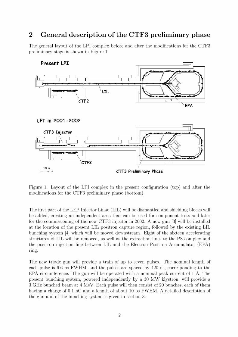
The general layout of the LPI complex before and after the modifications for the CTF3preliminary stage is shown in Figure 1.

Figure 1: Layout of the LPI complex in the present configuration (top) and after themodifications for the CTF3 preliminary phase (bottom).

The first part of the LEP Injector Linac (LIL) will be dismantled and shielding blocks willbe added, creating an independent area that can be used for component tests and laterfor the commissioning of the new CTF3 injector in 2002. A new gun [3] will be installedat the location of the present LIL positron capture region, followed by the existing LILbunching system [4] which will be moved downstream. Eight of the sixteen acceleratingstructures of LIL will be removed, as well as the extraction lines to the PS complex andthe positron injection line between LIL and the Electron Positron Accumulator (EPA)ring.

The new triode gun will provide a train of up to seven pulses. The nominal length ofeach pulse is 6.6 ns FWHM, and the pulses are spaced by 420 ns, corresponding to theEPA circumference. The gun will be operated with a nominal peak current of 1 A. Thepresent bunching system, powered independently by a 30 MW klystron, will provide a3 GHz bunched beam at 4 MeV. Each pulse will then consist of 20 bunches, each of themhaving a charge of 0.1 nC and a length of about 10 ps FWHM. A detailed description ofthe gun and of the bunching system is given in section 3.

2

The pulse train can be accelerated up to an energy of 380 MeV, using eight travellingwave accelerating structures, which are powered in groups of four by two 40 MWklystrons. In order to take into account an operational margin, a reference beam energyof 350 MeV is used in this note. The whole electron pulse train will be accelerated using asingle RF pulse. Since the maximum train length ( 2.5 µs) plus the cavities filling time( 1.5 µs) is not much shorter than the RF pulse length from the klystron ( 4.5 µs),it has been decided not to use the present RF pulse compression system (LIPS, for LILPower Saver). The beam parameters have been chosen in order to minimise the energyspread generated by beam-loading in the LIL structures, while still keeping a charge perbunch which is high enough to give a good resolution for the measurements of the beamtime structure with a streak camera. The beam-loading parameter in LIL is 0.2 MeV/nCper structure. The resulting energy spread within each pulse is about 3 MeV. Anadditional energy difference of roughly 3 MeV will occur between the first two pulses, i.e.before the steady state is reached. The total energy spread of about 6 MeV is within theEPA full acceptance (±1%). It can nevertheless be reduced by a factor of two by delayedRF filling of the structure, or by dumping the first two pulses in the train (out of seven).For the frequency multiplication test, one needs at most five pulses. The linac opticshas to be adapted to this new layout. The last two LIL accelerating structures will beremoved and replaced by a matching section to the injection line. Apart from the newgun, no new equipment is needed in the linac and only a re-arrangement of the existingcomponents is required. Some details on the new linac optics and on the matching regionare given in section 4.

The present transfer line from LIL to EPA is achromatic in both planes. It must benoted that, in addition to the main horizontal bending magnets, the line contains twovertical dipoles with a small bending angle, since the heights of LIL and EPA differ by15 cm in order to allow injection from the inside of the ring. However, the line mustalso be made isochronous, in order to preserve the bunch length from the linac to thering. This is essential for the combination process, for which short bunches (≤ 15 psFWHM) are needed (see section 7). Furthermore, the line has to be re-matched to thenew ring lattice. A new optics has been found, which satisfies the requirements of theCTF3 preliminary phase. Two quadrupoles must be added to the present layout, andsome of the existing quadrupoles must be moved. All quadrupoles in the transfer linewill be fed by independent power supplies. However, the overall geometry of the line ispreserved, such that no major hardware modifications are needed. The quadrupoles andthe power supplies from the dismantled beam lines can be re-used in the new line. Itsdesign is presented in section 5.

The lattice of EPA will be modified to make the ring isochronous and thus to preservethe bunch length and spacing during the combination process (up to five turns). In afirst isochronicity test performed in the EPA ring, the capability to control and measurethe momentum compaction to the level required for the preliminary phase of CTF3has been demonstrated [5]. In this experiment, the isochronous lattice was obtained bychanging the strength of the existing quadrupole families. However, the dispersion wasnot vanishing in the long straight sections and the transfer line was badly matched tothe ring, causing beam losses in the first few turns. Since the available aperture willbe further reduced when the RF deflectors for the new injection scheme are installed, a

3

different optics had to be found. In the new isochronous lattice, the dispersion vanishesin the long straight sections. It requires the displacement of four quadrupoles and thedecoupling of three out of the six existing quadrupole families. This new lattice of EPAis discussed in section 6.

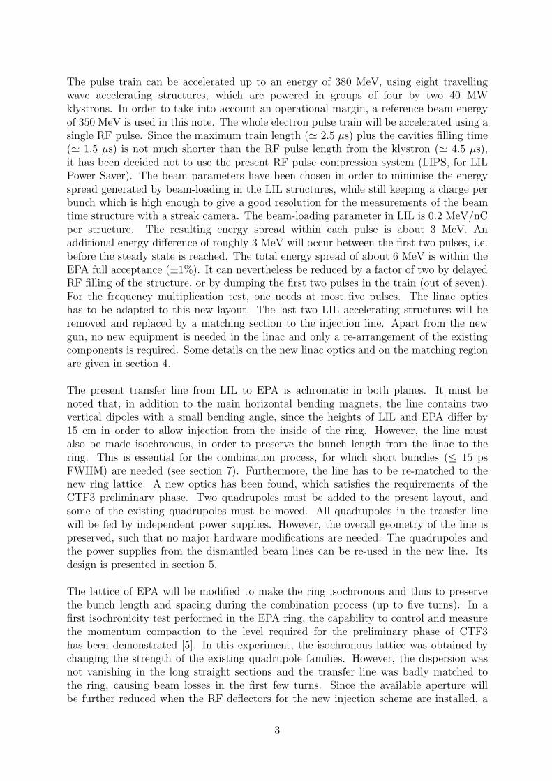
Two transverse RF deflectors will be used instead of the present fast injection kickers.They will create a time-dependent closed bump of the reference orbit, allowing the inter-leaving of three to five bunch trains. More details are given in Figure 2 for a frequencymultiplication factor of four. The bunch combination process requires:

C = nλ0 ± λ0/N (1)

where n is an integer, C is the ring circumference, N is the combination factor and λ0 isthe RF wavelength in the deflectors and the linac.

Figure 2: Schematic description of the injection by RF deflectors, for a bunch combinationfactor of four:1) When the first train arrives, all of its bunches are deflected by the second deflector onthe equilibrium orbit.2) After one turn the bunches of the first train arrive in the deflectors at the zero-crossingof the RF field, and stay on the equilibrium orbit. The second train is injected into thering.3) The first train bunches are kicked inside the ring, the second train bunches arrive atthe zero-crossing, and the third train is injected.4) The first train bunches arrive again at the zero-crossing, the second train bunches arekicked in the inner orbit, the third train bunches are also at the zero crossing and thefourth train is injected. The four trains are now combined in one single train and theinitial bunch spacing is reduced by a factor of four.

4

Combination factors of three, four and five will be tested in the preliminary phaseof CTF3. The whole range of combination factors can be explored by changing thefrequency of LIL and of the RF deflectors by ± 150 kHz. The frequency will be changedin the RF source at low level (before the klystrons), the bandwidth of the klystronsbeing wide enough to cover this range. The accelerating structures and the deflectorswill be tuned in operation by varying their temperature by ± 3C, in order to follow thechange of the RF frequency. Recent measurements have shown that this can be done inthe linac [6]. The RF deflectors are travelling wave iris-loaded structures. They havebeen used in the past to measure the bunch length in LIL [7]. They will be powered byone of the existing 30 MW klystrons and a power of about 7 MW is needed in each ofthem to obtain the nominal deflecting angle of 4.5 mrad at 350 MeV. The fast injectionkickers will be kept in the ring to allow conventional single-turn injection. They will beused during commissioning, in order to check the ring optics prior to the installation ofthe RF deflectors. Also, one of the positron injection kickers, located at the oppositeside of the ring, will remain in place and will be used to extract the circulating beam toa dump, located at the end of the present positron injection line. More details on theinjection process and the RF deflectors are given in section 7.

A tracking with realistic longitudinal and transverse distributions for the particles in thebeam has been performed in the transfer line and the EPA ring, in order to check thestability of the new optics when higher order effects are included. The results of thistracking are presented in section 8. In section 9, we briefly discuss the issue of the beamsteering in the CTF3 preliminary phase. Finally, a summary and some conclusions aregiven in section 10.

5

3 The LIL front-end

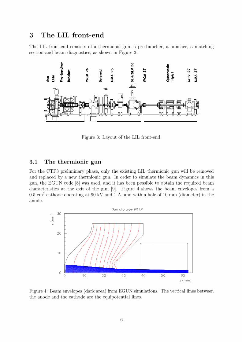
The LIL front-end consists of a thermionic gun, a pre-buncher, a buncher, a matchingsection and beam diagnostics, as shown in Figure 3.

Figure 3: Layout of the LIL front-end.

3.1 The thermionic gun

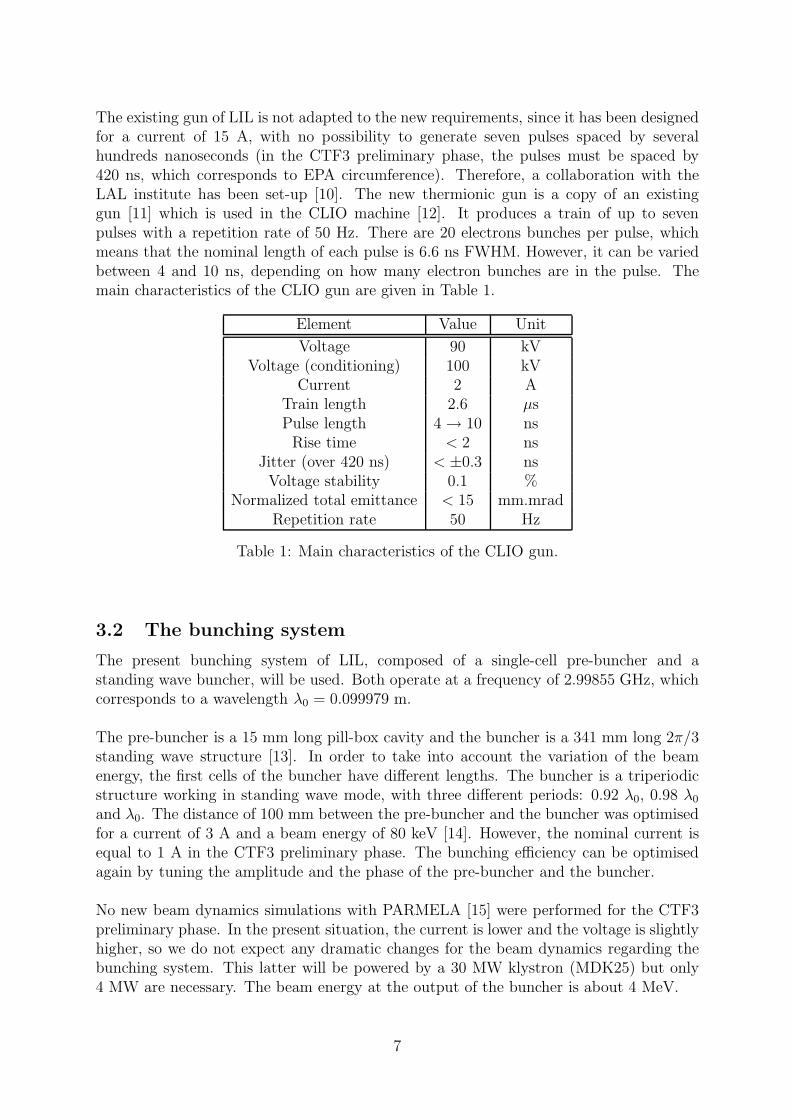
For the CTF3 preliminary phase, only the existing LIL thermionic gun will be removedand replaced by a new thermionic gun. In order to simulate the beam dynamics in thisgun, the EGUN code [8] was used, and it has been possible to obtain the required beamcharacteristics at the exit of the gun [9]. Figure 4 shows the beam envelopes from a0.5 cm2 cathode operating at 90 kV and 1 A, and with a hole of 10 mm (diameter) in theanode.

Figure 4: Beam envelopes (dark area) from EGUN simulations. The vertical lines betweenthe anode and the cathode are the equipotential lines.

6

The existing gun of LIL is not adapted to the new requirements, since it has been designedfor a current of 15 A, with no possibility to generate seven pulses spaced by severalhundreds nanoseconds (in the CTF3 preliminary phase, the pulses must be spaced by420 ns, which corresponds to EPA circumference). Therefore, a collaboration with theLAL institute has been set-up [10]. The new thermionic gun is a copy of an existinggun [11] which is used in the CLIO machine [12]. It produces a train of up to sevenpulses with a repetition rate of 50 Hz. There are 20 electrons bunches per pulse, whichmeans that the nominal length of each pulse is 6.6 ns FWHM. However, it can be variedbetween 4 and 10 ns, depending on how many electron bunches are in the pulse. Themain characteristics of the CLIO gun are given in Table 1.

Element Value Unit

Voltage 90 kVVoltage (conditioning) 100 kV

Current 2 ATrain length 2.6 µsPulse length 4 → 10 nsRise time < 2 ns

Jitter (over 420 ns) < ±0.3 nsVoltage stability 0.1 %

Normalized total emittance < 15 mm.mradRepetition rate 50 Hz

Table 1: Main characteristics of the CLIO gun.

3.2 The bunching system

The present bunching system of LIL, composed of a single-cell pre-buncher and astanding wave buncher, will be used. Both operate at a frequency of 2.99855 GHz, whichcorresponds to a wavelength λ0 = 0.099979 m.

The pre-buncher is a 15 mm long pill-box cavity and the buncher is a 341 mm long 2π/3standing wave structure [13]. In order to take into account the variation of the beamenergy, the first cells of the buncher have different lengths. The buncher is a triperiodicstructure working in standing wave mode, with three different periods: 0.92 λ0, 0.98 λ0

and λ0. The distance of 100 mm between the pre-buncher and the buncher was optimisedfor a current of 3 A and a beam energy of 80 keV [14]. However, the nominal current isequal to 1 A in the CTF3 preliminary phase. The bunching efficiency can be optimisedagain by tuning the amplitude and the phase of the pre-buncher and the buncher.

No new beam dynamics simulations with PARMELA [15] were performed for the CTF3preliminary phase. In the present situation, the current is lower and the voltage is slightlyhigher, so we do not expect any dramatic changes for the beam dynamics regarding thebunching system. This latter will be powered by a 30 MW klystron (MDK25) but only4 MW are necessary. The beam energy at the output of the buncher is about 4 MeV.

7

The distance between the exit of the buncher and the first accelerating section (ACS27)is an important parameter. It was optimised in order to minimise the bunch length at theentrance of the first accelerating section. In the simulations, the choice of the phase forthe buncher leads to an energy of 3.8 MeV (β = 0.9929) for the reference particle. In abunch with a RF phase extension of 16 (or a total bunch length of 14.8 ps), a particle inthe tail has an energy of 4.1 MeV (β = 0.9938). Therefore, ∆β/β = 0.1%. The electronsare not yet completely relativistic and the bunch length could be further reduced. When = 3.5 m, a RF phase extension of 20 (18.5 ps) is compressed down to 16 (14.8 ps).Some measurements were performed with a RF deflecting cavity in 1990 [7] and gave14 ps FWHM for the bunch length at a current of 3 A. Recent measurements, based onthe energy spectrum analysis at 200 MeV, were also performed at a lower current andthey gave 7 to 8 ps FWHM [16, 17].

Table 2 summarizes the main parameters of the injector for the CTF3 preliminary phase.

Element Value Unit

RF frequency 2.99855 GHzRF wavelength 0.099979 m

Nominal gun voltage 90 kVMaximum gun voltage 100 kVNominal gun current 1 AMaximum gun current 2 A

Repetition rate 50 HzDistance from pre-buncher to buncher 100 mm

Pre-buncher voltage 47 kVPre-buncher accelerating gradient 1.3 MV/mBuncher accelerating gradient 16 MV/m

Available RF power 30 MWTemperature of the bunching system 30 C

Beam energy 4 MeVDistance from buncher to ACS27 3.5 mRms normalized beam emittance 40 mm.mrad

Bunch length (FWHM) 10 psBunch charge 0.1 nC

Number of bunches 20 -Number of pulses 7 -

Table 2: Main parameters of the new LIL injector.

3.3 The front-end matching section

In order to control the transverse beam dynamics, one solenoid and one quadrupole tripletare implemented. The optimisation of their settings was done with the TRANSPORTcode [18]. Since the new conditions are very similar to the previous ones, it is proposed tokeep the same matching section before the entrance of the linac for the CTF3 preliminaryphase. The solenoid and the quadrupole triplet have independant power supplies, which

8

means four independent parameters to play with in the transverse phase space. Therefore,small variations of the initial conditions can be compensated by an optimisation of thematching conditions.

3.4 Beam instrumentation

The beam instrumentation used in the front-end is shown in Figure 3. A capacitiveelectrode (ECM), located just downstream the anode, allows to measure the beam currentbefore the bunching system. A Wall Current Monitor (WCM26) measures the beamcurrent at the exit of the bunching system. The ratio of the currents measured in WCM26and ECM gives the bunching efficiency. The slits SLH26 and SLV26 are used for machinedevelopment. The Beam Position Monitors UMA26 and UMA27 [19] allow to check thetransfer efficiency of the matching section and to align the beam in the first acceleratingstructure. They are also used to calibrate the WCMs. Finally a TV Monitor with thescintillator screen (MTV27) allows to check easily the presence of the beam and to get anestimate of the transverse beam sizes. On the existing front-end, the Transition-CherenkovMonitor TCM 11 [20, 21] will be removed and it will be installed in the matching sectionat the end of the linac (see section 4.5).

9

4 The linac and the matching section

4.1 Reference lattice parameters near the entrance of the linac

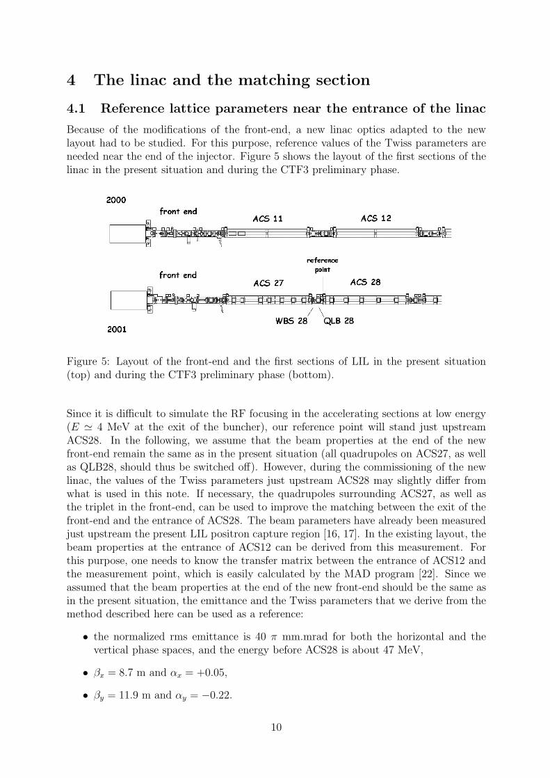
Because of the modifications of the front-end, a new linac optics adapted to the newlayout had to be studied. For this purpose, reference values of the Twiss parameters areneeded near the end of the injector. Figure 5 shows the layout of the first sections of thelinac in the present situation and during the CTF3 preliminary phase.

Figure 5: Layout of the front-end and the first sections of LIL in the present situation(top) and during the CTF3 preliminary phase (bottom).

Since it is difficult to simulate the RF focusing in the accelerating sections at low energy(E 4 MeV at the exit of the buncher), our reference point will stand just upstreamACS28. In the following, we assume that the beam properties at the end of the newfront-end remain the same as in the present situation (all quadrupoles on ACS27, as wellas QLB28, should thus be switched off). However, during the commissioning of the newlinac, the values of the Twiss parameters just upstream ACS28 may slightly differ fromwhat is used in this note. If necessary, the quadrupoles surrounding ACS27, as well asthe triplet in the front-end, can be used to improve the matching between the exit of thefront-end and the entrance of ACS28. The beam parameters have already been measuredjust upstream the present LIL positron capture region [16, 17]. In the existing layout, thebeam properties at the entrance of ACS12 can be derived from this measurement. Forthis purpose, one needs to know the transfer matrix between the entrance of ACS12 andthe measurement point, which is easily calculated by the MAD program [22]. Since weassumed that the beam properties at the end of the new front-end should be the same asin the present situation, the emittance and the Twiss parameters that we derive from themethod described here can be used as a reference:

• the normalized rms emittance is 40 π mm.mrad for both the horizontal and thevertical phase spaces, and the energy before ACS28 is about 47 MeV,

• βx = 8.7 m and αx = +0.05,

• βy = 11.9 m and αy = −0.22.

10

4.2 New linac optics

In order to reach an energy of 350 MeV in the EPA ring, each of the eight acceleratingstructures of LIL must ensure an energy gain ∆E 43 MeV. Since the LIL acceleratingstructures are surrounded by quadrupoles, a special treatment is necessary. In the opticscalculations with MAD, the behaviour of these quadrupoles is simulated by the followingsequence: acceleration up to the center of the quadrupole, drift in the backward directiondown to the entrance of the quadrupole, quadrupole, drift in the backward directiondown to the center of the quadrupole, acceleration up to the exit of the quadrupole.The RF focusing is taken into account in the simulation of the accelerating structureswith MAD, which is not the case in TRANSPORT (however, the differences between theresults given by these two codes are small).

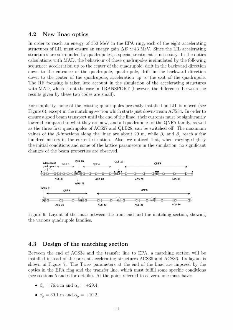
For simplicity, none of the existing quadrupoles presently installed on LIL is moved (seeFigure 6), except in the matching section which starts just downstream ACS34. In order toensure a good beam transport until the end of the linac, their currents must be significantlylowered compared to what they are now, and all quadrupoles of the QNFA family, as wellas the three first quadrupoles of ACS27 and QLB28, can be switched off. The maximumvalues of the β-functions along the linac are about 20 m, while βx and βy reach a fewhundred meters in the current situation. Also, we noticed that, when varying slightlythe initial conditions and some of the lattice parameters in the simulation, no significantchanges of the beam properties are observed.

Figure 6: Layout of the linac between the front-end and the matching section, showingthe various quadrupole families.

4.3 Design of the matching section

Between the end of ACS34 and the transfer line to EPA, a matching section will beinstalled instead of the present accelerating structures ACS35 and ACS36. Its layout isshown in Figure 7. The Twiss parameters at the end of the linac are imposed by theoptics in the EPA ring and the transfer line, which must fulfill some specific conditions(see sections 5 and 6 for details). At the point referred to as zero, one must have:

• βx = 76.4 m and αx = +29.4,

• βy = 39.1 m and αy = +10.2.

11

Figure 7: Schematic layout of the matching section located between the linac and thetransfer line to EPA.

For the design of the matching section, the values of the Twiss parameters at the exit ofACS34, as derived from the calculation done for the linac, are used for reference. A goodmatching can easily be obtained by optimizing the normalized gradient and the positionof each of the five quadrupoles.

4.4 Transverse beam dynamics in the new linac and in the

matching section

Figure 8 shows the β-functions that we use as a reference, between the entrance of ACS28and the point referred to as zero, when the settings of the various quadrupoles in thelinac and the matching section are the ones displayed in Table 3.

0.0 5. 10. 15. 20. 25. 30. 35. 40. 45. 50.s (m)

0.0

20.

40.

60.

80.

100.

120.

140.

160.

180.

200.

β(m

)

β x β y

Figure 8: Evolution of the β-functions along the linac and the matching section.

12

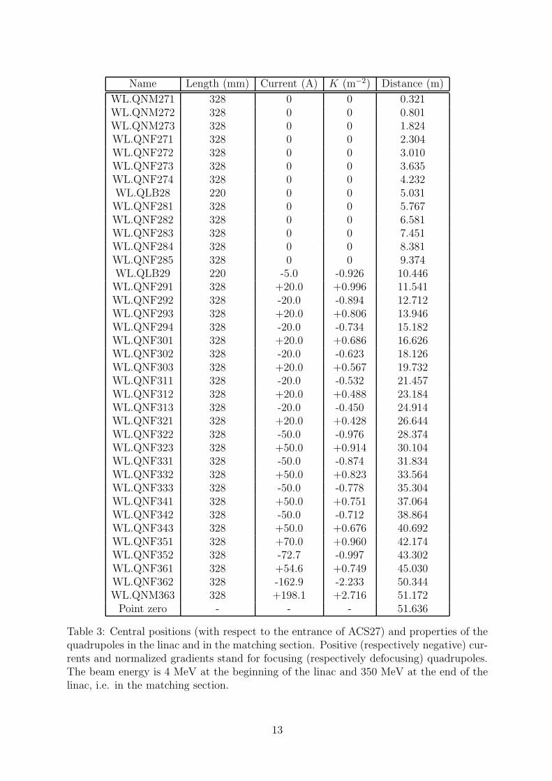
Name Length (mm) Current (A) K (m−2) Distance (m)

WL.QNM271 328 0 0 0.321WL.QNM272 328 0 0 0.801WL.QNM273 328 0 0 1.824WL.QNF271 328 0 0 2.304WL.QNF272 328 0 0 3.010WL.QNF273 328 0 0 3.635WL.QNF274 328 0 0 4.232WL.QLB28 220 0 0 5.031WL.QNF281 328 0 0 5.767WL.QNF282 328 0 0 6.581WL.QNF283 328 0 0 7.451WL.QNF284 328 0 0 8.381WL.QNF285 328 0 0 9.374WL.QLB29 220 -5.0 -0.926 10.446WL.QNF291 328 +20.0 +0.996 11.541WL.QNF292 328 -20.0 -0.894 12.712WL.QNF293 328 +20.0 +0.806 13.946WL.QNF294 328 -20.0 -0.734 15.182WL.QNF301 328 +20.0 +0.686 16.626WL.QNF302 328 -20.0 -0.623 18.126WL.QNF303 328 +20.0 +0.567 19.732WL.QNF311 328 -20.0 -0.532 21.457WL.QNF312 328 +20.0 +0.488 23.184WL.QNF313 328 -20.0 -0.450 24.914WL.QNF321 328 +20.0 +0.428 26.644WL.QNF322 328 -50.0 -0.976 28.374WL.QNF323 328 +50.0 +0.914 30.104WL.QNF331 328 -50.0 -0.874 31.834WL.QNF332 328 +50.0 +0.823 33.564WL.QNF333 328 -50.0 -0.778 35.304WL.QNF341 328 +50.0 +0.751 37.064WL.QNF342 328 -50.0 -0.712 38.864WL.QNF343 328 +50.0 +0.676 40.692WL.QNF351 328 +70.0 +0.960 42.174WL.QNF352 328 -72.7 -0.997 43.302WL.QNF361 328 +54.6 +0.749 45.030WL.QNF362 328 -162.9 -2.233 50.344WL.QNM363 328 +198.1 +2.716 51.172Point zero - - - 51.636

Table 3: Central positions (with respect to the entrance of ACS27) and properties of thequadrupoles in the linac and in the matching section. Positive (respectively negative) cur-rents and normalized gradients stand for focusing (respectively defocusing) quadrupoles.The beam energy is 4 MeV at the beginning of the linac and 350 MeV at the end of thelinac, i.e. in the matching section.

13

One should be aware that, during the commissioning of the linac, the values obtainedat the exit of ACS34 may be slightly different from what we have calculated here. Forinstance, one should not take for granted the accuracy of the simulation of the acceleratingstructures when a quadrupole and a constant electric field are superposed (another methodbased on an analytical description of this system is under investigation). Consequently,some flexibility must be kept for the matching section (however, as already mentioned,the beam properties are not strongly affected by small changes in the lattice). Duringthe commissioning of the machine, the accurate measurement of the beam parameters atthe entrance of the matching section will be important, in order to further find the bestmatching conditions with the simulation codes.

4.5 Beam instrumentation in the linac and the matching section

Wherever possible, it has been chosen to keep in place the present beam instrumentationin the linac.

UMAs are placed between the accelerating structures, except at two locations, whereWire Beam Scanners (WBS) are or will be installed. The use of UMAs for beamsteering will be discussed in section 9. Between ACS27 and ACS28, WBS28 is alreadyinstalled. Another Wire Beam Scanner (WBS31) will be recuperated and placed betweenACS30 and ACS31, where the present UMA31 is. These instruments will allow themeasurement of the transverse beam characteristics (emittance and Twiss parameters)through quadrupole scans. In particular, using WBS28 and WBS31, it will be possible tocheck the beam parameters at the exit of the front-end and at the linac reference pointupstream ACS28, respectively.

The matching section will be instrumented in order to provide a full characterization ofthe beam before injection into EPA (see Figure 7). The two UMAs at the beginning andat the end of the matching section (UMA35 and UMA37) will be kept at their presentlocation, while the third UMA (currently located between ACS35 and ACS36) will beslightly displaced. A Wire Beam Scanner (WBS37) and a Transition-Cherenkov Monitor(TCM37) will be placed in the straight line. The WBS will allow the determination ofthe transverse beam parameters at the entrance of the matching section. In the TCM, aTransition radiation screen or a Cherenkov screen can be alternatively put in the beampath. In conjunction with an image frame grabbing system and digital treatment, theTCM can be used for the determination of the transverse beam parameters and it willprovide a way to cross-check the results of the WBS. The aim is to eventually use theTCM routinely for emittance and Twiss parameters measurements, using an automatedprogram derived from the one currently in use in CTF2 [23], providing a much shortermeasurement time with respect to the quadrupole scan with a WBS. A camera (MTV37)will complete the instrumentation of the straight beam line.

A dipole magnet (BHZ36), recuperated from a dismantled line, will be installed in thematching section in order to deflect the beam into a spectrometer line. The line willbe equiped with a SEMgrid (MSH36) and a Transition-Cherenkov Monitor (TCM36).The nominal bending angle in BHZ36 will be 35. Since the dispersion at the MSHlocation will be about 0.75 m, and since the SEMgrid wires are spaced by 2 mm, the

14

energy resolution will be 0.3%. With 20 wires, the acceptance on the MSH36 screenwill be about 5%. Assuming that βx can be tuned down to 1 m in MSH36, with a rmsnormalized emittance of 40 π mm.mrad, the rms beam size for a monochromatic beamshould be around 0.2 mm and should thus not limit the spectrometer resolution.

An optical transport line will also be installed, in order to bring the light generated inTCM36 and TCM37 up to the streak camera laboratory. Therefore, TCM37 could beused for time-resolved measurements of the transverse beam parameters which can beuseful, e.g. to study chromatic aberrations in the linac. The use of the streak camerawith TCM36 will allow a time-resolved measurement of the beam energy spectrum. UsingTCM36, where the dispersion will be about 1 m, we should be able to resolve pulse-to-pulse and bunch-to-bunch energy variations due to beam-loading.

15

5 The injection line between the linac and EPA

The design of the transfer line between the linac and the EPA ring has to meet severalrequirements for the CTF3 preliminary phase. The main modification consists in havingan isochronous lattice, in order to avoid direct bunch lengthening. Also, the transverseTwiss functions have to be matched at both ends of the line, as well as the horizontaland vertical dispersion functions and their derivatives. On top of that, in order to keepchromatic effects at a low level, small β-functions are required, well under the presentvalues of a few kilometers. From a general point of view, the requirements on the newinjection line are more stringent than for the existing one: in particular, transverse anddispersion matching must be very precise due to the aperture restriction from the RFdeflectors in the ring (see section 7) and because of the achromaticity condition. Thisdiffers from the existing transfer line, where the tolerances on injection are relaxed becauseof the damping process in the accumulation ring used for lepton production.

5.1 Physics requirements

To first order, the evolution of the bunch length through the transfer line is controlled bythe coefficients of the linear 6×6 transfer matrix R. When neglecting vertical dispersion,which is indeed much smaller than the horizontal dispersion in the transfer line, the pathlength difference of a given particle with a relative momentum difference ∆p

pwith respect

to the reference particle is given by:

c∆t = R51x+R52x′ +R56

∆p

p. (2)

Here (x,x′) refers to the usual horizontal phase space at the entrance of the line and, fora reference path L along the line, the matrix coefficients are defined by:

R51 =∫LC

ρds , R52 =

∫LS

ρds , R56 =

∫LD

ρds (3)

where ρ is the bending radius, C and S are the cosine-like and sine-like principal solutionsof Hill’s equation of motion, and D is the horizontal dispersion.

As for the rms bunch length σ, the following equation can be obtained:

σ2f = σ2

i + (R56σE)2 + εxi(R

251βxi − 2R51R52αxi +R2

52γxi). (4)

In this equation, σE is the rms energy spread. The subscript i refers to the entrance ofthe transfer line, while the subscript f can refer to any point downstream.

The matching of the horizontal dispersion and its first derivative at both ends of thetransfer line requires a first order achromat: Dxi = D′

xi = 0 are the values of the dispersionand its derivative at the entrance of the line (end of the linac) while Dxf = D′

xf = 0 aretheir values at the end of the line (injection point in the EPA ring). For such boundaryconditions, it can be shown that R51 and R52 vanish:

Dxi = D′xi = 0

Dxf = D′xf = 0

=⇒ R51 = R52 = 0. (5)

16

From equations (2) and (4), the last condition to fulfill is the first-order isochronicity, i.e.R56 0. This requires the modification of the horizontal dispersion function along thetransfer line, in order to force the ratio D/ρ to change sign, so that the third integral ofequation (3) vanishes over the total path length. The new design of the transfer line wasmainly driven by this condition, and by the fact that the new layout should only generateminor modifications to the existing hardware.

5.2 Characteristics of the new transfer line

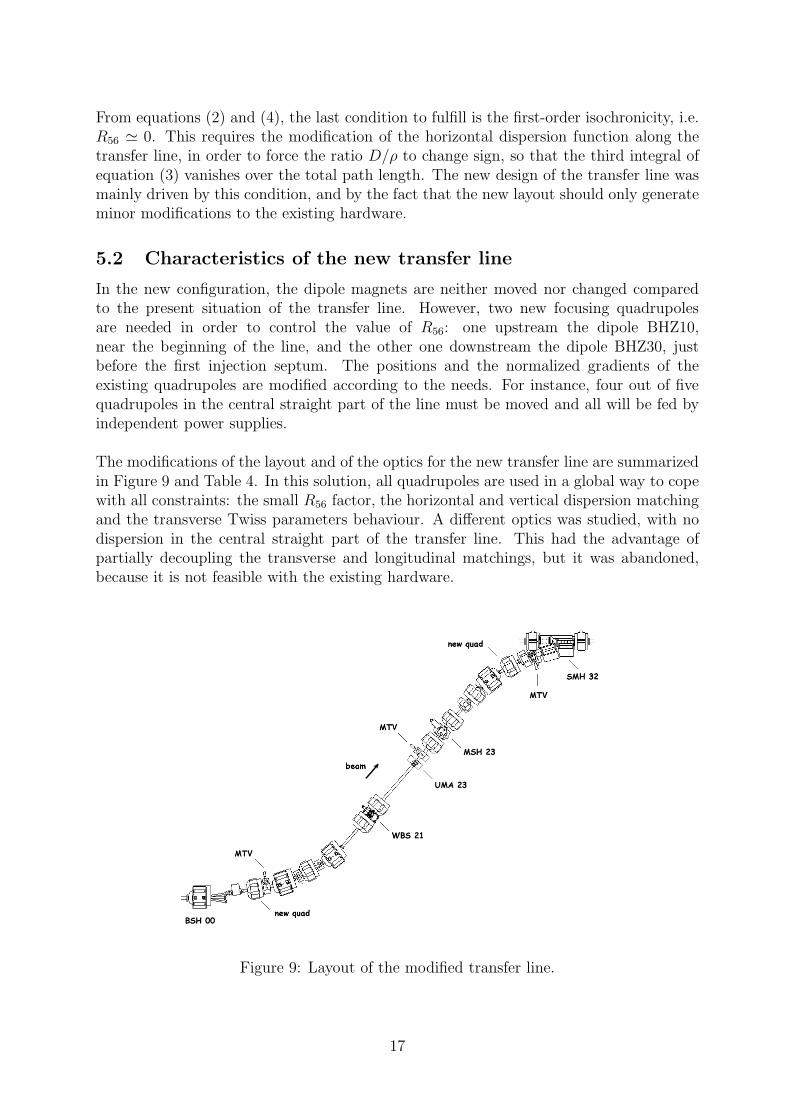
In the new configuration, the dipole magnets are neither moved nor changed comparedto the present situation of the transfer line. However, two new focusing quadrupolesare needed in order to control the value of R56: one upstream the dipole BHZ10,near the beginning of the line, and the other one downstream the dipole BHZ30, justbefore the first injection septum. The positions and the normalized gradients of theexisting quadrupoles are modified according to the needs. For instance, four out of fivequadrupoles in the central straight part of the line must be moved and all will be fed byindependent power supplies.

The modifications of the layout and of the optics for the new transfer line are summarizedin Figure 9 and Table 4. In this solution, all quadrupoles are used in a global way to copewith all constraints: the small R56 factor, the horizontal and vertical dispersion matchingand the transverse Twiss parameters behaviour. A different optics was studied, with nodispersion in the central straight part of the transfer line. This had the advantage ofpartially decoupling the transverse and longitudinal matchings, but it was abandoned,because it is not feasible with the existing hardware.

Figure 9: Layout of the modified transfer line.

17

Element Angle (degrees) Gradient (m−2) Position (m)

HIE.BSH00 -9 1.077 (unchanged)HIE.BVT00 +0.55 (vertical) 2.526 (unchanged)HIE.QFW01 +4.360 3.263 (new)HIE.BHZ10 -20 4.474 (unchanged)HIE.QDW11 -4.360 5.578 (unchanged)HIE.BHZ20 -20 6.724 (unchanged)HIE.QFW21 +2.870 8.383 (moved)HIE.QDW22 -2.948 9.258 (moved)HIE.QFW23 +2.154 12.649 (moved)HIE.QDW24 -3.040 13.975 (moved)HIE.QFW25 +3.712 15.450 (unchanged)HIE.BHZ30 +20 16.270 (unchanged)HIE.QFW30 +3.980 17.291 (new)HIE.BVT30 -0.55 (vertical) 17.918 (unchanged)HIE.SMH31 +21.75 18.916 (unchanged)HIE.SMH32 +7.25 19.619 (unchanged)

Table 4: Central positions (with respect to point zero) and properties of the magneticelements in the new transfer line for the CTF3 preliminary phase. Positive (respectivelynegative) gradients stand for focusing (respectively defocusing) quadrupoles.

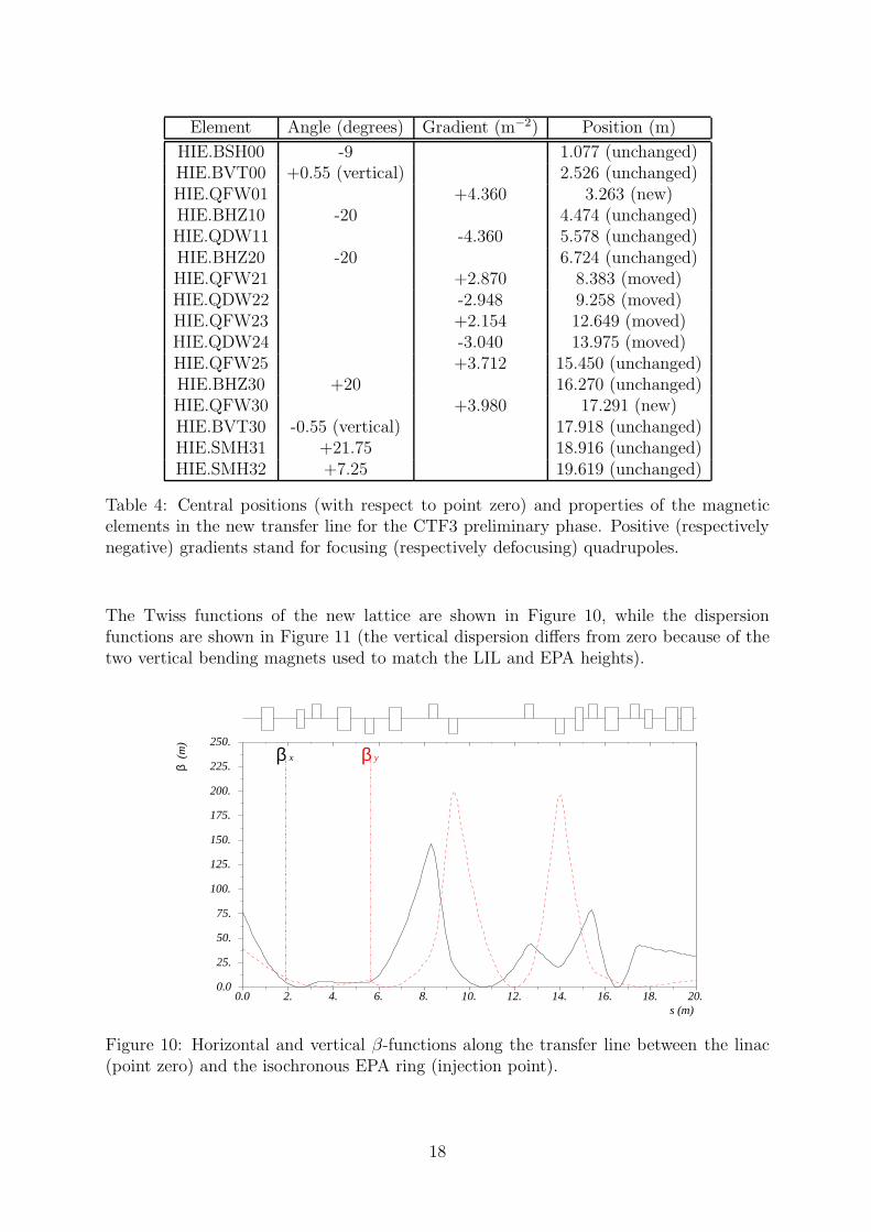
The Twiss functions of the new lattice are shown in Figure 10, while the dispersionfunctions are shown in Figure 11 (the vertical dispersion differs from zero because of thetwo vertical bending magnets used to match the LIL and EPA heights).

0.0 2. 4. 6. 8. 10. 12. 14. 16. 18. 20.s (m)

0.0

25.

50.

75.

100.

125.

150.

175.

200.

225.

250.

β(m

)

β x β y

Figure 10: Horizontal and vertical β-functions along the transfer line between the linac(point zero) and the isochronous EPA ring (injection point).

18

0.0 2. 4. 6. 8. 10. 12. 14. 16. 18. 20.s (m)

−1.50

−1.25

−1.00

−.75

−.50

−.25

0.0

.25

.50

.75

1.00

1.25

1.50

D(m

)Dx Dy

Figure 11: Horizontal and vertical dispersion functions along the transfer line betweenthe linac (point zero) and the isochronous EPA ring (injection point).

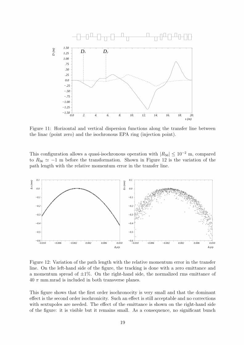
This configuration allows a quasi-isochronous operation with |R56| ≤ 10−2 m, comparedto R56 −1 m before the transformation. Shown in Figure 12 is the variation of thepath length with the relative momentum error in the transfer line.

−0.010 −0.006 −0.002 0.002 0.006 0.010

p/p∆

∆

−0.6

−0.5

−0.4

−0.3

−0.2

−0.1

0.0

0.1

s (m

m)

−0.010 −0.006 −0.002 0.002 0.006 0.010

p/p∆

∆

−0.6

−0.5

−0.4

−0.3

−0.2

−0.1

0.0

0.1

s (m

m)

Figure 12: Variation of the path length with the relative momentum error in the transferline. On the left-hand side of the figure, the tracking is done with a zero emittance anda momentum spread of ±1%. On the right-hand side, the normalized rms emittance of40 π mm.mrad is included in both transverse planes.

This figure shows that the first order isochronocity is very small and that the dominanteffect is the second order isochronicity. Such an effect is still acceptable and no correctionswith sextupoles are needed. The effect of the emittance is shown on the right-hand sideof the figure: it is visible but it remains small. As a consequence, no significant bunch

19

lengthening is observed between the entrance and the exit of the line. However, alongthe transfer line, the bunch length varies according to equation (4): it grows in the firstbends, reaches a maximum in the central straight part of the line and then decreases inthe last bends, following the value of R56. Figure 13 shows the evolution of the bunchlength as a function of the curvilinear abscisse in the transfer line.

0.8

1

1.2

1.4

1.6

1.8

2

0 2.5 5 7.5 10 12.5 15 17.5 20 22.5 25

Initial conditions at point zero:

Energy spread = 1%

εx = 0.06 π mm.mrad, βx = 76.4 m and αx = +29.4

εy = 0.06 π mm.mrad, βy = 39.1 m and αy = +10.2

Distance (m)

Rm

s bu

nch

leng

th (

mm

)

Figure 13: Evolution of the rms bunch length along the transfer line between the linac andthe EPA isochronous ring. An initial rms bunch length σli=0.9 mm and an energy spreadσE=1% are considered. Here, the emittance is 0.06 π mm.mrad (which corresponds to arms normalized emittance of 40 π mm.mrad, since the beam energy is 350 MeV).

The beam properties in the transverse plane at the beginning of the transfer line areimposed by the values of the Twiss parameters needed to match the transfer line to theEPA ring. At the injection point (15 cm downstream the exit of SMH32), they are:

• βx = 31.2 m and αx = +2.2,

• βy = 7.0 m and αy = −1.6.

Therefore, knowing the transfer matrix of the new transfer line, the Twiss parametersneeded at the end of the linac (point zero) can be derived. Their values are the oneswhich are used in section 4.3 and which are reported in Figure 13.

5.3 Beam diagnostics in the transfer line

The beam diagnostics elements of the transfer line are shown in Figure 9.

Three television cameras (MTV) are distributed along the line: the first one is locatedupstream BHZ10 in the first bending region, the second one is in the straight sectionupstream QFW23, and the last one is downstream BVT30, before the injection septa.These screens will help follow the beam through the injection line.

20

A WBS is located between the quadrupoles QFW21 and QDW22 in the straightsection. In the proposed optics, this position corresponds to a zero-crossing region ofthe dispersion function with high values of the β-functions in the vertical and horizontalplanes. This allows quadrupole scans so as to characterize the transverse behaviour ofthe beam and to make comparisons with the design optics.

A SEMgrid is also located downstream in the central straight part of the line, betweenthe quadrupoles QFW23 and QDW24, in a region with high dispersion, in order to checkthe value of the dispersion and to measure the mean energy and the energy spread at thispoint.

21

6 The EPA ring with isochronous optics

6.1 Isochronous optics with the nominal EPA machine

The momentum compaction factor of the nominal EPA optics (α = 0.034), combined witha momentum spread of ±1%, does not allow the injected bunches to remain short enoughafter five turns for the purposes of the CTF3 tests. The path length differences betweenthe particles with extreme momenta in the bunches exceed 80 mm per turn, which is toolarge by more than two orders of magnitude to preserve FWHM bunch lengths in the 10 psrange. In a first test in 1999, using existing magnets and cabling, the EPA optics wasmodified to yield α = 0 [24, 25]. Using the chromaticity sextupoles, the path length couldbe controlled to within 0.035 mm per turn across the momentum range of the bunches,while keeping the horizontal and vertical chromaticities close to zero. Unfortunately, thedispersion could not be cancelled in the injection region with the existing quadrupolelayout and powering. This resulted in a dispersion mismatch between the injection lineand the ring, and the injection efficiency was smaller than with the nominal EPA optics.Equally, the single turn path lengths were modulated by this mismatch, thus perturbingthe evolution of the bunch length over the first few turns.

6.2 Isochronous optics with the modified EPA ring

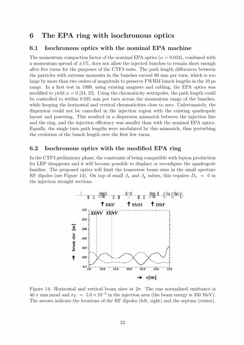
In the CTF3 preliminary phase, the constraint of being compatible with lepton productionfor LEP disappears and it will become possible to displace or reconfigure the quadrupolefamilies. The proposed optics will limit the transverse beam sizes in the small apertureRF dipoles (see Figure 14). On top of small βx and βy values, this requires Dx = 0 inthe injection straight sections.

Figure 14: Horizontal and vertical beam sizes at 2σ. The rms normalized emittance is40 π mm.mrad and σE = 5.0×10−3 in the injection area (the beam energy is 350 MeV).The arrows indicate the locations of the RF dipoles (left, right) and the septum (center).

22

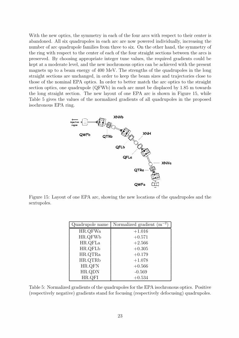
With the new optics, the symmetry in each of the four arcs with respect to their center isabandoned. All six quadrupoles in each arc are now powered individually, increasing thenumber of arc quadrupole families from three to six. On the other hand, the symmetry ofthe ring with respect to the center of each of the four straight sections between the arcs ispreserved. By choosing appropriate integer tune values, the required gradients could bekept at a moderate level, and the new isochronous optics can be achieved with the presentmagnets up to a beam energy of 400 MeV. The strengths of the quadrupoles in the longstraight sections are unchanged, in order to keep the beam sizes and trajectories close tothose of the nominal EPA optics. In order to better match the arc optics to the straightsection optics, one quadrupole (QFWb) in each arc must be displaced by 1.85 m towardsthe long straight section. The new layout of one EPA arc is shown in Figure 15, whileTable 5 gives the values of the normalized gradients of all quadrupoles in the proposedisochronous EPA ring.

Figure 15: Layout of one EPA arc, showing the new locations of the quadrupoles and thesextupoles.

Quadrupole name Normalized gradient (m−2)

HR.QFWa +1.016HR.QFWb +0.571HR.QFLa +2.566HR.QFLb +0.305HR.QTRa +0.179HR.QTRb +1.078HR.QFN +0.566HR.QDN -0.569HR.QFI +0.534

Table 5: Normalized gradients of the quadrupoles for the EPA isochronous optics. Positive(respectively negative) gradients stand for focusing (respectively defocusing) quadrupoles.

23

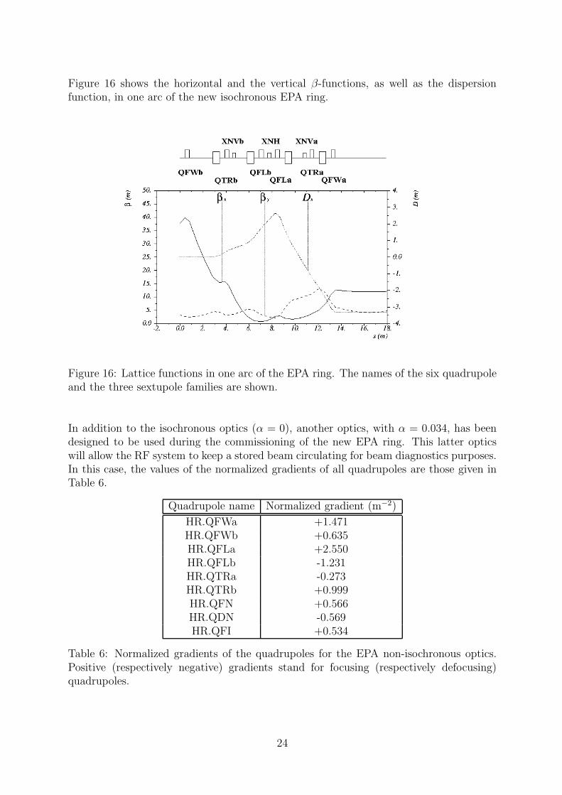
Figure 16 shows the horizontal and the vertical β-functions, as well as the dispersionfunction, in one arc of the new isochronous EPA ring.

Figure 16: Lattice functions in one arc of the EPA ring. The names of the six quadrupoleand the three sextupole families are shown.

In addition to the isochronous optics (α = 0), another optics, with α = 0.034, has beendesigned to be used during the commissioning of the new EPA ring. This latter opticswill allow the RF system to keep a stored beam circulating for beam diagnostics purposes.In this case, the values of the normalized gradients of all quadrupoles are those given inTable 6.

Quadrupole name Normalized gradient (m−2)

HR.QFWa +1.471HR.QFWb +0.635HR.QFLa +2.550HR.QFLb -1.231HR.QTRa -0.273HR.QTRb +0.999HR.QFN +0.566HR.QDN -0.569HR.QFI +0.534

Table 6: Normalized gradients of the quadrupoles for the EPA non-isochronous optics.Positive (respectively negative) gradients stand for focusing (respectively defocusing)quadrupoles.

24

6.3 Change of the EPA circumference

The LIL machine has a nominal RF frequency of 2.99855 GHz, which corresponds to awavelength λ0 = 0.099979 m. The circumference of the present EPA ring (nominally40 π m, confirmed by recent measurements [6]) is thus equal to 1256.9 λ0. Bunch trainrecombination over three, four or five turns in EPA requires circumferences of 1256.666 λ0,1256.750 λ0 or 1256.800 λ0 respectively. To keep these three options open with thesame ring layout, an average circumference value of 1256.73 nominal wavelengths hasbeen chosen. The required reduction of the EPA circumference is thus equal to 0.17 λ0,i.e. 17 mm. In order to switch between three, four or five turn recombination, the RFfrequency will be slightly detuned.

6.4 Performances

The isochronous optics for EPA provides Dx = 0 in the two injection long straightsections (see Figure 16), but a non-zero horizontal dispersion in the two other straightsections. The transfer matrices between injection elements are the same as in the nominalmachine. The beam sizes in the RF dipoles remain sufficiently small compared to theirmechanical aperture (the smallest diameter is 21 mm).

The natural chromaticities of the new isochronous optics are comparable to those ofthe nominal EPA optics. Equally, the off-momentum path lengths can be controlledusing the chromaticity sextupoles (now organised in three families instead of two) towithin 0.5 mm per turn across the momentum range of the bunches, while keeping thechromaticities small (see Figures 17 and 18), as in the 1999 EPA optics [24]. Trackingover 1000 turns shows horizontal and vertical dynamic apertures around 15σ across themomentum range of the incoming beam.

− .010 − .006 − .002 .002 .006 .010

p/p

4.50

4.55

4.60

4.65

4.70

4.75

4.80

4.85

4.90

4.95

5.00

3.50

3.55

3.60

3.65

3.70

3.75

3.80

3.85

3.90

3.95

4.00QQ x

x

Q Qy

y

∆

Figure 17: Horizontal and vertical tunes, versus the relative momentum error.

25

→

∆s

[mm

]

→ ∆p/p−0.01 −0.005 0 0.005 0.01

−0.2

0.0

0.2

0.4

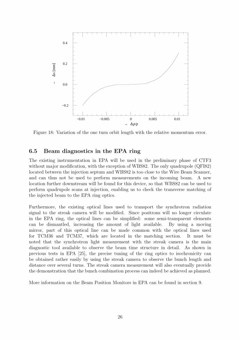
Figure 18: Variation of the one turn orbit length with the relative momentum error.

6.5 Beam diagnostics in the EPA ring

The existing instrumentation in EPA will be used in the preliminary phase of CTF3without major modification, with the exception of WBS82. The only quadrupole (QFI82)located between the injection septum and WBS82 is too close to the Wire Beam Scanner,and can thus not be used to perform measurements on the incoming beam. A newlocation further downstream will be found for this device, so that WBS82 can be used toperform quadrupole scans at injection, enabling us to check the transverse matching ofthe injected beam to the EPA ring optics.

Furthermore, the existing optical lines used to transport the synchrotron radiationsignal to the streak camera will be modified. Since positrons will no longer circulatein the EPA ring, the optical lines can be simplified: some semi-transparent elementscan be dismantled, increasing the amount of light available. By using a movingmirror, part of this optical line can be made common with the optical lines usedfor TCM36 and TCM37, which are located in the matching section. It must benoted that the synchrotron light measurement with the streak camera is the maindiagnostic tool available to observe the beam time structure in detail. As shown inprevious tests in EPA [25], the precise tuning of the ring optics to isochronicity canbe obtained rather easily by using the streak camera to observe the bunch length anddistance over several turns. The streak camera measurement will also eventually providethe demonstration that the bunch combination process can indeed be achieved as planned.

More information on the Beam Position Monitors in EPA can be found in section 9.

26

7 Injection using RF deflectors

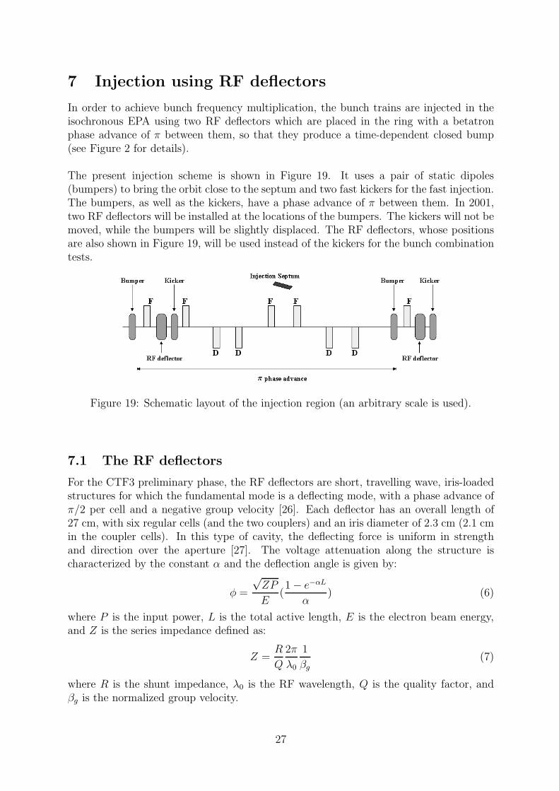
In order to achieve bunch frequency multiplication, the bunch trains are injected in theisochronous EPA using two RF deflectors which are placed in the ring with a betatronphase advance of π between them, so that they produce a time-dependent closed bump(see Figure 2 for details).

The present injection scheme is shown in Figure 19. It uses a pair of static dipoles(bumpers) to bring the orbit close to the septum and two fast kickers for the fast injection.The bumpers, as well as the kickers, have a phase advance of π between them. In 2001,two RF deflectors will be installed at the locations of the bumpers. The kickers will not bemoved, while the bumpers will be slightly displaced. The RF deflectors, whose positionsare also shown in Figure 19, will be used instead of the kickers for the bunch combinationtests.

Figure 19: Schematic layout of the injection region (an arbitrary scale is used).

7.1 The RF deflectors

For the CTF3 preliminary phase, the RF deflectors are short, travelling wave, iris-loadedstructures for which the fundamental mode is a deflecting mode, with a phase advance ofπ/2 per cell and a negative group velocity [26]. Each deflector has an overall length of27 cm, with six regular cells (and the two couplers) and an iris diameter of 2.3 cm (2.1 cmin the coupler cells). In this type of cavity, the deflecting force is uniform in strengthand direction over the aperture [27]. The voltage attenuation along the structure ischaracterized by the constant α and the deflection angle is given by:

φ =

√ZP

E(1− e−αL

α) (6)

where P is the input power, L is the total active length, E is the electron beam energy,and Z is the series impedance defined as:

Z =R

Q

2π

λ0

1

βg

(7)

where R is the shunt impedance, λ0 is the RF wavelength, Q is the quality factor, andβg is the normalized group velocity.

27

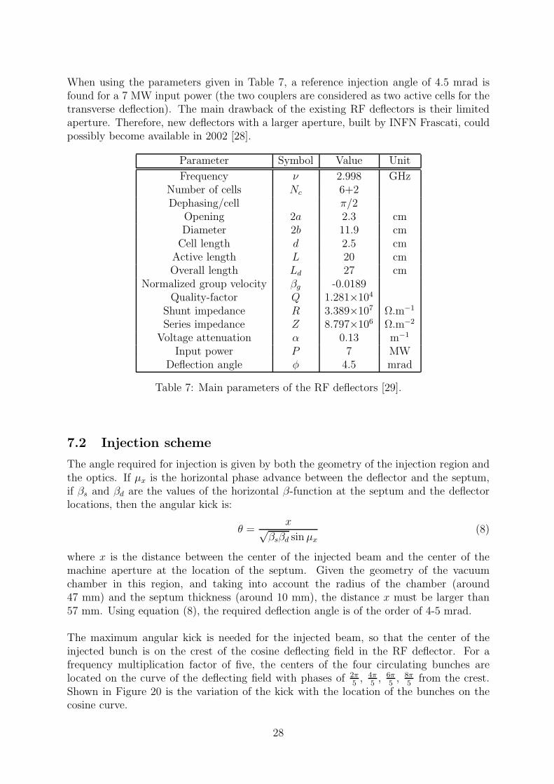
When using the parameters given in Table 7, a reference injection angle of 4.5 mrad isfound for a 7 MW input power (the two couplers are considered as two active cells for thetransverse deflection). The main drawback of the existing RF deflectors is their limitedaperture. Therefore, new deflectors with a larger aperture, built by INFN Frascati, couldpossibly become available in 2002 [28].

Parameter Symbol Value Unit

Frequency ν 2.998 GHzNumber of cells Nc 6+2Dephasing/cell π/2

Opening 2a 2.3 cmDiameter 2b 11.9 cmCell length d 2.5 cm

Active length L 20 cmOverall length Ld 27 cm

Normalized group velocity βg -0.0189Quality-factor Q 1.281×104

Shunt impedance R 3.389×107 Ω.m−1

Series impedance Z 8.797×106 Ω.m−2

Voltage attenuation α 0.13 m−1

Input power P 7 MWDeflection angle φ 4.5 mrad

Table 7: Main parameters of the RF deflectors [29].

7.2 Injection scheme

The angle required for injection is given by both the geometry of the injection region andthe optics. If µx is the horizontal phase advance between the deflector and the septum,if βs and βd are the values of the horizontal β-function at the septum and the deflectorlocations, then the angular kick is:

θ =x√

βsβd sin µx

(8)

where x is the distance between the center of the injected beam and the center of themachine aperture at the location of the septum. Given the geometry of the vacuumchamber in this region, and taking into account the radius of the chamber (around47 mm) and the septum thickness (around 10 mm), the distance x must be larger than57 mm. Using equation (8), the required deflection angle is of the order of 4-5 mrad.

The maximum angular kick is needed for the injected beam, so that the center of theinjected bunch is on the crest of the cosine deflecting field in the RF deflector. For afrequency multiplication factor of five, the centers of the four circulating bunches arelocated on the curve of the deflecting field with phases of 2π

5, 4π

5, 6π

5, 8π

5from the crest.

Shown in Figure 20 is the variation of the kick with the location of the bunches on thecosine curve.

28

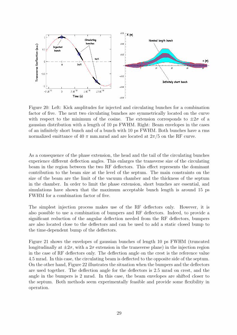
Figure 20: Left: Kick amplitudes for injected and circulating bunches for a combinationfactor of five. The next two circulating bunches are symmetrically located on the curvewith respect to the minimum of the cosine. The extension corresponds to ±2σ of agaussian distribution with a length of 10 ps FWHM. Right: Beam envelopes in the casesof an infinitely short bunch and of a bunch with 10 ps FWHM. Both bunches have a rmsnormalized emittance of 40 π mm.mrad and are located at 2π/5 on the RF curve.

As a consequence of the phase extension, the head and the tail of the circulating bunchesexperience different deflection angles. This enlarges the transverse size of the circulatingbeam in the region between the two RF deflectors. This effect represents the dominantcontribution to the beam size at the level of the septum. The main constraints on thesize of the beam are the limit of the vacuum chamber and the thickness of the septumin the chamber. In order to limit the phase extension, short bunches are essential, andsimulations have shown that the maximum acceptable bunch length is around 15 psFWHM for a combination factor of five.

The simplest injection process makes use of the RF deflectors only. However, it isalso possible to use a combination of bumpers and RF deflectors. Indeed, to provide asignificant reduction of the angular deflection needed from the RF deflectors, bumpersare also located close to the deflectors and can be used to add a static closed bump tothe time-dependent bump of the deflectors.

Figure 21 shows the envelopes of gaussian bunches of length 10 ps FWHM (truncatedlongitudinally at ±2σ, with a 2σ extension in the transverse plane) in the injection regionin the case of RF deflectors only. The deflection angle on the crest is the reference value4.5 mrad. In this case, the circulating beam is deflected to the opposite side of the septum.On the other hand, Figure 22 illustrates the situation when the bumpers and the deflectorsare used together. The deflection angle for the deflectors is 2.5 mrad on crest, and theangle in the bumpers is 2 mrad. In this case, the beam envelopes are shifted closer tothe septum. Both methods seem experimentally feasible and provide some flexibility inoperation.

29

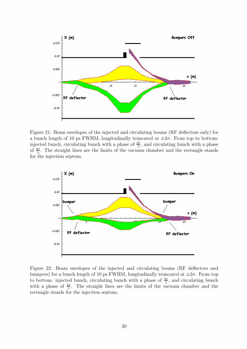
Figure 21: Beam envelopes of the injected and circulating beams (RF deflectors only) fora bunch length of 10 ps FWHM, longitudinally truncated at ±2σ. From top to bottom:injected bunch, circulating bunch with a phase of 2π

5, and circulating bunch with a phase

of 4π5. The straight lines are the limits of the vacuum chamber and the rectangle stands

for the injection septum.

Figure 22: Beam envelopes of the injected and circulating beams (RF deflectors andbumpers) for a bunch length of 10 ps FWHM, longitudinally truncated at ±2σ. From topto bottom: injected bunch, circulating bunch with a phase of 2π

5, and circulating bunch

with a phase of 4π5. The straight lines are the limits of the vacuum chamber and the

rectangle stands for the injection septum.

30

8 Complete tracking in the transfer line and in EPA

In order to check that the optics satisfies the requirements, a complete tracking throughthe modified transfer line and the isochronous ring has been carried out. Such a trackingallows to take into account the higher order effects in chromaticity and isochronicity ina global way. For this purpose, new tracking routines have been written on the basis ofthe MAD program, so as to generate realistic distributions of particles.

Longitudinally, the particles are distributed in time following a gaussian law and themomentum p is calculated for each particle using the formula:

p(t) = cos(2πνt+ φ) (9)

where ν is the RF frequency and φ is the RF phase. In this way, it is possible to describethe phase extension of the bunches on the RF curve, which is the main contribution to theenergy spread within the bunches. In the transverse plane, the normalized phase spaceis considered and a unitary bi-gaussian distribution is generated. Knowing the emittanceand the Twiss parameters, the transformation from the normalized phase space to thereal phase space used for tracking is done through the inverse Floquet transformationdefined as: (

qq′

)=

1√β

0

− α√β

−√β

(xx′

)(10)

where (x, x′) and (q, q′) are respectively the variables in the real and normalized phasespace, α and β being the Twiss parameters at the starting point.

The results of the tracking in the transfer line and the new EPA ring are presented inFigure 23. A tracking has also been performed through the matching section at the endof the linac, where no important aberration effects have been found. In the future, weintend to extend the analysis by starting the tracking at the beginning of the linac, afterthe front-end. For all simulations, the bunch length is set to 10 ps FWHM (or 1.28 mmrms), the normalized rms emittance is 40 π mm.mrad and the energy at the end of thelinac is 350 MeV.

The left-hand side of the figure shows the tracking in the transfer line. The initial phasespace is derived from the values of the Twiss parameters at the end of the linac (pointzero), assuming a perfect matching between the linac and the transfer line. The finaldistributions result from one passage through the line. The right-hand side of the figureshows the tracking in the isochronous EPA ring. The initial distributions are the resultfrom the tracking in the transfer line taken at the injection point, and the final distri-butions are given at the same point, after five turns in the ring. The difference betweenthe initial and final transverse distributions indicate a small mismatch at the entrance inthe ring. However, the discrepancy remains small. On the other hand, the longitudinaltracking shows no bunch lengthening. Less than 1% of the particles are lost after thetracking over five turns, mainly in the tails of the distributions. The tracking has beenextended to 100 turns in the ring: the losses are kept at a low level (around 1.5%) andoccur only in the first turns, which confirms the stability of the solution.

31

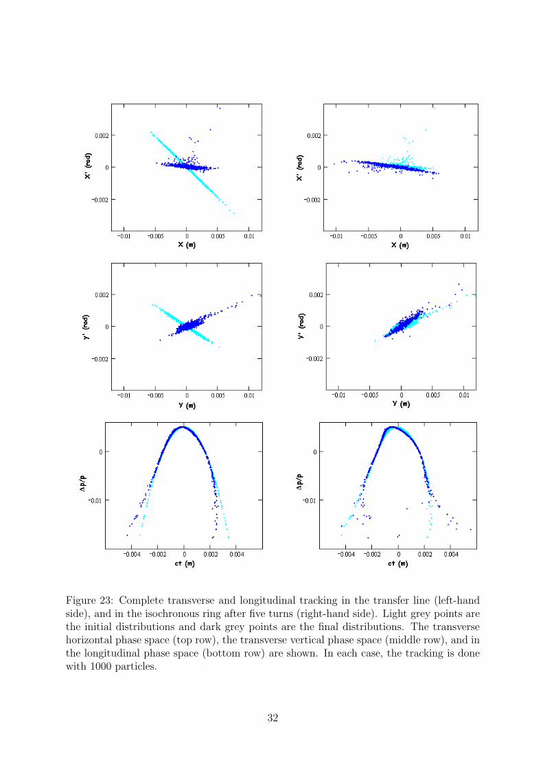
Figure 23: Complete transverse and longitudinal tracking in the transfer line (left-handside), and in the isochronous ring after five turns (right-hand side). Light grey points arethe initial distributions and dark grey points are the final distributions. The transversehorizontal phase space (top row), the transverse vertical phase space (middle row), and inthe longitudinal phase space (bottom row) are shown. In each case, the tracking is donewith 1000 particles.

32

9 Beam steering

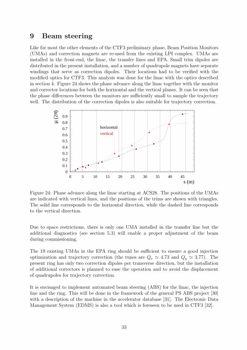
Like for most the other elements of the CTF3 preliminary phase, Beam Position Monitors(UMAs) and correction magnets are re-used from the existing LPI complex. UMAs areinstalled in the front-end, the linac, the transfer lines and EPA. Small trim dipoles aredistributed in the present installation, and a number of quadrupole magnets have separatewindings that serve as correction dipoles. Their locations had to be verified with themodified optics for CTF3. This analysis was done for the linac with the optics describedin section 4. Figure 24 shows the phase advance along the linac together with the monitorand corrector locations for both the horizontal and the vertical planes. It can be seen thatthe phase differences between the monitors are sufficiently small to sample the trajectorywell. The distribution of the correction dipoles is also suitable for trajectory correction.

s (m)

µ (2

π)

horizontal

vertical

0

0.1

0.2

0.3

0.4

0.5

0.6

0.7

0.8

0.9

0 5 10 15 20 25 30 35 40 45

Figure 24: Phase advance along the linac starting at ACS28. The positions of the UMAsare indicated with vertical lines, and the positions of the trims are shown with triangles.The solid line corresponds to the horizontal direction, while the dashed line correspondsto the vertical direction.

Due to space restrictions, there is only one UMA installed in the transfer line but theadditional diagnostics (see section 5.3) will enable a proper adjustment of the beamduring commissioning.

The 19 existing UMAs in the EPA ring should be sufficient to ensure a good injectionoptimization and trajectory correction (the tunes are Qx 4.73 and Qy 3.77). Thepresent ring has only two correction dipoles per transverse direction, but the installationof additional correctors is planned to ease the operation and to avoid the displacementof quadrupoles for trajectory correction.

It is envisaged to implement automated beam steering (ABS) for the linac, the injectionline and the ring. This will be done in the framework of the general PS ABS project [30]with a description of the machine in the accelerator database [31]. The Electronic DataManagement System (EDMS) is also a tool which is foreseen to be used in CTF3 [32].

33

10 Conclusions

In this note, we have given a description of the first stage of the CTF3 project (so calledCTF3 preliminary phase) and we have presented the results of the corresponding beamdynamics studies. The main goal of the preliminary phase is to test the new scheme ofelectron pulse compression and bunch frequency multiplication, which is at the heart ofthe CLIC RF power source concept, at low bunch charge and with short pulses. It willprovide a proof of principle of the scheme and it will be useful in order to gain experienceand to test component prototypes, in view of the following stages of the project. The testwill be performed in the area of the LPI complex, making use of existing components.While only a limited amount of new hardware will be used, several modifications tothe existing installation are needed. They will be made during a dedicated shut-downperiod starting in April 2001. It is planned to begin the commissioning of the modifiedinstallation before the end of 2001, and to complete the bunch combination test by theend of 2002.

A number of beam dynamics studies were performed in order to assess the feasibility ofthe test and to identify the needed hardware changes. Both analytical and numericalcalculations have been used, taking also into account the results of a series of beammeasurements made on the existing installation [16, 17]. This analysis is now completed,and its results have been presented in this note. In particular, we have described indetail the new configuration and the corresponding optics for the front-end, the linac,the transfer line, and the ring.

The linac will be shortened and a new gun will be fitted into it. The beam parametershave been defined and the gun specifications have been identified. The existing bunchingsystem and matching section to the linac will be used, and they should provide thedesired performances in terms of bunch length (≤ 10 ps FWHM) and charge (q = 0.1 nC).A new linac optics has been found, which requires only minimal hardware changes. Amatching section between the linac and the transfer line to the ring has been designed.This new section provides a large flexibility, which is valuable for the typical mode ofoperation of a test facility. The design of the transfer line has been modified (withoutchanging the positions and angles of the main bending dipoles) in order to be madeisochronous and achromatic, and it has been transversally matched to the new ringoptics. The ring layout will be slightly modified in order to obtain an optics which isisochronous and has a zero dispersion in the injection region, allowing for small beamsizes and good matching conditions at the injection. Chromatic corrections and secondorder isochronicity effects remaining at the desired level are achievable by using threesextupole families. The horizontal and vertical dynamic apertures are around 15σ forabout 1000 turns, over the expected beam momentum spread (≤ ± 1%), which iscomparable with the present performance. The variation of the total bunch length duringthe combination process (five turns) is negligible over this momentum range. This hasbeen verified by tracking using the MAD code (including the transfer line). For thispurpose, a complete six-dimension phase-space representation of the beam has been used,with realistic transverse and longitudinal distributions. The beam transverse stabilityhas been checked as well. The new injection scheme with transverse RF deflectors wasalso studied. A couple of existing deflectors can provide the requested injection angle of

34

about 4.5 mrad and they will be used for injection. The beam envelopes in the injectionregion have been evaluted. A five-turn combination process is possible with low beamlosses for bunches shorter than 15 ps FWHM, while for smaller combination factors thebeam requirements on bunch length are relaxed.

The beam instrumentation in the whole complex has been reviewed and modified wherenecessary. In particular, the new matching section will be equiped with a spectrometerline and beam profile monitors. The installation will allow to perform time-resolvedmeasurement with high resolution by using a streak camera and it will be used to fullycharacterize the beam at the end of the linac. A first check has also been made in orderto check that the beam position monitors and the correction dipoles ensure a sufficenttrajectory correction.

35

Appendix

The acronyms used in this note are summarized here:

• ACS = ACcelerating Structure

• CLIC = Compact LInear Collider

• CLIO = Collaboration pour un Laser a electrons libres dans l’Infrarouge a Orsay

• CTF3 = CLIC Test Facility 3

• EPA = Electron Positron Accumulator

• ECM = Electrode Capacitive Monitor (current monitor)

• HIE = (Hippodrome) Injection line for Electrons

• HIP = (Hippodrome) Injection line for Positrons

• INFN = Istituto Nazionale di Fisica Nucleare

• LAL = Laboratoire de l’Accelerateur Lineaire (Orsay)

• LEP = Large Electron Positron collider

• LIL = LEP Injector Linac

• LIPS = LIL Power Saver (RF pulse compression system)

• LPI = LEP Pre-Injector = LIL + EPA

• MDK = Modulator Klystron

• MSH = Monitor SEMgrid Horizontal (secondary emission monitor)

• MTV = Monitor TV

• PS = Proton Synchrotron accelerator

• SLH/SLV = SLit Horizontal/Vertical

• TCM = Transition-Cherenkov Monitor (profile monitor)

• UMA = pick-Up MAgnetic (beam position monitor)

• WBS = Wire Beam Scanner (profile monitor)

• WCM = Wall Current Monitor

36

References

[1] H.H. Braun, R. Corsini, T.E. D’Amico, J.P. Delahaye, G. Guignard, C.D. Johnson,A. Millich, P. Pearce, L. Rinolfi, A.J. Riche, R.D. Ruth, D. Schulte, L. Thorndal,M. Valentini, I. Wilson, W. Wunsch, ”The CLIC RF power source: a novel schemeof two beam acceleration for electron-positron linear colliders”, CERN-99-06 (1999).

[2] CLIC Study Team, ”Proposals for Future CLIC Studies and a New CLIC Test Facility(CTF3)”, CERN/PS 99-047 (LP) and CLIC Note 402 (1999).

[3] H. Braun, L. Rinolfi, ”Technical description for the CLIO gun”, CTF3 Note 2000-07.

[4] A. Pisent, L. Rinolfi, ”A new bunching system for the LEP Injector Linac”,CERN/PS/90-58 (LP).

[5] R. Corsini, J.P. Potier, L. Rinolfi, T. Risselada, ”Isochronous Optics and RelatedMeasurements in EPA”, Proceedings of the 7th European Particle Accelerators Con-ference, Wien, June 2000.

[6] R. Corsini, B. Dupuy, A. Ferrari, L. Rinolfi, T. Risselada, P. Royer, F. Tecker,”LIL bunch length, LIL lattice parameters, LIL energy, LIL temperature versus RFfrequency, EPA circumference and EPA isochronicity measurements”, CTF3 note2001-18 (MD), to be published.

[7] M.A. Tordeux, ”Etude des longueurs de paquets du LIL a 4 MeV”, PS/LP Note93-14 (MD).

[8] W. Hermannsfeldt, ”EGUN an electron optics and gun design”, SLAC Report 331,October 1988.

[9] B. Mouton, ”Proceedings of the fourth CTF3 collaboration meeting”, CLIC Note433, page 79, May 2000.

[10] ”Etude, suivi de fabrication, tests au LAL, participation aux essais et mise en serviceau CERN d’un canon thermo-ionique type CLIO”, Convention entre CERN et IN2P3,26 May 2000.

[11] R. Chaput, ”Electron gun for the FEL CLIO”, Proceedings of 2nd EPAC Conference,Nice, 1990.

[12] J.C. Bourdon, R. Belbeoch, M. Bernard, P. Brunet, B. Leblond, M. Omeich, E. Plou-viez, J. Rodier, ”Commissioning the CLIO injection system”, Nucl. Instr. Meth. inPhysics Research A304 (1991) 322-328.

[13] A. Benscessan, D.T. Tran, D. Tronc, ”High power standing wave triperiodic structurefor positron acceleration”, Nucl. Instr. Meth. 118 (1974) 349-355.

[14] J-C. Godot, L. Rinolfi, A. Pisent and H. Braun, ”A new front-end for the LEPInjector Linac”, CERN/PS/91-19 (LP), Proceedings of the 1991 Particle AcceleratorConference, 6-9 May 1991, San Francisco, California, USA.

[15] B. Mouton, ”The PARMELA program, version 4.3”, LAL/SERA 93-455.

37

[16] R. Corsini, A. Ferrari, L. Rinolfi, T. Risselada, P. Royer, F. Tecker, ”LIL bunch lengthand lattice parameters measurements in March 2000”, CTF3 Tech. Note 2000-09(MD-LPI), PS/LP Note 2000-01 (MD).

[17] R. Corsini, A. Ferrari, L. Rinolfi, T. Risselada, P. Royer, F. Tecker, ”New measure-ments of the LIL bunch length and lattice parameters”, CTF3 Tech. Note 2000-13(MD-LPI), PS/LP Note 2000-02 (MD).

[18] K.L. Brown, D.C. Carey, C. Iselin and F. Rothacker, ”TRANSPORT, a computerprogram for designing charged particle beam transport systems”, CERN 80-04.

[19] S. Battisti, M. Le Gras, J.M. Roux, B. Szeless, D.J. Williams, “Magnetic beamposition monitors for the LEP Pre-Injector”, CERN/PS 87-37-BR, IEEE, ParticleAccelerators Conference, Washington D.C., March 1987.

[20] S. Battisti, ”Measurement of the short bunch length in the CLIC test facility”,CERN/PS 93-40, CLIC Note 211.

[21] J.C. Thomi, ”La mesure de profils longitudinaux de faisceaux d’electrons”,PS/BD/Note 93-03.

[22] H. Grote and F.C. Iselin, ”The MAD Program”, CERN/SL 90-13 (AP), 1993.

[23] L. Groening, private communication.

[24] T. Risselada, ”An isochronous optics for EPA”, PS/LP Note 99-02 (tech).

[25] R. Corsini, J.P Potier, L. Rinolfi, T. Risselada, J.C. Thomi, ”First micro-bunchmeasurements in EPA as isochronous ring at 500 MeV”, PS/LP Note 99-03 (MD).

[26] R. Belbeoch, ”Utilisation d’une section acceleratrice pour la mesure du profil longi-tudinal des micro-paquets a la sortie du groupeur de la station d’essais du LAL”,SERA Note 89-09.

[27] Ph. Bernard, H. Langeler and V. Vaghin ”On the design of disk-loaded waveguidesfor RF separators”, CERN 68-30 (1968).

[28] S. Gallo, ”Proceedings of the first CLIC/CTF3 collaboration meeting held at CERN,3-5 May 1999”, CLIC Note 401, page 215.

[29] I. Syratchev, private communication.

[30] B. Autin, V. Ducas, A. Lombardi, M. Martini and E. Wildner, “Automated BeamOptics Correction for Emittance Preservation”, CERN-PS-97-007-DI, 3rd Interna-tional LHC Workshop: High-brightness Beams for Large Hadron Colliders, 13-18Oct 1996, Montreux, Switzerland.

[31] B. Autin, F. Di Maio, M. Gourber-Pace, M. Lindroos and J. Schinzel, “Database foraccelerator optics”, CERN-PS-97-065, International Conference on Accelerator andLarge Experimental Physics Control Systems, 3-5 Nov 1997, Beijing, China.

[32] L. Rinolfi, J. Schinzel, ”CTF3 Project Information Management Proposal”, CTF3Note 2000-017 (EDMS).

38