Bayesian Method for Groundwater Quality Monitoring Network Analysis

Bayesian Method for Groundwater Quality MonitoringNetwork Analysis

Khalil Ammar1; Mac McKee2; and Jagath Kaluarachchi3

Abstract: A new methodology is developed to analyze existing monitoring networks. This methodology incorporates different aspects ofmonitoring, including vulnerability/probability assessment, environmental health risk, the value of information, and redundancy reduction.A conceptual framework for groundwater quality monitoring is formulated to represent the methodology’s context. Relevance vectormachine �RVM� plays a basic role in this conceptual framework, and is employed to reduce redundancy and to create probability map ofcontaminant distribution, and accordingly to estimate the expected value of sample information. Disability adjusted life years approach ofthe global burden of disease is used for quantifying the health risk consequences. This is demonstrated through a case study applicationto nitrate contamination monitoring in the West Bank, Palestine. The results obtained from the RVM analysis showed that an overlap errorof less than 30% were obtained based on using around 30% of the monitoring sites �170 relevance vectors�. This reflects the importanceof the RVM as a useful model for improving the efficiency of monitoring systems, both in terms of reducing redundancy and increasingthe information content of the collected data. However, in this application, the results of health risk assessment and the evaluation ofmonitoring investments were less encouraging due to the minimal elasticity of the nitrate health effect with respect to monitoringinformation and uncertainty.

DOI: 10.1061/�ASCE�WR.1943-5452.0000043

CE Database subject headings: Groundwater management; Monitoring; Groundwater pollution; Bayesian analysis.

Author keywords: Groundwater; Monitoring; Pollution; Bayesian analysis; Relevance vector machine; Value of information.

Introduction

Efficient water management relies upon efficient monitoring sys-tems that have the capability to provide information that are de-cision relevant. Unfortunately, existing monitoring systems do notalways fulfill this objective, where many monitoring systems aredesigned to gather data that are redundant and do not addmanagement- or decision-relevant information of value. There-fore, the needs to acquire data that are decision-relevant, andefficient, establish a need for the development of cost-effectiveand flexible analytical methodology for water quality monitoringnetworks.

Recently, increase in using supervised learning machines inwater resources management applications has drawn more atten-tion in the research literature. Particularly, using the relevancevector machine �RVM� model in hydrological applications andgroundwater quality modeling, Bayesian deduction for redun-dancy detection in groundwater quality monitoring networks�Ammar et al. 2008�, and on selection of kernel parameters in

1Hydrogeological Scientist, International Center for Biosaline Agri-culture, Dubai, United Arab Emirates �corresponding author�. E-mail:[email protected]

2Director, Utah Water Research Laboratory, Utah State Univ., Logan,UT.

3Professor, Dept. of Civil and Environmental Engineering, Utah StateUniv., Logan, UT.

Note. This manuscript was submitted on September 5, 2008; approvedon July 31, 2009; published online on August 3, 2009. Discussion periodopen until June 1, 2011; separate discussions must be submitted for indi-vidual papers. This paper is part of the Journal of Water ResourcesPlanning and Management, Vol. 137, No. 1, January 1, 2011. ©ASCE,
ISSN 0733-9496/2011/1-51–61/$25.00.
JOURNAL OF WATER RESOURCES PLANN

Downloaded 14 May 2011 to 35.8.11.2. Redistributio

RVM for hydrologic applications �Tripathi and Govindaraju2006�. The work on applicability of statistical learning algorithmsin groundwater quality modeling �Khalil et al. 2005a�, real-timemanagement of reservoir releases �Khalil et al. 2005b�, and mod-eling of chaotic hydrologic time series �Khalil et al. 2006�. Con-tinuous advances in RVM performance have solved some of thelimitations of earlier formulations of these models, such as ex-tending the binary classifier to a multiclass classifier with associ-ated probability estimates as shown in the application ofmulticlass RVMs for selecting shape features �Zhang and Malik2005�. The extension of RVM to include multivariate outputs�Thayananthan et al. 2006�. The rationale for using the RVMmodel here, is due to its strengths as a forecasting tool: �1� itsdesign yields a sparse model �redundancy reduction�, which al-lows better generalization performance and avoids overfitting; �2�it has the capability to infer information contained in the data dueto its Bayesian framework; and �3� it derives accurate probabilis-tic prediction models and allows the computation of posteriorprobabilities for a prediction.

A Bayesian decision analysis approach is employed here. Thisapproach incorporates prior knowledge about the possible state ofa system, and adds new data in a preposterior analysis to produceposterior knowledge of full information about possible systemstates. In the case of groundwater quality monitoring, this is doneto account for uncertainty in the predictions and to estimate thevalue of information �VOI� in terms of quantifying health riskconsequences. In this study, health risk assessment is quantifiedusing the disability adjusted life years �DALY� metric. The maincharacteristics of DALY approach over other methods are: �1� itenables a comprehensive evaluation of health gains and losses interms of established public health concepts �quality and quantity
of life and social magnitude�, using time as a unit of measure-
ING AND MANAGEMENT © ASCE / JANUARY/FEBRUARY 2011 / 51

n subject to ASCE license or copyright. Visit http://www.ascelibrary.org

ment; �2� it combines annual mortality rates and nonlethal endpoints and explicitly addresses life and health expectancy; �3�DALY measures loss of health, an inverse form of the more gen-eral concept of quality adjusted life years, which measuresequivalent healthy years lived at the individual level instead ofthe health of a population; �4� it has been adopted in many coun-tries and by health development agencies as the standard healthaccounting; and �5� DALY measures the future stream of healthyyears of life lost due to each incident case of disease and for eachdeath.

Recently, the involvement of the VOI in decision-making pro-cess in many disciplines has increased dramatically. The VOI bydefinition is the amount the decision maker would be willing topay for information prior to making a decision. In monetaryterms, the expected monetary value of the decision with informa-tion minus the expected monetary value without the information.The concept of involving VOI in health risk assessment hashelped reduce uncertainty in the decision-making process throughthe collection of new data that have value in terms of providing agreater understanding of health consequences �Yokota and Th-ompson 2004�. They have conducted a review of VOI analysis inenvironmental health risk decisions. They showed that the com-plexity of solving VOI problems with continuous probability dis-tributions as inputs to models emerges as the main barrier togreater use of the VOI concept. They suggested the need to stan-dardize approaches and develop some prescriptive guidance forVOI analysts. Kim and Bridges �2006� proposed a structured ap-proach to decision making that explicitly considers the risks anduncertainties within an overall decision analysis framework toprovide a systematic process for evaluating how the predictedperformance of a management action and the uncertainty associ-ated with that prediction affects objectives that stakeholders careabout most. Khadam and Kaluarachchi �2003� proposed an inte-grated approach for the management of contaminated groundwa-ter resources using health risk assessment and economic analysisthrough a multicriteria decision analysis framework. The pro-posed decision analysis framework integrates probabilistic healthrisk assessment into a cost-based multicriteria decision analysisframework. The results showed the importance of using an inte-grated approach for decision making considering both costs andrisks. Bates et al. �2003� used a special case of Bayesian modelingto make inferences from deterministic models about environmen-tal risk assessment. The results obtained were posterior distribu-tions of contaminant concentrations in soil and vegetables takinginto account uncertainty.

The objective of this paper is to develop an improved meth-odology and a systematic approach for groundwater quality moni-toring network analysis, using state-of-the-art supervised RVM,and incorporating wide aspects of vulnerability assessment, healthrisk, and VOI reflected in a multiobjective perspective. This mul-tiobjective dimension includes cost of monitoring, the informa-tion content or level of uncertainty, and the risk to public and/orenvironmental health. This will help evaluate the worth of collect-ing additional data in selecting the optimal monitoring networkconfiguration. In addition, this will assist in deciding whetheravailable data are sufficient to support decisions on monitoringsite selection �monitoring strategy�, or insufficient in terms of theadded VOI they would supply, and the amount of uncertaintyreduction inherent in the information obtained from the monitor-ing network.

The main research contribution is in the introduction of newtechniques as the RVM and incorporating integrated methodolo-
gies of vulnerability assessment, health risk, and economic VOI
52 / JOURNAL OF WATER RESOURCES PLANNING AND MANAGEMENT


for groundwater quality monitoring analysis, assessed with re-spect to their efficiency and applicability to a real groundwaterproblem. This is an important contribution to the decision-makingprocess because of incorporating the multiobjective dimensionand quantification of possible tradeoffs between different objec-tives in groundwater monitoring.

Methodology

The methodology is described systematically as illustrated in theconceptual framework for groundwater quality monitoring net-work analysis figure. The main steps include selection of constitu-ent of concern �COC�, selection of a sparse model for creation ofvulnerability/probability maps, health risk assessment, and esti-mation of the value of information. The process of selecting theCOC is done by following the approach proposed by Harmancio-glu et al. �1999�. Probability map is created using the RVM modelthrough integrating data on the natural system �hydrogeologicalinformation� and human activities �land use and contaminant con-centration� within a probabilistic framework �Ammar 2007�.

A Bayesian decision analysis is adopted here to estimate thevalue of information, through calculating the expected value ofsample information �EVSI� by incorporating current knowledge�prior probability distribution� and adding newly collected data toproduce posterior probability distributions of the state of a sys-tem. The value of additional information is calculated as the dif-ference between the expected loss �or expected utility� that wouldbe achieved under posterior knowledge and the expected loss �ex-pected utility or payoff� under current �prior� knowledge. Thisshould help in deciding whether available data are sufficient tosupport decisions on monitoring site selection �monitoring strat-egy� or insufficient in terms of the added VOI and uncertaintyreduction as will be described later.

The organization of the methodology is as follows: first, wewill describe the RVM method. Second, we will describe theBayesian decision analysis, and most importantly the preposteriorcomponents: risk assessment and EVSI. For risk assessment wewill elaborate on the assumptions used in quantifying the risk,starting with defining the dose-response relationship as reflectedin the hazard quotient, and accordingly, the hazard index to de-lineate the areas that has adverse effect or acceptable risk, and todefine the health loss based on the DALYs approach. Finally, thiswill help define the EVSI.

Relevance Vector Machine

RVM plays a basic role in the conceptual framework as illustratedin Fig. 1. The main features of RVM model are sparsity �reducingredundancy�, good generalization performance, avoiding overfit-ting, and producing posterior probability as an output �Tipping2001�. Sparsity within the Bayesian framework of the RVM isachieved as follows: the weights of each input are governed by aset of hyperparameters. These hyperparameters describe the pos-terior distribution of the weights and are estimated iteratively dur-ing training. This continues until convergence occurs by judgingif we have attained a local maximum of the marginal likelihood.This implies that most hyperparameters approach infinity, and ac-cordingly setting the posterior distributions of the weights to zero.The remaining vectors with nonzero weights are called relevancevectors. Details of the description are given in the following para-graphs. Note that we used here multivariate output extension al-
gorithm which is an extension to the fast marginal likelihood
© ASCE / JANUARY/FEBRUARY 2011


maximization algorithm �Tipping and Faul 2003�. For simplicity,the RVM methodology is demonstrated according to Tipping for-mulation �Tipping 2001�. Interested readers can read a multivari-ate paper by Thayananthan �Thayananthan et al. 2006� regardingthe details of extending the univariate output to multivariate out-put. In his extension, he followed similar formulation of Tippingand let the algorithm iterate in two steps: in the first step, tocalculate the probability �likelihood� of each example belongingto each class, and in the second step, to estimate the parametersusing the probability calculated in the first step. He used a matrixtarget with number of columns equal to number of variates in-stead of a vector target, also extended the weight matrix, and useda diagonal covariance matrix.

Bayesian learning in RVMs begins by observing a data setconsisting of N pairs, �xn ,yn ,n=1,2 ,3 , . . . ,N�, where the xn

=inputs and the yn=targets. The targets form an N by P matrix,with P the number of regulatory classes, ynxP

= �y�n ,1� , . . . ,y�N , P��. The likelihood or probability of member-ship in one of the regulatory classes given information about theinput x, written as P �y �x�, can be written in terms of the mean orweight w and the variance �2 assuming the error follows inde-pendent zero-mean Gausian �normal� distribution �Tipping 2001�.This conditional target or data likelihood incorporates the uncer-tainty of prediction and is obtained as a function of weight vari-ables and hyperparameters. These hyperparameters are theparameters that determine the relevance of the associated basisfunction. The weight variables are then analytically integrated outto obtain marginal likelihood as function of the hyperparameters.

Fig. 1. Conceptual framework for groundwater quality monitoringnetwork analysis

An optimal set of hyperparameters is obtained by maximizing the



marginal likelihood over the hyperparameters. Then optimalweight matrix is obtained using these optimal set of hyperparam-eters. Details are described in the following. The mathematicalrepresentation of the likelihood is given below as

p�y�w,�2� = �2��2�−N/2exp�−1

2�2 y − �w2 �1�

where y= �y1 . . . .yN�T=targets; w= �wo . . . .wN�T=weights or rel-evance vector coefficients; �=design matrix that contains theresponse of all basis functions to the inputs, with �= ��x1� ,��x2� , . . . ,��xN��T, wherein ��xn�= �1,K�xn ,x1� ,K�xn ,x2� , ¯ ,K�xn ,xN��T. The kernel function �K�xn ,xN�� is usedto introduce nonlinearity into the mapping function. The kernelfunctions define a set of nonlinear fixed basis functions, �N�xn�=K�xn ,xN�, where the kernel function is centered on each of the Ntraining data points xn. An important feature of the kernel is thekernel width, which is considered for development of RVM mod-els as the key for forecast accuracy and consequently sparsity. Forexample, the Gaussian kernel �radial basis function kernel� widthis represented here by the standard deviation, �, or simply thevariance over the noise �2, as shown in the Gaussian kernel equa-tion

K�x,xi� = exp�−x − xi

�22� �2�

where K�x ,xi�, i=1, . . . ,n=kernel function for n by m matrix, andthe norm reflects the nearness of one point �x� to other point �xi�,while the variance controls the width of the bell shape of theGaussian distribution, i.e., smoothing parameter.

In the training process, the RVM considers the training data asprior data and infers the information about class membershipfrom this data. Accordingly, it recognizes a pattern in the data.The addition of new data updates the likelihood of class member-ship, which also updates the error between the observed data andpredicted data �or regulatory classes�. This Gaussian prior distri-bution is introduced to complement the likelihood function and isgiven in the form as

p�w�� = �2��−M/2 m=1

M

�m1/2 exp�−

�mwm2

2� �3�

where M =number of the independent hyperparameters, �= ��1 , . . . ,�M�T, each hyperparameter is individually controllingthe strength of the prior over its associated weight. This form ofthe prior is responsible for the sparsity properties of the RVMmodel. Given the previously defined prior and likelihood distri-butions, the posterior parameter distribution conditioned on thedata over all unknowns is defined using Bayes’ rule

P�w,�,�2�y� =P�y�w,�,�2�P�w,�,�2�

P�y��4�

The posterior in Eq. �4� is intractable; an approximation is ob-tained by decomposing the posterior to P�w ,� ,�2 �y�� P�w �y ,� ,�2�P�� ,�2 �y�. As a consequence, the posterior dis-tribution over the weight becomes analytically solvable. Detailsof analytically solving these equations are given in Tipping
�2001�. The analytical posterior distribution over weights is


P�w�y,�,�2� =P�y�w,�2�P�w��

P�y��,�2�= �2��−�N+1�/2��−1/2

exp�−1

2�w − ��T�−1�w − �� 5�

with posterior covariance �= ��−2�T�+A�−1 and mean �=�−2��Ty, and A=diag��1 ,�2 , . . . ,�M�. The estimated value ofthe model weights is given by the mean of the posterior distribu-tion Eq. �5�, which is also the maximum a posterior �MP� estimateof the weights using type-II maximum likelihood procedure �i.e.,maximizing the marginal likelihood�. The optimal values of manyhyperparameters �MP are infinite. This leads to a parameter pos-terior distribution infinitely peaked at zero for many weights withthe consequence that �MP correspondingly comprises very fewnonzero elements. That is, sparse Bayesian learning is formulatedas the local maximization of the marginal likelihood with respectto �.

Bayesian Decision Analysis

A Bayesian decision analysis is conducted as mentioned before,to evaluate the expected health loss function for each decision ormonitoring strategy from the range of all possible outcomes pro-duced from running the RVM model. In addition, to select thedecision that satisfies the objectives of monitoring design �multi-objective dimension�, i.e., selecting the design that minimizes theexpected health loss or maximizing EVSI, minimizes cost of sam-pling �roughly measured here in terms of the number of monitor-ing sites�, and simultaneously improves uncertainty.

The prior state is considered here as the state of having theminimum number of monitoring sites, and the associated prob-ability as the prior probability produced by running the RVMmodel. This prior probability is actually the posterior probabilityof the training data used in the RVM model formulation.

Preposterior analysis is the core of the approach for calculatingthe expected value of information. In this step, an assessment ofthe risk based upon updated information is conducted and, ac-cordingly, an estimation of the expected value of the sample in-formation for each update is done as described below.

Risk Assessment

Risk is the probability of an adverse outcome and risk assessmentis the process of quantifying risk �probability� and associated con-sequences. The main consequence that will be taken into accountin this study is the health loss consequence; other consequences,such as economic or environmental, will not be covered due tolack of data concerning these issues. Health risk assessment gen-erally consists of hazard identification, exposure assessment,dose-response relationship, and risk characterization.

The hazard quotient �HQ� is used to define the dose-responserelationship of contaminant �in this study is nitrate� exposure. TheHQ is the noncancer risk assessment of this exposure, defined asthe ratio of the exposure for some generalized or typical hypo-thetical member of the receptor population at a site, compared toan appropriate toxicity reference value that equates to an accept-able level of risk for that receptor and chemical �U.S. EPA 2001�.The main equation to calculate the HQ as defined by U.S. EPA�2001� is

CDI =C � IR � EF

�6�
BW � 365


HQ =CDI

RfD�7�

where CDI=chronic daily intake of contaminant �mg/kg-day�;C=contaminant concentration �mg/L�; IR=ingestion rate �L/day�;EF=exposure frequency �days/year�; BW=bodyweight �kg�; andRfD=reference dose for the contaminant.

The hazard index �HI� which is the sum of HQs �as definedbefore� and is used to evaluate the fraction of the population witha HQ above and below 1, where HQ values above 1 are inter-preted as indicating the potential for adverse effects and HQ val-ues below 1 are interpreted as indicating acceptable risk. This HIwill be used to determine the potential exposure in the population,mainly the infants. The health loss �HL� is the loss in health thatthe individual will get due to exposure to hazard material. The HLfunction is defined as

HL = DALYs for HI � 1 �8a�

HL = 0 Otherwise �8b�

where DALY=disability adjusted life years as described next. Inorder to characterize the risk, the concept of DALYs is adopted inthis study to quantify the HL, with time as the unit of measure-ment. This health impact measure combines years-of-life-lostwith years-lived-with-disability that is standardized by means ofseverity weights using time as the metric. The importance ofDALY appears in combining different aspects of public health:quantity of life �measured by life expectancy and duration ofdisease�, quality of lie �expressed through a severity weight forthe adverse health outcome�, and social magnitude �or number ofpeople affected�.

HL is defined according to the Global Burden of Disease�GBD� �Lopez et al. 2006� as time spent with reduced quality oflife aggregated over the population involved, combining years oflife lost �combining mortality and age of death data� and yearslived with disability, standardized through application of severityweights. Generally, HL using the DALY method is assessed byestimating the number of people affected, estimating the averageduration of the adverse health response, including loss of lifeexpectancy as a consequence of premature mortality, assigningweights for severity in unfavorable health conditions, and calcu-lating the HL in DALYs. Therefore, DALYs for a certain cause iscalculated as the sum of the years of life lost due to prematuremortality �YLL� from that cause and the years of healthy life lostas a result of the disability �YLD� for incident cases of the healthcondition

DALY = YLL + YLD �9�

where YLL=number of life years lost due to mortality andYLD=number of years lived with the disability, weighed with afactor between 0 �perfect health� and 1 �dead� for the severity ofthe disability for all relevant diseases

DALY = �i=1

n

�D � L + I � DW � T� �10�

where n=number of all relevant diseases, the first part of thesummation represents the mortality and YLL=D�L, with D beingthe number of deaths, and L the standard life expectancy at theage of death due to this cause. The second part of the summationrepresents the morbidity, YLD= I�DW�T, where I=number ofincident cases for both causes of disability; DW=disability
weight for both causes; and T=duration in years of the case until


remission or death. Due to the unavailability of data on mortality,only morbidity will be taken into account in this study.

Risk assessment is expressed as the expected HL, which isequal to the posterior probability of membership of contaminant�here is nitrate� in one of the regulatory classes for each monitor-ing site times the HL consequence. The expected HL for eachmonitoring strategy was calculated from

E�HL� = �i=1

N

posti · DALYs �11�

where E�HL�=expected HL; N=number of monitoring sites; andposti=posterior probability of the contaminant being in one of theregulatory classes at each monitoring site; and DALYs=quantification of the health consequences at each monitoringsite as described before.

EVSI

The expected value of sample information �EVSI� is a measure ofthe value of the reduction in uncertainty that may result from thecollection of new sample information. The EVSI is defined as thedifference between the expected HL given prior information andthe expected HL when provided updated information �U.S. EPA2001; Tappenden et al. 2004�. The expected value of perfect in-formation �EVPI� is the difference between the expected HL ofthe optimal management decision based on the prior analysis andthe expected HL of the optimal management decision if all uncer-tainty were to be eliminated; this provides the upper bound for theEVSI. A detail of obtaining uncertainty is described in the follow-ing.

Local Uncertainty

The probabilistic output of the RVM can obtained as an error baror predictive variance �̂2. This predictive variance �error bars�consists of two variance components: the estimated noise vari-ance �MP

2 �maximum a posterior� in the data and variance due touncertainty in the prediction of weights �uncertainty about theoptimal value of the weights reflected by the posterior distribution�4�� represented in the second part of Eq. �12� ��T��, with Fand � the basis function and posterior covariance, respectively, asdefined in Eq. �5� �Tipping 2001�

�̂2 = �MP2 + �T� �12�

The local uncertainty of predicted maximum nitrate concentra-tion is then quantified here based on the error bars as the width ofthe confidence interval of a specified probability for the predictedmaximum nitrate concentration �i.e., the response or output of theRVM� at each individual location of the existing monitoring sites�where, again, the location of a monitoring site is the input to theRVM�

CI = �� t�,�/2��̂2/n�1/2 �13�

where ��=predicted maximum nitrate concentration �mg/L�,i.e., the model output is calculated based on the relevance vectors�RVs�; t�,�c/2= t-test statistic at �=n− p degrees of freedom andconfidence level �c �for 95% confidence level=0.05�; n=number of monitoring sites in the existing network configura-tion; and p=number of model parameters �p=2, for weight and
bias�.


Case Study

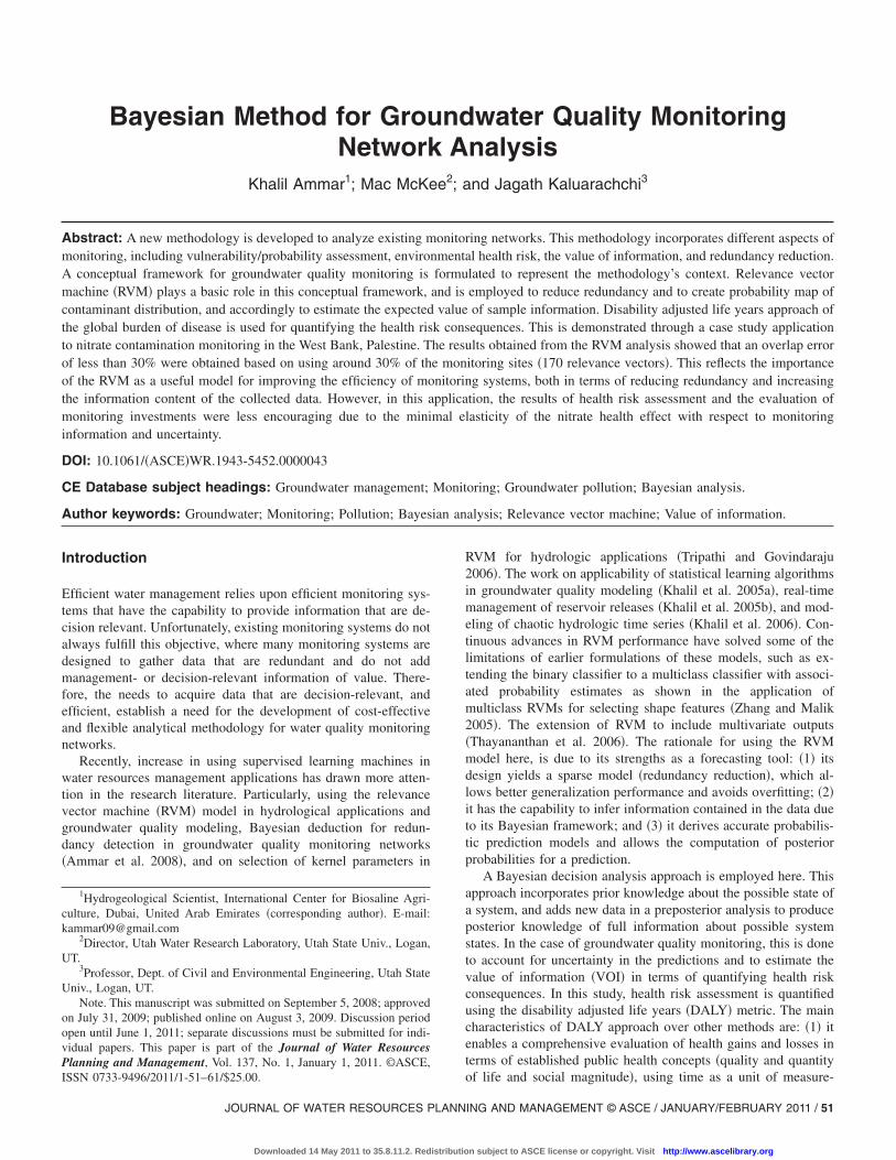
The methodology is applied on the West Bank/Palestine casestudy in the Middle East. The study area covers the whole WestBank area which is approximately 5 ,660 km2. The total Palestin-ian population living in the West Bank is about 2.5 million ac-cording to projections made by the Palestinian Central Bureau ofStatistics �PCBS� for the year 2005 �Palestinian Center Bureau ofStatistics �PCBS� 2002�. The West Bank has a semiarid climatewith average annual rainfall of 600 mm/year �24 in./year�. Rain-fall varies from north to south and from west to east, with theleast in the Jordan Valley close to the Dead Sea region �less than100 mm/year�. Rainfall is the main natural source for groundwa-ter recharge. Groundwater is the main natural source for all usesin the West Bank.

The West Bank groundwater system consists of three mainbasins: the eastern, northeastern, and western basins as shown inFig. 2. Generally, the aquifer system in these groundwater basinsis a Quaternary-Cretaceous geologic system of Holocene-Albianage; it is composed of karstic and permeable limestone and dolo-mite. The aquifer systems consists mainly of three main aquifers:�1� a shallow aquifer occurs in the Quaternay and Teriary systemsof Holocene-Paleocene age; �2� an upper aquifer occurs in theupper Cenomanian-Turonian age; and �3� a lower aquifer occursin the lower Cenomanian age. For more details on the West Bankgroundwater system, the reader is advised to read CH2M HILLreport �CH2M HILL 2001�.

Land Use Pattern

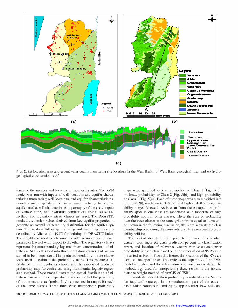
Several local practices affect nitrate loading to West Bank aqui-fers. These include application of fertilizers and pesticides in ir-rigated areas, leakage from septic tanks and sewage systems inurban areas, and industrial activities such as food processing andtextiles. For the purpose of this study, five land use categorieswere defined in terms of their nitrate contribution: �1� urban areasrepresenting the main cites of West Bank, including both domes-tic and industrial activities; �2� rural areas covering all villagebuilt-up areas, where most are not connected to sewage networks,and septic tanks are the major source of nitrate loading; �3� irri-gated areas in Jenin, Tulkarm, Qalqilya, Nablus, Tubas, and Jeri-cho; �4� forests and natural reserves representing natural areas;and �5� rainfed and range land areas covering most of the area ofthe West Bank as shown in Fig. 3.

Results and Discussion

To run the RVM model, the first step was to select the kernelparameters, i.e., kernel type and kernel width. A kernel type thatbest suits the structural properties of the data was selected byjudging the RVM performance against selected criteria �e.g., ac-curacy� of different kernel types �Gaussian, Laplace, spline,Cauchy, cubic, thinplate spline, and bubble�. Fig. 4 presents theperformance of the RVM model for different kernel types. Asshown in the figure, the best performance in terms of accuracy ofprediction was given by the Gaussian kernel, followed by theLaplace kernel. A systematic procedure was followed to set thekernel width or the variance to get an optimal monitoring networkconfiguration.

Several runs �20 runs� of the RVM model produced a range of
possible sampling plans or monitoring network configurations in


terms of the number and location of monitoring sites. The RVMmodel was run with inputs of well locations and aquifer charac-teristics �monitoring well locations, and aquifer characteristic pa-rameters including: depth to water level, recharge to aquifer,aquifer media, soil characteristics, topography of the area, impactof vadose zone, and hydraulic conductivity using DRASTICmethod, and regulatory nitrate classes as target. The DRASTICmethod uses index values derived from key aquifer properties togenerate an overall vulnerability distribution for the aquifer sys-tem. This is done following the rating and weighting proceduredescribed by Aller et al. �1987� for defining the DRASTIC index.The weights are used to determine the relative importance of eachparameter �factor� with respect to the other. The regulatory classesrepresent the corresponding log maximum concentrations of ni-trate �as NO3

−� classified into three regulatory classes and are as-sumed to be independent. The predicted regulatory nitrate classeswere used to estimate the probability maps. This produced thepredicted nitrate regulatory classes and the associated predictedprobability map for each class using multinomial logistic regres-sion method. These maps illustrate the spatial distribution of ni-trate occurrence in each specified class and reflect the possibilityof nitrate occurrence �probability� represented in ranges for each

Fig. 2. �a� Location map and groundwater quality monitoring site logeological cross section A-A�

of the three classes. These three class membership probability



maps were specified as low probability, or Class 1 �Fig. 5�a��,moderate probability, or Class 2 �Fig. 5�b��, and high probability,or Class 3 �Fig. 5�c��. Each of these maps was also classified intolow �0–0.29�, moderate �0.3–0.39�, and high �0.4–0.575� vulner-ability ranges �classes�. As is clear from these maps, low prob-ability spots in one class are associated with moderate or highprobability spots in other classes, where the sum of probabilityover the three classes at the same grid point is equal to 1. As willbe shown in the following discussion, the more accurate the classmembership prediction, the more reliable class membership prob-ability will be.

The spatial distribution of predicted classes, misclassifiedclasses �total incorrect class prediction percent or classificationerror�, and location of relevance vectors with associated priorprobability in each class based on prior information of 95 RVs arepresented in Fig. 5. From this figure, the locations of the RVs areclose to “hot-spot” areas. This reflects the capability of the RVMmodel to understand the information contained in the data. Themethodology used for interpolating these results is the inversedistance weight method of ArcGIS of ESRI.

Low nitrate concentration probability is noticed in the Senon-ian �aquitard� outcrops in the southeastern part of the eastern

s in the West Bank; �b� West Bank geological map; and �c� hydro-
cation
basin which confines the underlying upper aquifer. Few wells and



springs tap the underlying aquifer in this particular area �Fig.5�a��. Moderate nitrate contamination probability covers 60% ofthe West Bank study area, mainly in the shallow aquifer of theeastern basin and the upper aquifer of the eastern and westernbasins, as shown in Fig. 5�b�. High nitrate concentration probabil-ity covers 13% of the West Bank area and is observed mainly inthe vicinity of Hebron in the southern part of the west bank forwells and springs that tap water from the upper aquifer in both theeastern and western basins �Fig. 5�c��. Other high vulnerabilityspots occur near the cities of Jenin and Nablus, which draw water

Fig. 3. Land use map for the West Bank case study

Fig. 4. Kernel type selection



from the Eocene aquifer of the northeastern basin, and the com-munities of Tulkarm, Ramallah and Bethlehem, which obtainwater from the upper aquifer of the western basin.

Sparsity is a key feature of RVM model. This sparsity is illus-trated in the ability of the model to achieve good generalizationperformance and avoid overfitting while using small number ofbasis functions or RVs. These important features of RVM models�sparsity and generalization� reflect the potential of the RVMmodel use in water resources decision making and research. In thecontext of monitoring, the selection of the kernel width as de-scribed in the methodology section, prescribes the desired qualityof the resulting mapping function as well as the number of RVs�i.e., the size of the monitoring network� used in the predictionand characterization of contaminant distributions in the aquifer.For example, specifying a desired sparsity level �in terms of amaximum allowable number of relevance vectors� of 95 RVs gen-erated acceptable class prediction accuracy with associated erroror class misclassification of around 40%. Decreasing the sparsityof the model by decreasing the kernel width and accordingly in-creasing the number of RVs to 170 resulted in significant im-provements in prediction accuracy, with error reduction of 10%�the error associated with 170 RVs is 30%�. Bayesian decisionanalysis was used to select an appropriate or optimal monitoringstrategy as explained in the following steps.

Expected Health Loss

High nitrate concentrations in drinking water cause differenthealth outcomes, such as methemoglobinemia, cancer �due to thebacterial production of N-nitroso compounds�, hypertension, in-creased infant mortality, and diabetes �Fewtrell 2004�. Methemo-globin is formed when nitrite �due to bacterial conversion fromnitrate� oxidizes the ferrous iron in hemoglobin to the ferric form.In this study we will consider only the methemoglobinemia healtheffects due to high nitrate concentrations in drinking water. De-bate about the carcigonic effect of nitrate is still ongoing and nodecision on the issue of possible carcigonic effects related to ni-trates has been published in the U.S. EPA or World Health Orga-nization �WHO� 1996 guidelines.

Due to the limited availability of records from the PalestinianMinistry of Health �MOH� regarding the number of methemoglo-binemia cases in the West Bank, an approximate exposure assess-

on RVM model performance
based


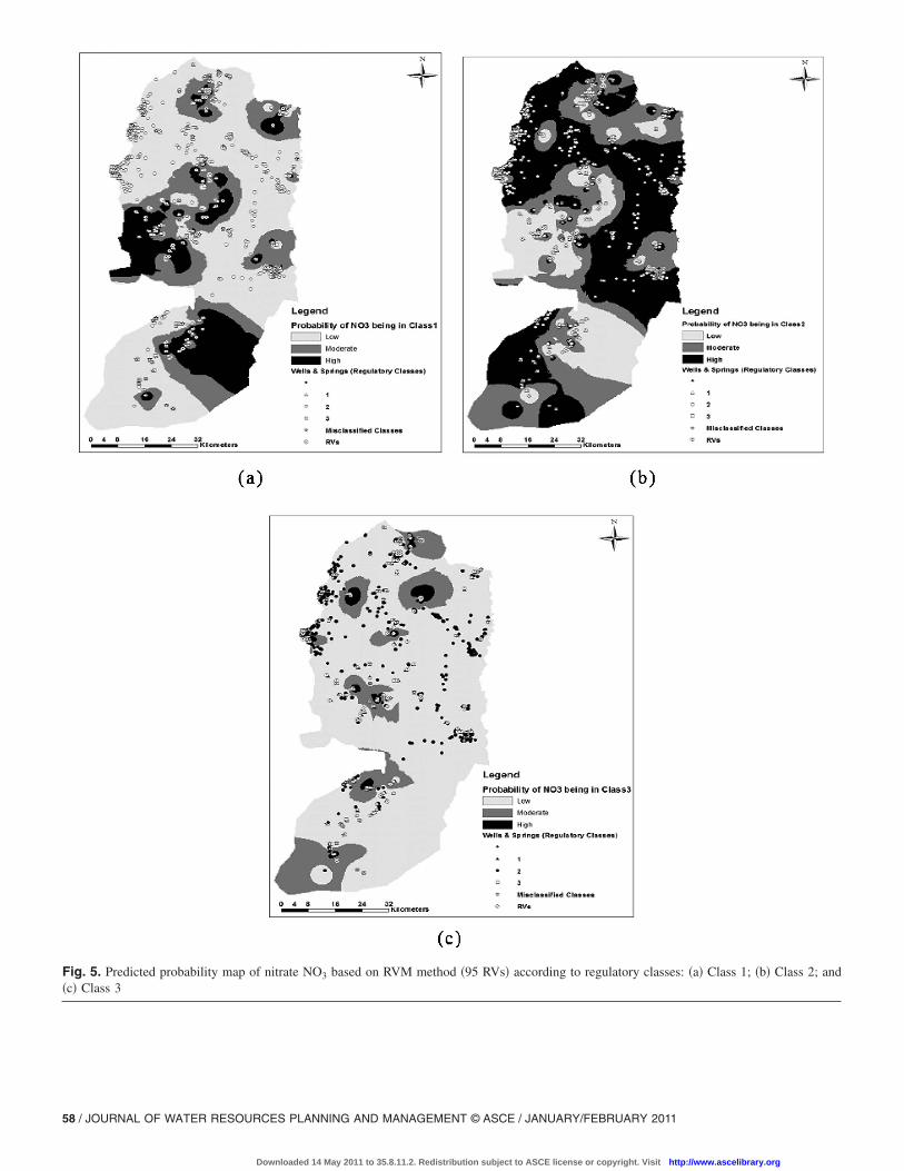
Fig. 5. Predicted probability map of nitrate NO3 based on RVM method �95 RVs� according to regulatory classes: �a� Class 1; �b� Class 2; and�c� Class 3

58 / JOURNAL OF WATER RESOURCES PLANNING AND MANAGEMENT © ASCE / JANUARY/FEBRUARY 2011

Downloaded 14 May 2011 to 35.8.11.2. Redistribution subject to ASCE license or copyright. Visit http://www.ascelibrary.org

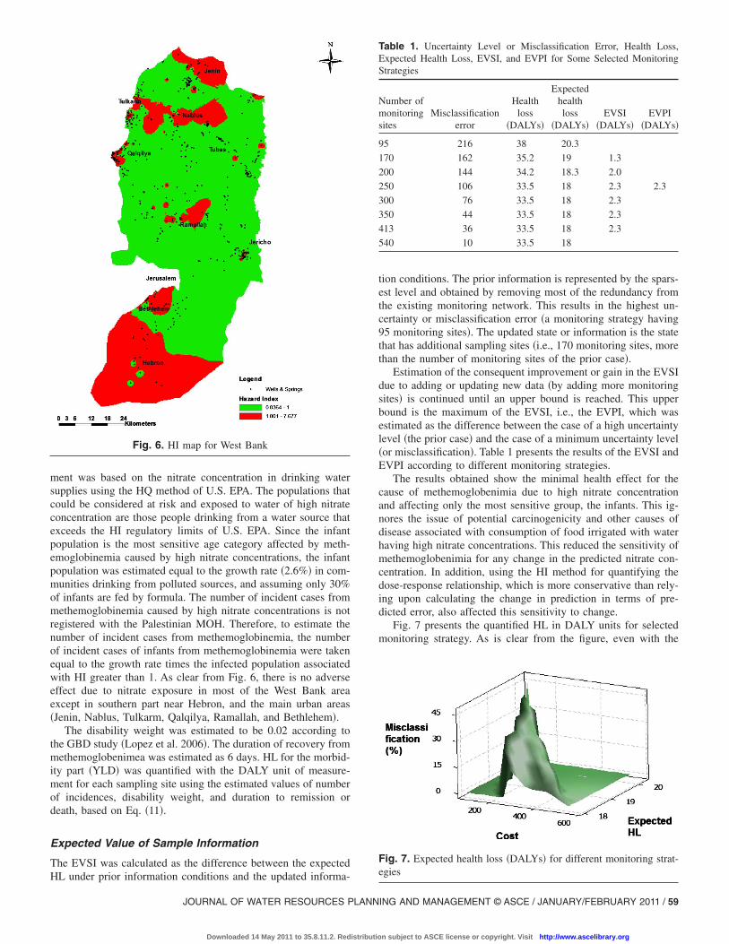
ment was based on the nitrate concentration in drinking watersupplies using the HQ method of U.S. EPA. The populations thatcould be considered at risk and exposed to water of high nitrateconcentration are those people drinking from a water source thatexceeds the HI regulatory limits of U.S. EPA. Since the infantpopulation is the most sensitive age category affected by meth-emoglobinemia caused by high nitrate concentrations, the infantpopulation was estimated equal to the growth rate �2.6%� in com-munities drinking from polluted sources, and assuming only 30%of infants are fed by formula. The number of incident cases frommethemoglobinemia caused by high nitrate concentrations is notregistered with the Palestinian MOH. Therefore, to estimate thenumber of incident cases from methemoglobinemia, the numberof incident cases of infants from methemoglobinemia were takenequal to the growth rate times the infected population associatedwith HI greater than 1. As clear from Fig. 6, there is no adverseeffect due to nitrate exposure in most of the West Bank areaexcept in southern part near Hebron, and the main urban areas�Jenin, Nablus, Tulkarm, Qalqilya, Ramallah, and Bethlehem�.

The disability weight was estimated to be 0.02 according tothe GBD study �Lopez et al. 2006�. The duration of recovery frommethemoglobenimea was estimated as 6 days. HL for the morbid-ity part �YLD� was quantified with the DALY unit of measure-ment for each sampling site using the estimated values of numberof incidences, disability weight, and duration to remission ordeath, based on Eq. �11�.

Expected Value of Sample Information

The EVSI was calculated as the difference between the expected

Fig. 6. HI map for West Bank

HL under prior information conditions and the updated informa-



tion conditions. The prior information is represented by the spars-est level and obtained by removing most of the redundancy fromthe existing monitoring network. This results in the highest un-certainty or misclassification error �a monitoring strategy having95 monitoring sites�. The updated state or information is the statethat has additional sampling sites �i.e., 170 monitoring sites, morethan the number of monitoring sites of the prior case�.

Estimation of the consequent improvement or gain in the EVSIdue to adding or updating new data �by adding more monitoringsites� is continued until an upper bound is reached. This upperbound is the maximum of the EVSI, i.e., the EVPI, which wasestimated as the difference between the case of a high uncertaintylevel �the prior case� and the case of a minimum uncertainty level�or misclassification�. Table 1 presents the results of the EVSI andEVPI according to different monitoring strategies.

The results obtained show the minimal health effect for thecause of methemoglobenimia due to high nitrate concentrationand affecting only the most sensitive group, the infants. This ig-nores the issue of potential carcinogenicity and other causes ofdisease associated with consumption of food irrigated with waterhaving high nitrate concentrations. This reduced the sensitivity ofmethemoglobenimia for any change in the predicted nitrate con-centration. In addition, using the HI method for quantifying thedose-response relationship, which is more conservative than rely-ing upon calculating the change in prediction in terms of pre-dicted error, also affected this sensitivity to change.

Fig. 7 presents the quantified HL in DALY units for selectedmonitoring strategy. As is clear from the figure, even with the

Table 1. Uncertainty Level or Misclassification Error, Health Loss,Expected Health Loss, EVSI, and EVPI for Some Selected MonitoringStrategies

Number ofmonitoringsites

Misclassificationerror

Healthloss

�DALYs�

Expectedhealthloss

�DALYs�EVSI

�DALYs�EVPI

�DALYs�

95 216 38 20.3

170 162 35.2 19 1.3

200 144 34.2 18.3 2.0

250 106 33.5 18 2.3 2.3

300 76 33.5 18 2.3

350 44 33.5 18 2.3

413 36 33.5 18 2.3

540 10 33.5 18

Fig. 7. Expected health loss �DALYs� for different monitoring strat-egies



minimal HL effect, we can still observe tradeoffs between differ-ent objectives: minimizing the cost versus improving accuracyand minimizing the expected HL i.e., maximizing the EVSI. Thisresult hints at directions for applying the proposed methodologyand framework on disease causes such as carcinogenic diseasesthat have greater public attention and more detailed data. ThisBayesian analysis could be extended to a simple multiobjectiveproblem by examining the possible tradeoffs among samplingcost �as represented by the number of sampling wells�, the valueof added information �quantified in DALYs�, and accuracy �interms of misclassification error�.

Conclusions and Recommendations

The conceptual framework proposed in this paper is an importantcontribution for efficient management of water information sys-tems in terms of saving time and effort needed to collect, prepare,and analyze data, and in understanding the physical structure ofthe groundwater system. The importance of this conceptualframework appears in its flexibility to suit a wide range of pos-sible applications for similar monitoring networks using differentwater quality monitoring parameters and hydrometric data collec-tion networks for both groundwater and surface water monitoringsystems. In addition, the aspects that have been incorporated intothe conceptual framework reflect the multiobjective dimension ofmonitoring network problems through integration of socioeco-nomic concerns in terms of health risk using the well-knownDALY approach, value of information, and cost of sampling. Pos-sible tradeoffs among different objectives increase the potentialusefulness of the conceptual framework in the sense that the re-sulting information is more understandable in terms of the quan-tified health outcome and reflects a measurable unit that hasmeaning for any decision taken.

The Bayesian framework of the RVM model features sparsity,accuracy, and incorporation of both subjective judgment of priorknowledge and statistical judgment of the posterior probability; ituses these to produce probabilistic output. The results of the useof the RVM model in this research illustrate a significant potentialfor future application in the decision-making process. The Baye-sian framework of the RVM model shows its capability to inferinformation contained in the data and understand the physicalsystem of the case study, taking into account the uncertainty inthe forecast it produced.

The modeling results provided here show that RVMs can pro-vide an attractive, simple to use, and straightforward analyticalforecasting model for application in monitoring network design.The RVM model identified a reliable network configuration that ispertinent to the information contained in the available monitoringdata, with the minimal number of sampling sites, and with themost significant sampling locations identified in terms of theirinformation content. Such information could be used to reduceunnecessary monitoring costs. Such savings could potentially beused to develop new monitoring locations in areas not previouslymonitored, which would be a research topic for further investiga-tion. The proposed tool could potentially assist decision makersand water resources planners for planning, developing, and pro-tecting groundwater resources, and adopting best managementpractices.

The work presented here concentrated on removing redun-dancy from an existing groundwater quality monitoring networkand selecting sampling sites based on spatial data. Therefore,
there is a need to explore the use of temporal data, or both spatial


and temporal data, to test if temporal data alone or a combinationof both spatial and temporal data produces different samplingstrategies.

More work is needed to improve the capability of RVMs toillustrate the prior, likelihood, and posterior probability as an out-come of the model, and allow for the gradual addition of new datato test for incremental improvements in prediction. This wouldmake the model easier to use and understand.

References

Aller, L., Bennett, T., Lehr, J. H., and Petty, R. J. �1987�. “DRASTIC: Astandardized system for evaluating groundwater pollution potentialusing hydrogeologic settings.” Rep. No. EPA/600/2-85/0108, U.S.EPA, Robert S. Kerr Environmental Research Laboratory, Ada, Okla.

Ammar, A. K. �2007�. “A Bayesian method for groundwater qualitymonitoring network analysis.” Dissertation, Utah State Univ., SaltLake City, Utah.

Ammar, K., Khalil, A., McKee, M., and Kaluarachchi, J. �2008�. “Baye-sian deduction for redundancy detection in groundwater quality moni-toring networks.” Water Resour. Res., 44, W08412.

Bates, S., Cullen, A., and Raftery, A. �2003�. “Bayesian uncertainty as-sessment in multicompartment deterministic simulation models forenvironmental risk assessment.” Environmetrics, 14, 355–371.

CH2M HILL. �2001�. “Aquifer modeling.” Water resources programphase III, USAID, Washington, D.C.

Fewtrell, L. �2004�. “Drinking-water nitrate, methemoglobinemia, andglobal burden of disease: A discussion.” Environ. Health Perspect.,112�14�, 1371–1374.

Harmancioglu, N. B., Fistikoglu, O., Ozkul, S. D., Singh, V. P., andAlpaslan, M. N. �1999�. Water science and technology library: Waterquality monitoring network design, Kluwer Academic, Dordrecht, TheNetherlands.

Khadam, I., and Kaluarachchi, J. �2003�. “Multi-criteria decision analysiswith probabilistic risk assessment for the management of contami-nated groundwater.” Environ. Impact. Asses. Rev., 23, 683–721.

Khalil, A., Almasri, M., McKee, M., and Kaluarachchi, J. �2005a�. “Ap-plicability of statistical learning algorithms in groundwater qualitymodeling.” Water Resour. Res., 41, W05010.

Khalil, A., McKee, M., Kemblowski, M., and Asefa, T. �2005b�. “SparseBayesian learning machine for real-time management of reservoir re-leases.” Water Resour. Res., 41�11�, W11401.

Khalil, A., McKee, M., Kemblowski, M., Asefa, T., and Bastidas, L.�2006�. “Multiobjective analysis of chaotic dynamic systems withsparse learning machines.” Adv. Water Resour., 29�1�, 72–88.

Kim, J., and Bridges, T. �2006�. “Risk, uncertainty, and decision analysisapplied to the management of aquatic nuisance species.” ERDC/TNANSRP-06-1, Aquatic Nuisance Species Research Program, Washing-ton, D.C.

Lopez, A., Mathers, C., Ezzati, M., Jamison, D., and Murray, C. �2006�.Global burden of disease and risk factors, The International Bank forReconstruction and Development/World Bank, Washington, D.C.

Palestinian Center Bureau of Statistics �PCBS�. �2002�. Results of popu-lation census of December 1997 in the West Bank and Gaza Strip,1998, Ramallah, Palestine.

Tappenden, P., Chilcott, J., Eggington, S., Oakley, J., and MaCabe, C.�2004�. “Methods for expected value of information analysis in com-plex health economic models: Developments on the health economicsof interferon-� and glatiramer acetate for multiple sclerosis.” HealthTechnol. Assess, 8�27�, 1–92.

Thayananthan, A., Navaratnam, R., Stenger, B. Torr, P., and R. Cilpolla.�2006�. “Multivariate relevance vector machines for tracking.” Proc.,European Conf. on Computer Vision, Dublin, Ireland.

Tipping, M. E. �2001�. “Sparse Bayesian learning and the relevance vec-tor machine.” J. Mach. Learn. Res., 1, 211–244.

Tipping M.E., and Faul A.C. �2003�. “Fast marginal likelihood maximi-



sation for sparse Bayesian models.” Proc., 9th Int. Workshop on Arti-ficial Intelligence and Statistic, C. M. Bishop and B. J. Frey, eds., KeyWest, Fla.

Tripathi, S., and Govindaraju, R. S. �2006�. “On selection of kernel pa-rameters in relevance vector machines for hydrologic applications.”Stochastic Environ. Res. Risk Assess., 21�6�, 747–764.

U.S. EPA. �2001�. “Risk assessment guidance for superfund: VolumeIII—Part A, Process for conducting probabilistic risk assessment.”EPA 540-R-02-002 OSWER 9285.7-45 PB2002 963302, Washington,
D.C., �http://www.epa.gov/superfund/RAGS3A/index.htm�.


World Health Organization �WHO� �1996�. “Health criteria and other

supporting information.” Guidelines for drinking water quality, 2nd.

Ed. Vol. 2, Geneva, Switzerland.Yokota, F., and Thompson, K. �2004�. “Value of information analysis in

environmental health risk management decisions: Past, present, andfuture.” Risk Anal., 24�3�, 635–650.

Zhang, H., and Malik, J. �2005�. “Selecting shape features using multi-class relevance vector machines.” Technical Rep. No. UCB/EECS-2005-6, EECS, University of California, Berkeley, Berkeley, Calif.



Bayesian Method for Groundwater Quality Monitoring Network Analysis

Documents

Transcript of Bayesian Method for Groundwater Quality Monitoring Network Analysis