Chapter 4 of Network Performance and Quality of Service: Basic Calculation of the Network’s Availability and Reliability

1. Availability Measurement Principle

One of the basic indicators of the performance of telecommunications

networks is availability, then here is given the important parameters of the

availability of measurement:

1) Mean Time between failure (MTBF) : average time between two

failure. This is vendor warranty for the availability of the

Telecommunication mobile network operator.

2) Mean Time To Repair (MTTR) : average time for repair and testing.

This is internal assurance for the availability of the

Telecommunication mobile network operator, especially the Network

Operation and Maintenance division and Internal Quality Division.

Sometime, this is the guarantees of "Maintenance Partner" to the

Telecommunication mobile network operator.

1.1. Formula

The formula for calculates the availability is written as follows:

Availability = (1 - (1/total down time)) * 100%

Where: Down Time = Time to repair + Testing time + Waiting,

Movement & Coordination time.

1.2. Some important things:

Here are important points to remember:

ISBN 976-602-18578-6-1

2

1 year is = 365 days = 8760 hours = 525,600 minutes = 31,536,000

seconds.

Downtime = 1 day then the availability = 99.726027% (two nine)

Downtime = 1 hour then the availability = 99.988584% (three nine)

Downtime = 1 minute then the availability = 99.999810% (five nine)

Downtime = 1 second then the availability = 99.999997% (seven

nine).

1.3. Calculation Examples:

1.3.1. Basic Network Availability Calculation

On a mobile operator, data failure of a particular service in October 2017

is as follows: The first failure occurred on October 2, 2017 at 12:05:10 in

1 minute 38 seconds. The second failure occurred on 15 October 2017 at

21:33:20 in 2 minutes 3 seconds, and the third failure occurred on 24

October 2017, at 10:07:29 in 15 minutes 17 seconds.

Calculate: MTTR, MTBF and service availability

Solution:

1) In this problem, we assumes that the MTTR (Mean Time to repair) is

the average time of Down time, since no information about the time

to repair, testing time and waiting, movement and coordination time,

then MTTR = ratio between total time of downtime and number of

failure.

Total time of down time = 1 minute 38 seconds + 2 minutes 3

seconds + 15 minutes 17 seconds = 18 minutes 58 seconds

Then MTTR = (18 minutes 58 seconds)/3 = 6 min 19.3 sec

ISBN 976-602-18578-6-1

3

2) In this problem, we assumes that the MTBF (Mean Time Between

Failure) is the Mean Time Between Down Time, since no information

about the time to repair, testing time and waiting, movement and

coordination time, then MTBF = average of time between down time,

since there are any 3 failures, then there are any two TBFs (time

between failure).T

TBF1 (time between failure 1 and failure 2) = time between (October

2, 2017 at 12:05:10) and (15 October 2017 at 21:33:20) = 321

hours 26 minutes 32 seconds.

TBF2 (time between failure 2 and failure 3) = time between (15

October 2017 at 21:33:20) and 24 October 2017, at 10:07:29 = 205

hours 32 minutes 5 seconds.

Then MTBF = (TBF1 + TBF2)/2 = 263 hours 29 minutes 19 seconds

3) Measurement period = October 2017 = 31 days = 31*24*60*60

seconds = 2,678,400 seconds.

Total time to repair, in this problem is total time of down time = 18

minutes 58 seconds = 1138 seconds.

Then the Availability = {(measurement period – total time to

repair)/measurement period} * 100 % = {(2,678,400 seconds -

1138 seconds)/ 2,678,400 seconds} * 100 % = 99, 96 %%

1.3.2. Availability Calculation of The Intermittent Service

Assume that:

ISBN 976-602-18578-6-1

4

Data Records of The Operation and Maintenance Division on an Intermittent

Service, Period: January 1, 2017 through December 31, 2017

Customers know that the connection is

broken

Connection is established by the

network operator

Dates Time Dates Time

12 Jan 10.00 am 12 Jan 06.00 pm

14 Feb 06.30 am 15 Feb 09.30 am

20 May 11.30 am 20 May 12.45 am

18 Jun 01.30 pm 18 Jun 09.30 pm

17 Nov 08.00 am 17 Nov 09.00 pm

28 Dec 09.00 am 28 Dec 09.30 am

Outage known by provider technicians

provider

Completed repairs and testings

Dates Time Dates Time

12 Jan 10.00 am 12 Jan 06.00 pm

20 Jan 09.00 am 20 Jan 11.00 am

14 Feb 05.30 am 15 Feb 09.30 am

20 May 00.30 pm 20 May 09.00 pm

18 Jun 08.00 am 18 Jun 09.00 pm

17 Nov 09.00 am 17 Nov 09.30 am

28 Dec 09.00 am 28 Dec 09.30 am

Calculate:

1. Calculate on the customer side:

a. number of failure

b. period of observation

c. total interruption period

d. average accessibility

e. overall mean time between outage = MTBO

f. the mean time to restore (MTTR)

g. Graph of the operating characteristic curve for operational

service interruption ( = mean time between service interruption

vs. interruption duration).

2. Calculate on the service provider side:

a. number of outage

b. period of observation

c. the total outage period

ISBN 976-602-18578-6-1

5

d. average of connection availability

e. outage lasting

f. overall mean time between outage = MTBO

g. mean time to repair (MTTR)

h. Indicate when (a) The duration of the service outage = service

interruption (b) The duration of the service outage much longer

than the perceived service interruption (c) The perceived

duration of the service interruption much longer than the actual

service outage (d) A service outage not result in an operational

service interruption at all.

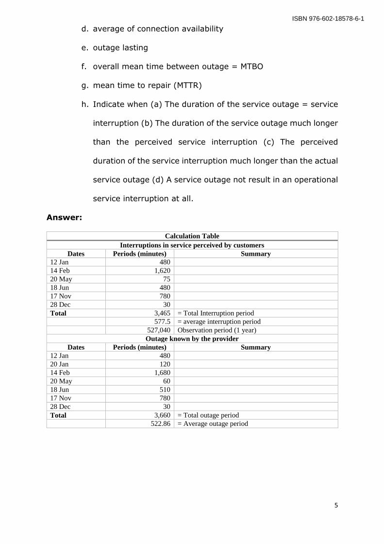
Answer:

Calculation Table

Interruptions in service perceived by customers

Dates Periods (minutes) Summary

12 Jan 480

14 Feb 1,620

20 May 75

18 Jun 480

17 Nov 780

28 Dec 30

Total 3,465 = Total Interruption period

577.5 = average interruption period

527,040 Observation period (1 year)

Outage known by the provider

Dates Periods (minutes) Summary

12 Jan 480

20 Jan 120

14 Feb 1,680

20 May 60

18 Jun 510

17 Nov 780

28 Dec 30

Total 3,660 = Total outage period

522.86 = Average outage period

ISBN 976-602-18578-6-1

6

Then:

Service outage

duration

(minutes)

number of outage where the

duration time ≥ its outage

duration or more

Mean Time Between Interruption

= ration between observation time

and number of interruption

30 1 75,291

75 2 87,840

120 3 105,408

480 4 131,760

780 6 263,520

1,620 7 527,040

1. Calculation on the customer side:

a. number of failure = 6

b. period of observation = 527,040 minutes

c. total of interruption period = 3,465 minutes

d. accessibility = (period of observation – total of interruption

period ) / period of observation = 0.993425546 = 99.34 % (=

two nine).

e. overall mean time between interruption = MTBO = (period of

observation – total of interruption period ) / number of

interruption = 87,262.5 minutes

f. the mean time to restore (MTTR) = total of interruption time /

number of interruption = 577.5 minutes

g. Figure 2 is the operating characteristic curve for operational

service interruption graph.

2. Calculation on the service provider side:

a. Number of outage = 7 (so the Provider know that the outage

occurred is more than the interruptions perceived by the

customer, indicating that there is an outage that does not cause

an interruptions in service.

ISBN 976-602-18578-6-1

7

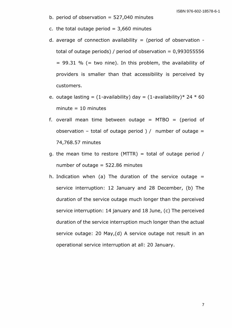
b. period of observation = 527,040 minutes

c. the total outage period = 3,660 minutes

d. average of connection availability = (period of observation -

total of outage periods) / period of observation = 0,993055556

= 99.31 % (= two nine). In this problem, the availability of

providers is smaller than that accessibility is perceived by

customers.

e. outage lasting = (1-availability) day = (1-availability)* 24 * 60

minute = 10 minutes

f. overall mean time between outage = MTBO = (period of

observation – total of outage period ) / number of outage =

74,768.57 minutes

g. the mean time to restore (MTTR) = total of outage period /

number of outage = 522.86 minutes

h. Indication when (a) The duration of the service outage =

service interruption: 12 January and 28 December, (b) The

duration of the service outage much longer than the perceived

service interruption: 14 january and 18 June, (c) The perceived

duration of the service interruption much longer than the actual

service outage: 20 May,(d) A service outage not result in an

operational service interruption at all: 20 January.

ISBN 976-602-18578-6-1

8

1.3.3. Network Availability Calculation of Continous Service

Data Records of the operation and maintenance division on a continuous

service which has an average capacity = 768 kbps.

Calculate:

a. the OEC (effective operational capacity) on the day of measurement,

when the data transfer is 5 Gbyte per customer

b. the OEC (effective operational capacity) where the availability of

providers = 99.67%

c. the throughput efficiency, if the probability that each transmission

unit will retransmit = 0.0005 and the probability that any information

exchange unit will retransmission = 0.005

d. handling overhead if the ratio between the number of transmission

units of information exchange unit and the number of transmission

used exclusively for handling traffic on each unit = 0.05

Calculation:

a. the OEC (effective operational capacity) on the day of measurement:

Provider capacity in a day = 24 * 3600 * 768 kbps = 66.3552 Gbit

per customer.

ISBN 976-602-18578-6-1

9

Then OEC = 5 Gbyte / 66.3552 Gbit = 5*8 Gbit / 66.3552 = 60.3 %

b. Where the availability of providers = 99.67%, then the provider

capacity = 0.9967* 66.3552 Gbit = 66.1362 Gbit per day.

Then OEC = 5 Gbyte/66.1362 Gbit = 5*8 Gbit / 66.1362 = 60.48 %

c. The throughput efficiency = TE = 1 / ((1 +0.0005) * (1 +0.005)) =

99.45 %

d. Handling overhead = HO = 0.05 / (1-0.05) = 5.263%

2. Routing Reliability Calculation

Routing realibility is the portion of the transmitted packets reach the proper

destination node

Calculation Example:

Calculate the realibility, assume that the measurement results for internet

services

a. The number of services per second = 100,000; successful services =

80,000; number of services to the proper destination address =

79,000

b. The number of packets received = 1,000,000,000; packet loss =

200,000; packets sent to the right address = 999,000,000

c. compare the results of the calculation of a and b

Answer

a. QoS perceived by the customer:

Routing reliability of the service = (79,000/100,000) = 79 %

b. QoSD (QoS Delivered by the Service Provider):

Packet loss = 20,000/1,000,000,000 = 0.02 %.

ISBN 976-602-18578-6-1

10

Routing reliability of the packets = (999,000,000/(1,000,000,000 –

200,000) = 99.92 % (3 nine)

c. Conclusion: QoSD is better than QoE (quality of experience)

3. Data Connection Quality Evaluation

The evaluation of the connection function is to calculate the transaction

time, so the lower transaction time the higher connection quality.

Calculation technique is use the following formulas:

)]()[(

)(_

ii

i

HT

HHOOverheadHandling [17]

)]1(*)1[(

1Efficiency Throughput

iutu RRTE

𝑇𝑟𝑎𝑛𝑠𝑎𝑐𝑡𝑖𝑜𝑛 𝑇𝑖𝑚𝑒 (𝑇𝑡) =[𝑏 ∗ (1 + 𝐻𝑂) ∗ (1 + 𝐸𝑂)]

(𝑑 ∗ 𝑇𝐸)

Calculation example:

a. Calculate the average transaction times at a Fixed Speed Protocols if

assume that the probability that a transmission unit will be

retransmitted = 0.001; the probability that an information exchange

unit will have to be retransmitted = 0.002; the ratio of the number

of transmission units, bits, or characters used to specify handling in

the ith exchange unit sampled and the corresponding total number of

transmission units, bits, or characters in the ith information exchange

unit = 0.08; Transmission use the ARQ error handling techniques with

the addition of one bit per message block size of 99 bits; the fixed

transmission speed = 0.7 Mbps; and injected a data bit = 1 Gbyte

ISBN 976-602-18578-6-1

11

b. By using the data as on problem a, calculate transaction time of the

Variable Speed Protocols when the average transmission speed = 0.8

Mbps.

Answer:

Basic calculation for problem a and b:

Handling overhead = HO = 0.08/(1-0.08) = 0.08696

Encoding Overhead = EO = total bits for encoding purposes / total

bits in a message after encoding = 1 / (99 +1) = 0.01

Throughput Efficiency = TE = 1 / ((1 +0.001) * (1 +0.002)) = 0.997

a. 𝑇𝑟𝑎𝑛𝑠𝑎𝑐𝑡𝑖𝑜𝑛 𝑇𝑖𝑚𝑒 (𝑇𝑡) =[𝑏∗(1+𝐻𝑂)∗(1+𝐸𝑂)]

(𝑑∗𝑇𝐸) =

(1,000,000,000*8*(1+0.08696)*(1+0.01))/(700,000*0.997) =

12.58 seconds

b. 𝑇𝑟𝑎𝑛𝑠𝑎𝑐𝑡𝑖𝑜𝑛 𝑇𝑖𝑚𝑒 (𝑇𝑡) =[𝑏∗(1+𝐻𝑂)∗(1+𝐸𝑂)]

(𝑑∗𝑇𝐸) =

(1,000,000,000*8*(1+0.08696)*(1+0.01))/(800,000*0.997) =

11.01 seconds

4. Continuity Connection

Evaluation of the continuity connection perform in the calculation of

spontaneous disconnect, disconnect report rate, and abnormal disconnect

rate.

The formulas are:

a. P [d | x] = the probability that a transaction, once initiated, will be

interrupted by a spontaneous disconnect = ration between

spontaneous disconnect and the total number of transactions

ISBN 976-602-18578-6-1

12

b. Disconnect report rate (DRR) = Nd / Nb; Where Nd is the number of

complaints of disconnects registeredand Nb is the number of billable

service

c. Abnormal disconnect rate (ADR) = 1 – (tc/ts); Where Tc is the

observed number of the transactions that were initiated and

completed without interruption ts is the total number of transactions

sampled.

Calculation example:

Evaluate the continuity connection of the following data: the spontaneous

disconnect = 10,000; the number of complaints of disconnects registered

= 1000; the number of billable service = 100 million; the observed number

of the initiated transactions that were completed without interruption = 124

million; the total number of transactions sampled = 125 million

Answer:

d. P [d | x] = 10,000/125,000,000 = 0.00008

e. Disconnect report rate (DRR) = 1,000/100,000,000 = 0.00001

f. Abnormal disconnect rate (ADR) = 1 - (124.000.000/125000000) =

0,008

ISBN 976-602-18578-6-1

13

Author: Sigit Haryadi is lecturer in ITB (Bandung Institute of Technology), Indonesia,

since 1984. Currently teaches several courses: Traffic Engineering, Quality and Regulatory

Services Telecommunications and Regulations. In addition to teaching at the ITB, Sigit Haryadi

also becomes experts at the Directorate General of Post and Telecommunication Indonesia

since 1986. Experience in the industry: since 1990 to become an expert in some Providers and

Telecom Operators in Indonesia. Since 2001, Sigit Haryadi became associate professor in the

institution.

References

[1] Hardy, C. William. (2001). QoS Measurement and Evaluation of

Telecommunications Quality of Service. John Wiley & Sons, Ltd. Baffins Lane,

Chichester, West Sussex, PO19 1UD, England.

[2] Sigit Haryadi. (2013). Telecommunication Traffic: Technical and Business

Consideration. Lantip Safari Media. Bandung, Indonesia.

[3] Sigit Haryadi. (2013). Telecommunication Service and Experience Quality. Lantip

Safari Media. Bandung, Indonesia.

[4] Haryadi, Sigit; Limampauw, Ivantius. (2012). QoS Measurement of Telephony

Services In 3G Networks Using Aggregation Method. Conference Proceeding of

TSSA 2012. Denpasar, Indonesia.

[5] Haryadi, Sigit; Nusantara, Sandy. (2012). QoS Measurement of Web Browsing

Services In 3G Networks Using Aggregation Method. Conference Proceeding of

TSSA 2012. Denpasar, Indonesia.

[6] Haryadi, Sigit; Pramudita, Arnold. (2012). QoS Measurement of Video Streaming

Services in a 3G Networks Using Aggregation Method. Conference Proceeding of

TSSA 2012. Denpasar, Indonesia.

[7] Haryadi, Sigit; Andina, Raisha. (2012). QoS Measurement of File Transfer Protocol

Services In 3G Networks Using Aggregation Method. Denpasar, Indonesia. 2012.

[8] Haryadi, S. (2018, January 25). Chapter 1. The Concept of Telecommunication Network

Performance and Quality of Service. Retrieved from osf.io/mukqb

[9] Haryadi, S. (2018, January 26). Chapter 2 of Network Performance and Quality of

Service: Determination of Key Performance Indicator (KPI). Retrieved from

osf.io/preprints/inarxiv/6gtnd

ISBN 976-602-18578-6-1

14

[10] Haryadi, S. (2018, January 26). Chapter 3 of Network Performance and Quality of

Service: Technical Measurement of a Mobile Network Performance and Quality of

Service. Retrieved from osf.io/q4wsz