Bars and spheroids in gravimetry problem - arXiv
24
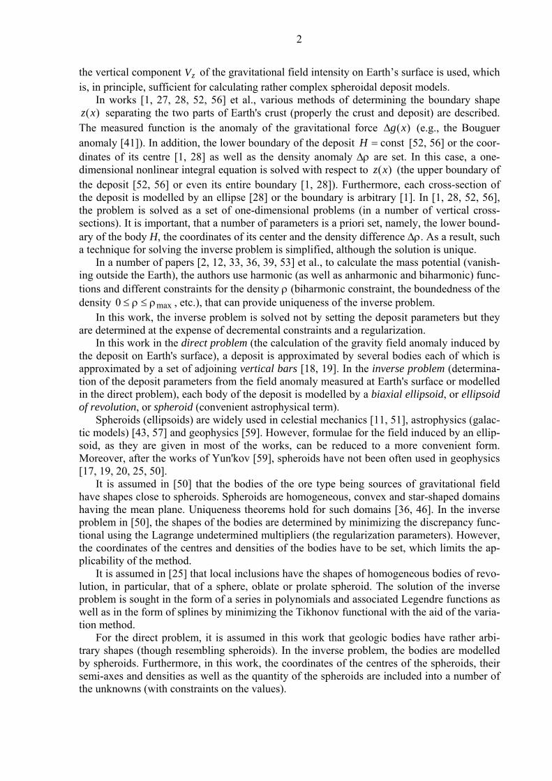
1 Bars and spheroids in gravimetry problem Valery Sizikov 1 and Vadim Evseev 2 1 University ITMO, Kronverksky pr., 49, 197101 Saint-Petersburg, Russia 2 Palacký University Olomouc, tř. 17 listopadu, 1192/12, 771 46 Olomouc, Czech Republic Email: [email protected] and [email protected] Abstract The direct gravimetry problem is solved by dividing each deposit body into a set of vertical adjoining bars, whereas in the inverse problem, each deposit body is modelled by a homogeneous ellipsoid of revolution (sphe- roid). Well-known formulae for the z-component of gravitational intensity for a spheroid are transformed to a convenient form. Parameters of a spheroid are determined by minimizing the Tikhonov smoothing functional with constraints on the parameters, which makes the ill-posed inverse problem by unique and stable. The Bulakh algorithm for initial estimating the depth and mass of a deposit is modified. The proposed technique is illustrated by numerical model examples of deposits in the form of two and five bodies. The inverse gravimetry problem is interpreted as a gravitational tomography problem or, in other words, as ‘introscopy’ of Earth's crust and mantle. Keywords: direct and inverse gravimetry problems, modelling of deposit bodies by spheroids, Tikhonov regularization with constraints, gravitational tomography, introscopy of the Earth 1. Introduction Modelling of deposits is one of principal approaches used in solving the direct and, especially, inverse gravimetry problems. The direct problem is the computation of the gravitational field produced by some modelled deposit on Earth's surface. The inverse problem is the determina- tion of the deposit parameters from the modelled or measured field anomaly (e.g., the Bouguer anomaly) on Earth's surface. For the direct problem, the approximation of a deposit by several bodies of arbitrary shape is one of preferable approaches. In the inverse problem, one should use the bodies of approximately regular form, but which corresponds to the shape of the deposit. 1.1. Models of deposits Some authors use the following simplified models of deposits [7, 10, 37, 47]: in the form of quadrangular truncated pyramids, prisms, cylinders, beams, polyhedrons, parallelepipeds, in- tersecting bars, etc. However, such figures have non-smooth surfaces and generate cumber- some (although not complicated) formulae (see, e.g., [47]). Let us also mention the plane- layered model [42]. In works [17–19], homogeneous (and inhomogeneous) spheroids, or el- lipsoids of revolution, are used as the deposit models and in work [20] et al., spheroids are used for modelling the Earth figure. Such models are effectively applied, e.g., in astrophysics for constructing the galactic models [43, 57]. In this work, we continue to use spheroids for deposit modelling. More complex (algebraic) models have also been developed, namely, 3D models and the inversion of gravity data using discretization grids with thousands and even millions of cells involving the solution of large matrix systems (e.g., [10, 15, 22, 29, 61], et al.). Such ap- proaches are more general and accurate, but more complex and require more computational resources. In some cases, the use of simplified models (e.g., in the form of spheroids) is more obvious and convenient as well as can serve as a good initial approximation when construct- ing complex models. Different kinds of initial data is used for calculating deposits, namely, the intensities of gravitational and magnetic fields [4, 7, 17–19, 34, 41], gravity gradient tensor components [37, 61], seismic data [4, 27], remote sensing from satellites [4, 32, 41], etc. In this work, only
-
Upload
khangminh22 -
Category
Documents
-
view
3 -
download
0
Transcript of Bars and spheroids in gravimetry problem - arXiv
1
Bars and spheroids in gravimetry problem Valery Sizikov1 and Vadim Evseev2 1University ITMO, Kronverksky pr., 49, 197101 Saint-Petersburg, Russia 2 Palacký University Olomouc, tř. 17 listopadu, 1192/12, 771 46 Olomouc, Czech Republic
Email: [email protected] and [email protected] Abstract
The direct gravimetry problem is solved by dividing each deposit body into a set of vertical adjoining bars, whereas in the inverse problem, each deposit body is modelled by a homogeneous ellipsoid of revolution (sphe-roid). Well-known formulae for the z-component of gravitational intensity for a spheroid are transformed to a convenient form. Parameters of a spheroid are determined by minimizing the Tikhonov smoothing functional with constraints on the parameters, which makes the ill-posed inverse problem by unique and stable. The Bulakh algorithm for initial estimating the depth and mass of a deposit is modified. The proposed technique is illustrated by numerical model examples of deposits in the form of two and five bodies. The inverse gravimetry problem is interpreted as a gravitational tomography problem or, in other words, as ‘introscopy’ of Earth's crust and mantle. Keywords:
direct and inverse gravimetry problems, modelling of deposit bodies by spheroids, Tikhonov regularization with constraints, gravitational tomography, introscopy of the Earth 1. Introduction Modelling of deposits is one of principal approaches used in solving the direct and, especially, inverse gravimetry problems. The direct problem is the computation of the gravitational field produced by some modelled deposit on Earth's surface. The inverse problem is the determina-tion of the deposit parameters from the modelled or measured field anomaly (e.g., the Bouguer anomaly) on Earth's surface. For the direct problem, the approximation of a deposit by several bodies of arbitrary shape is one of preferable approaches. In the inverse problem, one should use the bodies of approximately regular form, but which corresponds to the shape of the deposit. 1.1. Models of deposits Some authors use the following simplified models of deposits [7, 10, 37, 47]: in the form of quadrangular truncated pyramids, prisms, cylinders, beams, polyhedrons, parallelepipeds, in-tersecting bars, etc. However, such figures have non-smooth surfaces and generate cumber-some (although not complicated) formulae (see, e.g., [47]). Let us also mention the plane-layered model [42]. In works [17–19], homogeneous (and inhomogeneous) spheroids, or el-lipsoids of revolution, are used as the deposit models and in work [20] et al., spheroids are used for modelling the Earth figure. Such models are effectively applied, e.g., in astrophysics for constructing the galactic models [43, 57]. In this work, we continue to use spheroids for deposit modelling.
More complex (algebraic) models have also been developed, namely, 3D models and the inversion of gravity data using discretization grids with thousands and even millions of cells involving the solution of large matrix systems (e.g., [10, 15, 22, 29, 61], et al.). Such ap-proaches are more general and accurate, but more complex and require more computational resources. In some cases, the use of simplified models (e.g., in the form of spheroids) is more obvious and convenient as well as can serve as a good initial approximation when construct-ing complex models.
Different kinds of initial data is used for calculating deposits, namely, the intensities of gravitational and magnetic fields [4, 7, 17–19, 34, 41], gravity gradient tensor components [37, 61], seismic data [4, 27], remote sensing from satellites [4, 32, 41], etc. In this work, only
2
the vertical component zV of the gravitational field intensity on Earth’s surface is used, which is, in principle, sufficient for calculating rather complex spheroidal deposit models.
In works [1, 27, 28, 52, 56] et al., various methods of determining the boundary shape )(xz separating the two parts of Earth's crust (properly the crust and deposit) are described.
The measured function is the anomaly of the gravitational force )(xgΔ (e.g., the Bouguer anomaly [41]). In addition, the lower boundary of the deposit const=H [52, 56] or the coor-dinates of its centre [1, 28] as well as the density anomaly Δρ are set. In this case, a one-dimensional nonlinear integral equation is solved with respect to )(xz (the upper boundary of the deposit [52, 56] or even its entire boundary [1, 28]). Furthermore, each cross-section of the deposit is modelled by an ellipse [28] or the boundary is arbitrary [1]. In [1, 28, 52, 56], the problem is solved as a set of one-dimensional problems (in a number of vertical cross-sections). It is important, that a number of parameters is a priori set, namely, the lower bound-ary of the body H, the coordinates of its center and the density difference Δρ. As a result, such a technique for solving the inverse problem is simplified, although the solution is unique.
In a number of papers [2, 12, 33, 36, 39, 53] et al., to calculate the mass potential (vanish-ing outside the Earth), the authors use harmonic (as well as anharmonic and biharmonic) func-tions and different constraints for the density ρ (biharmonic constraint, the boundedness of the density max0 ρ≤ρ≤ , etc.), that can provide uniqueness of the inverse problem.
In this work, the inverse problem is solved not by setting the deposit parameters but they are determined at the expense of decremental constraints and a regularization.
In this work in the direct problem (the calculation of the gravity field anomaly induced by the deposit on Earth's surface), a deposit is approximated by several bodies each of which is approximated by a set of adjoining vertical bars [18, 19]. In the inverse problem (determina-tion of the deposit parameters from the field anomaly measured at Earth's surface or modelled in the direct problem), each body of the deposit is modelled by a biaxial ellipsoid, or ellipsoid of revolution, or spheroid (convenient astrophysical term).
Spheroids (ellipsoids) are widely used in celestial mechanics [11, 51], astrophysics (galac-tic models) [43, 57] and geophysics [59]. However, formulae for the field induced by an ellip-soid, as they are given in most of the works, can be reduced to a more convenient form. Moreover, after the works of Yun'kov [59], spheroids have not been often used in geophysics [17, 19, 20, 25, 50].
It is assumed in [50] that the bodies of the ore type being sources of gravitational field have shapes close to spheroids. Spheroids are homogeneous, convex and star-shaped domains having the mean plane. Uniqueness theorems hold for such domains [36, 46]. In the inverse problem in [50], the shapes of the bodies are determined by minimizing the discrepancy func-tional using the Lagrange undetermined multipliers (the regularization parameters). However, the coordinates of the centres and densities of the bodies have to be set, which limits the ap-plicability of the method.
It is assumed in [25] that local inclusions have the shapes of homogeneous bodies of revo-lution, in particular, that of a sphere, oblate or prolate spheroid. The solution of the inverse problem is sought in the form of a series in polynomials and associated Legendre functions as well as in the form of splines by minimizing the Tikhonov functional with the aid of the varia-tion method.
For the direct problem, it is assumed in this work that geologic bodies have rather arbi-trary shapes (though resembling spheroids). In the inverse problem, the bodies are modelled by spheroids. Furthermore, in this work, the coordinates of the centres of the spheroids, their semi-axes and densities as well as the quantity of the spheroids are included into a number of the unknowns (with constraints on the values).
3
1.2.Comparison with tomography The inverse gravimetry problem is often solved as a set of two-dimensional problems.
First, the density anomaly distribution is determined for some of the vertical cross-sections, and, second, a three-dimensional (volumetric) image is composed. This procedure quite resembles approaches typical for different types of tomography [30, 31, 44, 45, 58], and first of all, those of the X-ray computerized tomography (XCT) and magnetic resonance to-mography (MRT) [31, 44, 45, 58]. In this work, which uses spheroids (as in [17–19]), the three-dimensional problem is solved which is equivalent to the three-dimensional tomography [9]. It is therefore proposed to refer the inverse gravimetry problem to the class of tomogra-phy problems (which was already done in [17–19]) and to call the inverse gravimetry problem the gravitational tomography problem. Moreover, a special feature of the considered problem is that it enables to 'look' inside Earth by means of mathematical processing instead of drilling wells which reminds of the process of introscopy being typical also of tomography. Therefore, it is also proposed to call the inverse gravimetry problem the Earth introscopy problem [17–19]. The proposed interpretations suggest the possibility of application of the extensive devel-opments in the field of computerized tomography, in particular, XCT and MRT to solve the inverse gravimetry problem.
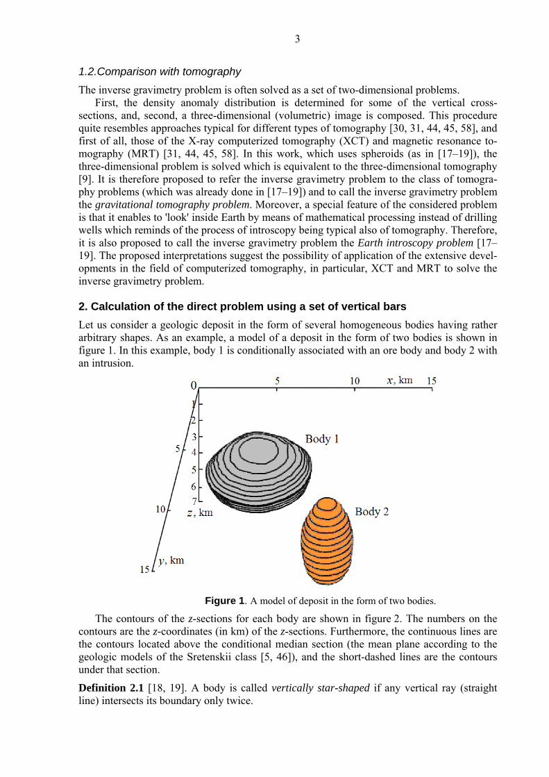
2. Calculation of the direct problem using a set of vertical bars Let us consider a geologic deposit in the form of several homogeneous bodies having rather arbitrary shapes. As an example, a model of a deposit in the form of two bodies is shown in figure 1. In this example, body 1 is conditionally associated with an ore body and body 2 with an intrusion.
Figure 1. A model of deposit in the form of two bodies.
The contours of the z-sections for each body are shown in figure 2. The numbers on the contours are the z-coordinates (in km) of the z-sections. Furthermore, the continuous lines are the contours located above the conditional median section (the mean plane according to the geologic models of the Sretenskii class [5, 46]), and the short-dashed lines are the contours under that section.
Definition 2.1 [18, 19]. A body is called vertically star-shaped if any vertical ray (straight line) intersects its boundary only twice.

4
Figure 2. The contours of the z-sections of the modelled deposit bodies.
Let const=ρ be the density of a body and let the body be vertically star-shaped. Let us approximate it by a set of elementary vertical bars with cross-sections ydxd ′′ and with boundaries ),(minmin yxzz ′′′=′ and ),(maxmax yxzz ′′′=′ (the roof and bottom according to the terminology of [5]) (figure 3). In the direct as well as inverse problems, only the z-components of the gravitational intensity induced by deposit bodies are considered.
Figure 3. The elementary cell zdydxd ′′′ and elementary vertical bar of a deposit body.

5
Lemma 2.1 (Gravitational field induced by an elementary bar). The intensity zV induced by an elementary bar at a point )0,,( yx equals [19]
ydxdzyyxxzyyxx
yxdVz ′′⎥⎥⎦
⎤
⎢⎢⎣
⎡
′+′−+′−−
′+′−+′−ργ=
2max
222min
22 )()(1
)()(1)0,,( , (2.1)
where γ is the gravitational constant and zyx ′′′ ,, are the coordinates of the elementary cell.
Proof. The z-intensity induced by an elementary cell zdydxd ′′′ of a deposit body at a point )0,,( yx (figure 3) equals
zdydxdr
zr
zdydxdd z ′′′′γρ
=θ′′′ρ
γ= 32 cosv , (2.2)
where 222 )()( zyyxxr ′+′−+′−= . Then, the z-intensity induced by an elementary bar at the point )0,,( yx is equal to the integral of the expression (2.2)
ydxdzdrzdyxdV
z
z
z
z zz ′′⎥⎦⎤
⎢⎣⎡ ′′
γρ== ∫∫′
′
′
′
max
min
max
min 3)0,,( v , (2.3)
which yields the expression (2.1). □
Corollary 2.1. The integration of (2.1) over all elementary bars adjacent to each other from ),(minmin yxzz ′′′=′ to ),(maxmax yxzz ′′′=′ yields the intensity )0,,( yxVz induced by the en-
tire body at the point )0,,( yx . But if the condition for a body being vertically star-shaped is not satisfied, the 'voids' must be excluded from the integration regions ],[ maxmin zz ′′ .
Remark. Strictly speaking, in the direct problem, a body is not modeled by a set of vertical bars. The bars are used only for the calculation of the field. Furthermore, a body can have an arbitrary shape.
This approach for modelling the direct problem is rather simple and effective, which is confirmed by the numerical examples (see the examples in [18, 19] and in this paper below). 3. Modelling the inverse problem using spheroids Definition 3.1. An ellipsoid is a body bounded by the surface
1222222 =ζ+η+ξ cba , where a, b and c are the semiaxes of the ellipsoid and the origin of the coordinate system is placed at the body centre.
In this work, biaxial ellipsoids, or ellipsoids of revolution around axis z, referred to as spheroids for short further in the text, are considered. In works [11, 20, 51, 59], formulae for the potential V and intensity components xV , yV , zV of a spheroid have been deduced. How-ever, formulae have not been reduced to a certain convenient form in the indicated works. This is attempted to be done further in this work for zV .
Remark. Following usual practice [11], the term ellipsoid (spheroid) is used to refer to the body bounded by the surface as well as only the surface.
Consider an oblate spheroid for which cba >= . In [11, 51, 59], a coordinate system x, y, z was introduced with the origin at the centre of the spheroid and with the z-axis directed ver-tically upwards along the minor axis c of the spheroid. For this case, formulae have been de-duced for the potential ),,( zyxV and intensity components ),,( zyxVx , ),,( zyxVy ,
),,( zyxVz induced by the spheroid at a point ),,( zyx outside the spheroid.
6
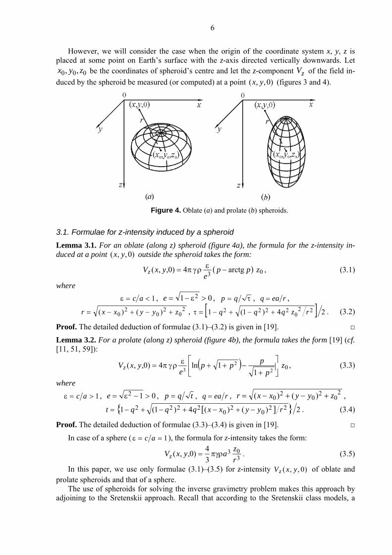
However, we will consider the case when the origin of the coordinate system x, y, z is placed at some point on Earth’s surface with the z-axis directed vertically downwards. Let
000 ,, zyx be the coordinates of spheroid’s centre and let the z-component zV of the field in-duced by the spheroid be measured (or computed) at a point )0,,( yx (figures 3 and 4).
Figure 4. Oblate (a) and prolate (b) spheroids.
3.1. Formulae for z-intensity induced by a spheroid Lemma 3.1. For an oblate (along z) spheroid (figure 4a), the formula for the z-intensity in-duced at a point )0,,( yx outside the spheroid takes the form:
( ) 034)0,,( zppe
yxVz arctg−εργπ= , (3.1)
where 1<=ε ac , 01 2 >ε−=e , τ= qp , reaq = ,
20
20
20 )()( zyyxxr +−+−= , [ ] 24)1(1 22
02222 rzqqq +−+−=τ . (3.2)
Proof. The detailed deduction of formulae (3.1)–(3.2) is given in [19]. □
Lemma 3.2. For a prolate (along z) spheroid (figure 4b), the formula takes the form [19] (cf. [11, 51, 59]):
( ) 022
3 11ln4)0,,( z
pppp
eyxVz ⎥
⎦
⎤⎢⎣
⎡
+−++εργπ= , (3.3)
where 1>=ε ac , 012 >−ε=e , tqp = , reaq = , 2
02
02
0 )()( zyyxxr +−+−= ,
2)()(4)1(1 }{ 220
20
2222 ][ ryyxxqqqt −+−+−+−= . (3.4)
Proof. The detailed deduction of formulae (3.3)–(3.4) is given in [19]. □
In case of a sphere ( 1==ε ac ), the formula for z-intensity takes the form:
303
34)0,,(
rzayxVz πγρ= . (3.5)
In this paper, we use only formulae (3.1)–(3.5) for z-intensity )0,,( yxVz of oblate and prolate spheroids and that of a sphere.
The use of spheroids for solving the inverse gravimetry problem makes this approach by adjoining to the Sretenskii approach. Recall that according to the Sretenskii class models, a
7
body possesses the mean plane P if any straight line perpendicular to this plane intersects the body surface only at two points on different sides of the plane P. If a geological body pos-sesses a mean plane, its gravity center is inside the body, and its density is constant (and is given!), then the inverse problem (determining the body shape from the potential) has a unique solution. Our approach extends the Sretenskii approach because (see section 5) we do not assume that the density ρ is given, but include it into a number of the sought parameters (along with parameters 000 ,,,, zyxa ε ). Furthermore, the uniqueness of the solution is pro-vided by introducing constraints on the parameters and a regularization1 (see also below).
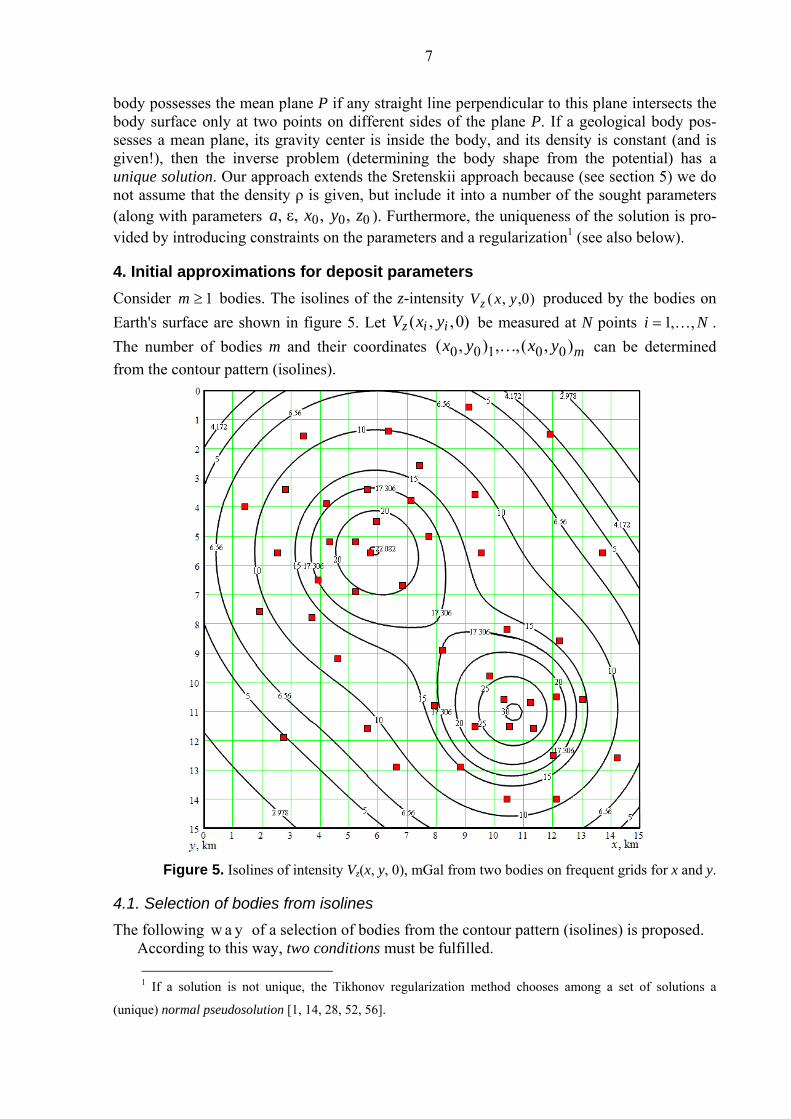
4. Initial approximations for deposit parameters Consider 1≥m bodies. The isolines of the z-intensity )0,,( yxVz produced by the bodies on Earth's surface are shown in figure 5. Let )0,,( iiz yxV be measured at N points Ni ,,1K= . The number of bodies m and their coordinates myxyx ),(,,),( 00100 K can be determined from the contour pattern (isolines).
Figure 5. Isolines of intensity Vz(x, y, 0), mGal from two bodies on frequent grids for x and y.
4.1. Selection of bodies from isolines The following w a y of a selection of bodies from the contour pattern (isolines) is proposed.
According to this way, two conditions must be fulfilled. 1 If a solution is not unique, the Tikhonov regularization method chooses among a set of solutions a
(unique) normal pseudosolution [1, 14, 28, 52, 56].
8
1. Valley in intensity zV between some two maxima (poles, peaks, hills) is not less than %20≈ of intensities in poles (as in the Rayleigh criterion [45]).
2. The noise level zVδ does not exceed 20% of the intensities in poles2. If both conditions are fulfilled, we assume that two peaks (and hence two bodies) are de-
termined from isolines. For example, figure 5 shows two poles with intensities 221 ≈zV and
302 ≈zV . We assume 262)( 21 ≈+= zzz VVV . The intensity between the poles is 17≈zv , i.e. the valley is %35346.0)( ≈=− zzz VV v . In this case, the noise level is %5≈δ zV (see section 6). As a result, both conditions are fulfilled and we can assume that two bodies are determined from isolines (see also figure 8 below).
The valley of 20% corresponds to some minimum distance between bodies in which they are delimited without mathematical processing. If the distance between the poles in figures 5 and 8 was 4≈ km, the valley would be equal to %20≈ , i.e. 4 km is the limiting distance be-tween the poles in which they are resolved. If the valley is less than %20≈ , the bodies can be resolved mainly mathematically. After separation of the bodies, we can make an estimate of some parameters of the deposit.
4.2. Bulakh algorithm for estimating the depth and mass of a deposit
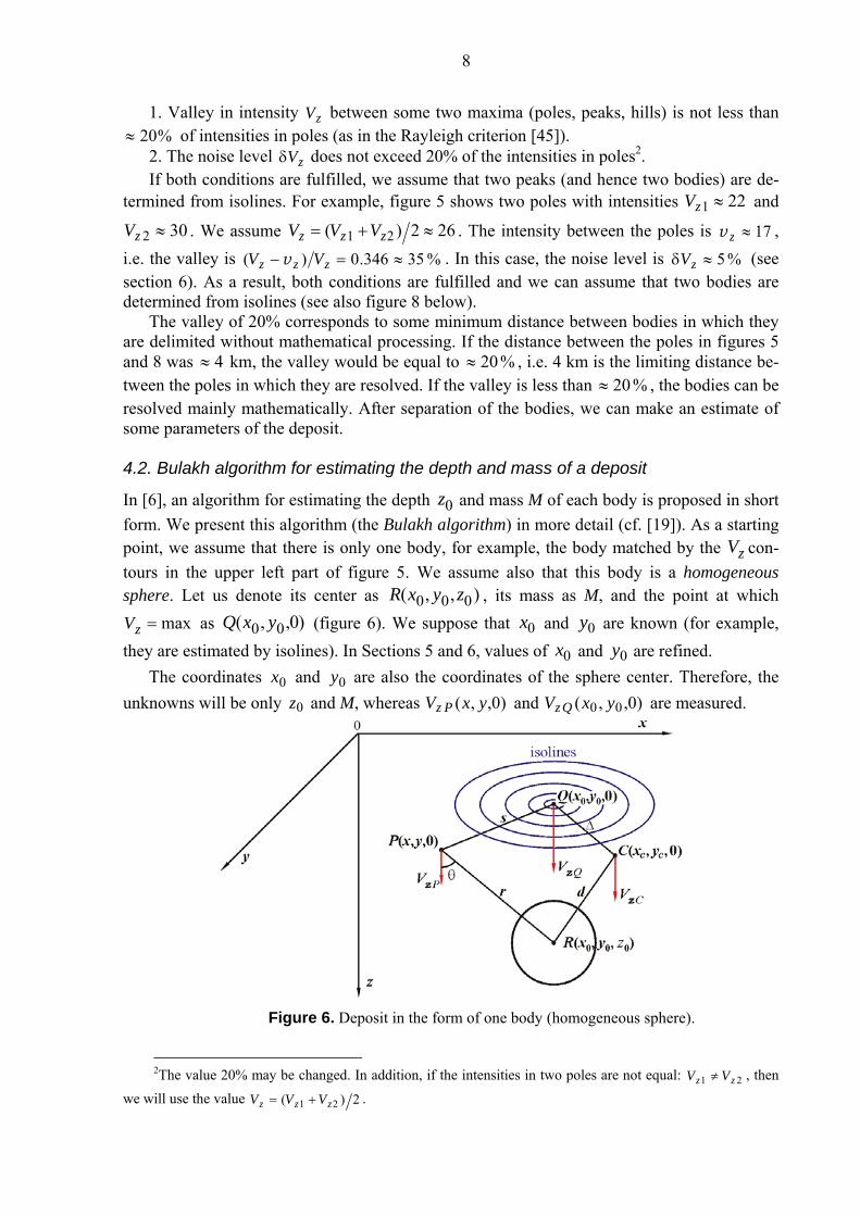
In [6], an algorithm for estimating the depth 0z and mass M of each body is proposed in short form. We present this algorithm (the Bulakh algorithm) in more detail (cf. [19]). As a starting point, we assume that there is only one body, for example, the body matched by the zV con-tours in the upper left part of figure 5. We assume also that this body is a homogeneous sphere. Let us denote its center as ),,( 000 zyxR , its mass as M, and the point at which
max=zV as )0,,( 00 yxQ (figure 6). We suppose that 0x and 0y are known (for example, they are estimated by isolines). In Sections 5 and 6, values of 0x and 0y are refined.
The coordinates 0x and 0y are also the coordinates of the sphere center. Therefore, the unknowns will be only 0z and M, whereas )0,,( yxV Pz and )0,,( 00 yxV Qz are measured.
Figure 6. Deposit in the form of one body (homogeneous sphere).
2The value 20% may be changed. In addition, if the intensities in two poles are not equal: 21 zz VV ≠ , then
we will use the value 2)( 21 zzz VVV += .
9
Lemma 4.1. The z-intensity )0,,( yxVz at point )0,,( yxP equals
( ) 2322
0
0
sz
zMV Pz+
γ= , (4.1)
where 20
20 )()( yyxxs −+−= is the distance between P and Q.
Proof. We have
rz
rM
rMyxVV zPz
022 cos)0,,( ⋅γ=θγ=≡ ,
where 220 szr += is the distance between P and R, and θ is the angle between PzV and r,
which implies (4.1). □
Corollary 4.1.The z-intensity at point Q equals
20
max00 )0,,(zMVyxVV zzQz γ==≡ . (4.2)
Relations (4.1) and (4.2) can be considered as a system of two equations with respect to
0z and M. Using the notation QzPz VV=ν , we obtain 2320
30 ]1)[()( +=ν szsz or
ν=⎟⎠
⎞⎜⎝
⎛+μ
μ23
2
2
1, (4.3)
where sz0=μ . Relation (4.3) is an equation with respect to )(νμ=μ at given (measured) ν. Its solution is
32
32
1)(
ν−ν=νμ , )1,0(∈ν , ),0( ∞∈μ . (4.4)
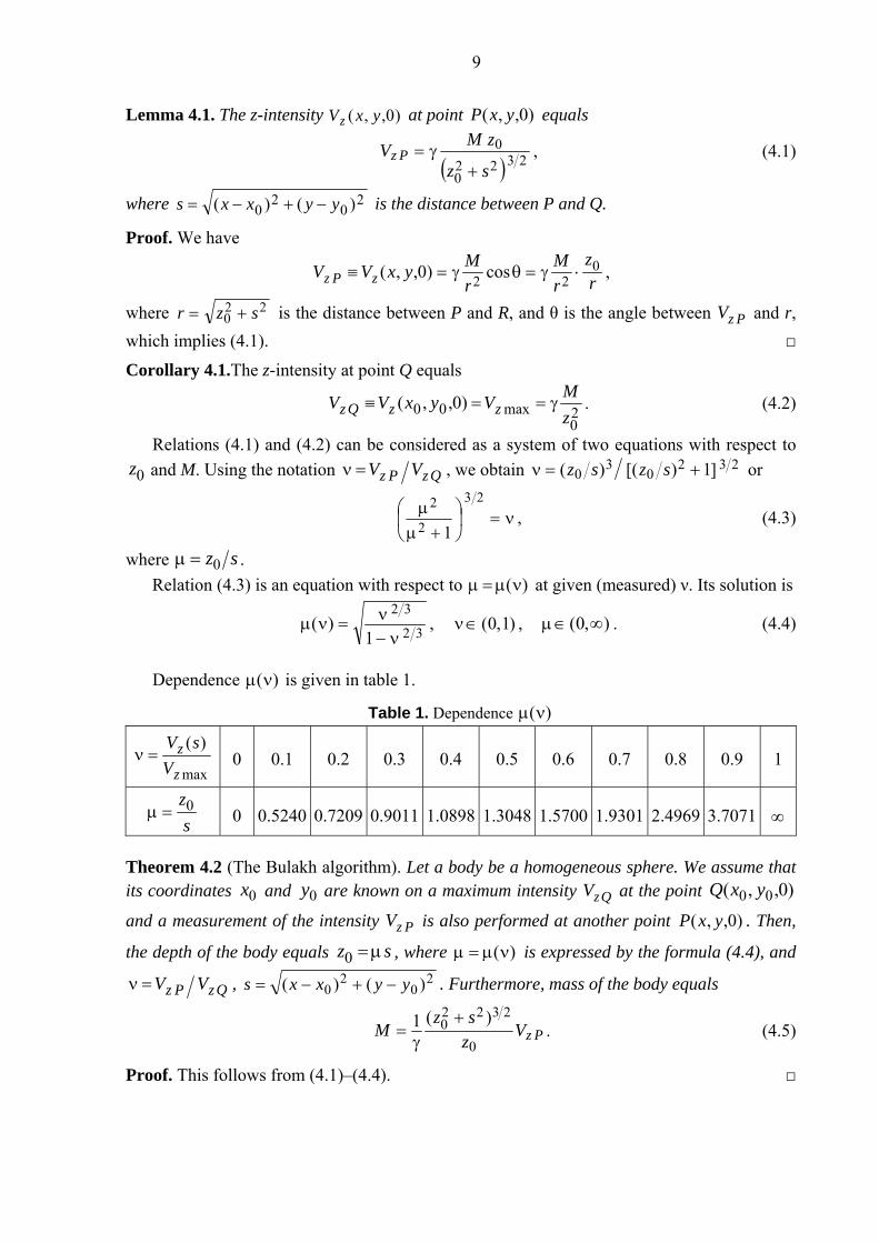
Dependence )(νμ is given in table 1.
Table 1. Dependence )(νμ
max
)(
z
zV
sV=ν 0 0.1 0.2 0.3 0.4 0.5 0.6 0.7 0.8 0.9 1
sz0=μ 0 0.5240 0.7209 0.9011 1.0898 1.3048 1.5700 1.9301 2.4969 3.7071 ∞
Theorem 4.2 (The Bulakh algorithm). Let a body be a homogeneous sphere. We assume that its coordinates 0x and 0y are known on a maximum intensity QzV at the point )0,,( 00 yxQ
and a measurement of the intensity PzV is also performed at another point )0,,( yxP . Then,
the depth of the body equals sz μ=0 , where )(νμ=μ is expressed by the formula (4.4), and
QzPz VV=ν , 20
20 )()( yyxxs −+−= . Furthermore, mass of the body equals
PzVzsz
M0
23220 )(1 +
γ= . (4.5)
Proof. This follows from (4.1)–(4.4). □
10
Remark 4.1. It is preferable that the chosen point P is located away from the other bodies, e.g., at x < 5 km and y < 5 km in figure 5. One can make several estimates of μ (and 0z ) from a few points P and average the result. This procedure should then be performed for each body.
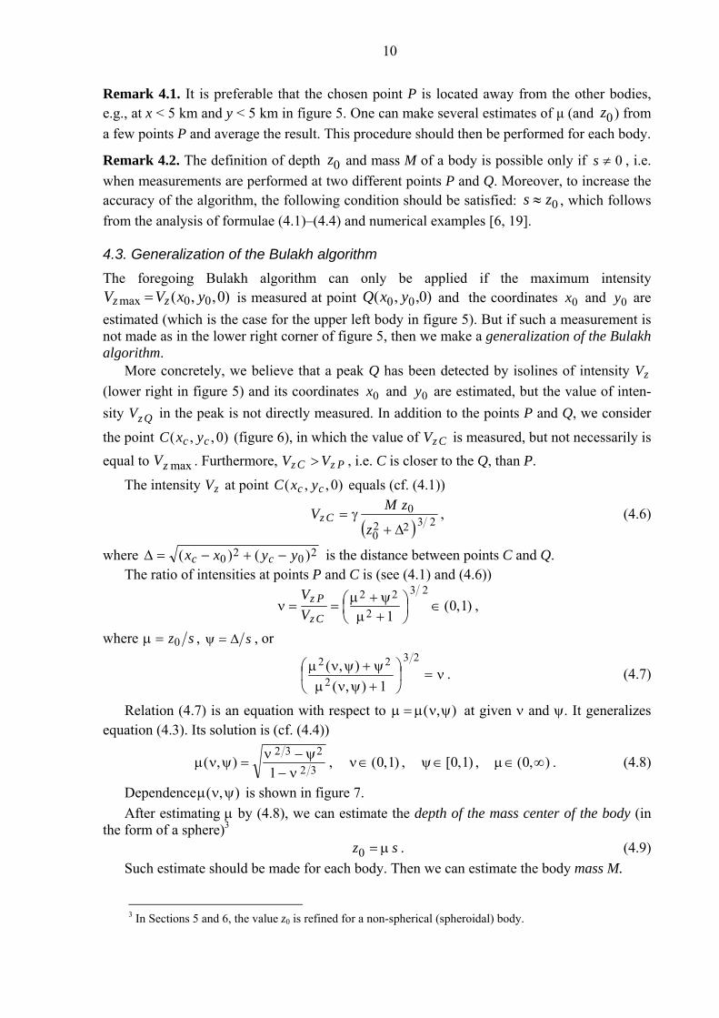
Remark 4.2. The definition of depth 0z and mass M of a body is possible only if 0≠s , i.e. when measurements are performed at two different points P and Q. Moreover, to increase the accuracy of the algorithm, the following condition should be satisfied: 0zs ≈ , which follows from the analysis of formulae (4.1)–(4.4) and numerical examples [6, 19]. 4.3. Generalization of the Bulakh algorithm The foregoing Bulakh algorithm can only be applied if the maximum intensity
)0,,( 00max yxVV zz = is measured at point )0,,( 00 yxQ and the coordinates 0x and 0y are estimated (which is the case for the upper left body in figure 5). But if such a measurement is not made as in the lower right corner of figure 5, then we make a generalization of the Bulakh algorithm.
More concretely, we believe that a peak Q has been detected by isolines of intensity zV (lower right in figure 5) and its coordinates 0x and 0y are estimated, but the value of inten-sity QzV in the peak is not directly measured. In addition to the points P and Q, we consider
the point )0,,( cc yxC (figure 6), in which the value of CzV is measured, but not necessarily is equal to maxzV . Furthermore, PzCz VV > , i.e. C is closer to the Q, than P.
The intensity zV at point )0,,( cc yxC equals (cf. (4.1))
( ) 2322
0
0
Δ+γ=
z
zMV Cz , (4.6)
where 2020 )()( yyxx cc −+−=Δ is the distance between points C and Q. The ratio of intensities at points P and C is (see (4.1) and (4.6))
)1,0(1
23
2
22∈⎟
⎠⎞
⎜⎝⎛
+μψ+μ==ν
Cz
PzVV
,
where sz0=μ , sΔ=ψ , or
ν=⎟⎠
⎞⎜⎝
⎛+ψνμψ+ψνμ
23
2
22
1),(),( . (4.7)
Relation (4.7) is an equation with respect to ),( ψνμ=μ at given ν and ψ. It generalizes equation (4.3). Its solution is (cf. (4.4))
32
232
1),(
ν−ψ−ν=ψνμ , )1,0(∈ν , )1,0[∈ψ , ),0( ∞∈μ . (4.8)
Dependence ),( ψνμ is shown in figure 7. After estimating μ by (4.8), we can estimate the depth of the mass center of the body (in
the form of a sphere)3 sz μ=0 . (4.9)
Such estimate should be made for each body. Then we can estimate the body mass M.
3 In Sections 5 and 6, the value z0 is refined for a non-spherical (spheroidal) body.

11
Figure 7. Dependence ),( ψνμ (see (4.8)).
Furthermore, if zV is not measured at the point )0,,( 00 yx of its maximum, but neverthe-less, the coordinates 00 , yx are estimated, then one can use the measurement of zV at some point )0,,( cc yxC and obtain an estimate of the mass from (4.6):
CzVzz
M0
23220 )(1 Δ+
γ= . (4.10)
But if zV is measured at the point )0,,( 00 yx of its maximum, one can obtain from (4.2)
max20
1zVzM
γ= . (4.11)
Remark 4.3. Formula (4.10) is similar to the formula (4.5) by writing. Nevertheless, these formulae differ essentially, namely, the point P can not turn into Q (s is strictly greater than zero), and point C may be at the maximum point Q (Δ may be zero). Therefore, formulae (4.6)–(4.8) and (4.10) may be considered as a generalization of the Bulakh algorithm.
The obtained result can be formulated in the following theorem.
Theorem 4.3 (generalization of the Bulakh algorithm). Let a body be a homogeneous sphere. Let us assume that in some way (e.g., from isolines of intensity zV ), we select a local maxi-mum (peak) Q and estimate its coordinates 0x and 0y , but does not measure the intensity
QzV . Let us assume that we measure the intensity PzV at the point )0,,( yxP and CzV at the
point )0,,( cc yxC , more closed to Q. Then the body depth is sz μ=0 , where ),( ψνμ=μ is
expressed by the formula (4.8), and CzPz VV=ν , sΔ=ψ , 20
20 )()( yyxxs −+−= ,
),0[)()( 2020 syyxx cc ∈−+−=Δ , and the body mass M is expressed by the formula (4.10). But if 0=Δ (C turns into Q), then this theorem turns into theorem 4.2.

12
Remark 4.4. Let the coordinates and distances x, y, z, s, r, Δ, d be expressed in kilometers, the mass M in billions of tons, and the gravitational intensity (anomaly) zV in mGal. Then formulae (4.10) and (4.11) take the form
CzVzz
M0
23220 )(
15.0Δ+
= , (4.12)
max2015.0 zVzM = . (4.13)
These results generalize the algorithm presented in [6] and yield a good initial approxima-tion to 0z and M (as well as to 0x and 0y ) for each body. In the next section, we demonstrate how to make more precise these (and other) parameters of non-spherical (spheroidal) bodies. 5. Refinement of the deposit parameters Consider the problem of refining the parameters of spheroids which approximate the bodies of a deposit. Let )0,,(~~
iiziz yxVV ≡ , Ni ,,1K= be the values of zV measured (with errors) at
a series of points )0,,( ii yx , Ni ,,1K= on Earth’s surface (in particular, on a ship), where N is the number of measurement points. Let the values of )0,,( iiziz yxVV ≡ are calculated using formulae (3.1), (3.3) or (3.5). Let k be the number of sought parameters for each of the m spheroids (the types of parameters are listed below), in total mk parameters. Let us denote the deposit parameters as jp , mkj ,,1K= . 5.1. Application of the Tikhonov regularization method with constraints The determination of the deposit parameters is an ill-posed problem, viz., unstable and hav-ing, generally speaking, a non-unique solution [3, 5, 6, 8, 17–19, 26, 30, 33, 46–49]. Even if a body is star-shaped and has the Sretenskii mean plane, the solution is anyway non-unique if the body density ρ is not given. A quite effective way to eliminate the non-uniqueness of the solution is to use constraints on the solution with the Tikhonov regularization method.
We will solve this problem by minimizing the Tikhonov smoothing (parametric) func-tional [56] (cf. [3, 10, 15, 16, 24, 25, 30, 55, 61]) in two variants [17–19]:
( )∑ ∑= =
=−α+−≡N
i pp
mk
jjjjiziz
mkppqVVF
1 ,,2
1mid
21
1min)(~K
(5.1)
or
( )∑ ∑= =
=α+−≡N
i pp
mk
jjjiziz
mkpqVVF
1 ,,1
222
1min~K
, (5.2)
where jq are the weights and 0>α is the regularization parameter (the Lagrange multiplier).
Functional (5.1) or (5.2) contains the discrepancy (or the data misfit) ∑ =−
Ni iziz VV1
2)~(
and stabilizer ∑ =−
mkj jjj ppq1
2mid )( or∑ =
mkj jj pq1
2 . In works [40, 60] et al., different vari-
ants of the stabilizer are considered conformably to the geophysical inversion problem with the purpose of focusing the noisy and insufficiently clear geophysical inverse images [10, 55, 61]. In [29], the problem of minimizing the objective function using discrepancy and weight functions is considered. Furthermore, the objective function includes a priori information and additional geophysical and geological constraints. The minimization of the objective function is achieved by using a generalized subspace inversion algorithm.
13
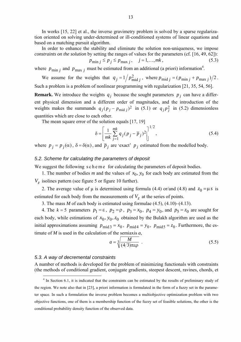
In works [15, 22] et al., the inverse gravimetry problem is solved by a sparse regulariza-tion oriented on solving under-determined or ill-conditioned systems of linear equations and based on a matching pursuit algorithm.
In order to enhance the stability and eliminate the solution non-uniqueness, we impose constraints on the solution by setting the ranges of values for the parameters (cf. [16, 49, 62]): jjj ppp maxmin ≤≤ , mkj ,,1K= , (5.3)
where jpmin and jpmax must be estimated from an additional (a priori) information4.
We assume for the weights that 2mid1 jj pq = , where 2)( maxminmid jjj ppp += .
Such a problem is a problem of nonlinear programming with regularization [21, 35, 54, 56].
Remark. We introduce the weights jq because the sought parameters jp can have a differ-ent physical dimension and a different order of magnitudes, and the introduction of the weights makes the summands 2
mid )( jjj ppq − in (5.1) or 2jj pq in (5.2) dimensionless
quantities which are close to each other. The mean square error of the solution equals [17, 19]
21
12)(1
⎥⎥⎦
⎤
⎢⎢⎣
⎡−=δ ∑
=
mk
jjjj ppq
mk, (5.4)
where )(α= jj pp , )(αδ=δ , and jp are ‘exact’ jp estimated from the modelled body. 5.2. Scheme for calculating the parameters of deposit We suggest the following s c h e m e for calculating the parameters of deposit bodies.
1. The number of bodies m and the values of 00, yx for each body are estimated from the
zV isolines pattern (see figure 5 or figure 10 further). 2. The average value of μ is determined using formula (4.4) or/and (4.8) and sz μ=0 is
estimated for each body from the measurements of zV at the series of points. 3. The mass M of each body is estimated using formulae (4.5), (4.10)–(4.13). 4. The 5=k parameters ε=1p , ρ=2p , 03 xp = , 04 yp = , and 05 zp = are sought for
each body, while estimations of 000 ,, zyx obtained by the Bulakh algorithm are used as the initial approximations assuming 03mid xp = , 04mid yp = , 05mid zp = . Furthermore, the es-timate of M is used in the calculation of the semiaxis a,
3)34( περ
= Ma . (5.5)
5.3. A way of decremental constraints A number of methods is developed for the problem of minimizing functionals with constraints (the methods of conditional gradient, conjugate gradients, steepest descent, ravines, chords, et
4 In Section 6.1, it is indicated that the constraints can be estimated by the results of preliminary study of
the region. We note also that in [23], a priori information is formulated in the form of a fuzzy set in the parame-
ter space. In such a formulation the inverse problem becomes a multiobjective optimization problem with two
objective functions, one of them is a membership function of the fuzzy set of feasible solutions, the other is the
conditional probability density function of the observed data.
14
al.) [21, 54, 56]. In exploration geophysics, the method of gradient descent is often used (the works of Kantorovich, et al.) [5]. However, the point of convergence in this method strongly depends on the initial approximation of the solution. Besides that, this method is using the de-rivatives of a functional and is not using constraints on solution.
In this paper, for minimizing the functional (5.1) or (5.2), we use a modification of the co-ordinate descent method [13] which is, to a certain degree, effective in case when constraints have form (5.3). A special feature of this method is that it does not allow the solution to fall outside the constraints (5.3), thus providing stability and convergence of the solution within the interval (‘corridor’) given by inequalities (5.3). However, it is not always possible to set a sufficiently narrow interval. In this case, first, one should set wide constraints, and then one must do more narrow constraints iteratively so that the solution does not go out of the interval (5.3). The following examples are solved in exactly this way. We call this method a way of decremental constraints.
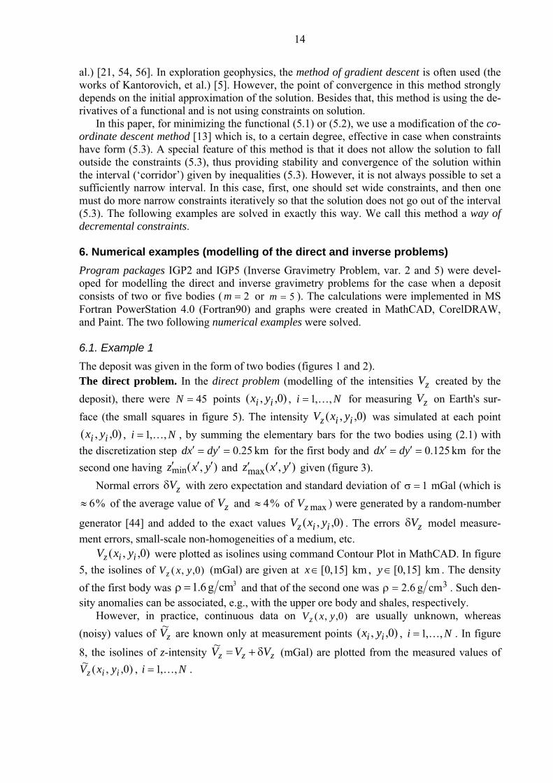
6. Numerical examples (modelling of the direct and inverse problems) Program packages IGP2 and IGP5 (Inverse Gravimetry Problem, var. 2 and 5) were devel-oped for modelling the direct and inverse gravimetry problems for the case when a deposit consists of two or five bodies ( 2=m or 5=m ). The calculations were implemented in MS Fortran PowerStation 4.0 (Fortran90) and graphs were created in MathCAD, CorelDRAW, and Paint. The two following numerical examples were solved. 6.1. Example 1 The deposit was given in the form of two bodies (figures 1 and 2). The direct problem. In the direct problem (modelling of the intensities zV created by the deposit), there were 45=N points )0,,( ii yx , Ni ,,1K= for measuring zV on Earth's sur-face (the small squares in figure 5). The intensity )0,,( iiz yxV was simulated at each point
)0,,( ii yx , Ni ,,1K= , by summing the elementary bars for the two bodies using (2.1) with the discretization step km 25.0=′=′ ydxd for the first body and km 125.0=′=′ ydxd for the second one having ),(min yxz ′′′ and ),(max yxz ′′′ given (figure 3).
Normal errors zVδ with zero expectation and standard deviation of 1=σ mGal (which is %6≈ of the average value of zV and %4≈ of maxzV ) were generated by a random-number
generator [44] and added to the exact values )0,,( iiz yxV . The errors zVδ model measure-ment errors, small-scale non-homogeneities of a medium, etc.
)0,,( iiz yxV were plotted as isolines using command Contour Plot in MathCAD. In figure 5, the isolines of )0,,( yxVz (mGal) are given at km ]15,0[∈x , km ]15,0[∈y . The density of the first body was 3cmg 6.1=ρ and that of the second one was 3cmg 6.2=ρ . Such den-sity anomalies can be associated, e.g., with the upper ore body and shales, respectively.
However, in practice, continuous data on )0,,( yxVz are usually unknown, whereas (noisy) values of zV~ are known only at measurement points )0,,( ii yx , Ni ,,1K= . In figure
8, the isolines of z-intensity zzz VVV δ+=~ (mGal) are plotted from the measured values of )0,,(~
iiz yxV , Ni ,,1K= .
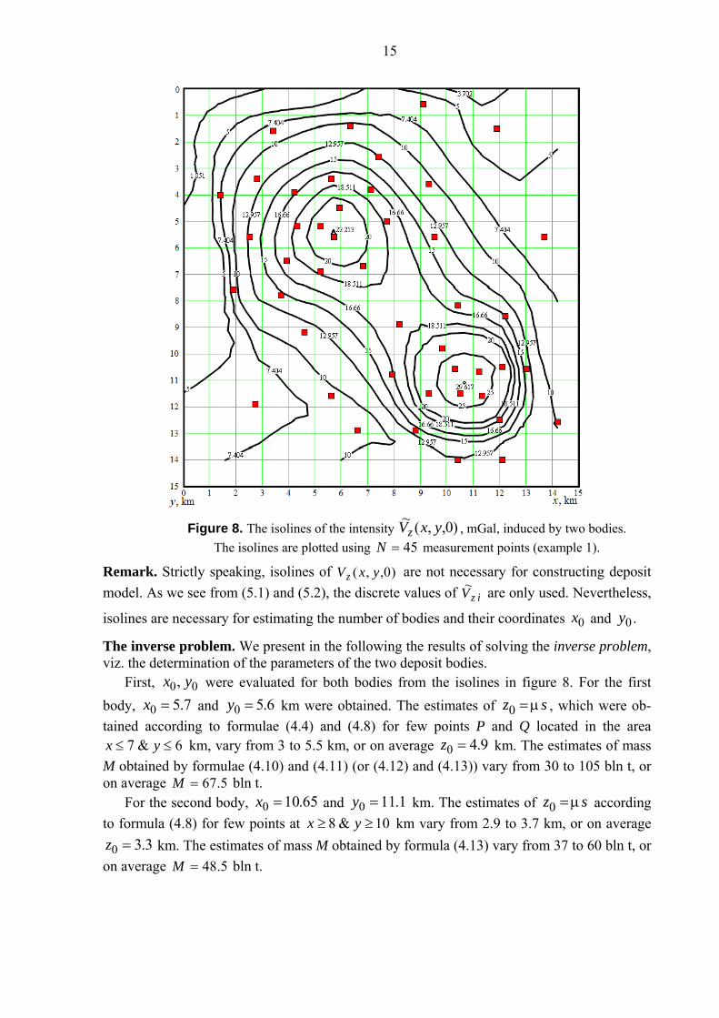
15
Figure 8. The isolines of the intensity )0,,(~ yxVz , mGal, induced by two bodies. The isolines are plotted using 45=N measurement points (example 1).
Remark. Strictly speaking, isolines of )0,,( yxVz are not necessary for constructing deposit model. As we see from (5.1) and (5.2), the discrete values of izV~ are only used. Nevertheless,
isolines are necessary for estimating the number of bodies and their coordinates 0x and 0y .
The inverse problem. We present in the following the results of solving the inverse problem, viz. the determination of the parameters of the two deposit bodies.
First, 00, yx were evaluated for both bodies from the isolines in figure 8. For the first body, 7.50 =x and 6.50 =y km were obtained. The estimates of sz μ=0 , which were ob-tained according to formulae (4.4) and (4.8) for few points P and Q located in the area
6&7 ≤≤ yx km, vary from 3 to 5.5 km, or on average 9.40 =z km. The estimates of mass M obtained by formulae (4.10) and (4.11) (or (4.12) and (4.13)) vary from 30 to 105 bln t, or on average 5.67=M bln t.
For the second body, 65.100 =x and 1.110 =y km. The estimates of sz μ=0 according to formula (4.8) for few points at 10&8 ≥≥ yx km vary from 2.9 to 3.7 km, or on average
3.30 =z km. The estimates of mass M obtained by formula (4.13) vary from 37 to 60 bln t, or on average 5.48=M bln t.

16
Then, the following ten sought parameters were refined by minimizing the functional 1F or 2F (see (5.1) or (5.2)): ε=1p , ρ=2p , 03 xp = , 04 yp = , 05 zp = for the first body and
ε=6p , ρ=7p , 08 xp = , 09 yp = , 010 zp = for the second one. In table 2, the initial lower constraints minp , the upper constraints maxp and the mean
values 2)( maxminmid ppp += are presented. These (approximate) values of the constraints can be estimated by the experts in this field on the basis of additional data obtained by results of preliminary investigations of the region5. Constraints on ρ are especially important, since the density knowledge connects with the problem of uniqueness. Then these values are deter-mined more accurately such that the sought solution 10,, ppi K does not fall outside the limits of the interval (5.3). Furthermore, estimate of the semiaxis a is realized by formula (5.5).
Table 2. Refined values of the constraints on the parameters and the obtained solution
p ε 3cmg,ρ 0x , km 0y , km 0z , km v, km3 M, bln t a, km
The first body minp 0.2 1.1 5.4 5.2 4.0
maxp 0.6 1.7 6.0 6.0 5.8
midp 0.4 1.4 5.7 5.6 4.9 solution 0.595 1.69 5.75 5.48 4.40 39.86 67.50 2.52
exact values 0.51 1.6 5.7 5.3 4.2 39.67 63.48 2.75
The second body minp 1.8 2.3 10.3 10.2 2.3
maxp 2.2 2.9 11.0 12.0 4.3
midp 2.0 2.6 10.65 11.1 3.3 solution 2.035 2.65 10.71 11.90 3.81 18.28 48.50 1.29
exact values 1.96 2.6 10.7 11.1 3.8 19.06 49.55 1.375
The dependence of the mean square error δ of the solution (see (5.4)) on the regularization
parameter α was calculated. Furthermore, values of ε, ρ, 0x , 0y , 0z , v, M and a based on the deposit estimation (figures 1 and 2) and given in Table 2, were taken as ‘exact’ parameters ε , ρ , 0x , 0y , 0z , v , M and a of the deposit bodies.
Note that the exact volumes v and masses M of bodies were calculated by summation over the bars, and the values of ε , ρ , 0x , 0y and 0z were estimated by the form of bodies. For example, the x half-length of the first body is 2.5 km and the y half-length is 3 km, i.e. the average half-length in the plane xy is 75.2=a km; the z half-length is 1.4 km, i.e. the ratio between the z and xy half-lengthes is 51.0=ε , etc.
Since a regularization is used, it is necessary to draw our attention to the problem of choosing the value of the regularization parameter α. A number of approaches for choosing α is developed (the Morozov discrepancy principle, L-curve algorithm, generalized cross-validation method et al.) [1, 14, 15, 28, 44, 55, 56]. However, in example 1, the rigid con-
5 As a result of such investigations, one can determine which bodies (ore, oil, quartzites, shales, etc.) occur
in the region. This makes possible to estimate their densities. As to ε, then at first we can put pmid1 = ε = 1.

17
straints are imposed on the solution p and they provide stability and uniqueness of the solu-tion without regularization. Practically, the problem has the same solution for any 810~ −<α and the solution does not depend on the type of the functional ( 1F or 2F ). But if the con-straints are less rigid than those given in table 2, the error )(αδ and the solution )(αp depend on α, and the value of the error δ at some optα=α can be smaller than that at 0=α .
In figure 9, the pictures of the two calculated spheroids are given. It can be seen that the modelling of a deposit by spheroids yields a quite satisfactory result.
Figure 9. Two spheroids imitating the deposit in example 1.
It should be pointed out that the initial value of the functional 1F (before its minimization) equals 2
1 10167.0 −⋅=F , and after the minimization by the coordinate descent method 3
1 10197.0 −⋅=F , i.e. the value of 1F decreased by one order of magnitude.
6.2. Example 2 In the capacity of the second example, we could consider an example based on real measured fields on Earth's surface. However, in this case the exact values of the parameters of the bod-ies would not be known and it would be difficult to estimate the errors in determining the pa-rameters. Of course, instead of estimating and comparing the parameters, one can use a com-parison of the measured isolines of zV~ (type of figures 8 and 10) and the isolines obtained as a result of calculating the spheroids (see figure 11 later). However, it will be an indirect estimat-ing the errors of body parameters. In addition, because of ill-posedness of the problem a small difference of isolines does not guarantee a small difference of body parameters.
It could be considered a synthetic example where the real data about deposit bodies are used, then calculations of the fields )0,,(~ yxVz are performed, after which the inverse prob-lem of determining the parameters of the spheroids is solved. In this case, we will be able to compare the calculated parameters of the spheroids with the parameters of the deposit bodies. However, it is difficult to get real data about deposit bodies with the necessary accuracy.
Therefore, as the second example we have considered an example in which (as in example 1) the parameters of the deposit bodies are given (see table 3 below), but the deposit has more bodies than in example 1. Further, the intensities zV are calculated at 73=N points on
18
Earth's surface (squares in figure 10) and 3% errors are added to values of zV . Example 2 is more complicated than example 1, and its purpose is to show potential possibilities of the me-thod on increasing the number of bodies.
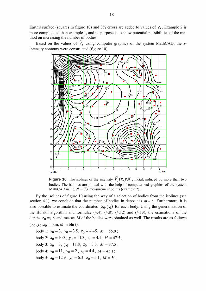
Based on the values of zV~ using computer graphics of the system MathCAD, the z-intensity contours were constructed (figure 10).
Figure 10. The isolines of the intensity )0,,(~ yxVz , mGal, induced by more than two bodies. The isolines are plotted with the help of computerized graphics of the system MathCAD using 73=N measurement points (example 2).
By the isolines of figure 10 using the way of a selection of bodies from the isolines (see section 4.1), we conclude that the number of bodies in deposit is 5=m . Furthermore, it is also possible to estimate the coordinates ),( 00 yx for each body. Using the generalization of the Bulakh algorithm and formulae (4.4), (4.8), (4.12) and (4.13), the estimations of the depths sz μ=0 and masses M of the bodies were obtained as well. The results are as follows ( 000 ,, zyx in km, M in bln t):
body 1: 30 =x , 5.30 =y , 45.40 =z , 9.55=M ; body 2: 3.100 =x , 3.110 =y , 1.40 =z , 5.47=M ; body 3: 30 =x , 8.110 =y , 8.30 =z , 5.37=M ; body 4: 110 =x , 20 =y , 4.40 =z , 1.43=M ; body 5: 9.120 =x , 3.60 =y , 1.50 =z , 30=M .
19
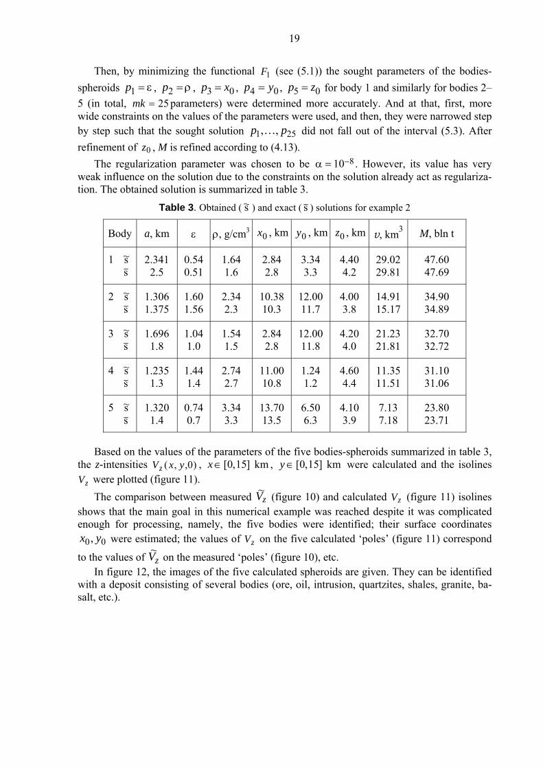
Then, by minimizing the functional 1F (see (5.1)) the sought parameters of the bodies-spheroids ε=1p , ρ=2p , 03 xp = , 04 yp = , 05 zp = for body 1 and similarly for bodies 2–5 (in total, 25=mk parameters) were determined more accurately. And at that, first, more wide constraints on the values of the parameters were used, and then, they were narrowed step by step such that the sought solution 251 ,, pp K did not fall out of the interval (5.3). After refinement of 0z , M is refined according to (4.13).
The regularization parameter was chosen to be 810−=α . However, its value has very weak influence on the solution due to the constraints on the solution already act as regulariza-tion. The obtained solution is summarized in table 3.
Table 3. Obtained ( s~ ) and exact ( s ) solutions for example 2
Body a, km ε ρ, g/cm30x , km 0y , km 0z , km v, km3 M, bln t
1 s~ s
2.341 2.5
0.54 0.51
1.64 1.6
2.84 2.8
3.34 3.3
4.40 4.2
29.02 29.81
47.60 47.69
2 s~ s
1.306 1.375
1.60 1.56
2.34 2.3
10.3810.3
12.0011.7
4.00 3.8
14.91 15.17
34.90 34.89
3 s~ s
1.696 1.8
1.04 1.0
1.54 1.5
2.84 2.8
12.0011.8
4.20 4.0
21.23 21.81
32.70 32.72
4 s~ s
1.235 1.3
1.44 1.4
2.74 2.7
11.0010.8
1.24 1.2
4.60 4.4
11.35 11.51
31.10 31.06
5 s~ s
1.320 1.4
0.74 0.7
3.34 3.3
13.7013.5
6.50 6.3
4.10 3.9
7.13 7.18
23.80 23.71
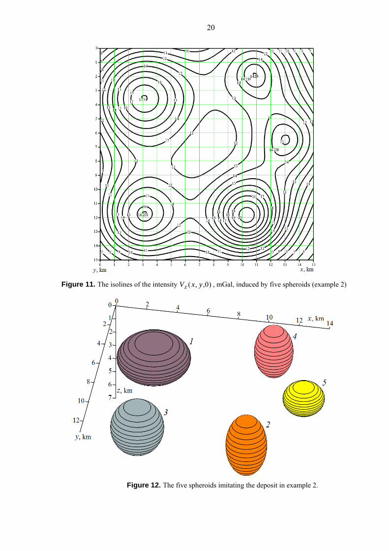
Based on the values of the parameters of the five bodies-spheroids summarized in table 3,
the z-intensities )0,,( yxVz , km ]15,0[∈x , km ]15,0[∈y were calculated and the isolines zV were plotted (figure 11).
The comparison between measured zV~ (figure 10) and calculated zV (figure 11) isolines shows that the main goal in this numerical example was reached despite it was complicated enough for processing, namely, the five bodies were identified; their surface coordinates
00, yx were estimated; the values of zV on the five calculated ‘poles’ (figure 11) correspond
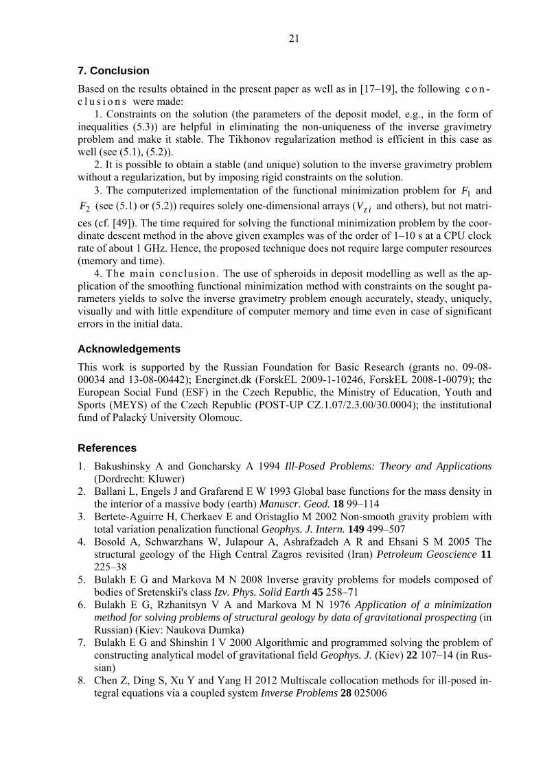
to the values of zV~ on the measured ‘poles’ (figure 10), etc. In figure 12, the images of the five calculated spheroids are given. They can be identified
with a deposit consisting of several bodies (ore, oil, intrusion, quartzites, shales, granite, ba-salt, etc.).
20
Figure 11. The isolines of the intensity )0,,( yxVz , mGal, induced by five spheroids (example 2)
Figure 12. The five spheroids imitating the deposit in example 2.
21
7. Conclusion Based on the results obtained in the present paper as well as in [17–19], the following c o n -c l u s i o n s were made:
1. Constraints on the solution (the parameters of the deposit model, e.g., in the form of inequalities (5.3)) are helpful in eliminating the non-uniqueness of the inverse gravimetry problem and make it stable. The Tikhonov regularization method is efficient in this case as well (see (5.1), (5.2)).
2. It is possible to obtain a stable (and unique) solution to the inverse gravimetry problem without a regularization, but by imposing rigid constraints on the solution.
3. The computerized implementation of the functional minimization problem for 1F and
2F (see (5.1) or (5.2)) requires solely one-dimensional arrays ( izV and others), but not matri-ces (cf. [49]). The time required for solving the functional minimization problem by the coor-dinate descent method in the above given examples was of the order of 1–10 s at a CPU clock rate of about 1 GHz. Hence, the proposed technique does not require large computer resources (memory and time).
4. The main conclusion. The use of spheroids in deposit modelling as well as the ap-plication of the smoothing functional minimization method with constraints on the sought pa-rameters yields to solve the inverse gravimetry problem enough accurately, steady, uniquely, visually and with little expenditure of computer memory and time even in case of significant errors in the initial data.
Acknowledgements This work is supported by the Russian Foundation for Basic Research (grants no. 09-08-00034 and 13-08-00442); Energinet.dk (ForskEL 2009-1-10246, ForskEL 2008-1-0079); the European Social Fund (ESF) in the Czech Republic, the Ministry of Education, Youth and Sports (MEYS) of the Czech Republic (POST-UP CZ.1.07/2.3.00/30.0004); the institutional fund of Palacký University Olomouc. References 1. Bakushinsky A and Goncharsky A 1994 Ill-Posed Problems: Theory and Applications
(Dordrecht: Kluwer) 2. Ballani L, Engels J and Grafarend E W 1993 Global base functions for the mass density in
the interior of a massive body (earth) Manuscr. Geod. 18 99–114 3. Bertete-Aguirre H, Cherkaev E and Oristaglio M 2002 Non-smooth gravity problem with
total variation penalization functional Geophys. J. Intern. 149 499–507 4. Bosold A, Schwarzhans W, Julapour A, Ashrafzadeh A R and Ehsani S M 2005 The
structural geology of the High Central Zagros revisited (Iran) Petroleum Geoscience 11 225–38
5. Bulakh E G and Markova M N 2008 Inverse gravity problems for models composed of bodies of Sretenskii's class Izv. Phys. Solid Earth 45 258–71
6. Bulakh E G, Rzhanitsyn V A and Markova M N 1976 Application of a minimization method for solving problems of structural geology by data of gravitational prospecting (in Russian) (Kiev: Naukova Dumka)
7. Bulakh E G and Shinshin I V 2000 Algorithmic and programmed solving the problem of constructing analytical model of gravitational field Geophys. J. (Kiev) 22 107–14 (in Rus-sian)
8. Chen Z, Ding S, Xu Y and Yang H 2012 Multiscale collocation methods for ill-posed in-tegral equations via a coupled system Inverse Problems 28 025006
22
9. Cho Z H, Jones J P and Singh M 1993 Foundations of Medical Imaging (New York: Wiley)
10. Commer M 2011 Three-dimensional gravity modelling and focusing inversion using rec-tangular meshes Geophys. Prospecting 59 966–79
11. Duboshin G N 1975 Celestial Mechanics. Basic Problems and Methods 3rd edn (in Rus-sian) (Moscow: Nauka)
12. Dufour H M 1977 Fonctions orthogonales dans la sphère. Résolution théorique du problème du potenciel terrestre Bull. Geod. 51 227–37
13. D'yakonov V P 1984 Handbook on Algorithms and Programs in Basic Language for PC (in Russian) (Moscow: Nauka)
14. Engl H, Hanke M and Neubauer A 1996 Regularization of Inverse Problems (Mathemat-ics and Its Applications) (Dordrecht: Kluwer)
15. Fischer D and Michel V 2012 Sparse regularization of inverse gravimetry–case study: spatial and temporal mass variations in South America Inverse Problems 28 065012
16. Frick K, Martinz P and Munk A 2012 Shape-constrained regularization by statistical mul-tiresolution for inverse problems: asymptotic analysis Inverse Problems 28 065006
17. Golov I N and Sizikov V S 2005 Modeling the inverse gravimetry problem with use of spheroids, nonlinear programming and regularization Geophys. J. (Kiev) 27 454–62 (in Russian)
18. Golov I N and Sizikov V S 2005 On correct solving the inverse gravimetry problem Rus. J. Geophysics (St. Petersburg) 39–40 84–91 (in Russian)
19. Golov I N and Sizikov V S 2009 Modeling of deposits by spheroids Izv. Phys. Solid Earth 45 258–71
20. Grafarend E W, You Rey-Jer and Syffus R 2014 Map Projections: Cartographic Informa-tion Systems 2nd edn (Berlin: Springer)
21. Himmelblau D M 1972 Applied Nonlinear Programming (New York: McGraw-Hill) 22. Jahandari H and Farquharson C G 2013 Forward modeling of gravity data using finite-
volume and finite-element methods on unstructured grids Geophysics 78 G69–G80 23. Kozlovskaya E 2000 An algorithm of geophysical data inversion based on non-probabilis-
tic presentation of a priori information and definition of Pareto-optimality Inverse Prob-lems 16 839
24. Krebs J 2011 Support vector regression for the solution of linear integral equations In-verse Problems 27 065007
25. Krizskii V N, Gerasimov I A and Viktorov S V 2002 Mathematical modeling inverse problems of potential geoelectric fields in axially symmetric piecewise homogeneous me-dia Vestnik Zaporozh. Gos. Univ. Fiz.-Mat. Nauki 1 1–5 (in Russian)
26. Lahmer T 2011 Optimal experimental design for nonlinear ill-posed problems applied to gravity dams Inverse Problems 27 125005
27. Lavrent'ev M M, Romanov V G and Shishatskiĭ S P 1986 Ill-Posed Problems of Mathe-matical Physics and Analysis (Translations of Mathematical Monographs vol 64) (Provi-dence, RI: American Mathematical Society)
28. Leonov A S 2010 Solving Ill-Posed Inverse Problems (in Russian) (Moscow: Librokom) 29. Li Y and Oldenburg W 1998 3-D inversion of gravity data Geophysics 63 109–19 30. MacLennan K, Karaoulis M and Revil A 2014 Complex conductivity tomography using
low-frequency crosswell electromagnetic data Geophysics 79 E23–E38 31. Marusina M Y and Kaznacheeva A O 2007 Contemporary state and perspectives of de-
velopment of tomography Sci-tech. Vestnik SPbSU IFMO 8 3–13 (in Russian) 32. Michel V 2005 Regularized wavelet-based multiresolution recovery of the harmonic mass
density distribution from data of the Earth’s gravitational field at satellite height Inverse Problems 21 997
23
33. Michel V and Fokas A S 2008 A unified approach to various techniques for the non-uni-queness of the inverse gravimetric problem and wavelet-based methods Inverse Problems 24 045019
34. Michel V and Wolf K 2008 Numerical aspects of a spline-based multiresolution recovery of the harmonic mass density out of gravity functionals Geophys. J. Intern. 173 1–16
35. Mottl J and Mottlova L 1984 The simultaneous solution of the inverse problem of gravim-etry and magnetics by means of non-linear programming Geophis. J. RAS 76 563–79
36. Novikoff P 1938 Sur le problème inverse du potenciel Comptes Rendus (Doklady) de l’Académie des Sci. de l’URSS XVIII 165–8
37. Pilkington M 2014 Evaluating the utility of gravity gradient tensor components Geophys-ics 79 G1–G14
38. Pizzetti P 1909 Corpi equivalenti rispetto alla attrazione newtoniana esterna Rom. Acc. L. Rend. XVIII 211–5
39. Pizzetti 1910 Intorno alle possibili distribuzioni della massa nell’interno della terra Annali di Mat., Milano XVII 225–58
40. Portniaguine O and Zhdanov M S 1999 Focusing geophysical inversion images Geophys-ics 64 874–87
41. Salem A, Green C, Campbell S, Fairhead D, Cascone L and Moorhead L 2013 Moho depth and sediment thickness estimation beneath the Red Sea derived from satellite and terrestrial gravity data Geophysics 78 G89–G101
42. Salem A, Green C, Stewart M and De Lerma D 2014 Inversion of gravity data with isostatic constraints Geophysics 79 A45–A50
43. Sizikov V S 1967 Mass distribution in galaxies deduced from radial-velocity and pho-tometry data Astrophysics 3, 124–8
44. Sizikov V S 2001 Mathemathical Methods for Processing the Results of Measurements (in Russian) (St. Petersburg: Politekhnika)
45. Sizikov V S 2011 Inverse Applied Problems and MatLab (in Russian) (St. Petersburg: Lan')
46. Sretensky L N 1954 On the uniqueness of the determination of the shape of an attractive body from its outer potential Doklady Akademii Nauk SSSR 99, 21–22 (in Russian)
47. Starostenko V I 1978 Stable Numerical Methods in Gravimetry Problems (in Russian) (Kiev: Naukova Dumka)
48. Starostenko V I, Pashko V F and Zavorot’ko A N 1992 Experience in solving strongly unstable inverse linear gravity problem Izv. Phys. Solid Earth 8 24–44
49. Strakhov V N 2004 New paradigm in the theory of linear ill-posed problems adequate to requirements of geophysical practice. I–V Geophys. J. (Kiev) 26 No. 1–4(in Russian)
50. Stepanova I E 2001 A robust algorithm for reconstructing an ellipsoid Izv. Phys. Solid Earth 37 955–60
51. Subbotin M F 1949 Course of Celestial Mechanics vol. 3 (in Russian) (Leningrad-Moscow: GITTL)
52. Tikhonov A N and Arsenin V Y 1977 Solution of Ill-Posed Problems (New York: Wiley) 53. Tscherning C C and Sünkel H 1981 A method for the construction of spheroidal mass dis-
tributions consistent with the harmonic part of the earth’s gravity potential Manuscr. Geod. 6 131–56
54. Vasiliev F P 1981 Methods for Solving Extreme Problems (in Russian) (Moscow: Nauka) 55. Vatankhah S, Renaut R A and Ardestani V E 2014 Regularization parameter estimation
for underdetermined problems by the χ2 principle with application to 2D focusing gravity inversion Inverse Problems 30 085002
56. Verlan' A F and Sizikov V S 1986 Integral Equations: Methods, Algorithms, Programs (in Russian) (Kiev: Naukova Dumka)

24
57. Vorontsov-Vel'yaminov B A 1987 Extragalactic Astronomy (Chur, Switzerland: Harwood Academic Publishers)
58. Webb S (ed) 1988 The physics of medical imaging in 2 vol. (Bristol: IOP) 59. Yun'kov A A and Afanas'ev N L 1952 The direct and inverse problem of Δg for a triaxial
ellipsoid and an ellipsoid of revolution Izv. Dnepropetrovsk. Gorn. Inst. 22 17–21 (in Rus-sian) (Moscow-Khar'kov: Ugletekhizdat)
60. Zhdanov M and Hursan G 2000 3D electromagnetic inversion based on quasi-analytical approximation Inverse Problems 16 1297
61. Zhdanov M S, Ellis R and Mukherjee 2004 Three-dimensional regularized focusing inver-sion of gravity gradient tensor component data Geophysics 69 925–37
62. Zhuravlev I A 1998 On solving the inverse gravimetry problem in the class of distributed density Geophys. J. (Kiev) 20 86–94 (in Russian)