Spatial scales in alluvial channels: on 2D coherent turbulent

structures and alternate bars formation

By

Aylen Carrasco Milian

A Dissertation Submitted to the Academic Committee of the

ENGINEERING AND WATER RESOURCES FACULTY

In partial fulfilment of the requirements to obtain the degree of

DOCTOR IN ENGINEERING

with mention in WATER RESOURCES

UNIVERSIDAD NACIONAL DEL LITORAL

2008

ii

iii

iv

v

List of Contents

List of Figures .........................................................................................................................vii List of Tables .............................................................................................................................x Resumen Extendido – Extended Abstract (in Spanish) .......................................................xi

INTRODUCCIÓN.................................................................................................................xi SEPARACIÓN DE ESCALAS EN UN FLUJO TURBULENTO POCO PROFUNDO....xii ESTUDIO DE LA FORMACIÓN DE BARRAS ALTERNADAS CON MÁRGENES EROSIONABLES Y NO EROSIONABLE........................................................................xiv

Chapter 1 On the river regime theory and the scaling argument concept..........................1 1.1 Introduction ....................................................................................................................1 1.2. Scaling Argument ..........................................................................................................4 1.3. On turbulent flows.......................................................................................................16 1.4. Dissertation outline......................................................................................................19

Chapter 2 Literature review ..................................................................................................21 2.1 On 2D coherent turbulent structures..........................................................................21 2.2 On free bars formation.................................................................................................24 2.2.1 Bar formation problem: alternate bars as the precursor mechanism for river

meandering? Linear stability analysis ..........................................................................31 2.2.2 Bar formation problem: meandering formation as a planimetric instability..34 2.2.3 Bar formation problem: non-linear theories.......................................................37 2.2.4 Bar formation problem: meandering formation as a resonant mechanism.....40 2.2.5 Bar formation problem: experimental approach and regime theories ............41

Chapter 3 Separation of scales on a broad, shallow turbulent flow ..................................45 3.1 Introduction ............................................................................................................45 3.2 On turbulent flows with a spectral gap ................................................................51 3.3 Experimental arrangement....................................................................................54 3.4 Results......................................................................................................................57 3.5 Conclusions..............................................................................................................64

CHAPTER 4 Laboratory study of alternate bar formations .............................................67 4.1 Introduction ..................................................................................................................67 4.2 . Materials and methods ...............................................................................................69 4.3 Experimental set up......................................................................................................73 4.3.1 Experiments with fixed banks (Series A) ............................................................77 4.3.2 Experiments with mobile banks (Series B)..........................................................78

4.4 Procedures used for collecting data ............................................................................80 4.4.1 Water discharge .....................................................................................................80 4.4.2 Sediment concentration.........................................................................................80 4.4.3 Channel bed and water surface slope. .................................................................82 4.4.4 Bedform characteristics ........................................................................................82 4.4.5 Bed migration rate measurement.........................................................................83 4.4.6 Cross-section geometry .........................................................................................83 4.4.7 Regime -or equilibrium- criterion........................................................................83

4.5 Results and discussion ..................................................................................................84 4.4 Chapter summary.......................................................................................................115

CHAPTER 5 Conclusions ....................................................................................................119 Bibliography..........................................................................................................................123 Appendix A Normal Flow Solution.....................................................................................137 Appendix B Sieve Analysis Of The Bed Material ..............................................................140 Appendix c Stability Analysis Of 2d Coherent Structures Of Shallow Waters..............141

vi

C.1 Introduction................................................................................................................141 C.2 Governing equation ...................................................................................................142 C.3 Boundary conditions..................................................................................................146 C.4 Base flow and dimensionless form............................................................................146 C.5 Linear stability analysis ............................................................................................147

Appendix D Dimensionless procedure of the governing equations..................................152 Appendix E The perturbed equation of motion.................................................................154 Appendix F Normal modes and gaussian elimination.......................................................158

Appendix G Recovering of the amplitude vector ( )yf ...................................................160

vii

List of Figures

Figura 0.1 Fotografía del patrón de flujo establecido en el gran cuenco experimental de la FICH. ................................................................................................................................xii

Figura 0.2 Cascada inversa en el rango inercial de turbulencia 2D ....................................... xiii Figura 0.3 Superposición de los espectros medidos en los puntos B, C y D en escala linear (el

segundo eje vertical esta referido al espectro del punto)................................................ xiii Figura 0.4 Espectros de energía estimados con la técnica de Fast Fourier Tranform (FFT

technique). a) espectro de u’ y w’ en 4x = − m, b) u’ y w’ en 1x = − m, c) u’ y w’ en 0x = m, d) u’ y w’ en 0.75x = m. ......................................................................................xiv

Figura 0.5 Canal de laboratorio usado en Newcastle University, Newcastle upon Tyne, UK. xv Figura 0.6 a) Experimentos con márgenes no erosionables (MNE). b) Experimentos con

márgenes erosionables (ME). ...........................................................................................xv Figura 0.7 Elevación del lecho para márgenes no erosionables y erosionables. .....................xvi Figura 0.8 Dispersión de longitud de onda..............................................................................xvi Figura 0.9 Variación de las márgenes con el tiempo...............................................................xvi Figura 0.10 Evolución de las barras en el tiempo....................................................................xvi 1

Figure 1.1 Spatial scales L/H for the Paraná River (from Tassi, 2001)......................................4 Figure 1.2 River basin length L as a function of basin area A (taken from Dade, 2001) ...........6 Figure 1.3 Universal scaling for rivers according to Parker (2007). ..........................................7 Figure 1.4 Upper left corner: flow instability on a shallow flow (wake of a grounded tank

ship, taken from Milton Van Dyke Album (Van Dyke, 1982). Upper right corner: same type of instability induced by highly localized friction due to the bridge pier. Lower left corner: sketch of the expected instabilities along the main channel-floodplain interface (Shiono and Knight, 1991). Lower right corner: observed instabilities along a main channel-floodplain interface (Sellin, 1964). .....................................................................11

Figure 1.5 Scales of flow resistance in alluvial channels (taken from Dietrich and Whiting (1989)) ..............................................................................................................................14

Figure 1.6 Relation between total bed shear stress oτ and flow velocity V for different bed

forms (Taken from Engelund and Fredsoe, 1981)............................................................15 Figure 1.7 Bed Forms in Alluvial Channels (after Chow (1973))............................................15 Figure 1.8 Inverse cascading in the inertial range of 2D turbulence........................................19

Figure 2.1 Bedform classification graph of Liu (taken from van Rijn, 1993)..........................26 Figure 2.2 Bedform classification graph of Simons and Richardson (taken from van Rijn,

1993). ................................................................................................................................27 Figure 2.3 Bedform classification graph of van den Berg and van Gelder (from van

Rijn,1993). ........................................................................................................................28 Figure 2.4 Bedform classification graph of van Rijn (1993)....................................................29 Figure 2.5 Bedform existence field across a range of grain sizes (in Robert, 2003)................30 Figure 2.6 Alternate bars diagram ............................................................................................30 Figure 2.7 Alternate bars in the Alpine Rhine, Border of Switzerland/Leichtenstein (taken

from Jaeggi, 1984)............................................................................................................31

Figure 3.1 Top: Aerial photograph of a portion of the Interstate Road 168 that runs through a large and very low-gradient floodplain of the Paraná river. Bottom: same portion of the road. In periods of extremely high waters, the average water depth on the floodplain is about 4m (photograph taken during the big flood of 1983, flow is from top to bottom). 46

Figure 3.2 Long exposure photograph of the shallow turbulent flow pattern established on a broad experimental basin available at FICH. ...................................................................47

viii

Figure 3.3 Fixed scour hole located at the contraction end. .....................................................51 Figure 3.4 Schematic diagram of the basin used for the experiments (1, weir; 2, input pipe; 3,

feeding flume; 4, test section)...........................................................................................56 Figure 3.5 3D mean velocity field recorded with an ADV inside the test section ...................57 Figure 3.6 One-dimensional energy spectra of the streamwise and the vertical turbulent

fluctuations estimated with FFT technique. a) u’ and w’ spectra at position 4−=x m, b) u’ and w’ spectra at 1−=x m, c) u’ and w’ spectra at 0=x m, d) u’ and w’ spectra at

75.0=x m.........................................................................................................................60 Figure 3.7 Superposition of the velocity fluctuation spectra (linear scale) measured at points

B, C, and D (spectrum of point D is referred to the second vertical axis)........................61 Figure 3.8 Auto-correlation functions at points A, B, C and D................................................61

Figure 4.1 Schematic layout of the regime flume. Taken from Ershadi (2005).......................70 Figure 4.2 Electromagnetic flow meter. ...................................................................................70 Figure 4.3 Commubox FXA 191 system..................................................................................71 Figure 4.4 Tilting gate placed at the channel outlet. ................................................................71 Figure 4.5 Energy diffusers at the channel in the inlet .............................................................72 Figure 4.6 Sediment feeder.......................................................................................................72 Figure 4.7 Threshold values for initiation to motion (Shield’s Curve). The circle enclosed the

initial conditions set up during the experiments (Table 4.1) ............................................74 Figure 4.8 A classical stability diagram (taken from Colombini et al., 1987) .........................75 Figure 4.9 Initial experimental cross-section excavated in the sand at Laboratory facilities

available at Newcastle University, Newcastle upon Tyne, UK........................................75 Figure 4.10 a) Experiments with fixed banks; b) Experiments with loose banks. ...................78 Figure 4.11 Initial cross-sections..............................................................................................79 Figure 4.12 a) The electronic sediment balance, b) The sand trap for collecting the sediment.

..........................................................................................................................................81 Figure 4.13 Alternate bar formation in straight channel experiment. Characteristics:

Wavelength 2-3m ( 5.6L B= ) and Height 0.007-0.0010m................................................83 Figure 4.14 Discharges for the experiments. ............................................................................86 Figure 4.15 Sediment transport concentration of total discharge with time.............................89 Figure 4.16 Widening with time...............................................................................................90 Figure 4.17 Bar migration in the channel. Dashed line indicates the bar migration along the

bank with time. The flow is left to right. ..........................................................................96 Figure 4.18 Evolution of alternate bar formation for 6 /Q l s= ................................................97 Figure 4.19 Evolution of alternate bar formation for 8 /Q l s= ................................................98 Figure 4.20 Evolution of alternate bar formation for 9 /Q l s= ................................................99 Figure 4.21 Evolution of alternate bar formation for 10 /Q l s= .............................................100 Figure 4.22 Final bed configurations for loose banks experiments........................................102 Figure 4.23 Final bed configurations for fixed banks experiments. .......................................103 Figure 4.24 Bar migration for Runs for 6l/s with fixed and loose banks. The arrow symbol

indicates the bar front migration along the bank with time. The flow is left to right. Bar wavelength varied from six to ten channels widths. The time in hours is indicated to the right.................................................................................................................................105

Figure 4.25 Plot of mean wavelength versus the aspect ratio for runs with fixed and loose banks. ..............................................................................................................................106

Figure 4.26 Plot of wavelength variability. ............................................................................107 Figure 4.27 Bed level evolutions............................................................................................110 Figure 4.28 Bed elevation, a) Run (R-2-05) with fixed banks and b) Run (R-1-05) with loose

banks. ..............................................................................................................................111

ix

Figure 4.29 Channel cross-section evolution with time. ........................................................112 Figure 4.30 Channel cross section evolution with time: Initial (red), equilibrium (blue) and

final (green). ...................................................................................................................114 1

Figure A.1 Solution behavior under an inflow perturbation 0/B B is not to scale..................139

Figure B.1 Sieve analysis curves of the used sand .................................................................140

Figure C.1 Reference system..................................................................................................143 Figure C.2 Calculated Stability Diagram ...............................................................................151

x

List of Tables

Table 1.1 Estimate of length scales found in the Paraná River (see Figure 1.1) ........................5

Table 2.1 Classification of bed forms, taken from Knighton (1984). ......................................25

Table 3.1 Progression of spectral changes as the flow approaches the contraction .................64

Table 4.1. Complete set of experiments run.............................................................................78 Table 4.2 Experimental results .................................................................................................85 Table 4.3 Rates of sediment transport ......................................................................................88 Table 4.4 Minimun slope for alternate bar formation, following Jaeggi (1984). .....................93 Table 4.5 Chang criterion for alternate bar formation (1985). ................................................94 Table 4.6 Mass balance results. .............................................................................................113

xi

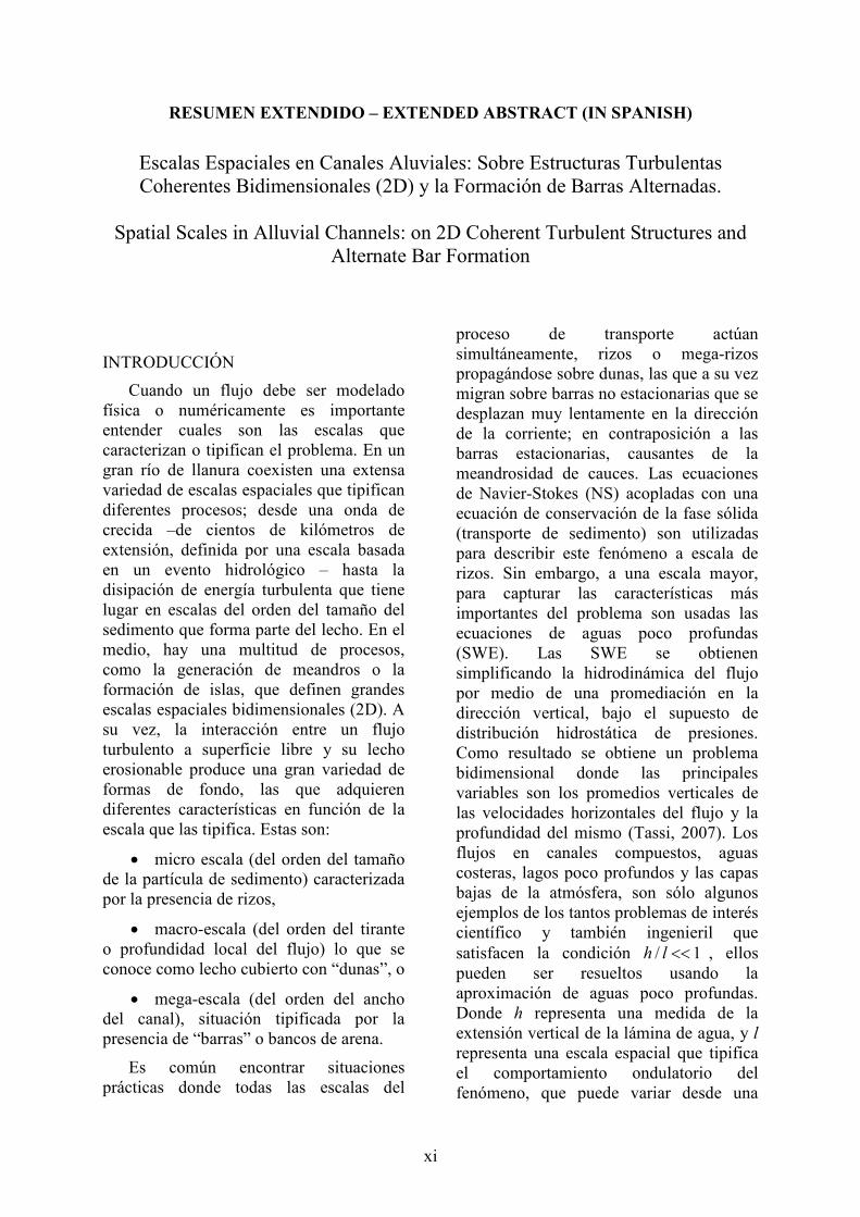
RESUMEN EXTENDIDO – EXTENDED ABSTRACT (IN SPANISH)

Escalas Espaciales en Canales Aluviales: Sobre Estructuras Turbulentas Coherentes Bidimensionales (2D) y la Formación de Barras Alternadas.

Spatial Scales in Alluvial Channels: on 2D Coherent Turbulent Structures and

Alternate Bar Formation

INTRODUCCIÓN

Cuando un flujo debe ser modelado física o numéricamente es importante entender cuales son las escalas que caracterizan o tipifican el problema. En un gran río de llanura coexisten una extensa variedad de escalas espaciales que tipifican diferentes procesos; desde una onda de crecida –de cientos de kilómetros de extensión, definida por una escala basada en un evento hidrológico – hasta la disipación de energía turbulenta que tiene lugar en escalas del orden del tamaño del sedimento que forma parte del lecho. En el medio, hay una multitud de procesos, como la generación de meandros o la formación de islas, que definen grandes escalas espaciales bidimensionales (2D). A su vez, la interacción entre un flujo turbulento a superficie libre y su lecho erosionable produce una gran variedad de formas de fondo, las que adquieren diferentes características en función de la escala que las tipifica. Estas son:

• micro escala (del orden del tamaño de la partícula de sedimento) caracterizada por la presencia de rizos,

• macro-escala (del orden del tirante o profundidad local del flujo) lo que se conoce como lecho cubierto con “dunas”, o

• mega-escala (del orden del ancho del canal), situación tipificada por la presencia de “barras” o bancos de arena.

Es común encontrar situaciones prácticas donde todas las escalas del

proceso de transporte actúan simultáneamente, rizos o mega-rizos propagándose sobre dunas, las que a su vez migran sobre barras no estacionarias que se desplazan muy lentamente en la dirección de la corriente; en contraposición a las barras estacionarias, causantes de la meandrosidad de cauces. Las ecuaciones de Navier-Stokes (NS) acopladas con una ecuación de conservación de la fase sólida (transporte de sedimento) son utilizadas para describir este fenómeno a escala de rizos. Sin embargo, a una escala mayor, para capturar las características más importantes del problema son usadas las ecuaciones de aguas poco profundas (SWE). Las SWE se obtienen simplificando la hidrodinámica del flujo por medio de una promediación en la dirección vertical, bajo el supuesto de distribución hidrostática de presiones. Como resultado se obtiene un problema bidimensional donde las principales variables son los promedios verticales de las velocidades horizontales del flujo y la profundidad del mismo (Tassi, 2007). Los flujos en canales compuestos, aguas costeras, lagos poco profundos y las capas bajas de la atmósfera, son sólo algunos ejemplos de los tantos problemas de interés científico y también ingenieril que satisfacen la condición / 1h l << , ellos pueden ser resueltos usando la aproximación de aguas poco profundas. Donde h representa una medida de la extensión vertical de la lámina de agua, y l representa una escala espacial que tipifica el comportamiento ondulatorio del fenómeno, que puede variar desde una

xii

onda de crecida hasta una onda de sedimento del lecho (barra, duna, o rizo).

El objetivo de este trabajo de tesis es la compilación de las experiencias adquiridas durante ensayos realizados en dos instalaciones experimentales, en las cuales se estudiaron dos fenómenos diferentes que pueden ser abordados a través de la aproximación de aguas poco profundas. Primero se analiza el problema de la separación de escalas que tiene lugar en un flujo turbulento poco profundo y de gran desarrollo horizontal. Esto es el producto de una trabajo experimental llevado a cabo en el laboratorio de Hidráulica de la Facultad de Ingeniería y Ciencias Hídricas, UNL, Argentina. Luego se estudia la formación de barras alternadas en un canal de régimen, para diferentes condiciones hidráulicas y rugosidad de márgenes. Esta última experiencia se llevó a cabo en el Laboratorio de Hidráulica de la Escuela de Ingeniería y Geociencia (School of Engineering and Geoscience) de la Universidad de Newcastle upon Tyne, Inglaterra.

SEPARACIÓN DE ESCALAS EN UN FLUJO TURBULENTO POCO PROFUNDO

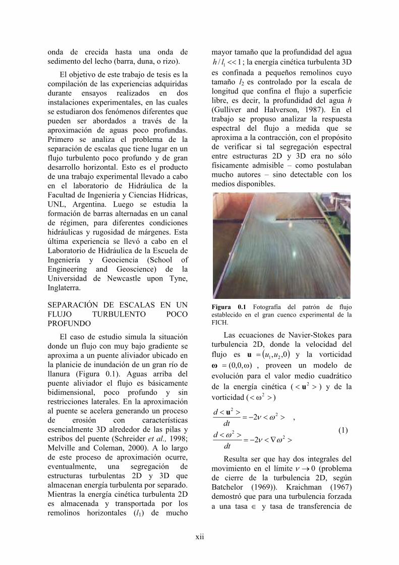
El caso de estudio simula la situación donde un flujo con muy bajo gradiente se aproxima a un puente aliviador ubicado en la planicie de inundación de un gran río de llanura (Figura 0.1). Aguas arriba del puente aliviador el flujo es básicamente bidimensional, poco profundo y sin restricciones laterales. En la aproximación al puente se acelera generando un proceso de erosión con características esencialmente 3D alrededor de las pilas y estribos del puente (Schreider et al., 1998; Melville and Coleman, 2000). A lo largo de este proceso de aproximación ocurre, eventualmente, una segregación de estructuras turbulentas 2D y 3D que almacenan energía turbulenta por separado. Mientras la energía cinética turbulenta 2D es almacenada y transportada por los remolinos horizontales (l1) de mucho

mayor tamaño que la profundidad del agua

1/ 1h l << ; la energía cinética turbulenta 3D es confinada a pequeños remolinos cuyo tamaño l2 es controlado por la escala de longitud que confina el flujo a superficie libre, es decir, la profundidad del agua h (Gulliver and Halverson, 1987). En el trabajo se propuso analizar la respuesta espectral del flujo a medida que se aproxima a la contracción, con el propósito de verificar si tal segregación espectral entre estructuras 2D y 3D era no sólo físicamente admisible – como postulaban mucho autores – sino detectable con los medios disponibles.

Figura 0.1 Fotografía del patrón de flujo establecido en el gran cuenco experimental de la FICH.

Las ecuaciones de Navier-Stokes para turbulencia 2D, donde la velocidad del flujo es u ( )0,, 21 uu= y la vorticidad ω ),0,0( ω= , proveen un modelo de evolución para el valor medio cuadrático de la energía cinética ( >< 2

u ) y de la vorticidad ( >ω< 2 )

22

22

2 ,

2

d

dt

d

dt

ν ω

ων ω

< >= − < >

< >= − < ∇ >

u

(1)

Resulta ser que hay dos integrales del movimiento en el límite 0ν → (problema de cierre de la turbulencia 2D, según Batchelor (1969)). Kraichman (1967) demostró que para una turbulencia forzada a una tasa ∈ y tasa de transferencia de

xiii

enstrofía ( )2 /d dtβ = < ω > , hay dos

cascadas de energía bien diferenciadas en el rango inercial de transferencia de energía turbulenta

33/2

3/53/2

)(

)(−

−

β≅

≅∈

kkE

kkE (2)

Puesto que el flujo de energía cinética a través de una cascada de enstrofía es cero (Kraichnan, 1967), la energía cinética producida a tasa ∈ en el número de onda ki solamente puede ir hacia escalas mayores que 1/ ik a través de una cascada inversa.

La Figura 0.2 muestra esquemáticamente lo discutido hasta ahora.

i∈

ik

53/2 −∈ k

33/2 −β k

k

Figura 0.2 Cascada inversa en el rango inercial de turbulencia 2D

En consecuencia, y con el fin de calcular la respuesta espectral del flujo, se midieron las velocidades en 4 puntos alineados desde aguas arriba – aguas abajo del ingreso al cuenco de ensayo – hasta la vecindad de la contracción, levemente aguas abajo de la hoya de erosión presente en el extremo del estribo (ver Figura 0.1). Las Figura 0.3 y Figura 0.4 muestran los cambios en la respuesta espectral del flujo en la medida que se aproxima a la contracción. Los puntos A y B se ubican aguas arriba de la contracción, donde el flujo se comienza a acelerar, el punto C se ubica sobre la contracción, en el interior de la hoya de erosión local, y el punto D se encuentra, aguas abajo de la contracción, donde el flujo se expande nuevamente.

Figura 0.3 Superposición de los espectros medidos en los puntos B, C y D en escala linear (el segundo eje vertical esta referido al espectro del punto).

Los experimentos muestran que la geometría y la topografía del canal crean un flujo turbulento con dos estructuras bien definidas: una componente cuasi-bidimensional de gran escala (l1) y otra componente tridimensional de pequeña escala (l2). Las cuales pueden ser identificadas en dos picos bien definidos del espectro de energía.

A pesar de que la separación de escalas es de un orden de magnitud mayor que la condición

( )2 3F F/ ~ C / ~ 3.9x10 C ~ 2.5x102 1 2 1l l l l − −>

derivada a partir de la teoría de aguas poco profundas, la condición de separación espectral 1/ 21, <<kkd es claramente

apreciable. Además, la turbulencia de pequeña escala generada en la hoya de erosión verifica la restricción 1/2 <hl ,

~ 0.15 / 0.30 0.5α = . La geometría del canal fuerza una

transferencia de energía, inicialmente almacenada en la escala 5~/ hlo , hacia

escalas mayores a través de un proceso de cascada inversa. Dicho proceso continua hasta que las escalas del tamaño de la geometría del flujo (lg) han sido completamente excitadas. También descubrimos que el espectro resultante presenta una relación k3 y k–3 (cascada de enstrofía) alrededor de la longitud de onda más larga (lg

−1).

xiv

10-2

10-1

100

101

102

100

101

102

103

-5/3

Ef

f(Hz)

-5/3

Ef

f(Hz)

-3

-1 -5/3

Ef

f(Hz)

-5/3

Ef

f(Hz)-5/3

3D

10-2

10-1

100

101

10210

-1

100

101

102

-1

-3

-3

-3Ef

3

f(Hz)

C

-1

10-2

10-1

100

101

102

10-1

100

101

102

-5/3

Ef -3

f(Hz)

B

10-2

10-1

100

101

102

10-1

100

101

102

-5/3

Ef

-3

f(Hz)

A

Figura 0.4 Espectros de energía estimados con la técnica de Fast Fourier Tranform (FFT technique). a) espectro de u’ y w’ en 4x = − m, b) u’ y w’ en

1x = − m, c) u’ y w’ en 0x = m, d) u’ y w’ en 0.75x = m.

Este rango del espectro con potencia 3 y -3 puede reproducirse a través simulaciones numéricas basadas en técnicas de simulación de grandes ondas largas (Large Eddy Simulations – LES).

Los efectos de la topografía, los cuales son locales debidos a la forma de la hoya de erosión, generan una gran cantidad de energía cinética turbulenta que se concentra en las pequeñas escalas. Las variaciones topográficas del lecho inyectan una gran cantidad de turbulencia a pequeña escala en el flujo, la cual se difunde hacia las escalas mayores a través de otro proceso de cascada inversa mientras son transportadas hacia aguas abajo por el flujo medio. En consecuencia, la topografía del canal reduce los efectos del número de Reynolds para las grandes escalas de

ν′ /11lu a 2211 / lulu ′′ aguas debajo de la región que presenta un alto gradiente topográfico.

ESTUDIO DE LA FORMACIÓN DE BARRAS ALTERNADAS CON MÁRGENES EROSIONABLES Y NO EROSIONABLE

Las barras alternadas son estructuras de una gran escala espacial. Generalmente presentan escalas verticales del orden del tirante hidráulico, y escalas longitudinales del orden de varias veces el ancho del canal. Son estructuras típicamente tridimensionales, y en consecuencia, se requiere emplear al menos dos dimensiones (2D) para capturar la esencia del proceso (Colombini et al., 1987). Es decir, se proyecta el problema sobre el plano horizontal y se trabaja con valores promediados en la vertical (resultado de la conocida aproximación de ondas largas).

Se propuso hacer un estudio comparativo para analizar las diferentes respuestas del lecho – si las hay – si se parte con márgenes erosionables ó no erosionables bajo idéntico caudal sólido y líquido, y pendiente del lecho. El propósito era dilucidar si la formación de barras alternadas es la escala espacial preferida

xv

del problema, retardando la migración lateral del canal, por erosión de sus márgenes, a escalas de tiempo mucho más largas. Bajo este supuesto, la formación de barras alternadas se puede interpretar como un estado de transición morfodinámico para cualquier canal con lecho y márgenes erosionables, cuya evolución final es muy posiblemente un río meandriforme o anastomosado. Como un subproducto, se puso como objetivo la obtención de datos de laboratorio de alta calidad para ser utilizados en la validación de códigos numéricos existentes o en desarrollo, y que busquen simular el proceso estudiado en este trabajo (Federici and Seminara, 2003; Tassi et al., 2007).

En esta parte de la tesis, se utilizó un canal recto de 22m de largo y 2.5m de ancho, cubierto con una capa de 0.6m de espesor de sedimento uniforme (arena de cuarzo de 50 0.94D = mm (Figura 0.5 y Figura 0.6). El canal posee un sistema de recirculación de la mezcla de agua-sedimento.

Figura 0.5 Canal de laboratorio usado en Newcastle University, Newcastle upon Tyne, UK.

Los ensayos realizados incluyeron situaciones con márgenes erosionable (ME), y no erosionables (MNE). Para el caso MNE, se fijaron las márgenes con delgadas placas de metal evitando toda interacción lecho-márgenes, mientras que para los ensayos ME, se permitió que las márgenes interactuaran libremente con el lecho y el flujo (Figura 0.6). El modo de transporte imperante durante los ensayos

fue de carga de fondo solamente. Se ensayaron descargas entre 6 l/s y 10 l/s.

Figura 0.6 a) Experimentos con márgenes no erosionables (MNE). b) Experimentos con márgenes erosionables (ME).

Partiendo de condiciones iniciales predichas por la teoría de régimen (White et al., 1981) se encontró que para el caso de ME la geometría global del canal se reconfigura, elevando el nivel del lecho y retrabajando las márgenes aunque sin generar meandrosidad en las 15-20hr de duración de los ensayos (Figura 0.7). Este reconfiguración de la geometría del canal fue más acentuada en unos casos que otros, indicando que las condiciones iniciales estaban más o menos cerca de la situación de equilibrio compatible con la descarga sólida y líquida impuesta para la pendiente dada del lecho. Una vez que el lecho estaba reconfigurado, se formaban barras libres en forma espontánea. Para el caso de los ensayos MNE el lecho tendía siempre a erosionarse y a formar barras libres en

a)

b)

xvi

forma espontánea, aunque presentaban un carácter más convectivo; se formaban, evolucionaban mientras migraban aguas abajo, y luego decrecían (Figura 0.8). En todos los casos el canal siguió ensanchándose a una tasa de cambio menor que 1% por hora (Figura 0.9), manteniendo la geometría recta sin llegar a volverse meandriforme en los tiempos ensayados (Figura 0.10).

Figura 0.7 Elevación del lecho para márgenes no erosionables y erosionables.

Figura 0.8 Dispersión de longitud de onda.

-10

-5

0

5

10

15

20

0 2 4 6 8 10 12 14 16

Time (t(hours))

Width Variation (%)

Q9 Q10 Q6 Q8

Figura 0.9 Variación de las márgenes con el tiempo.

Figura 0.10 Evolución de las barras en el tiempo.

1

CHAPTER 1 On the river regime theory and the scaling

argument concept

1.1 Introduction

Alluvial streams (rivers) are dynamic landforms subject to rapid change in channel shape

and flow pattern. Water and sediment discharges are the principal determinants of the

dimensions of a stream channel (width, depth, and meander wavelength and gradient).

Physical characteristics of stream channels, such as width/depth ratio and sinuosity, and types

of pattern (braided, meandering, straight) are significantly affected by changes in flow rate

and sediment discharge, and by the type of sediment load in terms of the ratio of suspended to

bed load. The pattern and degree of development of active bars are good indicators of

sediment load.

On one hand, changes in stream morphology within a few years indicate changes in water

and/or sediment discharge (Arnel, 1996; Knighton, 1998). For example, increases in width

indicate an increase in discharge and/or an increase in coarse sediment load, and decreases

indicate the opposite. Short-term changes may be in response to a specific flood event, whilst

longer-term changes over a sequence of events may reflect fundamental alterations in

discharge and/or sediment load.

On the other hand, the incident of climate variation over the rivers hydrology regime and

onto their subsequent morphology evolution is a complex problem that has being addressed

just recently by many researchers (Arnel, 1996; Thorne et al.; 1997, Knighton, 1998). As

2

pointed out by Mackling and Lewin (1997), changes in the frequency of severe floods and

droughts during the Holocene (the current geological epoch) would appear to be the clearest

manifestation of climate control of river systems. Indeed, the possible link between climate

change and river morphology evolution is still a puzzling issue facing the river engineer at the

present time, particularly because it is often extremely hard to distinguish between natural and

anthropogenic causes of river instability and evolution.

The time scales which usually concern the river engineer span only years and decades.

According to Werrity (1997), “the major controls governing the behaviour of the river system

at these time scales are sediment supply and flow regime (from immediately upstream),

channel and valley morphology (especially gradient), and the nature and volume of sediment

supplied to the river from the adjacent slopes and undercuts banks.” In other words, when an

alluvial channel conveys sediment laden water, both bed and banks may either scour or fill,

changing depth, slope and width until a state of balance is attained at which the channel is

said to be in equilibrium or in regime (Kennedy, 1895; Lindley, 1919; Lacey, 1929 and 1930).

Therefore, a river system has three degrees of freedom, and the problem is to establish

relationships that determine the state of balance among channel width, depth and slope (White

et al., 1981). Of course, within a scenario of changing river hydrology triggered by global

change some of these concepts deserve a closer look (Lewin et al., 1988). Nonetheless, the

implications of climate variation over a river hydrology regime and onto its morphology

evolution are not of this thesis concern.

Even though sediment supply and flow regime control the channel stability over a period

of years or decades, there are many subtle processes taking place within a sandy alluvial

channel that reflects a state of dynamical equilibrium rather than stationary. Those are the

migration of dunes and sand bars, which in turn modify the hydraulic resistance of the stream

flow and consequently the equilibrium water depth for a given discharge and slope. The

3

practical relevance of these morphodynamical features is evident. Whereas small scale

features such as ripples, mega-ripples and even dunes act essentially as large roughness

elements which add resistance to the flow, large scale features such as sand bars are one of the

major factors in controlling the intensity of riverbanks erosion processes, and with it, in

regulating the river meandering behaviour (Blondeaux and Seminara, 1985). Additionally, the

role of turbulence on sediment transport and morphologic processes in sandy-bed rivers has

been widely recognized through numerous studies (Clifford et al., 1993; McLean et al., 1994;

Mutlu Sumer et al., 2003). Coherent turbulent flow structures such as the ejection- and

sweep-like structures are ubiquitous in natural flows (Nezu and Nakagawa, 1993) and

extremely difficult to spot with field observations. Moreover, the acquired knowledge on

turbulent processes is usually based on data collected at small temporal and spatial scales. In

the time domain, measurement records of turbulence rarely exceed a few minutes which limits

the possibilities to look for the interactions between scales of fluid motion and for large scales

flow structures that may be linked to morphological features in rivers. In the spatial domain,

the impact of morphology on turbulent processes is often simplified to a local boundary

condition and rarely the impact of large morphological units is considered. There is an

obvious gap between the small turbulent scales and the large scales of the flow structure

that in turn may induce typical morphological scales (Figure 1.1). This thesis was an

attempt to address this issue, albeit partly bounded by the experimental facilities used along

the study. Whereas the initial part of this thesis concentrated on the turbulent scales of a broad

shallow turbulent flow, using the experimental basin available at FICH, the second part of the

study analyzed the formation and evolution of large scale features, known as free-bars, using

the sand box facility of the School of Civil Engineering and Geosciences at the University of

Newcastle (UK).

4

Figure 1.1 Spatial scales L/H for the Paraná River (from Tassi, 2001)

1.2. Scaling Argument

The scaling argument should not be underestimated. Once the scales are known, the

engineer or scientist may restrict the analysis to few essential scales, avoiding the challenging

problem of constructing a model that can be used to all scales (see Figure 1.1). These scales

may be dictated by the data collection method, availability of prior information, and/or goals

Río Colastiné

Río Paraná

Laguna Setúbal

SANTA FE

PARANA

Río Paraná

5

of the analysis. Indeed, morphological problems involving spatial scales are sufficiently

common to justify the trade-off between the use of comparatively simple models and analysis

strategy with the formidable task of obtaining models valid at all scales. The following are

examples:

Example 1: Typical spatial scales of the Paraná River: The Paraná River drains a basin of

2.3x106 Km2 with a mean discharge of about 18,000m3/s, and exhibits a complex behaviour

that shifts from near meandering in short reaches to braided channels (Amsler et al., 2005).

The Paraná is indeed a low gradient river flowing through a wide floodplain. Its main channel

is a succession of enlargements with narrower, shorter and deeper sectors between them

(Amsler and Ramonell, 2002). Average main channel widths (without island widths) are 2000

– 3000m with a mean depth of 5-8 m at enlargements, and 600 – 1200 m with a mean depth

of 15-25 m at constrictions. According to Ramonell et al., (2002), along the main channel of

the river patterns of sand bars and islands concentrate at enlargements, and consequently, the

river may be classified as a “bed load channel” with transitional planform characteristics, i.e.,

braided with sinuous or meandering thalweg pattern (pattern-type 4 of Schumm, 1985). The

annual mean total sediment transport of the river amounts to 145x106 t/year. Some of these

scales were used to construct Figure 1.1 (Table 1.1 ), where the scale spectrum was made

dimensionless against a mean water depth 10H m≈ .

Event / River features Scale L [m] L/H

Flood wave 106 105 Floodplain width 105 104 Meanders, 104 102 Dunes 102 10 Depth 10 10-1 Ripples / Fish 10-1 10-2 Capillary waves 10-3 10-4 Sediments 10-4 10-5

Kolmogorov Length Scales, 1/ 43 ν

= ε ℓ 10-4 10-5

Table 1.1 Estimate of length scales found in the Paraná River (see Figure 1.1)

6

Example 2: Length scales of a drainage basin: Montgomery and Dietrich (1992) found a

simple relationship between the length L of a drainage basin and its area A given by

( ) 2/13AL = (1.1)

Shown on Figure 1.2 are data from over 200 river basins of the world. The implication is

that there is universal similarity in the plan shape of drainage basins, each of which displays

an average width that is about 1/3 its length (Dade, 2001)

Figure 1.2 River basin length L as a function of basin area A (taken from Dade, 2001)

Example 3: Universal scaling for alluvial rivers: Parker (2007) recently utilized the

following scaling,

1/5

2 /5

bf

bf

g HH

Q=ɶ (1.2)

1/ 5

2/ 5

bf

bf

g BB

Q=ɶ (1.3)

2ˆ bfQQ

gDD= (1.4)

RD

SH bf

bf =*τ , Shields number (1.5)

7

Re p

RgDD

ν= , Particle Reynolds number (1.6)

Consequently,

2 /51/5bf bf

HH Q

g=ɶ

(1.7)

2 /51/5bf bf

HB Q

g=ɶ

(1.8)

2 ˆbfQ gDD Q= (1.9)

where , ,bf bf bfQ B H are the bankfull discharge (m3/s), width (m) and depth (m), respectively, S

is the bed slope, D is the surface geometric mean or median grain size (m); g the gravitational

acceleration (m2/s); R is the submerged specific gravity of sediment 1.65, and ν is the

kinematic viscosity of water (m2/s). Employing data from rivers all over the world are plotted,

the following diagram is obtained:

Figure 1.3 Universal scaling for rivers according to Parker (2007).

8

These data represent gravel bed streams (in red in Figure 1.3), sand bed streams (in blue),

and a small number of streams with grain size between 2 and 15 mm. It can be seen a fairly

coherent universal scaling exits for those streams, pointing out that channel width and water

depth go with the 2/5 power of bankfull discharge.

Example 4: Balance between inertia and gravity in shallow flows: Carrasco and Vionnet

(2004) stated that inertia and gravity are in balance in distances of the order of

0

FC

HL ≅ . (1.10)

This result can indeed be established by simple scaling arguments, i.e., assuming known

scales that supposedly weight the different terms present in the stationary form of the depth-

averaged equations of motion (Saint Venant Equations)

( )2

F

0

CO

dUHB

dX

dU dH UU g gS

dX dX H

=

+ = −

, (1.11)

where U, H, and B are mean flow velocity in streamwise direction, water depth, and channel

width, respectively, g is acceleration of gravity, S0 and X are the bed slope and the horizontal

coordinate, both measured along the streamwise direction, and CF is the bed resistance

coefficient that can be evaluated with the Keulegan relationship (Keulegan, 1938). Scaling

amounts to nondimensionalizing so that the relative magnitude of each term is indicated by a

dimensionless factor preceding that term. If U0, H0, and L represent scales of flow velocity,

water depth, and distance –over which U undergoes a significant change in magnitude– it is

clear that inertia and friction are in balance if

0

20F

20 C

H

U

L

U≅ , (1.12)

and (1.10) follows. This balance can be proved with the aid of the following exact solution to

the equations of motion (see Appendix A for details)

9

( ) 0F /C2200

0

21)( HX

eUUU

XU −δ+δ+= , (1.13)

where 0 0 0δ /U U U= ∆ represents a relative sudden departure in the velocity field at the inlet

0x = with respect to the normal flow solution U0, given by

2/1

F

000 C

=

SHgU . (1.14)

This solution is examined in detail in Appendix A, concluding that Eq.(1.10) holds true.

Example 5: Flow instabilities: known examples that reflect the competing mechanism

between inertia and friction can be seen in the following pictures (Figure 1.4), where the

observed flow instabilities are triggered by the existence of a high localized flow resistance.

These flow cases constitute examples of what are known as two-dimensional coherent

structures (2DCS), after Jirka (2001).

An adaptation of Hussain’s (1983) definition for general (three-dimensional) coherent

structures are the 2DCS, defined as “connected, large-scale turbulent fluid masses that extend

uniformly over the full water depth and contain a phase-correlated vorticity, with the

exception of a thin near-bottom boundary layer”.

The 2DCS are visually the most striking aspect of shallow flows. They have, like all

vertical elements, a whole life cycle consisting of generation, growth and decay. The vorticity

contained in 2DCS emanates from the initial transverse shear that has been imparted on these

flows during their generation. Jirka (2001) has defined three types of generating mechanism

for 2DCS, listed in order of their strength:

i. Type A; Topographical Forcing: This is the strongest generation mechanism

in which the shape of the obstacles placed in the flow or topographic features (islands,

headlands, jetties, groins, etc.) lead to local flow separation in form of detachment of

the boundary layer that has formed along the body periphery. This detached flow

forms an intense transverse shear layer, triggering spatially growing instabilities.

10

Examples of shallow wakes are a) the wake within the convective cloud layer (with its

cellular structure), b) a wake produced on a shallow water table. Chen and Jirka

(1995) have observed that the range of shallow vortex-street wakes with an oscillating

separation in the near-wake is given by small values of the shallow wake stability

parameter / 2fS C D H= ≤ , in which fC is a quadratic law factor defined by the

bottom stress formulation, 2/2UC fB ρ=τ , in which ρ is the fluid density, and D is the

body diameter. Thus, S represents a combination of the kinematic ( )/D H and

dynamic ( )fC effects due to shallowness. The topographical forcing mixing layer

appears in groin fields along rivers that are used to fix the navigational channel and to

provide sufficient water depth in low flow periods. Lateral momentum and mass

exchange between the main stream and the dead-water zones in the groin fields is a

key element for accurate predictive models for flow and pollutant transport in such

regulated rivers.

ii. Type B: Internal Transverse Shear Instabilities: Velocity variations in the

transverse directions that exist in the shallow flow domain give rise to a gradual

spatial growth of 2DCS. Such lateral velocity variations can be imposed by a number

of causes: due to source flows representing fluxes of momentum excess or deficit

(shallow jets, shallow mixing layers, shallow wakes) or due to gradual topography

changes or roughness distributions (e.g. flow in compound channels). Shallow mixing

layers with 2DCS arising from velocity differences between adjacent fluid streams are:

a laboratory simulation of the confluence of two streams, b) the meridional current

bands in the atmosphere of Jupiter.

11

Figure 1.4 Upper left corner: flow instability on a shallow flow (wake of a grounded tank ship, taken from Milton Van Dyke Album (Van Dyke, 1982). Upper right corner: same type of instability induced by highly localized friction due to the bridge pier. Lower left corner: sketch of the expected instabilities along the main channel-floodplain interface (Shiono and Knight, 1991). Lower right corner: observed instabilities along a main channel-floodplain interface (Sellin, 1964).

iii. Type C: Secondary Instabilities of Base Flow: this is the weakest type of

generating mechanism and experimental evidence is still limited. As remarked earlier,

the base flow is a uniform wide channel flow that is vertically sheared and contains a

3-D turbulence structure also with coherent features, i.e. the well-known 3-D burst

events, controlled by the bottom boundary layer. The flow is in a nominal equilibrium

state between turbulence production and dissipation. Imbalances in this equilibrium

flow process may lead to a wholesale redistribution of the momentum exchange

processes at the bottom boundary, including as an extreme case separation of the

bottom boundary layer. The distortion of the vortex lines caused by these flow

12

imbalances lead ultimately to 2DCS. Contributing factor may be localized roughness

zones or geometrical elements (underwater obstacles).

Whenever dealing with these generating mechanism (especially Types A and B) it must be

recognized that the generation of 2DCS always necessitates some travel time or convective

distance from the origin of generation.

Growth of 2DCS: the distribution of turbulent kinetic energy over different scales of the

two-dimensional eddies is governed by the “two-dimensional turbulence” theory of

Kraichman (1967), which states the possibility of an inverse energy transfer from smaller to

larger scales. This is contrary to what happens in three-dimensional turbulence, where kinetic

energy is primarily dissipated at small scales (high wavenumbers) and energy will thus be

transferred from larger scales (small wavenumbers) to the smaller ones to make up for this

loss.

Decay of 2DCS: the major mechanism that leads to the final decay of 2DCS in shallow

turbulent flows is the bottom friction. If the rate of decay of the total kinetic energy, K(T), is

equal to the dissipation rate, ε( )T , )(/ TdTdK ε−= , where T is the time, it can be inferred

that for large eddies with typical velocity U and size L, their kinetic energy and turnover time

are proportional to 2U and /L U , respectively. It follows that their rate of kinetic energy

decay is ( )2/ / /K T U L U∆ ∆ ∼ , which yields 3 /U Lε ∼ (usually referred as the first law of

turbulence), whereas the rate of energy dissipation by bottom friction per unit mass is

proportional to 2 2/ /B BUL HL U Hτ ρ = τ ρ . Equating both expressions, the estimate / FL H C∼

is obtained for the maximum allowable size of any eddy in a shallow turbulent flow (Jirka and

Uijttewaal, 2004), as long as the bottom friction is computed with the quadratic friction law,

2FC UB ρ=τ (1.15)

(note the factor 2 stemmed from Jirka’s Cf and the current CF). This balance between

dissipation rates represents a gradual decay process, unless the 2DCS are maintained by a

13

consistent shear mechanism (see Figure above). Typically, FC 0.005≈ (in the field) to 0.01

(in the lab), yielding a relative size estimate [ ]( )max / 100, 200L H ≈ Ο for the 2DCS.

Example 6: Scales for river meandering: Edwards and Smith (2002) claims that the decay

length F/ CH , i.e. Eq.(1.10), sets the scale for river meandering in their review of the

acclaimed Ikeda, Parker and Sawai river meandering model (Ikeda et al., 1981). This

argument is rather subtle and arises from analyzing the competition between the so-called

“Bernoulli shear”, which is attributed to differential flow acceleration along the cross-section

triggered by the uneven cross-stream surface elevation, –or lateral pressure gradient–, and the

secondary flow cell established in the plane perpendicular to the downstream direction. Using

simple scaling argument Edwards and Smith (2002) states that if H0 and U0 represent the

normal flow solution (1.14) of a straightened river, the channel flow velocity and water depth

of its meandering version should go with

3/10

3/10 , ii SHHSUU == − , (1.16)

where 62/ 0 −≈= LLSi is the river sinuosity factor, where again, L is estimated to be of the

order given by (1.10). The above result states that whenever the sinuosity of a river increases,

its flow speed is lowered and depth is increased, and accordingly, augmenting the likelihood

of flooding.

Example 7: Bedforms, and the dual problem of predicting flow resistance and sediment

transport: When a flow is confined by boundaries composed of loose sediment, the

continuous interaction between flow and boundaries mould the geometry of the channel and,

consequently, determine the hydraulic resistance. To make things even more complicated, the

rate of sediment transport, which is another quantity of fundamental interest, depends to a

large extent of the hydraulic resistance developed by the bed configuration. Depending on the

sediment and the flow parameters, the flow-bed interaction in straight channels with non-

cohesive material give rise to an extraordinary variety of forms, which may occur on a

14

‘microscale’ (of the order of the sediment size), on a ‘macroscale’ (of the order of flow

depth), or on a ‘megascale’ (of the order of the channel width). In turn, these modes of

interaction not only represent different modes of sediment transport, but also different

mechanisms of bed resistance (Figure 1.5). In the words of Engelund and Fredsoe (1981), “the

sediment transport creates ripples, dunes, and bars, which in turn are responsible for a major

part of the hydraulic resistance. Hence, a change of sediment transport rate will usually

change the resistance, and vice versa”.

Figure 1.5 Scales of flow resistance in alluvial channels (taken from Dietrich and Whiting (1989))

A complementary overview of bedforms dynamics in sand-bed streams was presented by

Engelund and Fredsoe (1981) by plotting the outcome of a hypothetical experiment where the

flume discharge is gradually increased, as shown in Figure 1.5. The ordinate is the total bed

shear stress τB and the abscissa is the mean flow velocity U. In the case of fixed bed, the

relation between τB and U would be the second-order curved given by the dotted line in

Figure 1.6, corresponding to Eq.(1.15), which defines the skin friction factor CF. The

formation of ripples and dunes clearly implies a considerable increase in the hydraulic

resistance. On the other hand, plane bed, standing waves, and weak antidunes (Figure 1.6)

bring the resistance back to skin friction only.

15

Figure 1.6 Relation between total bed shear stress oτ and flow velocity V for different bed forms (Taken from

Engelund and Fredsoe, 1981).

Figure 1.7 Bed Forms in Alluvial Channels (after Chow (1973)).

16

The current thinking in Fluvial Engineering is to split the total bed resistance in two

components, the skin friction component Bτ′ , and the form drag component Bτ′′ due to the

dissipation induced by the presence of bedforms (Figure 1.7). Under the hypothesis of acting

skin friction only, the mean velocity U can be approximated by boundary layer theory, and

consequently be given by (Keulegan, 1938)

+=

′sK

H

U

Uln5.26

*

, (1.17)

where Ks is the bed roughness, usually set as 50kn D for 2 3kn≤ ≤ , with D50 the mean grain

size, and

FgHSU =′* (1.18)

is the shear velocity attributed to skin friction only, where SF is the energy gradient (for

stationary and uniform flow, o FS S= ). Van Rijn (1984) later introduced a modification to

include bedform resistance in the roughness parameter Ks.

The point here is the need to emphasize that changing flow resistance represents indeed

different spatial scales (Figure 1.5 and Figure 1.6 are two heads of the same coin), which in

turn, gives rise to different modes of sediment transport.

1.3. On turbulent flows

Recent progress in turbulence modelling such as large eddy simulation (LES) and direct

numerical simulation (DNS) has enable the simulation of 3D turbulent flows with high

accuracy. Zedler and Street (2001), using DNS captured the flow turbulent structure over a

ripple covered bed. However, its cost in terms of computational requirements is still

prohibited if practical applications are to be addressed (ASCE Forum 2000). Consequently,

physically grounded turbulence modelling is still required to simulate large-scale river

morphodynamic processes such as those depicted in Figure 1.4. At large scales, however, the

17

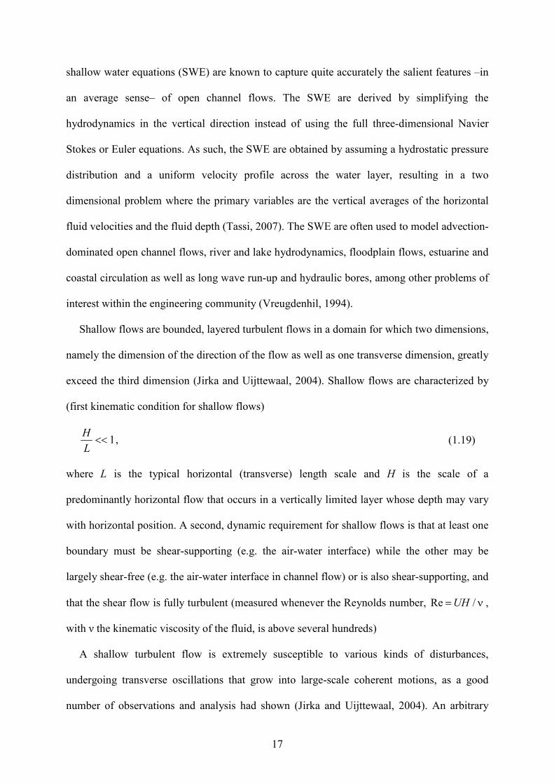
shallow water equations (SWE) are known to capture quite accurately the salient features –in

an average sense– of open channel flows. The SWE are derived by simplifying the

hydrodynamics in the vertical direction instead of using the full three-dimensional Navier

Stokes or Euler equations. As such, the SWE are obtained by assuming a hydrostatic pressure

distribution and a uniform velocity profile across the water layer, resulting in a two

dimensional problem where the primary variables are the vertical averages of the horizontal

fluid velocities and the fluid depth (Tassi, 2007). The SWE are often used to model advection-

dominated open channel flows, river and lake hydrodynamics, floodplain flows, estuarine and

coastal circulation as well as long wave run-up and hydraulic bores, among other problems of

interest within the engineering community (Vreugdenhil, 1994).

Shallow flows are bounded, layered turbulent flows in a domain for which two dimensions,

namely the dimension of the direction of the flow as well as one transverse dimension, greatly

exceed the third dimension (Jirka and Uijttewaal, 2004). Shallow flows are characterized by

(first kinematic condition for shallow flows)

1<<L

H, (1.19)

where L is the typical horizontal (transverse) length scale and H is the scale of a

predominantly horizontal flow that occurs in a vertically limited layer whose depth may vary

with horizontal position. A second, dynamic requirement for shallow flows is that at least one

boundary must be shear-supporting (e.g. the air-water interface) while the other may be

largely shear-free (e.g. the air-water interface in channel flow) or is also shear-supporting, and

that the shear flow is fully turbulent (measured whenever the Reynolds number, Re /UH= ν ,

with ν the kinematic viscosity of the fluid, is above several hundreds)

A shallow turbulent flow is extremely susceptible to various kinds of disturbances,

undergoing transverse oscillations that grow into large-scale coherent motions, as a good

number of observations and analysis had shown (Jirka and Uijttewaal, 2004). An arbitrary

18

transversely sheared profile ( ),u x y can trigger instabilities characterized by vertical

elements of length scale l2D that are much larger than the depth, 1/2 >>Hl D . The structure of

these turbulent motions is largely “two-dimensional” with vertically aligned vorticity vectors.

In summary, the following characterization emerges: “shallow flows are largely

unidirectional, turbulent shear flows driven by a piezometric gradient and occurring in a

confined layer of depth H. This confinement leads to a separation of turbulent motions

between small scale three-dimensional turbulence, 3 / 1D H ≤ℓ , and large scale two-

dimensional turbulent motions, 2 / 1D H >>ℓ , with some mutual interaction” (Jirka and

Uijttewaal, 2004)

Nadaoka and Yagi (1998) schematized the essential features of turbulence in shallow flows

following ideas set forth before by other researches, notably Dracos et al., (1992). The

spectral structure of a shallow turbulent flow, as conceptualized by Nadaoka and Yagi (1998),

is depicted in Figure 1.8. However, they failed to produce experimental data to support the

concept. Moreover, their claim of the inverse cascading of energy from small scales towards

large scales is not necessarily correct, as shown next.

The Navier-Stokes equations for 2D turbulence, with flow velocity u ( )1 2, ,0u u= and

vorticity ω ),0,0( ω= provide the evolution model for the mean square of the kinetic energy

( >< 2u ) and vorticity ( >ω< 2 )

>ω∇<ν−=>ω<

>ω<ν−=>< 2

22

2

2,2dt

d

dt

d u. (1.20)

There are two integral of motion in the limit ν → 0 (closure problem in 2D turbulence,

according to Batchelor (1969)). Kraichman (1967) showed that in the case of forced

turbulence at rate ∈ and enstrophy transfer rate ( )2 /d dtβ = < ω > , there are two well

distinguished cascades of energy transfer in the inertial range

19

33/2

3/53/2

)(

)(−

−

β≅

≅∈

kkE

kkE. (1.21)

Since the kinetic energy flux through the enstrophy cascade is zero, the kinetic energy

produced at rate ∈ at ki can only cascade backwards, toward scales larger than 1/ki.

Schematically,

i∈

ik

53/2 −∈ k

33/2 −β k

k

Figure 1.8 Inverse cascading in the inertial range of 2D turbulence

1.4. Dissertation outline

As was mentioned before, the impact of morphology on turbulent processes is often

simplified to a local boundary condition and rarely the impact of large morphological units is

considered. There is an obvious gap between the small turbulent scales and the large

scales of the flow structure that in turn may induce typical morphological scales. This

thesis in an attempt to bridge in part the gap, seeking a deeper understanding of which and

how some typical length scales characterizes the behaviour of a shallow turbulent flow. In

spite of some limitations imposed by the available laboratory equipment and facilities, the

emphasis of this work was put to detect the role of bed friction on the formation of 2DCS in

shallow turbulent flows. The role of bed friction in shallow turbulent flows was vividly

/3

E (k)

20

depicted by the aforementioned examples, which is contrary to the belief of Nadaoka and

Yagi (1998), who restrict the role of bed friction to be source of small-scale 3D turbulence

only. It is certainly true that a rough boundary generates vorticity on a broad band of high

wavenumbers, which is later diffused into the flow. However, an issue to address is to

determine if the overall bed resistance, once in balance with inertia for example, triggers the

formation of distinguishable 2DCS. There is ample evidence that the types of 2DCS described

so far represent a length scale well-resolved by the shallow water theory (Lloyd and Stansby,

1997)

This thesis compiles the experimental findings obtained in two different laboratory

settings, with all their limitations in equipment and facilities. Whereas the spectral response of

a contracting shallow turbulent flow was analyzed through experiments performed at FICH’s

facilities, the formation and evolution of large free bars was studied with the aid of the large

sand box facility available at the School of Geosciences at the University of Newcastle (UK).

Conceptually, the free bars can be considered a sort of 2DCS of the evolving bed fed by the

interacting turbulent flow and the sediment transport along the erodable bed.

The content of this thesis is as follows: first of all, the state of the art of shallow turbulent

flows is critically reviewed in Chapter 2 from the perspective of the turbulent scales that

typifies an open flow, either imposed by geometry or developed internally by the flow itself.

This is followed by an in depth literature review on the formation an evolution of free bars. In

Chapter 3, the spectral segregation between 2D and 3D turbulent scales of a broad shallow

turbulent flow, developed as the flow approaches a lateral contraction, is presented. For this

study, the large basin facility available at FICH was used. Then, experimental study on the

formation and evolution of free bars is presented in Chapter 4. Finally, conclusions and

recommendations are discussed in Chapter 5. The Appendixes found at the end compiled

supplemental material that was used along the development of the work.

21

CHAPTER 2 Literature review

2.1 On 2D coherent turbulent structures

Many engineers and scientists when studying the dynamical behaviour of water bodies use

the mathematical model based on the shallow water approximation, valid whenever the depth

h of the water layer is small compared to the length extent l of the wavelike motion of the

fluid. Indeed, there are many engineering problems involving water motion that can be treated

as shallow turbulent flows, where in addition to the shallowness condition / 1h l << , the fully

developed turbulence condition is achieved if the Reynolds number Re /Uh ν= of the flow

goes beyond a few hundred. Here, U is a characteristic velocity, typically the free-stream

velocity, and ν is the fluid kinematic viscosity. The flow in compound channel systems,

coastal waters, shallow lakes, and in the lower layers of the atmosphere are just few examples

of turbulent flows that can be analysed with the shallow water assumption, also known as the

long-wave approximation. However, 3D effects can sometimes hamper not only the versatility

but also the validity of the 2D shallow water approximation. A case in point is given by the

flow approaching the opening of a relief bridge located on a flat floodplain of a very low-

gradient, large river.

The hypothesis of separation of scales in shallow turbulent flows was postulated by

Nadaoka and Yagi (1998), among others, in their numerical study on compound channel

flows. However, they provide no experimental evidence to support the idea.

Indeed, the coexistence of 2D with 3D turbulence structures, and the possibility of treating

them in a separated manner may have profound influences in the numerical modelling of

22

shallow turbulent flows, as vividly suggested by Nadaoka and Yagi (1998) themselves. In

others words, a 3D numerical simulation of all the significant structures of a turbulent flow

could be costly prohibitive (Shi et al., 1999; Zedler and Street, 2001), if not impossible even

with today’s computers, while using the 2D depth-averaged shallow water equations could

provide almost the same information at much lower cost (Nadaoka and Yagi, 1998; Bousmar

and Zech, 2002). This conclusion was reported by Lloyd and Stansby (1997) when comparing

2D and 3D numerical shallow-water models with experimental data obtained in the wake of

conical islands. They found that in some cases, the 3D model produced poorer representations

of the wake features than the 2D model.

Usually, if the shallow flow is uniform and wide, the 3D structure of turbulence is

characterized by a streamwise vortex pattern in the plane normal to the local axis of the

primary flow (Gulliver and Halverson, 1987). In this case, the size of the 3D vortex pattern is

definitely bounded by the thickness of the water layer. However, some of these shallow

turbulent flows are readily susceptible to transverse disturbances that may grow into large-

scale instabilities characterized by 2D vortical structures. Examples of these large-scale

turbulent structures characterized by coherent eddies of Kelvin-Helmholtz type, and called 2D

coherent structures (2DCS) by Jirka (2001), are encountered in shallow wake flows (typically

an island wake (Wolanski et al., 1984), shallow jets (Dracos et al., 1992), and compound

channel flows (Tamai et al., 1986). Consequently, the distribution of turbulent energy in such

flows has a spatial structure determined by the internal geometry of the flow. These

observations have led researchers to formulate the hypothesis that turbulent energy is stored in

two separated structures; while 2D turbulent kinetic energy is stored and transported by large

horizontal eddies of size l1 much larger than the water depth, 1/ 1h l << , 3D turbulent kinetic

energy is confined to smaller eddies, whose size l2 is primarily controlled by the length scale

that bounds the free-surface flow (i.e., water depth; (Gulliver and Halverson, 1987)).

23

In spite of the physical basis of the concept, the existing measurements on the subject are

not entirely clear with regard to the physical mechanisms underlying the separation between

2D and 3D turbulent structures in shallow flows. (Dracos et al., 1992) provided some of the

most conclusive experimental evidence on shallow jets, where an inverse cascade of spectral

energy that follows the law of “2D turbulence” (Kraichman, 1967) is observed. Jirka (2001)

has recently reviewed this issue. A distinction should be made here between unstable and

stable flows. Whereas the aforementioned shear flows constitute the prototype of

hydrodynamic instabilities commonly found in many open flows, the approaching flow

problem considered here is not necessarily unstable in the sense of the linear stability theory

(Drazin and Reid, 1981). Indeed, for transversely sheared flows, namely shallow wakes,

shallow jets, and compound channel flows (also known as the shallow mixing layer), the

larger, resolvable coarse scale that characterizes the 2DCS is linearly unstable to small

perturbations and is governed by a modified version of the Orr-Sommerfeld equation. This

issue was established by Chen and Jirka (1998) for shallow jets, by Chen and Jirka (1997) for

shallow wakes and by Ghidaoui and Kolyshkin (1999) for compound channel flows, among

many other contributors to the subject. Conversely, in the approaching flow problem

considered here, there are neither topographic nor velocity discontinuities that may act as

forcing mechanisms to trigger the onset and growth of 2DCS, except downstream of the

contraction. So, it is natural to ask if only transversely sheared flows are likely to exhibit the

segregation between vertical (small) scales and horizontal (large) scales. Moreover, the

discharge to the floodplain downstream of narrow bridges could behave as a jet when looking

at from the far field (Dracos et al., 1992). Thus, the hypothetical formation of 2DCS

downstream of the opening could have considerable impact into the subsequent floodplain

evolution.

24

2.2 On free bars formation

Numerous classifications of bed forms have been proposed. A general description is

summarized in Table 2.1. Some authors generally classified bed forms according to their

shape and position. These types of forms, composed of a wide range of grain sizes, are usually

exposed at certain stages of flow. At first the more general bedforms classification existing in

the literature will be cover, mainly concern about dunes, and later followed by alternate bars.

The most widely used sequenced of bed forms commonly associated with sand-bed

streams are ripples, dunes, plane bed and antidunes, see Figure 1.7. Due to their links with

sediment transport and flow resistance, considerable effort has been invested in the study of

this sequence, particularly in laboratory flumes. The formation of these various bed features

indicates the presence of systematic tendencies in the ability of natural streams to sort and

transport material over a wide range of flow and bed material conditions.

Many authors suggest that the bed forms are the effect of instability at the water-sediment

interface. The deformation of an initially flat bed may lead to concentrations of grains, which

move intermittently when shear stresses are just above the movement threshold. These small

disturbances will, under certain conditions, influence the flow and local sediment transport

rate in such a way that scour and deposition occur in the troughs and over the crest

respectively, thereby increasing the amplitude of the initial bed undulations. Such an

increment disturbs the local transport rate still further, promoting additional growth through a

positive feedback until a limit is reached and ‘equilibrium amplitude’ attained.

There have been some attempts to classify the bedforms generated under a given flow

condition using (kinematics) instability analysis (Kennedy, 1963; Engelund, 1970). The

instability analysis indicates the conditions at which an initial perturbation of the bed will

grow, but it does not give information on the equilibrium dimension of the bedform. The most

25

reliable classification of bed form types is based on the analysis of bed forms as observed in

flume ad field conditions.

Bed form Dimension Shape Behaviour and occurrence

Bar

Lengths comparable to channel width

Variable

Five mean types: 1. Point bars: Form particularly in the inner banks of meanders. 2. Alternate bars: distributed periodically along one and then the other bank of a channel 3. Channel junction bars: develop where tributaries enter the main channel. 4. Transverse bars (include riffles): may be diagonal to the flow 5. Mid-channel bars: typical of braided reaches.

Ripples m;

0.04mHb

<

Triangular profile; gentle upstream slope sharp crest and steep downstream face

Generally restricted to sediment finer than 0.6 mm; discontinuous movement; at velocities much less than that of the flow

Dunes

λ 4-8 times flow depth, Hb up to 1/3 flow depth; much larger than ripples

Similar to ripples

Upstream slope may be rippled; discontinuous movement; out of phase with water surface

Lower regime of roughness; from roughness dominant

Plane bed

Bed surface devoid of bed forms; may not occur for some ranges of depth and bed material size

Antidunes

Relative low height dependent on flow depth and velocity

Sinusoidal profile; more symmetrical than dunes

Less common than dunes, occurring in steep streams; in phase with surface water waves; bed form may move upstream, downstream or remain stationary.

Upper regime of roughness; grain roughness dominant

Particularly sand-bed streams

λ - Bedform wavelength; Hb – bedform height.

Table 2.1 Classification of bed forms, taken from Knighton (1984).

Van Rijn (1993), for example, believed that bed forms are relief features initiated by the

fluid oscillation generated downstream of small local obstacles over a bottom consisting of

movable (alluvial) sediment materials. He mentions different classification criteria for sand

beds according to different authors: (i) Engelund (1974) used the Froude number (Figure 1.7);

(ii) Liu (1957) described the type of bed forms in terms of the suspension parameter

swu* and the particle-related Reynolds number ν50* du as shown in Figure 2.1, where *u is

26

the bed shear velocity, sw the particle fall velocity of bed material, 50d particle diameter and

ν kinematic viscosity coefficient, and (iii) Simons and Richardson (1966) used the stream

power ,b cuτ (where ,τb c is the critical shear stress and u the depth average velocity) and the

median fall diameter, fd , as shown in Figure 2.2

Figure 2.1 Bedform classification graph of Liu (taken from van Rijn, 1993).

Finally, (iv) Van Rijn (1984) and van den Berg and van Gelder (1989) used a

dimensionless bed-shear stress parameter and the dimensionless particle parameter. Van den

Berg and van Gelder (1989) used the particle mobility parameter ])ρρ[(τθ 50gdsb −′=′ , the

grain bed shear stress 2)(ρτ Cugb′=′ and the particle diameter parameters

)312log(18 90dhC =′ and *D ( )]ν)1([ 31250 gsd − as shown in Figure 2.3 ρ and ρs are the

water and sediment densities, respectively, g is the acceleration due to gravity, h is the water

depth and s is the specific gravity of the sediment.

27

Figure 2.2 Bedform classification graph of Simons and Richardson (taken from van Rijn, 1993).

While van Rijn used the bed shear stress parameter, , ,(τ τ ) τb b c b cT ′= − and the particle

diameter parameter to obtain a more specific classification. In this classification, it is possible

to find asymmetrical dune-type bedforms with a length scale much larger than the water depth

( L h>> ), observable features for 15T < . As well as, mega ripples, which are ripples with a

length scale of the order of the water depth ( L h≈ ), and mini-ripples, that have a length scale

of the near-bed turbulence length scale ( L h< ), superimposed on the dunes for 3 10T< <

and 10* ≤D (Figure 2.4).

Later, in 1996, Best presented a new attempt to determine bedform existence fields for a

wide range of particle sizes and shear stresses. In Figure 2.5, the bed features are shown

related to the Froude Number (Fr) for: the lower stage ( )1Fr < , the upper stage ( )1Fr > and

the transition zone (denoted by the dotted line). The dunes are divided into two types, two-

dimensional (2D) and three-dimensional (3D) the latter is just referred to as dunes. The above

bedforms were observed in steady flow over a mobile bed but, in alluvial streams, the form of

the bed varies with hydraulic quantities such as water depth, energy slope and sediment size.

28

Therefore, these materials can give a picture of response of channel bed when the variation

happens in the long term or very gradually.

Figure 2.3 Bedform classification graph of van den Berg and van Gelder (from van Rijn,1993).

Sand bars are the largest bed form (van Rijn, 1993) –such as alternate bars, side bars,

braid bars and transverse bars, which usually are generated in areas with relatively large

transverse flow components (bends, confluences or expansions). Alternate bars are

characterized by a sequence of steep consecutive diagonal fronts with deep pools at the

downstream face, and gentler riffles along the upstream face (Figure 2.6), whose horizontal

scale is typically of the order of several channel widths, while the vertical scale is of the order

of the flow depth. Braid bars are alluvial “islands” that separate the anabranches of braided

29

streams. Some bars can be observed distributed over cross-sections with a marked streamwise

elongation, and the flow over them is sinuous (wavy) in plan. They are call transverse bars

and are diagonal shoals of triangular-shaped plan along the bed with one side attached to it,

and have a large width-depth ratio. Side bars are the ones connected to river banks in a

meandering channel with no flow over them and a planform roughly triangular. Special

examples of this type are point bars and scroll bars.

Figure 2.4 Bedform classification graph of van Rijn (1993).

30

Figure 2.5 Bedform existence field across a range of grain sizes (in Robert, 2003).

Figure 2.6 Alternate bars diagram

Alternate bars, in particular, are frequently observed in rivers, and their formation has

acquired an increasing importance in highly developed countries where river regulation

works, such as canalization and artificial straightening motivated by land reclamation

purposes, leads to their unexpected appearance (Figure 2.7).

31

Figure 2.7 Alternate bars in the Alpine Rhine, Border of Switzerland/Leichtenstein (taken from Jaeggi, 1984)

2.2.1 Bar formation problem: alternate bars as the precursor mechanism for river

meandering? Linear stability analysis

Callander (1969) set forth the idea of “dynamic instability”: Under appropriate conditions

the non-cohesive flat bottom of a turbulent stream flowing in a straight channel loses stability

leading to a new configuration characterized by infinitesimals growing and migrating

perturbations, of length scale of the order of the channel width. It turns out that the bottom

perturbations tend to form an alternating sequence of deep and shallow reaches, as can be

seen in Figure 2.6, a pattern that can be interpreted as the precursor of river meandering”.

This concept has appeared in several papers about channels with loose boundaries (Leopold

and Wolman 1957, Callander 1969).

This tendency towards instability may be modified by the characteristics of the flow

resistance. Vanoni and Brooks (1957), Raudkivi (1963) and Kennedy and Brooks (1965) have

shown that the drag coefficient varies with velocity on an erodible bed. If the bed material is

fine grained, there may be a range of velocity through which the bed shear stress decreases as

32

the velocity increases. Then, an increase in velocity can, by making the bed less rough, cause

a further increase (Callander, 1969).

Callander (1969) applied only two-dimensional flow models assuming that the direction of

the local sediment transport is parallel to the local velocity vector, and that the sediment

transport rate is uniquely related to the bed shear stress. Bearing in mind that Callander (1969)

neglected the velocity variation along verticals and includes the internal friction as one-

dimensional description only, corresponding to gradually varying flow, Engelund and

Skovgaard (1973) developed a theory taking into account the three-dimensional nature of the

flow. They extended Callander’s analysis (1969) by introducing a three-dimensional flow

model which takes account of the helical motion induced by the non-uniform vertical velocity

distribution in the basic flow, an effect neglected in the previous approaches. Furthermore,

they introduced the effect of a transverse bed slope on the transportation of the sediment and

found that this effect is of great significance, because the theory predicts that a river will braid

into an infinite number of branches if that correction is not included. This suggests that an

accurate knowledge of the interaction of fluid flow and sediment motion is necessary in order

to develop an adequate description of the river instability.

Later, Parker (1976) considered the two-dimensional stability models of Callander (1969)

using expansion techniques to obtain an analytical description of the sediment transport as a

necessary condition for the occurrence of fluvial instability. Also he made a differentiation

between meandering and braided regimes, obtaining relations for the meander wavelength and

number of braids. Parker (1976) proposed that a theory of alternating bar formation in straight

rivers is also a theory of the origins of meandering and braiding, based in the following

statements: i) meandering and braiding rivers generally have a large width-depth ratios; ii) the

sinuous pattern of banks and bars is due to the emergence of a submerged alternating bar

pattern on the bed of an otherwise roughly straight river during low flow; iii) these alternating

33

bars occur even in channels with non-erodible banks. Justification of these statements for

natural river was provided by Kinoshita (1957) and Fanhestock and Maddock (1964). Thus

Parker (1976) performed an investigation into the cause of fluvial instability by theoretically

examining submerged bedforms in a shallow channel model treating meandering and braiding

as different degrees of the same instability phenomenon, highlighting that sediment transport

is a dynamically necessary condition for the occurrence of instability leading to meandering

either in flow or in the bed. The analysis of his work indicates that most streams have a

tendency to form bars even though they are in a graded state. If the slope and the width-depth

ratio at a formative discharge are sufficiently low, meandering is favoured. If the slope and

the width-depth are sufficiently high, braiding is favoured. The major disadvantage of

Parker’s theory (Parker, 1976) is the difficulty of applying it to natural rivers due the fact that

the channel width at a formative discharge must be known before any of the relations can be

evaluated.

Fredsoe (1978) used the same linearized flow model of Engelund and Skovgaard (1973)

but updated the theory in the following way: i) the linearized equation were solved

numerically without introducing further approximations; ii) the effect of a transverse slope of

the bed is accounted for; iii) the total amount of sediment is transported partly as bed load and

partly in suspension. The fact that for large flow rates a greater part of the sediment load will

be carried in suspension implies that there can be no unique relationships between the

transport rate and the bed shear stress. To account for this phenomenon it is necessary to

introduce a supplementary equation of continuity for the suspended sediment, and to be able

to estimate the transport rates of the bed load and the suspension separately.

These analyses outline the conditions for bar formation in the flow and sediment

parametric space, i.e., the wavelength and wave speed selected by the flow-erodible bed

system are given by the maximum growth rate of the perturbations. In the theoretical context

34

of all the above contributions, it was tacitly assumed that a sinuous migration thalweg within

a straight channel should somehow evolve into a sinuous planimetric instability and thus

leading to meandering.

Nevertheless, migrating alternate bars exhibit a relatively large migrating speed as

compared with the speed associated with the bank or lateral erodibility (Struiksma et al.,

1985; Struiksma, 1985). Consequently, the type of perturbations responsible for meandering

initiation must be somehow steady in order to determine such a slow process as that of bank

erosion (Seminara and Tubino 1989).

2.2.2 Bar formation problem: meandering formation as a planimetric instability.

All above analyses were somehow unsatisfactory since the effect of the bank deformation

was not included. They treat only the deformation of alternate bars between straight, non-

erodible banks; the flow may wind about the bars, but the channel does not meander. In the

early 1980´s, Ikeda, Parker and Sawai (1981) suggested the idea that meander formation was

associated with planimetric instability, the disestablishing mechanism being bank erosion

associated with the secondary flows induced by channel sinuosity. They develop a formal

stability theory of channels with sinuous banks; describing the bank erosion and considering

the stability criterion in terms of the growth-rate of lateral bend amplitude. The main

conclusion of this theory is that for alluvial streams ‘bar’ and ‘bend’ stabilities operate at

similar wavelengths when sinuosity is not too large. This provided justification for the

assumption that alternate bars formation eventually leads to a meandering channel with an

initial wavelength close to that of alternate bars.

In turn, Olesen (1983) suggested that steady spatially growing ‘bar’ perturbations was a

more reasonable candidate to explain meander formation. However, Olesen (1983) did not

explain which mechanism would excite the development of such perturbations that are not

‘naturally’ growing –their temporal growth rate being zero.

35

Blondeaux and Seminara (1985) introduced a unified approach where the forcing effect of

channel curvature upon some quasi-nonamplyfying and quasi-nonmigrating ‘bar’ modes

provided the excitation mechanism for steady spatially periodic perturbations. They employed

a model for fully developed flow in sinuous channels with small curvatures relaxing the above

mentioned condition on the meander length. It turns out that under these circumstances, the

curvature forces a ‘natural’ solution which represents a quasisteady bar perturbation. Thus it

emerge that ‘bend’ instability does not select the most unstable wavelength of ‘bar’

instability, but rather that which is nearest to resonance for any given set of flow parameters.

The wavelength selected by this bar-bend resonance mechanism was found to be about three

times as large as those predicted be a traditional ‘bar’ stability theories.

Later, the flow field model of Ikeda et al., (1981) was rederived by Johannenson and

Parker (1989) to take into account the convective transport of primary flow momentum by the

secondary flow. The planimetric evolution equation given in that paper not only confirm the

resonance phenomena discovered by Blondeaux and Seminara (1985) but also has formed the

basis of popular meander models such as the one of Howard (1996).

Attempts to verify experimentally the “resonance theory” (Colombini et al., 1987) were

successful to some extent but, in particular, the interaction between alternate migrating bars

and fixed point bars formed in channels bends and the conditions for the suppression of the

former were studied experimentally by Garcia and Niño (1993).

Recently, a new set of works tried to relate some other aspects leading to bar formation and

instability. Lanzoni and Tubino (1999) analysed the influence of grain sorting using a similar

stability analysis for the grain size distribution proposed by Seminara et al., (1996) to explain

the formation of bedload sheets, but retaining the full coupling between perturbations of

bottom topography and grain size distribution. The main output of this analysis implied the

36

decreasing of the growth rate of bar perturbations due to increasing values of the standard

deviation of the sediment mixture.

Federici and Seminara (2003) studied the convective instability nature of some persistent

perturbations observed in flume experiments. Up to now, temporal stability analyses consider

perturbations that amplify in time, starting from some initial spatially periodic perturbations,

i.e. they assume that the perturbation wavenumber λ is real while its frequency ω is complex.

Such analyses allow us to distinguish between stable configurations (all λ decay in time) and

unstable systems (some λ are amplified). When the nature of the instability is convective a

spatial stability analysis is applicable, considering perturbations that evolve in space, starting

from some initial temporal distribution, i.e., assuming that the perturbation wave number is

complex and the perturbation frequency is real.

Finally, Hall (2004) tried to determine which types of disturbances were converted into

instability waves – the receptivity problem. In the existing theory on bar formation little

attention has been given to the question of what physical mechanism generates a particular

bar wavelength. The assumption implicitly made is that in a river there are so many sources of

spatial inhomogeneities that there will always be sufficient forcing at all wavelengths to excite

the most unstable bar. However in less disturbed environments, e.g., in man-made channels or

in laboratory experiments, the situation is less clear-cut. In fact, there are a variety of sources

for the generation of instability waves. The major point to be appreciated is that boundary

layer instabilities are almost always convective in nature so an instability wave can only be

generated continuously if there is a disturbance source for all time. In the context of boundary

layer transition the process by which disturbances are converted into instability waves is

usually called the receptivity problem; see Ruban (1984), Denier et al. (1991), Asai and

Nishioka (1993), Duck et al. (1996), Saric et al. (2002) and Hammerton and Kerschen (2005)

for a discussion of receptivity problem and Görtler instabilities in boundary layers. Hall

37

(2004) shows how spatial variations associated with seepage into the channel; curvature

variations, local constrictions or other spatial variations can interact with the flow

unsteadiness to produce bars. In fact he related the amplitude of the bar generated to the

forcing mechanism through a ‘coupling coefficient’ to determine what kind of spatial

variations were more or less efficient in the generation of bar. Giving examples of how a dyke

entering the main channel or indentations made in the banks should be arranged so as to

minimize or maximize bar formation.

2.2.3 Bar formation problem: non-linear theories

It is now fairly well established that bar formation can be explained as a result of an

instability mechanism (Lanzoni, 2000). Critical conditions for bar growth as well as bar

wavelength and celerity can be easily predicted within a linear framework. However, when

conditions are far from critical condition, comparison with experimental observations show

that in general linear theories underpredict bar wavelength whereas bar celerity is

overpredicted (Blondeaux and Seminara, 1985; Nelson and Smith, 1989; Lanzoni, 2000). This

discrepancy is possibly due to the strongly nonlinear interactions arising between finite

amplitude disturbances of different wavelength, which characterized bar development.

Weakly nonlinear theories (Colombini et al., 1987; Schielen et al., 1993), which have been

developed in the neighbourhood of critical conditions, cannot account for the above strong

nonlinearity. While weakly nonlinear theory predicts fairly well the equilibrium bar height

(Colombini et al., 1987), bar wavelength and celerity predictions are not significantly

improved. Consequently, linear theories are still preferred to frame the range of physically

admissible parameter values within unstable condition. In more detail, the analysis of

Colombini et al., (1987) predicts finite amplitude of the alternate bars in a straight alluvial

channel for perturbations which grow on a time scale that is large compare to the typical

period of the waves. The equilibrium amplitude in that equation is also a function of the

38

Shields bottom shear stress, and the sediment size to depth ratio. The result of their two-

timescale analysis was a so-called Landau equation describing the time evolution of the wave

amplitude. They only considered the case were the wavenumber is fixed in the neighbourhood

of the critical wavenumber for which instability first occurs. The theory provides a simple

equation for the equilibrium amplitude of the alternate bars as a function of a small parameter

ε, defined as ( )ε β β /βc c= − , where β is the ratio between half the width of the channel and the

depth of flow, and βc is the critical value of β for the formation of alternate bars as obtained

from the neutral curve. Schielen et al., (1993) argued that considering only the wavenumber

in the neighbourhood of critical condition was disputable, since in fact all waves in a narrow

spectrum -centred on the critical value- are unstable. Owing to the dispersion of this wave

group, modulation will also occur on a spatial scale. If this effect is included in the weakly

nonlinear theory, a modified amplitude is found which is governed by a Ginzburg-Landau

equation. Since the group velocity varies with the wave number we may expect this equation

to describe local convergence and divergence of the perturbation energy, which may cause the

periodic solutions obtained from the Landau theory to become unstable (Lighthill, 1978). As a

result bar patterns with a more complex temporal and spatial behaviour may be expected.

Furthermore, it is possible to determine the stability of its solutions against several

perturbations (in contrast to the Landau theory, where one can only study the stability of

periodic solutions against perturbations with exactly the same wave number). Under the bases

of the Ginzburg-Landau theory, Schielen et al. (1993) investigated the modified behaviour of

bar patterns.

On the other hand, some efforts have been devoted in the past to simulate numerically free

bars evolution, and several mathematical coupled models for flow and bed topography have

been proposed in the literature (Olesen, 1983; Struiskma, 1985; Nelson and Smith, 1989;

Shimuzi and Itakura, 1989; Struiskma and Crosato, 1989; Colombini and Tubino, 1991;

39

Mosselman, 1992, 1998; Defina, 2003). Most of these models use a channel-fitted orthogonal

curvilinear coordinate system, which allows an accurate description of the fully nonlinear bar

evolution in simple-shaped domains (e.g., straight or meandering channels). Nevertheless, few

studies have attempted to use these models as a tool for better understanding the fully

nonlinear evolution of free bars, with the exception of the work of Federici and Seminara

(2003). Nelson and Smith (1989) simulated the temporal evolution of alternate bars from an

initially flat bed for two cases experimentally studied by Fujita and Muramoto (1985). They

formulated both hydrodynamic and sediment budget equations using a channel-fitted

orthogonal curvilinear coordinate system and obtained a solution by use of a standard finite

difference technique. The model predicted the generation of trains’ bars downstream of an

initial disturbance (i.e., a small asymmetric and erodible bump) whose characteristics were

very similar to those observed experimentally. They also argued that a carefully designed

two-dimensional model captures the main mechanism governing bar development. Another

numerical study to investigate the highly nonlinear competition between modes was

performed by Colombini and Tubino (1991). Using also a channel-fitted orthogonal

curvilinear coordinate system but solving the hydrodynamic and sediment budget equations

using a spectral method, they clearly confirmed the crucial importance of strongly nonlinear

interaction mechanisms in the development processes. More recently, Defina (2003), used a

two-dimensional finite element model for the morphodynamic evolution of a cohesionless bed

to test experimental observation of the formation and evolution of free bars. She studied the

strongly nonlinear interactions governing bar development, focusing on the influence of the

initial perturbation introduced in the flow field for bar inception. Her research found that the

type of disturbance plays a role of utmost importance as it can strongly affect both the

developing process and the equilibrium conditions

40

2.2.4 Bar formation problem: meandering formation as a resonant mechanism

If the overall picture given above is correct, it is then possible to see two different

phenomena occurring in the process of meander formation in alluvial channels (Colombini et

al., 1987): a) development of migrating alternate bars (or free bars) without lateral or bank

erodibility, a relatively fast process compared with the second slower process, i.e., b)

development of channel sinuosity (forced bars), a relatively slow process triggered by a

disturbance that contains a non-propagating part either due to curvature effects, i.e., the bar

resonance mechanism (Blondeaux and Seminara, 1985), or due to flow unsteadiness (Hall,

2004).

As it was mentioned, it is now fairly well established that the formation of free bars can be

explained by a classical normal mode stability analysis performed on the system of

conservation equations governing the hydrodynamics and sediment transport in channels with

a cohensionless bed. The ratio of channel width, or half-with B, to water depth H is the crucial

dimensionless parameter for the instability, though some authors claim that the relative

roughness parameter, which controls frictional forces play some weaker role (Federici and

Seminara, 2003). For some given hydraulic conditions, linear stability predicts a sequence of

increasing critical values of ( )cc HB /=β above which small-amplitude bar perturbations

characterized by m rows are amplified. For 1=m , bars give rise to a weakly meandering

pattern of the thalweg, whereas for 2≥m , a submerged braiding pattern develops.

The coexistence of free or migrating and forced or fixed bars in a meandering channel has

been observed in laboratory experiments by Kinoshita and Miwa (1974), Gottlieb (1976) and

Fujita and Muramoto (1985). However, the most interesting experiment from the point of

view of interactions between free and forced bars was the one conducted by Kinoshita and

Miwa (1974). They did an extensive set of experiments in a meandering channel, where the

channel was modelled as a set of straight segments forming and angle α to each other. Two

41

different regimes where detected depending on the relations of α with a critical value cα

which was found to be in the range of �20 to �40 , and depends on the meander wavelength.

2.2.5 Bar formation problem: experimental approach and regime theories

In parallel with theoretical works a variety of methods have been used to empirically

describe and characterize the formation of alternate bars in open channel flows. Available

approaches range from equations that predict the regime or graded morphology of equilibrium

channels to mathematical models that simulate channel changes in time and space. According

to experimental data (a series of experiments in a water and sediment recirculating flume of

30m long and 3m wide with smooth, rigid walls of sheet metal and a mobile bed), Chang et

al., (1971) found that alternate bars usually began to form when the value of width-depth ratio

reached 12. They observed a slow migrating pattern of alternate bars, as the sediments were

moving downstream, similar to the movement presented by dunes and ripples. Indicating that

the dimensionless parameter λ /FS H is related only to the Froude number of the channel flow,

where SF is the friction slope.

Jaeggi (1980) considered that alternate bars are a special form of dunes that occur in

subcritical flows in Gravel Rivers, assuming that the generating mechanism for alternate bars

and dunes is basically the same. Therefore the formulation of dunes can be applied to

alternate bars. The conclusion of his work was to propose an expression for the upper limit of

bar formation, relating the bedform wavelength )( Dλ to the meander (plan form) wavelength

( Mλ ). Later, Jaeggi (1984) conducted a series of experiments in a 25m long and 0.3m wide

flume filled with natural sands with mean grain sizes of 0.52, 1.8 and 4.0mm and PVC

granulate of cylindrical shape with mean diameter of 3.0mm. Jaeggi (1984) used this

experimental data, together Chang et al. (1971) data, to establish a new criterion for alternate

bar formation and characteristics, suggesting that the upper limit of bar formation is given by

42

0.15

50 50

θ2.93ln 3.13

θ ( ) θO

c s c

BS B

d d

γ= − γ − γ

(2.1)

and the respective lower limit of alternate bar formation is described by

0.67

90

50

θ

θc

d

d

=

(2.2)

where θc is the critical Shield stress, γ and γs are the specific weight of water and sediment,

respectively, and S the channel slope. In this method, the channel slope has a minimum

condition at which alternate bar formation will occur, being:

50

50

15.0

9.12

07.1exp

d

B

Md

B

S

+

> , (2.3)

where M is a function of the sediment grading and varies from 0.34 (uniform material) to 0.7

(widely graded material). Additionally, the method states that the total height of alternate bar

AB∆ is almost independent of discharge and slope, despite being a slight increase in the total

height of dunes and antidunes with increases in discharge. The scour depth ∆ is given by:

( ) 15.0506

76.0dB

BAB =∆=∆ . (2.4)

At the same time, Olesen (1983), presented a linear perturbation analysis of a horizontal

two-dimensional mathematical model for the flow and bed topography in straight alluvial

rivers with dominant bed load. As a result he suggests that the wavelengths of alternate bars

were 3-4 times the channel width.

Ikeda (1984) carried out a series experiments in a 15m long, and 0.50 m wide flume. He

crudely approximated the bar wavelength as B9=λ and suggested a linear relationship

between the maximum scour depth ∆ and the bar height as follows:

bH75.0=∆ (2.5)

43

Another criteria for alternate bar formation in straight alluvial channels with smooth rigid

banks was suggested by Chang (1985), based upon the relative magnitudes of the stable width

of stream flow, Bs, and the channel width between rigid banks. The general situation is

divided in three cases: in the first case, the stable width at higher discharge is greater than the

channel width; as a consequence meanders or alternate bars will not form. In the second case,

the stable width is less than the channel width; subsequently alternate bars can be considered

as large-scale bedforms which reflect meandering development in confined channels. Finally,

the third case, where the stable width is much smaller than the channel width, the consequent

development of free meanders will result in the disappearance of alternate bars. Therefore,

alternate bars in straight alluvial channels may develop if the stable width is less than the

channel width between the rigid banks,

2sB B< (2.6)

where B is half the channel width between rigid banks and Bs is the stable width of alluvial

channel. He recommended a rational regime expression to calculate the stable width as

follows:

0.150.4

0.48

50

1.656.62 1 1.3 ln

( )c c

s

s

B Qd

θ θ γ = + θ θ γ − γ (2.7)

with the discharge Q in litres per second and Bs and d50 in millimetres.

Furthermore, Yalin and Silva (1991) described the formation of alternate bars on the basis

of horizontal bursts, which occur in open channel flow. They found that the length of alternate

bars ( 6L B= ), is the same as the length of horizontal bursts producing them. Proposing

relationships for separate alternate bars from multiple bars and dunes:

3

1

50

46.26

≥

d

h

h

B for multiple bars (2.8)

44

50

215.0d

h

h

B≤ for dunes (2.9)

Garcia and Niño (1993) performed a series of experiments in two different flumes, one of

0.9m wide and 20m long, and the other of 1.8x50m, width and length respectively, covered

with uniform sediment of 0.53mm median size. They utilized one straight channel and three

meandering with a total length of 25m (approximately 4 wavelengths in the majority of the

sinuosity cases studied). They used the experimental data to test some specific aspects of the

developed linear and non-linear theoretical models for the formation, geometrical properties,

and migration characteristics of alternate bars. Pointing out that the linear theories of free bars

proposed by Colombini et al. (1987) is fairly successful predicting the wavelength and critical

conditions for the formation of alternate bars; this was corroborated with the experiments

performed in the straight channel. However, the wavelength of well developed bars tends to

be underestimated by the linear theory. They concluded that the closure relationships

employed in theoretical analysis play a fundamental role in the accuracy of prediction.

More recently, Babaeyan-Koopaei (1996) performed a set of experiments with self-formed

conditions and bedforms in equilibrium states. He then applied the above theories and

equations, which resulted from experiments in flumes with fixed walls, to his experimental

data and arrive to the conclusion that the published equations for characteristics of alternate

bars in channels with rigid banks can predict well for those with loose banks.

45

CHAPTER 3 Separation of scales on a broad, shallow turbulent

flow

3.1 Introduction

Many engineers and scientists when studying the dynamical behaviour of water bodies use

the mathematical model based on the shallow water approximation, valid whenever the depth

h of the water layer is small compared to the length extent l of the wavelike motion of the

fluid. Indeed, there are many engineering problems involving water motion that can be treated

as shallow turbulent flows, where in addition to the shallowness condition / 1h l << , the fully

developed turbulence condition is achieved if the Reynolds number Re /Uh ν= of the flow

goes beyond a few hundred. Here, U is a characteristic velocity, typically the free-stream

velocity, and ν is the fluid kinematic viscosity. The flow in compound channel systems,

coastal waters, shallow lakes, and in the lower layers of the atmosphere are just few examples

of turbulent flows that can be analysed with the shallow water assumption, also known as the

long-wave approximation. However, 3D effects can sometimes hamper not only the versatility

but also the validity of the 2D shallow water approximation. A case in point is given by the

flow approaching the opening of a relief bridge located on a flat floodplain of a very low-

gradient, large river (Figure 3.1). Upstream of the relief bridge, the approaching flow is

laterally unbounded, shallow and1 basically two-dimensional (2D). Then, the approaching

flow accelerates near the bridge opening triggering scouring processes around the bridge piers

1 This chapter had been published in Journal of Hydraulic Research, 42 (6), 2004.

46

and abutments, with characteristics that are essentially 3D (Schreider et al., 1998; Melville

and Coleman, 2000). This paper focuses, however, on the mechanisms that eventually

segregate the 2D and 3D turbulent structures of the broad, shallow turbulent flow that is

approaching the opening (Figure 3.2), rather than on the scouring process.

Figure 3.1 Top: Aerial photograph of a portion of the Interstate Road 168 that runs through a large and very low-gradient floodplain of the Paraná river. Bottom: same portion of the road. In periods of extremely high waters, the average water depth on the floodplain is about 4m (photograph taken during the big flood of 1983, flow is from top to bottom).

47

The hypothesis of separation of scales in shallow turbulent flows was postulated by

Nadaoka and Yagi (1998), among others, in their numerical study on compound channel

flows. However, they provide no experimental evidence to support the idea.

Figure 3.2 Long exposure photograph of the shallow turbulent flow pattern established on a broad experimental basin available at FICH.

Indeed, the coexistence of 2D with 3D turbulence structures, and the possibility of treating

them in a separated manner may have profound influences in the numerical modelling of

shallow turbulent flows, as vividly suggested by Nadaoka and Yagi (1998) themselves. Put

another way, a 3D numerical simulation of all the significant structures of a turbulent flow

could be cost prohibitive (Shi et al., 1999; Zedler and Street, 2001), if not impossible even

with today’s computers, while using the 2D depth-averaged shallow water equations could

provide almost the same information at much lower cost (Nadaoka and Yagi, 1998; Bousmar

and Zech, 2002). This conclusion was reported by Lloyd and Stansby (1997) when comparing

2D and 3D numerical shallow-water models with experimental data obtained in the wake of

conical islands. They found that in some cases, the 3D model produced poorer representations

of the wake features than the 2D model.

48

Usually, if the shallow flow is uniform and wide, the 3D structure of turbulence is

characterized by a streamwise vortex pattern in the plane normal to the local axis of the

primary flow (Gulliver and Halverson, 1987). In this case, the size of the 3D vortex pattern is

definitely bounded by the thickness of the water layer. However, some of these shallow

turbulent flows are readily susceptible to transverse disturbances that may grow into large-

scale instabilities characterized by 2D vortical structures. Examples of these large-scale

turbulent structures characterized by coherent eddies of Kelvin-Helmholtz type, and called 2D

coherent structures (2DCS) by Jirka (2001), are encountered in shallow wake flows (typically

an island wake (Wolanski, et al., 1984), shallow jets (Dracos et al., 1992), and compound

channel flows (Tamai et al., 1986). Consequently, the distribution of turbulent energy in such

flows has a spatial structure determined by the internal geometry of the flow. These

observations have led researchers to formulate the hypothesis that turbulent energy is stored in

two separated structures; while 2D turbulent kinetic energy is stored and transported by large

horizontal eddies of size l1 much larger than the water depth, 1/ 1h l << , 3D turbulent kinetic

energy is confined to smaller eddies, whose size l2 is primarily controlled by the length scale

that bounds the free-surface flow (i.e., water depth; (Gulliver and Halverson, 1987)). The

formation of horizontal large-scale eddies, or 2DCS, are determined by the magnitude and

distribution of the lateral flow velocities initially imparted by different acting mechanisms,

which, according to Jirka (2001), are reduced to two dominant types:

• Type A or Topographical “discontinuities” typically occur whenever there is an abrupt

change in bed topography (i.e., as encountered in a channel-floodplain system (Tamai et al.,

1986)); or at abrupt changes in flow width due to the presence of obstacles (such as islands,

groynes, etc.) that lead to the formation of a strong transverse shear layer and flow separation.

• Type B or Flow velocities “discontinuities” typically occur where an abrupt change in

the lateral distribution of the streamwise flow velocities gives rise to the gradual growth of 2D

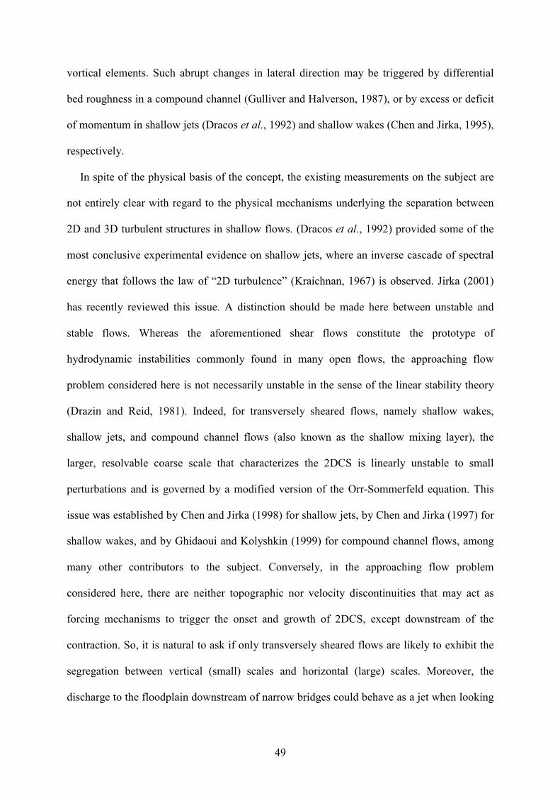
49

vortical elements. Such abrupt changes in lateral direction may be triggered by differential

bed roughness in a compound channel (Gulliver and Halverson, 1987), or by excess or deficit

of momentum in shallow jets (Dracos et al., 1992) and shallow wakes (Chen and Jirka, 1995),

respectively.

In spite of the physical basis of the concept, the existing measurements on the subject are

not entirely clear with regard to the physical mechanisms underlying the separation between

2D and 3D turbulent structures in shallow flows. (Dracos et al., 1992) provided some of the

most conclusive experimental evidence on shallow jets, where an inverse cascade of spectral

energy that follows the law of “2D turbulence” (Kraichnan, 1967) is observed. Jirka (2001)

has recently reviewed this issue. A distinction should be made here between unstable and

stable flows. Whereas the aforementioned shear flows constitute the prototype of

hydrodynamic instabilities commonly found in many open flows, the approaching flow

problem considered here is not necessarily unstable in the sense of the linear stability theory

(Drazin and Reid, 1981). Indeed, for transversely sheared flows, namely shallow wakes,

shallow jets, and compound channel flows (also known as the shallow mixing layer), the

larger, resolvable coarse scale that characterizes the 2DCS is linearly unstable to small

perturbations and is governed by a modified version of the Orr-Sommerfeld equation. This

issue was established by Chen and Jirka (1998) for shallow jets, by Chen and Jirka (1997) for

shallow wakes, and by Ghidaoui and Kolyshkin (1999) for compound channel flows, among

many other contributors to the subject. Conversely, in the approaching flow problem

considered here, there are neither topographic nor velocity discontinuities that may act as

forcing mechanisms to trigger the onset and growth of 2DCS, except downstream of the

contraction. So, it is natural to ask if only transversely sheared flows are likely to exhibit the

segregation between vertical (small) scales and horizontal (large) scales. Moreover, the

discharge to the floodplain downstream of narrow bridges could behave as a jet when looking

50

at from the far field (Dracos et al., 1992). Thus, the hypothetical formation of 2DCS

downstream of the opening could have considerable impact into the subsequent floodplain

evolution (Figure 3.1). In this case, the inlet conditions to those types of sheared large-scale

motions will be given by the problem studied here.

Thus, in keeping with the current state of knowledge on shallow turbulent flows, the

objectives of the experiments presented in this work were:

(i) to provide better insight into the mechanisms that may separate the 2D and 3D

turbulence scales in a broad, shallow and laterally contracted turbulent flow, and

(ii) to provide data sets that can be used as benchmarks for 2D and 3D shallow water

numerical modelling. To that end, the evolution of the power spectra at different flow

positions was used to verify the separation of scales hypothesis.

Emphasis was placed on studying the alternating 2D and 3D turbulence structures the flow

develops as it approaches the contraction, and as it encounters the fixed scour hole located at

the end of a long abutment (Figure 3.3), where a strong secondary flow sets in. Thus, it can be

argued that a combination of two forcing mechanisms were studied in this work:

(a) Geometrical forcing: given by the lateral contraction that breaks the plan-form

symmetry of an otherwise wide and uniform shallow flow (Figure 3.2), and

(b) Topographical forcing: generated by the scour hole located at the abutment end that

breaks an otherwise flat bottom (Figure 3.3). As a result, an extensive set of measurements of

the 3D velocity field established in a 0.1m thick layer of water flowing on the wide basin

sketched in Figure 3.4 was made with an Accoustic Doppler Velocimeter (ADV), as

explained in section 3.3.

51

Figure 3.3 Fixed scour hole located at the contraction end.

3.2 On turbulent flows with a spectral gap

Assuming initially that the aforementioned forcing mechanisms form two well-

differentiated inertial ranges with a spectral gap between them, it is possible to estimate the

expected length scales of the 2D and 3D turbulent structures of the open flow studied here by

resorting to shallow water theory.

The energy in a turbulent flow is primarily dissipated at small scales (large wavenumbers),

and thus energy is transferred from larger scales (small wavenumbers) to smaller ones to

compensate for this loss. Consequently, at relatively large scales, energy is simply transferred

from scale to scale. Kolmogorov’s hypothesis states that an intermediate range of scales

exists, the inertial range, which is sufficiently large for viscosity to be negligible but small

enough for the boundary effects to be safely ignored. Thus, the average rate of cascade of

turbulent kinetic energy ε is the only relevant information about the structure of the flow. If

the size l of the energy-containing eddies is in the inertial range, the statistics of the

52

corresponding turbulence intensity (or rms of the velocity fluctuation) u′must depend on l

and ε only through the relation 3~ ' /u lε . If these scales are now related with the dissipation

scales in turbulence for length ( )1/ 43~ /dl ν ε and velocity ( )1/3~d dlυ ε , typical velocities and

length scales differences are on the order of

1/ 4 3/ 4~ Re , ~ Re'd dl

u l

υ − − (3.1)

based on the Reynolds number Re ' /u l ν= for the large-scale turbulent motion. Pouquet et al.

(1983) stated that if 3~ /i i iu lε ′ and 1~ −ii lk are the energy production rate and the

characteristic injection wavenumber for the large-scale ( 1i = ) and the small-scale ( 2i = )

turbulence, respectively, where the two driving scales l1 and l2 are such that 1/ 12 <<ll . It

follows from (3.1) that the viscous cutoff for E2(k), the energy spectrum that would be

obtained with small-scale forcing only, is 3/ 4,2 2 2~ Redk k , whereas for E1(k), the spectrum that

would be obtained with large-scale forcing only, is ( ) 3/ 4

,1 1 1~ Reeffdk k . Here, 2 2 2Re /u l v′=

and 1 1 1 2 2Re /eff u l u l′ ′= are the Reynolds number for the small-scale turbulent motion and the

effective Reynolds number for the large-scale turbulent motion, respectively, assuming that

the small-scale turbulence acts on the large-scale as an eddy viscosity of the order of 22ul ′ .

Spectral segregation between both driving scales requires not only 1/ 12 <<ll but also

1/ 21, <<kkd .

The determination of 1u′ and 2u′ requires, in general, the use of special averaging

techniques (Tamburrino and Gulliver, 1999), whereas the ratio l2/l1 can be estimated in the

context of the shallow water theory. Then, by using simple scaling argument, it is possible to

establish that bed resistance and inertia are in balance on distances on the order of h/CF, where

CF is the bed friction coefficient, 2

Bτ / Uρ= (τB is the bed shear stress, and ρ is the fluid

53

density). Jirka (2001) stated that the distance 2h/CF is the largest eddy size that a 2DCS can

attain in a sheared, shallow turbulent flow (the factor 2 stems from different definitions on the

bed resistance law). Therefore, if it is assumed that the large-scale motion of the shallow

turbulent flow studied here is essentially 2D in the mean flow, scaling with F1 C/~ hl ,

whereas the 3D energy-containing eddies scale with a length hl α~2 such that α 1< , that is.,

bounded by the size of the water layer, the ratio for l2/l1 can be estimated as

F1

2 C~ αl

l (3.2)

within the bounds of the shallow water theory. Here, the bed friction coefficient was

evaluated using the smooth wall laws of von Kármán and Prandtl, with the pipe diameter

replaced by four times the water depth,

F

F

4Re 8C12log

2.518C

=

(3.3)

as dictated by the hydraulically smooth bed condition encountered during the experimental

work, as measured with the Reynolds number * *Re /sU k ν= based on the friction velocity

( ) 21B

/

* /U ρτ= , and on an equivalent bed roughness height ks for smooth cement,

approximately equal to 0.3mm.

Finally, an estimate for the signal-to-noise ratio (SNR) can be obtained if it is assumed that

the noise registered by the instrument, 2u′δ , represents about 10% of υd. From (3.1), this

estimation can be computed as

( )

1/ 42

1/ 4

~10 Re

~ 5.6 Re

SNR

α (3.4)

by assuming a rms of the order of 0.1U. This estimate of the SNR should not be confused with

the instrument accuracy. It is just a crude estimate of the expected separation between the

54

magnitude of the sought signal, 2u′ , and the background noise, 2u′δ , whenever the underlying

hypothesis is fulfilled.

For the free-stream conditions encountered well upstream from the opening (Figure 3.2),

where 16.0~U ms−1 and 1.0~h m, the approaching flow was fully turbulent with a Reynolds

number Re ~16000 and a Froude number ( )1/ 2/Fr U gh= approximately equal to 0.12. Here,

g is the acceleration of gravity. Other parameters values were 008.0~*U ms−1, *Re ~ 2.4 ,

025.0~2u′ ms−1, and 0025.0~CF . For the measurements, the ADV was mounted from above

(down-looking probe tip mode) sampling at its maximum standard rate of 25Hz with a

velocity range of ±10 cms-1. According to the manufacturer, expected noise at 25Hz is

approximately 1% of the velocity range, which is approximately twice as much as the

aforementioned estimated for the SNR, 50/22 uu ′≅′δ (taking α~0.4 for reasons that will

become clear later on). Therefore, the measured noise level was deemed smaller enough than

the expected velocity fluctuations, and in order to ensure a proper operation of the instrument,

the SNR was maintained above 15dB during the experiments, as recommended by the

manufacturer (Sontek, 2000).

3.3 Experimental arrangement

Figure 3.4 shows a schematic drawing of the facilities used for the present work. The

experiments were conducted on a rectangular basin with a horizontal floor made of smooth

cement, with a streamwise length of 20m and a width of 10m. Two pumps operating in

parallel drove the flow in the closed circuit. The system pumped water from a sump into a

constant head tank to ensure a constant discharge during the experiments. The supply flume

was fed from the constant head tank through a discharge pipe. At the upstream end of the

supply flume, a triangular weir measured the flow rate. Water was introduced to the basin

from the upstream end with the supply flume through a submerged row of honeycomb bricks.

55

This screen of bricks served to damp out any incoming disturbance into the basin. The lateral

walls of the basin were made with bricks lined with cement plaster. Two profiles were placed

on the lateral walls of the basin to allow the free displacement of a 10m wide, small cart that

carried one SontekAccoustic Doppler Velocimeter for measuring the thre components of the

velocity field. A smooth vertical screen was placed at 2m from the left wall all along the

length of the basin. The width of the test section was thereby restricted to 8m. A 3m long by

0.15m wide abutments was located at 10m from the entrance of the basin, leaving a 5m wide

gap to simulate the bridge opening effect (Figure 3.4). The average water depth was set to

0.1m during the experiments, and controlled with a 10m wide adjustable gate located at the

downstream end. The test section for measurements was set 4m upstream and 1.75m

downstream from the axis of the long abutment, and then divided into 11 cross-sections

0.25m apart, with the exception of two additional cross-sections located just upstream of the

long abutment, and 0.05m downstream of it. One more was located at the beginning of the

test section (Figure 3.4). Observations of the turbulent flow were taken with the ADV along

174 verticals, with a resolution ranging from 3 to 14 points each depending on the flow

region. The higher vertical resolution was employed in and around the scour hole region

(Figure 3.3). Since the center of the ADV sampling volume is 5cm from the probe tip, the first

measured point on each vertical was located approximately 5cm below the free surface, and

the last one about 5mm above the bottom.

56

Figure 3.4 Schematic diagram of the basin used for the experiments (1, weir; 2, input pipe; 3, feeding flume; 4,

test section).

A preliminary visualization of the free-surface velocities was made by seeding the flow

with small pieces of white paper, approximately 4mm in diameter (Figure 3.2). A complete

set of photographs of the flow pattern taken around abutments of different lengths using a

35mm camera with long exposure time can be found in the work of Scacchi (2003). These

preliminary observations, in combination with numerical results obtained with some 2D

computational codes (Telemac, 1998) determined that the structure of the approaching flow at

the beginning of the test section was not influenced by any small perturbation that could be

present at the inlet section. The inflow rate was 0.128m3s−1, and the flow was uniformly

distributed to within 4%± on a cross-section located 1m downstream of the inlet section. This

corresponds to a mean bulk velocity 16.0~U m/s-1 as previously explained.

57

3.4 Results

Figure 3.5 shows the 3D projection of the mean flow after averaging the flow

measurements obtained on the grid. The mass continuity discrepancy measured inside the test

section was ±5%. The two-dimensionality of the flow structure is clearly visible in most of

the approaching region, becoming 3D in and around the scour hole.

Figure 3.5 3D mean velocity field recorded with an ADV inside the test section

In order to compute the change in the spectral response of the flow, a minimum of 4096

points were collected with a sampling rate of 25Hz at every point of the defined measurement

grid to diminish the noise influence on the power spectral estimation. The recorded velocity

data file of 4096 points were divided into seven overlapping sub-records of 1024 points each.

Then, the power spectrum and correlation function were computed with a fast Fourier

transform (FFT) algorithm by averaging all seven sub-records. Figure 3.6 shows the

progression of spectral changes that occurs as the flow approaches the contraction. The four

points where the spectral density functions were calculated are labelled A, B, C, and D in

Figure 3.4. In summary, the spectral response of the flow is examined as the mean flow

58

gradually accelerates upstream of the contraction (point A and B), as it encounters the sudden

change in bed topography at the contracted region (point C), and as it suddenly expands

downstream of the contraction (point D). The spectra are presented in dimensional form

((cms-1)2/Hz-1) for the turbulent fluctuations of the longitudinal and vertical components of the

flow velocity, u’ and w’, respectively. All the spectra were computed from measurements

taken ~6cm below the free surface (Table 3.1), approximately, starting at the beginning of the

test section (Figure 3.4).

The first horizontal velocity spectrum (Figure 3.6a) flattens out in the range 5–12.5Hz,

while the vertical velocity spectrum falls out to the Nyquist frequency at 12.5Hz at the well-

known Kolmogoroff –5/3 power law. In other words, a universal inertial subrange is clearly

distinguishable for the vertical velocity component. The maximum of the energy density of

the longitudinal component is nearly flat, with two distinct peaks that are not reproduced by

the w’ spectrum. The location of the second peak marks the beginning of a subrange with an

energy cascade that exhibits the –3 wavenumber dependence, typical of an enstrophy cascade

of 2D turbulence. This peak is more distinguishable on the second spectrum (Figure 3.6b),

which also exhibits a small subrange compatible with the development of two-dimensional

turbulence characterized by an enstrophy cascade. The u’ spectrum of point C (Figure 3.6c)

shows two well-differentiated peaks followed by a –3 cascade. Then, the w’ spectrum shows

that the energy transfer relaxes towards three-dimensional turbulence following a –1

dependence, for wavenumbers larger than the associated k of the second peak (namely k2, see

Table 3.1), when the enstrophy cascade subrange ends. In the vicinity of k1, where k1 is the

wavenumber associated with the first peak of the spectrum (large-scale turbulence), the

spectrum follows a dependence close to k3 for 1kk < , and to k−3 for 1kk > . This k3 shape of

the spectrum is repeated in Figure 3.6d, where its energy peak shows an increase in magnitude

by a factor of 10. The u’ spectrum of point D exhibits a subrange with a –3 cascade, and an

59

inertial three-dimensional range for larger wavenumbers (better appreciated on the w’

spectrum). Again, there is a subrange in between the –3 and the –5/3 ranges that seems to

follow a –1 dependence. Dracos et al., (1992) also found this wavenumber dependence when

the transfer process relaxes from 2D to 3D turbulence. Changes in flow frequencies are

summarized in Table 3.1, and frequencies names are depicted in Figure 3.7 on a linear scale

plot, where the spectral gap is better appreciated. Figure 3.8a,b depict the autocorrelation

function computed for points A,B,C, and D. The autocorrelation point for point B shows a

better organization of the flow into large-scale structures with respect to point A, locate

upstream. The small-scale motion attributed to flow modes trapped by the local bed

topography give rise to quasi-periodic oscillations in the autocorrelation function

corresponding to point C. In this case, from the zero-crossing of the oscillating part of the

autocorrelation function, it is possible to infer that the mean period of oscillation is in good

agreement with the corresponding peak frequency f2 of the energy spectrum (Figure 3.6c).

The quasi-periodic oscillation of point C are superimposed to a larger time scale motion,

which is approximately of the same order of magnitude of the time scale observed in the

correlation function of point D.

60

10-2

10-1

100

101

102

100

101

102

103

-5/3

Ef

f(Hz)

-5/3

Ef

f(Hz)

-3

-1 -5/3

Ef

f(Hz)

-5/3

Ef

f(Hz)-5/3

3D

10-2

10-1

100

101

10210

-1

100

101

102

-1

-3

-3

-3Ef

3

f(Hz)

C

-1

10-2

10-1

100

101

102

10-1

100

101

102

-5/3

Ef -3

f(Hz)

B

10-2

10-1

100

101

102

10-1

100

101

102

-5/3

Ef

-3

f(Hz)

A

Figure 3.6 One-dimensional energy spectra of the streamwise and the vertical turbulent fluctuations estimated with FFT technique. a) u’ and w’ spectra at position 4−=x m, b) u’ and w’ spectra at 1−=x m, c) u’ and w’

spectra at 0=x m, d) u’ and w’ spectra at 75.0=x m.

61

Figure 3.7 Superposition of the velocity fluctuation spectra (linear scale) measured at points B, C, and D (spectrum of point D is referred to the second vertical axis).

Figure 3.8 Auto-correlation functions at points A, B, C and D.

62

Kraichnan (1967) showed that the dynamics of the stationary-forced homogeneous 2D

turbulence have two inviscid constants of motion. Consequently, it follows that there are two

distinguished cascade process: energy transfer at a rate ε and vorticity transfer (enstrophy

cascade) at a rate β. These two formal inertial ranges are expressed as 2 /3 5/3( ) ~E k kε − , and

33/2~)( −β kkE , where the latter needs a logarithmic correction factor to avoid a

logarithmically divergent total enstrophy (Kraichnan, 1971). Since the kinetic energy flux

through the enstrophy cascade is zero, the kinetic energy produced at rate ∈ at ki can only

cascade backwards, toward scales larger than 1/ ik . This process is clearly appreciated in the

spectra of Figure 3.6, where the energy initially confined in the neighbourhood of

~ 2 /o o ok f Uπ (at the beginning of the enstrophy cascade) is pumped toward larger and larger

scales (Figure 3.6c,d), while vorticity is pumped through the –3 range down to the dissipation

range. The wave packet containing most energy of the small-scale motion (second peak on

Figure 3.6c) is swamped by large-scale effects further downstream (point D, Figure 3.6d and

Figure 3.7). Indeed, another inverse cascade process is acting at point C, better appreciated on

the w’ spectrum, where energy produced at frequency f2 is pumped backward to smaller

frequencies (larger scales). In this case, the energy level on the w’ spectrum shows an increase

from 100 to 500 (cms-1)2/Hz-1 approximately (Figure 3.6c,d). The fact that the concentration

of small-scale energy observed within the scour hole is not longer sustained further

downstream reinforces the idea that small-scale effects act as an eddy viscosity on the large-

scale motion. In other words, the Reynolds number of the large-scale motion can be reduced

by a factor 22/ lu′ν downstream of the scour hole.

On one hand, the peak around 0.1Hz at the spectra of points C and D can be attributed to a

double inverse transfer process that continues piling up energy until scales the size of the

entire flow geometry, lg, are strongly excited. In this case, the size of the gap ( 5~gl m) is of

63

the same order of magnitude of the observed largest energy-containing eddy, ~1l 3.8m, at

point D (Table 3.1). The consistency of the k3 dependence as k→0 (infrared range) of the

energy spectra of points C and D suggests the expression

>β

<−

133/2

13

,

,~)(

kkk

kkkckE (3.5)

for some constant c. This form of the spectrum has been shown valid for freely decaying as

well as for forced-2D turbulence (Ossia and Lesieur, 2001). The geometrical forcing induces

an inverse cascade that piles up energy in the vicinity of the wavenumber 11 ~

−glk . Similar

inverse transfer of energy was observed along several streamwise alignments, parallel to the

line ABCD depicted in Figure 3.4 (Carrasco, 2002). Consequently, it is possible to argue that

the wavy 3D vortex patterns eventually present well upstream of the contraction, which are

unstable and therefore very hard to spot (Gulliver and Halverson, 1987; Tamburino and

Gulliver, 1999), evolve into different, large-scale 2D structures due to the geometrical

forcing, i.e., the turbulent energy is fed from the accelerating mean flow as the contraction is

approached, storing energy in the range of scales dictated by the flow geometry.

On the other hand, the second peak observed at the spectra of point C, namely at frequency

f2, is related to a mode trapped by the bed topography. Using the long-waves approximation,

the mth transverse natural mode of oscillation for a closed rectangular basin is given by

bghmf om 2/, = , where b represents the size of the basin (scour hole) in transverse direction.

Similarly, for a circular basin of radius b/2, the natural modes of oscillation are

bghzf nmnm π′= /,. , where nmz ,′ is the nth zero of the derivative of the mth Bessel function of

first kind, 0)( , =′′nmm zJ . It is clear that the shape of the scour hole is neither rectangular nor

perfectly circular, and has such a variable depth (Figure 3.3) that the determination of the

natural frequencies and modes requires numerical computations. Moreover, the solution must

64

satisfy the radiation condition, which is violated in the aforementioned formulae valid for

closed basins. Nevertheless, using h ~ 0.3m and b ~ 0.9m, which are the maximum depth and

the approximate size of the scour hole used during the experiments, respectively, the

agreement between observed and theoretical estimates are quite remarkable (Table 3.1). In

consequence, the peak observed at frequency f2 in Figure 3.6c can be attributed to flow modes

trapped by the local bed topography.

Pt x(m) z(m) U(m/s) h(m) f (Hz) iiii fUkl π− 2/~~ 1(m)

A −4.0 −0.058 0.15 0.1 oo ff ′, ~ 0.07, 0.32 2.14, 0.47

B −1.0 −0.058 0.19 0.1 oo ff ′, ~ 0.29, 0.42 0.66, 0.45

C 0.0 −0.077 0.27 0.3 f1 ~ 0.10

f2 ~ 1.86

f2,0 = 1.91 (rectangular basin)

f2,1 = 1.85 (circular basin)

f0,1 = 2.32 (circular basin)

2.70

0.15

D 0.75 −0.058 0.38 0.1 f1 ~ 0.10 3.80

Table 3.1 Progression of spectral changes as the flow approaches the contraction

3.5 Conclusions

The shallow turbulent flow that approaches the opening of a supposedly relief bridge, with

a local scour hole located at the contraction end in an otherwise flat bed, has been investigated

experimentally. It has been established that the geometrical and topographical forcing gives

rise to an energy spectrum with two well-differentiated peaks. This spectral segregation

represents quasi two-dimensional turbulent motion for the large-scale l1, and three-

dimensional turbulent motion for the small-scale l2, respectively.

The phenomenological estimate obtained for the separation of scales satisfies

F12 C~/ ll (within the bounds of the shallow water theory), which is one order of magnitude

smaller that the experimental findings reported here

3 2F 2 1(C ~ 2.5 10 / ~ 0.15 / 3.80 3.9 10 )l l− −× < ≅ × . Nevertheless, the required condition for the

65

spectral segregation to occur, 1/ 21, <<kkd , is clearly satisfied. In addition, the small-scale

turbulence generated inside the scour hole satisfies the constraint 1/2 <hl , that is,

α ~ 0.15 / 0.30 0.5= , as expected.

It was found that the flow turbulent energy that is initially stored at scales 5~/ hlo is

transferred to much larger scales by the geometrical forcing through an inverse cascade

process, until scales the size of the entire flow geometry, lg, are strongly excited. It was also

found that energy spectrum exhibits a k3 and k–3 (enstrophy cascade) dependence around the

large-scale wavenumber lg−1. This subrange with power 3 and –3 of the spectrum should be

reproduced by any numerical computation based on large eddy simulation (LES) techniques.

The topographical forcing, which only acts locally, produces a large amount of turbulent

kinetic energy concentrated at small-scales by trapping and exciting flow modes due to the

shape of the “submerged” scour hole. The highly variable bed topography injects a large

amount of small-scale turbulence into the flow, which is diffused toward larger scales by

another inverse cascade process (Figure 3.7) and transported downstream. Consequently, it is

likely that the topographical forcing reduces the effective large-scale Reynolds number from

ν′ /11lu to 2211 / lulu ′′ approximately, downstream of the region of high topographic gradient.

This observation, in combination with the potential formation of very large, horizontal

vortical structures downstream of the contraction should be of considerable importance for

those interested in simulating numerically the sediment transport capacity of such flows.

Finally, in spite of the fact that in the present study was possible to characterize the

spectral changes of the flow established upstream and on the vicinity of the contraction area

with an ADV instrument, it will be convenient to perform a similar study using PIV

techniques (Uijttewaal and Jirka, 2003). With the PIV capabilities, it will be possible to

determine the complete velocity and vorticity field of the large-scale motion at all relevant

positions in a completely non intrusive way.

66

Acknowledgments: We thank Prof. V.C Patel, Prof. G. Jirka, and an anonymous reviewer for their

comments, and M. Schreider for letting us to use the large experimental basin at FICH. This research was carried

out within the ANPCyT project 07-00110-02067. Financial support from CONICET is also gratefully

acknowledged.

67

CHAPTER 4 Laboratory study of alternate bar formations

4.1 Introduction

Alternate bars are prominent features of alluvial channels. They develop as a result of an

instability process that arises from the coupling between flow and sediment transport in

mobile channels on a spatial scale typically of the order of channel width, with a grow rate

associated with the bed erosion-deposition process. The presence of bars exerts a strong

influence on the flow field and the sediment transport process by forming a roughness effect

generated by the local expansion losses at the bar edges. The resulting pattern greatly

enhances the erosion of channel banks and, consequently, induces bend growth rate and

channel shifting. Thus, the presence of bars is one of the main factors controlling the

morphology of alluvial channels, affecting several aspects of fluvial engineering. Changes in

river morphology occur in response to several factors, including magnitude, duration,

frequency and sequence of floods, and the impact of sediment supply influenced both by

natural processes and human impacts. The natural variability in the morphology of a given

river reflects variations in the resistance of the banks to erosion and in the forces exerted by

the river on the banks. Variation in the form, size and slope of the channel interact with

channel flows and sediment regimes to produce complex local variations in flow hydraulics

and, thus, in the erosive forces imposed by the river on its bed. Variations in the materials

forming the bed and banks, vegetation cover and hydrological processes within the banks also

influence the resistance to erosive forces of the bed.

68

It has been shown that bars form when a small perturbation of the bottom is capable of

triggering a first bar. The flow field downstream of the initial bar then generates further bars

“just like in a chain reaction” (Fujita and Muramoto, 1985). The spatial stress exerted on the

bed combine with the availability of sediment, whether in the bed or supplied from local bank

erosion or upstream, is the mechanism that sustains the alternate bar evolution and migration.

The present investigation has been aimed at provide experimental evidence of the influence of

the sediment availability (mainly from the banks) in the alternate bar phenomena. Previous

studies have focussed upon bank materials and bank hydrological processes (e.g.

Couperthwaite et al., 1998, Wyzga, 1999), the shear stresses imposed by river flows (e.g.

Thorne, 1990; Abernethy and Rutherfurd, 1998) and the dynamics of the fluvial sediment

erosion, transport and deposition (e.g. Duysings, 1986, Mitchell et al., 1999). Therefore, few

experiments of alternate bars formation with loose lateral banks are available. Among them, it

is worth to mention the works of Schumm and Khan (1972) that investigated the effect of the

slope on channel patterns and determined slope ranges that marked significant changes on

channel pattern, and Federici and Paola (2003) who performed experiments aimed to analyze

the dynamics of channel bifurcations in loose sediments, finding that alternate bars formed

rapidly in a straight channel initially cut through the cohesionless flat sloping surface.

According to Federici and Paola (2003), the alternate bars patterns developed a sequence of

rhythmic bumps on both banks while the stream displayed a tendency to meander just 20 min

after the initiation of the experiment.

In this direction, a comparative study to analyze the differences between loose and fixed

banks under identical bed slope, water discharge, and sediment flux will help to clarify if the

formation of alternate bars is indeed the preferred evolving spatial scale of the problem,

delaying the riverbank erosion processes, and consequently, the lateral migration of the

stream for much longer time scales. To that aim, a set of laboratory experiments has been

69

conducted in a “regime flume” at the Novak Hydraulic Laboratory of the School of Civil

Engineering and Geosciences at the University of Newcastle upon Tyne, UK. This chapter

describes the experimental facilities used during the experiments, detailing the various series

of runs performed during this research, as well as the analysis and discussion of the

subsequent findings.

4.2. Materials and methods

To allow alternate bars to develop naturally, a straight channel of 22m long and 2.5m wide,

covered by a movable bed of 600mm depth of uniform sediment ( 50 0.94mmd = , taken from

Ershadi (2005)), was used (see Figure 4.1). The result of the sieve analysis taken from Ershadi

(2005) can be seen in Appendix B. The channel is built in a recirculating circuit for both

water and sediment. The channel length is divided into three parts, the inlet, the outlet and the

test reach. The inlet is 2m long and it is used as an upstream storage tank. The test reach is

18m long filled with the uniform sand, and the outlet is 2m long and it is also used as a

downstream storage tank. From there, a pipe of 80mm of diameter conveyed the sediment-

water mixture back into the channel, with the help of a centrifugal pump of 39l/s of maximum

capacity.

A calibrated electromagnetic flow meter is placed in the recirculating lines in order to

measure the flow discharge (Figure 4.2). The electromagnetic flow meter Promag 33F is

connected to a personal computer by a Commubox FXA 191 system (see Figure 4.3) and is

used to facilitate the flow rate control visualizing it values on the computer monitor in the

form of a user friendly graphical interface.

70

Figure 4.1 Schematic layout of the regime flume. Taken from Ershadi (2005).

Figure 4.2 Electromagnetic flow meter.

Sand

Water

Carriage

Adjustable rail

Sediment feeder

Gravel

Tilting Gate

Main channel sediment hopper

0.6 m

P M

MP

2.0 m 18.0 2.0 m

a Screeded channel 2.5m

a

Sand Water

Main channelSediment hopper

Tilting Gate

Carriage

Adjustable Ra il

Sedimen feeder

Gravel

71

Figure 4.3 Commubox FXA 191 system.

Figure 4.4 Tilting gate placed at the channel outlet.

In order to obtain uniform flow or normal depth, an adjustable tilting gate at the

downstream end controlled water level to a height accuracy of 0.1mm (Figure 4.4). The flow

is pumped to a guide channel that widens gradually up to the design experiment width. A

diffuser pipe and a honey-comb shaped metal diffuser in the guide channel, together with a

grid (metal mesh), and pebbles in the entrance of the main channel (Figure 4.5) dissipate

excess energy of the pumped water to allow free uniform flow of water and sediment mixture.

72

Figure 4.5 Energy diffusers at the channel in the inlet

Figure 4.6 Sediment feeder.

The flume is also equipped with a screw type sediment feeder, which is located above the

main channel inlet (Figure 4.6) allowing the sediment to be fed over the full width of the main

channel. The whole experimental facility has been intensively used in the last few years, and

consequently it has been assumed that all of its components were in good working conditions

73

for the purposes of this work. For further information regarding calibration of the

aforementioned equipments refer to Haidera (2002) and Ershadi (2005).

4.3 Experimental set up

The experimental conditions were carefully selected in such a way that the adopted initial

bed geometry, flow and sediment transport conditions not only conform with an equilibrium

cross-section according to regime or White, Paris and Bettess (WPB) theory (White et al.,

1981) for straight channels, as explained next, but also to assure that the prevalent conditions

were within bed load transport mode only cb** τ>τ (Figure 4.7) albeit well below from the

region of expected significant suspended sediment mode, cs** τ<τ . The latter threshold is

given by the Bagnold’s criteria, 1/* ≅swu , where *u is the shear velocity, ( ) 2/1* /ρτ= , and sw

is the bed sediment fall velocity. *τ is the dimensionless bed shear stress, ( τ /ρb gRD= , where

ρ is fluid density, g acceleration of gravity, and R submerged specific weight of the sediment,

ρ /ρ 1 1.65s= − = for the present case). The initial conditions chosen to run the experiments

were apparently within the unstable range of the controlling parameter β, according to

standard linear stability theories (Figure 4.8).

To set up the experiments the initial channel cross-section dimensions were predicted by

the WPB theory (White et al., 1981), and latter modified to better approximate the stable

width and depth. This was through a better approximation of boundary shear stress (Valentine

and Haidera, 2001). Previous work due to Shakir (1992), Babaeyan-Koopaei (1996),

Valentine et al., (2001), and Haidera (2002) showed that equilibrium cross-sections for

straight channels in laboratory conditions are wider and shallower than the section predicted

by the WBP theory. The ratio between the predicted and measured values for channel width

was between 0.46 and 0.51 and for channel depth was between 1.5 and 1.7. Therefore, the

predicted dimensions for the initial channel were adjusted according to Haidera’s (2002)

74

modification. The proposed initial channel is trapezoidal in cross-section and straight in

planform.

Figure 4.7 Threshold values for initiation to motion (Shield’s Curve). The circle enclosed the initial conditions set up during the experiments (Table 4.1)

The desired initial channel cross-section was excavated in the sand using a wooden board

fixed to a carriage placed on top of side rails (see Figure 4.9). These rails can be manually

adjusted to the desired slope. The carriage is also used to place the measurement kits, such as

the point gauge and current meter, allowing traversing the flume in crosswise or y-direction,

and travelling in longitudinal or x-direction along the channel, in both downstream and

upstream directions. After scraping the channel the bed slope and final moulded shape were

obtained using a point gauge.

75

Figure 4.8 A classical stability diagram (taken from Colombini et al., 1987)

Figure 4.9 Initial experimental cross-section excavated in the sand at Laboratory facilities available at Newcastle University, Newcastle upon Tyne, UK.

The experiments where started by letting flow a very low discharge over the bed to prevent

its deformation during the initial stage. The flow discharge was then slowly increased until

the desired value was attained. All the experiments were run for inbank situation under full

bank (FB) condition. After the experiment started, the bed deformation process began to

develop spontaneously. During this process, the bed deformation was monitored periodically

(every two hours), measuring local values of variables such as bar height and bar length, and

channel widening. The channel started adjusting under uniform flow condition until the

76

widening rate was below 1% per hour, suggesting an equilibrium state was reached. The

duration of the development process varied with flows and channel conditions (initial cross

section). A regime condition was generally achieved after a period of about 4 hours.

A primary procedure in any of the tests carried out in this work was to establish that the

flow was in an uniform state. This implied that the three gradient lines, namely the energy

slope ( )Sε , the water surface slope ( )wS and the longitudinal bed channel slope ( )oS were

equal, i.e., w oS S Sε = = . Under this condition, the average flow depth and velocity were

constant for all cross sections along the test section. To ensure that uniform flow was indeed

established along the channel, the water surface slope was measured with the point gauge

mounted on the carriage and any level differences with the bed slope was adjusted with the

tilting gate.

At the end of the development process, constant or equilibrium values of the different

parameters were reached - uniform sediment transport and equilibrium cross-section. Once

the equilibrium state was reached, the experiments were allowed to run for at least 10 hours,

thus giving them a total duration that ranged from about 10 to 20 hours.

Measurements of the water surface elevations were made before the end of the

experiments. Transverse profiles were taken every 0.5m along a control reach of 10m,

covering the central part of the test reach, allowing to characterize a few bar units. Longer

control lengths were not used because it was necessary to discard any possible perturbation

introduced by the inlet and outlet. Three longitudinal profiles located at 15%, 50% and 85%

of the channel width were measured to characterize the bed deformation in longitudinal

direction. Bed profiles were measured every two-hour period; and the widening rate and

sediment concentration were measured every 30 minutes.

To perform the bedforms measurements, the experiments were stopped by turning off the

pump every two-hour. This generated a rapid recession of the flow inside the channel, with

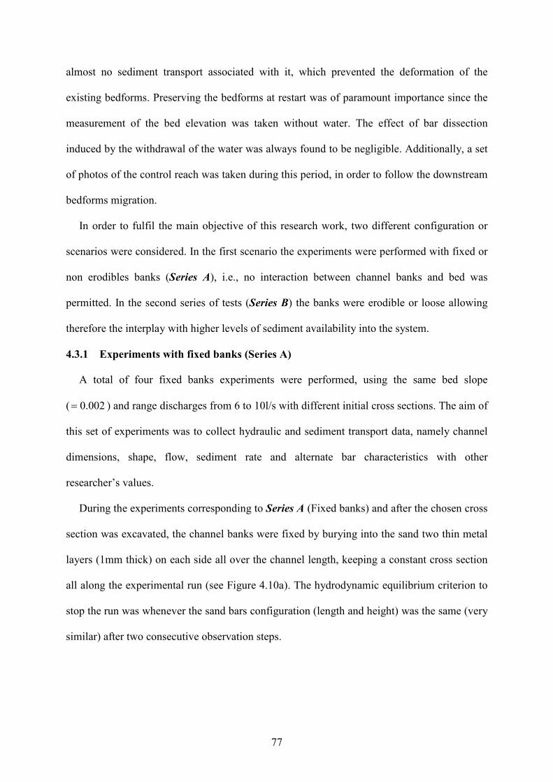
77

almost no sediment transport associated with it, which prevented the deformation of the

existing bedforms. Preserving the bedforms at restart was of paramount importance since the

measurement of the bed elevation was taken without water. The effect of bar dissection

induced by the withdrawal of the water was always found to be negligible. Additionally, a set

of photos of the control reach was taken during this period, in order to follow the downstream

bedforms migration.

In order to fulfil the main objective of this research work, two different configuration or

scenarios were considered. In the first scenario the experiments were performed with fixed or

non erodibles banks (Series A), i.e., no interaction between channel banks and bed was

permitted. In the second series of tests (Series B) the banks were erodible or loose allowing

therefore the interplay with higher levels of sediment availability into the system.

4.3.1 Experiments with fixed banks (Series A)

A total of four fixed banks experiments were performed, using the same bed slope

( 0.002= ) and range discharges from 6 to 10l/s with different initial cross sections. The aim of

this set of experiments was to collect hydraulic and sediment transport data, namely channel

dimensions, shape, flow, sediment rate and alternate bar characteristics with other

researcher’s values.

During the experiments corresponding to Series A (Fixed banks) and after the chosen cross

section was excavated, the channel banks were fixed by burying into the sand two thin metal

layers (1mm thick) on each side all over the channel length, keeping a constant cross section

all along the experimental run (see Figure 4.10a). The hydrodynamic equilibrium criterion to

stop the run was whenever the sand bars configuration (length and height) was the same (very

similar) after two consecutive observation steps.

78

Figure 4.10 a) Experiments with fixed banks; b) Experiments with loose banks.

4.3.2 Experiments with mobile banks (Series B)

During the mobile bed-bank experiments, the objective was to evaluate what sort of

potential impact the new sediment availability would have over the formation and evolution

of bars, in other words, starting from the same initial conditions as those used for the Series

A, Will the free bars form and behave similar to the fixed bank configuration, or the channel

with loose boundaries will tend to meander right away, as reported by Parker (1976), Federici

and Paola (2003) among others? For comparison purposes, the experimental conditions used

for both series of test is specified in Table 4.1, whereas Figure 4.11sketches the initial cross

sections used to start the experiments.

Experiment Q

(l/s)

S0

(m/m)

Bb

(mm)

z

(m/m)

Ho

(mm)

Ho+

(mm)

Bt

(mm) ββββ Banks

R_1_05 6 0.002 391 1.7 33.0 34.3 519 13.78 Mobile

R_2_05 6 0.002 391 1.7 33.0 34.3 519 13.78 Fixed

R_6_05 8 0.002 604 1.7 33.0 32.4 716 20.00 Mobile

R_5_05 8 0.002 604 1.7 33.0 32.4 716 20.00 Fixed

R_7_05 9 0.002 604 1.7 33.0 34.7 716 20.00 Mobile

R_8_05 9 0.002 604 1.7 33.0 34.7 716 20.00 Fixed

R_2_04 10 0.002 537 1.77 42.2 39.0 676 14.37 Mobile

R_4_05 10 0.002 537 1.77 42.2 39.0 676 14.37 Fixed

Table 4.1. Complete set of experiments run

a) b)

79

where Q is the steady discharge, So is the channel slope, Bb and Bt are bottom and top channel

cross-section width respectively, z is bank slope, Ho is the expected water depth obtained from

the regimen theory, Ho+ is the expected normal flow depth for flat bed computed with the

classical resistance formula of Keulegan, using D50 as the representative size of bed roughness,

and β=B/H is the channel width-depth which is the controlling parameter in linear stability

analysis (see e.g. Colombini et. al., 1897). The values of normal flow depth computed as

indicated differ within ±2 mm from those estimated using the WPB theory (Haidera, 2002)

under identical flow discharge, slope and sediment type.

Figure 4.11 Initial cross-sections

Bb

Bt

zH

Bb

Bt

Ho

80

4.4 Procedures used for collecting data

In this section, the procedures used to collect and calculate relevant data produced during

the experimental runs is discussed. Experimental data collected include the water discharge,

channel slope, sediment concentration, cross-sectional geometry, and bars configuration

(essentially, bed topography). These procedures are discussed in detail in the following

subsections.

4.4.1 Water discharge

All the experiments were carried out at steady discharge. The water discharge was

measured with the flow meters in litres per second (l/s) with an accuracy of 0.01± l/s. The

discharge was adjusted and recorded at each time step (every 30minutes). It was attempted to

keep the average discharge at its target discharge during each time step. The recorded values

of discharge were averaged to find out a representative value for the run. In all cases, the

discharge fluctuated around the mean discharge within 0.1± l/s, being the standard deviation

of the measured flow values from the mean value within 0.5± %.

4.4.2 Sediment concentration

The specialized literature covers a variety of opinions about the best way to represent the

sediment concentration of the channel (Leopold and Wolman, 1957; Schumm and Khan,

1971; Ackers and Charlton, 1970; among others). In previous works the sand fed at the

channel inlet has been used as representative of the sediment transport (e.g. Leopold and

Wolman, 1957 and Schumm and Khan, 1972). Nevertheless, this way to set up the sediment

concentration along the channel –determine by its inlet value– was not accurate enough due to

the sediment deposition along the channel, causing the amount of sand at the channel outlet

frequently to differ from the quantities fed into the channel. As a solution, Ackers and

Charlton (1970) measured the sediment concentration at the downstream end of the channel

and averaged it over the time span, once the channel established a stable condition.

81

For the present study, and following Haidera’s (2002), Babaeyan-Koopaei (1996), and

Shakir (1992) recommendations, the representative value of the sediment transport was

obtained as the mean of the measured sediment concentration at the channel outlet, once the

stable condition was attained. However, the problem of obtaining a representative sediment

concentration is very similar to the problem of fixing a representative discharge in a river with

variable flow. It may be perhaps a range rather than a single value that could represent the

channel sediment concentration in an alluvial channel. Nevertheless, when a channel reaches

an equilibrium state, the water surface profile becomes straight and the sediment transport rate

becomes uniform (Chang, 1985). Therefore, the average sediment transport rate, when the

channel becomes fully developed, can be used as representative for an equilibrium channel.

In all the experiments performed for this thesis, the sediment was recirculated into the

channel. The sediment concentration was measured at the downstream channel end by

collecting samples during 2 minutes every 30 minutes with a sediment trap (basket). The wet

samples were weighed using an electronic balance with an accuracy of 1± gram (Figure

4.12).

Figure 4.12 a) The electronic sediment balance, b) The sand trap for collecting the sediment.

The sediment concentration in terms of mg/l (ppm) was determined by mean of

( / ) *0.81sQX mg lQ

= (4.1)

b)

a) b)

82

where X is the sediment concentration in ppm, Qs is the wet sediment transport rate in mg/s,

and 0.81 is the wet to dry ratio of the bed material.

4.4.3 Channel bed and water surface slope.

The bed and water surface elevation at the channel centre line were measured with a point

gauge mounted on the carriage to determine the channel slope and the water surface slope,

respectively. The measured sections were 1m apart along the test reach, and the slope of the

line that best fit these values was considered the respective slopes. Both values were

calculated with a precision of 0.001± m/m.

4.4.4 Bedform characteristics

The definition of the variables used to describe the bed deformation produced during the

experiments is shown schematically in Figure 2.6. Basically they correspond to the set of

variables included in the dimensionless relationships from Appendix C (Eq.(C.15)). In the

Figure 2.6 the maximum scour is defined with respect to the initial bed elevation. The flow

depth was computed by first obtaining a mean value of the water surface elevation along the

channel, and then subtracting the mean bed elevation from this value.

Some researchers (e.g. Ikeda, 1984) define two characteristic values of the bar height. One

of those values is shown in Figure 2.6, and corresponds to the difference between the

maximum and minimum bed elevation at the section of maximum scour. The other parameter

usually employed is the maximum bar height, defined as the difference between the maximum

and the minimum bed elevation within a wavelength, which do not necessarily coincide at the

same cross section. Herein, such differentiation is not made because in all cases, the

maximum bar height was observed to occur precisely at the section of maximum scour.

The rest of the parameters characterizing the bed deformation, such as wavelength, were

computed directly from the data collected, such that mean values, characteristic of each

experiment, were computed as simple averages over the available measurements. As the

83

system ran, we monitored the location of migrating bars fronts down the entire flume length at

2 hours intervals. The flow was turned off and bed topography was mapped with a point

gauge (Figure 4.13).

Figure 4.13 Alternate bar formation in straight channel experiment. Characteristics: Wavelength 2-3m

( 5.6L B= ) and Height 0.007-0.0010m.

4.4.5 Bed migration rate measurement

A very approximate measurement of bar celerity rate was determined using a visual

method based on recording the time that the crest of a bed needs to travel between two

predetermine cross-sections.

4.4.6 Cross-section geometry

Every two hours, the bed levels were measured with an accuracy of ±0.5mm. The point

gauge used was attached to the carriage and moved transversely with an accuracy of ±1mm

and longitudinally with an accuracy of ±0.5cm. Three independent longitudinal profiles were

measured using this set up at 15%, 50% and 85% of the channel width, respectively.

4.4.7 Regime -or equilibrium- criterion

A channel with movable bed is said to be in ‘regime’ when it has adjusted its cross

sectional shape, slope, sediment carrying capacity and plan form geometry to an equilibrium

condition. In other words, a channel is in regime if it adjusts its plan and profile to a stationary

or equilibrium condition. A related concept is that of a graded river: a river which conveys

sediment downstream without net deposition or erosion through a series of reaches is referred

to as being graded or in equilibrium. It is still uncertain if such a graded river can exist in

nature and how it could be recognized presently or in ancient strata. Indeed, the fluvial grade

concept has long been a subject of debate and survived centuries of discussion (Muto and

84

Swenson, 2005). Consequently, the equilibrium condition criterion varies between

researchers. During their experiments, Leopold and Wolman (1957) determined an

equilibrium condition when the water surface was parallel to the stream bed after successive

measurements of the longitudinal profile of water surface and dry stream bed. Schumm and

Khan (1972) assumed that a channel was in equilibrium when the major channel adjustments

were complete and the channel becomes relatively stable. Stability here implies no further

significant adjustments of channel shape dimensions or pattern occur.

The regime concept is generally considered synonymous of equilibrium (Chang, 1998).

This concept originated from the study of stable alluvial canals, where for a mobile bed and

banks there is no degradation or aggradation over an operating cycle. However, due to natural

discharges variation in natural rivers, the true regime or dynamic equilibrium may never be

achieved, although each river is adjusting itself in this direction.

Due to the fact that no unified criterion was readily available to define equilibrium, for this

work whenever the water surface was straight, the widening rate was 2%≤ per hour, and the

sediment concentration measured was approximately uniform and regular, then the channel

was assumed to be in an equilibrium state. This is coincident with the criteria used for

previous research in these experimental facilities (see Shakir, 1992; Babaeyan-Koopeai, 1996;

Haidera, 2002; and Ershadi, 2005).

4.5 Results and discussion

The results description of the channel bed evolution in response to steady flow conditions

is based on measurements taken during eight different runs performed with fixed and mobile

banks. Table 4.2 contains values of all relevant parameters of performed runs. It can be

assumed that, for the measurements of the bed topography, the duration of all experiments

was sufficiently long to ensure the establishment of equilibrium conditions for sediment

transport and that bars reach their maximum configuration.

85

Run Q

(m3/s)

B

(m)

h

(m)

Area

(m2)

Rh

(m)

V

(m/s) Re Fr β

τb

(kg/m2)

X

(mg/l) θ

R-1-05 0.006 0.524 0.037 0.0210 0.032 0.286 10255 0.480 14.59 0.704 155.54 0.046

R-2-05 0.006 0.519 0.034 0.0193 0.029 0.311 10417 0.540 15.49 0.657 198.96 0.043

R-6-05 0.008 0.730 0.035 0.0279 0.032 0.286 10124 0.485 20.62 0.694 168.41 0.046

R-5-05 0.008 0.716 0.033 0.0254 0.030 0.314 10362 0.553 21.73 0.646 132.23 0.042

R-7-05 0.009 0.791 0.034 0.0314 0.034 0.286 10543 0.476 21.47 0.722 174.23 0.047

R-8-05 0.009 0.716 0.036 0.0278 0.032 0.323 11584 0.545 19.98 0.703 132.30 0.046

R-2-04 0.010 0.716 0.041 0.0325 0.037 0.308 12675 0.484 17.37 0.808 156.17 0.053

R-4-05 0.010 0.676 0.042 0.0315 0.037 0.317 13327 0.494 16.09 0.824 175.45 0.054

Table 4.2 Experimental results

The eight runs described in Table 4.2 were conducted with four different water discharges.

Figure 4.14 shows the records of water discharge for the eight runs, where it can be seen

that for all of them the water discharge variability was smaller than 1.5%, with standard

deviations smaller than 0.5%. From these plots, it can be safely assumed that water discharges

were fairly constant all along the experiments performed.

Regarding the sediment transport established during the experiments, and according to the

criterion for incipient motion of Shields (modified by Parker et al. (2003)) only bed load

transport mode could have been expected for the initial conditions in these experiments (see

Figure 4.7). It is interesting to use a sediment transport formulae, for example, Meyer-Peter

and Müller (1948) or MPM for shorthand, to compare with measured data

( )3/ 2* * * *8 , 0.047b c cq = τ − τ τ = (4.2)

86

Figure 4.14 Discharges for the experiments.

Q = 6 l/s

5.9

5.95

6

6.05

6.1

0.0 5.0 10.0 15.0 20.0

R_1_05 R_2_05

Q = 8 l/s

7.9

7.95

8

8.05

0.0 5.0 10.0 15.0 20.0

R_6_05 R_5_05

Q = 9 l/s

8.95

9

9.05

9.1

9.15

0.0 5.0 10.0 15.0 20.0

R_7_05 R_8_05

Q = 10l/s

9.85

9.9

9.95

10

10.05

10.1

0.0 5.0 10.0 15.0 20.0

R_2_04 R_4_05

t (hours)

87

The relation was derived using flume data pertaining to well-sorted sediment in the gravel

sizes. Recently Wong (2003) and Wong and Parker (2006) found an error in the analysis of

MPM. A re-analysis of all the data pertaining to plane-bed transport used by MPM resulted in

the corrected relation, where the exponent turns out to be 3.2/2 instead of 3/2

( )1.6* * * *4.93 , 0.047b c cq = τ − τ τ = (4.3)

whereas if the exponent 3/2 is retained, the best-fit relation is

( )3/ 2* * * *3.97 , 0.0495b c cq = τ − τ τ = . (4.4)

Other popular equation is the one due to Parker (1979), a fit to Einstein (1950) relation that

estimates the sediment transport for a flow condition known as “plane-bed” transport, i.e.,

transport in the absence of significant bedforms,

( )4.5*

1.5* * **

11.2 1 , 0.03cb cq

τ= τ − τ = τ

. (4.5)

All the above equations were made dimensionless with the scaling relationships

* bb

qq

RgDD= , and (4.6)

*

50

b

RgD

ττ =

ρ (4.7)

where R is the submerged specific gravity of sediment (1.65), g the acceleration of gravity, τ*

the Shields Number, τb the boundary shear stress at the bed, and ρ the water density.

Then, the sediment concentration was calculated using Eqs. (4.3) (4.4) and (4.5) and

compared with the measured sediment transport. The calculations are included in Table 4.3.

When sediment concentration was compared with classical MPM, modified MPM, and

Parker’s formulas (Eqs.(4.2), (4.4) and (4.5), respectively), it was found that modified MPM

and Parker’s formulas overestimate the actual sediment transport rates, measured following

88

the procedure mentioned before (Table 4.3). However the Wong and Parker (2006) formulae

(Parker, 1976) appears to perform better than the others.

Run Measured (ppm) MPM Wong and Parker

(2006)

Parker 1979 after Einstein

(1950)

R-1-05 1152 2516 2275 3517 R-2-05 1474 2268 2036 3170 R-6-05 1663 2463 2224 3444 R-5-05 1306 2211 1982 3091 R-7-05 1936 2614 2370 3655 R-8-05 1470 2508 2268 3507 R-2-04 1928 3094 2836 4326 R-4-05 2166 3184 2924 4453

Table 4.3 Rates of sediment transport

As explained before, sediment transport rates were experimentally determined during the

runs. Figure 4.15 shows the variation of sediment transport concentrations with time for run

R-1-05 and R-7-05. The fluctuation can be explained by the migration of bedforms (Knight,

2001). It can be seen in the figure that there was an exponential decay tendency for the first 2

hours showing the transition to equilibrium conditions –on average– from some unbalance

initial conditions. This tendency in the sediment transport is associated with bank erosion and

channel width adjustments, as explained next. Consequently, the reduction in the fluctuations

of the sediment transport rates can be considered as a sign of channel cross-section stability

after channel bed slope adjustments and the formation of free bars, which in turn, locally

affected the sediment transport rates.

89

Figure 4.15 Sediment transport concentration of total discharge with time

The channel width was measured manually in streamwise direction during the experiments,

together with water depth at the end of each run. Previous work by Shakir (1992), Babaeyan-

Koopaei (1996), Valentine et al. (2001) and Valentine and Haidera (2001) assumed that

stopping the flow after reaching the equilibrium conditions does not have any significant

effect on the channel dimensions. Moreover, Benson et al. (2001) used a solution of sodium

silicate to freeze the loose boundaries of an equilibrium channel confirming the previous

assumption.

0 2 4 6 8 1 0 1 2 1 4 1 6 1 8 2 0 2 2 2 4

0

2 0

4 0

6 0

8 0

1 0 0

1 2 0

1 4 0

1 6 0

1 8 0

2 0 0

M o b ile B a n k s , Q = 6 l/s

Sedim

ent Transport (gr/min)

T im e (h )

Q s

E x p D e c 1 f it o f R 1 2 0 0 5M o b i le _ Q s

E q u a t io n : y = A 1 *e x p ( - x / t1 ) + y0

0 2 4 6 8 1 0 1 2

0

2 0

4 0

6 0

8 0

1 0 0

1 2 0

1 4 0

1 6 0

1 8 0

2 0 0

M o b ile B a n k s , Q = 9 l /s

Sedim

ent Transport (gr/min)

T im e (h )

Q s

E x p G ro 1 f i t o f R 7 2 0 0 5m o b ile _ Q s

E q u a t io n : y = A 1 * e x p (x /t1 ) + y 0

90

Figure 4.16 shows the channel width adjustment during the development of Series B or

loose banks experiments. It can be seen that the rate of widening after the first two hours was

constant and very small, in coincidence with the settling of the sediment transport rates

depicted in Figure 4.15. It was found that the channel widening rate after 2 or 3 hours of

starting the run was less than 1%, which suggests that the channel has achieved an

equilibrium state thereafter (Figure 4.16). For the experiment with 6l/s, however, the

widening increased during the first few hours, from 2-5h, but latter decrease drastically to a

rate less than 1% per hour. This is an indication that the initial cross section predicted by the

rational approach (White et al., 1981) for run R-1-05 was far away from the true stable cross

section for the given combination of discharge, sediment transport, and slope. Any other local

discrepancy with the general tendency can be attributed to a measurement error.

Figure 4.16 Widening with time.

Soon after introducing water into the channel, alternate or free bars appear. The

mechanisms of free bars formation is considered fairly settled when sediment transport

mainly occurs as bed load, the flow is steady and the sediment is well sorted (Blondeaux and

Seminara, 1985; Colombini et al., 1987; Struiksma and Crosato, 1989; Schielen et al., 1993 ).

-10

-5

0

5

10

15

20

0 2 4 6 8 10 12 14 16

Time (t(hours))

Width Variation (%)

Q9 Q10 Q6 Q8

91

Under these circumstances both theoretical investigations and experimental observations

suggest that the crucial parameter controlling the formation of free bars is the width to depth

ratio β of the channel: free bars will form whenever β is above some threshold value

depending on both flow and sediment parameters (Figure 4.8). The instability diagram

depicted in Figure 4.8 was produced using linear theory, (see Appendix C for a complete

stability analysis). Linearization for small perturbations of a given couple basic flow-

sediment transport, usually starting from a flat bed configuration and governed by a set of

nonlinear partial differential equations representing conservation laws, is the first method to

be used in any study of the stability properties of the system. Simply put, the basic flow-bed-

sediment transport configuration is stable if all perturbations which are small initially remain

small for all time, and it is unstable if at least one perturbation which is small initially grows

beyond some bound such that it ceases to remain small after some time (Drazin and Reid,

1981). In the case of dominant bed load the nonlinear development of free bars has also been

investigated, and it has been shown that it may lead to a periodic (Colombini et al., 1987) or

quasi periodic pattern (Schielen et al., 1993). It is widely accepted that the initiation of

alternate bars responds to an intrinsic instability mechanism arising from the interaction of the

turbulent flow with the underlying erodible bed interface. In Figure 4.8, the shadowed area

denoted the range of width to depth ratio used during this work indicating the invariable

growth of any small perturbations introduced during the experimental run.

Olesen (1983) performed a linear perturbation analysis of a horizontal two-dimensional

mathematical model for the flow and bed topography in straight alluvial rivers with dominant

bed load. The results of this model suggested that wavelengths of alternate bars are about

three to four times the channel width:

(3 ~ 4)Bλ = (4.8)

92

For all the experiments performed for this thesis, the observed alternate bars wavelengths

were larger than those predicted by Olesen’s criteria (see Table 4.2)

It is also interesting to test the capabilities of some empirical criteria to predict the

formation of free bars given the conditions used in the experiments. Based upon experimental

data, Chang et al. (1971) found that alternate bars were observed when the width-depth ratio

of channel flow is greater than 12 (in coincidence with Figure 4.8). This is the case for all

experiments performed in the University of Newcastle facilities, as it can be seen in Table 4.2.

Jaeggi (1984) carried out a series of experiments in a 25x0.3m flume, using natural sands

with mean grain sizes of 0.52, 1.8 and 4mm; and PVC granulate of cylindrical shape with

mean diameter of 3.0mm, Jaeggi (1984) used this data in junction with the data of Chang et

al. (1971) to establish a criterion for alternate bars formation, which suggests limits for

alternate bar formation. The upper limit is given by

0.152.93ln 3.13B BZη = η − (4.9)

where η is the ratio of Shields factor to critical Shields factor / cη = θ θ ; ηB is the ratio of

Shields factor characterizing bar forming to critical Shields factor; and ZB is /B d , the relative

roughness related to channel width. For uniform materials the lower limit is given by the

beginning of motion of the bed material, i.e.

1cr

θη = =

θ (4.10)

Alternatively, a more general expression for defining the lower limit of alternate bar

formation is:

0.67

90

50cr

d

d

θη = = θ

(4.11)

Then, Jaeggi (1984) expressed that the minimum condition for the slope at which alternate

bars will form is

93

0.15

50

50

exp 1.07

12.9

BM

dS

B

d

+

>

(4.12)

where M is a function of sediment grading and varies from 0.34 (uniform material) to 0.7

(widely graded material). Table 4.4 shows the minimum slope for alternate bar formation for

our channel geometry and bed material. Besides the fact that the slope used during this work

(0.002 m/m) is very similar and sometimes slightly smaller than to the minimum slope

subjected by Jaeggi (1984), we had alternate bars in all the runs.

Run B (mm) Minimun Slope

R-1-05 524 0.002605

R-2-05 519 0.002619

R-6-05 730 0.002163

R-5-05 716 0.002186

R-7-05 791 0.002071

R-8-05 716 0.002186

R-2-04 716 0.002186

R-4-05 676 0.002257

Table 4.4 Minimun slope for alternate bar formation, following Jaeggi (1984).

Chang (1985) suggested another criterion for alternate bars formation based upon the

relative magnitudes of the stable width of streamflow, BS, and the channel width between the

banks, B. The stable width is proportional to the square root of the discharge

0.5sB Q∝ . (4.13)

If, at a higher discharge, the stable width is greater than the channel width, then the stable

width is constrained by the rigid banks. In such a situation, alternate bars do not form due to

the lack of freedom for stream sloping adjustment to the equilibrium conditions. For the

94

experiments performed in this work the stable width was always smaller than the channel

initial width, see Table 4.5 for results.

Cross section Run Q (m3/s) BS B (m)

1 R_1_05 and R_2_05 0.006 0.077 0.519

2 R_6_05 and R_5_05 0.008 0.089 0.716

3 R_7_05 and R_8_05 0.009 0.095 0.716

4 R_2_04 and R_4_05 0.010 0.100 0.676

Table 4.5 Chang criterion for alternate bar formation (1985).

Soon after introducing water into the channel, the rate of widening was initially fast, and

declined after three hours to less than 2% per hour. Finally a “stable state” was attained.

Nevertheless, it was necessary to run for a longer period of time in order to let the alternate

bars reach their maximum growth. From an almost flat bed, the selection process of bar length

was quite fast, where bars undergo a slower development process until they reach a quasi-

steady equilibrium amplitude (Fujita and Muramoto, 1985).

In the initial stage of bar formation, alternating sequences of scoured and deposits areas

were formed and channel morphology linked down the entire flume as described in Figure

4.17. As the bar grew and the channel widened, some particles were carried onto the bar head

and deposited there, while others were deposited laterally onto the distal end of the bar.

Following the pattern of bedload transport and deposition described by Kinoshita (1961) and

Fukuoka (1989): The flow diverges over the bars and converges in adjacent pools. The

sediment is transported over the entire bar surface and deposited over a slop face at the distal

end as the bar migrates downstream. Once the bars formed and reached a certain height,

growth of the bar almost stopped. Little or no material was then deposited on the top of the

bar, and the erosion zone was no longer located at the deepest point, but at the toe of the

upstream slope of the bar. Material then moved around the main body of the bar, and it was

deposited at the downstream end of the bar where a characteristic tail formed (Jaeggi 1984).

95

Details of the channel bed topography temporal evolution are plotted in Figure 4.17. The

alternate bars wavelengths ranging from initial values of around 0.58-0.88m, 1.57 to 2.36

channel widths, and final values of 2.8-3.0m, between 6.75 and 7.23 channel width.

Transverse profiles were taken along a control reach of 10m, covering the central part of the

test reach, allowing the characterization of two to three bar unit. The upstream 7m of the

channel were not considered since a few channel widths were necessary to allow both the

boundary layer to develop and the supply sediment to spread within the entire cross section.

The downstream limit of the measuring reach, moreover, was imposed by the overall size of

the moving carriage.

Initially ( 4 ~ 8t h= ), the bar form tends to be rather symmetrical. However, as the bar

grows, the lee face becomes much steeper than the upstream faces and the ideal boundary

between a riffle and the lateral pool rotates toward the front producing the characteristic

diagonal pattern (Defina, 2003). Clearly bar growth requires upstream bars to distort an

otherwise uniform sediment flow pattern. As long as the rate of bar decay is smaller than the

rate of bar generation, a train of bars of increasing length is formed in the channel. Otherwise

bars undergo a slow damping until suppression (Defina, 2003).

After the initial quick growth, a condition near equilibrium is attained, which is

characterized by very slow change in bar celerity, wavelength and height over time. During

the later stages of bar growth and in the vicinity of bar fronts, the flow field becomes three-

dimensional. At the beginning of bar growth, the rate of pool deepening is more pronounced

than the front shoaling rate, as a result, the maximum relative scour increases. Later, near

equilibrium, relative scour decreases back in accordance with both the theoretical findings of

Colombini et al. (1987), and the experimental observations of Ikeda (1982).

96

Figure 4.17 Bar migration in the channel. Dashed line indicates the bar migration along the bank with time. The

flow is left to right.

In Figure 4.18 is seen the evolution of bars along the experiments for water discharge of

6l/s. For the case of fixed banks (left of Figure 4.18 ), bars of different length developed

simultaneously along the channel after 2h run. On the contrary, for loose banks we can clearly

see the sequence generation-growth-migration of the bars (right of Figure 4.18 ). After six

hours, bars had reached the maximum configuration and migrate downstream without

significant changes in their dimensions.

97

4 6 8 10 12 14 16 18 20

200

210

220

230

4 6 8 10 12 14 16 18 20

210

220

230

240

4 6 8 10 12 14 16 18 20

200

210

220

230

4 6 8 10 12 14 16 18 20

210

220

230

240

4 6 8 10 12 14 16 18 20

200

210

220

230

4 6 8 10 12 14 16 18 20

220

230

240

5 10 15 20

200

210

220

230

4 6 8 10 12 14 16 18 20

210

220

230

240

4 6 8 10 12 14 16 18 20

200

210

220

230

4 6 8 10 12 14 16 18 20

210

220

230

240

5 10 15 20

200

210

220

230

4 6 8 10 12 14 16 18 20

210

220

230

240

4 6 8 10 12 14 16 18 20

200

210

220

230

4 6 8 10 12 14 16 18 20

210

220

230

240

4 6 8 10 12 14 16 18 20200

210

220

230

4 6 8 10 12 14 16 18 20210

220

230

240

After 10.5h

After 9.5h

After 7.5h

After 4h

After 2.5h

After 5.5h

Centre

16% from Left bank

16% from Right bank

After 4.5h

Mobile banks situation

Longitudinal (x (m))

h (mm)

Fixed banks situation

After 9.5h

After 12h

After 14h

After 16h

After 18h

After 20h

After 22hAfter 14.5h

After 12.5h

Figure 4.18 Evolution of alternate bar formation for 6 /Q l s=

98

8 12 16

200

210

220

230

Centre

15% Left Bank

15% Right Bank

After 6.5h

After 4.5h

After 2.5h

After 6h

After 4h

Mobile Bank Situation

Longitudinal (x (m))

h (mm)

Fixed Bank Situation

After 2h

8 12 16

200

210

220

230

8 12 16

200

210

220

230

8 12 16

200

210

220

230

8 12 16

200

210

220

230

8 12 16

200

210

220

230

8 12 16

200

210

220

230

After 10h

After 8h

8 12 16

200

210

220

230

After 8.5h

8 12 16

200

210

220

230

After 12h

8 12 16200

210

220

230

After 10.5h

8 12 16200

210

220

230

Figure 4.19 Evolution of alternate bar formation for 8 /Q l s=

99

6 8 10 12 14 16 18

200

210

220

230

6 8 10 12 14 16 18

200

210

220

230

6 8 10 12 14 16 18

200

210

220

230

6 8 10 12 14 16 18

200

210

220

230

6 8 10 12 14 16 18

200

210

220

230

6 8 10 12 14 16 18

200

210

220

230

6 8 10 12 14 16 18

200

210

220

230

6 8 10 12 14 16 18

200

210

220

230

6 8 10 12 14 16 18

200

210

220

230

Mobile Bank SituationFixed Bank Situation

16% from Leftbank

Centre

16% from RightBank

h (mm)

After 8h

After 6h

After 4h

After 2h

After 7h

After 5h

After 3h

After 9h

Longitudinal (x (m))

After 11.5h

After 10h

6 8 10 12 14 16 18

200

210

220

230

Figure 4.20 Evolution of alternate bar formation for 9 /Q l s=

100

6 8 10 12 14 16 18

200

210

220

230

6 8 10 12 14 16 18

200

210

220

230

6 8 10 12 14 16 18

200

210

220

230

6 8 10 12 14 16 18

200

210

220

230

6 8 10 12 14 16 18

200

210

220

230

6 8 10 12 14 16 18

200

210

220

230

6 8 10 12 14 16 18

200

210

220

230

6 8 10 12 14 16 18

200

210

220

230

6 8 10 12 14 16 18200

210

220

230

6 8 10 12 14 16 18

200

210

220

230

Fixed banks Situation

16% from Leftbank

16% from Rightbank

Centre

Mobile banks Situation

After 3h

After 14h

After 9.5h

After 7h

After 4.5h

After 2h

After 6h

After 8h

After 10h

After 14h

After 12h

Longitudinal (x (m))

h (mm)

6 8 10 12 14 16 18200

210

220

230

Figure 4.21 Evolution of alternate bar formation for 10 /Q l s=

In Figure 4.19 is seen the evolution of bars along the experiments for water discharge of

8l/s. In the case of fixed banks bars started to develop after 4h, and took another 6h to be fully

101

developed. In the case of loose banks bars start to develop after 2.5h and carry on growing

until they fully developed 8.5h after starting the experiment (right of Figure 4.19). Bars

behave in a similar way to those ones in the experiment for 6l/s. Similar comments can

translate for the remaining experiments (see Figure 4.20 and Figure 4.21 ).

The bank erosion process, for the case of loose banks, can explain the different behaviour

for fixed and loose banks experiments. In the case of the first experiments (Figure 4.18 ) the

initial cross section is closer to the equilibrium allowing the bars to develop faster than the

other experiments, achieving their maximum configuration sooner. Conversely, in the other

experiments (Figure 4.19, Figure 4.20 and Figure 4.21 ) the initial cross-sections were a bit

away from equilibrium slowing down the entire process. Finally, the bank erosion has a

strong stabilization effect in the loose banks experiment, driving the channel faster to

equilibrium.

In Figure 4.22 and Figure 4.23 the bed topography in the development process observed in

runs R-1-05 and R-2-05 are illustrated. Bars hardly develop uniformly along the whole reach

of the stream bed: a more developed bar always forms, upstream and downstream of which

alternate bars characterized by decreasing height are observed. It seems that the topography is

close to an equilibrium configuration when the most developed bar has reached the

downstream section of the flume: from that time on, the bar development seems to be constant

in time and spatially growing (in agreement with Federici and Colombini (2004)). The final

configuration of the bars seems to depend mostly on highly nonlinear interaction processes,

among which merging and dividing are the most important.

102

4 6 8 10 12 14 16 18

200

210

220

230

240

x (cm)x (cm)

Centre

Left bank

Right bank

4 6 8 10 12 14 16 18-30

-20

-10

0

10

20

30

4 6 8 10 12 14 16 18

200

210

220

230

240

∆∆ ∆∆y (cm)

y (cm)

Q = 10l/s

Q = 9l/s

Q = 8l/s

Centre

Left bank

Right bank

4 6 8 10 12 14 16 18-30

-20

-10

0

10

20

30

4 6 8 10 12 14 16 18

200

210

220

230

240

Centre

Left bank

Right bank

4 6 8 10 12 14 16 18-30

-20

-10

0

10

20

30

4 6 8 10 12 14 16 18

200

210

220

230

240

Centre

Left bank

Right bank

4 6 8 10 12 14 16 18-30

-20

-10

0

10

20

30

Q = 6l/s

Figure 4.22 Final bed configurations for loose banks experiments.

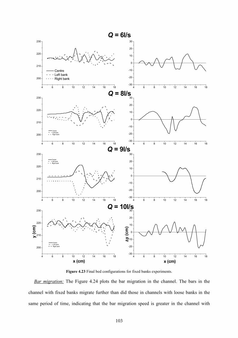
103

4 6 8 10 12 14 16 18

200

210

220

230

Q = 10l/s

Q = 9l/s

Q = 8l/s

Centre

Left bank

Right bank

Q = 6l/s

4 6 8 10 12 14 16 18-30

-20

-10

0

10

20

30

4 6 8 10 12 14 16 18

200

210

220

230

Centre

Left bank

Right bank

4 6 8 10 12 14 16 18-30

-20

-10

0

10

20

30

4 6 8 10 12 14 16 18

200

210

220

230

Centre

Left bank

Right bank

4 6 8 10 12 14 16 18-30

-20

-10

0

10

20

30

4 6 8 10 12 14 16 18

200

210

220

230

y (cm)

∆∆ ∆∆y (cm)

x (cm)x (cm)

Centre

Left bank

Right bank

4 6 8 10 12 14 16 18-30

-20

-10

0

10

20

30

Figure 4.23 Final bed configurations for fixed banks experiments.

Bar migration: The Figure 4.24 plots the bar migration in the channel. The bars in the

channel with fixed banks migrate further than did those in channels with loose banks in the

same period of time, indicating that the bar migration speed is greater in the channel with

104

stronger banks, in agreement with the findings of Jang and Shimizu (2004). The migration

speed decreased with time. Channel widening leads to a decrease in bar migration, which

affects the increase in bar wavelength. From Figure 4.24 it is possible to see that for the case

of loose banks, as the aspect ratio increased, the dimensionless bar migration speed decreased.

Fujita and Muramoto (1985) and Jang and Shimizu (2004) obtained similar results during

their experiments. Bar migration is influenced by bank strength. Perhaps the forcing effects

between the alternate bars and the side banks are weaker with stronger banks. This is in good

agreement with the theoretical prediction of Seminara and Tubino (1989).

Bar height: as the aspect ratio increased, the dimensionless bar height increased as shown

in Figure 4.24. This was seen in the experimental results of Fujita and Muramoto (1985). The

same dimensionless bar height, in a channel with weaker banks, occurs in a wider channel

than it does in a channel with stronger banks because of the higher forcing effects between the

bars and banks.

Bar wavelength: the mean wavelength is plotted for each time step in Figure 4.25. For the

case of loose banks each time step corresponds to a different aspect ratio. For the runs with a

water discharge of 6l/s (Figure 4.25a) the mean wavelength of loose bank channel is shorter

than for the fixed banks one and the variation of the mean wavelength is more significant

( ~ 60% for loose bank and ~ 37% ). Figure 4.25b shows similar results for the runs with

10l/s. In the former, the mean wavelength of the loose bank channel is again shorter than the

fixed banks case one and the variation of the mean wavelength is similar to the previous

experiment ( ~ 60% ), with a significant variation of the absolute value of the order of ~ 0.5

for 6l/s and ~ 1.5 for 10l/s). However, a significant reduction in the variation for fixed banks,

channel is seen with changes from 35%, for a water discharge of 6l/s, to a 20% for 10l/s. At

this point is necessary to highlight that the absolute variation is similar for both experiments

with fixed banks ( ~ 0.5 ).

105

Figure 4.24 Bar migration for Runs for 6l/s with fixed and loose banks. The arrow symbol indicates the bar front migration along the bank with time. The flow is left to right. Bar wavelength varied from six to ten channels widths. The time in hours is indicated to the right.

4 6 8 10 12 14 16 18

After 4.5h

After 9.5h

After 12h

After 14h

After 16h

After 22h

After 20h

After 18h

4 6 8 10 12 14 16 18

After 14.5h

After 12.5h

After 10.5h

After 9.5h

After 2.5h

After 7.5h

After 5.5h

After 4h

4 6 8 10 12 14 16 18

After 14.5h

After 12.5h

After 10.5h

After 9.5h

After 2.5h

After 7.5h

After 5.5h

After 4h

4 6 8 10 12 14 16 18

After 4.5h

After 9.5h

After 12h

After 14h

After 16h

After 22h

After 20h

After 18h

Loose banks

Fixed banks

Right side bar frontLeft side bar front

Longitudinal direction ( x(m))

106

Figure 4.25 Plot of mean wavelength versus the aspect ratio for runs with fixed and loose banks.

Figure 4.26 shows a comparison for wavelengths between loose and fixed banks. The

wavelength shows more variability for the case of fixed banks. For loose banks there is a clear

tendency to reach a maximum configuration, as the bars grow longer. On the contrary, for

fixed banks seems like if there were new bars appearing all the time in the channel. For

example time period 1 and 5 seems to have almost the same range of sizes. The time

evolution of wavelength bars for the fixed banks case seems to indicate the convective nature

0.0

0.5

1.0

1.5

2.0

2.5

3.0

0 1 2 3 4 5 6 7 8 9

Time Steps

Wavelenghts

Loose banks Fixed banksLog. (Fixed banks) Log. (Loose banks)

Q = 6l/s

0.0

0.5

1.0

1.5

2.0

2.5

3.0

0 1 2 3 4 5 6 7

Time steps

Wavelenghts

Loose banks Fixed banksLog. (Fixed banks) Log. (Loose banks)

Q = 10l/s

a)

b)

107

of free bars, where bars first appear, grow, and then decay to appear later again (Federici and

Seminara, 2003)

Figure 4.26 Plot of wavelength variability.

Figure 4.26a shows the results for loose banks run. The dispersion of the bars wavelength

(blue diamonds) is significant at the beginning of the experiment ( ~ 2.25 ). However, as the

channel evolves the bars wavelength concentrate around the mean wavelength (pink square),

reducing the dispersion in ~ 75% . In Figure 4.26b, for fixed banks runs the dispersion of the

bars wavelength (blue diamonds) is significant at the beginning of the experiment ( ~ 3.0 )

quite similar to the case of loose banks. As the channel evolves the bars wavelength change

Q = 6l/s Loosed banks

0.0

0.5

1.0

1.5

2.0

2.5

3.0

0 1 2 3 4 5 6 7 8 9

Time steps

Wavelenght

R-1-05

a)

Q = 6l/s Fixed banks

0.0

0.5

1.0

1.5

2.0

2.5

3.0

3.5

4.0

0 1 2 3 4 5 6 7 8 9

Time steps

Wavelenght

R-2-05

b)

108

exhibiting an oscillatory behaviour. At the beginning of the experiment the dispersion remains

constant for the first two time periods ( ~ 3.0 ), then bars reduce their length to achieve a

minimum (~ 1.5 ) in the fourth time period. After this, bars length expand and contract again

in the following time period but the magnitude of the variation is decreasing. This

phenomenon clearly shows the stabilizing effect of the loose banks. The erosion process

generates changes in the channels geometry, and also provides additional material to build up

the bars, changing the stability characteristics of the channel geometry. This phenomenon can

be seen in the appearance of the longer bars, that converges exponentially to the mean

wavelength value. In the case of the fixed banks channel the longer bars decrease in an

oscillatory way but in a stable fashion. In this channel, bars have to adjust their length to

satisfy the geometrical restrictions imposed by the channel, being the alternate bars

appearance the only stabilization mechanism available.

For many years researchers thought of alternate bars as the building block mechanism for

channel meandering; Parker (1976) highlight that sediment transport is a dynamical necessary

condition for the occurrence of instability leading to meandering either in flow or in the bed.

On the other hand, Seminara and Tubino (1989) explained theoretically the process where the

widening of the channel results in local bank erosion, which depends on the migration of bars

that could lead to a meandering or braiding channel. They showed that bar migration speed

was influenced by lateral expansion of the channel, which tended to slow bar migration and

increased bar wavelength. Besides, for the case of loose banks experiments, the interacting

erodible bed and the stationary flow modify the cross section slightly without introducing

channel sinuosity.

“As long as the river is neither or widening nor narrowing its channel, bank material is

being scoured and deposited inside it. If a stream maintains an equilibrium width (which it

109

happens to our experiments, this status must be interpreted as a statistical equality of the rate

of scour and the rate of deposition” (Einstein, 1972, notes).

The procedure followed during this experiment was similar to Haidera’s work, (Haidera,

2002; Haidera and Valentine, 1999). With the channel being subjected to inbank flow, the

main channel widened rapidly, especially during the first hours of the experiment, as the main

channel became shallower with increasing side slopes (Valentine et al., (2001). Valentine and

co-workers called this a ‘dish-shaped channel’. Following the introduction of water and

sediment into the channel, the channel started to widen and most of the channels attained 80

to 90% of their final stable channel width in the initial three to four hours. These was regarded

as acceptable as the channel had reached a stable configuration, by approaching a new regime

channel condition. This small increase in width seemed unavoidable in the case of such a non-

cohesive bank material. Although it was generally noticed that the channel width for this

experiments became relatively stable after 4-5 hours, the channel initial cross-section was

reworked increasing the bed height for the case of loose banks and eroding it for fixed banks

(Figure 4.27)

Figure 4.28 shows a comparison of the final bed elevation for an experiment with fixed and

loose banks respectively. For the former case, the bed elevation trend to erode with time,

while for the loose banks case the bed grows, rising with the time. So, for the second case,

there is a trend to redistribute sediment, raising the channel bed by eroding the banks.

Figure 4.29 and Figure 4.30 shows the channel cross section evolution with time, and

Table 4.6 summarizes the results of a simple mass balance performed for runs R-1-05 and R-

2-04, which were computed by comparing the cross section areas.

110

Figure 4.27 Bed level evolutions.

111

R-1-05, Loose banks

212

216

220

224

228

232

236

0 2 4 6 8 10 12 14 16 18 20

Longitudinal direction (X (m))

Bed level (m

m)

Initial

Final

R-2-05, Fixed banks

212

216

220

224

228

232

236

0 2 4 6 8 10 12 14 16 18 20

Longitudinal direction (X(m)

Bed level (m

m)

Initial

Final

Figure 4.28 Bed elevation, a) Run (R-2-05) with fixed banks and b) Run (R-1-05) with loose banks.

112

0.7 0.8 0.9 1 1.1 1.2 1.3 1.4 1.5 1.6 1.7200

220

240

260

0.7 0.8 0.9 1 1.1 1.2 1.3 1.4 1.5 1.6 1.7200

220

240

260

Initial Cross-section

Bed Elevation ( z(m

m))

0.7 0.8 0.9 1 1.1 1.2 1.3 1.4 1.5 1.6 1.7200

220

240

260

Channel Width (m)

Equilibrium Cross-section

Final Cross-section

R-1-05, Q = 6l/s

0.7 0.8 0.9 1 1.1 1.2 1.3 1.4 1.5 1.6 1.7200

220

240

260

0.7 0.8 0.9 1 1.1 1.2 1.3 1.4 1.5 1.6 1.7200

220

240

260

Initial Cross-section

Channel Depth ( z(m

m))

0.7 0.8 0.9 1 1.1 1.2 1.3 1.4 1.5 1.6 1.7200

220

240

260

Channel Width (m)

Equilibrium Cross-section

Final Cross-section

R-2-04, Q = 10l/s

Figure 4.29 Channel cross-section evolution with time.

113

Figure 4.29 shows the evolution for run R-1-05. The negative areas characterize the

erosion processes, while positive areas depict the aggradations process. In the transition from

initial cross-section to the equilibrium one both process take action by reshaping the channel:

the equilibrium cross-section is wider and shallower than the initial one in concordance with

the findings of Valentine et al. (1996) at the “Flow Channel Facilities, Wallingford”. The

erosion dominates this transition, 67.3% of the modification is due to erosion, while only

32.7% is due to aggradations (see Table 4.6). On the other hand, in the transition from the

equilibrium to the final cross-section the aggradation governs the reshaping process, where

13.4% of the cross-section changes are due to erosion while 86.6% is shaped by the

aggradations.

R-1-05 R-2-04

Section Initial

(S1)

Equilibrium

(S2)

Final (S3) Initial

(S1)

Equilibrium

(S2)

Final

(S3)

Area 0.0154 0.0165 0.018 0.0255 0.0282 0.0281 Area Diff with S1 0.0010 0.0025 0.0026 0.0025 Area Diff with S2 0.0014 -0.0001 Erosion Dif with S1 -0.0021 -0.0014 -0.0026 -0.0083 % 67.3 35.6 49.75 76.80 Erosion Dif with S2 -0.0002 -0.0067 % 13.4 102.23 Aggration Dif with S1 0.0032 0.0039 0.0053 0.0108 % 32.7 64.4 50.24 23.19 Aggration Dif with S2 0.0017 0.0065 % 86.6 -2.23

Table 4.6 Mass balance results.

114

0.7 0.8 0.9 1 1.1 1.2 1.3 1.4 1.5 1.6 1.7200

210

220

230

240

250

260

R-01-05, Q = 6l/s

Channel Width (m)

Bed Elevation (mm)

0.7 0.8 0.9 1 1.1 1.2 1.3 1.4 1.5 1.6 1.7200

210

220

230

240

250

260

R-2-04, Q = 10l/s

Channel width (m)

Bed Elevation (mm)

Figure 4.30 Channel cross section evolution with time: Initial (red), equilibrium (blue) and final (green).

115

4.4 Chapter summary.

It is known from well-controlled flume experiments that an initially straight prismatic

channel with erodible bed and banks will adjust its width, depth and slope to achieve a stable

quasi-dynamic configuration by transporting certain amount of water and sediment (Schumm

and Khan; 1972), albeit occasionally in unpredictable fashion (Federici and Seminara; 2003).

Moreover, even for the simplest case of well-sorted sediment being transported for a given

discharge, the final channel stable configuration can only be asserted with a high degree of

uncertainty, where the culprit can be traced to the development of bedforms (ASCE 2000).

Gravel bed rivers generally display an alternating structure, while central bars or higher-

order transverse modes are not likely to form spontaneously, unless the channel is fairly wide.

Notice that predicted and observed values of the longitudinal wavelength of bars fall in the

range of 5-12 channel widths.

Theoretical results for bar formation in both sandy rivers (Tubino et al., 1999) and tidal

channels (Seminara and Tubino, 1998, and 2001) have recently been derived within the

context of a linear framework. Both analyses refer to an infinitely long straight channel, with

a bed composed of fine homogeneous sediment; they essentially differ for the different

character of the basic flow of which the stability is investigated: the basic flow is steady in

Tubino et al., (1999), while the channel is subject to a propagation of a tidal wave in the

analysis of Seminara and Tubino (2001). In particular, in the latter work at the leading order

of approximation, local inertia and spatial variations of tidal wave are found to be negligible

at the scale of bars: hence, free bars feel the tidal wave as an oscillatory longitudinally

uniform flow. On the other hand Schielen et al. (1993), suggested that a straight reach with a

length of few hundred widths it required to appreciate the associated modulation of bottom

configuration.

116

In this chapter, the regime channel flume used during the experiments reported here, and

the associated equipments and the accuracies they are able to deliver were described. The

specific procedure followed for each run all along the experiments was explained, as well as

the salient details of the data collected. Then, the available laboratory data have been used to

describe the free bars formation for both fixed and loose banks.

Within the limitations imposed by the facilities and equipment available, the main

findings of this work are: the results confirm previous findings that a self-formed channel

under normal flow condition tends to produce a new regime straight section which is more

dish-shaped with gentler side slopes. These changes tend to minimise the interaction effect

between the main channel and bank. While the channel width became stable then the channel

shape became uniform along the channel reach, and thereafter the channel bed was adjusted.

According to the experimental results of Haidera (2002), the planform adjustment is a

response of the channel bed adjustment and the same for other changes. The results also show

that when the channel bed was modified, the sediment concentration was also modified. The

variation of sediment concentration was asymptotic to a constant representative value of

sediment concentration.

Though much knowledge has been gained about alternate bars from earlier flume studies,

such as those performed by Chang et al. (1971), Jaeggi (1984), Fujita and Muramoto (1985),

García and Niño (1993), and Lanzoni (2000) among many contributors to the subject, most of

the available experimental data were mostly obtained from experiments with loose beds and

non-erodible banks. Therefore, few experiments of alternate bars formation with loose lateral

banks are available. Among them, it is worth to mention the works of Schumm and Khan

(1972), and Federici and Paola (2003). Schumm and Khan (1972) investigated the effect of

the slope on channel patterns and determined slope ranges that marked significant changes on

channel pattern. More recently, Federici and Paola (2003), in a set of experiments aimed to

117

analyze the dynamics of channel bifurcations in loose sediments, also show that alternate bars

formed rapidly in a straight channel initially cut through the cohesionless flat sloping surface

(1.4%). Just 20 min after the initiation of the experiment, the alternate bars patterns developed

a sequence of rhythmic bumps on both banks while the stream displayed a tendency to

meander.

With the above antecedents, the idea of performing a comparative study to analyze the

differences between the formation of alternate bars in channels with loose and fixed banks

was set forward to clarify if is the alternate bar formation that is indeed the preferred evolving

spatial scale of the problem, delaying the lateral migration of the stream for much longer time

scales.

For all the experiments performed for loose and fixed banks we could observe the

formation of free bars that migrate downstream while growing. As was mentioned before free

bars can be considered a sort of 2DCS of the evolving bed fed by the interacting turbulent

flow and the sediment transport along the erodable bed. During the experiments with fixed

banks from time to time, poorly developed trains of bars formed toward the upstream part of

the flume, even after steady conditions were achieved. Periods in which a regular train of bars

was present in almost the entire flume were followed by intervals characterized by a very

irregular bar topography, in agreement with the findings of Lanzoni (2000). These partially

formed bars, possibly triggered by random disturbances in the boundary conditions (i.e., mix

of water+ sediment inflow) and/or by the presence of smaller-scale bed forms. This behaviour

resembles the theoretical picture outlined be Schielen et al., (1993) which showed that under

suitable conditions, nonlinear interactions between perturbations of different wavelength

might cause the periodic alternate bar pattern to become unstable.

Flow patterns established by the alternating bed topography may erode the banks at the

wavelength on the initial bed undulations. If bank migration is fast enough, or bar migration

118

slow enough, this systematic erosion of alternate banks should give rise to the regular changes

in that direction that establish a meander pattern (Whiting and Dietrich, 1993). In many

channels, however, the time scale of bank erosion may be far longer than that of bar

migration; consequently, there exists the potential for transient interactions between the

topography associated with the developing channel curvature and the bathymetric oscillations

associated with the alternate bars (Whiting and Dietrich, 1993).

Finally, during the experiments with loose banks was notably absent the presence of

periodic alternate bars with 10 channel widths separation or less, often viewed as a precursor

to meander development in agreement with Smith`s (1998) observations. We could conclude

that for the specific conditions used during the experiments the formation of alternate bars

was the preferred evolving spatial scale of the problem, delaying the riverbank erosion

processes, and consequently, the lateral migration of the stream for much longer time scales.

119

CHAPTER 5 Conclusions

The impact of morphology on turbulent processes is often simplified to a local boundary

condition and rarely the impact of large morphological units is considered. There is an

obvious gap between the small turbulent scales and the large scales of the flow structure that

in turn may induce typical morphological scales. This thesis was an attempt to bridge in part

that gap, seeking to understand the role of some typical spatial scales that characterizes the

behaviour of a shallow turbulent flow.

In brief, this thesis combined the experience gained at two different experimental facilities:

the first with broad experimental basin available at the Hydraulic Laboratory of the

Engineering and Water Resources Department (FICH) of UNL, in Santa Fe, Argentina, and

the second with the large sand box available at the School of Engineering and Geosciences of

Newcastle University, in Newcastle upon Tyne, UK. Consequently, the objective of this thesis

was also twofold: on one hand, to investigate the spectral response of a shallow turbulent flow

as approaches an opening of a supposedly relief bridge, with a local scour hole located at the

contraction end of an otherwise flat bed; on the other hand, and because the complex

behaviour of sand bars still attracts the interest of the scientific and engineering community,

an experimental investigation on the formation of free bars with fixed and loose banks

interaction with a shallow turbulent flow has been proposed.

What do they have in common? Firstly, spectral segregation of turbulent energy between

horizontal in the form of horizontal 2DCS –two-dimensional coherent structures– and much

120

smaller vertical structures is indeed possible. Secondly, free bars can be considered a sort of

2DCS driven by the interacting turbulent flow with the sediment transport along the erodible

bed.

For the first case, it has been established that the geometrical and topographical forcing

gives rise to an energy spectrum with two well-differentiated peaks. This spectral segregation

represents quasi two-dimensional turbulent motion for the large-scale l1, and three-

dimensional turbulent motion for the small-scale l2, respectively. The phenomenological

estimate obtained for the separation of scales satisfies F12 C~/ ll (within the bounds of the

shallow water theory). The flow turbulent energy initially stored at scales 5~/ hlo is

transferred to much larger scales by the geometrical forcing through an inverse cascade

process. On the other hand, the topographical forcing, which only acts locally, produces a

large amount of turbulent kinetic energy concentrated at small-scales by trapping and exciting

flow modes due to the shape of the “submerged” scour hole. The bed topography injects a

large amount of small-scale turbulence into the flow, which is diffused toward larger scales by

another inverse process.

For the second case, free-bars experiments were carried out in a flume 22m long, 2.5m

wide, and 0.6m deep, filled with uniform sand. These experiments included 4 inbank flow

condition with fixed banks, and 4 with loose banks for identical discharges, initial cross

section and bed slope. These experimental series provided an opportunity to compare the

response the alternate bars for both fixed and loose banks. The experimental programme was

designed to extend the alluvial channels database to test existing theories and methods; and to

investigate the causes of discrepancy between predicted and measured channel dimensions.

Additionally, a stability analysis supporting the alternate bar formation process was included

in the Appendix C. For all the experiments performed for loose and fixed banks the formation

of free bars that migrate downstream while growing was consistently observed. As it was

121

mentioned before free bars can be considered a sort of 2DCS of the evolving bed fed by the

interacting turbulent flow and the sediment transport along the erodable bed. During the

experiments with fixed banks, poorly developed train of bars formed toward the upstream part

of the flume from time to time, even after steady conditions were achieved. Periods with a

regular train of bars was present in almost the entire flume were followed by intervals

characterized by a very irregular bar topography, in agreement with the findings of Lanzoni

(2000). These partially formed bars, possibly triggered by random disturbances in the

boundary conditions (i.e., mix of water + sediment inflow) and/or by the presence of smaller-

scale bed forms. This behaviour resembles the theoretical picture outlined be Schielen et al.

(1993) which showed that under suitable conditions, nonlinear interactions between

perturbations of different wavelength might cause the periodic alternate bar pattern to become

unstable.

Flow patterns established by the alternating bed topography may erode the banks at the

wavelength on the initial bed undulations. If bank migration is fast enough, or bar migration

slow enough, this systematic erosion of alternate banks should give rise to the regular changes

in that direction that establish a meander pattern (Whiting and Dietrich, 1993). In many

channels, however, the time scale of bank erosion may be far longer than that of bar

migration; consequently, there exists the potential for transient interactions between the

topography associated with the developing channel curvature and the bathymetric oscillations

associated with the alternate bars (Whiting and Dietrich, 1993).

Finally, during the experiments with loose banks the presence of periodic alternate bars

with 10 channel widths separation or less was notably absent, often viewed as a precursor to

meander development in agreement with Smith´s (1998) observations. We could conclude

that for the specific conditions used during the experiments the formation of alternate bars

122

was the preferred evolving spatial scale of the problem, delaying the riverbank erosion

processes, and consequently, the lateral migration of the stream for much longer time scales.

As was mentioned before, the impact of morphology on turbulent processes is often

simplified to a local boundary condition and rarely the impact of large morphological units is

considered. There is an obvious gap between the small turbulent scales and the large

scales of the flow structure that in turn may induce typical morphological scales. This

thesis is an attempt to bridge in part the gap, seeking a deeper understanding of which and

how some typical length scales characterizes the behaviour of a shallow turbulent flow.

123

BIBLIOGRAPHY

Abernethy, B., and Rutherfud, I.D., (1998), Where along a river’s length will vegetation most

effectively stabilise the stream banks?, Geomorphology, 23, 55-75.

Ackers, P., and Charlton, F.G., (1970), The Geometry of Small Meandering Streams, Proc. of

the Inst. of Civil Eng., supplement XV, Paper 7328 S, 289-317.

Amsler, M.L., and Ramonell, C.G., (2002), Paraná River channel adjustments to dominant

discharge changes, in: Bousmar, D., and Zech, Y., River flow 2002, International

Conference on Fluvial Hydraulics, Balkema Publ, Belgium, 2, 921-930.

Amsler, M.L., Ramonell, C.G., and Toniolo, H.A., (2005), Morphologic changes in the

Paraná River channel (Argentina) in the light of the climate variability during the 20th

century, Geomorphology, 70, 257-278.

Arnel, N., (1996), Hydrology and climate change, in: Petts, G., Calow, P., (Eds), River Flows

and Channel Forms, Blackwell Sc., Oxford, England, 243-256.

Asai, M., and Nishioka, M., (1993), A numerical study on the receptivity process generating

Tollmien-Schlichting waves, Fluid Dynamics Res., 12, 4, 229-239.

ASCE Task Committee on Flow and Transport over Dunes (2000), Forum: Flow and

Transport over Dunes, J. of Hydraulic Eng., 128, 726-728

Babaeyan-Koopaei, K., (1996), A Study of Straight Stable Channel and Their Interactions

with Bridge Structures, PhD Thesis. University of Newcastle upon Tyne, Newcastle

upon Tyne, UK.

Batchelor, G.K., (1969), Computation of the energy spectrum in homogeneous two-

dimensional Turbulence, The Physics of Fluids Supplement II, II-233 – II-239.

124

Benson, I.A., Valentine, E.M., Nalluri, C., and Bathurts, J.C., (2001), Stabilising the sediment

bed in laboratory flumes, J. of Hydraulic Res., 39, 3, 1-4.

Blondeaux, P., and Seminara, G., (1985), A unified bar-bend theory of river meanders, J. of

Fluid Mech.. 112, 363-377.

Bousmar D., and Zech, Y., (2002), Periodical turbulent structures in compound channels, in:

Bousmar, D., and Zech, Y., (Eds.), Proc. Conf. on Fluvial Hydraulics, Swets &

Zeitlinger, Lisse, The Netherlands.

Callander, R.A., (1969), Instability and river channels, J. Fluid Mech. 36-3, 465-480.

Carrasco, A. (2002), Characterization of the length scales of a shallow turbulent flow laterally

contracted, Master Thesis, Engineering and Water Resources Dept (FICH), UNL, Santa

Fe, Argentina. (In Spanish).

Carrasco, A., and Vionnet, C.A., (2004), Separation of scales on a broad, shallow turbulent

flow, J. of Hydraulic Res., 42, 630-638.

Chang, Y., Simons, D., and Woolhiser, D.A., (1971), Flume experiments on alternate bar

formation, Proc.Waterways Div., ASCE, 97, WW1.

Chang, H.H., (1985), Formation of Alternate Bars, J. Hydraulic Eng., 111, 11, 1412-1420.

Chang, H.H. (1998) “Fluvial Processes in River Engineering”, Krieger Publishing Company,

Malabar, Florida.

Chen, D. and Jirka, G.H., (1995), Experimental study of plane turbulent wake in a shallow

layer, Fluid Dynamics Res., 16, 11.

Chen, D., and Jirka, G.H. ,(1997), Absolute and convective instabilities of plane turbulent

wakes in a shallow water layer, J. Fluid Mech., 338, 157-172.

Chen, D., and Jirka, G.H., (1998), Linear stability analysis of turbulent mixing layers and jets

in shallow water layers, J. Hydraulic. Res., 36, 815-829.

Chow, V. T., (1973), Open-Channel Hydraulic, McGraw-Hill, Singapore.

125

Clifford, N.J., French, J.R., and Hardisty, J., (Eds.), (1993), Turbulence. Perspectives on flow

and sediment transport, J. Wiley.

Colombini, M., Seminara, G., and Tubito, M., (1987), Finite-Amplitude Alternate Bars, J.

Fluid Mech., 181, 213-232.

Colombini, M., and Tubino, M., (1991), Finite-amplitude free bars: A fully nonlinear spectral

solution, in: Soulsby, R., and Bettes, R., (Eds.), Sand Transport in Rivers, Estuaries and

the Sea, A. A. Balkema, Brookfield, Vt., 163–169.

Couperthwaite, J.S., Mitchell, S.B., West, J.R., and Lawler, D.M., (1998), Cohesive sediment

dynamics on an inter-tidal bank on the Tidal Trent, UK, Marine Poll. Bull. 37, 144-154.

Dade, W.B., (2001), Multiple scales in river basin morphology, Amer. J. of Sc., 301, 60-73.

Defina, A., (2003), Numerical experiments on bar growth, Water Resour. Res., 39, 4, 2.1-

2.12.

Denier, J., Hall, P., and Seddougui, S.O., (1991), On the receptivity problem for Gortler

vortices: vortex motions induced by wall roughness, Phil. Trans. Roy. Soc. (A), 335,

51–85.

Dietrich, E.W., and Whiting, P., (1989) Bpundary shear stress and sediment transport in River

Meanders of sand and gravel, , in: Ikeda, S., and Parker, G., (Eds.), River Meandering,

AGU Water Resources Monograph 12, Washington.

Dracos, T., Giger, M., and Jirka, G.H., (1992), Plane turbulent jets in a bounded fluid layer, J.

Fluid Mech., 214-587-614.

Drazin, P.G., and Reid, W.H., (1981), Hydrodynamic stability, Cambridge University Press,

NY.

Duck, P.W., Ruban, A.I., and Zhikharev, C.N., (1996), The generation of Tollmien-

Schlichting waves by freestream turbulence, J. Fluid Mech., 312, 341–371.

126

Duysings, J.J.H.M., (1986), The sediment supply bystreambank erosion in a forested

catchment, Zietschrift fur Geomorphologic N. F., Su. Band, 60, 233-244.

Edwards, B.F., and Smith, D.H., (2002), River meandering dynamics, Phy. Rev. E, 65,

046303-1-046303-11.

Einstein, H.A., (1950), The bed load function for sediment transportation in open channels,

Tech. Rep. 1026, US Dept. of the Army, Soil Conservation Service.

Einstein, (1972), notes.

Engelund, F., (1970), Instability of erodible beds, J. Fluid Mech., 42, 225-244.

Engelund, F., (1974), Flow and bed topography in channel bends, J. Hydraul. Div., HY11,

1630-1648.

Engelund, F., and Skovgaard, O., (1973), On the origin of meandering and braiding in alluvial

streams, J. of Fluid Mech., 57, 289-302.

Engelund, F., and Fredsoe, J., (1981), Sediment ripples and dunes, An. Rev. of Fluid. Mech.,

14, 13-37.

Ershadi, C., (2005), The Effect of Unsteady Flow on the Stability of Straight Alluvial

Channels, PhD Thesis, School of Civil Eng. And Geosciences, University of Newcastle

upon Tyne, Newcastle, UK.

Fahnestock, R.K., and Maddock, T., (1964), Preliminary report on bedforms and flow

phenomena in the Rio Grande near El Paso, Texas, U.S.G.S. Prof Paper, 501-B.

Federici, B., and Paola, C., (2003), Dynamics of channel bifurcations in noncohesive

sediments, Water Resour. Res., 39, 6.

Federici, B., and Seminara, G., (2003), On the convective nature of bar instability, J. Fluid

Mech., 487, 125–145.

Fredsoe, J., (1978), Meandering and braiding of rivers, J. of Fluid Mech., 84, 609-624.

127

Fujita, Y., and Muramoto, Y., (1985), Studies on the process of development of alternate bars,

Bull. Disaster Prev. Res. Inst. Kyoto Univ., 35, 55– 86.

Fukuoka, S., (1989), Finite amplitude development of alternate bars, in: Ikeda, S., and Parker,

G., (Eds.), River Meandering, AGU Water Resources Monograph 12, Washington.

García, M., and Niño, Y., (1993), Dynamics of Sediment Bars in Straight and Meandering

Channels: Experiments on the Resonance Phenomenon, J. of Hydr. Res., 31, 6, 739-761.

Ghidaoui, M.S., and Kolyshkin, A.A,. (1999), Linear stability analysis of lateral motions in

compound open channels, J. Hydr. Eng. ASCE, 125, 871-880.

Gottlieb, L., (1976), Three-dimensional flow pattern and bed topography in meandering

channels, Tech. Univ. Denmark ISVA, Series paper, 11.

Gulliver, M., and Halverson, M.J., (1987), Measurements of large streamwise vortices in an

open channel-flow. Water Resour. Res., 23, 115-123.

Haidera, M.A., (2002), The Stability of Alluvial Channels with Overbank Flow, PhD Thesis,

University of Newcastle upon Tyne, Newcastle upon Tyne, UK.

Haidera, M. A., and E. M. Valentine. (1999), “A Laboratory Study of Alluvial Channels with

Overbank Flow”, The 18th Congress of IAHR, Abstract page 401, Graz, Austria.

Hall, P., (2004), Alternating bar instabilities in unsteady channel flows over erodible beds, J.

Fluid Mech., 499, 49–73.

Hammerton, P.W., and Kerschen, E.J., (2005), Leading-edge receptivity for bodies with mean

aerodynamic loading, J. Fluid Mech. 535:1-32.

Howard, A.D., (1996), Modelling channel evolution and floodplain morphology, in:

Anderson, M.G., Walling, D.E., and Bates, P.D., (Eds.), Floodplain Processes, John

Wiley.

Hussain, A.K.M.F., (1983), Coherent structures – reality and myth, Phys. Fluids, 26, 2816-

2850.

128

Ikeda, S., Parker, G., and Sawai, K., (1981), Bend theory of river meanders, Part I – linear

development, J Fluid Mech., 112, 363-377.

Ikeda, S., (1982), Prediction of alternate bar wavelength and height, Rep. Dept. Found. Eng.

And Const. Eng., Saimata Univ., 12, 23-45

Ikeda, S., (1984), Prediction of alternate bars wavelength and height, J. Hydr. Eng., 110, 4,

371-386.

Jaeggi, M.N.R., (1980), Discussion of Steepness of Sedimentary Dunes, by Yalin, M.S. and

Karahan, E., J. of Hydr. Eng. Div., ASCE, 106, HY1, 230-233.

Jaeggi, M.N.R., (1984), Formation and Effects of Alternate Bars, J. Hydr. Eng., 110, 2, 142-

156.

Jang, C.L., and Shimizu, Y., (2004), Numerical experiments on the alternate bars considering

the banks strength, in: Jirka, G., and Uijttewaal, W.S.J., (Eds.), Shallow Flows, Taylor

and Francis Group, London.

Jirka, G.H., (2001), Large scale flow structures and mixing processes in shallow flows, J.

Hydr. Res., 39, 6, 567-573.

Jirka, G.H., and Uijttewaal, W.S.J., (2004), Shallow flows: a definition, in: Jirka, G., and

Uijttewaal, W.S.J., (Eds.) Shallow Flows Conference, Taylor & Francis Group, London,

3-11.

Johannesson, H., and Parker, G., (1989), Linear theory of River Meanders, in: Ikeda, S., and

Parker, G., (Eds.), River Meandering, AGU Water Resources Monograph 12,

Washington.

Kennedy, R.G., (1895), The prevention of silting in irrigation canals, Proc. Inst. Civ. Engr.

119, 281-290.

Kennedy, J.F., (1963), The mechanism of dunes and antidunes in erodible bed channels, J.

Fluid Mech., 16, 521-544.

129

Kennedy, J.F., and Brooks, N.H., (1965), Laboratory study of an alluvial stream at constant

discharge, California Institute of Technology, Report KH-R-17, Pasadena, California.

Keulegan, G.H., (1938), Law of turbulence flow in open channels, J. Res. Nat. Bur. Stand.,

21, 707-741.

Kinoshita, R., (1957), Formation of Dunes on River bed, Transactions, Japan Society of Civil

Engineers, 42, 1-21. (In Japanese).

Kinoshita, R., (1961), Investigation of channel deformation in Ishikari River, Rep. Bur. of

Resour., Dept. Science and Technology, Japan, 1-174.

Kinoshita, R., and Miwa, H., (1974), River channel formation which prevents downstream

translation of transverse bars, Shinsabo, 94, 12–17. (in Japanese).

Knight, D.W., (2001), Flow and sediment transport in two-stage channels, 2nd IAHR

Symposium on River, Coastal and Estuarine Morphodynamics, Japan, 1-20.

Knighton, D., (1984), Fluvial Forms and Processes, Edward Arnold, London.

Knighton, D., (1998), Fluvial forms and processes, Arnold Publ., Cornwall, England.

Kraichnan, R., (1967), Inertial ranges in two-dimensional turbulence, Physic of Fluids, 10,

1417-1428.

Kraichnan, R. H., (1971), Inertial range transfer in two- and three-dimensional turbulence, J.

Fluid Mech., 47, 3, 525-535.

Lacey, G., (1929-30), Stable Channel in Alluvium, Minutes of Proc. ICE, 229, 259-384.

Lanzoni, S., and Tubino, M., (1999), Grain sorting and bar instability, J. of Fluid Mech., 393,

149-174.

Lanzoni, S., (2000), Experiments on bar formation in a straight flume 1. Uniform sediment,

Water Resour. Res., 36, 11, 3337-3349.

Leopold, L.B., and Wolman, M.G., (1957), River channel patterns-braided, meandering and

straight, US Geol. Survey Prof. Paper 282-B.

130

Lewin, J., Macklin, M.G., and Newson, M.D., (1988), Regime theory and environmental

change – irreconcilable concepts?, in: White, W.R., (Ed.), Int. Conf. on River Regime,

Wiley, Chichester, 431–445.

Lighthill, J., (1978), Waves in Fluids, Cambridge University Press.

Lindley, E.S., (1919), Regime Channels, Proc. Ounjab Engng Congr., 7, 63.

Lloyd, P.M., and Stansby, P.K., (1997), Shallow-water flow around model conical islands of

small side slope. I: Surface piercing. J. Hydraul. Engr. ASCE, 123, 1057-1067.

Macklin, M.G., and Lewin, J., (1997), Channel, Floodplain and Drainage Basin Response to

Environmental Change, in: Thorne, C.R., Hey, R.D., and Newson, M.D., (Eds), Applied

Fluvial Geomorphology for River Eng. and Management, Chapter 2, John Wiley & Sons

Ltd.

McLean, S.R., Nelson, J.M., and Wolfe, S.R., (1994), Turbulence structure over two-

dimensional bed forms: Implications for sediment transport, J. of Geoph. Res., 99, C6,

12,729 – 12,747

Melville, B.W., and Coleman, S.E., (2000), Bridge Scour, Water Resour. Publ. LLC,

Highlands Ranch (Colorado), USA.

Meyer-Peter, E., and Müller, R., (1948), Formulas for the bed load transport, In: Proceedings

of the 2nd meeting of the Inter. Assoc. for Hydr. Res., pp. 39-64. Stockholm, Sweden.

Milton Van Dyke, (1982), Album of Fluid Motion, Parabolic Pr.

Mitchell, S.B., Couperthwaite, J.S., West, J.R., and Lawler, D.M., (1999), Dynamics of

erosion and deposition events on an intertidal mudbank at Burringham, River Trent, UK,

Hydrological Processes 13, 1155-1166.

Montgomery, D.R., and Dietrich, W.E., (1992), Channel initiation and the problem of

landscape scale, Science, 255, 826-830.

131

Mosselman, E., (1992) Mathematical modelling of morphological processes in rivers with

erodible cohesive banks, Commun. Hydraul. Geotech. Eng., Delft Univ. of Technol.,

Delft, Netherlands, 92-3.

Mosselman, E., (1998), Morphological modelling of rivers with erodible banks, Hydrological.

Processes, 12, 1357–1370.

Mutlu Sumer, B., Chua, L.H.C., Cheng, N.-S., and Fredsoe, J., (2003), Influence of

Turbulence on Bed Load Sediment Transport, J. Hydr. Eng., 129, 8, 585-596.

Muto, T., and Swenson, J., (2005), A new view of the graded river: theory and flume

experiments, AAPG Annual Convention, Calgary, Canada, June 19-22.

Nadaoka K., and Yagi, H., (1998), Shallow-water turbulence modeling and horizontal large-

eddy computation of river flow, J. Hydr. Eng. ASCE, 124, 493-500.

Nelson, J.M., and Smith, J.D., (1989), Evolution and stability of erodible channel beds, in:

Ikeda, S., and Parker, G., (Eds.), River Meandering, AGU Water Resources Monograph

12, Washington, 321-377.

Nezu, I., and Nakagawa, H., (1993), Turbulence in Open-Channel Flows, A.A. Balkema.

Olesen, K.W., (1983), Alternate bars and meandering of alluvial rivers, Delft Univ. of Tech.,

Report 7-83.

Olesen, K.W. (1987) Bed topography in shallow river bends, Faculty of Civil Eng., Delft

Univ. Tech. Report 87-1

Ossia S., and Lesieur M., (2001), Large-scale energy and pressure dynamics in decaying 2D

incompressible isotropic turbulence, J. Turbulence, 2, 1-13.

Parker, G., (1976), On the cause and characteristics scales of meandering and braiding in

rivers, J. Fluid Mech., 76-3,457-480.

Parker, G., (1979), Hydraulic geometry of active gravel rivers, J. Hydr. Eng., ASCE, 105,

HY9, 1185-1201

132

Parker, G., (2007), Public Presentation at: Workshop on Morphpdynamic Processes in Large

Lowland Rivers, Santa Fe, Argentina.

Parker, G., Toro-Escobar, C.M., Ramey, M., and Beck, S., (2003), The effect of floodwater

extraction on the morphology of mountain streams, J. Hydr. Eng., 129(11), 885-895.

Pouquet, A., Frisch U., and Chollet, J.P., (1983), Turbulence with a spectral gap, Phys.

Fluids, 26, 877-880.

Ramonell, C.G., Amsler, M.L., and Toniolo, H., (2002), Shifting modes of the Parana River

thalweg in its middle/lower reach, Zeitschrift fur Geomorphologie, Supplemenrband

129, 129-142.

Raudkivi, A.J., (1963), Study of sediment ripple formation, J. of the Hydr. Div., ASCE, HY6.

Robert, A., (2003), River Processes: An Introduction to Fluvial Dynamic, Arnold, London.

Ruban, A.I., (1984), On the generation of Tollmien-Schlichting waves by sound, Izv. Akad.

Nauk SSSR Mech., Zhidk. & Gaza. 5, 44—52.

Saric, W.S., Reed, H.L., and Kerschen, E.J., (2002), Boundary Layer Receptivity to Free-

Stream Disturbances, Ann. Rev. Fluid Mech. 34, 291-319.

Scacchi, G., (2003), Scour on bridge abutments located on river floodplains. Master Thesis,

Engineering and Water Resources Dept (FICH), UNL, Santa Fe. (in Spanish).

Schielen, R.S., Doelman, A., and De Swart, H.E., (1993), On the nonlinear dynamics of free

bars in straight channels, J. Fluid Mech., 252, 325-356.

Schreider, M., Zanardi, L., Scacchi, G., and Franco, F., (1998), Contraction and abutment

scour on relief bridges located on alluvial valleys, Ing. Agua 5, 21-32. (In Spanish).

Schumm, S.A., and Khan, H.R., (1972), Experimental study channel patterns, Geological Soc.

of Amer. Bull., 83, 1755-1770.

Schumm, S.A., (1985), Patterns of alluvial rivers, An. Rev. of Earth and Planetary Sc., vol.

13, 5-27.

133

Sellin, R.H.J., (1964), A laboratory investigation in the interaction between flow in the

channel of a river and that of its floodplain, La Houille Blanche, 7, 793-801.

Seminara, G., and Tubino, M., (1989), Alternate bars and meandering: free, forced and mixed

interactions, In Ikeda, S., and Parker, G., (Eds.), River Meandering, AGU Water

Resources Monograph 12, Washington, 267-321.

Seminara, G., Colombini, M., and Parker, G., (1996), Nearly pure sorting waves and

formation of bedload sheets, J. Fluid Mech., 312, 253-278.

Seminara, G., and Tubino, M., (1998), On the formation of estuarine free bars, in: Dronkers,

J., and Scheffers, M., Physics of Estuaries and Coastal Seas, Balkema.

Seminara, G., and Tubino, M., (2001), Sand bars in tidal channels. Part I: Free bars, J. Fluid

Mech., 440, 49-74.

Shakir, A.S., (1992), An Experimental Investigation of Channel plan forms, PhD Thesis,

University of Newcastle upon Tyne, Newcastle upon Tyne, UK.

Shi J., Thomas, T.G., and Williams, J.J.R., (1999), Large-eddy simulation of flow in a

rectangular channel. J. Hydr. Res., 37, 345-361.

Shimizu, Y., and Itakura, T., (1989), Calculation of bed variation in alluvial channels, J.

Hydr. Div., Am. Soc. Civ. Eng., 115(HY3), 367– 384.

Shiono, K., and Knight, D.W., (1991), Turbulent open channels flows with variable depth

across the channel, J. Fluid Mech., 222, 617-646.

Simons, D.B., and Richardson, E.V., (1966), Resistance to flow in alluvial channels,

Geological Surv. Prof. Paper 422-I, Washington, USA.

Smith, C.E., (1998), Modelling high sinuosity meanders in a small flume, Geomorphology,

25, 19-30.

Sontek (2000), The ADV Operation Manual, Sontek Inc., San Diego, CA, USA.

134

Struiksma, N., Olesen, K.W., Flokstra, C., and De Vriend, H.J., (1985), Bed deformation in

alluvial channels, J. Hydr. Res., 23, 1, 57-79.

Struiksma, N., (1985), Prediction of 2-D bed topography in rivers, J. Hydr. Eng., Am. Soc.

Civ. Eng., III.

Struiksma, N., and Crosato, A., (1989), Analysis of a 2-D bed topography model for rivers,

in: Ikeda, S., and Parker, G., (Eds.), River Meandering, AGU Water Resources

Monograph 12, Washington, 153-180.

Talmon, A.M., Struiskma, N., and Mierlo, M.C.I.M. van, (1995), Laboratory measurements

of the direction of sediment transport on transverse alluvial bed slopes, IAHR, J. Hydr.

Res., 33, 4, 495-517.

Tamai, N., Asaeda, T., and Ikeda, H., (1986), Study on generation of periodical large surface

eddies in a composite channel flow, Water Resour. Res., 22, 1129-1138.

Tamburrino, A., and Gulliver, J.S., (1999), Large flow structures in a turbulent open channel

flow, J. Hydr. Res., 37, 363-380.

Tassi, P.A., (2001), Integración de tecnologías para la simulación numérica del escurrimiento

de un gran río de llanura, Master Thesis, Engineering and Water Resources Dept

(FICH), UNL, Santa Fe, Argentina. (In Spanish).

Tassi, P.A., (2007), Numerical modelling of rivers processes: Flow and river bed deformation,

PhD. Thesis, University of Twente, The Netherlands.

Telemac, (1998), Telemac Modelling System, Telemac-2D software 4.0, Reference Manual,

Electricité de France (EDF), Dep. Laboratoire National d`Hydraulique.

Thorne, C.R., (1990), Effects of vegetation on riverbank erosion and stability, in: Thornes,

J.B., (Ed.), Vegetation and erosion: Processes and Environments, John Wiley, New

York, 125-144.

135

Thorne, C.R.; Hey, R.D., and Newson, M.D., (1997), Applied Fluvial Geomorphology for

River Engineering and Management, John Wiley & Sons Ltd., Chichester, England.

Tubino, M., Repetto, R., and Zolezzi, G., (1999), Free bars in rivers, J. Hydraulic Res., 37, 6,

759-775.

Uijttewaal, W.S.J., and Jirka, G., (2003), Grid turbulence in shallow flows, J. Fluid Mech.,

849, 325-344.

Valentine, E.M., Benson, I.A., Nalluri, C., and Bathurst, J.C., (2001), Regime Theory and the

Stability of Straight Channels with Bankfull and over Bank Flow, J. Hydr. Res., 39, 3,

259-268.

Valentine, E.M., and Haidera, M.A., (2001), A proposed modification to the White, Bettes

and Paris Rational Regime Approach, The 2nd IAHR Symposium on River, Coastal and

Estuarine Morphodynamics, Japan, 275-284.

Van den Berg, J.H., and Van Gelder, A., (1989), Scour and fill sequences in flows over very

fine sand and silt, Proc. 4th Int. Conf. on Fluvial Sedimentology, Barcelona, Spain.

Van Dyke M., (1982), An Album of Fluid Motion, The Parabolic Press, Stanford, CA, USA.

Van Rijn, L.C., (1984), Sediment transport, Part I: Bed load transport, J. Hydraul. Eng.,

110(10), 1431-1456.

Van Rijn, L.C., (1993), Principles of Sediment Transport in Rivers, Estuaries and Coastal

Seas, Aqua Publications, Amsterdam, The Netherlands.

Vanoni, V.A., and Brooks, N.H., (1957), Laboratory studies of the roughness and suspended

load of alluvial streams, Sedimentation laboratory, California Institute of Technology,

Report E-68, Pasadena, California.

Vionnet, C.A., Tassi, P.A., and Martin Vide, J.P., (2004), Estimates of flow resistance and

eddy viscosity coefficients for 2D modelling on vegetated floodplains, Hydrological

Processes 18, 15, 2907-2926.

136

Vreugdenhil, C.B, (1994), Numerical methods for shallow water flow, 2nd Ed., Kluwer

Academic Publishers: Dordrecht, Netherlands

Werrity, A., (1997), Short-term Changes in Channel Stability, in: Thorne, C.R., Hey, R.D.,

and Newson, M.D., (Eds), Appl. Fluvial Geomorphology for River Eng. and

Management, Chapter 3, John Wiley & Sons Ltd.

White, W.R., Paris, E., and Bettess., R., (1981), River Regime Based on Sediment Transport

Concepts, Report IT 201, Hydr. Res. Station, Wallingford, England.

Whiting, P.J., and Dietrich, W.E., (1993), Experimental studies of bed topography and flow

patterns in large-amplitude meanders. 1. Observations, Water Resour. Res., 29, 3605-

3622.

Wolanski, E.J., Imberger, J., and Heron, M.L., (1984). Islands wakes in shallow coastal

waters, J. Geophys. Res., 89, 10553-10569.

Wong, M., (2003), Does the bedload transport relation Meyer-Peter and Müller fits it own

data?, Proc. 30th IAHR-Congress, IAHR, Thessaloniki, Greece.

Wong, M., and Parker, G., (2006), Reanalysis and correction of bed-load relation of Meyer-

Peter and Müller using their own database, J. of Hydr. Eng., 132, 11, 1159-1168.

Wyzga, B., (1999), Estimating mean flow velocity in channel and flood plain areas and its use

for exploring the pattern of overbank deposition and floodplain retention.

Geomorphology, 28, 281-297.

Yalin, M.S., and Silva, A.M.F., (1991), On the Formation of Alternate Bars, In Soulsby, R.,

and Bettess, R., (Eds.), Sand Transport in Rivers, Estuaries and the Sea, Balkema,

Rotterdam, Netherlands.

Zedler E.A., and Street, R.L., (2001), Large-eddy simulation of sediment transport: currents

over ripples. J. Hydr. Eng., ASCE, 127, 444-452.

137

Appendix A Normal Flow Solution

The response to a sudden increase in momentum applied at the inlet position, 0X = , can

be computed from Equation (1.11)

( ) )(2

C

2

222

0

F2

0 XU

UUH

U

dX

d i δ=−+

(A.1)

where 2/2iU is the required amount of kinetic energy to be added at 0X = , per unit of mass,

to increase the flow velocity from its normal magnitude U0 to 0 0U U+ ∆ . Changing now 2U

for Y, the above equation reduces to the linear ordinary differential equation

( ) )(2C 2

00

F XUYYHdX

dYi δ=−+ . (A.2)

The above equation is based upon the assumption that the sudden increase in momentum

affects the velocity field only; leaving the water depth H0 unchanged (normal flow). Using

now the Laplace transform

∫∞

−=0

)()(ˆ dXXYesY sX (A.3)

the governing equation transform to

20

20

(0)ˆ( )( )

i

i

aY UYY s

s s a s a s a

Y U

s s a

= + ++ + +

= ++

(A.4)

For F

0

2Ca

H= and 0 (0)Y Y= .

138

Whose solution, after transforming back to ( )U X , is

0F /C2220

2 )( HX

i eUUXU−+= (A.5)

The resulting flow velocity at the inlet allows to determine the required impulse, since

( ) 0 00U U U= + ∆ ,

( ) 220

200 iUUUU +=∆+ (A.6)

It follows that ( ) 00020

200

2 /,2 UUUUUUU i ∆=δδ+δ= , and the variation of flow velocity

with distance is finally given by

( ) 0F /C2200

0

21)( HX

eUUU

XU −δ+δ+= (A.7)

For numerical reasons it is convenient to introduce a slow geometric variation in the

channel width along the streamwise direction to accommodate the sudden momentum influx

at 0X = , which amounts to some addition of mass, required to increase the flow velocity

without changing the water depth, 0 :H H const= .

( ) 0F /C2200

0

0 21

1

)(

)(HX

eUUXU

U

B

XB

−δ+δ+== (A.8)

where B0 is the channel width at 0X = . The channel width variation is indeed slow enough to

render the above solution valid since change in momentum in lateral direction can be safely

neglected. Last but not least, the normal flow solution given by Eq. (1.14) can be posed in

dimensionless form as

F

020 C

SF = (A.9)

that reflects the exact balance between gravity and friction, whereas an increase in bed slope

tend to accelerate the flow, and increase in bed hydraulic resistance will have the opposite

effect. Here, 000 /F gHU= is the Froude number. A numerical experiment of this sort was

considered by Tassi and Vionnet (2002) using three different computational engines with

139

excellent agreement with the exact solution, showing that the expected behavior described by

Eq.(A.7) could indeed be achieved in practical situations.

The sudden increase in momentum influx at the inlet can be considered effectively extinct

whenever the exponential factor in Eq.(A.7) attains the value π−2e ( 0.002≈ , Batchelor (1969)).

Under this assumption the effective distance L that the flow must undergo to reestablish the

balance between gravity and friction is

F0 C/HL π≈ (A.10)

The following figure exhibits the solution behavior under an inflow perturbation equivalent

to 50% of the base flow, 5.00 =δU . For completeness and/or later comparison with

numerical solutions, other data used to generate the plot where FC 0.01= , and 0 0.2F = .

X / H0

U(X)/U

0

0 100 200 300 4000.2

0.4

0.6

0.8

1.0

1.2

1.4

1.6

normal flow

L / H0~ π /C

F

B(X) / B0 1

Figure A.1 Solution behavior under an inflow perturbation 0/B B is not to scale

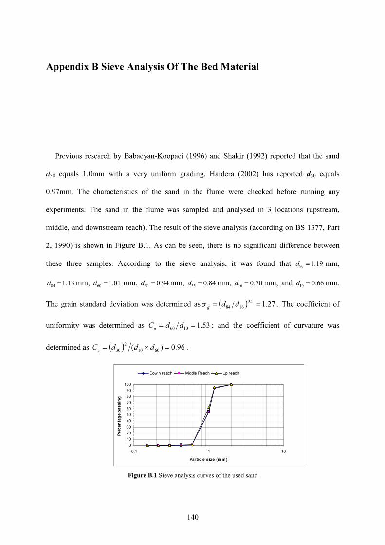
140

Appendix B Sieve Analysis Of The Bed Material

Previous research by Babaeyan-Koopaei (1996) and Shakir (1992) reported that the sand

d50 equals 1.0mm with a very uniform grading. Haidera (2002) has reported d50 equals

0.97mm. The characteristics of the sand in the flume were checked before running any

experiments. The sand in the flume was sampled and analysed in 3 locations (upstream,

middle, and downstream reach). The result of the sieve analysis (according on BS 1377, Part

2, 1990) is shown in Figure B.1. As can be seen, there is no significant difference between

these three samples. According to the sieve analysis, it was found that 90 1.19d = mm,

84 1.13d = mm, 60 1.01d = mm, 50 0.94d = mm, 35 0.84d = mm, 16 0.70d = mm, and 10 0.66d = mm.

The grain standard deviation was determined as ( ) 27.15.01684 == ddgσ . The coefficient of

uniformity was determined as 53.11060 == ddCu ; and the coefficient of curvature was

determined as ( ) 96.0)( 60102

30 =×= dddCc .

0

10

20

30

40

50

60

70

80

90

100

0.1 1 10

Particle size (mm)

Percentage passing

Dow n reach Middle Reach Up reach

Figure B.1 Sieve analysis curves of the used sand

141

Appendix C Stability Analysis Of 2d Coherent Structures Of

Shallow Waters.

C.1 Introduction

Bars are an essential large-scale feature of river topography, as is been well established

before. They consist of the repetitive sequences of scour holes and depositional diagonal

fronts, with planimetric scale in the magnitude order of the channel width. These structures

are often organized in the simplest pattern typical of alternate bars. Nevertheless, in wider

reaches more complicate transverse topographic expressions frequently occur, like central or

multiple bars. The increasing interest in alternate bars has mainly originated from practical

motivations. The possibility of predicting and preventing processes like bedforms

development in rivers, their migration and interaction with structures and navigation, bank

failures and channel shift, are some of the issues to deal with, in river control and hazard

prevention.

After three decades of research on fluvial bedforms, enlightened by the seminal

contribution of Kennedy (1963), most scientist today agree that, in the absence of forcing

mechanisms, sand-wave development is a problem of instability. The formation of river bars

has been conclusively explained in terms of an inherent instability of erodible beds subject to

a turbulent flow in almost straight channels, which leads to the spontaneous development of

bottom perturbations (free bars) migrating downstream. Furthermore, the occurrence of a

142

given transverse configuration has been often interpreted as the result of the dominance of an

associated transverse mode of the Fourier representation of bed elevation (Parker, 1976).

C.2 Governing equation

Following the standard viewpoint of hydrodynamics instability, free bars formation is

generally investigated by seeking the conditions under which the change in flow pattern and

sediment transport induced by a slight perturbation of bottom topography, with respect to the

plane configuration, leads to the amplification of bed perturbation. Implicit in this procedure

is the assumption, based on experimental observations, that the time scale of bed change

(amplification and migration) is much larger that the flow time scale, which implies that a

quasi steady approach can be used for the flow.

Let concentrate ourselves on a still fairly idealized model of bars formation: a laboratory

experiment performed under steady flow conditions, with no sediment transport in suspension

and uniform grain size distribution. This analysis requires a suitable description of the flow

field in an infinitely long straight channel, with constant width, which is assumed to be large

enough to justify the adoption of a shallow water approximation. Consequently, assuming a

flowing layer of water bounded from above by a free surface free of wind effects and from

below by a smooth albeit slowly erodible bottom, and if the vertical extent of the flowing

layer, oH , is small in comparison with the horizontal length of the wavelike motion of the

fluid, oL (i.e., if / 1o oH L ≪ ), the motion can be analyzed by a horizontal 2-D formulation

known as the long wave approximation, where small-scale effects are supposed to act as an

effective eddy viscosity on the large-scale motion (Carrasco and Vionnet, 2004), The latter

approach implies that the vertical accelerations are negligible compared with gravity.

143

Figure C.1 Reference system

Then, and with reference to Figure C.1, the resulting set of governing equations written in

non-conservative form can be obtained from the depth-integrated form of the Navier-Stokes

equations of motion, previously averaged over turbulence:

( ) ( )

( )( )

2

0

1,0 νρ

0

s b o s b

Bs o t

o s b

bB

Z Z H Z ZT

g Z gST H Z Z

Z

T

∂− +∇⋅ + − =

∂∂

+ ⋅∇ + ∇ = − + ∇∂ + −

∂+∇ ⋅ =

∂

U

TUU U U

S

(C.1)

(C.2)

(C.3)

where ( ),U VU = is the depth-average velocity in the ( ),X Y directions, T is the time, Zs and

Zb are the free-surface and bed level perturbations respectively, with respect to the

undisturbed or mean water depth Ho, ( )/ , /X Y∇ = ∂ ∂ ∂ ∂ is the gradient operator, g is the

acceleration due to gravity, ρ is the fluid density, and η ηo oS X= −ɶ gives the unperturbed

channel bottom elevation with respect to some datum, being So the longitudinal uniform

slope. The erodible bottom is assumed to vary slowly so that the quasi-steady flow field can

be considered to adapt instantaneously to changes in bottom configuration. Three additional

relationship must be provided to close the problem: (i) the bed resistance, ( , )X YB B BT T=T , (ii)

144

the eddy viscosity νt , and (iii) the sediment flow rate ( , )X YB B BS S=S . For the former, the

classical squared function dependency on the depth-averaged velocity is used:

2 2F( , ) ρC ( , ) , ,

X YB B BT T U V U V= = = +T U U (C.4)

where the friction coefficient FC is specified with the Keulegan relation

22

F 2

11C 2.5ln , / ρo

B

s

HUU

K

−

∗∗

= = =

T

U

(C.5)

Furthermore, CF is the local friction coefficient for which several empirical relationships

are available in the literature. sk represents an effective roughness height, usually

proportional to the particle size for flat bottom, or modified according to Van Rijn (1984)

approach for the case of dunes-covered bed, and *U denotes the shear velocity.

The classical depth-averaged estimate for the second closure relation is given by

Fν Ct oUHκ= , with κ the Von Karman constant (Uijttewaal and Jirka, 2003). In-channel

values for the SWE are given by Vionnet et al. (2004). To begin with, in this work the limit

case for what the viscosity can be ignored (ν 0)t → is considered first.

Finally, for the volumetric sediment flux SB it is well establish that the average bedload

motion in case of uniform plane turbulent flows is aligned with the average flow, and its

intensity is a monotonically increasing function of the excess of bed shear stress TB, for which

various empirical relationships have been proposed of the form

( )�

,1 C

N

B B B U U

a

n= − =

−U

S T T e eU

⌢

(C.6)

Here, n is the porosity of the noncohesive bed material, typically about 0.4, a⌢ and N

⌢ are

empirical constants, and CB

T is the threshold value of bed shear stress below which there is no

145

particle motion on the bed. In this work, it is assumed that the bed shear stress is well above

critical conditions but not as intense as to entrain particles into suspension, so only bedload

mode of transport such as saltation, rolling or even sliding of particles occur within a thin bed

interface of typical thickness of the order of 2D-3D. In addition, if it is further assumed that

the bedload transport will reduce its intensity to account for an uphill slope ahead, and

conversely, the above relation becomes after some elementary manipulation (Engelund and

Skovgaard, 1973; Schielen et al., 1993)

σ γ ,N

B bZ

= − ∇

US U

U

(C.7)

where ( )Fσ ρ C /1a n= −⌢

and 2N N= ɶ . Many transport formulae are of this type, see the

review in van Rijn (1989). Note that we omit the effect of secondary flow on the direction of

the sediment transport. To include such effect, the usual empirical approach taken by most

authors (Struiskma et al., 1985; Colombini et al., 1987; Johannesson and Parker, 1989;

Lanzoni and Tubino, 1999; Federici and Seminara, 2003; Hall, 2004) can be summarized as

follow

3

23/ 2

( , ) (cosδ,sin δ) ,( 1)

8(τ τ ) , τ( 1)

X YB B

c

S Ss gD

U

s gD

∗∗ ∗ ∗

Φ=

−

Φ = − =−

(C.8)

(C.9)

In the above equations, s is the relative density of sediments and equal to ρ / ρ 1s − , Φ is the

dimensionless bedload transport formula of Meyer-Peter and Müller (1948), τ∗ is the

dimensionless bed shear stress (Shields parameter), and δ is the angle made by the direction

of the bedload transport with the longitudinal direction. Talmon et al. (1995) suggest a

prediction for δ that can be read as

146

2 2

ηsin δ , β /

β τo

V rB H

YU V ∗

∂= − =

∂+

⌢

(C.10)

being r an empirical constant ranging between 0.5 0.6− .

C.3 Boundary conditions

Considering now a straight channel with erodible bed and fixed lateral banks, of width 2B,

the differential system (C.1)-(C.3) with the given closure relationships must be solved subject

to boundary conditions of vanishing fluid and sediment fluxes through the side walls of the

channel and at the free surface, hence

0 , 0 onYB

V S Y B= = = ± (C.11)

C.4 Base flow and dimensionless form

The above set of equations admits a simple solution given by a uniform flow ( ,0)o oU=U

on a straight channel with constant water depth oH and slope oS . According to the first

relationship, the equilibrium sediment discharge will be σo

N

B oS U= . Therefore, it is rather

straightforward to end up with the following dimensionless form of the governing equations

(See Appendix D).

( )2

0

ζ β 1,0

ξ γ0 , ξ

τ β

Bo o

N

B B

h

F Sh

∇⋅ =

⋅∇ +∇ = −

∂+∇ ⋅ = = − ∇ ∂

u

u u

us s u

u

ττττ

(C.12)

(C.13)

(C.14)

where the dimensional quantities have been made dimensionless employing the scales

dictated by the base flow

147

( ) ( ) ( )

( )2

F

, ,( , ) , , , , ,

, ,( , , ) , , ,

Co o

o

o o o o

s bB B

B B

o o B

X Y U V T UHx y u v h t

B U H B

Z Z T

H U S

ηη ζ ξ

ρ

= = = =

= = =S

s

⌢

ττττ

(C.15)

Once the problem is cast in dimensionless form and is supplemented by the required

closure assumptions, three dimensionless parameters arise, namely the aspect ratio β / oB H=

already defined, the ratio between the hydrodynamic flow and sediment flow rate,

/oB o oS U H∈= , and the Froude number 2 2 / / C

oo o o o FF U gH S= = . Consequently, after filtered

the fast flow response and taking the limit 0∈→ , the governing equations reduce to the

system given above.

C.5 Linear stability analysis

It is now possible to investigate the linear response of the flow to infinitesimal

perturbations. Therefore, if the base state is perturb by linear infinitesimal perturbations with

amplitudes of the kind

( ), , , η ou v h ′≡ = +φ φ φφ φ φφ φ φφ φ φ (C.16)

Then, linearizing by neglecting nonlinear terms, it is possible to obtain the following

reduced system (see Appendix E), which can be symbolically written as a matrix as ′ =L 0φφφφ

( ) ( )

( )

2

2

γτ β

2β 0 β 1 β 1 00 β 0 0

ζ 0

ξ 00

o x o x o o

o x o y

x y x x

x y xx yy

F S S M S M u

F S v

N

∂ + ∂ − + + ′ ∂ + ∂ ′ = ∂ ∂ ∂ −∂

∂ ∂ ∂ − ∂ +∂

(C.17)

Seeking the solution of this initial-value problem in the form of travelling waves of the

form

( ω )( )ei kx ty −′ = fφφφφ (C.18)

148

where k is the wavenumber, ω the complex frequency and ( )yf the vector with the amplitude

of the perturbations ( , , ζ,ξ)u v=⌢ ⌢ ⌢ ⌢

, it is possible to obtain the following fourth-order differential

linear equation for the bed perturbation after using Gaussian elimination (see Appendix F)

( ) ( )4 2

4 2

ξ ξ2ω ω ξ 0

d d

dy dy+ + + + =a b c d

⌢ ⌢⌢

(C.19)

Subject to the following boundary conditions

3

3

ξ ξ0, 0 1

d don y

dy dy= = = ±

⌢ ⌢

, (C.20)

the first derivate is from apply non-slip on the bottom, and the thirds if from choose a

symmetry criteria.

The above coefficients are given by

2i= − γa (C.21)

( ) 23 3 3ok N S ik= β − − γ − γb (C.22)

( )( )3 3 ok N S ik= β+ γ −c

(C.23)

( )3 ok i S k= β − β −d (C.24)

The linear differential equation for ξ⌢ represents a typical Sturm-Louville or eigenvalue

problem, which admits solutions of the form µξ e yA=⌢

. Therefore, its characteristic equation

reduces to

( ) ( )4 2µ 2ω µ ω 0+ + + + =a b c d (C.25)

which is an algebraic equation quadratic in µ with roots 1,2 1,2µ µ , ν ν= ± = ± . The solution

to (C.19) then reads

149

µ µ ν νξ e e e ey y y yA B C D− −= + + +⌢

. (C.26)

After applying the boundary conditions, the requirement of obtaining non-trivial solutions

leads to

( ) ( ) ( )( )2 22 2 2ν 2 2 2ν µ 0e e e e− ν µ − µν −µ ν +µ − + − = (C.27)

or

sinh sinh 0ν µ = (C.28)

If both roots ν and µ are complex (purely imaginary) then sinh siniz i z= . So, µ = ν must

have the form of i mπ , for 1, 2, 3,...m = ± . The associated eingenvalues of this problem is

cos( , , , ) :

sin

y

im y

y

m yeu v e

m ye

±µπ

±ν

πζ ξ ⇒ =

π

⌢ ⌢ ⌢ ⌢. (C.29)

Therefore, the wave-like solutions of the linearized problem should be of the form

( )( , , , ) ( , , , ) i kx m y tu v u v e + π −ω′ ′ ζ ξ = ζ ξ⌢ ⌢ ⌢ ⌢

(C.30)

with ( , , , ) :u v ζ ξ⌢ ⌢ ⌢ ⌢

arbitrary constant complex numbers in which the absolute value gives the

amplitude and the modulus the phase of the perturbation, 1i = − , ω is the wavenumber in

lateral direction and k is a complex wavenumber in longitudinal direction. The imaginary part

of k describes the development of the amplitude of the perturbation in the flow direction. By

back substitution into the four algebraic equations relating the amplitudes of the perturbation

(A.17) it is possible to recover the vector ( )yf (see Appendix G).

Finally, the frequency ω is related to the wavenumber k by the dispersion relation

( ;...)kω = ω , whose real and imaginary parts are

150

( )

2 2

2 2

r

i

AC BD

C D

i CB AD

C D

+ω =

+

−ω =

+

(C.31)

(C.32)

where

( ) ( )( ) ( )( )( )( )( )4 2 2 2 2 4 2 2 2 2 2 2 24 1 4 3 2o o o oA F Nk m S k F M m F M k m= π + π + γ + − + π γ + − − π β (C.33)

( )( ) ( ) ( ) ( )2 2 2 3 2 2 2 5 2 3 2 2 2 4 4 23 3 1 2B k M k m S Nk m k NM N M S k F k m F km Fo o o o o

= γ + − − π − + π + − − β + − + π − − π γ (C.34)

( ) ( )( )2 3 3 2 2 2 20 03 1oC M kS k F km F= + β + − + π β (C.35)

( )( )( )2 2 2 2 24 1 2o oD k F M m S= + − − π β (C.36)

It is obvious from (A.30) that the stability of the basic state is determined by the imaginary

part of ω. If the imaginary part iω of ω is smaller than 0, perturbation like (A.30) decay

exponentially in time, i.e. the basic state is stable. Accordingly, if iω is greater than zero, we

are dealing with exponentially growing solutions, i.e. an unstable basic state. Hence, 0iω = ,

the so-called neutral curve, is a boundary between the exponentially growing and decaying

solutions of the linear problem. Aditionally, iω will represent the rate of growth, and rω the

migration speed of the perturbation of the alternate bar type.

The dispersion relations ω are functions of different variables that has been organized in

two big groups depending of their characteristics as followed: (i) Variables that describe the

channel properties: Fo, Froude number of the undisturbed flow; So, bed slope; CF, local

friction coefficient; and sk , effective roughness height. (ii) Variables that describe the

disturbance properties like k, dimensionless wavenumber and m, parameter that quantify how

many rows will characterize the perturbation. For 1=m , bars give rise to a weakly

151

meandering pattern of the thalweg, whereas for 2≥m , a submerged braiding pattern

develops. An example of the neutral curves obtained for the simplify solution is presented in

Figure C.2, using λ and β as variables ( )k = λ . When comparing the neutral curve obtained

with our analysis with those ones presented in the general literature, see Figure 4.8,

(Colombini et al., (1987), Garcia and Niño (1993)) we found that besides the curve general

shape is similar to the literature, ours are out of scale.

Figure C.2 Calculated Stability Diagram

152

Appendix D Dimensionless procedure of the governing equations

It is possible to obtain the dimensionless form of the governing equation (C.1)-(C.3) using

the dimensional quantities dictated by the base flow and shown in (C.15).

Introducing dimensional quantities the continuity equation takes the form of

0o o o o

o o

H U H Uhh

B t B

∂+ ∇⋅ =

∂u (D.37)

Simplifying:

0h

ht

∂+∇⋅ =

∂u . (D.38)

Working now with the momentum equation and taking the limit case ν 0t → we have

( )2 2 2

FC τζ 1,0o o o o B

o

o o o o

U U H Uug gS

B t B B H h

∂+ ⋅∇ + ∇ = −

∂u u . (D.39)

Multiplying for 2o

o

B

U

( )2F2

τζ 1,0 βC

o

o Bo o

o

BuF gS

t U h

−∂+ ⋅∇ + ∇ = −

∂u u (D.40)

if

2

FC o

oo

o

UgS

H= (D.41)

then, the momentum equation after take common factor is

( )2F

τζ βC 1,0 B

o

uF

t h

−∂ + ⋅∇ + ∇ = − ∂ u u (D.42)

153

If now we multiply for 2oF the equation will be

( )2 τζ β 1,0 B

o o

uF S

t h

∂ + ⋅∇ +∇ = − ∂ u u (D.43)

taking in account that 2FC oo oS F= .

Finally the transport equation has the form

1 ζ0B

t

∂+∇⋅ =

∈ ∂s (D.44)

where /oB o oS U H∈= is the ratio between the hydrodynamic flow and sediment flow rate.

The dimensionless time t represents the fast time scale, or the fast flow response, which

was filtered by making the substitution, τ ,t=∈ then .t∂ →∈∂τ In this case, τ represents the

slow time scale, or morphological time response. Consequently, after substitution of t by τ

and taking the limit 0∈→ , the governing equations reduce to the system

( )2

0

ζ β 1,0

ξ γ0 , ξ

τ β

Bo o

N

B B

h

F Sh

∇⋅ =

⋅∇ +∇ = −

∂+∇ ⋅ = = − ∇ ∂

u

u u

us s u

u

ττττ

(D.45)

(D.46)

(D.47)

154

Appendix E The perturbed equation of motion.

The balance equations for the basic state are perturbed by linear infinitesimal perturbations

of the form

( )

( )

1,0

1 ζ ξ

1

τ 1,0 τB B

h

h

′= +

= + −

′= +

′= +

u u

(E.1)

(E.2)

(E.3)

The perturbations are substitute into the dimensionless governing differential system with

associated closure relationships and boundary conditions and the problem is linearised. The

continuity equations will read

( ) ( )( )1 1,0 0h ′ ′∇ ⋅ + + = u (E.4)

After the linearization process it is possible to obtain

0x x yh u v′ ′ ′+ + = (E.5)

The momentum equation will take the form

( )( ) ( )( ) ( ) ( )

( )( ) ( )( ) ( )

2

2

τ 1,01,0 1,0 ζ β 1,0

1

1,0 1,0 ζ β ,0 τ

B

o o

o o B

F Sh

F S h

′ + ′ ′+ ⋅∇ + +∇ = − ′+

′ ′ ′ ′ + ⋅∇ + +∇ = −

u u

u u

(E.6)

(E.7)

The momentum equation can be express in ( ),x y coordinates, where

1

2

2

2

τ: ζ β β

τ: v ζ β

B

o x x o o

B

o x y o

x F u S Sh

y F Sh

′ + = −

′ + = −

(E.8)

(E.9)

aside

155

( )

( )( )( )

τ 1,0τ

1

τ 1,0 1

BB

B

h h

h

′ +=

′+′ ′= + −

(E.10)

Thus, 1

τB will take the form of 1 1

τ τ 1B B h′ ′= + − (E.11)

and 2

τB will be 2 2

τ τB B′= (E.12)

Substituting (C.11) and (C.12) into (E.8) and (E.9)

( )1

2

2

2

: ζ β τ

: ζ β τ

o x x o B

o x y o B

x F u S h

y F v S

′ ′ ′+ = +

′ ′+ = −

(E.13)

(E.14)

It is necessary now to take a closer look at the tension term

Fτ ρCB = u u (E.15)

with

F FC C H= (E.16)

Using a Taylor series the tension can be expressed as

( ) ( )0 F

F 0

τ τCτ τ

Ci i

i

B B o

B B o j j

j

dH H U U

dH U

∂ ∂ = + − + − ∂ ∂

(E.17)

where ( )oH H H ′− = , and o

j j jU U U ′− = .

Working with the derivates

( )

3 / 2

1

FF

0

1/ 22 2F

CC5

τ ρC

o

o

B

d

dH H

U U V

= −

= +

(E.18)

1 2

F 0

τρ

CB

oU∂

= ∂ (E.189)

156

1 1

2 2

2 2

F F2 20

F 2 20

τ τ2ρC ; 2ρC

τ τρC ; 0

o

B B

o

B B

U VU

U UU V

UV

V VU V

∂ ∂ += = ∂ ∂+

∂ ∂ = = ∂ ∂+

(E.20)

( )2

1/ 22 2Fτ ρCB V U V= + (E.191)

2

F 0

τ0

CB∂

= ∂ (E.22)

2τ

0B

U

∂=

∂ (E23)

2

F

τρC

o

B

oUV

∂=

∂ (E.24)

Finally, substituting all derivates and dividing by oB

T it is possible to obtain

1 1

2 2

τ 1 2 ; τ 2

τ ; τ

B B

B B

Mh u u Mh

v v

′ ′ ′ ′ ′= − + = −

′ ′ ′= = (E.25)

where F5 Co

M = − .

Introducing the new definitions of 1, 2

τB in the momentum equations, it will take the form

( ) ( )( ) ( )

( )

2

2

: 2β β 1 ζ β 1 ξ 0

: β ζ 0

o x o x o o

o x o y

x F S u S M S M

y F S v

′∂ + + ∂ − + + + =

′∂ + + ∂ =

(E.26)

(E.27)

It is time to work with the transport equation

( )

ξ0

, ,ξ ,ξ

B

B B x yu v

τ∂

+∇⋅ =∂

=

s

s s

(E.28)

(E.29)

using series and taking derivates in the way

157

( ) ( )( ) γ1 1 1 ξ

β

γ1 ξ

β

xB x

x

Nu u u

Nu

′ ′ ′= + + − −

′= + −

s

(E.30)

γξ

βxB

x xxNux

∂′= −

∂

s (E.31)

( ) ( ) γ1 1 ξ

β

γξ

β

yB y

y

Nu v u

v

′ ′ ′= + − −

′= −

s

(E.32)

γξ

βyB

y yyvy

∂′= −

∂

s (E.33)

will lead to

( )ξ γξ ξ 0

τ βx y xx yyNu v∂

′ ′+ + − + =∂

(E.34)

Finally, grouping and rearrangement the linealised and dimensionless governing equations

( ) ( )( ) ( )

( )

( )

2

2

2β β 1 ζ β 1 ξ 0

β ζ 0

ζ ξ 0

γξ 0

τ β

o x o x o o

o x o y

x y x x

x y xx yy

F S u S M S M

F S v

u v

N u v

′∂ + + ∂ − + + + =

′∂ + + ∂ =

′ ′∂ + ∂ + ∂ −∂ =

∂′ ′∂ + ∂ + − ∂ + ∂ = ∂

(E.35)

(E.36)

(E.37)

(E.38)

158

Appendix F Normal modes and gaussian elimination

The postulated solution is assumed to be given by

⌢

( )

( )

( )

( )

i kx t

i kx t

i kx t

i kx t

u ue

v ve

e

e

ω

ω

ω

ω

ζ ζ

ξ ξ

−

−

−

−

′ =

′ =

′ =

′ =

⌢

⌢

⌢

(F.1)

(F.2)

(F.3)

(F.4)

where the ( ) ( , , ζ,ξ)y u v=f⌢ ⌢ ⌢ ⌢

is a complex number in which the absolute value gives the

amplitude and the modulus the phase of the perturbation, 1i = − .

Introducing the solution and their derivates in the system, making rigid-lid

approximation ( 0)oF → , ignoring any variation on the hydraulic resistance

coefficient ( )F/ CBM T= ∂ ∂ , calling Dy

∂=

∂ and expressing the system as a matrix, we obtain

( )2 2

2 0 00 0 0

0

0 0

o o o

o

S ik S S u

S D v

ik D ik ik

Nik D i D kγβ

β −β β β = − ζ − ω− + ξ

⌢

⌢

⌢

⌢

(F.5)

Performing now a Gaussian elimination over the coefficients matrix it is possible to obtain

( ) ( ) ( )( )

( )

2 20

2 22 20 0

1 1

2 3 2 2 2 2 2 2 3 4 2 43 3 2 3 3 3 20 0 0

2 2

ik D ik ik

i D k iNkD DN iNk

D D N i S Nk So o i D k iNk

D N D N

kD N k N kD kD S D i kS i k D S k i D k ik So o o o

D D N i S Nk ko

− − ωβ−γ +γ + β − −

β

− + β − − ωβ−γ +γ + β

− − − β +β − β − β γ+ ωβ − β ω+ γ + β γ − γ −βω − γ − + β

ˆ 0ˆ 0ˆ 0ˆ 0

uv

= ζ ξ

(F.6)

159

The last element of the matrix will give us the solution to ξ̂

( )2 3 2 2 2 2 2 2 3 4 2 4 ˆ3 3 2 3 3 3 2 0kD N k N kD kD S D i kS i k D S k i D k iko o o

β +β − β − β γ+ ωβ − β ω+ γ + β γ − γ −βω − γ ξ = (F.7)

After some algebraic arrangements will look like

( )( )2 2 3 4 3 2 2 ˆ2 4 2 3 3 3 3 3 0o o oi D kN k kS i k D k N ik k S i kS k− γ + β + ωβ− β − β γ + γ + β− γ + β − β ω− ωβ ξ =

(F.8)

If we name

2i= − γa (F.9)

( ) 23 3 3ok N S ik= β − − γ − γb (F.10)

( )( )3 3 ok N S ik= β+ γ −c (F.11)

( )3 ok i S k= β − β −d (F.12)

we will have a fourth-order differential linear equation for the bed perturbation (C.19).

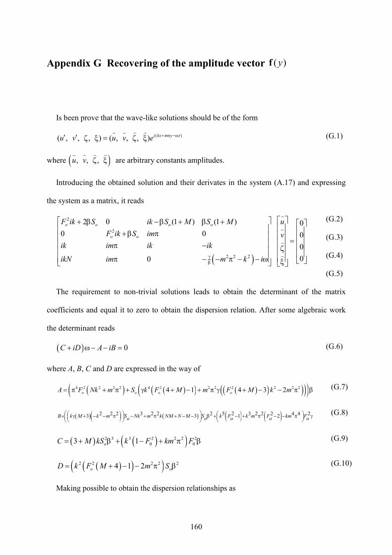
160

Appendix G Recovering of the amplitude vector ( )yf

Is been prove that the wave-like solutions should be of the form

( )( , , , ) ( , , , ) i kx m y tu v u v e + π −ω′ ′ ζ ξ = ζ ξ⌢ ⌢ ⌢ ⌢

(G.1)

where ( ), , ,u v ζ ξ⌢ ⌢ ⌢ ⌢

are arbitrary constants amplitudes.

Introducing the obtained solution and their derivates in the system (A.17) and expressing

the system as a matrix, it reads

( )

2

2

2 2 2

2 0 (1 ) (1 ) 00 0 0

0

00

o o o o

o o

uF ik S ik S M S M

F ik S im v

ik im ik ik

ikN im m k iγβ

+ β −β + β + +β π = π − ζ π − − π − − ω ξ

⌢

⌢

⌢

⌢

(G.2)

(G.3)

(G.4)

(G.5)

The requirement to non-trivial solutions leads to obtain the determinant of the matrix

coefficients and equal it to zero to obtain the dispersion relation. After some algebraic work

the determinant reads

( ) 0C iD A iB+ ω− − = (G.6)

where A, B, C and D are expressed in the way of

( ) ( )( ) ( )( )( )( )( )4 2 2 2 2 4 2 2 2 2 2 2 24 1 4 3 2o o o oA F Nk m S k F M m F M k m= π + π + γ + − + π γ + − − π β (G.7)

( )( ) ( ) ( ) ( )2 2 2 3 2 2 2 5 2 3 2 2 2 4 4 23 3 1 2B k M k m S Nk m k NM N M S k F k m F km Fo o o o o

= γ + − − π − + π + − − β + − + π − − π γ (G.8)

( ) ( )( )2 3 3 2 2 2 20 03 1oC M kS k F km F= + β + − + π β (G.9)

( )( )( )2 2 2 2 24 1 2o oD k F M m S= + − − π β (G.10)

Making possible to obtain the dispersion relationships as

161

( )

2 2

2 2i

AC BD

C D

i CB AD

C D

+ω =

+

−ω =

+

(G.11)