J. Domingo-Ferrer and V. Torra (Eds.): PSD 2004, LNCS 3050, pp. 87–98, 2004. Springer-Verlag Berlin Heidelberg 2004

Balancing Quality and Confidentiality for Multivariate Tabular Data

Lawrence H. Cox1, James P. Kelly2, and Rahul Patil2

1 National Center for Health Statistics, Centers for Disease Control and Prevention Hyattsville, MD 20782 USA

2 OptTek Systems, Inc., Boulder, CO 80302 USA

Abstract. Absolute cell deviation has been used as a proxy for preserving data quality in statistical disclosure limitation for tabular data. However, users’ pri-mary interest is that analytical properties of the data are for the most part pre-served, meaning that the values of key statistics are nearly unchanged. More-over, important relationships within (additivity) and between (correlation) the published tables should also be unaffected. Previous work demonstrated how to preserve additivity, mean and variance in for univariate tabular data. In this pa-per, we bridge the gap between statistics and mathematical programming to propose nonlinear and linear models based on constraint satisfaction to preserve additivity and covariance, correlation, and regression coefficient between data tables. Linear models are superior than nonlinear models owing to simplicity, flexibility and computational speed. Simulations demonstrate the models per-form well in terms of preserving key statistics with reasonable accuracy.

Keywords: Controlled tabular adjustment, linear programming, covariance

1 Introduction

Tabular data are ubiquitous. Standard forms include count data as in population and health statistics, concentration or percentage data as in financial or energy statistics, and magnitude data such as retail sales in business statistics or average daily air pollu-tion in environmental statistics. Tabular data remain a staple of official statistics. Data confidentiality was first investigated for tabular data [1, 2]. Tabular data are additive and thus naturally related to specialized systems of linear equations: TX = 0, where X represents the tabular cells and T the tabular equations, the entries of T are in the set {-1, 0, +1}, and each row of T contains precisely one -1.

In [3], Dandekar and Cox introduced a methodology for statistical disclosure limitation [4] in tabular data known as controlled tabular adjustment (CTA).

This development was motivated by computational complexity, analytical obsta-cles, and general user dissatisfaction with the prevailing methodology, complementary cell suppression [1, 5]. Complementary suppression removes from publication all sensitive cells – cells that cannot be published due to confidentiality concerns – and in addition removes other, nonsenstive cells to ensure that values of sensitive cells can-not be reconstructed or closely estimated by manipulating linear tabular relationships. Drawbacks of cell suppression for statistical analysis include removal of otherwise useful information and consequent difficulties analyzing tabular systems with cell

88 Lawrence H. Cox, James P. Kelly, and Rahul Patil

values missing not-at-random. By contrast, the CTA methodology replaces sensitive cell values with safe values, viz., values sufficiently far from the true value. Because the adjustments almost certainly throw the additive tabular system out of kilter, CTA adjusts some or all of the nonsensitive cells by small amounts to restore additivity. CTA is implemented using mathematical programming methods for which commer-cial and free software are widely available.

In terms of ease-of-use, controlled tabular adjustment is unquestionably an improvement over cell suppression. As CTA changes sensitive and other cell values, the issue is then: Can CTA be accomplished while preserving important data analytical properties of original data?

In [6], Cox and Dandekar describe how the original CTA methodology can be implemented with an eye towards preserving data analytic outcomes. In [7], Cox and Kelly demonstrate how to extend the mathematical programming model for CTA to preserve univariate properties of original data important to linear statistical models. In this paper, we extend the Cox-Kelly paradigm to the multivariate case, ensuring that covariances, correlations and regression coefficients between original variables are preserved in adjusted data. Specialized search procedures, including Tabu Search [8], can also be employed in formulations proposed in [7]. While it is easy to formulate nonlinear programming (NLP) models to do this, such models present difficulties in understanding and use in general statistical settings and exhibit computational limita-tions. The NLP models are computationally more expensive than linear programming (LP) models because the LP algorithms and re-optimization processes are much more efficient compared to NLP algorithms. Moreover, LP solvers guarantee global opti-mality, whereas to NLP models cannot guarantee global optimality for non-convex problems. Models presented here are based on linear programming and consequently are easy to develop and use and are applicable to a very wide range of problems types and sizes.

Section 2 provides a summary of the original CTA methodology of [3] and linear methods of [7] in the univariate case for preserving means and variances of original data and for ensuring high correlation between original and adjusted data. Section 3 provides new results addressing the multivariate case, providing linear programming formulations that ensure covariance, correlation and regression coefficient between two original variables exhibited in original data are preserved in adjusted data. Sec-tion 4 reports computational results. Section 5 provides concluding comments.

2 Controlled Tabular Adjustment and Data Quality for Univariate Data

2.1 The Original CTA Methodology

CTA is applicable to tabular data in any form but for convenience we focus on magni-tude data, where the greatest benefits reside. A simple paradigm for statistical disclo-sure in magnitude data is as follows. A tabulation cell, denoted i, comprises k respon-dents (e.g., retail clothing stores in a county) and their data (e.g., retails sales and employment data). It is assumed that each respondent knows the identity of the other respondents. The cell value is the total value of a statistic of interest (e.g., total retail

Balancing Quality and Confidentiality for Multivariate Tabular Data 89

sales), summed over nonnegative contributions of each respondent in the cell to this

statistic. Denote the cell value v(i) and the respondent contributions v j(i)

, ordered from

largest to smallest. It is possible for any respondent j to compute v(i) - v j(i)

which

yields an upper estimate of the contribution of any other respondent. This estimate is closest, in percentage terms, when the target is the largest respondent and j = 2. A standard disclosure rule, the p-percent rule, declares that the cell value represents disclosure whenever this estimate is less than (100 + p)-percent of the largest contri-bution. The sensitive cells are those failing this condition.

We also may assume that any respondent can use public knowledge to estimate the contribution of any other respondent to within q-percent (q > p, e.g., q = 50%). This

additional information allows the second largest to estimate v - v - v 2(i)

1(i)(i) , the sum

of all contributions excluding itself and the largest, to within q-percent. This upper

estimate provides the second largest a lower estimate of v1(i)

. The lower and upper protection limits for the cell value equal, respectively, the minimum amount that must be subtracted from (added to) the cell value so that these lower (upper) estimates are

at least p-percent away from the response v1(i)

. Numeric values outside the protection limit range of the true value are safe values for the cell. A common practice assumes that these protection limits are equal, to pi . Complementary cell suppression sup-

presses all sensitive cells from publication, replacing sensitive values by variables in the tabular system TX = 0. Because, almost surely, one or more suppressed sensitive cell values can be estimated via linear programming to within its unsafe range, it is necessary to suppress some nonsensitive cells until no sensitive estimates are obtain-able. This yields a mixed integer linear programming (MILP) problem, as in [9].

The original controlled tabular adjustment methodology [3] replaces each sensitive value with a safe value. This is an improvement over complementary cell suppression as it replaces a suppression symbol by an actual value. However, safe values are not necessarily unbiased estimates of true values. To minimize bias, [3] replaces the true

value by either of its nearest safe values, p - v i(i) or p + v i

(i) . Because this will al-

most surely throw the tabular system out of kilter, CTA adjusts nonsensitive values to restore additivity. Because choices to adjust each sensitive value down or up are bi-nary, combined these steps define a MILP [10]. Dandekar and Cox [3] present heuris-tics for the binary choices. The resulting linear programming relaxation is easily solved.

A (mixed integer) linear program in itself will not assure that analytical properties of original and adjusted data are comparable. Cox and Dandekar [6] address these issues in three ways. First, sensitive values are replaced by nearest safe values to re-duce statistical bias. Second, lower and upper bounds (capacities) are imposed on changes to nonsensitive values to ensure adjustments to individual datum are accepta-bly small. Statistically sensible capacities would, e.g., be based on estimated meas-urement error for each cell ei . Third, the linear program optimizes an overall measure of data distortion such as minimum sum of absolute adjustments or minimum sum of percent absolute adjustments. The MILP model is as follows.

90 Lawrence H. Cox, James P. Kelly, and Rahul Patil

Assume there are n tabulation cells of which the first s are sensitive, original data

are represented by the nx1 vector a, adjusted data by y - y + a -+; and y - y = y -+

. The MILP of [10] corresponding to the methodology of [3] for minimizing sum of absolute adjustments is:

)y + y( i

+

i

-n

=1i∑min

subject to: 0 = (y) T (1)

Ip = y ,)I - (1p = y iii

+iii

-, Ii binary, i = 1, ..., s

e y ,y 0 ii

+

i

- ≤≤ i = s+1, ..., n

If the capacities are too tight, this problem may be infeasible (lack solutions). In

such cases, capacities on nonsensitive cells may be increased. A companion strategy, albeit controversial, allows sensitive cell adjustments smaller than pi in well-defined

situations. This is justified mathematically because the intruder does not know if the adjusted value lies above or below the original value; see [6] for details.

The constraints used in [6] are useful. Unfortunately, choices for the optimizing measure are limited to linear functions of cell deviations. In the next two sections, we extend this paradigm in two separate directions, focusing on approaches to preserving mean, variance, correlation and regression coefficient between original and adjusted data.

Formulation (1) is a mixed integer linear program, the integer part can be solved by exact methods in small to medium-sized problems or via heuristics which first fix the integer variables and subsequently use linear programming to solve the linear pro-gramming relaxation [3,11]. Cox and Kelly [11] propose different heuristics to fix the binary variables and to reduce the number of the binary variables in order to improve the computational efficiency, and report good solutions in reasonable time. The re-mainder of this paper focuses on the problem of preserving data quality under CTA, and is not concerned with how the integer portion is being or has been solved. For that reason, for convenience we occasionally abuse terminology and refer to (1) and sub-sequent formulations as “linear programs”.

2.2 Using CTA to Preserve Univariate Relationships

We present linear programming formulations of [7] for preserving approximately mean, variance, correlation and regression slope between original and adjusted data while preserving additivity.

Preserving mean values is straightforward. Any cell value ai can be held fixed by

forcing its corresponding adjustment variables y y i

-

i

+ , to zero, viz., set each vari-

able’s upper capacity to zero. Means are averages over sums. So, for example, to fix the grand mean, simply fix the grand total. Or, to fix means over all or a selected set of rows, columns, etc., in the tabular system, simply capacitate changes to the corre-sponding totals to zero. To fix the mean of any set of variables for which a corre-

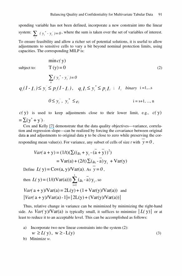
Balancing Quality and Confidentiality for Multivariate Tabular Data 91

sponding variable has not been defined, incorporate a new constraint into the linear

system: 0 = )y - y( i

-

i

+

i∑ , where the sum is taken over the set of variables of interest.

To ensure feasibility and allow a richer set of potential solutions, it is useful to allow adjustments to sensitive cells to vary a bit beyond nominal protection limits, using capacities. The corresponding MILP is:

y)minc(

subject to: 0 = (y) T (2)

0 = )y - y( i

-

i

+

ii∑

Ip y Iq ,)I - (1p y )I - (1q iii

+

iiiii

-

ii ≤≤≤≤ ; binaryI i i =1,...s

e y ,y 0 ii

+

i

- ≤≤ i = s+1, ..., n

y)c( is used to keep adjustments close to their lower limit, e.g., y)c(

)y + y( = -+∑ .

Cox and Kelly [7] demonstrate that the data quality objectives---variance, correla-tion and regression slope---can be realized by forcing the covariance between original data a and adjustments to original data y to be close to zero while preserving the cor-

responding mean value(s). For variance, any subset of cells of size t with 0 = y ,

Var(y) + y)a - a((2/t) + Var(a) =

)))y + a( - y + a(((1/t)( = )y + a

ii

2ii

∑

∑Var(

Define y)/Var(a) Cov(a, = y)L( . As 0 = y ,

then y)a - a()))(1/(tVar(a = y) ii

t

1=i∑L( , so

(a))Var(y)/Var + (1 + 2L(y) = )/Var(a)y + aVar( and

| r(a))(Var(y)/Va + 2L(y) | |= 1 - )/Var(a)y + aVar( |

Thus, relative change in variance can be minimized by minimizing the right-hand side. As y)/Var(a)Var( is typically small, it suffices to minimize |y)L(| or at least to reduce it to an acceptable level. This can be accomplished as follows:

a) Incorporate two new linear constraints into the system (2): L(y)- w, y) ≥≥ L( w (3)

b) Minimize w.

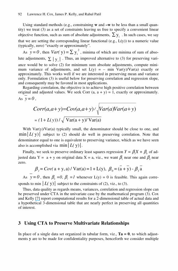
92 Lawrence H. Cox, James P. Kelly, and Rahul Patil

Using standard methods (e.g., constraining w and –w to be less than a small quan-tity) we treat (3) as a set of constraints leaving us free to specify a convenient linear objective function, such as sum of absolute adjustments, yi∑ . In such cases, we say

that we are setting the corresponding linear functional (e.g., L(y)) to a numeric value (typically, zero) “exactly or approximately”.

As 0 = y , then y = )y i2∑Var( , minima of which are minima of sum of abso-

lute adjustments, |y| i∑ . Thus, an improved alternative to (3) for preserving vari-

ance would be to solve (2) for minimum sum absolute adjustments, compute mini-mum variance of adjustments, and set L(y) = – min Var(y)/Var(a) exactly or approximately. This works well if we are interested in preserving mean and variance only. Formulation (3) is useful below for preserving correlation and regression slope, and consequently may be favored in most applications.

Regarding correlation, the objective is to achieve high positive correlation between original and adjusted values. We seek Corr (a, a + y) = 1, exactly or approximately.

As 0 = y ,

)()(),(),( yaVaraVaryaaCovyaaCorr / ++=+

= Var(a)y)/ Var(a / ))(1 ++ yL(

With Var(y)/Var(a) typically small, the denominator should be close to one, and |y)min L(| subject to (2) should do well in preserving correlation. Note that

denominator equal to one is equivalent to preserving variance, which as we have seen also is accomplished via |y)min L(| .

Finally, we seek to preserve ordinary least squares regression Y = β1X + β0 of ad-justed data Y = a + y on original data X = a, viz., we want β1 near one and β0 near zero.

a - )y + a( = L(y), + 1 = Var(a) / a) y, + a 10 βββ Cov( = 1

As 0 = y , then β0 =0, β1 =1 whenever L(y) = 0 is feasible. This again corre-

sponds to min |y)L(| subject to the constraints of (2), viz., to (3). Thus, data quality as regards means, variances, correlation and regression slope can

be preserved under CTA in the univariate case by the mathematical program (3). Cox and Kelly [7] report computational results for a 2-dimensional table of actual data and a hypothetical 3-dimensional table that are nearly perfect in preserving all quantities of interest.

3 Using CTA to Preserve Multivariate Relationships

In place of a single data set organized in tabular form, viz., Ta = 0, to which adjust-ments y are to be made for confidentiality purposes, henceforth we consider multiple

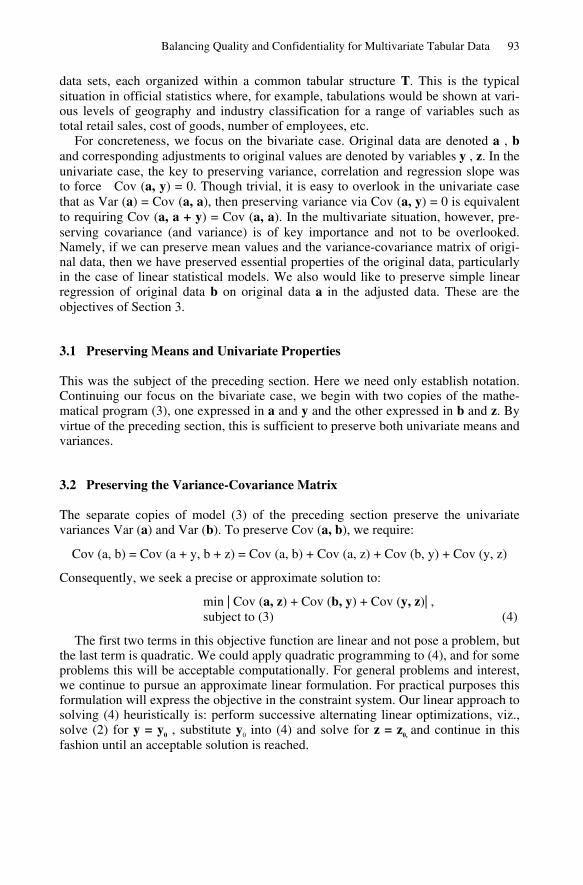
Balancing Quality and Confidentiality for Multivariate Tabular Data 93

data sets, each organized within a common tabular structure T. This is the typical situation in official statistics where, for example, tabulations would be shown at vari-ous levels of geography and industry classification for a range of variables such as total retail sales, cost of goods, number of employees, etc.

For concreteness, we focus on the bivariate case. Original data are denoted a , b and corresponding adjustments to original values are denoted by variables y , z. In the univariate case, the key to preserving variance, correlation and regression slope was to force Cov (a, y) = 0. Though trivial, it is easy to overlook in the univariate case that as Var (a) = Cov (a, a), then preserving variance via Cov (a, y) = 0 is equivalent to requiring Cov (a, a + y) = Cov (a, a). In the multivariate situation, however, pre-serving covariance (and variance) is of key importance and not to be overlooked. Namely, if we can preserve mean values and the variance-covariance matrix of origi-nal data, then we have preserved essential properties of the original data, particularly in the case of linear statistical models. We also would like to preserve simple linear regression of original data b on original data a in the adjusted data. These are the objectives of Section 3.

3.1 Preserving Means and Univariate Properties

This was the subject of the preceding section. Here we need only establish notation. Continuing our focus on the bivariate case, we begin with two copies of the mathe-matical program (3), one expressed in a and y and the other expressed in b and z. By virtue of the preceding section, this is sufficient to preserve both univariate means and variances.

3.2 Preserving the Variance-Covariance Matrix

The separate copies of model (3) of the preceding section preserve the univariate variances Var (a) and Var (b). To preserve Cov (a, b), we require:

Cov (a, b) = Cov (a + y, b + z) = Cov (a, b) + Cov (a, z) + Cov (b, y) + Cov (y, z)

Consequently, we seek a precise or approximate solution to:

min | Cov (a, z) + Cov (b, y) + Cov (y, z)| , subject to (3) (4)

The first two terms in this objective function are linear and not pose a problem, but the last term is quadratic. We could apply quadratic programming to (4), and for some problems this will be acceptable computationally. For general problems and interest, we continue to pursue an approximate linear formulation. For practical purposes this formulation will express the objective in the constraint system. Our linear approach to solving (4) heuristically is: perform successive alternating linear optimizations, viz., solve (2) for y = y0 , substitute y0 into (4) and solve for z = z0, and continue in this fashion until an acceptable solution is reached.

94 Lawrence H. Cox, James P. Kelly, and Rahul Patil

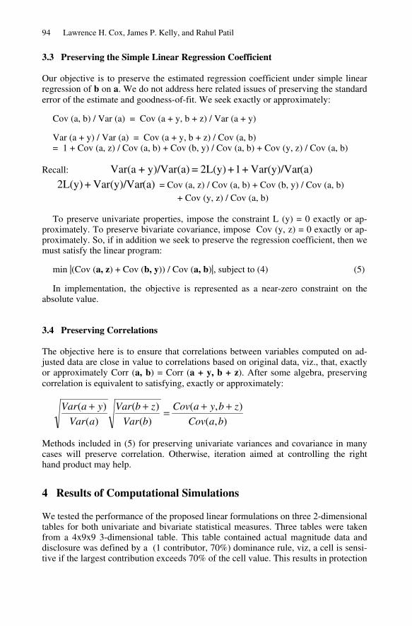
3.3 Preserving the Simple Linear Regression Coefficient

Our objective is to preserve the estimated regression coefficient under simple linear regression of b on a. We do not address here related issues of preserving the standard error of the estimate and goodness-of-fit. We seek exactly or approximately:

Cov (a, b) / Var (a) = Cov (a + y, b + z) / Var (a + y) Var (a + y) / Var (a) = Cov (a + y, b + z) / Cov (a, b) = 1 + Cov (a, z) / Cov (a, b) + Cov (b, y) / Cov (a, b) + Cov (y, z) / Cov (a, b)

Recall: (a)Var(y)/Var + 1 + 2L(y) = )/Var(a)y + Var(a

(a)Var(y)/Var + 2L(y) = Cov (a, z) / Cov (a, b) + Cov (b, y) / Cov (a, b) + Cov (y, z) / Cov (a, b)

To preserve univariate properties, impose the constraint L (y) = 0 exactly or ap-proximately. To preserve bivariate covariance, impose Cov (y, z) = 0 exactly or ap-proximately. So, if in addition we seek to preserve the regression coefficient, then we must satisfy the linear program:

min |(Cov (a, z) + Cov (b, y)) / Cov (a, b)|, subject to (4) (5) In implementation, the objective is represented as a near-zero constraint on the

absolute value.

3.4 Preserving Correlations

The objective here is to ensure that correlations between variables computed on ad-justed data are close in value to correlations based on original data, viz., that, exactly or approximately Corr (a, b) = Corr (a + y, b + z). After some algebra, preserving correlation is equivalent to satisfying, exactly or approximately:

),(

),(

)(

)(

)(

)(

baCov

zbyaCov

bVar

zbVar

aVar

yaVar ++=++

Methods included in (5) for preserving univariate variances and covariance in many cases will preserve correlation. Otherwise, iteration aimed at controlling the right hand product may help.

4 Results of Computational Simulations

We tested the performance of the proposed linear formulations on three 2-dimensional tables for both univariate and bivariate statistical measures. Three tables were taken from a 4x9x9 3-dimensional table. This table contained actual magnitude data and disclosure was defined by a (1 contributor, 70%) dominance rule, viz, a cell is sensi-tive if the largest contribution exceeds 70% of the cell value. This results in protection

Balancing Quality and Confidentiality for Multivariate Tabular Data 95

limits iii vvp −= 7.0/)( 1 . Tables A, B, C contain 6, 5, 4 sensitive cells respectively.

Upper bounds (capacities) for adjustments to nonsensitive cells were set at 20-percent of cell value.

First, we used the MILP formulation to compute exact solutions for the three in-stances AB, AC, BC. The MILP formulation used the mean and variance preserving constraints and a covariance change minimization objective, aimed at preserving both univariate and bivariate statistics. This kind of modeling has the advantage of building flexibility for controlling information loss. For example, if preserving the covariance is not important, then covariance preserving constraints would be relaxed to get better performance with respect to other statistics.

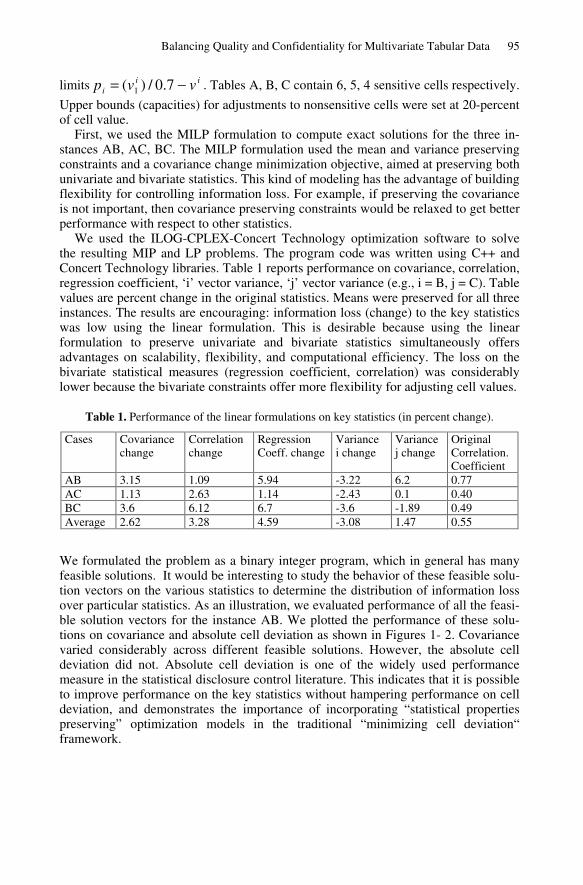
We used the ILOG-CPLEX-Concert Technology optimization software to solve the resulting MIP and LP problems. The program code was written using C++ and Concert Technology libraries. Table 1 reports performance on covariance, correlation, regression coefficient, ‘i’ vector variance, ‘j’ vector variance (e.g., i = B, j = C). Table values are percent change in the original statistics. Means were preserved for all three instances. The results are encouraging: information loss (change) to the key statistics was low using the linear formulation. This is desirable because using the linear formulation to preserve univariate and bivariate statistics simultaneously offers advantages on scalability, flexibility, and computational efficiency. The loss on the bivariate statistical measures (regression coefficient, correlation) was considerably lower because the bivariate constraints offer more flexibility for adjusting cell values.

Table 1. Performance of the linear formulations on key statistics (in percent change).

Cases

Covariance change

Correlation change

Regression Coeff. change

Variance i change

Variance j change

Original Correlation. Coefficient

AB 3.15 1.09 5.94 -3.22 6.2 0.77 AC 1.13 2.63 1.14 -2.43 0.1 0.40 BC 3.6 6.12 6.7 -3.6 -1.89 0.49 Average 2.62 3.28 4.59 -3.08 1.47 0.55

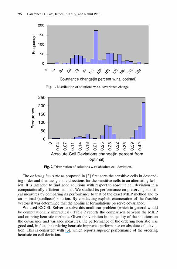
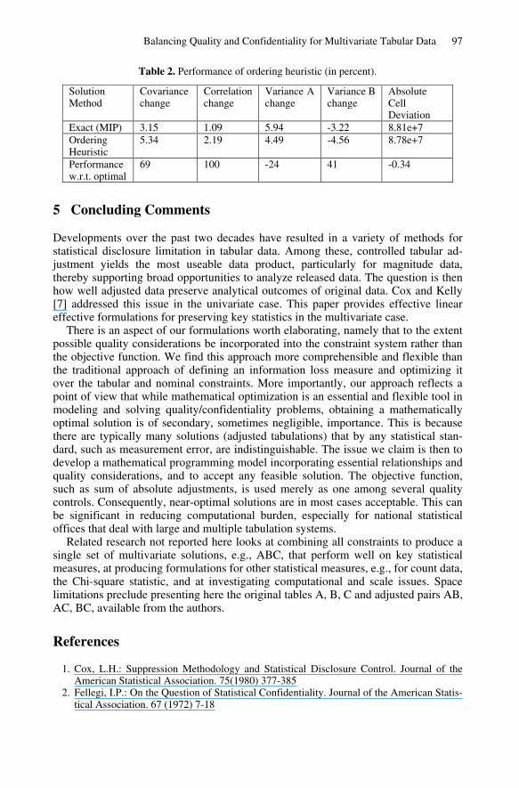
We formulated the problem as a binary integer program, which in general has many feasible solutions. It would be interesting to study the behavior of these feasible solu-tion vectors on the various statistics to determine the distribution of information loss over particular statistics. As an illustration, we evaluated performance of all the feasi-ble solution vectors for the instance AB. We plotted the performance of these solu-tions on covariance and absolute cell deviation as shown in Figures 1- 2. Covariance varied considerably across different feasible solutions. However, the absolute cell deviation did not. Absolute cell deviation is one of the widely used performance measure in the statistical disclosure control literature. This indicates that it is possible to improve performance on the key statistics without hampering performance on cell deviation, and demonstrates the importance of incorporating “statistical properties preserving” optimization models in the traditional “minimizing cell deviation“ framework.

96 Lawrence H. Cox, James P. Kelly, and Rahul Patil

0

50

100

150

200

0 19 39 58 78 97 117

137

156

176

195

215

234

Covariance change(in percent w.r.t. optimal)

Fre

quen

cy

Fig. 1. Distribution of solutions w.r.t. covariance change.

0

50

100

150

200

250

0

0.04

0.07

0.11

0.14

0.18

0.21

0.25

0.28

0.32

0.35

0.39

0.42

Absolute Cell Deviations change(in percent from optimal)

Fre

quen

cy

Fig. 2. Distribution of solutions w.r.t absolute cell deviation.

The ordering heuristic as proposed in [3] first sorts the sensitive cells in descend-ing order and then assigns the directions for the sensitive cells in an alternating fash-ion. It is intended to find good solutions with respect to absolute cell deviation in a computationally efficient manner. We studied its performance on preserving statisti-cal measures by comparing its performance to that of the exact MILP method and to an optimal (nonlinear) solution. By conducting explicit enumeration of the feasible vectors it was determined that the nonlinear formulations preserve covariance.

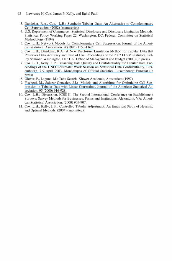
We used EXCEL-Solver to solve this nonlinear problem (which in general would be computationally impractical). Table 2 reports the comparison between the MILP and ordering heuristic methods. Given the variation in the quality of the solutions on the covariance and variance measures, the performance of the ordering heuristic was good and, in fact, the ordering heuristic improved performance on absolute cell devia-tion. This is consistent with [3], which reports superior performance of the ordering heuristic on cell deviation.

Balancing Quality and Confidentiality for Multivariate Tabular Data 97

Table 2. Performance of ordering heuristic (in percent).

Solution Method

Covariance change

Correlation change

Variance A change

Variance B change

Absolute Cell Deviation

Exact (MIP) 3.15 1.09 5.94 -3.22 8.81e+7 Ordering Heuristic

5.34 2.19 4.49 -4.56 8.78e+7

Performance w.r.t. optimal

69 100 -24 41 -0.34

5 Concluding Comments

Developments over the past two decades have resulted in a variety of methods for statistical disclosure limitation in tabular data. Among these, controlled tabular ad-justment yields the most useable data product, particularly for magnitude data, thereby supporting broad opportunities to analyze released data. The question is then how well adjusted data preserve analytical outcomes of original data. Cox and Kelly [7] addressed this issue in the univariate case. This paper provides effective linear effective formulations for preserving key statistics in the multivariate case.

There is an aspect of our formulations worth elaborating, namely that to the extent possible quality considerations be incorporated into the constraint system rather than the objective function. We find this approach more comprehensible and flexible than the traditional approach of defining an information loss measure and optimizing it over the tabular and nominal constraints. More importantly, our approach reflects a point of view that while mathematical optimization is an essential and flexible tool in modeling and solving quality/confidentiality problems, obtaining a mathematically optimal solution is of secondary, sometimes negligible, importance. This is because there are typically many solutions (adjusted tabulations) that by any statistical stan-dard, such as measurement error, are indistinguishable. The issue we claim is then to develop a mathematical programming model incorporating essential relationships and quality considerations, and to accept any feasible solution. The objective function, such as sum of absolute adjustments, is used merely as one among several quality controls. Consequently, near-optimal solutions are in most cases acceptable. This can be significant in reducing computational burden, especially for national statistical offices that deal with large and multiple tabulation systems.

Related research not reported here looks at combining all constraints to produce a single set of multivariate solutions, e.g., ABC, that perform well on key statistical measures, at producing formulations for other statistical measures, e.g., for count data, the Chi-square statistic, and at investigating computational and scale issues. Space limitations preclude presenting here the original tables A, B, C and adjusted pairs AB, AC, BC, available from the authors.

References

1. Cox, L.H.: Suppression Methodology and Statistical Disclosure Control. Journal of the American Statistical Association. 75(1980) 377-385

2. Fellegi, I.P.: On the Question of Statistical Confidentiality. Journal of the American Statis-tical Association. 67 (1972) 7-18

98 Lawrence H. Cox, James P. Kelly, and Rahul Patil

3. Dandekar, R.A., Cox, L.H.: Synthetic Tabular Data: An Alternative to Complementary Cell Suppression. (2002) (manuscript)

4. U.S. Department of Commerce.: Statistical Disclosure and Disclosure Limitation Methods, Statistical Policy Working Paper 22, Washington, DC: Federal. Committee on Statistical Methodology.(1994)

5. Cox, L.H.: Network Models for Complementary Cell Suppression. Journal of the Ameri-can Statistical Association. 90(1995) 1153-1162.

6. Cox, L.H., Dandekar, R.A.: A New Disclosure Limitation Method for Tabular Data that Preserves Data Accuracy and Ease of Use. Proceedings of the 2002 FCSM Statistical Pol-icy Seminar, Washington, DC: U.S. Office of Management and Budget (2003) (in press).

7. Cox, L.H., Kelly, J. P.: Balancing Data Quality and Confidentiality for Tabular Data. Pro-ceedings of the UNECE/Eurostat Work Session on Statistical Data Confidentiality, Lux-embourg, 7-9 April 2003, Monographs of Official Statistics. Luxembourg: Eurostat (in press)

8. Glover, F., Laguna, M.: Tabu Search. Kluwer Academic, Amsterdam (1997) 9. Fischetti, M., Salazar-Gonzalez, J.J.: Models and Algorithms for Optimizing Cell Sup-

pression in Tabular Data with Linear Constraints. Journal of the American Statistical As-sociation. 95 (2000) 916-928.

10. Cox, L.H.: Discussion. ICES II: The Second International Conference on Establishment Surveys: Survey Methods for Businesses, Farms and Institutions. Alexandria, VA: Ameri-can Statistical Association. (2000) 905-907.

11. Cox, L.H., Kelly, J. P.: Controlled Tabular Adjustment: An Empirical Study of Heuristic and Optimal Methods. (2004) (submitted).