Forming Clusters from Census Areas with Similar

Tabular Statistics

Murray A. Jorgensen

Department of Statistics, University of Waikato

Hamilton, New Zealand

maj@waikato.ac.nz

June 17, 2011

Abstract

This paper presents a methodology for the clustering of a large number of tables of sim-

ilar form. Data of this kind is often available from NationalStatistical Offices as tabulations

of a set of variables for each of a large number of geographic units. Model-based clustering

is employed, the underlying model being a finite mixture of multinomial distributions. We

discuss the choice of the number of clusters and the interpretation of the clusters found. As

a case study we consider a set of age-group by sex tables for small areas obtained in the

New Zealand Census of Population and Dwellings for the year 2006.

1 Introduction

National statistical officesoften nowmake available tabular data on census variables for fairly

small geographical regions. The United Kingdom National Statistics Office has a web site

www.neighbourhood.statistics.gov.uk from which tables at the post code level may be ob-

1

tained. Similarly Statistics New Zealand provides regional tables through “Table Builder” at

www.stats.govt.nz/tools and services/tools/TableBuilder.aspx.

The most common way in which such web sites are used is for the user to select a single area

or a relatively small number of areas of greatest interest tohim or her. When there is a more

general interest in the variables across a country or state the user is faced with the problem of

digesting information from perhaps thousands of contingency tables. If it is possible to group

the small areas for which data is available into larger regions such that the cell proportions in the

tables for areas within a region are similar this will be of great value for an exploratory analysis

of the data. The problem with tables for large geographical regions is that they combine smaller

regions for which the relationships between the variables may be quite different leading to a

misleading picture in the aggregated table. (Essentially the basis ofSimpson’s Paradox.)

Most clustering methodologies rely on having information recorded at the individual level.

Now while Statistics Offices are increasingly making available synthetic or confidentialized unit

record data there will probably always be more data available in tabular form. In this article we

illustrate the application of a clustering method appropriate for clustering small areas in such a

way that areas with similar cell proportions in an associated contingency table will tend to be

grouped together.

2 Age by Sex tables

As an example we will consider the tables of the variablesAgegroup andSex at the 2006 New

Zealand Census of Population and Dwellings. This data may beobtained from the Statistics

New Zealand Site mentioned above for different sizes of Geographic Unit. The geographic unit

chosen was the “area unit”, roughly equivalent to the US Census “block group” and averaging

somewhat under 3000 population. It is convenient to think ofan area unit as a small town or

suburb, although they do not necessarily correspond to realsocial units.

As an example consider the area unit named Raglan, which corresponds roughly to the small

town of the same name on the west coast of the North Island of New Zealand. The population

2

Table 1: Raglan population by age and sex at the 2006 Census

Agegroup 0-4 5-9 10-14 15-19 20-24 25-29 30-34 35-39 40-44

Male 96 96 111 93 54 81 96 78 81

Female 81 90 84 87 54 81 117 105 105

Agegroup 45-49 50-54 55-59 60-64 65-69 70-74 75-79 80- Total

Male 99 84 69 66 48 36 42 24 1272

Female 96 93 81 63 60 48 48 42 1365

counts obtained for this area unit as extracted from the web site are given in Table 1.

2.1 Random Rounding

A glance at Table 1 shows that all entries are divisible by 3. This is clearly by artifice, not

chance and is a consequence of the method ofrandom rounding which has been applied to the

counts before they are made available by Statistics New Zealand. In this method as used in these

census tables counts that are not multiples of 3 are perturbed by rounding either to the closest

multiple of 3 (with probability23) or to the second-closest multiple of 3 (with probability1

3).

More confidentiality but less accuracy may be obtained by similar schemes where the rounding

is to numbers divisible by 5 or by 10. The same rounding schemeis applied to the margins of

the table so that they need not agree with the appropriate totals of the rounded cell counts.

This feature is often felt to be undesirable and a related method known ascontrolled round-

ing ensures that the summation relations between the perturbedcell counts and margins are

respected. Both rounding methods are discussed by Willenborg and de Waal (2000) and Fed-

eral Committee on Statistical Methodology (2005) where further references are given.

From the point of view of statistical modelling any system ofcontrolled rounding must

introduce probabilistic dependence into the data and the independent perturbations of random

rounding would be preferred. It might also be argued that thetables produced by random

rounding are less likely to be mistakenly treated by the general user as exact counts if the

3

failure of marginal totals to be “correct” is noticed.

In this article we naively model the rounded counts as if theywere actual counts, but the

“missing information” approach of theEM algorithm could be extended to handle the informa-

tion missing due to rounding. A 30-cell table randomly rounded to counts that are multiples of

3 could, if it contains no zeros, have arisen from any one of530 tables of actual counts. Combi-

natorial considerations like this make the application ofEM to all rounded cells of such a large

table unfeasible. However a few cells could be handled and incertain circumstances this could

be an alternative to combining cells.

When summarizing census data the choice of the size of geographic unit to be used in

tabulations thus relies on a trade-off:

• If too small a unit is used, confidentiality procedures applied by the National Statistics

Office will introduce relatively large errors into the tables.

• If too large a unit is used, many subunits with quite different cell proportions will be

merged, destroying information.

With the size of units selected in our case study no doubt bothproblems still remain but hope-

fully neither problem dominates.

2.2 Preliminary Processing

To reduce the number of parameters in the models to be fitted some of the older age classes were

combined resulting in the new groups ‘65-74 years’ and ‘75 orolder’. The later was calculated

by subtraction from the margin and a few negative derived counts were replaced by zero. The

resulting tables are now 15 by 2 in dimension. To reduce the effect of random rounding on

the analyses area units with total count less than 600 (i.e. mean cell count less than 20) were

omitted. There were 1455 area units included in the analysiscontaining over 97% of the New

Zealand population.

4

3 Mixture Model Clustering

We now seek to cluster area units into groups of similar demographic (age by sex) structure.

The method that we use is based on finite mixture models. The description of these models may

be given fairly succinctly as follows.

A finite mixture model is a probability distribution of the form

p(y) =q

∑j=1

π j p j(y)

where for j = 1, . . . ,q theπ j are non-negative proportions summing to 1, and thep j are prob-

ability distribution functions. Usually thep j are assumed to come from the same parametric

model family. The pdfp(y) may be seen as a mixture of the pdf’sp j(y) in proportionsπ j. The

connection with clustering is that ify is a random observation from the population described by

p(y), the probability thaty comes from the subpopulation described byp j(y) is

z j =π j p j(y)

∑qj=1π j p j(y)

.

If the subpopulations are well-separated and well-fitted bythe p j then it is usually the case that

one of thez j is close to 1 and the others are close to zero. In these situations the roundedz j act

as indicator variables for theq clusters.

It is necessary to choose a value forq. Clearly we might adopt a model with one cluster

for each area unit and setq = n but this achieves no data reduction at all and consequently no

insight. The choice ofq is discussed in section 6.

If the p j are chosen from an exponential family it is straightforwardto apply theEM algo-

rithm (Dempster et al., 1977; McLachlan and Krishnan, 1997)to estimate both theπ j and the

parameters in thep j by maximum likelihood. Thez j are estimated along with the parameters

as part of the algorithm, and form the basis for the assignment of individual observations to

clusters.

One form of unidentifiability is always present in mixture models: a permutation of the

group labels leaves the likelihood unchanged so that any likelihood maximizing parameter vec-

tor shares this property with all its group-label permutations. This is not usually of concern in

5

clustering applications and a convention may be adopted to order the groups according to the

ordering of some function of the parameters. Some problems remain. For example in resam-

pling methods such as the bootstrap the appropriate ordering of the groups may not be preserved

under resampling. More local methods such as the infinitesimal jackknife would be more ap-

propriate for inference about parametric functions not invariant under group-label permutations.

Another type of unidentifiability arises when the number of mixture componentsq is large in

relation to the number of observationsn. Portela (2008) discusses this and concludes that this

will not occur if q ≤ (n+1)/2. This condition is far from being violated by the models that we

consider in this paper.

Although the use of mixture models in many applications of statistics has grown rapidly

in recent years they are relatively novel in Official Statistics. A recent example of their use in

Official Statistics is the work of Di Zio et al. (2007) on missing data imputation.

4 Mixtures Of Multinomial Distributions

The discussion above applies generally to all types of mixture models but we will now consider

models appropriate for clustering tabular data from a largenumber of geographic units.

We will be considering data where each observation is a tableconsisting of counts in each of

a number of categories. In the case of the Age by Sex study we have , for each of then = 1455

area units,p = 30 counts corresponding to the total number of 2006 residents of that area unit

in each of the 30= 15×2 demographic categories used in the study.

We now pose the question as to whether the great bulk of the area units fall into one of

a finite number of patterns as far as their demographic structure is concerned. The observed

category counts for a particular area unit might then be regarded as a sample from one ofq

30-category multinomial distributions.

Consider the following model for the probabilitypi(yi) that theith area unit has counts of

yi = (yi1,yi2, . . . ,yip)′ in the p = 30 demographic categories

pi(yi) = pi(yi1,yi2, . . . ,yip)

6

=q

∑j=1

π jmi!

yi1!yi2! · · ·yip!λ yi1

j1 λ yi2j2 · · ·λ yip

jp

=q

∑j=1

π j pi j(yi)

wheremi stands foryi1+ yi2 + · · ·+ yip and the mixing proportionsπ j sum to 1.

This is essentially a finite mixture of multinomial distributions Multi(mi,λ j1,λ j2, . . . ,λ jp),

except that the numbersmi vary depending on the area uniti. Mixture modelling seeks to

identify subclasses in the data of distinctly different structure. In the present context we may

hope that theq subclasses in the mixture model will correspond to different kinds of community.

5 The EM Algorithm

The EM algorithm, as applied to parameter estimation of finite mixture models, searches for

maxima of the usual likelihood function, but it does so not directly but using another likelihood

function. This other likelihood function is based on unobserved indicator variables for theq

subpopulations as well as the observed categorized resident counts for each area unit.

It is convenient to set up ann×q matrix of indicator variablesZ =(

zi j)

= (z′i) wherezi j = 1

if casei belongs to subclassj and otherwise is zero. These unobserved indicator variables play

a role in theEM fitting algorithm and their estimates are a basis for assigning observations to

clusters.

Theobserved data likelihood is the likelihood based onyik and is given by

L =n

∏i=1

[

q

∑j=1

(

π jmi!

yi1!yi2! · · ·yip!

p

∏k=1

λ yikjk

)]

=n

∏i=1

pi(yi)

whencel = logL = constant +n

∑i=1

logpi(yi).

The likelihood based onyik andzi j is given by

LC =n

∏i=1

mi!yi1!yi2! · · ·yip!

q

∏j=1

πzi jj

(

p

∏k=1

λ yikjk

)zi j

.

7

Taking logs and omitting the constant:

lC =n

∑i=1

q

∑j=1

[

zi j logπ j +p

∑k=1

yikzi j logλ jk

]

.

This is thecomplete-data log-likelihood in EM terminology. TheEM algorithm itself for

this estimation problem is defined by two steps:

E-step Takingπ andλ as given; estimateZ.

M-step TakingZ as given; estimateπ andλ .

which in our case leads to

E-step: zi j =π j pi j(yi)

pi(yi).

M-step: π j =∑i zi j

n; λ jk =

∑i yikzi j

∑i mizi j.

The E-step essentially estimates the unknown quantities inthe complete-data log-likelihood,

taking the current parameter values to be the true ones. The log-likelihoodl(π,λ) = log∑ni=1 pi(yi)

comes almost free as a byproduct of the E-step.

The M-step maximizes the so-estimated complete-data log-likelihood function to find an

improved set of parameter estimates. The theory of theEM algorithm (Dempster et al., 1977;

McLachlan and Krishnan, 1997) shows that a cycle of E-step plus M-step cannot decrease the

likelihood.

5.1 EM outputs

TheEM algorithm delivers estimates of thep = 30 cell probabilities for each of theq subpop-

ulations, as well as theq mixing proportions. By construction each set ofp cell probabilities

sums to 1 as do theq mixing proportions.

Also, and of direct relevance to the goal of identifying clusters, theEM algorithm produces

the zi j, estimates of the probability that area uniti belongs to clusterj.

8

The ith termli of the observed data log-likelihoodl (in other words the logged value of the

mixture density for theith area unit according to the current parameter values), is calculated in

the course of calculating the ˆzi j, (i = 1, . . . ,n) so thatl is available for each fit.

The natural way to use the ˆzi j is to associate each area unit to its most probable cluster,

although it might be reasonable to leave some area units unassigned unless their largest ˆzi j

exceeded some threshold.

An alternative is to use a probabilistic assignment in whicharea uniti is assigned to cluster

j with probability zi j. Although probabilistic assignment may not be optimal for aparticular

area unit it shows the shape and extent of a cluster better.

If Z is the n × q matrix with i, j element ˆzi j then the matrixZ′Z has as itsj,k element

the expected number of area units assigned to clusterj on one probabilistic assignment and

assigned to clusterk on another independent assignment( j,k = 1,2, . . . ,q). It is desirable that

the off-diagonal elements of this matrix are small. The larger off-diagonal elements indicate

which pairs of clusters are ‘close’ or ‘overlapping’. In this paper we will call this theoverlap

matrix.

6 Choosing the Number of Clusters

In the present case study should not be thought that an integer q can be identified which is the

‘true’ number of clusters that the census area units should be grouped into. Even if there were,

in fact, a finite number of regions such that tables for variables describing small connected

areas contained in a region could be treated as random samples from a regional multinomial

distribution this would not imply that the area units are allsuch samples. This is because area

unit boundaries are not chosen with such regions in mind and inevitably many would straddle

two or more regions.

In the present case where the variables under study are sex and age group a more specific

argument can be given. Consider the structure of the Raglan population in Table 1. Note

that the number of residents in their twenties is low compared to those immediately younger

9

or older. This bi-modal pattern is quite common in area unitsand in many cases reflects a

preponderance of nuclear family households with children living with their parents. However

the location of the ‘parent’ and ‘child’ modes differs between area units according to whether

the unit is dominated by younger or older families at the timeof the census. A finite mixture

model will assign such nuclear-family dominated area unitsinto a finite number of clusters.

Clearly, however, the underlying reality is that of a continuous mixture of family ages to which

the finite mixture merely provides an approximation.

So what we are trying to do when fitting a mixture model is to identify a small number of

typical patterns of cell probabilities that approximates the very much larger set of cell relative

frequencies in the data.

The simplest way to evaluate the quality of the approximation is via the observed data log-

likelihood l. Various information criteria are also used in the literature and a good survey in the

mixture model context is given by McLachlan and Peel (2000, sections 6.8,6.9). These include

the Classification Likelihood Criterion,l−e, the Bayesian Information Criterion,l−d log(n)/2,

and the Integrated Classification Likelihood Criterionl − d log(n)/2− e. We refer to these

criteria respectively as CLC, BIC and ICL. The CLC and the ICLwere introduced by Biernacki

et al. (1999). Hereq is the number of mixture components in the model,n = 1455 is the number

of area units,d = q−1+ q(p−1) = pq−1 is the number of independent model parameters

to be estimated, ande = ∑i ∑ j zi j log(zi j) is known as the entropy, and is small when each area

unit is assigned to a single cluster with high probability.

Various numbers of mixture componentsq were investigated in the following way. For each

value ofq, 100 random partitions of the area units intoq clusters were generated and theEM

algorithm run with these as the starting clusters. The solution with the greatest log-likelihood

of the 100 fits was chosen. In Table 2 we give likelihood and information statistics for a number

of model fits having a range of component numbers.

In Figure 1 the log-likelihoodl and the ICL are plotted against the number of mixture

components in the model. The BIC and the CLC lie in between these two curves.

10

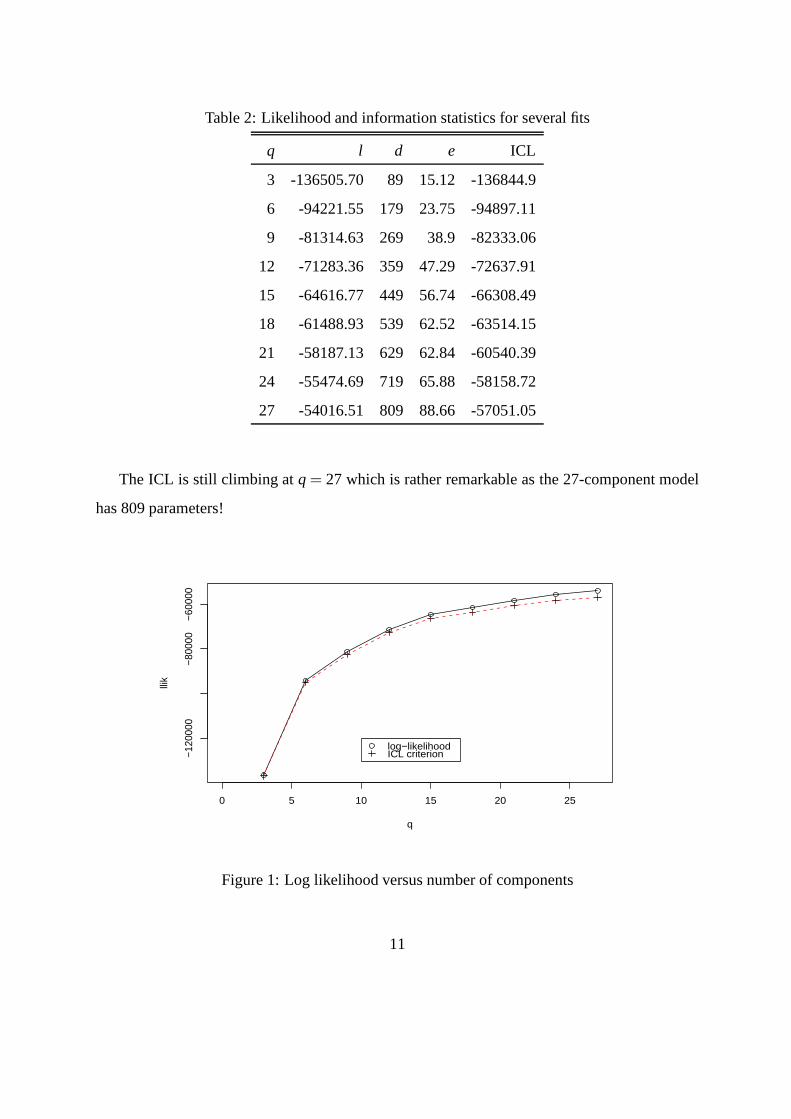
Table 2: Likelihood and information statistics for severalfits

q l d e ICL

3 -136505.70 89 15.12 -136844.9

6 -94221.55 179 23.75 -94897.11

9 -81314.63 269 38.9 -82333.06

12 -71283.36 359 47.29 -72637.91

15 -64616.77 449 56.74 -66308.49

18 -61488.93 539 62.52 -63514.15

21 -58187.13 629 62.84 -60540.39

24 -55474.69 719 65.88 -58158.72

27 -54016.51 809 88.66 -57051.05

The ICL is still climbing atq = 27 which is rather remarkable as the 27-component model

has 809 parameters!

0 5 10 15 20 25

−120

000

−800

00−6

0000

q

llik

log−likelihoodICL criterion

Figure 1: Log likelihood versus number of components

11

The reason for the usual criteria favouring a very large number of mixture components

seems to be that the multinomial distribution is underdispersed for use in this way, at least for

the data being considered. It may be worth exploring more dispersed component distributions

than the multinomial such as the Dirichlet-multinomial as in principle it would require fewer of

such components to approximate the distribution of the data. Wewill not pursue this approach

here.

From Figure 1 it appears that the 12-component solution is a good compromise between fit

and complexity and we choose this solution to describe more fully here for the sake of brevity.

7 Diagnostics

As mentioned in section 5.1, theEM algorithm provides the value of the fitted density function

at each area unit. Area units fitted poorly by the model will have relatively low values of this

density. The density values turn out to be very skew indeed and we recommend transforming

by log(− log(·)) to produce quantities that could be regarded as residuals for the area units.

In Figure 2 we display boxplots of log(− log(density)) values for each cluster. Notice that

Clusters A, B, and H are relatively poorly fit. We will discussthis further below.

23

45

6

log(−l

og(de

nsity

))

A B C D E F G H I J K L

Figure 2: Boxplots of log(− log(density)) by Cluster

12

25 30 35 40 45 50 55

0.45

0.50

0.55

0.60

0.65

Mean Age

Prop

ortio

n M

ale

GJD

B

K

A

EHFC

IL

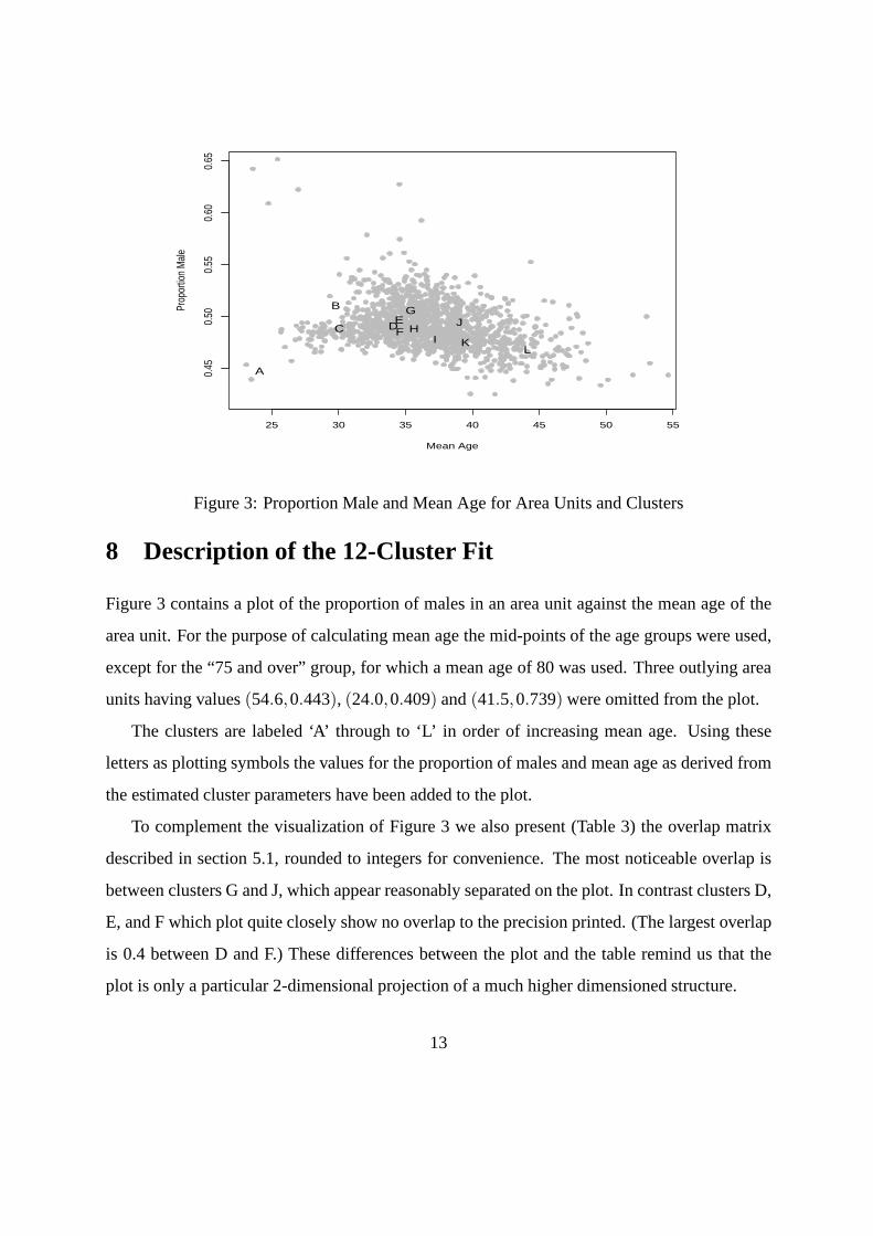
Figure 3: Proportion Male and Mean Age for Area Units and Clusters

8 Description of the 12-Cluster Fit

Figure 3 contains a plot of the proportion of males in an area unit against the mean age of the

area unit. For the purpose of calculating mean age the mid-points of the age groups were used,

except for the “75 and over” group, for which a mean age of 80 was used. Three outlying area

units having values(54.6,0.443), (24.0,0.409) and(41.5,0.739) were omitted from the plot.

The clusters are labeled ‘A’ through to ‘L’ in order of increasing mean age. Using these

letters as plotting symbols the values for the proportion ofmales and mean age as derived from

the estimated cluster parameters have been added to the plot.

To complement the visualization of Figure 3 we also present (Table 3) the overlap matrix

described in section 5.1, rounded to integers for convenience. The most noticeable overlap is

between clusters G and J, which appear reasonably separatedon the plot. In contrast clusters D,

E, and F which plot quite closely show no overlap to the precision printed. (The largest overlap

is 0.4 between D and F.) These differences between the plot and the table remind us that the

plot is only a particular 2-dimensional projection of a muchhigher dimensioned structure.

13

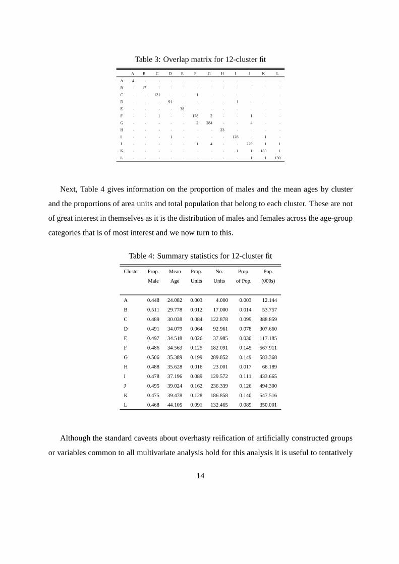
Table 3: Overlap matrix for 12-cluster fit

A B C D E F G H I J K L

A 4 · · · · · · · · · · ·

B · 17 · · · · · · · · · ·

C · · 121 · · 1 · · · · · ·

D · · · 91 · · · · 1 · · ·

E · · · · 38 · · · · · · ·

F · · 1 · · 178 2 · · 1 · ·

G · · · · · 2 284 · · 4 · ·

H · · · · · · · 23 · · · ·

I · · · 1 · · · · 128 · 1 ·

J · · · · · 1 4 · · 229 1 1

K · · · · · · · · 1 1 183 1

L · · · · · · · · · 1 1 130

Next, Table 4 gives information on the proportion of males and the mean ages by cluster

and the proportions of area units and total population that belong to each cluster. These are not

of great interest in themselves as it is the distribution of males and females across the age-group

categories that is of most interest and we now turn to this.

Table 4: Summary statistics for 12-cluster fit

Cluster Prop. Mean Prop. No. Prop. Pop.

Male Age Units Units of Pop. (000s)

A 0.448 24.082 0.003 4.000 0.003 12.144

B 0.511 29.778 0.012 17.000 0.014 53.757

C 0.489 30.038 0.084 122.878 0.099 388.859

D 0.491 34.079 0.064 92.961 0.078 307.660

E 0.497 34.518 0.026 37.985 0.030 117.185

F 0.486 34.563 0.125 182.091 0.145 567.911

G 0.506 35.389 0.199 289.852 0.149 583.368

H 0.488 35.628 0.016 23.001 0.017 66.189

I 0.478 37.196 0.089 129.572 0.111 433.665

J 0.495 39.024 0.162 236.339 0.126 494.300

K 0.475 39.478 0.128 186.858 0.140 547.516

L 0.468 44.105 0.091 132.465 0.089 350.001

Although the standard caveats about overhasty reification of artificially constructed groups

or variables common to all multivariate analysis hold for this analysis it is useful to tentatively

14

identify some of the clusters found with verbal descriptions.

We base our discussion primarily on the estimated cell proportions for each cluster but

also on the names of the area units as assigned to the cluster of highest estimated probability.

Unfortunately these area unit names for each cluster cannotbe listed for reasons of space, but

the author is happy to supply a file with this information.

In the plots of the cell proportions the points for males are connected by solid lines; those

for females by dashed lines. Each age group except the highest two has a 5 year range. The

second-highest age group represents 10 years and these proportions have been divided by 2 for

plotting; the highest age group is open-ended and has been divided by 3 for plotting. The ‘3’

was chosen after trial-and-error experimentation.

Some of the clusters seem to group together naturally and we take advantage of this to give

a more compact description.

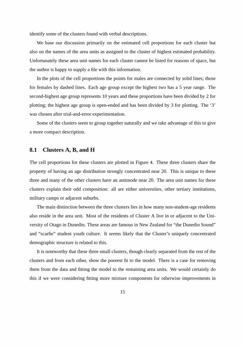
8.1 Clusters A, B, and H

The cell proportions for these clusters are plotted in Figure 4. These three clusters share the

property of having an age distribution strongly concentrated near 20. This is unique to these

three and many of the other clusters have an antimode near 20.The area unit names for these

clusters explain their odd composition: all are either universities, other tertiary institutions,

military camps or adjacent suburbs.

The main distinction between the three clusters lies in how many non-student-age residents

also reside in the area unit. Most of the residents of ClusterA live in or adjacent to the Uni-

versity of Otago in Dunedin. These areas are famous in New Zealand for “the Dunedin Sound”

and “scarfie” student youth culture. It seems likely that theCluster’s uniquely concentrated

demographic structure is related to this.

It is noteworthy that these three small clusters, though clearly separated from the rest of the

clusters and from each other, show the poorest fit to the model. There is a case for removing

them from the data and fitting the model to the remaining area units. We would certainly do

this if we were considering fitting more mixture components for otherwise improvements in

15

0 20 40 60 80

0.00

0.05

0.10

0.15

0.20

0.25

Age

Cel

l pro

porti

on

A A A

A

A

AA A A A A A A A AA A A

AA

AA A A A A A A A A

B B B

B

B

B

BB B B B B B B B

B B B

B

B

B

BB B B B B B B B

H H H

H

H

HH H H H H H H H H

H H H

H

H

HH H H H H H H H H

Figure 4: Cell proportions for Clusters A, B, and H

the likelihood would be dominated by how well the fit to these area units improved. From the

clustering viewpoint these clusters are well-understood and little would be gained by further

subdivision of them, which a purely likelihood-driven approach would lead to.

8.2 Clusters C and F

The cell proportions for these clusters are plotted in Figure 5.

0 20 40 60 80

0.00

0.01

0.02

0.03

0.04

0.05

Age

Cel

l pro

porti

on

C C C

C

C CC C C

C

CC

C

C

C

C C CC

C C C CC

C

CC

C

C

C

F FF

F

FF

FF F

FF

F

F

F

F

F FF F

F F

FF F

F

FF

F

F

F

Figure 5: Cell proportions for Clusters C and F

16

Leaving aside the rather artificial communities just discussed Cluster C is the cluster which

contains New Zealand communities with the greatest number of children per adult. Included

in this cluster are urban areas such as Otara and Cannons Creek with large Maori and other

Polynesian populations. The only South Island area unit in this cluster is Rolleston, a dormitory

suburb of Christchurch that has shown recent rapid growth.

Cluster F has a generally similar age profile to Cluster C but somewhat older. One might

expect communities in Cluster C to naturally evolve into Cluster F communities over time.

8.3 Clusters E and D

The cell proportions for these clusters are plotted in Figure 6.

Cluster E has an age profile that reminds one of the “student clusters” but less concentrated

and centered closer to 30 than 20. The area units associated with this cluster are essentially the

centers of the larger New Zealand cities. There are relatively few children and older people.

Taking these points together a colleague has suggested thatE be named the “Yuppie” cluster.

0 20 40 60 80

0.00

0.02

0.04

0.06

Age

Cel

l pro

porti

on

EE E

E

EE

E

EE

EE E

EE

E

EE E

E

EE

E

EE

EE

E

EE E

DD D D

D DD D

DD

DD

DD

D

DD D D

DD

D DD

DD

DD

DD

Figure 6: Cell proportions for Clusters E and D

Cluster D reflects a later stage in the life cycle than ClusterE, although its mean age has

been lowered by the presence of more young children. Most area units making up this cluster

are recognisably urban, but not quite as central asthosein Cluster E. Typically they are inner

17

suburbs. One might imagine families of Cluster E migrating to Cluster D as children begin to

arrive.

8.4 Clusters G and J

The cell proportions for these clusters are plotted in Figure 7.

The distinguishing feature of these clusters is a strongly bimodal age profile with an anti-

mode in the twenties. Also notable are the relatively low proportions of older residents. The

area units in these clusters tend to be either rural areas or “lifestyle” outer suburbs of cities.

These are not the sort of lifestyles that tend to interest young adults. The elderly would find the

remoteness from medical assistance a problem.

0 20 40 60 80

0.00

0.01

0.02

0.03

0.04

0.05

Age

Cel

l pro

porti

on

G

GG

G

GG

G

G

G G

GG

G

G

G

G

GG

G

G G

G

GG

G

GG

G

G

G

J

J

JJ

JJ

J

J

JJ

J J

J

J

J

J

J

J

J

J J

J

J

J JJ J

J

J

J

Figure 7: Cell proportions for Clusters G and J

Cluster J has a very similar age profile to Cluster G but somewhat older. As noted in sec-

tion 6, Clusters G and J should probably be understood as representing a continuum of profiles

of differing mean ages.

18

8.5 Clusters K and L

The cell proportions for these clusters are plotted in Figure 8.

0 20 40 60 80

0.00

0.01

0.02

0.03

Age

Cel

l pro

porti

on

KK

KK

KK

K

KK

KK

K

KK

K

KK

KK

K K

K

KK K

KK

KK

K

LL

LL

LL

L

LL

LL L

L L

L

LL

LL

L L

L

LL L

LL

L L

L

Figure 8: Cell proportions for Clusters K and L

These clusters have the highest mean ages and the greatest proportions of the top two age

groups among all the clusters. Ignoring the older age groupsthese clusters have the bimodal

profile associated with nuclear families with a child mode at12 and a parent mode around 42.

In some cases known to me the presence of a large rest home has modified the age profile of an

area and moved it into one of these clusters.

Many traditional retirement areas can be found among the areas of these clusters but the

areas tend not to be as isolated as those in Clusters G and J. Cluster L has a greater proportion

of residents in the oldest two age groups than Cluster K but otherwise has a similar profile. This

suggests that the elderly tend to migrate into Cluster L.

8.6 Cluster I

The cell proportions for this cluster are plotted in Figure 9.

The area units in this cluster are mostly suburbs in the larger cities. An unusual feature

is that there is neither a large peak nor a big trough in the 20-24 age group so in this cluster

19

0 20 40 60 80

0.00

0.01

0.02

0.03

0.04

Age

Cel

l pro

porti

onI

I I I

II

I I II

II

I

I

I

II I

I

II

I I II

II

I

II

Figure 9: Cell proportions for Cluster I

a higher proportion than usual of young adults are living alongside children and older adults.

For at least a proportion of these area units public transport is relatively good by New Zealand

standards so that young adults can travel for education and employment while continuing to

reside within or close to nuclear family households.

9 Sex ratios

The purpose of this article is to introduce a methodology foranalysing census tables for small

areas, and the actual tables studied (sex by age-group) are incidental to this purpose. However

these two variables were chosen in the hope that the methodology could shed some light on

one current phenomenon which is puzzling both providers andusers of Official Statistics in

New Zealand: a distinct majority of females over males in the30-40 age range in the published

census figures.

There is uncertainty and debate about whether this phenomenon is a real phenomenon or

reflective of a gender-biased undercount (Bycroft, 2006). In contrast the male majority among

the newborn and the female majority among the elderly are well-understood.

Consider, now, which of the groups of clusters show this female majority, focussing on the

20

age groups centered at 32, 37, and 42. Firstly the “Student” clusters (A, B, and H) do not show

the phenomenon: there are modest male majorities for these clusters. (Although in the age

groups centered at 17 and 22 we see female majorities.) The “child-oriented clusters” (C and

D) do show the female majority. The clusters E (urban) and D (inner-suburbs) go different ways

with E showing a male, D a female, majority in the age groups ofinterest.The strongly bimodal

clusters (G and J) show the female majority as do the older clusters (K and L) and Cluster I.

Is there a pattern in this? The only one that I am able to see is that it appears that the female

majority is related to the care-giver role of many women in the 30-44 age range. To follow up on

this we plot in Figure 10 the difference between the female and male proportions in the 30−44

age group (“Female Majority”) against the proportion in theage groups 0− 9, 75+ which

might be expected to contain the greater part of the population in need of care (“Proportion

0-9 & 75+”). Three points have been omitted from the plot:(0.21,−0.10), (0.19,−0.23), and

(0.20,−0.08).

0.1 0.2 0.3 0.4

−0

.06

−0

.02

0.0

2

Proportion 0−9 & 75+

Fe

ma

le M

ajo

rity

Figure 10: Female majority versus proportion of old and young

One explanation for the apparent positive association in this plot might be that (in this age

21

range, in comparison to men) women are more closely bound to the extended family which

tends to make them reside in localities with broad age distributions. (I do not suggest that that

the closeness or otherwise of the extended family necessarily corresponds to the personal wishes

of the individual man or woman.)

This does not in itself settle the question of whether the proportion of 30-44 year old males

is truly low or so as a result of census undercount. For example it could be that some males

avoid a caregiving role and also resist being enumerated forfear of official demands on their

time or resources, not realising or trusting that New Zealand census returns are confidential.

It does suggest a way of resolving the question. Beginning with randomly chosen children

and the elderly one could attempt to find the location of theirclose family members (parents or

children). Problems in locating the male family members would suggest an undercount expla-

nation; alternatively a greater proportion of male family members either deceased or overseas

would suggest a true female majority.

10 Conclusion

Availability of census data at the level of small areas is welcome, but the resulting data can be

difficult to study in an exploratory way. Grouping the areas into a moderate number of clusters

with differing patterns of cell proportions provides a way to understand the “message” of the

data, especially where the names and locations of the small regions are known to the analyst. A

similar methodology was used by Jorgensen (2004) to clusterpacket size distributions in packet

flows over the internet between computers. That analysis wasnot as easy to interpret in the

absence of background information about the various different packet flows.

Large Official Statistics data sets can be difficult for the user to assimilate because of the

lack of a visual dimension. The methodology presented in this paper provides an approach to

unlocking this key to understanding for large data sets.

22

References

Biernacki, C., Celeux, G., and Govaert, G. (1999). An improvement of the NEC criterion for

assessing the number of clusters in a mixture model.Pattern Recognition Letters, 20:267–

272.

Bycroft, C. (2006). Challenges in estimating populations.New Zealand Population Review,

32(2):21–47.

Dempster, A. P., Laird, N. M., and Rubin, D. B. (1977). Maximum likelihood from incomplete

data via theEM algorithm (with discussion).J. Roy. Statist. Soc. B, 39:1–38.

Di Zio, M., Guarnera, U., and Luzi, O. (2007). Imputation through finite gaussian mixture

models.Comput. Statist. Data Anal., 51:5305–5316.

Federal Committee on Statistical Methodology, . (2005). Report on statistical disclosure lim-

itation methodology. Statistical Policy Working Paper 22 (Second Version), U.S. Office of

Management and Budget, Washington, D.C.

Jorgensen, M. A. (2004). Using multinomial mixture models to cluster internet traffic.Austral.

and New Zealand J. Statist., 46:205–218.

McLachlan, G. J. and Krishnan, T. (1997).The EM algorithm and extensions. Wiley, New

York.

McLachlan, G. J. and Peel, D. (2000).Finite Mixture Models. Wiley, New York.

Portela, J. (2008). Clustering discrete data through the multinomial mixture model. Comm.

Statist. Theory Methods, 37:3250–3263.

Willenborg, L. C. R. J. and de Waal, T. (2000).Elements of Statistical Disclosure Control,

volume 155 ofLecture Notes in Statistics. Springer, New York.

23