balance of lake naivasha using 3-d transient groundwater model
65
GROUNDWATER AND LAKE WATER BALANCE OF LAKE NAIVASHA USING 3-D TRANSIENT GROUNDWATER MODEL GEBREHIWET LEGESE RETA March, 2011 SUPERVISORS: Drs. R. Becht Dr. Ir. M. W. Lubczynski
-
Upload
khangminh22 -
Category
Documents
-
view
0 -
download
0
Transcript of balance of lake naivasha using 3-d transient groundwater model

GROUNDWATER AND LAKE WATER BALANCE OF LAKE NAIVASHA USING
3-D TRANSIENT GROUNDWATER MODEL
GEBREHIWET LEGESE RETA March, 2011
SUPERVISORS: Drs. R. Becht Dr. Ir. M. W. Lubczynski

i
Thesis submitted to the Faculty of Geo-Information Science and Earth Observation of the University of Twente in partial fulfillment of the requirements for the degree of Master of Science in Geo-information Science and Earth Observation. Specialization: Water Resource and Environmental Management SUPERVISORS: Drs. R. Becht Dr. Ir. M.W. Lubczynski
THESIS ASSESSMENT BOARD: Prof. Dr. W. Verhoef (Chair) Dr. F.H. Kloosterman (External Examiner, (Subsurface and Groundwater Systems, Deltares-Utrecht)
GROUNDWATER AND LAKE WATER BALANCE OF LAKE NAIVASHA USING
3-D TRANSIENT GROUNDWATER MODEL
GEBREHIWET LEGESE RETA Enschede, The Netherlands, March, 2011

ii
DISCLAIMER
This document describes work undertaken as part of a program of study at the Faculty of Geo-Information Science and Earth
Observation of the University of Twente. All views and opinions expressed therein remain the sole responsibility of the
author, and do not necessarily represent those of the Faculty.

iii
ABSTRACT
Integrated water resources management is necessary, particularly in a system where considerable interactions exist between ground and surface water resources. Integrated study requires reliable estimation on an overall basin water budget and reliable estimates on hydrologic fluctuations between ground water and surface water resources. The objective of this study is to construct and calibrate a 3-D transient groundwater model that simulates the long term groundwater and lake water balance of the Lake Naivasha basin and that could be utilized to evaluate the effects of changes in system flux over time. Methodological design of this study starts with a field work Geodetic-GPS survey program in order to accurately measure height of the groundwater level and surface water levels. The data analysis involved a separate characterization of both surface and subsurface parameter. Time series data including lake level, surface water-inflow, evaporation and precipitation were analyzed on a monthly basis. Pump test data was analysed for recently drilled boreholes. Recharge was estimated by relating monthly change in groundwater level and average recharge measured in the area. Water abstraction data mainly from the irrigated commercial farms was analysed based on the irrigation area-depth relationship.
The model developed using GMS software, covers an area of 1817 sq. km with two aquifer systems. The
upper aquifer is unconfined and the lower aquifer is semi-confined. The upper aquifer is in hydraulic link
with the lake. The model grid contains 104 rows, 120 columns with a uniformly horizontal spacing equal
to 500 m. The lake bathymetry was represented by the lake package Triangular Networks (TIN) of GMS
functionality. The model design spans over 79 years (1932-2010) with a total of 942 stress periods and a
single time step. In the modeling process the applications of the conceptual model approach of Modflow
and Lake Package LAK3 was extensively explored.
Model calibration was highly constrained by observing the measured and calculated aquifer and Lake
Level. The final calibrated model, implements the application of parameter estimation tools, PEST. The
model matches the observed lake level with R2= 0.985, steady state and R2= 0.905, transient state. Model
sensitivity analysis result shows that the steady state model is highly sensitive to increasing and decreasing
of recharge and highly sensitive to a decreasing than increasing in hydraulic conductivity. The transient
model shows equal sensitivity with increasing and decreasing of the storativity but with a slow response.
The long term lake water balance is calculated by Modflow using the stage-volume rating curve of Lake
Package LAK3. The long term average storage volume is 8.4 * 108 m3/month. The long term average
fluxes in to the lake are precipitation 7.72 *106 m3/month, surface inflow 19.36*106 m3/month and
groundwater inflow (Lake seepage-in) 1.1*106 m3/month. The long term average fluxes out of the lake are
evaporation 21.41*106 m3/month, lake water abstraction 1.92 *106 m3/month (equivalent to 5*106
m3/month over the past 30 years) and groundwater outflow (Lake seepage-out) 5.5*106 m3/month. The
lake water balances suggests that the lake is not in equilibrium with the inflow and outflow terms, a long
term net lake level fall of 5.4m resulted in a lake storage loss of 6.73 * 108 m3 over the period, 1932-2010.
A long term groundwater budget is calculated reflecting all water flow in to and out of the regional aquifer.
The inflow components include recharge 2.8*106 m3/month, river leakage-in 1.4*105 m3/month and Lake
Seepage-in (groundwater outflow from the lake) 5.56*106 m3/month. The outflow components include
well abstraction 7.5*105 m3/month (equivalent to 2*106 m3/month over the past 30 years), river leakage-
out 2*104 m3/month, Lake Seepage-out (groundwater inflow in to the lake) 1.1*106 m3/month and
groundwater outflow through the head dependent boundaries 6.7*106 m3/month.The model water
balance suggests that lake Naivasha basin is in equilibrium with a net outflow about 1% greater than the
inflow over the calibrated period of time (1932-2010)
Key words: Lake Naivasha, Groundwater modeling, Transient, Water balance, Interaction Modeling
iv
ACKNOWLEDGEMENTS
First and for most I would like to gratefully acknowledge The Netherlands Government through the Netherlands Fellowship Programme for granting me the opportunity to study at the University of Twente. Very special thanks to my first supervisor, assistant professor Dr. R. Becht for his all rounded support, excellent guidance and encouragement during my study. His commitment all through my thesis work was overwhelming and above all, his critical ideas helped me to take this research in the right direction. I really appreciate his dedication, knee interest and deep knowledge in the study area. I am greatly indebted to my second supervisor Dr. Ir. M. W. Lubczynski for his constructive comments and very useful tips to improve my research work. I would like to extend my appreciation to the program director Ir. Arno Van Lieshout for his very useful suggestions and comment to improve my research work. I would like to acknowledge and appreciate the invaluable help of the water resources management authority (WRMA) of Naivasha, Kenya, Personnel and the field assistants during my fieldwork. The assistance of Mr. Dominik Wambua has been instrumental in my field work data collection I would like to express my gratitude to the Government of Ethiopia, through Tigray Water Resources Mines and Energy Bureau, for selecting me for this study I am very grateful to my beloved wife Eden Kidane and my daughter Hilina for their patience and encouragement while I am too far from them I would like to express my special thanks to my family, especially to my aunt Ms. Letemichal Teklay and Mr. Tesfay Gebreslassie, for all the full support I received in my career. I love you all so much I would like to extend my appreciation to my course mate WREM for their support, socialization and help each other. Everybody was wonderful in the cluster. I will not forget the Ethiopian fellow friends, for their support and encouragement in times of stress. Last but not least, I would like to thank my lecturers for giving me all the basics of science and their Courage to help everybody. My thanks also go to every staff in the program and the institute

v
TABLE OF CONTENTS
List of figures ...............................................................................................................................................................vii List of tables ............................................................................................................................................................... viii 1. Introduction...........................................................................................................................................................1
1.1. Background...................................................................................................................................................................1 1.2. Research problem........................................................................................................................................................1 1.3. Objective .......................................................................................................................................................................1 1.3.1. General objective.........................................................................................................................................................1 1.3.2. Specific objectives .......................................................................................................................................................1 1.4. Research questions ......................................................................................................................................................2 1.5. Research hypothesis ....................................................................................................................................................2 1.6. Relevance of the study................................................................................................................................................2 1.7. Literature review..........................................................................................................................................................2
2. Description of the study area..............................................................................................................................5 2.1. Location and accessibility...........................................................................................................................................5 2.2. Physiography and land use.........................................................................................................................................5 2.3. Climate, hydrology and drainage...............................................................................................................................6 2.4. Lake morphology and general setting ......................................................................................................................6 2.5. Geologic setting ...........................................................................................................................................................6 2.5.1. Sedimentary unit ..........................................................................................................................................................6 2.5.2. Volcanic unit ................................................................................................................................................................7 2.6. Hydrogeological setting..............................................................................................................................................7 2.6.1. Groundwater occurrence ...........................................................................................................................................7 2.6.2. Aquifer systems and aquifer properties ...................................................................................................................8 2.6.3. Piezometer and groundwater flow: ..........................................................................................................................8
3. Methodology..........................................................................................................................................................9 3.1. Data preparation..........................................................................................................................................................9 3.1.1. Pre field work...............................................................................................................................................................9 3.1.2. Field work .....................................................................................................................................................................9 3.1.3. Post field work .......................................................................................................................................................... 12
4. Data Analysis..................................................................................................................................................... 13 4.1. Study area set up....................................................................................................................................................... 13 4.1.1. Surface elevation model .......................................................................................................................................... 13 4.1.2. Surface elevation map.............................................................................................................................................. 13 4.2. Surface water data analysis...................................................................................................................................... 15 4.2.1. Precipitation............................................................................................................................................................... 15 4.2.2. Evaporation ............................................................................................................................................................... 15 4.2.3. Surface/River inflow................................................................................................................................................ 15 4.2.4. Lake level ................................................................................................................................................................... 16 4.3. Groundwater data analysis...................................................................................................................................... 17 4.3.1. Groundwater Level .................................................................................................................................................. 17 4.3.2. Pump test ................................................................................................................................................................... 17 4.4. Abstraction ................................................................................................................................................................ 19 4.5. Recharge..................................................................................................................................................................... 20 4.6. Irrigation return flow ............................................................................................................................................... 21 4.7. Evapotranspairation................................................................................................................................................. 22
5. Modeling.............................................................................................................................................................. 23 5.1. Model setup ............................................................................................................................................................... 23 5.1.1. Modeling protocol.................................................................................................................................................... 23 5.1.2. The groundwater flow equation............................................................................................................................. 23 5.1.3. Modflow lake package (LAK3) .............................................................................................................................. 24 5.1.4. Seepage between lake and aquifer ......................................................................................................................... 24 5.1.5. Lake water budget .................................................................................................................................................... 24 5.2. Conceptual model..................................................................................................................................................... 25 5.2.1. Hydrostratigraphic units.......................................................................................................................................... 26 5.2.2. Groundwater flow pattern ...................................................................................................................................... 26 5.3. Numerical model ...................................................................................................................................................... 27 5.3.1. Code selection ........................................................................................................................................................... 27 5.3.2. Type and number of layers ..................................................................................................................................... 27 5.3.3. Grid design ................................................................................................................................................................ 27

vi
5.3.4. The boundary conditions ........................................................................................................................................ 28 5.3.5. The initial conditions ............................................................................................................................................... 28 5.3.6. Representation of the lake ...................................................................................................................................... 28 5.4. Steady state calibration ............................................................................................................................................ 29 5.4.1. Initial model execution ............................................................................................................................................ 29 5.4.2. Steady state observation Data ................................................................................................................................ 30 5.4.3. Steady state calibration procedure ......................................................................................................................... 30 5.4.4. Calibration techniques ............................................................................................................................................. 30 5.4.5. Parameter Estimation Tools (PEST) .................................................................................................................... 30 5.4.6. Model parameterization........................................................................................................................................... 31 5.4.7. Defining the parameter zones ................................................................................................................................ 31 5.5. Transient model calibration.................................................................................................................................... 32 5.5.1. Storage parameters ................................................................................................................................................... 32 5.5.2. Initial condition......................................................................................................................................................... 32 5.5.3. Stress periods and time steps.................................................................................................................................. 33 5.5.4. Transient observation data...................................................................................................................................... 33 5.5.5. Transient calibration target ..................................................................................................................................... 33 5.5.6. Transient calibration procedure ............................................................................................................................. 33
6. Result and Descasion.........................................................................................................................................35 6.1. Evaluation of steady state calibration ................................................................................................................... 35 6.1.1. Steady state model calibration errors .................................................................................................................... 35 6.1.2. Steady state model scatter plot of observed and simulated heads ................................................................... 35 6.1.3. Steady state model water budget results............................................................................................................... 36 6.1.4. Steady state model contour map of simulated heads ......................................................................................... 36 6.2. Evaluation of the calibrated transient state mode .............................................................................................. 37 6.2.1. Transient model calibration Errors ....................................................................................................................... 37 6.2.2. Transient model time series plot of observed and calculated lake level ......................................................... 37 6.2.3. Transient model scatter plot of observed and calculated level......................................................................... 38 6.2.4. Sensitivity analysis .................................................................................................................................................... 39 6.2.5. Calibrated model parameters.................................................................................................................................. 39 6.3. Simulation of lake-aquifer abstraction from the basin....................................................................................... 40 6.3.1. Scenario one: Without abstraction ........................................................................................................................ 40 6.3.2. Scenario two: With abstraction .............................................................................................................................. 41 6.3.3. The contour map of simulated heads ................................................................................................................... 42 6.4. The long term water budget ................................................................................................................................... 44 6.4.1. Long term lake storage ............................................................................................................................................ 44 6.4.2. Long term aquifer-lake interaction........................................................................................................................ 44 6.4.3. The long term lake water budget ........................................................................................................................... 45 6.4.4. The long term groundwater and lake water budget ........................................................................................... 45 6.4.5. Comparison with other water balance models.................................................................................................... 46
7. Conclusion and Recommendation...................................................................................................................47 7.1. Conclusion ................................................................................................................................................................. 47 7.2. Recommendation ..................................................................................................................................................... 48
List of references .........................................................................................................................................................49

vii
LIST OF FIGURES
Figure 2:1 location map of the study area..................................................................................................................5 Figure 2:2 Generalized geological map of the study area........................................................................................7 Figure 3:1 Schematic representation of the breakdown and sequence of the study process ......................... 10 Figure 3:2 Locating the reference station (left) and well top elevation survey (right) ..................................... 11 Figure 4:1 Computation of surface elevation processing (left) and after processing (right) .......................... 13 Figure 4:2 Profile of Lake Naivasha WRAP (1998) .............................................................................................. 14 Figure 4:3 Surface area-Stage rating curve (left) and Volume-Stage rating curve (right) ................................ 14 Figure 4:4 Monthly precipitations........................................................................................................................... 15 Figure 4:5 Monthly evaporation............................................................................................................................... 15 Figure 4:6 Monthly discharge GB01 vs 2GB07 (left) and Flow rating curve 2GB7 (right) .......................... 16 Figure 4:7 Monthly surface inflow.......................................................................................................................... 16 Figure 4:8 Monthly lake-level.................................................................................................................................... 17 Figure 4:9 Pump test analysis result using Jacob straight-line method .............................................................. 18 Figure 4:10 Pump test analysis result using aquifer test method ........................................................................ 18 Figure 4:11 Trend of irrigation areas (1980-2010)................................................................................................. 19 Figure 4:12 Analysis result of abstraction from different water bodies............................................................. 20 Figure 4:13 Monthly recharge.................................................................................................................................. 21 Figure 5:1 Steps in modeling protocol adopted from Anderson & Woessner (1992)..................................... 23 Figure 5:2 conceptual model reflects the study area ............................................................................................. 25 Figure 5:3 Geological Log of well C11527 (sedimentary unit) and well C13181 (volcanic unit)................... 26 Figure 5:4 Representations of boundary conditions and the lake surface area................................................. 29 Figure 5:5 Parameter zones for Hydraulic conductivity (layer: 1) ...................................................................... 31 Figure 5:6 Parameter zones for recharge (layer: 1)............................................................................................... 32 Figure 5:7 Location map of calibration wells......................................................................................................... 34 Figure 6:1 Scatter plot of computed Vs observed values..................................................................................... 36 Figure 6:2 Contour map of simulated aquifer heads............................................................................................. 37 Figure 6:3 Time series plot of observed and calculated lake levels (1932 to 2010) ......................................... 37 Figure 6:4 Observed and calculated aquifer head (Observation, Jun, 2010)..................................................... 38 Figure 6:5 Scatter plot of observed and calculated lake levels (1932 to 2010).................................................. 38 Figure 6:6 scatter plot of observed and calculated aquifer heads (Jun, 2010)................................................... 38 Figure 6:7 Sensitivity of the steady state model (left) and transient model (right)........................................... 39 Figure 6:8 Observed and calculated aquifer head (abstraction not included)................................................... 40 Figure 6:9 Time series plot of observed and calculated lake level (abstraction not included) ....................... 41 Figure 6:10 Groundwater contour map of simulated heads (abstraction not included) ................................. 41 Figure 6:11 Response of the lake stage to the different abstraction schema .................................................... 43 Figure 6:12 Groundwater contour map of simulated heads (abstraction included) ........................................ 43 Figure 6:13 Simulated lake storage volume -stage-surface area relationship..................................................... 44 Figure 6:14 Graph showing long term ground inflow and outflow from the lake .......................................... 44 Figure 6:15 Compassion of results from Spread sheet and Modflow lake package models. ......................... 46

viii
LIST OF TABLES
Table 1:1 Summary of prevous studies in the study area........................................................................................4 Table 4:1 Transmissivity calculated by Clarke et al (1990) for the whole of Lake Naivasha ..........................18 Table 4:2 Direct recharge estimated from SWAP model (1991-1998) by Nalugya (2003)..............................20 Table 4:3 Direct recharge estimates from 1-D mixing model by Nalugya (2003) ............................................20 Table 6:1 Steady state error summary ......................................................................................................................35 Table 6:2 Steady state water budget for the Lake...................................................................................................36 Table 6:3 Steady state water budget for entire model ...........................................................................................36 Table 6:4 Summary of transient calibration error ..................................................................................................37 Table 6:5 Water budget for the Lake over the period 1932-2010 .......................................................................45 Table 6:6 Water budget for the entire model over the period (1932-2010).......................................................46

ix
LIST OF ABRIVATIONS
Abbreviations Description 3-D Three-Dimensional GPS Global Positioning System TIN Triangular Networking GMS Groundwater Modeling System LAK3 Lake Package 3 PEST Parameter Estimation Tool WRAP Water Resources Assessment and Planning Project GB01 Stream gauging stations name ASTER Advanced Spaceborne Thermal Emission and Reflection Radiometer UTM Universal Transverse Mercator 2GD1 Lake level measuring stations DO District office GIS Geographic Information System SRTM Shuttle Radar Topography Mission USGS United States Geological Survey DEM Digital Elevation Model WDD Water development Department RGS Regular gauging station LAYCODE Layer type for Modflow software LPF Layer Property Flow BCF Block Centred Flow
Mm3/month Million meter cube per month
GHB General Head boundary WREM Water Resource and Environmental Management


GROUNDWATER AND LAKE WATER BALANCE OF LAKE NAIVASHA USING 3-D TRANSIENT GROUNDWATER MODEL
1
1. INTRODUCTION
1.1. Background
Lake Naivasha has been considered as a highly significant national fresh water resource in Kenya by
several authors. Its water is not only being utilized for domestic water supply and recreation but also
sustains important economic activities such as flower and vegetable growing, tourism and fishing. Rapid
industrial development and increase in agricultural production like in Lake Naivasha, have led to
freshwater shortages in many parts of the world. In view of increasing demand of water for agricultural,
industrial and domestic consumptions, a greater emphasis is being laid for sustainability and optimal
utilization of water resources.
Sustainable development of water resources needs quantitative estimation of the available water resources.
Quantitative estimation is necessary to maintain the groundwater reservoir in a state of dynamic
equilibrium over a period of time and the water level fluctuations to be kept within a particular range over
the dry and wet seasons. Water balance studies have been extensively implements to make quantitative
estimates of water resources. Water balance also helps to evaluate quantitatively the contribution of
individual sources of water in the system in time and space and studies the degree of variation in water
regime due to changes in components of the system.
1.2. Research problem
Lake Naivasha is the only freshwater resources among many saline lakes in the Kenyan rift valley. The
freshness of the lake makes it suitable for development of flower production, horticultural production,
tourist industries and other human activities around the shores of the lake. In the last 10 years the
industrial expansion around the lake has definitely translated into a correspondingly high increase in the
demand of water use. At this time the ever increasing demand of lake and groundwater water usage for
irrigation and other activity is reflected by water level decline and water quality deterioration in the study
area.
In sought for solution and reflect what is going on the study area different water balance studies have been
made in the area. However most of the previous study attempts were to characterize the two, the lake and
the groundwater bodies as separate systems in the study area. Nevertheless, the degree interaction is less
investigated; the surrounding aquifer and the lake Naivasha are beloved to be in dynamic interactions.
Although the hydrogeological study of Lake Naivasha basin is expected to be very complex due to the
interaction of groundwater and surface water flows, 3-D transient modelling approach is presented in this
research to study the long term spatial and temporal variations in the system.
1.3. Objective
1.3.1. General objective
Construction and calibration of 3-D transient groundwater model that simulates the groundwater and lake
water balance of the study area and that could be utilized to evaluate the effects of changes in system flux
over time.
1.3.2. Specific objectives
The general objective will be achieving by solving the following specific objectives during this study.

GROUNDWATER AND LAKE WATER BALANCE OF LAKE NAIVASHA USING 3-D TRANSIENT GROUNDWATER MODEL
2
• Develop and calibrate 3-D transient groundwater model to the (1932-2010) years of lake/aquifer
exploitation
• Calculate long-term groundwater and lake water balance.
• Simulation of the lake-aquifer abstraction from the basin.
1.4. Research questions
• How fluxes in the aquifer/Lake system vary in space and time?
• What are the water balance components of the system?
• What is the steady state groundwater flow pattern of the area?
1.5. Research hypothesis
• The spatial and temporal variation of fluxes of the lake Naivasha basin can be simulated through
3-D transient flow model.
1.6. Relevance of the study
• Seasonal variability of groundwater-surface water exchange fluxes and its spatially and temporally
variable impact on the water balance. Hence water balance analysis is important in order to
quantify the linkages between the surface water and groundwater regime
• Lake Naivasha is fresh water which is currently as the center of industrial development. Hence
water balance analysis is important to provide a technical basis for decisions on the quantity of
water available and economic development activities on the area
1.7. Literature review
Lake Naivasha being a fresh water lake within the Kenyan rift valley with no known outflow has drawn many researchers interested in different aspects of the lake. Exploration of the Naivasha area began as early as the 1880’s by European explorers. Thompson, of the Royal Geographical Society of England, during a visit at that time, he noted the freshness of the lake’s waters, and attributed it to the lake being either of recent origin, or having an underground channel (LNROA, 1996) (Ojiambo, 1996)discusses the hydrogeologic conditions around the lake. He indicates that the main subsurface outflow is from around the intersection of Oloidien Bay and the main lake with outflow fluxes ranging from 18-50 * 106 m3/year. (Ojiambo, 1996)in his thesis Characterization of Subsurface Outflow from a closed basin Freshwater Tropical Lake, Rift Valley, Kenya, he pointed out that groundwater level to the north of the lake have dropped below the lake level compared to what they were in 1972 when studied by McCann. The drop in water levels in northern wells around Manera may not be wholly explained by the drop in the lake level, but may be largely explained due to increasing pumping from the aquifer (Mcann, 1974) In the report hydrogeologic investigation of the Rift Valley catchment, he pointed out that “in the Naivasha catchment groundwater generally flows towards the lake from the Mau and Aberdare escarpments, although it is diverted locally by the presence of faults that either form barriers or conduits (Sikes, 1936) made the first statistical attempt to estimate monthly and annual water budget for the lake, and estimated the magnitude of the proposed underground seepage. He estimated water was seeping out of the lake at a rate of 43 * 106 m3/year. (Mcann, 1974) estimated that about 34 * 106 m3/year of water recharge the shallow groundwater aquifers from Lake Naivasha. (Ase, 1986) worked on the surface hydrology of Lake Naivasha. He calculated the lakes monthly water balance for the period 1972 to 1980 based on mass balance equation. He estimated ground water outflow in the range 45-50 million cubic meters per month.

GROUNDWATER AND LAKE WATER BALANCE OF LAKE NAIVASHA USING 3-D TRANSIENT GROUNDWATER MODEL
3
(Trottman, 1998) exercised preliminary ground water model to investigate the hydraulic interaction between Lake Naivasha and the surrounding unconfined aquifer and to study the changes in ground water storage of the aquifer in response to fluctuating lake levels. However many assumptions and generalization were made in calculating the model inputs which oversimplified the complex aquifer system of this area. (Baher, 1999) was tried to improve the knowledge of interaction between the lake and the surrounding aquifers. He used a cross sectional model to study the interaction between the lake and groundwater. He studies ground water storage by optimizing different aquifer parameters like Transmissivity and storage coefficient, which are used to quantify the storage change. He also investigated the ground water storage behaviour of the aquifer in relation to the lake level and to quantify the contribution of ground water as a potential water resource with scarce aquifer parameters and inaccurate boundary conditions. (Mmbui, 1999) studied the long-term water balance of the basin and calculated a groundwater outflow of 4.6 * 106 m3/month. He estimated a long-term average total combined inflow into the lake 2.26 * 106 m3/month. (Owor, 2000) studied the long-term interaction of ground water with the lake to determine the long-term water budget for the lake and estimate water abstraction from both the surface and ground water resources. This was an integration of two previous studies: Long-term water balance of Lake Naivasha by Mmbui(1999) and groundwater flow modeling of the Lake Naivasha basin by Hernandez (1999). His study was a better approach in providing a more realistic insight into the long-term interaction of the lake and groundwater. (Kibona, 2000) modelled the aquifers north of the lake .She modelled the lake by using a specific definition of the upper layer as a lake. She sought to understand the variation of ground water levels in space & time by setting up both transient and steady state. For groundwater-surface water balance modeling recharge is the most important input variable. In attempt to understand the spatial and temporal distribution of recharge in the study area, (Nalugya, 2003) investigate that recharge in the study area is low and governed by Rainfall, Evapotranspiration and soil type. According to here study the natural areas around Kedong received the highest recharge (43.75mm/year), followed by Marula (33.75mm/year). Ndabibi and Three points receive the lowest, 0.69mm/year and 4.38mm/year respectively. Geophysical surveys particularly resistivity, gravity, and magnetic were carried out in the past on the geothermal areas in the Naivasha basin. The works of Tsiboah(2002) is among the most important studies in the basin that gives more attention on subsurface characterization aquifer geometry definition. According to the study Lake Naivasha basin is made up of two aquifer system exists at a depth of 20-40m and 50-80m (Tsiboah, 2002). (Becht & Harper, 2002) calculated the water balance of Lake Naivasha from a model based upon the long-term meteorological data of rainfall, evaporation and river inflows. The study estimated an annual
abstraction rate for the period (1983-1998) as 60*106 m3 /year. (Mohammedjemal, 2006) conducted a feasibility artificial recharge study in the horticultural area north of Lake Naivasha. He made injection and hydraulic conductivity test to investigate the infiltration capacity of the shallow aquifer in the study area To understand the hydro-geological behaviour of the rift lakes it is essential to gain good conceptual view of the geological and palate-hydrological processes. (Nabide, 2002) develop 3-D conceptual hydrogeological model for Lake Naivasha area based on the integration of geology, hydrochemistry, isotopic analysis, and boundary conditions. This model is a good basis to construct a calibrated groundwater model and to decrease the various assumptions made in the past modeling histories. The most recent study probably the most important analysis and recommendations about groundwater-lake water interaction was made by(Yihdego, 2005). He modifies the conceptual model developed by (Nabide,

GROUNDWATER AND LAKE WATER BALANCE OF LAKE NAIVASHA USING 3-D TRANSIENT GROUNDWATER MODEL
4
2002) and develops a steady state 3-D groundwater model using high conductivity “high-K lake” method to simulate the lake. However the “high-K lake” method is suitable for relatively simple geometries and lakes with slower and smaller fluctuations (Chui & Freyberg., 2008)
Table 1:1 Summary of prevous studies in the study area
Parameters Author Estimated values
Evapotranspiration (Ase, 1986) 1865 mm/year River inflow (Malewa River) (Podder, 1998) 215 Mcm /year River in flows (Gilgil River) (Lars-Erik Ase, 1986) 24 Mcm/year
(Sikes, 1936) 43 Mcm/year (Mcann, 1974) 34 Mcm/year (Ase, 1986) 46-56 Mcm/year (Clarke A.C.G. D. Allen, 1990) 50 Mcm/year (Ojiambo, 1996) 40 Mcm/year (Mmbui, 1999) 57 Mcm/month (Baher, 1999) 55 Mcm/year (Mmbui, 1999) 4.54 Mcm/ month (Asfaque, 1999) 5.46 mm pan evpo (Owor, 2000) 4.76 Mcm/month
Lake water outflow
(Becht & Harper, 2002) 60 Mcm/year (Viak, 1975) 1.8 Mcm/year (Graham, 1998) 60 mm/year (Graham, 1998) 137 mm/year
Lake water inflow (groundwater & baseflow)
(Owor, 2000) 0.22 Mcm/ month water bailiff’s 32.7 Mcm/year (Goldson, 1993) 35 Mcm/year Domestic (Water Bailiff, 1993) 21.6 Mcm/year (Hermandez, 1999) 18 000 m3/day (Owor, 2000) 18000-25000 m3/day
Abstraction (lake & aquifer)
(Kibona, 2000) 14 000 m3/day Aquifer transmisivity (Hermandez, 1999) 1- 5000 m2/day Aquifer storativity (Hermandez, 1999) 0.1-0.15 storage volumes (Owor, 2000) 6.9 Mcm/month

GROUNDWATER AND LAKE WATER BALANCE OF LAKE NAIVASHA USING 3-D TRANSIENT GROUNDWATER MODEL
5
2. DESCRIPTION OF THE STUDY AREA
2.1. Location and accessibility
The study area is located in the Kenyan, Nakuru District, at about 100 km Northwest of Nairobi. It is
located in the central rift valley of Kenya between latitudes 00 10’S to 10 00’S and longitudes 360 10’E to
360 45’E, with UTM zone 37 South and covers an area of about 3500 km2. It is accessible by the mainline
of the East African railways and a major road that services the western part of the country. There is an
even distribution of all-weather roads within the area. The study area is situated in North-eastern part of
the Naivasha basin at a mean altitude of 1885m above mean sea level.
Figure 2:1 location map of the study area
2.2. Physiography and land use
Lake Naivasha dominates the central part of the Naivasha basin. It has a mean surface area of 145 km2 at
an average altitude of 1887.3 m. a.m.s.l .(Mmbui, 1999).The Mau escarpment on the western fringe rises
up to a maximum of 3080 m. The escarpment is rugged and deeply incised with numerous faults and
scarps that are prevalent.
The principal land use is agriculture which includes crop farming (horticulture, vegetables and fruits)
around the lake and a mixing farming on the rain fed slopes of the escarpment. The Eburru hills, Mau,
and Longonot escarpments are all hosts to indigenous hard wood forests that form the main water shed of
the lake basin.
GROUNDWATER AND LAKE WATER BALANCE OF LAKE NAIVASHA USING 3-D TRANSIENT GROUNDWATER MODEL
6
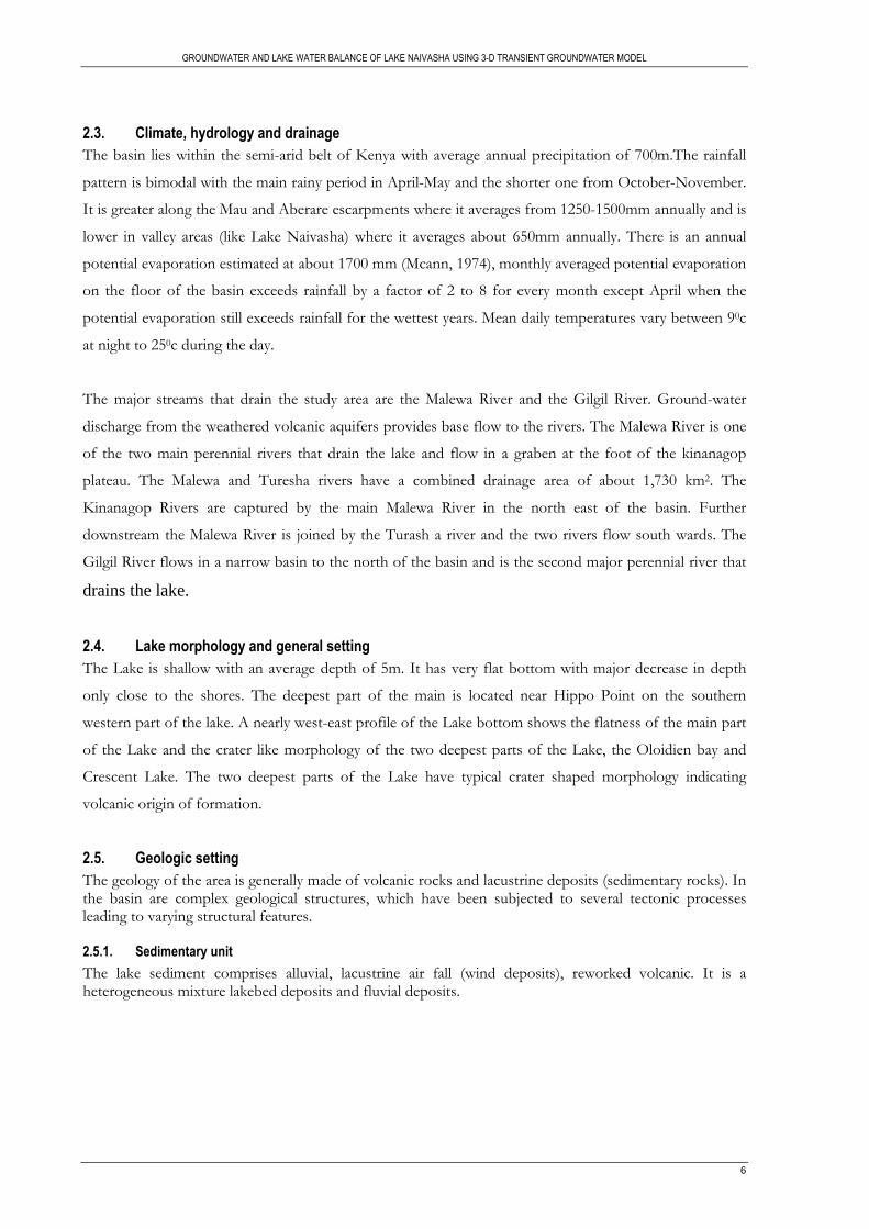
2.3. Climate, hydrology and drainage
The basin lies within the semi-arid belt of Kenya with average annual precipitation of 700m.The rainfall
pattern is bimodal with the main rainy period in April-May and the shorter one from October-November.
It is greater along the Mau and Aberare escarpments where it averages from 1250-1500mm annually and is
lower in valley areas (like Lake Naivasha) where it averages about 650mm annually. There is an annual
potential evaporation estimated at about 1700 mm (Mcann, 1974), monthly averaged potential evaporation
on the floor of the basin exceeds rainfall by a factor of 2 to 8 for every month except April when the
potential evaporation still exceeds rainfall for the wettest years. Mean daily temperatures vary between 90c
at night to 250c during the day.
The major streams that drain the study area are the Malewa River and the Gilgil River. Ground-water
discharge from the weathered volcanic aquifers provides base flow to the rivers. The Malewa River is one
of the two main perennial rivers that drain the lake and flow in a graben at the foot of the kinanagop
plateau. The Malewa and Turesha rivers have a combined drainage area of about 1,730 km2. The
Kinanagop Rivers are captured by the main Malewa River in the north east of the basin. Further
downstream the Malewa River is joined by the Turash a river and the two rivers flow south wards. The
Gilgil River flows in a narrow basin to the north of the basin and is the second major perennial river that
drains the lake.
2.4. Lake morphology and general setting
The Lake is shallow with an average depth of 5m. It has very flat bottom with major decrease in depth
only close to the shores. The deepest part of the main is located near Hippo Point on the southern
western part of the lake. A nearly west-east profile of the Lake bottom shows the flatness of the main part
of the Lake and the crater like morphology of the two deepest parts of the Lake, the Oloidien bay and
Crescent Lake. The two deepest parts of the Lake have typical crater shaped morphology indicating
volcanic origin of formation.
2.5. Geologic setting
The geology of the area is generally made of volcanic rocks and lacustrine deposits (sedimentary rocks). In the basin are complex geological structures, which have been subjected to several tectonic processes leading to varying structural features.
2.5.1. Sedimentary unit
The lake sediment comprises alluvial, lacustrine air fall (wind deposits), reworked volcanic. It is a heterogeneous mixture lakebed deposits and fluvial deposits.
GROUNDWATER AND LAKE WATER BALANCE OF LAKE NAIVASHA USING 3-D TRANSIENT GROUNDWATER MODEL
7
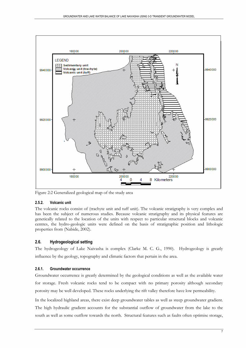
Figure 2:2 Generalized geological map of the study area
2.5.2. Volcanic unit
The volcanic rocks consist of (trachyte unit and tuff unit). The volcanic stratigraphy is very complex and has been the subject of numerous studies. Because volcanic stratigraphy and its physical features are genetically related to the location of the units with respect to particular structural blocks and volcanic centres, the hydro-geologic units were defined on the basis of stratigraphic position and lithologic properties from (Nabide, 2002).
2.6. Hydrogeological setting
The hydrogeology of Lake Naivasha is complex (Clarke M. C. G., 1990). Hydrogeology is greatly
influence by the geology, topography and climatic factors that pertain in the area.
2.6.1. Groundwater occurrence
Groundwater occurrence is greatly determined by the geological conditions as well as the available water
for storage. Fresh volcanic rocks tend to be compact with no primary porosity although secondary
porosity may be well developed. These rocks underlying the rift valley therefore have low permeability.
In the localized highland areas, there exist deep groundwater tables as well as steep groundwater gradient.
The high hydraulic gradient accounts for the substantial outflow of groundwater from the lake to the
south as well as some outflow towards the north. Structural features such as faults often optimise storage,

GROUNDWATER AND LAKE WATER BALANCE OF LAKE NAIVASHA USING 3-D TRANSIENT GROUNDWATER MODEL
8
Transmissivity and recharge with the significant of these occurring in places that are adjacent to or within
a surface drainage system. Shallow groundwater table, low precipitation and low values of recharge
characterize the valleys.
2.6.2. Aquifer systems and aquifer properties
(Clarke M. C. G., 1990) noted that aquifers are normally found in fractured volcanics, or along weathered
contacts between different lithological units. These aquifers are often confined or semi-confined and
storage coefficients are likely to be low. The main aquifer is found in sediments covering parts of the rift
floor. These, aquifers usually have relatively high permeability and are often unconfined with high specific
yield. On the rift escarpments, the estimated hydraulic conductivities range from 0.1 m/d for the
Kinangop Tuff and 1.1 m/d for the Limuru Trachyte.
2.6.3. Piezometer and groundwater flow:
(Clarke M. C. G., 1990) write that the area has a complex hydrogeology, because while it is lower than the Rift escarpments it is at the culmination of the Rift floor. Groundwater certainly flows away from Lake Naivasha because the lake water is fresh, even though the lake has no outlet and lies in an area of high evaporation. Northerly flow may occur both via Gilgil and under Eburru. Southerly flow must also occur, following the hydraulic gradient. Pizometric plots and isotopic studies show that underground movement of water is occurring both axially along the rift and laterally from the bordering highlands into the rift. Analysis of Pizometric map and aquifer properties of the rocks in the area show that much of the subsurface outflow from the Naivasha catchment is to the south, via Olkaria-Longonot towards Suswa The structure of the Rift Valley and in particular major marginal Rift faults and the system of grid faulting and the Rift floor undoubtedly have substantial effect on the groundwater flow systems of the area. In general faults are considered to have two effects on fluid flow. They may facilitate flow by providing channels of high permeability, or they may prove to be barriers to flow by offsetting zones of relatively high permeability. In the Rift Valley the main direction of faulting is along the axis of the Rift, and this has a significant effect on the flows across the Rift. It is apparent from the high hydraulic gradients that are developed across the Rift escarpments that the effect of the major faults is to act as zones of low permeability. The effect of faulting is to cause groundwater flows from the sides of the Rift towards the centre to flow longer paths reaching greater depths, and to align flows within the Rift along its axis.

GROUNDWATER AND LAKE WATER BALANCE OF LAKE NAIVASHA USING 3-D TRANSIENT GROUNDWATER MODEL
9
3. METHODOLOGY
Given that the objectives of research, the methodological design of this study involves separate characterization of both surface and subsurface parameter before put in to the model. The research contains three phase with the main stages being data preparation includes (pre-fieldwork and fieldwork) data processing and modeling: A schematic representation of the breakdown and sequence of the study process is shown in Figure: 3.1.
3.1. Data preparation
3.1.1. Pre field work
In the preliminary stages of the study a literature review and preparation for fieldwork was carried out. The existing well database was updated and reorganised. Available data were screened and pre-processed, field survey points mapped out, mapping units delineated and appropriate field materials and tools identified. The following materials were used Topographic Maps Geologic Maps: Geological Map of Longonot Volcano, the Greater Olkaria and Eburru Volcanic Complexes and adjacent areas, 1988, 1:100 000, Ministry of Energy Geothermal Section (Kenya) Satellite Images: Landsat TM images (bands 741) Groundwater well records: Pumping tests data, drilling completion records, groundwater level data References: Research papers, previous MSc thesis, drilling reports and journal articles from previous Works in the study area were used (see references). Equipment: Geodetic GPS for levelling of the wells, water level transducers Geological equipment: Geological compass, geological hammer, magnifier, Laptop and camera.
3.1.2. Field work
A 3-week fieldwork was carried out from the third week of Sep, 2010 to the first week of October, after
the required data has been identified and preparations were made. The following activities were carried out
in the field
Hydrogeological observation
Hydro geological observations were taken with the help of Aster satellite images, geological maps and
cross sections and previous studies of the area. The primary observation sites were selected along river
Malewa, river karate and previously drilled borehole site and geological cross section shafts. For
comparison with borehole drilling findings, the thickness and location of the different geological units
were recorded.

GROUNDWATER AND LAKE WATER BALANCE OF LAKE NAIVASHA USING 3-D TRANSIENT GROUNDWATER MODEL
10
Figure 3:1 Schematic representation of the breakdown and sequence of the study process
Analysis of available data
Literature review
Lake Naivasha basin
Proposal writing
Field work
Groundwater Data -water Level data -pumping tests -Well completion records -Abstraction data -Recharge/discharge -Irrigation return-flow
Surface water data -Precipitation -Evapotranspiration -River flow/runoff -Lake level -Lake Bathymetry data -Geodetic Surveys
Model input Monthly data (1932-2010)
Develop conceptual model
Revise Conceptual model Calibration of transient model
Sensitivity analysis
Acceptable Error
No
Yes
Calibration of steady state model
Model output
Data analysis
Conclusion and recommendation

GROUNDWATER AND LAKE WATER BALANCE OF LAKE NAIVASHA USING 3-D TRANSIENT GROUNDWATER MODEL
11
Geodetic survey A Geodetic GPS survey program was made during the field work. The main objective of this program is
order to accurately measure the groundwater level and surface level at each well, river stage and lake level. For this reason a Geodetic GPS of the Leica GPS Receiver type (tripod-mounted) was preferred than the
normal Garmin GPS.
The method of data acquisition in the field work requires a method of relative (differential) positioning
system where two Leica GPS operating at the same time. One GPS as base station mounted on a tripod at
a reference point and the second GPS as Rover on a pole which can be moved to the measuring site. The
concept of the relative (differential) positioning uses one stationary antenna as a reference point. The
stationary antenna’s receiver then tracks at least the same satellites (preferably all visible satellites) as the
moving receiver does.
Before start measuring the reference station was set at previously Geodetic levelled borehole named
Menera farm BH7 with known coordinates 211231E, 9924924N and elevation 1903.32m This point was
take as bench mark for the whole survey period. The antenna was centered above the station on a tripod
and the height to the antenna phase centre was measured. All the cables were connected and the receivers
were initialized so that visible satellites were acquired. After the R-time mode is set to “Reference” and the
appropriate antenna is selected survey began. The configuration of the second GPS (Rover) also follow a
similar set up except in this case the R-time mode is set to “Rover”
When the tracking had begun, it was ensured that the receiving device was functioning properly and that
both measurements and broadcast ephemeris were recorded. The tracking performance was then
monitored by watching receiver signal quality indicators. In this well levelling program an accuracy
maximum 23 cm and minimum 0.3 cm is registered
The office processing was done using software called Leica Geo Office. In the processing the reference
benchmark was used to compute co-ordinates of the other user-defined stations using baseline processing
and single point processing where required. After the whole data had been processed, the interpolation
method was used to relate and transform the co-ordinates from the Cartesian Clark 1880 system to the
local coordinate system. The two co-ordinate systems were then matched using common tie points to
obtain the transformation parameters. The transformation parameters were necessary to transform the
coordinates from one datum to another. The transformed coordinates was therefore obtained from
Projection: UTM, Spheroid: Clark 1880 and Datum: Arc 1960 in the local system coordinates system.
In this field work a total of 39 wells were geodetically levelled appendix: 1
Figure 3:2 Locating the reference station (left) and well top elevation survey (right)

GROUNDWATER AND LAKE WATER BALANCE OF LAKE NAIVASHA USING 3-D TRANSIENT GROUNDWATER MODEL
12
Water level Water level measurements of number boreholes with access openings were carried out by lowering a
probe attached to an electric cable. Water level was measured relative to the top of the access hole. Where
there was not access well, the measurement was taken relative to the top of the concrete slab. In few cases
the wells are found without access hole or electric pipes are installed in the wrong direction, in this case
the water level history of the well was traced from the drilling history record. Water level for geodetically
levelled wells was taken in centimetre accuracy.
Pump test Pump test data for the most recently drilled deep borehole is collected from different drilling companies.
In addition to pump test result from all previous works is collected to interpret the results based on the
present hydrogeological knowledge of the basin.
River flow data Time series river inflow data for 12 gauging stations is collected from the Naivasha district office (Dc’S).
The data are gauge height data collected on daily basis by stuff, weir and automatic data recorder. Most of
the Gauge stations are located outside the study area from which about 90% of the river inflow is
supposed to drain from. The main river is Malewa River (2GB 01) which has the longest record history in
the basin (1931-2007) and the smallest is Karati River (2GD02) with no data record. During the field work
the data for each station was checked for anomalies and missing gaps.
Lake level The water level of Lake Naivasha has been monitored since 1908. Stations 2GD1, 2GD4 and 2GD6 have
been the historical lake level measuring stations in the area (Mmbui, 1999). Recently other two stations
have been installed at Yacht club weather station and Oserian metrological station. During the field work
this station was not functioning due to maintenance problem. The Oserian metrological station is found
on the south-western side of the lake. The station has recording history since 1991.
Rainfall Rainfall data was one of the important input parameter to compute the amount of direct precipitation into
Lake Naivasha. Naivasha District officer (DO) rainfall station data was selected for its location relative to
the lake and data quality and availability. The station had data for the duration 1910 to 2010. For missed
data filling purpose, rainfall data from other two nearby stations (Naivasha Kongoni Farm and Kenya nut
rainfall station) were also collected
Evaporation Being inside the rift valley, Evaporation is an important component to calculate the water balance of the
lake. Evaporation data was obtained from Oserian metrological station. The station has recording history
since 1991 on daily basis. Evaporation data from (1932-1997) was documented by Mmbui (1999).
Water abstraction data Water abstraction data mainly from the irrigated commercial farms was collected along with the irrigation
techniques. In addition to time series satellite image processing was also made to calculate the irrigation
land cover change occurred since 2008. The development of irrigation lands, irrigation types as well as the
main crops grown per farm before 2008 was documented by Musota (2008)
3.1.3. Post field work
Post fieldwork was the main process of this work. It includes data analysis and modeling with their
scientific approach and application for this research.

GROUNDWATER AND LAKE WATER BALANCE OF LAKE NAIVASHA USING 3-D TRANSIENT GROUNDWATER MODEL
13
4. DATA ANALYSIS
4.1. Study area set up
Construction and delineations of the study area involves the application of GIS and remote sensing in
representing the areal image of the lake Naivasha basin. The general topographical and hydrological
background was described from available records, maps, aerial photos and satellite imagery. The Landsat
images band composite 543 was processed using ILWIS software. The study area boundary includes the
simulation of subsurface hydrogeological boundaries and influence of major structures in addition to the
catchment boundary.
4.1.1. Surface elevation model
In modeling of lake- aquifer interaction, a key step forward has been the incorporation of the Lake bottom
bathymetry in to the digital surface model in order to the map the aquifer out crops on the bottom of
lakes and to simulate the aquifer-lake interaction in detail. In this procedure the top surface elevation and
the lake bottom bathometry are processed differently and overlaid together to form the top surface
elevation of the study area. The accuracy assessment is made based on the geodetically levelled well head
points.
4.1.2. Surface elevation map
The surface elevation map is created from SRTM data available from the USGS server. The source data
has 90 m spatial resolution with absolute horizontal accuracy of 60m and vertical absolute accuracy of
16m. After the data is downloaded, imported and registered in ILWIS software, it was resampled to 50m
special resolution. In order to calibrate the DEM with the actual surface elevation of the area, elevation
points from the levelled wells and the row DEM are compared continually until the elevation match. In
Figure 4.1 (left), the DEM is directly compared with the measured elevation values and the correlation
value was 0.89. Next based on the constant reference objects like the lake surface, the DEM is made to
rise by a constant value 3m. Through successive calibration on the DEM and on the measured values, the
final result with a correlation of 0.98 Figure: 4.1(right) was used as the surface elevation map for the model
input.
computation surface elevation
y = 0.9365x + 119.96R2 = 0.8938
1850
1900
1950
2000
2050
2100
1850 1900 1950 2000 2050 2100
SRTM-elevation
Mea
sure
d-e
leva
tion
Computation of surface elevation
y = 0.9963x + 8.9196R2 = 0.9864
1850
1900
1950
2000
2050
2100
1850 1900 1950 2000 2050 2100
SRTM-elevation
Mea
sure
d e
leva
tion
Figure 4:1 Computation of surface elevation processing (left) and after processing (right)
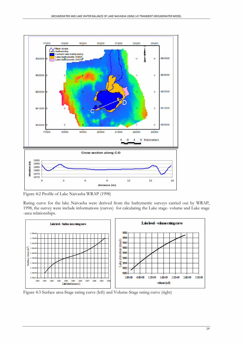
The base system of the lake bathymetry was originally surveyed in 1957 by the Ministry of water Works (Kenya). The contours of a map of the Naivasha area that was mapped by Viak (1975) were also raised by 2m to the level of the lake bathymetry. The digitization and interpolation of the contour maps were made by Owor (2000). Lake Bathymetry was incorporated in to the surface elevation map using map calculation function in ILWIS software. The lake bathymetry is an input parameter for the lake package in order to calculate the lake water balance of the model, Figure: 4.2
GROUNDWATER AND LAKE WATER BALANCE OF LAKE NAIVASHA USING 3-D TRANSIENT GROUNDWATER MODEL
14
Cross section along C-D
18701875
18801885
18901895
0 3 6 9 12 15 18
distance (m)
elev
atio
n (m
)
Figure 4:2 Profile of Lake Naivasha WRAP (1998)
Rating curve for the lake Naivasha were derived from the bathymetric surveys carried out by WRAP, 1998, the survey were include informations (curves) for calculating the Lake stage- volume and Lake stage -area relationships.
Figure 4:3 Surface area-Stage rating curve (left) and Volume-Stage rating curve (right)

GROUNDWATER AND LAKE WATER BALANCE OF LAKE NAIVASHA USING 3-D TRANSIENT GROUNDWATER MODEL
15
4.2. Surface water data analysis
4.2.1. Precipitation
Rainfall data was collected from Naivasha district office meteorological station found at the center of the study area. The station had data record for the duration 1910 to 2010. After filtering for anomalies, the daily rainfall records were aggregated in to a monthly basis, Figure 4.4. The rainfall data considered in this station will be applied as a direct precipitation into the lake and for the general model area that has been used for the runoff and recharge estimates.
Monthly Precipitation (1932-2010)
050
100150200
250300
350400
Jan-
32
Jan-
35
Jan-
38
Jan-
41
Jan-
44
Jan-
47
Jan-
50
Jan-
53
Jan-
56
Jan-
59
Jan-
62
Jan-
65
Jan-
68
Jan-
71
Jan-
74
Jan-
77
Jan-
80
Jan-
83
Jan-
86
Jan-
89
Jan-
92
Jan-
95
Jan-
98
Jan-
01
Jan-
04
Jan-
07
Jan-
10
Pre
cip
itat
ion
(m
m)
Figure 4:4 Monthly precipitations
4.2.2. Evaporation
Evaporation data was collected from Naivasha Water development Department (WDD) and from Oserian meteorological station. The WDD Evaporation data covers 1959-1990. The data was screened for typing errors and outliers using scatter plots and data gaps for missing data were in filled using linear regression. In order to backdate the evaporation data from 1959 to 1932, long term monthly averages were computed (Mmbui, 1999). These long-term averages were used to infill months with no recorded data. The Oserian station is a private station found on the western side of the lake. The station has been record evaporation on daily basis since 1991. The data from the main farm was pre-processed for anomalies and data gaps. After aggregating from daily to monthly the record was used to extend the record series to 2010, Figure: 4.5.
Monthly pan evaporation (1959-2010)
0
50
100
150
200
250
Jan-
58
Jan-
60
Jan-
62
Jan-
64
Jan-
66
Jan-
68
Jan-
70
Jan-
72
Jan-
74
Jan-
76
Jan-
78
Jan-
80
Jan-
82
Jan-
84
Jan-
86
Jan-
88
Jan-
90
Jan-
92
Jan-
94
Jan-
96
Jan-
98
Jan-
00
Jan-
02
Jan-
04
Jan-
06
Jan-
08
Jan-
10
Eva
po
rati
on
(m
m)
Figure 4:5 Monthly evaporation
4.2.3. Surface/River inflow
To quantify the time series river inflow in to lake Naivasha, The river discharge stations 2GB1and 2GB7 (Rivers Malewa), 2GA5 (on Gilgil) and 2GD2 on (Karati) were used. They were chosen for their proximity to the lake and discharge relationship among the stations. The amount of monthly discharge in to the lake
GROUNDWATER AND LAKE WATER BALANCE OF LAKE NAIVASHA USING 3-D TRANSIENT GROUNDWATER MODEL
16
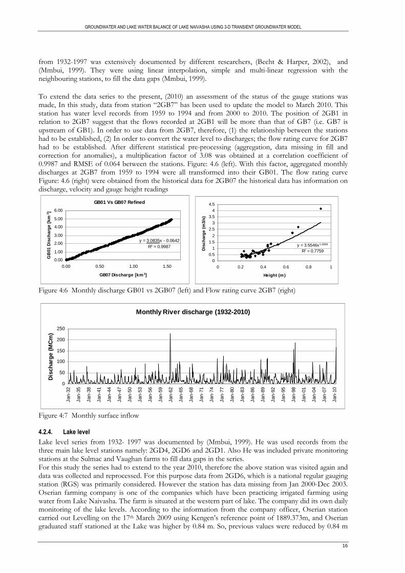
from 1932-1997 was extensively documented by different researchers, (Becht & Harper, 2002), and (Mmbui, 1999). They were using linear interpolation, simple and multi-linear regression with the neighbouring stations, to fill the data gaps (Mmbui, 1999).
To extend the data series to the present, (2010) an assessment of the status of the gauge stations was made, In this study, data from station “2GB7” has been used to update the model to March 2010. This station has water level records from 1959 to 1994 and from 2000 to 2010. The position of 2GB1 in relation to 2GB7 suggest that the flows recorded at 2GB1 will be more than that of GB7 (i.e. GB7 is upstream of GB1). In order to use data from 2GB7, therefore, (1) the relationship between the stations had to be established, (2) In order to convert the water level to discharges; the flow rating curve for 2GB7 had to be established. After different statistical pre-processing (aggregation, data missing in fill and correction for anomalies), a multiplication factor of 3.08 was obtained at a correlation coefficient of 0.9987 and RMSE of 0.064 between the stations. Figure: 4.6 (left). With this factor, aggregated monthly discharges at 2GB7 from 1959 to 1994 were all transformed into their GB01. The flow rating curve Figure: 4.6 (right) were obtained from the historical data for 2GB07 the historical data has information on discharge, velocity and gauge height readings
GB01 Vs GB07 Refined
y = 3.0835x - 0.0642R2 = 0.9987
0.00
1.00
2.00
3.00
4.00
5.00
6.00
0.00 0.50 1.00 1.50
GB07 Discharge [km 3]
GB
01 D
isch
arg
e [k
m3 ]
y = 3.5546x1.5669
R2 = 0.7759
0
0.5
1
1.5
2
2.5
3
3.5
4
4.5
0 0.2 0.4 0.6 0.8 1
Height (m)
Dis
char
ge
(m3/
s)
Figure 4:6 Monthly discharge GB01 vs 2GB07 (left) and Flow rating curve 2GB7 (right)
Monthly River discharge (1932-2010)
0
50
100
150
200
250
Jan-
32
Jan-
35
Jan-
38
Jan-
41
Jan-
44
Jan-
47
Jan-
50
Jan-
53
Jan-
56
Jan-
59
Jan-
62
Jan-
65
Jan-
68
Jan-
71
Jan-
74
Jan-
77
Jan-
80
Jan-
83
Jan-
86
Jan-
89
Jan-
92
Jan-
95
Jan-
98
Jan-
01
Jan-
04
Jan-
07
Jan-
10
Dis
char
ge
(MC
m)
Figure 4:7 Monthly surface inflow
4.2.4. Lake level
Lake level series from 1932- 1997 was documented by (Mmbui, 1999). He was used records from the three main lake level stations namely: 2GD4, 2GD6 and 2GD1. Also He was included private monitoring stations at the Sulmac and Vaughan farms to fill data gaps in the series. For this study the series had to extend to the year 2010, therefore the above station was visited again and data was collected and reprocessed. For this purpose data from 2GD6, which is a national regular gauging station (RGS) was primarily considered. However the station has data missing from Jan 2000-Dec 2003. Oserian farming company is one of the companies which have been practicing irrigated farming using water from Lake Naivasha. The farm is situated at the western part of lake. The company did its own daily monitoring of the lake levels. According to the information from the company officer, Oserian station carried out Levelling on the 17th March 2009 using Kengen’s reference point of 1889.373m, and Oserian graduated staff stationed at the Lake was higher by 0.84 m. So, previous values were reduced by 0.84 m

GROUNDWATER AND LAKE WATER BALANCE OF LAKE NAIVASHA USING 3-D TRANSIENT GROUNDWATER MODEL
17
length. The corrected daily record is available from 1991 to the present. After checking for type and some anomalies, the data from this station was used to fill the data gap for 2GD6. Finally the daily records were averaged to a monthly basis using excel software and the complete picture of the Lake Naivasha water level was constructed. Figure: 4.8
Monthly observed Lake Level (1932-2010)
1880
1882
1884
1886
1888
1890
1892
Jan-
32
Jan-
35
Jan-
38
Jan-
41
Jan-
44
Jan-
47
Jan-
50
Jan-
53
Jan-
56
Jan-
59
Jan-
62
Jan-
65
Jan-
68
Jan-
71
Jan-
74
Jan-
77
Jan-
80
Jan-
83
Jan-
86
Jan-
89
Jan-
92
Jan-
95
Jan-
98
Jan-
01
Jan-
04
Jan-
07
Jan-
10
leve
l (m
)
Figure 4:8 Monthly lake-level
4.3. Groundwater data analysis
4.3.1. Groundwater Level
The Pizometric surface of the wells was calculated as depth to water surface from the corrected Surface elevation map section 4.1 The wells with available groundwater levels in the area were collected from Naivasha District office (Kenya), GB drilling company (Nakuru, Kenya) and from previous works (ITC data base). Adjustments have been effected to reflect corrections based on the knowledge attained from recently drilled wells, newly levelled wells and the wells in which the water levels were measured during fieldwork.
4.3.2. Pump test
Pump test analysis was mad for 10 recently drilled boreholes in the study area. The analysis was made using two methods, Jacob straight-line method and Aquifer test software. During the analysis using the Jacob method, a plot of the drawdown versus time was constructed for the boreholes on a semi-log paper and an approximately straight-line graph were obtained from the test. When the best fit is obtained the Transmissivity of the boreholes is calculated from the pumping rate and the slope of the time-drawdown graph using the following relationship.
S
Q
Π∆=
4
3.2 T Equation: 1
Where; Q = pumping rate in m3
∆S = slope of the time-drawdown graph (change in drawdown per log cycle), and
T = Transmissivity

GROUNDWATER AND LAKE WATER BALANCE OF LAKE NAIVASHA USING 3-D TRANSIENT GROUNDWATER MODEL
18
Figure 4:9 Pump test analysis result using Jacob straight-line method
The some data set was calculated using Theis analysis in aquifer test considering a single well pump test analysis assumption Figure 4.10. The single well analysis method gives the opportunity to estimate the aquifer parameters of a single well. For this pumping test, there is only one well used for both pumping and for recording drawdown measurements. The Transmissivity value calculated using both methods is presented in appendix: 2. (a) Borhole information and (b) pumptest result
Figure 4:10 Pump test analysis result using aquifer test method
Previous estimate aquifer Transmissivity by Hermandez(1999) found values varying from less than 1 m2/day to more than 5000 m2/day. He estimated storativity values between 0.01. (Kibona, 2000) For well BH C at Three Point Ostrich farm within the lake sediments she estimates using the Hantush method a transmissivity of 1150 m2/d and a storativity of 3.95 x 10⁻³. With the Cooper-Jacob yields a transmissivity of 462 m2/d and storativity of 1.46 x 10⁻³. Table 4:1 Transmissivity calculated by Clarke et al (1990) for the whole of Lake Naivasha
Area Lithology Transmissivity m2/day
Average depth (m)
Hydraulic conductivity (m/d)
North east Sediment & volcanics 1170 307 60 19 South east Sediment & volcanics 3082 502 60 51
South west Sediment & volcanics 940 297 60 15 North west Sediment & volcanics 5308 1601 60 88
An analysis of shallow aquifer that yields water in the study area was done using well data kept by Ojiambo (1996). According to his analysis, transmissivity value in the area ranges from 3-1200 m2/day. The

GROUNDWATER AND LAKE WATER BALANCE OF LAKE NAIVASHA USING 3-D TRANSIENT GROUNDWATER MODEL
19
corresponding hydraulic conductivity calculated from transmissivity values range from 14 to 750 m/day. Summary of previous estimate of aquifer parameters if found in appendix: 3
4.4. Abstraction
Abstraction is the most undocumented input data in the study area. Water abstraction in the study area
occurs from irrigation and domestic wells. Abstraction for irrigation use is much larger than for domestic
use. Irrigation abstraction from the lake sediment aquifer is especially important in the commercial farms.
Water abstraction data mainly from the irrigated commercial farms was collected along with the irrigation
techniques and the area of the farms. Quantification of abstraction from different water bodies such as
Surface water (river, lake) and groundwater (boreholes) was made based on the abstraction record data
sheet obtained from the Naivasha District officers. The abstraction data sheet contains records such as the
total irrigated area, location, owner, abstraction permit (from surface and groundwater) and actual
abstraction per day for each irrigation farms. However it is often thought that the irrigation is supplied
more than the estimated irrigation demand. Assessment of mount of abstraction was also made by
considering the relation between abstraction and area of irrigation lands Abstraction rate (m3/day) = area of irrigated land * depth of irrigation Equation: 2
Estimation of historical development of irrigation areas in the basin was made by processing time series satellite images. Estimation of depth of irrigation was made based on previous estimations different statistical relationships. (Yihdego, 2005) estimation was 1000mm/year.
Figure 4:11 Trend of irrigation areas (1980-2010)
Water abstraction data mainly from the irrigated commercial farms was collected along with the irrigation
techniques and the area of the farms. Quantification of abstraction from different water bodies such as
Surface water (river, lake) and groundwater (boreholes) was made based on the abstraction record data
sheet obtained from the Naivasha District officers. The abstraction data sheet contains records such as the
total irrigated area, location, owner, abstraction permit (from surface and groundwater) and actual
abstraction per day for each irrigation farms.

GROUNDWATER AND LAKE WATER BALANCE OF LAKE NAIVASHA USING 3-D TRANSIENT GROUNDWATER MODEL
20
0
2
4
6
8
10
12
Jan-32 Feb-36 M ar-40 Apr-44 Jun-48 Jul-52 Aug-56 Sep-60 Nov-64 Dec-68 Jan-73 M ar-77 Apr-81 M ay-85 Jun-89 Aug-93 Sep-97 Oct -01 Dec-05 Jan-10
Ab
stra
ctio
n 1
06 *
m3 /
mo
nth
Total abstraction from the basin
Lake abstraction
Aquifer abstraction
Figure 4:12 Analysis result of abstraction from different water bodies
4.5. Recharge
The mechanisms of groundwater recharge in the study area are; direct recharge by direct percolation through the videos zone and indirect recharge from water bodies and lateral inflow from adjacent aquifers. The most factors contributing to recharge in the study area are rainfall, evapotranspiration rates and soil types. The area experiences an annual rainfall of 640mm and annual evapotranspiration of 1700mm which is characteristic of a semi-arid climate. Since the potential evapotranspiration of the area was estimated to be higher than rainfall, direct recharge is not a permanent process in the area, but a process which occurs during rain seasons and, only when there is high intensity (Nalugya, 2003) Table 4:2 Direct recharge estimated from SWAP model (1991-1998) by Nalugya (2003)
Local name Location Recharge(mm/day) Average recharge(mm/year)
UTM_X UTM_Y Min Max
Kedong 209691 9908544 0 7 43.75
Ndabibi 194490 9914863 0 0.27 0.69
TPF 213403 9924948 0 0.1 4.38
Marula 208444 9930840 0 5.5 33.75
Table 4:3 Direct recharge estimates from 1-D mixing model by Nalugya (2003)
Type of recharge Stable isotope mmday-1 mm year-1 Average (mmyear-1)
Mixed recharge; Lake: rain, 18-Oxygen 1x10⁻⁵ – 7x10⁻⁵ 3.65 – 25.55 14.6
Deuterium 3x10⁻⁵ – 7x10⁻⁵ 10.95 – 32.85 21.9
The reliability of recharge estimates using different techniques is variable, the techniques based on Surface-water and unsaturated zone data provide estimates of potential recharge whereas those based On groundwater data generally provide estimates of actual recharge (Scanlon, 2002)
Estimated groundwater recharge from a basin (Mcann, 1974)
SyhiAR
n
i
**1
∑=
∆= Equation: 3
Where
R=Total ground water recharge (m3/d), A=area (m2)
hi∆ = seasonal increase in ground water level (m)

GROUNDWATER AND LAKE WATER BALANCE OF LAKE NAIVASHA USING 3-D TRANSIENT GROUNDWATER MODEL
21
Sy =Specific yield of water yielding materials In this study the approach of Equation (3) is applied. The implementation follows the following procedure 1.The study made by Nalugya (2003) was taken as the steady state average recharge for the basin. 2. The seasonal increase in ground water level is assumed to be directly proportional to the lake level fluctuation. And can be replaced by monthly lake level increase. 3. The specific yield, I called it “the relating factor” is estimated from the relationship in equation: 3
∑=
∆=
n
i
hi
avRSy
1
Equation: 4
Where Sy= “Relating factor”
avR=average recharge in (m) of the area estimated by Nulugya(2003)
hi∆ = seasonal increase in lake level 4. The transient recharge was calculated using the relation of equation: 3 and equation: 4
SyhiARi ** ∆= Equation: 5
Where Sy= “Relating factor” constant hi∆ = seasonal increase in lake level at time t=i, indicates the stress period i=1-942 Ri= groundwater recharge at time t=i
Monthly recharge (1932-2010)
05
1015202530354045
Jan-
32
Jan-
35
Jan-
38
Jan-
41
Jan-
44
Jan-
47
Jan-
50
Jan-
53
Jan-
56
Jan-
59
Jan-
62
Jan-
65
Jan-
68
Jan-
71
Jan-
74
Jan-
77
Jan-
80
Jan-
83
Jan-
86
Jan-
89
Jan-
92
Jan-
95
Jan-
98
Jan-
01
Jan-
04
Jan-
07
Jan-
10
Rec
har
ge
(mm
)
Figure 4:13 Monthly recharge
4.6. Irrigation return flow
The process of re-entry of a part of the water used for irrigation is called return flow. Percolation from applied irrigation water, derived both from surface water and groundwater sources, constitutes one of the major components of groundwater recharge. Assessment of the irrigation return-flow can be made in different methods one of which is the estimation of the amount of Irrigation return water based on the Abstraction-Return flow relationship.
Return flow = C * Abstraction Equation: 6 Where, C is the return flow coefficient (0 < C < 1).

GROUNDWATER AND LAKE WATER BALANCE OF LAKE NAIVASHA USING 3-D TRANSIENT GROUNDWATER MODEL
22
The irrigation return flow depends on the soil characteristics, hydraulic properties of the aquifer, depth to water table, irrigation practice and type of crop. A study was made in the study area by (Mohammedjemal, 2006) targeting to assess the feasibility of artificial ground water recharge using the runoff harvested from the greenhouses. During the study, Injection and pumping test was carried out to determine the intake capacity and hydraulic property of the aquifer. In addition to grain size and water quality analysis was made. The field experiment results revealed the texture variation within the top 30 to 32m unsaturated zone. Besides the injection test results in very low intake rate potential and the hydraulic conductivity is in the order of 0.01 to 0.2mday-1. Based on The above findings he concludes the infeasibility of shallow infiltration in the study area.
Based on this argument and a similar argument by Hagos (2008) who also made another artificial recharge
test in the study area, the contribution of irrigation return flow in the long term water balance of the basin
is assumed to be insignificant and will not be considered in this study.
4.7. Evapotranspairation
The study area is characterized by an annual potential evaporation about 1700 mm (McCann, 1974). Monthly averaged potential evaporation on the floor of the basin exceeds rainfall by a factor of 2 to 8 for every month except April when the potential evaporation still exceeds rainfall save for the wettest years (Owor, 2000), (Yihdego, 2005). The natural vegetation surrounding the lake is mainly papyrus swamp vegetation. Natural vegetation outside of the lake surroundings are shrub, cactus, savannah and acacia (to the north). Acacia trees can be attributed to the shallower ground water table. The depth of root zone in the study area is assumed to be 3 to 12 metres (Asfaque, 1999). But little is known about the contribution of the Acacia trees for groundwater evapotranspiration. Generally due to the very nature of the study area, like; very high evaporation over precipitation, flat topography and rift valley environment, evapotranspiration from the land surface is assumed have insignificant contribution in the water balance of the basin. On the other hand, direct rainfall and evaporation from the lake surface includes estimates for swamp evapotranspiration on the lakeshores.

GROUNDWATER AND LAKE WATER BALANCE OF LAKE NAIVASHA USING 3-D TRANSIENT GROUNDWATER MODEL
23
5. MODELING
5.1. Model setup
5.1.1. Modeling protocol
Modeling protocol is intended to provide guidance that will promote consistency in the application of groundwater modeling in the study area. According to (Anderson & Woessner, 1992), modeling protocol includes code selection, model design, calibration, Sensitivity analysis and prediction. The basic modeling protocol implemented in this study is designed as
Figure 5:1 Steps in modeling protocol adopted from Anderson & Woessner (1992)
5.1.2. The groundwater flow equation
The partial-differential equation of ground-water flow used in modflow is (Harbaugh & McDonald, 2000)
t
hSW
z
hKzz
zy
hK
yx
hK
x syyXX ∂∂=+
∂∂
∂∂+
∂∂
∂∂+
∂∂
∂∂
Where Kxx, Kyy, and Kzz are values of hydraulic conductivity (L/T) along the x, y, and z coordinate axes h= is the potentiometric head (L); W= is a volumetric flux per unit volume representing sources and/or sinks of water, W<0.0 for flow out of the ground-water system, and W>0.0 for flow in SS= is the specific storage of the porous material T= is time (T).
Equation: 7

GROUNDWATER AND LAKE WATER BALANCE OF LAKE NAIVASHA USING 3-D TRANSIENT GROUNDWATER MODEL
24
5.1.3. Modflow lake package (LAK3)
In the Lake Package described in this study, the lake is represented as a volume of space within the model grid which consists of inactive cells extending downward from the upper surface of the grid. Active model grid cells bordering the space and adjacent aquifer, exchange water with the lake at a rate determined by the relative heads and by conductance that are based on grid cell dimensions, hydraulic conductivities of the aquifer material, and user-specified leakance distributions that represent the resistance to flow through the material of the lakebed. Implementation of a lake water budget includes input of parameters those representing the rate of lake atmospheric recharge and evaporation, overland runoff, and the rate of any direct withdrawal from, or augmentation of, the lake volume. The lake/aquifer interaction can be simulated in both transient and steady-state flow conditions.
5.1.4. Seepage between lake and aquifer
The direction and magnitude of seepage between a lake and the adjacent aquifer system depends on the relation between the lake stage and the hydraulic head in the ground-water system, both of which can vary substantially in time and space. Seepage from a lake into the surficial aquifer that surrounds it, where the lake acts as a source of recharge to the aquifer, occurs when and where the lake stage is higher than the altitude of the water table in the adjacent part of the aquifer. Quantification of the rate of seepage between the lake and the aquifer is made by an application of Darcy’s Law equation: 8. The volumetric flux (L3/T) is expressed by integrating the specific discharge over some cross section of area A (L2) in a plane perpendicular to the direction of flow equation: 9.
l
hhKq al
∆−
=
Where q = seepage rate (L/T); K = hydraulic conductivity (L/T) hl = is the stage of the lake (L); and ha= is the aquifer head (L); ∆ l = is the distance (L) hl and ha;
)()( alal hhchhl
KAqAQ −=−
∆==
Where c = KA/ ∆ l is the conductance (L2/T). K/ ∆ l = is the leakance (T -1).
5.1.5. Lake water budget
The interaction between the lake and the surficial aquifer is represented in this Lake Package by updating at the end of each time step a water budget for the lake that is independent of the ground-water budget represented by the solution for heads in the aquifer. Inherent in the calculation of a lake water budget is the computation of current values of lake volume and stage. The lake stage is crucial in making the estimates of ground-water seepage to and from the lake that are used by Modflow.
The implementation of a separate water budget for the lake that accounts for seepage losses to and seepage gains from the aquifer provides the capability to use the model to make a separate estimate of the stage of the lake and its relation to the water table. Updating a lake water budget also requires that estimates be made of gains and losses of water from the lake other than by seepage, such as (1) gains from rainfall, overland runoff, and inflowing streams, (2) losses to evaporation and out flowing streams, and (3) anthropogenic gains and losses (withdrawals for water supply or augmentation with water from another source. The water budget procedure incorporated in the Lake Package is implied by the equation used to update the lake stage. The explicit form of this equation is:
Equation: 8
Equation: 9

GROUNDWATER AND LAKE WATER BALANCE OF LAKE NAIVASHA USING 3-D TRANSIENT GROUNDWATER MODEL
25
A
QOQISPWSROEPthh
nn −+−−+−∆+= −1
11
Where h the lake stages (L)
∆ t time step length (T) P rate of precipitation (L3/T) E rate of evaporation (L3/T) SRO rate of surface runoff to the lake (L3/T) W rate of water withdrawal from the lake (L3/T) QI rate of stream inflow (L3/T) QO rate of stream outflow (L3/T) A surface area of the lake (L2) SP net rate of seepage between the lake and the aquifer (L3/T) (Positive Value indicates seepage from the lake into the aquifer)
5.2. Conceptual model
A conceptual model is the pictorial representation of the groundwater flow system. (Anderson &
Woessner, 1992), Hydro-geologically the area is complex due to rift floor geometry and tectonics.
Therefore the purpose of the construction this conceptual model is to simplify the field problems and
organize the associated field data so that the system can be analysed more readily. Simplification is
necessary because a complete reconstruction of the field system is not feasible (Anderson & Woessner,
1992).
The basic conceptual model assumes two non-coinciding aquifer systems. The upper aquifer is unconfined
aquifer: lake and fluvial/lacustrine sediment interbeded with clay silt and volcanic materials. The lower
aquifer is semi- confined aquifer: reworked and weathered/fractured volcanic materials. The upper aquifer
is in hydraulic link with the lake. It is characterized by variable (heterogeneous) horizontal and even
(homogenous) vertical aquifer properties. The lower aquifer is characterized by homogenous vertical and
horizontal aquifer properties. The lower aquifer is also in hydraulic connection to the upper aquifer
through a leakage terms.
Figure 5:2 conceptual model reflects the study area
Equation: 10

GROUNDWATER AND LAKE WATER BALANCE OF LAKE NAIVASHA USING 3-D TRANSIENT GROUNDWATER MODEL
26
5.2.1. Hydrostratigraphic units
The simplified Hydro Stratigraphic units of the area as discussed also by Nabide (2002) and
Yihdego(2005) consists of three units: tuff, trachyte and sedimentary. The sedimentary unit is composed
of fluvial and lacustrine sediment. The unit is laterally variable. The volcanic unit is composed of reworked
and weathered volcanic. The unit is laterally and vertically continuous. The tuff hydro-geological unit is
considered as impermeable base by assigning at least a two order of magnitude contrast in hydraulic
conductivity.
Figure 5:3 Geological Log of well C11527 (sedimentary unit) and well C13181 (volcanic unit)
5.2.2. Groundwater flow pattern
Groundwater flow system pattern and direction was analysed on the bases of the available heads. The
natural groundwater flow of the area was inferred from Piezometer heads before the abstraction stress on
the local aquifer was happened, roughly around 1980’s. As indicated in Figure: 5.4 below, the ground
water flow has two flow patterns: lateral flow pattern and axial flow pattern. The first component of lateral
flow into the basin was from the western escarpment that dispersed into three directions. North east
wards, South east wards and directly East wards that recharged the lake sediments. The second lateral flow
was from the eastern escarpments that dispersed again into three arms: North West wards, East wards to
the Lake and Southwest wards. Axially, the bulk of the flow from the lake was to the south through the
Olkaria-Longonot volcanic complexes and North and North West towards the lake Elementa. The
Northward flow from the lake towards and through the Eburru hills and Elmenteita Lake basin was
discussed by (Clarke A.C.G. D. Allen, 1990)
Construction of the conceptual model Two approaches can be used to construct a Modflow simulation: the grid approach and the conceptual
model approach. The grid approach involves working directly with the 3-D grid and applying
sources/sinks and other model parameters on a cell-by-cell basis. The conceptual model approach
involves application the GIS tools in the Map module to develop a conceptual model of the site being
modelled. The location of sources/sinks, layer parameters such as hydraulic conductivity, model
boundaries, and all other data necessary for the simulation can be defined at the conceptual model level.
Once this model is complete, the grid is generated and the conceptual model is converted to the grid
model and all of the cell-by-cell assignments are performed automatically. The conceptual model approach
is the most efficient approach for building realistic, complex models is the conceptual model approach...
For this modeling the conceptual model approach was used. The GIS input maps were pre-processed
using Arc GIS and ILWIS software.

GROUNDWATER AND LAKE WATER BALANCE OF LAKE NAIVASHA USING 3-D TRANSIENT GROUNDWATER MODEL
27
5.3. Numerical model
5.3.1. Code selection
One of the necessary criteria for code selection is weather the code includes a water balance computation.
A water balance calculation should be part of every modeling exercise (Anderson & Woessner, 1992). This
is because the water balance involves computation of flows across boundaries, to and from sources and
sinks and storage.
The Groundwater Modeling System (GMS) is a complete graphical user environment for performing
groundwater simulations. The entire GMS system consists of a graphical user interface (the GMS
program) and a number of analysis codes like Modflow. The GMS interface is developed by Aquaveo,
LLC in Provo, Utah
Modflow is a 3-D, cell-centered, finite difference, saturated flow model developed by the United States
Geological Survey (McDonald & Harbaugh, 1988). Modflow can perform both steady state and transient
simulations and has a wide variety of boundary conditions and input options. GMS supports Modflow as a
pre- and post-processor. The input data for Modflow are generated by GMS and saved to a set of files.
These files are read by Modflow when Modflow is launched from the GMS menu. The output from
Modflow is then imported for post-processing in GMS.
For this study GMS V.7 including Modflow 2000 was used for post and pre-processing. GMS v7
incorporates the lake package LAK3 which was utilized to estimate the water budget of the lake Naivasha.
5.3.2. Type and number of layers
The modelled domain covers an area of 1817sq km with two non-conceding aquifers. Layer one is
unconfined with a thickness that varies from few meters to 100m. Layer two is semi confined aquifer with
thickness varies from 30 to 220m. The first layer contains the lake. For simplification purpose the two
layers are simulated as a horizontal continuous layer with an average thickness 60m for the first layer and
100m for the second layer. In order to reflect the non-conceding nature of the layers a low hydraulic
conductivity was assigned to the boundaries of the first layer. A contrast of two orders of magnitude in
hydraulic conductivity (Neuman & Witherspoon., 1969) between the aquifer and a non-permeable unit at
the boundaries result in ignoring the horizontal flow in the layer (Anderson & Woessner, 1992).
To simulate the semi confined nature of the second aquifer a quasi-three dimensional modeling approach
was assumed. In quasi three dimensional modeling approaches, the confining layer to the second aquifer is
simulated by means of leakage terms. The leakage term is represents vertical flow between the two
aquifers. Modflow 2000 now has a package called the layer property flow package (LPF). The LPF
package relative to the BCF package is that there are now only two layer types: confined and convertible.
A convertible layer is similar to the layer LAYCODE = 2 and layer LAYCODE = 3 types in the BCF
package. The layer can be confined or unconfined depending on the elevation of the calculated water
table. In this modeling conceptualization the above two layer were simulated as convertible layer.
5.3.3. Grid design
The model grid contains 104 rows, 120 columns and two layers. The horizontal spacing is uniformly equal
to 500 meters. With a cells origin at 172251 m easting and 9896300 m northing, a total number of 24960
cells designed as 14562 active cells and 10398 in active cells.

GROUNDWATER AND LAKE WATER BALANCE OF LAKE NAIVASHA USING 3-D TRANSIENT GROUNDWATER MODEL
28
5.3.4. The boundary conditions
The boundary condutions are represented if Figure: 5.4
Western part: The watershed boundary that peaks at the Mau scarp was taken to be a no flow boundary.
North-western part: The north western boundary spanned by the Eburru hills beneath which are
acknowledged to be outflow to the Elmenteita Lake basin (Darling et al., 1996). In order to show the
conceptual implication of the outflow through this boundary, the boundary condition is located behind
the Eburru hills. This hydraulic boundary is simulated by General Head boundary with head elevation
specified at 1830m
Eastern part: The South Kinangop fault trending due NNW is considered to impede most of the inflow
from the Kinangop plateau. Most of the flux is considered to take place in the deeper horizons. Minimal
in flow through this area has been considered negligible. The boundary is specified as no flow boundary.
Southern part: Flow through the Olkaria and Longonot volcanic complexes has been considered to be
the conduit for most of the lake outflow from the basin most of which percolates into the deeper
geothermal systems. To the southeast of the Longonot volcano, some considerable outflow from the
basin has been considered to account for the fluxes from the Kinangop plateau that gets into the basin in
a south-westward direction. These boundaries are specified as General Head boundaries fixed at 1800m
(southern) and 1850m (south-eastern).
The basement: The bottom of the system has been considered to be composed of undifferentiated
volcanic materials that have a very low (Kzz<<Kxx≈Kyy).
The Surface: The lake surface at the centre of the domain is a time variant boundary whose boundary has
been defined within the Lake Package.
The two main rivers, Malewa and Gilgel, are time variant boundaries whose boundaries have been defined
within the River Package.
5.3.5. The initial conditions
The initial conditions have been considered to be the hydrologic stresses (lake levels, River flows,
evaporation, and precipitation) at the 1932 period. The initial groundwater levels have been derived as a
long-term average value from 1932 to 1979 interpolated within the model to obtain the initial Pizometric
surface.
5.3.6. Representation of the lake
The current coverage of the lake is approximately 110-120 sq. km (from ASTER image of 2009). However
the initial (historical lake surface area was about 181 sq. km (from historical data at the year 1932).
Therefore for model conceptualization purpose the lake surface area was set to the initial coverage as
surveyed in 1957 by the Ministry of water Works (Kenya). The initial lake bathymetry was represented by
the lake package Triangular networks (TIN) at the center of the model. The lake represented with a
minimum elevation 1874m (at the crescent lake) and maximum 1896m (maximum stage that can be
achieved during the simulation. In the steady state simulating the lake was assumed to have an initial stage
of 1891(stage at the initial condition of the year 1932) minimum stage 1874m and a maximum possible
stage 1896m

GROUNDWATER AND LAKE WATER BALANCE OF LAKE NAIVASHA USING 3-D TRANSIENT GROUNDWATER MODEL
29
Figure 5:4 Representations of boundary conditions and the lake surface area
5.4. Steady state calibration
An important part of any groundwater modeling process is the model calibration process. In order for a
groundwater model to be implemented in any type of management role, it must be established that the
model can successfully simulate observed aquifer behaviour. Calibration is a process where a certain
parameters of the model such as recharge and hydraulic conductivity are changed in a systematic fashion
and the model is repeatedly run until the computed solution matches field-observed values within an
acceptable level of accuracy.
5.4.1. Initial model execution
As discussed earlier in this modeling process the modeling approach followed is the conceptual modeling
approach. In this approach data was entered through the conceptual model. After synthesizing and
screening for errors, it converted/mapped in to Modflow layer and run. This process is a continuous
process throughout the modeling process.

GROUNDWATER AND LAKE WATER BALANCE OF LAKE NAIVASHA USING 3-D TRANSIENT GROUNDWATER MODEL
30
The initial hydrologic stresses (lake levels, River flows, evaporation, and precipitation) at the 1932 period
were used for the steady state calibration. The initial groundwater levels calculated as a long-term average
value from 1932 to 1979 was interpolated within the model to obtain the initial Pizometric surface. This
was so done because (1) levels within this duration correspond to the natural stresses that were acting in
the system then, (2) lack of enough data to adequately describe the Pizometric surface at the start of the
simulation period. Depending on the problem and modeling objectivity, it may be appropriate to assume
that water level measured during a certain period of time represents quasi steady state condition under
stress that prevail during that period (Anderson & Woessner, 1992).
5.4.2. Steady state observation Data
Two types of observation data were used in the calibration process: water table elevations from
observation wells and observed lake level in the year 1932. To consider the distribution and the density of
observation wells is an important step in steady state calibration process. For example a key to success at
using parameter estimation tools is to have a greater number of observations than parameters being
estimated.
5.4.3. Steady state calibration procedure
During steady state calibration, the model parameters of aquifer hydraulic conductivity and riverbed conductance and Lake Leakance were estimated. The steady state calibration was accomplished using 41 observations and 3 adjustable parameters: hydraulic parameters layer 1 and layer 2 recharge layer 1, River bed conductance (river Malewa and Gilgel) and Lake Leakance (Lake Naivasha). The steady state calibration was accomplished by minimizing the difference between model-predicted steady state aquifer water levels and measured groundwater level and lake stage during the time of simulation.
5.4.4. Calibration techniques
There are two calibration techniques commonly used in groundwater modeling environment. Trial and error calibration and automated calibration. A trial and error method can be used to iteratively adjust model parameters until the model computed values match the field observed values to an acceptable level of agreement. In this approach parameter values are adjuster by the modeler in sequential model run to much simulated heads to the calibration target. In this modeling process a trial and error adjustment was made to some parameters known with a high degree of certainty and therefore requires only slightly adjustment. However because trial and error calibration influenced by the modeler’s experience and biases, the method is less efficient to quantify the statistical uncertainty and reliability of the results. Anderson & Woessner(1992) express to this techniques as “unquantifiable” method to indicate the subjective of the method to the good judgment of the modeler. Better Calibration can be achieved using an inverse modeling. An inverse model is a tool that automates the parameter estimation process. The inverse model systematically adjusts a user-defined set of input parameters until the difference between the computed and observed values is minimized. GMS contains an interface to an inverse model called PEST. The following sections describe the parameter estimation tools used for the model Calibration.
5.4.5. Parameter Estimation Tools (PEST)
PEST, a nonlinear, least-squares inverse modeling program developed by (Doherty, 1998) was used to calibrate the model. During calibration, PEST runs the Modflow model thousands of times, comparing model-predicted results with observations. After each model run, the objective function is analyzed to determine whether the model run was an improvement over the previous run. After each model run, PEST evaluates each adjusted parameter to determine the next best adjustment to that parameter. PEST then prepares the input data set for the next model run with the adjusted parameters, runs the model and re-evaluates the output. The goal is a weighted, least-squares optimization of the fit between the model-predicted values and the observations.

GROUNDWATER AND LAKE WATER BALANCE OF LAKE NAIVASHA USING 3-D TRANSIENT GROUNDWATER MODEL
31
5.4.6. Model parameterization
Values of the Transmissivity/hydraulic conductivity characteristics of the aquifer systems by previous authors and recently calculated in this field work are listed in appendix: 2. Most of the aquifer parameters collected from pump test result that were basically derived from the geologic map and pump test result of the area, were in transmissivity values however the model requires hydraulic conductivity values. For this reason the field transmissivity values were converted in to hydraulic valued assuming an average thickness of 80m.These values were used to map the initial estimates for the zones. In the estimate for recharge an initial value of 20 mm/year (Nalugya, 2003)equivalent to about 4% of average precipitation within the rift area was assumed for the lake sediments. The western scarp area of Mau stretching north to the Eburru area was considered to have a higher recharge (Owor, 2000) Previous work by (Wiberg, 1976) estimates recharge at 50 mm/year equivalent to 7% of the average precipitation. (Mmbui, 1999) noted that the Pleistocene pyroclastic that flank the Mau and Aberdare escarpments appear relatively absorptive and doubtless transmit infiltrating precipitation and runoff to the underlying fracture and fissure systems of less absorptive and permeable rocks.
5.4.7. Defining the parameter zones
Parameter zonation was made for recharge (Layer: 1) and hydraulic conductivity (layer: 1) Figure: 5.5 and 5.6.Recharge was assigned only to layer one. Hydraulic conductivity for layer-2 was estimated as 0.1 m/day as initial values and was assumed to be uniform in the model area. The vertical hydraulic conductivity of the formations is not well known. It is often safe to assume 10% of the horizontal hydraulic conductivity. For the delineation of parameter zones the zonation made by Owor(2000) was used as initial estimation for the distribution of both hydraulic conductivity and recharge. But later the distribution was adjusted to reflect the latest finding; recharge by Nulgya(2003) and 3-D conceptual model by Yihdego (2005) and Nabide (2002). In the implementation of the parameter zonation with PEST, the number of zones is a function of the number of observation points. The number of zones or parameters to be estimated should be less than the number of observation points. On the other hand the number of zones defined for each parameter was also an important consideration for running PEST. The more zones there were, the longer it took to perform optimization iteration.
Figure 5:5 Parameter zones for Hydraulic conductivity (layer: 1)

GROUNDWATER AND LAKE WATER BALANCE OF LAKE NAIVASHA USING 3-D TRANSIENT GROUNDWATER MODEL
32
Figure 5:6 Parameter zones for recharge (layer: 1)
5.5. Transient model calibration
In transient problem the groundwater heads are a function of time. A transient simulation typically begins with a steady state initial condition and ends before or when a new steady state is reached (Anderson & Woessner, 1992). The simulated steady state aquifer heads were used as initial aquifer heads for the transient state simulation. Measure aquifer heads and the transient lake level were the important calibration targets for this run. The stress period step-size was increased to a monthly basis to match the available lake data. Mainly due to lake of date and few is known about it, groundwater evaporation from the saturated zone was not considered in this study.
5.5.1. Storage parameters
The transient simulation requires initial estimates for the storage coefficients of the aquifer. In the modeling conceptualization above the two layers were simulated as convertible layer, implies that the layer can be either confined or unconfined depending on the elevation of the computed water table. Storage parameter for convertible layers demands the assignment of both the specific storage (Ss) And Specific yield (Sy) for individual layers. However this parameter was the least known parameter in the study area. In this study the values that were initially considered by previous studies were taken as initial run for the model. These values include: Specific yield estimated by (Wiberg, 1976) (0.0015), (Ojiambo, 1996) (0.0044), (Trottman, 1998) (0.12 for the unconfined aquifer, and 0.0001 for the confined aquifer), (Hermandez, 1999) (0.01-0.15) and (Kibona, 2000) (0.00146-0.00395 for the lake sediments)
5.5.2. Initial condition
The initial conditions refer to the head distribution everywhere in the system at the beginning of the simulation and thus are boundary conditions in time. The initial condition for the transient simulation was the steady state head solution generated by the calibrated steady state. Use of model generated head values ensures that the initial head data and the model hydrologic inputs and parameters are consistent (Franke, 1987).

GROUNDWATER AND LAKE WATER BALANCE OF LAKE NAIVASHA USING 3-D TRANSIENT GROUNDWATER MODEL
33
5.5.3. Stress periods and time steps
Selection of the simulation time step is a critical step in transient model design because the value of the space and time discretization strongly influences the numerical results(Anderson & Woessner, 1992). Stress periods in Modflow are the blocks of time of variable length used in simulation of each time step. Stress periods and time steps should not be too large to miss important changes neither should they too small to take a long time to make unnecessary detail calculations in the system (Magombedze, 2002). As discussed in the analysis part of this study, data was available from 1932 to 2010 spanning over 79 years that included monthly lake levels, stream flow, and evaporation and precipitation data over the whole duration. The transient recharge was calculated based on the previous study by (Nalugya, 2003) to much the existing data in transient simulation. Transient water abstraction was estimated based on the irrigation area-depth relationship. To much the observed lake level, monthly stress periods were chosen with one time step each. Therefore the model was design with a total of 942 stress periods. And with a single time step uniform for each stress period. A trade-off had to be made with stress period and the time-step size with in each stress periods. More stress periods and more temporal variability in the calibration process, allow for a better fit between calculated and measured heads, but also make the calibration task more complicated and more time consuming because more stress periods and time steps need more input data and require therefore more processing time (W. Lubczynski & Gurwin, 2005).
5.5.4. Transient observation data
The lake level has been measured on monthly basis for the whole simulation time (1932-2010). Aquifer groundwater level was measured during this field work (Sep, 2010). A total of 14 water level data and the
lake stage were .assumed to constraint the model solution. The well location and descriptions of the observation data is given in appendix: 4
5.5.5. Transient calibration target
Since the lake stage is a reliable record to use as a base station, the main calibration target considers the observed lake level as a base for the other well records. The groundwater level were measured in Sep, 2010, the last simulation time of the transient model was Jun, 2010. There is a time gap of two months between the end of the simulation time and the water level observation time. Although the time gap is considered, the water level data is also as second important calibration target for the model.
5.5.6. Transient calibration procedure
During the transient state calibration, the steady state model parameters, boundary conditions, aquifer hydraulic conductivities, riverbed conductance and Lake Leakance were kept constant. The steady groundwater outflow and inflow which are indication of the groundwater - lake interaction are calculated as a function of the head difference between the lake and the aquifer. The storage parameters, specific storage and specific yields were adjusted by try and error in each calibration attempts. The transient model required a warm-up period of about five stress periods because observations during the initial stress period (1932) is partly dependent on events that occurred years prior to 1932. By using the ending steady state heads as the transient starting heads, the transient state were run as a steady state for five stress periods. This helps the model to introduced to and adjust itself with the successive stress periods in the simulation times.

GROUNDWATER AND LAKE WATER BALANCE OF LAKE NAIVASHA USING 3-D TRANSIENT GROUNDWATER MODEL
34
Figure 5:7 Location map of calibration wells

GROUNDWATER AND LAKE WATER BALANCE OF LAKE NAIVASHA USING 3-D TRANSIENT GROUNDWATER MODEL
35
6. RESULT AND DESCASION
6.1. Evaluation of steady state calibration
The result of the calibration should be evaluated both qualitatively and quantitatively (Anderson & Woessner, 1992). The measured and simulated heads with their difference are listed in appendix 4. Model residuals (the difference between model-calculated and observed values) are generated by the PEST software, providing an indication of how well the model calculated values match the observed values. Model statistics for the steady state calibration indicate an overall R2 =0.985 between measured and modeled aquifer water levels. The standard error for the aquifer water level estimates is 0.738m indicating that about 95 percent of the modeled aquifer water levels are within about -0.2m and 2.6m of observed values.
6.1.1. Steady state model calibration errors
The three ways of expressing the average difference between simulated heads (hs) and measured heads (hm) are: the (ME), Mean absolute error (MAE) and the root mean square error (RMS). The objective of the calibration is to minimize these errors. The mean error (ME): is the mean difference between measured head (hm) and simulated heads
io
n
ic hh
nME )(
1
1
−= ∑=
Equation: 11
The mean absolute error (MAE) is the mean of the absolute value of the difference in measured and simulated heads
|)(|1
1io
n
ic hh
nMAE −= ∑
=
Equation: 12
The root mean square error (RMS) or the standard deviation is the average of the square difference in measured and simulated heads
( )5.0
1
2/1
−= ∑=
n
ism ihhnRMS Equation: 13
The R2 value In statistics, a value is often required to determine how closely a certain function fits a particular set of experimental data. R2 values range from 0 to 1, with 1 representing a perfect fit between the observed and simulated aquifer heads, and 0 representing no statistical correlation between the data. The R2 value (often referred to as the goodness of fit) is computed as follows
∑ −∑ −∑ − −
=)(
)()(2
22
2
mm
msmmR
Equation: 14
Where
m = mean of observed lake level, m= observed lake level, s= simulated lake level Table 6:1 Steady state error summary
Evaluation Criteria Error value
Mean error 1.239 Mean absolute error 4.736 Root mean square error 5.729
R2 0.985
6.1.2. Steady state model scatter plot of observed and simulated heads
Scatter plot of measured against simulated heads was used to show the calibrated fit. Figure: 6.1. The scatter plot are visually examined whether points in a plot show deviation from the straight line in a random distribution or have systematic deviation, where systematic deviation of the plots can indicate

GROUNDWATER AND LAKE WATER BALANCE OF LAKE NAIVASHA USING 3-D TRANSIENT GROUNDWATER MODEL
36
systematic error in adjusting the parameter values with in parameter zone. The scatter plot shows a R2 = 0.985.
Figure 6:1 Scatter plot of computed Vs observed values
6.1.3. Steady state model water budget results
The steady state groundwater seepage from the lake amounts to 4.49 Mm3/month and seepage into the lake is calculated as 0.22 Mm3/month Table: 6.2. Significant inputs to the flow system of the area include recharge and lake seepage (sustained by the excess of the Surface inflow and precipitation over evapotranspiration).The outflow to the south and north of the basin provides the main outflow from the area. Table 6:2 Steady state water budget for the Lake
Flow components Inflow(Mm3/month) Outflow(Mm3/month)
Precipitation 8.788 0.000 Evaporation 0.000 22.138 River/surface inflow 17.624 0.000 Groundwater inflow (Lake seepage in) 0.224 0.000 Groundwater outflow (Lake seepage out) 0.000 4.498
Total 26.636 26.636
Inflow-Outflow 0.000
Table 6:3 Steady state water budget for entire model
Flow components Inflow(Mm3/month) Outflow(Mm3/month)
storage 0.000 0.000 Head dependent boundary 0.000 7.125 River leakage 0.114 1.192 Recharge 4.014 0.000 Lake seepage 4.498 0.224
Total 8.625 8.541
Inflow-Outflow 0.084
Percent of discrepancy 0.010
6.1.4. Steady state model contour map of simulated heads
The contour map of simulated aquifer heads is shown in, Figure 6.2. Both layers have a similar spatial Pizometric configuration. The Pizometric heads around the vicinity of the lake mapped exactly as the

GROUNDWATER AND LAKE WATER BALANCE OF LAKE NAIVASHA USING 3-D TRANSIENT GROUNDWATER MODEL
37
observed values. Away from the lake horizons, the aquifer hydraulic properties have been affected by different factors like heterogeneity and lithostratigraphy effects. The head dependent boundary specified at the North, south and south eastern were calibrated as 1830m, 1800m, and 1850m respectively.
Figure 6:2 Contour map of simulated aquifer heads
6.2. Evaluation of the calibrated transient state mode
6.2.1. Transient model calibration Errors
Table 6:4 Summary of transient calibration error
Evaluation Criteria Lake level Aquifer heads
Mean error -0.161 -0.932 Mean absolute error 0.387 1.54 Root mean square error 0.478 2.449
R2 0.905 0.732
6.2.2. Transient model time series plot of observed and calculated lake level
The transient model simulation results were evaluated by observing the measured and calculated aquifer and Lake Level. The transient simulation in this case includes 14 transient observation wells and the lake stage. Calculated aquifer head is presented in appendix: 5
1883
1884
18851886
1887
1888
18891890
1891
1892
Jan-32
Feb-36
Mar-40
Apr-44
Jun-48
Jul-52 Aug-56
Sep-60
Nov-64
Dec-68
Jan-73
Mar-77
Apr-81
May-85
Jun-89
Aug-93
Sep-97
Oct-01
Dec-05
Jan-10
date
Lak
e st
age
(m)
Observed lake levelCalculated Lake level
Figure 6:3 Time series plot of observed and calculated lake levels (1932 to 2010)

GROUNDWATER AND LAKE WATER BALANCE OF LAKE NAIVASHA USING 3-D TRANSIENT GROUNDWATER MODEL
38
1845
1850
1855
1860
1865
1870
1875
1880
1885
1890
ITC_2
010_0
1
ITC_2
010_0
2
ITC_2
010_0
3
ITC_2
010_0
4
ITC_2
010_
05
ITC_2
010_
06
ITC_2
010_
07
ITC_2
010_
08
ITC_2
010_
09
ITC_2
010_
10
ITC_2
010_
11
ITC_2
010_1
2
ITC_2
010_1
3
ITC_2
010_1
4
aqui
fer
hea
d (m
)
Observed
Calculated
Figure 6:4 Observed and calculated aquifer head (Observation, Jun, 2010)
6.2.3. Transient model scatter plot of observed and calculated level
Transient scatter plot of measured against simulated aquifer heads and lake stage was used to evaluate the transient model. The scatter plot are visually examined whether points in a plot show deviation from the straight line in a random distribution or have systematic deviation, where systematic deviation of the plots can indicate systematic error in adjusting the parameter values with in a parameter zone.
Figure 6:5 Scatter plot of observed and calculated lake levels (1932 to 2010)
Figure 6:6 scatter plot of observed and calculated aquifer heads (Jun, 2010)

GROUNDWATER AND LAKE WATER BALANCE OF LAKE NAIVASHA USING 3-D TRANSIENT GROUNDWATER MODEL
39
6.2.4. Sensitivity analysis
Sensitivity analysis is a measure of uncertainty in the calibrated model caused by uncertainty in the aquifer parameters and boundary conditions. The main objectify of the sensitivity analysis is to understand the influence of various model parameters and hydrogeological stresses on the aquifer system and to identify the most sensitive parameter(s) which will need a spatial attention in the feature studies. Sensitivity analysis was performed by systematically changing the calibrated value conditions (Anderson & Woessner, 1992). In similar approach, the sensitivity analysis for this particular study was performed by systematically changing aquifer and hydraulic parameters from calibrated values and evaluating the change on observed aquifer heads. Groundwater recharge and hydraulic conductivity (for the steady state model) and the storage parameter (for transient model) were each varied separately. In this procedure, the calibrated hydraulic conductivity and recharge values (steady state) and aquifer specific yield (transient state) were increased and decreased by a magnitude equivalent to 20%, 40% and 60% of the calibrated values. Root mean squire error (RMSE) was used as a statistical evaluation criteria. The analysis result is presented below. The steady state model is sensitive to both recharge and hydraulic conductivity. The model is highly sensitive to increasing and decreasing of recharge. The model is also show strong sensitivity to a decreasing than increasing in hydraulic conductivity. On the other hand the transient model shows equal sensitivity to increasing and decreasing of the specific yield but with a slow response.
0
5
10
15
20
25
30
0 0.2 0.4 0.6 0.8 1 1.2 1.4 1.6 1.8
Multiplier factor
RM
SE
of
hea
d c
han
ge
(m)
Recharge
H.conductivity
00.20.40.6
0.81
1.21.41.61.8
2
0 0.2 0.4 0.6 0.8 1 1.2 1.4 1.6 1.8
Multiplier factor
RM
SE
of
hea
d c
han
ge
(m)
Specific Yield
Figure 6:7 Sensitivity of the steady state model (left) and transient model (right)
6.2.5. Calibrated model parameters
Hydraulic conductivity Steady state simulation results indicate a wide range in horizontal hydraulic conductivities from 0.1 to 75 m/day for the lacustrine sediments and 0.001-0.1m/day for the volcanic aquifer. The steady state model was calibrated to the initial states of the lake (lake stage =1891m) this means that the initial aquifer water level around the lake had to be higher in order to have the some head as the lake itself. But later during the transient simulation, when the lake stage starts to decrease, the hydraulic head in the surrounding aquifer was not immediately respond to the stress on the lake. In other word, change in the lake flux does not bring the some effect on the lake shore aquifers. This means that the preliminary steady state hydraulic conductivity at the immediate vicinity of the lake had to be scaled up in order to allow lower hydraulic head equivalent to the lake stage during the transient simulation. For the some reason hydraulic conductivities along major outflow directions were also increased by 15-50% of the steady state calibration values. The adjustment does not bring a significant effect on the expected model solutions. Considering the sensitivity hydraulic conductivity in the model, Figure 6.8 the result indicates that the model is less sensitivity to an increasing in hydraulic conductivity. Aquifer storativity Initial values of aquifer storativity were estimated based on previous works. A values of specific yield in the range of (0.01-0.1) for the lacustrine sediments and (0.01-0.001) for the volcanic aquifer was calibrated. The corresponding specific storage values were in the range of (0.001-0.0001) adjusted during calibration. Storativity is often assumed to be uniform with in an aquifer or confined bed (Anderson & Woessner, 1992).The storage coefficient values in this study have been generally lumped into two main zones to the lake sediments/alluvial materials around the vicinity of the lake, and the reworked volcanic materials.

GROUNDWATER AND LAKE WATER BALANCE OF LAKE NAIVASHA USING 3-D TRANSIENT GROUNDWATER MODEL
40
General Head boundary (GHB) (Anderson & Woessner, 1992)Warns that Caution must be used in using the GHB to insure unrealistic flows do not develop. One of the effects of this package may the introducing of unlimited deeper recharge of groundwater over the model boundaries. In transient simulation Time-Variant Specified-Head package is rather preferred than the GHB to simulate specified head boundaries that can change within or between stress periods. However the GHB is found simple to implement, because it minimizes the model constrain in the process of calibration. One of the problems in the study area is the presence of boundary aquifer heads set below the elevation of the upper aquifer. The problem can result the development of unsaturated zone around the boundary heads which can be difficult to be simulated by Time-Variant Specified-Heads package. In this model the application of GHB package is implemented along the entire outflow boundaries. The model was calibrated by introducing a constraint mechanism that allowing only groundwater outflow from the model. The calibration method gives interesting results where no un-necessary recharge was introduced in to the model Table: 6.3 and Table: 6.4. The result is also logical in the context of topographic set up of the lake. The lake elevation (1887m .a.m.s.l) is exceptionally higher relative to the physical boundaries which are set at elevation (1800m .a.m.s.l).
6.3. Simulation of lake-aquifer abstraction from the basin
As an initial input to the model, amount of abstraction was estimated by considering the relation between abstraction and area of irrigation lands. Area of irrigation was calculated by calculating time series Landsat images and depth of irrigation was estimated using different statistical analysis (see section 4.4 for the detail). Simulation of abstraction in this study aims at estimation of combined abstraction (abstraction from the aquifer and withdrawal from the lake). The simulation was evaluated according to two main scenarios, “with abstraction” and “without abstraction”. The effect of the stress was evaluated based on the observed aquifer heads and lake stage at the end of the simulation time.
6.3.1. Scenario one: Without abstraction
Agricultural activities in the basin before 1980 were negligible. Owing to this reason all water loses from the lake during this period, save for loses due to evapotranspiration and groundwater outflow. This scenario assumes that the there was no abstraction at all before or after 1980. The model was made to run from 1932-2010 and the result was evaluated. The lake stage graph result shows a divergence around the 1980 Figure: 6.9. The effect is also evidence in the aquifer water levels where the calculated heads are
higher Figure: 6.8. The difference between observed and calculated aquifer and lake level after 1980 was taken as important indication of the effect of abstractions from the basin for agricultural, industrial and domestic purposes
184018451850185518601865187018751880188518901895
ITC_
2010
_01
ITC_
2010
_02
ITC_
2010
_03
ITC_
2010
_04
ITC_
2010
_05
ITC_
2010
_06
ITC_
2010
_07
ITC_
2010
_08
ITC_
2010
_09
ITC_
2010
_10
ITC_
2010
_11
ITC_
2010
_12
ITC_
2010
_13
ITC_
2010
_14
aquifer
hea
d (m
)
Observed
Calculated
Figure 6:8 Observed and calculated aquifer head (abstraction not included)

GROUNDWATER AND LAKE WATER BALANCE OF LAKE NAIVASHA USING 3-D TRANSIENT GROUNDWATER MODEL
41
18831884188518861887188818891890189118921893
Jan-32
Feb-36
Mar-40
Apr-44
Jun-48
Jul-52 Aug-56
Sep-60
Nov-64
Dec-68
Jan-73
Mar-77
Apr-81
May-85
Jun-89
Aug-93
Sep-97
Oct-01
Dec-05
Jan-10
date
Lak
e st
age
(m)
Observed lake levelCalculated Lake level
Figure 6:9 Time series plot of observed and calculated lake level (abstraction not included)
Figure 6:10 Groundwater contour map of simulated heads (abstraction not included)
6.3.2. Scenario two: With abstraction
According to the analysis on Section: 4.4, average abstraction from the basin estimated is about 6.25 *M
m3/month with a long term trend of abstraction ratio is 30% (groundwater) and 70% (lake water). In
order to observe the simulation of abstraction on the lake the model application of this scenario was break
down in to three.
1. All the abstraction was from the lake
2. All the abstraction was from the groundwater (aquifer)
3. Abstraction was in the ratio of 30% (groundwater) and 70% (lake water).

GROUNDWATER AND LAKE WATER BALANCE OF LAKE NAIVASHA USING 3-D TRANSIENT GROUNDWATER MODEL
42
Lake abstraction from the lake is implemented by applied the abstraction stress directly on the lake. Well
abstraction in the area is everywhere. However not all the single wells have measurable stress on the
aquifer of the area. The main wellfield is found on the Northeastern part of the lake. The site is highly
affected by groundwater abstraction since the history of agriculture activities in the basin.
In this scenario, the total stress of abstraction was applied to the aquifer. Implementation of the scenarios
is made on seven wells. The wells are indicated on the ground by the main Pivot wells found in three well
fields Figure: 6.12. Abstraction stress applied to all wells was the same, the total abstraction divided by the
seven wells.
Wellfield A: well field: A includes (Three Point, Manera and Delamer site) the wellfield is the most
exploited site in the area. The well field is represented by four wells.
Wellfield B: well field B includes all wells around Marula sites. The well field is represented by two wells.
Well field: C. Wellfield C includes all wells very near to the lake. The wellfield was represented by one
well (assuming that there could be an option to pump water directly from the lake).
Response of the lake stage to the different abstraction schema is presented in Figure: 6.11.The deviation
of simulated from observed water levels in the past three decades is distinct and indicates the magnitude
of industrial abstraction. The deviation between the different curves, as a result the different abstraction
stress in the area indicates the degree of interaction between the surface water bodies and the
groundwater.
Abstraction estimation was needed to optimize in order to match the observed values. Optimization was
made by adjusting the initial abstraction input values until the simulated aquifer and lake stage matches the
observed values. The final optimization result allows estimate of an average combined abstraction from
the basin to be about 7*Mm3/month equivalent to 84 Mm3/year since 1980. Previous estimation, 57*106
m3/year (Mmbui, 1999), and 60*106m3/year (Becht & Harper, 2002).
The result is in very good agreement to the estimates calculated from abstraction analysis Section: 4.4. The
little increase in the current estimate supports the current condition that the groundwater level at the
wellfield and the lake level are currently in the state of decreasing while abstraction is continuously
increasing. The calculated abstraction has resulted in a lake which might have been 4.8m higher than was
observed during the current field work, (Jun, 2010).
6.3.3. The contour map of simulated heads
The final simulation contour map of aquifer heads and lake stage shown in, Figure: 6.12. The long term groundwater level fluctuation of the area was between minimum of 1800.233m and maximum of 2337.773m. The long term lake stage fluctuation was between minimum 1885.8m and a maximum 1891m.The final lake stage is calibrated as 1885.8 the result was very close to the observed value which was 1885.45m. Low water level at the Northern, southern and southeastern limit shows the level specified at the boundary condition. The boundary heads specified at the boundaries were 1830m, 1800m, and 1850m respectively.
The most interesting part of this simulation is that the development of low groundwater level anomalies in
the well field: A. while no enhanced abstraction effect was observed in the other two well fields. The
second interesting result is that the cone of depression in this well field is remains confined to that specific
location. During the simulation dry cells were also observed only in this particular wellfield. The result
indicates that the wellfield is not in direct hydraulic connection to the main recharging water body, the
lake. The dry cells during simulation indicates the applied abstraction stress is the maximum stress that the
will field could carry.

GROUNDWATER AND LAKE WATER BALANCE OF LAKE NAIVASHA USING 3-D TRANSIENT GROUNDWATER MODEL
43
The reason why a similar development of cone of depression is not enhanced in the other well field could have several implications. One of this could the fact that these well-fields are located relatively very near to the main recharging zones. The Boreholes in the high abstraction area are suspected of another source of recharge namely from rivers. According to previous studies the isotopic composition of Marula (well-field: B) signifies that these boreholes have their source of recharge from precipitation and river Malewa (Oppong-Boateng, 2001).This is also confirmed from the isotopic composition of unsaturated zone of Marula (d18O =-2.80 o/oo, d2H = -23.6 o/oo) which is a mixed of river Malewa and rain (Naulgay 2003).
1882
1884
1886
1888
1890
1892
1894
Jan-32 Feb-36 Mar-40 Apr-44 Jun-48 Jul-52 Aug-56 Sep-60 Nov-64 Dec-68 Jan-73 Mar-77 Apr-81 May-85 Jun-89 Aug-93 Sep-97 Oct-01 Dec-05 Jan-10
Observed lake level
No abstraction
Lake abstraction
Aquifer abstraction
Lake+aquifer_abstraction
Optimized basin abstraction
Figure 6:11 Response of the lake stage to the different abstraction schema
Figure 6:12 Groundwater contour map of simulated heads (abstraction included)
A
B
C

GROUNDWATER AND LAKE WATER BALANCE OF LAKE NAIVASHA USING 3-D TRANSIENT GROUNDWATER MODEL
44
6.4. The long term water budget
6.4.1. Long term lake storage
The lake storage was calculated by Modflow using the stage-volume rating curve of Lake Package LAK3. Stage-volume rating curve was generated using the DTM-derived Lake bathymetry within the limitations of the DTM. The lake storage volume imitates the temporal lake level fluctuations Figure: 6.13 the average transient storage volume calculated is, 8.4 * 108 m3/ month.
0.E+00
2.E+07
4.E+07
6.E+07
8.E+07
1.E+08
1.E+08
1.E+08
2.E+08
Jan-
32
Jan-
35
Jan-
38
Jan-
41
Jan-
44
Jan-
47
Jan-
50
Jan-
53
Jan-
56
Jan-
59
Jan-
62
Jan-
65
Jan-
68
Jan-
71
Jan-
74
Jan-
77
Jan-
80
Jan-
83
Jan-
86
Jan-
89
Jan-
92
Jan-
95
Jan-
98
Jan-
01
Jan-
04
Jan-
07
Jan-
10
volu
me
(10-1
*m3 ),
area
(m2 )
1880
1882
1884
1886
1888
1890
1892
stag
e (m
)
Lake surface areaLake volumeLake Stage
Figure 6:13 Simulated lake storage volume -stage-surface area relationship
6.4.2. Long term aquifer-lake interaction
There is a temporal fluctuation of the total amount of water seeping in to and from the lake to the aquifer. The maximum quantities of seepage to the groundwater are during those periods of consistent lake stage rise Figure: 6.14. The long term lake seepage out (groundwater outflow from the lake) was calculated as 5.56 *106 m3/ month equivalent to 66.7 *106 m3/ year. The lake levels are sustained during those periods when the total inflow (stream inflow, runoff and rainfall) exceeds the total outflow (lake seepage abstraction and evapotranspiration). These periods are linked to consistent inflows into the lake possibly during the high rains after the dry spells. Similarly the long term lake seepage in (groundwater inflow in to the lake) was calculated as 1.1 *106 m3/ month equivalent to 13 *106 m3/ year. The result is quite comparable to the result obtained by previous researchers. The previous results for the outflow term was 50 *106 m3/year (Clarke M. C. G., 1990); 57 *106 m3/year (Owor, 2000); 56 *106 m3/ year (Becht & Harper, 2002) The relatively increase in the current estimation indicates the increase of lake water outflow as a result of intense abstraction in the study area.
0.E+00
5.E+06
1.E+07
2.E+07
2.E+07
Jan-32 Feb-36 Mar-40 Apr-44 Jun-48 Jul-52 Aug-56 Sep-60 Nov-64 Dec-68 Jan-73 Mar-77 Apr-81 May-85 Jun-89 Aug-93 Sep-97 Oct-01 Dec-05 Jan-10
month
flo
w (
m3 /m
on
th)
Groundwater inflow to the lake
Groundwater outflow from the lake
Figure 6:14 Graph showing long term ground inflow and outflow from the lake
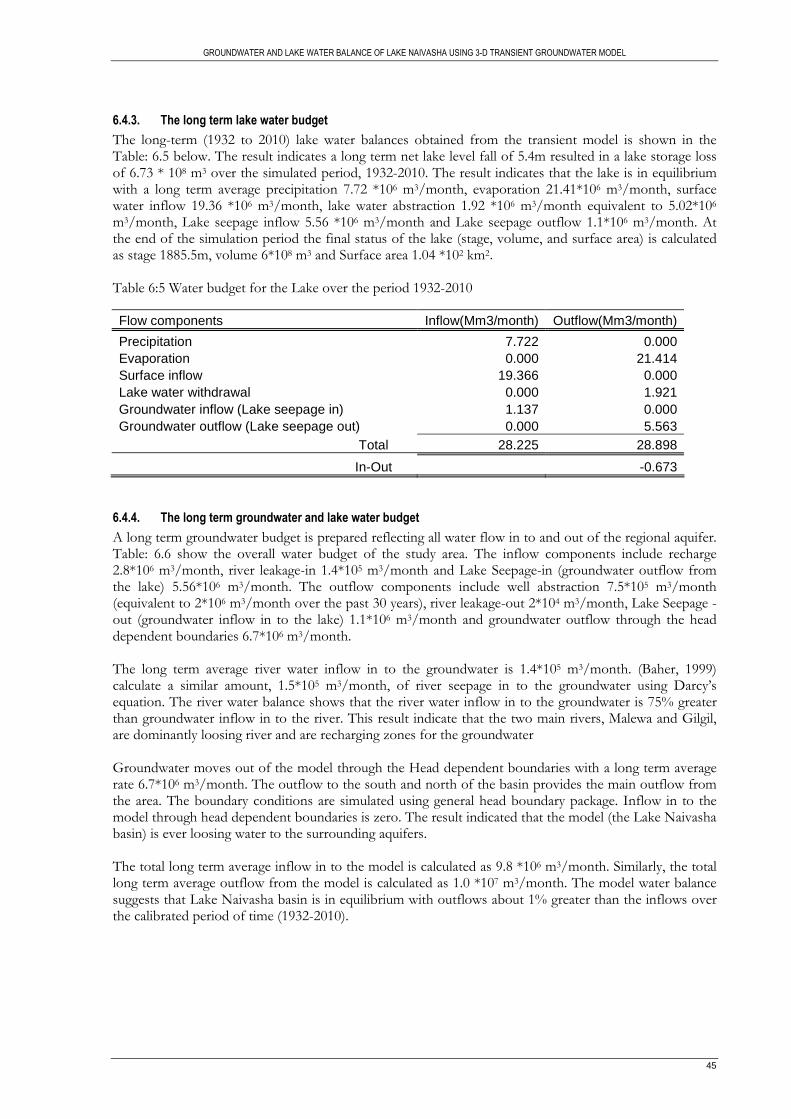
GROUNDWATER AND LAKE WATER BALANCE OF LAKE NAIVASHA USING 3-D TRANSIENT GROUNDWATER MODEL
45
6.4.3. The long term lake water budget
The long-term (1932 to 2010) lake water balances obtained from the transient model is shown in the Table: 6.5 below. The result indicates a long term net lake level fall of 5.4m resulted in a lake storage loss of 6.73 * 108 m3 over the simulated period, 1932-2010. The result indicates that the lake is in equilibrium with a long term average precipitation 7.72 *106 m3/month, evaporation 21.41*106 m3/month, surface water inflow 19.36 *106 m3/month, lake water abstraction 1.92 *106 m3/month equivalent to 5.02*106 m3/month, Lake seepage inflow 5.56 *106 m3/month and Lake seepage outflow 1.1*106 m3/month. At the end of the simulation period the final status of the lake (stage, volume, and surface area) is calculated as stage 1885.5m, volume 6*108 m3 and Surface area 1.04 *102 km2. Table 6:5 Water budget for the Lake over the period 1932-2010
Flow components Inflow(Mm3/month) Outflow(Mm3/month)
Precipitation 7.722 0.000 Evaporation 0.000 21.414 Surface inflow 19.366 0.000 Lake water withdrawal 0.000 1.921 Groundwater inflow (Lake seepage in) 1.137 0.000 Groundwater outflow (Lake seepage out) 0.000 5.563 Total 28.225 28.898
In-Out -0.673
6.4.4. The long term groundwater and lake water budget
A long term groundwater budget is prepared reflecting all water flow in to and out of the regional aquifer. Table: 6.6 show the overall water budget of the study area. The inflow components include recharge 2.8*106 m3/month, river leakage-in 1.4*105 m3/month and Lake Seepage-in (groundwater outflow from the lake) 5.56*106 m3/month. The outflow components include well abstraction 7.5*105 m3/month (equivalent to 2*106 m3/month over the past 30 years), river leakage-out 2*104 m3/month, Lake Seepage -out (groundwater inflow in to the lake) 1.1*106 m3/month and groundwater outflow through the head dependent boundaries 6.7*106 m3/month. The long term average river water inflow in to the groundwater is 1.4*105 m3/month. (Baher, 1999) calculate a similar amount, 1.5*105 m3/month, of river seepage in to the groundwater using Darcy’s equation. The river water balance shows that the river water inflow in to the groundwater is 75% greater than groundwater inflow in to the river. This result indicate that the two main rivers, Malewa and Gilgil, are dominantly loosing river and are recharging zones for the groundwater Groundwater moves out of the model through the Head dependent boundaries with a long term average rate 6.7*106 m3/month. The outflow to the south and north of the basin provides the main outflow from the area. The boundary conditions are simulated using general head boundary package. Inflow in to the model through head dependent boundaries is zero. The result indicated that the model (the Lake Naivasha basin) is ever loosing water to the surrounding aquifers. The total long term average inflow in to the model is calculated as 9.8 *106 m3/month. Similarly, the total long term average outflow from the model is calculated as 1.0 *107 m3/month. The model water balance suggests that Lake Naivasha basin is in equilibrium with outflows about 1% greater than the inflows over the calibrated period of time (1932-2010).

GROUNDWATER AND LAKE WATER BALANCE OF LAKE NAIVASHA USING 3-D TRANSIENT GROUNDWATER MODEL
46
Table 6:6 Water budget for the entire model over the period (1932-2010)
Flow components Inflow(Mm3/month) Outflow(Mm3/month)
Storage 1.295 1.359 Head dependent boundaries 0.000 6.770 wells 0.000 0.755 River leakage 0.141 0.020 Recharge 2.803 0.000 Lake seepage 5.563 1.137 Total 9.802 10.040
In-Out -0.238 Percent of discrepancy -0.013
6.4.5. Comparison with other water balance models
The interaction between the lake and the surficial aquifer in Modflow is represented in the Lake Package LAK3. By updating at the end of each time step, a water budget is calculated for the lake that is independent of the ground-water budget. The implementation of a separate water budget for the lake provides the capability to use the model to make a separate estimate of the budget of the lake and its relation to the aquifer through the seepage in and out from the lake. The spreadsheet water balance model was used for comparison of the lake water balance. The model was used for evaluation of the lake water balance by several previous researchers, Mmbui(1999) and Becht & Harper (2002). The model uses mass conservation equation to sums up the net flow to the lake (from the precipitation, evaporation and stream flow and surface runoff terms) and obtains the change in storage from the previous month’s storage. A new surface area is then derived and from which, using the rating curve, a new lake level is computed. The spreadsheet cannot directly simulate abstraction stress applied on the aquifer. The model was made to run using a similar metrological time series input data as the Modflow lake package but of course excluding the abstraction information. The graphs Figure: 6.15 show a close match with the modflow lake package result indicating that there is no significant differences in the way the two models evaluate the stages from the given time step.
18831884
18851886
188718881889
18901891
18921893
Jan-32
Feb-36
Mar-40
Apr-44 Jun-48
Jul-52 Aug-56
Sep-60
Nov-64
Dec-68
Jan-73
Mar-77
Apr-81 May-85
Jun-89
Aug-93
Sep-97
Oct-01 Dec-05
Jan-10
date
Lak
e st
age
(m)
Observed lake levelModflow lake packageSpreadsheet model
Figure 6:15 Compassion of results from Spread sheet and Modflow lake package models.

GROUNDWATER AND LAKE WATER BALANCE OF LAKE NAIVASHA USING 3-D TRANSIENT GROUNDWATER MODEL
47
7. CONCLUSION AND RECOMMENDATION
7.1. Conclusion
The objective of calibrating of the steady state and 3-D transient groundwater model of the study area is achieved. Evaluation of calibration of transient model was highly constrained by observing the measured and calculated aquifer and Lake Level. The final calibrated model, implements the application of parameter estimation tools, PEST. The model matches the observed lake level with R2= 0.985, steady state and R2= 0.905, transient simulation. The transient model covers 79 years of lake-aquifer data (1932-2010) discretized in 942 stress periods, this is the longest ever calibrated ranges of years in the study of the basin.
The long term lake water balance was calculated by Modflow using the stage-volume rating curve of Lake
Package LAK3. The long term average storage volume is 8.4 * 108 m3/ month. The long term average
fluxes in to the lake are precipitation 7.72 *106 m3/month, surface inflow 19.36*106 m3/month and
groundwater inflow (Lake seepage in) 1.1*106 m3/month. The long term average fluxes out of the lake: are
evaporation 21.41*106 m3/month, lake water abstraction 1.92 *106 m3/month and groundwater outflow
(Lake seepage out) 5.5*106 m3/month. The lake water balances suggests that the lake is not in equilibrium
with the inflow and outflow terms. The result indicates that a long term net lake level fall of 5.4m resulted
in a lake storage loss of 6.73 * 108 m3 over the simulated period, 1932-2010.
There is a temporal lake-aquifer interaction in the study area. The long term lake seepage-out
(groundwater outflow from the lake) was calculated as 5.5 *106 m3/ month and the long term lake
seepage-in (groundwater inflow in to the lake) was calculated as 1.1 *106 m3/ month. Using field abstraction data analysis and model simulation, the combined volume of lake-groundwater used for industrial abstraction since the last three decades was estimated. This requires an average abstraction amount 7.0 *106 m3/month with a long term trend of abstraction ratio 30% (groundwater) and 70% (lake water) since 1980. The amount resulted in a lake which might have been 4.8m higher than was observed in the last stress period (2010).
A long term groundwater budget is calculated reflecting all water flow in to and out of the regional aquifer.
The inflow components include recharge 2.8*106 m3/month, river leakage-in 1.4*105 m3/month and Lake
Seepage-in (groundwater outflow from the lake) 5.56*106 m3/month. The outflow components include
well abstraction 7.5*105 m3/month (equivalent to 2*106 m3/month over the past 30 years), river leakage-
out 2*104 m3/month, Lake Seepage-out (groundwater inflow in to the lake) 1.1*106 m3/month and
groundwater outflow through the head dependent boundaries 6.7*106 m3/month.The model water
balance suggests that lake Naivasha basin is in equilibrium with a net outflow about 1% greater than the
inflow over the calibrated period of time (1932-2010).
Model sensitivity analysis was made for aquifer hydraulic conductivity and recharge (steady state) and
aquifer storativity (transient model). The result shows that the model is highly sensitive to increasing and
decreasing of recharge. The model is also highly sensitive to decreasing in hydraulic conductivity but less
sensitive to increasing in hydraulic conductivity. On the other hand the transient model shows increasing
sensitivity to increasing and decreasing of the storativity values but with a slow response.
At the end of the work a comparison was made between Modflow lake-package water balance result and a
spreadsheet water balance model result. The spreadsheet water balance model cannot simulate abstraction
stress directly applied on the aquifer. Excluding the abstraction information, there was no significant
differences in the way the two models evaluate the stages from the given time step.

GROUNDWATER AND LAKE WATER BALANCE OF LAKE NAIVASHA USING 3-D TRANSIENT GROUNDWATER MODEL
48
7.2. Recommendation
Generally it is better to assume that the model is a regional groundwater model. For this reason, the model is best used for broad-scale predictions. At this point, the user should avoid the temptation to model localized impacts. A primary objective of the model development and calibration was the characterization of the interaction between the aquifer and the lake. The model can be used to provide a general sense of groundwater to surface water and groundwater to groundwater impacts in the basin. However, the model is best used for prediction of impacts to groundwater abstraction at a regional scale due to the uprising groundwater lake water usage in the basin. The model is calibrated with coarse grid spacing which is fairly enough for a regional groundwater models. For detail modeling around the lake, further refinement to the model grid using the regional-to-local conversion method can give better accuracy to the model solutions. The model water balance suggests that the basin is in equilibrium, with outflows greater than inflows over the simulated period (1932-2010). Extraction from water wells and withdrawal directly from the lake for agricultural purpose shows an increasing trend since the last three decades. Basin wise water resource management strategy can be design by integrating the regional groundwater model with other water evaluating soft wares. Ex. Water Evaluation and Planning (WEAP).

GROUNDWATER AND LAKE WATER BALANCE OF LAKE NAIVASHA USING 3-D TRANSIENT GROUNDWATER MODEL
49
LIST OF REFERENCES
Anderson, M. P., & Woessner, W. W. (1992). Applied groundwater modeling : simulation of flow and advective transport. San Diego etc.: Academic Press.
Ase, L.-E., Sernbo, K. & Syren, P. (1986). Studies of Lake Naivasha, Kenya and its Drainage Area. Forkningsrapporter 63, Stockholms Universitet Naturgeografiska Institutionen, Stockholm: 75 pp.
Asfaque. (1999). Estimating lake evaporation using metreological data and remote sensing. WREM. Enshede, ITC. Unpublished MSc thesis, ITC, Enschede.
Baher. (1999). Surface water -ground water interaction, Lake Navaisha,Kenya. WREM. Enshede, ITC. Unpublished MSc thesis, ITC, Enschede.
Becht, R., & Harper, D. M. (2002). Towards an understanding of human impact upon the hydrology of Lake Naivasha, Kenya. Hydrobiologia, 488(1), 1-11.
Chui, T. M., & Freyberg., D. L. (2008). Simulating a Lake as a High-Conductivity Variably-Saturated Porous Medium. Ground Water 46(5):688-694., ITC, Enschede.
Clarke A.C.G. D. Allen, G. D. (1990). Geological, Volcanological and Hydrogeological Controls on the Occurrence of the Geothermal Activity in the Area Sorrounding Lake Naivasha, Kenya. Ministry of Energy, Republic of Kenya. ITC, Enschede.
Clarke M. C. G., W., D. Allen and Darling G. (1990). Geological, volcanological and hydrogeological controls on the occurrence of geothermal activity in the area surounding Lake Naivasha, Ministry of Energy, Nairobi, Kenya.
Doherty, J. (1998). PEST; Model Independent Parameter Estimation, 1998; User’s Manual; Watermark Computing, Australia. Unpublished MSc thesis, ITC, Enschede.
Franke, O. L., Reilly, T.E., Bennett, G.D. (1987). Definition of boundary and initial conditions in the analysis of saturated ground-water flow systems – An introduction. Techniques of Water-Res. Invests. of the U.S. Geol. Survey, Book 3, Ch. B5: 15 pp. Unpublished MSc thesis, ITC, Enschede.
Goldson. (1993). A three phase environmental impact study of recent developments around lake Navaisha: Phase 1, Associates for the lake Navaisha Riparian owners association. ITC.
Graham, A. (1998). Ground water recharge estimation of the Malewa catchment,Navasha -Kenya. Unpublished MSc thesis, ITC, Enschede.
Hagos, G. G. (2008). Strategies to increase water use efficiency of irrigated farm, South of lake Naivasha, Kenya. Unpublished MSc thesis, ITC, Enschede.
Harbaugh, A. W., Banta, E.R., Hill, M.C.,, & McDonald, M. G. (2000). MODFLOW-2000, the U.S. Geological Survey modular ground-water model, User guide to modularization concepts and the Ground-Water Flow Process: U.S. Geological Survey Open-File Report 00-92, 121 p.
Hermandez, R. R. (1999). Ground water flow modeling of Navaisha basin, Kenya. Unpublished MSc thesis, ITC, Enschede.
Kibona. (2000). Temporal & spatial variation of ground water level north of lake Navaisha, Kenya. WREM. Enshede, ITC. Unpublished MSc thesis, ITC, Enschede.
Lars-Erik Ase. (1986). Studies of Lake Naivasha, Kenya, and its drainage area. ITC. LNROA. (1996). Lake Naivasha Riparian Owners Association, : Lake Naivasha Management Plan 1996,
(Incorporating Amendment List No.1), Naivasha, Kenya. Magombedze, L. M. (2002). Spatial and temporal variability of groundwater fluxes in a semi - arid
environment, Serowe, Botswana. ITC, Enschede. Mcann, D. L. (1974). Hydrogeolgic investigation of rift valley catchments, United nations-kenyan
government geothermal exploration project. Mmbui. (1999). A study of the long term water balance of the lake Navaisha,kenya. Unpublished MSc
thesis, ITC, Enschede. Mohammedjemal, A. (2006). Assessment of artificial groundwater recharge using greenhouses runoff,
North East Naivasha, Kenya. ITC, Enschede. Musota, R. (2008). Using weap and scenrios to assess sustainability of water resources in a basin. Case
study for lake Naivasha catchment - Kenya. Unpublished MSc thesis, ITC, Enschede. Nabide, I. K. (2002). Development of 3 - D conceptual hydrogeological model for Lake naivasha area :
based on the integration of geology, hydrochemistry, isotopic analysis and boundary conditions. Unpublished MSc thesis, ITC, Enschede.
Nalugya, E. (2003). Estimation of direct recharge of natural vegetations of the lake aquifer : a case study of Lake Naivasha basin, Kenya. ITC, Enschede.
GROUNDWATER AND LAKE WATER BALANCE OF LAKE NAIVASHA USING 3-D TRANSIENT GROUNDWATER MODEL
50
Neuman, S. P., & Witherspoon., P. A. (1969). Theory of flow in a confined two aquifer system, Water Resources Research, vol. 5, no. 4, pp. 803-816. . ITC, Enschede.
Ojiambo, B. S. (1996). Characterization of subsurface outflow from a closed basin freshwater tropical lake ,Rift valley, Kenya. Reno, Nevada. ITC, Enschede.
Owor, R. (2000). long term interaction of groundwater with lake Naivasha, Kenya : a numerical simulation of the relationschip between groundwater and lake allowing for fluctuating lake levels. Unpublished MSc thesis, ITC, Enschede.
Podder, A. H. (1998). Estimation of longterm Inflow into Lake Naivasha From the Malewa Catchment, Kenya. Unpublished MSc thesis, ITC, Enschede.
Scanlon, B. R., P.G. Cook, and R.W. Healy. (2002). Choosing appropriate Techniques for quantifying Groundwater Recharge." International Association of Hydro-geologists 10: 18-39. ITC, Enschede.
Sikes, H. L. (1936). Notes on the hydrology of Lake Naivasha. Journal of the East African and Uganda Natural History Society, 13, 73–89.
Trottman, D. K. (1998). Modelling groundwater storage change in response to fluctuating levels of Lake Naivasha, Kenya. ITC, Enschede.
Tsiboah, T. (2002). 2-D resistivity & time domain EM in aquifer mapping, a case study, north of lake Navaisha,Kenya. EREG. Enschede, ITC. Unpublished MSc thesis, ITC, Enschede.
Viak. (1975). Naivasha Water Supply Project, Ministry of Agriculture, Republic of Kenya., ITC. W. Lubczynski, M., & Gurwin, J. (2005). Integration of various data sources for transient groundwater
modeling with spatio-temporally variable fluxes--Sardon study case, Spain. Journal of Hydrology, 306(1-4), 71-96.
Wiberg, I. (1976). Naivasha Water Supply Project, Groundwater Investigation, VIAK EA Ltd., Consulting Engineering and Mapping Services. Unpublished MSc thesis, ITC, Enschede.
Yihdego, Y. (2005). three dimensional ground water model of the aquifer around lake Naivasha area, Kenya. Unpublished MSc thesis, ITC, Enschede.

GROUNDWATER AND LAKE WATER BALANCE OF LAKE NAIVASHA USING 3-D TRANSIENT GROUNDWATER MODEL
51
Appendix: 1 Geodetic surveyed wells (2010)
ITC_ID Northing Easting Elevation (m) accuracy (m) SWL (m) Description
ITC_2010_01 9924923.294 211233.2822 1897.9849 0.082 24.2 BH7, reference station
ITC_2010_02 9923252.304 213852.3951 1909.666 0.003 40.5 Delamer 10A
ITC_2010_03 9919980.587 212251.547 1889.3676 0.0025 5 Test Bh1
ITC_2010_04 9922228.934 200458.1637 1923.8582 0.3982 40.5 Lodia limited
ITC_2010_05 9921265.358 200916.8954 1894.079 0.0082 9 Lodia limited
ITC_2010_06 9924723.226 208641.65 1897.4728 0.0022 17.78 Kenya nut(pivot 105)
ITC_2010_07 9922045.093 211751.5971 1892.3977 0.0134 11.2 Manera Bh4
ITC_2010_08 9923300.054 212932.3438 1890.035 0.0064 12 C4161
ITC_2010_09 9924862.17 213392.9933 1908.8915 0.1239 43.78 Panda BH3(BHD)
ITC_2010_10 9924910.378 213399.8137 1908.385 0.0102 48 Panda BHC
ITC_2010_11 9924562.84 213531.7768 1907.0672 0.1264 40 C11527
ITC_2010_12 9924645.053 213078.6487 1906.154 0.0965 40.05 Delamer BHM
ITC_2010_13 9919571.109 212036.3711 1886.5406 0.14 0.31 Slug test1
ITC_2010_14 9919564.315 212034.5959 1886.7504 0.1861 0.86 Test Bh3
ITC_2010_15 9926448.192 214880.0144 1961.104 0.1048 45 New BH1
ITC_2010_16 9924454.035 215439.0949 1940.6366 0.0848 40.63 Creative Bh2
ITC_2010_17 9924547.767 215406.3941 1941.6053 0.0954 40.63 Creative Bh1
ITC_2010_18 9923235.888 213891.3037 1909.9927 0.0027 36.7 Delemer 11B
ITC_2010_19 9919423.528 211825.1219 1886.5343 0.1129 0 Lake
ITC_2010_20 9921981.51 213411.7433 1898.0275 0.0019 17.4 Test Bh2
ITC_2010_21 9919014.073 216073.4475 1996.6692 0.0031 118.75 Naivash Water supply
ITC_2010_22 9921869.19 213698.2665 1899.5502 0.0026 19.5 BH John stone
ITC_2010_23 9924646.993 211662.4998 1904.0702 0.1088 24 Manera farm (BH6?)
ITC_2010_24 9924467.903 211874.8561 1904.5513 0.2239 dry Old test bh
ITC_2010_25 9921482.386 202695.2235 1893.4861 0.2284 9.45 dug well
ITC_2010_26 9924790.561 209330.3976 1903.4394 0.0941 17.31 Kenya nut(95)
ITC_2010_27 9924894.645 213356.8879 1908.3756 0.0849 56 Panda BH4
ITC_2010_28 9924973.806 213328.9421 1908.894 0.1211 56.6 Panda BH5
ITC_2010_29 9925523.058 213722.6344 1915.3876 0.0946 34 Panda BHA
ITC_2010_30 9925011.115 213425.3737 1909.0467 0.1085 52 Panda BHB
ITC_2010_31 9921263.524 212983.1007 1893.0404 0.1419 11.5 dug well
ITC_2010_32 9925091.13 211934.9971 1911.6885 0.0045 35.9 Delamer BHO
ITC_2010_33 9919555.996 212044.0241 1886.4404 0.0026 0 Lake
ITC_2010_34 9927913.457 212868.1013 1915.1835 0.0019 30.7 Dray Training Institute
ITC_2010_35 9928025.108 212723.0743 1905.9599 0.2348 melewa river height
ITC_2010_36 9926841.27 212843.1553 1920.4787 0.0956 dry Old Hund dug
ITC_2010_37 9920012.954 209934.5925 1888.0712 0.154 4 Test Bh4
Appendix: 2(a) Borhole information where Pumptest analysis was conducted
Borehole_No Easting Northing Elev Depth (m) SWL (m) PWL (m) Discharge Aquifer
(m3/h) thickness (m)
Delamer BHO 213083 9924646 1906 81.00 35.50 64.81 104 30
Kreative BH1 215408 9924546 1946 133.00 40.63 48.78 21.00 60
(Morendat) BH1 209340 9924782 1929 95.00 15.78 16.50 24 36
(Morendat) BH2 208643 9924724 1904 105.00 17.78 24.14 207 60
Riftvalley BH1 212870 9927912 1920 130.00 40.90 88.35 30 54
Riftvalley BH2 212870 9927912 1920 120.00 30.70 48.64 70 42
Riftvalley BH3 212870 9927912 1920 120.00 30.20 102.76 68 42
Malewa BH 202214 9925931 2046 146.00 115.96 116.83 24 24
Sunshine BH 212613 9921328 _ 110.00 18.00 28.00 48 36
Upendo village 218185 9915646 2100 220.00 157.60 167.72 6 30

GROUNDWATER AND LAKE WATER BALANCE OF LAKE NAIVASHA USING 3-D TRANSIENT GROUNDWATER MODEL
52
Appendix: 2(b) Pumptest analysis result
Borehole_No Cooper -JacopeStr line Aquifer test Aquifer test Hydraulic
Transmissivity (m2/d) Transmissivity (m2/d) Storativity conductivity(m/d)
Delamer BHO 183 131 0.0000115 4.37
Kreative BH1 77 73 0.0021 1.21
(Morendat) BH1 557 557 15.47
(Morendat) BH2 1281 1360 0.0253 22.67
Riftvalley BH1 5 9 0.18
Riftvalley BH2 59 79 1.87
Riftvalley BH3 14 14 0.34
Malewa BH 527 959 0.000122 39.96
Sunshine BH 141 267 7.42
Upendo village 16 13 0.0242 0.43
Appendix: 3 Summary of previous estimate of aquifer parameters
BH_No Xcoord Ycoord Transmissivity
C1482 214316 9917024 1330 BH 207698 9925728 220 BH 1 212921 9923339 233.28 BH 3 212995 9923310 224.64 BH 4 212936 9923318 198.72 BH 9 211434 9921380 670 BH A 213712 9925550 1020 BH C 213459 9924929 1150 C1063 197600 9929926 38.9 C2071 202800 9909500 155 C2534 209050 9910000 166 C2557 195300 9912500 696 C2638 210050 9911100 166 C2657 193901 9913327 307 C2660 196950 9911950 166 C2701 195760 9909300 261 C2997 209900 9899950 21 C3924 205100 9908100 377 C4397 204900 9908300 1055 C4420 204800 9908250 671 C4500 198300 9914500 309 C4501 196100 9913900 267 C4989 208800 9909260 1382 C575 203050 9905900 6019 C579 201332 9911484 292 C630 197700 9906200 127 C630D 197700 9906200 3 KCC 209037 9925717 75 LB 214151 9920906 1000 UBH 203950 9909450 10660 PT1 210645 9911550 10640 PT2 210645 9911550 10640

GROUNDWATER AND LAKE WATER BALANCE OF LAKE NAIVASHA USING 3-D TRANSIENT GROUNDWATER MODEL
53
Appendix: 4 Steady state calibration, Observed vs calculated heads
Field BH_code Esthing Northing Observed head Computed head Residual
ITC136 219659 9902553 1872 1871.496 0.504 BLOCK INVEST. ESTATE 208754 9905957 1877 1880.084 -3.084 ITC102 199473 9909635 1878 1886.414 -2.414 AKIRA RANCH LTD. 219894 9902280 1878 1868.302 1.698 MARURA ESTATES 206889 9931768 1879 1887.329 -3.329 AKIRA RANCH 210617 9900426 1880 1887.796 -7.796 YUANMI 197610 9913329 1881 1888.471 -7.471 LOLDIA ESTATE 199465 9922547 1881 1886.267 -5.267 N24 204040 9925879 1882 1882.797 -0.797 LOLDIA LTD 205035 9920703 1882 1888.356 -6.356 ITC133 208751 9909641 1883 1887.84 -4.84 ITC042 207165 9925364 1886 1887.682 -1.682 ITC157 213271 9914310 1886 1890.517 -4.517 ITC082 206306 9931350 1886 1885.66 0.34 CHELINDA ESTATE 197605 9920698 1886 1887.699 -1.699 ITC043 210769 9920726 1887 1888.321 -1.321 ITC159 195974 9908951 1887 1887.399 -0.399 LONGONOT FARM/7473 212475 9904112 1887 1896.045 -9.045 ITC027 207680 9925645 1888 1888.173 -0.173 ITC074 213600 9921500 1888 1893.187 -5.187 ITC156 214009 9917763 1888 1889.42 -1.42 ITC160 196851 9915861 1888 1888.619 -0.619 ITC161 197660 9918954 1888 1888.336 -0.336 C1926 209700 9905700 1889 1884.065 4.935 ITC055 214375 9916225 1889 1890.648 -1.648 LOLDIA LTD 203174 9922549 1889 1886.648 2.352 C2557 195300 9912500 1892 1889.355 2.645 TARA 193897 9918859 1892 1889.265 2.735 ITC097 195762 9911480 1893 1889.073 3.927 C1404 190190 9915161 1894 1892.075 1.925 ITC076 212463 9922555 1894 1903.934 -4.934 MIN.OF LIV.VET.FARM 210603 9922554 1894 1894.302 -0.302 ITC084 214313 9920708 1895 1888.754 6.246 KAMERE ESTATE LTD 201333 9909636 1896 1886.424 3.576 ITC107 212412 9903826 1899 1896.011 2.989 C0466 190189 9917009 1907 1907.077 -0.077 N40 216441 9913361 1910 1914.542 -4.542 ITC047 208988 9937384 1934 1935.83 -1.83 N57 219112 9923847 1995 1999.914 -4.914 ITC058 218032 9922558 1999 1999.266 -0.266 ITC092 219888 9911496 2135 2131.418 3.582
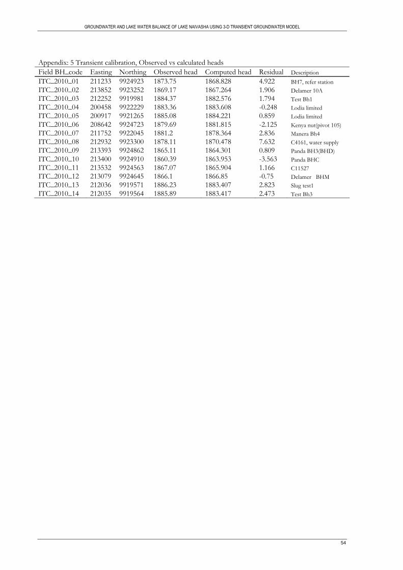
GROUNDWATER AND LAKE WATER BALANCE OF LAKE NAIVASHA USING 3-D TRANSIENT GROUNDWATER MODEL
54
Appendix: 5 Transient calibration, Observed vs calculated heads
Field BH_code Easting Northing Observed head Computed head Residual Description
ITC_2010_01 211233 9924923 1873.75 1868.828 4.922 BH7, refer station
ITC_2010_02 213852 9923252 1869.17 1867.264 1.906 Delamer 10A
ITC_2010_03 212252 9919981 1884.37 1882.576 1.794 Test Bh1
ITC_2010_04 200458 9922229 1883.36 1883.608 -0.248 Lodia limited
ITC_2010_05 200917 9921265 1885.08 1884.221 0.859 Lodia limited
ITC_2010_06 208642 9924723 1879.69 1881.815 -2.125 Kenya nut(pivot 105)
ITC_2010_07 211752 9922045 1881.2 1878.364 2.836 Manera Bh4
ITC_2010_08 212932 9923300 1878.11 1870.478 7.632 C4161, water supply
ITC_2010_09 213393 9924862 1865.11 1864.301 0.809 Panda BH3(BHD)
ITC_2010_10 213400 9924910 1860.39 1863.953 -3.563 Panda BHC
ITC_2010_11 213532 9924563 1867.07 1865.904 1.166 C11527
ITC_2010_12 213079 9924645 1866.1 1866.85 -0.75 Delamer BHM
ITC_2010_13 212036 9919571 1886.23 1883.407 2.823 Slug test1
ITC_2010_14 212035 9919564 1885.89 1883.417 2.473 Test Bh3