Backfilling missing microbial concentrations in a riverine database using artificial neural networks
11
Available at www.sciencedirect.com journal homepage: www.elsevier.com/locate/watres Backfilling missing microbial concentrations in a riverine database using artificial neural networks V. Chandramouli a,1 , Gail Brion b, , T.R. Neelakantan c , Srinivasa Lingireddy b a Indian Institute of Technology, Guwahati, Assam, India b Department of Civil Engineering and Environmental Health, University of Kentucky, Lexington, KY 40506-0281, USA c School of Civil Engineering, SASTRA Deemed University, Thanjavur 613402, India article info Article history: Received 8 June 2004 Received in revised form 19 August 2006 Accepted 22 August 2006 Available online 30 October 2006 Keywords: Artificial neural networks Fecal coliform bacteria Atypical bacteria Backfilling Abbreviations: ANN, Artificial neural network models RSE, Relative strength effect FC, Fecal coliform bacteria AC, Atypical total coliform colonies TC, Total coliform group colonies BG, Background colonies CFU, Colony forming units MSE, Mean square error MRE, Mean relative error. ABSTRACT Predicting peak pathogen loadings can provide a basis for watershed and water treatment plant management decisions that can minimize microbial risk to the public from contact or ingestion. Artificial neural network models (ANN) have been successfully applied to the complex problem of predicting peak pathogen loadings in surface waters. However, these data-driven models require substantial, multiparameter databases upon which to train, and missing input values for pathogen indicators must often be estimated. In this study, ANN models were evaluated for backfilling values for individual observations of indicator bacterial concentrations in a river from 44 other related physical, chemical, and bacteriological data contained in a multi-year database. The ANN modeling approach provided slightly superior predictions of actual microbial concentrations when compared to conventional imputation and multiple linear regression models. The ANN model provided excellent classification of 300 randomly selected, individual data observations into two defined ranges for fecal coliform concentrations with 97% overall accuracy. The application of the relative strength effect (RSE) concept for selection of input variables for ANN modeling and an approach for identifying anomalous data observations utilizing cross validation with ANN model are also presented. & 2006 Elsevier Ltd. All rights reserved. 1. Introduction It has been established that waterborne disease outbreaks are frequently associated with peak loadings of waterborne microbes in surface waters, as happened with the large protozoa outbreak that occurred in Milwaukee after heavy rains (Mac Kenzie et al., 1994). Waterborne outbreaks have occurred without the presence of indicator bacteria in treated water (Craun et al., 1997; Marshall et al., 1997), forcing the issue of source quality control to reduce potential health ARTICLE IN PRESS 0043-1354/$ - see front matter & 2006 Elsevier Ltd. All rights reserved. doi:10.1016/j.watres.2006.08.022 Corresponding author. Tel.: +1 859 257 4467. E-mail address: [email protected] (G. Brion). 1 Currently with Department of Civil Engineering, University of Kentucky, Lexington, KY 40506, USA. WATER RESEARCH 41 (2007) 217– 227
-
Upload
independent -
Category
Documents
-
view
3 -
download
0
Transcript of Backfilling missing microbial concentrations in a riverine database using artificial neural networks
ARTICLE IN PRESS
Available at www.sciencedirect.com
WAT E R R E S E A R C H 4 1 ( 2 0 0 7 ) 2 1 7 – 2 2 7
0043-1354/$ - see frodoi:10.1016/j.watres
�Corresponding auE-mail address:1 Currently with
journal homepage: www.elsevier.com/locate/watres
Backfilling missing microbial concentrations in a riverinedatabase using artificial neural networks
V. Chandramoulia,1, Gail Brionb,�, T.R. Neelakantanc, Srinivasa Lingireddyb
aIndian Institute of Technology, Guwahati, Assam, IndiabDepartment of Civil Engineering and Environmental Health, University of Kentucky, Lexington, KY 40506-0281, USAcSchool of Civil Engineering, SASTRA Deemed University, Thanjavur 613402, India
a r t i c l e i n f o
Article history:
Received 8 June 2004
Received in revised form
19 August 2006
Accepted 22 August 2006
Available online 30 October 2006
Keywords:
Artificial neural networks
Fecal coliform bacteria
Atypical bacteria
Backfilling
Abbreviations:
ANN, Artificial neural network
models
RSE, Relative strength effect
FC, Fecal coliform bacteria
AC, Atypical total coliform
colonies
TC, Total coliform group colonies
BG, Background colonies
CFU, Colony forming units
MSE, Mean square error
MRE, Mean relative error.
nt matter & 2006 Elsevie.2006.08.022
thor. Tel.: +1 859 257 [email protected] (G.
Department of Civil Eng
A B S T R A C T
Predicting peak pathogen loadings can provide a basis for watershed and water treatment
plant management decisions that can minimize microbial risk to the public from contact or
ingestion. Artificial neural network models (ANN) have been successfully applied to the
complex problem of predicting peak pathogen loadings in surface waters. However, these
data-driven models require substantial, multiparameter databases upon which to train,
and missing input values for pathogen indicators must often be estimated. In this study,
ANN models were evaluated for backfilling values for individual observations of indicator
bacterial concentrations in a river from 44 other related physical, chemical, and
bacteriological data contained in a multi-year database. The ANN modeling approach
provided slightly superior predictions of actual microbial concentrations when compared
to conventional imputation and multiple linear regression models. The ANN model
provided excellent classification of 300 randomly selected, individual data observations
into two defined ranges for fecal coliform concentrations with 97% overall accuracy. The
application of the relative strength effect (RSE) concept for selection of input variables for
ANN modeling and an approach for identifying anomalous data observations utilizing
cross validation with ANN model are also presented.
& 2006 Elsevier Ltd. All rights reserved.
1. Introduction
It has been established that waterborne disease outbreaks are
frequently associated with peak loadings of waterborne
microbes in surface waters, as happened with the large
r Ltd. All rights reserved.
Brion).ineering, University of K
protozoa outbreak that occurred in Milwaukee after heavy
rains (Mac Kenzie et al., 1994). Waterborne outbreaks have
occurred without the presence of indicator bacteria in treated
water (Craun et al., 1997; Marshall et al., 1997), forcing the
issue of source quality control to reduce potential health
entucky, Lexington, KY 40506, USA.
ARTICLE IN PRESS
WA T E R R E S E A R C H 4 1 ( 2 0 0 7 ) 2 1 7 – 2 2 7218
threats. Apart from physical and chemical water quality
measurements, bacterial concentrations in source waters are
still essential for estimating the potential presence of
pathogens and to minimize outbreaks of waterborne and
water contact diseases. The presence of fecal coliforms (FC) in
high numbers in a water sample indicates the water may
have received fecal matter from a pathogen source, but other
indicators may be needed for confirmation. To handle the
complex web of relationships between multiple water quality
indicators and pathogens, advanced data-driven modeling
techniques such as artificial neural network (ANN) models are
needed. However, it is difficult to assemble the large, robust,
multivariate databases used to train ANN models without
encountering the problem of occasional missing inputs, so an
appropriate method for backfilling missing data values is
required. This paper investigates the potential for ANN
modeling to fill missing microbial data collected from a
multiyear database obtained from a single location on the
Kentucky River and presents novel approaches to input
parameter selection and data cleaning.
In the past decade, ANNs have been successfully applied in
water resources and environmental research for forecasting,
prediction, classification and pattern recognition. Neelakan-
tan et al. (2001) used a simple feed forward artificial neural
network model to relate peak Cryptosporidium and Giardia
concentrations with other biological, chemical and physical
parameters at a single point along a multi-source impacted
river, and then investigated other, more sophisticated types of
training algorithms with limited improvement in predictive
results (Neelakantan et al., 2002). In other studies using ANN
models, new groups of microbial indicators were discovered
when the models would not train without their inclusion as
inputs. The relationship between atypical colonies (AC), total
coliform colonies (TC), and FC concentrations was key to ANN
classification of runoff types and predominate fecal pollution
sources (Brion et al., 2002; Brion and Mao, 2000; Brion and
Lingireddy, 1999) and for estimating the overall microbial
quality of surface water (Neiman and Brion, 2003). This study
extends this work by trying to predict FC and AC concentra-
tions by ANN modeling from other indicators of water quality.
The underlying relationships between microbial concentra-
tions in surface waters and environmental factors are
complex, and the behavior of single groups of fecal indicator
bacteria with respects to flow often indeterminate as found by
this study. While TC and FC from fecal sources normally die
off after being flushed into the river, the majority of AC are
thought to be more associated with the normal flora of the
river and exist in relatively stable concentrations that
fluctuate with nutrient spikes and runoff inputs. In addition
to modeling the complex relationships between groups of
potential indicator bacteria, it is difficult to predict microbial
concentrations with precision in part due to the expected
variance for any reported measurement from the analytical
methods used. Another approach that can be used is to assign
a classification representing ranges of bacterial concentra-
tions that are related to the underlying distribution of the
data, or imposed limits of interest.
In this study, the main objectives were: (i) to predict
concentration estimates for fecal coliform (FC) and atypical
(AC) bacterial concentrations using ANN models created from
a select group of physical, chemical and bacterial indices, (ii)
to compare the ANN prediction of FC and AC concentrations
using the same set of input parameters to other standard
multivariate modeling and imputation procedures, (iii) to
classify/categorize FC concentrations with respect to high and
low concentration schemes using ANN models, (iv) to
investigate the applicability of a first-order method based
upon the relative strength effect (RSE) for eliminating
nominal input variables, and (v) to see if ANN modeling
could be used to identify anomalous observations for
potential data cleaning.
2. Neural network models
Multi layered feed-forward networks have proven to be very
powerful computational tools that excel in pattern recogni-
tion and function approximation. The general structure and
working principles of a feed-forward neural network have
been described elsewhere (Brion et al., 2002; Masters, 1993). In
this study, simple feed-forward, three layered, ANN models
with back propagation training algorithm and the sigmoidal
activation function in the input and output nodes were used.
3. Methods
3.1. Database compilation
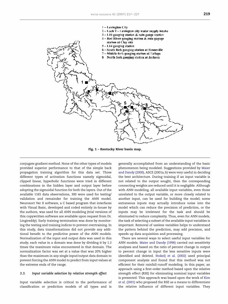
Surface water quality data was gathered routinely by stan-
dard methods by water treatment plant operators three times
daily at the intake (Lock 9) of a privately owned potable water
supply on the Kentucky River and collated into a database by
the authors during a USGS funded study (Fig. 1). Since the
river system is essentially a series of small lakes separated by
locks, and behaves quite differently under high and low flow
conditions as well as seasonally, water quality data were
augmented with flow and rainfall data from several upstream
sites at locks and gauging stations available from the USGS
hydrological data web site (Fig. 1). The resultant 1165 data set
that was used for modeling was comprised of 44 separate
input parameters per individual observation of FC or AC
concentrations. The database contained observations for 6
commonly measured indicator bacteria, 7 commonly mea-
sured physical/chemical water quality measurements, mea-
surements of rainfall at 3 points in the watershed,
measurements of flow at 6 points along the watershed, and
23 input fields created by lagging flow and rainfall data by 1, 2
or 3 days. The observations were randomly shuffled to
eliminate any temporal patterns and then split into training
and testing sets before use in separate ANN modeling
exercises, or used for other modeling or imputation studies.
3.2. Artificial neural networks
In this study, simple feed-forward, three-layered, ANN
models with back propagation training algorithm and the
sigmoidal activation function in the input and output nodes
were used after examining training algorithms such as radial
basis function network, genetic algorithm-based training and
ARTICLE IN PRESS
Fig. 1 – Kentucky River basin map.
WAT ER R ES E A R C H 41 (2007) 217– 227 219
conjugate gradient method. None of the other types of models
provided superior performance to that of the simple back
propagation training algorithm for this data set. Three
different types of activation functions namely sigmoidal,
clipped linear, hyperbolic functions were tried in different
combinations in the hidden layer and output layer before
adopting the sigmoidal function for both the layers. Out of the
available 1165 data observations, 300 were used for testing/
validation and remainder for training the ANN model.
Neurosort Ver II software, a C based program that interfaces
with Visual Basic, developed and coded entirely in-house by
the authors, was used for all ANN modeling (trial versions of
this copywritten software are available upon request from Dr.
Lingireddy). Early training termination was done by monitor-
ing the testing and training indices to prevent overtraining. In
this study, data transformations did not provide any addi-
tional benefit to the predictive power of the ANN models.
Normalization of the input and output data was used in this
study; each value in a domain was done by dividing it by 1.2
times the maximum value encountered in that domain. The
normalization factor was set at a value that was 20% higher
than the maximum in any single input/output data domain to
prevent forcing the ANN model to predict from input values at
the extreme ends of the range.
3.3. Input variable selection by relative strength effect
Input variable selection is critical to the performance of
classification or prediction models of all types and is
generally accomplished from an understanding of the basic
phenomenon being modeled. Suggestions provided by Maier
and Dandy (2000), ASCE (2001a, b) were very useful in deciding
the best architecture. During training if an input variable is
not related to the output sought, then the corresponding
connecting weights are reduced until it is negligible. Although
with ANN modeling, all available input variables, even those
unrelated to the output variable, or more closely related to
another input, can be used for building the model; some
extraneous inputs may actually introduce noise into the
model which can reduce the precision of prediction, or the
inputs may be irrelevant for the task and should be
eliminated to reduce complexity. Thus, even for ANN models,
the task of selecting a subset of the available input variables is
important. Removal of useless variables helps to understand
the pattern behind the prediction, may add precision, and
speeds up data acquisition and processing.
There are several ways to select useful input variables for
ANN models. Maier and Dandy (1996) carried out sensitivity
analyses and based on the ratio of percent change in output
to percent change in input the less sensitive inputs were
identified and deleted. Stokelj et al. (2002) used principal
component analysis and found that this method was not
efficient for their rainfall-runoff modeling. In this paper, an
approach using a first-order method based upon the relative
strength effect (RSE) for eliminating nominal input variables
is presented. This approach was based upon the work of Kim
et al. (2001) who proposed the RSE as a means to differentiate
the relative influence of different input variables. They
ARTICLE IN PRESS
WA T E R R E S E A R C H 4 1 ( 2 0 0 7 ) 2 1 7 – 2 2 7220
defined the RSE as the partial derivative of the output variable
yk, qyk=qxi. The RSE could be used to measure the relative
importance of inputs in contributing to predict outputs.
When qyk=qxi is positive, the increase in input, increases the
output; and if it is negative an increase in input causes a fall
in output.
For each data set examined in this study, the RSE value was
estimated for different inputs. Absolute maximum RSE values
among the inputs were used for normalizing the RSE values of
all the inputs. Hence, for a considered data set, the RSE value
would be between +1 and �1. For basic screening, the average
RSE value of an input for p data set used in training is
considered. The larger the absolute value of RSE, the greater is
the contribution of that input variable.
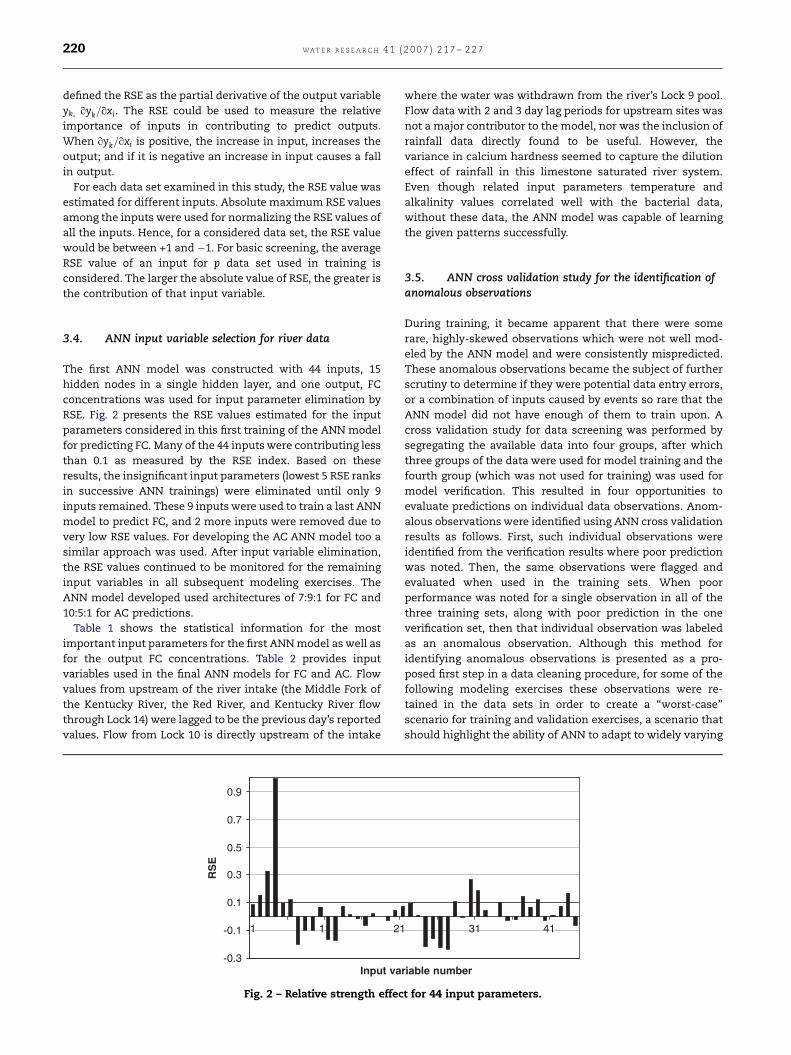
3.4. ANN input variable selection for river data
The first ANN model was constructed with 44 inputs, 15
hidden nodes in a single hidden layer, and one output, FC
concentrations was used for input parameter elimination by
RSE. Fig. 2 presents the RSE values estimated for the input
parameters considered in this first training of the ANN model
for predicting FC. Many of the 44 inputs were contributing less
than 0.1 as measured by the RSE index. Based on these
results, the insignificant input parameters (lowest 5 RSE ranks
in successive ANN trainings) were eliminated until only 9
inputs remained. These 9 inputs were used to train a last ANN
model to predict FC, and 2 more inputs were removed due to
very low RSE values. For developing the AC ANN model too a
similar approach was used. After input variable elimination,
the RSE values continued to be monitored for the remaining
input variables in all subsequent modeling exercises. The
ANN model developed used architectures of 7:9:1 for FC and
10:5:1 for AC predictions.
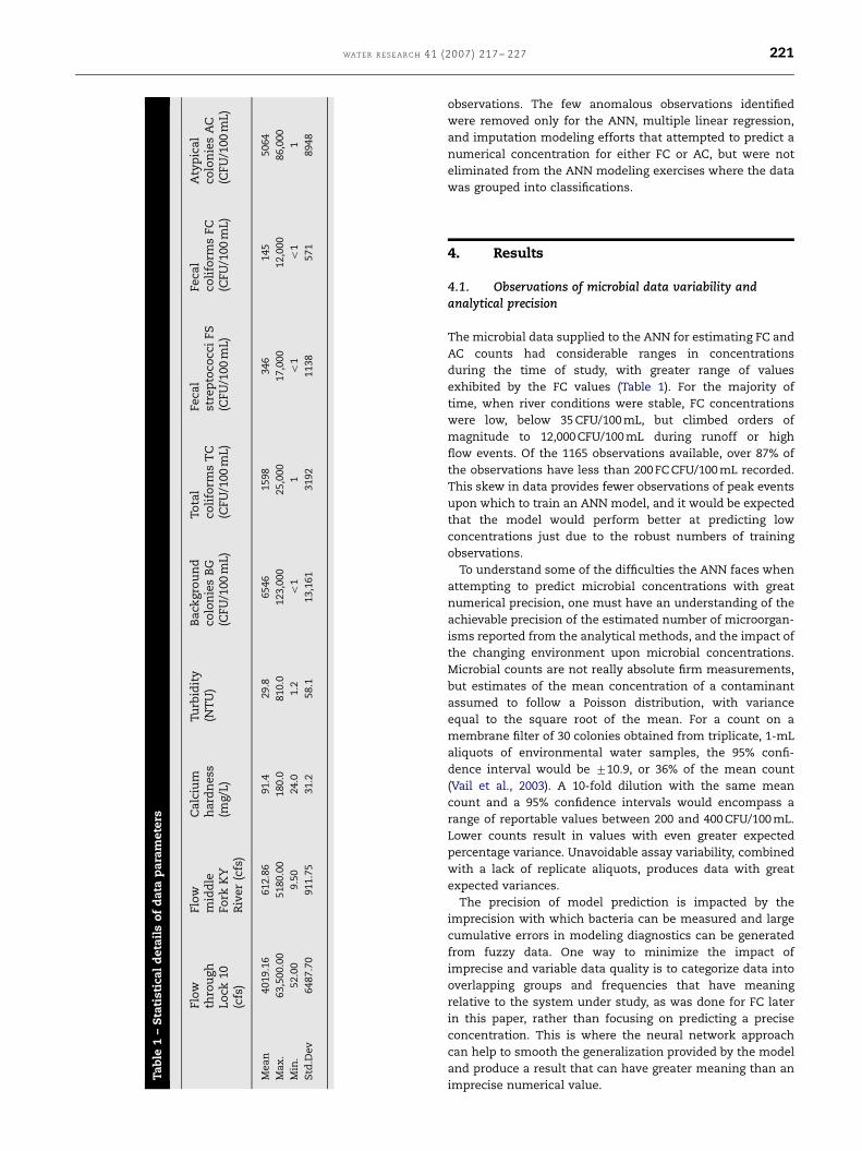
Table 1 shows the statistical information for the most
important input parameters for the first ANN model as well as
for the output FC concentrations. Table 2 provides input
variables used in the final ANN models for FC and AC. Flow
values from upstream of the river intake (the Middle Fork of
the Kentucky River, the Red River, and Kentucky River flow
through Lock 14) were lagged to be the previous day’s reported
values. Flow from Lock 10 is directly upstream of the intake
-0.3
-0.1
0.1
0.3
0.5
0.7
0.9
1 11 21
Input va
RS
E
Fig. 2 – Relative strength effec
where the water was withdrawn from the river’s Lock 9 pool.
Flow data with 2 and 3 day lag periods for upstream sites was
not a major contributor to the model, nor was the inclusion of
rainfall data directly found to be useful. However, the
variance in calcium hardness seemed to capture the dilution
effect of rainfall in this limestone saturated river system.
Even though related input parameters temperature and
alkalinity values correlated well with the bacterial data,
without these data, the ANN model was capable of learning
the given patterns successfully.
3.5. ANN cross validation study for the identification ofanomalous observations
During training, it became apparent that there were some
rare, highly-skewed observations which were not well mod-
eled by the ANN model and were consistently mispredicted.
These anomalous observations became the subject of further
scrutiny to determine if they were potential data entry errors,
or a combination of inputs caused by events so rare that the
ANN model did not have enough of them to train upon. A
cross validation study for data screening was performed by
segregating the available data into four groups, after which
three groups of the data were used for model training and the
fourth group (which was not used for training) was used for
model verification. This resulted in four opportunities to
evaluate predictions on individual data observations. Anom-
alous observations were identified using ANN cross validation
results as follows. First, such individual observations were
identified from the verification results where poor prediction
was noted. Then, the same observations were flagged and
evaluated when used in the training sets. When poor
performance was noted for a single observation in all of the
three training sets, along with poor prediction in the one
verification set, then that individual observation was labeled
as an anomalous observation. Although this method for
identifying anomalous observations is presented as a pro-
posed first step in a data cleaning procedure, for some of the
following modeling exercises these observations were re-
tained in the data sets in order to create a ‘‘worst-case’’
scenario for training and validation exercises, a scenario that
should highlight the ability of ANN to adapt to widely varying
31 41
riable number
t for 44 input parameters.
ARTICLE IN PRESS
Ta
ble
1–
Sta
tist
ica
ld
eta
ils
of
data
pa
ram
ete
rs
Flo
wth
rou
gh
Lo
ck10
(cfs
)
Flo
wm
idd
leFo
rkK
YR
iver
(cfs
)
Ca
lciu
mh
ard
nes
s(m
g/L)
Turb
idit
y(N
TU
)B
ack
gro
un
dco
lon
ies
BG
(CFU
/100
mL)
To
tal
coli
form
sT
C(C
FU
/100
mL)
Feca
lst
rep
toco
cci
FS
(CFU
/100
mL)
Feca
lco
lifo
rms
FC
(CFU
/100
mL)
Aty
pic
al
colo
nie
sA
C(C
FU
/100
mL)
Mea
n4019.1
6612.8
691.4
29.8
6546
1598
346
145
5064
Ma
x.
63,5
00.0
05180.0
0180.0
810.0
123,0
00
25,0
00
17,0
00
12,0
00
86,0
00
Min
.52.0
09.5
024.0
1.2
o1
1o
1o
11
Std
.Dev
6487.7
0911.7
531.2
58.1
13,1
61
3192
1138
571
8948
WAT ER R ES E A R C H 41 (2007) 217– 227 221
observations. The few anomalous observations identified
were removed only for the ANN, multiple linear regression,
and imputation modeling efforts that attempted to predict a
numerical concentration for either FC or AC, but were not
eliminated from the ANN modeling exercises where the data
was grouped into classifications.
4. Results
4.1. Observations of microbial data variability andanalytical precision
The microbial data supplied to the ANN for estimating FC and
AC counts had considerable ranges in concentrations
during the time of study, with greater range of values
exhibited by the FC values (Table 1). For the majority of
time, when river conditions were stable, FC concentrations
were low, below 35 CFU/100 mL, but climbed orders of
magnitude to 12,000 CFU/100 mL during runoff or high
flow events. Of the 1165 observations available, over 87% of
the observations have less than 200 FC CFU/100 mL recorded.
This skew in data provides fewer observations of peak events
upon which to train an ANN model, and it would be expected
that the model would perform better at predicting low
concentrations just due to the robust numbers of training
observations.
To understand some of the difficulties the ANN faces when
attempting to predict microbial concentrations with great
numerical precision, one must have an understanding of the
achievable precision of the estimated number of microorgan-
isms reported from the analytical methods, and the impact of
the changing environment upon microbial concentrations.
Microbial counts are not really absolute firm measurements,
but estimates of the mean concentration of a contaminant
assumed to follow a Poisson distribution, with variance
equal to the square root of the mean. For a count on a
membrane filter of 30 colonies obtained from triplicate, 1-mL
aliquots of environmental water samples, the 95% confi-
dence interval would be 710.9, or 36% of the mean count
(Vail et al., 2003). A 10-fold dilution with the same mean
count and a 95% confidence intervals would encompass a
range of reportable values between 200 and 400 CFU/100 mL.
Lower counts result in values with even greater expected
percentage variance. Unavoidable assay variability, combined
with a lack of replicate aliquots, produces data with great
expected variances.
The precision of model prediction is impacted by the
imprecision with which bacteria can be measured and large
cumulative errors in modeling diagnostics can be generated
from fuzzy data. One way to minimize the impact of
imprecise and variable data quality is to categorize data into
overlapping groups and frequencies that have meaning
relative to the system under study, as was done for FC later
in this paper, rather than focusing on predicting a precise
concentration. This is where the neural network approach
can help to smooth the generalization provided by the model
and produce a result that can have greater meaning than an
imprecise numerical value.

ARTICLE IN PRESS
Table 2 – Input parameters used to model bacterial concentrations
FlowLock 10
Flow middlefork KYa
Flow redrivera
Flowlock 14a
TC BG FS FC Turbidity Calciumhardness
FC X X X X X X X
AC X X X X X X X X X X
a One-day lagged flow value.
0
200
400
600
800
1000
1200
Actual Verification Training I Training II Training III
FC
co
un
ts in
100
ml
Fig. 3 – Anomalous observation identification by use of ANN prediction and cross validation.
WA T E R R E S E A R C H 4 1 ( 2 0 0 7 ) 2 1 7 – 2 2 7222
4.2. Examination of anomalous observations
Mistakes in data entry, variations in data quality, errors in
data measurement, and unusual events within a watershed
can result in anomalous observations that should not be
relied upon to generalize the underlying functions a model is
attempting to capture. In this study, consistent misprediction
of values during ANN cross validation studies was investi-
gated as a means to identify individual observations that
warranted closer investigation as a proposed first step in the
data cleaning process.
As an example of the procedures followed for examining
anomalous observations detected by ANN misprediction of
recorded values, five individual observations that had a
recorded FC value of 10 CFU/100 mL were selected from the
database for an analysis of the relative 7 key input parameter
values associated with this common river condition. The ANN
model developed predicted this low FC value well for 4 of the
5 observations, even though it was noted that there was
considerable variation in input values between the observa-
tions, especially flow at the Middle Fork of the Kentucky River
the day prior. However, while the ANN model predicted FC
values very close to those observed for 4 of the observations,
the 5th observation FC value was mispredicted by over a
factor of 10 (when the recorded value was 10 CFU/100 mL, the
model predicted 320 CFU/100 mL). This observation was dur-
ing April, 1998 after a rainfall in the upper catchments
increased flow and turbidity without increasing recorded FC
concentrations, a very rare and unexpected event that raises
suspicions of data entry error. On this 5th event, levels of
other fecally associated bacterial indicators that tended to
trend with FC levels were elevated (fecal streptococ-
ci ¼ 200 CFU/mL). While the reported value for fecal strepto-
cocci was under the geometric mean of 346 fecal streptococci
CFU/100 mL, one would expect FC levels to be much greater
than the recorded value of 10; nearer to the geometric mean
of 145 FC CFU/100 mL. Further consistent, misprediction of the
value of FC for this observation in cross validation analysis by
ANN modeling confirmed that the 5th observation was indeed
an anomalous observation for water quality conditions in this
watershed. It is suspected that the FC value recorded may
have been a data entry or recording error.
The use of the ANN to identify observations that warrant
further inspection identified conditions that could not be
easily attributed to recording or data entry errors. The results
of three different ANN training and validation predictions for
an observation with a high recorded FC value are presented in
Fig. 3. It is readily seen that this observation containing a very
high recorded value for FC was not properly modeled by the
ANN in either testing or training. The reasons for this remain
unknown and this may represent a rare event in the
watershed.
The cross validation identification of anomalous observa-
tions did not point out a large number for further inspection.
In total, only 25 anomalous observations were identified from
the total 1165 data observations, which were used for
predicting FC. Similarly, in the case of AC, only 19 anomalous
observations were identified. This is less than 4% of all
observations for these two bacterial groups combined, and
o2% of the total observations individually. It appears that the
ANN cross validation approach presented may provide a way
to identify anomalous events by the observation of consistent
misprediction. This may be a function that the authors
encode into the software they are developing to flag observa-
tions, but more study is needed to ratify this approach with
other more standard methods of identifying outliers.

ARTICLE IN PRESS
WAT ER R ES E A R C H 41 (2007) 217– 227 223
4.3. Results of ANN modeling of bacterial concentrations
ANN models were trained and verified on data sets with
anomalous observations removed for the ability to predict
concentrations of FC and AC at a single point in the Kentucky
River. Figs. 4 and 5 graphically show the observed versus
expected values for FC concentrations in the river predicted
from the four different groupings of the data sets during ANN
training and then when analyzed as a validation test data
group. To relate the two figures, Graphs labeled with Batch 1
would be where Training data sets 2, 3, and 4 are used during
training of the ANN, while data set 1 is used to test, or validate
the findings. As expected, training results in Fig. 5 show that
the FC concentrations can be fit well to all assembled data sets
by ANN during training with an average R2 value of 0.91 and
Batch 1y = 0.6538x + 44.517
R2 = 0.633
0
2000
4000
6000
8000
10000
12000
0
2000
4000
6000
8000
10000
12000
0 2000 4000 6000 8000 10000 12000
Observed FC (CFU/100ml)
0 2000 4000 6000 8000 10000 12000
Observed FC (CFU/100ml)
Est
imat
edF
C(C
FU
/100
ml)
Batch 3y = 0.6265x + 46.811
R2 =0.733
Est
imat
ed F
C(C
FU
/100
ml)
Fig. 4 – FC—results for ANN validation se
Batch 1y = 0.9315x + 17.944
R2 = 0.9407
0
3000
6000
9000
12000
0 2000 4000 6000 8000 10000 12000
Observed FC (CFU/100 ml)
Est
imat
ed F
C(C
FU
/100
ml)
Batch 3y = 0.8334x + 15.604
R2 = 0.8731
0
3000
6000
9000
12000
0 2000 4000 6000 8000 10000 12000
Observed FC (CFU/100ml)
Est
imat
ed F
C(C
FU
/100
ml)
Fig. 5 – FC—results for ANN training set
slope near 1. Validation on the unseen data sets has an average
R2 value of 0.71 with slopes varying from 0.66 to 1.6. The better
fit to the training data set is expected as the model sees all the
inputs in contrast to predicting on unknown observations
during verification tests. The variance in the predicted values
versus the observed values is greatest at FC concentrations
greater than 1000 CFU/100 mL. As well, the numbers of high FC
observations is limited (only 177 observations above
200 FC CFU/100 mL) and this can negatively impact the model’s
ability to generalize observations in this higher range. This can
be seen with the under-prediction of the recorded observation
of 12,000 FC CFU/100 mL as 6000 FC CFU/100 mL. While the ANN
model appears to be learning the training set, the precision of
predicting FC concentrations appears to be increasing as
reported values increase.
Batch 2y = 0.7757x + 55.446
R2 = 0.8053
0
2000
4000
6000
8000
10000
12000
0 2000 4000 6000 8000 10000 12000
Observed FC (CFU/100ml)
0 2000 4000 6000 8000 10000 12000
Observed FC (CFU/100ml)
Est
imat
ed F
C(C
FU
/100
ml)
0
2000
4000
6000
8000
10000
12000
Est
imat
ed F
C(C
FU
/100
ml)
Batch 4y = 0.7054x + 22.033
R2 =0.6692
ts (without anomalous observations).
Batch 2y = 0.8621x + 35.26
R2 = 0.8888
0
3000
6000
9000
12000
0 2000 4000 6000 8000 10000 12000
Observed FC (CFU/100ml)
Est
imat
ed F
C(C
FU
/100
ml)
Batch 4y = 0.9291x + 7.2746
R2 = 0.9364
0
3000
6000
9000
12000
0 2000 4000 6000 8000 10000 12000
Observed FC (CFU/100ml)
Est
imat
ed F
C(C
FU
/100
ml)
s (without anomalous observations).
ARTICLE IN PRESS
WA T E R R E S E A R C H 4 1 ( 2 0 0 7 ) 2 1 7 – 2 2 7224
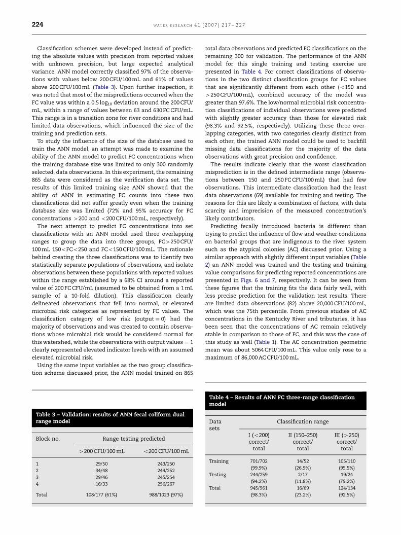
Classification schemes were developed instead of predict-
ing the absolute values with precision from reported values
with unknown precision, but large expected analytical
variance. ANN model correctly classified 97% of the observa-
tions with values below 200 CFU/100 mL and 61% of values
above 200 CFU/100 mL (Table 3). Upon further inspection, it
was noted that most of the mispredictions occurred when the
FC value was within a 0.5 log10 deviation around the 200 CFU/
mL, within a range of values between 63 and 630 FC CFU/mL.
This range is in a transition zone for river conditions and had
limited data observations, which influenced the size of the
training and prediction sets.
To study the influence of the size of the database used to
train the ANN model, an attempt was made to examine the
ability of the ANN model to predict FC concentrations when
the training database size was limited to only 300 randomly
selected, data observations. In this experiment, the remaining
865 data were considered as the verification data set. The
results of this limited training size ANN showed that the
ability of ANN in estimating FC counts into these two
classifications did not suffer greatly even when the training
database size was limited (72% and 95% accuracy for FC
concentrations 4200 and o200 CFU/100 mL, respectively).
The next attempt to predict FC concentrations into set
classifications with an ANN model used three overlapping
ranges to group the data into three groups, FC4250 CFU/
100 mL 150oFCo250 and FCo150 CFU/100 mL. The rationale
behind creating the three classifications was to identify two
statistically separate populations of observations, and isolate
observations between these populations with reported values
within the range established by a 68% CI around a reported
value of 200 FC CFU/mL (assumed to be obtained from a 1 mL
sample of a 10-fold dilution). This classification clearly
delineated observations that fell into normal, or elevated
microbial risk categories as represented by FC values. The
classification category of low risk (output ¼ 0) had the
majority of observations and was created to contain observa-
tions whose microbial risk would be considered normal for
this watershed, while the observations with output values ¼ 1
clearly represented elevated indicator levels with an assumed
elevated microbial risk.
Using the same input variables as the two group classifica-
tion scheme discussed prior, the ANN model trained on 865
Table 3 – Validation: results of ANN fecal coliform dualrange model
Block no. Range testing predicted
4200 CFU/100 mL o200 CFU/100 mL
1 29/50 243/250
2 34/48 244/252
3 29/46 245/254
4 16/33 256/267
Total 108/177 (61%) 988/1023 (97%)
total data observations and predicted FC classifications on the
remaining 300 for validation. The performance of the ANN
model for this single training and testing exercise are
presented in Table 4. For correct classifications of observa-
tions in the two distinct classification groups for FC values
that are significantly different from each other (o150 and
4250 CFU/100 mL), combined accuracy of the model was
greater than 97.6%. The low/normal microbial risk concentra-
tion classifications of individual observations were predicted
with slightly greater accuracy than those for elevated risk
(98.3% and 92.5%, respectively). Utilizing these three over-
lapping categories, with two categories clearly distinct from
each other, the trained ANN model could be used to backfill
missing data classifications for the majority of the data
observations with great precision and confidence.
The results indicate clearly that the worst classification
misprediction is in the defined intermediate range (observa-
tions between 150 and 250 FC CFU/100 mL) that had few
observations. This intermediate classification had the least
data observations (69) available for training and testing. The
reasons for this are likely a combination of factors, with data
scarcity and imprecision of the measured concentration’s
likely contributors.
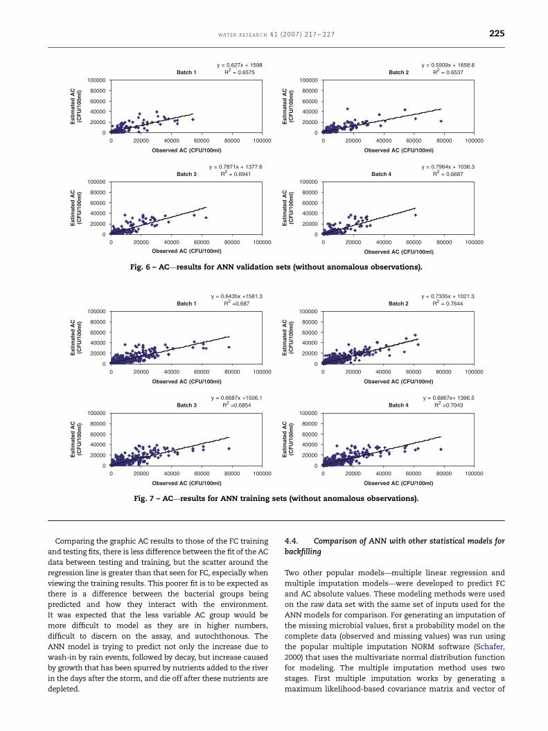
Predicting fecally introduced bacteria is different than
trying to predict the influence of flow and weather conditions
on bacterial groups that are indigenous to the river system
such as the atypical colonies (AC) discussed prior. Using a
similar approach with slightly different input variables (Table
2) an ANN model was trained and the testing and training
value comparisons for predicting reported concentrations are
presented in Figs. 6 and 7, respectively. It can be seen from
these figures that the training fits the data fairly well, with
less precise prediction for the validation test results. There
are limited data observations (82) above 20,000 CFU/100 mL,
which was the 75th percentile. From previous studies of AC
concentrations in the Kentucky River and tributaries, it has
been seen that the concentrations of AC remain relatively
stable in comparison to those of FC, and this was the case of
this study as well (Table 1). The AC concentration geometric
mean was about 5064 CFU/100 mL. This value only rose to a
maximum of 86,000 AC CFU/100 mL.
Table 4 – Results of ANN FC three-range classificationmodel
Datasets
Classification range
I (o200)correct/
total
II (150–250)correct/
total
III (4250)correct/
total
Training 701/702 14/52 105/110
(99.9%) (26.9%) (95.5%)
Testing 244/259 2/17 19/24
(94.2%) (11.8%) (79.2%)
Total 945/961 16/69 124/134
(98.3%) (23.2%) (92.5%)
ARTICLE IN PRESS
Batch 1y = 0.627x + 1598
R2 = 0.6575
0
20000
40000
60000
80000
100000
0
20000
40000
60000
80000
100000
0
20000
40000
60000
80000
100000
0
20000
40000
60000
80000
100000
0 20000 40000 60000 80000 100000
Observed AC (CFU/100ml)
0 20000 40000 60000 80000 100000
Observed AC (CFU/100ml)
0 20000 40000 60000 80000 100000
Observed AC (CFU/100ml)
0 20000 40000 60000 80000 100000
Observed AC (CFU/100ml)
Est
imat
ed A
C(C
FU
/100
ml)
Batch 2y = 0.5509x + 1658.8
R2 = 0.6537
Est
imat
ed A
C(C
FU
/100
ml)
Batch 3y = 0.7871x + 1377.6
R2 = 0.6941
Est
imat
ed A
C(C
FU
/100
ml)
Batch 4y = 0.7964x + 1036.3
R2 = 0.6687
Est
imat
ed A
C(C
FU
/100
ml)
Fig. 6 – AC—results for ANN validation sets (without anomalous observations).
Batch 1y = 0.6435x +1581.3
R2 =0.687
0
20000
40000
60000
80000
100000
0
20000
40000
60000
80000
100000
0
20000
40000
60000
80000
100000
0
20000
40000
60000
80000
100000
0 20000 40000 60000 80000 100000
Observed AC (CFU/100ml)
0 20000 40000 60000 80000 100000
Observed AC (CFU/100ml)
0 20000 40000 60000 80000 100000
Observed AC (CFU/100ml)
0 20000 40000 60000 80000 100000
Observed AC (CFU/100ml)
Est
imat
ed A
C(C
FU
/100
ml)
Batch 2y = 0.7335x + 1021.3
R2 = 0.7644
Est
imat
ed A
C(C
FU
/100
ml)
Batch 3y = 0.6687x +1506.1
R2 =0.6854
Est
imat
ed A
C(C
FU
/100
ml)
Batch 4y = 0.6867x+ 1396.5
R2 =0.7043
Est
imat
ed A
C(C
FU
/100
ml)
Fig. 7 – AC—results for ANN training sets (without anomalous observations).
WAT ER R ES E A R C H 41 (2007) 217– 227 225
Comparing the graphic AC results to those of the FC training
and testing fits, there is less difference between the fit of the AC
data between testing and training, but the scatter around the
regression line is greater than that seen for FC, especially when
viewing the training results. This poorer fit is to be expected as
there is a difference between the bacterial groups being
predicted and how they interact with the environment.
It was expected that the less variable AC group would be
more difficult to model as they are in higher numbers,
difficult to discern on the assay, and autochthonous. The
ANN model is trying to predict not only the increase due to
wash-in by rain events, followed by decay, but increase caused
by growth that has been spurred by nutrients added to the river
in the days after the storm, and die off after these nutrients are
depleted.
4.4. Comparison of ANN with other statistical models forbackfilling
Two other popular models—multiple linear regression and
multiple imputation models—were developed to predict FC
and AC absolute values. These modeling methods were used
on the raw data set with the same set of inputs used for the
ANN models for comparison. For generating an imputation of
the missing microbial values, first a probability model on the
complete data (observed and missing values) was run using
the popular multiple imputation NORM software (Schafer,
2000) that uses the multivariate normal distribution function
for modeling. The multiple imputation method uses two
stages. First multiple imputation works by generating a
maximum likelihood-based covariance matrix and vector of
ARTICLE IN PRESS
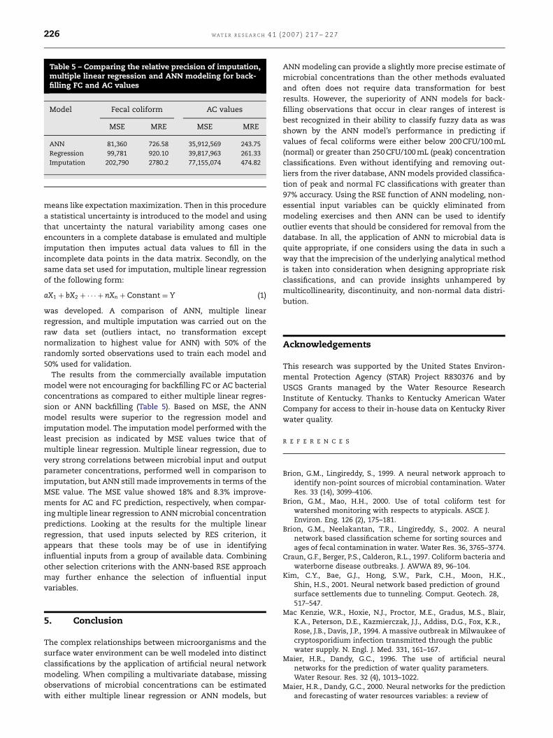
Table 5 – Comparing the relative precision of imputation,multiple linear regression and ANN modeling for back-filling FC and AC values
Model Fecal coliform AC values
MSE MRE MSE MRE
ANN 81,360 726.58 35,912,569 243.75
Regression 99,781 920.10 39,817,963 261.33
Imputation 202,790 2780.2 77,155,074 474.82
WA T E R R E S E A R C H 4 1 ( 2 0 0 7 ) 2 1 7 – 2 2 7226
means like expectation maximization. Then in this procedure
a statistical uncertainty is introduced to the model and using
that uncertainty the natural variability among cases one
encounters in a complete database is emulated and multiple
imputation then imputes actual data values to fill in the
incomplete data points in the data matrix. Secondly, on the
same data set used for imputation, multiple linear regression
of the following form:
aX1 þ bX2 þ � � � þ nXn þ Constant ¼ Y (1)
was developed. A comparison of ANN, multiple linear
regression, and multiple imputation was carried out on the
raw data set (outliers intact, no transformation except
normalization to highest value for ANN) with 50% of the
randomly sorted observations used to train each model and
50% used for validation.
The results from the commercially available imputation
model were not encouraging for backfilling FC or AC bacterial
concentrations as compared to either multiple linear regres-
sion or ANN backfilling (Table 5). Based on MSE, the ANN
model results were superior to the regression model and
imputation model. The imputation model performed with the
least precision as indicated by MSE values twice that of
multiple linear regression. Multiple linear regression, due to
very strong correlations between microbial input and output
parameter concentrations, performed well in comparison to
imputation, but ANN still made improvements in terms of the
MSE value. The MSE value showed 18% and 8.3% improve-
ments for AC and FC prediction, respectively, when compar-
ing multiple linear regression to ANN microbial concentration
predictions. Looking at the results for the multiple linear
regression, that used inputs selected by RES criterion, it
appears that these tools may be of use in identifying
influential inputs from a group of available data. Combining
other selection criterions with the ANN-based RSE approach
may further enhance the selection of influential input
variables.
5. Conclusion
The complex relationships between microorganisms and the
surface water environment can be well modeled into distinct
classifications by the application of artificial neural network
modeling. When compiling a multivariate database, missing
observations of microbial concentrations can be estimated
with either multiple linear regression or ANN models, but
ANN modeling can provide a slightly more precise estimate of
microbial concentrations than the other methods evaluated
and often does not require data transformation for best
results. However, the superiority of ANN models for back-
filling observations that occur in clear ranges of interest is
best recognized in their ability to classify fuzzy data as was
shown by the ANN model’s performance in predicting if
values of fecal coliforms were either below 200 CFU/100 mL
(normal) or greater than 250 CFU/100 mL (peak) concentration
classifications. Even without identifying and removing out-
liers from the river database, ANN models provided classifica-
tion of peak and normal FC classifications with greater than
97% accuracy. Using the RSE function of ANN modeling, non-
essential input variables can be quickly eliminated from
modeling exercises and then ANN can be used to identify
outlier events that should be considered for removal from the
database. In all, the application of ANN to microbial data is
quite appropriate, if one considers using the data in such a
way that the imprecision of the underlying analytical method
is taken into consideration when designing appropriate risk
classifications, and can provide insights unhampered by
multicollinearity, discontinuity, and non-normal data distri-
bution.
Acknowledgements
This research was supported by the United States Environ-
mental Protection Agency (STAR) Project R830376 and by
USGS Grants managed by the Water Resource Research
Institute of Kentucky. Thanks to Kentucky American Water
Company for access to their in-house data on Kentucky River
water quality.
R E F E R E N C E S
Brion, G.M., Lingireddy, S., 1999. A neural network approach toidentify non-point sources of microbial contamination. WaterRes. 33 (14), 3099–4106.
Brion, G.M., Mao, H.H., 2000. Use of total coliform test forwatershed monitoring with respects to atypicals. ASCE J.Environ. Eng. 126 (2), 175–181.
Brion, G.M., Neelakantan, T.R., Lingireddy, S., 2002. A neuralnetwork based classification scheme for sorting sources andages of fecal contamination in water. Water Res. 36, 3765–3774.
Craun, G.F., Berger, P.S., Calderon, R.L., 1997. Coliform bacteria andwaterborne disease outbreaks. J. AWWA 89, 96–104.
Kim, C.Y., Bae, G.J., Hong, S.W., Park, C.H., Moon, H.K.,Shin, H.S., 2001. Neural network based prediction of groundsurface settlements due to tunneling. Comput. Geotech. 28,517–547.
Mac Kenzie, W.R., Hoxie, N.J., Proctor, M.E., Gradus, M.S., Blair,K.A., Peterson, D.E., Kazmierczak, J.J., Addiss, D.G., Fox, K.R.,Rose, J.B., Davis, J.P., 1994. A massive outbreak in Milwaukee ofcryptosporidium infection transmitted through the publicwater supply. N. Engl. J. Med. 331, 161–167.
Maier, H.R., Dandy, G.C., 1996. The use of artificial neuralnetworks for the prediction of water quality parameters.Water Resour. Res. 32 (4), 1013–1022.
Maier, H.R., Dandy, G.C., 2000. Neural networks for the predictionand forecasting of water resources variables: a review of

ARTICLE IN PRESS
WAT ER R ES E A R C H 41 (2007) 217– 227 227
modeling issues and applications. Environ. Model. Software15, 101–124.
Marshall, M.M., Naumovitz, D., Ortega, Y., Sterling, C.R., 1997.Waterborne protozoan pathogens. Clin. Microb. Rev. 10 (1),67–85.
Masters, T., 1993. Practical Neural Network Recipes in C++.Academic Press, USA.
Neelakantan, T., Brion, G.M., Lingireddy, S., 2001. Neural networkmodeling of Cryptosporidium and Giardia concentrations in theDelaware river. Water Sci. Technol. 43 (12), 125–132.
Neelakantan, T., Lingireddy, G.M., Brion, S., 2002. Effectiveness ofdifferent artificial neural network training algorithms inpredicting protozoa in surface waters. J. Environ. Eng. ASCE128 (6), 533–542.
Neiman, J., Brion, G.M., 2003. Novel bacterial ratio for predictingfecal age. Water Sci. Technol. 47 (3), 45–49.
Schafer, J.L., 2000. NORM: multiple imputation of incompletemultivariate data under a normal model, version 2.03, soft-ware for Windows 95/98/NT, available from /www.stat.p-su.edu/�jls/misoftwa.htmlS.
Stokelj, T., Paravan, D., Golob, R., 2002. Enhanced artificial neuralnetwork inflow forecasting algorithm for run-of-river hydro-power plants. ASCE J. Water Resour. Plann. Manage. 128 (6),415–423.
Vail, J.H., Morgan, R., Merino, C.R., Gonzales, F., Millar, R., Ram, J.L.,2003. Enumeration of waterborne Escherichia coli with Petrifilmplates: comparison to standard methods. J. Environ. Qual. 32,368–373.